THE AMERICAN STATISTICIAN2019, VOL. 73, NO. S1, 328–339: Statistical Inference in the 21st Centuryhttps://doi.org/10.1080/00031305.2019.1565553

Multiple Perspectives on Inference for Two Simple Statistical Scenarios

Noah N. N. van Dongena, Johnny B. van Doornb, Quentin F. Gronaub, Don van Ravenzwaaijc, Rink Hoekstrac, Matthias N.Hauckec, Daniel Lakensd, Christian Hennige, Richard D. Moreyf, Saskia Homerf, Andrew Gelmang, Jan Sprengera, andEric-Jan Wagenmakersb

aDepartment of Philosophy and Education Sciences, University of Turin, Turin, Italy; bDepartment of Psychological Methods, University of Amsterdam,Amsterdam, The Netherlands; cDepartment of Psychology, University of Groningen, Groningen, The Netherlands; dDepartment of Industrial Engineering& Innovation Sciences, Technical University Eindhoven, Eindhoven, The Netherlands; eDepartment of Statistical Science, University College London,London, UK; fSchool of Psychology, Cardiff University, Cardiff, Wales, UK; gDepartment of Statistics and Department of Political Science, ColumbiaUniversity, New York, NY

ABSTRACTWhen data analysts operate within different statistical frameworks (e.g., frequentist versus Bayesian, empha-sis on estimation versus emphasis on testing), how does this impact the qualitative conclusions thatare drawn for real data? To study this question empirically we selected from the literature two simplescenarios—involving a comparison of two proportions and a Pearson correlation—and asked four teams ofstatisticians to provide a concise analysis and a qualitative interpretation of the outcome. The results showedconsiderable overall agreement; nevertheless, this agreement did not appear to diminish the intensity of thesubsequent debate over which statistical framework is more appropriate to address the questions at hand.

ARTICLE HISTORYReceived August 2018Accepted October 2018

KEYWORDSFrequentist or Bayesian;Multilab analysis; Statisticalparadigms; Testing orestimation

1. Introduction

When analyzing a specific dataset, statisticians usually operatewithin the confines of their preferred inferential paradigm. Forinstance, frequentist statisticians interested in hypothesis testingmay report p-values, whereas those interested in estimationmay seek to draw conclusions from confidence intervals. Inthe Bayesian realm, those who wish to test hypotheses mayuse Bayes factors and those who wish to estimate parametersmay report credible intervals. And then there are likelihood-ists, information-theorists, and machine-learners—there existsa diverse collection of statistical approaches, many of which arephilosophically incompatible.

Moreover, proponents of the various camps regularly explainwhy their position is the most exalted, either in practical ortheoretical terms. For instance, in a well-known article ‘WhyIsn’t Everyone a Bayesian?’, Bradley Efron claimed that “Thehigh ground of scientific objectivity has been seized by thefrequentists” (Efron 1986, p. 4), upon which Dennis Lindleyreplied that “Every statistician would be a Bayesian if he took thetrouble to read the literature thoroughly and was honest enoughto admit that he might have been wrong” (Lindley 1986, p.7). Similarly spirited debates occurred earlier, notably betweenFisher and Jeffreys (e.g., Howie 2002) and between Fisher andNeyman. Even today, the paradigmatic debates show no sign ofstalling, neither in the published literature (e.g., Benjamin et al.2018; McShane et al. in press; Wasserstein and Lazar 2016) noron social media.

CONTACT Eric-Jan Wagenmakers EJ.Wagenmakers@gmail.com University of Amsterdam, Department of Psychological Methods, University of Amsterdam,Nieuwe Achtergracht 129B, Amsterdam, 1018 VK, The Netherlands; Noah N. N. van Dongen nnnvandongen@gmail.com Department of Philosophy and EducationSciences, University of Turin, Turin, Italy.

The question that concerns us here is purely pragmatic:“does it matter?” In other words, will reasonable statisticalanalyses on the same dataset, each conducted within their ownparadigm, result in qualitatively similar conclusions (Berger2003)? One of the first to pose this question was RonaldFisher. In a letter to Harold Jeffreys, dated on March 29, 1934,Fisher proposed that “From the point of view of interestingthe general scientific public, which really ought to be muchmore interested than it is in the problem of inductive inference,probably the most useful thing we could do would be to takeone or more specific puzzles and show what our respectivemethods made of them” (Bennett 1990, p. 156; see also Howie2002, p. 167). The two men then proceeded to constructsomewhat idiosyncratic statistical “puzzles” that the otherfound difficult to solve. Nevertheless, three years and severalletters later, on May 18, 1937, Jeffreys stated that “Your letterconfirms my previous impression that it would only be oncein a blue moon that we would disagree about the inference tobe drawn in any particular case, and that in the exceptionalcases we would both be a bit doubtful” (Bennett 1990, p. 162).Similarly, Edwards, Lindman, and Savage (1963) suggested thatwell-conducted experiments often satisfy Berkson’s interoculartraumatic test—“you know what the data mean when theconclusion hits you between the eyes” (p. 217). Nevertheless,surprisingly little is known about the extent to which, inconcrete scenarios, a data analyst’s statistical plumage affectsthe inference.

© 2019 The Author(s). Published with license by Taylor & Francis Group, LLC.This is an Open Access article distributed under the terms of the Creative Commons Attribution-NonCommercial-NoDerivatives License (http://creativecommons.org/licenses/by-nc-nd/4.0/), whichpermits non-commercial re-use, distribution, and reproduction in any medium, provided the original work is properly cited, and is not altered, transformed, or built upon in any way.

THE AMERICAN STATISTICIAN 329

Table 1. Variable names and their description.

Variable Description

Cetirizine exposure Whether exposed to cetirizineBirth defect Whether birth defects were detectedCounts Count data for each cell

Here we revisit Fisher’s challenge. We invited four groups ofstatisticians to analyze two real datasets, report and interprettheir results in about 300 words, and discuss these results andinterpretations in a round-table discussion. The datasets areprovided online at https://osf.io/hykmz/ and described below.In addition to providing an empirical answer to the question“does it matter?”, we hope to highlight how the same dataset cangive rise to rather different statistical treatments. In our opinion,this method variability ought to be acknowledged rather thanignored (for a complementary approach see Silberzahn et al. inpress).1

The selected datasets are straightforward: the first datasetconcerns a 2×2 contingency table, and the second concerns acorrelation between two variables. The simplicity of the statisti-cal scenarios is on purpose, as we hoped to facilitate a detaileddiscussion about assumptions and conclusions that could other-wise have remained hidden underneath an unavoidable layer ofstatistical sophistication. The full instructions for participationcan be found online at https://osf.io/dg9t7/.

2. DataSet I: Birth Defects and Cetirizine Exposure

2.1. Study Summary

Cetirizine is a nonsedating long-acting antihistamine with somemast-cell stabilizing activity. It is used for the symptomatic reliefof allergic conditions, such as rhinitis and urticaria, which arecommon in pregnant women. In the study of interest, Weber-Schoendorfer and Schaefer (2008) aimed to assess the safety ofcetirizine during the first trimester of pregnancy when used.The pregnancy outcomes of a cetirizine group (n = 181) werecompared to those of the control group (n = 1685; pregnantwomen who had been counseled during pregnancy about expo-sures known to be nonteratogenic). Due to the observationalnature of the data, the allocation of participants to the groupswas nonrandomized. The main point of interest was the rate ofbirth defects.2 Variables of the dataset3 are described in Table 1and the data are presented in Table 2.

2.2. Cetirizine Research Question

Is cetirizine exposure during pregnancy associated with a higherincidence of birth defects? In the next sections each of four dataanalysis teams will attempt to address this question.

1 In contrast to the current approach, Silberzahn et al. (in press) used arelatively complex dataset and did not emphasize the differences in inter-pretation caused by the adoption of dissimilar statistical paradigms.

2 The original study focused on cetirizine-induced differences in major birthdefects, spontaneous abortions, and preterm deliveries. We decided to lookat all birth defects, because the sample sizes were larger for this comparisonand we deemed the data more interesting.

3 The dataset is made available on the OSF repository: https:// osf.io/ hykmz/ .

Table 2. Cetirizine exposure and birth defects.

Birth defects

Cetirizine exposure No Yes Total

No 1588 97 1685Yes 167 14 181Total 1755 111 1866

2.3. Analysis and Interpretation by Lakens and Hennig

2.3.1. PreambleFrequentist statistics is based on idealised models of data-generating processes. We cannot expect these models to beliterally true in practice, but it is instructive to see whetherdata are consistent with such models, which is what hypothesistests and confidence intervals allow us to examine. We doappreciate that automatic procedures involving for examplefixed significance levels allow us to control error probabilitiesassuming the model, but given that the models do never holdprecisely, and that there are often issues with measurement orselection effects, in most cases we think it is prudent to interpretoutcomes in a coarse way rather than to read too much meaninginto, say, differences between p-values of 0.047 and 0.062. Westick to quite elementary methodology in our analyses.

2.3.2. Analysis and SoftwareWe performed a Pearson’s chi-squared test with Yates’ continuitycorrection to test for dependence between exposure of preg-nant women exposed to cetirizine and birth defects using thechisq.test function in R software version 3.4.3 (R Develop-ment Core Team 2004). However, because Weber-Schoendorferand Schaefer (2008) wanted “to assess the safety of cetirizineduring the first trimester of pregnancy,” their actual researchquestion is whether we can reject the presence of a meaningfuleffect. We therefore performed an equivalence test on propor-tions (Chen, Tsong, and Kang, 2000) as implemented in theTOSTtwo.prop function in the TOSTER package (Lakens 2017).

2.3.3. Results and InterpretationThe chi-squared test yielded χ2(1, N = 1866) = 0.817, p = 0.366,which suggests that the data are consistent with an indepen-dence model at any significance level in general use. The answerto the question whether the drug is safe depends on a smallesteffect size of interest (when is the difference in birth defectsconsidered too small to matter?). This choice, and the selectionof equivalence bounds more generally, should always be justifiedby clinical and statistical considerations pertinent to the caseat hand. In the absence of a discussion of this essential aspectof the study by the authors, and in order to show an examplecomputation, we will test against a difference in proportions of10%, which, although debatable, has been suggested as a sensiblebound for some drugs (see Röhmel 2001, for a discussion).

An equivalence test against a difference in proportions(Mdif = 0.02, 95% CI[−0.02; 0.06]) of 10% based on Fisher’sexact z-test was significant, z = −3.88, p < 0.001. This meansthat we can reject differences in proportions as large, or larger,than 10%, again at any significance level in general use.

Is cetirizine exposure during pregnancy associated with ahigher incidence of birth defects? Based on the current study,

330 N. N. N. VAN DONGEN ET AL.

Figure 1. Estimates of the odds of a birth defect when no cetirizine (control) was taken during pregnancy and when cetirizine was taken. Horizontal dashed lines andshaded regions show point estimates and standard errors. The solid line labeled “Cetirizine worst case” shows the upper bound of the one-sided CI as a function of theconfidence coefficient (x-axis). The right axis shows the estimated increase in odds of a birth defect for the cetirizine group compared to the control group.

there is no evidence that cetirizine exposure during pregnancyis associated with a higher incidence of birth defects. Obviously,this does not mean that cetirizine is safe; in fact the observedbirth defect rate in the cetirizine group is about 2% higherthan without exposure, which may or may not be explainedby random variation. Is cetirizine during the first trimester ofpregnancy “safe”? If we accept a difference in the proportion ofbirth defects of 10%, and desire a 5% long run error rate, thereis clear evidence that the drug is safe. However, we expect thata cost–benefit analysis would suggest proportions of 5% to beunacceptably high, which is in the 95% confidence interval andtherefore well compatible with the data. Therefore, we wouldpersonally consider the current data inconclusive.

2.4. Analysis and Interpretation by Morey and Homer

Fitting a classical logistic model with the binary birth defectoutcome predicted from the cetirizine indicator confirmed thenonsignificant relationship (p = 0.287). The point estimate ofthe effect of taking cetirizine is to increase the odds of the birthdefect by only 37%. At the baseline levels of birth defects in thenon-cetirizine-exposed sample (approximately 6%), this wouldamount to about an extra two birth defects in every hundredpregnancies in the cetirizine-exposed group.

There are several problems with taking these data as evidencethat cetirizine is safe. The first is the observational nature of thedata. We have no way of knowing whether an apparent effect—or lack of effect—reflects confounds. Suppose, though, that weset this question aside and assess the evidence that birth defectsare not more common in the cetirizine group. We can use aclassical one-sided CI to determine the size of the differenceswe can rule out. We call the upper bound of the 100(1 −α)% CIthe “worst case” for that confidence coefficient. Figure 1 shows

that at 95%, the worst-case odds increase is for the cetirizinegroup is 124%. At 99.5%, the worst case increase is 195%. Wecan translate this into more a more intuitive metric of numbersof birth defects: at baseline rates of birth defects, these wouldamount to additional 6 and 10 birth defects per 100, respectively(Figure 2).

The large p-value of the initial significance test suggests thatwe cannot rule out that cetirizine group has lower rates of birthdefects; the one-sided test assuming a decrease in birth defectsas the null would not yield a rejection except at high α levels. Butalso, the “worst-case” analysis using the upper bound of the one-sided CI suggests we also cannot rule out a substantial increasein birth defects in the cetirizine group.

We are unsure whether cetirizine is safe, but it seems clearto us that these data do not provide much evidence of its rela-tive safety, contrary to what Weber-Schoendorfer and Schaefersuggest.

2.5. Analysis and Interpretation by Gronau, van Doorn,and Wagenmakers

We used the model proposed by Kass and Vaidyanathan (1992):

log! p1

1 − p1

"= β − ψ

2,

log! p2

1 − p2

"= β + ψ

2,

y1 ∼ Binomial(n1, p1),y2 ∼ Binomial(n2, p2).

(1)

Here, y1 = 97, n1 = 1, 685, y2 = 14, and n2 = 181, p1 is theprobability of a birth defect in the control group, and p2 is thatprobability in the cetirizine group. Probabilities p1 and p2 arefunctions of model parameters β and ψ . Nuisance parameter

THE AMERICAN STATISTICIAN 331

Figure 2. Frequency representations of the number of birth defects expected under various scenarios. Top: Expected frequency of birth defects when cetirizine was nottaken (control). Bottom-left: Point estimate of the expected frequency of birth defects when cetirizine is taken. Bottom-middle (bottom-right): Upper bound of a one-sided 95% (99%) CI for the expected frequency of birth defects when cetirizine was taken. Because the analysis is intended to be comparative, in the bottom panels theno-cetirizine estimate was assumed to be the truth when calculating the increase in frequency.

β corresponds to the grand mean of the log odds, whereas thetest-relevant parameter ψ corresponds to the log odds ratio. Weassigned β a standard normal prior and used a zero-centrednormal prior with standard deviation σ for the log odds ratio ψ .Inference was conducted withStan (Carpenter et al. 2017; StanDevelopment Team 2016) and thebridgesamplingpackage(Gronau, Singmann, and Wagenmakers in press). For ease ofinterpretation, the results will be shown on the odds ratio scale.

Our first analysis focuses on estimation and uses σ = 1.The result, shown in the left panel of Figure 3, indicates thatthe posterior median equals 1.429, with a 95% credible intervalranging from 0.793 to 2.412. This credible interval is relativelywide, indicating substantial uncertainty about the true value ofthe odds ratio.

Our second analysis focuses on testing and quantifies theextent to which the data support the skeptic’s H0 : ψ = 0versus the proponent’s H1. To specify H1 we initially use σ =0.4 (i.e., a mildly informative prior; Diamond and Kaul 2004),truncated at zero to respect the fact that cetirizine exposure ishypothesized to cause a higher incidence of birth defects: H+ :ψ ∼ N+(0, 0.42).

As can be seen from the right panel of Figure 3, the observeddata are predicted about 1.8 times better by H+ than by H0.According to Jeffreys (1961, Appendix B), this level of supportis “not worth more than a bare mention.” To investigate therobustness of this result, we explored a range of alternative priorchoices for σ under H+, varying it from 0.01 to 2. The resultsof this sensitivity analysis are shown in Figure 4 and reveal thatacross a wide range of priors, the data never provide more thananecdotal support for one model over the other. When σ isselected post hoc to maximize the support for H+ this yieldsBF+0 = 1.84, which, starting from a position of equipoise, raises

the probability of H+ from 0.50 to about 0.65, leaving a posteriorprobability of 0.35 for H0.

In sum, based on this dataset we cannot draw strong con-clusions about whether or not cetirizine exposure during preg-nancy is associated with a higher incidence of birth defects.Our analysis shows an “absence of evidence,” not “evidence forabsence.”

2.6. Analysis and interpretation by Gelman

I summarized the data with a simple comparison: the proportionof birth defects is 0.06 in the control group and 0.08 in thecetirizine group. The difference is 0.02 with a standard error of0.02. I got essentially the same result with a logistic regressionpredicting birth defect: the coefficient of cetirizine is 0.3 witha standard error of 0.3. I performed the analyses in R usingrstanarm (code available at https://osf.io/nh4gc/).

I then looked up the article, “The safety of cetirizine dur-ing pregnancy: A prospective observational cohort study,” byWeber-Schoendorfer and Schaefer (2008) and noticed someinteresting things:

(a) The published article gives N = 196 and 1686 for thetwo groups, not quite the same as the 181 and 1685 forthe “all birth defects” category. I could not follow the exactreasoning.4

(b) The two groups differ in various background variables:most notably, the cetirizine group has a higher smokingrate (17% compared to 10%).

4 Clarification: the original article does not provide a rationale for why severalparticipants were excluded from the analysis.

332 N. N. N. VAN DONGEN ET AL.

0 1 2 3 4

0.0

0.2

0.4

0.6

0.8

1.0

1.2

1.4

Den

sity

Population Odds Ratio

BF10 = 0.636BF01 = 1.572

median = 1.429

95% CI: [0.793, 2.412]

data|H1

data|H0

PosteriorPrior

(a) Estimation results.

0 1 2 3 4

0.0

0.5

1.0

1.5

2.0

2.5

3.0

Den

sity

Population Odds Ratio

BF+0 = 1.808BF0+ = 0.553

median = 1.349

95% CI: [1.023, 2.072]

data|H+

data|H0

PosteriorPrior

(b) Testing results.

Figure 3. Gronau, van Doorn, and Wagenmakers’ Bayesian analysis of the cetirizine dataset. The left panel shows the results of estimating the log odds ratio under H1with a two-sided standard normal prior. For ease of interpretation, results are displayed in the odds ratio scale. The right panel shows the results of testing the one-sidedalternative hypothesis H+ : ψ ∼ N+(0, 0.42) versus the null hypothesis H0 : ψ = 0. Figures inspired by JASP (jasp-stats.org).

0 0.5 1 1.5 2

1/10

1/3

1

3

10

Anecdotal

Moderate

Anecdotal

Moderate

EvidenceB

F+0

σ

Evidence for H+

Evidence for H0

max BF+0 :user prior: BF+0 = 1.808

1.841 at σ = 0.356

Figure 4. Sensitivity analysis for the Bayesian one-sided test. The Bayes factor BF+0 is a function of the prior standard deviation σ . Figure inspired by JASP.

(c) In the published article, the outcome of focus was “majorbirth defects,” not the “all birth defects” given for us tostudy.

(d) The published article has a causal aim (as can be seen, forexample, from the word “safety” in its title); our assign-ment is purely observational.

Now the question, “Is cetirizine exposure during pregnancyassociated with a higher incidence of birth defects?” I have notread the literature on the topic. To understand how the data athand address this question, I would like to think of the mappingfrom prior to posterior distribution. In this case, the prior wouldbe the distribution of association with birth defects of all drugsof this sort. That is, imagine a population of drugs, j = 1, 2, . . . ,taken by pregnant women, and for each drug, define θj as theproportion of birth defects among women who took drug j,minus the proportion of birth defects in the general popula-tion. Just based on my general understanding (which could bewrong), I would expect this distribution to be more positivethan negative and concentrated near zero: some drugs couldbe mildly protective against birth defects or associated withlow-risk pregnancies, most would have small effects and notbe strongly associated with low- or high-risk pregnancies, and

some could cause birth defects or be taken disproportionatelyby women with high-risk pregnancies. Supposing that the prioris concentrated within the range (−0.01, +0.01), the data wouldnot add much information to this prior.

To answer, “Is cetirizine exposure during pregnancy associ-ated with a higher incidence of birth defects?,” the key questionwould seem to be whether the drug is more or less likely to betaken by women at a higher risk of birth defects. I am guessingthat maternal age is a big predictor here. In the reported study,average age of the exposed and control groups was the same, butI do not know if that is generally the case or if the designers ofthe study were purposely seeking a balanced comparison.

3. DataSet II: Amygdalar Activity and Perceived Stress

3.1. Study Summary

In a recent study published in the Lancet, Tawakol et al. (2017)tested the hypothesis that perceived stress is positively associ-ated with resting activity in the amygdala. In the second studyreported in Tawakol et al. (2017), n = 13 individuals withan increased burden of chronic stress (i.e., a history of post-

THE AMERICAN STATISTICIAN 333

Table 3. Variable names and their description.

Variable Description

Perceived stress scale Participant score on the PSSAmygdalar activity Intensity of amygdalar resting state activity

Table 4. Raw data as extracted from Figure 5 in Tawakol et al. (2017), with help ofJurgen Rusch, Philips Research Eindhoven.

Perceived AmygdalarStress Scale Activity

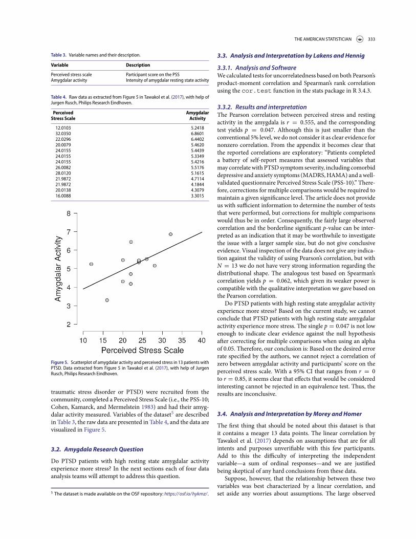
12.0103 5.241832.0350 6.860122.0296 6.440220.0079 5.462024.0155 5.443924.0155 5.334924.0155 5.421626.0082 5.517628.0120 5.161521.9872 4.711421.9872 4.184420.0138 4.307916.0088 3.3015

Figure 5. Scatterplot of amygdalar activity and perceived stress in 13 patients withPTSD. Data extracted from Figure 5 in Tawakol et al. (2017), with help of JurgenRusch, Philips Research Eindhoven.

traumatic stress disorder or PTSD) were recruited from thecommunity, completed a Perceived Stress Scale (i.e., the PSS-10;Cohen, Kamarck, and Mermelstein 1983) and had their amyg-dalar activity measured. Variables of the dataset5 are describedin Table 3, the raw data are presented in Table 4, and the data arevisualized in Figure 5.

3.2. Amygdala Research Question

Do PTSD patients with high resting state amygdalar activityexperience more stress? In the next sections each of four dataanalysis teams will attempt to address this question.

5 The dataset is made available on the OSF repository: https:// osf.io/ hykmz/ .

3.3. Analysis and Interpretation by Lakens and Hennig

3.3.1. Analysis and SoftwareWe calculated tests for uncorrelatedness based on both Pearson’sproduct-moment correlation and Spearman’s rank correlationusing the cor.test function in the stats package in R 3.4.3.

3.3.2. Results and interpretationThe Pearson correlation between perceived stress and restingactivity in the amygdala is r = 0.555, and the correspondingtest yields p = 0.047. Although this is just smaller than theconventional 5% level, we do not consider it as clear evidence fornonzero correlation. From the appendix it becomes clear thatthe reported correlations are exploratory: “Patients completeda battery of self-report measures that assessed variables thatmay correlate with PTSD symptom severity, including comorbiddepressive and anxiety symptoms (MADRS, HAMA) and a well-validated questionnaire Perceived Stress Scale (PSS-10).” There-fore, corrections for multiple comparisons would be required tomaintain a given significance level. The article does not provideus with sufficient information to determine the number of teststhat were performed, but corrections for multiple comparisonswould thus be in order. Consequently, the fairly large observedcorrelation and the borderline significant p-value can be inter-preted as an indication that it may be worthwhile to investigatethe issue with a larger sample size, but do not give conclusiveevidence. Visual inspection of the data does not give any indica-tion against the validity of using Pearson’s correlation, but withN = 13 we do not have very strong information regarding thedistributional shape. The analogous test based on Spearman’scorrelation yields p = 0.062, which given its weaker power iscompatible with the qualitative interpretation we gave based onthe Pearson correlation.

Do PTSD patients with high resting state amygdalar activityexperience more stress? Based on the current study, we cannotconclude that PTSD patients with high resting state amygdalaractivity experience more stress. The single p = 0.047 is not lowenough to indicate clear evidence against the null hypothesisafter correcting for multiple comparisons when using an alphaof 0.05. Therefore, our conclusion is: Based on the desired errorrate specified by the authors, we cannot reject a correlation ofzero between amygdalar activity and participants’ score on theperceived stress scale. With a 95% CI that ranges from r = 0to r = 0.85, it seems clear that effects that would be consideredinteresting cannot be rejected in an equivalence test. Thus, theresults are inconclusive.

3.4. Analysis and Interpretation by Morey and Homer

The first thing that should be noted about this dataset is thatit contains a meager 13 data points. The linear correlation byTawakol et al. (2017) depends on assumptions that are for allintents and purposes unverifiable with this few participants.Add to this the difficulty of interpreting the independentvariable—a sum of ordinal responses—and we are justifiedbeing skeptical of any hard conclusions from these data.

Suppose, however, that the relationship between these twovariables was best characterized by a linear correlation, andset aside any worries about assumptions. The large observed

334 N. N. N. VAN DONGEN ET AL.

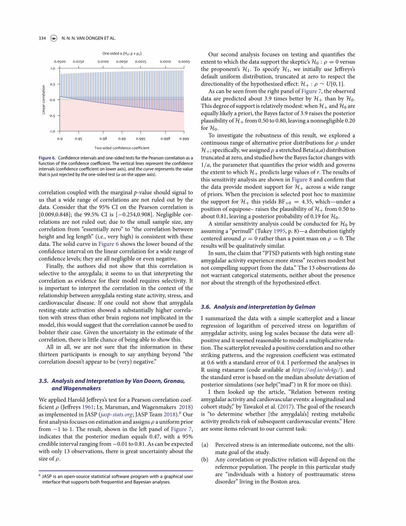
Figure 6. Confidence intervals and one-sided tests for the Pearson correlation as afunction of the confidence coefficient. The vertical lines represent the confidenceintervals (confidence coefficient on lower axis), and the curve represents the valuethat is just rejected by the one-sided test (α on the upper axis).

correlation coupled with the marginal p-value should signal tous that a wide range of correlations are not ruled out by thedata. Consider that the 95% CI on the Pearson correlation is[0.009,0.848]; the 99.5% CI is [−0.254,0.908]. Negligible cor-relations are not ruled out; due to the small sample size, anycorrelation from “essentially zero” to “the correlation betweenheight and leg length” (i.e., very high) is consistent with thesedata. The solid curve in Figure 6 shows the lower bound of theconfidence interval on the linear correlation for a wide range ofconfidence levels; they are all negligible or even negative.

Finally, the authors did not show that this correlation isselective to the amygdala; it seems to us that interpreting thecorrelation as evidence for their model requires selectivity. Itis important to interpret the correlation in the context of therelationship between amygdala resting state activity, stress, andcardiovascular disease. If one could not show that amygdalaresting-state activation showed a substantially higher correla-tion with stress than other brain regions not implicated in themodel, this would suggest that the correlation cannot be used tobolster their case. Given the uncertainty in the estimate of thecorrelation, there is little chance of being able to show this.

All in all, we are not sure that the information in thesethirteen participants is enough to say anything beyond “thecorrelation doesn’t appear to be (very) negative.”

3.5. Analysis and Interpretation by Van Doorn, Gronau,and Wagenmakers

We applied Harold Jeffreys’s test for a Pearson correlation coef-ficient ρ (Jeffreys 1961; Ly, Marsman, and Wagenmakers 2018)as implemented in JASP (jasp-stats.org; JASP Team 2018).6 Ourfirst analysis focuses on estimation and assigns ρ a uniform priorfrom −1 to 1. The result, shown in the left panel of Figure 7,indicates that the posterior median equals 0.47, with a 95%credible interval ranging from −0.01 to 0.81. As can be expectedwith only 13 observations, there is great uncertainty about thesize of ρ.

6 JASP is an open-source statistical software program with a graphical userinterface that supports both frequentist and Bayesian analyses.

Our second analysis focuses on testing and quantifies theextent to which the data support the skeptic’s H0 : ρ = 0 versusthe proponent’s H1. To specify H1, we initially use Jeffreys’sdefault uniform distribution, truncated at zero to respect thedirectionality of the hypothesized effect: H+ : ρ ∼ U[0, 1].

As can be seen from the right panel of Figure 7, the observeddata are predicted about 3.9 times better by H+ than by H0.This degree of support is relatively modest: when H+ and H0 areequally likely a priori, the Bayes factor of 3.9 raises the posteriorplausibility of H+ from 0.50 to 0.80, leaving a nonnegligible 0.20for H0.

To investigate the robustness of this result, we explored acontinuous range of alternative prior distributions for ρ underH+; specifically, we assigned ρ a stretched Beta(a,a) distributiontruncated at zero, and studied how the Bayes factor changes with1/a, the parameter that quantifies the prior width and governsthe extent to which H+ predicts large values of r. The results ofthis sensitivity analysis are shown in Figure 8 and confirm thatthe data provide modest support for H+ across a wide rangeof priors. When the precision is selected post hoc to maximizethe support for H+ this yields BF+0 = 4.35, which—under aposition of equipose– raises the plausibility of H+ from 0.50 toabout 0.81, leaving a posterior probability of 0.19 for H0.

A similar sensitivity analysis could be conducted for H0 byassuming a “perinull” (Tukey 1995, p. 8)—a distribution tightlycentered around ρ = 0 rather than a point mass on ρ = 0. Theresults will be qualitatively similar.

In sum, the claim that “PTSD patients with high resting stateamygdalar activity experience more stress” receives modest butnot compelling support from the data.” The 13 observations donot warrant categorical statements, neither about the presencenor about the strength of the hypothesized effect.

3.6. Analysis and interpretation by Gelman

I summarized the data with a simple scatterplot and a linearregression of logarithm of perceived stress on logarithm ofamygdalar activity, using log scales because the data were all-positive and it seemed reasonable to model a multiplicative rela-tion. The scatterplot revealed a positive correlation and no otherstriking patterns, and the regression coefficient was estimatedat 0.6 with a standard error of 0.4. I performed the analyses inR using rstanarm (code available at https://osf.io/nh4gc/). andthe standard error is based on the median absolute deviation ofposterior simulations (see help(“mad”) in R for more on this).

I then looked up the article, “Relation between restingamygdalar activity and cardiovascular events: a longitudinal andcohort study,” by Tawakol et al. (2017). The goal of the researchis “to determine whether [the amygdala’s] resting metabolicactivity predicts risk of subsequent cardiovascular events.” Hereare some items relevant to our current task:

(a) Perceived stress is an intermediate outcome, not the ulti-mate goal of the study.

(b) Any correlation or predictive relation will depend on thereference population. The people in this particular studyare “individuals with a history of posttraumatic stressdisorder” living in the Boston area.

THE AMERICAN STATISTICIAN 335

Figure 7. van Doorn, Gronau, and Wagenmakers’ Bayesian analysis of the amygdala dataset. The left panel shows the result of estimating the Pearson correlationcoefficient ρ under H1 with a two-sided uniform prior. The right panel shows the result of testing H0 : ρ = 0 versus the one-sided alternative hypothesis H+ :ρ ∼ U[0, 1]. Figures from JASP.

Figure 8. Sensitivity analysis for the Bayesian one-sided correlation test. The Bayesfactor BF+0 is a function of the prior width parameter 1/a from the stretchedBeta(a,a) distribution. Figure from JASP.

(c) The published article reports that “Perceived stress wasassociated with amygdalar activity (r = 0.56; p =0.0485).” Performing the correlation (or, equivalently, theregression) on the log scale, the result is not statisticallysignificant at the 5% level. This is no big deal given that Ido not think that it makes sense to make decisions basedon a statistical significance threshold, but it is relevantwhen considering scientific communication.

(d) Comparing my log-scale scatterplot to the raw-scale scat-terplot (Figure 5A in the published article), I would saythat the unlogged scatterplot looks cleaner, with the pointsmore symmetrically distributed. Indeed, based on thesedata alone, I would move to an unlogged analysis–that is,the estimated correlation of 0.56 reported in the article.

To address the question, “Do PTSD patients with high restingstate amygdalar activity experience more stress?,” we need twoadditional decisions or pieces of information. First, we mustdecide the population of interest; here there is a challenge inextrapolating from people with PTSD to the general popula-tion. Second, we need a prior distribution for the correlationbeing estimated. It is difficult for me to address either of theseissues: as a statistician my contribution would be to map from

assumptions to conclusions. In this case, the assumptions aboutthe prior distribution and the assumptions about extrapolationgo together, as in both cases we need some sense of how likely itis to see large correlations between the responses to a subjectivestress survey and a biomeasurement such as amygdalar activity.It could well be that there is a prior expectation of positive corre-lation between these two variables in the general population, butthat the current data do not provide much information beyondour prior for this general question.

4. Round-Table Discussion

As described above, the two datasets have each been analyzedby four teams. The different approaches and conclusions aresummarized in Table 5. The discussion was carried out viaE-mail and a transcript can be found online at https://osf.io/f4z7x/. Below we highlight and summarize the central elementsof a discussion that quickly proceeded from the data analysistechniques in the concrete case to more fundamental philo-sophical issues. Given the relative agreement among the con-clusions reached by different methodological angles, our dis-cussion started out with the following deliberately provocativestatement:

In statistics, it doesn’t matter what approach is used. As longas you do conduct your analysis with care, you will invariablyarrive at the same qualitative conclusion.7

In agreement with this claim, Hennig stated that “we all seemto have a healthy skepticism about the models that we are using.This probably contributes strongly to the fact that all our finalinterpretations by and large agree. Ultimately our conclusionsall state that “the data are inconclusive.” I think the importantpoint here is that we all treat our models as tools for thinkingthat can only do so much, and of which the limitations need to

7 The statement is based on Jeffreys’ claims “[a]s a matter of fact I haveapplied my significance tests to numerous applications that have also beenworked out by Fisher’s, and have not yet found a disagreement in the actualdecisions reached” (Jeffreys 1939, p. 365) and “it would only be once in ablue moon that we [Fisher and Jeffreys] would disagree about the inferenceto be drawn in any particular case, and that in the exceptional cases wewould both be a bit doubtful” (Bennett 1990, p. 162).

336 N. N. N. VAN DONGEN ET AL.

Table 5. Overview of the approaches and results of the research teams.Research team DataSet I: Cetirizine and birth defects DataSet II:Amygdalar Activity

Lakens and Hennig

• Frequentist test of equivalence• 10% equivalence region• Data deemed inconclusive

• Frequentist correlation, p = .047• Concerns about multiple comparisons• Data deemed inconclusive

Morey and Homer

• Frequentist logistic model, p = .287• Observational, so possible confounds• Data deemed inconclusive

• Frequentist correlation, p = .047• Small n means assumptions unverifiable• Is the effect specific for amygdala?• Data deemed inconclusive

Gronau, Van Doorn, andWagenmakers

• Default Bayes factor BF01 = 1.6• Evidence “not worth more than a bare mention”• Data deemed inconclusive

• Default Bayes factor BF10 = 2• Small n• Data deemed inconclusive

Gelman

• Bayesian analysis needs good prior• Data likely to be inconclusive• A key question is who takes the drug in the population

• Bayesian analysis needs good prior• Problems with generalizing to population• Data likely to be inconclusive

be explored, rather than ‘believing in’ our relying on any specificmodel (Email 29). On the other hand, Hennig wonders “whetherdifferences between us would’ve been more pronounced withdata that wouldn’t have allowed us to sit on the fence that easily”(Email 29) and Lakens wonders “about what would have hap-pened if the data were clearer” (Email 32). In addition, Moreypoints out that “none of us had anything invested in these ques-tions, whereas almost always analyses are published by peoplewho are most invested” (Email 33). Wagenmakers responds thatwe [referring to the group that organized this study] wanted touse simple problems that would not pose immediate problemsfor either one of the paradigms...[and] we tried to avoid data setsthat met Berkson’s ‘inter-ocular traumatic test’ (when the dataare so clear that the conclusion hits you right between the eyes)where we would immediately agree. (Email 31).

Moreover, the focus was on the analyses and discussion asfree as possible from other consideration (e.g., personal invest-ment in the questions).

However, differences between the analyses were emphasizedas well. First, Morey argued that the differences (e.g., researchplanning, execution, analysis, etc.) between the Bayesian andfrequentist approach are critically important and not easilyinter-translatable (Email 2). This gave rise to an extendeddiscussion about the frequentist procedures’ dependence ofthe sampling protocol, which Bayesian procedures lack. WhileBayesians such as Wagenmakers see this as a critical objectionagainst the coherent use of frequentist procedures (e.g., incases where the sampling protocol is uncertain), Hennigcontends that one can still interpret the p-value as indicatingthe compatibility of the data with the null model, assuminga hypothetical sampling plan (see Email 5–11, 16–18, 23,and 24). Second, Lakens speculated that, in the cases wherethe approaches differ, there “might be more variation withinspecific approaches, than between” (Email 1). Third, Hennigpointed out that differences in prior specifications could lead todiscrepancies between Bayesians (Email 4) and Homer pointedout that differences in alpha decision boundaries could leadto discrepancies between frequentists’ conclusions (Email 11).Finally, Gelman disagreed with most of what had been said in

the discussion thus far. Specifically, he said: “I don’t think ‘alpha’makes any sense, I don’t think 95% intervals are generally a goodidea, I don’t think it’s necessarily true that points in 95% intervalare compatible with the data, etc etc.” (Email 15).

A concrete issue concerned the equivalence test used byLakens and Hennig for the first dataset. Wagenmakers objectsthat it does not add relevant information to the presentation ofa confidence interval (Email 12). Lakens responds that it allowsto reject the hypothesis of a > 10% difference in proportionsat almost any alpha level, thereby avoiding reliance on defaultalpha levels, which are often used in a mindless way and withoutattention to the particular case (Email 13).

A more foundational point of contention with the twodatasets and their analysis was about the question of how toformulate Bayesian priors. For these concrete cases, Hennigcontends that the subject-matter information cannot besmoothly translated into prior specifications (Email 27), whichis the reason why Morey and Homer choose a frequentistapproach, while Gelman considers it “hard for me to imaginehow to answer the questions without thinking about subject-matter information” (Email 26).

Lakens raised the question of how much the approaches inthis paper are representative of what researchers do in gen-eral (Email 43 and 44). Wagenmakers’ discussion of p-valuesechoes this point. While Lakens describes p-values as a guideto “deciding to act in a certain way with an acceptable risk oferror” and contends many scientists conform to this rationale(Email 32), Wagenmakers has a more pessimistic view. In hisexperience, the role of p-values is less epistemic than social:they are used to convince referees and editors and to suggestthat the hypothesis in question is true (Email 37). Also Hennigdisagrees with Lakens, but from a frequentist point of view: p-values should not guide binary accept/reject-decisions, they justindicate the degree to which the observed data is compatiblewith the model specified by the null hypothesis (Email 34).

The question of how data analysis relates to learning, infer-ence and decision making was also discussed regarding themerits (and problems) of Bayesian statistics. Hennig contendsthat there can be “some substantial gain from them [priors] only

THE AMERICAN STATISTICIAN 337

if the prior encodes some relevant information that can help theanalysis. However, here we don’t have such information” andthe Bayesian “approach added unnecessary complexity” (Email23). Wagenmakers reply is that “the prior is not there to helpor hurt an analysis: it is there because without it, the modelsdo not make predictions; and without making predictions, thehypotheses or parameters cannot be evaluated” and that “theapproach is more complex, but this is because it includes someessential ingredients that the classical analysis omits” (Email 24).In fact, he insinuates that frequentists learn from data through“Bayes by stealth”: the observed p-values, confidence intervalsand other quantities are used to update the plausibility of themodels in an “inexact and intuitive” way. “Without invokingBayes’ rule (by stealth) you can’t learn much from a classicalanalysis, at least not in any formal sense.” (Email 24) Accordingto Hennig, there is more to learning than “updating epistemicprobabilities of certain parameter values being true. For exampleI find it informative to learn that ‘Model X is compatible with thedata’ ” (Email 25). However, Wagenmakers considers Hennig’sexample of learning as a synonymous to observing. Though heagrees that “it is informative to know when a specific modelis or is not compatible with data; to learn anything, however,by its very definition requires some form of knowledge updat-ing” (Email 30). This discussion evolved, finally, into a generaldiscussion about the philosophical principles and ideas under-lying schools of statistical inference. Ironically, both Lakens(decision-theoretically oriented frequentism) and Gelman (fal-sificationist Bayesianism) claim the philosophers of science KarlPopper and Imre Lakatos, known for their ideas of accumulatingscientific progress through successive falsification attempts, asone of their primary inspirations, although they spell out theirideas in a different way (Email 42 and 45).

Hennig and Lakens also devoted some attention to improv-ing statistical practice and either directly or indirectly ques-tioned the relevance of foundational debates. Concerning theabove issue with using p-values for binary decision making,Hennig suspects that “if Bayesian methodology would be inmore widespread use, we’d see the same issue there ... andthen ‘reject’ or ‘accept’ based on whether a posterior proba-bility is larger than some mechanical cutoff ” (Email 34) and“that much of the controversy about these approaches concernsnaive ‘mechanical’ applications in which formal assumptionsare taken for granted to be fulfilled in reality” (Email 29). Inaddition, Lakens points out that

whether you use one approach to statistics or another doesn’tmatter anything in practice. If my entire department woulduse a different approach to statistical inferences (now every-one uses frequentist hypothesis testing) it would have basi-cally zero impact on their work. However, if they would learnhow to better use statistics, and apply it in a more thoughtfulmanner, a lot would be gained. (Email 32)

Homer provides an apt conclusion to this topic by stating “Ithink a lot of problems with research happen long before statis-tics get involved. E.g. Issues with measurement; samples and/ormethods that can’t answer the research question; untrained orpoor observers” (Email 35).

Finally, an interesting distinction was made between a pre-scriptive use of statistics and a more pragmatic use of statistics.

As an illustration of the latter, Hennig has a more pragmaticperspective on statistics, because a strong prescriptive view (i.e.,fulfillment of modeling assumptions as a strict requirementfor statistical inference) would often mean that we can’t doanything in practice (Email 2). To clarify this point, he adds:“Model assumptions are never literally fulfilled so the questioncannot be whether they are..., but rather whether there is infor-mation or features of the data that will mislead the methodsthat we want to apply” (Email 23). The former is illustrated byHomer:

I think that assumptions are critically important in statisticalanalysis. Statistical assumptions are the axioms which allowa flow of mathematical logic to lead to a statistical inference.There is some wiggle room when it comes to things like ‘howrobust is this test, which assumes normality, to skew?’ but youare on far safer ground when all the assumptions are/appearto be met. I personally think that not even checking theplausibility of assumptions is inexcusable sloppiness (not thatI feel anyone here suggested otherwise). (Email 11)

From what has been said in the discussion, there is generalconsensus that not all assumptions need to be met and notall rules need to be strictly followed. However, there is greatdisagreement about which assumptions are important; whichrules should be followed and how strictly; and what can beinterpreted from the results when (it is uncertain if) these rulesand assumptions are violated. The interesting subtleties of thistopic and the discussants’ views on use of statistics can be readin the online supplement (model assumptions: Email 4, 11,23, and 24; alpha-levels, p-values, Bayes factors, and decisionprocedures: Email 2, 9, 11, 14, 15, 24, and 31–40; sampling plan,optional stopping, and conditioning on the data: Email 2, 5–11,16–18, 23, and 24).

In summary, dissimilar methods were used that resulted insimilar conclusions and varying views were discussed on howstatistical methods are used and should be used. At times itwas a heated debate with interesting arguments from both (ormore) sides. As one might expect, there was disagreement aboutparticularities of procedures and consensus on the expectationthat scientific practice would be improved by better generaleducation on the use of statistics.

5. Closing Remarks

Four teams each analyzed two published datasets. Despite sub-stantial variation in the statistical approaches employed, allteams agreed that it would be premature to draw strong conclu-sions from either of the datasets. Adding to this cautious attitudeare concerns about the nature of the data. For instance, the firstdataset was observational, and the second dataset may requirea correction for multiplicity. In addition, for each scenario, theresearch teams indicated that more background informationwas desired; for instance, “when is the difference in birth defectsconsidered too small to matter?”; “what are the effects for similardrugs?”; “is the correlation selective to the amygdala?”; and“what is the prior distribution for the correlation?”. Unfortu-nately, in the routine use of statistical procedures such informa-tion is provided only rarely.

338 N. N. N. VAN DONGEN ET AL.

It also became evident that the analysis teams not onlyneeded to make assumptions about the nature of the data andany relevant background knowledge, but they also needed tointerpret the research question. For the first dataset, for instance,the question was formulated as “Is cetirizine exposure duringpregnancy associated with a higher incidence of birth defects?”.What the original researchers wanted to know, however, iswhether or not cetirizine is safe—this more general questionopens up the possibility of applying alternative approaches, suchas the equivalence test, or even a statistical decision analysis:should pregnant women be advised not to take cetirizine? Wepurposefully tried to steer clear from decision analyses becausethe context-dependent specification of utilities adds anotherlayer of complexity and requires even more background knowl-edge than was already demanded for the present approaches.More generally, the formulation of our research questions wassusceptible to multiple interpretation: as tests against a pointnull, as tests of direction, or as tests of effect size. The goalsof a statistical analysis can be many, and it is important todefine them unambiguously—again, the routine use of statisticalprocedures almost never conveys this information.

Despite the (unfortunately near-universal) ambiguity aboutthe nature of the data, the background knowledge, and theresearch question, each analysis team added valuable insightsand ideas. This reinforces the idea that a careful statistical anal-ysis, even for the simplest of scenarios, requires more than amechanical application of a set of rules; a careful analysis isa process that involves both skepticism and creativity. Perhapspopular opinion is correct, and statistics is difficult. On the otherhand, despite employing widely different approaches, all teamsnevertheless arrived at a similar conclusion. This tentativelysupports the Fisher–Jeffreys conjecture that, regardless of thestatistical framework in which they operate, careful analysts willoften come to similar conclusions.

Funding

This work was supported in part by a Vici grant from the NetherlandsOrganisation of Scientific Research awarded to EJW (016.Vici.170.083) anda Vidi grant awarded to DL (452.17.013). NvD’s and JS’s work was supportedby ERC Starting Investigator Grant No. 640638.

References

Benjamin, D. J., Berger, J. O., Johannesson, M., Nosek, B. A., Wagenmakers,E.-J., Berk, R., Bollen, K. A., Brembs, B., Brown, L., Camerer, C., Cesarini,D., Chambers, C. D., Clyde, M., Cook, T. D., De Boeck, P., Dienes, Z.,Dreber, A., Easwaran, K., Efferson, C., Fehr, E., Fidler, F., Field, A. P.,Forster, M., George, E. I., Gonzalez, R., Goodman, S., Green, E., Green,D. P., Greenwald, A., Hadfield, J. D., Hedges, L. V., Held, L., Ho, T.-H.,Hoijtink, H., Jones, J. H., Hruschka, D. J., Imai, K., Imbens, G., Ioannidis,J. P. A., Jeon, M., Kirchler, M., Laibson, D., List, J., Little, R., Lupia,A., Machery, E., Maxwell, S. E., McCarthy, M., Moore, D., Morgan,S. L., Munafò, M., Nakagawa, S., Nyhan, B., Parker, T. H., Pericchi, L.,Perugini, M., Rouder, J., Rousseau, J., Savalei, V., Schönbrodt, F. D.,Sellke, T., Sinclair, B., Tingley, D., Van Zandt, T., Vazire, S., Watts,D. J., Winship, C., Wolpert, R. L., Xie, Y., Young, C., Zinman, J., andJohnson, V. E. (2018), “Redefine Statistical Significance.” Nature HumanBehaviour, 2:6–10. [328]

Bennett, J. H., editor (1990), Statistical Inference and Analysis: SelectedCorrespondence of R. A. Fisher. Clarendon Press, Oxford. [328,335]

Berger, J. O. (2003), “Could Fisher, Jeffreys and Neyman Have Agreed onTesting?” Statistical Science, 18:1–32. [328]

Carpenter, B., Gelman, A., Hoffman, M., Lee, D., Goodrich, B., Betancourt,M., Brubaker, M., Guo, J., Li, P., and Riddell, A. (2017). “Stan: A proba-bilistic Programming Language.” Journal of Statistical Software, 76:1–32.[331]

Chen, J. J., Tsong, Y., and Kang, S.-H. (2000), “Tests for Equivalence orNoninferiority Between Two Proportions.” Drug Information Journal,26:569–578. [329]

Cohen, S., Kamarck, T., and Mermelstein, R. (1983), “A Global Measureof Perceived Stress.” Journal of Health and Social Behavior, 24:385–396.[333]

Diamond, G. A., and Kaul, S. (2004), “Prior Convictions: BayesianApproaches to the Analysis and Interpretation of Clinical Megatrials,”Journal of the American College of Cardiology, 43:1929–1939. [331]

Edwards, W., Lindman, H., and Savage, L. J. (1963), “Bayesian StatisticalInference for Psychological Research,” Psychological Review, 70:193–242.[328]

Efron, B. (1986), “Why Isn’t Everyone a Bayesian?” The American Statisti-cian, 40:1–5. [328]

Gronau, Q. F., Singmann, H., and Wagenmakers, E.-J. (in press), “Bridge-sampling: An R Package for Estimating Normalizing Constants,” Journalof Statistical Software. [331]

Howie, D. (2002). Interpreting Probability: Controversies and Developmentsin the Early Twentieth Century. Cambridge: Cambridge University Press.[328]

JASP Team (2018). JASP (Version 0.9)[Computer software]. [334]Jeffreys, H. (1939). Theory of Probability (1st ed.). Oxford: Oxford Univer-

sity Press . [335]Jeffreys, H. (1961). Theory of Probability (3rd ed.). Oxford: Oxford Univer-

sity Press. [331,334]Kass, R. E., and Vaidyanathan, S. K. (1992), “Approximate Bayes Factors and

Orthogonal Parameters, With Application to Testing Equality of TwoBinomial Proportions,” Journal of the Royal Statistical Society, Series B,54:129–144. [330]

Lakens, D. (2017), “Equivalence Tests: A Practical Primer for t Tests, Corre-lations, and Meta-analyses,” Social Psychological and Personality Science,8:355–362. [329]

Lindley, D. V. (1986). “Comment on ‘Why Isn’t Everyone a Bayesian?’ ByBradley Efron.” The American Statistician, 40:6–7. [328]

Ly, A., Marsman, M., and Wagenmakers, E.-J. (2018), “Analytic Posteriorsfor Pearson’s Correlation Coefficient,” Statistica Neerlandica, 72:4–13.[334]

McShane, B. B., Gal, D., Gelman, A., Robert, C., and Tackett, J. L. (in press),“Abandon Statistical Significance,” The American Statistician. [328]

R Development Core Team (2004). R: A Language and Environment forStatistical Computing, Vienna, Austria: R Foundation for StatisticalComputing. ISBN 3–900051–00–3. [329]

Röhmel, J. (2001), “Statistical Considerations of FDA and CPMP Rules forthe Investigation of New Anti-Bacterial Products,” Statistics in Medicine,20:2561–2571. [329]

Silberzahn, R., Uhlmann, E. L., Martin, D. P., Anselmi, P., Aust, F., Awtrey,E., Bahník, u., Bai, F., Bannard, C., Bonnier, E., Carlsson, R., Cheung, F.,Christensen, G., Clay, R., Craig, M. A., Dalla Rosa, A., Dam, L., Evans,M. H., Flores Cervantes, I., Fong, N., Gamez–Djokic, M., Glenz, A.,Gordon–McKeon, S., Heaton, T. J., Hederos, K., Heene, M., HofelichMohr, A. J., F., H., Hui, K., Johannesson, M., Kalodimos, J., Kaszubowski,E., Kennedy, D. M., Lei, R., Lindsay, T. A., Liverani, S., Madan, C. R.,Molden, D., Molleman, E., Morey, R. D., Mulder, L. B., Nijstad, B. R.,Pope, N. G., Pope, B., Prenoveau, J. M., Rink, F., Robusto, E., Roderique,H., Sandberg, A., Schlüter, E., Schönbrodt, F. D., Sherman, M. F., Som-mer, S. A., Sotak, K., Spain, S., C., S., Stafford, T., Stefanutti, L., Tauber,S., Ullrich, J., Vianello, M., Wagenmakers, E.-J., Witkowiak, M., Yoon, S.,and Nosek, B. A. (in press), “Many Analysts, One Dataset: Making Trans-parent How Variations in Analytical Choices Affect Results,” Advances inMethods and Practices in Psychological Science. [329]

Stan Development Team (2016). rstan: The R interface to Stan. R packageversion 2.14.1. [331]

Tawakol, A., Ishai, A., Takx, R. A. P., Figueroa, A. L., Ali, A., Kaiser,Y., Truong, Q. A., Solomon, C. J. E., Calcagno, C., Mani, V., Tang,C. Y., Mulder, W. J. M., Murrough, J. W., Hoffmann, U., Nahren-dorf, M., Shin, L. M., Fayad, Z. A., and Pitman, R. K. (2017),

THE AMERICAN STATISTICIAN 339

“Relation Between Resting Amygdalar Activity and Cardiovascu-lar Events: A Longitudinal and Cohort Study,” The Lancet, 389:834–845. [332,333,334]

Tukey, J. W. (1995), “Controlling the Proportion of False Discoveriesfor Multiple Comparisons: Future Directions,” in Perspectives onStatistics for Educational Research: Proceedings of a Workshop, eds. V. S. L.Williams, L. V. Jones, and I. Olkin, Research Triangle Park, NC: NationalInstitute of Statistical Sciences, pp. 6–9. [334]

Wasserstein, R. L., and Lazar, N. A. (2016), “The ASA’s Statement onp–values: Context, Process, and Purpose,” The American Statistician,70:129–133. [328]

Weber-Schoendorfer, C. and Schaefer, C. (2008), “The Safety of CetirizineDuring Pregnancy: A Prospective Observational Cohort Study,” Repro-ductive Toxicology, 26:19–23. [329,331]