
Haralick feature extraction from LBP images for color texture classification
Upload
khangminh22Category
view
1download
0
Visual Inference with StatisticalModels for Color and Texture
A dissertation presented
by
Ayan Chakrabarti
to
The School of Engineering and Applied Sciences
in partial fulfillment of the requirements
for the degree of
Doctor of Philosophy
in the subject of
Engineering Sciences
Harvard University
Cambridge, Massachusetts
August 2011

c©2011 - Ayan Chakrabarti
All rights reserved.

Dissertation Advisor: Prof. Todd Zickler Ayan Chakrabarti
Visual Inference with StatisticalModels for Color and Texture
Abstract
Analyzing images, to estimate the underlying parameters that lead to their formation,
is fundamentally an inverse problem. Since the observed image alone is usually not enough to
uniquely determine these parameters, statistical models are frequently used to choose a likely solu-
tion from amongst those that are consistent with this observation. In this dissertation, we use such a
statistical approach to develop image models and corresponding inference algorithms for two vision
applications, and then explore image statistics in a new domain.
The first application seeks to segment moving objects from a static image using motion
blur as a cue. We introduce an image model defined in terms of a convenient local Fourier de-
composition, that captures the statistical properties of sharp edges while accounting for variations
in contrast. We then use this model to derive the likelihood of a candidate kernel acting in a local
region of the observed image, and combine this likelihood measure with color information for the
final segmentation.
The second application addresses the problem of color constancy and involves estimating
and correcting for the effect of an unknown illuminant on the colors in an observed image. We find
a joint spatio-spectral approach to be useful here, and describe a statistical model for the colors of
image sub-band coefficients. We derive an estimation algorithm to compute illuminant parameters
using this model and show that it can be conveniently extended to include prior knowledge about
illuminant statistics, when such knowledge is available.
Finally, we explore the statistical properties of hyperspectral images, i.e. those that include
dense spectral measurements at each pixel, using a new database of natural scenes. We determine
that the optimal basis to represent these images is separable along the spatial and spectral dimen-
sions, and then explore statistical models for coefficients in this separable basis.
iii

Table of Contents
Abstract iii
Acknowledgments viii
1 Introduction 1
1.1 Ill-posed Problems in Vision . . . . . . . . . . . . . . . . . . . . . . . . . . . . . 2
1.2 Image Models . . . . . . . . . . . . . . . . . . . . . . . . . . . . . . . . . . . . . 3
1.3 Statistical Inference . . . . . . . . . . . . . . . . . . . . . . . . . . . . . . . . . . 7
1.4 Related Approaches . . . . . . . . . . . . . . . . . . . . . . . . . . . . . . . . . . 9
1.4.1 Regularization . . . . . . . . . . . . . . . . . . . . . . . . . . . . . . . . 9
1.4.2 Machine Learning . . . . . . . . . . . . . . . . . . . . . . . . . . . . . . 11
1.5 Dissertation Outline . . . . . . . . . . . . . . . . . . . . . . . . . . . . . . . . . . 12
2 Estimating Blur 15
2.1 Introduction . . . . . . . . . . . . . . . . . . . . . . . . . . . . . . . . . . . . . . 16
2.2 Related work . . . . . . . . . . . . . . . . . . . . . . . . . . . . . . . . . . . . . 17
2.3 Observation Model . . . . . . . . . . . . . . . . . . . . . . . . . . . . . . . . . . 19
2.4 Inference with Image Prior . . . . . . . . . . . . . . . . . . . . . . . . . . . . . . 22
2.4.1 Gaussian Distribution . . . . . . . . . . . . . . . . . . . . . . . . . . . . . 23
2.4.2 Gaussian Scale Mixture . . . . . . . . . . . . . . . . . . . . . . . . . . . 25
2.4.3 Inference with Noisy Observations . . . . . . . . . . . . . . . . . . . . . . 27
2.5 Detecting Motion . . . . . . . . . . . . . . . . . . . . . . . . . . . . . . . . . . . 29
2.5.1 Selecting the Kernel . . . . . . . . . . . . . . . . . . . . . . . . . . . . . 30
2.5.2 Segmentation . . . . . . . . . . . . . . . . . . . . . . . . . . . . . . . . . 31
iv

Table of Contents
2.6 Experimental Results . . . . . . . . . . . . . . . . . . . . . . . . . . . . . . . . . 33
2.6.1 Implementation Details . . . . . . . . . . . . . . . . . . . . . . . . . . . . 33
2.6.2 Results . . . . . . . . . . . . . . . . . . . . . . . . . . . . . . . . . . . . 34
2.7 Discussion . . . . . . . . . . . . . . . . . . . . . . . . . . . . . . . . . . . . . . . 40
3 Color Constancy 43
3.1 Introduction . . . . . . . . . . . . . . . . . . . . . . . . . . . . . . . . . . . . . . 44
3.2 Problem Formulation . . . . . . . . . . . . . . . . . . . . . . . . . . . . . . . . . 45
3.3 Related Work . . . . . . . . . . . . . . . . . . . . . . . . . . . . . . . . . . . . . 47
3.4 Spatio-Spectral Modeling . . . . . . . . . . . . . . . . . . . . . . . . . . . . . . . 49
3.4.1 Image Model . . . . . . . . . . . . . . . . . . . . . . . . . . . . . . . . . 50
3.4.2 Learning Model Parameters . . . . . . . . . . . . . . . . . . . . . . . . . 52
3.5 Maximum-Likelihood Illuminant Estimation . . . . . . . . . . . . . . . . . . . . . 53
3.6 Illuminant Prior . . . . . . . . . . . . . . . . . . . . . . . . . . . . . . . . . . . . 55
3.7 Experimental Evaluation . . . . . . . . . . . . . . . . . . . . . . . . . . . . . . . 57
3.7.1 Implementation Details . . . . . . . . . . . . . . . . . . . . . . . . . . . . 58
3.7.2 Results . . . . . . . . . . . . . . . . . . . . . . . . . . . . . . . . . . . . 58
3.8 Discussion . . . . . . . . . . . . . . . . . . . . . . . . . . . . . . . . . . . . . . . 63
Appendix: Additional Results . . . . . . . . . . . . . . . . . . . . . . . . . . . . . . . 65
4 Hyperspectral Statistics 68
4.1 Introduction . . . . . . . . . . . . . . . . . . . . . . . . . . . . . . . . . . . . . . 69
4.2 Related Work . . . . . . . . . . . . . . . . . . . . . . . . . . . . . . . . . . . . . 70
4.3 Hyperspectral Image Database . . . . . . . . . . . . . . . . . . . . . . . . . . . . 71
4.4 Spatio-Spectral Representation . . . . . . . . . . . . . . . . . . . . . . . . . . . . 73
4.4.1 Separable Basis Components . . . . . . . . . . . . . . . . . . . . . . . . . 76
4.4.2 Camera-independent Basis . . . . . . . . . . . . . . . . . . . . . . . . . . 78
v

4.5 Coefficient Models . . . . . . . . . . . . . . . . . . . . . . . . . . . . . . . . . . 81
4.5.1 Modeling Individual Coefficients . . . . . . . . . . . . . . . . . . . . . . . 81
4.5.2 Joint Models . . . . . . . . . . . . . . . . . . . . . . . . . . . . . . . . . 83
4.6 Discussion . . . . . . . . . . . . . . . . . . . . . . . . . . . . . . . . . . . . . . . 86
5 Conclusion 89
Bibliography 93
vi

Dedicated to
Ma & Baba
vii

Acknowledgments
I would like to begin my thanking my advisor, Prof. Todd Zickler, for making graduate school a
wonderful and enriching experience. Todd has been available to provide guidance, support and
encouragement whenever I have needed it, for issues related to every aspect of being a researcher
and more. It is difficult to imagine a better mentor. In my career, I hope to at least partly be able to
emulate his approach to research and advising.
I have also had the opportunity to collaborate with a lot of wonderful people over the course of
my PhD. I want to thank Prof. Keigo Hirakawa, Prof. Bill Freeman, Prof. Daniel Scharstein, Prof.
Trevor Darrell, Dr. Kate Saenko, Trevor Owens and Ying Xiong. Working with them has shaped the
way I approach research. Sincere thanks are also due to Mohamed-Ali Belabbas, Alan O’ Connor,
Phil Owrutsky, Sanjeev Koppal, Ioannis Gkioulekas, Ritwik Kumar, Moritz Baecher, and all my
other friends and colleagues here at SEAS and the GVI group.
Ankur Agrawal and Anand Sampath were my flatmates for most of the time I was a graduate student,
and I have come to think of and depend on them as family. The same goes for my friend Punyashloka
Biswal and his parents, whom I have known for twenty years now. I also want to thank my friends
Siddharth Garg, Sandeep Bhadra, Aditya Gopalan, Arun Koshy, Smita Gopinath, Ajit Narayanan,
Siddharth Tata, Narayanan Ramachandran, Akhil Basha and Rachna Pande for lively and interesting
conversations, technical and otherwise.
But above all, I want to thank my parents, Smt. Basabi Chakrabarti and Shri. Amarnath Chakrabarti.
My graduation would perhaps have meant the most to them, and it is my greatest regret that they
were not around to witness it. Everything I do has been, and will be, an attempt to do justice to their
love, encouragement, and trust in me.
viii

1Introduction
“Facts are stubborn things, but statistics are more pliable.”
— Mark Twain
The image of a scene acquired by a camera depends on a variety of factors— scene geom-
etry, material properties, illumination, sensor noise, camera and object motion, etc. While knowing
these properties is of value to vision systems, their contributions to the final observed image are
usually confounding. Estimation is therefore often an ill-posed problem, meaning that there are
multiple solutions that explain the observed image and satisfy the image formation model equally
well. This chapter describes the utility of statistical modeling to solve such ill-posed estimation
problems, where a unique solution is arrived at by requiring it to be likely as well as consistent
with the observation. We give an overview of the approaches commonly used to define statistical
models, and to exploit them during inference. We also discuss other estimation strategies used for
visual tasks, and describe how they relate to these statistical approaches. Finally, we provide an
outline for the rest of this dissertation and list its contributions.
1

Chapter 1: Introduction
Figure 1.1: Visual inference usually involves solving ill-posed inverse problems. Shown here is
the example for color constancy (explored in depth in Chapter 3), where the observed image is a
function of true scene colors and the scene illuminant, both of which are unknown. Estimating
these from the image is an under-determined problem, because there exist many plausible solutions
consistent with the observation.
1.1 Ill-posed Problems in Vision
A variety of computer vision tasks involve solving inverse problems. Depending on the
formulation, the observed image (or set of images) is modeled as a function of multiple unknown
variables, and the task is to infer one or more of these variables from the observation. Examples
include estimating the albedo and surface normals (for photometric stereo), the scene illuminant and
object colors (for color constancy), the blur point spread function (PSF) and latent sharp image (for
deblurring), etc. Even applications such as object recognition and detection can be interpreted as
inverse problems, where the unknown variables are the object or category label along with factors
such as pose and intra-class variability that contribute to the appearance of the object in the observed
image.
These inverse problems are often under-determined, i.e. there exist multiple combinations
of the unknown variables that all explain the observations equally well. At other times, while there
is a unique solution under ideal circumstances, the inverse map is “ill-conditioned”, meaning that
estimation is very sensitive to observation noise. To address the ill-posed nature of these problems,
researchers use knowledge of the statistical properties of one or more of the unknown variables to
2

Chapter 1: Introduction
identify solutions that are probable, from amongst the set that are physically plausible (i.e. consistent
with the observation).
Typically, these problems are parametrized such that one of the unknown variables is a
canonical image of the scene, i.e. one captured with some standard values for the other unknown
variables (under a standard illuminant, with no noise or blur, etc.), and therefore a lot of research
in computer vision has sought to define accurate and tractable statistical models for natural images.
These models are then used, occasionally along with models for the other scene parameters, to
derive the desired estimator. In the rest of this chapter, we discuss examples of image models and
inference strategies commonly used to solve real-world vision tasks, and relate them to a few other
common approaches that address ill-posed estimation problems. We then state the contributions of
this dissertation, and outline the contents of the remaining chapters.
1.2 Image Models
An accurate description of natural image statistics is crucial for many statistical inference
methods in vision, and therefore, a lot of research has been aimed at developing image models that
are accurate yet tractable. The first step in defining a model involves choosing an appropriate image
representation. Rather than modeling pixels directly, it is common to define these models in an
appropriately chosen transform domain. Formally, a linear map Φ is applied to an image I to yield
a set of coefficients S = ΦTI . A probability distribution is then assigned to the elements of S, and
Φ is usually chosen such that these elements can be treated as being independent, or having limited
dependence. Inference is carried out on these coefficients, and if the task is to estimate the canonical
image, an inverse map Φ−1 is applied on the corresponding estimated canonical coefficients.
The transform Φ is usually chosen to decompose an image based on spatial frequency,
scale, orientation, etc. Examples include using the block discrete cosine transform (DCT) [1], or a
basis derived from principal component analysis (PCA) [2] on image patches. These typically en-
3

Chapter 1: Introduction
DCT [1] Steerable Pyramids [5]
Redundant dictionary learned from data [6]
Figure 1.2: Image representations. Statistical models for images are typically defined in terms of
coefficients in some chosen transform domain. Shown here are the basis elements for three example
transform domains.
sure optimal energy compaction, and ensure that the transform coefficients are uncorrelated. Other
approaches, such as Gaussian and Laplacian pyramids [3] and wavelets [4], use a multi-scale ap-
proach to define the transform Φ. They decompose an image by applying sets of filters that are
scaled versions of each other. The corresponding coefficients S can then be grouped according to
these scales, and interpreted as forming an image pyramid.
The canonical versions of these transforms are defined such that the map Φ corresponds
to an orthonormal basis. However, researchers have often found over-complete representations to
be more powerful during inference. Such representations can be formed simply by not including
sub-sampling steps with pyramid-based transforms, or by considering overlapping patches with
DCT and PCA-based transforms. Thus, they achieve over-completeness by considering various
shifted versions of the corresponding complete transforms. In contrast, steerable pyramids [5] are
4

Chapter 1: Introduction
designed from scratch to be over-complete without the constraints of having an orthonormal basis,
and include basis filters at various orientations.
The coefficients corresponding to an over-complete transform are clearly not independent,
but they are often treated as such for convenience. For example, coefficients corresponding to
overlapping patches may be modeled independently. Note that in applications where the goal is to
estimate a corrected image, the overlapping corrected coefficients are also estimated independently,
and therefore need not be consistent. The inverse map Φ−1 is then chosen accordingly to be a
pseudo-inverse that harmonizes these inconsistencies, for example, by computing an average of the
overlapping corrected patches.
Another approach, that is common with over-complete transforms, is to compute the co-
efficient vector through a minimization approach instead of a linear map [7, 8]. In fact, this min-
imization is often done simultaneously with the inference step. The set of basis elements here is
thought of as a redundant dictionary, and the corresponding coefficient vector is chosen so as to
be sparse, i.e. image regions are described as a linear combination of a small number of dictionary
elements. In addition to using standard representations (as described above), optimal dictionaries
that admit compact representations in this framework can also be learned from training data [6, 9].
In addition to the transforms described above to model generic images or patches, some
methods choose image representations tailored to specific discriminative tasks. These transforms
yield coefficient vectors (sometimes called feature vectors) that carry optimal information for some
classification or recognition problem. They can correspond to subsets of standard transforms [10],
statistical summaries of standard transform coefficients [11], or be learned from data [12].
Once an appropriate transform has been chosen, an image model is defined by assigning
appropriate distributions to the coefficients under that transform. Coefficients which correspond to
a local spatial average (also referred to as DC coefficients or scaling coefficients), are typically not
modeled, or assigned a uniform distribution. The remaining coefficients are usually found to have
zero-mean symmetric distributions. These are modeled using some convenient parametric form,
5

Chapter 1: Introduction
such as the Gaussian or Laplace distributions, generalized-Gaussians, discrete or continuous mix-
tures of Gaussians, etc. When available, the parameters of these distributions can be set from training
data, either by fitting the empirical histograms or by validation to yield minimum error during in-
ference. Coefficients may be modeled independently, though sometimes joint models are defined
by encoding dependencies between the parameters of the per-coefficient distributions. For exam-
ple, coefficients may be modeled as Gaussian mixtures, with a statistical model over the mixture
parameters for different coefficients [13, 14].
While some of the above models have been used for color images (such as redundant dic-
tionaries for color patches [6]), a vast majority of work in image modeling has focused on greyscale
data. However, color statistics have been exploited in applications that explicitly depend on them.
Demosaicking applications [15] use models that encode the correlation between different color
channels to estimate a full color image from the sub-sampled data captured by a typical camera.
They are loosely based on the fact that discontinuous changes in intensities for different channels
co-occur at material boundaries. Image models for color constancy, on the other hand, have by
and large focused on the distributions of color vectors for individual pixels (see Chapter 3 for an
extended discussion).
The list of modeling strategies discussed in this section is far from being exhaustive. Many
specialized models have been developed for specific applications, such as those involving Bayesian
networks and Markov random fields to encode relationships between pixels and regions [16, 17].
Scene parsing and recognition applications frequently use image models based on semantic content
(object categories [18], identities of people [19], etc.) rather than (or in addition to) low-level
features. Overall, there is no one image model that is optimal for all applications and a choice needs
to be made based on the task at hand. None of these models completely capture all the statistical
properties of natural scenes— sampling from them will not yield a plausible image. Instead, one
aims to choose a model that encodes all image properties that are informative for the given task, and
allows inference at reasonable computational cost.
6
Chapter 1: Introduction
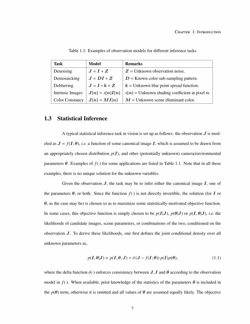
Table 1.1: Examples of observation models for different inference tasks
Task Model Remarks
Denoising J = I +Z Z = Unknown observation noise.
Demosaicking J =DI +Z D = Known color sub-sampling pattern.
Deblurring J = I ∗ k +Z k = Unknown blur point spread function.
Intrinsic Images J [n] = s[n]I[n] s[n] = Unknown shading coefficient at pixel n.
Color Constancy J [n] =MI[n] M = Unknown scene illuminant color.
1.3 Statistical Inference
A typical statistical inference task in vision is set up as follows: the observation J is mod-
eled as J = f (I;θ), i.e. a function of some canonical image I , which is assumed to be drawn from
an appropriately chosen distribution p(I), and other (potentially unknown) camera/environmental
parameters θ. Examples of f (·) for some applications are listed in Table 1.1. Note that in all these
examples, there is no unique solution for the unknown variables.
Given the observation J , the task may be to infer either the canonical image I , one of
the parameters θ, or both. Since the function f (·) is not directly invertible, the solution (for I or
θ, as the case may be) is chosen so as to maximize some statistically-motivated objective function.
In some cases, this objective function is simply chosen to be p(I |J ), p(θ|J ) or p(I ,θ|J ), i.e. the
likelihoods of candidate images, scene parameters, or combinations of the two, conditioned on the
observation J . To derive these likelihoods, one first defines the joint conditional density over all
unknown parameters as,
p(I ,θ|J ) ∝ p(I ,θ,J ) = δ (J − f (I;θ)) p(I)p(θ), (1.1)
where the delta function δ(·) enforces consistency between J , I and θ according to the observation
model in f (·). When available, prior knowledge of the statistics of the parameters θ is included in
the p(θ) term, otherwise it is omitted and all values of θ are assumed equally likely. The objective
7

Chapter 1: Introduction
function is then computed by marginalizing over all parameters other than those being estimated
(for example, p(I |J ) is computed by marginalizing over θ). Note that the solutions for I and θ
obtained by maximizing their joint conditional likelihood p(I ,θ|J ) need not be the same as those
derived from their individual likelihoods p(I |J ) and p(θ|J ).
Rather than set the objective to these conditional likelihoods, some methods define a no-
tion of the cost C(·, ·) of choosing an estimate I or θ, when the true value is I ′ or θ′ respectively.
The estimate is then chosen to minimize the expected value of this cost, under the conditional dis-
tribution for the true estimate computed as above. For example, the canonical image I may be
estimated as
I = arg minI
∫
C(I , I ′)p(I ′|J )dI ′. (1.2)
The cost C usually corresponds to some form of error (such as the sum of squared differences, 0-1
error, etc.) between the estimate and true value. Minimizing the expected error can lead to more
robust estimates— as illustrated in Fig. 1.3, in some cases the conditional distribution itself is noisy
and choosing the most likely value may correspond to an isolated peak. The integration in (1.2) can
be thought of as applying a smoothing operation to this distribution prior to estimation.
To compute the estimate from these objective functions, one has to solve the correspond-
ing optimization problem. While there is sometimes a closed form expression for this solution, iter-
ative strategies are frequently required. These include gradient descent methods, iteratively solving
for a subset of the unknowns keeping the others constant, successively approximating the objective
function near the expected solution with a functional form that is easy to optimize, etc. Overall,
models and inference strategies are chosen so as to yield accurate estimates with minimal com-
putational expense. Sometimes, this involves choosing models with simplifying assumptions (for
example, treating overlapping patches as independent) to keep estimation tractable. In other cases,
the inference strategy is adapted for optimum performance on a specific application. For instance,
in many deblurring algorithms [20, 21] that seek to estimate the latent sharp image I from a blurry
8
Chapter 1: Introduction
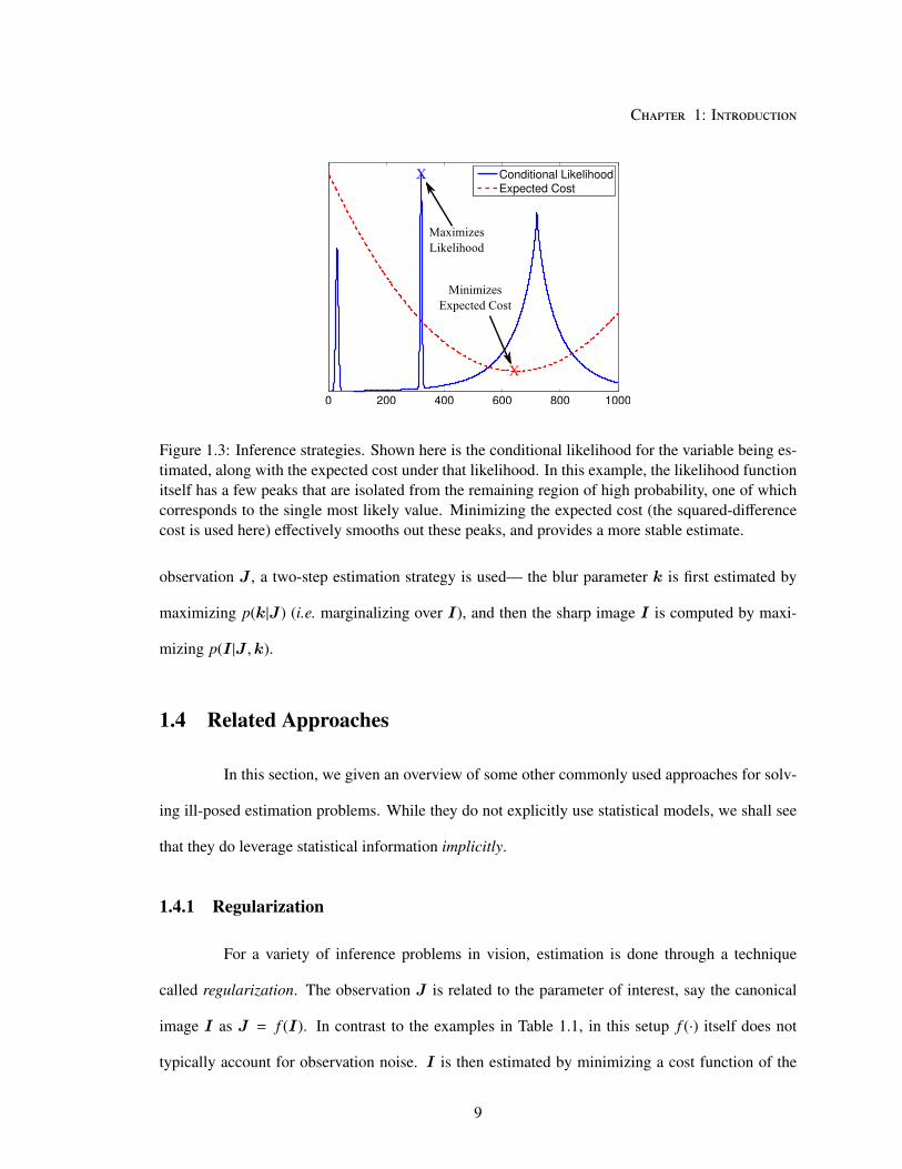
Figure 1.3: Inference strategies. Shown here is the conditional likelihood for the variable being es-
timated, along with the expected cost under that likelihood. In this example, the likelihood function
itself has a few peaks that are isolated from the remaining region of high probability, one of which
corresponds to the single most likely value. Minimizing the expected cost (the squared-difference
cost is used here) effectively smooths out these peaks, and provides a more stable estimate.
observation J , a two-step estimation strategy is used— the blur parameter k is first estimated by
maximizing p(k|J ) (i.e. marginalizing over I), and then the sharp image I is computed by maxi-
mizing p(I |J ,k).
1.4 Related Approaches
In this section, we given an overview of some other commonly used approaches for solv-
ing ill-posed estimation problems. While they do not explicitly use statistical models, we shall see
that they do leverage statistical information implicitly.
1.4.1 Regularization
For a variety of inference problems in vision, estimation is done through a technique
called regularization. The observation J is related to the parameter of interest, say the canonical
image I as J = f (I). In contrast to the examples in Table 1.1, in this setup f (·) itself does not
typically account for observation noise. I is then estimated by minimizing a cost function of the
9

Chapter 1: Introduction
form:
I = arg minI‖J − f (I)‖e + α‖I‖r, (1.3)
where the first term penalizes the error in terms of the model (under some norm e), and the second
term regularizes the estimation problem to compensate for the fact that f (·) can not be directly
inverted. The parameter α is a scalar that weighs the relative contributions of these two terms.
Although this approach is often motivated without an explicit statistical characterization, choosing
the parameter α and the forms of the error and regularization terms amounts to making assumptions
about the statistics of the image and observation noise.
In fact, we can show that there is an equivalent statistical approach that leads to the exact
same expression as in (1.3). We update the observation model to include a noise term Z as
J = f (I ,Z) = f (I) +Z, (1.4)
and choose the distributions for Z and I to match (1.3) as
p(Z) ∝ exp
(
−‖Z‖eβ
)
, p(I) ∝ exp
(
−‖I‖rγ
)
. (1.5)
We can now compute I in this formulation by maximizing p(I |J ) as
I = arg maxI
p(I |J ) = arg maxI
∫
δ(
J − f (I ,Z))
exp
(
−‖Z‖eβ
)
exp
(
−‖I‖rγ
)
dZ
= arg maxI
exp
(
−‖J − f (I)‖eβ
− ‖I‖rγ
)
= arg minI‖J − f (I)‖e +
β
γ‖I‖r, (1.6)
which is equivalent to the regularized estimate from (1.3), when α = β/γ. Therefore, the error
penalty in (1.3) can be interpreted as the log-likelihood of observation noise and the regularization
term as the log-likelihood of a candidate image. However, this connection is not always made when
setting up a regularization framework. This is appropriate in many cases when the models in (1.5)
are poor fits to observed empirical distributions, but the overall estimation strategy leads to desirable
results in practice.
10

Chapter 1: Introduction
1.4.2 Machine Learning
Learning-based methods like boosting, support vector classification and regression, etc. take
a different approach to estimation. They learn a mapping g(·) from the observation J to the variable
of interest, say θ. This mapping is chosen automatically from a space of functions H (sometimes
called the hypothesis space) so as to minimize estimation error on a training set of input-output pairs
{Jt,θt}Tt=1. To prevent “over-fitting”, i.e. choosing a complex mapping that fits exactly to the data,
including small perturbations possibly caused by noise, these approaches also seek to simultane-
ously minimize some notion of complexity (often measured in terms of smoothness) of the chosen
map. Formally, the map g(·) is chosen as
g = arg ming∈H
T∑
t=1
1
Terr (g(Jt);θt) + α ‖g‖H , (1.7)
where the first term corresponds to error on the training set, and the second measures complexity
as described above. Note that the expression in (1.7) can itself be interpreted as a regularized esti-
mation framework, used here to choose the map g(·) based on training data. Once this inverse map
g(·) has been computed, it is applied directly to novel observations to compute the corresponding
estimates of θ.
There is a clear parallel between picking g(·) as per (1.7) and minimizing the expected
cost under a conditional distribution as described in Sec. 1.3. The summation over the training
set in (1.7) approximates the joint distribution p(J ,θ), and corresponds to choosing a map that
minimizes the expected error value under this distribution. This approach has various advantages—
one avoids making the assumptions that are implicit in defining an observation model, assigning
statistical distributions to the image and other parameters, etc.. All these decisions are assumed
to be made automatically by the training algorithm in (1.7) for optimal performance. This can be
useful when the actual observation model and statistics are unknown or hard to model, and the
learning method can be trusted to discover the attributes of the observation that are most useful for
computing an accurate estimate.
11

Chapter 1: Introduction
However, learning-based methods make a design choice in picking the hypothesis space
H . The training step in (1.7) can at best learn the most accurate map in H , but H itself has to
be expressive enough and contain the class of functions appropriate for the estimation task. When
this task is complex, the hypothesis space H must be chosen to include adequately complex func-
tions, and a lot more training data is required to reliably learn the mapping g(·). In contrast, if the
observation model is known and a parametric form for image and parameter distributions has been
chosen, the parameters of these distributions can be learned with far fewer training samples and
using statistical inference methods may prove more convenient. Furthermore as noted in Sec. 1.3,
the optimal estimates derived from statistical models often do not have closed form solutions, but it
is impractical to define a hypothesis spaceH of maps that involve iterative computation.
In practice, statistical inference and machine learning serve as complementary approaches
for visual inference, with each being optimal for different types of applications, based on the com-
plexity of the problem and availability of training data. While it may be tempting to always use a
purely data-driven machine learning approach, the use of explicit statistical models and inference
approaches, that incorporate useful domain knowledge, can yield dividends in terms of improved
accuracy and speed for many applications .
1.5 Dissertation Outline
This dissertation seeks to demonstrate the efficacy of statistical modeling for visual in-
ference, and the design choices that need to be made to ensure accurate yet tractable inference
for different tasks. Accordingly, we present novel statistical estimation algorithms for two visual
inference tasks. Each involves the use of a different image model, individually adapted for each
application to encode different aspects of the statistical structure present in natural images.
Chapter 2 describes an algorithm to estimate the parameters of spatially-varying motion
blur acting on an image, allowing the segmentation of moving objects from a still image using
12

Chapter 1: Introduction
this blur as a cue. We use an image model to describe texture content in greyscale images to
estimate blur parameters, and augment it with per-pixel color appearance models to carry out the
segmentation. Chapter 3 tackles the problem of color constancy, i.e. correcting for the color cast
in an observed image caused by the spectrum of the scene illumination. This lets us automatically
estimate a canonical white-balanced image, in which object colors are independent of illumination
and can serve as, say, stable cues for recognition. For this task, we introduce a joint spatio-spectral
model that encodes the color statistics of spatial sub-band coefficients.
In Chapter 4, we investigate the statistical structure of hyperspectral images, and dis-
cuss modeling strategies in that domain. Hyperspectral images provide higher-resolution spectral
measurements of the incident light at each pixel, and are expected to be useful for various vision
applications. Using a new database of hyperspectral images of real-world scenes, we explore the
statistical properties that are likely to be useful when building hyperspectral image models for sta-
tistical inference.
With the goal of ensuring that the research presented here is reproducible, we have made
prototype implementations of the presented algorithms as well as all newly collected image data
available for download [22–24]. Also, note that early versions of this research have appeared in the
following publications:
• Ayan Chakrabarti, Keigo Hirakawa, and Todd Zickler, “Color Constancy Beyond Bags of
Pixels,” in Proceedings of the IEEE Conference on Computer Vision and Pattern Recognition
(CVPR), 2008.
• Ayan Chakrabarti, Todd Zickler, and William T. Freeman, “Analyzing Spatially-varying Blur,”
in Proceedings of the IEEE Conference on Computer Vision and Pattern Recognition (CVPR),
2010.
• Ayan Chakrabarti and Todd Zickler, “Statistics of Real-world Hyperspectral Images,” in Pro-
13

Chapter 1: Introduction
ceedings of the IEEE Conference on Computer Vision and Pattern Recognition (CVPR), 2011.
We conclude the dissertation in Chapter 5 with an overview of the contributions, and
describe opportunities to expand on the insights developed here and apply them for use in other
applications.
14

2Estimating Blur
“The English can’t draw a line without blurring it.”
— Winston Churchill
The image of an object or region is blurred when a pixel receives light from multiple scene
locations, due to motion or defocus. This induced blur can vary spatially across the image plane as a
function of scene content, such as depth and object motion parameters. In this chapter, we describe
an algorithm that uses spatially-varying motion blur as a cue to segment out a moving object from
a still image. At the core of this method is an image model that encodes the statistical properties
of sharp edges, independent of their contrast. A local Fourier-based representation allows us to use
this model for tractable inference, to compute the likelihood of a local region in the observed image
being blurred by a kernel from a candidate set. This likelihood measure is then combined with a
color model in a Markov random field (MRF) framework to carry out the actual segmentation. The
method is evaluated on a diverse set of real images captured using a variety of cameras, and found
to perform well.
15
Chapter 2: Estimating Blur
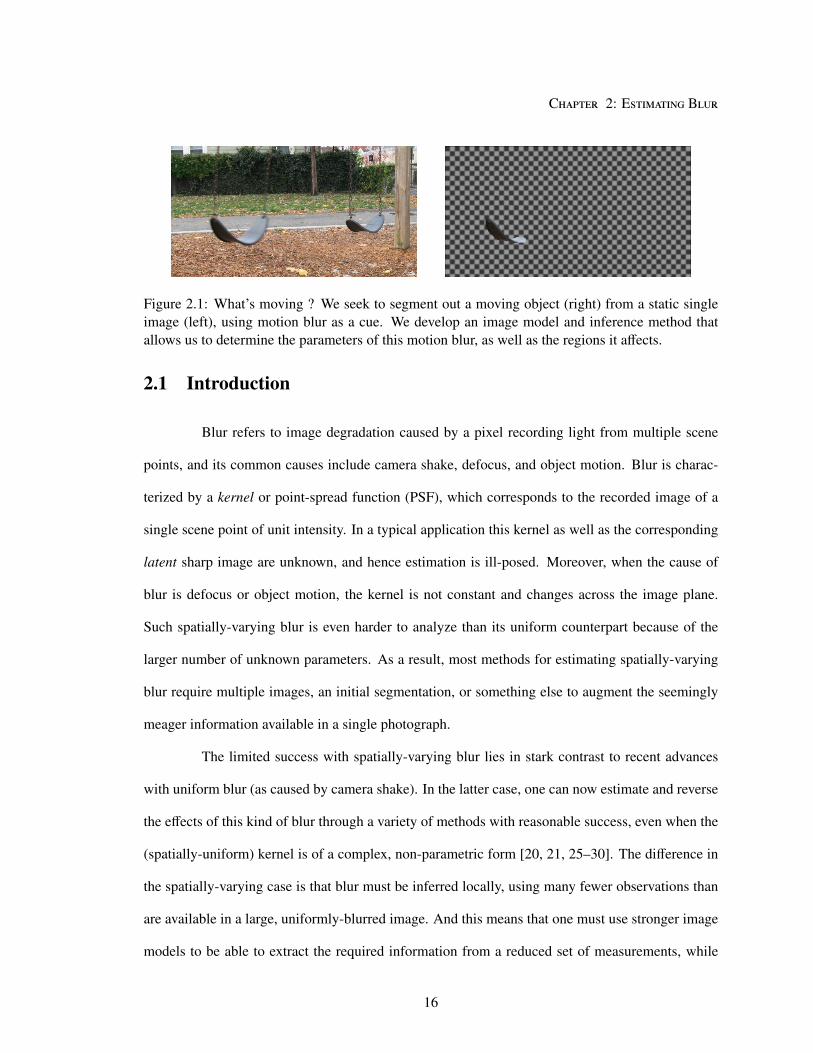
Figure 2.1: What’s moving ? We seek to segment out a moving object (right) from a static single
image (left), using motion blur as a cue. We develop an image model and inference method that
allows us to determine the parameters of this motion blur, as well as the regions it affects.
2.1 Introduction
Blur refers to image degradation caused by a pixel recording light from multiple scene
points, and its common causes include camera shake, defocus, and object motion. Blur is charac-
terized by a kernel or point-spread function (PSF), which corresponds to the recorded image of a
single scene point of unit intensity. In a typical application this kernel as well as the corresponding
latent sharp image are unknown, and hence estimation is ill-posed. Moreover, when the cause of
blur is defocus or object motion, the kernel is not constant and changes across the image plane.
Such spatially-varying blur is even harder to analyze than its uniform counterpart because of the
larger number of unknown parameters. As a result, most methods for estimating spatially-varying
blur require multiple images, an initial segmentation, or something else to augment the seemingly
meager information available in a single photograph.
The limited success with spatially-varying blur lies in stark contrast to recent advances
with uniform blur (as caused by camera shake). In the latter case, one can now estimate and reverse
the effects of this kind of blur through a variety of methods with reasonable success, even when the
(spatially-uniform) kernel is of a complex, non-parametric form [20, 21, 25–30]. The difference in
the spatially-varying case is that blur must be inferred locally, using many fewer observations than
are available in a large, uniformly-blurred image. And this means that one must use stronger image
models to be able to extract the required information from a reduced set of measurements, while
16

Chapter 2: Estimating Blur
also ensuring that inference is tractable.
This chapter describes a novel cue for analyzing blur locally and reasoning about non-
uniform cases. Starting with a standard sub-band decomposition (a “local” Fourier transform), we
introduce a probability model for unblurred natural images that is simple enough to “play well”
with the decomposition but powerful enough for accurate inference. This gives us a robust and
efficient likelihood measure for a small image window being blurred by a given kernel. This cue is
then applied to the problem of segmenting motion-blurred regions from otherwise sharp images and
simultaneously selecting the blur kernel acting on the affected region. We evaluate this approach
using a diverse collection of images that each contain a single moving object. It yields satisfactory
estimates of the blur kernel in most cases, and is able to obtain useful segmentations when combined
with color information.
2.2 Related work
Inferring the blur kernel from a blurred image requires simultaneously reasoning about
the kernel and the latent sharp image on which it operates. To address the problem, one must define
the family of blur kernels to be considered, as well as an image model which encodes the statistical
properties that distinguish sharp images from their blurred counterparts. Existing methods differ in
terms of the types of blur they consider, the observations they use as input, and whether or not they
allow the kernel to vary spatially.
When the blur is caused by camera shake and is spatially-uniform, one has the good for-
tune of being able to accumulate evidence across the entire image plane, and as a result, one can
afford to consider a very general class of blur kernels. In this context, a variety of recent techniques
have shown that it is possible to recover non-parametric and fairly arbitrary blur kernels, such as
those induced by camera shake, from as little as one image [20, 21, 25–28]. Even in instances of
camera shake when the actual kernel varies spatially, because the camera motion involves rotation
17

Chapter 2: Estimating Blur
or out of plane movement, these varying kernels can be related by using a homography to relate
images corresponding to different camera positions and orientations. Since the parameters of this
homography are still global, they can be estimated with reasonable accuracy by pooling cues from
across the image [29, 30]. One general insight that is drawn from these works is that instead of si-
multaneously estimating the blur kernel and a single sharp image that best explain a given input, it is
often preferable to first estimate the blur kernel (say, from its conditional distribution) by marginal-
izing over all consistent sharp images. Levin et al. [21] refer to this process as “MAPk estimation”,
and we will use it here.
Blur caused by motion or defocus usually varies spatially across an image, and in these
cases, one must infer the blur kernels largely using local evidence. To succeed at this task, most
methods consider a more constrained family of blur kernels, and they incorporate more input than
a single image. When two or more images are available, one can exploit the differences between
blur and sensor noise [31] or the required consistency between blur and apparent motion [32–35] or
blur and depth [36, 37]. As an alternative to using two or more images, one can use a single image
but assume that a solution to the foreground/background matting problem is given as input [38–40].
Finally, one may be able to successfully use a single image, but with special capture conditions to
exaggerate the effect of the blur. This is the approach taken in [41], where images captured with
a coded aperture are used (along with additional user input) to estimate defocus blur that varies
spatially as a function of scene depth.
More related to the method presented here is the pioneering effort of Levin [42], who also
considers the case with just a single image, acquired from a regular camera, as input. The idea
is to segment an image into blurred and non-blurred regions and to estimate the PSFs by exploit
differences in the distribution of intensity gradients within the two types of regions. These relatively
simple image statistics allow compelling results in some cases, but they fail dramatically in others.
One of our primary motivations in this chapter will be to understand these failures and develop
stronger computational tools to eliminate them.
18

Chapter 2: Estimating Blur
2.3 Observation Model
Let y[n] denote the observed image, with n ∈ R2 indicating the location of a pixel. We
shall consider the case where y[n] is a single-channel linear (i.e. not gamma-corrected) greyscale
image. Let x[n] be the corresponding latent sharp image, i.e. the image that would have been
captured in the absence of any blur or noise. The images x and y can then be related as
y[n] =
∑
n′x[n′] kn′[n − n′]
+ z[n], (2.1)
where z is sensor noise and kn is the blur kernel acting at pixel location n. Therefore, each pixel
n accumulates light from multiple neighboring pixels n′, weighted based on the corresponding
kernels kn′ acting at those locations. The observation noise z[n] is assumed to be white Gaussian
with variance σ2z :
z[n]iid∼ N(0, σ2
z ). (2.2)
Our goal is to estimate the blur kernel kn at every location n. This problem is under-
determined even when the kernel does not change from point to point, and allowing spatial varia-
tion adds considerable complexity. Allowing an arbitrary kernel at every pixel renders estimation
impractical, and we will need to make some simplifying assumptions to proceed. One assumption
we make is that the kernel is constant in local neighborhoods. This turns out to be a reasonable
assumption in most cases, but as we shall see, it limits our ability to obtain localized boundaries
based on blur information alone.
Note that when the blur is uniform and kn = k,∀n, the model in (2.1) reduces to a regular
convolution, i.e.
y[n] = (x ∗ k)[n] + z[n]. (2.3)
This case is naturally analyzed in the frequency domain. The convolution theorem lets us simplify
inference with the Fourier transform by diagonalizing the action of the constant kernel k as
Y(ω) = X(ω)K(ω) + Z(ω), (2.4)
19

Chapter 2: Estimating Blur
where ω ∈ [−π, π]2 corresponds to spatial frequency, and Y(ω), X(ω), K(ω) and Z(ω) are Fourier
transforms of x[n], y[n], k[n] and z[n] respectively. However, when the blur kernel varies spatially,
the signals x[n] and y[n] are no longer related by convolution, and a global Fourier transform is of
limited utility.
Instead, we use a localized frequency representation. Let w[n] ∈ {0, 1} be a symmetric
window function with limited spatial support, and { fi} be a set of complex-valued filters defined as
fi[n] = w[n] × e− j〈ωi,n〉, (2.5)
with frequencies ωi ∈ R2. The choice of {ωi}i will depend on the window size, and it is made
to ensure that the filters { fi}i are orthogonal, i.e. 〈 fi, f ∗j〉 = 0 for i , j, where f ∗
jrefers to the
complex conjugate of f j. Applying these filters to an image x yields the corresponding responses
xi[n] = (x ∗ fi)[n]. For every location n, the set of coefficients {xi[n]}i can be interpreted as the
Fourier decomposition of a local window centered at that location.
Now, we consider the corresponding local Fourier decomposition of the observed image
y[n]. As stated earlier, we make the assumption that the kernel is constant in local neighborhoods.
As illustrated in Fig. 2.2, we assume that for every location n, the same blur kernel kn acts at every
scene location in x[n] that contributes to any pixel in a window centered at n in the observed image
y[n]. This allows us to combine (2.1) and (2.5) and model the filter responses for the observed
image as
yi[n] = (x ∗ (kn ∗ fi)) [n] + (z ∗ fi)[n]. (2.6)
This is similar to the spatially-uniform case (2.4), but different in a critical way. In this spatially-
varying case, there is no means of expressing the transform coefficients {yi[n]}i in terms of the
corresponding {xi[n]}i alone, because pixels in any window of y have values determined by pixels
outside of that window in x.
However, we can derive a useful expression for the statistics of the observed coefficients,
under specific modeling assumptions. Consider the case where there is no observation noise. In
20

Chapter 2: Estimating Blur
Figure 2.2: Modeling images with spatially-varying blur. We use a localized frequency representa-
tion corresponding to Fourier transforms of local image windows (shown with solid red border). For
every window, a constant kernel kn is assumed to act at all locations in the neighborhood (shown
with a dotted border) that affect observed pixels inside that window. There is no deterministic re-
lationship between the corresponding observed and sharp coefficients, since observed coefficients
depend on the larger neighborhood and not just the Fourier window in the sharp image.
the local neighborhood around n where we assume the kernel to be constant, i.e. one equal to the
support of w plus that of kn, let all elements of x be independent and identically distributed as
N(0, σ2). Since each yi[n] is a linear combination of x[n], it is also distributed as a zero-mean
Gaussian, with variance given by
E |yi[n]|2 = E
∣
∣
∣
∣
∣
∣
∣
∑
l
x[n − l]( fi ∗ kn)[l]
∣
∣
∣
∣
∣
∣
∣
2
= σ2∑
l
|( fi ∗ kn)[l]|2, (2.7)
since the different x[n] are un-correlated. This can be thought of as an analogue to expression in
(2.4), and accordingly we refer to
{
σ2ki
}
i=
∑
l
|(k ∗ fi)[l]|2
i
, (2.8)
as the blur spectrum in the remainder of this chapter.
It is worth noting here that while the transform coefficients {xi[n]}i are un-correlated
owing to the filters { fi}i being orthogonal, strictly speaking the corresponding observed coefficients
21

Chapter 2: Estimating Blur
{yi[n]}i are not. Specifically for i , j, we have
E yi[n]y∗j[n] = σ2∑
l
( fi ∗ kn)[l]( f j ∗ kn)∗[l]
= σ2∑
l
∑
m1
∑
m2
kn[m1]kn[m2] fi[l −m1] f ∗j [l −m2]
= σ2∑
m1
∑
m2
kn[m1]kn[m2]
∑
l
fi[l] f ∗j [l − ∆m]
, (2.9)
where ∆m = m2 −m1. For all terms in the summation above where ∆m = 0, the expression in
parantheses is just the inner product between the filters fi and f j which evaluates to zero. For the
case of ∆m , 0, we have the following expression:
∑
l
fi[l] f ∗j [l − ∆m] =∑
l
w[l]e− j〈ωi,l〉 w[l − ∆m]e j〈ω j,l−∆m〉
= e− j〈ω j,∆m〉∑
l
w[l − ∆m] fi[l] f ∗j [l], (2.10)
using the definition of fi from (2.5). Therefore, the expressions for terms with ∆m , 0 differ in
two aspects— there is a phase-shift in the complex exponential which simply shows up as a unit-
magnitude constant outside the summation; and the summation itself is truncated because of the shift
in the window function w[l − ∆m]. Whereas the full summation corresponds to the inner product
〈 fi, f ∗j〉 and would have evaluated to zero, the truncation causes the above expression to yield a small
residual value. In practice, we find the cross-correlation values between the coefficients due to this
residual to be negligible, and therefore in the following sections, we treat the observed coefficients
as uncorrelated to simplify inference.
2.4 Inference with Image Prior
We now describe a statistical inference approach for estimating the blur kernels kn from
the observed image y[n], using an appropriate prior model for the latent sharp image x[n]. We
define this prior by modeling the distributions of image gradients. Formally, let x∇[n] = (∇ ∗ x)[n]
22

Chapter 2: Estimating Blur
correspond to the gradient map of x for a gradient filter ∇. We will consider different models for
x∇[n], and use them for inference on the gradient map y∇[n] of the observed image y[n].
2.4.1 Gaussian Distribution
We first look at using a Gaussian distribution to model the gradient map x∇[n]. Specifi-
cally, all gradient values in the image are assumed to be independent and identically distributed with
zero mean and a fixed variance s > 0, i.e.
x∇[n]iid∼ N(0, s). (2.11)
Now consider the local Fourier coefficients {y∇i
[n]} of the observed gradient map y∇[n]. In the
absence of observation noise, these are given by
y∇i [n] = (y∇ ∗ fi)[n] = (∇ ∗ y ∗ fi)[n] = (∇ ∗ x ∗ kn ∗ fi)[n] = (x∇ ∗ (kn ∗ fi))[n]. (2.12)
We can now use the identity in (2.7) to derive an expression for the likelihood p(kn = k|y∇[n]), of
a candidate kernel k acting on a window centered at location n, as
p(kn = k|y∇[n]) ∝ p({y∇i [n]}i|kn = k) ∝∏
i
N(
y∇i [n]|0, sσ2ki
)
∝
∏
i
σ2ki
−1/2
exp
− 1
2s
∑
i
|y∇i
[n]|2
σ2ki
, (2.13)
where σ2ki
is the blur spectrum of the candidate kernel k, as per (2.8).
A Gaussian prior has the virtue of simplicity, and the likelihood in (2.13) can be computed
easily in closed form. Moreover, despite the fact that empirical distributions of gradients in natural
images have significantly heavier tails than a Gaussian distribution, the model has been used with
some amount of success for blur estimation in the absence of spatial variation [21]. Unfortunately,
it is far less useful when dealing with spatially-varying blur.
This is illustrated in Fig. 2.3 using a toy one-dimensional “image”. We consider two local
windows, one that contains a low-contrast edge that is not blurred, and another with a high-contrast
23

Chapter 2: Estimating Blur
Figure 2.3: Inference with different priors on a toy example. We consider two windows in a 1-D
image (Left), containing a high contrast blurred edge (the dotted line corresponds to the latent sharp
edge) and a low contrast blurred edge. (Center) For each window, we show the ratio between the
likelihoods of it being blurred and sharp, under the Gaussian and GSM priors. For the Gaussian
prior, this ratio is shown as a function of the variance parameter s. A window is classified as blurred
if the log of the ratio is above 0. While the GSM-based likelihood yields the correct classification
for both edges, there is no single value of s for which both windows are classified correctly. (Right)
A comparison of the blur spectra (bottom) corresponding to the blur kernel σki and to no blur σδi,
with the actual observed coefficient magnitudes (top) for the two windows containing the blurred and
sharp edges. We see that while the observed magnitudes match the “shapes” of their corresponding
expected spectra, they are scaled differently based on the contrast of the edges.
edge that is blurred by a box filter k. Our task is to decide, by looking at the observed coefficients
{y∇i
[n]}i in each local window, whether that window was blurred by k (which is assumed to be
known), or was not blurred at all (i.e. it was blurred by an impulse kernel δ). We shall make this
decision based on the which kernel’s likelihood, as defined in (2.13), is greater.
Figure 2.3 (center) shows the ratio of these likelihoods for different values of the sharp
image model variance parameter s, and we see that the Gaussian-based likelihood measure in (2.13)
is never able to classify both windows correctly. That is, we can choose the model parameter to
correctly classify one or the other, but not both simultaneously. Intuitively, this results from the fact
that even if one can reasonably expect the mean square gradient values of an entire sharp image
to be close to s, the same is not true within different small windows of that sharp image, whose
statistics can change quite dramatically.
To gain further insight, we can look at the local spectra of the input image around the
24
Chapter 2: Estimating Blur
two edges, as depicted in Fig. 2.3 (right). We see that while the magnitudes of the spectra match
the shapes of the two blur kernel spectra, their relative scales are very different. The classification
fails, then, because the simple Gaussian-based likelihood model (2.13) involves absolute variance
values, at a scale that is fixed and determined by the choice of our image prior model parameter s.
Viewed another way, the likelihood term is “distracted” by the difference in contrasts between the
two edges, and this prevents it from being able to make a decision based purely on how sharp the
edges are.
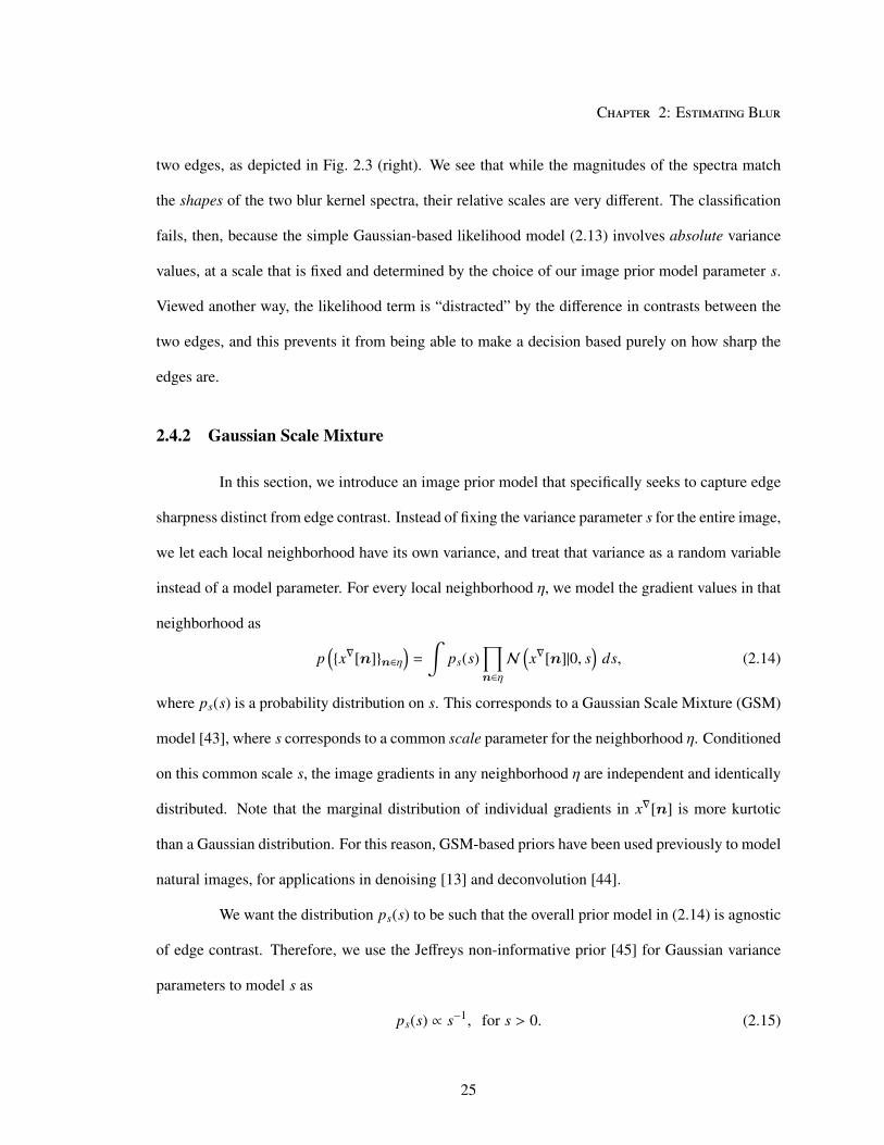
2.4.2 Gaussian Scale Mixture
In this section, we introduce an image prior model that specifically seeks to capture edge
sharpness distinct from edge contrast. Instead of fixing the variance parameter s for the entire image,
we let each local neighborhood have its own variance, and treat that variance as a random variable
instead of a model parameter. For every local neighborhood η, we model the gradient values in that
neighborhood as
p(
{x∇[n]}n∈η)
=
∫
ps(s)∏
n∈ηN
(
x∇[n]|0, s)
ds, (2.14)
where ps(s) is a probability distribution on s. This corresponds to a Gaussian Scale Mixture (GSM)
model [43], where s corresponds to a common scale parameter for the neighborhood η. Conditioned
on this common scale s, the image gradients in any neighborhood η are independent and identically
distributed. Note that the marginal distribution of individual gradients in x∇[n] is more kurtotic
than a Gaussian distribution. For this reason, GSM-based priors have been used previously to model
natural images, for applications in denoising [13] and deconvolution [44].
We want the distribution ps(s) to be such that the overall prior model in (2.14) is agnostic
of edge contrast. Therefore, we use the Jeffreys non-informative prior [45] for Gaussian variance
parameters to model s as
ps(s) ∝ s−1, for s > 0. (2.15)
25

Chapter 2: Estimating Blur
Note that this is an improper prior distribution, because it is not integrable. Nevertheless, as we
show next, it yields a well-defined likelihood measure, and one that is not biased by the scale of the
observed gradients.
Setting η to be the neighborhoods in x∇[n] on which each set of the observed local Fourier
transform coefficients {y∇i
[n]}i depend (i.e. equal to the sum of the supports of the window function
w and candidate blur kernel k), we can derive the likelihood p(kn = k|y∇[n]) under the GSM-based
prior model as
p(
kn = k∣
∣
∣y∇[n])
∝∫
1
s
∏
i
N(
y∇i [n]|0, sσ2ki
)
ds
∝∫
s−(F/2+1)
∏
i
σ2ki
−1/2
exp
− 1
2s
∑
i
|y∇i
[n]|2
σ2ki
ds, (2.16)
where F is the total number of frequency bands. Fortunately, this expression also has a closed form
solution, that can be derived by matching the integrand above to the form of the inverse-Gamma
distribution:
γ−1(s|α, β) = βα
Γ(α)s−(α+1)e−β/s. (2.17)
Using the fact that integrating the above distribution over s yields one, we have
p(
kn = k∣
∣
∣y∇[n])
∝
∏
i
σ2ki
−1/2
∑
i
|y∇i
[n]|2
σ2ki
−F/2
. (2.18)
We can show that the likelihood measure in (2.18) has several desirable properties. Note
that it can be re-written as:
p(
kn = k∣
∣
∣y∇[n])
∝
∏
i
|y∇i [n]|
−1 [
GM({rki[n]}i)AM({rki[n]}i)
]F/2
, (2.19)
where,
rki[n] =|y∇
i[n]|2
σ2ki
, (2.20)
are the ratios between the observed and blur spectra, and the GM(·) and AM(·) terms refer to their
geometric and arithmetic means, respectively. Scaling all the rki terms for a particular window by a
26

Chapter 2: Estimating Blur
constant will not affect the ratio between the geometric and arithmetic means. Therefore, we have
the following identity:
p(
kn = β1k1
∣
∣
∣αy∇[n])
p(
kn = β2k2
∣
∣
∣αy∇[n]) =
p(
kn = k1
∣
∣
∣y∇[n])
p(
kn = k2
∣
∣
∣y∇[n]) , (2.21)
for any scalars α, β1 and β2. This implies that for a candidate window, the likelihood ratio between
two candidate kernels is independent of the scale or absolute magnitudes of the kernels and observed
gradients.
Furthermore, we note that the geometric mean of a series is always less than or equal to
the arithmetic mean, with the two being equal only when all elements of the series, in this case the
ratios {rki}i, are the same. Therefore, for a given set of observed coefficients {y∇i
[n]}i, the likelihood
is maximal when |y∇i
[n]|2 = α σ2ki, ∀i, i.e. the observed spectrum is exactly a scaled version of
the candidate blur spectrum. Because of these properties, the likelihood measure in (2.18) can
be interpreted as matching the shapes of the observed spectrum to those of candidate blur kernels,
independent of their magnitudes. As a result, we see that the GSM-based likelihood is able to ignore
the contrasts of the two edges in our toy 1-D example and, as shown in Fig. 2.3 (center), is able to
classify both correctly.
2.4.3 Inference with Noisy Observations
So far, we have looked at computing blur likelihoods ignoring the effects of observation
noise, i.e. z[n] in (2.1). We now consider the effect of noise on the statistics of the observed gradient
coefficients {y∇i
[n]}. In the presence of noise, these coefficients are given by
y∇i [n] = y∇i [n] + z∇i [n], (2.22)
where {y∇i
[n]}i are the corresponding clean coefficients that would have been observed in the ab-
sence of noise, and {z∇i
[n]}i are the local Fourier coefficients of the gradient map of the noise image
z[n], given by
z∇i [n] = (∇ ∗ z ∗ fi)[n]. (2.23)
27

Chapter 2: Estimating Blur
Given the noise model in (2.2), where z[n] is assumed to be independent and identically
distributed as a Gaussian with variance σ2z in the pixel domain, it follows from the identity in (2.7)
that the expected variance of the noise gradient coefficients {z∇i
[n]} will be given by the spectrum
σ2∇i
of the gradient filter ∇ computed as per (2.8), i.e.
E
∣
∣
∣z∇i [n]∣
∣
∣
2= σ2
zσ2∇i = σ
2z
∑
n
|(∇ ∗ fi)[n]|2 . (2.24)
Unfortunately, updating the GSM-based prior likelihood to exactly model the effect of
these noise coefficients as
p(
kn = k∣
∣
∣y∇[n])
∝∫
ps(s)∏
i
N(
y∇i [n]|0, sσ2ki + σ
2zσ
2∇i
)
ds, (2.25)
is problematic. Using the Jeffreys prior from (2.15) no longer yields a finite likelihood measure,
because the integrand above goes to infinity as s approaches zero. Even if ps(s) were to be suitably
modified, there would be no closed form solution and the integration above would have to be done
numerically.
Instead, we take the following approach to approximately account for the effect of ob-
servation noise in our original likelihood measure in (2.18): for every window, we only consider
those observed coefficients whose magnitudes are significantly above the corresponding noise vari-
ances from (2.24), and then compute the likelihood from only these coefficients, treating them as
noise-free. This updated likelihood measure is given by
p(
kn = k∣
∣
∣y∇[n])
∝
∏
i∈I[n]
σ2ki
−1/2
∑
i∈I[n]
|y∇i
[n]|2
σ2ki
−|I[n]|/2
, (2.26)
where I[n] corresponds to the active set of coefficients for each window, and is given by
I[n] = { i : |y∇i [n]|2 > T σ2zσ
2∇i}, (2.27)
for some scalar T . This choice of I[n] is independent of the candidate kernel k, and the likelihood
measures for different kernels is computed over the same set of coefficients for each window.
28

Chapter 2: Estimating Blur
Finally, note that gradient filters are typically high-pass and therefore the values of σ2∇i
corresponding to the higher frequencies ωi will be large. As a result, the observed coefficients for
these bands will often fail to cross the noise threshold as defined in (2.27). Therefore, to reduce
computational cost, we avoid computing coefficients for bands with high values of σ2∇i
and apply
only a subset of the filters { fi}i to the observed image.
2.5 Detecting Motion
We now address the task of detecting and segmenting out a moving object from a single
still image. We describe an algorithm that exploits motion blur as a cue for this task, using the
likelihood measure described in the previous section. We assume that there is only one moving
object in the image, and instead of detecting a separate blur kernel for each region in this object,
we assume that the object is moving uniformly and that all regions inside the object are therefore
affected by the same kernel km. This assumption makes the segmentation more robust, and our
estimate of the kernel km provides direct information about the orientation and speed (relative to
exposure time) of the moving object [32–35].
Formally, for a given observed image y[n], every pixel is modeled as either part of the
stationary sharp “background” or the motion-blurred “foreground”. Therefore, we assume that every
kernel kn belongs to the set {k0, km}, where k0 corresponds to the blur kernel acting on the stationary
regions of the image and is chosen to either be an impulse (i.e. no blur at all) or a mild defocus blur;
and km is the motion blur kernel acting on the moving object. Our task is to estimate the motion
kernel km, and to assign a label M[n] to every location, where M[n] = 0 for pixels in stationary
regions, and 1 for pixels in the moving object. We shall interpret this to imply that kn = k0 for
M[n] = 0 and kn = km otherwise, but our assumptions about the blur kernel kn being constant in a
neighborhood clearly do not hold at the borders of this segmentation. Therefore, we will augment
the blur likelihood with a per-pixel color model that will help with inference near these boundaries.
29

Chapter 2: Estimating Blur
Figure 2.4: Candidate set of motion kernels. The kernel km acting on the moving object is assumed
to belong to a set of horizontal and vertical box filters of different length. These kernels corre-
spond to the object moving with different uniform velocities in the corresponding direction during
exposure.
2.5.1 Selecting the Kernel
We first address the task of choosing the blur kernel km. It is assumed to be one of a
discrete set of possible candidates, corresponding to horizontal or vertical box filters of different
lengths (see Fig. 2.4). These correspond roughly to horizontal or vertical object motion with fixed
velocity. Formally, for a chosen set of lengths {l1, l2, . . . lL}, we assume that
km ∈ {bhl1 , . . . bhlL , bvl1 , . . . bvlL}, (2.28)
where bhl is a horizontal “box” filter of length l (corresponding to number of pixels the object moved
during exposure), i.e.
bhl[n] =
1 if ny = 0, 0 ≤ nx < l,
0 otherwise,
(2.29)
and bvl is a similarly defined vertical box filter.
To handle both horizontal and vertical candidate blurs {bhl} and {bvl}, we need to use two
sets of coefficients {yhi[n]}i and {yv
i[n]}i defined as,
yhi [n] = ( fih ∗ ∇h ∗ y)[n], yv
i [n] = ( fiv ∗ ∇v ∗ y)[n], (2.30)
where ∇h and ∇v are horizontal and vertical gradient filters, and { fih}i and { fiv}i correspond to local
Fourier filters defined as per (2.5), using horizontal and vertical one-dimensional windows.
To select the motion blur kernel km, we need to derive an expression for the global likeli-
hood p(km = b). If b is horizontal, then the coefficients yhi[n] at all n should be explained either by
30

Chapter 2: Estimating Blur
b or k0, and the coefficients in the orthogonal direction yvi[n] should all be explained by k0 (i.e. they
are not affected by the motion blur). The converse is true if b is vertical, and this reasoning leads us
to define
p(km = blh) ∝
∏
n
maxk∈{k0,blh}
p
(
kn = k
∣
∣
∣
∣
{
yhi [n]
}
i
)
×
∏
n
p
(
kn = k0
∣
∣
∣
∣
{
yvi [n]
}
i
)
,
p(km = blv) ∝
∏
n
p
(
kn = k0
∣
∣
∣
∣
{
yhi [n]
}
i
)
×
∏
n
maxk∈{k0,blv}
p
(
kn = k
∣
∣
∣
∣
{
yvi [n]
}
i
)
, (2.31)
where the individual per-window likelihood measures are computed as per (2.26). The blur kernel
km can then be chosen amongst the candidate set in (2.28) to maximize this likelihood p(km). Note
that the most expensive part of computing the likelihoods, for each of the candidate kernels, is the
local Fourier decomposition, but this only needs to be done once for each orientation. Once the
coefficients {yhi[n]}i and {yv
i[n]}i have been computed, the kernel km can be selected very efficiently
using the above strategy.
2.5.2 Segmentation
Having chosen the motion kernel km, we now address the problem of assigning the seg-
mentation labels M[n] at every location n. As mentioned above, the blur likelihoods alone are
not sufficient for this task since they are not well-defined at segmentation boundaries, and also in
smooth regions where the most of the observed gradient coefficients are below the noise threshold in
(2.27). Therefore, these likelihoods are combined with a complimentary cue derived from statistical
distributions for object and background pixel colors into a Markov random field (MRF) model, as
used in traditional segmentation [46].
This MRF model will be defined in terms of an energy function that incorporates the blur
likelihoods, color distributions, and a spatial smoothness constraint on M[n] that favors adjacent
pixels having the same label assignments. The blur component Bn[m] of this energy, as a function
of the label m ∈ {0, 1} at that location, is defined simply as the negative log-likelihood of the
31
Chapter 2: Estimating Blur
corresponding kernel (i.e. km or k0), i.e.
Bn(m) = −m log p(
kn = km
∣
∣
∣y∇[n])
− (1 − m) log p(
kn = k0
∣
∣
∣y∇[n])
. (2.32)
Next, we define color models for pixels corresponding to the moving object and stationary
background. While the blur model was based on the linear greyscale version of the observed image,
these color models are defined on the gamma-corrected RGB vectors yc[n] ∈ R3. We use a finite
mixture of multivariate Gaussians to model both background and object pixels, where the object
color model is defined as
p
(
yc[n]∣
∣
∣
∣
θm ={
γ j,µ j,Σ j
}Jm
j=1
)
=
Jm∑
j=1
γ jN(
yc[n]∣
∣
∣µ j,Σ j
)
. (2.33)
Here, θm correspond to the parameters of this model that also need to be estimated. The back-
ground color model is defined in a similar way in terms of the corresponding parameters θ0 =
{
γ j,µj ,Σ j
}J0
j=1. The color component Cn(m) of the MRF energy is then defined as
Cn(m) = −m log p(
yc[n] |θm
) − (1 − m) log p(
yc[n] |θ0
)
. (2.34)
The labels M[n] ∈ {0, 1} are chosen as the solution to the following energy minimization
problem:
M[n] = arg minM
(
minθm,θ0
E (M[n],θm,θ0)
)
, (2.35)
where the energy function E(·) is defined as
E (M[n],θm,θ0) =∑
n
Bn (M[n]) + λ∑
n
Cn (M[n]) +ρ
2
∑
(n,n′)∈P
∣
∣
∣M[n] − M[n′]∣
∣
∣ . (2.36)
The first two terms in this energy function favor label assignments that match the likelihood mea-
sures under the blur and color models, with the scalar parameter λ controlling the relative contribu-
tion of the two. The third term enforces a smoothness constraint amongst all pairs P of neighboring
locations, by adding a penalty of ρ every time a pair is assigned different labels.
32

Chapter 2: Estimating Blur
Note that the minimization in (2.35) has to be done over both the labels M[n] as well
as the color model parameters θm and θ0. For a fixed value of the color parameters, the optimal
assignments for M[n] can be computed exactly using graph cuts [47] to best satisfy the smoothness
constraints. Therefore, we propose the following iterative algorithm to carry out the overall mini-
mization: we initialize the iterations by setting the label assignments M[n] using graph cuts, based
only on the blur and smoothness terms in (2.36) which do not involve the color parameters. At
each subsequent iteration, we set the color parameters θm and θ0 to minimize the energy function
keeping the current estimates of the label assignments M[n] fixed. This corresponds to fitting the
color parameters so as to maximize the log-likelihoods of the sets of object and foreground labeled
pixels under their respective distributions (as defined in (2.33)), and we do this using the Expecta-
tion Maximization (EM) algorithm [48]. The labels M[n] are then recomputed using these values
of the color model parameters. Note that both these steps reduce the value of the energy function in
(2.36), and we iterate till the label assignments M[n] converge.
2.6 Experimental Results
We now evaluate the algorithm on a database of images of real-world scenes, captured
using three consumer cameras: a digital SLR, a point-and-shoot and a cell-phone. Each image
contains a single motion-blurred object, and we evaluating the proposed method’s ability to latch on
to the motion blur present in the image, which includes choosing the correct approximate orientation
and length for the blur kernel, to yield a useful segmentation. This image database and a MATLAB
implementation of the algorithm are available for download [22].
2.6.1 Implementation Details
Both the horizontal and vertical sub-band transforms were defined in terms of windows
of length W = 61. The filters { fih} and { fiv} were then generated with ωi equal to the corresponding
33

Chapter 2: Estimating Blur
set of frequencies 2πu/W, u ∈ {1, . . . 15}, i.e. we only used the lower half set of frequencies which
had acceptable levels of noise variance in the gradient domain. The gradient filters ∇ were defined
simply as [−1, 1] (in the appropriate direction), i.e. the gradient values corresponded to the finite
differences between neighboring pixels.
For the blur length, we searched over the discrete set of integers from 4 to 15 pixels.
Larger lengths can be handled by downsampling the image to an appropriate resolution. For seg-
mentation, the object and foreground RGB color vectors were modeled as mixtures of 4 and 6
Gaussians respectively. The choices for all parameters (including σ2z , γ and ρ) were kept fixed for
all images.
The JPEG images generated by the cameras were gamma-corrected, and therefore the
input image had to be linearized for use with the blur model. Since the exact tone maps applied
by the cameras were unknown, we assumed standard sRGB gamma-correction and computed the
linear images by raising all intensities to the power (1/2.2). Note that this is only an approximation,
and better results are likely when using a calibrated camera.
2.6.2 Results
Figure 2.5 shows the full segmentation results for all images in the database. This in-
cludes a visualization of the blur and color components of the energy Bn and Cn, along with the
corresponding detected motion blur kernel km, and estimated color model parameters θm and θ0. We
then display the combination of these two energy components, and the final labels M[n] computed
using graph cuts.
We find that the algorithm does well on this diverse set of real world images, despite
approximate assumptions about noise variance, gamma correction, uniform object motion, etc. It is
also able to detect the blurred regions even in cases of relatively minor motion (such as for images
6 and 11), and is fairly robust even in cluttered backgrounds (such as image 3). The detected kernel
km are also found to approximately correlate to the direction and speed of apparent motion of these
34

Chapter 2: Estimating Blur
Input Image 1 Bn: km = Horiz., 6 pixels Cn: Moving object:
Background:
Bn + λ Cn Segmented Object: M[n] = 1 Background: M[n] = 0
Input Image 2 Bn: km = Horiz., 6 pixels Cn: Moving object:
Background:
Bn + λ Cn Segmented Object: M[n] = 1 Background: M[n] = 0
Input Image 3 Bn: km = Horiz., 7 pixels Cn: Moving object:
Background:
Bn + λ Cn Segmented Object: M[n] = 1 Background: M[n] = 0
Figure 2.5: Segmentation results on various image. For each input image, we show the blur and
color energy components Bn and Cn, where the intensity corresponds to the absolute difference
between the energies for the two labels, with blue regions indicating that the m = 0 label (i.e. for
the stationary background) is preferred, and green m = 1. Red corresponds to invalid or unavailable
data. Then, we show the combined energy, and the final segmentation M[n]. The chosen motion
kernel km, and estimated mean color parameters {µ j} j for the color models are also indicated.
35

Chapter 2: Estimating Blur
Input Image 4 Bn: km = Horiz., 4 pixels Cn: Moving object:
Background:
Bn + λ Cn Segmented Object: M[n] = 1 Background: M[n] = 0
Input Image 5 Bn: km = Horiz., 4 pixels Cn: Moving object:
Background:
Bn + λ Cn Segmented Object: M[n] = 1 Background: M[n] = 0
Figure 2.5: (continued)
36
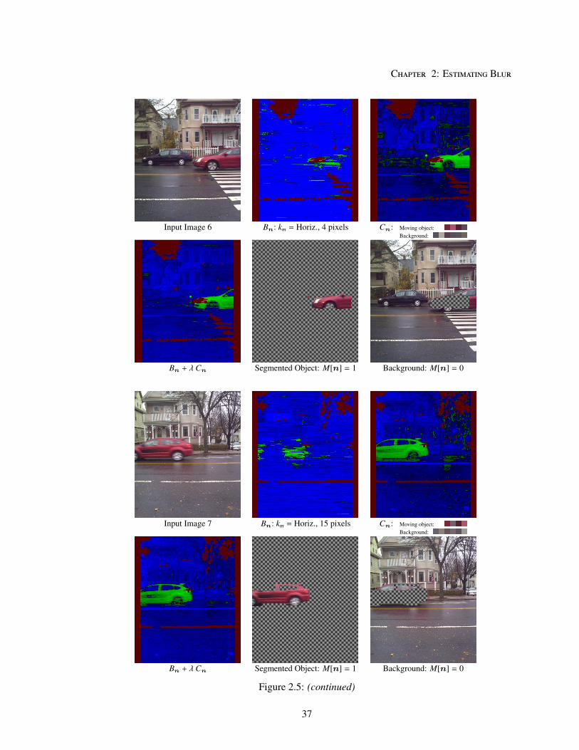
Chapter 2: Estimating Blur
Input Image 6 Bn: km = Horiz., 4 pixels Cn: Moving object:
Background:
Bn + λ Cn Segmented Object: M[n] = 1 Background: M[n] = 0
Input Image 7 Bn: km = Horiz., 15 pixels Cn: Moving object:
Background:
Bn + λ Cn Segmented Object: M[n] = 1 Background: M[n] = 0
Figure 2.5: (continued)
37

Chapter 2: Estimating Blur
Input Image 8 Bn: km = Horiz., 11 pixels Cn: Moving object:
Background:
Bn + λ Cn Segmented Object: M[n] = 1 Background: M[n] = 0
Input Image 9 Bn: km = Vert., 7 pixels Cn: Moving object:
Background:
Bn + λ Cn Segmented Object: M[n] = 1 Background: M[n] = 0
Input Image 10 Bn: km = Vert., 7 pixels Cn: Moving object:
Background:
Bn + λ Cn Segmented Object: M[n] = 1 Background: M[n] = 0
Figure 2.5: (continued)
38

Chapter 2: Estimating Blur
Input Image 11 Bn: km = Horiz., 4 pixels Cn: Moving object:
Background:
Bn + λ Cn Segmented Object: M[n] = 1 Background: M[n] = 0
Figure 2.5: (continued)
objects.
These results also demonstrate the complimentary nature of the blur and color cues. We
show that the blur map Bn typically has poor localization, with a region of confusion around the
boundaries equal to the window length W. While the color map Cn has much better localization,
since it is based on individual pixel colors, it is unable to differentiate between static and moving
regions with similar appearances— for instance, the two swings in image 1. But considered jointly,
these cues are able to overcome their individual drawbacks to yield an acceptable segmentation of
the moving object.
It is important to note the limitations of this approach. The color cue’s localization near
the boundaries, though better than that of the blur cue, is not perfect. This is because the pixels
in that region are weighted sums of the moving object and background, and will not be perfect fits
39
Chapter 2: Estimating Blur
to either of the object or background color models. The uniform motion assumption can also be
limiting in cases of complex non-rigid motion, such as in images 3, 4, 5 and 9, where both the
true motion speed and orientation change across the object. Finally, the blue cue is prone to mis-
classification in cases when there are stationary image regions that in fact appear blurred based on
the local gradient information, due to soft shadows for example, as is the case for the background
object in image 3. But note that these classification errors occur only when the region in question
matches the gradient statistics that specifically correspond to the selected kernel km, rather than for
every region that is a poor fit to our model for sharp edges.
2.7 Discussion
In this chapter, we described a statistical approach to analyze the spatially-varying pa-
rameters of motion blur that acts on an image. This method involved the use of a local Fourier
decomposition which gave us direct access to the effect of blur on image gradient statistics. This
was combined with an image model that was able to differentiate between sharp and blurred edges,
without being adversely affected by the natural variation in edge contrast that occurs in a typical
image. Equipped with this model and representation, we derived a closed form expression for the
likelihood of a local image window being blurred by a candidate kernel.
We used this likelihood measure to segment out moving objects from an image based on
motion blur, and as a part of this segmentation, also estimated the direction and “speed” of motion.
Since the blur model was based on image windows that were assumed to be blurred with a uniform
kernel, we augmented it with a color-based appearance model to yield better localizations at object
boundaries. We described a segmentation algorithm that combined cues from both the blur and
color models, and evaluated it on a database of diverse real images captured using consumer-level
cameras.
Future research should look at improving the quality of segmentations further, especially
40

Chapter 2: Estimating Blur
at the boundaries, by reasoning about both the blur and color models in these regions. This reasoning
may have to take the relative depth of the moving object into account, for example, to consider
different types of occlusion scenarios. The blur model could also be made more robust by a pre-
processing step that distinguishes between material boundaries, that are expected to be sharp, and
smooth gradients from shading effects that are poor fits to our current model, as we saw with soft
shadows in the experimental results. This processing step may require color information to be
directly used in the blur model itself.
Local Fourier decompositions with changing window sizes should also be considered
for the blur model, to optimally trade off localization and discriminability between blur kernels.
For instance, if the motion kernel km is found to be small, a smaller window can be used for the
segmentation part of the algorithm than the one used to select the kernel. Approaches to combine
different window sizes during segmentation should also be considered, with smaller windows near
boundaries and larger ones in the interior of objects likely to yield better results than a uniform
window size.
More broadly, the underlying blur model can be deployed for other vision tasks that in-
volve spatially-varying blur. For example, for defocus blur where the kernel changes with scene
depth, one can imagine using the framework in [41] but doing away with the requirement for spe-
cial capture conditions by using the proposed likelihood measure in (2.18) instead of cues from a
coded aperture. Other applications with motion blur are also worth considering. For instance, in-
stead of assuming uniform rigid motion, one could make local estimates of the blur kernel (possibly
using a weak smoothness constraint) to yield a single image counterpart to optical flow [49]. These
estimates, possibly combined with other cues, could allow the analysis of both object and camera
motion that is more complex than the case considered here.
The blur model in this chapter was based purely on the texture content of sharp images,
i.e. greyscale gradient information, since the action of blur (aside for cases of chromatic aberration)
is independent of color. In the next chapter, we address the problem of estimating the color of the
41

Chapter 2: Estimating Blur
illuminant in a scene. The nature of this task makes color a core cue during inference, and therefore
we will introduce an appropriate model that jointly encodes the color and texture statistics of natural
images.
42

3Color Constancy
“The red brick wall was the color of a brick-red Crayola.”
— Douglas Adams
In this chapter, we tackle the problem of color constancy— correcting the colors of an
observed image to remove the cast caused by the spectral distribution of the scene illuminant. This
is an ill-posed problem since both the illuminant spectrum and scene reflectances are unknown.
Therefore, we develop a statistical model for colors in canonical white-balanced images (i.e. those
that have no color cast), and use this model to infer the most likely illumination parameters in an
observed image. We find that by applying spatial band-pass filters to color images, one unveils color
distributions that are well-represented by a simple parametric form. Once these distributions are fit
to training data, they enable efficient maximum likelihood estimation of the dominant illuminant
in a new image. We show that this estimation method can be easily extended to leverage prior
information about illuminant statistics. Finally, experimental results on a standard image database
are used to verify the accuracy of these estimates.
43

Chapter 3: Color Constancy
Figure 3.1: The observed colors in a scene depend on the spectrum of the illuminant. To estimate
a stable color descriptor that is independent of illumination conditions, one seeks to correct for the
“color cast” corresponding to the unknown illuminant. This process is known as color constancy.
3.1 Introduction
In addition to its intrinsic reflectance properties, the observed color of a material depends
on the spectral and spatial distributions of its surrounding illumination. The same object can there-
fore have different recorded color values in different environments (see Fig. 3.1). In order to use
color as a reliable cue in applications such as recognition, we must somehow compensate for these
extrinsic factors and infer a color descriptor that is stable despite changes in lighting. The ability to
make this inference, termed color constancy, is exhibited by the human visual system to a certain
degree, and there are clear benefits to building it into machines.
One important part of computational color constancy, and the part we consider here, is
compensating for the “color cast” that affects the image as a whole. For this, one ignores spatial
variations in lighting spectra (as might be caused by multiple light sources), and makes the as-
sumption that the spectrum of the illuminant is approximately uniform throughout the scene. The
problem is then one of inferring the inverse map M−1 : R3 → R3 from the space of observed tris-
timulus vectors (RGB, human cone, etc.) to the space of canonical colors, i.e. those that would have
been obtained for the same scene by a standard observer under a standard illuminant. This version
of the color constancy problem is ill-posed since there exist multiple pairs of illuminant spectrum
and scene reflectances that serve as equally valid solutions for any observed image. To resolve this
44

Chapter 3: Color Constancy
ambiguity, we require a prior model for the set of canonical scene colors, and optionally one for
illuminants as well. The color cast (i.e. the map M ) can then be uniquely determined by choosing
the solution that is the most likely under the prior.
Traditional approaches to this problem use models based on statistics of per-pixel colors.
The principal challenge they face is in defining statistics that are informative and reliable, while
allowing tractable inference. Methods such as grey-world [50] and white-patch [51] use simple
first-order statistics— the mean and brightest scene color respectively. While these algorithms have
the benefit of speed, they are susceptible to outliers and dominant colors in a scene and can fail quite
dramatically. On the other hand, using sophisticated models for per-pixel scene colors, such as the
shape of their convex hull in color space [52] or a non-parametric representation of their empiri-
cal probability distribution [53–55], lead to improvements in performance but involve significant
computational cost during estimation.
We introduce a model that goes beyond statistics of per-pixel colors and leverages the
joint spatio-spectral structure that is found to exist in natural images. Motivated by the success of
filter-based methods [56, 57], we begin by decomposing an input color image into distinct spatial
sub-bands and then define an image prior in terms of separate models for the color statistics of each
sub-band. Unlike per-pixel colors, we find that the empirical probability distributions of the colors
in each sub-band can be accurately represented using simple parametric forms. Furthermore, they
allow robust and efficient inference of illumination color cast for an observed image. The resulting
method outperforms existing approaches on a standard database, and allows incorporating a prior
model for illuminants in a statistical framework.
3.2 Problem Formulation
Assuming a Lambertian model, we denote the effective spectral reflectance of a surface
patch observed at pixel n ∈ Z2 by κ(λ,n) ∈ R, where λ ∈ R denotes wavelength. Here, κ accounts
45

Chapter 3: Color Constancy
Figure 3.2: Camera measurements under different illuminants. The effective surface reflectance (κ)
gets shaped by the spectrum (ℓ) of the scene illuminant. Different illuminants can lead to signif-
icantly different radiance spectra (κ × ℓ) being incident on the camera, in turn leading to different
trichromatic measurements by the camera’s sensors (π).
for both the material reflectance and surface orientation with respect to the illuminant. We assume
a single dominant scene illuminant and represent its spectral distribution by ℓ(λ). As depicted in
Fig. 3.2, the spectral power distribution (SPD) of the radiance that is emitted toward the observer is
then the product of ℓ and κ.
The three spectral measurements recorded by a camera at each pixel n (assuming ideal
demosaicking [15, 58]) are then given by
y[n] =[
y{1}[n], y{2}[n], y{3}[n]]T=
∫
π(λ) κ(λ,n) ℓ(λ) dλ, (3.1)
where π(λ) = [π{1}(λ), π{2}(λ), π{3}(λ)]T are the spectral transmittance distributions of the camera’s
color filters. From image y[n] our task is to estimate an illuminant-invariant representation, or
“canonical color” image, x[n] given by
x[n] =
∫
π(λ) ℓ0(λ) κ(λ,n) dλ. (3.2)
We refer to ℓ0 as the “canonical illuminant”, and for the specific choice ℓ0(λ) = 1, each canonical
color x[n] can be interpreted as the trichromatic projection (via π) of the effective reflectance
κ(λ,n) at the corresponding surface point.
46

Chapter 3: Color Constancy
Note that the colors y and x in (3.1) and (3.2) are trichromatic reductions of the full
SPD that cannot be exactly reversed, even when the illuminant ℓ and ℓ0 are known. However, prior
work [59–61] suggests that a linear mapping of the form
x[n] =M−1 y[n], M ∈ R3×3 (3.3)
can achieve accurate chromatic adaptation in many cases, and that it can often be approximated fur-
ther as a diagonal transformation (i.e., Mi j = 0, if i , j). We apply such diagonal mappings directly
in the color space defined by π, even though applying them in an optimized (often called “sharp-
ened”) color space can improve performance [59–61]. For this reason, our results may provide a
conservative estimate of what can be achieved by our algorithm. With some abuse of notation, we
let M represent a diagonal matrix in the subsequent sections and refer to its recovery as “estimating
the illuminant”.
3.3 Related Work
Having settled on a linear diagonal form for the mapping from input color y to canonical
color x, the color constancy problem reduces to the task of estimating the three diagonal entries
of M . Since both the illuminant and scene reflectances are unknown, this is an under-determined
problem. Prior work in this area typically addresses this by introducing a statistical prior model
for surface reflectance κ or canonical color x. White-patch [51] and grey-world [50] are two well-
known methods with intuitive interpretations. Based on the observation that color-neutral or achro-
matic surfaces (i.e. those with constant spectral reflectance) are the most efficient reflectors, the
white-patch [51] algorithm posits that pixels observed to have the greatest intensity correspond to
a color-neutral surface patch. Similarly, based on the assertion that the mean surface reflectance in
a scene is likely to be color-neutral, the grey-world [50] method assumes that the sample mean of
canonical pixel colors is achromatic. The diagonal elements of M are then estimated as those that
map the corresponding vector y[nbrightest] or avg(y[n]) to white.
47

Chapter 3: Color Constancy
Other approaches perform more sophisticated analysis of pixel color distributions. The
gamut-mapping [52] method defines constraints on the set of canonical scene colors {x[n]}n in
terms of their convex hull, or “gamut”. Given an input image y, this approach estimates the illu-
minant M as that which maps the convex hull of {y[n]}n to this expected gamut. Finlayson et
al. [62] use a “di-chromatic” model to reason that, due to varying degrees of specular reflection,
the observed colors of each homogeneous surface in a scene will lie along a line in chromaticity
space (defined as the R and G components of a normalized RGB vector). While colors for different
surfaces correspond to different lines, the extended lines all intersect at a common point corre-
sponding to perfect specular reflection for each surface. This intersection point corresponds to the
chromaticity of the illuminant and can be used to set M , along with additional constraints based on
knowledge of natural illuminant chromaticities.
Another alternative is to develop a complete prior probability distribution over canonical
color images that permits, along with a prior distribution over illuminant spectra, the Bayesian es-
timation of M . To make this Bayesian approach tractable, pixels are assumed to be independent
and identically distributed with a probability density that is either Gaussian [53], or more gener-
ally, non-parametric [54, 55]. Related to these are a number of leaning-based approaches that use
databases of canonical color images to learn linear filters [63] or train neural networks [64] that can
then be used to infer illuminant M for a novel input image.
All of the above methods can be considered “pixel-based” because they model the set of
individual pixel colors without considering each pixel’s spatial context. One can arbitrarily re-order
the pixels of any input image, for example, without affecting the resulting estimate of illuminant M .
Because they ignore spatial structure, these methods can be negatively influenced by the presence
of large colorful objects or regions that skew the color histogram. A variety of work suggests that
improvements might be gained by employing spatial image features, such as segmentations or linear
filter responses, that incorporate spatial information in a tractable manner. For example, Gershon et
al. [65] assume that the average of mean colors of segmented regions of an image, rather than of
48

Chapter 3: Color Constancy
individual pixels, is color neutral. Alternatively, van de Weijer et al. [56] and Gijsenij et al. [57]
respectively apply the grey-world and gamut-mapping procedures described above to the outputs of
linear filters instead of the individual pixels they were originally designed for. The grey-edge [56]
method posits that image gradients are on average color neutral, while the generalized-gamut [57]
algorithm proposes strategies for combining cues from the expected gamuts of various linear filter
coefficients. Finally, Singh et al. [66] reason about the illuminant using a linear spatio-spectral basis
for small spatial patches of color images.
We propose an algorithm that seeks to leverage joint spatial and spectral structure in a
more efficient and reliable manner. We achieve this by representing the prior probability distribution
over canonical color images in terms of the color coefficients in distinct spatial sub-bands. We
empirically show that, unlike per-pixel colors, these sub-band coefficients have kurtotic distributions
that can be well-represented using convenient parametric forms, and that these parametric forms can
be used in a maximum-likelihood framework to estimate the illuminant M efficiently.
3.4 Spatio-Spectral Modeling
As stated above, we draw inspiration from previous studies [56, 57, 66] and move beyond
statistics of individual pixels colors to exploit information about a pixel’s spatial context. We take
an approach similar to the grey-edge [56] and generalized-gamut [57] methods, by looking at the
properties of filter coefficients instead of individual pixels. These methods represent important first
steps in looking beyond individual pixels and demonstrate that filter coefficients provide more robust
cues for color constancy. However, they are based on the direct application of pixel-based color
constancy techniques, grey-world [50] and gamut-mapping [52] respectively, to filter coefficients.
Therefore, there is reason to believe that a new estimation procedure specifically tailored to the
statistical behavior of these coefficients can improve performance.
We begin with the observation that statistics of filter coefficients show far more structure
49

Chapter 3: Color Constancy
Figure 3.3: Distributions of individual pixels vs. filter coefficients. Shown are empirical log-
histograms of the red values of individual pixels (Left) and coefficients (Right) of a sub-band
filter (Inset). The coefficient histogram shows more structure and can be modeled by parametric
distributions.
than those of individual pixels. Figure 3.3 compares the empirical histograms of red values of
individual pixels to those of coefficients for a particular band-pass filter, in images under a canonical
illuminant. We note that the histogram for the filter coefficients is uni-modal and symmetric, while
individual pixels show less discernible statistical structure. This lack of structure provides insight
in to the limitations that pixel-based color constancy methods face in terms of building reliable and
tractable models. In contrast, sub-band filter coefficients have distributions that can be described
accurately by parametric models. In this section, we propose such a model and describe a training
algorithm to learn its parameters from data. Subsequent sections present methods that use this model
to estimate the unknown illuminant from an observed image.
3.4.1 Image Model
We begin by defining a statistical model for an image x[n] observed under canonical illu-
mination. Since pixels in a spatial neighborhood are strongly correlated, we first apply a spatially-
decorrelating transform by filtering the image with a series of spatial sub-band filters { fk}k. While
these filters can be chosen to correspond to any standard image decomposition (such as wavelets or
steerable pyramids), Gaussian derivative filters have proved successful in edge-based color con-
stancy methods [56, 57]. Therefore, we use a decomposition based on horizontal and vertical
second-derivative Gaussian filters at multiple scales as illustrated in Fig. 3.4. Each filter is ap-
50

Chapter 3: Color Constancy
Figure 3.4: Sub-band Decomposition. We use horizontal and vertical second-derivative Gaussian
filters at multiple scales to spatially decorrelate the image, and model corresponding coefficients
independently.
plied separately to all channels of the image, and we define the trichromatic color coefficient vector
xk[n] as
xk[n] =[
(x{1} ∗ fk)[n], (x{2} ∗ fk)[n], (x{3} ∗ fk)[n]]T, (3.4)
where ∗ denotes convolution. We assume that following decomposition by the filter bank { fk}, each
sub-band canonical color image xk[n] can be modeled as being independent from the rest.
We represent the prior probability of each sub-band canonical color image as the product
of independent and identical distributions per trichromatic coefficient,∏
n p (xk[n]), and for the
coefficient distributions we use the “radial exponential” [67]:
p(xk) =1
π√
det(Σk)exp
(
−2
√
xTkΣ−1kxk
)
, (3.5)
where Σk is a 3× 3 positive-definite matrix corresponding to the covariance of xk. Note that p(xk),
as defined in (3.5), is more kurtotic, or heavy-tailed, than a multi-variate Gaussian distribution, and
can be thought of as a generalization of the Laplace distribution to the multi-variate case.
It differs, however, from the standard multi-variate Laplace distribution [68] in that the
multi-variate Laplace has equiprobable contours that are L1-spherical or “diamond” shaped (see
Fig. 3.5 (left)) while those of the radial exponential distribution are ellipsoidal (see Fig. 3.5 (center)).
This implies that the components of xk along the eigen-vectors of Σk are un-correlated but not
51

Chapter 3: Color Constancy
−150 −100 −50 0 50 100 150
−150
−100
−50
0
50
100
150
−150 −100 −50 0 50 100 150
−150
−100
−50
0
50
100
150
−150 −100 −50 0 50 100 150
−150
−100
−50
0
50
100
150
Laplace Radial Exponential Empirical
Figure 3.5: Equiprobable contours of the distribution of filter coefficient vectors xk[n], correspond-
ing to the filter shown in Fig. 3.3. Contours are shown along the two major eigen-vectors of the
covariance matrix Σk, for a multi-variate Laplace distribution (Left), a radial exponential distri-
bution (Center), and the empirical distribution computed using kernel density estimation (Right).
The empirical distribution has elliptical contours, making the radial exponential distribution a more
appropriate choice for modeling these coefficients.
independent under (3.5). Figure 3.5 (right) shows the equiprobable contours of the actual empirical
distribution of xk computed using kernel density estimation, and we see that these contours are
indeed ellipsoidal indicating that the choice of the “radial exponential” distribution for p(xk) in
(3.5) is appropriate.
3.4.2 Learning Model Parameters
Having defined a parametric statistical model for colors in a canonical image, p(x) =
∏
k
∏
n p (xk[n]), we now require the ability to fit the model parameters Σk given a training set
of canonical images. We treat each sub-band separately during this training step, so the problem
amounts to inferring the entries of a 3 × 3 matrix Σk given the correspond sub-band coefficients in
the training set, {xk,t}Tt=1. Although, Σk corresponds to the covariance matrix of xk, the maximum
likelihood (ML) estimate of Σk is not the empirical covariance of {xk,t}. The log-likelihood of the
training set coefficients as a function of Σk is
Jk(Σ) =∑
t
log p(
xk,t|Σ)
= −T
2log det(Σ) −
∑
t
2
√
xTk,tΣ−1xk,t. (3.6)
The ML estimate of Σk is therefore given by
Σk = arg max Jk(Σ). (3.7)
52
Chapter 3: Color Constancy
Unfortunately, this does not have a closed-form solution and we therefore propose an iterative pro-
cedure to compute Σk.
We begin the iterations by initializing Σk to the identity matrix. Then at each iteration,
based on the current estimate Σ∗k
of Σk, we define an approximation to Jk(·) as
J∗k (Σ|Σ∗k) = −T
2log det(Σ) −
∑
t
2xT
k,tΣ−1xk,t
√
xTk,tΣ∗k−1xk,t
. (3.8)
Accordingly, we update Σk in the following iteration as
Σk = arg maxΣ
J∗k (Σ|Σ∗k) =4
T
∑
t
xk,txTk,t
√
xTk,tΣ∗k−1xk,t
. (3.9)
Note that true ML estimate is a fixed point of these iterations, and in practice, we find that the
procedure converges quickly (usually in less than five iterations).
3.5 Maximum-Likelihood Illuminant Estimation
Once we have learned the parameters of the prior model, we are ready to infer the illumi-
nant M for an input color image y[n]. As per our model in (3.3), we assume that y[n] =Mx[n],
where M is a diagonal 3 × 3 matrix with positive entries. Since convolution is a linear operation, it
follows that yk[n] =Mxk[n], where yk[n] are the color sub-band coefficients of y[n] for filter fk
as in (3.4).
We begin by noting that under our prior model for xk, the likelihood of yk conditioned on
the illuminant M is given by
p(yk|M ) =1
π√
det(MΣkM )exp
(
−2
√
yTk
(MΣkM )−1yk
)
∝ 1
det(M )exp
(
−2
√
yTk
(MΣkM )−1yk
)
. (3.10)
Therefore, the observed coefficients yk[n] also have a radial exponential distribution, with the co-
variance matrix MΣkM . Figure 3.6 compares the covariance matrices Σk and MΣkM for a
53

Chapter 3: Color Constancy
Figure 3.6: Covariance matrices Σk and MΣkM , for coefficients observed under a canonical illu-
mination and a typical illuminant M . (Left) Ellipsoids corresponding to the covariance matrices,
and (Right) their projections onto the R-B and G-B planes. The illuminant causes a skew in the
shape of the covariance matrix, which serves as a cue for our estimation method.
typical illuminant M . This difference between the kth sub-band coefficient distributions for the
input image yk and the canonical color image xk, as embodied by these covariance matrices, is the
fundamental cue that we will exploit for illuminant estimation.
For notational convenience, we define m = [m1,m2,m3] and w = [w1,w2,w3] to be the
diagonal elements of M and M−1 respectively, where mi = w−1i
. Note the following identities for
any y ∈ R3 and S ∈ R3×3:
M−1y = w diag(y), diag(y) S diag(y) =(
yyT)
◦ S, (3.11)
where diag(y) ∈ R3×3 refers to a diagonal matrix whose entries correspond to y, and A◦B denotes
the Hadamard or “entry-wise” product of matrices A and B. Therefore, the ML estimate of M ,
conditioned on all observed coefficients {yk[n]}k,n, is given by
MML = arg maxM∈diag(R3)
∑
k,n
log p (yk[n]|M )
= arg min∑
k,n
[
log det(M ) + 2
√
yTk
[n](MΣkM )−1yk[n]
]
= arg min N log m1m2m3 +∑
k,n
2
√
wT[
(yk[n]yTk
[n]) ◦Σ−1k
]
w, (3.12)
where N =∑
k,n 1 is the total number of coefficients across all bands. Once we have solved for the
ML estimate MML above, the canonical image x[n] can be computed simply as x[n] = M−1ML
y[n].
54

Chapter 3: Color Constancy
We propose an iterative algorithm to solve (3.12) using a similar approach as the training
method in Sec. 3.4.2. We begin by initializing M to the identity. Based on the estimate M ∗ of the
illuminant at every iteration, we approximate the cost function in (3.12) as
L(M |M ∗) = N log m1m2m3 +∑
k,n
2wT
[
(yk[n]yTk
[n]) ◦Σ−1k
]
w√
yTk
[n](M ∗ΣkM ∗)−1yTk
[n]
= N
[
log m1m2m3 +1
2wTA∗w
]
, (3.13)
where A∗ is a 3 × 3 symmetric matrix given by
A∗ =4
N
∑
k
∑
n
yk[n]yTk
[n]√
yTk
[n](M ∗ΣkM ∗)−1yTk
[n]
◦Σ−1k . (3.14)
In the next iteration, the illuminant estimate M is set as
M = arg min L(M |M ∗). (3.15)
This minimization must also be done iteratively. There is a closed-form solution to this expression
for each element of mi of m when the others elements m j,i are fixed. This is given by
∂
∂mi
L(M |M ∗) = 0⇒ m2i −
∑
j,i
A∗ji
m j
mi − A∗ii = 0
⇒ mi =1
2
∑
j,i
A∗ji
m j
+
√
√
√
√
∑
j,i
A∗ji
m j
2
+ 4A∗ii
. (3.16)
We apply (3.16) iteratively on each channel i, keeping the others fixed. Once we have converged to
a solution for (3.15) through these “inner” iterations, we update the approximate cost as per (3.13).
3.6 Illuminant Prior
Implicit in the maximal likelihood estimation described in the previous section is the
notion that all illuminants are equally likely. In this section, drawing inspiration from existing color
constancy algorithms [53, 55] that try to leverage a-priori knowledge of illuminant statistics, we
55
Chapter 3: Color Constancy
develop a strategy to incorporate an illuminant prior in to the estimation process. We choose an
illuminant prior distribution p(M ) of the form
p(M ) =
(
2
π
)3/21
(m1m2m3)2√
det(Q)exp
(
−1
2wTQ−1w
)
, (3.17)
where Q is a 3×3 positive-definite matrix, and m,w > 0 are equal to the diagonal entries of M and
M−1 as before. Note that this corresponds to a multivariate Gaussian distribution on w (restricted
to positive values), and is a conjugate prior to the likelihood expression in (3.12).
We can use our prior model to describe the statistics of scene illuminants in general,
or those restricted to a category of illuminants (such as indoor v.s. outdoor) that the input image
y[n] is known to belong to. Ideally, the covariance parameter Q would be computed as a sample
covariance of a training set {wt} of illuminant coefficients. However, only the relative spectral
radiance of illuminants is usually available, meaning the absolute luminance of the illuminants in the
training set is unknown. Therefore, we compute the sample covariance Q′ over the set of illuminant
vectors normalized such that ‖mt‖ = 1 during training. During estimation, we first compute the ML
estimate MML of (3.12) without the illuminant prior, and then reweight Q′ covariance parameter as
Q = ‖mML‖2Q′. (3.18)
This reweighting has the effect of normalizing all elements of the training set {mt} to have the same
norm as the initial estimate ‖mML‖.
Let yk[n] be the kth sub-band coefficients of input image as before. The final illuminant
estimate incorporating p(M ) is obtained by solving
M = arg max
∑
k,n
log p(yk[n]|M )
+ α log p(M ). (3.19)
Here, α is a scalar parameter that weights the relative contribution of the prior to the image evidence,
and is learned using cross-validation to minimize estimation error on a training set. While for
the special case of α = 1, the above formulation corresponds to maximum a-posteriori (MAP)
estimation, we find that a larger weight on the prior yields better estimates in practice.
56

Chapter 3: Color Constancy
We solve the minimization problem in (3.19) using an approach similar to that for (3.16).
We define an approximated cost as
Lp(M |M ∗) = (N + 2α)
[
log m1m2m3 +1
2wTA∗pw
]
, (3.20)
where A∗p is a 3 × 3 matrix given by
A∗p =NA∗ + αQ
N + 2α, (3.21)
with A∗ defined as per (3.14). Applying (3.16) iteratively to A∗p (instead of A∗ as was done in
the previous section) solves M = arg min Lp(M |M ∗). If M ∗ is set to MML, we find that further
iterations to update Lp or Q are unnecessary.
3.7 Experimental Evaluation
We evaluate the proposed method on the 568 color images collected by Gehler et al. [55],
of which 246 were labeled as captured indoors, and 322 as captured outdoors. Each image has a
color checker chart at manually marked co-ordinates which serves as ground truth, and is masked
out during evaluation. We use the version of the database made available by Shi and Funt [69]. It
consists of 12-bit linear images in the sensor color space generated directly from the RAW captured
data — without using the camera’s auto-white balance, gamma-correction or any demosaicking (the
sensor data is sub-sampled to provide a trichromatic vector at each pixel). While the rest of this
section describes performance on this database, we also include results for another other common
databases in the appendix.
A recent survey [70] provides comprehensive evaluation of a large number of color con-
stancy methods on this database, allowing us to conveniently compare them to the proposed al-
gorithm. Performance is measured in terms of the angular deviation between the estimated and
true illuminant, where the later is computed from the brightest grey patch in the color chart. Us-
ing the same error metric and ground truth, we compare the proposed method to the state of the
57

Chapter 3: Color Constancy
art: grey-world [50], grey-edge [56], gamut-mapping [52], generalized-gamut mapping [57] and
Rosenberg [54, 55].
3.7.1 Implementation Details
We implement the proposed method with second-derivative Gaussian filters at three dif-
ferent scales (σ = 1, 2 and 4). We report performance both with and without the illumination prior.
For the case with the prior, we evaluate a general prior over all illuminants, as well as separate priors
for the indoor and outdoor images. To train the parameters of our model {Σk},Q′ and α, we use
three-fold cross validation where the database is split into three equal folds, and when testing on
each fold, we use the remaining images for training. A MATLAB implementation of the algorithm
is available for download [23].
Since the authors of [70] have made the estimated illuminants and errors for all evaluated
methods available, we report performance for most other methods directly from their data. How-
ever, we incorporate an important enhancement to the evaluation of grey-world and grey-edge that
improves their performance. While grey-world is often interpreted as assuming the mean color of
an image to be along [1, 1, 1] (as is the case in [70]), we posit that the mean is along some trichro-
matic unit vector g. The illuminant estimate is then given by m = [diag(g)]−1avg(y(n)), where
avg(y(n)) is the trichromatic average of the observed image. We apply the same interpretation to
grey-edge, and learn the vector g for each algorithm from a training set of images as the mean of
the unit-vectors corresponding to the pixel or edge averages of each image. We use three-fold cross
validation for this training, and to pick the optimal smoothing and norm parameters for grey-edge
as described in [70].
3.7.2 Results
We report the mean and median errors for all algorithms, as well as the “Worst-25%”
error which is a measure of robustness and refers to the mean of the 25% highest error values (note
58

Chapter 3: Color Constancy
Table 3.1: Angular error quantiles on all 568 images from the “Color Checker” database [55]
Method Mean Median Worst 25%
Grey-world [50] 4.6◦ 4.1◦ 8.7◦
Grey-edge (1st Order) [56] 4.1◦ 3.5◦ 8.0◦
Grey-edge (2nd Order) [56] 4.0◦ 3.4◦ 7.8◦
Gamut-mapping (σ = 5) [52] 4.1◦ 2.5◦ 10.3◦
Generalized-gamut (σ = 5,1-jet) [57] 4.1◦ 2.5◦ 10.3◦
Rosenberg [55] 4.8◦ 3.5◦ 10.5◦
Proposed (ML Estimate) 3.7◦ 3.0◦ 7.6◦
Proposed (with general Prior) 3.6◦ 3.0◦ 7.4◦
Proposed (with category-wise Prior) 3.1◦ 2.3◦ 6.5◦
Table 3.2: Angular error quantiles on 246 indoor images from the “Color Checker” database [55]
Method Mean Median Worst 25%
Grey-world [50] 5.8◦ 5.5◦ 9.9◦
Grey-edge (1st Order) [56] 4.8◦ 4.1◦ 8.8◦
Grey-edge (2nd Order) [56] 4.7◦ 4.0◦ 8.5◦
Gamut-mapping (σ = 5) [52] 5.5◦ 4.3◦ 12.3◦
Generalized-gamut (σ = 5,1-jet) [57] 5.5◦ 4.4◦ 12.4◦
Rosenberg [55] 6.5◦ 5.9◦ 12.0◦
Proposed (ML Estimate) 4.2◦ 3.6◦ 8.1◦
Proposed (with general Prior) 4.2◦ 3.6◦ 7.9◦
Proposed (with category-wise Prior) 4.1◦ 3.7◦ 7.8◦
that these may correspond to different images for different methods). Table 3.1 shows quantiles for
the entire database, while Tables 3.2 and 3.3 report values separately for the indoor and outdoor
sets respectively. Additionally, Figures 3.7 and 3.8 show examples of indoor and outdoor images
respectively, corrected according to the illuminant estimates of various methods.
We first look at the relative performance of the ML estimator, without any prior infor-
mation. Over the entire database, we find that it has the lower mean and worst 25% error values
59

Chapter 3: Color Constancy
Table 3.3: Angular error quantiles on 322 outdoor images from the “Color Checker” database [55]
Method Mean Median Worst 25%
Grey-world [50] 3.7◦ 3.1◦ 7.1◦
Grey-edge (1st Order) [56] 3.5◦ 2.9◦ 7.1◦
Grey-edge (2nd Order) [56] 3.5◦ 2.8◦ 7.1◦
Gamut-mapping (σ = 5) [52] 3.1◦ 1.8◦ 7.9◦
Generalized-gamut (σ = 5,1-jet) [57] 3.1◦ 1.8◦ 7.9◦
Rosenberg [55] 3.5◦ 2.4◦ 7.9◦
Proposed (ML Estimate) 3.3◦ 2.5◦ 7.1◦
Proposed (with general Prior) 3.2◦ 2.4◦ 6.9◦
Proposed (with category-wise Prior) 2.3◦ 1.9◦ 4.6◦
amongst all methods. The gamut-based methods have lower median errors, largely due to their
superior performance on the outdoor images that were captured in daylight. They have the lowest
mean and median errors for those images, although the proposed ML estimator appears to be more
robust with a lower worst 25% error. However, the gamut-based methods perform worse on indoor
images and have the highest error quantiles on that set after Rosenberg. In general, all algorithms
show poorer performance on the indoor set than on outdoor images, indicating that indoor scenes are
more likely to contain regions that act as outliers. However, the ML estimator performs noticeably
better than the state of the art, with the lowest values for all error quantiles on indoor images.
Next, we note that an illuminant prior, even a general one over all images, leads to an im-
provement in overall performance. The most significant improvement is to the worst 25% quantile
for all sets, indicating that the prior’s major contribution is in making the estimation process more
robust. It is worth noting here that while the performance improves overall, estimation errors on
individual images may increase as is the case for some examples in Figs. 3.7-3.8.
When the illuminant prior is defined separately over sets of indoor and outdoor images
(and it is possible that these labels may be obtained during estimation from a light-meter on the
camera or a scene-classification algorithm), the improvement in overall performance is more dra-
60

Chapter 3: Color Constancy
Input Grey-world (9.3◦) Grey-edge (3.0◦) Gen-gamut (6.2◦)
Rosenberg (4.2◦) Proposed (1.8◦) With general prior (2.0◦) With indoor prior (3.8◦)
Input Grey-world (0.9◦) Grey-edge (0.5◦) Gen-gamut (18.5◦)
Rosenberg (15.8◦) Proposed (1.5◦) With general prior (1.1◦) With indoor prior (0.7◦)
Input Grey-world (6.5◦) Grey-edge (3.5◦) Gen-gamut (4.8◦)
Rosenberg (4.7◦) Proposed (2.8◦) With general prior (2.8◦) With indoor prior (2.6◦)
Figure 3.7: Indoor images from the color checker database, corrected using different algorithms.
Angular errors for estimated illuminant are indicated below each image.
61

Chapter 3: Color Constancy
Input Grey-world (2.5◦) Grey-edge (2.7◦) Gen-gamut (1.3◦)
Rosenberg (2.9◦) Proposed (1.4◦) With general prior (1.5◦) With outdoor prior (1.4◦)
Input Grey-world (2.5◦) Grey-edge (5.3◦) Gen-gamut (5.5◦)
Rosenberg (6.9◦) Proposed (4.4◦) With general prior (4.1◦) With outdoor prior (3.6◦)
Input Grey-world (5.7◦) Grey-edge (2.0◦) Gen-gamut (2.4◦)
Rosenberg (1.9◦) Proposed (3.2◦) With general prior (2.7◦) With outdoor prior (1.9◦)
Figure 3.8: Outdoor images from the color checker database, corrected using different algorithms.
Angular errors for estimated illuminant are indicated below each image.
62
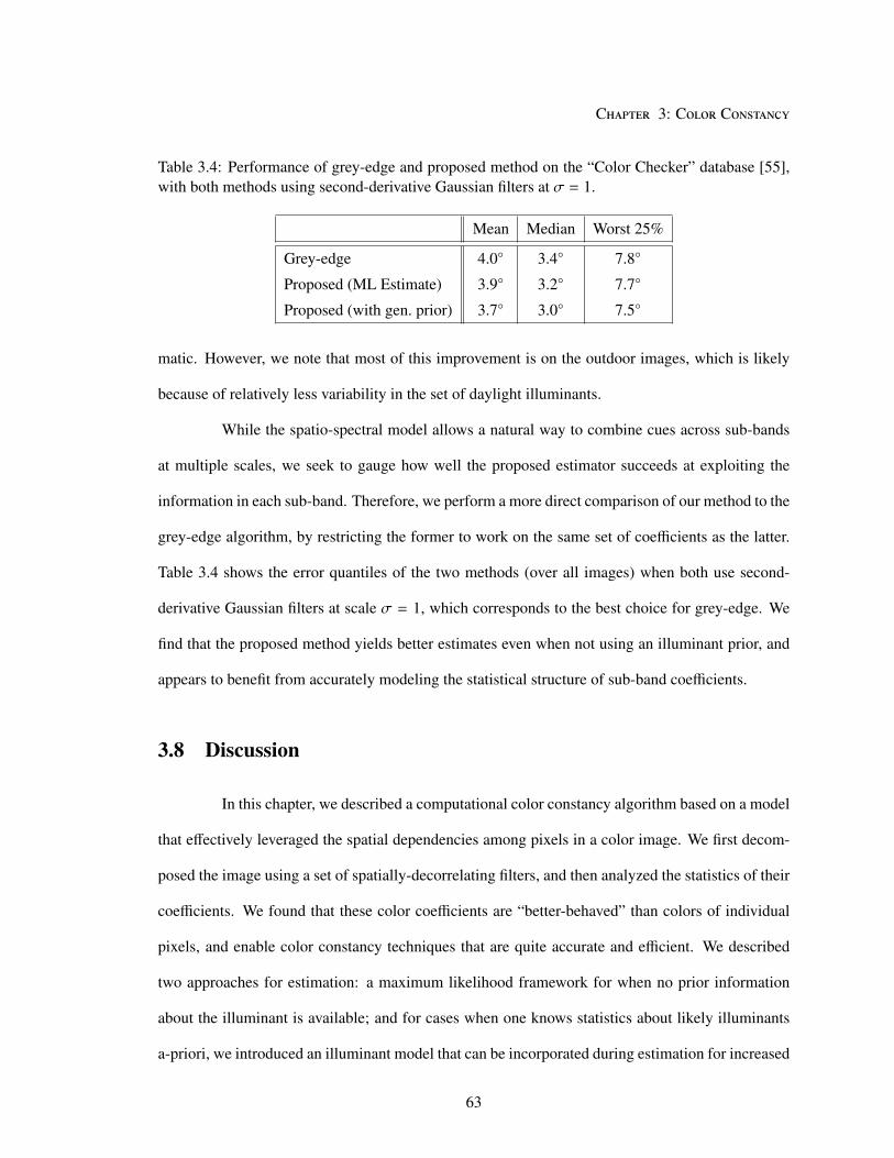
Chapter 3: Color Constancy
Table 3.4: Performance of grey-edge and proposed method on the “Color Checker” database [55],
with both methods using second-derivative Gaussian filters at σ = 1.
Mean Median Worst 25%
Grey-edge 4.0◦ 3.4◦ 7.8◦
Proposed (ML Estimate) 3.9◦ 3.2◦ 7.7◦
Proposed (with gen. prior) 3.7◦ 3.0◦ 7.5◦
matic. However, we note that most of this improvement is on the outdoor images, which is likely
because of relatively less variability in the set of daylight illuminants.
While the spatio-spectral model allows a natural way to combine cues across sub-bands
at multiple scales, we seek to gauge how well the proposed estimator succeeds at exploiting the
information in each sub-band. Therefore, we perform a more direct comparison of our method to the
grey-edge algorithm, by restricting the former to work on the same set of coefficients as the latter.
Table 3.4 shows the error quantiles of the two methods (over all images) when both use second-
derivative Gaussian filters at scale σ = 1, which corresponds to the best choice for grey-edge. We
find that the proposed method yields better estimates even when not using an illuminant prior, and
appears to benefit from accurately modeling the statistical structure of sub-band coefficients.
3.8 Discussion
In this chapter, we described a computational color constancy algorithm based on a model
that effectively leveraged the spatial dependencies among pixels in a color image. We first decom-
posed the image using a set of spatially-decorrelating filters, and then analyzed the statistics of their
coefficients. We found that these color coefficients are “better-behaved” than colors of individual
pixels, and enable color constancy techniques that are quite accurate and efficient. We described
two approaches for estimation: a maximum likelihood framework for when no prior information
about the illuminant is available; and for cases when one knows statistics about likely illuminants
a-priori, we introduced an illuminant model that can be incorporated during estimation for increased
63

Chapter 3: Color Constancy
robustness.
While we confined the bulk of our discussion to computational color constancy, work in
this domain has often been motivated by and been an attempt to explain the way in which the hu-
man visual system achieves color constancy [71, 72]. Therefore, the relative success of our method
naturally raises questions about whether the human visual system employs related processing for
adaptation and color constancy. Indeed, psychophysical experiments have shown a strong inter-
action between the spatial orientation and frequency of a stimulus and the chromatic adaptation
it induces [73, 74]. The mechanisms that govern these interactions are however poorly under-
stood [73], and the machinery developed in this paper might be useful in creating experiments to
analyze them further. Separate experiments have linked the textures of familiar objects to human
color perception [75, 76], and while texture is currently thought to affect color perception through
object memory, it is worth exploring the contribution of spatial correlations to this effect.
On the computational side, interesting avenues for future research include relaxing the
two main assumptions made in most color constancy algorithms discussed in this chapter: spatially-
constant illuminant spectrum and diagonal transforms for chromatic adaptation. Even when there is
a single illuminant in the scene, mutual illumination causes the “effective” illuminant spectrum to
vary from point to point. A first step that could lead to improvement would be to remove regions
that appear to be outliers to the general statistics of the image, in the hope that these are likely to
correspond to areas with significant inter-reflections. Alternatively, one could explore variants of
the proposed method that assume the scene to be lit by a mixture of n illuminants. The problem
would then be to estimate the colors of each of these illuminants, and their relative contributions at
each pixel in the image.
The problem of moving beyond diagonal transforms is interesting as well. One path is
to estimate general linear transforms under appropriate constraints. Another is to consider a set of
registered training images taken under different illuminants, and then “learn” the functional form of
the map between corresponding pixels. The parameters of this map can then be estimated from a
64

Chapter 3: Color Constancy
test image to do color constancy.
As was mentioned in Sec. 3.1, one of the reasons we seek color constancy is to be able
to use color as a stable descriptor. A robust illuminant estimation framework allows us to now
engage the problem of using color reliably in recognition and other visual tasks. Preliminary work
by Owens et al. [77] shows that object matching across multiple scenes and illuminant estimation
can be done jointly. However, it remains a challenge to be able to do color constancy with images
captured using consumer digital cameras that do not provide linear (RAW) image data. In this work
and in most color constancy algorithms, it is assumed that training and testing are performed with
linear images taken from the same or similar cameras. This is important, because as shown in [78],
the color spaces and non-linear processing done in cameras can vary significantly, affecting both the
sub-band statistics in {Σk} and the illuminant statistics in Q. Saenko et al. [79] look at the problem
of adapting visual category models learned from one camera to another. It would be interesting to
investigate whether the same can be done for color constancy in a way that would allow training
data from one camera or linear images to be adapted to a new domain, with minimal additional
information.
We end this discussion by noting that the model introduced in this chapter sought to
encode spatio-spectral dependencies in trichromatic images, which make just three spectral mea-
surements of the incident radiance at each pixel. In the next chapter, we study and model these
dependencies in hyperspectral images, i.e. those that have a higher spectral resolution and therefore
carry a far richer description of color.
Appendix: Additional Results
In this appendix, we report performance on another database considered in [70]. The
“Grey Ball” database[80] is a collection of 11355 images captured using a video camera. A diffuse
grey sphere is attached to the camera and is present at the same location in all images, serving
65

Chapter 3: Color Constancy
Table 3.5: Performance of various methods on “Grey Ball” set [80]
Method Mean Median Worst 25%
Grey World [50] 12.2◦ 9.7◦ 25.4◦
Grey Edge (1st Order) [56] 10.8◦ 9.2◦ 20.9◦
Grey Edge (2nd Order) [56] 11.4◦ 9.9◦ 21.5◦
Gamut Mapping [52] 11.8◦ 8.9◦ 24.9◦
Generalized Gamut Mapping [57] 11.8◦ 8.9◦ 24.9◦
Proposed (ML Estimate) 10.3◦ 8.9◦ 20.3◦
as ground truth. It is pioneering in being the first large database of real world images captured
to evaluate color constancy methods. However, the database is highly correlated with consecutive
frames often having very little change in scene content and illumination. Furthermore, the ground
truth information is unreliable in some cases since the grey ball is close to the camera and may be
lit by a different illuminant than the scene being captured (the color charts in the database in [55]
are placed within the scene to avoid this). As such, the error values on this database need to be
interpreted with caution.
The original database includes gamma-corrected (sRGB) images, and we follow the pro-
cedure in [70] by measuring performance after applying approximate inverse gamma-correction (by
raising all intensity values to the power 2.2) to the images and recomputing the ground truth accord-
ingly. We also adopt the approach suggested in [70] for cross-validation to avoid correlated images
appearing in the training and testing sets: since the database is divided into 15 videos, we carry out
estimation on the frames of each video using using the remaining videos as training.
Table 3.5 shows error quantiles of the proposed method and compares them to those of
other algorithms. We use the evaluation results from [70] as an indicator of the performance of state-
of-the-art methods, but again, we differ in applying the learning step to grey-world and grey-edge as
described in Sec. 3.7.1. We only report errors for the ML estimator, since the prior-based estimates
have identical error quantiles. Due to lower resolution, compression artifacts, and an approximate
66

Chapter 3: Color Constancy
gamma compensation, this database proves to be significantly more challenging with all algorithms
showing larger error values than for the color checker database in Sec. 3.7.2 (although, this could
partly be due to the unreliability of ground truth as discussed above). Nevertheless, we find that the
proposed method yields more accurate estimates than other algorithms, with the lowest values for
all quantiles.
67

4Hyperspectral Statistics
“We never really perceive what color is physically.”
— Josef Albers
In this chapter, we explore image statistics in a new domain. Hyperspectral images pro-
vide higher spectral resolution than typical RGB images by including a large number of irradiance
measurements in the visible spectrum, at every pixel. This additional spectral resolution is poten-
tially useful for visual tasks, such as segmentation, recognition, and relighting. We present a new
database of fifty hyperspectral images of natural indoor and outdoor scenes, and use this database to
explore hyperspectral statistics. Vision systems that seek to capture and exploit hyperspectral data
should benefit from statistical models of natural hyperspectral images. Additionally, these mod-
els provide greater access (than models in RGB) to information about the spatio-spectral structure
of scene radiance. We derive an optimized joint spatio-spectral basis for representing hyperspec-
tral image patches. Then, we explore the statistical properties of the coefficients in this basis, and
investigate the dependencies between different coefficients.
68
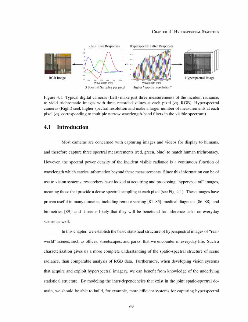
Chapter 4: Hyperspectral Statistics
Figure 4.1: Typical digital cameras (Left) make just three measurements of the incident radiance,
to yield trichromatic images with three recorded values at each pixel (eg. RGB). Hyperspectral
cameras (Right) seek higher spectral resolution and make a larger number of measurements at each
pixel (eg. corresponding to multiple narrow wavelength-band filters in the visible spectrum).
4.1 Introduction
Most cameras are concerned with capturing images and videos for display to humans,
and therefore capture three spectral measurements (red, green, blue) to match human trichromacy.
However, the spectral power density of the incident visible radiance is a continuous function of
wavelength which carries information beyond these measurements. Since this information can be of
use to vision systems, researchers have looked at acquiring and processing “hyperspectral” images,
meaning those that provide a dense spectral sampling at each pixel (see Fig. 4.1). These images have
proven useful in many domains, including remote sensing [81–85], medical diagnosis [86–88], and
biometrics [89], and it seems likely that they will be beneficial for inference tasks on everyday
scenes as well.
In this chapter, we establish the basic statistical structure of hyperspectral images of “real-
world” scenes, such as offices, streetscapes, and parks, that we encounter in everyday life. Such a
characterization gives us a more complete understanding of the spatio-spectral structure of scene
radiance, than comparable analysis of RGB data. Furthermore, when developing vision systems
that acquire and exploit hyperspectral imagery, we can benefit from knowledge of the underlying
statistical structure. By modeling the inter-dependencies that exist in the joint spatio-spectral do-
main, we should be able to build, for example, more efficient systems for capturing hyperspectral
69

Chapter 4: Hyperspectral Statistics
images and videos, that are able yield accurate reconstructions from fewer measurements and are
able to deal with noise and other imperfections in the capture process. Furthermore, it is important
to understand these dependencies when developing algorithms for visual inference tasks, such as
segmentation and recognition.
While previous analyses have separately considered the spectral statistics of point sam-
ples [90–92], we consider the spatial and hyperspectral dimensions jointly to uncover additional
structure. Using a new collection of fifty hyperspectral images captured with a time-multiplexed
31-channel camera, we evaluate difference choices of spatio-spectral bases for representing hyper-
spectral image patches and find that a separable basis is appropriate. Then, we characterize the
statistical properties of the coefficients in this basis and describe models that capture these proper-
ties effectively.
4.2 Related Work
Our work is motivated by successes in analyzing and modeling the statistical properties
of greyscale [9, 93, 94] and trichromatic [95–99] images. In the previous chapters, we have seen
how such models can enable accurate visual inference— for estimating motion blur and illuminant
spectra. But image statistics have found applications in a variety of domains. They have proven
useful for inferring accurate images from noisy and incomplete measurements, with applications in
denoising [13, 100], restoration [6, 101] and demosaicking [15, 58], and have also use as building
blocks for higher-level visual tasks such as segmentation and object detection [102–104]. Our goal
here is to develop comparable models for hyperspectral data, by considering the joint statistics of
variations with respect to space and wavelength.
The study in this chapter is enabled by recent advances in hyperspectral capture sys-
tems, such as those based on spatial-multiplexing with generalized color filter arrays [105], spatial-
multiplexing with a prism [106], time-multiplexing with liquid crystal tunable filters [107, 108],
70

Chapter 4: Hyperspectral Statistics
and time-multiplexing with varying illumination [109, 110]. Prior to these advances, studies of real-
world spectra have been limited to collections of point samples, such as those collected by a spec-
trometer. These studies have suggested, for example, that the spectral reflectances of “real-world”
materials are smooth functions that can be represented with 6-8 principal components [91, 92, 96]
(or a suitable sparse code [90]), and that the spectra of daylight and other natural illuminants can be
represented with even fewer principal components [111]. One of our goals in this study is to move
beyond point samples, and to investigate the properties of variations in spectral distributions within
spatial neighborhoods.
We expect that accurate statistical models will aid in the design of efficient hyperspectral
acquisition systems. Many proposed acquisition methods seek to reconstruct full spectral images
from a reduced set of measurements based on assumptions about the underlying statistics [105, 110].
Such methods are likely to benefit from accurate statistical models that are learned from real-world
hyperspectral data. These models may also prove useful for other applications, such as relighting,
segmentation, and recognition.
Other hyperspectral datasets that are related to the one introduced here include those of
Hordley et al. [108] and Yasuma et al. [105]. These datasets include 22 and 32 hyperspectral images,
respectively, and they are focused on objects captured with controlled illuminants in laboratory
environments. More related is the database of 25 hyperspectral images of outdoor urban and rural
scenes captured by Foster et al. [107]. A primary aim of our work has been to capture and analyze
a larger database that includes both indoor and outdoor scenes.
4.3 Hyperspectral Image Database
To enable an empirical analysis of the joint spatio-spectral statistics of real-world hyper-
spectral scenes, a commercial hyperspectral camera (Nuance FX, CRI Inc.) was used to collect a
database of fifty images under daylight illumination, both outdoors and indoors. As illustrated in
71

Chapter 4: Hyperspectral Statistics
Figure 4.2: Commercial hyperspectral camera (Nuance FX, CRI Inc.) with apo-chromatic lens
used to capture images in the database. The camera is equipped with a greyscale sensor and
a liquid crystal tunable filter that can be tuned to have 10nm wavelength pass bands centered at
steps on 10nm (see Fig. 4.1). (Left) A 31-channel hyperspectral image is captured through time-
multiplexed measurements by tuning the filter sequentially to each of these bands and capturing an
image stack. (Right) The effective per-band sensitivity is a combination of the filter transmittance
and wavelength-dependent sensor efficiency.
Fig. 4.2, the camera uses an integrated liquid crystal tunable filter and is capable of acquiring a hy-
perspectral image by sequentially tuning the filter through a series of thirty-one narrow wavelength
bands, each with approximately 10nm bandwidth and centered at steps of 10nm from 420nm to
720nm. Figure 4.2 (right) shows the relative sensitivity of the camera for each wavelength band,
accounting for both the quantum-efficiency of the 12-bit greyscale sensor and the per-band trans-
mittance of the effective filters. The camera is equipped with an apo-chromatic lens (CoastalOpt
UV-VIS-IR 60mm Apo Macro, Jenoptik Optical Systems, Inc.) and in all cases we used the small-
est viable aperture setting. The combination of the apo-chromatic lens and the avoidance of a
mechanical filter wheel allows us to acquire images that are largely void of chromatic aberration
and mis-alignment. To avoid contaminating the statistics by having different per-band noise levels,
we did not vary the exposure time across bands or normalize the captured bands with respect to
sensitivity. Therefore, all results in this chapter must be interpreted relative to the camera sensitivity
function, with the exception of Sec. 4.4.2 which discusses “camera-independent” statistics (after
making specific assumptions).
Due to the use of small apertures and the low transmittance of individual bands, the total
72

Chapter 4: Hyperspectral Statistics
acquisition times for an entire image (i.e., all wavelength bands) are high and vary from fifteen
seconds to over a minute. Accordingly, all images were captured using a tripod and by ensuring
minimal movement in the scene. Since having a perfectly static scene is often not feasible, in the
interest of having a diverse dataset, we have captured images with movement in some regions— but
these regions (and other areas affected by dust, etc.) are masked out manually before analysis. We
note that as a result, any regions with people in the captured scenes are masked out, and our analysis
does not include samples of human skin tones.
The captured dataset includes images of both indoor and outdoor scenes featuring a di-
versity of objects, materials and scale (see Fig. 4.3 for a few example images rendered in sRGB).
We have also captured twenty-five additional images taken under artificial and mixed illumination,
and while these are not used for the analysis presented in this work, they have been made available
to researchers along with the fifty natural illumination images [24]. We believe the database to be a
representative sample of real-world images, capturing both pixel-level material statistics and spatial
interactions induced by texture and shading effects. In addition to the analysis here, these images
may be useful “ground truth” to design and evaluate methods for various acquisition and vision
tasks that use hyperspectral data. They can also be used to synthetically generate ground truth RGB
images that correspond to true trichromatic measurements at each pixel, rather than those estimated
through demosaicking.
4.4 Spatio-Spectral Representation
We begin by exploring efficient representations for hyperspectral images. As is common
practice with greyscale and RGB images, we first divide the entire image into patches and consider
the properties of each patch independently. Let X[n, l] be a random P × P hyperspectral image
patch, where n ∈ {1, . . . P}2 and l ∈ {1, . . . 31} index pixel location and spectral band respectively.
For the rest of this chapter, we choose the patch size P = 8, but the results and conclusions from
73

Chapter 4: Hyperspectral Statistics
Dayli
gh
tA
rtifi
cial/
Mix
edIl
lum
inati
on
Figure 4.3: Example scenes from the captured database, rendered here in sRGB. The database con-
tains a diverse set of images of outdoor and indoor scenes, with fifty images illuminated by daylight
and an additional twenty-five under artificial and mixed illumination. Regions with unreliable data
(due to movement during exposure, etc.) were labeled manually, and are shown here with red masks.
different choices of P are qualitatively the same.
Since X is high-dimensional, we seek a representation that allows analysis in terms of a
smaller number of components. Formally, we wish to find an optimal orthonormal basis set {Vi} and
express X in terms of scalar coefficients xi as
X[n, l] = µ[n, l] +∑
i
xiVi[n, l], (4.1)
74

Chapter 4: Hyperspectral Statistics
Figure 4.4: General basis for 8 × 8 hyper-spectral patches learned across the database. Left: most
significant basis vectors (in reading order) rendered in RGB. Right: normalized variance of the
coefficients for the first 200 basis vectors. The variance decays rapidly indicating that a small
proportion of components are sufficient for accurate reconstruction.
where µ[n, l] is the “mean patch” and
xi = 〈X − µ,Vi〉n, l =∑
n,l
Vi[n, l] (X[n, l] − µ[n, l]). (4.2)
We learn a set of general basis vectors using principal component analysis (PCA) on
patches cropped from images in the database, through eigen-decomposition of their empirical co-
variance matrix. This corresponds to choosing a basis that ensures maximal “energy compaction”,
i.e. the set of basis vectors is chosen such that every truncated sub-set {Vi′}ii′=1minimizes the ex-
pected “reconstruction error” from that subset, defined as
ǫ(i) = E
∥
∥
∥
∥
∥
∥
∥
µ[n, l] +
i∑
i′=1
xi′Vi′[n, l]
− X[n, l]
∥
∥
∥
∥
∥
∥
∥
2
. (4.3)
Figure 4.4 shows the top twenty components rendered in RGB, as well as the variance for
the top 200 components. We see that the first two Vi essentially correspond to spatially-constant
“DC” components with distinct spectra, followed by vertical and horizontal derivative components.
We also find that there is a steep fall off in variance indicating that X can be described accurately by
a relatively small number of coefficients. Indeed, the first 20 basis vectors (out of a total of 1984)
account for 99% of the total variance.
75

Chapter 4: Hyperspectral Statistics
4.4.1 Separable Basis Components
Notice that the basis components in Fig. 4.4 has sets of vectors with similar spatial patterns
but different spectra or “colors”. Therefore, we next investigate the efficiency of a separable basis
{Vi}, that is formed as a Cartesian product of two orthonormal basis sets {S j[n]}P2
j=1and {Ck[l]}31
k=1,
that span the space of monochrome P×P spatial patches and the space of 31-channel spectral distri-
butions, respectively. Every Vi can therefore be expressed as Vi[n, l] = V jk[n, l] = S j[n]Ck[l], for
some values of j and k, and we denote the coefficient along V jk as x jk, where x jk =⟨
X − µ, S jCk
⟩
n, l.
Note that by construction, the vectors {V jk} are orthonormal since
⟨
V jk,V j′k′⟩
n, l=
∑
n,l
S j[n]Ck[l] S j′[n]Ck′[l] =
∑
n
S j[n]S j′[n]
∑
l
Ck[l]Ck′[l]
=⟨
S j, S j′⟩
n〈Ck,Ck′〉l =
1 if j = j′, k = k′,
0 otherwise.
(4.4)
As before, we use a training set to learn the optimal separable basis {V jk}, which corre-
sponds to learning the optimal spatial and spectral components {S j} and {Ck}. Let us assume that
we know the optimal spatial basis, and only have to estimate the spectral components {Ck}. For
energy compaction, we wish to choose these components such that for every k, the reconstruction
error, when using components composed of all {S j} and the truncated set {Ck′}kk′=1, is minimized.
This error is given by
ǫc(k) = E
∥
∥
∥
∥
∥
∥
∥
∥
µ[n, l] +
P2∑
j=1
k∑
k′=1
x jk′S j[n]Ck′[l]
− X[n, l]
∥
∥
∥
∥
∥
∥
∥
∥
2
= E‖X − µ‖2 −∑
j
k∑
k′=1
E
⟨
X − µ, S jCk′⟩2
n, l
= E‖X − µ‖2 −∑
n
k∑
k′=1
E 〈X − µ,Ck′〉2l . (4.5)
We note the reconstruction error is independent of the choice of {S j}, and therefore the
optimal spectral components {Ck} can be computed using PCA on the spectral distributions of indi-
vidual pixels. This reasoning also holds when computing the optimal spatial basis {S j}, which can
76

Chapter 4: Hyperspectral Statistics
420 470 520 570 620 670 720
5
4
3
2
1
Wavelength (nm)
Figure 4.5: Learned separable basis, with most significant (Left) spatial components {S j[n]}, and
(Right) spectral components {Ck[l]}. The overall separable basis is constituted by taking a Cartesian
product of these two sets, i.e. by forming basis vectors as S j[n]Ck[l], for ever pair ( j, k).
be learned through PCA on monochrome patches pooled across all bands. Figure 4.5 shows the first
few spatial and spectral components, {S j} and {Ck}, learned in this manner from the database. The
spatial components correspond to a DCT-like basis used commonly for modeling greyscale images,
with S 1 corresponding to the “DC” component. The spectral components in turn resemble a Fourier
basis scaled by the camera’s sensitivity function (see Fig. 4.2), where C1 can be loosely interpreted
as the average brightness or “luminance”.
Given the individual spatial and spectral bases, we can compute the energy or variance
for every combination (i.e. E x2jk
) and sort these combinations according to this variance. This
establishes a unique map from every pair ( j, k) to an index i ∈ {1, . . . P2 × 31}, such that the overall
reconstruction error ǫ(i) is minimized. In Fig. 4.6, we compare this reconstruction error to that
of the general joint basis. We find that the two have near-identical reconstruction errors for the
same number of components, indicating that separable basis is equally efficient. A wavelet-based
separable basis, with the spatial components {S j} corresponding to Haar wavelets, is also included
for comparison.
Figure 4.7 shows the map from the pairs ( j, k) to index i (truncated to i ≤ 15 for clarity),
77

Chapter 4: Hyperspectral Statistics
Figure 4.6: Comparison of different spatio-spectral basis sets in terms relative reconstruction error
using a limited number of components. The figure compares a general basis set to one restricted to
having separable spatial and spectral components. The separable basis has near identical reconstruc-
tion error to the general basis, indicating that it is equally efficient. The efficiency of a separable set
with Harr wavelets as the spatial basis is also shown.
and illustrates the relative importance of different combinations of the spatial and spectral basis vec-
tors in Fig. 4.5. We see that the combinations of the first spectral component (i.e. the luminance)
with various spatial components typically have higher variance than vectors involving higher spec-
tral components. Fig. 4.8 provides another look at the variance in this separable basis. For each of
the top spatial components, it plots the variance for their combination with each of the top spectral
components. We find that the these curves show similar decays along the spectral dimension, indi-
cating that the total variance in the different spatial components is distributed in similar proportions
amongst their spectral coefficients.
4.4.2 Camera-independent Basis
So far, we have looked at representations for patches relative to the camera’s sensitivity
function shown in Fig. 4.2. Since this function is known, it is possible to compute the corresponding
statistics for hyperspectral images captured by a different device with a different sensitivity, after
making appropriate assumptions about the observation noise in the database. As a specific case of
this, we look at properties of images captured by a hypothetical camera that has a flat sensitivity
78

Chapter 4: Hyperspectral Statistics
Spec
tral
index
k
Spatial index j
1 2 3 4 5 6 7 8 9 10 11
1 1 3 4 6 7 9 10 11 12 13 15
2 2 14
3 5
4 8
Figure 4.7: Relative importance of different combinations of the spatial and spectral components
S j and Ck, in terms of variance. Shown here is the map from every pair ( j, k) to the index i of
the corresponding joint basis vector V jk. Note that combinations of the first spectral component C1
(i.e. luminance) with various S j often rank higher than the combinations of S 1 (i.e. DC) with the
higher spectral components Ck, k > 1.
Figure 4.8: Variances in combinations with different spectral components, for the first five spatial
components. The horizontal grid lines correspond to the values of the DC component S 1. Note that
the different S i have similar decays along the spectral dimension.
function. These can be interpreted as the properties of the underlying scene itself, without varying
attenuation applied to the different wavelength bands.
Formally, we relate the captured hyperspectral patch X[n, l] to the true un-attenuated
version Xt[n, l] as
X[n, l] = s[l]Xt[n, l] + z[n, l], (4.6)
where s[l] is the known camera sensitivity, and z[·] is observation noise. Following the analysis
79

Chapter 4: Hyperspectral Statistics
420 470 520 570 620 670 720
5
4
3
2
1
Wavelength (nm)
Figure 4.9: Basis vectors for hyperspectral patches from a camera with uniform sensitivity. Left:
Most significant joint basis vectors, rendered in sRGB. Right: Spectral basis vectors {Ctk} that,
combined with the spatial vectors {S j} in Fig. 4.5, define an efficient separable basis.
above, we seek to find the optimal basis for Xt through an eigen-decomposition of the covariance
matrix EXtXTt . We assume white Gaussian noise, z[n, l]
i.i.d∼ N(0, σ2z ), which gives us the following
relation between the covariances of X and Xt:
EX2t [n, l] = s−2[l]
(
EX2[n, l] − σ2z
)
,
EXt[n, l]Xt[n′, l′] = s−1[l]s−1[l′]EX[n, l]X[n′, l′], if n , n′ or l , l′. (4.7)
We use the values of EXXT estimated from our database, and we set the noise variance σ2z to be
equal to half of its lowest eigen-value, i.e., half the variance along the least significant basis vector.
We can now compute the covariance matrix for Xt, and the optimal basis vectors thus obtained
through PCA are shown in Fig. 4.9 (left).
Since X was shown in Sec. 4.4 to be represented efficiently using a separable basis and
the camera sensitivity is the same for all pixels, it follows that the basis for Xt is also separable,
and composed of the same spatial basis {S j[n]} as for X and a spectral basis {Ctk[l]} shown in
Fig. 4.9 (right). As expected, from comparing Fig. 4.9 to Fig. 4.5, we find that spectral basis vectors
{Ctk[l]} for Xt represent an orthogonalized version of {s−1[l]Ck[l]}.
80
Chapter 4: Hyperspectral Statistics
We can also use our estimates of the covariance matrix of Xt to explore how efficient the
human cone responses are at capturing the variance in the scenes in our database. We find that
the sub-space spanned by the CIE XYZ vectors (designed to match the spectral response of human
visual system) account for 77.22% of the total variance in Xt. In comparison, the first three eigen-
vectors {Ctk}2k=0account for 99.14% of the total variation. However, it is important to remember that
human cone responses are restricted to have non-negative responses at all wavelengths (as is true
with any set of sensors). Also, the human visual system is likely to have evolved in different en-
vironments, and to be optimal for capturing spectral information helpful for specific discriminative
tasks.
Note that the assumption made in this section about the noise being i.i.d Gaussian, and
the manner in which its variance is chosen are approximations. Indeed, observation noise in typical
camera sensors is known to be Poisson distributed [112]. Therefore, while this analysis is helpful in
building intuition, we return to working with the camera-relative bases in subsequent sections.
4.5 Coefficient Models
Having identified a separable spatio-spectral basis we now explore statistical models for
coefficients in this basis. We look at distributions for each coefficient individually, as well as joint
models for different spectral coefficients along the same spatial basis.
4.5.1 Modeling Individual Coefficients
Let x jk be the coefficient of X in the basis component V jk = S j[n]Ck[l]. We begin by
looking at empirical distributions of the “DC” coefficients x1k in Fig. 4.10 (top). As was the case for
per-pixel distributions in Chapter 3, we find that these distributions differ qualitatively from those
of the other coefficients shown in Fig. 4.10 (bottom), and exhibit comparatively less structure. In
applications with greyscale and RGB images, DC coefficients are found to be poorly described by
81
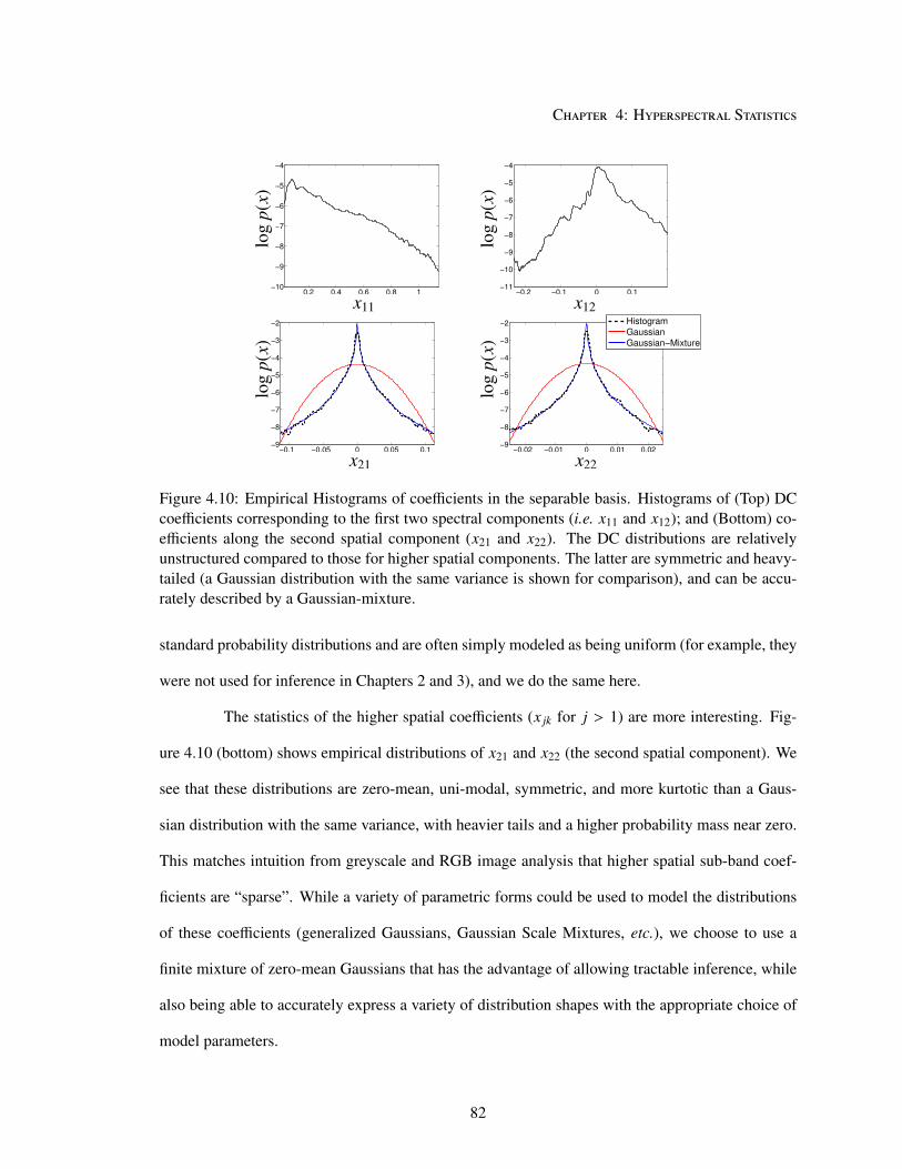
Chapter 4: Hyperspectral Statistics
Figure 4.10: Empirical Histograms of coefficients in the separable basis. Histograms of (Top) DC
coefficients corresponding to the first two spectral components (i.e. x11 and x12); and (Bottom) co-
efficients along the second spatial component (x21 and x22). The DC distributions are relatively
unstructured compared to those for higher spatial components. The latter are symmetric and heavy-
tailed (a Gaussian distribution with the same variance is shown for comparison), and can be accu-
rately described by a Gaussian-mixture.
standard probability distributions and are often simply modeled as being uniform (for example, they
were not used for inference in Chapters 2 and 3), and we do the same here.
The statistics of the higher spatial coefficients (x jk for j > 1) are more interesting. Fig-
ure 4.10 (bottom) shows empirical distributions of x21 and x22 (the second spatial component). We
see that these distributions are zero-mean, uni-modal, symmetric, and more kurtotic than a Gaus-
sian distribution with the same variance, with heavier tails and a higher probability mass near zero.
This matches intuition from greyscale and RGB image analysis that higher spatial sub-band coef-
ficients are “sparse”. While a variety of parametric forms could be used to model the distributions
of these coefficients (generalized Gaussians, Gaussian Scale Mixtures, etc.), we choose to use a
finite mixture of zero-mean Gaussians that has the advantage of allowing tractable inference, while
also being able to accurately express a variety of distribution shapes with the appropriate choice of
model parameters.
82

Chapter 4: Hyperspectral Statistics
Formally, we define
p(x jk) =
Z∑
z=1
p(z jk = z)N(
x jk|0, σ2jk,z
)
, (4.8)
where z jk ∈ {1, . . .Z} is a latent index variable indicating that x jk is distributed as a Gaussian with the
corresponding variance σ2jk,z
. Without loss of generality, we assume that the mixture components
are sorted by increasing variance. The model parameters {p(z jk = z), σ2jk,z}z are estimated from
the database using Expectation Maximization (EM) [48], and in practice we find that mixtures
of eight Gaussians (i.e. Z = 8) are able to fit the empirical distributions for all coefficients with
reasonable accuracy. These fits for the coefficients x21 and x22 are shown superimposed on the
empirical histograms in Fig. 4.10 (bottom).
4.5.2 Joint Models
Since the spatio-spectral basis vectors have been estimated through PCA, it follows that
x jk and x jk′ will be uncorrelated for k , k′, i.e. E(x jkx jk′) = 0. However, given the model for
individual coefficients in (4.8), this does not necessarily imply that they will be independent. In-
deed, different spatial coefficients at the same spatial location in greyscale images are known to be
related [14]. We now demonstrate that different spectral coefficients along the same spatial basis are
also mutually dependent, and propose a model that encodes these dependencies. This expands on
our intuition in Chapter 3 that sub-band color coefficient vectors have ellipsoidal equi-probability
contours.
We begin by examining whether knowing the value of the mixture index z jk carries any
information about the statistics of the coefficient x jk′ for a different spectral component k′ along the
same spatial basis j, as illustrated in Fig. 4.11 (left). We define σ2jk′ |z jk
(z) to be the variance of x jk′
conditioned on the mixture index z jk being z, and estimate it from a set of training patches {Xi} from
the database, as
σ2jk′ |z jk
(z) =
∑
i p(z jk = z|xijk
)(xijk′)
2
∑
i p(z jk = z|xijk
), (4.9)
83
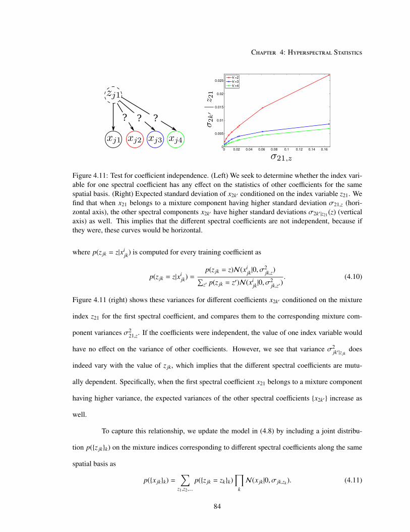
Chapter 4: Hyperspectral Statistics
Figure 4.11: Test for coefficient independence. (Left) We seek to determine whether the index vari-
able for one spectral coefficient has any effect on the statistics of other coefficients for the same
spatial basis. (Right) Expected standard deviation of x2k′ conditioned on the index variable z21. We
find that when x21 belongs to a mixture component having higher standard deviation σ21,z (hori-
zontal axis), the other spectral components x2k′ have higher standard deviations σ2k′ |z21(z) (vertical
axis) as well. This implies that the different spectral coefficients are not independent, because if
they were, these curves would be horizontal.
where p(z jk = z|xijk
) is computed for every training coefficient as
p(z jk = z|xijk) =
p(z jk = z)N(xijk|0, σ2
jk,z)
∑
z′ p(z jk = z′)N(xijk|0, σ2
jk,z′). (4.10)
Figure 4.11 (right) shows these variances for different coefficients x2k′ conditioned on the mixture
index z21 for the first spectral coefficient, and compares them to the corresponding mixture com-
ponent variances σ221,z
. If the coefficients were independent, the value of one index variable would
have no effect on the variance of other coefficients. However, we see that variance σ2jk′ |z jk
does
indeed vary with the value of z jk, which implies that the different spectral coefficients are mutu-
ally dependent. Specifically, when the first spectral coefficient x21 belongs to a mixture component
having higher variance, the expected variances of the other spectral coefficients {x2k′} increase as
well.
To capture this relationship, we update the model in (4.8) by including a joint distribu-
tion p({z jk}k) on the mixture indices corresponding to different spectral coefficients along the same
spatial basis as
p({x jk}k) =∑
z1,z2,...
p({z jk = zk}k)∏
k
N(x jk|0, σ jk,zk). (4.11)
84

Chapter 4: Hyperspectral Statistics
Note that this is only one possible choice for a joint model. Other choices include using a radial-
exponential distribution (as was done in Chapter 3) or a multi-variate Gaussian-mixture. While the
former allows only the variance of the distribution to be tuned but with a fixed shape, the latter is
more expressive but has a much larger number of parameters (it needs to learn a covariance matrix
across all spectral dimensions for each mixture component). The model in (4.11) offers a reasonable
compromise between the number of parameters and control over distribution shape. Furthermore,
the marginal distribution for any single coefficient under this model is the same as the one in (4.8).
Therefore, to fit this model, we first learn {p(z jk = z), σ jk,z} for each coefficient x jk individually as
before. We can then estimate the joint distribution of the indices p({z jk}k) from the set of training
patches {Xi} as
p({z jk = zk}k) ∝∑
i
∏
k
p(z jk = zk|xijk). (4.12)
This allows us to learn joint distributions over any subset of coefficients depending on the applica-
tion, and models for overlapping sets are guaranteed to be consistent (i.e. have the same marginal
distributions, etc.).
Having fit this model, we can use the learned joint distribution of the mixture indices
p({z jk}k) to reason about the relationships between the corresponding coefficients {x jk}k. Figure 4.12
shows the estimated conditional distributions p(z2k′ |z2k) for different pairs of spectral coefficients
along the spatial basis S 2. As expected, these distributions are different from the corresponding
marginal distributions p(z2k′) (also shown for comparison). We find that conditioned on the mixture
index z2k having a value corresponding to higher mixture component variance, the index z2k′ for a
different spectral coefficient x2k′ is more likely to correspond to higher variance mixture component
as well, which is consistent with our observations in Fig. 4.11. Therefore, observing a high mag-
nitude value for one coefficient makes a high value for another spectral coefficient along the same
spatial basis more likely. This joint model can be exploited during inference, for example, when
estimating a hyperspectral image from noisy or incomplete observations.
85

Chapter 4: Hyperspectral Statistics
p(z
22|z
21=
1)
1 2 3 4 5 6 7 80
0.1
0.2
0.3
0.4
p(z
22|z
21=
4)
1 2 3 4 5 6 7 80
0.1
0.2
0.3
0.4
p(z
22|z
21=
8)
z22 z22 z22
p(z
23|z
21=
1)
1 2 3 4 5 6 7 80
0.1
0.2
0.3
0.4
p(z
23|z
21=
4)
1 2 3 4 5 6 7 80
0.1
0.2
0.3
0.4
p(z
23|z
21=
8)
z23 z23 z23
p(z
23|z
22=
1)
1 2 3 4 5 6 7 80
0.1
0.2
0.3
0.4
p(z
23|z
22=
4)
1 2 3 4 5 6 7 80
0.1
0.2
0.3
0.4
p(z
23|z
22=
8)
z23 z23 z23
Figure 4.12: Relationship between mixture indices. Conditional distributions of the mixture indices
p(z2k′ |z2k) for different pairs of spectral coefficients along the same spatial basis S 2. Knowing the
value of the mixture index z2k for one spectral coefficient changes the distribution of the index z2k′ ,
corresponding to a different spectral coefficient, from the marginal distribution p(z2k′) (shown with
dotted black line for comparison). Broadly, these graphs suggest that higher/lower magnitudes of
one coefficient make higher/lower magnitudes respectively for other coefficients, along the same
spatial basis, more likely.
4.6 Discussion
In this chapter, we examined the joint spatial and spectral statistics of hyperspectral im-
ages using a new database of real-world scenes. We found that a separable basis, composed of
independent spatial and spectral components, serves as an efficient representation for hyperspectral
patches, and we studied the relative variance in these components. We then explored the statisti-
86

Chapter 4: Hyperspectral Statistics
cal properties of coefficients in this basis and found that higher-frequency spatial components are
accurately described by Gaussian mixture models. We also established that for the same spatial sub-
band, different spectral coefficients are mutually dependent, and we described a joint distribution
for mixture indices for different coefficients that encodes these dependencies.
A natural application of the statistical characterization described here is in hyperspectral
imaging. In the future, acquisition systems should exploit the interdependencies and correlations
between different spatio-spectral components, so as to efficiently acquire hyperspectral images with
fewer measurements. General color filter array patterns (such as those proposed in [105]) can be
designed to trade off spatial and spectral accuracy based on the relative variances of different compo-
nents, and reconstruction methods can use the joint coefficient models during estimation. Similarly,
these statistics are likely to be useful when estimating “clean” hyperspectral images from observa-
tions degraded by noise, blur, chromatic aberration, etc. The database can be used as “ground truth”
to evaluate different strategies for these applications.
This chapter presents a first look at spatio-spectral statistics and representations for hyper-
spectral images. Further research in this direction should include studies on the statistics of specific
classes of objects or regions in hyperspectral images, and ways to leverage these statistics for vision
applications. In addition to hyperspectral object models for recognition, understanding the differ-
ence in the statistics of homogenous regions with variations due to shading, relative to those of
regions that include material boundaries, may be useful for segmentation and recovering “intrinsic
images” [16]. Furthermore, these models can be expanded to include wavelengths beyond the visi-
ble spectrum, for example, to study the redundancies in the information carried by the infra-red and
long wavelength visible bands.
Other avenues of future work include looking at representations derived using more so-
phisticated techniques such as independent component analysis and fields of experts [9], with the
choice of representation likely to be geared towards specific vision tasks. It would also be interesting
to evaluate the utility of sparse codes, which have been previously proposed to describe spatial and
87

Chapter 4: Hyperspectral Statistics
spectral components independently in hyperspectral data [110]. Our observation about the mutual
dependence between spectral coefficients for different spatial bands suggests that it would be useful
to consider joint spatio-spectral coding strategies.
88

5Conclusion
89

Chapter 5: Conclusion
In this dissertation, we focused on the utility of statistical inference for problems in com-
puter vision. When the observed image does not uniquely determine the parameters we seek to
estimate, we showed that knowledge of the statistical properties of natural images, as well as those
of other scene parameters, can be used to arrive at a solution. We discussed the need for choosing
a modeling strategy that is adapted to the task at hand, and noted how this often involves making
assumptions to simplify inference, while leveraging the statistical properties that are useful for that
particular estimation problem.
We used this intuition in developing novel estimation algorithms for two vision applica-
tions. The first looked at estimating the parameters of spatially-varying motion blur in an image.
Since blur acts on the texture content of images (but uniformly across color channels), we used a
model that encoded the properties of sharp edges in greyscale, taking care to account for the arbi-
trary variation in the contrast of these edges from region to region. We found that we also had to
use a per-pixel color model in conjunction with this edge model to yield robust estimates.
The second application, color constancy, has a very different formulation. Here, a spatially-
uniform illuminant affected the colors of the observed scene at the pixel level, and therefore the
statistics of color in natural images had to be central to our approach. But we found that instead of
modeling the statistics of individual pixels, the colors of image derivatives were more informative
and easier to encode efficiently. Our proposed algorithm for this task also included an example of
modeling the statistical properties of other scene parameters, in this case the illuminant color, to
improve accuracy.
Hence, we introduced two very different statistical models for the same class of signals,
i.e. canonical images of natural scenes. Neither of these models is strictly more accurate than the
other, it is just that they encode different aspects of image statistics, and were chosen to allow
efficient and accurate inference for specific tasks. In addition to providing robust estimates for
their respective applications, these algorithms helped to illustrate the design choices that need to be
made when crafting a statistics-based algorithm for visual inference. Besides choosing appropriate
90

Chapter 5: Conclusion
image models for each application, these design choices included using a convenient local Fourier
representation for blur analysis, and a conjugate form for the illuminant distribution in the color
constancy method.
While other inference tasks are likely to need image models that are specifically adapted,
the models we proposed for the blur and illuminant estimation tasks can serve as useful starting
points. For example, the image model used for blur estimation essentially provides a mathematical
framework that favors image gradients being sharp, or spatially localized. While we used this model
for the case when this sharpness was affected by convolution with a blur kernel, the same framework
is likely to be useful for analyzing, say, the effect of a spatially smooth shading map being multiplied
with the underlying sharp material boundaries.
The spatio-spectral approach used for the color constancy application, that jointly mod-
eled the statistical properties of color and texture, is also likely to be useful for other tasks that deal
with color and material properties. That is why in Chapter 4, we did away with the constraint of
working with three channel images and explored these joint statistics for hyperspectral data. As
described in that chapter, these statistics are directly useful when designing hyperspectral cameras
and vision systems that use hyperspectral images as input. But the proposed representations and
statistical models for hyperspectral data can also be used to obtain deeper insights into the proper-
ties of regular RGB images, which can be thought of as “spectrally downsampled” projections of
their hyperspectral counterparts.
Current research trends in computer vision indicate that image statistics will have a cru-
cial role to play as we move to new modalities of imaging. The emerging field of Computational
Photography provides new and exciting opportunities to deploy image models, as we consider in-
ference on observations not restricted to being images taken by traditional cameras. With the goal of
recording more than just a projection of the light incident on the sensor plane, camera systems have
been proposed that modify the capture process in a variety of ways— using coded apertures [41],
programmable shutters [113], diffusion films [114], camera motion [115], etc.
91

Chapter 5: Conclusion
In Chapter 2, we used blur in images from traditional cameras to reason about object
motion. Computational cameras are often designed to deliberately introduce blur and other image
distortions into the capture process in a controlled manner, using the resulting observations to either
extract information that would not be present in a traditional image (such as depth, higher dynamic
range,etc.), or to compensate for some other form of degradation during capture (such as defocus or
motion blur, noise, etc.). To make optimal use of this flexibility to change the acquisition process
itself, appropriate statistical models should be used to design the best capture strategy, and for
estimation on the acquired data.
92

Bibliography
[1] N. Ahmed, T. Natarajan, and K. Rao, “Discrete cosine transfom,” IEEE Transactions on
Computers, vol. 100, no. 23, pp. 90–93, 1974.
[2] A. Chakrabarti and K. Hirakawa, “Effective separation of sparse and non-sparse image fea-
tures for denoising,” in Proceedings of the IEEE International Conference on Audio, Speech
and Signal Processing (ICASSP), 2008.
[3] P. Burt and E. Adelson, “The laplacian pyramid as a compact image code,” IEEE Transactions
on Communications, vol. 31, no. 4, pp. 532–540, 1983.
[4] S. Mallat, A wavelet tour of signal processing. Academic Press, 1999.
[5] E. Simoncelli and W. Freeman, “The steerable pyramid: A flexible architecture for multi-
scale derivative computation,” in Proceedings of the IEEE Conference on Image Processing
(ICIP), 1995.
[6] J. Mairal, M. Elad, and G. Sapiro, “Sparse representation for color image restoration,” IEEE
Transactions on Image Processing, vol. 17, no. 1, pp. 53–69, 2007.
[7] Y. Pati, R. Rezaiifar, and P. Krishnaprasad, “Orthogonal matching pursuit: Recursive function
approximation with applications to wavelet decomposition,” in Proceedings of the Asilomar
Conference on Signals, Systems and Computers, 1993.
[8] S. Chen, D. Donoho, and M. Saunders, “Atomic decomposition by basis pursuit,” SIAM
Journal on Scientific Computing, vol. 20, no. 1, pp. 33–61, 1999.
[9] S. Roth and M. Black, “Fields of experts: A framework for learning image priors,” in Pro-
ceedings of the IEEE Conference on Computer Vision and Pattern Recognition (CVPR), 2005.
[10] P. Viola and M. Jones, “Rapid object detection using a boosted cascade of simple features,” in
Proceedings of the IEEE Conference on Computer Vision and Pattern Recognition (CVPR),
2001.
[11] D. Lowe, “Object recognition from local scale-invariant features,” in Proceedings of the In-
ternational Conference on Computer Vision (ICCV). Published by the IEEE Computer
Society, 1999, p. 1150.
[12] A. Oliva and A. Torralba, “Building the gist of a scene: The role of global image features in
recognition,” Progress in Brain Research, vol. 155, pp. 23–36, 2006.
[13] J. Portilla, V. Strela, M. Wainwright, and E. Simoncelli, “Image denoising using scale mix-
tures of gaussians in the wavelet domain,” IEEE Transactions on Image Processing, vol. 12,
no. 11, pp. 1338–1351, 2003.
93

Bibliography
[14] M. Crouse, R. Nowak, and R. Baraniuk, “Wavelet-based statistical signal processing using
hidden markov models,” IEEE Transactions on Signal Processing, vol. 46, no. 4, pp. 886–
902, 1998.
[15] B. Gunturk, J. Glotzbach, Y. Altunbasak, R. Schafer, and R. Mersereau, “Demosaicking:
color filter array interpolation,” IEEE Signal Processing Magazine, vol. 22, no. 1, pp. 44–54,
2005.
[16] M. Tappen, W. Freeman, and E. Adelson, “Recovering intrinsic images from a single image,”
IEEE Transactions on Pattern Analysis and Machine Intelligence (PAMI), pp. 1459–1472,
2005.
[17] W. Freeman, T. Jones, and E. Pasztor, “Example-based super-resolution,” IEEE Computer
Graphics and Applications, pp. 56–65, 2002.
[18] J. Sivic, B. Russell, A. Efros, A. Zisserman, and W. Freeman, “Discovering objects and their
location in images,” in Proceedings of the International Conference on Computer Vision
(ICCV), vol. 1. IEEE, 2005, pp. 370–377.
[19] Z. Stone, T. Zickler, and T. Darrell, “Toward large-scale face recognition using social network
context,” Proceedings of the IEEE, vol. 98, no. 8, pp. 1408–1415, 2010.
[20] R. Fergus, B. Singh, A. Hertzmann, S. Roweis, and W. Freeman, “Removing camera shake
from a single photograph,” in ACM Transactions on Graphics Proceedings of SIGGRAPH,
2006.
[21] A. Levin, Y. Weiss, F. Durand, and W. Freeman, “Understanding and evaluating blind de-
convolution algorithms,” in Proceedings of the IEEE Conference on Computer Vision and
Pattern Recognition (CVPR), 2009.
[22] A. Chakrabarti, T. Zickler, and W. Freeman, “Spatially-varying blur analysis database and
code,” available at http://www.eecs.harvard.edu/~ayanc/svblur/.
[23] A. Chakrabarti, K. Hirakawa, and T. Zickler, “Color constancy with spatio-spectral statistics
matlab implementation,” available at http://www.eecs.harvard.edu/~ayanc/color-constancy/.
[24] A. Chakrabarti and T. Zickler, “Database of real-world hyperspectral images,” available at
http://vision.seas.harvard.edu/hyperspec/.
[25] J. Cai, H. Ji, C. Liu, and Z. Shen, “Blind motion deblurring from a single image using sparse
approximation,” in Proceedings of the IEEE Conference on Computer Vision and Pattern
Recognition (CVPR), 2009.
[26] H. Ji and C. Liu, “Motion blur identification from image gradients,” in Proceedings of the
IEEE Conference on Computer Vision and Pattern Recognition (CVPR), 2008.
94

Bibliography
[27] N. Joshi, R. Szeliski, and D. Kriegman, “PSF estimation using sharp edge prediction,” in
Proceedings of the IEEE Conference on Computer Vision and Pattern Recognition (CVPR),
2008.
[28] Q. Shan, J. Jia, and A. Agarwala, “High-quality motion deblurring from a single image,” in
ACM Transactions on Graphics Proceedings of SIGGRAPH, 2008.
[29] O. Whyte, J. Sivic, A. Zisserman, and J. Ponce, “Non-uniform deblurring for shaken images,”
in Proceedings of the IEEE Conference on Computer Vision and Pattern Recognition (CVPR).
IEEE, 2010, pp. 491–498.
[30] A. Gupta, N. Joshi, C. Lawrence Zitnick, M. Cohen, and B. Curless, “Single image deblurring
using motion density functions,” in Proceedings of the European Conference on Computer
Vision (ECCV), 2010, pp. 171–184.
[31] L. Yuan, J. Sun, L. Quan, and H. Shum, “Image deblurring with blurred/noisy image pairs,”
in ACM Transactions on Graphics Proceedings of SIGGRAPH, 2007.
[32] L. Bar, B. Berkels, M. Rumpf, and G. Sapiro, “A variational framework for simultaneous mo-
tion estimation and restoration of motion-blurred video,” in Proceedings of the International
Conference on Computer Vision (ICCV), 2007.
[33] B. Bascle, A. Blake, and A. Zisserman, “Motion deblurring and super-resolution from an
image sequence,” in Proceedings of the European Conference on Computer Vision, 1996.
[34] W. Chen, N. Nandhakumar, and W. Martin, “Image motion estimation from motion smear-a
new computational model,” IEEE Transactions on Pattern Analysis and Machine Intelligence
(PAMI), vol. 18, no. 4, pp. 412–425, 1996.
[35] S. Cho, Y. Matsushita, and S. Lee, “Removing non-uniform motion blur from images,” in
Proceedings of the International Conference on Computer Vision (ICCV), 2007.
[36] P. Favaro, M. Burger, and S. Soatto, “Scene and motion reconstruction from defocused and
motion-blurred images via anisotropic diffusion,” in Proceedings of the European Conference
on Computer Vision, 2004.
[37] P. Favaro and S. Soatto, “A variational approach to scene reconstruction and image segmen-
tation from motion-blur cues,” in Proceedings of the IEEE Conference on Computer Vision
and Pattern Recognition (CVPR), 2004.
[38] S. Dai and Y. Wu, “Estimating space-variant motion blur without deblurring,” in Proceedings
of the IEEE Conference on Image Processing (ICIP), 2008.
[39] ——, “Motion from blur,” in Proceedings of the IEEE Conference on Computer Vision and
Pattern Recognition (CVPR), 2008.
95

Bibliography
[40] J. Jia, “Single image motion deblurring using transparency,” in Proceedings of the IEEE
Conference on Computer Vision and Pattern Recognition (CVPR), 2007.
[41] A. Levin, R. Fergus, F. Durand, and W. Freeman, “Image and depth from a conventional cam-
era with a coded aperture,” in ACM Transactions on Graphics Proceedings of SIGGRAPH,
2007.
[42] A. Levin, “Blind motion deblurring using image statistics,” in Advances in Neural Informa-
tion Processing Systems (NIPS), 2006.
[43] M. Wainwright and E. Simoncelli, “Scale mixtures of gaussians and the statistics of natural
images,” in Advances in Neural Information Processing Systems (NIPS), 2000.
[44] Y. Zhang and N. Kingsbury, “Image deconvolution using a gaussian scale mixtures model
to approximate the wavelet sparseness constraint,” in Proceedings of the IEEE International
Conference on Audio, Speech and Signal Processing (ICASSP), 2009.
[45] H. Jeffreys, “An invariant form for the prior probability in estimation problems,” Proceedings
of Royal Society of London. Series A, Mathematical and Physical Sciences, pp. 453–461,
1946.
[46] C. Rother, V. Kolmogorov, and A. Blake, “Grabcut: Interactive foreground extraction using
iterated graph cuts,” in ACM Transactions on Graphics Proceedings of SIGGRAPH, 2004.
[47] Y. Boykov and G. Funka-Lea, “Graph cuts and efficient n-d image segmentation,” Interna-
tional Journal of Computer Vision (IJCV), vol. 70, no. 2, pp. 109–131, 2006.
[48] A. Dempster, N. Laird, and D. Rubin, “Maximum likelihood from incomplete data via the
em algorithm,” Journal of the Royal Statistical Society B, vol. 39, no. 1, pp. 1–38, 1977.
[49] S. Beauchemin and J. Barron, “The computation of optical flow,” ACM Computing Surveys
(CSUR), vol. 27, no. 3, pp. 433–466, 1995.
[50] G. Buchsbaum, “A spatial processor model for object colour perception,” Journal of the
Franklin Institute, vol. 310, no. 1, pp. 1–26, 1980.
[51] V. Cardei and B. Funt, “Committee-based color constancy,” in Proceedings of the IS&T/SID
Color Imaging Conference, 1999, pp. 311–313.
[52] D. Forsyth, “A novel algorithm for color constancy,” International Journal of Computer Vi-
sion (IJCV), vol. 5, no. 1, 1990.
[53] D. Brainard and W. Freeman, “Bayesian color constancy,” Journal of the Optical Society of
America (JOSA) A, vol. 14, no. 7, pp. 1393–1411, 1993.
96

Bibliography
[54] C. Rosenberg, T. Minka, and A. Ladsariya, “Bayesian color constancy with non-gaussian
models,” in Advances in Neural Information Processing Systems (NIPS), 2003.
[55] P. Gehler, C. Rother, A. Blake, T. Minka, and T. Sharp, “Bayesian color constancy revisited,”
in Proceedings of the IEEE Conference on Computer Vision and Pattern Recognition (CVPR),
2008.
[56] J. van de Weijer, T. Gevers, and A. Gijsenij, “Edge-based color constancy,” IEEE Transac-
tions on Image Processing, vol. 16, no. 9, pp. 2207–2214, 2007.
[57] A. Gijsenij, T. Gevers, and J. van de Weijer, “Generalized gamut mapping using image deriva-
tive structures for color constancy,” International Journal of Computer Vision (IJCV), vol. 86,
no. 2, pp. 127–139, 2010.
[58] K. Hirakawa and T. Parks, “Adaptive homogeneity-directed demosaicing algorithm,” in Pro-
ceedings of the IEEE Conference on Image Processing (ICIP), 2003.
[59] G. West and M. H. Brill, “Necessary and sufficient conditions for von kries chromatic adap-
tation to give color constancy,” Journal of Mathematical Biology, vol. 15, no. 2, pp. 249–258,
1982.
[60] G. Finlayson, M. Drew, and B. Funt, “Diagonal transforms suffice for color constancy,” in
Proceedings of the International Conference on Computer Vision (ICCV), 1993.
[61] H. Chong, S. Gortler, and T. Zickler, “The von Kries hypothesis and a basis for color con-
stancy,” in Proceedings of the International Conference on Computer Vision (ICCV), 2007.
[62] G. Finlayson and G. Schaefer, “Convex and non-convex illuminant constraints for dichro-
matic colour constancy,” in Proceedings of the IEEE Conference on Computer Vision and
Pattern Recognition (CVPR), 2001.
[63] A. Hurlbert and T. Poggio, “Synthesizing a color algorithm from examples,” Science, vol.
239, no. 4839, pp. 482–485, 1988.
[64] V. Cardei, B. Funt, and K. Barnard, “Estimating the scene illumination chromaticity using
a neural network,” Journal of the Optical Society of America (JOSA) A, vol. 19, no. 12, pp.
2374–2386, 2002.
[65] R. Gershon, A. Jepson, and J. Tsotsos, “From [r, g, b] to surface reflectance: computing color
constant descriptors in images,” Perception, vol. 17, pp. 755–758, 1988.
[66] B. Singh, W. Freeman, and D. Brainard, “Exploiting spatial and spectral image regularities
for color constancy,” in Proc. Workshop on Statistical and Computational Theories of Vision,
2003.
97

Bibliography
[67] I. Selesnick, “The estimation of laplace random vectors in additive white gaussian noise,”
IEEE Transactions on Signal Processing, vol. 56, no. 8, pp. 3482–3496, 2008.
[68] F. Sinz, S. Gerwinn, and M. Bethge, “Characterization of the p-generalized normal distribu-
tion,” Journal of Multivariate Analysis, vol. 100, no. 5, pp. 817–820, 2009.
[69] L. Shi and B. Funt, “Re-processed version of the gehler color constancy dataset of 568 im-
ages,” accessed from http://www.cs.sfu.ca/~colour/data/.
[70] A. Gijsenij, T. Gevers, and J. van de Weijer, “Computational color constancy: Survey and
experiments,” IEEE Transactions on Image Processing, 2011.
[71] E. Land and J. McCann, “Lightness and retinex theory,” Journal of the Optical Society of
America (JOSA) A, vol. 61, no. 1, p. 1, 1971.
[72] K. Hirakawa and T. Parks, “Chromatic adaptation and white-balance problem,” in Proceed-
ings of the IEEE Conference on Image Processing (ICIP), 2005.
[73] A. Werner, “The spatial tuning of chromatic adaptation,” Vision Research, vol. 43, no. 15, pp.
1611–1623, 2003.
[74] M. Webster, “Human colour perception and its adaptation,” Network: Computation in Neural
Systems, vol. 7, no. 4, pp. 587–634, 1996.
[75] T. Hansen, M. Olkkonen, S. Walter, and K. Gegenfurtner, “Memory modulates color appear-
ance,” Nature Neuroscience, vol. 9, no. 11, pp. 1367–1368, 2006.
[76] M. Olkkonen, T. Hansen, and K. Gegenfurtner, “Color appearance of familiar objects: Effects
of object shape, texture, and illumination changes,” Journal of Vision, vol. 8, no. 5, p. 13,
2008.
[77] T. Owens, K. Saenko, A. Chakrabarti, Y. Xiong, T. Zickler, and T. Darrell, “Learning ob-
ject color models from multi-view constraints,” in Proceedings of the IEEE Conference on
Computer Vision and Pattern Recognition (CVPR), 2011.
[78] A. Chakrabarti, D. Scharstein, and T. Zickler, “An empirical camera model for internet color
vision,” in Proceedings of BMVC, 2009.
[79] K. Saenko, B. Kulis, M. Fritz, and T. Darrell, “Adapting visual category models to new
domains,” in Proceedings of the European Conference on Computer Vision, 2010.
[80] F. Ciurea and B. Funt, “A large image database for color constancy research,” in Proceedings
of the IS&T/SID Color Imaging Conference, 2003.
[81] E. Belluco, M. Camuffo, S. Ferrari, L. Modenese, S. Silvestri, A. Marani, and M. Marani,
“Mapping salt-marsh vegetation by multispectral and hyperspectral remote sensing,” Remote
Sensing of Environment, vol. 105, no. 1, pp. 54–67, 2006.
98

Bibliography
[82] M. Borengasser, W. Hungate, and R. Watkins, Hyperspectral remote sensing: principles and
applications. CRC, 2008.
[83] A. Castrodad, Z. Xing, J. Greer, E. Bosch, L. Carin, and G. Sapiro, “Discriminative sparse
representations in hyperspectral imagery,” in Proceedings of the IEEE Conference on Image
Processing (ICIP), 2010.
[84] F. Melgani and L. Bruzzone, “Classification of hyperspectral remote sensing images with
support vector machines,” IEEE Transactions on Geoscience and Remote Sensing, vol. 42,
no. 8, pp. 1778–1790, 2004.
[85] E. Underwood, S. Ustin, and D. DiPietro, “Mapping nonnative plants using hyperspectral
imagery,” Remote Sensing of Environment, vol. 86, no. 2, pp. 150–161, 2003.
[86] D. Dicker, J. Lerner, P. Van Belle, S. Barth, D. Guerry et al., “Differentiation of normal skin
and melanoma using high resolution hyperspectral imaging.” Cancer Biology & Therapy,
vol. 5, no. 8, p. 1033, 2006.
[87] L. Randeberg, I. Baarstad, T. Løke, P. Kaspersen, and L. Svaasand, “Hyperspectral imaging
of bruised skin,” in Proc. SPIE, 2006.
[88] G. Stamatas, C. Balas, and N. Kollias, “Hyperspectral image acquisition and analysis of
skin,” in Proc. SPIE, 2003.
[89] R. Rowe, K. Nixon, and S. Corcoran, “Multispectral fingerprint biometrics,” in Proc. Info.
Assurance Workshop, 2005.
[90] S. Lansel, M. Parmar, and B. A. Wandell, “Dictionaries for sparse representation and recovery
of reflectances,” in Proceedings of SPIE— Computational Imaging VII, 2009.
[91] D. Marimont and B. Wandell, “Linear models of surface and illuminant spectra,” Journal of
the Optical Society of America (JOSA) A, vol. 9, no. 11, pp. 1905–1913, 1992.
[92] J. Parkkinen, J. Hallikainen, and T. Jaaskelainen, “Characteristic spectra of munsell colors,”
Journal of the Optical Society of America (JOSA) A, vol. 6, no. 2, pp. 318–322, 1989.
[93] R. Baddeley, P. Hancock, and L. Smith, “Principal components of natural images,” Network,
vol. 3, pp. 61–70, 1992.
[94] Y. Weiss and W. Freeman, “What makes a good model of natural images?” in Proceedings
of the IEEE Conference on Computer Vision and Pattern Recognition (CVPR), 2007.
[95] G. Heidemann, “The principal components of natural images revisited,” IEEE Transactions
on Pattern Analysis and Machine Intelligence (PAMI), vol. 28, no. 5, pp. 822–826, 2006.
99

Bibliography
[96] T. Lee, T. Wachtler, and T. Sejnowski, “The spectral independent components of natural
scenes,” in Biologically Motivated Computer Vision, 2000.
[97] C. Párraga, T. Troscianko, and D. Tolhurst, “Spatiochromatic properties of natural images
and human vision,” Current Biology, vol. 12, no. 6, pp. 483–487, 2002.
[98] D. Ruderman, T. Cronin, and C. Chiao, “Statistics of cone responses to natural images: im-
plications for visual coding,” Journal of the Optical Society of America (JOSA) A, vol. 15,
pp. 2036–2045, 1998.
[99] T. Wachtler, T. Lee, and T. Sejnowski, “Chromatic structure of natural scenes,” Journal of the
Optical Society of America (JOSA) A, vol. 18, no. 1, pp. 65–77, 2001.
[100] M. Elad and M. Aharon, “Image denoising via sparse and redundant representations over
learned dictionaries,” IEEE Transactions on Image Processing, vol. 15, no. 12, pp. 3736–
3745, 2006.
[101] J. Cai, H. Ji, C. Liu, and Z. Shen, “Blind motion deblurring from a single image using sparse
approximation,” in Proceedings of the IEEE Conference on Computer Vision and Pattern
Recognition (CVPR), 2009.
[102] H. Choi and R. Baraniuk, “Multiscale image segmentation using wavelet-domain hidden
markov models,” IEEE Transactions on Image Processing, vol. 10, no. 9, pp. 1309–1321,
2002.
[103] M. Oren, C. Papageorgiou, P. Sinha, E. Osuna, and T. Poggio, “Pedestrian detection using
wavelet templates,” in Proceedings of the IEEE Conference on Computer Vision and Pattern
Recognition (CVPR), 1997.
[104] M. Unser, “Texture classification and segmentation using wavelet frames,” IEEE Transac-
tions on Image Processing, vol. 4, no. 11, pp. 1549–1560, 2002.
[105] F. Yasuma, T. Mitsunaga, D. Iso, and S. Nayar, “Generalized assorted pixel camera: Post-
capture control of resolution, dynamic range and spectrum,” Columbia University, Tech. Rep.
CUCS-061-08, 2008.
[106] H. Du, X. Tong, X. Cao, and S. Lin, “A prism-based system for multispectral video acquisi-
tion,” in Proceedings of the International Conference on Computer Vision (ICCV), 2009.
[107] D. Foster, S. Nascimento, and K. Amano, “Information limits on neural identification of
colored surfaces in natural scenes,” Visual Neuroscience, vol. 21, no. 03, pp. 331–336, 2004.
[108] S. Hordley, G. Finalyson, and P. Morovic, “A multi-spectral image database and its appli-
cation to image rendering across illumination,” in Proc. Int. Conf. on Image and Graphics,
2004.
100

Bibliography
[109] J. Park, M. Lee, M. Grossberg, and S. Nayar, “Multispectral imaging using multiplexed il-
lumination,” in Proceedings of the International Conference on Computer Vision (ICCV),
2007.
[110] M. Parmar, S. Lansel, and B. A. Wandell, “Spatio-spectral reconstruction of the multispectral
datacube using sparse recovery,” in Proceedings of the IEEE Conference on Image Processing
(ICIP), Oct. 2008, pp. 473–476.
[111] G. Wyszecki and W. Stiles, Color Science: Concepts and Methods, Quantitative Data and
Formulas, 2nd Edition. Wiley-Interscience, 2000.
[112] R. Boie and I. Cox, “An analysis of camera noise,” IEEE Transactions on Pattern Analysis
and Machine Intelligence (PAMI), pp. 671–674, 1992.
[113] R. Raskar, A. Agrawal, and J. Tumblin, “Coded exposure photography: motion deblurring
using fluttered shutter,” ACM Transactions on Graphics Proceedings of SIGGRAPH, vol. 25,
no. 3, pp. 795–804, 2006.
[114] O. Cossairt, C. Zhou, and S. Nayar, “Diffusion coded photography for extended depth of
field,” ACM Transactions on Graphics Proceedings of SIGGRAPH, vol. 29, no. 4, p. 31,
2010.
[115] A. Levin, P. Sand, T. Cho, F. Durand, and W. Freeman, “Motion-invariant photography,” in
ACM Transactions on Graphics Proceedings of SIGGRAPH, 2008, pp. 1–9.
101
Copyright © 2022 FDOKUMEN