Simple reaction time and statistical facilitation: A parallel grains modelq

Simple reaction time and statistical facilitation:A parallel grains modelq

Jeff Millera,* and Rolf Ulrichb

a Department of Psychology, University of Otago, Dunedin, New Zealandb Abteilung f€uur Allgemeine Psychologie und Methodenlehre, Psychologisches Institut,

Universit€aat T€uubingen, Friedrichstr. 21, 72072 T€uubingen, Germany

Accepted 11 June 2002

Abstract

A race-like model is developed to account for various phenomena arising in simple reaction

time (RT) tasks. Within the model, each stimulus is represented by a number of grains of in-

formation or activation processed in parallel. The stimulus is detected when a criterion num-

ber of activated grains reaches a decision center. Using the concept of statistical facilitation,

the model accounts for many classical effects on mean simple RT, including those of stimulus

area, stimulus intensity, stimulus duration, criterion manipulations, redundant stimuli, and the

dissociation between intensity effects on simple RTs and temporal order judgments. The model

is also consistent with distributional properties of simple RTs.

� 2003 Elsevier Science (USA). All rights reserved.

1. Introduction

Ample neurophysiological data indicate that the feed-forward coding of incoming

sensory information (e.g., Delorme, Richard, & Fabre-Thorpe, 2000; Fabre-Thorpe,

Delorme, Marlot, & Thorpe, 2001) is massively parallel. For one thing, largely sep-

arate neural systems simultaneously code auditory, visual, and tactile stimuli (e.g.,

Martin, 1991). In addition, parallel subsystems code different attributes within each

sensory modality, as exemplified by the separate coding of form, color, and motion

Cognitive Psychology 46 (2003) 101–151

www.elsevier.com/locate/cogpsych

CognitivePsychology

qThe order of authorship was decided by a coin toss.* Corresponding author. Fax: +64-3-479-8335.

E-mail addresses: [email protected] (J. Miller), [email protected] (R. Ulrich).

0010-0285/03/$ - see front matter � 2003 Elsevier Science (USA). All rights reserved.

doi:10.1016/S0010-0285(02)00517-0

mail to: [email protected]

within the visual system (e.g., Kandel, 1991). Finally, parallel processing is the rule

even within specific neural subsystems; even a small visual stimulus, for example, in-

fluences the activities of many neurons in primary visual cortex (e.g., Hubel & Wie-

sel, 1959, 1962; W€aassle, Grunert, Rohrenbeck, & Boygott, 1990), and analogous

effects seem to be present in the auditory system (Rauschecker, 1998).Neurophysiological data also suggest that the parallel representation of sensory

information may be maintained even to the level at which sensorimotor connections

are made. The motor cortical areas accept inputs in parallel from a variety of areas

that are themselves driven by sensory systems (e.g., thalamus; Ghez, 1991). Indeed,

the primary motor cortex may even accept inputs directly from various sensory ar-

eas, because the activity of some of its neurons is time-locked better to stimulus onset

than to motor responding (Requin, Riehle, & Seal, 1992).

The possibility of parallel pathways from the sensory systems to the motor systemhas important implications for modeling of simple reaction time (RT) tasks. When

the observer must initiate the response as quickly as possible following the detection

of any stimulus onset, the reaction process may be conceived of as a race between

different parallel sensory inputs to the motor system, with response latency deter-

mined by the fastest racer or perhaps the fastest group of racers.

Raab (1962b) was the first to propose a race model for simple RT, suggesting that

a race could explain the redundant signals effect (RSE) observed in divided-attention

tasks. When the observer must make the same speeded response to either a visualsignal or an auditory one, for example, mean RT is less when both signals are pre-

sented (redundant signals) than when only one is presented. In Raab�s model, the de-

cision to respond was made when either the visual or the auditory signal was

detected, so a single racer was assumed to include all of the information from a single

stimulus. The latencies of the visual and auditory detection processes were random

variables with overlapping probability distributions. Responses to redundant signals

were especially fast because the decision was determined by the winner of a race be-

tween the two separate detection processes. With overlapping distributions of finish-ing times, the laws of probability dictate that the faster of two racers finishes in less

time, on average, than either of the individual racers.1 Thus, Raab suggested the la-

bel ‘‘statistical facilitation’’ for this explanation of the RSE.

Raab�s (1962b) analysis of statistical facilitation has been extremely influential in

the study of the RSE. As is discussed further later, there has been considerable work

aimed at deriving and testing quantitative predictions of Raab�s model (e.g., Colo-

nius, 1986, 1987, 1988; Diederich, 1992; Miller, 1982b; Mordkoff & Yantis, 1991;

Townsend & Nozawa, 1995; Ulrich & Giray, 1986; Ulrich & Miller, 1997). In addi-tion, there have been attempts to modify the race model so that it can be reconciled

with contradictory findings (e.g., Mordkoff & Yantis, 1991). For the present pur-

poses, however, there are two important limitations of Raab�s model. First, it has

been applied only to the RSE observed in divided-attention tasks. The available

1 An exception arises if the finishing times of the two racers are perfectly correlated. We will ignore this

exception, however, because perfect correlations are extremely implausible in noisy biological systems.

102 J. Miller, R. Ulrich / Cognitive Psychology 46 (2003) 101–151

physiological evidence for parallel coding suggests that the concept of statistical fa-

cilitation could be applied much more widely than this. Second, each stimulus is rep-

resented by a single racer, as noted earlier.2 The assumption of a single racer per

stimulus simplifies the mathematical analysis and it has also been made in other race

models of sensory and perceptual detection processes (e.g., Bundesen, 1987, 1990).Nonetheless, it seems inconsistent with evidence that each stimulus activates multiple

parallel codes. The purpose of the present article is to propose a more general race

model for simple RT with neither of these limitations; we show that the race mech-

anism could explain a number of phenomena within simple RT, given the reasonable

assumption that each stimulus activates a number of codes in parallel.

In view of the massively parallel nature of sensory processing, it is perhaps sur-

prising that models of simple RT have not given more emphasis to race processes

and statistical facilitation. In choice RT tasks, these concepts have been used to mod-el not only perceptual processes (e.g., Bundesen, 1987; Van der Heijden, 1981), but

also cognitive processes (e.g., Kounios, Osman, & Meyer, 1987; Logan & Cowan,

1984; Meyer, Irwin, Osman, & Kounios, 1988; Ruthruff, 1996), memory processes

(e.g., Logan, 1988; Townsend & Ashby, 1983; Vorberg & Ulrich, 1987), and motor

processes (e.g., Osman, Kornblum, & Meyer, 1986; Ulrich & Wing, 1991). In the lit-

erature on simple RT, however, most models of sensory detection latencies have pos-

tulated a single channel within which evidence accumulates (but see Burbeck & Luce,

1982; Rouder, 2000, and Smith, 1995, for two-channel models).The present article develops a general framework for the analysis of simple RT

tasks, emphasizing the concepts of race processes and statistical facilitation. This

framework borrows from previous detection latency models the basic idea of a noisy

evidence accumulation process. The framework departs from earlier approaches,

however, in that it allows each stimulus to activate multiple codes or grains in par-

allel, and it views the detection process as a race between these grains. Each grain is

assumed to represent the concerted activity of a large number of neurons, as does a

unit in a neural network model (e.g., Rumelhart & McClelland, 1982). Thus, differ-ent grains can be regarded either as qualitatively different information codes (e.g.,

Miller, 1982a, 1988; Treisman, 1988), as detectors of different types of stimulus fea-

tures (e.g., Burbeck & Luce, 1982; Estes, 1950), or as separate packets of activation

(e.g., Anderson, 1977; McClelland, 1979).

Within this framework, we develop a specific model that can explain various de-

tection latency phenomena previously modeled in isolation from one another, if at

all. For example, it is well established that simple RT decreases with increases

in the size, brightness, or duration of a visual stimulus. We will show that a relativelysimple set of core assumptions involving race processes provides a framework within

which statistical facilitation can provide a unified explanation of these and other

phenomena.

2 In many race models for choice RT tasks, the racers activate different responses rather than the same

response (e.g., LaBerge, 1962; Van Zandt, Colonius, & Proctor, 2000). Such models will not be considered

here because they do not produce statistical facilitation of the sort that is central to the current model.

J. Miller, R. Ulrich / Cognitive Psychology 46 (2003) 101–151 103

2. The Parallel Grains Model (PGM)

In this section, we describe the assumptions of PGM and develop it as a frame-

work within which to explain various simple RT phenomena in later sections. The

primary goal of this section is to derive the predicted mean RT. This derivation pro-ceeds in three steps: (a) present the assumptions of the model; (b) analyze the distri-

bution of each grain�s arrival time at a decision center; (c) show how the mean RT

can be obtained from the joint effects of all grains.

2.1. Assumptions

Fig. 1 may be used to illustrate PGM�s assumptions, because it depicts the race

process within the model. Each of the four panels corresponds to a single trial; thatis, it provides a simulation of all activation and transmission processes on that trial.

The pulses at the top of the figure depict the temporal courses of two stimuli of du-

ration d ¼ 50ms, with a relatively intense stimulus on the left and a relatively weak

one on the right. The simulation within each panel depicts the system�s response to

the stimulus above it. The specific assumptions about this process are as follows.

1. The basic assumption is that each stimulus can potentially activate a number of

independent grains from a pool of G available grains, where G will be assumed to

depend on stimulus characteristics (e.g., size). In each panel of Fig. 1, for example,G ¼ 9. In general, we imagine that G is large, so that each individual grain makes a

small contribution to the overall activation, mimicking a gradual increase. Fortu-

nately, we need not make any specific assumptions about the number of grains to

analyze the properties of PGM, because predictions can be derived for any value

of G.

2. When a stimulus is abruptly presented at time t ¼ 0, each grain will be activated

with a certain probability a that depends on both the intensity and the duration of

the stimulus. In Fig. 1, for example, the activation process for each grain is denotedby the solid line beginning at stimulus onset. If this process finishes before the stim-

ulus is terminated, then activation occurs, as denoted by the small arrowheads at the

ends of some but not all of the grains� solid lines. Out of the full set of G available

grains, then, a random number N will actually be activated on each trial.3 The time

needed for the activation of a single grain to occur, which we will call the activation

time, is a random variable X that also depends on stimulus characteristics.

3. After a single grain has been activated, some time Y is required for this activa-

tion to be transmitted to a decision center. In Fig. 1, this transmission process is de-noted for each grain by a dotted line. Because of inherent neuronal noise (e.g.,

Schmolesky et al., 1998; Seal & Commenges, 1985), this transmission time Y is also

a random variable. The total time required for a grain to reach the decision center,

3 In this article, we follow the common convention of using boldface letters to denote random

variables.


which we will call its arrival time at the decision center, is thus T ¼ Xþ Y. Clearly,

different activated grains will arrive at different times.

4. Stimulus detection occurs when sufficient grains have arrived to satisfy a deci-

sion criterion, c, and we will refer to the time when this happens as the detection time,

D. In Fig. 1, for example, the criterion is c ¼ 3, so detection occurs when the third-fastest grain arrives at the decision center, as indicated for each trial by the asterisk

and the D on the time line.

Fig. 1. Illustrations of the race processes assumed by PGM. Each of the four panels corresponds to the

race process on a single trial. The two trials shown on the left were driven by a 50ms intense stimulus,

depicted by the pulse at the top left, and the two trials on the right were driven by a weaker stimulus

of the same duration. In each trial, nine grains are available for activation. For each grain, an activation

process begins at stimulus onset, as depicted by a solid line, and the successful completion of this activa-

tion is denoted by a small arrowhead. Once a grain becomes active, a subsequent transmission process be-

gins, denoted by a dotted line, and it completes at the large arrowhead at the right end of each line. Note

that grains are more likely to be activated by the intense stimulus on the left than by the weak one on the

right. The detection time D depends on the criterion value, c. For example, with c ¼ 3, the detection time

would correspond to the third-fastest grain finishing time within each set, as indicated by the asterisks.


5. Once detection has occurred, the decision center signals the motor system to

initiate the response. Some further time (not illustrated in Fig. 1) is then needed

by the motor system before the overt response is initiated, including all the distal

processes needed to organize the motor response and begin its execution. The dura-

tion of these processes will be called the motor time, M. Thus, RT is equal to the sumof the detection time and the motor time

RT ¼ DþM: ð1Þ

In the remainder of this section, we derive mathematical expressions to exam-

ine the predictions of this model and in later sections we demonstrate how it pro-

vides a unified account for numerous classical phenomena in the literature on

simple RT. Besides the assumptions stated above, however, some additional sub-sidiary assumptions are needed to make the model mathematically tractable, as is

usually the case in the construction and evaluation of scientific theories (cf.

Bunge, 1967).

In line with most other RT models (cf. Luce, 1986), a key subsidiary assumption

is that M is approximately constant. It is virtually impossible to provide a mathe-

matically tractable RT model that includes all processes from the sensory receptor

level up to the point when an overt response is initiated, so RT modelers tend to

include a ‘‘nuisance factor’’ (Luce, 1986, p. 97) like M and to assume that the mainfeatures of interest in the RT data are attributable to the modeled decision process

rather than the peripheral motor processes. For predictions about mean RT—which

are the main focus of this article—we need only assume that the mean of M, lM , is

approximately constant across different physical stimulus parameters (e.g., stimulus

intensity). Evidence concerning this assumption is mixed, but it is supported by psy-

chophysiological evidence that the duration of motor processing is unaffected by

stimulus intensity (e.g., Miller, Ulrich, & Rinkenauer, 1999). For predictions about

the variance, skewness, and probability distribution of RT, we must make the addi-tional assumption that M�s variance is negligible. In fact, the size of M�s variance is

unknown; some arguments suggest that it is small (e.g., Meijers & Eijkman, 1974;

Ulrich & Stapf, 1984; Ulrich & Wing, 1991; Wing & Kristofferson, 1973), but others

suggest that it is not (e.g., Kvalseth, 1976; McCormack & Wright, 1964; Miller &

Low, 2001). It should be noted that the current emphasis on mean RT is more com-

mon in modeling of choice RT than in modeling of simple RT, and many useful RT

models either include the subsidiary assumption that RTs are constant rather than

variable within a condition (e.g., McClelland, 1979; Schweickert, 1978), or assumevariability but make no attempt to fit the exact shapes of observed RT distributions

(e.g., Laming, 1968; Link, 1975; Schwarz, 1989; Sternberg, 1969; Townsend & Ash-

by, 1983).

In addition to the assumption of constant motor time, some more technical sub-

sidiary assumptions (e.g., independence, exponential distributions) are also made to

simplify the mathematical development of the model. We consider these assumptions

further in the General Discussion and demonstrate by simulation that they do not

qualitatively change the predictions of the model.


2.2. Activation times

A simple model for the activation time X can be derived by conceiving of the stim-

ulus duration d as partitioned into m nonoverlapping intervals of length d, such that

d ¼ m � d. Furthermore, assume that any given grain will become activated withprobability p within each interval, given that it has not already been activated. Thus,

the probability is p that a given grain will be activated in the first interval, pð1 � pÞin the second, pð1 � pÞ2 in the third, etc. Furthermore, assume that these sensory

grains can become active only while the stimulus is physically present, not after it

terminates. Hence, the probability that the grain will be activated—its activation

probability a—is

a ¼ PrfX6 dg ¼ 1 � ð1 � pÞm: ð2Þ

A continuous version of this model is obtained by making d smaller and smaller.

It can be shown (cf. Feller, 1971) that as d approaches zero, the distribution of X ap-

proaches the truncated exponential distribution with probability density function

(PDF)

fX ðX ¼ tjX < dÞ ¼ kx expð�kxtÞ1 � expð�kxdÞ

ð3Þ

and, furthermore, the activation probability approaches the expression

a ¼ 1 � expð�kxdÞ: ð4ÞThe rate kx in both preceding expressions can be conceived as a quantity propor-

tional to p. Thus, intense stimuli would be associated with relatively large values of

both p and kx. It should be noted that with a very long stimulus duration all grainswill almost certainly be activated, and the distribution of X will be well approxi-

mated by the untruncated exponential distribution. In that case, the mean activation

time will be equal to lx ¼ 1=kx. Thus, for example, a mean of lx ¼ 20ms corresponds

to a rate of kx ¼ 1=20ms�1. Whenever it is convenient, we will use lx instead of kx,

but most formulas are easier to read and write using kx.

The upper panel of Fig. 2 provides two examples of fX ðtÞ, both of which are based

on a stimulus duration of d ¼ 50ms. One PDF is associated with a relatively strong

stimulus (lx ¼ 10ms), whereas the other is associated with a relatively weak one(lx ¼ 40ms). The corresponding conditional means of X are 9.7 and 19.9 ms, respec-

tively, and the activation probabilities, a, are .99 for the stronger stimulus and .71 for

the weaker one.

2.3. Arrival times

Since the arrival time of an activated grain corresponds to the sum T ¼ Xþ Y, the

PDF of T is given by the convolution of the distributions of X and Y. As mentionedabove, Y represents the grain�s transmission time, which is assumed to be indepen-

dent of the physical properties of the stimulus. To keep the model mathematically

tractable, we assume that Y is exponentially distributed with rate ky and mean


ly ¼ 1=ky . Under the assumption that Y is exponential, the cumulative distribution

function (CDF) of the grain arrival time is shown in Appendix A to be

FT ðtÞ ¼kx½1�expð�ky tÞ��ky ½1�expð�kxtÞ�

ðkx�ky Þ½1�expð�kxdÞ� if t6 d;kxf1�exp½�ðkx�ky Þd�g�½1�expð�ky tÞ�

ðkx�ky Þ½1�expð�kxdÞ� otherwise;

(ð5Þ

where kx and ky denote the rates of the activation and transmission time of a single

grain, respectively. The corresponding PDF is given in Appendix A.

The lower panel of Fig. 2 depicts the two arrival time distributions having the un-

derlying distributions of X given in the panels above them. The distribution of trans-

Fig. 2. Upper Panel. Examples of the distribution of activation times X for a single grain and a stimulus

duration of d ¼ 50ms. One distribution is associated with a stronger stimulus; the other one, with a weak-

er stimulus. The activation rates, kx, are 1/10 and 1=40ms�1, respectively, with corresponding activation

probabilities, a, of .99 and .71. The conditional means of X are 9.7 and 19.9ms, respectively. Lower Panel.

Examples of the distribution of arrival time T ¼ Xþ Y for a single grain. The depicted distributions

emerge when each of the activation time distributions shown in the upper panel is convoluted with an ex-

ponentially distributed transmission time Y that has a mean of ly ¼ 400ms. The mean arrival times are

409.7 and 419.9ms for the stronger and weaker stimuli, respectively.


mission times (Y) is in each case the exponential distribution with mean ly ¼ 400ms,

and the means of T are 409.7 and 419.9 ms for the strong and weak stimuli, respec-

tively. Note that the difference between the two means reflects only the mean differ-

ence in activation times, because, as stated above, the transmission time does not

depend on physical stimulus properties.

2.4. Detection times

As noted earlier, we assume that activated grains are transmitted to a decision

center in parallel and that the response is initiated as soon as c grains have arrived

at that center. Therefore, the detection time D is the interval from stimulus onset un-

til the arrival of the cth grain at the decision center.

The distribution of D can be derived on the basis of order statistics (see AppendixB for a more detailed presentation). Because c grains must arrive at the decision cen-

ter to satisfy the response criterion, the distribution of D is the distribution of the cth

fastest arrival time. If we assume that the arrival times are independent, then on a

trial with N ¼ n grains activated the CDF of finishing times would be (cf. Mood,

Graybill, & Boes, 1974)

FDðtjN ¼ nÞ ¼Xn

j¼c

nj

� �½FT ðtÞ�j½1 � FT ðtÞ�n�j

; ð6Þ

where FT ðtÞ is given by Eq. (5).

The mathematical development of PGM is complicated by the fact that there is

random trial-to-trial variation in the number of grains that are activated, N, out

of the total pool of G available grains. This is because each grain is only activated

with a certain probability, and, as discussed in Appendix B, the number of active

grains has a binomial distribution across trials. Across all trials, then, the cumulative

distribution function FDðtÞ of the cth fastest grain corresponds to a mixture of these

order statistics (see Appendix B), with mixture probabilities determined by the bino-mial distribution of the number of grains activated on each trial:

FDðtÞ ¼

PGn¼c

Gn

� �anð1 � aÞG�n Pn

j¼cnj


PGn¼c

Gn

� �anð1 � aÞG�n

; ð7Þ

where a is given by Eq. (4). Although a purely analytical evaluation of this expression

is hampered by its complexity, it can be computed numerically using a computer.

The moments of D can be computed from Eq. (7). Specifically, the mean and

variance of the detection time are4

4 Eqs. (8) and (9) are based on the fact (e.g., Feller, 1971, p. 150, Lemma 1) that the ith moment E½Xi�of any positive random variable X with CDF F ðxÞ can be computed from

E½Xi� ¼ iZ 1

0

xi�1½1 � F ðxÞ� dx:


E½D� ¼Z 1

0

½1 � FDðtÞ� dt ð8Þ

and

Var½D� ¼ 2

Z 1

0

t � ½1 � FDðtÞ� dt � E½D�2: ð9Þ

In summary, Eqs. (7)–(9) can be used to obtain predicted decision times from PGM.

As noted earlier, total RT is assumed to be the sum of the decision timeD and a motortime M that is assumed to be unaffected by stimulus and criterion manipulations (cf.

Luce, 1986). Thus, the predicted mean RT in a condition can be computed from esti-

mated values of G; c; lx; ly , and lM . Predictions about the higher moments of RT

such as the variance and skewness could also be computed from the further assump-

tion that D and M are independent random variables, as is common in RT modeling

(Luce, 1986), together with estimates of the higher moments of M.

2.5. Statistical facilitation

Within PGM, statistical facilitation arises because mean RT tends to decrease as the

number of available grains,G, increases. Fig. 3 illustrates this key phenomenon under a

variety of different parameter combinations. The upper left panel, for example, shows

mean RT as a joint function ofG and the mean grain activation time, lx. Note first that

mean RT decreases as the number of grains increases. Intuitively, the decrease with G

occurs because the criterion of c transmitted grains is reached sooner, on the average,

when G is large than when it is small; that is, the more grains are in the race, the fasterwill be the cth fastest, for any fixed c (i.e., statistical facilitation). Note also that facil-

itation saturates at large G, causing each curve to decrease towards an asymptote as G

increases.As the number of grains increases, the cth fastest finishing time decreases, but

this decrease is limited by the lower bound of the individual finishing time distribution.

In addition, this panel illustrates thatmeanRTdecreases as each grain�s activation time

decreases. Naturally, the response criterion is satisfied sooner when each individual

grain tends to finish sooner. Finally, the panel also illustrates an overadditive interac-

tion, because the number of grains has a larger effect when lx is large than when it issmall (i.e., when grains take longer to activate). In the top panel, for example, increas-

ing G from 20 to 480 decreases RT by 88 ms, 94 ms, and 108 ms with lx ¼ 10, 20, and

40 ms, respectively. Intuitively, this interaction arises because the larger values of lx are

also more variable and therefore produce more variable grain completion times

T ¼ Xþ Y. The increased statistical facilitation associatedwith a largerG tends to pro-

duce more benefit when there is more variability in T.

The upper right panel shows a similar interaction of response criterion, c, and

number of grains on mean RT. Increasing the criterion increases RT, because, in es-sence, it decreases statistical facilitation; for example, the fastest finisher in the race

must be very fast, but the 10th fastest need not be nearly so fast. This effect is more

pronounced when fewer grains are activated (i.e., fewer runners in the race).

Finally, the lower panel shows a similar interaction of the mean transmission

time, ly , and the number of available grains, G, on RT. The longer transmission


times again produce more variable finishing times T ¼ Xþ Y, increasing the effects

of statistical facilitation.

In summary, Fig. 3 illustrates that the predicted mean RT always decreases with

increases in the number of available grains, G. In addition, the effect of G tends to

increase with any parameter change that increases overall RT (e.g., increasingc; lx, or ly). In the next several sections we consider a variety of well-known simple

RT phenomena that have previously been examined in isolation from one another

and show how the concept of statistical facilitation as embodied in PGM provides

a simple unified account for them all.

3. Effects of stimulus area

In simple RT tasks, participants respond faster to large visual stimuli than to

small ones. This effect of stimulus area on mean RT was first noted by Froeberg

(1907) (discussed in Woodworth & Schlosberg, 1954). Within PGM, the area effect

Fig. 3. Illustration of the effects of statistical facilitation within PGM. Each panel shows how mean RT

decreases as the number of available grains G increases. The dotted line is common across panels, and

it was computed with parameters of c ¼ 4, d ¼ 1000ms, lx ¼ 20ms, ly ¼ 400ms, and lM ¼ 150ms. The

other lines within each panel were computed varying only the parameter indicated in the panel�s legend.


is easily explained in terms of statistical facilitation. Given what is known about the

spatiotopic mapping within the visual system (e.g., Cowey, 1979; Daniel & Whitte-

ridge, 1961), it is quite natural to suppose that a larger stimulus can potentially ac-

tivate a larger number of grains. We have already seen that RT decreases as the

number of available grains G increases (Fig. 3), so this plausible assumption is allthat is required for PGM to provide a qualitative explanation of the effect.

For quantitative fitting of the area effect, we examined a data set in which area

was factorially manipulated with stimulus intensity (Bonnet, Gurlekian, & Harris,

1992). Fig. 4 shows the joint effects of area and intensity on simple RT obtained

by Bonnet et al. (1992). The stimuli were foveally presented squares with sides rang-

ing from 3 to 61.5 min of arc and stimulus intensity was also varied (intensities of

0.78, 9.93, or 73cd=cm2). For each intensity level, RT decreased as stimulus size in-

creased, as in the classical area effect, and in addition the effect of area was larger fordim stimuli than for bright ones. Bonnet et al. (1992) suggested that these results

could be explained in terms of probability summation (cf. Colonius, 1990; Treisman,

1998), but they did not provide a specific model for their data. Similar results have

been reported by Hufford (1964) and Vaughan, Costa, and Gilden (1966), and a sim-

ilar theoretical account based on statistical facilitation has been considered by Huf-

ford (1964). Related theoretical accounts have also been developed to explain

analogous effects on psychophysical judgments (e.g., Howell & Hess, 1978) in terms

Fig. 4. Observed (points) and predicted (lines) median reaction time (RT) as a function of stimulus area

(on a logarithmic scale) and luminance level. The plotted data points are means of individual-participant

median RTs obtained in Experiment 2 of Bonnet et al. (1992), which employed a stimulus duration of

d ¼ 32ms. The solid vertical bar shows the size of two standard errors associated with each data point,

computed by pooling the error terms for the effects of stimulus intensity, duration, and their interaction.

The predicted RTs were obtained with parameter values of c ¼ 2, ly ¼ 142ms, lM ¼ 220ms, d ¼ 32ms,

and mean activation times lx of 3.9, 17, and 98ms for bright, medium, and dim stimuli, respectively.

The estimated number of grains G was related to the number of pixels P within a stimulus as

G ¼ 3:79 P 0:582. In each condition, the predicted median RT was computed from the parameter values

by an iterative search process using Eq. (7).


of probability summation models (e.g., Anderson & Burr, 1991; Pelli, 1985), or

modified versions of such models allowing lateral interactions between nearby visual

detectors (Usher, Bonneh, Sagi, & Herrmann, 1999).

As shown in Fig. 4, PGM can provide a reasonable quantitative account of Bonnet

et al.�s (1992) data.5 It can be seen that PGM provides a good fit to the area by inten-sity interaction, correctly predicting that the area effect would decrease as stimulus in-

tensity increases (cf. Fig. 3). The overall error in the fit is RMSe ¼ 5:1ms, which is

approximately the same size as the random error in the data values themselves (their

standard error is 6ms). In keeping with the assumptions stated earlier, stimulus area

affected only the number of grains available to be activated and stimulus intensity af-

fected only the mean lx of the activation time X. Specifically, we assumed that G

would increase as a power function of the area in pixels, P, of the visual stimulus

(i.e., G ¼ a � Pb), with a and b as free parameters whose values were estimated to beapproximately 3.79 and 0.582, respectively. The fact that G increases with area in a

negatively accelerated fashion (i.e., b < 1) would be expected if the density of grains

decreases with retinal eccentricity. There is some evidence that the number of grains

depends on the spatial distribution of the stimulus as well as its total area (e.g., Bon-

neh & Sagi, 1998; Usher et al., 1999), but this complication can be avoided in mod-

eling the present data set because all stimuli were squares. In principle, however,

PGM could be augmented in various ways to allow shape to influence G; a, or both.

4. Effects of stimulus duration

Just as people respond faster to larger stimuli, they respond faster to stimuli of

longer durations (Froeberg, 1907, discussed in Woodworth & Schlosberg, 1954),

with simple RT decreasing to an asymptote at durations of approximately 50 ms

or even less (Hildreth, 1973, 1979; Mansfield, 1973; Raab, 1962a; Ulrich, Rin-

kenauer, & Miller, 1998). As was true of the area effect, PGM can again accountfor the duration effect in terms of statistical facilitation. Within the model, an in-

crease in stimulus duration would correspondingly increase the probability of activa-

tion a, so a longer-lasting stimulus would tend to activate more grains than a shorter

one and would thus benefit from more statistical facilitation.

Several studies show that the duration effect increases as stimulus intensity de-

creases, just as the area effect did. Two studies illustrating this pattern are shown

in Fig. 5. The left panel shows data obtained by Hildreth (1973) using visual stimuli.

Note that for each level of stimulus intensity, mean RT decreases to an asymptote asstimulus duration increases to approximately 15 ms and that the asymptotic level de-

pends on stimulus intensity. Furthermore, RT increases steeply as stimulus duration

decreases below 15 ms and this increase is much steeper for the least intense stimulus

5 For all fits in this article, parameters were estimated using the simplex parameter search algorithm

(Rosenbrock, 1960) to minimize the root mean square error (RMSe) between predicted and observed

values. Because such search algorithms do not always find the optimal parameter estimates (e.g., due to

problems with local minima), PGM may actually produce somewhat better fits than we report.


(100 ms effect) than for the most intense one (20 ms effect). Raab (1962a) reportedsimilar results with auditory stimuli, as shown in the right panel.

PGM gives a reasonable quantitative account of the main effects and interaction

of duration and intensity in both of these data sets, as shown by the predicted values

in Fig. 5. Once again, statistical facilitation is responsible for the pattern of predic-

tions. As duration increases, more grains tend to be activated (cf. Eq. (2)), which in

turn produces more statistical facilitation (i.e., reduces RT). The benefits of statisti-

cal facilitation saturate at long durations, producing an asymptote, for two reasons.

First, with long durations all possible grains tend to be activated, producing themaximum possible statistical facilitation. Second, grains activated long after stimu-

lus onset—which can happen with long stimulus duration—tend to arrive at the de-

cision center too late to contribute to statistical facilitation. The asymptote depends

on intensity, of course, because activated grains tend to arrive at the decision center

sooner when the mean activation time lx is small.

A further prediction available from PGM is that increasing the number of avail-

able grains G should reduce both the overall duration effect and the intensity by du-

ration interaction. This is a consequence of the fact that statistical facilitationsaturates as the number of grains increases (cf. Fig. 3), as already discussed in con-

nection with the area by intensity interaction. This prediction could be tested by

varying the size of the stimulus as well as its duration and intensity, and PGM clearly

predicts that the effect of duration and its interaction with intensity should decrease

as stimulus area increases. We know of no direct experimental test of this prediction,

but some hints are provided by the considerable study-to-study variation in the sizes

of the duration effect and the duration by intensity interaction. In particular, these

Fig. 5. Observed (points) and predicted (lines) mean reaction time (RTs) as a function of stimulus dura-

tion and stimulus intensity. Data in the left panel were obtained by Hildreth (1973) using visual stimuli,

and those in the right panel were obtained by Raab (1962a) using auditory stimuli. Note that the RT axis

differs across panels, because responses to visual stimuli were substantially slower. For the left panel, the

predicted RTs were obtained with parameter values of G ¼ 80, c ¼ 2, ly ¼ 123ms, lM ¼ 185ms, and mean

activation times lx of 6, 19, and 86ms for bright, medium, and dim stimuli, respectively. For the right pa-

nel, the predicted RTs were obtained with parameter values of G ¼ 20, c ¼ 2, ly ¼ 21ms, lM ¼ 101ms,

and mean activation times lx of 46 and 72ms for loud and soft stimuli, respectively.


are generally smaller in studies with visual rather than auditory stimuli (for a review,

see Ulrich et al., 1998). One possible explanation for this variation is that visual stim-

uli tend to activate more grains than auditory stimuli, at least with the stimuli that

have been used in these studies. The numbers of activated grains would of course be

highly dependent on the physical characteristics of the stimuli (e.g., area of visualstimuli and perhaps frequency composition of auditory stimuli) and systematic stud-

ies are needed to check this prediction.

One additional finding involving stimulus duration—not illustrated in these two

data sets—is that RT sometimes increases slightly at the longest stimulus durations.

This phenomenon is usually called the Broca–Sulzer effect, and it is most often ob-

tained with intense auditory stimuli (Raab, Fehrer, & Hershenson, 1961; Ulrich

et al., 1998). The present version of PGM cannot account for this effect, but a plau-

sible extension of the model may do so. This extension assumes that an abrupt stim-ulus offset activates a number of grains corresponding to offset transients, and that

these grains can also count towards the response criterion, just like the grains acti-

vated by stimulus onset. In this model, RT will benefit from the activation of addi-

tional offset grains as long as they are activated early enough, but the offset grains

will clearly have no effect if they are not activated until after the response has already

been initiated by the onset grains. Thus, offset transients will facilitate RT for shorter

duration stimuli but not for longer ones, which could explain why RT would increase

slightly with a further increase in stimulus duration.

5. Criterion effects

So far, we have shown how PGM can account for effects of stimulus variables

(i.e., area, intensity, and duration) on simple RT. In all of these cases, the experimen-

tal manipulation would be expected to affect the process of activating grains within

PGM, and the phenomena seem fully explained by statistical facilitation. In addi-tion, however, the literature on simple RT provides ample evidence for instructional

effects that are not attributable to stimulus-driven processes (e.g., Henderson, 1970).

One illustrative study was conducted by Murray (1970), who measured simple RTs

to tones of 40, 70, and 100 dB. He compared three conditions expected to vary in cri-

terion: (a) in a speed-emphasis condition, participants were given a monetary reward

for fast responses; (b) in an accuracy-emphasis condition, 10% catch trials were in-

cluded; (c) in a control condition, there were no catch trials or monetary rewards.

As shown in Fig. 6, responses were faster with speed emphasis and slower with accu-racy emphasis, relative to the control condition. An overadditive interaction with

intensity was also obtained, with criterion condition having a larger effect for lower

intensity stimuli. The results of this experiment are quite representative of the litera-

ture in this area, with both overall RT and the effect of intensity increasing in condi-

tions for which participants would be expected to increase their response criterion

(for a review, see Nissen, 1977). Such effects of speed versus accuracy emphasis on

RT are generally interpreted as evidence that participants adjust an internal response

criterion according to task demands imposed by the experimenter (e.g., Grice, 1968).


Within PGM, the most natural way to account for instructional effects like these

is to let the response criterion c vary, with accuracy emphasis producing a higher cri-terion and speed emphasis producing a lower one.6 As shown in Fig. 6, PGM can

provide a good quantitative account of both the effects of instructions on overall

RT and the increase in these effects as stimulus intensity is lowered. It is easy to

see why PGM predicts a larger effect of instructions at lower intensities. Increasing

c generally prolongs mean RT because the detection has to wait for more grains to

arrive at the decision center. However, the delay will be relatively small for high in-

tensity stimuli, because grains are arriving relatively quickly, and it will be relatively

large for low intensity stimuli, because in this case they are arriving slowly.

6. The redundant signals effect

PGM also offers a simple framework within which to account for a somewhat more

complicated simple RT phenomenon called the ‘‘redundant signals effect’’ (RSE). The

RSE is observed in divided-attention tasks; in bimodal versions of these tasks, for ex-

ample, participants are asked tomake a speeded response to either an auditory signal, avisual signal, or both. In single-signal trials, only one signal is presented, whereas on

redundant-signals trials both are presented at the same or nearly the same time. In a

pioneering study, Todd (1912) observed faster responses to redundant signals than

Fig. 6. Observed (points) and predicted (lines) mean reaction time (RT) as a function of stimulus intensity

and instructional condition. The data values were estimated from Fig. 3 of Murray (1970). The predictions

were obtained with parameter values of G ¼ 25, ly ¼ 292ms, and lM ¼ 121ms in all conditions. The es-

timates of lx were 58, 126, and 206ms for high, medium and low stimulus intensity, respectively, and the

estimates of c were 2, 4, and 6 for the reward, control, and catch trials conditions.

6 The notion that increasing the criterion helps reduce errors implicitly assumes that grains are

sometimes spuriously activated by noise alone. PGM does not explicitly include this type of noise within

the model, but it would clearly be compatible with the basic postulates of the model.


to single signals, and this basic phenomenon—the RSE—has been replicated many

times (e.g., Corballis, 1998; Diederich, 1995; Diederich & Colonius, 1987; Giray & Ul-

rich, 1993; Hughes, Reuter-Lorenz, Nozawa, & Fendrich, 1994; Marzi et al., 1996;

Marzi, Tassinari, Aglioti, & Lutzemberger, 1986; Miller, 1982b, 1986; Murray, Foxe,

Higgins, Javitt, & Schroeder, 2001; Raab, 1962b; Schwarz & Ischebeck, 1994).Unlike the phenomena already modeled with PGM, the RSE has been the focus

of considerable theoretical work. As mentioned in the introduction and discussed in

detail below, Raab (1962b) suggested that race models provide one simple and plau-

sible explanation for the RSE based on the idea of statistical facilitation. Before

showing how PGM can account for the RSE, then, we will first briefly review the

race model for this phenomenon and some evidence against it that comes from anal-

yses of RT distributions. We will then show how PGM accounts for the problematic

facts concerning RT distributions and for additional data concerning mean RTs.

6.1. Evidence against race models from RT distributions

According to race models of the RSE (e.g., Raab, 1962b), each signal is processed

within its own channel and each channel produces its own activation, with the re-

sponse being initiated as soon as an activation criterion is exceeded in either channel.

If we denote the reaction times to the visual and auditory signals by RTv and RTa,

respectively, then according to race models the reaction time RTr in a redundant-sig-nals trial is RTr ¼ minðRTa;RTvÞ.7 If RTa and RTv are random variables, then the

inequality E½RTr�6 minðE½RTa�;E½RTv�Þ must hold, accounting for the RSE in

terms of statistical facilitation (cf. Raab, 1962b).8

Although race models provide a simple and plausible account of the RSE, a broad

class of these models can sometimes be ruled out using an inequality developed by

Miller (1978, 1982b). Specifically, according to many race models, the CDFs of

RTr;RTa, and RTv must satisfy the inequality

PrfRTr 6 tg6 PrfRTa 6 tg þ PrfRTv 6 tg ð10Þfor all t > 0. Observed RT distributions sometimes violate this inequality, however,

with the fastest 20–50% of RTs in redundant-signals trials being faster than predicted

by this inequality in both unimodal and bimodal divided-attention tasks (e.g.,

Diederich & Colonius, 1987; Giray & Ulrich, 1993; Miller, 1982b, 1986; Schwarz &

Ischebeck, 1994). For example, Fig. 7 shows data from four individual observers in a

visual/auditory simple RT task (Miller, 1982b). As can be seen, the CDF of RTr

(squares) clearly exceeds the sum of the single-signal CDFs (triangles) over a wide

range of percentiles, constituting a violation of Inequality 10.

7 Ulrich and Giray (1986) have shown that the predictions of race models discussed here and below are

not qualitatively different if one takes into account the influence of a variable motor component of RT, so

we will ignore that component to simplify the presentation.8 Raab (1962b) showed that this inequality is true for normal random variables, but a more general

proof is easily constructed for any random variables X and Y. Note that X� minðX;YÞP 0 must always

be true. Hence it follows that E½X�PE½minðX;YÞ�.


The observed violations of Inequality 10 are consistent with an alternative class of

‘‘coactivation’’ models (Miller, 1982b). In contrast to race models, these assume thatactivations are combined across channels and that a response is initiated as soon as

the combined activation exceeds a criterion level (see Colonius, 1988; Colonius &

Townsend, 1997; and Townsend & Nozawa, 1995, 1997, for more detailed mathemat-

ical treatments of such models). Thus, responses in redundant trials are especially fast

because the build-upof activation is based on two sources rather than only one (for spe-

cific models see Diederich, 1992, 1995; Grice, Canham, & Boroughs, 1984; Schwarz,

1989, 1994).

Fig. 7. Observed (points) and predicted (lines) cumulative probability density functions (CDFs) of reaction

time illustrating violations of the race race model inequality. The data were reported by Miller (1982b). The

triangles and solid lines correspond to the sum of the CDFs in the single-signal trials (i.e., right side of In-

equality 10), and the squares and dotted lines show the observed CDFs in the redundant trials. According

to many race models, the squares should lie to the right of the triangles, but the data clearly violate this pre-

diction. The predictions of PGM are consistent with the observed ordering of the CDFs. Estimates of the pa-

rameters (c;Ga;Gv;lxa;lxv ;ly , and lM ) were (2, 20, 11, 185, 199, 186, 146), (2, 20, 20, 141, 421, 192, 118), (2,

12, 8, 34, 126, 287, 95), and (2, 20, 10, 91, 145, 264, 107), for observers AU, DF, EH, and HW, respectively.


PGM can be extended to account for performance in divided-attention detection

tasks by assuming separate pools of grains for each input channel. Then, with c > 1,

PGM falls within the class of coactivation models, and it offers a simple explanation

for the RSE and for violations of the race model inequality. Specifically, for the case

of bimodal stimuli assume a total set of Ga þ Gv available grains—Gv visual grainsand Ga auditory ones. If a visual stimulus is presented, only the subset of Gv visual

grains is available for possible activation. Similarly, if an auditory stimulus is pre-

sented, only the complementary subset of Ga auditory grains is available. In either

case, detection occurs when the cth grain from the stimulus modality arrives at

the decision center. We assume equal transmission times for the two modalities

but allow different activation times, so the arrival times of visual and auditory grains

at the decision center are Tv ¼ Xv þ Y and Ta ¼ Xa þ Y, respectively. In redundant-

signals trials, all Ga + Gv grains are available. Activated grains from both modalitiescombine to satisfy the criterion, so detection corresponds to the arrival of the cth

grain from the entire activated set.

Within this extended version of PGM, the RSE results from the increased statis-

tical facilitation associated with more activated grains on redundant trials. As shown

in Appendix C, for the situation with response-terminated stimuli, as is most com-

mon in this experimental paradigm, the predicted CDF of decision time Dr on redun-

dant trials is

PrfDr 6 tg ¼XGaþGv

j¼c

Xj

i¼0

Ga

i

� �½FTa

ðtÞ�i½1 � FTaðtÞ�Ga�i

Gv

j� i

� �½FTv

ðtÞ�j�i½1 � FTvðtÞ�Gv�jþi

; ð11Þ

where FTaand FTv

are obtained from Eq. (5) by replacing kx with the modality-specific

activation rates kxaand kxv

, respectively. The CDFs of the single-signal decision times

Dv and Da are given by Eq. (7), where G has to be replaced by Gv and Ga, respectively.As shown in Fig. 7, PGM can provide a good quantitative account of the viola-

tions of the race model inequality for all four observers by means of the simple ex-

tension to divided-attention tasks just described.9 The race model inequality is

9 As discussed in the introduction, the version of PGM used to compute the fits shown in Fig. 7

assumes a constant motor time, M, and the fits thus illustrate that violations occur at the level of detection

times within PGM. If M were allowed to vary randomly, ad hoc assumptions about its probability

distribution (e.g., normal) and its relation to D (e.g., independence) would be needed to generate predicted

RT distributions. The extra flexibility provided by these ancillary assumptions would tend to improve the

fit, but we prefer to avoid making them in order to emphasize the violations that arise naturally within

PGM. Furthermore, even if there is motor variability, two considerations suggest that it may be safe to

ignore it in trying to model violations of the race model inequality. First, there is evidence that the

violations arise before the onset of motor processes (Miller, Ulrich, & Lamarre, 2001; Mordkoff, Miller, &

Roch, 1996; but see Giray & Ulrich, 1993), in which case detection and decision processes rather than

motor processes would be responsible for the effect. Second, Ulrich and Giray (1986) have shown that

motor variability would have only a quantitative rather than a qualitative effect on these violations if it

were present.


violated because—with c > 1—activated grains from both stimulus modalities can

combine to satisfy the criterion. Thus, a given response is not necessarily activated

by the faster of two separate stimulus detection processes; instead, it can be coacti-

vated by both of them.

6.2. Predicted mean RTr as function of SOA

Another rich source of data concerning the RSE comes from experiments in which

small stimulus onset asynchronies (SOAs) have been introduced between the two re-

dundant stimuli to see how RT depends on such temporal separations (e.g., Diede-

rich & Colonius, 1987; Giray & Ulrich, 1993; Miller, 1986). For example, panels A

and B of Fig. 8 display the results for two participants, BD and KY, who were tested

Fig. 8. Observed (points) and predicted (lines) mean redundant-trial reaction time (RTr) as a function of

the stimulus onset asynchrony (SOA) between redundant visual and auditory signals. A positive (negative)

SOA means that the auditory followed (preceded) the visual signal. Panels A and B: Data from partici-

pants B.D. and K.Y. in the study of Miller (1986, Table 1, p. 335). Panel C: Data from Giray and Ulrich

(1993, Table 2, p. 1283). Predictions were obtained using the parameter values c ¼ 2; d ¼ 1, and Ga ¼ 20

for all three panels. Estimates of the parameters (lxa ;lxv; ly ;Gv;lM ) were (23, 101, 807, 12, 129) for panel

A, (4, 40, 413, 12, 171) for panel B, and (15, 84, 222, 20, 165) for panel C.


extensively by Miller (1986). Panel C depicts group averages obtained in a similar

study reported by Giray and Ulrich (1993). In both studies signals were response ter-

minated (d ¼ 1), and SOA was measured from the onset of the visual signal to the

onset of the auditory one, so a negative SOA simply indicates that the auditory stim-

ulus was presented first by the specified number of milliseconds.We note three salient features of these data sets. First, responses are fastest when

both signals appear simultaneously (SOA¼ 0). Second, responses are generally faster

when the auditory signal is presented before the visual signal than the reverse, in

agreement with the finding that the auditory signal is detected more rapidly in sin-

gle-signal trials. Third, Giray and Ulrich (1993) obtained a less asymmetrical func-

tion relating RT to SOA than did Miller (1986), possibly due to differences in the

visual stimuli employed in the two studies. Giray and Ulrich used a rather large vi-

sual signal in an attempt to obtain similar RTs in the two unimodal conditions. Incontrast, the visual signal in Miller�s study was relatively small and produced much

longer single-signal RTs than did the auditory signal.

PGM can also account for these patterns of mean RTs obtained when SOAs

are introduced on redundant-signals trials. Extension of the model to allow non-

zero SOAs is straightforward: If the visual signal is presented kms after the audi-

tory one, then FTvðtÞ is replaced in Eq. (11) by FTv

ðt � kÞ and the equation is

modified analogously if the auditory signal is presented after the visual one. After

these adjustments, the predicted mean of Dr at each SOA can be computed viaEq. (8).

As shown in Fig. 8, PGM�s predictions nicely reproduce the essential features of

the data and provide a good quantitative fit to the observed values. The larger asym-

metry between positive and negative SOAs obtained by Miller (1986), relative to that

of Giray and Ulrich (1993), can be modeled by allowing more visual grains in fitting

the latter. As in modeling the area effect, then, we simply assumed that a larger stim-

ulus activates a larger number of grains.

In sum, PGM offers a simple explanation for the effects of redundant signals onRT in bimodal detection tasks. It can account for both observed violations of In-

equality 10 at the level of RT distributions and changes in mean RT as a function

of the interval between the onsets of redundant signals.

7. Differential effects of stimulus intensity on perceptual latency and RT

Several researchers have found that stimulus intensity has larger effects on simpleRT than on measures of perceptual latency obtained in temporal-order judgment

tasks (Menendez & Lit, 1983; Roufs, 1974; Sanford, 1974). For example, Sanford

(1974) measured perceptual latencies to tones of varying intensities. Participants

watched a pointer revolving around a clock face and reported the location of the

pointer at the perceived onset of the tone. The latency of tone perception (PL)

was estimated from the reported location, the actual location, and the speed of poin-

ter movement. As shown in Fig. 9, PL was smaller when the tones were more intense.

Mean simple RT to the same tones was also measured and the effect of intensity on


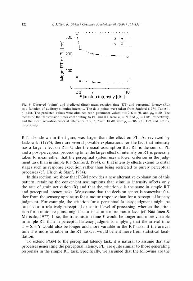
RT, also shown in the figure, was larger than the effect on PL. As reviewed by

Ja�sskowski (1996), there are several possible explanations for the fact that intensity

has a larger effect on RT. Under the usual assumption that RT is the sum of PL

and a post-perceptual processing time, the larger effect of intensity on RT is generally

taken to mean either that the perceptual system uses a lower criterion in the judg-

ment task than in simple RT (Sanford, 1974), or that intensity effects extend to distal

stages such as response execution rather than being restricted to purely perceptual

processes (cf. Ulrich & Stapf, 1984).In this section, we show that PGM provides a new alternative explanation of this

pattern, retaining the convenient assumptions that stimulus intensity affects only

the rate of grain activation (X) and that the criterion c is the same in simple RT

and perceptual latency tasks. We assume that the decision center is somewhat far-

ther from the sensory apparatus for a motor response than for a perceptual latency

judgment. For example, the criterion for a perceptual latency judgment might be

satisfied at a relatively perceptual or central level of processing, whereas the crite-

rion for a motor response might be satisfied at a more motor level (cf. N€aa€aat€aanen &Merisalo, 1977). If so, the transmission time Y would be longer and more variable

in simple RT than in perceptual latency judgments, implying that the arrival time

T ¼ Xþ Y would also be longer and more variable in the RT task. If the arrival

time T is more variable in the RT task, it would benefit more from statistical facil-

itation.

To extend PGM to the perceptual latency task, it is natural to assume that the

processes generating the perceptual latency, PL, are quite similar to those generating

responses in the simple RT task. Specifically, we assumed that the following are the

Fig. 9. Observed (points) and predicted (lines) mean reaction time (RT) and perceptual latency (PL)

as a function of auditory stimulus intensity. The data points were taken from Sanford (1974, Table 1,

p. 444). The predicted values were obtained with parameter values c ¼ 2;G ¼ 60, and lM ¼ 80. The

means of the transmission times contributing to PL and RT were ly ¼ 71 and ly ¼ 1108, respectively,

and the mean activation times at intensities of 2, 3, 7 and 18 dB were lx ¼ 686, 273, 159, and 123ms,

respectively.


same in both tasks: the pool of G available grains, the mean grain activation time lx

at each stimulus intensity, and the response criterion c. We assumed only two differ-

ences between PL values and RT values. First, the mean transmission time ly was

allowed to differ across tasks, because as already noted it is plausible to suppose that

the perceptual latency decision is a more perceptual (i.e., less motor) than the deci-sion to initiate a manual response. Second, the perceptual latency PL was assumed to

be simply the decision time, and its mean was computed using Eq. (8). That is, PL

was assumed not to include the motor component M, because it is an unspeeded

judgment rather than a speeded keypress.

The predictions shown in Fig. 9 illustrate that this extension of PGM can provide

a good quantitative account of the results. As in Sanford�s (1974) data, the predicted

overall effect of intensity is 38 ms in the perceptual latency task but 127 ms in the sim-

ple RT task. Clearly, then, PGM provides an alternative account of the differentialeffect of intensity on perceptual latency versus simple RT—an account retaining the

assumptions that the response criterion is independent of the task and the duration

of motor processing is independent of the stimulus intensity.

8. Reaction time distributions

Having established that PGM can account for a range of experimental effects ob-served in simple RT tasks, in this section we examine the model in more detail to see

whether its predicted RT distributions are generally consistent with known proper-

ties of observed RT distributions.

To be regarded as plausible, any model of simple RT must reproduce two main

properties found in virtually all analyses of RT distributions. First, the standard de-

viations of observed RT distributions always increase with the mean RTs; in fact,

several authors have reported an almost perfect linear relation between the mean

and the standard deviation of RT (see Luce, 1986, pp. 64–65). Second, observedRT distributions tend to be skewed, with a long tail in the direction of large RTs

(e.g., Woodworth & Schlosberg, 1954, pp. 37–39). Unfortunately, it is not clear

whether this skew should increase or decrease with mean RT. Few simple RT studies

have reported skewness values, and skewness sometimes increases with mean RT

(e.g., Gustafson, 1986; Ja�sskowski, 1983; Kohfeld, Santee, & Wallace, 1981; Smith,

1995) but sometimes remains constant or decreases (e.g., Hohle, 1965; Ja�sskowski,

Pruszewicz, & �SSwidzinski, 1990; Murray, 1970).10

Like many other RT modelers (e.g., Laming, 1968; Link, 1975; Schwarz, 1989,1994; Smith & Van Zandt, 2000; Townsend & Ashby, 1983; cf. Luce, 1986), we will

10 A difficulty in reaching any generalization about skewness changes is that authors who report

skewness values often do not specify exactly how they computed it. Thus, it is often unclear whether the

reported values are absolute skewness (i.e., third central moment, l3), relative skewness (third central

moment divided by sd3), or possibly some other measure altogether (for various definitions of skewness see

Stuart & Ord, 1987). This ambiguity is especially troublesome because relative and absolute measures of

skewness need not change in the same direction, as mean RT changes, because SD also varies.


not emphasize quantitative fits of PGM to observed RT distributions. We believe

that observed RT distributions are not as diagnostic as one might suppose, because

infinitely many RT models are compatible with any given observed distribution

(Dzhafarov, 1993; Van Zandt & Ratcliff, 1995). Moreover, fitting models to ob-

served distributions requires ad hoc and at present untestable assumptions aboutthe distribution of M and its correlation with D. Thus, instead of fitting these distri-

butions, in this section we simply asked whether PGM is qualitatively consistent with

observed distributions. Our evaluation of PGM�s distributional properties used Eq.

(7) because of our simplifying assumption that M is approximately constant, as dis-

cussed earlier. In essence, then, we assume that the effects of M do not qualitatively

alter the shape of the predicted RT distributions.

8.1. The distribution of D

The left column of Fig. 10 shows examples of the distributions of D predicted

by PGM. Each panel includes a common reference distribution, and the other

curves differ from it by one parameter to illustrate how changing that parameter

influences the distribution of D. Thus, the within-panel comparisons illustrate at

the distributional level some effects of parameter variations previously used to

explain changes in mean RT. Specifically, area effects were attributed to changes

in G (top panel); criterion effects, to changes in c (second panel); duration ef-fects, to changes in d (third panel); and intensity effects, to changes in lx (bot-

tom panel).

It is apparent from an examination of the left panels of Fig. 10 that PGM repro-

duces both of the main properties of observed RT distributions. First, the standard

deviations of the predicted RT distributions clearly increase with the mean RTs. In

fact, PGM is quite compatible with the linear relation typically observed between

these two measures. For example, we computed the correlation between the means

and standard deviations of the distributions shown in each panel of Fig. 10. Fromtop to bottom, the correlation coefficients for the four panels were 1.000, .998,

1.000, and .997, respectively, indicating almost perfect linear relationships in each

case. Second, PGM is clearly consistent with the usual observation of skewed RT

distributions. All of the predicted distributions exhibit the long right tail that is typ-

ically observed.

It is also instructive to examine in detail the distributional effects of changing in-

dividual parameter values. For example, the top left panel shows what happens as

the number G of available grains varies. As discussed earlier in connection withthe area effect, of course, the mean of D clearly decreases as G increases, reflecting

the effects of statistical facilitation. In addition, the decrease in mean is accompanied

by a decrease in D�s variability. This is to be expected because increasing the number

of grains produces more stable order statistics (see also Meijers & Eijkman, 1974).

For example, the values of the SDs of D are 50, 22, and 11 ms for these three distri-

butions, and values of this size are quite plausible for simple RT (cf. Murray, 1970;

Ulrich & Stapf, 1984). The absolute skewness values also diminish with increases of

G, but the relative skewness values do not. Specifically, the absolute skewness values


Fig. 10.Thepanels on the left showprobabilitydensity functions (PDFs)ofDpredictedbyPGM.Eachpanel

includes a common reference distribution (coarsely dashed line) with parameters G ¼ 60; c ¼ 4;lx

¼ 20; ly ¼ 400, and d ¼ 1000ms. The other lines in each panel illustrate the effects of changing the indicated

parameter to a different value. The panels on the right show the hazard functions ofD computed for each of

the PDFs shown on the left. Each hazard function was computed from the 0.1st percentile to the 99.99th per-

centile of the associated PDF.


for the three values of G are 54, 25, and 11 ms, respectively, and the corresponding

relative skewness values are 1.1, 1.2, and 1.0.

Distributional changes are also evident with changes in the criterion, c, the stim-

ulus duration, d, and the mean activation time, lx, as illustrated by the other three

panels on the left of Fig. 10. For each parameter, changes that increase the mean alsoincrease the variance and the absolute skewness. Interestingly, however, relative

skewness values are affected differently by the different parameters; with the stimulus

duration and the number of grains, relative skewness increases with mean RT, but

with the criterion and mean activation time, relative skewness decreases as mean

RT increases.

8.2. The hazard function of D

Several recent analyses of RT distributions have employed hazard functions (e.g.,

Burbeck & Luce, 1982; Green & Smith, 1982; Luce, 1986; Smith, 1995; Townsend &

Ashby, 1983), and in this section we consider the hazard functions predicted by

PGM. Conceptually, for each value of t, the hazard function of an RT distribution

describes the probability that a response will occur in the small time interval

(t; t þ d), given that it has not already occurred. More formally, the hazard function

hðtÞ of a random variable is defined by

hðtÞ ¼ f ðtÞ1 � F ðtÞ ; ð12Þ

where the functions f ðtÞ and F ðtÞ denote the PDF and CDF of this variable, re-

spectively. Hazard functions are of theoretical interest because they can sometimes

reveal dramatic differences in predicted RT distributions that are not apparent from

plots of predicted PDFs (see Luce, 1986, and the references therein).

Only a few researchers have reported the hazard functions estimated from their

observed distributions of simple RT (e.g., Burbeck & Luce, 1982; Green & Smith,1982; Smith, 1995; see also Luce, 1986, for hazard functions estimated from pre-

viously reported RT distributions), but the reports suggest that observed functions

have one of two distinct shapes. With some stimuli, they rise to an asymptote

(e.g., Burbeck & Luce, 1982, weak stimuli; Green & Smith, 1982, long stimuli;

Miller, 1982b, as computed by Luce, 1986; Smith, 1995, gradual-onset stimuli);

with other stimuli, however, they have a \ shape, typically rising to a maximum

somewhere in the upper half of the RT distribution, and then decreasing to a low-

er asymptote in the upper tail of the RT distribution (e.g., Burbeck & Luce, 1982,intense stimuli; Green & Smith, 1982, brief stimuli; Smith, 1995, abrupt onset

stimuli).

The right column of Fig. 10 shows examples of PGM�s predicted hazard functions

of D, computed with the same parameters used in the panels on the left. These haz-

ard functions increase in a negatively accelerated fashion, and most appear to ap-

proach an asymptote. Thus, PGM is capable of reproducing one of the two

empirical hazard function shapes just mentioned. In cases where an asymptote is ap-

proached, the approximate constancy of the hazard function for large values of t


shows that the right tail of the predicted RT distribution is nearly exponential, as is

sometimes found in observed RT distributions (cf. Luce, 1986).11

As shown in Fig. 11, PGM is also compatible with the finding that hazard func-

tions can have an \ shape. Such hazard functions tend to arise within PGM when

stimuli are brief rather than long, exactly as reported by Green and Smith (1982).With brief stimuli, the number of activated grains varies randomly from trial to trial

because the activation probability is less than one. Thus, the distribution of D is a

binomial mixture distribution with different numbers of grains in the race on differ-

ent trials. As is discussed further later in this section, hazard functions of mixture

distributions can have an \ shape (cf. Van Zandt & Ratcliff, 1995). With long stim-

uli, however, all grains tend to be activated and the distribution of D is not a mixture

but simply the distribution of the cth order statistic from G grains, yielding a mono-

tonically increasing hazard function.Luce (1986) suggested that differences in signal intensity are primarily responsible

for the shift between asymptotic and peaked hazard functions, with weak stimuli

producing asymptotic functions and strong stimuli producing peaked ones, and sev-

eral simple RT models have been developed to account for this pattern (e.g., Burbeck

& Luce, 1982; Rouder, 2000; Smith, 1995). These models have relied on neurophys-

iological and psychophysical evidence supporting a distinction between transient and

11 The asymptotic behavior of PGM�s hazard function with increasing t may be analyzed more

formally for the situation when all grains G become activated during a single trial. Such a situation occurs

with relatively intense or long stimuli. Let fDðtÞ be the PDF of decision time D for the case in which all

grains are activated in each trial. It is known that when � ln½fDðtÞ� is convex, the hazard function of fDðtÞmust be increasing (Thomas, 1971, Theorem 2.4). Applying this theorem to the PDF of PGM yields

ln½fDðtÞ� ¼ lnG!

ðc� 1Þ!ðG� cÞ!

� �þ ðc� 1Þ ln½FT ðtÞ� þ ðG� cÞ ln½1 � FT ðtÞ� þ ln½fT ðtÞ� ð13Þ

Thomas�s theorem can be rephrased (see Luce, 1986, p. 16) by saying that when the first derivative of

� ln½fDðtÞ� is increasing, the hazard function of fDðtÞ must be increasing. Taking the derivative of the

expression above and simplifying yields

ð� ln½fDðtÞ�Þ0 ¼ � ðc� 1Þ fT ðtÞFT ðtÞ

þ ðG� cÞ fT ðtÞ1 � FT ðtÞ

þ ð� ln½fT ðtÞ�Þ0; ð14Þ

¼ � ðc� 1Þ fT ðtÞFT ðtÞ

þ ðG� cÞhDðtÞ þ ð� ln½fT ðtÞ�Þ0; ð15Þ

where hDðtÞ denotes the hazard function of fT ðtÞ. Note that when fT ðtÞ has itself an increasing hazard

function, the latter two terms must increase with t whereas the first one decreases to zero; thus the hazard

function of D should increase (cf. Ross, 2000, p. 545). To illustrate the preceding equation, let fT ðtÞ be an

exponential distribution with rate a, then (cf. Luce, 1986, p. 507)

� f 0DðtÞfDðtÞ

¼ ðc� 1Þ � a1 � expða � tÞ þ ðG� cþ 1Þ � a ð16Þ

which is an increasing function of t, and thus the hazard function of D increases towards the asymptote

ðG� cþ 1Þ � a. In sum, then, it seems plausible that the hazard function of D approaches an asymptote

when the tail of fT ðtÞ is exponential. Further work is necessary to see whether this conclusion also applies

for cases in which only a percentage of all grains are activated during a single trial.


sustained channels (e.g., Breitmeyer & Ganz, 1976). In brief, these models have as-

sumed that some activation is provided by each type of channel, with the transient

channel providing especially large activation with intense stimuli.

PGM can also be elaborated to include the transient/sustained distinction, and the

most plausible way to do this is to include separate pools of grains for the transient

and sustained channels. Suppose that each stimulus can potentially activate Gt and

Gs grains in separate transient and sustained channels, respectively. Furthermore,suppose that activation of grains in the sustained channels are as we have described

previously, but activation of grains in the transient channels occurs (a) with a higher

rate, and (b) for only a short period of time, dt, after stimulus onset. According to

this version of the model, the distribution of D is a mixture distribution, with differ-

ent numbers of transient grains activated in each trial.

As illustrated in Fig. 12, this elaborated version of PGM produces \-shaped haz-

ard functions with an especially pronounced peak for high intensity stimuli. The rea-

Fig. 11. Probability density (left panels) and hazard (right panels) functions of D predicted by PGM with

short versus long stimuli of the durations used by Green and Smith (1982). The mean activation times were

lx ¼ 100, 200, and 400ms for the high, medium, and low intensities, respectively. The remaining param-

eter values were c ¼ 4;G ¼ 30, and ly ¼ 400ms.


son is essentially the same as in the other models for this effect: The overall RT dis-

tribution is a mixture of some trials in which the response criterion is satisfied mostly

by fast transient grains and other trials in which it is satisfied mostly by the slower

sustained grains. With high intensity stimuli, many transient grains are often acti-

vated, producing many fast responses. With low intensity stimuli, it is rare for morethan c transient grains to be activated, so there is little or no such peak in the hazard

function. Thus, the overall structure of PGM seems quite compatible with both of

the observed hazard function shapes and their dependence on intensity as discussed

by Luce (1986).

Despite the dependence of observed hazard function shapes on stimulus duration

and intensity, there are reasons to suspect that the change from\-shaped to monotonic

hazard functions could actually be due to something more general than these physical

stimulus parameters. Specifically, hazard functions have been found to be morepeaked in faster conditions than in slower ones not only in simple RT tasks but also

in choice RT tasks requiring subitizing (Balakrishnan & Ashby, 1992), memory scan-

ning (Ashby, Tein, & Balakrishnan, 1993), and categorization (Maddox, Ashby, &

Gottlob, 1998), leading the latter authors to conclude ‘‘This remarkable similarity

across such different tasks suggests a possible common mechanism that may operate

in virtually all perceptual decision-making tasks’’ (Maddox et al., 1998, p. 629).

Within PGM, a more general way to produce \-shaped hazard functions is to al-

low parameter values to vary somewhat from trial to trial. Although we have so farassumed for simplicity that PGM�s parameters are constant across trials, it is prob-

ably more realistic to assume that they fluctuate slightly due to changes in attention,

arousal, neural noise, etc. In that case the RT distribution is a mixture of the RT dis-

tributions obtained under the different possible sets of parameter values, and it is

known that mixture distributions can have \-shaped hazard functions even when

Fig. 12. Probability density (left panel) and hazard (right panel) functions of D predicted by the version of

PGM elaborated to include separate transient and sustained grains. The mean activation times for tran-

sient grains were lx ¼ 50, 100, and 200ms for the high, medium, and low intensities, respectively, and the

mean activation times for sustained grains were twice as long. The effective stimulus duration for transient

grains was assumed to be dt ¼ 2ms. The remaining parameter values were c ¼ 4;Gt ¼ Gs ¼ 30;ly ¼400ms, and d ¼ 1000ms.


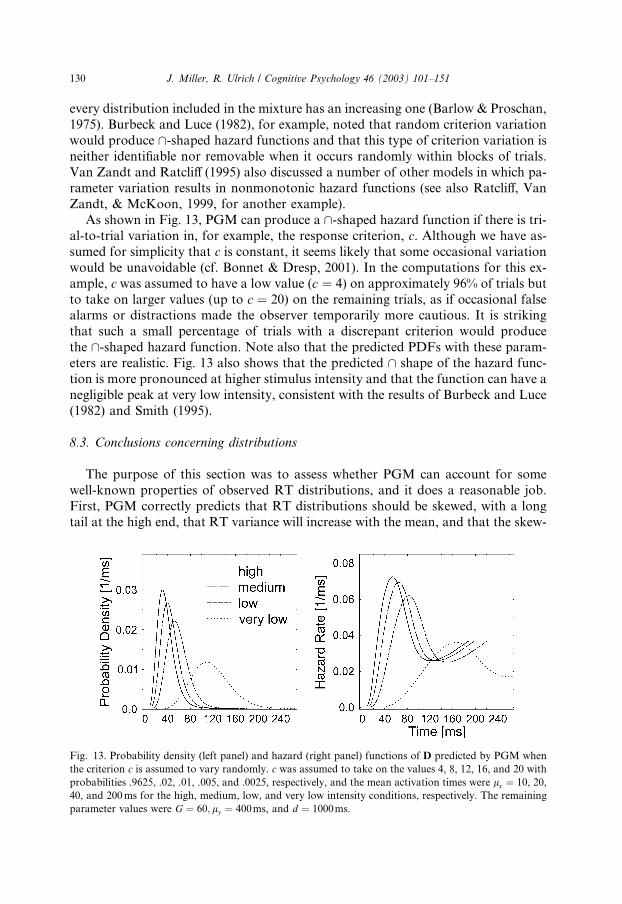
every distribution included in the mixture has an increasing one (Barlow & Proschan,

1975). Burbeck and Luce (1982), for example, noted that random criterion variation

would produce \-shaped hazard functions and that this type of criterion variation is

neither identifiable nor removable when it occurs randomly within blocks of trials.

Van Zandt and Ratcliff (1995) also discussed a number of other models in which pa-rameter variation results in nonmonotonic hazard functions (see also Ratcliff, Van

Zandt, & McKoon, 1999, for another example).

As shown in Fig. 13, PGM can produce a \-shaped hazard function if there is tri-

al-to-trial variation in, for example, the response criterion, c. Although we have as-

sumed for simplicity that c is constant, it seems likely that some occasional variation

would be unavoidable (cf. Bonnet & Dresp, 2001). In the computations for this ex-

ample, c was assumed to have a low value (c ¼ 4) on approximately 96% of trials but

to take on larger values (up to c ¼ 20) on the remaining trials, as if occasional falsealarms or distractions made the observer temporarily more cautious. It is striking

that such a small percentage of trials with a discrepant criterion would produce

the \-shaped hazard function. Note also that the predicted PDFs with these param-

eters are realistic. Fig. 13 also shows that the predicted \ shape of the hazard func-

tion is more pronounced at higher stimulus intensity and that the function can have a

negligible peak at very low intensity, consistent with the results of Burbeck and Luce

(1982) and Smith (1995).

8.3. Conclusions concerning distributions

The purpose of this section was to assess whether PGM can account for some

well-known properties of observed RT distributions, and it does a reasonable job.

First, PGM correctly predicts that RT distributions should be skewed, with a long

tail at the high end, that RT variance will increase with the mean, and that the skew-

Fig. 13. Probability density (left panel) and hazard (right panel) functions of D predicted by PGM when

the criterion c is assumed to vary randomly. c was assumed to take on the values 4, 8, 12, 16, and 20 with

probabilities .9625, .02, .01, .005, and .0025, respectively, and the mean activation times were lx ¼ 10, 20,

40, and 200ms for the high, medium, low, and very low intensity conditions, respectively. The remaining

parameter values were G ¼ 60; ly ¼ 400ms, and d ¼ 1000ms.


ness can increase or decrease with the mean, as reported in the literature. Second,

PGM is able to generate plausible hazard functions. Its hazard functions generally

increase to an asymptote, but they can have an \-shape for high-intensity stimuli

if the stimuli are brief or if there are small criterion fluctuations. The distributional

properties of the model are thus reasonably consistent with the main features of ob-served RT distributions.

9. General discussion

The basic framework of PGM involves a set of parallel grains, each of which can

potentially be activated by a stimulus and contribute its activation toward the re-

sponse. The latencies associated with each individual grain are quite noisy, with ran-dom fluctuations in both the time required for it to become active and the time

required for its activation to reach the decision center responsible for initiating the

response. In fact, with brief stimuli an available grain may not become active at

all on a trial, because the stimulus duration may be less than the time needed for

the grain to become active on that trial.

Despite its conceptual simplicity, this framework provides a cohesive explanation

for a number of well-established phenomena in the literature on simple RT. For ex-

ample, the model provides straightforward accounts for the effects of stimulus areaand duration on simple RT, as well as the interactions between each of these factors

and stimulus intensity. It also accounts for the effects of redundant signals and of

instructional manipulations designed to influence the participant�s criterion (e.g.,

speed versus accuracy emphasis). In addition, it provides a novel account for the

puzzling dissociation between the effects of intensity on simple RT versus tempo-

ral-order judgments. In all of these cases, the model seems capable of fitting the ob-

served mean RTs. In the case of the RSE, the model also accounts for coactivation in

RT distributions. Importantly, the model includes an inherently stochastic mecha-nism producing RT distributions with appropriate amounts of variability and skew

and with realistically-shaped hazard functions.

Most of the explanatory power of the model is derived from the phenomenon of

statistical facilitation: In general, the average completion time for the cth finisher in a

race tends to decrease as the number of racers increases. In PGM, the analogous ef-

fect is that the response criterion of c grains tends to be reached more rapidly when

the stimulus activates more grains. Naturally, we suppose that the number of acti-

vated grains tends to increase with the size, duration, and intensity of a stimulus,and that it would surely be greater for two redundant stimuli than for only one.

Within this framework, statistical facilitation seems easily capable of explaining

the effects and interactions just mentioned. One of the desirable features of PGM

as a model for simple RT, then, is that it can explain a variety of results with a single

mechanism that is conceptually simple enough so that its predictions can be under-

stood intuitively.

PGM is also theoretically appealing because it provides a bridge between the mi-

cro- and macro-levels of information processing. At the micro-level, the model is


constructed from many noisy grains operating in parallel, which is plausible in the

light of current physiological knowledge. Consistent with neurophysiological find-

ings (e.g., Schmolesky et al., 1998), the onset latencies of the grains would become

longer and more variable as one moves upward in the processing stream. At the

macro or behavioral level, PGM displays much greater stability than might be ex-pected from the degree of noise in the individual grains. This stability arises because

the order statistics of a sample are much less variable than the individual scores mak-

ing up the sample, especially if the sample is large. The stability of order statistics has

previously been discussed in connection with models of the motor system (e.g., Meij-

ers & Eijkman, 1974; Ulrich & Wing, 1991) and PGM extends the same principle to

the input side of the information processing system.

9.1. Comparison with previous models for simple RT

PGM shares with previous models of simple RT at least two main features that

seem to be common to all such models (see Luce, 1986, for a review). First, evidence

is assumed to accumulate over time, as inputs starting from the sensory transducers

are fed into a decision-making mechanism capable of initiating the response. Second,

the decision to respond is made when the decision-making mechanism has accumu-

lated enough evidence to satisfy a response criterion.

There are, however, significant theoretical differences between PGM and all pre-vious simple RT models. Some such models assume a noise-free evidence accumula-

tion process and put all stochastic variation into the response criterion (e.g., Ashby,

1982; Grice, 1968; McClelland, 1979); in contrast, PGM assumes that evidence accu-

mulation is highly stochastic and that the response criterion is relatively invariant.

Although Dzhafarov (1993) has shown that most fixed-criterion models can be mim-

icked by fixed-rate models and vice versa, the available physiological evidence seems

to support the assumption of a relatively fixed criterion (e.g., Gratton, Coles, Sire-

vaag, Eriksen, & Donchin, 1988; Hanes & Schall, 1996).Several other previous simple RT models have—like PGM—assumed noisy evi-

dence accumulation and a fixed criterion. For example, Smith and Van Zandt

(2000) describe an ‘‘accumulator’’ class of RT models in which the decision process

simply totals all of the inputs favoring a given response, and a response is initiated

when its total passes a response criterion. Like all simple RT models that we know

of, PGM is an accumulator-type model within Smith and Van Zandt�s (2000) classi-

fication scheme.

Unlike PGM, however, previous simple RT models have usually assumed that ev-idence is accumulated according to a Poisson process. This conception differs in prin-

ciple from the notion of a fixed set of grains embodied in PGM, because a Poisson

process can generate a potentially limitless number of pieces of evidence. In addition,

previous Poisson models have generally assumed that the average rate of accumula-

tion stays constant over time—an assumption known as ‘‘stationarity’’ (Burbeck &

Luce, 1982; Laming, 1968; Link, 1975; Link & Heath, 1975; Ratcliff, 1978; Smith,

1995; cf. Luce, 1986; but for an exception, see Smith & Van Zandt, 2000). In con-

trast, PGM�s evidence accumulation process is not stationary, because the rate at


which new activation arrives tends to decrease as the number of already-finished

grains increases.

We believe that there are two a priori reasons to prefer the conception of a non-

stationary activation system with a fixed number of grains, as embodied in PGM,

over a stationary activation system that can generate a potentially limitless numberof activation counts, as in Poisson models. One is that different sensory coding sys-

tems appear to have different latencies (Bullier & Nowak, 1995; Murphy, Wong, &

Kwan, 1985), so different stimuli or attributes would provide activation at different

times (Nissen & Pokorny, 1977) resulting in nonstationary activation growth. A sec-

ond is that the stationarity assumption leads to the prediction of a linear increase in

the amount of evidence, at least on the average. In contrast, it seems plausible to ex-

pect the growth of activation to be negatively accelerated in physiological systems,

because these tend to saturate at the highest activation levels (e.g., Anderson,1977). Nonlinear activation growth has also been a feature of other recent RT mod-

els (e.g., Smith & Van Zandt, 2000; Usher & McClelland, 2001), although only for

PGM does it arise as a natural consequence of the model�s structure.

More importantly, the emphasis of PGM is also different from that of previously

suggested models for simple RT. First, through its use of the concept of statistical

facilitation, PGM attempts to provide cohesive explanations for a variety of stimulus

effects that have previously been modeled in isolation from one another, if at all. As

discussed below, most previous simple RT models have been designed to accountmore specifically for a smaller set of phenomena. It is therefore difficult to compare

them to PGM, because they make no predictions about several phenomena that

PGM addresses. Second, PGM attempts to model explicitly the effects of stimulus

manipulations such as area and duration. In previous models, it has generally been

assumed that such manipulations simply had a more or less arbitrary influence on

the rate at which evidence accumulates—i.e., simply changed a parameter value.

Third, the main aim of PGM is to account for effects on mean RT across a fairly

large set of experimental conditions (e.g., factorial variations of area and intensity).More commonly, models of simple RT have focused on just one or two conditions to

be explained but sought to model them in more detail (e.g., Burbeck & Luce, 1982;

Smith, 1995).

For example, one previously suggested model is Grice�s (1968) variable-criterion

model, developed to account for the interaction of intensity and criterion effects. Ac-

cording to this model, the evidence accumulation process is deterministic, with a

higher rate of accumulation for more intense stimuli. The criterion varies from con-

dition to condition according to the instructions of the experimenter, and it also var-ies randomly from trial to trial according to a normal distribution. This model

predicts an interaction of intensity and criterion, as does Ashby�s (1982) formaliza-

tion of McClelland�s (1979) variable-criterion cascade model, although the latter

model was developed primarily for choice RT. These models cannot account for ef-

fects of stimulus area or duration, however, without making additional assumptions

about how evidence accumulation depends on stimulus characteristics.

Several previous models of simple RT have been designed to account mainly for

the distributional properties of simple RTs within a given condition. For example,


Green and Luce (1973) suggested that evidence accumulation could be modeled as a

Poisson counting process, with the response criterion defined in terms of either the

amount of time needed to reach a fixed number of counts or the number of counts

obtained within a fixed time. These models differ from PGM both theoretically and

in application. An important theoretical difference is that they include a stationaryevidence accumulation process, as discussed above. In application, the models differ

in that Green and Luce used their models to fit the shapes of simple RT distributions,

primarily evaluating the model�s predictions regarding the shape of the hazard func-

tion in the upper tail of the RT distribution, whereas PGM has been applied mainly

to the modeling of experimental effects on mean RT (stimulus area, duration, etc.).

One point of similarity between the Poisson models and PGM is that both can pro-

vide principled accounts of the duration effect. In the former models, it would be nat-

ural to assume that the Poisson process stopped at stimulus offset, just as PGM�sactivation process does. Indeed, Hildreth (1979) developed a version of the Poisson

model incorporating this assumption to account for the interactive effects of intensity

and duration on simple RT. The major difference between Hildreth�s model and

PGM, aside from the broader application of the latter, is that in the former model

counts contributing toward the response criterion are activated by a stationary Pois-

son process, and hence are potentially limitless in number, rather than by a fixed set

of stimulus-activated grains. Like PGM, this model could only account for the Bro-

ca–Sulzer effect with the additional assumption that stimulus offset triggers specialactivity (i.e., Poisson counts).

Other simple RT models have also been developed to account for specific stimu-

lus-related phenomena, especially the redundant signals effect in two-channel divid-

ed-attention tasks (e.g., Raab, 1962b; Schwarz, 1989; see Colonius & Townsend,

1997, and Townsend & Nozawa, 1995, 1997, for more detailed characterization of

these models). As mentioned earlier, Raab (1962b) proposed a race model in which

the response on a redundant-signals trial is determined by the faster of the detection

processes on the two separate channels (for elaborations of this model, see Gielen,Schmidt, & Van den Heuvel, 1983; Meijers & Eijkman, 1977). This model predicts

that RT distributions should satisfy Inequality 10, however, and is thus ruled out

by observed violations of it (Miller, 1982b). According to Schwarz�s (1989) superpo-

sition model, in contrast, the onset of a stimulus in either channel initiates a station-

ary counting process, and the response is initiated when a criterion number of counts

is reached. When redundant signals are presented, counting processes are initiated by

both channels, and the response is initiated when the total number of counts across

both channels reaches the criterion—that is, there is superposition of the countingprocesses. If the response criterion is greater than one, the superposition model is

not a race model, so it not only predicts the RSE but also is compatible with viola-

tions of Inequality 10. In fact, PGM is quite similar to this superposition model; the

main differences are—as already mentioned—that PGM has a nonstationary count-

ing process based on the order statistics from a finite set of grains, not a Poisson pro-

cess, and that PGM has been applied to a much broader range of phenomena.

Burbeck and Luce (1982), Rouder (2000), and Smith (1995) have also developed

race models of simple RT to account for effects of stimulus intensity and stimulus


onset type (i.e., abrupt versus ramped). In general, weak, gradual-onset stimuli yield

increasing RT hazard functions, but intense, abrupt-onset stimuli yield \-shaped

ones. Consistent with known physiology of sensory systems, their models allowed

transient and sustained stimulus properties to activate different channels, each of

which was represented in these models as a single detector. In Burbeck and Luce�smodel, simple RT was determined by the winner of a race between transient versus

sustained detectors; Smith considered both this race model and a model in which ac-

tivation was pooled across the two types of detectors. The models were mainly ap-

plied to the hazard functions of simple RT, and they provided good accounts of

the change in hazard function shape as a function of stimulus intensity.

Although PGM was not designed to account for the changing shapes of hazard

functions, it seemed worthwhile to consider how it might produce the observed pat-

terns because these are sometimes regarded as highly diagnostic for RT models (e.g.,Luce, 1986; Smith, 1995; but see Van Zandt & Ratcliff, 1995). The basic version of

PGM yields increasing hazard functions for most parameter values. If the stimuli are

presented briefly or if the model is elaborated by allowing either different types of

grains for sustained and transient stimulus properties or variation in c across trials,

however, predicted hazard functions can take on the \ shape. Moreover, this shape

is quite pronounced when stimulus intensity is high (i.e., when lx is small), and it

tends to flatten out as stimulus intensity decreases. Thus, PGM is quite capable of

providing an explanation for the observed change in hazard function shapes as afunction of stimulus intensity. Moreover, criterion variation could provide a general

mechanism to explain more wide-ranging evidence that hazard functions get less

peaked as RT increases in a variety of tasks (Maddox et al., 1998).

9.2. Evaluation of PGM’s assumptions

PGM is based on two primary assumptions: (1) the decision to respond occurs at

the arrival of the cth finisher from a large set of activated grains, and (2) the numberof activated grains tends to increase with stimulus area, duration, intensity, and

number. These are the two key assumptions required to produce statistical facilita-

tion, which is the mechanism underlying much of PGM�s success in predicting the

various patterns of data considered here. The former assumption is consistent in

spirit with virtually all accumulation models of RT, and the latter is quite consistent

with existing neurophysiological evidence.

In addition, we invoked a number of more detailed subsidiary assumptions to

simplify the model mathematically, and it is doubtful whether these assumptionsare exactly correct. The question naturally arises, then, of whether these subsidiary

assumptions are crucial for the basic predictions of the model. In this section, we

briefly present some simulations indicating that reasonable violations of these as-

sumptions do not seriously distort the basic qualitative predictions of the model, al-

though different parameter values would needed to obtain the same quantitative

predictions under alternative subsidiary assumptions.

The main subsidiary assumption was that motor time was approximately

constant. As already noted, however, this assumption has no impact on the model�s


predictions about statistical facilitation in mean RT, which are the main focus of the

model. In addition, there were three other more technical subsidiary assumptions:

First, the criterion c was assumed to be constant in fitting all of the data sets consid-

ered here, although we did briefly consider the possibility of a variable c in the dis-

cussion of \-shaped hazard functions. It would seem quite realistic to build in asmall amount of random variation in c across trials. Variation in the criterion is

plausible theoretically, because random fluctuations seem to be inherent in any bio-

logical system, and it is also suggested by certain empirical findings such as the in-

crease in RT following error trials (e.g., Rabbitt, 1989), although evidence

suggests that the amount of variation is small as already noted (Hanes & Schall,

1996). Second, the transmission time Y was assumed to follow an exponential distri-

bution. This assumption yields the simplest expressions for the decision time distri-

bution (e.g., Eq. (7)), but other distributions such as the gamma actually providetheoretically more plausible models of finishing times for the sort of transmission

process considered here (e.g., McGill, 1963; McGill & Gibbon, 1965). Third, the ar-

rival times of different grains T were assumed to be independent of one another. In

reality, it seems more likely that these arrival times would be positively correlated,

because they would likely be affected in the same manner by trial-to-trial fluctuations

in alertness, arousal, motivation, and so on.

Fig. 14 displays results obtained when these subsidiary assumptions are relaxed,

and these results suggest that the effects of statistical facilitation do not depend muchon the subsidiary assumptions. Each panel shows how predicted mean RT depends

on the number of grains under a different set of assumptions.12 The solid line in each

12 This footnote describes how we obtained predicted values with relaxed assumptions, as shown in the

four panels of Fig. 14. Panel A: The assumed variation in c produces a mixture distribution (Everitt &

Hand, 1981) of detection times as discussed in connection with Fig. 13. The overall mean of this mixture is

a weighted average of the conditional means given each of the possible c values, with weights equal to the

probabilities of those values, as given in the figure caption. Panel B: Assuming that transmission time

follows a gamma distribution rather than an exponential distribution changes the distribution of arrival

times, FT ðtÞ, from a convolution of two exponentials to the convolution of an exponential and a gamma.

This convolution was evaluated numerically and then used to compute the CDF of detection times, FDðtÞ,via Eq. (7). The mean detection time was then obtained from Eq. (8) using the CDF just computed. Panel

C: For each value of G, the predicted mean was computed by simulating 10,000 trials and averaging their

RTs. To simulate each trial, G transmission times were generated using a method that produced the

desired intercorrelations. In brief, the method started by generating G correlated normal random variables

using standard techniques (e.g., Graybill, 1969). Then, the CDF of each normal random variable was

computed, and it was replaced by the value with that same CDF in the desired exponential distribution

(ly ¼ 400) of transmission times. The extent of correlation of the underlying normals was adjusted by trial

and error to produce a value that would yield the desired numerical correlation (i.e., .4 or .8) after the

transformation to exponentials (see Miller, 1998, for further description). Once the G correlated

exponentials had been generated, each was incremented by a random activation time, and the c�th smallest

total was selected as the decision time for that trial. Panel D: Simulation was used for this panel as for

Panel C, with two main differences in procedure. First, on each trial the value of c was randomly chosen

using the same set of values and probabilities as in panel A. Second, each of the intercorrelated normal

random variables was replaced by the value with the same cumulative probability from the desired gamma

distribution of transmission times.


panel is for comparison purposes, and it displays once again PGM�s predictionsbased on all the subsidiary assumptions, as already shown in Fig. 3.

Panel A illustrates the effect of letting the criterion c vary randomly from trial to

trial. As specified in the figure caption, c took on values from 4 to 20. The value c ¼ 4

was used on most trials, consistent with evidence suggesting a relatively constant cri-

terion as noted earlier, but larger values of c were used on some trials to mimic small

Fig. 14. Effects of relaxing the subsidiary assumptions within PGM. Within each panel, the dotted and

dashed lines show predicted mean reaction time (RT) as a function of the number of available grains G

with PGM�s assumptions relaxed in one or more ways. For comparison purposes, the solid line in each

panel shows predictions computed with the specific assumptions that have been employed throughout this

article and with the following default parameters values: c ¼ 4; lx ¼ 20ms; ly ¼ 400ms; lM ¼ 150ms,

and d ¼ 1 (i.e., response-terminated stimuli). Panel A shows the effect of relaxing the assumption that

the criterion is constant. The dotted line shows mean RTs when c varies randomly from trial to trial using

the same distribution used in Fig. 13 (i.e., values of 4, 8 12, 16 and 20 with probabilities of .9625, .02, .01,

.005, and .0025, respectively). Panel B shows the effect of relaxing the assumption that the transmission

time Y is an exponential random variable. The predictions shown in the dotted line were computed using

instead a gamma distribution of transmission times with a mean of 400ms and a shape parameter of 3.

Panel C shows the effect of relaxing the assumption that the transmission times are uncorrelated. The dot-

ted lines show the predicted RTs when the transmission times are correlated to the indicated degree. Panel

D shows the combined effect of relaxing all three assumptions at the same time (i.e., c varying and corre-

lated gamma-distributed Y�s).


lapses in attention or readiness that might increase the criterion above this presum-

ably optimal level. The results are striking: the predictions allowing this criterion

variation are almost exactly identical to those without it, so the two lines in the figure

are nearly superimposed. Thus, it appears that criterion variation can have quite

large effects on the shapes of RT hazard functions (cf. Fig. 13) even though it hasrelatively small effects on mean RT.

Panel B shows what happens if transmission times are assumed to have a gamma

distribution rather than an exponential distribution. Specifically, we used a gamma

distribution with shape parameter equal to three, which produces a fairly bell-shaped

distribution with a long positive tail. The mean of this distribution was set to

ly ¼ 400ms to match that of the exponential it replaced. With gamma rather than

exponential transmission times, mean RTs are increased by approximately 100 ms,

but the overall pattern of statistical facilitation (i.e., decreasing RT with increasingG) is preserved nicely. The increase of 100 ms in overall RT is not important, because

it could be counteracted by reductions in the motor time, the mean transmission

time, or both. A more subtle point is that the amount of statistical facilitation is

not strictly tied to the variance of the transmission times, but also depends on their

distribution. In this example, the gamma produces approximately the same amount

of statistical facilitation (i.e., decrease in RT with increasing G) as the exponential,

despite the fact that the variance of the exponential is almost three times as large.

Apparently, the amount of statistical facilitation depends heavily on the shape ofthe lower tail of the transmission time distribution, not just on its overall variance.

Within the present context, this fact is important because it implies that realistic sta-

tistical facilitation could be obtained with much smaller transmission time variance

than is suggested by examining only the mathematically convenient case of exponen-

tial transmission times. It is also interesting that statistical facilitation approaches its

asymptote more slowly as G increases for the gamma than for the exponential; for

example, as G changes from 90 to 120, RT decreases approximately twice as much

for the gamma as for the exponential. Thus, it is difficult to estimate G from lookingat changes in RT, because the relationship between RT and G asymptotes at different

G values under different distributional assumptions.

Panel C displays the effects of assuming correlated rather than independent trans-

mission times. Specifically, the transmission times for all grains activated on a given

trial were correlated at the values of q ¼ :4 or q ¼ :8, as indicated in the figure. Ac-

tivation times were still independent of one another, and of the transmission times,

but this is not of much importance because activation times contribute little to the

overall RT. Interestingly, correlations among transmission times increase overallRT and slow the rate of decrease in RT as G increases. Intuitively, both of these ef-

fects arise because there is less statistical facilitation when the grains are positively

correlated. In the limit of perfectly correlated grains, for example, there would be

no statistical facilitation at all, and RTs would be both quite large and completely

insensitive to G. With imperfect correlations, of course, there is some statistical fa-

cilitation, but it grows more slowly with G and asymptotes at larger values of G

(e.g., mean RT decreases more as G changes from 90 to 120 with q ¼ :8 than with

q ¼ 0).


Panel D shows the combined effects of relaxing all assumptions simultaneously.

Here the predictions were obtained by simulating a version of PGM in which (a)

the criterion c varied randomly, as in Panel A; (b) the transmission times had a gam-

ma distribution, as in Panel B; and (c) the transmission times of different grains were

correlated, as in Panel C. The predicted RTs in this panel show the same effects ofcorrelation as already seen in Panel C, but they are longer overall because of the

gamma, as in Panel B.

In summary, the subsidiary assumptions of PGM do not seem to be crucial in de-

termining the qualitative patterns of its predictions, because the phenomenon of sta-

tistical facilitation is quite robust. Instead, the robustness of the predictions suggests

that the model could still provide reasonable predictions under different sets of sub-

sidiary assumptions than those employed here. Of course, the exact quantitative pre-

dictions of the model do depend on both the subsidiary assumptions and the valuesof the parameters. In particular, given a fixed set of parameter values (e.g., number

of grains, mean activation, and transmission times, etc.) the overall predicted RT is

substantially larger if the transmission times have a gamma rather than an exponen-

tial distribution or if the different grains have correlated rather than independent

transmission times. To fit a given data set under different subsidiary assumptions,

then, it would presumably be necessary to adjust these parameter values.

9.3. Parameter estimates

It is somewhat encouraging that reasonable parameter estimates were obtained in

fitting the data sets considered here. Usually, the criterion c was 2, G was approxi-

mately 10–80, lx values were approximately 1–200 ms (depending on stimulus inten-

sity), ly values were approximately 100–400 ms, and the mean motor time lM was

approximately 100–200 ms. Of course, some variation in parameter values across

studies is inevitable. Differences in stimulus parameters (e.g., modality, size, and in-

tensity) would naturally affect G; lx, and possibly c; differences in response manip-ulanda would affect lM ; and subject differences (e.g., age) could affect all parameters,

including ly . Reasonable parameter estimates and reasonable consistency of these es-

timates across data sets, however, are clearly desirable features of the model.

It also appears that the parameter values are identifiable—that is, that they can be

estimated separately from one another based on the sets of data considered here. The

mathematical structure of PGM is quite complex (e.g., Eq. (7)), so it is difficult to

establish their identifiability mathematically. When parameters are not identifiable,

however, problems are encountered in fitting the model with numerical search algo-rithms (Wickens, 1982). For example, the search may yield different sets of param-

eter estimates that give equally good fits to the data. Such problems did not arise

in fitting PGM to the present data sets, so it appears that the parameters actually

are identifiable (see Smith, 1995, for a similar argument).

Another positive point about the model is that it cannot account for all conceivable

patterns of results—that is, it is potentially falsifiable. As argued by Roberts and Pash-

ler (2000), good fits to data do not provide strong support for a model unless there are

also potentially plausible patterns of data with which the model is incompatible. To


examine the flexibility of the model, we generated an artificial set of data for the in-

tensity by area interaction. Instead of an overadditive interaction as is found in real

data (e.g., Fig. 4), the artificial data had an underadditive interaction—i.e., larger ef-

fect of area for more intense stimuli. Using the same parameter estimation techniques

applied to the real data set, we found that PGM was simply unable to fit this artificialunderadditive pattern. Certain parameter values produced near-additivity in the pre-

dicted means, but none produced underadditivity. This shows that the model is poten-

tially falsifiable, not simply a redescription of the data in an alternative notation (e.g.,

as is a second-order polynomial fit to three ordered data points).

On the other hand, several considerations suggest that PGM�s parameter values

cannot be taken too seriously. First, due to its nonlinearity, PGM may not fit an av-

erage data set even if it fits each of the data sets included in the average. As an ob-

vious example, suppose two observers had identical parameters except that one hadc ¼ 3 and the other had c ¼ 4. PGM would not fit the average data because c must

be an integer, and it is easy to imagine that the parameter estimates would be dis-

torted by this averaging process. Thus, it is doubtful whether the parameters esti-

mated from group averages would equal the average of the individual observer�sparameter values.

Second, PGM�s subsidiary assumptions have a substantial impact on the param-

eter estimates. As illustrated in Fig. 14, for example, predicted means are much long-

er if transmission times have gamma distributions or if grain times are correlated, ascompared with the assumption of uncorrelated exponentials. This implies that pa-

rameter estimates (e.g., the mean transmission time ly) might change considerably

under different subsidiary assumptions. The general structure of PGM (e.g., Eq.

(7)) could be used with other sets of subsidiary assumptions, but it is difficult at this

point to decide which subsidiary assumptions are most realistic.

Although it does not seem safe to base strong interpretations on PGM�s estimated

parameter values, PGM still appears quite useful as a general framework within

which to consider a variety of simple RT phenomena. In particular, the model showshow a small and plausible set of mechanisms can account for various RT phenomena

not addressed by previous models of simple RT. In addition, a broader data base

could increase the identifiability of parameter estimates and help constrain the mod-

el�s subsidiary assumptions (Restle & Greeno, 1970; Wickens, 1982).

9.4. Further extensions of PGM

In developing a new model, one is always faced with a delicate tradeoff betweentractability and generality. On one hand, it is desirable for the model to be gen-

eral—that is, to account for as many phenomena as possible within its domain of ap-

plication (e.g., simple RT). On the other hand, the model should also be tractable

enough to allow some intuitive grasp of its predictions concerning the various phe-

nomena under consideration. Usually, increasing the complexity of a model in-

creases the number of phenomena for which it can account but simultaneously

decreases its tractability. In developing PGM, our initial goal was to evaluate

whether the principle of statistical facilitation could account for various phenomena


in the domain of simple RT, but there are clearly a number of directions in which the

model could be extended—albeit with some loss of tractability—to account for addi-

tional phenomena.

One phenomenon that we have excluded from the present version is that partici-

pants tend to produce a certain percentage of anticipations before stimulus occur-rence. Such anticipation errors or false alarms are especially frequent when there

is time stress or when a weak stimulus must be detected within a stream of ongoing

background noise (e.g., Green & Luce, 1973). It is not difficult to imagine how an

extension of PGM might account for such false alarms. One could proceed from

the assumption that grains are sometimes spuriously activated by noise alone rather

than by a stimulus. For example, available grains could be activated by noise during

the foreperiod at a rate much lower than the rate after stimulus onset. If enough

grains are activated during the foreperiod, they could produce a false alarm re-sponse, and this will clearly be most likely when the criterion is low. We have delib-

erately excluded this complication in the present version of PGM, because it would

greatly complicate the mathematical representation of the model. In addition, it

would not help explain the effects considered here, which were after all obtained

in experiments using easily detectable stimuli and yielding few false alarms.

A second phenomenon that we have not addressed is that the physical properties

of the stimulus may influence the dynamics of response execution as well as RT. For

example, participants react not only more quickly but also more forcefully to intensestimuli than to weak ones (e.g., Angel, 1973; Ja�sskowski, Rybarczyk, Jaroszyk, & Le-

ma�nnski, 1995; Miller, Franz, & Ulrich, 1999). Similarly, response force also increases

with stimulus duration (Ulrich et al., 1998). These findings cannot be explained by

the present version of PGM, which only describes the latency of stimulus detection.

Nonetheless, a simple extension of PGM might also account for the effects of stim-

ulus properties on response dynamics. According to this extension, response output

dynamics (e.g., force) increase with the number of activated grains that arrive within

a short time after the response has been initiated. As in the present version, the arrivalof the c�th grain would determine the decision time and thus the RT. In addition, how-

ever, grains arriving after detection would also be transmitted to the motor system,

where they would tend to increase response force. Consider, for example, the study

of Ulrich et al. (1998). Participants were asked for speeded responses to stimuli vary-

ing in intensity and duration, and RT depended on both of these factors as already

shown in Fig. 5. In addition, response force increased with both the intensity and

the duration of the stimulus. More interestingly, response force continued to increase

with stimulus duration up to 200ms, whereas RT was independent of duration beyondabout 50 ms. These findings are completely consistent with the notion that grains ar-

riving after detection can increase force even though they are too late to influence RT.

10. Conclusions

In this article we have developed a model in which stimuli activate a number of

parallel grains, and detection occurs when a sufficient number of these grains


reach a decision center. Within this framework, we have shown how Raab�s(1962b) principle of statistical facilitation can explain various phenomena of sim-

ple RTs, including effects and interactions of stimulus intensity, duration, and

area, and coactivation effects. Statistical facilitation provides a coherent concep-

tual account of these phenomena requiring only the very plausible assumptionthat the number of activated grains depends in the obvious way on these

stimulus manipulations. Such an assumption is clearly also consistent with neuro-

physiological evidence concerning the parallel representations of incoming sensory

information.

It seems natural to ask whether the parallel grains model can also be extended to

other tasks, especially choice RT, and whether the principle of statistical facilitation

can also account for phenomena arising within a broader domain. Although a model

of choice RT is beyond the scope of this article, a variety of other work suggests thatit may be an important unifying principle in RT modeling. For example, Logan

(1988, 1992) has described a model of automaticity that relies heavily on the concept

of statistical facilitation to account for practice effects. In addition, Bundesen (1990)

used a race-model framework to account for the selection and recognition of single

stimuli in multi-element displays. Several authors have suggested race models to ex-

plain performance in the stop-signal paradigm, where participants must withhold a

choice-RT response if instructed to do so by a special stop signal (e.g., Logan & Co-

wan, 1984; Osman et al., 1986), and others have suggested versions of race models toaccount for redundant targets effects in choice RT (e.g., Mordkoff & Yantis, 1991;

Townsend & Nozawa, 1995). The fact that a number of specific phenomena in choice

RT can be explained by race models suggests that a theory based on the principle of

statistical facilitation may also provide a unifying framework within this broader do-

main.

Acknowledgments

This work was supported by cooperative research funds from the Deutsche

Raum- und Luftfahrtgesellschaft e.V. and the New Zealand Ministry of Research,

Science, and Technology. We thank Claude Bonnet for providing the observed me-

dian RTs in Fig. 4, Gordon Logan, Philip L. Smith, Marius Usher, and two anon-

ymous reviewers for helpful comments on earlier versions of the manuscript, and

Allen Osman for helpful discussions.

Appendix A. The distribution of a grain�s arrival time

In this section we derive the PDF and the CDF for the arrival time, T, of a single grain at the decision

center. As described in the text, the arrival time is assumed to be the sum of an activation time, X, and a

transmission time, Y, namely

T ¼ Xþ Y: ðA:1Þ


According to our assumptions, the activation time X has a truncated exponential distribution with rate kx

and PDF

fX ðtjX6 dÞ ¼ kx expð�kxtÞ1 � expð�kxdÞ

; ðA:2Þ

and the transmission time Y has an untruncated exponential distribution with rate ky and PDF

fY ðtÞ ¼ ky expð�ky tÞ: ðA:3Þ

Assuming that X and Y are independent, the PDF of T is given by the convolution of the two distributions

fT ðtjX6 dÞ ¼Z minðt;dÞ

0

fX ðt0jX6 dÞ � fY ðt � t0Þ dt0: ðA:4Þ

Inserting the corresponding expressions for fX ðtÞ and fY ðtÞ yields

fT ðtjX6 dÞ ¼Z minðt;dÞ

0

kx expð�kxt0Þ1 � expð�kxdÞ

� ky exp½�kyðt � t0Þ� dt0: ðA:5Þ

Integrating and simplifying gives

fT ðtjX6 dÞ ¼kxky ½expð�ky tÞ�expð�kx tÞ�ðkx�ky Þ½1�expð�kxdÞ� if t6 d;

kxkyf1�exp½�ðkx�ky Þd�g�expð�ky tÞðkx�ky Þ½1�expð�kxdÞ� otherwise:

(ðA:6Þ

The CDF of T is

FT ðtjX6 dÞ ¼ PrfT6 tg; ðA:7Þ

¼Z t

0

fT ðt0jX6 dÞ dt0: ðA:8Þ

Thus, integration of Eq. (A.6) yields the CDF of the grain arrival time T

FT ðtjX6 dÞ ¼kx ½1�expð�ky tÞ��ky ½1�expð�kx tÞ�

ðkx�ky Þ½1�expð�kxdÞ� if t6 d;kxf1�exp½�ðkx�ky Þd�g�½1�expð�ky tÞ�

ðkx�ky Þ½1�expð�kxdÞ� otherwise:

(ðA:9Þ

Appendix B. The distribution of the decision latency

In this section we derive the CDF of the detection latency D. It will be shown that this distribution is a

binomial probability mixture of order statistics.

First, let N represent the number of grains activated in a single trial and note that N is binomially dis-

tributed. Therefore, the probability that N ¼ n grains become active from a total pool of G grains is

PrfN ¼ ng ¼ Gn

� �akð1 � aÞG�n

; ðB:1Þ

where the grain activation probability a is given by Eq. (4). Thus, the probability of stimulus detection is

simply

PrfNP cg ¼ 1 � PrfN < cg; ðB:2Þ

¼ 1 �Xc�1

n¼0

G

n

� �akð1 � aÞG�n

: ðB:3Þ

A numerical example might help to illustrate this expression: Assuming a stimulus duration of d ¼ 40ms

and a mean grain activation time of l ¼ 20ms, then Eq. (4) yields a ¼ :865. Furthermore, assuming

G ¼ 60 grains and a criterion of c ¼ 8, the probability of stimulus detection is virtually one and on the

average M ¼ 51:9 ðSD ¼ 2:6Þ grains will be active.


Second, imagine that in a given trial n grains become active and satisfy the response criterion c (i.e.,

c6 n6G). Under this condition the CDF of decision latency D is the distribution of the cth order statistic

in the ordered sample T1:n < T2:n < � � � < Tn:n of arrival times, where T1:n denotes the fastest arrival time,

T2:n the second fastest, and so on. The CDF of the decision time D ¼ Tc:n can be obtained from the CDF

FT ðtÞ of T (cf. Mood et al., 1974)

FDðtjN ¼ nÞ ¼Xn

j¼c

nj

� �½FT ðtÞ�j½1 � FT ðtÞ�n�j: ðB:4Þ

Note that this CDF is conditioned on the exact number, n, of grains activated in a single trial.

Finally, standard techniques for probability mixtures (cf. Everitt & Hand, 1981) have to be employed

to compute the unconditioned CDF of D

FDðtÞ ¼PG

n¼c PrfN ¼ ng � FDðtjN ¼ nÞPrfNP cg ; ðB:5Þ

¼

PGn¼c

G

n

� �anð1 � aÞG�n � FDðtjN ¼ nÞ

PGn¼c

G

n


; ðB:6Þ

¼

PGn¼c

G

n

� �anð1 � aÞG�n Pn

j¼c

n

j


PGn¼c

G

n


: ðB:7Þ

Appendix C. The CDF of decision time Dr for redundant-signals trials

In this section we present the CDF of decision time Dr in redundant-signals trials. We derive this CDF

for signals of infinite durations, which seems to be an appropriate simplification for the experiments con-

sidered in this article, all of which used response-terminated stimuli. At the end, we indicate briefly how to

generalize the predictions to signals of finite duration, although we do not present the equations for this

case.

Let NaðtÞ and NvðtÞ denote the number of auditory and visual grains arriving at the decision center by

time t. Then, because of the following equivalence (Feller, 1971, p. 372):

fDr 6 tg () fNaðtÞ þNvðtÞP cg ðC:1Þ

we may write

PrfDr 6 tg ¼ PrfNaðtÞ þNvðtÞP cg; ðC:2Þ

¼XGaþGv

j¼c

PrfNaðtÞ þNvðtÞ ¼ jg; ðC:3Þ

¼XGaþGv

j¼c

Xj

i¼0

PrfNaðtÞ ¼ i \NvðtÞ ¼ j� ig: ðC:4Þ

Invoking independence of grain processing times yields

PrfDr 6 tg ¼XGvþGa

j¼c

Xj

i¼0

PrfNaðtÞ ¼ ig � PrfNvðtÞ ¼ j� ig: ðC:5Þ

NaðtÞ has a binomial distribution with parameters Ga and p ¼ FTaðtÞ, where FTa

ðtÞ is the CDF of Ta. Anal-

ogously, NvðtÞ follows a binomial distribution with parameters Gv and FTvðtÞ. Thus we can rewrite Eq.

(C.5) as


PrfDr 6 tg ¼XGaþGv

j¼c

Xj

i¼0

Ga

i

� �½FTa

ðtÞ�i½1 � FTaðtÞ�Ga�i Gv

j� i

� �½FTv

ðtÞ�j�i½1 � FTvðtÞ�Gv�jþi ðC:6Þ

with Ga

i

¼ 0 if i > Ga and Gv

j�i

� �¼ 0 if j� i > Gv. The mean and the variance of Dr can be obtained by

Eqs. (8) and (9), respectively, with PrfDr 6 tg replacing FDðtÞ.With signals of finite duration, only a subset of the pool of available grains within each modality is

activated. Thus the probability PrfDr 6 tg is the CDF of a mixture distribution, with each element of

the mixture conditioned on the numbers of activated grains within each modality, each of which follows

a binomial distribution as described by Eq. (B.1) in Appendix B. The probability PrfDr 6 tg can thus be

obtained with a version of Eq.(C.6), modified by letting the numbers of grains be random variables and

weighting by the binomial probabilities of their different values.

References

Anderson, J. A. (1977). Neural models with cognitive implications. In D. LaBerge & S. Samuels (Eds.),

Basic processes in reading: Perception and comprehension (pp. 27–90). Hillsdale, NJ: Erlbaum.

Anderson, S. J., & Burr, D. C. (1991). Spatial summation properties of directionally selective mechanisms

in human vision. Journal of the Optical Society of America, 8, 1330–1339.

Angel, A. (1973). Input–output relations in simple reaction time experiments. Quarterly Journal of

Experimental Psychology, 25, 193–200.

Ashby, F. G. (1982). Deriving exact predictions from the cascade model. Psychological Review, 89,

599–607.

Ashby, F. G., Tein, J. Y., & Balakrishnan, J. D. (1993). Response time distributions in memory scanning.

Journal of Mathematical Psychology, 37, 526–555.

Balakrishnan, J. D., & Ashby, F. G. (1992). Subitizing: Magical numbers or mere superstition.

Psychological Research, 54, 80–90.

Barlow, R. E., & Proschan, F. (1975). Statistical theory of reliability and life testing: Probability models.

New York: Holt, Rinehart, & Winston.

Bonnet, C., & Dresp, B. (2001). Reaction time studies of sensory magnitude and perceptual processing.

Psychologica, 28, 63–86.

Bonnet, C., Gurlekian, J., & Harris, P. (1992). Reaction time and visual area: Searching for the

determinants. Bulletin of the Psychonomic Society, 30, 396–398.

Bonneh, Y., & Sagi, D. (1998). Effects of spatial configuration on contrast detection. Vision Research, 38,

3541–3553.

Breitmeyer, B. G., & Ganz, L. (1976). Implications of sustained and transient channels for theories of

visual pattern masking, saccadic suppression, and information processing. Psychological Review, 83, 1–

36.

Bullier, J., & Nowak, L. G. (1995). Parallel versus serial processing: New vistas on the distributed

organization of the visual system. Current Opinion in Neurobiology, 5, 497–503.

Bundesen, C. (1987). Visual attention: Race models for selection from multielement displays. Psycho-

logical Research, 49, 113–121.

Bundesen, C. (1990). A theory of visual attention. Psychological Review, 97, 523–547.

Bunge, M. (1967). Scientific research I: The search for system. Berlin: Springer.

Burbeck, S. L., & Luce, R. D. (1982). Evidence from auditory simple reaction times for both change and

level detectors. Perception & Psychophysics, 32, 117–133.

Colonius, H. (1986). Measuring channel dependence in separate activation models. Perception &

Psychophysics, 40, 251–255.

Colonius, H. (1987). Modeling dependent processing in reaction time analysis. In E. E. Roskam

& R. Suck (Eds.), Progress in mathematical psychology (Vol. 1, pp. 197–207). Amsterdam:

Elsevier.

Colonius, H. (1988). Modeling the redundant signals effect by specifying the hazard function. Perception &



Colonius, H. (1990). Possibly dependent probability summation of reaction time. Journal of Mathematical

Psychology, 34, 253–275.

Colonius, H., & Townsend, J. T. (1997). Activation-state representation of models for the redundant-

signals-effect. In A. A. J. Marley (Ed.), Choice, decision, and measurement: Essays in honor of R.

Duncan Luce (pp. 245–254). Mahwah, NJ, USA: Lawrence Erlbaum.

Corballis, M. C. (1998). Interhemispheric neural summation in the absence of the corpus callosum. Brain,

121, 1795–1807.

Cowey, A. (1979). Cortical maps and visual perception: The Grindley Memorial Lecture. Quarterly

Journal of Experimental Psychology, 31, 1–17.

Daniel, P. M., & Whitteridge, D. (1961). The representation of the visual field on the cerebral cortex of the

monkey. Journal of Physiology, 159, 203–221.

Delorme, A., Richard, G., & Fabre-Thorpe, M. (2000). Ultra-rapid categorisation of natural scenes does

not rely on colour cues: A study in monkeys and humans. Vision Research, 40, 2187–2200.

Diederich, A. (1992). Intersensory facilitation. Frankfurt am Main: Peter Lang.

Diederich, A. (1995). Intersensory facilitation of reaction time: Evaluation of counter and diffusion

coactivation models. Journal of Mathematical Psychology, 39, 197–215.

Diederich, A., & Colonius, H. (1987). Intersensory facilitation in the motor component? A reaction time

analysis. Psychological Research, 49, 23–29.

Dzhafarov, E. N. (1993). Grice-representability of response time distribution families. Psychometrika, 58,

281–314.

Estes, W. K. (1950). Toward a statistical theory of learning. Psychological Review, 57, 94–107.

Everitt, B. S., & Hand, B. J. (1981). Finite mixture distributions. London: Chapman & Hall.

Fabre-Thorpe, M., Delorme, A., Marlot, C., & Thorpe, S. (2001). A limit to the speed of processing

in ultra-rapid visual categorization of novel natural scenes. Journal of Cognitive Neuroscience, 13,

171–180.

Feller, W. (1971). An introduction to probability theory and its applications (Vol. II, 2nd ed). New York:

Wiley.

Froeberg, S. (1907). The relation between magnitude of the stimulus and the time of the reaction. Archives

of Psychology NY, 8, 25.

Ghez, C. (1991). Voluntary movement. In E. R. Kandel, J. H. Schwartz, & T. M. Jessell (Eds.), Principles

of neural science (3rd ed., pp. 609–625). Norwalk, CT: Appleton & Lange.

Gielen, S. C. A. M., Schmidt, R. A., & Van den Heuvel, P. J. M. (1983). On the nature of intersensory

facilitation of reaction time. Perception & Psychophysics, 34, 161–168.

Giray, M., & Ulrich, R. (1993). Motor coactivation revealed by response force in divided and

focused attention. Journal of Experimental Psychology: Human Perception and Performance, 19, 1278–

1291.

Gratton, G., Coles, M. G. H., Sirevaag, E., Eriksen, C. W., & Donchin, E. (1988). Pre- and post-stimulus

activation of response channels: A psychophysiological analysis. Journal of Experimental Psychology:

Human Perception and Performance, 14, 331–344.

Graybill, F. A. (1969). Introduction to matrices with applications in statistics. Belmont, CA: Wadsworth.

Green, D. M., & Luce, R. D. (1973). Speed-accuracy trade off in auditory detection. In S. Kornblum (Ed.),

Attention and performance IV (pp. 547–569). New York: Academic Press.

Green, D. M., & Smith, A. F. (1982). Detection of auditory signals occurring at random times: Intensity

and duration. Perception & Psychophysics, 31, 117–127.

Grice, G. R. (1968). Stimulus intensity and response evocation. Psychological Review, 75, 359–373.

Grice, G. R., Canham, L., & Boroughs, J. M. (1984). Combination rule for redundant information in

reaction time tasks with divided attention. Perception & Psychophysics, 35, 451–463.

Gustafson, R. (1986). Alcohol and vigilance performance: Effect of small doses of alcohol on simple visual

reaction time. Perceptual and Motor Skills, 62, 951–955.

Hanes, D. P., & Schall, J. D. (1996). Neural control of voluntary movement initiation. Science, 274,

427–430.

Henderson, L. (1970). Simple reaction time, statistical decision theory, and the speed-slowness tradeoff.

Psychonomic Science, 21, 323–324.


Hildreth, J. D. (1973). Bloch�s law and a temporal integration model for simple reaction time to light.

Perception & Psychophysics, 14, 421–432.

Hildreth, J. D. (1979). Bloch�s law and a Poisson counting model for simple reaction time. Perception &


Hohle, R. H. (1965). Inferred components of reaction times as functions of foreperiod duration. Journal of


Howell, E. R., & Hess, R. F. (1978). The functional area for summation to threshold for sinusoidal

gratings. Vision Research, 18, 369–374.

Hubel, D. H., & Wiesel, T. N. (1959). Receptive fields of single neurons in the cat�s striate cortex. Journal

of Physiology, 148, 574–591.

Hubel, D. H., & Wiesel, T. N. (1962). Receptive fields, binocular interaction, and functional architecture

in the cat�s visual cortex. Journal of Physiology, 160, 106–154.

Hufford, L. E. (1964). Reaction time and the retinal area–stimulus intensity relationship. Journal of the

Optical Society of America, 54, 1368–1373.

Hughes, H. C., Reuter-Lorenz, P. A., Nozawa, G., & Fendrich, R. (1994). Visual–auditory interactions in

sensorimotor processing: Saccades versus manual responses. Journal of Experimental Psychology:


Ja�sskowski, P. (1983). Distribution of the human reaction time measurements. Acta Neurobiologiae

Experimentalis, 43, 221–225.

Ja�sskowski, P. (1996). Simple reaction time and perception of temporal order: Dissociations and

hypotheses. Perceptual and Motor Skills, 82, 707–730.

Ja�sskowski, P., Pruszewicz, A., & �SSwidzinski, P. (1990). VEP latency and some properties of simple motor

reaction-time distribution. Psychological Research, 52, 28–34.

Ja�sskowski, P., Rybarczyk, K., Jaroszyk, F., & Lema�nnski, D. (1995). The effect of stimulus intensity on

force output in simple reaction time task in humans. Acta Neurobiologiae Experimentalis, 55, 57–64.

Kandel, E. R. (1991). Perception of motion, depth, and form. In E. R. Kandel, J. H. Schwartz, & T. M.

Jessell (Eds.), Principles of neural science (3rd ed., pp. 440–466). Norwalk, CT: Appleton & Lange.

Kohfeld, D. L., Santee, J. L., & Wallace, N. D. (1981). Loudness and reaction time: II. Identification of

detection components at different intensities and frequencies. Perception & Psychophysics, 29, 550–562.

Kounios, J., Osman, A. M., & Meyer, D. E. (1987). Structure and process in semantic memory: New

evidence based on speed-accuracy decomposition. Journal of Experimental Psychology: General, 116,

3–25.

Kvalseth, T. O. (1976). Distribution of movement time in a target-aiming task. Perceptual and Motor

Skills, 43, 507–513.

LaBerge, D. (1962). A recruitment theory of simple behavior. Psychometrika, 27, 375–396.

Laming, D. R. J. (1968). Information theory of choice-reaction times. New York: Academic Press.

Link, S. W. (1975). The relative judgment theory of two choice response time. Journal of Mathematical


Link, S. W., & Heath, R. A. (1975). A sequential theory of psychological discrimination. Psychometrika,

40, 77–105.

Logan, G. D. (1988). Toward an instance theory of automatization. Psychological Review, 95, 492–527.

Logan, G. D. (1992). Shapes of reaction-time distributions and shapes of learning curves: A test of the

instance theory of automaticity. Journal of Experimental Psychology: Learning, Memory, and

Cognition, 18, 883–914.

Logan, G. D., & Cowan, W. B. (1984). On the ability to inhibit thought and action: A theory of an act of

control. Psychological Review, 91, 295–327.

Luce, R. D. (1986). Response times: Their role in inferring elementary mental organization. Oxford: Oxford

University Press.

Maddox, W. T., Ashby, F. G., & Gottlob, L. R. (1998). Response time distributions in multidimensional

perceptual categorization. Perception & Psychophysics, 60, 620–637.

Mansfield, R. J. W. (1973). Latency functions in human vision. Vision Research, 13, 2219–2234.

Martin, J. H. (1991). Coding and processing of sensory information. In E. R. Kandel, J. H. Schwartz, & T.

M. Jessell (Eds.), Principles of neural science (3rd ed., pp. 329–340). Norwalk, CT: Appleton & Lange.


Marzi, C. A., Smania, N., Martini, M. C., Gambina, G., Tomelleri, G., Palamara, A., Alessandrini, F., &

Prior, M. (1996). Implicit redundant-targets effect in visual extinction. Neuropsychologia, 34, 9–22.

Marzi, C. A., Tassinari, G., Aglioti, S., & Lutzemberger, L. (1986). Spatial summation across the vertical

meridian in hemianopics: A test of blindsight. Neuropsychologia, 24, 749–758.

McClelland, J. L. (1979). On the time relations of mental processes: A framework for analyzing processes

in cascade. Psychological Review, 86, 287–330.

McCormack, P. D., & Wright, N. M. (1964). The positive skew observed in reaction time. Canadian

Journal of Psychology, 18, 43–51.

McGill, W. (1963). Stochastic latency mechanisms. In R. D. Luce, R. Bush, & E. Galanter (Eds.),

Handbook of mathematical psychology (Vol. 1, pp. 309–360). New York: Wiley.

McGill, W. J., & Gibbon, J. (1965). The general-gamma distribution and reaction times. Journal of

Mathematical Psychology, 2, 1–18.

Meijers, L., & Eijkman, E. (1974). The motor system in simple reaction time experiments. Acta


Meijers, L., & Eijkman, E. (1977). Distributions of simple RT with single and double stimuli. Perception &


Menendez, A., & Lit, A. (1983). Effects of test-flash and steady background luminance on simple visual

reaction time (RT) and perceived simultaneity (PS). Investigative Ophthalmology and Visual Science,

24, 5.

Meyer, D. E., Irwin, D. E., Osman, A. M., & Kounios, J. (1988). The dynamics of cognition and action:

Mental processes inferred from speed-accuracy decomposition. Psychological Review, 95, 183–237.

Miller, J. O. (1978). Multidimensional same-different judgments: Evidence against independent compar-

isons of dimensions. Journal of Experimental Psychology: Human Perception and Performance, 4,

411–422.

Miller, J. O. (1982a). Discrete versus continuous stage models of human information processing: In search

of partial output. Journal of Experimental Psychology: Human Perception and Performane, 8, 273–296.

Miller, J. O. (1982b). Divided attention: Evidence for coactivation with redundant signals. Cognitive


Miller, J. O. (1986). Timecourse of coactivation in bimodal divided attention. Perception & Psychophysics,

40, 331–343.

Miller, J. O. (1988). Discrete and continuous models of human information processing: Theoretical

distinctions and empirical results. Acta Psychologica, 67, 191–257.

Miller, J. O. (1998). Bivar: A program for generating correlated random numbers. Behavior Research

Methods, Instruments, and Computers, 30, 720–723.

Miller, J. O., Franz, V., & Ulrich, R. (1999). Effects of auditory stimulus intensity on response force in

simple, go-no-go, and choice RT. Perception & Psychophysics, 61, 107–119.

Miller, J. O., & Low, K. A. (2001). Motor processes in simple, go/no-go, and choice reaction time tasks: A

psychophysiological analysis. Journal of Experimental Psychology: Human Perception and Perfor-

mance, 27, 266–289.

Miller, J. O., Ulrich, R., & Lamarre, Y. (2001). Locus of the redundant signals effect in bimodal divided

attention. Perception & Psychophysics, 63, 555–562.

Miller, J. O., Ulrich, R., & Rinkenauer, G. (1999). Effects of stimulus intensity on the lateralized

readiness potential. Journal of Experimental Psychology: Human Perception and Performance, 25,

1454–1471.

Mood, A. M., Graybill, F. A., & Boes, D. C. (1974). Introduction to the theory of statistics (3rd ed). New

York: McGraw-Hill.

Mordkoff, J. T., Miller, J. O., & Roch, A. C. (1996). Absence of coactivation in the motor component:

Evidence from psychophysiological measures of target detection. Journal of Experimental Psychology:


Mordkoff, J. T., & Yantis, S. (1991). An interactive race model of divided attention. Journal of

Experimental Psychology: Human Perception and Performance, 17, 520–538.

Murphy, J. T., Wong, Y. C., & Kwan, H. C. (1985). Sequential activation in motor cortex. Journal of

Neurophysiology, 53, 435–445.


Murray, H. G. (1970). Stimulus intensity and reaction time: Evaluation of a decision-theory model.


Murray, M. M., Foxe, J. J., Higgins, B. A., Javitt, D. C., & Schroeder, C. E. (2001). Visuo-spatial neural

response interactions in early cortical processing during a simple reaction time task: A high-density

electrical mapping study. Neuropsychologia, 39, 828–844.

N€aa€aat€aanen, R., & Merisalo, A. (1977). Expectancy and preparation in simple reaction time. In S. Dornic

(Ed.), Attention and performance VI (pp. 115–138). Hillsdale, NJ: Erlbaum.

Nissen, M. J. (1977). Stimulus intensity and information processing. Perception & Psychophysics, 22,

338–352.

Nissen, M. J., & Pokorny, J. (1977). Wavelength effects on simple reaction time. Perception &


Osman, A. M., Kornblum, S., & Meyer, D. E. (1986). The point of no return in choice reaction time:

Controlled and ballistic stages of response preparation. Journal of Experimental Psychology: Human

Perception and Performance, 12, 243–258.

Pelli, D. G. (1985). Uncertainty explains many aspects of visual contrast detection and discrimination.

Journal of the Optical Society of America A, Optics, Image Science, and Vision, 2, 1508–1532.

Raab, D. H. (1962a). Effects of stimulus-duration on auditory reaction-time. American Journal of


Raab, D. H. (1962b). Statistical facilitation of simple reaction times. Transactions of the New York

Academy of Sciences, 24, 574–590.

Raab, D. H., Fehrer, E. V., & Hershenson, M. (1961). Visual RT and the Broca–Sulzer phenomenon.


Rabbitt, P. M. A. (1989). Sequential reactions. In D. H. Holding (Ed.), Human skills (2nd ed., pp.

147–170). London: Wiley.

Ratcliff, R. (1978). A theory of memory retrieval. Psychological Review, 85, 59–108.

Ratcliff, R., Van Zandt, T., & McKoon, G. (1999). Connectionist and diffusion models of reaction time.

Psychological Review, 106, 261–300.

Rauschecker, J. P. (1998). Parallel processing in the auditory cortex of primates. Audiology & Neuro-

Otology, 3, 86–103.

Requin, J., Riehle, A., & Seal, J. (1992). Neuronal networks for movement preparation. In D. E. Meyer &

S. Kornblum (Eds.), Attention and performance XIV. Synergies in experimental psychology, artificial

intelligence, and cognitive neuroscience (pp. 745–769). Cambridge, MA: MIT Press.

Restle, F., & Greeno, J. G. (1970). Introduction to mathematical psychology. Reading, MA: Addison-

Wesley.

Roberts, S., & Pashler, H. (2000). How persuasive is a good fit? A comment on theory testing.


Rosenbrock, H. H. (1960). An automatic method for finding the greatest or least value of a function.

Computer Journal, 3, 175–184.

Ross, S. M. (2000). Introduction to probability models (7th ed). San Diego: Harcourt.

Rouder, J. N. (2000). Assessing the roles of change discrimination and luminance integration: Evidence for

a hybrid race model of perceptual decision making in luminance discrimination. Journal of

Experimental Psychology: Human Perception and Performance, 26, 359–378.

Roufs, J. A. J. (1974). Dynamic properties of vision—V: Perception lag and reaction time in relation to

flicker and flash thresholds. Vision Research, 14, 853–869.

Rumelhart, D. E., & McClelland, J. L. (1982). An interactive activation model of context effects in letter

perception: Part 2. The contextual enhancement effect and some tests and extensions of the model.


Ruthruff, E. D. (1996). A test of the deadline model for speed-accuracy tradeoffs. Perception &


Sanford, A. J. (1974). Attention bias and the relation of perception lag to simple reaction time. Journal of


Schmolesky, M. T., Youngchang, W., Hanes, D. P., Thompson, K. G., Leutgeb, S., & Schall, J. D. (1998).

Signal timing across the macaque visual system. Journal of Neurophysiology, 79, 3272–3278.


Schwarz, W. (1989). A new model to explain the redundant-signals effect. Perception & Psychophysics, 46,

498–500.

Schwarz, W. (1994). Diffusion, superposition, and the redundant-targets effect. Journal of Mathematical


Schwarz, W., & Ischebeck, A. (1994). Coactivation and statistical facilitation in the detection of lines.

Perception, 23, 157–168.

Schweickert, R. (1978). A critical path generalization of the additive factor method: Analysis of a Stroop

task. Journal of Mathematical Psychology, 18, 105–139.

Seal, J., & Commenges, D. (1985). A quantitative analysis of stimulus- and movement-related responses in

the posterior parietal cortex of the monkey. Experimental Brain Research, 58, 144–153.

Smith, P. L. (1995). Psychophysically principled models of visual simple reaction time. Psychological

Review, 102, 567–593.

Smith, P. L., & Van Zandt, T. (2000). Time-dependent Poisson counter models of response latency in

simple judgment. British Journal of Mathematical & Statistical Psychology, 53, 293–315.

Sternberg, S. (1969). The discovery of processing stages: Extensions of Donders� method. Acta


Stuart, A., & Ord, J. K. (1987). Kendall�s advanced theory of statistics. Volume 1: Distributional theory (5th

ed). London: Charles Griffin.

Thomas, E. A. C. (1971). Sufficient conditions for monotone hazard rate: An application to latency–

probability curves. Journal of Mathematical Psychology, 8, 303–332.

Todd, J. (1912). Reaction to multiple stimuli. Archives of Psychology, 3, 1–65.

Townsend, J. T., & Ashby, F. G. (1983). The stochastic modeling of elementary psychological processes.

Cambridge: Cambridge University Press.

Townsend, J. T., & Nozawa, G. (1995). Spatio-temporal properties of elementary perception: An

investigation of parallel, serial, and coactive theories. Journal of Mathematical Psychology, 39,

321–359.

Townsend, J. T., & Nozawa, G. (1997). Serial exhaustive models can violate the race model inequality:

Implications for architecture and capacity. Psychological Review, 104, 595–602.

Treisman, A. M. (1988). Features and objects: The fourteenth Bartlett memorial lecture. Quarterly Journal

of Experimental Psychology, Section A: Human Experimental Psychology, 40, 201–237.

Treisman, M. (1998). Combining information: Probability summation and probability averaging in

detection and discrimination. Psychological Methods, 3, 252–265.

Ulrich, R., & Giray, M. (1986). Separate-activation models with variable base times: Testability and

checking of cross-channel dependency. Perception & Psychophysics, 39, 248–259.

Ulrich, R., & Miller, J. O. (1997). Tests of race models for reaction time in experiments with asynchronous

redundant signals. Journal of Mathematical Psychology, 41, 367–381.

Ulrich, R., Rinkenauer, G., & Miller, J. O. (1998). Effects of stimulus duration and intensity on simple

reaction time and response force. Journal of Experimental Psychology: Human Perception and

Performance, 24, 915–928.

Ulrich, R., & Stapf, K. H. (1984). A double response paradigm to study stimulus intensity effects upon the

motor system. Perception & Psychophysics, 36, 545–558.

Ulrich, R., & Wing, A. M. (1991). A recruitment theory of force–time relations in the production of brief

force pulses: The parallel force unit model. Psychological Review, 98, 268–294.

Usher, M., Bonneh, Y., Sagi, D., & Herrmann, M. (1999). Mechanisms for spatial integration in visual

detection: A model based on lateral interactions. Spatial Vision, 12, 187–209.

Usher, M., & McClelland, J. L. (2001). The time course of perceptual choice: The leaky, competing

accumulator model. Psychological Review, 108, 550–592.

Van Zandt, T., Colonius, H., & Proctor, R. W. (2000). A comparison of two response time models applied

to perceptual matching. Psychonomic Bulletin & Review, 7, 208–256.

Van Zandt, T., & Ratcliff, R. (1995). Statistical mimicking of reaction time data: Single-process models,

parameter variability, and mixtures. Psychonomic Bulletin & Review, 2, 20–54.

Van der Heijden, A. H. C. (1981). Short-term visual information forgetting. London: Routledge & Kegan

Paul.


Vaughan, H. G., Jr., Costa, L. D., & Gilden, L. (1966). The functional relation of visual evoked response

and reaction time to stimulus intensity. Vision Research, 6, 654–656.

Vorberg, D., & Ulrich, R. (1987). Random search with unequal search rates: Serial and parallel

generalizations of McGill�s model. Journal of Mathematical Psychology, 31, 1–23.

W€aassle, H., Grunert, U., Rohrenbeck, J., & Boygott, B. B. (1990). Retinal ganglion cell density and

cortical magnification factor in the primate. Vision Research, 30, 1897–1911.

Wickens, T. D. (1982). Models for behavior: Stochastic processes in psychology. San Francisco: Freeman.

Wing, A. M., & Kristofferson, A. B. (1973). Response delays and the timing of discrete motor responses.

Perception & Psychophysics, 14, 5–12.

Woodworth, R. S., & Schlosberg, H. (1954). Experimental psychology. New York: Henry Holt.


Simple reaction time and statistical facilitation: A parallel grains modelq

Documents

Transcript of Simple reaction time and statistical facilitation: A parallel grains modelq