Multi-source domain adaptation on imbalanced data
169
HAL Id: tel-02417994 https://hal.archives-ouvertes.fr/tel-02417994 Submitted on 18 Dec 2019 HAL is a multi-disciplinary open access archive for the deposit and dissemination of sci- entific research documents, whether they are pub- lished or not. The documents may come from teaching and research institutions in France or abroad, or from public or private research centers. L’archive ouverte pluridisciplinaire HAL, est destinée au dépôt et à la diffusion de documents scientifiques de niveau recherche, publiés ou non, émanant des établissements d’enseignement et de recherche français ou étrangers, des laboratoires publics ou privés. Multi-source domain adaptation on imbalanced data: application to the improvement of chairlifts safety Kevin Bascol To cite this version: Kevin Bascol. Multi-source domain adaptation on imbalanced data: application to the improvement of chairlifts safety. Machine Learning [cs.LG]. Université jean Monnet, 2019. English. tel-02417994
-
Upload
khangminh22 -
Category
Documents
-
view
1 -
download
0
Transcript of Multi-source domain adaptation on imbalanced data
HAL Id: tel-02417994https://hal.archives-ouvertes.fr/tel-02417994
Submitted on 18 Dec 2019
HAL is a multi-disciplinary open accessarchive for the deposit and dissemination of sci-entific research documents, whether they are pub-lished or not. The documents may come fromteaching and research institutions in France orabroad, or from public or private research centers.
L’archive ouverte pluridisciplinaire HAL, estdestinée au dépôt et à la diffusion de documentsscientifiques de niveau recherche, publiés ou non,émanant des établissements d’enseignement et derecherche français ou étrangers, des laboratoirespublics ou privés.
Multi-source domain adaptation on imbalanced data:application to the improvement of chairlifts safety
Kevin Bascol
To cite this version:Kevin Bascol. Multi-source domain adaptation on imbalanced data: application to the improvementof chairlifts safety. Machine Learning [cs.LG]. Université jean Monnet, 2019. English. tel-02417994
École Doctorale ED488 Sciences, Ingénierie, Santé
Multi-source domain adaptation on imbalanced data:application to the improvement of chairlifts safety
Adaptation de domaine multisource sur donnéesdéséquilibrées : application à l’amélioration de la
sécurité des télésièges
Thèse préparée par Kevin Bascolau sein de l’Université Jean Monnet de Saint-Étienne
pour obtenir le grade de :
Docteur de l’Université de LyonSpécialité : Informatique
Univ Lyon, UJM-Saint-Etienne, CNRS, Institut d’Optique Graduate School,Laboratoire Hubert Curien UMR 5516, F-42023, Saint-Etienne, France.
Bluecime, 38330, Montbonnot Saint-Martin, France.
Thèse soutenue publiquement le 16 Décembre 2019 devant le jury composé de :Diane Larlus Researcher, NAVER LABS ExaminatricePatrick Pérez Scientific Director, HDR, Valeo.ai RapporteurLaure Tougne Professeure, Université Lumière Lyon 2 ExaminatriceChristian Wolf Maître de Conférences, HDR, INSA de Lyon RapporteurFlorent Dutrech Ingénieur R&D, Bluecime Membre invitéRémi Emonet Maître de Conférences, Université de Saint-Étienne Co-encadrantÉlisa Fromont Professeure, Université de Rennes I Directrice

Contents
Introduction 5
1 Background on machine learning (for the chairlift safety problem) 91.1 Machine learning settings . . . . . . . . . . . . . . . . . . . . . . . . . . . . . 91.2 Algorithms . . . . . . . . . . . . . . . . . . . . . . . . . . . . . . . . . . . . . 10
1.2.1 Deep learning . . . . . . . . . . . . . . . . . . . . . . . . . . . . . . . . 101.2.2 Other machine learning techniques . . . . . . . . . . . . . . . . . . . . 20
1.3 Domain adaptation . . . . . . . . . . . . . . . . . . . . . . . . . . . . . . . . . 211.3.1 Introduction . . . . . . . . . . . . . . . . . . . . . . . . . . . . . . . . . 211.3.2 Domain adaptation using optimal transport . . . . . . . . . . . . . . . 241.3.3 Domain adaptation in deep learning . . . . . . . . . . . . . . . . . . . 28
1.4 Learning with imbalanced data . . . . . . . . . . . . . . . . . . . . . . . . . . 34
2 Datasets and evaluation setting 372.1 Datasets . . . . . . . . . . . . . . . . . . . . . . . . . . . . . . . . . . . . . . . 37
2.1.1 Benchmark datasets . . . . . . . . . . . . . . . . . . . . . . . . . . . . 372.1.2 Bluecime dataset . . . . . . . . . . . . . . . . . . . . . . . . . . . . . . 40
2.2 Evaluation . . . . . . . . . . . . . . . . . . . . . . . . . . . . . . . . . . . . . . 442.2.1 Train and test sets settings . . . . . . . . . . . . . . . . . . . . . . . . 442.2.2 Performance measures . . . . . . . . . . . . . . . . . . . . . . . . . . . 46
3 First approach and training improvement 473.1 Selected architecture . . . . . . . . . . . . . . . . . . . . . . . . . . . . . . . . 47
3.1.1 Network architecture . . . . . . . . . . . . . . . . . . . . . . . . . . . . 473.1.2 Objective function and training . . . . . . . . . . . . . . . . . . . . . . 493.1.3 Feature extractors comparison . . . . . . . . . . . . . . . . . . . . . . . 50
3.2 Data augmentation strategies . . . . . . . . . . . . . . . . . . . . . . . . . . . 513.2.1 Classical strategies . . . . . . . . . . . . . . . . . . . . . . . . . . . . . 513.2.2 Data augmentation by patching RoI . . . . . . . . . . . . . . . . . . . 51
3.3 Baseline results . . . . . . . . . . . . . . . . . . . . . . . . . . . . . . . . . . . 57
4 Cost-sensitive learning for imbalanced data 594.1 F-measure gain-oriented training . . . . . . . . . . . . . . . . . . . . . . . . . 59
4.1.1 Introduction . . . . . . . . . . . . . . . . . . . . . . . . . . . . . . . . . 59
3

4 Contents
4.1.2 Experiments . . . . . . . . . . . . . . . . . . . . . . . . . . . . . . . . . 604.2 From cost-sensitive classification to tight F-measure bounds . . . . . . . . . . 61
4.2.1 Introduction . . . . . . . . . . . . . . . . . . . . . . . . . . . . . . . . . 614.2.2 F-measure bound . . . . . . . . . . . . . . . . . . . . . . . . . . . . . . 624.2.3 Geometric interpretation and algorithm . . . . . . . . . . . . . . . . . 664.2.4 Experiments . . . . . . . . . . . . . . . . . . . . . . . . . . . . . . . . . 684.2.5 Conclusion . . . . . . . . . . . . . . . . . . . . . . . . . . . . . . . . . 73
5 Questioning the usual domain adaptation results 755.1 Source domains selection for domain adaptation . . . . . . . . . . . . . . . . . 75
5.1.1 Introduction . . . . . . . . . . . . . . . . . . . . . . . . . . . . . . . . . 755.1.2 Distance between domains . . . . . . . . . . . . . . . . . . . . . . . . . 765.1.3 Domains selection method . . . . . . . . . . . . . . . . . . . . . . . . . 785.1.4 Experiments . . . . . . . . . . . . . . . . . . . . . . . . . . . . . . . . . 79
5.2 Multi-source domain adaptation with varying class distribution . . . . . . . . 845.2.1 Discussion on our previous results . . . . . . . . . . . . . . . . . . . . 845.2.2 Improving our approach . . . . . . . . . . . . . . . . . . . . . . . . . . 86
5.3 Conclusion . . . . . . . . . . . . . . . . . . . . . . . . . . . . . . . . . . . . . . 92
Conclusion and perspectives 95
List of publications 99
A Pattern discovery in time series using autoencoders 101
B Additional results 113
C Appendix of Chapter 4.2 117
D French translations 139
Bibliography 151
List of Figures 161
List of Tables 163

Introduction
Each winter, millions of people across the world go skiing, snowboarding, or sledding in skiresorts. In summer also, the resorts may be open, for hiking or cycling. Regardless of theseason, chairlifts are widely spread means of transportation across a resort. In the peakseason, a chairlift can transport thousands of people a day. Keeping all the passengers safe isa great concern for the resorts managers.
In France, a study analyzed the 108 severe accidents which happened on chairlifts between2006 and 20141. The results of the study showed that 70% of the accidents happened eitherat boarding or while disembarking the chairlifts vehicles. Moreover, they showed that 90% ofthe accidents were caused by the behavior of the passengers. Ensuring that the passengersare correctly seated in the vehicle and that they have properly closed the restraining bar mayallow the resorts to avoid numerous accidents.
In 2015, Bluecime was created to design a surveillance system to detect risky situationsat the boarding station of a chairlift. The proposed system is called “Système Intelligent deVision Artificielle par Ordinateur” (SIVAO) (Fig.1), and is composed of a camera, a computer,an alarm, and since winter 2018 a warning panel. If a risky situation is detected, the alarm istriggered to warn the chairlift operator, and the panel is lit to enjoin the passengers to closethe restraining bar. For privacy reasons, we do not give the chairlifts true names, we onlyassociate each of them to a letter (so, from “Chair. A” to “Chair. U”).
(a) SIVAO camera (b) Screenshot from Chair. D
Figure 1 – Bluecime’s “Système Intelligent de Vision Artificielle par Ordinateur” (SIVAO)
For each chairlift, a “detection pyramid” is configured (blue area on Fig.1b), marking the1http://www.domaines-skiables.fr/fr/smedia/filer_private/41/b9/41b95513-e9d4-4159-a261-5925e6d9f030/magazine-39.pdf#page=28
5
6 Introduction
zone where the chairlift vehicle is tracked. We call the back of the pyramid the entry pointof the vehicle in the detection zone. We call the front of the pyramid, the exit point ofthe vehicle from the detection zone, thus, the point where the decision to trigger or not thealarm, is made. At each frame inside the detection pyramid, different detections, using nonlearning-based image processing techniques, are performed:
• Presence of passengers
• Restraining bar in up position (totally opened)
• Restraining bar in down position (totally closed)
At the last frame of the detection pyramid, according to the detections made during thetracking of the vehicle, the system must assess the danger of a situation. For instance, if nopassenger is detected or if passengers are detected and the restraining bar is detected in downposition, then the situation is safe (the alarm should not be triggered). However, if passengersare detected and the restraining bar is detected in up position (or neither up nor down), thesituation is risky (the alarm should be triggered).
Each year, more chairlifts are equipped with SIVAO, allowing Bluecime to obtain more andmore data. Meanwhile, the SIVAO processes evolve to improve the detections and facilitatethe system configuration. Moreover, some research projects are currently underway to extendthe range of the detections. For instance, the system may localize, evaluate the height, andcount the number of passengers on a vehicle: this would allow Bluecime to give the resortan insight into the presence and the distribution of passengers on the chairlift. It could alsowarn the chairlift operator if a child is alone on a vehicle.
Even after a series of improvements of the configuration process, setting up a system isstill time-consuming for Bluecime engineers. Moreover, during the skiing season, some newconditions can appear. For instance, the position of the sun slightly changes from a monthto another, so that different shadows can appear on the video, which may force Bluecime tomanually reconfigure the system. Using machine learning techniques in this situation, wouldallow Bluecime to automatically configure the system. In addition, the performance of themachine learning techniques relies on a good generalization of the learned models. This makesthe models more robust to shift in the input image distributions, such as new shadows, asmentioned previously.
Since 2012, deep learning models have shown remarkable results, especially in image pro-cessing, and have thus drawn more and more the attention of the industry. In this context,Bluecime considers using deep learning techniques to tackle their detection problems. More-over, the SIVAO product includes a computer which could provide the computational powerrequired by deep learning techniques.
This CIFRE PhD thesis is carried out in collaboration with Bluecime and the HubertCurien laboratory. The objectives are to propose machine learning (particularly deep learning)techniques to improve the performances of SIVAO and, more generally, improve the Bluecimeprocesses.
In this context, different contributions have been made during this thesis:
7
An experimental setting We propose a complete experimental set up to evaluate the pos-sible machine learning use cases for Bluecime. This was described in Improving ChairliftSecurity with Deep Learning published at IDA 2017 (Bascol et al., 2017).
A baseline architecture We propose a deep learning architecture as a baseline to solve therisk assessment problem of Bluecime. The architecture uses different state-of-the-arttechniques: an object classification architecture (here: ResNet), a domain adaptationcomponent, and several (some proposed as contributions) data augmentation and learn-ing tricks. These contributions were partially presented in Improving Chairlift Securitywith Deep Learning at IDA 2017 (Bascol et al., 2017).
Two F-measure optimization techniques The F-measure is a well known performancemeasure which provides a trade-off between the Recall and the Precision of a givenclassifier. As such, it is well suited when one is particularly interested in the performanceof the classifier on a given class: the minority (here the risky) one. So, we proposetwo cost-sensitive methods to better optimize our model performance in terms of F-measure. They consist in weighting each error made during training depending onthe corresponding example label. First, we propose a method suited for the usualiterative training of a neural network. At each iteration, the training is oriented by thegain of F-measure we could have obtained at the previous iteration without making amistake on the considered example. The second method is an iterative method basedon a theoretical bound over the training F-measure. The classes weights depend on aparameter t. With a classifier trained according to a given t, the bound indicates theF-measure values unreachable for any other classifier trained with the surrounding tvalues. We propose an exploration algorithm which iteratively removes the unreachableF-measure values, allowing to test a small set of t values. This second method waspresented in From Cost-Sensitive Classification to Tight F-measure Bounds at AISTATS2019 (Bascol et al., 2019b).
A training set selection technique The data annotation and system configuration phasesare time consuming but necessary to obtain satisfactory results for both Bluecime andtheir clients. In that context, we propose to train a model specialized for each newlyinstalled chairlift. However, using images from chairlifts too different from the newone may harm the performance: this phenomenon is called negative transfer. To tacklethis problem, we propose to build the training sets so that they are composed of onlythe visually nearest already labeled chairlifts. This approach is presented in ImprovingDomain Adaptation By Source Selection at ICIP 2019 (Bascol et al., 2019a).
A study of multi-source domain adaptation with varying imbalance ratio We showthat applying domain adaptation in the multi-source setting may in fact harm the per-formance of a classifier solely trained on the source data. We show that we can link thisphenomenon to the varying imbalance ratio between the sources and the target sets.Considering this observation, we propose two ways of improving our approach in the

8 Introduction
multi-source setting. First, using pseudo-labels acquired from a model learned withoutthe target domain. The second method is to change our selected domain adaptationtechnique for one that considers the class distribution during the domain adaptation.
Outline
Chapter 1 This first chapter is dedicated to presenting some background on machine learn-ing in the context of our chairlift safety problem. We first define the two machine learningparadigms we encounter in this thesis. After, we explore some machine learning algorithms,focusing on deep learning algorithms and architectures. Then, we present the domain adap-tation problem, and show different domain adaptation techniques used with general machinelearning models but particularly with deep learning models. Finally, we present the challengeof learning with imbalanced datasets, and techniques to optimize the F-measure.
Chapter 2 In the first part of this second chapter, we present the datasets used during thisthesis. We present our benchmark datasets, then we present in details, the Bluecime dataset.In the second part, we present our experimental settings and the different performance mea-sures we use.
Chapter 3 We propose in this third chapter two contributions. First a baseline approachbased on deep learning and domain adaptation. We show that this approach presents a greatpotential, even in our most challenging setting. We then present our second contribution,which is a new data augmentation technique. This technique is based on the occlusion ofregions of interest in the images, allowing to train a more robust model.
Chapter 4 This fourth chapter presents our contributions to F-measure optimization. Wefirst present our F-measure gain oriented training method. We show that this method basedon cost-sensitive learning allows us to choose the trade-off between Precision and Recall. Wethen present another algorithm to optimize the F-measure. This algorithm is based on atheoretical bound over the F-measure depending on a weight applied to each class.
Chapter 5 We conclude this thesis with a chapter questioning the usual domain adaptationresults. We first propose a method to improve multi-source domain adaptation by selecting therelevant sources for a given target domain. This method aims at reducing the effect of negativetransfer. This phenomenon impairs the performance of domain adaptation methods whenusing source domains too different from the target one. We then discuss domain adaptationresults when adapting from multiple source domains with varying imbalance ratio. We showthat in the varying imbalance ratio scenario, using domain adaptation can be harmfull for theperformance. We also propose methods to address this problem.

Chapter 1
Background on machine learning (forthe chairlift safety problem)
In this chapter, we present different aspects of machine learning in the context of the chair-lifts safety problem, and provide insight of the literature available on each aspect. First weintroduce generalities on machine learning, and present some machine learning algorithms,mostly in deep learning, that we will apply during this thesis. We, then, introduce domainadaptation and different methods, putting again the emphasis on deep learning based ap-proaches. Finally, we present the challenges of learning a model with imbalanced data, andsome methods to optimize the right performance measure in this context.
1.1 Machine learning settings
The purpose of machine learning is to learn (or train) a model from some given data in orderto take decisions (for example predictions) on new unseen data. For instance, a model, called“classifier” in this case, could be learned to predict if a bank transaction is a fraud (or not) fromdifferent features of the data such as the amount associated with the transaction or the timeit was emitted. To learn such a model, different algorithms exist. The choice of the algorithmdepends on the type of data (e.g. images, sounds, ...), the task (e.g. detect the objects inimages, predict the next note in a music track, ...). But, first of all, this choice depends on thedata availability. In this thesis, we will consider two machine learning paradigms (see Bishop(2006) for more details about machine learning):
Unsupervised learning This setting implies that no label is available, only unlabeled ex-amples. This could be the most natural setting to tackle Bluecime’s anomaly detectionproblem, since it allows detecting risky situations unavailable in the data. For instance,no example of a passenger falling off the vehicle is available, moreover, it is so rare that itwill probably be never available. In Bascol et al. (2016), we presented an antoencoder-based method to find recurrent patterns (motifs) in time series in an unsupervisedfashion. To use this method on Bluecime’s problem, we could transform the videos into
9

10 Chapter 1. Background on machine learning (for the chairlift safety problem)
temporal documents, our method’s required input (for example with optical flows), andlearn the patterns characterizing a normal behavior. After training the autoencoder, anexample with an anomaly is expected to be badly reconstructed by the autoencoder, sowe could use the reconstruction error to detect anomalies (high reconstruction errors).You can find more information on this method in appendix A. However, Bluecime pro-vides labeled data (see below) covering the most common situations, thus, we choosenot to use this method.
Supervised learning This setting implies that we have access to a sufficiently large amountof labeled examples. This setting yields the best performance among the two consideredparadigms, because it is the one with the largest information on the task. Consideringthat Bluecime already labeled a fair number of images (into three defined classes: Empty ,Safe, and Unsafe), we will focus on this setting in the following.
In both paradigms, we learn from training data and test the performances of our model ondifferent testing examples. We test the generalization of our model which means that we testhow well the model generalizes the knowledge learned from the training examples to apply iton the other examples from the same data distribution. When training, the model risks tobecome too specialized to the training set, and so cannot generalize to new examples. Thisphenomenon is called “overfitting”.
1.2 Algorithms
In this section, we present the machine learning methods and algorithms used during thisthesis with a strong focus on methods based on deep learning.
1.2.1 Deep learning
Deep learning is nowadays almost a synonym for learning with deep (more than 2 layers)neural networks. We first give some generalities on neural networks, then we focus on afew architectures which yield good performances in image processing. We refer the user toGoodfellow et al. (2016) for more details.
1.2.1.1 Neural Networks (NN)
Multi-layer perceptron Rosenblatt (1958) presented an algorithm to learn a linear clas-sifier, named “perceptron” (Fig. 1.1a), used to solve binary classification tasks. We definethe dataset X ∈ RN×M of N examples represented by M features and the corresponding setof labels Y ∈ 0, 1N . We note the ith example Xi = (xi1, x
i2, . . . , x
iM ) and its associated
label yi. The perceptron computes a weighted sum of an example by some learned parametersW = (w1, w2, . . . , wM ), plus a bias term b. The results are given to a threshold function fsuch that:

1.2. Algorithms 11
f(Xi,W, b) =
1 if (W ·Xi + b) > 0
0 otherwise
The resulting linear classifier is defined by the hyperplane y = W ·Xi + b. The weightsof the perceptron are iteratively learned, during each learning iteration a training exampleis given to the perceptron. Then, the weights are updated following the rule: W (t) =
W (t− 1)− ν(yi− yi)xi, where ν is the learning rate, and yi is the prediction for the examplei. A loop over all the training set is called an “epoch”. The algorithm loops until reaching agiven number of epochs, or until the classification error of an epoch is below a given threshold.
(a) A perceptron. (b) A multi-layer perceptron with two hidden layers.
Figure 1.1
Learning with a single perceptron is limited to linearly separable problems. However, totackle more complex problems, a solution is to stack perceptrons in layers, as shown in Figure1.1b.
A multi-layer perceptron is composed of three subparts: an input layer, multiple hiddenlayers, and an output layer. In stacked perceptrons, the weight update is done by a differentalgorithm than simple perceptron, called the backpropagation algorithm. This algorithm usesstochastic gradient decent (SGD) over a loss function according to the weights. Each weightis updated according to the partial derivative of the error generated by an example. The errormay be computed with different “loss functions” (e.g the hinge loss, or the log loss).
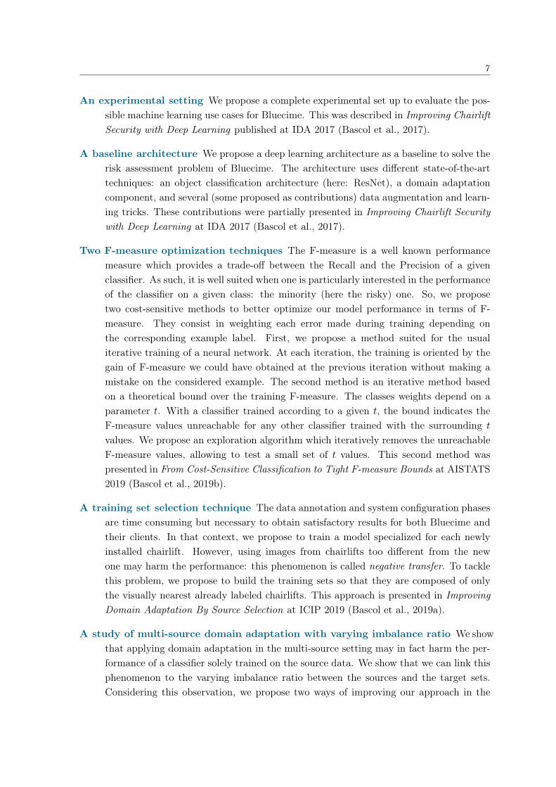
To compute the gradient, we need to replace the non differentiable threshold function usedin the original perceptron by another activation function. We give in Figure 1.2 examples ofcommonly used functions. In the following we use the rectified linear unit (ReLU).
Extending multi-layer perceptrons to multi-class problems, where y /∈ 0, 1N , is straight-forward as it only requires to have a neuron for each class in the output layer. In this setting,we represent the labels as one hot vectors:
Y = (y1,y2, . . . ,yn) with yk ∈
y ∈ 0, 1C |C∑j=1
yj = 1
∀k ∈ [1, N ]
12 Chapter 1. Background on machine learning (for the chairlift safety problem)
3 2 1 0 1 2 3
1.0
0.5
0.0
0.5
1.0
1.5
2.0
2.5
3.0Sigmoid: f(x) = 1/(1 + ex)H. Tangent: f(x) = tanh(x)ReLu: f(x) = max(0, x)
Figure 1.2 – Behavior of different activation functions.
The threshold functions of the output neurons are replaced by the softmax function:
S(Y i) =
(ey
ik∑C
j=1 eyij
∣∣ k ∈ (1, 2, . . . , C)
)
with C the number of classes, i the index of the considered examples. The softmax functiontransforms the output vector into a “probability vector”, giving the probability that the inputbelongs to each class. In this setting, the hinge loss is formulated:
LHinge(yi, t) =1
C
C∑j=1;j 6=t
max(0, µ+ yij − yit)
With i the index of the considered example, t the index of its true class, and µ a hyperpa-rameter (the margin). The log loss is formulated:
LLog(yi, t) = − log(yit)
The multi-layer perceptron is the simplest neural network architecture. At each layer,each neuron is connected to all the outputs of the previous layer (or all the input for the firstlayer), this type of neural network is called “fully-connected feedforward network”.
In practice, minibatch gradient descent (MGD) algorithms are preferred over SGD forthe backpropagation algorithm. Instead of updating the weights according to each trainingexample, in MGD, the weight update is computed over a small set of training examples (namedminibatch). Thus, the training is more robust to outlier examples with MGD than with SGDalgorithms.
Convolutional Neural Networks (CNN) In the context of image or text analysis, fully-connected networks present two major weaknesses that are “solved” by another type of archi-tecture called “convolutional neural networks” (CNN).
1.2. Algorithms 13
Our images are of dimensions 224× 224× 3 (see pre-training in “training tricks” section)meaning that with only one neuron we would have 150 528 parameters to learn. So, thecomplexity of the model would dramatically increase with the size of the network.
With structured inputs as images or text, the spatial aspect is crucial. The order of thesentences, and the order of the words within them, play an important role in the semantic ofa text. In an image, the position of the objects gives clues to understand the whole image(a person on a chairlift vehicle should be all right, contrary to a person under...). In fully-connected networks, because the whole input is connected to each neuron, considering allthe possible combinations of sentences or objects would require a high number of neurons.Moreover, most of the connections would be useless making the network highly inefficient.
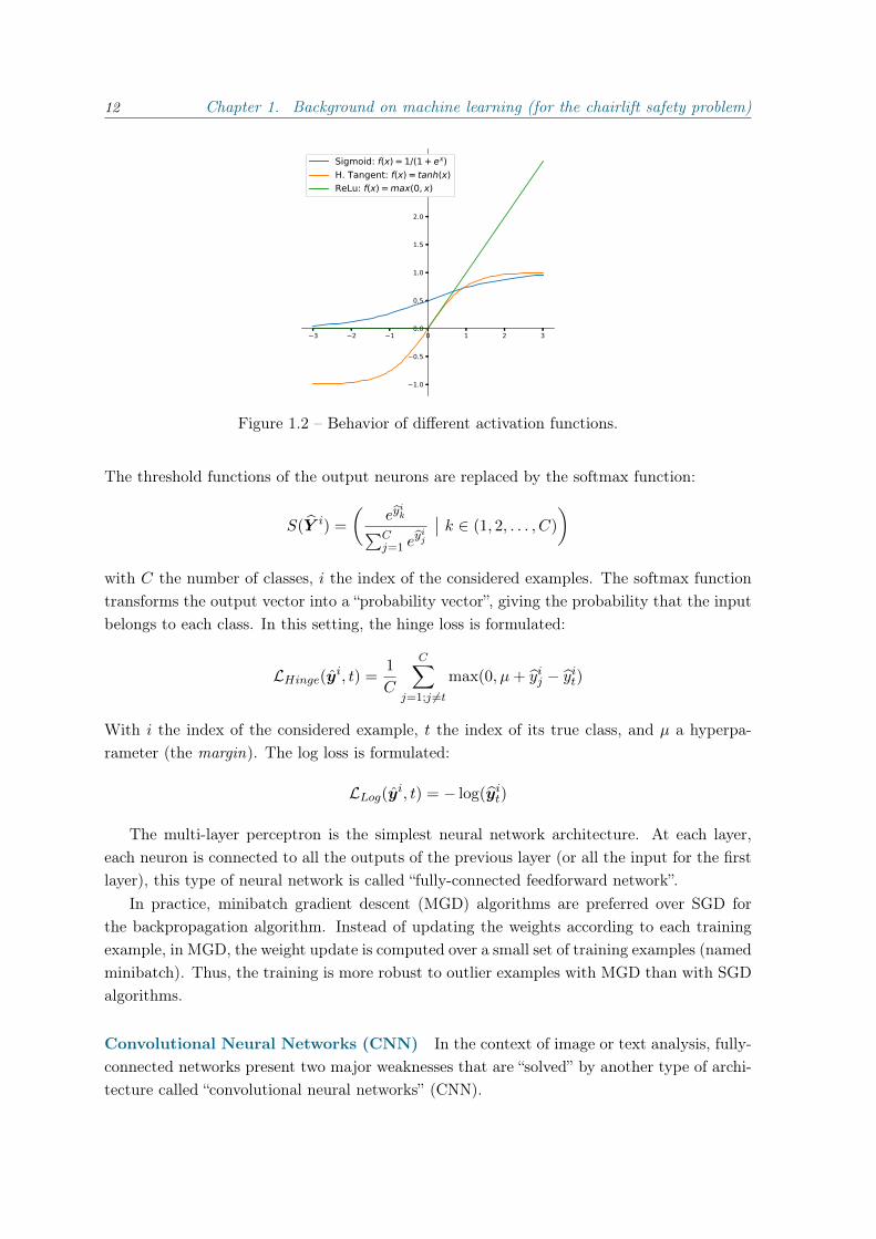
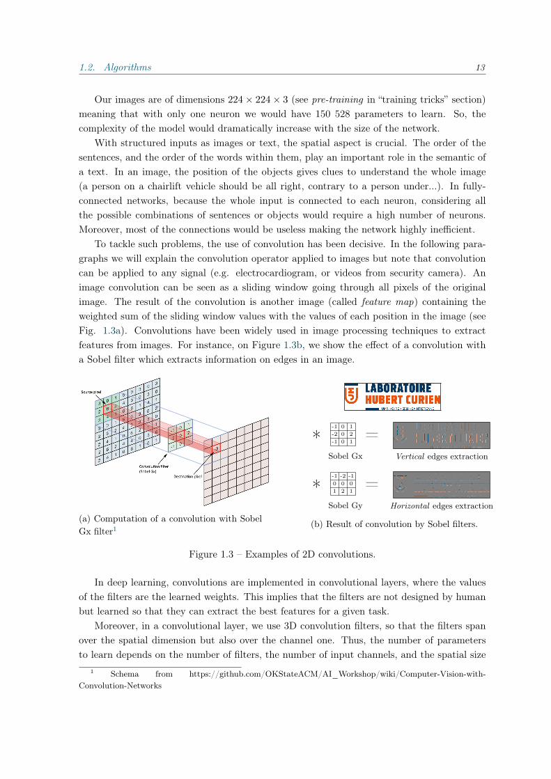
To tackle such problems, the use of convolution has been decisive. In the following para-graphs we will explain the convolution operator applied to images but note that convolutioncan be applied to any signal (e.g. electrocardiogram, or videos from security camera). Animage convolution can be seen as a sliding window going through all pixels of the originalimage. The result of the convolution is another image (called feature map) containing theweighted sum of the sliding window values with the values of each position in the image (seeFig. 1.3a). Convolutions have been widely used in image processing techniques to extractfeatures from images. For instance, on Figure 1.3b, we show the effect of a convolution witha Sobel filter which extracts information on edges in an image.
(a) Computation of a convolution with SobelGx filter1
*-1 0 1 =-2 0 2-1 0 1
Sobel Gx Vertical edges extraction
*-1 -2 -1 =0 0 01 2 1
Sobel Gy Horizontal edges extraction
(b) Result of convolution by Sobel filters.
Figure 1.3 – Examples of 2D convolutions.
In deep learning, convolutions are implemented in convolutional layers, where the valuesof the filters are the learned weights. This implies that the filters are not designed by humanbut learned so that they can extract the best features for a given task.
Moreover, in a convolutional layer, we use 3D convolution filters, so that the filters spanover the spatial dimension but also over the channel one. Thus, the number of parametersto learn depends on the number of filters, the number of input channels, and the spatial size
1 Schema from https://github.com/OKStateACM/AI_Workshop/wiki/Computer-Vision-with-Convolution-Networks
14 Chapter 1. Background on machine learning (for the chairlift safety problem)
of the filters. Since their spatial size is, most of the time, smaller than the input one (from3 × 3 to 9 × 9 pixels), replacing a fully-connected layer by a convolutional one dramaticallydecreases the number of parameters, and so, the complexity of the learned model.
To tackle classification problems, the first layers in the architecture correspond to a con-volutional neural network (CNN), i.e. stacked convolutional layers. This CNN is called thefeature extractor, whose purpose is to learn a representation smaller but more powerful thanthe input, to facilitate the classification task. From the extracted features, one or more fullyconnected layers are added to get the classification output.
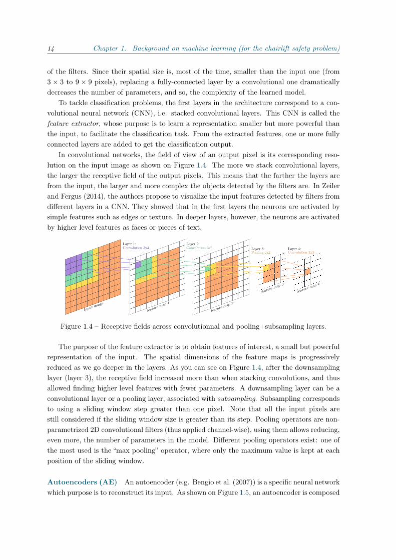
In convolutional networks, the field of view of an output pixel is its corresponding reso-lution on the input image as shown on Figure 1.4. The more we stack convolutional layers,the larger the receptive field of the output pixels. This means that the farther the layers arefrom the input, the larger and more complex the objects detected by the filters are. In Zeilerand Fergus (2014), the authors propose to visualize the input features detected by filters fromdifferent layers in a CNN. They showed that in the first layers the neurons are activated bysimple features such as edges or texture. In deeper layers, however, the neurons are activatedby higher level features as faces or pieces of text.
Figure 1.4 – Receptive fields across convolutionnal and pooling+subsampling layers.
The purpose of the feature extractor is to obtain features of interest, a small but powerfulrepresentation of the input. The spatial dimensions of the feature maps is progressivelyreduced as we go deeper in the layers. As you can see on Figure 1.4, after the downsamplinglayer (layer 3), the receptive field increased more than when stacking convolutions, and thusallowed finding higher level features with fewer parameters. A downsampling layer can be aconvolutional layer or a pooling layer, associated with subsampling. Subsampling correspondsto using a sliding window step greater than one pixel. Note that all the input pixels arestill considered if the sliding window size is greater than its step. Pooling operators are non-parametrized 2D convolutional filters (thus applied channel-wise), using them allows reducing,even more, the number of parameters in the model. Different pooling operators exist: one ofthe most used is the “max pooling” operator, where only the maximum value is kept at eachposition of the sliding window.
Autoencoders (AE) An autoencoder (e.g. Bengio et al. (2007)) is a specific neural networkwhich purpose is to reconstruct its input. As shown on Figure 1.5, an autoencoder is composed

1.2. Algorithms 15
of a first neural network, the encoder. This network’s purpose is to find a new representationof the AE inputs, called the latent representation. Then, from this representation, a secondneural network, the decoder, aims at reconstructing the inputs of the AE. To train an AE,no labels are needed, the loss function used is a reconstruction error measuring how well theinput is reconstructed by the model. For instance, we can use the Mean Squared Error (MSE):
LMSE(X, X) =1
B
B∑i=1
M∑j=1
(xij − xij
)2With X ∈ RB×M a minibatch of B examples represented by M features, we note the ith
example Xi = (xi1,xi2, ...,x
iM ).
An autoencoder is an unsupervised way to extract powerful representations, but also toreconstruct the inputs. This last property is used, for instance, in the denoising autoencoders(Vincent et al., 2008) which provide a uncorrupted version of their inputs.
Figure 1.5 – An autoencoder with a latent space of size 2.
1.2.1.2 Particular Architectures
Deep learning techniques have become tremendously popular since 2012, when a deep archi-tecture, called AlexNet, proposed by Krizhevsky et al. (2012) was able to win the ImageNetLarge Scale Visual Recognition Challenge (ILSVRC) with an outstanding improvement of theclassification results over the existing systems: the error rate was 15% compared to 25% forthe next ranked team. Since then, countless different deep learning architectures have shownexcellent performance in many domains such as computer vision, natural language processingor speech recognition (Goodfellow et al., 2016).
The amount of labeled data available, the systematic use of convolutions, the better op-timization techniques and the advances in manufacturing graphical processing units (GPU)have contributed to this success. However, deep networks were supposed to suffer from (atleast) three curses:
1. The deeper the network, the more difficult it is to update the weights of the first layers(the ones closer to the input): deep networks are subject to vanishing and explodinggradient that leads to convergence problems;

16 Chapter 1. Background on machine learning (for the chairlift safety problem)
2. The bigger the network, the more weights need to be learned. In statistical machinelearning, it is well-known that more complex models require more training examples toavoid overfitting phenomena and guarantee relatively good test accuracy;
3. Neural network training aims at minimizing a loss which is a measure of the differencebetween the computed output of the network and the target. The computed outputsdepend on (i) the inputs, (ii) all the weights of the network and (iii) the non-linearactivation functions that are applied at each layer of the network. The function tominimize is thus high-dimensional and non-convex. As the minimization process isusually achieved using stochastic gradient descent and back-propagation, it can easilyget trapped in local optimum.
Simonyan and Zisserman (2014) created VGGNet 16 and VGGNet 19 composed of re-spectively 13 and 16 convolutional layers followed by 3 fully-connected layers. As for thepreviously mentioned AlexNet, the spatial dimensions were reduced with max-pooling lay-ers, the inputs of the convolutions being typically padded so as to keep the same spatial sizeas before pooling. However, each time the spatial dimensions were divided by two (because ofthe pooling operator), the number of filters in the next layers was doubled to compensate forthe information loss (thus doubling the number of channels in the output). With this method,Simonyan et al. managed to obtain an error rate of 7% at ILSVRC 2014.
Following these results, several other techniques have been designed to train deeper net-works:
Residual Networks (ResNet) He et al. (2016) introduced the concept of residual mappingwhich allowed them to create a network with 18 to 152 convolutional layers called a ResidualNetwork (ResNet). Their architecture is divided into blocks composed of 2 or 3 convolutionallayers (depending on the total depth of the network). At the end of a block, its input isadded to the output of the last layers of the block. This sum of an identity mapping witha “residual mapping” has proven effective to overcome the vanishing gradient phenomenonduring the back-propagation phase and allows training very deep networks. Using residualblocks, the network is learned faster and with better performance. At ILSVRC 2015, ResNet152 showed the best performance with less than 4% of error rate. They also used other trickssuch as batch normalization (Ioffe and Szegedy, 2015) on the first (or first two) layer(s) ofeach residual block (the training tricks that are useful in our context are presented in section1.2.1.3). We use this architecture as the backbone for our solution for the Bluecime’s problem,and thus, will be presented in more details in Section 3.1.1.
Inception Networks In Szegedy et al. (2017), the authors propose inception-v4, the fourthversion of inception networks, first presented as “GoogLeNet” in Szegedy et al. (2015). Thisarchitecture is composed of different inception modules shown in Figure 1.6. These modulesare composed of several convolution layers in parallel with different filter sizes. Having differ-ent size of filter at the same level in the network allows to extract a large variety of featuresand provides a powerful representation of the inputs.

1.2. Algorithms 17
(a) Inception-v4 backbone. (b) Stem.
(c) Inception-A.
(d) Reduction-A.
(e) Inception-B. (f) Reduction-B.
(g) Inception-C.
Figure 1.6 – Inception-v4.
18 Chapter 1. Background on machine learning (for the chairlift safety problem)
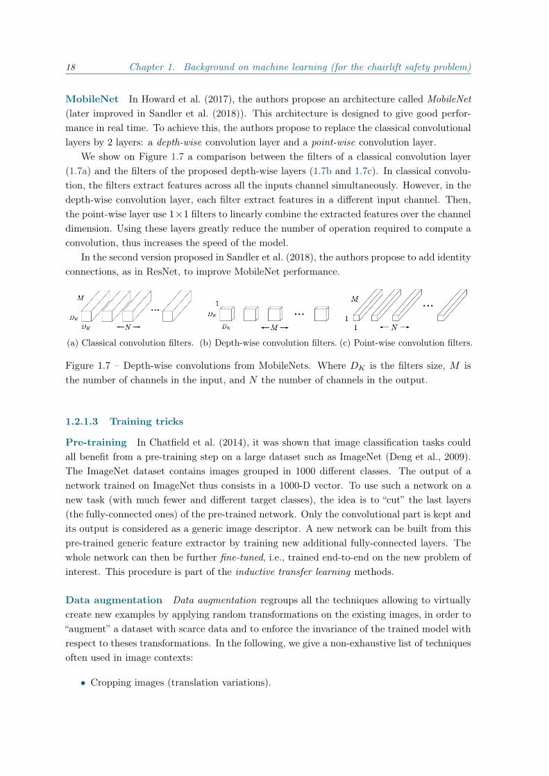
MobileNet In Howard et al. (2017), the authors propose an architecture called MobileNet(later improved in Sandler et al. (2018)). This architecture is designed to give good perfor-mance in real time. To achieve this, the authors propose to replace the classical convolutionallayers by 2 layers: a depth-wise convolution layer and a point-wise convolution layer.
We show on Figure 1.7 a comparison between the filters of a classical convolution layer(1.7a) and the filters of the proposed depth-wise layers (1.7b and 1.7c). In classical convolu-tion, the filters extract features across all the inputs channel simultaneously. However, in thedepth-wise convolution layer, each filter extract features in a different input channel. Then,the point-wise layer use 1×1 filters to linearly combine the extracted features over the channeldimension. Using these layers greatly reduce the number of operation required to compute aconvolution, thus increases the speed of the model.
In the second version proposed in Sandler et al. (2018), the authors propose to add identityconnections, as in ResNet, to improve MobileNet performance.
(a) Classical convolution filters. (b) Depth-wise convolution filters. (c) Point-wise convolution filters.
Figure 1.7 – Depth-wise convolutions from MobileNets. Where DK is the filters size, M isthe number of channels in the input, and N the number of channels in the output.
1.2.1.3 Training tricks
Pre-training In Chatfield et al. (2014), it was shown that image classification tasks couldall benefit from a pre-training step on a large dataset such as ImageNet (Deng et al., 2009).The ImageNet dataset contains images grouped in 1000 different classes. The output of anetwork trained on ImageNet thus consists in a 1000-D vector. To use such a network on anew task (with much fewer and different target classes), the idea is to “cut” the last layers(the fully-connected ones) of the pre-trained network. Only the convolutional part is kept andits output is considered as a generic image descriptor. A new network can be built from thispre-trained generic feature extractor by training new additional fully-connected layers. Thewhole network can then be further fine-tuned, i.e., trained end-to-end on the new problem ofinterest. This procedure is part of the inductive transfer learning methods.
Data augmentation Data augmentation regroups all the techniques allowing to virtuallycreate new examples by applying random transformations on the existing images, in order to“augment” a dataset with scarce data and to enforce the invariance of the trained model withrespect to theses transformations. In the following, we give a non-exhaustive list of techniquesoften used in image contexts:
• Cropping images (translation variations).
1.2. Algorithms 19
• Zooming in images (scale variations).
• Flipping vertically or horizontally.
• Rotating images.
• Adding Gaussian noise to the pixels.
Successful data augmentation happens when the created images “stay” in the originaldataset distribution. For instance, with the Bluecime dataset, applying vertical flip to theimages should be ineffective since the vehicles never appear upside down in real cases (thechairlifts are close in case of strong wind). However, adding horizontal flipping may be usefulas we still have coherent images.
Batch normalization Batch normalization, presented in Ioffe and Szegedy (2015) is asimple yet very effective idea which consists in normalizing the activation outputs Z of eachlayer of the network according to the current input batch:
Z ′ =Z − µ√σ2 + ε
with Z ∈ RD×K . In convolutional layers, D = B ×W × H, with B the minibatch size andW×H the spatial dimensions, K is the number of channels. In fully-connected layers, D = B,the minibatch size, K is the number of features. µ is the mean of each activation: µ = 1
D
∑z∈Z
z,
and σ2 is the vector of per-dimension variances such that: σ2j = 1
D
∑z∈Z
(zj − µj)2 (thus, both
µ and σ2 are vectors of size K). The resulting normalized activations are then scaled andshifted with two learned parameters γ and β (both are vectors of size K):
Z ′′ = γZ ′ + β
During the inference (testing) phase, µ and σ2 are fixed with constant values that havebeen estimated over all the training set. In practice, we use moving mean and varianceupdated during each training iteration.
The main benefit of batch normalization is to reduce the internal covariate shift. Thisphenomenon corresponds to the amplification of small changes in the input distribution aftereach layer, and so creates high perturbations in the inputs of the deepest layers.
Dropout Based on the observation that, to reduce the overfitting and improve the perfor-mance of a neural network approach, we can combine a set of models, Srivastava et al. (2014)propose a regularization named dropout. At each iteration, in given layers, a random set ofneurons is discarded, by setting their activation to zero (Fig. 1.8). So, during each trainingiteration only a reduced set of neurons are trained, which can be considered as a sub-network.However, during inference, all the neurons are used. This implies that, during the testingphase, the network corresponds to a combination of the trained sub-networks. Thus reducingthe overfitting of our model. In Fourure et al. (2017), the authors propose to use dropout to

20 Chapter 1. Background on machine learning (for the chairlift safety problem)
Figure 1.8 – Dropout. (a) A classical neural network. (b-d) A neural network with dropoutat 3 different iterations. (image from Srivastava et al. (2014))
discard entire layers, they call their method total dropout. The authors use a neural networkwith a grid pattern (called GridNet) to tackle semantic segmentation (classification of eachpixel in an image). In that context, total dropout allows them to address the vanishing gra-dient phenomenon reducing the training speed of the layers constituting the longest paths inthe grid.
Ghiasi et al. (2018) observes that dropout is less effective on convolutional layers than onfully-connected layers. The authors therefore propose to extends dropout with block dropout.The authors hypothesize that the spatial aspect of the input impairs the dropout effectiveness.Indeed, with dropout the activation are randomly discarded so that we only loose sparseportions of the input image. Thus, with dropout, the sub-networks would learn from nearlythe same input. In block dropout, the dropped activations are contiguous. This way, completefeatures may be discarded during the training enforcing the sub-networks to rely on diversefeatures. Thus, it improves the robustness of the final model.
Similarly to Ghiasi et al. (2018), DeVries and Taylor (2017) propose to randomly discardblocks during the training, however, only on the input. When an image is loaded, theyrandomly choose a square area to be masked. The authors also present their method as adata augmentation technique. Indeed, this method reduces the overfitting by augmenting thedataset and improves the robustness of the network against occlusions in the inputs. At thesame time as DeVries and Taylor (2017), Zhong et al. (2017) propose a very similar methoddiscarding blocks of pixel in the input image. The main difference between these two papersresides in the size of the blocks: DeVries and Taylor (2017) use fixed size blocks, whereasZhong et al. (2017) use randomly sized blocks. In Zhong et al. (2017), the authors also trydifferent colors to replace the image pixels, however, using random values seems to be thebest choice.
1.2.2 Other machine learning techniques
In this section, we present the other machine learning algorithms we used during this thesis:logistic regression (LR) and linear support vector machine (SVM). Both are linear classifiers,we thus keep the notation from the perceptron section. Given a dataset X ∈ RN×M ofN examples represented by M features and the corresponding set of labels Y ∈ −1, 1N
(note the difference with perceptron where Y ∈ 0, 1N ), we note the ith example Xi =

1.3. Domain adaptation 21
(xi1, xi2, ..., x
iM ) and its associated label yi. The final classifier is defined by the hyperplane
y = W ·Xi + b.Several formulations exist (Bishop, 2006), we present here the formulation with L2 regu-
larization, and the primal formulation of the soft-margin SVM with the (binary) hinge loss:
Logistic regression:
minW ,b
1
2‖W ‖22 + C
N∑i=1
log(e−yi(W ·Xi+b) + 1)
Support vector machine:
minW ,b
1
2‖W ‖22 + C
N∑i=1
max(0, 1− yi(W ·Xi + b))
In both problems, the first term is the L2 regularization, used to penalize the classifiercomplexity. The second term penalizes the errors made on the training data, in LR this termis the logistic loss, in SVM it corresponds to the hinge loss. With the logistic loss, LR uses theprobability of the examples to be well classified, whereas, SVM uses the distances between thehyperplane and the examples nearest to it (the hinge loss is zero if the considered exampleis well classified and far from the hyperplane yi(W ·Xi + b) > 1). C is a hyperparametercontrolling the importance of the errors. If C has a high value, the classifier will do few errorson the training set. It could, however, overfit the training set and thus give poor performanceon the test set.
1.3 Domain adaptation
In this section, we first present generalities about domain adaptation. Then, we introducesome methods using optimal transport. Finally, we present and put the emphasis on tech-niques to tackle domain adaptation problems with deep learning.
1.3.1 Introduction
As we stated in Section 1.1, in machine learning, the data and the corresponding labels arecrucial to obtain the best models. In some cases, we may not have access to labels, but haveaccess to a labeled dataset different but related to ours. So, we would like to learn a model onthe second dataset usable on our task. For instance, in Bluecime’s application, we will considereach chairlift as a particular data distribution, called a domain. For a new installation wewill learn with images from different chairlifts, but with related features. Domain adaptation(Ben-David et al., 2010) consists in learning, from one or more (labeled) source domain, amodel that will be used on a different (but related and often unlabeled) target domain. Manyreal world tasks require the use of domain adaptation simply because of a lack of (target)labeled data or because of some shift between the source and the target data distribution thatprevents from successfully using the learned model on the target data.
22 Chapter 1. Background on machine learning (for the chairlift safety problem)
Without domain adaptation (t=0)
Shared representation Pseudo-labeling (t=1) Pseudo-labeling (t=2) Sample weighting
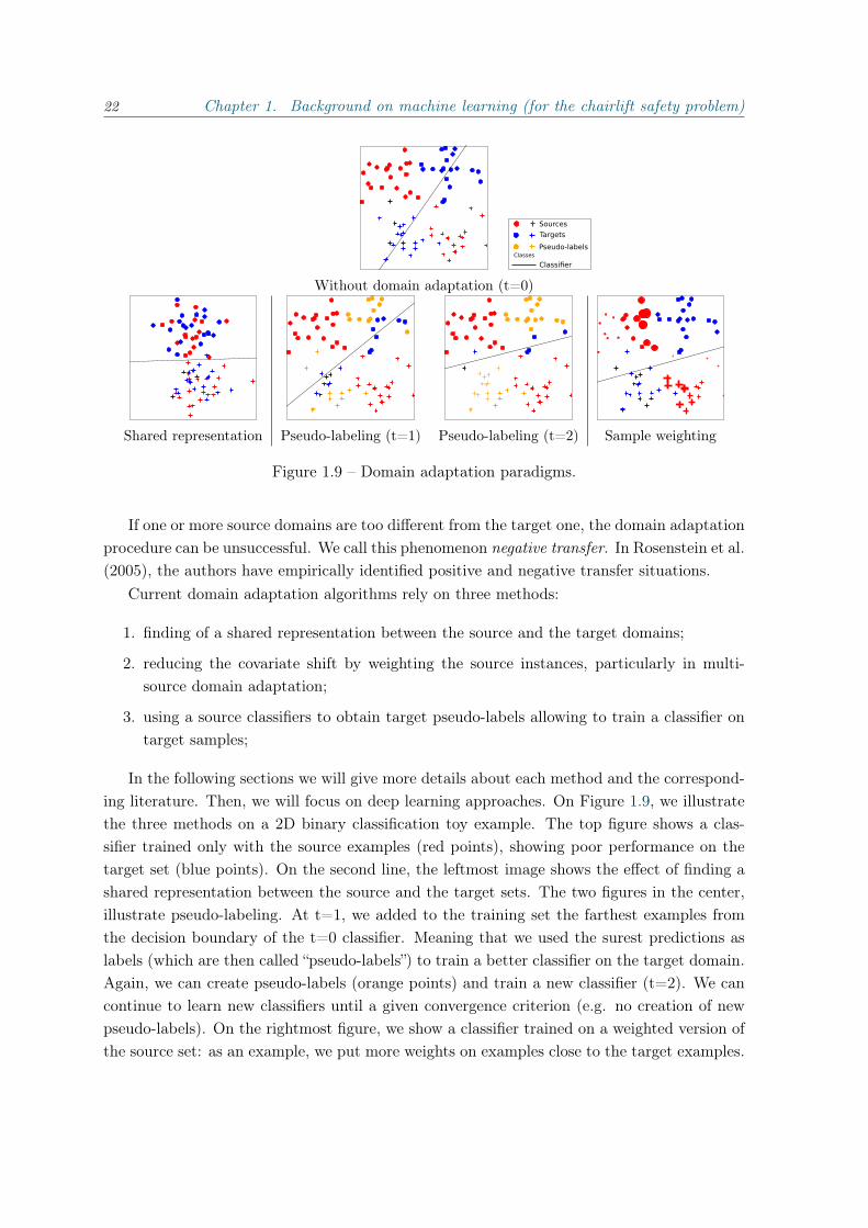
Figure 1.9 – Domain adaptation paradigms.
If one or more source domains are too different from the target one, the domain adaptationprocedure can be unsuccessful. We call this phenomenon negative transfer. In Rosenstein et al.(2005), the authors have empirically identified positive and negative transfer situations.
Current domain adaptation algorithms rely on three methods:
1. finding of a shared representation between the source and the target domains;
2. reducing the covariate shift by weighting the source instances, particularly in multi-source domain adaptation;
3. using a source classifiers to obtain target pseudo-labels allowing to train a classifier ontarget samples;
In the following sections we will give more details about each method and the correspond-ing literature. Then, we will focus on deep learning approaches. On Figure 1.9, we illustratethe three methods on a 2D binary classification toy example. The top figure shows a clas-sifier trained only with the source examples (red points), showing poor performance on thetarget set (blue points). On the second line, the leftmost image shows the effect of finding ashared representation between the source and the target sets. The two figures in the center,illustrate pseudo-labeling. At t=1, we added to the training set the farthest examples fromthe decision boundary of the t=0 classifier. Meaning that we used the surest predictions aslabels (which are then called “pseudo-labels”) to train a better classifier on the target domain.Again, we can create pseudo-labels (orange points) and train a new classifier (t=2). We cancontinue to learn new classifiers until a given convergence criterion (e.g. no creation of newpseudo-labels). On the rightmost figure, we show a classifier trained on a weighted version ofthe source set: as an example, we put more weights on examples close to the target examples.
1.3. Domain adaptation 23
Shared representation
Some approaches aim at finding a shared representation between the source and the targetdomains so that a classifier learned from this representation may show good performance bothon the source domains and the target domain.
For instance, in Blitzer et al. (2006), the authors propose the “Structural Correspon-dence Learning” (SCL), which aims at finding pivot features which correspond to domain-independent features allowing training classifiers efficiently for both the source and the targetdomains.
Sample weighting
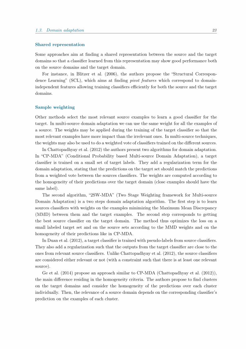
Other methods select the most relevant source examples to learn a good classifier for thetarget. In multi-source domain adaptation we can use the same weight for all the examples ofa source. The weights may be applied during the training of the target classifier so that themost relevant examples have more impact than the irrelevant ones. In multi-source techniques,the weights may also be used to do a weighted vote of classifiers trained on the different sources.
In Chattopadhyay et al. (2012) the authors present two algorithms for domain adaptation.In “CP-MDA” (Conditional Probability based Multi-source Domain Adaptation), a targetclassifier is trained on a small set of target labels. They add a regularization term for thedomain adaptation, stating that the predictions on the target set should match the predictionsfrom a weighted vote between the sources classifiers. The weights are computed according tothe homogeneity of their predictions over the target domain (close examples should have thesame label).
The second algorithm, “2SW-MDA” (Two Stage Weighting framework for Multi-sourceDomain Adaptation) is a two steps domain adaptation algorithm. The first step is to learnsources classifiers with weights on the examples minimizing the Maximum Mean Discrepancy(MMD) between them and the target examples. The second step corresponds to gettingthe best source classifier on the target domain. The method thus optimizes the loss on asmall labeled target set and on the source sets according to the MMD weights and on thehomogeneity of their predictions like in CP-MDA.
In Duan et al. (2012), a target classifier is trained with pseudo-labels from source classifiers.They also add a regularization such that the outputs from the target classifier are close to theones from relevant source classifiers. Unlike Chattopadhyay et al. (2012), the source classifiersare considered either relevant or not (with a constraint such that there is at least one relevantsource).
Ge et al. (2014) propose an approach similar to CP-MDA (Chattopadhyay et al. (2012)),the main difference residing in the homogeneity criteria. The authors propose to find clusterson the target domains and consider the homogeneity of the predictions over each clusterindividually. Then, the relevance of a source domain depends on the corresponding classifier’sprediction on the examples of each cluster.
24 Chapter 1. Background on machine learning (for the chairlift safety problem)
Target pseudo-labels
Learning a classifier in a supervised manner should yield the best performance on a givendomain, however it needs a sufficient amount of labeled examples which we may not have.The idea here is to iteratively create labels for the target examples: at each iteration a sourceclassifier is trained, the most reliable predictions on the targets examples are used as labels sothat we can add those examples to the training set of the next iteration. For instance, in Bhattet al. (2016), the authors mix the three methods to optimize the adaptation. They first selectK source domains thanks to a similarity function based on the H-divergence (Ben-David et al.(2010)) and a complementarity measure based on pivot features (Blitzer et al. (2006)). Thenthey find a shared representation between the K sources and the target with SCL. Finally,they iteratively train a target classifier corresponding to a weighted vote of classifiers trainedon each source domain and a classifier trained on target pseudo-labels. The voting weightsare adjusted in function of the sureness of the predictions of each classifier.
1.3.2 Domain adaptation using optimal transport
In this section, we first introduce the optimal transport paradigm. Then, we present differentdomain adaptation methods which use optimal transport.
1.3.2.1 Optimal transport
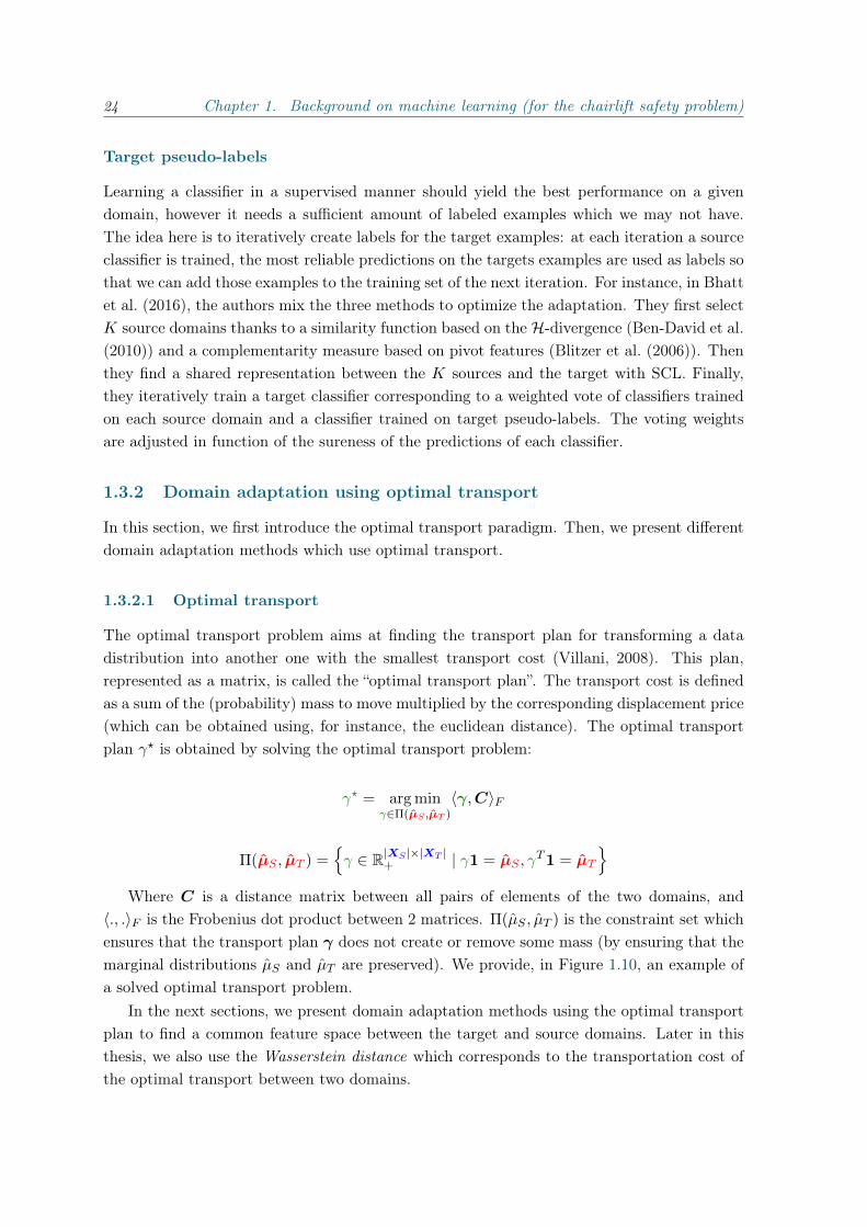
The optimal transport problem aims at finding the transport plan for transforming a datadistribution into another one with the smallest transport cost (Villani, 2008). This plan,represented as a matrix, is called the “optimal transport plan”. The transport cost is definedas a sum of the (probability) mass to move multiplied by the corresponding displacement price(which can be obtained using, for instance, the euclidean distance). The optimal transportplan γ? is obtained by solving the optimal transport problem:
γ? = arg minγ∈Π(µS ,µT )
〈γ,C〉F
Π(µS , µT ) =γ ∈ R|XS |×|XT |
+ | γ1 = µS , γT1 = µT
Where C is a distance matrix between all pairs of elements of the two domains, and
〈., .〉F is the Frobenius dot product between 2 matrices. Π(µS , µT ) is the constraint set whichensures that the transport plan γ does not create or remove some mass (by ensuring that themarginal distributions µS and µT are preserved). We provide, in Figure 1.10, an example ofa solved optimal transport problem.
In the next sections, we present domain adaptation methods using the optimal transportplan to find a common feature space between the target and source domains. Later in thisthesis, we also use the Wasserstein distance which corresponds to the transportation cost ofthe optimal transport between two domains.

1.3. Domain adaptation 25
NS
d
Input: XS
5 3
4 0
1 3
d
Input: XT
0
5
1
0
5
4
1
4
Input: C
25
1
9
5
17
29
13
25
5
13
1
5
Input: µS
13
13
13
NT
Input: µT
14
14
14
14
Output: γ?
0
14
0
14
0
0
112
0
16
0
112
16
Figure 1.10 – Example of optimal transport result. XS and XT are respectively the sourceand the target sets (XS ∈ RNS×d,XT ∈ RNT×d), µS and µT are their corresponding marginaldistributions. C is the cost matrix computed, here, using the squared Euclidean distance. γ?
is the optimal transport plan. (Figure from the presentation of Gautheron et al. (2018)).
1.3.2.2 Domain adaptation methods
In Courty et al. (2014), the authors propose to regularize the optimal transport problem witha term promoting the mass transport from sources of only one class to each target example.So, the transport obtained is coherent with the labels provided by the source set. Theiroptimal transport is formulated:
γ? = arg minγ∈Π(µj ,µi)
〈γ,C〉F −1
λΩe(γ) + ηΩc(γ)
where Ωe(γ) = −∑
i,j γi,j log(γi,j) is the entropy of gamma (the transport plan). Thisregularization is introduced in Cuturi (2013), and reduces the sparsity of gamma inducingmore coupling between the source and target distributions. Adding this term allows to use theSinkhorn-Knopp algorithm (Knight, 2008) to solve the optimal transport problem efficiently.Ωc(γ) =
∑j
∑c‖γIc,j‖
pq , with Ic the indexes of the source examples of class c, so that, γIc,j
is a vector containing the transport coefficients between the source examples of class c andthe target example j. This term is the regularization introduced by the authors to ensurethat the mass transported to a given target example comes from sources with the same class.In practice the authors propose to use p = 1
2 and q = 1, mostly due to optimization issues.With the resulting optimal transport plan, the source set is transported to the target setaccording to: XS = diag((γ?1NT
)−1)γ?XT (note that XS = NSγ?XT if µS is uniform). The
transported set is then used to train a classifier, which should thus present good performanceon the target set.
In Courty et al. (2016), the authors complete the work published in Courty et al. (2014).They propose another regularization called “Laplacian regularization”, which ensure that sim-

26 Chapter 1. Background on machine learning (for the chairlift safety problem)
ilar examples are still similar after transport. Ωc is then formulated:
Ωc(γ) =1
NS2
∑i,j
SSi,j‖xSi − xSj ‖22
Where SS is a matrix containing the similarity values between the source examples. Tokeep the label information after the transport, the authors propose to use Ssi,j = 0 if theexamples i and j have a different class. They propose also to consider the similarity betweenthe target examples if available, such that:
Ωc(γ) =(1− α)
NS2
∑i,j
SSi,j‖xSi − xSj ‖22 +α
NT2
∑i,j
STi,j‖xTi − xTj ‖22
with α a hyperparameter controlling the trade-off between the two terms.Note that in the target case, ST cannot be constrained to 0 according to the classes. Tooptimize their problem, they propose to use the generalized conditional gradient algorithm(Bredies et al., 2009). They also propose to use p = 1 and q = 2 in the Courty et al.(2014) formulation. Their experiments show that the formulation in Courty et al. (2014)gives better results than the Laplacian one. Moreover, tuning the p and q values gives betterthe performance than the one used in the original paper.
Courty et al. (2017) propose another method called joint distribution optimal transport(JDOT). This method aims at finding the optimal transport plan and training the classifierin the same time, the authors suggests that this method allows to consider both the datadistribution shift between source and target and the class distribution shift. The JDOTproblem is formulated as:
minγ∈Π(µT ,µS),f∈H
∑i,j
γi,j[αd(xSi ,x
Tj ) + L(ySi , f(xTj ))
]+ λΩ(f)
where L is any loss function continuous and differentiable, d is a metric (the authorspropose to use the squared Euclidean distance), and Ω is a regularization over the classifierparameters.
The optimization of the JDOT problem is conducted by alternatively considering f andγ fixed: with f fixed the problem is a classical optimal transport problem with each elementof the cost matrix defined such that: Ci,j = αd(xSi ,x
Tj ) + L(ySi , f(xTj )). With γ fixed, we
obtain another optimization problem: minf∈H
∑i,j γi,jL(ySi , f(xTj )) + λΩ(f).
In Redko et al. (2018), the author propose the joint class proportion and optimal trans-port method (JCPOT), a multi-source domain adaptation method. This approach allows tofind a transportation plan compensating the shift between the sources and the target classdistributions. With the resulting transport plan, the authors propose two methods to classifythe target examples. Based on the regularized optimal transport presented in Cuturi (2013),the authors propose an optimal transport solved by a Bregman projection problem (Benamouet al., 2015) formulated as:
γ? = arg minγ∈Π(µ1,µ2)
KL(γ|ζ)

1.3. Domain adaptation 27
with ζ = exp(−Cε ), and C the optimal transport problem cost matrix. KL is the Kullback-
Liebler divergence. If µ2 is undefined, γ? can be formulated only depending on µ1:
γ? = diag(µ1
ζ1)ζ, (1.1)
We note K the number of available sources. The empirical data distribution of the kth
source µkS can be estimated with: µkS = (mk)T δXk where mk = (mk1,m
k2, . . . ,m
knk) is a vector
containing the probability mass of each example in the source k, and δXk is a vector of Diracmeasures located at each example of the source k. We note hk = (hk1, h
k2, . . . , h
kL) the class
probability vector with L the number of classes, and hkl =∑nk
i=1 δ(yki = l)mk
i . Let Uk ∈ RL×nk
and Vk ∈ Rnk×L be two linear operators such that:
Ukl,i =
1 if yki = l
0 otherwise
V ki,l =
1
|ykj =l | ∀j∈1,2,...,nk| if yki = l
0 otherwise
These two operators allow retrieving mk from hk and vice versa, such that: hk = Ukmk,and mk = Vkhk.
The estimation of the class distribution of the target set is done with a constrained Wasser-stein barycenter problem (Benamou et al., 2015):
arg minh∈∆L
K∑k=1
λkWε,Ck
((Vkh)T δXk , µT
)where λk is a weight representing the kth source relevance (
∑Kk=1 λ
k = 1), and Wε,Ck is theregularized Wasserstein distance:
Wε,Ck(µkS , µT ) = minγk∈Π(µkS ,µT )
KL(γk|ζk)
For each source k we then have two constraints: γkT1n = 1n/n (considering µT uniform),and Ukγk1n = h. The first constraint can be solved for each source independently with thesolution of the Bregman projection defined in equation 1.1. The second constraint must besolved simultaneously on the K sources, to do so the authors propose a Bergman projectionproblem:
h? = arg minh∈∆L,Γ
K∑k=1
λkKL(γk|ζk)
s.t. ∀k Ukγk1n = h
with Γ = (γ1, γ2, ..., γK).
28 Chapter 1. Background on machine learning (for the chairlift safety problem)
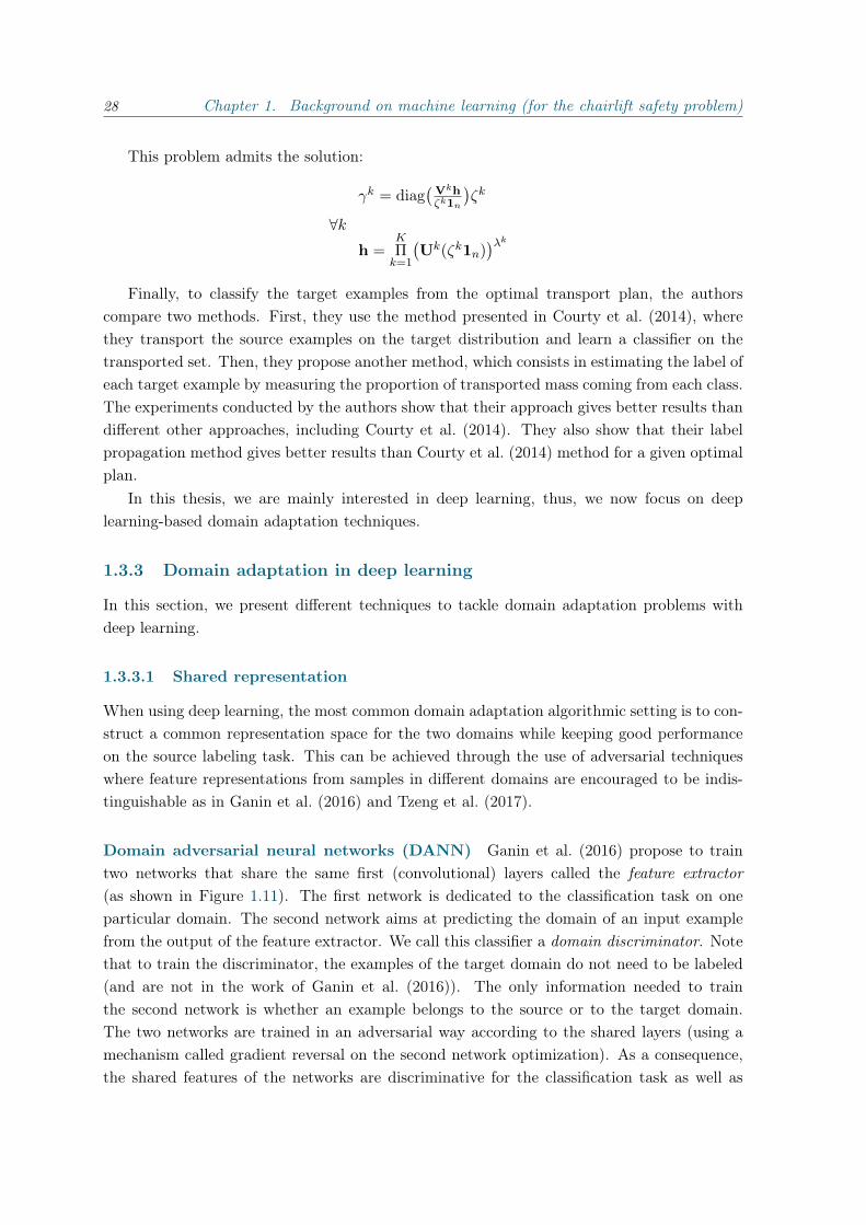
This problem admits the solution:
∀k
γk = diag(Vkhζk1n
)ζk
h =KΠk=1
(Uk(ζk1n)
)λkFinally, to classify the target examples from the optimal transport plan, the authors
compare two methods. First, they use the method presented in Courty et al. (2014), wherethey transport the source examples on the target distribution and learn a classifier on thetransported set. Then, they propose another method, which consists in estimating the label ofeach target example by measuring the proportion of transported mass coming from each class.The experiments conducted by the authors show that their approach gives better results thandifferent other approaches, including Courty et al. (2014). They also show that their labelpropagation method gives better results than Courty et al. (2014) method for a given optimalplan.
In this thesis, we are mainly interested in deep learning, thus, we now focus on deeplearning-based domain adaptation techniques.
1.3.3 Domain adaptation in deep learning
In this section, we present different techniques to tackle domain adaptation problems withdeep learning.
1.3.3.1 Shared representation
When using deep learning, the most common domain adaptation algorithmic setting is to con-struct a common representation space for the two domains while keeping good performanceon the source labeling task. This can be achieved through the use of adversarial techniqueswhere feature representations from samples in different domains are encouraged to be indis-tinguishable as in Ganin et al. (2016) and Tzeng et al. (2017).
Domain adversarial neural networks (DANN) Ganin et al. (2016) propose to traintwo networks that share the same first (convolutional) layers called the feature extractor(as shown in Figure 1.11). The first network is dedicated to the classification task on oneparticular domain. The second network aims at predicting the domain of an input examplefrom the output of the feature extractor. We call this classifier a domain discriminator. Notethat to train the discriminator, the examples of the target domain do not need to be labeled(and are not in the work of Ganin et al. (2016)). The only information needed to trainthe second network is whether an example belongs to the source or to the target domain.The two networks are trained in an adversarial way according to the shared layers (using amechanism called gradient reversal on the second network optimization). As a consequence,the shared features of the networks are discriminative for the classification task as well as

1.3. Domain adaptation 29
Figure 1.11 – The DANN approach (figure from Ganin et al. (2016)).
domain invariant. We note Lc, and Ld the losses respectively on the classifier, and thediscriminator. The loss on the feature extractor then is:
Le(h, d,X) = Lc(h,X)− λLd(d,X)
with h the classifier, d the domain discriminator, and X a minibatch. λ is the gradientreversal parameter increasing during the iteration i of the training procedure according to:
λ(i) =2
1 + e−γ(i/I)− 1
with γ a hyperparameter (fixed to 10 in the authors’ experiments), i the current iteration,and I the number of iterations. During the first iterations, λ ≈ 0, so, the discriminator canbe trained without adversary features. Then λ increases so that the features progressivelybecome domain independent. In that way, the discriminator outputs are accurate during theadaptation of the features, thus, the feature extractor is correctly adversarially trained.
In Cao et al. (2018), the authors tackle “partial transfer”, considering that the targettask is a sub-task of the source task (target labels being unavailable). To do that, theyextend the work of Ganin et al. (2016) and propose Selective Adversarial Networks (SAN).Instead of a unique domain discriminator, they propose to learn class-wise discriminators.To select the right discriminator during training, without target labels, they use the classifieroutput: in each domain discriminator loss, the target examples are weighted according to theirclassification probability vector. Thus, this method should improve the domain adaption overthe target predicted classes.
Correlation alignment for deep learning (Deep CORAL) Correlation alignment(CORAL), presented in Sun et al. (2016), is a domain adaptation method aiming at matchingthe source distribution DS on the target one DT . To do so, the authors propose to align thecovariance of the two distributions. The transformed source distribution DS is computed by:
DS = (DS ×C− 1
2S )×C
12T
where CS (resp. CT ) is the covariance matrix of DS (resp. DT ).

30 Chapter 1. Background on machine learning (for the chairlift safety problem)
In Sun and Saenko (2016), the authors propose to extend CORAL to deep learning tech-niques by training neural networks with two losses: the classification loss and the CORALloss. The classification loss is used to train the model to tackle the task. The CORAL lossencourages the feature extractor to be independent of the domains. It is formulated as:
LCORAL =1
4d2‖ CS −CT ‖2F
where ‖ . ‖F is the Frobenius norm. As in Ganin et al. (2016), during the training phase, onlythe source examples are used to compute the classification loss and both source and targetsets are used in the CORAL loss.
Adaptive batch normalization (AdaBN) AdaBN, presented in Li et al. (2016), is asimple, yet effective, method to do domain adaptation with batch normalization (see Section1.2.1.3). At training time, the batch normalization is conducted classically by normalizingactivations by mean and variance estimated over the minibatch. However, at test time, themean and variance parameters are estimated over all the target set. By doing so, source andtarget distribution are standardized to a similar one. Thus, this method aims at reducing theeffect of domain shift.
Automatic domain alignment layers (AutoDIAL) In Cariucci et al. (2017), the au-thors also propose to extend batch normalization to do domain adaptation. They use batchnormalization layers to align the source and target feature distributions at different levels ofa neural network (they call these layers “DA-layers”). During training, both source and targetexamples are given to the network, each distribution having its own loss. The source examplesbeing labeled, a classical log loss is used. However, the target examples being unlabeled, theauthors use the entropy of the predictions as a loss. In the DA-layers, the sources and targetexamples normalization is computed separately according to:
z′S =zS − µST,α√σ2ST,α + ε
; z′T =zT − µTS,α√σ2TS,α + ε
with zS (zT ) the input of the DA-layer from source (resp. target) examples, and z′S(z′T ) the corresponding outputs. µ and σ2 are respectively the mean and the variance,both are estimated over a minibatch. Such that, µST,α and σ2
ST,α are computed in zST,α =
αzS + (1 − α)zT , and µTS,α and σ2TS,α in zTS,α = αzT + (1 − α)zS . The α is a learned
parameter, clipped so that α ∈ [0.5, 1]: if α = 1 we have an independent alignment of the twodomains, whereas, if α = 0.5 we have a coupled normalization.
Adversarial discriminative domain adaptation (ADDA) ADDA, presented in Tzenget al. (2017), is another adversarial technique designed to get a shared representation betweenthe target and the source domains. This approach is divided into two steps. First, a neuralnetwork is trained on the source domain. Then, a discriminator is trained so that it has todistinguish between features extracted from source and target examples. The source features

1.3. Domain adaptation 31
Figure 1.12 – ADDA training and testing steps (figure from Tzeng et al. (2017)).
come from the feature extractor part of the source classifier with its weights fixed. The targetfeatures come from a feature extractor pre-trained with the weights from the source one,fine-tuned in an adversarial fashion with the discriminator. With the discriminator trainedto distinguish between source and target features, and the target features trained to fool thediscriminator, the resulting target features extractor should produce source-like features fromthe target images. Thus, the loss used to train the target feature extractor slightly changesfrom the one used in DANN method:
Le(h, d,X) = Lc(h,X) + Ld(1− d,X)
The final target classifier is composed of the target feature extractor and the classificationpart of the source classifier, as it should be effective on source-like features. This process isgraphically shown on Figure 1.12.
Decision-boundary iterative refinement training (DIRT-T) In Shu et al. (2018), theauthors first propose the virtual adversarial domain adaptation (VADA) model. VADA isbased on the Ganin et al. (2016) method, extended so that the cluster assumption holds onboth source and target training sets. The cluster assumption states that all the data pointfrom a given distribution with a given class must belong to the same cluster. Here, the authorsuse a loss to minimize the entropy of the classifier on the target domain:
LEnt(h,XT ) = − 1
BT
∑xT∈XT
h(xT ) · log(h(xT ))
with XT = (x1T , x
2T , ..., x
BTT ) the subset of a minibatch containing BT target examples, h
the classifier, and h(xT ) the prediction vector for example xT . This loss encourages theclassifier to be confident in its predictions, thus encourages the classifier’s decision boundaryto be far away from the target examples. This implies that the decision boundary should notcross any cluster of target example, so, according to the cluster assumption, this loss enforcesthe classifier to discriminate well the target classes. However, the learned classifier must belocally-Lipschitz to use this approximation (Grandvalet and Bengio, 2005). To respect thisconstraint, the authors propose to add another loss based on the Kullback-Liebler divergence

32 Chapter 1. Background on machine learning (for the chairlift safety problem)
(noted DKL):
LKL(h,X) =1
B
∑x∈X
max||r||<ε
DKL(h(x)||h(x+ r))
whereX = (x1,x2, ...,xB) is a minibatch containing B examples from both source and targetdomains, and r represents the adversarial perturbation (Miyato et al., 2018).
The authors present also a second algorithm named decision-boundary iterative refinementtraining (DIRT-T). They use VADA as a pre-training step, then iteratively fine-tune the modelwith target pseudo-labels. They use both LEnt, and LKL (using only the target examples).They also use a regularization term corresponding to the Kullback-Liebler divergence betweenthe model at the current iteration and the model at the previous iteration:
RKL(ht−1, ht,X) =1
B
∑x∈X
DKL(ht−1(x)||ht(x))
This term ensures that each iteration has a small impact on the prediction. So that, the finalmodel fits the target pseudo-labels without “loosing” the VADA pre-training on the sourcedomain.
Wasserstein distance guided representation learning (WDGRL) Shen et al. (2018)propose another adversarial method to tackle domain adaptation, named WDGRL. In theirapproach, the discriminator is replaced by a domain critic. This critic estimates a functionfw : RK → R which takes as input the K outputs from the feature extractor such that:
W (PxS ,PxT ) = sup||fw||≤1
EPxS[fw(fg(x))]− EPxT
[fw(fg(x))]
with fg the feature extractor, W (PxS ,PxT ) the Wasserstein distance between the sourceand the target distributions. To train this domain critic, the authors propose to maximize aloss approximating W :
Lwd(XS ,XT ) =1
BS
∑xS∈XS
fw(fg(xS)
)+
1
BT
∑xT∈XT
fw(fg(xT )
)with XS = x1
S ,x2S , ...,x
BSS and XT = x1
T ,x2T , ...,x
BTT the subsets of a minibatch respec-
tively containing BS source examples and BT target examples.This approach holds if fw is 1-Lipschitz. To ensure it, the authors use a loss function on
the gradient applied to fw:
Lgrad(g) =(||∇gfw(g)||2 − 1
)2where g contains the features corresponding to the source and target examples, but also tofeatures interpolated between each source and target features. The final loss on the domaincritic is expressed as: Lw = Lgrad−Lwd. The Wasserstein distance loss is maximized and thegradient loss is minimized. The loss on the classifier is a classical classification loss noted Lc.The feature extractor loss is: Lg = Lc + λLwd, so that, both the classification loss and the
1.3. Domain adaptation 33
Wasserstein distance are minimized (λ is a hyperparameter controlling the trade-off betweenthe two losses).
A training iteration is divided into two phases. First, the domain critic is trained n times(with n a hyperparameter). Then, both the classifier and the feature extractor are trainedonce. This two-phases approach allows to correctly approximate the Wasserstein distancebefore adversarially training the feature extractor.
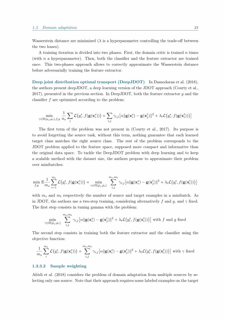
Deep joint distribution optimal transport (DeepJDOT) In Damodaran et al. (2018),the authors present deepJDOT, a deep learning version of the JDOT approach (Courty et al.,2017), presented in the previous section. In DeepJDOT, both the feature extractor g and theclassifier f are optimized according to the problem:
minγ∈Π(µj ,µi),f,g
1
ns
∑i
L(ysi , f(g(xsi ))
)+∑i,j
γi,j[α‖g(xsi )− g(xtj)‖2 + λtL
(ysi , f(g(xti))
)]The first term of the problem was not present in (Courty et al., 2017). Its purpose is
to avoid forgetting the source task, without this term, nothing guarantee that each learnedtarget class matches the right source class. The rest of the problem corresponds to theJDOT problem applied to the feature space, supposed more compact and informative thanthe original data space. To tackle the DeepJDOT problem with deep learning and to keepa scalable method with the dataset size, the authors propose to approximate their problemover minibatches:
minf,g
E1
ms
ms∑i=1
L(ysi , f(g(xsi ))
)+ minγ∈Π(µj ,µi)
ms,mt∑i,j
γi,j[α‖g(xsi )− g(xtj)‖2 + λtL
(ysi , f(g(xti))
)]with ms and mt respectively the number of source and target examples in a minibatch. Asin JDOT, the authors use a two-step training, considering alternatively f and g, and γ fixed.The first step consists in tuning gamma with the problem:
minγ∈Π(µj ,µi)
ms,mt∑i,j
γi,j[α‖g(xsi )− g(xtj)‖2 + λtL
(ysi , f(g(xti))
)]with f and g fixed
The second step consists in training both the feature extractor and the classifier using theobjective function:
1
ms
ms∑i
L(ysi , f(g(xsi ))
)+
ms,mt∑i,j
γi,j[α‖g(xsi )− g(xtj)‖2 + λtL
(ysi , f(g(xti))
)]with γ fixed
1.3.3.2 Sample weighting
Afridi et al. (2018) considers the problem of domain adaptation from multiple sources by se-lecting only one source. Note that their approach requires some labeled examples on the target

34 Chapter 1. Background on machine learning (for the chairlift safety problem)
domain (which may be difficult to obtain). On the other hand, the task on the selected sourcedomain can be different from the task on the target one (only the features are transferred)which can give a large choice of source domain. They propose to train a CNN per sourcedomain and a target CNN using the few target labeled data. Then, they use a validation setto rank the source CNN according to the mutual information between the features extractedby each source CNN and the output of the target CNN. The source CNN which gives themost information is used for pre-training the final classifier.
In the currently unpublished work from Schultz et al. (2018), the authors propose toselect multiple source domains as training set for a given target domain. The source domainsare selected according to a weighted combination of four distances (the χ2-divergence, theMaximum Mean Discrepancy, the Wasserstein distance and the Kullback-Liebler divergence)and according to the classification performance on each single source domain.
1.4 Learning with imbalanced data
In anomaly detection, we are confronted to the data imbalance since an anomaly rarely occurs:the proportion of positive (anomalous) examples is highly inferior to the proportion of negative(normal) ones. When a classifier is learned with common methods, the optimized metrics isthe accuracy, meaning the proportion of well classified examples. In the case of imbalanceddata, as the proportion of positive examples is low, a classifier always predicting negative willhave a good accuracy, but, in fact, will be useless in practice.
A positive (resp. negative) example correctly classified is called true positive (TP) (resp.negative (TN)). A positive (resp. negative) example incorrectly classified is called false nega-tive (FN) (resp. positive (FP)). A confusion matrix, as figure 1.13, can be built to summarizethe results of a classifier.
classpred
negative positive
negative #TN #FPpositive #FN #TP
Figure 1.13 – Confusion matrix. The rows correspond to the true classes, the columns to thepredictions, the cells contain the corresponding number of examples.
On imbalanced data, different measures exist to get more information on the performancethan the Accuracy:
• The Recall, which indicates the proportion of well classified positive examples amongall the positives:
Re =TP
TP + FN

1.4. Learning with imbalanced data 35
• The Precision showing the proportion of well classified positives among all the examplesclassified as positive:
Pr =TP
TP + FP
• The Fβ-measure (van Rijsbergen, 1974) which is the harmonic mean between the Pre-cision and the Recall :
Fβ =1
β2
1+β21Re + 1
1+β21Pr
=PrRe
β2
1+β2Pr + 11+β2Re
=(1 + β2)PrRe
β2Pr +Re
where β is a parameter controlling the trade-off between the Precision and the Recall.Using the first formulation we can easily observe that F0 = Pr and lim
β→∞Fβ = Re.
The F-measure, which corresponds to the Fβ-measure with β = 1, is a widely used mea-sure to assess the performance of a model. Particularly, in imbalanced settings where usingthe accuracy of the classifier would greatly favor the majority class (Chandola et al., 2009;Lopez et al., 2013). However, the F-measure being non-differentiable, non-separable, andnon-convex, we cannot learn a classifier directly optimizing this measure.
Several methods have been studied to solve the Fβ-measure optimization problem. Theycan roughly be separated into two categories:
Decision Theoretic Approaches (DTA) (Dembczyński et al., 2017) This consists in trying tofind the classifier that maximizes the expectation of the F-measure. More precisely,these methods usually fit a probabilistic model during training followed by an inferenceprocedure at prediction time (Decubber et al., 2018). The probabilistic model can belearned by optimizing a “simpler” surrogate function (e.g., (Dembczynski et al., 2011;Jansche, 2005; Ye et al., 2012; P.M. Chinta and Murty, 2013)).
Empirical Utility Maximization (EUM) This consists in learning multiple accurate modelswith different parameters and keep the model which maximizes the F-measure (Busa-Fekete et al., 2015; Joachims, 2005; Musicant et al., 2003; Parambath et al., 2014; Zhaoet al., 2013; Narasimhan et al., 2015). The parameters can be the different classificationthresholds for probabilistic models (Busa-Fekete et al., 2015; Joachims, 2005; Zhao et al.,2013; Narasimhan et al., 2015) or the costs on the classification errors for cost-sensitivemethods (Musicant et al., 2003; Parambath et al., 2014; Koyejo et al., 2014).
EUM methods focus on estimation on a possibly infinite training set, while DTA ap-proaches are concerned with generalization performance (Dembczyński et al., 2017). Ye et al.(2012) shows that both categories of methods give asymptotically the same results and proposeheuristics to decide on the category to use depending on the context.
One of the few recent papers addressing the F-measure optimization, from a theoreticalpoint of view, (see also (Busa-Fekete et al., 2015; Zhao et al., 2013; Koyejo et al., 2014;Narasimhan et al., 2015)) is the work from (Parambath et al., 2014). The authors propose agrid-based approach to find the optimal costs for which a cost-sensitive classifier would give
36 Chapter 1. Background on machine learning (for the chairlift safety problem)
the best F-measure. They theoretically prove that, with a sufficiently precise grid, one canbe arbitrarily close to the optimal F-measure. However, this method relies on a relativelyloose result which imposes to parse the whole grid leading an unnecessary computationalburden. The methods proposed by Koyejo et al. (2014) and by Narasimhan et al. (2015)achieve good performances with a limited time budget using a cost-sensitive approach. Theyroughly consist of fitting a probabilistic model then using a threshold in order to optimizethe F-measure. In the first cases the threshold is tuned on a validation set while an iterativeprocess based on the bisection algorithm (Boyd and Vandenberghe, 2004). However, we willsee in Chapter 4, that, despite their simplicity (and the theoretical guarantees provided), it ispossible to achieve higher performance by training (a few) number of models. Indeed, tuninga model is not enough, and we need to learn a different hyperplane to take the costs on eachclass into account.
To optimize the F-measure in deep learning, Pastor-Pellicer et al. (2013) modifies thecomputation of the F-measure to be differentiable, and thus, allows it to be used as lossfunction. To do that, the authors changed the discrete counting of the confusion matrixelements into continuous values using the prediction of the network:
TP =M∑i=1
yiyi FP =M∑i=1
yi(1− yi) FN =M∑i=1
(1− yi)yi
In their paper, Sanyal et al. (2018), the authors propose DAME, an algorithm to traindeep learning techniques to maximize pseudolinear measures, like the F-measure. They firstinitialize a neural network by pre-training it with a loss optimizing the accuracy. Then theyfine-tune only the classifier part with a two stage training. First they sample a minibatchand set a parameter v with the value of the considered measure obtained by the classifieron the minibatch. Then start a training loop over all the dataset, updating the weightsof the classifier according to a valuation function derived from the performance measure anddepending on v. As in, Pastor-Pellicer et al. (2013), the counted values are replaced by rewardfunction so that the valuation function can be derived. This process is repeated until all thedata has been sampled.
Chapter 2
Datasets and evaluation setting
In this chapter, we present the different datasets used to benchmark our approach. Wealso present the Bluecime dataset in details. We then present our first contribution: anexperimental framework to be associated with the Bluecime dataset. In this framework,we propose some training settings to emulate the different stage of the Bluecime industrialdeployment of machine learning approaches. We also compare some performance measures tobe used to optimize models on the Bluecime problem.
2.1 Datasets
In this section, we introduce the benchmark datasets we used during this thesis to provideresults on publicly available data. Then, we give more technical details on the Bluecimedataset.
2.1.1 Benchmark datasets
We first describe some benchmark datasets dedicated to image processing, then a number ofnon-image datasets composed of diverse continuous or categorical attributes, taken from UCI(Dua and Graff, 2017).
2.1.1.1 Images
Caltech Two Caltech datasets are available: Caltech101 (Fei-Fei et al., 2007) and Cal-tech256 (Griffin et al., 2007), the digits indicate the number of classes of the correspondingclassification problems. The classes are highly diverse, for instance, airplanes, lamps, or pandasin Caltech101. Note that some classes are common between the two datasets, but Caltech101is not entirely included in Caltech256. The images have various shapes and sizes from around200 to 700 pixels, and can be color or grayscale images. There are 30 to 800 images per class.
Office Presented in Saenko et al. (2010), Office is meant for benchmarking domainadaptation techniques. It is composed of three domains: Amazon, DSLR, and Webcam.
37
38 Chapter 2. Datasets and evaluation setting
The images are divided into 31 classes, such as bikes, keyboards, or monitors. Amazon isconstituted of images taken from Amazon’s website, thus, its images present a large diversityof objects. This domain contains 30 to 90 300 × 300 pixels images per class. DSLR andWebcam correspond to pictures of objects took, respectively with a high resolution cameraand a low resolution webcam. DSLR contains 7 to 31 1000 × 1000 pixels images per class.Webcam is composed of 11 to 43 images per class. Their sizes vary approximately from400× 400 to 800× 800.
ImageNet This dataset contains over 14 million web images divided into over 100 000classes (Deng et al., 2009). The classes are organized into hierarchies from the WordNetontology. In the following, when we refer to the ImageNet dataset we actually refer to asubset composed of around 1.2 million images over 1000 classes. This subset was used in theILSVR competition (Russakovsky et al., 2015). The classes cover a wide range of subjects,such as landscapes, trucks, or various dog breeds. The image resolution varies from less than100 pixels wide to more than 2000.
2.1.1.2 Attributes
The datasets marked with the “∗” symbol are taken from the LIBSVM website1. The onesmarked with the “” symbol come from the UCI repository2. We call imbalance ratio (I.R.) thenumber of majority class examples per minority class one, so that, the higher the imbalanceratio is the less balanced the dataset is.
Abalone 10/12 The task on Abalone dataset is to predict the age (from 1 to 29) ofabalones (sea snail) according to different measures. Each individual is characterized by 10attributes, such as sex, length, or height. The dataset contains 4 174 examples highly unevenlydistributed among the 29 classes, with 1 to 638 per class. We converted this multi-class taskto two binary tasks by considering a class as positive and the others as negative. With theclass 10 as positive we obtain a dataset with an imbalance ratio of 5.64, with the class 12 thedataset presents an imbalance ratio of 15.18.
Adult Also known as census dataset. Here, the task associated is to predict if a person’sincome is more or less than 50 000$/year. The examples are represented with 14 attributes,among which, for instance, the age, the education, or the occupation of the person. In practice,we transform the categorical attributes into one hot vectors, from the 14 attributes we thenobtain 123 different features. Adult is composed of 48 842 examples, with an imbalance ratioof 3.19.
IJCNN’01∗ Introduced for the IJCNN 2001 competition (Prokhorov, 2001), each datapoint corresponds to the state of a 10-cylinder engine at a given time. The task is to determine
1https://www.csie.ntu.edu.tw/~cjlin/libsvm/2https://archive.ics.uci.edu/ml/datasets.html

2.1. Datasets 39
if, at a given time, the engine is normally firing or not. The state of the engine is defined byfour attributes: the cylinder identifier, the rotation speed, the load, and the acceleration of thecrankshaft. Using the same pre-processing as the competition winner (Chang and Lin, 2001)we obtain a representation with 22 features. IJCNN’01 contains 141 691 examples with animbalance ratio (I.R.) of 9.39.
Page Blocks 3,4,5 The associated task is to determine the content of a given pageblock. It can be either a text, a horizontal line, a picture, a vertical line, or a graphic. Thedataset contains 5 473 examples, each represented by 10 attributes, such as the height andthe length of the block, or the percentage of black pixels the blocks contain. As with Abalone,we convert the task to a binary one, taking the 3 last classes as positives (and the two firstone as negative), the created dataset has an imbalance ratio of 22.7.
Satimage 4 This dataset is composed of small patches of 3 × 3 pixels from satelliteimages. The task is to determine the type of ground appearing in the patch, among sevenpossible classes, as for instance red soil or cotton crop. Each pixel has four channels, one forthe red color, one for the green color, and two infra-red. An example is thus represented by36 attributes. Satimage is composed of 6 435 images, we used the fourth class (damp greysoil) as positive, which creates a dataset with an imbalance ratio of 9.3.
Yeast 4 The task associated to Yeast is to predict the localization of proteins in ayeast cell, among 10 possible locations. This dataset contains 1 484 examples, each one isrepresented by 8 different scores used in biology. We used the fourth class as positive (ME2 )providing a dataset with an imbalance ratio of 28.1.
Wine 4 Actually named Red Wine Quality, the corresponding task is to predict thequality of a wine on a scale from 0 to 10. The examples have 11 attributes, such as the pH,the density, or the degree of alcohol. Wine contains 1 599 examples, we used the class 4 aspositive, implying an imbalance ratio of 29.17.
Letter The corresponding task is to predict the letter corresponding to the examples,so, there are 26 classes. The data points have 16 attributes corresponding to different measure-ments of the letter. For example, its length, its height, or the number of pixels in its boundingbox. Letter is composed of 20 000 examples, they are approximately evenly distributed, from734 to 813 examples per class.
News20∗ This dataset is composed of 19 928 documents, the task is to predict the topicthe most related to the examples. There are 20 classes (topics), such as, politics, motorcycle,or medicine. Each example is represented by 62 061 attributes, each providing the numberof occurrences of a given word in the document. We used a scaled version of the dataset,containing the inverse of the document size instead of the number of occurrences. The classes
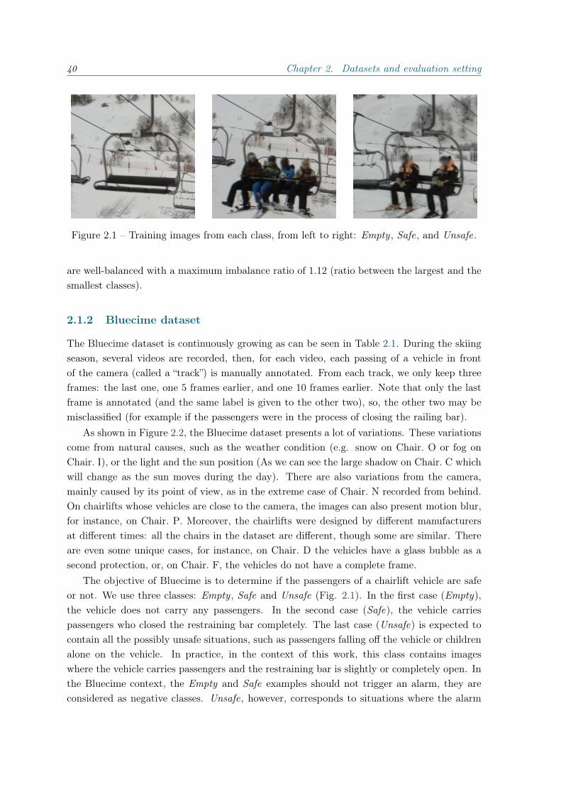
40 Chapter 2. Datasets and evaluation setting
Figure 2.1 – Training images from each class, from left to right: Empty , Safe, and Unsafe.
are well-balanced with a maximum imbalance ratio of 1.12 (ratio between the largest and thesmallest classes).
2.1.2 Bluecime dataset
The Bluecime dataset is continuously growing as can be seen in Table 2.1. During the skiingseason, several videos are recorded, then, for each video, each passing of a vehicle in frontof the camera (called a “track”) is manually annotated. From each track, we only keep threeframes: the last one, one 5 frames earlier, and one 10 frames earlier. Note that only the lastframe is annotated (and the same label is given to the other two), so, the other two may bemisclassified (for example if the passengers were in the process of closing the railing bar).
As shown in Figure 2.2, the Bluecime dataset presents a lot of variations. These variationscome from natural causes, such as the weather condition (e.g. snow on Chair. O or fog onChair. I), or the light and the sun position (As we can see the large shadow on Chair. C whichwill change as the sun moves during the day). There are also variations from the camera,mainly caused by its point of view, as in the extreme case of Chair. N recorded from behind.On chairlifts whose vehicles are close to the camera, the images can also present motion blur,for instance, on Chair. P. Moreover, the chairlifts were designed by different manufacturersat different times: all the chairs in the dataset are different, though some are similar. Thereare even some unique cases, for instance, on Chair. D the vehicles have a glass bubble as asecond protection, or, on Chair. F, the vehicles do not have a complete frame.
The objective of Bluecime is to determine if the passengers of a chairlift vehicle are safeor not. We use three classes: Empty , Safe and Unsafe (Fig. 2.1). In the first case (Empty),the vehicle does not carry any passengers. In the second case (Safe), the vehicle carriespassengers who closed the restraining bar completely. The last case (Unsafe) is expected tocontain all the possibly unsafe situations, such as passengers falling off the vehicle or childrenalone on the vehicle. In practice, in the context of this work, this class contains imageswhere the vehicle carries passengers and the restraining bar is slightly or completely open. Inthe Bluecime context, the Empty and Safe examples should not trigger an alarm, they areconsidered as negative classes. Unsafe, however, corresponds to situations where the alarm

2.1. Datasets 41
Chair. A (Unsafe) Chair. B (Safe) Chair. C (Safe) Chair. D (Unsafe)
Chair. E (Empty) Chair. F (Safe) Chair. G (Safe) Chair. H (Safe)
Chair. I (Safe) Chair. J (Unsafe) Chair. K (Unsafe) Chair. L (Empty)
Chair. M (Unsafe) Chair. N (Unsafe) Chair. O (Unsafe) Chair. P (Safe)
Chair. Q (Unsafe) Chair. R (Empty) Chair. S (Safe) Chair. T (Safe)
Chair. U (Unsafe)
Figure 2.2 – Examples from Bluecime dataset

42 Chapter 2. Datasets and evaluation setting
should be triggered, it is a positive class.
Year # Chairlifts # Tracks # Empty # Safe # Unsafe I.R2016 5 10 560 6 094 (57.7%) 3 924 (37.2%) 542 (5.1%) 18.52017 15 25 112 14 045 (55.9%) 9 129 (36.4%) 1 938 (7.7%) 12.02018 21 25 442 13 585 (53.4%) 9 685 (38.1%) 2 172 (8.5%) 10.72019 40 77 613 36 225 (46.7%) 33 372 (43.0%) 8 016 (10.3%) 8.7
Table 2.1 – Bluecime dataset size over the years.
Chairlift # Tracks # Empty # Safe # UnsafeChair. A 1420 410 (28.9%) 529 (37.3%) 481 (33.9%)Chair. B 927 119 (12.8%) 739 (79.7%) 69 (7.4%)Chair. C 985 817 (82.9%) 105 (10.7%) 63 (6.4%)Chair. D 757 498 (65.8%) 252 (33.3%) 7 (0.9%)Chair. E 1621 694 (42.8%) 793 (48.9%) 134 (8.3%)Chair. F 1188 652 (54.9%) 507 (42.7%) 29 (2.4%)Chair. G 526 251 (47.7%) 259 (49.2%) 16 (3.0%)Chair. H 1002 592 (59.1%) 321 (32.0%) 89 (8.9%)Chair. I 1396 1194 (85.5%) 137 (9.8%) 65 (4.7%)Chair. J 1624 1011 (62.3%) 498 (30.7%) 115 (7.1%)Chair. K 1288 623 (48.4%) 521 (40.5%) 144 (11.2%)Chair. L 2289 1408 (61.5%) 621 (27.1%) 260 (11.4%)Chair. M 498 136 (27.3%) 306 (61.4%) 56 (11.2%)Chair. N 344 204 (59.3%) 138 (40.1%) 2 (0.6%)Chair. O 730 371 (50.8%) 279 (38.2%) 80 (11.0%)Chair. P 1286 771 (60.0%) 401 (31.2%) 114 (8.9%)Chair. Q 2291 1201 (52.4%) 1027 (44.8%) 63 (2.7%)Chair. R 1253 516 (41.2%) 585 (46.7%) 152 (12.1%)Chair. S 502 361 (71.9%) 86 (17.1%) 55 (11.0%)Chair. T 930 482 (51.8%) 391 (42.0%) 57 (6.1%)Chair. U 2585 1274 (49.3%) 1190 (46.0%) 121 (4.7%)
Table 2.2 – Detailed Bluecime 2018 dataset.
As you can see in Table 2.1, in 2016, only 10k examples over 6 chairlifts were available.In 2017, the dataset increased to 25k examples and 15 chairlifts. In 2018, the number ofexamples stagnated to 25k, but over 21 chairlifts. The stagnation of the dataset size isexplained by changes of the camera orientation or position for some of the existing systems,cases in which the images corresponding to the previous positions were removed. In 2019,the number of chairlifts nearly doubled with 40 chairlifts, the number of tracks tripled with
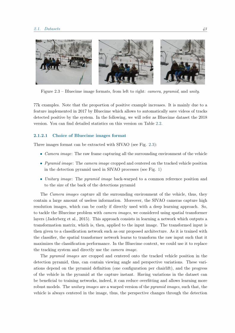
2.1. Datasets 43
Figure 2.3 – Bluecime image formats, from left to right: camera, pyramid, and unity.
77k examples. Note that the proportion of positive example increases. It is mainly due to afeature implemented in 2017 by Bluecime which allows to automatically save videos of tracksdetected positive by the system. In the following, we will refer as Bluecime dataset the 2018version. You can find detailed statistics on this version on Table 2.2.
2.1.2.1 Choice of Bluecime images format
Three images format can be extracted with SIVAO (see Fig. 2.3):
• Camera image: The raw frame capturing all the surrounding environment of the vehicle
• Pyramid image: The camera image cropped and centered on the tracked vehicle positionin the detection pyramid used in SIVAO processes (see Fig. 1)
• Unitary image: The pyramid image back-warped to a common reference position andto the size of the back of the detections pyramid
The Camera images capture all the surrounding environment of the vehicle, thus, theycontain a large amount of useless information. Moreover, the SIVAO cameras capture highresolution images, which can be costly if directly used with a deep learning approach. So,to tackle the Bluecime problem with camera images, we considered using spatial transformerlayers (Jaderberg et al., 2015). This approach consists in learning a network which outputs atransformation matrix, which is, then, applied to the input image. The transformed input isthen given to a classification network such as our proposed architecture. As it is trained withthe classifier, the spatial transformer network learns to transform the raw input such that itmaximizes the classification performance. In the Bluecime context, we could use it to replacethe tracking system and directly use the camera image.
The pyramid images are cropped and centered onto the tracked vehicle position in thedetection pyramid, thus, can contain viewing angle and perspective variations. These vari-ations depend on the pyramid definition (one configuration per chairlift), and the progressof the vehicle in the pyramid at the capture instant. Having variations in the dataset canbe beneficial to training networks, indeed, it can reduce overfitting and allows learning morerobust models. The unitary images are a warped version of the pyramid images, such that, thevehicle is always centered in the image, thus, the perspective changes through the detection
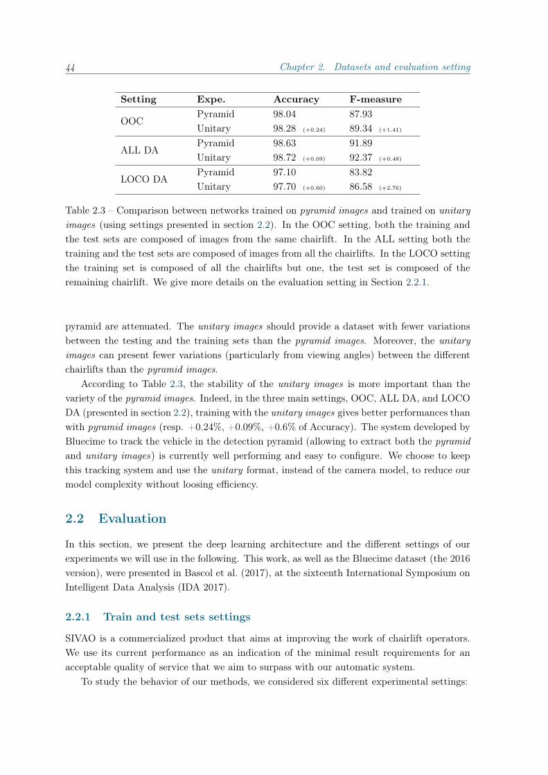
44 Chapter 2. Datasets and evaluation setting
Setting Expe. Accuracy F-measure
OOCPyramid 98.04 87.93Unitary 98.28 (+0.24) 89.34 (+1.41)
ALL DAPyramid 98.63 91.89Unitary 98.72 (+0.09) 92.37 (+0.48)
LOCO DAPyramid 97.10 83.82Unitary 97.70 (+0.60) 86.58 (+2.76)
Table 2.3 – Comparison between networks trained on pyramid images and trained on unitaryimages (using settings presented in section 2.2). In the OOC setting, both the training andthe test sets are composed of images from the same chairlift. In the ALL setting both thetraining and the test sets are composed of images from all the chairlifts. In the LOCO settingthe training set is composed of all the chairlifts but one, the test set is composed of theremaining chairlift. We give more details on the evaluation setting in Section 2.2.1.
pyramid are attenuated. The unitary images should provide a dataset with fewer variationsbetween the testing and the training sets than the pyramid images. Moreover, the unitaryimages can present fewer variations (particularly from viewing angles) between the differentchairlifts than the pyramid images.
According to Table 2.3, the stability of the unitary images is more important than thevariety of the pyramid images. Indeed, in the three main settings, OOC, ALL DA, and LOCODA (presented in section 2.2), training with the unitary images gives better performances thanwith pyramid images (resp. +0.24%, +0.09%, +0.6% of Accuracy). The system developed byBluecime to track the vehicle in the detection pyramid (allowing to extract both the pyramidand unitary images) is currently well performing and easy to configure. We choose to keepthis tracking system and use the unitary format, instead of the camera model, to reduce ourmodel complexity without loosing efficiency.
2.2 Evaluation
In this section, we present the deep learning architecture and the different settings of ourexperiments we will use in the following. This work, as well as the Bluecime dataset (the 2016version), were presented in Bascol et al. (2017), at the sixteenth International Symposium onIntelligent Data Analysis (IDA 2017).
2.2.1 Train and test sets settings
SIVAO is a commercialized product that aims at improving the work of chairlift operators.We use its current performance as an indication of the minimal result requirements for anacceptable quality of service that we aim to surpass with our automatic system.
To study the behavior of our methods, we considered six different experimental settings:

2.2. Evaluation 45
Figure 2.4 – Experimental settings
1. OOC (“Only One Chairlift”). Each chairlift is considered independently (as it is doneby SIVAO), thus the training and the testing sets are composed of images from a singlechairlift. Obviously, with only one chairlift per experiment, the domain adaptationcomponent (described in Section 3.1) is not used on this setting.
2. ALL One experiment is performed without using the domain adaptation component.The images are taken from all the chairlifts in the training and the testing set.
3. ALL DA Same as ALL setting, adding the domain adaptation component. The targetimages are the same as the source ones.
4. LOCO (“Leave One Chairlift Out”) In each experiment, we use only the feature extrac-tor and the classifier, with the images of all the chairlifts but one mixed in the trainingset and all the images of the remaining chairlift as test set.
5. LOCO DA- Same as LOCO but with domain adaptation. The target images are thesame as the source ones, so no example (labeled or not) from the tested chairlift areused during training, this is thus a domain generalization setting.
6. LOCO DA Same as LOCO but with classical unsupervised domain adaptation wheresome unlabeled examples of the target chairlift are used by the domain adaptationcomponent.
We show a graphical representation of these settings on Figure 2.4. All the presentedresults are averaged over five folds. Note that for the LOCO settings, only the test set (andtarget set for LOCO DA) changes across the different folds.
In Setting 1 (OOC), to reduce the number of experiments, we do not tune the hyper-parameters for each domain, but we use one single hyperparameter setting for all the chairlifts.In this setting, we expect the network to quickly overfit our data and also to be penalized bythe lack of examples especially for the least represented chairlifts.
In Settings 2 and 3 (ALL and ALL DA), we train our network using all the training dataavailable. We only build one model for all the chairlifts which makes this setting easier todeploy in practice. However, the hyperparameters of the system are also global which mayharm the final performance. These settings could be used with the current cameras installedby the company but do not evaluate the real ability of our system to work on new chairlifts.
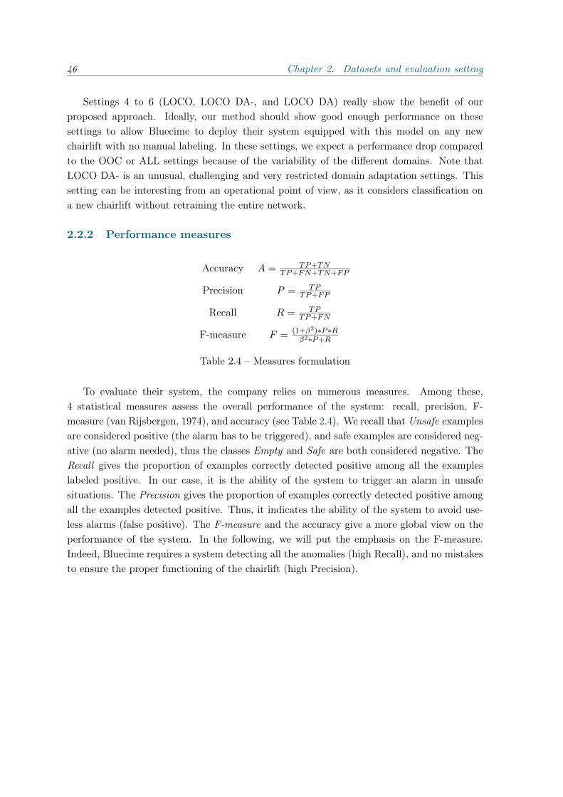
46 Chapter 2. Datasets and evaluation setting
Settings 4 to 6 (LOCO, LOCO DA-, and LOCO DA) really show the benefit of ourproposed approach. Ideally, our method should show good enough performance on thesesettings to allow Bluecime to deploy their system equipped with this model on any newchairlift with no manual labeling. In these settings, we expect a performance drop comparedto the OOC or ALL settings because of the variability of the different domains. Note thatLOCO DA- is an unusual, challenging and very restricted domain adaptation settings. Thissetting can be interesting from an operational point of view, as it considers classification ona new chairlift without retraining the entire network.
2.2.2 Performance measures
Accuracy A = TP+TNTP+FN+TN+FP
Precision P = TPTP+FP
Recall R = TPTP+FN
F-measure F = (1+β2)∗P∗Rβ2∗P+R
Table 2.4 – Measures formulation
To evaluate their system, the company relies on numerous measures. Among these,4 statistical measures assess the overall performance of the system: recall, precision, F-measure (van Rijsbergen, 1974), and accuracy (see Table 2.4). We recall that Unsafe examplesare considered positive (the alarm has to be triggered), and safe examples are considered neg-ative (no alarm needed), thus the classes Empty and Safe are both considered negative. TheRecall gives the proportion of examples correctly detected positive among all the exampleslabeled positive. In our case, it is the ability of the system to trigger an alarm in unsafesituations. The Precision gives the proportion of examples correctly detected positive amongall the examples detected positive. Thus, it indicates the ability of the system to avoid use-less alarms (false positive). The F-measure and the accuracy give a more global view on theperformance of the system. In the following, we will put the emphasis on the F-measure.Indeed, Bluecime requires a system detecting all the anomalies (high Recall), and no mistakesto ensure the proper functioning of the chairlift (high Precision).

Chapter 3
First approach and trainingimprovement
In this section, we present the deep learning architecture and the different settings of ourexperiments we will use in the following. This work was presented in Bascol et al. (2017), atthe sixteenth International Symposium on Intelligent Data Analysis (IDA 2017).
3.1 Selected architecture
Based on the state-of-the art study presented in Chapter 1, we propose an image classificationarchitecture using domain adaptation and a convolutional residual network pre-trained onImageNet. This architecture is shown in Figure 3.1 and is divided into three parts:
1. a feature extractor, which learns a new image representation (ResNet50 from He et al.(2016));
2. a classifier, which predicts the class of an image;
3. a domain discriminator, which ensures that the feature extractor is domain invariant,to improve classification accuracy on unseen data (DANN from Ganin et al. (2016)).Note that this part is only added with “DA” settings.
3.1.1 Network architecture
Our network inputs are RGB images of size 224 × 224 (imposed by constrains on the pre-training) that can be viewed as three-dimensional tensors (two spatial dimensions and onedimension for the RGB channels). After some trial and error (some results are presented inSection 3.1.3), we decided to use the ResNet architecture presented in the previous sectionwith 50 layers and pre-trained on the ImageNet dataset (see the training tricks section 1.2.1.3).Networks with more layers gave a slightly better accuracy but were longer to train and thebiggest ones (with more than 101 layers) did not allow us to process test images in real timeon a CPU. The 50 layers architecture (shown in Fig. 3.1) gave us a good trade-off between
47
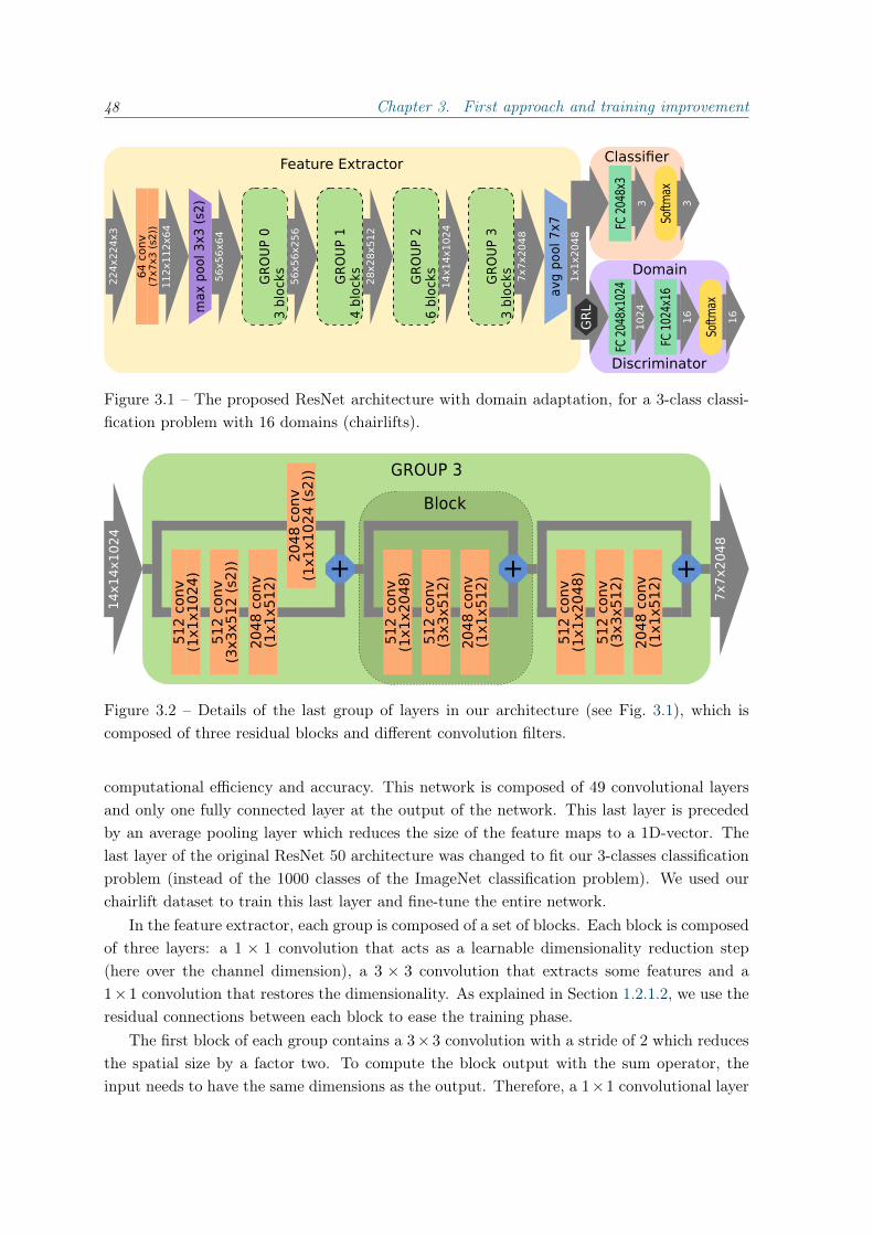
48 Chapter 3. First approach and training improvement
Figure 3.1 – The proposed ResNet architecture with domain adaptation, for a 3-class classi-fication problem with 16 domains (chairlifts).
Figure 3.2 – Details of the last group of layers in our architecture (see Fig. 3.1), which iscomposed of three residual blocks and different convolution filters.
computational efficiency and accuracy. This network is composed of 49 convolutional layersand only one fully connected layer at the output of the network. This last layer is precededby an average pooling layer which reduces the size of the feature maps to a 1D-vector. Thelast layer of the original ResNet 50 architecture was changed to fit our 3-classes classificationproblem (instead of the 1000 classes of the ImageNet classification problem). We used ourchairlift dataset to train this last layer and fine-tune the entire network.
In the feature extractor, each group is composed of a set of blocks. Each block is composedof three layers: a 1 × 1 convolution that acts as a learnable dimensionality reduction step(here over the channel dimension), a 3 × 3 convolution that extracts some features and a1×1 convolution that restores the dimensionality. As explained in Section 1.2.1.2, we use theresidual connections between each block to ease the training phase.
The first block of each group contains a 3× 3 convolution with a stride of 2 which reducesthe spatial size by a factor two. To compute the block output with the sum operator, theinput needs to have the same dimensions as the output. Therefore, a 1×1 convolutional layer

3.1. Selected architecture 49
with a stride of 2 is added to reduce the spatial size and also to match the number of featuremaps which changes according to the group. In Figure 3.2, we show in more details the lastgroup of layers in the feature extractor.
3.1.2 Objective function and training
Different losses are classically used in deep learning. The best known for image classificationis the cross-entropy (Goodfellow et al., 2016). After experimenting with different losses, wedecided to use the more robust multi-class hinge loss (eq. 3.1) commonly used in SVM:
L(W ,X, t) =1
B
B∑i=1
1
|C|∑
c∈C\t
max(0, oic − oit +m) (3.1)
where W is the set of all the parameters in the network, X is the subset of the inputdataset (minibatch) given to the network during a forward pass, B is the minibatch size,C is the set of classes, and t is the ground-truth label corresponding to each example ofthe minibatch. The margin m can be seen as the minimal “distance” required between thecomputed probability of the prediction of the target class (oit) and the other classes (oic).Indeed, the loss value is equal to 0 when oit ≥ oic +m. This loss presents several advantages:(i) it is defined on p(x) = 0 which makes it more robust than the cross-entropy; (ii) it does notpenalize the weights on well classified examples which could speed up the convergence of thenetwork; (iii) the slope and the margin of the function can be easily changed to give a customweight to the different type of errors (false positive, false negative). This last advantage willbe explored in Chapter 4.
Domains and classes balance Bluecime dataset is imbalanced both in the domain distri-bution and the class distribution. Having under-represented domains can be harmful, mainlyin the ALL setting, as the model would be trained with small data from these domains, thusimpairing the results on them. The imbalanced class distribution is also harmful, only a fewpositive examples would be used during the training of the classifier, thus impairing the re-sults on this class. This would particularly result in a low F-measure, as this measure putsthe emphasis on the good classification of the positive examples. To tackle both problems, wepropose to artificially balance the training set, by randomly selecting a domain and a classuniformly at each image loading. This implies that each Unsafe example is reused more oftenthan the Empty examples. We thus have a dataset with less variety, but in return we havevirtually more positive examples, which should allow us to obtain better results on this class.
We show on Tables 3.1 and 3.2, results modifying (or not) the balance of both the domainsand the classes. We see that balancing the classes is always a better option. This shows thatthe loss of variety in the training set is more than compensated by the increase of positiveexamples. However, balancing the domains is beneficial in ALL setting but not in the LOCOone. This confirms our first intuition that having under-represented domains in the trainingset is harmful only if we test on them. This also suggests that some under-represented chairlifts

50 Chapter 3. First approach and training improvement
Expe. Accuracy Recall Precision F-measureALL DA bcl bdom 98.72 90.54 94.28 92.37ALL DA ubcl bdom 98.70 (−0.02) 88.90 (−1.64) 95.55 (+1.27) 92.11 (−0.26)
ALL DA bcl ubdom 98.71 (−0.01) 90.19 (−0.35) 94.41 (+0.13) 92.25 (−0.12)
ALL DA ubcl ubdom 98.64 (−0.09) 90.10 (−0.44) 93.68 (−0.60) 91.86 (−0.51)
Table 3.1 – ALL DA results with and without domain and class balancing method. (u)bclindicates experiments with (un)balanced classes. (u)bdom indicates experiments with(un)balanced domains.
Expe. Accuracy Recall Precision F-measureLOCO DA bcl bdom 97.41 89.17 82.94 83.30LOCO DA ubcl bdom 94.64 (−2.77) 39.92 (−49.26) 93.73 (+10.78) 55.99 (−27.31)
LOCO DA bcl ubdom 97.63 (+0.22) 87.52 (−1.65) 85.17 (+2.23) 86.33 (+3.03)
LOCO DA ubcl ubdom 95.02 (−2.39) 43.32 (−45.85) 96.22 (+13.27) 59.75 (−23.55)
Table 3.2 – LOCO DA results with and without domain and class balancing method.(u)bcl indicates experiments with (un)balanced classes. (u)bdom indicates experiments with(un)balanced domains. Note that, in these experiments, the classes of the target examples arebalanced, which implies that it is not a correct unsupervised setting, this matter is discussedin length in the chapter 5.
induce negative transfer as we get better performance if we use fewer examples from them inthe LOCO training set. This phenomenon will be studied in more details in Chapter 5.
3.1.3 Feature extractors comparison
We show, in Table 3.3, results, and training and testing times using different feature extractors:ResNet with 50 layers, ResNet with 18 layers, MobileNet-v2, and Inception-v4. We can seethat using ResNet50 yields the best results. However, ResNet18 and MobileNet take lesstime to provide an output. These results confirm our choice to use the ResNet architecture.However, The choice of the number of layers to use is arguable. Indeed, we obviously needto have the best model, but we also need to get the output in real time. So, the choiceof ResNet50 or ResNet18 will be dependent on the integration of the model in SIVAO. Forinstance, if we only use one frame to decide, we should use ResNet50. However, if we want toaverage the prediction over several frames, ResNet18 would be more appropriate. In addition,currently, the SIVAO system contains only a CPU, reducing the models speed dramatically,which increases the need for speed in our approach.
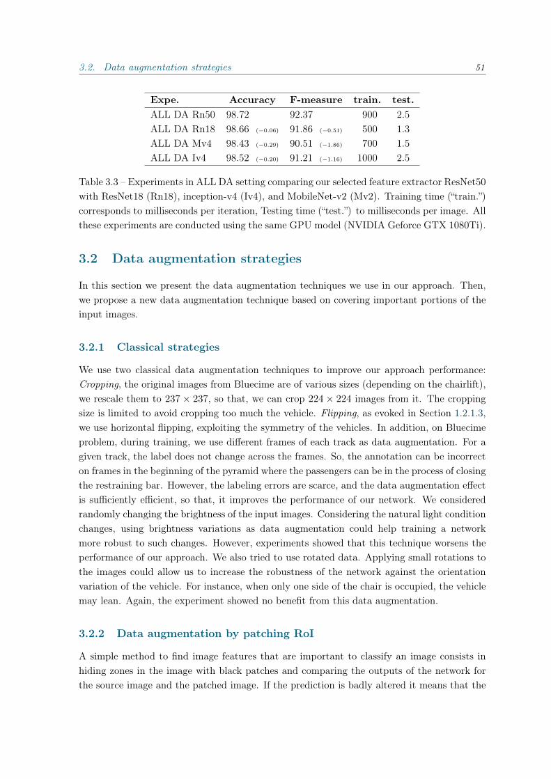
3.2. Data augmentation strategies 51
Expe. Accuracy F-measure train. test.ALL DA Rn50 98.72 92.37 900 2.5ALL DA Rn18 98.66 (−0.06) 91.86 (−0.51) 500 1.3ALL DA Mv4 98.43 (−0.29) 90.51 (−1.86) 700 1.5ALL DA Iv4 98.52 (−0.20) 91.21 (−1.16) 1000 2.5
Table 3.3 – Experiments in ALL DA setting comparing our selected feature extractor ResNet50with ResNet18 (Rn18), inception-v4 (Iv4), and MobileNet-v2 (Mv2). Training time (“train.”)corresponds to milliseconds per iteration, Testing time (“test.”) to milliseconds per image. Allthese experiments are conducted using the same GPU model (NVIDIA Geforce GTX 1080Ti).
3.2 Data augmentation strategies
In this section we present the data augmentation techniques we use in our approach. Then,we propose a new data augmentation technique based on covering important portions of theinput images.
3.2.1 Classical strategies
We use two classical data augmentation techniques to improve our approach performance:Cropping, the original images from Bluecime are of various sizes (depending on the chairlift),we rescale them to 237 × 237, so that, we can crop 224 × 224 images from it. The croppingsize is limited to avoid cropping too much the vehicle. Flipping, as evoked in Section 1.2.1.3,we use horizontal flipping, exploiting the symmetry of the vehicles. In addition, on Bluecimeproblem, during training, we use different frames of each track as data augmentation. For agiven track, the label does not change across the frames. So, the annotation can be incorrecton frames in the beginning of the pyramid where the passengers can be in the process of closingthe restraining bar. However, the labeling errors are scarce, and the data augmentation effectis sufficiently efficient, so that, it improves the performance of our network. We consideredrandomly changing the brightness of the input images. Considering the natural light conditionchanges, using brightness variations as data augmentation could help training a networkmore robust to such changes. However, experiments showed that this technique worsens theperformance of our approach. We also tried to use rotated data. Applying small rotations tothe images could allow us to increase the robustness of the network against the orientationvariation of the vehicle. For instance, when only one side of the chair is occupied, the vehiclemay lean. Again, the experiment showed no benefit from this data augmentation.
3.2.2 Data augmentation by patching RoI
A simple method to find image features that are important to classify an image consists inhiding zones in the image with black patches and comparing the outputs of the network forthe source image and the patched image. If the prediction is badly altered it means that the

52 Chapter 3. First approach and training improvement
patched zone is important for the classification. If the alteration of the prediction is negligiblethen the patched zone is not interesting for the network.
(a) (b) (c)
Figure 3.3 – Visualization with patch of size 28× 28 pixels (without overlapping). 3.3a is thesource image, the prediction variation for all the patches is shown on 3.3b (with the sourceimage in the background) and 3.3c (with the variation only). The color of a patch indicatesthe prediction of the network for the patched image. An orange patch corresponds to a highprobability on the Unsafe class. A green one indicates a high probability on the Safe class.
On the figure 3.3, we observe that if we hide the area around the vehicle the predictionis correct (class Unsafe since the security railing is up). However, if we hide the area wherethe railing should be when it is closed, the probability on the Safe class strongly increases sothat the images with theses patched areas are predicted Safe.
This visualization method shows us that the classification of an image can depend ona small region of interest (RoI). Following this, we tried to include patches inducing highnegative prediction variation to the network training. So that, it forced the network to usethe whole image, and thus, to increase the robustness of the model. To do that, during eachtraining iteration we do a forward pass with a given number of patched images. We thenadd to the dataset the images with a patch inducing a decrease of the probability on thetrue class superior to a given threshold (Fig. 3.4). This approach is similar to the dropoutmethod presented in Zhong et al. (2017) (whose work was done in parallel to ours). However,we propose to guide the discarded areas to produce harder examples, we thus expect a betterresult than using random patches.
3.2.2.1 Experiments
Randomly sampled batches In Table 3.4 we propose to compare our patching approachto our baseline ALL DA and ALL DA with patches randomly applied on the image loading(similarly to DeVries and Taylor (2017) or Zhong et al. (2017)). We observe that addingpatches during the training is beneficial with on average +0.07 pts of Accuracy and +0.30 ptsof F-measure. However, our method requires 25 batches of patched images to only match theresults using random addition of patches. We could try to increase the number of batches so

3.2. Data augmentation strategies 53
Figure 3.4 – Training iteration with patches in 5 steps: 1- the forward pass of the minibatch.2- the backward pass updating the weights. 3- sample images in the minibatch and randomlyadd one patch per image. 4- a forward pass with the patches images. 5- compute the differencebetween the predictions corresponding to the source images and the one corresponding to theirpatched version. Finally, save the patches with a high prediction difference.
that more patches are tested and thus more should be kept. Indeed, we can see that from 5batches to 25 batches we see a small gain of 0.04pts of Accuracy and +0.28 pts of F-measure.However, using 5 batches multiplies approximately the training time by 2, using 25 batchesmultiplies it by 6. Increasing the training time is not actually a strong constraint as it is doneoff-line. However, we decided to keep exploring other ways to improve our approach.
Expe. Accuracy Recall Precision F-measureALL DA 98.72 90.54 94.28 92.37ALL DA rp 98.79 (+0.07) 91.62 (+1.08) 94.00 (−0.28) 92.80 (+0.33)
ALL DA 5bp 98.77 (+0.05) 89.09 (−1.45) 96.22 (+1.94) 92.52 (+0.15)
ALL DA 25bp 98.81 (+0.09) 89.87 (−0.67) 95.92 (+1.64) 92.80 (+0.43)
Table 3.4 – Results with patches. “rp” indicates experiment with random patching at theloading of the images. “5bp” and “25bp” respectively correspond to experiments with 5 and25 batches of randomly patched images tested at each iteration.
Late start The patch selection is done with respect to the output of the network. Duringthe firsts training iterations the relevance of the outputs is uncertain, thus, it may be beneficialto start testing patches only after several simple training iterations. To avoid introducing ashift in the data by delaying the patching, we propose to randomly add patches during thefirst training iterations. We present in Table 3.5, the results delaying the patching. We can seethat delaying the patching of the images is slightly beneficial with +0.02pts of Accuracy and+0.16pts of F-measure compared to patches used directly from the first iteration. However,
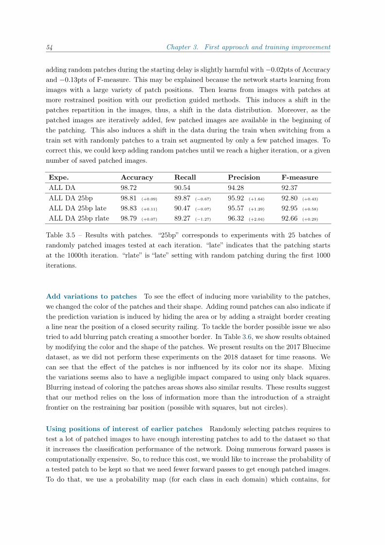
54 Chapter 3. First approach and training improvement
adding random patches during the starting delay is slightly harmful with −0.02pts of Accuracyand −0.13pts of F-measure. This may be explained because the network starts learning fromimages with a large variety of patch positions. Then learns from images with patches atmore restrained position with our prediction guided methods. This induces a shift in thepatches repartition in the images, thus, a shift in the data distribution. Moreover, as thepatched images are iteratively added, few patched images are available in the beginning ofthe patching. This also induces a shift in the data during the train when switching from atrain set with randomly patches to a train set augmented by only a few patched images. Tocorrect this, we could keep adding random patches until we reach a higher iteration, or a givennumber of saved patched images.
Expe. Accuracy Recall Precision F-measureALL DA 98.72 90.54 94.28 92.37ALL DA 25bp 98.81 (+0.09) 89.87 (−0.67) 95.92 (+1.64) 92.80 (+0.43)
ALL DA 25bp late 98.83 (+0.11) 90.47 (−0.07) 95.57 (+1.29) 92.95 (+0.58)
ALL DA 25bp rlate 98.79 (+0.07) 89.27 (−1.27) 96.32 (+2.04) 92.66 (+0.29)
Table 3.5 – Results with patches. “25bp” corresponds to experiments with 25 batches ofrandomly patched images tested at each iteration. “late” indicates that the patching startsat the 1000th iteration. “rlate” is “late” setting with random patching during the first 1000iterations.
Add variations to patches To see the effect of inducing more variability to the patches,we changed the color of the patches and their shape. Adding round patches can also indicate ifthe prediction variation is induced by hiding the area or by adding a straight border creatinga line near the position of a closed security railing. To tackle the border possible issue we alsotried to add blurring patch creating a smoother border. In Table 3.6, we show results obtainedby modifying the color and the shape of the patches. We present results on the 2017 Bluecimedataset, as we did not perform these experiments on the 2018 dataset for time reasons. Wecan see that the effect of the patches is nor influenced by its color nor its shape. Mixingthe variations seems also to have a negligible impact compared to using only black squares.Blurring instead of coloring the patches areas shows also similar results. These results suggestthat our method relies on the loss of information more than the introduction of a straightfrontier on the restraining bar position (possible with squares, but not circles).
Using positions of interest of earlier patches Randomly selecting patches requires totest a lot of patched images to have enough interesting patches to add to the dataset so thatit increases the classification performance of the network. Doing numerous forward passes iscomputationally expensive. So, to reduce this cost, we would like to increase the probability ofa tested patch to be kept so that we need fewer forward passes to get enough patched images.To do that, we use a probability map (for each class in each domain) which contains, for

3.2. Data augmentation strategies 55
Expe. Accuracy Recall Precision F-measureALL DA 97.98 85.83 87.43 86.62ALL DA blk sq 98.49 (+0.51) 86.71 (+0.89) 94.23 (+6.79) 90.31 (+3.69)
ALL DA wht sq 98.33 (+0.35) 84.78 (+1.04) 94.10 (+6.67) 89.20 (+2.58)
ALL DA mean sq 98.43 (+0.45) 86.71 (+0.89) 93.49 (+6.06) 89.97 (+3.35)
ALL DA blk cir 98.39 (+0.41) 87.44 (+1.61) 92.35 (+4.91) 89.83 (+3.20)
ALL DA vs blk sq 98.33 (+0.35) 83.09 (−2.73) 95.82 (+8.39) 89.00 (+2.38)
ALL DA vs blk cir 98.51 (+0.53) 87.20 (+1.37) 94.01 (+6.58) 90.48 (+3.85)
ALL DA all var 98.54 (+0.56) 87.14 (+1.31) 93.26 (+5.83) 90.09 (+3.47)
ALL DA blur sq 98.55 (+0.57) 87.44 (+1.61) 94.27 (+6.84) 90.73 (+4.10)
Table 3.6 – Results on the same experiment, patches tested over 25 batches per iteration.Note that these experiments were conducted on the 2017 Bluecime dataset. “blk”, “wht”, and“mean” corresponds to the color of the patches, respectively black, white, and average pixelcolor in the dataset. “sq” and “cir” correspond to square or circle patches. “vs” means that thesize of the patches is randomly chosen (between 16 and 64 pixels). “all var” corresponds topatches with randomly chosen color and shape (between the previously enumerated). “blur”indicate patches inducing a blurring effect (without adding color).
each pixel in the images, the probability for a patch to be interesting. The map is initializeduniformly (or with a Gaussian distribution centered in the image), during the training if weencounter an important patch we increase the probability of choosing this position again inthe next training iterations (the probabilities are clipped if they exceed 1). Table 3.7 showsresults using probability maps in the ALL DA setting. With only 5 patching batches added,the maps has almost no effect. However, with 25 batches we observe a good performance gainwith +0.09 of Accuracy and +0.6pts of F-measure when we add uniformly initialized maps.When using Gaussian initialization, we observe no effect. This can be explained by the highprobability to add a patch in the center of the image, which implies that we explore muchfewer patch locations that initializing uniformly. From this observation, we could exploretechniques to avoid having too high probability zones impairing the patch exploration. Forinstance, we could clip the maps with a value inferior to 1.
In Figure 3.5, we show examples of the probability maps. In red are the zones with ahigh probability of being patched. We can see that the red zones fit well the chairs of thevehicle, and covers the full size of the passengers. We also note that, on the map of the Unsafeclass, the red zone is extended higher to the top of the vehicle, where the restraining bar ispositioned when it is entirely opened (like on the Empty image). This suggests that the redzones may cover all the possible positions of the restraining bar and of its footrests. With this,we improve our patching approach by ignoring nearly all the background and uninformativepart of the vehicle such as its frame.

56 Chapter 3. First approach and training improvement
Expe. Accuracy Recall Precision F-measureALL DA 98.72 90.54 94.28 92.37ALL DA 5bp 98.77 (+0.05) 89.09 (−1.45) 96.22 (+1.94) 92.52 (+0.15)
ALL DA 5bp u+0.1 98.76 (+0.04) 89.92 (−0.62) 95.31 (+1.03) 92.54 (+0.17)
ALL DA 25bp 98.81 (+0.09) 89.87 (−0.67) 95.92 (+1.64) 92.80 (+0.43)
ALL DA 25bp u+0.1 98.91 (+0.19) 90.47 (−0.07) 96.51 (+2.13) 93.39 (+1.02)
ALL DA 25bp g+0.1 98.80 (+0.08) 90.70 (+0.16) 95.03 (+0.75) 92.82 (+0.45)
Table 3.7 – Results with patches. “5bp” and “25bp” respectively correspond to experimentswith 5 and 25 batches of randomly patched images tested at each iteration. “u” and “g”respectively indicates that the probabilities maps are initialized with a centered Gaussiandistribution and a uniform distribution. “+0.1” indicates that a kept patch increases theprobability on his location by 0.1.
(a) Empty map. (b) Safe map. (c) Unsafe map.
Figure 3.5 – Example of resulting probability map on the chairlift Chair. M after “ALL DA25bp u+0.1” training. The red zones indicate a high probability of applying a patch.
3.2.2.2 Conclusion
Our patching approach shows promising results with at most +0.19 pts of Accuracy and +1.03
pts of F-measure, with the only disadvantage to increase the training time. Moreover, thereis still room for improvements, particularly with the approach using the previous patchespositions. Indeed, we could increase the probability of a location by using for example theprediction variation. We could also experiment on reducing the probability of a location inthe case of a better prediction, this could be tricky as there are few patches of interest amongall the tested patches. We could also validate or possibly improve our approach by using othervisualization approaches. For instance, with GradCam (Selvaraju et al., 2017) or deep Taylordecomposition (Montavon et al., 2017), we could have regions of interest in an image withouttesting patch positions, thus reducing the training time and possibly increasing the numberof selected patches.

3.3. Baseline results 57
Expe. Accuracy Recall Precision F-measureSIVAO 98.54 92.68 90.43 91.54OOC 98.35 (−0.19) 85.96 (−6.72) 94.20 (+3.77) 89.89 (−1.65)
ALL 98.73 (+0.19) 90.93 (−1.75) 94.00 (+3.58) 92.44 (+0.90)
ALL DA 98.72 (+0.18) 90.54 (−2.14) 94.28 (+3.85) 92.37 (+0.83)
LOCO 95.63 (−2.91) 85.73 (−6.95) 69.87 (−20.56) 76.99 (−14.55)
LOCO DA- 96.72 (−1.82) 81.81 (−10.86) 83.77 (−6.66) 78.23 (−13.31)
LOCO DA 97.70 (−0.84) 87.06 (−5.61) 86.11 (−4.32) 86.58 (−4.95)
Table 3.8 – Baseline results (difference with SIVAO performance between brackets). Notethat, in the “DA” experiments, the classes of the target examples are balanced, which impliesthat the LOCO DA setting is not a correct unsupervised setting, this matter is discussed inlength in the chapter 5.
3.3 Baseline results
In Table 3.8, we present the results on all the datasets for all the experimental settings.The first line of the table gives the performance of SIVAO, the current system developed byBluecime. In the OOC setting, we get poor performances compared to SIVAO (−1.65 pts ofF-measure). In this setting as we use only the images of only one chairlift, we have trainingdataset too small and with too few variations. However, with the ALL setting, we observe animprovement of 0.83 to 0.9 pts of F-measure. Even though the gain is small, the training timeof ALL is about 5 hours while the time to configure SIVAO is higher and the configurationis different on each chairlift. So, ALL makes a very attractive solution from an industrialstandpoint.
As expected, during the LOCO experiment, performance losses occur for all the measures,with −14.55 pts of F-measure and −2.91 pts of Accuracy. In this setting, performance is toolow for industrial deployment. However, adding domain adaptation (LOCO DA) show a highimprovement with −4.95 pts of F-measure and only −0.84 pts of Accuracy. This result isworse than SIVAO or ALL, however, in this setting, the chairlift does not have any annotatedimages. So, we can consider the performance on LOCO DA as promising, considering that inthis setting, SIVAO cannot be configured, and we cannot train on ALL setting. Note that,using the LOCO DA-, we obtain results 1pts better than the LOCO setting (in both Accuracyand F-measure), but shows −1 pts of Accuracy and −8.36 pts of F-measure compared to theLOCO DA setting. These results show that we are forced to acquire some data to improvethe results on newly installed chairlifts, but, we avoid the labeling process which is more timecostly than just acquiring raw data. We show detailed results on F-measure in Table 3.9(detailed results in Accuracy, Precision, and Recall are available in Appendix B.1). Theseresults show a very challenging aspect of Bluecime dataset which is the high disparity of theresponse to a new method across the chairlifts. Indeed, if we compare ALL and ALL DA wecan see on Chair. O that adding the domain adaptation module decreases the F-measure by
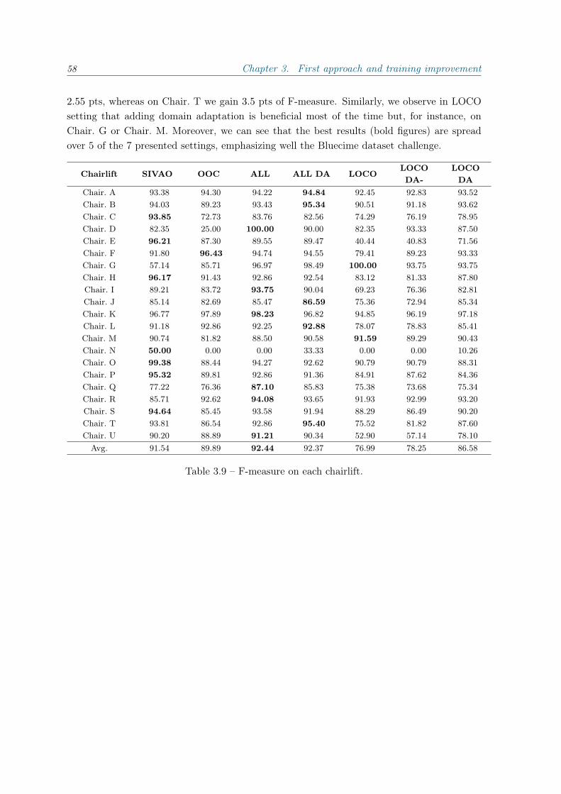
58 Chapter 3. First approach and training improvement
2.55 pts, whereas on Chair. T we gain 3.5 pts of F-measure. Similarly, we observe in LOCOsetting that adding domain adaptation is beneficial most of the time but, for instance, onChair. G or Chair. M. Moreover, we can see that the best results (bold figures) are spreadover 5 of the 7 presented settings, emphasizing well the Bluecime dataset challenge.
Chairlift SIVAO OOC ALL ALL DA LOCOLOCODA-
LOCODA
Chair. A 93.38 94.30 94.22 94.84 92.45 92.83 93.52Chair. B 94.03 89.23 93.43 95.34 90.51 91.18 93.62Chair. C 93.85 72.73 83.76 82.56 74.29 76.19 78.95Chair. D 82.35 25.00 100.00 90.00 82.35 93.33 87.50Chair. E 96.21 87.30 89.55 89.47 40.44 40.83 71.56Chair. F 91.80 96.43 94.74 94.55 79.41 89.23 93.33Chair. G 57.14 85.71 96.97 98.49 100.00 93.75 93.75Chair. H 96.17 91.43 92.86 92.54 83.12 81.33 87.80Chair. I 89.21 83.72 93.75 90.04 69.23 76.36 82.81Chair. J 85.14 82.69 85.47 86.59 75.36 72.94 85.34Chair. K 96.77 97.89 98.23 96.82 94.85 96.19 97.18Chair. L 91.18 92.86 92.25 92.88 78.07 78.83 85.41Chair. M 90.74 81.82 88.50 90.58 91.59 89.29 90.43Chair. N 50.00 0.00 0.00 33.33 0.00 0.00 10.26Chair. O 99.38 88.44 94.27 92.62 90.79 90.79 88.31Chair. P 95.32 89.81 92.86 91.36 84.91 87.62 84.36Chair. Q 77.22 76.36 87.10 85.83 75.38 73.68 75.34Chair. R 85.71 92.62 94.08 93.65 91.93 92.99 93.20Chair. S 94.64 85.45 93.58 91.94 88.29 86.49 90.20Chair. T 93.81 86.54 92.86 95.40 75.52 81.82 87.60Chair. U 90.20 88.89 91.21 90.34 52.90 57.14 78.10Avg. 91.54 89.89 92.44 92.37 76.99 78.25 86.58
Table 3.9 – F-measure on each chairlift.
Chapter 4
Cost-sensitive learning for imbalanceddata
In this chapter, we will present two approaches developed to improve the performance ofour method according to the F-measure. We first show an empirical method, based on theiterative training of the neural network. Then, we present an iterative algorithm based on atheoretical bound on the F-measure. This last work was presented in Bascol et al. (2019b), atthe 22nd International Conference on Artificial Intelligence and Statistics (AISTATS 2019).
4.1 F-measure gain-oriented training
In this section we describe our first approach on the F-measure optimization and then presentempirical results on the Bluecime dataset.
4.1.1 Introduction
Our first approach on F-measure optimization consists in modifying the training loss at eachiteration towards a hypothetical gain of F-measure, measured in the previous iteration.
We recall the Hinge Loss formulation (Sec. 1.2.1.1) used as our training loss:
LHinge(yi, t) =1
C
C∑j=1;j 6=t
max(0, µ+ yij − yit)
Our approach is a cost-sensitive training algorithm, we thus have a weighted loss:
L(α, Y ,Y ) =1
B
B∑i=1
αyiLHinge(yi,yi)
where Y = (y1, y2, .., yB) is the set of classifier outputs on a given batch of size B, andY = (y1,y2, ..,yB) is the set of corresponding labels. α is the vector containing the classweights.
59
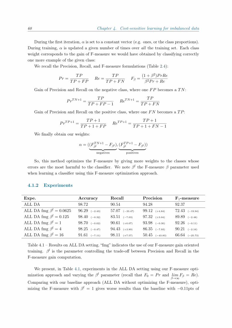
60 Chapter 4. Cost-sensitive learning for imbalanced data
During the first iteration, α is set to a constant vector (e.g. ones, or the class proportions).During training, α is updated a given number of times over all the training set. Each classweight corresponds to the gain of F-measure we would have obtained by classifying correctlyone more example of the given class:
We recall the Precision, Recall, and F-measure formulations (Table 2.4):
Pr =TP
TP + FPRe =
TP
TP + FNFβ =
(1 + β2)PrRe
β2Pr +Re
Gain of Precision and Recall on the negative class, where one FP becomes a TN :
PrTN+1 =TP
TP + FP − 1ReTN+1 =
TP
TP + FN
Gain of Precision and Recall on the positive class, where one FN becomes a TP :
PrTP+1 =TP + 1
TP + 1 + FPReTP+1 =
TP + 1
TP + 1 + FN − 1
We finally obtain our weights:
α = ((F TN+1βl − Fβl)︸ ︷︷ ︸negatives
, (F TP+1βl − Fβl)︸ ︷︷ ︸positives
)
So, this method optimizes the F-measure by giving more weights to the classes whoseerrors are the most harmful to the classifier. We note βl the F-measure β parameter usedwhen learning a classifier using this F-measure optimization approach.
4.1.2 Experiments
Expe. Accuracy Recall Precision F1-measureALL DA 98.72 90.54 94.28 92.37ALL DA fmg βl = 0.0625 96.29 (−2.43) 57.07 (−33.47) 99.12 (+4.84) 72.43 (−19.94)
ALL DA fmg βl = 0.125 98.40 (−0.32) 83.51 (−7.03) 97.32 (+3.04) 89.89 (−2.48)
ALL DA fmg βl = 1 98.70 (−0.02) 90.61 (+0.07) 93.98 (−0.30) 92.26 (−0.11)
ALL DA fmg βl = 4 98.25 (−0.47) 94.43 (+3.89) 86.35 (−7.93) 90.21 (−2.16)
ALL DA fmg βl = 16 91.61 (−7.11) 98.11 (+7.57) 50.45 (−43.83) 66.64 (−25.73)
Table 4.1 – Results on ALL DA setting. “fmg” indicates the use of our F-measure gain orientedtraining. βl is the parameter controlling the trade-off between Precision and Recall in theF-measure gain computation.
We present, in Table 4.1, experiments in the ALL DA setting using our F-measure opti-mization approach and varying the βl parameter (recall that F0 = Pr and lim
β→∞Fβ = Re).
Comparing with our baseline approach (ALL DA without optimizing the F-measure), opti-mizing the F-measure with βl = 1 gives worse results than the baseline with −0.11pts of

4.2. From cost-sensitive classification to tight F-measure bounds 61
0.0625 0.25 1 4 160.800
0.825
0.850
0.875
0.900
0.925
0.950
0.975
1.000F
mea
sure
Precision Recall
no fmgfmg l = 0.0625fmg l = 0.25fmg l = 1fmg l = 4fmg l = 16
Figure 4.1 – Fβ-measure in function of β, “fmg” indicates the use of our F-measure gainoriented training. βl is the parameter controlling the trade-off between Precision and Recallin the F-measure gain computation.
F-measure. However, if we change the βl parameter, with our method, we can guide themodel to achieve either better precision (βl < 1) or better Recall (βl > 1). For instance, withβl = 0.125 we observe a gain of +3.04pts of Precision and using βl = 4 we obtain +3.89ptsof Recall. In Figure 4.1, we show the Fβ-measure obtained with the models trained withdifferent value of βl. This figure illustrates well the trade-off between the Precision and theRecall and the effectiveness of our approach to control this trade-off. We observe that thecurve corresponding to the training with our approach optimizing the F1-measure (dark-reddash-dotted one) is slightly flatter than the baseline approach (blue plain one) this suggeststhat we obtain a better trade-off between Precision and Recall. However, we saw that weobtained a better F1-measure with the baseline approach. This suggests however that our ap-proach is promising, but this worse performance using βl = 1 emphasizes that this approachis approximately optimizing the F-measure. We thus propose in the next section anothermethod to optimize the F-measure, with some theoretical guarantees.
4.2 From cost-sensitive classification to tight F-measure bounds
We present in this section, CONE, an algorithm for F-measure optimization derived from atheoretical bound on the F-measure.
4.2.1 Introduction
The work presented in this chapter falls into the EUM based methods within a cost-sensitiveclassification approach (see Section 2.2.2). Indeed, by taking into account some per-classmisclassification-costs, cost-sensitive learning aims at dealing with problems induced by class-imbalanced datasets.
62 Chapter 4. Cost-sensitive learning for imbalanced data
Our contributions, in this section, can be summarized as follows:
• we demonstrate tight theoretical guarantees on the F-measure of classifiers obtainedfrom cost-sensitive learning;
• we give a geometric interpretation of the theoretical guarantees: they can be representedas unreachable regions (cones) in a 2D space where the x-axis gives the value of aparameter t that controls the relative costs of the considered classes, and the y-axisgives the F-measure of the corresponding cost-sensitive classifier;
• going beyond traditional asymptotic analysis, we study the actual behavior of ourbounds, on real datasets, showing it is much tighter than previous existing results;
• inspired by our bounds and their interpretation, we introduce an algorithm to explore thespace of costs: our experiments show the relevance of (i) using our algorithm comparedto other baselines (such as Parambath et al. (2014)), and (ii) retraining the model itera-tively compared to the previously described methods (Koyejo et al. (2014); Narasimhanet al. (2015)) that only tune an offset or threshold.
In Section 4.2.2, we introduce the notations and present our theoretical bound on theoptimal F-measure based on a cost-sensitive approach and the pseudo-linear property of theF-measure. We give a geometric interpretation in Section 4.2.3 and introduce an algorithmthat iteratively selects classification costs that lead to a near-optimal F-measure. Section 4.2.4is devoted to the experiments on real datasets. These experiments show the effectiveness of theproposed bounds from a practical point of view. Furthermore, they show that it is possibleto reach higher performance than a single model tuned a posteriori or much faster thangrid search methods. We finally conclude in Section 4.2.5. In addition, for clarity reasons,we present proofs, developments in multi-classes, and the complete experimental results inAppendix C.
4.2.2 F-measure bound
Notations Let X = (x1, ...,xm), where xi ∈ Rn, be the set of m training instances andY = (y1, ..., ym) their corresponding label, where yi ∈ 0, 1. Let H be a family of hypothesese.g., linear separators. For a given hypothesis h ∈ H learned from (X,Y), the errors that hmakes can be summarized in an error profile, noted E(h), which, in the binary case can bedefined as (FN(h), FP (h)).
In a binary setting, P is the proportion of positive instances and N the proportion ofnegative examples. We also denote by e the vector (e1, e2) where e1 and e2 are respectivelythe proportion of False Negative (FN) examples and the proportion of False Positive (FP)ones as introduced previously. We then denote as E(H) the set of all possible error profiles fora given set of hypotheses: an error profile e = (e1, e2) is in E(H) if there exists a hypothesish ∈ H that yields proportions of e1 false negatives and e2 false positives.

4.2. From cost-sensitive classification to tight F-measure bounds 63
We first recall the definition of F-measure for any value of β:
Fβ =(1 + β2)(P − FN)
(1 + β2)P − FN + FP
Using the above notations, the F-measure, Fβ(e), defined in terms of the error profile e canbe rewritten as:
Fβ(e) =(1 + β2)(P − e1)
(1 + β2)P − e1 + e2
Pseudo linearity property The F-measure is a linear-fractional function, i.e. it can bewritten as the ratio of two affine functions of the error profile. We briefly recall how to showthat the F-measure is a pseudo-linear function, which is one of the main property of linear-fractional functions. This property is the starting point of the demonstration of our maintheoretical result.
Definition 4.1. [from Rapcsák (1991)] A real differentiable function f defined on an openconvex set C ⊂ Rq is said to be pseudo-convex if for every e, e′ ∈ C,
〈∇f(e), (e′ − e)〉 ≥ 0 =⇒ f(e′) ≥ f(e)
where ∇f denotes the gradient of the function f .
The pseudo-convexity is used to define the pseudo-linearity as we see below.
Definition 4.2. A function f defined on an open convex C is said to be pseudo-linear if bothf and −f are pseudo-convex.
It is now easy to show that the F-measure has the property of pseudo-linearity.
Proposition 4.1. The F-measure is a pseudo-linear function.
Proof 1. See Section C.1.1.
Using this property, we are able, using a result from Cambini and Martein (2009) to give alink between the F-measure and a cost-sensitive function, i.e. a function which assigns weightsto each class.
Proposition 4.2. [Theorem 3.3.9 from Cambini and Martein (2009)] Let f be a non-constantdifferentiable function on an open convex set C ∈ Rq, q > 0. Then f is pseudo-linear on C ifand only if the following properties hold:(i) each of the level sets of f is the intersection of C with a hyperplane;(ii) ∇f(e) 6= 0 for all e ∈ C.
Let us consider the set of error profiles e ∈ R2 | (1+β2)P −e1 +e2 > 0 (which is alwaysthe case in practice with the F-measure). Then according to the previous theorem, we rewrite(i) as follows:There exists a : R→ R2 and b : R→ R such that
F (e) = t ⇐⇒ 〈a(t), e〉+ b(t) = 0

64 Chapter 4. Cost-sensitive learning for imbalanced data
which can be rewritten :
〈a(F (e)), e〉+ b(F (e)) = 0 (4.1)
For the F-measure, the functions a and b are defined by a(t) = (1 + β2 − t, t) andb(t) = (1 + β2)P (t− 1). The term 〈a(t), e〉 can be seen as a weighted error loss function, andthus a(t) can be seen as the costs to assign to each class.
Bounds on the optimal F-measure We now show the importance of the function a andof the parameter t to characterize the difference of F-measure between any two error profiles.
Step 1: impact of a change in the error profile We first derive the relation betweenthe difference in F-measure (F ) and the difference in error profile (e). We thus consider eand e′ any two error profiles and denote by F (e) and F (e′) the corresponding F-measures.
From the pseudo-linearity property (Eq. (4.1)), we have:
0 = 〈a(F (e)), e〉+ b(F (e)) (4.2)
0 = 〈a(F (e′)), e′〉+ b(F (e′)) (4.3)
We now develop 〈a(F (e′)), e − e′〉 and make the difference in F-measure appears in itsexpression.
〈a(F (e′)), e− e′〉 = 〈a(F (e′)), e〉+ b(F (e′))
= 〈a(F (e′)), e〉 − 〈a(F (e)), e〉 − b(F (e)) + b(F (e′))
〈a(F (e′)), e− e′〉 =(F (e′)− F (e)
)·((1 + β2)P1 − e1 + e2
)where the first line uses the linearity of the inner product and Eq. (4.3). The second uses
Eq. (4.2) and the last line uses the definition of a and b introduced previously.Now we can rewrite the difference in F-measure as:
F (e′)− F (e) = Φe · 〈a(F (e′)), e− e′〉, (4.4)
where Φe =1
(1 + β2)P − e1 + e2.
Step 2: bounds on the F-measure F (e′) We suppose that we have a value of t forwhich a weighted-classifier with weights a(t) has been learned. This classifier has an errorprofile e and a F-measure F (e). Note that the value t used to train the model is not thevalue of the F-measure, i.e. F (e) 6= t. We keep this notation for the sake of simplicity inthe following. We now imagine a hypothetical classifier which leads to an error profile e?
the optimal error profile, i.e. the one that maximized the F-measure and for which we haveF (e?) = t? (see Proposition 4 of Parambath et al. (2014)).
Starting from the result obtained in Eq. (4.4), we have:
F (e?)− F (e) = Φe (〈a(t?), e〉 − 〈a(t?), e?〉)
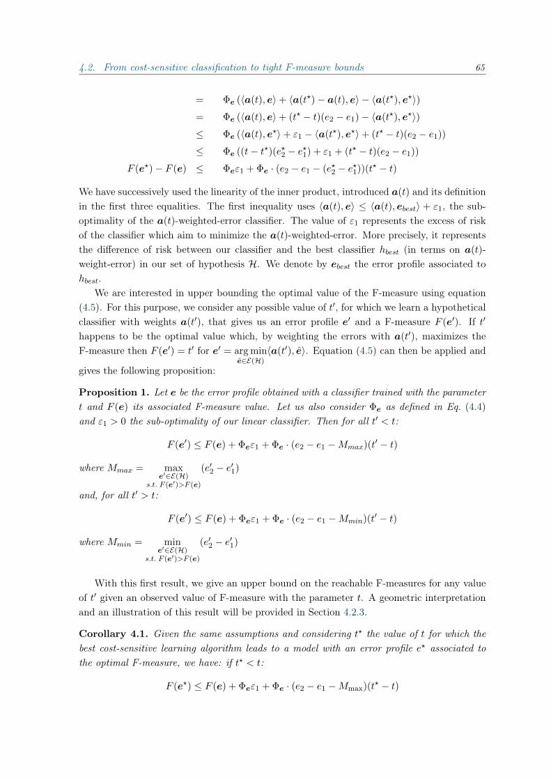
4.2. From cost-sensitive classification to tight F-measure bounds 65
= Φe (〈a(t), e〉+ 〈a(t?)− a(t), e〉 − 〈a(t?), e?〉)= Φe (〈a(t), e〉+ (t? − t)(e2 − e1)− 〈a(t?), e?〉)≤ Φe (〈a(t), e?〉+ ε1 − 〈a(t?), e?〉+ (t? − t)(e2 − e1))
≤ Φe ((t− t?)(e?2 − e?1) + ε1 + (t? − t)(e2 − e1))
F (e?)− F (e) ≤ Φeε1 + Φe · (e2 − e1 − (e?2 − e?1))(t? − t)
We have successively used the linearity of the inner product, introduced a(t) and its definitionin the first three equalities. The first inequality uses 〈a(t), e〉 ≤ 〈a(t), ebest〉 + ε1, the sub-optimality of the a(t)-weighted-error classifier. The value of ε1 represents the excess of riskof the classifier which aim to minimize the a(t)-weighted-error. More precisely, it representsthe difference of risk between our classifier and the best classifier hbest (in terms on a(t)-weight-error) in our set of hypothesis H. We denote by ebest the error profile associated tohbest.
We are interested in upper bounding the optimal value of the F-measure using equation(4.5). For this purpose, we consider any possible value of t′, for which we learn a hypotheticalclassifier with weights a(t′), that gives us an error profile e′ and a F-measure F (e′). If t′
happens to be the optimal value which, by weighting the errors with a(t′), maximizes theF-measure then F (e′) = t′ for e′ = arg min
e∈E(H)〈a(t′), e〉. Equation (4.5) can then be applied and
gives the following proposition:
Proposition 1. Let e be the error profile obtained with a classifier trained with the parametert and F (e) its associated F-measure value. Let us also consider Φe as defined in Eq. (4.4)and ε1 > 0 the sub-optimality of our linear classifier. Then for all t′ < t:
F (e′) ≤ F (e) + Φeε1 + Φe · (e2 − e1 −Mmax)(t′ − t)
where Mmax = maxe′∈E(H)
s.t. F (e′)>F (e)
(e′2 − e′1)
and, for all t′ > t:
F (e′) ≤ F (e) + Φeε1 + Φe · (e2 − e1 −Mmin)(t′ − t)
where Mmin = mine′∈E(H)
s.t. F (e′)>F (e)
(e′2 − e′1)
With this first result, we give an upper bound on the reachable F-measures for any valueof t′ given an observed value of F-measure with the parameter t. A geometric interpretationand an illustration of this result will be provided in Section 4.2.3.
Corollary 4.1. Given the same assumptions and considering t? the value of t for which thebest cost-sensitive learning algorithm leads to a model with an error profile e? associated tothe optimal F-measure, we have: if t? < t:
F (e?) ≤ F (e) + Φeε1 + Φe · (e2 − e1 −Mmax)(t? − t)

66 Chapter 4. Cost-sensitive learning for imbalanced data
and, if t? > t:
F (e?) ≤ F (e) + Φeε1 + Φe · (e2 − e1 −Mmin)(t? − t)
This means that if we learn a model with a parameter t sufficiently close to t? then, weguarantee to reach the optimal F-measure up to a constant equal to Φeε1.
4.2.3 Geometric interpretation and algorithm
In this section we provide a geometric interpretation of our main result, i.e. Proposition 1 ofSection 4.2.2 and compare it to the bound introduced in Parambath et al. (2014). We alsoshow how this theoretical result can be an inspiration to create an algorithm, CONE, whichoptimizes the F-measure by wrapping a cost-sensitive learning algorithm.
Figure 4.2 – Geometric interpretation of both theoretical results: our bound on the left andthe one from Parambath et al. (2014) on the right. Note that our “cone” is not symmetriccompared to the other one. On the left, the slanted values represent the slope of our cone oneach side : Φe · (e2 − e1 −Mmax) and Φe · (e2 − e1 −Mmin).
Unreachable regions In Fig. 4.2 (left), we give a geometric interpretation of the resultfrom Prop. 1 in the 2-D space where t is the x-axis and F is the y-axis. In this (t, F ) graph, theprevious near-optimality result yields an upper cone of values where F (e?) cannot be found.More precisely, when a model is learned for a given value of t (with weights a(t)), we measurethe value F (e) of this model and, given these two numbers, we are able to draw an upper conewhich represents the unreachable values of F-measure for any t′ on the x-axis. Furthermore,given ε1, the sub-optimality of the cost-sensitive learning algorithm for the weighted-0/1 loss,Φeε1 corresponds to the vertical offset of this cone, which means that the peak of the cone islocated at (t, F (e) + Φeε1).
Note that, even if the authors were focusing on asymptotic results, the bound givenin Parambath et al. (2014) can also be interpreted geometrically. Their bound is given as

4.2. From cost-sensitive classification to tight F-measure bounds 67
Input: training set S,Input: weighted-learning algorithm wLearn,Input: stopping criterion shouldStop.
Initialize L = 0, 1, Z0 = ∅ and i = 1.repeatti = findNextT (Zi−1, L)
classifieri = wLearn(1 + β2 − ti, ti, S)
Fi = Fβ(classifieri, S)
Vi = unreachableZone(ti, Fi, S, classifieri)
Zi = Zi−1 ∪ ViL = L ∪ tii = i+ 1
until shouldStop(i, classifieri, Zi, L)
(a) Pseudo-code.
(b) Illustration of the CONE algorithmin the middle of its fourth iteration. Thecolored areas represent the unreachableregions in the (t, F )-space.
Figure 4.3 – CONE Algorithm.
follows:
F (e?) ≤ F (e) + Φ · (2ε0M + ε1)
where M = maxe∈E(H)
‖e‖2, Φ = (β2P )−1 and ε0 is a gap parameter defined as the `2 norm of
the difference between a weighted function a and the optimal one a?. In Section C.1.3, wedetail how this bound can, in fact, be rewritten for all t, t′ ∈ [0, 1] as:
F (e′) ≤ F (e) + Φε1 + 4MΦ|t′ − t|
This bound also defines a cone which is, this time, symmetric with a slope equal to 4ΦM , asillustrated in Fig. 4.2 (right). Using real datasets, Section 4.2.4 compares the cones producedby this bound and ours.
A bound-inspired algorithm We now leverage the geometric interpretation from Sec-tion 4.2.3 to design CONE (Cone-based Optimal Next Evaluation), an iterative algorithmthat wraps a cost-sensitive classification algorithm (e.g., a weighted SVM). At every itera-tion i, CONE proposes a new value ti to be used by the cost-sensitive algorithm. CONE isillustrated in Fig. 4.3b and is explained below.
The choice of ti is based on the area Zi−1 which we define as the union of all cones obtainedfrom previous iterations. ti is chosen to reduce the maximum value of F for which (t, F ) isnot in any previous cone. To achieve this goal, CONE keeps track of a list L, initializedwith the values 0 and 1, and enriched at each iteration with the values of t that have beenconsidered. The selection of ti is done as follows: (i) search the value topt which maximizesFmax(t) = maxF, (t, F ) /∈ Zi−1, (ii) search for the greatest value tl in L such that tl < topt

68 Chapter 4. Cost-sensitive learning for imbalanced data
and the smallest value tr such that topt < tr. (iii) take the middle of the interval [tl, tr] as the
return value, i.e. ti =1
2(tl + tr).
The cost sensitive classification algorithm then provides a new value of Fi obtained fromcost ti, which is used to refine the unreachable area as Zi = Zi−1 ∪ Vi, where Vi is the conecorresponding to (ti, Fi). In the case where there are multiple values of t that maximizeFmax(t) (e.g., at the beginning, or when some range of t values yield F = 1), CONE selectsas topt the middle of the widest range at the first stage (i) (see the white dotted lines inFig. 4.3b).
From a practical perspective, Zi can be represented as a combination of linear constraintsor as a very dense grid of binary values (a rasterization of [0, 1] × [0, 1], the (t, F ) space).Both approaches can be made efficient (and negligible compared to wLearn). The stoppingcriterion shouldStop can take different forms including a fixed number of iterations, a fixedtime budget, or some rules on the current best F-measure and the current upper boundmaxt Fmax(t). While the algorithm we describe selects a single next value of t to consider,it can easily be generalized to produce multiple values of t to consider in parallel (to exploitparallel computing of multiple instances of wLearn).
By always selecting a ti that is in the middle of two previously tested t-values, CONEperforms a progressive refinement of a grid. We can (and do, in practice) restrict the valuesof t in the (t, F )-space that the algorithm considers. More precisely, we can limit the depthof the progressive refinement to an integer value k. In this case, and CONE will do at most2k − 1 iterations, in order to cover all possible values on a grid with stride 1
2k. However, as
the procedure is informed by the theoretical bounds, we will see in Section 4.2.4 that CONEfinds good models in its very first iterations.
4.2.4 Experiments
The experiments from this section study the tightness of our bounds and behavior of theCONE algorithm.
Datasets and experimental settings Table 4.2 describes the datasets we used for ourexperiments, with their Imbalance Ratio (I.R.). The higher this ratio, the more one shouldexpect that optimizing the classification accuracy is a bad choice in terms of trade-off betweenprecision and recall. The datasets IJCNN’01 and News20 are obtained from LIBSVM1. Theother ones come from the UCI repository2.
We reproduce the experimental settings from Parambath et al. (2014) which we describehere. For datasets with no explicit test set, 1
4 of the data is kept for testing. The training setis split at random, keeping 1
3 as the validation set, used to select the hyper-parameters usingthe F1-measure. The penalty constraint of the classifiers (hyper-parameter C) is consideredin 2−6, 2−5, ..., 26. In the experiments t is taken in [0, 1] as t belongs in the image space ofthe F-measure. Thus, the class weights a(t) belongs to [0, 1 + β2]. The maximal number of
1https://www.csie.ntu.edu.tw/~cjlin/libsvm/2https://archive.ics.uci.edu/ml/datasets.html

4.2. From cost-sensitive classification to tight F-measure bounds 69
Table 4.2 – Datasets details. The Imbalance Ratio (I.R.) is the ratio between negative andpositive instances (or between sizes of the largest and smallest classes, in a multiclass setting).
Dataset Instances Classes I.R. FeaturesAdult 48 842 2 3.19 123
Abalone10 4 174 2 5.64 10SatImage 6 400 2 9.3 36IJCNN’01 141 691 2 9.39 22Abalone12 4 174 2 15.18 10PageBlocks 5 500 2 22.7 10
Yeast 1 484 2 27.48 8Wine 1 599 2 28.79 11Letter 20 000 26 1.32 16News20 19 928 20 1.12 62 061
training iterations is set to 50 000. Fitting the intercept of the classifiers is achieved by addinga constant feature with value 1. We report test-time F1-measure averaged over 5 experiments.
We consider two different base cost-sensitive classification algorithms (both implementa-tions use LIBLINEAR): linear SVM and Logistic Regression (LR) for a fair comparison withKoyejo et al. (2014). We report the performance of 5 different approaches: using a singlestandard classification algorithm with hyperparameters tuned on the F-measure, the Gridwrapper proposed in Parambath et al. (2014) that regularly splits the interval [0, 1] of t values,the algorithm derived from our theoretical study, algorithm 2 from Narasimhan et al. (2015)based on the bisection method, and finally, an additional baseline (with the I.R. subscript),which consists in using a cost that re-balances the classes (the cost c of a False Negative isthe proportion of positive examples in the dataset and the cost of False Positive is 1− c).
About ε1 The value of ε1 (in all presented bounds) represents the a(t)-weighted sub-optimality of the classifier, compared to the best one from the hypothesis class. This sub-optimality cannot be computed efficiently as it would require a learning algorithm that pro-duces optimal classifiers in terms of a(t)-weighted error. We thus start by studying the impactof ε1 in Section 4.2.4 on our bounds. As the focus of this work is not on estimating ε1, we thenset ε1 = 0 which is computationally free, and shown by the experiment to be a reasonablechoice both in terms of bound analysis (the bound is most of the time respected) and in termsof overall results from the CONE algorithm.
Evaluation of the tightness of the bound In this section, we aim at illustrating andshowing the tightness of our bounds. To do so, we consider the (t, F ) values obtained by 19weighted-SVM learned on a regular grid of t values. For these same 19 models, we consider thecones obtained from our bounds and previous work (see Section 4.2.3 for details). For clarity,

70 Chapter 4. Cost-sensitive learning for imbalanced data
Table 4.3 – Classification F-measures for β = 1 with SVM and Logistic Regression algorithms.SVMG and LRTG are reproduced experiments of Parambath et al. (2014) and the subscript
I.R. is used for the classifiers trained with a cost depending on the Imbalance Ratio. Thesubscript B corresponds to the bisection algorithm presented by Narasimhan et al. (2015).LRT and LRTI.R. are reproduced experiments of Koyejo et al. (2014). Finally the C stands forour wrapper CONE and SVMT
C designed as a combination using the CONE + threshold.Reported F-measure values are averaged over 5 experiments (standard deviation betweenbrackets).
Dataset SVM SVMI.R. SVMG SVMC SVMTC LRT LRT
I.R. LRTG LRB
Adult 62.5 (0.2) 64.9 (0.3) 66.4 (0.1) 66.5 (0.1) 66.4 (0.1) 66.5 (0.1) 66.5 (0.1) 66.5 (0.1) 66.6 (0.1)
Abalone10 0.0 (0.0) 30.9 (1.2) 32.4 (1.3) 32.2 (0.8) 31.8 (1.9) 30.8 (2.2) 30.7 (1.9) 30.7 (1.9) 31.6 (0.6)
Satimage 0.0 (0.0) 23.4 (4.3) 20.4 (5.3) 20.6 (5.6) 30.9 (2.0) 21.2 (11.1) 28.6 (1.9) 28.6 (1.9) 21.4 (4.6)
IJCNN 44.5 (0.4) 53.3 (0.4) 61.6 (0.6) 61.6 (0.6) 62.6 (0.4) 59.4 (0.5) 56.5 (0.3) 56.5 (0.3) 59.2 (0.3)
Abalone12 0.0 (0.0) 16.8 (2.7) 16.8 (4.2) 18.3 (3.3) 16.3 (3.0) 15.5 (3.1) 17.0 (3.3) 17.0 (3.3) 17.7 (3.7)
Pageblocks 48.1 (5.8) 39.6 (4.7) 66.4 (3.2) 62.8 (3.9) 67.6 (4.0) 59.2 (8.1) 55.9 (6.4) 55.9 (6.4) 55.7 (5.7)
Yeast 0.0 (0.0) 29.4 (2.9) 38.6 (7.1) 39.0 (7.5) 35.4 (15.6) 37.4 (10.1) 39.9 (6.5) 27.6 (6.8) 27.6 (6.8)
Wine 0.0 (0.0) 15.6 (5.2) 20.0 (6.4) 22.7 (6.0) 19.3 (7.9) 21.5 (3.7) 25.2 (4.5) 25.2 (4.5) 18.3 (7.2)
Letter 75.4 (0.7) 74.9 (0.8) 80.8 (0.5) 81.0 (0.3) 81.0 (0.4) 82.9 (0.3) 82.9 (0.3) 82.9 (0.3) 74.9 (0.5)
News20 90.9 (0.1) 91.0 (0.2) 91.1 (0.1) 91.0 (0.1) 91.0 (0.1) 90.6 (0.1) 90.6 (0.1) 90.6 (0.1) 89.4 (0.2)
Average 32.1 (0.7) 44.0 (2.3) 49.5 (2.9) 49.6 (2.8) 50.4 (3.0) 48.8 (1.0) 48.2 (2.3) 49.1 (3.6) 47.0 (3.9)
we show only two illustrations, with two different datasets, but the Appendix C containssimilar illustrations for all datasets.
Impact of ε1 Both our bounds and the one from previous work are impacted by ε1
which shows up as an offset, multiplied by Φe for our bounds, and by Φ in previous work. AsΦe ≤ Φ, our bounds are less impacted by an increased ε1. With the 19-SVM setting, Fig. 4.4shows the evolution of the maximum still-achievable F-measure depending on the value of ε1,with a hard maximum at 1. The values of ε1 are expressed in number of points for an easierinterpretation.
The bound from Parambath et al. (2014) gives loose guarantees and the aggregate boundis most of the time above 1. The values, before being clipped to 1 can for example start atF = 7 and end up at F = 40 (on Yeast, if plotted on the same range of ε1 values). Thisrepresentation shows once again that our bounds are very tight. On Abalone10 and Letter,where the other bound starts below 1, the graph also confirms the fact that our bounds areless sensitive to the value of ε1 (Φe ≤ Φ).
Visualizing unreachable zones The grayed-out areas in Fig. 4.5 are the unreachablezones. This figure shows that the guarantees obtained with our bounds are much more relevantthan the ones from Parambath et al. (2014). Indeed, it is only on two datasets (Abalone10and Letter) that the previously existing bound actually gives a maximum possible F-measurethat is below 1. Our bounds give unreachable zones that go very close to the empirical points.
Looking at the cones with our tight bounds, we see that sometimes a point is in the cone
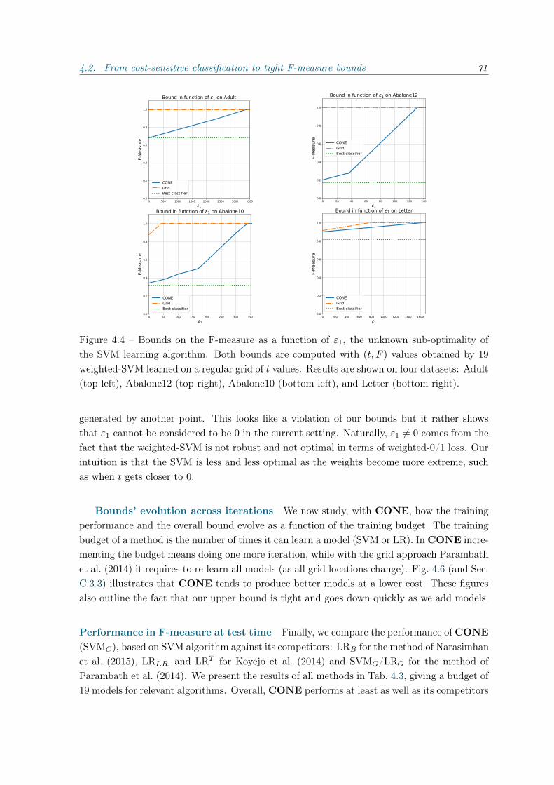
4.2. From cost-sensitive classification to tight F-measure bounds 71
Figure 4.4 – Bounds on the F-measure as a function of ε1, the unknown sub-optimality ofthe SVM learning algorithm. Both bounds are computed with (t, F ) values obtained by 19weighted-SVM learned on a regular grid of t values. Results are shown on four datasets: Adult(top left), Abalone12 (top right), Abalone10 (bottom left), and Letter (bottom right).
generated by another point. This looks like a violation of our bounds but it rather showsthat ε1 cannot be considered to be 0 in the current setting. Naturally, ε1 6= 0 comes from thefact that the weighted-SVM is not robust and not optimal in terms of weighted-0/1 loss. Ourintuition is that the SVM is less and less optimal as the weights become more extreme, suchas when t gets closer to 0.
Bounds’ evolution across iterations We now study, with CONE, how the trainingperformance and the overall bound evolve as a function of the training budget. The trainingbudget of a method is the number of times it can learn a model (SVM or LR). InCONE incre-menting the budget means doing one more iteration, while with the grid approach Parambathet al. (2014) it requires to re-learn all models (as all grid locations change). Fig. 4.6 (and Sec.C.3.3) illustrates that CONE tends to produce better models at a lower cost. These figuresalso outline the fact that our upper bound is tight and goes down quickly as we add models.
Performance in F-measure at test time Finally, we compare the performance ofCONE(SVMC), based on SVM algorithm against its competitors: LRB for the method of Narasimhanet al. (2015), LRI.R. and LRT for Koyejo et al. (2014) and SVMG/LRG for the method ofParambath et al. (2014). We present the results of all methods in Tab. 4.3, giving a budget of19 models for relevant algorithms. Overall, CONE performs at least as well as its competitors
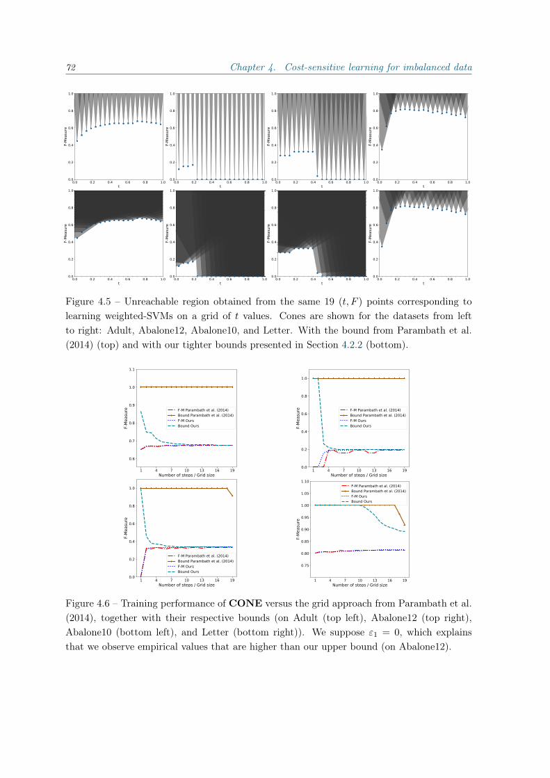
72 Chapter 4. Cost-sensitive learning for imbalanced data
Figure 4.5 – Unreachable region obtained from the same 19 (t, F ) points corresponding tolearning weighted-SVMs on a grid of t values. Cones are shown for the datasets from leftto right: Adult, Abalone12, Abalone10, and Letter. With the bound from Parambath et al.(2014) (top) and with our tighter bounds presented in Section 4.2.2 (bottom).
Figure 4.6 – Training performance of CONE versus the grid approach from Parambath et al.(2014), together with their respective bounds (on Adult (top left), Abalone12 (top right),Abalone10 (bottom left), and Letter (bottom right)). We suppose ε1 = 0, which explainsthat we observe empirical values that are higher than our upper bound (on Abalone12).

4.2. From cost-sensitive classification to tight F-measure bounds 73
in average, and the very best results are obtained by combining CONE with thresholding.The baseline of using a simple SVM completely fails on half of the datasets. The improved
SVM which consists in rebalancing the classes (SVMI.R.) still performs worse than otherapproaches in average, and on most datasets. Even with thresholding, the approaches thatlearn a single model (LRT and LRTI.R.) are still outperformed by the ones that learn multiplemodels with different class-weights like ours (all subscripts C) and the grid one (subscripts
G). This last result shows that it is insufficient to solely rely on tuning the threshold of asingle model.
In average, both our approach and the grid approach outperform all other consideredapproaches, including the bisection algorithm LRB. We see that the results of CONE arevery similar to the grid approach SVMG. However, looking at Fig. 4.7 (but also in Sec.C.3.4), we see that the proposed method is able to reach higher values with a limited numberof iterations, i.e. after training fewer models.
Figure 4.7 – F-measure obtained on the test set for four considered approaches on Adult (topleft), Abalone12 (top right), Abalone10 (bottom left), and Letter (bottom right) datasets,plotted as a function of the computing budget (number of weighted SVM to learn).
4.2.5 Conclusion
In this work, we have presented new bounds on the F-measure based on a cost-sensitiveclassification approach. These bounds have been shown to be tighter than existing ones andless sensitive to the sub-optimality of the learned classifier (ε1). Furthermore, we have shownthat our bounds are useful from a practical point of view by deriving CONE, an algorithmwhich iteratively selects class weights to reduce the overall upper bound on the optimal F-measure. Finally, CONE has been shown to perform at least as well as its competitors onvarious datasets.If this work focuses on the F-measure, it can be generalized to any other linear-fractionalperformance measure.Our perspectives include estimating ε1 (for example using (Bousquet et al., 2004)), refining ourframework to improve the search space exploration, and deriving generalization guarantees.

74 Chapter 4. Cost-sensitive learning for imbalanced data
We will also explore solutions to adapt it to SGD-based learning algorithms, so that we couldapply it with our architecture on the Bluecime dataset.

Chapter 5
Questioning the usual domainadaptation results
Domain adaptation is often presented as a technique to learn a model on labeled examplesfrom one data distribution (Source) and apply it on unlabeled example from another datadistribution (Target). In this Chapter, we explore domain adaptation in the multi-Sourcesetting where two question arise: Should we use all our sources? What if there is a discrepancybetween the sources and the target class distribution? To answer these questions, we will firstpropose an approach on selecting the best sources domains for a target. We then questionour domain adaptation results in our context with varying class distribution.
5.1 Source domains selection for domain adaptation
We present in this section our approach on selection the best sources domains used in thetraining set for learning the best classifier for a given target domain. This work was presentedin Bascol et al. (2019a), at The 26th International Conference on Image Processing (ICIP2019).
5.1.1 Introduction
The currently unpublished work from Schultz et al. (2018) is the closest to ours. The authorspropose to select multiple domains according to four possible distances (the χ2-divergence, theMaximum Mean Discrepancy, the Wasserstein distance and the Kullback-Liebler divergence)and according to the classification performance on each single source domain. Both thedistance and the performance features are weighted by a parameter β computed as:
β = arg minβ≥0
D∑i=1
D∑k=1;k 6=i
|ξ(Zi,Zk)− βf(Zi,Zk)|
with Z1...D the examples from the different domains, f the set of comparison operatorsconsidered by the authors and ξ(Zi,Zk) the performance of the classifier trained on Zi and
75

76 Chapter 5. Questioning the usual domain adaptation results
tested on Zk. The authors show that on a homogeneous dataset, their method is better thanrandomly selecting the domains but not better than when using all of them. However, on aheterogeneous dataset, selecting the sources with their proposed distance is better than bothselecting all the domains and selecting them randomly. Note that to optimize β, D classi-fiers should be trained which can be costly in practice (especially for deep neural networks).Besides, the authors do not provide any criterion to set the number of selected sources.
Domain Selection and Weighting Considering a target domain j and D source domains,we propose an approach that automatically computes a weight vector pj ∈ ∆D−1 ⊂ RD
(probability simplex) and uses pj to reweight the domains (when sampling minibatches) during“domain-adversarial training” (Ganin et al., 2016). This training phase is usually done tofine-tune a pre-trained network. The proposed approach is modular as we decompose thecomputation of the domains weight vector pj in three configurable steps :
1. the distance vector dj =dji
Di=1
is computed (distance of each source domain, i, tothe target one, j),
2. it is mapped to a score vector sj = score(dj),
3. it is normalized to a probability vector pj = sj/∑
i sji .
5.1.2 Distance between domains
We define, in this section, the different distances we explored in our work. To reduce thecomputational charge, and also to obtain more relevant distances, we compute the distanceson features extracted from the convolutional part of a ResNet50 pre-trained on ImageNet.
Euclidean distance The first distance is simply computed by taking the average minimalEuclidean distance between the examples of every domains, so that:
dji =1
|Xi|∑x1∈Xi
minx2∈Xj
‖x1 − x2‖
with Xi and Xj the examples of the ith and jth domains, and |Xi| the number of examplesin domains i.
Silhouette score If we consider the different domains sets as different clusters we can usemetrics measuring if clusters are well-defined. In our case, we can compute the Silhouettescore on examples from two domains. If the score is high, the clusters are well-defined, thus thedomains are far from each other. If the score is small, the clusters are difficult to distinguish,thus the domains are close. So, we can use this score directly as a distance between thedomains (the smaller the closer).
The Silhouette score is computed on a set of point X by:

5.1. Source domains selection for domain adaptation 77
Ss(X) =1
|X|∑x∈X
f(x,Cn)− f(x,Cx)
max(f(x,Cx), f(x,Cn))
where f(x,Cx) is the mean distance between x and all the examples of the cluster con-taining x. Cn corresponds to the nearest cluster (other that Cx) to x. In our context, toobtain our distance we can formulate this score as:
dji =1
|Xj |∑x∈Xj
f(x,Xi)− f(x,Xj)
max(f(x,Xj), f(x,Xi))
Calinski-Harabaz score In the same way as the Silhouette score, we can use the Calinski-Harabaz score which also measures if clusters are well-defined.
The Calinski-Harabaz score is computed on a set of point X by:
Sch(X) =Tr(B(X))
Tr(W (X))× |X| − k
k − 1
B(X) =k∑c=1
|Xc|(cen(Xc)− cen(X))(cen(Xc)− cen(X))T
W (X) =k∑c=1
∑x∈Xc
(x− cen(Xc))(x− cen(Xc))T
with k the number of clusters, Xc the cluster of index c, and cen(X) the centroid of theset of points X. We can then define our distance:
dji = Sch(Xi ∪Xj) such that Xi and Xj are considered as two clusters
Auto-encoders We consider that if a source example is well reconstructed by an auto-encoder trained on a target domain, the example should belong to a domain close to thetarget one. We thus can use the reconstruction error directly as a distance (the smaller thecloser). So, to compute the distances we train an auto-encoder per domain. Then, we doforward passes with the examples from the other domains and average the reconstructionerrors obtained, so that: dji = averagex∈Xi
‖x−AEj(x)‖2.
Wasserstein distance In the optimal transport problem (see Section 1.3.2), the minimaldisplacement cost is called the Wasserstein distance and constitutes a distance between dis-tribution. In our discrete case (samples of points), the distance can be expressed as:
dji =∑x∈Xj
∑y∈Xi
γ?x,yCx,y
where C is a distance matrix between all pair of elements of the two domains, and γ?
is the optimal transport plan. Note that, two sets of points, even if drawn from the samedistribution, will exhibit a variable non-zero Wasserstein distance.
78 Chapter 5. Questioning the usual domain adaptation results
We will present, in Section 5.1.4, different experiments we conducted during the develop-ment of our approach to compare the different distances cited above. We will see that theseresults led us to choose the Wasserstein distance.
5.1.3 Domains selection method
One way to select the source domains in the training set could be to completely remove thedomains too far from the target one. The threshold value should then represent a trade-off between the benefit of adding data from a domain and the possible negative transfer itwould induce. Such thresholding method raises a question on what to do with domains withdistances surrounding the threshold value. Indeed, is it right to equally consider a domainassociated with a distance just above the threshold and the nearest domain? Conversely, isa domain with a distance slightly below the threshold completely harmful to the training?These questions led us to use to consider another method to select the source domains. Wepresent in this section a smoother method to select the domains based on the derivation ofselection probabilities from the distances, then used to change the domain proportions in thetraining set.
Transforming distances into scores Possible score functions include the inverse distances(1d) or the inverse squared distances ( 1
d2). Here, we focus on the negative exponential scoring
function:sji = e−λd
ji
The parameter λ allows a smooth interpolation between putting all the weight on theclosest domain and having a uniform distribution of all domains. Thanks to this parameter,we will be able to control the variety of the subset of domains we are considering (see below).
Ensuring training set variety In case of many source domains and when some of themhave a very small number of training examples, it becomes important to avoid selecting toofew domains in the process (e.g., a single one). For generalization (i.e. avoiding overfitting)and transfer purpose, the training set should exhibit enough variety. For domain sizes n ∈ ND,a probability vector pj and a draw of N training samples (with replacement), we define thetraining set variety as the expected number of distinct samples we will use during each epoch.The variety can be approximated as:
variety(pj , n,N) ≈∑i
ni ·
1−
(1−
pjini
)NOur probability vector pj depends on the λ parameter. As such, by varying λ from ∞
to 0, we can move from a minimal variety (sampling from the closest domain i, getting adiversity of approximately ni, the number of examples in this closest domain) to a maximalone (using a uniform pj , getting a variety of N − N
(N−1N
)N ≈ 0.63N in case of a balancedn). In the experiments, we consider one epoch (with replacement) of N =
∑i ni samples. We
use pj and n to find the highest value of λ for which the variety is below a target variety.
5.1. Source domains selection for domain adaptation 79
5.1.4 Experiments
In this section, we first present the datasets settings used in our domain adaptation exper-iments. We then presents results, first on the choice of a distance, then on the completeapproach.
5.1.4.1 Datasets
Office-Caltech (O-C) This dataset, published by Gong et al. (2012), is a classical domainadaptation benchmark with four domains: Amazon (A), DSLR (D), Webcam (W) and Caltech(C). It is composed of the 10 classes (Backpack, Bike, Calculator, Headphones, Keyboard,Laptop, Monitor, Mouse, Mug, and Video-projector) common between the datasets Office-31 (Saenko et al., 2010) and Caltech256 (Griffin et al., 2007), both presented in Section 2.1.1.
ImageNet-Caltech (I-C) To control the discrepancy between each domain and validateour chosen domain similarity measure, we have designed a dataset using images from Cal-tech101 (Fei-Fei et al., 2007) (C1), Caltech256 (Griffin et al., 2007) (C2) and from Ima-geNet (Deng et al., 2009) (IN), all presented in Section 2.1.1. This dataset is composed ofthree different types of domain: the “Good” (G_) domains are created with images with theirtrue original classes, the “Bad” (B_) domains are created with images associated to differentbut similar original classes, and the “Random” (R_) domains are created with images labeledwith randomly chosen classes in the corresponding datasets. We use five classes: “bird”, “car”,“chair”, “dog”, and “person” (following, among others, Khosla et al. (2012); Fang et al. (2013)).We give the corresponding true classes for each domain in Table 5.1. With this design, the“Good” domains are expected to be closer to each other since their corresponding images areshowing the same objects. The “Bad” domains should be farther away from the “Good” onesand the “Random” domains should be the farthest (and are expected to be far from eachothers too).
Bluecime. Here, we use the 2018 release of the Bluecime dataset (see Section 2.1.2).
5.1.4.2 Distance choice
We present in Table 5.2, results obtained at different development stages of our approachleading us to choose the Wasserstein distance as our preferred distance between the domains.The first four experiments are conducted on the 2017 Bluecime dataset, “7S” indicates thatwe use the seven nearest sources in the training sets according to the silhouette score (“silh”),to the Calinski-Harabaz score (“chs”), and to autoencoders reconstruction errors (“ae”). Usinga distance based on the autoencoders reconstruction error provides better results than blindlyusing all the domains (chairlifts), which validates our approach. Moreover, this setting alsoyields better results than using the seven nearest domains according to both silhouette andCalinski-Harabaz clustering scores.
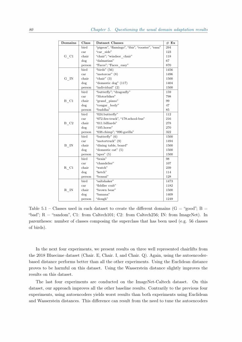
80 Chapter 5. Questioning the usual domain adaptation results
Domains Class Dataset Classes # Exbird “pigeon”, “flamingo”, “ibis”, “rooster”, “emu” 294car “car_side” 123
G_C1 chair “chair”; “windsor_chair” 118dog “dalmatian” 67person “Faces”; “Faces_easy” 870bird “birds” (56) 1456car “motorcar” (8) 1496
G_IN chair “chair” (3) 1500dog “domestic dog” (117) 1404person “individual” (2) 1500bird “butterfly”; “dragonfly” 159car “Motorbikes” 798
B_C1 chair “grand_piano” 99dog “cougar_body” 47person “buddha” 85bird “024.butterfly” 112car “072.fire-truck”, “178.school-bus” 216
B_C2 chair “011.billiards” 278dog “105.horse” 270person “038.chimp”; “090.gorilla” 322bird “butterfly” (6) 1500car “motortruck” (9) 1494
B_IN chair “dining table, board” 1500dog “domestic cat” (5) 1500person “apes” (5) 1500bird “brain” 98car “chandelier” 107
R_C1 chair “watch” 239dog “ketch” 114person “bonsai” 128bird “saltshaker” 1473car “fiddler crab” 1182
R_IN chair “brown bear” 1500dog “banana” 1409person “dough” 1249
Table 5.1 – Classes used in each dataset to create the different domains (G = “good”; B =“bad”; R = “random”, C1: from Caltech101; C2: from Caltech256; IN: from ImageNet). Inparentheses: number of classes composing the superclass that has been used (e.g. 56 classesof birds).
In the next four experiments, we present results on three well represented chairlifts fromthe 2018 Bluecime dataset (Chair. E, Chair. I, and Chair. Q). Again, using the autoencoder-based distance performs better than all the other experiments. Using the Euclidean distanceproves to be harmful on this dataset. Using the Wasserstein distance slightly improves theresults on this dataset.
The last four experiments are conducted on the ImageNet-Caltech dataset. On thisdataset, our approach improves all the other baseline results. Contrarily to the previous fourexperiments, using autoencoders yields worst results than both experiments using Euclideanand Wasserstein distances. This difference can result from the need to tune the autoencoders
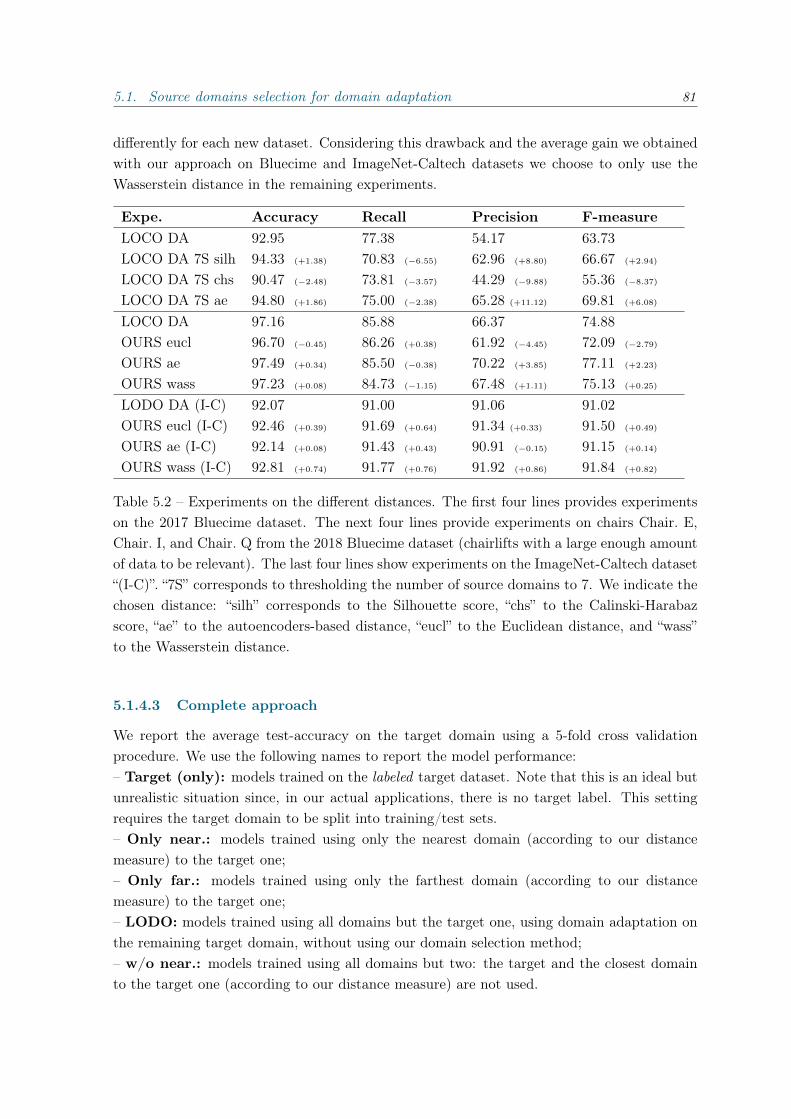
5.1. Source domains selection for domain adaptation 81
differently for each new dataset. Considering this drawback and the average gain we obtainedwith our approach on Bluecime and ImageNet-Caltech datasets we choose to only use theWasserstein distance in the remaining experiments.
Expe. Accuracy Recall Precision F-measureLOCO DA 92.95 77.38 54.17 63.73LOCO DA 7S silh 94.33 (+1.38) 70.83 (−6.55) 62.96 (+8.80) 66.67 (+2.94)
LOCO DA 7S chs 90.47 (−2.48) 73.81 (−3.57) 44.29 (−9.88) 55.36 (−8.37)
LOCO DA 7S ae 94.80 (+1.86) 75.00 (−2.38) 65.28 (+11.12) 69.81 (+6.08)
LOCO DA 97.16 85.88 66.37 74.88OURS eucl 96.70 (−0.45) 86.26 (+0.38) 61.92 (−4.45) 72.09 (−2.79)
OURS ae 97.49 (+0.34) 85.50 (−0.38) 70.22 (+3.85) 77.11 (+2.23)
OURS wass 97.23 (+0.08) 84.73 (−1.15) 67.48 (+1.11) 75.13 (+0.25)
LODO DA (I-C) 92.07 91.00 91.06 91.02OURS eucl (I-C) 92.46 (+0.39) 91.69 (+0.64) 91.34 (+0.33) 91.50 (+0.49)
OURS ae (I-C) 92.14 (+0.08) 91.43 (+0.43) 90.91 (−0.15) 91.15 (+0.14)
OURS wass (I-C) 92.81 (+0.74) 91.77 (+0.76) 91.92 (+0.86) 91.84 (+0.82)
Table 5.2 – Experiments on the different distances. The first four lines provides experimentson the 2017 Bluecime dataset. The next four lines provide experiments on chairs Chair. E,Chair. I, and Chair. Q from the 2018 Bluecime dataset (chairlifts with a large enough amountof data to be relevant). The last four lines show experiments on the ImageNet-Caltech dataset“(I-C)”. “7S” corresponds to thresholding the number of source domains to 7. We indicate thechosen distance: “silh” corresponds to the Silhouette score, “chs” to the Calinski-Harabazscore, “ae” to the autoencoders-based distance, “eucl” to the Euclidean distance, and “wass”to the Wasserstein distance.
5.1.4.3 Complete approach
We report the average test-accuracy on the target domain using a 5-fold cross validationprocedure. We use the following names to report the model performance:– Target (only): models trained on the labeled target dataset. Note that this is an ideal butunrealistic situation since, in our actual applications, there is no target label. This settingrequires the target domain to be split into training/test sets.– Only near.: models trained using only the nearest domain (according to our distancemeasure) to the target one;– Only far.: models trained using only the farthest domain (according to our distancemeasure) to the target one;– LODO: models trained using all domains but the target one, using domain adaptation onthe remaining target domain, without using our domain selection method;– w/o near.: models trained using all domains but two: the target and the closest domainto the target one (according to our distance measure) are not used.
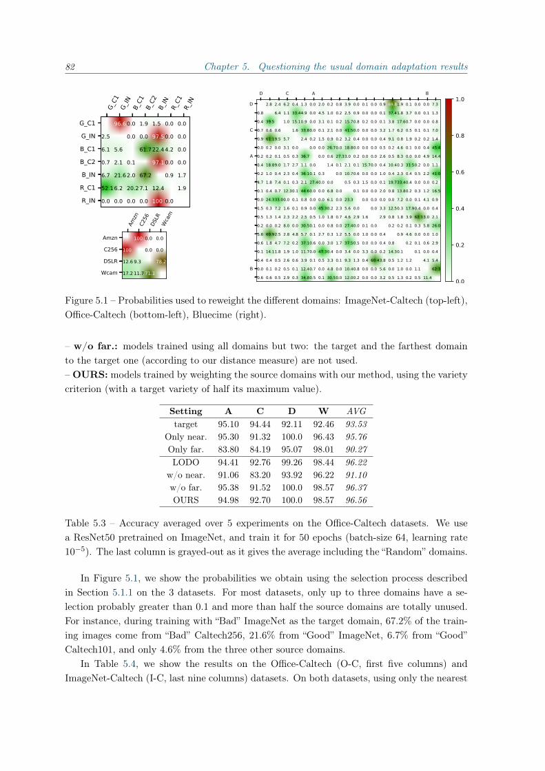
82 Chapter 5. Questioning the usual domain adaptation results
G_C1
G_IN
B_C1
B_C2
B_IN
R_C1
R_IN
G_C1G_INB_C1B_C2B_INR_C1R_IN
2.5
6.1
0.7
6.7
52.1
0.0
96.6
5.6
2.1
21.6
6.2
0.0
0.0
0.0
0.1
2.0
20.2
0.0
1.9
0.0
61.7
67.2
7.1
0.0
1.5
97.5
22.4
97.1
12.4
100
0.0
0.0
4.2
0.0
0.9
0.0
0.0
0.0
0.0
0.0
1.7
1.9
Amzn
C256
DSLR
Wca
m
Amzn
C256
DSLR
Wcam
100
12.6
17.2
100
9.3
11.7
0.0
0.0
71.1
0.0
0.0
78.2
D C A B
D
C
A
B
0.8
0.4
0.7
0.9
0.0
0.2
3.4
0.2
4.7
0.1
0.0
1.5
0.5
0.2
5.6
0.6
0.1
0.4
0.0
0.6
2.8
39.5
0.6
61.1
0.2
0.2
18.8
1.0
1.8
0.4
24.3
0.3
1.3
0.0
60.9
1.8
14.1
0.4
0.1
0.6
2.4
6.4
0.6
9.5
0.0
0.1
9.0
0.4
7.4
0.7
33.0
7.2
1.4
0.2
2.5
4.7
1.8
0.5
0.2
0.5
6.2
1.1
1.0
5.7
3.1
0.5
1.7
2.3
0.1
12.3
0.0
1.6
2.3
8.0
2.8
7.2
1.9
2.6
0.5
2.9
0.4
33.4
15.1
1.6
0.0
0.3
2.7
0.4
0.3
0.1
0.1
0.1
2.2
0.0
4.8
0.2
1.0
0.6
0.1
0.3
1.3
4.9
0.9
33.8
2.4
36.7
1.1
36.1
2.1
44.6
0.8
0.9
2.5
30.5
5.7
37.1
11.7
3.9
12.4
34.8
0.0
0.0
0.0
0.0
0.2
0.0
0.0
0.1
27.4
0.0
0.0
0.0
0.5
0.1
0.1
0.6
0.0
0.1
0.7
0.5
2.0
4.5
3.1
0.1
1.5
0.0
0.0
0.3
0.0
0.0
0.0
45.3
1.0
0.0
2.7
0.0
47.3
0.5
0.0
0.1
0.2
1.0
0.1
2.1
0.9
26.7
0.6
1.4
0.0
6.8
6.1
0.2
1.8
0.8
0.3
3.0
0.4
3.3
4.8
30.5
0.8
0.2
0.2
0.0
0.2
0.0
27.3
0.1
0.0
0.0
0.0
2.3
0.7
0.0
1.2
1.7
0.0
0.1
0.0
0.0
3.9
2.5
15.7
41.5
3.2
18.8
3.0
2.1
10.7
0.5
23.3
5.6
4.6
27.4
5.5
37.5
3.4
9.3
10.4
12.0
0.0
0.9
0.8
0.0
0.4
0.0
0.2
0.1
0.6
0.3
0.1
0.0
2.9
0.0
0.0
0.5
0.0
1.3
0.8
0.2
0.1
0.0
0.2
0.0
0.0
0.0
0.0
15.7
0.0
1.5
0.0
0.0
1.6
0.1
1.0
0.0
3.3
0.4
0.0
0.0
0.0
0.0
0.0
0.0
0.0
0.0
0.0
0.0
0.0
0.0
0.0
0.0
0.0
0.0
0.0
0.0
0.0
60.4
0.0
0.0
0.9
0.1
0.1
3.2
0.4
0.5
2.6
0.4
1.0
0.1
2.0
0.0
3.3
2.9
0.4
0.4
0.2
3.8
5.6
3.2
69.8
37.4
3.8
1.7
9.1
0.2
0.5
10.4
0.4
19.7
0.8
0.0
12.5
0.8
0.2
0.8
14.3
0.5
0.0
0.5
1.9
1.8
17.6
6.2
0.8
4.6
8.3
0.3
2.3
33.4
13.8
7.2
0.3
1.8
0.2
0.9
0.1
1.2
1.0
1.3
0.1
3.7
0.7
0.5
1.9
0.1
0.0
31.5
0.4
0.4
0.2
0.0
17.9
3.9
0.1
4.6
0.2
1.2
0.0
0.2
0.0
0.0
0.0
0.1
0.2
0.0
0.0
0.2
0.5
0.0
0.3
0.1
0.4
62.1
0.3
0.0
0.1
0.1
1.1
0.5
0.0
0.1
0.0
0.1
0.2
0.4
4.9
0.0
2.2
0.0
1.2
4.1
0.0
3.0
5.8
0.0
0.6
0.0
4.1
11.4
7.3
1.3
0.8
7.0
1.4
45.4
14.4
1.1
41.0
0.2
16.5
0.9
0.4
2.1
26.0
1.0
2.9
0.4
5.4
62.3
Figure 5.1 – Probabilities used to reweight the different domains: ImageNet-Caltech (top-left),Office-Caltech (bottom-left), Bluecime (right).
– w/o far.: models trained using all domains but two: the target and the farthest domainto the target one (according to our distance measure) are not used.– OURS: models trained by weighting the source domains with our method, using the varietycriterion (with a target variety of half its maximum value).
Setting A C D W AVGtarget 95.10 94.44 92.11 92.46 93.53
Only near. 95.30 91.32 100.0 96.43 95.76Only far. 83.80 84.19 95.07 98.01 90.27LODO 94.41 92.76 99.26 98.44 96.22
w/o near. 91.06 83.20 93.92 96.22 91.10w/o far. 95.38 91.52 100.0 98.57 96.37OURS 94.98 92.70 100.0 98.57 96.56
Table 5.3 – Accuracy averaged over 5 experiments on the Office-Caltech datasets. We usea ResNet50 pretrained on ImageNet, and train it for 50 epochs (batch-size 64, learning rate10−5). The last column is grayed-out as it gives the average including the “Random” domains.
In Figure 5.1, we show the probabilities we obtain using the selection process describedin Section 5.1.1 on the 3 datasets. For most datasets, only up to three domains have a se-lection probably greater than 0.1 and more than half the source domains are totally unused.For instance, during training with “Bad” ImageNet as the target domain, 67.2% of the train-ing images come from “Bad” Caltech256, 21.6% from “Good” ImageNet, 6.7% from “Good”Caltech101, and only 4.6% from the three other source domains.
In Table 5.4, we show the results on the Office-Caltech (O-C, first five columns) andImageNet-Caltech (I-C, last nine columns) datasets. On both datasets, using only the nearest

5.1. Source domains selection for domain adaptation 83
Setting G_C1 G_IN B_C1 B_C2 B_IN AVG R_C1 R_IN AVGtarget 99.81 96.17 99.56 98.32 98.23 98.42 100.0 98.21 98.61
Only near. 98.09 68.84 34.85 83.79 81.61 86.03 0.00 2.66 61.83Only far. 0.88 14.39 38.97 28.42 24.95 21.52 3.17 12.53 17.62LODO 94.40 87.24 93.86 91.80 91.88 91.67 11.76 9.01 68.56
w/o near. 77.77 75.56 95.72 81.88 86.43 83.47 11.99 5.68 62.15w/o far. 97.20 86.66 96.90 90.16 91.99 92.58 18.27 12.40 70.51OURS 97.54 84.93 97.38 94.73 91.13 93.14 8.89 16.81 70.20
Table 5.4 – Accuracy averaged over 5 experiments on the datasets created from ImageNet andCaltech. We use a ResNet50 pretrained on ImageNet, and train it for 50 epochs (batch-size64, learning rate 10−5). The last column is grayed-out as it gives the average including the“Random” domains.
Setting Chair. A Chair. B Chair. C Chair. D All 21LODO 95.70 98.26 98.28 98.69 95.94OURS 95.63 98.38 98.07 98.94 97.06
Table 5.5 – Accuracy on the Bluecime dataset, averaged on 5 experiments, on a selection of4 domains and on all available domains.
source domains is beneficial compared to using the farthest one (+5.49 accuracy points onO-C and +44.21 pts on I-C) which suggests that our distance is meaningful. On Office-Caltech, using the target domain as source (Target line) gives worse performance than usingthe nearest source (-2.23 pts), which can be explained by the lack of training data whichinduces an overfitting phenomena. Since ImageNet-Caltech contains more data, the Targetsetting is much more suited, as expected, than the Only nearest one (+36.78 pts).
Using the LODO setting (all source domains are used during training), we observe betterperformance than with the Only nearest and Only farthest ones thanks to a more diversetraining set (respectively, on O-C, +0.46 pts and +5.95 pts, on I-C, +6.73 pts and +50.94pts). This means that there is a real trade-off between the domain selection and the number ofremaining training data. However, if we remove the nearest source domain, the performancebecomes worse than for the LODO setting (-5.12 pts on O-C and -6.41 pts on I-C), on Office-Caltech we even get worse performance than using the Only nearest setting (-4.66 pts). If weremove the farthest source domain, we do obtain better performance than with the LODOsetting (+0.15 pts on O-C and +1.95 pts on I-C). We can conclude that using many data(LODO setting) is important and always better than choosing a single domain (even the mostsimilar one) but selecting a good number of sources can be beneficial.
Our distance-based weighting approach provides better performance than removing thefarthest source domain on Office-Caltech (+0.19 pts). On ImageNet-Caltech, we get worseresults than when removing the farthest domain (-0.31 pts), but, still notably better than withthe LODO setting (+1.64 pts). However, if we ignore the results on the “Random” domains(which are close to random by design), on average, the LODO setting gives 91.67% of accuracy,

84 Chapter 5. Questioning the usual domain adaptation results
w/o farthest 92.58%, and our approach allows us to get the best accuracy performance of93.14% which confirms the relevance of our approach.
In Table 5.5, we show the results on the Bluecime dataset. We detail the results on4 relevant domains and give the averaged results over the 21 domains. As with the otherdatasets, we obtain better results by selecting the source domains (+1.12 pts). This showsthat the proposed method works well even when there are much more source domains to selectfrom.
5.2 Multi-source domain adaptation with varying class distri-bution
In this section, we discuss the standard domain adaptation setting in presence of varying classdistributions across the domains. We also present the effects of varying the imbalance ratio onour different domain adaptation results. Then, we study different methods to apply domainadaptation in such context.
5.2.1 Discussion on our previous results
In this section, we discuss our baseline domain adaption results and the ones presented inSection 5.1.
5.2.1.1 Bluecime baseline results
The results on LOCO DA setting presented in the previous sections turned out to be over-optimistic. Indeed, we realized, quite late during this PhD, that due to a mistake in ourcode, the unlabeled target examples used during the training phase to train the adversarialnetwork were automatically balanced over the classes. However, in reality, no labels could havebeen used to balance the target classes. This mistake led us also to question the robustnessof the state-of-the-art domain adaptation techniques. We present in Table 5.6 the LOCOperformance according to (i) the use of domain adaptation or not (ii) the relative classesbalancing in the source and target sets. “bs” means that the source examples are balanced,“ibs” means that the sources examples are imbalanced. Conversely, “bt” and “ibt” mean thatthe target set is respectively balanced and imbalanced. We observe that domain adaptationincreases the performance of our network only when both the source and the target sets arebalanced. Without domain adaptation, balancing the source is not effective (-0.20 pts ofAccuracy compared to imbalanced sources), however, with domain adaptation the oppositeoccurs. Indeed, keeping balancing the source set but not the target set (LOCO DA bs ibt) isthe worst case (-19.53 pts of Accuracy compared to the balanced setting, LOCO bs). In thehypothetical setting where the source set is imbalanced whereas the target is (LOCO DA ibsbt), the Accuracy drop is relatively small (-1.45 pts compared to the setting LOCO ibs) butwe observe a dramatic drop of F-measure (-20.62 pts). If both sets are imbalanced (LOCODA ibs ibt) we also observe a drop of performance (-0.83 pts of Accuracy and -5.62 pts of

5.2. Multi-source domain adaptation with varying class distribution 85
F-measure compared to the LOCO ibs setting), which indicates that domain adaptation doesnot help in this setting.
From these results, we hypothesize that domain adaptation techniques relying on adver-sarial feature training, such as in Ganin et al. (2016), requires both the source and targetclass distributions to be similar to improve the performance.
Expe. Accuracy Recall Precision F-measureLOCO bs 96.52 81.90 81.58 76.73LOCO DA bs bt 97.41 (+0.89) 89.17 (+7.27) 82.94 (+1.36) 83.30 (+6.56)
LOCO DA bs ibt 76.99 (−19.53) 89.69 (+7.79) 27.83 (−53.76) 38.64 (−38.10)
LOCO ibs 96.72 (+0.20) 81.01 (−0.90) 82.33 (+0.75) 77.12 (+0.39)
LOCO DA ibs bt 94.87 (−1.65) 42.17 (−39.73) 88.75 (+7.17) 56.11 (−20.62)
LOCO DA ibs ibt 95.89 (−0.63) 80.40 (−1.50) 73.36 (−8.22) 71.51 (−5.23)
Table 5.6 – LOCO results with and without balancing the target and the sources sets. (i)bindicates experiments with (im)balanced set, s indicates source set and t indicates target set.
To get a better insight into the imbalanced class distributions problem over the sourcesand the target domains, we present results with the One Versus One (OVO) setting, i.e. usingone domain as source and one other domain as target. We present, in Table 5.7, the resultswith this setting between chairlifts (domains) with similar and dissimilar class distributions(we show some additional results in Section B.2). These results confirm that having similarclass distributions is a requirement for domain adaptation to be effective. Moreover, we notethat, in the mono-source setting, adding domain adaptation with imbalanced sets is beneficial,while we observe the opposite in the multi-source setting. This observation may indicate thatin the multi-source domain adaptation setting, with a sufficiently large number of sourcedomains, the training set contains enough variety to generalize well. This could mean thatusing domain adaptation in the multi-source setting could be ineffective. In Table 5.8, weshow results with domain adaptation and balanced sets such that either both source andtarget sets have a uniform class distribution (LOCO DA bs bt), or both have the naturaltarget class distribution (LOCO DA tcdbs ibt). We observe that in both cases the domainadaptation is effective. This shows that using multi-source adaptation is possibly effective, butrequires that the sources class distributions match the target one. In addition, we also observethat using uniform class distribution gives better results in F-measure than the other threesettings. Using natural target class distribution however gives the best results in Accuracy.This is coherent with our class balancing approach presented in Section 3.1.1.
5.2.1.2 Source selection results
In Tables 5.9 and 5.10, we show the same kind of results as the ones from Section 5.1 onOffice-Caltech without balancing the target set and respectively using balanced and imbal-anced sources sets. In mono-source domain adaptation (“only near.”, and “only far.” rows),adding domain adaptation is effective in both “only near.” and one “only far.” settings. These

86 Chapter 5. Questioning the usual domain adaptation results
Expe. ≈ class dist. 6= class dist.OVO bs 86.84 86.84
OVO DA bs bt 91.77 (+4.93) 90.77 (+3.94)
OVO ibs 79.20 (−7.64) 71.14 (−15.69)
OVO DA ibs ibt 93.20 (+6.36) 85.07 (−1.76)
Table 5.7 – One versus one (ovo) Accuracy averaged over domains with similar class distribu-tions and over domains with highly dissimilar class distributions (see more results in TablesB.4, B.5, and B.6). (i)bt and (i)bs indicate experiments with (im)balanced target and sourcesets.
Expe. Accuracy Recall Precision F-measureLOCO bs 96.52 81.90 81.58 76.73LOCO DA bs bt 97.41 (+0.89) 89.17 (+7.27) 82.94 (+1.36) 83.30 (+6.56)
LOCO ibs 96.72 (+0.20) 81.01 (−0.90) 82.33 (+0.75) 77.12 (+0.39)
LOCO DA tcdbs ibt 98.24 (+1.72) 80.38 (−1.52) 85.71 (+4.13) 82.70 (+5.97)
Table 5.8 – LOCO results with the same imbalance ratio between the target and sources sets.(i)b indicates experiments with (im)balanced set, s indicates the source set and t indicates thetarget set. tcdbs indicates that the source is balanced so that it has the same class distributionas the imbalanced target set (using the target labels, given only as reference).
results confirm the effectiveness of the domain adaptation approach in the mono-source set-ting. Moreover, it also confirms the benefit of our approach on selecting the source domain.However, in multi-source domain adaptation (“LOCO”, “w/o near.”, “w/o far.”, and “OURS”rows), in both balanced settings only the “w/o far.” setting presents successful domain adap-tation results. This suggests that our domain selection approach is effective when thresholdingthe number of sources. However, changing the selection probability of the source examplesaccording to the domain requires to have similar class distribution in both the target and thesource sets.
5.2.2 Improving our approach
In this section we study two possible methods to deal with the discrepancy between the sourcesclass distribution and the target class distribution.
5.2.2.1 Finding the target class distribution
In Hoffman et al. (2016), the authors propose to apply domain adaptation on semantic seg-mentation problems, a field of machine learning where each pixel of an image is classified.Their approach is an adversarial method, such as Ganin et al. (2016), but adapted to seman-tic segmentation. Indeed, the prediction of the domain discriminator is considered over all the

5.2. Multi-source domain adaptation with varying class distribution 87
Setting A A+DA C C+DA D D+DA W W+DA AVG AVG+DAtarget 95.52 95.59 95.88 95.61 98.11 98.11 97.50 98.65 96.75 96.99
only near. 94.66 94.64 87.20 89.71 98.85 100.00 99.64 97.14 95.09 95.37only far. 85.88 86.38 79.46 83.14 94.74 90.48 91.04 95.17 87.78 88.79LOCO 94.26 91.55 91.16 91.53 100.00 96.63 98.93 98.29 96.09 94.50
w/o near. 88.87 89.57 83.96 79.94 90.07 89.25 90.68 93.82 88.40 88.15w/o far. 94.89 94.97 90.81 91.99 100.00 100.00 98.93 98.93 96.16 96.47OURS 94.35 93.81 87.40 91.35 99.26 99.59 99.29 97.22 95.49 95.08
Table 5.9 – Results (in Accuracy) comparable to the ones in Table 5.4 but with imbalancedtarget set, and balanced source set. The columns with “+DA” indicates the results usingthe domain adaptation component.
Setting A A+DA C C+DA D D+DA W W+DA AVG AVG+DAtarget 95.91 95.84 95.61 95.70 96.63 95.81 97.29 97.58 96.36 96.23
only near. 94.76 94.16 86.35 90.58 100.00 100.00 97.86 96.43 94.74 95.29only far. 81.29 72.13 77.30 67.16 93.11 92.70 89.40 94.18 85.27 81.54LOCO 94.89 93.75 90.40 92.49 100.00 97.70 98.65 95.94 95.98 94.97
w/o near. 86.82 82.16 81.84 75.64 89.66 88.59 87.41 95.38 86.43 85.44w/o far. 95.09 94.63 90.38 91.99 100.00 99.26 98.29 99.29 95.94 96.29OURS 94.16 92.97 86.51 90.70 99.26 95.89 99.29 96.07 94.80 93.91
Table 5.10 – Results (in Accuracy) comparable to the ones in Table 5.4 but with imbalancedtarget set, and imbalanced source set. The columns with “+DA” indicates the resultsusing the domain adaptation component.
pixels of the last feature map extracted by the feature extractor. Moreover, they propose toconstrain their model so that the proportion of pixels predicted in a class must be similar tothe average proportion of this class in the source domain. This allows to train the target modelwith more information, in particular some information on a coherent proportion of each classwhich should be predicted in the target images. In addition, they propose to down-weightthe gradient generated by the constraints on the proportion of the most represented classes(classes representing at least 10% of the pixels in the source images) by a factor of 0.1. Bydoing so, the authors suggest that it allows them to get closer to having a balanced datasetand thus to reduce the over-fitting induced by the constraints on the well-represented classes.
Since we established in our experiments that domain adaptation works best when bothsource and target examples have the same class distribution and since this information isnot available for the target, we propose to estimate it. We propose to find weak labels forour target examples and use them to find a “weakly-balanced” setting improving domainadaptation. This setting is similar to the gradient down-weighting in Hoffman et al. (2016).However, we propose, here, to change the proportion of each class during the training, so thatthey are exactly uniformly distributed across the domains, according to the pseudo-labels.We also propose another “weakly-balanced” setting where the sources class distributions arere-balanced to match the target one instead of the uniform. In the uniform settings, note that
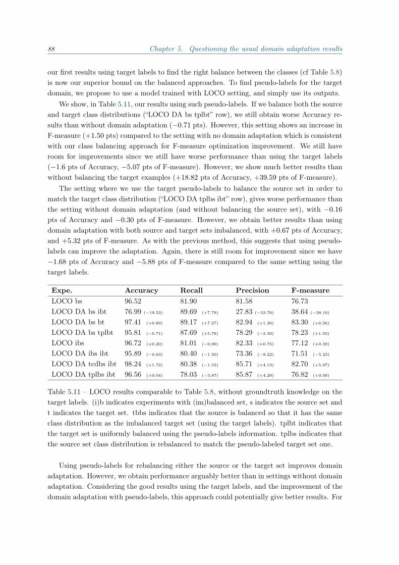
88 Chapter 5. Questioning the usual domain adaptation results
our first results using target labels to find the right balance between the classes (cf Table 5.8)is now our superior bound on the balanced approaches. To find pseudo-labels for the targetdomain, we propose to use a model trained with LOCO setting, and simply use its outputs.
We show, in Table 5.11, our results using such pseudo-labels. If we balance both the sourceand target class distributions (“LOCO DA bs tplbt” row), we still obtain worse Accuracy re-sults than without domain adaptation (−0.71 pts). However, this setting shows an increase inF-measure (+1.50 pts) compared to the setting with no domain adaptation which is consistentwith our class balancing approach for F-measure optimization improvement. We still haveroom for improvements since we still have worse performance than using the target labels(−1.6 pts of Accuracy, −5.07 pts of F-measure). However, we show much better results thanwithout balancing the target examples (+18.82 pts of Accuracy, +39.59 pts of F-measure).
The setting where we use the target pseudo-labels to balance the source set in order tomatch the target class distribution (“LOCO DA tplbs ibt” row), gives worse performance thanthe setting without domain adaptation (and without balancing the source set), with −0.16
pts of Accuracy and −0.30 pts of F-measure. However, we obtain better results than usingdomain adaptation with both source and target sets imbalanced, with +0.67 pts of Accuracy,and +5.32 pts of F-measure. As with the previous method, this suggests that using pseudo-labels can improve the adaptation. Again, there is still room for improvement since we have−1.68 pts of Accuracy and −5.88 pts of F-measure compared to the same setting using thetarget labels.
Expe. Accuracy Recall Precision F-measureLOCO bs 96.52 81.90 81.58 76.73LOCO DA bs ibt 76.99 (−19.53) 89.69 (+7.79) 27.83 (−53.76) 38.64 (−38.10)
LOCO DA bs bt 97.41 (+0.89) 89.17 (+7.27) 82.94 (+1.36) 83.30 (+6.56)
LOCO DA bs tplbt 95.81 (−0.71) 87.69 (+5.78) 78.29 (−3.30) 78.23 (+1.50)
LOCO ibs 96.72 (+0.20) 81.01 (−0.90) 82.33 (+0.75) 77.12 (+0.39)
LOCO DA ibs ibt 95.89 (−0.63) 80.40 (−1.50) 73.36 (−8.22) 71.51 (−5.23)
LOCO DA tcdbs ibt 98.24 (+1.72) 80.38 (−1.52) 85.71 (+4.13) 82.70 (+5.97)
LOCO DA tplbs ibt 96.56 (+0.04) 78.03 (−3.87) 85.87 (+4.29) 76.82 (+0.09)
Table 5.11 – LOCO results comparable to Table 5.8, without groundtruth knowledge on thetarget labels. (i)b indicates experiments with (im)balanced set, s indicates the source set andt indicates the target set. tbbs indicates that the source is balanced so that it has the sameclass distribution as the imbalanced target set (using the target labels). tplbt indicates thatthe target set is uniformly balanced using the pseudo-labels information. tplbs indicates thatthe source set class distribution is rebalanced to match the pseudo-labeled target set one.
Using pseudo-labels for rebalancing either the source or the target set improves domainadaptation. However, we obtain performance arguably better than in settings without domainadaptation. Considering the good results using the target labels, and the improvement of thedomain adaptation with pseudo-labels, this approach could potentially give better results. For
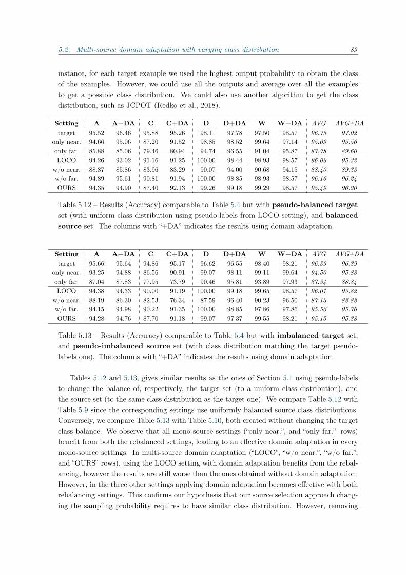
5.2. Multi-source domain adaptation with varying class distribution 89
instance, for each target example we used the highest output probability to obtain the classof the examples. However, we could use all the outputs and average over all the examplesto get a possible class distribution. We could also use another algorithm to get the classdistribution, such as JCPOT (Redko et al., 2018).
Setting A A+DA C C+DA D D+DA W W+DA AVG AVG+DAtarget 95.52 96.46 95.88 95.26 98.11 97.78 97.50 98.57 96.75 97.02
only near. 94.66 95.06 87.20 91.52 98.85 98.52 99.64 97.14 95.09 95.56only far. 85.88 85.06 79.46 80.94 94.74 96.55 91.04 95.87 87.78 89.60LOCO 94.26 93.02 91.16 91.25 100.00 98.44 98.93 98.57 96.09 95.32
w/o near. 88.87 85.86 83.96 83.29 90.07 94.00 90.68 94.15 88.40 89.33w/o far. 94.89 95.61 90.81 91.94 100.00 98.85 98.93 98.57 96.16 96.24OURS 94.35 94.90 87.40 92.13 99.26 99.18 99.29 98.57 95.49 96.20
Table 5.12 – Results (Accuracy) comparable to Table 5.4 but with pseudo-balanced targetset (with uniform class distribution using pseudo-labels from LOCO setting), and balancedsource set. The columns with “+DA” indicates the results using domain adaptation.
Setting A A+DA C C+DA D D+DA W W+DA AVG AVG+DAtarget 95.66 95.64 94.86 95.17 96.62 96.55 98.40 98.21 96.39 96.39
only near. 93.25 94.88 86.56 90.91 99.07 98.11 99.11 99.64 94.50 95.88only far. 87.04 87.83 77.95 73.79 90.46 95.81 93.89 97.93 87.34 88.84LOCO 94.38 94.33 90.00 91.19 100.00 99.18 99.65 98.57 96.01 95.82
w/o near. 88.19 86.30 82.53 76.34 87.59 96.40 90.23 96.50 87.13 88.88w/o far. 94.15 94.98 90.22 91.35 100.00 98.85 97.86 97.86 95.56 95.76OURS 94.28 94.76 87.70 91.18 99.07 97.37 99.55 98.21 95.15 95.38
Table 5.13 – Results (Accuracy) comparable to Table 5.4 but with imbalanced target set,and pseudo-imbalanced source set (with class distribution matching the target pseudo-labels one). The columns with “+DA” indicates the results using domain adaptation.
Tables 5.12 and 5.13, gives similar results as the ones of Section 5.1 using pseudo-labelsto change the balance of, respectively, the target set (to a uniform class distribution), andthe source set (to the same class distribution as the target one). We compare Table 5.12 withTable 5.9 since the corresponding settings use uniformly balanced source class distributions.Conversely, we compare Table 5.13 with Table 5.10, both created without changing the targetclass balance. We observe that all mono-source settings (“only near.”, and “only far.” rows)benefit from both the rebalanced settings, leading to an effective domain adaptation in everymono-source settings. In multi-source domain adaptation (“LOCO”, “w/o near.”, “w/o far.”,and “OURS” rows), using the LOCO setting with domain adaptation benefits from the rebal-ancing, however the results are still worse than the ones obtained without domain adaptation.However, in the three other settings applying domain adaptation becomes effective with bothrebalancing settings. This confirms our hypothesis that our source selection approach chang-ing the sampling probability requires to have similar class distribution. However, removing

90 Chapter 5. Questioning the usual domain adaptation results
the farthest source domain gives better performance than our approach which thus needs tobe improved. We could explore solutions to include the class distribution in the distance, forinstance, using the regularized optimal transport presented in Courty et al. (2014).
5.2.2.2 Domain adaptation with optimal transport
We propose, in this section, to experiment domain adaptation using DeepJDOT (Damodaranet al., 2018). This domain adaptation approach is designed to be effective with imbalanceddata. Indeed, DeepJDOT considers the transport between the source and the target setsboth in terms of data distribution and class distribution. In Table 5.14, we compare ourprevious domain adaptation approach based on Ganin et al. (2016) (GDA) and DeepJDOT(Damodaran et al., 2018) (JDA) on a mono-source domain adaptation setting on Bluecimedataset. In the balanced setting, using DeepJDOT gives better results than using Ganinmethods, in both similar and dissimilar class distribution settings (respectively +0.94 and+0.51 of Accuracy). This suggests that DeepJDOT allows learning better features than themethod from Ganin et al. that we use in this thesis (DANN). This improvement could be abenefit of considering the class distribution in DeepJDOT making features less sensitive tothe discrepancy between the training and testing sets class distributions. Moreover, unlikeDANN, when the source and target sets are imbalanced, we obtain with DeepJDOT goodperformance with both similar and dissimilar class distributions between source and targetsets. These results show the effectiveness of their approach in mono-source domain adaptationwith varying imbalance.
Expe. ≈ class dist. 6= class dist.OVO bs 86.84 86.84
OVO GDA bs bt 91.77 (+4.93) 90.77 (+3.93)
OVO JDA bs bt 92.71 (+5.87) 91.28 (+4.44)
OVO ibs 79.20 (−7.64) 71.14 (−15.69)
OVO GDA ibs ibt 93.20 (+6.36) 85.07 (−1.76)
OVO JDA ibs ibt 94.18 (+7.34) 91.37 (+4.53)
Table 5.14 – One versus one (OVO) Accuracy averaged over domains with similar class distri-butions and over domains with highly dissimilar class distributions (more results in Tables B.4,B.5, and B.6). (i)bt and (i)bs indicate experiments with (im)balanced target and source sets.GDA indicates experiments with DANN, JDA the experiments using DeepJDOT (Damodaranet al., 2018), with the hyperparameters α = 0.001 and λt = 0.0001 as proposed in the paper.
In Table 5.15, we show results using DeepJDOT and DANN approaches in the multi-sourcedomain adaptation problem. In this setting, DeepJDOT gives much worse results −1.73 ptsof Accuracy and −13.28 pts of F-measure comparing to DANN. DeepJDOT requires to splitthe minibatches equally between source and target. Considering that, in the multi-sourcesetting, all the sources are mixed, we tried to increase the size of each minibatch to 80 (the

5.2. Multi-source domain adaptation with varying class distribution 91
highest number reachable with one GPU) to sample more examples from each source. Inthis configuration, we have a slight improvement but still have bad results. To produce theseresults we simply used all the sources as one, the results in Table 5.15 may suggest that touse DeepJDOT in a multi-source setting, we need to modify our approach.
In the table 5.16, we explore the use of another set of parameters taken from the authorscode1 (“hpc” row). The new set of parameters gives more weight to the term controlling thetransport over the class distribution than to the term over the data distribution. In thissetting, we get even worse results as the setting using the paper parameter (“hpp” row). Thisresult shows how much the parameters value is important for this method, and so, should becarefully tuned. For time reasons, we only explore another setting and the effects of balancingthe training sets. In the initial DeepJDOT problem, only one source is used, so, using severalsources may be harmful with the transport component, especially with the reduced size ofsource examples (recall that in DeepJDOT, an optimal transport problem is optimized oneach minibatch). To cope with this problem, we propose another setting where we sample thesource examples from only one source per minibatch (“oos” row). Again, we observe a drop ofperformance. Considering our conclusions of Section 5.1.2, this performance in “oos” settingmay be the consequence of the introduction of minibatches entirely composed of examplescoming from highly distant domains impairing the training phase.
We present in Table 5.17 the results with DeepJDOT and when changing the class distri-bution of the training set. We can see that using a balanced set of source examples impairs theperformance with a loss of 20 pts of Accuracy compared to the setting using an imbalancedsource set. This bad performance could be caused by a bad choice of hyperparameters as wegive a high weight on the class distribution term while both the source and the target setsare balanced.
Expe. Accuracy Recall Precision F-measureLOCO ibs 96.72 81.01 82.33 77.12LOCO GDA ibs ibt 95.89 (−0.83) 80.40 (−0.60) 73.36 (−8.97) 71.51 (−5.62)
LOCO JDA ibs ibt 94.16 (−2.56) 60.57 (−20.44) 72.07 (−10.27) 58.32 (−18.80)
LOCO JDA ibs ibt b80 94.29 (−2.43) 63.39 (−17.61) 72.52 (−9.81) 59.60 (−17.52)
Table 5.15 – LOCO results with DANN and DeepJDOT domain adaptation. (i)bt and (i)bsindicate experiments with (im)balanced target and source sets. GDA indicates experimentswith DANN, JDA the experiments using DeepJDOT (Damodaran et al., 2018), with thehyperparameters α = 0.001 and λt = 0.0001 as proposed in the paper. “b80” indicates thatthe batch size has been increased from 64 to 80 examples.
1https://github.com/bbdamodaran/deepJDOT
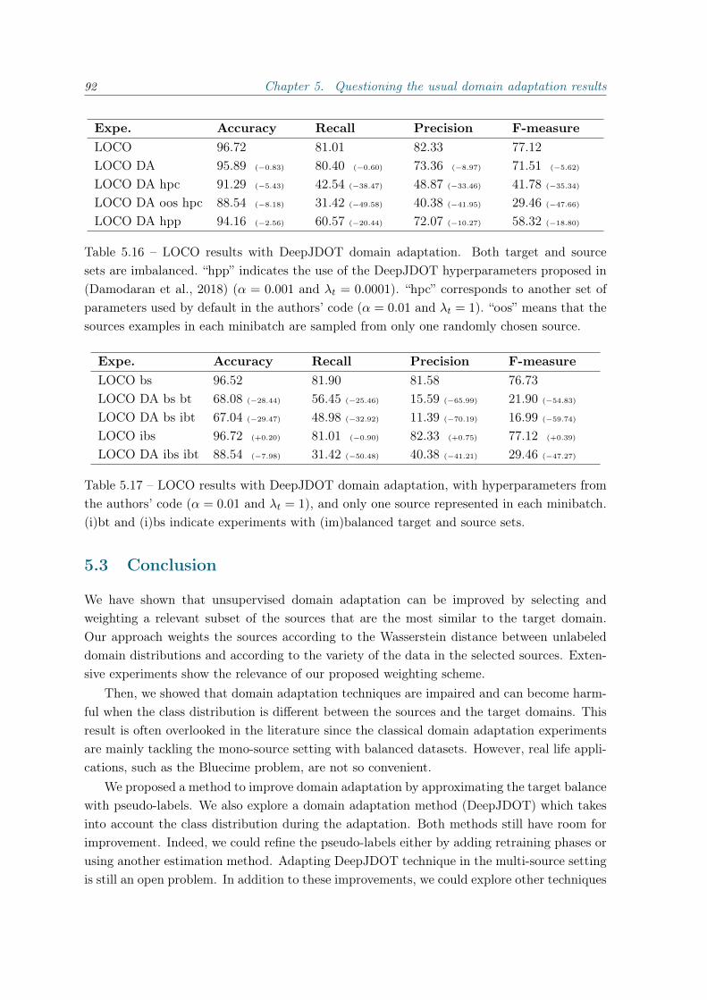
92 Chapter 5. Questioning the usual domain adaptation results
Expe. Accuracy Recall Precision F-measureLOCO 96.72 81.01 82.33 77.12LOCO DA 95.89 (−0.83) 80.40 (−0.60) 73.36 (−8.97) 71.51 (−5.62)
LOCO DA hpc 91.29 (−5.43) 42.54 (−38.47) 48.87 (−33.46) 41.78 (−35.34)
LOCO DA oos hpc 88.54 (−8.18) 31.42 (−49.58) 40.38 (−41.95) 29.46 (−47.66)
LOCO DA hpp 94.16 (−2.56) 60.57 (−20.44) 72.07 (−10.27) 58.32 (−18.80)
Table 5.16 – LOCO results with DeepJDOT domain adaptation. Both target and sourcesets are imbalanced. “hpp” indicates the use of the DeepJDOT hyperparameters proposed in(Damodaran et al., 2018) (α = 0.001 and λt = 0.0001). “hpc” corresponds to another set ofparameters used by default in the authors’ code (α = 0.01 and λt = 1). “oos” means that thesources examples in each minibatch are sampled from only one randomly chosen source.
Expe. Accuracy Recall Precision F-measureLOCO bs 96.52 81.90 81.58 76.73LOCO DA bs bt 68.08 (−28.44) 56.45 (−25.46) 15.59 (−65.99) 21.90 (−54.83)
LOCO DA bs ibt 67.04 (−29.47) 48.98 (−32.92) 11.39 (−70.19) 16.99 (−59.74)
LOCO ibs 96.72 (+0.20) 81.01 (−0.90) 82.33 (+0.75) 77.12 (+0.39)
LOCO DA ibs ibt 88.54 (−7.98) 31.42 (−50.48) 40.38 (−41.21) 29.46 (−47.27)
Table 5.17 – LOCO results with DeepJDOT domain adaptation, with hyperparameters fromthe authors’ code (α = 0.01 and λt = 1), and only one source represented in each minibatch.(i)bt and (i)bs indicate experiments with (im)balanced target and source sets.
5.3 Conclusion
We have shown that unsupervised domain adaptation can be improved by selecting andweighting a relevant subset of the sources that are the most similar to the target domain.Our approach weights the sources according to the Wasserstein distance between unlabeleddomain distributions and according to the variety of the data in the selected sources. Exten-sive experiments show the relevance of our proposed weighting scheme.
Then, we showed that domain adaptation techniques are impaired and can become harm-ful when the class distribution is different between the sources and the target domains. Thisresult is often overlooked in the literature since the classical domain adaptation experimentsare mainly tackling the mono-source setting with balanced datasets. However, real life appli-cations, such as the Bluecime problem, are not so convenient.
We proposed a method to improve domain adaptation by approximating the target balancewith pseudo-labels. We also explore a domain adaptation method (DeepJDOT) which takesinto account the class distribution during the adaptation. Both methods still have room forimprovement. Indeed, we could refine the pseudo-labels either by adding retraining phases orusing another estimation method. Adapting DeepJDOT technique in the multi-source settingis still an open problem. In addition to these improvements, we could explore other techniques

5.3. Conclusion 93
to better tackle domain adaptation with varying class balance. For instance, we could usethe SAN approach (Cao et al., 2018) where each class has a dedicated domain discriminator.This approach considering each class independently may improve our performance even withdifferent imbalance ratio.

94 Chapter 5. Questioning the usual domain adaptation results
Conclusion and perspectives
In this thesis, we studied techniques to tackle Bluecime’s chairlift safety problem and thedifferent challenges it implies:
1. large variety of chairlifts and weather conditions;
2. lack of labeled data (particularly on newly installed chairlifts);
3. imbalance in the data;
4. real-time decisions.
These challenges are not independent. For instance, we showed in this document that domainadaptation techniques, used to solve the first two challenges, are impaired by the third one.However, we managed to develop effective techniques (mainly based on deep learning) totackle Bluecime’s problem. Deep learning techniques are currently being implemented inSIVAO for passengers counting or bubble detection (the glass bubble on Chair. D in Fig. 2.2)and provide great performance.
Contributions
The first contribution presented in this thesis is a complete knowledge discovery pipeline (taskdefinition, data preprocessing, model, and evaluation framework) for Bluecime dataset. Weproposed to explore fully supervised settings (OOC and ALL), but also a setting simulatinga newly installed chairlift with no label available (LOCO). Our baseline model is based on astate-of-the-art deep learning architecture (ResNet) allowing to tackle the first challenge inreasonable time, thus also tackling the fourth challenge. We also propose to add a domainadaptation component to address the second challenge.
The subsequent contributions tackle the different challenges more specifically. Our secondcontribution consists in improving the robustness of our approach (first two challenges) usinga patching method. This method consists in creating new images by hiding small areas inthe original input image which are critically important for the network classification process.Thus, we aim at forcing the network to use the whole image and maximize the amount of in-formation used by the network. This approach can be considered either as data augmentationor a way to regularize the learning process (as with “dropout”).
Our third and fourth contributions are both considering cost-sensitive learning to optimizethe F-measure. This measure helps us focusing on the errors made by our classifier on theminority class (here, the unsafe cases). Optimizing it instead of the usual accuracy addresses
95
96 Conclusion and perspectives
our class imbalance challenge. Both methods showed good results that can be generalizedto other applications. These methods allowed us to trade-off the precision and recall of oursystem which is interesting for Bluecime since the number of false positives and false negativescases depends, among other factors, on the chairlift and the distance between the boardingstation and the SIVAO camera.
The fifth contribution of this thesis is a method to improve the multi-source domainadaptation problem by selecting the most relevant sources in the training set. With thiscontribution, we analyze how domain adaptation behaves in this multi-source setting but alsowhen the class distributions vary between the source and target examples. Here we questionthe general knowledge about domain adaptation and propose a few successful solutions forthis particular setting that are also useful to Bluecime.
Perspectives
Many opportunities to improve our different contributions are still to be explored. Our base-line approach could be improved with a more systematic comparison of the different archi-tectures in the literature. Indeed, many existing architectures were not considered, mainlyfor time reasons, but also because new deep learning models are constantly developed (andimproved), making it difficult to keep up with the state-of-the-art.
On our patching approach, we could further explore the use of the previous positions ofthe selected patches. In particular, we could increase differently the probability of a patchlocation to come back, and decrease it on locations inducing uninteresting patches.
On CONE, our algorithm for F-measure optimization, we could find a way to betteradapt it to deep learning. For instance, we could use the first model weights as pre-trainingfor the next trained model reducing the training time required to obtain enough classifiers toexplore the (t, F) space.
On the selection of the source domains, we could use other distances or improve the oneswe proposed. For instance, the autoencoder-based distance obviously depends on the autoen-coders training, thus, modifying its architecture or tuning differently the hyperparameter (e.g.the learning rate) may highly improve this method. We could also modify our variety term,for instance by integrating a constraint on a minimum number of selected sources. Indeed, ifa domain is very well represented and “close” to the target domain, it may be the only oneselected, thus, inducing a training set with low variety.
We could also explore, theoretically, the negative results of domain adaptation with im-balance class distributions between the target and source examples. On the practical side,we could improve our pseudo-labels method or find a better way to use DeepJDOT in amulti-source setting.
Moreover, all these methods have been designed independently to tackle the original prob-lem proposed by Bluecime. We have not studied if these methods are complementary, redun-dant or maybe adversary to tackle our end goal. We could use them all and hope for thebest or try to find the best combination. For instance, we could guide the patching methodeconsidering the F-measure and not only the prediction loss. We could also try to improve our

97
domain selection strategy using, for instance, the constrained optimal transport from Courtyet al. (2014), when computing the Wasserstein distance to better take into consideration theclass distributions.
Last but not least, in Bluecime’s context, we could conduct work on improving the networkefficiency. This could be done, for instance, by pruning the useless weights in the network,or quantizing the weights (Han et al., 2015). We could also explore ways to improve theperformance of smaller architectures, for instance, with knowledge distillation (Hinton et al.,2015). Having a more effective network has two advantages: the most obvious one is toincrease the inference speed, allowing us to have a real-time approach. The second advantageis to decrease the computation and memory load required by our deep learning approach. Thiswould allow Bluecime to provide other services, such as real-time statistics on the chairliftoccupation, without requiring to upgrade the system hardware.

98 Conclusion and perspectives

List of publications
Publications in international conferences
Kevin Bascol, Rémi Emonet, Elisa Fromont, and Raluca Debusschere. Improving chairlift securitywith deep learning. In International Symposium on Intelligent Data Analysis (IDA 2017), 2017
Kevin Bascol, Rémi Emonet, Elisa Fromont, Amaury Habrard, Guillaume Metzler, and Marc Sebban.From cost-sensitive classification to tight f-measure bounds. In Proceedings of the Twenty-SecondInternational Conference on Artificial Intelligence and Statistics (AISTATS-19), volume 89 of Pro-ceedings of Machine Learning Research. PMLR, 2019b
Kevin Bascol, Rémi Emonet, and Elisa Fromont. Improving domain adaptation by source selec-tion. In 2019 IEEE International Conference on Image Processing (ICIP), 2019a
The following paper was published during the PhD, but was the result of a second year Masterinternship. Thus it is unrelated to the main topic of the thesis.
Kevin Bascol, Rémi Emonet, Elisa Fromont, and Jean-Marc Odobez. Unsupervised interpretablepattern discovery in time series using autoencoders. In The joint IAPR International Workshops onStructural and Syntactic Pattern Recognition (SSPR 2016), 2016
Communications in national conferences
Kevin Bascol, Rémi Emonet, Elisa Fromont, Amaury Habrard, Guillaume Metzler, and Marc Sebban.Un algorithme d’optimisation de la f-mesure par pondération des erreurs de classification. In Con-férence francophone sur l’Apprentissage Automatique (CAp-18), 2018
99

100 List of publications

Appendix A
Pattern discovery in time series usingautoencoders
A.1 Introduction
Unsupervised discovery of patterns in temporal data is an important data mining topic dueto numerous application domains like finance, biology or video analysis. In some applications,the patterns are solely used as features for classification and thus the classification accuracyis the only criterion. This chapter considers different applications where the patterns canalso be used for data analysis, data understanding, and novelty or anomaly detection Emonetet al. (2011, 2014); Du et al. (2009); Sallaberry et al. (2011).
Not all time series are of the same nature. In this work, we consider the difficult caseof multivariate time series whose observations are the result of a combination of differentrecurring phenomena that can overlap. Examples include traffic videos where the activityof multiple cars causes the observed sequence of images Emonet et al. (2014), or aggregatepower consumption where the observed consumption is due to a mixture of appliances Kolterand Jaakkola (2012). Unlike many techniques from the data mining community, our aim isnot to list all recurrent patterns in the data with their frequency but to reconstruct the entiretemporal documents by means of a limited and unknown number of recurring patterns togetherwith their occurrence times in the data. In this view, we want to un-mix multivariate timeseries to recover how they can be decomposed in terms of recurrent temporally-structuredpatterns. Following the conventions used in Emonet et al. (2014), we will call a temporalpattern a motif, and an input multivariate time series a temporal document.
Artificial neural networks (or deep learning architectures) have (re)become tremendouslypopular in the last decade due to their impressive, and so far not beaten, results in image clas-sification, speech recognition and natural language processing. In particular, autoencoders areartificial neural networks used to learn a compressed, distributed representation (encoding) fora set of data, typically for the purpose of dimensionality reduction. It is thus an unsupervisedlearning method whose (hidden) layers contain representations of the input data sufficientlypowerful for compressing (and decompressing) the data while loosing as little information as
101
102 Appendix A. Pattern discovery in time series using autoencoders
possible. Given the temporal nature of our data, our pattern discovery task is fundamentallyconvolutional (the same network is applied at any instant and is thus time-shift invariant)since it needs to identify motifs whatever their time(s) of occurrence. To tackle this task, wewill thus focus on a particular type of autoencoders, the convolutional ones. However, whilewell adapted for discriminative tasks like classification Baccouche et al. (2012), the patternscaptured by (convolutional) autoencoders are not fully interpretable and often correlated.
In this appendix, we address the discovery of interpretable motifs using convolutionalauto-encoders and make the following contributions:• we show that the interpretability of standard convolutional autoencoders is limited;• we introduce an adaptive rectified linear unit (AdaReLU) which allows hidden layers to
capture clear occurrences of motifs,• we propose a regularization inspired by group-lasso to automatically select the number
of filters in a convolutional neural net,• we show, through experiments on synthetic and real data, how these elements (and
others) allow recovering interpretable motifs1.It is important to note that some previous generative models Varadarajan et al. (2013); Emonetet al. (2014) have obtained very good results on this task. However, their extensions to semi-supervised settings (i.e. with partially labeled data) or hierarchical schemes are cumbersometo achieve. In contrast, in this chapter, to solve the same modeling problem we present aradically different method which will lend itself to more flexible and systematic end-to-endtraining frameworks and extensions.
The chapter is organized as follows. In Section A.2, we clarify the link between ourdata mining technique and previous work. Section A.3 gives the details of our method whileSection A.4 shows experiments both on synthetic and real data. We conclude and draw futuredirections in Section A.5.
A.2 Related work
Our work shows how to use a popular method (autoencoders) to tackle a task (pattern discov-ery in time series) that has seldom been considered for this type of methods. We thus brieflyreview other methods used in this context and then, other works that use neural networks forunsupervised time series modeling.
A.2.1 Unsupervised pattern discovery in time series.
Traditional unsupervised approaches that deal with time series do not aim at modeling seriesbut rather at extracting interesting pieces of the series that can be used as high level descrip-tions for direct analysis or as input features for other algorithms. In this category fall all theevent-based (e.g. Y.-C. Chen and Lee (2015); W.-S. Chu and la Torre (2012); H. Shao andRamakrishnan (2013)), sequence Mooney and Roddick (2013) and trajectory mining methods
1The complete source code will be made available online
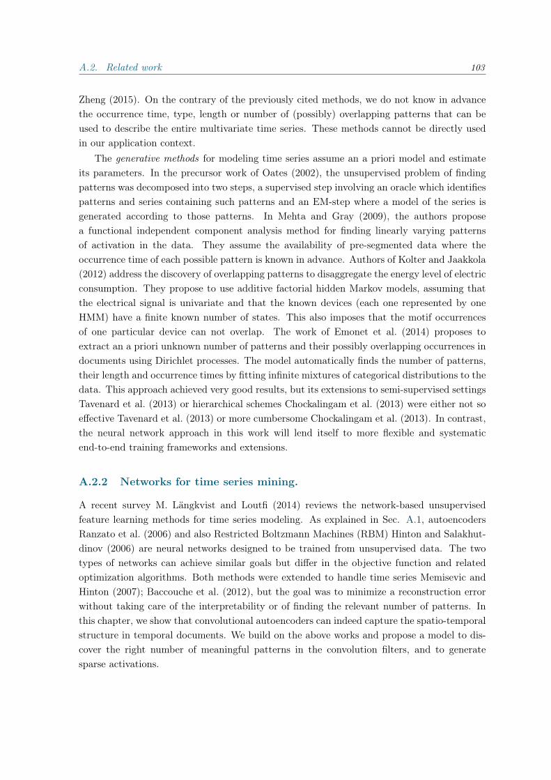
A.2. Related work 103
Zheng (2015). On the contrary of the previously cited methods, we do not know in advancethe occurrence time, type, length or number of (possibly) overlapping patterns that can beused to describe the entire multivariate time series. These methods cannot be directly usedin our application context.
The generative methods for modeling time series assume an a priori model and estimateits parameters. In the precursor work of Oates (2002), the unsupervised problem of findingpatterns was decomposed into two steps, a supervised step involving an oracle which identifiespatterns and series containing such patterns and an EM-step where a model of the series isgenerated according to those patterns. In Mehta and Gray (2009), the authors proposea functional independent component analysis method for finding linearly varying patternsof activation in the data. They assume the availability of pre-segmented data where theoccurrence time of each possible pattern is known in advance. Authors of Kolter and Jaakkola(2012) address the discovery of overlapping patterns to disaggregate the energy level of electricconsumption. They propose to use additive factorial hidden Markov models, assuming thatthe electrical signal is univariate and that the known devices (each one represented by oneHMM) have a finite known number of states. This also imposes that the motif occurrencesof one particular device can not overlap. The work of Emonet et al. (2014) proposes toextract an a priori unknown number of patterns and their possibly overlapping occurrences indocuments using Dirichlet processes. The model automatically finds the number of patterns,their length and occurrence times by fitting infinite mixtures of categorical distributions to thedata. This approach achieved very good results, but its extensions to semi-supervised settingsTavenard et al. (2013) or hierarchical schemes Chockalingam et al. (2013) were either not soeffective Tavenard et al. (2013) or more cumbersome Chockalingam et al. (2013). In contrast,the neural network approach in this work will lend itself to more flexible and systematicend-to-end training frameworks and extensions.
A.2.2 Networks for time series mining.
A recent survey M. Längkvist and Loutfi (2014) reviews the network-based unsupervisedfeature learning methods for time series modeling. As explained in Sec. A.1, autoencodersRanzato et al. (2006) and also Restricted Boltzmann Machines (RBM) Hinton and Salakhut-dinov (2006) are neural networks designed to be trained from unsupervised data. The twotypes of networks can achieve similar goals but differ in the objective function and relatedoptimization algorithms. Both methods were extended to handle time series Memisevic andHinton (2007); Baccouche et al. (2012), but the goal was to minimize a reconstruction errorwithout taking care of the interpretability or of finding the relevant number of patterns. Inthis chapter, we show that convolutional autoencoders can indeed capture the spatio-temporalstructure in temporal documents. We build on the above works and propose a model to dis-cover the right number of meaningful patterns in the convolution filters, and to generatesparse activations.
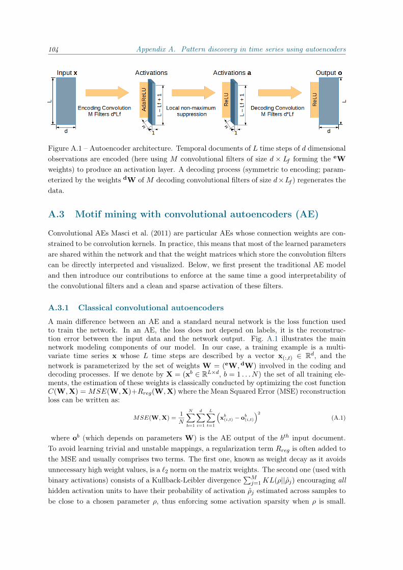
104 Appendix A. Pattern discovery in time series using autoencoders
Figure A.1 – Autoencoder architecture. Temporal documents of L time steps of d dimensionalobservations are encoded (here using M convolutional filters of size d × Lf forming the eW
weights) to produce an activation layer. A decoding process (symmetric to encoding; param-eterized by the weights dW of M decoding convolutional filters of size d×Lf ) regenerates thedata.
A.3 Motif mining with convolutional autoencoders (AE)
Convolutional AEs Masci et al. (2011) are particular AEs whose connection weights are con-strained to be convolution kernels. In practice, this means that most of the learned parametersare shared within the network and that the weight matrices which store the convolution filterscan be directly interpreted and visualized. Below, we first present the traditional AE modeland then introduce our contributions to enforce at the same time a good interpretability ofthe convolutional filters and a clean and sparse activation of these filters.
A.3.1 Classical convolutional autoencoders
A main difference between an AE and a standard neural network is the loss function usedto train the network. In an AE, the loss does not depend on labels, it is the reconstruc-tion error between the input data and the network output. Fig. A.1 illustrates the mainnetwork modeling components of our model. In our case, a training example is a multi-variate time series x whose L time steps are described by a vector x(:,t) ∈ Rd, and thenetwork is parameterized by the set of weights W = (eW, dW) involved in the coding anddecoding processes. If we denote by X = (xb ∈ RL×d, b = 1 . . . N) the set of all training ele-ments, the estimation of these weights is classically conducted by optimizing the cost functionC(W,X) = MSE(W,X)+Rreg(W,X) where the Mean Squared Error (MSE) reconstructionloss can be written as:
MSE(W,X) =1
N
N∑b=1
d∑i=1
L∑t=1
(xb(i,t) − ob
(i,t)
)2(A.1)
where ob (which depends on parameters W) is the AE output of the bth input document.To avoid learning trivial and unstable mappings, a regularization term Rreg is often added tothe MSE and usually comprises two terms. The first one, known as weight decay as it avoidsunnecessary high weight values, is a `2 norm on the matrix weights. The second one (used withbinary activations) consists of a Kullback-Leibler divergence
∑Mj=1KL(ρ||ρj) encouraging all
hidden activation units to have their probability of activation ρj estimated across samples tobe close to a chosen parameter ρ, thus enforcing some activation sparsity when ρ is small.

A.3. Motif mining with convolutional autoencoders (AE) 105
The parameters are typically learned using a stochastic gradient descent algorithm (SGD)with momentum using an appropriate rate scheduling Darken and Moody (1990).
A.3.2 Interpretable pattern discovery with autoencoders
In our application, the learned convolution filters should not only minimize the reconstructionerror but also be directly interpretable. Ideally, we would like to only extract filters whichcapture and represent interesting data patterns, as illustrated in Fig. A.2-c-d. To achievethis, we add a number of elements in the network architecture and in our optimization costfunction to constrain our network appropriately.
A.3.2.1 Enforcing non-negative decoding filters.
As the AE output is somehow defined as a linear combination of the decoding filters, thenthese filters can represent the patterns we are looking for, and we can interpret the hiddenlayers activations a (see Fig. A.1) as the occurrences of these patterns. Thus, as our inputis non-negative (a temporal document), we constraint the decoding filters weights to be non-negative by thresholding them at every SGD iteration. The assumption that the input isnon-negative holds in our case and it will also hold in deeper AEs provided that we useReLU-like activation functions. Note that for encoding, we do not constrain filters, so theycan have negative values to compensate for the pattern auto-correlation (see below).
A.3.2.2 Sparsifying the filters.
The traditional `2 regularization allows many small but non-zero values. To force these valuesto zero and thus get sparser filters, we replaced the `2 norm by the sparsity-promoting norm`1 known as lasso:
Rlas(W) =
M∑f=1
d∑i=1
Lf∑k=1
∣∣∣eWf(i,k)
∣∣∣+ M∑f=1
d∑i=1
Lf∑k=1
∣∣∣dWf
(i,k)
∣∣∣ (A.2)
A.3.2.3 Encouraging sparse activations.
The traditional KL divergence aims at making all hidden units equally useful on average,whereas our goal is to have the activation layer to be as sparse as possible for each giveninput document. We achieve this by encouraging peaky activations, i.e. of low entropywhen seen as a document-level probability distribution, as was proposed in Varadarajan et al.(2010) when dealing on topic models for motif discovery. This results in an entropy-basedregularization expressed on the set A = ab of document-level activations:
Rent(A) =− 1
N
N∑b=1
M∑f=1
L−Lf+1∑t=1
abf,t log
(abf,t
)with abf,t=ab
f,t
/ M∑f=1
L−Lf+1∑t=1
abf,t (A.3)

106 Appendix A. Pattern discovery in time series using autoencoders
A.3.2.4 Local non-maximum activation removal.
The previous entropy regularizer encourages peaked activations. However, as the encodinglayer remains a convolutional layer, if a filter is correlated in time with itself or another filter,then the activations cannot be sparse. This phenomenon is due to the feed forward nature ofthe network, where activations depend on the input, not on each others: hence, no activationcan inhibit its neighboring activations. To handle this issue we add a local non-maximumsuppression layer which, from a network perspective, is obtained by convolving activationswith a temporal Gaussian filter, subtracting from the result the activation intensities, andapplying a ReLU, focusing in this way spread activations into central peaks.
A.3.2.5 Handling distant filter correlations with AdaReLU.
The Gaussian layer cannot handle non-local (in time) correlations. To handle this, we proposeto replace the traditional ReLU activation function by a novel one called adaptive ReLU.AdaReLU works on groups of units and sets to 0 all the values that are below a percentage(e.g., 60%) of the maximal value in the group. In our architecture, AdaReLU is appliedseparately on each filter activation sequence.
A.3.2.6 Finding the true number of patterns.
One main advantage and contribution of our AE-based method compared to methods pre-sented in Section A.2 is the possibility to discover the “true” number of patterns in the data.One solution to achieve this is to introduce in the network a large set of filters and “hope”that the learning leads to only a few non null filters capturing the interesting patterns. How-ever, in practice, standard regularization terms and optimizations tend to produce networks“using” all or many more filters than the number of true patterns which results in partialand less interpretable patterns. To overcome this problem, we propose to use a group lassoregularization term called `2,1 norm Yuan and Lin (2006) that constrains the network to “use”as few filters as possible. It can be formulated for our weight matrix as:
Rgrp(W) =
M∑f=1
√√√√ d∑i=1
Lf∑k=1
(eWf
(i,k)
)2+
M∑f=1
√√√√ d∑i=1
Lf∑k=1
(dWf
(i,k)
)2(A.4)
A.3.2.7 Overall objective function.
Combining equations (A.1), (A.2), (A.4) and (A.3), we obtain the objective function that isoptimized by our network:
C(W,X) =MSE(W,X) + λlasRlas(W) + λgrpRgrp(W) + λentRent(A(W,X)) (A.5)
A.4 Experiments
A.4.1 Experimental setting
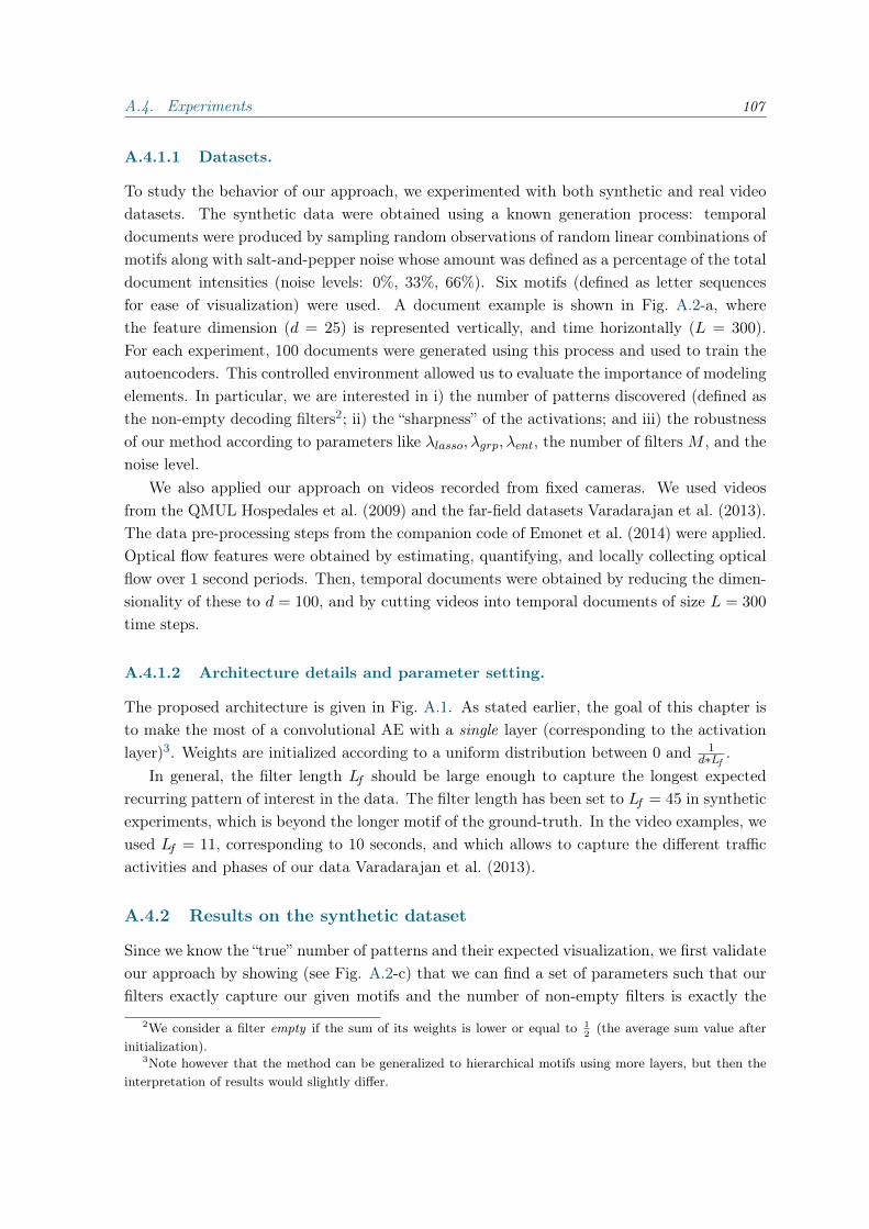
A.4. Experiments 107
A.4.1.1 Datasets.
To study the behavior of our approach, we experimented with both synthetic and real videodatasets. The synthetic data were obtained using a known generation process: temporaldocuments were produced by sampling random observations of random linear combinations ofmotifs along with salt-and-pepper noise whose amount was defined as a percentage of the totaldocument intensities (noise levels: 0%, 33%, 66%). Six motifs (defined as letter sequencesfor ease of visualization) were used. A document example is shown in Fig. A.2-a, wherethe feature dimension (d = 25) is represented vertically, and time horizontally (L = 300).For each experiment, 100 documents were generated using this process and used to train theautoencoders. This controlled environment allowed us to evaluate the importance of modelingelements. In particular, we are interested in i) the number of patterns discovered (defined asthe non-empty decoding filters2; ii) the “sharpness” of the activations; and iii) the robustnessof our method according to parameters like λlasso, λgrp, λent, the number of filters M , and thenoise level.
We also applied our approach on videos recorded from fixed cameras. We used videosfrom the QMUL Hospedales et al. (2009) and the far-field datasets Varadarajan et al. (2013).The data pre-processing steps from the companion code of Emonet et al. (2014) were applied.Optical flow features were obtained by estimating, quantifying, and locally collecting opticalflow over 1 second periods. Then, temporal documents were obtained by reducing the dimen-sionality of these to d = 100, and by cutting videos into temporal documents of size L = 300
time steps.
A.4.1.2 Architecture details and parameter setting.
The proposed architecture is given in Fig. A.1. As stated earlier, the goal of this chapter isto make the most of a convolutional AE with a single layer (corresponding to the activationlayer)3. Weights are initialized according to a uniform distribution between 0 and 1
d∗Lf .In general, the filter length Lf should be large enough to capture the longest expected
recurring pattern of interest in the data. The filter length has been set to Lf = 45 in syntheticexperiments, which is beyond the longer motif of the ground-truth. In the video examples, weused Lf = 11, corresponding to 10 seconds, and which allows to capture the different trafficactivities and phases of our data Varadarajan et al. (2013).
A.4.2 Results on the synthetic dataset
Since we know the “true” number of patterns and their expected visualization, we first validateour approach by showing (see Fig. A.2-c) that we can find a set of parameters such that ourfilters exactly capture our given motifs and the number of non-empty filters is exactly the
2We consider a filter empty if the sum of its weights is lower or equal to 12(the average sum value after
initialization).3Note however that the method can be generalized to hierarchical motifs using more layers, but then the
interpretation of results would slightly differ.

108 Appendix A. Pattern discovery in time series using autoencoders
a)
b)
c)
d)
e)0 64 128 191 255
Time
0
192
385
Inte
nsi
ty
01
23
4 5 6 7 8 9 10 11
f)0 64 128 191 255
Time
0
204
407
Inte
nsi
ty
01
23
4 5 6 7 8 9 10 11
g)0 64 128 191 255
Time
0
169
338
Inte
nsi
ty
01
23
4 5 6 7 8 9 10 11
Figure A.2 – Results on the synthetic data built from 6 patterns, with 66% of noise, M = 12
filters, and unless stated otherwise λlas = 0.004, λgrp = 2, λent = 0.2. a) Sample document;b) Obtained output reconstructed document; c) Weights of seven out of the 12 obtained filters(the 5 remaining filters are empty); d) Weights of seven filters when not using group lasso,i.e. with λgrp = 0 (note that the 5 remaining filters are non empty); (e,f,g) Examples ofactivation intensities (colors correspond to a given filter) with default parameters (e); withoutthe entropy sparsifying term (λent = 0) (f); with ReLU instead of AdaReLU (g).
“true” number of motifs in the dataset even when this dataset is noisy (this is also true fora clean dataset). In this case (see Fig.A.2-e) the activations for the complete document are,as expected, sparse and “peaky”. The output document (see Fig.A.2-b) is a good un-noisyreconstruction of the input document shown in Fig.A.2-a.
In Fig. A.3, we evaluate the influence of the given number of filters M and the noise levelon both the number of recovered motifs and the MSE while fixing the parameters as in Fig.A.2. We can see that with this set of parameters, the AE is able to recover the true numberof filters for the large majority of noise levels and values of M . For all noise levels, we seefrom the low MSE that the AEs is able to well reconstruct the original document as long asthe number of given filters is at least equal to the number of “true” patterns in the document.
A.4.2.1 Model selection: influence of λgrp.
Fig.A.4 shows the number of non-zero filters in function of λgrp and of the noise level for thesynthetic dataset with 6 known motifs when using 12 filters (left) and 16 filters (right). Thelight blue area is the area in which the AEs was able to discover the true number of patterns.With no group lasso regularization (λgrp = 0), the AE systematically uses all the available
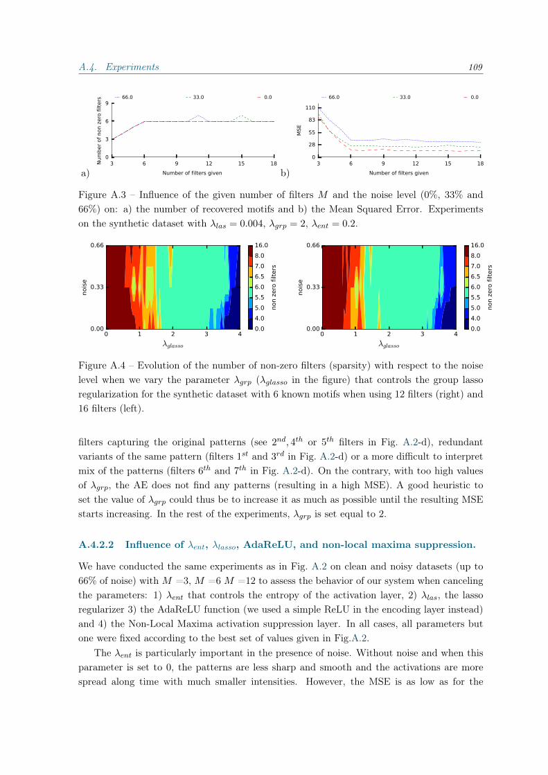
A.4. Experiments 109
a)181512963
Number of filters given
0
3
6
9N
um
ber
of
non z
ero
filt
ers 66.0 33.0 0.0
b)181512963
Number of filters given
0
28
55
83
110
MSE
66.0 33.0 0.0
Figure A.3 – Influence of the given number of filters M and the noise level (0%, 33% and66%) on: a) the number of recovered motifs and b) the Mean Squared Error. Experimentson the synthetic dataset with λlas = 0.004, λgrp = 2, λent = 0.2.
0 1 2 3 4
λglasso
0.00
0.33
0.66
nois
e
0.0
4.0
5.0
5.5
6.0
6.5
7.0
8.0
16.0
non z
ero
filt
ers
0 1 2 3 4
λglasso
0.00
0.33
0.66
nois
e
0.0
4.0
5.0
5.5
6.0
6.5
7.0
8.0
16.0
non z
ero
filt
ers
Figure A.4 – Evolution of the number of non-zero filters (sparsity) with respect to the noiselevel when we vary the parameter λgrp (λglasso in the figure) that controls the group lassoregularization for the synthetic dataset with 6 known motifs when using 12 filters (right) and16 filters (left).
filters capturing the original patterns (see 2nd, 4th or 5th filters in Fig. A.2-d), redundantvariants of the same pattern (filters 1st and 3rd in Fig. A.2-d) or a more difficult to interpretmix of the patterns (filters 6th and 7th in Fig. A.2-d). On the contrary, with too high valuesof λgrp, the AE does not find any patterns (resulting in a high MSE). A good heuristic toset the value of λgrp could thus be to increase it as much as possible until the resulting MSEstarts increasing. In the rest of the experiments, λgrp is set equal to 2.
A.4.2.2 Influence of λent, λlasso, AdaReLU, and non-local maxima suppression.
We have conducted the same experiments as in Fig. A.2 on clean and noisy datasets (up to66% of noise) with M =3, M =6 M =12 to assess the behavior of our system when cancelingthe parameters: 1) λent that controls the entropy of the activation layer, 2) λlas, the lassoregularizer 3) the AdaReLU function (we used a simple ReLU in the encoding layer instead)and 4) the Non-Local Maxima activation suppression layer. In all cases, all parameters butone were fixed according to the best set of values given in Fig.A.2.
The λent is particularly important in the presence of noise. Without noise and when thisparameter is set to 0, the patterns are less sharp and smooth and the activations are morespread along time with much smaller intensities. However, the MSE is as low as for the
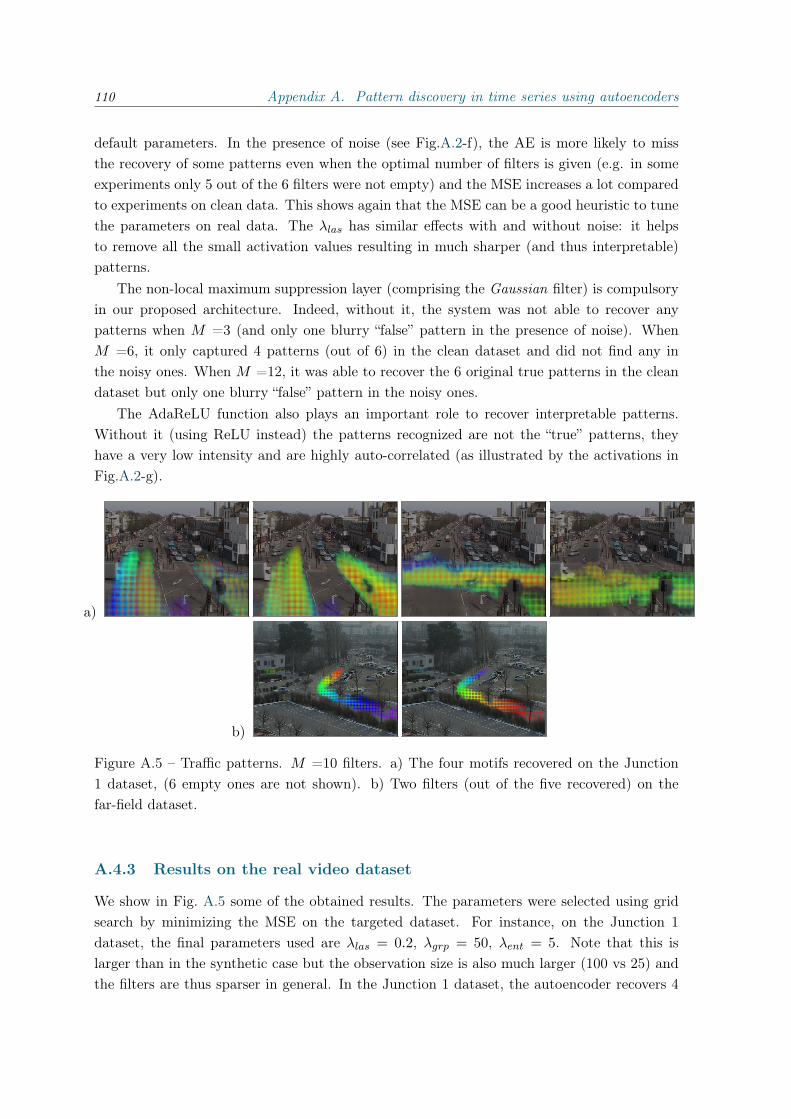
110 Appendix A. Pattern discovery in time series using autoencoders
default parameters. In the presence of noise (see Fig.A.2-f), the AE is more likely to missthe recovery of some patterns even when the optimal number of filters is given (e.g. in someexperiments only 5 out of the 6 filters were not empty) and the MSE increases a lot comparedto experiments on clean data. This shows again that the MSE can be a good heuristic to tunethe parameters on real data. The λlas has similar effects with and without noise: it helpsto remove all the small activation values resulting in much sharper (and thus interpretable)patterns.
The non-local maximum suppression layer (comprising the Gaussian filter) is compulsoryin our proposed architecture. Indeed, without it, the system was not able to recover anypatterns when M =3 (and only one blurry “false” pattern in the presence of noise). WhenM =6, it only captured 4 patterns (out of 6) in the clean dataset and did not find any inthe noisy ones. When M =12, it was able to recover the 6 original true patterns in the cleandataset but only one blurry “false” pattern in the noisy ones.
The AdaReLU function also plays an important role to recover interpretable patterns.Without it (using ReLU instead) the patterns recognized are not the “true” patterns, theyhave a very low intensity and are highly auto-correlated (as illustrated by the activations inFig.A.2-g).
a)
b)
Figure A.5 – Traffic patterns. M =10 filters. a) The four motifs recovered on the Junction1 dataset, (6 empty ones are not shown). b) Two filters (out of the five recovered) on thefar-field dataset.
A.4.3 Results on the real video dataset
We show in Fig. A.5 some of the obtained results. The parameters were selected using gridsearch by minimizing the MSE on the targeted dataset. For instance, on the Junction 1dataset, the final parameters used are λlas = 0.2, λgrp = 50, λent = 5. Note that this islarger than in the synthetic case but the observation size is also much larger (100 vs 25) andthe filters are thus sparser in general. In the Junction 1 dataset, the autoencoder recovers 4
A.5. Conclusion 111
non-empty and meaningful filters capturing the car activities related to the different trafficsignal cycles, whereas in the far-field case, the main trajectories of cars were recovered as alsoreported in Varadarajan et al. (2013).
A.5 Conclusion
We have shown that convolutional AEs are good candidate unsupervised data mining toolsto discover interpretable patterns in time series. We have introduced a number of layers andregularization terms to the standard convolutional AEs to enforce the interpretability of boththe convolutional filters and the activations in the hidden layers of the network. The filters aredirectly interpretable as spatio-temporal patterns while the activations give the occurrencetimes of each pattern in the temporal document. This allows us to un-mix multivariate timeseries. A direct perspective of this work is the use of multi-layer AEs to capture combinationof motifs. If this was not the aim of this work, it may help to reduce the number of parametersneeded to obtain truly interpretable patterns and capture more complex patterns in data.

112 Appendix A. Pattern discovery in time series using autoencoders

Appendix B
Additional results
B.1 Baseline results
In this section we show detailed baseline result (from Section 3.3) over each chairlift onAccuracy, Precision, and Recall.
Chairlift SIVAO OOC ALL ALL DA LOCOLOCODA-
LOCODA
Chair. A 95.70 96.20 96.20 96.52 94.93 95.14 95.77Chair. B 99.14 98.49 99.03 99.29 98.60 98.71 99.03Chair. C 99.19 96.95 98.07 98.07 97.26 97.46 97.56Chair. D 99.60 99.21 100.00 99.80 99.60 99.87 99.74Chair. E 99.38 98.03 98.27 98.25 76.74 77.11 94.26Chair. F 99.58 99.83 99.75 99.75 98.82 99.41 99.66Chair. G 95.44 99.24 99.81 99.91 100.00 99.62 99.62Chair. H 99.30 98.50 98.80 98.75 97.41 97.21 98.00Chair. I 98.93 98.50 99.43 99.10 97.71 98.14 98.42Chair. J 97.72 97.78 97.91 98.12 95.81 95.75 97.91Chair. K 99.30 99.53 99.61 99.30 98.84 99.15 99.38Chair. L 97.90 98.43 98.25 98.43 95.63 95.89 96.99Chair. M 97.99 95.98 97.39 97.89 98.19 97.59 97.79Chair. N 99.42 99.42 99.42 99.56 99.42 99.42 89.83Chair. O 99.86 97.67 98.77 98.42 98.08 98.08 97.53Chair. P 99.14 98.29 98.76 98.52 97.51 97.98 97.43Chair. Q 98.43 98.87 99.30 99.23 98.60 98.47 98.43Chair. R 96.88 98.24 98.56 98.48 97.92 98.24 98.32Chair. S 98.80 96.81 98.61 98.31 97.41 97.01 98.01Chair. T 99.25 98.49 99.14 99.46 96.24 97.42 98.39Chair. U 99.03 99.03 99.19 99.09 92.15 93.50 97.68Avg. 98.54 98.35 98.73 98.72 95.63 95.94 97.70
Table B.1 – Accuracy on each chairlift.
113
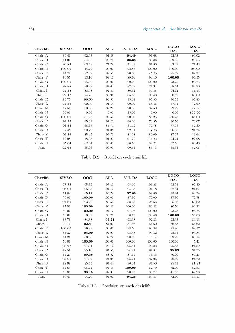
114 Appendix B. Additional results
Chairlift SIVAO OOC ALL ALL DA LOCOLOCODA-
LOCODA
Chair. A 89.40 92.93 91.48 94.49 91.68 92.93 90.02Chair. B 91.30 84.06 92.75 96.38 89.86 89.86 95.65Chair. C 96.83 63.49 77.78 71.43 61.90 63.49 71.43Chair. D 100.00 14.29 100.00 92.85 100.00 100.00 100.00Chair. E 94.78 82.09 89.55 90.30 95.52 95.52 87.31Chair. F 96.55 93.10 93.10 89.66 93.10 100.00 96.55Chair. G 100.00 75.00 100.00 100.00 100.00 93.75 93.75Chair. H 98.88 89.89 87.64 87.08 71.91 68.54 80.90Chair. I 95.38 83.08 92.31 86.92 55.38 64.62 81.54Chair. J 92.17 74.78 86.96 85.66 90.43 80.87 86.09Chair. K 93.75 96.53 96.53 95.14 95.83 96.53 95.83Chair. L 95.38 90.00 91.54 90.39 68.46 67.31 77.69Chair. M 87.50 80.36 89.29 90.18 87.50 89.29 92.86Chair. N 50.00 0.00 0.00 25.00 0.00 0.00 100.00Chair. O 100.00 81.25 92.50 90.00 86.25 86.25 85.00Chair. P 98.25 85.09 91.23 88.16 78.95 80.70 78.07Chair. Q 96.83 66.67 85.71 84.12 77.78 77.78 87.30Chair. R 77.48 90.79 94.08 92.11 97.37 96.05 94.74Chair. S 96.36 85.45 92.73 88.18 89.09 87.27 83.64Chair. T 92.98 78.95 91.23 91.22 94.74 94.74 92.98Chair. U 95.04 82.64 90.08 90.50 94.21 92.56 88.43Avg. 92.68 85.96 90.93 90.54 85.73 85.54 87.06
Table B.2 – Recall on each chairlift.
Chairlift SIVAO OOC ALL ALL DA LOCOLOCODA-
LOCODA
Chair. A 97.73 95.72 97.13 95.19 93.23 92.74 97.30Chair. B 96.92 95.08 94.12 94.33 91.18 92.54 91.67Chair. C 91.04 85.11 90.74 97.83 92.86 95.24 88.24Chair. D 70.00 100.00 100.00 87.50 70.00 87.50 77.78Chair. E 97.69 93.22 89.55 88.65 25.65 25.96 60.62Chair. F 87.50 100.00 96.43 100.00 69.23 80.56 90.32Chair. G 40.00 100.00 94.12 97.06 100.00 93.75 93.75Chair. H 93.62 93.02 98.73 98.72 98.46 100.00 96.00Chair. I 83.78 84.38 95.24 93.38 92.31 93.33 84.13Chair. J 79.10 92.47 84.03 87.56 64.60 66.43 84.62Chair. K 100.00 99.29 100.00 98.56 93.88 95.86 98.57Chair. L 87.32 95.90 92.97 95.53 90.82 95.11 94.84Chair. M 94.23 83.33 87.72 90.99 96.08 89.29 88.14Chair. N 50.00 100.00 100.00 100.00 100.00 100.00 5.41Chair. O 98.77 97.01 96.10 95.41 95.83 95.83 91.89Chair. P 92.56 95.10 94.55 94.81 91.84 95.83 91.75Chair. Q 64.21 89.36 88.52 87.69 73.13 70.00 66.27Chair. R 95.90 94.52 94.08 95.24 87.06 90.12 91.72Chair. S 92.98 85.45 94.44 96.04 87.50 85.71 97.87Chair. T 94.64 95.74 94.55 100.00 62.79 72.00 82.81Chair. U 85.82 96.15 92.37 90.23 36.77 41.33 69.93Avg. 90.43 94.20 94.00 94.28 69.87 72.10 86.11
Table B.3 – Precision on each chairlift.
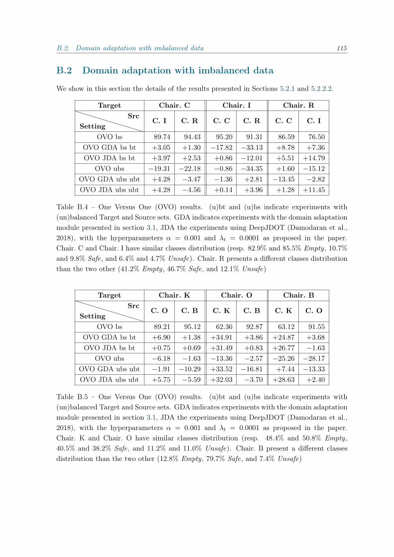
B.2. Domain adaptation with imbalanced data 115
B.2 Domain adaptation with imbalanced data
We show in this section the details of the results presented in Sections 5.2.1 and 5.2.2.2.
Target Chair. C Chair. I Chair. R
SettingSrc
C. I C. R C. C C. R C. C C. I
OVO bs 89.74 94.43 95.20 91.31 86.59 76.50
OVO GDA bs bt +3.05 +1.30 −17.82 −33.13 +8.78 +7.36
OVO JDA bs bt +3.97 +2.53 +0.86 −12.01 +5.51 +14.79
OVO ubs −19.31 −22.18 −0.86 −34.35 +1.60 −15.12
OVO GDA ubs ubt +4.28 −3.47 −1.36 +2.81 −13.45 −2.82
OVO JDA ubs ubt +4.28 −4.56 +0.14 +3.96 +1.28 +11.45
Table B.4 – One Versus One (OVO) results. (u)bt and (u)bs indicate experiments with(un)balanced Target and Source sets. GDA indicates experiments with the domain adaptationmodule presented in section 3.1, JDA the experiments using DeepJDOT (Damodaran et al.,2018), with the hyperparameters α = 0.001 and λt = 0.0001 as proposed in the paper.Chair. C and Chair. I have similar classes distribution (resp. 82.9% and 85.5% Empty , 10.7%and 9.8% Safe, and 6.4% and 4.7% Unsafe). Chair. R presents a different classes distributionthan the two other (41.2% Empty , 46.7% Safe, and 12.1% Unsafe)
Target Chair. K Chair. O Chair. B
SettingSrc
C. O C. B C. K C. B C. K C. O
OVO bs 89.21 95.12 62.36 92.87 63.12 91.55
OVO GDA bs bt +6.90 +1.38 +34.91 +3.86 +24.87 +3.68
OVO JDA bs bt +0.75 +0.69 +31.49 +0.83 +26.77 −1.63
OVO ubs −6.18 −1.63 −13.36 −2.57 −25.26 −28.17
OVO GDA ubs ubt −1.91 −10.29 +33.52 −16.81 +7.44 −13.33
OVO JDA ubs ubt +5.75 −5.59 +32.03 −3.70 +28.63 +2.40
Table B.5 – One Versus One (OVO) results. (u)bt and (u)bs indicate experiments with(un)balanced Target and Source sets. GDA indicates experiments with the domain adaptationmodule presented in section 3.1, JDA the experiments using DeepJDOT (Damodaran et al.,2018), with the hyperparameters α = 0.001 and λt = 0.0001 as proposed in the paper.Chair. K and Chair. O have similar classes distribution (resp. 48.4% and 50.8% Empty ,40.5% and 38.2% Safe, and 11.2% and 11.0% Unsafe). Chair. B present a different classesdistribution than the two other (12.8% Empty , 79.7% Safe, and 7.4% Unsafe)
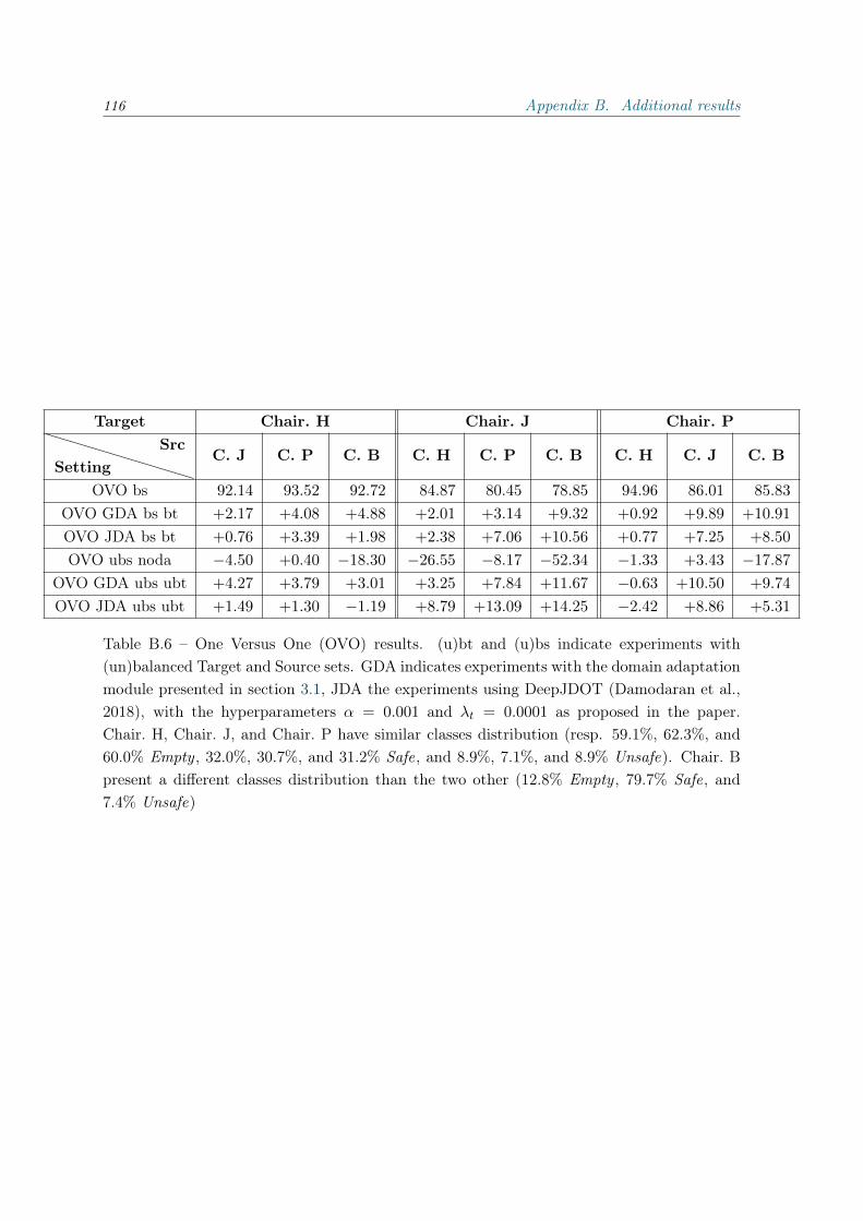
116 Appendix B. Additional results
Target Chair. H Chair. J Chair. P
SettingSrc
C. J C. P C. B C. H C. P C. B C. H C. J C. B
OVO bs 92.14 93.52 92.72 84.87 80.45 78.85 94.96 86.01 85.83
OVO GDA bs bt +2.17 +4.08 +4.88 +2.01 +3.14 +9.32 +0.92 +9.89 +10.91
OVO JDA bs bt +0.76 +3.39 +1.98 +2.38 +7.06 +10.56 +0.77 +7.25 +8.50
OVO ubs noda −4.50 +0.40 −18.30 −26.55 −8.17 −52.34 −1.33 +3.43 −17.87
OVO GDA ubs ubt +4.27 +3.79 +3.01 +3.25 +7.84 +11.67 −0.63 +10.50 +9.74
OVO JDA ubs ubt +1.49 +1.30 −1.19 +8.79 +13.09 +14.25 −2.42 +8.86 +5.31
Table B.6 – One Versus One (OVO) results. (u)bt and (u)bs indicate experiments with(un)balanced Target and Source sets. GDA indicates experiments with the domain adaptationmodule presented in section 3.1, JDA the experiments using DeepJDOT (Damodaran et al.,2018), with the hyperparameters α = 0.001 and λt = 0.0001 as proposed in the paper.Chair. H, Chair. J, and Chair. P have similar classes distribution (resp. 59.1%, 62.3%, and60.0% Empty , 32.0%, 30.7%, and 31.2% Safe, and 8.9%, 7.1%, and 8.9% Unsafe). Chair. Bpresent a different classes distribution than the two other (12.8% Empty , 79.7% Safe, and7.4% Unsafe)

Appendix C
Appendix of Chapter 4.2
For the sake of clarity, we will remind each statement before giving its proof. We also recallthe notations and the definitions that are used for our purpose.
In chapter 4.2, the error profile of a hypothesis h as been defined as E(h) = (e1(h), e2(h)) =
(FN(h), FP (h)). In the binary setting and using the previous notations, the F-Measure isdefined by:
F (e) =(1 + β2)(P − e1)
(1 + β2)P − e1 + e2. (C.1)
C.1 Main results of the chapter
In this section, we provide all the proofs of Chapter 4.2, but only in the binary setting.
C.1.1 Pseudo-linearity of F-Measure
We aim to prove the following proposition, which plays a key role to provide the bound onthe F-measure.
Proposition C.1. The F-measure, F , is a pseudo-linear function.
Proof. We need to show that both F and −F are pseudo-convex, i.e. that we have:
〈∇F (e), (e′ − e)〉 ≥ 0 =⇒ F (e′) ≥ F (e). (C.2)
The gradient of the F-measure is defined by:
∇F (e) = − 1 + β2
((1 + β2)P − e1 + e2)2
(β2P + e2
P − e1
).
We now develop the left-hand side of the implication (C.2):
〈∇F (e), (e′ − e)〉 ≥ 0,
− 1 + β2
((1 + β2)P − e1 + e2)2
[(β2P + e2)(e′1 − e1) + (P − e1)(e′2 − e2)
]≥ 0,
117
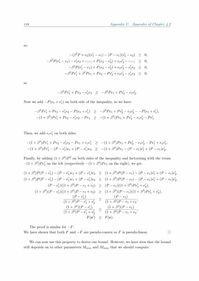
118 Appendix C. Appendix of Chapter 4.2
so,
−(β2P + e2)(e′1 − e1)− (P − e1)(e′2 − e2) ≥ 0,
−β2P (e′1 − e1)− e′1e2 + e1e2 + P (e2 − e′2) + e1e′2 − e1e2 ≥ 0,
−β2P (e′1 − e1) + P (e2 − e′2) + e1e′2 − e′1e2 ≥ 0,
−β2Pe′1 + β2Pe1 + Pe2 − Pe′2 + e1e′2 − e′1e2 ≥ 0.
so
−β2Pe′1 + Pe2 − e′1e2 ≥ −β2Pe1 + Pe′2 − e1e′2.
Now we add −P (e1 + e′1) on both side of the inequality, so we have:
−β2Pe′1 + Pe2 − e′1e2 − P (e1 + e′1) ≥ −β2Pe1 + Pe′2 − e1e′2 −−P (e1 + e′1),
−(1 + β2)Pe′1 + Pe2 − e′1e2 − Pe1 ≥ −(1 + β2)Pe1 + Pe′2 − e1e′2 − Pe′1.
Then, we add e1e′1 on both sides:
−(1 + β2)Pe′1 + Pe2 − e′1e2 − Pe1 + e1e′1 ≥ −(1 + β2)Pe1 + Pe′2 − e1e
′2 − Pe′1 + e1e
′1,
−(1 + β2)Pe′1 − (P − e′1)e1 + (P − e′1)e2 ≥ −(1 + β2)Pe1 − (P − e1)e′1 + (P − e1)e′2.
Finally, by adding (1 + β2)P 2 on both sides of the inequality and factorizing with the terms−(1 + β2)Pe′1 on the left (respectively −(1 + β2)Pe1 on the right), we get:
(1 + β2)P (P − e′1)− (P − e′1)e1 + (P − e′1)e2 ≥ (1 + β2)P (P − e1)− (P − e1)e′1 + (P − e1)e′2,
(1 + β2)P (P − e′1)− (P − e′1)e1 + (P − e′1)e2 ≥ (1 + β2)P (P − e1)− (P − e1)e′1 + (P − e1)e′2,
(P − e′1)((1 + β2)P − e1 + e2) ≥ (P − e1)((1 + β2)Pe′1 + e′2),
(1 + β2)(P − e′1)((1 + β2)P − e1 + e2) ≥ (1 + β2)(P − e1)((1 + β2)Pe′1 + e′2),
(P − e′1)
(1 + β2)P − e′1 + e′2≥ (P − e1)
(1 + β2)P − e1 + e2,
(1 + β2)(P − e′1)
(1 + β2)P − e′1 + e′2≥ (1 + β2)(P − e1)
(1 + β2)P − e1 + e2,
F (e′) ≥ F (e).
The proof is similar for −F .We have shown that both F and −F are pseudo-convex so F is pseudo-linear.
We can now use this property to derive our bound. However, we have seen that the boundstill depends on to other parameters Mmin and Mmax that we should compute.

C.1. Main results of the chapter 119
C.1.2 Computation of the values of Mmin and Mmax.
We aim to show how we can solve the optimization problems that define Mmin and Mmax
and show how it can be reduced to a simple convex optimization problem where the set ofconstraints is a convex polygon.
Computation of Mmax
Now, we would like to give an explicit value for Mmax. This value can be obtained by solvingthe following optimization problem:
maxe′∈E(H)
e′2 − e′1 s.t. Fβ(e′) > Fβ(e).
In the binary case, setting e = (e1, e2) and e′ = (e′1, e′2). We can write Fβ(e′) > Fβ(e) as:
(1 + β2)(P − e′1)
(1 + β2)P − e′1 + e′2>
(1 + β2)(P − e1)
(1 + β2)P − e1 + e2,
Now we develop and reduce these expressions.
(P − e′1)[(1 + β2)P − e1 + e2] > (P − e1)[(1 + β2)P − e′1 + e′2]),
(1 + β2)P 2 − (1 + β2)Pe′1 + (P − e′1)(e2 − e1) > (1 + β2)P 2 − (1 + β2)Pe1 + (P − e1)(e′2 − e′1),
(1 + β2)P (e1 − e′1) + P (e2 − e1 + e′1 − e′2) > e2e′1 − e1e
′2 + e′1e1 − e1e
′1.
Now, we set: e′1 = e1 +α1 and e′2 = e2 +α2. In other words, we study how much we haveto change e′ from e to solve our problem. We can then write:
−(1 + β2)Pα1 + P (α1 − α2) > e2(e1 + α1)− e1(e2 + α2),
α1(−(1 + β2)P + P − e2) + α2(−P + e1) > 0,
α1(β2P + e2) < −α2(P − e1).
Thus, the optimization problem can be rewritten as:
maxα
α2 − α1,
s.t. α1 <−α2(P − e1)
β2P + e2,
α1 ∈ [−e1, P − e1],
α2 ∈ [−e2, N − e2].
The optimization problem consists of maximizing a difference under a polygon set ofconstraints. In the binary setting, the set of constraints can be represented as shown inFig. C.1 where the line D is defined by the following equation:
α1 =−α2(P − e1)
β2P + e2. (C.3)
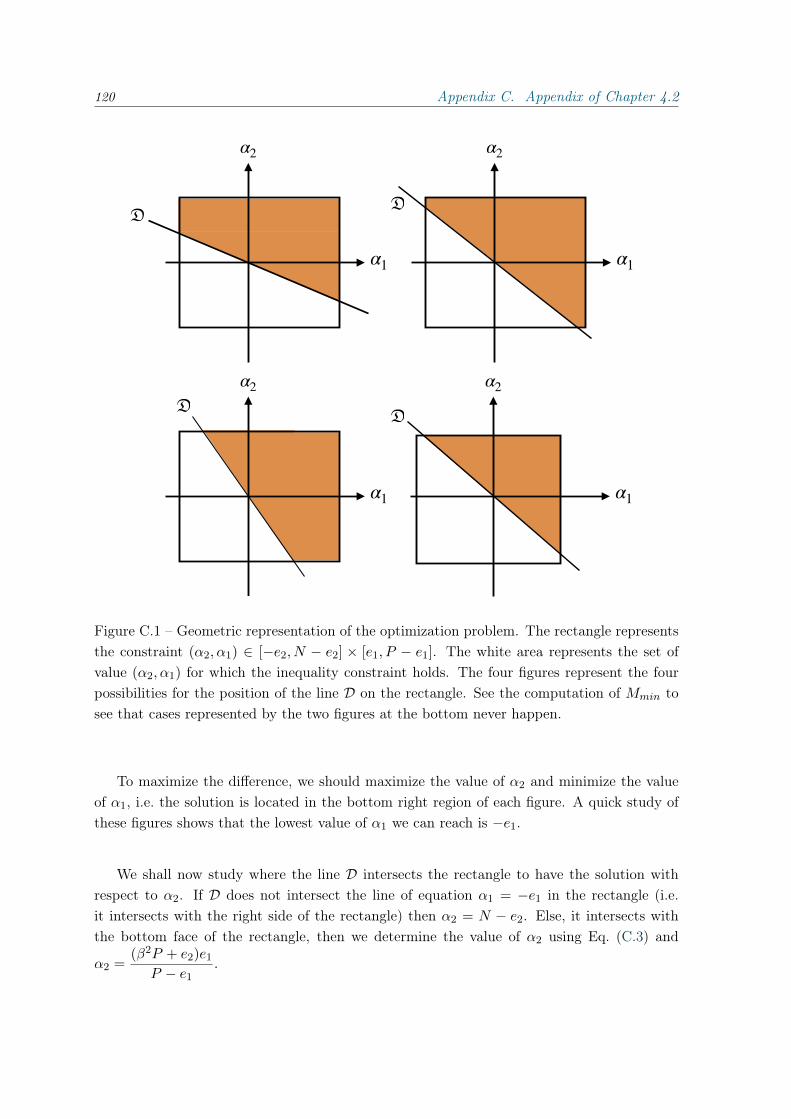
120 Appendix C. Appendix of Chapter 4.2
α1
α2
α1
α2
α1
α2
α1
α2
D<latexit sha1_base64="nBO2fehDgNL5I3IkUJPXj0XOric=">AAACz3icjVHLSsNAFD2Nr1pfVZdugkVwVRIRdFnUhcsW7APaIpN02obmxWSilFJx6w+41b8S/0D/wjtjCmoRnZDkzLn3nJl7rxP7XiIt6zVnLCwuLa/kVwtr6xubW8XtnUYSpcLldTfyI9FyWMJ9L+R16Umft2LBWeD4vOmMzlW8ecNF4kXhlRzHvBuwQej1PZdJojqdgMlhX7DR5GJ6XSxZZUsvcx7YGSghW9Wo+IIOeojgIkUAjhCSsA+GhJ42bFiIietiQpwg5Ok4xxQF0qaUxSmDETui74B27YwNaa88E6126RSfXkFKEwekiShPEFanmTqeamfF/uY90Z7qbmP6O5lXQKzEkNi/dLPM/+pULRJ9nOoaPKop1oyqzs1cUt0VdXPzS1WSHGLiFO5RXBB2tXLWZ1NrEl276i3T8TedqVi1d7PcFO/qljRg++c450HjqGxbZbt2XKqcZaPOYw/7OKR5nqCCS1RRJ+8Yj3jCs1Ezbo074/4z1chlml18W8bDB6tylFk=</latexit><latexit sha1_base64="nBO2fehDgNL5I3IkUJPXj0XOric=">AAACz3icjVHLSsNAFD2Nr1pfVZdugkVwVRIRdFnUhcsW7APaIpN02obmxWSilFJx6w+41b8S/0D/wjtjCmoRnZDkzLn3nJl7rxP7XiIt6zVnLCwuLa/kVwtr6xubW8XtnUYSpcLldTfyI9FyWMJ9L+R16Umft2LBWeD4vOmMzlW8ecNF4kXhlRzHvBuwQej1PZdJojqdgMlhX7DR5GJ6XSxZZUsvcx7YGSghW9Wo+IIOeojgIkUAjhCSsA+GhJ42bFiIietiQpwg5Ok4xxQF0qaUxSmDETui74B27YwNaa88E6126RSfXkFKEwekiShPEFanmTqeamfF/uY90Z7qbmP6O5lXQKzEkNi/dLPM/+pULRJ9nOoaPKop1oyqzs1cUt0VdXPzS1WSHGLiFO5RXBB2tXLWZ1NrEl276i3T8TedqVi1d7PcFO/qljRg++c450HjqGxbZbt2XKqcZaPOYw/7OKR5nqCCS1RRJ+8Yj3jCs1Ezbo074/4z1chlml18W8bDB6tylFk=</latexit><latexit sha1_base64="nBO2fehDgNL5I3IkUJPXj0XOric=">AAACz3icjVHLSsNAFD2Nr1pfVZdugkVwVRIRdFnUhcsW7APaIpN02obmxWSilFJx6w+41b8S/0D/wjtjCmoRnZDkzLn3nJl7rxP7XiIt6zVnLCwuLa/kVwtr6xubW8XtnUYSpcLldTfyI9FyWMJ9L+R16Umft2LBWeD4vOmMzlW8ecNF4kXhlRzHvBuwQej1PZdJojqdgMlhX7DR5GJ6XSxZZUsvcx7YGSghW9Wo+IIOeojgIkUAjhCSsA+GhJ42bFiIietiQpwg5Ok4xxQF0qaUxSmDETui74B27YwNaa88E6126RSfXkFKEwekiShPEFanmTqeamfF/uY90Z7qbmP6O5lXQKzEkNi/dLPM/+pULRJ9nOoaPKop1oyqzs1cUt0VdXPzS1WSHGLiFO5RXBB2tXLWZ1NrEl276i3T8TedqVi1d7PcFO/qljRg++c450HjqGxbZbt2XKqcZaPOYw/7OKR5nqCCS1RRJ+8Yj3jCs1Ezbo074/4z1chlml18W8bDB6tylFk=</latexit><latexit sha1_base64="nBO2fehDgNL5I3IkUJPXj0XOric=">AAACz3icjVHLSsNAFD2Nr1pfVZdugkVwVRIRdFnUhcsW7APaIpN02obmxWSilFJx6w+41b8S/0D/wjtjCmoRnZDkzLn3nJl7rxP7XiIt6zVnLCwuLa/kVwtr6xubW8XtnUYSpcLldTfyI9FyWMJ9L+R16Umft2LBWeD4vOmMzlW8ecNF4kXhlRzHvBuwQej1PZdJojqdgMlhX7DR5GJ6XSxZZUsvcx7YGSghW9Wo+IIOeojgIkUAjhCSsA+GhJ42bFiIietiQpwg5Ok4xxQF0qaUxSmDETui74B27YwNaa88E6126RSfXkFKEwekiShPEFanmTqeamfF/uY90Z7qbmP6O5lXQKzEkNi/dLPM/+pULRJ9nOoaPKop1oyqzs1cUt0VdXPzS1WSHGLiFO5RXBB2tXLWZ1NrEl276i3T8TedqVi1d7PcFO/qljRg++c450HjqGxbZbt2XKqcZaPOYw/7OKR5nqCCS1RRJ+8Yj3jCs1Ezbo074/4z1chlml18W8bDB6tylFk=</latexit>
D<latexit sha1_base64="nBO2fehDgNL5I3IkUJPXj0XOric=">AAACz3icjVHLSsNAFD2Nr1pfVZdugkVwVRIRdFnUhcsW7APaIpN02obmxWSilFJx6w+41b8S/0D/wjtjCmoRnZDkzLn3nJl7rxP7XiIt6zVnLCwuLa/kVwtr6xubW8XtnUYSpcLldTfyI9FyWMJ9L+R16Umft2LBWeD4vOmMzlW8ecNF4kXhlRzHvBuwQej1PZdJojqdgMlhX7DR5GJ6XSxZZUsvcx7YGSghW9Wo+IIOeojgIkUAjhCSsA+GhJ42bFiIietiQpwg5Ok4xxQF0qaUxSmDETui74B27YwNaa88E6126RSfXkFKEwekiShPEFanmTqeamfF/uY90Z7qbmP6O5lXQKzEkNi/dLPM/+pULRJ9nOoaPKop1oyqzs1cUt0VdXPzS1WSHGLiFO5RXBB2tXLWZ1NrEl276i3T8TedqVi1d7PcFO/qljRg++c450HjqGxbZbt2XKqcZaPOYw/7OKR5nqCCS1RRJ+8Yj3jCs1Ezbo074/4z1chlml18W8bDB6tylFk=</latexit><latexit sha1_base64="nBO2fehDgNL5I3IkUJPXj0XOric=">AAACz3icjVHLSsNAFD2Nr1pfVZdugkVwVRIRdFnUhcsW7APaIpN02obmxWSilFJx6w+41b8S/0D/wjtjCmoRnZDkzLn3nJl7rxP7XiIt6zVnLCwuLa/kVwtr6xubW8XtnUYSpcLldTfyI9FyWMJ9L+R16Umft2LBWeD4vOmMzlW8ecNF4kXhlRzHvBuwQej1PZdJojqdgMlhX7DR5GJ6XSxZZUsvcx7YGSghW9Wo+IIOeojgIkUAjhCSsA+GhJ42bFiIietiQpwg5Ok4xxQF0qaUxSmDETui74B27YwNaa88E6126RSfXkFKEwekiShPEFanmTqeamfF/uY90Z7qbmP6O5lXQKzEkNi/dLPM/+pULRJ9nOoaPKop1oyqzs1cUt0VdXPzS1WSHGLiFO5RXBB2tXLWZ1NrEl276i3T8TedqVi1d7PcFO/qljRg++c450HjqGxbZbt2XKqcZaPOYw/7OKR5nqCCS1RRJ+8Yj3jCs1Ezbo074/4z1chlml18W8bDB6tylFk=</latexit><latexit sha1_base64="nBO2fehDgNL5I3IkUJPXj0XOric=">AAACz3icjVHLSsNAFD2Nr1pfVZdugkVwVRIRdFnUhcsW7APaIpN02obmxWSilFJx6w+41b8S/0D/wjtjCmoRnZDkzLn3nJl7rxP7XiIt6zVnLCwuLa/kVwtr6xubW8XtnUYSpcLldTfyI9FyWMJ9L+R16Umft2LBWeD4vOmMzlW8ecNF4kXhlRzHvBuwQej1PZdJojqdgMlhX7DR5GJ6XSxZZUsvcx7YGSghW9Wo+IIOeojgIkUAjhCSsA+GhJ42bFiIietiQpwg5Ok4xxQF0qaUxSmDETui74B27YwNaa88E6126RSfXkFKEwekiShPEFanmTqeamfF/uY90Z7qbmP6O5lXQKzEkNi/dLPM/+pULRJ9nOoaPKop1oyqzs1cUt0VdXPzS1WSHGLiFO5RXBB2tXLWZ1NrEl276i3T8TedqVi1d7PcFO/qljRg++c450HjqGxbZbt2XKqcZaPOYw/7OKR5nqCCS1RRJ+8Yj3jCs1Ezbo074/4z1chlml18W8bDB6tylFk=</latexit><latexit sha1_base64="nBO2fehDgNL5I3IkUJPXj0XOric=">AAACz3icjVHLSsNAFD2Nr1pfVZdugkVwVRIRdFnUhcsW7APaIpN02obmxWSilFJx6w+41b8S/0D/wjtjCmoRnZDkzLn3nJl7rxP7XiIt6zVnLCwuLa/kVwtr6xubW8XtnUYSpcLldTfyI9FyWMJ9L+R16Umft2LBWeD4vOmMzlW8ecNF4kXhlRzHvBuwQej1PZdJojqdgMlhX7DR5GJ6XSxZZUsvcx7YGSghW9Wo+IIOeojgIkUAjhCSsA+GhJ42bFiIietiQpwg5Ok4xxQF0qaUxSmDETui74B27YwNaa88E6126RSfXkFKEwekiShPEFanmTqeamfF/uY90Z7qbmP6O5lXQKzEkNi/dLPM/+pULRJ9nOoaPKop1oyqzs1cUt0VdXPzS1WSHGLiFO5RXBB2tXLWZ1NrEl276i3T8TedqVi1d7PcFO/qljRg++c450HjqGxbZbt2XKqcZaPOYw/7OKR5nqCCS1RRJ+8Yj3jCs1Ezbo074/4z1chlml18W8bDB6tylFk=</latexit>
D<latexit sha1_base64="nBO2fehDgNL5I3IkUJPXj0XOric=">AAACz3icjVHLSsNAFD2Nr1pfVZdugkVwVRIRdFnUhcsW7APaIpN02obmxWSilFJx6w+41b8S/0D/wjtjCmoRnZDkzLn3nJl7rxP7XiIt6zVnLCwuLa/kVwtr6xubW8XtnUYSpcLldTfyI9FyWMJ9L+R16Umft2LBWeD4vOmMzlW8ecNF4kXhlRzHvBuwQej1PZdJojqdgMlhX7DR5GJ6XSxZZUsvcx7YGSghW9Wo+IIOeojgIkUAjhCSsA+GhJ42bFiIietiQpwg5Ok4xxQF0qaUxSmDETui74B27YwNaa88E6126RSfXkFKEwekiShPEFanmTqeamfF/uY90Z7qbmP6O5lXQKzEkNi/dLPM/+pULRJ9nOoaPKop1oyqzs1cUt0VdXPzS1WSHGLiFO5RXBB2tXLWZ1NrEl276i3T8TedqVi1d7PcFO/qljRg++c450HjqGxbZbt2XKqcZaPOYw/7OKR5nqCCS1RRJ+8Yj3jCs1Ezbo074/4z1chlml18W8bDB6tylFk=</latexit><latexit sha1_base64="nBO2fehDgNL5I3IkUJPXj0XOric=">AAACz3icjVHLSsNAFD2Nr1pfVZdugkVwVRIRdFnUhcsW7APaIpN02obmxWSilFJx6w+41b8S/0D/wjtjCmoRnZDkzLn3nJl7rxP7XiIt6zVnLCwuLa/kVwtr6xubW8XtnUYSpcLldTfyI9FyWMJ9L+R16Umft2LBWeD4vOmMzlW8ecNF4kXhlRzHvBuwQej1PZdJojqdgMlhX7DR5GJ6XSxZZUsvcx7YGSghW9Wo+IIOeojgIkUAjhCSsA+GhJ42bFiIietiQpwg5Ok4xxQF0qaUxSmDETui74B27YwNaa88E6126RSfXkFKEwekiShPEFanmTqeamfF/uY90Z7qbmP6O5lXQKzEkNi/dLPM/+pULRJ9nOoaPKop1oyqzs1cUt0VdXPzS1WSHGLiFO5RXBB2tXLWZ1NrEl276i3T8TedqVi1d7PcFO/qljRg++c450HjqGxbZbt2XKqcZaPOYw/7OKR5nqCCS1RRJ+8Yj3jCs1Ezbo074/4z1chlml18W8bDB6tylFk=</latexit><latexit sha1_base64="nBO2fehDgNL5I3IkUJPXj0XOric=">AAACz3icjVHLSsNAFD2Nr1pfVZdugkVwVRIRdFnUhcsW7APaIpN02obmxWSilFJx6w+41b8S/0D/wjtjCmoRnZDkzLn3nJl7rxP7XiIt6zVnLCwuLa/kVwtr6xubW8XtnUYSpcLldTfyI9FyWMJ9L+R16Umft2LBWeD4vOmMzlW8ecNF4kXhlRzHvBuwQej1PZdJojqdgMlhX7DR5GJ6XSxZZUsvcx7YGSghW9Wo+IIOeojgIkUAjhCSsA+GhJ42bFiIietiQpwg5Ok4xxQF0qaUxSmDETui74B27YwNaa88E6126RSfXkFKEwekiShPEFanmTqeamfF/uY90Z7qbmP6O5lXQKzEkNi/dLPM/+pULRJ9nOoaPKop1oyqzs1cUt0VdXPzS1WSHGLiFO5RXBB2tXLWZ1NrEl276i3T8TedqVi1d7PcFO/qljRg++c450HjqGxbZbt2XKqcZaPOYw/7OKR5nqCCS1RRJ+8Yj3jCs1Ezbo074/4z1chlml18W8bDB6tylFk=</latexit><latexit sha1_base64="nBO2fehDgNL5I3IkUJPXj0XOric=">AAACz3icjVHLSsNAFD2Nr1pfVZdugkVwVRIRdFnUhcsW7APaIpN02obmxWSilFJx6w+41b8S/0D/wjtjCmoRnZDkzLn3nJl7rxP7XiIt6zVnLCwuLa/kVwtr6xubW8XtnUYSpcLldTfyI9FyWMJ9L+R16Umft2LBWeD4vOmMzlW8ecNF4kXhlRzHvBuwQej1PZdJojqdgMlhX7DR5GJ6XSxZZUsvcx7YGSghW9Wo+IIOeojgIkUAjhCSsA+GhJ42bFiIietiQpwg5Ok4xxQF0qaUxSmDETui74B27YwNaa88E6126RSfXkFKEwekiShPEFanmTqeamfF/uY90Z7qbmP6O5lXQKzEkNi/dLPM/+pULRJ9nOoaPKop1oyqzs1cUt0VdXPzS1WSHGLiFO5RXBB2tXLWZ1NrEl276i3T8TedqVi1d7PcFO/qljRg++c450HjqGxbZbt2XKqcZaPOYw/7OKR5nqCCS1RRJ+8Yj3jCs1Ezbo074/4z1chlml18W8bDB6tylFk=</latexit>
D<latexit sha1_base64="nBO2fehDgNL5I3IkUJPXj0XOric=">AAACz3icjVHLSsNAFD2Nr1pfVZdugkVwVRIRdFnUhcsW7APaIpN02obmxWSilFJx6w+41b8S/0D/wjtjCmoRnZDkzLn3nJl7rxP7XiIt6zVnLCwuLa/kVwtr6xubW8XtnUYSpcLldTfyI9FyWMJ9L+R16Umft2LBWeD4vOmMzlW8ecNF4kXhlRzHvBuwQej1PZdJojqdgMlhX7DR5GJ6XSxZZUsvcx7YGSghW9Wo+IIOeojgIkUAjhCSsA+GhJ42bFiIietiQpwg5Ok4xxQF0qaUxSmDETui74B27YwNaa88E6126RSfXkFKEwekiShPEFanmTqeamfF/uY90Z7qbmP6O5lXQKzEkNi/dLPM/+pULRJ9nOoaPKop1oyqzs1cUt0VdXPzS1WSHGLiFO5RXBB2tXLWZ1NrEl276i3T8TedqVi1d7PcFO/qljRg++c450HjqGxbZbt2XKqcZaPOYw/7OKR5nqCCS1RRJ+8Yj3jCs1Ezbo074/4z1chlml18W8bDB6tylFk=</latexit><latexit sha1_base64="nBO2fehDgNL5I3IkUJPXj0XOric=">AAACz3icjVHLSsNAFD2Nr1pfVZdugkVwVRIRdFnUhcsW7APaIpN02obmxWSilFJx6w+41b8S/0D/wjtjCmoRnZDkzLn3nJl7rxP7XiIt6zVnLCwuLa/kVwtr6xubW8XtnUYSpcLldTfyI9FyWMJ9L+R16Umft2LBWeD4vOmMzlW8ecNF4kXhlRzHvBuwQej1PZdJojqdgMlhX7DR5GJ6XSxZZUsvcx7YGSghW9Wo+IIOeojgIkUAjhCSsA+GhJ42bFiIietiQpwg5Ok4xxQF0qaUxSmDETui74B27YwNaa88E6126RSfXkFKEwekiShPEFanmTqeamfF/uY90Z7qbmP6O5lXQKzEkNi/dLPM/+pULRJ9nOoaPKop1oyqzs1cUt0VdXPzS1WSHGLiFO5RXBB2tXLWZ1NrEl276i3T8TedqVi1d7PcFO/qljRg++c450HjqGxbZbt2XKqcZaPOYw/7OKR5nqCCS1RRJ+8Yj3jCs1Ezbo074/4z1chlml18W8bDB6tylFk=</latexit><latexit sha1_base64="nBO2fehDgNL5I3IkUJPXj0XOric=">AAACz3icjVHLSsNAFD2Nr1pfVZdugkVwVRIRdFnUhcsW7APaIpN02obmxWSilFJx6w+41b8S/0D/wjtjCmoRnZDkzLn3nJl7rxP7XiIt6zVnLCwuLa/kVwtr6xubW8XtnUYSpcLldTfyI9FyWMJ9L+R16Umft2LBWeD4vOmMzlW8ecNF4kXhlRzHvBuwQej1PZdJojqdgMlhX7DR5GJ6XSxZZUsvcx7YGSghW9Wo+IIOeojgIkUAjhCSsA+GhJ42bFiIietiQpwg5Ok4xxQF0qaUxSmDETui74B27YwNaa88E6126RSfXkFKEwekiShPEFanmTqeamfF/uY90Z7qbmP6O5lXQKzEkNi/dLPM/+pULRJ9nOoaPKop1oyqzs1cUt0VdXPzS1WSHGLiFO5RXBB2tXLWZ1NrEl276i3T8TedqVi1d7PcFO/qljRg++c450HjqGxbZbt2XKqcZaPOYw/7OKR5nqCCS1RRJ+8Yj3jCs1Ezbo074/4z1chlml18W8bDB6tylFk=</latexit><latexit sha1_base64="nBO2fehDgNL5I3IkUJPXj0XOric=">AAACz3icjVHLSsNAFD2Nr1pfVZdugkVwVRIRdFnUhcsW7APaIpN02obmxWSilFJx6w+41b8S/0D/wjtjCmoRnZDkzLn3nJl7rxP7XiIt6zVnLCwuLa/kVwtr6xubW8XtnUYSpcLldTfyI9FyWMJ9L+R16Umft2LBWeD4vOmMzlW8ecNF4kXhlRzHvBuwQej1PZdJojqdgMlhX7DR5GJ6XSxZZUsvcx7YGSghW9Wo+IIOeojgIkUAjhCSsA+GhJ42bFiIietiQpwg5Ok4xxQF0qaUxSmDETui74B27YwNaa88E6126RSfXkFKEwekiShPEFanmTqeamfF/uY90Z7qbmP6O5lXQKzEkNi/dLPM/+pULRJ9nOoaPKop1oyqzs1cUt0VdXPzS1WSHGLiFO5RXBB2tXLWZ1NrEl276i3T8TedqVi1d7PcFO/qljRg++c450HjqGxbZbt2XKqcZaPOYw/7OKR5nqCCS1RRJ+8Yj3jCs1Ezbo074/4z1chlml18W8bDB6tylFk=</latexit>
Figure C.1 – Geometric representation of the optimization problem. The rectangle representsthe constraint (α2, α1) ∈ [−e2, N − e2] × [e1, P − e1]. The white area represents the set ofvalue (α2, α1) for which the inequality constraint holds. The four figures represent the fourpossibilities for the position of the line D on the rectangle. See the computation of Mmin tosee that cases represented by the two figures at the bottom never happen.
To maximize the difference, we should maximize the value of α2 and minimize the valueof α1, i.e. the solution is located in the bottom right region of each figure. A quick study ofthese figures shows that the lowest value of α1 we can reach is −e1.
We shall now study where the line D intersects the rectangle to have the solution withrespect to α2. If D does not intersect the line of equation α1 = −e1 in the rectangle (i.e.it intersects with the right side of the rectangle) then α2 = N − e2. Else, it intersects withthe bottom face of the rectangle, then we determine the value of α2 using Eq. (C.3) and
α2 =(β2P + e2)e1
P − e1.
C.1. Main results of the chapter 121
Finally, the solution of the optimization problem is:
(α1, α2) =
(−e1,min
(N − e2,
(β2P + e2)e1
P − e1
)),
and the optimal value Mmax is defined by:
Mmax = e2 + min
(N − e2,
(β2P + e2)e1
P − e1
).
Computation of Mmin
We now aim to solve the following optimization problem:
mine′∈E(H)
e′2 − e′1 s.t. Fβ(e′) > Fβ(e).
As it has been done and using the same notations as in the previous section, we can rewritethe optimization problem as follows:
minα
α2 − α1,
s.t. α1 <−α2(P − e1)
β2P + e2,
α1 ∈ [−e1, P − e1],
α2 ∈ [−e2, N − e2].
The constraints remain unchanged. However, to minimize this difference, we have to max-imize the value of α1 and minimize the value of α2, i.e. we are interested in the upper leftregion of each rectangle. In each case represented in Fig C.1, we see that the minimum of α2
is equal to −e2.
If we have a look at the two figures at the bottom of Fig. C.1, we see that the optimalvalue of α1 is equal to P − e1. However, this value is not in the image of the function ofα2 defined by Eq (C.3). In fact, according to Eq. (C.3), the image of α2 = −e2 is equal toe2(P − e1)
β2P + e2which is lower than P − e1. So the two figures at the bottom represent cases that
never happen and the intersection of D with the rectangle of constraint is on left part of therectangle.
Finally, the solution of the optimization problem is:
(α1, α2) =
(e2(P − e1)
β2P + e2,−e2
),
and the optimal value Mmin is defined by:
Mmin = −e1 −e2(P − e1)
β2P + e2.

122 Appendix C. Appendix of Chapter 4.2
Now that we have provided all the details to compute and plot our bound, it remains toexplain how to compute the bound from Parambath et al. (2014) with respect to any costparameters t, t′ for a fair comparison.
C.1.3 Rewriting the bound of Parambath et al. (2014)
For the sake of clarity we restate the Proposition 5 of Parambath et al. (2014) for our purpose:
Proposition C.2. Let t, t ∈ [0, 1] and ε1 ≥ 0. Suppose that there exists Φ > 0 such that forall e, e′ ∈ E(H) satisfying F (e′) > F (e), we have:
F (e′)− F (e) ≥ Φ〈a(t′), e− e′〉. (C.4)
Furthermore, suppose that we have the two following conditions
(i) ‖a(t)− a(t′)‖2 ≤ 2|t− t′| (ii) 〈a(t), e〉 ≤ mine′′∈E(H)
〈a(t), e′′〉+ ε1
Let us also set M = maxe′′∈E(H)
‖e′′‖2, then we have:
F (e′) ≤ F (e) + Φε1 + 4MΦ|t′ − t|.
According to the authors, the point (i) is a consequence of a of being Lipschitz continuouswith Lipschitz constant equal to 2. The point (ii) is just the expression of the sub-optimalityof the learned classifier.
Proof. For all e, e ∈ E(H) and t, t′ ∈ [0, 1], we have:
〈a(t), e〉 = 〈a(t)− a(t′), e〉+ 〈a(t′), e〉,≤ 〈a(t′), e〉+ 2M |t′ − t|.
Where we have successively applied the Cauchy-Schwarz inequality and (i). Then:
mine′′∈E(H)
〈a(t), e′′〉 ≤ mine′′∈E(H)
〈a(t′), e′′〉+ 2M |t′ − t| = 〈a(t′), e′〉+ 2M |t′ − t|, (C.5)
where e′ denote the error profile learned by the optimal classifier trained with the cost functiona(t′) and is such that F (e′) > F (e). Then, writing 〈a(t′), e〉 = 〈a(t′) − a(t), e〉 + 〈a(t), e〉and applying the Cauchy-Schwarz inequality, we have:
〈a(t′), e〉 ≤ 〈a(t), e〉+ 2M |t′ − t|,≤ min
e′′∈E(H)〈a(t), e′′〉+ ε1 + 2M |t′ − t|,
≤ 〈a(t′), e′〉+ ε1 + 4M |t′ − t|,
where the second inequality comes from (ii) and the last inequality comes from Eq. (C.5). Byplugging this last inequality in inequality (C.4), we get the result.Furthermore, the existence of the constant Φ has been proved by the authors and is equal to(β2P )−1
Remark. This bound can be used in both binary and multi-class setting.
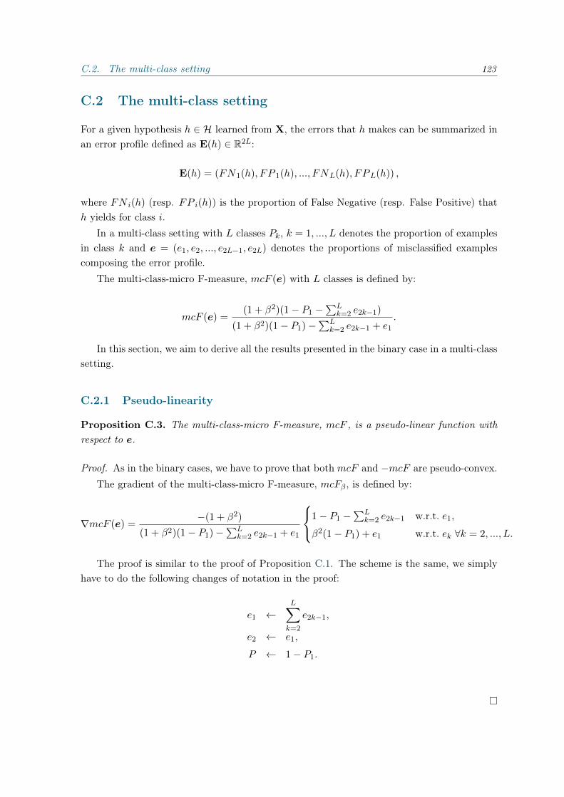
C.2. The multi-class setting 123
C.2 The multi-class setting
For a given hypothesis h ∈ H learned from X, the errors that h makes can be summarized inan error profile defined as E(h) ∈ R2L:
E(h) = (FN1(h), FP 1(h), ..., FNL(h), FPL(h)) ,
where FN i(h) (resp. FP i(h)) is the proportion of False Negative (resp. False Positive) thath yields for class i.
In a multi-class setting with L classes Pk, k = 1, ..., L denotes the proportion of examplesin class k and e = (e1, e2, ..., e2L−1, e2L) denotes the proportions of misclassified examplescomposing the error profile.
The multi-class-micro F-measure, mcF (e) with L classes is defined by:
mcF (e) =(1 + β2)(1− P1 −
∑Lk=2 e2k−1)
(1 + β2)(1− P1)−∑L
k=2 e2k−1 + e1
.
In this section, we aim to derive all the results presented in the binary case in a multi-classsetting.
C.2.1 Pseudo-linearity
Proposition C.3. The multi-class-micro F-measure, mcF , is a pseudo-linear function withrespect to e.
Proof. As in the binary cases, we have to prove that both mcF and −mcF are pseudo-convex.The gradient of the multi-class-micro F-measure, mcFβ , is defined by:
∇mcF (e) =−(1 + β2)
(1 + β2)(1− P1)−∑L
k=2 e2k−1 + e1
1− P1 −∑L
k=2 e2k−1 w.r.t. e1,
β2(1− P1) + e1 w.r.t. ek ∀k = 2, ..., L.
The proof is similar to the proof of Proposition C.1. The scheme is the same, we simplyhave to do the following changes of notation in the proof:
e1 ←L∑k=2
e2k−1,
e2 ← e1,
P ← 1− P1.

124 Appendix C. Appendix of Chapter 4.2
C.2.2 Derivation of the bound
As it was done in the binary case, we will use the property of pseudo-linearity of mcF (e) tobound the difference of micro F-measure in terms of the parameters of our weighted function.First, we introduce the definition of our weighted function a : R → R2L and express thedifference of micro F-measure of two error profiles in function of the two error profiles.In this section, for the sake of clarity, we will set e =
∑Lk=2 e2k−1.
First step: impact of a change in the error profile
Using the property of pseudo-linearity, we can show that there are two functions a : R→ R2L
and b : R→ R defined by:
0 = 〈a(mcF (e)), e〉+ b(mcF (e)),
where:
a(t) =
1 + β2 − t for e2k−1, k = 2, ..., L
t for e1,
0 otherwise,
and b(t) = (t− 1)(1 + β2)(1− P1).
From these definitions we can write:
〈a(mcF (e′)), e− e′〉 = 〈a(mcF (e′)), e〉+ b(mcF (e′)),
= 〈a(mcF (e′))− a(mcF (e)), e〉 − b(mcF (e)) + b(mcF (e′)),
= (mcF (e′)−mcF (e))(1 + β2)(1− P1)
+ (mcF (e′)−mcF (e))e1 + (mcF (e)−mcF (e′))e,
= (mcF (e′)−mcF (e))((1 + β2)(1− P1)− e+ e1
).
We can now write the difference of micro-F-measure as:
mcF (e′)−mcF (e) = Φe · 〈a(t), e− e′〉,
where:Φe =
1
(1 + β2)(1− P1)− e+ e1,
Second step: a bound on the micro F-measure mcF (e)
We suppose that we have a value of t for which a weighted-classifier with weights a(t) has beenlearned. This classifier has an error profile e and a F-measure mcF (e). We now imagine ahypothetical classifier that is learned with weights a(t′), and we denote by e′ the error profileof this classifier. For any value of t′, we derive an upper bound on the F-measure mcF (e′)
that this hypothetical classifier can achieve.
mcF (e′)−mcF (e) = Φe · 〈a(t′), e− e′〉,
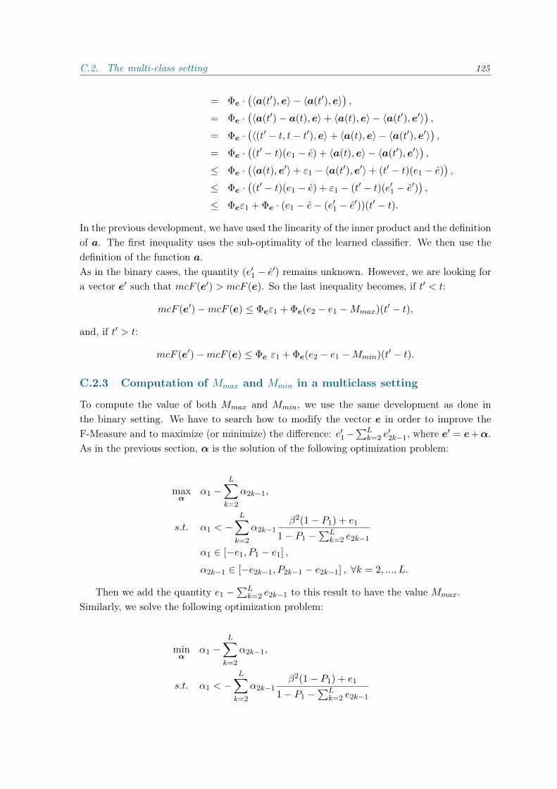
C.2. The multi-class setting 125
= Φe ·(〈a(t′), e〉 − 〈a(t′), e〉
),
= Φe ·(〈a(t′)− a(t), e〉+ 〈a(t), e〉 − 〈a(t′), e′〉
),
= Φe ·(〈(t′ − t, t− t′), e〉+ 〈a(t), e〉 − 〈a(t′), e′〉
),
= Φe ·((t′ − t)(e1 − e) + 〈a(t), e〉 − 〈a(t′), e′〉
),
≤ Φe ·(〈a(t), e′〉+ ε1 − 〈a(t′), e′〉+ (t′ − t)(e1 − e)
),
≤ Φe ·((t′ − t)(e1 − e) + ε1 − (t′ − t)(e′1 − e′)
),
≤ Φeε1 + Φe · (e1 − e− (e′1 − e′))(t′ − t).
In the previous development, we have used the linearity of the inner product and the definitionof a. The first inequality uses the sub-optimality of the learned classifier. We then use thedefinition of the function a.As in the binary cases, the quantity (e′1 − e′) remains unknown. However, we are looking fora vector e′ such that mcF (e′) > mcF (e). So the last inequality becomes, if t′ < t:
mcF (e′)−mcF (e) ≤ Φeε1 + Φe(e2 − e1 −Mmax)(t′ − t),
and, if t′ > t:
mcF (e′)−mcF (e) ≤ Φe ε1 + Φe(e2 − e1 −Mmin)(t′ − t).
C.2.3 Computation of Mmax and Mmin in a multiclass setting
To compute the value of both Mmax and Mmin, we use the same development as done inthe binary setting. We have to search how to modify the vector e in order to improve theF-Measure and to maximize (or minimize) the difference: e′1−
∑Lk=2 e
′2k−1, where e
′ = e+α.As in the previous section, α is the solution of the following optimization problem:
maxα
α1 −L∑k=2
α2k−1,
s.t. α1 < −L∑k=2
α2k−1β2(1− P1) + e1
1− P1 −∑L
k=2 e2k−1
α1 ∈ [−e1, P1 − e1] ,
α2k−1 ∈ [−e2k−1, P2k−1 − e2k−1] , ∀k = 2, ..., L.
Then we add the quantity e1 −∑L
k=2 e2k−1 to this result to have the value Mmax.Similarly, we solve the following optimization problem:
minα
α1 −L∑k=2
α2k−1,
s.t. α1 < −L∑k=2
α2k−1β2(1− P1) + e1
1− P1 −∑L
k=2 e2k−1

126 Appendix C. Appendix of Chapter 4.2
α1 ∈ [−e1, P1 − e1] ,
α2k−1 ∈ [−e2k−1, P2k−1 − e2k−1] , ∀k = 2, ..., L.
Then we add the quantity e1 −∑L
k=2 e2k−1 to this result to have the value Mmin.
C.3 Extended Experiments
This section is dedicated to the experiments. We provide the complete set of graphs andtables for all datasets.
C.3.1 Illustrations of unreachable regions
In this section we provide the unreachable regions (see Fig. C.2) of both presented bounds,our vs. the one obtained from Parambath et al. (2014). As it was noticed previously, ourresult gives a tighter bound on the optimal reachable F-measure. Moreover, we see that themore the data is imbalanced, the tightest is our bound.The fact that some points lie in the unreachable regions is explained by our setting. Indeed,we recall that we made the assumption that ε1 = 0, i.e. we suppose that learned classifier isthe optimal one, in terms of 0− 1 loss, but it is not the case in practice.

C.3. Extended Experiments 127
Figure C.2 – Unreachable regions obtained from the same 19 (t1, Fi) points corresponding tolearning weighted SVM on a grid of t values. Cones are shown for all datasets. The boundfrom Parambath et al. (2014) is represented on the left and our bound on the right.
C.3.2 Theoretical bound versus ε1
In this section we compare our bound with the one from Parambath et al. (2014) with respectto ε1. The graphics presented in Fig. C.3 show that the bound from Parambath et al. (2014)is uninformative since the value of the best reachable F-measure is always equal to 1 except onAbalone10 dataset. We see that our bound increases mostly linearly with ε1. The evolution
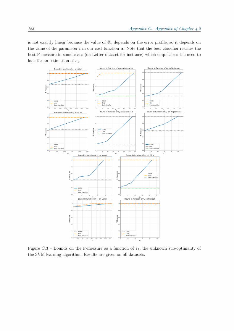
128 Appendix C. Appendix of Chapter 4.2
is not exactly linear because the value of Φe depends on the error profile, so it depends onthe value of the parameter t in our cost function a. Note that the best classifier reaches thebest F-measure in some cases (on Letter dataset for instance) which emphasizes the need tolook for an estimation of ε1.
Figure C.3 – Bounds on the F-measure as a function of ε1, the unknown sub-optimality ofthe SVM learning algorithm. Results are given on all datasets.

C.3. Extended Experiments 129
C.3.3 Evolution of Bounds vs. iterations/grid size
Figure C.4 – Comparison of our bound and the one from Parambath et al. (2014) withrespect to the number of iteration/ the size of the grid. We also represent the evolution ofboth associated algorithms.
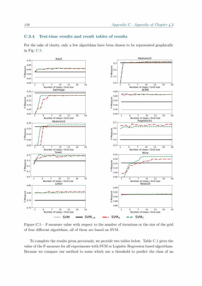
130 Appendix C. Appendix of Chapter 4.2
C.3.4 Test-time results and result tables of results
For the sake of clarity, only a few algorithms have been chosen to be represented graphicallyin Fig. C.5.
Figure C.5 – F-measure value with respect to the number of iterations or the size of the gridof four different algorithms, all of them are based on SVM.
To complete the results given previously, we provide two tables below. Table C.1 gives thevalue of the F-measure for all experiments with SVM or Logisitic Regression based algorithms.Because we compare our method to some which use a threshold to predict the class of an
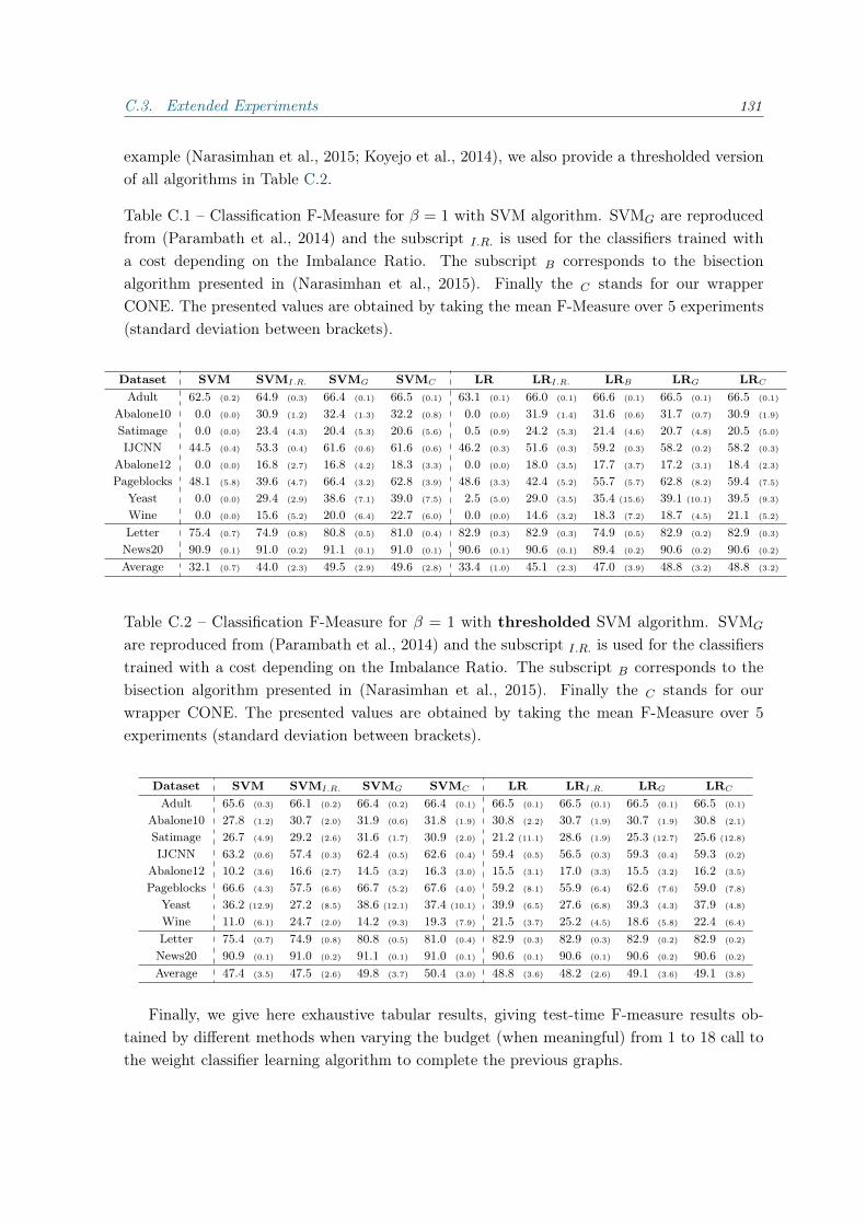
C.3. Extended Experiments 131
example (Narasimhan et al., 2015; Koyejo et al., 2014), we also provide a thresholded versionof all algorithms in Table C.2.
Table C.1 – Classification F-Measure for β = 1 with SVM algorithm. SVMG are reproducedfrom (Parambath et al., 2014) and the subscript I.R. is used for the classifiers trained witha cost depending on the Imbalance Ratio. The subscript B corresponds to the bisectionalgorithm presented in (Narasimhan et al., 2015). Finally the C stands for our wrapperCONE. The presented values are obtained by taking the mean F-Measure over 5 experiments(standard deviation between brackets).
Dataset SVM SVMI.R. SVMG SVMC LR LRI.R. LRB LRG LRC
Adult 62.5 (0.2) 64.9 (0.3) 66.4 (0.1) 66.5 (0.1) 63.1 (0.1) 66.0 (0.1) 66.6 (0.1) 66.5 (0.1) 66.5 (0.1)
Abalone10 0.0 (0.0) 30.9 (1.2) 32.4 (1.3) 32.2 (0.8) 0.0 (0.0) 31.9 (1.4) 31.6 (0.6) 31.7 (0.7) 30.9 (1.9)
Satimage 0.0 (0.0) 23.4 (4.3) 20.4 (5.3) 20.6 (5.6) 0.5 (0.9) 24.2 (5.3) 21.4 (4.6) 20.7 (4.8) 20.5 (5.0)
IJCNN 44.5 (0.4) 53.3 (0.4) 61.6 (0.6) 61.6 (0.6) 46.2 (0.3) 51.6 (0.3) 59.2 (0.3) 58.2 (0.2) 58.2 (0.3)
Abalone12 0.0 (0.0) 16.8 (2.7) 16.8 (4.2) 18.3 (3.3) 0.0 (0.0) 18.0 (3.5) 17.7 (3.7) 17.2 (3.1) 18.4 (2.3)
Pageblocks 48.1 (5.8) 39.6 (4.7) 66.4 (3.2) 62.8 (3.9) 48.6 (3.3) 42.4 (5.2) 55.7 (5.7) 62.8 (8.2) 59.4 (7.5)
Yeast 0.0 (0.0) 29.4 (2.9) 38.6 (7.1) 39.0 (7.5) 2.5 (5.0) 29.0 (3.5) 35.4 (15.6) 39.1 (10.1) 39.5 (9.3)
Wine 0.0 (0.0) 15.6 (5.2) 20.0 (6.4) 22.7 (6.0) 0.0 (0.0) 14.6 (3.2) 18.3 (7.2) 18.7 (4.5) 21.1 (5.2)
Letter 75.4 (0.7) 74.9 (0.8) 80.8 (0.5) 81.0 (0.4) 82.9 (0.3) 82.9 (0.3) 74.9 (0.5) 82.9 (0.2) 82.9 (0.3)
News20 90.9 (0.1) 91.0 (0.2) 91.1 (0.1) 91.0 (0.1) 90.6 (0.1) 90.6 (0.1) 89.4 (0.2) 90.6 (0.2) 90.6 (0.2)
Average 32.1 (0.7) 44.0 (2.3) 49.5 (2.9) 49.6 (2.8) 33.4 (1.0) 45.1 (2.3) 47.0 (3.9) 48.8 (3.2) 48.8 (3.2)
Table C.2 – Classification F-Measure for β = 1 with thresholded SVM algorithm. SVMG
are reproduced from (Parambath et al., 2014) and the subscript I.R. is used for the classifierstrained with a cost depending on the Imbalance Ratio. The subscript B corresponds to thebisection algorithm presented in (Narasimhan et al., 2015). Finally the C stands for ourwrapper CONE. The presented values are obtained by taking the mean F-Measure over 5experiments (standard deviation between brackets).
Dataset SVM SVMI.R. SVMG SVMC LR LRI.R. LRG LRC
Adult 65.6 (0.3) 66.1 (0.2) 66.4 (0.2) 66.4 (0.1) 66.5 (0.1) 66.5 (0.1) 66.5 (0.1) 66.5 (0.1)
Abalone10 27.8 (1.2) 30.7 (2.0) 31.9 (0.6) 31.8 (1.9) 30.8 (2.2) 30.7 (1.9) 30.7 (1.9) 30.8 (2.1)
Satimage 26.7 (4.9) 29.2 (2.6) 31.6 (1.7) 30.9 (2.0) 21.2 (11.1) 28.6 (1.9) 25.3 (12.7) 25.6 (12.8)
IJCNN 63.2 (0.6) 57.4 (0.3) 62.4 (0.5) 62.6 (0.4) 59.4 (0.5) 56.5 (0.3) 59.3 (0.4) 59.3 (0.2)
Abalone12 10.2 (3.6) 16.6 (2.7) 14.5 (3.2) 16.3 (3.0) 15.5 (3.1) 17.0 (3.3) 15.5 (3.2) 16.2 (3.5)
Pageblocks 66.6 (4.3) 57.5 (6.6) 66.7 (5.2) 67.6 (4.0) 59.2 (8.1) 55.9 (6.4) 62.6 (7.6) 59.0 (7.8)
Yeast 36.2 (12.9) 27.2 (8.5) 38.6 (12.1) 37.4 (10.1) 39.9 (6.5) 27.6 (6.8) 39.3 (4.3) 37.9 (4.8)
Wine 11.0 (6.1) 24.7 (2.0) 14.2 (9.3) 19.3 (7.9) 21.5 (3.7) 25.2 (4.5) 18.6 (5.8) 22.4 (6.4)
Letter 75.4 (0.7) 74.9 (0.8) 80.8 (0.5) 81.0 (0.4) 82.9 (0.3) 82.9 (0.3) 82.9 (0.2) 82.9 (0.2)
News20 90.9 (0.1) 91.0 (0.2) 91.1 (0.1) 91.0 (0.1) 90.6 (0.1) 90.6 (0.1) 90.6 (0.2) 90.6 (0.2)
Average 47.4 (3.5) 47.5 (2.6) 49.8 (3.7) 50.4 (3.0) 48.8 (3.6) 48.2 (2.6) 49.1 (3.6) 49.1 (3.8)
Finally, we give here exhaustive tabular results, giving test-time F-measure results ob-tained by different methods when varying the budget (when meaningful) from 1 to 18 call tothe weight classifier learning algorithm to complete the previous graphs.

132 Appendix C. Appendix of Chapter 4.2
Table C.3 – Mean F-Measure over 5 experiments and limiting the number of itera-tions/grid steps to 1 (standard deviation between brackets).
Dataset SVM SVMI.R. SVMG SVMC LR LRI.R. LRB LRG LRC
Adult 62.5 (0.2) 64.9 (0.3) 65.0 (0.4) 65.0 (0.4) 63.1 (0.1) 66.0 (0.1) 66.6 (0.1) 66.1 (0.1) 66.1 (0.1)
Abalone10 0.0 (0.0) 30.9 (1.2) 0.0 (0.0) 0.0 (0.0) 0.0 (0.0) 31.9 (1.4) 31.6 (0.6) 24.4 (1.2) 24.4 (1.3)
Satimage 0.0 (0.0) 23.4 (4.3) 0.9 (1.9) 0.0 (0.0) 0.5 (0.9) 24.2 (5.3) 21.4 (4.6) 3.5 (6.9) 3.5 (6.9)
IJCNN 44.5 (0.4) 53.3 (0.4) 61.6 (0.5) 61.6 (0.5) 46.2 (0.3) 51.6 (0.3) 59.2 (0.3) 58.3 (0.3) 58.3 (0.3)
Abalone12 0.0 (0.0) 16.8 (2.7) 0.0 (0.0) 0.0 (0.0) 0.0 (0.0) 18.0 (3.5) 17.7 (3.7) 0.0 (0.0) 0.0 (0.0)
Pageblocks 48.1 (5.8) 39.6 (4.7) 64.4 (2.9) 59.1 (3.8) 48.6 (3.3) 42.4 (5.2) 55.7 (5.7) 55.3 (4.7) 54.5 (4.4)
Yeast 0.0 (0.0) 29.4 (2.9) 12.1 (10.6) 22.9 (15.7) 2.5 (5.0) 29.0 (3.5) 35.4 (15.6) 24.9 (16.0) 24.4 (16.1)
Wine 0.0 (0.0) 15.6 (5.2) 0.0 (0.0) 0.0 (0.0) 0.0 (0.0) 14.6 (3.2) 18.3 (7.2) 5.5 (10.9) 11.6 (10.8)
Letter 75.4 (0.7) 74.9 (0.8) 80.2 (0.3) 80.3 (0.3) 82.9 (0.3) 82.9 (0.3) 74.9 (0.5) 82.6 (0.3) 82.6 (0.3)
News20 90.9 (0.1) 91.0 (0.2) 90.9 (0.2) 90.9 (0.2) 90.6 (0.1) 90.6 (0.1) 89.4 (0.2) 90.6 (0.2) 90.6 (0.2)
Average 32.1 (0.7) 44.0 (2.3) 37.5 (1.7) 38.0 (2.1) 33.4 (1.0) 45.1 (2.3) 47.0 (3.9) 41.1 (4.1) 41.6 (4.0)
Table C.4 – Mean F-Measure over 5 experiments and limiting the number of itera-tions/grid steps to 2 (standard deviation between brackets).
Dataset SVM SVMI.R. SVMG SVMC LR LRI.R. LRB LRG LRC
Adult 62.5 (0.2) 64.9 (0.3) 66.4 (0.2) 66.2 (0.3) 63.1 (0.1) 66.0 (0.1) 66.6 (0.1) 66.6 (0.1) 66.2 (0.1)
Abalone10 0.0 (0.0) 30.9 (1.2) 32.6 (1.4) 30.7 (1.1) 0.0 (0.0) 31.9 (1.4) 31.6 (0.6) 31.9 (1.7) 32.4 (1.9)
Satimage 0.0 (0.0) 23.4 (4.3) 6.1 (12.2) 5.9 (11.8) 0.5 (0.9) 24.2 (5.3) 21.4 (4.6) 6.2 (12.3) 6.1 (12.2)
IJCNN 44.5 (0.4) 53.3 (0.4) 60.7 (0.4) 61.6 (0.5) 46.2 (0.3) 51.6 (0.3) 59.2 (0.3) 56.8 (0.3) 58.3 (0.3)
Abalone12 0.0 (0.0) 16.8 (2.7) 0.0 (0.0) 0.0 (0.0) 0.0 (0.0) 18.0 (3.5) 17.7 (3.7) 2.8 (3.4) 13.3 (3.5)
Pageblocks 48.1 (5.8) 39.6 (4.7) 65.0 (7.6) 63.3 (4.1) 48.6 (3.3) 42.4 (5.2) 55.7 (5.7) 62.7 (7.1) 58.3 (6.8)
Yeast 0.0 (0.0) 29.4 (2.9) 30.9 (17.2) 25.4 (17.5) 2.5 (5.0) 29.0 (3.5) 35.4 (15.6) 27.8 (20.0) 33.0 (18.3)
Wine 0.0 (0.0) 15.6 (5.2) 0.0 (0.0) 11.7 (11.1) 0.0 (0.0) 14.6 (3.2) 18.3 (7.2) 8.7 (11.2) 15.6 (6.7)
Letter 75.4 (0.7) 74.9 (0.8) 80.7 (0.5) 80.4 (0.5) 82.9 (0.3) 82.9 (0.3) 74.9 (0.5) 82.9 (0.2) 82.8 (0.2)
News20 90.9 (0.1) 91.0 (0.2) 90.9 (0.2) 91.0 (0.2) 90.6 (0.1) 90.6 (0.1) 89.4 (0.2) 90.6 (0.2) 90.6 (0.1)
Average 32.1 (0.7) 44.0 (2.3) 43.3 (4.0) 43.6 (4.7) 33.4 (1.0) 45.1 (2.3) 47.0 (3.9) 43.7 (5.6) 45.7 (5.0)
Table C.5 – Mean F-Measure over 5 experiments and limiting the number of itera-tions/grid steps to 3 (standard deviation between brackets).
Dataset SVM SVMI.R. SVMG SVMC LR LRI.R. LRB LRG LRC
Adult 62.5 (0.2) 64.9 (0.3) 66.1 (0.2) 66.2 (0.3) 63.1 (0.1) 66.0 (0.1) 66.6 (0.1) 66.2 (0.1) 66.2 (0.1)
Abalone10 0.0 (0.0) 30.9 (1.2) 30.7 (1.1) 31.0 (1.4) 0.0 (0.0) 31.9 (1.4) 31.6 (0.6) 32.5 (1.5) 31.3 (2.2)
Satimage 0.0 (0.0) 23.4 (4.3) 5.9 (11.8) 20.2 (4.7) 0.5 (0.9) 24.2 (5.3) 21.4 (4.6) 6.1 (12.1) 20.3 (5.1)
IJCNN 44.5 (0.4) 53.3 (0.4) 61.6 (0.5) 61.6 (0.5) 46.2 (0.3) 51.6 (0.3) 59.2 (0.3) 58.3 (0.3) 58.3 (0.3)
Abalone12 0.0 (0.0) 16.8 (2.7) 0.0 (0.0) 16.7 (2.7) 0.0 (0.0) 18.0 (3.5) 17.7 (3.7) 14.2 (3.0) 16.6 (3.4)
Pageblocks 48.1 (5.8) 39.6 (4.7) 65.5 (2.0) 63.3 (4.1) 48.6 (3.3) 42.4 (5.2) 55.7 (5.7) 60.4 (6.4) 58.3 (6.8)
Yeast 0.0 (0.0) 29.4 (2.9) 32.6 (18.3) 37.8 (7.8) 2.5 (5.0) 29.0 (3.5) 35.4 (15.6) 32.1 (11.9) 32.6 (12.0)
Wine 0.0 (0.0) 15.6 (5.2) 11.8 (11.1) 19.5 (5.1) 0.0 (0.0) 14.6 (3.2) 18.3 (7.2) 17.5 (5.8) 20.0 (3.8)
Letter 75.4 (0.7) 74.9 (0.8) 80.5 (0.2) 80.4 (0.5) 82.9 (0.3) 82.9 (0.3) 74.9 (0.5) 82.9 (0.2) 82.9 (0.2)
News20 90.9 (0.1) 91.0 (0.2) 91.0 (0.2) 91.0 (0.2) 90.6 (0.1) 90.6 (0.1) 89.4 (0.2) 90.6 (0.2) 90.6 (0.1)
Average 32.1 (0.7) 44.0 (2.3) 44.6 (4.5) 48.8 (2.7) 33.4 (1.0) 45.1 (2.3) 47.0 (3.9) 46.1 (4.2) 47.7 (3.4)

C.3. Extended Experiments 133
Table C.6 – Mean F-Measure over 5 experiments and limiting the number of itera-tions/grid steps to 4 (standard deviation between brackets).
Dataset SVM SVMI.R. SVMG SVMC LR LRI.R. LRB LRG LRC
Adult 62.5 (0.2) 64.9 (0.3) 66.0 (0.2) 66.2 (0.3) 63.1 (0.1) 66.0 (0.1) 66.6 (0.1) 66.4 (0.1) 66.2 (0.1)
Abalone10 0.0 (0.0) 30.9 (1.2) 31.0 (1.0) 31.0 (1.4) 0.0 (0.0) 31.9 (1.4) 31.6 (0.6) 30.9 (1.7) 31.3 (2.2)
Satimage 0.0 (0.0) 23.4 (4.3) 16.4 (9.5) 20.6 (5.6) 0.5 (0.9) 24.2 (5.3) 21.4 (4.6) 17.0 (9.8) 20.5 (5.0)
IJCNN 44.5 (0.4) 53.3 (0.4) 61.5 (0.4) 61.1 (0.5) 46.2 (0.3) 51.6 (0.3) 59.2 (0.3) 57.8 (0.4) 58.3 (0.3)
Abalone12 0.0 (0.0) 16.8 (2.7) 16.5 (4.0) 16.9 (4.3) 0.0 (0.0) 18.0 (3.5) 17.7 (3.7) 17.6 (3.0) 17.6 (3.1)
Pageblocks 48.1 (5.8) 39.6 (4.7) 61.0 (6.0) 63.3 (4.1) 48.6 (3.3) 42.4 (5.2) 55.7 (5.7) 62.1 (7.8) 58.4 (6.7)
Yeast 0.0 (0.0) 29.4 (2.9) 35.4 (8.7) 39.0 (7.5) 2.5 (5.0) 29.0 (3.5) 35.4 (15.6) 31.1 (18.0) 32.5 (12.0)
Wine 0.0 (0.0) 15.6 (5.2) 11.5 (7.8) 19.5 (5.1) 0.0 (0.0) 14.6 (3.2) 18.3 (7.2) 17.9 (2.8) 20.0 (3.8)
Letter 75.4 (0.7) 74.9 (0.8) 80.5 (0.3) 80.4 (0.5) 82.9 (0.3) 82.9 (0.3) 74.9 (0.5) 82.9 (0.2) 82.9 (0.3)
News20 90.9 (0.1) 91.0 (0.2) 91.0 (0.1) 91.0 (0.2) 90.6 (0.1) 90.6 (0.1) 89.4 (0.2) 90.6 (0.2) 90.7 (0.1)
Average 32.1 (0.7) 44.0 (2.3) 47.1 (3.8) 48.9 (2.9) 33.4 (1.0) 45.1 (2.3) 47.0 (3.9) 47.4 (4.4) 47.8 (3.4)
Table C.7 – Mean F-Measure over 5 experiments and limiting the number of itera-tions/grid steps to 5 (standard deviation between brackets).
Dataset SVM SVMI.R. SVMG SVMC LR LRI.R. LRB LRG LRC
Adult 62.5 (0.2) 64.9 (0.3) 66.4 (0.3) 66.2 (0.2) 63.1 (0.1) 66.0 (0.1) 66.6 (0.1) 66.6 (0.1) 66.5 (0.1)
Abalone10 0.0 (0.0) 30.9 (1.2) 32.6 (1.4) 31.7 (1.0) 0.0 (0.0) 31.9 (1.4) 31.6 (0.6) 31.3 (0.7) 31.2 (2.3)
Satimage 0.0 (0.0) 23.4 (4.3) 16.4 (9.5) 20.6 (5.6) 0.5 (0.9) 24.2 (5.3) 21.4 (4.6) 17.0 (9.8) 20.5 (5.0)
IJCNN 44.5 (0.4) 53.3 (0.4) 61.4 (0.6) 61.1 (0.5) 46.2 (0.3) 51.6 (0.3) 59.2 (0.3) 58.3 (0.3) 58.3 (0.3)
Abalone12 0.0 (0.0) 16.8 (2.7) 16.5 (4.0) 16.5 (4.0) 0.0 (0.0) 18.0 (3.5) 17.7 (3.7) 17.6 (3.0) 18.1 (2.6)
Pageblocks 48.1 (5.8) 39.6 (4.7) 67.7 (4.0) 62.1 (5.0) 48.6 (3.3) 42.4 (5.2) 55.7 (5.7) 61.8 (7.3) 59.6 (7.3)
Yeast 0.0 (0.0) 29.4 (2.9) 31.8 (10.5) 39.0 (7.5) 2.5 (5.0) 29.0 (3.5) 35.4 (15.6) 30.1 (17.2) 38.8 (8.5)
Wine 0.0 (0.0) 15.6 (5.2) 11.5 (7.8) 20.4 (5.6) 0.0 (0.0) 14.6 (3.2) 18.3 (7.2) 17.9 (2.8) 21.2 (5.1)
Letter 75.4 (0.7) 74.9 (0.8) 80.5 (0.4) 80.4 (0.5) 82.9 (0.3) 82.9 (0.3) 74.9 (0.5) 82.9 (0.2) 82.9 (0.3)
News20 90.9 (0.1) 91.0 (0.2) 91.0 (0.1) 91.0 (0.2) 90.6 (0.1) 90.6 (0.1) 89.4 (0.2) 90.6 (0.2) 90.7 (0.1)
Average 32.1 (0.7) 44.0 (2.3) 47.6 (3.9) 48.9 (3.0) 33.4 (1.0) 45.1 (2.3) 47.0 (3.9) 47.4 (4.2) 48.8 (3.2)
Table C.8 – Mean F-Measure over 5 experiments and limiting the number of itera-tions/grid steps to 6 (standard deviation between brackets).
Dataset SVM SVMI.R. SVMG SVMC LR LRI.R. LRB LRG LRC
Adult 62.5 (0.2) 64.9 (0.3) 66.5 (0.1) 66.4 (0.1) 63.1 (0.1) 66.0 (0.1) 66.6 (0.1) 66.4 (0.2) 66.5 (0.1)
Abalone10 0.0 (0.0) 30.9 (1.2) 30.7 (1.1) 31.7 (1.0) 0.0 (0.0) 31.9 (1.4) 31.6 (0.6) 31.6 (1.0) 31.4 (2.2)
Satimage 0.0 (0.0) 23.4 (4.3) 20.4 (5.3) 20.6 (5.6) 0.5 (0.9) 24.2 (5.3) 21.4 (4.6) 20.1 (4.6) 20.5 (5.0)
IJCNN 44.5 (0.4) 53.3 (0.4) 62.1 (0.5) 61.3 (0.6) 46.2 (0.3) 51.6 (0.3) 59.2 (0.3) 58.0 (0.4) 58.1 (0.3)
Abalone12 0.0 (0.0) 16.8 (2.7) 16.9 (2.9) 18.2 (3.3) 0.0 (0.0) 18.0 (3.5) 17.7 (3.7) 15.5 (6.2) 17.7 (3.4)
Pageblocks 48.1 (5.8) 39.6 (4.7) 64.8 (3.1) 64.2 (4.6) 48.6 (3.3) 42.4 (5.2) 55.7 (5.7) 60.6 (9.1) 59.5 (7.4)
Yeast 0.0 (0.0) 29.4 (2.9) 32.0 (10.4) 39.0 (7.5) 2.5 (5.0) 29.0 (3.5) 35.4 (15.6) 33.0 (18.8) 38.8 (8.5)
Wine 0.0 (0.0) 15.6 (5.2) 19.4 (5.3) 19.0 (7.0) 0.0 (0.0) 14.6 (3.2) 18.3 (7.2) 19.6 (5.1) 21.1 (5.2)
Letter 75.4 (0.7) 74.9 (0.8) 80.8 (0.5) 80.5 (0.4) 82.9 (0.3) 82.9 (0.3) 74.9 (0.5) 82.9 (0.2) 82.9 (0.3)
News20 90.9 (0.1) 91.0 (0.2) 91.0 (0.2) 91.0 (0.2) 90.6 (0.1) 90.6 (0.1) 89.4 (0.2) 90.6 (0.1) 90.7 (0.1)
Average 32.1 (0.7) 44.0 (2.3) 48.5 (2.9) 49.2 (3.0) 33.4 (1.0) 45.1 (2.3) 47.0 (3.9) 47.8 (4.6) 48.7 (3.2)

134 Appendix C. Appendix of Chapter 4.2
Table C.9 – Mean F-Measure over 5 experiments and limiting the number of itera-tions/grid steps to 7 (standard deviation between brackets).
Dataset SVM SVMI.R. SVMG SVMC LR LRI.R. LRB LRG LRC
Adult 62.5 (0.2) 64.9 (0.3) 66.2 (0.1) 66.4 (0.1) 63.1 (0.1) 66.0 (0.1) 66.6 (0.1) 66.4 (0.1) 66.5 (0.1)
Abalone10 0.0 (0.0) 30.9 (1.2) 31.0 (1.0) 32.5 (1.0) 0.0 (0.0) 31.9 (1.4) 31.6 (0.6) 32.2 (0.6) 31.4 (2.2)
Satimage 0.0 (0.0) 23.4 (4.3) 20.2 (4.7) 20.6 (5.6) 0.5 (0.9) 24.2 (5.3) 21.4 (4.6) 20.3 (5.0) 20.5 (5.0)
IJCNN 44.5 (0.4) 53.3 (0.4) 61.5 (0.4) 61.5 (0.5) 46.2 (0.3) 51.6 (0.3) 59.2 (0.3) 58.3 (0.3) 58.1 (0.3)
Abalone12 0.0 (0.0) 16.8 (2.7) 16.9 (2.9) 18.3 (3.3) 0.0 (0.0) 18.0 (3.5) 17.7 (3.7) 17.5 (3.4) 17.7 (3.4)
Pageblocks 48.1 (5.8) 39.6 (4.7) 65.7 (2.6) 62.8 (3.9) 48.6 (3.3) 42.4 (5.2) 55.7 (5.7) 61.3 (9.9) 59.9 (7.0)
Yeast 0.0 (0.0) 29.4 (2.9) 38.8 (7.0) 39.0 (7.5) 2.5 (5.0) 29.0 (3.5) 35.4 (15.6) 32.7 (11.8) 38.9 (8.6)
Wine 0.0 (0.0) 15.6 (5.2) 19.5 (6.2) 19.0 (7.0) 0.0 (0.0) 14.6 (3.2) 18.3 (7.2) 18.7 (4.5) 21.1 (5.2)
Letter 75.4 (0.7) 74.9 (0.8) 80.6 (0.1) 80.5 (0.4) 82.9 (0.3) 82.9 (0.3) 74.9 (0.5) 82.9 (0.2) 82.9 (0.3)
News20 90.9 (0.1) 91.0 (0.2) 91.1 (0.1) 91.0 (0.2) 90.6 (0.1) 90.6 (0.1) 89.4 (0.2) 90.6 (0.1) 90.7 (0.1)
Average 32.1 (0.7) 44.0 (2.3) 49.2 (2.5) 49.2 (3.0) 33.4 (1.0) 45.1 (2.3) 47.0 (3.9) 48.1 (3.6) 48.8 (3.2)
Table C.10 – Mean F-Measure over 5 experiments and limiting the number of itera-tions/grid steps to 8 (standard deviation between brackets).
Dataset SVM SVMI.R. SVMG SVMC LR LRI.R. LRB LRG LRC
Adult 62.5 (0.2) 64.9 (0.3) 66.4 (0.1) 66.5 (0.1) 63.1 (0.1) 66.0 (0.1) 66.6 (0.1) 66.5 (0.1) 66.5 (0.1)
Abalone10 0.0 (0.0) 30.9 (1.2) 32.6 (1.4) 32.6 (1.0) 0.0 (0.0) 31.9 (1.4) 31.6 (0.6) 32.1 (0.8) 31.4 (2.2)
Satimage 0.0 (0.0) 23.4 (4.3) 20.2 (4.7) 20.6 (5.6) 0.5 (0.9) 24.2 (5.3) 21.4 (4.6) 20.3 (5.0) 20.5 (5.0)
IJCNN 44.5 (0.4) 53.3 (0.4) 61.9 (0.7) 61.5 (0.5) 46.2 (0.3) 51.6 (0.3) 59.2 (0.3) 58.0 (0.4) 58.1 (0.3)
Abalone12 0.0 (0.0) 16.8 (2.7) 16.9 (2.9) 18.3 (3.3) 0.0 (0.0) 18.0 (3.5) 17.7 (3.7) 17.5 (3.4) 18.1 (3.7)
Pageblocks 48.1 (5.8) 39.6 (4.7) 65.8 (4.3) 62.8 (3.9) 48.6 (3.3) 42.4 (5.2) 55.7 (5.7) 60.0 (8.8) 59.4 (7.5)
Yeast 0.0 (0.0) 29.4 (2.9) 33.3 (12.2) 39.0 (7.5) 2.5 (5.0) 29.0 (3.5) 35.4 (15.6) 39.4 (8.5) 38.9 (8.6)
Wine 0.0 (0.0) 15.6 (5.2) 19.5 (6.2) 22.4 (6.1) 0.0 (0.0) 14.6 (3.2) 18.3 (7.2) 18.7 (4.5) 21.1 (5.2)
Letter 75.4 (0.7) 74.9 (0.8) 80.6 (0.4) 80.5 (0.4) 82.9 (0.3) 82.9 (0.3) 74.9 (0.5) 82.9 (0.2) 82.9 (0.3)
News20 90.9 (0.1) 91.0 (0.2) 91.0 (0.1) 91.0 (0.2) 90.6 (0.1) 90.6 (0.1) 89.4 (0.2) 90.6 (0.1) 90.6 (0.1)
Average 32.1 (0.7) 44.0 (2.3) 48.8 (3.3) 49.5 (2.9) 33.4 (1.0) 45.1 (2.3) 47.0 (3.9) 48.6 (3.2) 48.8 (3.3)
Table C.11 – Mean F-Measure over 5 experiments and limiting the number of itera-tions/grid steps to 9 (standard deviation between brackets).
Dataset SVM SVMI.R. SVMG SVMC LR LRI.R. LRB LRG LRC
Adult 62.5 (0.2) 64.9 (0.3) 66.4 (0.1) 66.5 (0.1) 63.1 (0.1) 66.0 (0.1) 66.6 (0.1) 66.4 (0.1) 66.5 (0.1)
Abalone10 0.0 (0.0) 30.9 (1.2) 31.0 (1.0) 32.2 (0.8) 0.0 (0.0) 31.9 (1.4) 31.6 (0.6) 31.5 (0.4) 31.4 (2.2)
Satimage 0.0 (0.0) 23.4 (4.3) 20.4 (5.3) 20.6 (5.6) 0.5 (0.9) 24.2 (5.3) 21.4 (4.6) 20.8 (4.9) 20.5 (5.0)
IJCNN 44.5 (0.4) 53.3 (0.4) 61.5 (0.4) 61.5 (0.5) 46.2 (0.3) 51.6 (0.3) 59.2 (0.3) 58.3 (0.3) 58.1 (0.3)
Abalone12 0.0 (0.0) 16.8 (2.7) 16.7 (4.1) 18.3 (3.3) 0.0 (0.0) 18.0 (3.5) 17.7 (3.7) 15.1 (5.9) 18.0 (3.6)
Pageblocks 48.1 (5.8) 39.6 (4.7) 65.4 (2.3) 62.8 (3.9) 48.6 (3.3) 42.4 (5.2) 55.7 (5.7) 62.7 (8.3) 59.4 (7.5)
Yeast 0.0 (0.0) 29.4 (2.9) 38.3 (3.8) 39.0 (7.5) 2.5 (5.0) 29.0 (3.5) 35.4 (15.6) 38.9 (10.9) 38.9 (8.6)
Wine 0.0 (0.0) 15.6 (5.2) 15.5 (6.0) 22.7 (6.0) 0.0 (0.0) 14.6 (3.2) 18.3 (7.2) 20.7 (6.0) 21.1 (5.2)
Letter 75.4 (0.7) 74.9 (0.8) 80.8 (0.5) 80.5 (0.5) 82.9 (0.3) 82.9 (0.3) 74.9 (0.5) 82.9 (0.2) 82.9 (0.3)
News20 90.9 (0.1) 91.0 (0.2) 91.1 (0.1) 91.0 (0.2) 90.6 (0.1) 90.6 (0.1) 89.4 (0.2) 90.6 (0.2) 90.6 (0.1)
Average 32.1 (0.7) 44.0 (2.3) 48.7 (2.4) 49.5 (2.8) 33.4 (1.0) 45.1 (2.3) 47.0 (3.9) 48.8 (3.7) 48.7 (3.3)

C.3. Extended Experiments 135
Table C.12 – Mean F-Measure over 5 experiments and limiting the number of itera-tions/grid steps to 10 (standard deviation between brackets).
Dataset SVM SVMI.R. SVMG SVMC LR LRI.R. LRB LRG LRC
Adult 62.5 (0.2) 64.9 (0.3) 66.5 (0.1) 66.4 (0.1) 63.1 (0.1) 66.0 (0.1) 66.6 (0.1) 66.5 (0.1) 66.5 (0.1)
Abalone10 0.0 (0.0) 30.9 (1.2) 32.6 (1.4) 32.2 (0.8) 0.0 (0.0) 31.9 (1.4) 31.6 (0.6) 31.8 (1.0) 31.1 (2.0)
Satimage 0.0 (0.0) 23.4 (4.3) 20.4 (5.3) 20.6 (5.6) 0.5 (0.9) 24.2 (5.3) 21.4 (4.6) 20.8 (4.9) 20.5 (5.0)
IJCNN 44.5 (0.4) 53.3 (0.4) 61.9 (0.7) 61.5 (0.5) 46.2 (0.3) 51.6 (0.3) 59.2 (0.3) 58.0 (0.4) 58.1 (0.3)
Abalone12 0.0 (0.0) 16.8 (2.7) 16.7 (4.1) 18.3 (3.3) 0.0 (0.0) 18.0 (3.5) 17.7 (3.7) 15.1 (5.9) 17.8 (3.4)
Pageblocks 48.1 (5.8) 39.6 (4.7) 65.6 (4.1) 62.8 (3.9) 48.6 (3.3) 42.4 (5.2) 55.7 (5.7) 61.3 (7.3) 59.4 (7.5)
Yeast 0.0 (0.0) 29.4 (2.9) 32.5 (10.4) 39.0 (7.5) 2.5 (5.0) 29.0 (3.5) 35.4 (15.6) 38.9 (10.9) 39.5 (9.3)
Wine 0.0 (0.0) 15.6 (5.2) 15.5 (6.0) 22.7 (6.0) 0.0 (0.0) 14.6 (3.2) 18.3 (7.2) 20.7 (6.0) 21.1 (5.2)
Letter 75.4 (0.7) 74.9 (0.8) 80.8 (0.5) 80.7 (0.4) 82.9 (0.3) 82.9 (0.3) 74.9 (0.5) 82.9 (0.2) 82.9 (0.3)
News20 90.9 (0.1) 91.0 (0.2) 91.0 (0.1) 91.0 (0.2) 90.6 (0.1) 90.6 (0.1) 89.4 (0.2) 90.6 (0.2) 90.6 (0.1)
Average 32.1 (0.7) 44.0 (2.3) 48.4 (3.3) 49.5 (2.8) 33.4 (1.0) 45.1 (2.3) 47.0 (3.9) 48.7 (3.7) 48.8 (3.3)
Table C.13 – Mean F-Measure over 5 experiments and limiting the number of itera-tions/grid steps to 11 (standard deviation between brackets).
Dataset SVM SVMI.R. SVMG SVMC LR LRI.R. LRB LRG LRC
Adult 62.5 (0.2) 64.9 (0.3) 66.4 (0.1) 66.5 (0.1) 63.1 (0.1) 66.0 (0.1) 66.6 (0.1) 66.5 (0.1) 66.5 (0.1)
Abalone10 0.0 (0.0) 30.9 (1.2) 32.4 (1.3) 32.2 (0.8) 0.0 (0.0) 31.9 (1.4) 31.6 (0.6) 31.9 (0.7) 30.9 (1.9)
Satimage 0.0 (0.0) 23.4 (4.3) 20.2 (4.7) 20.6 (5.6) 0.5 (0.9) 24.2 (5.3) 21.4 (4.6) 20.7 (4.8) 20.5 (5.0)
IJCNN 44.5 (0.4) 53.3 (0.4) 61.4 (0.5) 61.8 (0.5) 46.2 (0.3) 51.6 (0.3) 59.2 (0.3) 58.3 (0.3) 58.1 (0.4)
Abalone12 0.0 (0.0) 16.8 (2.7) 16.7 (4.1) 18.3 (3.3) 0.0 (0.0) 18.0 (3.5) 17.7 (3.7) 17.2 (3.1) 17.8 (3.4)
Pageblocks 48.1 (5.8) 39.6 (4.7) 66.4 (3.5) 62.8 (3.9) 48.6 (3.3) 42.4 (5.2) 55.7 (5.7) 62.6 (8.0) 59.4 (7.5)
Yeast 0.0 (0.0) 29.4 (2.9) 38.4 (7.1) 39.0 (7.5) 2.5 (5.0) 29.0 (3.5) 35.4 (15.6) 38.7 (8.1) 39.5 (9.3)
Wine 0.0 (0.0) 15.6 (5.2) 16.4 (5.9) 22.7 (6.0) 0.0 (0.0) 14.6 (3.2) 18.3 (7.2) 20.5 (6.0) 21.1 (5.2)
Letter 75.4 (0.7) 74.9 (0.8) 80.7 (0.3) 80.9 (0.4) 82.9 (0.3) 82.9 (0.3) 74.9 (0.5) 82.9 (0.2) 82.9 (0.3)
News20 90.9 (0.1) 91.0 (0.2) 91.0 (0.2) 91.0 (0.2) 90.6 (0.1) 90.6 (0.1) 89.4 (0.2) 90.6 (0.2) 90.6 (0.1)
Average 32.1 (0.7) 44.0 (2.3) 49.0 (2.8) 49.6 (2.8) 33.4 (1.0) 45.1 (2.3) 47.0 (3.9) 49.0 (3.1) 48.7 (3.3)
Table C.14 – Mean F-Measure over 5 experiments and limiting the number of itera-tions/grid steps to 12 (standard deviation between brackets).
Dataset SVM SVMI.R. SVMG SVMC LR LRI.R. LRB LRG LRC
Adult 62.5 (0.2) 64.9 (0.3) 66.4 (0.1) 66.5 (0.1) 63.1 (0.1) 66.0 (0.1) 66.6 (0.1) 66.4 (0.1) 66.5 (0.1)
Abalone10 0.0 (0.0) 30.9 (1.2) 31.0 (1.0) 32.2 (0.8) 0.0 (0.0) 31.9 (1.4) 31.6 (0.6) 32.0 (0.7) 30.9 (1.9)
Satimage 0.0 (0.0) 23.4 (4.3) 20.4 (5.3) 20.6 (5.6) 0.5 (0.9) 24.2 (5.3) 21.4 (4.6) 20.3 (5.0) 20.5 (5.0)
IJCNN 44.5 (0.4) 53.3 (0.4) 61.8 (0.4) 61.6 (0.6) 46.2 (0.3) 51.6 (0.3) 59.2 (0.3) 58.0 (0.4) 58.2 (0.3)
Abalone12 0.0 (0.0) 16.8 (2.7) 16.9 (2.9) 18.3 (3.3) 0.0 (0.0) 18.0 (3.5) 17.7 (3.7) 17.5 (3.4) 17.8 (3.4)
Pageblocks 48.1 (5.8) 39.6 (4.7) 64.7 (3.2) 62.8 (3.9) 48.6 (3.3) 42.4 (5.2) 55.7 (5.7) 61.5 (10.0) 59.4 (7.5)
Yeast 0.0 (0.0) 29.4 (2.9) 38.1 (7.6) 39.0 (7.5) 2.5 (5.0) 29.0 (3.5) 35.4 (15.6) 39.1 (10.1) 39.5 (9.3)
Wine 0.0 (0.0) 15.6 (5.2) 20.0 (6.4) 22.7 (6.0) 0.0 (0.0) 14.6 (3.2) 18.3 (7.2) 18.7 (4.5) 21.1 (5.2)
Letter 75.4 (0.7) 74.9 (0.8) 80.8 (0.5) 80.9 (0.4) 82.9 (0.3) 82.9 (0.3) 74.9 (0.5) 82.9 (0.3) 82.9 (0.3)
News20 90.9 (0.1) 91.0 (0.2) 91.0 (0.1) 91.0 (0.2) 90.6 (0.1) 90.6 (0.1) 89.4 (0.2) 90.6 (0.1) 90.6 (0.2)
Average 32.1 (0.7) 44.0 (2.3) 49.1 (2.7) 49.6 (2.8) 33.4 (1.0) 45.1 (2.3) 47.0 (3.9) 48.7 (3.5) 48.7 (3.3)

136 Appendix C. Appendix of Chapter 4.2
Table C.15 – Mean F-Measure over 5 experiments and limiting the number of itera-tions/grid steps to 13 (standard deviation between brackets).
Dataset SVM SVMI.R. SVMG SVMC LR LRI.R. LRB LRG LRC
Adult 62.5 (0.2) 64.9 (0.3) 66.4 (0.1) 66.5 (0.1) 63.1 (0.1) 66.0 (0.1) 66.6 (0.1) 66.5 (0.1) 66.5 (0.1)
Abalone10 0.0 (0.0) 30.9 (1.2) 32.6 (1.4) 32.2 (0.8) 0.0 (0.0) 31.9 (1.4) 31.6 (0.6) 32.3 (1.1) 30.9 (1.9)
Satimage 0.0 (0.0) 23.4 (4.3) 20.4 (5.3) 20.6 (5.6) 0.5 (0.9) 24.2 (5.3) 21.4 (4.6) 20.3 (5.0) 20.5 (5.0)
IJCNN 44.5 (0.4) 53.3 (0.4) 61.9 (0.7) 61.6 (0.6) 46.2 (0.3) 51.6 (0.3) 59.2 (0.3) 58.2 (0.2) 58.2 (0.3)
Abalone12 0.0 (0.0) 16.8 (2.7) 16.9 (2.9) 18.3 (3.3) 0.0 (0.0) 18.0 (3.5) 17.7 (3.7) 17.5 (3.4) 17.8 (3.4)
Pageblocks 48.1 (5.8) 39.6 (4.7) 66.6 (3.1) 62.8 (3.9) 48.6 (3.3) 42.4 (5.2) 55.7 (5.7) 60.2 (9.0) 59.4 (7.5)
Yeast 0.0 (0.0) 29.4 (2.9) 33.3 (12.2) 39.0 (7.5) 2.5 (5.0) 29.0 (3.5) 35.4 (15.6) 39.1 (10.1) 39.5 (9.3)
Wine 0.0 (0.0) 15.6 (5.2) 20.0 (6.4) 22.7 (6.0) 0.0 (0.0) 14.6 (3.2) 18.3 (7.2) 18.7 (4.5) 21.1 (5.2)
Letter 75.4 (0.7) 74.9 (0.8) 80.8 (0.5) 80.9 (0.4) 82.9 (0.3) 82.9 (0.3) 74.9 (0.5) 82.9 (0.3) 82.9 (0.3)
News20 90.9 (0.1) 91.0 (0.2) 91.0 (0.1) 91.0 (0.2) 90.6 (0.1) 90.6 (0.1) 89.4 (0.2) 90.6 (0.1) 90.6 (0.2)
Average 32.1 (0.7) 44.0 (2.3) 49.0 (3.3) 49.6 (2.8) 33.4 (1.0) 45.1 (2.3) 47.0 (3.9) 48.6 (3.4) 48.7 (3.3)
Table C.16 – Mean F-Measure over 5 experiments and limiting the number of itera-tions/grid steps to 14 (standard deviation between brackets).
Dataset SVM SVMI.R. SVMG SVMC LR LRI.R. LRB LRG LRC
Adult 62.5 (0.2) 64.9 (0.3) 66.5 (0.1) 66.5 (0.1) 63.1 (0.1) 66.0 (0.1) 66.6 (0.1) 66.5 (0.1) 66.5 (0.1)
Abalone10 0.0 (0.0) 30.9 (1.2) 32.4 (1.3) 32.2 (0.8) 0.0 (0.0) 31.9 (1.4) 31.6 (0.6) 31.4 (0.5) 30.9 (1.9)
Satimage 0.0 (0.0) 23.4 (4.3) 20.4 (5.3) 20.6 (5.6) 0.5 (0.9) 24.2 (5.3) 21.4 (4.6) 20.8 (4.9) 20.5 (5.0)
IJCNN 44.5 (0.4) 53.3 (0.4) 61.6 (0.6) 61.6 (0.6) 46.2 (0.3) 51.6 (0.3) 59.2 (0.3) 58.0 (0.4) 58.2 (0.3)
Abalone12 0.0 (0.0) 16.8 (2.7) 16.8 (4.2) 18.3 (3.3) 0.0 (0.0) 18.0 (3.5) 17.7 (3.7) 15.1 (5.9) 17.8 (3.4)
Pageblocks 48.1 (5.8) 39.6 (4.7) 65.5 (4.2) 62.8 (3.9) 48.6 (3.3) 42.4 (5.2) 55.7 (5.7) 62.8 (8.2) 59.4 (7.5)
Yeast 0.0 (0.0) 29.4 (2.9) 38.0 (4.4) 39.0 (7.5) 2.5 (5.0) 29.0 (3.5) 35.4 (15.6) 38.2 (11.2) 39.5 (9.3)
Wine 0.0 (0.0) 15.6 (5.2) 19.1 (6.9) 22.7 (6.0) 0.0 (0.0) 14.6 (3.2) 18.3 (7.2) 18.9 (4.6) 21.1 (5.2)
Letter 75.4 (0.7) 74.9 (0.8) 80.8 (0.5) 80.9 (0.4) 82.9 (0.3) 82.9 (0.3) 74.9 (0.5) 82.9 (0.2) 82.9 (0.3)
News20 90.9 (0.1) 91.0 (0.2) 91.1 (0.1) 91.0 (0.2) 90.6 (0.1) 90.6 (0.1) 89.4 (0.2) 90.6 (0.2) 90.6 (0.2)
Average 32.1 (0.7) 44.0 (2.3) 49.2 (2.8) 49.6 (2.8) 33.4 (1.0) 45.1 (2.3) 47.0 (3.9) 48.5 (3.6) 48.7 (3.3)
Table C.17 – Mean F-Measure over 5 experiments and limiting the number of itera-tions/grid steps to 15 (standard deviation between brackets).
Dataset SVM SVMI.R. SVMG SVMC LR LRI.R. LRB LRG LRC
Adult 62.5 (0.2) 64.9 (0.3) 66.4 (0.1) 66.5 (0.1) 63.1 (0.1) 66.0 (0.1) 66.6 (0.1) 66.4 (0.1) 66.5 (0.1)
Abalone10 0.0 (0.0) 30.9 (1.2) 31.0 (1.0) 32.2 (0.8) 0.0 (0.0) 31.9 (1.4) 31.6 (0.6) 31.9 (0.5) 30.9 (1.9)
Satimage 0.0 (0.0) 23.4 (4.3) 20.4 (5.3) 20.6 (5.6) 0.5 (0.9) 24.2 (5.3) 21.4 (4.6) 20.7 (4.8) 20.5 (5.0)
IJCNN 44.5 (0.4) 53.3 (0.4) 61.8 (0.4) 61.6 (0.6) 46.2 (0.3) 51.6 (0.3) 59.2 (0.3) 58.2 (0.2) 58.2 (0.3)
Abalone12 0.0 (0.0) 16.8 (2.7) 16.8 (4.2) 18.3 (3.3) 0.0 (0.0) 18.0 (3.5) 17.7 (3.7) 17.2 (3.1) 18.4 (2.3)
Pageblocks 48.1 (5.8) 39.6 (4.7) 65.7 (2.1) 62.8 (3.9) 48.6 (3.3) 42.4 (5.2) 55.7 (5.7) 62.7 (8.3) 59.4 (7.5)
Yeast 0.0 (0.0) 29.4 (2.9) 39.0 (6.8) 39.0 (7.5) 2.5 (5.0) 29.0 (3.5) 35.4 (15.6) 39.1 (10.1) 39.5 (9.3)
Wine 0.0 (0.0) 15.6 (5.2) 20.0 (6.4) 22.7 (6.0) 0.0 (0.0) 14.6 (3.2) 18.3 (7.2) 18.7 (4.5) 21.1 (5.2)
Letter 75.4 (0.7) 74.9 (0.8) 80.8 (0.5) 80.9 (0.4) 82.9 (0.3) 82.9 (0.3) 74.9 (0.5) 82.9 (0.2) 82.9 (0.3)
News20 90.9 (0.1) 91.0 (0.2) 91.1 (0.1) 91.0 (0.1) 90.6 (0.1) 90.6 (0.1) 89.4 (0.2) 90.6 (0.2) 90.6 (0.2)
Average 32.1 (0.7) 44.0 (2.3) 49.3 (2.7) 49.6 (2.8) 33.4 (1.0) 45.1 (2.3) 47.0 (3.9) 48.8 (3.2) 48.8 (3.2)

C.3. Extended Experiments 137
Table C.18 – Mean F-Measure over 5 experiments and limiting the number of itera-tions/grid steps to 16 (standard deviation between brackets).
Dataset SVM SVMI.R. SVMG SVMC LR LRI.R. LRB LRG LRC
Adult 62.5 (0.2) 64.9 (0.3) 66.4 (0.1) 66.5 (0.1) 63.1 (0.1) 66.0 (0.1) 66.6 (0.1) 66.5 (0.1) 66.5 (0.1)
Abalone10 0.0 (0.0) 30.9 (1.2) 32.4 (1.3) 32.2 (0.8) 0.0 (0.0) 31.9 (1.4) 31.6 (0.6) 31.7 (0.7) 30.9 (1.9)
Satimage 0.0 (0.0) 23.4 (4.3) 20.4 (5.3) 20.6 (5.6) 0.5 (0.9) 24.2 (5.3) 21.4 (4.6) 20.7 (4.8) 20.5 (5.0)
IJCNN 44.5 (0.4) 53.3 (0.4) 61.6 (0.6) 61.6 (0.6) 46.2 (0.3) 51.6 (0.3) 59.2 (0.3) 58.0 (0.4) 58.2 (0.3)
Abalone12 0.0 (0.0) 16.8 (2.7) 16.8 (4.2) 18.3 (3.3) 0.0 (0.0) 18.0 (3.5) 17.7 (3.7) 17.2 (3.1) 18.4 (2.3)
Pageblocks 48.1 (5.8) 39.6 (4.7) 65.5 (4.2) 62.8 (3.9) 48.6 (3.3) 42.4 (5.2) 55.7 (5.7) 62.8 (8.2) 59.4 (7.5)
Yeast 0.0 (0.0) 29.4 (2.9) 38.6 (7.1) 39.0 (7.5) 2.5 (5.0) 29.0 (3.5) 35.4 (15.6) 39.1 (10.1) 39.5 (9.3)
Wine 0.0 (0.0) 15.6 (5.2) 20.0 (6.4) 22.7 (6.0) 0.0 (0.0) 14.6 (3.2) 18.3 (7.2) 18.7 (4.5) 21.1 (5.2)
Letter 75.4 (0.7) 74.9 (0.8) 80.8 (0.5) 81.0 (0.4) 82.9 (0.3) 82.9 (0.3) 74.9 (0.5) 82.9 (0.2) 82.9 (0.3)
News20 90.9 (0.1) 91.0 (0.2) 91.1 (0.1) 91.0 (0.1) 90.6 (0.1) 90.6 (0.1) 89.4 (0.2) 90.6 (0.2) 90.6 (0.2)
Average 32.1 (0.7) 44.0 (2.3) 49.4 (3.0) 49.6 (2.8) 33.4 (1.0) 45.1 (2.3) 47.0 (3.9) 48.8 (3.2) 48.8 (3.2)
Table C.19 – Mean F-Measure over 5 experiments and limiting the number of itera-tions/grid steps to 17 (standard deviation between brackets).
Dataset SVM SVMI.R. SVMG SVMC LR LRI.R. LRB LRG LRC
Adult 62.5 (0.2) 64.9 (0.3) 66.4 (0.1) 66.5 (0.1) 63.1 (0.1) 66.0 (0.1) 66.6 (0.1) 66.5 (0.1) 66.5 (0.1)
Abalone10 0.0 (0.0) 30.9 (1.2) 32.4 (1.3) 32.2 (0.8) 0.0 (0.0) 31.9 (1.4) 31.6 (0.6) 31.7 (0.7) 30.9 (1.9)
Satimage 0.0 (0.0) 23.4 (4.3) 20.4 (5.3) 20.6 (5.6) 0.5 (0.9) 24.2 (5.3) 21.4 (4.6) 20.7 (4.8) 20.5 (5.0)
IJCNN 44.5 (0.4) 53.3 (0.4) 61.6 (0.6) 61.6 (0.6) 46.2 (0.3) 51.6 (0.3) 59.2 (0.3) 58.2 (0.2) 58.2 (0.3)
Abalone12 0.0 (0.0) 16.8 (2.7) 16.8 (4.2) 18.3 (3.3) 0.0 (0.0) 18.0 (3.5) 17.7 (3.7) 17.2 (3.1) 18.4 (2.3)
Pageblocks 48.1 (5.8) 39.6 (4.7) 66.4 (3.2) 62.8 (3.9) 48.6 (3.3) 42.4 (5.2) 55.7 (5.7) 62.8 (8.2) 59.4 (7.5)
Yeast 0.0 (0.0) 29.4 (2.9) 38.6 (7.1) 39.0 (7.5) 2.5 (5.0) 29.0 (3.5) 35.4 (15.6) 39.1 (10.1) 39.5 (9.3)
Wine 0.0 (0.0) 15.6 (5.2) 20.0 (6.4) 22.7 (6.0) 0.0 (0.0) 14.6 (3.2) 18.3 (7.2) 18.7 (4.5) 21.1 (5.2)
Letter 75.4 (0.7) 74.9 (0.8) 80.8 (0.5) 81.0 (0.4) 82.9 (0.3) 82.9 (0.3) 74.9 (0.5) 82.9 (0.2) 82.9 (0.3)
News20 90.9 (0.1) 91.0 (0.2) 91.1 (0.1) 91.0 (0.1) 90.6 (0.1) 90.6 (0.1) 89.4 (0.2) 90.6 (0.2) 90.6 (0.2)
Average 32.1 (0.7) 44.0 (2.3) 49.5 (2.9) 49.6 (2.8) 33.4 (1.0) 45.1 (2.3) 47.0 (3.9) 48.8 (3.2) 48.8 (3.2)
Table C.20 – Mean F-Measure over 5 experiments and limiting the number of itera-tions/grid steps to 18 (standard deviation between brackets).
Dataset SVM SVMI.R. SVMG SVMC LR LRI.R. LRB LRG LRC
Adult 62.5 (0.2) 64.9 (0.3) 66.4 (0.1) 66.5 (0.1) 63.1 (0.1) 66.0 (0.1) 66.6 (0.1) 66.5 (0.1) 66.5 (0.1)
Abalone10 0.0 (0.0) 30.9 (1.2) 32.4 (1.3) 32.2 (0.8) 0.0 (0.0) 31.9 (1.4) 31.6 (0.6) 31.7 (0.7) 30.9 (1.9)
Satimage 0.0 (0.0) 23.4 (4.3) 20.4 (5.3) 20.6 (5.6) 0.5 (0.9) 24.2 (5.3) 21.4 (4.6) 20.7 (4.8) 20.5 (5.0)
IJCNN 44.5 (0.4) 53.3 (0.4) 61.6 (0.6) 61.6 (0.6) 46.2 (0.3) 51.6 (0.3) 59.2 (0.3) 58.2 (0.2) 58.2 (0.3)
Abalone12 0.0 (0.0) 16.8 (2.7) 16.8 (4.2) 18.3 (3.3) 0.0 (0.0) 18.0 (3.5) 17.7 (3.7) 17.2 (3.1) 18.4 (2.3)
Pageblocks 48.1 (5.8) 39.6 (4.7) 66.4 (3.2) 62.8 (3.9) 48.6 (3.3) 42.4 (5.2) 55.7 (5.7) 62.8 (8.2) 59.4 (7.5)
Yeast 0.0 (0.0) 29.4 (2.9) 38.6 (7.1) 39.0 (7.5) 2.5 (5.0) 29.0 (3.5) 35.4 (15.6) 39.1 (10.1) 39.5 (9.3)
Wine 0.0 (0.0) 15.6 (5.2) 20.0 (6.4) 22.7 (6.0) 0.0 (0.0) 14.6 (3.2) 18.3 (7.2) 18.7 (4.5) 21.1 (5.2)
Letter 75.4 (0.7) 74.9 (0.8) 80.8 (0.5) 81.0 (0.4) 82.9 (0.3) 82.9 (0.3) 74.9 (0.5) 82.9 (0.2) 82.9 (0.3)
News20 90.9 (0.1) 91.0 (0.2) 91.1 (0.1) 91.0 (0.1) 90.6 (0.1) 90.6 (0.1) 89.4 (0.2) 90.6 (0.2) 90.6 (0.2)
Average 32.1 (0.7) 44.0 (2.3) 49.5 (2.9) 49.6 (2.8) 33.4 (1.0) 45.1 (2.3) 47.0 (3.9) 48.8 (3.2) 48.8 (3.2)

138 Appendix C. Appendix of Chapter 4.2

Appendix D
French translations
Table des matières
Introduction 5
1 Contexte sur l’apprentissage automatique (pour la sécurité des télésièges) 91.1 Contexte en apprentissage automatique . . . . . . . . . . . . . . . . . . . . . 91.2 Algorithmes . . . . . . . . . . . . . . . . . . . . . . . . . . . . . . . . . . . . 10
1.2.1 Apprentissage profond . . . . . . . . . . . . . . . . . . . . . . . . . . . 101.2.2 Autres techniques en apprentissage automatique . . . . . . . . . . . . . 20
1.3 Adaptation de domaine . . . . . . . . . . . . . . . . . . . . . . . . . . . . . . 211.3.1 Introduction . . . . . . . . . . . . . . . . . . . . . . . . . . . . . . . . . 211.3.2 Adaptation de domaine via transport optimal . . . . . . . . . . . . . . 241.3.3 Adaptation de domaine en apprentissage profond . . . . . . . . . . . . 28
1.4 Apprentissage avec données déséquilibrées . . . . . . . . . . . . . . . . . . . 34
2 Jeux de données et protocole d’évaluation 372.1 Jeux de données . . . . . . . . . . . . . . . . . . . . . . . . . . . . . . . . . . 37
2.1.1 Jeux de données de comparaison . . . . . . . . . . . . . . . . . . . . . . 372.1.2 Jeu de données de Bluecime . . . . . . . . . . . . . . . . . . . . . . . . 40
2.2 Évaluation . . . . . . . . . . . . . . . . . . . . . . . . . . . . . . . . . . . . . 442.2.1 Choix des ensembles d’entrainement et de test . . . . . . . . . . . . . . 442.2.2 Mesures de performances . . . . . . . . . . . . . . . . . . . . . . . . . . 46
3 Première approche et amélioration de l’entrainement 47
139
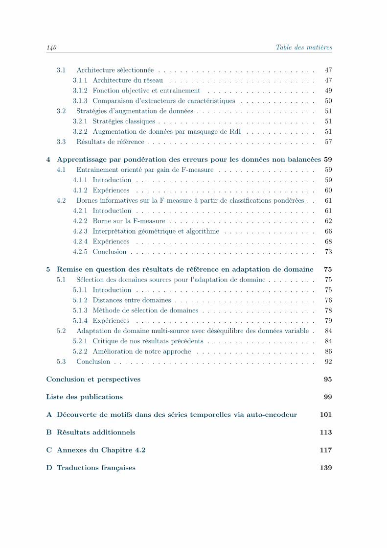
140 Table des matières
3.1 Architecture sélectionnée . . . . . . . . . . . . . . . . . . . . . . . . . . . . . 473.1.1 Architecture du réseau . . . . . . . . . . . . . . . . . . . . . . . . . . . 473.1.2 Fonction objective et entrainement . . . . . . . . . . . . . . . . . . . . 493.1.3 Comparaison d’extracteurs de caractéristiques . . . . . . . . . . . . . . 50
3.2 Stratégies d’augmentation de données . . . . . . . . . . . . . . . . . . . . . . 513.2.1 Stratégies classiques . . . . . . . . . . . . . . . . . . . . . . . . . . . . . 513.2.2 Augmentation de données par masquage de RdI . . . . . . . . . . . . . 51
3.3 Résultats de référence . . . . . . . . . . . . . . . . . . . . . . . . . . . . . . . 57
4 Apprentissage par pondération des erreurs pour les données non balancées 594.1 Entrainement orienté par gain de F-measure . . . . . . . . . . . . . . . . . . 59
4.1.1 Introduction . . . . . . . . . . . . . . . . . . . . . . . . . . . . . . . . . 594.1.2 Expériences . . . . . . . . . . . . . . . . . . . . . . . . . . . . . . . . . 60
4.2 Bornes informatives sur la F-measure à partir de classifications pondérées . . 614.2.1 Introduction . . . . . . . . . . . . . . . . . . . . . . . . . . . . . . . . . 614.2.2 Borne sur la F-measure . . . . . . . . . . . . . . . . . . . . . . . . . . . 624.2.3 Interprétation géométrique et algorithme . . . . . . . . . . . . . . . . . 664.2.4 Expériences . . . . . . . . . . . . . . . . . . . . . . . . . . . . . . . . . 684.2.5 Conclusion . . . . . . . . . . . . . . . . . . . . . . . . . . . . . . . . . . 73
5 Remise en question des résultats de référence en adaptation de domaine 755.1 Sélection des domaines sources pour l’adaptation de domaine . . . . . . . . . 75
5.1.1 Introduction . . . . . . . . . . . . . . . . . . . . . . . . . . . . . . . . . 755.1.2 Distances entre domaines . . . . . . . . . . . . . . . . . . . . . . . . . . 765.1.3 Méthode de sélection de domaines . . . . . . . . . . . . . . . . . . . . . 785.1.4 Expériences . . . . . . . . . . . . . . . . . . . . . . . . . . . . . . . . . 79
5.2 Adaptation de domaine multi-source avec déséquilibre des données variable . 845.2.1 Critique de nos résultats précédents . . . . . . . . . . . . . . . . . . . . 845.2.2 Amélioration de notre approche . . . . . . . . . . . . . . . . . . . . . . 86
5.3 Conclusion . . . . . . . . . . . . . . . . . . . . . . . . . . . . . . . . . . . . . 92
Conclusion et perspectives 95
Liste des publications 99
A Découverte de motifs dans des séries temporelles via auto-encodeur 101
B Résultats additionnels 113
C Annexes du Chapitre 4.2 117
D Traductions françaises 139

D.1. Introduction 141
D.1 Introduction
Chaque hiver, des millions de personnes à travers le monde font du ski, du snowboard oude la luge dans les stations de ski. En été également, les stations peuvent être ouvertes à larandonnée ou au vélo. Quelle que soit la saison, les télésièges sont un moyen de transport trèsrépandu pour traverser une station. En haute saison, un télésiège peut transporter des milliersde personnes par jour. Leur sécurité est une grande préoccupation pour les gestionnaires descentres de villégiature.
En France, une étude a analysé les 108 accidents graves qui se sont produits sur lestélésièges entre 2006 et 20141. Le résultat de l’étude a montré que 70 % des accidents sontsurvenus soit à l’embarquement, soit au débarquement des télésièges. De plus, ils ont montréque 90 % des accidents étaient causés par le comportement des passagers. Ainsi, s’assurerque les passagers soient correctement assis dans le véhicule et qu’ils aient correctement ferméla barre de retenue peut permettre aux stations d’éviter de nombreux accidents.
En 2015, Bluecime a été créée pour concevoir un système de surveillance permettant dedétecter les situations à risque à la station d’embarquement d’un télésiège. Le système proposés’appelle "Système Intelligent de Vision Artificielle par Ordinateur" (SIVAO) (Fig.1), et estcomposé d’une caméra, d’un ordinateur, d’une alarme, et depuis l’hiver 2018 d’un panneaude signalisation. Si une situation à risque est détectée, l’alarme est déclenchée pour avertirl’opérateur du télésiège, et le panneau est allumé pour enjoindre aux passagers de fermerla barre de retenue. Pour des raisons de confidentialité, nous ne donnons pas les noms destélésièges dans ce manuscrit et les désignons par “Chair. A-U”.
Pour chaque télésiège, une “pyramide de détection” est configurée (zone bleue sur la Fig.1b), marquant la zone où le véhicule est suivi. Nous appelons l’arrière de la pyramide le pointd’entrée du véhicule dans la zone de détection. Nous appelons l’avant de la pyramide, le pointde sortie du véhicule de la zone de détection, donc, le point où la décision, de déclencher ounon l’alarme, est prise. A chaque image à l’intérieur de la pyramide de détection, différentesdétections, utilisant des techniques de traitement d’images non basées sur l’apprentissage,sont effectuées :
• Présence de passagers
• Garde-corps en position up (complètement ouverte)
• Garde-corps en position down (totalement fermée)
À la dernière image de la pyramide de détection, selon les détections effectuées lors du suividu véhicule, le système doit évaluer le danger d’une situation. Par exemple, si aucun passagern’est détecté ou si des passagers sont détectés et que le garde-corps est détectée en positiondown, alors la situation est sûre (l’alarme ne doit pas être déclenchée). Alors que, si despassagers sont détectés et que le garde-corps est détectée en position up (ou ni up ni down),la situation est risquée (l’alarme doit être déclenchée).
1http://www.domaines-skiables.fr/fr/smedia/filer_private/41/b9/41b95513-e9d4-4159-a261-5925e6d9f030/magazine-39.pdf#page=28
142 Table des matières
Chaque année, de plus en plus de télésièges sont équipés de SIVAO, permettant à Bluecimed’obtenir de plus en plus de données. Parallèlement, les processus de SIVAO évoluent pouraméliorer les détections et faciliter la configuration du système. De plus, des projets derecherche sont actuellement en cours pour étendre l’éventail des détections. Par exemple,le système pourrait localiser, évaluer la hauteur et compter le nombre de passagers d’unvéhicule : cela permettrait à Bluecime de donner à la station un aperçu de la présence et dela répartition des passagers dans le télésiège, ou d’avertir l’opérateur du télésiège si un enfantest seul dans un véhicule.
Même après une série d’améliorations du processus de configuration, la mise en place d’unsystème prend du temps pour les ingénieurs de Bluecime. De plus, pendant la saison de ski,de nouvelles conditions peuvent apparaître. Par exemple, la position du soleil change légère-ment d’un mois à l’autre, de sorte que différentes ombres peuvent apparaître sur la vidéo,ce qui peut obliger Bluecime à reconfigurer manuellement le système. L’utilisation de tech-niques d’apprentissage automatique dans cette situation permettrait à Bluecime de configurerautomatiquement le système. De plus, les performances des techniques d’apprentissage au-tomatiques reposent sur une bonne généralisation des modèles appris. Cela rend les modèlesplus robustes aux variations dans les données, telles que les nouvelles ombres mentionnéesprécédemment.
Depuis 2012, l’apprentissage profond donne des résultats remarquables, notamment dansle traitement de l’image, et attire ainsi de plus en plus l’attention de l’industrie. Dans cecontexte, Bluecime envisage d’utiliser des techniques d’apprentissage profond pour s’attaquerà leur problème de détection. De plus, SIVAO contient un ordinateur qui pourrait fournirla puissance de calcul requise par les techniques d’apprentissage profond. Cela rend cestechniques très prometteuses dans le contexte de Bluecime.
Cette thèse CIFRE est réalisée en collaboration avec Bluecime et le laboratoire HubertCurien. Les objectifs sont de proposer des techniques d’apprentissage automatique (en parti-culier d’apprentissage profond) pour améliorer les performances de SIVAO et, plus générale-ment, améliorer les processus Bluecime.
Dans ce contexte, différentes contributions ont été apportées au cours de cette thèse :
Un cadre expérimental Nous proposons un cadre expérimental complet pour évaluer lescas d’utilisation possibles des approches d’apprentissage automatique dans le contextede Bluecime. Ceci a été décrit dans l’article Improving Chairlift Security with DeepLearning à IDA 2017 (Bascol et al., 2017).
Une architecture de base Nous proposons une architecture d’apprentissage profond commebase de référence pour résoudre le problème de l’évaluation des risques de Bluecime.L’architecture utilise différentes techniques de pointe : une architecture de classificationd’objets (ici : ResNet), une composante d’adaptation de domaine, et plusieurs aug-mentations de données et astuces d’apprentissage (certaines proposées comme contribu-tions). Ces contributions ont été en partie présentées dans l’article intitulé ImprovingChairlift Security with Deep Learning à IDA 2017 (Bascol et al., 2017).

D.1. Introduction 143
Deux techniques d’optimisation de la F-mesure La F-mesure est une mesure de per-formance bien connue qui fournit un compromis entre le Rappel et la Précision d’unclassifieur donné. En tant que telle, elle est bien adaptée lorsque l’on s’intéresse par-ticulièrement à la performance du classifieur sur une classe donnée : celle en minorité(ici, celle en minorité est la classe risquée). Nous avons donc proposé deux méthodespour mieux optimiser la performance de notre modèle en termes de F-mesure. Lesdeux méthodes consistent à pondérer chaque erreur commise lors de l’entraînementen fonction de l’étiquette de l’exemple correspondant. Tout d’abord, nous proposonsune méthode adaptée à l’apprentissage itératif habituel d’un réseau neuronal. A chaqueitération, l’entraînement est orienté par le gain en F-mesure que nous aurions pu obtenirà l’itération précédente sans faire l’erreur à pondérer. La deuxième méthode est uneméthode itérative basée sur une borne théorique sur la F-mesure obtenue en entraîne-ment. Les poids des classes dépendent d’un paramètre t. Avec un classifieur formé selonun t donné, la borne indique les valeurs F-mesure inaccessibles pour tout autre classi-fieur formé avec les valeurs t avoisinantes. Nous proposons un algorithme d’explorationqui élimine itérativement les valeurs F-mesure inaccessibles, permettant de tester unensemble réduit de valeurs t. Cette deuxième méthode a été présentée dans From Cost-Sensitive Classification to Tight F-measure Bounds à AISTATS 2019 (Bascol et al.,2019b).
Une technique d’optimisation d’ensemble d’entraînement Les phases d’annotation desdonnées et de configuration du système prennent beaucoup de temps mais sont néces-saires pour obtenir des résultats satisfaisants pour Bluecime et ses clients. Dans cecontexte, nous proposons d’entraîner un modèle spécialisé pour chaque télésiège nou-vellement installé. Cependant, l’utilisation d’images de télésièges trop différentes dela nouvelle remontée peut nuire à la performance, ce phénomène est appelé trans-fert négatif. Pour résoudre ce problème, nous proposons de construire les ensemblesd’entraînement de manière à ce qu’ils soient composés uniquement des télésièges déjàlabellisés les plus proches visuellement de la nouvelle. Cette approche est présentée dansImproving Domain Adaptation By Source Selection à ICIP 2019 (Bascol et al., 2019a).
Une étude de l’adaptation de domaine avec un déséquilibre de classe variable Nousmontrons que l’utilisation de l’adaptation de domaine dans un environnement multi-source peut en fait nuire à la performance. Nous montrons que nous pouvons lier cephénomène à la variation du rapport de déséquilibre entre les domaines sources et cibles.Compte tenu de ce constat, nous proposons deux façons d’améliorer notre approchedans un contexte multisource. Tout d’abord, l’utilisation de pseudo-étiquettes acquisesà partir d’un modèle appris sans le domaine cible. La deuxième méthode consiste àchanger notre technique d’adaptation de domaine de base pour une technique qui prenden compte la distribution des classes pendant l’adaptation de domaine.

144 Table des matières
Plan
Chapitre 1 Ce premier chapitre est consacré à la présentation de généralités sur l’apprentissageautomatique dans le contexte de notre problème de sécurité des télésièges. Nous définissonsd’abord les deux paradigmes d’apprentissage automatique que nous rencontrons dans cettethèse. Ensuite, nous explorons les algorithmes d’apprentissage automatique, en nous con-centrant sur les algorithmes et architectures d’apprentissage profond, mais aussi en présen-tant d’autres algorithmes utilisés dans cette thèse. Ensuite, nous présentons le problème del’adaptation de domaine et montrons les différentes techniques utilisées dans l’apprentissageautomatique et en particulier les techniques basées sur l’apprentissage profond. Enfin, nousprésentons le défi d’apprendre avec des ensembles de données déséquilibrés et des techniquespour optimiser la F-mesure.
Chapitre 2 Dans la première partie de ce second chapitre, nous présentons les ensemblesde données utilisés lors de cette thèse: les ensembles de données de référence, puis, plus endétail, l’ensemble de données de Bluecime. Dans la deuxième partie, nous présentons noscadres expérimentaux. Tout d’abord, la configuration des ensembles d’entraînement et detest, puis, les différentes mesures de performance que nous utilisons.
Chapitre 3 Nous proposons dans ce troisième chapitre deux contributions. Tout d’abord,une approche de base reposant sur de l’apprentissage profond et de l’adaptation du domaine.Nous montrons que cette approche présente un grand potentiel, même dans les situationsles plus difficiles. Nous présentons ensuite notre deuxième contribution, qui est une nouvelletechnique d’augmentation des données. Cette technique est basée sur l’occlusion de régionsd’intérêt dans les images, ce qui permet de former un modèle plus robuste.
Chapitre 4 Ce quatrième chapitre nous permet de présenter nos contributions en optimi-sation de la F-mesure. Nous présentons, tout d’abord, notre méthode d’entraînement orientépar le gain en F-mesure. Nous montrons que cette méthode basée sur l’apprentissage avecpondération des erreurs nous permet de choisir le compromis entre la Précision et le Rappel.Nous présentons ensuite un autre algorithme pour optimiser la F-mesure. Cet algorithme estbasé sur une limite théorique sur la F-mesure en fonction d’un poids appliqué à chaque classe.
Chapitre 5 Nous concluons cette thèse par un chapitre questionnant les résultats habituelsde l’adaptation de domaine. Nous proposons, dans un premier temps, une méthode pouraméliorer l’adaptation d’un domaine multisource en sélectionnant les sources appropriées pourun domaine cible. Cette méthode vise à réduire l’effet du transfert négatif. Ce phénomène al-tère les performances des méthodes d’adaptation de domaine lors de l’utilisation de domainessources trop différents du domaine cible. Nous discutons ensuite des résultats de l’adaptationde domaine dans le cas d’une adaptation à partir de domaines sources multiples avec un rap-port de déséquilibre variable. Nous montrons comment la variation du rapport de déséquilibre

D.2. Résumés des chapitres 145
dans l’ensemble d’entraînement peut impliquer que les techniques d’adaptation du domaineempirent les résultats. Nous proposons également des méthodes pour résoudre ce problème.
D.2 Résumés des chapitres
D.2.1 Chapitre 1
Dans ce premier chapitre nous proposons des connaissances de bases utiles à la compréhensionde cette thèse. Nous commençons par des généralités sur l’apprentissage automatique, nousdécrirons notamment l’apprentissage supervisé ou non et justifierons notre choix d’utiliserdes approches supervisées. Nous continuerons avec la présentation de différents algorithmesd’apprentissage automatique. Tout d’abord nous présentons des algorithmes d’apprentissageprofond, sur lesquels cette thèse se concentre. Nous partirons des premières et plus simplesarchitectures profondes, pour ensuite montrer des architectures de pointe spécialisées dansles tâches de classification d’images, telles que le problème de Bluecime. Pour terminer surl’apprentissage profond nous présentons différentes techniques et astuces utilisées pour op-timiser l’entraînement d’architectures profondes. Nous présentons ensuite deux algorithmesd’apprentissage automatique que nous utilisons dans le chapitre 4: la régression logistique etles machines à vecteurs de support linéaires.
Par la suite nous introduisons le concept d’adaptation de domaine. Il s’agit d’apprendreun modèle à partir d’exemple étiquetés provenant d’une ou plusieurs distribution source pourl’appliquer sur des exemples non labellisés provenant d’une distribution cible. Nous présentonsdifférentes techniques d’adaptation de domaine en général, puis nos donnerons plus de détailssur des méthodes spécifiques à apprentissage profond.
Nous finissons ce chapitre par la présentation des challenges induits par l’apprentissagede modèle sur des données déséquilibrées (c’est à dire ayant une ou plusieurs classes peureprésentées dans les données). Nous introduisons alors la F-mesure, une mesure de perfor-mance conçue pour les cas déséquilibré, et présentons différents papiers tentant d’apprendredes modèles optimisant cette mesure.
D.2.2 Chapitre 2
Dans ce chapitre, nous commençons par introduire les différentes bases de données utiliséesdans cette thèse. D’abord des bases de données ouvertes que nous utilisons pour fournir desrésultats comparables à la littérature, mais aussi qui puissent être reproduites. Puis, nousprésentons les données de Bluecime en détails.
Ensuite, nous présentons les différentes configurations de nos expériences. Nous proposonsnotamment trois principales configurations: OOC, où une expérience consiste à utiliser desdonnées d’une même remontée en entraînement et en test. Cette configuration devrait donnerles meilleurs résultats mais requière une importante quantité de données pour chaque télésiège.ALL, cette configuration consiste à mélanger, et dans l’ensemble d’entraînement et dans celuide test, les exemples provenant de toutes les remontées. Dans cette configurations, l’ensemble
146 Table des matières
d’entraînement est le plus fourni possible et présente une forte variété, utile à l’apprentissagede réseaux neuronaux, notamment pour améliorer la généralisation. Nous devrions donc, ici,obtenir de meilleurs résultats qu’avec la configuration OOC, notamment sur les remontéesles moins représentées. La dernière configurations est LOCO, il s’agit d’utiliser les exemplesd’une remontée en test et d’entraîner le modèles avec les exemples des autres remontées. Cetteconfiguration simule les résultats de nos modèles dans le cas de télésièges nouvellement instal-lés, et donc sans donnée étiqueté. Comme il s’agit d’utiliser des données d’autres remontéessur une remontées non étiqueté on s’attend ici à avoir de moins bonnes performances queOOC ou ALL. Cependant elle permet d’évaluer nos méthodes lors d’un démarrage à froiddu système, voire d’étudier la possibilité de se passer d’étiquettes qui prennent du temps àobtenir.
Nous concluons ce chapitre par la présentation des mesures de performance utilisées pourévaluer les performances de nos méthodes dans les différentes configurations.
D.2.3 Chapitre 3
Ce chapitre est dédié à la présentation du choix de notre architecture de base, des stratégiesd’augmentation de donnée que nous utilisons et que nous avons développées, et on conclue cechapitre par la présentation des résultats de référence obtenus dans les différentes configura-tions introduites dans le chapitre précédent. Nous commençons donc par présenter en détailsl’architecture ResNet que nous avons choisie d’utiliser dans cette thèse. Nous fournissons en-suite des détails sur l’entraînement (fonction de coût utilisée et constitution des minibatches).Nous montrons également une comparaison entre différentes architectures en termes de per-formances mais aussi de temps de calcul, ce qui nous mène à privilégier l’architecture ResNet.
Par la suite, nous présentons les augmentations de données que nous utilisons, puis lastratégie d’augmentation de données que nous proposons comme contribution. Cette stratégieconsiste à masquer des zones dans les images au cours de l’entraînement. Si cacher une zoneimplique que l’image devient difficile à classer pour le réseau (voire implique une erreur declassification), on ajoute cette image à la base de données. Par ce processus nous augmentonsla taille de la base de données, et en plus, nous ajoutons des images difficiles à classer. Cettestratégie nous permet donc d’éviter que le réseau ne se concentre que sur des zones réduitesdes images, ce qui le rend plus robuste.
Finalement nous montrons les performances de notre méthode de base sur les différentesconfigurations, nous montrons également l’apport de l’adaptation de domaine.
D.2.4 Chapitre 4
Ce chapitre nous permet d’introduire nos deux contributions pour l’optimisation de la F-mesure. Tout d’abord nous présentons une méthode basée sur l’apprentissage par pondéra-tion des erreurs guidant l’entraînement vers un gain en F-mesure. Régulièrement, pendantl’entraînement, les poids utilisés sont mis à jour comme suit : tout l’ensemble d’entraînementest passé dans le réseau pour obtenir les prédictions correspondantes, et à partir des ces

D.2. Résumés des chapitres 147
prédictions on obtient une valeur de F-mesure. Chaque erreur est alors pondérée selon la dif-férence entre cette valeur de F-mesure et celle qu’on aurait obtenue si l’erreur n’avait pas étécommise (donc si un faux négatif avait été un vrai positif, ou si un faux positive avait été unvrai négatif). On obtient donc un poids différent selon la classe de l’exemple correspondant,on va donc mettre plus de poids sur les classes impliquant le plus grand gain en F-mesurepossible.
Notre seconde méthode d’optimisation de la F-mesure est également basée sur de l’apprentissagepar pondération des erreurs. Nous avons aussi un poids différent pour chaque classe, qui, ici,dépend d’un paramètre t. Une borne théorique sur la F-mesure nous donne, à partir de laF-mesure obtenue par un classifieur entraîné avec un t donné, la F-mesure maximale que l’onpeut obtenir avec un classifieur entraîné avec un paramètre t′ dans le voisinage de t. Nousproposons donc un algorithme basé sur cette borne où on entraîne des classifieurs itérative-ment de sorte qu’on explore l’espace (Fm, t) jusqu’à converger vers la plus haute F-mesureatteignable selon notre borne.
D.2.5 Chapitre 5
Dans ce dernier chapitre, nous commençons par proposer une méthode pour améliorer l’adaptationde domaine, tout particulièrement dans le cas multisource. Cette méthode consiste à sélec-tionner les domaines sources les plus proches du domaine cible, afin d’éliminer les sources nonpertinentes pouvant introduire le phénomène de “transfert négatif” nuisant aux performancesdu modèle. Cette méthode se déroule en 4 étapes : d’abord on calcul les distance entre le do-maine cible et chaque domaine source (via la distance de Wasserstein). Ensuite on transformeces distances via une fonction de score que l’on normalisera pour obtenir un vecteur de prob-abilités de sélection de domaine source. Durant cette étape, on ajoute un paramètre optimiséde sorte que les sources sélectionnées constituent un ensemble d’entraînement avec suffisam-ment de variété pour entraîner correctement le modèle. Finalement pendant l’entraînement,le vecteur de probabilités est utilisé pour modifier la distribution des domaines de sorte queles domaines les plus pertinents soient plus représentés que les domaines moins pertinents (quipeuvent être totalement éliminés).
Dans un second temps, nous nous proposons d’étudier les résultats d’adaptation de do-maine dans le cas multisource avec une distribution de classe variable entre les domaines.En effet, on observe qu’utiliser une technique d’adaptation de domaine classique dans cetteconfiguration peut impliquer une perte en performance par rapport à un modèle entraîné sansadaptation de domaine. À partir de cette observation nous évaluons deux solution possibles.D’abord l’utilisation de pseudo-étiquettes sur l’ensemble cible, obtenues à partir des prédic-tions d’un modèle entraîné uniquement sur les domaines sources. Ces pseudo-étiquettes nouspermettent alors de changer artificiellement l’équilibrage des classes cibles et sources. Unedeuxième solution consiste à utiliser une technique d’adaptation de domaine qui prend encompte la distribution des classes lors de l’adaptation. Nous proposons d’utiliser la méthodeDeepJDOT.

148 Table des matières
D.3 Conclusion et perspectives
Dans cette thèse, nous avons étudié des techniques permettant d’aborder le problème desécurité des télésièges de Bluecime et les différents défis qu’il implique :
1. la grande variété de télésièges et de conditions météorologiques ;
2. l’absence de données étiquetées (surtout pour les télésièges nouvellement installés) ;
3. le déséquilibre dans les données ;
4. la contrainte temps réel.
De plus, ces défis ne sont pas indépendants. Par exemple, nous avons vu que les techniquesd’adaptation de domaine, utilisées pour résoudre les deux premiers défis, sont pénalisées parle troisième. Cependant, nous avons réussi à développer des techniques efficaces (basées prin-cipalement sur l’apprentissage profond) pour améliorer le système de Bluecime. Actuellement,des techniques d’apprentissage profond sont implémentées dans SIVAO, pour le comptage depassagers et la détection de bulles (la bulle de verre sur Chair. D dans la Fig. 2.2). Toutesdeux offrent d’excellentes performances et confirment le potentiel des techniques basées surl’apprentissage profond pour résoudre le problème de Bluecime.
Contributions
La première contribution présentée dans cette thèse consistait à fournir un pipeline completde découverte des connaissances (définition des tâches, prétraitement des données, modèleet cadre d’évaluation) pour le jeu de données Bluecime. Nous avons proposé d’explorer desconfigurations entièrement supervisées (OOC et ALL), mais aussi une configuration simulantun télésiège nouvellement installé sans étiquette disponible (LOCO). Notre modèle de baserepose sur une architecture d’apprentissage profond de pointe (ResNet) permettant de releverle premier défi dans un délai raisonnable, relevant ainsi le quatrième défi. Nous proposonségalement d’ajouter une composante d’adaptation de domaine pour relever le deuxième défi.
Les contributions qui suivent abordent plus spécifiquement les différents défis. Notredeuxième contribution consiste à améliorer la robustesse de notre approche (deux premiersdéfis) à l’aide d’une méthode de patch. Cette méthode consiste à créer de nouvelles imagesen masquant de petites zones qui étaient d’une importance critique pour le processus declassification du réseau. Ainsi, nous visons à forcer le réseau à utiliser l’image entière, c’est-à-dire à maximiser la quantité d’information utilisée par le réseau. Cette approche peut êtreconsidérée soit comme une augmentation des données, soit comme un moyen de régulariser leprocessus d’apprentissage (comme dans le cas du “dropout”).
Nos troisième et quatrième contributions examinent toutes deux l’apprentissage avecpondération des erreurs afin d’optimiser la F-mesure. Cette mesure nous aide à nous con-centrer sur les erreurs commises par notre classifieur sur la classe minoritaire (ici, les casdangereux). L’optimiser au lieu de la précision habituelle permet de résoudre notre problèmede déséquilibre de classe. Les deux méthodes ont donné de bons résultats qui peuvent êtregénéralisés à d’autres applications. Ces méthodes nous ont permis de choisir le compromis

D.3. Conclusion et perspectives 149
entre la Précision et le Rappel de notre système, ce qui est intéressant pour Bluecime puisquele nombre de faux positifs et de faux négatifs dépend, entre autres facteurs, du télésiège et dela distance entre le poste d’embarquement et la caméra SIVAO.
La cinquième contribution de cette thèse est une méthode pour résoudre le problème del’adaptation dans un domaine multisource en sélectionnant les sources les plus pertinentesdans l’ensemble d’entraînement. Avec cette contribution, nous analysons le comportementde l’adaptation de domaine dans le contexte multisource mais aussi lorsque les distributionsde classes varient entre les exemples source et cible. Nous nous interrogeons donc sur lesconnaissances générales de cette méthode et proposons quelques solutions pour ce contexteparticulier qui sont également utiles à Bluecime.
Perspectives
De nombreuses possibilités d’améliorer nos différentes contributions restent à explorer. Notreapproche de base pourrait être améliorée par une comparaison plus systématique des dif-férentes architectures de la littérature. En effet, de nombreuses architectures existantes n’ontpas été prises en compte, principalement pour des raisons de temps, mais aussi parce queles modèles d’apprentissage profond sont constamment développés (et améliorés), ce qui renddifficile la mise à jour des connaissances actuelles. Sur notre approche de patch, nous pou-vons encore explorer plus avant l’utilisation des positions précédentes des patchs sélectionnés.En particulier, nous pourrions augmenter différemment la probabilité qu’un emplacementde patch revienne, et la diminuer sur des emplacements induisant des patchs inintéressants.CONE, notre algorithme d’optimisation de la F-mesure, nous pourrions trouver un moyende mieux l’adapter à l’apprentissage profond. Par exemple, nous pourrions utiliser les poidsdu premier modèle comme pré-entraînement pour le modèle suivant, ce qui réduirait le tempsd’entraînement nécessaire pour obtenir suffisamment de classifieurs pour explorer l’espace(t, F). Sur la sélection des domaines sources, nous pourrions utiliser d’autres distances ouaméliorer la distance actuelle. Par exemple, la distance basée sur l’autoencodeur dépendévidemment de l’entraînement des autoencodeurs, donc, modifier son architecture ou réglerdifféremment les hyperparamètres (par exemple le taux d’apprentissage) peut grandementaméliorer cette méthode. Nous pourrions également modifier notre terme de variété, parexemple en intégrant une contrainte sur un nombre minimum de sources sélectionnées. Eneffet, si un domaine est très bien représenté et “proche” du domaine cible, il peut être leseul sélectionné, induisant ainsi un ensemble d’entraînement peu varié. Nous devons encoreexplorer plus avant, théoriquement, les résultats négatifs de l’adaptation de domaine avec desdistributions de classes différentes entre les exemples cible et source. Sur le plan pratique,nous pourrions améliorer nos méthodes de pseudo-étiquettes ou trouver une meilleure façond’utiliser DeepJDOT dans un environnement multisource.
De plus, toutes ces méthodes ont été conçues indépendamment pour résoudre le problèmeinitial proposé par Bluecime. Nous n’avons pas étudié si ces méthodes sont complémentaires,redondantes ou peut-être adverses pour atteindre notre objectif final. Nous pourrions toutesles utiliser et espérer le meilleur ou essayer de trouver la meilleure combinaison. Par exemple,

150 Table des matières
nous pourrions guider le patch en considérant le F-mesure et pas seulement la variation de laprédiction. Nous pourrions aussi essayer d’améliorer notre stratégie de sélection de domaineen utilisant, par exemple, le transport optimal contraint de Courty et al. (2014), lors du calculde la distance de Wasserstein pour mieux prendre en compte les distributions des classes.
Enfin et surtout, dans le contexte de Bluecime, nous pourrions travailler à l’amélioration del’efficacité du réseau. Ceci pourrait être fait, par exemple, en élaguant les poids inutiles dansle réseau, ou en quantifiant les poids (Han et al., 2015). Nous pourrions également explorerdes moyens d’améliorer les performances des architectures plus petites, par exemple, avec ladistillation des connaissances (Hinton et al., 2015). Disposer d’un réseau plus efficace présentedeux avantages : l’avantage le plus évident est l’augmentation de la vitesse du modèle, ce quinous permet d’avoir une approche en temps réel. Le deuxième avantage est la diminution dela charge de calcul et de mémoire requise par notre approche d’apprentissage profond. Celapermettrait à Bluecime de fournir d’autres services, tels que des statistiques en temps réel surl’occupation du télésiège, sans avoir à améliorer le matériel du système.
Bibliography
Muhammad Jamal Afridi, Arun Ross, and Erik M Shapiro. On automated source selectionfor transfer learning in convolutional neural networks. Pattern Recognition, 73:65–75, 2018.33
M. Baccouche, F. Mamalet, C. Wolf, C. Garcia, and A. Baskurt. Spatio-Temporal Con-volutional Sparse Auto-Encoder for Sequence Classification. In British Machine VisionConference (BMVC), 2012. 102, 103
Kevin Bascol, Rémi Emonet, Elisa Fromont, and Jean-Marc Odobez. Unsupervised inter-pretable pattern discovery in time series using autoencoders. In The joint IAPR Inter-national Workshops on Structural and Syntactic Pattern Recognition (SSPR 2016), 2016.9
Kevin Bascol, Rémi Emonet, Elisa Fromont, and Raluca Debusschere. Improving chairliftsecurity with deep learning. In International Symposium on Intelligent Data Analysis (IDA2017), 2017. 7, 44, 47, 142
Kevin Bascol, Rémi Emonet, Elisa Fromont, Amaury Habrard, Guillaume Metzler, and MarcSebban. Un algorithme d’optimisation de la f-mesure par pondération des erreurs de clas-sification. In Conférence francophone sur l’Apprentissage Automatique (CAp-18), 2018.
Kevin Bascol, Rémi Emonet, and Elisa Fromont. Improving domain adaptation by sourceselection. In 2019 IEEE International Conference on Image Processing (ICIP), 2019a. 7,75, 143
Kevin Bascol, Rémi Emonet, Elisa Fromont, Amaury Habrard, Guillaume Metzler, andMarc Sebban. From cost-sensitive classification to tight f-measure bounds. In Proceed-ings of the Twenty-Second International Conference on Artificial Intelligence and Statistics(AISTATS-19), volume 89 of Proceedings of Machine Learning Research. PMLR, 2019b. 7,59, 143
Shai Ben-David, John Blitzer, Koby Crammer, Alex Kulesza, Fernando Pereira, and Jen-nifer Wortman Vaughan. A theory of learning from different domains. Machine Learning,79(1):151–175, May 2010. 21, 24
151
152 Bibliography
Jean-David Benamou, Guillaume Carlier, Marco Cuturi, Luca Nenna, and Gabriel Peyré.Iterative bregman projections for regularized transportation problems. SIAM Journal onScientific Computing, 37(2):A1111–A1138, 2015. 26, 27
Yoshua Bengio, Pascal Lamblin, Dan Popovici, and Hugo Larochelle. Greedy layer-wisetraining of deep networks. In Advances in neural information processing systems, pages153–160, 2007. 14
Himanshu S Bhatt, Arun Rajkumar, and Shourya Roy. Multi-source iterative adaptation forcross-domain classification. In IJCAI, pages 3691–3697, 2016. 24
Christopher M Bishop. Pattern recognition and machine learning. springer, 2006. 9, 21
John Blitzer, Ryan McDonald, and Fernando Pereira. Domain adaptation with structural cor-respondence learning. In Proceedings of the 2006 conference on empirical methods in naturallanguage processing, pages 120–128. Association for Computational Linguistics, 2006. 23,24
Olivier Bousquet, Stéphane Boucheron, and Gábor Lugosi. Introduction to Statistical LearningTheory, pages 169–207. Springer Berlin Heidelberg, 2004. 73
Stephen Boyd and Lieven Vandenberghe. Convex Optimization. Cambridge University Press,New York, NY, USA, 2004. ISBN 0521833787. 36
Kristian Bredies, Dirk A Lorenz, and Peter Maass. A generalized conditional gradient methodand its connection to an iterative shrinkage method. Computational Optimization andApplications, 42(2):173–193, 2009. 26
Róbert Busa-Fekete, Balázs Szörényi, Krzysztof Dembczynski, and Eyke Hüllermeier. Onlinef-measure optimization. In NIPS, 2015. 35
Alberto Cambini and Laura Martein. Generalized Convexity and Optimization: Theory andApplications. Lecture Notes in Economics and Mathematical Systems 616. Springer-VerlagBerlin Heidelberg, 1 edition, 2009. ISBN 978-3-540-70875-9,978-3-540-70876-6. 63
Zhangjie Cao, Mingsheng Long, Jianmin Wang, and Michael I Jordan. Partial transfer learn-ing with selective adversarial networks. In Proceedings of the IEEE Conference on ComputerVision and Pattern Recognition, pages 2724–2732, 2018. 29, 93
Fabio Maria Cariucci, Lorenzo Porzi, Barbara Caputo, Elisa Ricci, and Samuel Rota Bulò.Autodial: Automatic domain alignment layers. In 2017 IEEE International Conference onComputer Vision (ICCV), pages 5077–5085. IEEE, 2017. 30
Varun Chandola, Arindam Banerjee, and Vipin Kumar. Anomaly detection: A survey. ACMComput. Surv., 2009. 35

Bibliography 153
Chih-chung Chang and Chih-Jen Lin. Ijcnn 2001 challenge: Generalization ability and textdecoding. In IJCNN’01. International Joint Conference on Neural Networks. Proceedings(Cat. No. 01CH37222), volume 2, pages 1031–1036. IEEE, 2001. 39
Ken Chatfield, Karen Simonyan, Andrea Vedaldi, and Andrew Zisserman. Return of the devilin the details: Delving deep into convolutional nets. In BMVC, 2014. 18
Rita Chattopadhyay, Qian Sun, Wei Fan, Ian Davidson, Sethuraman Panchanathan, andJieping Ye. Multisource domain adaptation and its application to early detection of fatigue.ACM Transactions on Knowledge Discovery from Data (TKDD), 6(4):18, 2012. 23
T. Chockalingam, R. Emonet, and J-M. Odobez. Localized anomaly detection via hierarchicalintegrated activity discovery. In AVSS, 2013. 103
Nicolas Courty, Rémi Flamary, and Devis Tuia. Domain adaptation with regularized optimaltransport. In Joint European Conference on Machine Learning and Knowledge Discoveryin Databases, pages 274–289. Springer, 2014. 25, 26, 28, 90, 97, 150
Nicolas Courty, Rémi Flamary, Devis Tuia, and Alain Rakotomamonjy. Optimal transportfor domain adaptation. IEEE transactions on pattern analysis and machine intelligence, 39(9):1853–1865, 2016. 25
Nicolas Courty, Rémi Flamary, Amaury Habrard, and Alain Rakotomamonjy. Joint distri-bution optimal transportation for domain adaptation. In Advances in Neural InformationProcessing Systems, pages 3730–3739, 2017. 26, 33
Marco Cuturi. Sinkhorn distances: Lightspeed computation of optimal transport. In Advancesin neural information processing systems, pages 2292–2300, 2013. 25, 26
Bharath Bhushan Damodaran, Benjamin Kellenberger, Rémi Flamary, Devis Tuia, and Nico-las Courty. Deepjdot: Deep joint distribution optimal transport for unsupervised domainadaptation. In European Conference on Computer Vision, pages 467–483. Springer, 2018.33, 90, 91, 92, 115, 116
C. Darken and J. E. Moody. Note on learning rate schedules for stochastic optimization. InNIPS, pages 832–838, 1990. 105
Stijn Decubber, Thomas Mortier, Krzysztof Dembczynski, and Willem Waegeman. Deep f-measure maximization in multi-label classification: A comparative study. page 16, 2018.35
Krzysztof Dembczyński, Wojciech Kotłowski, Oluwasanmi Koyejo, and Nagarajan Natarajan.Consistency analysis for binary classification revisited. In Doina Precup and Yee Whye Teh,editors, Proceedings of the 34th International Conference on Machine Learning, volume 70of Proceedings of Machine Learning Research, pages 961–969, International ConventionCentre, Sydney, Australia, 06–11 Aug 2017. PMLR. 35

154 Bibliography
Krzysztof J Dembczynski, Willem Waegeman, Weiwei Cheng, and Eyke Hüllermeier. Anexact algorithm for f-measure maximization. In NIPS, 2011. 35
Jia Deng, Wei Dong, Richard Socher, Li-Jia Li, Kai Li, and Li Fei-Fei. Imagenet: A large-scalehierarchical image database. In Computer Vision and Pattern Recognition, 2009. CVPR2009. IEEE Conference on, pages 248–255. Ieee, 2009. 18, 38, 79
Terrance DeVries and Graham W Taylor. Improved regularization of convolutional neuralnetworks with cutout. arXiv preprint arXiv:1708.04552, 2017. 20, 52
X. Du, R. Jin, l. Ding, V.E. Lee, and J.H. Thornton. Migration motif: a spatial - temporalpattern mining approach for financial markets. In KDD, pages 1135–1144. ACM, 2009. 101
Dheeru Dua and Casey Graff. UCI machine learning repository, 2017. URL http://archive.ics.uci.edu/ml. 37
Lixin Duan, Dong Xu, and Shih-Fu Chang. Exploiting web images for event recognition inconsumer videos: A multiple source domain adaptation approach. In Computer Vision andPattern Recognition (CVPR), 2012 IEEE Conference on, pages 1338–1345. IEEE, 2012. 23
R. Emonet, J. Varadarajan, and J.-M. Odobez. Multi-camera open space human activitydiscovery for anomaly detection. In IEEE Int. Conf. on Advanced Video and Signal-BasedSurveillance (AVSS), Klagenfurt, Austria, aug 2011. 101
R. Emonet, J. Varadarajan, and J-M. Odobez. Temporal analysis of motif mixtures usingdirichlet processes. IEEE PAMI, 2014. 101, 102, 103, 107
Chen Fang, Ye Xu, and Daniel N Rockmore. Unbiased metric learning: On the utilization ofmultiple datasets and web images for softening bias. In Proceedings of the IEEE Interna-tional Conference on Computer Vision, pages 1657–1664, 2013. 79
Li Fei-Fei, Rob Fergus, and Pietro Perona. Learning generative visual models from few trainingexamples: An incremental bayesian approach tested on 101 object categories. Computervision and Image understanding, 106(1):59–70, 2007. 37, 79
Damien Fourure, Rémi Emonet, Elisa Fromont, Damien Muselet, Alain Tremeau, and Chris-tian Wolf. Residual conv-deconv grid network for semantic segmentation. In BMVC 2017,2017. 19
Yaroslav Ganin, Evgeniya Ustinova, Hana Ajakan, Pascal Germain, Hugo Larochelle, FrançoisLaviolette, Mario Marchand, and Victor Lempitsky. Domain-adversarial training of neuralnetworks. The Journal of Machine Learning Research, 17(1):2096–2030, 2016. 28, 29, 30,31, 47, 76, 85, 86, 90
Léo Gautheron, Ievgen Redko, and Carole Lartizien. Feature selection for unsupervised do-main adaptation using optimal transport. In Joint European Conference on Machine Learn-ing and Knowledge Discovery in Databases, pages 759–776. Springer, 2018. 25
Bibliography 155
Liang Ge, Jing Gao, Hung Ngo, Kang Li, and Aidong Zhang. On handling negative transferand imbalanced distributions in multiple source transfer learning. Statistical Analysis andData Mining: The ASA Data Science Journal, 7(4):254–271, 2014. 23
Golnaz Ghiasi, Tsung-Yi Lin, and Quoc V Le. Dropblock: A regularization method forconvolutional networks. In Advances in Neural Information Processing Systems, pages10727–10737, 2018. 20
Boqing Gong, Yuan Shi, Fei Sha, and Kristen Grauman. Geodesic flow kernel for unsuperviseddomain adaptation. In 2012 IEEE Conference on Computer Vision and Pattern Recognition,pages 2066–2073. IEEE, 2012. 79
Ian Goodfellow, Yoshua Bengio, and Aaron Courville. Deep Learning. MIT Press, 2016.http://www.deeplearningbook.org. 10, 15, 49
Yves Grandvalet and Yoshua Bengio. Semi-supervised learning by entropy minimization. InAdvances in neural information processing systems, pages 529–536, 2005. 31
Gregory Griffin, Alex Holub, and Pietro Perona. Caltech-256 object category dataset. 2007.37, 79
M. Marwah H. Shao and N. Ramakrishnan. A temporal motif mining approach to unsu-pervised energy disaggregation: Applications to residential and commercial buildings. InProceedings of the 27th AAAI conference, 2013. 102
Song Han, Huizi Mao, and William J Dally. Deep compression: Compressing deep neu-ral networks with pruning, trained quantization and huffman coding. arXiv preprintarXiv:1510.00149, 2015. 97, 150
Kaiming He, Xiangyu Zhang, Shaoqing Ren, and Jian Sun. Deep residual learning for imagerecognition. In Computer Vision and Pattern Recognition (CVPR), 2016. 16, 47
G E Hinton and R R Salakhutdinov. Science, 313(5786):504–507, July 2006. 103
Geoffrey Hinton, Oriol Vinyals, and Jeff Dean. Distilling the knowledge in a neural network.arXiv preprint arXiv:1503.02531, 2015. 97, 150
Judy Hoffman, Dequan Wang, Fisher Yu, and Trevor Darrell. Fcns in the wild: Pixel-leveladversarial and constraint-based adaptation. arXiv preprint arXiv:1612.02649, 2016. 86,87
T. Hospedales, S. Gong, and T. Xiang. A markov clustering topic model for mining behaviorin video. In ICCV, 2009. 107
Andrew G Howard, Menglong Zhu, Bo Chen, Dmitry Kalenichenko, Weijun Wang, TobiasWeyand, Marco Andreetto, and Hartwig Adam. Mobilenets: Efficient convolutional neuralnetworks for mobile vision applications. arXiv preprint arXiv:1704.04861, 2017. 18

156 Bibliography
Sergey Ioffe and Christian Szegedy. Batch normalization: Accelerating deep network trainingby reducing internal covariate shift. In ICML, pages 448–456, 2015. 16, 19
Max Jaderberg, Karen Simonyan, Andrew Zisserman, et al. Spatial transformer networks. InAdvances in neural information processing systems, pages 2017–2025, 2015. 43
M. Jansche. Maximum expected f-measure training of logistic regression models. In EMNLP,2005. 35
T. Joachims. A support vector method for multivariate performance measures. In ICML,2005. 35
Aditya Khosla, Tinghui Zhou, Tomasz Malisiewicz, Alexei A Efros, and Antonio Torralba.Undoing the damage of dataset bias. In European Conference on Computer Vision, pages158–171. Springer, 2012. 79
Philip A Knight. The sinkhorn–knopp algorithm: convergence and applications. SIAM Jour-nal on Matrix Analysis and Applications, 30(1):261–275, 2008. 25
J. Z. Kolter and T. Jaakkola. Approximate inference in additive factorial hmms with appli-cation to energy disaggregation. In Proc. of AISTATS Conf., 2012. 101, 103
Oluwasanmi O Koyejo, Nagarajan Natarajan, Pradeep K Ravikumar, and Inderjit SDhillon. Consistent binary classification with generalized performance metrics.In Z. Ghahramani, M. Welling, C. Cortes, N. D. Lawrence, and K. Q. Wein-berger, editors, Advances in Neural Information Processing Systems 27, pages2744–2752. Curran Associates, Inc., 2014. URL http://papers.nips.cc/paper/5454-consistent-binary-classification-with-generalized-performance-metrics.pdf. 35, 36, 62, 69, 70, 71, 131
Alex Krizhevsky, Ilya Sutskever, and Geoffrey E. Hinton. Imagenet classification with deepconvolutional neural networks. In NIPS, 2012. 15
Yanghao Li, Naiyan Wang, Jianping Shi, Jiaying Liu, and Xiaodi Hou. Revisiting batchnormalization for practical domain adaptation. arXiv preprint arXiv:1603.04779, 2016. 30
Victoria Lopez, Alberto Fernandez, Salvador Garcia, Vasile Palade, and Francisco Herrera.An insight into classification with imbalanced data: Empirical results and current trendson using data intrinsic characteristics. Information Sciences, 250:113 – 141, 2013. 35
L. Karlsson M. Längkvist and A. Loutfi. A review of unsupervised feature learning and deeplearning for time-series modeling. Pattern Recognition Letters, 2014. 103
J. Masci, U. Meier, D. Cireşan, and J. Schmidhuber. Stacked convolutional auto-encoders forhierarchical feature extraction. In Proc. of ICANN, 2011. 104
N. A. Mehta and A. G. Gray. Funcica for time series pattern discovery. In Proceedings of theSIAM International Conference on Data Mining, pages 73–84, 2009. 103

Bibliography 157
R. Memisevic and G. E. Hinton. Unsupervised learning of image transformations. In ComputerVision and PatternRecognition (CVPR), 2007. 103
Takeru Miyato, Shin-ichi Maeda, Masanori Koyama, and Shin Ishii. Virtual adversarial train-ing: a regularization method for supervised and semi-supervised learning. IEEE transac-tions on pattern analysis and machine intelligence, 41(8):1979–1993, 2018. 32
Grégoire Montavon, Sebastian Lapuschkin, Alexander Binder, Wojciech Samek, and Klaus-Robert Müller. Explaining nonlinear classification decisions with deep taylor decomposition.Pattern Recognition, 65:211–222, 2017. 56
C. H. Mooney and J. F. Roddick. Sequential pattern mining – approaches and algorithms.ACM Comput. Surv., 45(2):19:1–19:39, March 2013. 102
David R Musicant, Vipin Kumar, Aysel Ozgur, et al. Optimizing f-measure with supportvector machines. In FLAIRS, 2003. 35
Harikrishna Narasimhan, Harish Ramaswamy, Aadirupa Saha, and Shivani Agarwal. Consis-tent multiclass algorithms for complex performance measures. In Francis Bach and DavidBlei, editors, Proceedings of the 32nd International Conference on Machine Learning, vol-ume 37 of Proceedings of Machine Learning Research, pages 2398–2407, Lille, France, 07–09Jul 2015. PMLR. 35, 36, 62, 69, 70, 71, 131
Tim Oates. Peruse: An unsupervised algorithm for finding recurring patterns in time series.In ICDM, 2002. 103
Shameem Puthiya Parambath, Nicolas Usunier, and Yves Grandvalet. Optimizing f-measuresby cost-sensitive classification. In NIPS, pages 2123–2131, 2014. 35, 62, 66, 68, 69, 70, 71,72, 122, 126, 127, 129, 131, 161, 162
Joan Pastor-Pellicer, Francisco Zamora-Martínez, Salvador España-Boquera, and María JoséCastro-Bleda. F-measure as the error function to train neural networks. In InternationalWork-Conference on Artificial Neural Networks, pages 376–384. Springer, 2013. 36
S.K. Shevade P.M. Chinta, P. Balamurugan and M.N. Murty. Optimizing f-measure withnon-convex loss and sparse linear classifiers. In IJCNN, 2013. 35
Danil Prokhorov. Ijcnn 2001 neural network competition. Slide presentation in IJCNN, 1:97,2001. 38
M. Ranzato, C. Poultney, S. Chopra, and Y. LeCun. Efficient learning of sparse representa-tions with an energy-based model. In NIPS. MIT Press, 2006. 103
T. Rapcsák. On pseudolinear functions. European Journal of Operational Research, 50(3):353–360, feb 1991. doi: 10.1016/0377-2217(91)90267-y. URL https://doi.org/10.1016/0377-2217(91)90267-y. 63

158 Bibliography
Ievgen Redko, Nicolas Courty, Rémi Flamary, and Devis Tuia. Optimal transport for multi-source domain adaptation under target shift. arXiv preprint arXiv:1803.04899, 2018. 26,89
Frank Rosenblatt. The perceptron: a probabilistic model for information storage and organi-zation in the brain. Psychological review, 65(6):386, 1958. 10
Michael T Rosenstein, Zvika Marx, Leslie Pack Kaelbling, and Thomas G Dietterich. Totransfer or not to transfer. In NIPS 2005 workshop on transfer learning, volume 898, pages1–4, 2005. 22
Olga Russakovsky, Jia Deng, Hao Su, Jonathan Krause, Sanjeev Satheesh, Sean Ma, ZhihengHuang, Andrej Karpathy, Aditya Khosla, Michael Bernstein, Alexander C. Berg, and Li Fei-Fei. ImageNet Large Scale Visual Recognition Challenge. International Journal of ComputerVision (IJCV), 115(3):211–252, 2015. doi: 10.1007/s11263-015-0816-y. 38
Kate Saenko, Brian Kulis, Mario Fritz, and Trevor Darrell. Adapting visual category modelsto new domains. In European conference on computer vision, pages 213–226. Springer, 2010.37, 79
A. Sallaberry, N. Pecheur, S. Bringay, M. Roche, and M. Teisseire. Sequential patternsmining and gene sequence visualization to discover novelty from microarray data. Journalof Biomedical Informatics, 44(5):760 – 774, 2011. 101
Mark Sandler, Andrew Howard, Menglong Zhu, Andrey Zhmoginov, and Liang-Chieh Chen.Mobilenetv2: Inverted residuals and linear bottlenecks. In Proceedings of the IEEE Con-ference on Computer Vision and Pattern Recognition, pages 4510–4520, 2018. 18
Amartya Sanyal, Pawan Kumar, Purushottam Kar, Sanjay Chawla, and Fabrizio Sebastiani.Optimizing non-decomposable measures with deep networks. Machine Learning, 107(8-10):1597–1620, 2018. 36
Lex Razoux Schultz, Marco Loog, and Peyman Mohajerin Esfahani. Distance based sourcedomain selection for sentiment classification. arXiv preprint arXiv:1808.09271, 2018. 34,75
Ramprasaath R Selvaraju, Michael Cogswell, Abhishek Das, Ramakrishna Vedantam, DeviParikh, and Dhruv Batra. Grad-cam: Visual explanations from deep networks via gradient-based localization. In Proceedings of the IEEE International Conference on ComputerVision, pages 618–626, 2017. 56
Jian Shen, Yanru Qu, Weinan Zhang, and Yong Yu. Wasserstein distance guided represen-tation learning for domain adaptation. In Thirty-Second AAAI Conference on ArtificialIntelligence, 2018. 32

Bibliography 159
Rui Shu, Hung H Bui, Hirokazu Narui, and Stefano Ermon. A dirt-t approach to unsuperviseddomain adaptation. In Proc. 6th International Conference on Learning Representations,2018. 31
Karen Simonyan and Andrew Zisserman. Very deep convolutional networks for large-scaleimage recognition. arXiv preprint arXiv:1409.1556, 2014. 16
Nitish Srivastava, Geoffrey Hinton, Alex Krizhevsky, Ilya Sutskever, and Ruslan Salakhutdi-nov. Dropout: a simple way to prevent neural networks from overfitting. The Journal ofMachine Learning Research, 15(1):1929–1958, 2014. 19, 20
Baochen Sun and Kate Saenko. Deep coral: Correlation alignment for deep domain adapta-tion. In European Conference on Computer Vision, pages 443–450. Springer, 2016. 30
Baochen Sun, Jiashi Feng, and Kate Saenko. Return of frustratingly easy domain adaptation.In Thirtieth AAAI Conference on Artificial Intelligence, 2016. 29
Christian Szegedy, Wei Liu, Yangqing Jia, Pierre Sermanet, Scott Reed, Dragomir Anguelov,Dumitru Erhan, Vincent Vanhoucke, and Andrew Rabinovich. Going deeper with convolu-tions. In IEEE Conference on Computer Vision and Pattern Recognition, pages 1–9, 2015.16
Christian Szegedy, Sergey Ioffe, Vincent Vanhoucke, and Alexander A Alemi. Inception-v4,inception-resnet and the impact of residual connections on learning. In Thirty-First AAAIConference on Artificial Intelligence, 2017. 16
R. Tavenard, R. Emonet, and J-M. Odobez. Time-sensitive topic models for action recognitionin videos. In Int. Conf. on Image Processing (ICIP), Mebourne, 2013. 103
Eric Tzeng, Judy Hoffman, Kate Saenko, and Trevor Darrell. Adversarial discriminative do-main adaptation. In 2017 IEEE Conference on Computer Vision and Pattern Recognition,CVPR, pages 2962–2971, 2017. 28, 30, 31
C. J. van Rijsbergen. Further experiments with hierarchic clustering in document retrieval.Information Storage and Retrieval, 10(1):1–14, 1974. 35, 46
J. Varadarajan, R. Emonet, and J.-M. Odobez. A sparsity constraint for topic models -application to temporal activity mining. In NIPS Workshop on Practical Applications ofSparse Modeling: Open Issues and New Directions, 2010. 105
J. Varadarajan, R. Emonet, and J-M. Odobez. A sequential topic model for mining recurrentactivities from long term video logs. Int. jl of computer vision, 2013. 102, 107, 111
Cédric Villani. Optimal transport: old and new, volume 338. Springer Science & BusinessMedia, 2008. 24
160 Bibliography
Pascal Vincent, Hugo Larochelle, Yoshua Bengio, and Pierre-Antoine Manzagol. Extractingand composing robust features with denoising autoencoders. In Proceedings of the 25thinternational conference on Machine learning, pages 1096–1103. ACM, 2008. 15
F. Zhou W.-S. Chu and F. De la Torre. Unsupervised temporal commonality discovery. InComputer Vision – ECCV 2012, 2012. 102
W.-C. Peng Y.-C. Chen and S.-Y. Lee. Mining temporal patterns in time interval-based data.IEEE Transactions on Knowledge and Data Engineering, 2015. 102
Nan Ye, Kian Ming Adam Chai, Wee Sun Lee, and Hai Leong Chieu. Optimizing f-measure:A tale of two approaches. In Proceedings of the 29th International Conference on MachineLearning, ICML 2012, 2012. 35
M. Yuan and Y. Lin. Model selection and estimation in regression with grouped variables.Journal of the Royal Statistical Society (B), 68(1):49–67, 2006. 106
Matthew D. Zeiler and Rob Fergus. Visualizing and understanding convolutional networks.In European Conference on Computer Vision, pages 818–833. Springer, 2014. 14
Ming-Jie Zhao, Narayanan Edakunni, Adam Pocock, and Gavin Brown. Beyond fano’s in-equality: Bounds on the optimal f-score, ber, and cost-sensitive risk and their implications.JMLR, 2013. 35
Y. Zheng. Trajectory data mining: An overview. ACM Trans. Intell. Syst. Technol., 6(3):29:1–29:41, May 2015. ISSN 2157-6904. 103
Zhun Zhong, Liang Zheng, Guoliang Kang, Shaozi Li, and Yi Yang. Random erasing dataaugmentation. arXiv preprint arXiv:1708.04896, 2017. 20, 52
List of Figures
1 Bluecime’s “Système Intelligent de Vision Artificielle par Ordinateur” (SIVAO) 5
1.1 Perceptron. . . . . . . . . . . . . . . . . . . . . . . . . . . . . . . . . . . . . . 111.2 Behavior of different activation functions. . . . . . . . . . . . . . . . . . . . . 121.3 Examples of 2D convolutions. . . . . . . . . . . . . . . . . . . . . . . . . . . . 131.4 Receptive fields across convolutionnal and pooling+subsampling layers. . . . . 141.5 An autoencoder with a latent space of size 2. . . . . . . . . . . . . . . . . . . 151.6 Inception-v4. . . . . . . . . . . . . . . . . . . . . . . . . . . . . . . . . . . . . 171.7 Depth-wise convolutions from MobileNets. . . . . . . . . . . . . . . . . . . . . 181.8 Dropout. . . . . . . . . . . . . . . . . . . . . . . . . . . . . . . . . . . . . . . . 201.9 Domain adaptation paradigms. . . . . . . . . . . . . . . . . . . . . . . . . . . 221.10 Example of optimal transport result. . . . . . . . . . . . . . . . . . . . . . . . 251.11 The DANN approach . . . . . . . . . . . . . . . . . . . . . . . . . . . . . . . . 291.12 ADDA training and testing steps. . . . . . . . . . . . . . . . . . . . . . . . . . 311.13 Confusion matrix. . . . . . . . . . . . . . . . . . . . . . . . . . . . . . . . . . . 34
2.1 Training images from each class. . . . . . . . . . . . . . . . . . . . . . . . . . 402.2 Examples from Bluecime dataset . . . . . . . . . . . . . . . . . . . . . . . . . 412.3 Bluecime image formats. . . . . . . . . . . . . . . . . . . . . . . . . . . . . . . 432.4 Experimental settings . . . . . . . . . . . . . . . . . . . . . . . . . . . . . . . 45
3.1 The proposed ResNet architecture with domain adaptation, for a 3-class clas-sification problem with 16 domains (chairlifts). . . . . . . . . . . . . . . . . . 48
3.2 Details of the last group of layers in our architecture (see Fig. 3.1), which iscomposed of three residual blocks and different convolution filters. . . . . . . 48
3.3 Patch visualization. . . . . . . . . . . . . . . . . . . . . . . . . . . . . . . . . . 523.4 Training iteration with patches. . . . . . . . . . . . . . . . . . . . . . . . . . . 533.5 Example of resulting probability map. . . . . . . . . . . . . . . . . . . . . . . 56
4.1 Fβ-measure in function of β for models trained with different βl. . . . . . . . 614.2 Geometric interpretation of our bound and the one from Parambath et al. (2014). 664.3 CONE Algorithm. . . . . . . . . . . . . . . . . . . . . . . . . . . . . . . . . . 674.4 Bounds on the F-measure as a function of ε1. . . . . . . . . . . . . . . . . . . 714.5 Unreachable region obtained from the same 19 (t, F ) points. . . . . . . . . . . 72
161
162 List of Figures
4.6 Training performance of CONE versus the grid approach from Parambathet al. (2014). . . . . . . . . . . . . . . . . . . . . . . . . . . . . . . . . . . . . 72
4.7 F-measure obtained on the test set for four considered approaches. . . . . . . 73
5.1 Probabilities used to reweight the different domains. . . . . . . . . . . . . . . 82
A.1 Autoencoder architecture. . . . . . . . . . . . . . . . . . . . . . . . . . . . . . 104A.2 Results on the synthetic data. . . . . . . . . . . . . . . . . . . . . . . . . . . . 108A.3 Influence of the given number of filters and the noise level. . . . . . . . . . . . 109A.4 Evolution of the number of non-zero filters (sparsity) with respect to the noise
level when we vary the parameter λgrp (λglasso in the figure) that controls thegroup lasso regularization for the synthetic dataset with 6 known motifs whenusing 12 filters (right) and 16 filters (left). . . . . . . . . . . . . . . . . . . . . 109
A.5 Traffic patterns. . . . . . . . . . . . . . . . . . . . . . . . . . . . . . . . . . . . 110
C.1 Geometric representation of the optimization problem. . . . . . . . . . . . . . 120C.2 Unreachable regions obtained from the same 19 (t1, Fi) points. . . . . . . . . . 127C.3 Bounds on the F-measure as a function of ε1. . . . . . . . . . . . . . . . . . . 128C.4 Comparison of our bound and the one from Parambath et al. (2014) with
respect to the number of iteration/ the size of the grid. . . . . . . . . . . . . . 129C.5 F-measure value with respect to the number of iterations or the size of the grid
of four different algorithms. . . . . . . . . . . . . . . . . . . . . . . . . . . . . 130
List of Tables
2.1 Bluecime dataset size over the years. . . . . . . . . . . . . . . . . . . . . . . . 422.2 Detailed Bluecime 2018 dataset. . . . . . . . . . . . . . . . . . . . . . . . . . . 422.3 Comparison between networks trained on pyramid images and trained on uni-
tary images. . . . . . . . . . . . . . . . . . . . . . . . . . . . . . . . . . . . . . 442.4 Measures formulation . . . . . . . . . . . . . . . . . . . . . . . . . . . . . . . . 46
3.1 ALL DA results with and without domains and classes balancing method. . . 503.2 LOCO DA results with and without domains and classes balancing method. . 503.3 Experiments in ALL DA setting comparing our selected feature extractor ResNet50
(Rn50) with ResNet18 (Rn18), inception-v4 (Iv4), and MobileNet-v2 (Mv2). . 513.4 Results with patches. . . . . . . . . . . . . . . . . . . . . . . . . . . . . . . . . 533.5 Results with delayed patching. . . . . . . . . . . . . . . . . . . . . . . . . . . 543.6 Results on patches variations. . . . . . . . . . . . . . . . . . . . . . . . . . . . 553.7 Results on using previous patches locations. . . . . . . . . . . . . . . . . . . . 563.8 Baseline results. . . . . . . . . . . . . . . . . . . . . . . . . . . . . . . . . . . . 573.9 F-measure on each chairlift. . . . . . . . . . . . . . . . . . . . . . . . . . . . . 58
4.1 Results using the ALL DA setting and training with different βl. . . . . . . . 604.2 Datasets details. . . . . . . . . . . . . . . . . . . . . . . . . . . . . . . . . . . 694.3 Classification F-measures for β = 1 with SVM and Logistic Regression algorithms. 70
5.1 Classes used in each dataset to create the different domains. . . . . . . . . . . 805.2 Experiments using different distances. . . . . . . . . . . . . . . . . . . . . . . 815.3 Accuracy averaged over 5 experiments on the Office-Caltech datasets. . . . . . 825.4 Accuracy averaged over 5 experiments on the datasets created from ImageNet
and Caltech. . . . . . . . . . . . . . . . . . . . . . . . . . . . . . . . . . . . . . 835.5 Accuracy on the Bluecime dataset, averaged on 5 experiments. . . . . . . . . 835.6 LOCO results with and without balancing the target and the sources sets. . . 855.7 One versus one (ovo) Accuracy averaged over domains with similar class dis-
tributions and over domains with highly dissimilar class distributions. . . . . 865.8 LOCO results with the same imbalance ratio between the target and sources
sets. . . . . . . . . . . . . . . . . . . . . . . . . . . . . . . . . . . . . . . . . . 865.9 Results comparable to the ones in Table 5.4 but with imbalanced target set,
and balanced source set. . . . . . . . . . . . . . . . . . . . . . . . . . . . . . 87
163

164 List of Tables
5.10 Results comparable to the ones in Table 5.4 but with imbalanced target set,and imbalanced source set. . . . . . . . . . . . . . . . . . . . . . . . . . . . 87
5.11 LOCO results comparable to Table 5.8, without groundtruth knowledge on thetarget labels. . . . . . . . . . . . . . . . . . . . . . . . . . . . . . . . . . . . . 88
5.12 Results comparable to Table 5.4 but with pseudo-balanced target set andbalanced source set. . . . . . . . . . . . . . . . . . . . . . . . . . . . . . . . 89
5.13 Results comparable to Table 5.4 but with imbalanced target set, and pseudo-imbalanced source set . . . . . . . . . . . . . . . . . . . . . . . . . . . . . . 89
5.14 One versus one (OVO) Accuracy averaged over domains with similar class dis-tributions and over domains with highly dissimilar class distributions. . . . . 90
5.15 LOCO results with DANN and DeepJDOT domain adaptation. . . . . . . . . 915.16 LOCO results with DeepJDOT domain adaptation. . . . . . . . . . . . . . . . 925.17 LOCO results with DeepJDOT domain adaptation. . . . . . . . . . . . . . . . 92
B.1 Accuracy on each chairlift. . . . . . . . . . . . . . . . . . . . . . . . . . . . . . 113B.2 Recall on each chairlift. . . . . . . . . . . . . . . . . . . . . . . . . . . . . . . 114B.3 Precision on each chairlift. . . . . . . . . . . . . . . . . . . . . . . . . . . . . . 114B.4 One Versus One (OVO) results. . . . . . . . . . . . . . . . . . . . . . . . . . . 115B.5 One Versus One (OVO) results. . . . . . . . . . . . . . . . . . . . . . . . . . . 115B.6 One Versus One (OVO) results. . . . . . . . . . . . . . . . . . . . . . . . . . . 116
C.1 Classification F-Measure for β = 1 with SVM algorithm. . . . . . . . . . . . . 131C.2 Classification F-Measure for β = 1 with thresholded SVM algorithm. . . . . 131C.3 Mean F-Measure over 5 experiments and limiting the number of itera-
tions/grid steps to 1 . . . . . . . . . . . . . . . . . . . . . . . . . . . . . . 132C.4 Mean F-Measure over 5 experiments and limiting the number of itera-
tions/grid steps to 2 . . . . . . . . . . . . . . . . . . . . . . . . . . . . . . 132C.5 Mean F-Measure over 5 experiments and limiting the number of itera-
tions/grid steps to 3 . . . . . . . . . . . . . . . . . . . . . . . . . . . . . . 132C.6 Mean F-Measure over 5 experiments and limiting the number of itera-
tions/grid steps to 4 . . . . . . . . . . . . . . . . . . . . . . . . . . . . . . 133C.7 Mean F-Measure over 5 experiments and limiting the number of itera-
tions/grid steps to 5 . . . . . . . . . . . . . . . . . . . . . . . . . . . . . . 133C.8 Mean F-Measure over 5 experiments and limiting the number of itera-
tions/grid steps to 6 . . . . . . . . . . . . . . . . . . . . . . . . . . . . . . 133C.9 Mean F-Measure over 5 experiments and limiting the number of itera-
tions/grid steps to 7 . . . . . . . . . . . . . . . . . . . . . . . . . . . . . . 134C.10 Mean F-Measure over 5 experiments and limiting the number of itera-
tions/grid steps to 8 . . . . . . . . . . . . . . . . . . . . . . . . . . . . . . 134C.11 Mean F-Measure over 5 experiments and limiting the number of itera-
tions/grid steps to 9 . . . . . . . . . . . . . . . . . . . . . . . . . . . . . . 134

Notes 165
C.12 Mean F-Measure over 5 experiments and limiting the number of itera-tions/grid steps to 10 . . . . . . . . . . . . . . . . . . . . . . . . . . . . . . 135
C.13 Mean F-Measure over 5 experiments and limiting the number of itera-tions/grid steps to 11 . . . . . . . . . . . . . . . . . . . . . . . . . . . . . . 135
C.14 Mean F-Measure over 5 experiments and limiting the number of itera-tions/grid steps to 12 . . . . . . . . . . . . . . . . . . . . . . . . . . . . . . 135
C.15 Mean F-Measure over 5 experiments and limiting the number of itera-tions/grid steps to 13 . . . . . . . . . . . . . . . . . . . . . . . . . . . . . . 136
C.16 Mean F-Measure over 5 experiments and limiting the number of itera-tions/grid steps to 14 . . . . . . . . . . . . . . . . . . . . . . . . . . . . . . 136
C.17 Mean F-Measure over 5 experiments and limiting the number of itera-tions/grid steps to 15 . . . . . . . . . . . . . . . . . . . . . . . . . . . . . . 136
C.18 Mean F-Measure over 5 experiments and limiting the number of itera-tions/grid steps to 16 . . . . . . . . . . . . . . . . . . . . . . . . . . . . . . 137
C.19 Mean F-Measure over 5 experiments and limiting the number of itera-tions/grid steps to 17 . . . . . . . . . . . . . . . . . . . . . . . . . . . . . . 137
C.20 Mean F-Measure over 5 experiments and limiting the number of itera-tions/grid steps to 18 . . . . . . . . . . . . . . . . . . . . . . . . . . . . . . 137

166 Notes

Notes 167
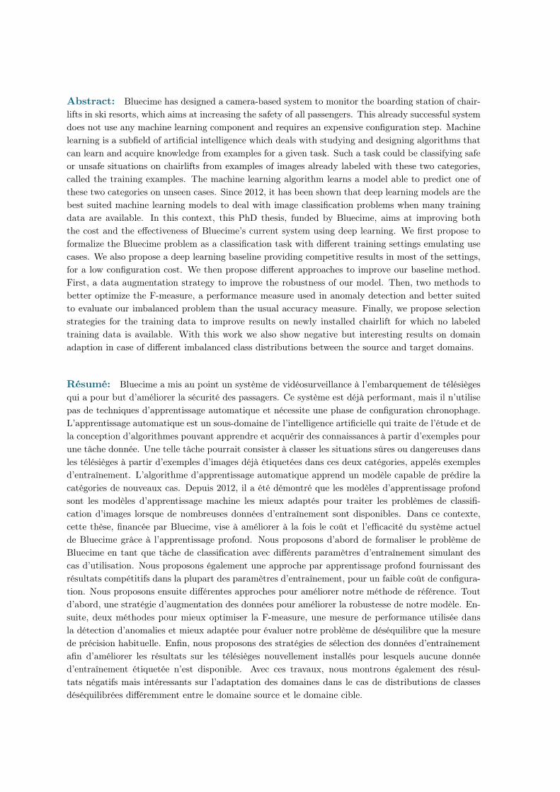
Abstract: Bluecime has designed a camera-based system to monitor the boarding station of chair-lifts in ski resorts, which aims at increasing the safety of all passengers. This already successful systemdoes not use any machine learning component and requires an expensive configuration step. Machinelearning is a subfield of artificial intelligence which deals with studying and designing algorithms thatcan learn and acquire knowledge from examples for a given task. Such a task could be classifying safeor unsafe situations on chairlifts from examples of images already labeled with these two categories,called the training examples. The machine learning algorithm learns a model able to predict one ofthese two categories on unseen cases. Since 2012, it has been shown that deep learning models are thebest suited machine learning models to deal with image classification problems when many trainingdata are available. In this context, this PhD thesis, funded by Bluecime, aims at improving boththe cost and the effectiveness of Bluecime’s current system using deep learning. We first propose toformalize the Bluecime problem as a classification task with different training settings emulating usecases. We also propose a deep learning baseline providing competitive results in most of the settings,for a low configuration cost. We then propose different approaches to improve our baseline method.First, a data augmentation strategy to improve the robustness of our model. Then, two methods tobetter optimize the F-measure, a performance measure used in anomaly detection and better suitedto evaluate our imbalanced problem than the usual accuracy measure. Finally, we propose selectionstrategies for the training data to improve results on newly installed chairlift for which no labeledtraining data is available. With this work we also show negative but interesting results on domainadaption in case of different imbalanced class distributions between the source and target domains.
Résumé: Bluecime a mis au point un système de vidéosurveillance à l’embarquement de télésiègesqui a pour but d’améliorer la sécurité des passagers. Ce système est déjà performant, mais il n’utilisepas de techniques d’apprentissage automatique et nécessite une phase de configuration chronophage.L’apprentissage automatique est un sous-domaine de l’intelligence artificielle qui traite de l’étude et dela conception d’algorithmes pouvant apprendre et acquérir des connaissances à partir d’exemples pourune tâche donnée. Une telle tâche pourrait consister à classer les situations sûres ou dangereuses dansles télésièges à partir d’exemples d’images déjà étiquetées dans ces deux catégories, appelés exemplesd’entraînement. L’algorithme d’apprentissage automatique apprend un modèle capable de prédire lacatégories de nouveaux cas. Depuis 2012, il a été démontré que les modèles d’apprentissage profondsont les modèles d’apprentissage machine les mieux adaptés pour traiter les problèmes de classifi-cation d’images lorsque de nombreuses données d’entraînement sont disponibles. Dans ce contexte,cette thèse, financée par Bluecime, vise à améliorer à la fois le coût et l’efficacité du système actuelde Bluecime grâce à l’apprentissage profond. Nous proposons d’abord de formaliser le problème deBluecime en tant que tâche de classification avec différents paramètres d’entraînement simulant descas d’utilisation. Nous proposons également une approche par apprentissage profond fournissant desrésultats compétitifs dans la plupart des paramètres d’entraînement, pour un faible coût de configura-tion. Nous proposons ensuite différentes approches pour améliorer notre méthode de référence. Toutd’abord, une stratégie d’augmentation des données pour améliorer la robustesse de notre modèle. En-suite, deux méthodes pour mieux optimiser la F-measure, une mesure de performance utilisée dansla détection d’anomalies et mieux adaptée pour évaluer notre problème de déséquilibre que la mesurede précision habituelle. Enfin, nous proposons des stratégies de sélection des données d’entraînementafin d’améliorer les résultats sur les télésièges nouvellement installés pour lesquels aucune donnéed’entraînement étiquetée n’est disponible. Avec ces travaux, nous montrons également des résul-tats négatifs mais intéressants sur l’adaptation des domaines dans le cas de distributions de classesdéséquilibrées différemment entre le domaine source et le domaine cible.