
Handling Imbalanced Classes - UEL Research Repository
206
Handling Imbalanced Classes: Feature Based Variance Ranking Techniques for Classification Solomon Henry EBENUWA A thesis submitted in partial fulfilment of the requirements of the University of East London for the degree of Doctor of Philosophy Architecture, Computing and Engineering (ACE), University of East London September 2019
-
Upload
khangminh22 -
Category
Documents
-
view
7 -
download
0
Transcript of Handling Imbalanced Classes - UEL Research Repository

Handling Imbalanced Classes:Feature Based VarianceRanking Techniques for
Classification
Solomon Henry EBENUWA
A thesis submitted in partial fulfilmentof the requirements of the University
of East London for the degree ofDoctor of Philosophy
Architecture, Computing and Engineering (ACE),
University of East London
September 2019

Supervisors:
Dr Ameer Al-NemratSenior Lecturer in Computer ScienceSchool of Architecture, Computing and Engineering (ACE)University of East London,Docklands Campus,4-6 University Way,London E16 2RD
Dr Saeed SharifSenior Lecturer in Computer ScienceSchool of Architecture, Computing and Engineering (ACE)University of East London,Docklands Campus,4-6 University Way,London E16 2RD
i

Abstract
To obtain good predictions in the presence of imbalance classes has posed significant
challenges in the data science community. Imbalanced classed data is a term used to
describe a situation where there are unequal number of classes or groups in datasets.
In most real-life datasets one of the classes are always higher in number than others
and is called the majority class, while the smaller classes are called the minority
class. During classifications even with very high accuracy, the classified minority
groups are usually very small when compared to the total number of minority in
the datasets and more often than not, the minority classes are what is being sought.
This work is specifically concern with providing techniques to improve classifications
performance by eliminating or reducing negative effects of class imbalance. Real-life
datasets have been found to contain different types of error in combination with
class imbalance. While these errors are easily corrected, but the solutions to class
imbalance have remained elusive.
Previously, machine learning (ML) technique has been used to solve the problems
of class imbalanced. There are notable shortcomings that have been identified while
using this technique. Mostly, it involve fine-tuning and changing parameters of the
algorithms and this process is not standardised because of countless numbers of algo-
rithms and parameters. In general, the results obtained from these unstandardised
(ML) technique are very inconsistent and cannot be replicated with similar datasets
and algorithms
We present a novel technique for dealing with imbalanced classes called variance
ranking features selection, that enables machine learning algorithms to classify more
of minority classes during classification, hence reducing the negative effects of class
imbalance. Our approaches utilised the intrinsic property of the datasets called
the variance. As the variance is one of the measures of central tendency of the
data items concentration within the datasets vector space. We demonstrated the
selections of features at different level of performance threshold thereby providing an
opportunity for performance and feature significance to be assessed and correlated at
different levels of prediction. In the evaluations we compared our features selections
with some of the best known features selections techniques using proximity distance
comparison techniques and verify all the results with different datasets, both binary
and multi classed with varying degree of class imbalance. In all the experiments, the
ii

results we obtained showed a significant improvement when compared with other
previous work in class imbalance.
iii

Dedication
This work is dedicated to those who had to take the brave journey alone. It was
cold, lonely and bitter, there was no person nor place to get help. The pains, anxiety
and despondence we had to bear, the endless wobbling and falling, the wiping out of
my resources and stagnation of every aspects of my existence while waiting for the
journey to end. There were days when it seems is not going to end, on hindsight I
wondered what kept me going. Some day, perhaps it may be worth all the toiling.
iv

Declaration
I Solomon Henry EBENUWA, Solemnly declare that the work in this thesis are
my and that every effort have been made to acknowledge all the academic papers,
Journals, book and other material used in accordance to academic best practises by
providing appropriate reference. I further state that some part of this thesis have
been and will be publish in academic papers, Journals, book and other materials for
the purpose of advancing knowledge and information.
v

Acknowledgements
This research journey would have been impossible if not for the contributions of
some notable individuals, I used this juncture to acknowledge their contributions
and say a big thank you to them.
First and formost are my able supervisory teams being led by the person of Dr Ameer
Nemrat my Director of Studies (DOS) and Dr Saeed Shareef (Supervisor), I would
also note the contributions of my first supervisor that started the Journey with me
Dr Abdul Tawil, I will remain grateful for all the support, encouragement, endless
meetings and corrections that you men provided me with. On many occasions I
had wanted to dropout but each time I meet with either of you my interest is
reinvigorated and I have a new reason to fight on. You gentlemen provided me an
invaluable advise, insight and strength without which this P.hD journey would not
have been possible , once again I say ”THANK YOU” and ”Doff My Hat”.
I will not forget the contributions of the following colleagues and friends; notably the
person of Dr Kennedy Isibor Ihianle, who specifically introduced me to many skills
I had to acquire for a successful Ph.d Journey and insights into Journal publications
without which my success today may not have been realistic.
I use this time to recognize the contributions of my senior sister Ms Uche Stella
EBENUWA and her daughter Jennifer, there were times when it was only we three
that was around each other, there were darkness and hopelessness everywhere how
we were able to cope and persevere is still a mystery to me; I really hope that we
could one day seat and reminisce.
Finally, I give thanks to God the creator or what ever that is up there watching over
me, I believe without any iota of doubt that ”Something or Someone” is watching
over me! On many occasion I have face an extreme situation that made me think
that I am a ”lost cause” , the situation was hopeless, but some how I manage to
survive, begin again and even prosper. Its just cannot be that is due to my effort
because my efforts alone would not have been enough to extricate me from the
quagmires that have dug my life ever since, to this I say Thank YOU GOD!.
Let me recognise the contribution of certain people earlier in my life Mr Osadebe,
Mr Franklin Eghomien; Oh my God! I remember my time at UNIBEN if not for
you two, it would have been worst. I am also acknowledging the contributions of all
those I did not mention their names here because of space, particularly the people
vi

I lived in ”The Gambia” with notably the ones that has remain good friends up to
these days, I say thank you all and may you have the courage to fight for what you
desire. For all my former friends that I have fallen apart with, I still say thank you
because as at the time we were friends you contributed in making life bearable.
I thank those that will have the patience to read this research work and I say to
them, may it give you as much pleasure and excitements as it has given me during
the research journey and also remember that a research work is not suppose to be
a ”finish product” rather an opening to more knowledge questions and that lead
to more questions for continuity and advancement of knowledge. For this I extend
my thanks to those earlier researcher that their work is in the public domain for
affording me the opportunity to read their work and hope that some day this work
will also join them in the same public space.
I thank you all , Adieu!!
vii

Contents
List of Figures xii
List of Tables xvi
Glossary xx
1 Introduction 2
1.1 Problems with real life data sets . . . . . . . . . . . . . . . . . . . . . 3
1.1.1 Imbalanced class . . . . . . . . . . . . . . . . . . . . . . . . . 3
1.1.2 Data structuralization . . . . . . . . . . . . . . . . . . . . . . 5
1.1.3 Dirty data . . . . . . . . . . . . . . . . . . . . . . . . . . . . . 5
1.1.4 Cleaning by data transformation . . . . . . . . . . . . . . . . 6
1.1.5 Identifying outliers and noise . . . . . . . . . . . . . . . . . . 6
1.1.6 High dimensionality . . . . . . . . . . . . . . . . . . . . . . . . 8
1.2 Motivation . . . . . . . . . . . . . . . . . . . . . . . . . . . . . . . . . 9
1.3 Aims . . . . . . . . . . . . . . . . . . . . . . . . . . . . . . . . . . . . 10
1.4 Contributions . . . . . . . . . . . . . . . . . . . . . . . . . . . . . . . 11
1.4.1 Terms Definitions . . . . . . . . . . . . . . . . . . . . . . . . . 12
1.5 Research Methodology . . . . . . . . . . . . . . . . . . . . . . . . . . 12
1.5.1 List of Publication . . . . . . . . . . . . . . . . . . . . . . . . 14
1.5.2 Summary of Thesis Report Layout . . . . . . . . . . . . . . . 15
2 Literature Review 17
2.1 Overview of imbalance data . . . . . . . . . . . . . . . . . . . . . . . 17
2.2 Techniques for handling imbalance class distribution . . . . . . . . . . 19
2.2.1 Overview of machine learning algorithm . . . . . . . . . . . . 20
2.2.2 Variance Techniques For Handling imbalanced classed data . . 21
2.2.3 Algorithm Techniques for imbalanced classed data . . . . . . . 22
2.2.4 Cost-Sensitive method . . . . . . . . . . . . . . . . . . . . . . 28
2.2.5 Ensemble Methods . . . . . . . . . . . . . . . . . . . . . . . . 31
2.2.6 Sampling based Methods . . . . . . . . . . . . . . . . . . . . . 32
2.2.7 The Attribute/Feature Selection Approaches to imbalanced
dataset . . . . . . . . . . . . . . . . . . . . . . . . . . . . . . . 35
viii
CONTENTS
2.2.8 A Case for Hybrid Approach to Imbalanced classed Problems 37
2.2.9 Researcher’s Further Development . . . . . . . . . . . . . . . . 38
2.3 The Measurement Evaluation for Imbalanced dataset . . . . . . . . . 39
2.3.1 Measurement Evaluation for Binary classed data . . . . . . . . 39
2.3.2 Measurement Evaluation for Multi-classed data (One-Versus-
all and One -Versus-One) . . . . . . . . . . . . . . . . . . . . . 40
2.3.3 The Receiver Operating Characteristics and Area Under the
Curve . . . . . . . . . . . . . . . . . . . . . . . . . . . . . . . 42
2.3.4 Data acquisition and descriptions: . . . . . . . . . . . . . . . . 44
2.3.5 General Data preparation and Techniques to Avoid Overfitting. 45
3 Variance Ranking Attribute Selection Technique 49
3.1 Proposed Method and Approach . . . . . . . . . . . . . . . . . . . . . 49
3.1.1 Variance and Variables Properties . . . . . . . . . . . . . . . 50
3.2 The Abstraction and High level Research Design: . . . . . . . . . . . 56
3.3 Experiment Design: . . . . . . . . . . . . . . . . . . . . . . . . . . . . 57
3.3.1 Sampling and Splitting the data set . . . . . . . . . . . . . . . 57
3.3.2 Experiments for Variance Ranking Attribute Selection . . . . 58
4 Comparison of Variance Ranking With Other Attributes Selection
71
4.1 Introduction . . . . . . . . . . . . . . . . . . . . . . . . . . . . . . . . 71
4.2 Comparison of Variance Ranking Attribute Selection (VR) Technique
with the Benchmarks . . . . . . . . . . . . . . . . . . . . . . . . . . . 72
4.3 Calculating Similarities of (VR) (PC) and (IG) using Ranked Order
Similarity-(ROS) . . . . . . . . . . . . . . . . . . . . . . . . . . . . . 82
4.3.1 Levenshtein Similarity . . . . . . . . . . . . . . . . . . . . . . 84
4.4 Motivation and Deriving Rank Order Similarity-(ROS) . . . . . . . . 86
4.4.1 Comparison of Rank Order Similarity with Levenshtein Simi-
larity . . . . . . . . . . . . . . . . . . . . . . . . . . . . . . . . 90
4.5 The Results of Comparing (VR),(PC) and (IG) using (ROS) technique 91
5 Validation 98
5.0.1 Validation of (VR) Technique for Binary Imbalance Dataset . 100
5.0.2 Decision Tree Experiments for Pima diabetes Data . . . . . . 101
5.0.3 Logistic Regression Experiments for Pima diabetes data . . . 104
5.0.4 Support Vector Machine Experiments for Pima diabetes data . 106
5.0.5 Decision Tree Experiments for Wisconsin Breast cancer data . 109
5.0.6 Logistic Regression Experiments for Wisconsin Breast cancer
data . . . . . . . . . . . . . . . . . . . . . . . . . . . . . . . . 111
5.0.7 Support Vector Machine Experiments for Wisconsin Breast
cancer data . . . . . . . . . . . . . . . . . . . . . . . . . . . . 113
ix

CONTENTS
5.0.8 Validation of (VR) technique for Multiclassed Imbalance Data
set . . . . . . . . . . . . . . . . . . . . . . . . . . . . . . . . . 115
5.0.9 Validation Experiments using the Glass data set results . . . 117
5.0.10 Logistic Regression Experiments for Glass data using One vs
All (class 1 as 1 and the others as class 0 ) see table . . . . . 118
5.0.11 Decision Tree Experiments for Glass data using One vs All
(class 1 as 1 and the others as class 0 ) see table 5.15 . . . . . 120
5.0.12 Support Vector Machine for Glass data using One vs All (class
1 as 1 others as class 0) see table 5.15 . . . . . . . . . . . . . . 122
5.0.13 Conclusion . . . . . . . . . . . . . . . . . . . . . . . . . . . . . 124
5.0.14 Logistic Regression Experiments for Glass Data Using One
Versus All (Class 3 as Class 1 and the Others as Class 0)see
table 5.15 . . . . . . . . . . . . . . . . . . . . . . . . . . . . . 124
5.0.15 Validation Experiments using the Yeast data set results . . . 126
5.0.16 Decision Tree Experiments for Yeast Data Using One Versus
All (Class ERL(5) as 1 and the others as class 0 (1479)) see
Table 5.15 . . . . . . . . . . . . . . . . . . . . . . . . . . . . . 126
5.0.17 Logistic Regression Experiments for Yeast data using One vs
All (class ERL(5) as 1 others as class 0 (1479)) see Table 5.15 129
5.0.18 Decision Tree and Support Vector Machine Experiments for
Yeast data using One vs All (class VAC (30) as class 1 others
as class 0 (1454)) see table 5.15 . . . . . . . . . . . . . . . . . 131
5.0.19 Logistic Regression Experiments for Yeast data using One vs
All (class VAC (30) as class 1 others as class 0 (1454)) see
table 5.15 . . . . . . . . . . . . . . . . . . . . . . . . . . . . . 132
5.0.20 Conclusion . . . . . . . . . . . . . . . . . . . . . . . . . . . . . 134
5.1 Comparison of Variance Ranking with the Work of Others On Imbal-
anced classed Data . . . . . . . . . . . . . . . . . . . . . . . . . . . . 134
5.1.1 Introduction . . . . . . . . . . . . . . . . . . . . . . . . . . . . 134
5.1.2 New approaches to Imbalanced Data And Introduction To
Sampling . . . . . . . . . . . . . . . . . . . . . . . . . . . . . 136
5.1.3 Similarities and Differences between (VR), (SMOTE) and (ADASYN)136
5.1.4 Performance comparisons Between (VR), (SMOTE) and (ADASYN)
on Common data sets . . . . . . . . . . . . . . . . . . . . . . 139
5.1.5 Experiment Set up . . . . . . . . . . . . . . . . . . . . . . . . 139
5.1.6 Conclusion . . . . . . . . . . . . . . . . . . . . . . . . . . . . . 141
6 Summary Discussion and Conclusions 143
6.1 Summary Critique of Existing Algorithm and Sampling Approaches . 143
6.1.1 Critique of Existing Algorithm Techniques. . . . . . . . . . . 144
6.1.2 Critique of Existing Sampling Techniques. . . . . . . . . . . . 144
x

CONTENTS
6.1.3 Summary of the Contributions of this Thesis . . . . . . . . . . 144
6.2 Recommendations . . . . . . . . . . . . . . . . . . . . . . . . . . . . . 145
6.3 Limitations . . . . . . . . . . . . . . . . . . . . . . . . . . . . . . . . 146
6.4 Future Work . . . . . . . . . . . . . . . . . . . . . . . . . . . . . . . . 147
6.4.1 Final Summary . . . . . . . . . . . . . . . . . . . . . . . . . . 148
A Appendix 150
Bibliography 164
xi

List of Figures
1.1 Problems of Real-Life data sets . . . . . . . . . . . . . . . . . . . . . 3
1.2 Interquartile Range . . . . . . . . . . . . . . . . . . . . . . . . . . . . 7
1.3 Box and Whiskers . . . . . . . . . . . . . . . . . . . . . . . . . . . . . 8
2.1 Imbalanced and Balance data . . . . . . . . . . . . . . . . . . . . . . 18
2.2 Machine learning algorithm . . . . . . . . . . . . . . . . . . . . . . . 20
2.3 Basic SVM imbalanced data points . . . . . . . . . . . . . . . . . . . 24
2.4 Decision Tree . . . . . . . . . . . . . . . . . . . . . . . . . . . . . . . 26
2.5 Neural Network . . . . . . . . . . . . . . . . . . . . . . . . . . . . . . 27
2.6 Neural Network output . . . . . . . . . . . . . . . . . . . . . . . . . . 27
2.7 Value of K is 3 in the sample space . . . . . . . . . . . . . . . . . . . 30
2.8 Multi-classed to Binary decomposition-One vs All . . . . . . . . . . . 41
2.9 Multi-classed to Binary decomposition-One vs One . . . . . . . . . . 41
2.10 ROC Curve . . . . . . . . . . . . . . . . . . . . . . . . . . . . . . . . 43
2.11 The Area Under the ROC Curve . . . . . . . . . . . . . . . . . . . . 44
2.12 Deducing AUC . . . . . . . . . . . . . . . . . . . . . . . . . . . . . . 44
2.13 K-Fold Cross validation . . . . . . . . . . . . . . . . . . . . . . . . . . 47
3.1 An Overview of the Proposed Method . . . . . . . . . . . . . . . . . . 50
3.2 Standard Deviation for Single Variable Normal Distribution . . . . . 51
3.3 3D Glass data Scatter plot . . . . . . . . . . . . . . . . . . . . . . . . 52
3.4 Algorithm flow chart for The Variance Ranking Attribute Selection . 54
3.5 Glass data contents proportion . . . . . . . . . . . . . . . . . . . . . 63
3.6 Yeast data contents proportion . . . . . . . . . . . . . . . . . . . . . 65
4.1 Presentation of Euclidean and Manhattan distance . . . . . . . . . . 83
4.2 Cosine Similarity . . . . . . . . . . . . . . . . . . . . . . . . . . . . . 84
4.3 Ranked Order Similarity-ROS Percentage Weighting Calculation for
α and β . . . . . . . . . . . . . . . . . . . . . . . . . . . . . . . . . . 88
4.4 Comparative Similarity between ROS and LEV . . . . . . . . . . . . 90
5.1 Accuracy vs Number of Attributes for Pima data using Decision Tree 103
5.2 Recall vs Number of Attributes for Pima data using Decision Tree . . 104
xii

LIST OF FIGURES
5.3 Accuracy vs Number of Attributes for Pima data using Logistic Re-
gression . . . . . . . . . . . . . . . . . . . . . . . . . . . . . . . . . . 105
5.4 Recall vs Number of Attributes for Pima data using Logistic Regression106
5.5 Accuracy vs Number of Attributes for Pima data using Support Vec-
tor Machine . . . . . . . . . . . . . . . . . . . . . . . . . . . . . . . . 107
5.6 Recall vs Number of Attributes for Pima data using Support Vector
Machine . . . . . . . . . . . . . . . . . . . . . . . . . . . . . . . . . . 108
5.7 Graph of DT Accuracy vs Numbers of Attributes for Wisconsin data
showing (PTP )Accuracy . . . . . . . . . . . . . . . . . . . . . . . . . . 110
5.8 Graph of DT Recall vs Numbers of Attributes for Wisconsin data
showing (PTP )Recall . . . . . . . . . . . . . . . . . . . . . . . . . . . 111
5.9 Graph of LR Accuracy vs Numbers of Attributes for Wisconsin data
showing (PTP )Accuracy at the position 6 attributes . . . . . . . . . . . 112
5.10 Graph of LR Recall vs Numbers of Attributes for Wisconsin data
showing (PTP )minority at the position of 4 attributes . . . . . . . . . 113
5.11 Graph of SVM Accuracy vs Numbers of Attributes for Wisconsin data
showing (PTP )Accuracy at the position of 4 attributes . . . . . . . . . 114
5.12 Graph of SVM Recall vs Numbers of Attributes for Wisconsin data
showing (PTP )minority at the position of 4 attributes . . . . . . . . . 115
5.13 Graph of LR Accuracy vs Numbers of Attributes for Glass data Mi-
nority class: Class 1 as 1 and the others as class 0, the (PTP )Accuracy
position. . . . . . . . . . . . . . . . . . . . . . . . . . . . . . . . . . . 119
5.14 Graph of LR Recall vs Numbers of Attributes for Glass data Minority
class: Class 1 as 1 and the others as class 0, the (PTP )minority in
different position. . . . . . . . . . . . . . . . . . . . . . . . . . . . . 119
5.15 Graph of DT Accuracy vs Numbers of Attributes for Glass data Mi-
nority class: Class 1 as 1 and the others as class 0 (PTP )Accuracy in
the 6 attribute position . . . . . . . . . . . . . . . . . . . . . . . . . . 121
5.16 Graph of DT Recall vs Numbers of Attributes for Glass data Minority
class: Class 1 as 1 and the others as class 0 (PTP )minority in the 4
attribute position . . . . . . . . . . . . . . . . . . . . . . . . . . . . . 121
5.17 Graph of SVM Accuracy vs Numbers of Attributes for Glass data
Minority class: Class 1 as 1 and the others as class 0, (PTP )Accuracy
in the position of 4 attributes . . . . . . . . . . . . . . . . . . . . . . 123
5.18 Graph of SVM Recall vs Numbers of Attributes for Glass data Mi-
nority class: Class 1 as 1 and the others as class 0, (PTP )minority in
the position of 4 attributes . . . . . . . . . . . . . . . . . . . . . . . 123
5.19 Graph of LR Accuracy vs Numbers of Attributes for Glass data Mi-
nority class: Class 3 as Class 1 and the others as class 0 (PTP )Accuracy
at the position of 9 attributes . . . . . . . . . . . . . . . . . . . . . . 125
xiii

LIST OF FIGURES
5.20 Graph of LR Recall vs Numbers of Attributes for Glass data Minority
class: Class 3 as Class 1 and the others as class 0, (PTP )minority at
the position of 4 attributes . . . . . . . . . . . . . . . . . . . . . . . 125
5.21 Extreme case of Ibalance of class ERL(5) as 1 others as class 0 (1479) 127
5.22 Graph of Accuracy vs Numbers of Attributes for Yeast class ERL(5)
as class 1 and the others as class0(1479) for DT minority showing
(PTP )Accuracy in both 8 and 4 attributes position . . . . . . . . . . . 128
5.23 Graph of Recall vs Numbers of Attributes for Yeast class ERL(5) as 1
and the others as class0(1479) for DT minority showing (PTP )minority
in the position of 4 attributes . . . . . . . . . . . . . . . . . . . . . . 129
5.24 Graph of Accuracy vs Numbers of Attributes for Yeast class ERL(5)
as class 1 and the others as class 0 (1479) for LR minority showing
(PTP )Accuracy in the position of 2 attributes . . . . . . . . . . . . . . 130
5.25 Graph of Recall vs Numbers of Attributes for Yeast class ERL(5)
as class 1 and the others as class0(1479) for LR minority showing
(PTP )minority in the position of 4 attributes . . . . . . . . . . . . . . 131
5.26 Extreme case of Imbalance class VAC(30) as 1 others as class0 (1454).docx132
5.27 Graph of the Accuracy vs Numbers of Attributes for Yeast class
VAC(30) as 1 others as class0(1454) for LR minority showing (PTP )Accuracy
at the position of 8 attributes . . . . . . . . . . . . . . . . . . . . . . 133
5.28 Graph of the Recall vs Numbers of Attributes for Yeast class VAC(30)
as 1 others as class0(1454) for LR minority showing (PTP )minority at
the position of 4 attributes . . . . . . . . . . . . . . . . . . . . . . . . 134
5.29 3D Glass data Scatter plot . . . . . . . . . . . . . . . . . . . . . . . . 137
5.30 3D Pima data Scatter plot . . . . . . . . . . . . . . . . . . . . . . . . 138
5.31 3D Iris data Scatter plot . . . . . . . . . . . . . . . . . . . . . . . . . 138
5.32 Graph Evaluation Metric And Performance Comparison LR . . . . . 140
5.33 Graph Evaluation Metric And Performance Comparison DT . . . . . 141
5.34 Graph Evaluation Metric And Performance Comparison SVM . . . . 141
A.1 Weka Interface experiment for all features in Pima data using Decision
Tree . . . . . . . . . . . . . . . . . . . . . . . . . . . . . . . . . . . . 152
A.2 Weka Interface experiment for only two features in Pima data using
Decision Tree . . . . . . . . . . . . . . . . . . . . . . . . . . . . . . . 152
A.3 Weka ROC for DT Wisconsin . . . . . . . . . . . . . . . . . . . . . . 153
A.4 weka Glass class1 as1 other0 LR, for minority captured . . . . . . . . 153
A.5 weka Glass class1 as1 other0 LR, for minority captured the ROC . . . 154
A.6 weka Glass class1 as1 other 0 DT-21 minority captured . . . . . . . . 154
A.7 weka Glass class1 as 1 other 0 DT, 0 minority captured . . . . . . . . 155
A.8 weka Glass class1 as1 other 0, DT 13 minority captured . . . . . . . . 155
A.9 weka Glass class3 as1 other0 LR, 2 minority captured . . . . . . . . . 156
xiv

LIST OF FIGURES
A.10 weka Glass class3 as1 other0 DT SVM, no minority captured . . . . . 156
A.11 Class Distribution Of Yeast Data . . . . . . . . . . . . . . . . . . . . 157
A.12 weka Interface SVM for Wisconsin . . . . . . . . . . . . . . . . . . . . 157
A.13 weka Interface SVM for Wisconsin-2 . . . . . . . . . . . . . . . . . . 158
A.14 wekaYeastclassERL(5)as1othersasclass0(1479) for DT . . . . . . . . . 158
A.15 wekaYeastclassERL(5)as1othersasclass0(1479) the ROC for DT . . . . 159
A.16 wekaYeastclassERL(5)as1othersasclass0(1479) for DT capture 1 Mi-
nority . . . . . . . . . . . . . . . . . . . . . . . . . . . . . . . . . . . 160
A.17 wekaYeastclassERL(5)as1othersasclass0(1479) the ROC Capture 1 for
DT . . . . . . . . . . . . . . . . . . . . . . . . . . . . . . . . . . . . . 161
A.18 weka Interface for Yeast class ERL(5)as 1 others as class0(1479) for
LR Capture all 5 minority . . . . . . . . . . . . . . . . . . . . . . . . 162
A.19 weka Interface for Yeast class VAC(30)as 1 others as class0(1454) for
DT Capture 0 minority . . . . . . . . . . . . . . . . . . . . . . . . . . 162
A.20 weka Interface for Yeast class VAC(30)as 1 others as class0(1454) for
ROC of DT Capture 0 minority . . . . . . . . . . . . . . . . . . . . . 163
A.21 weka Interface for Yeast class VAC(30)as 1 others as class0(1454) for
SVM Capture 0 minority . . . . . . . . . . . . . . . . . . . . . . . . . 163
xv

List of Tables
2.1 Cost Matrix Representation . . . . . . . . . . . . . . . . . . . . . . . 29
2.2 Common filter feature selection technique . . . . . . . . . . . . . . . . 36
2.3 Literature review summary in Chapter 2 . . . . . . . . . . . . . . . . 38
2.4 Confusion Matrix . . . . . . . . . . . . . . . . . . . . . . . . . . . . . 40
3.1 Variance Ranking attribute selection using Pima India data . . . . . . 60
3.2 Variance Ranking attribute selection using Bupa data . . . . . . . . . 60
3.3 Variance Ranking attribute selection using Wisconsin Breast Cancer
data . . . . . . . . . . . . . . . . . . . . . . . . . . . . . . . . . . . . 61
3.4 Variance Ranking attribute selection using Cod-rna data . . . . . . . 61
3.5 Variance Ranking attribute selection using Iris data . . . . . . . . . . 62
3.6 Glass data set details showing highly imbalance classes . . . . . . . . 62
3.7 Glass data class relabel to One-vs-All . . . . . . . . . . . . . . . . . . 64
3.8 Yeast data set details showing highly imbalance classes . . . . . . . . 64
3.9 Yeast data class relabel to One-vs-All . . . . . . . . . . . . . . . . . . 65
3.10 Experiment on Glass data . . . . . . . . . . . . . . . . . . . . . . . . 66
3.11 Experiment on Yeast data . . . . . . . . . . . . . . . . . . . . . . . . 68
3.12 Experiment on Yeast data continue . . . . . . . . . . . . . . . . . . . 69
4.1 Comparison of Variance Ranking with PC and IG variable selection
for Pima India diabetes data . . . . . . . . . . . . . . . . . . . . . . . 73
4.2 Comparison of Variance Ranking with PC and IG variable selection
for Liver Disorder Bupa data . . . . . . . . . . . . . . . . . . . . . . . 73
4.3 Comparison of Variance Ranking with PC and IG variable selection
for Wisconsin Breast cancer data . . . . . . . . . . . . . . . . . . . . 73
4.4 Comparison of Variance Ranking with PC and IG variable selection
for Cod-rna data . . . . . . . . . . . . . . . . . . . . . . . . . . . . . 74
4.5 Comparison of Variance Ranking with PC and IG variable selection
for Iris data . . . . . . . . . . . . . . . . . . . . . . . . . . . . . . . . 76
4.6 Comparison of Ranking significant with PC and IG variable selection
for Glass data . . . . . . . . . . . . . . . . . . . . . . . . . . . . . . . 77
4.7 Comparison of Variance significant with PC and IG variable selection
for Yeast data . . . . . . . . . . . . . . . . . . . . . . . . . . . . . . . 80
xvi

LIST OF TABLES
4.8 Comparison of Variance significant with PC and IG variable selection
for Yeast data continue . . . . . . . . . . . . . . . . . . . . . . . . . . 81
4.9 Levenshtein Process . . . . . . . . . . . . . . . . . . . . . . . . . . . . 85
4.10 Comparing two string using Levenshtein Similarity techniques . . . . 86
4.11 Three Sets arranged and ranked in different order . . . . . . . . . . . 87
4.12 ROS Calculation between VR and PC for Sub-table ”ERL as class 1,
others as class 0” in table 4.7 . . . . . . . . . . . . . . . . . . . . . . 89
4.13 ROS Calculation between VR and PC for Sub-table ”ERL as class 1,
others as class 0” in table 4.7 . . . . . . . . . . . . . . . . . . . . . . 89
4.14 Comparison of Rank Order Similarity with Levenshtein Similarity . . 90
4.15 Comparison of (VR), (PC) and (IG) using the (ROS) technique for
Pima, Bupa, Wisconsin and Cor-rna data . . . . . . . . . . . . . . . . 92
4.16 Comparison of (VR), (PC) and (IG) using the (ROS) technique for
Iris data . . . . . . . . . . . . . . . . . . . . . . . . . . . . . . . . . . 93
4.17 Comparison of (VR), (PC) and (IG) using the (ROS) technique for
Glass data . . . . . . . . . . . . . . . . . . . . . . . . . . . . . . . . 93
4.18 Comparison of (VR), (PC) and (IG) using the (ROS) technique for
Glass data . . . . . . . . . . . . . . . . . . . . . . . . . . . . . . . . 94
4.19 Comparison of (VR), (PC) and (IG) using the (ROS) technique for
Yeast data . . . . . . . . . . . . . . . . . . . . . . . . . . . . . . . . 95
4.20 Comparison of (VR), (PC) and (IG) using the (ROS) technique for
Yeast data continue . . . . . . . . . . . . . . . . . . . . . . . . . . . 96
5.1 Comparison of (VR), (PC) and (PC) Attributes selection for Pima
India diabetes data . . . . . . . . . . . . . . . . . . . . . . . . . . . . 102
5.2 Results of majority class for Pima data set for DT by (VR) feature
selection . . . . . . . . . . . . . . . . . . . . . . . . . . . . . . . . . . 102
5.3 Results of minority class for Pima data set for DT by (VR) feature
selection . . . . . . . . . . . . . . . . . . . . . . . . . . . . . . . . . . 103
5.4 Results of majority class for Pima data set for LR by (VR) feature
selection . . . . . . . . . . . . . . . . . . . . . . . . . . . . . . . . . . 104
5.5 Results of minority class for Pima data set for LR by (VR) feature
selection . . . . . . . . . . . . . . . . . . . . . . . . . . . . . . . . . . 105
5.6 Results of majority class for Pima data set for SVM by (VR) feature
selection . . . . . . . . . . . . . . . . . . . . . . . . . . . . . . . . . . 106
5.7 Results of minority class for Pima data set for SVM by (VR) feature
selection . . . . . . . . . . . . . . . . . . . . . . . . . . . . . . . . . . 107
5.8 Comparison of Variance significant with PC and IG variable selection
for Wisconsin Breast cancer data . . . . . . . . . . . . . . . . . . . . 109
5.9 Results of majority class for Wisconsin data set for DT by (VR), (PC)
and (IG) feature selection . . . . . . . . . . . . . . . . . . . . . . . . 109
xvii

LIST OF TABLES
5.10 Results of minority class for Wisconsin data set for DT by (VR), (PC)
and (IG) feature selection . . . . . . . . . . . . . . . . . . . . . . . . 110
5.11 Results of majority class for Wisconsin data set for LR by (VR), (PC)
and (IG) feature selection . . . . . . . . . . . . . . . . . . . . . . . . 112
5.12 Results of minority class for Wisconsin data set for LR by (VR), (PC)
and (IG) feature selection . . . . . . . . . . . . . . . . . . . . . . . . 112
5.13 Results of majority class for Wisconsin data set for SVM by (VR),
(PC) and (IG) feature selection . . . . . . . . . . . . . . . . . . . . . 113
5.14 Results of minority class for Wisconsin data set for SVM by (VR),
(PC) and (IG) feature selection . . . . . . . . . . . . . . . . . . . . . 114
5.15 A section of 4.6 table for Glass data . . . . . . . . . . . . . . . . . . . 116
5.16 A section of 4.7 table for Yeast data . . . . . . . . . . . . . . . . . . . 116
5.17 Results of majority class for Glass data set for LR by (VR), (PC) and
(IG) feature selection for class 1 as 1 and the others other as class 0 . 118
5.18 Results of minority class for Glass data set for LR by (VR), (PC) and
(IG) feature selection for class 1 as 1 and the others as class 0 . . . . 118
5.19 Results of majority class for Glass data set for DT by (VR), (PC)
and (IG) feature selection for class 1 as 1 and the others as class 0 . . 120
5.20 Results of minority class for Glass data set for DT by (VR), (PC)
and (IG) feature selection for class 1 as 1 and the others as class 0 . . 120
5.21 Results of majority class for Glass data set for SVM by (VR), (PC)
and (IG) feature selection for class 1 as 1 other as class 0 . . . . . . . 122
5.22 Results of minority class for Glass data set for SVM by (VR), (PC)
and (IG) feature selection for class 1 as 1 other as class 0 . . . . . . . 122
5.23 Results of majority class for Glass data set for LR by (VR), (PC) and
(IG) feature selection for class 3 as class 1 other as class 0 . . . . . . 124
5.24 Results of minority class for Glass data set for LR by (VR), (PC) and
(IG) feature selection for class 3 as class 1 other as class 0 . . . . . . 124
5.25 Results of majority class for Yeast data set for DT by (VR), (PC)
and (IG) feature selection for class ERL(5)as Class 1, Others(1479)
as class0 . . . . . . . . . . . . . . . . . . . . . . . . . . . . . . . . . . 127
5.26 Results of minority class for Yeast data set for DT by (VR), (PC)
and (IG) feature selection for class ERL(5)as Class 1, Others(1479)
as class 0 . . . . . . . . . . . . . . . . . . . . . . . . . . . . . . . . . . 128
5.27 Results of majority class for Yeast data set for LR by (VR), (PC)
and (IG) feature selection for class ERL(5)as Class 1, Others(1479)
as class0 . . . . . . . . . . . . . . . . . . . . . . . . . . . . . . . . . . 129
5.28 Results of minority class for Yeast data set for LR by (VR), (PC) and
(IG) feature selection for class ERL(5)as Class 1, and the others(1479)
as class0 . . . . . . . . . . . . . . . . . . . . . . . . . . . . . . . . . . 130
xviii

LIST OF TABLES
5.29 Results of majority class for Yeast data set for LR by (VR), (PC)
and (IG) feature selection for class VAC(30)as Class 1, Others(1454)
as class 0 . . . . . . . . . . . . . . . . . . . . . . . . . . . . . . . . . . 132
5.30 Results of minority class for Yeast data set for LR by (VR), (PC)
and (IG) feature selection for class VAC(30)as Class 1, Others(1454)
as class 0 . . . . . . . . . . . . . . . . . . . . . . . . . . . . . . . . . . 133
5.31 Evaluation Metric And Performance Comparison VR, SMOTE and
ADASYN . . . . . . . . . . . . . . . . . . . . . . . . . . . . . . . . . 140
A.1 Data used in the experiment continue . . . . . . . . . . . . . . . . . . 150
A.2 Data used in the experiment continue . . . . . . . . . . . . . . . . . . 151
xix

Glossary
(FPmaj) False Positive Majority xix, 99, 117
(FPmin) False Positive Minority xix, 99, 117
(TPmaj) True Positive Majority xix, 99, 117
(TPmin) True Positive Minority xix, 99, 117
(ADASYN) Adaptive Synthetic Sampling x, xix, 16, 33, 34, 136, 137, 139, 140,
141, 142, 148
(ANN) Artificial Neural Network xix, 26, 28
(ANOVA) Analysis of Variance xix, 55
(API) Application Programming Interface xix, 25, 28
(CRISP) Cross-industry standard process xix, 46
(CSL) Cost-Sensitive Learning xix, 28
(CSV) Comma-separated values xix, 5
(DM) Data mining xix, 37
(DNA) Deoxyribonucleic acid xix, 18
(DNA) deoxyribonucleic acid xix, 8
(DT) Decision Tree xix, 98, 99, 101, 102, 103, 104, 108, 116, 121, 124, 125, 126,
127, 141
(IG) Information Gain ix, xvii, xviii, xix, 13, 58, 71, 72, 74, 75, 78, 79, 82, 83, 84,
88, 91, 92, 93, 94, 95, 96, 97, 98, 99, 100, 101, 102, 109, 110, 111, 112, 113,
114, 115, 117, 118, 119, 120, 121, 122, 123, 124, 126, 127, 128, 129, 130, 132,
133, 134, 145, 148
(IQR) Interquartile Range xix, 7
(IR) Imbalance Ratio xix, 4, 10, 17, 23, 32, 37, 38, 49, 57, 100, 126, 136
xx

Glossary
(LR) Logistic Regression xix, 98, 99, 101, 108, 111, 115, 116, 124, 125, 126, 140
(ML) Machine Learning ii, xix, 5, 9, 10, 13, 21, 22, 23, 37, 108, 115, 116, 135, 137,
138, 143, 147, 148
(NN) Neural Network xix
(PC) Pearson Correlation ix, xvii, xviii, xix, 13, 58, 71, 72, 74, 75, 78, 79, 82, 83,
84, 88, 91, 92, 93, 94, 95, 96, 97, 98, 99, 100, 101, 102, 103, 105, 108, 109, 110,
111, 112, 113, 114, 115, 117, 118, 119, 120, 121, 122, 123, 124, 126, 127, 128,
129, 130, 132, 133, 134, 145, 148
(POC) Prove of Concept xix, 13, 108
(POC) proof of concept xix, 11
(PTA) Peak Threshold Accuracy xix
(PTP) Peak Threshold Performance xiii, xiv, xix, 11, 12, 99, 100, 101, 104, 105,
107, 108, 110, 111, 112, 113, 114, 115, 117, 119, 121, 122, 123, 124, 125, 128,
129, 130, 131, 133, 134, 139, 145
(ROS) Ranked Order Similarity ix, xvii, xix, 11, 13, 14, 71, 78, 79, 82, 83, 84, 85,
86, 88, 90, 91, 92, 93, 94, 95, 96, 97, 101, 116, 145, 146, 147, 148
(SMOTE) Synthetic Minority Over-sampling Technique x, xix, 16, 49, 136, 137,
139, 140, 141, 142, 148
(SMOTE) Synthetic Minority Over-samplingT echnique xix, 33, 37
(SVM) Support Vector Machine xix, 19, 98, 99, 101, 106, 107, 108, 115, 116, 124,
125, 126, 141
(VR) Variance Ranking from the significant of the variances in F-distributions ix,
x, xvii, xviii, xix, 11, 12, 13, 14, 15, 16, 48, 50, 58, 59, 61, 64, 67, 70, 71, 72,
74, 78, 79, 82, 83, 84, 88, 91, 92, 93, 94, 95, 96, 97, 98, 99, 100, 101, 102, 103,
104, 105, 106, 107, 108, 109, 110, 111, 112, 113, 114, 115, 116, 117, 118, 119,
120, 121, 122, 123, 124, 126, 127, 128, 129, 130, 131, 132, 133, 134, 136, 137,
138, 139, 140, 141, 142, 145, 146, 147, 148
1

Chapter 1
Introduction
Never in the history of humanity has the importance and usage of data has been
as it is presently, with the improvement in computer processing power and general
mechanism of collecting data have made the availability of any type of data possible.
Data could be obtained from practically anything and anywhere due to the robust-
ness of sensors and related technology. Even some activities like leisurely taking a
walk or jogging which were not intended to be used for data collections have become
very rich sources of data. The Internet which is one of the biggest inventions of our
time is just an ocean of data itself.
Collected and stored data could be Structured, Unstructured or Semi-structured
[1][2]. A dataset is said to be Structured if it is in any form of an organized format
like in databases, flat file, etc, where it could be searched, updated and manipulated
with an appreciable level of consistency. Semi-structured data has some level of
organizations within the data set but not as much as that of Structured data, while
Unstructured does not have any form of organizational formalism within them.
The usage of this data has given rise to a complex field of study aptly called data
science which includes but not limited to fields like data mining, machine learning,
artificial intelligence. Data science disciplines are ubiquitous and the techniques used
for dealing with issues relating to the discipline are equally so. The aims of data
science are to extract information and knowledge from data to support decision-
making processes. Most real-life datasets have some inherent problems. The nature
of input data is a major factor for a dependable result in any data analysis exercise
and decision making, therefore input data have to be processed and put into a for-
mat that would enable the extractions of knowledge to take place [3][4], processing
data before the extraction of knowledge therein has brought the problems associated
in dealing with real-life datasets to the fore. In the preceding session, some of the
problems would be reviewed.
2
CHAPTER 1. INTRODUCTION
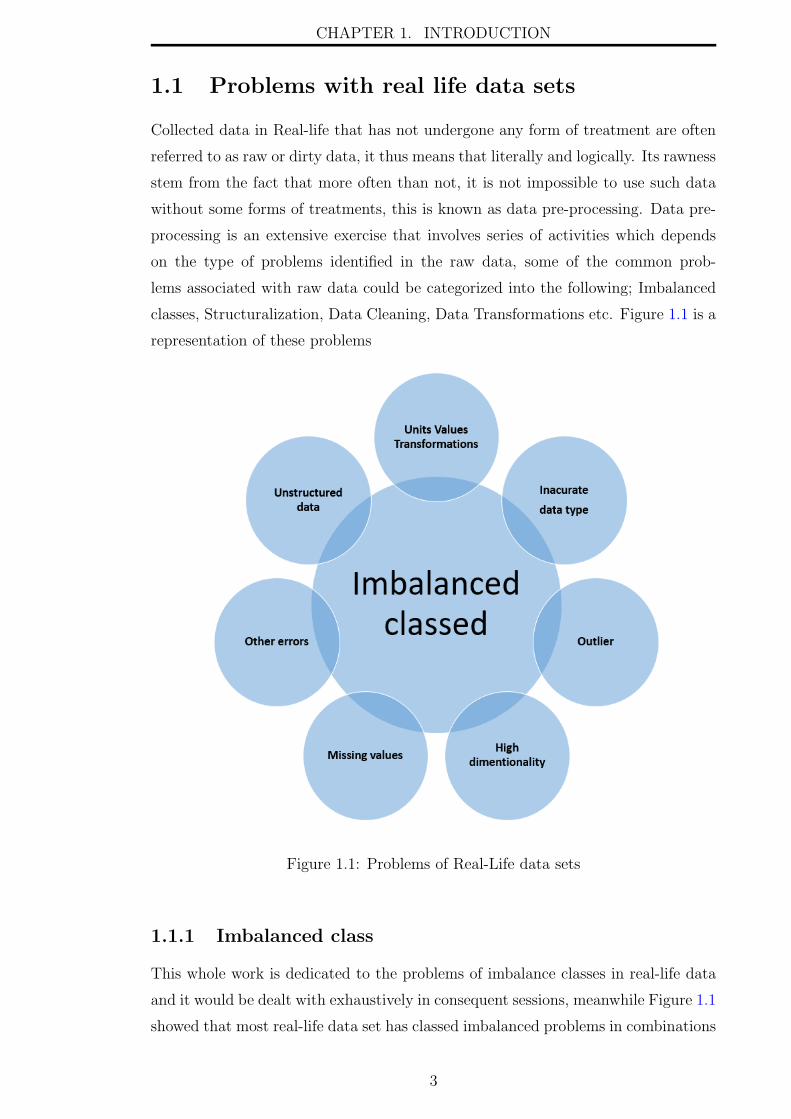
1.1 Problems with real life data sets
Collected data in Real-life that has not undergone any form of treatment are often
referred to as raw or dirty data, it thus means that literally and logically. Its rawness
stem from the fact that more often than not, it is not impossible to use such data
without some forms of treatments, this is known as data pre-processing. Data pre-
processing is an extensive exercise that involves series of activities which depends
on the type of problems identified in the raw data, some of the common prob-
lems associated with raw data could be categorized into the following; Imbalanced
classes, Structuralization, Data Cleaning, Data Transformations etc. Figure 1.1 is a
representation of these problems
Figure 1.1: Problems of Real-Life data sets
1.1.1 Imbalanced class
This whole work is dedicated to the problems of imbalance classes in real-life data
and it would be dealt with exhaustively in consequent sessions, meanwhile Figure 1.1
showed that most real-life data set has classed imbalanced problems in combinations
3

CHAPTER 1. INTRODUCTION
with other problems, for example in a binary scenario (two-class -yes or no, 1 or
0) and even multi-classed (more than two classes) the data are usually not evenly
divided. One group will always be dominant as such the sensitivities of most machine
learning algorithms are always predicting more of the dominant group at the expense
of the minority groups. The dominant groups with higher number are called majority
class, while the smaller group are called minority class. The ratio of the majority
class to the minority class is refers to as the imbalanced ratio (IR).
Imbalanced classed is not peculiar to only granular data, but many life scenarios
have an imbalanced problem, below are some of the examples, but the list is endless.
• Oil spillage - in identifying oil spillage in the ocean, small area of image
or water sample with the contamination compared to the large area of water
without contamination produces an imbalanced image or data respectively.
• Tracking migrations of species like birds - Tracking migrations of species
like birds; large areas of topography compared to a very small area dotted with
migrating species produces an imbalanced image of topographical identifica-
tions.
• In security image recognition - In the security image recognition; police
tracking a single or few suspects by using a CCTV Camera in a crowd of
people produce an imbalanced image recognition scenario.
• In health or intrusion data - The minority may be the few patients that
have lung cancer compared to a large amount of data of patient without cancer
or in intrusion detection data the few times that hackers have successfully
breached the network compared to millions of successful login.
Traditional approaches to classifications in the context of imbalanced classed
distributions in data sets has serious limitations, these will be introduced and dealt
with very well in chapter 2 and later chapters, but Figure 1.1 have left us with
compelling evidence of the the pervasiveness of the problem and how easily a data
set which exhibit imbalance problems could be mistaken for other problems and vice
versa. For example if a predictive modelling produces poor accuracy, this should
raise some important questions like, is the poor accuracy due to missing values or
other errors or due to uneven classes? What part of the poor performance are due
to imbalanced classes and what parts are due to other problems? could the causes
easily be identified ? eliminated or minimised?
The effect of class imbalance is a domain constant error inherent in most real life
4

CHAPTER 1. INTRODUCTION
scenario and manifest in what ever form is used to represent the scenario be it
granular or non granular data. Most machine learning (ML) algorithm have proven
inadequate [5] in dealing with the imbalanced. In the next sessions some of the errors
associated with data sets but are not due to imbalance classes will be reviewed.
1.1.2 Data structuralization
This is the process of giving a structure to a collected data in a data set. The extent
to which a dataset is organized is a measure of its level of structuralization, highly
organized data set possibly stored in databases, flat files or others that enables
manipulation of any sort, integration with other interfaces and software to aid and
support exploitation with algorithms and other forms of data processing techniques
with a view of extracting information and knowledge from the data are said to
be structured [6]. On the other hand, Unstructured data are opposite of this, in
that its a collection of data with no identifiable level of organizational formalism,
hence Unstructured data cannot be manipulated, queried, integrate or worked on
like Structured data.
One of the first activities of a Data Scientist is to improve the level of the structure
of the collected data through formalizing the data items structural organizations
based on the required and expected usage. Structuring the Unstructured data could
be as simple as importing or exporting into a database table by tabulating it with
identifiable rows and columns headings, another way may be exporting data into
a text or Comma-separated values (CSV) files with identifiable columns and rows.
Some could also involve using sophisticated processes and software that could enable
any item in the data set to be identified and queried using unique metadata for
extractions of a specific data item [7]. Whatever techniques used in structuring
unstructured data, the result is that the data set will become more organized and
any single data item could be identified and manipulated.
1.1.3 Dirty data
Is a term used in describing the different states of raw data that could impact on
its quality, the dirty data must be clean by the process of detecting, correcting or
removing inappropriate data item in the data set. To put it in perspective, what
makes a data dirty? Dirty data are regarded as having the following common issues
as listed below among many others.
• Incomplete data: If any position were a data item should be, have been left
blank, nothing is written in the position.
5
CHAPTER 1. INTRODUCTION
• Duplicate data: mistakenly repeating row in a table more than once.
• Inaccurate data type: the data item input is not correct, for example, if the
correct value for age is 36 year, but 360 is written.
• Incorrect data type: this is when wrong data types were used for example if for
the age of a person is 36 years, an error was made by inputting the alphabet
”wy” in place of 36 due to typographic error.
1.1.4 Cleaning by data transformation
The first part of this transformation is known as unit integration where the unit of
measurement of the variables must be equalized [8]. This part of Pre-processing data
is usually bespoke and context-dependent because the data transformation is based
on local rules and standard compliance [9]. For instance, in a data set that contains
a variable of prices of item in Pound Sterling and USA Dollars must be transformed
to the same Unit of Currency and scale because one USA Dollar is not equal to
One Pound Sterling. Also if in a data set where Date is written in DD/MM/YY
and is to be combined with another data set where the date DD/MM/YYYY, the
proper transformations must be done before any data mining and machine learn-
ing processes should be applied. The Unit integration processes are too numerous
to mention but depend on local context and standard, mostly they are typically
grouped into what is known as Extractions Transformation and Loading (ETL).
Most data mining tools and software have ETL supporting facilities that do this,
but the data scientist must know what data item is to be transformed and why.
1.1.5 Identifying outliers and noise
Outliers are values of a data item that are very much different from other values,
but noise is wrong values though may appear as real values or may not, in any
observation some values may be totally far away from others they are not wrong
values these are Outliers, in most cases the observation differs so much from others
hence become noticeable immediately [10]. For instance, if observations of adult age
contain a value of 400 as age, this would arise suspicious because no living adult is as
old as that, this is a noise because is a wrong value. For example, lets consider the
average annual income of six middle class adult as $45000, $59000, $66000, $48000,
$56000, $60000, $1500000 while most earned a five figure income the last person
earned seven figure income, if this is correct such a data is an outlier because is
remarkably different from the rest, but noise is just an incorrect data.
6

CHAPTER 1. INTRODUCTION
There are various ways to detect the presence of outliers in a data set, bar charts and
histograms are one of the easiest ways of visually identifying the outliers in data sets.
Another way of identifying suspected outlier is to use a statistical analysis known as
Interquartile Range (IQR). To find the (IQR) we have to define the following
terms Q1 which is the first quartile of all the data point from minimum, Q3 is the
third quartile of all the data point from the minimum. These are illustrated in
Figure 1.2.
Figure 1.2: Interquartile Range
IQR = Q3 −Q1 (1.1)
To deduce Outliers= Multiply 1.5 and IQR
1.5 ∗ IQRUpper Outliers are values greater than (1.5 ∗ IQR) +Q3
Lower Outliers are values lower than Q1 − (1.5 ∗ IQR)
Outliers could also be identified by using Box and Whiskers, Figure 1.3 is example
of Box and Whiskers.
Outlier could be shown using Box and Whisker, in general the rule of thumb in
identifying the outlier are data points that lie more than 1.5 IQR below the min or
1.5 IQR above the max are most likely to be Outliers, but the red flag could also lie
within Q1 and Q3 . Having been able to identify the outliers in your data set, the
implications and meaning of the outliers must be ascertained [11]. Is all Outliers
a dirty data? the answers is ”NO”, you must infer if the outlier constitute a dirty
data that must be corrected or done away with or it may be the ”gold” you are
mining for.
In a variable of ages of adults, if a value of 500 as the age is identified, is very
possible that it is an error and thus a dirty data for obvious reasons that no living
person should have such age and it must be appropriately treated like replacing it
or out-rightly removing it. But if the data set is for computer network intrusion
7

CHAPTER 1. INTRODUCTION
Figure 1.3: Box and Whiskers
detection, the outlier may represent the few times that hackers have breached the
network, therefore such outlier may be the ”gold” you are mining for hence should
be investigated further to ascertain what it stands for. It, therefore, comes down to
the domain knowledge of Business Understanding to be able to explain the meaning
and the implications of the discovered outliers or data items that are significantly
different from others.
1.1.6 High dimensionality
To put it simply dimensionality refers to the number of attributes or features in a
data set, if a data set is made of n rows; representing each data item and p columns
representing features or attributes, the comparative values of sizes of n to p defines
the order of dimensionality of the data set [12], while it has not been conclusively
established the values of p that is high dimension due to context domain dependent,
but is generally accepted that a data set is regarded as high dimension when p >
n. In some areas like Bioinformatics, Astronomy, Image Recognition and Finance,
data set with thousands of features are not uncommon [13], microarray which are
used to measure expression level of gene, Deoxyribonucleic Acid (DNA) information
are notoriously known for high dimensionality. The curse of dimensionality is the
difficulty associated with extracting the required information from data set due to
8

CHAPTER 1. INTRODUCTION
the high dimensionality. Techniques for reducing the dimensionality of data set into
manageable dimensions is an active areas of research, please see [14] [15] [16].
1.2 Motivation
This research is motivated by the inability of most predictive algorithm in dealing
effectively with imbalanced classes in real-life data set. For the fact that imbalanced
classed situations in context and concept are pervasive and recognizable in many
aspects of our life, therefore providing solutions to this problem will greatly improve
all aspects of predictive modeling. In both industries and academia, lots of predictive
algorithms are used daily to solve problems or arrive at decisions but the performance
of these algorithms varies in accuracy. These variations have been traceable to
imbalanced class situational context. To be specific, this research is motivated by
the following reasons.
• As depicted in Figure 1.1 imbalanced classed is a default problem that are
always present in associations with other (one or more) raw data problems.
Consequently, is a systematic error [17] [18] that is inherent in the dataset in
combination to other errors that the datasets has. Therefore to say that if it
is minimised or eliminated, the general result of all predictive modelling could
improve will be an understatement.
• To bring it into situational perspective, this work quest to find the answers
to questions like; “why is it that most algorithm could only predict less of
the minority classes and in most cases far less than 30% of these minority”?
[19], could these limitations in the predictions be attributed to the fault of
the algorithms, wrong processes and techniques or because of an underlying
characteristic of the data set, furthermore if imbalanced classes can never
be eliminated, at what threshold of imbalanced ratio should the result of a
classifier begins to loose its dependability, can we quantify these dependability
in comparison to the imbalanced ratio?
• It is obvious that much of the general performance of most classifier are limited
to their ability to deal with the imbalanced class issues, the data analysis
life circle, that are often referred to as Cross Industry Standard Process for
Data Mining (CRISP-DM) [20] is a bit silent in this regard for not factoring
imbalanced classes to any of its stages, for this we wished to investigate and
proffer solutions as to what stage imbalanced will be treated, more precisely we
would delve into the applications of this (ML) algorithm and the relationship to
9

CHAPTER 1. INTRODUCTION
the properties of the data item, we would deduce a quantitative and qualitative
generic influences of the algorithms and intrinsic data properties on the (IR)
and make recommendation on how to effectively treat imbalanced classes at
the appropriate stage in the life circle.
• Imbalanced Ratio(IR) varies significantly, from moderate to severe so are the
performance of the (ML) algorithms on the data during classification. But
most research have visibly avoided to investigate the relationship of the de-
gree of imbalanced to performance of classifiers. The research will establish
the correlations of the variations of imbalanced to the properties of the data
item and the performance of the (ML) on various levels of imbalance. This
will enable overview of the expected performance to be estimated before a de-
tailed analysis is carried out and also an informed decision on the type (ML),
data preprocessing and many other activities that would make sensitivities of
existing Machine learning (ML) to be able to target minority in an imbalanced
dataset while eliminating the negative influenced of class imbalanced .
Special emphasis will be paid to both binary and multi-classed imbalance with a
view of inventing a process that could be applied in both scenario ie binary and
multi-classed data. Perhaps since imbalance classes problems cannot be completely
eliminated but with the right processes the effects could be reduced to the barest
minimum, for this we would produce a system where the threshold of dependable
result will be known or estimated .
1.3 Aims
The aims of this research are to provide techniques to eliminate skewness of algo-
rithms towards identifying more of the dominant majority group during the imbal-
anced classes classification modelling. This will improve the accuracy and general
predictive performance in both binary and multi-classed datasets. The ubiquitous
nature of real-life datasets is such that a formalized approaches will be invented
to find the threshold of imbalanced ratio at which a classifier results becomes less
reliable. Finally, the correlation of the degree of overlapping and imbalance will be
demonstrated, this will also help in minimising the skewness of algorithm towards
capturing more of the dominant majority group(s) instead of the small minority
classes that are usually the reasons for the predictive modelling.
10

CHAPTER 1. INTRODUCTION
1.4 Contributions
In course of achieving the research aims, new processes and procedures will be in-
vented to provide alternatives to already existing techniques in dealing with imbal-
ance data, the solutions we proffer here is a significant contribution, consequently,
the work will itemize all major novelty and contribution as follows.
• This research produced a novel technique called Variance Ranking Attribute
Selection (VR) to handle imbalanced classes in both binary and multiclass
datasets. Though, it has been referred to as Variance Ranking in many in-
stances through out this thesis. The superiority of the (VR) over the exist-
ing techniques of dealing with class imbalanced have been demonstrated by
producing better results, being able to deal with overlapping classes more ef-
fectively and being algorithm independent. For the proof of concept (POC)
seven major dataset were used. These are further explained in chapter three
session 3.1.1
• A novel method of choosing significant attributes based on Peak Threshold
Performance -(PTP), which is defined as the point at which the predictive
model accuracy is at his highest, hence two types of (PTP) is identified these
are (PTP )Accuracy and (PTP )minority. The (PTP )Accuracy is the point in the
predictive model were the highest accuracy occurred, while (PTP )minority is
the point at which the predictive model has the highest recall of the minority
class group. This would also help to identify the threshold of attributes that
are required to obtain dependable results based on the context of discourse
and at the point where the significant attributes will be selected. These are
further explained in chapter five from session 5.0.1 to section 5.0.20.
• An introduction to a new similarity measurement techniques called Ranked
Order Similarity-(ROS), as a techniques to quantify the similarities among a
sets of items that may contain the same elements but ranked in different order.
To accomplished this, a novel distance measure called ”proximity distance”
that assessed the distances of comparative items were defined. The (ROS) is
a novel similarity measure that is applicable in situations where the existing
similarity measure is inadequate for example were similarities is by ranked.
These are further explained in chapter four session 4.4.
11
CHAPTER 1. INTRODUCTION
1.4.1 Terms Definitions
Effort have been made for all the invented (coined) words, phrases and nouns used
in the thesis to have a specific meaning as will be explained wherever such words
are used. When there are more than one words that refers to the same meaning and
is unavoidable to used one of the word for example this three words refers to the
same meaning; ”Variable”,”Attribute” and ”Feature”. The three words will be used
interchangeably as it has always been used in most academic reports and journals
and will comply to academic writing best practises.
One of the main concept is Variance Ranking Attributes selection (VR) and may be
referred to as Variance, particularly in some table where there is no enough space.
In any other places were any terms or words would appear differently the meaning
will be obvious or it will be explained or defined appropriately. Reader’s attentions
will be drawn to some common coined words that will be used through out this
thesis, these are listed below.
• Peak Threshold Performance (PTP); this is the position that at which the
highest accuracy and recall of the minority class groups were obtained. They
are two types of (PTP), these are , (PTP )Accuracy and (PTP )minority.
• Element Percentage Weighting (EPW). This is the sum total percentage quan-
tity of elements in two sets that are going to be compared; see section 4.4.
• Unit Element Percentage Weighting (EPW/n). This is the percentage weight-
ing of a single element in a set; see section 4.4.
• proximity distance; this is the number of steps a Unit element in a set moves
to align itself with a similar element in the another set, when both sets are
being compared;see section 4.4.
1.5 Research Methodology
The goal of this research is to produce a process that could limit or eliminate the
skewness of algorithm toward identifying more of the dominant majority group as
against the smaller minority that are often sought when using imbalanced classed
datasets. These goal has been fully articulated in the project specification vis-a-vis
the aims, and contributions therein. In so doing it will encompass every aspect of
relevant discussions that will ensure a wholistic conclusion with adequate proof of
validity, reliability of the assertions made in this document.
The techniques and resources used is to ensure that the primary research aims and
12

CHAPTER 1. INTRODUCTION
its objective are emphasised and not entwined in verbose research discourse [21],
hence the general research methodology, the Proof of Concept (POC), results will
be precise and straight to the point in order that the experiments could be replicated.
The sequence of flow of the research will be in a particular order from inception to
finish. Though these order boundaries are not strictly define, but to act as a guide to
enable clarity, understanding, and coherency of thought. The sequence is as follows;
• Problem Definition and Specifications and introductions to the real life context
of imbalanced data.
• Reviews of state of the art literature in dealing with imbalance data and met-
rics of evaluating the Binary and Multi-classed data classifications.
• Data acquisition, preparations, and sampling methodology.
• The re-coding of multi-classed into n Binary, where n represent the number
of classes in the multi-classed datasets.
• Experiment for Variance Ranking Attribute Selection Technique.
• Comparison of Variance Ranking Attribute Selection with two states of the
art Attribute Selection using the Pearson Correlation (PC) and Information
Gain (IG)
• Comparing the attributes ranked by (PC), (IG) and (VR) using the (ROS).
• Validation experiment of Variance Significant Ranking Attribute Selection us-
ing some major (ML) algorithms.
• Comparison by estimating the degree of similarity Variance Ranking Attribute
Selection with two sampling technique of dealing with class imbalance.
• Final discussion of results and conclusions.
Software, Hardware, and Algorithms
The list of all the major resources that were used in this research is as follows.
• Weka data mining software. That could be downloaded at [22].
• Python(v3) programming language. A very robust programming lan-
guage for scientific computation and data analysis. As at the time of writing
this thesis it has version 2 and version 3. The version used here is 3.
13

CHAPTER 1. INTRODUCTION
• Microsoft Office (Word, Excel, Paint, etc). A popular documentation
for PC mac book.
• Datasets all downloaded from [23]. This was downloaded from the university
of California dataset archive.
• Hardware, PC and laptop. The only hardware used is PC,laptop with
win10. There was no special capacity, any regular PC or laptop will do.
• Latex documentation. Thesis documentation carried out in Latex [24].
Though lots of latex editor online and those that could be installed on the
desktops , but I had used specifically the online overleaf that have been cited
earlier, I found it more convenient because being online made it accessible
anywhere.
• Algorithms used. There are two major processes derived in this research,
these are (VR) and (ROS). Each of these processes is as a result of other al-
gorithms. The major algorithm that was used to derived the (VR) processes
is one of the measure of central tendency called the ”Variance”, this is fur-
ther explained in chapter three, session 3.1.1. The (ROS) is derived from the
Levenshtein Similarity, this is futher explained in chapter four,session 4.3.1
A clear attempt will be made throughout this work to ensure that the aims, con-
tributions, and processes being carried out are very clear to the reader sometimes
through ”repetitions of the aims”, ”similar experimentation that emphasis the same
results” and other techniques, this is to ensure that the conclusion will be proven
beyond any reasonable doubt and to reinforce the sequence of understanding of the
research work.
The work is for Doctor of Philosophy and every aspect of this work must be made
to show deep thinking and originality and creation of knowledge. In presenting this
documentation, It seek to make sure it complies to be ” Clear Precise and Accurate”
according to [25].
1.5.1 List of Publication
• Ebenuwa, S.H., Sharif, M.S., Alazab, M. and Al-Nemrat, A., 2019. Variance
ranking attributes selection techniques for binary classification problem in im-
balance data. IEEE Access, 7, pp.24649-24666.
• Ebenuwa, S.H., Sharif, M.S., Al-Nemrat, A., Al-Bayatti, A.H., Alalwan, N.,
Alzahrani, A.I. and Alfarraj, O., 2019. Variance Ranking for Multi-Classed
14

CHAPTER 1. INTRODUCTION
Imbalanced Datasets: A Case Study of One-Versus-All. Symmetry, 11(12),
p.1504.
1.5.2 Summary of Thesis Report Layout
Chapter One(Introduction). In the introduction, we made the case for the
research topic by introducing the background of the study as being the general
problems encountered when working with real-life datasets. The positing of imbal-
anced classes as being very prevalent in additions to other real-life dataset issues
was made here. A detailed explanations of other data sets issues as an addition to
imbalanced class was presented. Furthermore, an explanation of similar imbalanced
scenario, processes of dealing with raw data. Clear problems definition by explaining
the research motivation, aims and contribution to knowledge was firmly rooted in
this chapter.
Chapter Two(literature Review). The chapter is an extensive presentation
of previous work that has been done in dealing with imbalanced class distribution
in data sets, we engage the argument of using data-centric research like data mining
and machine learning to provide a solution in real-life scenario, hence the extent and
attempt that has been made to provide solutions were explored here in a broader per-
spective. The metrics of evaluations for classifiers were introduced for both binary
and multi-classed data sets, we provided detailed explanation for 2 by 2 confusion
matrix for binary classification and One-Versus-All for multi-classed scenario
Chapter Three(Variance Ranking Attribute Selection (VR) Tech-
nique) In this chapter we presented the Variance Ranking Attribute Selection tech-
nique for handling the imbalanced classed distribution, a detailed explanations of
the datasets and data preparations, the theoretical basis of formula derivative used
throughout the report and the experiments result were also included in this chapter.
Chapter Four(Comparison of Variance Ranking Attribute Selection
(VR) Technique with the Bench Mark) In this chapter a comparison of Vari-
ance Ranking Attribute Selection(VR) and other bench mark in attribute selection
is provided , also a new similarity measurement techniques ”The Ranked Order
Similarity measurement-ROS” was used to compare and quantify the similarities
between the Variance Ranking Attribute Selection (VR) and two main bench marks
which are Pearson Correlation and Information Gain. The novelty of The Ranked
15

CHAPTER 1. INTRODUCTION
Order Similarity measurement-ROS was invented here.
Chapter Five(Validation) In this chapter predictive modelling experiments
were carrieed out using three machine learning algorithm and seven data set (four
binary and three multi classed). The accuracy , precision , recall etc were noted.
The capturing of the minority class group in the imbalanced situation were proven,
hence attesting to the efficacy of the (VR) techniques. More importantly, the com-
parison of Variance Ranking with (SMOTE) and ADASYN techniques. The chapter
provided and consolidated the reasons for the failure of using the algorithm based
methods which have been the the conventional means and made a case why the
(VR), (SMOTE) and (ADASYN) techniques that rely mostly on the numbers of the
class groups is the right approaches to use.
Chapter Six (Summary Discussion and Conclusions) This chapter high-
lighted the major achievements of the research with a blow by blow summary of how
the aims, and contributions were achieved, we also highlighted the shot comings of
the existing techniques of handling the imbalanced data set problems. We provided
a distinctive yet succinct presentations of all aspects of research that that made it
possible to any reader to be familiar with the central knowledge that have been
claimed achieved, we made ac case for the relevance of (VR) and the future work.
16
Chapter 2
Literature Review
2.1 Overview of imbalance data
Class imbalance is a major problem in using real-life data for predictive modelling.
A data set is said to be imbalanced when there is unequal number of groups, mean-
ing that one group is more than the others, the larger groups are the majority classes
while the smaller groups are called the minority classes, the ratio of the majority
class to the minority class is often referred to as the imbalance ratio (IR) in binary
classed imbalanced data. In the multi-classed imbalanced, the (IR) will be defined
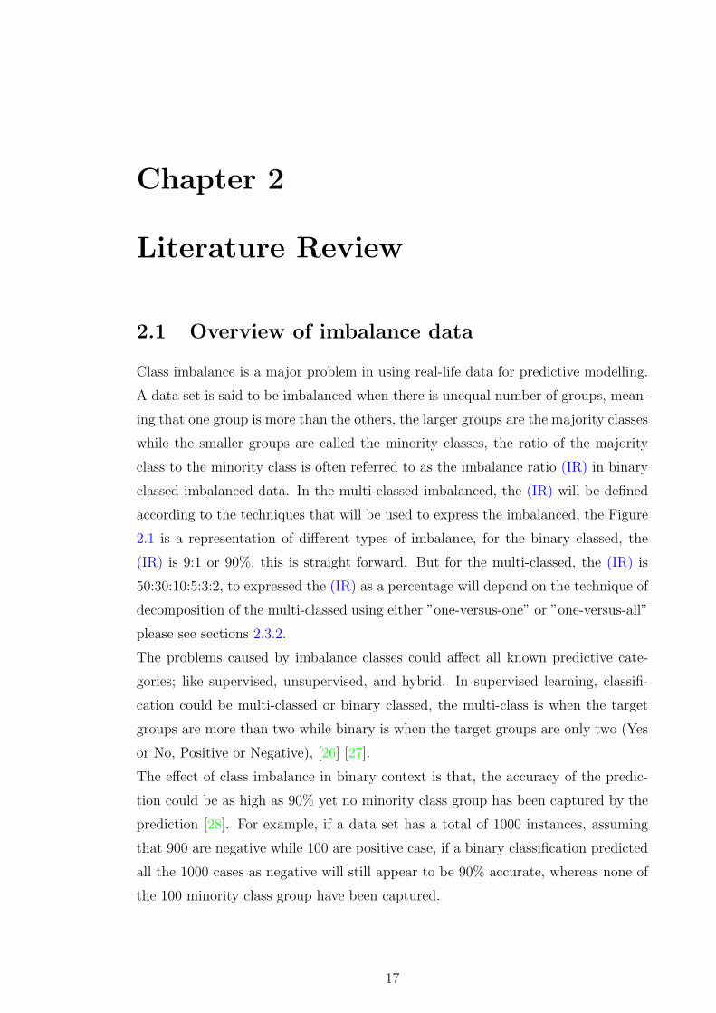
according to the techniques that will be used to express the imbalanced, the Figure
2.1 is a representation of different types of imbalance, for the binary classed, the
(IR) is 9:1 or 90%, this is straight forward. But for the multi-classed, the (IR) is
50:30:10:5:3:2, to expressed the (IR) as a percentage will depend on the technique of
decomposition of the multi-classed using either ”one-versus-one” or ”one-versus-all”
please see sections 2.3.2.
The problems caused by imbalance classes could affect all known predictive cate-
gories; like supervised, unsupervised, and hybrid. In supervised learning, classifi-
cation could be multi-classed or binary classed, the multi-class is when the target
groups are more than two while binary is when the target groups are only two (Yes
or No, Positive or Negative), [26] [27].
The effect of class imbalance in binary context is that, the accuracy of the predic-
tion could be as high as 90% yet no minority class group has been captured by the
prediction [28]. For example, if a data set has a total of 1000 instances, assuming
that 900 are negative while 100 are positive case, if a binary classification predicted
all the 1000 cases as negative will still appear to be 90% accurate, whereas none of
the 100 minority class group have been captured.
17
CHAPTER 2. LITERATURE REVIEW
Figure 2.1: Imbalanced and Balance data
The same wrong predictions in binary class is also very noticeable in a multi-
classed data as shown in Figure 2.1, consider a data set with classes as follows 50%,
30%, 10%, 5%, 3%, 2% being able to predict the small percentage groups (minority
classes) by using the conventional machine learning algorithm and processes is next
to impossible because by design and applications these algorithms assumed equal
classes, and during implementations the process is usually optimized for accuracy
thereby enhancing the capturing of the same majority classes. The irony is that, in
most prediction; binary or multi-classed using real-life data, the minority groups are
usually the interest or what we are looking to predict. Consider the case of binary
classification in intrusion detection dataset. The minority is the few times the net-
work may have been breached, in cancer research dataset, the minority group may
be the few patients that have cancer, while in clinical trial of drug interactions, the
few adverse interactions are usually the interest groups. In a multi-classed dataset
were the prediction of various numbers in group membership is required like the ages
of Abalones based on the numbers of rings [29], predicting a protein localization site
in the Deoxyribonucleic acid (DNA) [30]. The smaller groups are impossible to cap-
ture using the conventional machine learning algorithm and processes.
It is quite obvious that if a technique could be found to eliminate the problems of
class imbalance, the performance of most predictive algorithm will improve dras-
tically. At this juncture, let us provide a precise definition of the term predictive
modelling. What is predictive modelling? ”This a term used to describe processes
and techniques that use Statistics and machine learning to predict future events,
outcomes or items, while using earlier events, data or observations as inputs during
the process.”
18

CHAPTER 2. LITERATURE REVIEW
2.2 Techniques for handling imbalance class dis-
tribution
Imbalance classes have been a problem in predictive modelling when using the con-
ventional machine learning algorithm consequently have been a subject of interest in
both the academia and industries, different approaches have been proposed to han-
dle this problem with different level of successes. Each of these approaches could
be categorized as Machine Learning Algorithm methods, Cost-Sensitive methods,
Embedded Approaches, and Sampling-based Methods. In the preceding sections,
details of these approaches will be dealt with.
Before delving into these approaches, it is important to have an overview of the gen-
eral commonality to all of them in context. First and foremost, all the approaches
involves the machine learning algorithms at some points in the processes, but the
stress on names of the categories is to emphasis the deliberate efforts that have
been made to alter, combine or improve the machine learning algorithms for the
sole purpose of improving the accuracy of the results or general performance using
the standard measurement metrics.
The default predictive modelling techniques is to use machine learning algorithms,
data scientist uses algorithms and modifications of parameters to obtain some accu-
rate results, it was not intended to actually solve the problems of imbalance classes
because the numbers of classes that made the dataset imbalanced were not con-
sidered when using this approaches, but since it sometimes achieved good results
particularly when the data are imbalanced it became the norms. The parame-
ter changes like changing the kernel functions in (SVM) and other unstandardized
processes became the conventional way of modelling with imbalance data (afterall
almost all real-life data set are imbalanced). Other approaches, like the Embedded
Approaches and Cost-Sensitive methods, uses the same modification of the algorithm
methods. These parameter changes and different ”tweaking” of the algorithms are
one of the origins of the ”trial and error” that has become a well-known process in
data mining and machine learning methodology [31][32][33].
The first effort that was made to target imbalance classes in real-life data was car-
ried out by using sampling methods (Over Sampling and Under-Sampling). Though
different modifications of these Sampling methods have evolved over time. Section
2.2.6 and chapter 6 are fully dedicated to these techniques, and a detailed discussion
will be reserved until then.
19

CHAPTER 2. LITERATURE REVIEW
2.2.1 Overview of machine learning algorithm
In general, the algorithms used in data science are categorized into supervised and
unsupervised learning, as depicted in Figure 2.2. While supervised learning are used
when the target output Y is already known, the algorithm have to be trained to
learn the function F that is used to map the input X to the output, represented as
Y = F (X), hence it shows that any series of input X = {x1, x2, x3.......xn} could be
used to predict a series of output Y = {y1, y2, y3.......yn} using a mapping function F
[34]. Therefore, all supervised learning has a set of training input that is “learned”
by the algorithm to produce a generic mapping function that will be used to map all
the input to the various output target. The supervised learning is further classified
into two according to the nature of the output target being sort; if the output target
is discrete like yes or no, male or female, have the disease or don’t have the disease,
high or middle or low, there are called classification. The other type of supervised
learning is called regression in nature if the output could be a real number like the
following continuous values 56.34, 123.03, 0.34.
Figure 2.2: Machine learning algorithm
Unsupervised learning are those where there are no known explicit output targets
20

CHAPTER 2. LITERATURE REVIEW
[35]. It involves the input data being exposed to the machine learning algorithm
enabling it to find the previously unknown pattern in the input data. These hidden
patterns are usually invisible before being exposed to the algorithm, hence the term
mining. Most unsupervised learning algorithms are categorized as being clustering
or associations pattern-based. Therefore when the input data interacts with the
algorithm, clusters of data that share similar characteristics are noticed. In the
same way, if a data item is related to another data item by any associations, a rule-
based algorithm would expose the pattern. Semi-supervised learning is a hybrid of
supervised and unsupervised learning [34].
2.2.2 Variance Techniques For Handling imbalanced classed
data
This is one of the approaches for dealing with imbalanced classed datasets, the
variance is always used in combination with other intrinsic properties of the data
[36][37]. This research is based on this approach by using the variance to derived
the feature that are most significant to eliminate or reduce skewness of the (ML)
toward identifying more of the majority class as against the minority class.
The work of [38] provided a pointer as to how variance and feature selection could
lead to improved performance in classification. The work demonstrated a techniques
known as a Sensitivity Analysis (SA) which is based on Fourier amplitude test. The
Fourier test is depended on the variance test of the amplitude function of wave, but
the authors were able to applied this to Feedforward Neural Network (FNN) thereby
showing that the classes of datasets relatively depended on their variances and this
correlations was used to select the significant features. The results obtained showed
an improvements in the classifications, but the issues of skewness still remains, par-
ticularly in the highly overlapped datasets.
In order to assess the levels of imbalanced quantitatively [39] developend a method
called ”Bayes Imbalance Impact Index”, this techniques uses two metric called ”Indi-
vidual Bayes Imbalance Impact Index-(IBI3)” and ”Bayes Imbalance Impact Index-
(BI3)”. The IBI3 and BI3 are used to a measure the effects of imbalance on vari-
ables as the degree of imbalance increases. The authors also provided a prove to
show that if the datasets are normally distributed, the probability density functions
and the likelihood of finding a data item in the sample space could be deduced
from the mean and variance. Therefore a strong correlation between (IBI3) and
variances of the distribution was established.
Apparently, controlling of the variance to control other variables as evidence of de-
21
CHAPTER 2. LITERATURE REVIEW
pendencies were used by [40], where it was shown that reducing the variance would
optimise a Stochastic processes like the Stochastic Gradient Descent (SGD). Thus
as the variance is made smaller the estimated results of the SGD improves. Each
part of the Gradient Descent could be regarded as a point in the sample space like
each variables. The negative effect of class imbalance are augmented by overlapping
of contents classes in the datasets. Such correlation between variances in overlap-
ping classes and imbalance were one of the focus of [41], the work demonstrated the
probability density functions in relations to each classes deviation (variance), that
the more the classes are overlapped the more the effects of imbalanced.
The model feature selection using tweaking the variances of attributes called ”bias
variance” have been used by [42], they compared linear model and non linear to make
predictions and estimate the errors in the predictions which could be controlled by
controlling the variance in both linear and non linear regression models. The vari-
ance attributes selection were used to solve the case of high dimensional data by
applying Bayesian algorithm by [43] and applying the theory to linear regression
models ie Bayesian linear regression. In order to deduce the constant coefficient and
reduce the error in the predictions, they initialised the coefficient in median value of
0.5. The selection was done using posterior inclusion probabilities with a threshold
> than 0.5.
From these literature is obvious that variance of the datasets in a sample space is
synonymous to a density concept, even the units of variance are squared. Therefore,
we intend to explore this concept in relation to probability density function and
derive the quantitative relationship.
2.2.3 Algorithm Techniques for imbalanced classed data
Over the years, lots of effort have been put into solving the problems associated with
imbalanced classes in data sets at mostly at the algorithm level or any modifications
of it, owing to the realisations that one of the main reasons for any predictive
modelling is to capture the minority class groups, but there continue to be a fixed
patterns of inhibiting conditions to the performance, the patterns are that if the
minority classes groups are very small the model performs poorly. All the main (ML)
algorithms exhibited this pattern, and the analysis of these algorithms designs and
implementations did not show where the numbers of the classes in the dataset would
be entered. This design by implications assumed balanced classed because there is
no quantity that accommodates variations in the number of classes in the algorithm,
secondly most algorithms have been optimized for increase in the accuracy of the
22

CHAPTER 2. LITERATURE REVIEW
identified majority by the design boundary that favours the identifications of the
dominant classes [44][45][46] for example in Support Vector Machine, the hyperplane
could discover the demarcations line for the majority classes easily, even when a
kernel trick is used when the line is not linear. By implications, this led to poor
predictive results
All the same, the default and conventional techniques for dealing with the class
imbalanced is to interact with the classification algorithm with a view of making
it become less sensitive to the class imbalance [19]. Even though these were not
standardized, many variations of these algorithm processes could some times achieve
good results, but, the issues here is that such results cannot be replicated when using
different datasets or when another algorithm is used. Besides, it is not definitive
why the improve results were obtained. So why do we get a good results and very
poor results some times with the same domain data; like heart data, cancer data,
credit score data etc ? If what led to it is not known then our algorithm method
solutions is ”groping in the dark” and the standardization of this techniques is still a
long way due to the pervasiveness of real-life data set and as long as the (IR) which
is the main cause of imbalanced is not factored into the design of the algorithms.
In the next session, the reviews of the classification algorithms and various techniques
that have featured prominently in dealing with imbalanced problems with reference
to some of the recent modification of such algorithms would be carried out. We have
to realise that machine learning (ML) is very fluid and different modifications are
being invented by the day as such emphasis will be more on the parent algorithms;
after all the modifications and variations have not been fully tested and accepted
by the mainstream users as a standard.
Support Vector Machine algorithm and imbalance classed data
Support Vector Machine (SVM) is one of the algorithms that are very prominent
among supervised learning because of its applications to both classifications and re-
gressions output. The basic SVM considers all data items as a point in a dimensional
space where there is a dividing line that tends to separate the data into different
classes, therefore if the input training data is assumed in a two dimensional space
[47]. The SVM algorithm is a function that seeks to find the best hyperplane that
separates the data points in the dimensional space as in Figure 2.3a. A straight
dividing line representing the hyperplane separates the data points into two classes;
this enables any new input data to be placed in either of the two classes which
the data most likely belong to by the SVM algorithms as in Figure 2.3b. During
classifications, the margin of class separation is weakened to allow the hyperplane
23

CHAPTER 2. LITERATURE REVIEW
to accommodate extraneous data inputs through adjusting the class boundary in
what is known as the kernel functions of SVM algorithm [48]. The SVM algorithm
is optimised to find the separation hyperplane with the largest margin as depicted
in the enhanced diagram of the separation in Figure 2.3c where the separation line
is optimal hyperplane represented by the equation ω.x+ b = 0. For the data in the
each of the classes are (positive and negative) are represented by the two equations
ω.x+ b = +1 and ω.x+ b = −1 respectively.
But most real-life data sets could not be demarcating by straight line and their
separations are not distinctively defined due to overlapping of the data points as
in Figure 2.3d, therefore the data points may not be linearly separable by straight
lines in such situation techniques called Kernel trick”[49][50][51] are used to deduced
the separations. There are different Kernel trick such as Polynomial, radial basis
function (RBF), Sigmoid and quadratic kernel, and so on. The Kernel trick is just
a technique used to map the non-linear separation into a higher dimensional space
that it would become possible to be separated.
(a) multiple hyperplane in data points(b) optimum hyperplane separating datapoints
(c) large margin of separation (d) non linear separation
Figure 2.3: Basic SVM imbalanced data points
One of the main SVM modification that is used in the imbalance class situations
is called One Class-SVM [52] in this, input data are trained to only recognized one
24

CHAPTER 2. LITERATURE REVIEW
class aptly called the ”normal class” and any other classes that are different from
the normal class are detected by the algorithm, a new implementation of such SVM
for multi-classed data that combine SVM with a process called ”one- versus- one”
or one-versus-all were invented by [53]. But as have said earlier, any algorithm
dependent processes of solving imbalanced is unreliable because of inconsistencies
in results. Besides these modifications are not standardized, and many are continued
to be invented by different researchers.
Decision Tree and imbalanced classed data
In the classification algorithms, the decision tree is one of the most popular because
of the ease of use and understanding. Descriptively, decision tree has a parent node
at the beginning with two splits emanating from the node, each of the two divisions
would end in a leave node that will further split again, this goes on until a final leaf
node is reached. The final appearance looks like an inverted tree as in Figure 2.4.
The basic decision tree algorithm splits a population or sample of the data set
into two subgroups based on some of the attributes that have been identified as
significant, the continuous splitting developed into a series of rules.
At each splitting node, the algorithm would question the population and deduces
the most relevant attributes for the next split, this would add to the rule until the
final node. Though, there are various Decision Tree (DT) algorithms modifications
like Iterative Dichotomiser 3 (C4.5 and ID3), CHi-squared Automatic Interaction
Detector (CHAID), Classification and Regression Tree (CART) and many more [54].
The C4.5, ID3, and J48 are based on the concept of Entropy and Information Gain
and are the most recent implementations, and you may see them in the current
machine learning software like SPSS, Weka, Rapid Miner, etc. or even in same
programming (API) like Python, R, etc. [55][56][57]. Entropy is a test of the
homogeneity of data items when they are all the same, i.e. completely homogeneous-
the Entropy is zero, but when equally divided - the Entropy is one. The Entropy is
given by;
Entropy H(X) = −∑
p(X) log p(X) (2.1)
and
Information Gain I(X, Y ) = H(X)−H(X|Y ), (2.2)
25

CHAPTER 2. LITERATURE REVIEW
Figure 2.4: Decision Tree
p(X) represent the probability of data item x. The CART algorithm has been
used extensively and also popular it uses Gini Index give by
Gini(E) = 1−n∑j=1
(p)2 (2.3)
while p is the probabilities of each class, this is the criteria for node splitting
[58]. Compared with most classifiers DT could show good result in dealing with
imbalanced classed data for both binary and multi-classed [59] because of its di-
chotomous nature (could be split into two) and if the node were split at one of the
significant attributes, the results could be very accurate beside some new algorithm
of decision tree which is not sensitive to the size of classes called Class Confidence
Proportion Decision Tree (CCPDT) were developed by [60]. DT has also been used
in combination with other classifiers and processes, for example, [61] relied on DT
to generate a rule-based for under-sampling the class imbalance.
Neural networks and imbalanced classed data
A neural network or Artificial Neural Network (ANN) is one of the first attempts of
designing an algorithm to simulate the working of the human brain; it is designed
to replicate the way the biological brains function, its basic structure resembles
26

CHAPTER 2. LITERATURE REVIEW
the interconnection of neurons working together to solve problems [62][63][64]. The
algorithm is made up of three main levels called tiers nodes or layers nodes (input,
hidden and output layers), the hidden layer may contain more than one layers see
Figure 2.5, it works by receiving data input from the first tier which is like human
sensory organ eg, eyes, skin, etc. that is sensitive to sight and touch.
Figure 2.5: Neural Network
Each successive tier will received input from the output of previous tier. The
input layer consist of a set of inputs xi(i = 1, 2, 3, 4....n) each of these input
has a weighting wi(i = 1, 2, 3, 4....n) associated to it and sets of outputs yi(i =
1, 2, 3, 4....n) .
W1
W2
W3
X1
X2
X3
Figure 2.6: Neural Network output
To find the result y of a Perceptron is given by. A Perceptron is a representation
27

CHAPTER 2. LITERATURE REVIEW
of a single output of the neuron showing the inputs and the weightings as in Figure
2.6.
y =
n∑i=1
(xiwi) (2.4)
ANN has had uncertain past due to its tendency to overfit the training dataset
[65], besides its easily affected by outliers and the work of Minsky and Papert in 1969
[66] in the book titled Perceptrons brought about a wane in researcher’s interest on
neural network. Recently the emergence of Deep learning and the accuracy achieved
by computer using deep learning algorithm in image recognition, self-driving cars
and winning the world best player in the game of GO have rekindled researcher’s
interest in (ANN), and these demonstrate its adaptability to learning. In the quest
for handling the problems associated to imbalanced classed in data set, Neural net-
work and various modifications of it has had its fair share of outings, [67] presented
an approach of using a combination of Synthetic Minority Over-sampling Technique
(SMOTE) and Neural Network called Complementary Neural Network (CMTNN)
where each weighting wi of the node-link is optimized by SMOTE algorithm, though
an increased in the prediction and general accuracy were observed, but the compu-
tational cost became a hindrance. Genetic algorithm (GA) has also been used as
the activation function in (ANN) by [68], as GA is based on natural selection when
used as the weighting (wi) to train (ANN) produced an improved recognition of
the minority classes in imbalanced data set, inline with using GA and (ANN) [69]
proposed a method called multi-objective evolutionary algorithm to optimised the
weighting bias toward target classes in a multi-classed scenario. Using a dynamic
sampling method (DyS) for each hidden multi layer’s perceptrons [70] were able to
train (ANN) to target multiple classed in imbalanced data set.
New methods and modifications of (ANN) will continue to emerge, even the Deep
Learning that is taking the Data Science community by storm is not yet a matured
algorithm concept undermining that some remarkable results have been achieved by
it, but the new emergence of different Deep Learning (API) in every version releases
of programming language like Python, R, Matlab is an attestation of the fact that
Deep Learning is still evolving.
2.2.4 Cost-Sensitive method
The Cost-Sensitive Learning (CSL) approach consider the cost of misclassifications
and adjust the result into empirical consequences by allotting a different cost value
to the misclassified classes [71]. In a binary classification scenario, the cost of la-
28

CHAPTER 2. LITERATURE REVIEW
beling positive as negative may be different from the cost of labeling negative as
positive. This is true in real-life, considering the two example provided by [72],
the cost of misclassifying a cancer patient as not having cancer is more damaging
to misclassifying a healthy patient as having cancer, just as the cost of not being
able to pick up a terrorist would be more damaging to labelling a none terrorist as
terrorist.
This technique could be applied to the result of any classification algorithm (binary
or multi-classed). The cost-sensitive approach posits that accuracy is not as impor-
tant as the implication of the wrongly classified target of interest. The final results
are computed with values that leads to minimum cost for wrongly predicted values
of least consequence [73] and maximum for values of high consequences. During
implementation, the value of the cost is provided and set beforehand [72]. Most
time, CSL is used in combination with other classifiers that produce their results
in a confusion matrix [74]. It could be applied to both binary and multi-classed
classifications, Table 2.1 is a representation of a Cost Matrix using the Confusion
Matrix in Table 2.4, given that cicj is the cost of predicting i class while the actual
class is j, therefore cicj is false j (Fj).
PredictedPositive Negative
Actual positive c+, c+ c−, c+
Actual Negative c+, c− c−, c−
Table 2.1: Cost Matrix Representation
The similarities of the two tables are obvious, but the applications is were they
differs. If the errors in the classification is c−, c+ and c+, c−, and no error in correctly
classified data given by; c+, c+ and c−, c− therefore the Cost Matrix in Table 2.1
would reduce to a ratio; c−, c+ / c+, c−, while the total cost is then dedused as
Totalcost = c−, c+ ∗ FP + c+, c− ∗ FN (2.5)
Provided that the classifier’s result could be explained using a confusion matrix,
CSL could be derived from such classifier. In combining resampling, SVM with
CSL [75] showed that a baseline of measuring the acceptable cost could be modified
based on context situations. Combined algorithms like ensemble are very popular in
using CLS IN handing imbalance classes, [76] provided exploratory study on bagging
relationships and classes, [77] proposed a method of using ensemble (AdaBoost),
CSL, SVM and query-by-committee (QBC), first the classifier was performed on
the subset of the data sample having divided it by the imbalanced proportion, then
the QBC is used to produce the training set before the CSL-SVM is used to train
29

CHAPTER 2. LITERATURE REVIEW
the data. Training with cost-sensitive neural networks and increasing the threshold
of the cost such that the output is improved because data item with higher costs
become harder to be misclassified as proposed by [78].
K nearest neighbour and imbalanced classed data
This is a classification algorithm used in classifying a new data point within a sample
spaced by considering other neighbouring data points [79][80][81], hence the term
k-nearest neighbour. In its simplest form, let’s consider Figure 2.7a , if a new data
point (blue dot) have to be classified as either belonging to the black or the white
dot, its nearest neighbours has to be checked. If k is set to 3 (k=3) as in Figure 2.7b,
it means the closest 3 data points to the blue dot, in Figure 2.7b, the three nearest
neighbour to the blue dots are two white and one black. The majority vote is used
to classify the blue dot as belonging to the class of the white dot by measuring the
distance between the blue dots and its nearest neighbours, and it is assumed that
data points are similar to its neighbors if the distance between them is small.
(a) K nearest Neighbour in sample space (b) Relevant data
Figure 2.7: Value of K is 3 in the sample space
There are various metrics of measuring the distance of data points in KNN
algorithm, the most popular once are listed in Equation 2.6, 2.7 and 2.8 are for
continuous variables while the Hamming distance in Equation 2.9 which is almost
the same with Manhattan distance but applied when the data is categorical or
discrete.
Euclidean distance =
√√√√ n∑i=1
(xi − yi)2 (2.6)
Manhattan distance =
n∑i−1
‖ xi − yi ‖ (2.7)
Minkowski distance =
[n∑i−1
‖ xi − yi ‖q] 1
q
(2.8)
30
CHAPTER 2. LITERATURE REVIEW
Hamming distance =
n∑i−1
‖ xi − yi ‖ (2.9)
Various modification of k-nearest neighbour has been used to solve the problems
associated with imbalanced classed, for example large weighted- k nearest neighbour
(W-KNN) were used by [82], the process is to utilized wider region around the data
items distribution to deduced the nearest neighbour, but this has resulted in accom-
modating some extraneous data like outliers which may add some noise resulting in
the whole prediction becoming less accurate with data set that has large variances.
All the algorithm techniques for predictive modelling can never be exhausted, the
fluidity of the concept is such that on a daily basis, new modifications and modi-
fication of first modification are being invented. For example a modification of K
nearest neighbour called weighted- K nearest neighbour (W-KNN) that was dis-
cussed earlier created by [82], have been modified to used Decision tree boundaries
to select its K nearest neighbour, the wider region around the data items now have
a different metrics to qualify to vote for a new data as belonging to a particular
class, this improve the limited accuracy that was recorded by the (W-KNN), hence
some outliers will be voted out.
Recently, a new approach of handling imbalanced data set known as ”conditional
generative adversarial networks (cGAN)” was introduced by [83], this is based on
a concept of continuous competitions by two vectors known as generator and dis-
criminator. While the discriminator tries to learn the actual data set pattern by
comparing it to data being generated by the generator as against the feedback be-
tween the two vector result, this could lead to adaptation and improvement to the
data quality and finally the overall performance algorithm.
2.2.5 Ensemble Methods
Ensemble algorithm is basically a collection of the algorithm that works together
to enhance their final predictive capabilities. During classification, each of these
algorithms produces output results that acts as an input to the next layer algorithm
leading to more refinement until a final layer of the algorithm would produce the
final outputs.
The categories of ensemble algorithms are Boosting and Bagging. Boosting algo-
rithm is a family of ensemble invented by [84]. AdaBoost (Adaptive Boosting)
classifier is one of the most widely used applications of boosting, and it aimed to
31

CHAPTER 2. LITERATURE REVIEW
convert weak classifiers into robust classifiers. Given a boosting classifier as;
F (x) =
M∑m−1
Θmf(x), (2.10)
where f(x) is the function of the weak classifier and Θm is the correspond-
ing weighted summation of all of the weak classifiers M. Boosting iterates from
m1.......Mn at each iteration the classifier select one with the lowest weighted error
and used that as an input to improve the classification.
The bagging or bootstrap aggregating algorithm as it is popularly called is another
family of ensemble invented almost the same time as boosting and were popularised
by [85]. It optimises the predictive capabilities of decision tree through using multi-
ples of them in layers and applying the final output result as an input to a bootstrap
aggregating to produce the final optimized predictions [86][87]. Though many of the
ensemble contains one type of algorithm, while others may be made up of more than
one. For instance, Random Forest uses mostly simple collections of the decision tree
in layer with each of them adding their result output as the input to the bagging
algorithm [88] [89]. The theoretical bases for using bagging and boosting is that
each of the weak algorithms could produce strong classifications if combine [90].
Most algorithm that had performed poorly on imbalanced classed data have been
shown to be promising when integrated with boosting and bagging. For this, en-
semble are mostly applied to optimize the accuracy of other algorithms, notable in
this integration is Adaboost with SVM using Gaussian Mixture Modeling Super-
vector (GSV-ADSVM) by [91]. This work identified the recognition of phoneme
in speech using a super-vector generated by Gaussian Mixture Modeling in speech
recognition. A comparative work was provided by [92] for common algorithm and
imbalanced data the ensemble algorithm produces more stable results. The ensem-
ble has also been used in making selection in streaming life data or processes where
selection based on the majority and minority data feed is akin to imbalanced classed
situation [93].
2.2.6 Sampling based Methods
This is one of the techniques dedicated to handling imbalanced classed data set, and
it is regarded thus because for the first time, the (IR) featured in the derivatives
and influenced the overall results of the modelling. The main idea behind sampling-
based techniques is to balance the classes, this method of handling imbalance data
has become one of the most popular due to the ease of use, the process involves
32

CHAPTER 2. LITERATURE REVIEW
changing the total number of class data item by either increasing the minority class
[94][95] known as oversampling or reducing the majority class known as under-
sampling.
Oversampling
The oversampling techniques was made popular by the pioneering work of [94]
through a process called Synthetic Minority Over-Sampling Technique (SMOTE).
It involves artificially generating data item to increase the minority class in the data
set to the level where the imbalance ratio (IR); which is the ratio of the majority
to the minority class are approximately equal. The (SMOTE) data is generated by
the algorithm in 2.11.
xf = xi + <(0,1)(xj − xi) (2.11)
If data set of x(i.....j), taking the k-nearest neighbours of sample X as xj , where
xf is the new generated data item, xi is an original data item and <(0,1) is a ran-
dom number within (0,1). Though, this (SMOTE) techniques apparently has many
advantages, particularly solving the issues of class imbalance. But, it invariably
introduced issues like misclassification cost [96], and some researchers have also en-
countered the problems of overfitting which stem from creating a replica of the same
dataset and inheriting intrinsic errors therein, hence the necessity of new approaches
to solving the issues of class imbalance like having various modifications of oversam-
pling have been proposed. The Borderline-SMOTE by [97] where data item at the
borderline of K-nearest neighbour are over-sampled is one of such example; also
there is random oversampling used by [98] that tend to choose the training data
by random selection, this method though improved accuracy, but has led to delay
in the execution and overfitting when dealing with large data set. A generative
oversampling technique was used by [99], the process involves new data being cre-
ated by learning from the training data. This method made it possible that the
created data have the basic characteristics of the existing data thereby maintaining
the data integrity, but accuracy improvement is limited since the characteristics of
the training data is still maintained.
Adaptive Synthetic Sampling
This is another popular oversampling techniques is known by the acronym (ADASYN),
is different from the (SMOTE) due to the way it over sample (generate) the minority
data items. While (SMOTE) uses the K-Nearest neighbour of the minority class to
33
CHAPTER 2. LITERATURE REVIEW
decide which data to produce, the (ADASYN) on the other hand uses the distribu-
tions level of difficulties of minority classes ability to learn. This means that the
minority data items that have the least ability to learn in the training data will be
the one to over-sampled (generated).
Undersampling
An alternative technique called undersampling an opposite of oversampling, which is
basically reducing the number of majority classed data items to balance the number
of the classes in the dataset. This methods have also gained keen research interest
in the academia, [100] presented two methods of under-sampling as random and
informative; the random process is by choosing and eliminating data from existing
class until the classes are balanced, while the informative under-sampling is by
eliminating data observation class from the data set based on pre-selected criterion
to achieve balance. A process known as active under-sampling by getting rid of the
sample of the data items that are far away from the decision boundary was used
by [101]. These sampling methods have a problem with performance with large
dataset and could lead to removing important data items. Multiple resampling
techniques were employed by [44] as it provides better tuning results with every
circle of resampling.
A way of integrating over-sampling technique with cross-validation to improve the
general performance was proposed by [102]. Cluster sampling method has also be
used by [103] which introduces the process of cluster density and boundary density
threshold to determine the cluster and sampling boundary, [104] used a method
called A Bi-directional Sampling based on K-Means clustering which performed
very well with data that has too much noise and few samples. Each of the sampling
techniques has its pros and cons, which are very subjective and depending on the
context of application and usage [105].
A techniques that could result in an improved performance might not show the
same performance when used in different context. Therefore more modifications and
improvements in the existing sampling techniques have continued to be presented
and developed by researchers based on some local properties of the dataset. For
instance, some under sampling have incorporated the mean of the values of the
attributes as the metric for deriving the sampled data [106]. One of the main
disadvantages of the over-sampling method is the risk of overfitting due to generating
a replica of existing data [107]. For under-sampling; the main disadvantage is the
possibility of discarding some data that might present potential useful information
particularly during the process of variable selection that is cross dependent on other
34

CHAPTER 2. LITERATURE REVIEW
variables or when the potential data item is far away from the central means of the
attributes data items.
2.2.7 The Attribute/Feature Selection Approaches to im-
balanced dataset
Attributes or feature selection are not primarily intended to treat the issues of imbal-
anced classes. The reasons for supporting feature selection in data-centric research
include avoiding overfitting, lengthy training time and resource issues. Imagine ob-
taining approximately the same level of accuracy by using only 5 selected features
instead of a total of 10 features in a data mining process, considering the time and
other resources it may take to acquire all 10 that may not be necessary to the predic-
tion. Of course, feature selection improves the accuracy of classifiers and invariably
enhances the capture of the minority in a dataset, along with several advantages
[108]. Feature selection is categorized into two basic groups, namely, the filter and
wrapper techniques; some hybrid techniques that are combinations of these two
categories are also available. The filter techniques is algorithm independent, while
the wrapper approach is algorithm dependent [109][110]. There are various filter
techniques; as shown in Table 2.2, each of them uses different or combinations of
statistical functions like distance, correlation, information metric and similarities as
a means of ranking the feature relevance in the dataset [111]. Although filter tech-
niques are algorithm independent not all filters can be used for all types of predictive
modeling: Some are more suited for different type of modeling like classification, re-
gression and clustering.
Wrapper techniques are algorithm dependent; here a predetermined algorithm used
in the modeling is known or the technique recommends which algorithm is most suit-
able for the selected feature. Hence, a subset of the overall features in the dataset
is created, which should comprise the features deemed most important for a specific
classifier performance.
35

CHAPTER 2. LITERATURE REVIEW
Table 2.2: Common filter feature selection technique
More often than not, not all the features are included in the subset, as some
are eliminated. The subsets are combinations of various features based on some
black-box search algorithms called ”attribute evaluator”. Some of the most common
wrapper techniques are ”CfsSubsetEval,” ”ClassifierSubsetEval” and ”WrapperSub-
setEval.”
Feature or attributes selection is an active area of research related to solving the
issues associated with imbalanced data classes; apart from those listed in Table
2.2 many researchers have recently delved into solving this problem; notably [112]
proposed four metrics information gain (IG), chi-square (CHI), correlation coeffi-
cient (CC), and odds ratios (OR) the most effective way of selecting the features
in a datasets. Although the results of this recommendations were encouraging, but
failed when the four metrics did not triangulate or come together. This made the
validity of the work conditional based on only three methods triangulating. Another
notable work is that of [113] that uses the receiver operating characteristic-(ROC)
to imply that the significant features could be obtained using a techniques called
”Feature Assessment by Sliding Thresholds” (FAST)”, but the ROC is a ”what-if”
conditional probability simulations scenario, and in reality, such a condition may
not arise. The work of [114] uses an adaptations of ensemble (combinations) of
multiple classifier based on feature selection, re-sampling, and algorithm learning.
In line with using ensemble approaches to feature selections, a method called MIEE
36

CHAPTER 2. LITERATURE REVIEW
(mutual information-based feature selection for EasyEnsemble) was proposed by
[115]. Moreover, a comparison was shown with other ensemble methods, such as
asymmetric bagging, which the EasyEnsemble performs better. A technique called
K-OFSD, which combines K nearest neighbors and its dependency to rough set
theory for selecting features in high-dimensionality datasets was invented by [116].
Feature selection and imbalanced data is an active area of research, and new effort
will continue to be made to find solutions to both.
2.2.8 A Case for Hybrid Approach to Imbalanced classed
Problems
From the previous sections, it is evident that the imbalance classes in data sets are
one of the reasons of poor performance in predictive modelling and extensive research
is being conducted in both academia and industries in other to find solutions or to
reduce the effects of this bias. Many researchers have used different modifications of
(ML) algorithm as shown in sections 2.2, while others have approached the solution
by considering different attributes selection techniques as in sections 2.2.7, but the
fact remains that the solution has not been found and there is not going to be a
single solution due to the ”intrinsic properties” of data set. This is the reason why
a modelling algorithm that may perform very well on a data set may produce poor
results when used on different data set of the same domain and variables, besides
the nature of Data mining (DM)and Machine Learning (ML) processes incorporates
lots of trial and errors [117].
Therefore, we make a case for using a hybrid approach that could encompass both
(ML) algorithm and Feature selections. Another reason for opting for this approach
is that in all predictive modelling there is no single algorithm that is a ”silver bullet”
for all the problems rather a combination of processes and in most cases, trial and
error have higher probabilities of success [118][119][120].
Apart from the work of [94] who invented the (SMOTE) processes and some mod-
ification of it for example, borderline (SMOTE) by [95][97], no other work that is
in public domain have primarily targeted imbalanced classes in their design and
implementations. Though, there are huge lot of work that claimed to improve the
capturing of the minority groups, but the analysis of most of these works show that
the improved results obtained are due to the authors changing algorithm parameters
and other variables of the dataset, hence cannot be replicated if the processes were
tried on other datasets. Besides the (ML) did not factor the causes of the imbalance
which is the imbalance ratio (IR), so how could the problems became solved when
37
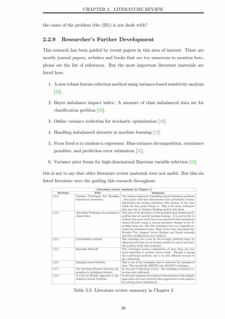
CHAPTER 2. LITERATURE REVIEW
the cause of the problem (the (IR)) is not dealt with?
2.2.9 Researcher’s Further Development
This research has been guided by recent papers in this area of interest. These are
mostly journal papers, websites and books that are too numerous to mention here,
please see the list of references. But the most important literature materials are
listed here.
1. A new robust feature selection method using variance-based sensitivity analysis
[38].
2. Bayes imbalance impact index: A measure of class imbalanced data set for
classification problem [39].
3. Online variance reduction for stochastic optimization [40].
4. Handling imbalanced datasets in machine learning [41].
5. From fixed-x to random-x regression: Bias-variance decomposition, covariance
penalties, and prediction error estimation [42].
6. Variance prior forms for high-dimensional Bayesian variable selection [43].
this is not to say that other literature review materials were not useful. But this six
listed literature were the guiding this research throughout.
Literature review summary in Chapter 2Sections Title Summary
2.2.2 Variance Techniques For Handlingimbalanced classeddata
The variance approach of handling classed imbalance problems, this papers used here demontrated that probabaility densitydistribution has strong correlation with variance of the classwhich the data point belong to. This is the main techniquesthat gave rise to Varinace Ranking used in this thesis
2.2.3 Algorithm Techniques for imbalancedclassed data
This part of the literature review provided most traditional al-gorithm that are used for machine learning . It is noteworthy torealised that good result have been produced with imbalancedclassed datasets owing to variaus parameter changes in the al-gorithm being use. But this techniques were not originally in-tended for imbalanced data. Many of the basic algorithms likeDecision Tree, Support Vector Machine and Neural networksand thier modifications were explored.
2.2.4 Cost-Sensitive method This technique set a cost for the wrongly predicted class, byadjusting each class cost it became possible to control and resetthe position of the class boundary
2.2.5 Ensemble Methods This techniques inolves combination of more than one treebased algorithm to produce better result. Though is amongthe tradiotional methods, but is its abit different because ofthe cobinations
2.2.6 Sampling based Methods This is one of the techniques that is dedicated for imbalanceddata. This specifically SMOTE and ADASYN techniques.
2.2.7 The Attribute/Feature Selection Ap-proaches to imbalanced dataset
In this part of litersture review , the techniques of feature se-lections were addressed.
2.2.8 A Case for Hybrid Approach to Im-balanced classed Problems
In this part emphasis were drawn to intergrations of all multipleapproaches that may involved others approaches as the panaceafor solving classed imbalanced.
Table 2.3: Literature review summary in Chapter 2
38

CHAPTER 2. LITERATURE REVIEW
2.3 The Measurement Evaluation for Imbalanced
dataset
The general performance for imbalanced classed data set does not follow the usual
accuracy measurement, rather the unequal amount of various classes in the data
set have to be reflected. Consequently, the metrics of measurement [121][122], have
to be specifically direct to empirical values of the numbers of classes captured in
the output test data, hence classification performances uses the confusion matrix
[123][124] as in Table 2.4; which is a cross-section table that evaluate how accurate
the model tends to classify the groups. One major reason for using this metric in
measuring classification is the insight into how the algorithm accurately identified
the classes and how many classes have been confused and mislabelled, as stated by
[125][126]. This would enable the assessment of the accuracy of the model given
captured and confused classes. Sections 2.3.1, 2.3.2 and 2.3.3 are the processes
measurement evaluation for imbalanced data set for both binary and multi-classed.
2.3.1 Measurement Evaluation for Binary classed data
The binary classification evaluation experiment is represented by a 2 x 2 confu-
sion matrix, as shown in Table 2.4. This is particularly useful for visualising a
binary classification against a multi-class classification, where multiple overlappings
of classification could confuse the algorithms and make the results; less discriminant;
a detailed analysis of the confusion matrix can be found in [127]. The definitions of
terms in confusion matrix tables are
• True positives (TP): The algorithm predicted yes, and the correct answer
is yes; (correctly predicted);
• True negatives (TN): The algorithm predicted no, and correct answer is no
(correctly predicted);
• False positives (FP): The algorithm predicted yes, but the correct answer
is no(incorrectly predicted); and
• False negatives (FN): The algorithm predicted no, but the correct answer
is yes(incorrectly predicted).
39

CHAPTER 2. LITERATURE REVIEW
Table 2.4: Confusion Matrix
The true positive rate (TPR) is the same as the sensitivity and recall. It is the
proportion of positive values that are correctly predicted:
Sensitivity = Recall =TP
(TP + FN). (2.12)
The Precision is the proportion of predicted positives which are actually positive
Precision =TP
(TP + FP ). (2.13)
Specificity is the proportion of actual negative which are predicted negative
FP (rate) = Specificity =TN
(TN + FP ). (2.14)
F-measure is the harmonic mean between precision and recall or The harmonic mean
between specificity and sensitivity.
Fmeasure = 2 ∗ Precision.Recall
(Precision+Recall). (2.15)
Accuracy =tp+ tn
(tp+ tn+ fp+ fn)=tp+ tn
n. (2.16)
The formulas show that the F-Measure is another mean of testing the accuracy of
binary classification accuracy [128].
2.3.2 Measurement Evaluation for Multi-classed data (One-
Versus-all and One -Versus-One)
The measure of classifier performance in imbalanced binary datasets is straightfor-
ward and easily understandable, but for multi-class cases, misclassified and overlap-
ping data make it impossible to effectively measure performance. one of the most
useful techniques is decomposing the classes into series of ntotal binary classes where
n is the number of classes [129][130].
40

CHAPTER 2. LITERATURE REVIEW
Figure 2.8: Multi-classed to Binary decomposition-One vs All
For clarity, Figure 2.8 shows three-class data represented by red stars, black cir-
cle, and green squares for implementing the One-versus-All technique. Let us take
the red stars as the positive class (Figure 2.8 a), demarcated by the red line; the
other components (black circles and green squares) are the negative class. Sequen-
tially, the black circles (Figure 2.8 b) and green squares (Figure 2.8 c) are taken in
turn to be positive while the rest are negative; this is the process of decomposing
multiple classes into (n)binary. With this decomposition, the binary performance
evaluations in section 2.3.1 could be applied to evaluate the multi-class data. The
”One-versus-all” could also be called one-versus-rest” and is one of the most popular
and accurate methods for handling multi-class datasets [130][131][132].
Another ways for handling multiple classes is ”one-versus-one” techniques; this pro-
cess takes each pair of classes in the multi-class dataset in turn, until all the classes
have been paired with each other
Figure 2.9: Multi-classed to Binary decomposition-One vs One
Figure 2.9 shows the one-versus-One for multi-classed data set were each class
41

CHAPTER 2. LITERATURE REVIEW
is paired with another until all the classes have been paired, for example in Figure
2.9 a, class 2 and class 3 is paired, class 1 and class 2 are paired in Figure 2.9 b and
finally class 1 and class 3 are paired in Figure 2.9 c.
There is extensive literature that has proposed and supported one-versus-all tech-
niques as the most accurate approach in handling multi-class classifications. The
work of [133][134][130][132] made strong cases as the only technique that could jus-
tifiably claim to have actually handle multiclassed classification in a real sense of it.
This is because one versus one makes a pair of binary data without according for
the influence of other data items, meaning that other data items that could interact
with the modeling have been eliminated or filtered out. In contrast, in one versus
all, those classes have not been removed. Furthermore, One-versus-One is computa-
tionally expensive. Hence, the one-versus-all approach is implemented in this work.
Therefore the metrics of measuring the performance in Equations 2.12, 2.13, 2.14,
2.15 and 2.16 in sections 2.3.1 will then be applicable to multi-classed imbalanced
data set because each iteration of classification is binary until all ntotal binary clas-
sification has been completed.
An average performance of the multi-classed n binary classifier may be deduced by
the summations of each metric as in
Equations 2.17,2.18,2.19,2.20.
Average Recall =
∑1i=j Recall
n(2.17)
Average Precision =
∑1i=j Precision
n(2.18)
Average Specificity =
∑1i=j Specificity
n(2.19)
Average Fmeasure =
∑1i=j Fmeasure
n(2.20)
There is no any major difference between the metrics for binary classed and that of
multi-classed that has been decomposed into ”one-versus-all”.
2.3.3 The Receiver Operating Characteristics and Area Un-
der the Curve
The graph of Receiver Operating Characteristics (ROC) is used to provides a trade-
off value between Sensitivity and Specificity. The y-axis is TP(rate) plotted against
42

CHAPTER 2. LITERATURE REVIEW
FP(rate) in the x-axis. The graph provides a corresponding score for any change
in either value [135][136], using the ROC graph is possible to predict all values
of TP(rate) and FP(rate) for any type of classifier both binary and multi-classed.
Figure 2.10 is a modified version (included yellow curve) of ROC graph used to
quantify the accuracy of a diagnostic test [137]. The scale of the graph is from 0.00
to 1.00 in both axes. The graph has four curves; yellow, green, red and blue. For
TP(rate) plotted in the y-axis the highest value is 1.00; therefore, the yellow curve
with the highest TP(rate) in y-axis at the position (0.00,1.00) is a perfect classifier
(more accurate) followed by green and red accordingly. In Figure 2.11 The blue
curve (straight line) is the result of random guess classification. The more the curves
get closer to the position (0.00,1.00) the better the classification. The area Under
the Curve (AUC) is another important metric, it is used to measure the accuracy
of the classification, ie accuracy is proportionally equal to the area under the ROC
curve, meaning that the larger this area the more accurate is the classification.
Figure 2.10: ROC Curve
The Figure 2.11 is a representation of an ROC graph with three curves; A, B
and C. Curve A is more accurate because it has a larger area, the area of C is
used to represent a random guess classification and usually 0.5. The ROC graph
for multi-classed (One-Versus-all) as described in section 2.3.2 are the same with
binary,
43
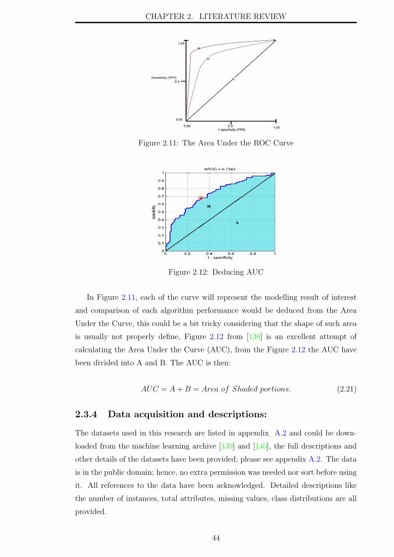
CHAPTER 2. LITERATURE REVIEW
Figure 2.11: The Area Under the ROC Curve
Figure 2.12: Deducing AUC
In Figure 2.11, each of the curve will represent the modelling result of interest
and comparison of each algorithm performance would be deduced from the Area
Under the Curve, this could be a bit tricky considering that the shape of such area
is usually not properly define, Figure 2.12 from [138] is an excellent attempt of
calculating the Area Under the Curve (AUC), from the Figure 2.12 the AUC have
been divided into A and B. The AUC is then:
AUC = A+B = Area of Shaded portions. (2.21)
2.3.4 Data acquisition and descriptions:
The datasets used in this research are listed in appendix A.2 and could be down-
loaded from the machine learning archive [139] and [140], the full descriptions and
other details of the datasets have been provided; please see appendix A.2. The data
is in the public domain; hence, no extra permission was needed nor sort before using
it. All references to the data have been acknowledged. Detailed descriptions like
the number of instances, total attributes, missing values, class distributions are all
provided.
44
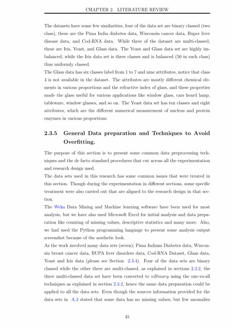
CHAPTER 2. LITERATURE REVIEW
The datasets have some few similarities, four of the data set are binary classed (two
class), these are the Pima India diabetes data, Wisconsin cancer data, Buper liver
disease data, and Cod-RNA data. While three of the dataset are multi-classed,
these are Iris, Yeast, and Glass data. The Yeast and Glass data set are highly im-
balanced, while the Iris data set is three classes and is balanced (50 in each class)
thus uniformly classed.
The Glass data has six classes label from 1 to 7 and nine attributes, notice that class
4 is not available in the dataset. The attributes are mostly different chemical ele-
ments in various proportions and the refractive index of glass, and these properties
made the glass useful for various applications like window glass, cars heard lamp,
tableware, window glasses, and so on. The Yeast data set has ten classes and eight
attributes, which are the different numerical measurement of nucleus and protein
enzymes in various proportions.
2.3.5 General Data preparation and Techniques to Avoid
Overfitting.
The purpose of this section is to present some common data preprocessing tech-
niques and the de facto standard procedures that cut across all the experimentation
and research design used.
The data sets used in this research has some common issues that were treated in
this section. Though during the experimentation in different sections, some specific
treatment were also carried out that are aligned to the research design in that sec-
tion.
The Weka Data Mining and Machine learning software have been used for most
analysis, but we have also used Microsoft Excel for initial analysis and data prepa-
ration like counting of missing values, descriptive statistics and many more. Also,
we had used the Python programming language to present some analysis output
screenshot because of the aesthetic look.
As the work involved many data sets (seven); Pima Indians Diabetes data, Wiscon-
sin breast cancer data, BUPA liver disorders data, Cod-RNA Dataset, Glass data,
Yeast and Iris data (please see Section 2.3.4). Four of the data sets are binary
classed while the other three are multi-classed, as explained in sections 2.3.2, the
three multi-classed data set have been converted to nBinary using the one-vs-all
techniques as explained in section 2.3.2, hence the same data preparation could be
applied to all the data sets. Even though the sources information provided for the
data sets in A.2 stated that some data has no missing values, but few anomalies
45

CHAPTER 2. LITERATURE REVIEW
were discovered during exploration (Data understanding) accordance with (CRISP)
of Data Mining [141] [142].
Missing data
Some of the data set has problem with missing values which must be dealt with,
the Pima India diabetes data, this was treated using the average of the data column
items because the Skewness for the missing columns are zero, hence their mean value
was used as replacement for the missing data in the body mass index (BMI) and
age attributes in the Pima Indians Diabetes data,
The Wisconsin Breast Cancer data are well organized and were treated from source,
so there were no problems with the data, while the cod-RNA dataset had very few
cases (6) of missing values; thus, it was deleted. Also for the BUPA Liver Disor-
ders data, the aspartate aminotransferase (sgot) and alanine aminotransferase (sgpt)
columns were also treated for missing data values. Additionally, none of the data
had any problem with outliers. Finally, the inconsistency of representing missing
values with zero in the Pima Indians Diabetes data was also addressed in the BMI
column.
During machine learning modelling processes one of the most common process error
that may occur is Overfitting and Underfitting, these two errors will be reviewed,
and the techniques used in avoiding them explained in these sections. Overfitting
is a modelling error that had occurred when the model created performed totally
below the result obtained during training when tested on a real independent data
[143][144][145]. By independent it means data that the model has not seen before,
this is due to the machine learning algorithm memorising the patterns of a dataset.
When the algorithm is exposed to the same data it will fit into the data patterns
so well that it produces very high accurate result. All this happened during train-
ing of the model. But the model is unable to generalise and replicate such high
accuracy in a new independent data. This shows that the model learning process is
false, although, overfitting has been traceable to be the consequence of noise in the
dataset. But other causes such as the over usage of the same data set such that it
increases the possibility of the modelling algorithms memorising the pattern of the
data items could also contribute to it. The underfitting is opposite of overfitting,
the model is unable to fit in the training data such that the accuracy result obtained
during training is very low. Perhaps, that is the reason underfitting error is not as
popular as overfitting because it cannot be used, after all, why should a model that
performed poorly be used?
46
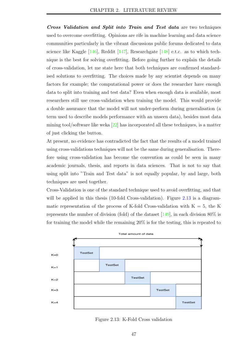
CHAPTER 2. LITERATURE REVIEW
Cross Validation and Split into Train and Test data are two techniques
used to overcome overfitting. Opinions are rife in machine learning and data science
communities particularly in the vibrant discussions public forums dedicated to data
science like Kaggle [146], Reddit [147], Researchgate [148] e.t.c. as to which tech-
nique is the best for solving overfitting. Before going further to explain the details
of cross-validation, let me state here that both techniques are confirmed standard-
ised solutions to overfitting. The choices made by any scientist depends on many
factors for example; the computational power or does the researcher have enough
data to split into training and test data? Even when enough data is available, most
researchers still use cross-validation when training the model. This would provide
a double assurance that the model will not under-perform during generalisation (a
term used to describe models performance with an unseen data), besides most data
mining tool/software like weka [22] has incorporated all these techniques, is a matter
of just clicking the button.
At present, no evidence has contradicted the fact that the results of a model trained
using cross-validations techniques will not be the same during generalisation. There-
fore using cross-validation has become the convention as could be seen in many
academic journals, thesis, and reports in data sciences. That is not to say that
using split into ”Train and Test data” is not equally popular, by and large, both
techniques are used together.
Cross-Validation is one of the standard technique used to avoid overfitting, and that
will be applied in this thesis (10-fold Cross-validation). Figure 2.13 is a diagram-
matic representation of the process of K-fold Cross-validation with K = 5, the K
represents the number of division (fold) of the dataset [149], in each division 80% is
for training the model while the remaining 20% is for the testing, this is repeated to
Figure 2.13: K-Fold Cross validation
47

CHAPTER 2. LITERATURE REVIEW
the number of the fold, the accuracy or performance of the model is obtained by
the average performance of each fold. Because the sets of data items being used for
the training and test data are repeatedly changed as depicted in Figure 2.13, the
machine learning algorithm would not be able memorised the fitting functions hence
overfitting problems will not arise. The cross-validation techniques have another ad-
vantage of allowing the model to use all the data without dividing the whole data
into training and test data particularly when the size of the data set is an issue.
In the next chapter of this research, the theoretical basis of the process that un-
derscores the derivatives of the techniques ” Variance Ranking Attribute Selection
(VR)” for handling the imbalanced will be deduced, one of the advantages of (VR)
is that its algorithm independent, hence machine learning algorithms, that could be
applied to both regression and classification problems will be used for validation of
our techniques.
48

Chapter 3
Variance Ranking Attribute
Selection Technique
3.1 Proposed Method and Approach
In chapter two, we provided the efforts that have been made so far to handle im-
balanced problems and also exposing the inadequacies in many of the existing ap-
proaches. Being that many of these approaches did not take the (IR) into con-
sideration nor utilised it in the algorithm. But are mostly based on tweaking and
using different modifications of algorithms. Although some good results could be
obtained sometimes, but the processes are difficult to replicate. Apart from the
sampling techniques were the process involves the (IR) because its either artificially
generating or reducing existing data items to equalized the classes as in (SMOTE).
Most academic pundits have criticise many of these approaches as not really solving
the problems of class imbalance.
Our approach is based on the variance of attributes, the reasons for choosing the vari-
ance as against other properties is because its best suited to describe and summarise
the positions of multiple data points within a vector space. Secondly, considering
the values of the attributes and how there are distributed, attributes that belong to
a particular class are usually concentrated together (have density). Therefore, the
variance values within a central terms of reference can provide an insight into the
relevance of such attribute class cluster and can be used to find the density of the
distributions of each cluster which are represented by the classes, hence the variance
can be used as a metrics to predict the classes of data item.
In most classification modelling, what we are searching for is just the minority
class items in both binary and multi-classed context, recall in chapter 2 that the
multi-classed could be decomposed to (n)Binary either using one-versus-one or one-
versus-all, but one-versus-all have been selected for this research the reasons for
49

CHAPTER 3. VARIANCE RANKING ATTRIBUTE SELECTIONTECHNIQUE
that, have been explained in chapter 2.
Figure 3.1: An Overview of the Proposed Method
To improve the capturing of minority classes in predictive modelling, new tech-
niques have to be developed because the existing approaches are skewing sensitivities
and capturing more of the majority classes which are not needed. To correct this,
we propose the processes as illustrated in Figure 3.1.
Though detailed of this process will be dealt with in subsequent sessions, but a
general black-box description of the Figure 3.1 will suffice for now. The process is
called ”Variance Ranking Attribute Selection” (VR) Technique. In the diagram, the
process starts with obtaining an imbalanced data (Binary or Multi-classed) then,
cleaning the data or any other preprocessing that the data may need. The data is
split into two classes (Positive class and negative class) or (class 1 and class 0), the
split classes is used to deduce important feature using a Variance Ranking process.
Finally, the results are evaluated by binary classifications.
3.1.1 Variance and Variables Properties
A typical datasets has lots of attributes (variables) each measured to different scale,
different data types (discrete or continuous). Each variable cluster centroid relative
to each may change or remain constant depending on the terms of reference. Some
of these variables may be dependent while some may be independent and also the
density function will remain constant. The question is, how could all these properties
be made to undergo the same statistical treatment? Is there a property of numeric
data that equalises them so that they could be subjecting to the same statistical
treatment and will not produce any bias. The work of [150][151][152][153] provided
a solution of derivative for this equalisation.
The two quantities that are mostly used to measure the distance of data items from
their mean position are variance (σ2) and standard deviation√
(σ2).
50

CHAPTER 3. VARIANCE RANKING ATTRIBUTE SELECTIONTECHNIQUE
Figure 3.2: Standard Deviation for Single Variable Normal Distribution
Even if, both could be deduced from each other and consequently share many
physical characteristic, but there exist some differences in the application of these
two quantities. For example, the standard deviation is mostly used for investigating
a single variable distribution as shown in Figure 3.2, but if the data set is multivariate
then variance are mostly used to describe the general spread of these variables from
the conceptual ”mean” position [154]. The term conceptual ”mean” is used to
indicate the fact of the changing values and position of the mean and variances of
one class relative to another class. And if the one class is taken in turn relative to the
rest as in One-vs-All, the ”mean” and ”variance” will be different to the next class.
But considering the density of all the classes in the sample space, which is called
the probability density function will remain constant because the total numbers of
the data item and the sample space is not changing, please see [155], though this
function is a probability concept and is described as the likelihood that the value of
a variable lies within a sample space. The review of Figure 3.3 is a representation
of Glass data in the 3D scattered plot, but the values of variances of class relative
to the other classes changes depending on the positioning of the class group that is
being considered, hence the terms conceptual mean, and variance. But the whole
density will remain the same. Note, in this case the density is considered to be
probabilistic because the data item in the sample space is not evenly spread and
the likely-hood of getting a data item in the sample space depends on the spread
or variance. In fact, this density probability concept is an active area of research
popularly called ”Probability density estimation” [156][157][158].
51

CHAPTER 3. VARIANCE RANKING ATTRIBUTE SELECTIONTECHNIQUE
Figure 3.3: 3D Glass data Scatter plot
By definition, variance is how spread the data items of number N from the mean
and is given by σ2 =∑
(x−µ)2
N . If the whole population is considered, however, this
equation is slightly different if a sample of the whole population is used and is given
by σ2 =∑
(x−µ)2
N−1 [159][154]. When taking a sample it must be large enough and
taken several times and average out to make sure that the sample mean is equal to
population mean and the variance of the sample mean is given by σm2 = σ2
n while
σm2 is the variance of the sample and n is equal to the number of times the sample
were taken. Therefore the variance of population is equal to σ2 = σ2m * n [160].
These data items were collected independently from each other, hence are inde-
pendent variables. In many numeric data, the variables could either be discrete or
continuous. To what extent does the type of variable data item affect the overall dis-
tribution from their means ie the variances? The effect of these intrinsic properties
of the data item can be deduced accordingly.
For an input dataset with N = {n1......nx}, where n is a combination of discrete
and continuous variables [161][162][163], if the variance of the independent random
variable x is given by V arx which is the expected value of the square of the the
deviation, for all the variable x with a mean of µ the variance is;
V arx = E{
(x− µ)2} (3.1)
The constant E represents the density function and E α 1N .
The Equation 3.1 [162] is modified to accommodate both discrete and continuous
variables. Hence, when variable x is continuous the variance is
V arx = E{
(x− µ)2} =
max∑i=min
∫ max
min
(x− µ)2 f (x) dx (3.2)
52

CHAPTER 3. VARIANCE RANKING ATTRIBUTE SELECTIONTECHNIQUE
Also for discrete variable Equation 3.1 would resolve to;
V arx = E{
(x− µ)2} =
n∑i=1
(xi − µ)2 f(x) (3.3)
and the whole population or the sample is considered, the population variance
becomes subjective to the probability density function f(x) such that the expecta-
tion values and variance of x within the same density is the sum of Equation 3.2
and Equation 3.3 V(total) = V(discrete) +V(continuous). Therefore, for any type of vari-
able (discrete and continuous) their total variances is the sum of individual variance
provided there are in the same sample space:
Vtotal =
n∑i=1
(xi − µ)2 f(x) +
max∑i=min
∫ max
min
(x− µ)2 f (x) dx (3.4)
each parts of equation 3.4 contains the same quantity apart from the change
function dx, therefore it could be simplify to equation 3.5 particularly when the
change is minima
∑f(x)dx (x− µ)2 (3.5)
if µ is considered as being the mean and the probability density functions is f(x)
and f(x)dx
which is constant in the sample space, hence
f(x) = f(x)dx = pi (3.6)
then for any population or sample variable, V(ar) is also deduced by [164]:
V(ar) =
n∑i=1
pi. (xi − µ)2 (3.7)
For all values of pi being the probability density functions, for equation 3.5
and 3.7, the equality is deduced by equating the integral to f (x) dx and∑n
i=1 pi
as in equation 3.6. Due to the premise of the same range of probability density
function, the variables transformable vis-a-vis discrete and continuous as provided
by [165][163][161].
This link between the discrete and continuous distribution under the condition of
the same range and their transformation from one to another were demonstrated
by [166][167] therefore equalized the variables; hence, the variances of the discrete
and continuous variables are equal if f (x) dx and∑n
i=1 pi are equal. Our technique
53

CHAPTER 3. VARIANCE RANKING ATTRIBUTE SELECTIONTECHNIQUE
implemented the concept of sample variance by taking n values in the range of
y1....yn of the population where n < N . Estimating the variance of the sample data
variables gives the average of the square deviations as in σy2 = 1n
∑ni=1 (y − y)2 =(
1n
∑ni=1
)− y2 = 1
n2
∑1i<j (yi − yj)2.
This computation confirms that the range of the variable values of x is still within
that of the mean, as explained earlier. This derivative will hold true in both cases
of variance if and only if the distribution of the variable x is completely determined
by the probability density function f(x) [168][169], which is shown in Equation 3.5
and 3.7. Having deduced the variance and variables properties, have provided an
insight to show that no matter the types of variable whether discrete and or continu-
ous or any other intrinsic properties of the variables, the same statistical operations
could be applied to the variables and will not invalidate the experiments.
Figure 3.4: Algorithm flow chart for The Variance Ranking Attribute Selection
54
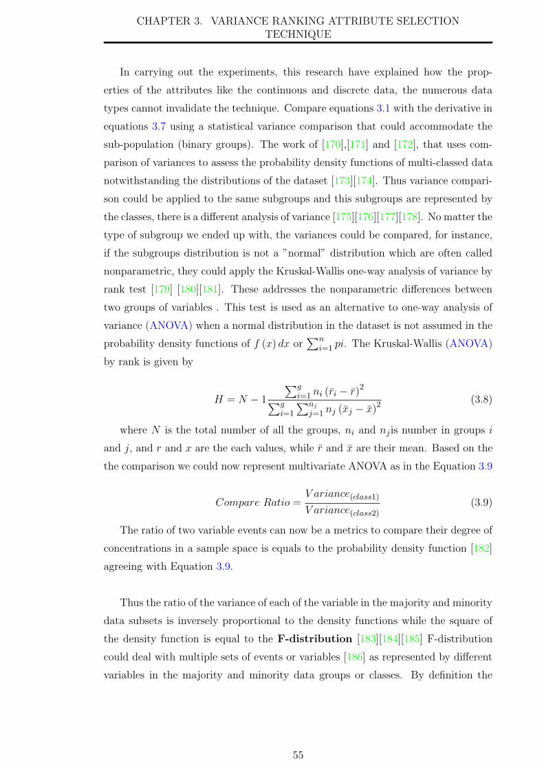
CHAPTER 3. VARIANCE RANKING ATTRIBUTE SELECTIONTECHNIQUE
In carrying out the experiments, this research have explained how the prop-
erties of the attributes like the continuous and discrete data, the numerous data
types cannot invalidate the technique. Compare equations 3.1 with the derivative in
equations 3.7 using a statistical variance comparison that could accommodate the
sub-population (binary groups). The work of [170],[171] and [172], that uses com-
parison of variances to assess the probability density functions of multi-classed data
notwithstanding the distributions of the dataset [173][174]. Thus variance compari-
son could be applied to the same subgroups and this subgroups are represented by
the classes, there is a different analysis of variance [175][176][177][178]. No matter the
type of subgroup we ended up with, the variances could be compared, for instance,
if the subgroups distribution is not a ”normal” distribution which are often called
nonparametric, they could apply the Kruskal-Wallis one-way analysis of variance by
rank test [179] [180][181]. These addresses the nonparametric differences between
two groups of variables . This test is used as an alternative to one-way analysis of
variance (ANOVA) when a normal distribution in the dataset is not assumed in the
probability density functions of f (x) dx or∑n
i=1 pi. The Kruskal-Wallis (ANOVA)
by rank is given by
H = N − 1
∑gi=1 ni (ri − r)2∑g
i=1
∑nj
j=1 nj (xj − x)2(3.8)
where N is the total number of all the groups, ni and nj is number in groups i
and j, and r and x are the each values, while r and x are their mean. Based on the
the comparison we could now represent multivariate ANOVA as in the Equation 3.9
Compare Ratio =V ariance(class1)
V ariance(class2)(3.9)
The ratio of two variable events can now be a metrics to compare their degree of
concentrations in a sample space is equals to the probability density function [182]
agreeing with Equation 3.9.
Thus the ratio of the variance of each of the variable in the majority and minority
data subsets is inversely proportional to the density functions while the square of
the density function is equal to the F-distribution [183][184][185] F-distribution
could deal with multiple sets of events or variables [186] as represented by different
variables in the majority and minority data groups or classes. By definition the
55

CHAPTER 3. VARIANCE RANKING ATTRIBUTE SELECTIONTECHNIQUE
F-distribution (F-test) [184][187] is given by
F =(Larger variance)2
(smaller variance)2(3.10)
Therefore, for subset (class 1 and 0) with additive variance of independent vari-
able will resolve into please see [188][189];
Ffinal =
{V ariance(final1)
V ariance(final2)
}2
(3.11)
therefore the of Ffinal is a ratio concept hence, has no unit, since both units
have cancel each other, hence Ffinal is a measure of the density of the variances
V ariance(final1) to V ariance(final2).
For a binary classed data or multi-classed decompose into n binary using One-vs-All,
if the sub classes variance is Vi and Vj , then the Equation 3.11 would resolved to
Equation 3.12, the squaring eliminates any negative value and also agreed with the
F-distribution (F-test), finally the value of (F-test) is Ffinal
Ffinal =
[V0j
V1j
]2
(3.12)
3.2 The Abstraction and High level Research De-
sign:
The high level research design is explained with the aid of the block algorithm di-
agram in figure 3.4. From the diagramme, the input data sources are assumed to
have been treated for any common error like missing values, incompatible data types
etc. The figure in 3.4 showed that each dataset have to be split into two according
to their classes. Even the multi-classed will be converted to nBinary, where n are
equal to the numbers of classes in the dataset. The dataset is split or separated into
class 1 and class 0 or class negative and class positive.
If the variances V0 = v01, v02, v03.....v0j of each of the variables in class 0 and the
variances of V1 = v1, v2, v3.....vj of each of the variables in class 1 are taken, for each
pair of the feature we find the ratio of the V0
V1.
The value (V0/V1) is the division ratio based on the variance significant F-distribution
giving by{V0
V1
}2to produce the values that could be squared, the squaring of these
values are particularly useful in case any of the quantity resolved to negative at any
point. The significant feature are selected by ranking the{V0
V1
}2from highest to
lowest. The highest being the most significant , while the lowest the least signifi-
56

CHAPTER 3. VARIANCE RANKING ATTRIBUTE SELECTIONTECHNIQUE
cant. All these are shown sequentially in the figure 3.4. For each of the datasets in
the experiments this high level design would act as a guide for clarity and reference
point.
3.3 Experiment Design:
3.3.1 Sampling and Splitting the data set
The dataset used is in Table A.2. The experimentation was conducted on the two
classes of data (the majority and minority classes) represented by 0 and 1 for the
binary classed and also the multi-classed have been decomposed to nBinary classed
using One-versus-all technique as explained in section 2.3.2 hence is also represented
by 0 and 1.
Where the number of the whole population is below 2000 like in (Pima India, Wis-
consin, Bupa, Iris, Glass, and Yeast), all the data set instances were divided into two
classes (0 and 1) to represent the majority and minority classes. But for Cod-RNA
with a population of 488565, the data sets were first split into nBinary of 0 and 1.
To obtain the sample size and ensure that the sample collected have the same
characteristics as the class population (0 and 1). The process utilised in the work of
[190] was used and also the concept of central limit theorem as explained at [191].
This is done by repeatedly randomising the collection of the sample from the pop-
ulation. The sample size selected for each class is based on the ratio of each classes
in the population thereby maintaining the imbalance ratio (IR). Furthermore, the
integrity of the sample is checked against the subset population by comparing the
distribution of the sample to that of the subset population using the Central Limit
Theorem concept [191], this is done by checking the n sample skewness given by1n
∑ni=1(x1−x)3
[ 1n−1
∑ni=1(x1−x)2]
32
(Fisher-Pearson). The skewness is a statistical function used to measure the
distribution of a data set, if two data set have the same skewness, therefore, their
distributions are the same.
The classes of the two subsets are used to represent the majority and minority
classes, the following term definition should be established without any confusion of
their meanings.
• Majority class, may also be known as negative class or class 0.
• Minority class, may also be known as positive class or class 1.
57
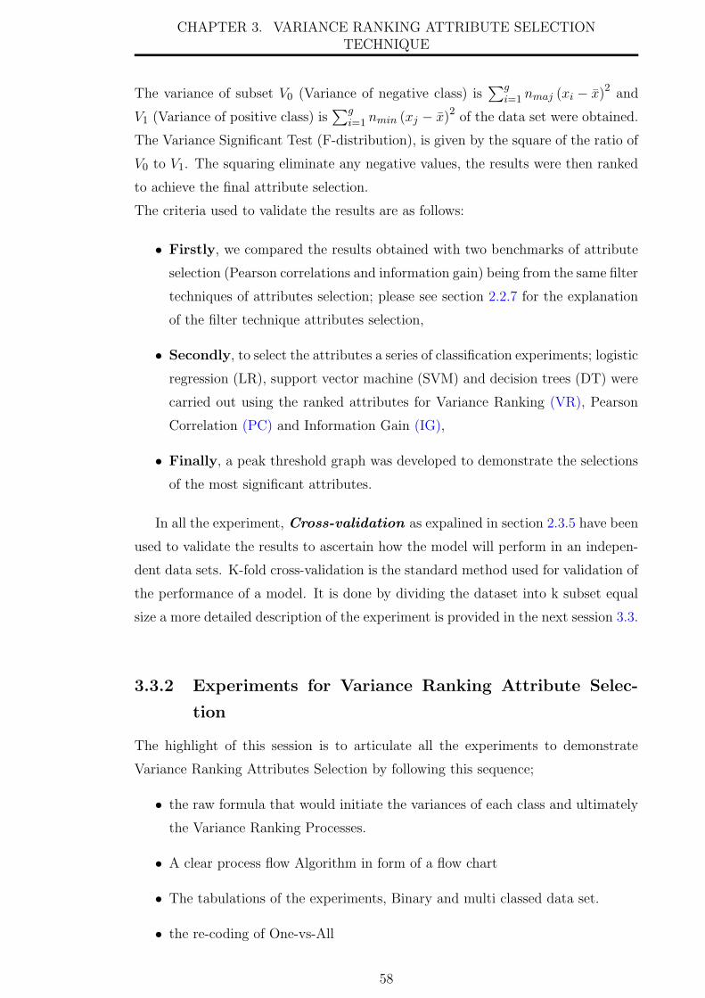
CHAPTER 3. VARIANCE RANKING ATTRIBUTE SELECTIONTECHNIQUE
The variance of subset V0 (Variance of negative class) is∑g
i=1 nmaj (xi − x)2 and
V1 (Variance of positive class) is∑g
i=1 nmin (xj − x)2 of the data set were obtained.
The Variance Significant Test (F-distribution), is given by the square of the ratio of
V0 to V1. The squaring eliminate any negative values, the results were then ranked
to achieve the final attribute selection.
The criteria used to validate the results are as follows:
• Firstly, we compared the results obtained with two benchmarks of attribute
selection (Pearson correlations and information gain) being from the same filter
techniques of attributes selection; please see section 2.2.7 for the explanation
of the filter technique attributes selection,
• Secondly, to select the attributes a series of classification experiments; logistic
regression (LR), support vector machine (SVM) and decision trees (DT) were
carried out using the ranked attributes for Variance Ranking (VR), Pearson
Correlation (PC) and Information Gain (IG),
• Finally, a peak threshold graph was developed to demonstrate the selections
of the most significant attributes.
In all the experiment, Cross-validation as expalined in section 2.3.5 have been
used to validate the results to ascertain how the model will perform in an indepen-
dent data sets. K-fold cross-validation is the standard method used for validation of
the performance of a model. It is done by dividing the dataset into k subset equal
size a more detailed description of the experiment is provided in the next session 3.3.
3.3.2 Experiments for Variance Ranking Attribute Selec-
tion
The highlight of this session is to articulate all the experiments to demonstrate
Variance Ranking Attributes Selection by following this sequence;
• the raw formula that would initiate the variances of each class and ultimately
the Variance Ranking Processes.
• A clear process flow Algorithm in form of a flow chart
• The tabulations of the experiments, Binary and multi classed data set.
• the re-coding of One-vs-All
58

CHAPTER 3. VARIANCE RANKING ATTRIBUTE SELECTIONTECHNIQUE
All the itemised will be presented in this section. When some process has been
carried out in other sections or chapters it would be referred and properly signed
post. The proposed method of attributes selections is for discrete and continuous
numeric data for a binary class and multi-classed (decomposed into n binary see
section 2.3.2) represented by 1 and 0.
The data preparation have been explained in sections 2.3.5 and 3.3.1 . Each of the
data set in Table A.2 was first split into two subsets of class 0 and class 1 and the
Variance of each attribute deduced using equation 3.13 and 3.14 respectively. The
Variance Significant is deduced using the equation of 3.15. In all the total number
of the majority and minority class is maintained through the number of the data
items as nmaj and nminj . In general the variance of each of the subsections; class
target 1 and class target 0, of dataset was computed using the following formula
Variance v =∑
(x−x2)(n−1)
. If The Variance subsection of class 0 is given by:
V0 =(x0 − x0
2)
(nmaj − 1)(3.13)
If then Variance subsection of class 1 is given by:
V1 =(x1 − x1
2)
(nmin − 1)(3.14)
The Variance Significant Attribute Selection is then deduced by:
V R =
((x0 − x0
2)
(nmaj − 1)/
(x1 − x12)
(nmin − 1)
)2
=
{V0
V1
}2
(3.15)
The total number of data items is inversely proportional to the variance or spread
from the mean position, that is V ariance ∝ 1nm
, this relationship shows that the
formula is generic, therefore if the ranking is done in either order it would remain
consistent. In Tables 3.1, 3.2, 3.3 and 3.4 , the column V1 and V0 is the results of the
variance of each subsection class (positive=1 and negatives=0) for each attribute.
Binary classed Experiments
The results of the experiment for the binary classed data is in Tables 3.1, 3.2, 3.3 and
3.4. The serial numbers in the tables are not mistakes but show how the attributes
were numbered before from the original data sets descriptions in Table A.2 and how
the (VR) techniques have ranked them.
59

CHAPTER 3. VARIANCE RANKING ATTRIBUTE SELECTIONTECHNIQUE
Table 3.1: Variance Ranking attribute selection using Pima India data
The result of the experiment using the Pima India data in Table 3.1 have a serial
number that has identified age followed by Body Mass Index (bmass) and plama
glucose as the three most significant. The ranking continued until the last attribute
which is insutest.
Table 3.2: Variance Ranking attribute selection using Bupa data
The Bupa data have also been ranked in the order from 4,3, 6, 5, 1 and 2 in
Table 3.2. While the Wisconsin and Cod-rna data have been ranked in Table 3.3
and 3.4
60

CHAPTER 3. VARIANCE RANKING ATTRIBUTE SELECTIONTECHNIQUE
Table 3.3: Variance Ranking attribute selection using Wisconsin Breast Cancer data
Table 3.4: Variance Ranking attribute selection using Cod-rna data
Multi-classed Experiments (n)Binary
The above three experiments demonstrated the (VR) technique for binary classed
data and is straight forward, but for multi-classed distributed dataset each of the
minority classes will be taken in turn as the positive or 1 while the rest will be
negative or class 0. This will result in more multiple experimentation equal to the
number of target classes. For example, if there are three classes in the dataset, this
would result into (n)Binary, while n = 3. The subsequent sessions would show the
experiment with Iris data set that has n = 3.
The result for Iris data in Table 3.5 is very obvious, the classes are label originally
as Iris Versicolor, Satosa and Virginica. For Iris Versicolor, the Petal width has been
identified as the most significant attribute that distinguishes it from the rest, fol-
lowed by the Petal length, Sepal length and Sepal width. The result for Satosa and
Virginica are the most interesting, even if the experiment were performed differently
both results are similar thereby showing that both flowers share more similarity to
61

CHAPTER 3. VARIANCE RANKING ATTRIBUTE SELECTIONTECHNIQUE
Table 3.5: Variance Ranking attribute selection using Iris data
each other than Versicolor.
The Glass data set that has n = 6 classes for details on this dataset please see
Table A.2. The imbalanced classes are from 1 to 7; notice that class 4 is not in this
dataset, so the total number of available classes is six, and they are labeled 1, 2, 3,
4, 5, and 7. Using the ”one-versus-all” process, as explained in sections 2.8 each of
these classes will be taken in turn as class 1 (minority class) and others as class 0
(majority class)
Table 3.6: Glass data set details showing highly imbalance classes
The Glass data imbalanced contents proportion is shown in Figure 3.5, which
represents the chemical elements compositions and the refractive index (RI) which is
a physical property of glass that measureS the bending of light as it passes through.
62

CHAPTER 3. VARIANCE RANKING ATTRIBUTE SELECTIONTECHNIQUE
Figure 3.5: Glass data contents proportion
The amount of the chemical compositions of a glass determines its application,
type, and classes; for example, class 1 is ”Building window float processed”, class
2 is the ”Building window non-float processed”, class 3 is ”vehicle window float
processed”, class 4 (not available in this dataset) is ”vehicle window non-float pro-
cessed”, class 5 is ”container”, class 6 is ”tableware,” and finally, class 7 is ”head-
lamps.” Therefore, the experiment will be conducted with class 1 as the minority
while the rest will be class 0 as the majority class. Each of the classes in the mi-
nority, as shown in Figure 3.5 will consequently be relabeled as class 1 and class 0.
Table 3.7 is the implementation of the one-versus-all approach; it shows the rela-
beled table with the actual numbers of minority classes as 70, 76, 17, 13, 9 and 29
and the corresponding majority classes are 144, 138, 197, 201, 205 and 185
63

CHAPTER 3. VARIANCE RANKING ATTRIBUTE SELECTIONTECHNIQUE
Table 3.7: Glass data class relabel to One-vs-All
The final result of using the (VR) techniques for the glass dataset is shown in
Table 3.10. Again, notice that the serial number as ranked by the experiment is
different from that presented in Table 3.6, excluding the ID number. Each of the
sub-tables in Table 3.10 is a representation of each class relabelled as class 1 and
the rest as class 0; for example, class 2 is relabelled as class 1 and the rest as class
0, (one versus all). This process is continued for all the classes in the dataset; see
Table 3.7.
Table 3.8: Yeast data set details showing highly imbalance classes
64

CHAPTER 3. VARIANCE RANKING ATTRIBUTE SELECTIONTECHNIQUE
463
429
244
163
5144
37 30
20 5
Target class of Yeast data set
CYT (cytosolic or cytoskeletal) NUC (nuclear)
MIT (mitochondrial) ME3 (membrane protein, no N-terminal signal)
ME2 (membrane protein, uncleaved signal) ME1 (membrane protein, cleaved signal)
EXC (extracellular) VAC (vacuolar)
POX (peroxisomal) ERL (endoplasmic reticulum lumen)
Figure 3.6: Yeast data contents proportion
Table 3.9: Yeast data class relabel to One-vs-All
For the Yeast data, the imbalanced classes could be seen in Table 3.8 and the
contents proportions in Figure 3.6. This dataset is one of the most popular ones,
and it has been used in various work for imbalanced multi-class data. The data
are numeric measurements of different protein in the nucleus and cell materials in
Yeast unicellular organisms. The objective of the dataset is using this physical
protein descriptor for ascertaining the localization, which in turn, may provide help
explaining the growth, health, and other physical and chemical properties of Yeast.
The data are made up of 1,484 instances. The re-coding of the dataset to one versus
all is shown in Table 3.9. For example, the recoding proceeds as ”CYT (463) as class
1, 1023 as class 0”; this continues until the last minority class, which is ”ERL(5) as
class 1, 1481 as class 0.
65

CH
AP
TE
R3.
VA
RIA
NC
ER
AN
KIN
GA
TT
RIB
UT
ESE
LE
CT
ION
TE
CH
NIQ
UE
Table 3.10: Experiment on Glass data
66

CHAPTER 3. VARIANCE RANKING ATTRIBUTE SELECTIONTECHNIQUE
The first sub-table in table 3.10 is class 1, and the rest classes (class 2,3,5,6 and
7; notice no class 4) are class 0. The (VR) technique ranks the most significant
attributes as follows Ba, Mg, K and so forth. The second experiment has class 2
relabeled as class 1 and the other classes (1, 3, 5, 6 and 7) as class 0. They are
ranked K, Al, Ba and so on, as the most significant. The next experiment is class
3 relabeled as class 1 while the rest as class 0; they ranked Ba, Mg, Ca, and so on.
All six classes are taken in turn.
The general postulate here from the experimental result is that the type of glass
depends on the amount of chemical element that the glass contains; this has been
captured by the (VR) technique.
67

CH
AP
TE
R3.
VA
RIA
NC
ER
AN
KIN
GA
TT
RIB
UT
ESE
LE
CT
ION
TE
CH
NIQ
UE
Table 3.11: Experiment on Yeast data
68

CH
AP
TE
R3.
VA
RIA
NC
ER
AN
KIN
GA
TT
RIB
UT
ESE
LE
CT
ION
TE
CH
NIQ
UE
Table 3.12: Experiment on Yeast data continue
69

CHAPTER 3. VARIANCE RANKING ATTRIBUTE SELECTIONTECHNIQUE
Summary
This chapter presented one of the main assertions of the research, it started with a
clear theoretical basis of the nature of numeric data and the techniques for transform-
ing from one data types to another within the conditions of the same range density
formalism. Then a demonstration of the framework which lays the background for
the heuristic axiomatic inferences that established the relationship between class
distribution and the variances of the data items in the domain of discourse vis a
vis the sample space were presented. The variance of the data items in the domain
space and how this is related to their class distribution was deduced and explained.
An introduction of variance comparison testing which culminated into (VR) tech-
nique was derived therein. The main research design like the processes of data
sampling for experimental validity and reliability were explained in details. A clear
process demonstrations for decomposing Multi-classed into Binary classed data were
explained in detailed with clear diagrams. The process of avoiding overfitting using
the state of the art cross-validation and the justifications as a process of producing
more dependable results were also explained.
The results of the experiments carried out in this chapter present a significant contri-
bution to the overall and major insight into some of the discovery and many claims
made by this research and also would become an input into later chapters. It is also
a whole knowledge in his own right that could lead to future work by any researcher.
This work may be seen as pioneering new field because, in most academics and in-
dustries, the correlations of the effects of the variances of data points and their
classes have not been investigated before. But, this work showed the correlation
with a concise inferences and presenting an axiomatic open field for new avenue of
knowledge insight and opportunities for further researches. The implication of the
knowledge discovered therein is in no doubt and limitless.
70

Chapter 4
Comparison of Variance Ranking
Attribute Selection With Other
Attribute Selections
4.1 Introduction
In this chapter, comparison of (VR) technique and two main state of the art features
selection techniques (algorithm) will be made, these two are (PC) and (IG) belong
to the categories of features selections known as ”filter” methods the other(s) are
”wrapper” and ”hybrid” which are just a combination of filter and wrapper meth-
ods. Please refer to section 2.2.7 for the details of these methods and reasons for
comparing the (VR) with (PC) and (IG). But just for a hint the (PC) and (IG) are
two most popular and state of the art feature selections.
Most feature selection results are heuristics [192][193][194][195], meaning that no
two feature selection on the same dataset will produce the same result perfectly,
especially in the filter algorithm; instead, each attribute identified are most likely
to be ranked slightly differently by different filter feature selection algorithms. To
estimate or measure the similarities in these results, the order of ranking of the
attributes becomes the metric used to quantify the similarities. Some of the iden-
tified attributes may be in the same position in the order of ranking, while others
may share similarities by proximity to the attribute’s positions. The result of (VR)
obtained in sections 3.1 will be paired with the result of (PC) and (IG) on the same
data to investigate the extents of their similarities and differences. A novel method
of quantifying similarity called ”Ranked Order Similarity Index”(ROS) will be dealt
with extensively in subsequent sections. The (ROS) is a similarity index quantifier
to assess two or more sets that may contain the same object but ranked differently.
The necessity of (ROS) came about from the fact that the existing similarity index
71

CHAPTER 4. COMPARISON OF VARIANCE RANKING WITH OTHERATTRIBUTES SELECTION
measure appeared to be inadequate when quantifying the similarity of sets of the
same items that are ranked differently, please see sections 4.3.
4.2 Comparison of Variance Ranking Attribute
Selection (VR) Technique with the Bench-
marks
Attribute selections, in general, could be categorized as filter or wrapper methods
[109][110]. The filter method uses the general characteristics of the data item to
determine the features that are more significant without involving any intended
learning algorithm, while wrapper method on the order hand tend to determined
the features in dataset that would produce the best performance on a predetermined
learning algorithm. Putting it succinctly, wrapper method suggest the attributes to
use for a given classifier algorithm. This suggestive and predetermining the clas-
sifier algorithm made the wrapper method less generic and limited as a means of
comparison with our method (VR) technique, which is independent of any learning
algorithm. Besides, wrapper methods create a subset of features which are deemed
to be most important for a specific classifier’s performance. These subsets more
often than not does not include all the original features meaning that some features
are eliminated in the subsets and each feature relevance to the subsets are not made
known. But, filter methods uses ranking processes to produce the order of rele-
vance of each, ie no feature is eliminated from the ranking [109]. The comparison of
(VR) attribute selection will be done with similar filter method that is not classifier
suggestive. Consequently, we compare our method to the state-of-art filter feature
selection methods; the Pearson correlation (PC) and [196][197][198] and information
gain (IG)[199][200]. The results are provided in Tables 4.1, 4.2, 4.3 and 4.4 for the
data sets used in the experiment.
V ariance Ranking (V R) =
((x0 − x0
2)
(nmaj − 1)/
(x1 − x12)
(nmin − 1)
)2
=
{V0
V1
}2
(4.1)
Pearson Correlation(PC) =
∑(x− x)(y − y)∑
(x− x)2∑
(y − y)2. (4.2)
Information Gain(x,y)(IG) = Entropy(x) − Entropy(x,y). (4.3)
72

CHAPTER 4. COMPARISON OF VARIANCE RANKING WITH OTHERATTRIBUTES SELECTION
Table 4.1: Comparison of Variance Ranking with PC and IG variable selection forPima India diabetes data
Table 4.2: Comparison of Variance Ranking with PC and IG variable selection forLiver Disorder Bupa data
Table 4.3: Comparison of Variance Ranking with PC and IG variable selection forWisconsin Breast cancer data
73
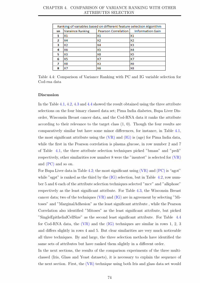
CHAPTER 4. COMPARISON OF VARIANCE RANKING WITH OTHERATTRIBUTES SELECTION
Table 4.4: Comparison of Variance Ranking with PC and IG variable selection forCod-rna data
Discussion
In the Table 4.1, 4.2, 4.3 and 4.4 showed the result obtained using the three attribute
selections on the four binary classed data set; Pima India diabetes, Bupa Liver Dis-
order, Wisconsin Breast cancer data, and the Cod-RNA data it ranks the attribute
according to their relevance to the target class (1, 0). Though the four results are
comparatively similar but have some minor differences, for instance, in Table 4.1,
the most significant attribute using the (VR) and (IG) is (age) for Pima India data,
while the first in the Pearson correlation is plasma glucose, in row number 2 and 7
of Table 4.1, the three attribute selection techniques picked ”bmass” and ”pedi”
respectively, other similarities row number 8 were the ”insutest” is selected for (VR)
and (PC) and so on.
For Bupa Liver data in Table 4.2; the most significant using (VR) and (PC) is “agot”
while ”sgpt” is ranked as the third by the (IG) selection, but in Table 4.2, row num-
ber 5 and 6 each of the attribute selection techniques selected ”mcv” and ”alkphose”
respectively as the least significant attribute. For Table 4.3, the Wisconsin Breast
cancer data; two of the techniques (VR) and (IG) are in agreement by selecting ”Mi-
toses” and ”MarginalAdhesion” as the least significant attribute , while the Pearson
Correlation also identified ”Mitoses” as the least significant attribute, but picked
”SingleEpithelialCellSize” as the second least significant attribute. For Table 4.4
for Cod-RNA data, the (VR) and the (IG) techniques are similar in rows 1, 2, 3
and differs slightly in rows 4 and 5. But clear similarities are very much noticeable
all three techniques. By and large, the three selection methods have identified the
same sets of attributes but have ranked them slightly in a different order.
In the next sections, the results of the comparison experiments of the three multi-
classed (Iris, Glass and Yeast datasets), it is necessary to explain the sequence of
the next section. First, the (VR) technique using both Iris and glass data set would
74

CHAPTER 4. COMPARISON OF VARIANCE RANKING WITH OTHERATTRIBUTES SELECTION
be compared with (IG) and (PC) this will be repeated for each n number of binary
classes from the decomposed multi-class data.
75

CH
AP
TE
R4.
CO
MP
AR
ISO
NO
FV
AR
IAN
CE
RA
NK
ING
WIT
HO
TH
ER
AT
TR
IBU
TE
SSE
LE
CT
ION
Table 4.5: Comparison of Variance Ranking with PC and IG variable selection for Iris data
76

CH
AP
TE
R4.
CO
MP
AR
ISO
NO
FV
AR
IAN
CE
RA
NK
ING
WIT
HO
TH
ER
AT
TR
IBU
TE
SSE
LE
CT
ION
Table 4.6: Comparison of Ranking significant with PC and IG variable selection for Glass data
77

CHAPTER 4. COMPARISON OF VARIANCE RANKING WITH OTHERATTRIBUTES SELECTION
Discusion
The table 4.5 is a presentation of the result of the Iris comparison using the (VR),
(IG) and (PC) techniques. All three feature selection have identified that petal
length or petal width as the two most significant and ranked them accordingly. In
condition of ”Satosa = 1, Others = 0” the (VR) differs to sightly to (IG) and (PC)
which are the same. In the condition ”Versicolor=1 Others=0” the (VR) and (PC)
are similar in identifying the two first attributes in column 1 and 2 while the (VR)
and (IG) are similar in columns 3 and 4. In the final condition of ”Virginica=1,
Others=0”, the (VR) and (IG) are similar in the first two rows while (IG) and (PC)
in the last two rows.
Table 4.6 is the presentation of the results of the comparison of (VR), (PC) and
(IG) feature selection techniques on the highly imbalanced Glass data. Originally,
the Glass dataset is made up of six classes labeled class 1,2,3,5,6,7 (notice there is no
class 4). Each of the smaller tables in Table 4.6 is a representation of these classes’
results. To carry out the ”One versus all” experiment explained in the previous
sections 2.3.2, and Table 3.7, each class was relabelled in turn as class 1 and others
combined as class 0. In the first smaller table, in Table 4.6 (class 1 labeled as
1 and the others as 0), the (VR) and (PC) identifies Ba, Mg, and K in the first
rows. The sixth and ninth rows have the same results. The (IG) and (VR) are
not far off from each other; the fourth and fifth rows identify Al, while the eighth
and ninth rows identify Fe. Although, there are no rows that identifies the same
elements the closeness is greater between (VR) and (IG) than it is between (PC) and
(IG) for this first experiment, in Table 4.6, (VR) and (IG) are more similar. The
quantitative weighting of the similarities in these three feature selection algorithm
would be calculated in sections 4.3 using the novel (ROS) technique.
In the second experiment (class 2 relabeled as class 1 and the others as 0), none
of the three feature selections ranked any of the elements in the same row, but
proximity between rows elements is was highly noticeable for (VR) and (PC) in row
one and row three identifying Ba and K, in rows fourth and fifth, Mg is identified,
as well as in many other rows. Similar proximities in the elements identified are
also noticeable throughout between (VR) and (IG), but the reversal of ranking of
identified elements between (PC) and (IG) is also noted.
In the third smaller table in Table 4.6 (class 3 relabeled as class 1 and the others as
class 0), rows one, two, seven, and nine are the same in (VR) and (PC) and many
other rows have proximity similarities; for example, rows three and four identify K,
rows fourth and fifth identifies Na.
78
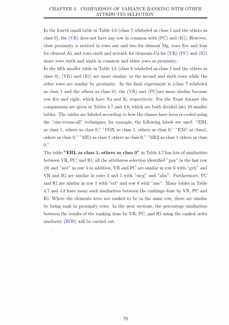
CHAPTER 4. COMPARISON OF VARIANCE RANKING WITH OTHERATTRIBUTES SELECTION
In the fourth small table in Table 4.6 (class 5 relabeled as class 1 and the others as
class 0), the (VR) does not have any row in common with (PC) and (IG). However,
close proximity is noticed in rows one and two for element Mg, rows five and four
for element Al, and rows sixth and seventh for elements Ca for (VR) (PC) and (IG)
share rows sixth and ninth in common and other rows as proximity.
In the fifth smaller table in Table 4.6 (class 6 relabeled as class 1 and the others as
class 0), (VR) and (IG) are more similar; in the second and sixth rows while the
other rows are similar by proximity. In the final experiment is (class 7 relabeled
as class 1 and the others as class 0), the (VR) and (PC)are more similar because
row five and eight, which have Na and Si, respectively. For the Yeast dataset the
comparisons are given in Tables 4.7 and 4.8, which are both divided into 10 smaller
tables. The tables are labeled according to how the classes have been re-coded using
the ”one-versus-all” techniques; for example, the following labels are used: ”ERL
as class 1, others as class 0,” ”POX as class 1, others as class 0,” ”EXC as class1,
others as class 0,” ”ME1 as class 1 others as class 0,” ”ME2 as class 1 others as class
0,”
The table ”ERL as class 1, others as class 0” in Table 4.7 has lots of similarities
between VR, PC, and IG, all the attributes selection identified ”pox” in the last row
(9) and ”mit” in row 4 in addition, VR and PC are similar in row 6 with ”gvh” and
VR and IG are similar in rows 3 and 5 with ”mcg” and ”alm”. Furthermore, PC
and IG are similar in row 1 with ”erl” and row 8 with ”nuc”. Many tables in Table
4.7 and 4.8 have many such similarities between the rankings done by VR, PC and
IG. Where the elements were not ranked to be in the same row, there are similar
by being rank in proximity rows. In the next sections, the percentage similarities
between the results of the ranking done by VR, PC, and IG using the ranked order
similarity (ROS) will be carried out.
.
79

CH
AP
TE
R4.
CO
MP
AR
ISO
NO
FV
AR
IAN
CE
RA
NK
ING
WIT
HO
TH
ER
AT
TR
IBU
TE
SSE
LE
CT
ION
Table 4.7: Comparison of Variance significant with PC and IG variable selection for Yeast data
80
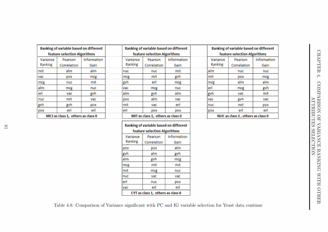
CH
AP
TE
R4.
CO
MP
AR
ISO
NO
FV
AR
IAN
CE
RA
NK
ING
WIT
HO
TH
ER
AT
TR
IBU
TE
SSE
LE
CT
ION
Table 4.8: Comparison of Variance significant with PC and IG variable selection for Yeast data continue
81

CHAPTER 4. COMPARISON OF VARIANCE RANKING WITH OTHERATTRIBUTES SELECTION
Summary
In this section, the comparison of (VR) and two main filter method attribute selec-
tions techniques have been carried out. Lets state here that no two feature selection
algorithm ever produces the same results from the same dataset’ this have been
explained in details in sections 4.1.
An extensive experiment has been conducted in this section using six data sets (see
table A.2), four of the data set are Binary (two classes distributed). The other
three (Iris, Yeast and Glass) are multi-classed, the Iris data is uniformly distributed
(Balanced), the Glass and Yeast data is highly imbalanced. The multi-classed data
have been decomposed into n Binary using ”One versus All” (see section 2.3.2).
The results are all in tables 4.1, 4.2, 4.3 and 4.4 for the binary classed data, for the
multi-classed data the results are in tables 4.5 and 4.6. The results in these tables
confirm the heuristic nature of the feature selection results meaning that no two
feature selection algorithm produces results that are perfectly the same. The filter
feature selection algorithm that uses ranking optimisation to present the selected
attributes tend to be more prone to this, which could be more or less an advantage
depending on context. Imagine if an attribute is ranked as fourth by an algorithm
but another algorithm ranked it as third or even fifth both algorithm shares a simi-
larity by the proximity of the results of the ranking, what it means is that in place
of this attribute the other may suffice.
Though in some of the results in the tables some reversal of ranking of identified
elements between the algorithms; (VR), (PC) and (IG) is also noted, these sequence
of consistency sort of add more veracity to the claimed superiority of (VR) tech-
nique. The next section 4.3 would investigate by presenting a novelty technique to
quantify the similarities between the results of (VR), (PC) and (IG).
4.3 Calculating Similarities of (VR) (PC) and (IG)
using Ranked Order Similarity-(ROS)
In both industry and academics, many types of similarity measure have been used to
compare the different concept to ascertain the accuracy, resources management and
general veracity of new techniques. The Similarity and dissimilarity measure has
been used to compare item and results of two or more structures, but quite recently
many data-centric types of research like data mining and machine learning have
used this process to compare and validate the results [201][202][203] of experiments
and predictive modeling. This is done by measuring the similarity index of a new
82

CHAPTER 4. COMPARISON OF VARIANCE RANKING WITH OTHERATTRIBUTES SELECTION
concept with existing benchmarks knowledge, concept or results. With this in mind
we propose a novel similarity measure technique called Rank Order Similarity (ROS).
We want to determine how similar the results of each of the three ((VR), (PC) and
(IG)) features selection algorithm are similar in Tables 4.1, 4.2, 4.3 and 4.4 and
also in 4.5 and 4.6. Should we say that the result((VR), (PC) and (IG)) are 80% or
90% similar? How could their similarities be graded?
Though, there are different approaches to measure similarities, the most common
is Euclidean distance, Manhattan Distance, Minkowski distance, Cosine Similarity,
and Jaccard similarity index. These are deduced as follows: the Euclidean is just
similar to Pythagoras theorem. In general, it is the square root of the sum of all the
data points and is given by:
Euclidean Distance (x, y) =
√√√√ n∑i=1
−(xi − yi)2 (4.4)
The Manhattan is often called the office block as it resembles the grid direction
within an office block. It shares a geometric diagram with Euclidean distance as
depicted in the diagram below:
Figure 4.1: Presentation of Euclidean and Manhattan distance
The Cosine similarity is a calculation of angular differences between two point in
the domain of interest. It uses the angular differences and the dot product between
the two data points as the metric, is given by Equation 4.5 and in Figure 4.2
83

CHAPTER 4. COMPARISON OF VARIANCE RANKING WITH OTHERATTRIBUTES SELECTION
Figure 4.2: Cosine Similarity
scosine(x,y) = cos θ =xy
||x|| · ||y||=
∑ni=1 xiyi√∑n
i=1 x2i
√∑ni=1 y
2i
(4.5)
In the context of the comparison of (VR), (PC) and (IG) algorithms, the Eu-
clidean, Manhattan, and Cosine similarity index is totally none applicable because
the Euclidean and Manhattan is using vector space as the metric parameter while
the Cosine is also using the angular metrics, hence none applicable also. The closest
similarity grading that is similar to the (ROS) is the Jaccard similarity index that
deduces similarity in a Sets of items. The Jaccard similarity is calculated by taking
the size of the intersection in a Set divided by the size of the union of the sets, as
provided in Equation 4.6. But the Jaccard fell short of its applications in the present
context due to not measuring similarities by ranking items, section 4.4
J(A,B) =|A⋂B|
|A⋃B|
=|A⋂B|
|A|+ |B| − |A⋂B|
(4.6)
4.3.1 Levenshtein Similarity
In sections 4.3 it was establish that the Cosine, Jaccard and the corresponding
distance metrics like Euclidean and Manhattan could not measure or be applicable
to find the similarity of item in Sets that has been ranked. Therefor the (ROS)
will be compared with Levenshtein Similarity [204][205][206]. If absolute length of
string a and b is given by | a | and | b |. The similarity between a and b is given by
84
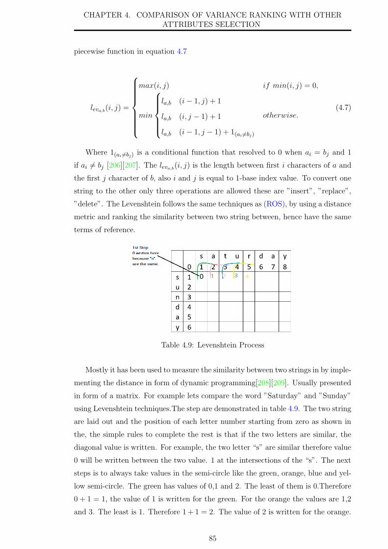
CHAPTER 4. COMPARISON OF VARIANCE RANKING WITH OTHERATTRIBUTES SELECTION
piecewise function in equation 4.7
leva,b(i, j) =
max(i, j) if min(i, j) = 0,
min
la,b (i− 1, j) + 1
la,b (i, j − 1) + 1
la,b (i− 1, j − 1) + 1(ai 6=bj)
otherwise.(4.7)
Where 1(ai 6=bj) is a conditional function that resolved to 0 when ai = bj and 1
if ai 6= bj [206][207]. The leva,b(i, j) is the length between first i characters of a and
the first j character of b, also i and j is equal to 1-base index value. To convert one
string to the other only three operations are allowed these are ”insert”, ”replace”,
”delete”. The Levenshtein follows the same techniques as (ROS), by using a distance
metric and ranking the similarity between two string between, hence have the same
terms of reference.
Table 4.9: Levenshtein Process
Mostly it has been used to measure the similarity between two strings in by imple-
menting the distance in form of dynamic programming[208][209]. Usually presented
in form of a matrix. For example lets compare the word ”Saturday” and ”Sunday”
using Levenshtein techniques.The step are demonstrated in table 4.9. The two string
are laid out and the position of each letter number starting from zero as shown in
the, the simple rules to complete the rest is that if the two letters are similar, the
diagonal value is written. For example, the two letter “s” are similar therefore value
0 will be written between the two value. 1 at the intersections of the “s”. The next
steps is to always take values in the semi-circle like the green, orange, blue and yel-
low semi-circle. The green has values of 0,1 and 2. The least of them is 0.Therefore
0 + 1 = 1, the value of 1 is written for the green. For the orange the values are 1,2
and 3. The least is 1. Therefore 1 + 1 = 2. The value of 2 is written for the orange.
85

CHAPTER 4. COMPARISON OF VARIANCE RANKING WITH OTHERATTRIBUTES SELECTION
This will continues until all the matrix are filled. The edit distance is 3 which is the
value furthest to zero. The completed table is 4.10.
s a t u r d a y0 1 2 3 4 5 6 7 8
s 1 0 1 2 3 4 5 6 7u 2 1 1 2 2 3 4 5 6n 3 2 2 2 3 3 4 5 6d 4 3 3 3 3 4 3 4 5a 5 4 3 4 4 4 4 3 4y 6 5 4 4 5 5 5 4 3
Table 4.10: Comparing two string using Levenshtein Similarity techniques
To get the Levenshtein distance could be a lengthy process but the grid table as
explained in table 4.9 and finally in 4.10 is to ensure accuracy. In most applications
like search engines Levenshtein distance is converted to ratio or percentages[210][211]
by normalising as in equation 4.8
Edit Ratio (a, b) = 1− Edit Distance(a, b)
| a | + | b |(4.8)
Therefore, if Edit Distance(a, b) between the two string ”saturday” and ”sunday”
is 4 gotten from converting ”sunday” to ”saturday” by inserting a, t and r and
deleting n and if | a | and | b | are 6 and 8 respectively. The
Edit Ratio (a, b) = 1− 4|6|+|8| = 0.71 or 71%
4.4 Motivation and Deriving Rank Order Similarity-
(ROS)
In the preceding sections 4.3, some expositions of the inadequacies of existing simi-
larity measures in context of a ranking based algorithm [212][213]. Therefore, it is
imperative that a new similarity measure that accommodates the ranking of items
in a set [88][214]. For instance, how could the similarity of two or more sets that
contains the same objects but arranged or ranked differently be measured? If three
Sets α = {a, b, c, d, e, f}, β = {a, b, c, f, e, d} and γ = {f, b, c, d, e, a} contain the
same elements but arranged or ranked in different order as in Table 4.11. Based on
the order of ranking, what are the percentage similarities between them?.
86

CHAPTER 4. COMPARISON OF VARIANCE RANKING WITH OTHERATTRIBUTES SELECTION
Table 4.11: Three Sets arranged and ranked in different order
Let us determine the similarities between α and β. The total elements in α and
β is 12 ie N=12. Since we wish to find the percentage similarities, this thesis use
Equation 4.9 to define a quantity which is called Element Percentage Weighting =
EPW given by:
EPW =∑ 100
N(4.9)
Therefore, 100/N = 8.33; thus, each element of the set has a percentage weight-
ing of 8.33%; two elements in a row would have a total percentage weighting of the
sum of their weightings. For example, in row 1 in Figure 4.3, the total percentage
weighting of an element a in Set α and element a in Set β is 8.33 + 8.33 = 16.66.
Additionally, each set has a total number of n. When an element moves down-
ward or upward in a column to be in the same row with its similar element, it
loses a percentage weighting equal to EPW − (2 ∗ EPWj
n ) ∗ St, while St is called
the similarity proximity distance, and is equal to the number of steps moved to
the new row starting from the elements initial row. The value 2 used above is
because there are two elements f and f. The quantity (EPWj
n ) is called the unit
Element Percentage Weighting. The sum of all the (EPWj
n ) is equal to the EPW
for the two set. This means that it takes a pair to earn an EPW hence if no pair,
no similarity or values to be summed:
ROS =
n∑1−j
2 ∗ EPW −(
2 ∗ EPWn∗ St)
(4.10)
87

CHAPTER 4. COMPARISON OF VARIANCE RANKING WITH OTHERATTRIBUTES SELECTION
Figure 4.3: Ranked Order Similarity-ROS Percentage Weighting Calculation for αand β
In rows 4 and 6 for sets α and β, the element d and f are not in the same
row with their similar item. To calculate their weighting using Equation 4.9 is
given by 8.33-∑
Loss percentage weighting, If Loss percentage weighting =
EPW/n = 8.33/6 = 1.388. Elements d and f have moved up and down three steps
(including their row). Therefore St = 3, the total Loss percentage weighting for
each is 3 ∗ 1.388 = 4.164, and the final weighting for each is 8.33 − 4.164 = 4.166.
Therefore in row 4, f+ f= 4.166 + 4.166 = 8.33. Additionally, in row 6, d+ d=
4.166 + 4.166 = 8.33. The similarity between sets α and β is 83.3%, please see
equation 4.10 and Figure 4.3 represents the process of calculating the ranked order
similarity-(ROS) in a tabular descriptions of the processes.
The steps below is the calculation between VR and PC using ROS for the sub-table
of ”ERL as class 1, others as class 0.”
If the EPW between VR and PC is given by EPW =∑
100N = 100
16 = 6.25,
the unit Element % Weighting is given byEPWj
n = 6.258 = 0.781.
The calculation of the similarity between VR and PC for the the sub-table of
”ERL as class 1, others as class 0” shows that both are 67.198% similar, please
see Table 4.12 for the steps to calculate ROS. In the next sections, the similarities
between the (VR), (PC) and (IG) for Glass and Yeast dataset are calculated using
the ROS technique.
88

CHAPTER 4. COMPARISON OF VARIANCE RANKING WITH OTHERATTRIBUTES SELECTION
Table 4.12: ROS Calculation between VR and PC for Sub-table ”ERL as class 1,others as class 0” in table 4.7
Table 4.13: ROS Calculation between VR and PC for Sub-table ”ERL as class 1,others as class 0” in table 4.7
89

CHAPTER 4. COMPARISON OF VARIANCE RANKING WITH OTHERATTRIBUTES SELECTION
4.4.1 Comparison of Rank Order Similarity with Leven-
shtein Similarity
Datasets Rank Oder Similarity (ROS)and Levenshtein Similarity(LEV)
Similarity Value (%)
pima VR-ROS 78
VR-LEV 77Wisconsin VR-ROS 68
VR-LEV 56Bupa VR-ROS 75
VR-LEV 75Califonia and Basket ROS 7.4
LEV 40
Table 4.14: Comparison of Rank Order Similarity with Levenshtein Similarity
Figure 4.4: Comparative Similarity between ROS and LEV
The table 4.14 and the associated graph in figure 4.4 is to present the superi-
ority of ROS over Levenshtein similarity. There are lots of similarity between both
algorithm (Levenshtein and (ROS)). The (ROS) were actually derived from the Lev-
enshtein, but instead of using the Edit distance as in the Levenshtein , the (ROS)
uses the proximity distance between item or letter in the objects being compared.
Just like many algorithm Levenshtein could be accurate in many instances but could
also fail woefully in some. For example in both the table table 4.14 and figure 4.4,
the Levenshtein calculated the similarity between Califonia and Basket string is
90

CHAPTER 4. COMPARISON OF VARIANCE RANKING WITH OTHERATTRIBUTES SELECTION
40% , that is rather very odd and totally wrong. But the (ROS) calculated it as
being 7.4%. This is because both have a common character ”a” and the answer of
7.4% is more reasonable and accurate. The problem of Levenshtein is that is inca-
pable of calculating dissimilarity because is base on numbers of steps to convert one
string to another, even if the two string are not similar in anyway (dissimilarity),
the Levenshtein will still go ahead and convert, therefore is incapable of providing
zero similarity. Most search engines that uses Levenshtein can easily be identified
by putting item that are not similar, it will still return some results even if those
results are totally wrong. This may be regarded as good or bad depending on the
user perspective.
This is one of the reasons (ROS) is better as shown in the figure 4.4. Apart from
the comparison of Califonia and Basket done above with the prove of the failure of
Levenshtein and superiority of (ROS). The rest charts also showed the comparison
of (ROS) and Levenshtein using the following datasets Pima, Wisconsin and Bupa.
In all the (ROS) showed a better results. The (ROS) is just a modification of Lev-
enshtein by using proximity distance instead of edit distance. In the next session;
session 4.5. The (ROS) will be used to compare the (VR) and two known attributes
selections the (PC) and (IG).
4.5 The Results of Comparing (VR),(PC) and (IG)
using (ROS) technique
From sections 4.14 the (ROS) is a better similarity comparative metrics than Lev-
enshtein and the rest like Jaccard, cosine etc are not applicable in ths context.
Therefore the (ROS) will be used to compare the results of (VR),(PC) and (IG).
This is to ascertain how class the (VR) is to the two well established bench marks.
91
CHAPTER 4. COMPARISON OF VARIANCE RANKING WITH OTHERATTRIBUTES SELECTION
Table 4.15: Comparison of (VR), (PC) and (IG) using the (ROS) technique forPima, Bupa, Wisconsin and Cor-rna data
Discussion
As no two feature selection algorithm could produce precisely the same result, par-
ticularly the ranking algorithms. Therefore, (ROS) has been used to measure the
similarities between the results of this feature selection, for example in Table 4.1 the
result of (PC) and (VR) on Pima diabetes data, what is the percentage similarity
of the two results?
All the results obtained using (VR), (PC) and (IG)) for the four binary data set in
Tables 4.1, 4.2, 4.3 and 4.4 have been compared using (ROS) and the comparison
is in table Table 4.15.
The Pima india diabetes data results for (VR), (PC) and (IG) is in table 4.1 and
the (ROS) comparison resuls is in Table 4.15. The result indicated that (VR) tech-
nique has 78.13% similarity to both (PC) and (IG) , while (PC) and (IG) are 73.44%
similar to each other. For the Bupa Liver Disorder data in Table 4.2, the (VR) is
75% similar to (PC), while it is 56% similar to (IG), also (PC) is 58.35% similar to
(IG). In Wisconsin Breast cancer data in table 4.3, the (VR) is 68% similar to (PC)
and 82% to (IG), while (PC) and (IG) are 78% similar. Finally in Cod-rna data in
table 4.4, the (VR) is 60.9% similar to (IG) and 59.4% similar to (PC), the (IG)
and (PC) are 70.3% similar.
92
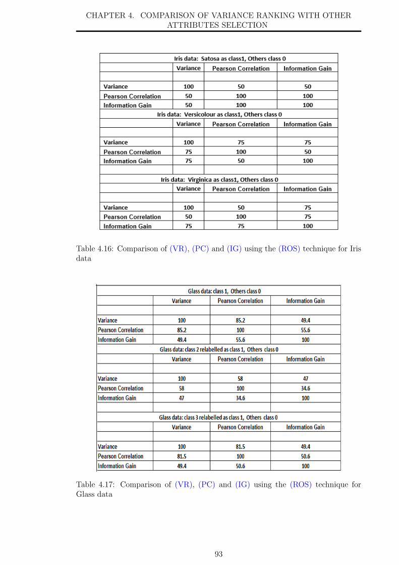
CHAPTER 4. COMPARISON OF VARIANCE RANKING WITH OTHERATTRIBUTES SELECTION
Table 4.16: Comparison of (VR), (PC) and (IG) using the (ROS) technique for Irisdata
Table 4.17: Comparison of (VR), (PC) and (IG) using the (ROS) technique forGlass data
93

CHAPTER 4. COMPARISON OF VARIANCE RANKING WITH OTHERATTRIBUTES SELECTION
Table 4.18: Comparison of (VR), (PC) and (IG) using the (ROS) technique forGlass data
The comparison of the (VR), (PC) and (IG) feature selection results using the
multiclassed data is in Tables 4.16 for the uniformly distributed Iris data. The
attributes are only four in number (Petal length, Petal width, Sepal length and
Sepal width). TableS 4.17 and 4.18 are for the highly imbalanced Glass datasets.
In Table 4.16 for the Iris dataset, the table divided into three parts each for different
type of Iris flower; which are Satosa, Versicolour Virginica. When Iris Satosa is taken
as class 1 and the rest is taken as class 0, the (VR) technique is 50% similar to both
(PC) and (IG), while the both (PC) and (IG) are 100% similar to each other. But
when Versicolour is taken as class 1 and the other is taken as class 0 (VR) is similar
to (PC) by 75% and 50% with (IG) and (PC) and (IG) are similar to each other
by 50%. Finally, when Virginica is taken as class 1 and the rest as class 0 , the
similarity is reversal the (VR) is 75% to (IG) but 50% to (PC), also (IG) and (PC)
are 75% similar.
For the highly imbalanced Glass dataset, the similarity measure using the (ROS)
technique shown in Tables 4.17 and 4.18; the two tables are divided into six parts
(three and three), for different classes of glass, recall that the Glass dataset has six
classes, originally labelled as classes 1, 2, 3, 5, 6 and 7 (no class 4); see Table 3.6 and
Figure 3.5. Each class is relabeled in turn as class 1, while others are 0, using the
”one versus all” technique to convert multi classed into n binary classes as explained
in earlier sections
94

CHAPTER 4. COMPARISON OF VARIANCE RANKING WITH OTHERATTRIBUTES SELECTION
In Table 4.17, when class 1 labeled as class 1 and all others as class 0, the (VR) is
85.2% similar to (PC) and 49.4% similar to (IG), with a 55.6% similarity between
(IG) and (PC). When class 2 is relabelled as class 1, while all others are class 0,
the (VR) is 58% similar to (PC) and 47% similar to (IG). There is 34.6% similarity
between (IG) and (PC). When class 3 is relabelled as class 1 and all others as class
0, (VR) and (PC) are 81.5% similar and 49.4% similar to (IG) with 50.6% between
(IG) and (PC).
In Table 4.18, when class 5 is relabeled as class 1 and others as class 0, the (VR)
is 49.3% similar to both (IG) and (PC), while the latter two are 56.8% similar to
each other. When class 6 is relabeled as class 1 and the others as class 0, the
similarity between (VR) and (PC) is 45.7% while VR is 75.3% similar to (IG).
Furthermore,(IG) and (PC) are 39.5% similar. Finally, when class 7 is relabelled as
class 1 and all the others as class 0, (IG) and (PC) are 44.44% similar, while (VR)
exhibits 56.8% and 49.38% similarity to (PC) and (IG), respectively.
Table 4.19: Comparison of (VR), (PC) and (IG) using the (ROS) technique forYeast data
95

CHAPTER 4. COMPARISON OF VARIANCE RANKING WITH OTHERATTRIBUTES SELECTION
Table 4.20: Comparison of (VR), (PC) and (IG) using the (ROS) technique forYeast data continue
The Yeast comparison in Table 4.19 and tables 4.20 using the (ROS) also pro-
vided the similarities of (VR), (PC) and (IG); lets us take the work example in Table
4.12 and 4.13 as a case study on how the similarity is arrived at. The similarity
between the (VR), (PC) is approximately 67.2% . while the similarity between (PC)
and (IG) is 75% and that between (IG) and (VR) is 62.5%. If the sub-table ”pox
as class 1 and others as class 0 ” is considered, the similarity between (VR) and
(PC) is 76.5%, and 53.13% with (IG), but it is 67.2% between (PC) and (IG). For
further similarity in all Yeast data ”one versus all” sub-tables between (VR), (PC),
and (IG), please see Tables 4.19 and 4.20
Summary and Conclusion
This chapter has presented very important aspect to evaluate the (VR) technique
in handling imbalanced distributed data by comparing the result of using the (VR)
technique with that of two State-of-the-art ((IG) and (PC)) feature selections on
the same data set. Owing to the fact that no two feature selection methods ever
produce the same results.
The feature selection method is categorised into Filter, Wrapper and Hybrid ap-
proach, the (VR) belong to the Filter approach which tends to rank the bases of the
feature on the degree of their significance in predicting the target class. Therefore
96

CHAPTER 4. COMPARISON OF VARIANCE RANKING WITH OTHERATTRIBUTES SELECTION
the issue here is to find the degree of similarity of the result of the two State-of-the-
art ((IG) and (PC)) on the same data set and also the same degree of similarity will
be used to compare with the (VR) technique. All the known similarity index are
not applicable to ranking items, hence a new similarity algorithm the (ROS) was
invented to accommodate similarity when items are ranked. From the analysis of
the results of similarities in the four tables ( 4.15, 4.16, 4.17 and 4.17) at any point
in time the similarity between (VR) and either of the technique is higher than the
similarity between the two (IG) and (PC).
97

Chapter 5
Validation
In this chapter, all the validation of (VR) technique will be carried out. To put
in specific terms, an assessment of the superiority of (VR) over (PC) and (IG) for
selecting the most significant attributes in a datasets that could make the machine
learning algorithm capture more of the minority classes during predictive modeling
processes will be verified.
The sequence of the section, is as follows; First using the result of the ranked at-
tributes obtained in earlier sections by (VR) and those ranked (IG) and (PC) will
be used on the following predictive algorithms: Decision Tree (DT), Support Vector
Machine (SVM), and Logistic Regression (LR) for the experiments.
One of the banes of predictive modelling is knowing the algorithm to choose from
the list of over fourteen major algorithms, besides how will parameters be changed;
by parameters here, it means the optimisation functions of the chosen algorithm for
example if you are using Support Vector Machine (SVM) on a particular data set
what kernel function would produce better results? If Decision tree algorithm is be-
ing used, how will the confidence factors be set, that will in turn affects the pruning
and performance of the algorithm on the training and test data? The altering and
tweaking of parameters and other variables during data mining and machine learn-
ing processes are just too much to itemize and did not make modelling processes
and exact science, hence trial and error are often associated with the processes.
Choosing the right algorithm is a huge topic that depends on lots of factors, you
only have to take a look at the research gate forum at [148] to realise how popular
this topic is.
Therefore different results could be obtained on the same dataset because of differ-
ent algorithm parameters tweaking and other variables that could be modified. But
the results should be within a certain heuristic range that is acceptable.
The reason for selecting these three algorithms for validating the (VR) is the
98

CHAPTER 5. VALIDATION
intention to use more broader family of algorithms that are representatives of other
major aalgorithms. For instance, the family of tree-based algorithms is represented
by (DT), while the family of regression classifiers is represented by (LR), and finally,
the hyperplane and vector-based algorithms are represented by (SVM). Apart from
this, many researchers, academics, and data scientists who have ventured into the
area of selecting the right algorithm, such as in [215]and [216], have produce some
guidelines for selecting the right algorithms. Therefore, if the (VR) techniques works
on these three algorithm, it will work on other algorithms.
Hence making the (VR) as not algorithm dependent. The performance of (VR) on
any dataset would depend on the intrinsic properties of the data, comparing these
results will establish the efficacy of (VR) techniques. During this validation each
of the confusion matrix and all associated metrics of measurement like the True
positive for majority (TPmaj), True positive for Minority (TPmin), False positive
for Majority and Minority (FPmaj) and (FPmin) and others will be made available,
please refer to sections 2.3.1 and 2.3.2 for various metric of measuring the binary and
multiclass data. Also, the technique of Peak Threshold Performance for selecting
the most significant features will be demonstrated and shown in this chapter. The
investigation into Imbalanced and Overlapped, extreme imbalanced and their effects
in predictive modeling will be carried out in this chapter and next.
Tabular Descriptions and Results Presentations
For this validation, experiments were conducted using Weka data mining software
and Python programming language, two major tables and graphs will be created;
the tables will have majority and minority classes as headings. The contents of the
tables are as follows:
• Algorithm: This comprises the attribute selection algorithm techniques, which
are (VR), (PC), and (IG);
• (%)Accuracy: This is the accuracy of the model; it is the measure of the
(PTP )Accuracy and is the same for both tables. It is obtained from the confu-
sion matrix (see section 2.3.1), and it is recorded in the tables as accuracy value100
• Precision: This is the precision of the majority or minority class, which will
be different for the two tables. It is obtained from the confusion matrix (see
section 2.3.1), and it is recorded in the tables as Precision value100
• Recall: This is the recall value of the majority or minority class; the values
are different for both tables. The Recall for the minority table will be used to
99

CHAPTER 5. VALIDATION
indicate the position of (PTP )minority. Recall is obtained from the confusion
matrix (see section 2.3.1), and its is recorded in the tables as Recall value100
• F-measure: This is the F-measure value of the majority or minority class; the
values are different for both tables, and they are obtained from the confusion
matrix (see section 2.3.1); it is recorded in tables as F−measure value100
• ROC: This represents the area under the ROC curve for both the majority
and minority table is recorded in the tables as ROC Area value100 and they are the
same for the majority and minority table.
• Graphs: There are two main graphs in this sections; their titles are ”Accuracy
versus Number of Attributes for VR” and ”Recall versus Number of Attributes
for VR”. Both graphs are plotted from the minority table. The graph ”Ac-
curacy versus Number of Attributes for VR” will indicate the (PTP )Accuracy
and is labelled in the graph as ”PTP for Accuracy”. The graph ”Recall versus
Number of Attributes for VR” will indicate the (PTP )minority and is labelled
in the graph as ”PTP for Accuracy.”
5.0.1 Validation of (VR) Technique for Binary Imbalance
Dataset
The (VR) technique have stood out as one of the few techniques that have specifically
targeted the imbalanced classed distributions in data sets and could be applied to
other imbalanced scenarios as provided in sections 1.1, The main reasons for this
claim is that the (VR) technique have factored the numbers of the majority class
and minority class group, ie the process is subject to the (IR) unlike many other
techniques.
The binary classed data set that will be used for this validations will be selected
from the list of the four data set that we had used in chapters 2 and three; these are
Wisconsin Breast cancer, Pima India diabetes, Bupa Liver disease, and Cod-RNA
data sets, for details of these data sets please see Table A.2.
The (VR) technique have been demonstrated in Tables 3.1, 3.2, 3.3 and 3.4, the
algorithm process flow chart is Figure 3.4, the results obtained have been compared
with that of the two most popular filter attributes selection techniques; the (IG)
and (PC), the results of the comparison is in chapter 4 Tables 4.1, 4.2, 4.3 and 4.4.
from these tables the following postulations are apparent;
• No two filter feature selection algorithms could produce results that are 100%
the same.
100
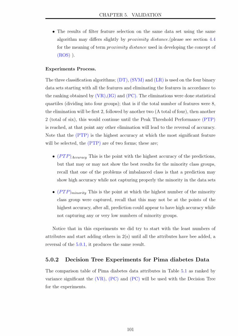
CHAPTER 5. VALIDATION
• The results of filter feature selection on the same data set using the same
algorithm may differs slightly by proximity distance.(please see section 4.4
for the meaning of term proximity distance used in developing the concept of
(ROS) ).
Experiments Process.
The three classification algorithms; (DT), (SVM) and (LR) is used on the four binary
data sets starting with all the features and eliminating the features in accordance to
the ranking obtained by (VR),(IG) and (PC). The eliminations were done statistical
quartiles (dividing into four groups); that is if the total number of features were 8,
the elimination will be first 2, followed by another two (A total of four), then another
2 (total of six), this would continue until the Peak Threshold Performance (PTP)
is reached, at that point any other elimination will lead to the reversal of accuracy.
Note that the (PTP) is the highest accuracy at which the most significant feature
will be selected, the (PTP) are of two forms; these are;
• (PTP )Accuracy This is the point with the highest accuracy of the predictions,
but that may or may not show the best results for the minority class groups,
recall that one of the problems of imbalanced class is that a prediction may
show high accuracy while not capturing properly the minority in the data sets
• (PTP )minority This is the point at which the highest number of the minority
class group were captured, recall that this may not be at the points of the
highest accuracy, after all, prediction could appear to have high accuracy while
not capturing any or very low numbers of minority groups.
Notice that in this experiments we did try to start with the least numbers of
attributes and start adding others in 2(s) until all the attributes have bee added, a
reversal of the 5.0.1, it produces the same result.
5.0.2 Decision Tree Experiments for Pima diabetes Data
The comparison table of Pima diabetes data attributes in Table 5.1 as ranked by
variance significant the (VR), (PC) and (PC) will be used with the Decision Tree
for the experiments.
101

CHAPTER 5. VALIDATION
59
Table 5.1: Comparison of (VR), (PC) and (PC) Attributes selection for Pima Indiadiabetes data
Table 5.2: Results of majority class for Pima data set for DT by (VR) featureselection
The interface of two of the Experiments for Decision Tree algorithm for two
feature is in figure A.1 and eight features are in figure A.2 using Weka data mining
software. Tables 5.2 and 5.3 are the results of the same experiments using (DT) on
the Pima diabetes data, the tables were separated for majority and minority class
for clarity. The main interest is table 5.3 because it shows the minority captured by
the predictions, the highest is 182 when the attributes are two, while the accuracy
at that point is the lowest at 68.5%. The (VR) technique and (IG) performed better
than the (PC).
102

CHAPTER 5. VALIDATION
Table 5.3: Results of minority class for Pima data set for DT by (VR) featureselection
The highest minority that the (PC) was able to capture is 165 at a percentage
of 75.7% by using six attributes, (VR) also got that same percentage of 75.7% also
using the same six attributes. The (DT) experiment is a classical example that shows
that high accuracy does not lead to high capture of minority in the predictions.
Figure 5.1: Accuracy vs Number of Attributes for Pima data using Decision Tree
103

CHAPTER 5. VALIDATION
Figure 5.2: Recall vs Number of Attributes for Pima data using Decision Tree
The Figure 5.1 is the (PTP )Accuracy and 5.2 is the (PTP )minority, both demon-
strations how the the most significant attributes is selected. At the position of
(PTP )minority shown in the graph in Figure 5.2 at that point has the highest recall
of 0.678 with two attributes and the total number of the minority captured is 182
which is also the highest in all the (DT) experiments.
5.0.3 Logistic Regression Experiments for Pima diabetes
data
The experiments of using the Logistic Regression algorithm on the Pima diabetes
data is provided in the next sessions.
Table 5.4: Results of majority class for Pima data set for LR by (VR) featureselection
104

CHAPTER 5. VALIDATION
The Logistic Regression experiments results is in Tables 5.4 for majority class
and 5.5 for the minority class, emphasis is on the general accuracy representaed by
(PTP )Accuracy and number of minority capture represented by (PTP )minority
Table 5.5: Results of minority class for Pima data set for LR by (VR) featureselection
The Table 5.5 showed the (PTP )minority of (VR) techniques has the value of
Recall of 0.578 and highest number of capture minority of 155. At that point the
number of attributes used to achieve this are four. The next best attributes selection
that achieve the same results is the (PC), but uses six attributes to achieve the result.
Figures 5.3 and 5.4 showed that the highest accuracy (PTP )Accuracy point occurred
with all the eight attributes, while the highest Recall (PTP )minority point is with
four attributes.
Figure 5.3: Accuracy vs Number of Attributes for Pima data using Logistic Regres-sion
105

CHAPTER 5. VALIDATION
Figure 5.4: Recall vs Number of Attributes for Pima data using Logistic Regression
5.0.4 Support Vector Machine Experiments for Pima dia-
betes data
The Support Vector Machine experiments is in Tables 5.6 and 5.7, the same numbers
of features were used just like in the Decision Tree and Logistic Regression.
Table 5.6: Results of majority class for Pima data set for SVM by (VR) featureselection
The results of the experiments has lots of interesting insight. For one, (SVM)
algorithm rely very much on demarcating data class groups in a hyperplane such
that the algorithm needs minimum number of features in a particular data set to
106

CHAPTER 5. VALIDATION
function properly, this fact of (SVM) was captured in the work of [217], hence the
algorithm could be extremely accurate of inaccurate. This extreme tendency is
noticeable Tables 5.6 and 5.7
Table 5.7: Results of minority class for Pima data set for SVM by (VR) featureselection
The best accuracy of 77.3% which is the (PTP )Accuracy point shown in Figure
5.5 were achieved using all the eight features and best recall of 0.545 for the minority
(PTP )minority shown in 5.6 point captured 146 minority class data.
Figure 5.5: Accuracy vs Number of Attributes for Pima data using Support VectorMachine
107

CHAPTER 5. VALIDATION
Figure 5.6: Recall vs Number of Attributes for Pima data using Support VectorMachine
Summary and Conclusion
In the section, the first of the series of validation of the Prove of Concept (POC)
as regard to the (VR) technique have been carried out. A popular binary dataset;
Pima diabetes data were used and three (ML) algorithms specially chosen because
of their being the foundation or being related to many other algorithms. In general,
the experimental results are in line with the expectations, for instance, the best
experiments that captured more of the minority ie (PTP )minority is the (DT) with
a recall of 67.9% of the minority, and two of the most significant attributes as
identified by the (VR) were used. (DT) is known to perform very well in binary
context by splitting its node into two, but the power of the (VR) is knowing the two
most significant feature to split through.
The (LR) is the next best performing experiment and the (PTP )minority point is at
four feature, the Recall is 57.8% while the same Recall was achieved by (PC) but
with six attributes.
The (SVM) has the least performance but the same pattern is also noticed. The
(VR) has the best (PTP )minority at the point of four features but reduced drastically
to a Recall of 2.2%.
108

CHAPTER 5. VALIDATION
5.0.5 Decision Tree Experiments for Wisconsin Breast can-
cer data
The Wisconsin Breast cancer data set has 699 instances, binary classed representing
Benign (458) and malignant (241), nine features (attributes) and target class, please
refer to Appendix A.2 for more details. The attributes selections by the ranking are
in Table 5.8, all the attributes selection have been ranked differently by each of
the algorithms, but some very close similarities still exist among the rankings. The
order of ranking and deducing the level of the similarities based on the rankings
have been dealt with extensively in section 4.3
Table 5.8: Comparison of Variance significant with PC and IG variable selection forWisconsin Breast cancer data
Table 5.9: Results of majority class for Wisconsin data set for DT by (VR), (PC)and (IG) feature selection
The Tables 5.9 and 5.10 is the result of Decision Tree for the Wisconsin data, the
superiority of the (VR) to target the minority class group is shown in both tables
and the associated graphs for the accuracy and recall of the minority class groups
are in the Figure 5.7 and 5.8. This particular experiments is note worthy in that it
is one of such cases where the accuracy of the predictions and the recall occurred
109

CHAPTER 5. VALIDATION
at the same number of attributes that mean the (PTP )Accuracy and (PTP )minority
are at the same point when the first four attributes where used,
Table 5.10: Results of minority class for Wisconsin data set for DT by (VR), (PC)and (IG) feature selection
Figure 5.7: Graph of DT Accuracy vs Numbers of Attributes for Wisconsin datashowing (PTP )Accuracy
110

CHAPTER 5. VALIDATION
Figure 5.8: Graph of DT Recall vs Numbers of Attributes for Wisconsin data show-ing (PTP )Recall
In general the (VR) technique performed better as always when compared with
the (PC) and (IG), the best in (PC) occurred when the whole nine attributes were
used, while the best by (IG) with a value of 219 as the total minority captured
occurred at the point where the first two attributes were used. Though the capturing
of the minority group meaning the the highest value of (PTP )minority is by the (VR)
technique, but its note worthy to appreciate that (IG) technique also achieved a good
level of high score (PTP )minority by using only two attributes.
5.0.6 Logistic Regression Experiments for Wisconsin Breast
cancer data
The (LR) also demonstrated the same case were there is differences between the ac-
curacy and minority captured, meaning that the (PTP )Accuracy and (PTP )minority
points are different. The results in Tables 5.11 and 5.12 also confirms the superiority
of the (VR) as against the other two the (PC) and (IG).
111

CHAPTER 5. VALIDATION
Table 5.11: Results of majority class for Wisconsin data set for LR by (VR), (PC)and (IG) feature selection
Table 5.12: Results of minority class for Wisconsin data set for LR by (VR), (PC)and (IG) feature selection
Figure 5.9: Graph of LR Accuracy vs Numbers of Attributes for Wisconsin datashowing (PTP )Accuracy at the position 6 attributes
112

CHAPTER 5. VALIDATION
Figure 5.10: Graph of LR Recall vs Numbers of Attributes for Wisconsin datashowing (PTP )minority at the position of 4 attributes
The recall is highest for all aspects of the (VR) technique. In this experiment
the highest recall did not occur at the point of highest accuracy, meaning the
(PTP )Accuracy point is different from (PTP )minority but the increase in the recall
rate is more than 10% for the best performing of the (PC) and (IG) techniques.
5.0.7 Support Vector Machine Experiments for Wisconsin
Breast cancer data
The Wisconsin breast cancer also demonstrated the (VR) abilities to target the
minority class group effectively, Tables 5.13 and 5.14 is the majority and minority
tables for the confusion matrix, the graphs of the relationships between the accuracy
and the recall is in Figure 5.11 and 5.12.
Table 5.13: Results of majority class for Wisconsin data set for SVM by (VR), (PC)and (IG) feature selection
113

CHAPTER 5. VALIDATION
Table 5.14 is the main focus and interest here, from the analysis the (VR) have
out performed the (PC) and (IG), with a highest minority Recall of 95.4% closely
followed by (IG) with also 95.4% but when the total number of the minority group
Recall is check is 230 and 229 respectively.
Table 5.14: Results of minority class for Wisconsin data set for SVM by (VR), (PC)and (IG) feature selection
The graph of the Accuracy against total number of attributes and Recall against
total number of Attributes also showed that the (PTP )Accuracy and (PTP )minority
occurred on the same number of attributes (4). The (VR) and (IG) has lots of
similarities in their results, for instance, both of their results are the same in for 9
and 6 attributes and both also show the highers Recall in the 4 attributes which
is the (PTP )minority but the actual value Recall is 230 and 229 respectively. The
Weka interface for the results is in Appendix A.12 and A.13
Figure 5.11: Graph of SVM Accuracy vs Numbers of Attributes for Wisconsin datashowing (PTP )Accuracy at the position of 4 attributes
114

CHAPTER 5. VALIDATION
Figure 5.12: Graph of SVM Recall vs Numbers of Attributes for Wisconsin datashowing (PTP )minority at the position of 4 attributes
Summary and Conclusion
The Wisconsin data validation experiments also supported the superiority of (VR)
over (PC) and (IG) feature selection. In all the experiments (VR) has shown more
capture of the minority class group as against the attributes suggested by (PC) and
(IG), these experiments have been carried out using the selected (ML) algorithms.
In the Wisconsin Experiments using the DT in table Tables 5.10, the (VR) uses four
attributes for a Recall of 94.1% the highest that was attained (PC) and (IG) is a
Recall of 90% using nine attributes, thus the (VR) is superior in term of higher Recall
and using less attributes, though the (PTP )Accuracy and (PTP )minority occured at
the same value of four attributes.
The (LR) and (SVM) in Tables 5.14 and 5.12 and the graphs in Figures 5.9 and
5.10 for LR and 5.11 and 5.12 for SVM. Also shows similar higher performance of
(VR) over (PC) and (IG) by the Recall of 96.8% and 95.4% respectively.
5.0.8 Validation of (VR) technique for Multiclassed Imbal-
ance Data set
This sections would validate the (VR) technique for the Multi-Class data set using
the One-versus-All that has been explained and supported with proof of concept in
earlier chapter 2 section 2.3.2.
The multiclass data set used for this validation are Glass and Yeast data set (highly
115

CHAPTER 5. VALIDATION
imbalanced) please see Tables A.2 for details of the data sets, all data preparations,
re-coding from multi-class to One-versus-All were done and explained in sections
3.3.2. In this section, the results in Table 4.6 for the Glass data and Tables 4.7 and
4.8 for the Yeast data will be used. Notice that the Glass data Table able (4.6) and
Yeast data TableS (4.7 and 4.8) are six and ten Tables in total, for clarity and to
avoid repetitions some sections of the tables have been selected for the validation,
these section is provided in Tables 5.15 and 5.16 below. The criteria for the selection
is to make sure class item groups are highly (extreme) imbalanced and Overlapped
and the two tables could be identified and located by the reader
Table 5.15: A section of 4.6 table for Glass data
Table 5.16: A section of 4.7 table for Yeast data
The Glass data is made up of six target classes and the Yeast data is ten target
classes each of these target classes have been recorded as class 1 while the rest as
class all in accordance with One-vs-All(Please see sections 3.3.2 tables 3.7 and 3.9)
for the re-cording. The characteristics of the tables 5.15 and 5.16 shows some levels
of similarities that has been deduced, calculated and adequately discussed in section
4.3 using the (ROS) techniques.
The sequence of the validation experiments for (VR) will go as follows;
• Run the selected (ML), experiments which may be (DT),(SVM),(LR) on all
116

CHAPTER 5. VALIDATION
the attributes in the tables 5.15 and 5.16. Then eliminate the least significant
attributes as suggested by (VR), (PC) and (IG) by the rate of statistical
quantile for example if attributes total is 8 you eliminate the first 2, follow by
another 2 finally another 2 But if attributes is a total of 9 you eliminate the
first 3 , then follow by another 2 finally another 2
• On each of the elimination experiment carried out Obtained the Confusion
matrix and record the following; (TPmaj), True positive for Minority (TPmin),
(FPmaj) and (FPmin),Accuracy and Recall for both the majority and minority
• Provide a graphical and visualisation of the Recall metrics from the experi-
ments and conclusion based on the analysis and Recall therein.
During the course of the attributes elimination, the Accuracy and Recall for
the minority will peak at the point we defined as the Peak Threshold Performance
(PTP) when this is reached the significant attributes will be selected after which
there would be reversal for both the (PTP )Accuracy and (PTP )minority.
Multi-classed imbalanced has some peculiar behaviour that could also affect the
abilities to capture the minority class, its called ”classed Overlapped”, though this
will be dealt with in detail in chapter 6, we may encounter such phenomena in this
chapter, therefore is proper to mention it now. Class overlapped is a situation where
the intrinsic properties of the data item of two or more classes are the same, because
of this the data items will occupy the same data point in a sample space such that
is difficult for any algorithm to differentiate which the classes the data item belong
to.
5.0.9 Validation Experiments using the Glass data set re-
sults
For this validations experiments, two Tables in 5.15 will be used, representing a
section of much larger Table 4.6. The Glass dataset is highly imbalanced and multi-
classed, each class represent a type of glass, such as tableware, car headlight, or
window glass. are originally labelled as class 1, class 2, and so on up to class 7.
However class 4 is not available, so a total of six classes is present in the original
datasets. The re-coding of multiple classes into ”one versus all” was done and
explained in earlier sections. However, to review, the re-coding involves labeling
class 1 as class 1 and the other classes as class 0, then using it for the experiments
after that round of experimentation. Then, class 2 is re-coded as class 1 and the
others as class 0, and this setup is used for the experiments. Next, class 3 is re-coded
117

CHAPTER 5. VALIDATION
as class 1 and others as class 0. This is continued until the experiment is complete.
The tabulation of the results and graphs is presented below. Our interest here is in
the minority table results that were used for the graphs.
5.0.10 Logistic Regression Experiments for Glass data using
One vs All (class 1 as 1 and the others as class 0 )
see table
Table 5.17: Results of majority class for Glass data set for LR by (VR), (PC) and(IG) feature selection for class 1 as 1 and the others other as class 0
Table 5.18: Results of minority class for Glass data set for LR by (VR), (PC) and(IG) feature selection for class 1 as 1 and the others as class 0
118

CHAPTER 5. VALIDATION
Figure 5.13: Graph of LR Accuracy vs Numbers of Attributes for Glass data Mi-nority class: Class 1 as 1 and the others as class 0, the (PTP )Accuracy position.
Figure 5.14: Graph of LR Recall vs Numbers of Attributes for Glass data Minorityclass: Class 1 as 1 and the others as class 0, the (PTP )minority in different position.
In this section, which is the 5.0.10 Logistic Regression experiments, where class 1
(70) is labelled as class 1 and other classes as class 0 (144). the interface for the
Weka reading for all the 9 attributes is in Appendix A.4 and ROC in Appendix
A.5. The (VR) outperformed the (PC) and (IG) with a value of 90% of recall of
the minority, representing a total of 63 from 70 of the number of the minority data
items. The graph of accuracy and recall for the minority is in Figure 5.13 and 5.14,
and it shows the positions of accuracy and recall and the number of the attributes
that were used to achieve them.
119
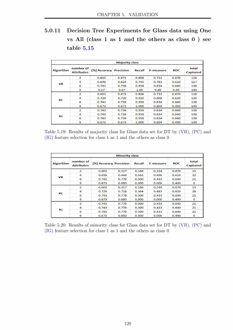
CHAPTER 5. VALIDATION
5.0.11 Decision Tree Experiments for Glass data using One
vs All (class 1 as 1 and the others as class 0 ) see
table 5.15
Table 5.19: Results of majority class for Glass data set for DT by (VR), (PC) and(IG) feature selection for class 1 as 1 and the others as class 0
Table 5.20: Results of minority class for Glass data set for DT by (VR), (PC) and(IG) feature selection for class 1 as 1 and the others as class 0
120

CHAPTER 5. VALIDATION
Figure 5.15: Graph of DT Accuracy vs Numbers of Attributes for Glass data Mi-nority class: Class 1 as 1 and the others as class 0 (PTP )Accuracy in the 6 attributeposition
Figure 5.16: Graph of DT Recall vs Numbers of Attributes for Glass data Minorityclass: Class 1 as 1 and the others as class 0 (PTP )minority in the 4 attribute position
The above Tables 5.19 and 5.20 show the (DT) results for the Glass data in the one
versus all approach for class 1 re-coded as class I and the others as class 0. some of
the Weka out put interface for the 21, 13 and 0 number of minority capture which is
common in is tables 5.20, please see appendix A.6, A.7 and A.8 The minority table
5.20 is our interest here; notice that the (VR) techniques captured more minority
class groups than (PC) and (IG) did, with a recall of 56% at an accuracy of 69.6%,
this result is a classic case of low accuracy but high recall. The graphs for the
121

CHAPTER 5. VALIDATION
accuracy and recall versus numbers of attributes is in Figure 5.15 and 5.16 which
shows the (PTP )Accuracy and (PTP )minority at the position of the most significant
attributes to be selected for the highest accuracy or highest recall of the minority
class.
5.0.12 Support Vector Machine for Glass data using One vs
All (class 1 as 1 others as class 0) see table 5.15
Table 5.21: Results of majority class for Glass data set for SVM by (VR), (PC) and(IG) feature selection for class 1 as 1 other as class 0
Table 5.22: Results of minority class for Glass data set for SVM by (VR), (PC) and(IG) feature selection for class 1 as 1 other as class 0
122

CHAPTER 5. VALIDATION
Figure 5.17: Graph of SVM Accuracy vs Numbers of Attributes for Glass dataMinority class: Class 1 as 1 and the others as class 0, (PTP )Accuracy in the positionof 4 attributes
Figure 5.18: Graph of SVM Recall vs Numbers of Attributes for Glass data Minorityclass: Class 1 as 1 and the others as class 0, (PTP )minority in the position of 4attributes
The SVM uses six attributes to attain the highest recall of 44.30% for the (VR),
while the highest levels for the (PC) and (IG) are recall rate of 37.1% and 38.6%,
respectively. The SVM result was the only situation where the highest accuracy was
attained with the lowest number of attributes (four), while the highest recall had
six attributes. These are shown in Table5.22 and Figures 5.17 and 5.18.
123

CHAPTER 5. VALIDATION
5.0.13 Conclusion
During the Glass dataset validation experiments, the sub-table ”class 1 as 1 and
the others as class 0” was employed, the three algorithms that were used were the
(DT), (LR) and (SVM). In all the experiments (VR) captured more of the minority
class data than PC and IG attribute selection did. These attributes were identified
using the (PTP )Accuracy and (PTP )minority positions in the various graphs. The
PC and IG are benchmark attribute selection techniques known in the data science
community, but VR has been shown in many instances to produce equivalent or
better results.
5.0.14 Logistic Regression Experiments for Glass Data Us-
ing One Versus All (Class 3 as Class 1 and the Others
as Class 0)see table 5.15
Table 5.23: Results of majority class for Glass data set for LR by (VR), (PC) and(IG) feature selection for class 3 as class 1 other as class 0
Table 5.24: Results of minority class for Glass data set for LR by (VR), (PC) and(IG) feature selection for class 3 as class 1 other as class 0
124

CHAPTER 5. VALIDATION
Figure 5.19: Graph of LR Accuracy vs Numbers of Attributes for Glass data Minor-ity class: Class 3 as Class 1 and the others as class 0 (PTP )Accuracy at the positionof 9 attributes
Figure 5.20: Graph of LR Recall vs Numbers of Attributes for Glass data Minorityclass: Class 3 as Class 1 and the others as class 0, (PTP )minority at the position of4 attributes
The Weka interface for the capture of 2 minority is in Appendix A.9 and 0 minority
is in Appendix A.10. The (LR) algorithm worked best for this dataset and produced
the only meaningful result. The other selected algorithms; (DT) and (SVM) were
unable to capture any minority class even if the accuracy is above 80%, Although
this may appear to be a failure, a closer analysis shows that what affects the state-
of-the-art attribute selection like PC and IG also affects the invented VR. This
125

CHAPTER 5. VALIDATION
supports the claim that VR belongs to the same league with the state of the art PC
and IG and in many instances have shown that it is performed better. All results
are in Tables 5.23 and 5.24, the graphs are in Figures 5.19 and 5.20.
5.0.15 Validation Experiments using the Yeast data set re-
sults
The components of the Yeast data make it one of the imbalanced datasets with the
most classes in the data science community; see appendix A.11 for Yeast data class
distribution and Table 3.9 for the representation of the class re-coding as ”one versus
all.” There are 10 classes with varying degree of imbalanced Ratio (IR) between each
class as class 1 and the rest classes (all) as class 0. The next sections present the
experiments for (LR), (DT) and (SVM) for the attributes selected by (VR), (PC)
and (IG).
5.0.16 Decision Tree Experiments for Yeast Data Using One
Versus All (Class ERL(5) as 1 and the others as class
0 (1479)) see Table 5.15
The Tables 5.25 and 5.26 relate to the (DT) experiment for class ERL(5) as class 1
and the others as class 0 (1479), the (IR) is 5:1479 or approximately 1: 296. This
means that for every 1 data item of class 1 (ERL), there are 296 data items of class
0 (others). This is an extreme case of imbalance, and Figure 5.21 shows how scanty
class ERL(5) is as class 1 is in the midst of the others as class 0 (1479). Thus, even if
any predictive modeling accuracy is as high as above 99%, it may not even capture
any minority data. The next session showed the table of majority and minority
capture recalls in different algorithms. This a case of extremely imbalanced and
extremely overlapped, see the 3D scattered plot in figure 5.21
126
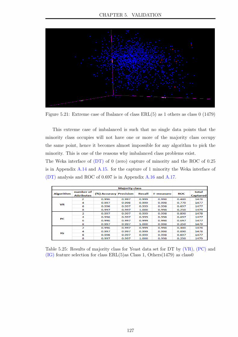
CHAPTER 5. VALIDATION
Figure 5.21: Extreme case of Ibalance of class ERL(5) as 1 others as class 0 (1479)
This extreme case of imbalanced is such that no single data points that the
minority class occupies will not have one or more of the majority class occupy
the same point, hence it becomes almost impossible for any algorithm to pick the
minority. This is one of the reasons why imbalanced class problems exist.
The Weka interface of (DT) of 0 (zero) capture of minority and the ROC of 0.25
is in Appendix A.14 and A.15. for the capture of 1 minority the Weka interface of
(DT) analysis and ROC of 0.697 is in Appendix A.16 and A.17.
Table 5.25: Results of majority class for Yeast data set for DT by (VR), (PC) and(IG) feature selection for class ERL(5)as Class 1, Others(1479) as class0
127
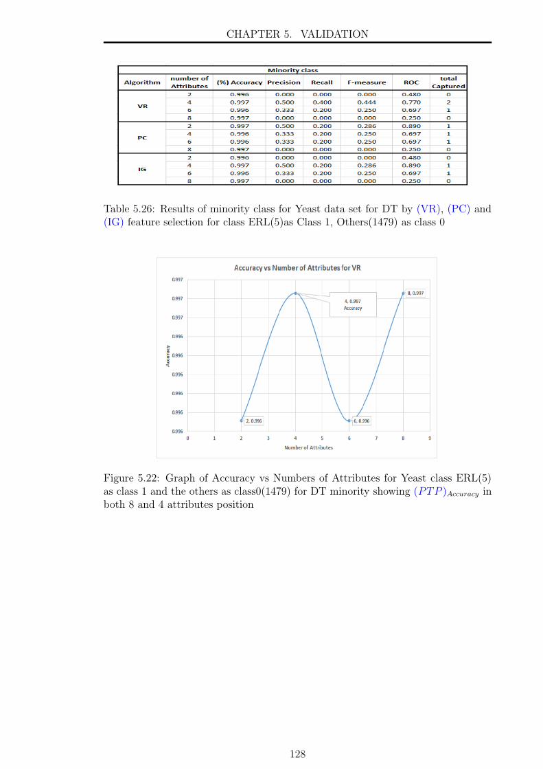
CHAPTER 5. VALIDATION
Table 5.26: Results of minority class for Yeast data set for DT by (VR), (PC) and(IG) feature selection for class ERL(5)as Class 1, Others(1479) as class 0
Figure 5.22: Graph of Accuracy vs Numbers of Attributes for Yeast class ERL(5)as class 1 and the others as class0(1479) for DT minority showing (PTP )Accuracy inboth 8 and 4 attributes position
128

CHAPTER 5. VALIDATION
Figure 5.23: Graph of Recall vs Numbers of Attributes for Yeast class ERL(5) as 1and the others as class0(1479) for DT minority showing (PTP )minority in the positionof 4 attributes
5.0.17 Logistic Regression Experiments for Yeast data using
One vs All (class ERL(5) as 1 others as class 0 (1479))
see Table 5.15
The results are in Tables 5.27 and 5.28, the graph is in Figure 5.24 and 5.25. The
logistic experiment performed better than the Decision tree in 5.0.19.
Table 5.27: Results of majority class for Yeast data set for LR by (VR), (PC) and(IG) feature selection for class ERL(5)as Class 1, Others(1479) as class0
129

CHAPTER 5. VALIDATION
Table 5.28: Results of minority class for Yeast data set for LR by (VR), (PC) and(IG) feature selection for class ERL(5)as Class 1, and the others(1479) as class0
Figure 5.24: Graph of Accuracy vs Numbers of Attributes for Yeast class ERL(5)as class 1 and the others as class 0 (1479) for LR minority showing (PTP )Accuracy
in the position of 2 attributes
130

CHAPTER 5. VALIDATION
Figure 5.25: Graph of Recall vs Numbers of Attributes for Yeast class ERL(5) asclass 1 and the others as class0(1479) for LR minority showing (PTP )minority in theposition of 4 attributes
This results is one of the best that demonstrates the performance by (VR) over
most other techniques; for being able to pick all the minority classes in an extremely
imbalanced situation, the analysis interface of the experiments is in Appendix A.18
5.0.18 Decision Tree and Support Vector Machine Exper-
iments for Yeast data using One vs All (class VAC
(30) as class 1 others as class 0 (1454)) see table 5.15
This two algorithm experiments was combined because their results were similar
and they were unable to capture any minority in a case of extreme imbalance and
extremely overlapping. Figure 5.26 is the 3D representation of the classes; notice
the small numbers of the minority classes and how they are overlapped with the
majority. This is regarded as the extreme case of imbalance.
131

CHAPTER 5. VALIDATION
Figure 5.26: Extreme case of Imbalance class VAC(30) as 1 others as class0(1454).docx
The Decision Tree and Support Vector machine algorithm is unable to capture
any minority even using any attributes selections including our (VR). The Weka
software analysis interface for the results and ROC Area values is in the Appendix
A.19, A.21 and A.20 This shows that the effects of an extreme case of imbalance
could also the effects the VR, PC, and IG. The point of this is that what ever affects
the benchmark attributes selections also affects our VR; hence, we make the case
that the VR is equal to the established attribute selections in terms of performance,
and in many instances, it is better than the benchmark attribute selections.
5.0.19 Logistic Regression Experiments for Yeast data using
One vs All (class VAC (30) as class 1 others as class
0 (1454)) see table 5.15
Table 5.29: Results of majority class for Yeast data set for LR by (VR), (PC) and(IG) feature selection for class VAC(30)as Class 1, Others(1454) as class 0
132

CHAPTER 5. VALIDATION
Table 5.30: Results of minority class for Yeast data set for LR by (VR), (PC) and(IG) feature selection for class VAC(30)as Class 1, Others(1454) as class 0
The results of the LR in Table 5.30 may initially appear odd because both (VR) and
(PC) have the same results (same number of minority values captured). However, on
close inspections of their comparison tables in 4.7 for the Yeast dataset with ”class
VAC as class 1 and the others as class 0,” it can be observed that both attribute
rankings of (VR) and (PC) are the same; as such; they should produce the same
result.
Figure 5.27: Graph of the Accuracy vs Numbers of Attributes for Yeast classVAC(30) as 1 others as class0(1454) for LR minority showing (PTP )Accuracy atthe position of 8 attributes
133

CHAPTER 5. VALIDATION
Figure 5.28: Graph of the Recall vs Numbers of Attributes for Yeast class VAC(30)as 1 others as class0(1454) for LR minority showing (PTP )minority at the positionof 4 attributes
5.0.20 Conclusion
In this section, extensive experimentation was carried out to validate the VR tech-
nique by using multi-class datasets. We have explained and provided evidence of
(PTP )Accuracy and (PTP )minority by using various graphs of accuracy and recall
versus numbers of attributes in so doing we provided a method of recognizing the
most significant attributes.
The experimentation and evidence provided in this section have shown that (VR)
technique is usually superior and sometimes comparable to the benchmark attribute
selections. The experiments also showed that (VR) techniques have more capability
to capture the minority groups in an imbalanced data and the performance is equal
or better when compared to either (PC) and (IG). Another advantages of the (VR)
is that the same level of performance could be achieved with fewer attributes hence
using less resource.
5.1 Comparison of Variance Ranking with the Work
of Others On Imbalanced classed Data
5.1.1 Introduction
The research into imbalance classes and various ways to target minority class in
both binary and multi-classed context have been one of the major challenges in
134

CHAPTER 5. VALIDATION
data science and its allied disciplines, and it will continue to remain so inasmuch
as whatever knowledge we sought to support decision making processes will remain
hidden in the midst of other distracting variables. For instance:
• If we sought to categorise different species of insects in a habitat.
• if we wish to identify a particular species of plant in the midst of other plants
(multi classed imbalanced).
• The search for a particular protein strand that has the same dimension to
more than ten other proteins (multi class imbalanced).
The list or situational occurrences of imbalanced classes are endless. Needless to
say, that data scientist is faced with imbalanced data class issues much more than
any other data analysis problems even if it may not be apparent. The questions
then are ” Why have they not been able to solve the problem up till now?” Though
some efforts have been made over the years to solve this problem, but the success
that has been achieved is abysmal in comparison to the enormity of the problems
and the research interest it has garnered over the years. So what is the problems?
During this research, we have come to conclusions that enough effort has been put
into the research of imbalance classes but the poor results are due to the approaches
that have been used, many researchers have approached the issues from the perspec-
tives of the algorithm. By the way, there is no shot of machine learning algorithm
and many of these have stood the test of time, from the last count, there are about
fourteen major (ML) algorithm and counting [218], not to talk of different modifi-
cations of each, for example, Neural Network have been extended or rather modify
to be Deep Learning and many others, also there are different modifications of deci-
sion tree, for example, ID3 (Iterative Dichotomiser 3), Classification and Regression
Trees (CART), and C4.5. Hence enough (ML) algorithm are available and more will
continue to come into the scene, please see [219].
From the analysis of all the major (ML) algorithm and their application in the
context of imbalanced data issue, most algorithms are not designed to capture the
minority group rather there are optimises to always capture the dominant majority
group classes. That is why, most modelling excises always fall shot in performance
as regard to the minority classes because by approaching the problems of imbalanced
data from the algorithm perspectives without taking into consideration the reasons
for the imbalanced.
135
CHAPTER 5. VALIDATION
5.1.2 New approaches to Imbalanced Data And Introduc-
tion To Sampling
In all the research work available to improve predictive performance. The only one,
that correctly dealt with class imbalanced is the sampling techniques. There are
two categories of sampling (Oversampling and Undersampling). Oversampling is to
increase the data items while Undersampling is to reduce them. We are concentrat-
ing on the Oversampling (please see chapter 2 for the reasons). Prominent amongst
the oversampling, which of course is the first to be invented is (SMOTE) which
stands for Synthetic Minority Over-sampling Technique. This was invented by [94],
followed a few years later by (ADASYN) which stands for Adaptive Synthetic Sam-
pling and invented by [220]. Over the years different modifications of oversampling
techniques like the BorderlineSMOTE, SMOTETomek, etc have continued to be
invented, Please see [221] [222].
First and foremost, what is the reason for the imbalance? This due to the unequal
numbers of the classes and is called the imbalanced ratio (IR), therefore any tech-
nique, formula or algorithm that did not factor the causes of the imbalance i.e.(IR)
will always produces unreliable and inconsistent results when trying to replicate the
experiments using different or even the same data.
Apart from the sampling techniques like the (SMOTE) and (ADASYN), Variance
Ranking (VR) is the only techniques that have factored the (IR) in dealing with the
imbalanced class problems. A detailed explanation of the (SMOTE) and (ADASYN)
technique have been provided in section 2.2.6. just to summarised it, is artificially
generating data items for the minority classes in other to make all the class groups
equal, making the (IR) become 1:1, meaning that equal numbers of both the ma-
jority and minority classes. In the preceding sections the (VR) would be compared
with (SMOTE) and (ADASYN) the reasons is that sampling techniques (Oversam-
pling) is the only techniques that have applied the (IR) in their implementations for
that, both techniques fell withing the same ”Terms of Reference” with (VR) this
provides the basis of the comparison between the three.
5.1.3 Similarities and Differences between (VR), (SMOTE)
and (ADASYN)
One of the first similarities within these techniques is that all three processes involved
the numbers of minority class groups, for example in (SMOTE) and (ADASYN), the
numbers are increased (Oversampled) to equalised with the number of the majority
class groups this, in turn, will interfere with the (IR).
136

CHAPTER 5. VALIDATION
Another basic similarity is that the three techniques are grouped as preprocessing
activities, that is (VR), (SMOTE), and (ADASYN) are carried out on the datasets
before any active (ML) algorithm is used or before modelling is carried out. There
are also similarities in the area of sampling which is subjective to the amount of
original dataset in the population. If the data set is in hundreds or a few thousand,
the researcher may wish to use all the dataset instance but if the dataset instances
is in the tens of thousands an appropriate sampling mechanism should be employed
to make sure the active sample used in the experimentation is a true representation
of the populations.
Impact of Class Overlapped to Performance of Modelling
There are also some differences between (VR) and the two oversampling; (SMOTE)
and (ADASYN). First, during the process of (VR) the number of minority class
groups or instances does not change, rather each of the class groups are separated
into their various classes eg class 0 for negative and class 1 for positive class, before
the sampling is done (please see section 3.3.2 for detailed explanations of (VR) and
Figure 3.4 for its algorithm in form of flow chart). The choice of oversampling to
use depends very much on the intrinsic properties of the classes of the data items.
For example, how well separated or the values variances of each classes groups. The
Figures 5.29 and 5.30 is a 3D scatter plot of Glass (Multi classed imbalanced) and
Pima (Binary classed imbalanced).
Figure 5.29: 3D Glass data Scatter plot
137

CHAPTER 5. VALIDATION
Figure 5.30: 3D Pima data Scatter plot
It could be observed that the values of the variances of each classes (both multi
and Binary classed data set) are not separated, but very much overlapped, compare
this two to Figure 5.31 of 3D scattered plot of Iris data set. notice the distinctive
concentrations of each classes, hence there are not as overlapped as the other two (
Figures 5.29 and 5.30).
Figure 5.31: 3D Iris data Scatter plot
Therefore due to this overlap of the classes, the sampling techniques may perform
very poorly but when the classes are separated as in Figure 5.31, sampling technique
will perform very well. This is one of the disadvantages of sampling techniques in
general and the advantage of (VR) over oversampling. Classes overlapped is one of
the hindrances to achieving good result in predictive modelling, overlapped classes
have most unit values of their attributes the same as such the (ML)algorithm will
not be able to differentiate class group members, therefore, more data point will be
confused and group into the wrong classes leading to high False Positive(s) and False
Negative(s). (VR) has an added advantages of not being affected by this overlap
and ”One versus All” used in this work have also augmented the separations of the
138

CHAPTER 5. VALIDATION
classes adding to distinctiveness of the class separation and better performance
5.1.4 Performance comparisons Between (VR), (SMOTE)
and (ADASYN) on Common data sets
In this section, a comparatives performance between these three ((VR), (SMOTE),
and (ADASYN)) imbalanced data classification techniques would be investigated.
before that is done, lets review ”The terms of reference” under which this comparison
will be carried out and to establish the ”comparator” in this case the results obtained
from the (VR). Therefore the terms of reference are as follows:
• which of these three techniques would capture the highest number of minority
class or have the highest ”Recall” at a specific number of attributes (The point
of (PTP )minority)
• of this three tecniques which shows the highest ”Accuracy” and at which
specific number of attributes (the points of (PTP )Accuracy)
As the focus is specifically on the recall of the minority class group, the comparison
will be focusing on that, this is to underscore the emphasis on the minority class and
the primary aim of any techniques to handle imbalanced data is to reduce the bias
toward the majority and provide an even playing field for the modelling algorithm
to equally target all the classes
5.1.5 Experiment Set up
In this comparative experiment. We shall try to replicate the (SMOTE) and (ADASYN)
experiment as much as possible and compare their performance with that of (VR),
the idea is to ascertain the one that will produce the best performance in terms of
the ”Accuracy” and the ”Recall” of the minority class groups. Three of the data set
(Pima diabetes, Ionosphere, and Wisconsin cancer data) that was used in the initial
experiment by [94] to the invent (SMOTE) in 2002 and also used by [220] to invent
(ADASYN) in 2008, are still available in public domain and I have also used two of
them extensively in this research. All data preparations, sampling, and processes
have been discussed in details in chapter 2.
The Table 5.31 is the experiments conducted for the comparisons, The relevant met-
ric is the (PTP )Accuracy represented by the Accuracy, the (PTP )minority represented
by the Recall and the F-measure.
139

CHAPTER 5. VALIDATION
Table 5.31: Evaluation Metric And Performance Comparison VR, SMOTE andADASYN
Figure 5.32: Graph Evaluation Metric And Performance Comparison LR
Detailed graphs of the tables are also presented in Figures 5.32, 5.33 and 5.34.
In the Table, the results of (SMOTE) and (ADASYN) have been compared to the
results of (VR). The in (LR) experiments for the Pima data the (ADASYN) per-
formed better in terms of the recall, but in term of the accuracy with 77.1% the
(VR) performed better, for the Wisconsin and Ionosphere data the (VR) performed
better in terms of both recall and accuracy. The Wisconsin has a value of 94.3% and
96.8% for the accuracy and recall. For the Ionosphere, the (VR) also outperformed
the (SMOTE) and (ADASYN) with of accuracy of 90.6% and 77.7% for recall. For
clarity, the graph in figure 5.32 is the (LR) experiments.
140

CHAPTER 5. VALIDATION
Figure 5.33: Graph Evaluation Metric And Performance Comparison DT
The (DT) experiments in the second table of Tables 5.31, the (VR) performed
better than (SMOTE) and (ADASYN) in recalls. In the Pima data the (VR) has a
recall of 67.9% as against 60% and 60.1% for (SMOTE) and (ADASYN), in Wiscon-
sin (VR) has a recall of 94.1% while (SMOTE) and (ADASYN) has 90% and 89.9%
respectively. In the Ionosphere data (VR) has a recall of 84.9%, while (SMOTE)
and (ADASYN) has recalls of 74% and 76.2%.
Figure 5.34: Graph Evaluation Metric And Performance Comparison SVM
Finaly, in the (SVM) experiments the (VR) also has a better recall for Pima data
with 74.2% while (SMOTE) and (ADASYN) has recalls of 58.1% and 60%. In Wis-
consin data, (VR) has recall of 95.1% and (SMOTE) has 89% while (ADASYN) has
90.1%. The Ionosphere data has 83.8% for (VR) while (SMOTE) and (ADASYN)
has recall of 76.2% and 82.5% respectively.
5.1.6 Conclusion
The (VR) techniques for dealing with imbalanced class problems have shown better
performance in the nine experiments carried out to compare it with (SMOTE) and
141

CHAPTER 5. VALIDATION
(ADASYN) techniques that are dedicated for dealing with imbalanced classed data.
Just like the (SMOTE) and (ADASYN), it’s also algorithm independent. In the
field of predictive modelling, the techniques to use depends on lots of factors like
computational power, scattered plot distributions of variable and even the intrinsic
properties of the data items, but (VR) have come to stay as a superior alternative
which has been demonstrated here.
142

Chapter 6
Summary Discussion and
Conclusions
This work has established the fact that imbalance data problems pervade all sec-
tions of real-life predictive modelling no matter the scenario or the nature of the
data (granular or non-granular), therefore devising the ways of dealing with this
problems will drastically improve the results of any predictive modelling.
This research is motivated by the apparent gap in knowledge as regards to the unre-
liable way that the existing techniques of dealing with imbalanced classed data since
the existing technique results are very subjective to lots of factors thereby bringing
the validity and reliability of the results obtained to question
The main aim of this research is to invent a new techniques (if not better one )
to handle imbalanced classed data that would be ”foolproof” and not subjective to
machine learning algorithm being used and or any other intrinsic properties of the
dataset and host of other factors that has been the bane of the existing techniques.
6.1 Summary Critique of Existing Algorithm and
Sampling Approaches
Though some good result have been achieved using different (ML) algorithm and
the sampling techniques, but the critiques of these techniques is around the context
of the validity and reliability of the modelling results, the reasons that led to this
criticism are summarised as follows:
143

CHAPTER 6. SUMMARY DISCUSSION AND CONCLUSIONS
6.1.1 Critique of Existing Algorithm Techniques.
• Most machine learning algorithm did not factor the imbalanced ratio in their
design as such were not made to be sensitive to small class groups (minority)
in the dataset.
• Most algorithm has optimisation functions that tend to recognise the majority
class groups, for example in Support Vector Machine algorithm has more than
four Kernel functions, while K- Nearest Neighbour could use Euclidean or
Manhattan distance, etc.
• Using algorithm involved changing the different parameter to achieve a desir-
able result, such parameter is not fixed but is different for different algorithms,
even when using the same algorithm the parameter could change depending
on the intrinsic properties of the data sets being used.
• It is difficult to replicate the results obtained using the algorithm methods,
hence the reliability and validity of the results are in question.
6.1.2 Critique of Existing Sampling Techniques.
Though in this work we have emphasis more on oversampling technique for the
simple fact that is more popular and undersampling is discouraged because of the
chances of removing important data items. In general sampling techniques critiques
could be summarised as follows:
• Very sensitive to overlapping classes, please see Figures 5.29, 5.30 and 5.31
• Oversampling produces a replica of the existing data items thereby increas-
ing the confused classes (False positives and false negatives) that will further
reduce the general accuracy of the model
• Sampling also has all the disadvantages of the algorithm techniques as men-
tioned above.
6.1.3 Summary of the Contributions of this Thesis
The contents of this research have provided completely new approaches to solving
the imbalanced classed problem that is algorithm independent, not affected by class
attributes overlapped and uses One-versus-All to augment the process. All major
contributions listed in the specifications have been achieved and evidenced with a
series of examples, for clarity, a summary review of the aims and objectives and the
144

CHAPTER 6. SUMMARY DISCUSSION AND CONCLUSIONS
Contributions are below.
The aim and objective of the research are to develop new techniques to solve the
problems of imbalanced classes in both binary and multi-classed data set. All aspects
of this research are channel towards achieving these aims and objectives that led to
a series of processes, procedure, and experimentation. And also many contributions
to knowledge.
• Review of Variance Ranking Technique. A novel attributes selection
called the (VR). The superiority of the techniques of over existing methods
were also vetted with adequate proof of Concept of how (VR) is algorithm
independent and not affected by overlapping classes. All these were developed
and explained chapter three session 3.1.1 .
• Review of Peak Threshold Performance. We demonstrated and intro-
duced the concept of Peak Threshold Performance to establish the points to
select the significant attributes at which the modelling performance could have
high Accuracy and high Recall for the minority class group. These two con-
ceptual points were defined as (PTP )Accuracy and (PTP )minority. And also
We introduced and provide ways to identify the point and the number of at-
tributes required to get dependable performance in any machine learning or
data mining activity. These are further explained in chapter five from session
5.0.1 to section 5.0.20.
• Review of Ranked Order Similarity . In comparing (VR) and other
established state of the art attributes selections that are categorised as filter
method, notably the (PC) and (IG) a new similarity measure was invented
called Ranked Order Similarity (ROS). Please see chapter four session 4.4. for
a complete explanations.
These are just the summary of the contributions of this thesis that has made this
work stand out. We believed beyond any doubt that this work has answered lots
of questions and in so doing has also raised some too, any person(s) that took the
pain to read it will have lots of insight for future work and scholarship.
6.2 Recommendations
The work has been exhaustive and many techniques invented were directly or in-
directly intended to minimise the negative effects of class imbalance, but along the
line many new and existing processes and procedures has been applied in a way that
145

CHAPTER 6. SUMMARY DISCUSSION AND CONCLUSIONS
has not been done before, that provided a novelty in his own right. On this note the
following recommendations is being made to further help in the implementations of
the novelty processes that were carried out in this research.
• This processes of (VR) is highly recommended for numeric data type where
the measurement of central tendency is possible.
• It is recommended that an exploratory activities should be carried in each
dataset to investigate the extent of overlapping of the classes before a detailed
implementation of the (VR) is carried out, this would give the researcher an
idea of the sample size that is needed.
• Just like most data centric research, the more sample the better results. No
matter the distribution of the data in the sample space, central limit theorem
may be used to estimate the population mean, deviation both before and after
the datasets are separated into their respective classes. This would enable
the research to estimate the differences between the classes data descriptive
statistics.
• Comparative feature selections should be run to compare (VR) and other
feature selection. This would provide higher level of confidence to the ranking
of the (VR) results.
• The (ROS) is recommended to quantify the similarity between two or more
items when other similarity index is not applicable.
• The (ROS) has also been found to be very accurate in word recognition. In
a situation where word recognition for query recall or when an Anagram is
needed.
6.3 Limitations
In formulating these research specifications and carrying it out, efforts have been
made to ensure that the solutions proffered are as encompassing and far-reaching as
much as possible to enable most imbalanced classed problems to be solved.
But there are some limitations, these have been explained below.
• The (VR) technique can only be applied to numeric data. we should remember
that is based on the measurement of one of the central tendency (variance).
Provided the central tendency like mean, median, mode standard deviation of
the attributes in the data set have a meaning in terms of being used to explain
146

CHAPTER 6. SUMMARY DISCUSSION AND CONCLUSIONS
and provide a ”summary statistics” of the data set, then this techniques could
be applied, but if the central tendency of the data could not be measure eg
categorical data this technique is not applicable.
• If some interval data could be re-corded into numeric data, for example first
position is 1, second position is 2 and third position is 3. In such situation
the mean, standard deviation and probability distribution could be obtained,
Then it is possible to apply the (VR). But not all interval scale could be re-
coded into numeric data and as such the measurement of the central tendency
is not possible, therefore (VR) will not be possible.
• Though many classed imbalanced problems have been solved here. That is
not to say that this thesis is the panacea to all imbalanced classed problems.
Far from it, the ubiquitous nature of real-life data is such that there will
never be a single solution to any modelling problems imbalanced or not, rather
collections of procedures and processes will continue to be invented to tackle
each peculiarity of imbalanced problems, hence they may be issues relating
to imbalanced that may emerge in future that we may not have seen before
because data science is relatively new and evolving by the day.
• The Ranked Order Similarity (ROS) is also limited to textual similarity just
like levenshtein similarity. It could identify and retreived a text if there is
similarity between a search input and a ”bag of words”. It does not use angles
between words like cosine similarity.
6.4 Future Work
The future work will be extending the technique to categorical data by implementing
a weighting strategy to enable a ”summary statistics” on such data type. Finding
a techniques to calculate the descriptive statistics of categorical data is an active
area of research for quite some time; one has to check the research data banks like
google scholar to realise the enormity of the research interest, the new direction is,
therefore, to utilise some of the research concepts to implements (VR) on categorical
data.
Classification algorithms are dichotomised, meaning the algorithm classifies a data
point to belong to this class or that class, therefore is very possible to integrate (VR)
techniques into many (ML) algorithm for more augmented dichotomy which may
improve the distinctions between the classes and improve the general performance
147

CHAPTER 6. SUMMARY DISCUSSION AND CONCLUSIONS
of the algorithm, the future research implications are in the direction of integration
of (VR) and most (ML) algorithm
6.4.1 Final Summary
In this thesis, we have ended up with the solution that addresses problems of classed
imbalanced in classification modelling. Thus has addressed a significant problems
associated with predictive modelling when using real-life dataset. It has proven
that classed imbalanced problems is more prevalent than any other errors associ-
ated with data and shows that imbalance problems are always in addition to any
other problems that the dataset may have. A techniques called Variance Ranking
Attributes Selection (VR) has been produced and demonstrated. A methods of
choosing the most significant attributes that would enable higher recall of the mi-
nority class groups through a process of Peak performance Threshold has also been
demonstrated. A process of similarity index called the Ranked Order Similarity
(ROS) has also been developed to compare the result of (VR) and that of (PC) and
(IG).
The question now remaining is this ”At what stage during predictive modelling pro-
cesses” does (VR) fit into? To answer this let us find a parallel with the techniques
we have compared (VR) with and find where all those techniques fit into. We have
compare (VR) with (PC) and (IG) attributes selection in chapter 4 because it is
an attributes selection technique, we have also compared it with (SMOTE) and
(ADASYN). All these four comparisons are at the stage of Preprocessing, therefor
without any doubt, (VR) should be carried out at the data Preprocessing stage.
Intriguing, revolutionary, etc, these are some of the words that have been used to
describe this thesis by the few people that have read it. I believe that the basis
of a Ph.D. is to think ”out of the box” with new radical ideas, not ”Business as
usual”. Knowledge grows when we experiment with new things and ideas and it will
continue to evolve. There were times when the best brain mankind could boast of
were those that believe the Earth was flat, we may laugh at them now, but alas!
they were the people that first raise the questions by asking what is the shape of
the Earth?
When the (SMOTE) techniques were invented it may also have been described as
intriguing and revolutionary then, but here I am trying to find solutions to some of
its shortcomings. Therefore this work is not intended to diminish their contributions
at all rather give maximum accolade to these deep thinking scholars. Maybe in some
years to come a new work may emerge onto the scene and provide some correction
148

CHAPTER 6. SUMMARY DISCUSSION AND CONCLUSIONS
to this work, but before then, I say have an exciting time as you read this thesis
and God Bless!!.
The End.
149

Appendix A
Appendix
Table A.1: Data used in the experiment continue
150

AP
PE
ND
IXA
.A
PP
EN
DIX
Table A.2: Data used in the experiment continue
151

APPENDIX A. APPENDIX
Figure A.1: Weka Interface experiment for all features in Pima data using DecisionTree
Figure A.2: Weka Interface experiment for only two features in Pima data usingDecision Tree
152

APPENDIX A. APPENDIX
Figure A.3: Weka ROC for DT Wisconsin
Figure A.4: weka Glass class1 as1 other0 LR, for minority captured
153

APPENDIX A. APPENDIX
Figure A.5: weka Glass class1 as1 other0 LR, for minority captured the ROC
Figure A.6: weka Glass class1 as1 other 0 DT-21 minority captured
154

APPENDIX A. APPENDIX
Figure A.7: weka Glass class1 as 1 other 0 DT, 0 minority captured
Figure A.8: weka Glass class1 as1 other 0, DT 13 minority captured
155

APPENDIX A. APPENDIX
Figure A.9: weka Glass class3 as1 other0 LR, 2 minority captured
Figure A.10: weka Glass class3 as1 other0 DT SVM, no minority captured
156

APPENDIX A. APPENDIX
Figure A.11: Class Distribution Of Yeast Data
Figure A.12: weka Interface SVM for Wisconsin
157

APPENDIX A. APPENDIX
Figure A.13: weka Interface SVM for Wisconsin-2
Figure A.14: wekaYeastclassERL(5)as1othersasclass0(1479) for DT
158

APPENDIX A. APPENDIX
Figure A.15: wekaYeastclassERL(5)as1othersasclass0(1479) the ROC for DT
159

APPENDIX A. APPENDIX
Figure A.16: wekaYeastclassERL(5)as1othersasclass0(1479) for DT capture 1 Mi-nority
160

APPENDIX A. APPENDIX
Figure A.17: wekaYeastclassERL(5)as1othersasclass0(1479) the ROC Capture 1 forDT
161

APPENDIX A. APPENDIX
Figure A.18: weka Interface for Yeast class ERL(5)as 1 others as class0(1479) forLR Capture all 5 minority
Figure A.19: weka Interface for Yeast class VAC(30)as 1 others as class0(1454) forDT Capture 0 minority
162

APPENDIX A. APPENDIX
Figure A.20: weka Interface for Yeast class VAC(30)as 1 others as class0(1454) forROC of DT Capture 0 minority
Figure A.21: weka Interface for Yeast class VAC(30)as 1 others as class0(1454) forSVM Capture 0 minority
163

Bibliography
[1] Fay Chang, Jeffrey Dean, Sanjay Ghemawat, Wilson C Hsieh, Deborah A Wal-
lach, Mike Burrows, Tushar Chandra, Andrew Fikes, and Robert E Gruber.
Bigtable: A distributed storage system for structured data. ACM Transactions
on Computer Systems (TOCS), 26(2):4, 2008.
[2] Brandon Doran. Structured vs. unstructured data, Nov 2017.
[3] Ian H Witten, Eibe Frank, Mark A Hall, and Christopher J Pal. Data Mining:
Practical machine learning tools and techniques. Morgan Kaufmann, 2016.
[4] Anna L Buczak and Erhan Guven. A survey of data mining and machine
learning methods for cyber security intrusion detection. IEEE Communica-
tions Surveys & Tutorials, 18(2):1153–1176, 2016.
[5] X Rong Li and Zhanlue Zhao. Relative error measures for evaluation of esti-
mation algorithms. In Information Fusion, 2005 8th International Conference
on, volume 1, pages 8–pp. IEEE, 2005.
[6] Henning Baars and Hans-George Kemper. Management support with struc-
tured and unstructured data—an integrated business intelligence framework.
Information Systems Management, 25(2):132–148, 2008.
[7] Justin Langseth, Nithi Vivatrat, and Gene Sohn. Analysis and transformation
tools for structured and unstructured data, January 11 2007. US Patent App.
11/172,957.
[8] Mark Hall, Eibe Frank, Geoffrey Holmes, Bernhard Pfahringer, Peter Reute-
mann, and Ian H Witten. The weka data mining software: an update. ACM
SIGKDD explorations newsletter, 11(1):10–18, 2009.
[9] Ralph Kimball and Joe Caserta. The Data WarehouseA ETL Toolkit: Prac-
tical Techniques for Extracting, Cleaning, Conforming, and Delivering Data.
John Wiley & Sons, 2011.
164

BIBLIOGRAPHY
[10] Simon Hawkins, Hongxing He, Graham Williams, and Rohan Baxter. Outlier
detection using replicator neural networks. In International Conference on
Data Warehousing and Knowledge Discovery, pages 170–180. Springer, 2002.
[11] Antonio Loureiro, Luis Torgo, and Carlos Soares. Outlier detection using clus-
tering methods: a data cleaning application. In Proceedings of KDNet Sym-
posium on Knowledge-based Systems for the Public Sector. Bonn, Germany,
2004.
[12] Marius Muja and David G Lowe. Scalable nearest neighbor algorithms for
high dimensional data. IEEE transactions on pattern analysis and machine
intelligence, 36(11):2227–2240, 2014.
[13] Claudio Reggiani, Yann-Ael Le Borgne, and Gianluca Bontempi. Fea-
ture selection in high-dimensional dataset using mapreduce. arXiv preprint
arXiv:1709.02327, 2017.
[14] PULKIT SHARMA. The ultimate guide to 12 dimensionality re-
duction techniques. https://www.analyticsvidhya.com/blog/2018/08/
dimensionality-reduction-techniques-python/, 27 August 2018. (Ac-
cessed on 31/07/2019).
[15] Melanie Hilario and Alexandros Kalousis. Approaches to dimensionality reduc-
tion in proteomic biomarker studies. Briefings in bioinformatics, 9(2):102–118,
2008.
[16] Btissam Zerhari, Ayoub Ait Lahcen, and Salma Mouline. Big data clustering:
Algorithms and challenges. In Proc. of Int. Conf. on Big Data, Cloud and
Applications (BDCA’15), 2015.
[17] Klaus Krippendorff. Estimating the reliability, systematic error and random
error of interval data. Educational and Psychological Measurement, 30(1):61–
70, 1970.
[18] Greg Atkinson and Alan M Nevill. Statistical methods for assessing mea-
surement error (reliability) in variables relevant to sports medicine. Sports
medicine, 26(4):217–238, 1998.
[19] Rukshan Batuwita and Vasile Palade. Class imbalance learning methods for
support vector machines. 2013.
165

BIBLIOGRAPHY
[20] Rudiger Wirth and Jochen Hipp. Crisp-dm: Towards a standard process
model for data mining. In Proceedings of the 4th international conference
on the practical applications of knowledge discovery and data mining, pages
29–39. Citeseer, 2000.
[21] Rachel Philpott. Entwined approaches: integrating design, art and science in
design research-by-practice. https://dspace.lboro.ac.uk/2134/12964, 10
Dec 2012. (Accessed on 04/06/2019).
[22] weka. Weka 3: Machine learning software in java. https://www.cs.waikato.
ac.nz/ml/weka/, 25 June 2019. (Accessed on 25/06/2019).
[23] All data set used. All data set used. https://archive.ics.uci.edu/ml/
index.php, 12 July 2015. (Accessed on 15/08/2018).
[24] latex documentation. Overleaf, online latex editor. https://www.overleaf.
com/, 12 July 2015. (Accessed on 15/08/2018).
[25] Monash University RESEARCH and LEARNING ONLINE. Writ-
ing clearly, concisely and precisely. https://www.monash.edu/rlo/
research-writing-assignments/writing/clear-communication/
writing-clearly-concisely-and-precisely, 12 July 2017. (Accessed on
16/08/2018).
[26] Shuo Wang and Xin Yao. Multiclass imbalance problems: Analysis and po-
tential solutions. IEEE Transactions on Systems, Man, and Cybernetics, Part
B (Cybernetics), 42(4):1119–1130, 2012.
[27] T Ryan Hoens, Qi Qian, Nitesh V Chawla, and Zhi-Hua Zhou. Building deci-
sion trees for the multi-class imbalance problem. In Pacific-Asia Conference
on Knowledge Discovery and Data Mining, pages 122–134. Springer, 2012.
[28] Xu-Ying Liu, Jianxin Wu, and Zhi-Hua Zhou. Exploratory undersampling for
class-imbalance learning. IEEE Transactions on Systems, Man, and Cyber-
netics, Part B (Cybernetics), 39(2):539–550, 2009.
[29] University of California data set. Machine learning repository. https:
//archive.ics.uci.edu/ml/datasets/Abalone, June 2017. (Accessed on
24/06/2018).
[30] University of California data set. Machine learning repository. https:
//archive.ics.uci.edu/ml/datasets/Yeast, June 2017. (Accessed on
24/06/2018).
166

BIBLIOGRAPHY
[31] Guorui Feng, Guang-Bin Huang, Qingping Lin, and Robert Gay. Error mini-
mized extreme learning machine with growth of hidden nodes and incremental
learning. IEEE Transactions on Neural Networks, 20(8):1352–1357, 2009.
[32] Hai-Jun Rong, Yew-Soon Ong, Ah-Hwee Tan, and Zexuan Zhu. A fast pruned-
extreme learning machine for classification problem. Neurocomputing, 72(1-
3):359–366, 2008.
[33] Donald Michie, David J Spiegelhalter, CC Taylor, et al. Machine learning.
Neural and Statistical Classification, 13, 1994.
[34] Olivier Chapelle, Bernhard Scholkopf, and Alexander Zien. Semi-supervised
learning (chapelle, o. et al., eds.; 2006)[book reviews]. IEEE Transactions on
Neural Networks, 20(3):542–542, 2009.
[35] Trevor Hastie, Robert Tibshirani, and Jerome Friedman. Unsupervised learn-
ing. In The elements of statistical learning, pages 485–585. Springer, 2009.
[36] Anurag Jha, Anand Chandrasekaran, Chiho Kim, and Rampi Ramprasad.
Impact of dataset uncertainties on machine learning model predictions: the
example of polymer glass transition temperatures. Modelling and Simulation
in Materials Science and Engineering, 27(2):024002, 2019.
[37] Anton Tsitsulin, Marina Munkhoeva, Davide Mottin, Panagiotis Karras, Alex
Bronstein, Ivan Oseledets, and Emmanuel Muller. The shape of data: Intrinsic
distance for data distributions. In Iclr 2020: Proceedings of the International
Conference on Learning Representations, 2020.
[38] Saman Sadeghyan. A new robust feature selection method using variance-
based sensitivity analysis. arXiv preprint arXiv:1804.05092, pages 3–6, 2018.
[39] Yang Lu, Yiu-ming Cheung, and Yuan Yan Tang. Bayes imbalance impact
index: A measure of class imbalanced data set for classification problem. IEEE
transactions on neural networks and learning systems, 2019.
[40] Zalan Borsos, Andreas Krause, and Kfir Y Levy. Online variance reduction for
stochastic optimization. arXiv preprint arXiv:1802.04715, pages 13–15, 2018.
[41] Baptiste Rocca. Handling imbalanced datasets in ma-
chine learning. https://towardsdatascience.com/
handling-imbalanced-datasets-in-machine-learning-7a0e84220f28,
27 Jan 2019. (Accessed on 13/04/2020).
167

BIBLIOGRAPHY
[42] Saharon Rosset and Ryan J Tibshirani. From fixed-x to random-x regres-
sion: Bias-variance decompositions, covariance penalties, and prediction error
estimation. Journal of the American Statistical Association, pages 1–14, 2018.
[43] Gemma E Moran, Veronika Rockova, Edward I George, et al. Variance prior
forms for high-dimensional bayesian variable selection. Bayesian Analysis,
pages 1091–1119, 2018.
[44] Andrew Estabrooks, Taeho Jo, and Nathalie Japkowicz. A multiple resampling
method for learning from imbalanced data sets. Computational intelligence,
20(1):18–36, 2004.
[45] Yanmin Sun, Andrew KC Wong, and Mohamed S Kamel. Classification of
imbalanced data: A review. International Journal of Pattern Recognition and
Artificial Intelligence, 23(04):687–719, 2009.
[46] YANMIN SUN, ANDREW K. C. WONG, and MOHAMED S. KAMEL. Clas-
sification of imbalanced data: A review. International Journal of Pattern
Recognition and Artificial Intelligence, 23(4):687–719, 2009.
[47] Florian Steinke, Bernhard Scholkopf, and Volker Blanz. Support vector ma-
chines for 3d shape processing. In Computer Graphics Forum, volume 24,
pages 285–294. Wiley Online Library, 2005.
[48] DF Team. Kernel functions-introduction to svm kernel examples. https://
data-flair.training/blogs/svm-kernel-functions/, 12 Aug 2017. (Ac-
cessed on 24/07/2018).
[49] Bernhard Scholkopf. The kernel trick for distances. In Advances in neural
information processing systems, pages 301–307, 2001.
[50] Martin Hofmann. Support vector machines—kernels and the kernel trick.
Notes, 26, 2006.
[51] Sebastian Mika, Gunnar Ratsch, Jason Weston, Bernhard Scholkopf, and
Klaus-Robert Mullers. Fisher discriminant analysis with kernels. In Neural
networks for signal processing IX, 1999. Proceedings of the 1999 IEEE signal
processing society workshop., pages 41–48. Ieee, 1999.
[52] Jose Martens Gary Ericson Roope Astala Jeannine Takaki, Berth-Anne Har-
vey. One-class support vector machine. https://docs.microsoft.
com/en-us/azure/machine-learning/studio-module-reference/
one-class-support-vector-machine, Jan 2018. (Accessed on 01/24/2018).
168

BIBLIOGRAPHY
[53] Hanaa Sameeh A Aziz Othman et al. A New Hierarchical Support Vector
Machine based Model for Classification of Imbalanced Multi-class Data. PhD
thesis, Sudan University of Science and Technology, 2017.
[54] Bhumika Gupta, Aditya Rawat, Akshay Jain, Arpit Arora, and Naresh Dhami.
Analysis of various decision tree algorithms for classification in data mining.
International Journal of Computer Applications, 163(8), 2017.
[55] Lior Rokach and Oded Maimon. Top-down induction of decision trees
classifiers-a survey. IEEE Transactions on Systems, Man, and Cybernetics,
Part C (Applications and Reviews), 35(4):476–487, 2005.
[56] Peter Waiganjo Wagacha. Induction of decision trees. Foundations of Learning
and Adaptive Systems, 2003.
[57] J. Ross Quinlan. Induction of decision trees. Machine learning, 1(1):81–106,
1986.
[58] B Chandra and P Paul Varghese. Fuzzifying gini index based decision trees.
Expert Systems with Applications, 36(4):8549–8559, 2009.
[59] Nitesh V Chawla. C4. 5 and imbalanced data sets: investigating the effect
of sampling method, probabilistic estimate, and decision tree structure. In
Proceedings of the ICML, volume 3, page 66, 2003.
[60] Wei Liu, Sanjay Chawla, David A Cieslak, and Nitesh V Chawla. A robust
decision tree algorithm for imbalanced data sets. In Proceedings of the 2010
SIAM International Conference on Data Mining, pages 766–777. SIAM, 2010.
[61] Salvador Garcıa, Alberto Fernandez, and Francisco Herrera. Enhancing the
effectiveness and interpretability of decision tree and rule induction classifiers
with evolutionary training set selection over imbalanced problems. Applied
Soft Computing, 9(4):1304–1314, 2009.
[62] Sulafa Hag Elsafi. Artificial neural networks (anns) for flood forecasting at
dongola station in the river nile, sudan. Alexandria Engineering Journal,
53(3):655–662, 2014.
[63] Martin T Hagan, Howard B Demuth, Mark H Beale, and Orlando De Jesus.
Neural network design, volume 20. Pws Pub. Boston, 1996.
[64] B Yegnanarayana. Artificial neural networks. PHI Learning Pvt. Ltd., 2009.
169

BIBLIOGRAPHY
[65] MathWorks. Improve neural network generalization and
avoid overfitting. https://uk.mathworks.com/help/nnet/ug/
improve-neural-network-generalization-and-avoid-overfitting.
html, November 18 2017. (Accessed on 03/09/2018).
[66] Andrey Kurenkov. A ’brief’ history of neural nets and
deep learning. http://www.andreykurenkov.com/writing/ai/
a-brief-history-of-neural-nets-and-deep-learning/, November
18 24, 2015. (Accessed on 01/09/2018).
[67] Piyasak Jeatrakul, Kok Wai Wong, and Chun Che Fung. Classification of
imbalanced data by combining the complementary neural network and smote
algorithm. In International Conference on Neural Information Processing,
pages 152–159. Springer, 2010.
[68] Apurva Sonak, Ruhi Patankar, and Nitin Pise. A new approach for handling
imbalanced dataset using ann and genetic algorithm. In Communication and
Signal Processing (ICCSP), 2016 International Conference on, pages 1987–
1990. IEEE, 2016.
[69] Alex Shenfield and Shahin Rostami. Multi-objective evolution of artificial neu-
ral networks in multi-class medical diagnosis problems with class imbalance.
In Computational Intelligence in Bioinformatics and Computational Biology
(CIBCB), 2017 IEEE Conference on, pages 1–8. IEEE, 2017.
[70] Minlong Lin, Ke Tang, and Xin Yao. Dynamic sampling approach to training
neural networks for multiclass imbalance classification. IEEE Transactions on
Neural Networks and Learning Systems, 24(4):647–660, 2013.
[71] Yanmin Sun, Mohamed S Kamel, Andrew KC Wong, and Yang Wang. Cost-
sensitive boosting for classification of imbalanced data. Pattern Recognition,
40(12):3358–3378, 2007.
[72] Charles X. Ling and Victor S. Sheng. Cost-Sensitive Learning, pages 231–235.
Springer US, Boston, MA, 2010.
[73] Charles Elkan. The foundations of cost-sensitive learning. In International
joint conference on artificial intelligence, volume 17, pages 973–978. Lawrence
Erlbaum Associates Ltd, 2001.
170

BIBLIOGRAPHY
[74] Takaya Saito and Marc Rehmsmeier. Basic evaluation measures from
the confusion matrix. https://classeval.wordpress.com/introduction/
basic-evaluation-measures/, May 2015. (Accessed on 14/07/2018).
[75] Nguyen Thai-Nghe, Zeno Gantner, and Lars Schmidt-Thieme. Cost-sensitive
learning methods for imbalanced data. In Neural Networks (IJCNN), The
2010 International Joint Conference on, pages 1–8. IEEE, 2010.
[76] Mateusz Lango and Jerzy Stefanowski. Multi-class and feature selection exten-
sions of roughly balanced bagging for imbalanced data. Journal of Intelligent
Information Systems, 50(1):97–127, 2018.
[77] Yong Zhang and Dapeng Wang. A cost-sensitive ensemble method for class-
imbalanced datasets. In Abstract and applied analysis, volume 2013. Hindawi,
2013.
[78] Zhi-Hua Zhou and Xu-Ying Liu. Training cost-sensitive neural networks
with methods addressing the class imbalance problem. IEEE Transactions
on Knowledge and Data Engineering, 18(1):63–77, 2006.
[79] Dr Saed Sayad. K nearest neighbors - classification. https://www.saedsayad.
com/k_nearest_neighbors.htm, November 18 24, 2015. (Accessed on
01/09/2018).
[80] Srishti Sawla. K-nearest neighbors. https://medium.com/@srishtisawla/
k-nearest-neighbors-f77f6ee6b7f5, Jun 8 2015. (Accessed on
01/06/2018).
[81] Adi Bronshtein. A quick introduction to k-nearest neigh-
bors algorithm. https://medium.com/@adi.bronshtein/
a-quick-introduction-to-k-nearest-neighbors-algorithm-62214cea29c7,
April, 11 2017. (Accessed on 01/09/2018).
[82] Harshit Dubey and Vikram Pudi. Class based weighted k-nearest neighbor
over imbalance dataset. In Pacific-Asia Conference on Knowledge Discovery
and Data Mining, pages 305–316. Springer, 2013.
[83] Georgios Douzas and Fernando Bacao. Effective data generation for imbal-
anced learning using conditional generative adversarial networks. Expert Sys-
tems with applications, 91:464–471, 2018.
171

BIBLIOGRAPHY
[84] Yoav Freund, Robert Schapire, and Naoki Abe. A short introduction to boost-
ing. Journal-Japanese Society For Artificial Intelligence, 14(771-780):1612,
1999.
[85] Leo Breiman. Stacked regressions. Machine learning, 24(1):49–64, 1996.
[86] Andy Liaw, Matthew Wiener, et al. Classification and regression by random-
forest. R news, 2(3):18–22, 2002.
[87] Jisoo Ham, Yangchi Chen, Melba M Crawford, and Joydeep Ghosh. Investi-
gation of the random forest framework for classification of hyperspectral data.
IEEE Transactions on Geoscience and Remote Sensing, 43(3):492–501, 2005.
[88] Saimadhu Polamuri. How the random forest algorithm works
in machine learning. https://dataaspirant.com/2017/05/22/
random-forest-algorithm-machine-learing/, May 2017. (Accessed
on 14/07/2018).
[89] Leo Breiman and Adele Cutler. Random forests. https://www.stat.
berkeley.edu/~breiman/RandomForests/cc_home.htm, May 2014. (Ac-
cessed on 14/07/2018).
[90] Chi Zhang. Adaboost and support vector machines for unbalanced data sets.
[91] Rimah Amami, Dorra Ben Ayed, and Noureddine Ellouze. Adaboost with
svm using gmm supervector for imbalanced phoneme data. In Human System
Interaction (HSI), 2013 The 6th International Conference on, pages 328–333.
IEEE, 2013.
[92] Hezlin Aryani Abd Rahman, Yap Bee Wah, Haibo He, and Awang Bulgiba.
Comparisons of adaboost, knn, svm and logistic regression in classification of
imbalanced dataset. In International Conference on Soft Computing in Data
Science, pages 54–64. Springer, 2015.
[93] Albert Bifet, Geoff Holmes, Bernhard Pfahringer, Richard Kirkby, and Ricard
Gavalda. New ensemble methods for evolving data streams. In Proceedings of
the 15th ACM SIGKDD international conference on Knowledge discovery and
data mining, pages 139–148. ACM, 2009.
[94] Nitesh V Chawla, Kevin W Bowyer, Lawrence O Hall, and W Philip
Kegelmeyer. Smote: synthetic minority over-sampling technique. Journal
of artificial intelligence research, 16:321–357, 2002.
172

BIBLIOGRAPHY
[95] J Brownlee. 8 tactics to combat imbalanced classes in your machine learning
dataset. Machine Learning Mastery, 2015.
[96] Gary M Weiss, Kate McCarthy, and Bibi Zabar. Cost-sensitive learning vs.
sampling: Which is best for handling unbalanced classes with unequal error
costs? DMIN, 7:35–41, 2007.
[97] Hui Han, Wen-Yuan Wang, and Bing-Huan Mao. Borderline-smote: a new
over-sampling method in imbalanced data sets learning. In International Con-
ference on Intelligent Computing, pages 878–887. Springer, 2005.
[98] Chris Drummond, Robert C Holte, et al. C4. 5, class imbalance, and cost
sensitivity: why under-sampling beats over-sampling. In Workshop on learning
from imbalanced datasets II, volume 11. Citeseer Washington DC, 2003.
[99] Alexander Liu, Joydeep Ghosh, and Cheryl E Martin. Generative oversam-
pling for mining imbalanced datasets. In DMIN, pages 66–72, 2007.
[100] Analytics Vidhya Content Team. Practical guide to deal with imbalanced clas-
sification problems. https://www.analyticsvidhya.com/blog/2016/03/
practical-guide-deal-imbalanced-classification-problems, March
2016. (Accessed on 19 03 2017).
[101] Zeping Yang and Daqi Gao. An active under-sampling approach for imbal-
anced data classification. In Computational Intelligence and Design (ISCID),
2012 Fifth International Symposium on, volume 2, pages 270–273. IEEE, 2012.
[102] Analytics Vidhya Content Team. Dealing with imbal-
anced data: undersampling, oversampling and proper
cross-validation. https://www.marcoaltini.com/blog/
dealing-with-imbalanced-data-undersampling-oversampling-and-proper-cross-validation,
Aug 2015. (Accessed on 10/07/2018).
[103] Peng Li, Tian-ge Liang, and Kai-hui Zhang. Imbalanced data set csvm classi-
fication method based on cluster boundary sampling. Mathematical Problems
in Engineering, 2016, 2016.
[104] Jia Song, Xianglin Huang, Sijun Qin, and Qing Song. A bi-directional sampling
based on k-means method for imbalance text classification. In Computer and
Information Science (ICIS), 2016 IEEE/ACIS 15th International Conference
on, pages 1–5. IEEE, 2016.
173
https://www.analyticsvidhya.com/blog/2016/03/practical-guide-deal-imbalanced-classification-problems

BIBLIOGRAPHY
[105] Krystyna Napierala and Jerzy Stefanowski. Types of minority class examples
and their influence on learning classifiers from imbalanced data. Journal of
Intelligent Information Systems, 46(3):563–597, 2016.
[106] David J Dittman, Taghi M Khoshgoftaar, Randall Wald, and Amri Napoli-
tano. Comparison of data sampling approaches for imbalanced bioinformatics
data. In FLAIRS Conference, 2014.
[107] Vaishali Ganganwar. An overview of classification algorithms for imbalanced
datasets. International Journal of Emerging Technology and Advanced Engi-
neering, 2(4):42–47, 2012.
[108] J Brownlee. 8 tactics to combat imbalanced classes in your ma-
chine learning dataset. https://machinelearningmastery.com/
tactics-to-combat-imbalanced-classes-in-your-machine-learning-dataset/,
Aug 18 2015. (Accessed on 04/28/2018).
[109] S Sasikala, S Appavu alias Balamurugan, and S Geetha. Multi filtration feature
selection (mffs) to improve discriminatory ability in clinical data set. Applied
Computing and Informatics, 12(2):117–127, 2016.
[110] Isabelle Guyon and Andre Elisseeff. An introduction to variable and feature
selection. Journal of machine learning research, 3(Mar):1157–1182, 2003.
[111] Alan Jovic, Karla Brkic, and Nikola Bogunovic. A review of feature selection
methods with applications. In 2015 38th International Convention on In-
formation and Communication Technology, Electronics and Microelectronics
(MIPRO), pages 1200–1205. IEEE, 2015.
[112] Zhaohui Zheng, Xiaoyun Wu, and Rohini Srihari. Feature selection for text
categorization on imbalanced data. ACM Sigkdd Explorations Newsletter,
6(1):80–89, 2004.
[113] Xue-wen Chen and Michael Wasikowski. Fast: a roc-based feature selection
metric for small samples and imbalanced data classification problems. In Pro-
ceedings of the 14th ACM SIGKDD international conference on Knowledge
discovery and data mining, pages 124–132. ACM, 2008.
[114] Li Yijing, Guo Haixiang, Liu Xiao, Li Yanan, and Li Jinling. Adapted en-
semble classification algorithm based on multiple classifier system and feature
selection for classifying multi-class imbalanced data. Knowledge-Based Sys-
tems, 94:88–104, 2016.
174

BIBLIOGRAPHY
[115] Tian-Yu Liu. Easyensemble and feature selection for imbalance data sets. In
2009 International Joint Conference on Bioinformatics, Systems Biology and
Intelligent Computing, pages 517–520. IEEE, 2009.
[116] Peng Zhou, Xuegang Hu, Peipei Li, and Xindong Wu. Online feature selec-
tion for high-dimensional class-imbalanced data. Knowledge-Based Systems,
136:187–199, 2017.
[117] Meta S. Brown. 10 common data mining mistakes (that you won’t make).
https://www.dummies.com/programming/big-data/data-science/
10-common-data-mining-mistakes-that-you-wont-make/, 10 Dec 2018.
(Accessed on 02/06/2019).
[118] Seth DeLand. Building a machine learning model through
trial and error. https://www.kdnuggets.com/2018/09/
mathworks-building-machine-learning-model-through-trial-error.
html, 2017. (Accessed on 02/21/2019).
[119] Kunihiro Nishimura and Michitaka Hirose. The study of past working his-
tory visualization for supporting trial and error approach in data mining. In
Symposium on Human Interface and the Management of Information, pages
327–334. Springer, 2007.
[120] Chidanand Apte, Bing Liu, Edwin PD Pednault, and Padhraic Smyth. Busi-
ness applications of data mining. Communications of the ACM, 45(8):49–53,
2002.
[121] Mark Dredze, Koby Crammer, and Fernando Pereira. Confidence-weighted
linear classification. In Proceedings of the 25th international conference on
Machine learning, pages 264–271. ACM, 2008.
[122] Pierre Baldi, Søren Brunak, Yves Chauvin, Claus AF Andersen, and Henrik
Nielsen. Assessing the accuracy of prediction algorithms for classification: an
overview. Bioinformatics, 16(5):412–424, 2000.
[123] Howard Hamilton. Confusion matrix. http://www2.cs.uregina.ca/~dbd/
cs831/notes/confusion_matrix/confusion_matrix.html, July 9 2018.
(Accessed on 24/07/2018).
[124] Jason Brownlee. What is a confusion matrix in machine learning. https:
//machinelearningmastery.com/confusion-matrix-machine-learning/,
November 18 2016. (Accessed on 24/07/2018).
175
https://www.kdnuggets.com/2018/09/mathworks-building-machine-learning-model-through-trial-error.html
https://www.kdnuggets.com/2018/09/mathworks-building-machine-learning-model-through-trial-error.html

BIBLIOGRAPHY
[125] Victoria Lopez, Alberto Fernandez, and Francisco Herrera. On the impor-
tance of the validation technique for classification with imbalanced datasets:
Addressing covariate shift when data is skewed. Information Sciences, 257:1–
13, 2014.
[126] Juan M Cespedes-Sanchez, Raul Ayuso-Montero, Antoni Marı-Roig, Carlos
Arranz-Obispo, and Jose Lopez-Lopez. The importance of a good evaluation in
order to prevent oral nerve injuries: a review. Acta Odontologica Scandinavica,
72(3):161–167, 2014.
[127] David Martin Powers. Evaluation: from precision, recall and f-measure to roc,
informedness, markedness and correlation. 2011.
[128] Tom Fawcett. An introduction to roc analysis. Pattern recognition letters,
27(8):861–874, 2006.
[129] Wies law Chmielnicki and Katarzyna Stapor. Using the one–versus–rest strat-
egy with samples balancing to improve pairwise coupling classification. Inter-
national Journal of Applied Mathematics and Computer Science, 26(1):191–
201, 2016.
[130] Ryan Rifkin and Aldebaro Klautau. In defense of one-vs-all classification.
Journal of machine learning research, 5(Jan):101–141, 2004.
[131] Mikel Galar, Alberto Fernandez, Edurne Barrenechea, Humberto Bustince,
and Francisco Herrera. An overview of ensemble methods for binary classi-
fiers in multi-class problems: Experimental study on one-vs-one and one-vs-all
schemes. Pattern Recognition, 44(8):1761–1776, 2011.
[132] Jin-Hyuk Hong, Jun-Ki Min, Ung-Keun Cho, and Sung-Bae Cho. Fingerprint
classification using one-vs-all support vector machines dynamically ordered
with naı¨ ve bayes classifiers. Pattern Recognition, 41(2):662–671, 2008.
[133] Xiaopeng Zhang, Hongkai Xiong, Wengang Zhou, and Qi Tian. Fused one-vs-
all mid-level features for fine-grained visual categorization. In Proceedings of
the 22nd ACM international conference on Multimedia, pages 287–296. ACM,
2014.
[134] Yashima Ahuja and Sumit Kumar Yadav. Multiclass classification and sup-
port vector machine. Global Journal of Computer Science and Technology
Interdisciplinary, 12(11):14–20, 2012.
176
BIBLIOGRAPHY
[135] Bob Horton. Calculating auc: the area under a roc curve. https://
www.r-bloggers.com/calculating-auc-the-area-under-a-roc-curve/,
November 22 2016. (Accessed on 24/07/2018).
[136] Kevin Markham. Roc curves and area under the curve explained
(video). https://www.dataschool.io/roc-curves-and-auc-explained/,
November 2014. (Accessed on 24/07/2018).
[137] Kristian Linnet, Patrick MM Bossuyt, Karel GM Moons, and Johannes BR
Reitsma. Quantifying the accuracy of a diagnostic test or marker. Clinical
chemistry, pages clinchem–2012, 2012.
[138] Vıctor Martınez-Cagigal. Roc curve. https://www.mathworks.com/
matlabcentral/fileexchange/52442-roc-curve, 13 Dec 2018. (Accessed
on 27/05/2019).
[139] National Diabetes Data Group (US), National Institute of Diabetes, Diges-
tive, and Kidney Diseases (US). Diabetes in America. Number 95. National
Institutes of Health, National Institute of Diabetes and Digestive and Kidney
Diseases, 1995.
[140] Rong-En Fan and Chih-Jen Lin. Libsvm data: Classification, regression,
and multi-label. https://www.csie.ntu.edu.tw/~cjlin/libsvmtools/
datasets/, May 5 2017. (Accessed on 10/06/2018).
[141] Pete Chapman, Julian Clinton, Randy Kerber, Thomas Khabaza, Thomas
Reinartz, Colin Shearer, and Rudiger Wirth. Crisp-dm 1.0 step-by-step data
mining guide. 2000.
[142] SB Kotsiantis, D Kanellopoulos, and PE Pintelas. Data preprocessing for
supervised leaning. International Journal of Computer Science, 1(2):111–117,
2006.
[143] Will Kenton. Overfitting. https://www.investopedia.com/terms/o/
overfitting.asp, Jan 2019. (Accessed on 12/03/2019).
[144] Keith T. Butler. Example of overfitting and underfitting in machine learning.
https://keeeto.github.io/blog/bias_variance/, March 08 2018. (Ac-
cessed on 12/03/2019).
[145] Eric Cai. overfitting and underfitting. https:
//chemicalstatistician.wordpress.com/2014/03/19/
177

BIBLIOGRAPHY
machine-learning-lesson-of-the-day-overfitting-and-underfitting/,
March 19 2014. (Accessed on 12/03/2019).
[146] kaggle discussion. kaggle,discussion. https://www.kaggle.com/discussion,
25 June 2019. (Accessed on 25/06/2019).
[147] reddit discussion. reddit,discussion. https://www.reddit.com/r/
MLQuestions/comments/7e9zft/kfold_cross_validation_vs_train_
test_split/, 25 June 2019. (Accessed on 25/06/2019).
[148] researchgate discussion. researchgate,discussion. https://www.
researchgate.net/post/Why_is_the_cross_validation_a_better_
choice_for_the_testing, 25 June 2019. (Accessed on 25/06/2019).
[149] The Social Science Research Institute The Pennsylvania State University.
Cross-validation tutoria. https://quantdev.ssri.psu.edu/tutorials/
cross-validation-tutorial, 2019. (Accessed on 12/03/2019).
[150] Star Trek. Independent random variables. https://stattrek.com/
random-variable/independence.aspx, 07 Feb 2015. (Accessed on
02/08/2019).
[151] Tugkan Batu, Eldar Fischer, Lance Fortnow, Ravi Kumar, Ronitt Rubinfeld,
and Patrick White. Testing random variables for independence and identity.
In Proceedings 42nd IEEE Symposium on Foundations of Computer Science,
pages 442–451. IEEE, 2001.
[152] Valentin Vladimirovich Petrov. Sums of independent random variables, vol-
ume 82. Springer Science & Business Media, 2012.
[153] Abram M Kagan and Gabor J Szekely. An analytic generalization of in-
dependence and identical distributiveness. Statistics & Probability Letters,
110:244–248, 2016.
[154] Tim Venn. Probability, mathematical statistics, stochastic processes. http://
www.randomservices.org/random/sample/Variance.html, 07 March 2014.
(Accessed on 02/08/2019).
[155] Department of Statistics Online Programs. Probability density func-
tions. https://newonlinecourses.science.psu.edu/stat414/node/287/,
12 Aug 2018. (Accessed on 03/08/2018).
178
BIBLIOGRAPHY
[156] Luca Scrucca, Michael Fop, T Brendan Murphy, and Adrian E Raftery. mclust
5: clustering, classification and density estimation using gaussian finite mix-
ture models. The R journal, 8(1):289, 2016.
[157] Markus Michael Rau, Stella Seitz, Fabrice Brimioulle, Eibe Frank, Oliver
Friedrich, Daniel Gruen, and Ben Hoyle. Accurate photometric redshift prob-
ability density estimation–method comparison and application. Monthly No-
tices of the Royal Astronomical Society, 452(4):3710–3725, 2015.
[158] David W Scott. Multivariate density estimation: theory, practice, and visual-
ization. John Wiley & Sons, 2015.
[159] Stephanie Glen. Sample variance. https://www.statisticshowto.
datasciencecentral.com/probability-and-statistics/
descriptive-statistics/sample-variance/, 15 March 2017. (Accessed
on 02/08/2019).
[160] David M. Lane. Sampling distribution of the mean. http://onlinestatbook.
com/2/sampling_distributions/samp_dist_mean.html, 12 July 2015. (Ac-
cessed on 15/08/2018).
[161] Prof. D. Joyce. Expectation and variance for continuous random variables.
https://mathcs.clarku.edu/~djoyce/ma217/contexp.pdf, Fall Fall 2014.
(Accessed on 05/13/2018).
[162] The Wyzant Team. Variance and standard deviation of a random vari-
able. https://www.wyzant.com/resources/lessons/math/statistics_
and_probability/expected_value/variance, May 2016. (Accessed on
05/13/2018).
[163] Jeremy Orloff and Jonathan Bloom. Expectation, vari-
ance and standard deviation for continuous random vari-
ables. https://ocw.mit.edu/courses/mathematics/
18-05-introduction-to-probability-and-statistics-spring-2014/
readings/MIT18_05S14_Reading6a.pdf, Spring 2014. (Accessed on
05/15/2018).
[164] yale university. Mean and variance of random variables. http://www.
stat.yale.edu/Courses/1997-98/101/rvmnvar.htm, 2017. (Accessed on
10/06/2018).
179

BIBLIOGRAPHY
[165] PROBABILITY DISTRIBUTIONS. Probability distributions. https://
www.le.ac.uk/users/dsgp1/COURSES/LEISTATS/STATSLIDE4.pdf, 06th Jun
2014. (Accessed on 24/Nov/2018).
[166] Kyle Siegrist. Transformations of random variables. http://www.
randomservices.org/random/dist/Transformations.html, July 24 2014.
(Accessed on 30/03/2019).
[167] Sven Erlander. On the relationship between the discrete and continuous mod-
els for combined distribution and assignment. Transportation Research Part
B: Methodological, 22(5):371–382, 1988.
[168] Maths Lecture Note. Mixed distributions. http://math.bme.hu/~nandori/
Virtual_lab/stat/dist/Mixed.pdf, 2014. (Accessed on 05/09/2018).
[169] Hossein Pishro-Nik. Introduction to probability, statistics and random pro-
cesses. http://math.bme.hu/~nandori/Virtual_lab/stat/dist/Mixed.
pdf, 2016. (Accessed on 02/03/2018).
[170] Scott Bruce, Zeda Li, Alex Hsiang Chieh, and Subhadeep Mukhopadhyay.
Nonparametric distributed learning architecture for big data: Algorithm and
applications. IEEE Transactions on Big Data, 2018.
[171] Francis Sahngun Nahm. Nonparametric statistical tests for the continuous
data: the basic concept and the practical use. Korean journal of anesthesiol-
ogy, 69(1):8–14, 2016.
[172] Suxin Guo, Sheng Zhong, and Aidong Zhang. Privacy-preserving kruskal–
wallis test. Computer methods and programs in biomedicine, 112(1):135–145,
2013.
[173] Salvador Garcıa, Daniel Molina, Manuel Lozano, and Francisco Herrera. A
study on the use of non-parametric tests for analyzing the evolutionary al-
gorithms’ behaviour: a case study on the cec’2005 special session on real
parameter optimization. Journal of Heuristics, 15(6):617, 2009.
[174] Nancy L Leech and Anthony J Onwuegbuzie. A call for greater use of non-
parametric statistics. 2002.
[175] Analytics Vidhya Content Team. A simple introduction to anova (with
applications in excel). https://www.analyticsvidhya.com/blog/2018/01/
anova-analysis-of-variance/, Aug 2015. (Accessed on 10/07/2018).
180

BIBLIOGRAPHY
[176] SPSSTUTORIALS Team. Spss tutorials. https://www.spss-tutorials.
com/anova/, 12 Aug 2015. (Accessed on 03/08/2018).
[177] Delphine S Courvoisier and Olivier Renaud. Robust analysis of the central
tendency, simple and multiple regression and anova: A step by step tutorial.
International Journal of Psychological Research, 3(1):78–87, 2010.
[178] Brian J Reich, Curtis B Storlie, and Howard D Bondell. Variable selection in
bayesian smoothing spline anova models: Application to deterministic com-
puter codes. Technometrics, 51(2):110–120, 2009.
[179] Francis Musyimi. Kruskal wallis h test: Definition, examples assumptions.
http://www.statisticshowto.com/kruskal-wallis/, May 5 2017. (Ac-
cessed on 23/05/2018).
[180] William H Kruskal and W Allen Wallis. Use of ranks in one-criterion variance
analysis. Journal of the American statistical Association, 47(260):583–621,
1952.
[181] Richard Lowry. Concepts and applications of inferential statistics-the kruskal-
wallis test. http://vassarstats.net/textbook/ch14a.html, 1999-2018.
(Accessed on 20/05/2018).
[182] Bertrand Delgutte. Random variables and probability density functions-
biomedical signal and image processing. http://web.mit.edu/~gari/
teaching/6.555/lectures/ch_pdf_sw.pdf, Spring Spring 2007. (Accessed
on 27/05/2018).
[183] wikipedia. F-distribution. https://en.wikipedia.org/wiki/F-test. (Ac-
cessed on 12/25/2018).
[184] Introduction to Statistics. The f distribution and the f-ratio.
https://courses.lumenlearning.com/introstats1/chapter/
the-f-distribution-and-the-f-ratio/. (Accessed on 12/25/2018).
[185] Stat Trek Teach yourself statistics. F distribution. https://stattrek.
com/probability-distributions/f-distribution.aspx. (Accessed on
12/25/2018).
[186] John Clark. F-distribution explained. https://magoosh.com/statistics/
f-distribution-explained/. (Accessed on 04/28/2018).
181

BIBLIOGRAPHY
[187] Douglas G Altman and J Martin Bland. Parametric v non-parametric methods
for data analysis. Bmj, 338:a3167, 2009.
[188] properties of variance. properties of variance. https://courses.cs.
washington.edu/courses/cse312/13wi/slides/var+zoo.pdf. (Accessed
on 12/25/2018).
[189] Isao Ishida and Robert F Engle. Modeling variance of variance: The square-
root, the affine and the cev garch models. Working Papers of Department of
Finances, Nueva York, 2002.
[190] Glenn D Israel. Determining sample size. 1992.
[191] Wayne W. LaMorte. Central limit theorem. http://sphweb.bumc.bu.edu/
otlt/MPH-Modules/BS/BS704_Probability/BS704_Probability12.html,
July 24 2016. (Accessed on 21/03/2019).
[192] Lori A Dalton et al. Heuristic algorithms for feature selection under
bayesian models with block-diagonal covariance structure. BMC bioinformat-
ics, 19(3):70, 2018.
[193] Stjepan Oreski and Goran Oreski. Genetic algorithm-based heuristic for fea-
ture selection in credit risk assessment. Expert systems with applications,
41(4):2052–2064, 2014.
[194] Miron B Kursa, Witold R Rudnicki, et al. Feature selection with the boruta
package. J Stat Softw, 36(11):1–13, 2010.
[195] Mark A Hall and Lloyd A Smith. Practical feature subset selection for machine
learning. 1998.
[196] Mark A Hall. Correlation-based feature selection of discrete and numeric class
machine learning. 2000.
[197] Michal Kosinski, David Stillwell, and Thore Graepel. Private traits and at-
tributes are predictable from digital records of human behavior. Proceedings
of the National Academy of Sciences, page 201218772, 2013.
[198] Genevieve Patterson, Chen Xu, Hang Su, and James Hays. The sun attribute
database: Beyond categories for deeper scene understanding. International
Journal of Computer Vision, 108(1-2):59–81, 2014.
182

BIBLIOGRAPHY
[199] Nazrul Hoque, DK Bhattacharyya, and Jugal K Kalita. Mifs-nd: a mutual
information-based feature selection method. Expert Systems with Applications,
41(14):6371–6385, 2014.
[200] Wei Dai and Wei Ji. A mapreduce implementation of c4. 5 decision tree
algorithm. International journal of database theory and application, 7(1):49–
60, 2014.
[201] Raymond T Ng and Jiawei Han. E cient and e ective clustering methods for
spatial data mining. In Proceedings of VLDB, pages 144–155, 1994.
[202] Jiawei Han, Jian Pei, and Micheline Kamber. Data mining: concepts and
techniques. Elsevier, 2011.
[203] Pavel Berkhin. A survey of clustering data mining techniques. In Grouping
multidimensional data, pages 25–71. Springer, 2006.
[204] Andre Hasudungan Lubis, Ali Ikhwan, and Phak Len Eh Kan. Combina-
tion of levenshtein distance and rabin-karp to improve the accuracy of docu-
ment equivalence level. International Journal of Engineering & Technology,
7(2.27):17–21, 2018.
[205] Min-Min Shao and Dong-Mei Qian. The application of levenshtein algorithm
in the examination of the question bank similarity. In 2016 International
Conference on Robots & Intelligent System (ICRIS), pages 422–424. IEEE,
2016.
[206] Athanasios Kiourtis, Argyro Mavrogiorgou, Sokratis Nifakos, and Dimosthenis
Kyriazis. A string similarity evaluation for healthcare ontologies alignment to
hl7 fhir resources. In Intelligent Computing-Proceedings of the Computing
Conference, pages 956–970. Springer, 2019.
[207] Khin Moe Myint Aung. Comparison of Levenshtein Distance Algorithm and
Needleman-Wunsch Distance Algorithm for String Matching. PhD thesis, Uni-
versity of Computer Studies, Yangon, 2019.
[208] Rein Luus. Iterative dynamic programming. CRC Press, 2019.
[209] Sergey Anatolievich Gorobets, Neil Richard Darragh, and Liam Michael
Parker. Dynamic programming adjustments based on memory wear, health,
and endurance, March 5 2019. US Patent 10,223,029.
183

BIBLIOGRAPHY
[210] Sandip Sarkar, Dipankar Das, Partha Pakray, and Alexander Gelbukh. Ju-
nitmz at semeval-2016 task 1: Identifying semantic similarity using levenshtein
ratio. In Proceedings of the 10th International Workshop on Semantic Evalu-
ation (SemEval-2016), pages 702–705, 2016.
[211] Chen Hao, Tao Chuanqi, and Jerry Gao. A quality evaluation approach to
search engines of shopping platforms. In 2017 IEEE Third International Con-
ference on Big Data Computing Service and Applications (BigDataService),
pages 299–304. IEEE, 2017.
[212] Tie-Yan Liu et al. Learning to rank for information retrieval. Foundations
and Trends R© in Information Retrieval, 3(3):225–331, 2009.
[213] Yizhou Sun, Yintao Yu, and Jiawei Han. Ranking-based clustering of hetero-
geneous information networks with star network schema. In Proceedings of
the 15th ACM SIGKDD international conference on Knowledge discovery and
data mining, pages 797–806. ACM, 2009.
[214] Sung-Hyuk Cha. Comprehensive survey on distance/similarity measures be-
tween probability density functions. City, 1(2):1, 2007.
[215] Microsoft Azure. Machine learning algorithm cheat sheet for azure
machine learning studio. https://docs.microsoft.com/en-us/azure/
machine-learning/studio/algorithm-cheat-sheet, 7 July 2019. (Ac-
cessed on 10/07/2019).
[216] Zaid Alissa Almaliki. Do you know how to choose the right machine learning
algorithm among 7 different types? https://towardsdatascience.com/
do-you-know-how-to-choose-the-right-machine-learning-algorithm-among-7-different-types-295d0b0c7f60/,
19 March 2019. (Accessed on 10/07/2019).
[217] Minh Hoai Nguyen and Fernando De la Torre. Optimal feature selection for
support vector machines. Pattern recognition, 43(3):584–591, 2010.
[218] NewTechDojo. List of machine learning algorithms. https://www.
newtechdojo.com/list-machine-learning-algorithms/, 6 March 2018.
(Accessed on 19/07/2019).
[219] SUNIL RAY. List of common machine learning algo-
rithms. https://www.analyticsvidhya.com/blog/2017/09/
common-machine-learning-algorithms/, 9 Septemeber 2019. (Accessed on
25/06/2019).
184

BIBLIOGRAPHY
[220] Haibo He, Yang Bai, Edwardo A Garcia, and Shutao Li. Adasyn: Adap-
tive synthetic sampling approach for imbalanced learning. In 2008 IEEE In-
ternational Joint Conference on Neural Networks (IEEE World Congress on
Computational Intelligence), pages 1322–1328. IEEE, 2008.
[221] Rohit Walimbe. Handling imbalanced dataset in su-
pervised learning using family of smote algorithm.
https://www.datasciencecentral.com/profiles/blogs/
handling-imbalanced-data-sets-in-supervised-learning-using-family,
24 April 2017. (Accessed on 15/07/2019).
[222] D. Oliveira C. Aridas G. Lemaitre, F. Nogueira. Compar-
ison of the different over-sampling algorithms. https://
imbalanced-learn.readthedocs.io/en/stable/auto_examples/
over-sampling/plot_comparison_over_sampling.html#
comparison-of-the-different-over-sampling-algorithms, 24 April
2017. (Accessed on 15/07/2019).
End of Document.
185