An Empirical Analysis of Imbalanced Data Classification

Computer and Information Science; Vol. 8, No. 1; 2015ISSN 1913-8989 E-ISSN 1913-8997

Published by Canadian Center of Science and Education

An Empirical Analysis of Imbalanced Data ClassificationShu Zhang1, Samira Sadaoui1 & Malek Mouhoub1

1 Department of Computer Science, University of Regina, SK, Canada

Correspondence: Samira Sadaoui, Department of Computer Science, University of Regina, SK, Canada. E-mail:[email protected]

Received: December 15, 2014 Accepted: January 3, 2015 Online Published: January 29, 2015

doi:10.5539/cis.v8n1p151 URL: http://dx.doi.org/10.5539/cis.v8n1p151

AbstractSVM has been given top consideration for addressing the challenging problem of data imbalance learning. Here,we conduct an empirical classification analysis of new UCI datasets that have di!erent imbalance ratios, sizes andcomplexities. The experimentation consists of comparing the classification results of SVM with two other popularclassifiers, Naive Bayes and decision tree C4.5, to explore their pros and cons. To make the comparative exper-iments more comprehensive and have a better idea about the learning performance of each classifier, we employin total four performance metrics: Sensitive, Specificity, G-means and time-based e"ciency. For each benchmarkdataset, we perform an empirical search of the learning model through numerous training of the three classifiersunder di!erent parameter settings and performance measurements. This paper exposes the most significant resultsi.e. the highest performance achieved by each classifier for each dataset. In summary, SVM outperforms the othertwo classifiers in terms of Sensitive (or Specificity) for all the datasets, and is more accurate in terms of G-meanswhen classifying large datasets.

Keywords: imbalanced data classification, SVM, Naive Bayes, decision tree, empirical search, performance met-rics

1. IntroductionData classification is a significant research topic in the areas of data mining and machine learning. There are twomajor tasks in data classification: the first one is to learn from the training sample with given labels, and the secondone is to employ the learned knowledge to assign a label to an unknown sample (Cherkassky Mulier, 2007). Awell-known (binary) classifier is the Support Vector Machine (SVM), which was initially introduced by Vapnik(Vapnik, 1998). SVM, a relatively new machine learning method, became very successful due to its strong theoryand excellent performance in data classification (Haibo Garcia, 2009; Boolchandani Sahula, 2011). Additionally,SVM has shown remarkable success in various domains, such as pattern recognition and text classification. For thereasons mentioned above, SVM has been given top priority for addressing the challenging problem of imbalanceddata, i.e., when the majority class is much larger than the minority class, or vice versa (Cao et al., 2013). Theimbalance learning problem is observed in many areas, like fraud detection and medical diagnosis. For instance, inonline auctions, fraud activities are fewer than normal activities. In fact, online auctions have skewed user datasets(normal vs. fraudsters). It is hard to classify the abnormal users, but it is significantly important to detect them(Mamum Sadaoui, 2013). Fraudulent behaviours, such as shill bidding and bidder collusion, usually result in anegative impact on honest users such as money loss and waisted e!ort (Mamum Sadaoui, 2013). Learning fromtraining data that are imbalanced is di!cult since the standard machine learning systems often misclassify minorityinstances as majority ones (Koknar-Tezel Latecki, 2009). This means that the prediction of classifying a newdata into the minority class is very low (Haibo Garcia, 2009). In many real-life situations, the cost of incorrectlyclassifying the minority event is much higher than misclassifying the normal event, for example misclassifying afraudulent bidder as an honest one. As a result, many researchers developed various techniques to correctly classifyimbalanced datasets, such as data sampling methods that have been proven to improve the classifier performance(Koknar-Tezel Latecki, 2009; Haibo Garcia, 2009). On the other hand, the imbalance problem is not the onlyfactor that impacts the classification accuracy, but the data complexity plays a more significant role (Haibo Garcia,2009).

In this study, we select five relatively new datasets from the UCI repository (the machine learning data centre)(UCI,2013) as there are no previous works that conducted the classification experiments on these data to the best of our

151

www.ccsenet.org/cis Computer and Information Science Vol. 8, No. 1; 2015

knowledge. In order to make the empirical analysis more interesting, the selected datasets have di!erent imbalanceratios (from slightly to extremely imbalanced), di!erent sizes (in terms of the number of instances) and di!erentcomplexities (in terms of the number of attributes). Regarding SVM, the kernel function selection and parame-ter setting have a great impact on the classification results. In our point of view, experimentation is a very goodapproach to determine which combination of a kernel and a parameter setting lead to the best performance. An em-pirical search of the learned model, consisting of the best kernel function and parameter setting (with K-fold crossvalidation and penalty C) is performed through many training of SVM under several performance measurements.Geometric-means has been utilized as the performance metric for the classification problem of class imbalance(Imam, et al., 2006). We also pay attention to the Sensitive metric since it provides the accuracy for the minorityclass samples, which we are most concerned with when classifying imbalanced data. According to (Akbani, et a.,2004), SVM performs not too badly for moderately imbalanced classes when compared to other machine learningtechniques, but fails on highly imbalanced data. Hence, before applying SVM, we first pre-process each datasetin order to improve the classification results, such as transforming a multi-class problem into a binary one, andsampling those datasets that are highly imbalanced. Furthermore, we compare the classification results of SVMwith two other famous classifiers, Naive Bayes and Decision Tree C4.5, to explore their pros and cons. To makethe comparative experiments more comprehensive and have a better idea about the learning performance of eachclassifier, we employ in total four metrics: Sensitive, Specificity, G-means and time-based e"ciency.

The following sections are organized as follows. Section 2 introduces the principles of SVM and the kernel func-tions as well as several performance metrics. Section 3 discusses existing classification solutions for imbalanceddata. Section 4 presents the empirical analysis approach we adopted for classifying imbalanced data. Section 5conducts in detail various experiments on five real-world datasets by using three supervised learning techniques:SVM, Naive Bayes and decision tree (C4.5), and discusses their classification results followed by a comparativeanalysis. Section 5 only exposes the most significant results i.e. the highest performance achieved by each clas-sifier for each dataset under each metric. Finally, Section 6 concludes this paper and presents one future researchdirection.

2. BackgroundIn this section, we introduce the concepts of the standard SVM as well as the kernel functions to overcome theissue of linearly inseparable data. In addition, we present various measurements for evaluating the performance ofthe classification techniques.

2.1 Support Vector Machine

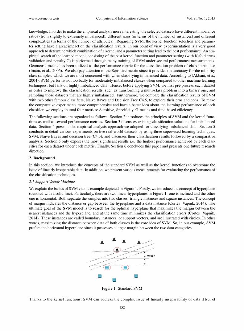
We explain the basics of SVM via the example depicted in Figure 1. Firstly, we introduce the concept of hyperplane(denoted with a solid line). Particularly, there are two linear hyperplanes in Figure 1: one is inclined and the otherone is horizontal. Both separate the samples into two classes: triangle instances and square instances. The conceptof margin indicates the distance or gap between the hyperplane and a data instance (Cortes Vapnik, 2014). Theultimate goal of the SVM model is to search for the optimal hyperplane that maximizes the margin between thenearest instances and the hyperplane, and at the same time minimizes the classification errors (Cortes Vapnik,2014). These instances are called boundary instances, or support vectors, and are illustrated with circles. In otherwords, maximizing the distance between data of both classes is the core idea of SVM. So, in our example, SVMprefers the horizontal hyperplane since it possesses a larger margin between the two data categories.

Figure 1. Standard SVM

Thanks to the kernel functions, SVM can address the complex issue of linearly inseparability of data (Hsu, et

152


al., 2010). In most real-life applications, data are not always linearly separable, consequently we need to finda non-linear classifier. It has been shown that SVM can always find a hyperplane that linearly separates thesamples in a certain high dimensional space for the linearly non-separable input data in the low dimensional space(Cortes Vapnik, 2014). Feature mapping is utilized to transfer this problem from low dimensional space to ahigher dimensional one. For example from two dimensional linearly un-separable into three dimensional linearlyseparable (Cortes Vapnik, 2014). Subsequently, from the three dimensional feature space, a kernel function canbe performed to obtain the non-linear classifier for the original two dimensional space.

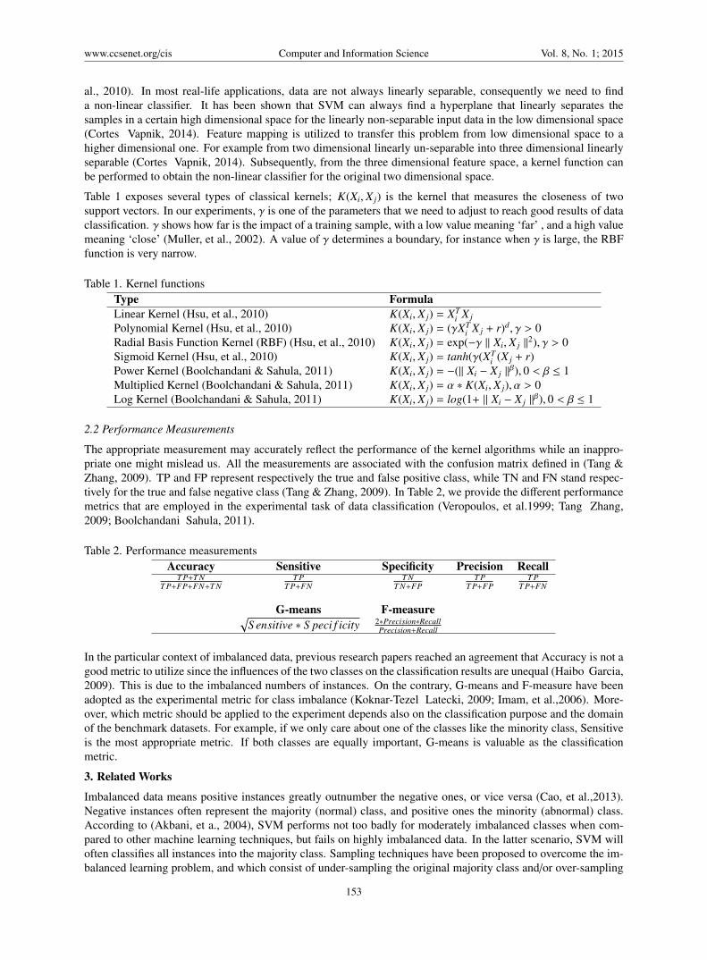
Table 1 exposes several types of classical kernels; K(Xi, Xj) is the kernel that measures the closeness of twosupport vectors. In our experiments, ! is one of the parameters that we need to adjust to reach good results of dataclassification. ! shows how far is the impact of a training sample, with a low value meaning ‘far’ , and a high valuemeaning ‘close’ (Muller, et al., 2002). A value of ! determines a boundary, for instance when ! is large, the RBFfunction is very narrow.

Table 1. Kernel functionsType FormulaLinear Kernel (Hsu, et al., 2010) K(Xi, Xj) = XT

i X jPolynomial Kernel (Hsu, et al., 2010) K(Xi, Xj) = (!XT

i X j + r)d, ! > 0Radial Basis Function Kernel (RBF) (Hsu, et al., 2010) K(Xi, Xj) = exp(!! " Xi, Xj "2), ! > 0Sigmoid Kernel (Hsu, et al., 2010) K(Xi, Xj) = tanh(!(XT

i (Xj + r)Power Kernel (Boolchandani & Sahula, 2011) K(Xi, Xj) = !(" Xi ! Xj ""), 0 < " # 1Multiplied Kernel (Boolchandani & Sahula, 2011) K(Xi, Xj) = # $ K(Xi, Xj),# > 0Log Kernel (Boolchandani & Sahula, 2011) K(Xi, Xj) = log(1+ " Xi ! Xj ""), 0 < " # 1

2.2 Performance Measurements

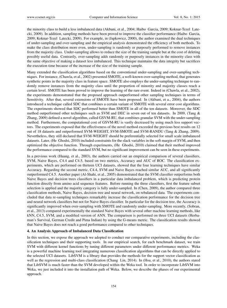
The appropriate measurement may accurately reflect the performance of the kernel algorithms while an inappro-priate one might mislead us. All the measurements are associated with the confusion matrix defined in (Tang &Zhang, 2009). TP and FP represent respectively the true and false positive class, while TN and FN stand respec-tively for the true and false negative class (Tang & Zhang, 2009). In Table 2, we provide the di!erent performancemetrics that are employed in the experimental task of data classification (Veropoulos, et al.1999; Tang Zhang,2009; Boolchandani Sahula, 2011).

Table 2. Performance measurementsAccuracy Sensitive Specificity Precision Recall

T P+T NT P+FP+FN+T N

T PT P+FN

T NT N+FP

T PT P+FP

T PT P+FN

G-means F-measure!S ensitive $ S peci f icity 2$Precision$Recall

Precision+Recall

In the particular context of imbalanced data, previous research papers reached an agreement that Accuracy is not agood metric to utilize since the influences of the two classes on the classification results are unequal (Haibo Garcia,2009). This is due to the imbalanced numbers of instances. On the contrary, G-means and F-measure have beenadopted as the experimental metric for class imbalance (Koknar-Tezel Latecki, 2009; Imam, et al.,2006). More-over, which metric should be applied to the experiment depends also on the classification purpose and the domainof the benchmark datasets. For example, if we only care about one of the classes like the minority class, Sensitiveis the most appropriate metric. If both classes are equally important, G-means is valuable as the classificationmetric.

3. Related WorksImbalanced data means positive instances greatly outnumber the negative ones, or vice versa (Cao, et al.,2013).Negative instances often represent the majority (normal) class, and positive ones the minority (abnormal) class.According to (Akbani, et a., 2004), SVM performs not too badly for moderately imbalanced classes when com-pared to other machine learning techniques, but fails on highly imbalanced data. In the latter scenario, SVM willoften classifies all instances into the majority class. Sampling techniques have been proposed to overcome the im-balanced learning problem, and which consist of under-sampling the original majority class and/or over-sampling

153


the minority class to build a less imbalanced data (Akbani, et al., 2004; Haibo Garcia, 2009; Koknar-Tezel Late-cki, 2009). In addition, sampling methods have been proved to improve the classifier performance (Haibo Garcia,2009; Koknar-Tezel Latecki, 2009). For example, in (Japkowicz, 2000), the author examined the dual techniquesof under-sampling and over-sampling and the empirical analysis demonstrated the e"ciency of both methods. Tomake the class distribution more even, under-sampling is randomly or purposely performed to remove instancesfrom the majority class. Under-sampling allows to reduce the size of the training sample but at the cost of deletingpossibly useful data. Contrarily, over-sampling adds randomly or purposely instances in the minority class withthe same objective of making a dataset less imbalanced. This technique maintains the data integrity but sacrificesthe execution time because of the increase of the size of the training sample.

Many extended the classification algorithms based on the conventional under-sampling and over-sampling tech-niques. For instance, (Chawla, et al., 2002) presented SMOTE, a well-known over-sampling method, that generatessynthetic points in the majority class in feature space. SMOTE also employs the under-sampling technique to ran-domly remove instances from the majority class until the proportion of minority and majority classes reach acertain level. SMOTE has been proved to improve the learning of the rare event. Indeed in (Chawla, et al., 2002),the experiments demonstrated that the proposed approach outperformed other sampling techniques in terms ofSensitivity. After that, several extensions of SMOTE have been proposed. In (Akbani, et a., 2004), the authorsintroduced a technique called SDC that combines a certain variant of SMOTE with several error cost algorithms.The experiments showed that SDC performed better than SMOTE in all of the ten datasets. Moreover, the SDCmethod outperformed other techniques such as SVM and DEC in seven out of ten datasets. In 2009, (Tang &Zhang, 2009) defined a novel algorithm, called GSVM-RU, that combines granular SVM with the under-samplingmethod. Furthermore, the computational cost of GSVM-RU is vastly decreased by using much less support vec-tors. The experiments exposed that the e!ectiveness of the novel method exceeded the previous best results on 12out of 18 datasets and outperformed SVM-WEIGHT, SVM-SMOTE and SVM-RANDU (Tang & Zhang, 2009).Nevertheless, they still declared that SVM-WEIGHT should be preferentially selected for small scale imbalanceddatasets. Later, (He Ghodsi, 2010) included constraints for the slack variables in the soft margin of SVM, and thenoptimized the objective function. Through experiments, (He Ghodsi, 2010) claimed that their method improvedthe performance compared to the standard SVM, but no significant improvement can be seen in these experiments.

In a previous work (Huang, et al., 2003), the authors carried out an empirical comparison of several classifiers,SVM, Naive Bayes, C4.4 and C4.5, based on two metrics, Accuracy and AUC of ROC. The classification ex-periments, which are performed on thirteen UCI datasets, showed that the four learning techniques have similarAccuracy. Regarding the second metric, C4.4, SVM and Naive Bayes reached similar AUC, and all significantlyoutperformed C4.5. Another paper (Al-Shahi, et al., 2005) demonstrated that the SVM classifier outperforms bothNaive Bayes and decision trees classifiers in a particular data imbalanced problem, which is predicting proteinfunction directly from amino acid sequence features. Before running the three classifiers, first the feature subsetselection is applied and the majority category is fully under-sampled. In (Chen, 2009), the author compared threeclassification methods, Naive Bayes, decision tree and neural network, on rebalanced data. The experiments con-cluded that data re-sampling techniques remarkably increase the classification performance for the decision treeand neural network classifiers but not for Naive Bayes classifier. In particular for the decision tree, the Accuracy issignificantly improved when over-sampling with SMOTE and randomly under-sampling. More recently, (Sobran,et al., 2013) compared experimentally the standard Naive Bayes with several other machine learning methods, likekNN, C4.5, SVM, and a modified version of ANN. The comparison is performed on three UCI datasets (Herba-man’s Survival, German Credit and Pima Indian) by using the G-means metric. The classification results showedthat Naive Bayes does not reach a good performance compared to other techniques.

4. An Analysis Approach of Imbalanced Data ClassificationIn this section, we expose the approach we adopted to conduct our comparative experiments, including the clas-sification techniques and their supporting tools. In our empirical search, for each benchmark dataset, we trainSVM with di!erent kernel functions by tuning di!erent parameters under di!erent performance metrics. Wekais a powerful machine learning tool integrating numerous classification algorithms that can be directly applied tothe selected UCI datasets. LibSVM is a library that provides the methods for the support vector classification aswell as the regression and multi-class classification (Chang Lin, 2014). In (Hsu, et al., 2010), the authors statedthat LibSVM is much faster than the SVM developed within the Weka tool. In order to incorporate LibSVM intoWeka, we just included it into the installation path of Weka. Below, we describe the phases of our experimentalapproach.

154


4.1 Data Selection

The first step is to choose relatively new datasets from the UCI repository to make the experiments more interesting.Otherwise, it will be the same repetitive analysis work when working on the same classic data, such as Iris,Breast and Wine (Holte, 1993), since a large number of previous experiments have already tested the classificationalgorithms on these data. Moreover, it is useful to select datasets that have di!erent imbalance ratios (from slightlyto extremely imbalanced), di!erent sizes (in terms of the number of instances), and di!erent complexities (in termsof the number of attributes).

4.2 Data Preprocessing

A. Data format adaptation: first the di!erent formats of the UCI datasets must be translated into the format thatis required by the Weka interface (i.e. ARFF). One option is to copy them into an Excel document and save themas .CSV files which are then systematically transformed by Weka to .ARFF.

B. Irrelevant feature removal: here irrelevant data features must be removed as they do not contain any valu-able information for the purpose of classification. Examples of these features are those that have been assignedautomatically by the companies (such as customer ID). Removing these irrelevant features will eliminate the inter-ference with other important features, and reduce the processing time of classification. Moreover, if a data featurehas missing values, then delete the corresponding instances.

C. Multi-class to binary class transformation: the multi-class data are transformed into a two-class problem bymerging some classes into one class.

D. Data Sampling: we need to sample the datasets for whose the classification results are unsatisfactory underany conditions. Weka employs the dual sampling techniques, under-sampling and over-sampling, to benefit fromboth of them. The data sampling is based on two parameters: bias and percentage. The larger the bias is, the morebalanced the data will be changed to. Percentage means the total number of instances compared to the one in theoriginal dataset. In all the experiments, we set bias to 0.5 and percentage to 100 (i.e. the total instances is the sameas in the original data).

4.3 Data Classification

A. Measurement selection: G-means has been utilized as the performance metric for the classification problemof class imbalance (Imam, et al., 2006). We also pay attention to Sensitive since it provides the accuracy for theminority class, which we are most concerned with when classifying imbalanced data. In many real-life scenarios,the rare case is often of interest. For example, in online auctions, we consider that misclassifying fraudulentas normal behaviour is much worse than misclassifying a normal behaviour as fraudulent. The consequence forthe latter one might be sending a warning to the bidder and verifying further his behaviour to confirm or rejectthe suspicion. Nevertheless, the former will result in money loss for honest bidders. Moreover, to make thecomparative experiments more comprehensive and have a better idea about the performance of each classifier, weemploy in total three metrics: Sensitive, Specificity (measures the accuracy of the majority samples), G-means(measures the accuracy of both classes). In addition, we compute the processing time for each classifier on eachdataset.

B. Classification with SVM: we first choose several kernel functions from Table 1, and then apply them to eachdataset under di!erent parameter settings as well as di!erent performance metrics. We train SVM with three typesof kernels: Linear, Polynomial, and non-linear RBF, as they are widely used in practice. We have in total threetuneable parameters: the penalty C, parameter !, and the K-fold cross validation. The purpose here is to examinethe influence of each parameter on each kernel.

The parameter C, called penalty, regulates the trade-o! between training error minimization and margin maximiza-tion Mulier 2007). When C is too big, overfitting may occur, and when it is too small, underfitting may occur.The K-fold cross-validation consists of splitting a dataset into K subsets, (K-1) as the training sample and 1 as atesting sample. The cross-validation method may stop the overfitting issue. We vary K from a small value to alarger one until the classification results reach a stable and relatively good state. However, the time complexity ofclassification is increased by K, so we always try to find a satisfiable but as small as possible value of K.

To attain the best results for SVM, we need to run numerous experiments for each dataset by varying the threeparameters for each kernel and under each performance measurement. For each data, the learned model is thekernel function and parameter setting that achieved the best performance. This model will be used in the future topredict the category of a new instance.

155


C. Classification with Naive Bayes and J48: In addition to SVM, we apply the other two widely used classifierson each dataset. Naive Bayes is a simple but important probabilistic classifier based on the Bayes theory andindependence assumption (Collins, 2014). J48 or C4.5 is a decision tree classifier proposed by Quinlan (Quinlan,1993). To achieve the best results for these two classifiers, we need to run several experiments by changing theparameter K on each dataset under each measurement. These two classifiers utilize the default values set by Weka.

4.4 Classifier Comparison

Here, we discuss the best classification results achieved by the three machine learning tools, SVM, Naive Bayesand J48 (C4.5), on each dataset under each performance metric: Sensitive, Specificity, G-means and ProcessingTime. We also compare the produced results to determine the best classifier for each dataset.

5. Empirical Analysis and ComparisonThis section exposes the experimental results of classifying new datasets with the three classifiers. We repeatthe same experiments on all the datasets by testing di!erent kernels and parameters. We only present the mostsignificant classification results. The experiments are conducted on Windows XP with Intel Core 2 Duo CPUT6400 2.00 GHz, and the figures are generated by using Matlab 2012a.

5.1 Data Selection

With the purpose of making the experiments more interesting, from diverse areas, we collect five new datasets fromthe UCI repository. Table 3 presents the major information of these datasets. To the best of our knowledge, thereare no previous works that showed the performance of the classification algorithms on these data. The size of thesefive pieces of data varies from a small scale (Fertility with 100) to a large scale (Bank Marketing with 4521). Maj.and Min. represent the number of instances in the majority and minority class respectively, and Att. the numberof attributes. The imbalance ratio varies from a slight imbalance (User Knowledge Modelling with 151:107) to anextreme imbalance (Seismic Bumps with 2414: 170).

Table 3. Benchmark datasets from UCIData Ins. Maj. Min. Att. Year AreaFertility 100 88 12 10 2013 BiomedicalUserKnowledgeModeling 258 151 107 6 2013 EducationVertebral Column 310 210 100 6 2011 BiomedicalSeismic Bumps 2564 2414 170 19 2013 Coal miningBank Marketing 4521 4000 521 17 2012 Business

5.2 Data Preprocessing

Below we summarize the preprocessing tasks for each piece of data. The first step is to transform the datasetformats to the one required by the Weka software. The User Knowledge Modelling data divides the studentknowledge levels into four categories: verylow, low, middle and high. In order to transform it into a binaryclassification problem, we classify verylow and low levels into the class fail, middle and high into the class pass. Inthe dataset of Bank Marketing, we remove four irrelevant features: contact type, last contact day of the month, lastcontact month of year, and last contact duration. In our opinion, these features do not contain useful informationfor the classification.

We found that it is di"cult for the three classifiers to process highly imbalanced datasets with satisfactory results.For instance, the three selected kernels perform poorly in terms of Sensitive in the original data of Seismic Bumpsand Bank Marketing. As a result, we sample these two data to make them less imbalanced by setting bias to 0.5and percentage to 100. Now Seismic Bumps data has a lower imbalance ratio of 1819:745, and Bank Marketingof 3097:1421. We may note that Fertility and VertebralColumn data do not require any preprocessing tasks.

5.3 Data Classification

We train SVM with Linear, Polynomial with degree 2, and Radial Basis Function (RBF). We keep adjusting thethree parameters K, C and ! until we reach satisfactory results for SVM.

5.3.1 Fertility

Table 4 indicates that Naive Bayes and J48 have di"culty addressing the minority instances for Fertility: theperformance of Sensitive is only 0.083 and 0.167 respectively. On the other hand, SVM proves outstanding when

156


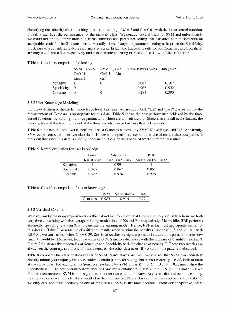
classifying the minority class, reaching 1 under the setting of K = 5 and C = 0.01 with the linear kernel function,though it sacrifices the performance for the majority class. We conduct several trials for SVM and unfortunatelywe could not find a combination of a kernel function and parameter setting that classifies both classes with anacceptable result for the G-means metric. Actually, if we change the parameter setting to improve the Specificity,the Sensitive is considerably decreased and vice versa. In fact, the trade-o! results for both Sensitive and Specificityare only 0.417 and 0.534 respectively under the parameter setting of K = 2, C = 0.1 with Linear function.

Table 4. Classifier comparison for fertility

SVM (K=5,C=0.01,Linear)

SVM (K=5,C=0.5, Lin-ear)

Naive Bayes (K=5) J48 (K=5)

Sensitive 1 0 0.083 0.167Specificity 0 1 0.966 0.932G-means 0 0 0.283 0.395

5.3.2 User Knowledge Modeling

For the evaluation of the student knowledge level, this time we care about both “fail“ and “pass“ classes, so that themeasurement of G-means is appropriate for this data. Table 5 shows the best performance achieved by the threekernel functions by varying the three parameters, which are all satisfactory. Since it is a small-scale dataset, thebuilding time of the learning model of the three kernels is very fast, less than 0.1 seconds.

Table 6 compares the best overall performance of G-means achieved by SVM, Naive Bayes and J48. Apparently,SVM outperforms the other two classifiers. However, the performances of other classifiers are also acceptable. Itturns out that since this data is slightly imbalanced, it can be well handled by the di!erent classifiers.

Table 5. Kernel evaluation for user knowledge

Linear Polynomial RBFK=10, C=5 K=5, !=2, C=3 K=10, !=0.5, C=0.5

Sensitive 1 0.991 1Specificity 0.967 0.967 0.954G-means 0.983 0.978 0.976

Table 6. Classifier comparison for user knowledge

SVM Naive Bayes J48G-means 0.983 0.956 0.974

5.3.3 Vertebral Column

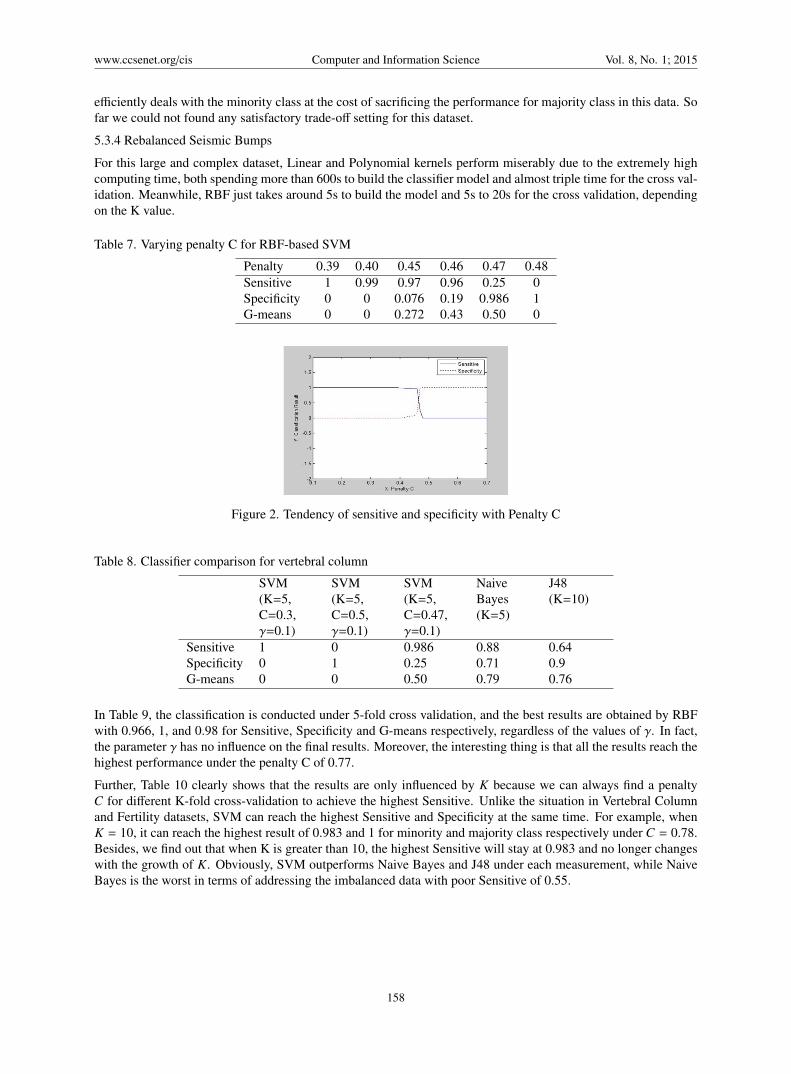
We have conducted many experiments on this dataset and found out that Linear and Polynomial functions are bothvery time consuming with the average building model time of 29s and 91s respectively. Meanwhile, RBF performse"ciently, spending less than 0.1s to generate the learning model. Hence, RBF is the most appropriate kernel forthis dataset. Table 7 presents the classification results when varying the penalty C under K = 5 and ! = 0.1 withRBF. So, we can see that when C <= 0.39, Sensitive reaches its highest point and stays at this point no matter howsmall C would be. Moreover, from the value of 0.39, Sensitive decreases with the increase of C until it reaches 0.Figure 2 illustrates the tendencies of Sensitive and Specificity with the change of penalty C. These two metrics arealways on the contrary, and if one of them increases, the other decreases. If we vary !, the pattern is observed.

Table 8 compares the classification results of SVM, Naive Bayes and J48. We can see that SVM can accuratelyclassify minority or majority instances under a certain parameter setting, but cannot correctly classify both of themat the same time. For example, the Sensitive reaches 1 by SVM under K = 5, C = 0.3, ! = 0.1, meanwhile theSpecificity is 0. The best overall performance of G-means is obtained by SVM with K = 5, ! = 0.1 and C = 0.47.For this measurement, SVM is not as good as the other two classifiers. Naive Bayes has the best overall accuracy.In conclusion, if we consider the overall classification metric, Naive Bayes is the best choice for this data. Ifwe only care about the accuracy of one of the classes, SVM is the most accurate. From our perspective, SVM

157


e"ciently deals with the minority class at the cost of sacrificing the performance for majority class in this data. Sofar we could not found any satisfactory trade-o! setting for this dataset.

5.3.4 Rebalanced Seismic Bumps

For this large and complex dataset, Linear and Polynomial kernels perform miserably due to the extremely highcomputing time, both spending more than 600s to build the classifier model and almost triple time for the cross val-idation. Meanwhile, RBF just takes around 5s to build the model and 5s to 20s for the cross validation, dependingon the K value.

Table 7. Varying penalty C for RBF-based SVM

Penalty 0.39 0.40 0.45 0.46 0.47 0.48Sensitive 1 0.99 0.97 0.96 0.25 0Specificity 0 0 0.076 0.19 0.986 1G-means 0 0 0.272 0.43 0.50 0

Figure 2. Tendency of sensitive and specificity with Penalty C

Table 8. Classifier comparison for vertebral column

SVM(K=5,C=0.3,!=0.1)

SVM(K=5,C=0.5,!=0.1)

SVM(K=5,C=0.47,!=0.1)

NaiveBayes(K=5)

J48(K=10)

Sensitive 1 0 0.986 0.88 0.64Specificity 0 1 0.25 0.71 0.9G-means 0 0 0.50 0.79 0.76

In Table 9, the classification is conducted under 5-fold cross validation, and the best results are obtained by RBFwith 0.966, 1, and 0.98 for Sensitive, Specificity and G-means respectively, regardless of the values of !. In fact,the parameter ! has no influence on the final results. Moreover, the interesting thing is that all the results reach thehighest performance under the penalty C of 0.77.

Further, Table 10 clearly shows that the results are only influenced by K because we can always find a penaltyC for di!erent K-fold cross-validation to achieve the highest Sensitive. Unlike the situation in Vertebral Columnand Fertility datasets, SVM can reach the highest Sensitive and Specificity at the same time. For example, whenK = 10, it can reach the highest result of 0.983 and 1 for minority and majority class respectively under C = 0.78.Besides, we find out that when K is greater than 10, the highest Sensitive will stay at 0.983 and no longer changeswith the growth of K. Obviously, SVM outperforms Naive Bayes and J48 under each measurement, while NaiveBayes is the worst in terms of addressing the imbalanced data with poor Sensitive of 0.55.

158


Table 9. Parameter setting for best RBF performance

! C Sensitive Specificity G-means0.1 0.77 0.966 1 0.981 0.77 0.966 1 0.9810 0.77 0.966 1 0.98100 0.77 0.966 1 0.98

Table 10. Classifier comparison for seismic bumps

Sensitive Specificity G-means K C

SVM (RBF)

0.8870.9660.9830.983

1111

0.940.980.990.99

251020

0.740.770.780.78

NaiveBayes 0.55 0.849 0.68 5 -J48 0.942 0.928 0.93 10 -

5.3.5 Rebalanced Bank Marketing

Similar to the Seismic Bumps data, Linear and Polynomial are very time consuming since this dataset is large andcomplex. From Table 11, we can see that SVM has the outstanding performance for both Sensitive and Specificityon the sampled Bank Marketing data. When K=10, SVM performs better when compared to K=2 and K=5.Actually, SVM achieves 1 and 0.919 for minority and majority classes respectively. It is probable that the trainingset is not enough to train the best model when K is less than 10. In essence, the overall performance achieved byJ48 is satisfactory while Naive Bayes shows a deficiency for classifying minority instances.

Table 11. Classifier comparison for bank marketing

Sensitive Specificity G-means K C

SVM (RBF)0.7490.89

1

11

0.919

0.870.940.96

2510

0.30.210.21

Naive Bayes 0.638 0.848 0.74 5 -J48 0.904 0.927 0.92 25 -

5.4 Classifier Comparison

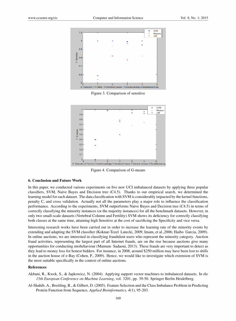
Figure 3 presents the evaluation of the three classifiers in terms of Sensitive on each of the four datasets. We maynote that User Knowledge Modeling is only learned by the G-means metric since it is a slightly imbalanced dataset,so the two classes are equally important. We can see that SVM outperforms Naive Bayes and J48 in all the fourdata. In particular, regarding data Fertility, both Naive Bayes and J48 show their huge weakness in classifyingcorrectly the minority instances. Naive Bayes performance is unsatisfactory for those large datasets such as BankMarketing and Seismic Bumps. It is also di"cult for J48 to classify minority instances for Vertebral Column.

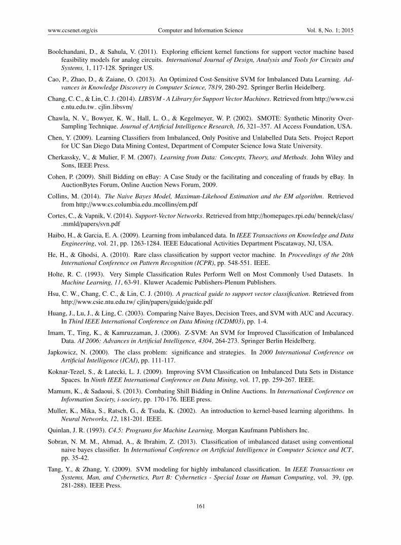
In Figure 4, for classifying both classes at the same time, SVM outperforms the other two classifiers for threedatasets excluding Fertility and Vertebral Column. Both J48 and Naive Bayes show a better performance in thesetwo small-scale data. We may note that Fertility and Vertebral Column seem the most di"cult data to addressbecause none of the three classifiers reached more than 90% for the G-means metric: less than 50% for Fertility,and less than 80% for Vertebral Column. In contrast, User Knowledge is the easiest data to be handled by the threeclassifiers with at least 95% for G-means. We may note that for large and complex datasets, SVM is much betterthat the two other classifiers.

Overall, Vertebral Column and Fertility, thought small scale data, are the most di"cult to be correctly classified.It is not as expected as most researchers consider that smaller the scale is, the easier the classification will be.Nonetheless, the penalty C considerably influences a certain data but has almost no influence on another data, andthe same can be concluded regarding the other tuning parameters.

159


Figure 3. Comparison of sensitive

Figure 4. Comparison of G-means

6. Conclusion and Future WorkIn this paper, we conducted various experiments on five new UCI imbalanced datasets by applying three popularclassifiers, SVM, Naive Bayes and Decision tree (C4.5). Thanks to our empirical search, we determined thelearning model for each dataset. The data classification with SVM is considerably impacted by the kernel functions,penalty C, and cross validation. Actually not all the parameters play a major role to influence the classificationperformance. According to the experiments, SVM outperforms Naive Bayes and Decision tree (C4.5) in terms ofcorrectly classifying the minority instances (or the majority instances) for all the benchmark datasets. However, inonly two small-scale datasets (Vertebral Column and Fertility) SVM shows its deficiency for correctly classifyingboth classes at the same time, attaining high Sensitive at the cost of sacrificing the Specificity and vice versa.

Interesting research works have been carried out in order to increase the learning rate of the minority events byextending and adapting the SVM classifier (Koknar-Tezel Latecki, 2009; Imam, et al.,2006; Haibo Garcia, 2009).In online auctions, we are interested in classifying fraudulent users who represent the minority category. Auctionfraud activities, representing the largest part of all Internet frauds, are on the rise because auctions give manyopportunities for conducting misbehaviour (Mamum Sadaoui, 2013). These frauds are very important to detect asthey lead to money loss for honest bidders. For instance, in 2008, around $250 million may have been lost to shillsin the auction house of e-Bay (Cohen, P., 2009). Hence, we would like to investigate which extension of SVM isthe most suitable specifically in the context of online auctions.

ReferencesAkbani, R., Kwek, S., & Japkowicz, N. (2004). Applying support vector machines to imbalanced datasets. In the

15th European Conference on Machine Learning, vol. 3201, pp. 39-50. Springer Berlin Heidelberg.

Al-Shahib, A., Breitling, R., & Gilbert, D. (2005). Feature Selection and the Class Imbalance Problem in PredictingProtein Function from Sequence, Applied Bioinformatics, 4(1), 95-203.

160


Boolchandani, D., & Sahula, V. (2011). Exploring e"cient kernel functions for support vector machine basedfeasibility models for analog circuits. International Journal of Design, Analysis and Tools for Circuits andSystems, 1, 117-128. Springer US.

Cao, P., Zhao, D., & Zaiane, O. (2013). An Optimized Cost-Sensitive SVM for Imbalanced Data Learning. Ad-vances in Knowledge Discovery in Computer Science, 7819, 280-292. Springer Berlin Heidelberg.

Chang, C. C., & Lin, C. J. (2014). LIBSVM - A Library for Support Vector Machines. Retrieved from http://www.csie.ntu.edu.tw cjlin libsvm/

Chawla, N. V., Bowyer, K. W., Hall, L. O., & Kegelmeyer, W. P. (2002). SMOTE: Synthetic Minority Over-Sampling Technique. Journal of Artificial Intelligence Research, 16, 321–357. AI Access Foundation, USA.

Chen, Y. (2009). Learning Classifiers from Imbalanced, Only Positive and Unlabelled Data Sets. Project Reportfor UC San Diego Data Mining Contest, Department of Computer Science Iowa State University.

Cherkassky, V., & Mulier, F. M. (2007). Learning from Data: Concepts, Theory, and Methods. John Wiley andSons, IEEE Press.

Cohen, P. (2009). Shill Bidding on eBay: A Case Study or the facilitating and concealing of frauds by eBay. InAuctionBytes Forum, Online Auction News Forum, 2009.

Collins, M. (2014). The Naive Bayes Model, Maximun-Likehood Estimation and the EM algorithm. Retrievedfrom http://www.cs.columbia.edu mcollins/em.pdf

Cortes, C., & Vapnik, V. (2014). Support-Vector Networks. Retrieved from http://homepages.rpi.edu/ bennek/class/mmld/papers/svn.pdf

Haibo, H., & Garcia, E. A. (2009). Learning from imbalanced data. In IEEE Transactions on Knowledge and DataEngineering, vol. 21, pp. 1263-1284. IEEE Educational Activities Department Piscataway, NJ, USA.

He, H., & Ghodsi, A. (2010). Rare class classification by support vector machine. In Proceedings of the 20thInternational Conference on Pattern Recognition (ICPR), pp. 548-551. IEEE.

Holte, R. C. (1993). Very Simple Classification Rules Perform Well on Most Commonly Used Datasets. InMachine Learning, 11, 63-91. Kluwer Academic Publishers-Plenum Publishers.

Hsu, C. W., Chang, C. C., & Lin, C. J. (2010). A practical guide to support vector classification. Retrieved fromhttp://www.csie.ntu.edu.tw/ cjlin/papers/guide/guide.pdf

Huang, J., Lu, J., & Ling, C. (2003). Comparing Naive Bayes, Decision Trees, and SVM with AUC and Accuracy.In Third IEEE International Conference on Data Mining (ICDM03), pp. 1-4.

Imam, T., Ting, K., & Kamruzzaman, J. (2006). Z-SVM: An SVM for Improved Classification of ImbalancedData. AI 2006: Advances in Artificial Intelligence, 4304, 264-273. Springer Berlin Heidelberg.

Japkowicz, N. (2000). The class problem: significance and strategies. In 2000 International Conference onArtificial Intelligence (ICAI), pp. 111-117.

Koknar-Tezel, S., & Latecki, L. J. (2009). Improving SVM Classification on Imbalanced Data Sets in DistanceSpaces. In Ninth IEEE International Conference on Data Mining, vol. 17, pp. 259-267. IEEE.

Mamum, K., & Sadaoui, S. (2013). Combating Shill Bidding in Online Auctions. In International Conference onInformation Society, i-society, pp. 170-176. IEEE press.

Muller, K., Mika, S., Ratsch, G., & Tsuda, K. (2002). An introduction to kernel-based learning algorithms. InNeural Networks, 12, 181-201. IEEE.

Quinlan, J. R. (1993). C4.5: Programs for Machine Learning. Morgan Kaufmann Publishers Inc.

Sobran, N. M. M., Ahmad, A., & Ibrahim, Z. (2013). Classification of imbalanced dataset using conventionalnaive bayes classifier. In International Conference on Artificial Intelligence in Computer Science and ICT ,pp. 35-42.

Tang, Y., & Zhang, Y. (2009). SVM modeling for highly imbalanced classification. In IEEE Transactions onSystems, Man, and Cybernetics, Part B: Cybernetics - Special Issue on Human Computing, vol. 39, (pp.281-288). IEEE Press.

161


UCI (2013). Centre for machine learning and intelligent systems. Retrieved from http://archive.ics.uci.edu/ml

Vapnik, V. (1998). Statistical Learning Theory. Wiley Interscience.

Veropoulos, K., Campbell, C., & Cristianini, N. (1999). Controlling the Sensitivity of Support Vector Machines.In International Joint Conference on Artificial Intelligence, pp. 55-60.

CopyrightsCopyright for this article is retained by the author(s), with first publication rights granted to the journal.

This is an open-access article distributed under the terms and conditions of the Creative Commons Attributionlicense (http://creativecommons.org/licenses/by/3.0/).

162

An Empirical Analysis of Imbalanced Data Classification

Documents

Transcript of An Empirical Analysis of Imbalanced Data Classification