
Symbolic One-Class Learning from Imbalanced Datasets: Application in Medical Diagnosis
37
March 31, 2009 15:41 WSPC-IJAIT 00013-cor International Journal on Artificial Intelligence Tools Vol. 18, No. 2 (2009) 273–309 c World Scientific Publishing Company SYMBOLIC ONE-CLASS LEARNING FROM IMBALANCED DATASETS: APPLICATION IN MEDICAL DIAGNOSIS LUIS MENA Department of Computer Science, Faculty of Engineering University of Zulia, Maracaibo, Venezuela National Institute of Astrophysics, Optics and Electronics Puebla, Mexico [email protected] JESUS A. GONZALEZ Department of Computer Science National Institute of Astrophysics, Optics and Electronics Puebla, Mexico [email protected] Received 4 October 2007 Accepted 2 August 2008 273 When working with real-world applications we often find imbalanced datasets, those for which there exists a majority class with normal data and a minority class with abnormal or important data. In this work, we make an overview of the class imbalance problem; we review consequences, possible causes and existing strategies to cope with the inconveniences associated to this problem. As an effort to contribute to the solution of this problem, we propose a new rule induction algorithm named Rule Extraction for MEdical Diagnosis (REMED), as a symbolic one-class learning approach. For the evaluation of the proposed method, we use different medical diagnosis datasets taking into account quantitative metrics, comprehensibility, and reliability. We performed a comparison of REMED versus C4.5 and RIPPER combined with over-sampling and cost-sensitive strategies. This empirical analysis of the REMED algorithm showed it to be quantitatively competitive with C4.5 and RIPPER in terms of the area under the Receiver Operating Characteristic curve (AUC) and the geometric mean, but overcame them in terms of comprehensibility and reliability. Results of our experiments show that REMED generated rules systems with a larger degree of abstraction and patterns closer to well-known abnormal values associated to each considered medical dataset. Keywords: Machine learning; imbalanced datasets; one-class learning; classification algorithm; rule extraction. 1. Introduction Machine learning algorithms provide the technical basis implemented in some practical data mining tasks. It is used to extract information from databases, which is expressed as novel, useful, and comprehensible patterns. The goal is to find strong patterns (those that make accurate predictions over new data) which would help to take effective decisions in
Transcript of Symbolic One-Class Learning from Imbalanced Datasets: Application in Medical Diagnosis

March 31, 2009 15:41 WSPC-IJAIT 00013-cor
International Journal on Artificial Intelligence ToolsVol. 18, No. 2 (2009) 273–309c© World Scientific Publishing Company
SYMBOLIC ONE-CLASS LEARNING FROM IMBALANCED
DATASETS: APPLICATION IN MEDICAL DIAGNOSIS
LUIS MENA
Department of Computer Science, Faculty of Engineering
University of Zulia, Maracaibo, Venezuela
National Institute of Astrophysics, Optics and Electronics
Puebla, Mexico
JESUS A. GONZALEZ
Department of Computer Science
National Institute of Astrophysics, Optics and Electronics
Puebla, Mexico
Received 4 October 2007Accepted 2 August 2008
273
When working with real-world applications we often find imbalanced datasets, those for which there
exists a majority class with normal data and a minority class with abnormal or important data. In this
work, we make an overview of the class imbalance problem; we review consequences, possible
causes and existing strategies to cope with the inconveniences associated to this problem. As an
effort to contribute to the solution of this problem, we propose a new rule induction algorithm named
Rule Extraction for MEdical Diagnosis (REMED), as a symbolic one-class learning approach. For
the evaluation of the proposed method, we use different medical diagnosis datasets taking into
account quantitative metrics, comprehensibility, and reliability. We performed a comparison of
REMED versus C4.5 and RIPPER combined with over-sampling and cost-sensitive strategies. This
empirical analysis of the REMED algorithm showed it to be quantitatively competitive with C4.5
and RIPPER in terms of the area under the Receiver Operating Characteristic curve (AUC) and the
geometric mean, but overcame them in terms of comprehensibility and reliability. Results of our
experiments show that REMED generated rules systems with a larger degree of abstraction and
patterns closer to well-known abnormal values associated to each considered medical dataset.
Keywords: Machine learning; imbalanced datasets; one-class learning; classification algorithm; rule
extraction.
1. Introduction
Machine learning algorithms provide the technical basis implemented in some practical
data mining tasks. It is used to extract information from databases, which is expressed as
novel, useful, and comprehensible patterns. The goal is to find strong patterns (those that
make accurate predictions over new data) which would help to take effective decisions in

274 L. Mena & J. A. Gonzalez
the business or scientific environment. Therefore, the use of machine learning tools and
techniques has increased, especially in real-world applications. It is clear that real data is
imperfect; it might contain inconsistencies and missing values. Therefore, machine
learning algorithms need to be robust to cope with the imperfections of data, and to be
able to extract really strong patterns. However, some machine learning algorithms that
were previously considered as robust (generally producing accurate results) have not
shown good performance in certain real-world applications.1-3
One of the causes of this
problem is that many real-world datasets present an additional problem: class imbalance.
Applications such as fraud detection, network intrusion, and medical diagnosis exhibit
the class imbalance problem, where there exists a majority or negative class with normal
data and a minority or positive class with abnormal or important data, which generally
has the highest cost of erroneous classification.
The main problem that current machine learning classifiers present when working
with imbalanced datasets, is the low performance achieved to correctly classify examples
of the minority class. Then, it is necessary to develop novel machine learning strategies
that combined with standard classifiers improve their performance when working with
imbalanced datasets. Most of the previous class imbalance works have focused on how to
evaluate the performance of machine learning classifiers exclusively in terms of their
capacity to minimize classification errors, they take into account the class imbalance
problem, but they do not consider how to evaluate the comprehensibility and reliability of
the found patterns.
In this work, we propose a new symbolic one-class learning approach to cope with
the class imbalance problem in real-world domains. We focus in a specific type of
imbalanced domain: medical diagnosis. For this kind of domain we need to express a
pattern as a transparent box whose construction describes the structure of the pattern.
Therefore, we need to evaluate the obtained patterns in terms of comprehensibility
besides the standard evaluation metrics to verify accuracy. However, the main reason to
select medical diagnosis tasks is that we additionally want to evaluate the reliability of
the patterns, this with the goal of establishing up to what degree is it really appropriate to
apply a specific machine learning strategy (such as over-sampling) to imbalanced
datasets. To achieve this, we compare the found patterns with well-known abnormal
values that could represent symptoms (diagnosis) or risk factors (prognosis) of certain
disease, therefore, the reliability of the obtained patterns could be evaluated according to
their medical validity.
In Section 2, we present an overview of the class imbalance problem. We discuss
possible causes, consequences and existing strategies to solve the problem. Section 3
shows a review of machine learning works in medical diagnosis, involved
inconveniences, and desired features to satisfactorily solve medical diagnosis tasks. In
Section 4, we present the details of our machine learning approach for imbalanced
datasets. Section 5 shows the experimental results of comparing our approach with other
machine learning strategies for imbalanced datasets. Finally, Section 6 analyzes and

Symbolic One-Class Learning from Imbalanced Datasets 275
discusses our results and in Section 7 we give our conclusions and indicate directions for
our future work.
2. The Class Imbalance Problem
The growing interest of the machine learning community to solve the class imbalance
problem gave rise to two workshops on learning from imbalanced datasets. The first
workshop was held by the American Association for Artificial Intelligence,4
and the
second by the International Conference on Machine Learning.5
In this section, we present
an overview of the types of problems that were considered by researchers in both
workshops, as well as in more recent works related to the class imbalance problem. We
finally present an overview of the possible causes of these problems and the previously
proposed possible solutions to solve them.
2.1. Performance evaluation
Generally speaking, the goal of machine learning algorithms for classification tasks is to
build classifiers that maximize accuracy. However, this assumption is not enough to
produce satisfactory classifiers in problems with imbalanced datasets because accuracy
by itself may yield misleading conclusions, given that it only considers the classifier’s
general performance and not the individual performance for each class. Therefore, it is
necessary to determine the appropriate way to evaluate machine learning algorithms for
the case of class imbalance problems.
Typically the performance of machine learning algorithms is evaluated with a
confusion matrix, from which we can calculate several evaluation metrics. Figure 1
shows an example of a confusion matrix for a binary classification problem (only 2
classes) and some evaluation metrics such as accuracy, sensitivity, specificity and
precision (positive predictive value). In the confusion matrix, TP (True Positives) and TN
(True Negatives) represent the number of positive and negative examples correctly
classified respectively, while FP (False Positives) and FN (False Negatives) represent the
number of positive and negative examples incorrectly classified respectively.
True Class P N
P Assigned Class N
Accuracy = TP + TN / (TP + FN + FP + TN)
Sensitivity = TP / (TP + FN)
Specificity = TN / (TN + FP)
Precision = TP / (TP + FP)
Fig. 1. A confusion matrix and some evaluation metrics.
TP FP
FN TN
276 L. Mena & J. A. Gonzalez
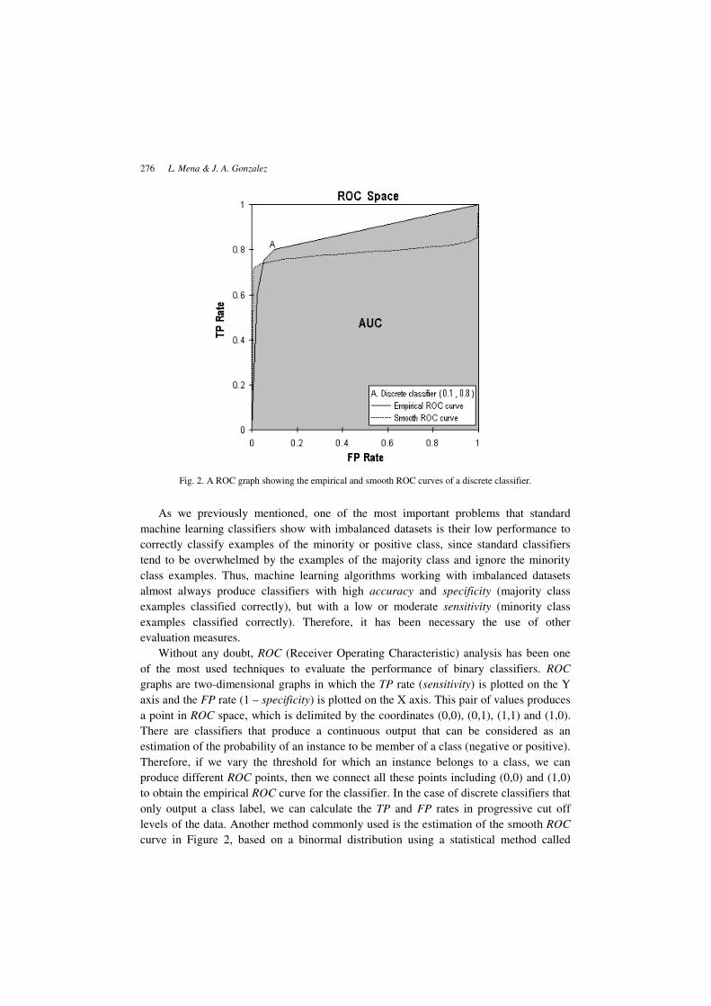
Fig. 2. A ROC graph showing the empirical and smooth ROC curves of a discrete classifier.
As we previously mentioned, one of the most important problems that standard
machine learning classifiers show with imbalanced datasets is their low performance to
correctly classify examples of the minority or positive class, since standard classifiers
tend to be overwhelmed by the examples of the majority class and ignore the minority
class examples. Thus, machine learning algorithms working with imbalanced datasets
almost always produce classifiers with high accuracy and specificity (majority class
examples classified correctly), but with a low or moderate sensitivity (minority class
examples classified correctly). Therefore, it has been necessary the use of other
evaluation measures.
Without any doubt, ROC (Receiver Operating Characteristic) analysis has been one
of the most used techniques to evaluate the performance of binary classifiers. ROC
graphs are two-dimensional graphs in which the TP rate (sensitivity) is plotted on the Y
axis and the FP rate (1 – specificity) is plotted on the X axis. This pair of values produces
a point in ROC space, which is delimited by the coordinates (0,0), (0,1), (1,1) and (1,0).
There are classifiers that produce a continuous output that can be considered as an
estimation of the probability of an instance to be member of a class (negative or positive).
Therefore, if we vary the threshold for which an instance belongs to a class, we can
produce different ROC points, then we connect all these points including (0,0) and (1,0)
to obtain the empirical ROC curve for the classifier. In the case of discrete classifiers that
only output a class label, we can calculate the TP and FP rates in progressive cut off
levels of the data. Another method commonly used is the estimation of the smooth ROC
curve in Figure 2, based on a binormal distribution using a statistical method called

Symbolic One-Class Learning from Imbalanced Datasets 277
maximum likelihood estimation.6
Some research works indicate that this method behaves
empirically well in a wide variety of situations.7 Informally, a classifier is considered
better than other, if it has a higher area under the ROC curve (AUC). In Figure 2 we show
the empirical and smooth ROC curves for a discrete classifier.
Another approach used to evaluate the performance of binary classifiers in class im-
balance problems is the geometric mean,8 which is defined as: yspecificitysensitivit × .
According to the authors, this measure has the distinctive property of being independent
of the distribution of the examples between classes. The advantage of the AUC and the
geometric mean measures is that both combine the sensitivity and specificity metrics,
providing a better way to represent the overall performance of a classifier for imbalanced
datasets than when we only use the accuracy measure.
2.2. Causes of the problem
Although it is clear that standard classifiers tend to decrease their performance with
imbalanced datasets, there are no studies that demonstrate that this degradation is directly
caused by the class imbalance problem. Therefore, in this section we make an overview
of the causes that could explain these deficiencies.
2.2.1. Rare cases
Rare cases correspond to a small number of training examples in particular areas of the
feature space.9 Although class imbalance and rare cases are not directly related, we
could expect that the minority class (due to its nature), contains a greater proportion of
rare cases than the majority class, and this is supported by some empirical studies.10
Thus, when standard classifiers are tested with rare cases, they produce higher error rates
than when tested with common cases. This happens because it is less likely to find rare
cases in the test set, and second because the general bias associated to standard classifiers
generally does not allow distinguishing between rare cases and noise, classifying rare
cases as common cases. Therefore, rare cases can be considered a special form of data
imbalance normally called within-class imbalance,11
and the problems associated with
class imbalance and rare cases could be solved using similar approaches.12
2.2.2. Small disjuncts
Usually machine learning algorithms create concept definitions from data, these
definitions are composed by disjuncts, where each disjunct is a conjunctive definition
describing a subconcept of the original concept. A small disjunct is defined as a disjunct
that only covers a few training examples.13
This can be considered a cause for a
significant loss of performance in standard classifiers because as we previously pointed,
in imbalanced datasets there exists a minority class with considerably fewer examples
than the majority class, and the disjuncts induced from them tend to cover even fewer
examples. Therefore, the poor representation of the minority class (few examples) could
be an obstacle for the induction of good classifiers. In this sense Jo and Japkowicz in

278 L. Mena & J. A. Gonzalez
Ref. 9 suggest that the problem is not directly caused by class imbalance, but rather, that
class imbalance and rare cases may yield small disjuncts which, in turn, will cause this
degradation.
Besides, small disjuncts might also be caused by the learning algorithm bias,14
because these algorithms try to generalize from the data to avoid overfitting (cases where
the learner may adjust to very specific random features of the training data). Therefore,
this general bias can adversely impact the ability to learn from imbalanced datasets. This
occurs because when the algorithm generalizes, it tends to induce disjuncts to cover
examples of the majority class (large disjuncts), overwhelming the examples of the
minority class. On the other hand, induction bias could also appear as another factor that
causes small disjuncts, because some machine learning algorithms prefer the most
common class in the presence of uncertainty. This is the case of most decision-tree
learners, which will predict the most frequent occurring class biasing their results against
rarer classes.12
2.2.3. Overlap among classes
Finally, other works suggest that the problem is not directly caused by class imbalance,
but it is related to the degree of overlapping among the classes.15,16
Thus, these works
argue that it does not matter neither what the size of the training set is nor how large the
degree of imbalance among classes is, if the classes are linearly separable or show well-
defined clusters (with a low degree of class overlapping), there is not a significant
degradation in the performance of standard classifiers.
2.3. Proposed strategies
Once we know some of the possible causes (rare cases, small disjuncts and class
overlapping) that might degrade the performance of standard classifiers in domains with
imbalanced datasets, in this section we focus on discussing the most recent machine
learning strategies proposed to tackle the class imbalance problem. These strategies have
been implemented to improve the performance of standard classifiers or to develop new
machine learning classifiers.
2.3.1. Sampling
Standard classifiers have shown good performance with well-balanced datasets. This is
why some of the previous approaches to solve the class imbalance problem tried to
balance the classes’ distributions. These solutions use different forms of re-sampling but
the two main sampling approaches are under-sampling and over-sampling. The first
consists of the elimination of examples from the majority class, while the second adds
examples to the minority class. However, there are many variants of both approaches; the
simplest variant consists of random sampling. Random under-sampling eliminates
majority class examples at random, while random over-sampling duplicates minority
class examples at random. Other form of sampling strategy is directed sampling, where
Symbolic One-Class Learning from Imbalanced Datasets 279
the selection of under-sampling and over-sampling examples is informed rather than
done at random. However, directed over-sampling continues replicating minority class
examples, that is; new examples are not created. On the other hand, directed under-
sampling generally consists of the elimination of redundant examples or examples
located farther away from the borders of regions containing minority class examples.
Finally, a smarter re-sampling strategy is advanced sampling. This is a type of
1) advanced over-sampling,17
which generates new examples (it does not just replicate
minority class examples), usually a new example is generated from similar examples of
the minority class (close in its feature space), or 2) the combination of the under-
sampling and over-sampling strategies, for example applying under-sampling to the over-
sampled training set as a data cleaning method.18
At this point of our overview of sampling strategies it is necessary to formulate two
important questions: 1) Which sampling approach is the best? and 2) What sampling
rate should be used?. The first issue is unclear yet, since recent works show that, in
general, over-sampling strategies provide more accurate results than under-sampling
strategies,15,18
but previous results seem to contradict this.19,20
However, we particularly
support over-sampling and specifically advanced over-sampling, because potentially
random under-sampling could eliminate some useful majority class examples; even
directed under-sampling does not guarantee that this would not happen. On the other
hand, random over-sampling and directed over-sampling could lead to overfitting,
because in both cases copies of minority class examples are introduced. Nonetheless, as a
deep thought, we should remember that part of the possible causes of the class imbalance
problem (such as rare cases and small disjuncts), are closer related with the small size of
the training set corresponding to the minority class, therefore, increasing the size of this
training set could improve the representation of the minority class, and thus help to
diminish the deficiencies of standard classifiers. On the other hand, the second issue
about what under/over sampling rates should be used (proportion of removed or added
examples), is even less clear.21
Therefore, both issues could represent inconveniences to
efficiently apply sampling strategies.
2.3.2. Cost-sensitive
Other important strategy to cope with the class imbalance problem has to do with the fact
that standard classifiers assume that the costs of making incorrect predictions are the
same. However, in real-world applications this assumption is generally incorrect, and
although the class imbalance and the asymmetric misclassification costs are not exactly
the same problem, we can establish a clear relationship between them, because generally
speaking the misclassification cost for the minority class is greater than the
misclassification cost for the majority class. Therefore, cost-sensitive strategies have been
developed to tackle the class imbalance problem.
The goal of cost-sensitive strategies for classification tasks is to reduce the cost
of misclassified examples instead of classification errors. Two main cost-sensitive
approaches have been implemented. The simpler approach consists of changing the class

280 L. Mena & J. A. Gonzalez
distributions of the training set regarding to misclassification costs.22
For example, in
the case of binary classification tasks, if the misclassification cost for the minority class
is x times higher than the misclassification cost for the majority class, then we should
make over-sampling of the minority class at x %, that is, the number of minority class
examples is increased by adding x % instances. Therefore, the final application of this
approach becomes a sampling strategy, where knowing the misclassification costs helps
to determine the re-sampling rate. The other cost-sensitive strategy consists of passing
the cost information to the machine learning algorithm during the learning process.12
The application of this strategy requires the construction of a cost matrix, which provides
the costs associated with each prediction. In the case of binary classification tasks
(Figure 3) with imbalanced datasets, the cost matrix contains 4 costs: TP cost (CTP), TN
cost (CTN), FP cost (CFP) and FN cost (CFN), where CTP and CTN are typically set
to 0, and CFN is greater than CFP because a FN means that a positive (minority class)
example was misclassified, and this represents a major misclassification cost. Thus, the
classifier performs better on the minority class due to the bias introduced with the
information of the cost matrix.
CTP CFP
CFN CTN
Fig. 3. A cost matrix for a binary classification problem.
This second approach tries to solve one of the problems associated with small
disjuncts, specifically the general and inductive bias of standard classifiers, which are not
appropriate for the class imbalance problem. To achieve this, the cost information from
cost matrices introduces a desirable bias, and this makes the classifier prefer a class with
a higher misclassification cost even when another class could be more probable. For
example, if a classifier initially has the positive class probability threshold set to 0.5, after
receiving the cost information the positive class probability threshold could be decreased
to 0.33, and then it could classify more examples as positives.23
However, in real-world
applications, misclassification costs are generally unknown, and in many cases their
estimate is particularly hard, since these costs depend on multiple factors that can not be
easily established.24
Therefore, if costs are known, the application of the first cost-sensitive strategy could
answer a previous question: What sampling rate should be used?, however, Elkan in
Ref. 25, argues that changing the balance of negative and positive training examples with
this cost-sensitive strategy has little effect on standard classifiers (Bayesian and decision
tree learning methods). With regard to the second approach, a new question emerges:
What is the appropriate value for CFN and CFP?. Although this question does not
have a clear answer, there are certain strategies to assign both costs. In the case of CFP a
cost of 1 is usually assigned,23
which is considered as a minimum cost. A real-world
example to verify if this is an appropriate strategy is medical diagnosis, where a FP
Symbolic One-Class Learning from Imbalanced Datasets 281
corresponds to a patient diagnosed as sick when he was actually healthy. This incorrect
prediction can be associated to a minimum cost, because more specific medical diagnosis
tests could discover the error. In the case of CFN there is a strategy that consists of
assigning the cost according to the imbalance ratio between classes. For example, if
the dataset presents a 1:10 class imbalance in favoring the majority class, the
misclassification cost for the minority class would be set to 9 times the misclassification
cost for the majority class.16
However, returning to the medical diagnosis tasks, the cost
estimated with this strategy could be insufficient, because a FN is a patient diagnosed as
healthy when he was actually sick. This situation could cause a life-threatening condition
that depending on the kind of disease could lead to death, therefore, it is necessary to
make a deeper analysis about how to assign the CFN, and this potentially represents an
inconvenience at the moment of applying the cost-sensitive strategies.
2.3.3. One-class learning
Finally, we focus on a third strategy called one-class learning, which is a recognition-
based approach that consists of learning classification knowledge to predict examples of
one class, and for the case of the class imbalance problem it is generally used to predict
positive examples. This strategy consists of learning from a single class rather than from
two classes, trying to recognize examples of the class of interest rather than discriminate
between examples of both classes.15
An important aspect of this strategy is that, under
certain conditions such as multi-modality of the domain space, one-class approaches may
provide a better solution to classification tasks than discrimination-based approaches.26,27
The goal of applying this strategy to the class imbalance problem consists of internally
biasing the discrimination-based process, so that we can compensate the class
imbalance.28
Therefore, this is another way of trying to solve the problems associated
with the inappropriate bias of standard classifiers when learning from imbalanced
datasets.
There are two main one-class learning strategies, the simpler approach consists of
training examples from a single class (positive or negative) to make a description of a
target set of objects, and detect if a new object resembles this training set. The objects
from this class can be called target objects, while all other objects can be called outliers.29
In some cases this approach is necessary because the only available information belongs
to examples of a single class. However, there are other cases where all the negative
examples are ignored,27
therefore, we can relate this to a total under-sampling of the
majority class. Multi-Layer Perceptron (MLP) and Support Vector Machines (SVMs)
have been used to apply this one-class approach (to learn only from a single class). In the
case of MLP the approach consists of training an autoassociator or autoencoder,30
which
is a MLP designed to reconstruct its input at the output layer. Once trained, if the MLP
(also called recognition-based MLP,31
) generalizes to a new object, then this must be a
target object, otherwise, it should be an outlier object. This approach has successfully
been used obtaining competitive results, using a training set exclusively composed
of cases from the minority class as in Refs. 26, 32 and 33 and the majority class as in

282 L. Mena & J. A. Gonzalez
Refs. 4 and 31. With respect to the one- class SVMs approach, the goal is to find a good
discriminating function f that scores the target class objects higher than the outlier class
objects, and this solution will be given in the form of a kernel machine. To achieve this,
there exists a methodology that after transforming the feature via a kernel treats the origin
as the only member of the outlier class,34
and an extended version of this approach in
which it is assumed that the origin is not the only point that belongs to the outlier class,
but also all the data points “close enough” to the origin could be considered as noise
or outliers objects.33
The one-class SVMs approach just as the MLP, has been used to
train only with the majority class examples,35
achieving the highest sensitivity, but
significantly decreasing specificity. However, most of the previous works use the one-
class SVMs approach to construct a classifier only from the minority class training
examples, and in some works this approach significantly outperformed the two-class
SVMs models.27,36
Other form of one-class learning trains using examples of both classes. To achieve
this, it is necessary to implement internal bias strategies during the learning process, with
the goal of making more accurate predictions of the minority class.8,28
Most works use
this one-class approach with symbolic classifiers, attempting to learn high confidence
rules to predict the minority class examples. One example of this approach is the BRUTE
algorithm,37
where the main goal is not classification, but rather the detection of rules that
predict the positive class, therefore; their primary interest consists of finding a few
accurate rules that can be interpreted to identify positive examples correctly. Other
similar approach is the SHRINK algorithm,38
which finds the rule that best covers the
positive examples, using the geometric mean to take into account the rule accuracy over
negative examples. Finally, the RIPPER algorithm39
is another important approach which
usually generates rules for each class from the minority class to the majority class;
therefore, it could provide an efficient method to learn rules only for the minority class.
3. Machine Learning for Medical Diagnosis
As we previously mentioned, the class imbalance problem is generally found in medical
diagnosis datasets, however, this is not the only problem to solve when applying machine
learning to this type of domains (medical). In this section we describe other
inconveniences associated with the application of machine learning to this type of
domains and we finally mention some specific requirements that a machine learning
algorithm should fulfill to satisfactorily solve medical diagnosis tasks.
3.1. Attribute selection
One of the most important aspects to efficiently solve a classification task is the selection
of relevant attributes that aid to discriminate among different classes. In the clinical
environment these important attributes are generally known as abnormal values
(diagnosis) or risk factors (prognosis) and are classified as changeable (e.g. blood
pressure, cholesterol, etc.) and non-changeable (e.g. age, sex, etc.). According to this, if
Symbolic One-Class Learning from Imbalanced Datasets 283
we select a non-changeable attribute such as age, which is considered a good attribute for
classification, it might not be very useful for medical interventions, because there does
not exist a medical treatment to modify the age of a patient. Therefore, we should focus
over changeable attributes, and this could make the classification task even harder.
3.2. Data collection
Modern hospitals are well equipped to gather, store, and share large amounts of data;
while machine learning technology is considered a suitable way for analyzing this
medical data. However, in the case of medical research, data is generally collected from a
longitudinal, prospective, and observational study. These studies consist of observing the
incidence of a specific disease in a group of individuals during a certain period of time;
this is done with the goal of establishing the association between the disease and possible
risk factors. At the end of the study, a binary classification is done and every individual is
classified as either sick or healthy, depending on whether the individual developed the
studied disease or not, respectively. However, the fact that these studies were designed to
culminate at a certain time might make the classifiers’ task harder, because an individual
that presented clear risk factors (with abnormal values in certain attributes) during the
period of study, but whose death was not caused by the studied disease (e.g. died in an
accident), or at the end of the study he did not present the disease (being probable that he
developed it just after the end of the study), is classified as healthy (a noisy class label),
and both situations tend to confuse the classifiers.
3.3. Comprehensibility
Perhaps one the most important differences between medical diagnosis and other
machine learning applications, is that the medical diagnosis problem does not end once
we get a model to classify new instances. That is, if the instance is classified as sick (the
important class) the generated knowledge should be able to provide the medical staff with
a novel point of view about the given problem, which could help to apply a medical
treatment on time to avoid, delay, or diminish the incidence of the disease. Therefore, the
classifier should behave as a transparent box whose construction reveals the structure of
the patterns, instead of a black box that hides these. Generally, this is solved using
symbolic learning methods (e.g. decision trees and rules), because it is possible to explain
the decisions in an easy way to understand by humans. However, the use of a symbolic
learning method generally sacrifices accuracy in prediction but obtains a more
comprehensible model.
3.4. Desired features
Finally, we mention some features that a machine learning algorithm should account to
satisfactorily solve medical diagnosis problems. In this sense, besides creating an
algorithm that obtains good performance, it is necessary to provide the medical staff
with the comprehensibility of the diagnostic knowledge, the ability to support decisions,

284 L. Mena & J. A. Gonzalez
and the ability of the algorithm to reduce the number of tests necessary to obtain a
reliable diagnosis.40
What we mean with obtaining good performance and the
comprehensibility of the diagnostic knowledge was previously described (Sections 2.1
and 3.3, respectively). The ability to support decisions refers to the fact that it is
preferable to provide the predictions with a reliability measure, for example if we state
that an example belongs to a class with probability p, this could provide the medical staff
with enough trust to put the new diagnostic knowledge in practice. Finally, it is desirable
to have a classifier that is able to reliably diagnose using a small amount of data about the
patients, because the collection of this data is often expensive, time consuming, and
harmful for them.40
4. REMED: Rule Extraction for MEdical Diagnosis
In this section we present a new symbolic one-class classification approach for
imbalanced datasets. This algorithm was designed to include the desired features
mentioned in Section 3.4 and to deal with the imbalanced class problem. The Rule
Extraction for MEdical Diagnosis (REMED) algorithm41
is a symbolic one-class
approach to solve binary classification tasks. It is trained with examples of both classes
and implements internal strategies during the learning process to maximize the correct
prediction of the minority class examples. REMED is a symbolic algorithm that includes
three main procedures: 1) attribute selection, 2) initial partitions selection, and finally
3) classification rules construction. In the following sections we thoroughly describe each
of these procedures.
4.1. Attribute selection
As we previously mentioned, REMED is considered a symbolic one-class approach,
therefore, in this first procedure (Figure 4) to select the best combination of attributes, we
focus on the selection of attributes strongly related to the minority class. For this reason
we used the simple logistic regression model,42
which allows us to quantify the risk of
Attributes Selection ( examples, attributes )
final_attributes ← ∅
confidence_level ← 1-α // 99% or 99.99%
ε ← 1/10k // Convergence Level
for x ∈ attributes do
e.x […] ← { values of the examples of the attribute x }
p,OR ← Logistic_Regression (e.x […],ε ) if p < ( 1 – confidence_level ) then
final_attributes
∪
← x, OR
end-if
end-for
Fig. 4. Procedure for the selection of attributes.

Symbolic One-Class Learning from Imbalanced Datasets 285
suffering certain disease (or the probability of belonging to the minority class), with
respect to the increase or decrease in the value of a specific attribute. Therefore, we can
model in Eq. (1) the probability of belonging to the minority class (p) as the logistic
function of the linear combination of the coefficients of the model and the considered
attribute (β0 +β1X):
( )
0 1
1
1X
pe
β β− +=
+
(1)
The coefficients of the model are estimated through the maximum likelihood
function,43
however, the most important of assembling this model in our algorithm, is that
the simple logistic regression model uses a probabilistic metric called odds ratio (OR),44
which allows us to determine if there exists or not any type of association between the
considered attribute and the minority class membership. Thus, an OR equal to 1 indicates
a non-association, an OR greater than 1 indicates a positive association (if the value of
the attribute increases then the probability of belonging to the minority class also
increases) and an OR smaller than 1 indicates a negative association (if the value of the
attribute decreases then the probability of belonging to the minority class increases).
Therefore, depending on the type of established association (positive or negative) through
the OR metric, we determine the syntax with which each attribute’s partition will appear
in our rules system. However, the fact of establishing a positive or negative association
between the minority class and an attribute is not enough, it is necessary to determine if
this association is statistically significant for a certain confidence level. To achieve this,
we always use high confidence levels (> 99%) to select attributes that are strongly
associated with the minority class, and thus, we can guarantee the construction of more
precise rules. At this time we only consider continuous attributes, this is because in the
clinical environment discrete attributes are usually binary (e.g. smoker and non-smoker)
and its association with certain disease is almost always well-known; then, continuous
attributes have a higher degree of uncertainty than discrete attributes.
4.2. Initial partitions selection
Partitions are a set of excluding and exhaustive conditions used to build a rule. These
conditions classify all the examples (exhaustive) and each example is assigned to only
one class (excluding). The procedure that REMED uses to select the initial partitions
(Figure 5), comes from the fact that if an attribute x has been associated in a statistically
significant way with the minority class membership, then its mean x (mean of the n
values of the attribute) is a good candidate for an initial partition of the attribute, because
a large number of n independent values of attribute x will tend to be normally distributed
(by the central limit theorem), therefore, once statistically significant association
(positive or negative) between x and the minority class membership has been established,
a single threshold above (positive association) or under (negative association) x will be a
partition that indicates an increase of the probability of belonging to the minority class.
286 L. Mena & J. A. Gonzalez
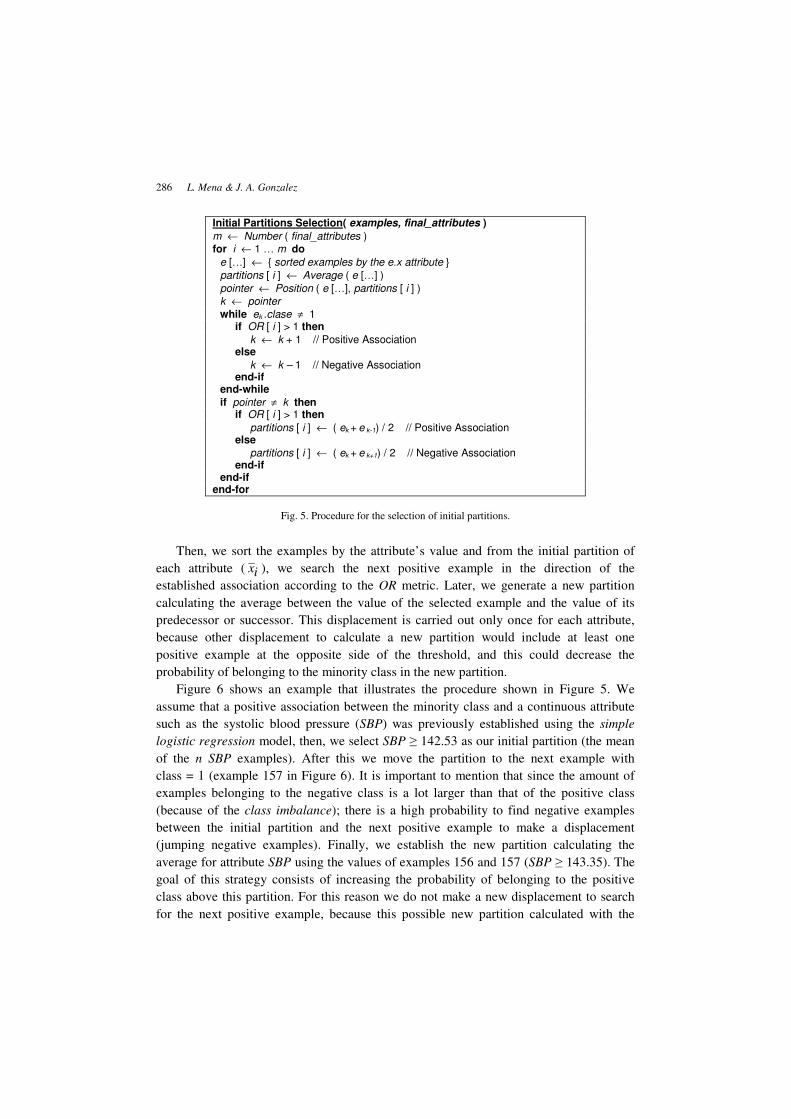
Initial Partitions Selection( examples, final_attributes )
m ← Number ( final_attributes ) for i ← 1 … m do
e […] ← { sorted examples by the e.x attribute }
partitions [ i ] ← Average ( e […] )
pointer ← Position ( e […], partitions [ i ] )
k ← pointer
while ek .clase ≠ 1 if OR [ i ] > 1 then
k ← k + 1 // Positive Association else
k ← k – 1 // Negative Association end-if end-while
if pointer ≠ k then if OR [ i ] > 1 then
partitions [ i ] ← ( ek + e k-1) / 2 // Positive Association else
partitions [ i ] ← ( ek + e k+1) / 2 // Negative Association end-if end-if end-for
Fig. 5. Procedure for the selection of initial partitions.
Then, we sort the examples by the attribute’s value and from the initial partition of
each attribute ( ix ), we search the next positive example in the direction of the
established association according to the OR metric. Later, we generate a new partition
calculating the average between the value of the selected example and the value of its
predecessor or successor. This displacement is carried out only once for each attribute,
because other displacement to calculate a new partition would include at least one
positive example at the opposite side of the threshold, and this could decrease the
probability of belonging to the minority class in the new partition.
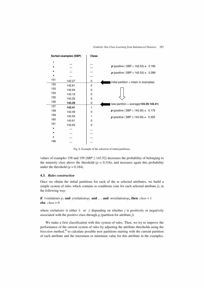
Figure 6 shows an example that illustrates the procedure shown in Figure 5. We
assume that a positive association between the minority class and a continuous attribute
such as the systolic blood pressure (SBP) was previously established using the simple
logistic regression model, then, we select SBP ≥ 142.53 as our initial partition (the mean
of the n SBP examples). After this we move the partition to the next example with
class = 1 (example 157 in Figure 6). It is important to mention that since the amount of
examples belonging to the negative class is a lot larger than that of the positive class
(because of the class imbalance); there is a high probability to find negative examples
between the initial partition and the next positive example to make a displacement
(jumping negative examples). Finally, we establish the new partition calculating the
average for attribute SBP using the values of examples 156 and 157 (SBP ≥ 143.35). The
goal of this strategy consists of increasing the probability of belonging to the positive
class above this partition. For this reason we do not make a new displacement to search
for the next positive example, because this possible new partition calculated with the
Symbolic One-Class Learning from Imbalanced Datasets 287
Sorted examples (SBP) Class
1 ………… …………
• ………… …………
• ………… …………
• ………… …………
151 142.27 0
152 142.81 0 153 142.94 0 154 143.19 0 155 143.25 0 156 143.29 0
157 143.41 1 158 143.49 0 159 143.54 1 160 143.61 0 161 143.63 0
• ………… …………
• ………… …………
• ………… …………
196 ………… …………
Fig. 6. Example of the selection of initial partitions.
values of examples 158 and 159 (SBP ≥ 143.52) decreases the probability of belonging to
the minority class above the threshold (p = 0.316), and increases again this probability
under the threshold (p = 0.184).
4.3. Rules construction
Once we obtain the initial partitions for each of the m selected attributes, we build a
simple system of rules which contains m conditions (one for each selected attribute j), in
the following way:
if 1<relation> p1 and j<relation>pj and …. and m<relation>pm then class = 1
else class = 0
where <relation> is either ≥ or ≤ depending on whether j is positively or negatively
associated with the positive class through pj (partition for attribute j).
We make a first classification with this system of rules. Then, we try to improve the
performance of the current system of rules by adjusting the attribute thresholds using the
bisection method,45
to calculate possible new partitions starting with the current partition
of each attribute and the maximum or minimum value for this attribute in the examples.
p (positive | SBP < 142.53) = 0.185 p (positive | SBP ≥ 142.53) = 0.289 initial partition = mean (n examples)
new partition = average(143.29,143.41) p (positive | SBP < 143.35) = 0.179
p (positive | SBP ≥ 143.35) = 0.325
288 L. Mena & J. A. Gonzalez
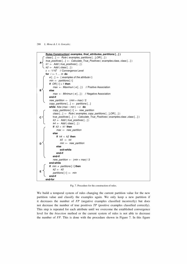
Rules Construction( examples, final_attributes, partitions […………] )
class […] ← Rule ( examples, partitions […],OR […] )
true_positives […] ← Calculate_True_Positives ( examples.class, class […] )
k1 ← Add ( true_positives […] )
k2 ← Add ( class […] )
ε ← 1/10k // Convergence Level
for i ← 1 … m do
e […] ← { examples of the attribute i }
min ← partitions [ i ]
if OR [ i ] > 1 then
max ← Maximun ( e […] ) // Positive Association
else
max ← Minimun ( e […] ) // Negative Association
end-if
new_partition ← (min + max) / 2
copy_partitions […] ← partitions […]
while Abs (max – min ) > ε do
copy_partitions [ i ] ← new_partition
class […] ← Rule ( examples, copy_partitions […],OR […] )
true_positives […] ← Calculate_True_Positives ( examples.class ,class […] )
k3 ← Add ( true_positives […] )
k4 ← Add ( class […] )
if k3 < k1 then
max ← new_partition
else
if k4 < k2 then
k5 ← k4
min ← new_partition
else
exit-while
end-if
end-if
new_partition ← (min + max) / 2
end-while
if min ≠ partitions [ i ] then
k2 ← k5
partitions [ i ] ← min
end-if
end-for
Fig. 7. Procedure for the construction of rules.
We build a temporal system of rules changing the current partition value for the new
partition value and classify the examples again. We only keep a new partition if
it decreases the number of FP (negative examples classified incorrectly) but does
not decrease the number of true positives TP (positive examples classified correctly).
This step is repeated for each attribute until we overcome the established convergence
level for the bisection method or the current system of rules is not able to decrease
the number of FP. This is done with the procedure shown in Figure 7. In this figure
A
E
D
C
B

Symbolic One-Class Learning from Imbalanced Datasets 289
we grouped sets of instructions in sections identified with letters from A to E, which are
described below.
(A) We build an initial system of rules from the set of initial partitions. Then we make a
first classification and save the results. We also store the number of positive
examples classified correctly in k1 and the total number of positive examples
predicted (TP + FP) by the initial system of rules in k2.
(B) Then, we begin an iterative process (1…m) to try to improve the predictive value of
each of the partitions. We estimate a new partition for attribute i by averaging its
initial partition with the maximum or minimum value of the examples for this
attribute (depending on the type of the established association). With the goal of
evaluating the performance of the new partition, we make a copy of the initial
partitions in the copy_partitions […] array.
(C) We build a new system of rules by changing the current partition of attribute i by
the new partition and then, we classify the examples again. We store the number of
positive examples classified correctly in k3 and the total of positive examples
predicted by this rules system in k4.
(D) We then evaluate the results obtained with the new classification. First, we verify if
the number of positive examples classified correctly decreased (k3 < k1), if this
happens we set the current partition as the maximum bench mark to calculate a new
partition. Otherwise we verify if the new classification decreased the number of
negative examples classified incorrectly (k4 < k2), if this happens we store the total
number of positive examples predicted by the current system of rules in k5 and
establish it as the minimum bench mark for the current partition. We continue
estimating new partitions for attribute i with the bisection method while the
difference in absolute value between the maximum and minimum bench mark does
not overcome the established convergence level for the bisection method, or the
current system of rules is not able to decrease the number of negative examples
classified incorrectly.
(E) If the new partition for attribute i improves the predictive values, it is included
in the set of final partitions. Then, the total number of positive examples predicted
by the current rule is upgraded (k2 ← k5), this process is repeated for the m
attributes.
As we can appreciate, the goal of REMED is to maximize the classification
performance of the minority class at each step of the procedures. It starts with the
selection of attributes that are strongly associated with the positive class. Then, it stops
the search for partitions that predict the minority class when it finds the first positive
example (we do this because we do not want to decrease the probability of belonging to
the positive class as shown in Figure 6), and finally it tries to improve the performance of
the rules system but without decreasing the number of TP (positive examples classified
correctly).

290 L. Mena & J. A. Gonzalez
5. Experiments
We compared our one-class approach versus sampling and cost-sensitive approaches.
The datasets used are real-world medical datasets with only two classes. With the
exception of the Cardiovascular Diseases dataset, all were obtained from the UCI
repository.46
In all the cases we only considered changeable (as discussed before in
Section 4.1) and continuous attributes (with higher degree of uncertainty than discrete
attributes). Besides REMED we used the C4.5 and Repeated Incremental Pruning to
Produce Error Reduction (RIPPER) symbolic classifiers, both used in previous works
concerning the class imbalance problem.17,47
In all the cases we applied the 10-fold cross
validation technique to avoid overfitting. Next, we briefly describe the medical datasets
and the symbolic classifiers used in our experiments. We also present the sampling
and cost-sensitive strategies applied to the C4.5 and RIPPER experiments, and describe
the evaluation measures used to evaluate the performance of the different approaches.
Finally, the results are compared in terms of evaluation metrics, comprehensibility
and reliability.
5.1. Datasets
As we previously mentioned, the data collection of real medical datasets is often
expensive, time consuming, and harmful for the patients, this is why medical datasets are
usually conformed by few examples (between 100 and 300) and even less attributes
(because of the high cost of medical tests). For our experiments we used datasets with
different characteristics including two typical medical datasets: Cardiovascular Diseases
and Hepatitis (which meet with the previously mentioned features: few examples and
even fewer attributes), a dataset with few examples but with a considerable number of
attributes: Breast Cancer, and a larger dataset with many examples but few attributes:
Hyperthyroid. The class imbalance rate for the datasets or ratio of positive and negative
examples varied from 1:3 to 1:49.
5.1.1. Cardiovascular diseases
Cardiovascular Diseases are one of the world’s most important causes of mortality which
affect the circulatory system comprising the heart and blood vessels. This dataset was
obtained from an Ambulatory Blood Pressure Monitoring (ABPM)48
study named “The
Maracaibo Aging Study”49
conducted by the Institute for Cardiovascular Diseases of the
University of Zulia, in Maracaibo, Venezuela. The final dataset was conformed by 312
observations and at the end of the study 55 individuals registered a kind of
Cardiovascular Disease, the class imbalance ratio is approximately of 1:5.
The attributes considered were the mean of the SBP and diastolic blood pressure
(DBP) readings, systolic global variability (SGV), diastolic global variability (DGV)
measured with the average real variability,50
and the systolic circadian variability (SCV)51
represented with the gradient of the linear approximation of the readings of SBP.

Symbolic One-Class Learning from Imbalanced Datasets 291
All the attributes were calculated from the ABPM valid readings during the period of
24 hours and the dataset did not present missing values.
5.1.2. Hepatitis
Hepatitis is a viral disease that affects the liver and is generally transmitted by ingestion
of infected food or water. The original dataset was conformed by 19 attributes including
binary discrete and non-changeable continuous attributes (such as age). For our
experiments we only considered 4 changeable continuous attributes: the levels of albumin
(AL), bilirrubin (BL), alkaline phosphatase (AP) and serum glutamic oxaloacetic
transaminase (SGOT) in the blood. The final dataset was conformed by 152 samples, with
30 positive examples, a class imbalance ratio of approximately 1:4 and a rate of missing
values of 23.03%.
5.1.3. Breast cancer
The Wisconsin prognostic Breast Cancer dataset consisted of 10 continuous-valued
features computed from a digitized image of a fine needle aspirate of a breast mass. The
characteristics of the cell nucleus present in the image were: radius (R), texture (T),
perimeter (P), area (A), smoothness (SM), compactness (CM), concavity (C), symmetry
(S), concave points (CP) and fractal dimension (FD). The mean (me), standard error (se),
and "worst" (w) or largest (mean of the three largest values) of these features were
computed for each image, resulting in 30 features. They also considered the tumour size
(TS) and the number of positive axillary lymph nodes observed (LN). This was the least
imbalanced dataset, with a class imbalance ratio approximately of 1:3. The dataset was
conformed by 151 negative examples and 47 positive examples and only 2.02% of the
data presented missing values.
5.1.4. Hyperthyroid
Finally, Hyperthyroid is a condition characterized by accelerated metabolism caused by
an excessive amount of thyroid hormones. This is an extremely imbalanced dataset with a
class imbalance ratio of 1:49 approximately, conformed by 3693 negative examples and
only 79 positive examples. The attributes considered to evaluate this disease of the
thyroid glands were: thyroid-stimulating hormone (TSH), triiodothyronin (T3), total
thyroxine (TT4), thyroxine uptake and free thyroxine index (FTI). The dataset presented
27.07% of missing values.
Once we known each of the medical datasets, we briefly describe in the following
section the classifiers (besides REMED) used in our experiments.
5.2. Classifiers
We only used symbolic classifiers (decision tree and rules), because as we previously
mentioned, black box classification methods (for example neural networks) are not

292 L. Mena & J. A. Gonzalez
generally appropriate for some medical diagnosis tasks, because the medical staff needs
to evaluate and validate the knowledge induced by the machine learning algorithm to
gain enough trust to use the diagnosis knowledge in practice. Therefore, symbolic
classifiers are a better way to reach both objectives, because the generated knowledge is
shown in a form that can be understood by the medical staff. The symbolic classifiers
that we used (C4.5 and RIPPER), besides REMED, were obtained from the Weka
framework.52
5.2.1. C4.5
C4.5 is a popular machine learning classifier for learning decision trees.53
C4.5 is a
discrimination-based approach that can solve multi-class problems and, therefore, it
generates a decision tree with class membership predictions for all the examples. The
tree-building process uses a partitions selection criterion called information gain, which
is an entropy-based metric that measures the purity degree between a partition and its
sub-partitions. C4.5 uses a recursive procedure to choose attributes that yield to purer
children nodes (a totally pure node would be one for which all the examples that it covers
belong to a single class) at each time. After building the decision tree, C45 applies a
pruning strategy to avoid overfitting.
5.2.2. RIPPER
RIPPER is a machine learning classifier that induces sets of classification rules.39
Although RIPPER can solve multi-class problems, the learning process used to solve
binary classification tasks is particularly interesting. RIPPER uses a divide-and-conquer
approach to iteratively build rules to cover previously uncovered training examples
(generally positive examples) into a growing set and a pruning set. Rules are grown by
adding conditions one at a time until the rule covers only a single example in the growing
set (generally negative examples). Thus, RIPPER usually generates rules for each class
from the minority class to the majority class; therefore, it could provide an efficient
method to learn rules only for the minority class.
5.3. Sampling strategy
We used an advanced over-sampling strategy, specifically the Synthetic Minority Over-
Sampling TEchnique (SMOTE).17
This over-sampling approach consists of adding
synthetic minority class examples along the line segments that join any or all the k
minority class nearest neighbours of each minority class example (by default SMOTE
uses k = 5). In general each synthetic sample of the minority class is generated from the
difference between the feature vector of the original sample under consideration and its
nearest neighbours. For our experiments, we only over-sampled the minority class of
each medical dataset at 100% and 200% of its original size. We only combined these
sampling strategies with C4.5 and RIPPER.

Symbolic One-Class Learning from Imbalanced Datasets 293
5.4. Cost-sensitive strategy
We used one of the meta-classifier approaches that the Weka framework provides,
specifically the weka.classifiers.meta.CostSensitiveClassifier. The cost-sensitive strate-
gies used to fill the cost matrix were the following: CTP and CTN were assigned a cost
of 0, CFP was assigned a cost of 1, while CFN was assigned several costs depending on
the class imbalance rate of the datasets. CFN was evaluated with the values of 3, 4, and 5
for almost all the medical datasets (the class imbalance rate of the Breast Cancer,
Hepatitis and Cardiovascular Diseases datasets respectively), except for the extremely
imbalanced (1:49) Hyperthyroid dataset, where we only assigned a cost of 49 to CFN. As
we did with the sampling strategies, we only combined the cost-sensitive strategies with
C4.5 and RIPPER.
5.5. One-class strategy
We used the REMED algorithm as our one-class approach. The unique parameter that
REMED needs is the confidence level to select the significant attributes. We always used
high confidence levels such as 99% or 99.99%. We only applied the REMED algorithm
to the original datasets. We also used the RIPPER algorithm without any of the sampling
and cost-sensitive strategies, because it is considered a good algorithm to learn rules only
for the minority class.12
5.6. Performance evaluation
We evaluated the overall performance of each approach, in terms of evaluation
metrics, comprehensibility and reliability. Regarding the first issue, we used all the
evaluation metrics shown in Figure 1 (accuracy, sensitivity, specificity, and precision).
We also used the geometric mean and AUC calculated with the conventional binormal
method through PLOTROC.xls, available at http://xray.bsd.uchicago.edu/krl/KRL_ROC/
software_index.htm. Besides, we used an additional measure called ranker calculating the
average between the geometric mean and AUC. With respect to the comprehensibility of
the rules, we evaluated the degree of abstraction of the rules systems according to their
size (number of rules and number of conditions in each rule). Finally, to evaluate the
reliability (defined in Section 1) of each rules system, we analyzed the medical validity of
the generated rules comparing their conditions’ thresholds with well-known abnormal
values to diagnose or predict the considered diseases.
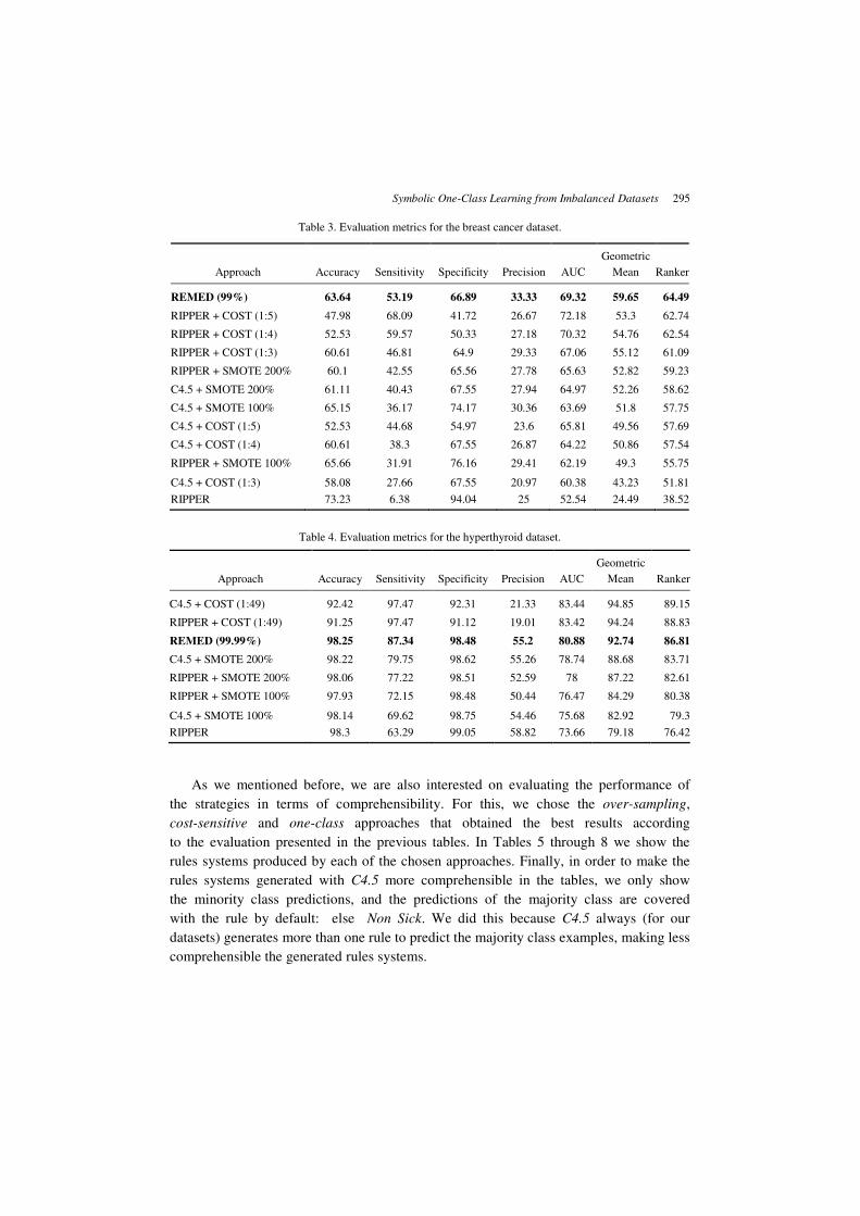
5.7. Experimental results
In this section we show our experimental results, we show them in terms of the
evaluation metrics accuracy, sensitivity specificity, precision, AUC, and geometric mean.
These results are summarized in Tables 1 through 4. In each table we report the results of
the experiments corresponding to each medical dataset. We indicate between parenthesis
the over-sampling rate used with SMOTE, the cost ratio of the used cost-sensitive
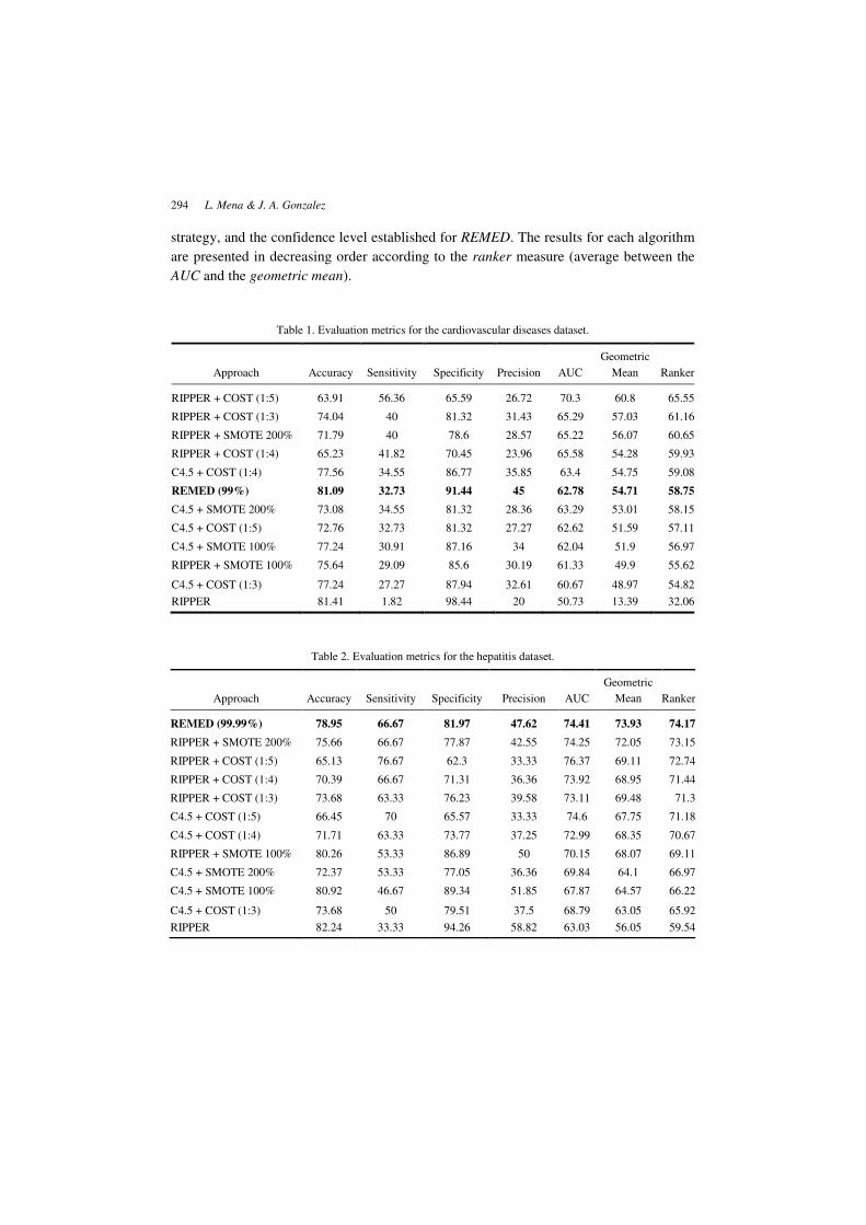
294 L. Mena & J. A. Gonzalez
strategy, and the confidence level established for REMED. The results for each algorithm
are presented in decreasing order according to the ranker measure (average between the
AUC and the geometric mean).
Table 1. Evaluation metrics for the cardiovascular diseases dataset.
Approach Accuracy Sensitivity Specificity Precision AUC
Geometric
Mean Ranker
RIPPER + COST (1:5) 63.91 56.36 65.59 26.72 70.3 60.8 65.55
RIPPER + COST (1:3) 74.04 40 81.32 31.43 65.29 57.03 61.16
RIPPER + SMOTE 200% 71.79 40 78.6 28.57 65.22 56.07 60.65
RIPPER + COST (1:4) 65.23 41.82 70.45 23.96 65.58 54.28 59.93
C4.5 + COST (1:4) 77.56 34.55 86.77 35.85 63.4 54.75 59.08
REMED (99%) 81.09 32.73 91.44 45 62.78 54.71 58.75
C4.5 + SMOTE 200% 73.08 34.55 81.32 28.36 63.29 53.01 58.15
C4.5 + COST (1:5) 72.76 32.73 81.32 27.27 62.62 51.59 57.11
C4.5 + SMOTE 100% 77.24 30.91 87.16 34 62.04 51.9 56.97
RIPPER + SMOTE 100% 75.64 29.09 85.6 30.19 61.33 49.9 55.62
C4.5 + COST (1:3) 77.24 27.27 87.94 32.61 60.67 48.97 54.82
RIPPER 81.41 1.82 98.44 20 50.73 13.39 32.06
Table 2. Evaluation metrics for the hepatitis dataset.
Approach Accuracy Sensitivity Specificity Precision AUC
Geometric
Mean Ranker
REMED (99.99%) 78.95 66.67 81.97 47.62 74.41 73.93 74.17
RIPPER + SMOTE 200% 75.66 66.67 77.87 42.55 74.25 72.05 73.15
RIPPER + COST (1:5) 65.13 76.67 62.3 33.33 76.37 69.11 72.74
RIPPER + COST (1:4) 70.39 66.67 71.31 36.36 73.92 68.95 71.44
RIPPER + COST (1:3) 73.68 63.33 76.23 39.58 73.11 69.48 71.3
C4.5 + COST (1:5) 66.45 70 65.57 33.33 74.6 67.75 71.18
C4.5 + COST (1:4) 71.71 63.33 73.77 37.25 72.99 68.35 70.67
RIPPER + SMOTE 100% 80.26 53.33 86.89 50 70.15 68.07 69.11
C4.5 + SMOTE 200% 72.37 53.33 77.05 36.36 69.84 64.1 66.97
C4.5 + SMOTE 100% 80.92 46.67 89.34 51.85 67.87 64.57 66.22
C4.5 + COST (1:3) 73.68 50 79.51 37.5 68.79 63.05 65.92
RIPPER 82.24 33.33 94.26 58.82 63.03 56.05 59.54
Symbolic One-Class Learning from Imbalanced Datasets 295
Table 3. Evaluation metrics for the breast cancer dataset.
Approach Accuracy Sensitivity Specificity Precision AUC
Geometric
Mean Ranker
REMED (99%) 63.64 53.19 66.89 33.33 69.32 59.65 64.49
RIPPER + COST (1:5) 47.98 68.09 41.72 26.67 72.18 53.3 62.74
RIPPER + COST (1:4) 52.53 59.57 50.33 27.18 70.32 54.76 62.54
RIPPER + COST (1:3) 60.61 46.81 64.9 29.33 67.06 55.12 61.09
RIPPER + SMOTE 200% 60.1 42.55 65.56 27.78 65.63 52.82 59.23
C4.5 + SMOTE 200% 61.11 40.43 67.55 27.94 64.97 52.26 58.62
C4.5 + SMOTE 100% 65.15 36.17 74.17 30.36 63.69 51.8 57.75
C4.5 + COST (1:5) 52.53 44.68 54.97 23.6 65.81 49.56 57.69
C4.5 + COST (1:4) 60.61 38.3 67.55 26.87 64.22 50.86 57.54
RIPPER + SMOTE 100% 65.66 31.91 76.16 29.41 62.19 49.3 55.75
C4.5 + COST (1:3) 58.08 27.66 67.55 20.97 60.38 43.23 51.81
RIPPER 73.23 6.38 94.04 25 52.54 24.49 38.52
Table 4. Evaluation metrics for the hyperthyroid dataset.
Approach Accuracy Sensitivity Specificity Precision AUC
Geometric
Mean Ranker
C4.5 + COST (1:49) 92.42 97.47 92.31 21.33 83.44 94.85 89.15
RIPPER + COST (1:49) 91.25 97.47 91.12 19.01 83.42 94.24 88.83
REMED (99.99%) 98.25 87.34 98.48 55.2 80.88 92.74 86.81
C4.5 + SMOTE 200% 98.22 79.75 98.62 55.26 78.74 88.68 83.71
RIPPER + SMOTE 200% 98.06 77.22 98.51 52.59 78 87.22 82.61
RIPPER + SMOTE 100% 97.93 72.15 98.48 50.44 76.47 84.29 80.38
C4.5 + SMOTE 100% 98.14 69.62 98.75 54.46 75.68 82.92 79.3
RIPPER 98.3 63.29 99.05 58.82 73.66 79.18 76.42
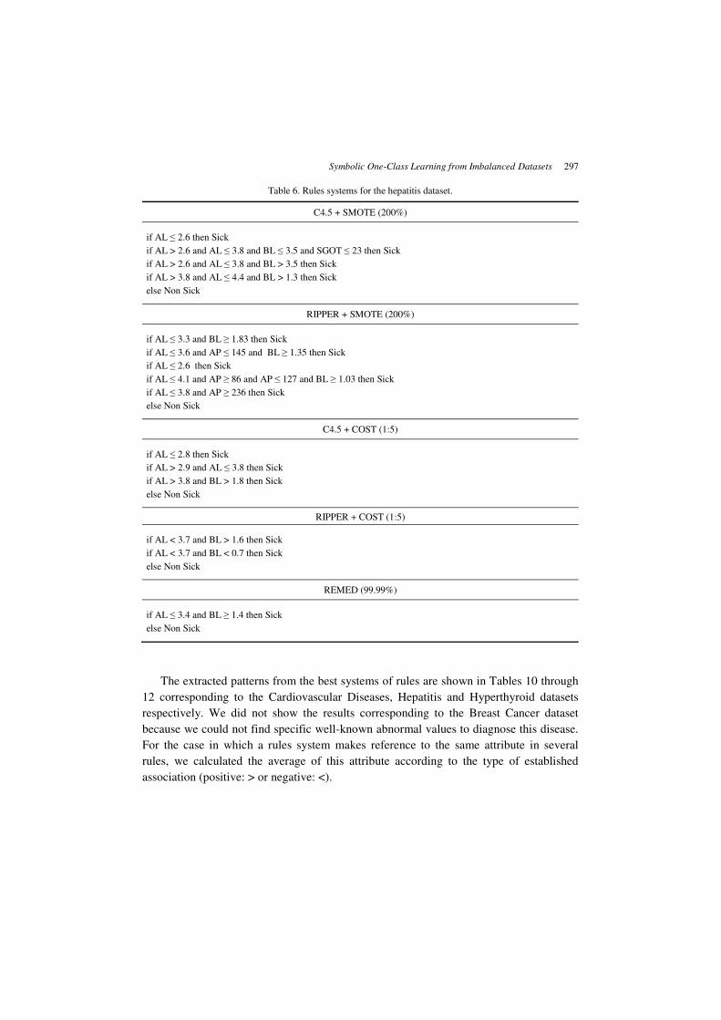
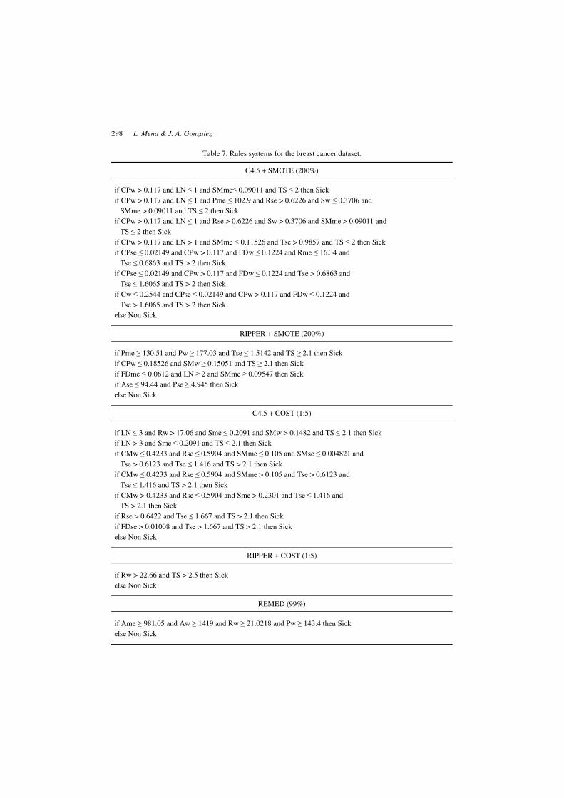
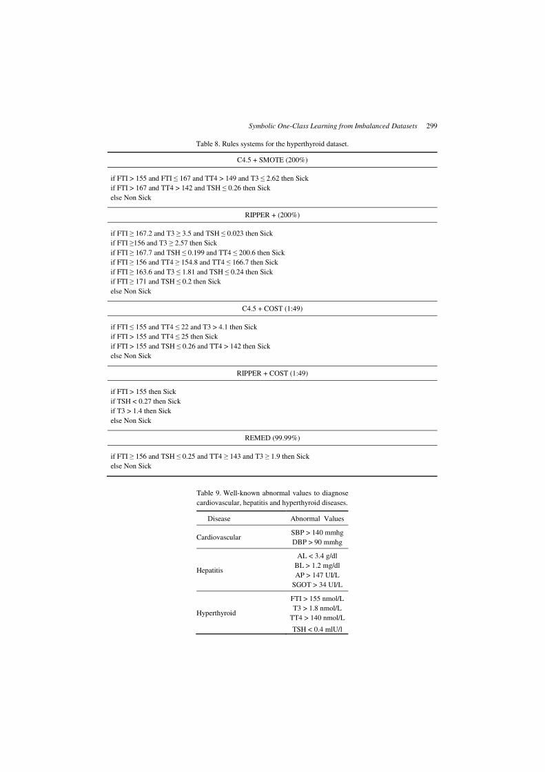
As we mentioned before, we are also interested on evaluating the performance of
the strategies in terms of comprehensibility. For this, we chose the over-sampling,
cost-sensitive and one-class approaches that obtained the best results according
to the evaluation presented in the previous tables. In Tables 5 through 8 we show the
rules systems produced by each of the chosen approaches. Finally, in order to make the
rules systems generated with C4.5 more comprehensible in the tables, we only show
the minority class predictions, and the predictions of the majority class are covered
with the rule by default: else Non Sick. We did this because C4.5 always (for our
datasets) generates more than one rule to predict the majority class examples, making less
comprehensible the generated rules systems.

296 L. Mena & J. A. Gonzalez
Table 5. Rules systems for the cardiovascular diseases dataset.
C4.5 + SMOTE (200%)
if DGV ≤ 7.641 and SBP ≤ 149.435 and SCV > -0.432 and SGV > 6.532 then Sick
if DGV > 7.641 and SBP > 147.015 and SBP ≤ 149.435 and SCV > -0.432 then Sick
if DGV > 6.536 and SBP > 149.435 and SBP ≤ 153.145 then Sick
if DGV > 6.536 and SBP > 153.145 and SCV ≤ -0.324 and SGV ≤ 9.439 then Sick
if DBP ≤ 95.074 and DGV > 6.536 and DGV ≤ 7.323 and SBP > 153.145 and
SCV ≤ -0.324 and SGV > 9.439 then Sick
if DBP ≤ 82.566 and DGV > 6.536 and SBP > 155.89 and SCV > -0.324 then Sick
if DBP > 82.566 and DGV > 6.536 and SBP > 153.145 and SCV > -0.324 then Sick
else Non Sick
RIPPER + SMOTE (200%)
if DBP ≥ 73.274 and SBP ≥ 145.696 and SCV ≥ -0.481 then Sick
if DGV ≤ 7.357 and SCV ≥ -0.348 and SGV ≥ 7.711 and SGV ≤ 9.617 then Sick
if SBP ≥ 123.671 and SBP ≤ 125.306 and SGV ≥ 8.128 then Sick
else Non Sick
C.45 + COST (1:4)
if SBP > 149.435 then Sick
else Non Sick
RIPPER + COST (1:5)
if SBP < 124.732 and SCV > -0.517 then Sick
if SBP > 123.054 then Sick
if SBP > 144.328 and SGV < 9.143 then Sick
if SBP < 128.543 and SGV < 9.143 then Sick
else Non Sick
REMED (99%)
if SBP ≥ 142.1784 and SCV ≥ -0.4025 and SGV ≥ 9.2575 then Sick
else Non Sick
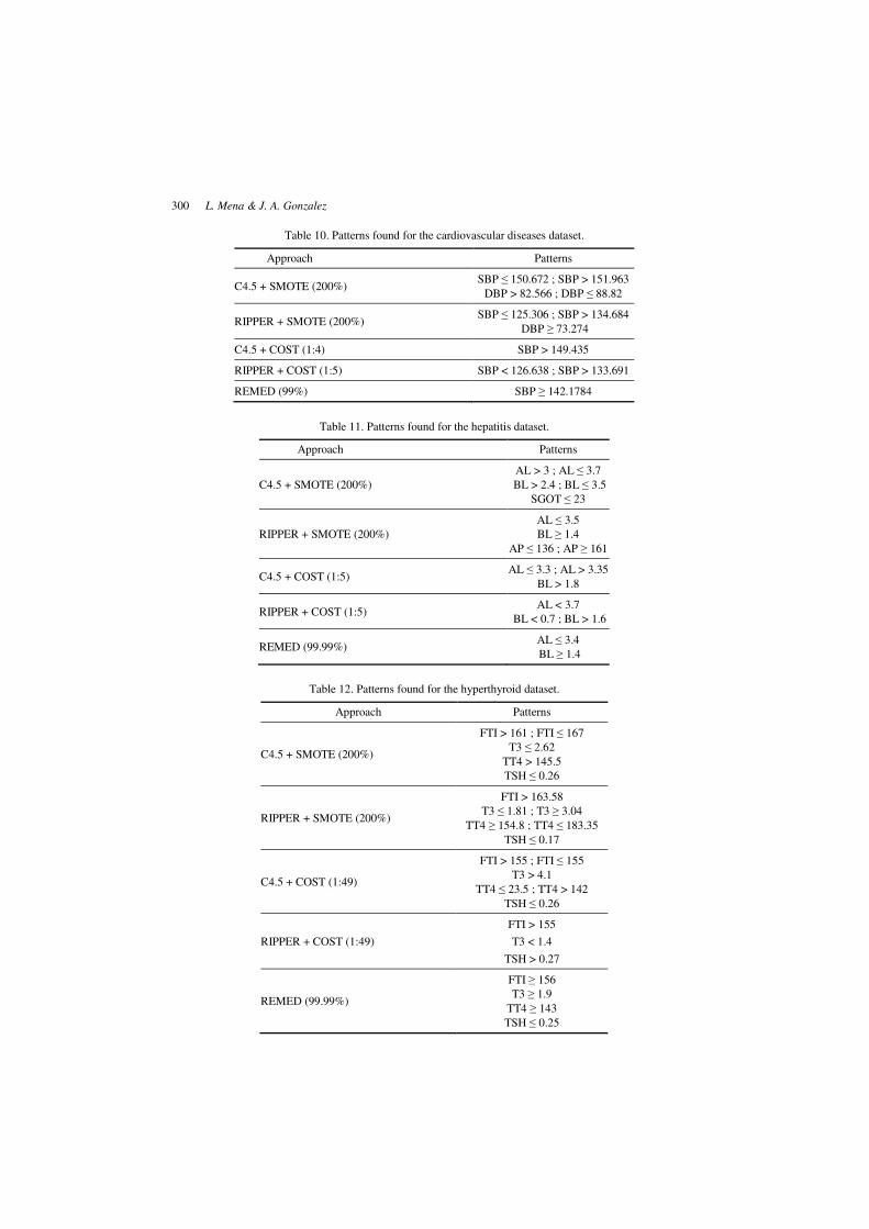
In the last step of our evaluation procedure, we compared the patterns described by
the best systems of rules with well-known abnormal values to diagnose certain
considered diseases. In Table 9 we show well-known abnormal values to diagnose
Cardiovascular, Hepatitis and Hyperthyroid diseases. The Cardiovascular Diseases
abnormal values are associated with hypertension problems (SBP and DBP). In the case
of the Hepatitis disease, these abnormal values are related with levels of proteins (AL),
enzymes (AP and SGOT), and products of degradation of the proteins (BL) in the blood.
Finally, the abnormal values related to the Hyperthyroid disease are associated with some
diagnostic tests of the thyroid hormones (T3, TT4, TSH and FTI).
Symbolic One-Class Learning from Imbalanced Datasets 297
Table 6. Rules systems for the hepatitis dataset.
C4.5 + SMOTE (200%)
if AL ≤ 2.6 then Sick
if AL > 2.6 and AL ≤ 3.8 and BL ≤ 3.5 and SGOT ≤ 23 then Sick
if AL > 2.6 and AL ≤ 3.8 and BL > 3.5 then Sick
if AL > 3.8 and AL ≤ 4.4 and BL > 1.3 then Sick
else Non Sick
RIPPER + SMOTE (200%)
if AL ≤ 3.3 and BL ≥ 1.83 then Sick
if AL ≤ 3.6 and AP ≤ 145 and BL ≥ 1.35 then Sick
if AL ≤ 2.6 then Sick
if AL ≤ 4.1 and AP ≥ 86 and AP ≤ 127 and BL ≥ 1.03 then Sick
if AL ≤ 3.8 and AP ≥ 236 then Sick
else Non Sick
C4.5 + COST (1:5)
if AL ≤ 2.8 then Sick
if AL > 2.9 and AL ≤ 3.8 then Sick
if AL > 3.8 and BL > 1.8 then Sick
else Non Sick
RIPPER + COST (1:5)
if AL < 3.7 and BL > 1.6 then Sick
if AL < 3.7 and BL < 0.7 then Sick
else Non Sick
REMED (99.99%)
if AL ≤ 3.4 and BL ≥ 1.4 then Sick
else Non Sick
The extracted patterns from the best systems of rules are shown in Tables 10 through
12 corresponding to the Cardiovascular Diseases, Hepatitis and Hyperthyroid datasets
respectively. We did not show the results corresponding to the Breast Cancer dataset
because we could not find specific well-known abnormal values to diagnose this disease.
For the case in which a rules system makes reference to the same attribute in several
rules, we calculated the average of this attribute according to the type of established
association (positive: > or negative: <).
298 L. Mena & J. A. Gonzalez
Table 7. Rules systems for the breast cancer dataset.
C4.5 + SMOTE (200%)
if CPw > 0.117 and LN ≤ 1 and SMme≤ 0.09011 and TS ≤ 2 then Sick
if CPw > 0.117 and LN ≤ 1 and Pme ≤ 102.9 and Rse > 0.6226 and Sw ≤ 0.3706 and
SMme > 0.09011 and TS ≤ 2 then Sick
if CPw > 0.117 and LN ≤ 1 and Rse > 0.6226 and Sw > 0.3706 and SMme > 0.09011 and
TS ≤ 2 then Sick
if CPw > 0.117 and LN > 1 and SMme ≤ 0.11526 and Tse > 0.9857 and TS ≤ 2 then Sick
if CPse ≤ 0.02149 and CPw > 0.117 and FDw ≤ 0.1224 and Rme ≤ 16.34 and
Tse ≤ 0.6863 and TS > 2 then Sick
if CPse ≤ 0.02149 and CPw > 0.117 and FDw ≤ 0.1224 and Tse > 0.6863 and
Tse ≤ 1.6065 and TS > 2 then Sick
if Cw ≤ 0.2544 and CPse ≤ 0.02149 and CPw > 0.117 and FDw ≤ 0.1224 and
Tse > 1.6065 and TS > 2 then Sick
else Non Sick
RIPPER + SMOTE (200%)
if Pme ≥ 130.51 and Pw ≥ 177.03 and Tse ≤ 1.5142 and TS ≥ 2.1 then Sick
if CPw ≤ 0.18526 and SMw ≥ 0.15051 and TS ≥ 2.1 then Sick
if FDme ≤ 0.0612 and LN ≥ 2 and SMme ≥ 0.09547 then Sick
if Ase ≤ 94.44 and Pse ≥ 4.945 then Sick
else Non Sick
C4.5 + COST (1:5)
if LN ≤ 3 and Rw > 17.06 and Sme ≤ 0.2091 and SMw > 0.1482 and TS ≤ 2.1 then Sick
if LN > 3 and Sme ≤ 0.2091 and TS ≤ 2.1 then Sick
if CMw ≤ 0.4233 and Rse ≤ 0.5904 and SMme ≤ 0.105 and SMse ≤ 0.004821 and
Tse > 0.6123 and Tse ≤ 1.416 and TS > 2.1 then Sick
if CMw ≤ 0.4233 and Rse ≤ 0.5904 and SMme > 0.105 and Tse > 0.6123 and
Tse ≤ 1.416 and TS > 2.1 then Sick
if CMw > 0.4233 and Rse ≤ 0.5904 and Sme > 0.2301 and Tse ≤ 1.416 and
TS > 2.1 then Sick
if Rse > 0.6422 and Tse ≤ 1.667 and TS > 2.1 then Sick
if FDse > 0.01008 and Tse > 1.667 and TS > 2.1 then Sick
else Non Sick
RIPPER + COST (1:5)
if Rw > 22.66 and TS > 2.5 then Sick
else Non Sick
REMED (99%)
if Ame ≥ 981.05 and Aw ≥ 1419 and Rw ≥ 21.0218 and Pw ≥ 143.4 then Sick
else Non Sick
Symbolic One-Class Learning from Imbalanced Datasets 299
Table 8. Rules systems for the hyperthyroid dataset.
C4.5 + SMOTE (200%)
if FTI > 155 and FTI ≤ 167 and TT4 > 149 and T3 ≤ 2.62 then Sick
if FTI > 167 and TT4 > 142 and TSH ≤ 0.26 then Sick
else Non Sick
RIPPER + (200%)
if FTI ≥ 167.2 and T3 ≥ 3.5 and TSH ≤ 0.023 then Sick
if FTI ≥156 and T3 ≥ 2.57 then Sick
if FTI ≥ 167.7 and TSH ≤ 0.199 and TT4 ≤ 200.6 then Sick
if FTI ≥ 156 and TT4 ≥ 154.8 and TT4 ≤ 166.7 then Sick
if FTI ≥ 163.6 and T3 ≤ 1.81 and TSH ≤ 0.24 then Sick
if FTI ≥ 171 and TSH ≤ 0.2 then Sick
else Non Sick
C4.5 + COST (1:49)
if FTI ≤ 155 and TT4 ≤ 22 and T3 > 4.1 then Sick
if FTI > 155 and TT4 ≤ 25 then Sick
if FTI > 155 and TSH ≤ 0.26 and TT4 > 142 then Sick
else Non Sick
RIPPER + COST (1:49)
if FTI > 155 then Sick
if TSH < 0.27 then Sick
if T3 > 1.4 then Sick
else Non Sick
REMED (99.99%)
if FTI ≥ 156 and TSH ≤ 0.25 and TT4 ≥ 143 and T3 ≥ 1.9 then Sick
else Non Sick
Table 9. Well-known abnormal values to diagnose
cardiovascular, hepatitis and hyperthyroid diseases.
Disease Abnormal Values
Cardiovascular SBP > 140 mmhg
DBP > 90 mmhg
Hepatitis
AL < 3.4 g/dl
BL > 1.2 mg/dl
AP > 147 UI/L
SGOT > 34 UI/L
Hyperthyroid
FTI > 155 nmol/L
T3 > 1.8 nmol/L
TT4 > 140 nmol/L
TSH < 0.4 mlU/l
300 L. Mena & J. A. Gonzalez
Table 10. Patterns found for the cardiovascular diseases dataset.
Approach Patterns
C4.5 + SMOTE (200%) SBP ≤ 150.672 ; SBP > 151.963
DBP > 82.566 ; DBP ≤ 88.82
RIPPER + SMOTE (200%) SBP ≤ 125.306 ; SBP > 134.684
DBP ≥ 73.274
C4.5 + COST (1:4) SBP > 149.435
RIPPER + COST (1:5) SBP < 126.638 ; SBP > 133.691
REMED (99%) SBP ≥ 142.1784
Table 11. Patterns found for the hepatitis dataset.
Approach Patterns
C4.5 + SMOTE (200%)
AL > 3 ; AL ≤ 3.7
BL > 2.4 ; BL ≤ 3.5
SGOT ≤ 23
RIPPER + SMOTE (200%)
AL ≤ 3.5
BL ≥ 1.4
AP ≤ 136 ; AP ≥ 161
C4.5 + COST (1:5) AL ≤ 3.3 ; AL > 3.35
BL > 1.8
RIPPER + COST (1:5) AL < 3.7
BL < 0.7 ; BL > 1.6
REMED (99.99%) AL ≤ 3.4
BL ≥ 1.4
Table 12. Patterns found for the hyperthyroid dataset.
Approach Patterns
C4.5 + SMOTE (200%)
FTI > 161 ; FTI ≤ 167
T3 ≤ 2.62
TT4 > 145.5
TSH ≤ 0.26
RIPPER + SMOTE (200%)
FTI > 163.58
T3 ≤ 1.81 ; T3 ≥ 3.04
TT4 ≥ 154.8 ; TT4 ≤ 183.35
TSH ≤ 0.17
C4.5 + COST (1:49)
FTI > 155 ; FTI ≤ 155
T3 > 4.1
TT4 ≤ 23.5 ; TT4 > 142
TSH ≤ 0.26
RIPPER + COST (1:49)
FTI > 155
T3 < 1.4
TSH > 0.27
REMED (99.99%)
FTI ≥ 156
T3 ≥ 1.9
TT4 ≥ 143
TSH ≤ 0.25

Symbolic One-Class Learning from Imbalanced Datasets 301
6. Discussion
In this section we discuss the experimental results presented in Section 5. Besides,
we try to determine an issue previously outlined: up to what degree is it really appropriate
to apply a sampling or cost-sensitive machine learning strategy to imbalanced datasets.
We do this with the goal of trying to establish the best strategy to solve the considered
class imbalance problem using the evaluation metrics, comprehensibility, and the
reliability of the results, and compare the advantages and disadvantages of applying each
strategy.
6.1. Evaluation Metrics
First, we should consider how complex it is to apply a machine learning strategy to
medical diagnosis. A clear example of this is the moderate performance achieved by the
used classifiers in terms of evaluation metrics, because in almost all the cases the best
performance did not reach a value of 80% (except for the Hyperthyroid dataset) in terms
of AUC, geometric mean, and ranker. Therefore, as we previously explained (in Section
3) there are some inconveniences that make even harder the classification task in medical
datasets, even more, we should also mention that in order to apply any class imbalance
strategy (such as over-sampling), it is necessary to determine additional parameters. This
is the case of the appropriate over-sampling and cost ratio rates. This is why our one-
class approach offers an advantage, because the only parameter that it needs to set is the
confidence level that it will use to select the significant attributes (99% or 99.99%), and
this allows a more automated learning process.
With respect to the REMED algorithm’s performance, it obtained competitive results
achieving the 6th, 1st, 1st and 3rd place (according to the ranker measure) in the
considered datasets. A difference with other symbolic one-class approaches such as
BRUTE and SHRINK, where the goal is to reach high sensitivity through accurate positive
rules without caring about the specificity loss, is that REMED achieved good sensitivity
without a concomitant decrease of specificity. On the other hand, REMED significantly
outperformed simple RIPPER (without sampling nor cost-sensitive strategies) in all the
cases.
With the goal of making a more complete analysis, we chose the best over-sampling
and cost-sensitive approaches (with RIPPER or C4.5) for each dataset, and we followed
the methodology presented by Mitchell in Ref. 54 to determine the level of significance
of the comparison of REMED versus these approaches. We used the two-tailed paired t-
test method with a confidence level of 95%. The results of this comparison are shown in
Tables 13 (performance averages) and 14 (two-tailed t-test comparison).
We can appreciate in Figure 13 that the best performance average was for the cost-
sensitive approaches (72.55) followed by REMED (71.06) and then the over-sampling
approaches (69.19), but without a statistical significant difference among them for the
selected confidence level (95%).

302 L. Mena & J. A. Gonzalez
Table 13. Performance averages of REMED and the best over-sampling and cost-sensitive approaches.
Dataset
Over-Sampling
Approaches
Cost-Sensitive
Approaches REMED
Cardiovascular Diseases 60.65 (RIPPER 200%) 65.55 (RIPPER 1:5) 58.75
Hepatitis 73.15 (RIPPER 200%) 72.74 (RIPPER 1:5) 74.17
Breast Cancer 59.23 (RIPPER 200%) 62.74 (RIPPER 1:5) 64.49
Hyperthyroid 83.71 (C4.5 200%) 89.15 (C4.5 1:49) 86.81
Average 69.19 72.55 71.06
Standard Deviation 11.53 11.84 12.28
Table 14. Results of two-tailed t-test for the performance comparison.
Comparison
Difference
(Mean X – Y)
Two-Tailed
P value
Statistical
Significance
REMED – Over-Sampling Approaches 1.87 0.543 Not Significant
REMED – Cost-Sensitive Approaches –1.49 0.5188 Not Significant
Cost-Sensitive – Over-Sampling Approaches 3.36 0.084 Not Significant
Table 15. Precision averages of REMED and the best over-sampling and cost-sensitive approaches.
Dataset
Over-Sampling
Approaches
Cost-Sensitive
Approaches REMED
Cardiovascular Diseases 28.57 (RIPPER 200%) 26.72 (RIPPER 1:5) 45
Hepatitis 42.55 (RIPPER 200%) 33.33 (RIPPER 1:5) 47.62
Breast Cancer 27.78 (RIPPER 200%) 26.67 (RIPPER 1:5) 33.33
Hyperthyroid 55.26 (C4.5 200%) 21.33 (C4.5 1:49) 55.2
Average 38.54 27.01 45.29
Standard Deviation 13.05 4.91 9.07
Table 16. Results of two-tailed t-test for the precision comparison.
Comparison
Difference
(Mean X – Y)
Two-Tailed
P value
Statistical
Significance
REMED – Over-Sampling Approaches 6.75 0.1469 Not Significant
REMED – Cost-Sensitive Approaches 18.28 0.0497 Significant
Cost-Sensitive – Over-Sampling Approaches –11.53 0.2308 Not Significant
On the other hand, REMED always achieved the highest precision combined with the
best performance in terms of the ranker measure; that is, it correctly classified more
positive examples (TP) with a less number of FP. We show in tables 15 and 16 the
results of the precision comparison between REMED and the best over-sampling and
cost-sensitive approaches (according to the ranker measure).
We can see in Table 16 that REMED significantly outperformed (P = 0.0497) the best
cost-sensitive approach in terms of precision, this is important because despite that the

Symbolic One-Class Learning from Imbalanced Datasets 303
cost-sensitive approaches achieved the best performance average in terms of the ranker
measure, these made it with the lowest precision average (27.01), while REMED
achieved a competitive performance average with the highest precision average (45.29),
generating rules systems with more precise positive rules.
With respect to the selection of the best over-sampling strategy, over-sampling at
200% (the highest sampling rate) it always gave better results than over-sampling at
100%. In the case of the best cost-sensitive strategy, usually selected the highest possible
cost producing the best results (except for C4.5 in the Cardiovascular Diseases dataset).
On the other hand, the over-sampling and cost-sensitive approaches with RIPPER almost
always outperformed the C4.5 results (except in the case of the Hyperthyroid dataset),
this was expected because simple RIPPER is a good algorithm to generate positive rules,
and when it is biased with over-sampling or cost-sensitive strategies it significantly
improved its performance in terms of evaluation metrics.
However, to be able to evaluate the overall performance of each approach, it is
necessary to compare the performance of these strategies in terms of comprehensibility
and reliability, and thus determine how dangerous (generating incomprehensible and
invalid results because of the unmeasured use of these techniques) can be the use of
sampling and cost-sensitive strategies combined with standard classifiers. In Sections 6.2
and 6.3 we discuss these issues.
6.2. Comprehensibility
As we can clearly appreciate in Tables 5 through 8, REMED almost always produced
more comprehensible systems of rules than the rest of the class imbalance approaches.
We conclude this because the degree of abstraction of the rules systems was almost
always larger, with the exception of C4.5 + COST (1:4) in the Cardiovascular Diseases
dataset and RIPPER + COST (1:4) in the Breast Cancer dataset, where it was the same
(Tables 5 and 7 respectively). Thus, REMED always generated rules systems with only
one rule to predict the minority class examples. Therefore, this represents an important
advantage in domains that require models with a high degree of comprehensibility, as it is
the case of medical diagnosis tasks.
Another advantage of REMED, specifically for medical domains, is that it does not
produce rules with enclosed intervals (e.g. a ≤ x ≤ b). This is important because it could
represent an inconvenience for medical diagnosis, where the risk of developing a disease
is directly proportional to the increase or decrease of the values of certain medical
attributes. Besides, the increment or decrement of a medical attribute could be related to
two different diseases (e.g. Hypothyroid and Hyperthyroid), and therefore a rule with
enclosed intervals could lead the medical staff to an erroneous medical diagnosis.
Thus, we can appreciate how in almost all the cases the rest of the class imbalance
approaches generated rules systems with enclosed intervals, or with rules that made
reference to the same attribute but establishing different types of association between the
attribute and the disease (positive and negative), and both situations could confuse the
medical staff at the moment of validating the diagnosis knowledge.

304 L. Mena & J. A. Gonzalez
6.3. Reliability
Finally, in relation with the reliability of the obtained patterns, we can observe in
Tables 10 through 12 that in all the cases the rules generated by REMED presented
patterns close to the well-known abnormal values considered for each disease as shown
in Table 9, and with the same type of association between the attribute and the disease.
This is how we prove that REMED’s results are reliable and even when other approaches
might produce results with higher performance in terms of the evaluation metrics these
are losing medical validity. We think that we can use these results to determine the level
of sampling and cost-sensitive ratio that should be used before falling in an overfitting
problem. It is also important to point out that the patterns obtained by REMED to
diagnose each disease, were obtained directly from the unique REMED’s rule to predict
the minority class examples in each medical dataset, while for the rest of the class
imbalance approaches, the corresponding pattern was almost always obtained from the
average of the partitions of several rules (except for C4.5 + COST (1:4) in the
Cardiovascular Diseases dataset and RIPPER + COST (1:49) in the Hyperthyroid
dataset).
In the case of the Cardiovascular Diseases dataset (Table 10), REMED generated the
closest pattern (> 142.1784) to the SBP abnormal value (> 140 mmhg), while the rest of
the class imbalance approaches generated average patterns that were not so close and
almost always with both types of association (positive and negative), except for C4.5 +
COST (1:4). With respect to the DBP abnormal value (> 90 mmhg), REMED excluded
this attribute of its rules system, while RIPPER + SMOTE (200%) presented an average
pattern with the same type of association but it was not so close (≥ 73.274), and C4.5 +
SMOTE (200%) was closer (≤ 88.82) but with the opposite type of association.
In the Hepatitis dataset (Table 11), REMED generated patterns (AL ≤ 3.4 and
BL ≥ 1.4) close to the AL and BL abnormal values (AL < 3.4 g/dl and BL > 1.2 mg/dl).
This time RIPPER + SMOTE (200%) also obtained average patterns (AL ≤ 3.5 and
BL ≥ 1.4) close to these abnormal values just as REMED did, but also included rules
with patterns (AP ≤ 136 ; AP ≥ 161) not so close and with both types of association for
the AP abnormal value (AP > 147 UI/L). Another approach that obtained patterns close
to the AL abnormal value was C4.5 + COST (1:5), but it included the two types of
association (AL ≤ 3.3 ; AL > 3.35) and it did not obtain a close pattern (BL > 1.8) to the
BL abnormal value. The C4.5 + SMOTE (200%) and RIPPER + COST (1:5) approaches
obtained AL and BL patterns that were not close to the well-known abnormal values and
included both types of associations, even C4.5 + SMOTE (200%) generated a not so close
pattern and with the opposed association: SGOT ≤ 23, while the SGOT abnormal value is
SGOT > 34 UI/L.
Finally, for the Hyperthyroid dataset (Table 12), REMED generated patterns
(FTI ≥ 156 ; T3 ≥ 1.9 ; TT4 ≥ 143 ; TSH ≤ 0.25) really close to almost all the well-
known abnormal values. It obtained the closest pattern to the T3 abnormal value
(T3 > 1.8 nmol/L as shown in Table 9). The only abnormal value for which REMED did
not obtain a close pattern was the TSH abnormal value (TSH < 0.4 mlU/l), but the rest of

Symbolic One-Class Learning from Imbalanced Datasets 305
the class imbalance approaches could not either obtain patterns close to this abnormal
value. In the case of the C4.5 and RIPPER + COST (1:49) approaches, they obtained
exact patterns for the FTI abnormal value (FTI > 155 nmol/L), but patterns far away from
the T3 abnormal value with an opposite type of association (T3 < 1.4) in the case of
RIPPER, while C4.5 + COST (1:49) generated patterns with both types of association for
both, the FTI abnormal value (FTI > 155 ; FTI ≤ 155) and for the TT4 abnormal value
(TT4 ≤ 23.5 ; TT4 > 142). The C4.5 and RIPPER + SMOTE (200%) approaches always
obtained patterns with values not so close to the well-known abnormal values and with
both types of association, even in the case of C4.5 + SMOTE (200%) with an opposed
type of association (T3 ≤ 2.62) for the T3 abnormal value.
It is important to point out that we compared the generated patterns with abnormal
values to diagnose certain diseases, only to measure the reliability of the patterns in terms
of their medical validity for well-known medical attributes, however, it is clear that the
main goal of machine learning in the medical diagnosis task is to find new patterns to
provide the medical staff with a novel point of view about a given problem, and this
could be the case of the patterns generated for the Breast Cancer dataset or the blood
pressure variability (global and circadian) in the Cardiovascular Diseases dataset.
7. Conclusions and Future Work
We can conclude from the obtained results, that REMED could be a very competitive
approach to work with class imbalance datasets, in particular for medical diagnosis
datasets because, as we could see, it possesses the desired features to solve medical
diagnosis tasks: 1) good overall performance, because REMED reached a good overall
performance in terms of evaluation metrics, comprehensibility and reliability, 2) the
comprehensibility of diagnostic knowledge, because REMED always generated rules
systems with the same or a larger degree of abstraction than the rest of the class
imbalance approaches (generating one rule to predict minority class examples
independently of the number of examples n and initial attributes m), 3) the ability to
support decisions, because the fact that the rules systems generated from REMED are
always supported by a selection of attributes with high confidence levels (99% or
99.99%), could provide the medical staff with enough trust to use these rules in practice,
and 4) the ability of the algorithm to reduce the number of medical tests necessary to
obtain a reliable diagnosis, because REMED uses the simple logistic regression model to
only select attributes strongly associated with the studied disease.
With respect to the implementation of the REMED algorithm as a general strategy to
work with class imbalance problems, we can appreciate how its overall performance was
better than that of the rest of the class imbalance approaches, because REMED showed to
be competitive with the best over-sampling and cost-sensitive approaches in terms of the
evaluation metrics used, ranked as 6th, 1st, 1st and 3rd and without statistical significant
difference with respect to these approaches, but significantly outperformed the best cost-
sensitive approaches in terms of precision. Besides, REMED always generated more
general systems of rules and therefore, with a lower degree of overfitting. However, the

306 L. Mena & J. A. Gonzalez
most important aspect to consider is the reliability of REMED’s patterns with respect to
their medical validity, because these patterns always presented values with the same type
of association and close to the well-known abnormal values considered for each disease,
while the other class imbalance approaches that ranked in the first positions in terms of
evaluation metrics (usually using a large over-sampling and cost ratio rate) presented a
lower performance in terms of reliability. Therefore, the bias introduced through the
over-sampling and cost-sensitive strategies, although could improve the performance in
terms of evaluation metrics, also generated biased knowledge with a high degree of
overfitting that might not be applicable to the general population. On the other hand, the
REMED’s knowledge extraction process is more automated, because it is not necessary to
establish an appropriate over-sampling rate or cost ratio (before running the algorithm),
and the patterns can be obtained directly from the unique generated rule to predict the
minority class examples.
Finally, REMED does not pretend to be the panacea of machine learning in medical
diagnosis, but a good approach with the previously mentioned features to solve medical
diagnosis tasks. On the other hand, the results obtained with REMED could be used to
establish the adequate over-sampling rate or cost ratio parameters required by other
approaches. We will continue with our research to find an automatic way to adjust these
parameters to produce patterns similar to those found with REMED (which are more
reliable as they adjusted to well-known risk factors) and then reduce the overfitting level
of algorithms using these techniques. For the application of REMED to other types of
class imbalance domains, we first should increase its versatility, including modifications
that allow it to consider discrete attributes, to work with multi-class problems, and in
some cases, to generate rules systems with enclosed intervals.
References
1. Prodomidis, A. L., & Stolfo, S. J. (1999). Agent-based distributed learning applied to fraud
detection. Technical Report CUCS-014-99, Department of Computer Science, Columbia
University.
2. Bojarczuck, C. C., Lopes, H. S., Freitas, A. A., & Michalkiewicz, E. L. (2004). A
constrained-syntax genetic programming system for discovering classification rules:
application to medical data sets. Artificial Intelligence in Medicine, 30(1): 27-48.
3. Herna, L. V., & Hongyu, G. (2004). Multiple classifier prediction improvements against
imbalanced datasets through added synthetic examples. In Proceedings of the 10th
International Workshop on Syntactical and Structural Pattern Recognition and 5th
International Workshop on Statistical Pattern Recognition (SSPR & SPR-2004), pp. 974-982.
4. Japkowicz, N. (2000). Learning from imbalanced data sets: a comparison of various strategies.
In Papers from the AAAI Workshop on Learning from Imbalanced Data Sets. Tech, rep. WS-
00-05, Menlo Park, CA: AAAI Press.
5. Chawla, N. V., Japkowicz, N., & Kolcz, A. (Eds.) (2003). Editorial in Proceedings of the
2003International Conference on Machine Learning (ICML-2003) Workshop on Learning
from Imbalanced Data Sets.
6. Metz, C.E., Herman, B. A., & Shen, J. H. (1998). Maximum likelihood estimation of receiver
operating characteristic (ROC) curves from continuously-distributed data. Statistics in
Medicine, 17(9):1033-53.

Symbolic One-Class Learning from Imbalanced Datasets 307
7. Hanley, J. A. (1996). The use of the 'binormal' model for parametric roc analysis of
quantitative diagnostic tests. Statistics in Medicine, 15(14):1575-1585.
8. Kubat, M., Holte, R.C., & Matwin, S. (1998). Machine learning for the detection of oil spills
in satellite radar images. Machine Learning, 30: 195-215.
9. Jo, T., & Japkowicz, N. (2004). Class imbalances versus small disjuncts. SIGKDD
Explorations, 6(1): 40-49.
10. Weiss, G. M., & Provost, F. (2003). Learning when training data are costly: the effect of class
distribution on tree induction. Journal of Artificial Intelligence Research, 19: 315-354.
11. Japkowicz, N. (2001). Concept Learning in the presence of between-class and within-class
imbalance. In Proceedings of the Fourteenth Conference of the Canadian Society for
Computational Studies of Intelligence, pp. 67-77.
12. Weiss, G. M. (2004). Mining with rarity: a unifying framework. SIGKDD Explorations,
6(1):7-19.
13. Holte, R. C., Acker, L.E., & Porter, B.W. (1989). Concept learning and the problem of small
disjuncts. In Proceedings of the Eleventh International Joint Conference on Artificial
Intelligence, pp. 813-818. San Mateo, CA: Morgan Kaufmann.
14. Prati, R. C., Batista, G. E. A. P. A., & Monard, M. C. (2004). Learning with class skews and
small disjuncts. In Proceedings of the 17th Brazilian Symposium on Artificial Intelligence
(SBIA-2004), pp. 296-306.
15. Japkowicz, N., & Stephen, S. (2002). The class imbalance problem: a systematic study.
Intelligent Data Analysis Journal, 6(5).
16. Prati, R. C., Batista, G. E. A. P. A., & Monard, M. C. (2004). Class imbalances versus class
overlapping: an analysis of a learning system behaviour. In Proceedings of the III Mexican
International Conference on Artificial Intelligence (MICAI-2004), pp. 312-321.
17. Chawla, N. V., Bowyer, K. W., Hall, L. O., & Kegelmeyer, W. P. (2002). SMOTE: Synthetic
Minority Over-sampling TEchnique. Journal of Artificial Intelligence, 16: 321-357.
18. Batista, G. E. A. P. A., Prati, R. C., & Monard, M. C. (2004). A study of the behavior of
several methods for balancing machine learning training data. SIGKDD Explorations, 6(1): 20-
29.
19. Ling, C., & Li, C. (1998). Data mining for direct marketing problems and solutions. In
Proceedings of the Fourth International Conference on Knowledge Discovery and Data
Mining (KDD-98), pp. 73-79 New York, NY. AAAI Press.
20. Domingos, P. (1999). MetaCost: A general method for making classifiers cost sensitive. In
Proceedings of the 5th ACM SIGKDD International Conference on Knowledge Discovery and
Data Mining, pp. 155-164 San Diego, CA. ACM Press.
21. Estabrooks, A., Japkowicz, N. (2001). A mixture-of-experts framework for learning from
learning from unbalanced data sets. In Proceedings of the 2001 Intelligent Data Analysis
Conference, pp. 34-43.
22. Breiman, L., Friedman, J. H., Olshen, R. A., & Stone, C. J. (1984). Classification and
regression trees. Wadsworth & Books, Pacific Grove, CA.
23. McCarthy K., Zabar B., & Weiss, G. (2005). Does cost-sensitive learning beat sampling for
classifying rare classes? In Proceedings of the 1st International Workshop on Utility-based
Data Mining. pp. 69-77 New York, NY. ACM Press.
24. Chawla, N. V. (2003). C4.5 and imbalanced data sets: investigating the effect of sampling
method, probabilistic estimate, and decision tree structure. In Proceedings of the 2003
International Conference on Machine Learning (ICML-2003) Workshop on Learning from
Imbalanced Data Sets.
25. Elkan, C. (2001). The foundations of cost-sensitive learning. In Proceedings of the
Seventeenth International Conference on Machine Learning (ICML-2001), pp. 239-246.

308 L. Mena & J. A. Gonzalez
26. Japkowicz, N. (2001). Supervised versus unsupervised binary-learning by feedforward neural
networks. Machine Learning, 42(1/2): 97-122.
27. Raskutti, B., & Kowalczyk, A. (2004). Extreme rebalancing for svms: a case study. SIGKDD
Explorations, 6(1): 60-69.
28. Barandela, R., Sanchez, J. S., Garcia, V., & Rangel, E. (2003). Strategies for learning in class
imbalance problems. Pattern Recognition, 36(3): 849-851.
29. Tax, D. (2001). One-class classification. Ph.D. thesis, Delft University of Technology.
30. Hinton, G. (1989). Connectionist learning procedures. Artificial Intelligence, 40:185-234.
31. Japkowicz, N. (2001). The class imbalance problem: significance and strategies. In
Proceedings of the 2000 International Conference on Artificial Intelligence (ICAI-2001),
vol. 1, pp. 111-117.
32. Japkowicz, N., Myers, C., & Gluck, M.A. (1995). A novelty detection approach to
classification. In Proceedings of the Fourteenth Joint Conference on Artificial Intelligence,
pp. 518-523.
33. Manevitz L., & Malik, Y. (2001). One-class svms for document classification. Journal of
Machine Learning Research, pp. 139-154.
34. Schölkopf, B., Platt, J., Shawe-Taylor, J. Smola, A. J., & Williamson, R. C. (2001). Estimating
the support of a high-dimensional distribution. Neural Computation, 13(7):1443-1472.
35. Cohen, G., Hilario, M., & Pellegrini, C. (2004). One-class support vector machines with a
conformal kernel. A case study in handling class imbalance. In Proceedings of the 10th
International Workshop on Syntactical and Structural Pattern Recognition and 5th
International Workshop on Statistical Pattern Recognition (SSPR & SPR-2004), pp.850-858.
36. Zhang, J., Ma, K., Er, M. H., & Chong, V. (2004). Tumor segmentation from magnetic
resonance imaging by learning via one-class support vector machine. International Workshop
on Advanced Image Technology (IWAIT04), pp. 207-211.
37. Riddle, P., Segal, R., & Etzioni, O. (1994). Representation design and brute-force induction in
a boeing manufacturing domain. Applied Artificial Intelligence, 8:125-147
38. Kubat, M., Holte, R., & Matwin, S. (1997). Learning when negative examples abound. In
Proceeding of the 9th European Conference on Machine Learning (ECML-1997), Prague.
39. Cohen, W. (1995). Fast effective rule induction. In Proceedings of Twelfth International
Conference on Machine Learning (ICML-95), pp. 115-123 Lake Tahoe, CA: Morgan
Kaufman.
40. Kononenko, I. (2001). Machine learning for medical diagnosis: history, state of the art and
perspective. Artificial Intelligence in Medicine, 23(1): 89-109.
41. Mena, L., & Gonzalez, J. A. (2006). Machine learning for imbalanced datasets: application in
medical diagnostic. In Proceedings of the Nineteenth International Florida Artificial
Intelligence Research Society Conference (FLAIRS-2006), pp. 574-579, Melbourne Beach, FL.
AAAI Press.
42. Hosmer, D., & Lemeshow, S. (1989). Applied logistic regression. John Wiley and Sons, Inc.
43. Aldrich, J. (1997). R.A. Fisher and the making of maximum likelihood 1912-1922. Statistical
Science, 12(3): 162-176.
44. Zheng, Z., Wu, X., & Srihari, R. (2004). Feature selection for text categorization on
imbalanced data. SIGKDD Explorations, 6(1):80-89.
45. Burden, R. L., & Faires, J. D. (2000). Numerical Analysis, 7th ed., Brooks/Cole.
46. Murphy, P., & Aha, D. (1994). UCI repository of machine learning databases [machine-
readable data repository]. Technical Report, University of California, Irvine.
47. Weiss, G. M. (2003). The effect of small disjuncts and class distribution on decision tree
learning. Ph.D. thesis, Department of Computer Science, Rutgers University.
48. Mancia, G. (1990). Ambulatory blood pressure monitoring: research and clinical applications.
Journal of Hypertension, (Suppl 7): S1-S13.

Symbolic One-Class Learning from Imbalanced Datasets 309
49. Maestre, G., Pino, G., Molero, A., Silva, E., Zambrano, R., Falque, L., Gamero M. P., &
Sulbaran, T. A. (2002). The Maracaibo aging study: population and methodological issues.
Neuropidemiology, 21: 194-201.
50. Mena, L., Pintos, S., Queipo, N., Aizpurua, J., Maestre, G., & Sulbaran, T. (2005). A reliable
index for the prognostic significance of blood pressure variability. Journal of Hypertension,
23: 505–512.
51. Frattola, A., Parati, G., Cuspidi, C., Albini, F., & Mancia, G. (1993). Prognostic value of
24-hour blood pressure variability. Journal of Hypertension, 11: 1133-1137.
52. Witten, I. H., & Frank, E. (2000). Data mining: practical machine learning tools and
techniques with Java implementations. San Francisco, CA: Morgan Kaufmann.
53. Quinlan, J. R. (1993). C4.5: Programs for Machine Learning. San Mateo, CA: Morgan
Kaufmann.
54. Mitchell, T. (1997). Machine Learning. McGraw-Hill.