Symbolic feature detection for image understanding

aIbDept. o

In this study wto represent uphotometric circular and shape class aviews. For recolor-based mexploiting muwork to impro Keywords: o

Automatic immost importamedical diagn

A flow diagra

One has tworegular grid pimage evidengeometric andLaplace/Affin(Maximally SRegions) [8],

Descriptors rthe neighborh

Symbo

Internationaof Electrical

we propose a underlying loand similarityelliptic respecambiguity of ecognition of umethod in avultispectral anove the propo

object recognit

mage understanant and challnosis, from re

am of the ima

o options for points of the inces from the d photometricne [3], SIFT Stable Extrem and Edge Ba

represent the lhood of point

olic featuSinem As

al Computerl and Electro

model-drivenocal shapes thy transformatctively pit andeach pixel. Wunknown obje

verage, howevnalysis and mosed approach

tion, pixel lab

nding, which lenging problmote sensed i

ge understand

Fi

descriptor extimage, possibso called inte

c transformatio(Scale Invari

mal Regions) sed Regions (

ocal characters. However, o

ure deteslana, Ceyhur Institute, Eonics Engin

A

n codebook gehey reside in.ions applied d hill and usedWe achieved ects, we couldver we could

multiscale apprfurther.

belling, model

1. INinvolves scenems in compimaging to me

ding process is

igure 1. A flow

traction: The ly with some erest points, wons. State-of-aiant Feature T[6], EBSR (E

(EBR) [9].

ristics of the ione may desir

ction forun Burak AkEge Universneering, Bo

ABSTRACT

eneration methIn the first von eight protd randomized~90% accurad not outperfo

d outperform roach. We pr

-driven dictio

NTRODUCne segmentatioputer vision. edia content an

s given in Figu

diagram of ima

first option iskip distance

which are saliart interest poTransform) [4Entropy Based

mage points. re more discri

r image ukgülb, Bülensity, 35100

aziçi Univ

T

hod used to asversion of the totypical shap

d decision foreacy in identifiorm texture, gexisting meth

resent a progr

onary construc

TION on, detection oIts applicationalysis [1-2].

ure 1.

age understandi

is dense sampe between gridient points wioint detectors a4], SURF (Spd Salient Reg

The simplest iminative desc

understant Sankurb

Bornova, Izversity, Bebe

ssign probabilsymbol libra

pes of flat plaest as the statiication of knoglobal and lochods for threress plan to b

ction, local stru

of objects, labons range from

ing

pling where dd points. Theth a certain dare as Harris-L

peeded Up Rogion Detector)

descriptor wocriptors and/o

anding

zmir, Turkeek, Istanbul

lity scores to pary we limitedateau, ramp, istical classifiown objects fcal shape methee individual e accomplish

ucture of imag

beling patchesm industrial

descriptors are second optiodegree of invaLaplace/Affinobust Feature) [7], IBR (In

ould be the rawor descriptors

ey; l, Turkey

pixels in orderd ourselves tovalley, ridge

ier to computefrom alternatehods, but onlycategories byed as a future

ges

, is one of theinspection, to

re obtained onon is to collecariance againsne [3], Hessians) [5], MSER

ntensity Based

w pixel data inrobust agains

r o e, e e y y e

e o

n ct st n R d

n st

Image Processing: Machine Vision Applications VII, edited by Kurt S. Niel, Philip R. Bingham,Proc. of SPIE-IS&T Electronic Imaging, SPIE Vol. 9024, 902406 · © 2014 SPIE-IS&T

CCC code: 0277-786X/14/$18 · doi: 10.1117/12.2040783

Proc. of SPIE-IS&T/ Vol. 9024 902406-1

Downloaded From: http://proceedings.spiedigitallibrary.org/ on 05/09/2014 Terms of Use: http://spiedl.org/terms

the effects of illumination, geometric transformations and noise. Desiderata for descriptors are to be distinctive as well as invariant to photometric and geometric transformations. Li and Allinson [10] categorize descriptors as filter-based, distribution-based, textons, derivative-based, phase-based, and color-based. One could also add point descriptors [11-12] to this list. Recent surveys on detectors and descriptors are [10][13][14] indicate the effectiveness of local features like LBP [15], SIFT [4], HOG [16], GLOH [17] etc. The multidimensional descriptors extracted from an image set will be very numerous, and a more concise set can be obtained via clustering, e.g., K-means [18], K-SVD [19] or using one of the many data-driven dictionary building methods [20-22]. Jurie and Triggs have drawn attention to the pitfalls of the K-means algorithm and ways to avoid it. This reduced set is referred to as the visual code book or dictionary.

Once descriptors and the consequent code books are obtained, higher-level semantic information can be extracted toward the goals of segmentation, object detection and visual categorization of the scene [22-26]. This stage is based on encoding or nonlinearly mapping the descriptors. A very popular way of doing this is using Bag of Visual Words model [18]. In the Bag of Visual Words approach, an image is represented by the histogram visual words (dictionary elements) that the image contains. The encoding of the image into a bag-of-visual words histogram can be done using hard-assignment and soft-assignment [23-28].

In this paper, we propose a new approach to obtain symbolic mapping of images focused on image understanding, called Symbolic Patch Classifier (SPC). The SPC method consists of a parametric dictionary of local patch shapes, rich enough to mitigate the effects of illumination, rotation, and to some degree, of scaling. The visual word dictionary is not data-driven, but is constructed from first principles, that is, using elementary geometric shapes that can potentially be encountered in luminance or depth images. These prototypical shapes are flat plateau, ramp, valley, ridge, circular and elliptic respectively pit and hill. As described in Section 2, these prototypical shapes are subjected to scaling, rotation and photometric transformations to create dictionaries of arbitrary size.

The rationale of resorting to a model-driven dictionary in lieu of popular data-driven ones are the following:

i. Robustness: The dictionary is conceived from its inception to be quasi-invariant to photometric changes and geometric transformations such as scaling and rotation. This is achieved by augmenting the dictionary by subjecting the prototypical shapes to geometric and photometric transformations. Notice that any desired type of robustness can be incorporated in the dictionary, for example, against affine or perspective transformations.

ii. Reproducibility: The visual dictionary does not depend on any image set or database, hence it is generic enough. Furthermore, its level of detail can be controlled by the set of parameters chosen, and it can be extended by introducing new prototypical shapes and/or by considering new image transformations on these prototypes

iii. Analysis and Synthesis: SPC provides a means to analyze images and label its patches according to their similitude to one or more of the shape category; conversely, it can be used to synthesize images given the word transition (N-gram) statistics.

The work in the literature closest to our approach is that of Crosier and Griffin [29]. In [29], labels of pixels are computed by measuring their response to a set of Gaussian derivative filters. Our method differs from [29] in that we generate the visual word dictionary by parametric generators rather than using Gaussian derivative kernels.

The remainder of the paper is structured as follows: In Section 2 we explain the parametric generators that we use to generate the shape library, we give details of implementation scheme of the method on real-world images, the preliminary results will be given in Section 4. Finally, we conclude in Section 5.

2. GENERATION OF SHAPE LIBRARY The flow diagram of the proposed SPC method is given in Figure 2. In this section we detail the first block of the diagram: Parametric patch appearance generators.

A gray-level image I(x,y), can be viewed as a surface in 3D with intensity I(x,y) at coordinates (x,y). To model I(x,y) appearance shapes, we have used eight basic image appearance forms corresponding to flat regions (or plateaus), ramps, ridges/valleys, circular pits/hills and elliptical pits/hills. Given these seed shape prototypes or primitives one can obtain a very large set of their variations by modeling transformations that real-life images can be subjected to. These can be photometric transformations, similarity transformations (translation, rotation, scaling, reflection), affine transformations, projective transformations (homography), and various nonlinear transformations. In this work, we limited ourselves to photometric transformations (contrast stretching, illumination level) and to similarity transformations.



Figure 2. Flow diagram of the proposed SPC method For each symbol class, we generated N image patches. These patches reflect the various forms that the prototypical shape will assume under the effect of scaling, rotation, contrast stretching and illumination. The variation parameters are chosen by random but dense sampling within the parameter ranges specified, as detailed below. In addition to the transformation parameters, in order to approximate real-world conditions, the dataset is enriched by small amounts of noise addition. Table 1 gives the generator function for each shape class and the definitions of input parameters.

For plateau class, N intensity level values are sampled randomly from the uniform distribution via sampling with replacement in the range of intensities [25 230]. Sigmoid functions are used to generate ramp, valley/ridge and pit/hill shapes as in Table 1. The parameter controls the transition rate, that is, it determines the steepness of the transition from dark to light regions, and vice versa. We have sampled transition rate parameter from an exponential distribution in order to uniformly cover the range of sigmoidal ramps. The width of ellipses is controlled by adjusting minor and major axes via the parameters A and k where A is the minor axis and k is the ratio of the major axis to the minor axis. Finally parameter denotes the azimuth angle of the ramps, ridge/valleys and ellipses, and since this angle is uniformly sampled in the [0, 2 ] range for ramps and [0, ] range for the others, the method becomes robust to rotations.

The antipodal shapes, i.e., valley and ridge, pit and hill are obtained by reversing image flag s; for example, for s = 0, one obtains a ridge or hill, and for s = 1, a darker shape i.e. valley or pit is generated. Coefficients b and m in the generator functions are used to scale the patch so that its amplitude resides in the [0, 1] range. All patches were eventually rescaled from [0, 1] to the [25 230] range and smoothed random Gaussian noise is added on them. We

compute the standard deviation for the white Gaussian noise as 10/

22

10255PSNR , of which PSNR value is forced to be in

the interval of [33 38] dB, since 38 dB is at the just noticeable level, and 33 dB is at the borderline of perceived quality loss. We have used colored noise by smoothing the white noise by the Gaussian kernel with size 5×5 and standard deviation of 1,25. Since we aim to generate patches with size 15×15, we decided the kernel size as 5×5 and the standard deviation of the smoothing filter is computed in a way that %95 of the mass of the Gaussian curve was inside the kernel. It must be noticed that the variance of the colored noise is not the same as the one of the white noise, the final PSNR values computed for the generated patches on which colored noise was added are in the interval of [31 40] dB.

Parametric Patch

Generators

Feature Extraction

Classifier training Classifier

Patches of Real life

Image

Feature Extraction

Class posterior computation for each pixel

Flat,Ramp,Canyon,Ridge,Dark Spot,Light Spot,Dark Ellipse,Light Ellipse,

Normalized arctangent between point pairs

1C2C

3C4C

5C6C7C8C

TRAINING SET

PROPOSED DESCRIPTOR

87654321 CCCCCCCC PPPPPPPP

RDF

RDF



Table 1. Parametric Generators.

Input parameters: psize (patch size) = 15×15, ksize (smoothing filter kernel size) = 5 × 5, psnr_white (range of PSNR values to generate white noise) = [33, 38], range_intensity (range of gray-level intensity values) = [25, 230],

_range (range of transition rate values), _range (range of azimuth angle values in radian), A_range (range of values for minor axis of ellipse), and k_range(range of values for major/minor axis of ellipse): are given in the table;

Output parameters: psnr_colored (range of PSNR values computed for patches with colored noise) = [31, 40]; coefficients used to scale the seed surface to reside in [0 1]: m = 2, b = -1

Block diagram Generator function 3D Surface Diagram

),( yxP =

25 < amplitude range < 230

)sincos(11),( yxe

yxR

0.2 < transition rate < 2.4

0 < azimuth < 2

)(1

1),( 2)sincos(sb

emyxL Sbyx

0.05 < transition rate < 1.2

0 < azimuth <

)(1

1),()( 22 sb

emyxC sbyx

0.05 < ramp slope < 1

PLATEAU GENERATOR

P(x,y)

psize

psnr_white

range_intensity

ksize

N

PATCH DATASET

psnr_colored



2

2

2

2 )cossin()sincos(),(B

yxA

yxyxz

)(1

1),(),(

sbe

myxE Sbyxz

0 < azimuth <

1.5 < A< 3.75

1.5 < k < 1.65

B=k×A

3. PROCESSING OF IMAGE PATCHES 3.1 Extraction of Patch Features

Feature point descriptors have been used in computer vision applications such as object detection [11], image matching [12], visual categorization and segmentation [34], As compared to SIFT [4], HOG [16], Haar features [30] etc. they are more compact, require less memory, and their effectiveness has been demonstrated in [11], [12], and [34] by embedding them in ensemble methods as weak classifiers. The ray feature set proposed in [11] focuses on relative distances of randomly sampled points in an image patch and successfully applied for detecting irregular shapes like nuclei and mitochondria data. BRIEF proposed by Calonder et. al [12], is essentially a binary string acquired by comparing gray-level values of two random points sampled on an image patch. The binary nature of BRIEF makes it a very fast descriptor as well as it is reported in [12] that repeatability of it is better than that of SURF. In [34], image local characteristics were extracted as responses to very simple pixel operations like addition and subtraction. It is reported in [34] that while the proposed system gives poor performance for pixel categorization, by pooling the statistics of semantic textons and category distribution of them over an image region, performance improves for image segmentation and categorization tasks.

Given the capability of point descriptors as demonstrated in [11-12] and [34], we opted to follow this track. We set out to label pixels with class labels using some point descriptor followed by ensembles of randomized decision in order to obtain symbolic images. The image is processed to generate a dense symbolic map, in our case, for each pixel, although alternative skip distances can also be considered. Every pixel is characterized by the local geometry features consisting of normalized four-quadrant inverse tangent1 values extracted from the surrounding d×d-sized patch. Within the patch area, we sample pixel pairs (pi, pj) randomly and calculate the gray-level slope angle between them as in Eq. 3 where I(xi,yi) denotes the intensity value of the pixel pi that resides on the location of (xi,yi) and d denotes the size of the patch. The ensemble of gray-level slope angles is insensitive to rotation transformation. Furthermore, gray-level slope angle is more insensitive to noise perturbations than simple gray-level comparisons [12], since the output range in radians is diminished by the arc-tangent function.

},...,1{,,2/])()([

255/]),(),([2tan),(

22dji

dyyxx

yxIyxIapp

jiji

jjiiji (3)

An alternative point descriptor is the one used by Shotton et al. [34], based on comparing the simple gray-level value features such as A, A+B, A-B, |A-B| where A and B are the gray-level value of two randomly selected points in the neighborhood of a test pixel.

1 http://en.wikipedia.org/wiki/Atan2



3.2 Computation of Pixel Categories

The goal for pixel categorization is, given a patch, to estimate posterior category probabilities. We implemented the pixel categorization via Random Decision Forests (RDF) [35], an ensemble method that fuses output of many different decision trees, each of which has been trained by randomly selected subsets of the training data. The training dataset consists of the 15x15-sized synthetic image patches described in Section 3.

The forest is trained in two steps: (i) the trees are built, that is, splitting threshold values for each tree node are determined by optimizing a purity measure, and (ii) trees are filled and a category distribution P(c\l) is learned for each leaf node l.

(i) Tree Building:

In our case, we use a random subset of whole training set which consists of 15x15-sized synthetic image patches. As a training patch subset traverses the tree from the root node to the leaf nodes, recursively it gets split into two new subsets at each node. At each node, a simple pixel descriptor is computed between two randomly selected points for all patches that have arrived in that node, and a threshold value t which maximizes the expected information gain about the node categories in Eq. 4 is determined [34]:

)(||||

)(||||

rightn

rightleft

n

left IEI

IIE

II

E (4)

where E(I) is the Shannon entropy of categories in the set of patches I, In is the training patches at node n, Ileft is the subset branched to the left according to Eq. 5 and Iright is the subset branched to the right side according to Eq. 6, and where f(vi) is the feature vector computed for an image patch in the set of In. As mentioned in Section 4.1, we used normalized gray-level slope angle in Eq. 3 as feature point descriptor.

})(|{ tvfIiI inleft (5)

leftnright III \ (6)

This split test is repeated K times for each node and at each iteration the expected information gain is compared with the previous one to decide the final splitting threshold for that node. In [34] K=500 iterations are done, yet we decided that K=225 was enough for our system since we use a much larger sized forest compared to the one built in [34].

(ii) Tree Filling:

We feed all 32000 training image patches generated as mentioned in Section 3 pixel by pixel with 15x15-sized context around them in order to fill each tree of the forest starting at root. Point descriptors for all training image pixels are computed simultaneously at each node between two random points selected for each pixel on its 15x15-sized neighborhood and patches traverse the tree until reaching to the leaf nodes according to the split tests determined during tree building. Since a training label was given each patch previously, the posterior class distribution P(c\l) is computed which is actually a normalized histogram of training pixels’ categories that have reached a leaf node l:

c l

l

cHcHlcP )|( (7)

where Hl[c] is the number of pixels of class c reached the leaf node l in training.

In the testing stage, each pixel of an image is considered with its 15x15-sized context, this patch (context) is fed to each of the trees and the leaf nodes that the test patch reaches are recorded. The posterior class probability of that pixel is computed as the average of all posterior probabilities of all the leaf nodes in the forest that the pixel has reached.

We have trained an RDF using the generated patch library. The training dataset consisted of the 32000 patch varieties (4000 per class) and of sizes 15×15 (see Table 2). The goal was to tune the forest so that shape category posteriors can be collected at the leaves.



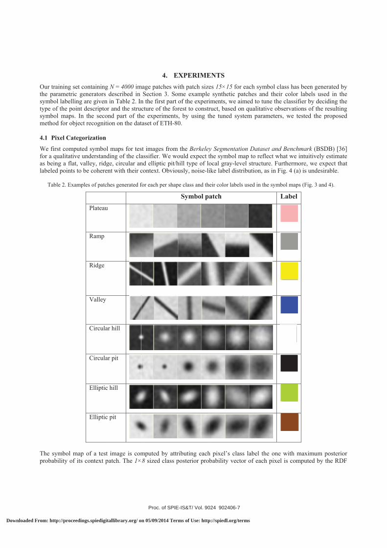
Our training sthe parametrisymbol labelltype of the posymbol mapsmethod for ob 4.1 Pixel Ca

We first comfor a qualitatias being a flalabeled points

Table 2. Ex

The symbol mprobability of

set containingic generators ling are givenoint descriptos. In the secobject recognit

ategorization

mputed symbolive understandat, valley, ridgs to be cohere

xamples of patc

Plateau

Ramp

Ridge

Valley

Circula

Circula

Elliptic

Elliptic

map of a testf its context p

g N = 4000 imdescribed in

n in Table 2. Inr and the stru

ond part of thion on the dat

l maps for tesding of the clage, circular anent with their c

hes generated f

u

ar hill

ar pit

c hill

c pit

t image is compatch. The 1×

4. Emage patches w

Section 3. Sn the first partcture of the fo

he experimenttaset of ETH-8

st images fromassifier. We wnd elliptic pit/context. Obvio

for each per sha

mputed by att8 sized class

EXPERIMEwith patch sizeome examplet of the experiorest to constrts, by using t80.

m the Berkeleywould expect t/hill type of loously, noise-li

ape class and th

Symbol p

tributing eachposterior prob

ENTS es 15×15 for e synthetic paiments, we aimruct, based onthe tuned syst

y Segmentatiothe symbol mocal gray-leveike label distri

heir color labels

atch

h pixel’s classbability vecto

each symbol catches and themed to tune thn qualitative otem paramete

on Dataset anap to reflect wel structure. Fibution, as in

used in the sym

s label the onor of each pix

class has beeneir color labehe classifier bobservations oers, we tested

nd Benchmarkwhat we intuitFurthermore, wFig. 4 (a) is u

mbol maps (Fig

Label

ne with maximel is compute

n generated byls used in they deciding the

of the resultingthe proposed

k (BSDB) [36tively estimatewe expect tha

undesirable.

g. 3 and 4).

mum posteriored by the RDF

y e e g d

] e

at

r F



configurationof 5.

We first examfeatures based[34], and graythe sample m[34] the map feature in Eqexpected, ramlook more likline regions in

Figure 3. Sym

By fixing thetree, we examsubsets of tratrees improvesizes and depmaximum deto result in asearch of fore

Figure 4. Symb

n trained with

mined the effd on comparisy-level slope

max approach in Figure 3(b

q. (3) the symbmps, ridges anke ramps thenn all various d

mbol map of a tSym

e feature type mined the effaining data, thes generalizatpths, one witpth of 5. The

a noisier map,est size is need

bol map of a te

the patch libra

fect of the chsons of the graangle in Eq. 3without any ) is dominatedbolic map in

nd valleys are dn lines. Noticedirections.

test image frommbol map compu

and other pafect of forest ey are adequaion [37]. We th 20 trees wresulting sym

, so that in thded to be mad

st image from B

ary. We fixed

oice of the loay-level value3. The resultinspatial smootd by circular aFig. (3c) hasdeclared on th

e that due to th

m BSDB, (a) Tes

uted by using n

arameters suchsize on the q

ately different computed the

with allowed mmbol maps arehe sequel we de in a goal-or

BSDB, constructrees wit

d the size of th

ow-level image of two randong symbol mathing, the symand elliptic pits a more evenhe eyebrows, lhe rotation inv

st image, (b) Synormalized four

h as patch sizquality of the

from one anoe symbol mapmaximum depe given in Figu

use forests wriented task.

cted by (a) RDFth maximum de

he forests as 20

ge features byomly selected aps are given mbolic maps at/hills outsiden spread of shlips and trellisvariance of ou

ymbol map comr-quadrant inver

ze, number of symbol maps

other, so increps of the test ipth of 8, andure 4. The out

with 200 shall

F with 20 trees epth of 5.

00 trees with a

y comparing tpoints in the nin Figure 3. I

are noisy. Usi the flat regio

hape classes os-like head cour dictionary,

mputed by usingrse tangent func

f split tests apps. Since all treasing the foreimage by two

d the other witcome of the slow trees. Obv

with maximum

an allowed ma

the simple graneighborhoodIt can be obseing the point ns, while usin

outside the flaver; her fingewe could cap

g point descriptoction.

plied and datrees are traineests size with o forests of wiith 200 trees smaller-sized viously, a mo

m depth of 8, (b)

aximum depth

ay-level valued of a test pixeerved that with

descriptors inng the arc-tangat regions. Asers at this scalepture edge and

ors in [34], (c)

a sampled pered by randommany shallowidely differenwith allowedforest appears

ore exhaustive

) RDF with 200

h

e el h n g s e d

r m w nt d s e

0



These prelimpreference fo

4.2 Object R

To test the vdataset ETH-for the “fruit“vehicles” hiis represented3280 images transformatioIdentificationknown by the

Scenario 1: Id

We randomlyremaining 11category. SPCNearest Neigconsist predoconsidering oand soft-assigprobability sybased encodinsoft-assignmeranked classeassignment bthey were noacquired with

minary pixel cr the arctange

Recognition

validity of the-80 [38]. ETHts and vegetaigher-categorid by 41 views

in total. All ons. We invesn of objects foe system befor

Identification o

y selected 30 1 ones (~30%)C is applied oghbors using tominantly of fonly seven shaignment basedymbol class tong is the classent based encoes over the whbased encodingot included, sh (WF: With F

categorizationent features.

e proposed meH-80 dataset coables”, cows, ies; one view os sampled uniobjects are c

stigated the rer views differre. Details of t

Figure 5

of known obje

out of 41 im) as testing im

on grayscale imthe posterior flat plateau reape classes. Td encoding. Io the pixel ans histogram reoding, we sorthole image to g is a code vesince these R Flat) and witho

n experiments

ethod, we stuonsist of 80 ob

dogs, horsesof ten instantiiformly over tcentered in thecognition perent than thosethe experimen

5. Sample ima

ects from alter

mages (~70%)mages. Therefmages. The obscores given egions, we rahe image leveIn the hard-a

nd we did avereflecting perceted symbol probtain the corector with (8×

histograms wout (WOF: W

have given

udy the perforbjects with 8 bs for the “aniations of objethe upper view

he image witherformance ofe in the gallerynts are as follo

ages from the

rnate views:

belonging tofore we have bject categorizby the random

an the experimel codes are acassignment barage-pooling oentage occurrerobabilities of rresponding h×R) bins whenwere concaten

WithOut Flat) F

us an idea a

rmance of thebasic categorinimals”, cups ect classes is swing (azimuthh the same scf the proposedy images, andows:

ETH-80 Obje

o each object 300 training

zation is implmized decisio

ment also by cquired in twoased encodingon the whole ence of the claf each pixel in istogram, onen the flat postnated. FigureFlat class post

as for the cho

e SPC methodes, which are for “handm

shown in Figuh and elevatiocale, and the d method in td (ii) Recognit

ects [38].

instantiation images and 1emented by a

on forests. Sinignoring the o ways: hard-g, we assignimage, so the

ass symbols odescending o

e for each rankteriors were in 6 demonstra

teriors. The re

oice of forest

d on the objeapples, pearsade objects”

ure 5. Each of on) hemispherviews includtwo different tion of objects

as training im110 testing im

simple classince the imageflat posterior

-assignment bned the label e output of haover the wholeorder and we ak. Hence, the oncluded in andates the perfod triangular m

t size and the

ect recognitions and tomatoes

and cars forthe 80 objectsre resulting in

de some affinescenarios: (i

s that were no

mages and themages for eachifier, 5-fold Ke backgrounds

class, that isased encodingof maximum

ard-assignmene image. In theaveraged top Routput of softd (7×R) when

ormance resulmark shown on

e

n s r s n e )

ot

e h

K-s

s, g

m nt e R -n lt n



the Rank = 1assignment bstructural shabetter than refrequency is n

Figure 6. Ob

The average improvementthan 4 rank h

Scenario 2: R

In this experiproblem has aMag-Lap [39We used leavtested on unsTable 3. In approach in Smultispectral resolution, wthe class decwith Rank =outperform texploited mucategory signobjects that w

There are sevi) Enriching

pixel in tmore akin

ii) Spatial pspatial po

tick is the clased encoding

apes like edgesults of WF. Inot very infor

bject recognitio(WF

recognition at occurs whenistograms are

Recognition of

iment we invealready been s

9]), global (PCve-one-out croseen objects. TSPC-Gr, we SPC-R|G|B|S1analysis and

e decreased thcisions acquire= 7 (WF). Wtexture, globaultispectral annificantly and were recognize

veral ways by g the shape libthe center of n to that, for e

pooling: The sooling scheme

lassification ag, recognitiones, lines, etc. inIn the ETH darmative.

on accuracy for F: With Flat) an

accuracies as n rank 2 histoused.

f unknown obj

estigate the restudied by LeCA Masks andoss validationThe performaapplied SPC

1|S2, that is, d since our 1he resolution oed are fused. hen we obse

al and local snalysis and m

outperform ted with the po

which we canbrary: The prthe d×d patchexample, encospatial correlaes such as max

accuracy achien accuracy impn the identificataset, the flat

different viewsnd (ii) not inclu

more of theogram was inc

jects:

ecognition of uibe and Schied PCA Gray)

n similarly to ance results of

on grayscalewe separately5×15 sized pof the grayscaIn SPC-Gr arve the averashape based multiscale appthe existing moorest perform

n improve the roposed shapeh. Allowing oountered in [4ation of the cx pooling or a

eved by hard-proves to ~90cation of objecategory is co

s of different obuding Flat platea

ranks are included. The c

unseen objectele for the for and local sha[38] and we t

f the method ie images andy analyzed eapatches mightale images by and SPC-RGBage accuracy methods, butproach, we c

methods for frmance are give

performance e library is cenout-of-center a1]. class posterioraverage poolin

assignment co%. By excludct categories,ommon to all

bjects [38] usingau posteriors (W

ncluded givenclassification

ts as belongingETH-80 datasape (Cont. Grtrained the syin [38] and of

d we exploiteach color chant be too myothe factor of

B|S1|S2 we exresults comp

t only the cocould improveruits and vegeen in Figure 7.

of the SPC: ntralized in thand asymmetr

r probabilitiesng should be c

odes which isding flat poster

however WOclasses, hence

g codes (i) incluWOF: WithOut

n in the graphaccuracy bec

g to a specificset [38]. Theyreedy and Coystem with evf the proposed

ed multispectrnnel using the

opic for some in S1 and

xploited soft-aputed over allolor-based mee the recognietables catego.

hat the patch rric patterns w

s is presentlyconsidered.

s ~63%. Whenriors we aime

OF results are e its IDF: inve

uding Flat plateFlat)

h in Figure 6omes saturate

c object categy used color, tent. DynProg

very view of 7d SPC methoral analysis ae SPC approa

e objects, andS2. Finally, a

assignment bal categories, ethod. Howevition performories. Two ex

represents the will generate a

y nor into acc

n we use softed to prime theonly 1% - 2%erse documen

eau posteriors

6. The biggesed when more

gory [38]. Thisexture (DxDy[40]) features79 objects andd are given in

and multiscaleach to included at the givenall the score orased encodingwe could no

ver, when wemance of eachxamples of the

context of thea shape library

count. Various

-e

% nt

st e

s y, s. d n e e n r g

ot e h e

e y

s



iii) Contour extract ctechnique

Apple

Pear

Tomato

Cow

Dog

Horse

Cup

Car

Average

Figure 7. An

In this study,visual vocaburecognition dproposed patscale-space an

information: Tclass informates.

Color D

57.56% 85

66.10% 90

98.54% 94

86.59% 82

34.63% 62

32.68% 58

79.76% 66

62.93% 98

64.85% 79

example view

we explored ulary that can dataset ant prech generationnd considerin

The contour intion along the

Table 3. ReDxDy Mag

Lap

5.37% 80.2

0.00% 85.3

4.63% 97.0

2.68% 94.3

2.44% 74.3

8.78% 70.9

6.10% 77.8

8.29% 77.5

9.79% 82.2

of the objects t

the constructpotentially beliminary reco

n method. Weng spatial smoo

nformation ofe contour, rep

ecognition resulg-

p PCA Masks

24% 78.78%

37% 99.51%

07% 67.80%

39% 75.12%

39% 72.20%

98% 77.80%

80% 96.10%

56% 100.0%

23% 83.41%

that were recognno: 4 ),

5.tion of an imae used for vargnition results

e plan to deveothing that tak

f all objects inpresent the o

lts for categoriz

s PCA Gray

% 88.29%

% 99.76%

% 76.59%

% 62.44%

% 66.34%

% 77.32%

% 96.10%

% 97.07%

% 82.99%

nized poorest. C Horse (object i

CONCLUSage dataset-indrious image uns, albeit basedelop this scheke account the

n the ETH dataobject as a str

zation of unseenCont. Greedy

CD

77.07% 7

90.73% 9

70.73% 7

86.83% 8

81.95% 6

84.63% 8

99.76% 9

99.51% 1

86.40% 8

Cow (object id id no: 2)

SION dependent symnderstanding td on limited seeme further bye posterior pro

abase is proviring of labels

n objects [38] Cont DynProg

SP

6.34% 73

1.71% 87

0.24% 90

6.34% 64

7.84% 49

4.63% 39

9.02% 55

00.0% 90

6.40% 68

no: 7), Dog (ob

mbolic mid-letasks. We testet of features y enriching th

obabilities of n

ided. It will bes, and use str

PC-Gr SR

.66% 92

7.80% 99

0.73% 99

4.88% 7

9.51% 52

9.27% 54

5.37% 70

0.24% 9

8.93% 79

bject id no: 6), C

evel feature mted our methoindicate the phe shape alphneighbor side.

e of interest toring matching

PC-R|G|B|S1|S2

2.19%

9,76%

9,76%

6.83%

2.68%

4.15%

0.73%

1.71%

9.73%

Cup (object id

map, a versatiled on an objec

potential of thehabet, work in.

o g

e ct e n



REFERENCES

[1] Ramanan, A., and Niranjan, M., “A review of codebook models in patch-based visual object recognition,” Journal of Signal Processing Systems, 68(3), 333-352 (2012).

[2] Jiang, Y.G., Yang, J., Ngo, C.W., and Hauptmann, A.G., “Representations of keypoint-based semantic concept detection: A comprehensive study,” IEEE Transactions on Multimedia, 12(1), 42-53 (2010).

[3] Mikolajczyk, K., and Schmid, C., “Scale & affine invariant interest point detectors,” International journal of computer vision, 60(1),63–86 (2004).

[4] Lowe, D. G., “Distinctive image features from scale-invariant keypoints,” International journal of computer vision, 60(2), 91–110 (2004).

[5] Bay, H., Tuytelaars, T., and Van Gool, L., “SURF: Speeded up robust features,” in Proceedings of the European Conference on Computer Vision, 404–417, (2006).

[6] Matas, J., Chum, O., Urban, M., and Pajdla, T., “Robust wide-baseline stereo from maximally stable extremal regions,” Image and vision computing, 22(10), 761-767 (2004).

[7] Kadir, T., Zisserman, A., and Brady, M., “An affine invariant salient region detector,” In proc. of. European Conf. on Computer Vision, 228-241 (2004).

[8] Tuytelaars, T. and Van Gool, L., “Content-based image retrieval based on local a nely invariant regions,” In Intern. Conf. on Visual Information and Information Systems, 493-500 (1999).

[9] Tuytelaars, T. and Van Gool, L., “Wide baseline stereo matching based on local, a nely invariant regions,” in Proceedings of the British Machine Vision Conference, 412–425 (2000).

[10] Li, J., and Allinson, N. M., “A comprehensive review of current local features for computer vision,” Neurocomputing, 71(10), 1771-1787 (2008).

[11] Smith, K., Carleton, A., and Lepetit, V., “Fast ray features for learning irregular shapes,” Proc. of IEEE 12th Int. Conf. on Computer Vision, 397-404 (2009)

[12] Calonder, M., Lepetit, V., Strecha, C., and Fua, P., “Brief: Binary robust independent elementary features,” European Conf. On Computer Vision, 778-792 (2010).

[13] Tuytelaars, T., and Mikolajczyk, K., “Local invariant feature detectors: a survey,” Foundations and Trends® in Computer Graphics and Vision 3.3, 177-280 (2008).

[14] Zhang, J., Marsza ek, M., Lazebnik, S., and Schmid, C., “Local features and kernels for classification of texture and object categories: A comprehensive study,” International journal of computer vision, 73(2), 213-238, (2007).

[15] Ojala, T., Pietikäinen, M., and Harwood, D., “A comparative study of texture measures with classification based on featured distributions,” Pattern recognition, 29(1), 51-59 (1996).

[16] Dalal, N., and Triggs, B., “Histograms of oriented gradients for human detection,” In IEEE Computer Society Conference on Computer Vision and Pattern Recognition, (1), 886-893 (2005).

[17] Mikolajczyk, K., & Schmid, C., “A performance evaluation of local descriptors,” IEEE Transactions on Pattern Analysis and Machine Intelligence, 27(10), 1615-1630 (2005).

[18] Csurka, G., Dance, C., Fan, L., Willamowski J., and Bray, C., “Visual categorization with bags of keypoints,” In Workshop on statistical learning in computer vision, (1), 22, (2004).

[19] Aharon, M., Elad, M., and Bruckstein, A., “K-SVD: an algorithm for designing overcomplete dictionaries for sparse representation,” IEEE Transactions on Signal Processing, (54)4311–4322 (2006).

[20] Van Gemert, J. C., Snoek, C. G., Veenman, C. J., Smeulders, A. W., and Geusebroek, J. M.,“Comparing compact codebooks for visual categorization,” Computer Vision and Image Understanding, 114(4), 450-462 (2010).

[21] Jurie, F., and Triggs, B., “Creating efficient codebooks for visual recognition,” In Tenth IEEE International Conference on Computer Vision, (1), 604-610 (2005).

[22] Liao, Z., Farhadi, A., Wang, Y., Endres, I., and Forsyth, D., “Building a dictionary of image fragments,” In IEEE Conference on Computer Vision and Pattern Recognition, 3442-3449 (2012)

[23] Yang, J., Yu, K., Gong, Y., and Huang, T., “Linear spatial pyramid matching using sparse coding for image classification,” In IEEE Conference on Computer Vision and Pattern Recognition, 1794-1801(2009).

[24] Boureau, Y. L., Bach F., LeCun, Y., and Ponce, J., “Learning mid-level features for recognition,” In IEEE Conference on Computer Vision and Pattern Recognition , 2559-2566 (2010).

[25] Coates, A., and Ng, A. “The importance of encoding versus training with sparse coding and vector quantization,” In Proceedings of the 28th International Conference on Machine Learning, 921-928 (2011).



[26] Coates, A., Ng, A., and Lee, H., “An analysis of single-layer networks in unsupervised feature learning,” In International Conference on Artificial Intelligence and Statistics, 215-223 (2011).

[27] Liu, L., Wang, L., and Liu, X., “In defense of soft-assignment coding” In IEEE International Conference on Computer Vision, 2486-2493 (2011).

[28] Van Gemert, J. C., Veenman, C. J., Smeulders, A. W., and Geusebroek, J. M., “Visual word ambiguity,” IEEE Transactions on Pattern Analysis and Machine Intelligence, 32(7), 1271-1283 (2010).

[29] Crosier, M., and Griffin, L. D., “Using basic image features for texture classification,” International Journal of Computer Vision, 88(3), 447-460 (2010).

[30] Viola, P., and Jones, M. J., “Robust real-time face detection,” International journal of computer vision, 57(2), 137-154 (2004).

[31] Calonder, M., Lepetit, V., Fua, P., Konolige, K., Bowman, J., and Mihelich, P., “Compact signatures for high-speed interest point description and matching,” In IEEE 12th International Conference on Computer Vision, 357-364 (2009).

[32] Torralba, A., Fergus, R., and Weiss, Y., “Small codes and large image databases for recognition,” In IEEE Conference on Computer Vision and Pattern Recognition, 1-8 (2008).

[33] Calonder, M., Lepetit, V., Ozuysal, M., Trzcinski, T., Strecha, C., and Fua, P., “BRIEF: Computing a local binary descriptor very fast,” IEEE Transactions on Pattern Analysis and Machine Intelligence, 34(7), 1281-1298 (2012).

[34] Shotton, J., Johnson, M., and Cipolla, R., “Semantic texton forests for image categorization and segmentation,” In IEEE Conference on Computer Vision and Pattern Recognition, 1-8 (2008).

[35] Breiman, L., “Random forests,” Machine learning, 45(1), 5-32 (2001). [36] Arbelaez, P., Fowlkes, C., and Martin, D., “The berkeley segmentation dataset and benchmark,” see http://www.

eecs. berkeley. edu/Research/Projects/CS/vision/bsds (2007). [37] Criminisi, A., Shotton, J., and Konukoglu, E., “Decision forests for classification, regression, density

estimation, manifold learning and semi-supervised learning,” Microsoft Research Cambridge, Tech. Rep. MSRTR-2011-114, 5(6), 12 (2011).

[38] Leibe, B., and Schiele, B., “Analyzing appearance and contour based methods for object categorization,” In Proc. IEEE Computer Society Conference on Computer Vision and Pattern Recognition, 2, 409 (2003).

[39] Schiele, B., and Crowley, J. L., “Recognition without correspondence using multidimensional receptive field histograms,” International Journal of Computer Vision, 36(1), 31-50 (2000).

[40] Belongie, S., Malik, J., and Puzicha, J. “Matching shapes,” In Eighth IEEE International Conference on Computer Vision1, 454-461 (2001).

[41] Sallee, P., and Olshausen, B. A., “Learning sparse multiscale image representations,” In Advances in neural information processing systems, 1327-1334 (2002).



Symbolic feature detection for image understanding

Documents

Transcript of Symbolic feature detection for image understanding