Int. J. Global Environmental Issues, Vol. 5, Nos. 3/4, 2005 225

Copyright © 2005 Inderscience Enterprises Ltd.

Multi-scale integrated analysis of societal metabolism: learning from trajectories of development and building robust scenarios

Jesus Ramos-Martin* and Mario Giampietro Istituto Nazionale di Ricerca per gli Alimenti e la Nutrizione, Roma, Italy E-mail: ramos@inran.it E-mail: giampietro@inran.it *Corresponding author

Abstract: This paper presents two applications of the multi-scale integrated analysis of societal metabolism (MSIASM) approach. The first application shows that accounting the metabolism of a society in both economic and biophysical terms supports a better understanding of mechanisms determining evolutionary trajectories. This is done by analysing the constraints determined by the parallel evolution of different economic sectors and by establishing a link between material standard of living, population size, technology, and the resulting environmental impact. The case study of this first example deals with the recent economic history of Ecuador and Spain. The second application uses MSIASM for scenarios analysis. The goal is to illustrate an example of quality check on future scenarios of economic development. The case study is a set of hypotheses of economic development for Vietnam in the year 2010.

Keywords: integrated analysis; societal metabolism; complex systems; impredicative loop-analysis; exosomatic energy; development; Vietnam; Ecuador; Spain.

Reference to this paper should be made as follows: Ramos-Martin, J. and Giampietro, M. (2005) ‘Multi-scale integrated analysis of societal metabolism: learning from trajectories of development and building robust scenarios’, Int. J. Global Environmental Issues, Vol. 5, Nos. 3/4, pp.225–263.

Biographical notes: Jesus Ramos-Martin (MPhil Ecological Economics, MA Environmental Politics) had been Lecturer of natural resources economics at the Autonomous University of Barcelona, combining this activity with research in the fields of societal metabolism, especially of energy, climate change, and in participatory approaches such as social multi-criteria evaluation. Presently, he is researcher in an Italian funded project on participatory integrated assessment of the introduction of GMOs to the Italian agricultural sector at INRAN. He is organiser of the Biennial Ibero-American Congress of Development and Environment.

Mario Giampietro (PhD Food Systems Economics) is the Director of the Unit of Technological Assessment at the National Institute of Research on Food and Nutrition (INRAN). Giampietro’s expertise covers issues such as multi-scale integrated analysis (MSIA), biophysical analysis of agricultural and socio-economic development; agro-ecosystem analysis with specific experience on sustainability research in Southeast Asia and China. He has been Visiting Professor at the Cornell University, Autonomous University of Barcelona, University of Wageningen, and at the University of Wisconsin-Madison. He is the organiser of the Biennial International Workshop of Advances in Energy Studies being held, since 1996, in Portovenere, Italy.

226 J. Ramos-Martin and M. Giampietro

1 Introduction

In the past decades, analyses aimed at economic development (both in the scientific literature and in the discussions in policy agencies) have focused mainly on representations based solely on economic variables. This strategic choice has lessened attention to biophysical variables (such as energy conversion, human time allocation, materials use, or land use), which were very present in earlier economic discussions. We happen to believe that an integrated analysis of the economic and biophysical dimension of development, which is able to put back into the picture these neglected variables, is crucial for an effective description of the evolution of societies and their technological development, as well as for understanding possible constraints for further development.

Accounting for both economic and biophysical variables requires a wider focus than that adopted by neo-classical economics. It calls for a methodological approach able to link the various relevant dimensions of analysis associated to the economic process within a holistic view of the evolution of socio-economic systems interacting with an ecological context. To achieve this goal, traditional economic reading should be complemented by an analysis of flows of both matter and energy going ‘into the society’, ‘through the society’, and ‘out of the society’ according to the metaphor of metabolism. In the field of ecological economics, this integration is associated with the concept of ‘societal metabolism’ (Martinez-Alier, 1987; Fischer-Kowalski, 1997; Schandl et al., 2002). This concept has a long history in biophysical analysis of the interaction of socio-economic system with their environment, and can be consistently found in the writings of those authors that see the socio-economic process as a process of self-organisation. Pioneering work in this field was done, among others, by Podolinsky (1883), Jevons (1965), Ostwald (1907), Lotka (1922, 1956), White (1943, 1959), and Cottrel (1955). Cottrel worked out the idea that the very definition of an energy carrier (what should be considered an energy input) depends on the definition of the energy converter (what is using the input to generate useful energy). The idea that metabolism implies an expected relation between typologies of matter and energy flows has been explored by Odum (1971, 1983) (for studying the interaction between ecosystems and human societies); Rappaport (1971) (for anthropological studies); Georgescu-Roegen (1971) (for the sustainability of the economic process). Georgescu-Roegen, in exploring the relation between the economic process analysed in terms of energetic and material flows, coined a new term for such an integrated analysis namely ‘Bio-economics’ (Mayumi, 2001). Georgescu-Roegen (1971) called the flows associated to a given socio-economic structure ‘metabolic flows’. This metaphor stresses the fact that human societies must use large amounts of materials and energy to sustain their structure and activities, exactly like organisms do. Within this rationale, Georgescu-Roegen (1975) proposed the distinction – first introduced by Lotka (1956) – between exosomatic energy flows (i.e., use of energy sources for energy conversions outside the human body, but operated under human control, for stabilising the turn over of matter within societal structures) and endosomatic energy flows (i.e., use of energy needed to maintain the internal metabolism of a human being, that is, energy conversions linked to human physiological processes fuelled by food energy). He proposed to use this distinction as an analytical tool for the energetic analyses of bio-economics and sustainability. In this sense, the ‘exosomatic metabolism’ of societies or ‘societal metabolism’ deals with the consumption of exosomatic energy (e.g., for the

Multi-scale integrated analysis of societal metabolism 227

making and operation of tools and machinery), which is required for guaranteeing the set of useful activities associated with sustainability.

When considering the societal metabolism of economies, one has to acknowledge the fact that economies are complex, adaptive, dissipative systems. They are composed of a large and increasing number of both components and relationships between them. Economies are also teleological systems (they have an aim or end, a telos). Moreover, they are capable of incorporating guessed consequences of their possible actions into their actual decisions. That is, they are anticipatory systems (Rosen, 1985) and because of this property they can even update their own definitions of goals and models. That is, they learn from past mistakes and from present developments, and they react, by changing both current and future actions. They are thus self-reflexive. Because of this they have the option of either adapt to new boundary conditions or consciously alter boundary conditions they do not like. Therefore, an economy can be understood as a complex, adaptive, self-reflexive, and self-aware system (Kay and Regier, 2000).

In terms of structure, economic systems are nested hierarchical systems. That is, they consist of elements defined on different hierarchical levels (the whole is made of parts, each part is made of sub-parts, the whole belongs to a larger network). In the case of a national economy, we can distinguish several subsystems such as economic sectors within it. Every sector may be split into different sub-sectors (e.g., industrial ‘types’ sharing common features) and so on. The various hierarchical levels of an economy do exchange flows of human activity and energy (i.e., among them at the same level, and across levels and scales). The resulting network of flows reflects the interconnected nature of those systems (the output of one sector enters another sector as an input, and vice versa). The feed-back of flows across scales implies a kind of chicken-egg behaviour that may be analysed by means of impredicative loop analysis (more on this concept in the previous paper: Giampietro and Ramos-Martin (2005)).

Ecosystems and human systems (as open complex systems) are autopoietic systems. Autopoiesis (Varela et al., 1974; Maturana and Varela, 1980) refers to the ability that living systems have to renew themselves and maintain their structure. In this frame, their capacity for self-reproduction has to be understood in relation to the fact that they are teleological (end-oriented) entities. They hold the essential characteristics of:

• openness to energy and matter flows

• presence of autocatalytic loops (closed to the system), which maintain the identity of the system

• differentiation of organisational structure and functions for different parts that allows the systems to adapt to the changing boundary conditions, by becoming something different in time.

This process of self-reproduction and adaptation is therefore related to their ability to process both information and energy/matter (Jantsch, 1987). In this context, the usefulness of information can be related to the ability:

• to develop and transmit strategies of development useful to confront fluctuations or future challenging boundary conditions

• to generate and select different narratives useful for describing and representing the interaction with their context.

228 J. Ramos-Martin and M. Giampietro

The usefulness of energy and matter flows can be related to the ability to maintain compatibility of structures and functions against thermodynamic constraints.

Two other useful concepts for the analysis of self-production are:

• ‘autocatalytic loop’ (i.e., activities that affect themselves through an interaction with the context – a positive autocatalytic loop implies a reinforcement and amplification of an activity)

• ‘the key role of hyper-cycles’ (i.e., the special role autocatalytic loops play in the evolution of dissipative systems) (Ulanowicz, 1986).

When describing ecosystems as networks of dissipative elements, Ulanowicz (1986) distinguished between two main parts:

• a part responsible for generating the hyper-cycle (i.e., the subset of activities generating the surplus on which the whole system feeds)

• a part representing a pure dissipative structure.

That is, a hyper-cycle (those processes taking primary energy from the environment – e.g., solar energy for ecosystems – and converting it into available energy for other processes – e.g., supply of different energy carriers – biomass for other ecological agents) must always be associated with a purely dissipative part (e.g., herbivores and carnivores feeding on net primary productivity). The same analogy can be applied to economies.

The role of the hyper-cycle is, therefore, “to drive and keep the whole system away from thermodynamic equilibrium” (Giampietro and Mayumi, 1997, p.459), whereas the dissipative part is required to stabilise the system by avoiding an excessive take over of the hyper-cycle (without a complementing part damping their effect, positive autocatalytic loops just blow up!).

As soon as we undertake an analysis of socio-economic processes based on energy accounting, we have to recognise that the stabilisation of societal metabolism requires the existence of an autocatalytic loop of useful energy. That is, a certain fraction of the useful energy invested in human activity must be used to stabilise the input of energy carriers taken from the environment. In the example used in this paper, we characterise the autocatalytic loop stabilising societal metabolism in terms of a reciprocal ‘entailment’ of two resources:

• ‘human activity used to control the operation of exosomatic devices’

• ‘fossil energy used to power exosomatic devices’ (Giampietro, 1997).

The term autocatalytic loop indicates a positive feedback, a self-reinforcing chain of effects (the establishment of a chicken-egg pattern). The two resources, therefore, enhance each other in a chicken-egg pattern (human activity enhances the use of fossil energy, the use of fossil energy enhances the generation and expression of human activity).

All the above characteristics of economies analysed as complex systems make them difficult to be understood and comprehended when using the drastic simplifications associated with reductionism (= the use of a single level of analysis, a single scale, and a single dimension). This is why we need a methodology that combines information coming from different disciplines (e.g., economic, demographic, and biophysical

Multi-scale integrated analysis of societal metabolism 229

variables), and from different hierarchical levels of the system (scales) in a coherent way. The methodology used here is multi-scale integrated analysis of societal metabolism (MSIASM), which is described in detail in (Giampietro, 2000, 2003). As discussed in a previous paper of this special issue (Giampietro and Ramos-Martin, 2005), the integrated use of non-equivalent models to characterise changes in economies makes it possible to handle different sets of variables to generate parallel descriptions of the same facts on different levels. This ability is essential when dealing with the issue of sustainability. In fact, the resulting generation of a ‘mosaic effect’ among the various pieces of information improves the robustness of the analysis and provides new insights generated by synergism in the parallel use of different pieces of information.

After having selected a useful narrative in relation to the research goal, MSIASM provides a representation of the performance of the given system in terms of a finite set of attributes by using ‘parallel non-equivalent descriptive domains’ (economic reading, demographic reading, technical reading, biophysical reading). In so far MSIASM should be considered as a ‘discussion support tool’ that may be used, as we shall show, for both historical analysis and scenarios analysis. In the latter case, the intention is not to forecast the future behaviour of variables and the exact value they may take. Rather the goal is to improve the quality of the narratives adopted for building scenarios. That is, MSIASM can provide hints on future trends of key variables, and possible biophysical or economical constraints for future development scenarios, pointing at those attributes of performance that should be considered when selecting and evaluating scenarios. The basic idea is that when dealing with the future, it is better to be aware of possible attributes of performance that will be relevant – even if this implies not guessing with accuracy the value taken by the relative variable – rather than guessing with accuracy the future value taken by variables that can result irrelevant.

The rationale of the approach is based on the three concepts discussed at length in the previous paper dealing with the theoretical aspects of multi-scale integrated analysis (Giampietro and Ramos-Martin, 2005):

• Mosaic effects across levels, obtained by using redundancy in the representation of parts and whole of the system using non-equivalent external referents (data source) across non-equivalent descriptive domains.

• Impredicative loop analysis, obtained when addressing, rather than denying, the existence of chicken-egg paradoxes in self-organising adaptive systems. This analysis is required whenever the identity of the whole defines the identity of the parts and vice versa.

• The continuous search and the updating of useful narratives for surfing in complex time based on the acknowledgement of the fact that the observer/observed complex requires the simultaneous consideration of several non-reducible relevant time differentials. • the ‘time differential’ at which the system evolves • the ‘time differential’ adopted in the set of differential equations used in models • the ‘time differential’ at which the observer changes its perception of what is

relevant about the observed.

The structure of the rest of the paper is as follows: Section 2 presents a historical application of MSIASM for analysing the bifurcation in the development trajectories

230 J. Ramos-Martin and M. Giampietro

between Spain and Ecuador. Section 3 presents an example of scenario analysis in Vietnam. Finally, the conclusion makes a few theoretical considerations about the advantages of using the MSIASM approach to analyse the exosomatic evolution of societies. As explained in the following text, we do not claim that the scenarios and numbers used in this paper according to the narratives we selected are ‘the correct ones’. The opposite cannot be proven in substantive terms by anyone. What is relevant, therefore, is the illustration of the potentials of this approach when applied for an integrated analysis of scenarios. Such an analysis can be improved, by increasing the degree of overlapping across different types of data (using simultaneously more external referents) and bridging descriptions referring to different hierarchical levels. A last observation, in this paper, is that the MSIASM approach is applied to the level of ‘national economy’ as the focal level (n) of analysis, but other levels of analysis are possible (e.g., using the village or the household as the focal level of analysis – (Giampietro, 2003)).

2 Learning from development trajectories: biophysical constraints to economic development in Spain and Ecuador 1976–1996

2.1 A methodological note

Carrying out an MSIASM always requires following three basic steps:

• Choosing a set of variables able to map the size of the system (i.e., economic system) as perceived from within the black box (variable # 1, required to generate a multi-level matrix for the analysis). Typical examples are: ‘hours of human activity’ and ‘hectares of land’.

• Choosing a set of variables able to map the size of the system as perceived by its context in terms of exchanged flows (variable # 2, required to be able to use external referents, i.e., different sources of data at different levels). Assessing the exchanged flows makes it possible to describe the interaction of the system with its context at different levels. Examples are: ‘specific flows of exosomatic energy’ (e.g., MJ of exosomatic energy – for the whole country, for an economic sector, for a particular plant), ‘specific flows of added value’ (e.g., $ – for the whole country, for an economic sector, for a particular plant), ‘specific flows of other key material’ (e.g., kg of water or kg of nitrogen – for the whole country, for an economic sector, for a particular plant).

• Mapping the nested hierarchical structure associated to the metabolic system using in parallel the two variables # 1, # 2, and the ratio of the two (variable # 3). The resulting family of intensive variables # 3 will result in an integrated biophysical accounting (e.g., exosomatic energy flows per unit of human activity or exosomatic energy flows per unit of land area) and economic accounting (flows of added value per unit of human activity or flows of added value per unit of land area). The resulting assessment MJ/hour of human activity, MJ/ha of land use, $/hour of human activity, or $/ha of land use can be related to different hierarchical levels (the whole country, an economic sector, a particular plant, or household) and can be used to define typologies through benchmarking.

Multi-scale integrated analysis of societal metabolism 231

When representing the system in this way, we achieve coherence in the resulting information space (e.g., economic and biophysical readings referring to different levels of the nested holarchy that are related to each other) using equations of congruence. Such an integrated analysis allows seeing underlying constraints, problems, and relations associated with economic development, which are difficult to see when applying traditional analytical tools from economics.

2.2 Goal of the example

This section presents an application of the multi-scale integrated analysis of societal metabolism to the recent economic history of Ecuador and Spain. The main goal of this comparison is to understand the relationship between changes in gross domestic product (GDP) and related changes in the throughput of matter and energy over time. Understanding this link is crucial for studying the sustainability of modern societies. MSIASM applied to historical analysis of development is based on the identification of different ‘types’ of parts (sub-sectors, sectors) and whole (countries at different levels of development) that can be used for characterising trajectories of development.

The analysis of historical changes of Spain and Ecuador is based on the relative values taken by the characteristics of parts (various economic sectors, which are characterised in terms of typologies, using a set of expected values for a given set of variables – benchmarks) in relation to the characteristics of the whole (the national economy, which is characterised in terms of typologies, using a set of expected values for a given set of variables – benchmarks). This makes it possible to explain the different paths taken by these two countries over the period considered.

Another side result we found in this analysis is the strong relationship between: • economic labour productivity (= $ of added value generated in a sector per unit of

working time in that sector) • a proxy variable for biophysical capitalisation of economies (measured by the

exosomatic metabolic rate; that is, exosomatic energy consumption per hour of working time).

This link makes it possible to better understand the biophysical and economical constraints implied by the parallel evolution of the different elements of an economy, seen as a nested hierarchical system.

In this example, when considering the dynamics of economic development, Spain was able to take a path different from that taken by Ecuador thanks to the different characteristics of its energy budget and the relative values taken by other key variables such as population structure [affecting the profile of human time allocation] and the pace of population change. The integrated set of relevant changes is described using a mix of economic and biophysical variables (both extensive and intensive). The representation of these parallel changes (on different levels) requires the use of different variables, which can be kept in coherence by adopting the frame provided by MSIASM. In particular, the integrated representation based on a mix of extensive and intensive variables kept in congruence over a 4-angle figure, is based on the approach presented in Giampietro and Ramos-Martin (2005) (see the example of metabolism of 100 people on a remote island). A deeper analysis of both cases – Ecuador and Spain – using MSIASM and other more conventional approaches can be found in Falconi-Benitez (2001) and Ramos-Martin (2001), respectively.

232 J. Ramos-Martin and M. Giampietro

In the following paragraphs, we present an example of mosaic effect and an impredicative loop analysis applied to the process that stabilises the metabolism of a society both in the short run and the long run. In a metabolic system, what enters as an input to be consumed is then used to carry out several activities. A fraction of these activities must be directed to guarantee the (re)production of what is later consumed as input (short-run stabilisation referring to the concept of efficiency). On the other hand, those other activities not aimed at the stabilisation in the short term of the various inputs (because they are purely dissipative) are still important, since they guarantee reproduction and adaptability in the long term by means of other activities such as education (Giampietro, 1997).

With the representation of the metabolism across scales and hierarchical levels, this process can be represented using a set of different identities for: • energy carriers (level n-2; that of the individual members of the system) • converters used by components (on the interface level n-2/level n-1) • the whole metabolic system seen as a network of parts (on the interface

level n-1/level n) • the whole seen as a black box interacting with its context (on the interface

level n/level n+1).

The need of achieving a dynamic budget implies a mechanism of self-entailment among the various definitions of identity for sub-parts, parts, wholes, and context describing this interaction across levels. The way to deal with such a task is illustrated in the example given in Giampietro and Ramos-Martin (2005) – we refer the reader to Figure 1. The impredicative loop analysis based on the 4-angle representation refers to the forced congruence among two different forms of energy flowing in the socio-economic process: • fossil energy used to power exosomatic devices, which is determining/is

determined by • human activity used to control the operation of exosomatic devices.

Figure 1 Dendogram of ExMR in Spain in 1976

Multi-scale integrated analysis of societal metabolism 233

2.3 Analysis based on the mapping of flows against the multi-level matrix: human activity

2.3.1 The relations used in this analysis

The variables used in this example are: THA: total human activity of the whole socio-economic system considered

(hours/year). The value of this variable (the size of the economy in terms of human activity is obtained by multiplying human population by 8760 (the hours per capita in one year).

HAi: hours of Human Activity invested in Sector i. (SOHA + 1): societal overhead of human activity, THA/HAPW where PW indicates

the hours of work in all the sectors generating added value; that is, productive sectors (PS) and services and government (SG).

TET: total exosomatic throughput of the whole system considered (Joules/year) expressed in primary energy equivalent as done in UN statistics of national energy consumption.

ETi: Joules of exosomatic energy consumed per year in Sector i. (SOET + 1): societal overhead of energy throughput, TET/ETPW where PW indicates

the amount of primary energy invested in all the sectors generating added value; that is, productive sectors (PS) and services and government (SG).

ExMRAS: exosomatic metabolic rate (average whole system), the rate of consumption of exosomatic energy per unit of human activity (EMRAS = TET/THA).

ExMRi: exosomatic metabolic rate per hour of human activity in Sector i. GDP: gross domestic product, measured in constant dollars. ELPi: economic labour productivity in Sector i, that is, GDPi/HAi in dollars

per hour of activity.

For a more detailed explanation of the formalisation used in the 4-angle figures, see Giampietro (1997, 2000, 2003) and Giampietro et al. (2001).

2.3.2 Dendogram of ExMRi (relevant flow – extensive variable#2 – ‘Exosomatic Energy’ vs. a variable defining size – extensive variable#1 – ‘Human Activity’)

Figures 1 and 2 represent the dendograms of exosomatic metabolic rates, ExMRi, for Spain in the years 1976 and 1996. We start our analysis by identifying two extensive variables that define the size of the system, in this case Total Human Activity (THA, extensive variable #1) and Total Energy Throughput (TET, extensive variable #2). In our representation of the hyper-cycle of the economy (Figure 3), this would be the right-hand side of the graph. In our 4-angle representation (Figure 4), this would be the upper right quadrant. It represents the level n of the analysis, that of the national economy.

234 J. Ramos-Martin and M. Giampietro

Figure 2 Dendogram of ExMR in Spain in 1996

Figure 3 Hypercycle of exosomatic energy in Spain 1996

Figure 4 Biophysical impredicative loop for Spain and Ecuador

Multi-scale integrated analysis of societal metabolism 235

In Figures 1 and 2, the first disaggregation distinguishes between investments of both ‘Human Activity’ and ‘Energy Throughput’ either in the ‘Household sector (HH)’ or in the ‘Paid-Work sector (PW)’. In other words, this represents the split between the consumption side and the production side. In our analysis represented at level n-1, a second disaggregation may imply splitting the performance of the household sector into different household types at the level n-2 (such as urban and rural, or different household types depending on income level). Since we do not have data for the household sector at this level of disaggregation (level n-2), we do not present data for this level, as done for the paid-work sector. The MSIASM mechanism of accounting, however, is robust insofar, as this does not affect the possibility of obtaining relevant information about different characteristics of the socio-economic systems outside the household sector. In fact, we do split the paid-work sector, at the level n-2, between the different sectors: Productive Sector (PS, including industry and mining), services and government sector (SG) and agriculture (AG). In our analysis of level n-2, in the 4-angle representation adopted in this paper, this would represent the left lower quadrant, where the productive sector is the focus for analysis. Obviously, a different goal of the analysis could have included any of the other two sectors (SG or AG) instead.

The ratio between extensive variable #1 and extensive variable #2 (assessed over different elements at different levels) determines the value of the intensive variable #3, which in our case is ExMRi. This variable reflects a biophysical accounting of the system. In the 4-angle representation, intensives variables are those found at the corners of the quadrants, whereas the length of the axis would represent the total size of the system or compartment (extensive variables, as perceived from the inside – extensive variable #1 – or from the outside – extensive variable #2). The value of the intensive variable#3 can be determined:

• from the congruence of the value of extensive variables defined at a given level (e.g., level n)

• from the typology (e.g., technical coefficient or economic characteristics) describing the component of the system at level n-1.

The representation of the characteristics of elements belonging to different hierarchical levels by using a dendogram makes evident an important characteristic of MSIASM: the ability of simultaneously handling a set of values taken by key variables on different hierarchical levels. That is, a given value of an intensive variable can be seen as being determined by:

• relations of values taken by variables belonging to a higher level

• the aggregation of values associated with typologies defined on lower levels.

This feature is crucial when analysing scenarios of future development. In fact, the analysis presented in Figures 1 and 2 implies a representation of past trends. This is a case in which all data can be known in retrospect. However, in case of scenario analysis, we would not need all the data, because of the forced congruence across scales and the possibility of establishing mosaic effects missing data can be complemented. In other words, the value of some of the variables can be obtained using different methods of ‘guesstimation’. Future characteristics can be guesstimated by extrapolating into the future expected changes in typologies on the lower levels (scaling up), or guesstimating future characteristics of types on the higher levels (scaling down). For instance, the value

236 J. Ramos-Martin and M. Giampietro

taken by the variable EMRHH can be used as a proxy for the level of material standard of living of the household sector (average for the whole country). This value can be found using a bottom-up approach if we know:

• the set of household types existing in the country – i.e., urban/rural, income levels, household size

• the profile of distribution of these households types over all households

• the different EMRi of these household types (observed using a ‘consumption survey’, for instance).

On the other hand, if we approach the assessment of the value of EMRHH with a top-down procedure, we will just need to look at the values of ET and HA found at level n of analysis. The value of EMRHH is the ratio between ETHH and HAHH. Obviously, the same rationale applied to the assessment of EMRHH can also be used for other intensive variables #3, in this case, for the other EMRi.

A similar disaggregation as shown above for human time and energy use can be done for other key variables, such as added value and land use. A useful feature of MSIASM is that it becomes possible to link non-equivalent representations of the economic process within a common frame. The same multi-level matrix represented by extensive variables #1, allows for mapping the size of the system (e.g., ‘hours of human activity’ and ‘hectares of land area’) across levels (e.g., whole society, components, sub-components) against a set of extensive variables #2 describing the interaction of the system with its context (‘flows of exosomatic energy’, ‘flows of added value’, ‘other flows of key material inputs’) at different scales. In this way, it becomes possible to see how a change in the value taken by a given variable, at a particular hierarchical level, does affect the value taken by the other variables defined on the same and/or on different hierarchical levels. The fact that several levels and several typologies of variables have to be considered simultaneously in this mechanism of accounting has important consequences. It implies that the constraint of congruence does not translate into a deterministic relation among possible changes. Over and above, the same change in the value taken by a given variable at a given level (an increase of energy efficiency at the level of a sub-sector) can generate different re-adjustments of the values taken by either the same variable on different levels (a different use of energy in the other sectors) and/or on different variables (a different profile of distribution of human activity across sectors). This insight demonstrates the impossibility of formalising within reductionist analytical concepts such as Kuznet’s environmental curves or the famous I = PAT equation proposed by Ehlrich. Using the mosaic effect, we can look for congruence of flows across different scales and dimensions of analysis. The problem, however, is that multi-level systems may react to the very same change by adjusting in a different way the variables determining congruence. That is, there are different combinations of values for extensive variables [changes in ‘size’] and intensive variables [changes in typical ranges of metabolic flows] – defined at the level n-1 – which can generate the same set of characteristics at the level n, as is shown in Figure 3.

This is why, in order to understand the relation between changes and effects in different variables (extensive and intensive) on different levels, one needs to apply an impredicative loop analysis, as the one shown in Figure 4. The four angles given in Figure 4 (which are labelled using Greek characters) are the same four angles indicated in Figure 3.

Multi-scale integrated analysis of societal metabolism 237

This denotes that Figure 3 represents a bridge between the dendograms presented in Figures 1 and 2 and the 4-angle-impredicative loop analysis given in Figure 4. Here we have a representation of the hyper-cycle of exosomatic energy (the autocatalytic loop of useful commercial energy) for Spain in 1996. In the right part of the graph we represent the system at the level n; that is, it combines an extensive variables #1 (total human activity) and an extensive variables #2 (total exosomatic throughput) into the resulting intensive variable #3 (exosomatic metabolic rate, average for the society). On the left-hand side of the graph we show the representation of the system at level n-1; that is, the distribution of the human time among the set of different types of activities considered in this analysis, as well as the dissipative rates, assessed in Mega-joules per hour of human activity.

This kind of representation focuses on possible internal constraints in the energy budget. For instance, one can see that in terms of human activity a rather small productive sector (with only 7 Gh of human time over a total amount of 344 Gh) must be able to guarantee a sufficient inflow of exosomatic energy to the overall system. The productive sector has to guarantee the metabolism required for the structural stability of the overall system (and its components) in the short-run. This explains why its metabolic rate is the highest among the different systems components (333 MJ/hour). The large hyper-cycle associated with fossil energy, on the other hand, requires a very high level of capitalisation of the productive sector for its handling. In this context the idea proposed by Georgescu-Rogen of using the Exo/Endo ratio to describe a system can be useful to explain our data. A flow of 333 MJ/hour of exosomatic energy handled by one hour of human activity in the PS sector, implies an amplification of the energy controlled by humans there of 833 times! (since the rate of endosomatic energy is about 0.4 MJ/hour). The rate of exo/endo in different sectors therefore can be considered as a proxy for the level of capitalisation of that sector and implies huge differences compared with the average values found for a country. For example, whereas the average value for Spain in 1996 is an exo/endo of 32/1, the biophysical constraint of technical coefficients associated to the ability of stabilising the energy budget requires an exo/endo of 833/1 in the PS sector (let alone if we would consider the exo/endo of the energy sector in which the amount of exosomatic energy controlled by one hour of work is in the order of GJ!).

After presenting the desegregation of the different variables required to generate the mosaic effect, we can now proceed with an impredicative loop analysis using the 4-angle framework as shown in Figure 4. The approach used to draw Figure 4 is the same explained in Giampietro and Ramos-Martin (2005). The only difference is that ‘the set of activities required for food production’ within the autocatalytic loop of endosomatic energy considered in the example of the 100 people confined on a remote island, has been translated into ‘the set of activities producing the required input of useful energy for machines’ (energy and mining + manufacturing)’ in the analysis of Spain and Ecuador.

There are two sets of 4-angle representations shown in Figure 4. namely formalisations of the impredicative loop generating the energy budget of Ecuador and Spain for the years 1976 and 1996 (smaller quadrants represent Ecuador, larger ones represent Spain). To allow for comparison we adopt the same protocol for the formalisation of these 4-impredicative loops. This figure clearly shows that by adopting this approach it is possible to address the issue of the relation between:

238 J. Ramos-Martin and M. Giampietro

• qualitative changes (related to the re-adjustment of reciprocal value of intensive variables within a given whole, represented by a change in the value shown at the angle)

• quantitative changes (related to the value taken by extensive variables – that is the change in the size of internal components and the change of the system as a whole, represented by the length of the segments on the axes).

Please note that when using this representation in Figure 4 we are not ‘normalising’ values; therefore, a given ratio among two extensive variables (e.g., TET/THA) can be related to the cotangent of the angle determined by the length of the two segments – TET and THA. There are cases, though, in which representing differences in extensive variables without rescaling the relative values on the axes can imply graphs very difficult to read. In these cases, it can be useful to adopt different scales for the different axes (for more details see Section 7.3.2 of Giampietro (2003)).

Economic growth is often associated to an increase in the total throughput of societal metabolism and therefore to an increase in the size of the whole system (when seen as a black box). When studying the impredicative loop over the relative integrated set of changes in the identities of various elements (e.g., individual economic sectors and sub-sectors), we can better understand the nature of the constraints and the relative effects of these changes. That is, the mechanism of self-entailment of the possible values taken by the angles (intensive variables) reflects the existence of constraints on the possible profiles of distribution of the total throughput over lower level components.

The examples given in Figure 4 represent the set of variables for both Ecuador and Spain. In particular, in the upper right quadrant, we have an extensive variable #1 (THA), an extensive variable #2 (TET), and the ratio between them – the intensive variable #3 (ExMRSA). In the upper left quadrant, we have the loss associated with the societal overhead on human activity. This is the fraction of human activity, which is invested in leisure, education, personal care, and cultural interactions. These activities can be regarded as aimed at boosting the adaptability of the system in the long term, and this explains the term societal overhead on human activity. In the lower left quadrant, we have the representation of the characteristics of the Productive Sector based on the use of the same set of 3 variables defined before applied to that component in particular (i.e., HAPS, ETPS, and ExMRPS). In this application of impredicative loop analysis, the PS sector is used in this position since it is linked with the stabilisation of the structure of the overall system in terms of operation of exosomatic devices, a short-term activity. Finally, in the lower right quadrant, we can see the fraction of exosomatic energy associated with the value taken by the societal overhead on exosomatic energy. This fourth angle reflects the split of the Total Exosomatic Energy Throughput between those activities required and used by the PS sector for its own operation, and those activities included in the HH and SG sector. Therefore, there is a certain fraction of TET, which is required to run the hyper-cycle, which is included in the total consumption, but not available as disposable energy to support long-term activities. The term Societal Overhead on exosomatic energy indicates, on the contrary, the fraction of the total throughput, which is required for final consumption and therefore not accessible to the PS sector. The PS sector operates over the interface of three levels:

Multi-scale integrated analysis of societal metabolism 239

• level n (supplying flows to the whole)

• n-1 (processing flows at its own level)

• n-2 (using energy carriers – e.g., fossil energy fuels – defined at the lower level).

Basic differences between the dynamic energy budget of Spain and Ecuador can be characterised in terms of:

• profile of allocation of human activity over different sectors

• different levels of exosomatic metabolic rate (i.e., levels of biophysical capitalisation of different sectors).

As shown in Figure 4, Spain changed, over two decades, the characteristics of its metabolism both in:

• qualitative terms (development – different profile of distribution of the throughput over the internal components – changes in the value taken by intensive#3 variables – capitalisation of various sectors)

• quantitative terms (growth – increase in the total throughput – changes in the value taken by extensive#2 variables).

On the other hand, Ecuador, in the same period of time, basically expanded the size of its metabolism (the throughput increased as result of an increase in redundancy, i.e., more of the same – increase in extensive variable#2), but maintained the original relation among intensive variables (the same profile of distribution of values of intensive variables#3, reflecting the characteristics of lower level components). In a nutshell, Ecuador’s economy operated at the same level of capitalisation over two decades, thereby experiencing growth without development.

In more detail, when comparing the Spanish trajectory of development with that presented for Ecuador, it can be said that in the case of Spain, low population growth and low debt service allowed for entering a positive spiral (as explained in detail in Ramos-Martin (2001). Available surplus was initially invested to increase EMRPS (dETPS > dHAPS), as seen in Figure 4 shifted from 203 MJ/h to 332 MJ/h. This fact led to an increase in the economic labour productivity that allowed the increase in the surplus (due to the temporary holding of EMRHH, that is, the level of biophysical capitalisation in the household sector). When a sufficient level of capitalisation was reached in the PS sector, the surplus was allocated to expand the Services and Government (SG) sector and to increase EMRHH, which may reflect improvements in the material standard of living, which is represented in Figure 4 by the change in EMRSA from 8.3 MJ/h to 12.3 MJ/h. It has to be stressed, however, that the dramatic difference in demographic trends between Spain and Ecuador, as documented by the change in the variable THA (dTHAEcuador > dTHASpain) is crucial to explain the different side of the bifurcation taken by Spain in its trajectory of development. In fact, the rate at which new human activity was entering into the work force in Spain, (+dHAPS) was smaller than the rate at which Spain could generate additional capital (+dETPS). This made possible a dramatic increase in the level of capitalisation in that sector (++dEMRPS).

In contrast to Spain, the lack of development experienced by Ecuador can be seen as generated by two factors:

240 J. Ramos-Martin and M. Giampietro

• the necessity of a fast capitalisation of the economy of the country (both in the productive sectors and in building infrastructures) in those decades due to the very low values of these variables when considering it as a benchmark (need of increasing EMRPW)

• the side effect on demographic trends allowed by better economic conditions or, better said, by a widespread expectation for better economic conditions (experienced increase in HAPW).

As a consequence, the servicing of the debt, among other factors like exogenous shocks as the fall in oil prices, reduced the speed at which the country could capitalise its economic sectors. In this situation, the rate of increase of dHAPW (the rate of active population with a growth rate of THA of 2.6% a year) generated a ‘mission impossible’ for the economy, which was required to:

• generate additional capital at a rate that could keep dETPW > dHAPW

• at the same time paying back the debt.

As a result, improvements in EMRPS were almost negligible. This different path taken by Ecuador is reflected in Figure 4 as a change in the scale of the economy (growth, determining more length of the segments relative to extensive variables on the axes) but not as a change implying development (a change in the values shown at the angles of the figure). For more details, see Falconi-Benitez (2001).

2.3.3 Dendogram of ELPi (relevant flow ‘Added Value’ vs. variable defining size ‘Human Activity’)

Figure 5 Dendogram of ELP in Spain in 1976

Analogously to the previous section on Ecuador, we can represent the dendogram of ELPi for Spain in the years 1976 and 1996. Again, we start our analysis by looking at the two extensive variables that are defining the size of the system, i.e., total human activity (THA, extensive variable #1) and gross domestic product (GDP, extensive variable #2). In our 4-angle representation, this would be the upper right quadrant, and it represents level n of the analysis, the national economy. Here, the first disaggregation we made

Multi-scale integrated analysis of societal metabolism 241

earlier does not apply since we are considering here the two sides of the economy: the production side (represented by all sectors included in PW) and the consumption side (represented by the households). Therefore, in this context level, n-1 implies analysing the performance of the household sector by different household types (such as urban and rural, or depending on income), and the paid-work sector between the different sectors of Productive Sector (PS, meaning industry and mining), Services and Government Sector (SG), and Agriculture (AG). As in the case of ExMR, in our 4-angle representation (Figure 6), this would represent the left lower quadrant for the specific sector under analysis (PS in this particular analysis).

Figure 6 Dendogram of ELP in Spain in 1996

The ratio between extensive variable #1 and extensive variable #2 gives intensive variable #3, which is ELPi (Economic Labour Productivity, see definition in Secstion 2.3.1). This variable reflects an economic accounting of the system. In fact, it just tells us the productivity in dollars per hour of work. This variable on its own is relevant for policy, especially if disaggregated for sectors, but it is even more relevant when linking it to the level of capitalisation of the sector considered as we shall see later.

As in the previous case for ExMRi, the same logic – forced congruence of variables across levels – applies here for both historical (past–present) and future scenario (present–future) analysis.

The economic analysis based on the 4-angle framework is shown in Figure 7. The approach used to draw Figure 7 is the same as explained before. That is ‘the set of activities producing the required input of useful energy for machines’ (energy, mining and manufacturing)’ within the autocatalytic loop of exosomatic energy has been translated into ‘the set of activities producing the required added value for stabilising the compartments of the sector’.

There are two sets of 4-angle figures that are shown in Figure 7. The two smaller quadrants represent two formalisations of the impredicative loop generating the necessary added value for stabilising the components of Ecuador at two points in time (1976 and 1996). The two larger quadrants represent two formalisations of the impredicative loop generating the necessary added value for stabilising the compartments of Spain at the same two points in time: 1976 and 1996.

242 J. Ramos-Martin and M. Giampietro

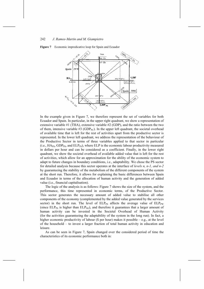
Figure 7 Economic impredicative loop for Spain and Ecuador

In the example given in Figure 7, we therefore represent the set of variables for both Ecuador and Spain. In particular, in the upper right quadrant, we show a representation of extensive variable #1 (THA), extensive variable #2 (GDP), and the ratio between the two of them, intensive variable #3 (GDPPC). In the upper left quadrant, the societal overhead of available time that is left for the rest of activities apart from the productive sector is represented. In the lower left quadrant, we address the representation of the behaviour of the Productive Sector in terms of three variables applied to that sector in particular (i.e., HAPS, GDPPS, and ELPPS), where ELP is the economic labour productivity measured in dollars per hour and can be considered as a coefficient. Finally, in the lower right quadrant, we show the societal overhead of available added value that is left for the rest of activities, which allow for an approximation for the ability of the economic system to adapt to future changes in boundary conditions, i.e., adaptability. We chose the PS sector for detailed analysis because this sector operates at the interface of levels n, n-1, and n-2 by guaranteeing the stability of the metabolism of the different components of the system at the short run. Therefore, it allows for explaining the basic differences between Spain and Ecuador in terms of the allocation of human activity and the generation of added value (i.e., financial capitalisation).

The logic of the analysis is as follows: Figure 7 shows the size of the system, and the performance, this time represented in economic terms, of the Productive Sector. This sector generates the necessary amount of added value to stabilise all other components of the economy (complemented by the added value generated by the services sector) in the short run. The level of ELPPS affects the average value of ELPPW (since ELPPS is higher than ELPSG), and therefore it guarantees that a larger amount of human activity can be invested in the Societal Overhead of Human Activity (for the activities guaranteeing the adaptability of the system in the long run). In fact, a higher economic productivity of labour ($ per hour) makes it possible – e.g., at the level of the household – to invest a larger fraction of total human activity in education and leisure.

As can be seen in Figure 7, Spain changed over the considered period of time the characteristics of its economic performance both in:

Multi-scale integrated analysis of societal metabolism 243

• qualitative terms (development – different profile of distribution of the throughput over the internal components – changes in the value taken by intensive#3 variables)

• quantitative terms (growth – increase in total throughput – changes in the value taken by extensive#2 variables).

This is reflected, for instance, by the increase in ELPPS from 17.91 $/h to 30.68 $/h in the period analysed, and by the related increase in GDP per capita. The increase in the productivity is both a consequence of:

• the capitalisation of the sector (as measured in biophysical terms by higher values of EMRPS)

• a necessity for the system to be able to free an increasing fraction of human activity from those sectors guaranteeing short-term stability to be invested in sectors dealing with long-term adaptability (e.g., research and education).

On the other hand, Ecuador, in the same period of time, basically expanded only the size of its economy (the throughput increased as a result of an increase in redundancy – more of the same – increase in extensive variable#2), but maintaining and even worsening the original relation among intensive variables (the same profile of distribution of values of intensive variables#3, reflecting the characteristics of lower level components, i.e., growth without development). For instance, Ecuador shows an increase in GDP and in Population, but rather shows a decrease in ELPPS, which explains why the system could not undergo a deep change in developmental terms, as reflected by the minor advancement in GDP per capita.

2.3.4 Establishing a bridge between ExMRi and ELPi

The MSIASM approach makes it possible to support an informed discussion about the required/expected levels of capitalisation in the various economic sectors including the household sector. The approach is based on the use of ExMRi as a proxy for the level of capitalisation of economic sectors (explaining the availability of exosomatic devices to support human activity in an economic sector by increasing the exo/endo ratio, see definition at Section 2.3.1), whose size is assessed in terms of investment of hours of Human Activity. Obviously, the performance of the different economic sectors can also be mapped in terms of the relative flow of added value they generate. This monetary flow can be mapped using:

• extensive variables: the total amount of added value of the sector per year

• intensive variables: the amount of added value generated per hour of human activity. At this stage, it becomes possible to use benchmark values to help building scenarios.

The assessment of ‘added value generated per hour of work’ can be used to compare the situation of different economies, or the situation of different regions within the same country, as well as to compare the performance of different firms within the same sector of the same country. Moreover, it is well known that, at the national level, there is a consistent correlation between the intensity of biophysical capitalisation of a productive sector (ExMRi) and the relative ability to generate added value per hour of human activity (ELPi) – (Cleveland et al., 1984; Hall et al., 1986). This link can provide a clue

244 J. Ramos-Martin and M. Giampietro

on what level of capitalisation can be expected in the future in the different economic sectors, by learning the benchmark values found in different trajectories of economic development of other similar countries.

We can use the MSIASM approach to check the validity of the possible correlation between the capitalisation of productive sectors (assessed by their exosomatic energy consumption, fixed plus circulating) and their ability to produce GDP. Accepting this hypothesis implies that ExMRPS and ELPPS are correlated. The good correlation obtained by Cleveland et al. (1984) in their historic analysis of US economy, is confirmed by the curves shown in Figure 8 for Spain and Ecuador. Here, however, we represent instead changes of ExMRPW and ELPPW, that is, all sectors generating added value in the economy (Productive Sector, plus Services and Government, plus Agriculture). In doing so, we find a similar shape or tendency for the considered period: exosomatic energy consumption per unit of working time in the paid work sectors follows the GDP trend. The relationship between these two curves does not imply that these countries have experienced the same course of development, a fact that is confirmed by the comparative analysis of their societal metabolism. In fact, each nation’s development trajectory has been entirely different.

Figure 8 Establishing a bridge between ExMR and ELP in paid work sectors (Spain and Ecuador)

Sources: Ramos–Martin (2001) and Falconi (2001)

The relation between ExMRPW and ELPPW indicates that there is a quantitative link between GDP and energy consumption growth. However, the growth of total economic output can be explained by:

Multi-scale integrated analysis of societal metabolism 245

• increase in population (THA)

• rise in the material standard of living (increase in EMRHH over time)

• increase in the capitalisation of economic sectors included in PW (increase of EMRPW).

Whenever an economy generates a surplus (an extra added value spare from what is used for its maintenance), this surplus can be spent for increasing each and/or all of these three parameters.

What are the implications, then, of the link between ExMRPW and ELPPW, shown in Figure 8? In order to have economic growth, the paid work sectors must increase their energy consumption faster than the rate at which human time is allocated to that sectors; otherwise, the energy surplus will be eaten up by the extra work force. This will be reflected in an increase in ExMRPW, which will bring about a larger availability of investment for producing GDP. Such increased capitalisation will lead, with a time-lag, to an increase in the productivity of labour that will help economies to reduce the amount of human time allocated in PS (short-term stability of components), and to allocate it to activities that increase the range of adaptation paths (i.e., services, medical assistance, research and education, leisure). Clearly, the priority among the possible end uses of available surplus • increasing THA • increasing ExMRHH • increasing ExMRPW

will depend on demographic variables, political choices, and historical circumstances. In the case of Spain, the surplus generated by economic development was big enough

to absorb both new population (due to internal demographic growth) and the exodus of workers from the agriculture sector. The demographic stability of the country made it possible to enter a positive spiral very quickly.

In the case of Ecuador, the crisis following the oil boom can be understood as generated by an insufficient level of capitalisation of the PW sectors (as shown before with ExMRi) that drove the unsatisfying behaviour of ELPi. This can be explained by the fact that economic surplus was almost entirely dedicated to pay the external debt, and to guarantee a minimum level of standard of living to the flow of new population implied by demographic growth. Therefore, the dramatic difference in demographic trends between Spain and Ecuador is crucial to explain the different side of the bifurcation taken by Spain in its trajectory of development.

What are the implications of this result from a methodological point of view? Representing the behaviour of the system across different hierarchical scales and using parallel non-equivalent descriptive domains (e.g., economic, land use, energy use, human time allocation) allows for seeing the inherent biophysical constraints on the socio-economic development of a system. Therefore, it acknowledges that a change of a variable (e.g., a GDP growth goal) implies always a certain requirement in terms of land use (depending on the structural distribution of GDP among sectors), a certain requirement in terms of investment of human activity (depending on how labour intensive the activities are) and in terms of energy consumption (depending on the exosomatic metabolic rates of the different system components).

246 J. Ramos-Martin and M. Giampietro

2.4 Multi-objective integrated representation of performance (MOIR)

The MSIASM approach maintains coherence in a heterogeneous information space referring to different dimensions and different hierarchical levels of analysis using the concepts of ‘mosaic effect’ (dendograms of extensive and intensive analysis across multi-level matrices) and ‘impredicative loop analysis’ (dynamic budget analysis). It is important, however, that this innovative tool can be interfaced with more conventional analysis – e.g., multi-criteria analysis – based on an integrated package of indicators reflecting different dimensions and attributes of performance. This is the subject of the final paper of this special issue (Gomiero and Giampietro, 2005) and therefore does not require much discussion here. An example of a multi-objective integrated representation (MOIR) – a set of different indicators reflecting different criteria of performance selected in relation to different objectives associated with a given analysis – is given in Figure 9. In this example, we have visualised in a graphical form the information given in Figures 1, 2, 4, and 5.

Figure 9 Multi-objective integrated representation of performance in Spain

2.5 Lessons learned from this example

The four examples provided in Figure 7 comparing the situation of Spain and Ecuador at two points in time – 1976 and 1996 – can be used to explain what has generated the differences in the value of extensive and intensive variables. The difference between growth and development can be studied by looking at the relative pace of growth of the value taken by the two types of extensive variables (e.g., the increase in GDP compared to the increase in population size). It is commonplace that studying changes in the level of economic development of a country implies studying changes in GDP per capita (an intensive variable) rather than changes in GDP in absolute terms. The GDP of a country can in fact increase due to a dramatic increase in population when at the same time the GDP per capita is slightly decreasing, i.e., when on average people are getting poorer. By performing in parallel several impredicative loop analyses, based on different selections of extensive variable#1 and extensive variable#2, and by using different definitions of direct and indirect components, it is possible to study this very same

Multi-scale integrated analysis of societal metabolism 247

mechanism at different hierarchical levels of the system and in relation to different dimensions of the dynamic budget.

The approach enables to compare in quantitative terms trajectories of development. For example, at the level of economic sectors, an assessment of intensive variable#3 (the throughput of MJ of exosomatic energy per hour of human activity) has been used to analyse and compare the trajectory of development of Spain (Ramos-Martin, 2001) with that of other countries. In this case, average reference values for typologies of economic sectors found by analysing the trajectory of OECD countries have been used as benchmark values. The set of reference values [e.g., 100 MJ/hour for the service sector; 300 MJ/hours for the productive sector, and 4 MJ/hour for the household sector] made possible to identify characteristics of the Spanish situation. In this particular example, the power of resolution of this approach made possible to detect a ‘memory effect’ left in the Spanish system by the dictatorship of Franco. That is, a certain compression of the level of consumption in the household sector, under the Franco’s regime, enabled Spanish economy to have a quick capitalisation of the economy (reflected by an increase in the exosomatic metabolic rate per hour of working time, in a higher exo/endo ratio in the productive sector). At the same time, this compression caused a very low level of capitalisation of the household sector (the Exosomatic Metabolic Rate – Intensive variable#3 – the exo/endo ratio of human activity invested in the household sector). In fact, the ExMR of the household component – Intensive variable#3 at the level n-1– was 1.7 MJ/hour in 1976. This was by far the lowest level in Europe in that year also compared to countries such as Greece and Portugal (Ramos-Martin, 2001). If someone in 1976 would have had to produce scenarios of future changes in the Spanish economy by looking at differences in this benchmark value, they would have had a walk-over to guess a very rapid growth of this value. Actually, the value of ExMRHH almost doubled until 1996. Such a result could have been guessed, by looking at the European benchmark for the HH sector, which is around 4 MJ/hour. As a general rule, we can expect that the existence of big gradients in the characteristics of intensive variables referring to analogous sectors, among countries, tend to indicate top priorities in development strategy adopted by those countries lagging far behind.

Just to give another example of the kind of results that we can get by adopting an MSIASM approach, we can anticipate how economic growth and energy consumption may drive changes in the values related to demographic variables. For instance, MSIASM supports a better understanding of the ongoing process of mass emigration occurring nowadays in Ecuador. Just looking at the previous graphs, one can see that the major problem of Ecuador has been generated by a sudden increase in population that has induced a stagnation of the economic productivity of labour due to a low rate of capitalisation of economic sectors [dHAPW > dETPW]. This determined a poor performance in terms of increase of ExMRi over time. Therefore, one of the ways out of this impasse is that of allowing a fraction of the work force to emigrate (to reduce the internal increase in HAPW). This is exactly what happened in Ecuador in the recent years. One should expect that people at the age of work tend to emigrate in order to get higher salaries, for instance in Spain. In this case, disposable human activity (HAPW) no matter where generated, tends to follow gradients of capitalisation (moving where ExMRPW is higher), no matter where located. This explains movements of work force from developing countries (where SOET and SOHA is lower) towards developed ones.

248 J. Ramos-Martin and M. Giampietro

Spain has shifted its role from being a source of emigrants (in the previous century) to be a host for immigrants very recently. This is due to the fact that population has stabilised because of one of the lowest fertility rates in the world. In this context, further economic development of Spain requires not only adding new capital, but also new working population. This could be done by increasing the low activity rate (decreasing the Societal Overhead on Human Activity) of the whole economy (55% in 2003 – www.ine.es Spanish National Statistics Institute), or that of women in particular (only 44% of Spanish women in 2003 were in employment). The slow changes in the value of these variables due to cultural lock-in opened the door for new labour force coming from developing countries like Ecuador. Thus, in year 2002, the number of legal Ecuadorian immigrants in Spain has reached 125,000 (Colectivo Ioé, 2002), most of them arriving in Spain in the period 1996–2002 (122,000), due to the economic crisis of Ecuador.

A key characteristic of Ecuadorian emigration to Spain is that 90% of the people are aged between 21 and 50 (Anguiano-Téllez, 2002). Ecuadorians therefore go to Spain basically searching for work (a movement across countries of HAPW).

The issue of migration is usually addressed by demography or economics, but without being able to establish a direct link between demographic or economic variables to environmental ones. With the MSIASM approach, on the contrary, it is possible to establish a clear link between these variables. The reciprocal effect of changes of demographic and economic variables can be explained in biophysical terms. For instance, when looking at the 4-angle figures presented earlier, it is easy to see that the Ecuadorian economy did not capitalise enough to raise the productivity of labour. This fact translated into an insufficient material standard of living. On the contrary, Spain, in the same period of time, experienced stagnation in population growth that in the short-term allowed to rapidly increasing the level of capitalisation and therefore the material standard of living. This very same fact, however, implied, in the mid- and long run, a shortage of human activity to be invested in the PS sector that may drive an economic crisis. This explains the need to receive immigrants to increase the working population. With the MSIASM approach, we can see the inherent biophysical constraints (either in terms of available energy or of human time) of economic development. But there is more, by using a set of intensive variables #3 (those variables related to the intensity of interaction of different elements at different levels measured in terms of matter and energy flows), we can establish a bridge between this type of analysis (linking economic and biophysical variables describing the socio-economic system) to environmental analyses of the impact of societal metabolism. This would require complementing the analysis presented so far with a parallel analysis that uses as multi-level matrix – an extensive variable # 1 – a variable based on land use typologies.

In this section, we presented an example of application of a multi-scale integrated analysis of societal metabolism to the analysis of recent economic history of Ecuador and Spain, focusing on the relation between economic, demographic, and energetic changes. This was done with the goal of providing a complementary tool of analysis to be used in addition to those already available (historical analysis, social analysis, institutional analysis, economic analysis, etc.).

The major advantage of this integrated method of analysis is not in the provision of totally ‘new’ or ‘original’ explanations for events. Rather, it creates the possibility of integrating the various insights already provided by different disciplines. It can discover situations in which there are contradictions among them, or on the contrary, agreements.

Multi-scale integrated analysis of societal metabolism 249

In the example discussed here, we have just focused on human time as a variable to map the size and on added value and exosomatic energy consumption to map the interaction with the environment, but other key variables, such as land uses, may be used instead.

3 MSIASM for scenarios analysis: looking for biophysical constraints for economic development in Vietnam 2000–2010

3.1 Goal of the example

In this section, MSIASM is used for scenarios analysis. The goal of this example is to illustrate the mechanism through which MSIASM can perform a quality check on future scenarios of economic development. To do that, MSIASM is applied to check the robustness of a set of hypotheses of economic development for Vietnam in the year 2010. In the case of Vietnam, we perform an impredicative loop analysis based on a 4-angle representation in relation to profiles of allocation of relevant flows (e.g., added value; exosomatic energy; endosomatic energy, i.e., food) over:

• the economy as a whole

• different economic sectors in charge for the production and consumption of these flows.

This requires including the household sector in the analysis. In this example, we use two relevant extensive variables #1 (multi-level matrix):

• ‘Human Activity’ to define the size of the whole (THA) and the size of the parts (HAi)

• ‘Land Use’ to define the size of the whole (TAL, Total Available Land) and the size of the parts (LUi, Land Used in Activity i).

3.2 Mapping flows against the multi-level matrix: human activity

In this example, we do not carry out an exhaustive analysis as we didbefore for Spain and Ecuador; rather, we use data for Vietnam in 1999 and a set of hypotheses of development for a few key variables in 2010. Data sources include: OECD (2002) for data on population, GDP, and energy consumption in 1999. The working population and its distribution among sectors are taken from UN Statistics, whereas the GDP distribution among sectors is taken from Cuc and Chi (2003). Population in 2010 is derived from UN projections, whereas GDP, GDP distribution among sectors, working population and distribution among sectors are taken from Cuc and Chi (2003) reflecting Vietnam Government projections. Energy consumption for 2010 is assumed to remain at 3.41% of Asia’s energy consumption, according to the projections from International Energy Agency (2003). We also assume that the work load is at 1,800 hours a year (a very generous underestimation), and that the fraction of working population increases to 50% of total population in 2010, due to a reduction in the fertility rate and the entrance in the working age of the previous generation.

250 J. Ramos-Martin and M. Giampietro

3.2.1 Dendrogram of EMRi (relevant extensive variable #2: ‘Exosomatic Energy’ vs. multi-level matrix – extensive variable #1: ‘Human Activity’)

Figures 10 and 11 represent the dendograms of ExMRi for Vietnam in the years 1999 and 2010. The rationale and interpretation of the figures are the same as in Section 2.3.2 for Spain. These variables, as explained earlier, reflect a biophysical accounting of the system.

Figure 10 Dendogram of ExMR in Viet Nam in 1999

Figure 11 Dendogram of ExMR in Viet Nam in 2010

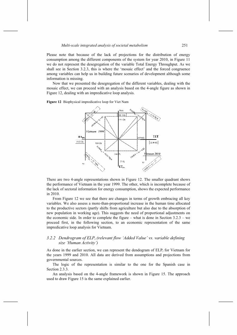
Multi-scale integrated analysis of societal metabolism 251

Please note that because of the lack of projections for the distribution of energy consumption among the different components of the system for year 2010, in Figure 11 we do not represent the desegregation of the variable Total Energy Throughput. As we shall see in Section 3.2.3, this is where the ‘mosaic effect’ and the forced congruence among variables can help us in building future scenarios of development although some information is missing.

Now that we presented the desegregation of the different variables, dealing with the mosaic effect, we can proceed with an analysis based on the 4-angle figure as shown in Figure 12, dealing with an impredicative loop analysis.

Figure 12 Biophysical impredicative loop for Viet Nam

There are two 4-angle representations shown in Figure 12. The smaller quadrant shows the performance of Vietnam in the year 1999. The other, which is incomplete because of the lack of sectoral information for energy consumption, shows the expected performance in 2010.

From Figure 12 we see that there are changes in terms of growth embracing all key variables. We also assess a more-than-proportional increase in the human time allocated to the productive sectors (partly shifts from agriculture but also due to the absorption of new population in working age). This suggests the need of proportional adjustments on the economic side. In order to complete the figure – what is done in Section 3.2.3 – we proceed first, in the following section, to an economic representation of the same impredicative loop analysis for Vietnam.

3.2.2 Dendrogram of ELPi (relevant flow ‘Added Value’ vs. variable defining size ‘Human Activity’)

As done in the earlier section, we can represent the dendogram of ELPi for Vietnam for the years 1999 and 2010. All data are derived from assumptions and projections from governmental sources.

The logic of the representation is similar to the one for the Spanish case in Section 2.3.3.

An analysis based on the 4-angle framework is shown in Figure 15. The approach used to draw Figure 15 is the same explained earlier.

252 J. Ramos-Martin and M. Giampietro

Figure 13 Dendogram of ELP in Viet Nam in 1999

Figure 14 Dendogram of ELP in Viet Nam in 2010

Figure 15 Economic impredicative loop for Viet Nam

Multi-scale integrated analysis of societal metabolism 253

As can be seen from Figure 15, Vietnam is expected to undergo important changes over the next decade. This implies new characteristics for Vietnam’s economic performance both in:

• qualitative terms (development – different profile of distribution of the throughput over the internal components – changes in the value taken by intensive#3 variables)

• quantitative terms (growth – increase in the total throughput – changes in the value taken by extensive#2 variables).

This is reflected, for instance, by an increase in per capita GDP. However, in contrast to what happened in Spain, and more similar to the development of Ecuador, the increase in GDP per capita is not expected to be associated with qualitative changes in the productive sectors. In other words, increases in the economic productivity of labour in such a sector, ELPPS, are missing. Rather ELPPS is expected to decrease. Therefore, the moderate increase of GDP per capita in Vietnam will reflect two types of changes:

• The movement of a certain fraction of HAPW from the AG (agricultural sector) to the SG (Service and Government) and PS (Productive Sector). That is, HAAG will move from 68% of HAPW to 50% of HAPW; whereas HASG will move from 20% of HAPW to 26% of HAPW; and finally HAPS will move from 12% of HAPW to 24% of HAPW (which results in a doubling of the human activity invested in PS!).

• Changes in demographic variables, which will imply a different profile of allocation of the budget of human activity. This can be associated with a decrease in the societal overhead (determining the difference between THA and HAPW). SOHA = (THA – HAPW)/HAPW will move from 10.3 to 9.7.

This result is most relevant, since it indicates that a good performance in the short run (i.e., a quick increase in GDP per capita) may be realised at the expense of long-term adaptability of the whole system. This is especially evident in the People’s Republic of China today, with almost 60% of the population in the work force (due to the drastic population policy in the previous decades). However, when the relative age cohorts will reach the retirement age, it is not clear what type of consequences can be expected. Therefore, a warning sign must be put here to alert about the possible constraints, or lock-in that this scenario of development may impose on the Vietnamese economy in the future. The demographic dynamics remind of Ecuador that led to the present economic crisis in that country, as explained in Section 2.5.

If we accept the validity of the relationship between ExMR and ELP discussed earlier, that is, that we should expect a direct link between the level of biophysical capitalisation (exosomatic metabolic rate per hour of work in a given sector) and the economic productivity of labour, we can use the values of ELP suggested by the hypothesis of development for 2010 to guess the values of ExMR for the same year. This permits closing the 4-angle representation of Figure 12. This is done in the following section.

3.2.3 An application of the ‘mosaic effect’

The representation of the characteristics of different elements defined at different hierarchical levels by using a dendogram makes evident the fact mentioned before that in this type of analysis, we do not need to know all data. Because of the forced congruence

254 J. Ramos-Martin and M. Giampietro

across scales, and because of the parallel non-equivalent descriptive domains used to represent the behaviour of the Vietnamese economy, we can estimate the value taken by a variable using different ways, i.e., approaching it from information referring to the lower levels and scaling up, or approaching it from information referring to the higher levels of the system and scaling down.

This is seen in Figure 16.

Figure 16 Biophysical impredicative loop for Viet Nam after using ELP

The hypothesis of a link between ExMR and ELP is used to complete Figure 12. By adopting this approach, we can forecast a very limited increase in the material standard of living (ExMRSA) for Vietnam in spite of the expected increase in GDP per capita. Indeed, most of the increase in energy consumption will be invested for the capitalisation of the productive sectors of Vietnam (ET will move from 348 PJ to 840 PJ). This may reduce the societal overhead over the Total Energy Throughput, which is the relative share of energy that can be invested in other activities (SG and HH) that may affect the long-term stability of the system. This is a result that we already found when doing the economic reading for the Vietnamese economy. As in the Ecuadorian case, this might have huge implications for future development, since it reduces the speed at which the country could capitalise its productive sector, at the very same moment in which the rate of active population will be peaking due to population rise. This may create a potential evolutionary lock-in for future development.

What is relevant in this example are not the predictions or the following interpretations given by us. Rather, what is relevant is the role that MSIASM can play in helping the social actors involved in a discussion of future scenarios to focus on the relevance and credibility of assumptions, hypotheses, and scenarios, as well as providing criteria to verify the quality of the process (by using benchmark values to make comparison with other similar situations. Due to the internal congruence required in the information space, and due to the use of parallel non-equivalent descriptive domains and different scales to represent the same facts, we can:

• re-construct some data series in which some values are missing, a fact of particular relevance when working with scenarios of development

• verify against known benchmark values the credibility of changes forecasted in different elements of the socio-economic system.

Multi-scale integrated analysis of societal metabolism 255

3.3 Mapping flows against the multi-level matrix: land use

In the previous section, we had shown an example of application of MSIASM, which was based on the same selection of variables used for describing the size of the system and its components as used in the case of Spain and Ecuador. The MSIASM approach, however, allows using other variables. We present here a simple exercise using as extensive variable #1 providing the multi-level common matrix, a variable for land use. In this simple example, we focus on the existence of possible trade-offs between economic development and food security in relation to future choices of production/consumption of food in Vietnam. Actual data, referring to the year 2000, are compared with two possible scenarios of grain production for 2010. The analysis looks for biophysical constraints that may help eliminating inconsistent scenarios. To make the example simpler, we focus just on rice production. A more sophisticated study, which is not done here, could provide, by using the same set of tools (dendograms and 4-angle figures) an analysis of the link between typologies of land use (associated to a definition of identities of whole and parts across levels) and: • generation of added value (economic reading) • consumption of exosomatic energy (biophysical reading).

3.3.1 Characterising the situation in year 2000

The distribution of a set of different land use categories for Vietnam in year 2000 is given in Figure 17. There is a first distinction between Plains (21% of the territory) and Mountains and Uplands (79% of the territory). In the lowlands, we can define two land use categories: built-up area and agricultural land. For the sake of simplicity, we assume that all forest and non-used land is located in Mountains and Uplands. In fact, Vietnam is a very densely populated country and there is a very high pressure on lowlands for agricultural, infrastructures, and residential uses. Moreover, most of the agricultural land producing rice is located in lowlands where soils are more fertile and do not suffer from high slopes. However, considerable parts of swidden agriculture are located in the uplands.

Figure 17 Viet Nam Land Use in 2000

256 J. Ramos-Martin and M. Giampietro

With that distribution of land, Vietnam produced 34 million tonnes of grain in the year 2000, of which 3.6 million tonnes were exported (Cuc and Chi, 2003). This translates into a consumption of 389 kg/year per capita. Given the fact that only 85% of the agricultural land is in fact cultivated land (Tam and Hien, 1998), we can estimate the yields for lowland and upland rice production. Please take into account that these are rough estimates of the flow of produced rice per year (not accounting for the agronomic performance characterised when considering the Multi-Crop Index).

When doing this simplification by assuming that at the level n-1:

• EV#1: ha of land in rice production in lowland (ThaLL = 4.9 Mha)

• EV#1: ha of land in rice production in upland (ThaUL = 2.7 Mha)

• IV#3: yield of land in rice production in lowland (tonnes/haLL = 5.3)

• IV#3: yield of land in rice production in upland (tonnes/haUL = 3.0)

we can write the assessment of total rice production as:

Level n-1 = (4,900,000 haLL × 5.3 t/ha) + (2,700,000 haUL × 3 t/ha) = 34 Mt

Level n = 34 Mt (internal consumption + export).

3.3.2 Looking for biophysical constraints for future development: scenario A

We can assume that in the next decade, in Vietnam the major part of the increase in built-up areas and infrastructures derived from economic development and population growth will take place in the lowland. Because of this, we should expect a reduction of agricultural land in production in these favourable parts of the country. We assume that in the year 2010 a share of 15% of the agricultural land actually in rice production in the lowland will be lost. If this is true, we should also expect that the increased demand for food and for agricultural commodities for both increased internal consumption (for a larger population) and increased export (for increased economic revenue from the agricultural sector) will generate an important pressure for increasing the land in rice production in the uplands. We can check the congruence between the amount of food required for internal consumption and for export, as predicted by the scenario and the biophysical constraints associated to the production of flows of food at the field level (at the level n-1). The possible allocation of land in production both in lowland and highland has also to include the requirement of land for housing (for the growing population of the cities), industrial sites, infrastructures (as roads, railroads, ports, warehouses).

As mentioned earlier, it is very likely that the vast majority of these alternative land uses will occur in the low land (expanding the area around existing cities and transforming large villages into small cities).

On the other hand, agricultural land in the uplands has a lower productivity and this would require a huge increase in the quantity of fertilisers used for production to increase the yields, not mentioning the problem of soil erosion implied by high slopes. Moreover, accepting the natural low productivity per hectare will translate into an extensive deforestation of what is left of the original forest in the uplands. It should be noted that the hypothesis of economic growth considered here also assumes that the forest coverage in 2010 will reach 45% of the total area (Cuc and Chi, 2003) as a part of a governmental

Multi-scale integrated analysis of societal metabolism 257

reforestation plan. In this case, we experience parallel goals competing with the same limited endowment of land:

• an increase in population requiring space for infrastructure and domestic production of food

• an increase in GDP from agriculture, requiring space for producing crops for export

• an increase in the forest cover occurring mainly in the uplands, because of the governmental reforestation plan (where the additional crop production should take place) at the expense of non-used land.

The possibility of keeping a wide range of alternative land uses while reducing the pressure on the environment could only be matched by a dramatic intensification of agricultural production (in terms of a dramatic boosting of yields, both in high and low land).

Coming to an analysis of technical coefficients referring to lower level analysis (e.g., agronomic performance), we can say that in the lowland a dramatic increase of yields would result problematic. In fact, the major boost associated with the adoption of green revolution technology has already been obtained, and we are in the part of the curve yield/input that implies considerable diminishing returns. It is comparably easy to move from 2 tons/ha to 4 tons/ha, it is expensive to move from 4 tons/ha to 6 tons/ha, whereas it is extremely difficult to move from 6 tons/ha to 8 tons/ha. Moreover, an additional intensification of the use of technical inputs could worsen the already heavy environmental impact associated with agricultural production. On highlands, the problem of getting an intensification of yields will be even more noticeable when considering soil erosion for upland cultivation of rice. But the main problem in this case would be related to the high labour demand of this system of production, which would imply locking a large fraction of the working population in agricultural production (and therefore on a very low level of ELPi).

By using an analysis of flows of rice (used as extensive variable #2 in this example) against a multi-level matrix of land uses (used as extensive variable #1 in this example), we link agricultural production objectives (i.e., depending on the selected hypotheses of development scenarios) to land use and to possible environmental impact of agricultural production.

In the first scenario, we take population projections expecting a population in 2010 of 89 million people. We assume there is a minor increase in the per capita consumption from 389 kg to 420 kg and that exports also increase to six million tonnes (according to the objective set out in government’s development strategy). Despite being very expensive in terms of energy, and probably in terms of the resulting pollution, we also assume here that a rise in yields will be possible. Thus, yields in the lowlands increase up to seven tonnes per hectare (i.e., due to a larger use of fertiliser), whereas yields in the uplands remain at three tonnes per hectare. This is so because an increase in fertilisers will have to make up for the lower fertility of marginal land added. These numbers, along with the loss of 15% of agricultural land in lowlands mentioned earlier, provides the picture given in Figure 17.

With these assumptions, we will have at level n-1:

258 J. Ramos-Martin and M. Giampietro

• EV#1: ha of land in rice production in lowland (ThaLL = 3.9 Mha)

• EV#1: ha of land in rice production in upland (ThaUL = 2.7 Mha)

• IV#3: yield of land in rice production in lowland (tonnes/haLL = 7.0)

• IV#3: yield of land in rice production in upland (tonnes/haUL = 3.0)

we can write the assessment of total rice production as:

Level n-1 = (3,900,000 haLL × 7 t/ha) + (5,600,000 haUL × 3 t/ha) = 44 Mt

Level n = 44 Mt (internal consumption + export)

In order to produce the rice necessary for internal consumption and exports, Vietnam would have to increase agriculture land in rice production in the uplands up to more than 5.5 million hectares. This would imply adding two million hectares to the area already in production in the year 2000!

Figure 18 Viet Nam Land Use in 2010 scenario A

It is interesting to notice that just producing more food for feeding the new population would imply major problems from an environmental point of view. For instance, the increase in both agricultural production and forests in the uplands implies a dramatic reduction of the category ‘land not in use’ to less than half of the value in year 2000. This change is in conflict with the goal of increasing the forest cover. We are talking of an incongruence that has to be analysed in detail, since strong incongruence in conflicting demands for different land uses may have permanent impacts in ecological terms. Moreover, it is clear that a strong tension between the objective of reforestation and increasing agricultural production should be expected. Moreover, a certain part of the land not in use is not suitable for any activity. This could concentrate the conflicts in particular locations.

Multi-scale integrated analysis of societal metabolism 259

3.3.3 Looking for biophysical constraints for economic development: scenario B

This is a less optimistic scenario based on the same set of hypotheses of socio-economic development used in Scenario A but adopting the same level of agricultural yields achieved in the year 2000. The rationale for this choice is that increasing yields at any cost, not necessarily should result in the most convenient choice (diminishing returns imply a more than proportional use of inputs, which can have negative effects both in economic and environmental terms). Moreover, the analysis done in Section 3.2 seems to indicate that we should not expect an increase in the level of biophysical capitalisation of the economy (ExMR) as a whole. This should therefore translate into a shortage of energy and resources to be invested in agriculture. In fact, it is well known that investments in the agricultural sector do have lower returns than that in other sectors of the economy. To make things worse, we should recall here that the Societal Overhead of Energy Throughput was even expected to decrease. Put in another way, it is very unlikely that we will see a major change in the technical coefficients for rice production especially in the uplands. So, if we keep the given yields at 5.3 tons per hectare for lowland and three tons per hectare in uplands, in order to produce the required 44 million tonnes of rice, Vietnam should increase the agricultural use of land in the uplands up to 7.7 M ha in rice production, without including other agricultural land uses (to arrive to 8.4 M ha). This would represent an almost threefold increase as compared to the amount of agricultural land in the year 2000. Again, if this is to be achieved along with the reforestation plan, this will imply that only 1.5 million hectares will be left as non-used land (see Figure 19). This seems to be an unachievable scenario to be checked using a more detailed analysis of possible land uses and land cover changes.

Figure 19 Viet Nam Land Use in 2010: Scenario B

4 Conclusion

The analysis of economic development and its relationship with the relative environmental impact implies dealing with the interaction of ecosystems and economic

260 J. Ramos-Martin and M. Giampietro

systems considered both as complex, nested, hierarchical systems. When doing so, individual reductionist analyses are not useful for describing the results of such an interaction. An integrated approach such as the one presented here offers some advantages since it links, by means of relations of congruence, the economic reading to the biophysical reading, as well as it offers the possibility to gather data on different hierarchical levels. This helps to better understand the inherent constraints associated with the process of change. That is, economic growth shall always imply a growth in the metabolism of the socio-economic system; therefore, we should always expect an associated impact on the environment.

The MSIASM approach can be used for both carrying out historical analysis – as done in Section 2 – and for prospective analysis – as carried out in Section 3. In the first case, the use of MSIASM can help us to characterise the development path followed by the system, by means of different ‘useful types’ such as economic sectors, different groups of agents, along with their associated impact.

We have acknowledged here the fact that economic systems are complex systems. When using MSIASM for conducting prospective analysis, like in the case of Vietnam, we do not see the possibility of making predictions. From an epistemological point of view, this was already said by Rosen, who stated that if a basic characteristic of complex systems is that “they can only be approximated, locally and temporarily, by dynamical systems”, but we still try to control them by using predictive dynamic models, we may face a ‘global failure’ (Rosen, 1987 p.134, emphasis in the original) in the form of a growing discrepancy between what the system is doing and what the model can predict.

We believe that the selection and discussion of scenarios has more to do with the selection of useful narratives (i.e., soft modelling) rather than with forecasting (i.e., hard modelling). This is so because of the nature of complex adaptive systems, characterised by irreversibility and stochasticity in their evolution. The existence of numerous possible future trajectories associated with high levels of uncertainty (the sure emergence of novelties) implies that their future is largely unpredictable. We have to admit that there are no deterministic explanations (universal and a-historical) for the present states of complex adaptive systems. Rather, we can describe and understand these systems by finding historical and spatial regularities, and by looking at the emergence of specific systems’ properties (Ramos-Martin, 2003). This requires still finding useful types for conducting research at the different levels. However, the selection of types must be later on tailored for coping with the particularities of specific situations. In this way, we can inform the decision process about the possible constraints implied by different courses of action. In our view, this translates into improving the quality of the narratives used to characterise, analyse, and describe the behaviour of complex system such as ecosystems, economies, and their interaction.

Coming to technical aspects of the MSIASM methodology, we would make the following four points:

• When building scenarios, we need to use in parallel non-equivalent descriptive domains, that is, parallel readings of the system referring to different dimensions of analysis and perceptions of events referring to different levels and scales. An integrated use of information coming from different disciplines applied at different scales provides more insight than the use of disciplinary findings (e.g., economic variables) used one at the time in relation to a single scale at the time.

Multi-scale integrated analysis of societal metabolism 261

• The use of different dimensions of analysis applied at different hierarchical levels of the system requires a certain degree of congruence across levels. This entails the use of an accounting system especially tailored on this task. The proposed approach – MSIASM – can fulfil this requirement.

• The congruence in the definition of the whole, the parts, and the relations that link them (over the same level and across levels) is what generates the ‘mosaic effect’. Mosaic effects are desirable because they generate redundancy in the information space. Within a proper accounting system able to define certain ‘types’ of activities and expected relations among components of the system, one does not always need to know all data for generating and analysing future scenarios. The example of crossword puzzles should be recalled here. If the value of a variable is missing at a lower level (e.g., a particular ExMR) that information can be obtained by our knowledge of the situation on the higher level by crossing information related to a different reading.

• The impredicative loop analysis of dynamic budgets (against a multi-level matrix used for defining compartments across levels) allows a better understanding of the internal constraints affecting the stability of the budget. In this way, it becomes possible to identify possible bottlenecks, and lock-in situations. This makes it also possible to define which part of the metabolic flow is directed to short-term stability – usually linked to efficiency – and which part may be allocated to long-term stability – linked to adaptability. It should be noticed that in general, reductionist analysis of scenarios does not deal with this second part. Efficiency is considered as a key optimising factor, and adaptability is not considered as relevant for driving future unknown trajectories of development. The MSIASM approach explicitly acknowledges the need of operating a continuous mediation between the two contrasting goals of increasing efficiency and adaptability.

References Anguiano-Téllez, M.E. (2002) ‘Emigración reciente de latinoamericanos a España: trayectorias

laborales y movilidad ocupacional’, Papeles de Población, No. 33, pp.101–115, Julio–Septiembre, México.

Cleveland, C.J., Costanza, R., Hall, C.A.S. and Kaufmann, R. (1984) ‘Energy and the US economy: a biophysical perspective’, Science, Vol. 225, pp.890–897.

Colectivo Ioé (Walter Actis, Carlos Pereda y Miguel Ángel de Prada) (2002) Inmigración, escuela y mercado de trabajo: Una radiografía actualizada, Fundación ‘La Caixa’, Colección Estudios Sociales, No. 11, http://www.estudios.lacaixa.es.

Cottrel, W.F. (1955) Energy and Society: The Relation between Energy, Social Change, and Economic Development, McGraw-Hill, New York, p.330.

Cuc, L.T. and Chi, T.K. (2003) ‘Vietnam: socio-economic development strategy 2001–2020’, Presented at the 3rd Project Workshop Southeast Asia in Transition, 2–6 June, Vienna, Austria, p.8.

Falconi-Benitez, F. (2001) ‘Integrated assessment of the recent economic history of Ecuador’, Population and Environment, Vol. 22, No. 3, pp.257–280.

Fischer-Kowalski, M. (1997) ‘Society’s metabolism: on the childhood and adolescence of a rising conceptual star’, in Redclift, M. and Woodgate, G. (Eds.): The International Handbook of Environmental Sociology, Edward Elgar, Cheltenham, p.512.

262 J. Ramos-Martin and M. Giampietro

Georgescu-Roegen, N. (1971) The Entropy Law and the Economic Process, Harvard University Press, Cambridge, Massachusetts, p.476.

Georgescu-Roegen, N. (1975) ‘Energy and economic myths’, Southern Economic Journal, Vol. 41, pp.347–381.

Giampietro, M. (1997) ‘Linking technology, natural resources, and the socioeconomic structure of human society: a theoretical model’, Advances in Human Ecology, Vol. 6, pp.75–130.

Giampietro, M. (2003) ‘Multi-scale integrated analysis of agro-ecosystems’, in Edwards, C. (Ed.): Series of Advances in Agroecology, CRC Press, Boca Raton, p.472.

Giampietro, M. (Ed.) (2000) ‘Special issue of ‘population and environment’ on societal metabolism – part 1 of 2: introduction of the analytical tool in theory, examples, and validation of basic assumptions’, Population and Environment, Vol. 22, No. 2, pp.97–254.

Giampietro, M. and Ramos-Martin, J. (2005) ‘Multi-scale integrated analysis of sustainability: a methodological tool to improve the quality of narratives’, International Journal of Global Environmental Issues, Vol. 5, Nos. 3–4, pp.119–141.

Giampietro, M., and Mayumi, K. (1997) ‘A dynamic model of socioeconomic systems based on hierarchy theory and its application to sustainability’, Structural Change and Economic Dynamics, Vol. 8, pp.453–469.

Giampietro, M., Mayumi, K. and Bukkens, S.G.F. (2001) ‘Multiple-scale integrated assessment of societal metabolism: an innovative approach to development and sustainability’, mimeo.

Gomiero, T. and Giampietro, M. (2005) ‘Graphic tools for data representation in integrated analysis of farming systems’, International Journal of Global Environmental Issues, Vol. 5, Nos. 3–4, pp.264–301.

Hall, C.A.S., Cleveland, C.J. and Kaufmann, R.K. (1986) The Ecology of the Economic Process: Energy and Resource Quality, John Wiley & Sons, New York, p.602.

International Energy Agency (2003) Key World Energy Statistics, Paris, p.82. Jantsch, E. (1987) The Self-Organizing Universe, Pergamon Press, Oxford, p.343. Jevons, W.S. (1865) The Coal Question: An Inquiry Concerning the Progress of the Nation, and

the Probable Exhaustion of Our Coal-Mines, in Flux, A.W. (Ed.): 3rd ed. rev. Augustus M. Kelley, New York, Reprinted in 1965.

Kay, J.J. and Regier, H. (2000) ‘Uncertainty, complexity, and ecological integrity: insights from an ecosystem approach’, in Crabbé, P., Holland, A., Ryszkowski, L. and Westra, L. (Eds.): Implementing Ecological Integrity: Restoring Regional and Global Environmental and Human Health, Kluwer, NATO Science Series, pp.121–156.

Lotka, A.J. (1922) ‘Contribution to the energetics of evolution’, Proc. Nat. Acad. Sci., Vol. 8, pp.147–154.

Lotka, A.J. (1956) Elements of Mathematical Biology, Dover Publications, New York, p.465. Martinez-Alier, J. (1987) Ecological Economics: Energy, Environment, and Society, Blackwell’s

Book Services, Oxford, p.287. Maturana, H.R. and Varela, F. (1980) Autopoiesis and Cognition: The Realization of the Living,

D. Reidel, Boston, p.141. Mayumi, K. (2001) The Origins of Ecological Economics: The Bioeconomics of

Georgescu-Roegen, Routledge, London, p.174. Odum, H.T. (1971) Environment, Power, and Society, Wiley-Interscience, New York, p.331. Odum, H.T. (1983) Systems Ecology, John Wiley, New York, p.644. OECD (2002) OECD Statistical Compendium on CD-ROM, Paris. Ostwald, W. (1907) ‘The modern theory of energetics’, Monist, Vol. 17, pp.481–515. Podolinsky, S. (1883) ‘Menschliche Arbeit und Einheit der Kraft’, Die Neue Zeit, Stuttgart, p.413. Ramos-Martin, J. (2001) ‘Historical analysis of energy intensity of Spain: from a ‘conventional

view’ to an ‘integrated assessment’, Population and Environment, Vol. 22, No. 3, pp.281–313.

Multi-scale integrated analysis of societal metabolism 263

Ramos-Martin, J. (2003) ‘Empiricism in ecological economics: a perspective from complex systems theory’, Ecological Economics, Vol. 46, pp.387–398.

Rappaport, R.A. (1971) ‘The flow of energy in an agricultural society’, Sci. Am., Vol. 224, pp.117–133.

Rosen, R. (1985) Anticipatory Systems: Philosophical, Mathematical and Methodological Foundations, Pergamon Press, New York, p.436.

Rosen, R. (1987) ‘On complex systems’, European Journal of Operational Research, Vol. 30, pp.129–134.

Schandl, H., Grünbühel, C.M., Haberl, H. and Weisz, H. (2002) A Handbook on Methodologies to Describe the Physical Dimension of Socio-economic Activities with respect to Environmental Change – Accounting for Society’s Metabolism and Appropriation of Net Primary Production, Mimeo, IFF – Dept. Social Ecology, Vienna.

Tam, T.T.B. and Hien, H.M. (1998) ‘Land use and cover change in Vietnam’, Paper presented at the Land Use/Cover Change – Data and Information Systems (LUCC-DIS) Workshop, 13th August, Chulalongkorn University, Bangkok, Thailand.

Ulanowicz, R.E. (1986) Growth and Development: Ecosystem Phenomenology, Springer, New York, p.224.

Varela, F., Maturana, H.R. and Uribe, R. (1974) ‘Autopoiesis: the organization of living systems, its characterization, and a model’, Biosystems, Vol. 5, pp.187–196.

White, L.A. (1943) ‘Energy and evolution of culture’, Am. Anthropol., Vol. 14, pp.335–356. White, L.A. (1959) The Evolution of Culture: The Development of Civilization to the Fall of Rome,

McGraw-Hill, New York.