Multi-modal Medical Image Processing
132
Multi-modal Medical Image Processing with Applications in Hybrid X-ray/Magnetic Resonance Imaging Multimodale medizinische Bildverarbeitung mit Anwendungen in der hybriden R¨ ontgen-/Magnetresonanzbildgebung Der Technischen Fakult¨ at der Friedrich-Alexander-Universit¨ at Erlangen-N¨ urnberg zur Erlangung des Doktorgrades Dr.-Ing. vorgelegt von Bernhard Stimpel aus M¨ unchen, Deutschland
-
Upload
khangminh22 -
Category
Documents
-
view
0 -
download
0
Transcript of Multi-modal Medical Image Processing
Multi-modal Medical Image Processingwith Applications in Hybrid
X-ray/Magnetic Resonance Imaging
Multimodale medizinische Bildverarbeitung mit Anwendungenin der hybriden Rontgen-/Magnetresonanzbildgebung
Der Technischen Fakultatder Friedrich-Alexander-Universitat
Erlangen-Nurnberg
zur
Erlangung des Doktorgrades Dr.-Ing.
vorgelegt von
Bernhard Stimpelaus
Munchen, Deutschland

Als Dissertation genehmigtvon der Technischen Fakultatder Friedrich-Alexander-Universitat Erlangen-Nurnberg
Tag der mundlichen Prufung: 21.01.2021Vorsitzender des Promotionsorgans: Prof. Dr.-Ing. Knut GraichenGutachter: Prof. Dr.-Ing. habil. Andreas Maier
Prof. Ge Wang, PhD
Abstract
Modern medical imaging allows for a detailed insight into the human body. The widerange of imaging methods enables the acquisition of a large variety of information,but the individual modalities are usually limited to a small part of it. Therefore, of-ten several acquisition types in different modalities are necessary to obtain sufficientinformation for the assessment. The evaluation of this extensive information posesgreat challenges for clinical users. In addition to the time expenditure, the identifica-tion of correlations across multiple data sets is a difficult task for human observers.This highlights the urgency of holistic processing of the accruing information. Thesimultaneous evaluation and processing of all available information thus not only hasthe potential to uncover previously unimagined correlations but is also an importantstep towards relieving the burden on clinical personnel. In this thesis, we investigatemultiple approaches for the processing of multi-modal medical image data in differentapplication areas.
First, we will focus on hybrid X-ray and magnetic resonance (MR) imaging. Thecombination of these modalities has great potential especially in interventional ima-ging due to the combination of fast, high-resolution X-ray imaging and the highcontrast diversity of magnetic resonance imaging. For further processing of this data,however, it is often advantageous to have the information from both modalities in onedomain. Therefore, we investigate the possibility of a deep learning-based projection-to-projection translation of MR projection images to corresponding X-ray-like views.In the course of this work, we show that the characteristics of projection images posespecial challenges to the methods of image synthesis. We tackle these by weightingthe objective function with a focus on high-frequency structures and a correspondingadaptation of the network architecture. Both modifications show clear improvementscompared to conventional approaches, quantitative as well as qualitative.
Second, we deal with the topic of comprehensibility in the course of deep learning-based processing of multi-modal image data. Specifically, we investigate the combi-nation of established deep learning approaches with known operators, in this casethe guided filter. The conducted experiments show that this combination allows fora processing that performs less manipulation of the image content, is more robustto degraded input data, and ensures a higher level of protection against adversarialattacks. All this can be achieved with little or no loss of pure performance.
Third, we are concerned with an approach for the optimization of image processingmethods based solely on feedback from a human user. This approach addresses adifficult problem of image processing, namely the automated evaluation of imagequality. While human observers can rarely explicitly provide a reference as the targetof the optimization process, their ability to judge results is usually excellent. We usethis to set up an objective function in a forced-choice experiment, which is basedonly on the judgment of a user. We show that the presented strategy can be usedsuccessfully for optimization, from simple parameterized operators up to complexneural networks.
Zusammenfassung
Die moderne medizinische Bildgebung ermoglicht einen detaillierten Einblick in denmenschlichen Korper. Die große Bandbreite der Akquisitionsmethoden erlaubt dieErfassung einer Vielzahl von Informationen, aber die einzelnen Modalitaten sind inder Regel auf einen kleinen Teil dieser beschrankt. Oft sind deshalb mehrere Akqui-sitionstypen in verschiedenen Modalitaten notwendig um hinreichende Informatio-nen fur die Begutachtung dieser zu erlangen. Die Auswertung dieser umfangreichenInformationen stellt die klinischen Nutzer vor große Herausforderungen. Zusatzlichzum notigen Zeitaufwand ist die Erkennung von Zusammenhangen uber mehrere Da-tensatze hinweg eine schwierige Aufgabe fur menschliche Betrachter. Dies verdeutlichtdie Dringlichkeit einer ganzheitlichen Verarbeitung der anfallenden Informationen.Die simultane Verarbeitung aller vorhandenen Informationen hat somit nicht nur dasPotential bisher ungeahnte Zusammenhange aufzudecken, sondern ist auch ein wich-tiger Schritt zur Entlastung des klinischen Personals. In dieser Arbeit untersuchen wirdeshalb mehrere Ansatze zur Verarbeitung von multi-modalen medizinischen Bildda-ten in verschiedenen Anwendungsgebieten.
Zuerst wird die hybride Rontgen und Magnetresonanz Bildgebung betrachtet.Diese hat großes Potential aufgrund der Verbindung von schneller, hochauflosenderRontgenbildgebung mit der hohen Konstrastvielfalt der Magnetresonanztomographie.In der interventionellen Radiologie ist die auf Rontgenstrahlung basierte Projektions-bildgebung von besonderer Bedeutung. Deshalb untersuchen wir die Moglichkeit einerProjektion-zu-Projektion Translation von MR Projektionsbildern zu korrespondieren-den Rontgenprojektionen. Es wird gezeigt, dass die Charakteristika von Projektions-bildern spezielle Herausforderungen an die Bildsynthese stellen. Wir wirken diesenmit einer Gewichtung der Zielfunktion mit einem Fokus auf hochfrequente Struktu-ren und einer Anpassung der Netzwerkarchitektur entgegen. Beide Modifikationenzeigen dabei deutliche Verbesserungen im Vergleich zu gewohnlichen Ansatzen, so-wohl quantitativ als auch qualitativ.
Anschließend beschaftigen wir uns mit dem Thema der Nachvollziehbarkeit bei derDeep Learning basierten Verarbeitung von multimodalen Bilddaten. Konkret unter-suchen wir die Verbindung von Deep Learning Ansatzen mit bekannten Operatoren,im Speziellen dem Guided Filter. Die durchgefuhrten Experimente zeigen, dass dieseKombination eine Verarbeitung ermoglicht die weniger Manipulation an den Bildin-halten durchfuhrt, robuster gegenuber degradierten Inputdaten ist und ein erhohtesMaß an Sicherheit gegen adverserielle Attacken gewahrleistet. All dies kann dabeimit keinem oder nur geringem Verlust an reiner Performance erreicht werden.
Zuletzt wird ein Ansatz zur Optimierung von Methoden zur Bildverarbeitung, deralleine auf dem Feedback durch einen menschlichen Nutzer basiert, behandelt. DiesesVorgehen ermoglicht ein schwieriges Problem der Bildverarbeitung anzugehen, dieautomatisierte Bewertung der Bildqualitat. Wahrend menschliche Beobachter nurselten explizit eine Referenz als Ziel des Optimierungsprozesses angeben konnen, istihre Fahigkeit zur Bewertung von Ergebnissen meist exzellent. Wir nutzen dies, umin einem Forced-Choice Experiment eine Zielfunktion aufzustellen, die auf der Bewer-tung eines Nutzers basiert. Dabei konnen wir zeigen, dass die prasentierte Strategieerfolgreich zur Optimierung eingesetzt werden kann, von einfachen parametrisiertenOperatoren bis hin zu komplexen Neuronalen Netzwerken.
Acknowledgment
While the writing of this dissertation was done by myself, many people contributedto make this possible. I would like to take this opportunity to thank them.First and foremost, I would like to express my gratitude to my supervisor Prof. An-dreas Maier. He played a key role in developing my scientific interests already duringmy studies. Later, he made it possible for me to join the Pattern Recognition Labto pursue my PhD. In particular, the trust, freedom, and support I received thereallowed me to constantly enjoy my work and to fully concentrate on my researchactivities.While doing so, I had the pleasure to be part of the Department of Neuroradiologyof the University clinics Erlangen. I want to thank Prof. Arnd Dorfler who enabledthis great opportunity. Being so close to clinical practice provided us extensive in-sights and focus for our research. Furthermore, we received invaluable opportunitiesand support in conducting clinical experiments. At this point I also want to thankDr. Philip Holter who was always keen on learning about our activities and oftensacrificed his free time to help us with our projects.Completing the core project team, Dr. Martino Leghissa played an important role inshaping our vision of the hybrid X-ray/MR imaging device. I want to thank him forsharing his deep expertise in physics and engineering with us as well as for all thetime together in the imaging booth. Furthermore, he spent endless hours coordinat-ing and aligning all our formal project work which I greatly appreciate.Additionally, I have to thank Prof. Ge Wang. His fundamental research towards hy-brid X-ray/MR imaging and Omnitomography marked the way for me when startingmy PhD in this field. Consequently, it was a great pleasure having him as a reviewerof this thesis.A big thank you to all my colleagues at the Pattern Recognition Lab. I truly enjoyedbeing part of this community. Over three years we shared many great discussions,experiences, difficulties, and memories and along this way many of them have becomefriends. Everyone contributed to make this a special time of my life and I want toaddress some of the most important ones here. To keep it concise, everyone is listedonly once even if they could be mentioned at multiple occasions.In particular, I have to thank Christopher Syben. I profited greatly from his exten-sive knowledge and helpfulness. We shared most of our daily work during the wholetime of my PhD and despite all difficulties and challenges it was not only a greatcollaboration but always a fun time.I want to thank Lina for being such a good friend. I miss our daily snack breaks.Thank you Katharina, Alexander, and Tobias W. for sharing advice and good timesin and out of the lab. I always enjoyed spending time at our shared office thanksto Katrin, Jurgen, Jonathan, Philipp R., Elisabeth, and Tristan. Additionally, To-bias G., Frank, Oliver, and Sebastian helped me having a smooth onboarding to thelab and the academic system in general. Here, I have to mention Mathias in par-ticular. His supervision during the last year of my studies sparked my interest inacademic research and was an important factor in deciding to pursue a PhD.During my doctorate, I had the pleasure of attending multiple conferences. Thanks
Jens, Felix L., Christoph, Victor, and Nishant for sharing these exciting experiencesand the great vacations that followed those. Many more colleagues and friends helpedto create a counterbalance to work. Thank you Jennifer for being a great host, Bas-tian, Manuel, Franziska, Julia, Peter, Matthias, and all the ones who I enjoyed doingsports with, and Stefan, Felix D., and Philipp K. who were the backbone of our videogaming sessions.I also want to thank all my friends outside the Pattern Recognition Lab, many ofwhom have played a large part in me getting to this point in the first place. Here,I would like to address a special thank you to Jule. The decision that I pursue mydoctorate was a mutual one and she has supported me and had my back throughoutthis journey.Lastly and most importantly, I would like to thank all of my family from the bottomof my heart. While I have been able to take good care of myself for the past fewyears, I would never have made it to this point without the support of my parents.At no point did I have to worry about anything except my education which is animmeasurable privilege. Thank you so much.
Bernhard Stimpel
Contents
I Introduction and Theoretical Background 1
Chapter 1 Introduction 31.1 Motivation. . . . . . . . . . . . . . . . . . . . . . . . . . . . . . . . . . . . . . . . . . . . . . . . 31.2 Scientific Contributions . . . . . . . . . . . . . . . . . . . . . . . . . . . . . . . . . . . . . . . 4
1.2.1 Projection-to-Projection Translation in X-ray/MR projection Imaging. . . 41.2.2 Multi-modal Deep Guided Filtering and Comprehensible ImageProcessing . . . . . . . . . . . . . . . . . . . . . . . . . . . . . . . . . . . . . . . . . . . . . . . 51.2.3 User-specific Image Quality Assessment . . . . . . . . . . . . . . . . . . . . . . . 61.2.4 Other Contributions . . . . . . . . . . . . . . . . . . . . . . . . . . . . . . . . . . . . 7
1.3 Organization of the Thesis. . . . . . . . . . . . . . . . . . . . . . . . . . . . . . . . . . . . . 7
Chapter 2 Fundamentals & Background: Medical Imaging 92.1 Modalities in Medical Imaging . . . . . . . . . . . . . . . . . . . . . . . . . . . . . . . . . . 92.2 X-ray Imaging . . . . . . . . . . . . . . . . . . . . . . . . . . . . . . . . . . . . . . . . . . . . . 10
2.2.1 X-ray Generation & Acquisition. . . . . . . . . . . . . . . . . . . . . . . . . . . . . 102.2.2 X-ray Applications. . . . . . . . . . . . . . . . . . . . . . . . . . . . . . . . . . . . . . 11
2.3 Magnetic Resonance Imaging . . . . . . . . . . . . . . . . . . . . . . . . . . . . . . . . . . . 132.3.1 Physics of MRI . . . . . . . . . . . . . . . . . . . . . . . . . . . . . . . . . . . . . . . . 132.3.2 MRI Applications . . . . . . . . . . . . . . . . . . . . . . . . . . . . . . . . . . . . . . 16
Chapter 3 Fundamentals & Background: Deep Learning 193.1 Introduction to Neural Networks. . . . . . . . . . . . . . . . . . . . . . . . . . . . . . . . . 19
3.1.1 Multilayer Perceptron . . . . . . . . . . . . . . . . . . . . . . . . . . . . . . . . . . . 193.1.2 Optimization . . . . . . . . . . . . . . . . . . . . . . . . . . . . . . . . . . . . . . . . . 20
3.2 Neural Network Building Blocks . . . . . . . . . . . . . . . . . . . . . . . . . . . . . . . . . 233.2.1 Activation Functions . . . . . . . . . . . . . . . . . . . . . . . . . . . . . . . . . . . . 243.2.2 Convolutional Layers . . . . . . . . . . . . . . . . . . . . . . . . . . . . . . . . . . . . 253.2.3 Pooling Layers . . . . . . . . . . . . . . . . . . . . . . . . . . . . . . . . . . . . . . . . 273.2.4 Normalization Methods . . . . . . . . . . . . . . . . . . . . . . . . . . . . . . . . . . 283.2.5 Residual Learning . . . . . . . . . . . . . . . . . . . . . . . . . . . . . . . . . . . . . . 293.2.6 Pixel Shuffle . . . . . . . . . . . . . . . . . . . . . . . . . . . . . . . . . . . . . . . . . . 30
3.3 Neural Network Architectures. . . . . . . . . . . . . . . . . . . . . . . . . . . . . . . . . . . 313.3.1 Encoder-Decoder Structure . . . . . . . . . . . . . . . . . . . . . . . . . . . . . . . 313.3.2 U-net . . . . . . . . . . . . . . . . . . . . . . . . . . . . . . . . . . . . . . . . . . . . . . 323.3.3 WDSR. . . . . . . . . . . . . . . . . . . . . . . . . . . . . . . . . . . . . . . . . . . . . . 32
i
3.4 Objective Functions . . . . . . . . . . . . . . . . . . . . . . . . . . . . . . . . . . . . . . . . . 333.4.1 Pixel-wise Metrics . . . . . . . . . . . . . . . . . . . . . . . . . . . . . . . . . . . . . . 343.4.2 Feature Matching . . . . . . . . . . . . . . . . . . . . . . . . . . . . . . . . . . . . . . 343.4.3 Generative Adversarial Networks . . . . . . . . . . . . . . . . . . . . . . . . . . . . 353.4.4 Hinge loss . . . . . . . . . . . . . . . . . . . . . . . . . . . . . . . . . . . . . . . . . . . 36
II Methods for Multi-modal Medical Image Processing 39
Chapter 4 Projection-to-Projection Translation in X-ray/MR imaging 414.1 Introduction. . . . . . . . . . . . . . . . . . . . . . . . . . . . . . . . . . . . . . . . . . . . . . . 424.2 MR Projection Imaging . . . . . . . . . . . . . . . . . . . . . . . . . . . . . . . . . . . . . . . 434.3 Related Work. . . . . . . . . . . . . . . . . . . . . . . . . . . . . . . . . . . . . . . . . . . . . . 434.4 Preparatory Phantom Study. . . . . . . . . . . . . . . . . . . . . . . . . . . . . . . . . . . . 44
4.4.1 Evaluation of Network Architectures . . . . . . . . . . . . . . . . . . . . . . . . . 454.4.2 Evaluation of Objective Functions . . . . . . . . . . . . . . . . . . . . . . . . . . . 454.4.3 Experiments . . . . . . . . . . . . . . . . . . . . . . . . . . . . . . . . . . . . . . . . . . 454.4.4 Results & Discussion . . . . . . . . . . . . . . . . . . . . . . . . . . . . . . . . . . . . 47
4.5 Projection-to-Projection Translation using Clinical Patient Data . . . . . . . . . . . 494.5.1 Network architecture . . . . . . . . . . . . . . . . . . . . . . . . . . . . . . . . . . . . 494.5.2 Objective Function . . . . . . . . . . . . . . . . . . . . . . . . . . . . . . . . . . . . . 50
4.6 Experiments. . . . . . . . . . . . . . . . . . . . . . . . . . . . . . . . . . . . . . . . . . . . . . . 514.7 Results . . . . . . . . . . . . . . . . . . . . . . . . . . . . . . . . . . . . . . . . . . . . . . . . . . 524.8 Discussion . . . . . . . . . . . . . . . . . . . . . . . . . . . . . . . . . . . . . . . . . . . . . . . . 544.9 Conclusion. . . . . . . . . . . . . . . . . . . . . . . . . . . . . . . . . . . . . . . . . . . . . . . . 57
Chapter 5 Comprehensible Multi-modal Image Processing 595.1 Introduction. . . . . . . . . . . . . . . . . . . . . . . . . . . . . . . . . . . . . . . . . . . . . . . 595.2 Methods . . . . . . . . . . . . . . . . . . . . . . . . . . . . . . . . . . . . . . . . . . . . . . . . . 60
5.2.1 Guided Filtering . . . . . . . . . . . . . . . . . . . . . . . . . . . . . . . . . . . . . . . 615.2.2 Guidance Map Generator: . . . . . . . . . . . . . . . . . . . . . . . . . . . . . . . . 62
5.3 Experiments. . . . . . . . . . . . . . . . . . . . . . . . . . . . . . . . . . . . . . . . . . . . . . . 645.3.1 Data . . . . . . . . . . . . . . . . . . . . . . . . . . . . . . . . . . . . . . . . . . . . . . . 655.3.2 Evaluation . . . . . . . . . . . . . . . . . . . . . . . . . . . . . . . . . . . . . . . . . . . 655.3.3 Comprehensibility . . . . . . . . . . . . . . . . . . . . . . . . . . . . . . . . . . . . . . 65
5.4 Results . . . . . . . . . . . . . . . . . . . . . . . . . . . . . . . . . . . . . . . . . . . . . . . . . . 675.5 Discussion . . . . . . . . . . . . . . . . . . . . . . . . . . . . . . . . . . . . . . . . . . . . . . . . 695.6 Conclusion. . . . . . . . . . . . . . . . . . . . . . . . . . . . . . . . . . . . . . . . . . . . . . . . 74
Chapter 6 User-specific Image Quality Assessment 776.1 Introduction. . . . . . . . . . . . . . . . . . . . . . . . . . . . . . . . . . . . . . . . . . . . . . . 776.2 User Loss . . . . . . . . . . . . . . . . . . . . . . . . . . . . . . . . . . . . . . . . . . . . . . . . 786.3 Methods . . . . . . . . . . . . . . . . . . . . . . . . . . . . . . . . . . . . . . . . . . . . . . . . . 79
6.3.1 Image Fusion . . . . . . . . . . . . . . . . . . . . . . . . . . . . . . . . . . . . . . . . . 796.3.2 Image Denoising . . . . . . . . . . . . . . . . . . . . . . . . . . . . . . . . . . . . . . . 796.3.3 Generation of valid Choices . . . . . . . . . . . . . . . . . . . . . . . . . . . . . . . 80
ii
6.4 Experiments. . . . . . . . . . . . . . . . . . . . . . . . . . . . . . . . . . . . . . . . . . . . . . . 816.5 Results . . . . . . . . . . . . . . . . . . . . . . . . . . . . . . . . . . . . . . . . . . . . . . . . . . 826.6 Discussion . . . . . . . . . . . . . . . . . . . . . . . . . . . . . . . . . . . . . . . . . . . . . . . . 856.7 Conclusion. . . . . . . . . . . . . . . . . . . . . . . . . . . . . . . . . . . . . . . . . . . . . . . . 86
III Outlook and Summary 87
Chapter 7 Outlook 89
Chapter 8 Summary 93
Acronyms 97
List of Symbols 101
Bibliography 107
iii

P A R T I
Introduction and TheoreticalBackground
1

C H A P T E R 1
Introduction
1.1 MotivationSince time immemorial, visual observation, whether with the naked eye or later withoptical instruments, has been the only way to examine the human body and pos-sible malfunctions. This changed with the discovery of X-rays in 1895 by WilhelmRontgen [Ront 95]. X-ray emerged as the first imaging modality that is capable ofproviding a view of the interior of the human body without surgery. The clinical ben-efit of this invention was recognized and applied almost immediately [Spie 95]. Sincethe discovery of X-ray, medical imaging has come a long way. In particular, the spreadof computers has rapidly expanded the possibilities of medical imaging, including theacquisition of volumetric scans. Today, there exists a multitude of imaging modalitiesand procedures. A brief overview will be given Section 2.1. Many of these allow forheavily specialized imaging protocols designed for specific use-cases or applications.Leveraged by advances in technology and prosperity, at least in the privileged part ofthe world, this leads to a steadily increasing number of examinations that are carriedout [OECD 17]. While the additional insights might be beneficial for the individualpatient, this trend presents physicians and the healthcare system with major chal-lenges. The amount of collected medical data (not limited to image data) increasedat a rate of 48% per year from 2013 to 2020 [Harn 17]. In terms of diagnostics, everysingle imaging examination has to be assessed by an expert. Consequently, the in-terest in computer assistance in the medical imaging field is rapidly growing [Gill 16].However, not only the automation of manual tasks is part of the current development,but also the fundamental approach to the handling of medical data [Andr 15]. Theconnection of medical information of any kind is an important step that could makepreviously unimaginable connections apparent. Regardless of the great possibilitiesoffered by the large-scale interconnection of image data with biomarkers, structuraldata, genomics, and many more, a first step is the linking of the multi-modal imagedata itself. The information that can be acquired with different modalities is oftencomplementary to each other. For example, X-ray-based modalities provide out-standing contrast for dense-tissue structures such as bones while magnetic resonanceimaging (MRI) features excellent soft-tissue contrast. Exploiting this complementaryinformation that accrues in the clinical environment is therefore a valuable point forthe improvement of treatment quality, relief of clinical personnel, and optimal use ofresources.
3
4 Chapter 1. Introduction
1.2 Scientific Contributions
In the course of this thesis, we present approaches to the optimal use of the multi-faceted multi-modal clinical image data. On the one hand, we target the inter-domaintransfer of data with a focus on hybrid X-ray/magnetic resonance (MR) imaging. Onthe other hand, great emphasis is put on the comprehensibility of medical imageprocessing and the role of multi-modal data in this context. Last but not least, weare concerned with the possibility of considering the individual preferences of theend-users in the optimization process. The following section gives an overview of thescientific contributions that are fundamental for the presented contents in this work.
1.2.1 Projection-to-Projection Translation in X-ray/MR projec-tion Imaging
Fundamental research in the field of hybrid X-ray/MR imaging demonstrates greatpotential for this application, especially in the interventional setting [Fahr 01, Wang 13,Wang 15, Gjes 16]. This is due to the excellent soft-tissue contrast of MRI combinedwith the speed and high spatial resolution of X-ray imaging. In order to make optimaluse of the large number of existing methods and, thus, fully exploit this potential, thepossibility of a domain transfer would prove to be useful. Domain transfer techniquesare already frequently applied based on tomographic MR and computed tomography(CT) data for radiotherapy treatment planning [Nava 13, Nie 17, Wolt 17, Xian 18].In contrast, in interventional procedures, dynamic X-ray projection imaging is theworkhorse of clinical routine. To meet this demand, we investigated the possibility ofa domain transfer in the projective domain. In a preliminary phantom study, experi-mental evaluation of different network architectures and according objective functionswas carried out. Subsequently, the gained insights were applied to a larger cohort ofclinical patient data in two steps to provide a realistic evaluation of the possibilities.The results of these studies were published in two conference proceedings and onejournal article.
[Stim 17b]
B. Stimpel, C. Syben, T. Wurfl, K. Mentl, A. Dorfler, and A. Maier.“MR to X-Ray Projection Image Synthesis”. In: Proceedings ofthe Fifth International Conference on Image Formation in X-RayComputed Tomography, 2017.
[Stim 18a]
B. Stimpel, C. Syben, T. Wurfl, K. Breininger, K. Mentl, J. Lom-men, A. Dorfler, and A. Maier. “Projection Image-to-image Trans-lation In Hybrid X-ray/MR Imaging”. In: Medical Imaging 2019:Image Processing, 2018.
[Stim 19b]
B. Stimpel, C. Syben, T. Wurfl, K. Breininger, P. Hoelter,A. Dorfler, and A. Maier. “Projection-to-Projection Translationfor Hybrid X-ray and Magnetic Resonance Imaging”. Scientific Re-ports, Vol. 9, No. 1, 2019.
The basis for projection-to-projection translation in X-ray/MR imaging is the fastgeneration of X-ray-like MR projection images. While parallel beam projections can
1.2. Scientific Contributions 5
be easily and quickly acquired with an MR scanner, X-ray projections are subject toa cone-beam geometry in their generation. Imitating this with an MR device is non-trivial. Multiple contributions were made to elevate the parallel beam projections ofMRI first onto fan-beam and then onto cone-beam projection images.
[Sybe 17]
C. Syben, B. Stimpel, M. Leghissa, A. Dorfler, and A. Maier. “Fan-beam Projection Image Acquisition using MRI”. In: 3rd Conferenceon Image-Guided Interventions & Fokus Neuroradiologie, pp. 14–15, 2017.
[Lomm 18]
J. M. Lommen, C. Syben, B. Stimpel, S. Bayer, A. Nagel, R. Fahrig,A. Dorfler, and A. Maier. “MR-projection Imaging with PerspectiveDistortion as in X-ray Fluoroscopy for Interventional X/MR-hybridApplications”. In: 12th Interventional MRI Symposium, p. 54, 2018.
[Sybe 18]
C. Syben, B. Stimpel, J. Lommen, T. Wurfl, A. Dorfler, andA. Maier. “Deriving Neural Network Architectures using PrecisionLearning: Parallel-to-fan beam Conversion”. In: Proceedings Pat-tern Recognition, 40th German Conference, pp. 503–517, Stuttgart,2018.
[Sybe 20]
C. Syben, B. Stimpel, P. Roser, A. Dorfler, and A. Maier. “KnownOperator Learning enables Constrained Projection Geometry Con-version: Parallel to Cone-beam for Hybrid MR/X-ray Imaging”.IEEE Transactions on Medical Imaging, 2020.
1.2.2 Multi-modal Deep Guided Filtering and ComprehensibleImage Processing
The advent of deep learning (DL) revolutionized computer-aided image processing.In many affected areas, existing benchmarks were surpassed by far. Despite thegreat potential, data-driven end-to-end training sacrifices a high degree of controlover the processing. In many fields of application, this is outweighed by the empir-ically convincing results. However, in an area as error-sensitive as medical imaging,the tolerance for mistakes is far lower. One way to (partly) regain control over theapplied transformations is the application of known operators in conjunction withDL-based methods. This thesis presents an approach of this type, the combination ofthe Guided Filter (GF) with a guidance map that is learned end-to-end from multi-modal image data. The conducted experiments investigate both, the performanceand the comprehensibility of the results, in comparison with conventional DL meth-ods. These results were previously published in one conference paper and one journalarticle.
6 Chapter 1. Introduction
[Stim 19a]
B. Stimpel, C. Syben, F. Schirrmacher, P. Hoelter, A. Dorfler, andA. Maier. “Multi-Modal Super-Resolution with Deep Guided Fil-tering”. In: Bildverarbeitung fur die Medizin, pp. 110–115, SpringerVieweg, Wiesbaden, 2019.
[Stim 20]
B. Stimpel, C. Syben, F. Schirrmacher, P. Hoelter, A. Dorfler, andA. Maier. “Multi-Modal Deep Guided Filtering for Comprehen-sible Medical Image Processing”. IEEE Transactions on MedicalImaging, Vol. 39, No. 5, pp. 1703–1711, 2020.
However, the connection of known operators and DL is not limited to the afore-mentioned applications. Concurrently with the topics discussed in this thesis, con-tributions to further research in the field of comprehensible image processing wereconducted. On the one hand, this is a general investigation of the possibilities ofKnown Operator Learning. On the other hand, a framework was presented thatenables the embedding of reconstruction operators in popular DL development envi-ronments.
[Maie 19b]
A. K. Maier, C. Syben, B. Stimpel, T. Wurfl, M. Hoffmann,F. Schebesch, W. Fu, L. Mill, L. Kling, and S. Christiansen. “Learn-ing with Known Operators Reduces Maximum Error Bounds”. Na-ture Machine Intelligence, Vol. 1, No. 8, pp. 373–380, 2019.
[Sybe 19]
C. Syben, M. Michen, B. Stimpel, S. Seitz, S. Ploner, and A. K.Maier. “Technical Note: PYRO-NN: Python reconstruction opera-tors in neural networks”. Medical Physics, Vol. 46, No. 11, pp. 5110–5115, 2019.
1.2.3 User-specific Image Quality Assessment
Many optimization problems in image processing rely on the automated assessmentof image quality. While this is possible using common objective functions, they donot necessarily reflect the preferred characteristics of the user. However, for manyimage processing tasks, the point of optimality is not well defined. Reasons for thisare, e.g., a trade-off between image restoration and manipulation of image contents,or problems with unknown and task-specific ground truth, such as image fusion. Inorder to overcome these problems, we have developed a method that allows the userto influence the optimization process. This is achieved by a forced-choice experiment,for which only the rating of the generated images by the user but no ground truth isneeded.
[Zare 19]
S. Zarei, B. Stimpel, C. Syben, and A. Maier. “User Loss: A Forced-Choice-Inspired Approach to Train Neural Networks Directly byUser Interaction”. In: Bildverarbeitung fur die Medizin, pp. 92–97,Springer, 2019.
1.3. Organization of the Thesis 7
1.2.4 Other ContributionsAn example for the variety of possible visualizations in different modalities is vascularimaging. The vascular system is a crucial part of the human body, as nearly allparts of it rely on an appropriate supply with fresh oxygenated blood. Failure ofthe vascular system, e.g., by occlusions, can cause severe consequences. Therefore,imaging of blood vessels and the diseases associated with them is a widespread topic.The choice of the imaging modality depends on the desired characteristics of theimages, the application, and availability. Consequently, also our contributions tovascular imaging cover more than one modality.
We presented an approach for automated screening of the coronary arteries inmagnetic resonance angiography. The coronary arteries are an essential part of thevascular system as they supply the heart muscle itself with oxygenated blood. Fail-ure of these is also known as a heart attack, a life-threatening incident. By rapid,fully automated screening based on a heavily accelerated single breath-hold cardiacmagnetic resonance angiography imaging protocol, screening of the coronary arteriesbecomes feasible even in the time constrained clinical routine. The development ofthis approach resulted in one conference paper and one journal article.
[Stim 17a]
B. Stimpel, C. Forman, J. Wetzl, M. Schmidt, A. Maier, and M. Un-berath. “Automated Coronary Artery Ostia Detection in MagneticResonance Angiography”. Proceedings of the 25th Annual Meetingof the ISMRM, p. 3139, 2017.
[Stim 18b]
B. Stimpel, J. Wetzl, C. Forman, M. Schmidt, A. Maier, and M. Un-berath. “Automated Curved and Multiplanar Reformation forScreening of the Proximal Coronary Arteries in MR Angiography”.Journal of Imaging, Vol. 4, No. 11, p. 124, 2018.
Imaging of vascular disorders and diseases can also be performed using CT imag-ing. In the following, two approaches for the diagnosis and treatment of anotherlife-threatening disease in the form of ischemic stroke were presented.
[Lobe 17]
P. Lober, B. Stimpel, C. Syben, A. K. Maier, H. Ditt, P. Schramm,B. Raczkowski, and A. Kemmling. “Automatic Thrombus Detec-tion in Non-enhanced Computed Tomography Images in PatientsWith Acute Ischemic Stroke”. In: Eurographics Workshop on VisualComputing for Biology and Medicine, 2017.
[Preu 19a]
A. Preuhs, M. Manhart, P. Roser, B. Stimpel, C. Syben, M. Psycho-gios, M. Kowarschik, and A. Maier. “Image Quality Assessment forRigid Motion Compensation”. In: Medical Imaging meets NeurIPSWorkshop, 2019
Please note that these topics are not further discussed in this thesis.
1.3 Organization of the ThesisThis thesis is subdivided into three parts. Part I introduces the topic and familiarizesthe reader with the important backgrounds. First, in Chapter 1 the motivation of
8 Chapter 1. Introduction
this thesis was given and the scientific contributions that were made during thecourse of the work were presented. Second, Chapter 2 gives an overview of popularmedical imaging modalities used in the clinical environment. In addition, greaterfocus is set on the two modalities that are used throughout this thesis, namely X-ray and MR imaging. For these, the fundamental physical principles are explainedto give an intuition on how the acquired signal types are created and why the offercomplementary information. Third, Chapter 3 covers the underlying image processingmethods. To begin, a general introduction to deep learning is given. Subsequently,the components and techniques used in this work are explained in detail.
Equipped with this background in medical imaging and methodology, Part II isdedicated to the scientific contribution to multi-modal medical image processing. InChapter 4, the projection-to-projection translation in hybrid MR and X-ray imagingis presented. This section is concerned with the possibility of a domain transferbetween modalities, with particular focus on the specific characteristics of projectionimaging. It is shown that existing methods are suboptimal for this kind of images.Instead, we propose modifications that are better tailored to projection imaging andevaluate them experimentally. Chapter 5 deals with a more wide-ranging problem, thecomprehensibility of medical image processing. For this purpose, the Guided Filter(GF), a known operator, is employed in conjunction with the powerful capabilities ofDL. In multiple experiments it is shown that this combination is superior in terms ofthe comprehensibility of the results when compared with conventional DL methods.Simultaneously, little to no decrease in performance has to be taken into account. Toconclude Part II, an objective function for image quality assessment solely based onuser judgment is presented. This has the purpose to consider the desired user andtask-specific image characteristics during the optimization process. Finally, Part IIIcompletes this thesis. First, Chapter 7 concludes the previously presented results andfindings and gives an outlook to future developments. Second, Chapter 8 summarizesthe contents presented in the underlying manuscript in concise fashion.
C H A P T E R 2
Fundamentals & Background:Medical Imaging
Imaging modalities in the medical environment come in a large variety of typesand a comprehensive presentation would exceed the scope of this manuscript. Whiledetailed knowledge about the physical principles or the image formation process isnot necessary to understand the contents presented in this work, it is advantageousto ensure an understanding of the acquired information and signal types. In thefollowing, an overview of the important modalities is presented in Section 2.1. Sub-sequently, a more detailed emphasis is put on those that are important for this thesisin Sections 2.2 and 2.3.
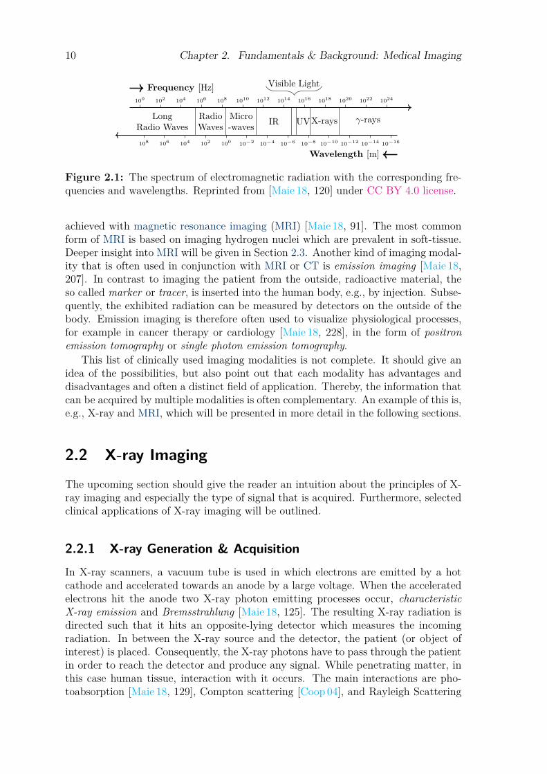
2.1 Modalities in Medical ImagingUltrasound is frequently used in clinical practice because of its low cost and lack ofionizing radiation [Maie 18, 237]. Loosely spoken, the image formation is based onthe reflection of sonic waves at material boundaries. As the ultrasound frequenciesin medical images are usually in the range of 2 MHz to 40 MHz and therefore clearlyabove the upper limit of the human perception at around 20 kHz these are inaudibleto humans. It is mostly used to examine soft-tissue structures, such as muscles, inter-nal organs, ligaments, and vessels, but can also be used to image fluids [Maie 18, 248].Another more straightforward approach to image generation is the use of visible light,e.g., in the form of microscopy [Maie 18, 69], endoscopy [Maie 18, 57], or photography[Pere 13, 569]. These methods rely on the small spectrum of electromagnetic radiationthat is visible for human observers, see Figure 2.1. Unfortunately, most modalitiesbased on visible light are incapable of penetrating the surface of tissue. An exceptionto this is, e.g., optical coherence tomography which applies electromagnetic radiationwith frequencies at the upper limit of the human visual system and beyond, and isable to acquire information up to a few millimeter below the surface of biologicaltissue [Maie 18, 252]. Deeper penetration requires higher energetic radiation, e.g., inthe form of X-rays. Despite its ionizing radiation, X-ray is routinely used in clinicalpractice for diagnostic as well as interventional procedures. The image formationprocess is subject to an absorption model and therefore is especially useful for imag-ing dense tissue and structures. Details regarding X-ray imaging will be discussed inSection 2.2. This also enables the application of computed tomography (CT) whichallows for 3D tomographic reconstructions of the whole human body. This can also be
9
10 Chapter 2. Fundamentals & Background: Medical Imaging
100 102 104 106 108 1010 1012 1014 1016 1018 1020 1022 1024
10−1610−1410−1210−1010−810−610−410−2100102104106108
LongRadio Waves
RadioWaves
Micro-waves IR
Visible Light
UVX-rays γ-rays
Frequency [Hz]
Wavelength [m]
Figure 2.1: The spectrum of electromagnetic radiation with the corresponding fre-quencies and wavelengths. Reprinted from [Maie 18, 120] under CC BY 4.0 license.
achieved with magnetic resonance imaging (MRI) [Maie 18, 91]. The most commonform of MRI is based on imaging hydrogen nuclei which are prevalent in soft-tissue.Deeper insight into MRI will be given in Section 2.3. Another kind of imaging modal-ity that is often used in conjunction with MRI or CT is emission imaging [Maie 18,207]. In contrast to imaging the patient from the outside, radioactive material, theso called marker or tracer, is inserted into the human body, e.g., by injection. Subse-quently, the exhibited radiation can be measured by detectors on the outside of thebody. Emission imaging is therefore often used to visualize physiological processes,for example in cancer therapy or cardiology [Maie 18, 228], in the form of positronemission tomography or single photon emission tomography.
This list of clinically used imaging modalities is not complete. It should give anidea of the possibilities, but also point out that each modality has advantages anddisadvantages and often a distinct field of application. Thereby, the information thatcan be acquired by multiple modalities is often complementary. An example of this is,e.g., X-ray and MRI, which will be presented in more detail in the following sections.
2.2 X-ray Imaging
The upcoming section should give the reader an intuition about the principles of X-ray imaging and especially the type of signal that is acquired. Furthermore, selectedclinical applications of X-ray imaging will be outlined.
2.2.1 X-ray Generation & AcquisitionIn X-ray scanners, a vacuum tube is used in which electrons are emitted by a hotcathode and accelerated towards an anode by a large voltage. When the acceleratedelectrons hit the anode two X-ray photon emitting processes occur, characteristicX-ray emission and Bremsstrahlung [Maie 18, 125]. The resulting X-ray radiation isdirected such that it hits an opposite-lying detector which measures the incomingradiation. In between the X-ray source and the detector, the patient (or object ofinterest) is placed. Consequently, the X-ray photons have to pass through the patientin order to reach the detector and produce any signal. While penetrating matter, inthis case human tissue, interaction with it occurs. The main interactions are pho-toabsorption [Maie 18, 129], Compton scattering [Coop 04], and Rayleigh Scattering
2.2. X-ray Imaging 11
[Youn 81, Kiss 00]. The proportion of their occurrence is influenced by the energy ofthe X-ray photons and the material properties.
Photoabsorption occurs when an incident X-ray photon carries enough energy to”knock out” an innermost electron of the traversed atom [Burc 73]. This happens ifthe energy of the photon is larger than the binding energy of the hit electron. As aconsequence, the X-ray photon disappears. The affected atom is in an ionized, i.e.,charged state. Return to the initial state happens as an electron from the outer shellwith higher energy fills the occuring gap in the lower shell. The difference in energycauses the release of X-ray radiation. The electron that has been dislodged travelsat high velocity and has a high probability of ionizing other atoms until all of theenergy is spent. This progressive ionization is detrimental to human tissue.
Compton Scattering is one of two scattering processes that are observable. Itoccurs if the incident X-ray photon possesses enough energy to eject an outer shellelectron from an atom. It is an inelastic scattering process in which the deflectionangle of the photon is subject to its energy [Maie 18, 129].
Rayleigh Scattering or Thomson scattering occurs by interaction of the photonwith the whole atom [Kiss 00]. It is an elastic scattering process. As a result, neitherthe atom nor the photon loose energy and the wavelength stays constant, but thedirection of the photon is changed [Buzu 11]. Rayleigh scattering is only a minorcontributor to the overall attenuation.
The interaction of X-ray photons with human tissue leads to a loss or deflectionof photons from the original beam. This attenuation of the beam is measured at theX-ray detector of the system. For a polychromatic beam, i.e., photons with differentenergies, the beam intensity at the detector ρ is given by
ρ =∫ Emax
0ρ0(E)e−
∫ν(E,τ)dτdE , (2.1)
where E is the energy, E ∈ [0, Emax], ν(E, τ) is the material and energy dependentattenuation coefficient for each point on the path τ , and ρ0(E) is the X-ray sourceenergy. In practice, this is processed at the detector to yield the line integral orprojection data.
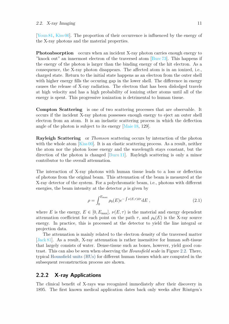
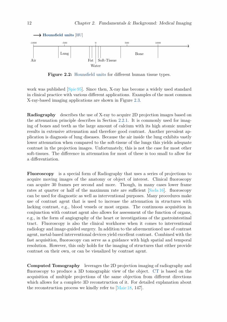
The attenuation is mainly related to the electron density of the traversed matter[Jack 81]. As a result, X-ray attenuation is rather insensitive for human soft-tissuethat largely consists of water. Dense-tissue such as bones, however, yield good con-trast. This can also be seen when observing the Hounsfield scale in Figure 2.2. There,typical Hounsfield units (HUs) for different human tissues which are computed in thesubsequent reconstruction process are shown.
2.2.2 X-ray ApplicationsThe clinical benefit of X-rays was recognized immediately after their discovery in1895. The first known medical application dates back only weeks after Rontgen’s
12 Chapter 2. Fundamentals & Background: Medical Imaging
-1000 -500 0 500 1000
Air Soft-TissueFatBone
Water
Lung
Hounsfield units [HU]
Figure 2.2: Hounsfield units for different human tissue types.
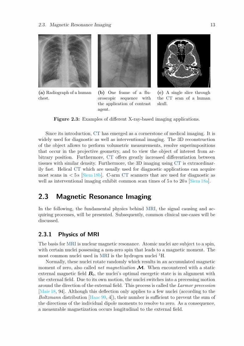
work was published [Spie 95]. Since then, X-ray has become a widely used standardin clinical practice with various different applications. Examples of the most commonX-ray-based imaging applications are shown in Figure 2.3.
Radiography describes the use of X-ray to acquire 2D projection images based onthe attenuation principle describes in Section 2.2.1. It is commonly used for imag-ing of bones and teeth as the large amount of calcium with its high atomic numberresults in extensive attenuation and therefore good contrast. Another prevalent ap-plication is diagnosis of lung diseases. Because the air inside the lung exhibits vastlylower attenuation when compared to the soft-tissue of the lungs this yields adequatecontrast in the projection images. Unfortunately, this is not the case for most othersoft-tissues. The difference in attenuation for most of these is too small to allow fora differentiation.
Fluoroscopy is a special form of Radiography that uses a series of projections toacquire moving images of the anatomy or object of interest. Clinical fluoroscopycan acquire 30 frames per second and more. Though, in many cases lower framerates at quarter or half of the maximum rate are sufficient [Sada 16]. fluoroscopycan be used for diagnostic as well as interventional purposes. Many procedures makeuse of contrast agent that is used to increase the attenuation in structures withlacking contrast, e.g., blood vessels or most organs. The continuous acquisition inconjunction with contrast agent also allows for assessment of the function of organs,e.g., in the form of angiography of the heart or investigations of the gastrointestinaltract. Fluoroscopy is also the clinical workhorse when it comes to interventionalradiology and image-guided surgery. In addition to the aforementioned use of contrastagent, metal-based interventional devices yield excellent contrast. Combined with thefast acquisition, fluoroscopy can serve as a guidance with high spatial and temporalresolution. However, this only holds for the imaging of structures that either providecontrast on their own, or can be visualized by contrast agent.
Computed Tomography leverages the 2D projection imaging of radiography andfluoroscopy to produce a 3D tomographic view of the object. CT is based on theacquisition of multiple projections of the same objection from different directionswhich allows for a complete 3D reconstruction of it. For detailed explanation aboutthe reconstruction process we kindly refer to [Maie 18, 147].
2.3. Magnetic Resonance Imaging 13
(a) Radiograph of a humanchest.
(b) One frame of a flu-oroscopic sequence withthe application of contrastagent.
(c) A single slice throughthe CT scan of a humanskull.
Figure 2.3: Examples of different X-ray-based imaging applications.
Since its introduction, CT has emerged as a cornerstone of medical imaging. It iswidely used for diagnostic as well as interventional imaging. The 3D reconstructionof the object allows to perform volumetric measurements, resolve superimpositionsthat occur in the projective geometry, and to view the object of interest from ar-bitrary position. Furthermore, CT offers greatly increased differentiation betweentissues with similar density. Furthermore, the 3D imaging using CT is extraordinar-ily fast. Helical CT which are usually used for diagnostic applications can acquiremost scans in < 5 s [Siem 18b]. C-arm CT scanners that are used for diagnostic aswell as interventional imaging exhibit common scan times of 5 s to 20 s [Siem 18a].
2.3 Magnetic Resonance ImagingIn the following, the fundamental physics behind MRI, the signal causing and ac-quiring processes, will be presented. Subsequently, common clinical use-cases will bediscussed.
2.3.1 Physics of MRIThe basis for MRI is nuclear magnetic resonance. Atomic nuclei are subject to a spin,with certain nuclei possessing a non-zero spin that leads to a magnetic moment. Themost common nuclei used in MRI is the hydrogen nuclei 1H.
Normally, these nuclei rotate randomly which results in an accumulated magneticmoment of zero, also called net magnetization M. When encountered with a staticexternal magnetic field B0, the nuclei’s optimal energetic state is in alignment withthe external field. Due to its own motion, the nuclei switches into a precessing motionaround the direction of the external field. This process is called the Larmor precession[Maie 18, 94]. Although this deflection only applies to a few nuclei (according to theBoltzmann distribution [Haac 99, 4]), their number is sufficient to prevent the sum ofthe directions of the individual dipole moments to resolve to zero. As a consequence,a measurable magnetization occurs longitudinal to the external field.
14 Chapter 2. Fundamentals & Background: Medical Imaging
B0
B1
M before excitation
M after excitation
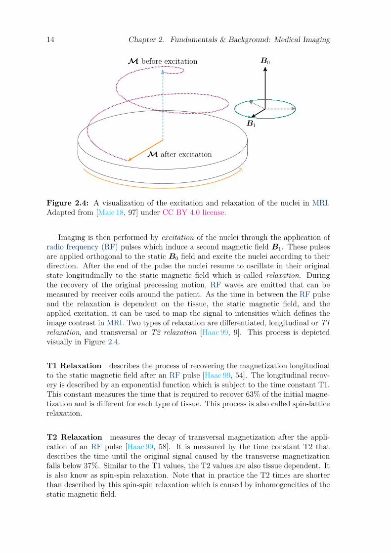
Figure 2.4: A visualization of the excitation and relaxation of the nuclei in MRI.Adapted from [Maie 18, 97] under CC BY 4.0 license.
Imaging is then performed by excitation of the nuclei through the application ofradio frequency (RF) pulses which induce a second magnetic field B1. These pulsesare applied orthogonal to the static B0 field and excite the nuclei according to theirdirection. After the end of the pulse the nuclei resume to oscillate in their originalstate longitudinally to the static magnetic field which is called relaxation. Duringthe recovery of the original precessing motion, RF waves are emitted that can bemeasured by receiver coils around the patient. As the time in between the RF pulseand the relaxation is dependent on the tissue, the static magnetic field, and theapplied excitation, it can be used to map the signal to intensities which defines theimage contrast in MRI. Two types of relaxation are differentiated, longitudinal or T1relaxation, and transversal or T2 relaxation [Haac 99, 9]. This process is depictedvisually in Figure 2.4.
T1 Relaxation describes the process of recovering the magnetization longitudinalto the static magnetic field after an RF pulse [Haac 99, 54]. The longitudinal recov-ery is described by an exponential function which is subject to the time constant T1.This constant measures the time that is required to recover 63% of the initial magne-tization and is different for each type of tissue. This process is also called spin-latticerelaxation.
T2 Relaxation measures the decay of transversal magnetization after the appli-cation of an RF pulse [Haac 99, 58]. It is measured by the time constant T2 thatdescribes the time until the original signal caused by the transverse magnetizationfalls below 37%. Similar to the T1 values, the T2 values are also tissue dependent. Itis also know as spin-spin relaxation. Note that in practice the T2 times are shorterthan described by this spin-spin relaxation which is caused by inhomogeneities of thestatic magnetic field.
2.3. Magnetic Resonance Imaging 15
(a) Short TR, short TE:T1-weighted
(b) Long TR, short TE:PD-weighted
(c) Long TR, Long TE:T2-weighted
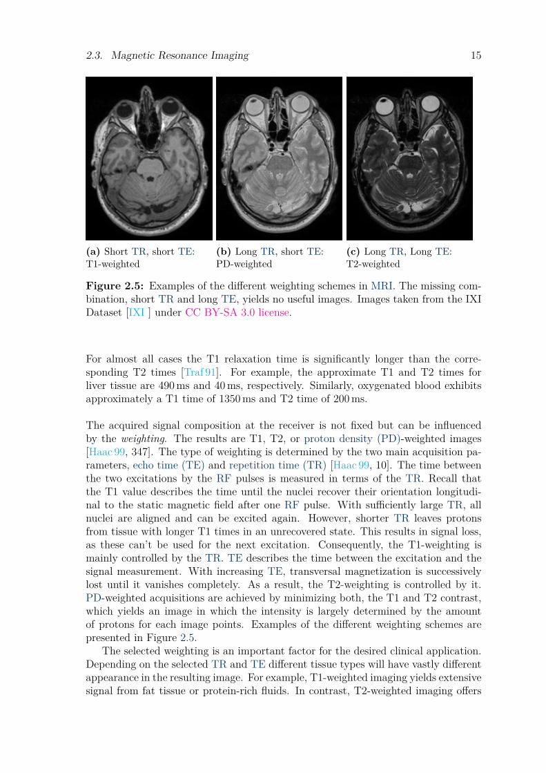
Figure 2.5: Examples of the different weighting schemes in MRI. The missing com-bination, short TR and long TE, yields no useful images. Images taken from the IXIDataset [IXI ] under CC BY-SA 3.0 license.
For almost all cases the T1 relaxation time is significantly longer than the corre-sponding T2 times [Traf 91]. For example, the approximate T1 and T2 times forliver tissue are 490 ms and 40 ms, respectively. Similarly, oxygenated blood exhibitsapproximately a T1 time of 1350 ms and T2 time of 200 ms.
The acquired signal composition at the receiver is not fixed but can be influencedby the weighting. The results are T1, T2, or proton density (PD)-weighted images[Haac 99, 347]. The type of weighting is determined by the two main acquisition pa-rameters, echo time (TE) and repetition time (TR) [Haac 99, 10]. The time betweenthe two excitations by the RF pulses is measured in terms of the TR. Recall thatthe T1 value describes the time until the nuclei recover their orientation longitudi-nal to the static magnetic field after one RF pulse. With sufficiently large TR, allnuclei are aligned and can be excited again. However, shorter TR leaves protonsfrom tissue with longer T1 times in an unrecovered state. This results in signal loss,as these can’t be used for the next excitation. Consequently, the T1-weighting ismainly controlled by the TR. TE describes the time between the excitation and thesignal measurement. With increasing TE, transversal magnetization is successivelylost until it vanishes completely. As a result, the T2-weighting is controlled by it.PD-weighted acquisitions are achieved by minimizing both, the T1 and T2 contrast,which yields an image in which the intensity is largely determined by the amountof protons for each image points. Examples of the different weighting schemes arepresented in Figure 2.5.
The selected weighting is an important factor for the desired clinical application.Depending on the selected TR and TE different tissue types will have vastly differentappearance in the resulting image. For example, T1-weighted imaging yields extensivesignal from fat tissue or protein-rich fluids. In contrast, T2-weighted imaging offers

16 Chapter 2. Fundamentals & Background: Medical Imaging
low signal from fat but strong response for tissues or fluids with high water contents.Though, in practice, every acquired weighting is a combination of all, T1, T2, andPD-weighted signals [Haac 99, 347]. Furthermore, all of these are tied to the presenceof protons to magnetize. As usually hydrogen is imaged, this is mostly the case insoft-tissue structures. Bones and similar structures on the other hand yield little tono signal in common MRI acquisitions.
The exact design of the RF pulses as well as the subsequent image formation pro-cess comes in large variations in MRI. Many of the possibilities are tailored to specificuse-cases and associated clinical applications. As an understanding of the origin ofthe acquired signal is sufficient for the topics presented in this thesis, we kindly referthe interested reader to further literature [Maie 18, Haac 99]. One important point,however, is that most MRI scans consist of a set of 2D tomographic slices that formthe resulting 3D image volume. This means that, in contrast to CT, the acquisitionof individual tomographic slices of the patient is possible. This is of special inter-est for interventional imaging using MRI which will be discussed in Section 2.3.2.Nevertheless, ”real” 3D acquisitions are also possible in MRI.
2.3.2 MRI ApplicationsMRI is applied for a broad spectrum of applications concerned with soft-tissue struc-tures. Thereby, the vast majority of applications is of diagnostic nature. This is dueto the fact that the acquisition of MRI is slow when compared to CT. It is difficult togive exact acquisition times as these vary greatly with the selected acquisition type,but as an indication it should be noted that a high-resolution MR scan usually takesseveral minutes for the acquisition [Siem 18c], whereas a corresponding CT scan canbe acquired in a few seconds. Despite this drawback, MRI is widely used in theclinical setting also due to the lack of ionizing radiation, which renders it a less riskyalternative to X-ray and CT. In the following, example applications will be presented.This list is not exhaustive, but it is intended to give an impression of the wide rangeof imaging options available.
Diagnostic MRI is the most common application form. As outlined previously,MRI excels at the imaging of various soft-tissues, e.g., in the brain, heart, or liver.Thereby, various different imaging protocols exist to highlight different tissue types.Yet, MRI is not limited to this. It can also be used to visualize joint diseases andtears, mostly based on PD-weighted images. The visualization of any type of fluidsis possible. For example, angiography can be performed in MRI with and withoutcontrast agent. MRI can also be used to acquire moving images, e.g., in the form ofcardiac cine MRI. Despite these structural MRI called acquisition types, also perfu-sion weighted and functional imaging is possible in MRI.
Interventional MRI faces multiple challenges. The strong magnetic field necessi-tates the absence of other magnetic materials in the vicinity of the scanner. Further-more, the closed bore of the scanner restricts access to the patient which is not the casefor interventional C-arm CT devices. Due to the trade-off between spatial resolutionand acquisition time, image-guided procedures also encounter challenges in accurate

2.3. Magnetic Resonance Imaging 17
and fast visualization of the interventional devices. Despite the increased technicaldifficulties when using MRI in the interventional setting, the excellent achievablesoft-tissue contrast has led to selected clinical applications [Bark 17]. For example,neurosurgical exams can benefit greatly from the detailed soft-tissue visualization.The same holds for cardiac interventions, such as cardiac catheter ablation, as wellas MR-guided breast interventions, e.g., for cancer biopsy. One common feature of allof these methods is that they are based on the acquisition of individual tomographicslice images. In contrast to 3D volumes, the acquisition of those is possible in ”realtime” with an appropriate imaging protocol.


C H A P T E R 3
Fundamentals & Background:Deep Learning
Deep Learning (DL) is a sub-field of machine learning (ML) that has gainedenormous traction over the last years. The name DL originates from the use ofdeep artificial neural networks (ANNs) which will be explained in Section 3.1. Espe-cially in image processing, DL has lead to rapid progression in most related fields ofresearch. Driven by the strong performance increase of image classification meth-ods on the popular ILSVRC [Russ 14] benchmark [Kriz 12, Simo 15, He 16], DL-based approaches conquered the state-of-the-art in many other tasks, e.g., segmen-tation [Ronn 15, Badr 17, Chen 18], object detection [Redm 16, Ren 15], and imagegeneration [Gaty 16, Good 14, Karr 17, Yu 18]. This development has also reached themedical community [Maie 19a, Wang 18a] where it has the potential to significantlyrelieve the burden on physicians and healthcare by automating manual work [Este 19].In the following, the fundamental DL techniques will be presented to the reader toensure an appropriate understanding of the methods utilized in this thesis. First,the basic principles of neural networks and their training will be explained in Sec-tion 3.1. Second, considerations regarding the design choices and different modulesand of neural networks will be given in Sections 3.2 to 3.4.
3.1 Introduction to Neural NetworksNeural Networks (NNs) are the foundation of DL. The primal form of these networksis the multilayer perceptron (MLP), an acyclic graph of several neurons [Rose 58].Today, however, the term neural network is used in most cases synonymously withany kind of entity organized as a network in machine learning (ML), including cyclicgraphs.
3.1.1 Multilayer Perceptron
The aim of MLPs is to approximate a function f by the function f that defines themapping y = f(x;θ) from an input x to the output y with respect to some learnedparameters θ. These networks consist of multiple so called neurons that form anacyclic graph, hence the name feedforward networks. Networks composed of cyclicgraphs in the form of, e.g., recurrent neural networks are possible, but will not becovered in this thesis. A visualization of a single neuron is given in Figure 3.1. The
19
20 Chapter 3. Fundamentals & Background: Deep Learning
Activationfunctionfact
y
Output
∑w1x1
......
wnxn
1 b
Inputs Weights
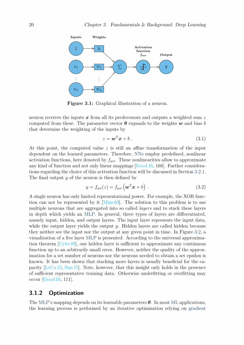
Figure 3.1: Graphical illustration of a neuron.
neuron receives the inputs x from all its predecessors and outputs a weighted sum zcomputed from these. The parameter vector θ expands to the weights w and bias bthat determine the weighting of the inputs by
z = wTx+ b . (3.1)
At this point, the computed value z is still an affine transformation of the inputdependent on the learned parameters. Therefore, NNs employ predefined, nonlinearactivation functions, here denoted by fact. These nonlinearities allow to approximateany kind of function and not only linear mappings [Good 16, 168]. Further considera-tions regarding the choice of this activation function will be discussed in Section 3.2.1.The final output y of the neuron is then defined by
y = fact(z) = fact(wTx+ b
). (3.2)
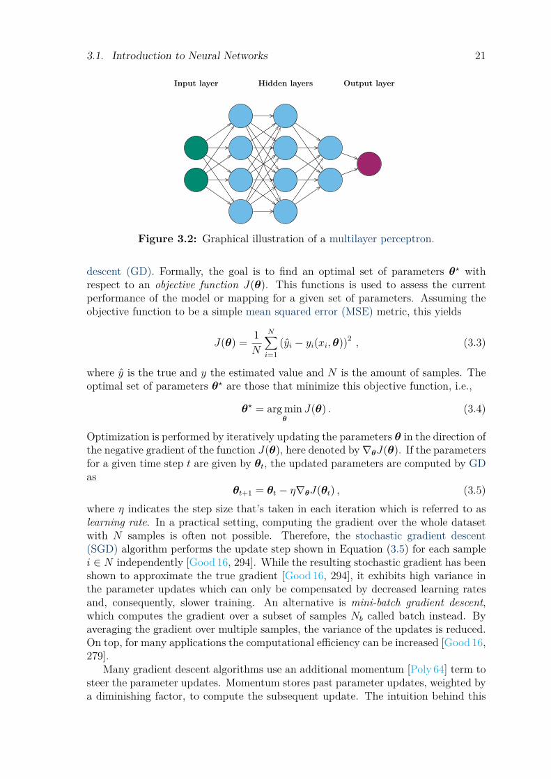
A single neuron has only limited representational power. For example, the XOR func-tion can not be represented by it [Mins 69]. The solution to this problem is to usemultiple neurons that are aggregated into so called layers and to stack these layersin depth which yields an MLP. In general, three types of layers are differentiated,namely input, hidden, and output layers. The input layer represents the input data,while the output layer yields the output y. Hidden layers are called hidden becausethey neither see the input nor the output at any given point in time. In Figure 3.2, avisualization of a five layer MLP is presented. According to the universal approxima-tion theorem [Cybe 89], one hidden layer is sufficient to approximate any continuousfunction up to an arbitrarily small error. However, neither the quality of the approx-imation for a set number of neurons nor the neurons needed to obtain a set epsilon isknown. It has been shown that stacking more layers is usually beneficial for the ca-pacity [LeCu 15, Sun 15]. Note, however, that this insight only holds in the presenceof sufficient representative training data. Otherwise underfitting or overfitting mayoccur [Good 16, 111].
3.1.2 OptimizationThe MLP’s mapping depends on its learnable parameters θ. In most ML applications,the learning process is performed by an iterative optimization relying on gradient
3.1. Introduction to Neural Networks 21
Hidden layersInput layer Output layer
Figure 3.2: Graphical illustration of a multilayer perceptron.
descent (GD). Formally, the goal is to find an optimal set of parameters θ? withrespect to an objective function J(θ). This functions is used to assess the currentperformance of the model or mapping for a given set of parameters. Assuming theobjective function to be a simple mean squared error (MSE) metric, this yields
J(θ) = 1N
N∑i=1
(yi − yi(xi,θ))2 , (3.3)
where y is the true and y the estimated value and N is the amount of samples. Theoptimal set of parameters θ? are those that minimize this objective function, i.e.,
θ? = arg minθ
J(θ) . (3.4)
Optimization is performed by iteratively updating the parameters θ in the direction ofthe negative gradient of the function J(θ), here denoted by∇θJ(θ). If the parametersfor a given time step t are given by θt, the updated parameters are computed by GDas
θt+1 = θt − η∇θJ(θt) , (3.5)where η indicates the step size that’s taken in each iteration which is referred to aslearning rate. In a practical setting, computing the gradient over the whole datasetwith N samples is often not possible. Therefore, the stochastic gradient descent(SGD) algorithm performs the update step shown in Equation (3.5) for each samplei ∈ N independently [Good 16, 294]. While the resulting stochastic gradient has beenshown to approximate the true gradient [Good 16, 294], it exhibits high variance inthe parameter updates which can only be compensated by decreased learning ratesand, consequently, slower training. An alternative is mini-batch gradient descent,which computes the gradient over a subset of samples Nb called batch instead. Byaveraging the gradient over multiple samples, the variance of the updates is reduced.On top, for many applications the computational efficiency can be increased [Good 16,279].
Many gradient descent algorithms use an additional momentum [Poly 64] term tosteer the parameter updates. Momentum stores past parameter updates, weighted bya diminishing factor, to compute the subsequent update. The intuition behind this
22 Chapter 3. Fundamentals & Background: Deep Learning
is that multiple beneficial steps in one direction in the past should have a positiveimpact on the next step and, thus, decrease the variance in the updates. With thediminishing factor being denoted by γ, the momentum term can be computed by
vt = γvt−1 − η∇θJ(θt) , (3.6)θt+1 = θt + vt . (3.7)
While momentum includes previous steps in the calculation of the next step, thereis no information about the state in the next step itself. To include this informationin the update step, the Nesterov accelerated gradient method [Nest 83] computes anestimate of the subsequent position by
vt = γvt−1 − η∇θJ(θt − γvt−1) , (3.8)θt+1 = θt + vt . (3.9)
The diminishing weighting factor γ is usually set in the range between 0.9 and 0.99.One drawback of momentum-based SGD is that the computed terms are inde-
pendent of the individual parameters. In practice, however, different parametersmay require different learning rates for an optimal training. Building on the conceptof momentum, many adaptive methods emerged [Zeil 12, Duch 11, King 15]. A fre-quently used representative of this group is the adaptive moment estimation (ADAM)algorithm [King 15]. Its key concept is the estimation of lower-order moments of thegradient, based on which individual learning rates for the trainable parameters arecomputed. Though, more recent studies exposed flaws in the convergence of ADAMand other adaptive optimization methods, especially when considering overparame-terized problems [Sash 18, Wils 17]. One proposed solution to this problem was theAmsgrad optimizer [Sash 18] which replaces the exponential moving average used inADAM by the maximum of the past squared gradients. With this modification,the convergence for Amsgrad could be shown in cases where Adam fails [Sash 18].Though, also Amsgrad is not uncontested. A recent study claims that hyperpa-rameter optimization is the single most important influence on the performance ofoptimization procedures in DL and that most empirical approaches to the comparisonof those do not adequately account for this [Choi 19], including the recent Amsgradalgorithm.
So far, no optimal solution to the optimization of neural networks has been found.Though, despite its flawed convergence, ADAM is widely used and has proven to yieldgood performance when applied with adequate hyperparameters [King 15, Choi 19].
Backpropagation For each parameter update, the gradient ∇θJ(θ) of the objec-tive function J(θ) with respect to the parameters θ must be known. An analyticexpression for this gradient can be found, however, it is computationally expensiveto evaluate. As usually a large amount of parameter updates must be computed toreach an optimum, this is impracticable. To this end, Rumelhart et al. [Rume 88]introduced an efficient way to the compute the gradient by recursive application ofthe chain rule, the backpropagation algorithm. After a full forward pass through thenetwork, the output of the objective function J(θ) gives feedback on how far thepredicted outcome diverges from the desired outcome, which is usually referred to as
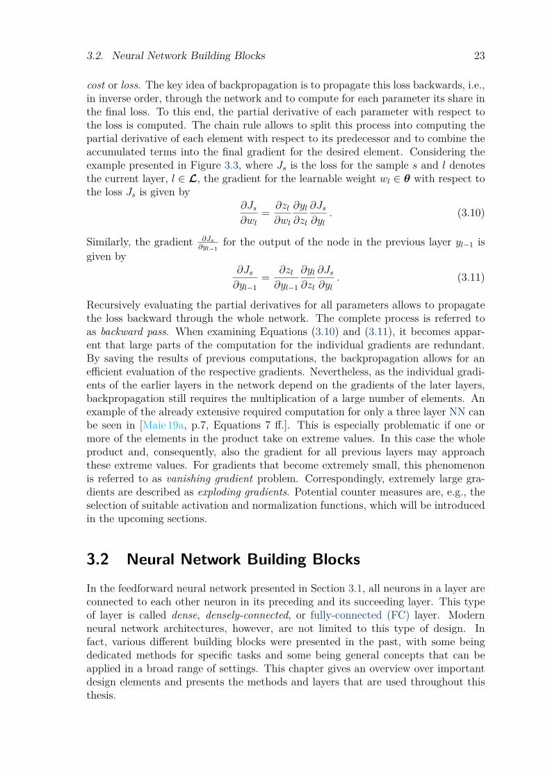
3.2. Neural Network Building Blocks 23
cost or loss. The key idea of backpropagation is to propagate this loss backwards, i.e.,in inverse order, through the network and to compute for each parameter its share inthe final loss. To this end, the partial derivative of each parameter with respect tothe loss is computed. The chain rule allows to split this process into computing thepartial derivative of each element with respect to its predecessor and to combine theaccumulated terms into the final gradient for the desired element. Considering theexample presented in Figure 3.3, where Js is the loss for the sample s and l denotesthe current layer, l ∈ L, the gradient for the learnable weight wl ∈ θ with respect tothe loss Js is given by
∂Js∂wl
= ∂zl∂wl
∂yl∂zl
∂Js∂yl
. (3.10)
Similarly, the gradient ∂Js
∂yl−1for the output of the node in the previous layer yl−1 is
given by∂Js∂yl−1
= ∂zl∂yl−1
∂yl∂zl
∂Js∂yl
. (3.11)
Recursively evaluating the partial derivatives for all parameters allows to propagatethe loss backward through the whole network. The complete process is referred toas backward pass. When examining Equations (3.10) and (3.11), it becomes appar-ent that large parts of the computation for the individual gradients are redundant.By saving the results of previous computations, the backpropagation allows for anefficient evaluation of the respective gradients. Nevertheless, as the individual gradi-ents of the earlier layers in the network depend on the gradients of the later layers,backpropagation still requires the multiplication of a large number of elements. Anexample of the already extensive required computation for only a three layer NN canbe seen in [Maie 19a, p.7, Equations 7 ff.]. This is especially problematic if one ormore of the elements in the product take on extreme values. In this case the wholeproduct and, consequently, also the gradient for all previous layers may approachthese extreme values. For gradients that become extremely small, this phenomenonis referred to as vanishing gradient problem. Correspondingly, extremely large gra-dients are described as exploding gradients. Potential counter measures are, e.g., theselection of suitable activation and normalization functions, which will be introducedin the upcoming sections.
3.2 Neural Network Building BlocksIn the feedforward neural network presented in Section 3.1, all neurons in a layer areconnected to each other neuron in its preceding and its succeeding layer. This typeof layer is called dense, densely-connected, or fully-connected (FC) layer. Modernneural network architectures, however, are not limited to this type of design. Infact, various different building blocks were presented in the past, with some beingdedicated methods for specific tasks and some being general concepts that can beapplied in a broad range of settings. This chapter gives an overview over importantdesign elements and presents the methods and layers that are used throughout thisthesis.
24 Chapter 3. Fundamentals & Background: Deep Learning
bl
yl−1
wl
zl yl Js
∂zl∂yl−1
∂zl∂bl
∂zl∂wl
∂yl∂zl
∂Js∂yl
Figure 3.3: Graphical illustration of the backpropagation algorithm. Black arrowsindicate the forward pass while orange denote the backward pass with the respectivepartial derivatives. As introduced in Equations (3.1) and (3.2), zl and yl denote thecomputation results before and after activation, respectively. Consequently, duringbackpropagation also the derivative of the activation function f ′actl
(zl) needs to becomputed.
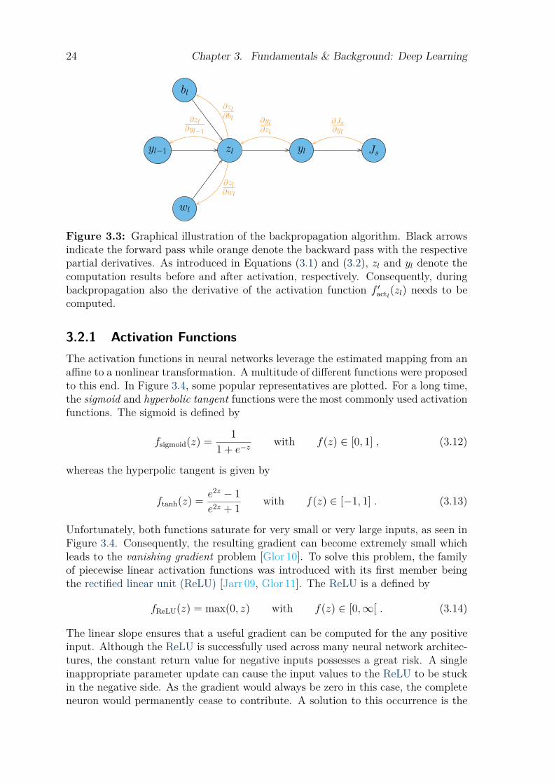
3.2.1 Activation FunctionsThe activation functions in neural networks leverage the estimated mapping from anaffine to a nonlinear transformation. A multitude of different functions were proposedto this end. In Figure 3.4, some popular representatives are plotted. For a long time,the sigmoid and hyperbolic tangent functions were the most commonly used activationfunctions. The sigmoid is defined by
fsigmoid(z) = 11 + e−z
with f(z) ∈ [0, 1] , (3.12)
whereas the hyperpolic tangent is given by
ftanh(z) = e2z − 1e2z + 1 with f(z) ∈ [−1, 1] . (3.13)
Unfortunately, both functions saturate for very small or very large inputs, as seen inFigure 3.4. Consequently, the resulting gradient can become extremely small whichleads to the vanishing gradient problem [Glor 10]. To solve this problem, the familyof piecewise linear activation functions was introduced with its first member beingthe rectified linear unit (ReLU) [Jarr 09, Glor 11]. The ReLU is a defined by
fReLU(z) = max(0, z) with f(z) ∈ [0,∞[ . (3.14)
The linear slope ensures that a useful gradient can be computed for the any positiveinput. Although the ReLU is successfully used across many neural network architec-tures, the constant return value for negative inputs possesses a great risk. A singleinappropriate parameter update can cause the input values to the ReLU to be stuckin the negative side. As the gradient would always be zero in this case, the completeneuron would permanently cease to contribute. A solution to this occurrence is the
3.2. Neural Network Building Blocks 25
-2 -1 1 2-1
1
2
z
f(z)
sigmoid(z)tanh(z)
-2 -1 1 2-1
1
2
z
f(z)
ReLU(z)Leaky ReLU(z)
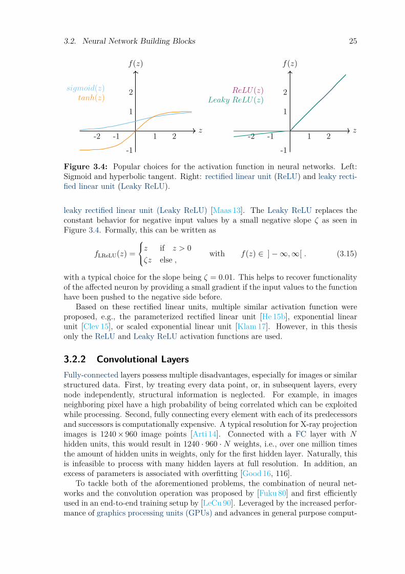
Figure 3.4: Popular choices for the activation function in neural networks. Left:Sigmoid and hyperbolic tangent. Right: rectified linear unit (ReLU) and leaky recti-fied linear unit (Leaky ReLU).
leaky rectified linear unit (Leaky ReLU) [Maas 13]. The Leaky ReLU replaces theconstant behavior for negative input values by a small negative slope ζ as seen inFigure 3.4. Formally, this can be written as
fLReLU(z) =
z if z > 0ζz else ,
with f(z) ∈ ]−∞,∞[ . (3.15)
with a typical choice for the slope being ζ = 0.01. This helps to recover functionalityof the affected neuron by providing a small gradient if the input values to the functionhave been pushed to the negative side before.
Based on these rectified linear units, multiple similar activation function wereproposed, e.g., the parameterized rectified linear unit [He 15b], exponential linearunit [Clev 15], or scaled exponential linear unit [Klam 17]. However, in this thesisonly the ReLU and Leaky ReLU activation functions are used.
3.2.2 Convolutional LayersFully-connected layers possess multiple disadvantages, especially for images or similarstructured data. First, by treating every data point, or, in subsequent layers, everynode independently, structural information is neglected. For example, in imagesneighboring pixel have a high probability of being correlated which can be exploitedwhile processing. Second, fully connecting every element with each of its predecessorsand successors is computationally expensive. A typical resolution for X-ray projectionimages is 1240× 960 image points [Arti 14]. Connected with a FC layer with Nhidden units, this would result in 1240 · 960 · N weights, i.e., over one million timesthe amount of hidden units in weights, only for the first hidden layer. Naturally, thisis infeasible to process with many hidden layers at full resolution. In addition, anexcess of parameters is associated with overfitting [Good 16, 116].
To tackle both of the aforementioned problems, the combination of neural net-works and the convolution operation was proposed by [Fuku 80] and first efficientlyused in an end-to-end training setup by [LeCu 90]. Leveraged by the increased perfor-mance of graphics processing units (GPUs) and advances in general purpose comput-
26 Chapter 3. Fundamentals & Background: Deep Learning
-1 -1 -1
0 0 0
1 1 1
4 8 6 6
9 6 1 7
7 7 8 2
5 9 1 7
4 -3
-1 3
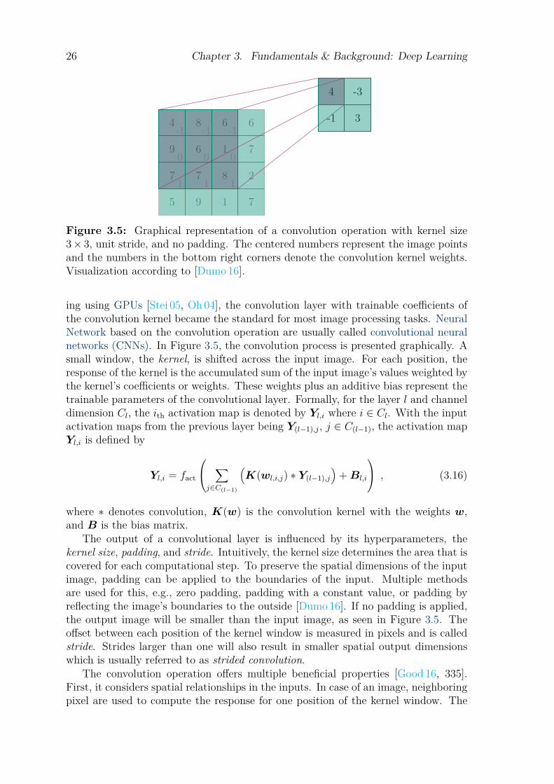
Figure 3.5: Graphical representation of a convolution operation with kernel size3× 3, unit stride, and no padding. The centered numbers represent the image pointsand the numbers in the bottom right corners denote the convolution kernel weights.Visualization according to [Dumo 16].
ing using GPUs [Stei 05, Oh 04], the convolution layer with trainable coefficients ofthe convolution kernel became the standard for most image processing tasks. NeuralNetwork based on the convolution operation are usually called convolutional neuralnetworks (CNNs). In Figure 3.5, the convolution process is presented graphically. Asmall window, the kernel, is shifted across the input image. For each position, theresponse of the kernel is the accumulated sum of the input image’s values weighted bythe kernel’s coefficients or weights. These weights plus an additive bias represent thetrainable parameters of the convolutional layer. Formally, for the layer l and channeldimension Cl, the ith activation map is denoted by Yl,i where i ∈ Cl. With the inputactivation maps from the previous layer being Y(l−1),j, j ∈ C(l−1), the activation mapYl,i is defined by
Yl,i = fact
∑j∈C(l−1)
(K(wl,i,j) ∗ Y(l−1),j
)+Bl,i
, (3.16)
where ∗ denotes convolution, K(w) is the convolution kernel with the weights w,and B is the bias matrix.
The output of a convolutional layer is influenced by its hyperparameters, thekernel size, padding, and stride. Intuitively, the kernel size determines the area that iscovered for each computational step. To preserve the spatial dimensions of the inputimage, padding can be applied to the boundaries of the input. Multiple methodsare used for this, e.g., zero padding, padding with a constant value, or padding byreflecting the image’s boundaries to the outside [Dumo 16]. If no padding is applied,the output image will be smaller than the input image, as seen in Figure 3.5. Theoffset between each position of the kernel window is measured in pixels and is calledstride. Strides larger than one will also result in smaller spatial output dimensionswhich is usually referred to as strided convolution.
The convolution operation offers multiple beneficial properties [Good 16, 335].First, it considers spatial relationships in the inputs. In case of an image, neighboringpixel are used to compute the response for one position of the kernel window. The
3.2. Neural Network Building Blocks 27
2 8 4 5
2 7 2 8
7 9 3 9
4 1 7 5
8
8
88
99
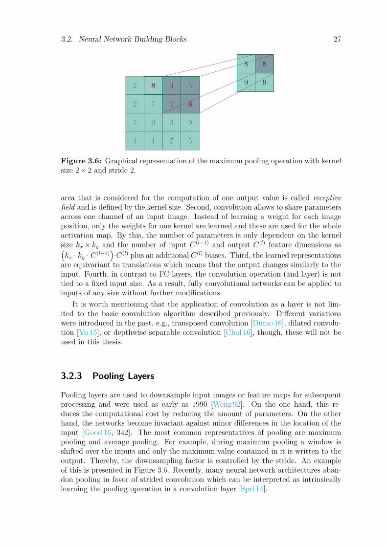
Figure 3.6: Graphical representation of the maximum pooling operation with kernelsize 2× 2 and stride 2.
area that is considered for the computation of one output value is called receptivefield and is defined by the kernel size. Second, convolution allows to share parametersacross one channel of an input image. Instead of learning a weight for each imageposition, only the weights for one kernel are learned and these are used for the wholeactivation map. By this, the number of parameters is only dependent on the kernelsize kx× ky and the number of input C(l−1) and output C(l) feature dimensions as(kx · ky · C(l−1)
)·C(l) plus an additional C(l) biases. Third, the learned representations
are equivariant to translations which means that the output changes similarly to theinput. Fourth, in contrast to FC layers, the convolution operation (and layer) is nottied to a fixed input size. As a result, fully convolutional networks can be applied toinputs of any size without further modifications.
It is worth mentioning that the application of convolution as a layer is not lim-ited to the basic convolution algorithm described previously. Different variationswere introduced in the past, e.g., transposed convolution [Dumo 16], dilated convolu-tion [Yu 15], or depthwise separable convolution [Chol 16], though, these will not beused in this thesis.
3.2.3 Pooling Layers
Pooling layers are used to downsample input images or feature maps for subsequentprocessing and were used as early as 1990 [Weng 92]. On the one hand, this re-duces the computational cost by reducing the amount of parameters. On the otherhand, the networks become invariant against minor differences in the location of theinput [Good 16, 342]. The most common representatives of pooling are maximumpooling and average pooling. For example, during maximum pooling a window isshifted over the inputs and only the maximum value contained in it is written to theoutput. Thereby, the downsampling factor is controlled by the stride. An exampleof this is presented in Figure 3.6. Recently, many neural network architectures aban-don pooling in favor of strided convolution which can be interpreted as intrinsicallylearning the pooling operation in a convolution layer [Spri 14].

28 Chapter 3. Fundamentals & Background: Deep Learning
3.2.4 Normalization MethodsDeep NNs are represented by a combination of multiple functions in the form ofmany stacked layers. The output of each intermediate layer influences the input toall subsequent layers of this network. By this, deeper layers can benefit from good”decisions” in previous layers but also have to compensate for bad ones. Duringoptimization, parameter updates are done for all elements independently withoutknowledge about the change in other elements [Good 16, 317]. For example, a nodein layer l can update its weights for the next step t + 1 based on the gradient ofthe respective node calculated in time step t. However, also its subsequent nodein layer l + 1 will perform an independent update step. As both updates are doneunder the assumption that the remaining nodes are constant, it may occur that theprediction slightly undershoots the ground truth in step t but vastly overshoots inthe subsequent step t + 1 because both nodes updated in the exact same directionwithout knowledge of each other. To prevent this behavior, normalization methodsbecame a widely used method in deep neural networks. These apply an adaptivereparameterization in order to stabilize the optimization and, eventually, increasethe performance.
Batch Normalization is the first normalization method that achieved widespreaduse in CNNs by significantly improving the results on many tasks, especially imageclassification [Ioff 15]. The idea of batch normalization is to correct each of the outputactivations of one layer by the mean and variance of the currently processed batch ofinputs. For a set of output activations yi, i ∈ Q where Q denotes the cardinality ofthe batch q, batch normalization takes the mean µq and variance σ2
q and computesthe normalized activations yi by
y′i = yi − µq√σ2q + ε
. (3.17)
Subsequently, the normalized activations are scaled by
y′′i = δy′i + ξ , (3.18)
where δ and ξ are learnable parameters that are optimized in conjunction with theremaining parameters θ.
A core assumption of batch normalization is that the mean and variance computedover the current batch are close to the mean and variance for the whole dataset.Naturally, this is not true for small batch sizes as it is often the case in generativetasks, e.g., image synthesis or super resolution, which can lead to worse performancethan without normalization.
Instance Normalization was proposed to address the challenges of low batch sizesand largely varying inputs [Ulya 16b]. Instead of considering the complete batch,instance normalization performs a batch normalization-like approach for each exam-ple independently by normalizing it with respect to its mean and variance. Thismeans, batch normalization normalizes over all elements of a batch and all spatial
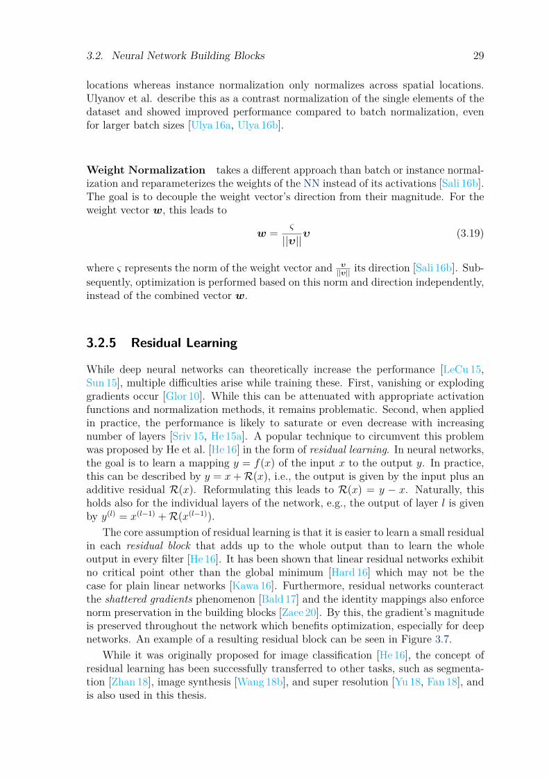
3.2. Neural Network Building Blocks 29
locations whereas instance normalization only normalizes across spatial locations.Ulyanov et al. describe this as a contrast normalization of the single elements of thedataset and showed improved performance compared to batch normalization, evenfor larger batch sizes [Ulya 16a, Ulya 16b].
Weight Normalization takes a different approach than batch or instance normal-ization and reparameterizes the weights of the NN instead of its activations [Sali 16b].The goal is to decouple the weight vector’s direction from their magnitude. For theweight vector w, this leads to
w = ς
||υ||υ (3.19)
where ς represents the norm of the weight vector and υ||υ|| its direction [Sali 16b]. Sub-
sequently, optimization is performed based on this norm and direction independently,instead of the combined vector w.
3.2.5 Residual Learning
While deep neural networks can theoretically increase the performance [LeCu 15,Sun 15], multiple difficulties arise while training these. First, vanishing or explodinggradients occur [Glor 10]. While this can be attenuated with appropriate activationfunctions and normalization methods, it remains problematic. Second, when appliedin practice, the performance is likely to saturate or even decrease with increasingnumber of layers [Sriv 15, He 15a]. A popular technique to circumvent this problemwas proposed by He et al. [He 16] in the form of residual learning. In neural networks,the goal is to learn a mapping y = f(x) of the input x to the output y. In practice,this can be described by y = x+R(x), i.e., the output is given by the input plus anadditive residual R(x). Reformulating this leads to R(x) = y − x. Naturally, thisholds also for the individual layers of the network, e.g., the output of layer l is givenby y(l) = x(l−1) +R(x(l−1)).
The core assumption of residual learning is that it is easier to learn a small residualin each residual block that adds up to the whole output than to learn the wholeoutput in every filter [He 16]. It has been shown that linear residual networks exhibitno critical point other than the global minimum [Hard 16] which may not be thecase for plain linear networks [Kawa 16]. Furthermore, residual networks counteractthe shattered gradients phenomenon [Bald 17] and the identity mappings also enforcenorm preservation in the building blocks [Zaee 20]. By this, the gradient’s magnitudeis preserved throughout the network which benefits optimization, especially for deepnetworks. An example of a resulting residual block can be seen in Figure 3.7.
While it was originally proposed for image classification [He 16], the concept ofresidual learning has been successfully transferred to other tasks, such as segmenta-tion [Zhan 18], image synthesis [Wang 18b], and super resolution [Yu 18, Fan 18], andis also used in this thesis.
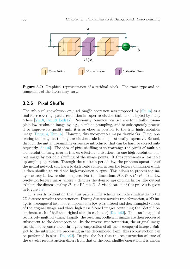
30 Chapter 3. Fundamentals & Background: Deep Learning
. . . + . . .
y
x
R(x)
Convolution Normalization Activation Func.
Figure 3.7: Graphical representation of a residual block. The exact type and ar-rangement of the layers may vary.
3.2.6 Pixel ShuffleThe sub-pixel convolution or pixel shuffle operation was proposed by [Shi 16] as atool for recovering spatial resolution in super resolution tasks and adopted by manyothers [Yu 18, Fan 18, Ledi 17]. Previously, common practice was to initially upsam-ple a low-resolution image by, e.g., bicubic upsampling, and to subsequently processit to improve its quality until it is as close as possible to the true high-resolutionimage [Dong 14, Kim 16]. However, this incorporates major drawbacks. First, pro-cessing the image at the high-resolution scale is computationally expensive. Second,through the initial upsampling errors are introduced that can be hard to correct sub-sequently [Shi 16]. The idea of pixel shuffling is to rearrange the pixels of multiplelow-resolution images, or in this case feature activations, to one high-resolution out-put image by periodic shuffling of the image points. It thus represents a learnableupsampling operation. Through the constant periodicity, the previous operations ofthe neural network can learn to distribute content across the feature dimension whichis then shuffled to yield the high-resolution output. This allows to process the im-age entirely in low-resolution space. For the dimensions H ×W ×C · r2 of the lowresolution feature maps, where r denotes the desired upsampling factor, the outputexhibits the dimensionality H · r×W · r×C. A visualization of this process is givenin Figure 3.8.
It is worth to mention that this pixel shuffle scheme exhibits similarities to the2D discrete wavelet reconstruction. During discrete wavelet transformation, a 2D im-age is decomposed into four components, a low pass filtered and downsampled versionof the original image and three high pass filtered images containing the ”detail” co-efficients, each of half the original size (in each axis) [Daub 92]. This can be appliedrecursively multiple times. Usually, the resulting coefficient images are then processedsubsequent to the decomposition. In the inverse transformation, the original imagecan then be reconstructed through recomposition of all the decomposed images. Sub-ject to the intermediate processing in the decomposed form, this reconstruction canbe performed lossless [Daub 92]. Despite the fact that the reconstruction scheme ofthe wavelet reconstruction differs from that of the pixel shuffles operation, it is known
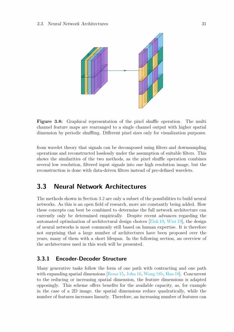
3.3. Neural Network Architectures 31
Figure 3.8: Graphical representation of the pixel shuffle operation. The multichannel feature maps are rearranged to a single channel output with higher spatialdimension by periodic shuffling. Different pixel sizes only for visualization purposes.
from wavelet theory that signals can be decomposed using filters and downsamplingoperations and reconstructed losslessly under the assumption of suitable filters. Thisshows the similarities of the two methods, as the pixel shuffle operation combinesseveral low resolution, filtered input signals into one high resolution image, but thereconstruction is done with data-driven filters instead of pre-defined wavelets.
3.3 Neural Network ArchitecturesThe methods shown in Section 3.2 are only a subset of the possibilities to build neuralnetworks. As this is an open field of research, more are constantly being added. Howthese concepts can best be combined to determine the full network architecture cancurrently only be determined empirically. Despite recent advances regarding theautomated optimization of architectural design choices [Elsk 19, Wist 19], the designof neural networks is most commonly still based on human expertise. It is thereforenot surprising that a large number of architectures have been proposed over theyears, many of them with a short lifespan. In the following section, an overview ofthe architectures used in this work will be presented.
3.3.1 Encoder-Decoder StructureMany generative tasks follow the form of one path with contracting and one pathwith expanding spatial dimensions [Ronn 15, John 16, Wang 18b, Han 18]. Concurrentto the reducing or increasing spatial dimension, the feature dimensions is adaptedopposingly. This scheme offers benefits for the available capacity, as, for examplein the case of a 2D image, the spatial dimensions reduce quadratically, while thenumber of features increases linearly. Therefore, an increasing number of features can
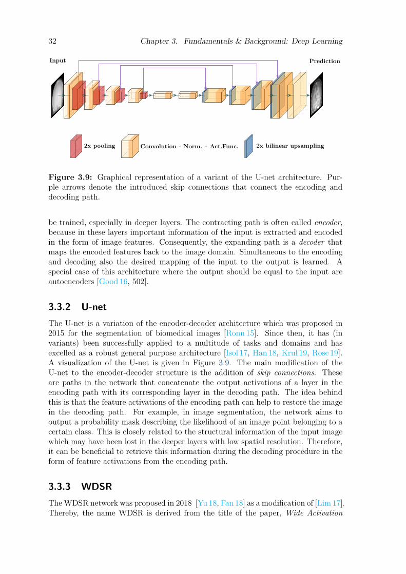
32 Chapter 3. Fundamentals & Background: Deep Learning
PredictionInput
2x pooling Convolution - Norm. - Act.Func. 2x bilinear upsampling
Figure 3.9: Graphical representation of a variant of the U-net architecture. Pur-ple arrows denote the introduced skip connections that connect the encoding anddecoding path.
be trained, especially in deeper layers. The contracting path is often called encoder,because in these layers important information of the input is extracted and encodedin the form of image features. Consequently, the expanding path is a decoder thatmaps the encoded features back to the image domain. Simultaneous to the encodingand decoding also the desired mapping of the input to the output is learned. Aspecial case of this architecture where the output should be equal to the input areautoencoders [Good 16, 502].
3.3.2 U-netThe U-net is a variation of the encoder-decoder architecture which was proposed in2015 for the segmentation of biomedical images [Ronn 15]. Since then, it has (invariants) been successfully applied to a multitude of tasks and domains and hasexcelled as a robust general purpose architecture [Isol 17, Han 18, Krul 19, Rose 19].A visualization of the U-net is given in Figure 3.9. The main modification of theU-net to the encoder-decoder structure is the addition of skip connections. Theseare paths in the network that concatenate the output activations of a layer in theencoding path with its corresponding layer in the decoding path. The idea behindthis is that the feature activations of the encoding path can help to restore the imagein the decoding path. For example, in image segmentation, the network aims tooutput a probability mask describing the likelihood of an image point belonging to acertain class. This is closely related to the structural information of the input imagewhich may have been lost in the deeper layers with low spatial resolution. Therefore,it can be beneficial to retrieve this information during the decoding procedure in theform of feature activations from the encoding path.
3.3.3 WDSRThe WDSR network was proposed in 2018 [Yu 18, Fan 18] as a modification of [Lim 17].Thereby, the name WDSR is derived from the title of the paper, Wide Activation
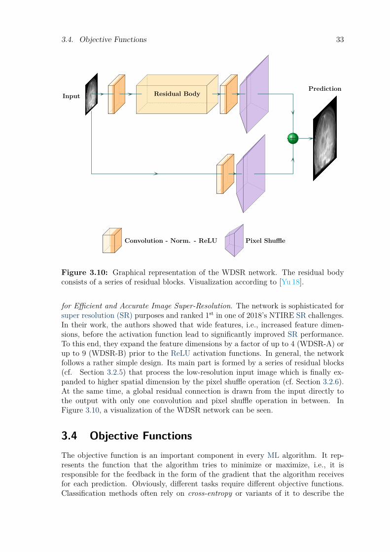
3.4. Objective Functions 33
Input Residual Body
+
Prediction
Convolution - Norm. - ReLU Pixel Shuffle
Figure 3.10: Graphical representation of the WDSR network. The residual bodyconsists of a series of residual blocks. Visualization according to [Yu 18].
for Efficient and Accurate Image Super-Resolution. The network is sophisticated forsuper resolution (SR) purposes and ranked 1st in one of 2018’s NTIRE SR challenges.In their work, the authors showed that wide features, i.e., increased feature dimen-sions, before the activation function lead to significantly improved SR performance.To this end, they expand the feature dimensions by a factor of up to 4 (WDSR-A) orup to 9 (WDSR-B) prior to the ReLU activation functions. In general, the networkfollows a rather simple design. Its main part is formed by a series of residual blocks(cf. Section 3.2.5) that process the low-resolution input image which is finally ex-panded to higher spatial dimension by the pixel shuffle operation (cf. Section 3.2.6).At the same time, a global residual connection is drawn from the input directly tothe output with only one convolution and pixel shuffle operation in between. InFigure 3.10, a visualization of the WDSR network can be seen.
3.4 Objective FunctionsThe objective function is an important component in every ML algorithm. It rep-resents the function that the algorithm tries to minimize or maximize, i.e., it isresponsible for the feedback in the form of the gradient that the algorithm receivesfor each prediction. Obviously, different tasks require different objective functions.Classification methods often rely on cross-entropy or variants of it to describe the
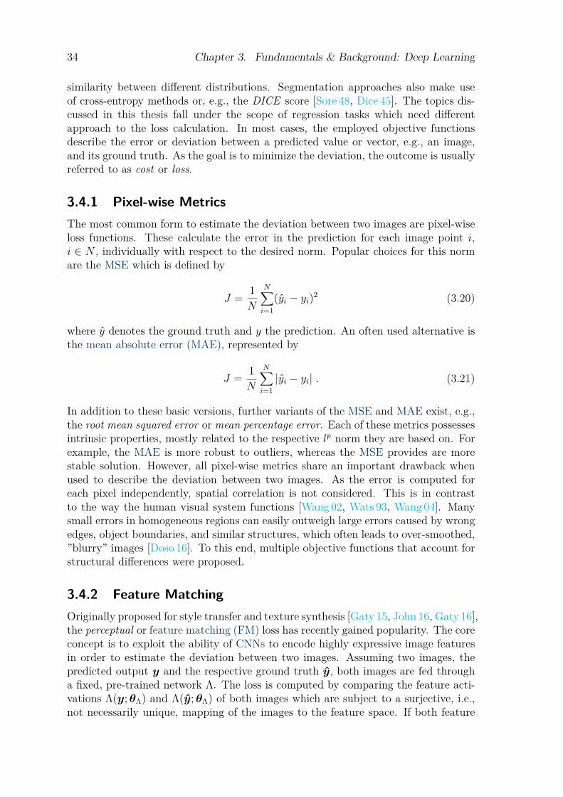
34 Chapter 3. Fundamentals & Background: Deep Learning
similarity between different distributions. Segmentation approaches also make useof cross-entropy methods or, e.g., the DICE score [Sore 48, Dice 45]. The topics dis-cussed in this thesis fall under the scope of regression tasks which need differentapproach to the loss calculation. In most cases, the employed objective functionsdescribe the error or deviation between a predicted value or vector, e.g., an image,and its ground truth. As the goal is to minimize the deviation, the outcome is usuallyreferred to as cost or loss.
3.4.1 Pixel-wise MetricsThe most common form to estimate the deviation between two images are pixel-wiseloss functions. These calculate the error in the prediction for each image point i,i ∈ N , individually with respect to the desired norm. Popular choices for this normare the MSE which is defined by
J = 1N
N∑i=1
(yi − yi)2 (3.20)
where y denotes the ground truth and y the prediction. An often used alternative isthe mean absolute error (MAE), represented by
J = 1N
N∑i=1|yi − yi| . (3.21)
In addition to these basic versions, further variants of the MSE and MAE exist, e.g.,the root mean squared error or mean percentage error. Each of these metrics possessesintrinsic properties, mostly related to the respective lp norm they are based on. Forexample, the MAE is more robust to outliers, whereas the MSE provides are morestable solution. However, all pixel-wise metrics share an important drawback whenused to describe the deviation between two images. As the error is computed foreach pixel independently, spatial correlation is not considered. This is in contrastto the way the human visual system functions [Wang 02, Wats 93, Wang 04]. Manysmall errors in homogeneous regions can easily outweigh large errors caused by wrongedges, object boundaries, and similar structures, which often leads to over-smoothed,”blurry” images [Doso 16]. To this end, multiple objective functions that account forstructural differences were proposed.
3.4.2 Feature MatchingOriginally proposed for style transfer and texture synthesis [Gaty 15, John 16, Gaty 16],the perceptual or feature matching (FM) loss has recently gained popularity. The coreconcept is to exploit the ability of CNNs to encode highly expressive image featuresin order to estimate the deviation between two images. Assuming two images, thepredicted output y and the respective ground truth y, both images are fed througha fixed, pre-trained network Λ. The loss is computed by comparing the feature acti-vations Λ(y;θΛ) and Λ(y;θΛ) of both images which are subject to a surjective, i.e.,not necessarily unique, mapping of the images to the feature space. If both feature
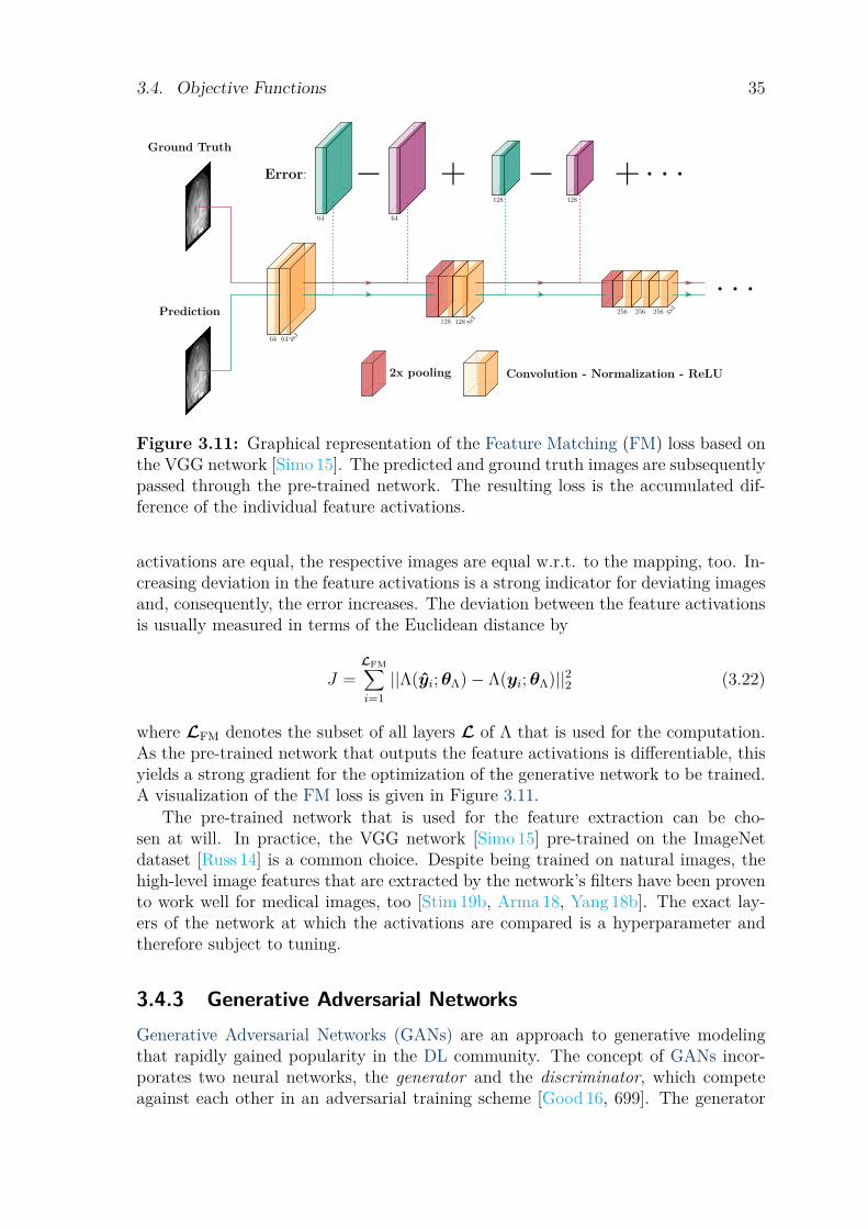
3.4. Objective Functions 35
64 64 3x3
128 128 3x3
256 256 256 3x3
. . .
Error:
6464
128128
− + − + . . .
2x pooling Convolution - Normalization - ReLU
Prediction
Ground Truth
Figure 3.11: Graphical representation of the Feature Matching (FM) loss based onthe VGG network [Simo 15]. The predicted and ground truth images are subsequentlypassed through the pre-trained network. The resulting loss is the accumulated dif-ference of the individual feature activations.
activations are equal, the respective images are equal w.r.t. to the mapping, too. In-creasing deviation in the feature activations is a strong indicator for deviating imagesand, consequently, the error increases. The deviation between the feature activationsis usually measured in terms of the Euclidean distance by
J =LFM∑i=1||Λ(yi;θΛ)− Λ(yi;θΛ)||22 (3.22)
where LFM denotes the subset of all layers L of Λ that is used for the computation.As the pre-trained network that outputs the feature activations is differentiable, thisyields a strong gradient for the optimization of the generative network to be trained.A visualization of the FM loss is given in Figure 3.11.
The pre-trained network that is used for the feature extraction can be cho-sen at will. In practice, the VGG network [Simo 15] pre-trained on the ImageNetdataset [Russ 14] is a common choice. Despite being trained on natural images, thehigh-level image features that are extracted by the network’s filters have been provento work well for medical images, too [Stim 19b, Arma 18, Yang 18b]. The exact lay-ers of the network at which the activations are compared is a hyperparameter andtherefore subject to tuning.
3.4.3 Generative Adversarial NetworksGenerative Adversarial Networks (GANs) are an approach to generative modelingthat rapidly gained popularity in the DL community. The concept of GANs incor-porates two neural networks, the generator and the discriminator, which competeagainst each other in an adversarial training scheme [Good 16, 699]. The generator
36 Chapter 3. Fundamentals & Background: Deep Learning
network produces samples of a distribution, yg = g(x;θg) whereas the discrimina-tor tries to distinguish fake samples produced by the generator from real samples ofthe original distribution. A direct correspondence between the samples is not nec-essary, therefore GANs can be used for unsupervised learning. The output for thediscriminator in this case is a probability value d(yg;θd) describing the likelihood ofyg belonging to the true data distribution. This results in a scenario where bothnetworks try to optimize for opposing terms during training, i.e., the combined lossfunction J(g, d) is given by
minθg
maxθd
J(g, d) = Ey∼pdata log d(y;θd) + Ey∼pmodel log(1− d(g(x;θg);θd)) , (3.23)
where pdata and pmodel denote the real and fake distribution, respectively [Good 14].The learnable discriminator serves as a powerful guidance for the generator net-
work. In contrast to the pre-trained feature extractor employed for the FM loss, thediscriminator is not limited to differentiating between high-level image features of pre-dicted and ground truth samples, but is optimized to learn a separation tailored tothe specific data distribution. The original GAN approach proposed in [Good 14] usesa noise sample as input x that is transformed to the output sample yg. Alternatively,it is also possible to learn a distribution p(x|χ) conditioned on an auxiliary input χ,which is referred to as conditional generative adversarial network (CGAN)[Mirz 14].
While the adversarial training scheme is guaranteed to converge in an ideal set-ting [Good 14, Yang 18b], the necessary assumptions are rarely the case in prac-tice [Oden 19]. Training the discriminator and the generator simultaneously posesgreat challenges on the balancing between the two networks. As a result, the train-ing of GANs faces several problems. Mode collapse describes a phenomenon inwhich the generator turns into a state of generating only samples with limited di-versity [Sali 16a]. The adversarial training scheme is also prone to non-convergence,in the form that both networks oscillate around a certain point, failing to convergeforever [Good 16, 701]. Also diminishing gradients can become a problem if the dis-criminator becomes too powerful, which can also lead to mode collapse [Than 19].Consequently, research regarding methods and optimization strategies towards im-proving and stabilizing the training of GANs is an ongoing topic [Radf 15, Sali 16a,Karr 17, Mesc 18, Than 19, Oden 19]. A detailed overview is outside the scope of thiswork. In addition to improved training methods, the GAN loss is often combined withother objective functions, e.g., the previously discussed FM loss, that constrain thegenerated samples to be close to the ground truth [Stim 19b, Wang 18b, Yang 18b].
3.4.4 Hinge lossThe hinge loss function is applied for maximum margin classification in ”traditional”ML. Its most prominent use case is in support vector machines (SVMs) [Bish 06, 326].For the optimization of those it would be ideal to directly minimize the zero-onemisclassification error. Unfortunately, this function is non-convex. The hinge loss isan approximation to the zero-one error function and exhibits the benefit of being aconvex function [Bish 06, 337]. It is defined by
J =N∑i=1
max(0, 1− yi · yi(xi,θ)) (3.24)

3.4. Objective Functions 37
-2 -1 1 2-1
1
2
z
f(z)
Zero-one lossHinge loss
Figure 3.12: A graphical representation of the zero-one error function and the hingeloss function.
where yi denotes the ground truth and y the actual prediction. The resulting functionpenalizes misclassifications and correct classifications that are withing the margin lin-early with respect to the distance to the decision boundary. Correct classificationswith sufficient margin are assigned zero cost. Consequently, extremely wrong pre-dictions lead to a extreme loss whereas extraordinary correct predictions are notextraordinarily rewarded. Both, the hinge loss and the zero-one error function arepresented in Figure 3.12. Thereby, the name hinge is derived from the function’scharacteristic shape.
While the hinge loss function is mainly used in classical ML approaches such asSVMs, it has its use cases also in DL as will be demonstrated in Chapter 6.

P A R T II
Methods for Multi-modalMedical Image Processing
39

C H A P T E R 4
Projection-to-ProjectionTranslation in X-ray/MR
projection Imaging
Hybrid X-ray/MR imaging offers great potential, especially for interventional ap-plications. To take full advantage of the available possibilities, it is useful to be ableto transfer information between the domains. However, image-to-image translationhas so far been performed exclusively for the case of tomographic CT and MR data.In the following, we therefore investigate this case for the dominant modality in theinterventional setting, X-ray projection imaging. Concretely, we aim to achieve aDL-based projection-to-projection translation from MR projections to correspondingX-ray-like projection images. We show that the characteristics of projection imagesdiffer significantly from those of tomographic images. To solve this problem, an initialphantom study is conducted in which we evaluate the influence of the chosen networkarchitecture of the image generator as well as the selected objective function on thegenerated projection images. Following the gained insights in this study, we finallypropose two changes to state-of-the-art image generation networks, a redistribution ofthe network capacity to higher resolution layers and a weighting of the objective func-tion to focus on the high frequency image components. We can show that these mod-ifications achieve clear improvements in the projection images, quantitatively as wellas qualitatively. The contents of the following chapter were previously published in:
[Stim 17b]
B. Stimpel, C. Syben, T. Wurfl, K. Mentl, A. Dorfler, and A. Maier.“MR to X-Ray Projection Image Synthesis”. In: Proceedings ofthe Fifth International Conference on Image Formation in X-RayComputed Tomography, 2017.
[Stim 18a]
B. Stimpel, C. Syben, T. Wurfl, K. Breininger, K. Mentl, J. Lom-men, A. Dorfler, and A. Maier. “Projection Image-to-image Trans-lation In Hybrid X-ray/MR Imaging”. In: Medical Imaging 2019:Image Processing, 2018.
[Stim 19b]
B. Stimpel, C. Syben, T. Wurfl, K. Breininger, P. Hoelter,A. Dorfler, and A. Maier. “Projection-to-Projection Translationfor Hybrid X-ray and Magnetic Resonance Imaging”. Scientific Re-ports, Vol. 9, No. 1, 2019.
41
42 Chapter 4. Projection-to-Projection Translation in X-ray/MR imaging
4.1 Introduction
Medical imaging enables deep insight into structural and physiological information ofthe imaged subject. In Section 2.1, an overview of the available modalities in medicalimaging is given. Despite the vast amount of information that can be acquired ingeneral, most modalities only cover a small, limited part of it. Naturally, this leads tothe desire for simultaneous, hybrid imaging of several modalities [Wang 05, Wang 12,Wang 13, Wang 15]. Preliminary work on this topic showed that hybrid imaging offerslarge benefits for many clinical applications [Fahr 01, Xi 16, Gjes 16]. A prominentrepresentative of this group is hybrid X-ray/MR imaging.
As two of the most common modalities, X-ray and MRI allow for the acquisition ofa wide spectrum of structural information targeting both soft and dense tissue. Thishas great potential, especially for imaging in image-guided interventions. Many ofthese procedures are concerned with soft tissue manipulation, e.g., cardiac catheteri-zation, aortic repair, or thrombectomy [Pepi 91, Powe 15, Brei 18b, Brei 18a]. Despiteits insensitivity to this soft tissue contrast, X-ray fluoroscopy (cf. Section 2.2.2) isthe common choice for interventional guidance. The main reason for this is its highspatial and temporal resolution which is often required for accurate guidance of in-terventional devices. However, the target structures can only be visualized indirectlyby the application of contrast agent, or through overlays of preoperative, diagnos-tic scans. Simultaneously providing native soft-tissue contrast through MRI couldclearly increase the accuracy of medical procedures and ease the workflow for thephysician. This complementary information could be used for various image pro-cessing applications. A straightforward approach would be image fusion, e.g., in theform of image overlays [Kout 16, McKa 16, Brei 20]. Yet, also image enhancement canbe a valuable alternative. As radiation dose and noise are directly related in X-rayimaging, image processing-based denoising is a prevalent topic [Maie 11]. Similarly,also SR is widely discussed [Sind 18]. As these methods are ongoing fields of research,numerous approaches have been proposed up to now with most of them targeting in-formation from a single modality. In order to take advantage of the research alreadycarried out, it is therefore advantageous to have the recorded information availablein the same domain or to transfer it there.
Domain transfer in X-ray and MR imaging is a familiar topic in radiation ther-apy [Nava 13, Nie 17, Wolt 17, Xian 18]. In this setting, MRI scans are acquired andmapped to corresponding CT data in order to create attenuation maps for precise can-cer treatment planning without exposing the patient to ionizing radiation. Though,the applied domain transfer is based entirely on tomographic images. Most image-guided procedures, however, rely on dynamic projection imaging provided by X-rayfluoroscopy. This significantly increases the difficulty of a domain transfer originat-ing from MRI. First, X-ray projection imaging is subject to perspective distortiondue to the projective geometry. The direct acquisition of MR projections matchingthis cone-beam projection distortion was only made possible by recent research ef-forts that will be explained in more detail in Section 4.2. Second, the synthesis ofX-ray signal from corresponding MRI data is an ill-posed problem. Tomographicimages allow for precise structural differentiation between tissues. This structuralinformation is lost during the integration of the X-rays on the detector. The result
4.2. MR Projection Imaging 43
is a linear combination of tomographic images with unknown path lengths. Tissues,bones, and other structures are therefore subject to overlaps while imaged by projec-tion imaging and can no longer be distinctively resolved. Third, a property of MRIthat exacerbates this problem is that bone and air provide little to no signal in mostMR imaging protocols (cf. Section 2.3). In contrast, X-ray images provide excellentcontrast for dense-tissues such as bone. The ambiguity between bone and air in MRItherefore yields no direct solution to replicate the X-ray contrast solely based on theacquired intensity values. In combination with the aforementioned lack of structuralinformation, this further increases the difficulty of the synthesis task.
Driven by the advances in fast MR projection imaging, we seek a solution toprojection-to-projection translation from MR projection images to corresponding X-ray views.
4.2 MR Projection ImagingThe most common acquisition types of MRI data are tomographic slices or full vol-umes. In contrast, image-guided interventions rely on projection imaging based onX-ray fluoroscopy. Acquiring full MRI volumes and forward projecting these wouldyield MR projections with similar cone-beam geometry, yet, this is impractical dueto the long acquisition times. To match the dynamic imaging of X-ray fluoroscopyin MRI, it is therefore necessary to directly acquire the projection images. Thereby,the acquisition of projection images subject to parallel-beam geometry is straight-forward [Lomm 18, Sybe 18]. This property can be exploited to generated projectionimages with X-ray-like distortion directly without the need of acquiring a full vol-ume first [Wach 18]. In prior work, we have shown that rebinning can be used toconvert multiple parallel-beam MR projections to corresponding fan or cone-beamprojection images [Sybe 17, Lomm 18]. Due to interpolation, however, this entails aloss of resolution. To avoid this, we presented a neural network-based approach togenerate a rebinning algorithm to generate this perspective distortion in a follow-upstudy [Sybe 20].
4.3 Related WorkEstablishing a mapping between MR and X-ray projection images falls under thebroader scope of image-to-image translation in machine learning. The considereddomain transfer is subject to the problems mentioned in Section 4.1 that arise fromthe projective geometry, i.e., projective distortion, overlapping tissue and ambiguoussignal. Still, prior work concerned with the generation of tomographic CT data fromcorresponding MRI scans is of great value. The efforts in this field are mainly cen-tered around radiation therapy and focus on two different approaches. The first kindgroups atlas-based methods which create a representative pair of an MR and a CTscan with known correspondence [Uh 14, Dege 16]. A new MR scan with unknowncorresponding CT information can subsequently be transformed to match the atlasMR scan for which the corresponding CT scan is known. However, the required im-age registration process is error-prone and exhibits high computational complexity
44 Chapter 4. Projection-to-Projection Translation in X-ray/MR imaging
which makes it unsuitable for a dynamic interventional application. The second typeof approaches are learning-based methods that try to extract a representation of aCT scan conditioned on the input MR scan. Early representatives used for the es-timation of attenuation maps were based on ”classical” machine learning techniquessuch as random forests [Nava 13]. With the ascent of DL (cf. Chapter 3) CNNs raisedthe bar for image-to-image translation similar to most other related fields. Withthe increased popularity of DL-based methods, many image synthesis approacheswere presented [Yan 15, Zhan 16]. Following the success of GANs [Good 14] (cf. Sec-tion 3.4.3), their use for general purpose image synthesis could be shown in manystudies [Isol 17, Nie 17, Wolt 17, Zhu 17]. This development also translated to imagesynthesis in medical imaging. In [Nie 17], the successful combination of a GAN withan auto-context model could be shown for the domain transfer between MR andCT. While this approach relied on corresponding datasets from both modalities fortraining, it was shown in [Yang 18a, Wolt 17] that this task can also be solved withunpaired datasets. This list of approaches shows the rapid advance in the field ofmedical image synthesis over the last years. However, all of these exclusively targetthe domain transfer between tomographic MR and CT datasets. The examinationof a domain transfer using these modalities in the case of projection imaging is aso far unconsidered problem. Therefore, we aim to close this gap and investigate aDL-based solution for the task of MR to X-ray projection-to-projection translation.
Large parts of the work in natural image synthesis targets the generation of imagesconditioned on, e.g., the style or content of an input image, a semantic layout, orsemantic descriptions. In almost all cases, this is subject to a one-to-many mapping,i.e., for one input multiple adequate solutions for the output exist. In contrast,the underlying problem of projection-to-projection translation considers a one-to-onemapping as a clear correspondence between two projection images from differentmodalities exists. The desired mapping can be described by P = f(I) where theinput MR projection I is mapped to the predicted X-ray projection P . Due tothe one-to-one correspondence between the projection images, this mapping can betrained in a supervised fashion such that P approximates to the known ground truthX-ray projection L as good as possible.
4.4 Preparatory Phantom Study
As outlined in Section 3.3, the possibilities for the design of CNNs are extensive.This renders the choice of an appropriate design for a specific task often a heuristicsolution or a question of computational resources. In the run-up to a larger-scalestudy with clinical patient data, we therefore make preparations for this using exper-iments based on an anthropomorphic phantom. From this we expect to be able tomake a preselection for the choice of methods, the network architecture used and theassociated objective function.
4.4. Preparatory Phantom Study 45
4.4.1 Evaluation of Network ArchitecturesFalling under the scope of generative tasks, many approaches in image synthesismake use of the encoder-decoder structure for the design of the CNN architecture(cf. Section 3.3.1). To assess the influence of the chosen network architecture forthe projection-to-projection translation task, we compare three different, popular ap-proaches based on their performance. The first one is a U-net-like network (cf. Sec-tion 3.3.2). Instead of pooling, strided convolution is used for downsampling the fea-ture maps (cf. Section 3.2.2). The second tested approach is an encoder-decoder ar-chitecture using residual blocks (cf. Section 3.2.5) as used, e.g., in [John 16, Wang 18b]which will in the following be abbreviated as ResNet. Our approach features nineresidual blocks applied at the lowest resolution layer to build the main processingblock of the network. The third network architecture is the cascaded refinementnetwork (CRN) proposed by Chen et al. [Chen 17]. The network was originally pro-posed to generate natural images from semantic layouts and showed highly appealingresults on this task. The design is strongly based on the U-net architecture withthe big difference that in the encoding path only bilinear downsampling instead ofpooling or strided convolution is used. All three networks are schematically depictedin Figure 4.1.
4.4.2 Evaluation of Objective FunctionsSince the objective function provides the feedback for the training of the network, theselection of this is an important point of any machine learning algorithm. Dependingon this choice, specific properties will prevail when generating the results. In orderto investigate the effects of the chosen objective function on the task of projection-to-projection translation, we therefore compare two different approaches. On the onehand, a pixel-wise metric is used in the form of the `1-norm of the error between thepredicted and the ground truth X-ray projection, the MAE (cf. Section 3.4.1). Thismethod is widely used across many generative tasks [Zhao 17]. On the other hand,the FM loss is applied (cf. Section 3.4.2). To this end, a VGG19 [Simo 15] networkpre-trained on ImageNet [Russ 14] is employed.
Based on these two objective functions, we can test two fundamentally differentapproaches. While the MAE tries to minimize the numerical difference of the pro-jection images, we expect the FM loss to generate images that are visually moreappealing.
4.4.3 ExperimentsExperimental validation of the aforementioned design choices is performed basedon an X-ray and MR sensitive human head-like phantom. Data acquisition wasperformed on an Axiom-Artis C-arm CT Scanner for X-ray and a 1.5 T Aera Scannerfor MR data (Siemens Healthcare GmbH, Forchheim, Germany). The acquired scanscome in an isotropic spatial resolution of 0.48× 0.48× 0.48 mm3 for the CT and0.48× 0.48× 0.48 mm3 MR volumes.
The volumetric scans are aligned by rigid registration using 3D Slicer [Fedo 12].This allows to create matching cone-beam projection images by forward projection
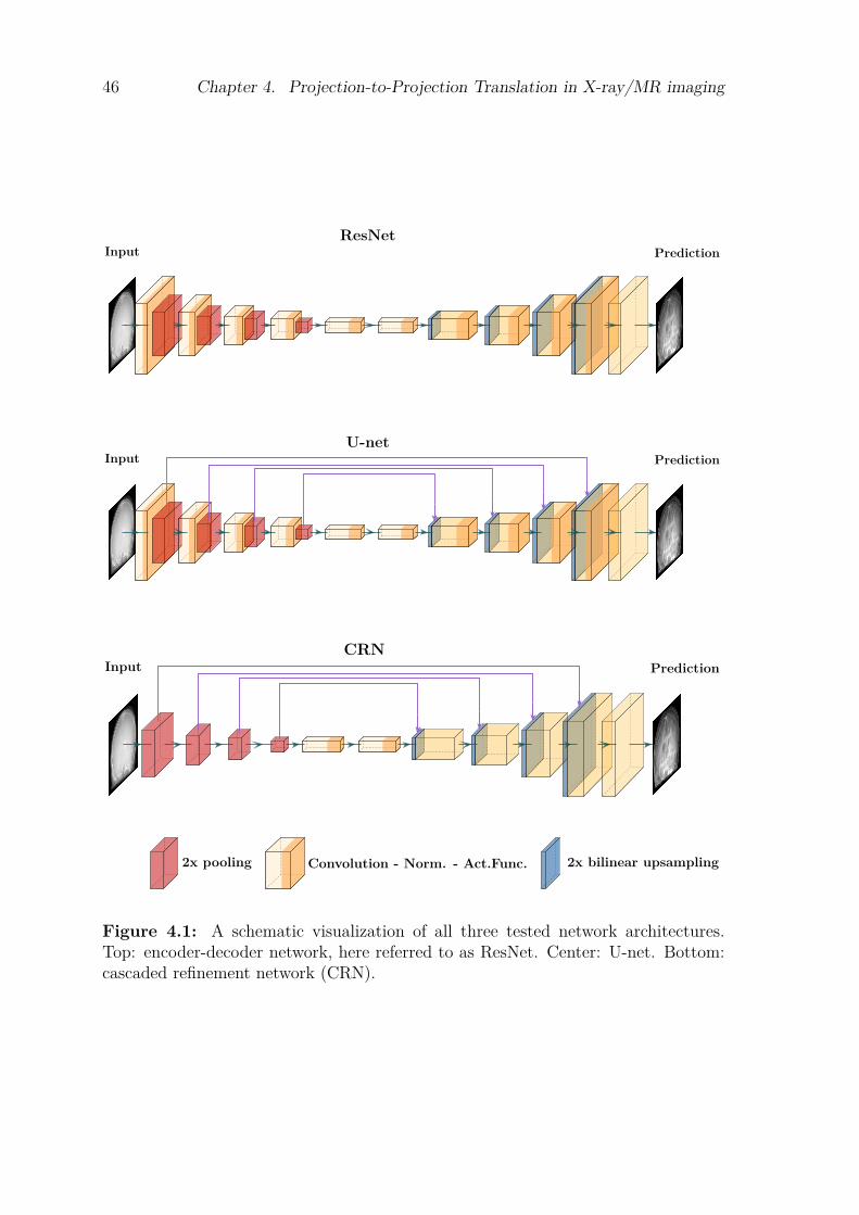
46 Chapter 4. Projection-to-Projection Translation in X-ray/MR imaging
PredictionInputResNet
PredictionInputU-net
PredictionInput
2x pooling Convolution - Norm. - Act.Func. 2x bilinear upsampling
CRN
Figure 4.1: A schematic visualization of all three tested network architectures.Top: encoder-decoder network, here referred to as ResNet. Center: U-net. Bottom:cascaded refinement network (CRN).

4.4. Preparatory Phantom Study 47
Patient axis
X-ray source direction
±30◦
Figure 4.2: A visualization of all possible X-ray source positions used for the datageneration.
of the registered volumes. The CONRAD framework [Maie 13] is used to this end.In order to ensure extensive coverage of the entire volume while being representativeof the clinical use case, 450 projections are acquired from equiangular distances inazimuthal direction and -30◦ to +30◦ inclination angle. This is depicted graphicallyin Figure 4.2. Subsequently, the created projections are randomly split into distincttraining (80%), validation (10%) and test (10%) sets. It is ensured that no projectionwith the exact same projection geometry is in both, the test and the training data.However, it is still possible that projections from adjacent projection angles whichhave similar appearance are to be found in the different data sets. While we areaware that this is not an ideal separation of seen and unseen data, we stick with thissimple splitting scheme for the underlying phantom study as all projections are fromthe same object anyway. Future evaluation with real clinical scans will address thisissue with an appropriate data separation on the patient level.
Training of all networks is performed using unit batch size and the ADAM opti-mizer (cf. Section 3.1.2) with a learning rate of 1e−4 for 100 epochs with retrospectiveselection of the best performing model.
The generated results are evaluated quantitatively in terms of the MSE, struc-tural similarity (SSIM), and peak signal-to-noise ratio (PSNR) metrics. To this end,all images are normalized to a value range of -1 to 1 beforehand. For qualitativeevaluation representative examples of the generated X-ray projections are presented.
4.4.4 Results & DiscussionIn Table 4.1, the evaluation metrics for all combinations of network architecture andloss function are presented. When examining the MSEs it becomes apparent that thedifference in the numerical results between the different network architectures is lowfor both, the FM and the MAE loss. Thereby, the lowest MSE of 0.058 is observedfor the ResNet in combination with the MAE loss. The numeric results with respectto the MSE are equally close for the FM loss. Here, the CRN performs best withan MSE of 0.071. Slightly larger differences can be observed in the presented SSIMmetrics. The best performance is achieved by the ResNet trained with the MAE
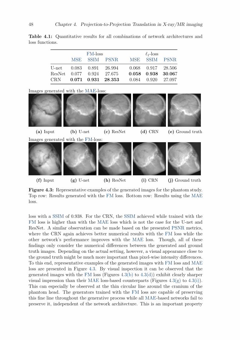
48 Chapter 4. Projection-to-Projection Translation in X-ray/MR imaging
Table 4.1: Quantitative results for all combinations of network architectures andloss functions.
FM-loss `1-lossMSE SSIM PSNR MSE SSIM PSNR
U-net 0.083 0.891 26.994 0.068 0.917 28.506ResNet 0.077 0.924 27.675 0.058 0.938 30.067CRN 0.071 0.931 28.353 0.084 0.920 27.097
Images generated with the MAE-loss:
(a) Input (b) U-net (c) ResNet (d) CRN (e) Ground truth
Images generated with the FM-loss:
(f) Input (g) U-net (h) ResNet (i) CRN (j) Ground truth
Figure 4.3: Representative examples of the generated images for the phantom study.Top row: Results generated with the FM loss. Bottom row: Results using the MAEloss.
loss with a SSIM of 0.938. For the CRN, the SSIM achieved while trained with theFM loss is higher than with the MAE loss which is not the case for the U-net andResNet. A similar observation can be made based on the presented PSNR metrics,where the CRN again achieves better numerical results with the FM loss while theother network’s performance improves with the MAE loss. Though, all of thesefindings only consider the numerical differences between the generated and groundtruth images. Depending on the actual setting, however, a visual appearance close tothe ground truth might be much more important than pixel-wise intensity differences.To this end, representative examples of the generated images with FM loss and MAEloss are presented in Figure 4.3. By visual inspection it can be observed that thegenerated images with the FM loss (Figures 4.3(b) to 4.3(d)) exhibit clearly sharpervisual impression than their MAE loss-based counterparts (Figures 4.3(g) to 4.3(i)).This can especially be observed at the thin circular line around the cranium of thephantom head. The generators trained with the FM loss are capable of preservingthis fine line throughout the generative process while all MAE-based networks fail topreserve it, independent of the network architecture. This is an important property
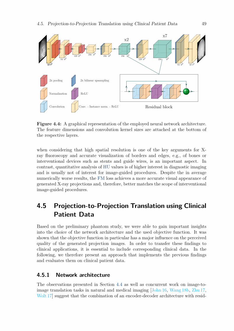
4.5. Projection-to-Projection Translation using Clinical Patient Data 49
32 7x732 7x7
64 3x3
128 3x3 256 3x
3256 3x
3 256 3x3
128 3x3 256 3x
3
64 3x3 32 1x
1
x2x7
2x pooling 2x bilinear upsampling
Normalization ReLU
Convolution Conv. - Instance norm. - ReLU
. . . + . . .
Residual block
Figure 4.4: A graphical representation of the employed neural network architecture.The feature dimensions and convolution kernel sizes are attached at the bottom ofthe respective layers.
when considering that high spatial resolution is one of the key arguments for X-ray fluoroscopy and accurate visualization of borders and edges, e.g., of bones orinterventional devices such as stents and guide wires, is an important aspect. Incontrast, quantitative analysis of HU values is of higher interest in diagnostic imagingand is usually not of interest for image-guided procedures. Despite the in averagenumerically worse results, the FM loss achieves a more accurate visual appearance ofgenerated X-ray projections and, therefore, better matches the scope of interventionalimage-guided procedures.
4.5 Projection-to-Projection Translation using ClinicalPatient Data
Based on the preliminary phantom study, we were able to gain important insightsinto the choice of the network architecture and the used objective function. It wasshown that the objective function in particular has a major influence on the perceivedquality of the generated projection images. In order to transfer these findings toclinical applications, it is essential to include corresponding clinical data. In thefollowing, we therefore present an approach that implements the previous findingsand evaluates them on clinical patient data.
4.5.1 Network architectureThe observations presented in Section 4.4 as well as concurrent work on image-to-image translation tasks in natural and medical imaging [John 16, Wang 18b, Zhu 17,Wolt 17] suggest that the combination of an encoder-decoder architecture with resid-
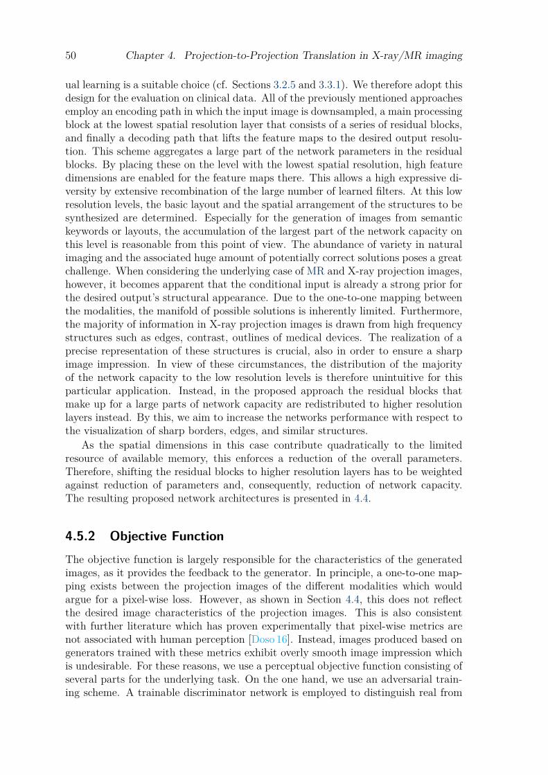
50 Chapter 4. Projection-to-Projection Translation in X-ray/MR imaging
ual learning is a suitable choice (cf. Sections 3.2.5 and 3.3.1). We therefore adopt thisdesign for the evaluation on clinical data. All of the previously mentioned approachesemploy an encoding path in which the input image is downsampled, a main processingblock at the lowest spatial resolution layer that consists of a series of residual blocks,and finally a decoding path that lifts the feature maps to the desired output resolu-tion. This scheme aggregates a large part of the network parameters in the residualblocks. By placing these on the level with the lowest spatial resolution, high featuredimensions are enabled for the feature maps there. This allows a high expressive di-versity by extensive recombination of the large number of learned filters. At this lowresolution levels, the basic layout and the spatial arrangement of the structures to besynthesized are determined. Especially for the generation of images from semantickeywords or layouts, the accumulation of the largest part of the network capacity onthis level is reasonable from this point of view. The abundance of variety in naturalimaging and the associated huge amount of potentially correct solutions poses a greatchallenge. When considering the underlying case of MR and X-ray projection images,however, it becomes apparent that the conditional input is already a strong prior forthe desired output’s structural appearance. Due to the one-to-one mapping betweenthe modalities, the manifold of possible solutions is inherently limited. Furthermore,the majority of information in X-ray projection images is drawn from high frequencystructures such as edges, contrast, outlines of medical devices. The realization of aprecise representation of these structures is crucial, also in order to ensure a sharpimage impression. In view of these circumstances, the distribution of the majorityof the network capacity to the low resolution levels is therefore unintuitive for thisparticular application. Instead, in the proposed approach the residual blocks thatmake up for a large parts of network capacity are redistributed to higher resolutionlayers instead. By this, we aim to increase the networks performance with respect tothe visualization of sharp borders, edges, and similar structures.
As the spatial dimensions in this case contribute quadratically to the limitedresource of available memory, this enforces a reduction of the overall parameters.Therefore, shifting the residual blocks to higher resolution layers has to be weightedagainst reduction of parameters and, consequently, reduction of network capacity.The resulting proposed network architectures is presented in 4.4.
4.5.2 Objective FunctionThe objective function is largely responsible for the characteristics of the generatedimages, as it provides the feedback to the generator. In principle, a one-to-one map-ping exists between the projection images of the different modalities which wouldargue for a pixel-wise loss. However, as shown in Section 4.4, this does not reflectthe desired image characteristics of the projection images. This is also consistentwith further literature which has proven experimentally that pixel-wise metrics arenot associated with human perception [Doso 16]. Instead, images produced based ongenerators trained with these metrics exhibit overly smooth image impression whichis undesirable. For these reasons, we use a perceptual objective function consisting ofseveral parts for the underlying task. On the one hand, we use an adversarial train-ing scheme. A trainable discriminator network is employed to distinguish real from
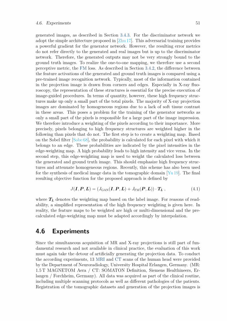
4.6. Experiments 51
generated images, as described in Section 3.4.3. For the discriminator network weadopt the simple architecture proposed in [Zhu 17]. This adversarial training providesa powerful gradient for the generator network. However, the resulting error metricsdo not refer directly to the generated and real images but is up to the discriminatornetwork. Therefore, the generated outputs may not be very strongly bound to theground truth images. To realize the one-to-one mapping, we therefore use a secondperceptive metric, the FM loss. As described in Section 3.4.2, the difference betweenthe feature activations of the generated and ground truth images is compared using apre-trained image recognition network. Typically, most of the information containedin the projection image is drawn from corners and edges. Especially in X-ray fluo-roscopy, the representation of these structures is essential for the precise execution ofimage-guided procedures. In terms of quantity, however, these high frequency struc-tures make up only a small part of the total pixels. The majority of X-ray projectionimages are dominated by homogeneous regions due to a lack of soft tissue contrastin these areas. This poses a problem for the training of the generator networks asonly a small part of the pixels is responsible for a large part of the image impression.We therefore introduce a weighting of the pixels according to their importance. Moreprecisely, pixels belonging to high frequency structures are weighted higher in thefollowing than pixels that do not. The first step is to create a weighting map. Basedon the Sobel filter [Sobe 68], the probability is calculated for each pixel with which itbelongs to an edge. These probabilities are indicated by the pixel intensities in theedge-weighting map. A high probability leads to high intensity and vice versa. In thesecond step, this edge-weighting map is used to weight the calculated loss betweenthe generated and ground truth image. This should emphasize high frequency struc-tures and attenuate homogeneous regions. Recently, this scheme has also been usedfor the synthesis of medical image data in the tomographic domain [Yu 19]. The finalresulting objective function for the proposed approach is defined by
J(I,P ,L) = (JGAN(I,P ,L) + JFM(P ,L)) · TL , (4.1)
where TL denotes the weighting map based on the label image. For reasons of read-ability, a simplified representation of the high frequency weighting is given here. Inreality, the feature maps to be weighted are high or multi-dimensional and the pre-calculated edge-weighting map must be adapted accordingly by interpolation.
4.6 ExperimentsSince the simultaneous acquisition of MR and X-ray projections is still part of fun-damental research and not available in clinical practice, the evaluation of this workmust again take the detour of artificially generating the projection data. To conductthe according experiments, 13 MRI and CT scans of the human head were providedby the Department of Neuroradiology, University Hospital Erlangen, Germany. (MR:1.5 T MAGNETOM Aera / CT: SOMATON Definition, Siemens Healthineers, Er-langen / Forchheim, Germany). All data was acquired as part of the clinical routine,including multiple scanning protocols as well as different pathologies of the patients.Registration of the tomographic datasets and generation of the projection images is
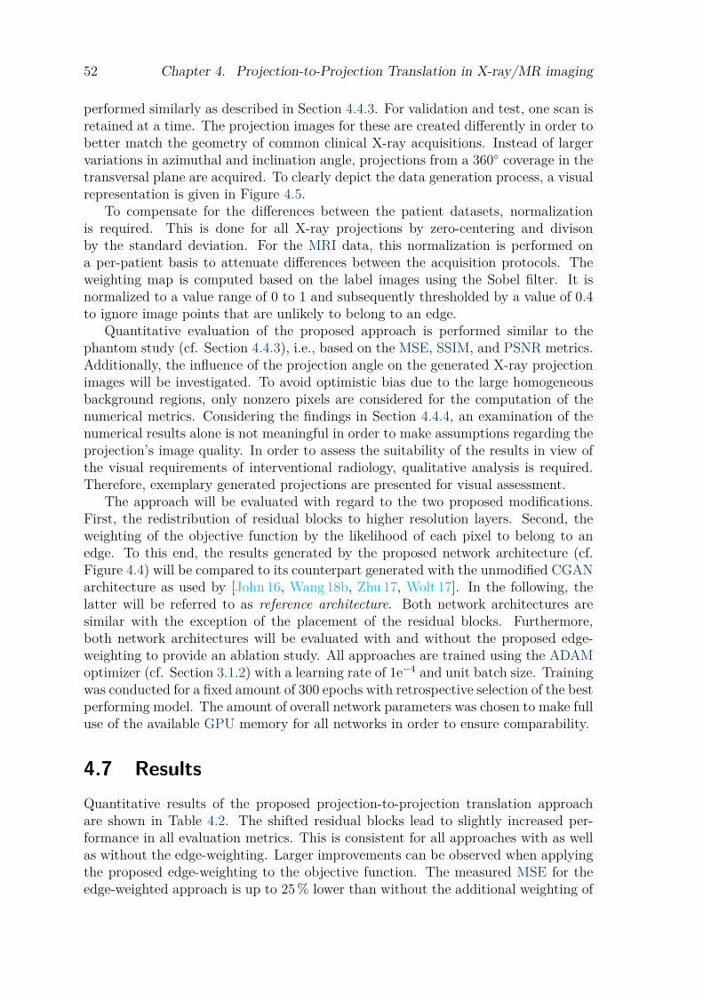
52 Chapter 4. Projection-to-Projection Translation in X-ray/MR imaging
performed similarly as described in Section 4.4.3. For validation and test, one scan isretained at a time. The projection images for these are created differently in order tobetter match the geometry of common clinical X-ray acquisitions. Instead of largervariations in azimuthal and inclination angle, projections from a 360◦ coverage in thetransversal plane are acquired. To clearly depict the data generation process, a visualrepresentation is given in Figure 4.5.
To compensate for the differences between the patient datasets, normalizationis required. This is done for all X-ray projections by zero-centering and divisonby the standard deviation. For the MRI data, this normalization is performed ona per-patient basis to attenuate differences between the acquisition protocols. Theweighting map is computed based on the label images using the Sobel filter. It isnormalized to a value range of 0 to 1 and subsequently thresholded by a value of 0.4to ignore image points that are unlikely to belong to an edge.
Quantitative evaluation of the proposed approach is performed similar to thephantom study (cf. Section 4.4.3), i.e., based on the MSE, SSIM, and PSNR metrics.Additionally, the influence of the projection angle on the generated X-ray projectionimages will be investigated. To avoid optimistic bias due to the large homogeneousbackground regions, only nonzero pixels are considered for the computation of thenumerical metrics. Considering the findings in Section 4.4.4, an examination of thenumerical results alone is not meaningful in order to make assumptions regarding theprojection’s image quality. In order to assess the suitability of the results in view ofthe visual requirements of interventional radiology, qualitative analysis is required.Therefore, exemplary generated projections are presented for visual assessment.
The approach will be evaluated with regard to the two proposed modifications.First, the redistribution of residual blocks to higher resolution layers. Second, theweighting of the objective function by the likelihood of each pixel to belong to anedge. To this end, the results generated by the proposed network architecture (cf.Figure 4.4) will be compared to its counterpart generated with the unmodified CGANarchitecture as used by [John 16, Wang 18b, Zhu 17, Wolt 17]. In the following, thelatter will be referred to as reference architecture. Both network architectures aresimilar with the exception of the placement of the residual blocks. Furthermore,both network architectures will be evaluated with and without the proposed edge-weighting to provide an ablation study. All approaches are trained using the ADAMoptimizer (cf. Section 3.1.2) with a learning rate of 1e−4 and unit batch size. Trainingwas conducted for a fixed amount of 300 epochs with retrospective selection of the bestperforming model. The amount of overall network parameters was chosen to make fulluse of the available GPU memory for all networks in order to ensure comparability.
4.7 ResultsQuantitative results of the proposed projection-to-projection translation approachare shown in Table 4.2. The shifted residual blocks lead to slightly increased per-formance in all evaluation metrics. This is consistent for all approaches with as wellas without the edge-weighting. Larger improvements can be observed when applyingthe proposed edge-weighting to the objective function. The measured MSE for theedge-weighted approach is up to 25 % lower than without the additional weighting of
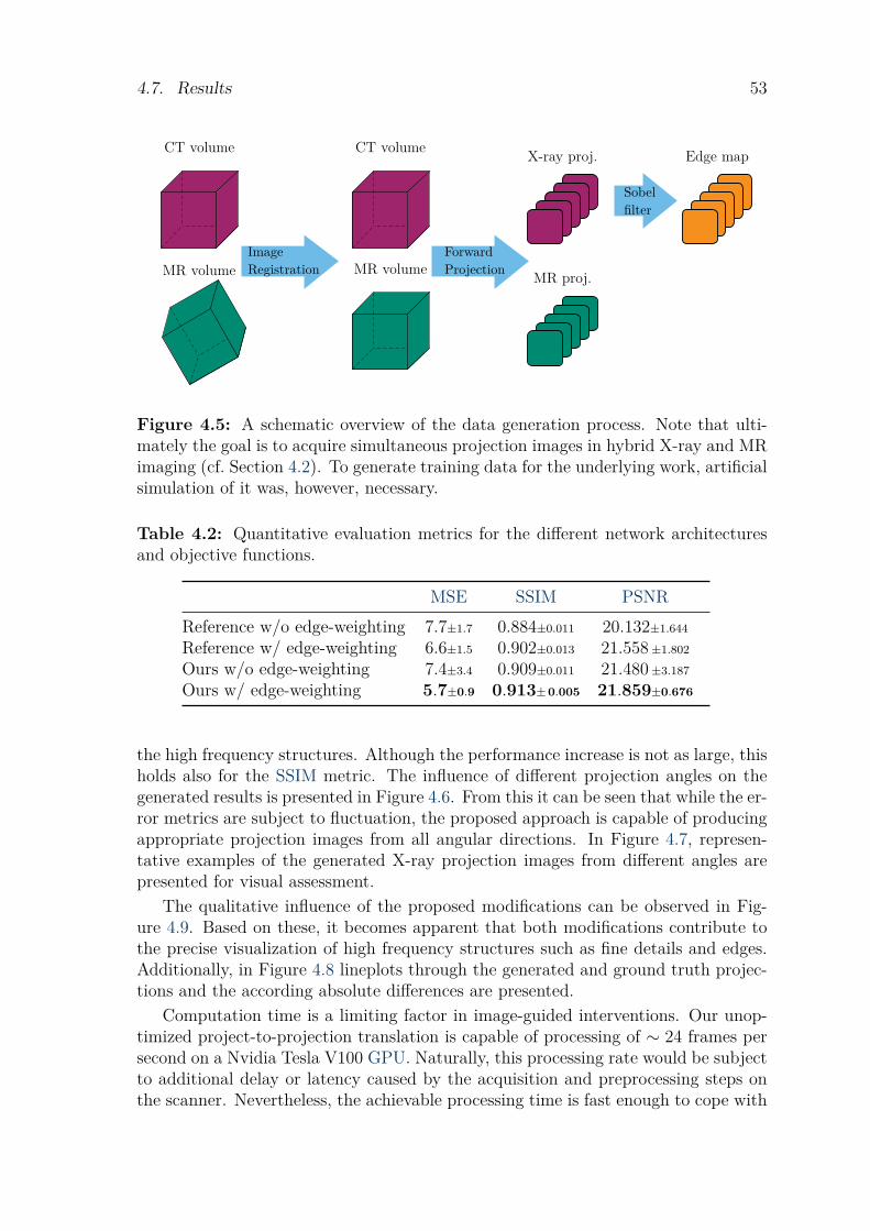
4.7. Results 53
MR volume
CT volume
ImageRegistration MR volume
CT volume
ForwardProjection
Sobelfilter
X-ray proj.
MR proj.
Edge map
Figure 4.5: A schematic overview of the data generation process. Note that ulti-mately the goal is to acquire simultaneous projection images in hybrid X-ray and MRimaging (cf. Section 4.2). To generate training data for the underlying work, artificialsimulation of it was, however, necessary.
Table 4.2: Quantitative evaluation metrics for the different network architecturesand objective functions.
MSE SSIM PSNRReference w/o edge-weighting 7.7±1.7 0.884±0.011 20.132±1.644
Reference w/ edge-weighting 6.6±1.5 0.902±0.013 21.558 ±1.802
Ours w/o edge-weighting 7.4±3.4 0.909±0.011 21.480 ±3.187
Ours w/ edge-weighting 5.7±0.9 0.913±0.005 21.859±0.676
the high frequency structures. Although the performance increase is not as large, thisholds also for the SSIM metric. The influence of different projection angles on thegenerated results is presented in Figure 4.6. From this it can be seen that while the er-ror metrics are subject to fluctuation, the proposed approach is capable of producingappropriate projection images from all angular directions. In Figure 4.7, represen-tative examples of the generated X-ray projection images from different angles arepresented for visual assessment.
The qualitative influence of the proposed modifications can be observed in Fig-ure 4.9. Based on these, it becomes apparent that both modifications contribute tothe precise visualization of high frequency structures such as fine details and edges.Additionally, in Figure 4.8 lineplots through the generated and ground truth projec-tions and the according absolute differences are presented.
Computation time is a limiting factor in image-guided interventions. Our unop-timized project-to-projection translation is capable of processing of ∼ 24 frames persecond on a Nvidia Tesla V100 GPU. Naturally, this processing rate would be subjectto additional delay or latency caused by the acquisition and preprocessing steps onthe scanner. Nevertheless, the achievable processing time is fast enough to cope with

54 Chapter 4. Projection-to-Projection Translation in X-ray/MR imaging
Figure 4.6: Quantitative evaluation of the generated X-ray projections with respectto the projection angle. Here, 0◦ denotes an RAO angle of 90◦ while 180◦ represents90◦ LAO. Note that due to tilt and the projective geometry opposing projectionimages are not equal.
common clinical X-ray fluoroscopy frame rates and will likely exceed the expectedacquisition time for cone-beam MR projection images on a real scanner by far.
4.8 DiscussionSimilar image synthesis approaches proposed for medical imaging solely target theapplication based on tomographic images. In contrast, the synthesis of projectionimages is a field that has not yet been examined in greater detail. A direct comparisonof quantitative metrics is, therefore, neither feasible nor meaningful.
Data generation For the underlying work, 13 tomographic MR and CT data setswere used. Although this is not enough to represent the full range of possible variationin projection images, this amount is sufficient for an initial study, as it becomes clearfrom the results. One reason for this is data augmentation. Data augmentationhas been found to be highly useful in covering a large amount of variations withonly limited data [Pere 17]. The most common forms of this are cropping certainparts of the images, rotation, deformation and similar techniques. The process ofgenerating the projection data, i.e., forward projection of the volume, is intrinsicallya powerful augmentation method. This integral transformation is called the X-raytransformation. The mapping X fX-ray(ι) of the X-ray transformation for a functionf(ι) and the line ι is defined by
X fX-ray(ι) =∫RfXray(u0 + tψ)dt , (4.2)
with u0 being the starting point on the line ι with the unit direction vector ψ.Assuming f(ι) to be constant, the output of X-ray transformation will be different foreach projection angle. Caused by effects such as perspective distortion, the projectiontrajectory, and others, this results in an effective augmentation technique that iscapable of generating diverse projection data from only few tomographic volumes.
Of course, this augmentation only affects the information that is already presentin the scans. This does not apply to structural differences due to delayed acquisition,but also to medical indications of individual patients. In the considered case of neuro-logical data sets, these could be, for example, bone fractures, lesions, aneurysms, andmuch more. Two examples of the occurring differences are presented in Figure 4.10.
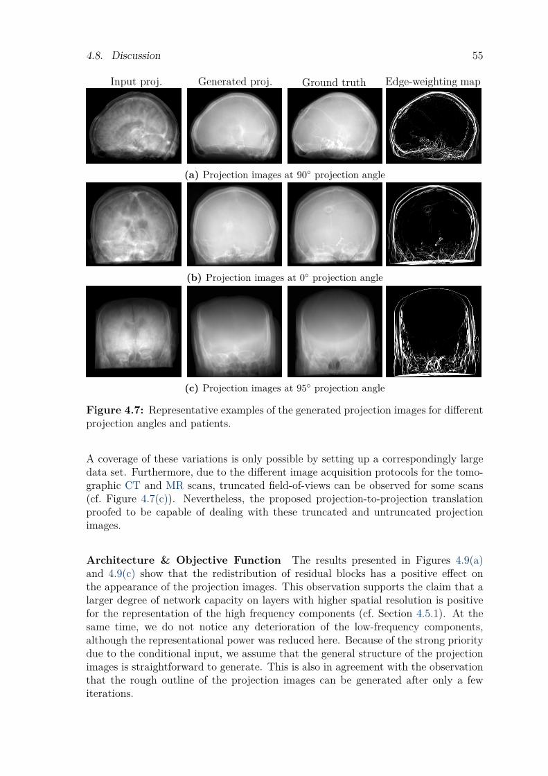
4.8. Discussion 55
Input proj. Generated proj. Ground truth Edge-weighting map
(a) Projection images at 90◦ projection angle
(b) Projection images at 0◦ projection angle
(c) Projection images at 95◦ projection angle
Figure 4.7: Representative examples of the generated projection images for differentprojection angles and patients.
A coverage of these variations is only possible by setting up a correspondingly largedata set. Furthermore, due to the different image acquisition protocols for the tomo-graphic CT and MR scans, truncated field-of-views can be observed for some scans(cf. Figure 4.7(c)). Nevertheless, the proposed projection-to-projection translationproofed to be capable of dealing with these truncated and untruncated projectionimages.
Architecture & Objective Function The results presented in Figures 4.9(a)and 4.9(c) show that the redistribution of residual blocks has a positive effect onthe appearance of the projection images. This observation supports the claim that alarger degree of network capacity on layers with higher spatial resolution is positivefor the representation of the high frequency components (cf. Section 4.5.1). At thesame time, we do not notice any deterioration of the low-frequency components,although the representational power was reduced here. Because of the strong prioritydue to the conditional input, we assume that the general structure of the projectionimages is straightforward to generate. This is also in agreement with the observationthat the rough outline of the projection images can be generated after only a fewiterations.
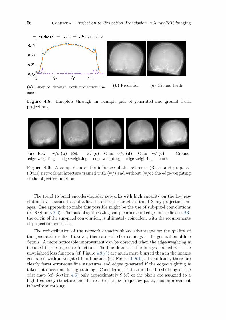
56 Chapter 4. Projection-to-Projection Translation in X-ray/MR imaging
(a) Lineplot through both projection im-ages.
(b) Prediction (c) Ground truth
Figure 4.8: Lineplots through an example pair of generated and ground truthprojections.
(a) Ref. w/oedge-weighting
(b) Ref. w/edge-weighting
(c) Ours w/oedge-weighting
(d) Ours w/edge-weighting
(e) Groundtruth
Figure 4.9: A comparison of the influence of the reference (Ref.) and proposed(Ours) network architecture trained with (w/) and without (w/o) the edge-weightingof the objective function.
The trend to build encoder-decoder networks with high capacity on the low res-olution levels seems to contradict the desired characteristics of X-ray projection im-ages. One approach to make this possible might be the use of sub-pixel convolutions(cf. Section 3.2.6). The task of synthesizing sharp corners and edges in the field of SR,the origin of the sup-pixel convolution, is ultimately coincident with the requirementsof projection synthesis.
The redistribution of the network capacity shows advantages for the quality ofthe generated results. However, there are still shortcomings in the generation of finedetails. A more noticeable improvement can be observed when the edge-weighting isincluded in the objective function. The fine details in the images trained with theunweighted loss function (cf. Figure 4.9(c)) are much more blurred than in the imagesgenerated with a weighted loss function (cf. Figure 4.9(d)). In addition, there areclearly fewer erroneous fine structures and edges generated if the edge-weighting istaken into account during training. Considering that after the thresholding of theedge map (cf. Section 4.6) only approximately 9.8% of the pixels are assigned to ahigh frequency structure and the rest to the low frequency parts, this improvementis hardly surprising.
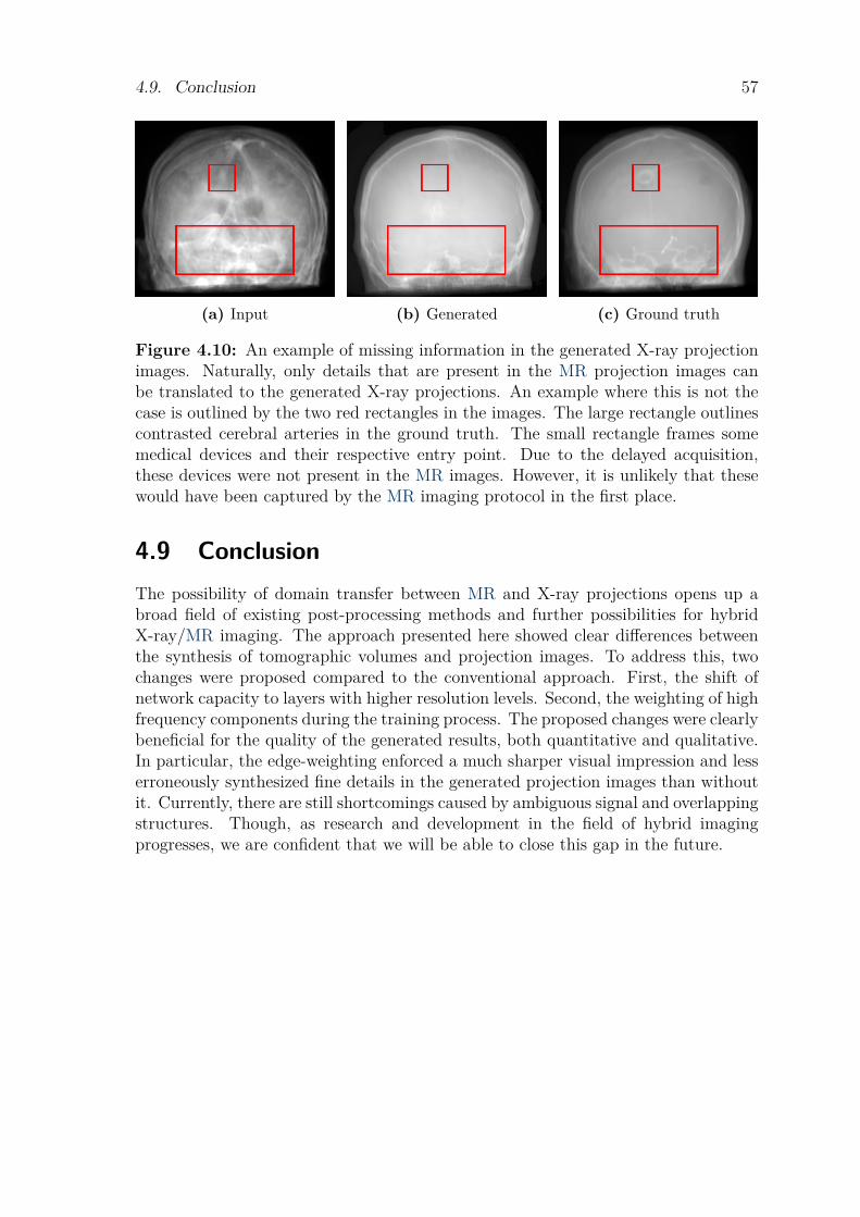
4.9. Conclusion 57
(a) Input (b) Generated (c) Ground truth
Figure 4.10: An example of missing information in the generated X-ray projectionimages. Naturally, only details that are present in the MR projection images canbe translated to the generated X-ray projections. An example where this is not thecase is outlined by the two red rectangles in the images. The large rectangle outlinescontrasted cerebral arteries in the ground truth. The small rectangle frames somemedical devices and their respective entry point. Due to the delayed acquisition,these devices were not present in the MR images. However, it is unlikely that thesewould have been captured by the MR imaging protocol in the first place.
4.9 ConclusionThe possibility of domain transfer between MR and X-ray projections opens up abroad field of existing post-processing methods and further possibilities for hybridX-ray/MR imaging. The approach presented here showed clear differences betweenthe synthesis of tomographic volumes and projection images. To address this, twochanges were proposed compared to the conventional approach. First, the shift ofnetwork capacity to layers with higher resolution levels. Second, the weighting of highfrequency components during the training process. The proposed changes were clearlybeneficial for the quality of the generated results, both quantitative and qualitative.In particular, the edge-weighting enforced a much sharper visual impression and lesserroneously synthesized fine details in the generated projection images than withoutit. Currently, there are still shortcomings caused by ambiguous signal and overlappingstructures. Though, as research and development in the field of hybrid imagingprogresses, we are confident that we will be able to close this gap in the future.

C H A P T E R 5
Comprehensible Multi-modalImage Processing by Deep
Guided Filtering
DL-based image processing achieves high quality results for a wide range of ap-plications (cf. Chapter 3). However, these possibilities come at the expense of anincomprehensible black box transformation of the data. In such a sensitive field asmedical image processing, this is a major obstacle to the application of DL methodsin clinical practice. In order to utilize the power of DL and at the same time maintainthe comprehensibility of the results, we present the combination of the Guided Filter(GF) with an end-to-end learned guidance map. This combination is in the sense ofknown operator learning [Maie 17, Maie 19b], which has emerged as an excellent wayof maintaining control over the outputs of deep neural networks. We are able to showthat by employing a GF approach, the network’s transformations can be restrictedto less image manipulation while achieving results that are on-par with conventionalmethods. In addition, the integration of the GF has a positive effect on the robust-ness of the processing chain. The following contents were previously published in:
[Stim 19a]
B. Stimpel, C. Syben, F. Schirrmacher, P. Hoelter, A. Dorfler, andA. Maier. “Multi-Modal Super-Resolution with Deep Guided Fil-tering”. In: Bildverarbeitung fur die Medizin, pp. 110–115, SpringerVieweg, Wiesbaden, 2019.
[Stim 20]
B. Stimpel, C. Syben, F. Schirrmacher, P. Hoelter, A. Dorfler, andA. Maier. “Multi-Modal Deep Guided Filtering for Comprehen-sible Medical Image Processing”. IEEE Transactions on MedicalImaging, Vol. 39, No. 5, pp. 1703–1711, 2020.
5.1 IntroductionDeep learning has decisively changed computational image processing in recent years.As outlined in Chapter 3, the possibilities have expanded significantly in many areas.With the help of neural networks, approximations of high-dimensional, non-linearfunctions can be represented. However, the exact mode of operation of these is notknown [Koh 17, Shwa 17, Carl 17, Antu 19]. Due to the empirically outstanding resultsof DL methods, this lack of insight is justifiable in many application areas. In medical
59
60 Chapter 5. Comprehensible Multi-modal Image Processing
imaging, however, the lives of patients are at stake, which significantly reduces thetolerance for failure. Some methods only generate additional information which canbe evaluated by the clinically trained user. More critical, however, are applicationswhere information is generated or modified, as it is the case in image reconstruction,SR, or denoising. In such cases, a subsequent assessment of the plausibility of theresults isn’t possible at all or only to a limited extent. In order to alleviate the short-comings in understanding, recent work deals with the linkage of known operators andmachine learning procedures [Wurf 16, Adle 18, Hamm 18, Maie 19b]. The fundamen-tal idea is to use clearly defined operators for the processing which are capable tobenefit from the power of data-driven learning. In view of the success of this strategy,we present the combination of the Guided Filter (GF), a locally linear operator, withan end-to-end learned guidance map. Originally proposed by He et al. [He 13], theGF was applied to a wide variety of image processing tasks [He 13, Li 13, Kou 15].It calculates a filtered output based on the input image and a guidance map, whichis usually a similar image to the input image but with the desired characteristicsfor the specific task. As recently shown by Wu et al. [Wu 18], this guidance mapcan also be learned directly from data by a neural network in a task-optimal fash-ion. This is particularly useful in medical imaging, where data of many modalitiesis often available, but the combination of these is not straightforward. This is, forexample, the case for diagnostic MRI scans, PET-CT acquisitions, or novel hybridimaging devices [Wang 15, Fahr 01]. By recombination of the complementary infor-mation from the individual modalities, low quality scans can be improved [Fels 20].This also addresses a problem that is an inherent part of single-image image restora-tion, namely the hallucination of non-existent information. The GF is used at thispoint to process the actual inputs exclusively with locally linear operations as wellas to decouple the trainable guidance map, i.e., the neural network, from the out-put data. With the combination of these two powerful concepts we aim to offer acomprehensible approach to image processing in the medical environment. To thisend, we show that: (1) The GF in conjunction with a guidance map that is learnedend-to-end from multi-modal inputs produces results that are on-par with the state-of-the-art. (2) Significantly less manipulation of the underlying image’s content isrequired than with conventional approaches. (3) The proposed approach offers in-creased robustness regarding degraded input images and a defense against adversarialattacks. The aforementioned claims are validated with respect to two common med-ical image processing tasks: image super resolution [Okta 16, Pham 17, Yu 18] anddenoising [Gond 16, Amio 16, Zhan 17, Yang 18b].
5.2 MethodsThe basis of the proposed approach is a guidance map generator and the GuidedFilter. The multi-modal input consists of an input to be processed I and a furtherimage of arbitrary modality G, which will be referred to as guide in the following.The generator extracts the most important information from the inputs I and G andmerges them into a common representation, the guidance map M . Subsequently, theGF calculates the predicted output P based on a locally linear combination of theinput I and the guidance map. In addition to the calculation of the output, the GF
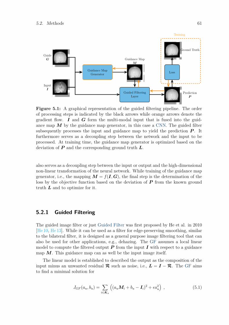
5.2. Methods 61
Guidance MapGenerator
Guided FilteringLayer
Loss
Training
Ground Truth
PredictionP
Guidance MapM
GuideG
InputI
Figure 5.1: A graphical representation of the guided filtering pipeline. The orderof processing steps is indicated by the black arrows while orange arrows denote thegradient flow. I and G form the multi-modal input that is fused into the guid-ance map M by the guidance map generator, in this case a CNN. The guided filtersubsequently processes the input and guidance map to yield the prediction P . Itfurthermore serves as a decoupling step between the network and the input to beprocessed. At training time, the guidance map generator is optimized based on thedeviation of P and the corresponding ground truth L.
also serves as a decoupling step between the input or output and the high-dimensionalnon-linear transformation of the neural network. While training of the guidance mapgenerator, i.e., the mapping M = f(I,G), the final step is the determination of theloss by the objective function based on the deviation of P from the known groundtruth L and to optimize for it.
5.2.1 Guided Filtering
The guided image filter or just Guided Filter was first proposed by He et al. in 2010[He 10, He 13]. While it can be used as a filter for edge-preserving smoothing, similarto the bilateral filter, it is designed as a general purpose image filtering tool that canalso be used for other applications, e.g., dehazing. The GF assumes a local linearmodel to compute the filtered output P from the input I with respect to a guidancemap M . This guidance map can as well be the input image itself.
The linear model is established to described the output as the composition of theinput minus an unwanted residual R such as noise, i.e., L = I −R. The GF aimsto find a minimal solution for
JGF (au, bu) =∑i∈Ku
((auMi + bu − Ii)2 + εa2
u
), (5.1)
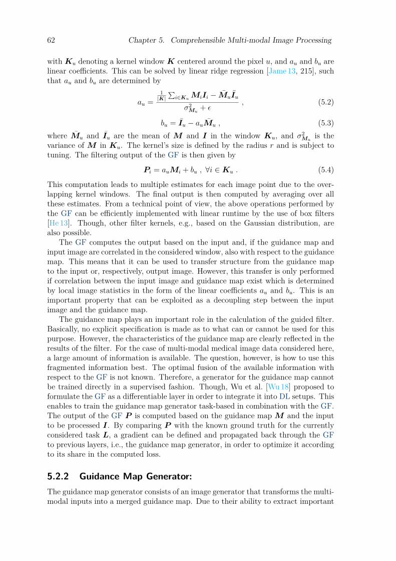
62 Chapter 5. Comprehensible Multi-modal Image Processing
with Ku denoting a kernel window K centered around the pixel u, and au and bu arelinear coefficients. This can be solved by linear ridge regression [Jame 13, 215], suchthat au and bu are determined by
au =1|K|
∑i∈Ku
MiIi − MuIu
σ2Mu
+ ε, (5.2)
bu = Iu − auMu , (5.3)where Mu and Iu are the mean of M and I in the window Ku, and σ2
Muis the
variance of M in Ku. The kernel’s size is defined by the radius r and is subject totuning. The filtering output of the GF is then given by
Pi = auMi + bu , ∀i ∈Ku . (5.4)
This computation leads to multiple estimates for each image point due to the over-lapping kernel windows. The final output is then computed by averaging over allthese estimates. From a technical point of view, the above operations performed bythe GF can be efficiently implemented with linear runtime by the use of box filters[He 13]. Though, other filter kernels, e.g., based on the Gaussian distribution, arealso possible.
The GF computes the output based on the input and, if the guidance map andinput image are correlated in the considered window, also with respect to the guidancemap. This means that it can be used to transfer structure from the guidance mapto the input or, respectively, output image. However, this transfer is only performedif correlation between the input image and guidance map exist which is determinedby local image statistics in the form of the linear coefficients au and bu. This is animportant property that can be exploited as a decoupling step between the inputimage and the guidance map.
The guidance map plays an important role in the calculation of the guided filter.Basically, no explicit specification is made as to what can or cannot be used for thispurpose. However, the characteristics of the guidance map are clearly reflected in theresults of the filter. For the case of multi-modal medical image data considered here,a large amount of information is available. The question, however, is how to use thisfragmented information best. The optimal fusion of the available information withrespect to the GF is not known. Therefore, a generator for the guidance map cannotbe trained directly in a supervised fashion. Though, Wu et al. [Wu 18] proposed toformulate the GF as a differentiable layer in order to integrate it into DL setups. Thisenables to train the guidance map generator task-based in combination with the GF.The output of the GF P is computed based on the guidance map M and the inputto be processed I. By comparing P with the known ground truth for the currentlyconsidered task L, a gradient can be defined and propagated back through the GFto previous layers, i.e., the guidance map generator, in order to optimize it accordingto its share in the computed loss.
5.2.2 Guidance Map Generator:The guidance map generator consists of an image generator that transforms the multi-modal inputs into a merged guidance map. Due to their ability to extract important

5.2. Methods 63
32 7x7
64 3x3
128 3x3 256 3x
3
32 7x7
64 3x3
128 3x3 256 3x
3
512 3x3
384 3x3
768 3x3
640 3x3
384 3x3
256 3x3 1 1x
1
Prediction P
Input I
Guide G
2x pooling Convolution - Norm. - ReLU 2x bilinear upsampling
Figure 5.2: Graphical representation of the employed multi-modal U-Net network.c©2021 IEEE.
information directly from data, CNNs are predestined for this task. In the following,the combination of the guided filter with a trainable guidance map generator is shownbased on two tasks, SR and denoising. To ensure reproducibility, only proven networkarchitectures are selected to do so. We only change these to the extent that theprocessing of multiple input images becomes possible. In order to investigate theeffect of the selected network on the guided filtering pipeline presented, two differentnetworks are evaluated for SR.
Denoising
For the denoising task we utilize the U-net network as it has proven to be a robustchoice for many image processing applications (cf. Section 3.3.2). To enable the pro-cessing of multi-modal inputs, we duplicate the encoding branch, one for the input andone for the guide image. The two encoding branches are finally merged by concate-nation at the lowest resolution level. Furthermore, we replace batch normalizationby instance normalization due to the expected low batch sizes (cf. Section 3.2.4). InFigure 5.2, a graphical representation of the applied U-net is given.
Super Resolution (SR)
In order to investigate the influence of the selected network architecture on the guidedfiltering pipeline, we use two different networks for the SR task. First, the previouslypresented U-net is re-used. Second, we apply the WDSR network (cf. Section 3.3.3).The WDSR network is a network specifically designed for SR that also ranked 1st
in one of the 2018’s NTIRE SR challenges. We adopt the network as it is provided
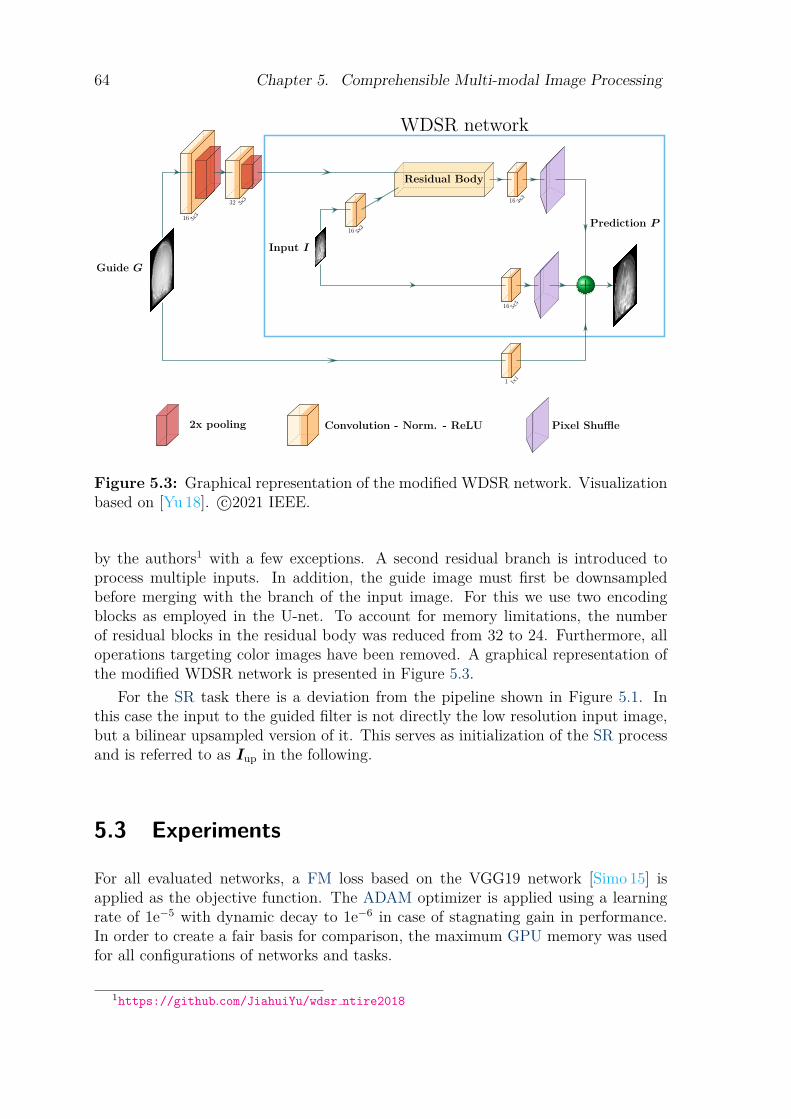
64 Chapter 5. Comprehensible Multi-modal Image Processing
WDSR network
Input I16 3x
3
Residual Body
16 3x3
+16 5x
5
Guide G
1 1x1
16 3x3
32 3x3
Prediction P
2x pooling Convolution - Norm. - ReLU Pixel Shuffle
Figure 5.3: Graphical representation of the modified WDSR network. Visualizationbased on [Yu 18]. c©2021 IEEE.
by the authors1 with a few exceptions. A second residual branch is introduced toprocess multiple inputs. In addition, the guide image must first be downsampledbefore merging with the branch of the input image. For this we use two encodingblocks as employed in the U-net. To account for memory limitations, the numberof residual blocks in the residual body was reduced from 32 to 24. Furthermore, alloperations targeting color images have been removed. A graphical representation ofthe modified WDSR network is presented in Figure 5.3.
For the SR task there is a deviation from the pipeline shown in Figure 5.1. Inthis case the input to the guided filter is not directly the low resolution input image,but a bilinear upsampled version of it. This serves as initialization of the SR processand is referred to as Iup in the following.
5.3 Experiments
For all evaluated networks, a FM loss based on the VGG19 network [Simo 15] isapplied as the objective function. The ADAM optimizer is applied using a learningrate of 1e−5 with dynamic decay to 1e−6 in case of stagnating gain in performance.In order to create a fair basis for comparison, the maximum GPU memory was usedfor all configurations of networks and tasks.
1https://github.com/JiahuiYu/wdsr ntire2018
5.3. Experiments 65
5.3.1 DataFor the evaluation of the proposed approach, 21 pairs of clinical patient datasetsare available. On the one hand, there are 8 pairs of tomographic T1 and T2 FlairMRI datasets. Image registration of these is performed using 3D Slicer [Piep 04].On the other hand, cone-beam projections generated from 13 pairs of CT and MRscans are used (MR: 1.5 T MAGNETOM Aera / CT: SOMATON Definition, SiemensHealthineers, Erlangen / Forchheim, Germany). The cone-beam projections werepreviously used for the projection-to-projection translation (cf. Chapter 4). For adetailed description of their generation, please refer to Section 4.6. For validationand testing, two pairs of datasets were reserved. It is important to note that theproposed approach has not been developed specifically for these data types, but thatthis combination only serves as an example of different modalities and domains.
The ground truth data for the SR task are generated by 4-fold nearest neighbordownsampling. Noisy X-ray projections are created by the application of Poissonnoise with low, medium, and high noise levels. This does not reflect the actualphysical processes. Noise in X-ray imaging is not only occurring in the form ofPoisson noise, but as a combination of several noise types [Hari 18]. Furthermore, inMRI the spatial resolution and the signal-to-noise ratio are directly related [Redp 98],so that a simple downsampling is only an estimate of the real signal. A more detailedsimulation is therefore necessary for an exact analysis of the respective problem area.However, as the focus of this work is on the comprehensibility of image processingwith deep guided filtering, an approximation of the real processes is sufficient at thispoint.
5.3.2 EvaluationQuantitative evaluation of both tasks is carried out using the MAE and SSIM. For alltasks the performance is evaluated with (w/ GF) and without (w/o GF) the GuidedFilter. With the GF, the output of the network is the guidance map, whereas withoutthe GF the prediction is generated directly. For the quantitative analysis only pixelswithin the head are considered to avoid a bias due to the large homogeneous regionsin the background. For qualitative analysis exemplary output images for all tasks arepresented. In addition, an analysis of the important parameters of the guided filter,the radius r of the kernelK and the corresponding ε is performed (cf. Equations (5.1)to (5.4)).
5.3.3 ComprehensibilityDue to the severe possible consequences of faulty decisions, the comprehensibility ofthe processing steps is an important point in medical image processing. For many DLapplications this is currently impossible or only feasible to a limited extent [Koh 17,Shwa 17, Carl 17, Antu 19]. In order to remedy this shortcoming, we therefore conductthree experiments specifically to investigate the comprehensibility of the generatedresults. We use these to compare the outputs of the guided filtering pipeline withthose of conventional CNNs. The experiments are concerned with the preservation
66 Chapter 5. Comprehensible Multi-modal Image Processing
of the image content of the input images, the influence of degraded inputs, as well asthe robustness against adversarial attacks.
Content Preservation
The image information is distributed over the whole frequency spectrum. Whilehigh frequencies mainly contain fine details and edges (cf. Chapter 4), the generalcontent of the images, i.e., anatomical structures and pathologies, is stored in the lowfrequency bands. A preservation of this low frequency information is therefore crucialin the context of medical image processing and any tampering should be treated withcaution. In contrast, alteration of the high frequency components is inevitable for SRand denoising applications. In order to cope with these circumstances, we thereforeinvestigate the change in the low frequency components during the processing of theimages.
For this purpose, the images are decomposed into their frequency bands usingtwo-times wavelet decomposition (Daubechies-4 [Daub 92]) and, subsequently, thelow frequency components of the predicted super-resolved images are compared withthe low resolution input or, respectively, the decomposed denoised images with thedecomposed ground truth images. Considering that a change in the low frequencycomponents is undesirable, the corresponding pairs should exhibit the smallest pos-sible deviation from each other. An example of the wavelet decomposed images ispresented in Figure 5.4.
Insusceptibility to Disturbances
Ideally, the guide image provides complementary information to the input image,which should help to restore it as accurately as possible. However, if this guide imageis disturbed or degraded, the processing should still take place undisturbed, basedonly on the input image instead. To verify this, we manipulate the guide image atinference time with gradually increasing zero-mean Gaussian noise and compare theoutcome of the output with and without the GF.
Robustness against Adversarial Attacks
In a third experiment, we investigate the susceptibility of the processing chain toadversarial attacks. The effectiveness of adversarial attacks on different types of net-works has been demonstrated in the past [Antu 19, Yuan 17]. Ideally, the guidedfilter acts as a form of decoupling between the attacked network and the processedoutput, thus limiting the influence of the adversarial attack on the results. To val-idate this experimentally, we perform a simple form of an adversarial attack andcompare the results with and without the GF. For this, we seek to find two adver-sarial examples, EI and EG, that represent an additive residual to the input andguide image, respectively. When added, these adversarial examples should causean as large as possible deviation of the prediction from the ground truth. Simul-taneously, the examples are constrained to be small in their Euclidean norm asthey should, ideally, be undetectable in the inputs by visual assessment. Assum-ing a fixed, pre-trained guidance map generator that employs the transformation
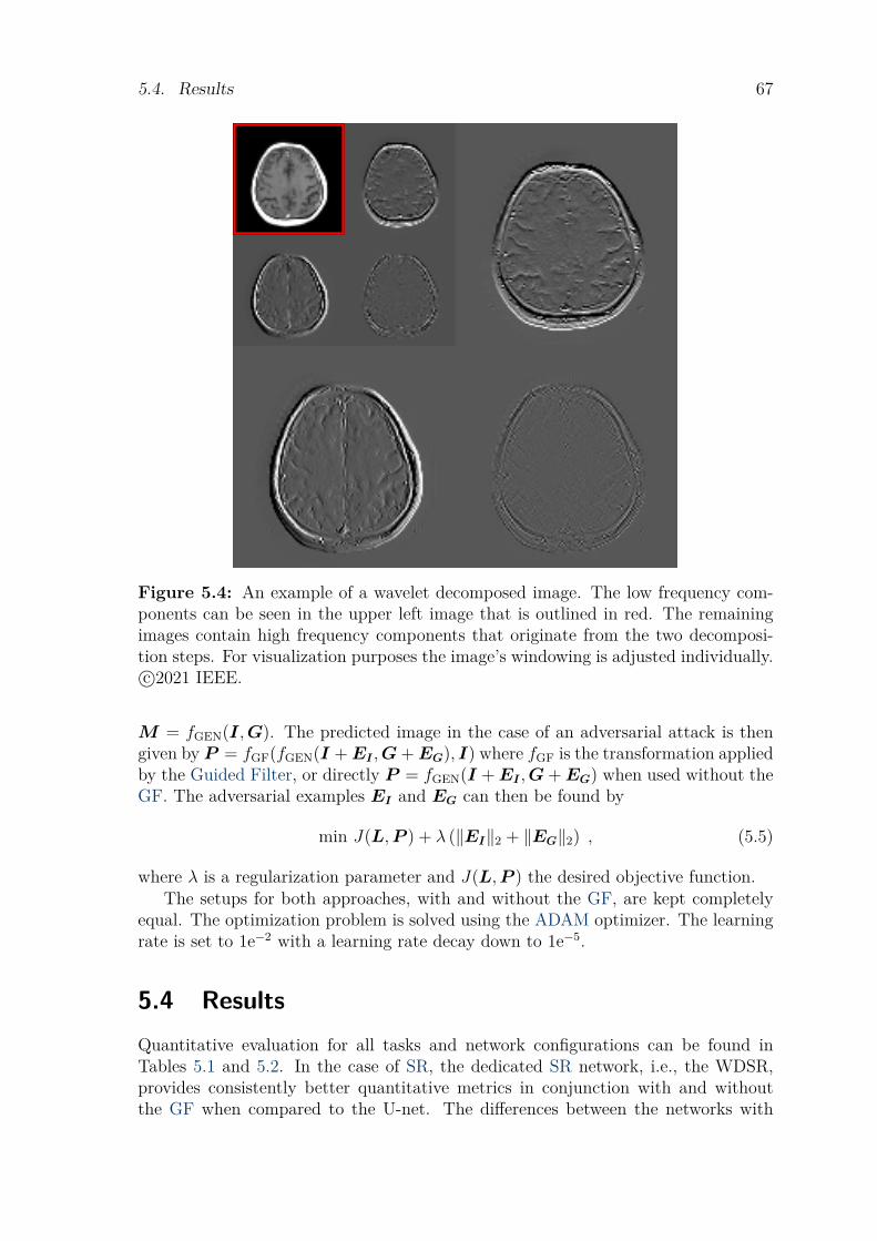
5.4. Results 67
Figure 5.4: An example of a wavelet decomposed image. The low frequency com-ponents can be seen in the upper left image that is outlined in red. The remainingimages contain high frequency components that originate from the two decomposi-tion steps. For visualization purposes the image’s windowing is adjusted individually.c©2021 IEEE.
M = fGEN(I,G). The predicted image in the case of an adversarial attack is thengiven by P = fGF(fGEN(I +EI ,G+EG), I) where fGF is the transformation appliedby the Guided Filter, or directly P = fGEN(I +EI ,G+EG) when used without theGF. The adversarial examples EI and EG can then be found by
min J(L,P ) + λ (‖EI‖2 + ‖EG‖2) , (5.5)
where λ is a regularization parameter and J(L,P ) the desired objective function.The setups for both approaches, with and without the GF, are kept completely
equal. The optimization problem is solved using the ADAM optimizer. The learningrate is set to 1e−2 with a learning rate decay down to 1e−5.
5.4 ResultsQuantitative evaluation for all tasks and network configurations can be found inTables 5.1 and 5.2. In the case of SR, the dedicated SR network, i.e., the WDSR,provides consistently better quantitative metrics in conjunction with and withoutthe GF when compared to the U-net. The differences between the networks with
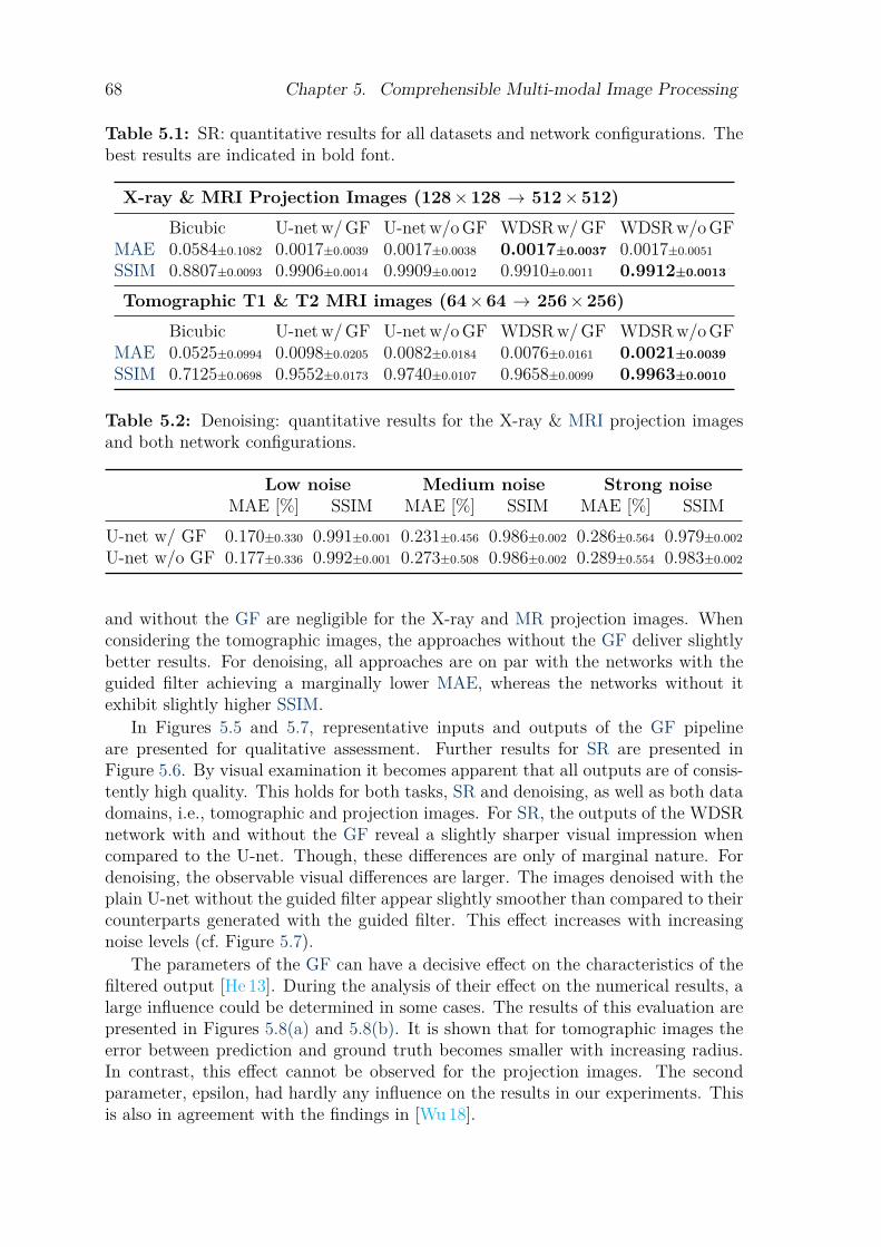
68 Chapter 5. Comprehensible Multi-modal Image Processing
Table 5.1: SR: quantitative results for all datasets and network configurations. Thebest results are indicated in bold font.
X-ray & MRI Projection Images (128×128 → 512×512)
Bicubic U-net w/ GF U-net w/o GF WDSR w/ GF WDSR w/o GFMAE 0.0584±0.1082 0.0017±0.0039 0.0017±0.0038 0.0017±0.0037 0.0017±0.0051
SSIM 0.8807±0.0093 0.9906±0.0014 0.9909±0.0012 0.9910±0.0011 0.9912±0.0013
Tomographic T1 & T2 MRI images (64×64 → 256×256)
Bicubic U-net w/ GF U-net w/o GF WDSR w/ GF WDSR w/o GFMAE 0.0525±0.0994 0.0098±0.0205 0.0082±0.0184 0.0076±0.0161 0.0021±0.0039
SSIM 0.7125±0.0698 0.9552±0.0173 0.9740±0.0107 0.9658±0.0099 0.9963±0.0010
Table 5.2: Denoising: quantitative results for the X-ray & MRI projection imagesand both network configurations.
Low noise Medium noise Strong noiseMAE [%] SSIM MAE [%] SSIM MAE [%] SSIM
U-net w/ GF 0.170±0.330 0.991±0.001 0.231±0.456 0.986±0.002 0.286±0.564 0.979±0.002
U-net w/o GF 0.177±0.336 0.992±0.001 0.273±0.508 0.986±0.002 0.289±0.554 0.983±0.002
and without the GF are negligible for the X-ray and MR projection images. Whenconsidering the tomographic images, the approaches without the GF deliver slightlybetter results. For denoising, all approaches are on par with the networks with theguided filter achieving a marginally lower MAE, whereas the networks without itexhibit slightly higher SSIM.
In Figures 5.5 and 5.7, representative inputs and outputs of the GF pipelineare presented for qualitative assessment. Further results for SR are presented inFigure 5.6. By visual examination it becomes apparent that all outputs are of consis-tently high quality. This holds for both tasks, SR and denoising, as well as both datadomains, i.e., tomographic and projection images. For SR, the outputs of the WDSRnetwork with and without the GF reveal a slightly sharper visual impression whencompared to the U-net. Though, these differences are only of marginal nature. Fordenoising, the observable visual differences are larger. The images denoised with theplain U-net without the guided filter appear slightly smoother than compared to theircounterparts generated with the guided filter. This effect increases with increasingnoise levels (cf. Figure 5.7).
The parameters of the GF can have a decisive effect on the characteristics of thefiltered output [He 13]. During the analysis of their effect on the numerical results, alarge influence could be determined in some cases. The results of this evaluation arepresented in Figures 5.8(a) and 5.8(b). It is shown that for tomographic images theerror between prediction and ground truth becomes smaller with increasing radius.In contrast, this effect cannot be observed for the projection images. The secondparameter, epsilon, had hardly any influence on the results in our experiments. Thisis also in agreement with the findings in [Wu 18].
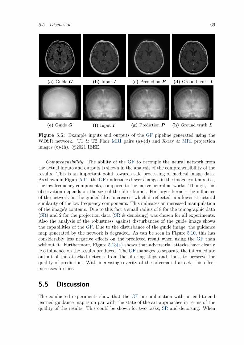
5.5. Discussion 69
(a) Guide G (b) Input I (c) Prediction P (d) Ground truth L
(e) Guide G (f) Input I (g) Prediction P (h) Ground truth L
Figure 5.5: Example inputs and outputs of the GF pipeline generated using theWDSR network. T1 & T2 Flair MRI pairs (a)-(d) and X-ray & MRI projectionimages (e)-(h). c©2021 IEEE.
Comprehensibility: The ability of the GF to decouple the neural network fromthe actual inputs and outputs is shown in the analysis of the comprehensibility of theresults. This is an important point towards safe processing of medical image data.As shown in Figure 5.11, the GF undertakes fewer changes in the image contents, i.e.,the low frequency components, compared to the native neural networks. Though, thisobservation depends on the size of the filter kernel. For larger kernels the influenceof the network on the guided filter increases, which is reflected in a lower structuralsimilarity of the low frequency components. This indicates an increased manipulationof the image’s contents. Due to this fact a small radius of 8 for the tomographic data(SR) and 2 for the projection data (SR & denoising) was chosen for all experiments.Also the analysis of the robustness against disturbances of the guide image showsthe capabilities of the GF. Due to the disturbance of the guide image, the guidancemap generated by the network is degraded. As can be seen in Figure 5.10, this hasconsiderably less negative effects on the predicted result when using the GF thanwithout it. Furthermore, Figure 5.13(a) shows that adversarial attacks have clearlyless influence on the results produced. The GF manages to separate the intermediateoutput of the attacked network from the filtering steps and, thus, to preserve thequality of prediction. With increasing severity of the adversarial attack, this effectincreases further.
5.5 DiscussionThe conducted experiments show that the GF in combination with an end-to-endlearned guidance map is on par with the state-of-the-art approaches in terms of thequality of the results. This could be shown for two tasks, SR and denoising. When
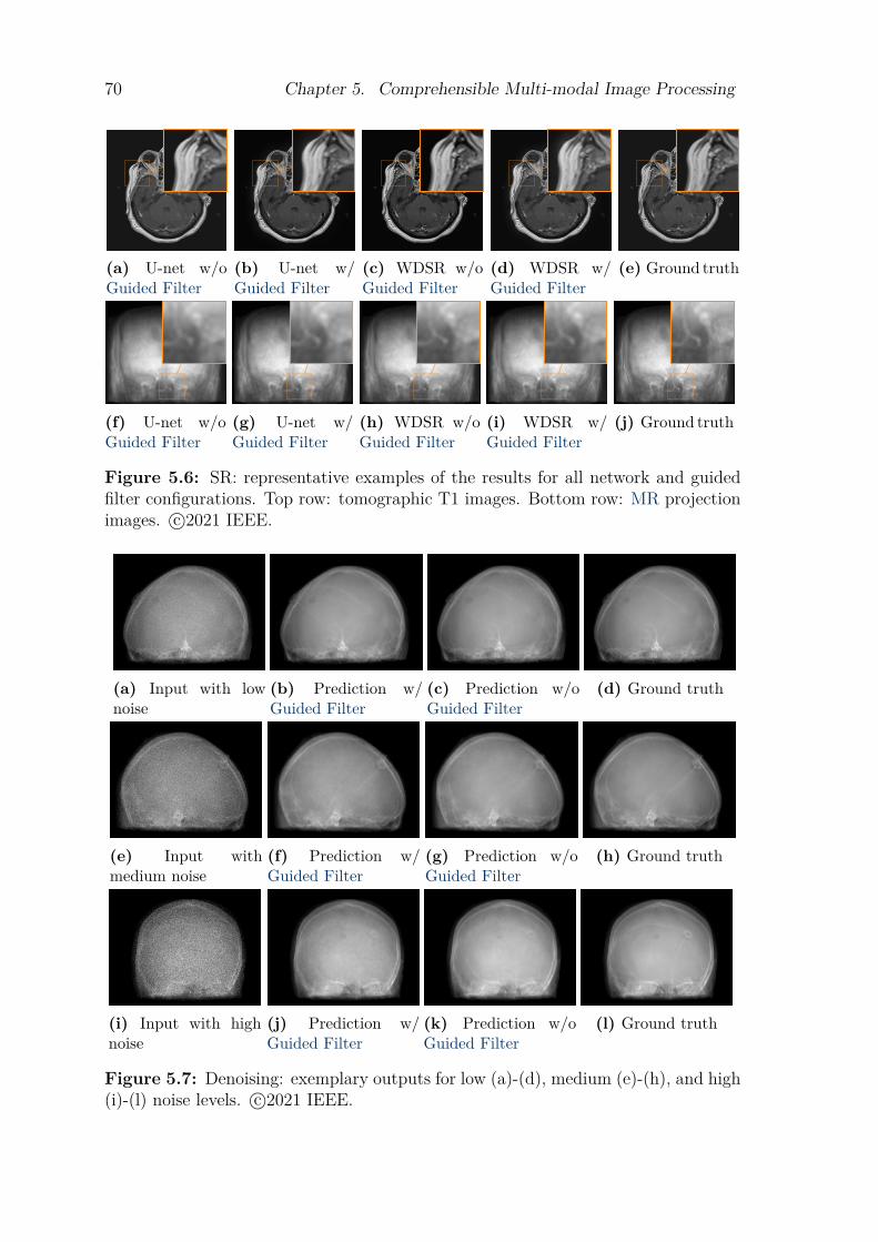
70 Chapter 5. Comprehensible Multi-modal Image Processing
(a) U-net w/oGuided Filter
(b) U-net w/Guided Filter
(c) WDSR w/oGuided Filter
(d) WDSR w/Guided Filter
(e) Ground truth
(f) U-net w/oGuided Filter
(g) U-net w/Guided Filter
(h) WDSR w/oGuided Filter
(i) WDSR w/Guided Filter
(j) Ground truth
Figure 5.6: SR: representative examples of the results for all network and guidedfilter configurations. Top row: tomographic T1 images. Bottom row: MR projectionimages. c©2021 IEEE.
(a) Input with lownoise
(b) Prediction w/Guided Filter
(c) Prediction w/oGuided Filter
(d) Ground truth
(e) Input withmedium noise
(f) Prediction w/Guided Filter
(g) Prediction w/oGuided Filter
(h) Ground truth
(i) Input with highnoise
(j) Prediction w/Guided Filter
(k) Prediction w/oGuided Filter
(l) Ground truth
Figure 5.7: Denoising: exemplary outputs for low (a)-(d), medium (e)-(h), and high(i)-(l) noise levels. c©2021 IEEE.
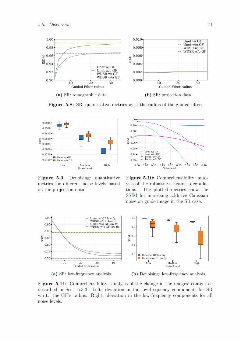
5.5. Discussion 71
10 20 30Guided Filter radius
0.90
0.92
0.94
0.96
0.98
1.00SS
IM
Unet w/ GFUnet w/o GFWDSR w/ GFWDSR w/o GF
(a) SR: tomographic data.
10 20 30Guided Filter radius
0.000
0.002
0.004
0.006
0.008
0.010
MAE
Unet w/ GFUnet w/o GFWDSR w/ GFWDSR w/o GF
(b) SR: projection data.
Figure 5.8: SR: quantitative metrics w.r.t the radius of the guided filter.
Low Medium HighNoise Level
0.9750
0.9775
0.9800
0.9825
0.9850
0.9875
0.9900
0.9925
SSIM
Unet w/ GFUnet w/o GF
Figure 5.9: Denoising: quantitativemetrics for different noise levels basedon the projection data.
0.00 0.05 0.10 0.15 0.20 0.25 0.30 0.35 0.40Noise level
0.93
0.94
0.95
0.96
0.97
0.98
0.99
1.00
SSIM
Proj. w/ GFProj. w/o GFTomo. w/ GFTomo. w/o GF
Figure 5.10: Comprehensibility: anal-ysis of the robustness against degrada-tions. The plotted metrics show theSSIM for increasing additive Gaussiannoise on guide image in the SR case.
10 20 30 40Guided filter radius
0.70
0.75
0.80
0.85
0.90
0.95
1.00
SSIM
U-net w/ GF low fq. WDSR w/ GF low fq.U-net w/o GF low fq.WDSR w/o GF low fq.
(a) SR: low-frequency analysis.
Low Medium HighNoise Level
0.6
0.7
0.8
0.9
1.0
SSIM
U-net w/ GF low fq.U-net w/o GF low fq.
(b) Denoising: low-frequency analysis.
Figure 5.11: Comprehensibility: analysis of the change in the images’ content asdescribed in Sec. 5.3.3. Left: deviation in the low-frequency components for SRw.r.t. the GF’s radius. Right: deviation in the low-frequency components for allnoise levels.
72 Chapter 5. Comprehensible Multi-modal Image Processing
using the GF, however, this is achieved with significantly less manipulation of theimage’s content, as well as increased robustness against unforeseen changes in theinputs. This enables the application of DL methods even in such sensitive areasas the processing of medical patient data. Three experiments were carried out tosubstantiate the claim of increased comprehensibility of the results when applyingthe GF.
Discussion: Content Preservation
The first experiment considered the preservation of image content during processing(cf. Figure 5.11). It became evident that for small radii the generated images with theGF were subjected to clearly less manipulation of the low frequency components thanwithout the GF (cf. Figure 5.11(a)). For larger radii, a smaller deviation of the finaloutput from the ground truth was measured, but the deviation in the image’s contentincreases. This indicates that the influence of the network on the filtered outputsincreases with increasing radius. The aforementioned observations occur for both,SR and denoising. For the denoising case, it can be observed that the low frequencyparts of the results generated with the GF show both a higher structural similarity tothe ground truth and a drastically lower standard deviation (cf. Figure 5.11(b)). Withincreasing noise this observation intensifies further. This leads to the assumption thata larger amount of information is hallucinated by the network at higher noise levels.
Discussion: Insusceptibility to Disturbances
As a second experiment, the vulnerability of the proposed pipeline to disturbances ofthe input image was investigated. For increasing additive noise on the guide imagethe generated guidance map degrades steadily. When using the GF, however, theinfluence of this degradation on the result is strongly limited (cf. Figure 5.10). Incontrast, if the stand-alone neural network is employed, significant deterioration ofthe predicted images occurs.
The shown example of additive Gaussian noise is just a simple case of a possibledegradation. It would be easy to train the networks to be invariant to this noise. Fora real world application, however, the variability and severity of degradations is socomplex that it is impossible to cover every single case during training. The GF, onthe other hand, provides an inherent protection against this occurrence.
Discussion: Robustness against Adversarial Attacks
The third experiment dealt with the effectiveness of adversarial attacks on the pipeline.It was shown that the GF is an effective safety measure in this case, too (cf. Fig-ure 5.13). When applied with the GF, the generated outputs exhibit a slightly blurredappearance (cf. Figure 5.13(b)). Nevertheless, these still closely resemble the groundtruth. Without the GF, the results created by the attacked network are heavilydetoriated (cf. Figure 5.13(c)). Furthermore, the GF not only provides an effectivedefense against adversarial attacks but it also makes it harder to generated adequateadversarial examples in the first place, as seen in Figure 5.12.
These experiments clearly show that the GF acts as a strong decoupler between
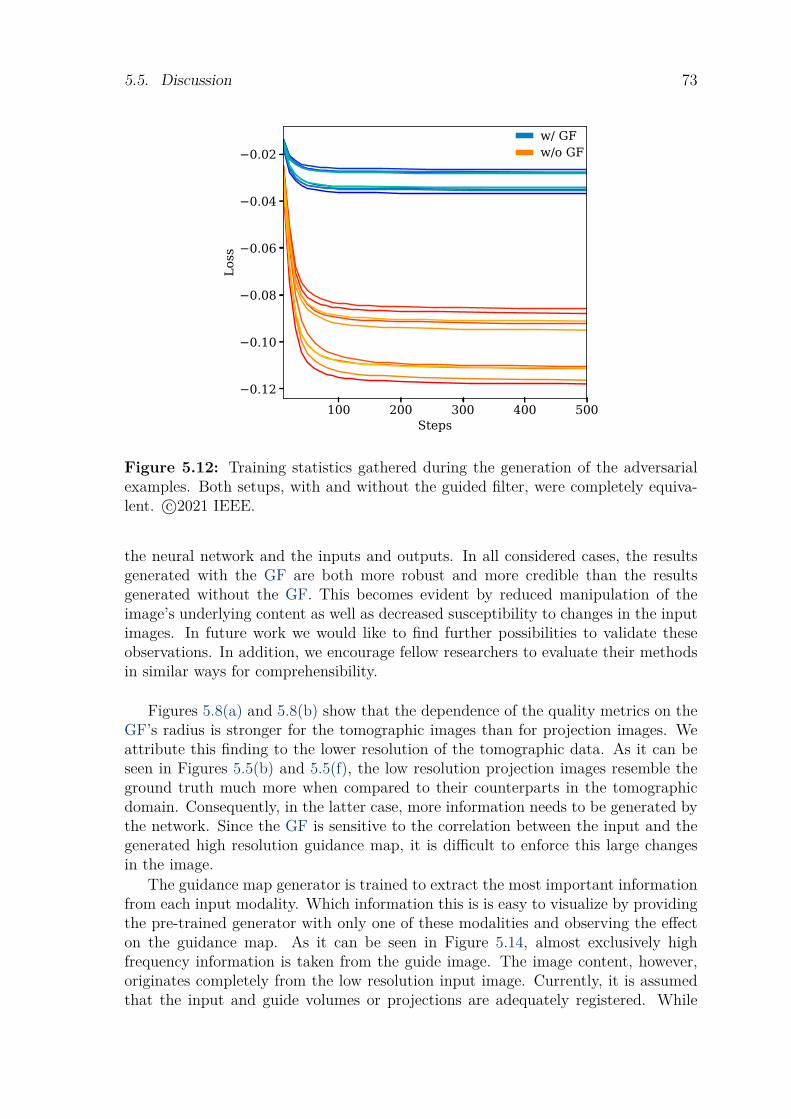
5.5. Discussion 73
100 200 300 400 500Steps
0.12
0.10
0.08
0.06
0.04
0.02
Loss
w/ GFw/o GF
Figure 5.12: Training statistics gathered during the generation of the adversarialexamples. Both setups, with and without the guided filter, were completely equiva-lent. c©2021 IEEE.
the neural network and the inputs and outputs. In all considered cases, the resultsgenerated with the GF are both more robust and more credible than the resultsgenerated without the GF. This becomes evident by reduced manipulation of theimage’s underlying content as well as decreased susceptibility to changes in the inputimages. In future work we would like to find further possibilities to validate theseobservations. In addition, we encourage fellow researchers to evaluate their methodsin similar ways for comprehensibility.
Figures 5.8(a) and 5.8(b) show that the dependence of the quality metrics on theGF’s radius is stronger for the tomographic images than for projection images. Weattribute this finding to the lower resolution of the tomographic data. As it can beseen in Figures 5.5(b) and 5.5(f), the low resolution projection images resemble theground truth much more when compared to their counterparts in the tomographicdomain. Consequently, in the latter case, more information needs to be generated bythe network. Since the GF is sensitive to the correlation between the input and thegenerated high resolution guidance map, it is difficult to enforce this large changesin the image.
The guidance map generator is trained to extract the most important informationfrom each input modality. Which information this is is easy to visualize by providingthe pre-trained generator with only one of these modalities and observing the effecton the guidance map. As it can be seen in Figure 5.14, almost exclusively highfrequency information is taken from the guide image. The image content, however,originates completely from the low resolution input image. Currently, it is assumedthat the input and guide volumes or projections are adequately registered. While
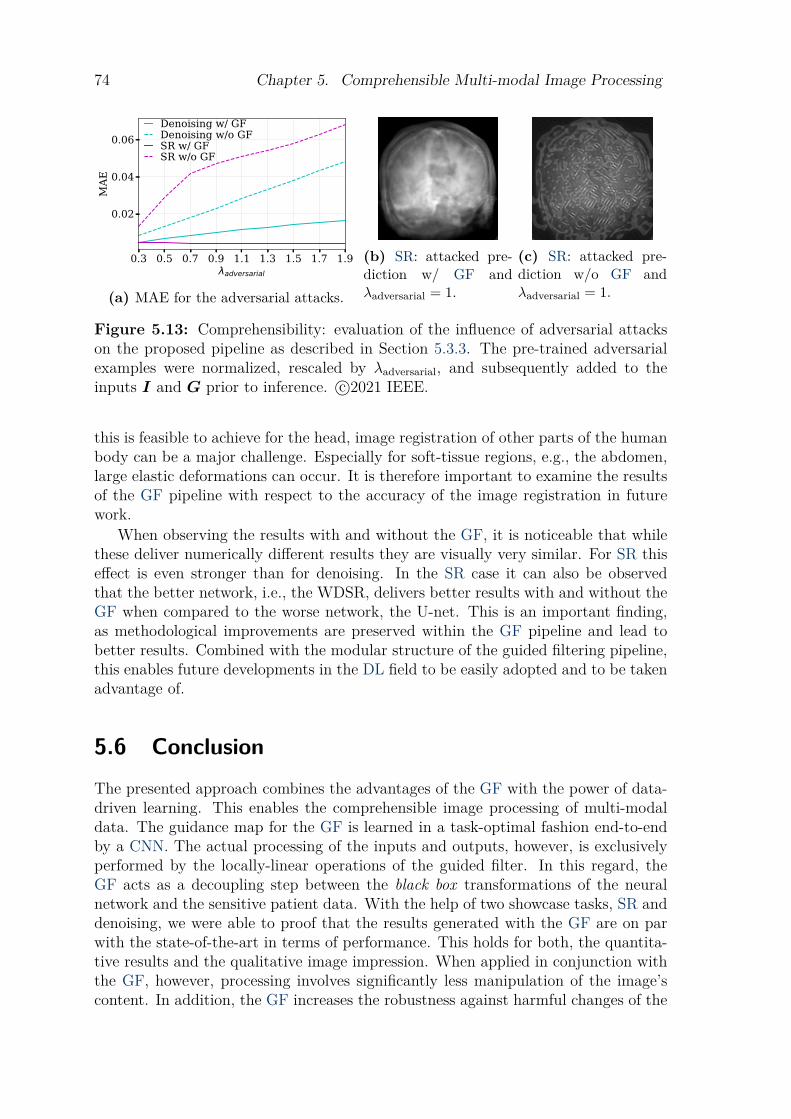
74 Chapter 5. Comprehensible Multi-modal Image Processing
0.3 0.5 0.7 0.9 1.1 1.3 1.5 1.7 1.9adversarial
0.02
0.04
0.06
MAE
Denoising w/ GFDenoising w/o GFSR w/ GFSR w/o GF
(a) MAE for the adversarial attacks.
(b) SR: attacked pre-diction w/ GF andλadversarial = 1.
(c) SR: attacked pre-diction w/o GF andλadversarial = 1.
Figure 5.13: Comprehensibility: evaluation of the influence of adversarial attackson the proposed pipeline as described in Section 5.3.3. The pre-trained adversarialexamples were normalized, rescaled by λadversarial, and subsequently added to theinputs I and G prior to inference. c©2021 IEEE.
this is feasible to achieve for the head, image registration of other parts of the humanbody can be a major challenge. Especially for soft-tissue regions, e.g., the abdomen,large elastic deformations can occur. It is therefore important to examine the resultsof the GF pipeline with respect to the accuracy of the image registration in futurework.
When observing the results with and without the GF, it is noticeable that whilethese deliver numerically different results they are visually very similar. For SR thiseffect is even stronger than for denoising. In the SR case it can also be observedthat the better network, i.e., the WDSR, delivers better results with and without theGF when compared to the worse network, the U-net. This is an important finding,as methodological improvements are preserved within the GF pipeline and lead tobetter results. Combined with the modular structure of the guided filtering pipeline,this enables future developments in the DL field to be easily adopted and to be takenadvantage of.
5.6 ConclusionThe presented approach combines the advantages of the GF with the power of data-driven learning. This enables the comprehensible image processing of multi-modaldata. The guidance map for the GF is learned in a task-optimal fashion end-to-endby a CNN. The actual processing of the inputs and outputs, however, is exclusivelyperformed by the locally-linear operations of the guided filter. In this regard, theGF acts as a decoupling step between the black box transformations of the neuralnetwork and the sensitive patient data. With the help of two showcase tasks, SR anddenoising, we were able to proof that the results generated with the GF are on parwith the state-of-the-art in terms of performance. This holds for both, the quantita-tive results and the qualitative image impression. When applied in conjunction withthe GF, however, processing involves significantly less manipulation of the image’scontent. In addition, the GF increases the robustness against harmful changes of the

5.6. Conclusion 75
(a) Upsampled InputIup
(b) Guidance mapM w/o guide G
(c) Guidance mapMw/o input I
(d) Ground truth
Figure 5.14: Analysis of the influence of the different input modalities on theguidance map based on the SR task. The pre-trained guidance map generator wasprovided with only the low-resolution input image (b) or only the guide image (c). Itbecomes apparent that exclusively high-frequency information such as edges is drawnfrom the higher resolution guide image, while the image’s content originates from thelow-resolution input image. The square pattern visible in (c) is assumed to be causedby the pixel shuffle operation applied in the WDSR network. c©2021 IEEE.
inputs when compared to the conventional DL approach. It also provides an effec-tive defense against adversarial attacks. Thus, the GF enables the comprehensibleapplication of image processing algorithms in such an error-sensitive field as medicalimage processing.


C H A P T E R 6
User-specific Image QualityAssessment
Image quality assessment is a frequently encountered problem in most image pro-cessing tasks. Common objective functions allow for automated optimization, how-ever, they do not necessarily favor the same image characteristics as human observers.Explicitly providing reference images with the desired image characteristics is oftennot feasible for the user. Though, in most most applications human users possessexcellent capabilities to judge images based on their perceived quality. In the fol-lowing, we exploit this capability in a forced-choice scheme that aims to serve as anobjective function for parameter optimization. We evaluate this approach based ontwo tasks, image denoising and image fusion. It can be shown that the presentedapproach allows for the optimization of simple one-parameter models as well as morecomplex neural networks. For the former, the proposed user loss scheme is able toexpress the user’s preferences in the resulting images. In the latter case, optimizationis possible in principle. Though, additional efforts regarding the generation of validsamples for the user to choose from is required in order to allow for stable trainingof large NNs.
Parts of the following contents were previously published in:
[Zare 19]
S. Zarei, B. Stimpel, C. Syben, and A. Maier. “User Loss: A Forced-Choice-Inspired Approach to Train Neural Networks Directly byUser Interaction”. In: Bildverarbeitung fur die Medizin, pp. 92–97,Springer, 2019.
6.1 IntroductionMore and more tasks in image processing and enhancement can be solved by auto-mated methods, e.g., as presented in the previous sections. Parameter optimizationof the models is performed with the goal to minimize the underlying metric that isemployed as cost function. This can for example be an image quality metric thatexpresses the deviation between the generated output and a known ground truth oran unsupervised clustering metric.
As already outlined in Section 3.4, different metrics prefer different outcomeswhich renders the choice of the metric a heuristic. A common property of nearly allimage quality metrics is that these are not influenceable by the user. This can beproblematic as the human observer may focus on other image characteristics than the
77
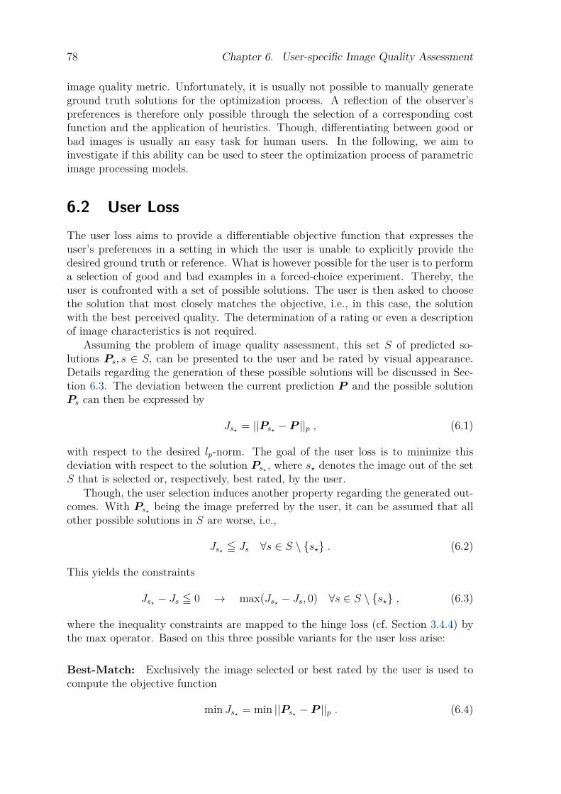
78 Chapter 6. User-specific Image Quality Assessment
image quality metric. Unfortunately, it is usually not possible to manually generateground truth solutions for the optimization process. A reflection of the observer’spreferences is therefore only possible through the selection of a corresponding costfunction and the application of heuristics. Though, differentiating between good orbad images is usually an easy task for human users. In the following, we aim toinvestigate if this ability can be used to steer the optimization process of parametricimage processing models.
6.2 User LossThe user loss aims to provide a differentiable objective function that expresses theuser’s preferences in a setting in which the user is unable to explicitly provide thedesired ground truth or reference. What is however possible for the user is to performa selection of good and bad examples in a forced-choice experiment. Thereby, theuser is confronted with a set of possible solutions. The user is then asked to choosethe solution that most closely matches the objective, i.e., in this case, the solutionwith the best perceived quality. The determination of a rating or even a descriptionof image characteristics is not required.
Assuming the problem of image quality assessment, this set S of predicted so-lutions Ps, s ∈ S, can be presented to the user and be rated by visual appearance.Details regarding the generation of these possible solutions will be discussed in Sec-tion 6.3. The deviation between the current prediction P and the possible solutionPs can then be expressed by
Js? = ||Ps? − P ||p , (6.1)
with respect to the desired lp-norm. The goal of the user loss is to minimize thisdeviation with respect to the solution Ps? , where s? denotes the image out of the setS that is selected or, respectively, best rated, by the user.
Though, the user selection induces another property regarding the generated out-comes. With Ps? being the image preferred by the user, it can be assumed that allother possible solutions in S are worse, i.e.,
Js? 5 Js ∀s ∈ S \ {s?} . (6.2)
This yields the constraints
Js? − Js 5 0 → max(Js? − Js, 0) ∀s ∈ S \ {s?} , (6.3)
where the inequality constraints are mapped to the hinge loss (cf. Section 3.4.4) bythe max operator. Based on this three possible variants for the user loss arise:
Best-Match: Exclusively the image selected or best rated by the user is used tocompute the objective function
min Js? = min ||Ps? − P ||p . (6.4)

6.3. Methods 79
Forced-Choice: The loss is computed based on minimizing all constraints inducedby the user’s selection. This enforces that the prediction is closer to the selectedoption s? than to all other possibilities S \ {s?}:
minS\{s?}∑
s
max(Js? − Js, 0) . (6.5)
Hybrid: A combination of Best-Match and Forced-Choice is used to determine theloss:
minJs? +
S\{s?}∑s
max(Js? − Js, 0) , (6.6)
which closely resembles the soft-margin support vector machine with the Best-Matchterm expressing the normal vector length and the Forced-Choice term the additionalconstraints [Bish 06, 337].
6.3 MethodsWe examine the user loss based on two tasks with unclear or difficult to reach pointsof optimality. First, the problem of image fusion will be investigated. Second, theapplication of the user loss in image denoising is examined.
6.3.1 Image FusionWhile medical imaging can provide a broad variety of information, this data is usuallyspread across different acquisition types and modalities. Individual assessment ofthese is tedious and discovering relationships across images may be hard for thehuman observer. Visualizing the information of multiple acquisitions in one imagecan therefore be potentially beneficial. However, as fused images are nonexistent inthe real world, no optimal image fusion procedure is known, which renders this an userand task-specific problem. In the following, a simple alpha blending [Port 84] schemewith only one parameter is employed to compose two input images into one fusedrepresentation. Assuming two pre-registered input images I1 and I2, the predictedfused representation is given by
P = αI1 + (1− α)I2 , α ∈ [0, 1] . (6.7)
The parameter setting is initialized with an even fusion rule of α = 0.5 and sub-sequently adjusted to the user’s preferences by the loss functions described in Sec-tion 6.2.
6.3.2 Image DenoisingNoise is a typical form of data corruption in all kinds of acquisitions and images.Methods for denoising these signals are, therefore, highly popular. The point ofoptimality in these type of problems is clearly defined in theory in the form of theoriginal signal without the additional corruption through noise. In practice, however,
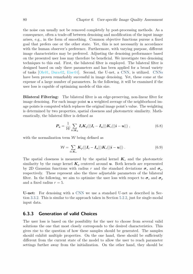
80 Chapter 6. User-specific Image Quality Assessment
the noise can usually not be removed completely by post-processing methods. As aconsequence, often a trade-off between denoising and modification of the input imagearises, e.g., in the form of smoothing. Common objective functions pursue a fixedgoal that prefers one or the other state. Yet, this is not necessarily in accordancewith the human observer’s preference. Furthermore, with varying purpose, differentimage characteristics may be preferred. Adjusting the denoising performance basedon the presented user loss may therefore be beneficial. We investigate two denoisingtechniques to this end. First, the bilateral filter is employed. The bilateral filter isdesigned based on only three parameters and has been applied for a broad varietyof tasks [Oh 01, Dura 02, Eise 04]. Second, the U-net, a CNN, is utilized. CNNshave been proven remarkably successful in image denoising. Yet, these come at theexpense of a large number of parameters. In the following, it will be examined if theuser loss is capable of optimizing models of this size.
Bilateral Filtering: The bilateral filter is an edge-preserving, non-linear filter forimage denoising. For each image point u a weighted average of the neighborhood im-age points is computed which replaces the original image point’s value. The weightingis determined by two properties, spatial closeness and photometric similarity. Math-ematically, the bilateral filter is defined as
Pu = 1W
∑i∈Ku
IiKp(||Ii − Iu||)Ks(||i− u||) , (6.8)
with the normalization term W being defined as
W =∑i∈Ku
Kp(||Ii − Iu||)Ks(||i− u||) . (6.9)
The spatial closeness is measured by the spatial kernel Ks and the photometricsimilarity by the range kernel Kp centered around u. Both kernels are representedby 2D Gaussian functions with radius r and the standard deviations σs and σp,respectively. These represent also the three adjustable parameters of the bilateralfilter. In the following, we aim to optimize the user loss with respect to σs and σpand a fixed radius r = 5.
U-net: For denoising with a CNN we use a standard U-net as described in Sec-tion 3.3.2. This is similar to the approach taken in Section 5.2.2, just for single-modalinput data.
6.3.3 Generation of valid ChoicesThe user loss is based on the possibility for the user to choose from several validsolutions the one that most closely corresponds to the desired characteristics. Thisgives rise to the question of how these samples should be generated. The samplesshould exhibit multiple properties. On the one hand, these should be sufficientlydifferent from the current state of the model to allow the user to reach parametersettings further away from the initialization. On the other hand, they should be
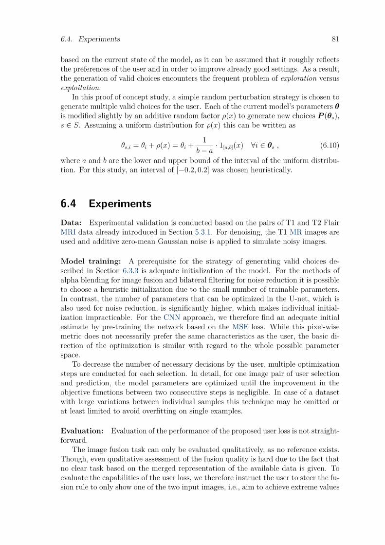
6.4. Experiments 81
based on the current state of the model, as it can be assumed that it roughly reflectsthe preferences of the user and in order to improve already good settings. As a result,the generation of valid choices encounters the frequent problem of exploration versusexploitation.
In this proof of concept study, a simple random perturbation strategy is chosen togenerate multiple valid choices for the user. Each of the current model’s parameters θis modified slightly by an additive random factor ρ(x) to generate new choices P (θs),s ∈ S. Assuming a uniform distribution for ρ(x) this can be written as
θs,i = θi + ρ(x) = θi + 1b− a
· 1[a,b](x) ∀i ∈ θs , (6.10)
where a and b are the lower and upper bound of the interval of the uniform distribu-tion. For this study, an interval of [−0.2, 0.2] was chosen heuristically.
6.4 ExperimentsData: Experimental validation is conducted based on the pairs of T1 and T2 FlairMRI data already introduced in Section 5.3.1. For denoising, the T1 MR images areused and additive zero-mean Gaussian noise is applied to simulate noisy images.
Model training: A prerequisite for the strategy of generating valid choices de-scribed in Section 6.3.3 is adequate initialization of the model. For the methods ofalpha blending for image fusion and bilateral filtering for noise reduction it is possibleto choose a heuristic initialization due to the small number of trainable parameters.In contrast, the number of parameters that can be optimized in the U-net, which isalso used for noise reduction, is significantly higher, which makes individual initial-ization impracticable. For the CNN approach, we therefore find an adequate initialestimate by pre-training the network based on the MSE loss. While this pixel-wisemetric does not necessarily prefer the same characteristics as the user, the basic di-rection of the optimization is similar with regard to the whole possible parameterspace.
To decrease the number of necessary decisions by the user, multiple optimizationsteps are conducted for each selection. In detail, for one image pair of user selectionand prediction, the model parameters are optimized until the improvement in theobjective functions between two consecutive steps is negligible. In case of a datasetwith large variations between individual samples this technique may be omitted orat least limited to avoid overfitting on single examples.
Evaluation: Evaluation of the performance of the proposed user loss is not straight-forward.
The image fusion task can only be evaluated qualitatively, as no reference exists.Though, even qualitative assessment of the fusion quality is hard due to the fact thatno clear task based on the merged representation of the available data is given. Toevaluate the capabilities of the user loss, we therefore instruct the user to steer the fu-sion rule to only show one of the two input images, i.e., aim to achieve extreme values
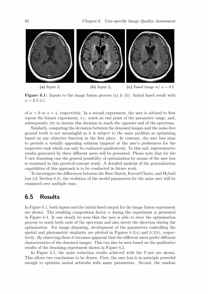
82 Chapter 6. User-specific Image Quality Assessment
(a) Input I1 (b) Input I2 (c) Fused image w/ α = 0.5
Figure 6.1: Inputs to the image fusion process (a) & (b). Initial fused result withα = 0.5 (c).
of α = 0 or α = 1, respectively. In a second experiment, the user is advised to firstrepeat the former experiment, i.e., reach an end point of the parameter range, and,subsequently, try to inverse this decision to reach the opposite end of the spectrum.
Similarly, computing the deviation between the denoised images and the noise-freeground truth is not meaningful as it is subject to the same problem as optimizingbased on any objective function in the first place. In contrast, the user loss aimsto provide a visually appealing solution targeted at the user’s preferences for therespective task which can only be evaluated qualitatively. To this end, representativeresults generated by three different users will be presented. Please note that for theU-net denoising case the general possibility of optimization by means of the user lossis examined in this proof-of-concept study. A detailed analysis of the generalizationcapabilities of this approach is to be conducted in future work.
To investigate the differences between the Best-Match, Forced-Choice, and Hybridloss (cf. Section 6.2), the evolution of the model parameters for the same user will beexamined over multiple runs.
6.5 ResultsIn Figure 6.1, both inputs and the initial fused output for the image fusion experimentare shown. The resulting composition factor α during the experiment is presentedin Figure 6.4. It can clearly be seen that the user is able to steer the optimizationprocess to reach both ends of the spectrum and also invert the direction during theoptimization. For image denoising, development of the parameters controlling thespatial and photometric similarity are plotted in Figures 6.3(a) and 6.3(b), respec-tively. By observing these it becomes apparent that the different users prefer differentcharacteristics of the denoised images. This can also be seen based on the qualitativeresults of the denoising experiment shown in Figure 6.2.
In Figure 6.5, the noise reduction results achieved with the U-net are shown.This allows two conclusions to be drawn. First, the user loss is in principle powerfulenough to optimize neural networks with many parameters. Second, the random

6.5. Results 83
(a) Input (b) Initial denoised (c) Ground truth
(d) Denoised by user 1 (e) Denoised by user 2 (f) Denoised by user 3
Figure 6.2: Results of the denoising experiment using the bilateral filter. Top row:noisy input (a), denoised output using initial parameter setting (b), and ground truth(c). Bottom row: Results for all three users after the optimization process.
0 5 10 15step
0.5
1.0
1.5
2.0
spat
ial
User 1User 2User 3
(a) Optimization process for σspatial.
0 5 10 15step
0.0
0.2
0.4
0.6
0.8
phot
o
User 1User 2User 3
(b) Optimization process for σphoto.
Figure 6.3: Results of the bilateral filter’s parameter optimization process for threedifferent users.
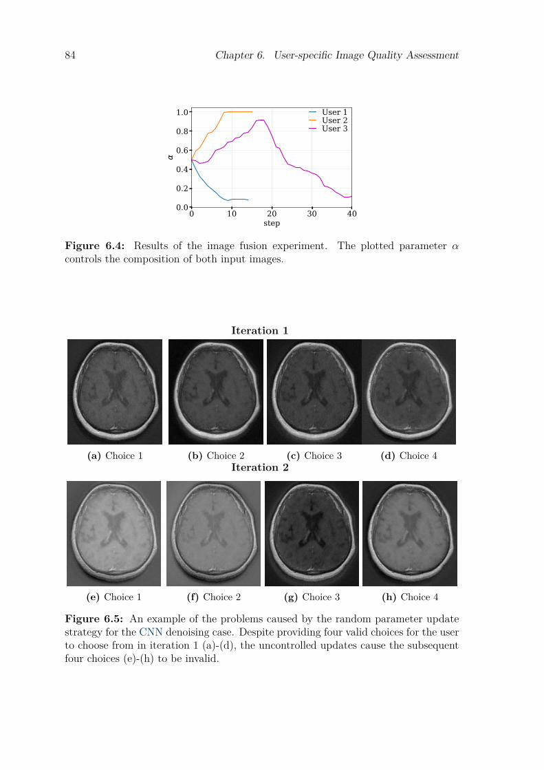
84 Chapter 6. User-specific Image Quality Assessment
0 10 20 30 40step
0.0
0.2
0.4
0.6
0.8
1.0 User 1User 2User 3
Figure 6.4: Results of the image fusion experiment. The plotted parameter αcontrols the composition of both input images.
Iteration 1
(a) Choice 1 (b) Choice 2 (c) Choice 3 (d) Choice 4Iteration 2
(e) Choice 1 (f) Choice 2 (g) Choice 3 (h) Choice 4
Figure 6.5: An example of the problems caused by the random parameter updatestrategy for the CNN denoising case. Despite providing four valid choices for the userto choose from in iteration 1 (a)-(d), the uncontrolled updates cause the subsequentfour choices (e)-(h) to be invalid.
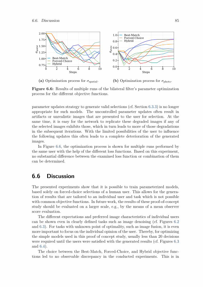
6.6. Discussion 85
0 2 4 6 8 10Steps
0.75
1.00
1.25
1.50
1.75
2.00sp
atia
l
Best-MatchForced-ChoiceHybrid
(a) Optimization process for σspatial.
0 2 4 6 8 10Steps
0.0
0.2
0.4
0.6
0.8
1.0
phot
o
Best-MatchForced-ChoiceHybrid
(b) Optimization process for σphoto.
Figure 6.6: Results of multiple runs of the bilateral filter’s parameter optimizationprocess for the different objective functions.
parameter updates strategy to generate valid selections (cf. Section 6.3.3) is no longerappropriate for such models. The uncontrolled parameter updates often result inartifacts or unrealistic images that are presented to the user for selection. At thesame time, it is easy for the network to replicate these degraded images if any ofthe selected images exhibits those, which in turn leads to more of those degradationsin the subsequent iterations. With the limited possibilities of the user to influencethe following updates this often leads to a complete deterioration of the generatedimages.
In Figure 6.6, the optimization process is shown for multiple runs performed bythe same user with the help of the different loss functions. Based on this experiment,no substantial difference between the examined loss function or combination of themcan be determined.
6.6 DiscussionThe presented experiments show that it is possible to train parameterized models,based solely on forced-choice selections of a human user. This allows for the genera-tion of results that are tailored to an individual user and task which is not possiblewith common objective functions. In future work, the results of these proof-of-conceptstudy should be evaluated on a larger scale, e.g., by the means of a mean observerscore evaluation.
The different expectations and preferred image characteristics of individual userscan be shown even in clearly defined tasks such as image denoising (cf. Figures 6.2and 6.3). For tasks with unknown point of optimality, such as image fusion, it is evenmore important to focus on the individual opinion of the user. Thereby, for optimizingthe simple models used in this proof of concept study, usually less than 20 decisionswere required until the users were satisfied with the generated results (cf. Figures 6.3and 6.4).
The choice between the Best-Match, Forced-Choice, and Hybrid objective func-tions led to no observable discrepancy in the conducted experiments. This is in
86 Chapter 6. User-specific Image Quality Assessment
contrast to the findings in [Zare 19], which, for another methodological task, found adifference between the selected objective functions with the Hybrid version emergingas the superior variant. Therefore, an additional evaluation including further taskswill be necessary in future work in order to draw a final conclusion about the choiceof the user loss function.
A key aspect of this approach that currently limits the possibility of training largemodels such as CNNs is the generation of valid choices for the user to choose from.Randomly updating the model’s parameters is successful if only few, clearly definedparameters are present as it is the case for the alpha blending and bilateral filtering.Though, for more complex problems, such as, e.g., convolution kernel weights in theU-net denoising case, this can lead to undesired effects in the presented choices, asseen in Figure 6.5. The development of a more elaborate strategy for the generationof valid samples is therefore indispensable for this use case.
6.7 ConclusionIn this proof of concept study, we presented a forced-choice experiment that is capa-ble of optimizing parametric models, from simple one-parameter functions to CNNswith over one million parameters. This allows to overcome the gap between the im-age characteristics enforced by conventional objective functions and the propertiespreferred by human users. Furthermore, the presented approach allows for the opti-mization of models in settings with an undefined point of optimality, such as imagefusion and similar generative tasks. An existing challenge is the generation of validchoices for the user to choose from in the forced-choice experiment. However, we areconfident that this problem can be successfully tackled by the incorporation of moreelaborate methods like probabilistic models, which would allow for the optimizationof even large models like state-of-the-art CNNs.

P A R T III
Outlook and Summary
87


C H A P T E R 7
OutlookIn this thesis, we presented three contributions to the field of medical image pro-
cessing in the presence of multi-modal data. First, a method for the synthesis ofX-ray projection images based on corresponding MR projections was investigated.This study showed the potential of deep learning-based generative models to tackleeven as ill-posed problems as the domain transfer of projection images. In orderto be successful in the face of this difficult task, special adjustments to the objec-tive function and the network architecture had to be conducted. These changesconsiderably improved the visual appearance of the synthesized projection images.Nevertheless, there are still some flaws in the generated X-ray projections. The syn-thesis of the strongly overlapping structures on the integrated image represents amajor challenge. In addition, the ambiguity of the acquired signal, bone and airmap to similar intensity ranges in MRI, further increases the difficulty of this task.As resolving this problem based on spatial structure or intensity values is difficult,the addition of temporal information has the potential to facilitate the underlyingtask. In image-guided interventions, fluoroscopy is usually used to acquire a sequenceof images for dynamic imaging. This implies a certain degree of consistency of thestructures across the temporal dimensions. The same applies to the imaging of to-mographic volumes where successive projections are acquired from slightly differentangles. Previous work has shown that this consistency can be used to improve theresults in multiple areas [Aich 15, Enge 18, Lai 18, Preu 19b]. In future work, wetherefore target to investigate if these insights can be transferred to the underlyingtask of projection-to-projection translation. Nevertheless, in many interventional ap-plications an approximation of the correct solution is sufficient for large parts of theprojection images. Smooth deviations of the intensity values in the homogeneous re-gions are often not of interest for the physician, assuming these are even visible for ahuman observer. In fact, some post-processing applications are only made possible bya slight mismatch of projections. An example would be one-shot digital subtractionangiography, which would be possible with a real X-ray projection with contrastedblood vessels and a synthetic X-ray projection generated from an MR projectionwithout contrast agent [Legh 19].
Furthermore, we aim to evaluate the projection-to-projection translation on fur-ther data sets and body regions in the future. In particular, we are interested in datasets that contain highly diverse information in different modalities. For example, intorso imaging, X-ray covers bones such as the ribs and the spine, as well as the lungs,whereas MR data mainly records signals from soft tissue structures, e.g., the heart.This possesses great potential for the simultaneous acquisition of signal from differentmodalities as well as challenges in the form of incoherent information.
89
90 Chapter 7. Outlook
As demonstrated, there is still a lot of untapped potential in this field that lendsitself to further research. Thereby, the insights gained so far are not limited to thesynthesis of projection images, but apply to all image data with similar character-istics, i.e., dominant high-frequency structures. We therefore target to evaluate thisweighting scheme also on other tasks that rely on the precise generation of fine detailstructures.
The second approach that was presented in this thesis considered the comprehen-sibility in image processing. It is based on the combination of a known operator, theGuided Filter, with proven DL-based approaches. This combination makes it possibleto effectively extract the complementary information from multi-modal input data,generate state-of-the-art results, and at the same time ensure the comprehensibilityof the output. The presented approach benefits from the presence of multi-modalinput data but is not limited to it. Even with inputs from a single modality, themethodological procedure ensures the comprehensible processing of the underlyingdata. While we use the GF in the presented work, the concept of known operatorlearning in itself is modular. The GF is employed like a regular layer on top of theCNN and can be exchanged with any other differentiable operator or series of oper-ators. Many of those were proposed in the past in image processing research. Thisopens up a vast amount of possibilities to investigate the combination of traditionalanalytic methods with DL.
Finally, a proof of concept study investigating the possibility of optimizing pa-rameterized image processing operators or models solely based on user inputs waspresented. It could be shown that the problem of automated image quality assess-ment, i.e., the discrepancy between the preferred image characteristics of commonobjective functions and the actual preferences of human observers, can be tackledby a forced-choice user selection. A popular example in view of multi-modal imageprocessing is image fusion which can hardly be optimized in a supervised fashion duethe intrinsic lack of reference images. Furthermore, the presented concept extends tomany applications with an unknown or hard to reach point of optimality.
We have shown the effectiveness of this optimization technique for two popularalgorithms with few parameters. However, when tackling more complex tasks, e.g., aspresented in the training of deep CNNs, problems with the currently used parameterupdate strategy became apparent. In order to use these powerful methods, moreadvanced approaches to generate the necessary examples for the user to choose fromare essential. A possible solution could be the application of probabilistic models suchas (conditional) variational autoencoders [King 13, Kohl 18]. The objective of these isnot to learn a direct mapping between input and output, but to learn a distributionof valid solutions, eventually conditioned on an input variable. This would rendersampling various choices for the user a straightforward possibility. Though, also inthis case a good trade-off between exploration and exploitation would have to befound heuristically. So far, the presented method was evaluated qualitatively basedon the visual appearance of the generated samples as well as the inter and intra useragreement on the selected parameter values. In future work, this proof-of-conceptstudy should be evaluated on a larger scale, e.g., by the means of a mean observerscore evaluation.
91
The concepts and methods presented in the course of this thesis are not limitedto multi-modal imaging but show the advantage that the existence of data of differ-ent modalities can possess. As a result of the technical advances and the increasingavailability of medical imaging in many regions of the world, the amount and va-riety of medical image data is expected to increase steadily (cf. Section 1.1). Thisdevelopment entails possibilities but also challenges. The increased quantity of infor-mation can be beneficial for patients in order to receive more reliable or personalizedpredictions. The clinical staff, however, faces the difficult task of coping with thisamount and variety of data. While assessment or the annotation of single imagesor volume is tedious, it is often a well understood task that can be mastered withexpertise by the individuals. In contrast, grasping relationships among informationthat are spread over multiple acquisitions or even different modalities is a clearlymore difficult task for human observers. In view of this ever-increasing challenge, thedevelopment of automated solutions for processing multi-modal image information isan important step. On the one hand, this concerns the development of fully auto-mated decision making mechanisms such as image classification approaches On theother hand, methods for preprocessing of the data into a human-understandable formare important, e.g., in the form of image fusion, as well as enhancement of the dataof interest. Advances in this field will not only allow for improved diagnostics andtreatment, but also relieve the burden on physicians and other hospital staff, whichin turn can lead to an improvement in the overall health care system.

C H A P T E R 8
SummaryThis thesis presents three approaches for the exploitation of the extensive infor-
mation generated by clinical multi-modal medical imaging. The proposed methodsdeal with the advantages of the often complementary and/or redundant image in-formation as well as the resulting challenges, such as the lack of naturally occurringreference images or the combination of data of different modalities.
In the first chapter, possibilities and challenges induced by the technical advance-ments in medical imaging are outlined. Due to the constantly increasing numberof medical imaging exams in all of its variants, a holistic processing of these in thesense of multi-modal image processing is an important aspect for the future of med-ical imaging. This may allow the uncovering of previously unimagined relationshipsamong diseases and malfunctions as well as the distillation of the ever-increasing datavolumes. Subsequent to the motivation of the topic, the scientific contributions thatform the basis for the upcoming chapters are introduced.
The second chapter conveys the fundamental prerequisites on medical imagingthat are necessary for understanding the subsequently presented methods. Thereare many different methods available for imaging both the inner and outer partsof the human body. To begin, an overview of those imaging modalities that arecommonly used in clinical everyday life is given. Subsequently, the fundamentalphysical processes of the two modalities used in this thesis are presented in moredetail. On the one hand, this is X-ray imaging which is used for the acquisitionof radiographs, in fluoroscopy, and in computed tomography (CT) imaging. Themain advantage lies in the acquisition of dense tissue with high spatial and temporalresolution. The fast and flexible imaging capabilities render X-ray-based modalitiesone of the cornerstones of modern medical imaging. In addition to the prevalentuse in diagnostics, X-ray fluoroscopy is also the workhorse of interventional radiologymostly due to its capability to visualize devices inside the human body in real time.However, all these advantages come at the cost of ionizing radiation and limited softtissue contrast. In particular, the former is a closely monitored factor that subjectsthe use of X-ray-based radiation to careful consideration.
On the other hand, magnetic resonance imaging (MRI) data is used in this thesis.MRI is based on the principle of nuclear magnetic resonance which exhibits no knownsafety concerns for most patients. While the image formation process of alignment,excitation, and measurement of response of the nuclei is in most cases the same, theexact implementation of it allows for a vast variety of possibilities. As a result, MRI isable to acquire and visualize extremely diverse soft tissue contrasts. It therefore offersa lot of complementary information to its CT counterpart. The most popular formof MRI data representation is in the form of tomographic volumes. However, these
93
94 Chapter 8. Summary
volumes require the acquisition of a large quantity of data which is time consuming.As an alternative, we investigate the use of MRI projection images. Projective MRIimaging is of special interest for interventional image-guided procedures, as it pro-vides a compact data representation and is less time consuming in the acquisition.Furthermore, it allows for the acquisition of data matching the clinical gold standardin interventional radiology, X-ray fluoroscopy.
The whole image formation process is much more complex than shown in Chap-ter 2. However, the physical backgrounds of the image acquisition are sufficient tounderstand the different resulting image characteristics.
With the medical data at hand, an introduction to deep learning-based image pro-cessing is presented in Chapter 3. Due to its recent success, deep learning (DL) hasemerged as one of the premier research directions for image processing in the medicalfield. Consequently, also many of the approaches presented in this thesis are basedon DL methods. First, the general concepts of the multilayer perceptron (MLP) andneural networks (NNs) are introduced. An important point in their application isthe gradient descent-based optimization procedure for which multiple variants havebeen proposed in recent years. A common property is that all are based on thebackpropagation algorithm which allows for an efficient calculation of the gradientalso for a large number of neurons. Second, popular building blocks and architec-tural concepts that contribute to the recent advent of DL are explained, starting withthe choice of activation functions, which are responsible for the non-linearity of NN.Subsequently, the application of the convolution operation in DL is discussed. Theresulting convolutional neural networks (CNNs) represent a milestone in image pro-cessing using DL and are now the de facto standard in this application. Furthermore,several popular concepts that are used throughout this thesis are explained in Sec-tion 3.2, e.g., different normalization methods, as well as the concept of residuallearning. Third, Section 3.3 presents popular approaches for the combination of thesingle building blocks of CNNs which is commonly referred to as architectures. Whilemany of these architectures are proposed each year, we focus on the ones that areused throughout this thesis. Finally, common objective functions, a key componentfor every optimization procedure, are presented in Chapter 3. Objective functionsare used for performance assessment during the optimization. Thereby, each objec-tive function exhibits intrinsic properties which are often reflected in characteristicoutcomes in the results. These properties are discussed Chapter 3 and all proposedapproaches in this work are based on these methods.
Equipped with the necessary prerequisites, Chapter 4 presents the first novel ap-proach that is presented in this work. Here, the problem of domain transfer of imagedata, i.e., image-to-image translation, is considered in view of hybrid X-ray/magneticresonance (MR) imaging. This imaging technique promises large potential in inter-ventional medical imaging applications due to the broad variety of contrast of MRIcombined with fast imaging of X-ray-based modalities. To fully utilize the potential ofthe vast amount of existing image enhancement techniques, the corresponding infor-mation from both modalities must be present in the same domain. Arising from theinterventional demands, X-ray fluoroscopy has proven to be the modality of choice.Translation of one modality to another in this case is an ill-posed problem due toambiguous signal and overlapping structures in the projective geometry. To tackle
95
these challenges, we present a learning-based solution to MR to X-ray projection-to-projection translation. At first, we investigate the performance of state-of-the-artapproaches based on a phantom study. Concretely, the influence of the chosen NNarchitecture as well as the corresponding objective function on the generated results isassessed based on a anthropomorphic head phantom. The insights gained throughoutthis phantom study substantiate that common approaches for the synthesis of natu-ral images or tomographic medical images are not suited for the synthesis of X-rayprojection images. The images arising from the X-ray acquisition exhibit sparse struc-tures and consist mostly of outlines, edges, and similar details. These characteristicsneed to be appropriately addressed during the synthesis process. By using a genera-tor network focusing on high representational capacity in higher resolution layers, wecan show that this benefits the generation of high-frequency details. Furthermore,an additional weighting scheme of the objective function that favors high-frequencystructures results in a clearly improved image impression, especially with respect toimportant details and contours in projection imaging. These qualitative observationsalso translate to the quantitative error metrics. The presented approach achievesa deviation from the ground truth of only 6 % and structural similarity measure of0.913 ± 0.005. An important aspect is that the insights gained in the course of thisproject are not limited to projection-to-projection translation but extend to manyother application areas that require similar image characteristics.
In Chapter 5, an often overlooked aspect of medical image processing and imageprocessing in general is discussed, namely the comprehensibility of the generated out-puts. While, DL-based image processing can achieve highly appealing results, it isconsidered a black box transformation. The interpretability of the applied methods isoften limited and formal guarantees are rare. In many non-safety critical applications,this can be tolerated due to the empirically good results. However, in the process-ing of medical image data the patient’s life is at stake and every mistake can havesevere consequences. We try to remedy this lack of comprehensibility by integratingthe concepts of known operators into common DL-based image processing pipelines.Considering the problem of image enhancement, we propose the use of the GuidedFilter (GF) in combination with DL for comprehensible medical image processing.Due to its locally linear and differentiable nature, the GF can be used in conjunctionwith a learned guidance map originating from a NN for general purpose medical im-age processing. This combination enforces two properties. First, the guidance map ofthe GF can be trained task-optimal in an end-to-end fashion, even from multi-modalinputs. In this thesis, we show the capabilities for X-ray and MRI data in differentdomains. Second, the input to be enhanced is only processed by the locally linearoperations of the GF. This ensures that the input to be processed is at no point ofthe pipeline in contact with the actual NN and its high dimensional non-linear trans-formations. Evaluated based on two popular tasks, image super resolution (SR) anddenoising, we can show that this approach offers clearly increased comprehensibil-ity when compared to common state-of-the-art approaches. Concretely, the images’content is almost unchanged after processing. On top, the proposed pipeline offersincreased robustness against degradation of the inputs as well as adversarial attacks.All this can be achieved while maintaining raw performance metrics that are on parwith the state of the art. It is also noteworthy that the presented approach is not
96 Chapter 8. Summary
necessarily tied to the GF and the shown tasks. In contrast, the modular nature ofthe pipeline and large variety of possible tasks encourages the exploration of furtheroperators and algorithms that fit into the concept of known operator learning.
A common property of both previously presented approaches is the need for suit-able objective functions. Many image processing tasks, especially in multi-modalimaging, suffer from the problem of an unknown or hard to reach point of optimality.This renders automated image quality assessment a difficult task. In Chapter 6, wepresent an optimization scheme solely based on user input. It exploits the fact thathuman observers can excellently judge images according to their perceived quality,even if they are not able to explicitly provide a reference. We apply this in an it-erative, differentiable forced-choice experiment, in which the user can choose out ofmultiple possible solutions the image best matching to his desired characteristics.The underlying procedure is two-fold. First, the parameters of the algorithm are op-timized to produce results that closely match the example previously chosen by theuser. Second, based on the updated parameter settings, new possible solutions arecreated for the user to make a renewed selection. The proposed user loss scheme canbe applied to multiple tasks, for simple single parameter operators as well as the opti-mization of large CNNs. In this proof-of-concept study, we could show the suitabilityof the approach for a simple image fusion scheme as well as for image denoising usingthe popular bilateral filter. Currently, the proposed approach is still facing challengesregarding the generation of the possible solutions for the forced-choice experiment.This is problematic especially in the optimization of many interrelated parameters asit is the case for CNNs. However, utilizing more elaborate methods for this task suchas, e.g., probabilistic models, is likely to successfully tackle these remaining problems.
Finally, Chapter 7 summarizes the insights gained from this work and their impacton multi-modal medical image processing. Furthermore, the limitations and potentialfuture work regarding the previously presented approaches are addressed. Despitethe apparent existence of open points, we indicate clear directions and approaches onhow to resolve them. Overall, it can be seen that the availability and processing ofmulti-modal image data exhibits many challenges but also entails distinct advantages.The full insight into the human body is distributed across many modalities andthis knowledge can only by gained by the combination of this heterogeneous data.Though, large parts of the acquired information is redundant. Efforts regarding theholistic processing of all available data allow to distill the large amount of informationinto representations that can be grasped by humans observers.
AcronymsADAM
adaptive moment estimation 22, 47, 52, 65, 67
ANNartificial neural network 19
CGANconditional generative adversarial network 36, 52
CNNconvolutional neural network 26, 28, 34, 44, 45, 61, 63, 66, 74, 80, 81, 84, 86,90, 94, 96, 104
CTcomputed tomography 4, 7, 10, 12, 13, 16, 17, 41, 43, 44, 47, 52, 54, 55, 60, 65,93
DLdeep learning 5, 6, 8, 19, 22, 35, 37, 41, 44, 59, 60, 62, 66, 72, 74, 75, 90, 94, 95
FCfully-connected 23, 25, 27
FMfeature matching 34–36, 45, 48, 49, 51, 65, 103
GANgenerative adversarial network 35, 36, 44
GDgradient descent 21
GFGuided Filter 6, 8, 59–62, 65–75, 90, 95, 96, 104
GPUgraphics processing unit 26, 53, 54, 65
97

98 Acronyms
HUHounsfield unit 11, 12, 49, 103
Leaky ReLUleaky rectified linear unit 25
MAEmean absolute error 34, 45, 48, 49, 65, 68
MLmachine learning 19, 21, 33, 36, 37
MLPmultilayer perceptron 19–21, 94, 103
MRmagnetic resonance 4, 5, 8, 16, 41–44, 47, 50, 54, 55, 57, 65, 68, 70, 81, 89, 94,95
MRImagnetic resonance imaging 3–5, 10, 13–17, 42–44, 52, 60, 65, 68, 69, 81, 89,93–95, 103, 105
MSEmean squared error 21, 34, 47, 48, 52, 53, 81
NNneural network 19, 20, 23, 26, 28, 29, 77, 94, 95
PDproton density 15, 16
PSNRpeak signal-to-noise ratio 47, 48, 52, 53
ReLUrectified linear unit 24, 25, 33
RFradio frequency 14–16
SGDstochastic gradient descent 21, 22

Acronyms 99
SRsuper resolution 28, 33, 42, 56, 60, 63–66, 68, 69, 71, 72, 74, 75, 95, 104
SSIMstructural similarity 47, 48, 52, 53, 65, 68, 71
SVMsupport vector machine 36, 37
TEecho time 15, 16
TRrepetition time 15, 16


List of Symbolsa Scalars are denoted by lower case letters.
a Vectors are written as lower case letters in bold font.
A Matrices are denoted by upper case letters in bold font.
f Function
x Input
y Output
M Guidance image
G Guide image
I Input image
L Ground truth image
P Predicted image
q Batch of inputs
b Bias
K Kernel window
L Set of layers
θ Parameter vector
J Objective function
d Discriminator function or network
g Generator function or network
r Radius
R Residual
w Weight
101

List of Figures
2.1 The spectrum of electromagnetic radiation. . . . . . . . . . . . . . . . 102.2 Hounsfield Unit for different human tissue types. . . . . . . . . . . . . 122.3 Examples of different X-ray-based imaging applications. . . . . . . . . 132.4 Visualization of the excitation and relaxation of the nuclei in MRI. . 142.5 Examples of the different weighting schemes in MRI. . . . . . . . . . 15
3.1 Graphical illustration of a neuron. . . . . . . . . . . . . . . . . . . . . 203.2 Graphical illustration of a multilayer perceptron. . . . . . . . . . . . . 213.3 Graphical illustration of the backpropagation algorithm. . . . . . . . 243.4 Popular choices for the activation function in neural networks. . . . . 253.5 Graphical representation of a convolution operation. . . . . . . . . . . 263.6 Graphical representation of the maximum pooling operation. . . . . . 273.7 Graphical representation of a residual block. . . . . . . . . . . . . . . 303.8 Graphical representation of the pixel shuffle operation. . . . . . . . . 313.9 Graphical representation of a variant of the U-net architecture. . . . . 323.10 Graphical representation of the WDSR network. . . . . . . . . . . . . 333.11 Graphical representation of the feature matching loss. . . . . . . . . . 353.12 A graphical representation of the zero-one error function and the hinge
loss function. . . . . . . . . . . . . . . . . . . . . . . . . . . . . . . . 37
4.1 A schematic visualization of all three tested network architectures. . . 464.2 A visualization of all possible X-ray source positions used for the data
generation. . . . . . . . . . . . . . . . . . . . . . . . . . . . . . . . . . 474.3 Projection synthesis results of the phantom study. . . . . . . . . . . . 484.4 Graphical representation of the proposed network architecture for the
projection-to-projection translation. . . . . . . . . . . . . . . . . . . . 494.5 A schematic overview of the data generation process. . . . . . . . . . 534.6 Quantitative evaluation of the generated X-ray projections with re-
spect to the projection angle. . . . . . . . . . . . . . . . . . . . . . . 544.7 Representative examples of the generated projection images for differ-
ent projection angles and patients. . . . . . . . . . . . . . . . . . . . 554.8 Lineplots through the generated and ground truth projections. . . . . 564.9 Comparison of the different network architectures and weighted and
unweightes objective functions. . . . . . . . . . . . . . . . . . . . . . 564.10 An example of missing information in the generated X-ray projection
images. . . . . . . . . . . . . . . . . . . . . . . . . . . . . . . . . . . . 57
5.1 A graphical representation of the guided filtering pipeline. . . . . . . 615.2 Graphical representation of the employed multi-modal U-Net network. 635.3 Graphical representation of the modified WDSR network. . . . . . . 645.4 An example of a wavelet decomposed image. . . . . . . . . . . . . . . 67
103
104 List of Figures
5.5 Example inputs and outputs of the GF pipeline. . . . . . . . . . . . . 695.6 SR: representative examples of the results for all network and guided
filter configurations. . . . . . . . . . . . . . . . . . . . . . . . . . . . 705.7 Denoising: exemplary outputs for the different noise levels. . . . . . . 705.8 Quantitative metrics for SR. . . . . . . . . . . . . . . . . . . . . . . . 715.9 Denoising: quantitative metrics for different noise levels based on the
projection data. . . . . . . . . . . . . . . . . . . . . . . . . . . . . . . 715.10 Comprehensibility: analysis of the robustness against degradations. . 715.11 Comprehensibility: analysis of the change in the images’ content. . . 715.12 Training statistics gathered during the generation of the adversarial
examples. . . . . . . . . . . . . . . . . . . . . . . . . . . . . . . . . . 735.13 Comprehensibility: evaluation of the influence of adversarial attacks
on the proposed pipeline. . . . . . . . . . . . . . . . . . . . . . . . . . 745.14 Analysis of the influence of the different input modalities on the guid-
ance map. . . . . . . . . . . . . . . . . . . . . . . . . . . . . . . . . . 75
6.2 Results of the denoising experiment using the bilateral filter. . . . . . 836.4 Results of the image fusion experiment. . . . . . . . . . . . . . . . . . 846.5 An example of the problems caused by the random parameter update
strategy for the CNN denoising case. . . . . . . . . . . . . . . . . . . 84
List of Tables
4.1 Quantitative evaluation metrics for the projection-to-projection trans-lation using the human head phantom. . . . . . . . . . . . . . . . . . 48
4.2 Quantitative evaluation metrics for the projection-to-projection trans-lation using clinical patient data. . . . . . . . . . . . . . . . . . . . . 53
5.1 SR: quantitative results for all datasets and network configurations. . 685.2 Denoising: quantitative results for the X-ray & MRI projection images. 68
105

Bibliography[Adle 18] J. Adler and O. Oktem. “Learned Primal-Dual Reconstruction”. IEEE
Transactions on Medical Imaging, Vol. 37, No. 6, pp. 1322–1332, 2018.
[Aich 15] A. Aichert, M. Berger, J. Wang, N. Maass, A. Doerfler, J. Hornegger,and A. K. Maier. “Epipolar Consistency in Transmission Imaging”. IEEETransactions on Medical Imaging, Vol. 34, No. 11, pp. 2205–2219, 2015.
[Amio 16] C. Amiot, C. Girard, J. Chanussot, J. Pescatore, and M. Desvignes.“Spatio-Temporal Multiscale Denoising of Fluoroscopic Sequence”. IEEETransactions on Medical Imaging, Vol. 35, No. 6, pp. 1565–1574, 2016.
[Andr 15] J. Andreu-Perez, C. C. Y. Poon, R. D. Merrifield, S. T. C. Wong, andG.-Z. Yang. “Big Data for Health”. IEEE Journal of Biomedical andHealth Informatics, Vol. 19, No. 4, pp. 1193–1208, 2015.
[Antu 19] V. Antun, F. Renna, C. Poon, B. Adcock, and A. C. Hansen. “OnInstabilities of Deep Learning in Image Reconstruction - Does AI comeat a Cost?”. arXiv:1902.05300, 2019.
[Arma 18] K. Armanious, C. Jiang, M. Fischer, T. Kustner, K. Nikolaou, S. Ga-tidis, and B. Yang. “MedGAN: Medical Image Translation using GANs”.arXiv:1806.06397v2, 2018.
[Arti 14] “Artis zeego Multi-axis system for interventional imaging”.https://www.deltamedicalsystems.com/DeltaMedicalSystems/media/Product-Details/Artis-zeego-Data-Sheet.pdf, 2014. Ac-cessed on 09. Aug. 2019.
[Badr 17] V. Badrinarayanan, A. Kendall, and R. Cipolla. “SegNet: A Deep Convo-lutional Encoder-Decoder Architecture for Image Segmentation”. IEEETransactions on Pattern Analysis and Machine Intelligence, Vol. 39,No. 12, pp. 2481–2495, 2017.
[Bald 17] D. Balduzzi, M. Frean, L. Leary, J. Lewis, K. W.-D. Ma, andB. McWilliams. “The shattered gradients problem: If resnets are theanswer, then what is the question?”. In: 34th International Conferenceon Machine Learning, pp. 342–350, JMLR. org, 2017.
[Bark 17] J. Barkhausen, T. Kahn, G. A. Krombach, C. K. Kuhl, J. Lotz,D. Maintz, J. Ricke, S. O. Schonberg, T. J. Vogl, F. K. Wacker, G. Adam,G. Antoch, M. Beer, T. Bley, A. Bucker, C. Duber, M. Forsting,B. Hamm, K. Hauenstein, W. Heindel, N. Hosten, O. Jansen, H. U.Kauczor, M. Langer, M. Laniado, A. Mahnken, K. Nikolaou, M. Reiser,E. Rummeny, H. Schild, R. P. Spielmann, C. Stroszczynski, U. Te-ichgraber, and M. Uder. “White Paper: Interventional MRI: CurrentStatus and Potential for Development Considering Economic Perspec-tives, Part 1: General Application”. Fortschr Rontgenstr, Vol. 189, No. 7,pp. 611–622, 2017.
[Bish 06] C. M. Bishop. Pattern Recognition and Machine Learning. Springer,2006.
107
108 Bibliography
[Brei 18a] K. Breininger, S. Albarqouni, T. Kurzendorfer, M. Pfister,M. Kowarschik, and A. Maier. “Intraoperative Stent Segmentationin X-ray Fluoroscopy for Endovascular Aortic Repair”. InternationalJournal of Computer Assisted Radiology and Surgery, pp. 1–11, 2018.
[Brei 18b] K. Breininger, T. Wurfl, T. Kurzendorfer, S. Albarqouni, M. Pfister,M. Kowarschik, N. Navab, and A. Maier. “Multiple Device Segmentationfor Fluoroscopic Imaging using Multi-task Learning”. In: IntravascularImaging and Computer Assisted Stenting and Large-scale Annotation ofBiomedical Data and Expert Label Synthesis, pp. 19–27, Springer, 2018.
[Brei 20] K. Breininger, M. Pfister, M. Kowarschik, and A. Maier. “Move OverThere: One-Click Deformation Correction for Image Fusion During En-dovascular Aortic Repair”. In: Medical Image Computing and Computer-Assisted Intervention - MICCAI, pp. 713–723, 2020.
[Burc 73] W. E. Burcham. Nuclear Physics: An Introduction. Longmans, 2 Ed.,1973.
[Buzu 11] T. M. Buzug. “Computed Tomography”. In: Springer Handbook of Med-ical Technology, pp. 311–342, Springer, 2011.
[Carl 17] N. Carlini and D. Wagner. “Towards Evaluating the Robustness of NeuralNetworks”. In: IEEE Symposium on Security and Privacy, pp. 39–57,2017.
[Chen 17] Q. Chen and V. Koltun. “Photographic Image Synthesis with CascadedRefinement Networks”. In: IEEE International Conference on ComputerVision, pp. 1520–1529, 2017.
[Chen 18] L. C. Chen, G. Papandreou, I. Kokkinos, K. Murphy, and A. L. Yuille.“DeepLab: Semantic Image Segmentation with Deep Convolutional Nets,Atrous Convolution, and Fully Connected CRFs”. IEEE Transactions onPattern Analysis and Machine Intelligence, Vol. 40, No. 4, pp. 834–848,2018.
[Choi 19] D. Choi, C. J. Shallue, Z. Nado, J. Lee, C. J. Maddison, and G. E. Dahl.“On Empirical Comparisons of Optimizers for Deep Learning”. arXivpreprint arXiv:1910.05446, 2019.
[Chol 16] F. Chollet. “Xception: Deep Learning with Depthwise Separable Convo-lutions”. arXiv:1610.02357, 2016.
[Clev 15] D.-A. Clevert, T. Unterthiner, and S. Hochreiter. “Fast and Accu-rate Deep Network Learning by Exponential Linear Units (ELUs)”.arXiv:1511.07289, 2015.
[Coop 04] M. J. Cooper, M. Cooper, P. E. Mijnarends, P. Mijnarends, N. Shiotani,N. Sakai, and A. Bansil. X-ray Compton scattering. Oxford UniversityPress on Demand, 2004.
[Cybe 89] G. Cybenko. “Approximations by Superpositions of a Sigmoidal Func-tion”. Mathematics of Control, Signals and Systems, Vol. 2, pp. 183–192,1989.
[Daub 92] I. Daubechies. Ten Lectures on Wavelets. SIAM, 1992.
Bibliography 109
[Dege 16] J. Degen and M. P. Heinrich. “Multi-Atlas Based Pseudo-CT SynthesisUsing Multimodal Image Registration and Local Atlas Fusion Strategies”.In: Proceedings of the IEEE Conference on Computer Vision and PatternRecognition Workshops, pp. 160–168, 2016.
[Dice 45] L. R. Dice. “Measures of the Amount of Ecologic Association BetweenSpecies”. Ecology, Vol. 26, No. 3, pp. 297–302, 1945.
[Dong 14] C. Dong, C. C. Loy, K. He, and X. Tang. “Learning a Deep Convolu-tional Network for Image Super-Resolution”. In: European Conferenceon Computer Vision, pp. 184–199, Cham, 2014.
[Doso 16] A. Dosovitskiy and T. Brox. “Generating Images with Perceptual Simi-larity Metrics based on Deep Networks”. In: Advances in Neural Infor-mation Processing Systems, pp. 658–666, 2016.
[Duch 11] J. Duchi, E. Hazan, and Y. Singer. “Adaptive Subgradient Methodsfor Online Learning and Stochastic Optimization”. Journal of MachineLearning Research, Vol. 12, No. Jul, pp. 2121–2159, 2011.
[Dumo 16] V. Dumoulin and F. Visin. “A Guide to Convolution Arithmetic for DeepLearning”. arXiv:1603.07285, 2016.
[Dura 02] F. Durand and J. Dorsey. “Fast Bilateral Filtering for the Display of High-Dynamic-Range Images”. In: ACM Transactions on Graphics, pp. 257–266, 2002.
[Eise 04] E. Eisemann and F. Durand. “Flash Photography Enhancement via In-trinsic Relighting”. In: ACM Transactions on Graphics, pp. 673–678,2004.
[Elsk 19] T. Elsken, J. H. Metzen, and F. Hutter. “Neural Architecture Search: ASurvey”. Journal of Machine Learning Research, Vol. 20, No. 55, pp. 1–21, 2019.
[Enge 18] S. Engelhardt, R. De Simone, P. M. Full, M. Karck, and I. Wolf. “Im-proving Surgical Training Phantoms by Hyperrealism: Deep UnpairedImage-to-Image Translation from Real Surgeries”. In: Medical ImageComputing and Computer Assisted Intervention – MICCAI, pp. 747–755,2018.
[Este 19] A. Esteva, A. Robicquet, B. Ramsundar, V. Kuleshov, M. DePristo,K. Chou, C. Cui, G. Corrado, S. Thrun, and J. Dean. “A Guide toDeep Learning in Healthcare”. Nature Medicine, Vol. 25, No. 1, pp. 24–29, 2019.
[Fahr 01] R. Fahrig, K. Butts, J. A. Rowlands, R. Saunders, J. Stanton, G. M.Stevens, B. L. Daniel, Z. Wen, D. L. Ergun, and N. J. Pelc. “A trulyHybrid Interventional MR/X-ray System: Feasibility Demonstration”.Journal of Magnetic Resonance Imaging, Vol. 13, No. 2, pp. 294–300,2001.
[Fan 18] Y. Fan, J. Yu, and T. S. Huang. “Wide-activated Deep ResidualNetworks-based Restoration for BPG-compressed Images”. In: IEEEConference on Computer Vision and Pattern Recognition Workshop,pp. 2621–2624, 2018.
110 Bibliography
[Fedo 12] A. Fedorov, R. Beichel, J. Kalpathy-Cramer, J. Finet, J.-C. Fillion-Robin, S. Pujol, C. Bauer, D. Jennings, F. Fennessy, M. Sonka, J. Buatti,S. Aylward, J. V. Miller, S. Pieper, and R. Kikinis. “3D Slicer as an ImageComputing Platform for the Quantitative Imaging Network”. MagneticResonance Imaging, Vol. 30, No. 9, pp. 1323–1341, 2012.
[Fels 20] L. Felsner, S. Kaeppler, A. Maier, and C. Riess. “Truncation Correc-tion for X-ray Phase-Contrast Region-of-Interest Tomography”. IEEETransactions on Computational Imaging, Vol. 6, pp. 625–639, 2020.
[Fuku 80] K. Fukushima. “Neocognitron: A Self-organizing Neural Network Modelfor a Mechanism of Pattern Recognition Unaffected by Shift in Position”.Biological Cybernetics, Vol. 202, pp. 193–202, 1980.
[Gaty 15] L. A. Gatys, A. S. Ecker, and M. Bethge. “A Neural Algorithm of ArtisticStyle”. arXiv:1508.06576, 2015.
[Gaty 16] L. A. Gatys, A. S. Ecker, and M. Bethge. “Image Style Transfer UsingConvolutional Neural Networks”. In: IEEE Conference on ComputerVision and Pattern Recognition, pp. 2414–2423, 2016.
[Gill 16] R. J. Gillies, P. E. Kinahan, and H. Hricak. “Radiomics: Images Are MoreThan Pictures, They Are Data”. Radiology, Vol. 278, No. 2, pp. 563–577,2016.
[Gjes 16] L. Gjesteby, Y. Xi, M. Kalra, Q. Yang, and G. Wang. “Hybrid ImagingSystem for Simultaneous Spiral MR and X-ray (MRX) Scans”. IEEEAccess, Vol. 5, pp. 1050–1061, 2016.
[Glor 10] X. Glorot and Y. Bengio. “Understanding the Difficulty of Training DeepFeedforward Neural Networks”. In: Thirteenth International Conferenceon Artificial Intelligence and Statistics, pp. 249–256, 2010.
[Glor 11] X. Glorot, A. Bordes, and Y. Bengio. “Deep Sparse Rectifier Neural Net-works”. In: Fourteenth International Conference on Artificial Intelligenceand Statistics, pp. 315–323, Fort Lauderdale, 2011.
[Gond 16] L. Gondara. “Medical Image Denoising Using Convolutional Denois-ing Autoencoders”. In: IEEE International Conference on Data MiningWorkshops, pp. 241–246, 2016.
[Good 14] I. J. Goodfellow, J. Pouget-Abadie, M. Mirza, B. Xu, D. Warde-Farley, S. Ozair, A. Courville, and Y. Bengio. “Generative Adversar-ial Networks”. In: Advances in Neural Information Processing Systems,pp. 2672–2680, 2014.
[Good 16] I. Goodfellow, Y. Bengio, and A. Courville. Deep learning. MIT press,2016.
[Haac 99] E. M. Haacke, R. W. Brown, M. R. Thompson, R. Venkatesan, andOthers. Magnetic Resonance Imaging: Physical Principles and SequenceDesign. Vol. 82, Wiley-Liss New York:, 1999.
[Hamm 18] K. Hammernik, T. Klatzer, E. Kobler, M. P. Recht, D. K. Sodickson,T. Pock, and F. Knoll. “Learning a Variational Network for Reconstruc-tion of Accelerated MRI Data”. Magnetic Resonance in Medicine, Vol. 79,No. 6, pp. 3055–3071, 2018.
Bibliography 111
[Han 18] Y. Han and J. C. Ye. “Framing U-Net via Deep Convolutional Framelets:Application to Sparse-View CT”. IEEE Transactions on Medical Imaging,Vol. 37, No. 6, pp. 1418–1429, 2018.
[Hard 16] M. Hardt and T. Ma. “Identity matters in deep learning”. In: 5th Inter-national Conference on Learning Representations, 2016.
[Hari 18] S. G. Hariharan, N. Strobel, M. Kowarschik, R. Fahrig, and N. Navab.“Simulation of realistic low dose fluoroscopic images from their high dosecounterparts”. In: Informatik aktuell, pp. 80–85, 2018.
[Harn 17] “Harnessing the Power of Data in Health - Stan-ford Medicine 2017 Health Trends Report”. https://med.stanford.edu/content/dam/sm/sm-news/documents/StanfordMedicineHealthTrendsWhitePaper2017.pdf, 2017. Accessedon 21. Aug. 2019.
[He 10] K. He, J. Sun, and X. Tang. “Guided Image Filtering”. In: EuropeanConference on Computer Vision, pp. 1–14, Springer, 2010.
[He 13] K. He, J. Sun, and X. Tang. “Guided image filtering”. IEEE Transactionson Pattern Analysis and Machine Intelligence, Vol. 35, No. 6, pp. 1397–1409, 2013.
[He 15a] K. He and J. Sun. “Convolutional Neural Networks at Constrained TimeCost”. In: IEEE Conference on Computer Vision and Pattern Recogni-tion, pp. 5353–5360, 2015.
[He 15b] K. He, X. Zhang, S. Ren, and J. Sun. “Delving Deep into Rectifiers:Surpassing Human-Level Performance on ImageNet Classification”. In:IEEE International Conference on Computer Vision, 2015.
[He 16] K. He, X. Zhang, S. Ren, and J. Sun. “Deep Residual Learning for ImageRecognition”. In: IEEE International Conference on Computer Vision,pp. 770–778, 2016.
[Ioff 15] S. Ioffe and C. Szegedy. “Batch Normalization: Accelerating Deep Net-work Training by Reducing Internal Covariate Shift”. In: 32nd Inter-national Conference on International Conference on Machine Learning,pp. 448–456, 2015.
[Isol 17] P. Isola, J. Y. Zhu, T. Zhou, and A. A. Efros. “Image-to-image Trans-lation with Conditional Adversarial Networks”. In: IEEE Conference onComputer Vision and Pattern Recognition, pp. 1125–1134, 2017.
[IXI ] “IXI-Dataset – Brain Development”. https://brain-development.org/ixi-dataset/. Accessed on 11. Aug. 2019.
[Jack 81] D. F. Jackson and D. J. Hawkes. “X-ray attenuation coefficients of el-ements and mixtures”. Physics Reports, Vol. 70, No. 3, pp. 169–233,1981.
[Jame 13] G. James, D. Witten, T. Hastie, and R. Tibshirani. An Introduction toStatistical Learning. Vol. 112, Springer, 2013.
[Jarr 09] K. Jarrett, K. Kavukcuoglu, M. Ranzato, and Y. LeCun. “What Is theBest Multi-stage Architecture for Object Recognition?”. In: IEEE Inter-national Conference on Computer Vision, pp. 2146–2153, IEEE, 2009.
112 Bibliography
[John 16] J. Johnson, A. Alahi, and L. Fei-Fei. “Perceptual Losses for Real-TimeStyle Transfer and Super-Resolution”. In: European Conference on Com-puter Vision, pp. 694–711, 2016.
[Karr 17] T. Karras, T. Aila, S. Laine, and J. Lehtinen. “Progressive Growing ofGANs for Improved Quality, Stability, and Variation”. 1710.10196, 2017.
[Kawa 16] K. Kawaguchi. “Deep learning without poor local minima”. In: Advancesin Neural Information Processing Systems, pp. 586–594, 2016.
[Kim 16] J. Kim, J. Kwon Lee, and K. Mu Lee. “Accurate Image Super-ResolutionUsing Very Deep Convolutional Networks”. In: IEEE Conference onComputer Vision and Pattern Recognition, 2016.
[King 13] D. P. Kingma and M. Welling. “Auto-Encoding Variational Bayes”. In:2nd International Conference on Learning Representations, 2013.
[King 15] D. P. Kingma and J. Ba. “Adam: A Method for Stochastic Optimization”.In: International Conference on Learning Representations, 2015.
[Kiss 00] L. Kissel. “RTAB: The Rayleigh scattering database”. Radiation Physicsand Chemistry, 2000.
[Klam 17] G. Klambauer, T. Unterthiner, A. Mayr, and S. Hochreiter. “Self-Normalizing Neural Networks”. In: Advances in Neural Information Pro-cessing Systems, pp. 971–980, 2017.
[Koh 17] P. W. Koh and P. Liang. “Understanding Black-box Predictions via Influ-ence Functions”. In: 34th International Conference on Machine Learning,pp. 1885–1894, 2017.
[Kohl 18] S. A. A. Kohl, B. Romera-Paredes, C. Meyer, J. De Fauw, J. R. Ledsam,K. H. Maier-Hein, S. M. A. Eslami, D. J. Rezende, and O. Ronneberger.“A Probabilistic U-Net for Segmentation of Ambiguous Images”. In: Ad-vances in Neural Information Processing Systems., 2018.
[Kou 15] F. Kou, W. Chen, C. Wen, and Z. Li. “Gradient Domain Guided ImageFiltering”. IEEE Transactions on Image Processing, Vol. 24, No. 11,pp. 4528–4539, 2015.
[Kout 16] G. Koutouzi, H. Roos, O. Henrikson, H. Leonhardt, and M. Falkenberg.“Orthogonal Rings, Fiducial Markers, and Overlay Accuracy When Im-age Fusion is Used for EVAR Guidance”. European Journal of Vascularand Endovascular Surgery, Vol. 52, No. 5, pp. 604–611, 2016.
[Kriz 12] A. Krizhevsky, I. Sutskever, and G. E. Hinton. “ImageNet Classifica-tion with Deep Convolutional Neural Networks”. In: Advances in NeuralInformation Processing Systems, 2012.
[Krul 19] A. Krull, T.-O. Buchholz, and F. Jug. “Noise2Void - Learning DenoisingFrom Single Noisy Images”. In: IEEE Conference on Computer Visionand Pattern Recognition, 2019.
[Lai 18] W.-S. Lai, J.-B. Huang, O. Wang, E. Shechtman, E. Yumer, and M.-H. Yang. “Learning Blind Video Temporal Consistency”. In: EuropeanConference on Computer Vision, pp. 170–185, 2018.
[LeCu 15] Y. LeCun, Y. Bengio, and G. Hinton. “Deep learning”. Nature, Vol. 521,p. 436, 2015.
Bibliography 113
[LeCu 90] Y. LeCun, B. E. Boser, J. S. Denker, D. Henderson, R. E. Howard, W. E.Hubbard, and L. D. Jackel. “Handwritten Digit Recognition with a Back-propagation Network”. In: Advances in Neural Information ProcessingSystems, 1990.
[Ledi 17] C. Ledig, L. Theis, F. Huszar, J. Caballero, A. Cunningham, A. Acosta,A. Aitken, A. Tejani, J. Totz, Z. Wang, and W. Shi. “Photo-RealisticSingle Image Super-Resolution Using a Generative Adversarial Network”.In: IEEE Conference on Computer Vision and Pattern Recognition, 2017.
[Legh 19] M. Leghissa, A. Maier, B. Stimpel, and C. Syben. “Methods for Perform-ing Digital Subtraction Angiography, Hybrid Imaging Devices, ComputerPrograms, and Electronically Readable Storage Media”. 2019.
[Li 13] S. Li, X. Kang, and J. Hu. “Image Fusion with Guided Filtering”. IEEETransactions on Image Processing, Vol. 22, No. 7, pp. 2864–2875, 2013.
[Lim 17] B. Lim, S. Son, H. Kim, S. Nah, and K. Mu Lee. “Enhanced DeepResidual Networks for Single Image Super-Resolution”. IEEE Conferenceon Computer Vision and Pattern Recognition, 2017.
[Lobe 17] P. Lober, B. Stimpel, C. Syben, A. K. Maier, H. Ditt, P. Schramm,B. Raczkowski, and A. Kemmling. “Automatic Thrombus Detection inNon-enhanced Computed Tomography Images in Patients With AcuteIschemic Stroke”. In: Eurographics Workshop on Visual Computing forBiology and Medicine, 2017.
[Lomm 18] J. M. Lommen, C. Syben, B. Stimpel, S. Bayer, A. Nagel, R. Fahrig,A. Dorfler, and A. Maier. “MR-projection Imaging with PerspectiveDistortion as in X-ray Fluoroscopy for Interventional X/MR-hybrid Ap-plications”. In: 12th Interventional MRI Symposium, p. 54, 2018.
[Maas 13] A. L. Maas, A. Y. Hannun, and A. Y. Ng. “Rectifier Nonlinearities Im-prove Neural Network Acoustic Models”. 30th International Conferenceon Machine Learning, Vol. 28, p. 6, 2013.
[Maie 11] A. Maier, L. Wigstrom, H. G. Hofmann, J. Hornegger, L. Zhu, N. Stro-bel, and R. Fahrig. “Three-dimensional anisotropic adaptive filtering ofprojection data for noise reduction in cone beam CT”. Medical Physics,Vol. 38, No. 11, pp. 5896–5909, 2011.
[Maie 13] A. Maier, H. G. Hofmann, M. Berger, P. Fischer, C. Schwemmer, H. Wu,K. Muller, J. Hornegger, J.-H. Choi, C. Riess, A. Keil, and R. Fahrig.“CONRAD - A Software Framework for Cone-beam Imaging in Radiol-ogy”. Medical Physics, Vol. 40, No. 11, 2013.
[Maie 17] A. Maier, F. Schebesch, C. Syben, T. Wurfl, S. Steidl, J.-H. Choi, andR. Fahrig. “Precision Learning: Towards Use of Known Operators inNeural Networks”. In: International Conference on Pattern Recognition(ICPR) 2018, 2017.
[Maie 18] A. Maier, S. Steidl, V. Christlein, and J. Hornegger. Medical ImagingSystems: An Introductory Guide. Vol. 11111, Springer, 2018.
[Maie 19a] A. Maier, C. Syben, T. Lasser, and C. Riess. “A gentle introduction todeep learning in medical image processing”. Zeitschrift fur MedizinischePhysik, Vol. 29, No. 2, pp. 86–101, 2019.

114 Bibliography
[Maie 19b] A. K. Maier, C. Syben, B. Stimpel, T. Wurfl, M. Hoffmann, F. Schebesch,W. Fu, L. Mill, L. Kling, and S. Christiansen. “Learning with Known Op-erators Reduces Maximum Error Bounds”. Nature Machine Intelligence,Vol. 1, No. 8, pp. 373–380, 2019.
[McKa 16] T. McKay, C. R. Ingraham, G. E. Johnson, M. J. Kogut, S. Vaidya,and S. A. Padia. “Cone-beam CT with Fluoroscopic Overlay VersusConventional CT Guidance for Percutaneous Abdominopelvic AbscessDrain Placement”. Journal of Vascular and Interventional Radiology,Vol. 27, No. 1, pp. 52–57, 2016.
[Mesc 18] L. Mescheder, A. Geiger, and S. Nowozin. “Which Training Methodsfor GANs do actually Converge?”. In: 35th International Conference onMachine Learning, pp. 3481–3490, 2018.
[Mins 69] M. Minsky and S. Papert. Perceptron: An Introduction to ComputationalGeometry. Vol. 19, MIT press, 1969.
[Mirz 14] M. Mirza and S. Osindero. “Conditional Generative Adversarial Nets”.arXiv:1411.1784, 2014.
[Nava 13] B. K. Navalpakkam, H. Braun, T. Kuwert, and H. H. Quick. “MagneticResonance-based Attenuation Correction for Pet/MR Hybrid ImagingUsing Continuous Valued Attenuation Maps”. Investigative Radiology,Vol. 48, No. 5, pp. 323–332, 2013.
[Nest 83] Y. E. Nesterov. “A Method for Solving the Convex Programming Prob-lem With Convergence Rate O(1/kˆ2”. Dokl. Akad. Nauk SSSR, Vol. 269,pp. 543–547, 1983.
[Nie 17] D. Nie, R. Trullo, J. Lian, C. Petitjean, S. Ruan, Q. Wang, and D. Shen.“Medical Image Synthesis with Context-Aware Generative AdversarialNetworks”. Medical Image Computing and Computer-Assisted Interven-tion - MICCAI, pp. 417–425, 2017.
[Oden 19] A. Odena. “Open Questions about Generative Adversarial Networks”.Distill, Vol. 4, No. 4, p. 18, 2019.
[OECD 17] OECD. Health at a Glance 2017: OECD Indicators. Health at a Glance,OECD Publishing, Paris, 2017.
[Oh 01] B. M. Oh, M. Chen, J. Dorsey, and F. Durand. “Image-based Modelingand Photo Editing”. In: 28th Annual Conference on Computer Graphicsand Interactive Techniques, pp. 433–442, 2001.
[Oh 04] K. S. Oh and K. Jung. “GPU Implementation of Neural Networks”.Pattern Recognition, Vol. 37, No. 6, pp. 1311–1314, 2004.
[Okta 16] O. Oktay, W. Bai, M. Lee, R. Guerrero, K. Kamnitsas, J. Caballero,A. De Marvao, S. Cook, D. O’Regan, and D. Rueckert. “Multi-input Car-diac Image Super-resolution Using Convolutional Neural Networks”. In:Medical Image Computing and Computer-Assisted Intervention – MIC-CAI, pp. 246–254, 2016.
[Pepi 91] C. J. Pepine, H. D. Allen, T. M. Bashore, J. A. Brinker, L. H. Cohn, J. C.Dillon, L. D. Hillis, F. J. Klocke, W. W. Parmley, T. A. Ports, E. Rapa-port, J. Ross, B. D. Rutherford, T. J. Ryan, and P. J. Scanlon. “Acc/Aha

Bibliography 115
Guidelines for Cardiac Catheterization and Cardiac Catheterization Lab-oratories: American College of Cardiology/American Heart AssociationAd Hoc Task Force on Cardiac Catheterization”. Circulation, Vol. 84,No. 5, pp. 2213–2247, 1991.
[Pere 13] M. R. Peres. The Focal Encyclopedia of Photography. Taylor & Francis,2013.
[Pere 17] L. Perez and J. Wang. “The Effectiveness of Data Augmentation in ImageClassification using Deep Learning”. arXiv preprint arXiv:1712.04621,2017.
[Pham 17] C. H. Pham, A. Ducournau, R. Fablet, and F. Rousseau. “Brain MriSuper-resolution Using Deep 3D Convolutional Networks”. In: IEEE 14thInternational Symposium on Biomedical Imaging, pp. 197–200, IEEE,2017.
[Piep 04] S. Pieper, M. Halle, and R. Kikinis. “3D Slicer”. In: 2nd IEEE Interna-tional Symposium on Biomedical Imaging: Macro to Nano, pp. 632–635,2004.
[Poly 64] B. T. Polyak. “Some Methods of Speeding up the Convergence of Iter-ation Methods”. USSR Computational Mathematics and MathematicalPhysics, Vol. 4, No. 5, pp. 1–17, 1964.
[Port 84] T. Porter and T. Duff. “Compositing Digital Images”. SIGGRAPH Com-put. Graph., Vol. 18, No. 3, pp. 253–259, 1984.
[Powe 15] W. J. Powers, C. P. Derdeyn, J. Biller, C. S. Coffey, B. L. Hoh, E. C.Jauch, K. C. Johnston, S. C. Johnston, A. A. Khalessi, C. S. Kidwell, J. F.Meschia, B. Ovbiagele, and D. R. Yavagal. “2015 American Heart Asso-ciation/American Stroke Association Focused Update of the 2013 Guide-lines for the Early Management of Patients With Acute Ischemic StrokeRegarding Endovascular Treatment”. Stroke, Vol. 46, No. 10, pp. 3020–3035, 2015.
[Preu 19a] A. Preuhs, M. Manhart, P. Roser, B. Stimpel, C. Syben, M. Psychogios,M. Kowarschik, and A. Maier. “Image Quality Assessment for RigidMotion Compensation”. In: Medical Imaging meets NeurIPS Workshop,2019.
[Preu 19b] A. Preuhs, N. Ravikumar, M. Manhart, B. Stimpel, E. Hoppe, C. Syben,M. Kowarschik, and A. Maier. “Maximum Likelihood Estimation of HeadMotion Using Epipolar Consistency”. In: Bildverarbeitung fur die Medi-zin, pp. 134–139, 2019.
[Radf 15] A. Radford, L. Metz, and S. Chintala. “Unsupervised RepresentationLearning with Deep Convolutional Generative Adversarial Networks”.arXiv:1511.06434, 2015.
[Redm 16] J. Redmon, S. Divvala, R. Girshick, and A. Farhadi. “You Only LookOnce: Unified, Real-time Object Detection”. In: IEEE Conference onComputer Vision and Pattern Recognition, pp. 779–788, 2016.
[Redp 98] T. W. Redpath. “Signal-to-noise Ratio in MRI”. British Journal ofRadiology, Vol. 71, pp. 704–707, 1998.

116 Bibliography
[Ren 15] S. Ren, K. He, R. Girshick, and J. Sun. “Faster R-CNN: Towards Real-Time Object Detection with Region Proposal Networks”. In: Advancesin Neural Information Processing Systems, pp. 91–99, 2015.
[Ronn 15] O. Ronneberger, P. Fischer, and T. Brox. “U-Net: Convolutional Net-works for Biomedical Image Segmentation”. Medical Image Computingand Computer Assisted Intervention – MICCAI, pp. 234–241, 2015.
[Ront 95] W. C. Rontgen. “Uber eine neue Art von Strahlen”. Sitzungsber. Physikal.Med. Gesellsch. Wurtzburg, pp. 132–141, 1895.
[Rose 19] P. Roser, X. Zhong, A. Birkhold, N. Strobel, M. Kowarschik, R. Fahrig,and A. Maier. “Physics-driven Learning of X-ray Skin Dose DistributionIn Interventional Procedures”. Medical Physics, Vol. 46, No. 10, pp. 4654–4665, 2019.
[Rose 58] F. Rosenblatt. “The Perceptron: A Probabilistic Model for InformationStorage and Organization in the Brain”. Psychological Review, Vol. 65,No. 6, p. 386, 1958.
[Rume 88] D. E. Rumelhart, G. E. Hinton, R. J. Williams, and Others. “LearningRepresentations by Back-propagating Errors”. Cognitive Modeling, Vol. 5,No. 3, p. 1, 1988.
[Russ 14] O. Russakovsky, J. Deng, H. Su, J. Krause, S. Satheesh, S. Ma, Z. Huang,A. Karpathy, A. Khosla, M. Bernstein, A. C. Berg, and L. Fei-Fei. “Ima-geNet Large Scale Visual Recognition Challenge”. International Journalof Computer Vision, Vol. 115, No. 3, pp. 211–252, 2014.
[Sada 16] K. Sadamatsu and Y. Nakano. “The Effect of Low Frame Rate Flu-oroscopy on the X-ray Dose during Coronary Intervention”. InternalMedicine, Vol. 55, No. 15, pp. 1943–1946, 2016.
[Sali 16a] T. Salimans, I. Goodfellow, W. Zaremba, V. Cheung, A. Radford,X. Chen, and X. Chen. “Improved Techniques for Training GANs”.In: Advances in Neural Information Processing Systems, pp. 2234–2242,2016.
[Sali 16b] T. Salimans and D. P. Kingma. “Weight Normalization: A Simple Repa-rameterization to Accelerate Training of Deep Neural Networks”. In:Advances in Neural Information Processing Systems, pp. 901–909, 2016.
[Sash 18] J. R. Sashank, K. Satyen, and K. Sanjiv. “On the Convergence of Adamand Beyond”. In: 6th International Conference on Learning Representa-tions, 2018.
[Shi 16] W. Shi, J. Caballero, F. Huszar, J. Totz, A. P. Aitken, R. Bishop,D. Rueckert, and Z. Wang. “Real-Time Single Image and Video Super-Resolution Using an Efficient Sub-Pixel Convolutional Neural Network”.In: IEEE Conference on Computer Vision and Pattern Recognition,pp. 1874–1883, 2016.
[Shwa 17] R. Shwartz-Ziv and N. Tishby. “Opening the Black Box of Deep NeuralNetworks via Information”. arXiv:1703.00810, 2017.
[Siem 18a] “Siemens ARTIS pheno product brochure”. https://static.healthcare.siemens.com/siemens hwem-hwem ssxa websites-context-root/wcm/idc/groups/public/@global/@imaging/@angio/
Bibliography 117
documents/download/mda4/ndm2/˜edisp/artis-pheno-robotic-imaging-product-brochure-05552228.pdf, 2018. Accessed on 21.Aug. 2019.
[Siem 18b] “Siemens CT SOMATOM Force product brochure”.https://static.healthcare.siemens.com/siemens hwem-hwem ssxa websites-context-root/wcm/idc/groups/public/@global/@imaging/@ct/documents/download/mda4/ndqx/˜edisp/di ct brochure somatom force brochure 07-2018-05556644.pdf,2018. Accessed on 21. Aug. 2019.
[Siem 18c] “Siemens MAGNETOM Vida product brochure”. https://static.healthcare.siemens.com/siemens hwem-hwem ssxa websites-context-root/wcm/idc/groups/public/@global/@imaging/@mri/documents/download/mda4/njg3/˜edisp/siemens-healthineers mri magnetom-vida brochure 2018-10-05834968.pdf,2018. Accessed on 21. Aug. 2019.
[Simo 15] K. Simonyan and A. Zisserman. “Very Deep Convolutional Networks forLarge-Scale Image Recognition”. arXiv:1409.1556, 2015.
[Sind 18] A. Sindel, K. Breininger, J. Kaßer, A. Hess, A. Maier, and T. Kohler.“Learning from a handful volumes: MRI resolution enhancement withvolumetric super-resolution forests”. In: 2018 25th IEEE InternationalConference on Image Processing (ICIP), pp. 1453–1457, IEEE, 2018.
[Sobe 68] I. Sobel and G. Feldman. “A 3x3 Isotropic Gradient Operator for ImageProcessing”. In: Stanford Artificial Intelligence Project (SAIL), 1968.
[Sore 48] T. J. Sørensen. A Method of Establishing Groups of Equal Amplitude InPlant Sociology Based on Similarity of Species Content and Its Applica-tion To Analyses of the Vegetation on Danish Commons. I kommissionhos E. Munksgaard, 1948.
[Spie 95] P. K. Spiegel. “The First Clinical X-ray Made in America – 100 Years”.American Journal of Roentgenology, Vol. 164, No. 1, pp. 241–3, 1995.
[Spri 14] J. T. Springenberg, A. Dosovitskiy, T. Brox, and M. Riedmiller. “Strivingfor Simplicity: The All Convolutional Net”. arXiv:1412.6806, 2014.
[Sriv 15] R. K. Srivastava, K. Greff, and J. Schmidhuber. “Highway Networks”.arXiv:1505.00387, 2015.
[Stei 05] D. Steinkraus, I. Buck, and P. Y. Simard. “Using GPUs for machinelearning algorithms”. In: International Conference on Document Analysisand Recognition, pp. 1115–1120, IEEE, 2005.
[Stim 17a] B. Stimpel, C. Forman, J. Wetzl, M. Schmidt, A. Maier, and M. Un-berath. “Automated Coronary Artery Ostia Detection in Magnetic Res-onance Angiography”. Proceedings of the 25th Annual Meeting of theISMRM, p. 3139, 2017.
[Stim 17b] B. Stimpel, C. Syben, T. Wurfl, K. Mentl, A. Dorfler, and A. Maier.“MR to X-Ray Projection Image Synthesis”. In: Proceedings of the FifthInternational Conference on Image Formation in X-Ray Computed To-mography, 2017.

118 Bibliography
[Stim 18a] B. Stimpel, C. Syben, T. Wurfl, K. Breininger, K. Mentl, J. Lommen,A. Dorfler, and A. Maier. “Projection Image-to-image Translation In Hy-brid X-ray/MR Imaging”. In: Medical Imaging 2019: Image Processing,2018.
[Stim 18b] B. Stimpel, J. Wetzl, C. Forman, M. Schmidt, A. Maier, and M. Un-berath. “Automated Curved and Multiplanar Reformation for Screen-ing of the Proximal Coronary Arteries in MR Angiography”. Journal ofImaging, Vol. 4, No. 11, p. 124, 2018.
[Stim 19a] B. Stimpel, C. Syben, F. Schirrmacher, P. Hoelter, A. Dorfler, andA. Maier. “Multi-Modal Super-Resolution with Deep Guided Filtering”.In: Bildverarbeitung fur die Medizin, pp. 110–115, Springer Vieweg, Wies-baden, 2019.
[Stim 19b] B. Stimpel, C. Syben, T. Wurfl, K. Breininger, P. Hoelter, A. Dorfler,and A. Maier. “Projection-to-Projection Translation for Hybrid X-rayand Magnetic Resonance Imaging”. Scientific Reports, Vol. 9, No. 1,2019.
[Stim 20] B. Stimpel, C. Syben, F. Schirrmacher, P. Hoelter, A. Dorfler, andA. Maier. “Multi-Modal Deep Guided Filtering for Comprehensible Med-ical Image Processing”. IEEE Transactions on Medical Imaging, Vol. 39,No. 5, pp. 1703–1711, 2020.
[Sun 15] S. Sun, W. Chen, L. Wang, X. Liu, and T.-Y. Liu. “On the Depth of DeepNeural Networks: A Theoretical View”. In: Thirtieth AAAI Conferenceon Artificial Intelligence, 2015.
[Sybe 17] C. Syben, B. Stimpel, M. Leghissa, A. Dorfler, and A. Maier. “Fan-beam Projection Image Acquisition using MRI”. In: 3rd Conference onImage-Guided Interventions & Fokus Neuroradiologie, pp. 14–15, 2017.
[Sybe 18] C. Syben, B. Stimpel, J. Lommen, T. Wurfl, A. Dorfler, and A. Maier.“Deriving Neural Network Architectures using Precision Learning:Parallel-to-fan beam Conversion”. In: Proceedings Pattern Recognition,40th German Conference, pp. 503–517, Stuttgart, 2018.
[Sybe 19] C. Syben, M. Michen, B. Stimpel, S. Seitz, S. Ploner, and A. K. Maier.“Technical Note: PYRO-NN: Python reconstruction operators in neuralnetworks”. Medical Physics, Vol. 46, No. 11, pp. 5110–5115, 2019.
[Sybe 20] C. Syben, B. Stimpel, P. Roser, A. Dorfler, and A. Maier. “Known Op-erator Learning enables Constrained Projection Geometry Conversion:Parallel to Cone-beam for Hybrid MR/X-ray Imaging”. IEEE Transac-tions on Medical Imaging, 2020.
[Than 19] H. Thanh-Tung, T. Tran, and S. Venkatesh. “Improving Generalizationand Stability of Generative Adversarial Networks”. arXiv:1902.03984,2019.
[Traf 91] D. D. Traficante. “Relaxation. Can T2, be longer than T1?”. Conceptsin Magnetic Resonance, Vol. 3, No. 3, pp. 171–177, 1991.
[Uh 14] J. Uh, T. E. Merchant, Y. Li, X. Li, and C. Hua. “MRI-based Treat-ment Planning with Pseudo CT Generated Through Atlas Registration”.Medical Physics, Vol. 41, No. 5, p. 051711, 2014.
Bibliography 119
[Ulya 16a] D. Ulyanov, V. Lebedev, A. Vedaldi, and V. S. Lempitsky. “TextureNetworks: Feed-forward Synthesis of Textures and Stylized Images.”. In:International Conference on Machine Learning, p. 4, 2016.
[Ulya 16b] D. Ulyanov, A. Vedaldi, and V. Lempitsky. “Instance Normalization:The Missing Ingredient for Fast Stylization”. arXiv:1607.08022, 2016.
[Wach 18] K. Wachowicz, B. Murray, and B. G. Fallone. “On the Direct Acqui-sition Of Beam’s-eye-view Images in MRI for Integration with ExternalBeam Radiotherapy”. Physics in Medicine and Biology, Vol. 63, No. 12,p. 125002, 2018.
[Wang 02] Z. Wang, A. C. Bovik, and L. Lu. “Why is image quality assessment sodifficult?”. In: IEEE International Conference on Acoustics, Speech andSignal Processing, pp. 3313–3316, 2002.
[Wang 04] Z. Wang, A. C. Bovik, H. R. Sheikh, and E. P. Simoncelli. “Image Qual-ity Assessment: From Error Visibility to Structural Similarity”. IEEETransactions on Image Processing, Vol. 13, No. 4, pp. 600–612, 2004.
[Wang 05] G. Wang, S. Zhao, H. Yu, C. A. Miller, P. J. Abbas, B. J. Gantz, S. W.Lee, and J. T. Rubinstein. “Design, Analysis and Simulation for De-velopment of the first Clinical Micro-CT Scanner”. Academic radiology,Vol. 12, No. 4, pp. 511–525, 2005.
[Wang 12] G. Wang, J. Zhang, H. Gao, V. Weir, H. Yu, W. Cong, X. Xu, H. Shen,J. Bennett, M. Furth, Y. Wang, and M. Vannier. “Towards omni-tomography-grand fusion of multiple modalities for simultaneous interiortomography”. PLoS ONE, Vol. 7, No. 6, 2012.
[Wang 13] G. Wang, F. Liu, F. Liu, G. Cao, H. Gao, and M. W. Vannier. “Top-Level Design of the first CT-MRI scanner”. In: 12th Fully 3D Meeting,pp. 5–8, 2013.
[Wang 15] G. Wang, M. Kalra, V. Murugan, Y. Xi, L. Gjesteby, M. Getzin, Q. Yang,W. Cong, and M. Vannier. “Vision 20/20: Simultaneous CT-MRI - NextChapter of Multimodality Imaging”. Medical Physics, Vol. 42, No. 10,pp. 5879–5889, 2015.
[Wang 18a] G. Wang, J. C. Ye, K. Mueller, and J. A. Fessler. “Image Reconstructionis a New Frontier of Machine Learning”. IEEE Transactions on MedicalImaging, Vol. 37, No. 6, pp. 1289–1296, 2018.
[Wang 18b] T.-C. Wang, M.-Y. Liu, J.-Y. Zhu, A. Tao, J. Kautz, and B. Catanzaro.“High-Resolution Image Synthesis and Semantic Manipulation with Con-ditional GANs”. In: IEEE Conference on Computer Vision and PatternRecognition, pp. 8798–8807, 2018.
[Wats 93] A. B. Watson and Bernd. Digital Images and Human Vision. MIT Press,1993.
[Weng 92] J. Weng, N. Ahuja, and T. S. Huang. “Cresceptron: A Self-organizingNeural Network Which Grows Adaptively”. In: International Joint Con-ference on Neural Networks, pp. 576–581, 1992.
[Wils 17] A. C. Wilson, R. Roelofs, M. Stern, N. Srebro, and B. Recht. “TheMarginal Value of Adaptive Gradient Methods in Machine Learning”. In:I. Guyon, U. V. Luxburg, S. Bengio, H. Wallach, R. Fergus, S. Vish-wanathan, and R. Garnett, Eds., Advances in Neural Information Pro-cessing Systems 30, Curran Associates, Inc., 2017.
120 Bibliography
[Wist 19] M. Wistuba, A. Rawat, and T. Pedapati. “A Survey on Neural Architec-ture Search”. arXiv:1905.01392, 2019.
[Wolt 17] J. M. Wolterink, A. M. Dinkla, M. H. F. Savenije, P. R. Seevinck, C. A. T.van den Berg, and I. Isgum. “Deep MR to CT Synthesis Using UnpairedData”. In: International Workshop on Simulation and Synthesis in Med-ical Imaging, pp. 14–23, 2017.
[Wu 18] H. Wu, S. Zheng, J. Zhang, and K. Huang. “Fast End-to-End TrainableGuided Filter”. In: IEEE Conference on Computer Vision and PatternRecognition, 2018.
[Wurf 16] T. Wurfl, F. C. Ghesu, V. Christlein, and A. Maier. “Deep LearningComputed Tomography”. In: Medical Image Computing and Computer-Assisted Intervention – MICCAI, pp. 432–440, 2016.
[Xi 16] Y. Xi, J. Zhao, J. R. Bennett, M. R. Stacy, A. J. Sinusas, and G. Wang.“Simultaneous CT-MRI Reconstruction for Constrained Imaging Geome-tries Using Structural Coupling and Compressive Sensing”. IEEE Trans-actions on Biomedical Engineering, Vol. 63, No. 6, pp. 1301–1309, 2016.
[Xian 18] L. Xiang, Q. Wang, D. Nie, L. Zhang, X. Jin, Y. Qiao, and D. Shen.“Deep embedding convolutional neural network for synthesizing CT im-age from T1-Weighted MR image”. Medical Image Analysis, Vol. 47,pp. 31–44, 2018.
[Yan 15] X. Yan, J. Yang, K. Sohn, and H. Lee. “Attribute2Image: ConditionalImage Generation from Visual Attributes”. In: European Conference onComputer Vision, pp. 776–7, 2015.
[Yang 18a] H. Yang, J. Sun, A. Carass, C. Zhao, J. Lee, Z. Xu, and J. Prince. “Un-paired Brain MR-to-CT Synthesis using a Structure-Constrained Cycle-GAN”. In: International Workshop on Multimodal Learning for ClinicalDecision Support, pp. 174–182, Springer, Cham, 2018.
[Yang 18b] Q. Yang, P. Yan, Y. Zhang, H. Yu, Y. Shi, X. Mou, M. K. Kalra,Y. Zhang, L. Sun, and G. Wang. “Low-Dose CT Image Denoising Usinga Generative Adversarial Network With Wasserstein Distance and Per-ceptual Loss”. IEEE Transactions on Medical Imaging, Vol. 37, No. 6,pp. 1348–1357, 2018.
[Youn 81] A. T. Young. “Rayleigh scattering”. Applied Optics, Vol. 20, No. 4,pp. 533–535, 1981.
[Yu 15] F. Yu and V. Koltun. “Multi-Scale Context Aggregation by DilatedConvolutions”. arXiv:1511.07122, 2015.
[Yu 18] J. Yu, Y. Fan, J. Yang, N. Xu, Z. Wang, X. Wang, and T. Huang.“Wide Activation for Efficient and Accurate Image Super-Resolution”.arXiv:1808.08718, 2018.
[Yu 19] B. Yu, L. Zhou, L. Wang, Y. Shi, J. Fripp, and P. Bourgeat. “Ea-GANs: Edge-aware Generative Adversarial Networks for Cross-modalityMR Image Synthesis”. IEEE Transactions on Medical Imaging, pp. 1–1,2019.
[Yuan 17] X. Yuan, P. He, Q. Zhu, and X. Li. “Adversarial Examples: Attacks andDefenses for Deep Learning”. arXiv:1712.07107, 2017.
Bibliography 121
[Zaee 20] A. Zaeemzadeh, N. Rahnavard, and M. Shah. “Norm-preservation: Whyresidual networks can become extremely deep?”. IEEE Transactions onPattern Analysis and Machine Intelligence, 2020.
[Zare 19] S. Zarei, B. Stimpel, C. Syben, and A. Maier. “User Loss: A Forced-Choice-Inspired Approach to Train Neural Networks Directly by UserInteraction”. In: Bildverarbeitung fur die Medizin, pp. 92–97, Springer,2019.
[Zeil 12] M. D. Zeiler. “ADADELTA: An Adaptive Learning Rate Method”.arXiv:1212.5701, 2012.
[Zhan 16] R. Zhang, P. Isola, and A. A. Efros. “Colorful Image Colorization”. In:European Conference on Computer Vision, pp. 649–666, 2016.
[Zhan 17] K. Zhang, W. Zuo, Y. Chen, D. Meng, and L. Zhang. “Beyond a GaussianDenoiser: Residual Learning of Deep Cnn for Image Denoising”. IEEETransactions on Image Processing, Vol. 26, No. 7, pp. 3142–3155, 2017.
[Zhan 18] Z. Zhang, Q. Liu, and Y. Wang. “Road Extraction by Deep ResidualU-net”. IEEE Geoscience and Remote Sensing Letters, Vol. 15, No. 5,pp. 749–753, 2018.
[Zhao 17] H. Zhao, O. Gallo, I. Frosio, and J. Kautz. “Loss Functions for ImageRestoration with Neural Networks”. IEEE Transactions on Computa-tional Imaging, Vol. 3, No. 1, 2017.
[Zhu 17] J. Y. Zhu, T. Park, P. Isola, and A. A. Efros. “Unpaired Image-to-ImageTranslation Using Cycle-Consistent Adversarial Networks”. In: IEEEInternational Conference on Computer Vision, pp. 2242–2251, 2017.