Multi-Antenna Systems & Interconnection Strategiesfor CDMA Wireless Access Networks

by

Halim Yanikomeroglu

A thesis submitted in conformity with the requirements

for the Degree of Doctor of Philosophy,

Department of Electrical and Computer Engineering,

at the University of Toronto

c Copyright by Halim Yanikomeroglu 1998

Multi-Antenna Systems & Interconnection Strategies for CDMA

Wireless Access Networks

Halim Yanikomeroglu

Degree of Doctor of Philosophy

Department of Electrical and Computer Engineering

University of Toronto

1998

Abstract

Interference management is utmost important in CDMA systems, since any reduction in inter-

ference translates into a direct increase in capacity. The main objective of this thesis is to utilize

antennas in novel ways so as to achieve performance benets at the system level through spatial

interference management. To this end, we study CDMA multi-antenna wireless access networks

(where the transmission and reception are through multiple antennas distributed in the service

area), and compare the performance of such networks with that of the conventional types where

there is only one central antenna (CA), which is the base station antenna.

It is well known that CDMA distributed antenna (DA) provides coverage and diversity. We

analyze the impact of these features on the power control process, and demonstrate that even

with few antenna elements (AE's), power control dynamic range can be reduced signicantly, by

eliminating the occasional requirements for transmission at impractically high power levels in order

to attain perfect power control; this yields a notable reduction in the outage. We also study the

relation between the number of AE's and the yielding reverse link SIR (signal-to-interference ratio).

Although the capacity of a DA system may be considerably higher than that which employs

a CA, the resultant increments in the capacity are nevertheless due to indirect eects. Therefore,

the capacity is still low per AE, especially for large numbers of AE's, due to the multiple access

interference accumulating in the common feeder. In order to overcome this shortcoming of the

DA structure, we present a new antenna architecture, called sectorized distributed antenna (SDA),

where each AE is connected to a separate feeder. An SDA system can, alternatively, be thought of

as a system where the users are in continuous soft-hando with all the antennas in the system. It

is interesting to note that in such an interpretation the cellular structure does not exist anymore

(at least locally).

The reverse links of the multi-antenna systems are especially of interest. The transmitted energy

from a wireless user naturally reaches to the other cells and are treated as interference (intercell

i

interference) in the conventional cellular systems. Therefore, a multi-antenna system that collects

and makes use this leaking energy will outperform that which treats it as interference.

We demonstrate analytically and through simulations that in a CDMA SDA system the SIR

increases approximately linearly with increasing numbers of AE's (sectors). This increase in SIR

can be mapped into an equivalent increase in the capacity. If there is not enough demand for

all of the potential capacity oered by an SDA system, the increase in SIR can always be partly

transformed into higher transmission rates for the existing users. In an SDA system, the reverse

link capacity will be more than the forward link one. In order to equalize the capacities in both

links, more resources (such as bandwidth), from the given pool, can be allocated for the forward

link.

The power control algorithms developed for the conventional CA systems do not perform sat-

isfactorily in the macrodiversity environment of the SDA type. Therefore, we suggest a novel

nonlinear power control algorithm which balances the SIR in SDA systems, and present an iter-

ative solution for this algorithm that always converges. The convergence characteristics of this

algorithm are investigated, and a suitable termination criteria is given. Then, the relation between

the number of iterations and the yielding error statistics are analyzed.

The SDA system has two main advantages over the cellular type. The increase in capacity in

an SDA system is still valid (unlike in a cellular type), even if the antenna patterns of the AE's

overlap, and the users are not distributed homogeneously throughout the service area. Therefore,

sectorization in the context of DA is more ecient than cell-splitting in the conventional cellular

systems.

In order to attain the full benet from the SDA architecture, the interference picked up by an AE

for a user should be uncorrelated with those picked up by other AE's. Therefore, having many AE's,

and thus, a Rake with many ngers, does not automatically guarantee a better performance; we

must ensure that the corresponding interference components are uncorrelated (or slightly correlated

so that its eect is insignicant). To this end, the conditions, under which the correlated interference

occurs, are evaluated, and the eects of the system parameters on the correlation are analyzed.

In an extensive network with thousands of AE's and numerous processors/switches, it may be

crucial to have a strategy or algorithm to achieve the interconnection in an ecient manner, since

even modest improvements in the design of the wireless access network would result in signicant

savings. To this end, antenna interconnection strategies are studied in order to determine cost-

ecient as well as robust and exible interconnection architectures, by using results from the

minimal networks theory, especially those on Steiner trees.

ii

Contents

Abstract i

Contents iii

List of Figures vii

List of Tables xii

1 Introduction 1

1.1 Wireless Access Networks . . . . . . . . . . . . . . . . . . . . . . . . . . . . . . . . . 2

1.1.1 Main Features of Conventional Wireless Access Networks . . . . . . . . . . . 3

1.1.2 Cellular Air-Interface Standards . . . . . . . . . . . . . . . . . . . . . . . . . 4

1.1.3 The Nature of Multiple Access Interference in Various Multiple Access Schemes 5

1.2 Spatial Interference Control Features of Recent CDMA-Based WAN's . . . . . . . . 6

1.3 Distributed Antenna Systems . . . . . . . . . . . . . . . . . . . . . . . . . . . . . . . 7

1.3.1 Narrowband DA Systems . . . . . . . . . . . . . . . . . . . . . . . . . . . . . 8

1.3.2 CDMA DA Systems . . . . . . . . . . . . . . . . . . . . . . . . . . . . . . . . 9

1.3.3 Main Features of CDMA DA Systems . . . . . . . . . . . . . . . . . . . . . . 10

1.4 Thesis Motivation and Outline . . . . . . . . . . . . . . . . . . . . . . . . . . . . . . 11

2 Reverse Link Power Control and Number of Antenna Elements

in CDMA Distributed Antenna Systems 14

2.1 System Model . . . . . . . . . . . . . . . . . . . . . . . . . . . . . . . . . . . . . . . . 14

2.2 DA and Perfect Power Control . . . . . . . . . . . . . . . . . . . . . . . . . . . . . . 15

2.2.1 Power-Balanced Power Control Algorithm . . . . . . . . . . . . . . . . . . . . 16

2.2.2 Single-Cell Systems . . . . . . . . . . . . . . . . . . . . . . . . . . . . . . . . . 16

iii

2.2.3 Multi-Cell Systems . . . . . . . . . . . . . . . . . . . . . . . . . . . . . . . . . 18

2.3 Analysis and Simulation Results . . . . . . . . . . . . . . . . . . . . . . . . . . . . . 18

2.3.1 Range of SIR for the Case of PPC . . . . . . . . . . . . . . . . . . . . . . . . 19

2.3.2 Number of AE's and PPC Dynamic Range . . . . . . . . . . . . . . . . . . . 21

2.3.3 SIR Statistics for the Case of no PC . . . . . . . . . . . . . . . . . . . . . . . 24

2.3.4 SIR Statistics for the Case of PC with Limited DR . . . . . . . . . . . . . . . 25

2.4 Chapter Summary and Remarks . . . . . . . . . . . . . . . . . . . . . . . . . . . . . 27

2.5 Future Research Directions . . . . . . . . . . . . . . . . . . . . . . . . . . . . . . . . 28

3 CDMA Sectorized Distributed Antenna System 29

3.1 The Concept of Sectorizing in a Distributed Antenna Structure . . . . . . . . . . . . 29

3.2 Lower and Upper Limits of SIR in an SDA System with SBMPC . . . . . . . . . . . 31

3.3 Simulation Results . . . . . . . . . . . . . . . . . . . . . . . . . . . . . . . . . . . . . 33

3.4 Features of the SDA System . . . . . . . . . . . . . . . . . . . . . . . . . . . . . . . . 35

3.5 Chapter Summary and Remarks . . . . . . . . . . . . . . . . . . . . . . . . . . . . . 38

4 SIR-Balanced Macro Power Control for the Reverse Link of

CDMA Sectorized Distributed Antenna Systems 39

4.1 Power Balanced Power Control in CDMA Systems . . . . . . . . . . . . . . . . . . . 39

4.1.1 CA Systems . . . . . . . . . . . . . . . . . . . . . . . . . . . . . . . . . . . . . 40

4.1.2 DA Systems . . . . . . . . . . . . . . . . . . . . . . . . . . . . . . . . . . . . . 40

4.1.3 SDA Systems . . . . . . . . . . . . . . . . . . . . . . . . . . . . . . . . . . . . 43

4.2 SIR-Balanced PC in CA Systems . . . . . . . . . . . . . . . . . . . . . . . . . . . . . 45

4.3 SIR-Balanced Macro PC (SBMPC) . . . . . . . . . . . . . . . . . . . . . . . . . . . . 46

4.4 Termination Criterion for Iterations . . . . . . . . . . . . . . . . . . . . . . . . . . . 47

4.5 Observations . . . . . . . . . . . . . . . . . . . . . . . . . . . . . . . . . . . . . . . . 50

4.6 Comparison with Hanly's Work [50] Part I: Correction to Hanly's Theorem 1 . . . 51

4.7 Chapter Summary and Remarks . . . . . . . . . . . . . . . . . . . . . . . . . . . . . 52

4.8 Future Research Directions . . . . . . . . . . . . . . . . . . . . . . . . . . . . . . . . 53

4.8.1 Other SBMPC Iterative Solution Algorithms . . . . . . . . . . . . . . . . . . 53

4.8.2 More Realistic Initial Conditions . . . . . . . . . . . . . . . . . . . . . . . . . 55

4.8.3 Other Termination Criteria for Iterations . . . . . . . . . . . . . . . . . . . . 56

iv

5 Correlated Interference Analysis in SDA Systems 62

5.1 Introduction . . . . . . . . . . . . . . . . . . . . . . . . . . . . . . . . . . . . . . . . . 62

5.2 Denitions and Corollaries . . . . . . . . . . . . . . . . . . . . . . . . . . . . . . . . . 63

5.3 Correlation Coecient Analysis for Synchronous Users . . . . . . . . . . . . . . . . . 67

5.3.1 Dependence of Correlation Coecient on Propagation Delays . . . . . . . . . 67

5.3.2 Dependence of Correlation Coecient on User and AE Locations . . . . . . . 73

5.4 Correlation Coecient Analysis for Asynchronous Users . . . . . . . . . . . . . . . . 77

5.5 Approximation of the Caution Zones . . . . . . . . . . . . . . . . . . . . . . . . . . . 80

5.6 The Hyperbolic Grid . . . . . . . . . . . . . . . . . . . . . . . . . . . . . . . . . . . . 82

5.7 The Eects of System Parameters on the Caution Zone . . . . . . . . . . . . . . . . 85

5.7.1 The sRc Product . . . . . . . . . . . . . . . . . . . . . . . . . . . . . . . . . . 85

5.7.2 AE Locations . . . . . . . . . . . . . . . . . . . . . . . . . . . . . . . . . . . . 86

5.8 Correlation Analysis for L=2 with Many Users . . . . . . . . . . . . . . . . . . . . . 87

5.9 Correlation Analysis for Many AE's with Many Users . . . . . . . . . . . . . . . . . 89

5.10 Comparison with Hanly's Work [50] Part II . . . . . . . . . . . . . . . . . . . . . . 90

5.11 Chapter Summary and Remarks . . . . . . . . . . . . . . . . . . . . . . . . . . . . . 92

5.12 Future Research Directions . . . . . . . . . . . . . . . . . . . . . . . . . . . . . . . . 92

6 Antenna Interconnection Strategies 94

6.1 Antenna Interconnection Architectures and Resulting Logical Network Topologies . . 94

6.1.1 Complexity/Intelligence Distribution and the Logical Network Topology . . . 95

6.1.2 Microcellular Systems . . . . . . . . . . . . . . . . . . . . . . . . . . . . . . . 95

6.1.3 Distributed Antenna and Sectorized Distributed Antenna Systems . . . . . . 97

6.1.4 Logical Topology versus Conduit Structure . . . . . . . . . . . . . . . . . . . 97

6.2 The Steiner Minimal Tree Architecture . . . . . . . . . . . . . . . . . . . . . . . . . . 98

6.2.1 Shortest Interconnection Network Problem . . . . . . . . . . . . . . . . . . . 98

6.2.2 SMT Construction Principles . . . . . . . . . . . . . . . . . . . . . . . . . . . 99

6.2.3 SMT Construction for Hexagonal Layout . . . . . . . . . . . . . . . . . . . . 100

6.2.4 SMT Construction for Square Layout . . . . . . . . . . . . . . . . . . . . . . 102

6.3 Conduit Length Comparisons between Star and SMT Architectures . . . . . . . . . . 103

6.4 Interconnection of Central Stations . . . . . . . . . . . . . . . . . . . . . . . . . . . . 104

6.5 Cable Congurations in the SMT Conduit Architecture . . . . . . . . . . . . . . . . 105

6.6 Chapter Summary and Remarks . . . . . . . . . . . . . . . . . . . . . . . . . . . . . 107

6.7 Appendix . . . . . . . . . . . . . . . . . . . . . . . . . . . . . . . . . . . . . . . . . . 108

v

7 Concluding Remarks 124

7.1 Results from Chapters 3 and 4 . . . . . . . . . . . . . . . . . . . . . . . . . . . . . . 124

7.1.1 Conventional Cellular Systems . . . . . . . . . . . . . . . . . . . . . . . . . . 124

7.1.2 SDA Systems . . . . . . . . . . . . . . . . . . . . . . . . . . . . . . . . . . . . 127

7.2 Results from Chapter 2 . . . . . . . . . . . . . . . . . . . . . . . . . . . . . . . . . . 127

7.3 Results from Chapter 5 . . . . . . . . . . . . . . . . . . . . . . . . . . . . . . . . . . 128

7.4 Chapter 6 . . . . . . . . . . . . . . . . . . . . . . . . . . . . . . . . . . . . . . . . . . 128

Bibliography 129

vi

List of Figures

1.1 The wireless access network. . . . . . . . . . . . . . . . . . . . . . . . . . . . . . . . . 2

1.2 Conventional wireless access network. . . . . . . . . . . . . . . . . . . . . . . . . . . 3

1.3 Many-to-one set relationship between the set of wireless users and the set of BS's. . 4

1.4 Many-to-many set relationship between the set of wireless users and the set of BS's,

in a cellular system with soft hando. . . . . . . . . . . . . . . . . . . . . . . . . . . 7

1.5 (a) Leaky feeder. (b) Distributed antenna. . . . . . . . . . . . . . . . . . . . . . . . . 8

1.6 CDMA DA system. . . . . . . . . . . . . . . . . . . . . . . . . . . . . . . . . . . . . . 10

1.7 Uniform coverage with CDMA DA system. . . . . . . . . . . . . . . . . . . . . . . . 11

1.8 Many-to-many relationship between the set of wireless users and the set of BS's, in

a system where users are in continuous soft hando with all BS's. . . . . . . . . . . . 12

2.1 The link gain model in a DA cell. . . . . . . . . . . . . . . . . . . . . . . . . . . . . . 15

2.2 Coverage in a hostile environment: (a) with a CA, (b) with a DA with few AE's,

and (c) with many AE's. . . . . . . . . . . . . . . . . . . . . . . . . . . . . . . . . . . 17

2.3 AE locations for the case of L=16. . . . . . . . . . . . . . . . . . . . . . . . . . . . . 19

2.4 The P matrices corresponding to DA,PBPC,LL and DA,PBPC,UL cases. . . . . . . . . 20

2.5 SIR statistics for varying numbers of AE's in a single-cell system, for the case of

PPC, with and without multipath fading, drawn in regular and enlarged scales. . . . 22

2.6 PPC dynamic range statistics in a single-cell system for varying numbers of AE's:

(a) no fading, and (b) multipath fading cases. . . . . . . . . . . . . . . . . . . . . . . 24

2.7 SIR statistics in a single-cell system, for varying numbers of AE's, when there is no

PC, also for the CA when there is PPC (all for the case when there is no fading). . . 25

2.8 SIR statistics in a single-cell system for the case where there is multipath fading

with limited and unlimited DR. . . . . . . . . . . . . . . . . . . . . . . . . . . . . . . 26

2.9 SIR statistics in a single-cell system for the case where there is multipath fading and

the DR is limited to 62 dB, L = 1; 4. . . . . . . . . . . . . . . . . . . . . . . . . . . . 27

vii

3.1 CDMA sectorized distributed antenna system. . . . . . . . . . . . . . . . . . . . . . . 30

3.2 Comparison of the ratio of the upper and lower limits of SIR, for various values of

L, in an SDA system with SBMPC. . . . . . . . . . . . . . . . . . . . . . . . . . . . 33

3.3 Comparison of SIR CDF's for SDA systems (employing SBMPC) for (a) K = 20,

L=4, and 16, (b) K=80, L=4, and 16, (c) K=400, L=4, and 16. . . . . . . . . . . 34

3.4 Median SIR value (dB) with respect to L. . . . . . . . . . . . . . . . . . . . . . . . . 35

3.5 Comparison of SIR CDF's for SDA systems (employing SBMPC) which have L=4

AE's, with K=5, 20, 80, 100, and 400. . . . . . . . . . . . . . . . . . . . . . . . . . . 36

4.1 An exemplary DA cell with L=4 and K=5. . . . . . . . . . . . . . . . . . . . . . . . 41

4.2 Approximate equivalent situation felt at the ngers of the Rake receiver correspond-

ing to 5th user, w5, from each AE in the DA system: (a) 1st nger, (b) 2nd nger,

(c) 3rd nger, and (d) 4th nger. . . . . . . . . . . . . . . . . . . . . . . . . . . . . . 42

4.3 CDF of SDA,PBPC for L=4; K=5, and L=4; K=100. . . . . . . . . . . . . . . . . . 45

4.4 A set of user locations that cause a type I problem, for the case of (L= 4; K= 5),

and the resulting irregular oscillations in =N ( and denote the AE and user

locations, respectively). . . . . . . . . . . . . . . . . . . . . . . . . . . . . . . . . . . 48

4.5 Another set of user locations that cause a type I problem, for the case of (L=4; K=

5), and the resulting oscillations in =N . . . . . . . . . . . . . . . . . . . . . . . . . . 49

4.6 A set of user locations that cause a type II problem, for the case of (L=4; K=5),

and the resulting oscillations in =N . . . . . . . . . . . . . . . . . . . . . . . . . . . . 57

4.7 A type III problem for the case of (L=4; K=100). . . . . . . . . . . . . . . . . . . . 58

4.8 A type III problem for the case of (L=16; K=100). . . . . . . . . . . . . . . . . . . 58

4.9 The ow chart of the multi-stage termination program. . . . . . . . . . . . . . . . . . 59

4.10 CDF of NoI's, for (a) (L=4; K=5), and (L=4; K=100), (b) (L=16; K=20), and

(L=16; K=400). . . . . . . . . . . . . . . . . . . . . . . . . . . . . . . . . . . . . . . 60

4.11 CDF of SIR error, , for (a) (L=4; K=5), (L= 4; K=100), (b) (L=16; K=20),

and (L=16; K=400). . . . . . . . . . . . . . . . . . . . . . . . . . . . . . . . . . . . 61

5.1 Propagation delays in an SDA system with L = 2 and K = 2. . . . . . . . . . . . . . 63

5.2 The modulation and demodulation processes in the reverse link of an SDA system

with L=2 and K=2. . . . . . . . . . . . . . . . . . . . . . . . . . . . . . . . . . . . 64

5.3 The data signal, b(t), the spreading code, c(t), and the product signal, m(t) = b(t)c(t). 65

viii

5.4 Demonstration of Corollary 2: although (a) c1(t; 1)c2(t; 2), (b) c1(t; 12)c2(t),

and (c) c1(t)c2(t; 21), are all dierent time functions, hc1(t; 1)c2(t; 2)i= hc1(t; 12)c2(t)i= hc1(t)c2(t; 21)i. . . . . . . . . . . . . . . . . . . . . . . . . . . . . . . . . . . . . . 66

5.5 Correlation coecient as a function of t12II , for t12I= = 0:00; 0:10; 0:25; 0:50; 0:75; 0:90,

and 1:00, for synchronous users (12=0). . . . . . . . . . . . . . . . . . . . . . . . . 70

5.6 Correlation coecient as a function of t12I and t12II , for 0 t12I and t12II 2 , for synchronous users (12=0). . . . . . . . . . . . . . . . . . . . . . . . 71

5.7 Correlation coecient as a function of t12I and t12II , for synchronous users (12=0). 72

5.8 Non-zero 12;III region in terms of t12I and t12II , for synchronous users (12=0). . 73

5.9 For synchronous users (12=0), the shaded areas show the following regions: (a) 0 <

t12I < 0 < (h1Ih2I ) < 0:075, (b) t12II 2 0:075 < (h1IIh2II) <0:15. In both gures s=400 and Rc=10 Mcps. . . . . . . . . . . . . . . . . . . . . . 74

5.10 For synchronous users (12= 0), the shaded area shows the following region: 0 <

(h1I h2I) < 0:075 and 0:075 < (h1II h2II) < 0:15 (s=400 and Rc=10 Mcps). . 75

5.11 The caution zone for user 1 (s = 400 and Rc = 10 Mcps), for synchronous users

(12=0). . . . . . . . . . . . . . . . . . . . . . . . . . . . . . . . . . . . . . . . . . . 76

5.12 Non-zero 12;III region in terms of t12I and t12II , for asynchronous users (12=0:7). 77

5.13 The caution zone for user 1 (s = 400 and Rc = 10 Mcps), for asynchronous users

(12=0:5). . . . . . . . . . . . . . . . . . . . . . . . . . . . . . . . . . . . . . . . . . 79

5.14 The t12;III==2;1; 0; 1, and 2 lines along with the caution zone for user 1, for

the case of synchronous users (12=0), with s=400 and Rc=10 Mcps. . . . . . . . 80

5.15 The t12;III==2;1; 0; 1, and 2 lines along with the caution zone for user 1, for

the case of asynchronous users (12=0:5), with s=400 and Rc=10 Mcps. . . . . . . 81

5.16 The hyperbolic grid and approximate caution zone, for s=400, Rc=10 Mcps, and

user 1 location (.375,.625). . . . . . . . . . . . . . . . . . . . . . . . . . . . . . . . . . 83

5.17 The hyperbolic grid and approximate caution zone, for s=400, Rc=10 Mcps, and

user 1 location (.819,.139). . . . . . . . . . . . . . . . . . . . . . . . . . . . . . . . . . 84

5.18 The hyperbolic grid, actual and approximate caution zones, for s = 800, Rc = 10

Mcps, and user 1 location (.375,.625). . . . . . . . . . . . . . . . . . . . . . . . . . . 86

5.19 The hyperbolic grid and approximate caution zone, for s=400, Rc=10 Mcps, user 1

location (.375,.625), and AE I & II locations (.45,.5) and (.55,.5), respectively. . . . 87

5.20 The approximate caution zone, for s=400, Rc=10 Mcps, user 1 location (.375,.625),

and AE I & II locations (.125,.875) and (.875,.125), respectively. . . . . . . . . . . . 88

ix

5.21 A system with L=2 and K=10, and the corresponding correlation matrix, U, for

s=400 and Rc=10 Mcps. . . . . . . . . . . . . . . . . . . . . . . . . . . . . . . . . . 89

5.22 The average percent correlation, , values for various combinations of AE locations,

and s and Rc values, in systems with L=2 and K=100. . . . . . . . . . . . . . . . . 90

5.23 A system with L=4 and K=10, and the corresponding correlation matrix, U, for

s=400 and Rc=10 Mcps. . . . . . . . . . . . . . . . . . . . . . . . . . . . . . . . . . 91

5.24 The average percent correlation, , in systems with L=4 and K=100. . . . . . . . . 91

6.1 Microcellular access networks for PCS using optical ber. (a) SCM links (logical

star topology). (b) Double-star links (logical bus topology). (c) TDM links (logical

bus topology). . . . . . . . . . . . . . . . . . . . . . . . . . . . . . . . . . . . . . . . . 110

6.2 (a) Star, and (b)(c) MST architectures in hexagonal layout. . . . . . . . . . . . . . 111

6.3 SMT construction: (a) L=3, general case,4123 has an angle 120. (b) L=3,

general case,4123 has no angles 120. (c) L=3, the special case of hexagonal

layout. (d) L=4, general case. (e) L=4, general case, an ST (not an SMT). (f) and

(g) L=4, the special case of hexagonal layout. . . . . . . . . . . . . . . . . . . . . . . 112

6.4 SMT construction for a case of L=10. (a) Decomposition. (b) Yielding SMT. . . . . 113

6.5 SMT construction in hexagonal layout: decomposition and the resultant SMT. . . . 113

6.6 SMT's for general cell shapes in a hexagonal layout. (a) L=13, (b) L=23, (c) L=5. 114

6.7 SMT construction in a square layout for the special case of a square service region

with n=8. (a) Decomposition. (b) Yielding SMT. . . . . . . . . . . . . . . . . . . . 114

6.8 Decomposition strategies for square service region in square layout. . . . . . . . . . . 115

6.9 Conduit length comparisons between star and SMT architectures. . . . . . . . . . . . 115

6.10 (a) Star, (b) SMT and (c) MST architectures for the case where the CS is in the

corner of the cell. . . . . . . . . . . . . . . . . . . . . . . . . . . . . . . . . . . . . . . 116

6.11 Rectangular cells in hexagonal layout with L = 37 AE's: (a) Star, (b) SMT, and

(c) MST architectures with the CS in the center. (d) Star architecture with the CS

in the corner. . . . . . . . . . . . . . . . . . . . . . . . . . . . . . . . . . . . . . . . . 117

6.12 Cell splitting for SMT architecture. . . . . . . . . . . . . . . . . . . . . . . . . . . . . 118

6.13 Double-SMT architecture for interconnecting CS's in hexagonal layout. (a) Details

of the architecture. (b) Two-level tree representation. . . . . . . . . . . . . . . . . . 119

6.14 Conduit length comparisons for single and double-layer architectures. . . . . . . . . . 120

6.15 (a) Extended-SMT and (b) single-layer SMT architectures for interconnecting cells

in hexagonal layout. . . . . . . . . . . . . . . . . . . . . . . . . . . . . . . . . . . . . 121

x

6.16 Conduit length comparisons for various interconnection strategies, with ML=3367. 122

6.17 SMT conduit architecture for an access network which has (a) logical star, (b) logical

bus topology. . . . . . . . . . . . . . . . . . . . . . . . . . . . . . . . . . . . . . . . . 122

6.18 Concentric rings of Micro-BS's around the CS. . . . . . . . . . . . . . . . . . . . . . 123

7.1 An ideal cellular system with perfect electromagnetic isolation between cells (shown

by thick lines), and with equal numbers of users in each cell. . . . . . . . . . . . . . . 125

7.2 User distributions that correspond to (a) best, and (b) worst cases, from SIR point

of view. . . . . . . . . . . . . . . . . . . . . . . . . . . . . . . . . . . . . . . . . . . . 126

7.3 Nonhomogeneous user distribution in a cellular system. . . . . . . . . . . . . . . . . 127

xi

List of Tables

4.1 ij=N and i=N values, in dB, for DA without power control (noPC) and with power

balanced power control (PBPC). . . . . . . . . . . . . . . . . . . . . . . . . . . . . . 43

4.2 ij=N and i=N values, in dB, for SDA without power control (noPC) and with

power balanced power control (PBPC). . . . . . . . . . . . . . . . . . . . . . . . . . 44

xii

Chapter 1

Introduction

Wireless communications have captured the attention of the public, media and industry [15].

Clearly, it is, by any measure, the fastest growing segment of telecommunications.

Only a decade ago, a few business people or wealthy individuals who had bulky and expensive

vehicular phones would have had access to mobile communications. Today, the cellular phone

has become a widespread consumer product. Also, it is apparent that there is a huge potential

market for data communication services with wireless terminals. The demand for wireless data

communications includes not only fax and e-mail (which is already available to a limited extent),

but also wireless web-browsing and web-based applications. In fact, it is expected that data trac

of wireless networks will exceed voice trac in the near future.

Given the pace of development in the wireless industry, it is not easy to anticipate future wireless

services, for instance, those that will be available in twenty years. However, one can state quite

condently that wireless service providers face many challenges, even in matching the needs of

today's wireless users.

As far as the service provider is concerned, more and more capacity is required within the

margins of a reasonable infrastructure/deployment cost. From the wireless user's perspective,

however, the provision of voice communications comparable to wire-line quality, and the availability

of data rates that would comfortably enable web-browsing and web-based applications are required;

moreover, these services should be possible with compact and low-cost wireless terminals. Finally,

an almost ubiquitous radio coverage is essential.

The current wireless systems are far from capable of fullling these requirements, and fur-

thermore, there is no single ideal method of implementing a network with such appealing results.

Indeed, there are many dierent wireless systems, architectures, technologies, and services being

planned or proposed.

This thesis is about code division multiple access (CDMA) multi-antenna systems. We try

1

to demonstrate that multi-antenna systems, combined with eective power control algorithms,

yield ecient interference management in CDMA systems.1 This results in an improved signal-

to-interference ratio (SIR) and increased capacity. In a system with many antennas, practical

issues of implementation are also of concern. To this end, cost-ecient, robust and exible antenna

interconnection strategies are also discussed in this thesis.

In Sec. 1.1, a brief overview of wireless access networks (WAN's) is presented. In Sec. 1.2,

the spatial interference control features of recent CDMA-based WAN's are addressed. An antenna

system known as the distributed antenna, which is very eective in interference management, is

discussed in Sec. 1.3, and nally, the motivation and outline of this thesis are given in Sec. 1.4.

1.1 Wireless Access Networks

WAN is the interface between the wireless users and the xed network (such as, the public switched

telephone network [PSTN] or other broad-band networks), as shown in Fig. 1.1. WAN's interact

NETWORKWIRELESS ACCESS

NetworkFixed

Figure 1.1: The wireless access network.

with existing xed networks to extend information services to wireless terminals.

Our objective in this section is to explore the relationship between the WAN architecture and

the multiple access interference (MAI), especially in CDMA systems, in order to develop insight

into the techniques that can eciently reduce the MAI.2

1In this thesis, CDMA refers to direct sequence (DS) CDMA, unless otherwise stated.2A limited number of references are given in this section; for a more thorough discussion, the interested reader

can refer to one of the many good books on the subject, such as [69] on cellular mobile communications, and [1012]

on CDMA systems.

2

1.1.1 Main Features of Conventional Wireless Access Networks

We use the word conventional to indicate the WAN's that have been deployed in the last two

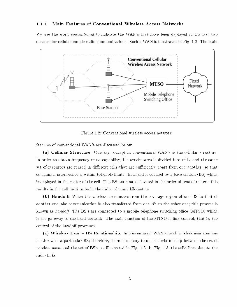
decades for cellular mobile radio communications. Such a WAN is illustrated in Fig. 1.2. The main

MTSO

Base Station

Mobile TelephoneSwitching Office

FixedNetwork

Wireless Access NetworkConventional Cellular

Figure 1.2: Conventional wireless access network.

features of conventional WAN's are discussed below.

(a) Cellular Structure: One key concept in conventional WAN's is the cellular structure.

In order to obtain frequency reuse capability, the service area is divided into cells, and the same

set of resources are reused in dierent cells that are suciently apart from one another, so that

co-channel interference is within tolerable limits. Each cell is covered by a base station (BS) which

is deployed in the center of the cell. The BS antenna is elevated in the order of tens of meters; this

results in the cell radii to be in the order of many kilometers.

(b) Hando: When the wireless user moves from the coverage region of one BS to that of

another one, the communication is also transferred from one BS to the other one; this process is

known as hando. The BS's are connected to a mobile telephone switching oce (MTSO) which

is the gateway to the xed network. The main function of the MTSO is link control; that is, the

control of the hando processes.

(c) Wireless User BS Relationship: In conventional WAN's, each wireless user commu-

nicates with a particular BS; therefore, there is a many-to-one set relationship between the set of

wireless users and the set of BS's, as illustrated in Fig. 1.3. In Fig. 1.3, the solid lines denote the

radio links.

3

users

BS’s

Figure 1.3: Many-to-one set relationship between the set of wireless users and the set of BS's.

(d) Distributed Processing: One other main feature of conventional WAN's is that the

processing is distributed in the system. In other words, along with the processes performed in

bulk (such as, amplication), all the signal-specic processing (such as, ltering, modulation, and

detection) is performed at the BS's. Obviously, this yields expensive BS's.

1.1.2 Cellular Air-Interface Standards

Before discussing the interference-related issues in conventional WAN's, we will brie y address the

main cellular air-interface standards in North America and Europe.

The rst cellular standard in North America, AMPS (advanced mobile phone system), was

introduced in 1983. AMPS is a frequency division multiple access (FDMA) -based analog system

which employs frequency modulation (FM). AMPS and similar analog standards are referred to as

rst generation (1G) systems.

The next widely deployed cellular standard in North America is IS-54 which was introduced

in 1990. IS-54 is sometimes referred to as digital-AMPS because of its capability of backward

compatibility. Around the same time (in 1991), another standard, GSM (global system for mobile),

was introduced in Europe. Both IS-54 and GSM are time division multiple access (TDMA) -based

digital systems.

Finally, in 1993, IS-95 standard was introduced. IS-95 is also a digital system, but based on

code division multiple access (CDMA). The digital IS-54, GSM, and IS-95 standards are referred

to as second generation (2G) systems.

Presently, the specications of the third generation (3G) systems are being discussed. There is

strong indication that the 3G systems will employ wideband-CDMA technique, and are expected

to be deployed early in the next century.

4

1.1.3 The Nature of Multiple Access Interference in Various Multiple Access

Schemes

In multiple access schemes, since more than one user can utilize the same resource (time or fre-

quency), MAI occurs. There are two types of MAI, namely, intracell and intercell interference, and

their relative signicance diers from one multiple access scheme to another.

TDMA and FDMA are slotted schemes; that is, the resources are allocated to users in a dis-

jointed manner. In TDMA or FDMA systems, since the orthogonality of the time or frequency

slots in a cell can easily be maintained, the intracell interference can be eliminated completely.

Therefore, in these systems, it is the intercell interference which is the single most important factor

preventing the use of the available time or frequency slots in adjacent cells. Consequently, the

reduction of interference in TDMA or FDMA systems yields a smaller reuse distance, in other

words, a smaller cluster3 size.

Clearly, in TDMA and FDMA systems, the interference is from users in other clusters. In a

CDMA system, however, resources are all allocated to simultaneous users (this yields a cluster size

of 1). Therefore, each user in the system contributes to the background noise aecting the other

users.

The forward4 link of a cellular system constitutes a one-to-many channel, and the reverse link,

a many-to-one type. However, because of the disjoint allocation of channels and the maintenance

of orthogonality in FDMA and TDMA systems, both the forward and reverse links are, indeed,

composed of many one-to-one channels. Similarly, in the forward link of a CDMA system, through

the use of synchronization and orthogonal spreading codes, the orthogonality can be maintained;

so the forward link of a CDMA system is also composed of many one-to-one channels. On the other

hand, synchronization in the reverse link of a CDMA system is, in general, very dicult. As a

result, all the users interfere with one another; in other words, the reverse link of a CDMA system

constitutes a truly many-to-one channel.

Interference management is very important in cellular systems regardless of the multiple access

scheme used. After all, it is the level of interference that determines the frequency reuse eciency.

However, it should be emphasized that the concept of interference management is fundamentally

more important for CDMA systems than for FDMA and TDMA types | this applies especially

3A cluster is a set of cells in which all the available bandwidth is utilized. Therefore, a cluster is the main

building block in constructing the frequency reuse pattern. In FDMA and TDMA systems, cluster sizes of 4 and 7

are commonly used.4The forward link is dened as the radio link from the BS to the wireless users, and the reverse link is that from

the wireless users to the BS.

5

in the reverse link of an asynchronous CDMA system, because of the many-to-one nature of the

multiple access channel, as discussed above. Any reduction in MAI, in a CDMA system, yields a

direct increase in the capacity. Interference reduction also yields a capacity increase in FDMA and

TDMA systems, but this increase is not as signicant as that in CDMA types.

In the next section, spatial processing features of recent WAN's, which yield ecient interference

reduction, are discussed.

1.2 Spatial Interference Control Features of Recent CDMA-Based

WAN's

The conventional WAN architecture discussed in the previous section was originally designed for

FDMA systems. Later on, when TDMA systems were introduced, they also used the same WAN

architecture. In time, when greater capacity and better coverage were required, smaller cells with

less elevated antennas have been deployed. The deployment of even smaller cells, which are referred

to as microcells, has been discussed in the literature for a signicant period [13, 14]. It is worth

noting, however, that despite the smaller cell size and less elevated BS antennas, the microcellular

systems have essentially the same architecture, and thus the same features, as the conventional

WAN's discussed in Sec. 1.1.1.

The conventional WAN architecture does not have rigorous spatial processing capability, which

is very eective in interference reduction in CDMA systems. Because of this fact, with the standard-

ization of CDMA with IS-95, some modications were made in the conventional WAN architecture

to introduce spatial processing features.5 Although the scope of these modications were limited,

they resulted in signicant capacity enhancements in IS-95 based systems. A summary of the major

spatial interference control features of such WAN's are discussed below.

(a) Sectorized Antennas: By employing (360=p)o sectorized antennas (p is a positive integer),

MAI can be reduced approximately p times, and thus the capacity can be increased approximately

p times.6 Sectorized antennas are also eective in FDMA and TDMA systems; by employing 120o

(p = 3) sectorized antennas, the cluster size can be reduced from 7 to 4. However, it should be

noted that the resulting increase in capacity (1.75 times) is still signicantly lower than that (3

times) in a CDMA system.

5During the course of time, some of these modications have also been adapted for FDMA- and TDMA-based

systems.6The increase in capacity will, however, be less than p times in practice, because of the imperfections in the

antenna patterns.

6

(b) Soft Hando: In the reverse link of a CDMA system, during the process of hando, the

users

BS’s

Figure 1.4: Many-to-many set relationship between the set of wireless users and the set of BS's, in

a cellular system with soft hando.

wireless user may communicate with two or more BS's simultaneously; this process is known as

soft hando. Soft hando (in the forward link) is a unique capability of CDMA systems; such a

concept does not exist in (the forward links of) FDMA and TDMA systems. In a system with soft

hando, there is a many-to-many set relationship between the set of wireless users and the set of

BS's, as shown in Fig 1.4, unlike the many-to-one type in the conventional WAN's (see Fig 1.3). In

Fig 1.4, the solid and broken lines denote the permanent and temporary radio links, respectively.

(c) Antenna Arrays: By using an array of collocated antenna elements (AE's), the antenna

radiation pattern can be electronically steered, so that the main lobe and the nulls of the radiation

pattern can be directed towards the user of interest and the interferers, respectively. Obviously,

this scheme yields substantial enhancements in SIR values [1517].

(d) Distributed Antennas: A distributed antenna (DA) system also employs many AE's, but

these AE's are distributed throughout the cell, unlike an antenna array where the AE's are located

only a few wavelengths apart. The DA structure is radically dierent than the conventional BS

antenna type. Since DA and its derivatives constitute the main topics of this thesis, this antenna

structure is discussed in detail in the next section.

Power control algorithms (which are essential in CDMA systems), as well as advanced signal

processing techniques, such as multiuser detection, are not included in the above list, since the

improvements obtained from these techniques do not result directly from the spatial processing

features of the WAN architecture.7

1.3 Distributed Antenna Systems

In mid-1950's, it was accidentally discovered that an imperfectly shielded wire radiates continuously.

This was the origin of leaky feeder techniques (shown in Fig. 1.5(a)), which were used without being

7Power control will be discussed in great detail in Ch.s 2 and 4.

7

Leaky Feeder Distributed Antenna

(a) (b)

AB

12

3 4

5

6

7

8

9

Central Station Central Station

Figure 1.5: (a) Leaky feeder. (b) Distributed antenna.

entirely understood for about 20 years [18,19]. Leaky feeders have found wide usage in subsurface

communications, such as in mines and tunnels, in order to achieve simple coverage. Recently, leaky

coaxial feeders are being considered for road vehicle communications in intelligent transportation

systems [20].

DA is the discrete version of the leaky feeder structure. Because of the signicant conceptual

dierences between the narrowband DA and CDMA DA systems, these two types are discussed

separately.

1.3.1 Narrowband DA Systems

In a DA system, many simple omni-directional AE's are coupled to a common feeder, as shown in

Fig. 1.5(b), and the same signal is transmitted from (and received by) all of these AE's. This is

generally called simulcasting. There is no signal-specic processing at the AE's; all of the processing

is performed at a central station (CS).8 However, amplication in the feeder and/or AE's would,

most likely, be inevitable.9

In a DA system, the AE's are distributed throughout the cell area; this is in contrast with the

situation in conventional cells where the BS antenna is centralized; we refer to this latter case as the

central antenna (CA) type. Note that the conventional CA system can be thought of as a special

case of the DA type with one AE.

The similarity between leaky feeder and DA is as that between integration and summation.

One main advantage of DA over leaky feeder is that there is more control on the DA structure,

since the radiation is from controlled locations.8The word central does not refer to the geographical center of the service area, but rather to the centralized nature

of signal processing. The CS can be located at any convenient place in the service area.9The practical issues related to deployment and implementation are discussed in detail in Ch. 6.

8

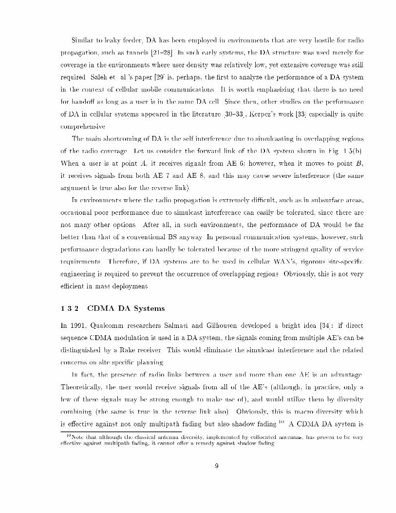
Similar to leaky feeder, DA has been employed in environments that are very hostile for radio

propagation, such as tunnels [2128]. In such early systems, the DA structure was used merely for

coverage in the environments where user density was relatively low, yet extensive coverage was still

required. Saleh et. al.'s paper [29] is, perhaps, the rst to analyze the performance of a DA system

in the context of cellular mobile communications. It is worth emphasizing that there is no need

for hando as long as a user is in the same DA cell. Since then, other studies on the performance

of DA in cellular systems appeared in the literature [3033], Kerpez's work [33] especially is quite

comprehensive.

The main shortcoming of DA is the self-interference due to simulcasting in overlapping regions

of the radio coverage. Let us consider the forward link of the DA system shown in Fig. 1.5(b).

When a user is at point A, it receives signals from AE 6; however, when it moves to point B,

it receives signals from both AE 7 and AE 8, and this may cause severe interference (the same

argument is true also for the reverse link).

In environments where the radio propagation is extremely dicult, such as in subsurface areas,

occasional poor performance due to simulcast interference can easily be tolerated, since there are

not many other options. After all, in such environments, the performance of DA would be far

better than that of a conventional BS anyway. In personal communication systems, however, such

performance degradations can hardly be tolerated because of the more stringent quality of service

requirements. Therefore, if DA systems are to be used in cellular WAN's, rigorous site-specic

engineering is required to prevent the occurrence of overlapping regions. Obviously, this is not very

ecient in mass deployment.

1.3.2 CDMA DA Systems

In 1991, Qualcomm researchers Salmasi and Gilhousen developed a bright idea [34]: if direct

sequence CDMA modulation is used in a DA system, the signals coming from multiple AE's can be

distinguished by a Rake receiver. This would eliminate the simulcast interference and the related

concerns on site-specic planning.

In fact, the presence of radio links between a user and more than one AE is an advantage.

Theoretically, the user would receive signals from all of the AE's (although, in practice, only a

few of these signals may be strong enough to make use of), and would utilize them by diversity

combining (the same is true in the reverse link also). Obviously, this is macro diversity which

is eective against not only multipath fading but also shadow fading.10 A CDMA DA system is

10Note that although the classical antenna diversity, implemented by collocated antennas, has proven to be veryeective against multipath fading, it cannot oer a remedy against shadow fading.

9

L:

K: # of users

# of antenna elements

Dem

odulator

Com

binerM

aximal R

atio

... ...= Σ

...

...th

...

1

i

K

L L

11

i1

j=1

L

i user’s receiver

Γ

i ΓijΓ

Central Station (CS)

L

123

DA Cell

DD

D

D

D D

Figure 1.6: CDMA DA system.

illustrated in Fig. 1.6.

In order to dierentiate the many replicas of the same signal at the receiver, CDMA modulation

is employed, and delay elements are inserted into the feeder in order to make sure that the time

dierence between the signals received from any two AE's is at least one pseudo-noise (PN) code

chip duration. In Fig. 1.6, D indicates the delay element.11 It should be noted that the delays

introduced throughout the feeder do not necessarily need to have the same value [36]. Also, it is

interesting to note that, depending on the inter-AE distance, the required delays for path resolution

may naturally be introduced as a result of the propagation delay in the cable.

1.3.3 Main Features of CDMA DA Systems

The salient features of the CDMA DA system can be discussed under two main categories: coverage

and diversity.

(a) Coverage: DA is very ecient in attaining coverage [37, 38]; this is especially important

in environments hostile to propagation. After all, coverage is the very main reason why DA (and

its precedent, leaky feeder) found widespread applications.

There are other benets related to ecient coverage. For instance, let us consider a linear area

(such as a highway) to be given radio coverage. If a CA is used, there is a signicant power waste, as

shown in Fig. 1.7. However, if a DA scheme is used, energy is injected only where it is required. The

11One way to realize the delay elements is through the use of surface acoustic wave (SAW) technology [35].

10

D

D

D

D

CS CS

Distributed AntennaCentral Antenna

Figure 1.7: Uniform coverage with CDMA DA system.

corollary of this statement is that the formation of cells with desirable shapes, even non-contiguous

ones, is possible [39]. Ecient use of transmit power yields transmission with relatively low power

levels [40,41]. Power savings are especially important for the wireless terminals, since this results

in extended battery recharge times.

Ecient coverage has a very important impact on interference management: by using DA,

intercell interference can be reduced signicantly. This issue will be discussed in more detail in

Ch. 2.

(b) Diversity: DA provides not only microdiversity against multipath fading, but also macro-

diversity against shadow fading [37,38]. DA's macrodiversity capability is particularly important,

because schemes such as collocated antennas and antenna arrays cannot oer ecient solutions to

shadow fading.

It is worth noting that in the literature, CDMA DA has mainly been proposed for indoor

wireless communications [34,40]. The outdoor deployments of CDMA DA have been quite limited;

one such rare example is San Diego, California, area.12

1.4 Thesis Motivation and Outline

The following fundamental question is investigated in this thesis: In a CDMA system, how should

the signals be collected from and distributed to the wireless users? To this end, the main objective

of this thesis is to utilize antennas in novel ways so as to achieve performance benets at the system

12Personal communication with Ed Tiedemann, Vice-President, Technology, Qualcomm Inc., June 1998.

11

level.

The importance of nding ecient ways of delivering and receiving signals in wireless multiple

access environments is very well known. In this context, leading spatial interference control tech-

niques have been qualitatively discussed in Sec.s 1.1.3 and 1.2. The major part of this thesis is

devoted to furthering the understanding of spatial interference control, and the corresponding per-

formance improvements, in multi-antenna CDMA systems (where the transmission and reception

are through multiple antennas distributed in the service area).

The thesis outline is presented here. The motivation of the research in each chapter, not the

results, will be shown. At the end of each individual chapter, there is a section summarizing the

results of that chapter.

Chapter 2: Since CDMA DA provides coverage, and diversity against both shadow and multi-

path fading, it is intuitive to expect that this architecture would ease power control (PC), compared

to the conventional CA type. The relationship between the number of AE's in a DA system and

the resulting improvements in PC are discussed in Ch. 2.

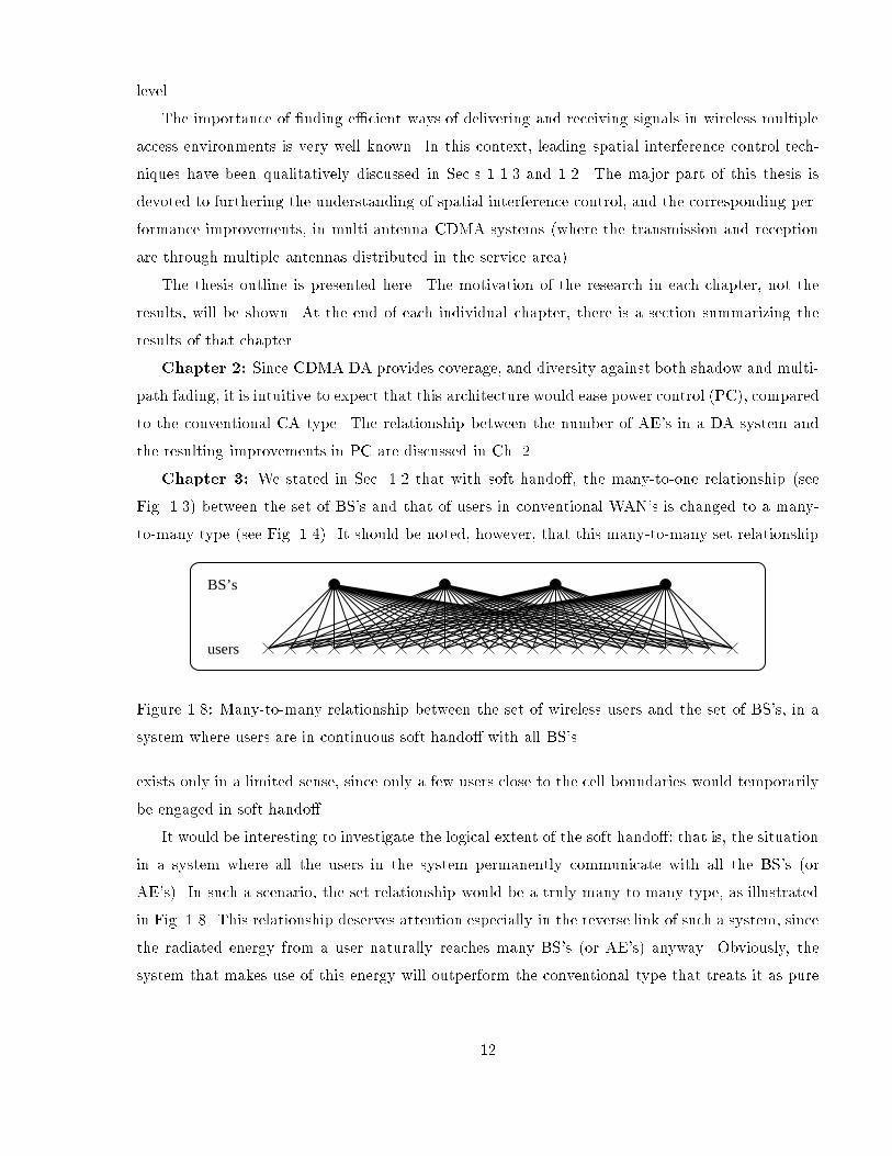
Chapter 3: We stated in Sec. 1.2 that with soft hando, the many-to-one relationship (see

Fig. 1.3) between the set of BS's and that of users in conventional WAN's is changed to a many-

to-many type (see Fig. 1.4). It should be noted, however, that this many-to-many set relationship

users

BS’s

Figure 1.8: Many-to-many relationship between the set of wireless users and the set of BS's, in a

system where users are in continuous soft hando with all BS's.

exists only in a limited sense, since only a few users close to the cell boundaries would temporarily

be engaged in soft hando.

It would be interesting to investigate the logical extent of the soft hando; that is, the situation

in a system where all the users in the system permanently communicate with all the BS's (or

AE's). In such a scenario, the set relationship would be a truly many-to-many type, as illustrated

in Fig. 1.8. This relationship deserves attention especially in the reverse link of such a system, since

the radiated energy from a user naturally reaches many BS's (or AE's) anyway. Obviously, the

system that makes use of this energy will outperform the conventional type that treats it as pure

12

interference. This system is called sectorized distributed antenna (SDA)13, and will be analyzed in

Ch. 3.

Chapter 4: In the SDA system described in Ch. 3, the concept of PC deserves special at-

tention. Because, the PC algorithms in the literature, developed mainly for conventional WAN

architectures (where the set relationship between the BS's and users is a many-to-one type), do

not necessarily perform eciently in an SDA system where the set relationship is many-to-many

due to macrodiversity. A new PC algorithm for SDA systems is introduced in Ch. 4.

Chapter 5: It is intuitive to expect that in an SDA system placing more AE's would yield a

better performance. But, in a given service area to be covered by an SDA cell, is it possible to place

as many AE's as we wish without an upper limit, or the law of diminishing returns apply after a

certain point? Also, in a service area, are some AE locations better than the others? The eects of

the number and location of AE's on the performance of SDA systems are analyzed in Ch. 5.

Chapter 6: In a system which consists of a few BS's and a switching oce, it may not

matter how the interconnection of these network elements is made. But, if there is an extensive

network with thousands of AE's and numerous processors/switches, then it may be crucial to have

a strategy or algorithm to achieve the interconnection in an ecient manner, since even modest

improvements in the design of the WAN would result in signicant savings. In this chapter, antenna

interconnection strategies for wireless access networks are studied in order to determine cost-ecient

as well as robust and exible interconnection architectures.

Chapter 7: In this chapter, some of the main results of Ch.s 2-6 are reemphasized, by com-

paring the multi-antenna systems addressed in this thesis with the conventional cellular systems.

A nal note is that in the rest of this thesis, DA and SDA refer to CDMA DA and CDMA SDA

systems, respectively, unless otherwise stated.

Parts of this thesis (Ch.s 2, 3, 4, and 6) were published (or are accepted for publication)

in [4248]. The work in Ch. 5 is under preparation for publication.

13The reason for using the term sectorized will be explained in Ch. 3.

13

Chapter 2

Reverse Link Power Control and Number of Antenna Elements in

CDMA Distributed Antenna Systems

In this chapter the relationship between the number of AE's in a CDMA DA system and the

yielding reverse link SIR is investigated by taking PC dynamic range into account.

In environments hostile to propagation, perfect power control may not be realized with a CA,

because this would require an impractically high dynamic range. This situation may yield a signif-

icant decrease in capacity. In such environments, the DA system is an ideal solution, since as the

number of antenna elements increases, the dynamic range of the power control decreases.

2.1 System Model

In a CDMA DA system, the resolved signals are individually demodulated and then combined in a

maximal ratio combining scheme to attain diversity, as illustrated in Fig. 1.6. In such a case, the

output SIR at the CS for any user i, i, would be

i =LXj=1

ij ; i 2 f1; : : : ; Kg; (2.1)

where K is the number of users, L is the number of AE's, and ij is the SIR at the jth nger of

the receiver corresponding to user i.

Throughout this thesis, a at fading channel is considered. For small cell sizes with IS-95 type

chips rates (around 1 Mcps), the at fading assumption would be a realistic one. In such a case,

there is assumed to be only one path between a user and an AE. Then, a total of L distinguishable

signals would be received at the CS from each user. Since the signals picked up by all the AE's

accumulate in the feeder, there are a total of LK signals delivered to the CS. In a particular user's

receiver, each nger of the Rake locks unto that user's signal received by one of the AE's, and

14

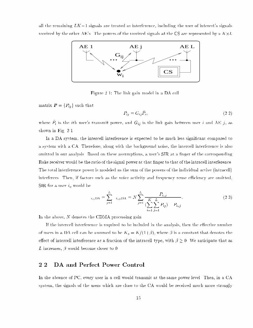
all the remaining LK1 signals are treated as interference, including the user-of-interest's signals

received by the other AE's. The powers of the received signals at the CS are represented by a KL

CS

... ...Gij

i

AE 1 AE j AE L

w

Figure 2.1: The link gain model in a DA cell.

matrix P = fPijg such that

Pij = Gij~Pi; (2.2)

where ~Pi is the ith user's transmit power, and Gij is the link gain between user i and AE j, as

shown in Fig. 2.1.

In a DA system, the intercell interference is expected to be much less signicant compared to

a system with a CA. Therefore, along with the background noise, the intercell interference is also

omitted in our analysis. Based on these assumptions, a user's SIR at a nger of the corresponding

Rake receiver would be the ratio of the signal power at that nger to that of the intracell interference.

The total interference power is modeled as the sum of the powers of the individual active (intracell)

interferers. Then, if factors such as the voice activity and frequency reuse eciency are omitted,

SIR for a user io would be

io;DA =LXj=1

ioj;DA = NLXj=1

Pioj

(KXi=1

LXj=1

Pij) Pioj: (2.3)

In the above, N denotes the CDMA processing gain.

If the intercell interference is required to be included in the analysis, then the eective number

of users in a DA cell can be assumed to be Ko = K=(1+), where is a constant that denotes the

eect of intercell interference as a fraction of the intracell type, with 0. We anticipate that as

L increases, would become closer to 0.

2.2 DA and Perfect Power Control

In the absence of PC, every user in a cell would transmit at the same power level. Then, in a CA

system, the signals of the users which are close to the CA would be received much more strongly

15

than those of distant users; this would be detrimental in the reverse link of a CDMA system |

a phenomenon known as the near-far problem. In addition, shadow and multipath fading occurs.

Therefore, it is essential to employ PC to eliminate the potential excessive dierences in the powers

of the received signals corresponding to dierent users.

2.2.1 Power-Balanced Power Control Algorithm

We consider a power-balanced PC (PBPC) algorithm similar to that of IS-95; i.e., the total received

power for every user is kept at a constant level.1 The PBPC problem in a DA system can be dened

as follows:

nd ~Pi; subject toLXj=1

Pij =LXj=1

Gij~Pi = 1; 8i: (2.4)

Obviously,

~Pi =

0@ LXj=1

Gij

1A1

; 8i: (2.5)

Therefore, if the link gains are known, PBPC is computationally very simple.

If PC can always be maintained despite distance, and shadow & multipath fading, then we

refer such a case as the perfect PC (PPC) type. In other words, if there is no upper or lower limit

imposed on the dynamic range (DR), or the required ~Pi always turns out to be between these limits

anyway, this is a PPC case.2 On the other hand, the case where these limits do exist due to the

practical limitations and thus ~Pi is at least occasionally hard-limited, is referred to as the limited

dynamic range type.

In the denition of PPC, we followed the convention in the literature. It is worth noting,

however, that perfectness in this context does not necessarily mean optimality. That is, a PC

algorithm may be perfect but suboptimal, such as the PBPC algorithm in a DA case. We will

discuss the optimal SIR-balanced PC algorithm in Ch. 4.

2.2.2 Single-Cell Systems

Let us consider a single-cell system with a CA andK users. If PPC is possible, then, by substituting

1The actual value of this constant does not aect the SIR value, because the SIR will be the ratio of the signal

and interference powers (when the background noise is omitted). Without loss of generality, we will assume that this

constant is 1.2In the PPC case, the power adjustments are assumed to be performed instantaneously with the required step

size.

16

CS

CS

CS

D D D D D

D D D

D

(a)

(b)

(c)

Figure 2.2: Coverage in a hostile environment: (a) with a CA, (b) with a DA with few AE's, and

(c) with many AE's.

L=1 in Eqn. 2.3, the SIR can simply be calculated as

i =N

K1 ; 8i: (2.6)

This is the best value achievable for such a scenario, therefore there is no need for DA in this case.

However, in environments with shadow and multipath fading, as the one depicted in Fig 2.2(a),

to maintain PPC continuously is often impossible. When a user's signal is in a deep fade, especially

because of blockage, a very high level of power would needed to be sent for relatively long periods,

and this would require an impractically large DR. It is worth noting that if PPC were possible,

then the SIR would still be the expression given in Eqn. 2.6.

The unrealistic requirements on the DR of PC, due to the blockage and shadow fading problems,

can be alleviated by using a DA (Fig 2.2(b)). In a DA cell, no user is almost ever signicantly

aected from shadow fading; therefore, the SIR is close to that of an ideal CA case as given in

Eqn. 2.6, where PPC is possible.

If the DR of PC is still high due to multipath fading, additional AE's can be used as illustrated

in Fig. 2.2(c).

17

2.2.3 Multi-Cell Systems

The situation is quite dierent in a multi-cell system because of the intercell interference. As

stated earlier, if a user's signal is in a deep fade or if blockage occurs between the user and the

corresponding CA, then this user must transmit at a very high power level in order to maintain

PPC. Since the multipath fading (and also to some extent the shadow fading) between a user and

the neighboring CA's is independent of that between the user and the corresponding CA, high

levels of interference occur for those neighboring CA's during the maintenance of PPC.3 Therefore,

continuous maintenance of PPC, which yields optimal results in a single-cell system, may yield a

considerable decrease in SIR (and thus, in capacity) in a multi-cell system employing CA's [49]. In

fact, it is shown in [49] that limiting the maximum transmitted power level in situations requiring

the transmission of very high levels of power, is a good compromise that increases the SIR (and

thus, the capacity) by reducing the excessive intercell interference.

In a DA system, on the other hand, such situations requiring the transmission of very high

levels of power are almost eliminated, even in systems with moderate L values. Therefore, in a

multi-cell environment even if maintaining PPC is possible with a CA, a DA system should be

preferred; because, by this way interference to adjacent cells is kept at a minimal level and thus

the system capacity is increased.

In the rest of this chapter, the benets of using the DA in a single-cell system is demonstrated;

it is worth noting that the returns are even more when the DA is employed in a multi-cell system.

2.3 Analysis and Simulation Results

Simulations with and without multipath fading have been run. For these cases, Gij 's are simply

taken to be

Gij;no-fading =1

d4ij; Gij;multipath-fading =

ijd4ij: (2.7)

In the above, dij is the distance between user i and AE j, and ij 's are independent exponential

random variables with E(ij) = 1; 8i; j (E(.) denotes the expected value). As it is well known,

the square of a Rayleigh distributed random variable is exponentially distributed.

Simulations have been run for various values of L which are chosen such thatpL's are integers;

namely, L = 1, 4, 16, and 100. L=1 corresponds to the CA, and L=100 is considered to give an

example of a case where L is very large. The AE's are assumed to be uniformly placed on a square

3The same reasoning is valid even if the required power level for maintaining PPC is beyond practical limits and

thus the wireless user transmits at the maximum power level available instead.

18

cell with side length y meters. It is further assumed that the AE's are meters above the users,

so the minimum value of dij is .

Based on these assumptions, the AE locations can be represented by the vector Z = fZlgl=Ll=1 ,

where Zl's are triplet entries denoting the coordinates of AE's:

Zl =

2[(l1) mod

pL] + 1

2pL

y; (1 2dl=pLe 1

2pL

) y;

!: (2.8)

In the above, d:e denotes the ceiling function. AE locations for the case of L= 16 is depicted in

y

: AE Location

y

κ

Figure 2.3: AE locations for the case of L=16.

Fig. 2.3. In the simulations is taken to be 0:02 y.

The rst two coordinates of the user locations are determined by two independent uniform

random variables in the range [0, y], and the third coordinate is always kept at zero. Finally, the

following values are chosen for N and K: N=128, K=50.

For a certain set of user locations, the SIR's for all the users are calculated, and this process is

repeated 200 times yielding a collection of 10,000 points to plot the CDF's (cumulative distribution

functions) accurately.

2.3.1 Range of SIR for the Case of PPC

For the case of PPC, the lower and upper limits of the SIR can be calculated. It is worth noting

that, in general, im 6= in , for fim; ing 2 f1; :::; Kg and im 6= in (see Eqn. 2.3).

A user im will have the lowest possible SIR if the signals from this user have equal strengths at

each AE; i.e., Pimj = 1=L; 8j (see Eqn. 2.4). If there is no fading, this will occur when the user is

at a point which is equidistant from all the AE's in the cell; i.e., if Gimj is the same for 8j. FromEqn. 2.3, the SIR at a nger of the Rake receiver of this user is calculated as

imj = N1=L

K 1=L=

N

LK1 ; 8j: (2.9)

19

After combining, the lower limit of SIR in a DA system with PBPC, DA,PBPC,LL, is found as

DA,PBPC,LL = L imj =NL

LK1 : (2.10)

On the contrary, a user in will have the highest possible SIR, if only one of the entries in the

inth row of P is 1, and all the rest are 0; i.e., if

Pinj =

8<: 1 if j = jn;

0 otherwise:(2.11)

For the case of no fading, this will occur when the user in is very close to an AE jn, thus its signal

is received by practically only this AE. In this case, there is no need for diversity combining, since

inj = 0; for j 6= jn. The upper limit of SIR, DA,PBPC,UL, is then the SIR at the jnth nger since

...i 1/L 1/L 1/L ... 1/L

K

1

1 2 j L

...i ...K

1

1 2 j L

0 1 0 0

P =P =

The Best CaseThe Worst Case

Figure 2.4: The P matrices corresponding to DA,PBPC,LL and DA,PBPC,UL cases.

there is no contribution from the other ngers of the Rake:

DA,PBPC,UL =N

K1 : (2.12)

The P matrices corresponding to DA,PBPC,LL and DA,PBPC,UL cases are illustrated in Fig. 2.4.

Note that the SIR expressions given in Eqn.s 2.6 and 2.12 are identical. Therefore, if the above

described scenario for the upper limit of SIR is true for all the users, i.e., i = DA,PBPC,UL; 8i,this means that the DA is behaving like a CA with PPC, which is the ideal case.

For an arbitrary set of user locations, the SIR's will be between the above limits depending on

the locations of the AE's and the users in the cell:N

K<

LN

LK1 i N

K1 ; 8i: (2.13)

Note that in the above, the upper limit corresponds to the case of L= 1 when there is power

control, while the lower one corresponds to the general case of L AE's with the limiting case of

20

L!1 given in parenthesis in Eqn. 2.13. Therefore, in a single-cell system, once PPC is achieved

with a certain number of AE's, adding more of them would not improve the performance. In fact,

the SIR would deteriorate, but only slightly, since the upper and lower limits are very close to each

other.

One may nd this result counter-intuitive, because a greater L corresponds to a Rake receiver

with a greater number of ngers, which, in turn, corresponds to more diversity branches. However,

it should be remembered that in the reverse link of a DA system, since all the received signals

accumulate in the feeder, with an increasing number of AE's the multiple access interference also

increases. This is a case where the Rake receiver has more ngers with poorer SIR values, which,

in the end, yields no further gain (once again, this is true as long as PPC is maintained).

In a multi-cell system, on the other hand, a greater L would yield a lower level of intercell

interference, which would correspond to a greater SIR value; however, the returns would diminish

gradually. Taking the increasing complexity and processing in the system into account, adding

more AE's would not worth after a point.

The CDF's of the SIR's for various number of AE's, with and without multipath fading, is

plotted in Fig. 2.5. It is observed from this gure that the range of SIR is

N

K= 4:08 dB NL

LK1 < N

K1 = 4:17 dB; (2.14)

in agreement with Eqn. 2.13.

2.3.2 Number of AE's and PPC Dynamic Range

As stated before, PC is essential to mitigate against the near-far problem. When the number of

AE's increases, the near-far problem becomes less signicant. Therefore, higher L values translate

into smaller PC DR's.

For the case where there is no fading, the maximum and minimum values of the transmit power

~P , namely, ~Pmax and ~Pmin, can be calculated, and then by taking their ratio, the PC DR can be

found. The calculations for L= 1 and L= 4 cases are given below; those for L= 16 and L= 100

cases are more tedious but can be carried out in a similar way.

L = 1: First, the following observation is made from Eqn.s 2.4 and 2.7: for the special case of

L=1, ~Pi reduces to ~Pi = d4i1; 8i.A user im will have to transmit at the maximum power level if it is at the farthest location from

the single AE, which corresponds to the corners of the cell: f(0; y; 0), (y; y; 0), (0; 0; 0), (y; 0; 0)g.Since Z = f(0:5y; 0:5y; 0:02y)g,

~Pmax = d4im1 = (0:52 + 0:52 + 0:022)2y4 = 0:25y4: (2.15)

21

4.08 4.09 4.1 4.11 4.12 4.13 4.14 4.15 4.16 4.170

0.1

0.2

0.3

0.4

0.5

0.6

0.7

0.8

0.9

1

x (dB)

P(S

IR ≤

x)

L=1, No Fading

L=1, Multipath Fading

L=4, No Fading

L=4, Multipath Fading

L=16, No Fading

L=16, Multipath Fading

L=100, No Fading

L=100, Multipath Fading

0 1 2 3 4 5 60

0.5

1

P(S

IR ≤

x)

Figure 2.5: SIR statistics for varying numbers of AE's in a single-cell system, for the case of PPC,

with and without multipath fading, drawn in regular and enlarged scales.

On the other hand, a user in will have to transmit at the minimum power level if it is at the

point (0.5y, 0.5y, 0), which is the closest location to the AE. So,

~Pmin = d4in1 = (0:02y)4 = 1:6 107y4: (2.16)

Now, the DR can be obtained from Eqn.s 2.15 and 2.16 as

Dynamic Range = ~Pmax= ~Pmin = 62 dB: (2.17)

L = 4: Similar to the L=1 case, a user im will have to transmit at the maximum power level

if it is at one of the corners of the cell; say, at the point (0; y; 0). The corresponding link gains are

calculated from Eqn. 2.7 as Gim = f63:59; 2:56; 2:56; 0:79g y4, where Gim is the imth row of the

22

link gain matrix, G. Then, ~Pmax is obtained as

~Pmax = 1:44 102y4: (2.18)

A user in will have to transmit at the minimum power level when it is at the closest location

to an AE, which corresponds to one of the following points: f(0:25y; 0:75y; 0); (0:75y; 0:75y; 0);(0:25y; 0:25y; 0); (0:75y; 0:25y; 0)g; for instance, the point (0:25y; 0:75y; 0). Then, Gin = f6:25106; 15:95; 15:95; 3:99g y4, and

~Pmin = 1:60 107: (2.19)

Finally, from Eqn.s 2.18 and 2.19, the DR is calculated as

Dynamic Range = ~Pmax= ~Pmin = 49:5 dB: (2.20)

For comparison, the DR's obtained from the simulations are also given in the following table:

Dynamic Range (dB)

L 1 4 16 100

No Fading 58.6 49.4 36.1 20.8

Rayleigh Fading 99.7 66.5 53.8 35.3

The CDF's of the DR's are plotted in Fig. 2.6, for the cases where there is no fading and where

there is multipath fading. It is obvious from this gure and from the above table that as L increases,

the DR decreases. Also, note that for the case where there is multipath fading, the reduction in

the DR is most signicant (more than 43 dB) when L is increased from 1 to 4.

It is further observed from Fig. 2.6 and the above table that the DR is considerably higher for

the cases where there is multipath fading; this is even more signicant for smaller L values.

In the limiting case, a 2-dimensional leaky feeder can be imagined; this would correspond to

the case where L ! 1. In such a case, there would not be any near-far problem, and thus, there

would not be any need for PC:

L = 1 ) Dynamic Range: Very high (may!1)

L!1 ) Dynamic Range = 0 dB: (2.21)

Eqn. 2.21 implies that in the limiting case of L !1, a coverage rule other than d type, where

is the distance-power-law coecient, is attained:

L = 1 ) d

L!1 )8<: d0; inside the DA cell

0; outside the DA cell.(2.22)

23

0 10 20 30 40 50 60 70 80 900

0.1

0.2

0.3

0.4

0.5

0.6

0.7

0.8

0.9

1

x (dB)

P(Dy

nami

c Ran

ge ≤

x)(a) No Fading

L=1 L=4 L=16 L=100

0 10 20 30 40 50 60 70 80 900

0.1

0.2

0.3

0.4

0.5

0.6

0.7

0.8

0.9

1

x (dB)

P(Dy

nami

c Ran

ge ≤

x)

(b) Multipath Fading

L=1 L=4 L=16 L=100

Figure 2.6: PPC dynamic range statistics in a single-cell system for varying numbers of AE's: (a)

no fading, and (b) multipath fading cases.

This would yield perfectly uniform coverage with no intercell interference.

However, it is worth noting that as L increases, so does the complexity and processing in the

system; the case where L!1 would require a Rake receiver with an innite number of ngers!

A nal note is that the SIR's corresponding to the cases addressed in this section will be similar

to those plotted in Fig. 2.5, where, due to PPC, the maximum and minimum values are between

the limits given in Eqn. 2.13.

2.3.3 SIR Statistics for the Case of no PC

Since the need for PC becomes less signicant as L increases, it is worth investigating the statistics

of SIR for the case where there is no PC at all. Fig. 2.7 shows the corresponding CDF's for varying

numbers of AE's, when there is no fading. For comparison purposes, the CDF of SIR for the case

24

−20 −15 −10 −5 0 5 10 150

0.1

0.2

0.3

0.4

0.5

0.6

0.7

0.8

0.9

1

x (dB)

P(S

IR ≤

x)

L=1, noPC L=4, noPC L=16, noPC L=100, noPCL=1, PPC

Figure 2.7: SIR statistics in a single-cell system, for varying numbers of AE's, when there is no

PC, also for the CA when there is PPC (all for the case when there is no fading).

of L=1 with PPC, i.e., the ideal case, is also shown in the same gure.

It is observed from Fig. 2.7 that as L increases, the SIR statistics approach that of the CA with

PPC; however, even for very large L values (such as 100), PC is still essential, but the corresponding

DR would be much smaller as discussed in the previous section.

Note that when there is multipath fading, the discrepancy between the cases where there is no

PC, and the CA case with PPC, would be even greater.

2.3.4 SIR Statistics for the Case of PC with Limited DR

So far, a DR without any limits is considered for the PC, which is referred to as the PPC. In this

section, the SIR statistics for the case of the limited PC DR, in the presence of multipath fading,

is investigated.

In order to set a realistic range for the DR, it is assumed that if there were no multipath fading,

PPC should have been maintained by one AE (i.e., the CA), therefore, the DR is set to 62 dB, the

value given in Eqn. 2.17. If the required power level for any user i, ~Pi;required, is greater than the

value given in Eqn. 2.15, or less than the one given in Eqn. 2.16, ~Pi is hard limited to these values,

25

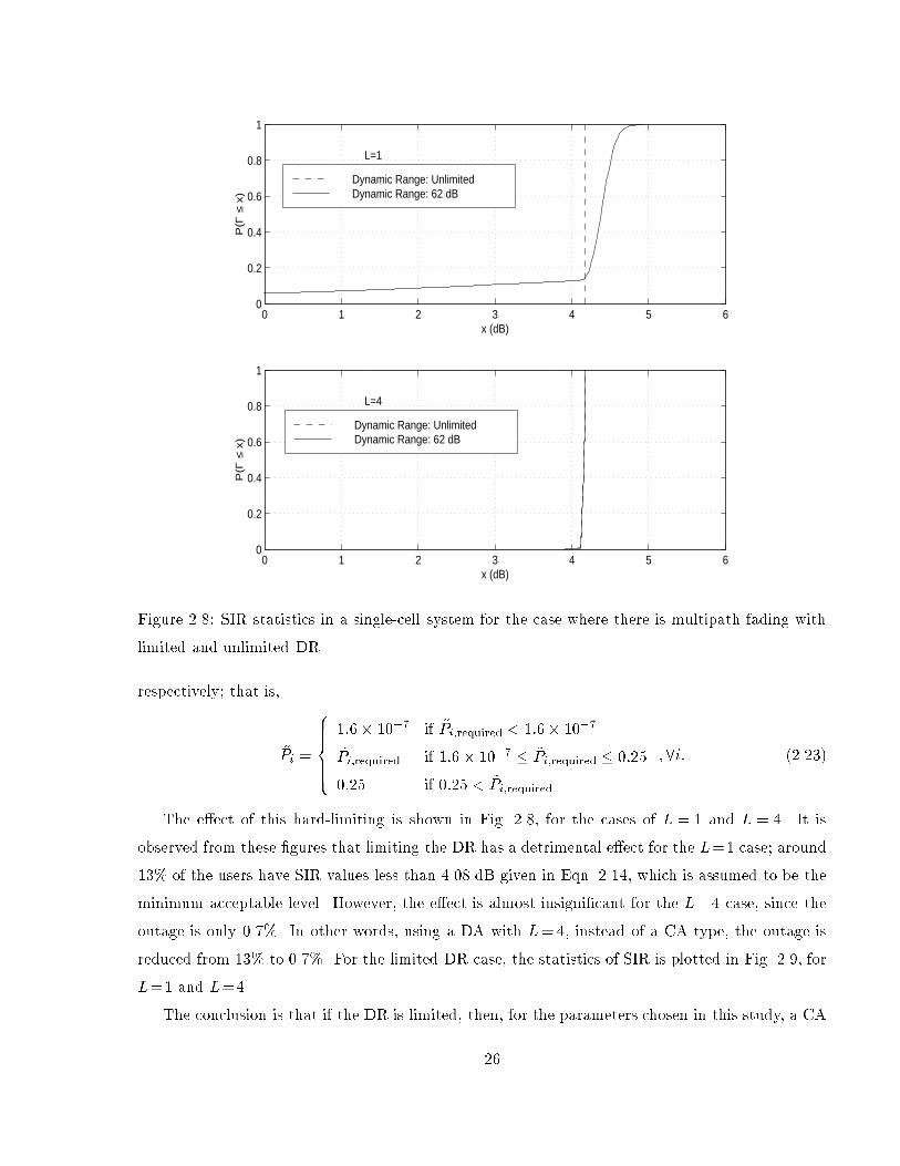
0 1 2 3 4 5 60

0.2

0.4

0.6

0.8

1

x (dB)

P(Γ

≤ x

)

L=1

Dynamic Range: UnlimitedDynamic Range: 62 dB

0 1 2 3 4 5 60

0.2

0.4

0.6

0.8

1

x (dB)

P(Γ

≤ x

)

L=4

Dynamic Range: UnlimitedDynamic Range: 62 dB

Figure 2.8: SIR statistics in a single-cell system for the case where there is multipath fading with

limited and unlimited DR.

respectively; that is,

~Pi =

8>>><>>>:

1:6 107 if ~Pi;required < 1:6 107

~Pi;required if 1:6 107 ~Pi;required 0:25

0:25 if 0:25 < ~Pi;required

; 8i: (2.23)

The eect of this hard-limiting is shown in Fig. 2.8, for the cases of L = 1 and L = 4. It is

observed from these gures that limiting the DR has a detrimental eect for the L=1 case; around

13% of the users have SIR values less than 4.08 dB given in Eqn. 2.14, which is assumed to be the

minimum acceptable level. However, the eect is almost insignicant for the L=4 case, since the

outage is only 0.7%. In other words, using a DA with L=4, instead of a CA type, the outage is

reduced from 13% to 0.7%. For the limited DR case, the statistics of SIR is plotted in Fig. 2.9, for

L=1 and L=4.

The conclusion is that if the DR is limited, then, for the parameters chosen in this study, a CA

26

0 1 2 3 4 5 60

0.1

0.2

0.3

0.4

0.5

0.6

0.7

0.8

0.9

1

Dynamic Range: 62 dB

x (dB)

P(Γ

≤ x

)

L=1L=4

Figure 2.9: SIR statistics in a single-cell system for the case where there is multipath fading and

the DR is limited to 62 dB, L = 1; 4.

system does not perform satisfactorily; however, the performance can be improved almost to that

of an ideal CA by using a DA with L=4.

2.4 Chapter Summary and Remarks

In environments hostile to propagation, achieving PPC may not be possible by using a CA, because

this would require an impractically large DR. This situation may yield a signicant decrease in the

capacity of the system. In such situations, the DA system is an ideal solution, since as the number

of AE's in a DA system increases, the DR of the PC decreases. It is demonstrated that by using a

DA system with as small as 4 AE's, instead of the CA type, the outage can be reduced from 13%

to 0.7%. It should be noted, however, that PC is essential even for DA systems with very large

numbers of AE's.

However, in a single-cell system (where intercell interference is not an issue), once the DR of

PC is between practical limits, adding more AE's to a DA does not improve the SIR. Yet, as L

increases, so does the complexity and processing in the system. Therefore, the optimal strategy for

27

a single-cell system can be stated as to put as many AE's as necessary to achieve PPC, but not to

exceed this number.

It is worth noting that in a single-cell system, even if all the energy in the air were to be

collected by a DA with innitely many AE's, the performance would not surpass that of an optimal

CA, which would most likely be a hypothetical one however, where signal uctuations can be

compensated for, in all fading conditions by a perfect PC scheme. So, the only extra benet would

be the reduction in PC DR, at the expense of increased complexity. In fact, if such a system were

possible, then, from solely an SIR point of view, there would be no need to introduce a DA system.4

In a multi-cell system, on the other hand, the DA system has the additional advantage of

reducing the intercell interference (compared to the CA type) with increasing number of AE's,

which would yield even higher SIR values. Therefore, the higher the L is the better the system

performs; however, even in this case, the returns would diminish gradually. Moreover, the increasing

complexity and processing in the system further imposes a limit on the number of AE's.

2.5 Future Research Directions

In the simulations, a Rayleigh fading channel model, which corresponds to the worst case, is

considered. However, in a DA system with many AE's, there will, most likely, be line-of-sight

between a wireless user and one or more AE's. Furthermore, in such cases, the distance-power-law

coecient, , may be around -2 rather than -4. In that case, the PC DR will further decrease by

using a DA structure.

On the other hand, in the analysis in this chapter, the loss (attenuation) in the cable is omitted;5

if the cable loss were incurred, the reduction in PC DR would have been more modest.

It would be interesting to perform a more realistic PC DR analysis by including the above

mentioned two points. In such an analysis, (a) a Rician channel, with d2 type signal attenuation

in the air, should be assumed between a user and the few closest AE's the channel between the

rest of the AE's should still be of Rayleigh type with d4 type attenuation; (b) the cable loss should

be incurred.

It is possible that these two eects may balance each other, and therefore, the gures that we

give in this chapter may, indeed, be not too far away from the real ones.

4It should be emphasized, however, that even in such a case DA has still other benets, as discussed in Sec. 1.3.3.

For instance, both the average and peak transmit power levels are considerably less in a DA system compared to

that which employs a CA. This translates into compactness and/or extended battery life for wireless terminals, which

might be quite an important factor.5We will brie y discuss the cable loss in Sec. 6.1.2 from an implementational point of view.

28

Chapter 3

CDMA Sectorized Distributed Antenna System

Although the simple structure of the DA system is quite attractive, it possesses an inherent limi-

tation: since all the AE's are coupled to a common feeder and there is no signal-specic processing

at the AE's, the multiple access interference, MAI, is accumulated in the feeder. This imposes a

direct limit on the capacity since CDMA systems are interference limited.

In summary, in a DA system, the \SIR", or equivalently, the \capacity", versus \number of

AE's (L)" curve would plateau with increasing values of L due to MAI. It is worth noting that

although the capacity of a DA system may be considerably higher than that which employs a CA

(due to diversity, maintenance of perfect PC, minimization of intercell interference, and so on), the

resultant increments in the capacity are nevertheless due to indirect eects. Therefore, the capacity

is still low per AE, especially for high L values. Indeed, this is the main limitation of a DA system.

3.1 The Concept of Sectorizing in a Distributed Antenna Struc-

ture

The accumulation of MAI is a consequence of the simple architecture of the DA system. It would be

most desirable if an architectural change yielding substantial reductions in the MAI were possible

without signicantly complicating the structure of the system.

In fact, such a change can be realized simply by connecting the AE's with separate feeders to

the CS as illustrated in Fig. 3.1. In this thesis, the limiting case of one AE per sector is investigated.

In such a case, a wireless user's signal can be picked up by all the AE's in a cell, and then, can be

optimally combined at the central station to enhance the performance. We call this novel antenna

architecture sectorized distributed antenna, SDA. In the reverse link of an SDA system, MAI can

be reduced by approximately a factor of L, and therefore, the SIR can be increased approximately

L times. The rest of the discussion regarding SDA will be on the reverse link, and in Sec.3.4 we

29

.

..

.

..D

emodulator

Com

binerM

aximal R

atio

...

= Σ

Central

(CS)

th

st

th

1 1

i 1

L

K

j=1

L

K: # of users

L: # of antenna elements

user’s receiver

1 user’s receiverStation

user’s receiver

K

i

ΓijiΓ

Γi1

2

......

...

L L-1

SDA Cell

Figure 3.1: CDMA sectorized distributed antenna system.

will address the possibilities in the forward link.

The SDA system is, in essence, still of a DA type, since all the salient characteristics of the DA

are preserved, such as the reception of the same signal by all the AE's, and the performance of all

the signal-specic processing at the CS. The AE's are also omnidirectional | the term sectorized

is used for this system because of the conceptual parallelism with sectorization in the conventional

cellular systems.

Along with possession of all the appealing features of the DA system, such as diversity and

reduction of intercell interference, the SDA system has one additional feature: the capacity limita-

tion in the DA system is eliminated. The increase in capacity will be demonstrated quantitatively

in Sections 3.2 and 3.3; nevertheless, for the sake of illustration, we give the following example to

compare the SIR's corresponding to DA and SDA systems.

Consider a hypothetical situation where each user's signal is received at approximately the same

power level at each AE. If this system is a DA type, then there would be a total of LK signals

accumulated in the feeder, from which only one would be utilized at a Rake nger. Thus, the SIR

for a user i can be calculated by using Eqn. 2.3 as

i;DA = NL=(LK1): (3.1)

In the case of the SDA system, however, there would only be K signals accumulated in each of the

30

separate feeders. Therefore,

i;SDA = NL=(K1): (3.2)

Now, the ratio of i;SDA to i;DA can easily be found as

i;SDA=i;DA = (LK1)=(K1) L; (3.3)

which maps to an approximately L-fold increase in capacity.

In an SDA system, certain system parameters, such as the cell geometry, location of AE's and

propagation conditions, can be such that a user's signal may eciently be received by only Lo L

AE's. Let us consider a system in which each user's signal is received by only Lo AE's at the same

power level, and the remaining LLo AE's do not receive any signal from that particular user. If

we assume that the users and AE's are distributed uniformly throughout the SDA cell, then, there

would be a total of LoK=L signals in each feeder. Therefore,

i;SDAjLo NLo

(LoK=L)1 =NL

K(L=Lo) NL

K1 : (3.4)

From Eqn.s 3.2 and 3.4 we conclude that even for the case of Lo L signicant signals, the almost-

linear increase in SIR is preserved. In the rest of this thesis, however, we assume that Lo = L,

unless otherwise stated.

In Ch. 2, a power-balanced PC algorithm is used. It will be demonstrated in Ch. 4 that,

although PBPC works very well in DA systems, it yields great variations among the SIR values of

dierent users in the SDA system.

In order to x this problem, we propose a PC algorithm which keeps the SIR for all users at

the same constant level, say , as follows: nd ~Pio subject to

io = NLXj=1

Gioj~Pio

KXi=1

Gij~PiGioj

~Pio

= ; 8io: (3.5)

We refer the above PC scheme as SIR-balanced macro power control (SBMPC). The details of the

SBMPC algorithm, its iterative solution, and the convergence characteristics of these iterations will

be analyzed in Ch. 4.

3.2 Lower and Upper Limits of SIR in an SDA System with

SBMPC

The lower and upper limits of SIR in a DA system with PBPC, DA,PBPC,LL and DA,PBPC,UL, are

given by Eqn.s 2.10 and 2.12. Similarly, we will compute the lower and upper limits of SIR in an

31

SDA system with SBMPC, namely, SDA,SBMCP,LL and SDA,SBMPC,UL. It should be borne in mind

that, in general, ik;DA,PBPC 6= il;DA,PBPC for ik 6= il; however, ik;SDA,SBMPC = ik ;SDA,SBMPC

for 8ik; il.In an SDA system, the users will experience the lowest possible SIR value if, at each AE, the

received signals from all the users are at the same power level; that is, Pij = mj , 8i; j. In the

above, mj is a constant. In general, mjk 6= mjl for jk 6= jl, where jk; jl 2 f1; : : : ; Lg . In this case,

at each Rake nger, there would be K signals of equal power (one of them is the signal of interest

and the remaining K1 are the interfering signals), and the contribution to SIR from each Rake

nger would be the same. Based on these facts, SDA,SBMPC,LL can be computed as

SDA,SBMPC,LL = NL=(K1): (3.6)

On the contrary, the users will experience the highest possible SIR, if only one of the entries

in each row of P is nonzero, and in each column there are K=L (assuming K=L is an integer)

nonzero entries with the same value; i.e., (Pij=(nj _ 0)) ^ (PL

j=1 Pij=nj ) ^ (PK

i=1 Pij=njK=L),

where nj is a constant, and ^ and _ denote the logical \and" and \or" operation, respectively. In

general, njk 6= njl for jk 6= jl, where jk; jl 2 f1; : : : ; Lg . In this case, there is no need for diversity

combining, and

SDA,SBMPC,UL =N

K=L 1=

NL

K L: (3.7)

The above expression is valid for the cases where L < K. If, however, L K, then SDA,SBMPC,UL

may approach innity according to our modelling. We note that in practical cases, almost always

L < K. Even in the exceptional cases where L K, SIR will never approach 1, because of the

background noise that we are omitting.

Now, using Eqn.s 2.10, 2.12, 3.6, and 3.7, we obtain

SDA,SBMPC,LL=DA,PBPC,LL=(LK1)=(K1)L; (3.8)

SDA,SBMPC,UL=DA,PBPC,UL=L(K1)=(KL)L: (3.9)

The results shown in Eqn.s 3.8 and 3.9 translate into an approximately L-fold increase in capacity.

Finally, we calculate the ratio of SDA,SBMPC,UL to SDA,SBMPC,LL, using Eqn.s 3.6 and 3.7, as

SDA,SBMPC,UL=SDA,SBMPC,LL = (K1)=(KL): (3.10)

The above expression is plotted in Fig. 3.2 as a function of K for various values of L, with K > L.

It is observed that for loaded systems (where K=L 1), the ratio given in Eqn. 3.10 is close to

unity; however, it may assume much greater values for unloaded systems (where K is in the order

32

0 10 20 30 40 50 600

2

4

6

8

10

12

14

16

K: number of users

SIR

SD

A,S

BM

PC

,UL/S

IRS

DA

,SB

MP

C,L

L

L=4 L=9 L=16

Figure 3.2: Comparison of the ratio of the upper and lower limits of SIR, for various values of L,

in an SDA system with SBMPC.

of L). The reason for this is that when K is in the order of L, the relative positions of the users

and the AE's have a greater impact on the SIR expression. Because, in an unloaded system, it is

possible to have a user distribution such that each user (or group of few users) is close to a dierent

AE. For the cases where K=L 1, on the other hand, there would always be many users around

each AE.

3.3 Simulation Results

For simulations, a single SDA cell with L AE's and K users is considered. The same assumptions

on the user distribution and AE locations (see Eqn. 2.8 and Fig. 2.3) are made. In this chapter,

L=4 and L=16 cases are considered with =0:02 y and N=128.

The intercell interference is, once again, omitted in our analysis. It is further assumed that

the multipath fading is averaged out; in this case, the performance of the system will only depend

on the local average received power. Based on these assumptions, the link gains are modeled as

Gij = Aij=dij , where Aij is a random quantity that models the power variation due to shadowing.

Aij 's are assumed to be independent, identically distributed log-normal random variables with 0 dB

expectation and 8 dB standard deviation. Also, = 4 is used in the simulations.

33

In the simulations, for a certain set of random user locations, rst, the G matrix is formed, and

then the balanced SIR value is calculated through the iterative solution of the SBMPC algorithm.

This process is repeated for 10,000 dierent user location sets in order to collect enough data to

plot the cumulative distribution functions (CDF's) accurately.

The SIR CDF's for various SDA systems with varying K and L values are shown in Fig. 3.3(a),

(b), and (c). In these gures, the number of users is kept xed (K=20, 80, and 400, respectively),

−5 0 5 10 15 20 250

0.2

0.4

0.6

0.8

1

(a)

L=1, K=20 L=4, K=20 L=16, K=20

−5 0 5 10 15 20 250

0.2

0.4

0.6

0.8

1

(b)

P(S

IR ≤

x)

L=1, K=80 L=4, K=80 L=16, K=80

−5 0 5 10 15 20 250

0.2

0.4

0.6

0.8

1

(c)

x(dB)

L=1, K=400 L=4, K=400 L=16, K=400

Figure 3.3: Comparison of SIR CDF's for SDA systems (employing SBMPC) for (a) K=20, L=4,

and 16, (b) K=80, L=4, and 16, (c) K=400, L=4, and 16.

but the number of EA's is increased from 1 to 4 to 16. It is observed that when L increases from

1 to 4, there is a gain of 6.5, 6.1 and 6.0 dB in the median values of the SIR's corresponding to

K=20, 80, and 400 cases, respectively; when L increases from 4 to 16, the corresponding gains are

7.4, 6.4, and 6.1 dB, respectively. This variation in gain is a result of the dierence between the

34

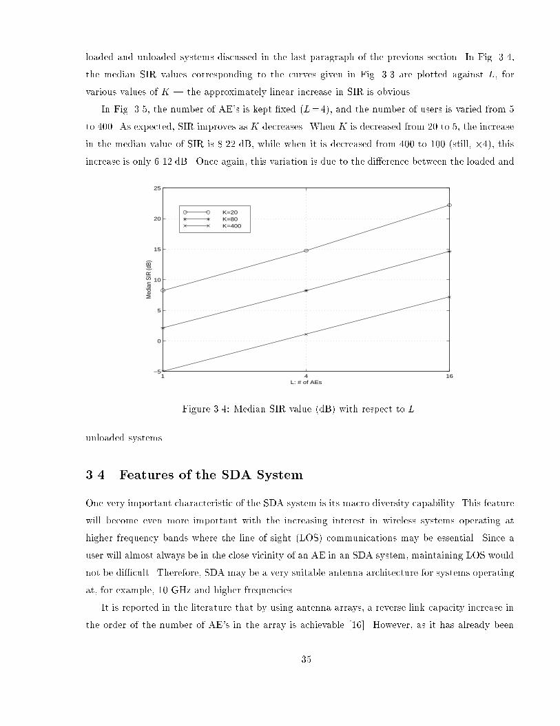
loaded and unloaded systems discussed in the last paragraph of the previous section. In Fig. 3.4,

the median SIR values corresponding to the curves given in Fig. 3.3 are plotted against L, for

various values of K | the approximately linear increase in SIR is obvious.

In Fig. 3.5, the number of AE's is kept xed (L=4), and the number of users is varied from 5

to 400. As expected, SIR improves as K decreases. When K is decreased from 20 to 5, the increase

in the median value of SIR is 8.22 dB, while when it is decreased from 400 to 100 (still, 4), thisincrease is only 6.12 dB. Once again, this variation is due to the dierence between the loaded and

1 4 16−5

0

5

10

15

20

25

L: # of AEs

Med

ian

SIR

(dB)

K=20 K=80 K=400

Figure 3.4: Median SIR value (dB) with respect to L.

unloaded systems.

3.4 Features of the SDA System

One very important characteristic of the SDA system is its macro diversity capability. This feature

will become even more important with the increasing interest in wireless systems operating at

higher frequency bands where the line of sight (LOS) communications may be essential. Since a

user will almost always be in the close vicinity of an AE in an SDA system, maintaining LOS would

not be dicult. Therefore, SDA may be a very suitable antenna architecture for systems operating

at, for example, 10 GHz and higher frequencies.

It is reported in the literature that by using antenna arrays, a reverse link capacity increase in

the order of the number of AE's in the array is achievable [16]. However, as it has already been

35

0 5 10 15 20 250

0.1

0.2

0.3

0.4

0.5

0.6

0.7

0.8

0.9

1

x (dB)

P(S

IR ≤

x)

L=4, K=5 L=4, K=20 L=4, K=80 L=4, K=100L=4, K=400

Figure 3.5: Comparison of SIR CDF's for SDA systems (employing SBMPC) which have L = 4

AE's, with K=5, 20, 80, 100, and 400.

discussed in Sec. 1.3.3(d), the antenna arrays do not have macro diversity capability. Hence, when

a blockage occurs in the radio link, an antenna array cannot provide a solution! Thus, an antenna

array cannot oer the immunity against shadowing eects that an SDA architecture can.

In microcellular systems, intercell interference is a nuisance that must be managed; therefore,

in cellular design, the propagation characteristics should be taken into account in order to nd

appropriate base station locations that would minimize the overlapping of the antenna radiation

patterns, and thus the intercell interference. However, intercell interference cannot be entirely

eliminated, and this inevitably introduces degradation in system performance. In an SDA system,

on the other hand, overlapping of the AE radiation patterns is not a problem; in fact, this may

yield an even better result due to diversity reception.

One other important point to note is that in the capacity calculations of microcellular systems,

the assumption of homogeneous user distribution throughout the service area is generally made.

In practise, however, this is usually not the case. As an example, let us consider a microcellular

system with 4 cells. If the capacity per cell is K users, then the system capacity is said to be 4K.

However, if these 4K users are in fact distributed as, say, 2K=3, 2K=3, 2K=3, and 2K users, among

the 4 cells in the system, then the system would be able to support only 3K users, not 4K! The

36

inhomogeneous user distribution is, in general, not a signicant problem in an SDA system.

The idea of sectorization in the context of DA is rst introduced in [39] in a qualitative manner.

In that conceptual study, a few AE's are placed in each DA sector, and mobile-transparent hando

is performed among the sectors. The SDA architecture presented here corresponds to the limiting

case of one AE per sector. However, there is still a major dierence between the system discussed

in [39] and the SDA architecture presented here, and that is the macrodiversity feature of the SDA

system in the reverse link. Because of this feature of the SDA system, the signals received by all

the AE's (sectors) are collectively decoded at the CS.

The discussions presented so far have been on the reverse link of SDA systems. As mentioned

in Section 3.1, in the reverse link of an SDA system, although a user's signal is picked up by all the

AE's, having separate feeders for each AE prevents the accumulation of MAI. This is not the case,

however, for the forward link. If, in the forward link, a user's signal is transmitted by all the AE's,

then the system will operate as a conventional DA type. Clearly, this would result in quite a large

dierence in the forward and reverse link capacities. As a remedy for this situation we propose

the following solution: in the forward link, the signal for a particular user could be transmitted

through the AE which has the highest SIR in the reverse link for that particular user.1 Therefore,

there would be selection diversity in the forward link, and thus, the benets of the macro diversity

would still be valid. In this SDA system, the reverse link would still outperform the forward one.

Yet, it should be noted that higher capacity in the reverse link is never a \problem"; in order to

equalize the capacities in both links, more resources (such as bandwidth), from the given pool, can

be allocated for the forward link.

The CDMA SDA system may have quite diverse applications with a wide range of cell sizes

and number of AE's. For example, an SDA cell may be as small as a microcell (or even a picocell)

with only a few AE's (even 2), or it may cover many square kilometers with many AE's. The

SDA structure may be utilized both indoors and outdoors, including linear service areas, such as

highways.

One other issue is related to the cost of the SDA system: since the SDA architecture has logical

star topology (that is, each AE requires a separate link to the CS), in an SDA system with a

large number of AE's, the deployment cost of the wired-network infrastructure may be of concern.

Robust, exible, and cost ecient AE interconnection strategies will be discussed in Ch. 7.

In [50], the ultimate reverse link capacity of a CDMA network is investigated. Although the

terminology and modeling in [50] is dierent than those used here (our work was done independently

1Alternatively, a few EA's can be utilized; in this case, the system will work similar to that described in [39] in

the forward link.

37

from that in [50]), the two systems are conceptually similar. Yet, the entirely dierent motivation,

approach, and emphasis in this thesis make it a dierent study than that of [50]. In Sec. 4.6, we

will make a comparison between the results of this chapter & the next one and those in [50].

3.5 Chapter Summary and Remarks

Despite possessing many appealing features, CDMA DA systems suer from low capacity per AE

as a result of the MAI accumulated in the common feeder. To overcome this capacity limitation, we

propose an antenna architecture called CDMA sectorized distributed antenna (SDA). In an SDA

system, a cell has many sectors in which separate feeders run, so MAI in the reverse link is reduced.

In this chapter, the limiting case of one AE per sector is investigated. In such a case, a wireless

user's signal can be picked up by all the AE's in an SDA cell, and then, can be optimally combined

at a central station.

We have demonstrated analytically and through simulations that in a CDMA SDA system the

SIR increases approximately linearly with increasing numbers of AE's (sectors). This increase in

SIR can be mapped into an equivalent increase in the capacity. If there is not enough demand for

all of the potential capacity oered by an SDA system, the increase in SIR can always be partly

transformed into higher transmission rates for the existing users.

Although an SDA cell with one AE per sector is similar in essence to a microcellular cluster

with many microcells, the SDA system has two main advantages as a result of the macro diversity

capability, combined with the SBMPC algorithm: the increase in capacity in an SDA system is still

valid (unlike in a microcellular type), even if (a) the antenna patterns of the AE's overlap, and (b)

the users are not distributed homogeneously throughout the service area. Therefore, sectorization

in the context of DA is more ecient than cell-splitting in the conventional cellular systems.

There still remains a fundamental question: in a given service area that is to be covered by

an SDA cell, can we put as many AE's as we wish without an upper limit? In an SDA system,

putting more AE's would always yield better performance (this is analogous to a dish antenna:

the greater the diameter, the better the performance). However, the returns in SIR may diminish

gradually as L increases, since signals received by dierent AE's would start being correlated. This

is an immediate consequence of the fact that when L increases, the AE's become closer together.

Taking the increasing complexity and processing in the system into account, adding more AE's

would not be worthwhile after a point, which puts an upper limit on the number of AE's (sectors).

The correlation eects will be discussed in Ch.s 5 and 6.

38

Chapter 4

SIR-Balanced Macro Power Control for the Reverse Link of

CDMA Sectorized Distributed Antenna Systems

Power control is a scheme by which the transmit power levels of the users in a system are controlled

and adjusted according to some criteria. The main purpose in employing PC is to keep the SIR level

(at the receiver) for all the users above a certain threshold. By employing PC, the possible extensive

disparities in users' signals (due to distance and multipath & shadow fading) are compensated for,

and at the same time, the injection of excessive energy into the system is prevented. Since each

user is a potential source of interference to other users in the system, any reduction in the transmit

power of a user also yields a reduction in MAI which aects all of the other users. However, the

transmit power of a user should not be reduced in an unregulated manner, since this may cause the

SIR level at the receiver (for that user) to drop to unacceptably low levels. It should be obvious

even from this short discussion that nding a good PC scheme is not a trivial problem.

In a CDMA system, PC is more critical and complicated in the reverse link, due to the well-

known near-far problem. Therefore, we consider only the reverse link PC problem.

4.1 Power Balanced Power Control in CDMA Systems

Many dierent PC algorithms have been suggested and examined in the literature. A commonly

used type in practice (such as in IS-95), due to its computational simplicity and satisfactory per-

formance, is the power-balanced power control PBPC algorithm discussed in Sec. 2.2.1. In PBPC,

each row of the received power vector, P, sums to a constant; that is, for each user, the total

received signal power from all the AE's is the same.

Although PBPC algorithm balances the signal power, it does not guarantee the same interference

for all users. Therefore, when PBPC is employed, in general, ik 6= il , for ik; il 2 f1; 2; : : : ; Kgand ik 6= il.

39

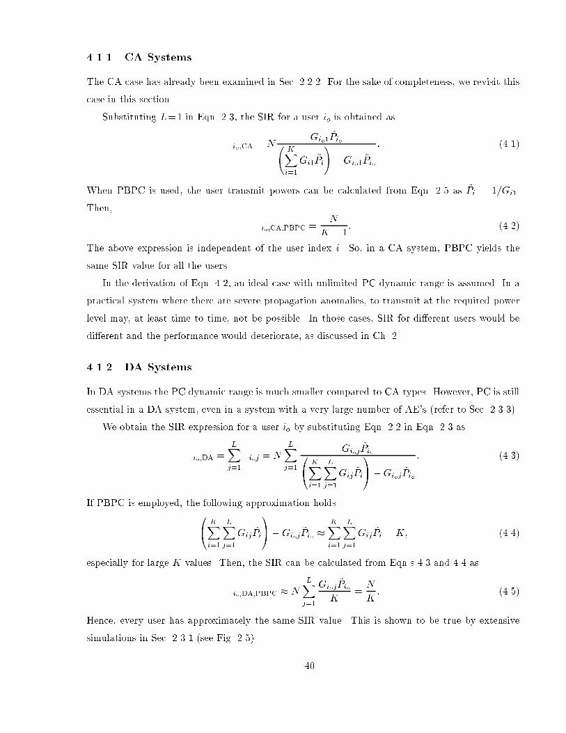
4.1.1 CA Systems

The CA case has already been examined in Sec. 2.2.2. For the sake of completeness, we revisit this

case in this section.

Substituting L=1 in Eqn. 2.3, the SIR for a user io is obtained as

io;CA = NGio1

~Pio KXi=1

Gi1~Pi

!Gio1

~Pio

: (4.1)

When PBPC is used, the user transmit powers can be calculated from Eqn. 2.5 as ~Pi = 1=Gi1.

Then,

io ;CA,PBPC =N

K 1: (4.2)

The above expression is independent of the user index i. So, in a CA system, PBPC yields the

same SIR value for all the users.

In the derivation of Eqn. 4.2, an ideal case with unlimited PC dynamic range is assumed. In a

practical system where there are severe propagation anomalies, to transmit at the required power

level may, at least time to time, not be possible. In those cases, SIR for dierent users would be

dierent and the performance would deteriorate, as discussed in Ch. 2.

4.1.2 DA Systems

In DA systems the PC dynamic range is much smaller compared to CA types. However, PC is still

essential in a DA system, even in a system with a very large number of AE's (refer to Sec. 2.3.3).

We obtain the SIR expression for a user io by substituting Eqn. 2.2 in Eqn. 2.3 as

io;DA =LXj=1

ioj = NLXj=1

Gioj~Pio0

@ KXi=1

LXj=1

Gij~Pi

1A Gioj

~Pio

: (4.3)

If PBPC is employed, the following approximation holds0@ KXi=1

LXj=1

Gij~Pi

1A Gioj

~Pio KXi=1

LXj=1

Gij~Pi = K; (4.4)

especially for large K values. Then, the SIR can be calculated from Eqn.s 4.3 and 4.4 as

io;DA,PBPC NLXj=1

Gioj~Pio

K=N

K: (4.5)

Hence, every user has approximately the same SIR value. This is shown to be true by extensive

simulations in Sec. 2.3.1 (see Fig. 2.5).

40

In order to develop a better insight into the relation between the MAI and PC in a DA system,

we consider a simple case with L= 4 and K = 5 as illustrated in Fig. 4.1. We assume that the

AE 4

AE 2AE 1D

D

D

w

w

w

w

CS

w

AE 3

DA Cell

x = 1 3

2

4

1

5 = (0.32, 0.28, 0.0),(0.20, 0.81, 0.0), (0.09, 0.46, 0.0),(0.52, 0.56, 0.0),(0.78, 0.34, 0.0)

User Locations

= AE1, AE2, AE3, AE4

= (0.25, 0.75, 0.02),(0.75, 0.75, 0.02), (0.25, 0.25, 0.02),(0.75, 0.25, 0.02)

Antenna Locations

= w1, w2, w3, w4, w5

Figure 4.1: An exemplary DA cell with L=4 and K=5.

5th user, w5, is the user of interest. As it is seen from Fig. 4.1, w5 is the closest user to AE4, and

moreover, there are no other users in the vicinity of AE4. However, in the same DA cell there are

other users which are closer to some other AE's, such as the pairs w1 AE3, and w2 AE1.

The approximate equivalent congurations sensed at the CS, at each nger of the Rake receiver

corresponding to w5, are depicted in Fig. 4.21; that is, as long as interference alone is considered,

Fig. 4.2 illustrates the approximation of each AE of the DA cell by a CA. In order to simplify the

illustration, it is assumed in Fig. 4.2 that a user's signal is picked up by only the closest AE.

The situation at the 4th nger of the Rake receiver is particularly important, because it can

easily be anticipated that the most signicant contribution to the nal SIR value would be from

this nger. Although this expectation is true, it is observed from Fig. 4.2(d) that the equivalent

conguration sensed at this nger is as if the distant users, which are in the vicinity of some other

AE's (that is, w1 and w2), were actually very close to AE4, which is the one near the user of

interest. Therefore, due to MAI, one would not be surprised to nd that even 54 will not be very

high.

The ij=N and i=N values for all users, in dB, without power control (noPC) and with PBPC,

are given in Table 4.1. In order to have a predictable (deterministic) case, the link gains are modelled

as Gij = d4ij , where dij is the distance between user i and AE j.2 When there is no power control,

1The delay elements inserted into the feeder are not shown in Fig. 4.2.2In the simulations presented in Sec. 4.4, a more realistic channel model with fading is considered.

41

AE 1 AE 2

AE 4AE 3

(a) (b)

(c) (d)

CS

CS

CS

CS

w

w

3

2 w1

w4

w5

w

ww

w

w

4

12

3

5

w w

ww

w

3

2

4

1

5

w

w

ww

w4

3

5

12

Figure 4.2: Approximate equivalent situation felt at the ngers of the Rake receiver corresponding

to 5th user, w5, from each AE in the DA system: (a) 1st nger, (b) 2nd nger, (c) 3rd nger, and

(d) 4th nger.

Pi's are taken to be constant, and for the case of PBPC, they are calculated according to Eqn. 4.3.

Also, it is worth noting that users w4 and w5 are not close to any AE, therefore the SIR values

corresponding to them is expected to be lower than the other 3 users.

Finally, we note the eect of PC: it is observed from Table 4.1 that for this given case, when there

is no PC, there is a dierence of approximately 22 dB between the highest and lowest SIR values;

on the other hand, this dierence is less than 1 dB for the case of PBPC. Even more important is

the fact that, the lowest SIR value is increased more than 17 dB when PBPC is employed instead

of noPC.

42

ij=N (dB) i=N

wnAE AE1 AE2 AE3 AE4P

w1 -34.99 -40.08 -1.37 -33.30 -1.37

w2 -2.06 -37.63 -37.91 -43.70 -2.06

DA noPC w3 -28.73 -42.23 -24.80 -41.53 -23.21

w4 -28.68 -26.92 -32.48 -31.39 -23.30

w5 -40.96 -32.48 -37.13 -6.49 -6.47

wnAE AE1 AE2 AE3 AE4P

w1 -38.24 -43.33 -6.03 -36.55 -6.02

w2 -6.03 -40.46 -40.74 -46.53 -6.02

DA PBPC w3 -12.26 -25.98 -7.94 -25.29 -6.47

w4 -12.11 -10.22 -16.06 -14.94 -6.71

w5 -40.60 -32.12 -36.78 -6.05 -6.03

Table 4.1: ij=N and i=N values, in dB, for DA without power control (noPC) and with power

balanced power control (PBPC).

4.1.3 SDA Systems

Since PBPC works well in DA systems, it would be logical to investigate the performance of this

PC scheme in SDA systems.

In an SDA system, since a substantial portion of the multiple access interference is rejected,

SIR takes the following form:

io;SDA =LXj=1

ioj = NLXj=1

Gioj~Pio

KXi=1

Gij~Pi

!Gioj

~Pio

: (4.6)

When PBPC is employed, it is, in general, not accurate to approximate the denominator of the

above expression (inside the summation) by the rst term which is in parentheses. Moreover, even

if this were possible, it would not yield an SIR expression independent of user index, because the

summationPK

i=1Gij~Pi depends on the AE index j, and thus, does not yield a constant. Therefore,

in an SDA system employing PBPC, SIR for dierent users may vary signicantly.

In order to illustrate this point in a quantitative manner, we continue with the example given

in Sec. 4.1.2; this time we consider an SDA system instead of a DA type. The ij=N and i=N

values for all users, in dB, without power control and with PBPC, are given in Table 4.2. In the

43

ij=N (dB) i=N

wnAE AE1 AE2 AE3 AE4P

w1 -30.86 -14.59 20.00 -25.96 20.00

w2 20.94 -12.03 -34.20 -36.37 20.94

SDA noPC w3 -24.60 -16.79 -21.08 -34.19 -14.87

w4 -24.54 3.55 -28.77 -24.04 3.57

w5 -36.83 -6.21 -33.42 21.47 21.48

wnAE AE1 AE2 AE3 AE4P

w1 -33.21 -32.87 0.88 -30.23 0.89

w2 2.43 -30.01 -36.33 -40.21 2.43

SDA PBPC w3 -6.63 -15.42 -2.09 -18.93 -0.57

w4 -6.45 14.25 -11.46 -8.14 14.32

w5 -35.57 -21.64 -32.37 7.64 7.65

Table 4.2: ij=N and i=N values, in dB, for SDA without power control (noPC) and with power

balanced power control (PBPC).

preparation of this table, the same assumptions are made as in the preparation of Table 4.1. It is

observed from Table 4.2 that for this exemplary case, the lowest SIR value is increased by more

than 14 dB, by using PBPC instead of noPC. Moreover, the dierence between the highest and

lowest SIR values is decreased from almost 36 dB to about 15 dB. Although these are signicant

improvements, the 15 dB dierence in SIR values among various users is still unacceptably high.

We note that this dierence is less than 1 dB in the DA case with PBPC (see Table 4.1).

After giving the above example for the purpose of developing insight into the PC problem, we

provide the CDF's of SDA,PBPC's in Fig. 4.3, for the cases of L=4; K=5, and L=4; K=100.3 It

is observed from Fig. 4.3 that the disparity among the SIR values is more signicant in unloaded

(low K=L ratio) systems compared to that in loaded (high K=L ratio) ones. This is the result of

the averaging eect in the loaded systems: despite the possible extensive dierences (many orders

of magnitude) among the entries of the P matrix, the column sums, (PK

i=1Gij~Pi) tend to be in the

same order of magnitude when K is large. Therefore, PBPC performs worse in unloaded systems.

We conclude from the discussions in this section that there is a need to search for a better PC

algorithm.

3The assumptions made and the simulation parameters used to plot the curves in Fig. 4.6 are discussed in Sec. 4.4.

44

5 10 15 20 25 30 35 40 450

0.1

0.2

0.3

0.4

0.5

0.6

0.7

0.8

0.9

1

x (dB)

P(Γ

≤ x)

L=4 AEs, K=5 users, PBPC L=4 AEs, K=100 users, PBPC

Figure 4.3: CDF of SDA,PBPC for L=4; K=5, and L=4; K=100.

4.2 SIR-Balanced PC in CA Systems

Since the system performance depends on the SIR, not on the received power level, a PC scheme

which balances SIR, rather than the received power, would expected to perform better. Moreover,

this is a fair PC scheme since it yields the same SIR level for all users. In fact, PC algorithms

which balance the SIR value have been studied in the literature, for conventional cellular systems

with CA's, under the name SIR-balancing.

The concept of SIR-balancing is rst introduced in [51] in the context of interference manage-

ment in satellite communications. These results are broadened in [5254] and applied to non-fading

cellular DS-CDMA systems. Subsequently, an optimal global PC algorithm that minimizes outage

probability using SIR-balancing with cell removal is demonstrated in [55]; this PC algorithm is

applicable mainly for TDMA and FDMA systems. The main drawback of this algorithm is that it

requires continuous access to all radio paths in the system; therefore, its use in practical cellular

systems is very dicult. Nevertheless, the results provide estimates for the optimal performance.

An almost-distributed algorithm that converges to the optimal one is discussed in [56]. In that

study, each base station (and user) would control its own transmit power based on only limited

knowledge about the link gain matrix. It is shown in [57] that maximizing the minimum SIR level,

or equivalently minimizing the maximum one, is equivalent to SIR-balancing.

In [5156], the problem of SIR-balanced PC, which we will refer to as SBPC, is rst presented

45

in matrix notation, then transformed into an eigenvalue problem, and nally, solved analytically

using matrix algebra. However, there is a major dierence between those cases and the SDA system

that we are analyzing: in the SDA system there is diversity reception which complicates the PC

problem signicantly.

In the conventional cellular systems, in the absence of macro diversity, each user communicates

with only one base station. Obviously, this is signicantly dierent than the SDA system where

each user communicates with all the AE's. Consequently, modelling of such a conventional cellular

system is quite dierent than that of an SDA type. If we use the same L and K values for both

systems, then for the conventional cellular case, there would be L dierent cells each with one CA,

compared to one cell with L AE's in the case of an SDA system. Also, the number of users in each

of the conventional cells would be K=L, assuming uniform user distribution.

4.3 SIR-Balanced Macro PC (SBMPC)

In this section, a PC algorithm that balances SIR in SDA systems is given; we refer to this algorithm

as SIR-balanced macro PC (SBMPC).

SBMPC Algorithm: nd f ~PigKi=1 subject to

i;SDA,SBMPC = NLXj=1

Gij~Pi

KXk=1

Gkj~Pk

!Gij

~Pi

= ; 8i: (4.7)

Because of the outmost summation (P

j) in Eqn. 4.7, which appears as a result of diversity com-

bining, the set of equations given in Eqn. 4.7 become nonlinear. Therefore, the eigenvalue method

described in the previous section does not apply here.

However, we can nd the transmit power vector, ~P, by solving Eqn. 4.7 iteratively. Note that

there are K equations, but K+1 unknowns, namely, and f ~PigKi=1. Therefore, ~Pi's will be obtainedwithin a multiplicative constant. We x ~P1 and nd f ~PigKi=2 as proportional to ~P1. Therefore, ~P1

at the th step of iterations is ~P()1 = ~P

(0)1 .

First, we rearrange Eqn. 4.7, and denote the ith equation by Ei, as follows:

E1 : = NLXj=1

G1j~P1

KXk=1

Gkj~Pk

!G1j

~P1

; (4.8)

46

Ei : ~Pi =

NLXj=1

Gij KXk=1

Gkj~Pk

! Gij

~Pi

; i = 2; 3; : : : ; K: (4.9)

Now, we can state the iterative solution.

SBMPC Iterative Solution Algorithm I:4

~P(0) =n~P(0)i

o=

8><>:0@ KXj=1

Gij

1A19>=>; ; i = 1; 2; : : : ; K;

(+1) = E1~P()

;

~P(+1)1 = ~P

()1 ;

~P(+1)i = Ei

(+1); ~P()

n~P()i

o; i = 2; 3; : : : ; K: (4.10)

The algorithm starts with an initial vector which is calculated according to PBPC. In the above

algorithm, Ei(:) denotes inserting the variables in the brackets into Ei given in Eqn.s 4.8 and 4.9.

Obviously, one very important concern is the termination criterion for the iterations. This

nontrivial issue is discussed in the next section.

4.4 Termination Criterion for Iterations

Simulations are carried out to determine the convergence characteristics of the iterative solution for

the SBMPC algorithm introduced in the previous section. The objective is to nd a termination

criterion that would yield low disparities among the SIR levels of dierent users for a reasonable

number of iterations (NoI's). In the simulations, we make the same assumptions stated in Sec. 3.3.

Let us denote the nal step of iterations by t, i.e., NoI = t. The yielding SIR vector, (t)

= f(t)i gKi=1, can be calculated by using ~P(t) (which is obtained from Eqn. 4.10) in Eqn. 4.7.

The SIR error for a user i after t steps of iteration, (t)i , is dened as a measure that shows the

dierence between (t)i and the optimal value, :5

(t)i = 10

log (t)i = dB: (4.11)

In the simulations, for a certain set of random user locations, rst, the G matrix is formed, and

then the balanced SIR value is calculated through the iterative solution of the SBMPC algorithm

4Algorithms II and III will be discussed in Sec. 4.8.5The optimal values of ~P and are denoted by ~P and , respectively.

47

introduced in the previous section. This process is repeated for dierent user location sets in order

to collect enough data to plot accurate CDF's for NoI's and .

One straightforward termination criterion would be

stop if 10log (+1)= () dB; (4.12)

where is suciently close to 0. However, this criterion does not yield satisfactory results, because

of the nature of the convergence characteristics of the iterations, which varies according to L and

K values, and shows occasional anomalies.

Three types of problems are encountered; we refer to them as type I, type II, and type III

2 4 6 8 10 12 14 161.38

1.4

1.42

1.44

1.46

1.48

1.5

ν: iteration #

γ(ν)/N

L=4, K=5

Figure 4.4: A set of user locations that cause a type I problem, for the case of (L=4; K=5), and

the resulting irregular oscillations in =N ( and denote the AE and user locations, respectively).

problems.

A type I problem occurs when

10log (+1)= () dB; : : : ;

48

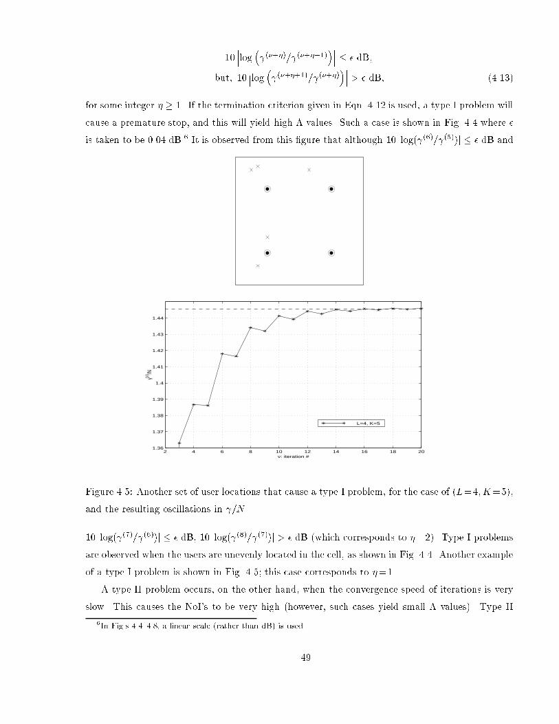
10log (+)= (+1) dB;

but; 10log (++1)= (+) > dB; (4.13)

for some integer 1. If the termination criterion given in Eqn. 4.12 is used, a type I problem will

cause a premature stop, and this will yield high values. Such a case is shown in Fig. 4.4 where

is taken to be 0.04 dB.6 It is observed from this gure that although 10j log( (6)= (5))j dB and

2 4 6 8 10 12 14 16 18 201.36

1.37

1.38

1.39

1.4

1.41

1.42

1.43

1.44

ν: iteration #

γ(ν)/N

L=4, K=5

Figure 4.5: Another set of user locations that cause a type I problem, for the case of (L=4; K=5),

and the resulting oscillations in =N .

10j log( (7)= (6))j dB, 10j log( (8)= (7))j > dB (which corresponds to =2). Type I problems

are observed when the users are unevenly located in the cell, as shown in Fig. 4.4. Another example

of a type I problem is shown in Fig. 4.5; this case corresponds to =1.

A type II problem occurs, on the other hand, when the convergence speed of iterations is very

slow. This causes the NoI's to be very high (however, such cases yield small values). Type II

6In Fig.s 4.44.8, a linear scale (rather than dB) is used.

49

problems are observed when each user is close to an AE; such a case is shown in Fig. 4.6.

In the simulations, the occasional type I and type II problems are encountered only in the

cases that correspond to unloaded systems. In loaded systems, on the other hand, another type

of problem, type III, is observed occasionally. For some user positions, rst reaches a maximum

and then converges to ; in such cases, there is the possibility of premature termination (similar

to type I problem). Examples of type III problem are shown in Fig.s 4.7 and 4.8.

For an arbitrarily close to 0 in Eqn. 4.12, all the anomalies of can be handled. But this would

yield a very high NoI for all types of problems (and an unnecessarily high accuracy). Therefore,

the solution is not making close to 0, but rather considering a multi-stage termination criterion.

The ow chart of such a multi-stage termination criterion is shown in Fig. 4.9. We note that the

\update " and \update ~P" lines in the ow chart are performed according to Eqn.s 4.8 and 4.9,

respectively. After the nal stop, = fig is calculated using Eqn. 4.7.

4.5 Observations

Simulations are carried out for a wide range of L and K values (L=4 and K=5 to 100, and L=16

and K=20 to 400). In all the cases, the iterations have always converged; that is, lim!1~P = ~P,

and lim!1 = .

Initial transmit power vectors, ~P(0), other than that given in Eqn. 4.10 are also considered, and

it is observed that the resulting NoI's are similar (although, ~P(0) given in Eqn. 4.10 yields slightly

lower NoI's). Therefore, the iterative solution algorithm is very robust with respect to the choice

of ~P(0); in other words, whatever ~P(0) is, the iterative algorithm converges to ~P.

CDF's for NoI's and are given in Fig.s 4.10-4.11 for = 0:1 dB, and m=1; 3, and 5, where

m denotes the number of stages in the multi-stage stop criterion (see Fig. 4.9). It is observed from

these gures that NoI's are lower for the loaded systems [(L=4; K=100), and (L=16; K=400)]

compared to the unloaded ones [(L=4; K=5), and (L=16; K=400)]. This demonstrates eciency

since the required computation at each iteration step for the loaded systems is much more than

that for the unloaded ones (due to the size of the link gain matrix G).

We note from Fig. 4.10 that there is signicant improvement in the statistics of , when a

3-stage stop criterion is used instead of a 1-stage type. This is due to the fact that most of the

type I problems are eliminated by using a 3-stage stop criterion. On the other hand, NoI's increase

for m=3 case compared to the m=1 case (see Fig. 4.11), as expected, however, the increase is not

substantial. Therefore, m=3 constitutes a good compromise.

50

4.6 Comparison with Hanly's Work [50] Part I: Correction to

Hanly's Theorem 1

In Ch. 3, we found the range for the balanced-SIR, , for given K and L values (see Eqn.s 3.6

and 3.7). The value of , in this range, depends on the link gain matrix G (which, in turn, is

dependent on the user locations and the fading conditions). In our case, since all the users have

the same SIR, we consequently assume that they all have the same quality of service requirement.

Hanly considered a more general case in [50], where the users have dierent quality of service

requirements; in that case, the objective is to achieve a target SIR vector = f1;2; : : : ;Kg,rather than balancing all the users to a common SIR value, . Hanly tries to determine whether

there exists a unique ~P which will yield the target , for given K and L values.

Hanly's Theorem 1 [50]:

a) IfPK

i=1 i NL, then there is no solution to .

b) IfPK

i=1 i < NL, then there exists a unique solution ~P to .

Based on the above theorem, Hanly states [50]: \We use this power control problem to derive

the network capacity region and nd that the feasibility of a conguration of users is independent

of their positions in the network; each user can be assigned a bandwidth that is independent of the

user's position in the network. : : : An important feature from a network management point of view

is that this constraint is linear; each user can be assigned a bandwidth. : : :The surprising conclusion

from Theorem 1 is that (G,) is feasible if and only ifPK

i=1 i < NL, a condition independent of

G. This suggests that call admission is very easy in a spread spectrum network with macrodiversity.

To see if K users with SIR requirements (1;2; : : : ;K) can be accommodated, we simply add up

: : : and compare with : : : NL."

Now, let us compare Hanly's Theorem 1 with our results. Our case corresponds to a special

target vector, such that i = , 8i. The results found in Sec. 3.2, in particular, Eqn.s 3.6

and 3.7, indicate that i SDA,SBMPC,LL can always be achievable, and i > SDA,SBMPC,UL can-

not be achievable. Moreover, achievability in the region SDA,SBMPC,LL < i SDA,SBMPC,UL

depends on the entries of the link gain matrix, that is, on the positions of the users in the

network! From Eqn.s 3.6 and 3.7, we calculate thatPK

i=1 SDA,SBMPC,LL = NLK=(K1), andPKi=1 SDA,SBMPC,UL = NLK=(KL). In Hanly's Theorem 1, there are two regions with one

threshold (NL) separating them, but according to our results there should be three regions with

two thresholds [NLK=(K1) and NLK=(KL)].The discrepancy between Hanly's Theorem 1 and our results is due to an approximation in

51

Hanly's modelling. He includes the user's own signal in the interference; that is, he omits the

subtracted term in the denominator of Eqn. 3.5. In that case, Eqn. 3.6 would be SDA,SBMPC,LL =

NL=K, and Eqn. 3.7 would be SDA,SBMPC,UL = N=(K=L); so, with that approximation, the two

thresholds merge to a single one, NL, and Hanly's Theorem 1 holds.

Based on the above discussion, we present the corrected version of Hanly's Theorem 1:7

Hanly's Theorem 1 Revised:

a) IfPK

i=1 i > NLK=(KL), then there is no solution to .

b) IfPK

i=1 i NLK=(K1), then there exists a unique solution ~P to .

c) If NLK=(K1)<PKi=1 i NLK=(KL), then the existance of a unique solution

~P to depends on the G matrix.

It is worth noting that NLK=(K1) NL for K 1, NLK=(KL) NL for K=L 1, and

SDA,SBMPC,LL=SDA,SBMPC,UL 1 (see Eqn. 3.10), once again, for K=L 1. Therefore, although

Hanly's Theorem 1 is not exact, it is a good approximation of the Revised Theorem given above,

especially for loaded systems.

It is interesting to note that the revision in Hanly's Theorem 1 has almost no eect on Hanly's

above quoted statements. In order to demostrate why this is so, let us consider a network with K1users and assume that a new user (user K) is asking permission for admission into the network. If

with the prospective user K, condition b) in the Revised Theorem is satised, then, obviously, user

K can be admitted into the network. However, if condition a) is satised, then user K should not

be admitted. Alternatively, if condition c) were satised, then user K should still not be admitted,

even with the existence of ~P. The reason is that condition c) depends on G; therefore, even if ~P

exists for this moment, there is no guarantee of its existence in the following moment, due to the

mobility of the users and the change in the fading conditions. Thus, the appropriate strategy is

to admit the prospective user K only if condition b) is satised. This means that the decision to

admit is independent of G, as Hanly stated.

We will continue the comparison of this work with that of Hanly's in the next chapter.

4.7 Chapter Summary and Remarks

In an SDA system, a power control algorithm that balances the SIR should be considered, since

the conventional power-balanced power control algorithm results in considerable disparities among

the SIR levels of dierent users. In this chapter, a nonlinear SIR-balanced PC algorithm, which is

7We are intending to send a correction/comment note to IEEE Trans. Commun. on this theorem.

52

referred to as the SIR-balanced macro PC (SBMPC) because of its handling of macro diversity, is

developed for CDMA SDA systems.

In SBMPC, the set of equations to be solved are nonlinear (due to diversity) which makes

the solutions for SIR-balancing algorithms, given in the literature, inapplicable. Therefore, we

propose an iterative solution to the SBMPC algorithm which always converges. Because of the

non-smooth convergence characteristics of the iterations, nding a suitable termination criterion

for the iterations is a nontrivial problem. We suggest a multi-stage criterion which yields very low

disparities among the SIR levels of dierent users for reasonably low numbers of iterations.

Although the SBMPC algorithm and its iterative solution addressed in this chapter are pre-

sented in the context of SDA systems, they may have other important applications. One such

application is the power control problem in cellular systems employing macro diversity [50]. Our

results are compared with those in [50], and Theorem 1 in that paper is corrected accordingly.

In the iterative solution of the SBMPC algorithm, it is assumed that we have instantaneous

access to the entire link gain matrix G. Since all the AE's are connected to a CS, this is not an

unrealistic assumption.

4.8 Future Research Directions

4.8.1 Other SBMPC Iterative Solution Algorithms

An iterative algorithm (Algorithm I) for the solution of SBMPC is given in Sec. 4.3, and its

convergence characteristics are analyzed in Sec.s 4.4 and 4.5, through exhaustive simulations. The

main conclusion drawn from these simulations is that algorithm I always converges, although the

speed of convergence may be low for certain user positions (see Fig.s 4.10 and 4.11). In this section,

we will discuss two other iterative algorithms for the solution of SBMPC.

SBMPC Iterative Solution Algorithm II:

~P(0) =n~P(0)i

o=

8><>:0@ KXj=1

Gij

1A19>=>; ; i = 1; 2; : : : ; K;

(+1) = E1~P()

;

~P(+1)1 = ~P

()1 ;

~P(+1)i = Ei

(+1);

n~P(+1)1 ; : : : ; ~P

(+1)i1 ; ~P

()i+1; : : : ;

~P()K

o; i = 2; 3; : : : ; K; : (4.14)

The dierence between Algorithms I and II is as follows: in Algorithm II, within a step of iteration,

while updating the transmit power of a user i, the already updated transmit power values for users

53

1 to i1 are used. In Algorithm I, however, the updated ~Pi's are not used until the next step of

iterations.

SBMPC Iterative Solution Algorithm III:

~P(0) =n~P(0)i

o=

8><>:0@ KXj=1

Gij

1A19>=>; ; i = 1; 2; : : : ; K;

(+1;1) = E1~P()

;

~P(+1)1 = ~P

()1 ;

~P(+1)i = Ei

(+1;i1);

n~P(+1)1 ; : : : ; ~P

(+1)i1 ; ~P

()i+1; : : : ;

~P()K

o (+1;i) = E1

n~P(+1)1 ; : : : ; ~P

(+1)i ; ~P

()i+1; : : : ;

~P()K

o; i = 2; 3; : : : ; K: (4.15)

The dierence between Algorithms II and III is as follows: in Algorithm III, within each step of

iteration, the update of the transmit power of each user is followed by an update of . In other

words, within each step of iteration, is updated K times, unlike Algorithm II (and I) where

is updated only once. Obviously, these extra updates would increase the required computation for

Algorithm III, compared to Algorithms I and II.

We made an initial analysis on the convergence speed of Algorithms II and III, and realized that

these algorithms have convergence problems; that is, for certain K and L values they do not balance

the SIR for certain user locations. To be more precise, the occasional converge problems occured

for (L=4; K=5), (L=4; K=10), (L=16; K=5), and (L=16; K=20) cases for Algorithm I, and

for the (L=4; K=5) case for Algorithm III. Obviously, all of these cases correspond to unloaded

systems. The limited simulations run for some other K and L combinations suggest that there is

no convergence problem for loaded cases; however, the results are not conclusive due to the limited

number of simulations run.

In this initial analysis, algorithm II seemed to be somewhat faster than Algorithm I for the cases

where Algorithm II did converge, and more interestingly, Algorithm III seemed to be signicantly

faster than the other two algorithms, whenever it did converge. Once again, exhaustive simulations

should be run to verify these initial ndings.

If the above ndings are true, that is, if Algorithm III always converges for loaded cases with a

speed signicantly faster than those of the other two algorithms, then, perhaps, a threshold (e.g.

) in terms of K=L (which would separate the loaded and unloaded cases), can be found.

In [50], Hanly proved the convergence of a somewhat similar PC algorithm (in [50], there is no

discussion on the speed of convergence though). Perhaps, a similar proof technique (monotonicity

in cooperative systems) can be used to show that Algorithm III always converges for K=L > . If

54

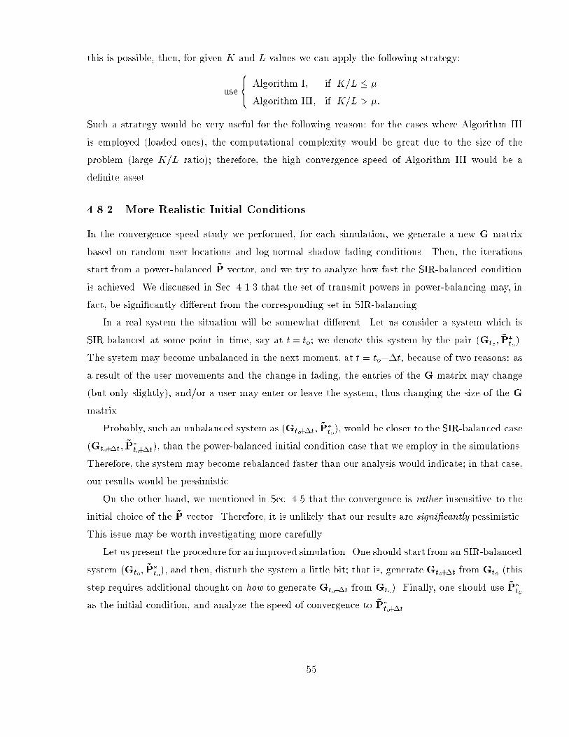
this is possible, then, for given K and L values we can apply the following strategy:

use

8<: Algorithm I; if K=L

Algorithm III; if K=L > :

Such a strategy would be very useful for the following reason: for the cases where Algorithm III

is employed (loaded ones), the computational complexity would be great due to the size of the

problem (large K=L ratio); therefore, the high convergence speed of Algorithm III would be a

denite asset.

4.8.2 More Realistic Initial Conditions

In the convergence speed study we performed, for each simulation, we generate a new G matrix

based on random user locations and log-normal shadow fading conditions. Then, the iterations

start from a power-balanced ~P vector, and we try to analyze how fast the SIR-balanced condition

is achieved. We discussed in Sec. 4.1.3 that the set of transmit powers in power-balancing may, in

fact, be signicantly dierent from the corresponding set in SIR-balancing.

In a real system the situation will be somewhat dierent. Let us consider a system which is

SIR-balanced at some point in time, say at t= to; we denote this system by the pair (Gto; ~Pto).

The system may become unbalanced in the next moment, at t = to+t, because of two reasons: as

a result of the user movements and the change in fading, the entries of the G matrix may change

(but only slightly), and/or a user may enter or leave the system, thus changing the size of the G

matrix.

Probably, such an unbalanced system as (Gto+t; ~Pto), would be closer to the SIR-balanced case

(Gto+t; ~Pto+t), than the power-balanced initial condition case that we employ in the simulations.

Therefore, the system may become rebalanced faster than our analysis would indicate; in that case,

our results would be pessimistic.

On the other hand, we mentioned in Sec. 4.5 that the convergence is rather insensitive to the

initial choice of the ~P vector. Therefore, it is unlikely that our results are signicantly pessimistic.

This issue may be worth investigating more carefully.

Let us present the procedure for an improved simulation. One should start from an SIR-balanced

system (Gto; ~Pto), and then, disturb the system a little bit; that is, generate Gto+t from Gto (this

step requires additional thought on how to generate Gto+t from Gto). Finally, one should use ~Pto

as the initial condition, and analyze the speed of convergence to ~Pto+t.

55

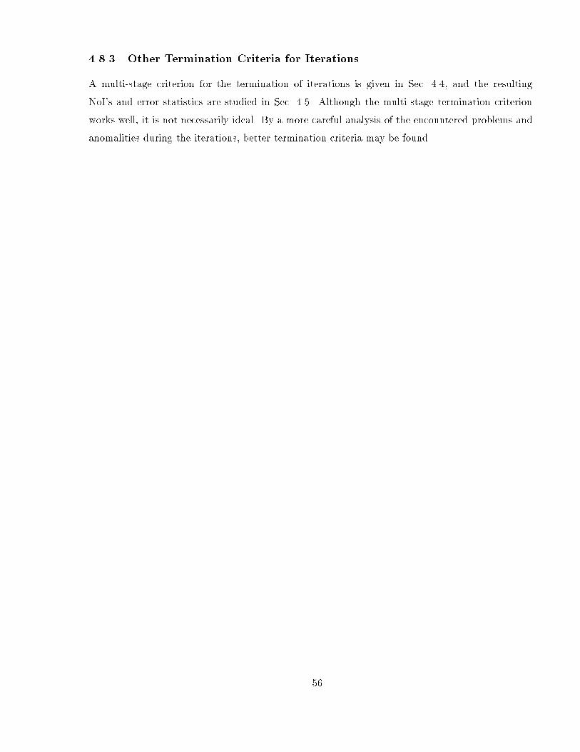
4.8.3 Other Termination Criteria for Iterations

A multi-stage criterion for the termination of iterations is given in Sec. 4.4, and the resulting

NoI's and error statistics are studied in Sec. 4.5. Although the multi-stage termination criterion

works well, it is not necessarily ideal. By a more careful analysis of the encountered problems and

anomalities during the iterations, better termination criteria may be found.

56

0 10 20 30 40 50 60 70 80 90 1000

20

40

60

80

100

120

140

160

180

200

ν: iteration #

γ(ν)/N

L=4, K=5

900 910 920 930 940 950 960 970 980 990 10001

1.5

2

2.5

3

3.5

ν: iteration #

γ(ν)/N

L=4, K=5

Figure 4.6: A set of user locations that cause a type II problem, for the case of (L=4; K=5), and

the resulting oscillations in =N .

57

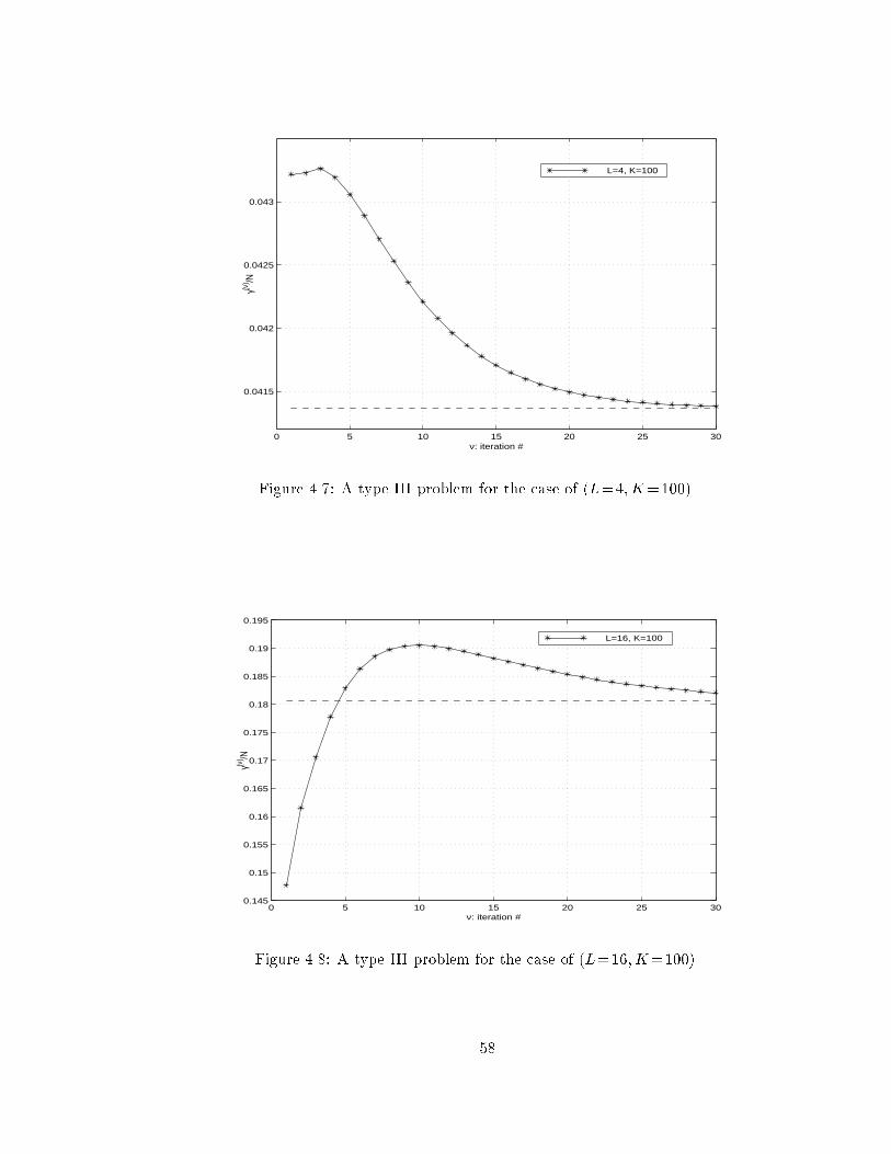
0 5 10 15 20 25 30

0.0415

0.042

0.0425

0.043

ν: iteration #

γ(ν) /N

L=4, K=100

Figure 4.7: A type III problem for the case of (L=4; K=100).

0 5 10 15 20 25 300.145

0.15

0.155

0.16

0.165

0.17

0.175

0.18

0.185

0.19

0.195

ν: iteration #

γ(ν) /N

L=16, K=100

Figure 4.8: A type III problem for the case of (L=16; K=100).

58

Update P

γ γold

Update γ

Start

γ 10-10

No

No

Yes

Yes

Yes

No

stagesm

(0)ComputeP

γ γold

Update γ

Update P

Stop

ComputeΓ

γ /γold?) < 10 log( ε

γ /γold?) < 10 log( ε

γ /γold?) < 10 log( εdB

dB

dB

Figure 4.9: The ow chart of the multi-stage termination program.

59

0 2 4 6 8 10 12 14 16 18 200

0.1

0.2

0.3

0.4

0.5

0.6

0.7

0.8

0.9

1

ν

P(N

oI ≤

ν)

(a)

L=4, K=5, m=1

L=4, K=5, m=3

L=4, K=5, m=5

L=4, K=100, m=1

L=4, K=100, m=3

L=4, K=100, m=5

0 2 4 6 8 10 12 14 16 18 200

0.1

0.2

0.3

0.4

0.5

0.6

0.7

0.8

0.9

1

ν

P(N

oI ≤

ν)

(b)

L=16, K=20, m=1

L=16, K=20, m=3

L=16, K=20, m=5

L=16, K=400, m=1

L=16, K=400, m=3

L=16, K=400, m=5

Figure 4.10: CDF of NoI's, for (a) (L=4; K=5), and (L=4; K=100), (b) (L=16; K=20), and

(L=16; K=400).

60

0 0.05 0.1 0.15 0.2 0.250

0.1

0.2

0.3

0.4

0.5

0.6

0.7

0.8

0.9

1

x (dB)

P(Λ

≤ x)

L=4, K=5

L=4, K=100

(a)

m=1m=3m=5

0 0.05 0.1 0.15 0.2 0.250

0.1

0.2

0.3

0.4

0.5

0.6

0.7

0.8

0.9

1

x (dB)

P(Λ

≤ x)

L=16, K=20

L=16, K=400

(b)

m=1m=3m=5

Figure 4.11: CDF of SIR error, , for (a) (L=4; K=5), (L=4; K=100), (b) (L=16; K=20), and

(L=16; K=400).

61

Chapter 5

Correlated Interference Analysis in SDA Systems

5.1 Introduction

It has been demonstrated in Ch.s 3 and 4 that through the use of SDA scheme with SBMPC,

an almost linear gain is achievable in the system capacity or in the transmission rate. However,

one may expect, intuitively, that the law of diminishing returns should apply with the increasing

number of AE's. In this chapter, we will present an initial correlation analysis that may eventually

enable us to understand how and why the returns plateau with the increasing number of AE's.

Before proceeding with a comprehensive analytical study, we present the following intuitive

reasoning: when the number of AE's (and thus the number of users) increase, the AE's (as well as

the users) would inevitably become closer to each other. In such a case, we may suspect that the

signals received by dierent AE's may not be independent any more.

In order the maximal ratio combining (MRC) scheme maximize the output SIR, the noise

components at the ngers of the Rake receiver must be uncorrelated. If this is the case, then the

output SIR is the sum of the nger SIR's. If, however, the noise components are correlated, then

the output SIR will be less than the sum of the nger SIR's. In fact, in the case of signicant

correlation between the noise components of dierent ngers, the MRC scheme will not be the

best linear combining technique any more. In order to demonstrate this fact, let us consider

a hypothetical case, where the signal components at the Rake ngers are dierent but the noise

components are identical. In such a case, the best linear combining technique would be the selection

combining; that is, selecting the nger with the highest SIR.

Moreover, in a diversity scheme, if the signal and noise components at the ngers are both iden-

tical, then there is no gain at all from what is supposed to be diversity reception, since amplication

does not increase the SIR.

The correlation analysis in an SDA system is quite complicated, and thus, this is a rather long

62

chapter. We will start from a very simple case and then will analyze the more general cases in

sequence. To be more specic, an SDA system with 2 AE's and 2 users will be considered rst;

then, the obtained results will be generalized for a system with 2 AE's and K users, and nally,

the most general case of L AE's and K users will be investigated.

5.2 Denitions and Corollaries

We consider an SDA system with 2 AE's which are denoted as AE I and AE II , and 2 users. We

assume that user 1 is the user of interest.

user 1

user 2

t2I t2II

t1I t1IIIII

CS

I,ct

II,ct

Figure 5.1: Propagation delays in an SDA system with L = 2 and K = 2.

Fig. 5.1 shows the propagation delays in the system. t1I;t is the total propagation time from

user 1 to the CS through AE I , and it is equal to

t1I;t = t1I + tI;c; (5.1)

where t1I is the propagation time in the air from user 1 to AE I , and tI;c is that in the cable from

AE I to the CS. We note that tI;c does not depend on the location of user 1. Similarly,

t1II;t = t1II + tII;c; (5.2)

where t1II;t is the total propagation time from user 1 to the CS through AE II , t1II is that in the

air from user 1 to AE II , and tII;c is that in the cable from AE II to the CS. Propagation times

regarding user 2 are dened in a similar way, and are obvious from Fig. 5.1.

The modulation process at the users and the demodulation process for user 1 at the CS are

illustrated in Fig. 5.2. Also, the spreading code and the related assumptions are depicted in Fig. 5.3.

At user 1's receiver, the despreading at the Ist nger of the Rake is performed by multiplying the

received signal by c1(t t1I;t; 1), where c1(t) is the spreading code for user 1 and 1 is the

corresponding code phase. 1 is represented in terms of ; in other words,

c1(t t1I;t; 1) = c1(t t1I;t 1): (5.3)

63

cos πc(2 f [t-t ])1II,t

cos πc 1I,t(2 f [t-t ])

cos π(2 f t)c

cos π(2 f t)c

T

Tb (t)2

b (t)1

user 2

user 1

Central Station

1∆1c (t-t ; )Decision

Combiner

Receiver of user 1

Receiver of user 2

device

AE II

AE I

c (t; )∆22

c (t; )1 ∆1

m (t)1

m (t)2

1 1I,t ∆1c (t-t ; )

1II,t

Figure 5.2: The modulation and demodulation processes in the reverse link of an SDA system with

L=2 and K=2.

The situation at the IInd nger of user 1 is similar; obviously, in this case the despreading is

performed by c1(t t1II;t; 1).

Let 1I and 1II be the interference (noise) components at the ngers of the Rake receiver of

user 1 corresponding to AE's I and II , respectively. 1I and 1II are composed of two components

as follows

1I = 1I n1I ; (5.4)

1II = 1II n1II ; (5.5)

where 1I and 1II are the deterministic components at the Ist and IInd ngers, respectively, and

n1I = hc1(t t1I;t; 1)c2(t t2I;t; 2)i ; (5.6)

n1II = hc1(t t1II;t; 1)c2(t t2II;t; 2)i ; (5.7)

are the random components, again at the Ist and IInd ngers, respectively. In Eqn.s 5.6 and 5.7,

h:i denotes the inner product, i.e.,

hc1(t)c2(t)i =ZT

c1(t)c2(t)dt; (5.8)

where T is the bit duration (refer to Fig. 5.3).

64

t

t

t

N

+1

-1

+1

-1

+1

-1m(t)

Spreading codec(t)

Data signalb(t)

Product signal

τ

T

τ : chip durationc0 c1 c2 cN-1

Figure 5.3: The data signal, b(t), the spreading code, c(t), and the product signal, m(t) = b(t)c(t).

We are interested in evaluating the correlation coecient of the random variables 1I and 1II ,

12;III , which is dened as

12;III =E(1I 1II) E(1I)E(1II)q

E(21I) E2(1I)qE(21II) E2(1II)

: (5.9)

In the above, E(.) denotes expectation operator. One can easily show that Eqn. 5.9 reduces to

12;III =E(n1I n1II) E(n1I)E(n1II)q

E(n21I) E2(n1I)qE(n21II) E2(n1II)

: (5.10)

We conclude from Eqn.s 5.9 and 5.10 that the deterministic components 1I and 1II do not have

any eect on the correlation coecient. Therefore, in the rest of this chapter we will focus on n1I

and n1II .

We also dene dierential code phase, 12, as the dierence between the spreading code phases

of users 1 and 2; i.e.,

12 = 1 2: (5.11)

Without loss of generality, 12 is modeled as a uniform random variable in the interval [0; 1).

Before we proceed, we will present some corollaries that will be used later in this chapter. We

start by noting that although c1(t)c2(t) 6= c1(t t0)c2(t t0), where t0 denotes some delay, the

following corollary holds:

Corollary 1 hc1(t)c2(t)i = hc1(t t0)c2(t t0)i.

From Eqn. 5.3 and Corollary 1, we obtain the second corollary:

Corollary 2 hc1(t; 1)c2(t; 2)i = hc1(t; 12)c2(t)i = hc1(t)c2(t; 21)i;

65

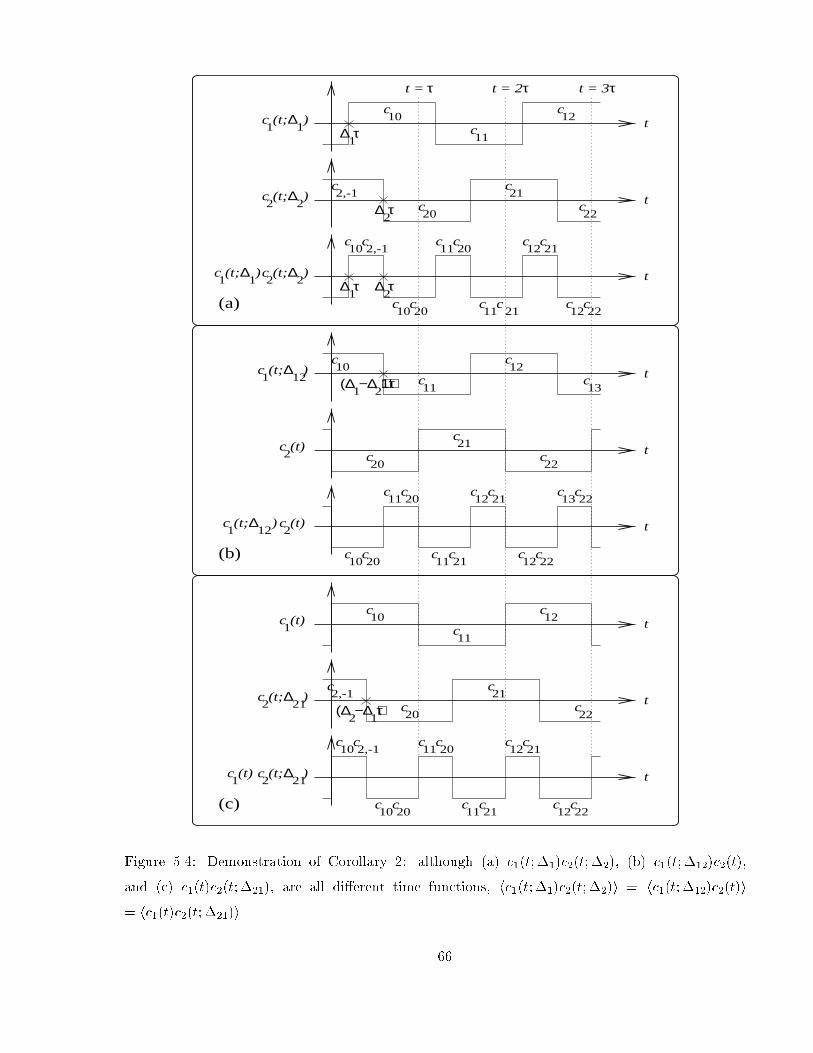
c (t)1

∆2 21c (t; )

c (t)1

∆2 21c (t; )

∆1 12c (t; )

c (t)2

c10

c11

c12

t

c10

c2,-1

c10

c20

c11

c20

c11

c21

c12

c21

c12

c22

c21

c20

c2,-1

c22

t

t

t = τ τ τt = 2 t = 3

1∆ τ

∆2τ

∆1τ ∆

2τ

∆22

c (t; )

(a)

1∆

1c (t; )

∆22

c (t; )

1∆

1c (t; )

c10

c

c12

11

c10

c2,-1

c10

c20

c11

c20

c11

c21

c12

c21

c12

c22

2,-1c

c20

c21

c22

t

t

t

(∆ −∆ )τ2 1

(c)

12c

c11

c10

c13

22c20

c

c21

c10

c20

c11

c20

c11

c21

c12

c21

c12

c22

c13

c22

t

t

tc (t)2

(∆ −∆ +1)τ1 2

(b)

∆1 12c (t; )

Figure 5.4: Demonstration of Corollary 2: although (a) c1(t; 1)c2(t; 2), (b) c1(t; 12)c2(t),

and (c) c1(t)c2(t; 21), are all dierent time functions, hc1(t; 1)c2(t; 2)i = hc1(t; 12)c2(t)i= hc1(t)c2(t; 21)i.

66

where 12 and 21 are dened according to Eqn. 5.11. The result of Corollary 2 is depicted in

Fig. 5.4. Also from Eqn. 1, the third corollary follows right away:

Corollary 3 hc1(t t1)c2(t t2)i = hc1(t [t1t2])c2(t)i = hc1(t)c2(t [t2t1])i;

where t1 and t2 denote some delays. Finally, from Corollaries 2 and 3, the most general case can

be obtained as

Corollary 4 hc1(t t1; 1)c2(t t2; 2)i = hc1(t [t1t2]; 12)c2(t)i = hc1(t)c2(t [t2t1]; 21)i:

However, it is important to note that for some delays t11 and t12, with t11 6= t12,

E(hc1(t t11)c2(t)ihc1(t t12)c2(t)i) 6= E(hc1(t [t11t12])c2(t)ihc1(t)c2(t)i); (5.12)

but rather, the left hand side depends on the actual values of t11 and t12. It will become apparent

in Section 5.3 that this result will complicate our analysis.

5.3 Correlation Coecient Analysis for Synchronous Users

In this section and the next one, the correlation coecient corresponding to the noise components

at the Ist and IInd ngers of the Rake receiver of user 1, 12;III , will be determined. As a starting

point, we make the assumption that users are synchronized, in other words, 1 = 2, that is,

12 = 0. The general case, where 12 is a uniform random variable in the region [0; 1), will be

considered in Section 5.4.

We will start by demonstrating the dependence of 12;III on the propagation delays incurred

in the system.

5.3.1 Dependence of Correlation Coecient on Propagation Delays

Corollary 4 can be used to simplify n1I and n1II , dened by Eqn.s 5.6 and 5.7, as

n1I = hc1(t t1I;t; 1)c2(t t2I;t; 1)i = hc1(t t12I)c2(t)i; (5.13)

n1II = hc1(t t1II;t; 1)c2(t t2II;t; 1)i = hc1(t t12II)c2(t)i; (5.14)

where,

t12I = t1I;t t2I;t = (t1I+tI;c) (t2I+tI;c) = t1I t2I ; (5.15)

t12II = t1II;t t2II;t = (t1II+tII;c) (t2II+tII;c) = t1II t2II : (5.16)

67

In the simplication of t12I and t12II , Eqn.s 5.1 and 5.2 are used. It is observed from Eqn.s 5.15

and 5.16 that t12I and t12II depend only on the propagation delays in the air.

Without loss of generality we will rst assume that 0 t12I ; we will consider the most

general case later in this section.

Now, n1I can be computed as (refer to Fig. 5.4)

n1I =N1Xk=0

[( t12I)c1;k c2;k + t12I c1;k c2;k+1] : (5.17)

We assume that fcikg are independent identically distibuted equi-probable Bernoulli random vari-

ables with values equal to 1. With this assumption, it is easy to show that

E(n1I) = 0: (5.18)

The variance of n1I can be computed from Eqn. 5.17, by realizing that c2ik = 1, as

E(n21I) = N( t12I)2 + t212I

: (5.19)

It is observed from Eqn. 5.17 that in order n1I and n1II be correlated, n1II should have com-

ponents in the form of c1k c2k and/or c1k c2;k+1. It is not dicult to show that for t12II < or

t12II > 2 , n1II does not have such components. We will investigate the remaining range for t12II

in three intervals, namely, t12II 0, 0 t12II , and t12II 2 .

If t12II 0, then n1II can be shown to be equal to

n1II =N1Xk=0

[t12II c1;k c2;k1 + (t12II + )c1;k c2;k] (5.20)

The mean and variance of n1II are found as

E(n1II) = 0; (5.21)

E(n21II) = N(t12II + )2 + t212II

: (5.22)

Now, using Eqn.s 5.17 and 5.20, the correlation, E(n1I n1II), can be computed as

E(n1I n1II) = N( t12I)(t12II + ): (5.23)

Substituting Eqn.s 5.19, 5.22, and 5.23, in Eqn. 5.10, 12;III can be obtained as

12;III =( t12I)(t12II + )q

( t12I)2 + t212I

qt212II + (t12II + )2

: (5.24)

68

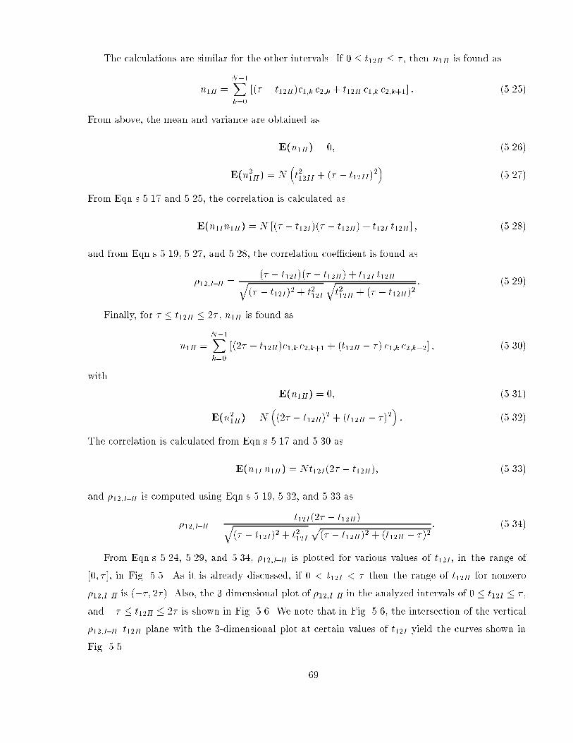
The calculations are similar for the other intervals. If 0 t12II , then n1II is found as

n1II =N1Xk=0

[( t12II)c1;k c2;k + t12II c1;k c2;k+1] : (5.25)

From above, the mean and variance are obtained as

E(n1II) = 0; (5.26)

E(n21II) = Nt212II + ( t12II)2

(5.27)

From Eqn.s 5.17 and 5.25, the correlation is calculated as

E(n1In1II) = N [( t12I)( t12II) + t12I t12II ] ; (5.28)

and from Eqn.s 5.19, 5.27, and 5.28, the correlation coecient is found as

12;III =( t12I)( t12II) + t12I t12IIq

( t12I)2 + t212I

qt212II + ( t12II)2

: (5.29)

Finally, for t12II 2 , n1II is found as

n1II =N1Xk=0

[(2 t12II)c1;k c2;k+1 + (t12II ) c1;k c2;k+2] ; (5.30)

with

E(n1II) = 0; (5.31)

E(n21II) = N(2 t12II)

2 + (t12II )2: (5.32)

The correlation is calculated from Eqn.s 5.17 and 5.30 as

E(n1I n1II) = Nt12I(2 t12II); (5.33)

and 12;III is computed using Eqn.s 5.19, 5.32, and 5.33 as

12;III =t12I(2 t12II)q

( t12I)2 + t212Ip( t12II)2 + (t12II )2

: (5.34)

From Eqn.s 5.24, 5.29, and 5.34, 12;III is plotted for various values of t12I , in the range of

[0; ], in Fig. 5.5. As it is already discussed, if 0 < t12I < then the range of t12II for nonzero

12;III is (; 2). Also, the 3-dimensional plot of 12;III in the analyzed intervals of 0 t12I ,

and t12II 2 is shown in Fig. 5.6. We note that in Fig. 5.6, the intersection of the vertical

12;IIIt12II plane with the 3-dimensional plot at certain values of t12I yield the curves shown in

Fig. 5.5.

69

−1 −0.5 0 0.5 1 1.5 20

0.1

0.2

0.3

0.4

0.5

0.6

0.7

0.8

0.9

1

t12II

/τ

ρ 12

t12I

/τ=0.00

t12I

/τ=0.10

t12I

/τ=0.25

t12I

/τ=0.50

−1 −0.5 0 0.5 1 1.5 20

0.1

0.2

0.3

0.4

0.5

0.6

0.7

0.8

0.9

1

t12II

/τ

ρ 12

t12I

/τ=0.50

t12I

/τ=0.75

t12I

/τ=0.90

t12I

/τ=1.00

Figure 5.5: Correlation coecient as a function of t12II , for t12I= = 0:00; 0:10; 0:25; 0:50; 0:75; 0:90,

and 1:00, for synchronous users (12=0).

70

0

0.2

0.4

0.6

0.8

1

−1

−0.5

0

0.5

1

1.5

2

0

0.2

0.4

0.6

0.8

1

t12I

/τt12II

/τ

ρ12

Figure 5.6: Correlation coecient as a function of t12I and t12II , for 0 t12I and t12II 2 , for synchronous users (12=0).

The results obtained so far for the case of 0 t12I , can be generalized for t12I values in any

interval. Without giving the details, we will state 12;III for the general case of n t12I (n+1) ,

71

where n is an integer:

12;III =

8>>>>>>>>>>>>>>>>>>>>>>>>>><>>>>>>>>>>>>>>>>>>>>>>>>>>:

[(n+1) t12I ][t12II (n1) ]q[(n+1) t12I ]2 + (t12I n)2

q(n t12II)2 + [t12II (n1) ]2

;

if (n1) t12II n ;

[(n+1) t12I ][(n+1) t12II ] + (t12I n)(t12II n)q[(n+1) t12I ]2 + (t12I n)2

q[(n+1) t12II ]2 + (t12II n)2

;

if n t12II (n+1) ;

(t12I n)[(n+2) t12II ]q[(n+1) t12I ]2 + (t12I n)2

q[(n+2) t12II ]2 + [t12II (n+1) ]2

;

if (n+1) t12II (n+2):

(5.35)

Then, 12;III qiven by Eqn.s 5.24, 5.29, and 5.34 corresponds to n=0 case. In Fig. 5.7, the general

−1

−0.5

0

0.5

1

1.5

2

−2

−1

0

1

2

3

0

0.5

1

t12I

/τt12II

/τ

ρ12

Figure 5.7: Correlation coecient as a function of t12I and t12II , for synchronous users (12=0).

expression for 12;III given in Eqn. 5.35 is plotted with respect to t12I and t12II .

72

−2 −1.5 −1 −0.5 0 0.5 1 1.5 2 2.5 3−3

−2

−1

0

1

2

3

4

t12I

/τ

t 12II/τ

t12I

−t12II

= −2τ t12I

−t12II

= −τ

t12I

−t12II

= 0

t12I

−t12II

= τ

t12I

−t12II

= 2τ

Figure 5.8: Non-zero 12;III region in terms of t12I and t12II , for synchronous users (12=0).

It is observed from Eqn. 5.35 and Fig. 5.7 that

t12I = n !8<: 12;III = 0; for t12II (n1) and t12II (n+1)

12;III > 0; for (n1) < t12II < (n+1);

n < t12I < (n+1) !8<: 12;III = 0; for t12II (n1) and t12II (n+2)

12;III > 0; for (n1) < t12II < (n+2);

(5.36)

where n is an integer. The regions of t12I and t12II for which 12;III is nonzero is shown in Fig. 5.8

by the shaded area. Fig. 5.8 can be thought of as looking at Fig. 5.7 from right above (the z-axis).

In this section, the dependence of 12;III on t12I and t12II is investigated. Since the propagation

time depends on the distance, there is an equivalent dependence of 12;III on the location of users

and AE's.

5.3.2 Dependence of Correlation Coecient on User and AE Locations

In this section, the dependence of 12;III on the user and AE locations will be investigated. The

goal is to nd the region for user 2 which will result in a non-zero 12;III , for a given set of AE and

user 1 locations. The time domain requirements for this region is already known from Eqn. 5.36.

Therefore, the task is to nd the equivalent of Eqn. 5.36 in terms of distance.

73

As it is well known, the propagation time, t, depends on the distance, d, as

t =d

c; (5.37)

where c is the speed of light which will be taken as 3 108 m/sec. Therefore, from Eqn.s 5.15,

5.16, and 5.37, t12I and t12II can be stated in terms of distances as

t12I =d1I d2I

c; (5.38)

t12II =d1II d2II

c; (5.39)

where dij is the distance between user i and AE j, i 2 f1; 2g, j 2 fI; IIg.

0 0.1 0.2 0.3 0.4 0.5 0.6 0.7 0.8 0.9 10

0.2

0.4

0.6

0.8

1

h1I

AE I AE II

user 1

10

(a)

0 0.1 0.2 0.3 0.4 0.5 0.6 0.7 0.8 0.9 10

0.2

0.4

0.6

0.8

1

h1II

AE I AE II

user 1

01

2

−1

(b)

Figure 5.9: For synchronous users (12=0), the shaded areas show the following regions: (a) 0 <

t12I < 0 < (h1Ih2I ) < 0:075, (b) t12II 2 0:075 < (h1IIh2II ) < 0:15. In both

gures s=400 and Rc=10 Mcps.

74

We will work on a unit square cell with side 1 m. Distances in this unit cell will be denoted by

h. In other words, h is the normalized distance which is related to the actual distance, d, as

d = h s; (5.40)

where s is the scaling factor. For instance, if s=500, this means that the cell has the shape of a

square with side length 500 meters. Also, we dene the chip rate, Rc, as

Rc =1

: (5.41)

0 0.1 0.2 0.3 0.4 0.5 0.6 0.7 0.8 0.9 10

0.1

0.2

0.3

0.4

0.5

0.6

0.7

0.8

0.9

1

0

1

2

−1

1

0

AE I AE II

user 1

Figure 5.10: For synchronous users (12 = 0), the shaded area shows the following region: 0 <

(h1I h2I) < 0:075 and 0:075 < (h1II h2II) < 0:15 (s=400 and Rc=10 Mcps).

We will rst nd the region corresponding to n < t12I < (n+1) . This region is a function

of the locations of users 1 and 2, and AE I (but, not AE II). Then, we will nd the region

corresponding to (n1) < t12II < (n+2) , which is a function of the locations of users 1 and 2,

and AE II (but, not AE I).

We start by analyzing the n=0 case. Using Eqn.s 5.38, 5.39 and 5.40, we can write

0 < t12I = t1I t2I < ! 0 < (h1I h2I) < c

s; (5.42)

75

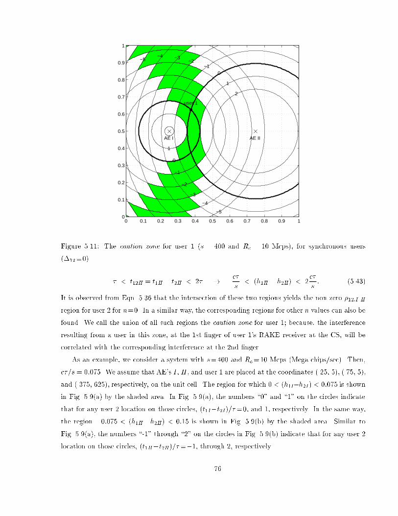
0 0.1 0.2 0.3 0.4 0.5 0.6 0.7 0.8 0.9 10

0.1

0.2

0.3

0.4

0.5

0.6

0.7

0.8

0.9

1

0

1

2

−1−2

−3−4−5

1

0

−1

−2

−3

−4

−5

AE I AE II

user 1

Figure 5.11: The caution zone for user 1 (s = 400 and Rc = 10 Mcps), for synchronous users

(12=0).

< t12II = t1II t2II < 2 ! cs

< (h1II h2II) < 2c

s: (5.43)

It is observed from Eqn. 5.36 that the intersection of these two regions yields the non-zero 12;III

region for user 2 for n=0. In a similar way, the corresponding regions for other n values can also be

found. We call the union of all such regions the caution zone for user 1; because, the interference

resulting from a user in this zone, at the 1st nger of user 1's RAKE receiver at the CS, will be

correlated with the corresponding interference at the 2nd nger.

As an example, we consider a system with s=400 and Rc=10 Mcps (Mega chips/sec). Then,

c=s = 0:075. We assume that AE's I , II , and user 1 are placed at the coordinates (.25,.5), (.75,.5),

and (.375,.625), respectively, on the unit cell. The region for which 0 < (h1Ih2I ) < 0:075 is shown

in Fig. 5.9(a) by the shaded area. In Fig. 5.9(a), the numbers \0" and \1" on the circles indicate

that for any user 2 location on those circles, (t1It2I)==0, and 1, respectively. In the same way,

the region 0:075 < (h1IIh2II) < 0:15 is shown in Fig. 5.9(b) by the shaded area. Similar to

Fig. 5.9(a), the numbers \-1" through \2" on the circles in Fig. 5.9(b) indicate that for any user 2

location on those circles, (t1IIt2II)==1, through 2, respectively.

76

−2 −1.5 −1 −0.5 0 0.5 1 1.5 2 2.5 3−3

−2

−1

0

1

2

3

4

t12I

/τ

t 12II/τ

t12I

−t12II

= −2τ t12I

−t12II

= −τ

t12I

−t12II

= 0

t12I

−t12II

= τ

t12I

−t12II

= 2τ

Figure 5.12: Non-zero 12;III region in terms of t12I and t12II , for asynchronous users (12=0:7).

The intersection of the regions shown in Fig.s 5.9(a) and (b) is depicted in Fig. 5.10. Similarly,

using Eqn.s 5.36, 5.38, 5.39 and 5.40, the corresponding regions for other n values can also be

found. We realize that for n 1, the conditions given in Eqn.s 5.42 and 5.43 do not yield an

overlapping region. In Fig. 5.11 the caution zone for user 1 is shown, which is the union of the

regions corresponding to n=6;5; ; 0.We note that the analysis presented so far is for the case where the users are synchronized.

Next, we will investigate the general case where users 1 and 2 are asynchronous.

5.4 Correlation Coecient Analysis for Asynchronous Users

In this section, we turn our attention to the eect of the chip phase in the correlation analysis.

Based on Eqn.s 5.6, 5.7, 5.15, 5.16, and Corollary 2, n1I and n1II can be written as

n1I = hc1(t t12I ; 12)c2(t)i; (5.44)

n1II = hc1(t t12II ; 12)c2(t)i: (5.45)

Using Eqn. 5.3, the above n1I and n1II expressions take the following form:

n1I = hc1(t t12I 12)c2(t)i; (5.46)

77

n1II = hc1(t t12II 12)c2(t)i: (5.47)

Dening t012I and t012II as

t012I = t12I +12; (5.48)

t012II = t12II +12; (5.49)

Eqn.s 5.46 and 5.47 can be rewritten as

n1I = hc1(t t012I)c2(t)i; (5.50)

n1II = hc1(t t012II)c2(t)i: (5.51)

Comparing Eqn.s 5.50 and 5.51 with those for the synchronous users, namely, Eqn.s 5.13

and 5.14, we notice that both sets of equations are in the same form with the only dierence that

t12I and t12II in Eqn.s 5.13 and 5.14 are replaced with t012I and t012II , respectively, in Eqn.s 5.50

and 5.51. Therefore, we conclude that the 12;III expressions found in the previous section (such

as Eqn. 5.35) as well as the curves plotted in Fig.s 5.5 and 5.7 are still valid provided that t12I and

t12II are substituted by t012I and t012II , respectively.

Based on Eqn.s 5.48, 5.49, and the above observation, Eqn. 5.36 can be modied as

t12I = (n12) !8<: 12;III = 0; for t12II [(n1)12] and t12II [(n+1)12]

12;III > 0; for [(n1)12] < t12II < [(n+1)12];

(n12) < t12I < [(n+1)12] !8<: 12;III = 0; for t12II [(n1)12)] and t12II [(n+2)12]

12;III > 0; for [(n1)12] < t12II < [(n+2)12]:(5.52)

In fact, Eqn. 5.36 can be obtained from Eqn. 5.52 for the special case of 12=0.

Similar to Fig. 5.8 which is drawn based on Eqn. 5.36, the region for non-zero 12;III is shown

in Fig. 5.12 which is drawn based on Eqn. 5.52. In Fig. 5.12, 12 is taken to be 0:7. Also in this

gure, the dotted lines show the boundary of the non-zero 12;III region for the synchronous case

(refer to Fig. 5.8) for comparison.

Following the same steps presented in Section 5.3.2, the time domain expressions, given in

Eqn. 5.52 and shown in Fig. 5.12 for the non-zero 12;III region, can be converted into the ex-

pressions in terms of distances on the unit cell. For this conversion, Eqn.s 5.38, 5.39, 5.40, 5.48,

and 5.49 should be used in Eqn. 5.52. Since the procedure is very similar to the one presented in

78

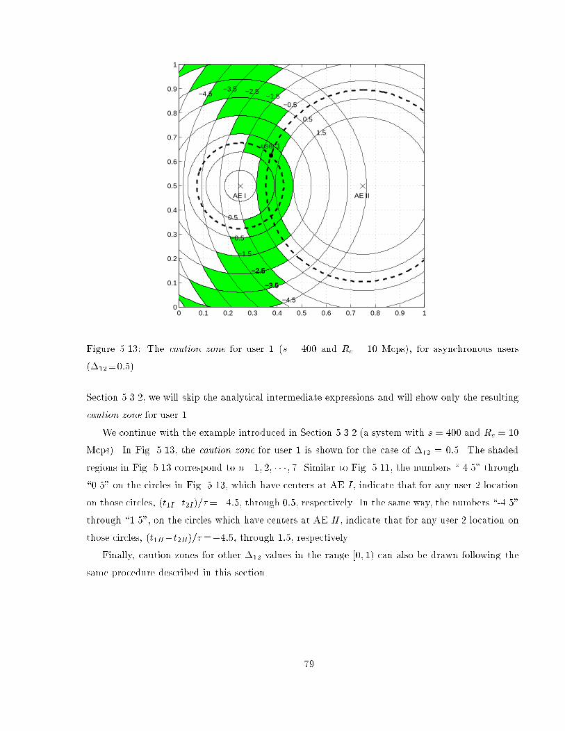
0 0.1 0.2 0.3 0.4 0.5 0.6 0.7 0.8 0.9 10

0.1

0.2

0.3

0.4

0.5

0.6

0.7

0.8

0.9

1

1.5

0.5

−0.5−1.5

−2.5−3.5−4.5

0.5

−0.5

−1.5

−2.5

−3.5

−2.5

−3.5

−2.5

−3.5

−4.5

AE I AE II

user 1

Figure 5.13: The caution zone for user 1 (s = 400 and Rc = 10 Mcps), for asynchronous users

(12=0:5).

Section 5.3.2, we will skip the analytical intermediate expressions and will show only the resulting

caution zone for user 1.

We continue with the example introduced in Section 5.3.2 (a system with s = 400 and Rc = 10

Mcps). In Fig. 5.13, the caution zone for user 1 is shown for the case of 12 = 0:5. The shaded

regions in Fig. 5.13 correspond to n=1; 2; ; 7. Similar to Fig. 5.11, the numbers \-4.5" through\0.5" on the circles in Fig. 5.13, which have centers at AE I , indicate that for any user 2 location

on those circles, (t1It2I)==4:5, through 0:5, respectively. In the same way, the numbers \-4.5"through \1.5", on the circles which have centers at AE II , indicate that for any user 2 location on

those circles, (t1IIt2II)==4:5, through 1:5, respectively.Finally, caution zones for other 12 values in the range [0; 1) can also be drawn following the

same procedure described in this section.

79

5.5 Approximation of the Caution Zones

We start by dening the dierential delay, t12;III , from t012I and t012II (refer to Eqn.s 5.15, 5.16,

5.48, and 5.49) as

t12;III = t012It012II = (t12I+12)(t12II+12) = t12It12II = (t1It2I )(t1IIt2II ); (5.53)

which can be rewritten as

t12;III = (t1It1II) (t2It2II): (5.54)

We note from Eqn.s 5.53 and 5.54 that t12;III is independent of the dierential code phase, 12,

that is, t12;III is the same for both synchronous and asynchronous users. In Fig.s 5.8 and 5.12,

the partial lines correspond to t12;III = 2;; 0; , and 2 .

0 0.1 0.2 0.3 0.4 0.5 0.6 0.7 0.8 0.9 10

0.1

0.2

0.3

0.4

0.5

0.6

0.7

0.8

0.9

1

0

1

2

−1−2

−3−4−5

1

0

−1

−2

−3

−4

−5

AE I AE II

user 1

∆t12,I−II

/τ=2

∆t12,I−II

/τ=1

∆t12,I−II

/τ=0

∆t12,I−II

/τ=−1

∆t12,I−II

/τ=−2

Figure 5.14: The t12;III= =2;1; 0; 1, and 2 lines along with the caution zone for user 1, for

the case of synchronous users (12=0), with s=400 and Rc=10 Mcps.

We notice from Eqn.s 5.35, 5.36, and 5.52 that 12;III depends on the actual values of t12I

and t12II , rather than their dierence, t12;III . In fact, it is observed from Fig. 5.7 that 12;III

exhibits periodicity with respect to t12;III when 2 < t12;III < 2 . The correlation analysis

80

would have been much simpler if 12;III were constant (rather than being periodic) with respect

to t12;III . In that case, a (2-dimensional) plot of 12;III , as a function of t12;III would have

been sucient.

0 0.1 0.2 0.3 0.4 0.5 0.6 0.7 0.8 0.9 10

0.1

0.2

0.3

0.4

0.5

0.6

0.7

0.8

0.9

1

1.5

0.5

−0.5−1.5

−2.5−3.5−4.5

0.5

−0.5

−1.5

−2.5

−3.5

−2.5

−3.5

−2.5

−3.5

−4.5

AE I AE II

user 1

∆t12,I−II

/τ=2

∆t12,I−II

/τ=1

∆t12,I−II

/τ=0

∆t12,I−II

/τ=−1∆t

12,I−II/τ=−2

Figure 5.15: The t12;III= =2;1; 0; 1, and 2 lines along with the caution zone for user 1, for

the case of asynchronous users (12=0:5), with s=400 and Rc=10 Mcps.

Let us investigate the dependence of 12;III on t12;III more closely. It is clear from Fig.s 5.5-

5.7 that t12I = t12II corresponds to the worst case and jt12I t12II j > 2 guarantees the uncorre-

latedness. In other words, (using Eqn. 5.53) it can be stated that

jt12;III j

= 0 ! 12;III = 1; (5.55)

jt12;III j

2 ! 12;III = 0: (5.56)

One other important observation from Fig. 5.5 is that

1 jt12;III j

< 2 ! 0 12;III 0:5: (5.57)

Obviously, it is desirable to have 12;III = 0. However, it is important to note that even in

the case of a 12;III very close to unity, such as 12;III = 0:99, analytically there would still be

81

some gain from diversity combining, although this gain would be minuscule. Even in the limiting

case of 12;III =1, although there would be no gain from diversity combining, there would be no

harm either. In a practical system, however, there are other factors to be taken into consideration

besides SIR. If 12;III is close to unity, the insignicant returns in SIR would not justify the

increased processing, complexity, and thus, cost.

It would be ecient if a threshold value for 12;III is determined, say o, such that it can

be argued that if 0 12;III o, then there would be benet from diversity, however, if o <

12;III 1, then practically there would not be much gain from diversity. We note that in order

the output SIR in a MRC scheme be the sum of the nger SIR's, 12;III should be equal to 0.

Therefore, for 12;III = o, as described above, the output SIR will be less than the sum of the

nger SIR's.

We choose a conservative value for o:

o = 0:5: (5.58)

Based to Eqn.s 5.55 and 5.57, setting o to 0.5 is equivalent to the following inequality:

jt12;III j

> 1: (5.59)

It is obvious from the discussion so far that jt12;III j= is a critical quantity in the correlation

analysis.

Fig.s 5.14 and 5.15 show the t12;III==2;1; 0; 1, and 2 lines along with the caution zone

for 12=0, and 0:5, respectively, for the example case (s=400; Rc=10 Mcps). Fig.s 5.14 and 5.15

are in conrmity with Eqn. 5.56, in other words, 12;III=0 for t12;III= >2. Also from Fig.s 5.14

and 5.15, Eqn. 5.54 is conrmed, that is, t12;III= does not depend on 12.

The implications of Eqn.s 5.58 and 5.59 is that the caution zones (the shaded areas) in Fig.s 5.14

and 5.15 can be approximated by the area between the t12;III= = 1 and 1 lines. We know

from Eqn. 5.57 that 12;III is less than 0.5 in the shaded regions outside the approximated caution

zones, therefore, the performance degradation introduced by such an approximation is expected to

be insignicant.

5.6 The Hyperbolic Grid

In this section, a systematic way of nding the approximate caution zones on the unit cell will be

presented. We assume that AE locations are xed and given.

For a given user 1 location, we calculate h1Ih1II (refer to Eqn. 5.40), and denote this dierenceby #1. From analytic geometry, it is known that \a hyperbola is the set of all points in a plane

82

the dierence of whose distances from two xed points is a constant" [58, pp. 595]. Then, for the

given user 1 location, a hyperbola can be drawn for representing all the points which satisfy

h1I h1II = #1: (5.60)

We note that for a given AE I and II locations, there is only a unique hyperbola through the user 1

location.

0 0.1 0.2 0.3 0.4 0.5 0.6 0.7 0.8 0.9 10

0.1

0.2

0.3

0.4

0.5

0.6

0.7

0.8

0.9

1

3

2

1 0 −1 −2 −3 −4 −5 −6 −7

−8

−9

AE I AE II

user 1

Figure 5.16: The hyperbolic grid and approximate caution zone, for s= 400, Rc = 10 Mcps, and

user 1 location (.375,.625).

For an arbitrary user 2 location, we similarly calculate h2I h2II , and denoted it by #2. A

corresponding hyperbola can also be drawn for representing all the points which satisfy

h2I h2II = #2: (5.61)

The importance of the expression t12;III= has been discussed in Section 5.5; now, we will

express this expression in terms of #1 and #2. From Eqn.s 5.38, 5.40, 5.41, and 5.54, t12;III=

can be written ast12;III

=sRc

c[(h1Ih1II) (h2Ih2II)] : (5.62)

83

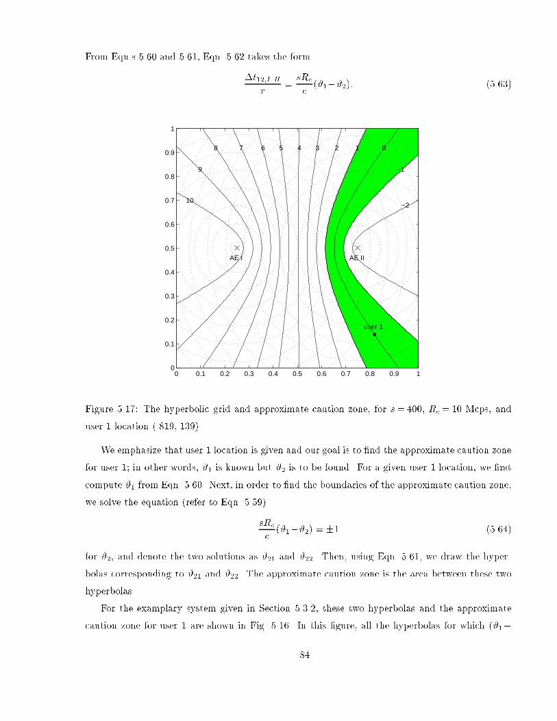
From Eqn.s 5.60 and 5.61, Eqn. 5.62 takes the form

t12;III

=sRc

c(#1#2): (5.63)

0 0.1 0.2 0.3 0.4 0.5 0.6 0.7 0.8 0.9 10

0.1

0.2

0.3

0.4

0.5

0.6

0.7

0.8

0.9

1

10

9

8 7 6 5 4 3 2 1 0

−1

−2

AE I AE II

user 1

Figure 5.17: The hyperbolic grid and approximate caution zone, for s= 400, Rc = 10 Mcps, and

user 1 location (.819,.139).

We emphasize that user 1 location is given and our goal is to nd the approximate caution zone

for user 1; in other words, #1 is known but #2 is to be found. For a given user 1 location, we rst

compute #1 from Eqn. 5.60. Next, in order to nd the boundaries of the approximate caution zone,

we solve the equation (refer to Eqn. 5.59)

sRc

c(#1#2) = 1 (5.64)

for #2, and denote the two solutions as #21 and #22. Then, using Eqn. 5.61, we draw the hyper-

bolas corresponding to #21 and #22. The approximate caution zone is the area between these two

hyperbolas.

For the examplary system given in Section 5.3.2, these two hyperbolas and the approximate

caution zone for user 1 are shown in Fig. 5.16. In this gure, all the hyperbolas for which (#1

84

#2)sRc=c is an integer are also shown; we call this set of hyperbolas the hyperbolic grid. On each

hyperbola in the hyperbolic grid, the corresponding (#1#2)sRc=c value is written; it is observed

from Eqn. 5.63 that these integers are indeed t12;III= values. We note that the \origin" of the

hyperbolic grid is the hyperbola on which user 1 is located.

It is worth emphasizing that in Fig. 5.16, if user 1 were not at the given location but were at

some other location on the same hyperbola which satises h1Ih1II = #1 (that is, the hyperbola

indicated by \0" in Fig. 5.16), the locations of the other hyperbolas and the approximate caution

zone would still be the same. Similarly, as far as the correlation analysis is concerned, as long as

user 2 is on a particular hyperbola, it does not matter where it is on that hyperbola.

Similar to Fig. 5.16, the hyperbolic grid and approximate caution zone for user 1 are shown in

Fig. 5.17, this time for some other user 1 location: (.819,.139). In Fig. 5.17, the same s and Rc

values introduced in the example given in Section 5.3.2 are used (s=400; Rc=10 Mcps).

5.7 The Eects of System Parameters on the Caution Zone

5.7.1 The sRc Product

As it has already been stated jt12;III j= is a critical quantity in the correlation analysis (refer

to Eqn. 5.59). It is observed from Eqn. 5.62 that jt12;III j= depends on a few parameters. In

the right had side of Eqn. 5.62, c is a constant, and hij , i2f1; 2g, j2fI; IIg, depends on the user

and AE locations. Therefore, the product sRc is the most important system parameter. It is also

noticed that for a certain value of the product sRc, the actual values of s and Rc do not matter.

Hence, as long as the correlation analysis is concerned, a system with s=400 and Rc=10 Mcps is

equivalent to the one with s=1000 and Rc=4 Mcps.

Let us investigate the eect of sRc more closely. For a large sRc value, the hyperbolic grid will

be denser; in other words, the hyperboles, for which (#1#2)sRc=c is an integer, will be closer to

each other. Since the approximate caution zone is the area between the hyperbolas -1 and 1, this

area will be smaller. Therefore, it is desirable to have a large sRc value. In Fig. 5.18, the hyperbolic

grid, the actual and approximate (thick lines) caution zones for user 1 are shown for the case of

sRc=8109, with user 1 location (.375,.625). This may, for instance, correspond to a system with

s = 800 and Rc = 10 Mcps. We note that in the example given in Sec. 5.3.2, sRc = 4109 (see

Fig. 5.16).

85

0 0.1 0.2 0.3 0.4 0.5 0.6 0.7 0.8 0.9 10

0.1

0.2

0.3

0.4

0.5

0.6

0.7

0.8

0.9

1

AE I AE II

user 1

Figure 5.18: The hyperbolic grid, actual and approximate caution zones, for s=800, Rc=10 Mcps,

and user 1 location (.375,.625).

5.7.2 AE Locations

The density and orientation of the hyperbolic grid also depend on the AE locations in the service

area. For a given sRc value, the density of the hyperbolic grid will increase with the increasing

distance between the AE's. Therefore, to minimize the caution zone (and thus, the correlation

eect), AE's must be placed as far apart as possible | an intuitively satisfying result.

We will demonstate this result by two examples. Fig. 5.19 shows the hyperbolic grid and the

actual caution zone for a system where the two AE's are in very close proximity. In this case,

the approximate caution zone covers almost half of the service area! Fig. 5.19, on the other hand,

shows the hyperbolic grid and the approximate caution zone for a system where the two AE's are

far apart. As expected, the corresponding approximate caution zone is much smaller. Note that

for both of the systems illustrated in Fig.s 5.19 and 5.20, sRc value (s= 800 and Rc = 10 Mcps)

and the user 1 location (.375,.625) are the same.

In the rest of this thesis, the term caution zone will be used to indicate the approximate caution

zone (that is, the area between the hyperbolas t12;III==1 and 1), unless otherwise stated.

86

0 0.1 0.2 0.3 0.4 0.5 0.6 0.7 0.8 0.9 10

0.1

0.2

0.3

0.4

0.5

0.6

0.7

0.8

0.9

1

AE I AE II

user 1

∆t12,I−II

/τ=0 ∆t12,I−II

/τ=−1 ∆t12,I−II

/τ=−2

Figure 5.19: The hyperbolic grid and approximate caution zone, for s=400, Rc=10 Mcps, user 1

location (.375,.625), and AE I & II locations (.45,.5) and (.55,.5), respectively.

5.8 Correlation Analysis for L=2 with Many Users

The analysis we performed so far corresponds to the special case of L=2 AE's with K=2 users.

In this section, we will extend our analysis to the more general case of L=2 with many users.

In a system with K users, for each user i, we determine whether the remaining K1 users arein the caution zone for user i. By this way, we construct a KK correlation matrix, U= fuijgsuch that

uij =

8<: 0; if user j is not in the caution zone for user i;

1; if user j is in the caution zone for user i.(5.65)

We note that uii=0, i=1; 2; : : : ; K; since a user does not create interference to itself. Also, it can

be shown that if user j is in the caution zone for user i, then user i must be in the caution zone

for user j. It can further be shown that if user j is in the caution zone for user i, and user k is in

the caution zone for user j, then this does not necessarily mean that user k will be in the caution

zone for user i. The conclusion from the above two sentences, in mathematical terms, is that U is

a symmetric non-transitive matrix.

87

0 0.1 0.2 0.3 0.4 0.5 0.6 0.7 0.8 0.9 10

0.1

0.2

0.3

0.4

0.5

0.6

0.7

0.8

0.9

1

∆t12,I−II

/τ=2

∆t12,I−II

/τ=1

∆t12,I−II

/τ=0

∆t12,I−II

/τ=−1

∆t12,I−II

/τ=−2

AE I

AE II

user 1

Figure 5.20: The approximate caution zone, for s=400, Rc=10 Mcps, user 1 location (.375,.625),

and AE I & II locations (.125,.875) and (.875,.125), respectively.

In Fig. 5.21, a system with L=2 and K=10 is illlustrated and the corresponding U matrix is

given (s=400 and Rc=10 Mcps). In Fig. 5.21, the caution zones are not drawn. But, if we were

to draw the caution zone for user 8, for instance, then users 2 and 4 would be in that caution zone.

Consequently, u82=1, u84=1, and all the other entries in the 8th row of the U matrix are 0's.

In the worst case, all of the K1 entries in a row of U will be 1's, and in the best case, all

of those entries will be 0's. Based on this observation, we dene a quantity which we call percent

correlation, , as follows

i =# of 1's in the ith row of the U matrix

K1 100; i = 1; 2; : : : ; K: (5.66)

It is worth noting that is not equal to the correlation coecient.

Based on the discussion in Sec. 5.7, the percent correlation for a user will depend on that par-

ticular user's location in the system, as well as the AE locations, and s and Rc values. Simulations

have been run to obtain the values for various combinations of these system parameters. For

each such combination, 100 systems (each with L=2 and K=100) are randomly (uniform user dis-

tribution) generated; consequently, a total of 10,000 values are collected. The arithmetic means

88

0 0 0 0 0 0 1 0 0 0

0 0 0 1 0 0 0 1 0 0

0 0 0 0 0 0 0 0 0 0

0 1 0 0 0 0 0 1 0 0

0 0 0 0 0 0 0 0 0 0

0 0 0 0 0 0 0 0 1 0

1 0 0 0 0 0 0 0 0 0

0 1 0 1 0 0 0 0 0 0

0 0 0 0 0 1 0 0 0 0

0 0 0 0 0 0 0 0 0 0

1

10

9

8

7

6

5

4

3

2

1 2 3 4 5 6 7 8 9 10

Correlation MatrixU:

2

3

5

6

7

8

10

I II

1

9 4

Figure 5.21: A system with L= 2 and K = 10, and the corresponding correlation matrix, U, for

s=400 and Rc=10 Mcps.

of these values, , for various combinations of the system parameters, are given in Fig. 5.22.

5.9 Correlation Analysis for Many AE's with Many Users

In this section, we extend our analysis to the most general case of L AE's with K users.

In this case, for each user, a total of L(L1)=2 caution zones exist, each of which corresponds

to a particular AE pair. Therefore, the U matrix is composed of L(L1)=2 submatrices (one foreach antenna pair), with sizes KK. Consequently, the correlation matrix, U, is 3-dimensional

with size [L(L1)=2]K K. Such a system, for the case of L=4 and K=10, is illustrated in

Fig. 5.23.

For a user i, the most disadvantageous situation will occur if all of the remaining K1 usersare in all of the L(L1)=2 caution zones for user i. Obviously, this is an event with a very low

likelihood! Such a situation will yield (K1)[L(L1)=2] 1's in the 2-dimensional ith row of the U

matrix. Based on this observation, we dene the percent correlation, , as

i =# of 1's in the 2-dimensional ith row of the U matrix

(K1)L(L1)2

100; i = 1; 2; : : : ; K: (5.67)

The size of the simulations grows rapidly due to the L(L1)=2 factor. Therefore, we consideredonly L= 4 and K = 100 case with s= 400 and Rc = 10 Mcps. Similar to the simulations in the

previous section, 100 systems are randomly (uniform user distribution) generated, and thus, a total

89

K = 100 users

R = 10 Mcpsc

s = 1000

s = 400

s = 40 90.11

27.09

14.26

5.95 15.06

32.58

100.00

52.41

3.46

8.67

17.07

69.02

3.70

9.23

18.37

75.33

s = 200

AE I (0,0)

AE II (1,1)

AE II (1,.5)AE I (0,.5)AE I (.25,.5)

AE II (.75,.5) AE II (.6,.5)

AE I (.4,.5)

Figure 5.22: The average percent correlation, , values for various combinations of AE locations,

and s and Rc values, in systems with L=2 and K=100.

of 10,000 values are collected. The average percent correlation, , is found to be 12.75, as shown

in Fig 5.24.

5.10 Comparison with Hanly's Work [50] Part II

In Sec. 4.6, we made some comparisons between our results and those given in a somewhat similar

study [50]. In this section, we continue with the comparison. To the best of our knowledge, the

only work in the literature on space-related correlation analysis in CDMA macrodiversity systems

is Section 7 of [50]. Although the approach of that section to the problem is correct, the discussion

is rather brief and qualitative. Based on the rigorous analysis we presented in this chapter, we will

comment on some of the statements in [50].

Hanly states in [50]: \: : :More precisely, for user u, let tu(j; k) be the dierence in propagation

delays between the user and the receivers j and k, respectively. If two users u and v are so close

that jtu(j; k) tv(j; k)j is less than a chip time, then the interference at j and k, for the decoder

of user u (or v) will be correlated. : : : For example, if W =20 MHz, then the chip time is 5 108

seconds, during which time light travels 15 m. It is clear that the proportion of users in a network

that have path dierences within 15 m will be very small." In this quotation, W denotes the spread

spectrum bandwidth.

The expression tu(j; k) tv(j; k) given in [50] is the equivalent of the dierential delay 12;III

that we dened in Eqn. 5.53. We have shown throughout this chapter that j12;III j= < 1

90

2

3

5

6

7

10

1

8

II

2

3

5

6

7

8

10

1

I

III

3

5

6

7

8

10

1

I

2

IV

3

5

6

7

10

1

3

5

6

7

10

1

3

5

6

7

8

10

1

8

II

2

III

8

II

2

IV

2

IV

9 4

9 4

9 4

9 4

9 4

9 4

III

I

1

10

9

8

7

6

5

4

3

2

0 0 0 0 1 0 0 0 0 0

0 0 0 0 0 0 0 0 0 0

0 0 1 0 0 0 0 0 0 0 0

0 0 0 0 0 0 0 0 0 0 0 0

0 0 0 0 0 0 0 0 0 0 0 0 0

0 0 1 0 0 0 0 0 0 0 0 1 0

0 0 0 0 0 0 0 0 0 0 00 0 0 0 0 0 0 0 0 0 0 0

0 1 0 0 0 0 0 0 0 0 0 0 0 00 0 0 0 0 0 0 0 0 0 0 0 0 0 0

0 0 0 1 0 1 0 0 0 0 0 0 0 0 0

0 0 0 0 0 0 0 0 1 0 0 0 0 0 0

0 1 0 0 0 1 0 0 0 0 0 0 0 0 0

0 1 0 1 0 0 0 0 0 0 0 0 0 0

0 0 0 0 0 0 0 0 0 1 0 1 0 0 0

I-II

I-III

I-IV

II-III

II-IV

III-IV

I-IIII-II

III-IVII-IVII-III

1 2 3 4 5 6 7 8 9 10

I-IV

Correlation MatrixU:

Figure 5.23: A system with L= 4 and K = 10, and the corresponding correlation matrix, U, for

s=400 and Rc=10 Mcps.

c

K = 100 users

s = 400

φ =12.75R = 10 McpsAE I AE II

AE III AE IV

Figure 5.24: The average percent correlation, , in systems with L=4 and K=100.

corresponds only to an approximation of the areas where the correlated interference exists. The

actual such areas (caution zones) depend on the values of tu(j; k) and tv(j; k) (refer to, for example,

Fig.s 5.7 and 5.8). Therefore, the rst part of the above quoted statement is imprecise.

In the second part of the quotation, Hanly considers only a small area around a user as the

caution zone. However, we have demostrated analytically and shown in numerous gures that the

caution zones are, in fact, much broader due to the geometry of the problem. Two users that are

at dierent sides of the service region may cause signicant correlated interference to one another.

91

5.11 Chapter Summary and Remarks

If the interference (noise) components at the ngers of the Rake receiver are uncorrelated, then

MRC yields an output SIR that is the algebraic sum of the nger SIR's. If, however, the interference

components start becoming correlated, the returns from combining will decrease accordingly. In

the limiting case of identical signal and interference components at the Rake ngers, there is no

gain at all from combining. Therefore, having many AE's, and thus, a Rake with many ngers,

does not automatically guarantee a better performance; we must ensure that the corresponding

interference components are uncorrelated (or slightly correlated so that its eect is insignicant).

To this end, the objective of this chapter is to evaluate the conditions under which the correlated

interference occurs, and to determine its eects on the system performance.

We started this chapter by analyzing the simplest case of L=2 with K=2, in order to develop

some insight into the problem of correlated interference. For this special case, we were able to obtain

the correlation coecient as a function of the distances involved in the service region. Hence, for

a given user location, we were able to determine the portions of the service region in which other

user(s) would cause correlated interference to the given user; we called this region the caution zone

for the given user. We then found an approximate expression (and an approximate caution zone)

in simpler terms.

Subsequently, we extended our analysis to the more general case of L = 2 with many users.

In this case, since obtaining the correlation coecient would be very tedious, we worked with a

simpler quantity which we called the percent correlation. Finally, we considered the most general

case of many AE's with many users.

We found that the caution zone, for a given user, depends on the location of that particular

user, as well as the AE locations, cell size, and the chip rate. Increasing the chip rate, and putting

the AE's as far as possible from each other,1 results in a reduced correlated interference eect.

Our initial results indicate that for reasonably high chip rates and for cells that are not very

small, the eect of correlation is mild if the number of AE's is not very high. Further investigation

is required to make similar conclusions for the cases with high numbers of AE's.

5.12 Future Research Directions

As stated earlier, almost no literature exists on the space-related correlation analysis in CDMA

macrodiversity systems. Therefore, we believe that our work lays down a foundational framework

1For large L values, this is equivalent to distributing the AE's uniformly throughout the service region.

92

in this area. Although the simulations that we performed may not be comprehensive, and thus,

conclusive, for certain cases (such as the ones with high L values), they are still very important,

since this initial analysis may eventually enable us to understand how and why the returns in SIR

plateau with increasing number of AE's. Some of the possible research directions are given below:

We stated that the locations of AE's are very important as long as the correlation eect

is considered. For an irregular service region, obtaining the optimal AE locations requires some

further investigation. It is interesting to note from Fig. 5.22 that, the system with AE locations

(0,.5) and (1,.5) yields a better result than that with AE locations (0,0) and (1,1), although the

inter-AE distance is larger in the latter system.

We dened the percent correlation, , in Sec. 5.8. This quantity is very useful in comparing

two systems with dierent parameters; obviously, the one with a lower is preferable. However,

what is a reasonable value for ? In other words, up to what value of we can neglect the eect

of correlated interference? These questions should be investigated by analytic methods.

The simulations should be extended to cover larger L values with dierent K=L ratios. We

obtained = 12:75 for L = 4 and K = 100 case, and this is better than 14.26, which is the

corresponding value for the L= 2 and K = 100 case; however, it is unfair to compare these two

gures, since K=L ratios in the two systems are dierent (25 and 50, respectively).

There still remains a fundamental question: in a given service area that is to be covered by anSDA cell, can we put as many AE's as we wish without an upper limit? In an SDA system, putting

more AE's would always yield better performance (this is analogous to a dish antenna: the greater

the diameter, the better the performance). However, the returns in SIR may diminish gradually

as L increases, since signals received by dierent AE's would start being correlated. Taking the

increasing complexity and processing in the system into account, adding more AE's would not be

worthwhile after a point, which puts an upper limit on the number of AE's. Finding this upper

limit may yield an interesting spatial sampling theorem.

93

Chapter 6

Antenna Interconnection Strategies

In order to provide high capacity, ubiquitous coverage, and to be able to support compact and

lightweight wireless terminals, a very large number of antennas should be deployed in urban areas;

according to one estimate, more than 5000 cells would be required in the Tokyo metropolitan

area [59]. Therefore, building an aordable infrastructure for the WAN is a major challenge.

In a WAN, there are two main cost factors: the cost of the BS's, and that of the interconnecting

infrastructure that links these BS's, which is proportional to the length of the wired-network. In

this chapter, antenna interconnection strategies for WAN's are studied in order to determine cost-

ecient as well as robust and exible interconnection architectures. To this end, some results from

minimal networks theory are used, in particular, those dealing with the well-known problem of

Steiner trees.

In Sec. 6.1, the relation between the antenna interconnection architecture and the logical net-

work topology is presented. In Sec. 6.2, the Steiner minimal tree (SMT) architecture is described,

and SMT construction in hexagonal and square layouts is discussed. The conduit length compar-

isons between the star and SMT architectures are presented in Sec. 6.3. In Sec. 6.4, interconnec-

tion strategies for linking various central stations are examined. The realization of logical network

topologies within the optimal SMT conduit infrastructure is addressed in Sec. 6.5; and nally,

concluding remarks are made in Sec. 6.6.

6.1 Antenna Interconnection Architectures and Resulting Logical

Network Topologies

In the current cellular mobile communication systems (such as AMPS or GSM), T1 lines or mi-

crowave radio links are most commonly used for connecting the BS's to the MTSO [60]. In the

case of the T1 cables, generally, the star architecture is employed, mainly due to its topological

94

simplicity. In a star architecture, if a new BS is to be added to the network, a cable is laid down

between the new BS and MTSO. Hence, there is no need for coordination with the other BS's.

Also, a fault in any BS, or in the cable, would only aect that particular BS, and moreover, the

distance between any BS and the MTSO is minimal, which may eliminate the need for ampliers

in the feeder. However, the required cabling for the star architecture is excessive.

6.1.1 Complexity/Intelligence Distribution and the Logical Network Topology

Dierent ways of distributing the complexity/intelligence in the system yield a variety of logical

network topologies in which the above mentioned two cost factors (BS and interconnecting infras-

tructure costs) con ict.

The length and logical topology of a network are closely related. However, simply changing the

logical topology of a network, in order to decrease its length, is not necessarily a solution, since

doing so may increase the cost of the base stations.

6.1.2 Microcellular Systems

Since the radius of a microcell is in the order of a few hundred meters or less, a very large number

of microcells will be required to cover metropolitan areas. If a conventional BS is needed for

each microcell, then the deployment cost would become extremely high. Furthermore, it is very

dicult to nd convenient locations for the bulky BS equipment every few hundred meters in

urban areas. Therefore, it would be very desirable if the microcell BS (Micro-BS) could contain a

minimal amount of hardware, and if most of the processing could be performed at a CS located at

a convenient economical site, serving many of these microcells.

Dierent possible methods of distributing the processing among a Micro-BS and the CS yield a

variety of systems. The microcellular systems which have low levels of complexity at the Micro-BS's

have naturally logical star topologies, resulting in greater network lengths. On the other hand, the

systems with logical bus topologies, have shorter lengths; however, they suer from a higher level of

complexity at the Micro-BS's, since the signals from dierent Micro-BS's should be distinguishable

at the CS.

Ultimately, all the signal specic processing can be moved to the CS, from which the radio

signals are delivered to Micro-BS's via ber optic, coaxial or microwave links [14,61].

In a metropolitan area where the Micro-BS's are many kilometers away from the CS, it is

almost impossible to have line-of-sight links between the utility-post-mounted Micro-BS antennas

and the CS. This would yield severe multipath and shadowing phenomena in addition to the

95

path loss. Therefore, despite their easy installation, microwave links are not suitable in many

environments (although the networking of CS's may be realized via microwave links as we will

address in Section 6.4). The main problems associated with coaxial links are the signicant losses

in the cable and the poor frequency response [61]. Even if high-gain RF ampliers are inserted in

the feeder, the resulting SNR is not sucient, unless the distances between the CS and Micro-BS's

are short enough to utilize repeaterless coaxial cables [62].

On the other hand, advances in lightwave technologies, along with the availability of wide-

bandwidth, very low-loss (around to 0.2 dB/km) ber optic cables, enable the tranmission of radio

signals between the CS and Micro-BS's without amplication for more than 20 km, using sub-

carrier multiplexing (SCM) [59,63]. In this case, the Micro-BS would contain only an optoelectric

(O/E) converter and power amplier (PA) in the forward link, and a low noise amplier (LNA)

and an electrooptic (E/O) converter in the reverse link as shown in Fig. 6.1(a).1 The ber optic

antenna remoting oers other advantages along with simple and economical Micro-BS's, for in-

stance, centralized control (which is suitable for macro diversity and dynamic channel allocation),

and transparency to the modulation scheme (FDMA, TDMA or CDMA) employed [60].

The above described system has a logical star topology because of the point-to-point nature of

SCM ber optic links [Fig. 6.1(a)] [61, 6466]. The star architecture provides high reliability and

easy maintenance due to its topology; however, it requires an enormous investment for the wired

network infrastucture. In order to decrease the infrastucture cost, an alternative architecture,

the passive double star (PDS), has been proposed which employes optical passive splitters, as

illustrated in Fig. 6.1(b) [66]. Although the PDS architecture yields great savings in wired network

infrastucture, the simplicity of Micro-BS, which was originally one of the major motivations for

using ber optic links, is lost. This is due to the fact that, since the PDS architecture has a logical

bus topology, the CS cannot distinguish between the signals coming from dierent Micro-BS's

unless Micro-BS's are equipped with transmitter/receivers (TX/RX) modems.

One other possibility is to implement a bus architecture, in which case many Micro-BS's are

coupled to a ber optic bus via passive optical couplers as shown in Fig. 6.1(c), and time-division

multiplexing (TDM) is employed to distinguish the signals of dierent Micro-BS's [67]. In this

scheme, however, to compensate for the coupling losses, optical ampliers should be inserted in the

cable, and furthermore, hardware should be included at Micro-BS's for TDM. An amplier chain

in the feeder is not desirable since, in such a case, the Micro-BS's that are further away from the

1This concept has been addressed in the literature under dierent names, such as \antenna remoting" [60],

\extension", or \separation" [61], and the Micro-BS has been referred to as \remote cell site" [60], \microcell base

unit" [13], \antenna remote unit" (ARU) [63], and \radio base station" (RBS) [64].

96

CS have much poorer reliability compared to those which are closer.

Hybrid coaxial/SCM-ber links can also be utilized for the PCS access network [62]. In this

system, the Micro-BS's which belong to the same cluster of microcells can be connected to a signal

combiner via coaxial cables (as long as the coaxial cable length is less than a few hundred metres so

that there is no need for amplication in the feeder), and the combiner is connected to the CS via a

ber optic link. Since the signals from all the microcells in a cluster are summed at the combiner,

this architecture, which is suitable for FDMA and TDMA schemes, cannot be used with the CDMA

scheme. We note that the hybrid coaxial/ber network is also a double-star architecture (with a

small splitting ratio), and therefore it has a logical bus topology.

6.1.3 Distributed Antenna and Sectorized Distributed Antenna Systems

Both DA and SDA systems have logical bus topologies. In the case of a DA scheme, a coaxial bus

link can be used to connect the AE's and the CS, as long as the cell is not very large; obviously,

a ber optic bus employing SCM is another possibility. In either case, ampliers may need to be

inserted in the feeder to compensate for the coupling losses. It is worth noting that, unlike the

microcellular bus link discussed in the previous section, the DA bus link does not require the use

of TDM or frequency conversions at the antenna elements since, in a DA cell, the same signal is

fed to all of the AE's.

In the case of an SDA, a separate bus link runs in each sector, which may be either a coaxial or

a ber optic cable, although the ber may be more approporiate for the farther sectors. A hybrid

coaxial/ber bus link may be another possibility; the radio signal may be delivered to a distant

sector via a ber cable, and in the sector, a coaxial bus may be used. For the limiting case of one

AE per sector in an SDA, the architecture is the star type, and transmission without repeaters is

possible since there are no coupling losses.

6.1.4 Logical Topology versus Conduit Structure

A cable can be installed only on those links of a wired network where a conduit has been placed.

Since the conduit placement is far more expensive than the material cost of the cable, the cost-

saving cable deployment strategy is to let a conduit path be shared by many dierent cable routes

wherever possible [68]. For instance, in a microcellular network which has logical star topology,

there is only one cable route between the CS and a Micro-BS; however, the connections are not

necessarily restricted to the \point-to-point" type. In other words, the logical topology and the

actual conduit layout do not need to have the same architecture. In the following few sections, the

97

focus will be on constructing ecient conduit architectures, and in Sec. 6.5, a discussion will be

presented on how to map a logical cable topology into the optimal conduit infrastructure.

6.2 The Steiner Minimal Tree Architecture

Let us consider a typical access network where many AE's (or Micro-BS's) are to be connected to

a CS. The straightforward and conventional interconnection structure is the star architecture as

shown in Fig. 6.2(a) for the hexagonal layout. However, as mentioned earlier, the main problem in

implementing this architecture is the enormous nancial investment required for the construction

of the conduit infrastructure.

The architectures illustrated in Fig. 6.2 may correspond to DA (or SDA) systems with AE's and

CS's, or to microcellular systems with Micro-BS's and CS's. Without loss of generality, however,

we will assume that the architectures studied in this paper correspond to DA systems. Thus, a

hexagonal region shown by dotted lines in Fig. 6.2 (and also in other gures) does not denote an

individual cell; rather, it is the area wherein a wireless user is most likely to receive the strongest

signal from the corresponding AE in the center of the region. A cell, then, refers to the area

bordered by thick lines in the gures that encloses many AE's and a CS. On the other hand, for

the case of a microcellular system, this bordered area would correspond to a service area covered

by many Micro-BS's connected to a CS.

6.2.1 Shortest Interconnection Network Problem

A network architecture which consists of AE's and transmission links can be represented by a

connected graph where the AE's are shown by vertices (points) and the links by edges. Let =

f1;2; :::;Lg be a set of L points in the plane, denoting L AE's to be interconnected. Since the

objective is to minimize the total conduit length, the corresponding graph that interconnects these

L points should not contain any cycles because removing an edge from the cycle will readily reduce

the total length (or weight), but this will not disconnect the graph. Therefore, a tree structure

that spans all of the vertices and also yields the minimum total length is required.

If no new points are allowed to be added to the original set (i.e, if the vertices of the

required tree are exactly the points in ), then the shortest network connecting these points is

called a minimal spanning tree (MST). Two classical algorithms for nding such a tree are Prim's

algorithm (1957), which adds edges which extend the existing tree and do not create cycles, and

Kruskal's algorithm (1956), which adds edges which connect components [69, pp. 593598]. In

Fig. 6.2(b) and (c), two dierent MST's in a hexagonal layout are illustrated. We note that since

98

the lengths (weights) of the edges in the hexagonal layout are not all dierent, MST is not unique.

However, it is possible to construct still shorter trees connecting 1; :::;L by adding extra

vertices beside the i. The shortest possible tree constructed in this way is called the Steiner

minimal tree (SMT) and the additional vertices are called Steiner points [70,71].

A tree interconnecting a set of L points in the plane, by adding extra vertices (Steiner points)

if necessary, is called a Steiner tree (ST) if it satises the following conditions [72]:

1) No two edges meet at less than 120.

2) There are at most L2 Steiner points.3) Each Steiner point has exactly three incident edges.

Conditions 1) and 3) together imply that every Steiner point has exactly three edges meeting at

120. An SMT is simply the shortest ST; thus, it should be emphasized that not every ST is an

SMT. Finally, an ST is called full (FST) if it has exactly L2 Steiner points.

6.2.2 SMT Construction Principles

The SMT constructions for L= 3 and L= 4 are well known. A summary is presented below for

these cases along with the general case of L points.

L = 3: If 4123 has an angle 120, then adding Steiner points does not help in reducing

the total length of the network [Fig. 6.3(a)]. Otherwise, three equilateral triangles are drawn on

the sides of 4123. If the far vertex of each equilateral triangle is joined to the opposite i,

then these lines meet at a single Steiner point2[Fig. 6.3(b)]. The length of the SMT constructed in

this way, SMT = 1S + 2S + 3S, satises [73, p. 140]:

SMT = 1A = 2B = 3C: (6.1)

For the special case of the hexagonal layout, with hexagon radius a, it is obvious from Fig. 6.3(c)

that

SMT = 3a: (6.2)

L = 4: Similar to the case for L=3, equilateral triangles are drawn on the sides 13 and 24

[Fig. 6.3(d)], and then their far vertices (A and B, respectively) are joined. The intersection of this

line and the circles shown locates Steiner points S1 and S2. It can be shown [74] that in Fig. 6.3(d)

1S1 + 3S1 = AS1 and 2S2 +4S2 = BS2: (6.3)

2In Fig.s 6.3 and 6.4, the Steiner points are shown by white dots.

99

Therefore, the length of the SMT with vertices 1;2;3;4; S1 and S2, is equal to AB. We note

that another ST can be formed [Fig. 6.3(e)] in general; however, the ST with the longer central

edge is the SMT. For the special case of hexagonal layout [Fig. 6.3(f) and (g)], SMT(= AB) is

the hypotenuse of a right triangle whose other two sides have lengths 4:5a andp3a=2; so using the

Pythagorean theorem, LSMT can be shown as

SMT =q(4:5a)2 + (

p3a=2)2 =

p21a: (6.4)

It is worth noting that for the hexagonal layout, both of the possible ST's [Fig.s 6.3(f) and (g)] are

SMT's.

L-Point Case: If L 5, then SMT construction becomes very dicult. The existence of a nite

algorithm for SMT construction was proven by Melzak in 1961 [75]; but this problem in the general

case is extremely complicated. Melzak's algorithm makes use of the following observation: if the

SMT does not have as many as L2 Steiner points, then the SMT will decompose into a number of

smaller FST's which meet each other at some subset of the given vertices [74]. Melzak's algorithm

makes use of the following facts [76]: SMT() (which denotes the SMT corresponding to set )

may always be decomposed into sets SMT(L1), SMT(L2

), : : :, SMT(Ll), where L1, L2

, : : :,

Ll are subsets of with j Li \ Lj j 1, 8 Li 6= Lj , where SMT(Lk) is an FST for Lk ,

and the edges of the SMT(Lk) form a partition of the edges of SMT(). Fig. 6.4(a) and (b)3

shows such a decomposition and the yielding SMT, respectively, for a case of L= 10. Although

we do not know a priori how to decompose the given L points into subsets, the total number of

possible decompositions is nite [73]. However, if we try all possibilities, their number will grow

exponentially. The exponentiality is more of a problem inherent to the SMT rather than just with

Melzak's algorithm [71]; indeed, it is shown in [77] that the SMT construction for a general set

is NP-complete.

6.2.3 SMT Construction for Hexagonal Layout

An important consideration for NP-complete problems is the study of special cases. To this end,

in this section, we discuss the SMT construction for hexagonal layout. We note the practical

importance of this layout since the hexagon is the most commonly used geometrical shape in

modeling the service area of an AE in wireless communications.

Let us rst introduce the concept of the Steiner ratio. For a given arbitrary set of points , if

MST and SMT denote the lengths of the MST and SMT, respectively, then, the following theorem

holds (for the proof, see [70, pp. 166177]):

3Fig. 6.4(b) is taken from [73, p. 142].

100

Theorem 1: (Steiner ratio) = inf(SMT()=MST()) =p3=2 = 0:8660 : : :, where

\inf" is taken over all possible sets of .

We note that it is quite important to know to what extent a heuristic (like MST) approximates

the optimum structure (SMT) since the problem of SMT construction is NP-complete. Since, for

any layout,

=

p3

2= 0:8660 SMT

MST 1; (6.5)

the maximum increase in conduit length for constructing an MST instead of the SMT can be

calculated as1p3=2p

3=2 100% ' 15%: (6.6)

Hexagonal Cells

We start by examining the special case of a hexagonal cell in the hexagonal layout.

Theorem 2: For a hexagonal cell in the hexagonal layout, the SMT construction is

achieved by decomposing the vertices into subsets of 3 points which form equilateral

triangles.

Since the vertices in the hexagonal layout are located at the intersection points of the triangular

grid, this decomposing strategy is intuitively satisfying. There are many possible ways of forming

these three-point subsets; one of them, along with the corresponding SMT, is illustrated in Fig. 6.5.

This theorem is proven in [78] by induction. Here, we will give an alternate proof based on the

concept of the Steiner ratio.

Proof: It can be shown that in a hexagonal cell constructed in the hexagonal layout,

for a given n (which is the number of AE's at one side of the hexagonal cell), there are

L = 3n(n 1) + 1 (6.7)

AE's (points), for instance, in Fig. 6.5, n=4 and L=37.

Let 0 be the length of the tree structure illustrated in Fig. 6.5. It is not dicult to

show that there are a total of (L1)=2 three-point subsets in such a tree with L points.

Since the three-point FST's formed for each subset have lengths of 3a,

0 =L 1

23a: (6.8)

It is well known that if a graph is a tree with L vertices, then it has precisely L1edges. In the hexagonal layout with hexagon radius a, the distance between any two

101

neighboring vertices, which is the length of an edge of the MST, is found to bep3a.

Therefore, MST for an L-point hexagonal cell [see Fig. 6.2(b) and (c)] is

MST = (L1)p3a: (6.9)

If the ratio of the above two equations is taken, we obtain

0=MST =

p3

2: (6.10)

But this is equal to , the Steiner Ratio; therefore, MST = 0. This result shows that

the decomposition strategy in the form of three-point subsets depicted in Fig. 6.5 yields

SMT's. 2

General Cell Shape

Based on the proof given in the previous section, many other interconnecting structures for arbi-

trary cell shapes can also be shown to be SMT's as long as L is an odd number and the exact

decomposition of set into three-point subsets is possible, as shown in Fig. 6.6(a) and (b). If L is

an even number, however, this exact decomposition into subsets of three-points cannot be realized.

Even for an odd L, there may be cell shapes for which subsets with number of points other than

three may needed to be formed; an example is shown in Fig. 6.6(c) where two-point subsets along

with a three-point one are formed to construct the SMT. For such cases, where the exact decompo-

sition into subsets of three-points is not possible, however, we can not use the Steiner ratio theorem

to prove that these interconnecting structures are indeed SMT's.

Because of the fact stated in Eqn. 6.5, we can be certain that whatever the cell shape is,

MST =3

2(N1)a SMT MST = (L1)

p3a: (6.11)

6.2.4 SMT Construction for Square Layout

To construct SMT's in a layout other than the hexagonal one is quite challenging. In this section

we discuss a square layout with square service regions of L = n2 AE's, with inter-AE distance a.

For the special case of n = 2k (or L = 22k), k = 1; 2; : : : ; the SMT is constructed by decomposing

the set into 4-point subsets which form squares [76]. The case for n = 8 is shown in Fig. 6.7(a)

and the resulting tree structure is illustrated in Fig. 6.7(b). There are a total of (L1)=3 suchsubsets, with each FST for each subset having a length (

p3 + 1)a. Therefore,

SMT =L13

(p3 + 1)a: (6.12)

102

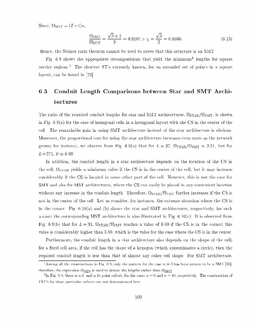
Since, MST = (L1)a,

SMT

MST=

p3 + 1

3= 0:9107> =

p3

2= 0:8660: (6.13)

Hence, the Steiner ratio theorem cannot be used to prove that this structure is an SMT.

Fig. 6.8 shows the appropriate decompositions that yield the minimum4 lengths for square

service regions.5 The shortest ST's currently known, for an extended set of points in a square

layout, can be found in [79].

6.3 Conduit Length Comparisons between Star and SMT Archi-

tectures

The ratio of the required conduit lengths for star and SMT architectures, STAR=SMT, is shown

in Fig. 6.9(a) for the case of hexagonal cells in a hexagonal layout with the CS in the center of the

cell. The remarkable gain in using SMT architecture instead of the star architecture is obvious.

Moreover, the proportional cost for using the star architecture increases even more as the network

grows; for instance, we observe from Fig. 6.9(a) that for L = 37, STAR=SMT is 2.51, but for

L=271, it is 6.69.

In addition, the conduit length in a star architecture depends on the location of the CS in

the cell; STAR yields a minimum value if the CS is in the center of the cell, but it may increase

considerably if the CS is located in some other part of the cell. However, this is not the case for

SMT and also for MST architectures, where the CS can easily be placed in any convenient location

without any increase in the conduit length. Therefore, STAR=SMT further increases if the CS is

not in the center of the cell. Let us consider, for instance, the extreme situation where the CS is

in the corner. Fig. 6.10(a) and (b) shows the star and SMT architectures, respectively, for such

a case; the corresponding MST architecture is also illustrated in Fig. 6.10(c). It is observed from

Fig. 6.9(b) that for L= 91, STAR=SMT reaches a value of 6.60 if the CS is in the corner; this

value is considerably higher than 3.89, which is the value for the case where the CS is in the center.

Furthermore, the conduit length in a star architecture also depends on the shape of the cell;

for a xed cell area, if the cell has the shape of a hexagon (which approximates a circle), then the

required conduit length is less than that of almost any other cell shape. For SMT architecture,

4Among all the constructions in Fig. 6.8, only the pattern for the case n = 3 has been proven to be a SMT [76];

therefore, the expression MIN is used to denote the lengths rather than SMT.5In Fig. 6.8, there is a 3- and a 10-point subset, for the cases n = 6 and n = 10, respectively. The construction of

FST's for these particular subsets are not demonstrated here.

103

however, the eect of cell shape on the conduit length is marginal, as described in Section 6.2.3.

In Fig. 6.11, rectangular cells in the hexagonal layout with L=37 are illustrated. If the CS is in

the center of the cell, then STAR=SMT [see Fig. 6.11(a) and (b)] would be 3.80 [Fig. 6.9(c)]; this

is considerably higher than the 2.51 obtained from Fig. 6.9(a), which is the corresponding ratio for

a hexagonal cell, again with L= 37. In Fig. 6.11(c), an MST architecture, for which the conduit

length is totally independent of the cell shape, is also shown.

Obviously, for star architecture, the combined eect of the cell shape and the CS location is

even more severe on the conduit length. For instance, for the case illustrated in Fig. 6.11(d), where

the CS is located in the corner of a rectangular cell with L= 37, STAR=SMT increases to 7.21

[Fig. 6.9(d)]; this value is signicantly higher than 2.51, which is the corresponding ratio for the

case where the CS is in the center of a hexagonal cell.

If a cell grows too large, it may become benecial or necessary to split it into two (or more)

cells. In a star architecture, since all the existing conduits meet in a central location, splitting a

cell requires a major reconguration; therefore, it is not practical, as shown in Fig. 6.12(a) [80].

An SMT (also MST) architecture, however, can easily be split without any major reconguration

[Fig. 6.12(b)].

6.4 Interconnection of Central Stations

In general, an access network infrastructure consists of AE's, CS's, main switches, and transmission

links interconnecting them. In such a network, AE's are connected to the corresponding CS, and

various CS's are connected to a main switch, which links the entire network to a xed network such

as the PSTN.

One way to establish this interconnection is to link a CS and the corresponding AE's in the form

of an SMT, and then connect the CS's and the main switch, again in an SMT form, as shown in

Fig. 6.13(a). We call this structure an double-SMT architecture. Such a structure can be thought of

as a tree with two stages, as illustrated in Fig. 6.13(b). It is worth noting that, although both levels

of this interconnecting tree are constructed as SMT's, the overall tree is not an SMT, nor even an

ST. Therefore, the length of a double-SMT architecture is (slightly) more than that of a single-SMT

type. It is reported in literature, however, that the double-star architecture is signicantly shorter

than the single-star type [66,80]. Consequently, it is not a good strategy to construct a double-SMT

architecture instead of a single-SMT type, unlike the case for the star architecture. Nevertheless, a

double-SMT architecture is still shorter than a double-star type, simply because the SMT in each

level of the tree is shorter than the corresponding star type. Fig. 6.14 shows the conduit length

104

comparisons, in terms of hexagon radius a, for the one- and two-level architectures, for the cases

of 7 cells with 7 AE's, 7 cells with 19 AE's, and 19 cells with 19 AE's. For all of these cases, both

the cells and the structures formed by the combination of cells are in hexagonal shapes.

As far as the conduit length is concerned, an improved method of realizing the interconnection

is shown in Fig. 6.15(a). In this case, the overall structure is a single SMT, which we call an

extended SMT architecture; hence, it yields the minimum total conduit length.

One other possibility is that the interconnection between the CS's and the main switch may be

established via radio [Fig. 6.15(b)]. In such a case, the structure can be thought of as a collection

of unconnected SMT's; therefore, the conduit length need only be considered for the connections

in the rst level of the tree shown in Fig. 6.13(a). Although this architecture, which we call a

single-layer SMT, requires less conduit than the extended-SMT type, there is the additional cost of

the radio equipment to implement the second level of the tree illustrated in Fig. 6.13(a).

As an example, let us consider the case where a xed area is served by M cells, each having N

AE's. Using Eqn. 6.8, the required conduit lengths for the three architectures described above can

be found, in terms of hexagon radius a, as

extended SMT =3

2(ML1)a; (6.14)

single-layer SMT =3

2M(L1)a; (6.15)

double SMT =3

2M(L1)a+ 3

2(M 1)

pLa: (6.16)

The required conduit lengths are plotted in Fig. 6.16 for the case of ML = 3367. It is observed

from Fig. 6.16 that if an double-SMT architecture has to be implemented, the best strategy would

be to maximize the number of AE's in each cell (or, equivalently, to minimize the number of cells

in the xed service area); this would give a large L and small M . However, if the CS's could be

connected to the main switch via radio links (single-layer SMT), then it would be most ecient

to minimize the number of AE's in each cell (or, equivalently, to maximize the number of cells),

hence yielding a small L and large M .

6.5 Cable Congurations in the SMT Conduit Architecture

All the logical topologies described in Section 6.1 can be realized within the optimal SMT conduit

infrastructure. Fig. 6.17(a) shows the mapping of a wired network which has logical star topology

into an SMT conduit architecture. This network may correspond to a ber optic microcellular

system utilizing SCM, or to an SDA system with one AE per sector. Physical implementation

105

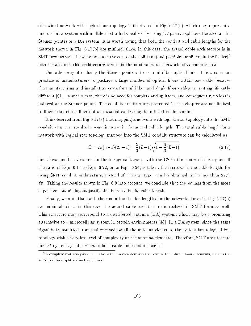
of a wired network with logical bus topology is illustrated in Fig. 6.17(b), which may represent a

microcellular system with multilevel star links realized by using 1:2 passive splitters (located at the

Steiner points) or a DA system. It is worth noting that both the conduit and cable lengths for the

network shown in Fig. 6.17(b) are minimal since, in this case, the actual cable architecture is in

SMT form as well. If we do not take the cost of the splitters (and possible ampliers in the feeder)6

into the account, this architecture results in the minimal wired network infrastructure cost.

One other way of realizing the Steiner points is to use multiber optical links. It is a common

practice of manufacturers to package a large number of optical bers within one cable because

the manufacturing and installation costs for multiber and single-ber cables are not signicantly

dierent [81]. In such a case, there is no need for couplers and splitters, and consequently, no loss is

induced at the Steiner points. The conduit architectures presented in this chapter are not limited

to ber links; either ber optic or coaxial cables may be utilized in the conduit.

It is observed from Fig 6.17(a) that mapping a network with logical star topology into the SMT

conduit structure results in some increase in the actual cable length. The total cable length for a

network with logical star topology mapped into the SMT conduit structure can be calculated as

= 2n(n1)(2n1) = 2

3(L1)

r1 +

4

3(L1); (6.17)

for a hexagonal service area in the hexagonal layout, with the CS in the center of the region. If

the ratio of Eqn. 6.17 to Eqn. 6.22, or to Eqn. 6.24, is taken, the increase in the cable length, for

using SMT conduit architecture, instead of the star type, can be obtained to be less than 27%,

8n. Taking the results shown in Fig. 6.9 into account, we conclude that the savings from the more

expensive conduit layout justify this increase in the cable length.

Finally, we note that both the conduit and cable lengths for the network shown in Fig. 6.17(b)

are minimal, since in this case the actual cable architecture is realized in SMT form as well.

This structure may correspond to a distributed antenna (DA) system, which may be a promising

alternative to a microcellular system in certain environments [36]. In a DA system, since the same

signal is transmitted from and received by all the antenna elements, the system has a logical bus

topology with a very low level of complexity at the antenna elements. Therefore, SMT architecture

for DA systems yield savings in both cable and conduit lengths.

6A complete cost analysis should also take into consideration the costs of the other network elements, such as the

AE's, couplers, splitters and ampliers.

106

6.6 Chapter Summary and Remarks

In this chapter, some concepts from minimal networks theory are utilized in order to determine

cost-ecient, as well as robust and exible antenna interconnection architectures for WAN's.

The optimum SMT and the suboptimum MST architectures both result in a tremendous reduc-

tion in conduit length compared to the conventional star type, especially in large networks. The

conduit length in a star architecture depends on both the service area shape and CS location in

the service area. The conduit length for the SMT architecture, however, is independent of the CS

location, and the eect of the service area shape on the conduit structure is marginal. For the MST

architecture, these two factors do not have any eect at all on the conduit length. As a result, if

the CS is not in the center of the service area and/or if the shape of the service area is not close

to a circle, then the relative dierence in conduit length between star and SMT (and also MST)

architectures becomes even more signicant. Furthermore, splitting a service area can be achieved

with minimum network reconguration for the SMT and MST architectures, unlike the star type

which requires major reconguration. Therefore, the SMT and MST architectures not only result

in signicantly less conduit, but they are also much more robust and exible compared to the star

type. Finally, the SMT (or MST) architecture can also be used for interconnecting various CS's in

a network.

In this chapter, it is also demonstrated that WAN's having star or bus logical topologies can

be realized within the proposed optimal SMT conduit structure. For the systems which have

logical bus topologies with centralized complexity, such as the DA systems, the SMT architecture

is optimal in both cable and conduit lengths.

The SMT's that are considered in this study are formed for hexagonal and square layouts. In

practice, though, the layout almost never has a regular shape. However, even if this were the case,

to install the conduit according to an SMT structure may not be practical. Nevertheless, it is quite

important to have a general understanding of the interconnection architectures. For an arbitrary

layout, the most reasonable strategymay be to use an MST structure; because, as mentioned earlier,

there are straightforward algorithms for constructing an MST, however, it may not be possible to

construct the SMT as it is an NP-complete problem. Although there is an increase in the conduit

length of the MST architecture over that of the SMT type of at most 15%, both architectures still

oer substantial savings in conduit length, along with exibility and robustness, compared to the

star architecture.

107

6.7 Appendix

In a hexagonal service region with parameter n, there are a total of n1 concentric rings of Micro-

BS's around the CS. Let q denote the total length of the links between the Micro-BS and the CS

for the q-th ring; such a case with n=8 and q=7 is illustrated in Figure 6.18. Therefore,

STAR =nX

q=2

q: (6.18)

For the sake of simplicity, let a = 1. Then, making use of the symmetry of the layout, q can be

calculated for the odd- and even-numbered layers as

q = 12

q3

2Xi=1

vuut32(q1)

2+

"(2i)

p3

2

#2

+ 6

"2(q1)

p3

2+3

2(q1)

#; q : odd; (6.19)

q = 12

q2

2Xi=1

vuut32(q1)

2+

"(2i1)

p3

2

#2

+ 6

"2(q1)

p3

2

#; q : even: (6.20)

We rst consider the case where n is an odd number. Now, STAR can be calculated by making

the following substitution

m =

8<: 2j + 1; q: odd

2j; q: even

9=; ; j = 1; : : : ;

n 1

2(6.21)

in Eqn.s 6.19 and 6.20, and then by using Eqn.s 6.19 and 6.20 in Eqn 6.18:

STAR = 3p3n(n1) + 9

4(n21)

+ 12

n1

2Xj=2

j1Xi=1

"q9j2 + 3i2 +

r9(j 1

2)2 + 3(i 1

2)2

#;

n: odd: (6.22)

For the case where n is an even number, instead of Eqn. 6.21, the following substitution should

be made in Eqn.s 6.19 and 6.20:

q =

8<: 2j + 1; j = 1; : : : ; (n 1)=2; q: odd

2j; j = 1; : : : ; n=2; q: even:(6.23)

108

Following the same procedure described for the n: odd case, STAR can be calculated as

STAR = 3p3n(n1) + 9

4n(n2)

+ 12

n2

2Xj=2

j1Xi=1

q9j2 + 3i2

+ 12

n2X

j=2

j1Xi=1

r9(j 1

2)2 + 3(i 1

2)2; n: even: (6.24)

109

CS

(a)

(b)

O/E

E/O

PALNA

Micro-BS

CS

...

...Micro-BS withTX/RX and MODEM

...

Passive Splitter

OC OC

TDM hardware

Optical Amp.

CS

(c)

Micro-BS’s with

Figure 6.1: Microcellular access networks for PCS using optical ber. (a) SCM links (logical star

topology). (b) Double-star links (logical bus topology). (c) TDM links (logical bus topology).

110

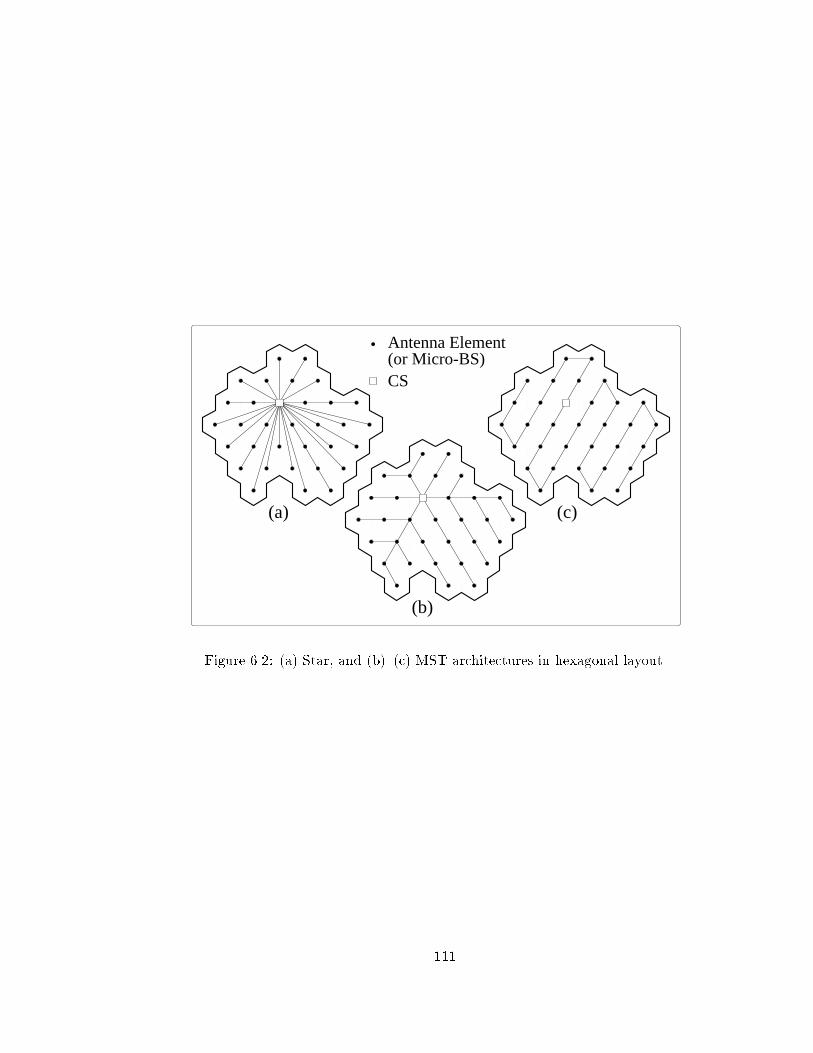
(a)

(b)

(c)

Antenna Element(or Micro-BS)CS

Figure 6.2: (a) Star, and (b)(c) MST architectures in hexagonal layout.

111

(d) (e)

(f) (g)

BΨ1

S1

Ψ3

A

Ψ4

Ψ2

S2

Ψ2

Ψ4

A

S1

S2

A

B

aΨ2

Ψ3

Ψ1S1 S2Ψ4 A

Ψ3

Ψ1 BS2

S1

Ψ1

Ψ3

B

(b)

SΨ2

C

A

B

C

A

B

S

Ψ2

Ψ3

a

Ψ3

Ψ1

(c)

(a)

Ψ2 Ψ3

Ψ1

Ψ1

Ψ2

Ψ4

Figure 6.3: SMT construction: (a) L=3, general case, 4123 has an angle 120. (b) L=3,

general case, 4123 has no angles 120. (c) L = 3, the special case of hexagonal layout.

(d) L=4, general case. (e) L=4, general case, an ST (not an SMT). (f) and (g) L=4, the special

case of hexagonal layout.

112

Ψ1

Ψ6Ψ7

Ψ10

Ψ9

Ψ8

Ψ4

Ψ3

Ψ2

(a)

Ψ8

Ψ9

Ψ10

S4

Ψ7Ψ6S3

S2S1

(b)Ψ1

Ψ3

Ψ2

Ψ5

Ψ4

Ψ5

Figure 6.4: SMT construction for a case of L=10. (a) Decomposition. (b) Yielding SMT.

a

CSAE

Figure 6.5: SMT construction in hexagonal layout: decomposition and the resultant SMT.

113

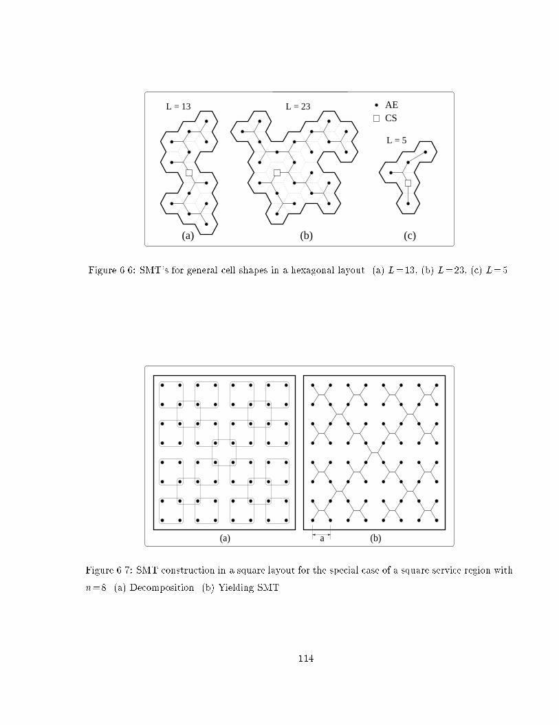
L = 13

L = 5

CS

(a) (b) (c)

L = 23 AE

Figure 6.6: SMT's for general cell shapes in a hexagonal layout. (a) L=13, (b) L=23, (c) L=5.

(a) (b)a

Figure 6.7: SMT construction in a square layout for the special case of a square service region with

n=8. (a) Decomposition. (b) Yielding SMT.

114

n=7, L=49

0.9330

/

0.91070.92180.9138

496481

10010987

ΩΩMIN MST

9162536

n

3456

n MSTΩ/MINΩ0.91620.91070.91290.9122

n=10, L=100 n=9, L=81

n=3, L=9 n=5, L=25 n=6, L=36

L L

Figure 6.8: Decomposition strategies for square service region in square layout.

1 19 37 61 91 127 169 217 271 331 397 4690

1

2

3

4

5

6

7

8

9

10

L = 3n(n−1)+1: number of Micro−BS

ΩS

TAR/Ω

SM

T

(a) Hexagonal region, CS in the center (b) Hexagonal region, CS in the corner (c) Rectangular region, CS in the center(d) Rectangular region, CS in the corner

Figure 6.9: Conduit length comparisons between star and SMT architectures.

115

CSAE

(b)

(a) (c)

Figure 6.10: (a) Star, (b) SMT and (c) MST architectures for the case where the CS is in the

corner of the cell.

116

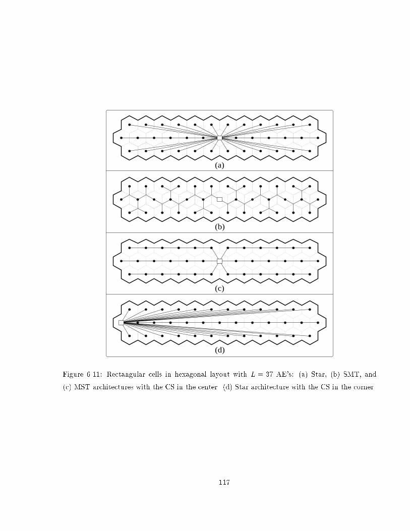
(a)

(b)

(c)

(d)

Figure 6.11: Rectangular cells in hexagonal layout with L = 37 AE's: (a) Star, (b) SMT, and

(c) MST architectures with the CS in the center. (d) Star architecture with the CS in the corner.

117

(b)

CS

AE

(a)

Figure 6.12: Cell splitting for SMT architecture.

118

(a)

(b)

1st LevelSMT SMT

SMT

. . .

. . . . . .

2nd Level AECSMain Switch

Figure 6.13: Double-SMT architecture for interconnecting CS's in hexagonal layout. (a) Details of

the architecture. (b) Two-level tree representation.

119

49 = 7 x 7 133 = 7x19 381 =19x190

500

1000

1500

2000

2500

3000

3500

4000

4500

(# of AEs) = (# of cells) x (# of AEs in a cell)

Ω(a

)

Single StarDouble StarSingle SMT Double SMT

Figure 6.14: Conduit length comparisons for single and double-layer architectures.

120

AECSMain Swich

(a)

(b)

Figure 6.15: (a) Extended-SMT and (b) single-layer SMT architectures for interconnecting cells in

hexagonal layout.

121

481, 7 259,13 91, 37 37, 91 13,259 7, 4814200

4400

4600

4800

5000

5200

5400

5600

5800

6000

6200

M: # of cells, L: # of antenna elements in each cell

Ω(a

)

Double SMT Extended SMT Single−layer SMT

Figure 6.16: Conduit length comparisons for various interconnection strategies, with ML=3367.

(a)

(b)

Passive Splitter

Conduit

AE

CS

Figure 6.17: SMT conduit architecture for an access network which has (a) logical star, (b) logical

bus topology.

122

...

...

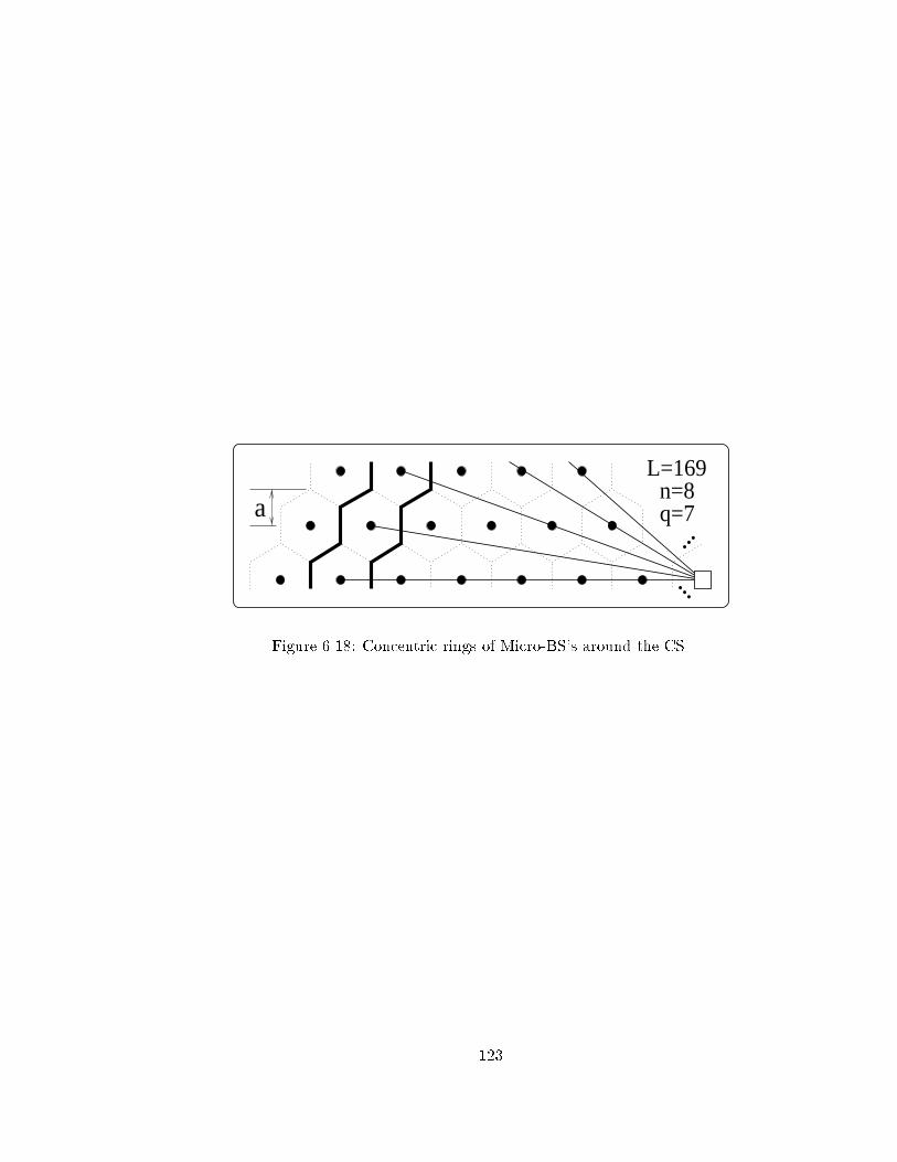
a

L=169n=8q=7

Figure 6.18: Concentric rings of Micro-BS's around the CS.

123

Chapter 7

Concluding Remarks

This thesis is about CDMA multi-antenna systems. As stated in Ch. 1, the following fundamental

question is investigated throughout the thesis: In a CDMA system, how should the signals be

collected from and distributed to the wireless users? To this end, the main objective of this thesis

is to utilize multi-antennas to achieve performance benets at the system level.

In Ch 1, an introduction to WAN's is presented, with special emphasis on the issues related

to interference control and management. Since at the end of each individual chapter, there is a

section summarizing the results of that chapter, we will not repeat that process here. Instead, we

will reemphasize some of the main results of Ch.s 2-6, by comparing the multi-antenna systems

addressed in this thesis with the conventional cellular systems.

7.1 Results from Chapters 3 and 4

In order to illustrate the results obtained in Ch.s 3 and 4, we will present a reverse link capacity

comparison between a cellular system and an SDA system that employs SBMPC.

7.1.1 Conventional Cellular Systems

Let us rst consider a conventional CDMA cellular system with K users and L cells, where no

macrodiversity exists. We start by considering an ideal case, then we will investigate a more

realistic non-ideal case.

A. Ideal Case:

This case is referred to as ideal because of the two unrealistic assumptions made:

a) Antenna radiation patterns do not overlap; that is, the cells are perfectly isolated,

and therefore, intercell interference does not exist.

124

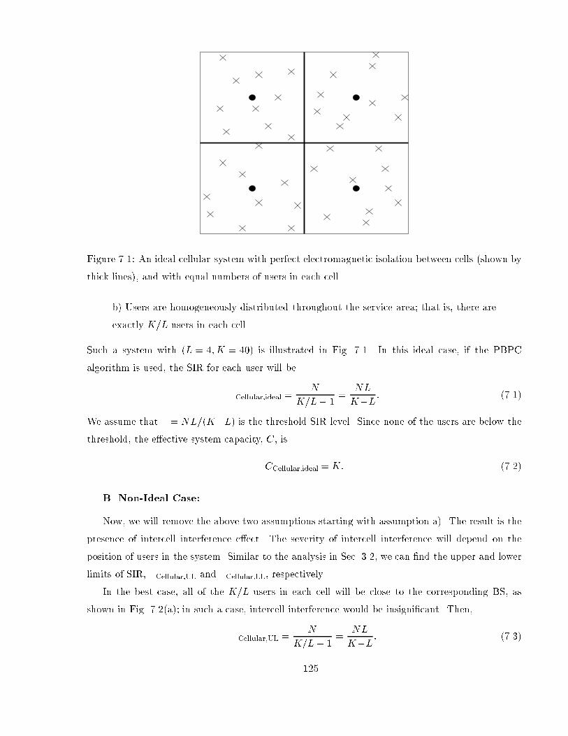
Figure 7.1: An ideal cellular system with perfect electromagnetic isolation between cells (shown by

thick lines), and with equal numbers of users in each cell.

b) Users are homogeneously distributed throughout the service area; that is, there are

exactly K=L users in each cell.

Such a system with (L = 4; K = 40) is illustrated in Fig. 7.1. In this ideal case, if the PBPC

algorithm is used, the SIR for each user will be

Cellular,ideal =N

K=L 1=

NL

KL: (7.1)

We assume that = NL=(KL) is the threshold SIR level. Since none of the users are below the

threshold, the eective system capacity, C, is

CCellular,ideal = K: (7.2)

B. Non-Ideal Case:

Now, we will remove the above two assumptions starting with assumption a). The result is the

presence of intercell interference eect. The severity of intercell interference will depend on the

position of users in the system. Similar to the analysis in Sec. 3.2, we can nd the upper and lower

limits of SIR, Cellular,UL and Cellular,LL, respectively.

In the best case, all of the K=L users in each cell will be close to the corresponding BS, as

shown in Fig. 7.2(a); in such a case, intercell interference would be insignicant. Then,

Cellular,UL =N

K=L 1=

NL

KL: (7.3)

125

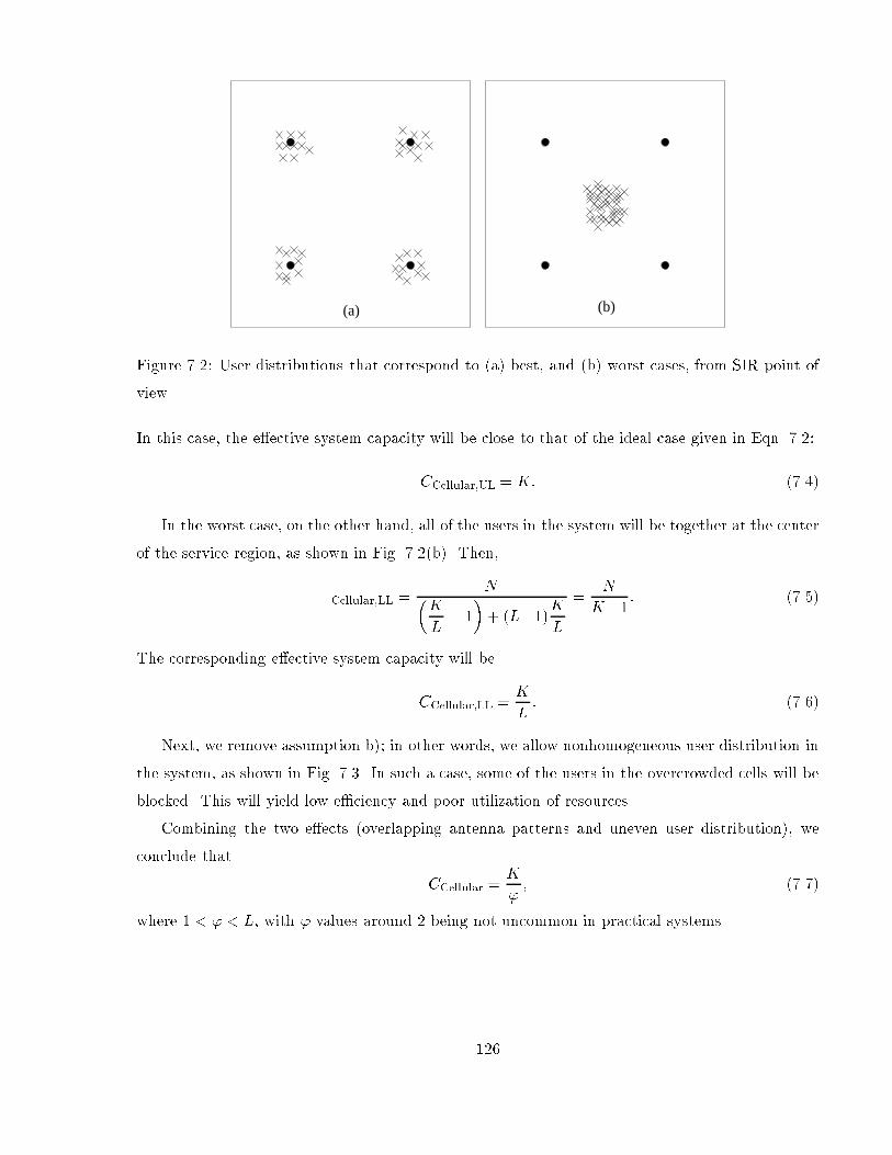
(b)(a)

Figure 7.2: User distributions that correspond to (a) best, and (b) worst cases, from SIR point of

view.

In this case, the eective system capacity will be close to that of the ideal case given in Eqn. 7.2:

CCellular,UL = K: (7.4)

In the worst case, on the other hand, all of the users in the system will be together at the center

of the service region, as shown in Fig. 7.2(b). Then,

Cellular,LL =N

K

L 1

+ (L1)K

L

=N

K1 : (7.5)

The corresponding eective system capacity will be

CCellular,LL =K

L: (7.6)

Next, we remove assumption b); in other words, we allow nonhomogeneous user distribution in

the system, as shown in Fig. 7.3. In such a case, some of the users in the overcrowded cells will be

blocked. This will yield low eciency and poor utilization of resources.

Combining the two eects (overlapping antenna patterns and uneven user distribution), we

conclude that

CCellular =K

'; (7.7)

where 1 < ' < L, with ' values around 2 being not uncommon in practical systems.

126

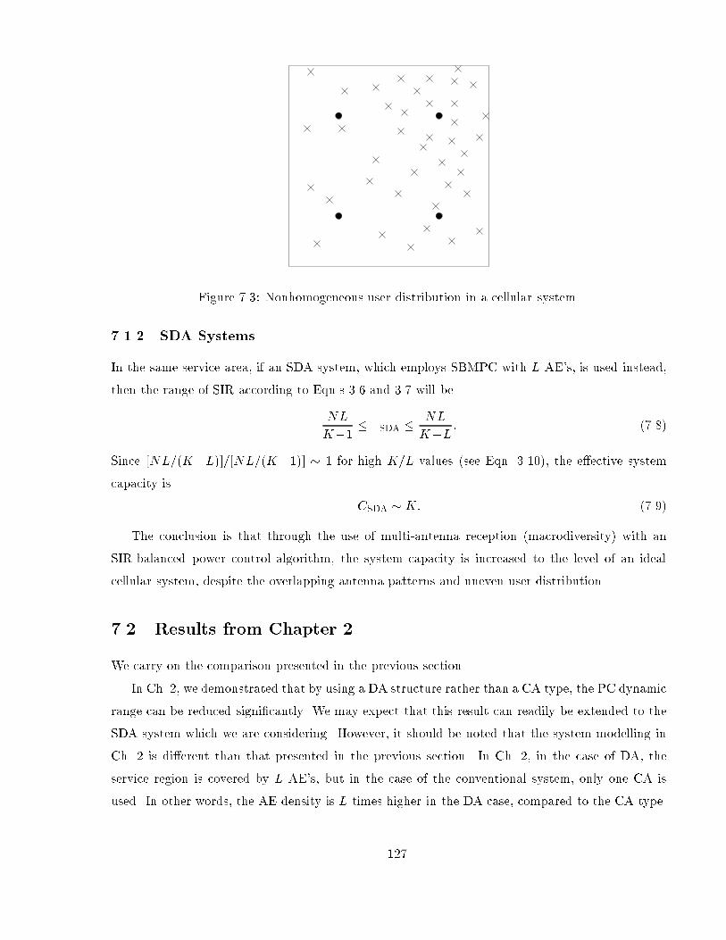
Figure 7.3: Nonhomogeneous user distribution in a cellular system.

7.1.2 SDA Systems

In the same service area, if an SDA system, which employs SBMPC with L AE's, is used instead,

then the range of SIR according to Eqn.s 3.6 and 3.7 will be

NL

K1 SDA NL

KL: (7.8)

Since [NL=(KL)]=[NL=(K1)] 1 for high K=L values (see Eqn. 3.10), the eective system

capacity is

CSDA K: (7.9)

The conclusion is that through the use of multi-antenna reception (macrodiversity) with an

SIR-balanced power control algorithm, the system capacity is increased to the level of an ideal

cellular system, despite the overlapping antenna patterns and uneven user distribution.

7.2 Results from Chapter 2

We carry on the comparison presented in the previous section.

In Ch. 2, we demonstrated that by using a DA structure rather than a CA type, the PC dynamic

range can be reduced signicantly. We may expect that this result can readily be extended to the

SDA system which we are considering. However, it should be noted that the system modelling in

Ch. 2 is dierent than that presented in the previous section. In Ch. 2, in the case of DA, the

service region is covered by L AE's, but in the case of the conventional system, only one CA is

used. In other words, the AE density is L times higher in the DA case, compared to the CA type.

127

As a consequence, the distance between a user and the closest AE in a DA system is almost always

less than that between a user and the CA in the conventional system.

In the comparison given in the previous section, on the other hand, we considered the same

number of AE's and BS's in both SDA and cellular systems, respectively. Therefore, the advantage

of closeness is no longer valid. Yet, in an SDA system, since all the AE's receive a user's signal,

there is still an advantage against fading. When the path between a user and the closest AE is

faded, the signals reaching other AE's may be utilized despite their weakness.

Therefore, we expect that the SBMPC DR in an SDA system will be less than PBPC DR in

a conventional cellular system.1 This will yield further performance enhancements in the SDA

system.

7.3 Results from Chapter 5

In the comparison given in Sec. 7.1, the correlation eect discussed in Ch. 5 is not taken into

account. Although the results from Ch. 5 indicate that, for reasonably high chip rates and for

service areas which are not very small, the eect of correlation is mild if the number of AE's is

not very high, we must still be careful. If the user distribution is very uneven, yielding situations

where many users are very close to each other, then the correlation eect should be taken into

consideration. The results found in Ch. 4 are indeed an upper bound; the returns will actually be

more modest due to the interference eect.

7.4 Chapter 6

The iterative solution for SBMPC suggests centralized intelligence, which is the case for the SDA

system. In cellular systems the intelligence is distributed, which allows for bus structure (SDA, on

the other hand, is a logical star). Interestingly, both structures can be realized within the optimal

SMT or suboptimal MST conduit architectures, as shown in Ch. 6. In this case, the extra cable

length for SDA (see Sec. 6.5) will be marginal.

1If the PC DR reduction is still less than desired, some of the SDA AE's can be replaced with DA structures with

few AE's.

128

Bibliography

[1] S. Chia, \The universal mobile telecommunication system," IEEE Commun. Mag., pp. 5462,

December 1992.

[2] R. Steele, \The evolution of personal communications," IEEE Personal Commun. Mag., pp. 6

11, 2nd Quarter 1994.

[3] D. C. Cox, \Wireless personal communications: What is it?," IEEE Personal Commun. Mag.,

pp. 2035, April 1994.

[4] A. J. Viterbi, \The evolution of digital wireless technology from space exploration to personal

communication services," IEEE Trans. Veh. Technol., vol. 43, pp. 638644, August 1994.

[5] W. C. Y. Lee, \Future vision for wireless communications," Proc. IEEE 7th Int. Symp. Per-

sonal, Indoor, and Mobile Radio Commun. (PIMRC'96), vol. 1, pp. 14, 1996. Taipei, Taiwan,

R.O.C.

[6] W. C. Y. Lee,Mobile Cellular Telecommunications: Analog and Digital Systems. McGraw-Hill,

2nd ed., 1995.

[7] J. D. Gibson, The Mobile Communications Handbook. CRC Press, 1996.

[8] T. S. Rappaport, Wireless Communications: Principles and Practice. Prentice Hall PTR,

1996.

[9] W. C. Y. Lee, Mobile Communications Engineering: Theory and Applications. McGraw-Hill,

2nd ed., 1998.

[10] A. J. Viterbi, CDMA: Principles of Spread Spectrum Communications. Addison-Wesley, 1995.

[11] R. Prasad, CDMA for Wireless Personal Communications. Artech House, 1996.

129

[12] S. Glisic and B. Vucetic, Spread Spectrum CDMA Systems for Wireless Communications.

Artech House, 1997.

[13] L. J. Greenstein, N. Amitay, T.-S. Chu, L. J. Cimini, Jr., G. J. Foschini, M. J. Gans, C.-L. I,

A. J. Rustako, Jr., R. A. Valenzuela, and G. Vanucci, \Microcells in personal communications

systems," IEEE Commun. Mag., pp. 7688, December 1992.

[14] J. Sarnecki, C. Vinodrai, A. Javed, P. O'Kelly, and K. Dick, \Microcell design principles,"

IEEE Commun. Mag., pp. 7682, April 1993.

[15] A. F. Naguib, A. Paulraj, and T. Kailath, \Capacity improvement with base-station antenna

arrays in cellular CDMA," IEEE Trans. Veh. Technol., vol. 43, pp. 691698, August 1994.

[16] J. S. Thompson, P. M. Grant, and B. Mulgrew, \Smart antenna arrays for CDMA systems,"

IEEE Personal Commun. Mag., pp. 1625, October 1996.

[17] L. C. Godara, \Applications of antenna arrays to mobile communications, part I: performance

improvement, feasibility, and system considerations," Proc. IEEE, vol. 85, pp. 10311060, July

1997.

[18] P. Delogne, Leaky Feeders and Subsurface Radio Communications. Teregrinus, 1982.

[19] P. Delogne, \EM propagation in tunnels," IEEE Trans. Antennas Propagat., vol. 39, pp. 401

406, March 1991.

[20] M. Nakamura, H. Tsunomachi, and R. Fukui, \Road vehicle communication system for vehicle

control using leaky coaxial cable," IEEE Commun. Mag., pp. 8489, October 1996.

[21] J. Harrington and D. Geller, \Re-radiation of signals employing guided antenna systems oper-

ating in tandem with two-way signal booster amplier," Proc. IEEE 38th Vehicular Technol.

Conf. (VTC'88), pp. 312320, 1988.

[22] R. A. Isberg and W. C. Y. Lee, \Performance tests of a low power cellular enhancer in a

parking garage," Proc. IEEE 39th Vehicular Technol. Conf. (VTC'89), vol. 2, pp. 542546,

1989.

[23] R. A. Isberg and M. Pristupa, \Multichannel VHF, UHF and 800 MHz subway radio com-

munications tests in Toronto," Proc. IEEE 39th Vehicular Technol. Conf. (VTC'89), vol. 2,

pp. 839845, 1989.

130

[24] B. J. Le, \Application engineering considerations for cellular repeaters," Proc. IEEE 39th

Vehicular Technol. Conf. (VTC'89), vol. 2, pp. 532534, 1989.

[25] F. A. Thatcher, \Design of a subsurface radio communications system using several types of

distributed radiators," Proc. IEEE 40th Vehicular Technol. Conf. (VTC'90), vol. 1, pp. 152

155, 1990.

[26] R. A. Isberg and T. E. Herold, \Tests of distributed antenna system along a railway test

track," Proc. IEEE 42nd Vehicular Technol. Conf. (VTC'92), vol. 1, pp. 196201, 1992.

[27] M. A. Franklin, \Radio communications in the channel tunnel," IEE 7th European Conf. on

Mobile Personal Commun., pp. 120124, December 13-15, 1993.

[28] R. J. Jakubowski, \Results of distributed antenna and leaky feeder systems tests at 800 MHz

in the Washington D.C. metro system tunnels," Proc. IEEE 44st Vehicular Technol. Conf.

(VTC'94), pp. 11131116, 1994.

[29] A. A. M. Saleh, A. J. Rustako, Jr., and R. S. Roman, \Distributed antennas for indoor radio

communications," IEEE Trans. Commun., vol. COM-35, pp. 12451251, December 1987.

[30] T. S. Chu and M. J. Gans, \Fiber optic microcellular radio," Proc. IEEE 41st Vehicular

Technol. Conf. (VTC'91), pp. 339344, 1991.

[31] P. Chow, A. Karim, V. Fung, and C. Dietrich, \Performance advantages of distributed an-

tennas in indoor wireless communication systems," Proc. IEEE 44st Vehicular Technol. Conf.

(VTC'94), pp. 15221526, 1994.

[32] R. W. Donaldson and A. S. Beasley, \Wireless CATV network access for personal communi-

cations using simulcasting," IEEE Trans. Veh. Technol., vol. 43, pp. 666671, August 1994.

[33] K. J. Kerpez, \A radio access system with distributed antennas," IEEE Trans. Veh. Technol.,

vol. 45, pp. 265275, May 1996.

[34] A. Salmasi and K. Gilhousen, \On the system design aspect of code division multiple access

(CDMA) applied to digital cellular and personal communications networks," Proc. IEEE 41st

Vehicular Technol. Conf. (VTC'91), pp. 5762, 1991.

[35] S. G. Gopani, J. H. Thompson, and R. Dean, \GHz SAW delay line for direct sequence spread

spectrum, CDMA in-door communication system," IEEE Ultrasonics Symp., vol. 1, pp. 8993,

1993.

131

[36] H. Yanikomeroglu and E. S. Sousa, \CDMA distributed antenna system for indoor wire-

less communications," Proc. IEEE 2nd Int. Conf. Universal Personal Commun. (ICUPC'93),

vol. 2, 12-15 October, 1993. Ottawa, Canada.

[37] J. Yang, \Analysis and simulation of a CDMA PCS indoor system with distributed antennae,"

Proc. IEEE 6th Int. Symp. Personal, Indoor, and Mobile Radio Commun. (PIMRC'95), vol. 3,

pp. 11231127, 1995. Toronto, Canada.

[38] G.-H. Chen, C.-M. Yu, and C.-C. Huang, \A simulation study of a distributed antenna-

based CDMA," Proc. IEEE 7th Int. Symp. Personal, Indoor, and Mobile Radio Commun.

(PIMRC'96), vol. 2, pp. 517521, 1996.

[39] E. S. Sousa, \Antenna architectures for CDMA integrated wireless access networks," Proc.

IEEE 6th Int. Symp. Personal, Indoor, and Mobile Radio Commun. (PIMRC'95), vol. 3,

pp. 921925, 1995. Toronto, Canada.

[40] A. J. Viterbi and R. Padovani, \Implications of mobile cellular CDMA," IEEE Commun.

Mag., pp. 3841, December 1992.

[41] H. H. Xia, A. Herrera, S. Kim, F. Rico, and B. Bettencourt, \Measurements and modeling of

CDMA PCS in-building system with distributed antenna," Proc. IEEE 44st Vehicular Technol.

Conf. (VTC'94), pp. 733737, 1994.

[42] H. Yanikomeroglu and E. S. Sousa, \Interconnection strategies for wireless access net-

work architectures," Proc. 3rd Int. Workshop on Mobile Multimedia Commun. (MoMuc'96),

p. A.1.1.3, September 25-27, 1996. Princeton, NJ, USA.

[43] H. Yanikomeroglu and E. S. Sousa, \Steiner minimal tree architectures for the interconnection

of wireless access networks," Proc. 5th Canadian Workshop on Infromation Theory, pp. 113

116, June 3-6, 1997. Toronto, Canada.

[44] H. Yanikomeroglu and E. S. Sousa, \Interconnection strategies for wireless access networks,"

Proc. IEEE 8th Int. Symp. Personal, Indoor, and Mobile Radio Commun. (PIMRC'97), vol. 3,

pp. 882886, September 1997. Helsinki, Finland.

[45] H. Yanikomeroglu and E. S. Sousa, \Antenna interconnection strategies for personal com-

munication systems," IEEE J. Select. Areas Commun., vol. 15/7, pp. 13271336, September

1997.

132

[46] H. Yanikomeroglu and E. S. Sousa, \On the power control and number of antenna elements in

CDMA distributed antenna systems," Proc. IEEE Int. Conf. Commun. (ICC'98), pp. 1040

1045, June 7-11, 1998. Atlanta, GA, USA.

[47] H. Yanikomeroglu and E. S. Sousa, \CDMA sectorized distributed antenna system," to ap-

pear in Proc. IEEE Int. Symp. Spread Spectrum Techniques and Applications (ISSSTA'98),

September 2-4, 1998. Sun City, South Africa.

[48] H. Yanikomeroglu and E. S. Sousa, \SIR-balanced macro power control for CDMA sectorized

distributed antenna systems," to appear in Proc. IEEE 9th Int. Symp. Personal, Indoor and

Mobile Radio Commun. (PIMRC'98), September 8-11, 1998. Boston, MI, USA.

[49] B. Hashem and E. S. Sousa, \On the capacity of a cellular DS/CDMA system under slow

multipath fading and xed step power control," Proc. IEEE 6th Int. Conf. Universal Personal

Commun. (ICUPC'97), pp. 352355, 1997.

[50] S. V. Hanly, \Capacity and power control in spread spectrum macrodiversity radio networks,"

IEEE Trans. Commun., pp. 247256, February 1996.

[51] J. M. Aein, \Power balancing in systems employing frequency reuse," COMSAT Tech. Rev.,

vol. 3, no. 2, Fall 1973.

[52] R. W. Nettleton, \Trac theory and interference management for a spread spectrum cellular

mobile radio system," Proc. IEEE Int. Conf. Commun. (ICC'80), pp. 24.5.124.5.5, 1980.

[53] H. Alavi and R. W. Nettleton, \Downstream power control for a spread spectrum cellular

mobile radio system," Proc. IEEE Globecom, pp. 8488, 1982.

[54] R. W. Nettleton and H. Alavi, \Power control for spread-spectrum cellular mobile radio sys-

tem," Proc. IEEE Veh. Technol. Conf. (VTC'83), pp. 242246, 1983.

[55] J. Zander, \Performance of optimum transmitter power control in cellular radio systems,"

IEEE Trans. Veh. Technol., vol. 41, pp. 5762, February 1992.

[56] J. Zander, \Distributed cochannel interference control in cellular radio systems," IEEE Trans.

Veh. Technol., vol. 41, pp. 305311, August 1992.

[57] S. A. Grandhi, R. Vijayan, D. J. Goodman, and J. Zander, \Centralized power control in

cellular radio systems," IEEE Trans. Veh. Technol., vol. 42, pp. 466468, November 1993.

133

[58] R. A. Silverman, Calculus with Analytic Geometry. Englewood Clis, NJ: Prentice-Hall, 1985.

[59] M. Shibutani, T. Kanai, W. Domon, K. Emura, and J. Namiki, \Optical ber feeder for

microcellular mobile communication system (H-015)," IEEE J. Select. Areas Commun., vol. 11,

September 1993.

[60] D. Tang, \Fiber-optic antenna remoting for multisector cellular cell sites," Proc. IEEE Int.

Conf. Commun. (ICC'92), vol. 1, pp. 7681, 1992.

[61] K. Morita and H. Ohtsuka, \The new generation of wireless communications based on ber-

radio technologies," IEICE Trans. Commun., vol. E76-B, pp. 10611068, September 1993.

[62] H. Jung and O. K. Tonguz, \Access network for PCS," Proc. IEEE 7th Int. Symp. Personal,

Indoor, and Mobile Radio Commun. (PIMRC'96), vol. 3, pp. 12671271, 1996. Taipei, Taiwan,

R.O.C.

[63] J. C. Fan, C. L. Lu, R. F. Kalman, and L. G. Kazovsky, \Design and analysis of a novel ber-

based PCS optical network," Proc. IEEE Int. Conf. Commun. (ICC'95), vol. 1, pp. 601605,

1995.

[64] O. K. Tonguz and H. Jung, \Personal communications access networks using subcarrier mul-

tiplexed optical links," J. Lightwave Technol., vol. 14, pp. 14001409, June 1996.

[65] W. I. Way, \Optical ber-based microcellular systems: An overview," IEICE Trans. Commun.,

vol. E76-B, pp. 10911102, September 1993.

[66] K. Kumozaki, \A ber-optic passive double star network for microcellular radio communication

systems applications," IEICE Trans. Commun., vol. E76-B, pp. 11221127, September 1993.

[67] H. Harada, S. Kajiya, K. Tsukamoto, S. Komaki, and N. Morinaga, \TDM intercell connec-

tion ber-optic bus link for personal radio communication systems," IEICE Trans. Commun.,

vol. E78-B, pp. 12871294, September 1995.

[68] D. W. Tcha and M. G. Yoon, \Conduit and cable installation for a centralized network with

logical star-star topology," IEEE Trans. Commun., vol. 43, February/March/April 1995.

[69] K. H. Rosen, Discrete Mathematics and Its Application. New York: McGraw-Hill, 3rd ed.,

1995.

[70] A. O. Ivanov and A. A. Tuzhilin, Minimal Networks: The Steiner Problem and Its General-

ization. Boca Raton, FL: CRC Press, 1994.

134

[71] F. K. Hwang and D. S. Richards, \Steiner tree problems," Networks, vol. 22, pp. 5589, 1992.

[72] F. K. Hwang and J. F. Weng, \Hexagonal coordinate systems and Steiner minimal trees,"

Discrete Mathematics, vol. 62, pp. 4957, 1986.

[73] Z. A. Melzak, Companion to Concrete Mathematics. New York: John Wiley, 1973.

[74] H. O. Pollak, \Some remarks on the Steiner problem," J. Combinatorial Theory, pp. 278295,

1978. Series A 24.

[75] Z. A. Melzak, \On the problem of Steiner," Canadian Mathematical Bulletin, vol. 4/2, pp. 143

148, May 1961.

[76] F. Chung and R. Graham, \Steiner trees for ladders," Annals of Discrete Mathematics 2,

pp. 173200, 1978.

[77] M. R. Garey, L. R. Graham, and D. S. Johnson, \The complexity of computing Steiner minimal

trees," SIAM J. Applied Mathematics, vol. 32, pp. 835859, 1977.

[78] F. K. Hwang and D. Z. Du, \Steiner minimal trees on Chinese checkerboards," Mathematics

Magazine, vol. 64, pp. 332339, December 1991.

[79] F. Chung, M. Gardner, and R. Graham, \Steiner trees on a checkerboard," Mathematics

Magazine, vol. 62/2, pp. 8396, April 1989.

[80] K. A. Falcone and O. K. Tonguz, \Practical constraints in growth of lightwave networks,"

IEEE Trans. Commun., vol. 44, pp. 348355, March 1996.

[81] J. Bannister, M. Gerla, and M. Kovacevic, \An all-optical multiber tree network," J. Light-

wave Technol., vol. 11, pp. 9971008, May/June 1993.

135