Energies 2022, 15, 1919. https://doi.org/10.3390/en15051919  www.mdpi.com/journal/energies 

Article 

Multi‐Agent‐Based Coordinated Control of ABS and AFS for 

Distributed Drive Electric Vehicles 

Niaona Zhang 1,2,*, Jieshu Wang 1, Zonghao Li 1,2, Shaosong Li 1,2,* and Haitao Ding 2 

1  School of Electrical and Electronic Engineering, Changchun University of Technology,   

Changchun 130000, China; wangjieshu2021@163.com (J.W.); lizonghao2021@163.com (Z.L.) 2  State Key Laboratory of Automobile Simulation and Control, Jilin University, Changchun 130000, China; 

dinght@jlu.edu.cn 

*  Correspondence: zhangniaona@ccut.edu.cn (N.Z.); lishaosong@ccut.edu.cn (S.L.) 

Abstract: A vehicle with a four‐channel anti‐lock braking system (ABS) has poor safety and stability 

when braking on a low‐adhesion road or off‐road. In view of this situation, this paper proposes a 

multi‐objective optimization coordinated control method  for ABS and AFS based on multi‐agent 

model predictive control (MPC). Firstly, the single‐wheel control method is adopted to establish the 

single‐wheel equation based on the slip rate and the stability equation of the centroid yaw based on 

AFS. The four wheels and the centroid are regarded as agents. The mathematical model of distrib‐

uted drive electric vehicles based on graph theory and the coordinated control of AFS and ABS is 

established to reduce the dimension of the model. Secondly, on the basis of the multi‐agent theory, 

an integrated coordinated control method for AFS and ABS based on distributed model predictive 

control (DMPC) is proposed to realize the ideal values of the vehicle’s slip rate, yaw rate, and side‐

slip angle, and improve the braking safety and handling stability of the vehicle. Then, to solve the 

problems of high levels of resource consumption, low real‐time performance, and complex imple‐

mentation in the optimization of the DMPC solution, a prediction solution method using a discrete 

simplified dual neural network (SDNN)  is proposed to balance the computational efficiency and 

system dynamic performance. Finally, a hardware‐in‐the‐loop (HIL) test bench is built to test the 

effectiveness of the proposed method under the conditions of a low‐adhesion road and an off‐road. 

Keywords: distributed drive electric vehicle; active front steering (AFS); anti‐lock braking system 

(ABS); coordinated control; heterogeneous multi‐agent 

 

1. Introduction 

In recent years, with the development of electronic technology, various vehicle active 

safety control systems have been continuously applied to actual vehicles, which greatly 

improves the active safety of these vehicles, with these systems including ABS, AFS, direct 

yaw moment control  (DYC)  [1,2]. Since each system only affects  the performance of a 

certain vehicle in a specific area, to optimize the vehicle’s dynamic performance, devel‐

oping the coordinated control of each chassis subsystem will become the focus of future 

vehicle dynamic control research [3]. ABS can adjust the wheel braking pressure to ensure the best slip rate in the braking 

process,  to  obtain  good  lateral  force,  and,  at  the  same  time,  to obtain higher  braking 

strength and shorten the braking distance. In the braking steering condition, due to the 

unreasonable longitudinal braking force and lateral force distribution of each wheel, the 

vehicle is prone to dangerous conditions, such as sideslip, sharp rotation, and track devi‐

ation. By adjusting the wheel angle of the steering vehicle with a servo motor, AFS can 

obtain an effective yaw moment, improve the stability of a vehicle’s steering while brak‐

ing, and realize active safety and yaw stability in coordination with steering, braking, and 

suspension systems.   

Citation: Zhang, N.; Wang, J.; Li, Z.; 

Li, S.; Ding, H. Multi‐Agent‐Based 

Coordinated Control of ABS and 

AFS for Distributed Drive Electric 

Vehicles. Energies 2022, 15, 1919. 

https://doi.org/10.3390/en15051919 

Academic Editor: Valery Vodovozov 

Received: 21 December 2021 

Accepted: 3 March 2022 

Published: 6 March 2022 

Publisher’s Note: MDPI  stays  neu‐

tral  with  regard  to  jurisdictional 

claims in published maps and institu‐

tional affiliations. 

 

Copyright: © 2022 by the authors. Li‐

censee  MDPI,  Basel,  Switzerland. 

This article  is an open access article 

distributed under the terms and con‐

ditions of the Creative Commons At‐

tribution (CC BY) license (https://cre‐

ativecommons.org/licenses/by/4.0/). 

Energies 2022, 15, 1919  2  of  17  

 

Y et al. proposed an integrated MPC method based on the four‐wheel independent 

steering system (4WIS) and a DYC of the chassis of the distributed drive electric vehicle 

based on the unscented Kalman filter (UKF) observer, which effectively improves the ve‐

hicle stability [4]. S et al. proposed a linear matrix inequality (LMI) H∞ controller based 

on the integration of DYC and AFS, which effectively improves vehicle stability [5]. Wang 

et al. proposed a coordinated control method of ABS and DYC based on sliding mode 

variable structure control (SMC) three‐layer hierarchical control architecture to shorten 

the braking distance and ensure vehicle stability under emergency braking under complex 

driving conditions [6]. Feng et al. proposed a coordinated control method for ABS, DYC, 

and AFS based on the three‐layer hierarchical control architecture of fuzzy control and 

SMC, which  improved  the braking safety and directional stability of  the vehicle  in  the 

separation of road emergency braking [7]. Wang et al. proposed an integrated controller 

of AFS with electronic stability control (ESC) based on an MPC overall control framework 

to solve the problems of mutual interference and control allocation in the integrated con‐

trol of AFS and ESC, and effectively improved vehicle stability [8]. Pugi, L. et al. used an 

electric  traction/brake  fuzzy  logic controller  to  improve  the  longitudinal dynamics and 

overall vehicle stability of a green shuttle vehicle (GSV) driving on a road with reduced 

adhesion  [9]. Guodong Yin’s  team proposed  an H∞  controller  combined with  the T‐S 

fuzzy method to integrate AFS and DYC to improve vehicle control performance and sta‐

bility [10]. Tian et al. proposed an adaptive path tracking control strategy based on the 

MPC algorithm to coordinate AFS and DYC to ensure the stability of vehicles under high 

speed and  large curvature conditions  [11]. At present,  the methods  to  improve vehicle 

stability based on integrated ABS, AFS, and DYC controls include SMC, MPC, fuzzy con‐

trol, H∞ control, etc. Among them, DMPC has become an important tool for dealing with 

large‐scale complex systems with its advantages of online optimization, flexible structure, 

clear constraint solution, and nonlinearity [12,13]. DMPC conforms to the characteristics 

of the distributed system and has higher flexibility and fault tolerance. It can realize the 

model dimension reduction of complex systems, reduce the amount of calculation, and 

improve  the control efficiency, especially when  the system has high‐order models and 

state and control constraints. The coordinated control of ABS, DYC, and AFS in the above 

literature adopts a hierarchical integrated control method. However, in practical applica‐

tions,  the complex system has  the characteristics of  large scale, multiple variables, and 

multiple constraints, and the traditional control method cannot meet the control require‐

ments [14]. Guodong Yin’s team proposes a distributed coordinated control architecture 

for AFS and DYC  for distributed drive electric vehicles based on a multi‐agent system 

(MAS) based on the MPC control method, which regards AFS and DYC as multi‐agents 

and jointly improves the lateral stability of vehicles [15]. Therefore, following Guodong 

Yin’s team [15], this paper proposes a coordinated control method with integrated ABS 

and AFS based on DMPC, which solves the complexity problem of the traditional hierar‐

chical centralized control systems and improves the solving speed of the model. 

The constraint optimization control ability of DMPC is mainly generated by solving 

constraint quadratic programming (QP) problems online. Although the traditional QP nu‐

merical algorithm is widely used, it involves matrix inversion, decomposition, and other 

operations, and has the problems of complex implementation and high levels of resource 

consumption. Several common, fast model predictive control algorithms are explicit MPC 

(EMPC), MPC based on the traditional numerical method, MPC based on a neural net‐

work, and MPC based on a discrete and online combination [16]. Tavernini et al. proposed 

a traction control (TC) system for in‐wheel motor electric vehicles based on explicit non‐

linear model predictive control and demonstrated the real‐time capability of the strategy 

with  microsecond‐level  computation  times  [17]. Melanie  et  al.  proposed  a  real‐time 

suboptimal model predictive control combining explicit MPC and online optimization, 

which solved the problem of MPC’s limitations in terms of storage space and computation 

time [18].Liu et al. proposed a simplified dual neural network solution method for quad‐

ratic  programming,  which  solved  the  problems  of  the  slow  convergence  and 

Energies 2022, 15, 1919  3  of  17  

 

computational complexity of neural networks [19]. Lehel et al. proposed an explicit MPC‐

based RBF neural network controller to solve the problem of the slow online computation 

of MPC [20]. It can be seen that neural networks are widely used in fast model predictive 

control algorithms  for  their advantages of natural parallelism, adaptability, and circuit 

realizability. The neural network to solve QP is the same as the traditional numerical so‐

lution to solve QP, and it belongs to the online solution method. However, the literature 

[19–20] does not consider the solution method when the system has disturbance. In this 

paper, the state equation of the system with disturbance is established, and SDNN is used 

to solve the QP problem of DMPC.   

MAS refers to a system composed of multiple agents, which can solve problems more 

quickly through decentralized control and parallel processing. It has a high level of intel‐

ligence and has been widely used in the automotive field [21,22]. Agents can acquire ex‐

ternal environment  information through environmental perception, act on the environ‐

ment in time to meet their design goals as computing entities or programs, and can com‐

municate with other agents through communication modules with good responsiveness, 

autonomy, and flexibility [23]. The main structural feature of the distributed drive electric 

vehicle is that the drive motor is directly installed in or near the drive wheel, which has 

the outstanding advantages of a short drive chain, high transmission efficiency, compact 

structure, and many controllers. MAS provides a feasible method for the coordinated con‐

trol of electric vehicles that  is scalable, adaptive, and flexible  in dynamic environments 

[24]. The control architecture of MAS can effectively  realize  the coordinated control of 

chassis subsystems, and solve the problems of the traditional  integrated control frame‐

work, such as a lack of flexibility and scalability, which mean that the traditional vehicle 

chassis control system is not suitable for new distributed drive electric vehicles [25]. Due 

to  the modular architecture of MAS,  the vehicle platform  is reconfigurable and robust, 

which is conducive to the upgrading of the electronic control system. Therefore, in this 

paper, the four single‐wheel control systems based on slip rate and the centroid yaw sta‐

bility control system based on AFS control are regarded as agents with decision‐making 

abilities. The coordination and cooperation between various agents are realized in com‐

plex work applications, which can greatly improve work efficiency, system flexibility, and 

robustness [26]. 

The division of this article is as follows. In the second section, the single‐wheel con‐

trol mode is adopted to establish the single‐wheel state equation based on the slip ratio. 

The stability equation of centroid yaw based on AFS control is established according to 

the ideal two degrees of freedom (DOF) vehicle model. The wheel tire model is established 

to obtain the ideal slip ratio under different road conditions. In the third section, the vehi‐

cle is regarded as five multi‐agent systems composed of four wheel agents and centroid 

agents. The mathematical model of distributed drive electric vehicles based on graph the‐

ory and the coordinated control of AFS and ABS is established to reduce the dimension of 

the model. In the fourth section, the DMPC‐based coordinated control method of AFS and 

ABS is used to define the performance index under the condition of considering the mu‐

tual influence of the five multi‐agents, taking into account the energy saving of the vehicle 

and the braking distance, so as to realize the ideal values of the vehicle’s slip rate, yaw 

rate, and centroid sideslip angle, shorten the braking distance, and improve the braking 

safety and handling stability of  the vehicle. To solve the problems of high  levels of re‐

source consumption, low real‐time performance, and complex implementation in the op‐

timization of DMPC,  the discrete SDNN  is used  to solve  the QP problem of DMPC  to 

further improve the solving speed of the model. The hardware used in the loop test results 

is presented and discussed  in Section 5. Finally, the sixth section provides conclusions. 

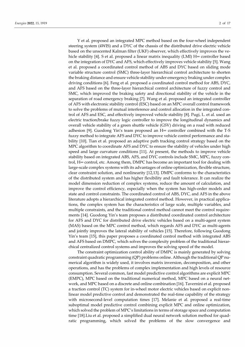
The overall architecture of the system is shown in Figure 1. Here,  il   represents the slip 

rate of the wheel agent,  il  represents the ideal slip rate of the wheel agent,  iT   repre‐

sents the braking torque transmitted by the motor to the wheel,  fd   is the front wheel 

angle of the vehicle,  fd   is the additional front wheel steering angle of the vehicle,  b   is 

Energies 2022, 15, 1919  4  of  17  

 

the vehicle centroid sideslip angle,  g   is the vehicle yaw rate,  refb   is the vehicle ideal cen‐

troid sideslip angle,  refg   is the vehicle ideal yaw rate,  ( 51)eb   is the vehicle centroid side‐

slip angle deviation value,  ( 52)eg   is the vehicle yaw rate deviation value,  ie   is the ve‐hicle slip rate deviation value, and  xv   is the vehicle longitudinal speed. 

Yaw sta

bility

 contro

ller based on 

hete

rogeneous m

ulti‐a

gent

Vehicle model

Centroid Multi‐agent Reference Model

DMPC1

DMPC2

DMPC3

DMPC4

DMPC5

 

Figure 1. The overall architecture of the system. 

2. Establishment of the Vehicle Dynamics Model 

2.1. Seven DOF Vehicle Dynamics Model 

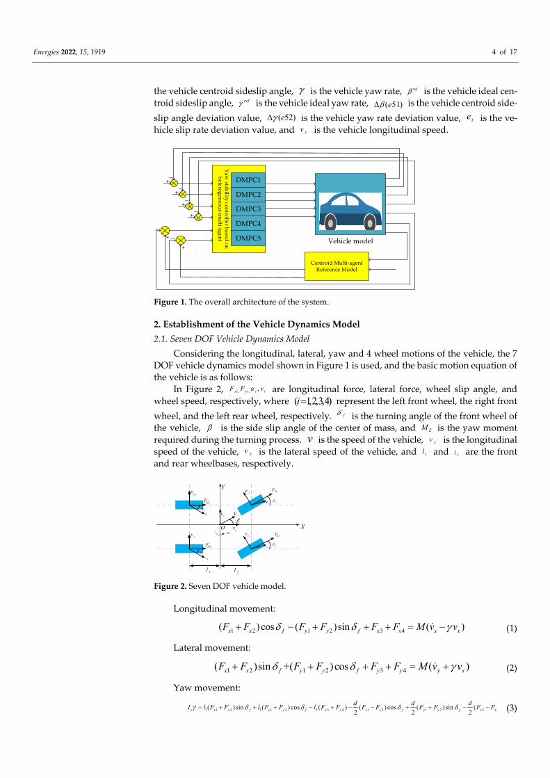
Considering the longitudinal, lateral, yaw and 4 wheel motions of the vehicle, the 7 

DOF vehicle dynamics model shown in Figure 1 is used, and the basic motion equation of 

the vehicle is as follows: 

In  Figure  2,  , , ,xi yi i iF F va   are  longitudinal  force,  lateral  force, wheel  slip  angle,  and 

wheel speed, respectively, where  ( 1,2,3,4)i   represent the left front wheel, the right front 

wheel, and the left rear wheel, respectively.  fd   is the turning angle of the front wheel of 

the vehicle,  b   is the side slip angle of the center of mass, and  ZM   is the yaw moment 

required during the turning process.  v   is the speed of the vehicle,  xv   is the longitudinal 

speed of the vehicle,  yv   is the lateral speed of the vehicle, and  1l   and  2l   are the front 

and rear wheelbases, respectively. 

Y

XO

1XF

2XF

3XF

4XF

1yF

2yF

3yF

4yF

1l 2l

xv

yv vb

fd

fd

ZM

3a

3V

4a

4v

1v1a

2v2a

 

Figure 2. Seven DOF vehicle model. 

Longitudinal movement: 

1 2 1 2 3 4( ) cos ( )sin ( )x x f y y f x x x xF F F F F F M v vd d g   (1)

Lateral movement: 

1 2 1 2 3 4( )sin +( )cos ( )x x f y y f y y y xF F F F F F M v vd d g   (2)

Yaw movement: 

1 1 2 1 1 2 2 3 4 1 2 1 2 3 4( ) sin ( ) cos ( ) ( ) cos ( ) sin (2 2 2z x x f y y f y y x x f y y f x x

d d dI l F F l F F l F F F F F F F Fg d d d d (3)

Energies 2022, 15, 1919  5  of  17  

 

Rotational motion of the four wheels: 

i xi biJ F R T   (4)

where,  M   is the mass of the vehicle, d is the distance between the left and right wheels, 

zI   is the moment of inertia in the vertical direction,  fd   is the steering angle of the front 

wheel,  g   is the yaw rate of the vehicle,  J   is the moment of inertia of the wheel,  i   is the tire angular velocity,  R   is the tire radius, and  b iT   is the tire braking torque. 

Vertical load of each tire: 

21 2

1 1[ ]2 2

yZ x

a hlmF gl a h

L d , 2

2 2

1 1[ ]2 2

yZ x

a hlmF gl a h

L d  

13 1

1 1[ ]2 2

yZ x

a hlmF gl a h

L d , 1

4 1

1 1[ ]2 2

yZ x

a hlmF gl a h

L d  

(5)

In Equation (5),  Z iF ( 1,2,3,4)i   represent the vertical load of the left front wheel, the 

right front wheel, the left rear wheel, and the right rear wheel, h is the height of the center 

of mass from the ground, L is the wheelbase,  ya   is the lateral acceleration,  xa   is the lon‐

gitudinal acceleration, and  m   is the wheel mass. 

Slip angle of each tire: 

11 arctan( )

2

yf

x

v l

dv

ga d

g

, 12 arctan( )

2

yf

x

v l

dv

ga d

g

 

23 arctan( )

2

y

x

v l

dv

ga

g

, 24 arctan( )

2

y

x

v l

dv

ga

g

 (6)

The longitudinal velocity of each wheel center in the wheel coordinate system: 

1 1( ) cos ( ) sin2x y

dv v v lg d g d ,

2 1( ) cos ( )sin2x y

dv v v lg d g d  

3 2x

dv v g ,

4 2x

dv v g  

(7)

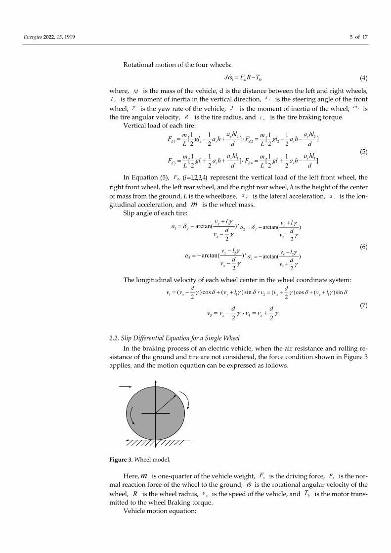
2.2. Slip Differential Equation for a Single Wheel 

In the braking process of an electric vehicle, when the air resistance and rolling re‐

sistance of the ground and tire are not considered, the force condition shown in Figure 3 

applies, and the motion equation can be expressed as follows. 

 Figure 3. Wheel model. 

Here,m   is one‐quarter of the vehicle weight,  xF   is the driving force,  zF   is the nor‐

mal reaction force of the wheel to the ground,  w   is the rotational angular velocity of the wheel,  R   is the wheel radius,  xV   is the speed of the vehicle, and  bT   is the motor trans‐

mitted to the wheel Braking torque.   

Vehicle motion equation: 

Energies 2022, 15, 1919  6  of  17  

 

i ximv F   (8) 

Longitudinal friction of wheels: 

xi i ziF F   (9) 

When the vehicle is emergency braking, the vehicle anti‐lock braking system adjusts 

the wheel speed by controlling the braking torque, so that the wheel slip rate  l   is kept near the optimal slip rate  dl   to ensure the stability and safety of the vehicle during braking. 

The degree of slip is expressed by the slip ratio: 

= i ii

i

Rn wl

n

  (10) 

The first derivative of  il   is: 

1= [(1 ) ]i i i i

i

v Rv

  (11) 

Let (4) into (11) 21

= i zi i zi i zii i bi

i i i i

F F FR RT

vm v J v J v m   (12) 

In Equation (12),  m   is one‐quarter of the weight of the car body,  iv   is the speed of 

the vehicle, x iF   is the driving force,  iw   is the rotational angular velocity of the wheel, 

im   is the adhesion coefficient of the wheel and the ground,  J   is the moment of inertia 

of the wheel around the wheel center,  R   is the radius of the wheel, and  d iT   is the brak‐

ing torque transmitted by the motor to the wheel. 

Establish the state equation of a single wheel from Equation (12) and set 

i zi

i

Fa

v m

m ,

1

i

Rb

v J ,

2

( ) i zi i zi

i i

F FRd t

v J v m

m m  

Formula (12) is written as: 

= + ( )i i bia bT d t   (13) 

2.3. Vehicle Centroid Model 

2.3.1. Ideal 2 DOF Vehicle Model 

Vehicle stability can be reflected by the sideslip angle and yaw rate. This paper con‐

siders the effect of vertical load variation on the tire sideslip characteristics. In order to 

reduce the complexity of the model and the solving time, only the longitudinal and lateral 

handling stability are considered, so the role of suspension is ignored. A 2 DOF model of 

the vehicle is established. The 2 DOF vehicle model is shown in Figure 4. 

 

Figure 4. Two DOF vehicle model. 

Energies 2022, 15, 1919  7  of  17  

 

Assuming  that  the  longitudinal velocity  xv   of  the vehicle on  the axis  x   is a con‐stant value,  then  the  lateral motion and yaw dynamics equations of  the vehicle are as 

shown in Equation (14): 

1 2

1 1 2 2

( )x Y Y

z Y Y

mv F F

I l F l F

b g

g

  (14) 

In the equation,  1l   and  2l   are the distance between the centroid and the front axle 

and the rear axle,  zI   is the moment of inertia around the axis,  m   is the vehicle quality, and  1YF   and  2YF   are the total lateral force of the front and rear tires. 

When the tire cornering characteristic is in a linear range, the total cornering force of 

the front and rear tires is as shown in Equation (15): 

1 1

2 2

=

=Y r

Y f

F C

F Ca

a

a

a

  (15) 

where  rCa   and  fCa   are the total cornering stiffness of the front and rear tires, and  1a   and 

2a   are  the  front  and  rear  tire  cornering  angles,  respectively.  Since  fd   is  small,  and cos 1fd , combining (14) and (15) can be written as: 

1 2

1 1 2 2

( )x r f

z r f

mv C C

I l C l Ca a

a a

b g a a

g a a

 

(16) 

The state equation of the vehicle 2 DOF model is: refref

frefrefA B

  (17) 

Of which: 

1 2

2

2 21 2 1 2

1r f r f

x x

r f r f

z z x

C C l C l C

mv mvA

l C l C l C l C

I I v

,

1= r r

x z

C l CB

mv I

 

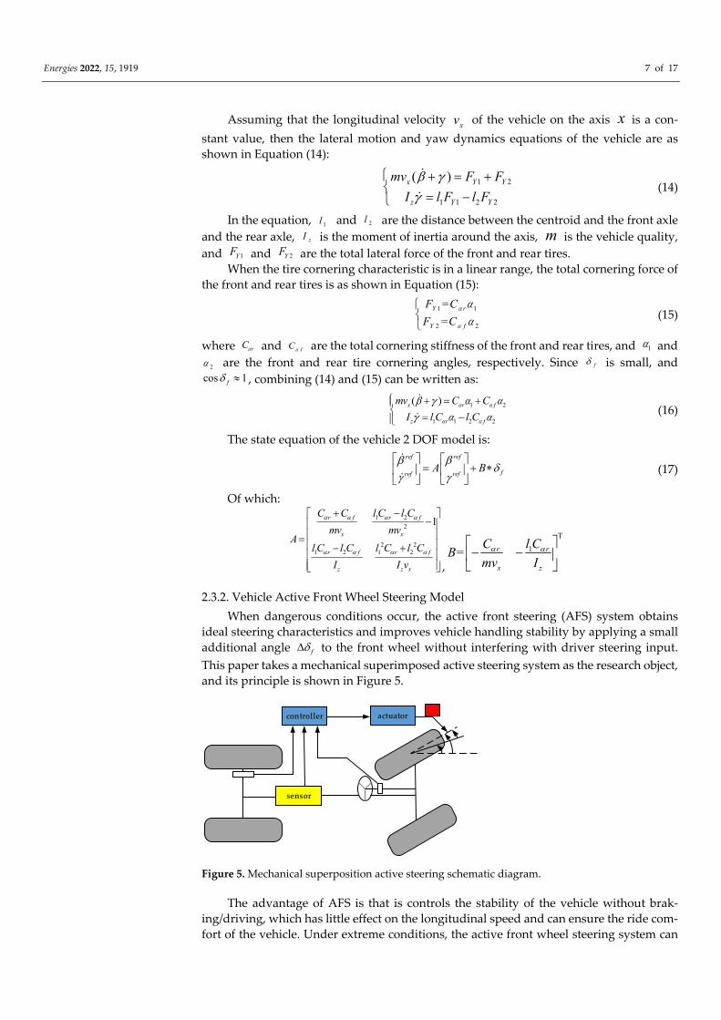
2.3.2. Vehicle Active Front Wheel Steering Model 

When dangerous  conditions occur,  the active  front  steering  (AFS)  system obtains 

ideal steering characteristics and improves vehicle handling stability by applying a small 

additional angle  fd   to  the  front wheel without  interfering with driver steering  input. 

This paper takes a mechanical superimposed active steering system as the research object, 

and its principle is shown in Figure 5. 

controller actuator

sensor

 

Figure 5. Mechanical superposition active steering schematic diagram. 

The advantage of AFS  is  that  is controls  the stability of  the vehicle without brak‐

ing/driving, which has little effect on the longitudinal speed and can ensure the ride com‐

fort of the vehicle. Under extreme conditions, the active front wheel steering system can 

Energies 2022, 15, 1919  8  of  17  

 

improve the stability of the vehicle by appropriately modifying the front wheel steering 

angle according to the running state of the vehicle and the driver’s intention. In this paper, 

the vehicle centroid equation of active front wheel steering control based on yaw stability 

is established [27], as shown in Equation (18). 

1fA B Bu

 (18) 

Of which  fd   is the additional front wheel steering angle. 

1r r

x z

C CB

mv I

, fu d  

2.4. Wheel Tire Model 

To facilitate the analysis and research, this paper uses a simple and practical Burck‐

hardt tire model, using the model parameters to obtain the ideal slip rate under different 

roads. The Burckhardt tire model is expressed as follows [28]: 

21 3[1 ]c

x c e clm l   (19) 

where c1, c2, and c3 are the fitting coefficient, value size, and specific tires related to road 

adhesion conditions. From Equation  (19),  the optimal slip ratio and  the peak adhesion 

coefficient of the road surface can be obtained, respectively, as follows: 

1 2opt

2 3

1= ln

c c

c cl

 (20) 

3 1 2max 1

2 3

(1 ln )c cc

cc c

m  

(21) 

In this paper, 6 kinds of common standard road are selected as comparison roads, 

and the specific parameters are shown in Table 1. 

Table 1. Ideal slip ratio and adhesion coefficients of different road surfaces. 

Road  Dry Cement Dry   

Bitumen 

Wet   

Asphalt Snow  Ice 

Wet   

Pebbles 

1c   1.1973  1.280  0.857  0.1946  0.0005  0.4004 

2c   25.168  23.99  33.82  94.129  306.39  33.708 

3c   0.5373  0.52  0.347  0.0646  0.001  0.1204 

optl   0.16  0.17  0.13  0.06  0.03  0.14 

maxm   1.09  1.17  0.8013  0.1907  0.05  0.34 

3. Vehicle Model Based on Graph Theory 

The four wheels are designed as agents 1, 2, 3, and 4, respectively, and the center of 

mass is agent 5. The wheel agent obtains the optimal slip rate of the typical road surface 

through the Burckhardt tire model, and the centroid agent follows the ideal value of the 2 

DOF vehicle model. When  the  five agents  interact with each other,  the  five agents can 

follow the ideal values of slip ratio, yaw rate, and centroid sideslip angle. 

According to the definition and properties of the multi‐agents and the topological 

structure diagram of  the  five‐multi‐agent  system,  the corresponding adjacency matrix, 

penetration matrix, and Laplace matrix of the system are as follows: 

Energies 2022, 15, 1919  9  of  17  

 

0 1 1 1 1

1 0 1 1 1

1 1 0 1 1

1 1 1 0 1

1 1 1 1 0

A

,

4 0 0 0 0

0 4 0 0 0

0 0 4 0 0

0 0 0 4 0

0 0 0 0 4

D

,

4 1 1 1 1

1 4 1 1 1

1 1 4 1 1

1 1 1 4 1

1 1 1 1 4

L D A

 

 

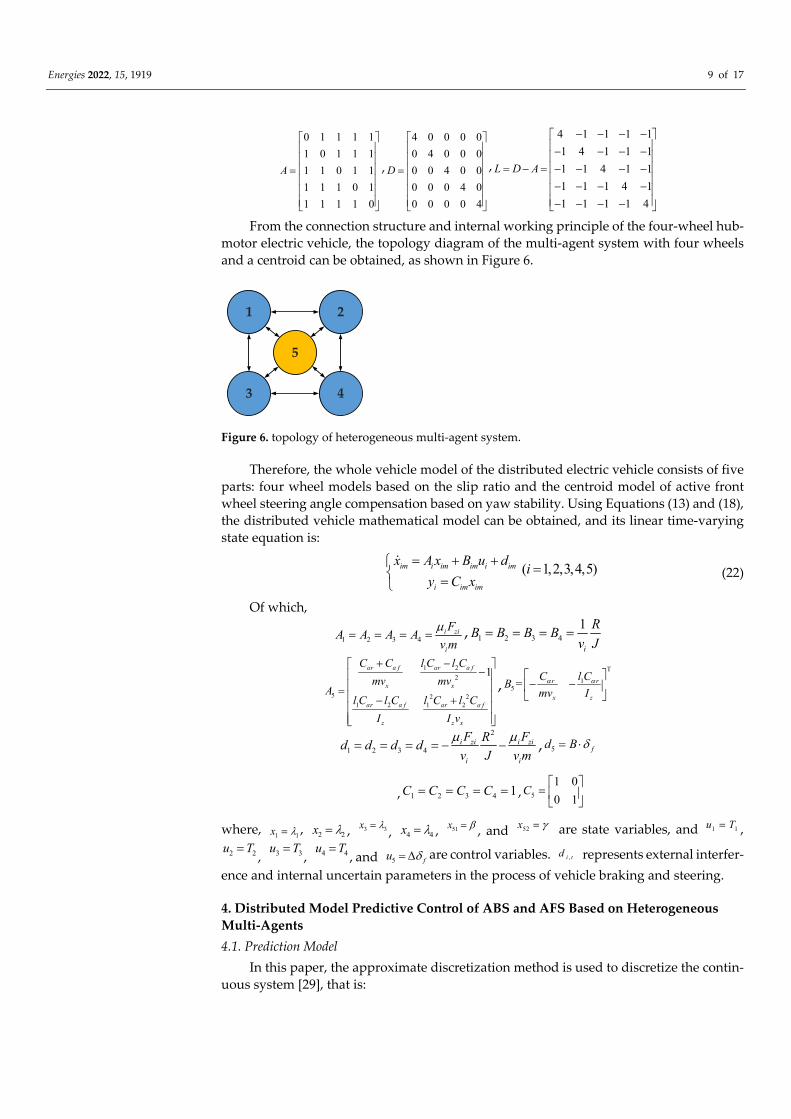
From the connection structure and internal working principle of the four‐wheel hub‐

motor electric vehicle, the topology diagram of the multi‐agent system with four wheels 

and a centroid can be obtained, as shown in Figure 6. 

1

5

2

43

 

Figure 6. topology of heterogeneous multi‐agent system. 

Therefore, the whole vehicle model of the distributed electric vehicle consists of five 

parts: four wheel models based on the slip ratio and the centroid model of active front 

wheel steering angle compensation based on yaw stability. Using Equations (13) and (18), 

the distributed vehicle mathematical model can be obtained, and its linear time‐varying 

state equation is: 

im i im im i im

i im im

x A x B u d

y C x

( 1,2,3,4,5)i   (22) 

Of which, 

1 2 3 4i zi

i

FA A A A

v m

, 1 2 3 4

1

i

RB B B B

v J  

1 2

2

5 2 21 2 1 2

1r f r f

x x

r f r f

z z x

C C l C l C

mv mvA

l C l C l C l C

I I v

a a a a

a a a a

, 15=

r r

x z

C l CB

mv I

 

2

1 2 3 4i zi i zi

i i

F FRd d d d

v J v m

, 5 fd B  

, 1 2 3 4 1C C C C , 5

1 0

0 1C

 

 

where, 1 1x l ,  2 2x l ,  3 3x l

,  4 4x l ,  51x b , and  52x g   are state variables, and  1 1u T , 

2 2u T,  3 3u T

,  4 4u T, and  5 fu d are control variables.  ,i td   represents external interfer‐

ence and internal uncertain parameters in the process of vehicle braking and steering. 

4. Distributed Model Predictive Control of ABS and AFS Based on Heterogeneous 

Multi‐Agents 

4.1. Prediction Model 

In this paper, the approximate discretization method is used to discretize the contin‐

uous system [29], that is: 

Energies 2022, 15, 1919  10  of  17  

 

,

,

,

=im t i

im t i

im t i

A TA

B TB

d Td

 (23) 

Combining Equations (22) and (23), the linear time‐varying distributed model pre‐

diction equation based on heterogeneous multi‐agents can be obtained. 

, , ,( 1) ( ) ( ) ( )

( ) ( )im im t im im t i im t

i im im

x k A x k B u k d k

y k C x k

1,2,3, 4,5)i （   (24) 

Here,  ,im tA , ,im tB ,  imC   together  represent  the  coefficient matrix  of  the  prediction 

model.  yn

iy R   is the controlled variable,  uniu R   is the control variable, and  xn

imx R   is 

the state variable. 

Let  ( ) [ ( ) ( ) ]i im ix k x k kh , where  ( ) ( )i ik y kh ,  and  the  incremental model of 

state space is: 

, , ,( 1) ( ) ( ) ( )

( ) ( )i i t i i t i i t

i i i

x k A x k B u k d k

y k C x k

1, 2, 3, 4, 5)i （   (25) 

where, 

,,

,

0im ti t

im im t

AA

C A I

,,

,,

im ti t

im im t

BB

C B

, 0iC I , ,,

( )( )

0im t

i t

d kd k

   

Assuming that the current time is time  k , the prediction time domain of the system 

is  P, the control time domain is  M , and  p m＞ ; under the action of  M   continuous con‐trol  ( ), ( 1), , ( 1)i i iu k u k u k M , the output prediction value of the system at the time 

P   in the future is: Order, 

( ) [ ( +1| ) ( +2| ) ( | ) ]iP i i iY k y k k y k k y k P k  

( ) [ ( ) ( 1) ( 1) ]iM i i iU k u k u k u k M  

The multi‐step prediction equation is: 

,( ) ( | ) ( ) ( )iP i i i iM i i tY k Hx k k K U k Sd k     (26) 

where,   

,

, , ,2

, , , , ,

1 2 3, , , , , , , ,

i i t

i i t i t i i t

i i t i t i i t i t i i ti

P P P P Mi i t i t i i t i t i i t i t i i t i t

C B

C A B CB

C A B C A B CBK

C A B C A B C A B C A B

,

,2

,3

,

,

i i t

i i t

i i ti

Pi i t

C A

C A

C AH

C A

,

,2

,

1,

i

i i t

i i ti

Pi i t

C

C A

C AS

C A

4.2. Rolling Optimization 

Assuming that the current time is time k, the ideal value predicted by the whole ve‐

hicle system at time P in the future is defined as: 

( ) [ ( +1| ) ( +2| ) ( | ) ]ref ref ref refiP i i iY k y k k y k k y k P k 1,2,3,4)i （  

51 51

51 51 515

52

51 51

( +1| ) ( +1| )

( | ) ( +2| ) ( +2| )( ) [ 1][ ]

( | )

( + | ) ( + | )

ref ref

def ref refrefP def

ref ref

y k k y k k

Y k P k y k k y k kY k

Y k P k

y k P k y k P k

r

rr

r

 

where  r   is defined as the weight coefficient, and the error function of the prediction of 

the future  P  time of the whole vehicle system is defined as: 

Energies 2022, 15, 1919  11  of  17  

 

( ) ( ) ( ) ( 1| ) ( 2 | ) ( | )refiP iP iP i i iE k Y k Y k e k k e k k e k P k

( 1,2,3,4,5)i   (27) 

To improve the braking safety and handling stability of the whole vehicle and reduce 

the loss of control energy, the objective function  iJ   as part of the multi‐objective optimi‐

zation is defined. 

Firstly, the four wheel agents and the centroid agent follow the ideal values for the 

slip  ratio, yaw  rate,  and  centroid  sideslip  angle,  and  the  interaction  between  the  five 

agents is minimized. Therefore, we define  1iJ   as: 5 5

2

11 1

( ) ( ) ( ) ( ) ( ( ( ) ( )) ( ( ( ) ( ))e

i Pi Pi e Pi ij Pi Pj e ij Pi PjQj j

J k k k Q k a E k E k Q a E k E kx x x

( 1,2,3,4,5)i  (28) 

where,  ija   is the element of adjacency matrix  A , and  eQ   is the weighting matrix of the 

controlled variable. 

Secondly, we hope that the control action in the whole control process will be as small 

as possible  to  reduce energy  loss and consider  the energy saving of  the whole vehicle 

system. Therefore, we define  2iJ   as: 2

2 ( ) ( ) ( ) ( )u

i iM iM u iMQJ k U k U k Q U k

( 1,2,3,4,5)i

 (29) 

where,  uQ   is the weighting matrix of the control increment. 

Finally, the braking control system should guarantee the braking distance while en‐

suring the braking stability. Define 3iJ   as: 

3 0( )

t

i xiJ k v dt   (30)

Our ultimate optimization goal is to improve the safety and stability of electric vehi‐

cles during braking and steering under extreme working conditions, namely: 

1 2 3( ) ( )min ( ) min ( ) ( )+ ( )iM iM

i i i iU k U kJ k J k J k J k

( 1,2,3,4,5)i   (31) 

The whole vehicle system has the following constraints: 

When the vehicle is driving, the steering angle of the vehicle steering actuator is lim‐

ited, and the front wheel steering angle constraint must be set: 

max maxf f fd d d   (32) 

where,  max 4fd. 

To prevent sudden change and the  loss of stability of the steering actuator during 

collision avoidance, the increment of the front wheel angle must also be limited: 

max maxf f fd d d   (33) 

where,  max 0.85degfd . 

Whether it is a mechanical, hydraulic, pneumatic, or electromagnetic braking system, 

considering the limitations and safety of the system, the maximum braking torque and its 

change rate are constrained: 

max maxi i iT T T 1,2,3,4)i （   (34) 

max maxi i iT T T 1,2,3,4)i （   (35) 

where,  max 800iT N, max 20iT N. 

There is a limit to the lateral displacement of the vehicle: 

min maxi i iY Y Y 1,2,3,4)i （   (36)

where, min 3iY m,

max 5iY m. 

Energies 2022, 15, 1919  12  of  17  

 

When solving Equations (31)–(35), they can be transformed into a constrained stand‐

ard linear quadratic programming (QP) problem. 

1min ( )

2QPi

iQP iQP i iQP i iQP ixJ x x W x c x d ( 1,2,3,4,5)i  

.s t   i i iQP il E x h  

where,  niQPx R   is  the decision variable,  n n

iW R , and matrix iW   is a Hessian matrix, 

which describes the quadratic part of the objective function. Vector  ic   describes the lin‐

ear part, id   is  independent of  iQP

x   and  independent of  the determined  i QPx

,  p niE R , 

and  , pi il h R . When the  iW  matrix is a positive definite or semi‐positive definite matrix 

and  the  constraint  is  linear,  the above optimization problem  is a  convex optimization 

problem with a unique solution [30]. 

To improve the solving speed of QP and further the engineering applications, in this 

paper,  the discrete simplified dual neural network algorithm (SDNN)  is applied  to  the 

rolling optimization of DMPC by using the method proposed  in reference [31], and by 

considering factors such as system deviation and the presence of multi‐agents. The corre‐

sponding relationship between discrete SDNN parameters and quadratic programming 

parameters can be obtained: 

( ) ( ) 1( )i i MiQP iMx U k R ,

5

1

2 ( ) M Mi ij i e i u

j

W a Q Q R

,

2M Mi iu M ME B I R

 

5

1

2( ( ( ) ( ) ( )+ ( ) ( ) ( ) ( ) ( ) ( ) ( )def defi ij i e i i i e i i i e i j e j

j

c a k Q F k x k k Q S k d k k Q Y k k Q Y k

2 1min min[ ( 1) ] M

i i i il U U k U R ,2 1

max min[ ( 1) ] Mi i i ih U U k U R  

where, 

( 1) ( 1) ( 1) ( 1)i i i iU k u k u k u k ,

( ) ( 1) ( )iM i iu iMU k U k B U k  

u u

u u u uiu

u u u u u u M M

I

I IB

I I I

( 1,2,3,4,5)i  

Here,  u uI   and  M MI   are the unit matrices of  u u   and  M M , respectively. 

4.3. Feedback Mechanism 

After the model predictive control is solved in each control cycle, the control input 

increment in the control time domain is obtained: 

( ) [ ( ) ( 1) ( 1) ]iM i i iU k u k u k u k M ( 1,2,3,4,5)i  

The first element in the control sequence acts on the system as a control input incre‐

ment, that is: 

Energies 2022, 15, 1919  13  of  17  

 

( ) ( 1) ( )i i iu k u k u k ( 1,2,3,4,5)i  

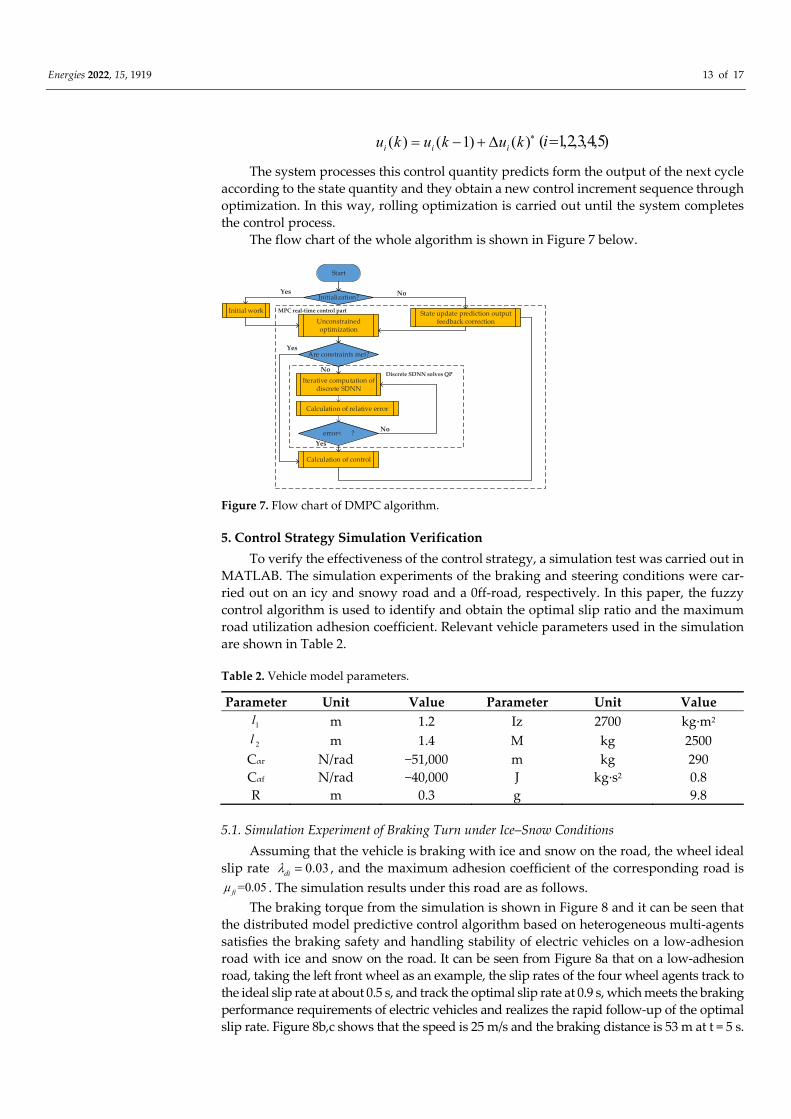
The system processes this control quantity predicts form the output of the next cycle 

according to the state quantity and they obtain a new control increment sequence through 

optimization. In this way, rolling optimization is carried out until the system completes 

the control process. 

The flow chart of the whole algorithm is shown in Figure 7 below. 

Start

Initialization?

Unconstrained optimization

Are constraints met?

Iterative computation of discrete SDNN

Calculation of relative error

error<      ?

Calculation of control

Initial work State update prediction output feedback correction

Yes No

Yes

Yes

No

No

Discrete SDNN solves QP

MPC real‐time control part

 

Figure 7. Flow chart of DMPC algorithm. 

5. Control Strategy Simulation Verification 

To verify the effectiveness of the control strategy, a simulation test was carried out in 

MATLAB. The simulation experiments of the braking and steering conditions were car‐

ried out on an icy and snowy road and a 0ff‐road, respectively. In this paper, the fuzzy 

control algorithm is used to identify and obtain the optimal slip ratio and the maximum 

road utilization adhesion coefficient. Relevant vehicle parameters used in the simulation 

are shown in Table 2. 

Table 2. Vehicle model parameters. 

Parameter  Unit  Value  Parameter  Unit  Value 

1l   m  1.2  Iz  2700  kg∙m2 

2l   m  1.4  M  kg  2500 

Cαr  N/rad  −51,000  m  kg  290 

Cαf  N/rad  −40,000  J  kg∙s2  0.8 

R  m  0.3  g    9.8 

5.1. Simulation Experiment of Braking Turn under Ice–Snow Conditions 

Assuming that the vehicle is braking with ice and snow on the road, the wheel ideal 

slip rate  0.03dil , and the maximum adhesion coefficient of the corresponding road is 

=0.05fim . The simulation results under this road are as follows. 

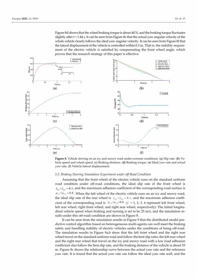
The braking torque from the simulation is shown in Figure 8 and it can be seen that 

the distributed model predictive control algorithm based on heterogeneous multi‐agents 

satisfies the braking safety and handling stability of electric vehicles on a low‐adhesion 

road with ice and snow on the road. It can be seen from Figure 8a that on a low‐adhesion 

road, taking the left front wheel as an example, the slip rates of the four wheel agents track to 

the ideal slip rate at about 0.5 s, and track the optimal slip rate at 0.9 s, which meets the braking 

performance requirements of electric vehicles and realizes the rapid follow‐up of the optimal 

slip rate. Figure 8b,c shows that the speed is 25 m/s and the braking distance is 53 m at t = 5 s. 

Energies 2022, 15, 1919  14  of  17  

 

Figure 8d shows that the wheel braking torque is about 44 N, and the braking torque fluctuates 

slightly after t = 1.44 s. It can be seen from Figure 8e that the actual yaw angular velocity of the 

whole vehicle closely follows the ideal yaw angular velocity. It can be seen from Figure 8f that 

the lateral displacement of the vehicle is controlled within 0.3 m. That is, the stability require‐

ment of  the electric vehicle  is  satisfied by  compensating  the  front wheel angle, which 

proves that the research strategy of this paper is effective. 

   

(a)  (b) 

   (c)  (d) 

   

(e)  (f) 

Figure 8. Vehicle driving on an icy and snowy road under extreme conditions. (a) Slip rate. (b) Ve‐

hicle speed and wheel speed. (c) Braking distance. (d) Braking torque. (e) Ideal yaw rate and actual 

yaw rate. (f) Vehicle lateral displacement. 

5.2. Braking Steering Simulation Experiment under off‐Road Condition 

Assuming that the front wheel of the electric vehicle runs on the standard uniform 

road  condition  under  off‐road  conditions,  the  ideal  slip  rate  of  the  front  wheel  is 

1 2= 0.1d dl l , and the maximum adhesion coefficient of the corresponding road surface is 

3 4= 0.8f fm m . When the left wheel of the electric vehicle runs on an icy and snowy road, 

the ideal slip rate of the rear wheel is  2 4= 0 .1d dl l , and the maximum adhesion coeffi‐

cient of the corresponding road is  2 4= =0.8f fm m   ( i   = 1, 2, 3, 4 represent left front wheel, 

left rear wheel, right front wheel, and right rear wheel, respectively). The initial longitu‐

dinal vehicle speed when braking and turning is set to be 25 m/s, and the simulation re‐

sults under this off‐road condition are shown in Figure 8.   

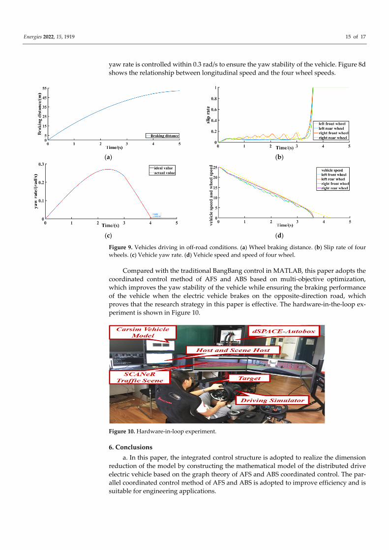
It can be seen from the simulation results in Figure 9 that the distributed model pre‐

dictive control algorithm based on heterogeneous multi‐agents can well meet the braking 

safety and handling stability of electric vehicles under the conditions of being off‐road. 

The  simulation  results  in Figure 9a,b  show  that  the  left  front wheel and  the  right  rear 

wheel travel on the standard uniform road and follow the best slip ratio; the left rear wheel 

and the right rear wheel that travel on the icy and snowy road with a low road adhesion 

coefficient also follow the best slip rate, and the braking distance of the vehicle is about 53 

m. Figure 8c shows the relationship curve between the actual yaw rate and the reference 

yaw rate. It is found that the actual yaw rate can follow the ideal yaw rate well, and the 

Energies 2022, 15, 1919  15  of  17  

 

yaw rate is controlled within 0.3 rad/s to ensure the yaw stability of the vehicle. Figure 8d 

shows the relationship between longitudinal speed and the four wheel speeds. 

   (a)  (b) 

   

(c)  (d) 

Figure 9. Vehicles driving in off‐road conditions. (a) Wheel braking distance. (b) Slip rate of four 

wheels. (c) Vehicle yaw rate. (d) Vehicle speed and speed of four wheel. 

Compared with the traditional BangBang control in MATLAB, this paper adopts the 

coordinated  control method  of AFS  and ABS  based  on multi‐objective  optimization, 

which improves the yaw stability of the vehicle while ensuring the braking performance 

of  the  vehicle when  the  electric  vehicle  brakes  on  the  opposite‐direction  road, which 

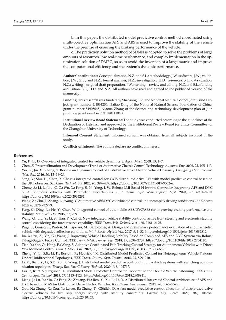
proves that the research strategy in this paper is effective. The hardware‐in‐the‐loop ex‐

periment is shown in Figure 10. 

 

Figure 10. Hardware‐in‐loop experiment. 

6. Conclusions 

a. In this paper, the integrated control structure is adopted to realize the dimension 

reduction of the model by constructing the mathematical model of the distributed drive 

electric vehicle based on the graph theory of AFS and ABS coordinated control. The par‐

allel coordinated control method of AFS and ABS is adopted to improve efficiency and is 

suitable for engineering applications.   

Energies 2022, 15, 1919  16  of  17  

 

b. In this paper, the distributed model predictive control method coordinated using 

multi‐objective optimization AFS and ABS is used to improve the stability of the vehicle 

under the premise of ensuring the braking performance of the vehicle.   

c. The prediction solution method of SDNN is adopted to solve the problems of large 

amounts of resources, low real‐time performance, and complex implementation in the op‐

timization solution of DMPC, so as to avoid the inversion of a large matrix and improve 

the computational efficiency and the system’s dynamic performance. 

Author Contributions: Conceptualization, N.Z. and S.L.; methodology, J.W.; software, J.W.; valida‐

tion, J.W., Z.L., and N.Z.; formal analysis, N.Z.; investigation, H.D.; resources, S.L.; data curation, 

N.Z.; writing—original draft preparation, J.W.; writing—review and editing, N.Z. and S.L.; funding 

acquisition, S.L., H.D. and N.Z. All authors have read and agreed to the published version of the 

manuscript. 

Funding: This research was funded by Shaosong Li of the National Natural Science Joint Fund Pro‐

ject, grant number U1864206, Haitao Ding of  the National Natural Science Foundation of China, 

grant number 51905045, Niaona Zhang of  the Science and  technology development plan of  Jilin 

province, grant number 20210201110GX. 

Institutional Review Board Statement: The study was conducted according to the guidelines of the 

Declaration of Helsinki, and approved by the Institutional Review Board (or Ethics Committee) of 

the Changchun University of Technology. 

Informed Consent Statement:  Informed consent was obtained  from all  subjects  involved  in  the 

study. 

Conflicts of Interest: The authors declare no conflict of interest. 

References 

1. Yu, F.; Li, D. Overview of integrated control for vehicle dynamics. J. Agric. Mach. 2008, 39, 1–7. 

2. Chen, Z. Present Situation and Development Trend of Automotive Chassis Control Technology. Automot. Eng. 2006, 28, 105–113. 

3. Yin, G.; Jin, X.; Zhang, Y. Review on Dynamic Control of Distributive Drive Electric Vehicle Chassis. J. Chongqing Univ. Technol. 

(Nat. Sci.) 2016, 30, 13–19+26. 

4. Song, Y.; Shu, H.; Chen, X. Chassis integrated control for 4WIS distributed drive EVs with model predictive control based on 

the UKF observer. Sci. China Technol. Sci. 2020, 63, 397–409. https://doi.org/10.1007/s11431‐019‐9552‐6. 

5. Cheng, S.; Li, L.; Liu, C.‐Z.; Wu, X.; Fang, S.‐N.; Yong, J.‐W. Robust LMI‐Based H‐Infinite Controller Integrating AFS and DYC 

of  Autonomous  Vehicles  with  Parametric  Uncertainties.  IEEE  Trans.  Syst.  Man  Cybern.  Syst.  2020,  51,  6901–6910. 

https://doi.org/10.1109/tsmc.2020.2964282. 

6. Wang, Z.; Zhu, J.; Zhang, L.; Wang, Y. Automotive ABS/DYC coordinated control under complex driving conditions. IEEE Access 

2018, 6, 32769‐32779. 

7. Feng, C.; Ding, N.; He, Y.; Chen, W. Integrated control of automobile ABS/DYC/AFS for improving braking performance and 

stability. Int. J. Veh. Des. 2015, 67, 259. 

8. Wang, G.; Liu, Y.; Li, S.; Tian, Y.; Cui, G. New integrated vehicle stability control of active front steering and electronic stability 

control considering tire force reserve capability. IEEE Trans. Veh. Technol. 2021, 70, 2181–2195. 

9. Pugi, L.; Grasso, F.; Pratesi, M.; Cipriani, M.; Bartolomei, A. Design and preliminary performance evaluation of a four wheeled 

vehicle with degraded adhesion conditions. Int. J. Electr. Hybrid Veh. 2017, 9, 1–32. https://doi.org/10.1504/ijehv.2017.082812. 

10. Jin, X.; Yu, Z.; Yin, G.; Wang, J. Improving Vehicle Handling Stability Based on Combined AFS and DYC System via Robust 

Takagi‐Sugeno Fuzzy Control. IEEE Trans. Intell. Transp. Syst. 2018, 19, 2696–2707. https://doi.org/10.1109/tits.2017.2754140. 

11. Tian, Y.; Yao, Q.; Hang, P.; Wang, S. Adaptive Coordinated Path Tracking Control Strategy for Autonomous Vehicles with Direct 

Yaw Moment Control. Chin. J. Mech. Eng. 2022, 35, 1. https://doi.org/10.1186/s10033‐021‐00666‐0. 

12. Zheng, Y.; Li, S.E.; Li, K.; Borrelli, F.; Hedrick, J.K. Distributed Model Predictive Control for Heterogeneous Vehicle Platoons 

Under Unidirectional Topologies. IEEE Trans. Control. Syst. Technol. 2016, 25, 899–910. 

13. Li, K.; Bian, Y.; Li, S.E.; Xu, B.; Wang, J. Distributed model predictive control of multi‐vehicle systems with switching commu‐

nication topologies. Transp. Res. Part C Emerg. Technol. 2020, 118, 102717. 

14. Liu, P.; Kurt, A.; Ozguner, U. Distributed Model Predictive Control for Cooperative and Flexible Vehicle Platooning. IEEE Trans. 

Control Syst. Technol. 2019, 27, 1115–1128. https://doi.org/10.1109/tcst.2018.2808911. 

15. Liang, J.; Lu, Y.; Yin, G.; Fang, Z.; Zhuang, W.; Ren, Y.; Xu, L.; Li, Y. A Distributed Integrated Control Architecture of AFS and 

DYC based on MAS for Distributed Drive Electric Vehicles. IEEE Trans. Veh. Technol. 2021, 70, 5565–5577. 

16. Guo, N.; Zhang, X.; Zou, Y.; Lenzo, B.; Zhang, T.; Göhlich, D. A fast model predictive control allocation of distrib‐uted drive 

electric  vehicles  for  tire  slip  energy  saving  with  stability  constraints.  Control  Eng.  Pract.  2020,  102,  104554. 

https://doi.org/10.1016/j.conengprac.2020.10455. 

Energies 2022, 15, 1919  17  of  17  

 

17. Tavernini, D.; Metzler, M.; Gruber, P.; Sorniotti, A. Explicit Nonlinear Model Predictive Control for Electric Vehicle Traction 

Control. IEEE Trans. Control Syst. Technol. 2019, 27, 1438–1451. https://doi.org/10.1109/tcst.2018.2837097. 

18. Zeilinger, M.N.; Jones, C.; Morari, M. Real‐Time Suboptimal Model Predictive Control Using a Combination of Explicit MPC 

and Online Optimization. IEEE Trans. Autom. Control 2011, 56, 1524–1534. https://doi.org/10.1109/tac.2011.2108450. 

19. Liu, S.; Wang J. A simplified dual neural network for quadratic programming with its KWTA application. IEEE Trans. Neural 

Netw. 2006, 17, 1500–1510. 

20. Cseko, L.H.; Kvasnica, M.; Lantos, B. Explicit MPC‐Based RBF Neural Network Controller Design with Discrete‐Time Actual 

Kalman  Filter  for  Semiactive  Suspension.  IEEE  Trans.  Control  Syst.  Technol.  2015,  23,  1736–1753. 

https://doi.org/10.1109/tcst.2014.2382571. 

21. Yin, G.; Zhu, T.; Ren, Z.; Li, G.; Jin, X. Framework of Intelligent Control System for Electric Vehicle Chassis Based on Multi‐

Agent. China Mech. Eng. 2018, 29, 7. 

22. Chen, T.; Khajepour, A. Wheel Modules with Distributed Controllers: A Multi‐Agent Approach to Vehicular Control. IEEE Trans. 

Veh. Technol. 2020, 69, 10879–10888. 

23. Sharma, A.; Srinivasan, D.; Trivedi, A. A Decentralized Multi‐Agent Approach for Service Restoration in Uncertain Environ‐

ment. IEEE Trans. Smart Grid 2018, 9, 3394–3405. https://doi.org/10.1109/tsg.2016.2631639. 

24. Zhang, C.; Wu, H.; He, J.; Xu, C. Consensus tracking for multi‐motor system via observer based variable structure approach. J. 

Frankl. Inst. 2015, 352, 3366–3377. https://doi.org/10.1016/j.jfranklin.2015.01.035. 

25. Liang, J.; Lu, Y.; Pi, D.; Yin, G.; Zhuang, W.; Wang, F.; Feng, J.; Zhou, C. A Decentralized Cooperative Control Framework for 

Active  Steering  and  Active  Suspension:  Multi‐agent  Approach.  IEEE  Trans.  Transp.  Electrif.  2021,  1–1. 

https://doi.org/10.1109/tte.2021.3096992. 

26. Tang, Y.; Xing, X.; Karimi, H.R.; Kocarev, L.; Kurths, J. Tracking Control of Networked Multi‐Agent Systems Under New Char‐

acterizations  of  Impulses  and  Its  Applications  in  Robotic  Systems.  IEEE  Trans.  Ind.  Electron.  2016,  63,  1299–1307. 

https://doi.org/10.1109/tie.2015.2453412. 

27. Leng, B.; Jin, D.; Xiong, L.; Yang, X.; Yu, Z. Estimation of tire‐road peak adhesion coefficient for intelligent electric vehicles based 

on cam‐era and tire dynamics information fusion. Mech. Syst. Signal Processing 2021, 150, 107275. 

28. Gong, J.W.; Jiang, Y.; Xu, W. Model Predictive Control of Unmanned Ground Vehicle; Beijing Institute of Technology Press: Beijing, 

China, 2014. 

29. Kuhne, F.; Lages, W.F.; da Silva, J.G., Jr. Model Predictive Control of a Mobile Robot Using Linearization. In Proceedings of the 

Mechatronics and Robototics, 2004; 4, 525–530. 

30. Zhao,  L.;  Tang,  L. A  Simple Method  of ABS Optimal  Slip Ratio  Identification. Adv. Mater. Res.  2011,  383‐390,  2453–2457. 

https://doi.org/10.4028/www.scientific.net/amr.383‐390.2453. 

31. Aly, A.A.  Intelligent  fuzzy control  for antilock brake system with  road‐surfaces  identifier.  In Proceedings of  the 2010  IEEE 

International  Conference  on  Mechatronics  and  Automation,  Xiʹan,  China,  4–7  August  2010;  pp.  699–705. 

https://doi.org/10.1109/icma.2010.5589106.