Motion-Based Prediction Is Sufficient to Solve the Aperture Problem

LETTER Communicated by Linda Bowns

Motion-Based Prediction Is Sufficient to Solvethe Aperture Problem

Laurent U. [email protected] S. [email protected] de Neurosciences de la Timone, CNRS/Aix-Marseille University 13385Marseille Cedex 5, France

In low-level sensory systems, it is still unclear how the noisy informationcollected locally by neurons may give rise to a coherent global percept.This is well demonstrated for the detection of motion in the apertureproblem: as luminance of an elongated line is symmetrical along its axis,tangential velocity is ambiguous when measured locally. Here, we de-velop the hypothesis that motion-based predictive coding is sufficient toinfer global motion. Our implementation is based on a context-dependentdiffusion of a probabilistic representation of motion. We observe in sim-ulations a progressive solution to the aperture problem similar to physio-logy and behavior. We demonstrate that this solution is the result of twounderlying mechanisms. First, we demonstrate the formation of a track-ing behavior favoring temporally coherent features independent of theirtexture. Second, we observe that incoherent features are explained away,while coherent information diffuses progressively to the global scale.Most previous models included ad hoc mechanisms such as end-stoppedcells or a selection layer to track specific luminance-based features as nec-essary conditions to solve the aperture problem. Here, we have provedthat motion-based predictive coding, as it is implemented in this func-tional model, is sufficient to solve the aperture problem. This solutionmay give insights into the role of prediction underlying a large class ofsensory computations.

1 Introduction

1.1 Problem Statement. A central challenge in neuroscience is toexplain how local information that is represented in the activity of singleneurons can be integrated to enable global and coherent responses at pop-ulation and behavioral levels. A classic illustration of this problem is givenby the early stages of visual motion processing. Visual cortical areas, suchas the primary visual cortex (V1) or the mediotemporal (MT) extrastriatearea, can extract geometrical structures from luminance changes that are

Neural Computation 24, 2726–2750 (2012) c© 2012 Massachusetts Institute of Technology

Motion-Based Prediction and the Aperture Problem 2727

sensed by large populations of direction- and speed-selective neuronswithin topographically organized maps (Hildreth & Koch, 1987). However,these cells have access to only the limited portion of the visual space fallinginside their classical receptive fields. Therefore, local information is oftenincomplete and ambiguous, as, for instance, when measuring the motion ofa long line that crosses their receptive field. Because of the symmetry alongthe line’s axis, the measure of the tangential component of translationvelocity is completely ambiguous, leading to the aperture problem (seeFigure 1A). As a consequence, most V1 and MT neurons indicate the slowestelement from the family of vectors compatible with the line’s translation,that is, the speed perpendicular to the line orientation (Albright, 1984).These neurons are often called component-selective cells and can signalonly orthogonal motions of local 1D edges from more complex movingpatterns. Integrated in area MT, such local preferences introduce biasesin the estimated direction and speed of the translating line. A behavioralconsequence is that perceived direction of an elongated tilted line is initiallybiased toward the motion direction orthogonal to its orientation (Born,Pack, Ponce, & Yi, 2006; Lorenceau, Shiffrar, Wells, & Castet, 1992; Masson& Stone, 2002; Pei, Hsiao, Craig, & Bensmaia, 2010; Wallace, Stone, & Mas-son, 2005). There are, however, other MT neurons, called pattern-selectivecells, that can signal the true translation vector corresponding to suchcomplex visual patterns and, hence drive correct, steady-state behaviors(Movshon, Adelson, Gizzi, & Newsome, 1985; Pack & Born, 2001; Rodman& Albright, 1989). Ultimately, these neurons provide a solution similar tothe interception of constraints (IOC) (Adelson & Movshon, 1982; Fennema& Thompson, 1979) by combining the information of multiple componentcells (for a recent model, see Bowns, 2011).

The classic view is that these pattern-selective neurons integrate infor-mation from a large pool of component cells signaling a wide range ofdirections, spatial frequencies, speeds, and so on (Rust, Mante, Simoncelli,& Movshon, 2006). However, this two-stage, feedforward model of motionintegration is challenged by several recent studies that call for more complexcomputational mechanisms (see Masson & Ilg, 2010, for reviews). First, thereare neurons outside area MT that can solve the aperture problem. For in-stance, V1 end-stopped cells are sensitive to particular features such as lineendings and can therefore signal unambiguous motion at a much smallerspatial scale, providing that the edge falls within their receptive field (Pack,Gartland, & Born, 2004). These neurons could contribute to pattern selec-tivity in area MT (Tsui, Hunter, Born, & Pack, 2010), but this solution onlypushes the problem back to earlier stages of cortical motion processing sinceone must now explain the emergence of end-stopping cells. Second, all neu-ral solutions to the aperture problem are highly dynamic and build up overdozens of milliseconds after stimulus onset (Pack & Born, 2001; Pack et al.,2004; Pack, Livingstone, Duffy, & Born, 2003; Smith, Majaj, & Movshon,2010). This can explain why perceived direction of motion gradually

2728 L. Perrinet and G. Masson

changes over time, shifting from component to pattern translation(Lorenceau et al., 1992; Masson & Stone, 2002; Wallace et al., 2005). Clas-sic feedforward models cannot account for such temporal dynamics andits dependence on several properties of the input such as contrast or barlength (Rust et al., 2006; Tsui et al., 2010). Third, classic computationalsolutions ignore the fact that any object moving in the visual world at nat-ural speeds will travel across many receptive fields within the retinotopicmap. Thus, any single, local receptive field will be stimulated over a pe-riod of time that is much less than the time constants reported above forsolving the aperture problem (see Masson, Montagnini, & Ilg, 2010). Still,single-neuron solutions for ambiguous motion have been documented sofar only with conditions where the entire stimulus is presented within thereceptive field (Pack et al., 2004) and with the same geometry (Majaj, Caran-dini, & Movshon, 2007) over dozens of milliseconds.

Thus, there is an urgent need for more generic computational solutions.We recently proposed that diffusion mechanisms within a cortical map can


solve the aperture problem without the need for complex local mechanismssuch as end stopping or pooling across spatiotemporal frequencies (Tlapale,Kornprobst, Masson, & Faugeras, 2011; Tlapale, Masson, & Kornprobst,2010). This approach is consistent with the role of recurrent connectivity inmotion integration (Bayerl & Neumann, 2004) and can simulate the tempo-ral dynamics of motion integration in many different conditions. Moreover,it can reverse the perspective that is dominant in feedforward models wherelocal properties such as end stopping, pattern selectivity, or other types ofextraclassic receptive fields phenomena are implemented by built-in, spe-cific neuronal detectors. Instead, these properties can be seen as solutionsemerging from the neuronal dynamics of the intricate, recursive contribu-tions of feedforward, feedback, and lateral interactions. A vast theoreticaland experimental challenge is therefore to elucidate how diffusion models

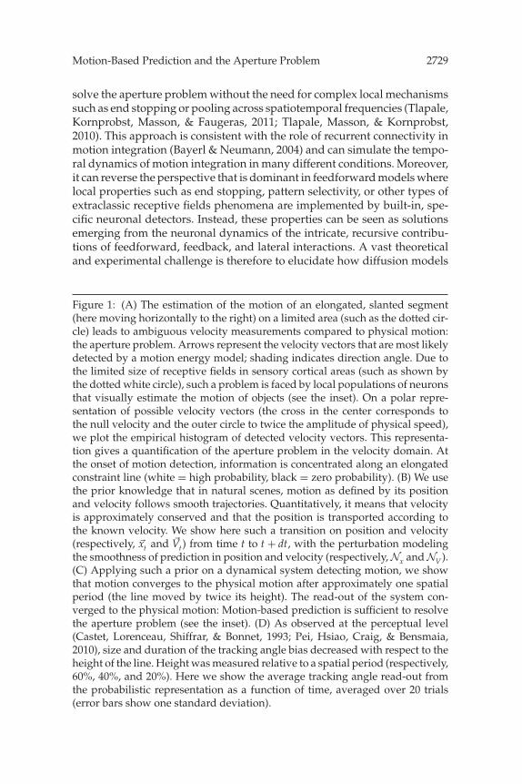
Figure 1: (A) The estimation of the motion of an elongated, slanted segment(here moving horizontally to the right) on a limited area (such as the dotted cir-cle) leads to ambiguous velocity measurements compared to physical motion:the aperture problem. Arrows represent the velocity vectors that are most likelydetected by a motion energy model; shading indicates direction angle. Due tothe limited size of receptive fields in sensory cortical areas (such as shown bythe dotted white circle), such a problem is faced by local populations of neuronsthat visually estimate the motion of objects (see the inset). On a polar repre-sentation of possible velocity vectors (the cross in the center corresponds tothe null velocity and the outer circle to twice the amplitude of physical speed),we plot the empirical histogram of detected velocity vectors. This representa-tion gives a quantification of the aperture problem in the velocity domain. Atthe onset of motion detection, information is concentrated along an elongatedconstraint line (white = high probability, black = zero probability). (B) We usethe prior knowledge that in natural scenes, motion as defined by its positionand velocity follows smooth trajectories. Quantitatively, it means that velocityis approximately conserved and that the position is transported according tothe known velocity. We show here such a transition on position and velocity(respectively, �xt and �Vt) from time t to t + dt, with the perturbation modelingthe smoothness of prediction in position and velocity (respectively, Nx and NV ).(C) Applying such a prior on a dynamical system detecting motion, we showthat motion converges to the physical motion after approximately one spatialperiod (the line moved by twice its height). The read-out of the system con-verged to the physical motion: Motion-based prediction is sufficient to resolvethe aperture problem (see the inset). (D) As observed at the perceptual level(Castet, Lorenceau, Shiffrar, & Bonnet, 1993; Pei, Hsiao, Craig, & Bensmaia,2010), size and duration of the tracking angle bias decreased with respect to theheight of the line. Height was measured relative to a spatial period (respectively,60%, 40%, and 20%). Here we show the average tracking angle read-out fromthe probabilistic representation as a function of time, averaged over 20 trials(error bars show one standard deviation).


can be implemented by realistic populations of neurons dealing with noisyinputs.

The aperture problem in vision must be seen as an instance of the moregeneric problem of information integration in sensory systems. The aper-ture problem, as well as the correspondence problem, can be seen as aclass of underconstrained inverse problems faced by many different sen-sory and cognitive systems. Interestingly, recent experimental evidence haspointed out strong similarities in the dynamics of the neural solution forspatiotemporal integration of information in space. For instance, there isa tactile counterpart of the visual aperture problem, and neurons in themonkey somatosensory cortex exhibit similar temporal dynamics to that ofarea MT neurons (Pei, Hsiao, & Bensmaia, 2008; Pei et al., 2010; Pei, Hsiao,Craig, & Bensmaia, 2011). These recent results point to the need to builda theoretical framework that can unify these generic mechanisms such asrobust detection and context-dependent integration and propose a solutionthat applies to different sensory systems. An obvious candidate is to buildassociation fields that would gather neighboring information and enhanceconstraints on the response. This is the goal of our study: to provide atheoretical framework using probabilistic inference.

In this letter, we explore the hypothesis that the aperture problem canbe solved using predictive coding. We introduce a generic probabilisticframework for motion-based prediction as a specific dynamical spatiotem-poral diffusion process on motion representation, as originally proposedby Burgi, Yuille, and Grzywacz (2000). However, we do not perform anapproximation of the dynamics of probabilistic distributions using a neuralnetwork implementation, as they did. Instead, we develop a method to sim-ulate precise predictions in topographic maps. We test our model againstbehavioral and neuronal results that are signatures of the key properties ofprimate visual motion detection and integration. Furthermore, we demon-strate that several properties of low-level motion processing (i.e., featuremotion tracking, texture-independent motion, context-dependent motionintegration) naturally emerge from predictive coding within a retinotopicmap. Finally, we discuss the putative role of prediction in generic neuralcomputations.

1.2 Probabilistic Detection of Motion. First, we define a generic prob-abilistic framework for studying the aperture problem and its solution.Translation of an object in the planar visual space at a given time is fullygiven by the probability distribution of its position and velocity, that is,as a distribution of the different degrees of belief among a set of possiblevelocities. It is usual to define motion probability at any given location.If one particular velocity is certain, its probability becomes 1, while otherprobabilities are 0. The more the measurement is uncertain (e.g., when in-creasing noise), the more the distribution of probabilities will be spreadaround this peak. This type of representation can be successfully used to


solve a large range of problems related to visual motion detection. Theseproblems belong in all generality to optimal detection problems of a signalperturbed by different sources of noise and ambiguity. In particular, theaperture problem is explicitly described by an elongated probability distri-bution function (PDF) along the constraint defined by the orientation of theline (see Figure 1A inset). This constitutes an ill-posed inverse problem, asdifferent possible velocities may correspond to the physical motion of theline.

In such a framework, Bayesian models make explicit the optimal inte-gration of sensory information with prior information. These models maybe decomposed in three stages. First, one defines likelihoods as a measureof belief knowing the sensory data. This likelihood is based on the defi-nition of a generative model. Second, any prior distribution—that is, anyinformation known before observing these data—may be combined to thelikelihood distribution to compute a posterior probability using Bayes’ rule.The prior defines generic knowledge on the generative model over a set ofinputs, such as regularities observed in the statistics of natural images or be-haviorally relevant motions. Finally, a decision can be made by optimizinga behavioral cost dependent on this posterior probability. A common choiceis the belief that corresponds to the maximum a posteriori probability. Theadvantage of Bayesian inference compared to other heuristics is that it ex-plicitly states qualitatively and quantitatively all hypotheses (generativemodels of observation noise and of the prior) that lead to a solution.

1.3 Luminance-Based Detection of Motion. Such a Bayesian schemecan be applied to motion detection using a generative model of the lumi-nance profile in the image. This is first based on the luminance conservationequation. Knowing the velocity �V , we can assume that luminance is approx-imately conserved along this direction, that is, that after a small lapse dt,

It+dt (�x + �V · dt) = It (�x) + NI, (1.1)

where we define luminance at time t by It(�x) as a function of position �xand NI is the observation noise. Using the Laplacian approximation, onecan derive the likelihood probability distribution p(It(�x)|�V ) as a gaussiandistribution. In such a representation, precision is finer for a lower variance.Indeed, it is easy to show that the logarithm of p(It(�x)|�V ) is proportionalto the output of correlation-based elementary motion sensors or, equiva-lently, a motion-energy detector (Adelson & Bergen, 1985). Second, Weiss,Simoncelli, and Adelson (2002) showed that using a prior distribution p(�V )

that favors slow speeds, one could explain why the initial perceived di-rection in the aperture problem is perpendicular to the line. Interestingly,lower-contrast motion results in wider distributions of likelihood and thusposterior p(�V|It(�x)). Therefore, contrast dynamics for a wide variety of


simple motion stimuli is determined by the shape of the probability distri-bution (i.e., gaussian-like distributions) and the ratio between variances oflikelihood and prior distributions, as was validated experimentally on be-havioral data (Barthelemy, Perrinet, Castet, & Masson, 2008). With ambigu-ous inputs, this scheme gives a measure consistent with our formulation ofthe aperture problem, where probability is distributed along a constraintline defined by the orientation of the line (see Figure 1A, inset).

The generative model explicitly assumes a translational motion �V overthe observation aperture, such as the receptive field of a motion-sensitivecell. Usually a distributed set �Vt (�x) of motion estimations at time t overfixed positions �x in the visual field gives a fair approximation of ageneric, complex motion that can be represented in a retinotopic mapsuch as V1/MT areas. This provides a field of probabilistic motion mea-sures p(It(�x)|�Vt (�x))). To generate a global read-out from this local infor-mation, we may integrate these local probabilities over the whole visualfield. Assuming independence of the local information as in Weiss et al.(2002), we model spatiotemporal integration at time T by equation 1.1 andp(�V|I0:T ) ∝ ∏

�x,0≤t≤T p(It(�x)|�V(�x))p(�V ), where we write as I0:t the informa-tion on luminance from time 0 to t. Such models of spatiotemporal integra-tion can account for several nonlinear properties of motion integration suchas monotonic spatial summation and contrast gain control and are success-ful in explaining a wide range of neurophysiological and behavioral data.In particular, it is sufficient to explain the dynamics of the solution to theaperture problem if we assume that information from lines and line end-ings was a priori segmented (Barthelemy et al., 2008). This type of modelprovides a solution similar to the vector average, and we have previouslyshown that the hypothesis of an independent sampling cannot account forsome nonlinear aspects of motion integration, such as supersaturation ofthe spatial summation functions, unless some ad hoc mechanisms such assurround inhibition are added (Perrinet & Masson, 2007). In the case of ourdefinition of the aperture problem (see Figure 1A), the information fromsuch Bayesian measurement at every time step will always give the sameprobability distribution function (described by its mean �Vm and variance �),where �Vm shows a bias toward the perpendicular of the line (see Figure 1A,inset). The independent integration of such information will therefore nec-essarily lead to finer precision (the variance becomes �/T) but with alwaysthe same mean: the aperture problem is not solved.

1.4 Motion-Based Predictive Coding. Failure of the feedforward mod-els in accounting for the dynamics of global motion integration originatesfrom the underlying hypothesis of independence of motion signals in neigh-boring parts of visual space. The independence hypothesis set out aboveformally states that the local measurement of global motion is the sameeverywhere, independent of the position of different motion parts. In fact,the independence hypothesis assumes that if local motion signals were


randomly shuffled in position, they would still yield the same global motionoutput (e.g., Movshon et al., 1985). As Watamaniuk, McKee, and Grzywacz(1995) showed, this hypothesis is particularly at stake for motion along co-herent trajectories: motion as a whole is more than the sum of its parts. Asolution used in previous models solving the aperture problem is to addsome heuristics, such as a selection process (Nowlan & Sejnowski, 1995;Weiss et al., 2002) or a constraint that motion is relatively smooth awayfrom luminance discontinuities (Tlapale, Masson, et al., 2010). A first as-sumption is that the retinotopic position of motion is an essential pieceof information to be represented. In particular, in order to achieve finelygrained predictions, it is essential to consider that the spatial position ofmotion �x, instead of being a given parameter (classically, a value on a grid),is an additional random variable for representing motion along with �V .Compared to the representation p(�V(�x)|I) used in previous studies (Burgiet al., 2000; Weiss et al., 2002), the probability distribution p(�x, �V|I) morecompletely describes motion by explicitly representing its spatial positionjointly with its velocity. Indeed, it is more generic, as it is possible to rep-resent any distribution p(�V(�x)|I) with a distribution p(�x, �V|I), while thereverse is not true without knowing the spatial distribution of the positionof motion p(�x|I). This introduces an explicit representation of the segmen-tation of motion in visual space, an essential ingredient in motion-basedpredictive coding.

Here, we explore the hypothesis that we may take into account most de-pendence of local motion signals between neighboring times and positionsby implementing a predictive dependence of successive measurements ofmotion along a smooth trajectory. In fact, we know a priori that naturalscenes are predictable due to both the rigidity and inertia of physical ob-jects. Due to the projection of their motion in visual space, visual objectspreferentially follow smooth trajectories (see Figure 1B). We may implementthis constraint into a generative model by using the transport equation onmotion itself. This assumes that at time t, during the small lapse dt, motionwas translated proportional to its velocity:

�xt+dt = �xt + �Vt · dt + N�x, (1.2)

�Vt+dt = �Vt + N�V , (1.3)

where N�x and N�V are, respectively, position and velocity unbiased noiseson the motion’s trajectory. In the noiseless case, on the limit when dt tendsat zero, this is the auto-advection term in the Navier-Stokes equations andthus implements a fluid prior in the inference of local motion. In fact, it is im-portant to properly tune N�x and N�V since the variance of these distributionsexplicitly quantifies the precision of the prediction (see Figure 1B).

We may now use this generative model to integrate motion information.Assuming for simplicity that sensory representation is acquired at discrete,


regularly spaced times, we define integration using a Markov random chainon joint random variables zt = �xt,

�Vt :

p(zt |I0:t−dt ) =∫

dzt−dt

p(zt |zt−dt ) · p(zt−dt |I0:t−dt ), (1.4)

p(zt |I0:t ) = p(It |zt ) · p(zt |I0:t−dt )/p(It |I0:t−dt ). (1.5)

To implement this recursion, we first compute p(It |zt ) from the obser-vation model, equation 1.1. The predictive prior probability p(zt |zt−dt ),that is, p(�xt,

�Vt |�xt−dt,�Vt−dt ), is defined by the generative model defined in

equations 1.2 and 1.3. Note that prediction (see equation 1.4) always in-creases the variance by diffusing information. On the other hand, duringestimation (see equation 1.5), coherent data increase the precision of the es-timation, while incoherent data increase the variance. This balance betweendiffusion and reaction will be the most important factor for the convergenceof the dynamical system. Overall, these master equations, along with thedefinition of the prior transition p(zt |zt−dt ), define our model as a dynamicalsystem with a simple global architecture but with complex recurrent loops(see Figure 2).

Unfortunately, the dimensionality of the probabilistic representationmakes impossible the implementation of realistic simulations of the fulldynamical system on classical computer hardware. In fact, even with amoderate quantization of the relevant representation spaces, computingintegrals over hidden variables in the filtering and prediction equations(respectively, equations 1.4 and 1.5) leads to a combinatorial explosion ofparameters that is intractable with the limited memory of current sequen-tial computers. Alternatively, if we assume that all probability distribu-tions are gaussian, this formulation is equivalent to Kalman filtering onjoint variables. This type of implementation may be achieved using, for in-stance, a neuromorphic approximation of the above equations (Burgi et al.,2000). Indeed, one may assume that master equations are implemented bya finely tuned network of lateral and feedback interactions. One advan-tage of this recursive definition in the master equations is that it gives asimple framework for implementing association fields. However, this im-plementation has the consequence of blurring predictions. We explore an-other route using the condensation algorithm (Isard & Blake, 1998), whichsurpasses the above approximation. In addition, it allows us to explorethe role of prediction in solving the aperture problem on a more genericlevel.

2 Model and Methods

2.1 Particle Filtering. Master equations can be approximated usingsequential Monte Carlo (SMC). This method (also known as particle filters)


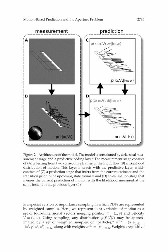
Figure 2: Architecture of the model. The model is constituted by a classical mea-surement stage and a predictive coding layer. The measurement stage consistsof (A) inferring from two consecutive frames of the input flow (B) a likelihooddistribution of motion. This layer interacts with the predictive layer, whichconsists of (C) a prediction stage that infers from the current estimate and thetransition prior to the upcoming state estimate and (D) an estimation stage thatmerges the current prediction of motion with the likelihood measured at thesame instant in the previous layer (B).

is a special version of importance sampling in which PDFs are representedby weighted samples. Here, we represent joint variables of motion as aset of four-dimensional vectors merging position �x = (x, y) and velocity�V = (u, v). Using sampling, any distribution p(�x, �V|I) may be approx-imated by a set of weighted samples, or “particles,” π1:N = {π i}i∈1:N ={(xi, yi, ui, vi)}i∈1:N, along with weights w1:N = {wi}i∈1:N. Weights are positive


(∀i, wi ≥ 0) and normalized (∑N

i=1 wi = 1). By definition, p(�x, �V|I) ≈p(�x, �V|I) with

p(�x, �V|I) =∑i∈1:N

wi · δ(�x − (xi, yi), �V − (ui, vi)), (2.1)

where δ is the Dirac measure. There are many different sampling solutionsto one given PDF. Prototypical solutions are either a uniform samplingof position and velocity spaces with weights proportional to p(�x, �V|I) orthe sampling corresponding to uniform weights with a density of samplesproportional to the PDF. Compared to other approximations, such as theLaplacian approximation of the PDF by a gaussian, this representation hasthe advantage of allowing the representation of arbitrary distributions,such as the sparse or multimodal distributions that are often encounteredwith natural scenes.

This weighted sample representation makes the implementation ofequations 1.4 and 1.5 tractable on a sequential computer. To initialize thealgorithm, we set particles π1:N

t=0 to random values with uniform weights.Then the following two steps are repeated in order to recursively computeparticles π1:N

t . This set represents p(�xt,�Vt |I0:t ), while particles π1:N

t−dt rep-resent p(�xt−dt,

�Vt−dt |I0:t−dt ). First, the prediction equation implemented byequation 1.4, which uses the prior predictive knowledge on the smoothnessof the trajectory, may be implemented to each particle by a deterministicshift followed by a diffusion such as defined in the generative model (seeequations 1.2 and 1.3). The noise Nπ = (N�x,N�V ) is described here as a four-dimensional centered and decorrelated gaussian. This intermediate set ofparticles represents an approximation of p(�xt,

�Vt |I0:t−dt ).Second, we update measures as recorded by the observation likelihood

distribution p(It |�xt,�Vt ) computed from the input sensory flow. As in the

SMC algorithm, we apply equation 1.5 using the sampling approximationby updating the weights of the particles: ∀i,

wit = 1/Z · wi

t−dt · p(It |π it ), (2.2)

where the scalar Z ensures normalization of the weights (∑N

i=1 wit = 1). Like-

lihood p(It |π it ) is computed using equation 1.1 thanks to a standard method,

which we describe below. Finally, a usual numerical problem with SMC isthe presence of particles with small weights due to sample impoverishment.We use a classical resampling method that results in eliminating particlesthat assign lower weights (as detected by a threshold relative to the av-erage weight) and duplicating particles that assign the largest weights. Inanalogy with an homeostatic transform, it has the property of distribut-ing resources while not changing the representation (Perrinet, 2010). In


summary, this formulation is similar to the processing steps in the conden-sation algorithm which was used in another context for tracking movingshapes (Isard & Blake, 1998), and we apply it here to motion-based predic-tion as defined in equations 1.2 and 1.3. Note that although our probabilisticapproach is exactly similar to that of Burgi et al. (2000) at the computationaland algorithmic levels, the actual implementation is completely different.The approach of Burgi et al. (2000) seeks to achieve an implementation closeto neural networks. We will see that using the particle filtering approach,though a priori less neuromorphic, allows achieving higher precision inmotion-based prediction, which is essential in observing the emergence ofcomplex behavior characteristics of neural computations.

An advantage of importance sampling is that it allows easily computingmoments of the distribution. This is particularly useful to define differentread-out mechanisms in order to compare the output of our model withbiological data. For instance, we can compute the read-out for trackingeye movements as the best estimator (i.e., the conditional mean) using theapproximation of p(�x, �V|I):

〈�V|I〉 =∫

p(�x, �V|I) · �V · d�V · d�x ≈⎛⎝

∑Ni=1 wi · ui

∑Ni=1 wi · vi

⎞⎠ . (2.3)

Furthermore, by restricting the integration to a subpopulation of neurons,we can also compare a model output with single-neuron selectivity andthus test how neuronal properties such as contrast gain control or center-surround interactions could emerge from such predictive coding.

2.2 Numerical Simulations. The SMC algorithm itself is controlled byonly two parameters. The first is the number of particles N, which tunesthe algorithmic complexity of the representation. In general, N should belarge enough; an order of magnitude of N ≈ 210 was always sufficient in oursimulations. In the experimental settings that we have defined here (movingdots or lines), the complexity of the scene is controlled and low. Controlexperiments have tested the behavior for different numbers of particles(from 25 to 216) and have shown, except for N smaller than 100, that resultswere always similar. However, we held N to this quite high value to keepthe generality of the results for further extensions of the model. The otherparameter is the threshold for which particles are resampled. We foundthat this parameter had little qualitative influence providing that its valueis large enough to avoid staying in local minima. Typically a resamplingthreshold of 20% was sufficient.

Once the parameters of the SMC were fixed, the only free parameters ofthe system were the variances used to define the likelihood and the noisemodel Nπ . Likelihood of sensory motion was computed using equation 1.1


using the same method as Weiss et al. (2002). We defined space and time asthe regular grid on the toroidal space to avoid border effects. Next, visualinputs were 128 × 128 grayscale images on 256 frames. All dimensions wereset in arbitrary units, and we defined speed such that V = 1 correspondsin toroidal space to the velocity of one spatial period within one temporalperiod that we defined arbitrarily to 100 ms biological time. Raw imageswere preprocessed (whitening, normalization), and we computed at eachprocessing step the likelihood locally at each point of the particle set. Thiscomputation was dependent only on image contrast and the width of thereceptive field over which likelihood was integrated. We tested differentparameter values that resulted in different motion direction or spatiotem-poral resolution selectivities. For instance, a larger receptive field size gavea better estimate of velocity but poorer precision for position, and viceversa. Therefore, we set the receptive fields size to a value yielding a goodtrade-off between precision and locality (i.e., 5% of the image’s width in oursimulations). Similarly, the contrast of likelihood was tuned to match theaverage noise value in the set of images. We also controlled that using a priorfavoring slow speeds had little qualitative influence on our results, and weused a flat prior on speeds throughout this letter. Once fixed, these twovalues were kept constant across all simulations. Note that the individualmeasurements of the likelihood may represent multimodal densities if thecorresponding individual motions are more than an order of the receptivefield’s size (as when tracking multiple dots). However, such measurementsmay be perturbed if individual motions are superimposed on a receptivefield. Such a generative model of the input may be accounted for by usinga gaussian mixture model (Isard & Blake, 1998). The types of stimuli we areconsidering are always well described by a unimodal distribution, and wehere restrict ourselves to this simple formulation.

All simulations were performed using Python with modules Numpy(Oliphant, 2007) and Scipy (respectively, versions 2.6, 1.5.1, and 0.8.0) ona cluster of Linux nodes. Visualization was performed using Matplotlib(Hunter, 2007). (All source code is available on request from L.U.P.)

3 Results

3.1 Prediction Is Sufficient to Solve the Aperture Problem. Similar toclassic studies on a biological solution to the aperture problem, we first usedas input the image of a horizontally moving diagonal bar. The initial repre-sentation shows a bias toward the perpendicular of the line, as previouslyfound with neuronal (Pack & Born, 2001; Pei et al., 2010), behavioral andperceptual responses (Born et al., 2006; Lorenceau et al., 1992; Masson &Stone, 2002; see Figure 1A). Moreover, the global motion estimation repre-sented by the probability density function converges quickly to the physicalmotion in terms of both retinotopic position and velocity (see Figure 1C).Changing the length of the line did not qualitatively change the dynamics


but rather proportionally scaled the time it takes to the system for converg-ing to the physical solution (Born et al., 2006; Castet, Lorenceau, Shiffrar, &Bonnet, 1993; see Figure 1D). This result demonstrates that motion-basedprediction is sufficient to resolve the aperture problem.

Interestingly, results show that line endings are preferentially tracked(see section 3.3). In fact, the system responds optimally to predictablefeatures, and thus it can correctly detect line endings motion with a prob-ability that is higher than observed for any points located at, say, the mid-dle of the line segment. Moreover, it was shown behaviorally that whenblurring the stimulus’s line endings, motion representation still convergestoward the physical motion, albeit with a slower dynamics (Wallace et al.,2005). This is another key signature that we successfully replicated in ourmodel. This shows that end-stopped cells (or, more generally, local 2D mo-tion detectors, Wilson, Ferrera, & Yo, 1992) are not necessary to solve theaperture problem. On the contrary, a reliable 2D tracking motion system ap-pears to be rather no more than the consequence of cells tuned to predictivetrajectories.

This result has some generic consequences that were not described in pre-vious models such as Bayerl and Neumann (2007) and Burgi et al. (2000).First, the emergence of line-ending detectors is caused by the fact that themodel filters coherent motion trajectories. This property emerges as lineendings follow a coherent trajectory, but this property is not limited to lineendings. As a consequence, the most salient difference is that “interesting”features are defined not by a property of the luminance profile but ratherby the coherence of their motion’s trajectory. Such a distinction is impor-tant with regard to biological experiments. Indeed, at the behavioral level,Watamaniuk et al. (1995) have shown that the sequential detection of lineendings is not sufficient to explain at a global level the change of behaviorwhen an object moves on a coherent trajectory. Second, at the physiologicallevel, Pack et al. (2003) have shown in the macaque monkey different phasesin the dynamics of MT neurons tuned for line endings.This suggests thatthe selective response to line endings is a consequence of the presentationof a coherent trajectory.

3.2 Emergence of Texture-Independent Motion Trackers. To furtherunderstand these mechanisms, we tested the response of the dynamicalsystem to a coherently moving dot. This was defined as a gaussian blobof luminance. Its center moved with a constant translational velocity. Fora wide range of parameters, we found that the particles representing thedistribution of motion quickly concentrate on the dot’s center, while theirvelocity converged to the true physical velocity. Thanks to the additionalinformation given by the predictive information, this convergence is muchquicker than what would be obtained by simply integrating temporallythe raw inputs. Moreover, the response of the system is qualitatively dif-ferent from what is expected in the absence of prediction. In fact, if the


dot’s motion is coherent with the predictive generative model, informationis either amplified or reduced, resulting in progressively more and morebinary responses as time progresses. This behavior is the consequence ofthe autoreferential formulation of our motion detection scheme. Indeed,precision of motion estimation is modulated by a prediction that is itselfestimated using motion. We therefore see the emergence of a basic trackingbehavior where the dot’s trajectory is captured by the system.

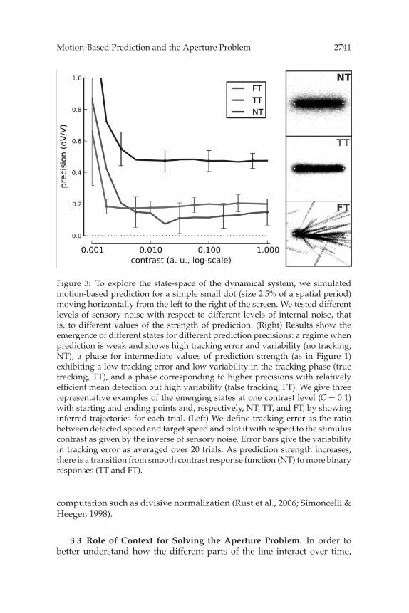
We explored the effects of some key parameters on the tracking behav-ior of the model. First, when progressively adding uniform gaussian whitenoise to the stimulus, we found that convergence time to veridical track-ing increased with respect to the level of noise. Then, at a certain level ofnoise, error bias in the prediction becomes larger than required for the bal-ance in tracking amplification and dots are rapidly lost. This can define atracking sensitivity threshold that can be characterized by plotting the con-trast response function of our system (see Figure 3). Second, we varied theprecision of prediction. It is quantitatively defined by the inverse varianceof the noise present in the generative model (see equations 1.2 and 1.3).We observed that the convergence speed of tracking grew proportionallywith this parameter. For very low precision values, the tracking behavioris lost. Moreover, we observed that increasing this prediction’s precisionabove a certain threshold leads to the detection of false positives: An initialmovement may be predicted in a false trajectory but is not discarded bysensory data. In fact, this is due to the high positive feedback generatedby the high precision assigned to the prediction. In summary, varying bothparameters, that is, external and internal variability, we can identify threedistinct regimes in this state-space: an area of correct tracking (see Figure 3,TT), an area where there is no tracking due to low precision or high noise(see Figure 3, NT), and an area of false tracking (see Figure 3, FT). Thesethree regimes fully characterize the emergence of the tracking behavior ofthe dynamical system implementing motion-based prediction.

We then studied how such tracking behavior is independent of the lu-minance profile of the object being tracked. To achieve that, we tested oursystem with the same dot but whose envelope was multiplied by a ran-dom white noise texture. When this texture consists of a static grating, weobtain one instance of second-order motion (see Lu & Sperling, 2001, fora review). Although the convergence was longer and more variable, track-ing was still observed in a robust fashion, and the envelope’s motion wasultimately retrieved. This property is due to the fact that in the generativemodel, we define the prediction as based on both the position and trajec-tory of motion, independent of the local geometry of image features. This isdifferent from motion detection models, which try to track a particular lu-minance feature (Lu & Sperling, 2001; Wilson et al., 1992). As a consequence,this dynamical system will have a preference for objects conserving theirmotion along a trajectory, independent of their texture. Such invariance isusually obtained by introducing, and tuning, a well-known static nonlinear


Figure 3: To explore the state-space of the dynamical system, we simulatedmotion-based prediction for a simple small dot (size 2.5% of a spatial period)moving horizontally from the left to the right of the screen. We tested differentlevels of sensory noise with respect to different levels of internal noise, thatis, to different values of the strength of prediction. (Right) Results show theemergence of different states for different prediction precisions: a regime whenprediction is weak and shows high tracking error and variability (no tracking,NT), a phase for intermediate values of prediction strength (as in Figure 1)exhibiting a low tracking error and low variability in the tracking phase (truetracking, TT), and a phase corresponding to higher precisions with relativelyefficient mean detection but high variability (false tracking, FT). We give threerepresentative examples of the emerging states at one contrast level (C = 0.1)with starting and ending points and, respectively, NT, TT, and FT, by showinginferred trajectories for each trial. (Left) We define tracking error as the ratiobetween detected speed and target speed and plot it with respect to the stimuluscontrast as given by the inverse of sensory noise. Error bars give the variabilityin tracking error as averaged over 20 trials. As prediction strength increases,there is a transition from smooth contrast response function (NT) to more binaryresponses (TT and FT).

computation such as divisive normalization (Rust et al., 2006; Simoncelli &Heeger, 1998).

3.3 Role of Context for Solving the Aperture Problem. In order tobetter understand how the different parts of the line interact over time,


we finally investigated modulation of neighboring motions in the apertureproblem. In fact, this also corresponds to the case of the diagonal line. Atthe initial time step, motion position information is spread preferentiallyalong the edge of the line and represents motion ambiguity with a speedprobability distributed along the constraint line (see Figure 1A, inset). Inparticular, trajectories are inferred on different trajectories preferentially on


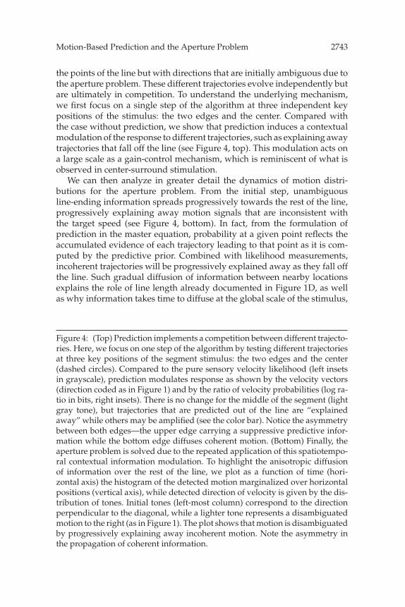
the points of the line but with directions that are initially ambiguous due tothe aperture problem. These different trajectories evolve independently butare ultimately in competition. To understand the underlying mechanism,we first focus on a single step of the algorithm at three independent keypositions of the stimulus: the two edges and the center. Compared withthe case without prediction, we show that prediction induces a contextualmodulation of the response to different trajectories, such as explaining awaytrajectories that fall off the line (see Figure 4, top). This modulation acts ona large scale as a gain-control mechanism, which is reminiscent of what isobserved in center-surround stimulation.

We can then analyze in greater detail the dynamics of motion distri-butions for the aperture problem. From the initial step, unambiguousline-ending information spreads progressively towards the rest of the line,progressively explaining away motion signals that are inconsistent withthe target speed (see Figure 4, bottom). In fact, from the formulation ofprediction in the master equation, probability at a given point reflects theaccumulated evidence of each trajectory leading to that point as it is com-puted by the predictive prior. Combined with likelihood measurements,incoherent trajectories will be progressively explained away as they fall offthe line. Such gradual diffusion of information between nearby locationsexplains the role of line length already documented in Figure 1D, as wellas why information takes time to diffuse at the global scale of the stimulus,

Figure 4: (Top) Prediction implements a competition between different trajecto-ries. Here, we focus on one step of the algorithm by testing different trajectoriesat three key positions of the segment stimulus: the two edges and the center(dashed circles). Compared to the pure sensory velocity likelihood (left insetsin grayscale), prediction modulates response as shown by the velocity vectors(direction coded as in Figure 1) and by the ratio of velocity probabilities (log ra-tio in bits, right insets). There is no change for the middle of the segment (lightgray tone), but trajectories that are predicted out of the line are “explainedaway” while others may be amplified (see the color bar). Notice the asymmetrybetween both edges—the upper edge carrying a suppressive predictive infor-mation while the bottom edge diffuses coherent motion. (Bottom) Finally, theaperture problem is solved due to the repeated application of this spatiotempo-ral contextual information modulation. To highlight the anisotropic diffusionof information over the rest of the line, we plot as a function of time (hori-zontal axis) the histogram of the detected motion marginalized over horizontalpositions (vertical axis), while detected direction of velocity is given by the dis-tribution of tones. Initial tones (left-most column) correspond to the directionperpendicular to the diagonal, while a lighter tone represents a disambiguatedmotion to the right (as in Figure 1). The plot shows that motion is disambiguatedby progressively explaining away incoherent motion. Note the asymmetry inthe propagation of coherent information.


as is reported at the physiological level (Pack et al., 2003). In summary,contrary to other models consisting of a selection stage, the system selectscoherent features in an autonomous and progressive manner based on thecoherence of all their possible trajectories. This ultimately explains why inthe aperture problem, information diffuses in the system from line endingsto the rest of the segment to ultimately resolve the correct physical motion.

A counterintuitive result is that the leading bottom line ending is less in-formative that the trailing upper line ending. This was already evident fromthe asymmetry revealed in Figure 4 (top), which makes explicit that motion-based prediction will have a different effect on both line endings. Indeed, inthe leading line ending, most information is diffused to the rest of the lineand is not explained away. On the contrary, for the trailing line ending, thediffusion of information is more constrained, as any motion hypothesizedto be going upward would soon be explained away from motion-based pre-diction, as it would fall off the line. This asymmetry is clearly observable inFigure 4 (bottom) as the ambiguous information (distributed on the wholeline at the left-most initial time) is progressively resolved by the diffusionof the information originating from the trailing line ending. Unfortunately,the experiments using blurring of the line performed by Wallace et al. (2005)were preformed symmetrically, that is, similar for both edges. We thus pre-dict that blurring the trailing line ending should lead to a greater bias angleas blurring the leading line ending only.

4 Discussion

Our computational model shows that motion-based prediction is sufficientto solve the aperture problem as well as other motion integration phenom-ena. The aperture problem instantiated with slanted lines in visual spacehelps to capture several generic computations that are often consideredas essential features of any sensory areas. We have shown that predictivecoding through diffusion is sufficient to explain the emergence of local 2Dmotion detectors but also texture-independent motion grabbers. It can alsoimplement context-dependent competition between local motion signals.All of these computations are emerging properties from the dynamics ofthe system. This view is opposite to the classical assumptions that thesemechanisms are implemented by specific, separated mechanisms (Gross-berg, Mingolla, & Viswanathan, 2001; Lu & Sperling, 2001; Tsui et al., 2010;Wilson et al., 1992). Instead, we demonstrate here that all of these proper-ties must be seen as the mere consequence of a simple, unifying computa-tional principle. By implementing a predictive field, motion information isanisotropically propagated as modulated by sensory, local estimations suchthat motion representation dynamically diffuses from a local to a globalscale. This model offers a simplification of our original model (Tlapale,Masson, et al., 2010).


4.1 Relation to Other Models. In fact, we can take advantage of thework from Tlapale, Kornprobst, Bouecke, Neumann, and Masson (2010) tocompare our model with Tlapale, Masson, et al. (2010) and a large range ofmodels in the community. This study compared the results obtained fromdifferent modeling approaches on the same aperture problem and usedtheir model as a reference point, but with two main differences. First, itdoes not try to make a neuromorphic approach except the fact that (to re-spect the definition of the aperture problem) information is grabbed locallyand propagated on a neighborhood. Moreover, in our model, information isrepresented explicitly by probabilities, and we make no assumption on howit is represented in the neural activity as this would introduce an unneces-sary hypothesis regarding our objective. Second, motion-based predictiondefines an anisotropic, context-dependent direction of propagation, whilemost previous models were using an isotropic diffusion dependent on somefeature characteristics (like gating the diffusion by luminance). However,our model explicitly uses the selectivity brought by the anisotropic dif-fusion. As a consequence, it needs less tuning of the parameters of thediffusion mechanisms, a common problem in the latter type of models. Afurther advantage of our approach is that it does not contradict previousmodels. Rather, motion-based prediction seems to be a promising approachto implement in neuromorphic models.

In particular, several parts of our model are similar to previous modelsof motion detection, although its implementation is radically novel. First,it inherits properties of functional models such as the probabilistic formu-lation of Weiss et al. (2002) but with simpler hypotheses. For instance, wedo not need a prior distribution favoring slow speeds or some selectiveprocess needed to preprocess the data (Barthelemy et al., 2008; Weiss et al.,2002). Our model uses a simple Markov chain formulation that has beenused for spatial luminance-based prediction or shape tracking with SMCin the Condensation algorithm (Isard & Blake, 1998), but this was to ourknowledge not applied to an explicit definition of motion-based prediction.Note that the model presented in Bayerl and Neumann (2007) includes ananisotropic diffusion based on motion-based prediction but that this studywas using a neural approximation of the kind that Burgi et al. (2000) used.However, they did not study in particular the role of prediction in the pro-gressive resolution of the aperture problem and its characteristic signaturecompared to biological data. The application of their fast implementation toour model appears to be a promising perspective. Ultimately our model alsogives a more formal description of the dynamical Bayesian model that weoriginally suggested to implement dynamical inference solution for motionintegration (Bogadhi, Montagnini, Mamassian, Perrinet, & Masson, 2011;Montagnini, Mamassian, Perrinet, Castet, & Masson, 2007).

Moreover, when compared to other models designed for understandingvisual motion detection (Bayerl & Neumann, 2004; Grossberg et al., 2001;Wilson et al., 1992), our approach is more parsimonious as we do not need


to explicitly model specialized edge detectors. On the contrary, we showthat these local feature detectors must be seen as emerging properties froma subset of coherent-motion detectors. Nevertheless, this emergence needs afinely scaled prediction, as we have shown that these properties depend onthe precision of prediction. Our computational implementation using SMCcould reach higher precision levels compared to the earlier predictive modelproposed by Burgi et al. (2000). We could therefore explore a range of param-eters and stimuli (such as the aperture problem) that is radically differentfrom the original study. Moreover, some nonlinear behaviors observed inour model are similar to other signatures of linear and nonlinear modelssuch as the cascade model from Rust et al. (2006) or mesoscopic models(Bayerl & Neumann, 2004, 2007; Tlapale, Masson, et al., 2010). However,these last models are specifically tuned by assembling complex and preciseknowledge from the dynamical behavior of neurons and their interactionsto fit the results that were obtained neurophysiologically. In our model,though, these properties emerge from the interactions in the probabilisticmodel.

4.2 Toward a Neural Implementation. More generally, this probabilis-tic and dynamical approach unveils how complex neural mechanisms ob-served at population levels (or from their read-outs) may be explained bythe interactions of local dynamical rules. As mentioned above, both vi-sual (Pack & Born, 2001; Pack et al., 2003, 2004; Smith et al., 2010) andsomatosensory (Pei et al., 2010) systems exhibit similar neuronal dynam-ics when solving the aperture problem or other sensory integration tasksin space and time. This suggests that different sensory cortices might usesimilar computational principles for integrating sensory inflow into a co-herent, nonambiguous representation the motion of objects. By avoidingmechanisms such as neuronal selectivities for some specific local features,our approach offers a more generic framework. It also allows seeking sim-ple, low-level mechanisms underlying complex visual behavior and theirdynamics as observed, for instance, with reflexive tracking eye movements(see Masson & Perrinet, 2012, for a review). Finally, we propose that distribu-tions of neural activity on cortical maps act as probabilistic representationsof motion over the whole sensory space. This suggests that, for instance,in cortical areas V1 and MT, all probable solutions are initially superposed.This is coherent with the dynamics of the population of MT neurons whensolving the aperture problem or computing plaid pattern motion (Pack &Born, 2001; Pack et al., 2004; Smith et al., 2010). Simple decision rules canbe applied to these maps to trigger different behaviors such as saccadic andsmooth pursuit eye movements as well as perceptual judgments of motionsuch as direction and speed. Then the temporal dynamics of these behav-ioral responses can be explained by the dynamics of predictive coding at asensory stage (Bogadhi et al., 2011).


This work provides new insights for neuroscience and computationalparadigms. In fact, biological vision still outperforms any artificial systemfor simple tasks such as motion segmentation. Our simple model is vali-dated based on neurophysiological and behavioral data and gives severalperspectives for its application to image processing. In the future, our modelwill provide interesting perspectives for exploring novel probabilistic andcontextual interactions thanks to the use of neuromorphic implementations.Indeed, it is impossible in practice today to implement the full system onclassical von Neumann architectures due to the size of the memory requiredto implement such complex association fields. However, as we saw above,the probabilistic representation of motion has a natural representation in aneural architecture, where many simple processors are densely connected.Thus, this model is structurally compatible with generic neural architec-tures and is a candidate for functional implementation on wafer-like hard-ware. Such recent innovative computing architectures enable constructingspecialized neuromorphic systems, allowing new possibilities thanks totheir massive parallelism (Bruderle et al., 2011). In return, this approachwill allow us to implement models simulating complex association fields.Studying novel computational paradigms in such systems will help extendour understanding of neural computation.

Acknowledgments

This work is supported by EC IP project FP6-015879, “FACETS,” andFP7-269921, “BrainScaleS.” Code to reproduce figures and supplemen-tary material is available online on L.U.P.’s Web site at http://invibe.net/LaurentPerrinet/Publications/Perrinet12pred.

References

Adelson, E. H., & Bergen, J. R. (1985). Spatiotemporal energy models for the percep-tion of motion. Journal of Optical Society of America, A, 2(2), 284–299.

Adelson, E. H., & Movshon, J. A. (1982). Phenomenal coherence of moving visualpatterns. Nature, 300(5892), 523–525.

Albright, T. D. (1984). Direction and orientation selectivity of neurons in visual areaMT of the macaque. Journal of Neurophysiology, 52, 1106–1130.

Barthelemy, F. V., Perrinet, L. U., Castet, E., & Masson, G. S. (2008). Dynamics ofdistributed 1D and 2D motion representations for short-latency ocular following.Vision Research, 48(4), 501–522.

Bayerl, P., & Neumann, H. (2004). Disambiguating visual motion through contextualfeedback modulation. Neural Computation, 16, 2041–2066.

Bayerl, P., & Neumann, H. (2007). A fast biologically inspired algorithm for recurrentmotion estimation. IEEE Transactions on Pattern Analysis and Machine Intelligence,29(2), 246–260.


Bogadhi, A. R., Montagnini, A., Mamassian, P., Perrinet, L. U., & Masson, G. S.(2011). Pursuing motion illusions: A realistic oculomotor framework for Bayesianinference. Vision Research, 51, 867–880.

Born, R. T., Pack, C. C., Ponce, C. R., & Yi, S. (2006). Temporal evolution of 2-dimensional direction signals used to guide eye movements. Journal of Neuro-physiology, 95(1), 284–300.

Bowns, L. (2011). Taking the energy out of spatio-temporal energy models of humanmotion processing: The component level feature model. Vision Research, 51, 2425–2430.

Bruderle, D., Petrovici, M., Vogginger, B., Ehrlich, M., Pfeil, T., Millner, S., et al. (2011).A comprehensive workflow for general-purpose neural modeling with highlyconfigurable neuromorphic hardware systems. Biological Cybernetics, 104(4), 263–296.

Burgi, P.-Y., Yuille, A. L., & Grzywacz, N. M. (2000). Probabilistic motion estimationbased on temporal coherence. Neural Computation, 12(8), 1839–1867.

Castet, E., Lorenceau, J., Shiffrar, M., & Bonnet, C. (1993). Perceived speed of movinglines depends on orientation, length, speed and luminance. Vision Research, 33(14),1921–1936.

Fennema, C. L., & Thompson, W. B. (1979). Velocity determination in scenes contain-ing several moving objects. Computer Graphics and Image Processing, 9(4), 301–315.

Grossberg, S., Mingolla, E., & Viswanathan, L. (2001). Neural dynamics of motionintegration and segmentation within and across apertures. Vision Research, 41(19),2521–2553.

Hildreth, E., & Koch, C. (1987). The analysis of visual motion: From computationaltheory to neuronal mechanisms. Annual Review of Neuroscience, 10, 477–533.

Hunter, J. D. (2007). Matplotlib: A 2D graphics environment. Computing in Scienceand Engineering, 9(3), 90–95.

Isard, M., & Blake, A. (1998). Condensation—conditional density propagation forvisual tracking. International Journal of Computer Vision, 29(1), 5–28.

Lorenceau, J., Shiffrar, M., Wells, N., & Castet, E. (1992). Different motion sensitiveunits are involved in recovering the direction of moving lines. Vision Research,33(9), 1207–1217.

Lu, Z.-L., & Sperling, G. (2001). Three-systems theory of human visual motion per-ception: Review and update. J. Opt. Soc. Am. A, 18(9), 2331–2370.

Majaj, N. J., Carandini, M., & Movshon, J. A. (2007). Motion integration by neuronsin macaque MT is local, not global. Journal of Neuroscience, 27(2), 366–370.

Masson, G. S., & Ilg, U. J. (Eds.). (2010). Dynamics of visual motion processing: Neuronal,behavioral and computational approaches. Berlin: Springer.

Masson, G. S., Montagnini, A., & Ilg, U. J. (2010). When the brain meets the eye:Tracking object motion dynamics of visual motion processing. In U. J. Ilg &G. S. Masson (Eds.), Dynamics of visual motion processing (pp. 161–188). New York:Springer.

Masson, G. S., & Perrinet, L. U. (2012). The behavioral receptive field underlyingmotion integration for primate tracking eye movements. Neuroscience and Biobe-havioral Reviews, 36, 1–25.

Masson, G. S., & Stone, L. S. (2002). From following edges to pursuing objects. Journalof Neurophysiology, 88(5), 2869–2873.


Montagnini, A., Mamassian, P., Perrinet, L. U., Castet, E., & Masson, G. S. (2007).Bayesian modeling of dynamic motion integration. Journal of Physiology (Paris),101(1–3), 64–77.

Movshon, J. A., Adelson, E. H., Gizzi, M. S., & Newsome, W. T. (1985). The analysisof moving visual patterns. In C. Chagas, R. Gattass, & C. Gross (Eds.), Patternrecognition mechanisms (pp. 117–151). Rome: Vatican Press.

Nowlan, S. J., & Sejnowski, T. J. (1995). A selection model for motion processing inarea MT of primates. Journal of Neuroscience, 15, 1195–1214.

Oliphant, T. E. (2007). Python for scientific computing. Computing in Science andEngineering, 9(3), 10–20.

Pack, C. C., & Born, R. T. (2001). Temporal dynamics of a neural solution tothe aperture problem in visual area MT of macaque brain. Nature, 409, 1040–1042.

Pack, C. C., Gartland, A. J., & Born, R. T. (2004). Integration of contour and terminatorsignals in visual area MT of alert macaque. Journal of Neuroscience, 24(13), 3268–3280.

Pack, C. C., Livingstone, M. S., Duffy, K. R., & Born, R. T. (2003). End-stopping andthe aperture problem: Two-dimensional motion signals in macaque V1. Neuron,39(4), 671–680.

Pei, Y.-C., Hsiao, S. S., & Bensmaia, S. J. (2008). The tactile integration of local motioncues is analogous to its visual counterpart. Proceedings of the National Academy ofSciences USA, 105(23), 8130–8135.

Pei, Y.-C., Hsiao, S. S., Craig, J. C., & Bensmaia, S. J. (2010). Shape invariant codingof motion direction in somatosensory cortex. PLoS Biology, 8(2), e1000305.

Pei, Y.-C., Hsiao, S. S., Craig, J. C., & Bensmaia, S. J. (2011). Neural mechanisms oftactile motion integration in somatosensory cortex. Neuron, 69(3), 536–547.

Perrinet, L. U. (2010). Role of homeostasis in learning sparse representations. NeuralComputation, 22(7), 1812–1836.

Perrinet, L. U., & Masson, G. S. (2007). Modeling spatial integration in the ocularfollowing response using a probabilistic framework. Journal of Physiology (Paris),101(1–3), 46–55.

Rodman, H. R., & Albright, T. D. (1989). Single-unit analysis of pattern-motionselective properties in the middle temporal visual area (MT). Experimental BrainResearch, 75(1), 53–64.

Rust, N. C., Mante, V., Simoncelli, E. P., & Movshon, J. A. (2006). How MT cellsanalyze the motion of visual patterns. Nature Neuroscience, 9(11), 1421–1431.

Simoncelli, E. P., & Heeger, D. J. (1998). A model of neuronal responses in visual areaMT. Vision Res., 38(5), 743–761.

Smith, M. A., Majaj, N., & Movshon, J. A. (2010). Dynamics of pattern motion com-putation. In G. S. Masson & U. J. Ilg (Eds.), Dynamics of visual motion processing:neuronal, behavioral and computational approaches (pp. 55–72). Berlin: Springer.

Tlapale, E., Kornprobst, P., Bouecke, J., Neumann, H., & Masson, G. (2010). Towardsa bio-inspired evaluation methodology for motion estimation models (Tech. Rep. No.RR-7317). Lille: INRIA.

Tlapale, E., Kornprobst, P., Masson, G. S., & Faugeras, O. (2011). A neural field modelfor motion estimation mathematical image processing. In M. Bergounioux (Ed.),Mathematical image processing (pp. 159–179). Berlin: Springer.


Tlapale, E., Masson, G. S., & Kornprobst, P. (2010). Modelling the dynamics of motionintegration with a new luminance-gated diffusion mechanism. Vision Research, 50,1676–1692.

Tsui, J.M.G., Hunter, J. N., Born, R. T., & Pack, C. C. (2010). The role of V1 surroundsuppression in MT motion integration. Journal of Neurophysiology, 103(6), 3123–3138.

Wallace, J. M., Stone, L. S., & Masson, G. S. (2005). Object motion computation for theinitiation of smooth pursuit eye movements in humans. Journal of Neurophysiology,93(4), 2279–2293.

Watamaniuk, S. N., McKee, S. P., & Grzywacz, N. M. (1995). Detecting a trajectoryembedded in random-direction motion noise. Vision Research, 35(1), 65–77.

Weiss, Y., Simoncelli, E. P., & Adelson, E. H. (2002). Motion illusions as optimalpercepts. Nature Neuroscience, 5(6), 598–604.

Wilson, H. R., Ferrera, V. P., & Yo, C. (1992). A psychophysically motivated modelfor two-dimensional motion perception. Visual Neuroscience, 9(1), 79–97.

Received September 18, 2011; accepted April 6, 2012.

Motion-Based Prediction Is Sufficient to Solve the Aperture Problem

Documents

Transcript of Motion-Based Prediction Is Sufficient to Solve the Aperture Problem