Volcanology: Lessons learned from Synthetic Aperture Radar imagery
Upload
khangminh22Category
view
0download
0
Synthetic Aperture Sonar
Micronavigation Using An Active
Acoustic Beacon.
Edward N. Pilbrow, B.E.(Hons I)
A thesis presented for the degree of
Doctor of Philosophy
in
Electrical and Computer Engineering
at the
University of Canterbury,
Christchurch, New Zealand.
January 2007


ABSTRACT
Synthetic aperture sonar (SAS) technology has rapidly progressed over the past fewyears with a number of commercial systems emerging. Such systems are typicallybased on an autonomous underwater vehicle platform containing multiple along-trackreceivers and an integrated inertial navigation system (INS) with Doppler velocity logaiding. While producing excellent images, blurring due to INS integration errors andmedium fluctuations continues to limit long range, long run, image quality. This isparticularly relevant in mine hunting, the main application for SAS, where it is criticalto survey the greatest possible area in the shortest possible time, regardless of seaconditions.
This thesis presents the simulation, design, construction, and sea trial results fora prototype “active beacon” and remote controller unit, to investigate the potentialof such a device for estimating SAS platform motion and medium fluctuations. Thebeacon is deployed by hand in the area of interest and acts as an active point sourcewith real-time data uploading and control performed by radio link. Operation is tightlyintegrated with the operation of the Acoustics Research Group KiwiSAS towed SAS,producing one-way and two-way time of flight (TOF) data for every ping by detectingthe sonar chirps, time-stamping their arrival using a GPS receiver, and replying backat a different acoustic frequency after a fixed time delay. The high SNR of this replysignal, combined with the knowledge that it is produced by a single point source,provides advantages over passive point-like targets for SAS image processing.
Stationary accuracies of <2 mm RMS have been measured at ranges of up to 36 m.This high accuracy allowed the beacon to be used in a separate study to characterisethe medium fluctuation statistics in Lyttelton Harbour, New Zealand, using an indoordive pool as a control. Probability density functions were fitted to the data thenincorporated in SAS simulations to observe their effect on image quality.
Results from recent sea trials in Lyttelton Harbour show the beacon TOF data,when used in a narrowband motion compensation (MOCOMP) process, provided im-provements to the quality of SAS images centred on frequencies of 30 kHz and 100 kHz.This prototype uses simple matched-filtering algorithms for detection and while per-forming well under stationary conditions, the fluctuations caused by the narrow sonartransmit beam pattern (BP) and changing superposition of seabed multipath often

iv ABSTRACT
cause dropouts and inaccurate detections during sea trials. An analysis of the BP ef-fects and how the accuracy and robustness of the detection algorithms can be improvedis presented. Overcoming these problems reliably is difficult without dedicated largescale testing facilities to allow conditions to be reproduced consistently.
ACKNOWLEDGEMENTS
Thanks to my supervisors Professor Peter Gough and Dr Michael Hayes for their ded-icated guidance and support during my time of research. Their ideas, advice, and theodd English lesson have been invaluable as I was introduced into the world of SAS andsignal processing. I do appreciate all that both of you have done for me.
A big thanks to the other core sonar students: Hayden Callow, Phil Barclay, SteveFortune, and Al Hunter for all their help. Other members, Dave Wilkinson, MarkNoonchester, Loic Sibeud, Dave Mulligan, Tony Culliford have all been great friendsand helped along the way. Special thanks to Daniel Meng for the effort put into theJava GUI software.
I would also like to thank Steve Downing, from the department workshop, forhis mechanical contributions and advice, Phileeep Hof for embedded hardware sup-port, Dudley Berry for sourcing parts, and Mike Cusdin, our friendly technician whocompletes the Acoustics Research Group, particularly for the stellar effort he puts inpreparing gear before each sea trial. Finally, thanks to Bill Kirkwood from the Mon-terey Bay Aquarium Research Institute for the invaluable suggestions for the beaconvacuum sealing system that is also implemented in the towfish. It has saved us fromdisaster many times.
It often goes without saying, but a big thank you goes out to my family (my parentsNeil and Pauline, various cats and fish, and sister Anna). They have all been verysupportive in their own special way, respectively providing cheap(ish) accommodation,distraction, cubicle interest, and experimental evidence that it is possible to finish.


PREFACE
This work began as a project to design and build an inertial navigation system (INS) forthe KIWISAS towfish. Once completed and operational, it was extended to designingand building an acoustic positioning system to complement the INS. An active beacondesign was chosen. Unfortunately the INS was destroyed in 2005 when the sonardeveloped a major leak. This setback also delayed sea trials with the active beacon asthe sonar was out of commission for several months being repaired.
The beacon has undergone continual development to refine the design into a robustprototype. During the most recent sea trials, in May 2006, c.f., Chapter 5, operationwent smoothly, with more problems occurring deploying targets than with the beacon.
ASSUMED KNOWLEDGE
The reader is assumed to be familiar with synthetic aperture sonar (SAS) and have agood background in signal processing. Several references are provided throughout thethesis on these topics. A background in acoustics is also recommended. An excellentreference is [Carey 2006], giving a thorough explanation of common acoustic equationsand units. A number of examples are also given.
PUBLICATIONS
Several conference papers were written and presented at different stages of the beacondevelopment, most of which are available for download from the Acoustics ResearchGroup (ARG) website [Acoustics Research Group 2006]. The following page lists thepublications in order of presentation.

[1] E.N. Pilbrow, P.T. Gough, and M.P. Hayes. Long baseline precision naviga-tion system for synthetic aperture sonar. In The 11th Australasian RemoteSensing and Photogrammetry Association Conference, Brisbane, Australia,2002.
[2] E.N. Pilbrow, P.T. Gough, and M.P. Hayes. Inertial navigation system fora synthetic aperture sonar towfish. In Electronics New Zealand Conference,Dunedin, New Zealand, 2002.
[3] E.N. Pilbrow, P.T. Gough, and M.P. Hayes. Dual transponder precisionnavigation system for synthetic aperture sonar. In Electronics New ZealandConference, Dunedin, New Zealand, 2002.
[4] E.N. Pilbrow and M.P. Hayes. Active sonar beacons to aid synthetic aper-ture sonar autofocussing: Beacon-controller design and performance. InElectronics New Zealand Conference, Hamilton, New Zealand, 2003.
[5] E.N. Pilbrow and M.P. Hayes. Acoustic timing simulation of active beaconsfor measuring the tow-path of a synthetic aperture sonar. In Image andVision Computing New Zealand, Palmerston North, New Zealand, 2003.
[6] E. N. Pilbrow, M. P. Hayes, and P. T. Gough. Autofocus of active beaconsfor measuring the tow-path of a synthetic aperture sonar: Preliminary seatest results. In OCEANS05, Washington, USA, 2005.
[7] E. N. Pilbrow, M. P. Hayes, and P. T. Gough. Autofocus of activebeacons for measuring the tow-path of a synthetic aperture sonar. InOCEANS05EUROPE, Brest, France, 2005.
[8] E. N. Pilbrow, M. P. Hayes, and P. T. Gough. Time of flight statistics forshallow water, high ping-rate sonars - tank tests and sea trial results. InUnderwater Acoustic Measurements, Heraklion, Crete, 2005.
1
viii PREFACE

Contents
ABSTRACT iii
ACKNOWLEDGEMENTS v
PREFACE vii
ACRONYMS AND SYMBOLS xv
CHAPTER 1 INTRODUCTION 11.1 Introduction 11.2 The KiwiSAS sonar platform 11.3 Platform motion and image blur 11.4 Required accuracy 41.5 Underwater positioning systems 5
1.5.1 Class one—acoustic positioning systems 51.5.2 Class two—inertial navigation systems 71.5.3 Comparison and selection for KiwiSAS 7
1.6 Chapter summary 101.7 Thesis outline 11
CHAPTER 2 NAVIGATION SYSTEM DESIGN 132.1 Introduction 13
2.1.1 Requirements 132.1.2 The role of autofocus and DPCA 14
2.2 Timing terms and definitions 152.3 LBL operation 15
2.3.1 Spherical LBLs 162.3.2 Hyperbolic LBLs 172.3.3 Comparison 192.3.4 Timing synchronisation 21
2.4 Transponder numbers and overdetermined systems 222.5 Signal flow 23
2.5.1 Timing synchronisation 232.5.2 Source ambiguity 232.5.3 Motion effects 23

x CONTENTS
2.5.4 Summary 242.6 Operating frequencies 24
2.6.1 Signal attenuation 252.6.2 Sonar transmit beam pattern (BP) 252.6.3 Data sampling and storage 262.6.4 Summary 26
2.7 Transponder location 262.8 Data storage 272.9 Sound speed in seawater 27
2.9.1 Spatial sound speed variation 272.9.1.1 Experimental results 282.9.1.2 Discussion of sound speed related errors 28
2.10 Chapter summary 30
CHAPTER 3 HARDWARE AND SOFTWARE 313.1 Introduction 313.2 Beacon controller unit (BCU) 31
3.2.1 Hardware 313.2.1.1 Communication link 313.2.1.2 Time stamping the sonar transmissions 35
3.2.2 Navigation computer software 373.2.3 Synchronising the chirps 39
3.3 Beacon seabed unit (BSU) 393.3.1 Power supplies 393.3.2 Acoustic transducer 433.3.3 Other sensors 45
3.4 Beacon floating unit (BFU) 473.4.1 Hardware 47
3.4.1.1 PIC 513.4.1.2 DSP 513.4.1.3 TAT accuracy 523.4.1.4 SPI bus 53
3.4.2 Printed circuit board (PCB) 533.5 Embedded software 54
3.5.0.1 DSP 543.5.0.2 PIC 55
3.6 Operation at sea 563.6.1 Reliability 58
3.7 Mechanical construction 583.7.1 Casings 583.7.2 Cable 593.7.3 Vacuum system 59
3.8 Chapter summary 60

CONTENTS xi
CHAPTER 4 BEACON SIGNAL PROCESSING 634.1 Introduction 634.2 Filtering the chirp from the received signal 63
4.2.1 Signal intensity variation 634.2.2 Step 1: Chirp detection 65
4.2.2.1 Achieving real-time operation 674.2.3 Step 2: Intelligent peak finding 68
4.2.3.1 Multiple sets of taps 684.2.3.2 Multipath rejection 71
4.2.4 Step 3: Subsample peak fitting 754.2.5 Step 4: Time stamping and transmitting 78
4.3 Multipath accuracy study 784.3.1 TOA error due to multipath superposition 78
4.3.1.1 Simulation results 794.4 Matched filter accuracy study 79
4.4.1 Theoretical accuracy 814.4.2 Simulations 83
4.4.2.1 Peak-finding algorithms applied to thematched filter output 84
4.4.2.2 Case 1: Varying the received echo sampleoffset 84
4.4.2.3 Case 2: Varying the SNR 884.4.2.4 Case 3: Varying the oversampling kernel
width 914.4.2.5 Case 4: Varying the oversampling factor 91
4.4.3 Study conclusions 944.5 Sonar transmit beam pattern (BP) 94
4.5.1 OF, TVR, RPR, and directivity equations 964.5.2 Comparison with measured directivity
plots 984.5.3 BP effect on beacon performance 99
4.5.3.1 Summary 1024.6 Motion estimation and motion compensation (MOCOMP) 102
4.6.1 Method one: One-way TOF using GPS timing 1024.6.2 Method two: Two-way TOF using sonar imaging 1024.6.3 Outlier removal and smoothing 1044.6.4 Calculating sway from TOF 1054.6.5 Estimating the beacon position 1054.6.6 Narrowband MOCOMP 107
4.7 Chapter summary 107
CHAPTER 5 SEA TRIAL RESULTS 1115.1 Introduction 1115.2 Experiment and processing details 111

xii CONTENTS
5.2.1 Estimating beacon position and sonar velocity 1115.2.2 Estimating the speed of sound 1125.2.3 Contrast measure 1145.2.4 Outlier identification and removal 114
5.3 Results and discussion 1175.3.1 Object identification 1175.3.2 Beacon appearance in image 117
5.3.2.1 BSU 1175.3.2.2 BFU 120
5.3.3 Sway estimation 1205.3.4 Image quality improvement from MOCOMP 121
5.4 Chapter summary 128
CHAPTER 6 MEDIUM FLUCTUATION STATISTICS AND SASSIMULATIONS 1296.1 Introduction 129
6.1.1 Statistical model 1296.2 Experimental beacon measurement error 130
6.2.1 Experimental distribution fitting 1306.2.2 Theoretical beacon measurement error 130
6.2.2.1 Matched filter timing error 1326.2.2.2 Event capture timing errors 1326.2.2.3 GPS timing errors 1326.2.2.4 DSP clock resolution timing error 132
6.2.3 Comparison and discussion 1336.3 Medium fluctuations 133
6.3.1 Modelling the medium fluctuations 1346.3.1.1 Fourier transform (FT) approach 1346.3.1.2 Method of moments approach 134
6.3.2 Harbour and pool experiments 1356.3.2.1 Results and discussion 137
6.4 SAS simulations using the experimental medium fluctua-tion model 1416.4.1 Results and conclusions 1416.4.2 Simulation limitations 146
6.4.2.1 Imaging 1466.4.2.2 Medium fluctuations 1466.4.2.3 Sonar path 1466.4.2.4 Noise 147
6.5 Chapter summary 147
CHAPTER 7 CONCLUSIONS 149

CONTENTS xiii
CHAPTER 8 FUTURE IMPROVEMENTS 1538.1 Introduction 1538.2 Signal processing improvements 153
8.2.1 Problem 1—sidelobes 1548.2.2 Problem 2—carrier frequency 1568.2.3 Application and overhead 157
8.2.3.1 Step 1: Improved chirp detection 1578.2.3.2 Step 2: Improved intelligent peak finding 157
8.3 Hardware improvements 1588.3.1 GPS 1588.3.2 Processors and oscillators 1588.3.3 RF modem 159
8.4 Chapter summary 159
APPENDIX A PUBLICATION: BEACON-CONTROLLER DESIGNAND PERFORMANCE 161
APPENDIX B RAY BENDING 169B.1 Introduction 169B.2 Ray paths 169
APPENDIX C BEACON COMMANDS 171
APPENDIX D PACKET FORMAT 173D.1 Status packets 173
D.1.1 Beacon status 1 173D.1.2 Beacon status 2 174D.1.3 Beacon Status 3 174D.1.4 Beacon Status 4 174D.1.5 DSP raw data 175D.1.6 Boat Status1 175D.1.7 Boat Status 2 176
D.2 Timing packets 176D.2.1 Ping transmitted by towfish 176D.2.2 Ping received by beacons 176D.2.3 Beacon status special 177
APPENDIX E SPHERICAL AND HYPERBOLIC POSITIONINGEQUATIONS 179E.1 Spherical positioning 179E.2 Hyperbolic positioning 181
APPENDIX F RICIAN MOMENTS 183F.1 Introduction 183

xiv CONTENTS
APPENDIX G DISTRIBUTION CHARTS 185G.1 Introduction 185G.2 Parameters 185G.3 Converting moments 187
APPENDIX H METHOD OF MOMENTS 189H.1 Introduction 189H.2 Gaussian distribution 189H.3 Gamma distribution 189H.4 Weibull distribution 190H.5 Rician distribution 190H.6 Method of moments—gamma example 191H.7 Method of moments—Rician example 191H.8 Method of moments—Weibull example 192
APPENDIX I TRANSDUCER VELOCITY POTENTIAL 193
APPENDIX J KiwiSAS PROJECTOR EQUATIONS 195J.1 KiwiSAS BP 195
J.1.0.1 KiwiSAS TVR and directivity 198
APPENDIX K TRANSDUCER MODEL 201K.1 Introduction 201
K.1.1 Transformer effects 201K.1.2 Water model 201
K.2 Transmit transfer function 204K.3 Receive transfer function and RPR 204
REFERENCES 209
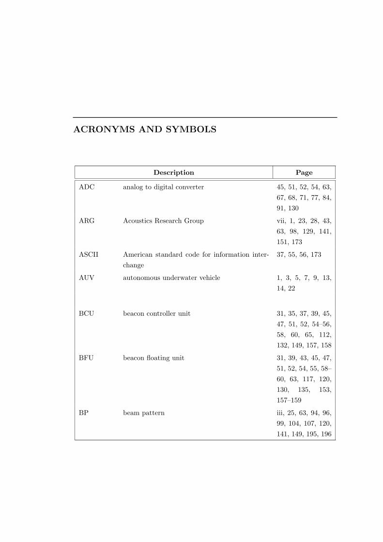
ACRONYMS AND SYMBOLS
Description Page
ADC analog to digital converter 45, 51, 52, 54, 63,67, 68, 71, 77, 84,91, 130
ARG Acoustics Research Group vii, 1, 23, 28, 43,63, 98, 129, 141,151, 173
ASCII American standard code for information inter-change
37, 55, 56, 173
AUV autonomous underwater vehicle 1, 3, 5, 7, 9, 13,14, 22
BCU beacon controller unit 31, 35, 37, 39, 45,47, 51, 52, 54–56,58, 60, 65, 112,132, 149, 157, 158
BFU beacon floating unit 31, 39, 43, 45, 47,51, 52, 54, 55, 58–60, 63, 117, 120,130, 135, 153,157–159
BP beam pattern iii, 25, 63, 94, 96,99, 104, 107, 120,141, 149, 195, 196

xvi ACRONYMS AND SYMBOLS
Description Page
BSU beacon seabed unit 31, 39, 43–45, 47,51, 55, 58–60, 63,111, 112, 114,117, 120, 121,130, 135, 149,150, 158
CDMA code division multiple access 21
CEP circular error probability 7, 9
CPLD complex programmable logic device 51–53, 67
CPU central processing unit 37, 54, 78
CRLB Cramer-Rao lower bound 81, 84, 88, 91,130, 150
DAC digital to analog converter 51, 52, 54, 65
DMA direct memory access 51, 54, 78
DPCA displaced phase centre antennas 14
DSP digital signal processor 47, 51–54, 60,63, 67, 77, 78,84, 104, 132, 133,149, 153, 154, 159
DVL Doppler velocity log 3, 7, 9, 146
EEPROM electrically erasable programmable read onlymemory
58
EMC electromagnetic compatibility 53
FIR finite impulse response 65, 67, 84, 154
FM frequency modulated 79, 81, 94, 96
FT Fourier transform 65, 81, 104, 107,134, 135, 137, 147
GDOP geometric dilution of precision 22

ACRONYMS AND SYMBOLS xvii
Description Page
GPS global positioning system 7, 9, 19, 21, 23,24, 26, 30, 35,37, 47, 51–53, 55,56, 102, 104, 105,112, 128, 130,132, 133, 135,151, 157–159
GSM global standard for mobile communications 15
GUI graphical user interface 37
INS inertial navigation system iii, vii, 3, 7, 9, 22,151
IO inputs and outputs 201
JFET junction field effect transistor 43
JTAG Joint Test Action Group 52
KiwiSAS Kiwi Synthetic Aperture Sonar 1, 3, 5, 9, 10,13, 26–28, 45, 59,66, 78, 81, 94, 96,98, 105, 107, 128,146, 149, 151,154, 159, 195,199, 203
KS Kolmogorov-Smirnov 130, 137, 147, 185
LBL long baseline positioning system 6, 7, 9, 10, 13, 15–17, 21, 22, 30, 149
MAC multiply and accumulate 54, 67

xviii ACRONYMS AND SYMBOLS
Description Page
MOCOMP motion compensation iii, 1, 9, 10, 14,24, 28, 30, 63,99, 102, 105, 107,112, 117, 121,128, 137, 141,146, 147, 151
NMEA National Marine Electronics Association 35, 45, 47, 51, 52,54, 173
NVRAM non-volatile random access memory 51, 52, 54, 55
OF obliquity factor 195, 196
PCB printed circuit board x, 31, 39, 52, 53,59
PCI peripheral component interconnect 1
PDF probability density function 129, 130, 135,137, 147, 151,189, 190
PIC programmable in-circuit microcontroller 31, 35, 39, 45,47, 51–55, 58, 60,132, 158
PLL phase locked loop 158
ppm parts per million 21
PPS pulse per second 51, 52, 55, 132,158
ppt parts per thousand 27, 112
PVDF polyvinylidene fluoride 1
RAM random access memory 52, 78
RF radio frequency 13, 30, 31, 35,37, 45, 47, 51–53,55, 56, 58, 61, 63,65, 102, 130, 149,157–159

ACRONYMS AND SYMBOLS xix
Description Page
RMS root mean square 7, 61, 84, 88, 91,141, 158
ROV remotely operated vehicle 5
RPR receive pressure response 96, 199, 204, 206
RS232 the RS232 protocol 31, 35, 51, 53
RTK real time kinematic GPS 26
SAR synthetic aperture radar 24
SAS synthetic aperture sonar iii, vii, 1, 3, 7, 9,10, 13, 14, 24, 26–28, 30, 102, 107,114, 117, 129,134, 137, 141,147, 151
SBL short baseline positioning system 6, 7
SLA sealed lead acid 39
SNR signal to noise ratio 4, 24, 63, 65,79, 81–83, 88, 91,99, 111, 130, 132,154, 159
SNRi signal to noise ratio at the matched filter input 84
SOP start of ping 35
SPI serial peripheral interface 52–54
STD standard deviation 81, 83, 84, 88,91, 129, 130, 132,133, 189
TAT turn around time 51–53, 63, 77,102, 104, 128, 158
TCP transmission control protocol 37
TDOF time difference of flight 16, 17, 19, 181
TOA time of arrival 5, 14, 16, 17, 19,23, 24, 27, 37, 47,51, 63, 68, 77, 78,102, 158

xx ACRONYMS AND SYMBOLS
Description Page
TOD time of departure 5, 14, 16, 17, 19,23, 24, 27, 35, 37,65
TOF time of flight iii, 5, 10, 14, 16,17, 23, 30, 37, 53,56, 61, 67, 68,78, 81, 83, 84,88, 91, 94, 102,104, 105, 107,111, 114, 120,128, 129, 133–135, 137, 141,146, 147, 149,151, 154, 179
T/R transmit/receive 43
TVR transmit voltage response 96, 98, 198, 199,204, 206
UART universal asynchronous receiver/transmitter 53
USB universal serial bus 31
USBL ultra short baseline positioning system 6, 7, 16
WGN white Gaussian noise 79, 81, 83
XML extensible markup language 37
Chapter 1
INTRODUCTION
1.1 INTRODUCTION
Synthetic aperture sonar (SAS) is a method of operating a sonar which provides ad-vantages over traditional side scan sonars. The main advantage is constant along-trackimage resolution, independent of range and frequency. Disadvantages include the needfor additional computer processing of the data to obtain an image (minor) and in-creased sensitivity to sonar deviation from a straight and level path (major). Thislatter well-known problem, and the development of a unique solution using an “activebeacon”, is the basis for this thesis. For a complete, concise, illustrated, summaryof SAS operation and performance, the reader is referred to the following publica-tions: [Callow 2003, Chaps. 1–2], [Hunter June 2006, Chap. 1], [Barclay August 2006,Chap. 1], and [Griffiths 1995]. The main application for SAS is mine hunting [Healdand Griffiths 1998].
1.2 THE KiwiSAS SONAR PLATFORM
The Acoustics Research Group (ARG) at the University of Canterbury has designedand built a SAS (KiwiSAS) that has been operational for a number of years [Hayeset al. 2002, Callow et al. 2003] [Hawkins 1996, chap. 7]. Table 1.1 lists the currentspecifications and a photo is shown in Fig. 1.1. The electronics are based around acompact PCI embedded Pentium 3 computer, controlling the digitising and on boardstorage of all data on hard disk [Hayes et al. 2002]. The tow cable provides a 100 Mb/sEthernet connection to the tow boat computers, for real-time display of images, andsupplies the sonar with 24 V power from batteries on the tow boat.
1.3 PLATFORM MOTION AND IMAGE BLUR
SAS imaging is particularly sensitive to platform motion and image blurring frequentlyresults, even with large autonomous underwater vehicles (AUV) operating well belowthe sea surface. By measuring the platform motion (motion estimation), the blurring

2 CHAPTER 1 INTRODUCTION
Figure 1.1: The KiwiSAS sonar is towed from the nose. With a low mass (60 kg) andslight positive buoyancy, it can be deployed by hand at a wharf and towed on thesurface out to the area of interest. When used as a sonar, a weight is attached to thetow cable close to the tow point, causing it to sink to the desired depth—typically 5 m.The depth is somewhat adjustable by changing the boat speed and cable length. Thistowing configuration means the sonar exhibits very little yaw - an essential behaviourfor obtaining good SAS images. The KiwiSAS is under continual development andsince this photo was taken, the transmitter has been moved to the centre of the towfishand mounted internally.
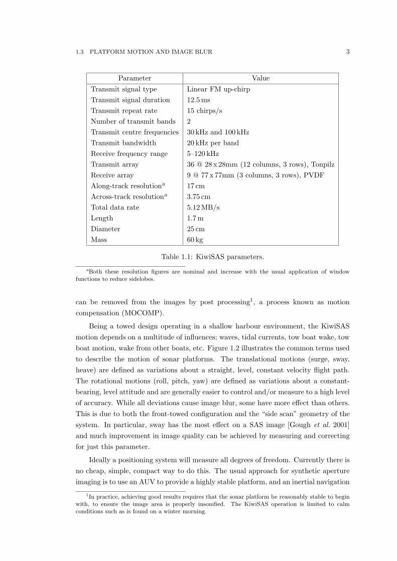
1.3 PLATFORM MOTION AND IMAGE BLUR 3
Parameter ValueTransmit signal type Linear FM up-chirpTransmit signal duration 12.5msTransmit repeat rate 15 chirps/sNumber of transmit bands 2Transmit centre frequencies 30 kHz and 100 kHzTransmit bandwidth 20 kHz per bandReceive frequency range 5–120 kHzTransmit array 36 @ 28 x 28mm (12 columns, 3 rows), TonpilzReceive array 9 @ 77 x 77mm (3 columns, 3 rows), PVDFAlong-track resolutiona 17 cmAcross-track resolutiona 3.75 cmTotal data rate 5.12MB/sLength 1.7mDiameter 25 cmMass 60 kg
Table 1.1: KiwiSAS parameters.
aBoth these resolution figures are nominal and increase with the usual application of windowfunctions to reduce sidelobes.
can be removed from the images by post processing1, a process known as motioncompensation (MOCOMP).
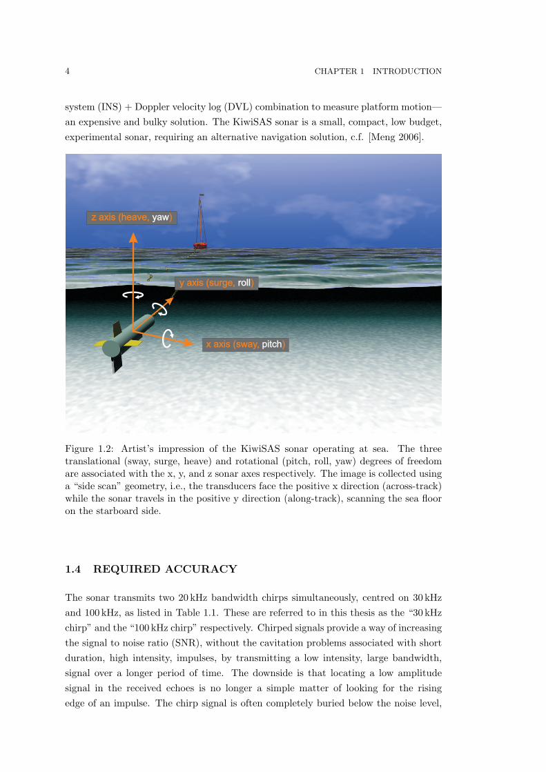
Being a towed design operating in a shallow harbour environment, the KiwiSASmotion depends on a multitude of influences; waves, tidal currents, tow boat wake, towboat motion, wake from other boats, etc. Figure 1.2 illustrates the common terms usedto describe the motion of sonar platforms. The translational motions (surge, sway,heave) are defined as variations about a straight, level, constant velocity flight path.The rotational motions (roll, pitch, yaw) are defined as variations about a constant-bearing, level attitude and are generally easier to control and/or measure to a high levelof accuracy. While all deviations cause image blur, some have more effect than others.This is due to both the front-towed configuration and the “side scan” geometry of thesystem. In particular, sway has the most effect on a SAS image [Gough et al. 2001]and much improvement in image quality can be achieved by measuring and correctingfor just this parameter.
Ideally a positioning system will measure all degrees of freedom. Currently there isno cheap, simple, compact way to do this. The usual approach for synthetic apertureimaging is to use an AUV to provide a highly stable platform, and an inertial navigation
1In practice, achieving good results requires that the sonar platform be reasonably stable to beginwith, to ensure the image area is properly insonified. The KiwiSAS operation is limited to calmconditions such as is found on a winter morning.
4 CHAPTER 1 INTRODUCTION
system (INS) + Doppler velocity log (DVL) combination to measure platform motion—an expensive and bulky solution. The KiwiSAS sonar is a small, compact, low budget,experimental sonar, requiring an alternative navigation solution, c.f. [Meng 2006].
Figure 1.2: Artist’s impression of the KiwiSAS sonar operating at sea. The threetranslational (sway, surge, heave) and rotational (pitch, roll, yaw) degrees of freedomare associated with the x, y, and z sonar axes respectively. The image is collected usinga “side scan” geometry, i.e., the transducers face the positive x direction (across-track)while the sonar travels in the positive y direction (along-track), scanning the sea flooron the starboard side.
1.4 REQUIRED ACCURACY
The sonar transmits two 20 kHz bandwidth chirps simultaneously, centred on 30 kHzand 100 kHz, as listed in Table 1.1. These are referred to in this thesis as the “30 kHzchirp” and the “100 kHz chirp” respectively. Chirped signals provide a way of increasingthe signal to noise ratio (SNR), without the cavitation problems associated with shortduration, high intensity, impulses, by transmitting a low intensity, large bandwidth,signal over a longer period of time. The downside is that locating a low amplitudesignal in the received echoes is no longer a simple matter of looking for the risingedge of an impulse. The chirp signal is often completely buried below the noise level,

1.5 UNDERWATER POSITIONING SYSTEMS 5
requiring filtering to determine its location and this is discussed further in Chapter 4.
The transmitted wavelength is given by:
λ =c
f, (1.1)
where f is the frequency in Hz and c is the speed of sound in seawater (∼1500 m/s).This equates to 5 cm at 30 kHz and 1.5 cm at 100 kHz. A good image, i.e., one withminimal blurring and high dynamic range, can be obtained when the path deviationsare less than, or measured to an accuracy of, ∼λ
8 [Hawkins 1996, p165]. The minimumrequired accuracy in deviation from a straight path is therefore <1 cm to provide goodresults for the 30 kHz band. The accuracy must be independent of the image content,i.e., still valid for a featureless image, and independent for every chirp so that everyposition measurement stands on its own (no reliance on any form of averaging). Thismeans the system is tolerant of dropped or miss-detected data, provided these can beidentified and removed.
The accuracy requirements are relative not absolute, i.e., there is no requirementto reference any of the navigation measurements to world coordinates because the goalof an experimental sonar like KiwiSAS is simply to improve the quality of the images,not to locate them on a map [Liu and Pang 2001]. To remove the effects of motion blurrequires knowing how the sonar moved, rather than where it was in the ocean. Thisis an important difference from many commercial underwater positioning applicationswhere the accuracy must be specified in absolute coordinates e.g., bottom surveyingand pipeline inspection.
1.5 UNDERWATER POSITIONING SYSTEMS
Positioning systems for underwater vehicles (tethered, towed, or autonomous) can beclassified into two distinct classes of design; here designated class one and class two.There also exist hybrid designs combining the advantages of each type [Whitcombet al. 1999, Pan Mook et al. 2005]. Common terms for tethered, towed and autonomousunderwater vehicles are remotely operated vehicle (ROV), towfish, and AUV respec-tively.
1.5.1 Class one—acoustic positioning systems
Class one systems require positioning equipment external to the vehicle. This externalequipment is invariably an acoustic system2,3, based on the transmission of acoustic
2Although underwater electromagnetic wave propagation has been demonstrated over tens of metresusing small high frequency antennas [Al Shamma’a et al. 2004], no experimental or commercial RFpositioning systems exist that use this principle.
3Very close range positioning (∼2m) can also be achieved with taut wires [Mio et al. 1998] orpassive arms, [Soares da Cunha et al. 1993].

6 CHAPTER 1 INTRODUCTION
signals to and/or from transponders. Depending on the system, the transponders maybe transmitters, receivers, or both (alternating). By using a combination of time ofarrival (TOA), time of departure (TOD), and time of flight (TOF) information of theacoustic signals, distances and angles are measured underwater. The transponders maybe stationary on the seabed (most accurate), ship mounted (less accurate), or floating(least accurate). Floating and ship mounted designs require additional navigationsensors to measure the (changing) position and attitude of the transponders.
There are three types of class one system; the long baseline positioning system(LBL), the short baseline positioning system (SBL), and the ultra short baseline po-sitioning system (USBL), a widely adopted classification [Austin 1994, Vickery 1998a,Vickery 1998b] describing the resultant separation distance of the transponders due tothe system design.4
LBLs have independently deployed transponders and are the most accurate. Ifabsolute positioning is required, their location must be independently measured afterdeployment. This is usually done acoustically from the surface and for deep water it iscritical that the sound-speed profile with depth is measured to account for ray-bending[Lurton and Millard 1994, Isshiki 2004]. If relative positioning is required, only theirseparation need be measured.5 If they move, e.g., floating buoys, these measurementsmust be continuously updated. The separation between transponders is usually greaterthan 10 m.
SBLs have all transponders attached to a common rigid frame so their separationneed only be measured once to achieve relative positioning. If absolute positioning isrequired, it can be achieved by independently measuring the location of the frame itselfafter deployment. The frame may be a submersible structure or the hull of a boat, inwhich case, for absolute positioning, continuous independent monitoring of the boatrotations and translations is required. The requirement for high rigidity6 imposes apractical separation limit of <10 m. Due to recent advances in USBL technology, SBLsystems are less common now, having most of the setup disadvantages of an LBL andan accuracy only slightly better than USBL.
USBLs have all transponders attached to a common rigid frame, sufficiently closethat the phase difference at each transponder can be unambiguously determined, i.e.,the separation is less than half of the wavelength.7 The total size of the array is usually<1 m. These systems are sold as a single unit so the geometrical disadvantage of havingan “ultra short” baseline are somewhat offset by the very tight manufacturing tolerances
4The exception is a single transponder system which has no baseline but is usually referred to asa LBL.
5This is often done acoustically using the transponders themselves.6If the frame is not rigid, the system is technically an LBL and the transponder separations and/or
locations must always be measured after each deployment.7Some systems have greater separations than this, to improve the accuracy, and use various tech-
niques to disambiguate the phase [Watson et al. 1998, Austin et al. 1997].

1.5 UNDERWATER POSITIONING SYSTEMS 7
determining transponder separation, and high rigidity, compared with a SBL. If theunit is mounted on the hull of a boat, active beam-forming is used to reduce the effectsof engine noise and multipath from the hull [Vickery 1998b].
LBLs and SBLs use timing information to measure the position of the vehiclerelative to each of the transponders. USBLs use timing and phase-difference to pro-duce a range and bearing to the vehicle relative to the whole unit so the horizontalposition accuracy8 is range dependent. Many systems are combinations of all three,e.g., the tracking of sperm whales using multiple floating SBL arrays, positioned byglobal positioning system (GPS), separated by hundreds of metres to form an LBL[Ura et al. 2004]. Some example class one systems are listed in Table 1.2 and furtheranalysis of LBLs is given in Chapter 2.
1.5.2 Class two—inertial navigation systems
Class two systems are those where the positioning equipment is contained entirelyon board the vehicle. Typically a variety of sensors are used to directly measuretranslational and angular rates,9 e.g., acceleration and angular velocity, and the datais combined, typically using a Kalman filter [Hassab and Watson 1974, Hedge 1994,Nicosevici et al. 2004, Meng 2006], and integrated as necessary to obtain position andangle.
Commonly used sensors include accelerometers (acceleration), gyroscopes (angu-lar velocity), and magnetometers (angle). These sensors all provide fast update rates,allowing navigation data to be collected for every chirp. To achieve high positioning ac-curacy, these systems require careful assembly and calibration to ensure sensor axes arecorrectly aligned [Stokey and Austin 2000, Kinsey and Whitcomb 2002]. Experimentaldata showing accuracy and drift is provided by [Liu and Pang 2001] and [Barshan andDurrant Whyte 1995] for cheap accelerometers and gyroscopes and by [Ford et al. 2001]for a high-end system.
1.5.3 Comparison and selection for KiwiSAS
Class two systems have the advantage of being completely self contained inside thesonar. This is especially useful for AUVs, the main platform for modern SASs, allowingfast setup and deployment at sea and requiring minimal interaction with the surfacevessel during operation. Two examples are shown in Table 1.3. The main disadvantageof an INS comes from the mathematical integration required to convert the sensordata, usually measuring rate of change of velocity and angle, to position and angle.The integration process causes any small errors in the measurements to accumulateover time, limiting the period over which the navigation data is useful [Stokey and
8The horizontal position is usually the most important and challenging parameter to measure.9Position and angle cannot yet be measured directly with sufficient accuracy.

8 CHAPTER 1 INTRODUCTION
Manufacturer/Model
Configurationand description
Updaterate
Horizontalaccuracy
Publications
Nautronix/NASnet
LBL. Seabedtransmitters,surveyed intoposition. Vehiclescontain receivers.
0.1Hz ±2 m @ 5 kmCEP
[Thomson and El-son 2002]
ACSA/ GIB LBL. Floatingreceiver buoyslocated usingDGPS. Vehi-cle contains atransmitter.
1 Hz 1 m [Thomas 1998]
Sonicworks/APNS
LBL. Self cali-brating cabledseabed receivers.Vehicle containstransmitter. Mul-tiple pings inflight.
50 Hz ±3 mm @100 m
(research)/EXACT
LBL. Seabedtranspondersinterrogated bytransponder onvehicle.
3 Hz 2 cm @ 100m [Langrock 1993]
(research)/HPASS
LBL. Seabedtranspondersinterrogated by astationary diverwith a hand heldtransponder.
On de-mand
2 cm at 50 m [Green and Dun-can 1998, Greenand Duncan 1999]
Ixsea/ GAPS USBL. Fourtransducers ina tetrahedronconfiguration.
10 Hz 0.2% RMS ofslant range,i.e., 20 cm @100 m
[Napolitanoet al. 2005, Au-dric 2004]
Ore Offshore/TrackPoint 3
USBL. Can track4 vehicles simul-taneously.
2 Hz 0.5% RMS ofslant range,i.e., 50 cm @100 m
[McKeown andHeffler 1997, Blackand Butler 1994]
Table 1.2: Specifications for various acoustic positioning systems obtained from man-ufacturer’s datasheets and websites.

1.5 UNDERWATER POSITIONING SYSTEMS 9
Austin 2000, Huddle 1998]. This can be reduced by several orders of magnitude, onan underwater vehicle, by using a DVL to provide an independent estimate of thehorizontal velocity [Larsen 2000a]. However, the size (and mass) of a DVL is comparableto an INS, resulting in a significant volume and power being consumed by these itemsin a small sonar.
If there is no requirement to align successive images, the integration process canbe periodically reset and the navigation data from this point on will be relative, unlesssome additional form of absolute measurement, e.g., surfacing10 for a GPS reading, isacquired. For large surveys, it is possible to reduce the error accumulation (avoidinga reset) by periodically providing the INS with known conditions, e.g., rotating aboutthe vertical axis [Uliana et al. 1997] or parking the vehicle stationary on the seabed[Huddle 1998], although the latter is not practical for a towed sonar like KiwiSAS.In practice when combined with a DVL, the high accuracy of modern INS sensorsmeans the integration time limit is long enough (minutes) to provide good MOCOMPof sufficiently large SAS images. Hence, this combination is commonly used in SASAUV operation today [Asada et al. 2004, Jalving et al. 2003], despite the high cost(>NZ$150000), large size, and high power consumption. The KiwiSAS sonar has nei-ther the space or financial budget to accommodate a sufficiently accurate INS + DVLnavigation system.
Manufacturer Ixsea KearfottINS model Phins KN5053Horizontal position drift CEP 3 m/h 3 m/hVolume (cm3) 4096 8332Power consumption (W) 12 35Publications [Gaiffe 2006] [Beiter et al. 1998]
Table 1.3: Datasheet figures for two commercial INS products designed for underwa-ter vehicles. The drift performance assumes the vehicle also has an integrated DVL.Without DVL data aiding the navigation solution, a drift of 3 m in 2 minutes is typical.
Class one systems measure position11 directly so do not suffer from integrationerror accumulation, i.e., the error is bounded [Bingham and Seering 2006]. However,unlike class two systems, the accuracy depends on the location of the vehicle within thesystem geometry [Deffenbaugh et al. 1996b, Alcocer et al. 2006, Matos et al. 1999] socare must be taken during setup. Even on modern systems, a certain number of dataoutliers should be expected, mainly due to multipath [Bingham and Seering 2006], as
10GPS propagation in seawater is just a few millimetres.11While multiple transducers could be used on the vehicle to allow rotational motion to be measured,
the short baseline of this approach yields poor results. Acoustic positioning systems usually rely onadditional on-board sensors for measuring rotation, similar to the rotational sensors used in class twosystems.

10 CHAPTER 1 INTRODUCTION
discussed in Chapter 4 . If the transponder location is known then the data is abso-lute, making this class the preferred choice for underwater surveying and inspection.However, to get the best accuracy, seabed transponders must be used, requiring an ex-pensive, time consuming setup and/or calibration process12 [Send et al. 1995, Kussatet al. 2005, Sharkey 1985] to determine their separation or location. Most LBL sys-tems are designed for positioning over large areas (>100 m) where decimetre accuracyis acceptable and the long travel times for the acoustic signals mean update rates areslow compared to class two systems. However, for short ranges, higher update ratesare possible, and some very high accuracy, short range solutions have appeared duringthe last few years as shown in Table 1.2.
An interesting property of class one systems is that the measurements rely on thespeed of sound remaining constant. Changes to the speed of sound, known as “mediumfluctuations” occur over time due to changes in pressure, temperature, and salinity (seeSec. 2.9). These same medium fluctuations also cause blurring of SAS images so a classone system, with transponders in the same location as the image and synchronisedto the sonar chirps, will inherently compensate for medium fluctuations when used forMOCOMP. In other words, the navigation data will not be completely accurate interms of the actual path taken by the sonar but it will perfectly compensate for thecombined effect of motion and medium fluctuation blur in the SAS image13 becausethe SAS data collection process was subject to the exact same motion and mediumfluctuations.
The KiwiSAS transmits acoustic signals and has a wide receive bandwidth (seeTable 1.1) so is well suited to operation with a class one navigation system. This hasbeen implemented as an “active beacon” transponder. Chapter 2 discusses the designprocess in more detail.
1.6 CHAPTER SUMMARY
An introduction to the KiwiSAS sonar and the problems of image blur due to unknownplatform motion and medium fluctuations was presented. Analysing acoustic and iner-tial based positioning systems revealed the strengths and weaknesses of each type. Theacoustic class of system, configured as a LBL to measure sway, is the most suitable de-sign for a prototype positioning system for the KiwiSAS sonar. Achieving the requiredaccuracy (<1 cm,) in an ocean environment, is a challenging task that is most feasiblewith a LBL and the ability to measure the medium fluctuations is a useful feature forSAS imaging.
12If the seabed is sufficiently flat, the transponders can determine their separation acoustically.13Limited to the region around the LBL transponders within which the medium fluctuations exhibit
no spatial variation.

1.7 THESIS OUTLINE 11
1.7 THESIS OUTLINE
Chapter two presents the design process of the navigation system by analysing dif-ferent configurations of LBL acoustic positioning systems. The advantages and dis-advantages are balanced against real world issues, such as cost and limited test andcalibration facilities, finally arriving at the design for the active beacon.
Chapter three presents complete technical details of the hardware (electronic andmechanical), and software (embedded and PC) required for the beacon system and theremote controller. Block diagrams and photos are shown of the various parts of thesystem.
Chapter four explains how the beacon signal processing algorithms were developedand presents simulated results showing their expected performance and limitations. Ananalysis is presented showing how the properties of the sonar transmit beam pattern,and the effects of multipath, introduce detection problems and how these manifestedthemselves in experimental results.
Chapter five presents experimental results from two runs from recent sea trials inLyttelton Harbour. Simple MOCOMP is applied to the SAS images using data fromthe active beacon. Although the beacon operation is currently far from optimal, a clearimprovement can be seen in both the 30 kHz and 100 kHz images.
Chapter six presents a set of experiments where the active beacon is used in a com-pletely separate role—measuring medium fluctuations. The beacon is used to measurethe variation in TOF at different ranges at sea, and in a pool for comparison, andprobability distributions are fitted to the data. SAS simulations incorporating thesedistributions are presented showing how medium fluctuations can affect the perfor-mance of MOCOMP algorithms.
Chapter seven lists the conclusions. Chapter eight presents ideas for improvingperformance. Most of the recommendations involve using more sophisticated signalprocessing algorithms than those implemented in this first prototype. As the beaconwas developed and problems were discovered and solved, limitations in the hardwarebecame apparent, particularly the memory available in the microcontroller. To take theactive beacon concept to the next level, i.e., making operation robust and autonomousunder all sea conditions, requires a more sophisticated system of data capture, analysis,and real time adjustment of parameters within the beacon. This includes a redesign ofthe main PCB to allow better communication between devices and the use of a micro-controller with significantly larger memory.

12 CHAPTER 1 INTRODUCTION

Chapter 2
NAVIGATION SYSTEM DESIGN
2.1 INTRODUCTION
There are many possible configurations for an acoustic positioning system. In Chap-ter 1, the choice of system was narrowed down to a LBL due to the combination of lowcost, ease of calibration, high accuracy, and ability to measure medium fluctuations.This chapter presents the decision process used to arrive at the final configuration forthe LBL for the KiwiSAS sonar.
2.1.1 Requirements
Achieving good performance from an acoustic positioning system requires implement-ing a customised design to optimise any advantages and work around any restrictionsimposed by the vehicle. For example with AUV operation, the positioning solutionmust be determined in real time inside the AUV so it can navigate safely. This limitsthe size, weight, and processing power, and requires fusing of information from sensorswith different latencies [Mandt et al. 2001]. For tethered vehicles, the positioning solu-tion is simply used to guide the surface-based operator so the control algorithms do notneed to be as sophisticated. For towed SAS the positioning solution is only requiredfor post processing but a real time solution opens up many additional research options,e.g., spotlight SAS [Hayes 2003] and circular tow paths. The type of transponder usedalso depends on the situation. For long term deployments, transponders usually sleepuntil interrogated to save power. However, for multiple AUV operation or formationflying [Baker et al. 2005], interrogation by several vehicles becomes impractical [Fre-itag et al. 2001] and a system where the transponders transmit and the AUVs listen ismore suitable. If acoustic signals are already being used for imaging or communication,the positioning system must not interfere with these signals. Finally, deployment andcalibration time are significant factors for short-term operations.
The KiwiSAS sonar has several properties that can be exploited when designinga positioning system. The most important is the fact that the goal is to improve thequality of the SAS images, so the positioning system benefits by being exposed to the

14 CHAPTER 2 NAVIGATION SYSTEM DESIGN
exact same fluctuating medium conditions as the imaging system. Real time opera-tion is not essential so there is no requirement for high speed data links between thevarious parts of the system. The positioning solution can be relative rather than abso-lute, avoiding the need for precise deployment of the transponders. The stable towfishdesign means not all degrees of freedom cause significant image blur, eliminating theneed for full “six axis” measurement. Shallow operating depth allows easy data trans-fer between the seabed and surface using cables, and all data in the sonar is availableon the tow boat via the tow cable. This allows timing synchronisation to be achievedusing a common radio frequency (RF) timebase—a useful feature for one-way sphericalpositioning systems as explained in the following sections. The wide bandwidth trans-mitted chirp, used for imaging, is well suited for positioning, eliminating the need toadd additional transducers and amplifiers to the sonar. Finally, the sonar receives overa wide bandwidth with multiple receivers, resulting in much flexibility with frequencyselection and the potential to modify the beam width during post processing.
The main restrictions are cost and lack of sophisticated calibration facilities.
2.1.2 The role of autofocus and DPCA
Autofocus and displaced phase centre antennas (DPCA) are image processing tech-niques, commonly used in SAS, that are able to improve image quality using just theimage data itself. The reader is referred to [Callow 2003], [Gough and Hawkins 1997],[Bellettini and Pinto 2002], and [Wang et al. 2001] for an in-depth analysis. Whileboth techniques can provide navigation data as an output1, both give poor resultswhen large sonar motion has occurred [Callow et al. 2005] and depend on the imagecontent and seafloor topography [Hansen et al. 2005b]. Hence, these methods aloneare not a reliable way of obtaining coarse motion information and are usually appliedto SAS images after coarse MOCOMP (provided by a navigation system) to providefurther improvements to image quality [Sutton et al. 2002, Marx et al. 2000].
The requirement for these extra steps, after MOCOMP, exists for two reasons;firstly, the accuracy of even the best positioning systems alone is not sufficient, andsecondly, image blur is also caused by medium fluctuations [Stanic et al. 2000, Bergemand Pace 1998] and this effect is not measured by inertial-based positioning systems—the systems most commonly used for SAS AUVs. An acoustic based system, operatingin the same seafloor area, responding to the same chirps used for SAS imaging, doesmeasure the effects of medium fluctuations. The active beacon operates this way, asexplained in the rest of this chapter. Chapter 6 presents experimental results of mediumfluctuations measured at sea.
1DPCA requires numerous horizontally-separated receiving hydrophones on the sonar so has notbeen implemented on the KiwiSAS.

2.2 TIMING TERMS AND DEFINITIONS 15
2.2 TIMING TERMS AND DEFINITIONS
Underwater positioning systems operate by sending time-limited (duty cycle <<1)acoustic signals, e.g., chirps, from one place to another underwater and measuringvarious timing events associated with this. A timing event is the absolute time ofdeparture (TOD) or time of arrival (TOA) of a signal from or at a particular place,e.g., when a chirp is transmitted from a transponder or when a chirp is received by asonar, respectively. This leads to the concept of time of flight (TOF)—the differencebetween the TOA and the TOD. Figure 2.1 illustrates these concepts.
Figure 2.1: An example showing some common timing definitions. The top trace isthe signal transmitted from a particular location. It travels through the water and isreceived (along with background noise) a short time later at another location, as thebottom trace. Significant distortion occurs to acoustic signals in shallow reverberantenvironments.
2.3 LBL OPERATION
LBLs are well proven in the field of navigation, from early uses to guide landingaircraft [Hallman 1948], to modern applications with radio telescope imaging [Na-tional Radio Astronomy Observatory 2006], and vehicle navigation using GSM cell-towers [Chadwick Jr and Stapp 2002, Mizusawa 1996]. Early uses in long range under-water navigation [Christensen 1979] report similar accuracies to modern systems. Thisis probably because, at long ranges, the main source of error for acoustic positioning

16 CHAPTER 2 NAVIGATION SYSTEM DESIGN
systems is medium fluctuations causing changes in the speed of sound over time [Kussatet al. 2005].
An LBL works by making measurements of the time of flight (TOF) (for sphericaloperation) or time difference of flight (TDOF) (for hyperbolic operation) of acousticsignals travelling between a vehicle, e.g., a sonar, and a number of individual transpon-ders. Details of the signal processing are provided in Chapter 4. The signals can travelin either or both directions, i.e., the transponders may be transmitters, receivers, orboth, and the implications of this are discussed in Sec. 2.5.
The most important design decision is the system of timing synchronisation be-tween the sonar and the individual transponders. The terms spherical and hyperbolicare used to describe positioning systems where the TOD is known and unknown respec-tively. It can be shown [Deffenbaugh et al. 1996b] that these two designs represent theend points of a continuum of systems parameterised by the accuracy with which theTOD is known. Spherical positioning is generally more accurate, especially outside thearea enclosed by the baselines and along the extended baselines. Hyperbolic positioningaccuracy can be improved, if the transmit rate is constant and the receiver is movingslowly, by estimating the TOD. However, this requires accurate TOA data from severalsuccessive pings, i.e., no dropped pings or detection problems, and only approachesthe spherical accuracy if highly stable clocks are used [Deffenbaugh et al. 1996b]. Thetracking of sperm whales via their acoustic emissions [Rajendar et al. 2004][Mohl andWahlberg 2001] is an example of a hyperbolic system because the TOD of the emissionsis unknown.
For three dimensional positioning a spherical LBL requires a minimum of threetransponders and a hyperbolic LBL requires a minimum of four transponders. Systemsusing additional transponders are overdetermined (if noiseless) and this is discussed inSection 2.4.
2.3.1 Spherical LBLs
A spherical LBL measures the TOD and TOA of acoustic signals travelling betweenthe sonar and the transponders. The difference is the TOF. The TOF contributionsfrom each transponder describe spherical surfaces and their intersection is the positionof the sonar. The process of finding the intersection point from the TOFs is calledtrilateration.2
The TOFs are found and converted to ranges using
TOFn = TOAs − TODn, (2.1)
2The term triangulation is often wrongly used here. Triangulation is the process of finding theintersection point given bearings from fixed transponders, i.e., more like a USBL system.

2.3 LBL OPERATION 17
or
TOFn = TOAn − TODs, (2.2)
and
rn = TOFnc, (2.3)
where TOAn and TOAs are the TOAs at transponder n and the sonar respectively,TODn and TODs are the equivalent TODs, TOFn is the TOF between the sonar andtransponder n, rn is the range from the sonar to transponder n, and c is the speedof sound (assumed constant). Each additional transponder adds one new piece ofindependent information to the system.
For a system with one transponder, the solution is a sphere so two additionalmeasurements in two additional dimensions (i.e., not perpendicular to the surface) arerequired to locate the sonar in three dimensions, e.g., depth and velocity.
For a system with two transponders, the solution is the intersection of two spheres(a circle) so one additional measurement in one other dimension (i.e., not perpendicularto the plane containing the circle) is required to locate the sonar in three dimensions,e.g., depth. This can be seen with the green and red spheres in Fig. 2.2(b).
For a system with three transponders, the solution is the intersection of threespheres (two points). Equations for this situation are derived in Appendix E. Thepoints are on opposite sides of a plane intersecting the transponders, i.e., if the trans-ponders lie on the seabed then one point is above the seabed and one below the seabed,so one additional piece of information is required to eliminate one of the points, e.g.,the depth of the sonar relative to the transponders. If this information is not availablethen it is usually safe to assume that the sonar is located above the transducers3 allow-ing the below-seabed point to be easily identified and discarded so the system is fullydetermined. Figure 2.2(b) shows the special case where the sonar lies in the plane ofthe transponders so the three spheres meet at a single point.
2.3.2 Hyperbolic LBLs
A hyperbolic LBL measures the TOA of acoustic signals arriving at the sonar or tran-sponders. The difference4 between pairs of TOAs is the TDOF.5 One transponder is
3The sonar could drop below a seabed transponder if the seabed is undulating and the transponderis up on a shelf/ridge or if the sonar drops into a sub-seabed trench.
4There also exists ellipsoidal positioning in which the sum of the TOAs is formed. However, thesolution equations are equivalent to those for hyperbolic positioning [Fang 1990] so are not discussedhere.
5In a system where the transponders transmit and the sonar receives, the transponder TODs mustbe equal or have known offsets from each other.

18 CHAPTER 2 NAVIGATION SYSTEM DESIGN
−10 0 10 20 30 40 50
−10
0
10
20
30
x
y
(a) Scene viewed in 2D.
(b) Scene viewed in 3D.
Figure 2.2: 2D (a) and 3D (b) views of a three transponder (gray circles) spherical LBL.The TOF measurements produce spheres in (b) (circles in 2D) where the blue sphereoriginates from the transponder at (0, 0, 0), the green sphere originates from (0, 20, 0),and the red sphere originates from (40, 0, 0). The sonar (black square) is located at(5, 2, 0).

2.3 LBL OPERATION 19
designated as the reference.6 The TDOF contributions between the reference and theother transponders form hyperbolic surfaces (hyperboloids) and their intersection is theposition of the sonar. The process of finding the intersection point from the TDOFs iscalled multilateration.
The TDOFs are found from
TDOFmn = TOAm − TOAn, (2.4)
∆mn = TDOFmnc, (2.5)
where TOAm is the TOA at the reference transponder, TOAn is the TOA at transpon-der n, TDOFmn is the TDOF between transponder n and the reference transponderwith associated distance difference ∆mn. Unlike a spherical system, a hyperbolic sys-tem cannot operate with one transponder because pairs of TOA values are required.Each additional transponder, after the reference transponder, adds one new piece ofindependent information to the system.
For a system with two transponders, the solution is a hyperbolic surface (a hy-perboloid7) so two additional measurements in two additional dimensions (i.e., notperpendicular to the surface) are required to locate the sonar in three dimensions, e.g.,depth and velocity.
For a system with three transponders, the solution is the intersection of two8
hyperboloids (an ellipse or hyperbola [Fang 1990]) so one additional measurement inone other dimension (i.e., not perpendicular to the plane containing the ellipse orhyperbola) is required to locate the sonar in three dimensions, e.g., depth. Figure 2.3(b)shows an example.
For a system with four transponders, the solution is the intersection of three hy-perboloids (two points). Equations for this situation are presented in Appendix E. Aswith the three-transponder spherical system, one of the points must be eliminated9,resulting in a fully determined system.
2.3.3 Comparison
A hyperbolic system has many disadvantages compared to a spherical system, requiringan extra transponder and having generally lower accuracy. The one advantage is that
6In theory this choice is arbitrary. However, in practice, if seabed undulations or other structuresoccasionally occlude the signals there may be one transponder that is generally less occluded than theothers.
7Technically a hyperboloid is a surface with two concave parts (mirror images of each other) butwe can eliminate one part if there is no ambiguity regarding the source of the received signals. Seesection 2.5.2.
8It may seem as if a third hyperboloid could be constructed between the two non-reference trans-ponders but this information is not independent.
9For a hyperbolic system, this turns out to be non-trivial so an additional measurement, e.g., depthis usually required.

20 CHAPTER 2 NAVIGATION SYSTEM DESIGN
−10 0 10 20 30 40−20
−10
0
10
20
x
y
(a) Scene viewed in 2D.
(b) Scene viewed in 3D.
Figure 2.3: 2D (a) and 3D (b) views of an example of a three transponder (gray circles)hyperbolic LBL. The TDOF measurements produce hyperboloids in (b) (hyperbolas in2D) where the green hyperboloid is associated with transponders located at (0, 0, 0),and (0, 20, 0), and the red hyperboloid is associated with (0, 0, 0) and (40, 0, 0). Thehyperbolas have infinite extent so are shown here truncated. The sonar (black square)is located at (5, 2, 0).

2.3 LBL OPERATION 21
the transponders run independently of the sonar, requiring no time synchronisation.However, the transponders themselves require either synchronising with each other orhighly accurate clocks. A spherical system, operating with one-way signals, requiressome sort of synchronisation between the transponders and sonar to record both theTOA and TOD using a common timebase.10 For the very shallow depths (<10 m)that the KiwiSAS operates in, this is easily provided using GPS timing via a cabledconnection to the surface.11 The sonar can be similarly synchronised, via the tow cable,to a GPS timing receiver on the tow-boat. In this way, all the benefits of a sphericalsystem can be enjoyed while still remaining practical to deploy.
2.3.4 Timing synchronisation
Time is measured by counting the number of pulses of an oscillator, of known frequency,between two events. If the events occur at two geographically different locations, suchas a sonar and a transponder, some form of synchronisation of the oscillators at theselocations is required to prevent oscillator drift errors. Standard12 crystal oscillatorstability is most sensitive to changes in temperature and age [Isotemp 2006], withtypical values of 20 ppm (0–70C), and 5 ppm (1 year) respectively. Stabilities of thismagnitude are significant, e.g., consider a frequency uncertainty, due to a temperaturedrift, resulting from a 7C change in temperature, i.e., one tenth of the range. Thatresults in a frequency shift of one tenth of the temperature stability parameter, i.e.,2 ppm, and over 3.3 s of operation this produces a timing error of 66µs, correspondingto a 1 cm distance error, exceeding the target accuracy of the whole positioning system.Thus, to use unsynchronised oscillators over periods of minutes or hours, the oscillatorfrequency must be measured, before every sea trial, against a stable laboratory referenceat the exact temperature the circuit operates at when at sea. Experimental oceantemperature measurements are presented in Sec. 2.9.1.1.
A more practical alternative is to make use of an external time reference. Thereare two high accuracy timing references that are both widely available and accessedthrough cheap off-the-shelf receivers; code division multiple access (CDMA) via celltowers13 and GPS via satellites. GPS timing is more accurate (<100 ns, 1 sigma) andmore widely available (anywhere where a large portion of the sky is visible) so is an idealchoice for use at sea. Details of using GPS timing for oscillator frequency measurementare provided in Sec. 3.4.1.2, and time stamping of events are provided in Appendix A.
10Two-way systems avoid this requirement but are less accurate, as explained in Sec. 2.5.11While less elegant than a self contained submerged unit, a surface cable provides many other
debugging and control advantages which are highly useful in a prototype system.12Temperature compensated and oven controlled oscillators have much greater stability but proved
difficult to obtain in small quantities.13CDMA timing is synchronised using GPS. It has the advantage of working more reliably indoors
and under cover.

22 CHAPTER 2 NAVIGATION SYSTEM DESIGN
2.4 TRANSPONDER NUMBERS AND OVERDETERMINED
SYSTEMS
A minimum of one transponder is required for a spherical LBL. This is convenient,both logistically and financially, for a prototype system, allowing the design, testingand debugging to be achieved with a single transponder. Once reliable operation isachieved, more can be constructed and added to the system. The work presented inthis thesis applies to a single transponder LBL. Initially, care was taken to ensure thedesign was easily expandable to multiple transponders. However, as development ofthe prototype progressed, this had to be abandoned in favour of optimising embeddedcode to fit within the system memory restrictions.
Many AUV LBL systems operate with just a single transponder [Hassab and Wat-son 1974, Larsen 2000b, Scherbatyuk 1995], usually obtaining the necessary additionalmeasurement data from INS (velocity) and pressure (depth) sensors on board the AUV.The LBL is used to compensate for the inherent accumulation of errors in the INS sys-tem (see Sec. 1.5.3), allowing longer continuous operation. Single transponder systemsare also used for homing i.e., guiding an AUV into a dock at the end of a mission[Vaganay et al. 2000, Baccou and Jouvencel 2003].
Miss-detected pings are common with acoustic positioning systems [Bingham andSeering 2006, Olson et al. 2004, Deffenbaugh et al. 1996a]. Operating with the minimumnumber of transducers (three) provides no contingency. In practice, systems usuallyoperate at higher data rates than required, so dropping the occasional data sampleis acceptable, especially if a good system model is available to estimate the missingdata, e.g., via a Kalman filter [Hansen et al. 2005a]. However, if accuracy is criticalfor every data sample then the best performance is achieved with an overdeterminedsystem, i.e., four or more transponders.14 Many options exist for utilising the extratransponder data. The positioning solutions from different combinations of transpon-ders can be averaged, possibly using different weightings depending on some qualityfactor, e.g., variance, range, proximity to other structures, or geometric dilution ofprecision (GDOP)15 [Chadwick and Bricker 1990]. Transponders can be dropped fromthe solution during periods when their variance is high, e.g., due to occlusions emerg-ing as the sonar position changes. If five or more transponders are used it should bepossible to identify a consistently poorly performing or faulty unit with an otherwiselow variance, e.g., consistently measuring multipath, instead of the direct signal, dueto shadowing from uneven bottom topography [Deffenbaugh et al. 1996a, Zielinski and
14Five for hyperbolic. See [Mizusawa 1996] for a thorough analysis of overdetermined hyperbolicpositioning systems.
15GDOP, a term frequently used in GPS positioning, is a numerical measure of the geometricalquality of a LBL, based on the relative locations of the transponders and the vehicle, i.e., transpondersclose to each other, relative to the range to the vehicle, give poor position accuracy so would have alow GDOP.

2.5 SIGNAL FLOW 23
Option # Path type Signal direction1 one-way sonar → transponders2 one-way transponders → sonar3 two-way sonar → transponders → sonar4 two-way transponders → sonar → transponders
Table 2.1: One-way and two-way path options for acoustic positioning systems.
Wu 1989, Rajendar et al. 2004].
2.5 SIGNAL FLOW
An acoustic positioning system can operate using a one-way (sonar transmits to tran-sponders or vice versa) or two-way (sonar transmits to transponders which reply backor vice versa) acoustic path. Table 2.1 summarises the four options. Their advantagesand disadvantages are discussed in the following sections.
2.5.1 Timing synchronisation
A one way system, like option one or two in Table 2.1, requires a common time basebetween the sonar and transponders. As mentioned in Sec. 2.3.4, this is easily achievedwith GPS timing receivers. A two-way system does not require this, e.g., option threeuses the sonar clock to time-stamp the TOD and TOA so, provided the clock driftduring the TOF is small, no external timing synchronisation is required.
2.5.2 Source ambiguity
In options one, three, and four, the sonar is receiving signals from multiple transpondersso some form of encoding of the signals is required in order to identify them uniquely,e.g., Gold codes [Villadangos et al. 2005]. Without this, the system is no longer fullydetermined, resulting in multiple solutions for the sonar position. This ambiguity doesnot occur when the sonar is only acting as a transmitter because there is only onesignal for the transponders to receive.
2.5.3 Motion effects
When the object is stationary, one-way and two-way paths give the same result.16
However, when the object is moving, option one is the most accurate because the sonarmotion occurring while the pings are in flight is ignored. Options two, three, and four
16Ignoring the additional medium fluctuations associated with the longer path and the errors intro-duced by the extra detection process required for a two-way system.

24 CHAPTER 2 NAVIGATION SYSTEM DESIGN
result in the sonar moving between receiving the signals, requiring the independentmeasurement of an additional unknown—the sonar velocity [Smith and Kronen 1997].The problem is no longer simple trilateration and even if this extra data were available,testing the system under controlled motion is beyond the ARG facilities.
2.5.4 Summary
Option one provides the most accurate operation, providing GPS timing is used tosynchronise the beacon and the sonar. However, having the transponders respond, i.e.,option three, provides great advantages for SAS imaging because each appears as astrong point-target, with wide extent, in an extra image covering just that particularfrequency band, collected simultaneously with the standard SAS images of the seafloor.Motion estimation is easier with this “active beacon image” image than with a passiveSAS image of the seafloor because each active beacon is known to be a single strongomnidirectional point target, uncorrupted by background noise or reflections off otherobjects. Any distortions that have occurred to the passive SAS images, e.g., due tomedium fluctuations, also affect the beacon image so the same MOCOMP correctionsmade to the beacon image can be applied to the other SAS images, regardless of theircontent. This process is explained further in Chapter 5. Thus, both option one andoption three are integrated into a single “active beacon” where the operation (seeFig. 2.4 for a timeline) is as follows: the sonar transmits (recording the TOD), thebeacon records the TOA of the one-way path, then replies17, and the sonar recordsthe TOA of the reply, completing the two-way journey. The beacon reply is at adifferent frequency to the sonar transmission so that the SAS images of passive objectsin the scene are unaffected by the reply signals. A similar concept is used in syntheticaperture radar (SAR) imaging for the purposes of intensity calibration, i.e., a ground-based beacon provides a return of known strength [Kemp and Martin 1990, Dumperet al. 1999].
2.6 OPERATING FREQUENCIES
The sonar transmits two 20 kHz bandwidth chirps simultaneously, centred on 30 kHzand 100 kHz, and receives from 5–120 kHz, as listed in Table 1.1. The following sectionsdiscuss how the operating frequencies of the active beacon were chosen for detectingand responding to the sonar.
17For practical reasons, the beacon actually records the TOD of the reply and the TOA is obtainedby subtracting the constant TAT. This is explained in Sec. 3.4.1.2.

2.6 OPERATING FREQUENCIES 25
Figure 2.4: Timing diagram for a sonar ping and single beacon (transponder) response.The reasons for choosing these particular operating frequencies are presented in Sec. 2.6.
2.6.1 Signal attenuation
Acoustic wave attenuation in seawater is frequency dependent with a highly non-linearslope. At 30 kHz the attenuation is 10 dB/km but at 100 kHz it rises to 40 dB/km andat 300 kHz, 100,dB/km [Burdic 1984, p140]. Chapter 4 shows how the accuracy of theposition estimate is proportional to the SNR so, given a fixed bandwidth, using a lowerfrequency is preferable.
The other significant attenuation term is the spreading loss which is dependent onthe range, r, as
TLspreading = 20 log(r
r0
)(2.6)
where r0 = 1m. This determines the beacon transmit power, given the typical operat-ing range and the desired amplitude of the signals being recorded by the sonar. If theamplitude is too high, the sonar preamp input clips. Section 3.3.2 presents transmitpower measurements.
2.6.2 Sonar transmit beam pattern (BP)
Another advantage to detecting the 30 kHz chirp over the 100 kHz chirp is the increasedwidth of the beam pattern (BP). This is covered in more detail in Chapter 4. Ideally,a positioning system would use omnidirectional transducers on both the vehicle andthe transponders, to allow detection at any angle. An omnidirectional transducer was

26 CHAPTER 2 NAVIGATION SYSTEM DESIGN
chosen for the beacon (see Sec. 3.3.2) but the rectangular sonar projector, shown inFig. 1.1 has a focused BP, limiting the along-track extent over which the positioningsystem can operate. A narrow BP also makes the system more sensitive to angulardeviations of the sonar, especially yaw and roll.
2.6.3 Data sampling and storage
To adequately sample, i.e., greater than the Nyquist rate, the 100 kHz chirp requiresnearly three times the sampling rate than for the 30 kHz chirp and, consequently, nearlythree times more memory storage and processing requirements for the subsequent signalprocessing.18
2.6.4 Summary
The previous sections show the 30 kHz chirp is the better of the two signals to use whenthe beacon is detecting the transmissions from the sonar. When the sonar is receiving,the available range spans 40–90 kHz and it was decided to use the same bandwidth(20 kHz) for the beacon transmissions as the sonar transmissions, to simplify the postprocessing of the sonar data. The beacon transmit centre frequency was chosen to be70 kHz, i.e., a 60–80 kHz chirp, because the available transducer is more efficient athigher frequencies, and because this range does not produce any second harmonics inthe 90–110 kHz band. More details on the transducer are given in Sec. 3.3.2.
2.7 TRANSPONDER LOCATION
The active beacons can be located at the sea surface (floating) or sea floor (fixed ortethered). Table 1.2 gives examples of both. Floating systems are substantially fasterto deploy and set up in deep water but the advantage diminishes in shallow harbourswhere the KiwiSAS operates. Both locations require the beacons to be stationary orhave their position precisely monitored with respect to the imaging reference frame,e.g., using GPS to position floating beacons [Bell et al. 1991]. Floating systems alsohave the advantage of allowing an unrestricted operating area by moving the beaconsin conjunction with the vehicle, e.g., using self propelled or towed beacons to survey along river [Matos and Cruz 2005, Cruz et al. 2001, Matos et al. 1999]. Any type of mon-itoring introduces additional errors and even the best real time kinematic GPS (RTK)positioning, with centimetre level accuracy, is not accurate enough for the KiwiSASrequirements. The best location for the KiwiSAS beacons is stationary on the seabedwhere this error is eliminated. This is also the best place to measure the mediumfluctuations that distort the SAS images of the seabed.
18This can be eliminated by converting the sampled signal to a complex baseband representation.However, this in itself requires storage and processing time and complicates subsequent processing.

2.8 DATA STORAGE 27
Lyttelton Harbour seabed tidal flow figures have been variously estimated andmeasured as 0.17 m/s maximum [Heath 1975], 0.22m/s average [Inglis et al. 2006], and0.3m/s maximum [Garner and Ridgway 1955]. A motion sensor (see Sec. 3.3.3) is usedto check that the beacon remains stationary during sea trials.
2.8 DATA STORAGE
With no requirement for real time positioning, the TOA data can either be storedwhere it is measured, i.e., locally in each beacon, or transmitted to the tow boat tobe stored along with the SAS image data. Based on past experience, local storage wasrejected due to the possibility of losing data if a beacon was, for some reason, unableto be retrieved. Details of how this transmission is performed over a radio link to theboat are covered in Chapter 3.
Real or near-real time operation offers many additional advantages, the main onebeing the ability to monitor performance and (if the link is bidirectional) adjust oper-ation during experiments. This turned out to be invaluable when diagnosing problemsthat could not be reproduced in the quiet, calm, conditions of the University test tank.Saving the data as it is generated also produces fewer synchronisation problems whentrying to match up each sonar TOD with each beacon TOA at a later time.
2.9 SOUND SPEED IN SEAWATER
Acoustic positioning systems rely on knowledge of the 3D sound speed field, within thevolume of operation, to convert timing data into distance data. If the sound speed isnot constant, ray bending will occur [Ziomek 1995, Hunter June 2006]. There are twokinds of sound speed variations to consider: spatial variations and temporal variations.Temporal variations (medium fluctuations) are covered in Chapter 6. Spatial variationsare discussed in the following sections.
2.9.1 Spatial sound speed variation
Empirical formulas can be used to find the speed of sound in seawater, with accuraciesunder one metre-per-second, based on salinity, temperature, and pressure measure-ments. For several years the formula of Chen and Millero [Chen and Millero 1977] wasconsidered an industry standard [Dushaw et al. 1993] but recently it has fallen out offavour [Meinen and Watts 1997] compared with that of Del Grosso [Del Grosso 1974].Simpler versions of Del Grosso’s formula (still with sub m/s accuracy but valid over asmaller data range) [Mackenzie 1981][Medwin 1975], using salinity, temperature, anddepth, are used here to calculate the speed of sound in Lyttelton Harbour.

28 CHAPTER 2 NAVIGATION SYSTEM DESIGN
2.9.1.1 Experimental results
Seawater samples were collected from Lyttelton Harbour [Noonchester ] at Parson’sRock, a typical location for KiwiSAS sea trials. The samples were taken at midday atdepth intervals of 2 m starting at a depth of 1m.19 The temperature was measuredimmediately, using a calibrated thermometer, and all samples measured 14.5C. Thesalinity was measured immediately, using an uncalibrated hydrometer, and all sampleswere found to be identical. One sample was then taken back to the laboratory andmeasured with a calibrated hydrometer, after heating to the required 23.9C calibra-tion temperature, producing a reading of 1025 kg/m3. Using the seawater equation ofstate [Fofonoff and Millard 1983, Sensing 2006], this equates to a salinity of 33.6 ppt.No published measurements for salinity in Lyttelton Harbour could be found. However,this measurement is in general agreement with ocean measurements show decreasingsalinity when approaching the harbour mouth with the closest approach point mea-suring 34.5 ppt at ¡10 km from the harbour mouth [Heath 1971, p186][Heath 1985,p84][Heath 1972, p507]. Figure 2.5(a) shows the resultant sound speed profile.
The general trend is a slight linear20 decrease in the sound speed with depth whichmatches with other shallow experimental ocean data [Cable et al. 2006, Fig. 2]. Thenear constant sound speed can be attributed to thorough mixing due to tidal action21
and causes slight downwards ray-bending. This is plotted in Fig. 2.5(b) using equationsfrom Appendix B.
2.9.1.2 Discussion of sound speed related errors
At 50m (the typical maximum imaging distance for the KiwiSAS) the horizontal errordue to ray bending is 20 cm. This error increases with range, causing a range-dependentdistortion of the SAS image. A similar effect occurs if there is a global error in thespeed of sound measurement, e.g., if the temperature of the ocean warms or cools overtime. Ideally the speed of sound would be measured before each sea trial, at multipledepths, and at multiple locations within the area of interest. However, the ARG doesnot own portable accurate equipment for doing this.
The current practice for the ARG is to assume a constant value of 1500 m/s whenreconstructing the KiwiSAS images because the focus of our research is on “imagequality” rather than “image accuracy”. While this assumption results in a range-dependent distortion of the image (due to both the ray bending effect and the effect ofa global sound speed error), it has been found that the distortion has minimal effect
19At depths <1m the temperature and salinity were found to vary.20Sound speed profiles are generally non-linear, e.g., in deep oceans [Isshiki 2004], or in stationary
bodies of water where mixing is minimal, e.g., lakes, where measurements have shown variations ofseveral m/s in just a few metres of depth[Baker et al. 2005].
21Lyttelton Harbour is approximately rectangular with a length of∼10 km, width of∼1.75 km, depth<10m, tidal height variation of ∼2m, and tidal volume variation of 800,000m3 [Inglis et al. 2006].

2.9 SOUND SPEED IN SEAWATER 29
1503 1503.2 1503.4 1503.6 1503.8 1504
1
2
3
4
5
6
7
Sound speed (m/s)
Dep
th (
m)
MedwinMackenzie
(a) Sound speed profile, calculated from the formulas by Medwin and Mackenzie using salinity,temperature, and depth measurements. The formulas are in good agreement and the minimalvariation with depth suggests thorough mixing due to tidal action.
0 10 20 30 40 50 60 70 80 90 100
3
3.5
4
4.5
5
5.5
6
6.5
7
Range (m)
Dep
th (
m)
(b) Ray diagram comparing the measured sound speed profile with a constant sound speedprofile. The solid lines are the ray paths using the Medwin sound speed profile of Fig. 2.5(a)and the dashed lines are the ray paths assuming a constant sound speed profile with depth.The range differences between the two models, at a depth of 7 m, are 20 cm, and 1.2 m at 50mand 100 m range respectively.
Figure 2.5: Experimental sound speed data from Lyttelton Harbour, New Zealand.

30 CHAPTER 2 NAVIGATION SYSTEM DESIGN
on the parameters related to perceived image quality, i.e., sharpness and contrast. Asa consequence, the beacon positioning system will also work best if subjected to thesesame conditions of operation, i.e., it will not measure the sonar position accurately ina global sense but, provided the beacon is in the same general area as the objects ofinterest, it experiences the same distortions, as mentioned earlier in this chapter. Whenreconstructing the 70 kHz active beacon image, the same 1500 m/s speed of sound valueshould be used so that any distortion introduced into the 30 kHz and 100 kHz imagesis similarly included in the motion estimation and MOCOMP processes performed onthe 70 kHz image.
2.10 CHAPTER SUMMARY
The design process for the active beacon LBL was presented. The final design wasdetermined by analysing the various options for shallow water LBL operation to de-termine how best to integrate this with the operation of the KiwiSAS sonar. A singleseabed-based beacon, operating as a spherical LBL, recording the one-way and two wayTOF in response to the sonar chirps, was chosen. The beacon transmits at a differentfrequency to the sonar so can be reconstructed into a separate image on which motionestimation can be performed. GPS timing provides the synchronisation necessary forone-way operation, via a floating antenna, with RF communication providing real timeuploading of the timing data to the tow boat. The effects of ray bending were foundto be significant, in terms of pure position accuracy, but these effects are also commonto the passive SAS images so are expected to cancel when the beacon MOCOMP datais used to correct for sonar motion and medium fluctuation effects in the images.

Chapter 3
HARDWARE AND SOFTWARE
3.1 INTRODUCTION
The complete beacon system, shown in Fig. 3.1 consists of three main units; the beaconcontroller unit (BCU) which resides on the tow boat, the beacon floating unit (BFU)and the beacon seabed unit (BSU). The BFU and BSU comprise the active beaconand are connected by a cable. Figure 3.1(b) shows the information flow between theunits. The following sections cover the design and operation of each unit while theembedded software, which shares much commonality between the units, is coveredin Sec. 3.5. Unless otherwise noted, all hardware design, construction, testing, andsoftware development was performed by the author.
3.2 BEACON CONTROLLER UNIT (BCU)
The BCU is based around a two layer printed circuit board (PCB) controlled by a Mi-crochip PIC16F877 programmable in-circuit microcontroller (PIC). Figure 3.2 showsphotos of the electronics in operation. The BCU has two tasks. The main task is toprovide a two-way communication link between the beacon and the navigation com-puter on the tow boat. The second task is to time stamp each sonar transmission.Additional information about the BCU can be found in Appendix A.
3.2.1 Hardware
Figure 3.3 shows a block diagram of the BCU. The following sections describe theoperation.
3.2.1.1 Communication link
The BCU connects to the navigation computer via a universal serial bus (USB) (orRS232) and to the beacon via RF link. This allows data generated in the beacon tobe saved safely onto a hard disk on the tow boat and control commands, generated
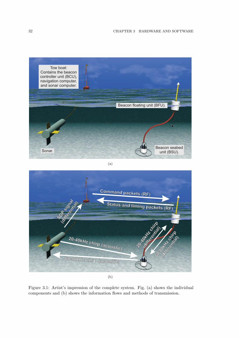
32 CHAPTER 3 HARDWARE AND SOFTWARE
(a)
(b)
Figure 3.1: Artist’s impression of the complete system. Fig. (a) shows the individualcomponents and (b) shows the information flows and methods of transmission.

3.2 Beacon controller unit (BCU) 33
(a) The BCU and case. The top right PCB is a GPS timing receiver. Thebottom right PCB is an RF modem. Both computer communication cableoptions (RS232 cable and USB) are shown entering from the top of the image.
(b) Operating with the navigation computer on the tow boat during a trial.
Figure 3.2: Photos of the BCU.

34 CHAPTER 3 HARDWARE AND SOFTWARE
SPI
TTL RS232
RS232 TTL RS232
USB
8 bit parallel
SOP
USB module(DLP-USB245M)
SPI UART(MAX-3100)
PIC(PIC-16F877)
SPI UART(MAX-3100)
Navigation computer
Driver(MAX-232)
RF modem(MOD433)
BCU PCB
SOP
Optocoupler(HCPL-2400)
100PPS
GPS(Oncore UT+)
Figure 3.3: Block diagram of the BCU. All connections and buses are bidirectionalexcept for the 100 PPS and SOP signals. A complete description of the timing isprovided in Appendix A.

3.2 Beacon controller unit (BCU) 35
by the navigation computer, to be sent to the beacon. Appendix C lists the controlcommands and Appendix D lists the different data packets generated in the beacon.The USB link also provides power to run the BCU. The current draw is ∼450 mA sothe USB host must be a “high power” type. If the RS232 cable is used instead, nopower is supplied by the computer and a separate DC power supply is required.
The RF link between the beacon and BCU was achieved using Bluechip MOD433RF modems. Essentially a bi-directional RS232 to RF converter, their operation isdesigned to be transparent to the user, with all error checking, frequency hopping, andretries performed automatically. A “many to one” mode of operation allows multipleslave modems to communicate with a single master, providing an easy extension of thesystem to multiple beacons. Unfortunately their performance was a source of muchfrustration, particularly in the embedded software design covered in Sec. 3.5. The datasheet specification for the RS232 connection to the modem stated 9600 baud. However,it was discovered that this speed only applied to the serial interface and the averagespeed for continuous RF data transmission, from one modem to another, was closerto 2000 baud. This was due to both regular and seemingly random-length pauses inthe modem operation as shown in Fig. 3.4. Although this was just adequate for thedata rate of a single beacon, the original project design had called for three beaconsoperating simultaneously and the modems had been selected with this higher data ratein mind. Furthermore, this speed was only achievable if the longest permissible packetlength (64 bytes) was used, requiring a comparatively large block of memory to bereserved in the PIC for storing the packet before transmission.
The RF modem output power is 10mW—well within the 25 mW New Zealand max-imum legal level for unlicensed products in the 433 MHz band [Ministry of EconomicDevelopment 2004]. A quarter-wave antenna provides omnidirectional performance inthe horizontal direction. The usable range was found to be 100m indoors and 200 mat sea.
3.2.1.2 Time stamping the sonar transmissions
The sonar transmits with a repeat rate of up to fifteen pings per second. The chirps aregenerated in the sonar (by clocking out waveforms stored in memory), by an embeddedPentium 3 computer, along with a start of ping (SOP) signal—a logic signal where thepositive going edge occurs at the start of every chirp. The SOP signal is sent up thetow cable as a differential signal on a twisted pair [Hayes et al. 2002]. The differentialdriver was constructed by a technician, Mike Cusdin.
On the tow boat, the SOP signal is routed to a PIC capture port on the BCU viaan optocoupler. A Motorola Encore UT+ GPS timing receiver connects to the othercapture port allowing the accurate time stamping of the time of departure (TOD) ofevery chirp. Details of how the time stamping is performed can be found in Appendix A.

36 CHAPTER 3 HARDWARE AND SOFTWARE
(a) Reasonably consistent (but slow) transmission rate of ∼3.5 packets per second, i.e., ∼2000 baud.
(b) Some medium pauses of 750 ms. These occur at random every few seconds.
(c) Occasional long pause of 1.75 s. These occur at random every few minutes.
Figure 3.4: Testing an RF link (one way data flow from transmitter to receiver) bymonitoring the RS232 output from an RF modem receiver. The test setup ensuresthere is no delay at the RS232 input to the RF modem transmitter so any gaps in thedata are caused by the RF link itself. Each packet is 64 characters. The oscilloscopetime scale is 500ms per division. Adjusting the antenna orientation, proximity to otherobjects, and separation did not alter the performance.

3.2 Beacon controller unit (BCU) 37
Once per second, the TODs for the previous one second epoch are packaged into anNational Marine Electronics Association (NMEA) 0183 [Association 2002] sentence andsent to the navigation computer.
The GPS timing receiver requires an external cable-powered active antenna. A Mo-torola Timing2000 antenna was used giving excellent performance over a cable lengthof several metres, even when mounted inside the tow boat cabin.
3.2.2 Navigation computer software
A graphical user interface (GUI) client, shown in Fig. 3.5, was written in Java tointerpret the data packets from the beacon, monitor its vital signs, and provide a simplemeans of sending command packets to the beacon, all in real time. The client runson the navigation computer and connects via TCP to a server program, also writtenin Java, that interfaces directly with the BCU. Java was used to allow execution onboth Windows and Linux. The separate client/server approach was used because it wasoriginally envisaged that a separate dedicated, networked, computer would be used fordata storage for both the sonar and the beacon. However, for the trials performed sofar, the client and server have been run together on the navigation computer, separatefrom the sonar computer, as shown in Fig. 3.2(b).
The server performs basic checksum and field-size checking of the incoming packetsfrom the BCU and saves them to a text file on the hard disk. The client reads fromthis file and processes the data packets to display them in a useful form with standardunits. It checks for serious errors, e.g., water leakage or GPS synchronisation loss, anddisplays warnings as necessary. Error, status, and warning codes are represented inthe data packets by single ASCII bytes1 and the client translates them into completesentences using a lookup table. There is a space reserved for these codes in the headerof every packet transmitted by the beacon. This ensures the beacon operating statusis constantly kept up to date, no matter which type of packets are being transmitted,without consuming significant bandwidth or requiring large memory storage for ASCIImessages in the beacon.
The position of the beacon, boat, and sonar are calculated from a combinationof GPS and time of flight (TOF) data, once the TOD packets (time-stamped in theBCU) and the time of arrival (TOA) packets (time-stamped in the beacon) have beenmatched up with each other and displayed on a nautical map of the area. The clientperforms an intelligent matching process, based on timing thresholds, so that missedpackets and out of order packets are correctly handled. Real time operation (15 pingsper second) is achievable on a 900 MHz Intel Centrino processor using ∼80 % CPUtime.
1There are less than 127 of these codes required so this is achieved with a single ASCII byte tosave memory.

38 CHAPTER 3 HARDWARE AND SOFTWARE
(a) Complete view showing several received data packets and a map of Lyttelton Har-bour.
(b) Closeup of the map window showing the beacon (triangle), boat, and sonar in PurauBay during a recent sea trial. The dotted line is the approximate sonar path based onthe GPS position of the boat.
Figure 3.5: Java GUI client running on the navigation computer for monitoring andcontrolling the beacon in real time during sea trials.

3.3 Beacon seabed unit (BSU) 39
The client displays a list of beacon commands, specified in an extensible markuplanguage (XML) configuration file, allowing the transmission of these to the beaconusing a single mouse click. This allows the beacon to be reset, switched betweendifferent test modes, and adjusted for the conditions, e.g., changing the preamp gains.The client constructs the appropriate header and checksum for each command and sendsit to the server. This passes the packet to the BCU to send via RF to the beacon. Theuser is informed if the transmission was successful or has timed out due to high RF load.The software development began as part of a 4th year undergraduate software teamproject, lead by Julian Maclaren. Their work was tidied up by the author to allowbasic testing with the hardware and substantially expanded by a Masters student,Daniel Meng, to include all necessary features for sea trials.
3.2.3 Synchronising the chirps
At the start of each imaging run, the sonar pings are stopped, the client instructs theserver to close the current file, increment the filename, and start writing to a new file.The sonar pings are then started which causes the BCU to start time stamping so it issynchronised from that point onwards.
3.3 BEACON SEABED UNIT (BSU)
The BSU sits motionless on the seabed providing the acoustic reference point (thetransducer) for the navigation. It is based around a two layer PCB controlled by aMicrochip PIC16F876 PIC, mainly used to collect sensor data and control the preampgain in response to instructions from the BFU. A block diagram is shown in Fig. 3.6and images are shown in Fig. 3.7. The following sections describe the operation.
3.3.1 Power supplies
Two 12V 7 AH sealed lead acid (SLA) batteries in the BSU provide enough power torun the beacon for a typical one day trial.2 During operation the batteries are connectedin series to provide an unregulated 24 V bus. This directly supplies the power amplifier.A 12 V bus is derived from this and used in both the BFU and BSU as the supply fromwhich all others are derived. Voltage levels of 9 V, 5V, 5 V analogue, 3.3V, and 1.8 Vare required in the BFU and 9 V, 8 V analogue, -8 V analogue, and 5 V are required inthe BSU.
Recharging is achieved without opening the casing by connecting a 20 V powersupply between the end caps of both units. The end caps are connected, via diodes,
2The high power consumption can be attributed to most of the regulators being linear, to minimisenoise and keep the design simple.

40 CHAPTER 3 HARDWARE AND SOFTWARE
I2C
TTL
BSU PCB
Power amplifier
Temp sensors(DS18B20)
ONE-WIRE
Analog
Leakagesensor
Transducer(SB45C)
Pressure sensor(19C050PA4K)
Tip sensor(CM1421-0)
Motion sensor(MS24)
TTL
TTL
TTL
Preamp
PIC(PIC-16F876)
Driver(MAX-232)
Figure 3.6: Block diagram of the BSU. All connections and buses are bidirectionalexcept where the direction is indicated by arrows.

3.3 Beacon seabed unit (BSU) 41
(a) PCB.
(b) Inverted in a bucket with the casing removed to allow basic acoustic testing whilestill having access to the electronics.
Figure 3.7: Photos of the BSU internals.

42 CHAPTER 3 HARDWARE AND SOFTWARE
(a) Deployment for testing in Lyttelton Marina in very calm conditions. The flatbase of this early design was later modified to raise the casing by up to 0.5m offthe seabed as shown below.
(b) On deck during a recent sea trial. The height isset to the highest of the three possible positions toprovide the maximum direct/multipath separation,as described in Sec. 4.2.3.2.
Figure 3.8: Photos of the BSU in action.
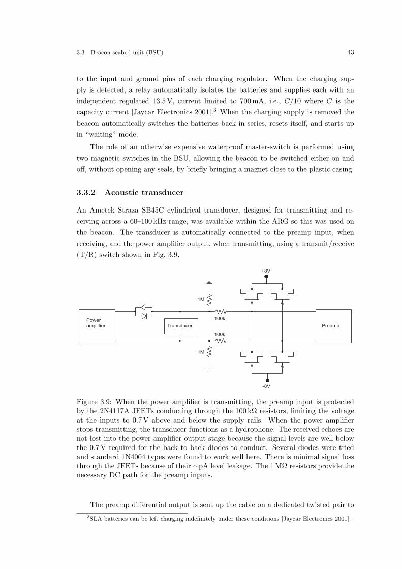
3.3 Beacon seabed unit (BSU) 43
to the input and ground pins of each charging regulator. When the charging sup-ply is detected, a relay automatically isolates the batteries and supplies each with anindependent regulated 13.5 V, current limited to 700 mA, i.e., C/10 where C is thecapacity current [Jaycar Electronics 2001].3 When the charging supply is removed thebeacon automatically switches the batteries back in series, resets itself, and starts upin “waiting” mode.
The role of an otherwise expensive waterproof master-switch is performed usingtwo magnetic switches in the BSU, allowing the beacon to be switched either on andoff, without opening any seals, by briefly bringing a magnet close to the plastic casing.
3.3.2 Acoustic transducer
An Ametek Straza SB45C cylindrical transducer, designed for transmitting and re-ceiving across a 60–100 kHz range, was available within the ARG so this was used onthe beacon. The transducer is automatically connected to the preamp input, whenreceiving, and the power amplifier output, when transmitting, using a transmit/receive(T/R) switch shown in Fig. 3.9.
Figure 3.9: When the power amplifier is transmitting, the preamp input is protectedby the 2N4117A JFETs conducting through the 100 kΩ resistors, limiting the voltageat the inputs to 0.7 V above and below the supply rails. When the power amplifierstops transmitting, the transducer functions as a hydrophone. The received echoes arenot lost into the power amplifier output stage because the signal levels are well belowthe 0.7 V required for the back to back diodes to conduct. Several diodes were triedand standard 1N4004 types were found to work well here. There is minimal signal lossthrough the JFETs because of their ∼pA level leakage. The 1MΩ resistors provide thenecessary DC path for the preamp inputs.
The preamp differential output is sent up the cable on a dedicated twisted pair to3SLA batteries can be left charging indefinitely under these conditions [Jaycar Electronics 2001].

44 CHAPTER 3 HARDWARE AND SOFTWARE
the BFU where it is digitised. The differential transmit signal (generated in the BFU)arrives from the cable on a dedicated twisted pair and provides the input signal for thepower amplifier.
The output impedance of the BSU power amplifier, Zp(f), is fixed so maximumpower transfer will occur if the complex conjugate of the load impedance is matchedto it [Bobrow 1985, p195], i.e.,
Z∗h(f) = Zp(f), (3.1)
where Zh(f) is the impedance of the transducer. An alternative to this, when theimpedances are not well characterised or easily changeable, is to match the magnitudesusing a transformer with np turns on the primary and ns turns on the secondary (aturns ratio of φ) giving
φ =ns
np, (3.2)
=
√|Zh||Zp|
(3.3)
where an estimate for Zp can be obtained by assuming it is similar to the recommendedload impedance for the power amplifier. This expands to
φ =
√√√√√R2
h(f) +X2h(f)
Rp(3.4)
by modelling the power amplifier output impedance as a resistive component, Rp, andthe transducer impedance as a frequency dependent RC series combination, Rh(f) andCh(f) with associated reactance Xh(f).
Once φ has been determined, np is then chosen as a trade off between minimisingthe resistive losses of the wire but still providing sufficient inductance, Lp, for thetransformer to operate correctly, governed by
np =√Lp
AL(3.5)
where AL is the inductance factor of the transformer core. Lower frequencies requirelarger values of inductance and hence more turns. At lower frequencies the transduceris also more capacitive (c.f. the reactance curves, X, in Fig. 3.11) so more likely tocause the power amplifier to go into oscillation. This is compounded by the fact thatthe transformer causes the transducer capacitance seen at the power amplifier outputto be multiplied by φ2.
The transducer impedance was characterised using a Wayne Kerr B601 radio fre-

3.3 Beacon seabed unit (BSU) 45
quency bridge driven by 4.7Vpp sine wave and monitored with an HP 35665A dynamicsignal analyser (0–102.4 kHz) and HP 3588A spectrum analyser (110–220 kHz). Twopoints (20 kHz and 100 kHz) were also checked using a Philips PM6304 RCL meter. Theresults are plotted in Figs. 3.10 and 3.11 along with a typical plot from the datasheetwhich has a similar shape but a narrower vertical span.
The ideal operating point for transmitting is the first resonant point around 95 kHz.This is where the transducer is least reactive so more of the power supplied to it is ra-diated as acoustic power (and heat) rather than being returned to the power amplifier.Unfortunately this point overlaps the upper imaging band (90–110 kHz) used by thesonar so an operating band of 60–80 kHz was chosen, as discussed earlier in Sec. 2.6.4.The impedance at the middle of this band is ∼3400 Ω and the power amplifier is basedaround a ST TDA2030 amplifier designed to drive loads of 4-8 Ω [STMicroelectron-ics 1998] so, making the assumption that Rp is a similar size, transformer turns ratiosof 20–30 were tried. A primary to secondary turns ratio of 7:200 on an N30 core(AL = 5.7µH) was found to produce the maximum output signal across the transducer(∼500Vpp) at 70 kHz without going into oscillation. This produced a current in thetransducer of 51 mA RMS at a power factor of 0.12 giving a real power of 1.2W duringtransmission, comfortably within the 7.5W rating. At the standard rate of 15 chirpsper second where each chirp is 12.5 ms in duration, this equates to a continuous powerof 0.2W. Although much lower than could have been achieved at resonance, this powerlevel still produces a strong return in the sonar images (see Chapter 5) at the shortranges (<50 m) that the KiwiSAS typically operates.
3.3.3 Other sensors
Several sensors interface to the PIC. These are sampled once per second, packaged intoan NMEA 0183 packet, and sent up the cable to the BFU which passes them on tothe BCU via the RF modem. A leakage sensor, located near the base of the casing,monitors water entry. A SenSym 19C050PA4K pressure sensor is used to measurethe depth. An Assemtech MS24 motion sensor is used to monitor that the BSU isstationary. An Assemtech CM1421-0 tip sensor, which activates at 45 degrees fromvertical, is used to determine if the beacon lands on its side. The built in PIC ADCsare used to monitor the battery voltages when charging and in operation.
Two one-wire Dallas DS18B20 sensors measure the ambient temperature and thewater temperature via contact with the aluminium end cap.4 The original intention wasto use this data, in conjunction with the water temperature measurements collected bythe sonar, to construct a sound speed profile between the sonar (mid-water) and theBSU (seabed). The one wire bus is implemented in software by bit-bashing a pin on the
4Although the end cap is also the PCB heat sink, the large contact area with the water means thesmall amount of heat produced has no measurable effect on the temperature sensor readings.

46 CHAPTER 3 HARDWARE AND SOFTWARE
0.0
0.1
0.2
0.3
0.4
0.5
0.6
0.7
0.8
10 30 50 70 90 110 130 150 170 190 210 230
Frequency (kHz)
Adm
itta
nce (
mill
isie
mens)
(a)
50
95
90
190
0
0.1
0.2
0.3
0.4
0.5
0.6
0.7
0 0.1 0.2 0.3
Conductance (millisiemens)
Su
scep
tan
ce (
mil
lisie
men
s)
(b)
Figure 3.10: Measured admittance (a) and admittance components (b). Two points ofresonance can be seen around 95 kHz and 190 kHz.

3.4 Beacon floating unit (BFU) 47
0
200
400
600
800
1000
1200
1400
1600
1800
2000
2200
2400
2600
50 60 70 80 90 100 110
Frequency (kHz)
Re
sis
tan
ce
(Ω
)
-4400
-4200
-4000
-3800
-3600
-3400
-3200
-3000
-2800
-2600
-2400
-2200
-2000
-1800
Re
acta
nce
(Ω
)
X
R
(a) Measured impedance components. (b) Typical impedance component values from thedatasheet.
Figure 3.11: Plots of the SB45C transducer modelled as a combination of resistive andcapacitive components in series.
PIC. Although the software is complicated to implement, (because of the precise timingrequirements of the one-wire protocol) the electronics are much simpler compared toanalog temperature sensors. Another advantage is the high accuracy of 0.5C.5
3.4 BEACON FLOATING UNIT (BFU)
The BFU floats partly submerged, tethered to the BSU by the beacon cable. A weightedkeel keeps it upright at all times. Its main job is performing real time signal process-ing of the received sonar chirps to determine the precise TOA. This is done by a TITMS320VC33 digital signal processor (DSP) which also generates the transmit chirps.The time stamping is performed by a Microchip PIC16F877 PIC, the main controllerfor the unit. Photos are shown in Figs. 3.12 and 3.13.
3.4.1 Hardware
Figure 3.14 shows a block diagram of the BFU. The following sections describe theoperation.
5This can be improved by an additional factor of ten using quadratic error curve fitting [DallasSemiconductor 2002].

48 CHAPTER 3 HARDWARE AND SOFTWARE
Figure 3.12: BFU floating tethered in Lyttelton Marina, New Zealand, in very calmconditions.

3.4 Beacon floating unit (BFU) 49
(a) Inside the casing. Here the GPS timing receiver and RF modem are mounted onthe case wall. This was later changed to a direct PCB mounting to simplify assembly.The long coaxial cable is required to attenuate the active GPS antenna so it does notoverload the GPS receiver.
(b) PCB mounted on the aluminium end cap. The power supply regulators bolt to thisend cap to dissipate heat into the water. In this photo the large black cable from theBSU is glued to a metal sheath. This eventually leaked so was later changed to a cablegland.
Figure 3.13: Photos of the BFU internals.

50 CHAPTER 3 HARDWARE AND SOFTWARE
SPI
TTL RS232
RS232 TTL
SPI UART(MAX-3100)
PIC(PIC-16F877)
SPI UART(MAX-3100)
Driver(MAX-232)
RF modem(MOD433)
BFU PCB
TOA100PPS
GPS(Oncore UT+)
SPI*
CPLD(XC9572XL)
TOA*
Temp sensors(DS18B20)
ONE-WIRE
NVRAM(DS1350W)
ADC(AD7723)
LATCH(74LVT16374)
DAC(DAC902)
8 bit parallel
TTL
8 bit parallel*
Leakagesensor
DSP(TMS320VC33)
Driver(MAX-232)
TTL
Figure 3.14: Block diagram of the BFU. All connections and buses are bidirectionalexcept where the direction is indicated by arrows. Asterisks denote signals that havebeen level shifted to allow communication between components with different supplyvoltages.

3.4 Beacon floating unit (BFU) 51
3.4.1.1 PIC
The PIC in the BFU has a similar job to that in the BCU. It is responsible for con-structing NMEA 0183 compliant packets to send to the BCU via a RF modem, andtime stamping the start of the reply chirp transmission using a GPS timing receiver asa reference. There are two kinds of packets; status packets and timing packets.
Status packets contain non-critical data on the status of the beacon, e.g., batteryvoltages, temperature, etc. The beacon cycles through the different packet types,generating one or two packets per second, depending on RF load, or requesting packetsfrom the BSU, and sending them to the BCU.
Timing packets contain TOA data for up to 15 received pings and are stored in astack in the non-volatile random access memory (NVRAM). They are generated onceper second and take priority over status packets, i.e., if there are timing packets inthe buffer waiting to be sent, the status packets are only generated every 5th seconduntil the backlog of timing packets has been cleared. The retrieval order is not criticalbecause each packet is individually time-stamped. The NVRAM has enough storagefor 17 hours of continuous operation so the data can still be uploaded back in thelab should the RF link fail at sea. Because of the large volume of data involved, theTOA time stamps are sent to the BCU as a compressed binary packet rather than anNMEA packet. The BCU decompresses the packets, constructs individual NMEA 0183compliant sentences for each ping, and sends these to the navigation computer. SeeAppendix D for further details.
As well as transmitting RF status and timing packets, the BFU PIC receives anddecodes RF command packets from the BCU and, if required, sends them down thecable to the BSU using RS232.
Similar to the BSU, there are two Dallas DS18B20 temperature sensors and aleakage sensor in the BFU, monitored by the PIC. The supply voltages are monitoredalso.
3.4.1.2 DSP
The DSP continuously samples the received echoes using an Analog Devices AD7723ADC, under direct memory access (DMA) control, and performs matched filteringto detect incoming sonar chirps. The signal processing is covered in more detail inChapter. 4. Once the exact TOA has been determined, it sleeps6 until the turn aroundtime (TAT) has elapsed from the TOA.7 It then wakes and transmits a 60–80 kHz chirp
6Unlike the PIC, the DSP does not have any form of “timer compare” feature to generate anevent with fixed latency. The only way to achieve this is to set up a timer interrupt, disable all otherinterrupts, and put the processor to sleep. When the interrupt occurs, the processor wakes and thelatency to service the interrupt is constant.
7The TOA is found by simply subtracting the 25ms TAT from the data. It takes ∼22ms todetermine the TOA so the sleep time is ∼3ms.

52 CHAPTER 3 HARDWARE AND SOFTWARE
from a lookup table, via a Burr Brown DAC902 DAC under DMA control, down thecable as a differential signal to the power amplifier in the BSU. A Xilinx XC9572XLcomplex programmable logic device (CPLD) converts the DAC clock into a one-shotsignal which the PIC time stamps and sends to the BCU. A test mode is also availablewhere the CPLD feeds a 12.5Hz square wave into the PIC capture port in place ofthe one-shot signal. The square wave is generated by passing the 100 pulse per second(PPS) GPS output through a divide-by-eight divider in the CPLD. A timeline of thesystem operation is provided in Figure 2.4.
Both the ADC and DAC share the DSP parallel bus (using 8 of the 16 bits) usingthe automatic memory bank addressing of the DSP. The NVRAM also shares this busand is used for boot loading the DSP upon startup and for storing NMEA packets priorto transmission. A JTAG port on the DSP is used to transfer the program code into theNVRAM. The PCB was designed before the RF modem problems were discovered (seeSec. 3.2.1.1) so it was assumed that the PIC would assemble packets and send them tothe BCU in near real time. However, the RF modem problems meant that significantbuffering (hundreds of bytes) of the data packets in the BFU was required. The PICinternal RAM is only 368 bytes so the NVRAM was used for this task. Because theNVRAM is not connected to the PIC, where all the NMEA packets are generated, theDSP must act as the go-between, essentially providing an serial peripheral interface(SPI) link to the NVRAM for the PIC. The CPLD provides the logic level shiftingrequired to interface the 5 V PIC to the 3.3V DSP.
For diagnostic purposes the DSP can be instructed to save the raw sample dataand/or matched filter output data in the NVRAM as NMEA packets. This is thenfetched by the PIC and sent to the BCU over a period of several minutes. Examplesare shown in Sec. 4.2.3.2.
3.4.1.3 TAT accuracy
In reality, achieving a precise 25 ms TAT, in both the warm laboratory environmentand at sea is impossible without using expensive stabilised oscillators and calibratingthese to determine their exact frequency. To avoid this problem, no attempt is madeto control the oscillator frequency. Instead, it is measured by counting the elapsedoscillator pulses between every 1 PPS GPS pulse and this information is included inevery timing packet. The PIC performs this task by counting every fourth oscillatorpulse via the internal divide-by-four prescaler on the clock input. The oscillator fre-quency is 14.31818 MHz so the PIC requires three bytes to count to 3579545 over aduration of one second. However, it was found that the variation between the labo-ratory and the ocean was less than 10 counts per second and once the temperaturestabilised, the variation was less than 1 during operation so a single byte was sufficientfor tracking the changes. So the “precise 25 ms TAT” may not be exactly 25 ms, but

3.4 Beacon floating unit (BFU) 53
measuring the clock frequency every second, allows the actual TAT used during a seatrial to be recorded and can then be used when post-processing the sonar images. Thepost-processing is explained in Sec. 4.6.
The required accuracy of measuring the actual elapsed TAT is the same as anyother timing measurement in the system, such as the TOF. In Sec. 1.4 the systemaccuracy was defined as <1 cm or 6.67µs. Keeping the individual timing componentsbelow one tenth of this is a good rule of thumb, i.e., <667 ns. The PIC counter clockperiod is 279 ns so the desired accuracy is achieved.
3.4.1.4 SPI bus
The PIC communicates bi-directionally with the GPS, RF modem, and DSP over ashared SPI bus. The PIC is the master so provides the SPI clock for the other deviceson the bus acting as slaves. The PIC controls the enable line of each device to ensureonly one device connects to the SPI bus at once. Interrupt lines from each device letthe PIC know when data needs to be read from each device.
Implementation was straightforward for the GPS and RF modem. Both are RS232devices so a Maxim MAX3100 RS232 to SPI UART was used to interface each oneto the SPI bus. The DSP was more difficult. It was discovered, after selection, thatalthough the serial ports can be configured as slave SPI receivers, it is not possible toset them up as slave SPI transmitters. The two areas of incompatibility are the clock(CLKX0 pin) and frame sync (FSX0 pin) requirements. The DSP serial port expects acontinuously running clock with data transfers initiated using the frame sync pin. Thisis different to SPI where the master provides bursts of eight clock pulses during whicheight bits of data are transferred between master and slave with no synchronisation.
To enable SPI communication from the DSP to the PIC, the extra serial portrequirements of the DSP are provided by the CPLD to achieve a “DSP serial port toSPI” conversion. The CPLD monitors the DSP “SPI enable” line, from the PIC, andconnects the DSP serial port to the SPI bus. It then generates the three extra clockpulses required by the DSP and provides a frame sync signal (a rising edge on the thirdpulse) so that when the following eight SPI clock pulses arrive, the DSP is ready toreceive them and transmit eight bits of data back to the PIC. This is shown in Fig. 3.15.
3.4.2 PCB
The electronics were initially designed as a two layer PCB, however, this was latermodified to a four layer PCB to provide improved performance. Although a fourlayer PCB is sub-optimal in terms of minimizing electromagnetic compatibility (EMC)emissions and maximizing signal quality, it still provides a significant improvement over

54 CHAPTER 3 HARDWARE AND SOFTWARE
Figure 3.15: The enable signal from the PIC triggers the CPLD to generate three extrapulses that precede the eight SPI clock pulses provided by the PIC on the DSP transmit-clock input pin (CLKX0). The CPLD also precisely controls the DSP transmit-frame-sync input pin (FSX0). This allows the DSP to transmit SPI data to the PIC. TheDSP is already SPI compatible upon receive by simply routing the enable signal to thereceive-frame-sync input pin (FSR0).
a two layer PCB for only a modest increase in cost [Ott 2003]. The two internal layerswere used as a dedicated ground plane layer and a combination ground-plane/clock-trace layer. This freed up the top layer for signals and the bottom layer for powerplanes plus any signals that could not be successfully routed on the top layer. Thelayer stack-up is shown in Fig. 3.16.
3.5 EMBEDDED SOFTWARE
The following sections present an overview of how the embedded software in the BFUand BCU reliably manages the wide variety of asynchronous events encountered duringoperation.
3.5.0.1 DSP
Transfers from the ADC are written to a circular buffer (FIFO) under DMA control.This allows the processor to simultaneously check the incoming samples for clippingand convert them to floating point representation in preparation for the single cyclemultiply and accumulate (MAC) operations during filtering.
Transfers to the DAC are also DMA controlled. During this time, the DSP CPU is
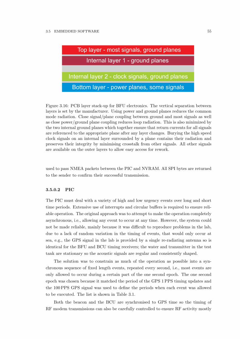
3.5 EMBEDDED SOFTWARE 55
Figure 3.16: PCB layer stack-up for BFU electronics. The vertical separation betweenlayers is set by the manufacturer. Using power and ground planes reduces the commonmode radiation. Close signal/plane coupling between ground and most signals as wellas close power/ground plane coupling reduces loop radiation. This is also minimized bythe two internal ground planes which together ensure that return currents for all signalsare referenced to the appropriate plane after any layer changes. Burying the high speedclock signals on an internal layer surrounded by a plane contains their radiation andpreserves their integrity by minimising crosstalk from other signals. All other signalsare available on the outer layers to allow easy access for rework.
used to pass NMEA packets between the PIC and NVRAM. All SPI bytes are returnedto the sender to confirm their successful transmission.
3.5.0.2 PIC
The PIC must deal with a variety of high and low urgency events over long and shorttime periods. Extensive use of interrupts and circular buffers is required to ensure reli-able operation. The original approach was to attempt to make the operation completelyasynchronous, i.e., allowing any event to occur at any time. However, the system couldnot be made reliable, mainly because it was difficult to reproduce problems in the lab,due to a lack of random variation in the timing of events, that would only occur atsea, e.g., the GPS signal in the lab is provided by a single re-radiating antenna so isidentical for the BFU and BCU timing receivers; the water and transmitter in the testtank are stationary so the acoustic signals are regular and consistently shaped.
The solution was to constrain as much of the operation as possible into a syn-chronous sequence of fixed length events, repeated every second, i.e., most events areonly allowed to occur during a certain part of the one second epoch. The one secondepoch was chosen because it matched the period of the GPS 1PPS timing updates andthe 100 PPS GPS signal was used to define the periods when each event was allowedto be executed. The list is shown in Table 3.1.
Both the beacon and the BCU are synchronised to GPS time so the timing ofRF modem transmissions can also be carefully controlled to ensure RF activity mostly

56 CHAPTER 3 HARDWARE AND SOFTWARE
Pulse # Event description0–15 Receive and analyse GPS ASCII timing information16–24 Send a timing packet or construct and send a status packet via RF
to the BCU25–54 Retrieve a timing packet from the NVRAM55–59 Listen for command packet from BCU via RF modem60–69 Send a timing packet via RF to the BCU70–89 Retrieve a timing packet from the NVRAM90–94 Construct and send a status message via RF to the BCU95–99 Receive a status packet from the BSU
Table 3.1: PIC software event cycle for the synchronous events in the BFU. Operation issimilar for the BCU except the RF transmissions are replaced with USB transmissionsto the navigation computer. Pulse # refers to the GPS 100PPS timing pulses givinga complete cycle duration of one second. The asynchronous events can occur at anytime so are handled by fast interrupt routines.
occurs when both ends of the RF link are expecting it.8 The result is that the BFU andBCU PICs follow a strict cycle of events every epoch where each event has a definedperiod during which it is executed. This consistency makes it easier to write simpler,more reliable code for the few remaining asynchronous events, e.g., a ping arriving,so that they can be reliably handled at any time. Embedded system debugging alsobecomes simpler when the events follow a regular repeating cycle. If an error is occuringat a regular point in the epoch then the corresponding event can be easily identified.If an error is occuring at a random time then it is likely to be related to one of theasynchronous events.
3.6 OPERATION AT SEA
The system alternates between “imaging” and “waiting” modes as the sonar is towedaround an area of interest. This is illustrated by the solid and dashed parts of thetowpath of Fig. 3.17. Table 3.2 summarises the two modes.
During an imaging run, the BCU avoids transmitting to the beacon. This ensuresthe beacon can reliably process all received pings without any RF modem problemsoccurring. During the waiting period, between imaging runs, the navigation computeris permitted to send command packets to the beacon. This period is generally used toadjust the chirp detection parameters or upload raw sample or correlation data savedduring the the previous run.
8The random RF pauses, discussed in Sec. 3.2.1.1 mean that RF modem events cannot be reliedupon to be 100% synchronous.

3.6 OPERATION AT SEA 57
Imaging mode Waiting modeSonar transmitting and receiv-ing.
Sonar not transmitting or receiv-ing.
Beacon listening for pings and re-sponding.
Beacon listening for pings.
Beacon sending RF TOF packetsto BCU.
Beacon sending RF status pack-ets to BCU.
BCU receiving RF TOF packetsfrom beacon.
BCU sending RF commandpackets to beacon and receivingRF status packets.
Table 3.2: Principle differences between “waiting mode” and “imaging mode”.
Figure 3.17: A birds eye view of a typical run, following an approximately rectangularpath around a seabed area containing objects of interest, including the beacon. Thesolid line shows when the sonar is in “imaging mode”, travelling as straight and steadyas possible, transmitting chirps and recording all received echo data. The dotted lineshows when the sonar is in “waiting mode”, taking a fast, silent, unspecific path to getback into position for the start of the next imaging run. Although this repositioningis done as quickly as possible, it still takes several minutes and during this time RFcommand packets can be sent from the navigation computer to the beacon.

58 CHAPTER 3 HARDWARE AND SOFTWARE
3.6.1 Reliability
Sea trials are expensive and time consuming so beacon reliability is essential. Manyinternal checks are made to ensure that the beacon timing remains synchronised to theGPS and all the peripherals are behaving correctly. The GPS timing receiver outputsthe number of used satellites once per second as part of the ASCII sentence of timinginformation. The antenna location is not fixed so a minimum of four satellites arerequired to first synchronise to GPS time and three required to maintain it. However,the accuracy is considerably improved when using four so a warning is generated if theGPS drops below this number.
The beacon attempts to transmit an RF packet every second so it is immediatelyapparent on the boat if it has crashed.9 A number of safety features have been imple-mented should this situation arise. The navigation computer can issue a reset commandto the beacon during the “waiting” period to reset either the BSU, the BFU, or thewhole beacon.10 Should the beacon not respond to a reset command, e.g., if the RFmodems have failed, software watchdog timers in the BFU PIC and BSU PIC will resetthe beacon after 90 seconds and 240 seconds respectively.11
Every time the surface unit is reset it logs the details to EEPROM. It sends thelog to the BCU to display on the navigation computer at startup so if an automaticreset occurs, the problem can be diagnosed afterwards.
3.7 MECHANICAL CONSTRUCTION
Where possible, the mechanical design and construction was performed by the author,due to the limited department technician time available at the University of Canterbury.This included all aspects of construction except for lathe work and o-ring seals.
3.7.1 Casings
All of the seals below the water line, that are designed to be opened, use double o-rings.This can be seen on the the upper end cap of the BSU shown in Fig. 3.7(b). Althoughnot technically necessary for the shallow design-depth of the beacon, experience hasshown it to useful when o-rings get dirty or damaged during assembly.
The metal parts of the beacon are stainless steel or aluminium. Aluminium ispreferred over stainless steel because it is lighter and easier to machine. With only a
9This is now a rare (once-per-day) event with the beacon proving more reliable than the sonarduring the latest sea trial.
10This involves a complete power-down, power-up cycle and is a last resort because a wait of up toone minute is required while the GPS re-establishes the satellite link.
11These long timeouts were chosen to allow updating of the embedded software in either PIC withoutthe other unit initiating a power cycle due to inactivity during programming.

3.7 MECHANICAL CONSTRUCTION 59
few trials per year performed in salt water, non-anodised, standard grade, aluminiumwas found to be adequate, exhibiting only superficial corrosion, even after several years.
3.7.2 Cable
The cable connecting the BSU and BFU is a GeneralCable B50 containing six shieldedtwisted pairs. It is continuous from PCB to PCB rather than the more expensive ap-proach of terminating with waterproof connectors or feedthroughs at each unit. Cableglands, again using double o-rings, seal the cable where it enters the casing end caps.On both units, after exiting the casing, the cable immediately passes through a seriesof supporting tubes, progressively reducing in rigidity. This provides strain relief sothe cable gland is never stressed and ensures the cable does not become kinked duringthe rigours of deployment and retrieval.
The cable is surrounded by a nylon self splicing braid to provide protection andtake up any strain developed between the two units, e.g, during retrieval from a softseabed.
3.7.3 Vacuum system
A vacuum system is used in the BFU to verify the seals are functioning correctly. Thissimple, cheap, and extremely useful technique is also implemented in the KiwiSASsonar and has proven its worth several times. It quickly identifies sealing problemsin the lab, without immersion, rather than discovering them at sea, after immersion.The system consists of a one-way valve with release tap, mounted anywhere on thecasing and an absolute pressure sensor mounted anywhere inside the casing. Attachinga vacuum pump to the valve allows the pressure in the casing to be lowered, similar tothe effect of the external pressure increasing with depth. A ∼50 kPa pressure drop12
from atmospheric pressure (nominally 101.3 kPa) is sufficient to fully seat the o-rings.Once the tap is closed, if the pressure remains stable for at least 30 minutes then theBFU is properly sealed and ready for a sea trial. An added benefit is that the o-ringsare now fully compressed, providing reliable sealing during the risky first few metres ofimmersion when the water pressure is minimal.
Pressure monitoring can be achieved using an electronic sensor or, in the case of theBFU which has a transparent window, a simple analogue gauge.13 The analogue optionis particularly useful when setting up for a sea trial because it allows an immediatevisual confirmation that the unit is watertight, before immersion, and can be performedin a few seconds, by an untrained operator, without requiring power. Without the
12The sonar is operated at 70–80 kPa absolute, to allow proper operation of the hard disk.13In practice, a common analogue pressure gauge that measures positive “gauge pressure” can be
used here by sealing the port at atmospheric pressure. The reading will then increase as pressuredecreases below atmospheric.

60 CHAPTER 3 HARDWARE AND SOFTWARE
vacuum test, there is no way of knowing if the seals have failed until the sea trialbegins14 and the leakage sensor is activated.
The vacuum system concept was not known at the time the BFU and BSU weredesigned. The BFU initially had leakage problems so was retrofitted with a vacuumsystem using a Festo MAP-40-1-1/8-EN analogue gauge. This also proved invaluableduring testing. The BSU has a simple case design, operates under a high externalpressure, is rarely opened, and has never leaked. For these reasons it was thought thata vacuum system was unnecessary. However, it was discovered that the cable connectingthe two units acted like an air hose, causing the pressure to equalise between them overa period of several minutes so the whole beacon operates under vacuum.
Figure 3.18: Complete beacon on deck ready for deployment.
3.8 CHAPTER SUMMARY
The electronic and mechanical hardware details of the prototype active beacon werepresented. An overview of the embedded software was given for the PIC processors in
14Although immersion tests can be performed in the lab prior to a sea trial, these are time consumingand do not reveal damage caused by the subsequent packing, transporting, and setup at sea.
3.8 CHAPTER SUMMARY 61
the BCU, BSU, and BFU, and the DSP in the BFU. The current design works welland has performed reliably in numerous tests and recent sea trials.
The measured reactance of the available transducer differed in magnitude fromthe datasheet plots by up to a factor of two, particularly near resonance, although theshape of the plots were similar. The transducer consumes a power of 1.2W RMS duringtransmission—enough to produce a strong response in the sonar images.
The flow of data packets and control packets was presented showing how the activebeacon is remotely controlled from the navigation computer on the tow boat usingJava client and server applications. This allows real-time performance monitoring andparameter adjustment. While the TOF data can be uploaded to the tow boat in real-time, the RF modem speed currently restricts the ability to collect much diagnosticdata. Achieving further improvement in the performance of the beacon as a navigationsolution requires a faster RF link.


Chapter 4
BEACON SIGNAL PROCESSING
4.1 INTRODUCTION
The active beacon must reliably determine the precise time of arrival (TOA) of eachchirp from the sonar. Once determined, the transmission of the reply chirp must occuran exact time delay after the TOA, known as the turn around time (TAT). Providedthis can be done within the chirp repeat period, the beacon remains synchronisedwith the sonar for any chirp repeat rate at any range. This chapter explains the signalprocessing used in the beacon DSP to achieve this task and the difficulties encountered.After first presenting the signal processing algorithms implemented in the prototypebeacon, the theoretical performance of the chirp detection and the effects of multipathare investigated using simulations and data from recent sea trials. The theoretical sonartransmit directivity is derived and compared with experimental results showing howthe beam pattern (BP) nulls affect the detection performance. Finally, an explanationis given of the beacon MOCOMP process.
4.2 FILTERING THE CHIRP FROM THE RECEIVED SIGNAL
The following sections present a breakdown of the steps involved in the chirp detectionprocess in the beacon floating unit (BFU). Flow diagrams for each step are shown inFigs. 4.2, 4.3, and 4.8. All simulated waveforms in this chapter are plotted at the scaleof the output of the 16-bit ADC used in the beacon, to allow direct comparison withexperimental data from the beacon.
4.2.1 Signal intensity variation
When detecting the sonar chirps, the main problem encountered is the variation ofsignal intensity over time. This variation is the result of several different effects; listedin Table 4.1. The biggest problems are those that occur rapidly within each run, i.e.,BP effects. These cause frequent dropouts and miss-detections and are analysed inSec. 4.5. All the effects are predictable if the sonar motion is known by the beacon,

64 CHAPTER 4 BEACON SIGNAL PROCESSING
Type ofvariation
Details Variation occurs
Range
Sonar across-track location is notthe same for each run.
between successive runs
Sonar-beacon separation follows ahyperbolic path as the sonar travelspast the beacon.
slowly within each run
MotionSonar motion, particularly yaw,changes where the peaks and nullsof the BP are pointing.
randomly within eachrun
BP
The sonar transmit BP is not omni-directional so varies in intensity asthe sonar travels past the beacon.
slowly within each run
The sonar transmit BP nulls moveduring each chirp, as the fre-quency changes, causing a reductionin bandwidth dependent on along-track position.
rapidly within each run
GainThe sonar transmit amplitude is ad-justed to achieve good SNR, de-pending on the swath width, seabed,and target reflectivity.
between successive runs
Table 4.1: Sources of amplitude variation of the signal received at the beacon.

4.2 FILTERING THE CHIRP FROM THE RECEIVED SIGNAL 65
e.g., the beacon seabed unit (BSU) preamp gain could be progressively decreased thenincreased, as the sonar travelled past the beacon, to counter the variation due to the hy-perbolic change in sonar-beacon separation. However, the beacon only measures range(not angle). Sending the other dimensions of the sonar motion to it in real-time is notpossible with the low bandwidth RF link available. While the passing of the sonarcould be inferred from the increase and decrease of the received signal amplitude, thecombination of the effects in Table 4.1, combined with misses and miss-detections,make this a problematic approach without large, controlled, tank testing facilities tofine-tune the algorithms. Currently the ARG is limited to a trial and error process ofimplementing ideas in the lab and observing the outcome during sea trials. For thisreason, the beacon was designed to treat each ping independently, making no assump-tions about previous TOA data. Once consistent operation is achieved, the automaticadjustment of parameters, e.g., preamp gain, during a run can be investigated.
4.2.2 Step 1: Chirp detection
The low signal amplitude that can occur during a run, discussed in the previous section,precludes the use of any edge-detection schemes being applied directly to the signal.Because the signal being detected is known, a matched filter can be used to improvethe SNR.1 Additional details on the matched filter accuracy are provided in Sec. 4.4.
As discussed in the previous section, the beacon does not attempt to predict whenthe next chirp will arrive.2 Hence, the matched filtering is performed continuously untila chirp is detected. This is computationally intensive and in practice some trade-offsare required to achieve real-time operation, as discussed in the following sections.
Consider a real signal transmitted by the sonar, s(t) with corresponding FT S(f).After propagation through the medium (distortion, noise, multipath, etc) it is receivedby the beacon as a real signal e(t) with corresponding FT E(f). The matched filter,g(t) with corresponding FT G(f), for these two signals can be expressed in severalforms;
g(t) =∫ ∞
−∞e(τ)s(t− τ) dτ , (4.1)
= e(t) s(−t), (4.2)
= e(t) ? s(t), (4.3)
G(f) = E(f)S∗(f), (4.4)
where represents a convolution and ? represents a correlation. A correlation can be
1Matched filtering is also used in the sonar to increase the SNR of the weak echoes.2Although the sonar and beacon have a (slow) RF modem link (via the beacon controller unit
(BCU)), so in theory could exchange information about the time of departure (TOD) and chirp repeatrate, it was desired to have the beacon operate fully independently, as discussed in the previous section.

66 CHAPTER 4 BEACON SIGNAL PROCESSING
implemented discretely as a finite impulse response (FIR) filter where s[n] = s(n∆t) isthe set of filter taps and ∆t is the sampling period.3
All realizable signals have the form
s(t) = a(t) cos (Φ(t)) . (4.5)
The chirp signals used in the KiwiSAS are band limited so Φ(t) is usually written inthe form
Φ(t) = 2πfct+ φ(t) (4.6)
where 2πfct is a carrier term (in radians) centred on the carrier frequency fc, and φ(t)is a time varying phase term (in radians). For a linear chirp with a bandwidth W ,duration T , and centre frequency fc,
Φ(t) = 2π(fc −
B
2
)t+ π
B
Tt2 + φo (4.7)
where φo is a constant offset term (in radians, see Sec. 4.2.3.1) due to the phase shiftintroduced by the sonar power amplifier and transducer. The amplitude term a(t) isthe envelope (sometimes referred to as the natural envelope) of s(t);
a(t) = |s+(t)| , (4.8)
= |s(t)| , (4.9)
where s+(t) is the pre-envelope and s(t) is the complex envelope (sometimes referredto as the baseband) of s(t) given respectively by
s+(t) = s(t) + js(t), (4.10)
= s(t) + jHs(t), (4.11)
s(t) ≈ s+(t)e−j2πfct, (4.12)
where H is the Hilbert transform. The pre-envelope is easily calculated by scalings(t) in the frequency domain to satisfy
S+(f) =
2S(f), f > 0
S(0), f = 0
0, f < 0
. (4.13)
For the KiwiSAS chirps, a(t) is nominally equal to 32767 (the maximum amplitude
3A more accurate set of taps can be obtained by measuring the s(t) after passing through the DAC,power amplifier and transducer, each of which introduce distortion.

4.2 FILTERING THE CHIRP FROM THE RECEIVED SIGNAL 67
using a signed 16 bit representation) but tapers to zero at the start and end of eachchirp, as can be seen in Figs. 4.5(a) and 4.5(b). This is done to reduce the harmonicsproduced by the power amp.
4.2.2.1 Achieving real-time operation
The number of samples required to span a signal of duration T sampled at a rate fs
(in Hz) is
Na = fsT. (4.14)
The clock for the ADC is derived from the system clock (14.31818 kHz) after passingit through a divide by four block implemented in the CPLD. The ADC operates in32-times oversampling mode resulting in an output sample rate of ∼112 kHz (every9µs) which is just above the Nyquist rate for the 20–40 kHz sonar chirp. The chirpduration, from Table 1.1, is 12.5 ms so Na evaluates to 1398, i.e., 1398 reference tapsare required for a full length filter. When implemented as a FIR filter, 1398 DSP MACoperations are required every time a new ADC sample arrives.
Figure 4.1 shows an example of how the filter output varies as it approaches andpasses the samples containing the start of the chirp. This waveform is known as acorrelation. Each time a new filter output is generated it is compared against a referencethreshold level to determine if the samples being filtered contained a chirp or noise. Fora noise-free chirp, the first sidelobe of the envelope is ∼13 dB (∼4.5 times) lower thanthe peak so setting the threshold higher than this will ensure the peak is consistentlydetected. However, as mentioned in Sec. 4.2.1, at sea the peak height depends onrange and gain settings and varies from chirp to chirp. Noise is also present. Thus, thethreshold setting becomes a compromise between achieving fewer reliable detections ormore unreliable detections, e.g., in Fig. 4.1, the threshold should be set higher than∼0.3x10¹² to ensure the noise peaks and sidelobes do not cause false triggering. Duringsea trials, the best threshold setting was determined experimentally by monitoring themeasured time of flight (TOF) variance during several runs past the beacon, keepingthe sonar at the same across-track distance.
A new ADC sample arrives every 9µs but the DSP takes ∼10µs to produce onecorrelation sample plus an additional 12µs of overhead. So in practice, to achieve realtime operation, only every third correlation sample is generated, i.e., N∆ = 3. It canbe seen in Fig. 4.1 that in the immediate vicinity of the peak there are at least twoadjacent carrier cycles with amplitudes above the threshold, so the peak region willnot be missed at this sparse sample rate. The alternative to generating sparse samplesis using a shorter filter. However, this decreases the SNR gain of the filter making itmore likely for random noise to meet the reference threshold level. The final part of

68 CHAPTER 4 BEACON SIGNAL PROCESSING
620 640 660 680 700 720 740 760 780−1
−0.5
0
0.5
1x 10
12
Sample #
Figure 4.1: Each sample in this correlation is obtained by applying the 1398 tapmatched filter at one position through the received data buffer. The complete cor-relation is obtained by incrementing the starting position by one sample after eachcomplete filter operation is performed. In this example, the start of the chirp is locatedat the 700th ADC sample. The y-axis scale is the numerical output of the matchedfilter when the input data is in the form of signed 16 bit integers.
Step one is to store an additional Nb ADC samples in the circular buffer to make surethe buffer contains the true peak. A flow diagram of these steps is shown in Fig. 4.2.
4.2.3 Step 2: Intelligent peak finding
Step one used a fast inaccurate approach to find the approximate TOA. The schemeoperates in real time so when a chirp is detected, it must have arrived at the beacon∼12.5ms ago so is already fully sampled into the memory buffer. At this point theADC is stopped and a slower, more accurate, approach is taken, as described in thenext section and shown in Fig. 4.3. The only time constraint is that the next chirp isexpected in 54 ms time if the sonar is transmitting at its maximum rate of 15 chirpsper second.4
4.2.3.1 Multiple sets of taps
To find the true peak, several correlation samples to each side of the rough TOFestimate are generated. This involves applying the matched filter to successive samplepositions, i.e., N∆ = 1 instead of skipping two out of every three samples as in stepone, ensuring the highest correlation sample will be included. To ensure the true peaklies within the range of samples being matched-filtered, the filter is applied to Nb
samples forward and back from where the peak was roughly detected to be in stepone. This generates a total of 2Nb filter samples. This is described in Fig. 4.3 usinga pointer analogy. In practice, the algorithm was found to work well with 2Nb = 40
4It is still desirable to minimise the time spent determining the TOA so that a reply can betransmitted back to the sonar before the medium properties have altered significantly.

4.2 FILTERING THE CHIRP FROM THE RECEIVED SIGNAL 69
no
yes
Save in circular
buffer
Check for clipping and convert
to floating point format
yes
yes
Begin step 2
Begin step 1
Clear circular buffer
New ADC sample arrived?
Circular buffer
contains > Na samples?
Filter output exceeds threshold?
Have N∆
new ADC
samples arrived?
yes
Stop ADC
Have Nb new ADC
samples arrived?
Matched-filter Na most recent
samples in buffer with taps set #1
Simultaneously start
ADC and DSP timer1
Figure 4.2: Flow diagram of step 1: chirp detection.

70 CHAPTER 4 BEACON SIGNAL PROCESSING
no
Store in next available
position in array #1
Begin step 3
Matched filter buffer samples
from P1 to P2 with taps set #1
yes
Matched filter buffer samples
from P1 to P2 with taps set #2
Matched filter buffer samples
from P1 to P2 with taps set #3
Matched filter buffer samples
from P1 to P2 with taps set #4
Decrement P1
and P2 by 1
Determine which array contains the highest magnitude
value, ignoring multipath peaks. Save this value and
adjacent 2 values and note their positions in the array
Arrays each contain 2Nb samples?
Store in next available
position in array #2
Store in next available
position in array #3
Store in next available
position in array #4
Begin step 2
Clear array #1, #2, #3, and #4
Set pointer P2 to address of most recent circular buffer sample
Set pointer P1 to P2 minus Na
Figure 4.3: Flow diagram of step 2: intelligent peak finding.
4.2 FILTERING THE CHIRP FROM THE RECEIVED SIGNAL 71
(2Nb = 358µs) so the filter output looks like the examples of Fig. 4.4 from ADC samplenumber 20 to 60.
Because there is no longer the constraint of operating in real time, this is done fourtimes using four different sets of taps, successively offset by delays of 0, 0.25, 0.5, and0.75 samples. The taps are precomputed using (4.7) to give
Φ1(t) = 2π(fc − B
2
)t+ πB
T t2
Φ2(t− τ2) = 2π(fc − B
2
)(t− τ2) + πB
T (t− τ2)2
Φ3(t− τ3) = 2π(fc − B
2
)(t− τ3) + πB
T (t− τ3)2
Φ4(t− τ4) = 2π(fc − B
2
)(t− τ4) + πB
T (t− τ4)2
, (4.15)
where
τ2 = 14fs
τ3 = 12fs
τ4 = 34fs
, (4.16)
and stored at compile time in a lookup table. The first and last few taps from eachcorrelation are plotted in Figs. 4.5(a) and 4.5(b).
All four sets of taps in (4.15) are separately correlated with the received echosamples 2Nb times to produce four arrays of 2Nb length. The array that contains thehighest absolute correlation peak is deemed to be the best match for the received ping.5
This approach is required because it was found that using a single set of taps oftenresulted in the wrong sample being picked as the peak when the echo sample offsetdiffered significantly from that of the taps. This is shown in Fig. 4.6. In equation4.39 it is shown that the standard deviation of estimating the position of the peak ofa matched-filter is independent of the sample rate. This means the accuracy of usingfour sets of taps and four correlations is no different to using a single set of taps offour times the length, sampling the ADC four times faster, and performing a singlecorrelation of four times the length.
4.2.3.2 Multipath rejection
An algorithm was designed to determine which of the four correlations best matches thedata and find the peak sample. This does not simply involve taking the absolute valueand picking the highest point, because of the presence of seabed multipath. Multipathreflections from the seabed produce additional copies of the correlation, in some casesdelayed by only a few samples from the (desired) direct path peak, causing the peaks
5Simply sampling the ADC four times faster and correlating with a single large set of taps wouldexceed the internal memory space in the DSP.
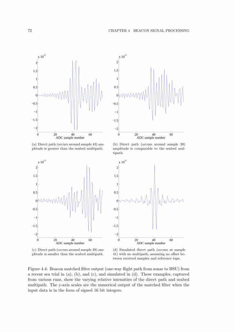
72 CHAPTER 4 BEACON SIGNAL PROCESSING
0 20 40 60
−2
−1.5
−1
−0.5
0
0.5
1
1.5
2
x 1011
ADC sample number
(a) Direct path (occurs around sample 43) am-plitude is greater than the seabed multipath.
0 20 40 60
−2
−1.5
−1
−0.5
0
0.5
1
1.5
2
x 1011
ADC sample number
(b) Direct path (occurs around sample 39)amplitude is comparable to the seabed mul-tipath.
0 20 40 60
−2
−1.5
−1
−0.5
0
0.5
1
1.5
2
x 1011
ADC sample number
(c) Direct path (occurs around sample 39) am-plitude is smaller than the seabed multipath.
0 20 40 60
−2
−1.5
−1
−0.5
0
0.5
1
1.5
2
x 1011
ADC sample number
(d) Simulated direct path (occurs at sample41) with no multipath, assuming no offset be-tween received samples and reference taps.
Figure 4.4: Beacon matched filter output (one-way flight path from sonar to BSU) froma recent sea trial in (a), (b), and (c), and simulated in (d). These examples, capturedfrom various runs, show the varying relative intensities of the direct path and seabedmultipath. The y-axis scales are the numerical output of the matched filter when theinput data is in the form of signed 16 bit integers.

4.2 FILTERING THE CHIRP FROM THE RECEIVED SIGNAL 73
0 2 4 6 8 10 12 14 16−8000
−6000
−4000
−2000
0
2000
4000
6000
8000
Reference taps
Am
plitu
de
(a) First few taps.
1382 1384 1386 1388 1390 1392 1394 1396 1398 1400−8000
−6000
−4000
−2000
0
2000
4000
6000
8000
Reference taps
Am
plitu
de
(b) Last few taps.
Figure 4.5: Timing offsets of 0, 0.25, 0.5, and 0.75 samples corresponding to red, blue,green and black sets of taps respectively. The stars show the resultant waveform if allthe taps were appropriately delayed and combined into a single large set of taps. They-axis scales result from the samples being in the form of signed 16 bit integers.

74 CHAPTER 4 BEACON SIGNAL PROCESSING
694 696 698 700 702 704 706−8
−6
−4
−2
0
2
4
6
8x 10
11
ADC Sample number
(a) The four correlations for the four sets of taps. The circles are the highest points after oversamplingof the waveforms. If oversampling the complete matched filter output was feasible then any of the fouroutputs will produce a peak close to the TOA.
694 696 698 700 702 704 7060
1
2
3
4
5
6
7
8x 10
11
ADC Sample number
(b) Absolute value of the above plot. The beacon does not have enough processing power to oversamplethe correlation outputs so instead, relies on picking the highest sample (after taking the absolute value,shown by the square symbols) and then interpolating about that point. With four outputs to choosefrom this works well for the typical noise levels encountered at sea, i.e., the blue output has the highestsample here. However, if only one set of taps was used, e.g., black, the highest sample is not alwaysthe one closest to the TOA, producing a large error.
Figure 4.6: Correlations using multiple sets of taps with timing offsets of 0, 0.25, 0.5,and 0.75 samples corresponding to red, blue, green and black respectively. The verticaldashed line is the exact TOA of the echo which has an offset of 0.25 samples. Asexpected, the highest peak is the closest match and belongs to the blue output becauseit has the same offset as the echo. The y-axis scales are the numerical output of thematched filter when the input data is in the form of signed 16 bit integers.

4.2 FILTERING THE CHIRP FROM THE RECEIVED SIGNAL 75
to merge together. Fig. 4.7 shows the geometry and Fig. 4.4 shows the effect on realcorrelation data. It can be seen that the algorithm needs to find the highest pointcorresponding to the direct path and ignore the (possibly higher) subsequent peaksdue to multipath. The key is having enough separation between the peaks to be ableto identify the general trend of rising data values before the direct path peak andsufficient smaller data values after it.
It was originally assumed that the multipath amplitude would be small due tothe absorption of the signal energy by the seabed. However, a surprising discoverywas that the seabed multipath amplitude is often greater than that of the direct path.This is thought to be due to constructive interference of echoes from different parts ofthe seabed, i.e., a focusing effect caused by the uneven bottom, as shown in Fig. 4.7.Once this was discovered, the original beacon design was modified to raise the beacontransducer further off the seabed, to provide greater separation of the peaks in thematched filter output. With a clear separation between the peaks, it is possible toidentify the direct path peak even if the subsequent peaks are higher. Increasing theseparation is also important for reducing the error caused by the superposition of themultipath peak (and sidelobes) with the direct path peak in the matched filter output,distorting the direct path peak shape. This is explained further in Sec. 4.3 with examplematched filter output waveforms. Fig. 3.8 shows the beacon design before and afterthis change.
4.2.4 Step 3: Subsample peak fitting
Once the highest sample of the direct path has been found, a quadratic is fitted throughthis sample and the adjacent samples. An example, along with other types of curves,is shown in Fig. 4.14. If the coordinates of the highest sample are given by (t2, y2) andthe adjacent samples by (t1, y1) and (t3, y3) then the coordinates, (tp, yp), of the peakof a quadratic of the form
y = At2 +Bt+ C, (4.17)
where t represents time, are calculated using6
tp = − B
2A, (4.18)
yp = At2p +Btp + C. (4.19)
6While the calculation of the height of the peak, yp, is not required to determine the TOF, it isuseful for diagnostic purposes, e.g., an unusually low value indicates a sidelobe peak, rather than themain peak, has been found.

76 CHAPTER 4 BEACON SIGNAL PROCESSING
(a) A single seabed multipath reflection onto the beacon. The direct path (dashed) is likely to be thestronger signal.
(b) Uneven seabed focusing many reflections onto the beacon. The multipath signal is likely to bestronger than the direct path signal.
Figure 4.7: Diagram of the direct acoustic path and the multipath reflections from theseabed. The shallow water geometry means the length difference between the directpath and the seabed reflection is very small. The surface reflection (not shown) arrivesmuch later so is easily identified and rejected.

4.2 FILTERING THE CHIRP FROM THE RECEIVED SIGNAL 77
A, B, and C are found from the three highest correlation samples using
A =(y1 − y2)/(x1 − x2)− (y2 − y3)/(x2 − x3)(x2
1 − x22)/(x1 − x2)− (x2
2 − x23)/(x2 − x3)
, (4.20)
B =y1 − y2 −A(x2
1 − x22)
x1 − x2, (4.21)
C = y1 −Ax21 −Bx1. (4.22)
tp is then quantised to the DSP clock period, with a resolution of 28 ns, to give theTOA of the chirp in clock pulses. Figure 4.8 shows these steps.
yes
Begin step 3
Find A, B, and C coefficients of a quadratic fitted
through the peak and adjacent values
Find exact quadratic peak height and
fractional position between values
Quantise fractional position to a whole number of
DSP timer1 clock cycles to determine what the
DSP timer1 reading was when the peak occurred
Begin step 4
Determine what the DSP timer1 reading will be at
TAT seconds after the peak reading and sleep until
DSP timer1 reaches this reading.
25ms TAT elapsed on DSP timer1
since peak occurred?
Stop DSP timer1 and
transmit 60-80kHz chirp
Figure 4.8: Flow diagram of step 3: subsample peak fitting, and step 4: time stampingand transmitting.

78 CHAPTER 4 BEACON SIGNAL PROCESSING
4.2.5 Step 4: Time stamping and transmitting
While the TOA is being determined, the DSP timer counts the elapsed clock pulsessince the ADC sampling began. This allows the DSP to determine how many clockpulses it must wait before transmitting a 60–80 kHz chirp reply back to the sonar suchthat the TAT is exactly 25 ms as explained in Sec. 3.4.1.2. Figure 2.4 shows a timelineand Figure 4.8 shows the flow diagram.
The reply chirp is generated by the DSP once at startup, using discrete versionsof (4.6) combined with (4.7), and stored as a lookup table in RAM. Although this per-manently ties up that RAM, it means the DMA can control the transmission, allowingthe CPU to perform other tasks.
4.3 MULTIPATH ACCURACY STUDY
Multipath causes additional delayed copies of s(t) to sum coherently at the beacon,e.g., for a direct path signal and a single seabed multipath signal delayed by τ1 fromthe direct path, the echo received by the beacon (in the absence of medium distortion)is
e(t) = αs(t) + α1s(t− τ1), (4.23)
where α and α1 represent the scaling of the signal strength due to energy loss inthe medium. Section 4.2.3.2 showed how constructive interference between multipathsignals can produce delayed multipath peaks of greater amplitude than the direct pathpeak, requiring a complicated approach to identifying the direct path peak. A moresubtle problem is the superposition of the multipath sidelobes and the direct path peakcausing a skew in the peak shape resulting in an error in the TOA estimate. Thisoccurs because the matched filter output is the sum of the direct and delayed copiesof the sonar transmit chirp. If the multipath peaks are sufficiently close to the directpath peak, the amplitude of the direct path samples are affected. Table 4.2 shows thedirect path and multipath TOFs for some typical geometries of the KiwiSAS sonar andactive beacon.
4.3.1 TOA error due to multipath superposition
A simulation was performed to measure the error due to multipath superposition. Adelay between the direct path and the seabed multipath of 10 ADC samples, i.e., the30 m case in Table 4.2, was used. For completeness, the sea surface multipath is includedwith a delay of 175 samples despite this being sufficiently large to have no effect. Thematched filter output is shown in Fig. 4.9(a) where the envelope is also plotted to show

4.4 MATCHED FILTER ACCURACY STUDY 79
Sonar transmitter height off seabed (m) 3Beacon transducer height off seabed (m) 0.65
Water depth (m) 8Horizontal separation (m) 20 30 40
Direct path TOF (m), (ms) 20.1, 13.4 30.1, 20.1 40.1, 26.7Seabed multipath TOF (m), (ms) 20.3, 13.6 30.2, 20.1 40.2, 26.8Surface multipath TOF (m), (ms) 23.5, 15.7 32.4, 21.6 41.9, 27.9
Seabed/Direct difference (µs), (samples) 128, 14.4 86.2, 9.64 64.8, 7.25Surface/Direct difference (ms), (samples) 2.25, 251 1.57, 175 1.2, 134
Table 4.2: The direct path, seabed multipath, and surface multipath path lengths(given as times in ms and the equivalent distance in m) between the sonar and thebeacon for some typical geometries.
the separation between the peaks more clearly. The multipath amplitude was chosento be 0.8 of the direct path amplitude.
4.3.1.1 Simulation results
The skew of the direct path peak, shown in Fig. 4.9(b), produces a timing error of400 ns or 0.6 mm, well under the target accuracy of <1 cm defined in Sec. 1.4. Fig. 4.10shows the error at different seabed/direct path delays. The beacon error is still under1 mm when the multipath arrival is only five samples behind the direct path, allowingoperation beyond 40 m using the geometry of column three in Table 4.2. When thedelay is between zero samples and three samples, the error becomes very large becausethe multipath and direct path peaks merge together.
The error can be further reduced by using a window to shape the matched filteroutput to reduce the sidelobes of the peaks. This is investigated further in Chapter 8.
4.4 MATCHED FILTER ACCURACY STUDY
The detection task (detecting a known signal in the presence of noise) is common forradar and sonar systems [Van Trees 1968, ch8-14]. Here the signal, s(t), is a linearfrequency modulated (FM) chirp transmitted by the sonar, shown in Fig. 4.11, and thenoise, n(t), is a combination of ambient sea noise and electronic noise in the beacon.For simplicity, and in the absence of good measurements, the noise is assumed to beadditive white Gaussian noise (WGN). The beacon samples the incoming signals at112 kHz and the noise is assumed to have constant power spectral density, over thefrequencies of interest, as shown in Fig. 4.12.

80 CHAPTER 4 BEACON SIGNAL PROCESSING
2100 2150 2200 2250 2300 2350 2400 2450 2500
−5
0
5
x 1011
ADC sample number
(a) Peaks from left to right: direct path, seabed multipath, sea surface multipath. The sea surfacemultipath (sample 2374) delay is large enough to have no effect on the direct path signal (sample 2199).
2197.5 2198 2198.5 2199 2199.5 2200
−5
0
5
x 1011
ADC sample number
(b) Closeup of the direct path peak of (a) showing how the sidelobes of the seabed multipath peakhave interfered with the direct path samples adjacent to the peak which would otherwise have thesame amplitude. The result is sample 2200 is higher than sample 2198, causing the interpolated peak(circle) to shift to the right of the true TOA (magenta line).
Figure 4.9: Matched filter output of a simulation of the beacon DSP operation usingthe geometry from the 30m column of Table 4.2. The magenta line and red crossesshow the true TOA of the direct path and multipaths respectively. The blue circleshows the peak of the direct path after quadratic interpolation. The green line is theenvelope. For comparison, Fig. 4.4(d) shows an example of a direct path signal withoutmultipath. The y-axis scales are the numerical output of the matched filter when theinput data is in the form of signed 16 bit integers.
4 6 8 10 12 14 16 18 20
−2
−1
0
1
2
Seabed/Direct path difference (samples)
TO
F e
rror
(m
m)
Figure 4.10: Simulation of the the situation of Fig. 4.9, varying the seabed multipathdelay. Once the delay is greater than five samples, the distortion it causes to the directpath peak TOA estimate is less than ±1 mm.

4.4 MATCHED FILTER ACCURACY STUDY 81
Figure 4.11: Received echo spectrum, S(f).
Figure 4.12: Received noise spectrum, N(f).
Of all linear filters, the matched filter yields the largest output SNR for WGN[Helstrom 1995, p50][Rihaczek 1969, pp28-30].7 The following sections present equa-tions for the theoretical gain and accuracy, in terms of typical sonar parameters, andsimulations to verify the theory. Chapter 6 presents experimental results using thebeacon in a test-tank.
4.4.1 Theoretical accuracy
It has been shown [Helstrom 1968, p276], [Woodward 1964, p105], [Rihaczek 1969, p47],[Whalen 1971, pp337-339] that the Cramer-Rao lower bound (CRLB) of the standarddeviation (STD) of the TOF error (in seconds), when using a matched filter to detecta reference chirp s(t) from an echo corrupted by WGN n(t), is given by
σD =1
2πβ0
√SNRMF
(4.24)
where β0 is the root of the second moment of the normalised energy density spectrumof the chirp signal8,
β0 =
√∫ ∞0 f2|S(f)|2 df∫ ∞0 |S(f)|2 df
, (4.25)
7With the addition of a whitening filter, the matched filter is also the optimal filter for colourednoise [Rihaczek 1969, pp28-30], [Whalen 1971, pp170-173].
8β0=30789Hz for the KiwiSAS tapered linear FM chirp of 20 kHz bandwidth centred on 30 kHz.

82 CHAPTER 4 BEACON SIGNAL PROCESSING
where S(f) is the (complex) FT of the reference chirp in V/Hz. SNRMF is the SNRat the output of the matched filter and can be equivalently defined as either [Hel-strom 1995, p50]
SNRMF =E2
MF
σ2MF
(4.26)
or [Helstrom 1995, p47]
SNRMF =2EN0
(4.27)
where EMF is the peak of the matched filter output with the echo as the only input,σ2
MF is the matched filter output variance with noise as the only input, E is the energyof the reference chirp in joules, and N0
2 is the noise power spectral density (assumedconstant) in W/Hz. Equation (4.27) can be calculated from
2EN0
=1fs
∑Ni=1 |s[i]|
2
N02
, (4.28)
=1fs
∑Ni=1 |s[i]|
2
σ2n
fs
, (4.29)
=∑N
i=1 |s[i]|2
σ2n
, (4.30)
where fs is the sampling frequency in Hz, s[i] = s( ifs
), N is the number of samples inthe chirp, and σ2
n is the variance of the in-band noise in watts, i.e., the noise containedin the bands in Fig. 4.11.
The SNR at the input of the matched filter, i.e., after the analog amplification anddigital sampling stages, is the ratio of the chirp energy to the in-band noise energy
SNRi =E
2WT N02
(4.31)
where T is the chirp length in seconds, and W is the chirp bandwidth in Hz. The SNRgain is
ηSNR =SNRMF
SNRi, (4.32)
= 2WT. (4.33)
Sometimes the SNR gain of a matched filter is given in radar and sonar literature asjust WT . This arises when the output SNR is defined using the average signal energyrather than the peak used in (4.26) [Curlander and McDonough 1991, p130].
It is useful to be able to express (4.24) in terms more commonly used when param-

4.4 MATCHED FILTER ACCURACY STUDY 83
eterising sonar systems. Using the method from Quazi [Quazi 1981], which assumesrectangular spectra as shown in Figs. 4.11 and 4.12, and substituting the limits ofintegration into (4.25) leads to
β0 =
√√√√ |S(f)|2∫ f2
f1f2 df
|S(f)|2∫ f2
f1df
, (4.34)
=
√13
(f22 + f1f2 + f2
1
), (4.35)
so that (4.24) becomes
σD =1
2π√
13
(f22 + f1f2 + f2
1
)√SNRMF
. (4.36)
Making the following substitutions using the centre frequency, f0, in Hz;
f1 = f0 −W
2, f2 = f0 +
W
2, (4.37)
yields
σD =1
2πf0
√1 + W 2
12f20
√SNRMF
(4.38)
and substituting (4.33) gives
σD =1
√8πf0
√TW
√1 + W 2
12f20
√SNRi
. (4.39)
Inspection of (4.39) reveals the standard deviation can be reduced by increasing theSNR, signal duration, bandwidth, or operating frequency.
4.4.2 Simulations
A Monte Carlo simulation was performed to verify the STD predictions of (4.39) and(4.24) using (4.26) and (4.27). The detection method and sampling rate were the sameas used in the beacon. The simulations consisted of 20 runs where each run measuredthe TOF STD from 2000 trials9 and each trial involved matched-filtering 1 receivedecho in the presence of WGN. Several methods of peak-finding were investigated anddetails of these are provided in the next section. Four separate cases were studied. Caseone involved varying the sampling offset, i.e., the phase, of the received echo. Case twoinvolved varying SNRi. Case three involved varying the width of the kernel used to
9This size was chosen for practicality, resulting in overnight simulation times.

84 CHAPTER 4 BEACON SIGNAL PROCESSING
oversample the matched filter output. Case four involved varying the oversamplingfactor.
In all cases the three approaches to calculating the theoretical CRLB were in closeagreement with the simulated STD when a high level of sinc oversampling was used onthe matched filter output. Unfortunately the processing time and memory requirementsof this approach make it impractical for use in the beacon so the following discussionsfocus on the performance and trade-offs resulting from using alternative peak-findingmethods.
4.4.2.1 Peak-finding algorithms applied to the matched filter output
The beacon samples the incoming echo slightly faster (112 kHz) than the Nyquist rate(80 kHz) so the matched filter output has a low resolution. Using a peak-finding algo-rithm provides a significant increase in timing resolution.
A number of approaches were investigated, each requiring different amounts of pro-cessing time and memory storage. These are summarized in Table 4.3 and Figures 4.13,4.14, and 4.15. “Oversampling” is used here to describe the process of reconstructingadditional samples in the matched filter output. This interpolation is performed us-ing a FIR filter where the kernel taps are a truncated-sinc waveform, i.e., a sinc withfinite extent. Although a frequency domain approach would be computationally moreefficient, the time domain was used because that would be more easily implemented inthe beacon DSP. This method of interpolation is valid if a signal is band-limited (i.e.,sampled above Nyquist) [Schwartz and Shaw 1975, p43] and this condition is met inthe beacon because of the built in low-pass filter in the sigma-delta ADC.
4.4.2.2 Case 1: Varying the received echo sample offset
In the real world, the clock in the sonar that generates the chirps and the clock inthe beacon that controls the ADC sampling are not synchronised so the echo sampleoffset will change with every ping, even when the range is fixed like in the mediumfluctuation experiments in Chapter 6. To investigate this, the echo sample offset wasvaried in discrete steps between 0 and 0.25 samples.
Upon inspection of Fig. 4.16(a) it would seem for most of the offsets that quadraticfitting is a good method, producing a lower STD (green line, square markers) than theCRLB (red lines).10 However, Figs. 4.16(b)–4.16(d) show (green diamonds) that theTOF error is not centred about zero, i.e., the TOF estimates are not centred aboutthe true value, except when the echo samples align with the taps samples at 0 and0.25 samples of offset. Although the variation in the TOF estimate is low, the TOFestimates are biased, producing a large TOF RMS error for most echo sample offsets.
10The CRLB is a bound on an unbiased estimator. If a biased estimator is used then the STD andthe RMS of the estimates can be lower than the CRLB.

4.4 MATCHED FILTER ACCURACY STUDY 85
Description Processing cost Memory cost
Quadratic:
Fit a quadratic through the threehighest samples. Find the peak ofthe quadratic.
A few calculations. Negligible.
Linear-quadratic:
Use linear interpolation to find twonew samples, adjacent to the high-est sample, and fit a quadraticthrough these new samples and thehighest sample. Find the peak ofthe quadratic.
A few calculations. Negligible.
Sinc:
Use sinc interpolation, with a largekernel size nk, between the high-est two samples to generate ns newsamples. Choose the highest sam-ple.
nkns MAC opera-tions followed by ns
comparisons.
nkns kernel taps.
Partial sinc:
Use sinc interpolation, with a smallkernel size nk, between the high-est two samples to generate ns newsamples. Choose the highest sam-ple.
nkns MAC opera-tions followed by ns
comparisons.
nkns kernel taps.
Partial sinc-quadratic:
Same as the partial sinc methodwith the additional step of fittinga quadratic through the three high-est samples. Find the peak of thequadratic.
As for partial sincplus a few calcula-tions.
As for partial sincplus a negligible ad-ditional amount.
Table 4.3: Comparison of the peak-finding methods that were investigated in the sim-ulation. Diagrams are provided in Figs. 4.13–4.15. The sinc method is impractical tocalculate in the beacon in real-time but is included in the simulations as a “best case”reference. The quadratic method is currently used in the beacon because of its speed(low processing cost), size (negligible memory cost), and simplicity of implementation.

86 CHAPTER 4 BEACON SIGNAL PROCESSING
694 696 698 700 702 704 706
−8
−6
−4
−2
0
2
4
6
8
x 1011
ADC Sample number
Figure 4.13: Matched filter output illustrating the various methods of peak-finding inTable 4.3. Close-ups are shown in Figs. 4.14 and 4.15. The y-axis scale is the numericaloutput of the matched filter when the input data is in the form of signed 16 bit integers.See Fig. 4.15 for legend.
699 699.5 700 700.5 701
−2
−1
0
1
2
3
4
5
6
7
8x 10
11
ADC Sample number
Figure 4.14: Close-up of the peak area of Fig. 4.13 showing how the peak-findingmethods are applied to the three highest samples. The y-axis scale is the numericaloutput of the matched filter when the input data is in the form of signed 16 bit integers.See Fig. 4.15 for legend.

4.4 MATCHED FILTER ACCURACY STUDY 87
699.75 699.8 699.85 699.9 699.95 700
7.25
7.3
7.35
7.4
7.45
x 1011
ADC Sample number
Noisy data samplesLinear−quadratic fitQuadratic fitSinc fitPartial sinc fitPartial sinc−quadratic fitLinear−quadratic peakQuadratic peakSinc peakPartial sinc peakPartial sinc−quadratic peakActual peak time
Figure 4.15: Close-up of the highest data sample of Fig. 4.13 showing the accuracy ofthe fitted peaks compared with the true peak time (pink vertical dashed line). Thesignal to noise ratio at the matched filter input (SNRi) is 6 dB and the fractional offsetof the received echo is 0.125 samples from a nominal arrival time coinciding with ADCsample 700. The computationally expensive sinc method (peak: black cross) useda kernel width of nk = 40 samples and an oversampling factor of ns = 1000 but wasmatched in performance by the faster partial sinc-quadratic method (peak: pink circle)using the same kernel width and an oversampling ratio of ns = 10. The y-axis scale isthe numerical output of the matched filter when the input data is in the form of signed16 bit integers.

88 CHAPTER 4 BEACON SIGNAL PROCESSING
The STD statistic hides this offset so the RMS statistic is a better measure to use andthis can be seen back in Fig. 4.16(a) where the RMS error is plotted for the quadraticmethod (green line, asterisk markers). The offset-dependent bias in the estimates isworse for the linear-quadratic method. However, there is no bias with any of themethods based on sinc interpolation, i.e., the STD of the error and the RMS error ofthe TOF estimates are equal.
The large rise in STD of the quadratic based methods when the offset approaches0.125 samples is explained as follows: The echo samples lie half way between the firsttwo sets of taps11 so the noise dictates which set best matches the received echo for anyparticular run. This can be seen in Fig. 4.16(b) where the offset is 0.1255 samples andthe TOF error alternates between two bands centred at ±380 ns resulting in a largeSTD of ∼380 ns.
Of the sinc-based methods the partial sinc method produces good results and thesinc and partial sinc-quadratic methods produce excellent, nearly-identical results thatclosely follow the CRLB. The extra quadratic step of the partial sinc-quadratic methodis clearly worth doing considering the small computational cost.
4.4.2.3 Case 2: Varying the SNR
Figure 4.17 shows that all peak-finding methods produced STDs that followed theinverse trend predicted by the theory. However, as in Case 1, the methods based onsinc interpolation produced STDs that closely matched the CRLBs while the methodsbased on quadratic interpolation did not match well, particularly at low SNRs wherethey were highly dependent on the received echo fractional offset.
As the SNR drops, the wrong set of taps is more frequently selected as being thebest match to the echo (because spurious noise samples distort the amplitude of thematched filter output). This does not affect the methods based on sinc interpolationbut produces a large TOF error with the quadratic based methods. The point at whichthis starts to occur is around -2 dB in Fig. 4.17(b) and around 3 dB in Fig. 4.17(c)where a discontinuity in the curves based on the quadratic methods can be seen.
At the plotted SNR the highest sample is always being correctly identified. How-ever, as the SNR drops below -7 dB, samples within the side lobes of the matched filteroutput are sometimes higher than the samples within the true peak. The peak findingis then applied in the wrong place so the system fails.
11See Section 4.2.3.1 for an explanation of the use of multiple sets of taps.

4.4 MATCHED FILTER ACCURACY STUDY 89
0 0.05 0.1 0.15 0.2 0.250
100
200
300
400
500
600
700
800T
ime
(ns)
Received echo fractional offset (samples)
CRLB #1CRLB #2CRLB #3Linear−quadratic RMS errorLinear−quadratic std devQuadratic RMS errorQuadratic std devPartial sinc RMS errorPartial sinc std devPartial sinc−quadratic RMS errorPartial sinc−quadratic std devSinc RMS errorSinc std dev
(a) CRLB and simulated TOF RMS error and STD of error for an echo arriving at the beaconwhen the received echo sample offset is varied. CRLB #1 was calculated from (4.27). CRLB #2was calculated from (4.26). CRLB #3 was calculated from (4.39). The CRLB data (red) is hiddenbehind the sinc data (black).
0 500 1000 1500 2000−1000
−500
0
500
1000
Iteration #
Err
or (
ns)
Linear−quadraticQuadraticSincPartial sincPartial sinc−quadratic
(b) Received echo offset: 0.1255 samples.
0 200 400 600 800 1000 1200 1400 1600 1800 2000−600
−400
−200
0
200
400
600
Iteration #
Err
or (
ns)
(c) Received echo offset: 0.0255 samples.
0 200 400 600 800 1000 1200 1400 1600 1800 2000−600
−400
−200
0
200
400
600
Iteration #
Err
or (
ns)
(d) Received echo offset: 0.2245 samples.
Figure 4.16: Simulated results showing the effect of varying the received echo sampleoffset. SNRi for these trials was 6 dB. The sinc-based methods used a kernel width of40 samples and an oversampling factor of 32.

90 CHAPTER 4 BEACON SIGNAL PROCESSING
−10 0 10 20 300
200
400
600
800
1000
Tim
e (n
s)
Input SNR (dB)
CRLB #1CRLB #2CRLB #3Linear−quadratic RMS errorLinear−quadratic std devQuadratic RMS errorQuadratic std devPartial sinc RMS errorPartial sinc std devPartial sinc−quadratic RMS errorPartial sinc−quadratic std devSinc RMS errorSinc std dev
(a) Received echo offset: 0.1255 samples.
−10 −5 0 5 10 15 20 25 300
100
200
300
400
500
600
Tim
e (n
s)
Input SNR (dB)
(b) Received echo offset: 0.0255 samples.
−10 −5 0 5 10 15 20 25 300
100
200
300
400
500
600
700
Tim
e (n
s)
Input SNR (dB)
(c) Received echo offset: 0.18 samples.
Figure 4.17: CRLB and simulated TOF RMS error and STD of error for an echoarriving at the beacon when SNRi is varied. CRLB #1 was calculated from (4.27).CRLB #2 was calculated from (4.26). CRLB #3 was calculated from (4.39). TheCRLB data (red) is hidden behind the sinc data (black). The sinc-based methods useda kernel width of 40 samples and an oversampling factor of 32.

4.4 MATCHED FILTER ACCURACY STUDY 91
4.4.2.4 Case 3: Varying the oversampling kernel width
Figure 4.18 shows (as a general trend) that both sinc-based, peak-finding methodsproduce better results when larger sinc kernels are used.12 However, larger kernelsrequire more computation and consume more memory storage and the returns rapidlydiminish as the kernel width increases. Choosing the minimum kernel width that givesacceptable accuracy is important for an embedded system.
Figure 4.18(a) shows that when the oversampling factor is essentially unlimited(here we use 1000) a kernel width of 40 samples allows both partial methods to achievesimilar accuracy to the sinc method which uses the same oversampling level. In apractical implementation the oversampling factor will be much lower, as shown inFigs. 4.18(b) and 4.18(c), but kernel widths of 40 samples still achieve a similar level ofperformance when the partial sinc-quadratic method is used. Reasonable performanceis still achieved using this method with kernel widths of 20. Once again, it significantlyoutperforms the partial-sinc method when practical (i.e., low) levels of oversamplingare used.13
4.4.2.5 Case 4: Varying the oversampling factor
Figure 4.19 shows (as a general trend) that both sinc-based, peak-finding methods pro-duce better results when higher levels of oversampling are used. However, higher over-sampling requires more computation and consumes more memory, c.f. Table 4.3, andreturns rapidly diminish. This is especially noticeable with the partial sinc-quadraticmethod which benefits little from oversampling factors higher than 10. In Figs. 4.19(a)and 4.19(b) it achieves comparable accuracy to the sinc method with less than 10 timesoversampling. Contrast this with partial-sinc method which is not close to the CRLBeven after 20 times oversampling. As with case 1 the extra quadratic step of the partialsinc-quadratic method is clearly worth doing considering the small computational cost.
Odd effects can occur with the partial sinc method at low oversampling rates,requiring careful interpretation. The apparent “near perfect detection” with an over-sampling factor of 8 occurs in this example because the matched filter peak happensto lie close to 1
8 of an ADC sample for this particular value of received echo sampleoffset (0.1255 samples). The oversampled samples also line up well with an oversam-pling factor around 16 however the quantisation level is now sufficiently fine that thepresence of noise means the highest matched filter sample is not always the same oneso a greater variation is observed.
12Local exceptions to this trend, e.g., in Fig. 4.18(a) a kernel width of 24 appears to give morevariation than one of 14, are highly dependent on the received echo offset. Here a near worst-case offsetof 0.1255 samples is used so these effects are emphasized.
13Fig. 4.18(b) shows an example of how low oversampling rates produce no benefit for the partial-sincmethod if the original matched filter output samples already lie close to the peak.

92 CHAPTER 4 BEACON SIGNAL PROCESSING
0 5 10 15 20 25 30 35 40100
110
120
130
140
150
160
170
180
190
200
Tim
e (n
s)
Kernel width
CRLB #1CRLB #2CRLB #3Partial sinc RMS errorPartial sinc std devPartial sinc−quadratic RMS errorPartial sinc−quadratic std devSinc RMS errorSinc std dev
(a) Oversampling factor: 1000.
0 5 10 15 20 25 30 35 40100
150
200
250
300
350
400
Tim
e (n
s)
Kernel width
(b) Oversampling factor: 12.
0 5 10 15 20 25 30 35 40100
120
140
160
180
200
220
240
Tim
e (n
s)
Kernel width
(c) Oversampling factor: 32.
Figure 4.18: CRLB and simulated TOF RMS error and STD of error for an echoarriving at the beacon when the sinc kernel width is varied. SNRi for these trialswas 6 dB and the received echo offset is set to the worst case situation; 0.1255 samples.CRLB #1 was calculated from (4.27). CRLB #2 was calculated from (4.26). CRLB #3was calculated from (4.39). The CRLB data (red) is hidden behind the sinc data(black).

4.4 MATCHED FILTER ACCURACY STUDY 93
0 2 4 6 8 10 12 14 16 18 200
200
400
600
800
1000
1200
Tim
e (n
s)
Oversampling ratio
(a) Kernel width: 20.
0 2 4 6 8 10 12 14 16 18 200
200
400
600
800
1000
1200
Tim
e (n
s)
Oversampling ratio
(b) Kernel width: 40.
0 2 4 6 8 10 12 14 16 18 20−50
0
50
100
150
200
Tim
e (n
s)
Oversampling ratio
CRLB #1CRLB #2CRLB #3Partial sinc RMS errorPartial sinc std devPartial sinc−quadratic RMS errorPartial sinc−quadratic std devSinc RMS errorSinc std dev
(c) Closeup of Fig. 4.19(a).
Figure 4.19: CRLB and simulated TOF RMS error and STD of error for an echoarriving at the beacon when the received echo sinc oversampling ratio is varied. SNRi
for these trials was 6 dB and the received echo offset is set to the worst case situation;0.1255 samples. CRLB #1 was calculated from (4.27). CRLB #2 was calculated from(4.26). CRLB #3 was calculated from (4.39). The CRLB data (red) is hidden behindthe sinc data (black).

94 CHAPTER 4 BEACON SIGNAL PROCESSING
4.4.3 Study conclusions
The current peak-finding method used in the beacon, based on quadratic fitting withfour sets of reference taps, is not the best method to use when the data sampling isclose to Nyquist. It will produce a TOF RMS error that is significantly higher thanthe theoretical CRLB, due to the TOF mean being biased from the true TOF, whenthe echo samples do not align with the reference taps. A better approach is to usea method based on sinc interpolation to oversample the matched filter output. Thiseliminates the bias so the TOF RMS error matches the theoretical CRLB regardlessof SNR or sample offset. In addition, this method is independent of the received echosample offset and behaves predictably over a wide range of SNR levels.
Sinc oversampling methods require more memory storage and processing than sim-ple quadratic peak finding so the system must be optimally designed to be practicalas an embedded system. More taps and more oversampling requires more memory andmore processing so a partial sinc method using a reduced number of taps and mini-mal oversampling is required. The simulations suggest good results can be achievedwith kernel widths of 20 taps combined with an oversampling ratio of 8, provided theoversampling is followed by a quadratic peak finding step. This extra step significantlyimproves performance for very little extra computational or memory storage cost.
The processing cost of sinc oversampling methods can be further reduced by adopt-ing a binary search process where the true peak is always assumed to lie between thetwo highest samples, eliminating the need to compute samples outside this successivelydiminishing region [Sabel and Cowley 1992, Ragauskas and Bagdonas 2005].
4.5 SONAR TRANSMIT BEAM PATTERN (BP)
The KiwiSAS sonar uses a rectangular 36 element transmitter array as shown inFig. 4.20(a) resulting in an angular-dependent, sinc-like, BP. The transmitted FMwaveform has a large bandwidth (compared to the centre frequency) so the BP shapechanges during the duration (12.5 ms) of each chirp. This is illustrated in Figs. 4.20(b)and 4.20(c). Of particular interest are the null angles and how they translate into nullregions on the seabed both during a chirp (intra-chirp null motion) and as the sonarmoves. If the beacon lies in a null region it cannot detect the sonar so no navigationdata will be available for those pings. A greater problem is when the beacon lies neara null region. This means it receives a weak or fluctuating signal and produces an inac-curate estimate of the TOF. These estimates must somehow be identified and removedfrom the navigation data and this is discussed further in Sec. 4.6.3.

4.5 SONAR TRANSMIT BEAM PATTERN (BP) 95
(a) Projector array (plan and elevation views).
−30dB −25dB −20dB −15dB −10dB −5dB
0dB
0°
15°
30°
45°
60° 75°90°
−90°−75°−60°
−45°
−30°
−15°
(b) Horizontal BP varying θ, ϕ = 0.
−30dB −25dB −20dB −15dB −10dB −5dB
0dB
0°
15°
30°
45°
60° 75°90°
−90°−75°−60°
−45°
−30°
−15°
(c) Vertical BP varying θ, ϕ = 90.
Figure 4.20: KiwiSAS projector layout and polar plot of the transmit BP in two dimen-sions at 20kHz (blue), 30 kHz (red), and 40 kHz (green) showing the changing shapeduring a chirp.

96 CHAPTER 4 BEACON SIGNAL PROCESSING
4.5.1 OF, TVR, RPR, and directivity equations
All transducers and arrays have an angular-dependent component to their acoustic re-sponse. This component is called the beam pattern (BP) and, provided the transmitteris reversible14, is identical for transmitting and receiving [Kinsler 2000, p193–195]. Itarises from the superposition of signals, originating from different locations, causing ar-eas of constructive and destructive interference in the acoustic field. This is illustratedin Fig. 4.21(a). The BP is usually presented as a polar plot of pressure as a functionof angle, θ and or ϕ, defined in Fig. 4.20(a), and acoustic frequency, f , normalised tothe broadside value, i.e., the value when θ and ϕ are zero.
The transducer transmit voltage response (TVR) is the radiated pressure15 pro-duced by an applied voltage in dB re 1V/µPa @1m at broadside. The receive pressureresponse (RPR) is the measured voltage given the applied pressure at the transducerin dB re 1V/µPa. The total response of a transducer, known as the directivity, can befound by multiplying the angular dependent component, i.e., the BP, by the broadsidecomponent [Urick 1975, p50], i.e., the TVR for a projector or RPR for a hydrophone.Using the example of a projector gives
p(f, θ, ϕ|r, L, V ) = pBS(f |r, L, V )BP(f, θ, ϕ) (4.40)
in Pa/Hz where pBS(f |r, L, V ) is the pressure at broadside. Plots of p(f, θ|r, L, V )(directivity plots) and pBS(f |r, L, V ) (TVR plots) are given in transducer datasheets.Directivity is plotted on a polar plot to show the variation of pressure (for projectors) orvoltage (for hydrophones) with angle when frequency is held constant. TVR and RPRare plotted on Bode plots to show the variation of absolute pressure (or voltage in thecase of the RPR plot) with frequency at broadside. Directivity is usually normalisedto the highest overall dB value over the range of frequencies and angles considered.
The BP equation is normalised so is equivalent to a directivity plot at a singlefrequency. To compare the complete response at multiple angles and frequencies, oftwo theoretical transducer designs or a theoretical design with experimental pressuremeasurements from a real transducer, pBS(f |r, L, V ) needs to be specified for the trans-ducers. This is required for the KiwiSAS because of the wide bandwidth of the FMwaveforms. Appendix J shows a derivation of far-field BP, directivity, and TVR of theKiwiSAS projector and the next section discusses how well it matches observations ofreal transducers. The RPR is derived in Appendix K and the receive directivity canbe found by multiplying the RPR by the BP, analogous to the relationship describedby (4.40).
14Aside from obvious exceptions, e.g., a built in preamp, most transducers are reversible, providedthey are not operated outside rated conditions.
15For large projectors, where the near field extends past 1m, the pressure is actually measured inthe far field then extrapolated back to 1m from the projector [Kinsler 2000, p398].

4.5 SONAR TRANSMIT BEAM PATTERN (BP) 97
(a) The wave fronts from different transducers in anarray (or, for a single transducer, from different partsof that transducer) sum together causing regions ofcancellation and reinforcement of pressure.
(b) As the angle to broadside increases, the effective transducer length(red) is scaled down compared to the true length (black). The scaling isnot uniform with length, having a smaller effect on the parts closer tothe observer. These effects are approximated by the obliquity factor.
Figure 4.21: Illustrations of two BP concepts.

98 CHAPTER 4 BEACON SIGNAL PROCESSING
4.5.2 Comparison with measured directivity plots
For piezoelectric transducers driven by a constant magnitude voltage, the far-field pres-sure produced is proportional to transducer acceleration in the frequency range wherethe dimensions of the transducer are small compared with the wavelength, i.e., belowthe first resonance [Bruel & Kjaer 1983, Ting et al. 1996]. In this region the transduceris stiffness controlled16 and displacement is proportional to the voltage resulting in afrequency-squared pressure dependence (12 dB/octave)17, i.e.,
pBS ∝ f2. (4.41)
Inspection of (J.23) shows that the broadside pressure is a function of the productof f and U(f). Appendix K shows that U(f) is linear with frequency below the regionof the first resonance, provided the transducer can be modelled as an RLC circuit andthe water can be modelled as purely resistive. This results in a frequency-squaredpressure dependence for (J.25) in this region, agreeing with the theory of (4.41).
A ∼12 dB/octave frequency dependence is often observed in datasheet TVR plotsfor spherical and cylindrical transducers [International Transducer Corporation 2004b,International Transducer Corporation 2004a] below resonance. For small transducers[Bruel & Kjaer 1983, Sound & Vibration 2004] it can be observed at frequencies ashigh as 0.75 of the resonant frequency. TVR plots that extend well below the first res-onant frequency are rarely published for transducer arrays.18 However, a 12 dB/octavefrequency dependence has been observed for flat transducers [Howarth 1999, Newn-ham et al. 2001, Benjamin and Petrie 2000] at up to half of the resonant frequency,suggesting (J.25) is valid within this region.
For frequencies near or above resonance, (J.25) is unlikely to be valid and thegeneric (J.23) must suffice. This is because, at these frequencies, the transducer sizeis comparable to the acoustic wavelength so a simple RLC equivalent circuit model isunlikely to adequately describe the transducer velocity, U(f). A combination of finiteelement analysis and near field19 acoustic measurements has been successfully used tomodel the transducer in this range [Qingshan and Bjorno 1997, Knight 1987, Hawkinsand Gough 1996]. The measurements suggest that the TVR is flat (within 3 dB) acrossthe 20–40 kHz band so a flat response was used in the following sections where the
16Stiffness controlled means that the impedance is mostly capacitive and the transducer behaveslike a spring with little mass. In the region above the first resonant frequency, the transducer is masscontrolled, i.e., the impedance is mostly inductive and the transducer behaves like a rigidly-coupledheavy mass.
17Recall that acceleration is the second derivative of displacement. Transducer velocity is constantif the driving current magnitude is constant producing a linear dependence on pressure (6 dB/octave)[Bruel & Kjaer 1983].
18The KiwiSAS transmit array has not been measured in this frequency region due to a lack of a testtank large enough for far field measurements and power amplifiers with sufficient low-end bandwidth.
19The ARG does not have a test tank large enough for far field measurements of the KiwiSAStransmit array.

4.5 SONAR TRANSMIT BEAM PATTERN (BP) 99
effect of the intra-chirp null motion is studied. The directivity is plotted at variousfrequencies in three dimensions in Figs. 4.22(a), 4.22(c) and 4.22(e) (see Fig. 4.20 fororientation details).
4.5.3 BP effect on beacon performance
To investigate the effect of the intra-chirp null motion, the null angles were projectedonto the seabed at various frequencies, according to (J.12), using a typical sonar altitudeof 4 m. This was done separately for across-track, as shown in Figs. 4.22(b), 4.22(d),and 4.22(f), and along-track, as shown in Figs. 4.23(a) and 4.23(b).
The across-track intra-chirp motion of the vertical nulls is confined to the first 8 mfrom the sonar. This will not affect the beacon because it is usually operated at across-track ranges of >20 m, remaining in the main lobe of the transmit BP, provided thesonar does not exhibit significant roll. For the geometry of the example in Fig. 4.22,an upward roll of 15 causes the first lower null to extend out to an across-track rangeof 20 m and a downward roll of 35 causes the first upper null to extend in to anacross-track range of 30m.
The along-track intra-chirp motion of the horizontal nulls has a major affect onthe beacon. The horizontal main lobe is narrow and even at an across-track range of20 m the along-track null-to-null span is <5 m at 40 kHz. If the beacon cannot operatereliably outside this region, MOCOMP will be restricted to the objects within thisnarrow range. Fig. 4.23(c) shows unreconstructed beacon data from an early sea trialat an across-track range of ∼23 m. The features are not symmetrical about the centre,e.g., the large dropout regions occur at ∼-7 m and ∼8 m, suggesting a constant sonaryaw. By comparing with the plots of Fig. 4.23(b) or Fig. 4.23(a) at 23 m range, the BPaffects can be clearly seen. Reasonable beacon operation occurs for the first ∼±2 mwith just a few dropouts. From ∼±2–8 m, operation is patchy due to the first andsecond intra-chirp null sweeps. At ∼±8 m a large dropout occurs. This is where thesecond and third nulls overlap, resulting in very little signal being transmitted in thisregion. Operation improves past this region where only the third intra-chirp null sweepis present.
An indication of the signal energy arriving at the beacon can be obtained by av-eraging the sonar transmit directivity power at all chirp frequencies, i.e., for any givenangle, averaging the squared amplitude over the range of frequencies spanned by theplots in Fig. 4.20(b). This is plotted in Fig. 4.24 where it can be seen that the combi-nation of the lower amplitude of the sidelobes and the intra-chirp null sweeping resultsin most of the energy being concentrated in the narrow main lobe.
Problems with the sonar horizontal receive BP nulls are avoided due to two reasons.Firstly, the receiver size is smaller than the transmitter size (see Table 1.1), resultingin a wider main lobe. Secondly, the high SNR of the beacon allows the dimensions

100 CHAPTER 4 BEACON SIGNAL PROCESSING
(a) 3D directivity, 20 kHz.
0 2 4 6 8−8
−7
−6
−5
−4
−3
−2
−1
Across−track (m)
Dep
th (
m)
SonarSeabedBeam pattern@ 20kHz
(b) Vertical directivity, 20 kHz.
(c) 3D directivity, 30 kHz.
0 2 4 6 8−8
−7
−6
−5
−4
−3
−2
−1
Across−track (m)
Dep
th (
m)
1st null span2nd null spanSonarSeabedBeam pattern@ 30kHz
(d) Vertical directivity, 30 kHz.
(e) 3D directivity, 40 kHz.
0 2 4 6 8−8
−7
−6
−5
−4
−3
−2
−1
Across−track (m)
Dep
th (
m)
1st null span2nd null spanSonarSeabedBeam pattern@ 40kHz
(f) Vertical directivity, 40 kHz.
Figure 4.22: KiwiSAS theoretical projector directivity plots showing the intra-chirpshape changes and the associated movement of the nulls across the seabed for a typ-ical scene geometry. The red and blue horizontal bars in (b), (d), and (f) identifythe across-track range swept/spanned by each null during a chirp from 20 kHz up tothe instantaneous snapshot frequency (the shade changes from dark to light as thefrequency changes from 20 to 40 kHz). This is known as the “null span”. The BPs aresnapshots at 20, 30, and 40 kHz where the dashed lines show the position of the nullsat that instant. Although the chirp rate is linear, the across-track sweep rate of thenulls across the seabed is not. This can be seen in (d) where the position of the nulldoes not lie at the centre of the red bar.

4.5 SONAR TRANSMIT BEAM PATTERN (BP) 101
0 5 10 15 20 25 300
5
10
15
20
25
30
35
Along−track (m)
Acr
oss−
trac
k (m
)
1st null span2nd null span3rd null spanBeam pattern@ 20kHzSonar
(a) Seabed across-track and along-track null position, 20 kHz.
0 5 10 15 20 25 300
5
10
15
20
25
30
35
Along−track (m)
Acr
oss−
trac
k (m
)
1st null span2nd null span3rd null spanBeam pattern@ 40kHzSonar
(b) Seabed across-track and along-track null position, 40 kHz.
Along−track (m)
Acr
oss−
trac
k (m
)
−10 −8 −6 −4 −2 0 2 4 6 8 1022
24
26
(c) 70 kHz unreconstructed beacon raw data at ∼23m across-track.
Figure 4.23: KiwiSAS theoretical along-track intra-chirp null motion plots. These areanalogous to the across-track intra-chirp null motion plots of Figs. 4.22(b), 4.22(d),and 4.22(f). Figures (a) and (b) are one-sided plots of the of the sonar transmitintra-chirp null motion across the seabed, plotted at 5 m across-track intervals. Thedashed lines show the null angles at 20 kHz and 40 kHz respectively. The red, blue andgreen triangles indicate the horizontal line swept by each intra-chirp null, at variousacross-track ranges, where the height decreases and shade darkens to show decreasingfrequency, and the vertical bars indicate the mid frequency (30 kHz) point. Figure (c)shows early experimental unreconstructed beacon data at ∼23 m across-track. Thelargest empty regions occur at an along-track position (∼±8 m) that matches well withthe theoretical overlapping blue/green null regions in both (b) and (a) at a similar 23 macross-track range.

102 CHAPTER 4 BEACON SIGNAL PROCESSING
to be further reduced by using fewer receiver elements when processing the beaconimage, further increasing the main lobe width. In practice, good results are obtainedby summing the echoes from three receiver elements horizontally.
4.5.3.1 Summary
The narrow horizontal directivity pattern of the sonar projector is not ideal for anacoustic positioning system. Detection problems observed during early sea trials matchwell with the theoretical intra-chirp null motion, particularly in areas where the secondand third nulls overlap. The vertical directivity pattern appears to be sufficiently wideto allow operation in the main lobe, using typical sonar and beacon geometries.
4.6 MOTION ESTIMATION AND MOTION COMPENSATION
There are two methods for obtaining motion estimates from the beacon system, usingeither one-way or two-way TOF data, as defined in Sec. 2.5. Both methods operatesimultaneously, producing independent estimates of the sonar sway that can be usedin a narrowband MOCOMP process to correct the 30 kHz and 100 kHz SAS images.The two different motion estimation methods and the common MOCOMP process areexplained in the following sections.
4.6.1 Method one: One-way TOF using GPS timing
GPS timing is used to measure the TOF of chirps transmitted by the sonar and receivedat the beacon as described in Chapter 2. This method has two disadvantages. Firstly,it includes the errors associated with the GPS timing receivers and the time-stampingprocess, summarised in Table 6.1. Secondly, it does not measure (and therefore isunable to compensate) the medium fluctuations of the return acoustic path whichcause additional blurring of the SAS images. The advantage of this method is that thetiming data is obtained directly, eliminating the need for additional signal processingand thus allowing near20 real time calculation of the sonar sway.
4.6.2 Method two: Two-way TOF using sonar imaging
Operating as an active transponder, listening for sonar chirps and replying back at adifferent frequency after a fixed TAT (see Sec.2.5.4), allows the beacon to be imagedby the sonar, similar to passive objects in the area of interest. By post processing this70 kHz beacon image, an estimate of the sway can be obtained. Figure 4.25 shows theprocess steps using simulated data.
20The only delay is the lag associated with the beacon RF modem uploading the TOA data to thenavigation computer.

4.6 MOTION ESTIMATION AND MOTION COMPENSATION (MOCOMP) 103
−30dB −25dB −20dB −15dB −10dB −5dB
0dB
0°
15°
30°
45°
60° 75°90°
−90°−75°−60°
−45°
−30°
−15°
Figure 4.24: KiwiSAS theoretical along-track projector directivity plot, i.e., the angularand frequency dependent BP, averaged (RMS) over a 20–40 kHz frequency sweep.

104 CHAPTER 4 BEACON SIGNAL PROCESSING
In Fig. 4.25(a) the pulse-compressed, 70 kHz, beacon raw data, ssTAT(t, u), isshown. The fixed 25ms TAT, tTAT must be subtracted to shift it to the correct location,shown in Fig. 4.25(b). This can be done in the frequency domain using
SS(f, u) = SSTAT(f, u)e−j2πftTAT , (4.42)
where SSTAT(f, u) is the FT of ssTAT(t, u). With the TAT removed, the raw data hasthe same (distorted) hyperbolic shape as would have been observed if the beacon hadbeen a passive point target. Finding the peak sample in each ping gives the TOF fromthe sonar to the beacon, denoted tn for the nth ping.
This method has two advantages over method one. Firstly, it measures both thesway and the medium fluctuations that affected the image so should prove better atremoving their effects. Secondly, the two-way operation means that the GPS timing andevent time-stamping processes are not required, eliminating the timing errors associatedwith these operations. The main disadvantage of this method stems from the non-zeroTAT. Ideally, it would be zero, like a passive point target. Using a faster DSP wouldsubstantially reduce it from the current 25 ms. However, the matched filter (as with allfilters) is causal so the TAT cannot be reduced below the length of the chirp (12.5ms).A non-zero TAT causes the same skewing of the image that results from having thesonar projector displaced in along-track from the receiver[Pilbrow and Hayes 2003a].
4.6.3 Outlier removal and smoothing
Under ideal conditions, i.e., high SNR, constant signal intensity, and no multipath,each chirp transmitted by the sonar is reliably detected. At sea the conditions arefar from ideal, resulting in missed detections and poor detections (outliers). Misseddetections are easily identified and unavoidable, due to the nulls in the sonar BP. Theirpresence indicates correct operation of the detection algorithm, designed to prevent theproblem of poor detections, e.g., detecting the multipath peak instead of the direct pathpeak, which can be difficult to identify if occurring frequently. The mass and shape ofthe sonar impose bounds on how fast the direction can change underwater from pingto ping, allowing poor detections to be identified by their deviation from a movingaverage, provided the majority of detections are not poor. Chapter 5 presents resultsfrom sea trials where many poor detections occur, making outlier identification difficult,resulting in different solutions for the one-way and two-way paths.
Filling in the TOF values for missed detections and removed outliers is done usingthe Matlab shape-preserving cubic interpolation routine interp1.

4.6 MOTION ESTIMATION AND MOTION COMPENSATION (MOCOMP) 105
4.6.4 Calculating sway from TOF
The TOF measurements for each ping are an estimate of the distance between thesonar and the beacon. The sway of the sonar at ping n can be found from the TOF tn
using
sxn = bx −√
(tnc)2 −
(by − syn
)2 − (bz − szn)2 (4.43)
where the sonar and beacon transducer positions are given by (sx, sy, sz) and (bx, by, bz)respectively and the directions are defined in Fig. 1.2. An estimate of the sonar along-track position, sy, at each ping can be determined from the boat GPS velocity orby fitting hyperbolas corresponding to different velocities to the beacon image. Bothapproaches are demonstrated on real data in Chapter 5. If the beacon image data andthe image data requiring MOCOMP are slant plane images, i.e., not transformed tothe across-track plane, sz and bz can be ignored. This is how the KiwiSAS images areprocessed. Angular motion is also ignored because, as explained in Sec 1.3, the physicalproperties and towing arrangement of the KiwiSAS mean sway motion has the greatesteffect on images so a simple approach of compensating for sway alone should yield asignificant improvement in image quality. The next section explains how the beaconposition is estimated.
4.6.5 Estimating the beacon position
There is no predefined world coordinate system or heading vector to align the imageswhen processing and reconstructing. Instead, the process of aligning each echo side-by-side to form the unreconstructed images of Fig. 4.25 defines the coordinate frameof that particular data and the bearing the reconstruction occurs along. Equation(4.43) requires the beacon position to be specified in that same coordinate frame. Aninitial estimate for the beacon position can be obtained from the peak of the pingcorresponding to the point of closest approach, i.e., the shortest TOF. This estimatecan then be refined by an iterative process of reconstructing and observing image qualitywhile shifting the beacon position by regular across-track and along-track increments,e.g., 0.5 m. Alternatively, the location can be found from the apex of the best fittinghyperbola to the unreconstructed beacon image. This assumes a constant averagevelocity and was found to work well with real data, as shown in Chapter 5.
Simulations have shown that the along-track accuracy required for the beaconposition estimate is much more critical to image quality than the across-track accuracy.An along-track error skews the image, as shown in Fig. 4.26 where a 1 m error producesnoticeable blurring but a 0.5m error produces very little distortion. An across-trackerror shifts the image in the across-track direction, resulting in the wrong range centresbeing used during reconstruction. This is shown in Fig. 4.27 where a 5 m error produces
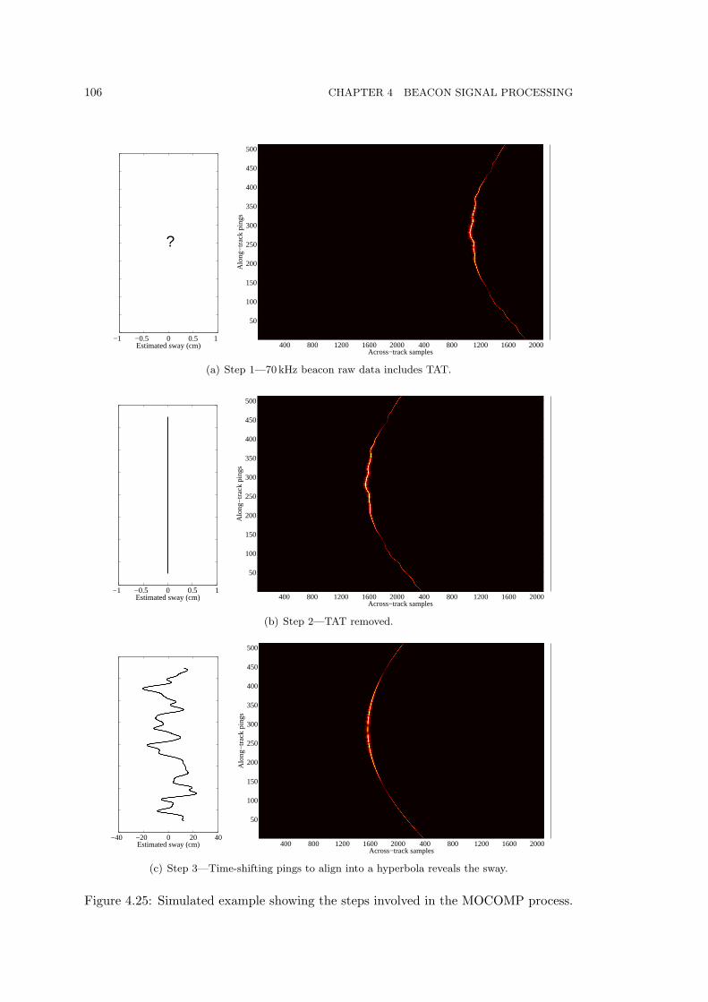
106 CHAPTER 4 BEACON SIGNAL PROCESSING
−1 −0.5 0 0.5 1 Estimated sway (cm)
?A
long
−tr
ack
ping
s
Across−track samples
400 800 1200 1600 2000 400 800 1200 1600 2000
50
100
150
200
250
300
350
400
450
500
−30
−25
−20
−15
−10
−5
0
(a) Step 1—70 kHz beacon raw data includes TAT.
−1 −0.5 0 0.5 1Estimated sway (cm)
Alo
ng−
trac
k pi
ngs
Across−track samples
400 800 1200 1600 2000 400 800 1200 1600 2000
50
100
150
200
250
300
350
400
450
500
−30
−25
−20
−15
−10
−5
0
(b) Step 2—TAT removed.
−40 −20 0 20 40Estimated sway (cm)
Alo
ng−
trac
k pi
ngs
Across−track samples
400 800 1200 1600 2000 400 800 1200 1600 2000
50
100
150
200
250
300
350
400
450
500
−30
−25
−20
−15
−10
−5
0
(c) Step 3—Time-shifting pings to align into a hyperbola reveals the sway.
Figure 4.25: Simulated example showing the steps involved in the MOCOMP process.

4.7 CHAPTER SUMMARY 107
noticeable blurring but a 1 m error produces very little distortion. This effect is worsefor the 30 kHz images than the 100 kHz images because more distortion occurs over thelonger 30 kHz synthetic aperture.
4.6.6 Narrowband MOCOMP
Because the beacon is known to be a point source, the process of calculating the swayis equivalent to time-shifting the pings in the 70 kHz pulse-compressed raw data untilthe data forms the traditional hyperbolic shape associated with a point source at thatrange. This assumes constant along-track speed, a condition aimed for in sea trials.This is shown in Fig. 4.25(c). Having obtained an estimate for the sway, MOCOMPcan be performed, before reconstruction, by applying the same time-shifts to the pingsin the 30 kHz and 100 kHz raw data. This is a narrowband approximation, i.e., onlyexact when the sonar is broadside to the target. Simulations in Sec. 6.4 show that thisapproach performs well with the narrow KiwiSAS BPs.
If ss(t, u) is the pulse compressed (complex) baseband image, i.e., the 30 kHz or100 kHz raw data, and SS(f, u) is the FT of ss(t, u), and p(u) the sway estimate in m,then the sway can be removed by time shifting using the equivalent time and frequencydomain approaches:
ssshift(t, u) = ss
(t− 2p(u)
c, u
), (4.44)
SSshift(f, u) = SS(f, u)e−j4πfp(u)
c . (4.45)
4.7 CHAPTER SUMMARY
The signal processing algorithms, used in the active beacon for detecting the sonar20–40 kHz chirps amongst noise and multipath, were presented. Investigations of dif-ferent methods of finding the direct path peak in the matched filter output showedhow the current quadratic interpolation approach could be significantly improved withadditional sinc oversampling. The error due to the superposition of the direct pathpeak and the seabed multipath peak, was shown to be minimal, providing the beacondetection algorithm can reliably identify the direct path peak. This can be challenging,especially when the multipath peak is larger but further refining of the algorithms isdifficult with the limited testing facilities available.
An expression for the KiwiSAS sonar projector directivity was derived and usedto confirm that problems experienced with missed detections in early sea trials weredue to the intra-chirp null motion in the horizontal directivity pattern. The beacondetection algorithms have since been improved, but this problem is still the majorlimitation to the along-track operating range, reducing the usefulness of the beacon asa motion estimation tool for large SAS images using narrow beam sonars.

108 CHAPTER 4 BEACON SIGNAL PROCESSING
Along−track (m)
Ran
ge (
m)
−10 −5 0 5 10
30
35
40
45
−40dB
−35dB
−30dB
−25dB
−20dB
−15dB
−10dB
−5 dB
(a) 1m estimate error, 100 kHz.
Along−track (m)
Ran
ge (
m)
−10 −5 0 5 10
30
35
40
45
−40dB
−35dB
−30dB
−25dB
−20dB
−15dB
−10dB
−5 dB
(b) 0.5 m estimate error, 100 kHz.
Figure 4.26: Simulations showing how an error in the along-track beacon positionestimate affects the beacon MOCOMP process, distorting the reconstructed images. A1 m error produces noticeable blurring but a 0.5 m error produces very little distortion.See Fig. 6.9(a) for the same image with no error in the beacon position estimate andcomplete simulation details.

4.7 CHAPTER SUMMARY 109
Along−track (m)
Ran
ge (
m)
−10 −5 0 5 10
30
35
40
45
−40dB
−35dB
−30dB
−25dB
−20dB
−15dB
−10dB
−5 dB
(a) 5m estimate error, 100 kHz.
Along−track (m)
Ran
ge (
m)
−10 −5 0 5 10
30
35
40
45
−40dB
−35dB
−30dB
−25dB
−20dB
−15dB
−10dB
−5 dB
(b) 1 m estimate error, 100 kHz.
Figure 4.27: Simulations showing how an error in the across-track beacon positionestimate affects the beacon MOCOMP process, distorting the reconstructed images. A5 m error produces noticeable blurring but a 1m error produces very little distortion.See Fig. 6.9(a) for the same image with no error in the beacon position estimate andcomplete simulation details.

110 CHAPTER 4 BEACON SIGNAL PROCESSING
Two methods of obtaining motion estimation data from the beacon were discussed.The two-way TOF method, using the sonar to image the 70 kHz beacon replies, is likelyto perform best, due to the absence of certain timing errors and the similarities thisapproach shares with the imaging process.

Chapter 5
SEA TRIAL RESULTS
5.1 INTRODUCTION
Results from two runs from a recent sea trial are presented, showing beacon motionestimation and MOCOMP attempts using both the one-way and two-way methods de-scribed in Sec. 4.6. Improvements in image quality can be seen in both runs, despite thepresence of many outliers in the time of flight (TOF) data. Experiment and processingdetails are presented first, followed by discussion of the results. Lastly, data plots andimages from both runs are shown.
5.2 EXPERIMENT AND PROCESSING DETAILS
The Purau Bay sea trial location is shown in Fig. 5.1 with photos in Fig. 5.2. Thebeacon was deployed in ∼4 m of water and a number of runs of ∼30 m length, withthe sonar at a depth of ∼1 m, were imaged in the manner illustrated in Fig. 3.17.Unfortunately, a tri-plane target that was also intended for deployment was damagedearlier in the day, in rougher conditions in the centre of the harbour, so the onlystationary known target in the scene is the beacon seabed unit (BSU). It would appearfrom the images that the seabed is otherwise featureless.
The scene geometry for both runs is shown in Fig. 5.3. The runs are hereby referredto as “run 335” and “run 339” and are passes on opposite sides of the scene.
5.2.1 Estimating beacon position and sonar velocity
Estimates of the beacon position and towfish velocity, required for trilateration of thesway from the TOF data as explained in Sec. 4.6.5, were obtained by fitting a hyperbolato the 70 kHz beacon raw data. The fitted hyperbola is equivalent to the TOF datarecorded when travelling past a perfect point target, on a straight path, at constantspeed. The fit was performed iteratively by eye, varying the beacon position and sonarvelocity, to achieve the results in Figs. 5.4(b) and 5.5(b). With only a few datasets toconsider, manual fitting was efficient but in practice this process could be automated

112 CHAPTER 5 SEA TRIAL RESULTS
Figure 5.1: Sea trial location (white X) in Purau Bay, Lyttelton Harbour, Christchurch,New Zealand. Chart datum depths are shown as spot values and contours in m anddm. The tide height during the experiments varied from +0.58m to +1.95m above thedatum.
fairly easily using a cost function based on the intensity of the signal in the raw data.This would give greater emphasis to the data nearer the apex of the curve and awayfrom the nulls where the higher SNR is likely to give better quality results.
Although the sonar did not take a straight path past the target, and probably didnot travel at a constant speed, the deviations from these ideal conditions are smallenough for this method to still produce an accurate estimate of the average sonarvelocity. This can be seen by comparing, in Fig. 5.5, the fitted estimate for run 339(1.275m/s) with the tow boat velocity, obtained from the beacon controller unit (BCU)GPS receiver, showing an average of ∼1.28 m/s over the same period of that run.Similarly close matches are observed for run 335 (Fig. 5.4) where a velocity of 1.00 m/swas found to be the best fit.
5.2.2 Estimating the speed of sound
The speed of sound was estimated to be 1502.5m/s, using the process described inSec. 2.9, and assumed constant with depth. Depths were measured using pressuresensors on the BSU and in the sonar. Temperature was measured to be 14.5C on theseabed using the temperature sensor in the BSU. Salinity was assumed to be unchangedfrom the 33.6 ppt measured previously.

5.2 EXPERIMENT AND PROCESSING DETAILS 113
(a) KiwiSAS sonar floating behind the tow boat (before deployment).
(b) BFU in operation.
Figure 5.2: Photos from a sea trial in Purau Bay, May 2006.

114 CHAPTER 5 SEA TRIAL RESULTS
−2 0 2 4 6 8 10 12 14 16−5
−4
−3
−2
−1
0
1
Across−track (m)
Dep
th (
m)
Figure 5.3: Sea trial geometry for run 339 showing the sonar (circle), BSU (square),direct acoustic path (solid line) and multipath (dashed lines). Run 335, has a similargeometry. No other multipath bounces were observed.
5.2.3 Contrast measure
A simple contrast measure [Fortune June 2005] was used to quantify the contrastimprovement due to MOCOMP:
C =M∑
m=1
N∑n=1
|ff[m,n]|4 (5.1)
where ff[m,n] = ff(m∆r, n∆y) is a portion of the reconstructed image of size M byN pixels, r is the range coordinate, and y is the along-track coordinate. The imageportion is carefully chosen to include only the BSU and an uncluttered area of seabedso that the non-stationary objects, which do not properly reconstruct, do not skew theresult. The exception were the 70 kHz beacon images, containing only the BSU, wherethe contrast was calculated using the entire image.
5.2.4 Outlier identification and removal
Attempts were made to use a moving median filter on the TOF data to identify andremove outliers. However, the large number of outliers meant that it was more reliableto do this manually, by eye, to achieve a smooth sway path. While this task only takesa few minutes per image, an automatic algorithm is required for practical SAS workon a larger scale, e.g., mine hunting. Because the TOF data is going to be nominallyhyperbolic, a possible approach would be to fit a hyperbolic curve (or similar shapeconsisting of a small number of parameters) using a least squares error cost function tothe data. Then the outliers could be identified by their distance from the fitted curve,using a threshold. However, considering the relatively few experiments performed so

5.2 EXPERIMENT AND PROCESSING DETAILS 115
1 512
0.9
1
1.1
1.2
1.3B
oat v
eloc
ity (
m/s
)
Ping #
(a) GPS boat velocity (solid line) and 300-ping moving median (dashed line).
Alo
ng−
trac
k pi
ngs
Range (m)
15 20 25
50
100
150
200
250
300
350
400
450
500
0.925 m/s1 m/s1.075 m/s
−30dB
−25dB
−20dB
−15dB
−10dB
−5 dB
0 dB
(b) Fitted hyperbolas, corresponding to travelling at various constant velocitiespast a point source centred on the white X, overlaid on the non-reconstructed,pulse-compressed, 70 kHz beacon raw data (corrected for TAT). The hyperbolacorresponding to a velocity of 1.00 m/s provides the best match.
Figure 5.4: Run 335. Comparing the sonar fitted velocity estimate with the tow boatmeasured velocity.

116 CHAPTER 5 SEA TRIAL RESULTS
1 512
1.15
1.2
1.25
1.3
1.35
Boa
t vel
ocity
(m
/s)
Ping #
(a) GPS boat velocity (solid line) and 300-ping moving median (dashed line).
Alo
ng−
trac
k pi
ngs
Range (m)
15 20 25
50
100
150
200
250
300
350
400
450
500
1.2 m/s1.275 m/s1.35 m/s
−40dB
−35dB
−30dB
−25dB
−20dB
−15dB
−10dB
−5 dB
0 dB
(b) Fitted hyperbolas, corresponding to travelling at various constant velocitiespast a point source centred on the white X, overlaid on the non-reconstructed,pulse-compressed, 70 kHz beacon raw data (corrected for TAT). The hyperbolacorresponding to a velocity of 1.275m/s provides the best match.
Figure 5.5: Run 339. Comparing the sonar fitted velocity estimate with the tow boatvelocity.

5.3 RESULTS AND DISCUSSION 117
far, it would be more productive to concentrate efforts on fine-tuning the system tocollect better quality data before attempting to automate the fitting process.
5.3 RESULTS AND DISCUSSION
The following sections present plots and images from both runs. The results are inter-preted and discussed, and contrast figures are presented.
5.3.1 Object identification
Figure 5.6 shows the reconstructed (without MOCOMP) 30 kHz and 100 kHz imagesfor run 335 with the corresponding images for run 339 shown in Fig. 5.7. The BSU,beacon floating unit (BFU), and floating buoy1, identified by the overlays, can be clearlyseen in the 30 kHz images.2 The BSU identity is confirmed by measuring the range ofthe closest approach point in the 70 kHz raw data of Figs. 5.4(b) and 5.5(b)—a usefultechnique in the absence of independent ground truth information. The 100 kHz imagesare badly affected by motion blur so the same overlays are plotted to help identify theobjects for each run.
The close proximity (horizontally) of the BFU to the BSU suggests that the 10 mcable connecting them is not fully extended, implying low tidal flow. This is consistentwith the sea trial occurring at the turn of high tide—a deliberate schedule chosen toensure maximum water depth and slack water. The bunched coils of cable may explainthe additional smaller reflections observed in the images.
5.3.2 Beacon appearance in image
The appearance of the two units of the beacon, the BSU and BFU, in SAS images isdependent on reflectivity, shape, illumination, and multipath. These are discussed inthe next sections.
5.3.2.1 BSU
The diameter of the BSU casing is 24 cm and the base 90 cm. The casing contains∼400 cm3 of air so should reflect well. The aluminium base is surrounded by plastichose which may trap air bubbles and reflect somewhat. The scene geometry, shown inFig. 5.3, causes additional echoes at 27.7 cm and 46.7 cm greater range than the directpath for the seabed and surface multipath bounces respectively.
1A small emergency device, connected by a thin rope to the BSU to allow retrieval of the BSU ifthe BFU sinks or breaks loose.
2Additional evidence supporting the identification of the BFU and buoy is provide by visual sightingof the proximity and alignment of these objects on the sea surface, during the time of the trial.

118 CHAPTER 5 SEA TRIAL RESULTS
Along−track (m)
Ran
ge (
m)
5 10 15 20
12
14
16
18
20
22
24
26
−35dB
−30dB
−25dB
−20dB
−15dB
−10dB
−5 dB
(a) Objects identified, no MOCOMP, 30 kHz.
Along−track (m)
Ran
ge (
m)
5 10 15 20
12
14
16
18
20
22
24
26
−45dB
−40dB
−35dB
−30dB
−25dB
−20dB
−15dB
−10dB
−5 dB
(b) Objects identified, no MOCOMP, 100 kHz.
Figure 5.6: Run 335, reconstructed images identifying the scene objects. In (a) theBSU (continuous oval), BFU (continuous rectangle), and buoy (dashed rectangle) areeasily identified. In (b) the BSU and buoy are poorly illuminated, probably becausethey lie outside the main transmit lobe, as shown in Fig. 5.8. The additional smallbright object (dashed oval) may be part of the beacon cable/rope assembly joining thetwo units. The long thin object extending to the left of the BSU may also be this cable.Each plot is normalised to the maximum intensity in the scene.

5.3 RESULTS AND DISCUSSION 119
Ran
ge (
m)
Along−track (m)
15 20 25 30 354
6
8
10
12
14
16
18
20
−30dB
−25dB
−20dB
−15dB
−10dB
−5 dB
(a) Objects identified, no MOCOMP, 30 kHz.
Ran
ge (
m)
Along−track (m)
15 20 25 30 354
6
8
10
12
14
16
18
20
−45dB
−40dB
−35dB
−30dB
−25dB
−20dB
−15dB
−10dB
−5 dB
(b) Objects identified, no MOCOMP, 100 kHz.
Figure 5.7: Run 339 reconstructed images identifying the scene objects. In (a) the BSU(continuous oval), BFU (continuous rectangle), and buoy (dashed rectangle) are easilyidentified. In (b) the BSU and buoy are poorly illuminated, probably because they lieoutside the main transmit lobe, as shown in Fig. 5.8. The additional bright object at(28,16), not present in (a), may be part of the beacon cable/rope assembly joining thetwo units. The small bright object (dashed oval) and long thin object extending tothe right of the BSU may also be this cable. Each plot is normalised to the maximumintensity in the scene.

120 CHAPTER 5 SEA TRIAL RESULTS
In the 30 kHz and 100 kHz reconstructed images, the BSU appears as a circularfeature with ∼1 m diameter. This matches well with the physical dimensions andprobably includes multipath reflections.
5.3.2.2 BFU
The diameter of the BFU casing is the same as the BSU but the greater height andminimal contents give it a much greater (submerged) volume of ∼1500 cm3. This is themain reason why a much stronger reflection is observed than for the BSU, in both the30 kHz and 100 kHz images.
An additional contributing effect, particularly in the 100 kHz images, is the verticalsonar transmit BP. This is plotted in Fig. 5.8, assuming no roll, where it can be seenthat, unlike with the wide vertical BP at 30 kHz, the 100 kHz main lobe is narrow andwhen horizontal, illuminates the floating BFU while a smaller sidelobe illuminates theBSU. Using a single row of the sonar receiver results in a vertical receive BP similar tothe transmit BP, at any frequency, because the vertical dimension is similar. A singlerow of receiver elements is summed to produce the images in the following sections.
0 5 10 15 20−5
−3
−1
0
−2
−4
Across−track (m)
Dep
th (
m)
1st null span2nd null spanSonarSeabedBeam pattern@ 100kHz
Figure 5.8: Scale diagram of the theoretical sonar 100 kHz transmit and receive BPsand the across-track area swept by the intra-chirp nulls when horizontal. Dependingon the sonar roll angle, the beacon, at ∼15 m range, may be located in or near the firstnull or sidelobe, explaining the poor illumination. When horizontal, the BFU, floatingon the surface, lies well within the main beam, producing a strong reflection, as seenin the images. See Fig. 4.22 for the equivalent diagram for the 30 kHz chirp.
5.3.3 Sway estimation
Slant plane sway was calculated from the measured TOF data and estimated velocitydata as described in Sec. 4.6.4. Both one-way and two-way TOF data was used and athird sway solution was obtained by averaging the sway estimates of these two methods.
Plots of the TOF before and after outlier removal and the three sway estimates areshown in Figs. 5.9 and 5.10 for run 335 and run 339 respectively. The large outliers in

5.3 RESULTS AND DISCUSSION 121
the TOF data are missed detections and the smaller outliers are poor detections. The“late” detections occur when the seabed multipath correlation peaks are higher thanthe direct path peak and the “early” detections occur when the sidelobes of the mainpeak correlation are high enough to be mistaken for the main peak, as discussed inChapter 4. Chapter 8 presents detailed ideas for improving the detection algorithm toprevent both these problems.
The data from run 335 is significantly better than run 339 with very few misseddetections and fewer poor detections. The difference between these two runs, apartfrom being runs past opposite sides of the scene, is that the preamp gain in the beaconwas reduced by 3 dB in run 335. The higher gain probably caused the sidelobes of thematched filter output to exceed the detection threshold and the subsequent processingalgorithms may have rejected these detections when a well defined peak was not found,producing missed detections.3
After removing the outliers and interpolating, the sway estimates of Figs. 5.9(c)and 5.10(c) resulted. Although the general shape of the solutions is similar, there aresignificant differences in the offsets and in the small scale fluctuations. The followingsection discusses the image quality improvement resulting from MOCOMP using eachof the three sway estimates. The sway estimate produced by the two-way method wasfound to produce consistently superior results.
5.3.4 Image quality improvement from MOCOMP
MOCOMP was performed using the narrowband approach described in Sec. 4.6.6. TheBSU is the only stationary object in the scene so is the only object that can be expectedto improve after MOCOMP. Because it is symmetrical, and the geometry of both runsis very similar, it should also reconstruct similarly in both runs.
A clear improvement in image quality is seen with the BSU feature in Figs. 5.11and 5.12 where the sway estimate from the two-way method was used. The smallerextent, closer to the expected 24 cm diameter of the casing, achieved with Fig. 5.12,suggests the sway data for run 335 is superior. This conclusion is reinforced by Fig. 5.13,showing a small improvement in the BSU object at 100 kHz, suggesting sub-centimetreaccuracy is being achieved. No improvement was observed with the equivalent 100 kHzimage of run 339 (not shown). Figure 5.14 shows a closeup of the BSU transducer inthe 70 kHz beacon image showing how the smearing has sharpened to a well definedpoint. Minimal improvement was observed with the equivalent 70 kHz beacon image ofrun 339 (not shown).
The contrast improvements, using (5.1), are shown in Table 5.1. The MOCOMP
3The peak finding algorithm recognises basic error conditions, e.g., when the peak sample is foundto be at one end of a range of samples being searched then the peak must have been detected incorrectly,and produces no output in this case.

122 CHAPTER 5 SEA TRIAL RESULTS
10 12 14 16 18 20 2210
10.2
10.4
10.6
10.8
11
Along−track (m)
TO
F (
ms)
(a) TOF data unprocessed.
10 12 14 16 18 20 2210
10.2
10.4
10.6
10.8
11
Along−track (m)
TO
F (
ms)
(b) TOF after removing outliers and smoothing.
10 12 14 16 18 20 22−20
−10
0
10
20
Along−track (m)
Sw
ay (
cm)
(c) Sway.
Figure 5.9: Run 335 TOF and sway estimates using the two-way method (blue), the one-way method (red), and the average of both methods (green). While the major fluctua-tions are common, the curves differ significantly during periods of smaller, straighter,motion.

5.3 RESULTS AND DISCUSSION 123
17 18 19 20 21 22 23 24 25 26 27 2810
10.5
11
11.5
Along−track (m)
TO
F (
ms)
(a) TOF data unprocessed.
17 18 19 20 21 22 23 24 25 26 27 2810
10.5
11
11.5
Along−track (m)
TO
F (
ms)
(b) TOF after removing outliers and smoothing.
17 18 19 20 21 22 23 24 25 26 27 28
−10
0
10
20
Along−track (m)
Sw
ay (
cm)
(c) Sway.
Figure 5.10: Run 339 TOF and sway estimates using the two-way method (blue),the one-way method (red), and the average of both methods (green). While the ma-jor fluctuations are common, the curves differ significantly during periods of smaller,straighter, motion.

124 CHAPTER 5 SEA TRIAL RESULTS
Along−track (m)
Ran
ge (
m)
16 18 20 22 24 26 2812
13
14
15
16
17
18
19
20
−30dB
−25dB
−20dB
−15dB
−10dB
−5 dB
(a) No MOCOMP, 30 kHz.
Along−track (m)
Ran
ge (
m)
16 18 20 22 24 26 2812
13
14
15
16
17
18
19
20
−30dB
−25dB
−20dB
−15dB
−10dB
−5 dB
(b) After two-way MOCOMP, 30 kHz.
Figure 5.11: Run 339. Reconstructed images showing the improvement to the BSUobject, at (21,15.6), after MOCOMP using the sway estimate of Fig. 5.10(c) obtainedby the two-way TOF method. See Fig. 5.7(a) for identification of the objects in theimage. Both plots are normalised to the maximum intensity of the BSU object in (b).

5.3 RESULTS AND DISCUSSION 125
Along−track (m)
Ran
ge (
m)
10 12 14 16 18 20 2212
13
14
15
16
17
18
19
20
−30dB
−25dB
−20dB
−15dB
−10dB
−5 dB
(a) No MOCOMP, 30 kHz.
Along−track (m)
Ran
ge (
m)
10 12 14 16 18 20 2212
13
14
15
16
17
18
19
20
−30dB
−25dB
−20dB
−15dB
−10dB
−5 dB
(b) After two-way MOCOMP, 30 kHz.
Figure 5.12: Run 335. Reconstructed images showing the improvement to the BSUobject, at (16.5,15.1), after MOCOMP using the sway estimate of Fig. 5.9(c) obtainedby the two-way TOF method. See Fig. 5.6(a) for identification of the objects in theimage. Both plots are normalised to the maximum intensity of the BSU object in (b).

126 CHAPTER 5 SEA TRIAL RESULTS
Along−track (m)
Ran
ge (
m)
10 12 14 16 18 20 2212
13
14
15
16
17
18
19
20
−30dB
−25dB
−20dB
−15dB
−10dB
−5 dB
(a) No MOCOMP, 100 kHz.
Along−track (m)
Ran
ge (
m)
10 12 14 16 18 20 2212
13
14
15
16
17
18
19
20
−30dB
−25dB
−20dB
−15dB
−10dB
−5 dB
(b) After two-way MOCOMP, 100 kHz.
Figure 5.13: Run 335. Reconstructed images showing the improvement to the BSUobject, at (16.5,15.1), after MOCOMP using the sway estimate of Fig. 5.9(c) obtainedby the two-way TOF method. See Fig. 5.6(a) for identification of the objects in theimage. Both plots are normalised to the maximum intensity of the BSU object in (b).

5.3 RESULTS AND DISCUSSION 127
Along−track (m)
Ran
ge (
m)
14 15 16 17 18 1913.5
14
14.5
15
15.5
16
16.5
17
17.5
18
−30dB
−25dB
−20dB
−15dB
−10dB
−5 dB
(a) No MOCOMP, 70 kHz beacon image.
Along−track (m)
Ran
ge (
m)
14 15 16 17 18 1913.5
14
14.5
15
15.5
16
16.5
17
17.5
18
−30dB
−25dB
−20dB
−15dB
−10dB
−5 dB
(b) After two-way MOCOMP, 70 kHz beacon image.
Figure 5.14: Run 335. Reconstructed images showing the improvement to the BSUtransducer after MOCOMP using the sway estimate of Fig. 5.9(c) obtained by thetwo-way TOF method. Each plot is normalised to the maximum intensity in the scene.

128 CHAPTER 5 SEA TRIAL RESULTS
data from run 335 shows consistently greater percentage improvements over run 339,confirming the observations seen in the images.
Run ImageMethod
Two-way One-way Averagerun 335 30 kHz 301% 55% 130%run 335 100 kHz 23% -18% -22%run 335 70 kHz 903% -53% 56%run 339 30 kHz 52% -2% 17%run 339 100 kHz no improvementrun 339 70 kHz minimal improvement
Table 5.1: Percentage increase in contrast, after MOCOMP, using three different meth-ods of estimating the sonar sway.
5.4 CHAPTER SUMMARY
Results from two runs were presented that showed how the active beacon motion esti-mation data and MOCOMP process proved successful in reducing the blur in shallowwater KiwiSAS images. Both runs showed improvement at 30 kHz, after the removaland smoothing of several outliers in the TOF data. Run 335, with fewer outliers,also showed some improvement at 100 kHz, suggesting sub-centimetre accuracy wasachieved. These visual observations were verified by a contrast metric. With the highnumber of outliers currently experienced, best results were achieved when identificationand removal was performed manually.
In the cases where an improvement in image quality was achieved, the two-way TOFmethod was consistently superior, followed by the two-way/one-way average method,then the one-way TOF method. This may be due to the extra timing errors introducedby the time-stamping of the chirp departure and arrival events, from the sonar and atthe beacon respectively, not present in the two-way method. It may also be due to thereturn-path medium fluctuations which affect the images but are not measured usingthe one-way method.
The effects of the additional sonar motion occurring during the non-zero turnaround time (TAT), present in the two-way TOF data but not present in the images,do not appear to prevent the active beacon concept from producing useful MOCOMPresults, even at the short 1.5 cm wavelengths used in the 100 kHz images.
Fitting a hyperbola, by eye, to the 70 kHz beacon raw data produced a velocityestimate for the sonar that was within ±0.025 m/s of the tow boat velocity, for bothruns, when measured using GPS and averaged over the run length.

Chapter 6
MEDIUM FLUCTUATION STATISTICS AND SASSIMULATIONS
6.1 INTRODUCTION
The ocean is a dynamic environment. The speed of sound underwater is continuallyfluctuating as changes occur to the three main variables upon which it depends; pres-sure, temperature, and salinity [Kussat et al. 2005]. Short term effects, e.g., the increasein pressure from an approaching wave, and long term effects, e.g., the drop in tempera-ture as night falls, cause fluctuations in the time of flight (TOF) of sonar chirps resultingin image distortion. Few TOF experiments have been performed in very shallow waterand fewer still have attempted to parameterise the observations statistically, insteaddescribing the fluctuations as a single standard deviation (STD) figure with no com-ment on the probability density function (PDF) shape. Previous investigations haveshown long-term correlation with the tide height [Porter et al. 1998] and short termcorrelation with the combined effects of surface wave height and temperature changes[Bergem and Pace 1998, Bergem et al. 1999, Meredith et al. 2004, Stanic et al. 2000],and the presence of bubbles [Goodman et al. 2000, Terrill 1997].
Characterising the medium fluctuations allows their effects to be reproduced insonar simulations for further study. This chapter presents a study attempting to modelthe short term TOF fluctuations as random variables, based on experimental datafrom the active beacon. The goal is to characterise the TOF fluctuations using simpleprobability distributions, allowing straightforward inclusion in the Acoustics ResearchGroup (ARG) SAS simulator. Section 6.4 presents simulated results that clearly showthe effects of medium fluctuations on reconstructed images.
6.1.1 Statistical model
The TOF data can be modelled as a random variable, Z, with associated PDF fZ(z);a combination of the measurement error of the beacon, X with associated PDF fX(x),

130 CHAPTER 6 MEDIUM FLUCTUATION STATISTICS AND SAS SIMULATIONS
and the medium fluctuations, Y with associated PDF fY(y), i.e.,
Z = X + Y, (6.1)
fZ(z) = fX(x) fY(y), (6.2)
where represents a convolution.
The following sections explain how fX, fY, and fZ were determined through aseries of tank and sea tests. Pool tests were also performed at similar ranges to providecontrol data.
6.2 EXPERIMENTAL BEACON MEASUREMENT ERROR
An estimate for fX can be obtained by fitting a distribution to experimental data sam-ples measured in the absence of medium fluctuations. This experiment was performedin the covered outdoor sonar test tank at the University of Canterbury. The covershelters the water from external disturbances and a small opening provides access toGPS and RF communication signals for the beacon floating unit (BFU). The beaconseabed unit (BSU) was placed on the tank floor and a fixed acoustic transmitter waslocated ∼2 m away at a depth of ∼1 m. Several trials of 5 minutes duration at 15 chirpsper second were run, increasing the transmitter amplitude (and hence the SNR) eachtime. The results are shown in Fig. 6.1.
6.2.1 Experimental distribution fitting
To choose a suitable distribution to fit to the test tank data, a β1β2 chart was used(appendix G contains further information). This plot of kurtosis (β2) vs skewnesssquared (β1) provides a visual indication of which common distribution the data islikely to fit, based on its proximity. The test tank data is plotted in Fig. 6.1(b) whereit can be seen that the data points lie in the region representing beta distributions withseveral other distributions close by, the simplest being the normal. A Kolmogorov-Smirnov (KS) test [Harnett 1982, pp712–713][Steel and Torrie 1980, pp535–537], afterfitting with both normal and beta distributions, revealed the normal to be the closermatch. Fitting a normal distribution to the data was achieved by equating the meanand STD of the data from one of the higher SNR runs with the two Gaussian parametersµ and σ respectively in (H.1). The fitted PDF is shown in Fig. 6.5(a).
6.2.2 Theoretical beacon measurement error
The test tank data includes all the timing errors in the beacon system. A breakdownof these are provided in the next sections where theoretical values are derived andcompared to the experimental results.

6.2 EXPERIMENTAL BEACON MEASUREMENT ERROR 131
18 20 22 24 26 28260
270
280
290
300
310
320
330
340
SNR (dB)
STD
(ns
)
(a) Standard deviation.
0 0.1 0.2 0.3 0.4 0.5 0.6 0.7
2.5
2.6
2.7
2.8
2.9
3
3.1
3.2
3.3
β1
β 2
Beta (U shaped)Beta (J shaped)Beta (unimodal)Pearson type VIPearson type IVRicianPoisson (discrete)ChiWeibull
Non central chi2
GammaInverse GaussianLog normalPearson type VPearson type IIStudent’s TNormalMaxwellRayleigh
(b) β1β2 plot.
Figure 6.1: Variation of one-way short range TOF statistics with SNRi in the universitytest tank where no medium fluctuations are expected. The point in (a) at 22.4dB and(b) at (0.09,2.84) is clearly an outlier and was subsequently discarded. The TOF datais plotted in Fig. 6.4(b).

132 CHAPTER 6 MEDIUM FLUCTUATION STATISTICS AND SAS SIMULATIONS
6.2.2.1 Matched filter timing error
The theoretical CRLB on the STD of the timing error (seconds) is found from (4.39).For the SNR values used in the experiment this equates to a range of 10–30 ns. Thisassumes a perfect detection, i.e., that the process of sub-sample interpolation of thematched filter output peak (to determine the exact time of arrival) does not introduceany error. The beacon uses a simple quadratic interpolation method, as discussed inSec. 4.4.2, which is likely to cause additional errors with the low ADC sampling rateused, resulting in an increased STD.
6.2.2.2 Event capture timing errors
The counters used for capturing timing events (GPS 100 PPS edges, ping arrivals, andping departures) are derived from (nominally) 14.31818 MHz and 10 MHz oscillators inthe beacon and the BCU respectively. The PIC clock inputs have a divide-by-four stage,giving internal clock periods, TCY, of 279 ns and 400 ns respectively. A timing eventcan be captured with an error-span equal to TCY. Assuming a rectangular distribution,the STD of the timing error is
σCY =
√T 2
CY
12. (6.3)
The experimental data includes event timing errors associated with four timing events.Two are associated with the ping departure at the transmitter (the departure time; themost recent GPS 100 PPS edge) and two are associated with the ping arrival at thebeacon (the arrival time; the most recent GPS 100 PPS edge). Using (6.3) gives a STDof 81 ns for each event at the beacon and 115 ns for each event at the transmitter.
6.2.2.3 GPS timing errors
The GPS timing receivers used as a timing reference at the transmitter and in thebeacon specify a datasheet STD of 130 ns.
6.2.2.4 DSP clock resolution timing error
The counter used in the DSP, to keep track of when to respond to a detected chirp, isderived from a (nominal) 14.31818 MHz oscillator in the beacon. The DSP clock inputhas an internal times-five multiplier and the internal counter input has a divide-by-two, giving a period of 28 ns. This means that after the chirp arrival time has beenaccurately determined from the matched filter peak, it is quantised to 28 ns becausethat is the smallest time-step increment of the counter. Using (6.3) gives a STD of 8 nsfor the timing error.
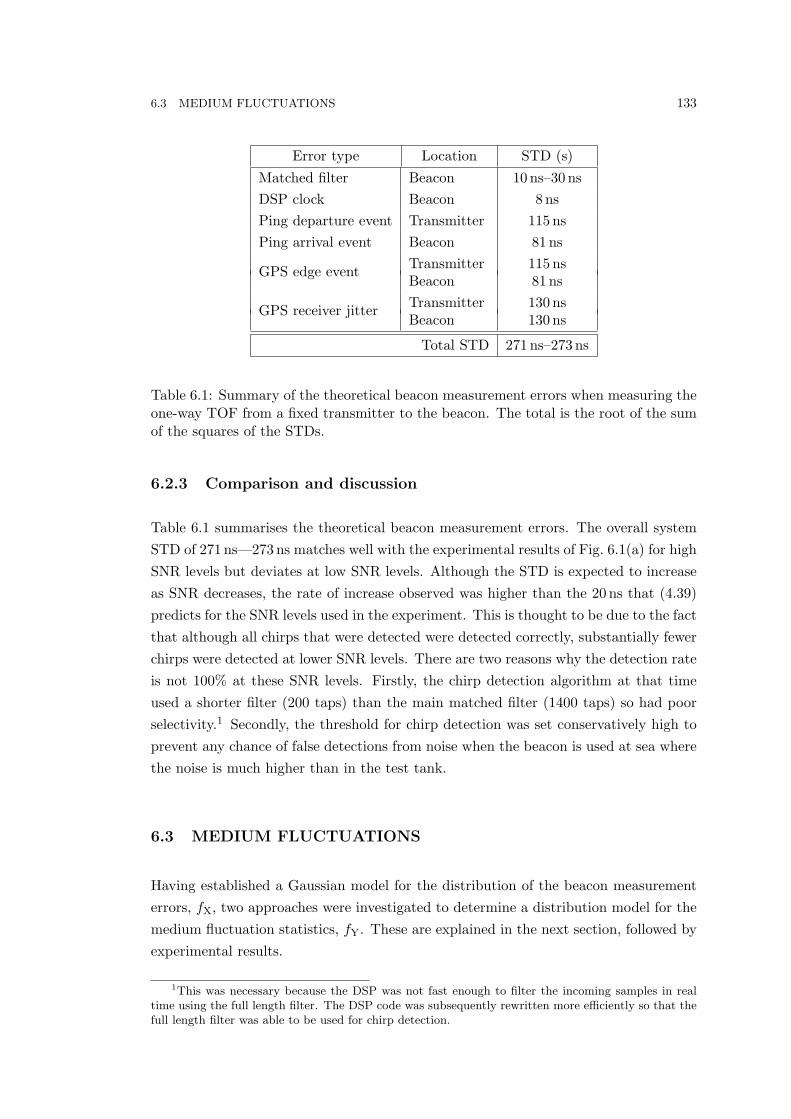
6.3 MEDIUM FLUCTUATIONS 133
Error type Location STD (s)Matched filter Beacon 10 ns–30 nsDSP clock Beacon 8 nsPing departure event Transmitter 115 nsPing arrival event Beacon 81 ns
GPS edge event Transmitter 115 nsBeacon 81 ns
GPS receiver jitter Transmitter 130 nsBeacon 130 ns
Total STD 271 ns–273 ns
Table 6.1: Summary of the theoretical beacon measurement errors when measuring theone-way TOF from a fixed transmitter to the beacon. The total is the root of the sumof the squares of the STDs.
6.2.3 Comparison and discussion
Table 6.1 summarises the theoretical beacon measurement errors. The overall systemSTD of 271 ns—273 ns matches well with the experimental results of Fig. 6.1(a) for highSNR levels but deviates at low SNR levels. Although the STD is expected to increaseas SNR decreases, the rate of increase observed was higher than the 20 ns that (4.39)predicts for the SNR levels used in the experiment. This is thought to be due to the factthat although all chirps that were detected were detected correctly, substantially fewerchirps were detected at lower SNR levels. There are two reasons why the detection rateis not 100% at these SNR levels. Firstly, the chirp detection algorithm at that timeused a shorter filter (200 taps) than the main matched filter (1400 taps) so had poorselectivity.1 Secondly, the threshold for chirp detection was set conservatively high toprevent any chance of false detections from noise when the beacon is used at sea wherethe noise is much higher than in the test tank.
6.3 MEDIUM FLUCTUATIONS
Having established a Gaussian model for the distribution of the beacon measurementerrors, fX, two approaches were investigated to determine a distribution model for themedium fluctuation statistics, fY. These are explained in the next section, followed byexperimental results.
1This was necessary because the DSP was not fast enough to filter the incoming samples in realtime using the full length filter. The DSP code was subsequently rewritten more efficiently so that thefull length filter was able to be used for chirp detection.

134 CHAPTER 6 MEDIUM FLUCTUATION STATISTICS AND SAS SIMULATIONS
6.3.1 Modelling the medium fluctuations
If the medium fluctuations, fY, were significantly larger than the beacon measurementerrors, (6.2) would simplify to the trivial
fY(y) = fZ(z). (6.4)
Unfortunately, the medium fluctuations for the short ranges typically used in high-resolution SAS imaging are comparable to the beacon measurement errors so anotherapproach is required.
6.3.1.1 Fourier transform (FT) approach
Equation (6.2) can be directly inverted;
FY(fy) =FZ(fz)FX(fx)
, (6.5)
where capital letters denote an FT and fx, fy, and fz are the Fourier pairs of x, y, andz respectively, i.e.,
FX(fx) =∫ ∞
−∞fX(x)e−j2πfxx dx (6.6)
etc. However, in practice, the small values in FX(fx) dominate the result, maskingmost of the signal in noise. This can be prevented using a Wiener filter,
FY(fy) =FZ(fz)F ∗
X(x)W (f)|FX(fx)|2 + φ(f)
, (6.7)
where φ(f) is the noise to signal ratio (in these experiments assumed constant withfrequency), and W (f) is a window chosen to suppress any remaining noise at the edgesof the band where the signal level is low. The Wiener filter is an optimal filter, i.e., itminimises the mean square error in the inverse filtering process [Jansson 1997, Gonzalezet al. 2004]. Applying an inverse FT to FY(fy) reveals fY(y), the medium fluctuations,and the fitting of a suitable distribution can then be investigated, e.g., using a β1β2
chart.
6.3.1.2 Method of moments approach
This approach equates the raw moments of fZ(z) with the raw moments of the data,producing a set of simultaneous equations. By successively including higher ordermoments, until the number of unknown distribution parameters equals the number ofequations, all parameters can be found. Expressions for the raw moments of Z are

6.3 MEDIUM FLUCTUATIONS 135
found from the expected values of powers of Z. To do this, Y must be split into aconstant offset term, O, assumed to be the true TOF, and the medium fluctuations, Y ,
Y = O + Y . (6.8)
If the distribution chosen for Y has two parameters, e.g., gamma, Rician, or Weibull,then three equations are required to solve for these and O;
E[Z] = E[X +O + Y
]= µ′1(z),
E[Z2
]= E
[(X +O + Y
)2]
= µ′2(z), (6.9)
E[Z3
]= E
[(X +O + Y
)3]
= µ′3(z).
If there is no theoretical reason to select a particular distribution to fit to Y ,the FT approach described earlier in this section can be used to produce a PDF offY(y). Alternatively a simple visual inspection of fZ(z) and fX(x) may suffice for a“first guess”. For the experiments presented in the next section, Gamma, Rician, andWeibull distributions were identified as suitable candidates for fitting, based on theresults of the FT approach. The Rician was chosen because of its previous use withlow frequency TOF data [Giellis 1989] and also in the related field of modelling theamplitude of received echoes [Jourdain 1994, Wilson et al. 1993]. The Gamma andWeibull were chosen because of their flexibility.2 Log-normal fitting has also been usedsuccessfully [Terrill 1997]. Full equations are presented in Appendix H.
6.3.2 Harbour and pool experiments
Two sets of experiments were performed to investigate the FT and method of mo-ments approaches of Sec. 6.3.1. The first were at Lyttelton Marina, Christchurch, NewZealand. A transmitter was fixed to a wharf pile at a depth of ∼1 m and the BSU wasplaced on the seabed at a depth of ∼4 m. Trials of 5 minutes duration at a chirp rateof 15 chirps per second were run at 3 separation distances. The experimental setup isshown in Fig. 6.2.
The second set of experiments, using the same equipment with similar geometry,was set up in the indoor dive pool at Queen Elizabeth II Park, Christchurch, NewZealand. This location allows greater separation than can be achieved in the universitytest tank while retaining the ripple-free surface and (hopefully) stable medium. Thisexperiment was designed to act as a control, i.e., to verify the equipment behaved cor-rectly at the long ranges being used for the harbour experiments, in a known medium.
2Although we have not identified a theoretical link between these distributions and the physicalsituation, recall that the goal is to find a simple description for the TOF fluctuations to allow them tobe reproduced in simulations so a completely empirical approach is taken here.
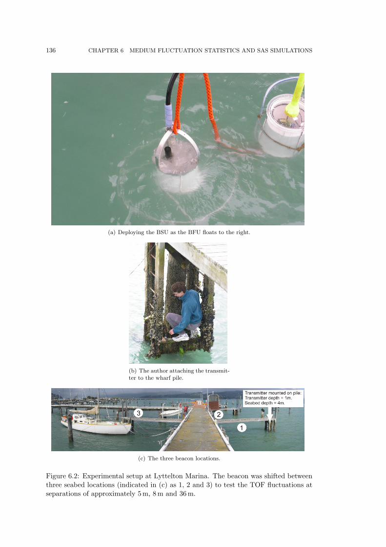
136 CHAPTER 6 MEDIUM FLUCTUATION STATISTICS AND SAS SIMULATIONS
(a) Deploying the BSU as the BFU floats to the right.
(b) The author attaching the transmit-ter to the wharf pile.
(c) The three beacon locations.
Figure 6.2: Experimental setup at Lyttelton Marina. The beacon was shifted betweenthree seabed locations (indicated in (c) as 1, 2 and 3) to test the TOF fluctuations atseparations of approximately 5 m, 8 m and 36 m.

6.3 MEDIUM FLUCTUATIONS 137
The beacon cable length was sufficient to allow the BFU to be placed outside thebuilding to access GPS signals. The experimental setup is shown in Fig. 6.3.
6.3.2.1 Results and discussion
The best fits to the harbour data were obtained with the method of moments approachusing gamma, Rician, and Weibull distributions. Each produced similar KS test resultsas shown in Fig. 6.4(a). The parameter values, averaged over four runs, are given inTable 6.2. The FT approach produced poorer KS test results so was not pursuedfurther.
Distribution Parameter 1 Parameter 2Gamma α = 4.5 β = 135 nsRician σ = 390 ns A = 115 nsWeibull α = 1.5 β = 450 ns
Table 6.2: Fitted distribution parameters for the medium fluctuations using the methodof moments approach. See Appendix H for the distribution formulas.
The fitted PDFs are shown in Fig. 6.5. Figure 6.5(a) shows the Gaussian PDFfitted to the test tank TOF data. No medium fluctuations are expected in the testtank so this PDF represents the measurement error of the beacon when performingone-way TOF measurements. Figure 6.5(b) shows various estimates of the PDF ofthe medium fluctuations, obtained using the FT and method of moments approachesof Sec. 6.3.1. Figure 6.5(c) shows the convolution of the measurement errors and themedium fluctuations, fitted to the TOF data from Lyttelton Harbour at ∼36 m range,as described by the model of (6.2).
The control experiments in the dive pool were inconclusive. While the span of theTOF data was less than the harbour data at similar ranges, the histograms exhibitedpositive skew suggesting the medium was not stable. A possible reason is that, unlikethe university test tank, the dive pool water undergoes slow, heated, circulation. Therandom nature of the resulting thermal currents may be the cause of the instability.This is unfortunate because, as with any experiment attempting to measure mediumfluctuations, the lack of a control means the harbour data results cannot be guaranteedto be due solely to the medium and not some range-dependent property of the testequipment. Control experiments are rarely mentioned in TOF publications, probablydue to the difficulty of finding large stationary bodies of water.

138 CHAPTER 6 MEDIUM FLUCTUATION STATISTICS AND SAS SIMULATIONS
(a) Portable setup for driving and monitoring the transmitter.
(b) Transmitter deployed at 1m depth. (c) BSU deployed at 2m depth.
Figure 6.3: Experimental dive pool setup. The transmitter was shifted between threepoolside locations to test the TOF fluctuations at separations of approximately 5 m,10 m and 20 m.

6.3 MEDIUM FLUCTUATIONS 139
1 2 3 40.02
0.03
0.04
0.05
0.06
0.07
0.08
0.09
0.1
0.11
Run #
FFTGammaRicianWeibull
(a) KS test results (lower is better) of fitting various PDFs to Lyttelton Harbour TOF data, at∼36m range, by the approaches described in Sec. 6.3.1. The fitted PDFs are shown in Fig. 6.5(c).
0 500 1000−1.5
−1
−0.5
0
0.5
1
1.5
Ping #
Var
iatio
n ab
out m
ean
TO
F (µs)
(b) Test tank at ∼2m range.
0 500 1000−1.5
−1
−0.5
0
0.5
1
1.5
Ping #
Var
iatio
n ab
out m
ean
TO
F (µs)
(c) Lyttelton Harbour at ∼36m range.
Figure 6.4: TOF data from Lyttelton Harbour and the university test tank.

140 CHAPTER 6 MEDIUM FLUCTUATION STATISTICS AND SAS SIMULATIONS
−1 −0.5 0 0.5 10
2
4
6
8
10
12
14x 10
5
Variation about mean TOF (µs)
Pro
babi
lity
dens
ity (
s−1 )
(a) PDF estimate of the measurement error of the beacon, fX(x), obtained byfitting a Gaussian PDF to the histogram (shown here) of one of the high SNRtank test TOF datasets. The TOF data is plotted in Fig. 6.4(b).
23.845 23.8455 23.846 23.8465 23.847 23.8475
0
5
10
15
20x 10
5
TOF (ms)
Pro
babi
lity
dens
ity (
s−1 )
(b) PDF estimates of the medium fluctuations, fY(y), obtained by fittingPDFs to the histogram of Fig. 6.5(c) by the two approaches described inSec. 6.3.1. See Fig. 6.5(c) for legend.
23.845 23.8455 23.846 23.8465 23.847 23.84750
2
4
6
8
10
12x 10
5
TOF (ms)
Pro
babi
lity
dens
ity (
s−1 )
DataFFTGammaRicianWeibull
(c) PDF estimates of the measured TOF data, fZ(z), obtained by fitting vari-ous PDFs to the histogram (shown here) of measured TOF data from LytteltonHarbour at a range of ∼36m. The TOF data is plotted in Fig. 6.4(c).
Figure 6.5: Estimates of fZ(z), fX(x), and fY(y) from (6.2).

6.4 SAS SIMULATIONS USING THE EXPERIMENTAL MEDIUM FLUCTUATION MODEL141
6.4 SAS SIMULATIONS USING THE EXPERIMENTAL
MEDIUM FLUCTUATION MODEL
Characterising medium fluctuations is important for SAS imaging. After motion com-pensation (MOCOMP) has been performed, image quality is ultimately limited bymedium fluctuations [Stanic et al. 2000] and the ability of autofocus algorithms tocorrect for the associated image blur [Putney et al. 2001].
A simulation was performed, using the ARG SAS simulator [Hunter et al. 2003,Hunter and Hayes 2005, Hunter June 2006], incorporating the results from the previoussections. This was done for two purposes: to verify the MOCOMP potential of theactive beacon, and to investigate the effects of beacon measurement errors and mediumfluctuations on SAS images.
The beacon measurement errors were modelled as a normally distributed randomvariable, given by (H.1) with σ = 50ns, centred about µ where µ is the true TOF. Thisconstant was obtained by RMS summation of the top two3 entries in Table 6.1 plus asuitable margin of error.4
The medium fluctuations were modelled as a gamma distributed random variable,given by (H.7) with α = 4 and β = 135 ns from Table 6.2, offset by y0 where y0 is thetrue TOF.
6.4.1 Results and conclusions
Figure 6.6(a) shows the scene used. Simulating without any form of data corruption orerrors produces good reconstructions, as shown in Fig. 6.7. The SAS processing meansboth images have the same resolution but the shadows are sharper at 100 kHz becauseof the narrower BP, as discussed in Sec. 4.5.
Figure 6.8 shows the effect of the sonar experiencing a large uncompensated swaymotion. Interestingly, the 30 kHz image shows more distortion than the 100 kHz image,despite using a longer wavelength. This is probably because the synthetic aperture islonger at 30 kHz, due to the wider BP, so more of the sway oscillations contribute tothe distortion.
Using the active beacon 70 kHz image data to measure the sonar path, followedby narrowband MOCOMP to unblur the 100 kHz images as described in Sec. 4.6.2,is shown in Fig. 6.9(a). The result is as good as the straight-path simulation whereno blurring occurred, shown in Fig. 6.7(b), despite the Gaussian distributed beaconmeasurement errors. However, if medium fluctuations are simulated but not correctedin the MOCOMP process, there is a noticeable difference, as seen in Fig. 6.9(b). The
3The other sources of error listed in the table are only applicable to one-way timing measurements.4Included to account for the fact that the distribution shape of the combination of just these two
errors was not measured.

142 CHAPTER 6 MEDIUM FLUCTUATION STATISTICS AND SAS SIMULATIONS
(a) 3D scale rendering of the scene that was simulated. The left object is a solid teapot, theright object is a solid cylinder, and the foreground object is the BSU.
−10 −5 0 5 10−30
−20
−10
0
10
20
30
Along−track (m)
Sw
ay (
cm)
(b) Simulated sonar sway path.
Figure 6.6: Scene model and tow-path used for the SAS simulation.

6.4 SAS SIMULATIONS USING THE EXPERIMENTAL MEDIUM FLUCTUATION MODEL143
Along−track (m)
Ran
ge (
m)
−10 −5 0 5 10
30
35
40
45
−40dB
−35dB
−30dB
−25dB
−20dB
−15dB
−10dB
−5dB
(a) “Perfect” reconstruction, 30 kHz.
Along−track (m)
Ran
ge (
m)
−10 −5 0 5 10
30
35
40
45
−40dB
−35dB
−30dB
−25dB
−20dB
−15dB
−10dB
−5dB
(b) “Perfect” reconstruction, 100 kHz.
Figure 6.7: Reconstructed simulated 100 kHz images of the scene in Fig. 6.6(a), usingthe parameters of the KiwiSAS sonar. These reconstructions are the “perfect reference”cases i.e., a straight level tow-path with no noise or medium fluctuations.

144 CHAPTER 6 MEDIUM FLUCTUATION STATISTICS AND SAS SIMULATIONS
Along−track (m)
Ran
ge (
m)
−10 −5 0 5 10
30
35
40
45
−40dB
−35dB
−30dB
−25dB
−20dB
−15dB
−10dB
−5dB
(a) No MOCOMP, 30 kHz.
Along−track (m)
Ran
ge (
m)
−10 −5 0 5 10
30
35
40
45
−40dB
−35dB
−30dB
−25dB
−20dB
−15dB
−10dB
−5dB
(b) No MOCOMP, 100 kHz.
Figure 6.8: Reconstructions of the scene in Fig. 6.6(a), using the parameters of theKiwiSAS sonar and the tow-path in Fig. 6.6(b).

6.4 SAS SIMULATIONS USING THE EXPERIMENTAL MEDIUM FLUCTUATION MODEL145
Along−track (m)
Ran
ge (
m)
−10 −5 0 5 10
30
35
40
45
−40dB
−35dB
−30dB
−25dB
−20dB
−15dB
−10dB
−5dB
(a) No medium fluctuations, 100 kHz.
Along−track (m)
Ran
ge (
m)
−10 −5 0 5 10
30
35
40
45
−40dB
−35dB
−30dB
−25dB
−20dB
−15dB
−10dB
−5dB
(b) Gamma-distributed medium fluctuations, 100 kHz.
Figure 6.9: Reconstruction of the scene in Fig. 6.6(a), using the parameters of theKiwiSAS sonar, the tow-path in Fig. 6.6(b), and MOCOMP using the active beacon,as described in Sec. 4.5. The medium fluctuations have negligible effect at 30 kHz soare not shown.

146 CHAPTER 6 MEDIUM FLUCTUATION STATISTICS AND SAS SIMULATIONS
beacon is slightly more blurry and there are bands of distortion in front of the cylinderand behind the teapot.
6.4.2 Simulation limitations
There are a number of limitations with this simulation. These are briefly listed in thefollowing sections. While the conclusions drawn in the previous section are still valid,experimental results using the free-towed KiwiSAS are unlikely to produce images ofthis quality.
6.4.2.1 Imaging
Several physical phenomena were omitted to reduce the simulation duration and, insome cases, due to lack of implementation. These include sea bed/surface multipath,multiple scattering between and within objects, beacon shadow, continuous sonar mo-tion between pings, and refraction within the water column. See [Hunter June 2006]for full implementation details of these properties.
6.4.2.2 Medium fluctuations
A constant distribution for medium fluctuations is assumed. Although not shown here,the skew of the TOF histograms from Lyttelton Harbour increased with range, suggest-ing that the distribution parameters in the simulation should be range dependent. Themedium fluctuation statistics are from measurements collected on a calm day. Oftenthe KiwiSAS sonar is operated in worse conditions where the medium fluctuations areexpected to be larger.
6.4.2.3 Sonar path
Of the six possible degrees of freedom, only a deviation in sway was simulated. Whilesway is one of the most significant contributors to image blur, the other motions,particularly yaw and roll, cause additional blurring in real images.
The narrowband MOCOMP approach only corrects for sway so is unlikely to per-form as well on real images unless all other sonar motion is estimated and corrected bysome other means.
The velocity is known perfectly when reconstructing the simulated images. Exper-imentally, a DVL is normally used to achieve a good estimate of the sonar velocity butthe KiwiSAS does not have such equipment installed.

6.5 CHAPTER SUMMARY 147
6.4.2.4 Noise
The simulation was performed without noise in order to show the medium fluctuationeffects more clearly. Sea noise affects the image quality and the variance of the detectionaccuracy of the beacon, as discussed in Chapter 4.
6.5 CHAPTER SUMMARY
The FT approach to fitting a PDF to the medium fluctuations performed poorly. Us-ing the method of moments worked well, producing lower KS test results for gamma,Rician and Weibull distribution fits to TOF data from Lyttelton Harbour. The pa-rameters for the gamma fit were used in a SAS simulation where the active beaconwas used to perform MOCOMP on image corrupted by sonar sway. The medium fluc-tuations had little effect on the 30 kHz images but produced noticeable artefacts inthe 100 kHz images where the wavelength is of a comparable size. This suggests thatthe MOCOMP process for high frequency SAS imaging in very shallow water shouldincorporate real-time measurement of medium fluctuations, either through an acousticpositioning system like the active beacon or a data driven approach if the data containssuitable content.
The experimental results from the dive pool, suggesting it is not a stable medium,highlight the difficulty of performing rigorous TOF control experiments without theuse of dedicated test facilities.

Chapter 7
CONCLUSIONS
The simulation, design, construction, and sea trial results for a prototype active beaconand controller were presented. The process of selecting this unique beacon design isdetailed in chapter 2. The best design for a first prototype system to operate with theKiwiSAS sonar, given the limited budget and testing facilities, is a single transponderLBL, with RF surface communication, deployed by hand in the imaging area of inter-est. Both one-way and two way time of flight (TOF) measurements are produced bydetecting the 30 kHz sonar chirps and replying back with a 70 kHz chirp after a precisefixed delay. The data is uploaded in real-time via an RF link to the beacon controllerunit (BCU) on the tow boat and displayed on custom software that also controls thebeacon operation. The RF link is only required for debugging purposes and could beeliminated on a production design.
Chapter 3 details the mechanical, electrical, and software design. Attempting todesign the system to operate within the bounds of the limited memory, limited processorspeed, and limited RF bandwidth available meant a lot of time was wasted and thereis little room for further improvement. A major electrical redesign is recommendedto implement any additional changes, as detailed in chapter 8. The mechanical de-sign was satisfactory, although time-consuming to assemble, and future improvementsshould focus on reducing the size and weight to make deployment easier. In partic-ular, using lithium-based batteries would significantly reduce the volume, and hencethe required weight, of the beacon seabed unit (BSU). The negative pressurising ofthe beacon chambers combined with a gauge readout was invaluable for ensuring thesystem was waterproof before and during sea trials. This is an essential feature in anylong-term prototype design containing non-submerged pressure chambers where sealsdo not naturally compress tight in operation. The ability to charge the internal bat-teries by connecting crocodile clips to the appropriate parts of the metal casing is alsoan excellent time saving feature.
The major limitation of the current design is the embedded signal processing.Unlike conventional acoustic positioning systems where the signals are usually omnidi-rectional, the sonar transmit BP is narrow in the along-track direction and numerous

150 CHAPTER 7 CONCLUSIONS
nulls exist within the BP sidelobes. This complicates the signal detection task as ex-plained in chapter 4. The current approach (using a matched filter, implemented in aDSP, based on the output of the filter exceeding a fixed threshold) is highly sensitive tovariations in the sonar transmit BP and the required sub-centimetre accuracy resultswere only achieved with careful manual processing. Two changes are recommendedto make the system reliable enough to consider automatic operation, both of whichare detailed in chapter 8. Firstly, the matched-filter taps should be scaled, using afrequency-domain window, to reduce the sidelobes in the filter output. This gives amuch wider tolerance on the level of the threshold setting because the risk of a side-lobe having sufficient amplitude to meet the threshold is reduced. Secondly, the initialdetection should be done by comparing the threshold to the envelope of the matchedfilter output, not the filter output itself because the envelope is a well defined peakwhereas the matched filter output varies rapidly due to the 30 kHz carrier frequencyof the chirp. This would eliminate the problem of the current approach involving asearch to either side of the suspected peak sample to find the highest sample whileattempting to ignore the often higher multipath peaks. Having established the peakfrom the envelope, the matched filter output samples should be used directly to findthe sub-sample peak position for maximum accuracy, as in the current approach. Anadded benefit of a more reliable system is the implementation of an automatic gain orthreshold control becomes feasible, i.e., as the sonar travels away from the beacon, thereceived signal strength reduces so the threshold should be reduced or gain increased.Such advanced features may prove impractical to implement due to the likelihood ofrequiring substantial time investment in sea-trial tests because of the minimal testingfacilities available for controlled reproduction of sonar motion and beacon calibration.
Limitations of the hardware available at the time of design resulted in the bea-con sample rate being close to the Nyquist rate. The sub-sample peak interpolationmethod used (quadratic curve fitting) is not optimal for this situation, with an accu-racy dependent on the sampling offset of the received signal. One option is to increasethe sampling rate. This would be feasible with the increased speed and memory sizescommon on modern processors. It is also recommended that the quadratic sub-samplepeak interpolation method be preceded by an oversampling step to interpolate addi-tional samples near the peak region. Simulations in chapter 4 show that excellentresults are obtained using sinc interpolation to oversample the peak region by a factorof 8 using a kernel width of 20 samples followed by a binary peak search. When followedby the existing quadratic fitting routine, the simulated accuracy is close to the CRLBand independent of the sampling offset of the received signal.
Seabed multipath problems can be managed by ensuring the BSU is designed suchthat the transducer is raised above the seabed. The current height of 0.65m means thereis a 10 sample delay between the direct path and the seabed multipath for a typicalscene geometry. Simulations in chapter 4 show that this gap is sufficient to prevent the

151
peaks interfering to distort the direct path peak in the matched filter output. However,the gap reduces at greater ranges and for a practical long-range mine-hunting system,a greater elevation is required.
Chapter 6 presents sea trials using the active beacon with a stationary transmitterin Lyttelton Marina, to measure one-way medium fluctuations, produced TOF datafor ranges up to 36 m. A control experiment in a dive pool produced TOF data atranges up to 18 m, showing a smaller span when similar ranges were compared. Bothdatasets produced histograms with positive skew, suggesting neither medium was sta-ble. Gamma, rician and Weibull PDFs were successfully fitted to the histograms usingthe method of moments to account for the Gaussian distributed beacon internal mea-surement error. The beacon concept is an excellent tool for medium fluctuation studieswith the experimental setup and data collection requiring less than one day - a sig-nificantly simpler approach than other published studies which also don’t include acontrol. The fitted gamma parameters were used in the ARG SAS simulator to modelthe effect of unmeasured medium fluctuations on image reconstruction. The resultsshow that medium fluctuations of the levels measured in Lyttelton Marina produceminor but noticeable image distortion at 100 kHz (but not 30 kHz) if motion compen-sation is performed using just the sonar path data, e.g., as would be measured by anon-acoustic method like an INS.
Sea trials using the active beacon with the towed KiwiSAS sonar, performed inPurau Bay, were presented in chapter 5. Currently the removal of outliers is performedmanually with cubic interpolation used to fill in the missing data. Two runs, pastopposite sides of the beacon, showed an improvement to the 30 kHz image quality usinga narrowband MOCOMP routine and two-way TOF data. In one run an improvementwas also achieved in the 100 kHz image, suggesting sub-centimetre TOF accuracy wasachieved. The one-way TOF data produced a smaller improvement in both runs at30 kHz and no improvement in the 100 kHz images so two-way operation is essential toproduce the best motion estimation data in the conditions found in Lyttelton Harbour.The average sonar velocity was estimated by fitting a hyperbola to the 70 kHz beaconraw data. In both runs this estimate was within 0.025 m/s of the average velocitydata from the GPS receiver on the tow-boat making the beacon an excellent tool forestimating velocity. The beacon produces a strong return in the 70 kHz raw data andthe hyperbolic shape extends further in along track than that of passive targets inthe 30 kHz and 100 kHz raw data, providing potential for point-target based imageprocessing routines to autofocus the image.
The prototype has successfully demonstrated the active beacon concept as a toolfor motion estimation and medium fluctuation measurement. The TOF data from seatrials produced an improvement in SAS image quality from a towed sonar at 30 kHzand 100 kHz, independent of the objects in the scene and the hardware and embeddedsoftware has proven to be stable and reliable during sea trials.


Chapter 8
FUTURE IMPROVEMENTS
8.1 INTRODUCTION
There is much scope for improvement to the prototype beacon. Chapter 4 identifiedlimitations in the signal processing and detection algorithms. Testing has identifiedareas where hardware changes would enhance performance. This chapter discusseshow these and other improvements might be realised in the next version of the activebeacon.
8.2 SIGNAL PROCESSING IMPROVEMENTS
Two major problems, identified in Sec. 4.2, exist with the current detection algorithmin the beacon floating unit (BFU). The following sections discuss solutions that couldbe implemented in the BFU DSP and the resulting affect on speed and memory require-ments. Improving the reliability of the detection is an essential first step to implement-ing real-time automatic parameter adjustment into the beacon, such as automatic gainor threshold adjustment. The manual gain and threshold settings in the current designare known conditions and the beacon can be easily reconfigured on the test bench todiagnose a problem that occurred during a sea trial. Without good systems availableto monitor the automatic beacon operation for a given set of input conditions, it willbe difficult to reliably diagnose or reproduce problems.
Recall the definition for the matched filter output in sec. 4.2.2 where e(t) is thereceived signal and s(t) is the reference signal:
g(t) = e(t) ? s(t), (8.1)
plotted as the blue line in Fig. 8.1(a). The sidelobes exhibit a sync-like shape and thehighest carrier peak has a similar magnitude to the adjacent negative carrier peaks.This makes peak detection difficult during large amplitude changes and is further com-plicated by additional multipath peaks.

154 CHAPTER 8 FUTURE IMPROVEMENTS
8.2.1 Problem 1—sidelobes
The taps for the matched filter in the BFU are a replica of the chirp transmitted bythe sonar. The resulting sidelobes in the matched filter output can be mistaken forthe peak by the threshold detection algorithm, as explained in Sec. 4.2 and observedin Figs. 5.9(a) and 5.10(a). As the strength of e(t) changes, the sidelobe amplitudeschange so the threshold must change to ensure none are mistaken for the peak.
The simplest solution would be to modify the sonar chirp to lower the sidelobes.Several suggestions for different signal encodings are made by Austin [Austin 1994].However the sonar is primarily an imaging system, not a positioning system, and majormodifications to the currently successful chirp design are unlikely in the near future.
An alternative approach to reduce the sidelobes is to shape the reference signaltaps using a window function, w(t). This is easily done in the frequency domain,
S′(f) = S(f)W (f), (8.2)
and inverse Fourier transformed to the time domain to form the taps for the DSP FIRfilter, resulting in a cleaner output signal, g′(t), after filtering, i.e.,
g′(t) = e(t) ? s′(t). (8.3)
This can be seen in Fig. 8.1(b) where the sidelobes are significantly reduced over thestandard matched filter of Fig. 8.1(a).
Applying a window function has an unwanted side effect—a width increase in thecorrelation peaks, resulting in additional merging of the seabed multipath peak withthe direct path peak. This can be seen by comparing the envelope (green line) ofFigs. 8.1(a) and 8.1(b). A Wiener or inverse filter can reduce the effect,
S′(f) =S∗(f)W (f)|S(f)|2 + Φ(f)
, (8.4)
g′(t) = e(t) ? s′(t), (8.5)
by choosing an appropriate value for Φ(f), as described in Sec. 6.3.1.1. ComparingFigs. 8.1(b) and 8.1(c) shows the inverse filter produces narrower peaks. However,comparing wider views of the same two filters (Figs. 8.1(d) and 8.1(e)) shows the inversefilter output also contains more noise. As Φ(f) is increased, the output SNR improvesand the peak broadens as the equation approaches that of a windowed matched filter.
In Sec. 4.3.1 it was established that the time of flight (TOF) error resulting fromthe merging of the seabed multipath peak with the direct path peak was insignificant(<1 mm) for typical KiwiSAS sea trial geometries, when no windowing was used. Toinvestigate the effect on the TOF error resulting from the widening of the peaks due

8.2 SIGNAL PROCESSING IMPROVEMENTS 155
2150 2160 2170 2180 2190 2200 2210 2220 2230 2240 2250
−5
0
5
x 1011
ADC sample number
(a) Matched filter, no window.
2150 2160 2170 2180 2190 2200 2210 2220 2230 2240 2250−5
0
5x 10
11
ADC sample number
(b) Matched filter, Blackman four term window.
2150 2160 2170 2180 2190 2200 2210 2220 2230 2240 2250
−0.2
0
0.2
ADC sample number
(c) Inverse filter, Blackman four term window.
1900 2000 2100 2200 2300 2400 2500−5
0
5x 10
11
ADC sample number
(d) Matched filter, Blackman four term window.
1900 2000 2100 2200 2300 2400 2500
−0.2
0
0.2
ADC sample number
(e) Inverse filter, Blackman four term window.
Figure 8.1: Examples of the output of different filters with 10 dB SNRi. See Fig. 4.9for details and symbol descriptions.

156 CHAPTER 8 FUTURE IMPROVEMENTS
to the application of a window, a 100 iteration Monte Carlo simulation was performed.The simulation parameters and detection method were identical to those used in theactive beacon DSP. The results, in Table 8.1 show that in all cases the window reducesthe TOF error over the non-windowed matched filter.
Filter Window Error (mm)
Matched
none 0.59Hamming 0.46Blackman three term 0.34Blackman four term 0.21
InverseHamming 0.46Blackman three term 0.25Blackman four term 0.13
Table 8.1: Simulated TOF error, in mm, due to the interference between the seabedmultipath peak and the direct path peak when different filters and windows are usedfor the correlation taps. The SNRi was 10 dB.
8.2.2 Problem 2—carrier frequency
Although g(t) is an excellent signal to use to interpolate the direct path peak near alocal maximum, the initial detection of that local maximum is complicated becauseg(t) rapidly oscillates. For any peak contender, the detection algorithm must checkahead by a few samples to make sure a greater peak of the opposite sign does not exist,risking detection of a large multipath peak instead.
A better approach is to use the envelope of g(t) or, even better, the envelope ofg′(t) because it has minimal sidelobes as explained in Sec. 8.2.1. Examples of envelopesare plotted (green lines) in Fig. 8.1.
Once the highest point on the envelope is found, g(t) can then be used to interpolatearound that same sample to find the true peak. This is more accurate than interpolatingthe envelope directly because, at the peak, g(t) changes more rapidly than the envelope.
To keep the code simple, it is desirable for the signal processing in the DSP to beperformed in the time domain. This can be achieved using the following equation for

8.2 SIGNAL PROCESSING IMPROVEMENTS 157
the envelope, using (4.8);
a(t) =∣∣g′+(t)
∣∣ , (8.6)
=
√|g′(t)|2 +
∣∣∣g′(t)∣∣∣2, (8.7)
=
√|e(t) ? s′(t)|2 +
∣∣∣e(t) ? s′(t)∣∣∣2, (8.8)
=√∣∣e(t) ? Re
s′+(t)
∣∣2 +∣∣e(t) ? Im
s′+(t)
∣∣2, (8.9)
where here we have used the windowed reference signal s′(t) instead of s(t) to minimisethe sidelobes. Note that s′(t) is a constant so Re
s′+(t)
and Im
s′+(t)
can be
precomputed at compile time.
8.2.3 Application and overhead
The following sections compare the current methods for chirp detection and peak find-ing in the active beacon, described in the first two steps of Sec. 4.2, with the improvedmethods described in the previous sections.
8.2.3.1 Step 1: Improved chirp detection
The current approach for chirp detection uses a fixed threshold operating on g(t) sodoes not discriminate well between the main lobe and sidelobes.
The new approach, using a fixed threshold operating on g′(t), suppresses the side-lobes so should reliably detect the main lobe within a much wider dynamic range ofreceived echo. No additional overhead is incurred.
8.2.3.2 Step 2: Improved intelligent peak finding
The increased accuracy of the new approach to step one means the search distance instep two can be reduced. By operating on the envelope, a(t), and not the carrier, thenew approach to peak finding is simplified. The gradient of the envelope can be used toidentify the main lobe e.g., on each side of the main lobe peak the gradient should bepositive for several samples then negative, with similar magnitude, for several samples.
The new approach, (8.9), requires two correlations for every one in the currentapproach, (8.1). However, this is somewhat offset by the reduction in the search dis-tance. Additional memory overhead is unavoidable, requiring twice the storage for theprecomputed filter taps Re
s′+(t)
and Im
s′+(t)
vs. the single set, s(t), currently
required.

158 CHAPTER 8 FUTURE IMPROVEMENTS
8.3 HARDWARE IMPROVEMENTS
Advances in processor, RF modem and GPS receiver technology, since this projectwas first begun, have been significant. Upgrading these components would producesignificant performance improvements. The following apply to both the BFU andbeacon controller unit (BCU).
8.3.1 GPS
The GPS timing receiver currently used in the beacon has a dynamic timing accu-racy of 130 ns RMS. This is significant when measuring medium fluctuations, as dis-cussed in Chapter 6. The latest generation have accuracies of less than half this figure[Navsync 2006].
Additional benefits of using newer technology include lower power consumption,faster acquisition time, faster data transfer, and smaller size. The last point is partic-ularly important because it allows the GPS receiver to be mounted closer to the PICcapture port, reducing the jitter on the 100 PPS timing signal edges.
The GPS jitter can be further reduced by using the 100 PPS signal to control aphase locked loop (PLL) that provides the oscillator for the PIC instead of the currentapproach where the PIC is clocked from a free running oscillator and captures each100 PPS edge.
8.3.2 Processors and oscillators
The other major source of error in the one-way timing accuracy is the quantisationof events to the oscillator clock edges. The oscillator speed is limited by the existingPIC processor. Using a processor tolerant of faster clock speeds would provide a finerquantisation period. A faster processor would also allow more sophisticated signalprocessing, as discussed in Sec. 8.2.3.2, longer correlations, and a reduced turn aroundtime (TAT).
As mentioned in Sec. 3.4.1.2 the standard oscillator in the beacon seabed unit(BSU) was found to exhibit negligible drift during operation. This is probably be-cause, once operating, the BFU internal temperature remains stable, due to the largethermal mass of the surrounding ocean. Using temperature compensated or oven con-trolled oscillators is unlikely to offer any additional improvement except (possibly)exhibiting less jitter. Jitter measurement requires specialist test equipment so has notbeen measured for the current oscillator.

8.4 CHAPTER SUMMARY 159
8.3.3 RF modem
The RF modem in the current design has proven a major bottleneck in developmentand testing. With careful design, the beacon has been optimised to allow real-timeuploading of time of arrival (TOA) data to the BCU, but little bandwidth is left foruploading debugging data. To improve the beacon performance further, significantquantities of debugging data are required.
Ideally every correlation would be uploaded in real-time, unlike the current systemthat requires several minutes to upload a single correlation. With the current lengthof 1398 samples using 16 bit samples and a ping rate of 15 per second, the data rateto achieve this would be 336 kbps, well within the data rate of (now well established)mesh RF protocols such as Zigbee. With readily available amplifiers [Maxstream 2006]the ∼100 m range required for KiwiSAS trials can easily be achieved.
8.4 CHAPTER SUMMARY
With the higher speeds and larger memory of modern embedded processors, comparedto the technology available when the beacon was first designed, it is now feasible toperform more advanced real-time signal processing. Applying a spectral window to thefilter taps and detection of the signal envelope were investigated as alternatives to thesignal processing currently used in the BFU DSP. Although window functions widenthe correlation peaks, this is outweighed by reducing the chance of mistaking a highenergy sidelobe for the direct path peak. Simulations show the seabed multipath peakis sufficiently separated from the direct path peak to avoid this problem for typicalKiwiSAS imaging geometries.
Good sidelobe reduction is achieved using a Blackman four term window andmatched filter. In addition, reduced peak widening can be achieved using an inversefilter, at the expense of reduced SNR.
A more reliable detection step allows the simplification of the subsequent peakfinding step, reducing the risk of mistaking the multipath peak for the direct pathpeak. This increased reliability comes at the expense of twice the memory required tostore the additional taps.
Improvements in GPS, processor, and RF modem technology have resulted in agreater choice of products to use in the next generation of beacon, allowing a simplerdesign, higher timing accuracies and improved debugging abilities.


Appendix A
ACTIVE SONAR BEACONS TO AID SYNTHETICAPERTURE SONAR AUTOFOCUSSING:BEACON-CONTROLLER DESIGN ANDPERFORMANCE
This appendix is a reproduction of the publication “Active Sonar Beacons to aid Syn-thetic Aperture Sonar Autofocussing: Beacon-Controller Design and Performance” byEdward Pilbrow and Dr Michael Hayes [Pilbrow and Hayes 2003b]. It was presentedat the ENZcon03 conference.
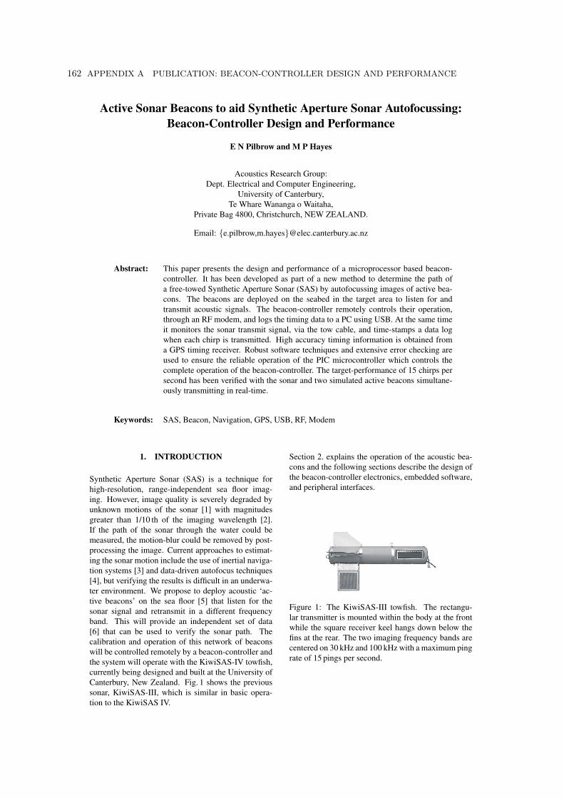
Active Sonar Beacons to aid Synthetic Aperture Sonar Autofocussing:Beacon-Controller Design and Performance
E N Pilbrow and M P Hayes
Acoustics Research Group:Dept. Electrical and Computer Engineering,
University of Canterbury,Te Whare Wananga o Waitaha,
Private Bag 4800, Christchurch, NEW ZEALAND.
Email: e.pilbrow,[email protected]
Abstract: This paper presents the design and performance of a microprocessor based beacon-controller. It has been developed as part of a new method to determine the path ofa free-towed Synthetic Aperture Sonar (SAS) by autofocussing images of active bea-cons. The beacons are deployed on the seabed in the target area to listen for andtransmit acoustic signals. The beacon-controller remotely controls their operation,through an RF modem, and logs the timing data to a PC using USB. At the same timeit monitors the sonar transmit signal, via the tow cable, and time-stamps a data logwhen each chirp is transmitted. High accuracy timing information is obtained froma GPS timing receiver. Robust software techniques and extensive error checking areused to ensure the reliable operation of the PIC microcontroller which controls thecomplete operation of the beacon-controller. The target-performance of 15 chirps persecond has been verified with the sonar and two simulated active beacons simultane-ously transmitting in real-time.
Keywords: SAS, Beacon, Navigation, GPS, USB, RF, Modem
1. INTRODUCTION
Synthetic Aperture Sonar (SAS) is a technique forhigh-resolution, range-independent sea floor imag-ing. However, image quality is severely degraded byunknown motions of the sonar [1] with magnitudesgreater than 1/10 th of the imaging wavelength [2].If the path of the sonar through the water could bemeasured, the motion-blur could be removed by post-processing the image. Current approaches to estimat-ing the sonar motion include the use of inertial naviga-tion systems [3] and data-driven autofocus techniques[4], but verifying the results is difficult in an underwa-ter environment. We propose to deploy acoustic ‘ac-tive beacons’ on the sea floor [5] that listen for thesonar signal and retransmit in a different frequencyband. This will provide an independent set of data[6] that can be used to verify the sonar path. Thecalibration and operation of this network of beaconswill be controlled remotely by a beacon-controller andthe system will operate with the KiwiSAS-IV towfish,currently being designed and built at the University ofCanterbury, New Zealand. Fig. 1 shows the previoussonar, KiwiSAS-III, which is similar in basic opera-tion to the KiwiSAS IV.
Section 2. explains the operation of the acoustic bea-cons and the following sections describe the design ofthe beacon-controller electronics, embedded software,and peripheral interfaces.
Figure 1: The KiwiSAS-III towfish. The rectangu-lar transmitter is mounted within the body at the frontwhile the square receiver keel hangs down below thefins at the rear. The two imaging frequency bands arecentered on 30 kHz and 100 kHz with a maximum pingrate of 15 pings per second.
162 APPENDIX A PUBLICATION: BEACON-CONTROLLER DESIGN AND PERFORMANCE

2. ACOUSTIC BEACONS
A number of active beacons will be freely deployed tosit on the seabed, connected to floating surface unitsby cables, as shown in Fig. 2. Antennas on the sur-
Figure 2: A conceptual drawing of the towboat andsonar passing by two acoustic beacons deployed onthe seabed. The surface units of each beacon allow RFcommunication with the beacon-controller and accessto GPS timing signals.
face units allow real time RF communication with thebeacon-controller, located on the boat, so all the mea-surements can be safely stored. As the boat tows thesonar past the target area, each beacon listens for thesonar acoustic chirp signal and responds back with achirp in a different frequency band. The sonar formsan image of the beacons that can be later reconstructedand autofocussed to determine the sonar path. Thispath knowledge can be used to remove the effect ofmotion-blur from the SAS image of the seabed.
Calibration of the distance between the beacons is ini-tiated by an RF command from the beacon-controller.The beacons then transmit acoustic signals betweenthemselves and determine their separation by mea-suring the flight-time. This allows the scaling ofthe reconstructed images to be verified and corrected.Periodic calibration, between imaging runs, allowschanges in the speed of sound to be monitored overtime.
3. ELECTRONICS OVERVIEW
Fig. 3 is a block diagram of the beacon-controllershowing how it connects to the external peripherals.Everything except the sonar is powered from the USBport of the host computer. The following sections de-tail its operation.
4. POWER SUPPLY AND DATA STORAGE
The controller and its peripherals all operate from a5 V supply with the exception of the RF modem. It
RF modem(MOD433)
GPSOncore UT+
SPI UART(MAX-3100)
SPI UART(MAX-3100)
Driver(MAX-232)
SPI
TTL RS232
RS232 TTL RS232
PIC(PIC-16F877)
Computer
USB module(DLP-USB245M)
USB
8 bit parallel
Optocoupler(HCPL-2400
Pulse edge
Figure 3: The dotted line encloses the modules thatmake up the beacon-controller. The heart of the sys-tem is a PIC-16F877 microcontroller. Extra serialports for the PIC are provided by MAX3100 UARTson a shared SPI bus to interface to the RF modem andGPS.
requires 9 V and this is provided by a MAX-761 step-up converter powered from the 5 V supply. These sup-ply requirements and all data transfer requirements areprovided by the USB bus.
4.1 USB Power Supply
When first plugged into the USB bus, only theDLP-USB245M module powers up drawing less than100mA as required by the USB specification [7]. Itthen requests permission to enable the rest of the PCBto draw a total current of 430 mA. The PC will grantthis request if the total current drawn from all deviceson the bus will not exceed 500mA.
Although the USB supply voltage is nominally 5 V,it is good practice to regulate it using a step-up con-verter e.g., a MAX-1797, because in operation it canbe significantly lower as Fig. 4 shows. Unfortunately,the switching nature of a step-up converter exacer-bates the problem of high startup currents causing theUSB supply voltage to droop. A transient droop of upto 330mV is permitted at startup and when enablingthe high-power section of the PCB. Testing revealedthat some computers are tolerant of much greater volt-age droops however this can cause brownout problemswith other devices on the bus. It can even cause theDLP-USB245M to reset, causing a reset of the thewhole beacon-controller. In an effort to avoid theseproblems and comply with the USB specification, aLM-3525 USB switch was used. The data sheet listsone of its applications as ”High Power USB DevicesRequiring Inrush Limiting” however it did not limit
163

Figure 4: This diagram, from the USB specification, shows how the 5 V nominal USB supply voltage can be as lowas 4.5 V (high current application like a bus-powered hub) or 4.35 V (low current application when powered froma bus-powered hub) at the application PCB. A further 330 mV transient voltage droop is permitted at switch-on orduring hot-plugging. [7]
the supply voltage droop sufficiently and produced er-rors on some computers. It was subsequently discov-ered that it only provides a simple 1 A current limit anddoes not monitor the supply voltage. To achieve fullcompliance, a dedicated current limiting switch e.g.,a MOSFET in series with the supply rail, should beused. It is recommended that the current limit be setat a similar level to the maximum current drawn undernormal operating conditions [8] i.e., 430 mA.
4.2 USB Data Storage
Virtual COM port drivers for Windows XP are usedto send commands and receive data from the beacon-controller via the DLP-USB245M module. This al-lows the USB port to be accessed like a standard COMport. For initial testing, Windows Hyperterminal wasused to display the data and log it to a file. A dedicatedJava program is currently being written to do this.
5. REMOTE CONTROL AND DATALOGGING
The beacon-controller and beacons communicate us-ing BlueChip MOD-433 RF modems featuring built-in error correction. They operate on the unlicensed433 MHz band with a transmission power of 10 mWequating to a range of 600 m in the open using 0 dBantennas.
5.1 Modem Hardware Handshaking
The beacon-controller modem operates as a DCE(Data Communications Equipment) using hardwarehandshaking lines CTS (Clear To Send) and RTS(Ready To Send) to control the transmission of each
packet of data. It asserts CTS to signal that it is readyto accept a packet from the beacon-controller andmonitors RTS to determine if the beacon-controlleris ready to accept a packet from the beacons. Everypacket of data sent to the modem must be precededby eight bytes of overhead specifying the destinationmodems address and the packet length. Despite know-ing the packet length, CTS remains asserted for an ad-ditional 5 ms after the last byte of a packet has been re-ceived before going low. This means it is not sufficientfor the beacon-controller to monitor the CTS level todetermine if the modem is ready to accept data or not.It must monitor the CTS signal edges as well and onlyattempt to send one packet for each rising CTS edge.
5.2 Data Transfer Rate vs Baud Rate
To achieve bidirectional communication betweenmore than two modems requires the MOD-433s to beused in ‘Peer to Peer’ mode [9] where each modem hasa unique address. In this mode the modems communi-cate using RS232 with a baud rate of 9600 bps, how-ever the average data rate is much slower due to irreg-ular pauses in their operation between each receivedRS232 packet. The pauses, usually close to 300 msbut can occasionally be up to 1.8 s, are presumablydue to error checking and RF negotiations between themodems. Averaging the data rate over several secondsshows that the highest data rates are achieved by send-ing long packets. This is shown in Table 1. Interest-ingly, the very long 1.8 s pauses occur less often whentwo modems are trying to transmit to one modem atthe same time.
6. TESTING WITH MULTIPLE MODEMS
The beacon-controller has been tested with simulatedtiming data sent to its MOD-433 via two other MOD-
164 APPENDIX A PUBLICATION: BEACON-CONTROLLER DESIGN AND PERFORMANCE

Table 1: The average data rate of the MOD-433 RF modems depends on the transmitted packet size. Using largerpackets allows significantly higher data rates. The maximum packet size is 64 bytes.
Data Overhead Packet size Packet rate Data rate(bytes) (bytes) (bytes) (packets/s) (bytes/s)
Small packet example 10 8 18 6 60Large packet example 50 8 58 3.5 175
433s simultaneously. This simulates the real-time con-current operation of two beacons although ultimately,many more will be used. When two MOD-433s at-tempt to transmit a packet to a third MOD-433 at thesame time, each one alternately gets priority for a shortrandom period of time. This ranges from a singlepacket of data up to a few seconds but the long termpriority averages out to be 50% for each modem. Thesimulated timing data is generated using a programwritten in Java to send the data to two serial ports ona PC. A separate thread for each serial port monitorsthe level and edge of the CTS signal of the attachedmodem to transmit the data is rapidly as the modemswill allow.
7. TIME-STAMPING THE ACOUSTICEVENTS
An event in time can be time-stamped in absoluteterms by adding an ‘absolute’ time, (preceding theevent) to an ‘offset’ time (up to the event). Fig. 5 illus-trates this. The offset time is obtained by counting
Absolute:
12 min,
34 sec
Offset: 1234 pulses
Timeline
Figure 5: What time did it happen? An event, de-picted by the inverted pyramid, can be time-stampedby adding an ‘absolute’ time, shown by the vertical ar-row, to an ‘offset time’ shown by the horizontal arrow.An example of this is shown in Fig. 6.
the number of oscillator clock cycles that have elapsedsince the last known absolute time update. Oscilla-tor output frequency drifts with temperature, age, andsupply voltage so regular absolute time updates are re-quired to prevent timing errors from building up and toestablish the exact frequency of the oscillator. Abso-lute time updates are provided by a Global PositioningSystem (GPS) receiver. This has the additional benefitof providing position information as well.
7.1 GPS Timing
The beacon-controller uses a Motorola Oncore UT+GPS timing receiver and a Motorola Timing 2000active-antenna. The GPS provides two timing outputs;a pulse signal (a regular rising edge every 0.01 s witha longer pulse every second) and a serial data stream(once per second corresponding to the rising edge ofthe pulse following the previous long pulse). The dy-namic i.e., under motion, timing accuracy is claimedto be ± 130 ns with GPS selective availability acti-vated. A standard Cmac 14.31818 MHz oscillator with30 ppm stability drives the PIC to provide a nominaltiming period resolution of 280 ns due to the internalPIC divide-by-four clock system. Fig. 6 shows howthese three pieces of timing information are used totime-stamp the 15 Hz acoustic signals transmitted bythe towfish.
The UT+ can output GPS time or UTC (UniversalTime Coordinated) time, formally known as GMT(Greenwich Mean Time). GPS time is a uniformlycounting time reference. It was synchronized to UTCtime on January 6, 1980, and now lags behind UTCtime by approximately 23 s due to the up to twice-yearly insertion of ‘leap-seconds’ to synchronize UTCtime to the changing rotation period of the earth. Thiscan happen at midnight UTC on June 30 or Decem-ber 31. Although GPS receivers can alert the user to apending leap second adjustment several weeks beforethe event, the use of GPS time as a reference meansleap-seconds can be ignored.
When the GPS is switched on, it performs a self-test,lasting 800 ms, and won’t accept serial commands dur-ing this time. A short period of time is then requiredfor it to lock-on and acquire data from a minimumof four satellites to provide timing information un-der dynamic conditions. A 3 V lithium battery pro-vides backup power to store satellite ephemeris andalmanac data when the beacon-controller is switchedoff. This helps to minimize the startup time to under15 s although it can be longer if the GPS has not beenswitched on recently.
8. SOFTWARE
The PIC16F877 microcontroller at the heart of thebeacon-controller has three main tasks. It must time-
165

100 PPS
1 second 1 second
15 Hz
3.6 MHz
Figure 6: Time stamping a 15 Hz event (not to scale). To time stamp the circled pulse, the serial data associatedwith the previous absolute GPS time reference (shown by the vertical arrow) is used to determine the absoluteminutes and seconds of the pulse following the long pulse. By adding on the offset time i.e., the number of100 PPS GPS pulses and 3.6 MHz pulses, the time the event occurred can be established. The actual frequency ofthe 3.6 MHz clock will drift and is measured by counting the total number of 3.6 MHz pulses between each GPS1 second update.
stamp the beginning of each acoustic transmissionfrom the towfish, it must remotely control and log datafrom the active beacons, and it must format the col-lected data and send it to a PC for storage. The ir-regular and overlapping nature of the tasks means arobust software design is required to ensure no con-flicts occur. This is achieved with a high speed mainloop, high speed subroutines for each of the tasks, andinterrupt-driven ring buffers for all incoming data. Byspending a small amount of time with each task on avery frequent basis, the PIC can service them all, nomatter when or in which order they occur. In betweenservicing the main tasks, many error checking proce-dures are performed. These include checks for ringbuffer overflow, missed timing pulses, and that suffi-cient satellite are visible for a good timing solution.The following sections explain the main tasks further.
8.1 Time-stamping the Towfish Transmissions
The towfish transmits two simultaneous linear fre-quency modulated chirps of 20 kHz bandwidth cen-tered on 30 kHz and 100 kHz. The chirps are typically12.5 ms long and have a repeat rate of up to 15 Hz. Thestart of each transmission is characterized by a rising-edge opto-isolated logic level signal that originates inthe towfish and is sent up the tow cable to the beacon-controller. Here, it is time-stamped, using the ‘captureport’ on the PIC, using the method explained in Sec-tion 7. This port operates independently and requiresno processor intervention. The processor only has toensure it reads the result into a ring buffer before thenext event occurs and processes the ring buffer con-tents before the buffer overflows.
8.2 RF Control and Logging of Beacons
Many aspects of the operation of the beacons willbe controlled by RF messages sent from the beacon-controller. These will include switching off the poweramplifiers to extend the battery life, changing thepreamp gain to maximize SNR but prevent clipping,and coordinating the calibration sequence.
The timing data associated with the arrival at eachbeacon of each towfish chirp (absolute and offset) istransmitted as a single RF packet back to the beacon-controller, once per second. By consolidating the tim-ing data into one-second packets a substantial reduc-tion in the amount of data can be made. Only a sin-gle absolute time reference of the minutes and sec-onds needs to be sent per packet. The 15 chirp ar-rival times can be represented by the offset (numberof 100 PPS pulses and number of 3.6 MHz pulses) ofeach chirp from the absolute reference. The absolutereference requires 2 bytes, each offset time requires 3bytes, 1 byte is used for beacon identification, 1 bytefor a checksum, and 1 byte to track the small deviationof the oscillator frequency from its nominal value of14.31818 MHz. For the maximum towfish chirp rateof 15 chirps per second, the packet length is 50 bytes.
Periodic logging of the local parameters for each bea-con e.g., battery life, depth, water temperature, andleakage status, will also be performed.
8.3 Data Formatting and PC Storage
All data received from the beacons is checked for er-rors against the checksum, calculated as the sequentialbitwise exclusive-or of the other bytes in the packet.This is a simple method to implement however error-correction is not possible so bad packets must be dis-carded and resent. The PIC formats the received data
166 APPENDIX A PUBLICATION: BEACON-CONTROLLER DESIGN AND PERFORMANCE

into NMEA-0183 [10] compliant sentences, with anew checksum, and sends it to a PC via USB for per-manent storage and later post processing.
The packets from the beacons are split into separatesentences (15 per second) containing the absolute timeand offset time for each received chirp. Similar sen-tences are constructed for each of the towfish trans-mitted chirps (15 per second). The GPS position datais converted into latitude and longitude sentences (1per second) to record the path of the towboat throughthe target area. The heading and velocity data arealso recorded (1 per second) along with the numberof satellites being used by the GPS, to ensure the so-lution is reliable. With two beacons operating at fullspeed this makes a total of 47 sentences per second.
9. CHEAP PCB MANUFACTURING
The Printed Circuit Board (PCB) for the beacon-controller was made by the Californian company,Sierra Proto Express (www.sierraprotoexpress.com).The Electrical and Computer Engineering Departmenthas had a number of PCBs made by this firm recentlydue to the low cost of their ‘No Touch’ service. Thisis a very basic service where no continuity testing isperformed on the finished board and adherence to thedesign rules is the responsibility of the customer. De-spite this, the results are normally excellent. Howeverinspection is essential since, occasionally, errors dooccur in the form of merged tracks where tolerancesare tight.
The total cost for the minimum order of two PCBsis US$118.15 made up of US$34 per PCB, a US$20service charge, and a US$30.15 shipping charge. Theturnaround time ranges from four to seven days. Themain features include two layers (four layers are avail-able), plated through holes, double sided silkscreenand solder mask, 6 mil minimum track widths andclearances, maximum dimensions 7.9 x 10.9 inchesplus a maximum area of 85 square inches, and singleedge-route with square corners only. The PCB file for-mat must be gerber.
10. CONCLUSIONS
The design of a beacon-controller to remotely controland log data from active beacons, operating with aSAS, was presented. It has been successfully testedwith two simulated beacons and sonar at a chirp rateof 15 chirps per second.
The use of ring buffers and interrupts in the PIC em-bedded software has allowed reliable, simultaneousinterfacing to slow and fast peripherals with irregu-lar data rates. A fast main loop with short subroutineloops means any pending events are quickly processed
and errors are quickly spotted. Checksums on all datapackets help to ensure data integrity.
Additional serial ports were added to the PIC micro-controller using SPI UARTs to enable serial commu-nication with an RF modem and GPS timing receiver.
Although USB compliance, with respect to the startupinrush current, has not been achieved, the beacon-controller has been tested on different computers anddid not cause any USB errors.
11. REFERENCES
[1] P. T. Gough and D. W. Hawkins. Imagingalgorithms for a strip-map synthetic aperturesonar: minimising the effects of aperture errorsand aperture undersampling. IEEE Journal ofOceanic Engineering, 22:27–39, 1997.
[2] D. W. Hawkins. Synthetic Aperture Imaging Al-gorithms: with application to wide bandwidthsonar. PhD thesis, Department of Electricaland Computer Engineering, University of Can-terbury, October 1996.
[3] E. N. Pilbrow, P. T. Gough, and M. P. Hayes.Inertial navigation system for a synthetic aper-ture sonar towfish. In Proceedings of Elec-tronics New Zealand Conference, Dunedin, NewZealand, 14-15 November 2002.
[4] P. T. Gough, M. P. Hayes, H. J. Callow, and S. A.Fortune. Autofocussing procedures for high-quality acoustic images generated by a syntheticaperture sonar. In Proceedings of InternationalCongress on Acoustics, Rome, Italy, September2001.
[5] E. N. Pilbrow, P. T. Gough, and M. P. Hayes.Dual transponder precision navigation system forsynthetic aperture sonar. In Proceedings of Elec-tronics New Zealand Conference, Dunedin, NewZealand, 14-15 November 2002.
[6] J. Pihl, P. Ulriksen, O. Kroling, B. Lovgren, andG. Shippey. Mlo classification using an rov-mounted wideband synthetic aperture sonar. InProceedings of The 5th European Conference onUnderwater Acoustics, Lyon, France, July 2000.
[7] USB Implementers Forum, www.usb.org. Uni-versal serial bus specification Revision 2.0.
[8] USB Implementers Forum, www.usb.org. USBDevelopers frequently asked questions.
[9] BlueChip Communication AS,www.bluechip.no. User manual for BCCradio modem 433MHz, Rev. A.
[10] National Marine Electronics Association,www.nmea.org. NMEA 0183 Interface Stan-dard.
167


Appendix B
RAY BENDING
B.1 INTRODUCTION
A non-constant sound speed profile causes ray bending, due to refraction, in the watercolumn. The equations for calculating the ray paths in two dimensions are presentedhere.
B.2 RAY PATHS
Consider an acoustic ray being emitted from a point (x0, z0), where x0 is the across-track co-ordinate and z0 is the depth, at an angle θ0 where θ0 = 0 when the ray isbeing emitted vertically upwards. If the sound speed profile changes linearly from czmax
at zmax to czmin at zmin then the equation describing the set of n points through whichthe ray passes, (xn, zn), is given by
zn = z0 +C0
K
(sin(θn)sin(θ0)
− 1)
(B.1)
where
K =czmin − czmax
zmax − zmin, (B.2)
C0 = czmax +K (z0 − zmin) , (B.3)
θn = cos−1
[cos (θ0)−
sin (θ0)K (xn − x0)C0
]. (B.4)


Appendix C
BEACON COMMANDS
This .h file is compiled with the DSP and microcontroller c code used in the boat andbeacon electronics. Each single byte command code is used to control one aspect ofthe system.
#ifndef COMMANDS_H
#define COMMANDS_H
/*Example command to restart the surface PIC: 2|2 */
/*Codes sent from the BCU to the BSU (via the BFU).*/
#define SET_PREAMP_TO_DEFAULT 120 /*ASCII x.*/
#define SET_POWERAMP_TO_DEFAULT 119 /*ASCII w.*/
#define SET_PREAMP_TO_MINIMUM 96 /*ASCII ’.*/
#define ENABLE_POWERAMP 118 /*ASCII v.*/
#define DISABLE_POWERAMP 117 /*ASCII u.*/
#define DECREASE_POWERAMP_GAIN 116 /*ASCII t.*/
#define INCREASE_POWERAMP_GAIN 115 /*ASCII s.*/
#define DECREASE_PREAMP_GAIN 114 /*ASCII r.*/
#define INCREASE_PREAMP_GAIN 113 /*ASCII q.*/
/*Codes sent from the boat computer to the surface unit.*/
/*Remember to do g before doing ~ or y.*/
#define POWER_OFF_ON_BEACON 122 /*ASCII z.*/
#define RESTART_AND_CLEAR_BEACON_LOG 123 /*ASCII .*/
#define RESTART 124 /*ASCII |.*/
#define RESTART_AND_RESET_GPS 125 /*ASCII .*/
#define RESTART_AND_CLEAR_DSP_NVRAM_PING_COUNTER 105 /*ASCII i.*/
#define PING_SOURCE_GPS 126 /*ASCII ~.*/

172 APPENDIX C BEACON COMMANDS
#define PING_SOURCE_EXTERNAL 121 /*ASCII y.*/
#define PING_SOURCE_DSP 112 /*ASCII p.*/
#define DSP_PING_PACKET_COUNTER_CLEAR 109 /*ASCII m.*/
#define DSP_INCREASE_THRESHOLD_LEVEL 107 /*ASCII k.*/
#define DSP_DECREASE_THRESHOLD_LEVEL 106 /*ASCII j.*/
#define SWITCH_DSP_RETRIEVE_MODE 103 /*ASCII g.*/
#define SWITCH_DSP_NORMAL_MODE 102 /*ASCII f.*/
#define SWITCH_DSP_DIAG_MODE 88 /*ASCII X.*/
#define SWITCH_PIC_NORMAL_MODE 104 /*ASCII h.*/
#define SWITCH_PIC_MONITORING_MODE 99 /*ASCII c.*/
#define DSP_SAVE_CORR_RAW 111 /*ASCII o.*/
#define DSP_SAVE_NOISE_RAW 108 /*ASCII l.*/
#define DSP_SAVE_PING_RAW 110 /*ASCII n.*/
#define DSP_SAVE_SAMPLES_RAW 97 /*ASCII a.*/
#define CALIBRATE_PREAMP 98 /*ASCII b.*/
#define CANCEL_CALIBRATE_PREAMP 89 /*ASCII Y.*/
/*Codes sent from the boat computer to the boat.*/
#define GPS_TIME_ENQUIRY 100 /*ASCII d.*/
#define RESET_BOAT_NOW 101 /*ASCII e.*/
/*Codes sent from the surface unit to the seabed unit.*/
#define HAS_SEABED_INITIALISED_OK 82 /*ASCII R.*/
#define GET_STATUS1 81 /*ASCII Q.*/
#define GET_STATUS2 80 /*ASCII P.*/
/*Codes sent from the seabed unit to the surface unit.*/
#define SEABED_OK_RESET_TIMEOUT 95 /*ASCII _.*/
#define SEABED_OK_RESET_TIMEOUT_CHARGING 94 /*ASCII ^.*/
#define SEABED_OK_RESET_TRANSFER_CHARGING 93 /*ASCII ].*/
#define BEACON_IS_CHARGING 92 /*ASCII \.*/
#define SEABED_OK 91 /*ASCII [.*/
#define SEABED_OK_RESET_TRANSFER 90 /*ASCII Z.*/
#endif

Appendix D
PACKET FORMAT
A list of the National Marine Electronics Association (NMEA) 0183 status packets andtiming packets sent from the beacon to the boat via RF modem. The packets followthe NMEA 0183 standard for marine data. Each packet is identified by a unique fivecharacter header. As specified by the standard, the first character is ‘P’ for proprietary,the following three characters identify the manufacturer, Acoustics Research Group(ARG), and the final character identifies the type of packet that follows. This allowsup to 26 different packet types. Packets are human readable American standard codefor information interchange (ASCII) and each field is separated by a comma. Thepacket is terminated with the following sequence: ‘*’, a two digit checksum, a carriagereturn, and a line feed.
D.1 STATUS PACKETS
D.1.1 Beacon status 1
$PARGJ,a,q,bb,cc,dddd,eee,fff,g,h*XXCRLF
(total length 38 bytes)
Field Description Range Units
a Beacon ID number 1 to 9
q error/warning/information code 0 to 127 0 is no message
bb Preamp gain 0 to 90
cc poweramp gain 0 to 90
dddd Seabed water pressure 0 to 9999 (Metres*27.088)+270.88
eee Seabed internal temperature 0 to 999 Degrees x 16
fff Seabed water temperature 0 to 999 Degrees x 16
g Seabed leakage detected 0 or 1 0 is a leak
h motion and tipping detected 0,1,2,3 1 is moving, 2 is tipped,3 is both

174 APPENDIX D PACKET FORMAT
D.1.2 Beacon status 2
$PARGK,a,q,bbbb,cccc,dddd,eeee*XXCRLF
(total length 35 bytes)
Field Description Range Units
a beacon ID number 1 to 9
q error/warning/information code 0 to 127 0 is no message
bbbb Seabed supply voltage 0 to 9999 V x 30.63
cccc poweramp voltage 0 to 9999 V x 30.63
dddd Battery2 voltage 0 to 9999 V x 35.41
eeee Battery1 voltage 0 or 9999 V x 72.73
D.1.3 Beacon Status 3
$PARGW,a,q,bbbbb,cccc,ddd,e*XXCRLF
(total of 32 bytes)
Field Description Range Units
a beacon ID number 1 to 9
q error/warning/information code 0 to 127 0 is no message
bbbbb Velocity 0 to 51400 cm/s
cccc Heading 0 to 3599 Degrees x 10
ddd Surface internal temperature 0 to 999 Degrees x 16
e Surface leakage detected 0 or 1 0 is a leak
D.1.4 Beacon Status 4
$PARGX,a,q,bbbbbbbbbc,ddddddddde,fff,ggg*XXCRLF
(total of 45 bytes)

D.1 STATUS PACKETS 175
Field Description Range Units
a beacon ID number 1 to 9
q error/warning/informationcode
0 to 127 0 is no message
bbbbbbbbb Longitude 0 to 648000000 Milli arc seconds
c Longitude direction E or W
ddddddddd Latitude 0 to 324000000 Milli arc seconds
e Latitude direction N or S
fff Surface supply voltage 0 to 999 V x 35.93
ggg Surface water temperature 0 to 999 Degrees x 16
D.1.5 DSP raw data
The DSP can send a number of raw data sets through which are split into short sen-tences of 4 pieces of data. Each type of data is identified by the NMEA headers$PARGR, $PARGS, $PARGT, $PARGU, and $PARGV. The position of each shortpacket within the data set is identified by the bbbb field which is the index of thefollowing field.
$PARG?,a,q,bbbb,ccccc,ddddd,eeeee,fffff*XXCRLF
(total of 44 bytes)
Field Description Range Units
a beacon ID number 1 to 9
q error/warning/information code 0 to 127 0 is no message
bbbb index of the following byte, i.e., ccccc,within the dataset
Anything
D.1.6 Boat Status1
$PARGC,aa,b,ccccc,dddd,*XXCRLF
(total of 28 bytes)
Field Description Range Units
aa Visible GPS satellites 0 to 12
b Satellites being tracked 0 to 8
ccccc Velocity 0 to 51400 cm/s
dddd Heading 0 to 3599 Degrees x 10

176 APPENDIX D PACKET FORMAT
D.1.7 Boat Status 2
$PARGD,aaaaaaaaab,cccccccccd,eee*XXCRLF
(total of 37 bytes)
Field Description Range Units
aaaaaaaaa Longitude 0 to 648000000 Milli arc seconds
b Longitude direction E or W
ccccccccc Latitude 0 to 324000000 Milli arc seconds
d Latitude direction N or S
eee Supply voltage 0 to 999 V x 18.5
D.2 TIMING PACKETS
D.2.1 Ping transmitted by towfish
$PARGE,a,bb,cc,ddd,eee,fffff*XXCRLF
(total of 33 bytes)
Field Description Range Units
a Boat ID number 0
bb Last GPS time update 0 to 59 Minutes
cc Last GPS time update 0 to 59 Seconds
ddd Oscillator LSB Around 154 Pulses
eee Number of 100PPS pulses since lastGPS time update
0 to 200
fffff Number of 2.5MHZ pulses since last100PPS pulse
0 to about 25000
D.2.2 Ping received by beacons
$PARGF,a,bb,cc,ddd,eee,fffff*XXCRLF
(total of 33 bytes)

D.2 TIMING PACKETS 177
Field Description Range Units
a Beacon ID number 1 to 9
bb Last GPS time update 0 to 59 Minutes
cc Last GPS time update 0 to 59 Seconds
ddd Oscillator LSB Around 103 pulses
eee Number of 100PPS pulses since lastGPS time update
0 to 200
fffff Number of 3.579545MHZ pulses sincelast 100PPS pulse
0 to about 35796
D.2.3 Beacon status special
This packet is sent more often that the regular status packets because it contains themost useful set of status information.
$PARGY,a,q,bb,c,ddd,eee,fff,gg,h,iii,jjj*XXCRLF
(total of 45 bytes)
Field Description Range Units
a beacon ID number 1 to 9
q error/warning/information code 0 to 127 0 is no message
bb Current time 0 to 59 Seconds
c Satellites being tracked 0 to 8
ddd parameter1 0 to 255 ?
eee parameter2 0 to 255 ?
fff parameter3 0 to 255 ADC samples
gg Number of pings in the last packet 0 to 16 Pings
h Ping packets in memory 0 to 9 Packets
iii Maximum ping to ping variation 0 to 255 µs*100
jjj parameter4 0 to 255 % of full scale


Appendix E
SPHERICAL AND HYPERBOLIC POSITIONINGEQUATIONS
Consider an acoustic positioning system where N fixed transponders are tracking asonar. The transponders and sonar are located at (xn, yn, zn) and (xs, ys, zs) respec-tively for n = 1 . . . N . The following sections present equations for locating the positionof the sonar in three dimensions using spherical and hyperbolic modes of operation.The sonar is assumed to be static and the systems are assumed to be able to uniquelyidentify all the acoustic signals, i.e., some form of coding is used.
E.1 SPHERICAL POSITIONING
A spherical positioning system measures the time of flight (TOF) from the sonar toeach transponder and converts this to distance by multiplying by the speed of sound.There are three unknowns (the sonar coordinates) so using three beacons provides afully determined system. The equations describing the system geometry are
(xs − x1)2 + (ys − y1)2 + (zs − z1)2 = r21, (E.1)
(xs − x2)2 + (ys − y2)2 + (zs − z2)2 = r22, (E.2)
(xs − x3)2 + (ys − y3)2 + (zs − z3)2 = r23, (E.3)
where rn is the distance from the sonar to transponder n, measured by the system.Solving this system of equations for xs, ys, and zs follows the method used by Chadwick[Chadwick and Bricker 1990]. Subtracting (E.2) from (E.1) and (E.3) from (E.1) andmaking the following substitutions for the constant parts,
R2i = x2
i + y2i + z2
i , (E.4)
Xi = xi − x1, (E.5)
Yi = yi − y1, (E.6)
Zi = zi − z1, (E.7)

180 APPENDIX E SPHERICAL AND HYPERBOLIC POSITIONING EQUATIONS
gives the following two equations:
2xsX2 + 2ysY2 + 2zsZ2 +R21 −R2
2 = r21 − r22, (E.8)
2xsX3 + 2ysY3 + 2zsZ3 +R21 −R2
3 = r21 − r23. (E.9)
Solving simultaneously produces
xs =−2zs (Y3Z2 − Y2Z3) + Y3
(r21 − r22 +R2
2 −R21
)− Y2
(r21 − r23 +R2
3 −R21
)2 (Y3X2 − Y2X3)
, (E.10)
ys =−2zs (X3Z2 −X2Z3) +X3
(r21 − r22 +R2
2 −R21
)−X2
(r21 − r23 +R2
3 −R21
)2 (X3Y2 −X2Y3)
.
(E.11)
Recognising that (E.10) and (E.11) can be written in the form
xs = A2zs +A1, (E.12)
ys = B2zs +B1, (E.13)
and substituting both of these into (E.1) produces a quadratic equation in z;
C1z2s + C2zs + C3, (E.14)
where the constants are given by
A1 =Y3
(r21 − r22 +R2
2 −R21
)− Y2
(r21 − r23 +R2
3 −R21
)2 (Y3X2 − Y2X3)
, (E.15)
A2 =−2 (Y3Z2 − Y2Z3)2 (Y3X2 − Y2X3)
, (E.16)
B1 =X3
(r21 − r22 +R2
2 −R21
)−X2
(r21 − r23 +R2
3 −R21
)2 (X3Y2 −X2Y3)
, (E.17)
B2 =−2 (X3Z2 −X2Z3)2 (X3Y2 −X2Y3)
. (E.18)
C1 = A22 +B2
2 + 1, (E.19)
C2 = −2 (A2x1 +B2y1 + z1 −A1A2 −B1B2) , (E.20)
C3 = A21 +B2
1 + z21 − x1 (2A1 − x1)− y1 (2B1 − y1)− r21, (E.21)
with solutions
zs =−C2 ±
√C2
2 − 4C1C3
2C1, (E.22)
The negative solution can be eliminated by assuming the sonar is flying above theseabed. By inspection (C1 is always positive) this can be seen to be solution involvingthe addition of the square root. Expressions for x and y are found by substituting into

E.2 HYPERBOLIC POSITIONING 181
(E.12) and (E.13) giving a sonar position of
xs = A2zs +A1, (E.23)
ys = B2zs +B1, (E.24)
zs =−C2 +
√C2
2 − 4C1C3
2C1. (E.25)
E.2 HYPERBOLIC POSITIONING
A hyperbolic positioning system measures the time difference of flight (TDOF) betweenpairs of transponders and converts this to distance differences by multiplying by thespeed of sound. There are four unknowns (the three sonar coordinates and the dis-tance between the sonar and the designated reference transponder, chosen here to betransponder one) so using four transponders provides a fully determined system. Theequations describing the system geometry are based on
(xs − xn)2 + (ys − yn)2 + (zs − zn)2 = r2n, (E.26)
where rn is given by
rn = ∆nm + rm (E.27)
where ∆nm is the difference in distance between transponder n and transponder m,measured by the system. The complete set of equations is
(xs − x1)2 + (ys − y1)2 + (zs − z1)2 = r21, (E.28)
(xs − x2)2 + (ys − y2)2 + (zs − z2)2 = (∆21 + r1)2 , (E.29)
(xs − x3)2 + (ys − y3)2 + (zs − z3)2 = (∆31 + r1)2 , (E.30)
(xs − x4)2 + (ys − y4)2 + (zs − z4)2 = (∆41 + r1)2 . (E.31)
Solving this system of equations for xs, ys, and zs follows a similar approach tothe spherical system. Full working is presented by Bucher [Bucher and Misra 2000][Bucher 2000] with a minor mistake in the derivation of L. The corrected solution forthe sonar position is
zs =N ±
√N2 − 4MO
2M, (E.32)
ys = Izs + J, (E.33)
xs = Gzs +H, (E.34)

182 APPENDIX E SPHERICAL AND HYPERBOLIC POSITIONING EQUATIONS
where the constants are given by
A =∆13X21 −∆12X31
∆12Y31 −∆13Y21, (E.35)
B =∆13Z21 −∆12Z31
∆12Y31 −∆13Y21, (E.36)
C =∆13
(∆2
12 +R21 −R2
2
)−∆12
(∆2
13 +R21 −R2
3
)2 (∆12Y31 −∆13Y21)
, (E.37)
D =∆34X23 −∆32X43
∆32Y43 −∆34Y23, (E.38)
E =∆34Z23 −∆32Z43
∆32Y43 −∆34Y23, (E.39)
F =∆34
(∆2
32 +R23 −R2
2
)−∆32
(∆342 +R2
3 −R24
)2 (∆32Y43 −∆34Y23)
, (E.40)
G =E −B
A−D, (E.41)
H =F − C
A−D, (E.42)
I = AG+B, (E.43)
J = AH + C, (E.44)
K = ∆213 +R2
1 −R23 + 2X31H + 2Y31J, (E.45)
L = 2(X31G+ Y31I + Z31), (E.46)
M = 4∆213
(G2 + I2 + 1
)− L2, (E.47)
N = 8∆213 (G (x1 −H) + I (y1 − J) + z1) + 2LK, (E.48)
O = 4∆213
((x1 −H)2 + (y1 − J)2 + z2
1
)−K2, (E.49)
where Pnm = pn − pm for P ∈ X,X,Z.

Appendix F
RICIAN MOMENTS
F.1 INTRODUCTION
The Rician pdf is given by [Whalen 1971, 105][Kay 1993, 31][Rice 1945, 101, eq. 3.10-16]
fM (m) =m
σ2em2+A2
−2σ2 I0
(Am
σ2
)(F.1)
where Ik() is the modified Bessel function of the first kind, order k.
The raw moments are given by [Whalen 1971, 105][Rice 1945, 101, eq. 3.10-12]
µ′n =(2σ2
)n2 Γ
(1 +
n
2
)1F1
(−n
2; 1;− A2
2σ2
)(F.2)
where µ′n is the nth raw moment, 1F1() is the confluent hypergeometric function of thefirst kind, and Γ() is the gamma function. Using the following generalized Laguerrepolynomial identity [Abramowitz and Luke 1975, p434]
L(α)β (x) =
(α+ 1)n
n! 1F1(−β;α+ 1;x), (F.3)
where (a)n is the rising factorial
(a)n = (1)(a+ 0)(a+ 1)(a+ 2) . . . (a+ n− 1) =(a+ n− 1)!
(a− 1)!, (F.4)
allows (F.2) to be written as
µ′n = (2σ)n2 Γ
(1 +
n
2
)L
(0)n2
(− A2
2σ2
)(F.5)
Simple expressions for the even moments are easily obtained by evaluating (F.5) how-ever the odd moments are complicated.

184 APPENDIX F RICIAN MOMENTS
The first four raw moments evaluate as [Sijbers 1998, 11]
µ′1 = σφ, (F.6)
µ′2 = A2 + 2σ2, (F.7)
µ′3 = σ3θ, (F.8)
µ′4 = A4 + 8σ2A2 + 8σ4, (F.9)
where
φ =√π
2e−
ψ4
[(1 +
ψ
2
)I0
(ψ
4
)+
(ψ
2
)I1
(ψ
4
)], (F.10)
θ =√π
2e−
ψ4
[(3 + 3ψ +
ψ2
2
)I0
(ψ
4
)+
(2ψ +
ψ2
2
)I1
(ψ
4
)], (F.11)
ψ =A2
σ2. (F.12)
Using (G.4) the first four central moments are
µ1 = 0 (F.13)
µ2 = σ2(−φ2 + ψ + 2
), (F.14)
µ3 = σ3(2φ3 − 3φ(ψ + 2) + θ
), (F.15)
µ4 = σ4(−3φ4 + 6φ2(ψ + 2)− 4φθ + ψ2 + 8ψ + 8
). (F.16)
and the Pearson coefficients, defined in Appendix G, are
β1 =
(2φ3 − 3φ (ψ + 2) + θ
)2
(−θ2 + ψ + 2)3, (F.17)
β2 =−3φ4 + 6φ2 (ψ + 2)− 4φθ + ψ2 + 8ψ + 8
(−φ2 + ψ + 2)2. (F.18)
Note that β1 and β2 both depend on a single parameter, ψ, so the Rician distributionis represented by a line on the β1β2 chart.

Appendix G
DISTRIBUTION CHARTS
G.1 INTRODUCTION
Distribution charts allow visual comparisons of families of distributions using a compactchart of areas, lines, and points. One commonly used distribution chart, known as theβ1β2 chart [Johnson et al. 1994, 23][Pearson et al. 1954, fig. 7], is a plot of kurtosis (β2)vs skewness squared (β1). Traditionally β1 increases to the right on the horizontal axisand β2 decreases down the vertical axis as shown in Fig. G.1. Its conception is oftenattributed to Karl Pearson who used it to illustrate the Pearson system of distributions[Ord 1972, Chap. 1][Kendall et al. 1987, Chap. 6]. Plotting the point (β1, β2) for a setof data samples shows visually (based on proximity) which common distributions couldbe fitted to the data. Splitting the data into smaller sets and plotting (β1, β2) for eachset gives an indication of how consistent the data is, by considering the spread of thepoints, e.g., the variance.
Selecting a common distribution type to represent the observed data usually in-volves a choice (i.e., the point or set of points lie close to multiple distributions) whichwill likely depend on external factors, such as ease of computation or to conform withpreviously published work. Once a distribution has been selected and fitted to the data,a goodness-of-fit test, e.g., Kolmogorov-Smirnov (KS) [Harnett 1982, pp712–713][Steeland Torrie 1980, pp535–537], should be performed to check that the fit is appropriatefor the application.
G.2 PARAMETERS
The equations are based on the standard definitions for skewness and kurtosis,
β1 =µ2
3
µ32
(G.1)
β2 =µ4
µ22
, (G.2)

186 APPENDIX G DISTRIBUTION CHARTS
β1
β 2
0 0.5 1 1.5 2 2.5 3 3.5 4
1
2
3
4
5
6
7
8
9
Beta (U shaped)Beta (J shaped)Beta (unimodal)Pearson type VIPearson type IVBernoulliParetoTriangularRicianPoisson (discrete)ChiWeibullNon central chi2
GammaInverse GaussianLog normalPearson type VPearson type IIStudent’s TUniformNormalMaxwellRayleighLogisticExtreme valueLaplaceHalf normalExponentialImpossible region
Figure G.1: β1β2 chart of many common statistical distributions.

G.3 CONVERTING MOMENTS 187
where µn is the nth central sample moment (the moment about the sample mean, µ),i.e.,
µn = E[(x− µ)n]. (G.3)
G.3 CONVERTING MOMENTS
Often only the raw moments (moments about zero) of a distribution are published.The central moments (moments about the mean) can be obtained from raw momentsusing the binomial transform
µn =n∑
k=1
n!(n− k)!k!
(−1)n−kµ′kµ′n−kk (G.4)
where µ′k is the kth raw moment.


Appendix H
METHOD OF MOMENTS
H.1 INTRODUCTION
The following sections present equations for fitting combinations of common distribu-tions to datasets using the method of moments.
H.2 GAUSSIAN DISTRIBUTION
The Gaussian or normal probability density function (PDF) is [Simon 2002, p1]
fG(g) =1
σ√
2πe−(g−µ)2
2σ2 (H.1)
where µ is the mean and σ is the standard deviation (STD). If µ = 0 then the raw-moment equation is
µ′n =
0, n odd
σn∏n
2k=1 2k − 1, n even
(H.2)
leading to the first three raw moments
µ′1 = E[G] = 0,
µ′2 = E[G2
]= σ2, (H.3)
µ′3 = E[G3
]= 0.
H.3 GAMMA DISTRIBUTION
The two-parameter gamma PDF is [Johnson et al. 1994, p343]
fY (y) =yα−1
βαΓ(α)e−yβ . (H.4)

190 APPENDIX H METHOD OF MOMENTS
The raw-moment equation is [Patil 1984, p64]
µ′n =βnΓ(α+ n)
Γ(α)(H.5)
leading to the first three raw moments
µ′1 = E[Y ] = αβ,
µ′2 = E[Y 2
]= α (α+ 1)β2, (H.6)
µ′3 = E[Y 3
]= α (α+ 1) (α+ 2)β3.
Equation (H.4), as with any two-parameter distribution that does not include a“location” parameter, can be extended to a three-parameter distribution by includinga constant offset, y0;
fY (y) =(y − y0)
α−1
βαΓ(α)e−(y−y0)
β . (H.7)
H.4 WEIBULL DISTRIBUTION
The two-parameter Weibull PDF is [Johnson et al. 1994, p656]
fW (w) =αwα−1
βαe−
“wβ
”α(H.8)
The raw-moment equation is [Johnson and Kotz 1970, p252]
µ′n = βnΓ(1 +
n
α
)(H.9)
leading to the first three raw moments
µ′1 = E[Y ] = βΓ(
1 +1α
),
µ′2 = E[Y 2
]= β2Γ
(1 +
2α
), (H.10)
µ′3 = E[Y 3
]= β3Γ
(1 +
3α
).
H.5 RICIAN DISTRIBUTION
The Rician PDF, the raw-moment equation and the first four raw moments are givenby (F.1), (F.2), and (F.6) - (F.9) respectively.

H.6 METHOD OF MOMENTS—GAMMA EXAMPLE 191
H.6 METHOD OF MOMENTS—GAMMA EXAMPLE
Consider a random variable Z
Z = G+ Y +O (H.11)
where G is a Gaussian-distributed random variable with zero mean and known varianceV = σ2, Y is a gamma-distributed random variable, and O is a constant. The firstthree raw moments of Z are
µ′1 = E[G+ Y +O],
µ′2 = E[(G+ Y +O)2
], (H.12)
µ′3 = E[(G+ Y +O)3
],
which expands and simplifies to
µ′1 = αβ +O,
µ′2 = αβ2 (α+ 1) + 2αβO +O2 + V, (H.13)
µ′3 = αβ3 (α+ 1) (α+ 2) + 3αβ2O (α+ 1) + 3αβO2 +O3 + 3αβV.
The system of (H.13) can be solved numerically for the unknowns (α, β, O) for a givenset of data by replacing µ′1, µ
′2, and µ′3 with the raw moments of the data.
H.7 METHOD OF MOMENTS—RICIAN EXAMPLE
Consider a random variable Z
Z = G+M +O (H.14)
where G is a Gaussian-distributed random variable with zero mean and known varianceV = σ2, M is a Rician-distributed random variable, and O is a constant. The firstthree raw moments of Z are
µ′1 = E[G+M +O],
µ′2 = E[(G+M +O)2
], (H.15)
µ′3 = E[(G+M +O)3
],

192 APPENDIX H METHOD OF MOMENTS
which expands and simplifies to
µ′1 = σφ+O,
µ′2 = σ2 (ψ + 2) + 2σφO +O2 + V, (H.16)
µ′3 = 3σ2O (ψ + 2) + 3σφO2 +O3 + σ3θ + 3σφV,
where θ, ψ, and φ are all functions of the two Rician parameters, A and σ, defined in(F.1). The system of (H.16) can be solved numerically for the unknowns (A, σ, O) fora given set of data by replacing µ′1, µ
′2, and µ′3 with the raw moments of the data.
H.8 METHOD OF MOMENTS—WEIBULL EXAMPLE
Consider a random variable Z
Z = G+W +O (H.17)
where G is a Gaussian-distributed random variable with zero mean and known varianceV = σ2, W is a Weibull-distributed random variable, and O is a constant. The firstthree raw moments of Z are
µ′1 = E[G+W +O],
µ′2 = E[(G+W +O)2
], (H.18)
µ′3 = E[(G+W +O)3
],
which expands and simplifies to
µ′1 = βΓ(φ) +O,
µ′2 = β
(βΓ
(1 +
2α
)+ 2OΓ(φ)
)+ V +O2, (H.19)
µ′3 = β3Γ(
1 +3α
)+ 3Oβ2Γ
(1 +
2α
)+ V (3βΓ(φ) + 3O) + 3O2βΓ(φ) +O3,
where
φ = 1 +1α. (H.20)
The system of (H.19) can be solved numerically for the unknowns (α, β, O) for a givenset of data by replacing µ′1, µ
′2, and µ′3 with the raw moments of the data.

Appendix I
TRANSDUCER VELOCITY POTENTIAL
The following is a derivation of the relationship between the acoustic velocity potentialof the fluid at the surface of a flat piston transducer and the transducer surface velocity.
Consider a flat transducer surface, vibrating with a scalar velocity U(f) in m/s/Hz,radiating in a direction given by n, a normalised vector (unit length) perpendicular tothe transducer surface, as illustrated in Fig. I.1.
Figure I.1: Geometry for a flat transducer. a(x′ − x0) is the aperture function, definedin J.
Assuming the transducer is rigid and assuming continuity of velocity between thetransducer and the fluid, the particle velocity vector at a point x′, located an infinites-imally small distance away from the surface of the transducer, describes a plane wave;
U(f,x′) = U(f)e−jkn·x′n, (I.1)
where k = 2πfc , ignoring edge effects.
The particle velocity vector and the velocity potential1, ψ(f,x), at any point in an
1A scalar field, formally called the acoustic velocity potential field in m2/s/Hz [Ziomek 1995, pp17-18]

194 APPENDIX I TRANSDUCER VELOCITY POTENTIAL
irrotational fluid, are related via the Laplacian operator;
U(f,x) = ∇ψ(f,x), (I.2)
=(∂
∂xψ(f,x),
∂
∂yψ(f,x),
∂
∂zψ(f,x)
). (I.3)
Making the assumption that the velocity potential at x′ can be approximated by aplane wave [Hunter June 2006, p26], i.e.,
ψ(f,x′) = H(f)e−jkn·x′ (I.4)
where H(f) is the appropriate transfer function, then (I.3) evaluated at x′ is
U(f,x′) = H(f)∇(e−jknxx′xe−jknyx′ye−jknzx′z
)(I.5)
= H(f)(−jknxe
−jkn·x′ ,−jknye−jkn·x′ ,−jknze
−jkn·x′)
(I.6)
= −jkH(f)e−jkn·x′ (nx, ny, nz) (I.7)
= −jkH(f)e−jkn·x′n. (I.8)
Equating (I.1) and (I.8) reveals the transfer function H(f);
H(f) =U(f)−jk
(I.9)
in m2/s/Hz. Substituting into (I.4) completes the equation for the relationship betweenψ(f,x′), the acoustic velocity potential of the fluid at the surface of a flat pistontransducer, and U(f), the transducer velocity;
ψ(f,x′) =U(f)−jk
e−jkn·x′ . (I.10)
See Appendix K for the derivation of an expression for U(f).

Appendix J
KiwiSAS PROJECTOR EQUATIONS
J.1 KiwiSAS BP
The Kiwi Synthetic Aperture Sonar (KiwiSAS) transmit array uses closely spaced trans-ducers so, in the far field,1 can be approximated by a continuous array. Most acousticstextbooks [Urick 1975, p50][Camp 1970, p162][Medwin and Clay 1998, p137] use thesimplified derivation taken by Huygens where the aperture is represented by a largenumber of small point sources radiating in all directions, resulting in a sinc functionwith an obliquity factor (OF) of one.2 The OF is a secondary effect where the effectivetransducer length is scaled down when viewed from angles other than broadside, asshown in Fig. 4.21(b). Fresnel and Kirchoff, working in the field of optics, improvedupon Huygens’ model and arrived at an obliquity factor of 1
2 (1 + cos θ) [Goodman 2005,eq. 3-50]. Their derivation is for a plane wave diffracting through an aperture formedby an opening in an infinite sheet. However, the same OF results when considering asingle-sided vibrating transducer in free space [Hunter June 2006, p26-33].
A continuous line array of length L centred at x = 0 can be described as a function,a1(x), of position, known as the aperture function. The spatial Fourier transform,A1(fx), evaluated at the direction cosines in spherical coordinates is given by
a1(x) = rect(xL
), (J.1)
A1(fx) = Fx a1(x) (J.2)
A1(f, θ) = A1
(f
csin θ
)(J.3)
= L sinc(f
cL sin θ
), (J.4)
where sinc (x) = sin(πx)πx . The equivalent [Ziomek 1995, p471] for a continuous rectan-
1The far field is the distance at which the beam pattern (BP) can be considered to be independentof range, i.e., only dependent on angle.
2The universal omission of the OF in textbook beam pattern (BP) equations is thought to bebecause most acoustics applications are concerned with the properties of the main lobe where θ issmall.

196 APPENDIX J KiwiSAS PROJECTOR EQUATIONS
gular array (length Lx, width Ly) centred on (x = 0, y = 0), as shown in Figs. J.2 andJ.1, is
a2(x, y) = rect(x
Lx
)rect
(y
Ly
), (J.5)
A2(fx, fy) = Fx,y a2(x, y) , (J.6)
A2 (f, θ, ϕ) = A2
(f
csin θ cosϕ,
f
csin θ sinϕ
), (J.7)
= LxLy sinc(f
cLx sin θ cosϕ
)sinc
(f
cLy sin θ sinϕ
). (J.8)
The beam pattern (BP) combines the OF with the angular dependent components
x0
Figure J.1: Geometry for a flat transducer using a spherical coordinate system.
of A1(f, θ) or A2(f, θ, ϕ) for a line array and rectangular array respectively;
BP1(f, θ) = sinc(f
cL sin θ
)12
(1 + cos θ) , (J.9)
BP2(f, θ, ϕ) = sinc(f
cLx cos θ sinϕ
)sinc
(f
cLy sin θ sinϕ
)12
(1 + cos θ) . (J.10)
The BP is unitless, and has a maximum value of unity at broadside.
The angles corresponding to the nulls in the BP, in one dimension, can be foundby equating (J.9) to zero [Camp 1970, pp165–170] and solving for θ using
sinc (n) = 0 (J.11)

J.1 KiwiSAS BP 197
Figure J.2: Projector array (plan and elevation views).
for n = ±1,±2,±3, .... This gives
θnull(n) = sin−1
(nλ
L
), (J.12)
θnull−to−null(n) = 2 sin−1
(nλ
L
), (J.13)
where λ = cf so the main beam null-to-null width is
θmain = 2 sin−1
(λ
L
). (J.14)
For high frequencies or large arrays, θmain is often small enough to allow the approxi-mation
sin θ ≈ θ, (J.15)
so
θmain ≈2λL. (J.16)

198 APPENDIX J KiwiSAS PROJECTOR EQUATIONS
J.1.0.1 KiwiSAS TVR and directivity
The time-domain pressure at a point in space, given by the spherical coordinates r, θ,and ϕ can be approximated by [Ziomek 1995, p483]
p(t, r, θ, ϕ) ≈ −ρ0∂
∂tψ(t, r, θ, ϕ), (J.17)
where ψ(t, r, θ, ϕ) is the acoustic field velocity potential in m2/s and ρ0 is the densityof the fluid in kg/m3. The equivalent representation in the frequency domain is
p(f, r, θ, ϕ) ≈ −ρ0j2πfψ(f, r, θ, ϕ). (J.18)
The far-field frequency-domain velocity potential for a vibrating rectangular pistontransducer is [Hunter June 2006, eq 2.58]
ψ(f, θ, ϕ, |r, L) = jke−j2πrf/c
4πrH(f)A2(f, θ, ϕ)OF(θ), (J.19)
= jke−j2πrf/c
4πrH(f)LxLyBP2(f, θ, ϕ), (J.20)
in m2/s/Hz, where k = 2πfc , provided the acoustic field on the transducer surface has
the form of (I.4). From Appendix I
H(f) =U(f)−jk
. (J.21)
Substituting into (J.18) reveals the pressure;
p(f, θ, ϕ|r, L, V ) = kfρ0e−j2πrf/c
2rH(f)LxLyBP2(f, θ, ϕ), (J.22)
=jfρ0e
−j2πrf/cU(f)LxLyBP2(f, θ, ϕ)2r
, (J.23)
in Pa/Hz. Appendix K shows
U(f) =φV (f)
ZM (f) + ZR(f)(J.24)
using simple models for the transducer and water load, giving the complete directivityequation;
p(f, θ, ϕ|r, L, V ) =jfρ0e
−j2πrf/cφV (f)LxLyBP2(f, θ, ϕ)2r (ZM (f) + ZR(f))
. (J.25)

J.1 KiwiSAS BP 199
The transmit voltage response (TVR) is then
pBS(f |r, L, V ) =jfρ0e
−j2πrf/cφV (f)LxLy
2r (ZM (f) + ZR(f)). (J.26)
Inspection of (J.25) reveals the TVR is frequency dependent. This is not a problemif the projector is being driven at a constant frequency.3 However, significant outputvariation will occur with a wide bandwidth signal centred on a low frequency4, such asthe KiwiSAS 30 kHz chirp. In this situation, a transducer design better suited to widebandwidth signals, e.g., a multi-resonant Tonpilz, is a better choice [Knight 1987].
Equation J.25 can be reversed to obtain the transducer output voltage due toa far field pressure. Note, however, that this is a different quantity to the receivepressure response (RPR) or receive directivity in datasheets which plots the transduceroutput voltage due to a constant pressure at the transducer. The RPR is derived inAppendix K.
3Projectors are usually operated at the resonant frequency to maximise efficiency.4In practice, the physical geometry of transducers causes deviation from this ideal formula, espe-
cially near resonance and for larger transducers containing multiple interacting elements.


Appendix K
TRANSDUCER MODEL
K.1 INTRODUCTION
By modelling a transducer as a two-port network (an electrical port and a mechanicalport), with associated inputs and outputs (IO), the electrical IO (voltage and current)can be related to the mechanical IO (force and velocity) using the appropriate sourceand load for transmitting or receiving. The mechanical properties are modelled usingequivalent electrical components and the IO at each port are found from Kirchoff’slaws for electrical circuit analysis. Figure K.1 shows a simple two-port network for apiezoelectric transducer immersed in water [Burdic 1984, p84] with properties definedin Table K.1.
K.1.1 Transformer effects
The transformer primary:secondary ratio, 1 : φ, represents the sensitivity of the trans-ducer by relating the electrical properties to the mechanical properties. It can bereplaced by a direct connection by referring the secondary voltages, currents, andimpedances (including those of the load) to the primary side. This is done by dividingall secondary side voltages, currents, and impedances by φ, 1
φ , and φ2 respectively.Figure K.2 shows an example of applying this to an isolated transducer. For a crystaltransducer, φ is real and constant for most frequencies of interest [Kinsler 2000, p392].
K.1.2 Water model
The water load can be modelled as a complex three-dimensional impedance networkusing the transmission line method. However, for a plane wave it can be approximatedby a single frequency dependent impedance. For a circular piston transducer, thisimpedance can be modelled using resistive (friction) and inductive (mass) components

202 APPENDIX K TRANSDUCER MODEL
(a) Transmitting.
(b) Receiving.
Figure K.1: Two-port piezoelectric transducer model when immersed in water. Theratio φ relates the electrical properties RS , CE , RE , and RP to the mechanical proper-ties represented by the equivalent electrical components Rm, Lm, Cm, and Zr. Capitalsubscripts denote primary side properties.
Symbol Description UnitsTime domain Frequency domain
VS Source voltage V V/HzV Transducer voltage V V/HzI Transducer current A A/HzRS Source output impedance ΩCE Electrical capacitance Fφ Electrical:mechanical ratio N/VRm Mechanical losses kg/sLm Mass kgCm Compliance N/mU Transducer velocity m/s m/s/HzF Transducer force N N/HzZr Water impedance kg/sRP Preamp input impedance ΩP Water pressure Pa PaA Transducer area m2
Table K.1: Properties of the two-port network in Fig. K.1.

K.1 INTRODUCTION 203
Figure K.2: Transducer model after referring to the primary side.
[Kinsler 2000, pp184–187][Burdic 1984, p86],
ZR(f) = ρ0cA (R1(f) + jX1(f)) , (K.1)
where
R1(f) = 1−2J1
(√16Aπf/c
)√
16Aπf/c, (K.2)
X1(f) =2H0
(√16Aπf/c
)√
16Aπf/c, (K.3)
ρ0 is the density of the medium, c is the speed of sound in the medium, J1() is the firstorder Bessel function of the first kind, and H0() is the zeroth order Struve function[Abramowitz and Luke 1975, p413].
At low frequencies and for small transducer areas, X1(f) is significant. However,when the condition1
√16Aπf/c >> 1 (K.4)
is satisfied then
R1 ≈ 1, (K.5)
X1(f) ≈ 0, (K.6)
so ZR becomes a purely resistive constant;
ZR(f) = RR ≈ ρ0cA. (K.7)
For a single projector element from the Kiwi Synthetic Aperture Sonar (KiwiSAS) arraymounted in an enclosure, (K.7) evaluates2 to ∼1400 Ω. Experimental measurements
1For the rectangular Kiwi Synthetic Aperture Sonar (KiwiSAS) projector, (K.4) evaluates to∼24 @ 30 kHz This satisfies the condition, assuming it is also valid for non-circular transducers.
2There is some uncertainty because the formula was derived for a circular piston whereas the

204 APPENDIX K TRANSDUCER MODEL
[Knight 1987, p52] suggest the water load is closer to 2200Ω. This discrepancy isprobably because the small area of a single element does not satisfy the condition of(K.4) very well ((K.4) evaluates to five) so the reactive term may not be small enoughto ignore.
Substituting the water load into Fig. K.1(a) requires referring to the secondaryside of the transformer using
Rr = φ2RR. (K.8)
K.2 TRANSMIT TRANSFER FUNCTION
Fig. K.1(a) shows the situation where the transducer is being driven as a projector.The ratio of the projector velocity to input voltage is found from Kirchoff’s voltagelaw;
U(f) =φV (f)
ZM (f) + ZR(f)(K.9)
where
ZM (f) =Rm + j
(2πfLm − 1
2πfCm
)φ2
(K.10)
and
ZR(f) =Rr
φ2(K.11)
from (K.7) and (K.8). Equation (K.9) has a 6 dB per octave positive slope for fre-quencies below the region of the first resonance. This can be observed in Fig. K.3,using a simple two-port transducer model derived from published measurements froma real transducer [Sensor Technology Limited 2006]. See Sec. 4.5.2 for further discus-sion on the frequency response of transducers when transmitting and the derivation ofthe transmit voltage response (TVR).
K.3 RECEIVE TRANSFER FUNCTION AND RPR
Fig. K.1(b) shows the situation when the transducer is acting as a hydrophone. Thepreamp input impedance is usually large enough for V (f) to be considered to be un-loaded.
transducer has a square head but is mounted behind a circular rubber face supported by a circularenclosure.

K.3 RECEIVE TRANSFER FUNCTION AND RPR 205
A1:(6.0K,-95) A2:(3.0K,-101) DIFF(A):(3.0K,6.2)
1.0KHz 3.0KHz 10KHz 30KHz 100KHz
Frequency20*log10(I(Rr)/V(V:+)/2)
-70
-80
-90
-100
-110
-120
Figure K.3: A dB plot of (K.9) using the circuit in Fig. K.1(a) assuming φ = 1. Atfrequencies below the resonant peak region, the slope is linear with frequency, i.e.,∼6 dB per octave. This can be verified from the cursor readout at the top of the plot.

206 APPENDIX K TRANSDUCER MODEL
Unlike the TVR, where the effect of propagating the transmitted pressure wavefrom the transducer face out through the medium to a distance of 1m must also beincluded, the receive pressure response (RPR) can be derived directly from the transferfunction of the two-port circuit. Assuming continuity of pressure, the pressure on thehydrophone is equal to the pressure in the water, P (f), immediately adjacent to theface. The force on the hydrophone is
F (f) = P (f)A, (K.12)
where P (f) is the resultant pressure after propagation through the medium from anacoustic source in the far field. In practice, P (f) can be obtained from the datasheetTVR plot for the acoustic source3 and will be frequency dependent due to the frequencydependent characteristics of the source and the water, as explained in the previoussections.
From Kirchoff’s voltage law;
V (f) =F (f)φ
ZE(f)ZM (f) + ZE(f)
, (K.13)
=P (f)A
φ (ZM (f)/ZE(f) + 1), (K.14)
where
ZE(f) = RE
∥∥∥ −j2πfCE
, (K.15)
≈ −j2πfCE
, (K.16)
because RE is usually large enough to be ignored.
Plotting (K.14) in Fig. K.4, again using a typical two-port model, shows thatbelow the resonant region, the response becomes asymptotically flat with frequency.This shape is commonly observed in datasheet RPR plots extending across severaldecades [Sound & Vibration 2004, Bruel & Kjaer 1983].
3The presence of the hydrophone will present an additional load [Kinsler 2000, pp416–418] causinga reduction in P (f) from the datasheet value, although for small hydrophones this can be ignored.

K.3 RECEIVE TRANSFER FUNCTION AND RPR 207
A1:(23K,-22) A2:(1.0K,-25) DIFF(A):(22K,3.0)
1.0KHz 3.0KHz 10KHz 30KHz 100KHz
Frequency20*log10(V(RE:2)/V(F:+)/2)
-10
-15
-20
-25
Figure K.4: A dB plot of (K.14) using the circuit in Fig. K.1(b) assuming φ = 1. Thecursor readout at the top of the plot shows the response is flat (within 3 dB) up to23 kHz.


REFERENCES
Abramowitz, M. and Luke, Y.L. (1975), Mathematical functions and their approx-imations, Academic Press, New York, [Rev ]. ed.
Acoustics Research Group (2006), ‘Acoustics Research Group’.http://www.elec.canterbury.ac.nz/research/acoustics/.
Al Shamma’a, A.I., Shaw, A. and Saman, S. (2004), ‘Propagation of electromag-netic waves at MHz frequencies through seawater’, Antennas and Propagation,IEEE Transactions on, Vol. 52, No. 11, pp. 2843–2849. 0018-926X.
Alcocer, A., Oliveira, P. and Pascoal, A. (2006), ‘Underwater acoustic posi-tioning systems based on buoys with GPS’, In Eighth European Conference onUnderwater Acoustics, 8th ECUA, Carvoeiro, Portugal.
Asada, A., Ura, T., Koyama, H., Sakamaki, T., Nose, Y., Obara, T. and
Nagahashi, K. (2004), ‘Expanded interferometry and synthetic aperture ap-plied to a side scanning sonar for seafloor bathymetry mapping’, In UnderwaterTechnology, 2004, pp. 47–50.
Association, N.M.E. (2002), ‘NMEA 0183 Interface Standard’. www.nmea.org.
Audric, M. (2004), ‘GAPS, a new concept for USBL [Global Acoustic Positioning Sys-tem for Ultra Short Base Line positioning]’, In OCEANS, Kobe, Japan, pp. 786–788 Vol.2.
Austin, T.C. (1994), ‘The application of spread spectrum signaling techniques tounderwater acoustic navigation’, In Autonomous Underwater Vehicle Technology,1994. AUV ’94., Cambridge, MA, pp. 443–449.
Austin, T.C., Stokey, R., von Alt, C., Arthur, R. and Goldsborough, R.
(1997), ‘”RATS”, a Relative Acoustic Tracking System developed for deep oceannavigation’, In OCEANS, Halifax, NS, pp. 535–540 vol.1.
Baccou, P. and Jouvencel, B. (2003), ‘Simulation results, post-processing experi-mentations and comparisons results for navigation, homing and multiple vehicles

210 REFERENCES
operations with a new positioning method using on transponder’, In IntelligentRobots and Systems, pp. 811–817 vol.1.
Baker, B.N., Odell, D.L., Anderson, M.J., Bean, T.A. and Edwards,
D.B. (2005), ‘A New Procedure for Simultaneous Navigation of MultipleAUV’s’, In Oceans, Washington, USA, pp. 1–4.
Barclay, P.J. (August 2006), Interferometric synthetic aperture sonar design andperformance: A thesis submitted for the degree of Doctor of Philosophy in Elec-trical and Electronic Engineering at the University of Canterbury, Christchurch,New Zealand, PhD thesis, University Of Canterbury.
Barshan, B. and Durrant Whyte, H.F. (1995), ‘Inertial navigation systems formobile robots’, Robotics and Automation, IEEE Transactions on, Vol. 11, No. 3,pp. 328–342. 1042-296X.
Beiter, S., Poquette, R., Filipo, B.S. and Goetz, W. (1998), ‘Precision hy-brid navigation system for varied marine applications’, In Position Location andNavigation Symposium, Palm Springs, CA, pp. 316–323.
Bell, B.M., Howe, B.M., Mercer, J.A. and Spindel, R.C. (1991), ‘NonlinearKalman filtering of long-baseline, short-baseline, GPS, and depth measurements’,In Signals, Systems and Computers, Pacific Grove, CA, pp. 131–136 vol.1.
Bellettini, A. and Pinto, M. (2002), ‘Theoretical accuracy of synthetic aperturesonar micronavigation using a displaced phase-center antenna’, Oceanic Engi-neering, IEEE Journal of, Vol. 27, No. 4, pp. 780–789. TY - JOUR.
Benjamin, K.C. and Petrie, S. (2000), ‘A new Navy calibration standard trans-ducer using 1-3 piezocomposite’, In OCEANS 2000 MTS/IEEE Conference andExhibition, pp. 1299–1304 vol.2.
Bergem, O. and Pace, N. (1998), ‘Sound speed fluctuations and signal coherencein very shallow water: experimental description’, In OCEANS ’98 ConferenceProceedings, pp. 219–223 vol.1. TY - CONF.
Bergem, O., Pace, N. and Dilorio, D. (1999), ‘Surface wave influence on acousticpropagation in very shallow water’, In OCEANS ’99 MTS/IEEE. Riding theCrest into the 21st Century, pp. 434–438 vol.1. TY - CONF.
Bingham, B. and Seering, W. (2006), ‘Hypothesis Grids: Improving Long BaselineNavigation for Autonomous Underwater Vehicles’, Oceanic Engineering, IEEEJournal of, Vol. 31, No. 1, pp. 209–218. 0364-9059.

REFERENCES 211
Black, M.R. and Butler, B. (1994), ‘Arctic Ocean trials of Trackpoint ultrashortbaseline acoustic positioning systems’, In Autonomous Underwater Vehicle Tech-nology, Cambridge, MA, pp. 297–302.
Bobrow, L.S. (1985), Fundamentals of electrical engineering, HRW series in electricaland computer engineering, Holt Rinehart and Winston, New York.
Bruel & Kjaer (1983), Introduction to Underwater Acoustics, Naerum Offset,Naerum.
Bucher, R. (2000), ‘A Synthesizable Low Power VHDL Model of theExact Solution of Three Dimensional Hyperbolic Positioning System’.http://ralph.bucher.home.att.net/project.html.
Bucher, R. and Misra, D. (2000), ‘A Synthesizable Low Power VHDL Model ofthe Exact Solution of Three Dimensional Hyperbolic Positioning System’, In In-ternational Conference on Modeling and Simulation of Microsystems, San Diego,USA, pp. 225 – 228.
Burdic, W.S. (1984), Underwater acoustic system analysis, Prentice-Hall signal pro-cessing series, Prentice-Hall, Englewood Cliffs, NJ.
Cable, P.G., Yudichak, T.W., Dorfman, Y., Knobles, D.P., Zhang, R.,
Peng, Z., Li, F. and Li, Z. (2006), ‘On Shallow-Water Bottom Reverber-ation Frequency Dependence’, Oceanic Engineering, IEEE Journal of, Vol. 31,No. 1, pp. 145–155. 0364-9059.
Callow, H.J. (2003), Signal processing for synthetic aperture sonar image enhance-ment : a thesis presented for the degree of Doctor of Philosophy in Electricaland Electronic Engineering at the University of Canterbury, Christchurch, NewZealand, PhD thesis, University Of Canterbury. Hayden J. Callow. Typescript(photocopy). ”April 2003.” Thesis (Ph. D.)–University of Canterbury, 2003. In-cludes bibliographical references (p. [233]-249) and index.
Callow, H.J., Hayes, M.P. and Gough, P.T. (2003), ‘Stripmap phase gradientautofocus’, In Oceans, San Diego, CA., pp. 2414–2421 Vol.5.
Callow, H.J., Saebo, T.O. and Hansen, R.E. (2005), ‘Towards robust qualityassessment of SAS imagery using the DPCA algorithm’, In Oceans, Brest, France,pp. 1095–1100 Vol. 2.
Camp, L. (1970), Underwater acoustics, Wiley-Interscience, New York.
Carey, W.M. (2006), ‘Sound Sources and Levels in the Ocean’, Oceanic Engineering,IEEE Journal of, Vol. 31, No. 1, pp. 61–75. 0364-9059.

212 REFERENCES
Chadwick, J.B. and Bricker, J.L. (1990), ‘A vehicle location system (VLS) solu-tion approach’, In Position Location and Navigation Symposium, Las Vegas, NV,pp. 127–132.
Chadwick Jr, W. and Stapp, M. (2002), ‘A deep-sea observatory experiment usingacoustic extensometers: precise horizontal distance measurements across a mid-ocean ridge’, Oceanic Engineering, IEEE Journal of, Vol. 27, No. 2, pp. 193–201.TY - JOUR.
Chen, C.T. and Millero, F.J. (1977), ‘Speed of sound in seawater at high pressures’,Journal of the Acoustical Society of America, Vol. 62, No. 5, pp. 1129–1135.
Christensen, J. (1979), ‘LBL NAV - An Acoustic Transponder Navigation System’,In OCEANS, pp. 507–512.
Cruz, N., Madureira, L., Matos, A. and Pereira, F.L. (2001), ‘A versatileacoustic beacon for navigation and remote tracking of multiple underwater vehi-cles’, In OCEANS, Honolulu, Hawaii, pp. 1829–1834 vol.3.
Curlander, J.C. and McDonough, R.N. (1991), Synthetic aperture radar : sys-tems and signal processing, Wiley series in remote sensing, Wiley, New York.
Dallas Semiconductor (2002), ‘Application note 208’. http://pdfserv.maxim-ic.com/en/an/app208.pdf.
Deffenbaugh, M., Schmidt, H. and Bellingham, J.G. (1996a), ‘Acoustic posi-tioning in a fading multipath environment’, In Oceans, Ft. Lauderdale, Florida,pp. 596–600 vol.2.
Deffenbaugh, M., Bellingham, J. and Schmidt, H. (1996b), ‘The relationshipbetween spherical and hyperbolic positioning’, In OCEANS ’96. MTS/IEEE.’Prospects for the 21st Century’. Conference Proceedings, pp. 590–595 vol.2. TY- CONF.
Del Grosso, V.A. (1974), ‘New equation for the speed of sound in natural wa-ters (with comparisons to other equations)’, Journal of the Acoustical Society ofAmerica, Vol. 56, No. 4, pp. 1084–1091.
Dumper, K., Buck, C.H. and Dawkins, A.W.J. (1999), ‘Cost-effective calibra-tion transponders for future synthetic aperture radars’, In IGARSS, Hamburg,pp. 416–418 vol.1.
Dushaw, B.D., Worcester, P.F. and Cornuelle, B.D. (1993), ‘On equationsfor the speed of sound in seawater’, Journal of the Acoustical Society of America,Vol. 93, No. 1, pp. 255–275.

REFERENCES 213
Fang, B.T. (1990), ‘Simple solutions for hyperbolic and related position fixes’,Aerospace and Electronic Systems, IEEE Transactions on, Vol. 26, No. 5, pp. 748–753. 0018-9251.
Fofonoff, N.P. and Millard, R.J. (1983), ‘Algorithms for computation of fun-damental properties of seawater’, UNESCO technical papers in marine science,Vol. 44, p. 58.
Ford, T., Neumann, J., Fenton, P., Bobye, M. and Hamilton, J. (2001),‘OEM4 inertial: An inertial/GPS navigation system on the OEM4 receiver’, InInt. Symp. on Kinematic System in Geodesy, Geomatics and Navigation.
Fortune, S.A. (June 2005), Phase error estimation for synthetic aperture imagery: Athesis submitted for the degree of Doctor of Philosophy in Electrical and ElectronicEngineering at the University of Canterbury, Christchurch, New Zealand, PhDthesis, University Of Canterbury.
Freitag, L., Johnson, M., Grund, M., Singh, S. and Preisig, J. (2001), ‘Inte-grated acoustic communication and navigation for multiple UUVs’, In OCEANS,Honolulu, Hawaii, pp. 2065–2070 vol.4.
Gaiffe, T. (2006), ‘From High Technology to Solutions: The Experience of iXSea’.http://www.ixsea.com/pdf/2006-oceans-singapore.pdf.
Garner, D.M. and Ridgway, N.M. (1955), ‘A note on tidal circulation in LytteltonHarbour’, N.Z. Journal of Science and Technology, Vol. B37, No. 1, pp. 47–53.
Giellis, George, R. (1989), ‘Amplitude and phase fluctuations of Arctic cw signals’,Journal of the Acoustical Society of America, Vol. 85, No. 2, pp. 680–691.
Gonzalez, R.C., Woods, R.E. and Eddins, S.L. (2004), Digital Image processingusing MATLAB, Pearson/Prentice Hall, Upper Saddle River, NJ.
Goodman, J.W. (2005), Introduction to Fourier optics, Roberts & Co. Publishers,Englewood, Colo., 3rd ed.
Goodman, R.R., Caruthers, J.W., Stanic, S.J. and Wilson, M.A. (2000),‘Observation of high-frequency sound propagation in shallow water with bubblesdue to storm and surf’, Oceanic Engineering, IEEE Journal of, Vol. 25, No. 4,pp. 501–506. 0364-9059.
Gough, P. and Hawkins, D. (1997), ‘Imaging algorithms for a strip-map syntheticaperture sonar: Minimizing the effects of aperture errors and aperture under-sampling’, Oceanic Engineering, IEEE Journal of, Vol. 22, No. 1, pp. 27–39. TY- JOUR.

214 REFERENCES
Gough, P., Hayes, M., Callow, H. and Fortune, S. (2001), ‘Autofocussingprocedures for high-quality acoustic images generated by a synthetic aperturesonar’, In International Congress on Acoustics, Rome, Italy.
Green, J. and Duncan, A. (1998), ‘Report on the 1998 evaluation trials of theHigh Precision Acoustic Surveying System (HPASS)’, International Journal ofNautical Archaeology (IJNA), Vol. 28, No. 1, pp. pp.85–93.
Green, J. and Duncan, A. (1999), ‘Surveying shipwrecks and tracking ROVs withthe High Precision Acoustic Surveying System (HPASS)’, In Shallow Water Con-ference.
Griffiths, H.D. (1995), ‘Radar and sonar imaging-a tutorial introduction’, In RecentDevelopments in Radar and Sonar Imaging Systems: What Next?,, pp. 1/1–1/7.
Hallman, L. B., J. (1948), ‘Considerations in the Design of a Universal BeaconSystem’, Proceedings of the IRE, Vol. 36, No. 12, pp. 1526–1529. 0096-8390.
Hansen, R.K., Castellani, U., Murino, V., Fusiello, A., Puppo, E., Pa-
paleo, L., Pittore, M., Gobbi, M., Bisone, L., Kleppe, K. and Hall,
M. (2005a), ‘Mosaicing of 3D sonar data sets - techniques and applications’, InOCEANS, pp. 2326–2333 Vol. 3.
Hansen, R.E., Saebo, T.O., Callow, H.J., Hagen, P.E. and Hammerstad, E.
(2005b), ‘Synthetic aperture sonar processing for the HUGIN AUV’, In Oceans,Brest, France, pp. 1090–1094 Vol. 2.
Harnett, D.L. (1982), Statistical methods, Addison-Wesley, USA.
Hassab, J. and Watson, D. (1974), ‘Positioning and navigation under the sea: Anacoustic method’, In OCEANS, pp. 145–149.
Hawkins, D.W. (1996), Synthetic aperture imaging algorithms : With applicationto wide bandwidth sonar : A thesis presented for the degree of Doctor of Phi-losophy in Electrical and Electronic Engineering at the University of Canter-bury, Christchurch, New Zealand, PhD thesis, University Of Canterbury. DavidW. Hawkins. Typescript (photocopy). Thesis (Ph. D.)–University of Canterbury,1996. Includes bibliographical references (p. [227]-238) and index.
Hawkins, D.W. and Gough, P.T. (1996), ‘Multiresonance design of a Tonpilz trans-ducer using the finite element method’, Ultrasonics, Ferroelectrics and FrequencyControl, IEEE Transactions on, Vol. 43, No. 5, pp. 782–790. 0885-3010.
Hayes, M.P. (2003), ‘A real-time beam steering system for KiwiSAS-IV’, In Electron-ics New Zealand Conference, Hamilton, New Zealand.

REFERENCES 215
Hayes, M.P., Barclay, P.J. and Hawkins, T.J. (2002), ‘An embedded compactPCI computer system for a synthetic aperture sonar towfish.’, In Electronics NewZealand Conference, Dunedin, New Zealand.
Heald, G.J. and Griffiths, H.D. (1998), ‘A review of underwater detection tech-niques and their applicability to the landmine problem’, In Detection of Aban-doned Land Mines, 1998. Second International Conference., pp. 173–176.
Heath, R.A. (1971), ‘Hydrology and circulation in Central and Southern Cook Strait,New Zealand’, N.Z. JOURNAL OF MARINE & FRESHWATER RESEARCH,Vol. 5, No. 1, pp. 178–199.
Heath, R.A. (1972), ‘The Southland Current’, N.Z. JOURNAL OF MARINE &FRESHWATER RESEARCH, Vol. 6, No. 4, pp. 497–533.
Heath, R.A. (1975), ‘Stability of some New Zealand coastal inlets’, N.Z. JOURNALOF MARINE & FRESHWATER RESEARCH, Vol. 9, No. 4, pp. 449–457.
Heath, R.A. (1985), ‘A review of the physical oceanography of the seas aroundNew Zealand’, N.Z. JOURNAL OF MARINE & FRESHWATER RESEARCH,Vol. 19, pp. 79–124.
Hedge, A.R. (1994), ‘Enhanced positioning of subsea vehicles - some practical Kalmanfilters’, In Electronic Engineering in Oceanography,, Cambridge, UK, pp. 35–39.
Helstrom, C.W. (1968), Statistical theory of signal detection, Pergamon Press, Ox-ford ; New York, 2d , rev. and enl. ed.
Helstrom, C.W. (1995), Elements of signal detection and estimation, PTR PrenticeHall, Englewood Cliffs, N.J.
Howarth, T.R. (1999), ‘Acoustic projectors for AUV and UUV applications inshallow-water regions’, International Society for Optical Engineering, Vol. 3711,pp. 79–89.
Huddle, J.R. (1998), ‘Trends in inertial systems technology for high accuracy AUVnavigation’, In Autonomous Underwater Vehicles, Cambridge, MA, USA, pp. 63–73.
Hunter, A.J. and Hayes, M.P. (2005), ‘Towards more accurate shadow modelingfor simulated SAS imagery’, In OCEANS05EUROPE, Brest, France.
Hunter, A., Hayes, M. and Gough, P. (2003), ‘Simulation of multiple-receiver, broadband interferometric SAS imagery’, In OCEANS 2003. Proceed-ings, pp. 2629–2634 Vol.5. TY - CONF.

216 REFERENCES
Hunter, A.J. (June 2006), Underwater acoustic modelling for synthetic aperturesonar: A thesis presented for the degree of Doctor of Philosophy in Electricaland Electronic Engineering at the University of Canterbury, Christchurch, NewZealand, PhD thesis, University Of Canterbury.
Inglis, G., Gust, N., Fitridge, I., Floerl, O., Woods, C., Hayden, B. and
Fenwick, G. (2006), Port of Lyttelton. Baseline survey for non-indigenous ma-rine species, Technical Report, National Institute of Water and Atmospheric Re-search.
International Transducer Corporation (2004a), ‘Deep Water Omnidirec-tional Transducer MODEL NUMBER ITC-1089D’, 2006. http://www.itc-transducers.com/.
International Transducer Corporation (2004b), ‘Deep Water Omnidirec-tional Transducer MODEL NUMBER ITC-1042’, 2006. http://www.itc-transducers.com/.
Isotemp (2006), ‘146010 Specifying Crystal Oscillators’.http://www.isotemp.com/docs/146-010.pdf.
Isshiki, H. (2004), ‘Precise positioning of a transponder placed on a sea floor. 3.Improvement of convergence of iteration calculation’, In Underwater Technology,pp. 127–132.
Jalving, B., Gade, K., Hagen, O.K. and Vestgard, K. (2003), ‘A toolbox ofaiding techniques for the HUGIN AUV integrated inertial navigation system’, InOceans, San Diego, CA, pp. 1146–1153 Vol.2.
Jansson, P.A. (1997), Deconvolution of Images and Spectra, Academic Press, NewYork, USA.
Jaycar Electronics (2001), ‘Using and charging SLA batteries’.www1.jaycar.com.au/images uploaded/slabatts.pdf.
Johnson, N.L. and Kotz, S. (1970), Continuous univariate distributions, Distribu-tions in statistics, Hougton Mifflin, New York.
Johnson, N.L., Kotz, S. and Balakrishnan, N. (1994), Continuous univariatedistributions, Wiley series in probability and mathematical statistics, Wiley, NewYork, 2nd ed.
Jourdain, D. (1994), ‘High frequency signal fluctuations in shallow water propaga-tion’, In OCEANS ’94. ’Oceans Engineering for Today’s Technology and Tomor-row’s Preservation.’ Proceedings, pp. II/278–II/283 vol.2. TY - CONF.

REFERENCES 217
Kay, S.M. (1993), Fundamentals of statistical signal processing, Prentice Hall signalprocessing series, Prentice-Hall PTR, Englewood Cliffs, N.J.
Kemp, W.M. and Martin, N.M. (1990), ‘A synthetic aperture radar calibrationtransponder at ¡e1¿C¡/e1¿-band’, In IEEE International Radar Conference, Ar-lington, VA, pp. 81–85.
Kendall, M.G., Stuart, A. and Ord, J.K. (1987), Advanced theory of statisticsKendall’s advanced theory of statistics, Oxford University Press, New York, 5th/ ed.
Kinsey, J.C. and Whitcomb, L.L. (2002), ‘Towards in-situ calibration of gyroand Doppler navigation sensors for precision underwater vehicle navigation’, InRobotics and Automation, pp. 4016–4023 vol.4.
Kinsler, L.E. (2000), Fundamentals of acoustics, Wiley, New York, 4th ed.
Knight, J.S. (1987), Ultrasonic transducer development for a CTFM synthetic aper-ture sonar : submitted as a requirement for the degree of Master of Electricaland Electronic Engineering at the University of Canterbury, Christchurch, NewZealand, Master’s thesis, University Of Canterbury. by John S. Knight. Type-script (photocopy). ”February 1987.” Thesis (M.E.)–University of Canterbury,1987. Bibliography: leaves 102-104.
Kussat, N.H., Chadwell, C.D. and Zimmerman, R. (2005), ‘Absolute positioningof an autonomous underwater vehicle using GPS and acoustic measurements’,Oceanic Engineering, IEEE Journal of, Vol. 30, No. 1, pp. 153–164. 0364-9059.
Langrock, D.G. (1993), ‘Application of dynamic positioning techniques to workingclass remotely operated vehicles (ROVs)’, In Control and Guidance of UnderwaterVehicles, London, UK, pp. 9/1–9/5.
Larsen, M.B. (2000a), ‘High performance Doppler-inertial navigation-experimentalresults’, In OCEANS, Providence, RI, pp. 1449–1456 vol.2.
Larsen, M. (2000b), ‘Synthetic long baseline navigation of underwater vehicles’, InOCEANS 2000, Providence, RI, pp. 2043–2050 vol.3. TY - CONF.
Liu, H.H.S. and Pang, G.K.H. (2001), ‘Accelerometer for mobile robot positioning’,Industry Applications, IEEE Transactions on, Vol. 37, No. 3, pp. 812–819. 0093-9994.
Lurton, X. and Millard, N.W. (1994), ‘The feasibility of a very-long baselineacoustic positioning system for AUVs’, In Oceans, pp. III/403–III/408 vol.3.

218 REFERENCES
Mackenzie, K.V. (1981), ‘Nine-term equation for sound speed in the oceans’, Journalof the Acoustical Society of America, Vol. 70, No. 3.
Mandt, M., Gade, K. and Jalving, B. (2001), ‘Integrating DGPS-USBL posi-tion measurements with inertial navigation in the HUGIN 3000 AUV’, In 8thSaint Petersburg International Conference on Integrated Navigation Systems, StPetersburg, Russia.
Marx, D., Nelson, M., Chang, E., Gillespie, W., Putney, A. and Warman,
K. (2000), ‘An introduction to synthetic aperture sonar’, In The 10th IEEEworkshop on Statistical Signal and Array Processing, Pocono Manor, PA, pp. 717–721.
Matos, A. and Cruz, N. (2005), ‘AUV navigation and guidance in a moving acousticnetwork’, In Oceans 2005 - Europe, Brest, France, pp. 680–685 Vol. 1.
Matos, A., Cruz, N., Martins, A. and Lobo Pereira, F. (1999), ‘Develop-ment and implementation of a low-cost LBL navigation system for an AUV’, InOCEANS, pp. 774–779 vol.2.
Maxstream (2006), ‘XBEE-PRO ZIGBEE/802.15.4 RS232 RF MODEM’.http://www.maxstream.net/products/xbee/xbee-pro-pkg-r-modem-zigbee.php.
McKeown, D.L. and Heffler, D.E. (1997), ‘Precision navigation for benthic sur-veying and sampling’, In OCEANS, Halifax, NS, pp. 386–390 vol.1.
Medwin, H. (1975), ‘Speed of sound in water: A simple equation for realistic parame-ters’, Journal of the Acoustical Society of America, Vol. 58, No. 6, pp. 1318–1319.
Medwin, H. and Clay, C.S. (1998), Fundamentals of acoustical oceanography, Ap-plications of modern acoustics, Academic Press, Boston.
Meinen, C.S. and Watts, D.R. (1997), ‘Further evidence that the sound-speedalgorithm of Del Grosso is more accurate than that of Chen and Millero’, Journalof the Acoustical Society of America, Vol. 102, No. 4, pp. 2058–2062.
Meng, D. (2006), Design and implementation of sensor fusion for the towed syntheticaperture sonar: A thesis submitted for the degree of Master of Electrical and Elec-tronic Engineering at the University of Canterbury, Christchurch, New Zealand,PhD thesis, University Of Canterbury.
Meredith, R.W., Stanic, S.J., Goodman, R.R., Kennedy, E.T. and Pace,
N.G. (2004), ‘Comparisons of high-frequency acoustic fluctuations with ocean-temperature and sea-surface fluctuations in shallow water’, Oceanic Engineering,IEEE Journal of, Vol. 29, No. 2, pp. 524–533. 0364-9059.

REFERENCES 219
Ministry of Economic Development (2004), ‘Radiocommunications Regulations(General User Radio Licence for Short Range Devices) Notice go8187’, 2007.
Mio, K., Doisy, Y. and Rigaud, V. (1998), ‘Underwater vehicle positioning withcorrelation sonar’, In OCEANS, Nice, France, pp. 98–102 vol.1.
Mizusawa, G.A. (1996), Performance of hyperbolic position location techniques forcode division multiple access, Master’s thesis, Blacksburg, Virginia.
Mohl, B. and Wahlberg, M. (2001), ‘A large-aperture array of nonlinked receiversfor acoustic positioning of biological sound sources’, Journal of the AcousticalSociety of America, Vol. 109, No. 1, pp. 434–437.
Napolitano, F., Cretollier, F. and Pelletier, H. (2005), ‘GAPS, combinedUSBL + INS + GPS tracking system for fast deployable & high accuracy multipletarget positioning’, In Oceans 2005, Europe, Brest, France, pp. 1415–1420 Vol. 2.
National Radio Astronomy Observatory (2006), ‘Very Long Baseline Array!’,2006. http://www.vlba.nrao.edu/.
Navsync (2006), ‘CW25-TIM’. http://www.navsync.com/docs/CW25 TIM.pdf.
Newnham, R.E., Alkoy, S., Hladky, A.C., Hughes, W.J., Markley, D.C.,
Meyer, R. J., J. and Zhang, J. (2001), ‘Underwater flat-panel transducerarrays’, In OCEANS, 2001. MTS/IEEE Conference and Exhibition, pp. 1529–1535 vol.3.
Nicosevici, T., Garcia, R., Carreras, M. and Villanueva, M. (2004), ‘Areview of sensor fusion techniques for underwater vehicle navigation’, In Oceans,Kobe, Japan, pp. 1600–1605 Vol.3.
Noonchester, M.A. (), ‘Unpublished work’.
Olson, E., Leonard, J. and Teller, S. (2004), ‘Robust range-only beacon local-ization’, In Autonomous Underwater Vehicles, pp. 66–75.
Ord, J.K. (1972), Families of frequency distributions, Griffin, London.
Ott, H. (2003), ‘Tech tips, PCB Stack-UP’.http://www.hottconsultants.com/tips.html.
Pan Mook, L., Bong Huan, J., Hyun Taek, C. and Seok Won, H. (2005), ‘Anintegrated navigation systems for underwater vehicles based on inertial sensorsand pseudo LBL acoustic transponders’, In OCEANS 2005, Washington, USA,pp. 555–562 Vol. 1.

220 REFERENCES
Patil, G.P. (1984), Dictionary and classified bibliography of statistical distributionsin scientific work, Statistical distributions in scientific work series ; v. 6-8, Inter-national Co-operative Publishing House, Fairland, Md.
Pearson, E.S., Hartley, H.O. and Pearson, K. (1954), Biometrika tables forstatisticians, C.U.P. for Biometrika Trustees, Cambridge.
Pilbrow, E. and Hayes, M. (2003a), ‘Acoustic timing simulation of active beaconsfor measuring the tow-path of a synthetic aperture sonar’, In Image and VisionComputing New Zealand, Palmerston North, New Zealand.
Pilbrow, E. and Hayes, M. (2003b), ‘Active sonar beacons to aid synthetic aperturesonar autofocussing: Beacon-controller design and performance’, In ElectronicsNew Zealand Conference, Hamilton, New Zealand.
Porter, M., Stephan, Y., Demoulin, X., Jesus, S. and Coelho, E. (1998),‘Shallow-water tracking in the Sea of Nazare’, In Underwater Technology, 1998.Proceedings of the 1998 International Symposium on, pp. 29–34. TY - CONF.
Putney, A., Chang, E., Chatham, R., Marx, D., Nelson, M. and Warman,
L.K. (2001), ‘Synthetic aperture sonar-the modern method of underwater remotesensing’, In Aerospace conference, Big Sky, MT, pp. 4/1749–4/1756 vol.4.
Qingshan, Y. and Bjorno, L. (1997), ‘Broadband tonpilz underwater acoustictransducers based on multimode optimization’, Ultrasonics, Ferroelectrics andFrequency Control, IEEE Transactions on, Vol. 44, No. 5, pp. 1060–1066. 0885-3010.
Quazi, A. (1981), ‘An overview on the time delay estimate in active and passivesystems for target localization’, Acoustics, Speech, and Signal Processing [seealso IEEE Transactions on Signal Processing], IEEE Transactions on, Vol. 29,No. 3, pp. 527–533. TY - JOUR.
Ragauskas, A. and Bagdonas, A. (2005), ‘Time-of-flight estimation using binarysearch system identification technique’, Ultragarsas, Vol. 55, No. 2.
Rajendar, B., Nakatani, T., Ura, T. and Sakata, M. (2004), ‘Automatic clas-sification of diving sperm whales by analysis of click time delay using two hy-drophones’, In OCEANS, pp. 2316–2320 Vol.4.
Rice, S.O. (1945), ‘Mathematical analysis of random noise’, Bell System TechnicalJournal, Vol. 24, pp. 46–156.
Rihaczek, A.W. (1969), Principles of high-resolution radar, McGraw-Hill, New York.

REFERENCES 221
Sabel, L.P. and Cowley, W.G. (1992), ‘A recursive algorithm for the estimation ofsymbol timing in PSK burst modems’, In Global Telecommunications Conference,Orlando, FL, USA, pp. 360–364 vol.1.
Scherbatyuk, A.P. (1995), ‘The AUV positioning using ranges from one transponderLBL’, In OCEANS, San Diego, California, pp. 1620–1623 vol.3.
Schwartz, M. and Shaw, L. (1975), Signal processing : discrete spectral analysis,detection, and estimation [by] Mischa Schwartz [and] Leonard Shaw, McGraw-Hill, N.Y.
Send, U., Visbeck, M. and Krahmann, G. (1995), ‘Aspects of acoustic transpondersurveys and acoustic navigation’, In OCEANS, San Diego, California, pp. 1631–1642 vol.3.
Sensing, A.O.R. (2006), ‘A Sea Water Equation of State Calculator’.http://fermi.jhuapl.edu/denscalc.html.
Sensor Technology Limited (2006), ‘SQ21 Transmit/Receive Hydrophone’, 2006.www.sensortech.ca.
Sharkey, J. (1985), ‘Oceano Instruments’ acoustic long baseline sequential relay cal-ibration routine’, In OCEANS, pp. 184–190.
Sijbers, J. (1998), Signal and noise estimation from Magnetic Resonance Images : Athesis presented for the degree of Doctor of Philosophy in Physics at the Universityof Antwerp, Antwerp, Belgium., PhD thesis, University of Antwerp.
Simon, M.K. (2002), Probability distributions involving Gaussian random variables : ahandbook for engineers and scientists, Kluwer international series in engineeringand computer science SECS 683, Kluwer Academic Publishers, Boston.
Smith, S.M. and Kronen, D. (1997), ‘Experimental results of an inexpensive shortbaseline acoustic positioning system for AUV navigation’, In Oceans, Halifax,NS, pp. 714–720 vol.1.
Soares da Cunha, J., Costa, R., Hsu, L. and Meyer Sant’Anna, A. (1993),‘Short range position measurement systems for underwater vehicle dynamic po-sitioning’, In OCEANS ’93. ’Engineering in Harmony with Ocean’. Proceedings,pp. II484–II489 vol.2. TY - CONF.
Sound & Vibration, G. (2004), ‘Hydrophone Type 10CT’, 2006.http://www.acoutronic.se/detail product.php?Index=879.
Stanic, S., Goodman, R., Meredith, R. and Kennedy, E. (2000), ‘Measurementsof high-frequency shallow-water acoustic phase fluctuations’, Oceanic Engineer-ing, IEEE Journal of, Vol. 25, No. 4, pp. 507–515. TY - JOUR.

222 REFERENCES
Steel, R.G.D. and Torrie, J.H. (1980), Principles and procedures of statistics : abiometrical approach, McGraw-Hill, New York, 2nd ed.
STMicroelectronics (1998), ‘TDA2030 14W Hi-Fi Audio Amplifier’, 1998.http://www.st.com/stonline/books/pdf/docs/1458.pdf.
Stokey, R.P. and Austin, T. (2000), ‘The NaviComputer: a portable long baselinenavigation system designed for interface to an autonomous underwater vehicle’,In OCEANS 2000, Providence, RI, pp. 2115–2121 vol.3.
Sutton, T.J., Griffiths, H.D. and Robinson, J. (2002), ‘Synthetic aperture sonarimaging using an unmanned underwater vehicle’, In IOA Conference on Acous-tics.
Terrill, E. (1997), ‘Sound-speed measurements in the surface-wave layer’, Journalof the Acoustical Society of America, Vol. 102, No. 5, pp. 2462–3216.
Thomas, H. (1998), ‘GIB buoys: an interface between space and depths of the oceans’,In Autonomous Underwater Vehicles, 1998. AUV’98. Proceedings Of The 1998Workshop on, pp. 181–184. TY - CONF.
Thomson, D. and Elson, S. (2002), ‘New generation acoustic positioning systems’,In OCEANS, pp. 1312–1318 vol.3.
Ting, R.Y., Howarth, T.R. and Gentilman, R.L. (1996), ‘Underwater evaluationof piezocomposite panels as active surfaces’, International Society for OpticalEngineering, Vol. 2721, pp. 214–221.
Uliana, M., Andreucci, F. and Papalia, B. (1997), ‘The navigation system of anautonomous underwater vehicle for Antarctic exploration’, In OCEANS, Halifax,NS, pp. 403–408 vol.1.
Ura, T., Bahl, R., Sakata, M., Kojima, J., Fukuchi, T., Ura, J., Mori, K.,
Nakatani, T., Nose, Y. and Sugimatsu, H. (2004), ‘Development of AUV-based system for acoustic tracking of diving sperm whales’, In OCEANS, Kobe,Japan, pp. 2302–2307 Vol.4.
Urick, R.J. (1975), Principles of underwater sound, McGraw-Hill, N.Y., [2d ]. ed.
Vaganay, J., Baccou, P. and Jouvencel, B. (2000), ‘Homing by acoustic rangingto a single beacon’, In OCEANS, pp. 1457–1462 vol.2.
Van Trees, H.L. (1968), Detection, estimation, and modulation theory, Wiley, NewYork.

REFERENCES 223
Vickery, K. (1998a), ‘Acoustic positioning systems. A practical overview of currentsystems’, In Autonomous Underwater Vehicles, 1998. AUV’98. Proceedings OfThe 1998 Workshop on, pp. 5–17. TY - CONF.
Vickery, K. (1998b), ‘Acoustic positioning systems. New concepts-the future’, InAutonomous Underwater Vehicles, Cambridge, MA, pp. 103–110.
Villadangos, J.M., Urena, J., Mazo, M., Hernandez, A., Alvarez, F., Gar-
cia, J.J., De Marziani, C. and Alonso, D. (2005), ‘Iimprovement of ul-trasonic beacon-based local position system using multi-access techniques’, InIntelligent Signal Processing,, Portugal, pp. 352–357.
Wang, L., Bellettini, A., Hollett, R., Tesei, A., Pinto, M., Chapman,
S. and Gade, K. (2001), ‘InSAS’00: interferometric SAS and INS aided SASimaging’, In OCEANS, 2001. MTS/IEEE Conference and Exhibition, pp. 179–187vol.1. TY - CONF.
Watson, M., Loggins, C. and Ochi, Y.T. (1998), ‘A new high accuracy super-shortbaseline (SSBL) system’, In Underwater Technology, pp. 210–215.
Whalen, A.D. (1971), Detection of signals in noise, Academic Press, New York.
Whitcomb, L., Yoerger, D. and Singh, H. (1999), ‘Combined Doppler/LBLbased navigation of underwater vehicles’, In 11th International Symposium onUnmanned Untethered Submersible Technology, Durham, New Hampshire.
Wilson, M., Farwell, R. and Stanic, S. (1993), ‘Statistics of shallow water, high-frequency acoustic scattering and propagation’, In OCEANS ’93. ’Engineering inHarmony with Ocean’. Proceedings, pp. I93–I98 vol.1. TY - CONF.
Woodward, P.M. (1964), Probability and information theory, with applications toradar, International series of monographs on electronics and instrumentation ; v.3, Pergamon Press, Oxford, 2d ed.
Zielinski, A. and Wu, L. (1989), ‘Underwater acoustics positioning using surfacemultipath’, In Communications, Computers and Signal Processing, Victoria, BC,pp. 553–556.
Ziomek, L.J. (1995), Fundamentals of acoustic field theory and space-time signal pro-cessing, CRC Press, Boca Raton, Fla.
All internet references last accessed February 2008.
Copyright © 2022 FDOKUMEN