Monte Carlo tests of the Rasch model based on

scalability coefficients

KB Christensen

S Kreiner

Dep. of Biostatistics, Univ. of Copenhagen

1

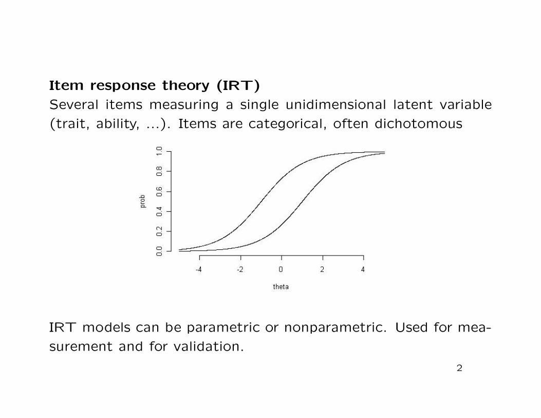
Item response theory (IRT)

Several items measuring a single unidimensional latent variable

(trait, ability, ...). Items are categorical, often dichotomous

IRT models can be parametric or nonparametric. Used for mea-

surement and for validation.

2

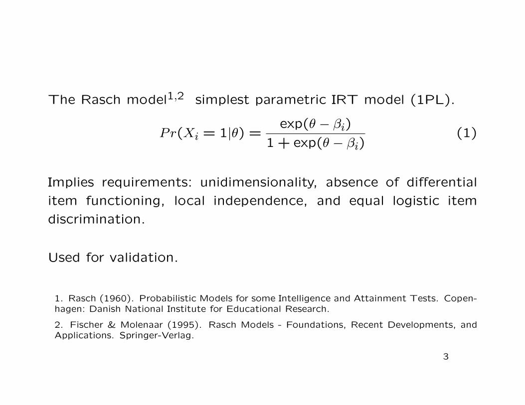
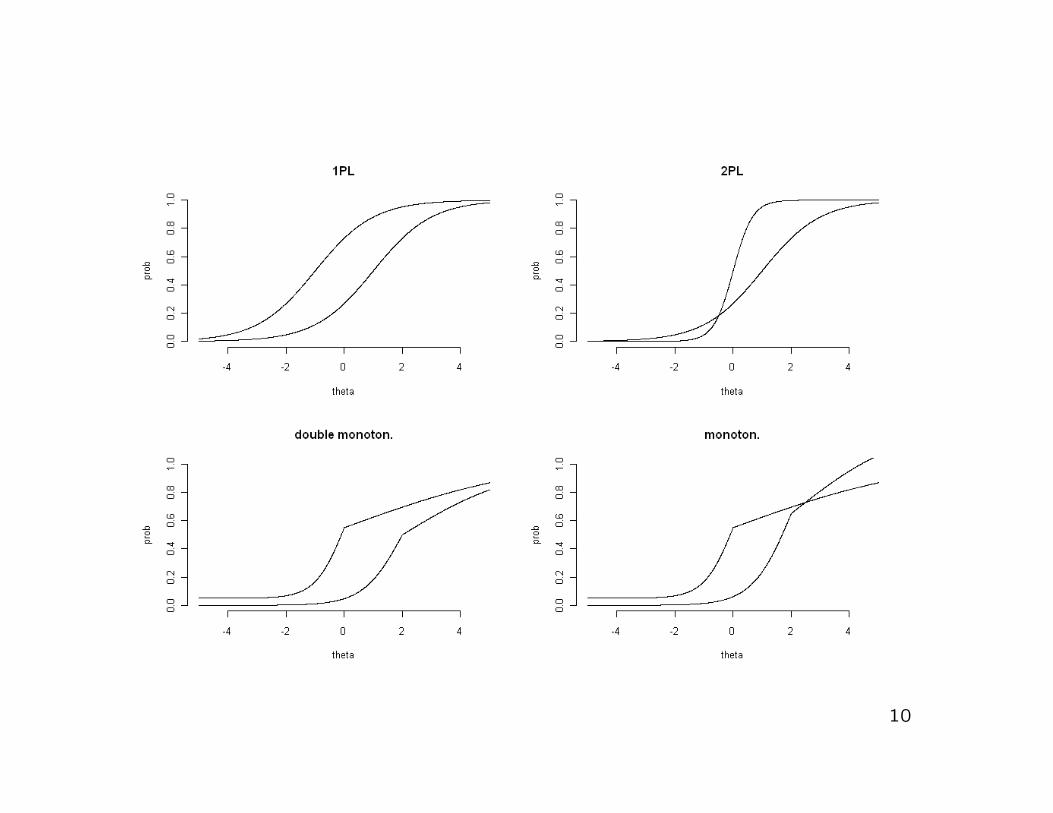
The Rasch model1,2 simplest parametric IRT model (1PL).

Pr(Xi = 1|θ) =exp(θ − βi)

1 + exp(θ − βi)(1)

Implies requirements: unidimensionality, absence of differential

item functioning, local independence, and equal logistic item

discrimination.

Used for validation.

1. Rasch (1960). Probabilistic Models for some Intelligence and Attainment Tests. Copen-hagen: Danish National Institute for Educational Research.

2. Fischer & Molenaar (1995). Rasch Models - Foundations, Recent Developments, andApplications. Springer-Verlag.

3

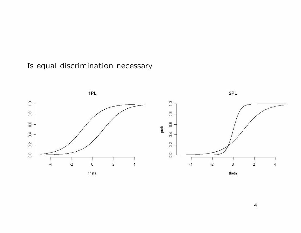
Is equal discrimination necessary

4

Rasch advocated, but never implemented, exact conditional in-

ference: Study distribution of test statistic independent of person

and item parameters.

Computing p-values feasible using MCMC sampling techniques.

5

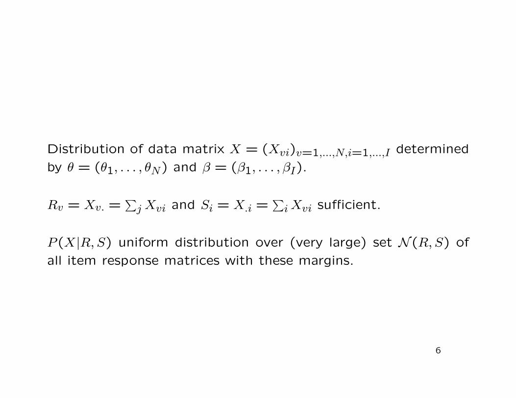
Distribution of data matrix X = (Xvi)v=1,...,N,i=1,...,I determined

by θ = (θ1, . . . , θN) and β = (β1, . . . , βI).

Rv = Xv. =∑

j Xvi and Si = X.i =∑

i Xvi sufficient.

P (X|R, S) uniform distribution over (very large) set N (R, S) of

all item response matrices with these margins.

6

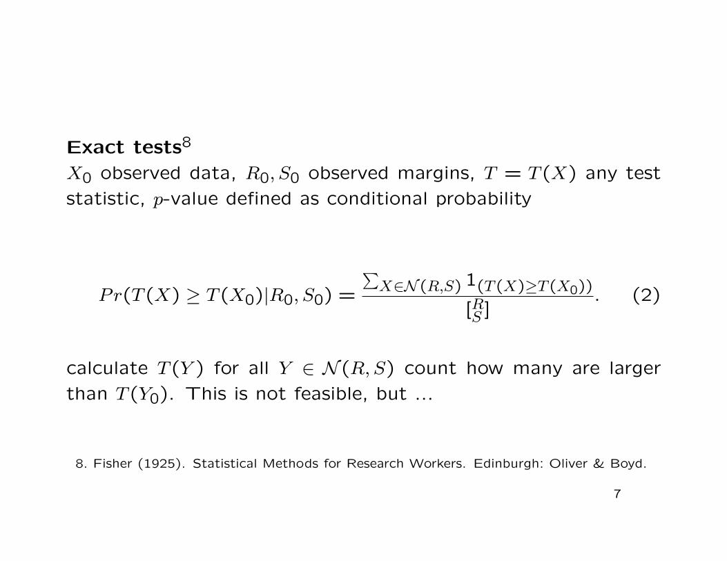
Exact tests8

X0 observed data, R0, S0 observed margins, T = T (X) any test

statistic, p-value defined as conditional probability

Pr(T (X) ≥ T (X0)|R0, S0) =

∑X∈N (R,S) 1(T (X)≥T (X0))

[RS ]. (2)

calculate T (Y ) for all Y ∈ N (R, S) count how many are larger

than T (Y0). This is not feasible, but ...

8. Fisher (1925). Statistical Methods for Research Workers. Edinburgh: Oliver & Boyd.

7

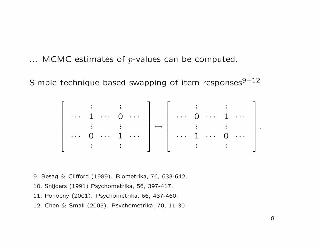
... MCMC estimates of p-values can be computed.

Simple technique based swapping of item responses9−12

... ...· · · 1 · · · 0 · · ·

... ...· · · 0 · · · 1 · · ·

... ...

7→

... ...· · · 0 · · · 1 · · ·

... ...· · · 1 · · · 0 · · ·

... ...

.

9. Besag & Clifford (1989). Biometrika, 76, 633-642.

10. Snijders (1991) Psychometrika, 56, 397-417.

11. Ponocny (2001). Psychometrika, 66, 437-460.

12. Chen & Small (2005). Psychometrika, 70, 11-30.

8

Nonparametric IRT

Mokken model of (double) monotonicity3−6 : unidimensionality,

local independence, nondecreasing (and nonintersecting) item

response functions.

Rasch model is a special case.

3. Mokken (1971). A Theory and Procedure of Scale Analysis with Applications in PoliticalResearch. Walter de Gruyter.

4. Mokken & Lewis (1982). Appl. Psych. Measurement, 6, 417-430.

5. Mokken et al (1986). Appl. Psych. Measurement, 10, 279-285.

6. Sijtsma & Molenaar (2002). Introduction to nonparametric item response theory, Sage.

9

10

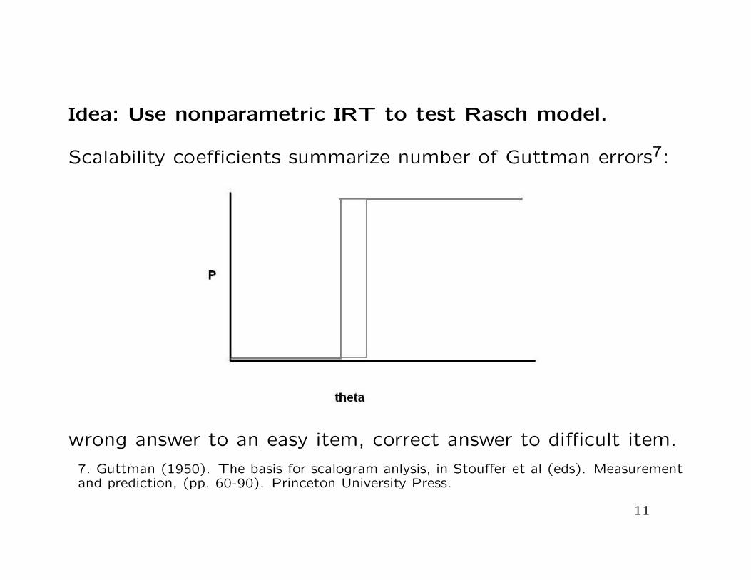
Idea: Use nonparametric IRT to test Rasch model.

Scalability coefficients summarize number of Guttman errors7:

wrong answer to an easy item, correct answer to difficult item.

7. Guttman (1950). The basis for scalogram anlysis, in Stouffer et al (eds). Measurementand prediction, (pp. 60-90). Princeton University Press.

11

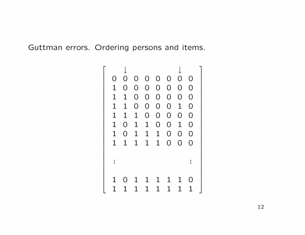
Guttman errors. Ordering persons and items.

↓ ↓0 0 0 0 0 0 0 01 0 0 0 0 0 0 01 1 0 0 0 0 0 01 1 0 0 0 0 1 01 1 1 0 0 0 0 01 0 1 1 0 0 1 01 0 1 1 1 0 0 01 1 1 1 1 0 0 0

... ...

1 0 1 1 1 1 1 01 1 1 1 1 1 1 1

12

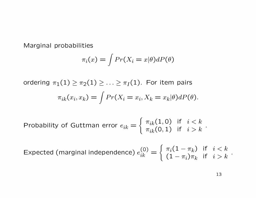
Marginal probabilities

πi(x) =∫

Pr(Xi = x|θ)dP (θ)

ordering π1(1) ≥ π2(1) ≥ . . . ≥ πI(1). For item pairs

πik(xi, xk) =∫

Pr(Xi = xi, Xk = xk|θ)dP (θ).

Probability of Guttman error eik =

{πik(1,0) if i < kπik(0,1) if i > k

.

Expected (marginal independence) e(0)ik =

{πi(1− πk) if i < k(1− πi)πk if i > k

.

13

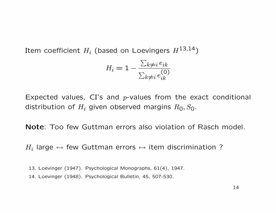
Item coefficient Hi (based on Loevingers H13,14)

Hi = 1−∑

k 6=i eik∑k 6=i e

(0)ik

Expected values, CI’s and p-values from the exact conditional

distribution of Hi given observed margins R0, S0.

Note: Too few Guttman errors also violation of Rasch model.

Hi large ↔ few Guttman errors ↔ item discrimination ?

13. Loevinger (1947). Psychological Monographs, 61(4), 1947.

14. Loevinger (1948). Psychological Bulletin, 45, 507-530.

14

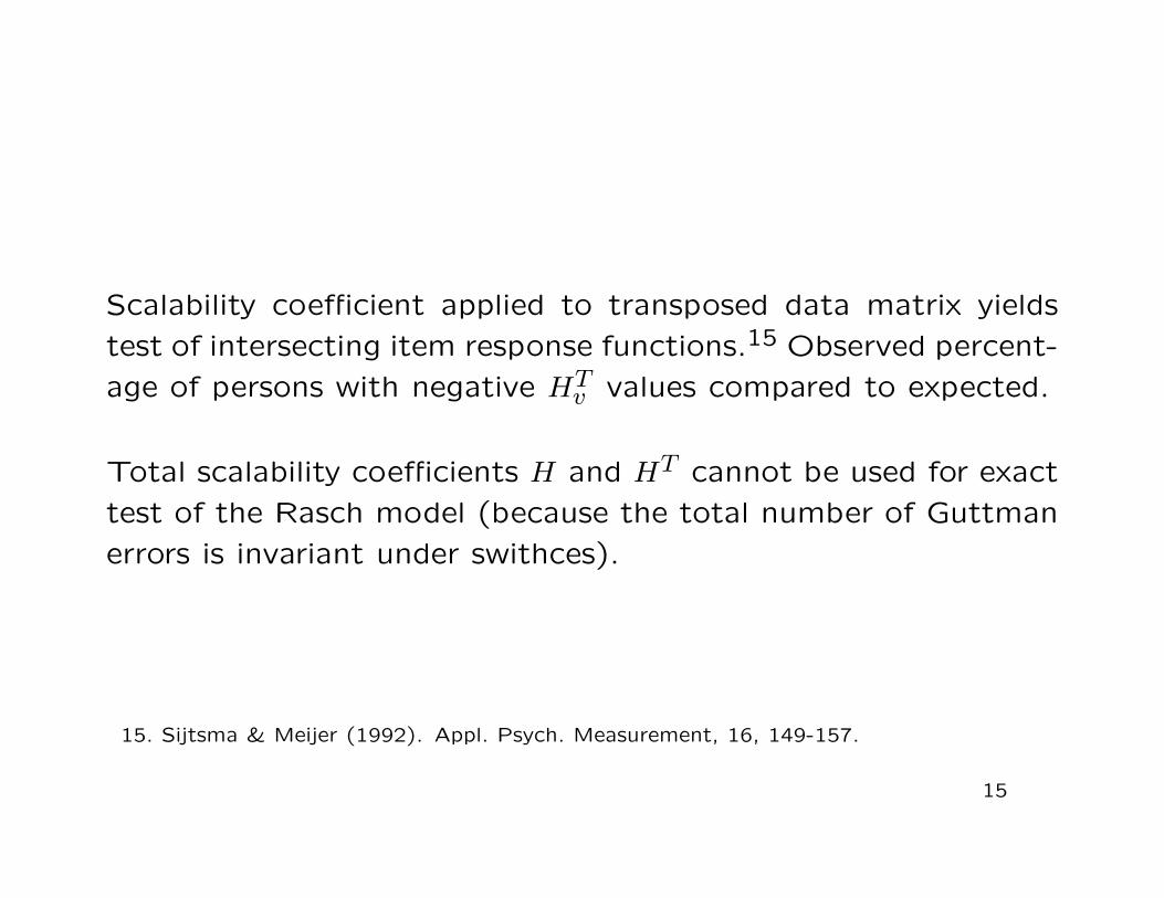
Scalability coefficient applied to transposed data matrix yields

test of intersecting item response functions.15 Observed percent-

age of persons with negative HTv values compared to expected.

Total scalability coefficients H and HT cannot be used for exact

test of the Rasch model (because the total number of Guttman

errors is invariant under swithces).

15. Sijtsma & Meijer (1992). Appl. Psych. Measurement, 16, 149-157.

15

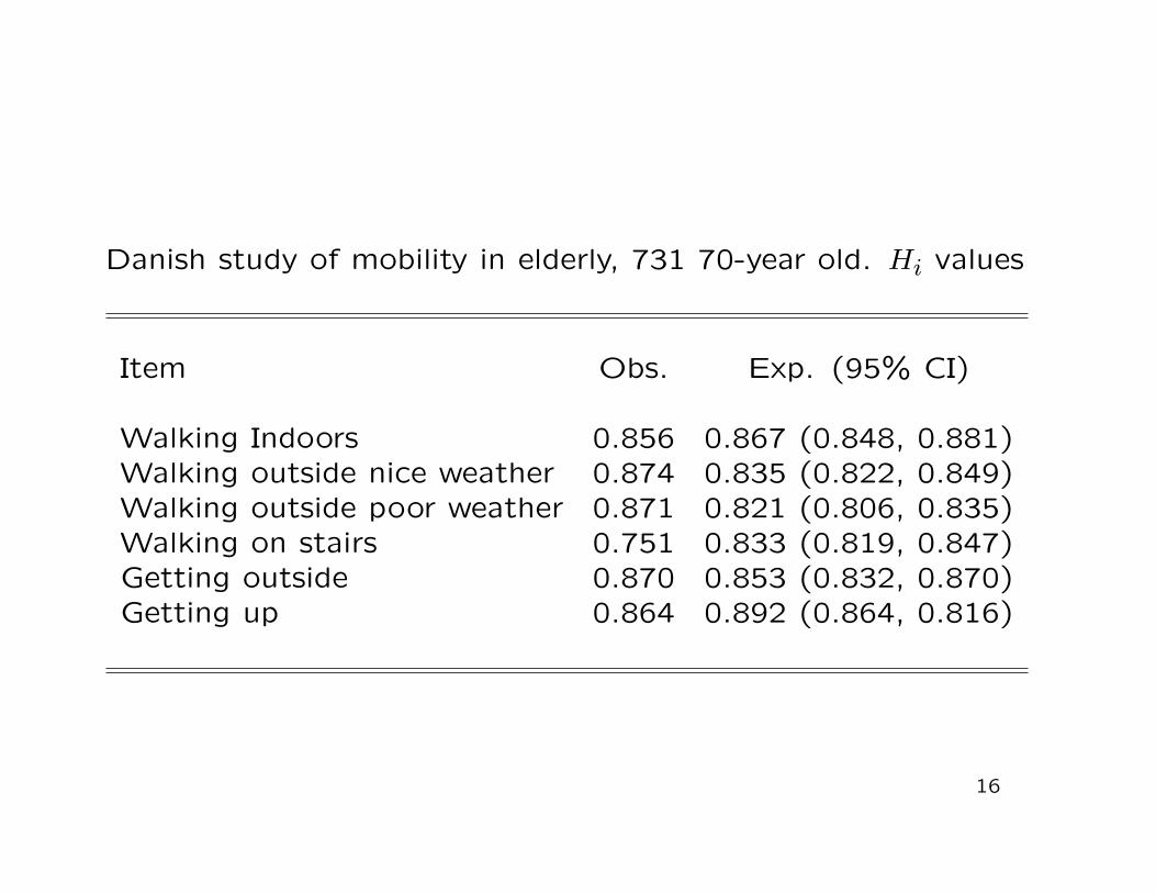
Danish study of mobility in elderly, 731 70-year old. Hi values

Item Obs. Exp. (95% CI)

Walking Indoors 0.856 0.867 (0.848, 0.881)Walking outside nice weather 0.874 0.835 (0.822, 0.849)Walking outside poor weather 0.871 0.821 (0.806, 0.835)Walking on stairs 0.751 0.833 (0.819, 0.847)Getting outside 0.870 0.853 (0.832, 0.870)Getting up 0.864 0.892 (0.864, 0.816)

16

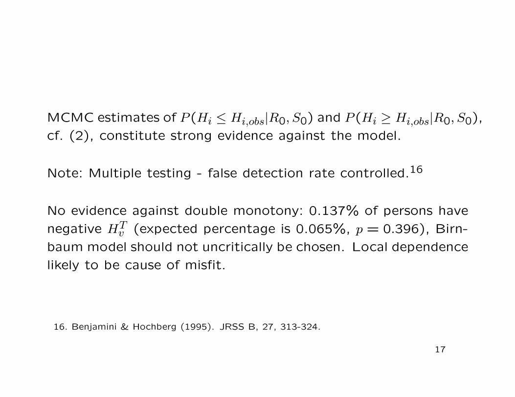
MCMC estimates of P (Hi ≤ Hi,obs|R0, S0) and P (Hi ≥ Hi,obs|R0, S0),

cf. (2), constitute strong evidence against the model.

Note: Multiple testing - false detection rate controlled.16

No evidence against double monotony: 0.137% of persons have

negative HTv (expected percentage is 0.065%, p = 0.396), Birn-

baum model should not uncritically be chosen. Local dependence

likely to be cause of misfit.

16. Benjamini & Hochberg (1995). JRSS B, 27, 313-324.

17

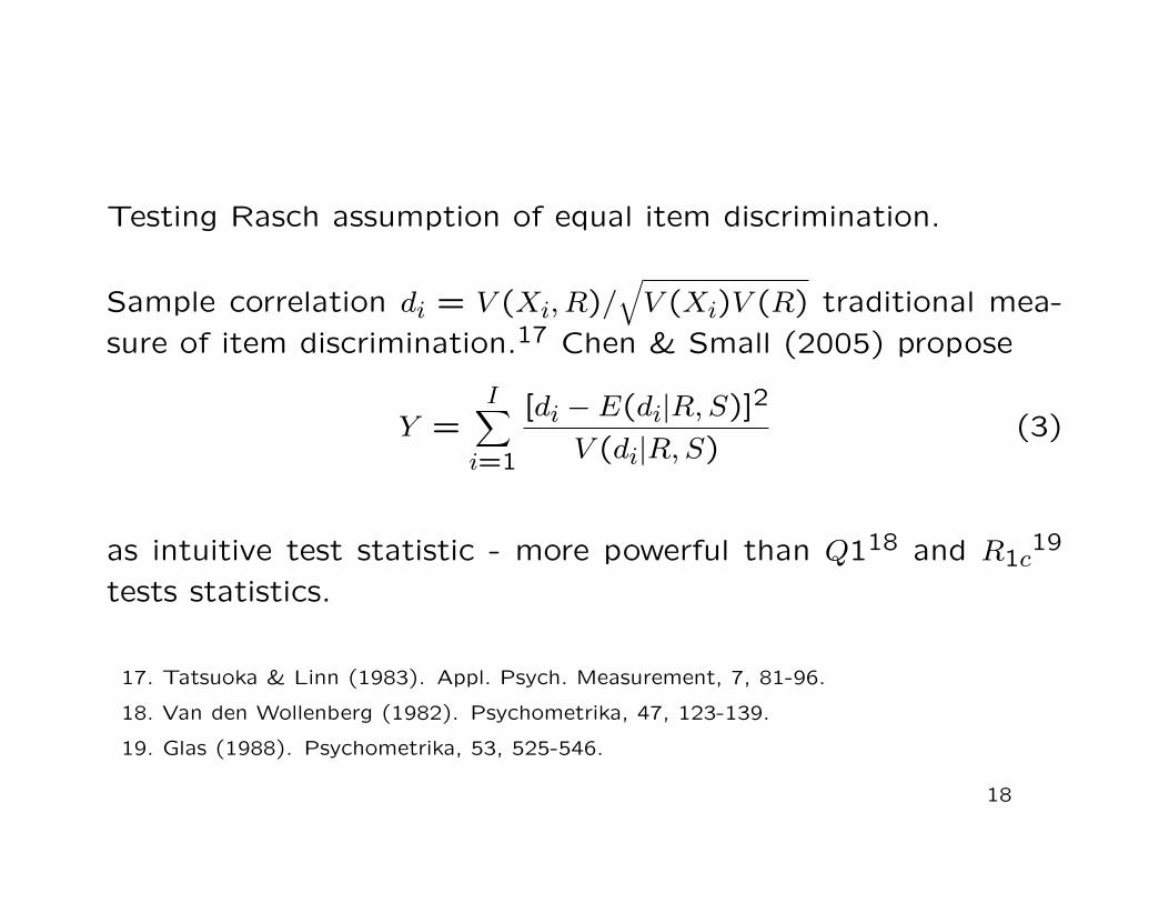
Testing Rasch assumption of equal item discrimination.

Sample correlation di = V (Xi, R)/√

V (Xi)V (R) traditional mea-

sure of item discrimination.17 Chen & Small (2005) propose

Y =I∑

i=1

[di − E(di|R, S)]2

V (di|R, S)(3)

as intuitive test statistic - more powerful than Q118 and R1c19

tests statistics.

17. Tatsuoka & Linn (1983). Appl. Psych. Measurement, 7, 81-96.

18. Van den Wollenberg (1982). Psychometrika, 47, 123-139.

19. Glas (1988). Psychometrika, 53, 525-546.

18

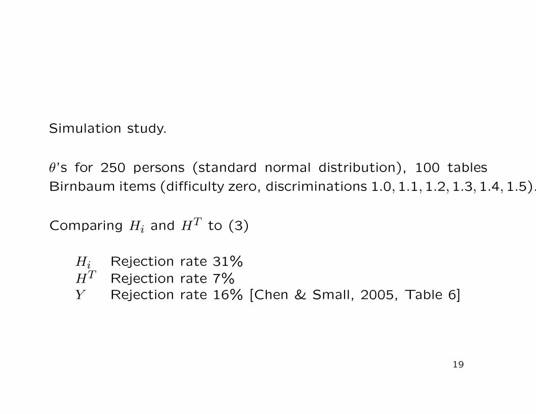
Simulation study.

θ’s for 250 persons (standard normal distribution), 100 tables

Birnbaum items (difficulty zero, discriminations 1.0,1.1,1.2,1.3,1.4,1.5).

Comparing Hi and HT to (3)

Hi Rejection rate 31%HT Rejection rate 7%Y Rejection rate 16% [Chen & Small, 2005, Table 6]

19