Scalability of Classical Terramechanics Models for ... - DTIC
Upload
khangminh22Category
view
0download
0
Improving the Scalability ofMulticore Systems
With a Focus on H.264 Video Decoding


Improving the Scalability ofMulticore Systems
With a Focus on H.264 Video Decoding
PROEFSCHRIFT
ter verkrijging van de graad van doctoraan de Technische Universiteit Delft,
op gezag van de Rector Magnificus prof.ir. K.Ch.A.M Luyben,voorzitter van het College voor Promoties,
in het openbaar te verdedigen
op vrijdag 9 juli 2010 om 15:00 uur
door
Cornelis Hermanus MEENDERINCK
elektrotechnisch ingenieurgeboren te Amsterdam, Nederland.

Dit proefschrift is goedgekeurd door de promotoren:Prof. dr. B.H.H. JuurlinkProf. dr. K.G.W. Goossens
Samenstelling promotiecommissie:
Rector Magnificus, voorzitter Technische Universiteit DelftProf. dr. B.H.H. Juurlink, promotor Technische Universitat BerlinProf. dr. K.G.W. Goossens, promotor Technische Universiteit DelftProf. dr. H. Corporaal Technische Universiteit EindhovenProf. dr. ir. A.J.C. van Gemund Technische Universiteit DelftDr. H.P. Hofstee IBM Systems and Technology GroupProf. dr. K.G. Langendoen Technische Universiteit DelftDr. A. Ramirez Universitat Politecnica de Catalunya
Prof. dr. B.H.H. Juurlink was werkzaam aan de Technische Universiteit vanDelft tot eind december 2009, en heeft als begeleider in belangrijke mate bij-gedragen aan de totstandkoming van dit proefschrift.
ISBN: 978-90-72298-08-9
Keywords: multicore, Chip MultiProcessor (CMP), scalability, powerefficiency, thread level-parallelism (TLP), H.264, video decoding, instructionset architecture, domain specific accelerator, task management
Acknowledgements: This work was supported by the European Com-mission in the context of the SARC integrated project #27648 (FP6).
Copyright c© 2010 C.H. MeenderinckAll rights reserved. No part of this publication may be reproduced, stored ina retrieval system, or transmitted, in any form or by any means, electronic,mechanical, photocopying, recording, or otherwise, without permission of theauthor.
Printed in the Netherlands

Dedicated to my wifefor loving and supporting me.


Improving the Scalability ofMulticore Systems
With a Focus on H.264 Video Decoding
Abstract
In pursuit of ever increasing performance, more and more processor archi-tectures have become multicore processors. As clock frequency was nolonger increasing rapidly and ILP techniques showed diminishing results,
increasing the number of cores per chip was the natural choice. The transis-tor budget is still increasing and thus it is expected that within ten years chipscan contain hundreds of high performance cores. Scaling the number of cores,however, does not necessarily translate into an equal scaling of performance.In this thesis, we propose several techniques to improve the performance scal-ability of multicore systems. With those techniques we address several keychallenges of the multicore area.
First, we investigate the effect of the power wall on future multicore architec-ture. Our model includes predictions of technology improvements, analysis ofsymmetric and asymmetric multicores, as well as the influence of Amdahl’sLaw.
Second, we investigate the parallelization of the H.264 video decoding ap-plication, thereby addressing application scalability. Existing parallelizationstrategies are discussed and a novel strategy is proposed. Analysis shows thatusing the new parallelization strategy the amount of available parallelism is inthe order of thousands. Several implementations of the strategy are discussed,which show the difficulty and the possibility of actually exploiting the avail-able parallelism.
Third, we propose an Application Specific Instruction Set (ASIP) processor forH.264 decoding, based on the Cell SPE. ASIPs are energy efficient and allowperformance scaling in systems that are limited by the power budget.
Finally, we propose hardware support for task management, of which the ben-efits are two-fold. First, it supports the SARC programming model, whichis a task-based dataflow programming model based on StarSS. By providinghardware support for the most time-consuming part of the runtime system, itimproves the scalability. Second, it reduces the parallelization overhead, suchas synchronization, by providing fast hardware primitives.
i


Acknowledgments
Many people contributed to this work in some way and I owe them a debt ofgratitude. To reach this point it takes professors who teach you, colleagueswho assist you, and family and friends who support you.
First of all, I thank Ben Juurlink for supervising me. You helped focusing thiswork, while at the same time pointing me to numerous potential ideas. Youshowed me what others had done in our research area and how we might ei-ther build on that or fill a gap. You suggested me to visit BSC and collaboratewith them closely. Also when I wanted to visit HiPEAC meetings you sup-ported me. Al those trips, where I met other researchers, other ideas, and otherscientific work, have been of great value.
I’m also thankful to Stamatis Vassiliadis for giving me the opportunity to workon the SARC project. I profited from the synergy effect within such a largeproject. The shift to the SARC project also meant the end of the collaborationwith Sorin Cotofana. Sorin, I thank you for the time we worked together. Youwere the one who introduced me into academia, you taught me how to writepapers, and I still remember the conversations we had about life, religion, gas-tronomy, and jazz. I also thank Kees Goossens for being one of my promoters.
Over the years I have worked together with several other PhD students andsome MSc students. I thank Arnaldo and Mauricio for all the work we didtogether on parallelizing H.264 and porting it to the Cell processor. I thankAlejandro, Felipe, Augusto, and David for all the effort they put into the sim-ulator and helping me to use and extend it. I thank Efren for implementingthe Nexus system in the simulator. I thank Carsten, Martijn, and Chi for doingtheir MSc project with us, by which you helped me and others. I thank Pepijnfor helping me with Linux issues and being a pleasant room mate.
I thank Alex Ramirez and Xavi Martorell for warmly welcoming me inBarcelona, the collaboration, and your insight. My visits to Barcelona car-ried a lot of fruit. It helped me to put my research in a larger perspective; it
iii

both broadened and deepened my knowledge, and taught me how to enjoy lifein an intense way.
I thank Jan Hoogerbrugge for the valuable discussions on parallelizing H.264.I thank Stefanos Kaxiras for his input on the methodology used to estimatethe power consumption of future multicores. I thank Peter Hofstee and BrianFlachs for commenting on the SPE specialization. I thank Ayal Zaks for help-ing me with compiler issues. I thank Yoav Etsion for the discussions and col-laboration on hardware dependency resolution.
Secretaries and coffee; they always seem to go together. Whether I was in Delftor in Barcelona, the secretary’s office was always my source of coffee and achat. Lidwina and Monique, thank you for the coffee, the chats, and helpingme with the administrative stuff. Lourdes, thank you for the warm welcome inBSC, the coffee, and the conversations.
I thank the European Network of Excellence on High Performance and Em-bedded Architecture and Compilation (HiPEAC) for financing the collabora-tion with BSC and some trips to the HiPEAC workshops and conferences.
I’m very grateful to my parents who raised me, who loved me, and who sup-ported me continuously throughout the years. I thank God for giving me thecapabilities of doing a PhD and being my guidance through life.
Many, many thanks to my dearest wife; the princess of my life. Thank youfor loving me, for supporting me, and for taking this wonderful journey of lifetogether with me.
C.H. Meenderinck Delft, The Netherlands, 2010
iv

Contents
Abstract i
Acknowledgments iii
List of Figures xii
List of Tables xiv
Abbreviations xv
1 Introduction 1
1.1 Motivation . . . . . . . . . . . . . . . . . . . . . . . . . . . . 2
1.2 Objectives . . . . . . . . . . . . . . . . . . . . . . . . . . . . 7
1.3 Organization and Contributions . . . . . . . . . . . . . . . . .9
2 (When) Will Multicores hit the Power Wall? 11
2.1 Methodology . . . . . . . . . . . . . . . . . . . . . . . . . .13
2.2 Scaling of the Alpha 21264 . . . . . . . . . . . . . . . . . . .13
2.3 Power and Performance Assuming Perfect Parallelization . . .18
2.4 Intermezzo: Amdahl vs. Gustafson . . . . . . . . . . . . . . .20
2.5 Performance Assuming Non-Perfect Parallelization . . . . . .25
2.6 Conclusions . . . . . . . . . . . . . . . . . . . . . . . . . . .32
3 Parallel Scalability of Video Decoders 35
v

3.1 Overview of the H.264 Standard . . . . . . . . . . . . . . . .36
3.2 Benchmarks . . . . . . . . . . . . . . . . . . . . . . . . . . .41
3.3 Parallelization Strategies for H.264 . . . . . . . . . . . . . . .42
3.3.1 GOP-level Parallelism . . . . . . . . . . . . . . . . .43
3.3.2 Frame-level Parallelism . . . . . . . . . . . . . . . .44
3.3.3 Slice-level Parallelism . . . . . . . . . . . . . . . . .44
3.3.4 Macroblock-level Parallelism . . . . . . . . . . . . .45
3.3.5 Block-level Parallelism . . . . . . . . . . . . . . . . .48
3.4 Scalable MB-level Parallelism: The 3D-Wave . . . . . . . . .49
3.5 Parallel Scalability of the Dynamic 3D-Wave . . . . . . . . .52
3.6 Case Study: Mobile Video . . . . . . . . . . . . . . . . . . .62
3.7 Experiences with Parallel Implementations . . . . . . . . . . .63
3.7.1 3D-Wave on a TriMedia-based Multicore . . . . . . .65
3.7.2 2D-Wave on a Multiprocessor System . . . . . . . . .67
3.7.3 2D-Wave on the Cell Processor . . . . . . . . . . . .68
3.8 Conclusions . . . . . . . . . . . . . . . . . . . . . . . . . . .70
4 The SARC Media Accelerator 73
4.1 Related Work . . . . . . . . . . . . . . . . . . . . . . . . . .74
4.2 The SPE Architecture . . . . . . . . . . . . . . . . . . . . . .76
4.3 Experimental Setup . . . . . . . . . . . . . . . . . . . . . . .79
4.3.1 Benchmarks . . . . . . . . . . . . . . . . . . . . . . .79
4.3.2 Compiler . . . . . . . . . . . . . . . . . . . . . . . .80
4.3.3 Simulator . . . . . . . . . . . . . . . . . . . . . . . .81
4.4 Enhancements to the SPE Architecture . . . . . . . . . . . . .84
4.4.1 Accelerating Scalar Operations . . . . . . . . . . . . .85
4.4.2 Accelerating Saturation and Packing . . . . . . . . . .92
4.4.3 Accelerating Matrix Transposition . . . . . . . . . . .99
4.4.4 Accelerating Arithmetic Operations . . . . . . . . . .106
4.4.5 Accelerating Unaligned Memory Accesses . . . . . .124
4.5 Performance Evaluation . . . . . . . . . . . . . . . . . . . . .127
vi
4.5.1 Results for the IDCT8 Kernel . . . . . . . . . . . . .127
4.5.2 Results for the IDCT4 kernel . . . . . . . . . . . . . .131
4.5.3 Results for the Deblocking Filter Kernel . . . . . . . .133
4.5.4 Results for the Luma/Chroma Interpolation Kernel . .138
4.5.5 Summary and Discussion . . . . . . . . . . . . . . . .142
4.6 Conclusions . . . . . . . . . . . . . . . . . . . . . . . . . . .145
5 Intra-Vector Instructions 147
5.1 Experimental Setup . . . . . . . . . . . . . . . . . . . . . . .148
5.1.1 Simulator . . . . . . . . . . . . . . . . . . . . . . . .148
5.1.2 Compiler . . . . . . . . . . . . . . . . . . . . . . . .149
5.1.3 Benchmark . . . . . . . . . . . . . . . . . . . . . . .149
5.2 The Intra-Vector SIMD Instructions . . . . . . . . . . . . . .150
5.2.1 IDCT8 Kernel . . . . . . . . . . . . . . . . . . . . .151
5.2.2 IDCT4 Kernel . . . . . . . . . . . . . . . . . . . . .153
5.2.3 Interpolation Kernel (IPol) . . . . . . . . . . . . . . .153
5.2.4 Deblocking Filter Kernel (DF) . . . . . . . . . . . . .157
5.2.5 Matrix Multiply Kernel (MatMul) . . . . . . . . . . .165
5.2.6 Discrete Wavelet Transform Kernel (DWT) . . . . . .170
5.3 Discussion . . . . . . . . . . . . . . . . . . . . . . . . . . . .175
5.4 Conclusions . . . . . . . . . . . . . . . . . . . . . . . . . . .176
6 Hardware Task Management Support for the StarSS Program-ming Model: the Nexus System 179
6.1 Background . . . . . . . . . . . . . . . . . . . . . . . . . . .181
6.2 Benchmarks . . . . . . . . . . . . . . . . . . . . . . . . . . .183
6.3 Scalability of the StarSS Runtime System . . . . . . . . . . .185
6.3.1 CD Benchmark . . . . . . . . . . . . . . . . . . . . .185
6.3.2 SD Benchmark . . . . . . . . . . . . . . . . . . . . .192
6.3.3 ND Benchmark . . . . . . . . . . . . . . . . . . . . .193
6.4 A Case for Hardware Support . . . . . . . . . . . . . . . . . .195
vii

6.4.1 Comparison with Manually Parallelized Benchmarks .195
6.4.2 Requirements for Hardware Support . . . . . . . . . .198
6.5 Nexus: a Hardware Task Management Support System . . . .200
6.5.1 Nexus System Overview . . . . . . . . . . . . . . . .201
6.5.2 The Task Life Cycle . . . . . . . . . . . . . . . . . .202
6.5.3 Design of the Task Pool Unit . . . . . . . . . . . . . .203
6.5.4 The Nexus API . . . . . . . . . . . . . . . . . . . . .209
6.6 Evaluation of the Nexus System . . . . . . . . . . . . . . . .213
6.6.1 Experimental Setup . . . . . . . . . . . . . . . . . . .214
6.6.2 Performance Evaluation . . . . . . . . . . . . . . . .217
6.7 Future Work . . . . . . . . . . . . . . . . . . . . . . . . . . .225
6.7.1 Dependency Resolution . . . . . . . . . . . . . . . .225
6.7.2 Task Controller . . . . . . . . . . . . . . . . . . . . .227
6.7.3 Other Features . . . . . . . . . . . . . . . . . . . . .227
6.7.4 Evaluation of Nexus . . . . . . . . . . . . . . . . . .228
6.8 Conclusions . . . . . . . . . . . . . . . . . . . . . . . . . . .228
7 Conclusions 231
7.1 Summary and Contributions . . . . . . . . . . . . . . . . . .231
7.2 Possible Directions for Future Work . . . . . . . . . . . . . .235
Bibliography 237
List of Publications 253
Samenvatting 259
Curriculum Vitae 261
viii

List of Figures
1.1 Power density trend. . . . . . . . . . . . . . . . . . . . . . .3
1.2 Road to performance growth. . . . . . . . . . . . . . . . . . .4
1.3 Example of the SARC multicore architecture. . . . . . . . . .8
2.1 The power wall problem (taken from [114]). . . . . . . . . . .12
2.2 Area of one core. . . . . . . . . . . . . . . . . . . . . . . . .15
2.3 Number of cores per die. . . . . . . . . . . . . . . . . . . . .16
2.4 Power of one core running at the maximum possible frequency.17
2.5 Total power consumption of the scaled multicore over the years.19
2.6 Power-constrained performance growth. . . . . . . . . . . . .19
2.7 Wrong comparison of Amdahl’s and Gustafson’s Laws. . . . .21
2.8 Gustafson’s explanation of the difference. . . . . . . . . . . .22
2.9 Prediction with Amdahl’s and Gustafson’s assumptions. . . . .24
2.10 Prediction of speedup with proposed equation. . . . . . . . . .25
2.11 Amdahl’s prediction for prediction for symmetric multicores. .26
2.12 Amdahl’s prediction for asymmetric multicores. . . . . . . . .27
2.13 Amdahl’s prediction for heterogeneous multicores. . . . . . .28
2.14 Optimal area factor of serial processor. . . . . . . . . . . . . .29
2.15 Area of the optimal serial processor. . . . . . . . . . . . . . .30
2.16 Amdahl’s prediction for heterogeneous multicores. . . . . . .30
2.17 Gustafson’s prediction for symmetric multicores. . . . . . . .31
3.1 Block diagram of the decoding process. . . . . . . . . . . . .37
ix

3.2 Block diagram of the encoding process. . . . . . . . . . . . .37
3.3 A typical frame sequence and dependencies between frames. .38
3.4 H.264 data structure. . . . . . . . . . . . . . . . . . . . . . .44
3.5 Dependencies between adjacent MBs in H.264. . . . . . . . .45
3.6 2D-Wave approach for exploiting MB parallelism. . . . . . . .46
3.7 Amount of parallelism using the 2D-Wave approach. . . . . .46
3.8 3D-Wave strategy: dependencies between MBs. . . . . . . . .50
3.9 3D-Wave strategy. . . . . . . . . . . . . . . . . . . . . . . . .50
3.10 Dynamic 3D-Wave: number of parallel MBs. . . . . . . . . .54
3.11 Dynamic 3D-Wave: number of frames in flight. . . . . . . . .54
3.12 Dynamic 3D-Wave: number of parallel MBs (esa encoding). .57
3.13 Dynamic 3D-Wave: number of frames in flight (esa encoding).57
3.14 Dynamic 3D-Wave: limited MBs in flight. . . . . . . . . . . .59
3.15 Dynamic 3D-Wave: limited MBs in flight. . . . . . . . . . . .59
3.16 Dynamic 3D-Wave: limited frames in flight. . . . . . . . . . .61
3.17 Dynamic 3D-Wave: limited frames in flight. . . . . . . . . . .61
3.18 Dynamic 3D-Wave: parallelism for case study. . . . . . . . .64
3.19 Dynamic 3D-Wave: frames in flight for case study. . . . . . .64
3.20 Scalability of the 3D-Wave on the TriMedia multicore system.66
3.21 Scalability of the 2D-Wave on the multiprocessor system. . . .67
3.22 Scalability of the 2D-Wave on the Cell processor. . . . . . . .69
4.1 Overview of the Cell architecture. . . . . . . . . . . . . . . .77
4.2 Overview of the SPE architecture. . . . . . . . . . . . . . . .77
4.3 Execution time breakdown of the FFmpeg H.264 decoder. . . .80
4.4 Overview of the as2ve instructions. . . . . . . . . . . . . . . .89
4.5 Eklundh’s matrix transpose algorithm. . . . . . . . . . . . . .101
4.6 Overview of the swapoe instructions. . . . . . . . . . . . . . .102
4.7 Graphical representation of theswapoehw instruction. . . . . 102
4.8 Overview of the sfxsh instructions. . . . . . . . . . . . . . . .107
4.9 Using the RRR format to mimic the new RRI3 format. . . . .112
x

4.10 Computational structure of the one-dimensional IDCT8. . . .119
4.11 Computational structure of the one-dimensional IDCT4. . . .121
4.12 The process of deblocking one macroblock. . . . . . . . . . .134
4.13 Overview speedups and instruction count reductions. . . . . .143
5.1 Example of vertical processing of a matrix. . . . . . . . . . .150
5.2 Example of horizontal processing of a matrix. . . . . . . . . .151
5.3 Speedup and instruction count reduction. . . . . . . . . . . . .152
5.4 Breakdown of the execution cycles. . . . . . . . . . . . . . .152
5.5 Explanation interpolation filter. . . . . . . . . . . . . . . . . .154
5.6 Theipol instruction computes eight FIR filters in parallel. .154
5.7 The computational structure of the FIR filter. . . . . . . . . .155
5.8 The process of deblocking one macroblock. . . . . . . . . . .157
5.9 Computational structure of the dfy1 filter function. . . . . . . 160
5.10 Data layout of the baseline4× 4 matrix multiply. . . . . . . . 166
5.11 Data layout of the enhanced4× 4 matrix. . . . . . . . . . . . 167
5.12 The three phases of the forward DWT lifting scheme. . . . . .171
5.13 Computational structure of the inverse DWT. . . . . . . . . .172
5.14 Computational structure of theidwt intra-vector instruction. .173
5.15 Speedup and instruction count reduction of DWT kernel. . . .175
5.16 The speedup as a function of the relative instruction latencies.177
6.1 Dependency patterns of the benchmarks. . . . . . . . . . . . .185
6.2 StarSS scalability - CD benchmark - default configuration. . .186
6.3 Legend of the StarSS Paraver traces. . . . . . . . . . . . . . .186
6.4 Trace of CD benchmark with default configuration. . . . . . .187
6.5 StarSS scalability - CD benchmark -(1, 1, 1) configuration. . 188
6.6 StarSS trace - CD benchmark -(1, 1, 1) conf. - large task size. 189
6.7 StarSS trace - CD benchmark -(1, 1, 1) conf. - small task size.190
6.8 StarSS scalability - CD benchmark -(1, 1, 4) configuration. . . 192
6.9 StarSS scalability - SD benchmark -(1, 1, 8) configuration. . . 193
xi

6.10 StarSS trace - SD benchmark -(1, 1, 8) configuration. . . . . .194
6.11 StarSS scalability - ND benchmark -(1, 1, 8) configuration. . . 195
6.12 Scalability of the manually parallelized CD benchmark. . . . .196
6.13 Scalability of the manually parallelized SD benchmark. . . . .196
6.14 Scalability of the manually parallelized ND benchmark. . . . .196
6.15 The iso-efficiency lines of the StarSS and Manual systems. . .197
6.16 Overview of the Nexus system. . . . . . . . . . . . . . . . . .201
6.17 The task life cycle and the corresponding hardware units. . . .202
6.18 Block diagram of the Nexus TPU. . . . . . . . . . . . . . . .204
6.19 An example of multiple reads/write to the same address. . . .207
6.20 Example of dependency resolution process. . . . . . . . . . .208
6.21 Legend of the StarSS + Nexus Paraver traces. . . . . . . . . .218
6.22 Nexus trace - CD benchmark. . . . . . . . . . . . . . . . . . .219
6.23 Scalability limit of the Nexus system. . . . . . . . . . . . . .221
6.24 Impact of the TPU latency on the performance . . . . . . . . .222
6.25 Nexus scalability - CD benchmark. . . . . . . . . . . . . . . .223
6.26 The iso-efficiency of the three systems. . . . . . . . . . . . . .224
6.27 Task dependencies through overlapping memory regions. . . .226
xii

List of Tables
2.1 Parameters of the Alpha 21264 chip. . . . . . . . . . . . . . .14
2.2 Technology parameters of the ITRS roadmap. . . . . . . . . .15
3.1 Comparison of video coding standards and profiles. . . . . . .39
3.2 Maximum parallel MBs using the 2D-Wave approach. . . . . .47
3.3 Static 3D-Wave: MB parallelism and frames in flight. . . . . .51
3.4 Dynamic 3D-Wave: MB-level parallelism and frames in flight.53
3.5 Dynamic 3D-Wave: MB parallelism and frames in flight (esa).55
3.6 Comparison parallelism using hex and esa encoding. . . . . .56
3.7 Compression improvement of esa encoding relative to hex. . .56
4.1 SPU instruction latencies. . . . . . . . . . . . . . . . . . . . .82
4.2 Comparison CellSim and SystemSim. . . . . . . . . . . . . .83
4.3 Profiling of the baseline IDCT8 kernel. . . . . . . . . . . . . .128
4.4 Speedup and instruction count reduction IDCT8 kernel. . . . .130
4.5 Profiling of the baseline IDCT4 kernel. . . . . . . . . . . . . .132
4.6 Speedup and instruction count reduction IDCT4 kernel. . . . .133
4.7 Top-level profiling of the DF kernel for one macroblock. . . .135
4.8 Profiling of the functions of the DF kernel. . . . . . . . . . . .135
4.9 Speedup and instruction count reduction DF kernel . . . . . .138
4.10 Profiling results of the baseline Luma kernel. . . . . . . . . .139
4.11 Speedup and instruction count reduction Luma kernel. . . . .142
4.12 Overview speedups and instruction count reductions. . . . . .144
xiii

5.1 Validation of CellSim. . . . . . . . . . . . . . . . . . . . . .149
5.2 Resultsipol instruction. . . . . . . . . . . . . . . . . . . . .156
5.3 Results complex DF instruction. . . . . . . . . . . . . . . . .163
5.4 Results simple DF instruction. . . . . . . . . . . . . . . . . .165
5.5 Resultsfmatmul instruction. . . . . . . . . . . . . . . . . .169
5.6 Resultsfmma instruction. . . . . . . . . . . . . . . . . . . . .169
5.7 Resultsidwt instruction. . . . . . . . . . . . . . . . . . . . .174
6.1 The iso-efficiency values of the StarSS and Manual systems. .198
6.2 Performance comparison of the StarSS and Manual system. . .199
6.3 CellSim configuration parameters. . . . . . . . . . . . . . . .215
6.4 Validation of CellSim. . . . . . . . . . . . . . . . . . . . . .216
6.5 Execution time of the CD benchmark using Nexus. . . . . . .217
6.6 The task throughput of the PPE and the TPU. . . . . . . . . .220
6.7 The iso-efficiency of the three systems. . . . . . . . . . . . . .224
xiv

Abbreviations
ABT Adaptive Block size TransformALU Arithmetic Logic UnitAPI Application Programming InterfaceASIC Application Specific Integrated CircuitASIP Application Specific Instruction set ProcessorsAVC Advanced Video CodingB Bi-directional predicted frame, slice, or macroblockBP Baseline ProfileCABAC Context Adaptive Binary Arithmetic CodingCAVLC Context Adaptive Variable Length CodingccNUMA cache coherent Non-Uniform Memory AccessCIF Common Intermediate Formate (352×288 pixels)CMP Chip MultiProcessorDCT Discrete Cosine TransformDF Deblocking FilterDLP Data Level ParallelismDMA Direct Memory AccessDWT Discrete Wavelet TransformEC Entropy CodingED Entropy DecodingEP Extended Profileesa exhaustive search motion estimation algorithmFHD Full High Definition (1920×1088 pixels)FIR Finite Impulse ResponseFMO Flexible Macroblock OrderingFU Functional UnitGOP Group of PicturesGPP General Purpose ProcessorGPU Graphics Processing Unit
xv

HD High Definition (1280×720 pixels)HD-DVD High Definition Digital Video Dischex hexagonal motion estimation algorithmHiP High ProfileI Intra predicted frame, slice, or macroblockIDCT Inverse Discrete Cosine TransformIDWT Inverse Discrete Wavelet TransformILP Instruction Level ParallelismIPC Instructions Per CyclesIpol InterPolationIQ Inverse QuantizationISA Instruction Set ArchitectureITRS International Technology Roadmap for SemiconductorsITU International Telecommunication UnionLS Local StoreMatMul Matrix MultiplyMB MacroBlockMC Motion CompensationME Motion EstimationMFC Memory Flow ControllerMP Main ProfileMPEG Moving Picture Experts GroupMT Matrix TranspositionMV Motion VectorOpenMP Open MultiProcessingP Predicted frame, slice, or macroblockPOSIX Portable Operating System Interface (for uniX)PPE Power Processing ElementPPU Power Processing UnitPSNR Peak Signal-to-Noise RatioQCIF Quarter Common Intermediate Format (176×144 pixels)RISC Reduced Instruction Set ComputerSAT SaturateSD Standard Definition (720×576 pixels)SDK Software Development KitSIMD Single Instruction Multiple DataSMT Simultaneous MultiThreadingSoC System on ChipSPE Synergistic Processing Element
xvi

SPMD Single Program Multiple DataSPU Synergistic Processing UnitTC Task ControllerTLP Thread Level ParallelismTPU Task Pool UnitUVLC Universal Variable Length CodingVCEG Video Coding Experts GroupVHDL VHSIC Hardware Description LanguageVHSIC Very High Speed Integrated CircuitVLC Variable Length CodingVLIW Very Large Instruction Word
xvii


Chapter 1
Introduction
Computer architecture has reached a very interesting era where scien-tific research is of great importance to tackle the problems currentlyfaced. Up to the beginning of this millennium processor performance
improved mainly by techniques to exploit Instruction-Level Parallelism (ILP)and increased clock frequency. The latter caused a memory gap, as memorylatency decreased at a much slower pace. This problem was relieved by usingthe ever growing transistor budget to build larger and larger caches.
Currently, however, the landscape has completely changed. Multicore is thenew way to obtain performance improvement. From high-end servers to em-bedded systems, multicores have found their way to the market. For servers,chips with 6 or 8 cores are currently available but this number is increasingrapidly. At the recently held Hot Chips 2009, IBM announced its Power7 con-taining 8 cores with 4 threads each [54]. Moreover, 32 of those chips can beconnected directly to form a single server. Sun Microsystems described theRainbow Falls chip; 16 cores with 8 threads each [55]. AMD started ship-ping their 6-core Opteron this year [13] and Intel presented an 8-core Nehalemversion [25].
Desktop computing is mostly based on quad cores currently. Intel sells theCore i7 [11] and AMD its Phenom X4 [1]. Higher core counts are found inspecial purpose architectures. The most well-known of these is the 9-core Cellprocessor developed by IBM, Toshiba, and Sony for the gaming industry [127].It was groundbreaking as it is heterogeneous and uses scratchpad memory in-stead of coherent shared memory. The ClearSpeed CSX700 has 192 coresand is a low-power accelerator for high performance technical computing [47].The Cisco CRS-1, also called Metro or SPP, has 188 RISC cores [14]. This
1

2 CHAPTER 1. INTRODUCTION
massively many-core custom network processor is used in Cisco’s highest endrouters. The picoChip products for wireless communication go up to 273 corescurrently [128].
That brings us to the embedded market where we find, among others, theFreescale 8641D (dual core) [61], the ARM Cortex-A9 MPCore (supporting2 to 4 cores) [3], Pluralitys Hypercore processor (capable of supporting 16to 256 cores) [130], and Tileras Tile-Gx processor (up to 100 cores) [156].Also among SoCs (System on Chips) multicore platforms are found, such asthe Cavium Octeon (communication) [36], the Freescale QorIQ (communica-tion) [62], and the Texas Instruments OMAP (multimedia) [155].
The list is far from complete (we have not even mentioned Graphical Process-ing Units (GPUs) yet), but the picture is clear: multicores are everywhere, and“they are here to stay”. We have not yet explained why the shift towards mul-ticores was made, neither why they bring along new challenges for computerarchitects. Those issues are addressed in the next section as we present themotivation for this work.
1.1 Motivation
The increase of processor performance is so steady that Moore’s Law is ap-plicable to it, although it was initially posed to express the doubling of thenumber of transistors every two years [116]. Initially the growth in perfor-mance and transistor count were directly related. The number of transistors perchip increased because their size shrunk. At the same time, smaller transistorsenabled higher clock frequencies which translated into higher performance.The additional transistors also allowed techniques that exploit ILP, such asdeep pipelining, branch prediction, multiple issue, out-of-order execution, etc.These two factors have for long been the main source of performance growth,but not anymore, although the transistor budget is still following Moore’s Law.
The exploitation of ILP seems to have reached its limits. Some improvementsare still made, but the costs are enormously high in terms of area and powerconsumption. In aggressive ILP cores many transistors are deployed to keepthe functional units busy. The transistor budget allows this additional hard-ware, but the power consumption is a problem.
The power consumption of processors grew steadily over the years. Figure 1.1depicts the power density trend of Intel processors. The chart is more than10 years old, but it shows the trend up to that time as well as the problem.

1.1. MOTIVATION 3
Figure 1.1: Power density trend. Source: Fred Pollack, Intel. Keynote speechMicro32, 1999.
The power consumed by the chip produces heat that should be removed toprevent the chip from burning. Packaging and cooling, however, can handlea limited amount of heat and thus the power consumption can maximally bearound 200W , assuming conventional cooling technology. That limit has beenreached and thus power has become one of the dominant design constraints.The dynamic power consumption is given byPdyn = αCfV 2, whereα is thetransistor activity factor,C is the gate capacitance,f is the clock frequency,andV is the power supply voltage. Limits onV andC, and diminishing returnson α forces to turn to frequency to keep the power consumption within thebudget. That is the main reason why frequency is hardly increasing anymore.
Without ILP improvements and clock frequency increases as sources for per-formance improvements, turning towards the exploitation of Thread-Level Par-allelism (TLP) was the natural choice. Multithreading already found its wayinto processors to increase the utilization of the functional units. Putting mul-tiple cores on a chip allows to exploit TLP to a higher degree. And the goodnews is: the nominal performance of a multicore is proportional to the numberof cores, which in turn is proportional to the transistor budget. Therefore, dueto the multicore paradigm, performance can potential keep up with Moore’sLaw.

4 CHAPTER 1. INTRODUCTION
more active transistorsHeterogeneous
higher frequency
Special purpose
higher frequencymore active transistors
1980
Single thread performancemore active transistors, higher frequency
more active transistors, higher frequencyMulticores
Perf
orm
ance
2005 2015? 2025?? 2035???
Figure 1.2: Peter Hofstee’s (IBM Austin) view on how performance growth will beobtained over the years.
We write ‘potentially’ because performance does not automatically scale withthe number of cores. Scalability is the goal, preferably into the many-coredomain where hundreds or thousands of cores in a single chip efficiently andcooperatively are at work. Computer architects and even computer engineersin general are facing many challenges in the pursuit of this goal.
The first challenge is the power wall. A naive multicore architecture wouldhave replicated cores as many as would fit on the die and use a clock frequencysuch that the power budget is just met. Such an approach, however, is notoptimal in terms of performance. Moreover, for many-core architectures it isexpected not to provide performance improvements at all.
Figure 1.2 shows Peter Hofstee’s view on how performance growth will beobtained over the years. We are currently in the phase where we have moretransistors but not higher frequency. As explained before, in such a situationusing multiple cores instead of a single one provides performance improve-ments. In a next phase, there will be more transistors, but not all of them canbe active concurrently (unless the frequency is reduced). In this phase a hetero-geneous architecture is required to obtain performance improvements. Cores,specialized for application domains, are activated depending on the workload.Cores that are not used are shut down such that the power budget is divided
1.1. MOTIVATION 5
among the active cores. In the final phase, it might not be possible to put moretransistors on a die. The only way to improve performance in such a situation,is to provide special purpose hardware.
Indeed, Application Specific Integrated Circuits (ASICs) show us that powerefficiency can be achieved by being application specific. But in those situa-tions where programmability, flexibility, and/or wide applicability are needed,a programmable processor is required. Thus we formulate the first challengeas follows:
Challenge 1 To get as much as possible performance out of the power budgetwithout significantly compromising wide applicability, programmability, andflexibility.
Providing TLP, by putting many cores on a chip, does not automatically im-prove performance improvement. There are many challenges in exploitingTLP, the two most important are mentioned below.
On the algorithm or software level, we have to find TLP. Most algorithms andapplications were developed for serial execution. For the near future, TLPhas to be discovered within those existing algorithms and applications. Forthe far future, preferably new algorithms are developed, exhibiting more par-allelism. Automated parallelization has been studied for a while now, but notmuch progress has been reported. Thus, we will have to learn how to extractparallelism there where it is not obvious.
Challenge 2 To find parallelism in algorithms and applications, especially inapplications where it is not obviously available.
Probably the most debated multicore related topic is programmability. Mul-ticores add another dimension to programming, making it very difficult forthe average programmer to obtain good performance within reasonable time.He or she has to consider partitioning, scheduling, synchronization, maintain-ing dependencies, etc. For the Cell processor also Direct Memory Accesses(DMAs) have to be programmed, SPU (Synergistic Processing Unit) specificintrinsics have to be used, SIMDimization (Single Instruction Multiple Data)should be applied, and branches should be avoided.
Many of those issues require a thorough understanding of the architecture.Moreover, careful analysis of the execution is necessary to understand the be-havior of the program. Only then scalability bottlenecks can be removed inorder to actually benefit from the parallelization.

6 CHAPTER 1. INTRODUCTION
Therefore much research is put in this area. New programming models areproposed to ease the job of the programmer. In some cases runtime systemsare added to handle scheduling and dependency resolution dynamically. Fur-thermore, tools are developed to assist the programmer in creating and under-standing parallel programs.
Challenge 3 To increase programmability, enabling a significant number ofprogrammers to create efficient parallel code within reasonable time.
A challenge that is older than multicore, but so far only briefly mentioned inthis introduction, is the memory wall. The memory latency, measured in clockcycles, is growing. A processor that has to wait for data wastes resources andhas lower performance. Two factors mainly cause this increased gap. First, theoff-chip bandwidth grows slower than the performance of processors. Second,as feature sizes shrink the latency to reach the other side of the chip or to gooff-chip, is increasing.
A cache hierarchy can be used to mitigate the effect of the power wall, butin the multicore era this poses another issue. To obtain low latency, typicallythe L1 cache is private to a core. Thus coherency has to be maintained amongshared data, either in hardware or software. The overhead of maintaining co-herency increases rapidly with the number of cores, posing a scalability prob-lem [34]. This is exacerbated by the fact that interconnection speeds are notscaling well with technology.
Another direction is to use scratchpad memory with DMA controllers as wasdone in the Cell processor. It allows complete control of the data and thus per-formance can be optimized. Programmability, however, suffers a lot and mostlikely not every application domain is suitable for this type of data manage-ment. This brings about the fourth challenge:
Challenge 4 To continuously provide each core with sufficient data to operateon.
Having identified parallelism in the application, being able to program it, andrunning it on a parallel architecture does not necessarily mean that scalabilityhas been achieved. Similar to exploiting ILP and DLP, the exploitation of TLPbrings along overhead, reducing the scalability. Thus, the fifth challenge is thefollowing:
Challenge 5 To minimize the impact of TLP exploitation overhead on scala-bility and performance.

1.2. OBJECTIVES 7
These challenges are among the main challenges recognized by the commu-nity, although there are many more that are also important. There are chal-lenges in the area of reliability, caused by entering the nano-scale area. Alsoserial performance remains an issue as shown by Hill and Marty [74]. Theybased their results on Amdahl’s Law and its corresponding assumptions, whichmight turn out to be too pessimistic, though. More challenges could be men-tioned here, but we will focus on how the work presented in this thesis con-tributes to these five important challenges.
1.2 Objectives
The research presented in this thesis was conducted in the context of the EUFP6 project SARC (Scalable computer ARChitecture). The goal of this projectwas to develop long-term sustainable approaches to advanced computer archi-tecture in Europe. It focused on multicore technology for a broad range of sys-tems, ranging from small energy critical embedded systems right up to largescale networked data servers. The project brought together research in archi-tecture, interconnect, design space exploration, low power design, compilerconstruction, programming models, and runtime systems.
Our role in the project was to improve or obtain scalability in the many-corearea based on architectural enhancements. Similar to Peter Hofstee’s view,the SARC project assumes that heterogeneous architectures are a necessityin the many-core domain. The power budget prevents all cores being activeconcurrently. Thus, the transistor budget is best spent on providing cores thatare specialized for an application domain. Figure 1.3 shows an example ofsuch an architecture, as considered in the SARC project. It contains generalpurpose processors (P) and domain specific accelerators (A), connected in aclustered fashion. Within a cluster, the memory hierarchy is also specializedfor the application domain it targets.
The clusters show similarity with the Cell processor. At the start of the project,the Cell processor was the only heterogeneous multicore processor availableand thus it was chosen as the baseline architecture. Moreover, its DMA-styleof accessing memory has proven to enable data optimizations for locality andthus enhance scalability.
The overall objective of this thesis, i.e., to improve scalability in the many-core area, is very general. In this section we define more concrete and specificobjectives, based on the challenges mentioned in the previous section, and thecontext of the project. Several application domains are targeted within the

8 CHAPTER 1. INTRODUCTION
$P
LS
A $
LS
A $
LS
A $
LS
A $
LS
A $
LS
A $
$P$P
DM
A
LS
A
DM
A
LS
A
DM
A
LS
A
DM
A
LS
A
DM
A
LS
A
DM
ALS
A
MIC
L2 Cache L2 Cache
A $
L2 Cache
IO
Figure 1.3: Example of the multicore architecture considered within the SARCproject, in which context this research was performed.
project, of which this work focuses on the media domain. As main benchmarkapplication, the H.264 video decoder was chosen. Media applications remainan important workload in the future and video codecs are considered to beimportant benchmarks for all kind of systems, ranging from low-power mobiledevices to high performance systems. H.264 is the most advanced video codedcurrently. It is highly complex and hard to parallelize.
Objective 1 Analyze the H.264 decoding application. Find new ways to par-allelize the code in a scalable fashion. Analyze the parallelization strategiesand determine bottlenecks in current parallel systems. This objective corre-sponds to Challenge 2.
Objective 2 Specialize the cores of the Cell processor for H.264 in order toobtain performance and power benefits. This objective corresponds to Chal-lenge 1.

1.3. ORGANIZATION AND CONTRIBUTIONS 9
Objective 3 Design hardware mechanism to reduce the overhead of managingthe parallel execution. This objective corresponds to Challenge 5.
Objective 4 Improve programmability by providing hardware support. Thisobjective corresponds to Challenge 3.
Challenge 4 is only implicitly addressed in this thesis by using scratchpadmemory in combination with DMAs, and by applying double buffering.
1.3 Organization and Contributions
This work focuses on a single goal: improving/obtaining scalability into themany-core area. As scalability depends on several issues, as indicated by thechallenges and objectives, this work, however, is not focused on a single issue,but rather encompasses a few. Each issue is described in a separate chapter,which are mostly self containing. Introduction to the specific issues are pro-vided within the chapters as well as discussion of related work. An exceptionis Chapter 5 which extends the work described in Chapter 4.
In Chapter 2 the power wall problem is investigated in more detail. That is,Challenge 1 is investigated in more detail. Specifically, the impact on mul-ticore architecture is investigated. In this chapter we developed a model thatincludes predictions of technology improvements, analysis of symmetric andasymmetric multicores, as well as the influence of Amdahl’s Law.
Objective 1 is addressed in Chapter 3. The H.264 standard is reviewed, ex-isting parallelization strategies are discussed, and a new strategy is proposed.Analysis of real video sequences reveals that the amount of parallelism avail-able is in the order of thousands. Several parallel implementations, mainlydeveloped by colleagues of the author, are discussed. They show the difficultyand the possibility of actually exploiting the available parallelism.
The thesis continues in Chapter 4 with the design of the SARC Media Accel-erator. Based on a thorough analysis of the execution of the H.264 kernels onthe Cell processor, architectural enhancements to the SPE core are proposed.Specifically, a handful of application specific instructions are added to improveperformance. Kernel speedups between 1.84 and 2.37 are obtained.
One of the application specific instructions proposed in the Chapter 4 per-forms intra-vector operations. In Chapter 5 we investigate the applicability ofsuch instructions to other applications. Our analysis shows that mainly two-

10 CHAPTER 1. INTRODUCTION
dimensional signal processing kernels benefit from this type of instructions.Speedups up to 2.06, with an average of 1.45 are measured.
Finally, in Chapter 6 we propose a hardware support system for task manage-ment. We analyze the scalability of manually coded task management as wellas that of StarSS [129, 30]. StarSS includes a programming model, compiler,and runtime system. Although easy to program, the scalability of StarSS islimited. The proposed hardware support alleviates this problem by performingtask dependency resolution in hardware.
Chapter 7 concludes this thesis. The main contributions are summarized andopen issues are discussed.

Chapter 2
(When) Will Multicores hit thePower Wall?
It is commonly accepted that we have reached thepower wall, meaning thatuniprocessor performance improvements has stagnated due to power con-straints. The main causes for the increased power consumption are higher
clock frequencies and power inefficient techniques to exploit more Instruction-Level Parallelism (ILP), such as wide-issue superscalar execution. Hitting thepower wall is also one of the reasons why industry has shifted towards multi-cores. Because multicores exploit explicit Thread-Level Parallelism (TLP),their cores can be simpler and do not need additional hardware to extractILP. In other words, multicores allow exploiting parallelism in a more power-efficient way.
Figure 2.1 illustrates the power wall. Uniprocessors have basically reached thepower wall. As argued above, multicores can postpone hitting the power wallbut they are also expected to hit the power wall. Several questions arise suchas when will multicores hit the power wall, what limitation will cause this tohappen, what can computer architects do to avoid or alleviate the problem, etc.It is generally believed that power efficiency of multicores can be improved bydesigning asymmetric or heterogeneous multicores [74]. For example, severaldomain specific accelerators could be employed which are turned on and shutdown according to the actual workload. But, is the power saving it providesworth the area cost? In this chapter we provide an answer to those questions.
Specifically, in this chapter we focus on technology improvements as they havebeen one of the main reasons for performance growth in the past. Accordingto the ITRS roadmap [84, 85], technology improvements are expected to con-
11

12 CHAPTER 2. (WHEN) WILL MULTICORES HIT THE POWER WALL ?
Figure 2.1: The power wall problem (taken from [114]).
tinue. The 2009 roadmap predicts a clock frequency of 14 GHz for the year2022 and an astonishing number of available transistors. Because of powerconstraints, however, it might not be possible to exploit those technology im-provements, e.g., it might not be possible to turn on all transistors concurrently.In this chapter we analyze the limits of performance growth due to technologyimprovements with respect to power constraints. We assume perfectly paral-lelizable applications but also performance growth for non-perfect paralleliza-tion is analyzed using both Amdahl’s [24] and Gustafson’s Law [70]. Basedon the results of our experiments, we conclude that multicores can offer sig-nificant performance improvements in the next decade provided a number ofprinciples are followed.
Of course our model is necessarily rudimentary. For example, it does not con-sider bandwidth constraints nor static power dissipation due to leakage. Nev-ertheless, the power wall has been predicted, multicores are expected to be aremedy, asymmetric multicores have been envisioned, but to the best of ourknowledge this has never been quantified. From our results we hope to derivesome principles which can be the base for future work as well as the rest ofthis thesis.
Complementary to this work is the extension of Amdahl’s Law for energy ef-ficiency in the many-core era by Woo and Lee [167]. For three systems (sym-metric superscalar, symmetric simple, asymmetric combination) they provideequations to compute power efficiency. Their results show that energy effi-ciency can be improved when asymmetric multicores are used. Their method-ology is based on architectural parameters, is very general, and provides rela-

2.1. METHODOLOGY 13
tive numbers. Our work is based on technology parameters, is more specific,and provides absolute numbers. Most importantly, in our analysis the multi-core is actually power constrained while in the former the power budget is notconsidered.
This chapter is organized as follows. The methodology used throughout thischapter is described in Section 2.1 while in Section 2.2 we present the modeledmulticore architecture by scaling an existing core. The power and performanceanalysis of the modeled multicore is presented in Section 2.3. In Section 2.4Amdahl’s and Gustafson’s Law are reviewed, which are used in Section 2.5 toanalyze the effect of non-perfect application parallelization on the performancegrowth. Finally, Section 2.6 concludes this chapter.
2.1 Methodology
To analyze the effects of technology improvements on the performance of fu-ture multicores, and to investigate the power consumption trend, the follow-ing experiment was performed. We assume an Alpha 21264 chip (processingcore and caches), scale it to future technology nodes according to the ITRSroadmap, create a hypothetical multicore consisting of the scaled cores, andderive the power numbers. Specifically, we calculate the power consumptionof a multicore when all cores are active and run at the maximum possible fre-quency. Furthermore, we analyze the performance growth over time if thepower consumption is restricted to the power budget allowed by packaging.
The Alpha 21264 [89] core was chosen as subject of this experiment for tworeasons. First, the Alpha 21264 has been well documented in literature, pro-viding the required data for the experiment. Second, it is a moderately sizedcore lacking the aggressive ILP techniques of current high performance cores.Thus, it is a good representative of what is generally expected to be the pro-cessing element in future many-cores. Table 2.1 provides an overview of thekey parameters of the 21264 relevant for this analysis.
2.2 Scaling of the Alpha 21264
The 21264 is scaled according to data in the 2007 edition of the InternationalTechnology Roadmap for Semiconductors (ITRS) [84]. At the time this analy-sis was performed that was the latest version available. At time of writing thisthesis though, the 2009 edition has been published. The relevant data has only

14 CHAPTER 2. (WHEN) WILL MULTICORES HIT THE POWER WALL ?
Table 2.1: Parameters of the Alpha 21264 chip.
year 1998technology node 350nmsupply voltage 2.2Vdie area 314mm2
dynamic power (400MHz) 48Wdynamic power (600MHz) 70W
slightly changed compared to the 2007 edition, resulting in moderately moreoptimistic results in terms of performance growth. As the general trend is notaffected, in this chapter we present the original analysis using the 2007 editionof the roadmap.
The relevant parameters are given in Table 2.2. The time frame consideredis 2007-2022, which is the exact time span of the roadmap. The values of thetechnology node and the on-chip frequency were taken from Page 79 of the Ex-ecutive Summary Chapter. The on-chip frequency is based on the fundamentaltransistor delay, and an assumed maximum number of 12 inverter delays. Thedie area values were taken from the table on Page 81 of the Executive Sum-mary. Finally, the values of the supply voltage and the gate capacitance (permicron device) were taken from the table starting at Page 11 of the ProcessIntegration, Devices, and Structures Chapter of the roadmap.
To model the experimental multicore for future technology nodes, we scale allrequired parameters of the 21264 core. The values that are available in theITRS, we use as such. The others we scale using the available parameters bytaking the ratio between the original 21264 parameter values and the predic-tions of the roadmap. Below we describe in detail for each scaled parameterhow this was done. The gate capacitance of the 21264 was not found in litera-ture, thus we extrapolated the values reported in the roadmap and calculated avalue of1.1× 10−15F/µm for 1998.
First, the area of one core was scaled. LetL(t) be the process technology sizefor yeart and letLorig be the process technology size of the original core. Thearea of one 21264 core in yeart will be
A1(t) = Aorig ×(
L(t)Lorig
)2
. (2.1)
Figure 2.2 depicts the results for the time frame considered. The area of one

2.2. SCALING OF THE ALPHA 21264 15
Table 2.2: Technology parameters of the ITRS roadmap.
2007 2008 2009 2010 2011 2012technology (nm) 68 57 50 45 40 36frequency (MHz) 4700 5063 5454 5875 6329 6817die area (mm2) 310 310 310 310 310 310supply voltage (V ) 1.1 1 1 1 1 0.9Cg,total (F/µm) 7.10E-16 8.40E-16 8.43E-16 8.08E-16 6.5E-16 6.29E-16
2013 2014 2015 2016 2017 2018technology (nm) 32 28 25 22 20 18frequency (MHz) 7344 7911 8522 9180 9889 10652die area (mm2) 310 310 310 310 310 310supply voltage (V ) 0.9 0.9 0.8 0.8 0.7 0.7Cg,total (F/µm) 6.28E-16 5.59E-16 5.25E-16 5.07E-16 4.81E-16 4.58E-16
2019 2020 2021 2022technology (nm) 16 14 13 11frequency (MHz) 11475 12361 13351 14343die area (mm2) 310 310 310 310supply voltage (V ) 0.7 0.65 0.65 0.65Cg,total (F/µm) 4.1E-16 3.91E-16 3.62E-16 3.42E-16
0
2
4
6
8
10
12
2007 2008 2009 2010 2011 2012 2013 2014 2015 2016 2017 2018 2019 2020 2021 2022
Are
a (m
m2 )
Year
Figure 2.2: Area of one core.

16 CHAPTER 2. (WHEN) WILL MULTICORES HIT THE POWER WALL ?
0
100
200
300
400
500
600
700
800
900
1000
2007 2008 2009 2010 2011 2012 2013 2014 2015 2016 2017 2018 2019 2020 2021 2022
Cor
es p
er d
ie
Year
Figure 2.3: Number of cores per die.
core decreases more or less quadratically over time, and is predicted to beabout one third of a square millimeter in 2022.
Second, using the scaled area of one core, the number of cores that could fit ona single die was calculated. The ITRS roadmap assumes a die area of310mm2
for the entire time frame. Thus, the total number of cores per die in yeart isgiven by
N(t) =310
A1(t), (2.2)
which is depicted in Figure 2.3.
According to those results, in 2010 a 60-core chip would be possible. Thisseems reasonable considering the state-of-the-art multicores in 2010. TheTilera Tile-Gx100 [156] contains up to 100 cores, each having their own L1and L2 cache and can run a full operating system autonomously. These coresare similar to the Alpha 21264 from an architectural point of view. The Clear-Speed CSX700 [47] contains 192 cores, which are simpler and targeted atexploiting data-level parallelism. Intel has created an experimental many-corecalled ’Single-chip Cloud Computer’, which contains 48 x86 cores [82]. From2007 on the graph shows a doubling of cores roughly every three years whichis in line with the expected increase [148]. In 2022 our calculations predict amulticore with nearly one thousand cores.

2.2. SCALING OF THE ALPHA 21264 17
0
2
4
6
8
10
12
14
16
18
2007 2008 2009 2010 2011 2012 2013 2014 2015 2016 2017 2018 2019 2020 2021 2022
Pow
er o
ne c
ore
(W)
Year
Figure 2.4: Power of one core when running at the maximum possible frequency.
Finally, the power of one core was scaled. Power consumption consists of adynamic and a static part, of which the latter is dominated by leakage. Thedata required to scale the static power is not available to us and thus we restrictthis power analysis to dynamic power. It is expected that leakage remains aproblem and thus our estimations are conservative.
The dynamic power is given by
Pdyn = αCfV 2, (2.3)
whereα is the transistor activity factor,C is the gate capacitance,f is theclock frequency, andV is the power supply voltage. The activity factorα ofthe 21264 processor is unknown and also depends on the application, but sincethis does not change with scaling, it can be assumed to be constant. The capac-itanceC (F ) in the equation is different from capacitanceCg,total (F/µm) inTable 2.2, but they relate to each other according toC ∝ Cg,total × L. Thus,the dynamic power at yeart is calculated as:
P (t) = Porig × Cg,total(t)× L(t)Cg,total,orig × Lorig
× f(t)forig
×(
V (t)Vorig
)2
. (2.4)
Figure 2.4 depicts the power of one core over time, assuming it runs at the max-imum possible frequency. As the curve shows, it roughly decreases linearly,

18 CHAPTER 2. (WHEN) WILL MULTICORES HIT THE POWER WALL ?
resulting in 1.5W in 2022. The power density, on the other hand, increases.For example, in 2022 one core is modeled to be 0.3mm2 large, and thus thepower density would be 5Watts/mm2. Therefore, the maximum frequencymight not be obtainable.
2.3 Power and Performance Assuming Perfect Paral-lelization
Now that all parameters have been scaled, it is possible to calculate the powerconsumption of the entire multicore. It is assumed that all cores are active andthus
Ptotal(t) = N(t)× P (t). (2.5)
Figure 2.5 depicts the total power over time and shows that for the assumptionsof this analysis the total power consumption in 2008 is 600W , gradually in-creases, and reaches about 1.5kW in 2022. The roadmap also predicts that thepower budget allowed due to packaging constraints is 198W . It is clear thatfor the entire calculated time span the power consumption of our hypotheticalmulticore exceeds the power budget. This is why power has become one of themain design constraints.
The figure also shows that the difference between the power budget and thepower consumption of the full blown hypothetical multicore is increasing overtime. That means that a large part of the technology improvement cannot beput into effect for performance growth. For example, between 2011 and 2020the roadmap predicts that technology allows doubling the on-chip frequency.The power consumption, however, would increase with a factor 1.5. Thus, forequal power only a small frequency improvement would be possible.
Next we analyze the performance improvement that can be achieved by thismulticore. Assuming that the application is perfectly parallelizable, the pa-rameters that influence performance are frequency and the number of cores.In this case the speedupS(t) in yeart, relative to the original 21264 core, isgiven by
S(t) =f(t)forig
× N(t)1
. (2.6)
We refer to this speedup as the non-constrained speedup. It is depicted inFigure 2.6.
We are interested in the speedup achieved by multicores that meet the powerbudget of 198W . As the results show the power budget is exceeded when

2.3. POWER AND PERFORMANCEASSUMINGPERFECTPARALLELIZATION 19
0
200
400
600
800
1000
1200
1400
2007 2008 2009 2010 2011 2012 2013 2014 2015 2016 2017 2018 2019 2020 2021 2022
Tot
al p
ower
(W
)
Year
Figure 2.5: Total power consumption of the scaled multicore over the years.
1
10
100
1000
2007 2008 2009 2010 2011 2012 2013 2014 2015 2016 2017 2018 2019 2020 2021 2022
Spe
edup
(re
l. to
200
7)
Year
non-constrained speeduppower-constrained speedup
Figure 2.6: Power-constrained performance growth.

20 CHAPTER 2. (WHEN) WILL MULTICORES HIT THE POWER WALL ?
all cores are used concurrently at the maximum frequency. Thus, the non-constrained speedup is not expected to be achievable in practice. To meet thepower budget, either the frequency could be scaled down or a number of corescould be shut down. Since both measures decrease the speedup linearly, thepower-constrained speedup can be defined as:
Spower constr.(t) =f(t)forig
× N(t)1
× Pbudget
Ptotal(t), (2.7)
wherePbudget is the power budget allowed by packaging.
Figure 2.6 depicts the power-constrained performance of the case study mul-ticore over time. To increase the readability we have normalized the resultto 2007. The curve shows a performance growth of 27% per year. The non-constrained performance growth is also depicted. The latter is growing with37% per year, and thus the gap between the two is increasing. To put these re-sults in historical perspective we compare them to Figure 2.1 of Hennessey andPatterson [73]. From the mid-1980s to 2002 the latter graph shows an annualperformance growth of 52%. Then from 2002 the annual performance growthdropped to 20%. Considering this historical perspective, the predicted annualperformance growth of 27% is slightly higher, but not far off. The main con-clusion from these results is that although power severely limits performance,substantial performance growth is still possible using the multicore paradigm.
2.4 Intermezzo: Amdahl vs. Gustafson
So far we assumed a perfectly parallelizable application. In practice this is notalways the case as there might be code that needs to be executed serially. If thisis the case we can apply either Amdahl’s Law [24] or Gustafson’s Law [70].In this intermezzo we review them both briefly.
Amdahl’s Law is the most well known of the two. In general terms it statesthat the performance improvement achieved by some feature is limited by thefraction of time the feature can be used. Originally Amdahl formulated hislaw to argue against parallel computers. He observed that typically 40% of theinstructions were overhead which consisted of serial code that cannot be par-allelized. Therefore, the speedup that can be achieved by a parallel computer

2.4. INTERMEZZO: AMDAHL VS . GUSTAFSON 21
0
200
400
600
800
1000
0% 1% 2% 3% 4% 5% 6% 7% 8% 9% 10%
Spe
edup
Serial fraction
AmdahlGustafson
Figure 2.7: Wrong comparison of speedup under Amdahl’s and Gustafson’s Law forN = 1024.
would be very limited. In a formal way, Amdahl’s Law is given by:
Speedup =(s + p)
(s + p/N)
=1
(s + p/N), (2.8)
whereN is the number of cores,s is the fraction of time spent on serial partsof a program, andp = 1−s is the fraction of time spent (by a single processor)on parts of the program that can be done in parallel.
Amdahl’s Law assumes firstly that the serial and the parallel part both take aconstant number of calculation steps independent ofN , and secondly that theinput size remains constant, independent ofN . In other words, Amdahl doesnot consider scaling the problem size, while multiprocessors are generally usedto solve larger problems.
Figure 2.7 depicts Amdahl’s Law as a function ofs for N = 1024. It showsthat the function is very steep fors close to zero. On the other hand, Gustafsonnoticed that on a 1024-processor machine they achieved speedups between1016 and 1021 fors = 0.4 − 0.8 percent. Fors = 0.4% Amdahl’s Lawpredicts a maximum speedup of 201 and thus Gustafson’s findings seemingly

22 CHAPTER 2. (WHEN) WILL MULTICORES HIT THE POWER WALL ?
s p
1 N
Time = 1
Time = s + p/N
Serial
Parallel
Time = 1
1 N
s’ p’
Time = s’+Np’
Figure 2.8: Gustafson’s explanation of the difference between his speedup (right) andAmdahl’s speedup (left).
conflicted with Amdahl’s Law.
From these results Gustafson concluded that Amdahl’s Law was inappropriateto massive parallel systems and he proposed a new law to calculate the speedupof massive parallel systems. He started reasoning from the parallel machineand defineds′ andp′ as the serial and parallel fractions of time spent on aparallel system∗. The time on the parallel system is given bys′ + p′ = 1 anda serial processor would require times′ + p′ × N to perform the same task.Gustafson explained the difference between his reasoning and that of Amdahlusing Figure 2.8. The reasoning of Gustafson leads to the following equation,now known as Gustafson’s Law:
Scaled speedup = (s′ + p′ ×N)/(s′ + p′)= (s′ + p′ ×N)= N + (1−N)× s′ (2.9)
Gustafson called the results of his equation the ‘scaled speedup’ assuminghe calculated a different speedup. Figure 2.7 shows, beside the speedup un-der Amdahl’s Law, the speedup using Gustafson’s equation. The latter corre-sponds to the experimental findings of Gustafson.
Gustafson, however, used a different definition of the serial fraction than Am-dahl did. The first measureds′ in the parallel program while the latter mea-sureds in the serial program (see Figure 2.8). Yuan Chi proved that actuallythe two equations are identical [139], which is not difficult to understand. Takethe experiment of Gustafson withs′ = 0.4% (measured on a parallel machine)andN = 1024, which results in speedup of 1020 using Gustafson’s Law. As-sume that on a parallel machine the total execution time is 1. Then the serial
∗We distinguish betweens andp from Amdahl ands′ andp′ from Gustafson. As we showlater, those are not the same although apparently Gustafson did not realize that.

2.4. INTERMEZZO: AMDAHL VS . GUSTAFSON 23
part takes 0.004 time units. The same task on a serial machine would takes′ + Np′ = 1019.908 time units. The fraction of the serial part on this serialrun is0.004/1019.908 = 3.92 × 10⁻⁶. Filling this value ofs into Amdahl’sLaw results in a speedup of 1020, exactly as Gustafson’s Law predicted andthe experiments showed. This also explains why Figure 2.7 provides a wrongcomparison of the two laws.
That is, however, not all there is to say about the two laws. Gustafson showedthat Amdahl’s pessimistic prediction of the future was wrong and he alsopointed out why. Amdahl assumed that the larges measured in his time wouldremain large in the future, i.e., he considered the fractions to be a constant, be-cause he assumed a fixed program and input size. Gustafson correctly observedthat over time the problem size had grown and also that the serial fraction isdependent on the problem size.
Therefore, in predicting the future Gustafson assumed that the problem sizescales with the number of processors. Furthermore, he assumed that the exe-cution time of the serial part is independent on the problem size. That is, heassumed the absolute value of the serial fraction to be constant over the num-ber of processors in contrast to Amdahl who assumed the relative value of theserial fraction to be constant over the number of processors.
The different assumptions are hidden in the two equations in the way the serialfraction is defined. Usually, when predicting the future, people simply take afixed values and use either of the two equations to calculate the speedup fora number of processors (see Figure 2.9). Taking a fixed value fors, however,means something different in the two laws and thus the user (unfortunately of-ten unconsciously) agrees with the assumptions corresponding to the chosenequation. Because the assumptions are different, the equations produce dif-ferent results although they are identical. It is not the different equation thatproduces the different results; it is the different set of assumptions that producethe different result. For example, it is possible to use Amdahl’s equation withGustafson’s assumptions and find Gustafson’s prediction. To do that, for everyN you have to recalculate the value ofs′ to match Amdahl’s definition ofs.
Therefore, when predicting the future one has to consider the assumptionscarefully. Otherwise, one is amenable to making the same mistake as Am-dahl who in 1967 pessimistically predicted that there was no future for mas-sive parallel systems. On the other hand, using Gustafson’s assumptions onemight obtain a too optimistic prediction. The best way is to thoroughly ana-lyze the application domain under consideration and classify it as ‘Amdahl’ or‘Gustafson’. But this has to be done careful as the following example shows.

24 CHAPTER 2. (WHEN) WILL MULTICORES HIT THE POWER WALL ?
0
100
200
300
400
500
0 100 200 300 400 500
Spe
edup
Number of processors (N)
Amdahl’s predictionGustafson’s prediction
Figure 2.9: Prediction of speedup fors = s′ = 1% with Amdahl’s and Gustafson’sassumptions.
H.264 video decoding contains an entropy decoding stage. It is parallelizableon the slice and frame level but any strategy exploiting this was generally as-sumed to be impractical or not scalable. Thus, often Amdahl’s assumptionswere used to predict a pessimistic future for parallelizing H.264. In Chapter 3,however, a new parallelization strategy is proposed where exploiting frame-level parallelism can effectively be deployed. With this parallelization strategythe ‘serial’ entropy decoding can be parallelized to a certain extent resultingin a much more optimistic prediction. In this case the difference is not in theassumption of a fixed problem size but that of the fixed program.
Not all application domains can be strictly classified as Amdahl or Gustafson,but something in between would be more appropriate. We will use the follow-ing equation to model that:
S =N
s(N−1)
s+ n√N(1−s)+ 1
. (2.10)
This equation is equivalent to Amdahl’s and Gustafson’s equations but modelsthe assumption on the serial fractions through the variablen. A value ofn = 1equals Gustafson’s assumption whilen = ∞ equals Amdahl’s assumption.Figure 2.10 depicts the speedups predicted for different values ofn.

2.5. PERFORMANCEASSUMING NON-PERFECTPARALLELIZATION 25
0
100
200
300
400
500
0 100 200 300 400 500
Spe
edup
Number of processors (N)
n = 1n = 1.5
n = 2n = 3n = 5
n = 10n = ∞
Figure 2.10: Prediction of speedup fors = 1% using Equation 2.10;n = 1 equalsGustafson’s assumptions whilen = ∞ equals Amdahl’s assumptions.
An interesting research question is what value ofn should be assigned to whatapplication (domain). If this would be possible it would resolve the issue ofwhich assumptions to use in predicting the future and hopefully the confusionabout the two laws would diminish. Such research should go beyond a scala-bility analysis at the algorithm levels and include historical trends in data sizeand advances in algorithms.
2.5 Performance Assuming Non-Perfect Paralleliza-tion
In the previous section we showed how Amdahl’s and Gustafson’s assump-tions and equations can be applied in predicting the future for non-perfectparallelization. The choice between the two showed to be dependent on the(assumed) characteristics of the application domain. In this section we ana-lyze the impact of non-perfect parallelization on the power-constrained perfor-mance growth using both Amdahl’s and Gustafson’s assumptions. Dependingon the application domain, it should be determined which one is more appro-priate.

26 CHAPTER 2. (WHEN) WILL MULTICORES HIT THE POWER WALL ?
0.1
1
10
100
2007 2008 2009 2010 2011 2012 2013 2014 2015 2016 2017 2018 2019 2020 2021 2022
Spe
edup
(re
l. to
200
7)
Year
s=0%s=0.1%s=0.5%
s=1%s=5%
s=10%
Figure 2.11: Prediction of power-constrained performance growth for several frac-tions of serial codes assuming a symmetric multicore and with Am-dahl’s assumptions.
First, we take Amdahl’s assumptions to predict the power-constrained perfor-mance growth. We assume a symmetric multicore where all cores are beingused during the parallel part. The clock frequency of all cores is equal and hasbeen scaled down to meet the power budget. The power-constrained speedupthat this symmetric multicore can achieve is given by
SAmdahl power−constr. sym.(t) =1
s + 1−sN(t)
× f(t)forig
× Pbudget
Ptotal(t)(2.11)
and is depicted in Figure 2.11. We used a serial fractions ranging from0.1%to 10%. The figure shows that fors = 0.1% there is a slight performancedrop, compared to ideal, going up to a factor of 2 for 2022. Fors = 1%,however, there is a performance drop of 10x for 2022 and fors = 10% thereis no performance growth at all.
Indeed we see that Amdahl’s prediction is pessimistic, which is an argumentfor asymmetric or heterogeneous multicores. If the serial part can be accel-erated by deploying one faster core, more speedup through parallelism couldbe achieved. This serial processor could be an aggressive superscalar core,a domain specific accelerator, or a core that runs at a higher clock frequency

2.5. PERFORMANCEASSUMING NON-PERFECTPARALLELIZATION 27
0.1
1
10
100
2007 2008 2009 2010 2011 2012 2013 2014 2015 2016 2017 2018 2019 2020 2021 2022
Spe
edup
(re
l. to
200
7)
Year
s=0%s=0.1%s=0.5%
s=1%s=5%
s=10%
Figure 2.12: Prediction of power-constrained performance growth for several frac-tions of serial codes assuming an asymmetric multicore and with Am-dahl’s assumptions.
than the others. Using a serial processor with a higher clock frequency thanthe other cores, but with the same architecture, we refer to this multicore asasymmetric. When a different architecture is used for the serial processor, werefer to this multicore as heterogeneous. We analyze the effect of both typeof multicores on the power constrained performance increase with Amdahl’sassumptions.
In the asymmetric multicore we assume identical cores but increase the clockfrequency of one core during the serial part. Note that during this time the othercores are inactive and thus the power budget is not exceeded. Limitations dueto power density are not considered, though. The speedup this asymmetricmulticore can achieve is given by
SAmdahl power−constr. asym.(t) =1
s× forig
f(t) + 1−sN(t) ×
forig
f(t) × Ptotal(t)Pbudget
(2.12)and is depicted in Figure 2.12. Note that both this equation and Equation (2.11)become identical to Equation (2.7) ifs = 0%. The results show that fors = 0.1% there is only a very small performance drop compared to idealparallelization. Fors = 1% the performance drop is 2.3x in 2022 while for

28 CHAPTER 2. (WHEN) WILL MULTICORES HIT THE POWER WALL ?
0.1
1
10
100
2007 2008 2009 2010 2011 2012 2013 2014 2015 2016 2017 2018 2019 2020 2021 2022
Spe
edup
(re
l. to
hom
ogen
eous
200
7)
Year
s=0%s=0.1%s=0.5%
s=1%s=5%
s=10%
Figure 2.13: Prediction of power-constrained performance growth for several frac-tions of serial codes assuming a heterogeneous multicore (serial pro-cessor is 8x larger than others) and with Amdahl’s assumptions.
s = 10% the performance drops 14 times compared to ideal parallelizationbut considerable performance growth is predicted over time. These resultsshow that asymmetric multicores are a good choice to improve performance,if Amdahl’s assumptions are correct and if the serial fraction is larger thanapproximately0.5%.
To model the heterogeneous multicore we use Pollack’s rule, as was donein [32, 75]. The rule states that performance increase is roughly proportionalto the square root of the increase in complexity, where complexity refers toprocessor logic and thus equals area. A processor that is four times largertherefore is expected to have twice the performance.
To start, we model a multicore with one core that is 8 times larger than theother cores. This serial processor runs at the maximum clock frequency. Thefrequency of the other cores is reduced to meet the power budget of the chip.The serial part runs on the serial core, while the parallel part runs on all cores.The power constrained performance improvement for this heterogeneous mul-ticore is depicted in Figure 2.13. Two effects are visible. First, for fully orhighly parallel applications (lows), the performance is lower compared to theasymmetric multicore. This performance drop is significant for the early years

2.5. PERFORMANCEASSUMING NON-PERFECTPARALLELIZATION 29
0
10
20
30
40
50
60
2007 2008 2009 2010 2011 2012 2013 2014 2015 2016 2017 2018 2019 2020 2021 2022
Opt
imal
are
a fa
ctor
of s
eria
l pro
cess
or
Year
s=10%s=5%s=1%
s=0.5%s=0.1%
s=0%
Figure 2.14: The optimal area factor of the serial processor for several fractions ofserial codes.
(up to 2x) while for the later years it is negligible. Second, applications witha larger serial fraction have a better performance on the heterogeneous mul-ticore compared to the asymmetric multicore. This performance increase isnegligible for the early years, but significant (up to 2.5x) for the later years.
This example shows that a serial processor with a 8x size is not beneficialfor all cases. The optimal area of the serial processor is depending on theserial fraction as well as on the technology parameters. Figure 2.14 showsthe optimal area factors for several serial fractions. Figure 2.15 shows thepercentage of die area such a serial processor would cost. Fors = 0% theoptimal area factor is always 1, which is the lowest we consider. For largervalues ofs, the optimal area factor increases over time. Fors = 10%, in2022 the optimal area factor is 58x, which equals approximately 880 milliontransistors.
The power constrained performance increase for heterogeneous multicorescontaining the optimally sized serial core, is depicted in Figure 2.16. It dif-fers from performance obtained with the asymmetric multicore, mainly forlarger values ofs. In 2022, fors = 10% the heterogeneous multicore has a4.5 times higher performance that the asymmetric multicore. Even for smallervalues ofs, the performance is higher than that of the asymmetric multicore.

30 CHAPTER 2. (WHEN) WILL MULTICORES HIT THE POWER WALL ?
0.001
0.01
0.1
1
2007 2008 2009 2010 2011 2012 2013 2014 2015 2016 2017 2018 2019 2020 2021 2022
Are
a of
opt
imal
ser
ial p
roce
ssor
(%
)
Year
s=10%s=5%s=1%
s=0.5%s=0.1%
s=0%
Figure 2.15: The area of the optimal serial processor (in percentage of the total die)for several fractions of serial codes.
0.1
1
10
100
2007 2008 2009 2010 2011 2012 2013 2014 2015 2016 2017 2018 2019 2020 2021 2022
Spe
edup
(re
l. to
hom
ogen
eous
200
7)
Year
s=0%s=0.1%s=0.5%
s=1%s=5%
s=10%
Figure 2.16: Prediction of power-constrained performance growth for several frac-tions of serial codes assuming a heterogeneous multicore (with optimalserial processor) and with Amdahl’s assumptions.

2.5. PERFORMANCEASSUMING NON-PERFECTPARALLELIZATION 31
0.1
1
10
100
2007 2008 2009 2010 2011 2012 2013 2014 2015 2016 2017 2018 2019 2020 2021 2022
Spe
edup
(re
l. to
200
7)
Year
s=0%s=0.1%s=0.5%
s=1%s=5%
s=10%
Figure 2.17: Prediction of power-constrained performance growth for several frac-tions of serial codes′ assuming a symmetric multicore with Gustafson’sassumptions.
Therefore, if Amdahl’s assumptions are correct and the serial fraction is largerthan0.5%, a heterogeneous architecture is a better choice than an asymmetricarchitecture.
Second, we predict the power-constrained performance growth usingGustafson’s assumptions. Again, we assume a symmetric multicore whereall cores are being used during the parallel part. The clock frequency of allcores is equal and has been scaled down to meet the power budget. The power-constrained speedup that this symmetric multicore can achieve is given by
SGustafson power−constr. sym.(t) =(N + (1−N)× s′
)× f(t)forig
× Pbudget
Ptotal(t)(2.13)
and is depicted in Figure 2.17. The figure shows that for any values′ be-tween0% and10% there will be no significant performance loss compared toideal parallelization. Fors′ = 10% in 2022 the performance is11% less thanthe ideal parallelizations′ = 0% case. Thus we can conclude that homoge-neous multicores are the best choice if the applications are mainly classified as‘Gustafson’. In case both application types should be covered, there is benefit

32 CHAPTER 2. (WHEN) WILL MULTICORES HIT THE POWER WALL ?
in using per-core voltage-frequency control. For ‘Gustafson’ type applications,a symmetric multicore is created by assigning each core an equal frequency.For ‘Amdahl’ type applications, an asymmetric multicore is created by assign-ing a higher clock frequency to the core(s) running the serial part.
2.6 Conclusions
In this chapter we analyzed the impact of the power wall on multicore design.Specifically, we investigated the limits to performance growth of multicoresdue to technology improvements with respect to power constraints. As a casestudy we modeled a multicore consisting of Alpha 21264 cores, scaled to fu-ture technology nodes according to the ITRS roadmap. Analysis showed thatin 2022 such a multicore could contain nearly one thousand cores, each con-suming 1.5W when running at the maximum possible frequency of 14GHz.The total multicore, at full blown operation, would consume 1.5kW while thepower budget predicted by the ITRS is 198W .
From these figures it is clear that power has become a major design con-straint, and will remain a major bottleneck for performance growth. It doesnot mean, however, that the power wall has been hit for multicores. We calcu-lated the power-constrained performance growth and showed that technologyimprovements enable a doubling of performance every three years for multi-cores, which is in line with the number of cores per die.
There is another threat, however, for multicores which is Amdahl’s Law. Thespeedup achieved by parallelism is limited by the size of the serial fractions.Amdahl assumes a fixed program and input size and thus uses a constant frac-tion s over time. Using Amdahl’s equation and assumptions we predicted thepower-constrained performance growth for several fractionss. For a symmet-ric multicore, a serial fraction of 1% decreases the speedup by a factor of up to10. For an asymmetric multicore, where the serial code is executed on a corethat runs at a higher clock frequency, 1% of serial code reduces the achievablespeedup by a factor of up to 2. This can be further reduced to 1.4 by using aheterogeneous architecture, containing one larger (and thus faster) core.
On the other hand, there is Gustafson’s Law which assumes that the input sizegrows equally with increasing number of processors and that the serial part hasa constant execution time independent of the input size. We also predicted thepower-constrained performance increase using Gustafson’s assumptions. Theresults are much more optimistic as even fors′ = 10% in 2022 the perfor-mance loss is only11% compared to ideal parallelization.

2.6. CONCLUSIONS 33
Whether Amdahl’s or Gustafson’s assumptions are valid for a certain appli-cation domain remains to be determined. Most likely some domains can becharacterized as ‘Amdahl’, some as ‘Gustafson’ and other as something in be-tween. This confirms that serial performance remains a challenge, as was alsoindicated in [74].
From the results of this chapter we conclude that in order to avoid hitting thepower wall the following two principles should be followed. First, at the ar-chitectural level power efficiency has to become the main design constraintand evaluation criterion. The transistor budget is no longer the limit but thepower those transistors consume. Thus performance alone should no longer bethe metric but performance per watt (or a similar power efficiency metric likeperformance per transistor [78],BIPS3/W [95], and others [77]). Second,for application domains that follow Amdahl’s assumptions asymmetric or het-erogeneous designs are necessary. For those the need to speedup serial coderemains. A challenge for computer architects is to combine speedup of serialcode with power efficiency.
A multicore that follows these principles could for example consists of a fewgeneral purpose high speed cores (e.g., aggressive superscalar), many gen-eral purpose power-efficient cores (not wide issue, no out-of-order, no deeppipelines, etc.), and domain specific accelerators. Note that the architecturalframework assumed throughout this work (see Figure 1.3) perfectly matchessuch a design. The accelerators provide the most power-efficient solution andalso allow fast execution of serial code. For example, entropy coding in videocodecs is a perfect candidate to be implemented by an accelerator. It is highlyserial and benefits from high clock frequencies, but has mainly bit-level oper-ations and thus a simple 8- or 16-bit core with a small instruction set wouldbe best (see also Chapter 3). Furthermore, dynamic voltage/frequency scalingcan be applied to optimize the performance-power balance, while hardwaresupport for thread and task management reduces the energy of the overheadintroduced by parallelism. A lot more techniques and architectural directionsare possible.
Summarizing, from this study we conclude that for the next decade multicorescan provide significant performance improvements without hitting the powerwall, even though power severely limits performance growth. Technology im-provements will provide the means. To achieve the possible performance im-provements, however, power efficiency should be the main design criterion atthe architectural level.


Chapter 3
Parallel Scalability of VideoDecoders
With the doubling of the number of cores roughly every three years,within a decade tens to a hundred of high performance cores canfit on a chip. For power efficiency reasons those multicores might
as well contain up to thousands of simple and small cores [27, 167]. A cen-tral question is whether applications scale to such large number of cores. Ifapplications are not extensively parallelizable, cores will be left unused andperformance suffers. Also, achieving power efficiency on many-cores relieson the amount of TLP available in applications.
In this chapter we investigate this issue for video decoding workloads by an-alyzing their parallel scalability. Multimedia applications remain importantworkloads in the future and video coders/decoders (codecs) are expected to beimportant benchmarks for all kind of systems, ranging from low power mo-bile devices to high performance systems. Specifically, we analyze the parallelscalability of the FFmpeg [58] H.264 decoder. We briefly review existing par-allelization techniques, propose a more scalable strategy, analyze the availableamount of TLP, and discuss actual implementations of the parallel H.264 de-coder.
This work was performed in cooperation with two other PhD students (ArnaldoAzevedo and Mauricio Alvarez) and one MSc student (Chi Ching Chi). Thischapter mainly describes the work performed by the author. For completenessthough, certain work done by others is shortly presented and discussed. Wewill clearly indicate those sections.
35

36 CHAPTER 3. PARALLEL SCALABILITY OF V IDEO DECODERS
This chapter is organized as follows. In Section 3.1 a brief overview of theH.264 standard is provided. Next, in Section 3.2 we describe the benchmarksused throughout this chapter. In Section 3.3 existing parallelization strategiesare discussed and related work is reviewed. In Section 3.4 we propose the Dy-namic 3D-Wave parallelization strategy. Using this new parallelization strat-egy we investigate the parallel scalability of H.264 in Section 3.5 and demon-strate that it exhibits huge amounts of parallelism. Section 3.6 describes a casestudy to assess the practical value of a highly parallelized decoder. Our experi-ences with actual implementations of the parallel H.264 decoder are discussedin Section 3.7. Section 3.8 concludes this chapter.
3.1 Overview of the H.264 Standard
Currently, the best video coding standard, in terms of compression and qualityis H.264 [119]. It is used in HD-DVD and blu-ray Disc, and many coun-tries are using or will use it for terrestrial television broadcast, satellite broad-cast, and mobile television services. It has a compression improvement ofover two times compared to previous standards such as MPEG-4 ASP [87],H.262/MPEG-2 [86], etc. The H.264 standard [120] was designed to serve abroad range of application domains ranging from low to high bitrates, fromlow to high resolutions, and a variety of networks and systems, e.g., Inter-net streams, mobile streams, disc storage, and broadcast. The H.264 standardwas jointly developed by ITU-T Video Coding Experts Group (VCEG) andISO/IEC Moving Picture Experts Group (MPEG). It is also called MPEG-4part 10 or AVC (advanced video coding).
Figures 3.1 and 3.2 depict block diagrams of the decoding and the encodingprocess of H.264, respectively. The main kernels are Prediction (intra predic-tion or motion estimation), Discrete Cosine Transform (DCT), Quantization,Deblocking filter, and Entropy Coding. These kernels process on macroblocks(MBs), which are blocks of16× 16 pixels, although the standard allows somekernels to process smaller blocks, down to4× 4. H.264 uses the YCbCr colorspace with mainly a 4:2:0 subsampling scheme. Each group of2 × 2 pixelsconsists of four luma samples (Y), and two chroma samples (one Cb and oneCr). Thus, Cb and Cr are subsampled. Y is the luminance of the pixel, whileCb and Cr indicate the color as the difference from blue and red, respectively.
A movie is a sequence of images called frames, which can consist of severalslices or slice groups. A slice is a partition of a frame such that all comprisedMBs are in scan order (from left to right, from top to bottom). The Flexible

3.1. OVERVIEW OF THE H.264 STANDARD 37
Uncompressedvideo
Compressedvideo Entropy
IDCTDeblocking
filterInverse
quantization
bufferFrame
MCprediction
predictionIntra
decoding
Figure 3.1: Block diagram of the decoding process.
Uncompressedvideo
Compressedvideo
DCT coding
Entropy
bufferFrame
Deblockingfilter
Intraprediction
MCprediction
IDCTInverse
quantization
Quantization
MEprediction
Decoder
+
Figure 3.2: Block diagram of the encoding process.
Macroblock Ordering (FMO) feature allows slice groups to be defined, whichconsist of an arbitrary set of MBs. Each slice group can be partitioned intoslices in the same way a frame can. Slices are self contained and can be de-coded independently. Throughout this chapter the terms slice and frame areinterchangeable, unless indicated differently, as we assume each frame con-sists of one slice.
H.264 defines three main types of slices/frames: I, P, and B-slices. An I-sliceuses intra prediction and is independent of other slices. In intra prediction aMB is predicted based on adjacent blocks. A P-slice uses motion estimationand intra prediction and depends on one or more previous slices, either I, Por B. Motion estimation is used to exploit temporal correlation between slices.Finally, B-slices use bidirectional motion estimation and depend on slices fromthe past and future [60]. Figure 3.3 shows a typical slice order and the depen-dencies, assuming each frame consist of one slice only. The standard also

38 CHAPTER 3. PARALLEL SCALABILITY OF V IDEO DECODERS
I B B P B B P
Figure 3.3: A typical frame sequence and dependencies between frames.
defines SI and SP slices that are slightly different from the ones mentionedbefore and which are targeted at mobile and Internet streaming applications.
The H.264 standard has many options. In the next sections we briefly mentionthe key features per kernel and compare them to previous standards. Table 3.1provides an overview of the discussed features for MPEG-2, MPEG-4 ASP,and H.264. The different columns for H.264 represent profiles which are ex-plained later. For more details the interested reader is referred to [165, 153].
Motion Estimation
Advances in motion estimation is one of the major contributors to the compres-sion improvement of H.264. The standard allows variable block sizes rangingfrom 16 × 16 down to4 × 4, and each block has its own motion vector(s).The motion vector is quarter sample accurate. Multiple reference frames canbe used in a weighted fashion. This significantly improves the compressionrate of coding occlusion areas, where an accurate prediction can only be madefrom a frame further in the past.
Intra Prediction
Three types of intra coding are supported, which are denoted as Intra4x4,Intra 8x8 and Intra16x16. The first type uses spatial prediction on each4× 4luminance block. Eight modes of directional prediction are available, amongthem horizontal, vertical, and diagonal. This mode is well suited for MBs withsmall details. For smooth image areas the Intra16x16 type is more suitable,

3.1. OVERVIEW OF THE H.264 STANDARD 39
Tabl
e3.
1:C
ompa
rison
ofvi
deo
codi
ngst
anda
rds
and
profi
les.
MP
EG
-2M
PE
G-4
AS
PH
.264
BP
H.2
64M
PH
.264
XP
H.2
64H
iP
Pic
ture
type
sI,
P,B
I,P,
BI,
PI,
P,B
I,P,
B,S
I,S
PI,
P,B
Fle
xibl
em
ac-
robl
ock
orde
ring
No
No
Yes
No
Yes
No
Mot
ion
bloc
ksi
ze16×1
616×1
6,16×8
,8×8
16×1
6,16×8
,8×
16,
8×8,
8×4,
4×8,
4×4
16×1
6,16×8
,8×
16,
8×8,
8×4,
4×8,
4×4
16×1
6,16×8
,8×
16,
8×8,
8×4,
4×8,
4×4
16×1
6,16×8
,8×
16,
8×8,
8×4,
4×8,
4×4
Mul
tiple
refe
renc
efr
ames
No
No
Yes
Yes
Yes
Yes
Mot
ion
pel
accu
-ra
cy1,
1/2
1,1/
2,1/
41,
1/2,
1/4
1,1/
2,1/
41,
1/2,
1/4
1,1/
2,1/
4
Wei
ghte
dpr
edic
-tio
nN
oN
oN
oY
esY
esY
es
Tra
nsfo
rm16×1
68×
8D
CT
4×4
inte
ger
DC
T4×
4in
tege
rD
CT
4×4
inte
ger
DC
T4×
4,8×
8in
te-
ger
DC
TIn
-loop
debl
ocki
ngfil
ter
No
No
Yes
Yes
Yes
Yes
Ent
ropy
codi
ngV
LCV
LCC
AVLC
,UV
LCC
AVLC
,U
VLC
,C
AB
AC
CAV
LC,U
VLC
CAV
LC,
UV
LC,
CA
BA
C

40 CHAPTER 3. PARALLEL SCALABILITY OF V IDEO DECODERS
for which four prediction modes are available. The high profile of H.264 alsosupports intra coding on8×8 luma blocks. Chroma components are estimatedfor complete MBs using one specialized prediction mode.
Discrete Cosine Transform
MPEG-2 and MPEG-4 part 2 employ an8 × 8 floating point transform, al-though often implemented using fixed point operations. Due to the decreasedgranularity of the motion estimation, however, there is less spatial correlationin the residual signal. Thus, standard a4×4 (that means2×2 for chrominance)transform is used, which is as efficient as a larger transform [109]. Moreover,a smaller block size reduces artifacts known as ringing and blocking. An op-tional feature of H.264 is Adaptive Block size Transform (ABT), which adaptsthe block size used for DCT to the size used in the motion estimation [166].Furthermore, to prevent rounding errors that occur in floating point implemen-tations, an integer transform was chosen.
Deblocking Filter
Processing a frame in MBs can produce blocking artifacts, generally consid-ered the most visible artifact in prior standards. This effect can be resolvedby applying a deblocking filter around the edges of a block. The strength ofthe filter is adaptable through several syntax elements [102]. While in H.263+this feature was optional, in H.264 it is standard and it is placed within themotion compensated prediction loop (see Figure 3.1) to improve the motionestimation.
Entropy Coding
Two classes of entropy coding are available in H.264: Variable Length Cod-ing (VLC) and Context Adaptive Binary Arithmetic Coding (CABAC). Thelatter achieves up to 10% higher compression but at the cost of high compu-tational complexity [110]. The VLC class consists of Context Adaptive VLC(CAVLC) for the transform coefficients, and Universal VLC (UVLC) for thesmall remaining part. CAVLC achieves large improvements over simple VLC,used in prior standards, without the full computational cost of CABAC.
The standard was designed to suite a broad range of video application do-mains. Each domain, however, is expected to use only a subset of the available

3.2. BENCHMARKS 41
options. For this reason profiles and levels were specified to mark confor-mance points. Encoders and decoders that conform to the same profile areguaranteed to interoperate correctly. Profiles define sets of coding tools andalgorithms that can be used, while levels place constraints on the parametersof the bitstream.
The standard initially defined two profiles, but was since then extended to atotal of 11 profiles, including three main profiles, four high profiles, and fourall-intra profiles. The three main profiles and the most important high profileare:
• Baseline Profile (BP):This is the simplest profile mainly used for videoconferencing and mobile video.
• Main Profile (MP): This profile is intended to be used for consumerbroadcast and storage applications, but is overtaken by the high profile.
• Extended Profile (XP):This profile is intended for streaming video andincludes special capabilities to improve robustness.
• High Profile (HiP) This profile is intended for high definition broadcastand disc storage, and is used in HD-DVD and Blu-ray.
Besides HiP there are three other high profiles that support up to 14 bits persample, 4:2:2 and 4:4:4 sampling, and other features [149]. The all-intra pro-files are similar to the high profiles and are mainly used in professional cameraand editing systems.
In addition, 16 levels are currently defined which are used for all profiles. Alevel specifies, for example, the upper limit for the picture size, the decoderprocessing rate, the size of the multi-picture buffers, and the video bitrate.Levels have profile independent parameters as well as profile specific ones.
3.2 Benchmarks
Throughout this chapter we use the HD-VideoBench [22], which consists ofmovie test sequences, an encoder (X264 [168]), and a decoder (FFmpeg [58]).The benchmark contains the following test sequences:
• rush hour: This sequence shows a rush-hour in the city of Munich. Ithas a static background and slowly moving objects on the forefront.

42 CHAPTER 3. PARALLEL SCALABILITY OF V IDEO DECODERS
• riverbed: This sequence shows a river bed seen through waving water.It has abrupt and stochastic changes.
• pedestrian: This sequence is a shot of a pedestrian area in a city center.It has a static background and fast moving objects on the forefront.
• blue sky: This sequence shows the top of two trees against a blue sky.The objects are static but the camera is sliding.
All movies are available in three formats: 720×576 (SD), 1280×720 (HD),1920×1088 (FHD). Each movie has a frame rate of 25 frames per second anda length of 100 frames. For some experiments longer sequences were required,which we created by replicating the sequences. Unless specified otherwise,for SD and HD we used sequences of 300 frames while for FHD we usedsequences of 400 frames.
The benchmark provides the test sequences in raw format. Encoding is donewith the X264 encoder using the following options: 2 B-frames between I andP frames, 16 reference frames, weighted prediction, hexagonal motion estima-tion algorithm (hex) with maximum search range 24, one slice per frame, andadaptive block size transform. Movies encoded with this set of options repre-sent the typical case. To test the worst case scenario we also created movieswith large motion vectors by encoding the movies with the exhaustive searchmotion estimation algorithm (esa) and a maximum search range of 512 pixels.The first movies are marked with the suffix ‘hex’ while for the latter we use‘esa’.
3.3 Parallelization Strategies for H.264∗
In this section we briefly review existing parallelization strategies of H.264.An in-depth analysis of those, performed by Mauricio Alvarez, was presentedin [112]. Our proposal to obtain higher scalability is described in the nextsection.
Parallelization strategies for H.264 can be divided in two categories: function-level and data-level decomposition. In function-level decomposition paral-lelism is obtained by pipelining the decoding process and assigning the differ-ent functions to different processors. In data-level decomposition parallelismis obtained by dividing the data among several processors, each running thesame code.
∗This section is based on text written mainly by Mauricio Alvarez.

3.3. PARALLELIZATION STRATEGIES FORH.264 43
Most parallelization techniques use data-decomposition as it is better in termsof load balancing and scalability. Using function-level decomposition, balanc-ing the load is difficult because the time to execute each function is not knowna priori and depends on the data being processed. Therefore, cores will oftenbe idle waiting for a producer or consumer core, which reduces the efficiencyof the system. Scalability is also difficult to achieve. The number of kernels inthe H.264 decoding process is limited and therefore the scalability. Moreover,changing the number of cores used in this parallelization requires changingthe mapping of kernels to cores. Function-level decomposition was applied toH.264 in a few works though [68, 135].
Data-level decomposition can be applied at different levels of the H.264 datastructure (see Figure 3.4). A video sequence is composed out of Group OfPictures (GOPs) which are independent sections of the video sequence. GOPsare used for synchronization purposes because there are no temporal depen-dencies between them. Each GOP is composed of a set of frames that canhave temporal dependencies among them if motion prediction is used. Eachframe consists of one or more slices, depending on the choice of the encoder.Each slice contains a set of macroblocks and there are no temporal or spatialdependencies between slices. Macroblocks are composed of luma and chromablocks of variable size. Finally, each block is composed of picture samples.Data-level parallelism can be exploited at each level of the data structure, eachone having different constraints and requiring different parallelization method-ologies. The next sections discus those parallelization briefly, except for themacroblock-level. The latter is discussed in more detail as the parallelizationproposed in this chapter is based on macroblock-level parallelism.
3.3.1 GOP-level Parallelism
H.264 can be parallelized at the GOP level by defining a GOP size ofN framesand assigning each GOP to a processor. GOP-level parallelism requires a lotof memory for storing all the frames, and therefore this technique maps well tomulticomputers in which each processing node has a lot of memory resources.In multicores with a shared cache, cache pollution prevents this parallelizationfrom being efficient. Moreover, parallelization at the GOP-level results in avery high latency which is generally only acceptable in encoding. GOP-levelparallelism was applied to H.264 by [132].

44 CHAPTER 3. PARALLEL SCALABILITY OF V IDEO DECODERS
Figure 3.4: H.264 data structure.
3.3.2 Frame-level Parallelism
As shown in Figure 3.3, in a sequence of I-B-B-P frames inside a GOP, someframes are used as reference for other frames (like I and P frames) but someframes (the B frames in this case) are not. Therefore, in this case the Bframes can be decoded in parallel. Frame-level parallelism has scalabilityproblems, however, due to the fact that usually there are no more than twoor three B frames between P frames. This limits the amount of TLP to a fewthreads. The main disadvantage of frame-level parallelism is that, unlike pre-vious video standards, in H.264 B frames can be used as reference [60]. Asthe encoding parameters are typically a given fact, this type of parallelism isuncertain. Frame-level parallelism has been applied to an H.264 encoder byChen et al. [41] and has been proposed for multi-view H.264 encoding by Panget al. [123].
3.3.3 Slice-level Parallelism
Although support for slices have been designed for error resilience, it can beused for exploiting TLP because slices in a frame can be encoded or decoded inparallel. The main advantage of slices is that they can be processed in parallelwithout dependency or ordering constraints. This allows exploitation of slice-

3.3. PARALLELIZATION STRATEGIES FORH.264 45
CurrentMBDF
Intra Pred.
Intra Pred.DF
Intra Pred. Intra Pred.
Figure 3.5: Dependencies between adjacent MBs in H.264.
level parallelism without making significant changes to the code.
The disadvantages of exploiting slice-level parallelism are the following. First,the number of slices per frame is determined by the encoder, and thus theamount of parallelism is uncertain. Second, although slices are completely in-dependent, the deblocking filter possibly has to be applied across slice bound-aries, reducing scalability. Third, there might be imbalance in the load of thecores if the decoding times of the slices are not equal. Finally, and most im-portantly, the bitrate increases proportional with the number of slices [113],at a rate which is unacceptable in most situations. Slice-level parallelism wasapplied to H.264 by [41, 133, 132]
3.3.4 Macroblock-level Parallelism
Data-level decomposition can also be applied at the MB-level. Usually MBsin a frame or slice are processed in scan order, which means starting from thetop left corner of the frame and moving to the right, row after row. To exploitparallelism between MBs inside a frame it is necessary to take into account thedependencies between them. In H.264, motion vector prediction, intra predic-tion, and the deblocking filter use data from neighboring MBs defining a struc-tured set of dependencies. These dependencies are shown in Figure 3.5. MBscan be processed out of scan order provided these dependencies are satisfied.Processing MBs in a diagonal wavefront manner satisfies all the dependenciesand at the same time allows exploiting parallelism between MBs. We refer tothis parallelization technique as 2D-Wave.
Figure 3.6 depicts an example of the 2D-Wave for a 5×5 MBs image (80×80pixels). Each MB is labeled with a time slot that indicates the time slot atwhich it could be processed, assuming the MB decoding time is constant. Attime slot T7 three independent MBs can be processed: MB (4,1), MB (2,2)and MB (0,3). The figure also shows the dependencies that need to be satisfied

46 CHAPTER 3. PARALLEL SCALABILITY OF V IDEO DECODERS
MBs processed
MBs to be processed
MBs in flight
T3 T4 T5
T3
T5
T7
T4 T5 T6 T7
T6 T7 T8 T9
T8 T9 T10 T11
T9 T10 T11 T12 T13
MB (2,0) MB (3,0) MB (4,0)
MB (0,1) MB (1,1) MB (2,1) MB (3,1) MB (4,1)
MB (0,2) MB (1,2) MB (2,2) MB (3,2) MB (4,2)
MB (0,3) MB (1,3) MB (2,3) MB (3,3) MB (4,3)
MB (0,4) MB (1,4) MB (2,4) MB (3,4) MB (4,4)
MB (0,0)T1
MB (1,0)T2
Figure 3.6: 2D-Wave approach for exploiting MB parallelism within a frame. Thearrows indicate dependencies.
0
10
20
30
40
50
60
0 50 100 150 200 250
Par
alle
l mac
robl
ocks
Time
Figure 3.7: The amount of MB parallelism for a single FHD frame using the 2D-Waveapproach.
in order to process each of these MBs. The maximum number of independentMBs in each frame depends on the resolution. In Table 3.2 these maximumnumber of independent MBs for different resolutions is stated. For a low res-olution such as QCIF there are only 6 independent MBs during 4 time slots.For High Definition (1920x1088) there are 60 independent MBs during 9 slotsof time. Figure 3.7 depicts the available MB parallelism over time for an FHDresolution frame, assuming that the time to decode a MB is constant.
MB-level parallelism has many advantages over other H.264 parallelizationschemes. First, this scheme can have a good scalability. As shown in Table 3.2the number of independent MBs increases with the resolution of the image.
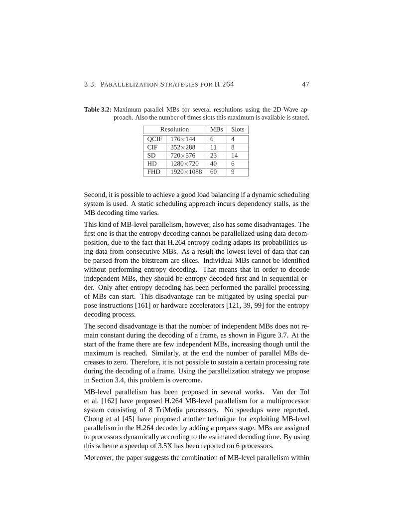
3.3. PARALLELIZATION STRATEGIES FORH.264 47
Table 3.2: Maximum parallel MBs for several resolutions using the 2D-Wave ap-proach. Also the number of times slots this maximum is available is stated.
Resolution MBs Slots
QCIF 176×144 6 4CIF 352×288 11 8SD 720×576 23 14HD 1280×720 40 6FHD 1920×1088 60 9
Second, it is possible to achieve a good load balancing if a dynamic schedulingsystem is used. A static scheduling approach incurs dependency stalls, as theMB decoding time varies.
This kind of MB-level parallelism, however, also has some disadvantages. Thefirst one is that the entropy decoding cannot be parallelized using data decom-position, due to the fact that H.264 entropy coding adapts its probabilities us-ing data from consecutive MBs. As a result the lowest level of data that canbe parsed from the bitstream are slices. Individual MBs cannot be identifiedwithout performing entropy decoding. That means that in order to decodeindependent MBs, they should be entropy decoded first and in sequential or-der. Only after entropy decoding has been performed the parallel processingof MBs can start. This disadvantage can be mitigated by using special pur-pose instructions [161] or hardware accelerators [121, 39, 99] for the entropydecoding process.
The second disadvantage is that the number of independent MBs does not re-main constant during the decoding of a frame, as shown in Figure 3.7. At thestart of the frame there are few independent MBs, increasing though until themaximum is reached. Similarly, at the end the number of parallel MBs de-creases to zero. Therefore, it is not possible to sustain a certain processing rateduring the decoding of a frame. Using the parallelization strategy we proposein Section 3.4, this problem is overcome.
MB-level parallelism has been proposed in several works. Van der Tolet al. [162] have proposed H.264 MB-level parallelism for a multiprocessorsystem consisting of 8 TriMedia processors. No speedups were reported.Chong et al [45] have proposed another technique for exploiting MB-levelparallelism in the H.264 decoder by adding a prepass stage. MBs are assignedto processors dynamically according to the estimated decoding time. By usingthis scheme a speedup of 3.5X has been reported on 6 processors.
Moreover, the paper suggests the combination of MB-level parallelism within

48 CHAPTER 3. PARALLEL SCALABILITY OF V IDEO DECODERS
frames and among frames to increase the availability of independent MBs. Theuse of inter-frame MB-level parallelism is determined statically by the lengthof the motion vectors. Chen et al. [40] have evaluated a similar approach for theH.264 encoder on Pentium machines with SMT and multicore capabilities. Inthose two works the exploitation of inter-frame MB-level parallelism is limitedto two consecutive frames and the identification of independent MBs is donestatically by taking into account the limits of the motion vectors. Although thiscombination of intra-frame and inter-frame MB-level parallelism increases theamount of independent MBs, it requires that the encoder puts some limits onthe length of the motion vectors in order to define statically which MBs of thenext frame can start execution while decoding the current frame.
So far we only discussed MB-level parallelism within a frame. As suggestedby [162], MB-level parallelism can also be exploited between frames, consid-ering the dependencies through the motion compensation kernel are met. ForH.264 encodingthis has been implemented in X264 [168] and in the H.264Codec that is part of the Intel Integrated Performance Primitives [83]. The firstobtains a maximum speedup of approximately 16.4 using 32 threads.
Zhao et al. [170] combined inter-frame and intra-frame MB-level parallelismfor H.264 encoding. This scheme is a variation of what we refer to in thisthesis as static 3D-Wave. They obtained a speedup of approximately 3 using4 cores and discarded an analysis for a high number of cores as an impracticalcase. The parallelization strategy that we propose in this thesis is also basedon a combination of inter-frame and intra-frame MB-level parallelism. Weconsider H.264 decoding, which is more difficult to parallelize as encoding.Furthermore, by determining dynamically the actual dependencies betweenMBs, our approach is much more scalable as explained in Section 3.4.
3.3.5 Block-level Parallelism
Finally, the finest grained data-level parallelism is at the block level. Most ofthe computations of the H.264 kernels are performed at the block level. Thisapplies, for example, to the interpolations that are performed in the motioncompensation stage, to the IDCT, and to the deblocking filter. This level ofdata parallelism maps well to SIMD instructions [171, 140, 21, 96]. SIMDparallelism is orthogonal to the other levels of parallelism described above andbecause of that it can be mixed, for example, with MB-level parallelization toincrease the performance of each thread.

3.4. SCALABLE MB-LEVEL PARALLELISM : THE 3D-WAVE 49
3.4 Scalable MB-level Parallelism: The 3D-Wave
None of the approaches described in the previous section scales to future many-core architectures containing 100 cores or more. In the 2D-Wave there is aconsiderable amount of MB-level parallelism, but at the start and end of aframe there are only a few independent MBs.
In order to overcome this limitation, it is possible to exploit both intra-frameand inter-frame MB-level parallelism. Inside a frame, spatial MB-level paral-lelism can be exploited using the 2D-Wave scheme mentioned previously. Si-multaneously, among frames temporal MB-level parallelism can be exploited.
Temporal MB-level parallelism can be exploited when considering the depen-dencies due to Motion Compensation (MC). MC can be regarded as copyingan area, called the reference area, from the reference frame, and then to addthis predicted area to the residual MB to reconstruct the MB in the currentframe. The reference area is pointed to by a Motion Vector (MV). The MVlength is limited by two factors: the H.264 level and the motion estimationalgorithm. The H.264 level defines, amongst others, the maximum length ofthe vertical component of the MV [120]. Not all encoders, however, followthe guidelines of the levels, but use the absolute limit of the standard which is512 pixels vertical and 2048 pixels horizontal. In practice the motion estima-tion algorithm defines a maximum search range of dozens of pixels, becausea larger search range is very computationally demanding and provides only asmall benefit [104].
When the reference area has been decoded it can be used by the referencingframe. Thus it is not necessary to wait until a frame is completely decodedbefore decoding the next frame. The decoding process of the next frame canstart after the reference areas of the reference frames are decoded. Figure 3.8shows an example of two frames where the second depends on the first. Thefigure shows that MB(2, 0) of framei + 1 depends on MB(2, 1) of frameiwhich has been decoded. Thus this MB can be decoded even though frameiis not completely decoded. Similarly, MB(0, 1) of frame i + 1 depends onMB (0, 2) of framei. This dependency is resolved, as well as the intra-framedependencies. Therefore, also this MB can be decoded.
Figure 3.8 shows a 2D-Wave decoding within each frame of the two frames.This technique can be extended to much more than two frames, adding a thirddimension to the parallelization, as illustrated in Figure 3.9. Hence, we referto this parallelization strategy as 3D-Wave.
The scheduling of MBs for decoding can be performed in a static or a dy-

50 CHAPTER 3. PARALLEL SCALABILITY OF V IDEO DECODERS
MBs to be processedMBs in flightMBs processed
T4 T5
T5
T7
T4 T5 T6 T7
T6 T8 T9
T8 T9 T10 T11
T9 T10 T11 T12 T13
MB (3,0) MB (4,0)
MB (1,1) MB (2,1) MB (3,1) MB (4,1)
MB (0,2) MB (1,2) MB (3,2) MB (4,2)
MB (1,3) MB (2,3) MB (3,3) MB (4,3)
MB (0,4) MB (1,4) MB (2,4) MB (3,4) MB (4,4)
MB (0,0)T1
MB (1,0)T2
MB (0,3)
T7MB (2,2)
MB (2,0)T3T3 T4 T5
T3
T5
T4 T5 T6
T6 T7 T8 T9
T8 T9 T10 T11
T9 T10 T11 T12 T13
MB (2,0) MB (3,0) MB (4,0)
MB (0,1) MB (1,1) MB (2,1) MB (3,1)
MB (0,2) MB (1,2) MB (2,2) MB (3,2) MB (4,2)
MB (1,3) MB (2,3) MB (3,3) MB (4,3)
MB (0,4) MB (1,4) MB (2,4) MB (3,4) MB (4,4)
MB (0,0)T1
MB (1,0)T2
T7MB (0,3)
T7MB (4,1) MB (0,1)
T3
frame i frame i+1
Figure 3.8: 3D-Wave strategy: intra-frame and inter-frame dependencies betweenMBs.
Figure 3.9: 3D-Wave strategy: frames can be decoded in parallel because inter-framedependencies have limited spatial range.
namic way. Static 3D-Wave exploits temporal parallelism by assuming thatthe motion vectors have a restricted length. Based on that, it uses a fixed offsetbetween the 2D-Waves of consecutive frames. This static approach has beenimplemented in previous work for the H.264 encoder [170]. It is more suitablefor the encoder because it has the flexibility of selecting the size of the motionsearch area.
The static 3D-Wave for H.264 decoding has been investigated by Azevedo(see [113]). The amount of MB parallelism it exhibits is depending on themotion vector range (see Table 3.3). Motion vectors are typically short (< 16)and thus potentially a lot of parallelism is available. For FHD resolution evenmaximally 1360 MBs in parallel are available. The problem is the worst case

3.4. SCALABLE MB-LEVEL PARALLELISM : THE 3D-WAVE 51
Table 3.3: Static 3D-Wave: maximum MB parallelism and frames in flight for severalMV ranges and three resolutions.
MV range Max # parallel MBs Max # frames in flightSD HD FHD SD HD FHD
512 - 36 89 - 2 3256 33 74 163 3 4 5128 60 134 303 5 7 1064 108 240 544 8 12 1732 180 400 907 13 19 2916 276 600 1360 20 28 43
scenario, which for FHD is a motion vector of length 512. As the static 3D-Wave always has to account for the worst case, the amount of parallelism thateffectively can be exploited in such case is maximally 89.
Our proposal is the Dynamic 3D-Wave approach. It is not based on restrictedvalues of the motion vectors. Instead, it uses a dynamic scheduling system inwhich MBs are scheduled for decoding when all the dependencies (intra-frameand inter-frame) have been satisfied. As illustrated in Figure 3.8, as soon asthe search area in the reference frame has been decoded, the depending MB ina different frame can be processed. The dynamic system is best suited for thedecoder taking into account that the length of motion vectors is not known apriori and that the decoding time of each MB is input-dependent. The Dynamic3D-Wave system results in better scalability as we will show.
The dynamic scheduling can be implemented in various ways. Several issuesplay a role in this matter such as thread management overhead, data commu-nication overhead, memory latency, centralized vs. distributed control, etc. InSection 3.7, while discussing our implementations of parallel H.264 decoding,we comment in more detail on the dynamic scheduling implementations.
Another issue is entropy decoding which does not exhibit TLP within a slice.Thus, entropy decoding is decoupled from the MB-decoding process using afunction-level decomposition. That is, one core performs entropy decoding,which output is fed into the parallel MB-decoding process using several cores.If all cores are equal, one entropy decoding core can sustain approximatelyeight MB-decoding cores. Entropy decoding, however, can be parallelizedat the slice level. Thus, multiple entropy decoding cores can be deployed,each processing a different slice or frame. Furthermore, entropy decoding canbe accelerated by using specialized cores or ASICs. Assuming four entropydecoding cores are utilized, each twice as fast as a general purpose core, than a

52 CHAPTER 3. PARALLEL SCALABILITY OF V IDEO DECODERS
total of 64 MB-decoding cores can be used efficiently. In the remainder of thischapter we focus on the parallelism in the MB decoding process, unless statedotherwise.
In the next section the parallel scalability of the Dynamic 3D-Wave is analyzed.The scalability obtained for actual implementations of the Dynamic 2D-Waveand 3D-Wave are discussed in Section 3.7.
3.5 Parallel Scalability of the Dynamic 3D-Wave
In this section we analyze the parallel scalability of the H.264 decoder by ex-ploring the limits of the amount of TLP it exhibits. This research is similarto the ILP limit study for video applications presented in [100]. Investigatingthe limits to TLP, however, requires to put a boundary on the granularity ofthe threads. Without this boundary a single instruction can be a thread, whichis clearly not feasible. Thus, using emerging techniques such as light-weightmicro-threading [92], possibly even more TLP can be exploited. We show,however, that macroblock-level granularity is sufficient to sustain a many-coresystem.
To determine the amount of parallelism, we modified the FFmpeg H.264 de-coder to analyze the dependencies in real movies, which we took from theHD-VideoBench. We analyzed the dependencies of each MB and assignedeach MB a timestamp as follows. The timestamp of a MB is simply the maxi-mum of the timestamps of all MBs upon which it depends (in the same frameas well as in the reference frames) plus one. Because the frames are processedin decoding order†, and within a frame the MBs are processed from left toright and from top to bottom, the MB dependencies are observed and it is as-sured that the MBs on which a MBB depends have been assigned their correcttimestamps by the time the timestamp of MBB is calculated. As before, weassume that it takes one time unit to decode a MB.
The way inter-frame dependencies are handled needs further explanation. Thepixels required for motion compensation are not only those of the sub-blockthe motion vector is pointing to. If the motion vector is fractional, the pixelsused for MC are computed by interpolation and for this the pixels surroundingthe sub-block are also required. Further, the standard defines that deblockingfiltered pixels should be used for MC. The bottom and right four pixels of each
†The decoding order of frames is not equal to display order. The sequence I-B-B-P as inFigure 3.3 is decoded as I-P-B-B sequence.

3.5. PARALLEL SCALABILITY OF THE DYNAMIC 3D-WAVE 53
Table 3.4: Maximum available MB parallelism and frames in flight for normal en-coded movies. The maximum and the average motion vectors (in squarepixels) are also stated.
SD HDMBs frames max mv avg mv MBs frames max mv avg mv
rushhour 1199 92 380,5 1.3 2911 142 435 1.8riverbed 1511 119 228.6 2 3738 185 496 2.2pedestrian 1076 95 509.7 9.2 2208 131 553.5 11blue sky 1365 99 116 4.4 2687 135 298 5.1
FHDMBs frames max mv avg mv
rushhour 5741 211 441 2.2riverbed 7297 245 568.9 2.6pedestrian 4196 205 554.2 9.9blue sky 6041 214 498 5.6
MB are filtered only when the bottom or left MB is decoded. Thus, although aMV points to a sub-block that lies entirely in a MBA, the actual dependenciesmight go as far as the right and/or bottom neighbor of MBA. We took thisinto account by adding to each MV the pixels needed for interpolation andchecking if the DF of the neighboring blocks would affect the required pixels.
To start, the maximum available MB-level parallelism is analyzed. This ex-periment does not consider any practical or implementation issues, but simplyexplores the limits of the amount of parallelism available in the application.We use the modified FFmpeg as described before and for each time slot wedetermined, the number of MBs that can be processed in parallel during thattime slot. In addition, we keep track of the number of frames in flight. Finally,we keep track of the motion vector lengths. All experiments are performedfor both normally encoded and esa encoded movies. The first uses a hexago-nal (hex) motion estimation algorithm with a search range of 24 pixels, whilethe latter uses an exhaustive search algorithm and results in worst case motionvectors.
Table 3.4 summarizes the results for normally encoded movies and shows thata huge amount of MB-level parallelism is available. Figure 3.10 depicts theMB-level parallelism time curve for FHD (i.e., the number of MBs that can beprocessed in parallel in each time slot), while Figure 3.11 depicts the numberof frames in flight in each time slot. For the other resolutions the time curveshave a similar shape. The MB parallelism time curve shows a ramp up, a

54 CHAPTER 3. PARALLEL SCALABILITY OF V IDEO DECODERS
0
1000
2000
3000
4000
5000
6000
7000
8000
0 200 400 600 800 1000 1200
Par
alle
l mac
robl
ocks
Time
rush_hourriverbed
pedestrianblue_sky
Figure 3.10: Number of parallel MBs in each time slot, using the 3D-Wave paral-lelization, for FHD resolution using a 400 frame sequence.
0
50
100
150
200
250
0 200 400 600 800 1000 1200
Fra
mes
in fl
ight
Time
rush_hourriverbed
pedestrianblue_sky
Figure 3.11: Number of frames in flight in each time slot, using the 3D-Wave paral-lelization, for FHD resolution using a 400 frame sequence.

3.5. PARALLEL SCALABILITY OF THE DYNAMIC 3D-WAVE 55
Table 3.5: Maximum MB parallelism and frames in flight for esa encoded movies.Also the maximum and the average motion vectors (in square pixels) arestated.
SD HDMBs frames max mv avg mv MBs frames max mv avg mv
rushhour 505 63 712,0 6.9 708 84 699.3 9riverbed 150 27 704.9 62.3 251 25 716.2 63.1pedestrian 363 50 691.5 23.5 702 70 709.9 27.7blue sky 138 19 682.0 10.5 257 23 711.3 13
FHDMBs frames max mv avg mv
rushhour 1277 89 706.4 9.4riverbed 563 37 716.2 83.9pedestrian 1298 88 708.5 23.6blue sky 500 24 705.7 15.7
plateau, and a ramp down. For example, for bluesky the plateau starts at timeslot 200 and last until time slot 570. Riverbed exhibits such a huge amount ofMB-level parallelism that it has a small plateau. Due to the stochastic changingcontent of the movie, the encoder mostly uses intra-coding, resulting in veryfew dependencies between frames. Pedestrian exhibits the least amount ofparallelism. The fast moving objects in the movie result in many large motionvectors. Especially objects moving from right to left on the screen cause largeoffsets between MBs in consecutive frames.
Rather surprising is the maximum MV length found in the movies (see Ta-ble 3.4). The search range of the motion estimation algorithm is limited to 24pixels, but still lengths of more than 500 square pixels are reported. Accordingto the developers of the X264 encoder this is caused by drifting [169]. For eachMB the starting MV of the algorithm is predicted using the result of surround-ing MBs. If a number of MBs in a row use the motion vector of the previousMB and add to it, the values accumulate and reach large lengths. This driftinghappens only occasionally, and does not significantly affect the parallelism inthe dynamic approach, but would force a static approach to use a large offsetresulting in little parallelism.
To evaluate the worst case, the same experiment was performed for moviesencoded using the exhaustive search algorithm (esa). Table 3.5 shows that theaverage MV is substantially longer than for normally encoded movies. Theexhaustive search decreases the amount of parallelism significantly. The time

56 CHAPTER 3. PARALLEL SCALABILITY OF V IDEO DECODERS
Table 3.6: Comparison of the maximum and average amount of MB-level parallelismfor hex and esa encoded movies (FHD only).
FHDmax MB avg MB
hex esa ∆ hex esa ∆rushhour 5741 1277 -77.8% 4121.2 892.3 -78.3%riverbed 7297 563 -92.3% 5181.0 447.7 -91.4%pedestrian 4196 1298 -69.1% 3108.6 720.8 -76.8%blue sky 6041 500 -91.7% 4571.4 442.6 -90.3%
Table 3.7: Compression improvement of esa encoding relative to hex.
SD HD FHD average
rushhour -0.7% 0.0% -0.3% -0.3%riverbed 1.4% 1.9% 3.2% 2.1%pedestrian 0.6% 1.6% 1.2% 1.1%blue sky -1.4% -1.5% 1.4% -0.5%
average 0.0% 0.5% 1.4% 0.6%
curves in Figures 3.12 and 3.13 have a very jagged shape with large peaksand thus the average on the plateau is much lower than the peak. In Table 3.6the maximum and the average parallelism for normally (hex) and esa encodedmovies is compared. The average is taken over all 400 frames, including rampup and ramp down. Although the drop in parallelism is significant, the amountof parallelism is still large for this worst case scenario.
As we are comparing two encoding methods, it is important to look at someother aspects as well. In Table 3.7 we compare the compression ratios of hexand esa encoding. Only for FHD a considerable compression improvementis achieved when using esa encoding. The cost of this improvement in termsof encoding time, however, is large. A 300-frame FHD sequence takes lessthan 10 minutes to encode using hexagonal motion estimation and running ona modern desktop computer (Pentium D, 3.4 GHz, 2GB memory). The samesequence takes about two days to encode when using the esa option, which isalmost 300 times slower. Thus we can assume that this worst case scenario isunlikely to occur in practice.

3.5. PARALLEL SCALABILITY OF THE DYNAMIC 3D-WAVE 57
0
200
400
600
800
1000
1200
1400
0 1000 2000 3000 4000 5000 6000 7000 8000
Par
alle
l mac
robl
ocks
Time
rush_hourriverbed
pedestrianblue_sky
Figure 3.12: Number of parallel MBs in each time slot, using the 3D-Wave paral-lelization, for FHD using esa encoding.
0
10
20
30
40
50
60
70
80
90
0 1000 2000 3000 4000 5000 6000 7000 8000
Fra
mes
in fl
ight
Time
rush_hourriverbed
pedestrianblue_sky
Figure 3.13: Number of frames in flight in each time slot, using the 3D-Wave paral-lelization, for FHD using esa encoding.

58 CHAPTER 3. PARALLEL SCALABILITY OF V IDEO DECODERS
The analysis above reveals that H.264 exhibits significant amounts of MB-level parallelism. To exploit this type of parallelism on a multicore the MBdecoding tasks need to be assigned to the available cores. Even in future many-cores, however, the hardware resources, e.g., the number of cores, the sizeand bandwidth of memory, and the NoC bandwidth, will be limited. We nowinvestigate the impact of such resource limitations.
We model limited resources as follows. A limited number of cores is modeledby limiting the number of MBs in flight, as each MB in flight requires one coreto execute on. Memory requirements are mainly proportional to the numberof frames in flight, as each frame in flight should be stored in main memory.Thus limited memory is modeled by restricting the number of frames that canbe in flight concurrently.
The experiment has been performed for all four movies of the benchmark, forall three resolutions, and both types of motion estimation. The effect of thelimitations is similar for all movies, and thus only the results for the normallyencoded bluesky movie at FHD resolution are presented.
First, the impact of limiting the number of MBs in flight is analyzed. Fig-ure 3.14 depicts the available MB-level parallelism for several limits on thenumber of MBs in flight. As can be expected, for lower limits, the height ofthe plateau is lower and the ramp up and ramp down are on average slightlyshorter. More important is that for lower limits, the plateau becomes veryflat. This translates to a high utilization rate of the available cores. Further-more, the figure shows that the total decoding time is approximately inverselyproportional to the limit on the number of MBs in flight, i.e., if the limit is de-creased by a factor of 2, the decoding time increases approximately by a factorof 2 too. This is especially true for lower limits, where the core utilization isalmost 100%. For higher limits, the core utilization decreases and the relationno longer holds.
Figure 3.15 depicts the number of frames in flight as a function of time whenthe number of MBs in flight is limited. Not surprisingly, because limiting thenumber of MBs in flight also limits the number of frames that can be in flight,the shape of the curves are similar to those of the available MB parallelism,although with a small periodic fluctuation.
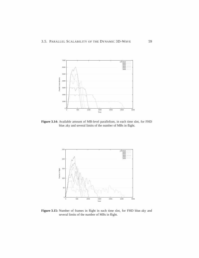
3.5. PARALLEL SCALABILITY OF THE DYNAMIC 3D-WAVE 59
0
1000
2000
3000
4000
5000
6000
7000
0 500 1000 1500 2000 2500 3000
Par
alle
l mac
robl
ocks
Time
unlimited50004000300020001000
Figure 3.14: Available amount of MB-level parallelism, in each time slot, for FHDblue sky and several limits of the number of MBs in flight.
0
50
100
150
200
250
0 500 1000 1500 2000 2500 3000
Fra
mes
in fl
ight
Time
unlimited50004000300020001000
Figure 3.15: Number of frames in flight in each time slot, for FHD bluesky andseveral limits of the number of MBs in flight.

60 CHAPTER 3. PARALLEL SCALABILITY OF V IDEO DECODERS
Next, we analyze the impact of restricting the number of frames concurrentlyin flight. The MB-level parallelism curves are depicted in Figure 3.16 andshow large fluctuations, possibly resulting in under-utilization of the availablecores. The fluctuations are caused by the ramping effect illustrated in Fig-ure 3.7 for one frame. It shows that at the start and end of a frame less paral-lelism is available. The same ramping effect occurs in this case. As a limitednumber of frames are in flight concurrently, and frames start decoding quicklyone after another, they are approximately in the same phase. Thus, if all framesin flight are about halfway the frame, many parallel MBs are available. On theother hand, if all frames are close to the end only very little parallelism isavailable.
Figure 3.17 shows the actual frames in flight for several limits. The plateausin the curves translate to full memory utilization.
From this experiment we conclude that for systems with a limited numberof cores, dynamic scheduling is able to achieve near optimal performance by(almost) fully utilizing the available computational power. On the contrary,for systems where the memory size is the limitation, additional performancelosses might occur because of temporal under-utilization of the available cores.In Section 3.6 we perform a case study, indicating that memory will most likelynot be the limitation.
We have shown that using the Dynamic 3D-Wave strategy huge amounts ofparallelism are available in H.264 decoding. Analysis of real movies has re-vealed that the average number of parallel MBs ranges from 3000 to 7000. Thisamount of MB parallelism might be larger than the number of cores available.Thus, we have evaluated the parallelism for limited resources and found thatlimiting the number of MBs in flight results in a equivalent larger decodingtime, but a near optimal utilization of the cores.

3.5. PARALLEL SCALABILITY OF THE DYNAMIC 3D-WAVE 61
0
1000
2000
3000
4000
5000
6000
7000
0 500 1000 1500 2000 2500 3000 3500
Par
alle
l mac
robl
ocks
Time
unlimited1501005025
Figure 3.16: Available MB parallelism in FHD bluesky for several limits of the num-ber of frames in flight.
0
50
100
150
200
250
0 500 1000 1500 2000 2500 3000 3500
Fra
mes
in fl
ight
Time
unlimited1501005025
Figure 3.17: Number of actual frames in flight for FHD bluesky, for several limits ofthe number of frames in flight.

62 CHAPTER 3. PARALLEL SCALABILITY OF V IDEO DECODERS
3.6 Case Study: Mobile Video
So far we have mainly focused on high resolution and explored the potentiallyavailable MB-level parallelism. The 3D-Wave strategy discloses an enormousamount of parallelism, possibly more than what a high performance multicorein the near future could provide. Therefore, in this section we perform a casestudy to assess the practical value and possibilities of a highly parallelizedH.264 decoding application.
For this case study we assume a mobile device such as the iPhone, but in theyear 2015. We take a resolution of 480×320 just as the screen of the currentiPhone. It is reasonable to expect that the size of mobile devices will notsignificantly grow, and the limited accuracy of the human eye implies that theresolution does not have to increase.
Multicores are power efficient, and thus we expect mobile devices to adoptthem quickly, and therefore we project a 100-core chip in 2015. Two exam-ples of state-of-the art embedded multicores are the Tilera Tile64 [157] andthe Clearspeed CSX600 [46], containing 64 and 96 cores respectively. Bothare good examples of what is already possible today and the eagerness of theembedded market to adopt the multicore paradigm. A doubling of cores ev-ery three years is expected [148]. Even if this growth would be less still theassumption of 100 cores in 2015 seems reasonable.
At time of performing this analysis (2007), the iPhone 2G was available with8GB of memory. Using Moore’s Law for memory (doubling every two years),in 2015 this mobile device would contain 128 GB. It is unclear how much ofthe flash drive memory is used as main memory, but for this case study weassume it is only 1%. In 2015 that would mean 1.28GB and if only half of itis available for video decoding, then still almost 1400 frames of video wouldfit in main memory. Thus, it seems that memory size is not going to be alimitation.
We place a limit of 1 second on the latency of the decoding process. That is areasonable time to wait for the movie to appear on the screen, and much longerwould not be acceptable. The iPhone uses a frame rate of 30 frames/second,and thus limiting the frames in flight to 30, causing a latency of 1s. Thiscan be explained as follows. Let us assume that the clock frequency is scaleddown as much as possible to save power. When the decoding of framex isstarted, framex − 30 has just finished and is currently displayed. But, sincethe framerate is 30, framex will be displayed 1 second later. Of course this isa rough method and does not consider variations in frame decoding time, but

3.7. EXPERIENCES WITHPARALLEL IMPLEMENTATIONS 63
it is a good estimate.
Putting all assumptions together, for the future device the Dynamic 3D-Wavestrategy has a limit of 100 parallel MBs and up to 30 frames can be in flightconcurrently. For this case study we use the four normally encoded movieswith a length of 200 frames and a resolution of 480×320.
Figure 3.18 presents the available MB-level parallelism under these assump-tions as well as for unlimited resources. The figure shows that even for thissmall resolution, all 100 cores are utilized nearly all the time. The curves forunrestricted resources show that there is much more parallelism available thanthe hardware of this future mobile device has to offer. This provides opportu-nities for scheduling algorithms to reduce communication overhead.
Figure 3.19 depicts the number of frames in flight for this case study. Theaverage is approximately 12 frames with peaks of up to 19. From the graphswe can also conclude that the decoding latency is approximately 0.5 second,since around 15 frames are in flight.
From this case study we draw the following conclusions:
• Even a low resolution movie exhibits sufficient parallelism to fully uti-lize 100 cores efficiently.
• For mobile devices, the memory size will most likely not be a limitation.
• For mobile devices with a 100-core chip, the frame latency will be short(around 0.5s).
3.7 Experiences with Parallel Implementations
Motivated by the results of the previous sections our team has implementedseveral parallel H.264 decoders. Azevedo [28] has implemented the Dynamic3D-Wave on a TriMedia multicore platform during an internship at NXP. Al-varez [20] has implemented the 2D-Wave on a multiprocessor system. Finally,Chi [43, 44] has implemented the 2D-Wave on the Cell processor. The lasttwo works are based on an unpublished initial parallelization by Paradis andAlvarez.
Although the author was not the prime developer, the experiences are veryinteresting and for completeness should be presented briefly in this chapter.The full experimental results and analysis can be found in [28, 20, 43, 44].

64 CHAPTER 3. PARALLEL SCALABILITY OF V IDEO DECODERS
0
100
200
300
400
500
600
0 200 400 600 800 1000 1200
Par
alle
l mac
robl
ocks
Time
rush_hour unrestrictedriverbed unrestricted
pedestrian unrestrictedblue_sky unrestricted
rush_hourriverbed
pedestrianblue_sky
Figure 3.18: Number of parallel MBs for the mobile video case study. Also depictedis the available MB-level parallelism for the same resolution but withunrestricted resources.
0
5
10
15
20
25
0 200 400 600 800 1000 1200
Fra
mes
in fl
ight
Time
rush_hourriverbed
pedestrianblue_sky
Figure 3.19: Number of frames in flight for the mobile video case study.

3.7. EXPERIENCES WITHPARALLEL IMPLEMENTATIONS 65
The scalability analysis of Section 3.5 is theoretical in nature and reveals theparallelism exhibited by the application. Exploiting this parallelism also in-volves the hardware architecture, the runtime system, and the operating sys-tem, whose characteristics affect the actual obtainable scalability. Therefore,these implementations are briefly reviewed in the following sections. We dis-cuss what obstacles were encountered in achieving scalability. Also results areshown and the differences with the theoretical study are analyzed.
3.7.1 3D-Wave on a TriMedia-based Multicore
For this 3D-Wave implementation [28] the NXP H.264 decoder is used, whichis highly optimized for NXPs TriMedia processor. As a starting point, Hooger-brugge [79] already implemented the 2D-Wave, on which this implementationis based. The cycle accurate NXP proprietary simulator was used to evaluatethe 3D-Wave on a TriMedia-based multicore system. It is capable of simulat-ing up to 64 TM3270 cores [161], each with a 64KB private L1 cache, and ashared L2 cache.
The programming model follows the task pool model. The task pool libraryimplements submission and requests of tasks to/from the task pool, synchro-nization mechanisms, and the task pool itself. The system contains one controlprocessor and several worker processors. The latter request tasks from the taskpool and execute it. The task pool library is very efficient as the time to requesta task is only 2% of the MB decoding time.
The implementation of the 3D-Wave required quite some modifications to thecode. In order to decode multiple frames concurrently some additional soft-ware buffers were required. Further, the task pool library was extended with asubscription mechanism (kick-off lists). The dependencies through the motionvectors are not known a priori. Thus, the MB decoding is split in two parts.In the first part the motion vectors are predicted. In case the reference areahas been decoded, the core continues with the second part, which contains therest of the MB decoding process. In case an unresolved dependency is met,the current MB subscribes itself to the MB it depends on. The latter starts theexecution of the former MB once it has been decoded.
Due to the additional administrative overhead, the 3D-Wave is 8% slower thanthe 2D-Wave on a single core. The scalability of the 3D-Wave, however, ismuch better than that of the 2D-Wave as shown in Figure 3.20. Whereas thescalability of the 2D-Wave saturates at around 15, the 3D-Wave provides ascalability of almost 55. Note that the scalability of a case is always relative to
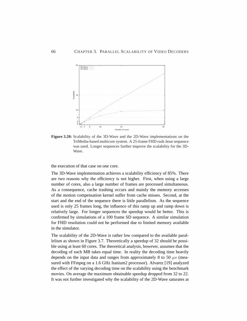
66 CHAPTER 3. PARALLEL SCALABILITY OF V IDEO DECODERS
124
8
16
32
64
1 2 4 8 16 32 64
Sca
labi
lity
Number of cores
3D-Wave2D-Wave
Figure 3.20: Scalability of the 3D-Wave and the 2D-Wave implementations on theTriMedia-based multicore system. A 25-frame FHD rushhour sequencewas used. Longer sequences further improve the scalability for the 3D-Wave.
the execution of that case on one core.
The 3D-Wave implementation achieves a scalability efficiency of 85%. Thereare two reasons why the efficiency is not higher. First, when using a largenumber of cores, also a large number of frames are processed simultaneous.As a consequence, cache trashing occurs and mainly the memory accessesof the motion compensation kernel suffer from cache misses. Second, at thestart and the end of the sequence there is little parallelism. As the sequenceused is only 25 frames long, the influence of this ramp up and ramp down isrelatively large. For longer sequences the speedup would be better. This isconfirmed by simulations of a 100 frame SD sequence. A similar simulationfor FHD resolution could not be performed due to limited memory availablein the simulator.
The scalability of the 2D-Wave is rather low compared to the available paral-lelism as shown in Figure 3.7. Theoretically a speedup of 32 should be possi-ble using at least 60 cores. The theoretical analysis, however, assumes that thedecoding of each MB takes equal time. In reality the decoding time heavilydepends on the input data and ranges from approximately 8 to 50µs (mea-sured with FFmpeg on a 1.6 GHz Itanium2 processor). Alvarez [19] analyzedthe effect of the varying decoding time on the scalability using the benchmarkmovies. On average the maximum obtainable speedup dropped from 32 to 22.It was not further investigated why the scalability of the 2D-Wave saturates at

3.7. EXPERIENCES WITHPARALLEL IMPLEMENTATIONS 67
0
5
10
15
20
25
30
1 2 3 5 7 9 11 13 15 17 19 21 23 25 27 29 31 32
Sca
labi
lity
Number of cores
tail submit right firsttail submit down-left first
dynamic schedulingstatic scheduling
Figure 3.21: Scalability of the 2D-Wave implementation on a 128-core SGI Altix sys-tem.
around 15. A plausible explanation is that it is caused by synchronization andcommunication overhead.
3.7.2 2D-Wave on a Multiprocessor System
This implementation of the parallel H.264 decoder [20] was implemented andtested on an SGI Altix machine with 128 cores and a cc-NUMA (cache coher-ent Non-Uniform Memory Access) memory design. Blades with two dual-coreIntel Itanium-II processors (1.6 GHz) and 8 GB of RAM were used. The bladesare connected through a high performance interconnect (NUMAlink-4) with a6.4 GB/s peak bandwidth.
The FFmpeg H.264 decoder was parallelized using a similar task model asdescribed in the previous section. The worker threads are responsible forupdating the dependency table. This allowed the implementation of severalscheduling strategies such as tail-submit. POSIX threads were used as well assemaphores and mutexes for synchronization.
The scalability of the 2D-Wave implementation was measured with all fourbenchmark movies (see Section 3.2). In this case sequences of 100 frameswere used. Figure 3.21 depicts the scalability obtained using up to 32 coresand for several scheduling policies. Both the static and dynamic schedulingscale very poorly. The static scheduling does not use the task pool, but usesa fixed decoding order instead, i.e., a zigzag scan order following the 2D-

68 CHAPTER 3. PARALLEL SCALABILITY OF V IDEO DECODERS
Wave pattern. Due to the variable decoding time, this scheduling strategy failsto exploit the available parallelism. The dynamic scheduling implementationdoes use the task pool, but the overhead for submitting to and retrieving tasks isa bottleneck of the system. Using a tail-submit scheduling, the task pool is lessfrequently accessed and thus the scalability improves. The right-first policy(next MB is the right neighboring MB) has the best performance as it exploitsmore data locality than the down-left-first policy (next MB is the down-leftneighboring MB).
The limited scalability of this implementation is mainly caused by synchro-nization. Using one core, to get a MB from the task pool takes6.1µs, whileusing 8 cores this time has increased to132µs. Using more cores the timeincreases further, but then the limited amount of available parallelism startsplaying a role as well. The execution time of the getmb function, which re-trieves a MB from the task pool, is dominated by the semwait (semaphorewait), which in turn spends most of its time in the OS intervention. Apparentlythis OS intervention increases with the number of participating cores.
From this study we conclude that synchronization overhead radically affectsthe scalability if it is not implemented efficiently. Standard libraries such asthe p-thread library do not seem to provide this efficiency.
The 3D-Wave was not implemented on this multiprocessor system. Theamount of available parallelism was not the limitation, and thus there is noneed to use the 3D-Wave strategy. The conclusions from this study also applyto the 3D-Wave though, which is the reason why this section was included.
3.7.3 2D-Wave on the Cell Processor
Chi [43, 44], an MSc student from Delft University of Technology, developeda very scalable implementation of the 2D-Wave on the Cell Processor. He ob-served that the mailbox API offered by the standard libraries has much largerlatencies than the actual hardware system. Therefore, instead he used a mail-box API that accesses the problem state of the SPEs directly.
Another major improvement he made concerns the data communication. Theinitial implementation contained many DMAs, each transferring a part of theinformation required to decode the macroblock. Chi reduced the number ofDMAs to a minimum by creating a new data structure containing all informa-tion in one place.
Figure 3.22 shows that this optimized Task Pool (TP) based 2D-Wave imple-mentation achieves a scalability of 10.2 on 16 SPEs, which is approximately

3.7. EXPERIENCES WITHPARALLEL IMPLEMENTATIONS 69
0
2
4
6
8
10
12
14
16
1 2 3 4 5 6 7 8 9 10 11 12 13 14 15 16
Sca
labi
lity
Number of SPEs
RL 2D-WaveTP 2D-Wave
Figure 3.22: Scalability of the 2D-Wave implementations on the Cell processor. At16 SPEs the difference in scalability is 20%. The Ring-Line (RL) basedimplementation, however, has twice the performance of the Task Pool(TP) based implementation.
the same as the 2D-Wave implementation on the TriMedia with equal numberof cores. In this implementation, scalability is mainly limited by contention onthe off-chip bus to main memory.
The TP 2D-Wave implementation does not yet fully utilize the capabilities ofthe Cell processor. The SPEs are connected to each other in a ring, which isexploited by the Ring-Line (RL) implementation of the 2D-Wave strategy. Ituses a distributed and static scheduling instead of a dynamic task pool. Eachline of macroblocks is assigned to one SPE, such that adjacent lines are pro-cessed on adjacent SPEs. Synchronization among SPEs is done by sending theoutput of one SPE to its neighbor. Besides removing the bottleneck of cen-tralized control, also much more locality is exploited resulting in much lessbandwidth requirements.
Figure 3.22 also shows the scalability of the ring-line implementation. It scalesbetter than the 2D-Wave based on the task pool from 10 SPEs on, and achievesa scalability of 12.0 using 16 SPEs. The theoretical scalability limit of thisimplementation is lower than that of the task pool implementation due to im-plementation issues not discussed here. The obtained scalability is close to thistheoretical limit, and therefore much higher scalability is not possible.
The actual performance of the ring-line implementation, however, is muchhigher than the task pool version. The latter achieves a throughput of 76 frames

70 CHAPTER 3. PARALLEL SCALABILITY OF V IDEO DECODERS
per second while the former implementation achieves 149 frames per secondon FHD resolution. There are two reasons for this difference. First, the lowerbandwidth requirements of the ring-line 2D-Wave implementation allow it toscale to a much higher frame throughput. Second, in the ring-line implemen-tation, the communication and computation are performed concurrently. In thetask pool 2D-Wave this could be implemented, for example by applying tail-submit. It is not so easy, however, to implement and it would stress the controlprocessor even more.
Those two implementations also show that the 2D-Wave is appropriate forsmall scale systems and can achieve high performance. Scalability is lim-ited, though, to about 16 to 20 cores. For larger scale systems the 3D-Wavewill have to be used. The latter is not yet implemented on the Cell proces-sor. The 2D-Wave on Cell has shown that low latency synchronization is ofvital importance to obtain scalability. Furthermore, it has shown that a smartscheduling of the data movements can significantly increase performance. Fi-nally, we conclude from this study that a centralized control processor easilybecomes a bottleneck for fine-grained thread-level parallelism, as used in ourimplementation of H.264 decoding.
3.8 Conclusions
In this chapter we have investigated if applications exhibit sufficient paral-lelism to exploit the large number of cores expected in future multicores. Thisis important for performance as well as for power efficiency. As a case study,we have analyzed the parallel scalability of an H.264 decoder, currently thebest video coding standard.
First, we discussed possible parallelization strategies. Most promising is MB-level parallelism, which can be exploited inside a frame in a diagonal wave-front manner. As MBs in different frames are only dependent through motionvectors, intra-frame and inter-frame MB-level parallelism can be combined.Such a parallelization approach is referred to as the 3D-Wave. It has been ap-plied to encoding before, but not to decoding as we have done. In this chapterwe have observed that motion vectors typically have a limited range. There-fore, by applying dynamic scheduling a much higher scalability can be ob-tained. This novel parallelization strategy is called the Dynamic 3D-Wave.
Using this new parallelization strategy we have performed a limit study of theamount of MB-level parallelism available in H.264. We modified FFmpeg andanalyzed real movies. The results have revealed that motion vectors are typi-

3.8. CONCLUSIONS 71
cally small on average. As a result a large amount of parallelism is available.For FHD resolution the total number of parallel MBs ranges from 4000 to7000.
The amount of MB parallelism disclosed by the Dynamic 3D-Wave could belarger than the number of cores available. Moreover, the number of frames inflight to achieve this parallelism might require more memory than available.Thus, we have evaluated the parallelism for limited resources and found thatlimiting the number of MBs in flight results in a larger decoding time, but anear optimal utilization of cores. Limiting the number of frames in flight, onthe other hand, results in large fluctuations of the available parallelism, likelyunder-utilization of the available cores and thus performance loss.
We have also performed a case study to assess the practical value and possibil-ities of the highly parallel H.264 decoder. In general, the results show that ourstrategy provides sufficient parallelism to efficiently exploit the capabilities offuture many-cores, even in future mobile devices.
Finally, we have discussed a few implementations of the 2D-Wave and 3D-Wave strategy. The 3D-Wave was successfully implemented on a TriMedia-based multicore platform. With 64 cores a scalability of 55 was achieved,whereas the scalability of the 2D-Wave saturates around 15. On a single core,the 3D-Wave is 8% slower than the 2D-Wave, due to management overhead.From 4 cores on, however, the 3D-Wave outperforms the 2D-Wave. Moreover,the implementation proved that in order to scale to a large number of cores, the3D-Wave is required. Experiences with the 2D-Wave on an SMT machine andon the Cell processor have shown that low latency synchronization is essentialfor fine-grained parallelism as exploited in the 3D-Wave as well as in the 2D-Wave.


Chapter 4
The SARC Media Accelerator
As has been shown in Chapter 2, the impact of the power wall is in-creasing over time. That means that the power budget, and neithertechnology nor the transistor budget, will be the main limitation to ob-
tain higher performance. Clock frequencies will have to be throttled down andeventually it will not be possible to use all available cores concurrently. In sucha situation performance increase can only be obtained by improving the powerefficiency of the system. This will lead to specialization of cores (referred to asdomain specific accelerators) in such way that they can run a specific domainof applications in short time using relatively less area, and thus being powerefficient.
In this chapter the specialization of an existing core for H.264 [120] video de-coding is presented. As discussed in Chapter 3, H.264 is the best video codingstandard in terms of compression ratio and picture quality currently availableand is a good representative of future media workloads. As the baseline corefor specialization we take the Cell SPE. The Cell broadband engine has eightSPEs that operate as multimedia accelerators for the PowerPC (PPE) core. TheCell processor has been used in several Sony products for professional videoproduction [144, 145]. IBM has shown the utilization of the Cell processorfor video surveillance systems [103]. The SPE architecture has also been usedin the SpursEngine [76] from Toshiba. It is a media oriented coprocessor, de-signed for video processing in consumer electronics and set-top boxes. There-fore, the SPE architecture is an excellent starting point for specialization.
As the work presented in this thesis is part of the SARC project, the specializedSPE as proposed in this chapter is referred to as the SARC Media Accelerator.It is part of the SARC architecture, which is a futuristic many-core platform
73

74 CHAPTER 4. THE SARC MEDIA ACCELERATOR
containing several domain specific accelerators, e.g., bioinformatics accelera-tors, vector accelerators, and media accelerators.
This chapter is organized as follows. First, related work is reviewed in Sec-tion 4.1. Section 4.2 provides a brief overview of the SPE architecture. In Sec-tion 4.3 the experimental setup is described. The architectural enhancementsof and modifications to the SPE are described in Section 4.4. The resultingmedia accelerator is evaluated in Section 4.5. Finally, Section 4.6 concludesthis chapter.
4.1 Related Work
There are many architectures that aim at speeding up media applications. Firstof all, there are General Purpose Processors (GPPs) with (multi)media SIMDextensions. The Intel IA-32 architecture was extended with MMX [125] andlater with SSE [131]. AMD has its 3DNow! [52] technology, IBM’s Pow-erPC was extended with Altivec/VMX [53], VIS [159] was used in Sun’sSPARC architecture, the MIPS architecture was extended with MDMX [71],and MVI [71] was added to the Alpha processor. A very small media exten-sion (16 instructions only) was the MAX-2 [97] used in HP’s PA-RISC core.GPPs provide high flexibility and programmability, but are power inefficientand cannot always meet real-time constraints [113].
The second class of architectures is the multimedia processor that aims at ac-celerating a broad range of multimedia applications. Especially for embeddeddevices such a broad range of applications has to be supported. Most of themultimedia processors available in the market are actually SoCs, such as theIntel CE 2110 [10] and the Texas Instruments DaVinci Digital Media Proces-sors [9]. Both are capable of H.264 video coding, but employ a hardwarecodec for it. Such platforms lack the flexibility of enabling new codecs orcodec profiles.
Also academia has proposed several multimedia architectures. Amongthose are stream/vector processors such as Imagine [90], VIRAM [93], andALP [134]. Prerequisites to using these architectures efficiently are certainapplication characteristics such as little data reuse (pixels are read once frommemory and are not revisited) and high data parallelism (the same set of op-erations independently compute all pixels in the output image) [90]. Manymedia applications exhibit these characteristics. Modern video codecs such asH.264, however, are such complex that they do not have those characteristics.Motion compensation causes data to be accessed multiple times in an irregular

4.1. RELATED WORK 75
fashion. DLP is limited by the size of the sub-block that can be as small as4× 4 . Because macroblocks can be partitioned in sub-blocks in various waysand because each sub-block can be coded with different parameters, there isno regular loop that architectures such as the VIRAM require to exploit DLP.Moreover, due to many data dependencies parallelizing is not trivial. There-fore, we expect that stream processors are less suitable for a modern codecsuch as H.264.
The CSI [42], MOM [48], and MediaBreeze [152] architectures optimizeSIMD extensions by reducing the overhead of data accesses using techniquesas hardware address generation, hardware looping, data sectioning, alignment,reorganization, packing/unpacking, etc. The MOM architecture is matrix ori-ented and supports efficient memory access for small matrices as well as somematrix operations like matrix transpose. All of these architectures providetwo or more dimensions of parallelism, yet recognize the need to exploit fine-grained parallelism. Some of these techniques could be effective for modernvideo coding. Issues like alignment, reorganization, and packing/unpackingare also addressed in the SARC Media Accelerator.
The third class of architectures is the Application-Specific Instruction set Pro-cessor (ASIP). Such architecture is optimized for one or few applications inthe multimedia domain. ASIPs provide good power efficiency while maintain-ing flexibility and programmability and can therefore support a wide varietyof standards. The SARC Media Accelerator is an ASIP based on the Cell SPEarchitecture. The TriMedia is a VLIW ASIP for audio and video processing.The latest version (TM3270) has been specialized for H.264 encoding and de-coding [161]. Our architecture is specialized for decoding only but takes spe-cialization a step further. Tensilica’s Diamond 388VDO Video Engine has twocores and a DMA unit [15]. One core is a SIMD architecture while the otheris a stream architecture. The latter is used for entropy coding and assists theSIMD core in motion prediction. Further architectural details of this processorcould not be found.
An early ASIP for video coding is found in [150] and contains an instructionfor motion estimation, some instructions for packing and interleaving, a spe-cialized datapath, and IO for audio/video. Another early ASIP for video cod-ing is found in [98] and has an interesting system architecture. A RISC coreis used as control processor, a SIMD processor is used for the main decoding,and a sequence processor is used to perform entropy decoding. Moreover, thesystem has a local memory with a DMA unit. The cores itself though are verysimple and are not specialized. In [91] an ASIP was proposed to enhance pixel

76 CHAPTER 4. THE SARC MEDIA ACCELERATOR
processing. It uses SIMD vectors with 8 bits for the luma component and twotimes 4 bits for the chroma components. This kind of SIMD can exploit onlya limited amount of DLP. Furthermore, the H.264 colorspace uses mainly a4:2:0 subsampling scheme. That means that the number of chroma samples isreduced instead of the number of bits per chroma component. Thus this archi-tecture cannot be used for modern video codecs. Two other ASIPs are foundin [126, 50]. Both processors target motion estimation only.
Not a complete ASIP, but rather an ISA specialization for video coding waspresented in [31] in 1999. The authors suggested some simple instructions forthe upcoming MPEG4 standard. Many of the proposed instructions, e.g., arbi-trary permute, MAC, round, and average, are being used in nowadays architec-tures. In [138] an ISA specialization is presented for H.263. The instructionscan be used for H.264 as well but are not as powerful as the ones we propose.
Finally, the last class of architectures is the ASIC. Some combinations ofASICs with GPPs for multimedia in general are mentioned above. There arealso many examples of GPPs extended with an ASIC for a very specific tar-get [118, 124, 151, 63]. ASICs are the most power-efficient solution and havefound their way in many embedded systems. In systems where a large numberof standards have to be supported, however, they might not be the most cost ef-ficient solution. Furthermore, when programmability is required, for exampleto support future standards or profiles, ASICs are not an option.
So far we discussed architectures at a high level. There is also some workthat is more specifically related to particular instructions that we propose. Forclarity of exposition reasons we discuss these works after presenting the appli-cation specific instructions.
4.2 The SPE Architecture
The baseline architecture for this research is the Cell SPE (Synergistic Pro-cessing Element) [59]. At the time this research was performed (2008), theCell processor was one of the most advanced chip multiprocessors available.It consists of one PPE and eight SPEs (Synergystic Processing Elements), asdepicted in Figure 4.1. The PPE is a general-purpose PowerPC that runs theoperating system and controls the SPEs. The SPEs function as accelerators;they operate autonomously but are depending on the PPE for receiving tasksto execute.

4.2. THE SPE ARCHITECTURE 77
EIB
SPE SPE SPE SPE
SPE SPE SPE SPE
MemoryMain
PPEDevice
Devices
Graphics
I/O
Figure 4.1: Overview of the Cell architecture.
SPU
Unit
(SFP)
Floating−Point
SPU Channel
and DMA
Unit
(SSC)
SPU
Register File
Unit
(SRF)
SPU Even
Fixed−Point
Unit
(SFX)
SPU
Control
Unit
(SCN)
SPU Load
and Store
Unit
(SLS)
SPU Odd
Fixed−Point
Unit
(SFS)
Memory
Flow
Controller
(MFC)
LocalStore(LS)
Even Pipeline
Odd Pipeline
SPU
Element Interconnect Bus (EIB)
Figure 4.2: Overview of the SPE architecture (based on [80]).
The SPEs consist of a Synergistic Processing Unit (SPU), a Local Store (LS),and a Memory Flow Controller (MFC) as depicted in Figure 4.2. The SPU hasdirect access to the LS, but global memory can only be accessed through theMFC by DMA commands. As the MFC is autonomous, a double bufferingstrategy can be used to hide the latency of global memory access. While theSPU is processing a task, the MFC is loading the data needed for the next taskinto the LS.
The SPU has 128 registers, each of which is 128 bits wide. All data trans-fers between the SPU and the LS are 128-bit wide. Also the LS accesses are

78 CHAPTER 4. THE SARC MEDIA ACCELERATOR
quadword aligned. The ISA of the SPU is completely SIMD and the 128-bitvectors can be treated as one quadword (128-bit), two double words (64-bit),four words (32-bit), eight halfwords (16-bit), or 16 bytes.
There is no scalar datapath in the SPU, but scalar operations are performedusing the SIMD registers and pipelines. For each data type, a preferred slot isdefined in which the scalar value is maintained. Most of the issues of scalarcomputations are handled by the compiler.
The SPU has six functional units, each assigned to either the even or oddpipeline. The SPU can issue two instructions concurrently if they are locatedin the same doubleword and if they execute in a different pipeline. Instructionswithin the same pipeline retire in order.
The Cell SPE was chosen as a starting point for specialization because of itsproperties. Specific, the architectural features discussed next were main rea-sons to choose the SPE.
The fundamental idea behind theDMA-style of accessing global memory is theshopping list model. In this model, before processing a task all the requireddata is brought in the local store through DMA. For video decoding this modelsuits well as almost all required data is known a priori. The only exception isin the motion compensation where the motion vector can point to an arbitrarylocation in a previously decoded frame.
The register fileof the SPE is rather large as it has 128 registers 128-bit each.As a result, the data processed by a kernel fits entirely in the register file in mostcases. Generating code that does so, however, is not straightforward. Basicallyall pointers have to be replaced by arrays that can be declaredregister .Often kernels consist of multiple functions. To maintain data in the registerfile and have all the functions operate on these registers, function calls have tobe avoided, i.e., the functions have to be replaced by macros. For large kernelssuch as motion compensation this is not straightforward. Moreover, the effectof this on the code size will not be insignificant and might constitute a problem.
The Local Store(LS) of the SPE is 256KB large and contains both data andinstructions. The entire H.264 decoding application does not fit in this LS, butit does not have to. The media accelerator is meant to function in cooperationwith a general-purpose core. The latter would run the main application andspawns threads to one or more accelerators. Using the 2D-Wave or 3D-Waveparallelization strategy (see Chapter 3), the accelerators are responsible for de-coding single macroblocks. Thus, only the code that decodes one macroblockhas to fit in the LS. The code from FFmpeg compiled for the SPE without op-timizations is 256KB large. Compilation with the -O3 optimizations, however,

4.3. EXPERIMENTAL SETUP 79
results in a code of 155KB, while using -Os results in 118KB. Note that also24KB for data is required and also some additional memory for intermediatevalues, a stack, etc. Thus the LS size is sufficiently large but leaves little roomto implement optimizations as mentioned in the previous paragraph.
The SPU is completely SIMD with avector widthof 128 bits and has no scalardata path. Scalar operations are performed using the SIMD path and thus ascalar path is not necessary. The width of the SIMD vectors is well-suited forH.264. Although the pixel components are encoded in 8 bits, all computationis performed using 16-bit values in order not to lose precision. That means thatin one SIMD vector eight elements can be stored. Since, the kernels operatemostly on4 × 4 and 8 × 8 sub-blocks, they would not benefit very muchfrom longer SIMD vectors. In the deblocking filter the functions for the lumacomponents could use a larger vector size. In the motion compensation onlythe functions for the Luma16 × 16 , 16 × 8, and8 × 16 mode could benefitfrom this. Using a longer vector size, however, would increase the overheadfor all 8× 8 based functions.
4.3 Experimental Setup
In this section we describe the experimental setup consisting of the bench-marks, the compiler, and the simulator. The target baseline architecture, theCell SPE, was reviewed in the previous section.
4.3.1 Benchmarks
As benchmarks we used the kernels of an H.264 video decoding application.H.264. One of the best publicly available H.264 decoders is FFmpeg [58]. Col-leagues of the author ported the kernels to the Cell SPE and vectorized themusing the SPE SIMD instructions [29]. We used the following H.264 kernelsfor the analysis in this work: Inverse Discrete Cosine Transform (IDCT), De-blocking Filter (DF), and luma interpolation (Luma). The latter is one of thetwo elements of the motion estimation kernel. The other is the chroma inter-polation kernel, which is very similar to the Luma kernel and was thereforeomitted. There is also an entropy decoding kernel in H.264. We did not usethis kernel in this research as it is highly bit serial and requires a different typeof accelerator.
Figure 4.3 shows the execution time breakdown of the entire FFmpeg appli-cation. This analysis was performed on a PowerPC with Mac-Os-X and run-
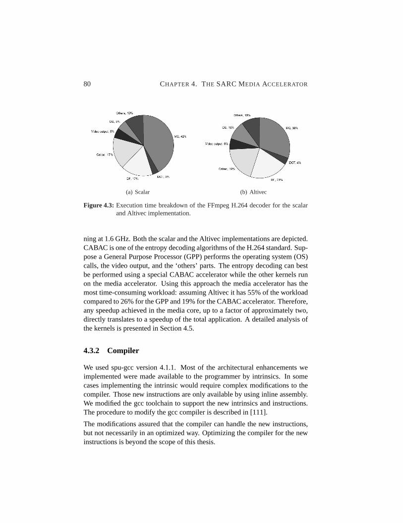
80 CHAPTER 4. THE SARC MEDIA ACCELERATOR
(a) Scalar (b) Altivec
Figure 4.3: Execution time breakdown of the FFmpeg H.264 decoder for the scalarand Altivec implementation.
ning at 1.6 GHz. Both the scalar and the Altivec implementations are depicted.CABAC is one of the entropy decoding algorithms of the H.264 standard. Sup-pose a General Purpose Processor (GPP) performs the operating system (OS)calls, the video output, and the ‘others’ parts. The entropy decoding can bestbe performed using a special CABAC accelerator while the other kernels runon the media accelerator. Using this approach the media accelerator has themost time-consuming workload: assuming Altivec it has 55% of the workloadcompared to 26% for the GPP and 19% for the CABAC accelerator. Therefore,any speedup achieved in the media core, up to a factor of approximately two,directly translates to a speedup of the total application. A detailed analysis ofthe kernels is presented in Section 4.5.
4.3.2 Compiler
We used spu-gcc version 4.1.1. Most of the architectural enhancements weimplemented were made available to the programmer by intrinsics. In somecases implementing the intrinsic would require complex modifications to thecompiler. Those new instructions are only available by using inline assembly.We modified the gcc toolchain to support the new intrinsics and instructions.The procedure to modify the gcc compiler is described in [111].
The modifications assured that the compiler can handle the new instructions,but not necessarily in an optimized way. Optimizing the compiler for the newinstructions is beyond the scope of this thesis.

4.3. EXPERIMENTAL SETUP 81
4.3.3 Simulator
Analysis of the kernels on the Cell SPE could be done using the real proces-sor. Analyzing architectural enhancements, however, requires an experimentalenvironment that can be modified. Therefore we used CellSim [7]; a simulatorof the Cell processor developed in the Unisim environment.
Profiling in CellSim
First, we implemented a profiling tool for CellSim as such as tool was notavailable. The profiling tool allows to gather many statistics (such as cycles,instructions, IPC, etc.) either from the entire application or from a specificpiece of selected code. The profiler is controllable from the native code (thecode running on the simulated processor). Furthermore, the profiler allowsgenerating a trace output for detailed analysis of the execution of the kernels.
Profiling the code, however, can influence its execution, especially if the sizeof the profiled code is small. Each call to the profiler inserts one line of volatileinline assembly. This ensures that only code that is between the start and stopcommand of the profiler is measured. Because instructions are not allowed tocross thisvolatileboundary, however, there is less opportunity for the compilerto optimally schedule the instructions.
Section 4.5 presents the profiling analysis of the kernels that shows the amountof time the different execution phases take. The execution times reported inthose particular analyses are off by approximately 25%. The purpose, however,is to show the relative size of the phases rather than the actual cycles spent onthem. Thus, the influence of the profiling itself is not problematic.
When reporting the total execution time of the kernels, the influence of the pro-filing can be neglected. For this analysis only a start and stop command haveto be inserted at the beginning and end of the kernel respectively. No volatileboundaries are included inside the kernel and thus all compiler optimizationsare unaltered.
Configuration of CellSim
CellSim has many configuration parameters, most of which have a defaultvalue that matches the actual Cell processor. The execution latencies of allinstructions classes, however, were all set by default to 6 cycles. We adjustedthese to match the ones reported in [80] as described in Table 4.1. The table

82 CHAPTER 4. THE SARC MEDIA ACCELERATOR
Table 4.1: SPU instruction latencies.
Instructionclass
Latency(cycles)
Description CellSim pipe
SP 6 Single-precision floating-point FP6FI 7 Floating point integer FP7DP 13 Double-precision floating point FPDFX 2 Simple fixed point FX2WS 4 Word rotate and shift FX3BO 4 Byte operations FXBSH 4 Shuffle SHUFLS 6 Loads and stores LSP
mentions both the name of the instruction class as used in the IBM documen-tation as well as the pipeline name as used in CellSim and in spu-gcc. Eachinstruction class maps to one of the units depicted in Figure 4.2 (see [80] formore details). The execution latency of an instruction class is the time it takesthe corresponding execution unit to produce the result. More precise, it is thenumber of clock cycles between the time the operands enter the execution unitand the time the results is available (by forwarding) as input for another com-putation. Thus, the instruction latency does not include instruction fetch, de-code, dependency check, issue, routing, register file access, etc. For a detaileddescription of the SPU pipeline, the reader is referred to [59].
The table does not include all latencies. The latency of channel instructions aremodeled in a different way in CellSim and were not adjusted. The latency ofbranches, i.e., the branch miss penalty, was not modeled in CellSim. M. Briejerimplemented this while implementing the branch hint instructions [33].
In addition, we adjusted the fetch parameters. The fetch width was set to oneline of 32 instructions. The fetch buffer size was set to 78, which correspondsto 2.5 lines of 32 instructions. Finally, we adjusted the instruction fetch rateof CellSim. The real processor can fetch two instructions per cycle, but canexecute them simultaneously only if one executes in the odd pipeline and theother in the even pipeline. CellSim does not distinguish between the odd andeven pipeline and therefore initially fetched too many instructions per cycleon average. We determined empirically that an instruction fetch rate of 1.4 inCellSim corresponds closely with the behavior of the real processor.

4.3. EXPERIMENTAL SETUP 83
Table 4.2: Comparison of execution times and instruction count in CellSim and Sys-temSim.
Cycles InstructionsKernel SystemSim CellSim Error SystemSim CellSim ErrorIDCT8 917 896 -2.3% 1099 1103 0.4%IDCT4 2571 2524 -1.9% 1853 1858 0.3%DF 121465 122122 0.5% 101111 101480 0.4%Luma 2534 2598 2.5% 2557 2572 0.6%
To improve simulation speed some adjustments were made to the PPE configu-ration parameters. The issue width was set to 1000 while the L1 cache latencywas set to zero cycles. Both measures increase the IPC of the PPE, which isrequired to spawn the SPE threads, and thus speedup simulation time. Thesemodifications have no effect on the simulation results, however, as the kernelsrun on the SPE.
Validation of CellSim
To validate the configuration of CellSim, several tests were performed. Theexecution times measured in CellSim were checked by comparing them to theIBM full system simulator SystemSim. We did not use the real processor asSystemSim provides more statistics and is accurate as well. These additionalstatistics allowed us to check the correctness of CellSim on more aspects thanjust execution time.
Table 4.2 shows the execution times and the dynamic instruction count of allthe kernels using both SystemSim and CellSim. It shows that the difference inexecution time is at most 2.5%. The number of executed instructions is slightlydifferent. As the profiling was started and stopped at exactly the same point inthe C code, we expect this difference in instruction count to be caused by thedifferent implementations of the profiling tool.
The results presented here are measurements of entire kernel execution times.As discussed on page 81, when performing a detailed profiling analysis ofthe kernel phases, the profiling itself affects the execution time, resulting in alarger error.
Altogether, from these results we conclude that CellSim is sufficiently accurateto evaluate the architectural enhancements described in this chapter. Compar-

84 CHAPTER 4. THE SARC MEDIA ACCELERATOR
ison of other statistics generated by the two simulators also showed that Cell-Sim is well suitable for its purpose. Off course, when evaluating architecturalenhancements we always compare between results that are all obtained withCellSim.
4.4 Enhancements to the SPE Architecture
In this section we present the architectural enhancements and modificationsto the SPE that create the media accelerator. The enhancements and modifi-cations are based on the identified deficiencies in the execution of the H.264kernels. These deficiencies are discussed in detail in Section 4.5, while dis-cussing the results for the kernels.
To identify the deficiencies in the execution of the H.264 kernels, we per-formed a thorough analysis down to the assembly level. Among others, thisanalysis comprised the following. We compared the C code with the generatedassembly code to determine which simple operations require many overheadinstructions. We performed extensive profiling to determine the most time-consuming parts. Analyzing trace files allowed us to determine why certainparts were time consuming. We analyzed both C and assembly code to findopportunities for instruction collapsing.
The newly added instructions are presented in detail in this section. One of thedetails we show is the chosen opcode for each instruction. We do not know thestructure in the opcodes and thus we chose available ones. We show them, toprove that the added instructions fit (or not) in the ISA.
The notation used in this thesis to describe the instruction set architecture fol-lows the notation used in the IBM documentation with a few extensions. First,temporary valuesw are 64-bit wide. Second, temporary valuesp are 16-bitwide. Third, temporary valuesd are 8-bit wide. An extensive description ofthe notation is provided in [81], for example.
In the code depicted in this thesis we use the following notation for vectortypes. Avector signed short type is denoted asvsint16 t whilea vector unsigned char type is denoted asvuint8 t . In general theinteger types are denoted asv[s/u]int[8/16/32] t .
This section is organized as follows. First, we present four categories of newinstructions that we added to the ISA. Finally, we propose a modification tothe architecture that allows unaligned memory accesses to the local store.

4.4. ENHANCEMENTS TO THESPE ARCHITECTURE 85
4.4.1 Accelerating Scalar Operations
Since the SPU has a SIMD-only architecture, scalar operations are performedby placing the scalar in the so-called preferred slot and using the SIMD FUs.For operations that involve only scalar variables this works well; the compilerplaces the scalar variable in a memory location congruent with the preferredslot even if this wastes memory. But if the operand is a vector element a lotof rearrangement overhead is required to move the desired element to the pre-ferred slot. Rather than providing a full scalar datapath, which would increasethe silicon area significantly, we propose adding a few scalar instructions.
Lds Instructions
The lds (LoaD Scalar) instructions load a scalar from a quadword unalignedaddress inside the local store and store it in the preferred slot of a register. Theoriginal SPU architecture allows only quadword aligned accesses with sizeof 128 bits. To load a scalar from a non quadword-aligned location, a lot ofadditional instructions are required.
Listing 4.1 shows an example of an array access. The left part of the figureshows the C code including the declaration of the used array and index vari-able. The middle of the figure shows the assembly code generated by the com-piler for the original SPU architecture. The first instruction (shli ) performsa shift left on the index variablei , stored in$5 by 2 bits. That is, the index ismultiplied by 4 and the result is the distance of the desired element to the startof the array in bytes. The second instruction (ila ) loads the start address ofthe array into a register. The third instruction (lqx ) loads the quadword (128bits) that contains the desired element. It adds the index in bytes to the startaddress of the array, truncates it to a multiple of 16, and accesses the quadwordat that address. At this point the desired element of the array is in register$4but not necessarily in the preferred slot. The fourth instruction (a) adds theindex in bytes to the start address of the array. The four least significant bits ofthis result is used by the last instruction (rotqby ) to rotate the loaded valuesuch that the desired element is in the preferred slot.
Using theldsw (LoaD Scalar Word) instruction the same array access can bedone in two instructions, as shown on the right side of Listing 4.1. The firstinstruction (ila ) stores the base address of the array in a register. Next, theldsw instruction takes as input the index ($5), the start address of the array($6), and the destination register ($2). It loads the corresponding quadwordfrom the local store, then selects the correct word and puts it in the preferred

86 CHAPTER 4. THE SARC MEDIA ACCELERATOR
Listing 4.1: Example of how the lds instructions speed up code. Left is an arrayaccess in plain C code, in the middle is the original assembly code, whilethe right depicts the assembly code using theldsw instruction.
1 i n t a r r a y [ 8 ] ; s h l i $2 , $5 , 2 i l a $6 , a r r a y2 i n t i ; i l a $6 , a r r a y ldsw $2 , $6 , $53 i n t a= a r r a y [ i ] ; l qx $4 , $2 , $64 a $2 , $2 , $65 r o t q b y $2 , $4 , $2
slot, and finally stores the result in the destination register.
The addressing mode is base plus scaled index, i.e., the effective address ofldsw $2,$6,$5 is $6 + 4x$5 . The ldsw instruction loads a word (fourbytes) and thus its index is multiplied by four. For the other lds instructions theindex is scaled in a similar way. The scalars that are loaded should be alignedaccording to their size. For example, words should be word aligned. The baseaddress provided to the instruction does not have to be properly aligned, asthe effective address is truncated according to the data size (see also instruc-tion details below). Note that the base plus scaled index addressing mode issupported in several ISAs (e.g., x86), but not found to be very useful becausethe compiler can often eliminate the index variables. In this case, however, thedatapath is completely SIMD and the index is used to select a specific elementof the loaded quadword.
Loads and stores are handled by the SLS (SPU Load and Store) execution unit.The SLS has direct access to the local store and to the register file unit. Be-sides loads and stores, the SLS also handles DMA requests to the LS and loadbranch-target-buffer instructions. In order to implement theldsw instructiona few modifications to the SLS unit are required. First, computing the targetaddress is slightly different than for a normal load. Instead of adding the twooperands, the index should be multiplied by four before adding it to the startaddress of the array. This multiplication can be done by a simple shift opera-tion. Second, for each outstanding load (probably maintained in a buffer) twomore select bits are required to store the SIMD slot in which the element willbe located. These two bits are bits 2 and 3 of the target address. For normalloads, these two bits should be set to zero. Finally, when the quadword is re-ceived from the local store, the correct word should be shifted to the preferredslot. This can be done by inserting a 4-to-1 mux in the data path which iscontrolled by the select bits.

4.4. ENHANCEMENTS TO THESPE ARCHITECTURE 87
The lds instructions fit the RR format. The instruction details are depicted be-low. Although for the benchmarks used in this work only theldsw instructionis required, for completeness we defined the lds instructions for halfwords andbytes as well. These element sizes are used frequently in media applicationsand thus it is reasonable to provide them. Doublewords are not considered inthis work as neither long integers nor single precision floating point are usedin the media applications targeted. Furthermore, the SPU ISA does not containany long integer operations.
313029282726252423222120191817161514131211109876543210
RTRA0000 1 1 1 0 1 1
rt,ra,rb
0 RB
ldsw
LSA ← (RA0:3 + RB0:3 << 2) & LSLR & 0xFFFFFFF0b ← (RA0:3 + RB0:3 << 2) & 0x0000000CQ ← LocStor(LSA,16)RT 0:3 ← Qb::4
313029282726252423222120191817161514131211109876543210
RTRA00 1
rt,ra,rb
0 RB1 0 0 1 0 1
ldshw
1
LSA ← (RA0:3 + RB0:3 << 1) & LSLR & 0xFFFFFFF0b ← (RA0:3 + RB0:3 << 1) & 0x0000000EQ ← LocStor(LSA,16)RT 0:1 ← Qb::2

88 CHAPTER 4. THE SARC MEDIA ACCELERATOR
313029282726252423222120191817161514131211109876543210
RTRA00 1
rt,ra,rb
RB1 0 0 1 0 1 01
ldsb
LSA ← (RA0:3 + RB0:3) & LSLR & 0xFFFFFFF0b ← (RA0:3 + RB0:3) & 0x0000000FQ ← LocStor(LSA,16)RT 0 ← Qb
The lds instructions were made available to the programmer through intrin-sics of the formd = spu_ldsx(array,index) wherex ∈ b, hw,w ,array is a pointer to a word, andindex is a word. The compiler generatesboth theldsx and theila instruction required to load the desired element ofthe array.
The lds instructions were added to the simulator and the latency was set toseven cycles for the following reasons. A normal load or store operation takessix cycles, and we added one cycle to account for the extra mux in the datapath.
As2ve Instructions
As2ve (Add Scalar to Vector element) instructions add a scalar to a specificelement of a vector. As the SPU architecture is completely SIMD, scalar op-erations often require a considerable amount of time. Listing 4.2 shows anexample from the IDCT8 kernel where the constant value 32 has to be addedto the first element of a vector of halfwords.
The middle of the figure depicts how the normal SPU ISA handles this code.The pointer*block is stored in$4 . First, it is calculated (ai ) by how muchbytes the vector must be rotated to put the desired element in the preferredslot. This shift count is stored in$2 . Second, the vector is loaded (lqd ) intoregister$8 . Third, a mask is created (chd ) and stored in$7 which is neededby the shuffle latter on. Fourth, the vector is rotated (rotqby ) based on theshift count. Fifth, the value 32 is added (ahi ) to the desired element that nowis in the preferred slot. Finally, the result of the addition is shuffled (shufb )back into its original position of the vector. Note that this compiler generatedcode is not optimal. The shift count is known a priori as pointer*block isquadword aligned. Apparently the compiler is not aware of that.

4.4. ENHANCEMENTS TO THESPE ARCHITECTURE 89
Listing 4.2: Example of how the as2ve instructions speed up code. Left are two linesof code from the IDCT8 kernel, in the middle is the normal assemblycode, while the right depicts the assembly code using as2ve instructions.
1 v s i n t 1 6 t ∗ b lock ; a i $2 , $4 , 1 4 lqd $8 , 0 ( $4 )2 b lock [ 0 ] + = 3 2 ; lqd $8 , 0 ( $4 ) as2vehwi $8 , 3 2 , 03 chd $7 , 0 ( $4 )4 r o t q b y $2 , $8 , $25 a h i $2 , $2 ,326 shu fb $6 , $2 , $8 , $7
as2veb rt,ra,immb \\rt[immb] += ra \ for vectoras2vebi rt,imma,immb \\rt[immb] += imma / of bytes.as2vehw rt,ra,immb \\rt[immb] += ra \ for vectoras2vehwi rt,imma,immb \\rt[immb] += imma / of halfwords.as2vew rt,ra,immb \\rt[immb] += ra \ for vectoras2vewi rt,imma,immb \\rt[immb] += imma / of words.
Figure 4.4: Overview of the as2ve instructions.
Using the as2ve instructions the same addition of the scalar to the vector canbe done in one instruction (or two, if the load is included as in the example).In the example of Listing 4.2 we used theas2vehwi instruction that adds ahalfword immediate to a vector of halfwords. Figure 4.4 shows all the as2veinstructions. Only the instructions for bytes and halfwords are used in thebenchmarks, but we provide the word versions as well as media applicationsometimes use this data type. For each data type there are two instructions.The first assumes the scalar is hold in the preferred slot of a register. Thesecond assumes the scalar is put as immediate value in the instruction.
One might consider the lds instruction, augmented with an sts (store scalar) toperform this operation. This might, however, incur a lot of overhead. Supposethe as2ve operation is in the middle of a series of instructions that operate onvariables in the register file. In that case, first the vector should be stored inmemory, second using an lds instruction the vector element is loaded into theregister file, third the addition can be done, fourth an sts instruction has tobe used to store the vector element back into the vector, and finally the entirevector has to be loaded again for further operation. This method requires fouroverhead instructions that are dependent and have a large latency.

90 CHAPTER 4. THE SARC MEDIA ACCELERATOR
The as2ve instructions fit the RI7 format except theas2vebi , as2vehwi ,and as2vewi instructions. The latter have two immediate values and oneregister value, instead of one immediate value and two register values. Theinstruction details are depicted below.
313029282726252423222120191817161514131211109876543210
RT0000 1 1 1 1 RA0 1 1
rt,ra,imm
I7
as2veb
b ← RA3
c ← RepLeftBit(I7,8) & 0x0Fd ← RT c
RT c ← d + b
313029282726252423222120191817161514131211109876543210
RTI7a00000 1 1 1
rt,imma,immb
1 0 1 I7b
as2vebi
b ← RepLeftBit(I7a,8)c ← RepLeftBit(I7b,8) & 0x0Fd ← RT c
RT c ← d + b
313029282726252423222120191817161514131211109876543210
RT0000 1 1 1 1 01 0 RA
rt,ra,imm
I7
as2vehw
s ← RA2:3
b ← RepLeftBit(I7,8) & 0x07r ← RT 2b::2
RT 2b::2 ← r + s
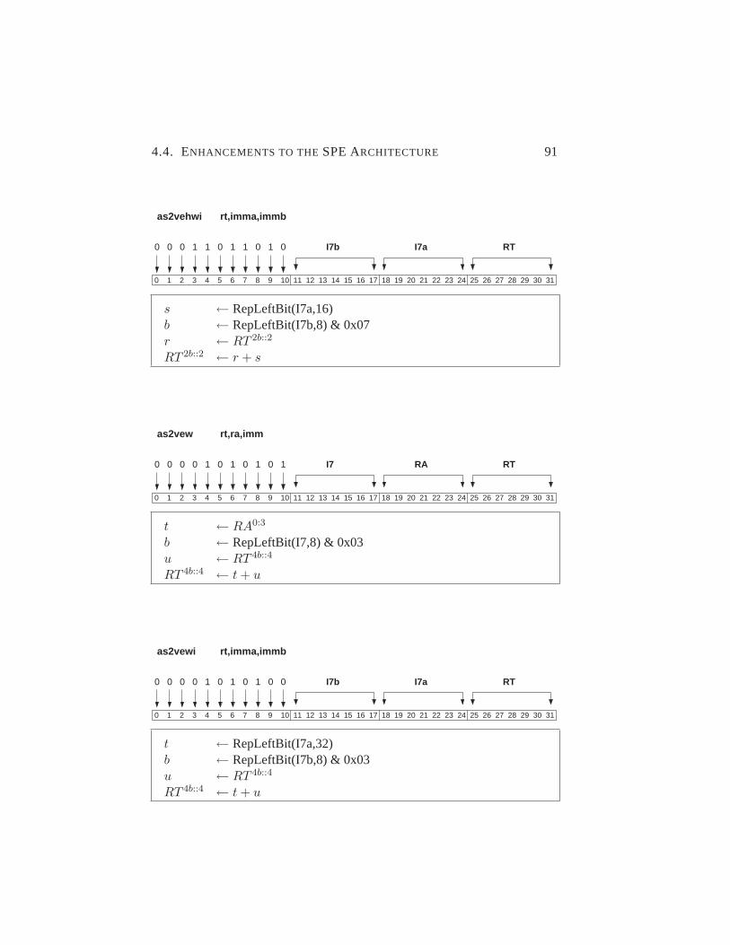
4.4. ENHANCEMENTS TO THESPE ARCHITECTURE 91
313029282726252423222120191817161514131211109876543210
RT0000 1 1 1 1 I7b0 I7a0 1
rt,imma,immbas2vehwi
s ← RepLeftBit(I7a,16)b ← RepLeftBit(I7b,8) & 0x07r ← RT 2b::2
RT 2b::2 ← r + s
313029282726252423222120191817161514131211109876543210
RT0000 1 1 RA1
rt,ra,imm
I70 0 1 0
as2vew
t ← RA0:3
b ← RepLeftBit(I7,8) & 0x03u ← RT 4b::4
RT 4b::4 ← t + u
313029282726252423222120191817161514131211109876543210
RTI7a00000 1 1
rt,imma,immb
I7b0 0 1 0
as2vewi
t ← RepLeftBit(I7a,32)b ← RepLeftBit(I7b,8) & 0x03u ← RT 4b::4
RT 4b::4 ← t + u

92 CHAPTER 4. THE SARC MEDIA ACCELERATOR
The as2ve instructions were made available to the programmer through in-trinsics of the forma = spu_as2vebi(a,c,x) wherea is the vectoroperand. The latter is both input and output, which is a case the compilerwas not build for. Therefore, not in all cases the intrinsics worked properlyand we had to use inline assembly as follows:
asm ("as2vebi %0,c,x" \: "=r" (a) \: "0" (a) \
);
The instructions were added to the simulator and the latency was set to threecycles. A possible implementation uses the FX2 (fixed point) pipeline andreplicates the scalar to all SIMD slots of input a. The vector goes to input bof the ALU. Some additional control logic selects the proper SIMD slot to doaddition while the others transfer input b. The latency of the FX2 pipeline istwo cycles. Adding another cycle, for the increases complexity, results in threecycles.
4.4.2 Accelerating Saturation and Packing
The elementary data type to store pixel information is a byte. Computation,however, is done using halfwords (16 bits) in order not to lose precision. Thisintroduces some overhead known as pack/unpack. In this section we proposethree instruction classes that reduce the cost of this overhead. They also accel-erate saturation, which is often performed in conjunction with a pack opera-tion.
Clip Instructions
Clip instructions saturate the elements of a vector between two values. A clipinstruction can be used to emulate saturating arithmetic but also saturationbetween arbitrary boundaries. For example, in de deblocking filter kernel theindex of a table lookup has to be clipped between 0 and 51. In the normal SPUarchitecture this operation requires four instructions (see Listing 4.3). First,two masks are created by comparing the input vector with the lower and upperboundaries. Second, using the masks the result is selected from the input andthe boundary vectors.
The clip operation is mainly used in integer and short computations. The in-struction could be implemented for bytes as well, but we do not expect any

4.4. ENHANCEMENTS TO THESPE ARCHITECTURE 93
Listing 4.3: C code of a clip function using the normal SPU ISA. The clip instructionsperform this operation in one step.
1 v s i n t 1 6 t c l i p ( v s i n t 1 6 t a , v s i n t 1 6 t min , v s i n t 1 6 t max ) {2 v u i n t 1 6 t min mask , maxmask ;3 min mask = spucmpgt ( min , a ) ;4 max mask = spucmpgt ( a , max ) ;5 v s i n t 1 6 t temp = s p u s e l ( a , min , minmask ) ;6 re turn s p u s e l ( temp , max , maxmask ) ;7 }
application to use it. The clip instructions fit the RR format if the source anddestination register (of the vector to clip) are the same. The instruction detailsare depicted below.
313029282726252423222120191817161514131211109876543210
RTRA000 1 1 1 1
rt,ra,rb
RB1 1 00
cliphw
for j = 0 to 7if RT 2j::2 > RB2j::2 then RT 2j::2 ← RB2j::2
if RT 2j::2 < RA2j::2 then RT 2j::2 ← RA2j::2
end
313029282726252423222120191817161514131211109876543210
RTRA000 1 1 1 1
rt,ra,rb
RB1 10 1
clipw
for j = 0 to 3if RT 2j::4 > RB2j::4 then RT 2j::4 ← RB2j::4
if RT 2j::4 < RA2j::4 then RT 2j::4 ← RA2j::4
end

94 CHAPTER 4. THE SARC MEDIA ACCELERATOR
The clip instructions were made available to the programmer through intrinsicsof the form a = spu_cliphw(a, min, max) where the operands allhave the same data type. We created intrinsics for both vectors and scalars.Note that the same instruction can be used for both.
Using these intrinsics to perform a saturation to 8 or 16-bit values, requires theprogrammer to define two variables containing the minimum and maximumvalue. To ease programming intrinsics of the forma = spu_satub(a)(saturate to unsigned byte value) can be created. This requires some smallmodifications to the machine description in the back-end of the compiler, suchthat it creates the two vectors containing the minimum and maximum values.
In certain cases the clip intrinsics suffered the same problem the as2ve intrin-sics, namely that the compiler did not understand that the source and destina-tion registers are the same. The solution is to use inline assembly as follows:
asm ("clipw %0,%1,%2" \: "=r" (a), "=r" (amin), "=r" (amax) \: "0" (a), "1" (amin), "2" (amax) \
);
The clip instructions were added to the simulator and the latency was set tofour cycles. A normal compare operation takes two cycles. The two comparescan be done in parallel but that requires that three quadwords are read from theregister file into the functional unit. Another approach would be to serializethe operation. First two operands are loaded, while these are compared and theresult is selected the third operand is loaded, and finally the latter is comparedto the result of the first compare. We added one cycle to account for loadingthree quadwords and also one cycle to account for the extra mux in the datapaththat selects the correct value.
Sat pack Instructions
The satpack instructions takes two vectors of a larger data type, and saturatesand packs them into one vector of a smaller data type. This operation is useful,for example, whenever data has been processed in signed 16-bit values but hasto be stored to memory as unsigned 8-bit values. Listing 4.4 shows such a pieceof code from the Luma kernel that can entirely be replaced by one satpackinstruction. The kernel operates on16 × 16 matrices (entire macroblocks).The vectorsva andvb together contain one row of the output matrix.
The satpack instructions fit the RR instruction format. For each type ofoperands satpack instructions could be implemented, but for H.264 decod-

4.4. ENHANCEMENTS TO THESPE ARCHITECTURE 95
Listing 4.4: Example code from the Luma kernel that can be replaced by one satpackinstruction. The code saturates the vectorsva andvb between 0 and 255,and packs all 16 elements into one vector of unsigned bytes.
1 v s i n t 1 6 t va , vb , v t , s a t ;2 v u i n t 8 t v t u 8 ;3 v u i n t 8 t mask = {0 x01 , 0 x03 , 0 x05 , 0 x07 , 0 x09 , 0 x0B , 0 x0D , 0 x0F ,\4 0x11 , 0 x13 , 0 x15 , 0 x17 , 0 x19 , 0 x1B , 0 x1D , 0 x1F}5 v s i n t 1 6 t vze ro = s p u s p l a t s ( 0 ) ;6 v s i n t 1 6 t vmax = s p u s p l a t s ( 2 5 5 ) ;7 s a t = spucmpgt ( va , vze ro ) ;8 va = spu and ( va , s a t ) ;9 s a t = spucmpgt ( va , vmax ) ;
10 va = s p u s e l ( va , vmax , s a t ) ;11 s a t = spucmpgt ( vb , vze ro ) ;12 vb = spu and ( vb , s a t ) ;13 s a t = spucmpgt ( vb , vmax ) ;14 vb = s p u s e l ( vb , vmax , s a t ) ;15 v t u 8 = s p u s h u f f l e ( va , vb , mask ) ;
ing only packing from 16-bit signed to 8-bit unsigned is required. For audioprocessing packing from 32-bit signed to 16-bit signed can be useful. We im-plemented two different ways of packing. Thesp2x (x=ub,hw) instructionpacks the elements of the first and second operand to the first and second dou-bleword respectively. Thespil2x instruction interleaves the elements of thetwo operands, i.e., the elements of the first operand go to the odd elements andthose of the second operand to the even elements. The latter instruction is use-ful when the unpack was performed by a multiply instruction. The instructiondetails are depicted below.
The satpack instructions were made available to the programmer through in-trinsics and were added to the simulator. The latency was set to two cycles asthe complexity of the instruction is similar to that of fixed point operations.
A combination of pack and saturation is also found in the pack.sss and pack.ussinstructions of the IA64 architecture [16]. Also MMX has instructions thatcombine pack and saturate. In the TriMedia there are a few instructions thatinclude a clip operation.
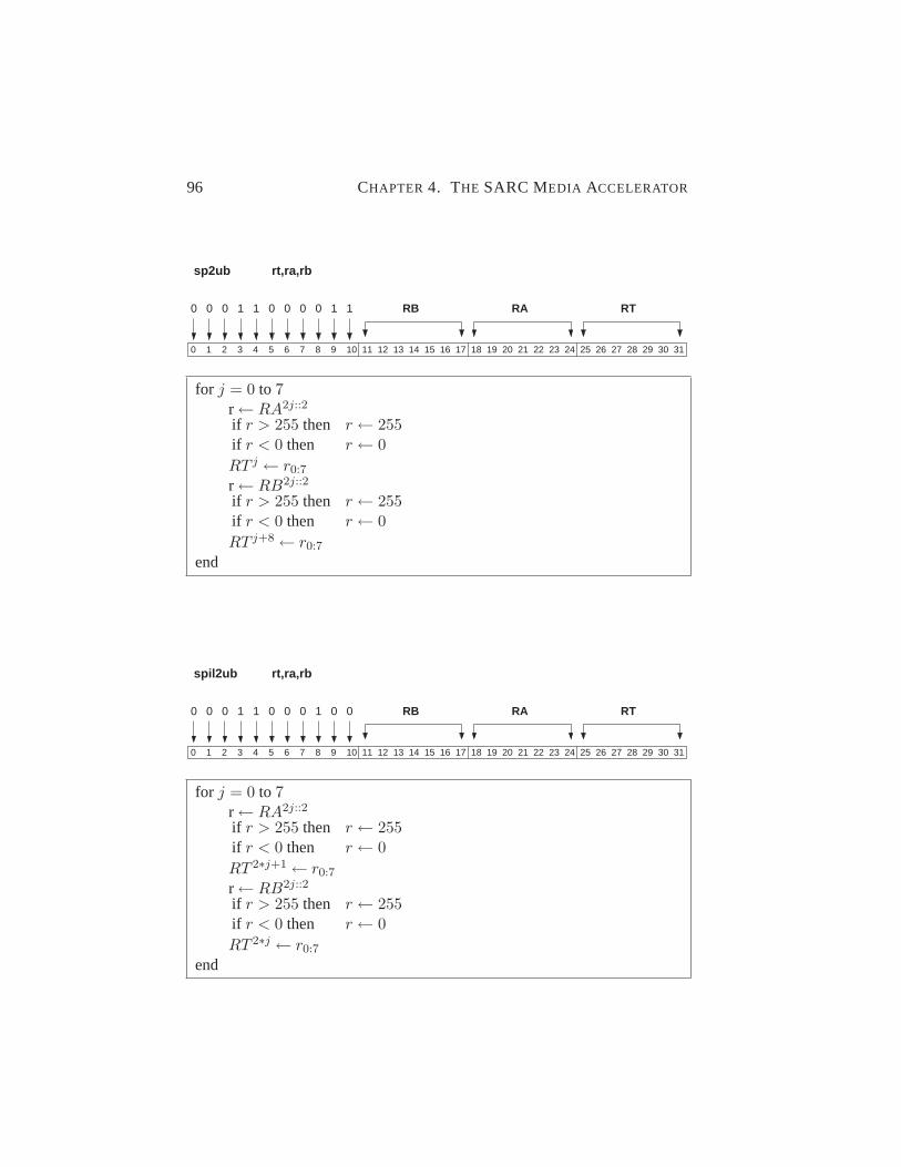
96 CHAPTER 4. THE SARC MEDIA ACCELERATOR
313029282726252423222120191817161514131211109876543210
RT0000 1 1 RA0 1
rt,ra,rb
RB0 0 1
sp2ub
for j = 0 to 7r ← RA2j::2
if r > 255 then r ← 255if r < 0 then r ← 0RT j ← r0:7
r ← RB2j::2
if r > 255 then r ← 255if r < 0 then r ← 0RT j+8 ← r0:7
end
313029282726252423222120191817161514131211109876543210
RT0000 1 1 RA
rt,ra,rb
RB0 0 1 0 0
spil2ub
for j = 0 to 7r ← RA2j::2
if r > 255 then r ← 255if r < 0 then r ← 0RT 2∗j+1 ← r0:7
r ← RB2j::2
if r > 255 then r ← 255if r < 0 then r ← 0RT 2∗j ← r0:7
end

4.4. ENHANCEMENTS TO THESPE ARCHITECTURE 97
313029282726252423222120191817161514131211109876543210
RT0000 1 1 RA1
rt,ra,rb
RB0 0 1 0
sp2hw
for j = 0 to 3t ← RA4j::4
if t > 32767 then t ← 32767if t < −32768 then t ← −32768RT j::2 ← t0:15
t ← RB4j::4
if t > 32767 then t ← 32767if t < −32768 then t ← −32768RT j+8::2 ← t0:15
end
313029282726252423222120191817161514131211109876543210
RT0000 1 1 RA
rt,ra,rb
RB0 0 1 1 0
spil2hw
for j = 0 to 3t ← RA4j::4
if t > 32767 then t ← 32767if t < −32768 then t ← −32768RT 4∗j+2::2 ← t0:15
t ← RB4j::4
if t > 32767 then t ← 32767if t < −32768 then t ← −32768RT 4∗j::2 ← t0:15
end

98 CHAPTER 4. THE SARC MEDIA ACCELERATOR
Listing 4.5: Example code from the IDCT8 kernel that can be replaced by one asp in-struction. The code adds the vectorsva andvb , saturates them between0 and 255, and packs the elements to 8-bit values.
1 v s i n t 1 6 t va , vb , v t , s a t ;2 v u i n t 8 t v t u 8 ;3 cons t v u i n t 8 t packu16 =4 {0 x01 , 0 x03 , 0 x05 , 0 x07 , 0 x09 , 0 x0B , 0 x0D , 0 x0F ,\5 0x11 , 0 x13 , 0 x15 , 0 x17 , 0 x19 , 0 x1B , 0 x1D , 0 x1F}6 v s i n t 1 6 t vze ro = s p u s p l a t s ( 0 ) ;7 v s i n t 1 6 t vmax = s p u s p l a t s ( 2 5 5 ) ;8 v t = spu add ( va , vb ) ;9 s a t = spucmpgt ( v t , vze ro ) ;
10 v t = spu and ( v t , s a t ) ;11 s a t = spucmpgt ( v t , vmax ) ;12 v t = s p u s e l ( v t , vmax , s a t ) ;13 v t u 8 = s p u s h u f f l e ( v t , vze ro , packu16 ) ;
Asp Instructions
Although the IDCT kernels require some packing operations, it cannot utilizethe satpack instructions due to the way the data is stored in memory. Es-pecially for this kernel, the asp (Add, Saturate, and Pack) instructions weredeveloped which combine an addition, a saturation, and a pack.
Listing 4.5 shows a piece of code from the IDCT kernel that entirely can bereplaced by one asp instruction. The code adds the result of the IDCT to thepredicted picture. First, it adds two vectors of signed halfwords. Second, theelements of the vector are saturated between 0 and 255. Finally, the elementsare packed to bytes and stored in the first half of the vector. Using the nor-mal SPU ISA many instructions and auxiliary variables are needed. The aspinstructions are tailored for this kind of operation and can perform the entireoperation at once. Note, that if only a saturate and a pack is required, one ofthe operands can be assigned a zero vector.
The asp instructions fit the RR format. For each type of operands an asp in-struction could be implemented, but we found it only necessary to implementone: asp2ub (add, saturate, and pack to unsigned bytes). It takes as inputtwo vectors of signed halfwords and stores the output in a vector of unsignedbytes. The eight elements are stored in the first eight slots while the last eightslots are assigned value zero. The instruction details are depicted below.

4.4. ENHANCEMENTS TO THESPE ARCHITECTURE 99
313029282726252423222120191817161514131211109876543210
RT0000 1 1 1 1 RA0 10
rt,ra,rb
RB
asp2ub
for j = 0 to 7r ← RA2j::2 + RB2j::2
if r > 255 then r ← 255if r < 0 then r ← 0RT j ← r0:7
end
The asp instruction was made available to the programmer through an intrinsic.The instruction was added to the simulator and the latency was set to fourcycles. A normal addition costs two cycles and we added two more cycles forthe saturation and the data rearrangement.
4.4.3 Accelerating Matrix Transposition
Matrix Transposition (MT) is at the heart of many media algorithms and cantake up a large part of the execution time. Typically, multimedia data is orga-nized in blocks (matrices) of16×16, 8×8, and sometimes smaller. This allowsutilization of SIMD instructions to exploit DLP. Computations, however, haveoften to be performed row-wise and column-wise. Thus matrix transposes arerequired to arrange the data for SIMD processing.
In this section we show how fast matrix transposition at low cost can beachieved using swapoe (swap odd-even) instructions. But first we review ex-isting methodologies for matrix transposition using SIMD.
Conventional SIMD Matrix Transposition
The conventional way of performing a MT with SIMD instructions is to per-form a series of permutations. We review an8 × 8 transpose in AltiVec as anexample. Altivec has 128-bit SIMD registers and thus we assume a matrix ofhalfwords, stored in eight registers (a0 througha7). The code in Listing 4.6performs the MT and stores the result in registers (b0 throughb7).

100 CHAPTER 4. THE SARC MEDIA ACCELERATOR
Listing 4.6: An 8×8 matrix transpose using Altivec instructions.
1 TRANSPOSE8 ALTIVEC ( a0 , a1 , a2 , a3 , a4 , a5 , a6 , a7 ,\2 b0 , b1 , b2 , b3 , b4 , b5 , b6 , b7 ){3 b0 = vec mergeh ( a0 , a4 ) ;4 b1 = vec merge l ( a0 , a4 ) ;5 b2 = vec mergeh ( a1 , a5 ) ;6 b3 = vec merge l ( a1 , a5 ) ;7 b4 = vec mergeh ( a2 , a6 ) ;8 b5 = vec merge l ( a2 , a6 ) ;9 b6 = vec mergeh ( a3 , a7 ) ;
10 b7 = vec merge l ( a3 , a7 ) ;11 a0 = vec mergeh ( b0 , b4 ) ;12 a1 = vec merge l ( b0 , b4 ) ;13 a2 = vec mergeh ( b1 , b5 ) ;14 a3 = vec merge l ( b1 , b5 ) ;15 a4 = vec mergeh ( b2 , b6 ) ;16 a5 = vec merge l ( b2 , b6 ) ;17 a6 = vec mergeh ( b3 , b7 ) ;18 a7 = vec merge l ( b3 , b7 ) ;19 b0 = vec mergeh ( a0 , a4 ) ;20 b1 = vec merge l ( a0 , a4 ) ;21 b2 = vec mergeh ( a1 , a5 ) ;22 b3 = vec merge l ( a1 , a5 ) ;23 b4 = vec mergeh ( a2 , a6 ) ;24 b5 = vec merge l ( a2 , a6 ) ;25 b6 = vec mergeh ( a3 , a7 ) ;26 b7 = vec merge l ( a3 , a7 ) ;27 }
The instructionvec_mergeh(ra, rb) functions as follows. Assume thatthe elements of each vector are numbered beginning with 0. The even-numbered elements of the result are taken, in order, from the elements in themost significant 8 bytes ofra . The odd-numbered elements of the result aretaken, in order, from the elements in the most significant 8 bytes ofrb . Theinstructionvec_mergel(ra, rb) functions similar but takes the elementsfrom the least significant 8 bytes.
The AltiVec MT requires 24 instructions for an8×8 matrix. In general this ap-proach requireslog n steps ofn instructions. Thus in totaln log n instructionsare required. Forn = 16 64 AltiVec or SPU instructions are required.

4.4. ENHANCEMENTS TO THESPE ARCHITECTURE 101
51 52 53 54
61 62 63 64
71 72 73 74
81 82 83 84
7877
88876867
5857
75 76
85 86
after second step
55 56
65 66
15
25
17
27
18
28
16
26
47 48
37 38
45 46
35 36
45 46 47 48
15 16 17 18
25 26 27 28
35 36 37 38
8881 82 83 84 85 86 87
final
55
66
15
17
28
26
48
37
46
35
68
57 77
88
75
8616
25
36
45
56
65
76
85
18
27
38
47
58
67
78
87
11 51
84
73
71
13
24
31
22 62 82
44
33
42
53
64
21
12 32
41
52
61
72
81
14
23
34
43
54
63
74
83
41 42 43 44 45 46 47 48
11 12 13 14 15 16 17 18
21 22 23 24 25 26 27 28
31 32 33 34 35 36 37 38
41 42 43 44
11 12 13 14
21 22 23 24
31 32 33 34
11 12 51
8483
73 74
52 71 7232
13
23 24
14
31
21 22 61 62 81 82
43 44
33 34
41 42
53 54
63 64
5855 56 57
6865 66 67
7875 76 77
8885 86 87
after first step
5851 52 53 54 55 56 57
6861 62 63 64 65 66 67
7871 72 73 74 75 76 77
initial
Figure 4.5: Eklundh’s matrix transpose algorithm.
Matrix Transposition using Swapoe Instructions
In this section we present the swapoe instructions and explain how they speedup matrix transposition. The swapoe instructions are similar to the mix instruc-tions introduced by Lee [97] and used in HP’s MAX-2 multimedia extensionto the PA-RISC architecture. Although the mix instructions found their wayinto the IA-64 architecture because of the collaboration between HP and Intel,no modern multimedia extension incorporates it. We rediscover the swapoeinstructions and show how it is valuable for contemporary media applications.
The swapoe instructions are inspired by Eklundh’s recursive matrix transposi-tion algorithm [56], which is illustrated in 4.5 for an8 × 8 matrix. The newinstructions have two source registers and two destination registers. In thischapter we assume that the source and the destination registers are the same,but if allowed by the instruction format, they can also be different. Using thesame registers for source and destination has the advantage that the transposewill be performed in-situ. The complete set of swapoe instructions is depictedin Figure 4.6.

102 CHAPTER 4. THE SARC MEDIA ACCELERATOR
swapoedw ra,rb \\Swap doublewordsswapoew ra,rb \\Swap wordsswapoehw ra,rb \\Swap halfwordsswapoeb ra,rb \\Swap bytes
Figure 4.6: Overview of the swapoe instructions.
a0 a1 a2 a3 a4 a5 a6 a7
b0 b1 b2 b3 b4 b5 b6 b7
b1 b3 b5 b7
a0 a2 a4 a6b0 b2 b4 b6
a1 a3 a5 a7
Figure 4.7: Graphical representation of theswapoehw instruction. The odd ele-ments of thea register are swapped with the even elements of theb reg-ister.
The instructions swap the odd elements of registerra with the even elementsof rb . Figure 4.7 shows theswapoehw instruction as example. On top thetwo registers before the instruction is executed are depicted. The bottom ofthe figure shows the contents of the register after theswapoehw. The otherinstructions operate similar but on different element sizes.
The swapoe instructions directly implement the steps of Eklundh’s matrixtranspose algorithm. The8 × 8 MT function using swapoe is shown in List-ing 4.7. This implementation requires 12 instructions. Note that this methodperforms the MT in-situ, i.e., no additional registers are required for temporalstorage. Depending on the size of the register file and the kernel the MT is usedin, this might save a lot of loads and stores and further increase performance.
In general for ann × n matrix each step can be accomplished usingn/2 in-structions. Since there arelog n stages, the total number of instructions is(n log n)/2, assuming the matrix is already loaded in the register file. Thus,whenn = 16 32 instructions are required. Indeed our approach also requireshalf the number of instructions compared to the AltiVec implementation.
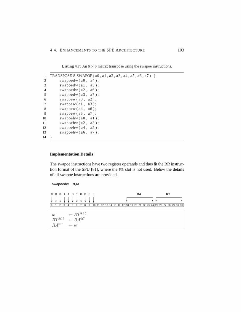
4.4. ENHANCEMENTS TO THESPE ARCHITECTURE 103
Listing 4.7: An 8× 8 matrix transpose using the swapoe instructions.
1 TRANSPOSE8 SWAPOE( a0 , a1 , a2 , a3 , a4 , a5 , a6 , a7 ){2 swapoedw ( a0 , a4 ) ;3 swapoedw ( a1 , a5 ) ;4 swapoedw ( a2 , a6 ) ;5 swapoedw ( a3 , a7 ) ;6 swapoew ( a0 , a2 ) ;7 swapoew ( a1 , a3 ) ;8 swapoew ( a4 , a6 ) ;9 swapoew ( a5 , a7 ) ;
10 swapoehw ( a0 , a1 ) ;11 swapoehw ( a2 , a3 ) ;12 swapoehw ( a4 , a5 ) ;13 swapoehw ( a6 , a7 ) ;14 }
Implementation Details
The swapoe instructions have two register operands and thus fit the RR instruc-tion format of the SPU [81], where theRBslot is not used. Below the detailsof all swapoe instructions are provided.
313029282726252423222120191817161514131211109876543210
RTRA00000 1 1 1
rt,ra
0 0 0
swapoedw
w ← RT 8:15
RT 8:15 ← RA0:7
RA0:7 ← w
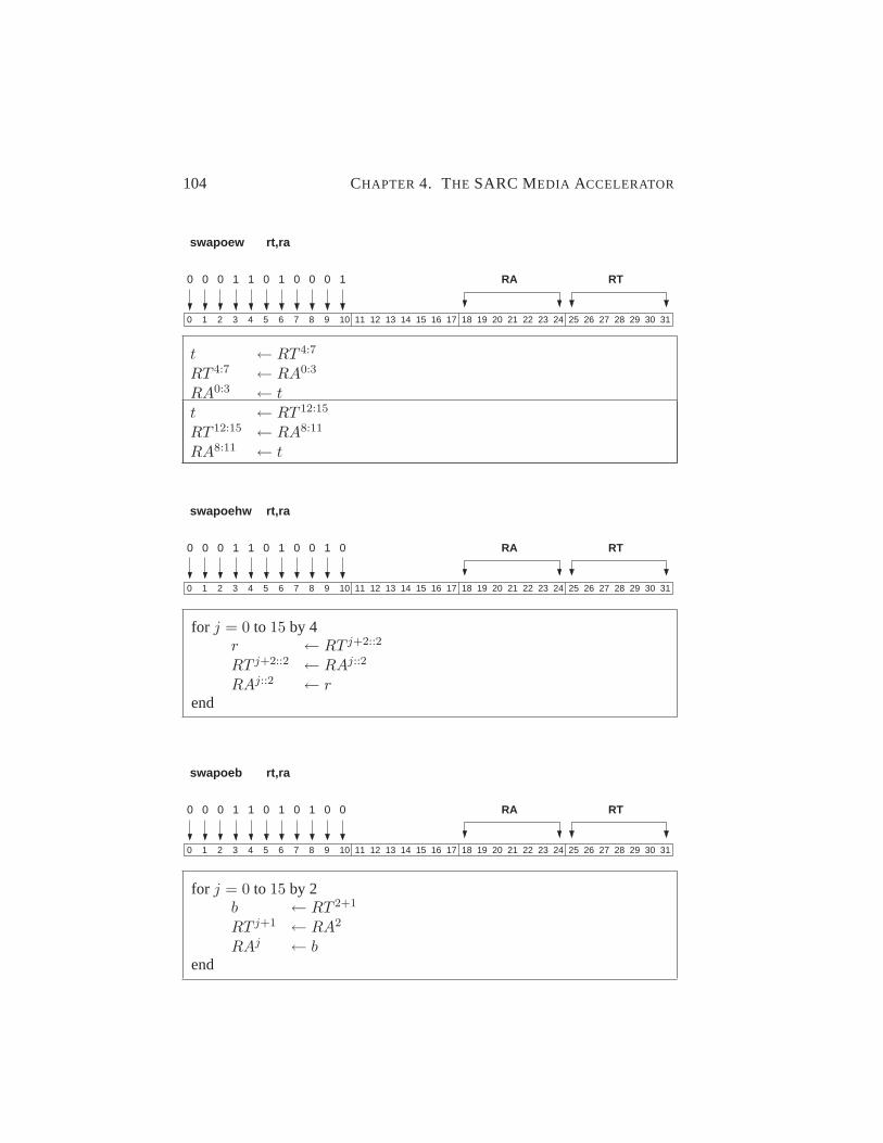
104 CHAPTER 4. THE SARC MEDIA ACCELERATOR
313029282726252423222120191817161514131211109876543210
RTRA00000 1 1 1
rt,ra
0 0 1
swapoew
t ← RT 4:7
RT 4:7 ← RA0:3
RA0:3 ← tt ← RT 12:15
RT 12:15 ← RA8:11
RA8:11 ← t
313029282726252423222120191817161514131211109876543210
RTRA000000 1 1 1
rt,ra
0 1
swapoehw
for j = 0 to 15 by 4r ← RT j+2::2
RT j+2::2 ← RAj::2
RAj::2 ← rend
313029282726252423222120191817161514131211109876543210
RTRA0000000 1 1 1 1
rt,raswapoeb
for j = 0 to 15 by 2b ← RT 2+1
RT j+1 ← RA2
RAj ← bend

4.4. ENHANCEMENTS TO THESPE ARCHITECTURE 105
All swapoe instructions were made accessible from C code through in-trinsics. Using the intrinsic, however, can cause problems due tothe following. The SPU compiler assumes that for an instructionmnemonic rt, ra, [rb/rc/im] only registerrt is modified. As aconsequence, the compiler assumes the variable located in registerra is alsoavailable in memory, and might decide to re-use the register for another vari-able. To avoid this problem inline assembly was used, which allows the pro-grammer to specify the mode of each register:
asm volatile ("swapoedw %0,%1" \: "=r" (a0), "=r" (a4) \: "0" (a0), "1" (a4) \);
Note that we used the keywordvolatile here. It was not required to main-tain correct order of execution. We used it to enforce the compiler to maintainthe hand optimized order of instructions. Simulations confirmed that indeedthe hand optimized order of these swapoe instruction resulted in faster execu-tion compared to compiler scheduled swapoe instructions.
The swapoe instructions were added to the simulator and to the compiler. Weassume a latency of three clock cycles for the predefined permutations of theswapoe instructions. The instructions, however, write to two registers insteadof one. Writing to two registers can be serialized if only one write-port is avail-able. The SPU register file probably has two write-ports as it has an odd andeven pipeline. Thus, the swapoe instructions could as well use both these writeports. This might, however, cause a stall in the other pipeline. We account forthe second write, no matter how it is implemented, by adding one extra cycle.So in total the latency of the swapoe instructions was set to four clock cycles.
Related Work
A linear time matrix transposition method was proposed in [72], which uti-lizes a special vector register file that allows diagonal access. The in-situ ma-trix transpose (IPMT) algorithm allows a matrix, stored in register file, to betransposed by performing a number of rotations on the diagonal registers. Thenumber of instructions required by this approach, assuming the buffered imple-mentation, is2n− 2. For the common casesn = 16 andn = 8 this approachrequires 30 and 14 instructions, respectively which both are approximatelytwice as fast as the AltiVec matrix transpose. Our implementation using theswapoe instruction takes 32 and 12 instructions forn = 16 andn = 8, respec-

106 CHAPTER 4. THE SARC MEDIA ACCELERATOR
Listing 4.8: Example of how the sfxsh instructions speed up code of the IDCT kernel.Left are two lines of C code, in the middle is the normal assembly code,while the right depicts the assembly code using sfxsh instructions.
1 b1 = a7>>2 + a1 ; ro tmah i $11 , $9 ,−2 shaddhw $11 , $11 , $9 , 22 b3 = a3 + a5>>2; ah $11 , $11 , $4 shaddhw $8 , $8 , $15 , 23 r o tmah i $8 , $15 ,−24 ah $8 , $8 , $7
tively. Thus our approach is as fast as IPMT but is much simpler as we use aconventional register file.
As mentioned in Section 4.1, the MOM architecture provides a matrix trans-pose instruction. According to [48] this transpose takes eight cycles for an8×8matrix. As the architecture is only described at the ISA level, it is unclear howthis is implemented and what the impact on the performance is.
4.4.4 Accelerating Arithmetic Operations
In this section we propose several instruction classes that enhance the execu-tion of regular arithmetic expressions in video decoding.
Sfxsh Instructions
Sfxsh (Simple FiXed point & SHift) instructions combine simple fixed pointoperations with a shift operation. Listing 4.8 shows an example from theIDCT8 kernel where one operand is shifted and added to the second. Usinga normal ISA, these two lines of code would require four instructions.
This kind of code is found frequently in the kernels we investigated. Moregeneral, they can be characterized as follows. There are two register operands,a simple arithmetic operation (such as addition and subtraction), and one shiftright by a small constant amount of bits. Our analysis showed that the in-structions depicted in Figure 4.8 are beneficial. Our benchmarks only usedthe instructions that operate on vectors of halfwords, but we provide the sameoperations for vectors of words as well. To prevent overflow, computation isgenerally not performed using bytes but halfwords. Thus, the sfxsh instruc-tions for bytes do not seem to be useful and are omitted.
The sfxsh instructions could fit the RRR format of the SPU ISA if the im-mediate value would be stored in a register. This approach, however, would

4.4. ENHANCEMENTS TO THESPE ARCHITECTURE 107
shaddhw rt,ra,rb,imm \\rt = ra + rb>>imm \shsubhw rt,ra,rb,imm \\rt = ra - rb>>imm | for vectoraddshhw rt,ra,rb,imm \\rt = (ra + rb)>>imm | of halfwordssubshhw rt,ra,rb,imm \\rt = (ra - rb)>>imm /shaddw rt,ra,rb,imm \\rt = ra + rb>>imm \shsubw rt,ra,rb,imm \\rt = ra - rb>>imm | for vectoraddshw rt,ra,rb,imm \\rt = (ra + rb)>>imm | of wordssubshw rt,ra,rb,imm \\rt = (ra - rb)>>imm /
Figure 4.8: Overview of the sfxsh instructions.
cause an unnecessary load to a register. Furthermore, there are not enough op-codes of the RRR format available to implement all instructions. It is the case,though, that the shift operation is only performed by a few bits, i.e., the shiftcount is between 0 and 7. Thus, the immediate value can be represented by 3bits only. Using this observation we defined the RRI3 instruction format thatuses 8 bits for the opcode, 3 bits for the immediate value, and 7 bits for each ofthe three register operands. The instruction details, depicted below, show theRRI3 format graphically.
313029282726252423222120191817161514131211109876543210
RTRA000 1
rt,ra,rb,imm
1 0 0 0 RBI3
shaddhw
s← RepLeftBit(I3,16)for j = 0 to 15 by 2
p← RT j::2
for b = 0 to 15if (b− s) > 0 then rb ← pb−s
else rb ← 0endRBj::2 ← RAj::2 + r
end

108 CHAPTER 4. THE SARC MEDIA ACCELERATOR
313029282726252423222120191817161514131211109876543210
RTRA000 1
rt,ra,rb,imm
1 0 0 RBI31
shsubhw
s← RepLeftBit(I3,16)for j = 0 to 15 by 2
p← RT j::2
for b = 0 to 15if (b− s) > 0 then rb ← pb−s
else rb ← 0endRBj::2 ← RAj::2 − r
end
313029282726252423222120191817161514131211109876543210
RTRA000 1
rt,ra,rb,imm
1 0 RBI301
addshhw
s← RepLeftBit(I3,16)for j = 0 to 15 by 2
p← RAj::2 + RT j::2
for b = 0 to 15if (b− s) > 0 then rb ← pb−s
else rb ← 0endRBj::2 ← r
end

4.4. ENHANCEMENTS TO THESPE ARCHITECTURE 109
313029282726252423222120191817161514131211109876543210
RTRA000 1
rt,ra,rb,imm
1 0 RBI31 1
subshhw
s← RepLeftBit(I3,16)for j = 0 to 15 by 2
p← RAj::2 −RT j::2
for b = 0 to 15if (b− s) > 0 then rb ← pb−s
else rb ← 0endRBj::2 ← r
end
313029282726252423222120191817161514131211109876543210
RTRA00 1
rt,ra,rb,imm
1 0 0 0 RBI3
shaddw
1
s← RepLeftBit(I3,16)for j = 0 to 15 by 4
t ← RT j::4
for b = 0 to 31if (b− s) > 0 then ub ← tb−s
else ub ← 0endRBj::4 ← RAj::4 + u
end

110 CHAPTER 4. THE SARC MEDIA ACCELERATOR
313029282726252423222120191817161514131211109876543210
RTRA00 1
rt,ra,rb,imm
1 0 0 RBI31
shsubw
1
s← RepLeftBit(I3,16)for j = 0 to 15 by 4
t ← RT j::4
for b = 0 to 31if (b− s) > 0 then ub ← tb−s
else ub ← 0endRBj::4 ← RAj::4 − u
end
313029282726252423222120191817161514131211109876543210
RTRA00 1
rt,ra,rb,imm
1 0 RBI301
addshw
1
s← RepLeftBit(I3,16)for j = 0 to 15 by 4
t ← RAj::4 + RT j::4
for b = 0 to 31if (b− s) > 0 then ub ← tb−s
else ub ← 0endRBj::4 ← u
end

4.4. ENHANCEMENTS TO THESPE ARCHITECTURE 111
313029282726252423222120191817161514131211109876543210
RTRA00 1
rt,ra,rb,imm
1 0 RBI31 1
subshw
1
s← RepLeftBit(I3,16)for j = 0 to 15 by 4
t ← RAj::4 −RT j::4
for b = 0 to 31if (b− s) > 0 then ub ← tb−s
else ub ← 0endRBj::4 ← u
end

112 CHAPTER 4. THE SARC MEDIA ACCELERATOR
313029282726252423222120191817161514131211109876543210
RTRA00 1
rt,ra,rb,imm
1 RBI7
I3opcode Programmer and simulator view
Compiler viewrrrx
Figure 4.9: The rrrx instruction of format RRR was used inside the compiler tohandle the sfxsh instructions with format RRI3. At the programmers sidean offset was added to the immediate value to set bits 4 to 7.
Listing 4.9: Defines translate the sfxsh intrinsics to the rrrx intrinsic and add the offsetto the immediate value.
1 # d e f i n e spu shaddhw ( a , b , c ) s p ur r r x ( a , b , c ) ;2 # d e f i n e spu shsubhw ( a , b , c ) s p ur r r x ( a , b , c + 8 ) ;3 # d e f i n e spu addshhw ( a , b , c ) s p ur r r x ( a , b , c +16 ) ;4 # d e f i n e spu subshhw ( a , b , c ) s p ur r r x ( a , b , c +24 ) ;5 # d e f i n e spu shaddw ( a , b , c ) s p ur r r x ( a , b , c +32 ) ;6 # d e f i n e spu shsubw ( a , b , c ) s p ur r r x ( a , b , c +40 ) ;7 # d e f i n e spu addshw ( a , b , c ) s p ur r r x ( a , b , c +48 ) ;8 # d e f i n e spu subshw ( a , b , c ) s p ur r r x ( a , b , c +56 ) ;
The sfxsh instructions were made available to the programmer through intrin-sics. We did not modify the compiler to handle the new instruction format.Instead we used a little trick at the programmer’s side, such that the com-piler could handle the sfxsh instructions as if they were of the RRR format.Inside the compiler we created the instructionrrrx rt,ra,rb,imm us-ing the RRR format except that we replacedrc with an immediate (see Fig-ure 4.9). The opcode is 4 bits and has value0x480 (1001 ). This instructionis available through the intrinsicd = spu_rrrx(a,b,imm) . To create theinstruction word corresponding to the sfxsh instructions we created the definesof Listing 4.9 that add an offset to the immediate value. The offset will changebits 4 to 7 of the instruction word such that the right RRI3 opcode is created.
The simulator was modified to recognize the new RRI3 instruction format andthe new instructions. The latency of the sfxsh instructions was set to five cy-cles. Normal shift and rotate instructions take four cycles. We added one cycleto this for the extra addition or subtraction.

4.4. ENHANCEMENTS TO THESPE ARCHITECTURE 113
Listing 4.10: Example code from the Luma kernel that can be replaced by one mpytrinstruction. In the code, first the odd elements ofinput are multipliedby constant 5, followed by the even elements. A shuffle packs the twovectors of words into one vector of halfwords.
1 v s i n t 1 6 t v5 = s p u s p l a t s ( 5 ) ;2 v u i n t 8 t mask = {0 x02 , 0 x03 , 0 x12 , 0 x13 , 0 x06 , 0 x07 , 0 x16 , 0 x17 ,\3 0x0A , 0 x0B , 0 x1A , 0 x1B , 0 x0E , 0 x0F , 0 x1E , 0 x1F} ;4 v s i n t 3 2 t A = spu mulo ( i n p u t , 5 ) ;5 v s i n t 3 2 t B = spu mule ( i n p u t , v5 ) ;6 v s i n t 1 6 t r e s u l t = s p u s h u f f l e (B , A , mask ) ;
Mpytr Instructions
The Mpytr (multiply and truncate) instructions perform a multiply or multiply-add on vectors of halfwords and stores the results as halfwords as well by trun-cating the most significant bits. The normal multiply instructions in the SPUISA take halfword operands as input and produce word values. The reason isof course not to lose precision, but the side effect is that only four SIMD slotsare used while the input vector consists of eight elements.
In video decoding the primary input and output data type is unsigned byte.In order not to lose precision, computations are mostly performed in signedhalfword values. In the Luma and Chroma interpolation filters several multi-plications are performed. Using the normal ISA the intermediate results arewords (32 bits) while we know from the algorithm that the maximum possiblevalue can be represented by 15 bits. Using the mpytr instructions, the conver-sion to 32-bit values is avoided.
Listing 4.10 shows a piece of code from the Luma kernel that multiplies thevector input , containing eight signed halfwords, with a constant 5. Firstthe odd elements are multiplied (spu_mulo ) followed by the even elements(spu_mule ). Using a shuffle the two vectors of words are packed into onevector of halfwords. Furthermore, there is some overhead involved to create avector of constants and to load the mask. This overhead though is performedonce per function call and thus shared among a few multiplications.
The code of Listing 4.10 can be replaced by onempytrhwi instruction, whichmultiplies a vector of signed halfwords by an unsigned immediate value. Theother instructions in this class arempytrhw (multiply two vectors of signedhalfwords) andmaddtrhw (multiply-add two vectors of signed halfwords).We do not expect mpytr instructions for unsigned halfwords to be useful as

114 CHAPTER 4. THE SARC MEDIA ACCELERATOR
most media computations are done using signed values. Mpytr instructionsfor bytes do not seem useful as unpacking to 16-bit is generally necessary andthus normal byte multiplication instructions can be used (see next section).Mpytr instructions for words might be useful in certain cases. As we are notaware of any, we did not implement those instructions. Further investigationof applications, for example audio processing, would be useful in this respect.
Thempytrhw instruction has the RR format and thempytrhwi has the RI7format. Thus the latter has seven bits for the immediate value which is enoughfor video decoding. The RI10 format could be used as well in case more bitsare necessary for the immediate value. Themaddtrhw instruction has theRRR format. The instruction details are depicted below.
313029282726252423222120191817161514131211109876543210
RT00 1 RA0 01 1 0 0 0
rt,ra,rb
RB1
mpytrhw
for j = 0 to 7t ← RA2j::2 ∗RB2j::2
RT 2j::2 ← t0:15
end
313029282726252423222120191817161514131211109876543210
RT00 1 RA0 0
rt,ra,imm
I71 1 0 0 0 0
mpytrhwi
for j = 0 to 7t ← RA2j::2 ∗ I7RT 2j::2 ← t0:15
end
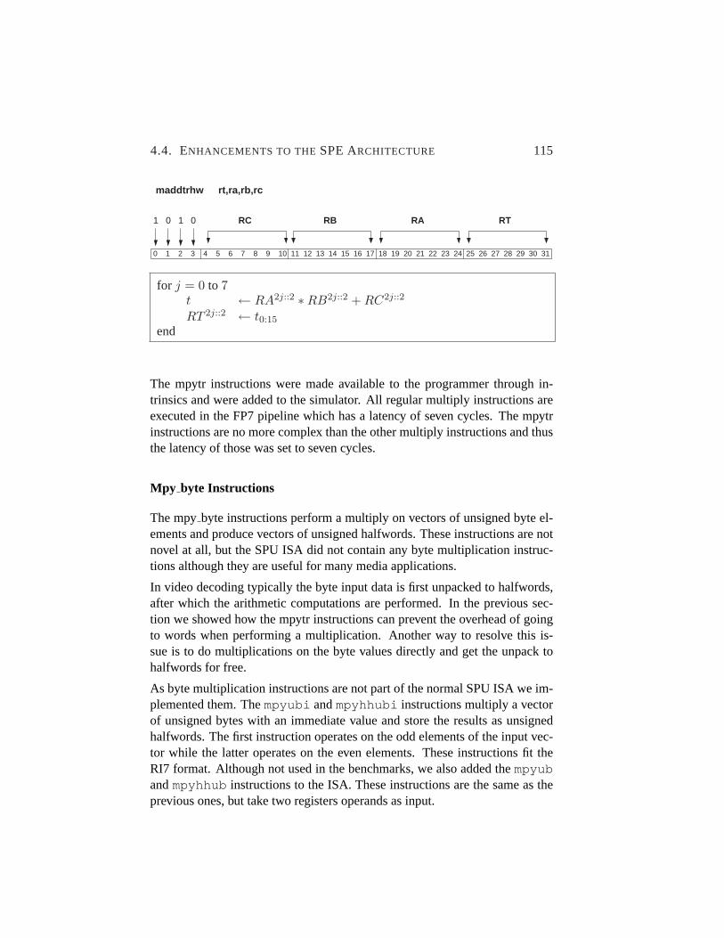
4.4. ENHANCEMENTS TO THESPE ARCHITECTURE 115
313029282726252423222120191817161514131211109876543210
RTRA1 0 RB
rt,ra,rb,rc
RC1 0
maddtrhw
for j = 0 to 7t ← RA2j::2 ∗RB2j::2 + RC2j::2
RT 2j::2 ← t0:15
end
The mpytr instructions were made available to the programmer through in-trinsics and were added to the simulator. All regular multiply instructions areexecuted in the FP7 pipeline which has a latency of seven cycles. The mpytrinstructions are no more complex than the other multiply instructions and thusthe latency of those was set to seven cycles.
Mpy byte Instructions
The mpybyte instructions perform a multiply on vectors of unsigned byte el-ements and produce vectors of unsigned halfwords. These instructions are notnovel at all, but the SPU ISA did not contain any byte multiplication instruc-tions although they are useful for many media applications.
In video decoding typically the byte input data is first unpacked to halfwords,after which the arithmetic computations are performed. In the previous sec-tion we showed how the mpytr instructions can prevent the overhead of goingto words when performing a multiplication. Another way to resolve this is-sue is to do multiplications on the byte values directly and get the unpack tohalfwords for free.
As byte multiplication instructions are not part of the normal SPU ISA we im-plemented them. Thempyubi andmpyhhubi instructions multiply a vectorof unsigned bytes with an immediate value and store the results as unsignedhalfwords. The first instruction operates on the odd elements of the input vec-tor while the latter operates on the even elements. These instructions fit theRI7 format. Although not used in the benchmarks, we also added thempyubandmpyhhub instructions to the ISA. These instructions are the same as theprevious ones, but take two registers operands as input.

116 CHAPTER 4. THE SARC MEDIA ACCELERATOR
The maddub andmsubub perform a multiply-add and multiply-sub opera-tion on vectors of unsigned bytes and store the result as a vector of unsignedhalfwords. These instructions operate on the odd elements of the input vectors.These two instructions fit the RRR format. Only a few opcodes of the RRRformat are available and in the normal SPU ISA only two were left unused.We already used these opcodes, however, for therrrx andmaddtrhw in-structions. To be able to use themaddub andmsubub anyway, we removedtwo floating point instructions from the ISA. For a media accelerator thesefloating point instructions are not needed and thus this choice is justified. If amore general purpose core is targeted, themsubub is most likely not worth re-moving another instruction for. Simulation results showed that this instructionprovides very limited benefit compared to others.
We also implemented thempyhhaub which multiply-adds the even elementsof vectors of bytes. Similar to the existingmpyhha instruction it has the RRformat and thus writes the result to the register of the first operand. We ex-pected this instruction to be a good addition to themaddub instruction. Simu-lation results, however, showed no speedup using this instruction compared tousing a shuffle and a normal multiply-add. Therefore we did not include it inthe accelerator architecture. For the same reason we omitted thempyhhsub(multiply high high and sub unsigned bytes) instruction.
We did not implement any multiplication instructions for signed bytes. We arenot aware of any media application using this data type. The details of the newbyte multiplication instructions that we implemented are depicted below.
313029282726252423222120191817161514131211109876543210
RT00 0
rt,ra,imm
1 1 0 0 1
mpyub
1 0 1 RARB
for j = 0 to 7RT 2j::2 ← RA2j+1 | ∗ | RB2j+1
end

4.4. ENHANCEMENTS TO THESPE ARCHITECTURE 117
313029282726252423222120191817161514131211109876543210
RT00 0
rt,ra,imm
1 1 0 0 1 1 RARB
mpyhhub
1 0
for j = 0 to 7RT 2j::2 ← RA2j | ∗ | RB2j
end
313029282726252423222120191817161514131211109876543210
RT00 RA0 0
rt,ra,imm
I71 1 0 0 1 0 1
mpyubi
for j = 0 to 7RT 2j::2 ← RA2j+1 | ∗ | I7
end
313029282726252423222120191817161514131211109876543210
RT00 RA0
rt,ra,imm
I71 1 0 0 1 0 1 1
mpyhhubi
for j = 0 to 7RT 2j::2 ← RA2j | ∗ | I7
end

118 CHAPTER 4. THE SARC MEDIA ACCELERATOR
313029282726252423222120191817161514131211109876543210
RA11 RB
rt,ra,rb,rc
RT RC1 1
maddub
for j = 0 to 7RT 2j::2 ← RA2j+1 | ∗ | RB2j+1 + RC2j+1
end
313029282726252423222120191817161514131211109876543210
RA11 RB
rt,ra,rb,rc
RT RC1 0
msubub
for j = 0 to 7RT 2j::2 ← RA2j+1 | ∗ | RB2j+1 −RC2j+1
end
The mpybyte instructions were made available to the programmer throughintrinsics and were added to the simulator. Just as the mpytr instruction, thempy byte instructions are no more complex than the other multiply instructionsand thus the latency of those was set to seven cycles.
IDCT8 Instruction
The Inverse Discrete Cosine Transform (IDCT) is an operation often found instill picture and video processing. The IDCT is typically performed on8 × 8or 4 × 4 pixel blocks. Performing the IDCT comprises a one-dimensionalIDCT row-wise followed by a one-dimensional IDCT on each column. FFm-peg uses the LLM IDCT algorithm [105]. The computational structure of theone-dimensional IDCT8 is depicted in Figure 4.10. If elements 0 through 7 area row of the matrix, then this diagram represents a row-wise one-dimensionalIDCT8. The diagram also shows that the IDCT consists of simple additions,subtractions, and some shifts.
The typical way to SIMDimize this one-dimensional IDCT is to perform theoperations on vectors of elements. Thus for the row-wise 1D IDCT, a vector

4.4. ENHANCEMENTS TO THESPE ARCHITECTURE 119
++ −−
+ + − −
− + + + − + +
− − + +
+ −+ −
0 1 2 3 4 5 6 7
+ + + + − − − −
0 1 2 3 4 5 6 7
+
Figure 4.10: Computational structure of the one-dimensional IDCT8. Arrows indi-cate a shift right by one bit. A dotted line means that the two inputoperands are the same.
would be a column of the matrix, while for the column-wise 1D IDCT a vectorwould be a row of the matrix. Assuming the sub-block is stored in memory rowmajor (row elements in consecutive addresses), the whole IDCT is performedin four steps: matrix transpose (MT); row-wise 1D IDCT; MT; column-wise1D IDCT.
We propose theIDCT8 instruction that performs the row-wise 1D IDCT8.This intra-vector instruction takes one row of the matrix as input, performsthe arithmetic operations as depicted in Figure 4.10, and stores the result in aregister. Thus, for an8 × 8 matrix the total row-wise 1D IDCT8 takes eightinstructions. Besides the reduction in the number of executed instructions, thetwo MTs are also avoided. This is because using theIDCT8 instruction thewhole IDCT can be performed in two steps: row-wise 1D IDCT using theIDCT8 instruction, followed by a conventional column-wise 1D IDCT.
The IDCT8 instruction fits the RR format where theRB slot is not used.RegisterRA is the input register whileRT is the output register. Usually forthe IDCT8 these two would be the same but the instruction allows them to bedifferent. TheIDCT8 instruction assumes its operand to be a vector of signedhalfwords. The instruction details are depicted below.

120 CHAPTER 4. THE SARC MEDIA ACCELERATOR
313029282726252423222120191817161514131211109876543210
RT0000 1 1 1 RA
idct8 rt,ra
0 1 1 0
r0 ← RA0:1 +RA8:9
r2 ← RA0:1 −RA8:9
r4 ← RA2:3/2 −RA12:13
r6 ← RA2:3 +RA12:13/2
s0 ← r0 + r6s2 ← r2 + r4s4 ← r2− r4s6 ← r0− r6
r1 ← RA10:11 −RA6:7 −(RA14:15 +RA14:15/2)r3 ← RA2:3 +RA14:15 −(RA6:7 +RA6:7/2)r5 ← RA14:15 −RA2:3 +(RA10:11 +RA10:11/2)r7 ← RA6:7 +RA10:11 +(RA2:3 +RA2:3/2)
s1 ← r7/4 + r1s3 ← r3 + r5/4s5 ← r3/4− r5s7 ← r7− r1/4
RT 0:1 ← s0 + s7RT 2:3 ← s2 + s5RT 4:5 ← s4 + s3RT 6:7 ← s6 + s1RT 8:9 ← s6− s1RT 10:11 ← s4− s3RT 12:13 ← s2− s5RT 14:15 ← s0− s7

4.4. ENHANCEMENTS TO THESPE ARCHITECTURE 121
++ −−
+ + − −
0 1 2 3
0 1 2 3
Figure 4.11: Computational structure of the one-dimensional IDCT4. An arrow indi-cates a shift right by one bit.
The IDCT8 instruction was made available to the programmer through an in-trinsic. The instruction was added to the simulator and the latency was set toeight cycles for the following reason. Fixed point operations take two cyclesin the SPU architecture. TheIDCT8 instruction performs four steps of simplefixed point operations and thus the latency of the new instruction is at mostfour times two making a total of eight cycles.
IDCT4 Instruction
The IDCT4 is similar to the IDCT8 but operates on a4 × 4 pixel block. Thecomputational structure of the one-dimensional IDCT4 is simpler than that ofthe IDCT8 as shown in Figure 4.11.
For the IDCT4 kernel a similar approach could be used as for the IDCT8. As a4×4 matrix of halfwords, however, completely fits in two registers of 128-bits,the entire two-dimensional IDCT4 could be performed using one instructionwith two operands. Such an instruction would read the matrix from its twooperand registers, perform the arithmetic operations, and store the result backin the two registers. Storing the result could be done in one cycle if the registerfile has two write ports, or otherwise two cycles are required.
The IDCT4 instructions fits the RR format where theRB slot is not used.RegisterRA is the input and output register that contains the first two rows ofthe matrix whileRT holds the last two rows. The IDCT4 instruction assumesits operands to be vectors of signed halfwords. The instruction details aredepicted below.

122 CHAPTER 4. THE SARC MEDIA ACCELERATOR
313029282726252423222120191817161514131211109876543210
RT0000 1 1 1 RA
rt,ra
0 1 1
idct4
1
for i = 0 to 8 by 8r0 ← RAi::2 +RA(i+4)::2
r1 ← RAi::2 −RA(i+4)::2
r2 ← (RA(i+2)::2 >> 1) −RA(i+6)::2
r3 ← RA(i+2)::2 +(RA(i+6)::2 >> 1)
Qi::2 ← r0 +r3Q(i+2)::2 ← r1 +r2Q(i+4)::2 ← r1 −r2Q(i+6)::2 ← r0 −r3
r0 ← RT i::2 +RT (i+4)::2
r1 ← RT i::2 −RT (i+4)::2
r2 ← (RT (i+2)::2 >> 1) −RT (i+6)::2
r3 ← RT (i+2)::2 +(RT (i+6)::2 >> 1)
Ri::2 ← r0 +r3R(i+2)::2 ← r1 +r2R(i+4)::2 ← r1 −r2R(i+6)::2 ← r0 −r3
endfor i = 0 to 3
r0 ← Q2i::2 + R2i::2
r1 ← Q2i::2 −R2i::2
r2 ← (Q2(i+4)::2 >> 1)−R2(i+4)::2
r3 ← Q2(i+4)::2 + (R2(i+4)::2 >> 1)
RA2i::2 ← ((r0 + r3) >> 6)RA2(i+4)::2 ← ((r1 + r2) >> 6)RT 2i::2 ← ((r1− r2) >> 6)RA2(i+4)::2 ← ((r0− r3) >> 6)
end

4.4. ENHANCEMENTS TO THESPE ARCHITECTURE 123
As the instruction details show, the result is shifted right by six bits beforewriting to the registers. This operation is not depicted in Figure 4.11 but isalways performed after the two one-dimensional IDCTs have been computed.Therefore we added this operation to theIDCT4 instruction.
The IDCT4 instruction was made available to the programmer through inlineassembly. Using inline assembly it is possible to specify that both operands ofthe instruction are read and written. The following code shows how to do this:
asm volatile ("idct4 %0,%1" \: "=r" (v0), "=r" (v1) \: "=0" (v0), "=1" (v1) \);
The instruction was added to the simulator and the latency was set to ten cyclesfor the following reason. Fixed point operations take two cycles in the SPUarchitecture. TheIDCT4 instruction performs four steps of simple fixed pointoperations making a total of eight. We also count one cycle for the final shift(although this could be hardwired) and one cycle for writing the second resultto the register file.
Related Work
The sfxsh instructions collapse two operations in one instructions. The opera-tion pattern of the sfxsh instructions is frequently found in the H.264 kernelsand is therefore useful to provide in hardware. In [26] it is described how suchrecurring operation patterns can automatically be determined.
The (inverse) discrete cosine transform has been used in many applicationsthat compress image data. Several algorithms exist to compute the (I)DCTand many hardware implementations have been proposed. Some of the morerecent proposals can be found in [69] and [66], both of which provide a goodoverview of other implementations in the past. Simai et al. [141] proposed animplementation for a programmable media processor. They extended the Tri-Media processor with a reconfigurable execution unit and demonstrated howto implement the IDCT on it.
The (I)DCT algorithm used in the H.264 standard is a simplified version thatis much less complex than previous algorithms. For example, it uses onlyaddition, subtraction, and shifts where other algorithm required many multi-plications. This algorithm was proposed in [109, 108] for the4× 4 transformwhile the algorithm for the8 × 8 transform was proposed in [67]. To the bestof our knowledge, the only hardware implementation of this algorithm was

124 CHAPTER 4. THE SARC MEDIA ACCELERATOR
Listing 4.11: Example code from the Luma kernel that loads one quadword from anunaligned memory address (src ).
1 i n t pe rm src = (unsigned i n t ) s r c & 1 5 ;2 v u i n t 8 t srcA = ∗ ( v u i n t 8 t ∗ ) ( s r c ) ;3 v u i n t 8 t srcB = ∗ ( v u i n t 8 t ∗ ) ( s r c +16 ) ;4 v u i n t 8 t s r c = s p u o r ( s p u s l q w b y t e ( srcA , pe rms rc ) ,5 spu r lmaskqwby te ( srcB , pe rms rc−16) ) ;
proposed in [49]. It performs the8 × 8 2D IDCT in a sequential manner, i.e.,it consumes and produces one sample per cycle. Their hardware unit was de-signed to be used in a streaming environment and therefore is not very suitablefor a programmable media accelerator. Another difference with our approachis that we exploit DLP to reduce the latency of the IDCT operation.
Similar to our work, in [137] the authors proposed some techniques to speedupthe Discrete Wavelet Transform (DWT) on SIMD architectures. DWT has ahigher compression ratio but is computationally more complex than the DCT.The authors proposed to add a MAC instruction to the ISA, use the extendedsubwords technique, and use a special matrix register file.
4.4.5 Accelerating Unaligned Memory Accesses
In the SPE architecture, accesses to the local store are quadword aligned. Thefour least significant bits of a memory address used in a load or store instruc-tion are truncated. Thus, byte aligned memory addresses can be used but theLS store always returns an aligned quadword.
If a quadword has to be loaded or stored from an unaligned address this hasto be done in several steps. Listing 4.11 shows an example of an unalignedload taken from the Luma kernel. First, two aligned quadwords are loaded,each containing a part of the targeted quadword. Next, the two quadwordsare shifted left and right respectively to put the elements in the correct slot.Finally, the two words are combined using an OR instruction. The procedurefor an unaligned store is even more complicated and involves two loads andtwo stores.
To overcome this limitation of the SPE architecture we implemented unalignedloads and stores. To assure backward compatibility of code the existing loadand store operations were not altered. Instead, we added new instructions thatperform the unaligned loads and stores. The details of these instructions are

4.4. ENHANCEMENTS TO THESPE ARCHITECTURE 125
depicted below. We did not implement the unaligned version of the a-formLoad and Store (L/S) instructions as we did not find those necessary.
313029282726252423222120191817161514131211109876543210
RT00 1 RA
lqdu rt,symbol(ra)
0 0 I100 1 1
LSA ← (RepLeftBit(I10 || 0b0000,32) + RA0:3 & LSLR
RT ← LocStor(LSA, 16)
313029282726252423222120191817161514131211109876543210
RT000 1 RA10
rt,ra,rb
RB
lqxu
1 1 0 0 1
LSA ← (RA0:3 + RB0:3) & LSLR
RT ← LocStor(LSA, 16)
313029282726252423222120191817161514131211109876543210
RT00 1 RA
rt,symbol(ra)
0 I100 1 1
stqdu
1
LSA ← (RepLeftBit(I10 || 0b0000,32) + RA0:3 & LSLR
LocStor(LSA, 16) ← RT

126 CHAPTER 4. THE SARC MEDIA ACCELERATOR
313029282726252423222120191817161514131211109876543210
RT000 1 RA
rt,ra,rb
RB1 1 0 0 1
stqxu
1 0
LSA ← (RA0:3 + RB0:3) & LSLR
LocStor(LSA, 16) ← RT
To allow byte aligned accesses, some modifications to the local store are re-quired. A quadword might be aligned across two memory lines. Thus ad-ditional hardware is required to load or store the misaligned quadword frommemory. To account for this we added one cycle to the latency of the localstore.
The unaligned L/S instructions were made available to the programmerthrough inline assembly only. Modifying the compiler to automatically usethe unaligned L/S instructions is a complex task beyond the scope of this the-sis. We tried to use intrinsics but we could not make them work properly withinreasonable time.
Analysis of the assembly code revealed that the compiler was not able to sched-ule the unaligned L/S instructions as optimal as it does for normal L/S instruc-tions. Therefore, we optimized the scheduling of the unaligned L/S instruc-tions manually. We did not hand optimize the scheduling of other instructionsto keep the comparison fair.
Unaligned memory access has been applied before. In vector processing, ofwhich SIMD is a sub class, there is often a mismatch between the data orderused in memory and the data order required for computation. Therefore, mostvector and DSP processors provide complex memory access that can be di-vided in three groups: unaligned access, strided access, and irregular access.In SIMD processors, due to the short vectors, mainly unaligned access is an is-sue. Multimedia SIMD extensions such as MMX, and SSE support unalignedaccesses in hardware at the cost of some additional latency. In other SIMDarchitectures, such as Altivec/VMX, VIS, and 3DNow! alignment has to beperformed in software, which is very costly in terms of latency.
Alignment issues on different multimedia SIMD architectures has been inves-tigated in [136]. The paper describes several software approaches to minimizethe overhead costs. The benefits of supporting unaligned access in hardware

4.5. PERFORMANCEEVALUATION 127
is studied in detail in [23] for the Altivec/VMX architecture. Although the re-search is general, the authors give an example of how unaligned access couldbe implemented. Similar work is presented in [38, 37], but these focus moreon the actual memory access architecture and compiler optimizations. The lat-est TriMedia processor, which was specialized for H.264 supports unalignedmemory access.
4.5 Performance Evaluation
In the previous section we have presented several ISA enhancements to accel-erate media applications, especially H.264 decoding. This section evaluatesthe performance improvement obtained with the proposed instruction on thekernels of our benchmark suite. Each kernel is analyzed by means of profil-ing, the identified deficiencies are described, and it is shown how the proposedarchitectural enhancements resolve the deficiencies.
4.5.1 Results for the IDCT8 Kernel
The first benchmark considered is the IDCT kernel, which is the smallest ofall. It takes as input a macroblock of16 × 16 16-bit elements, divides it inblocks of8 × 8 or 4 × 4 . On each sub-block it performs a one-dimensionaltransformation first row-wise then column-wise, thus a two-dimensional trans-formation in total. The size of the sub-blocks depends on the mode of themacroblock. We will refer to these modes as IDCT8 and IDCT4, respectivelyand treat them as different kernels. This section describes the IDCT8 kernelwhile the next section describes the IDCT4 kernel.
The IDCT8 kernel was analyzed by splitting the kernel in parts and measuringthe execution times taken by each part. The kernel consists of four8 × 8IDCTs, which are identical. In this analysis of the kernel we measured one8×8 IDCT only. Table 4.3 presents the results. We remark again that this low-level profiling influences the compiler optimizations and thus the measuredexecution times. For the purpose of this analysis, however, it suffices to knowthe relative execution times.
We briefly describe the parts of the IDCT8 function. Although we profiled onlyone8×8 IDCT, we included the overhead caused by the loop that starts the four8× 8 IDCTs needed to process the entire macroblock. This overhead includescalculating the pointers to the source and destination address of the data andthe stride. The initialization of variables mainly consists of creating or loading

128 CHAPTER 4. THE SARC MEDIA ACCELERATOR
Table 4.3: Profiling of the baseline IDCT8 kernel. Both the original and the optimizedversion are depicted. No architectural enhancements are included.
Original Optimizedcycles % cycles %
Loop overhead 33 6% 36 11%Initialize variables 11 2% 11 3%Load data & offset 18 4% 30 9%Control 62 12% 77 24%First transpose 28 5% 27 8%First 1D IDCT 38 7% 38 12%Second transpose 33 6% 32 10%Second 1D IDCT 37 7% 37 11%Shift right 6 12 2% 12 4%IDCT 148 28% 146 45%Calculate dst shift 8 2% 14 4%Addition and store 300 58% 89 27%Addition 308 60% 103 31%
Total 518 100% 326 100%
constants in the register file. Loading the data includes address computationbut also adding an offset to the first element of the8 × 8 matrix for roundingpurposes. The real computation of the IDCT involves two transposes, twosequences of one-dimensional IDCTs, and finally a divide by 64 (or a shiftright by 6 bits).
Another part of the kernel adds the result of the IDCT to the result of the pre-diction stage. In the original code this part consumes most of the executiontime. Analysis of the trace files revealed that it has a very low IPC because thecompiler is not able to schedule that part of the code in an efficient way. Theaddition and storepart consists basically of one macro for each matrix row.The macro loads one row of the matrix containing the result of the predictionstage, aligns the data, unpacks it, adds the result of the IDCT to it, packs theresult, and stores it in memory. This macro expands into twelve instructionsthat are completely serial and have many dependencies. The compiler sched-ules these blocks of twelve instructions sequentially resulting in an IPC of only0.36 for this part. In other words, instructions are mainly stalled, waiting forthe previous instruction to finish.

4.5. PERFORMANCEEVALUATION 129
We optimized this part of the code by interleaving the instructions correspond-ing to the different blocks manually. This is possible as processing the differentrows of the matrix is completely independent. Furthermore, we removed oneunnecessary operation and combined a shift and a shuffle in one shuffle. Theseoptimizations speed up this part of the kernel by a factor of three, as depictedin the right side of Table 4.3.
We chose to use the optimized version of the kernel as our baseline for evaluat-ing architectural enhancements. If the non-optimized kernel would have beentaken, it would be to easy to achieve speedup by architectural enhancementsresulting in biased results.
Besides profiling the kernel, we also analyzed the assembly code of the kerneland the trace files generated by the simulator. By doing so we identified a num-ber of deficiencies in the execution of the IDCT8 kernel. Below we present theidentified deficiencies and show how the proposed architectural enhancementsof Section 4.4 resolve these issues.
• Matrix transposes: In order to utilize the SIMD capabilities, each matrixhas to be transposed twice. This takes a lot of time, about as much as theactual IDCT computation does. Matrix transposes can be acceleratedusing the swapoe instructions. Using the IDCT8 instruction, however,the matrix transposes are completely avoided.
• Scalar operations: Due to the lack of a scalar data path, a scalar computa-tion that involves a vector element requires a lot of instructions. Scalarsare stored in the preferred slot of a vector. If one of the operands is avector element, it has to be shifted to the preferred slot, the computationhas to be performed, and using a shuffle the result has to be stored inthe original vector. The as2ve instructions allow to add a scalar to onevector element in one instruction.
• Lack of saturating arithmetic: The SPUs do not have saturating arith-metic and thus this has to be performed in software. This involves un-packing, adding, comparing, selecting, and packing. The asp instructioncontains saturating arithmetic and can be used to avoid software satura-tion.
• Pack/unpack & alignment: Packing and unpacking has to be performedexplicitly and is done using shuffle instructions. Moreover, most packingand unpacking require alignment which has to be performed explicitly

130 CHAPTER 4. THE SARC MEDIA ACCELERATOR
as well. Consider an unpack from eight bytes elements to halfwords el-ements. If the programmer cannot be sure whether the eight bytes arein the lower or upper part of the vector, he or she has to check the ad-dress, compute the shift and rotate the data. After that the unpack can bedone. In the IDCT kernel this is the case. A part of this problem (mainlypacking) is solved by the asp instruction. Alignment issues remain adeficiency.
Besides the enhancements mentioned above, also the sfxsh instructions arebeneficial to the IDCT8 kernel. Table 4.4 shows the effect of the enhancementson the execution time and the instruction count of the IDCT8 kernel. First, itshows the effect of each of the enhancement separately. Finally, also the com-bination of all enhancements was analyzed. This set of enhancements excludedthe swapoe instructions as they become obsolete when using the IDCT8 in-struction, which eliminates the matrix transposes. For this analysis we run theIDCT kernel on one complete macroblock. We remark again that this kernel-level profiling does not influence the compiler optimizations and thus theseresults are accurate.
The speedup achieved by each enhancement separately is between 0.99 and1.39. Not surprisingly, the IDCT8 instruction achieves the largest speedup,mostly due to avoiding matrix transposes. The swapoe instructions do not pro-vide speedup in this kernel. The amount of ILP in the kernel is low and thusthe critical path in the dependency graph determines the latency of the kernel.Although using swapoe instructions reduces the number of executed instruc-tions, the critical path of the matrix transpose does not change. Therefore, thecritical path of the entire kernel does not change and neither does the latency.
Table 4.4: Speedup and reduction in instruction count of the IDCT8 kernel using theproposed architectural enhancements. The effect of each separate enhance-ment is listed as well as the aggregate effect.
Enhancement Cycles InstructionsBaseline Enhanced Speedup Baseline Enhanced Reduction
Swapoe 896 908 0.99 1103 988 1.12IDCT8 896 645 1.39 1103 756 1.46Sfxsh 896 840 1.07 1103 984 1.12Asp 896 781 1.15 1103 928 1.19As2ve 896 865 1.04 1103 1072 1.03All (but swapoe) 896 488 1.84 1103 488 2.26

4.5. PERFORMANCEEVALUATION 131
The speedup achieved when combining all architectural enhancements is 1.84.Note that also a reduction in the number of instructions of 2.26 is achieved. Thelatter is important for power efficiency, which has become a design constraintin contemporary processor design (see also Chapter 2). The achieved speedupis directly related to the reduction in instruction count, but does not necessar-ily has the same magnitude. For most kernels the speedup is lower than theinstruction count reduction. This is expected since multiple shorter-latencyinstructions have been replaced by a single instruction with a longer latency.In other words, the latency of the arithmetic operations stays the same. Forexample, the latency of the IDCT8 instructions is assumed to be 8 cycles, be-cause there are 4 simple fixed point operations on the critical path, each takingtwo cycles. The application-specific instructions we have introduced mainlyreduce the overhead and eliminate stalls due to data dependencies.
4.5.2 Results for the IDCT4 kernel
Besides the IDCT8 kernel we also investigated the IDCT4 kernel. The IDCT4kernel splits a MB into 16 sub-blocks of4×4 pixels and performs the transformon these sub-blocks. We analyzed this kernel by profiling the execution timespent on the different parts. The IDCT4 kernel has the same execution steps asthe IDCT8 and the explanation of those can be found in the previous section.As in the IDCT8 we measured the execution of one4×4 IDCT only. Table 4.5presents the results.
We optimized the code of the IDCT4 kernel in the same way we optimized theIDCT8 kernel. In theaddition and storepart we interleaved intrinsics in orderto achieve a higher ILP. Furthermore, we removed one unnecessary operationand combined a shift and a shuffle in one shuffle. Again, these optimizationsspeed up this part of the kernel by a factor three as depicted in the right sideof Table 4.5. For the same reasons as mentioned in the previous section wechose the optimized version as our baseline for evaluating architectural en-hancements.
We identified the deficiencies in the execution of the IDCT4 kernel by ana-lyzing the profiling results and a trace output. The identified deficiencies aresimilar as for the IDCT8 kernel, but there are some differences. Below we ex-plain the deficiencies and show how the proposed architectural enhancementsof Section 4.4 resolve these issues.
• Matrix transpositions: Because of the small matrix size the transposi-tions are less costly but more of them are required so they still take up

132 CHAPTER 4. THE SARC MEDIA ACCELERATOR
Table 4.5: Profiling of the baseline IDCT4 kernel. Both the original and the optimizedversion are depicted. No architectural enhancements are included.
Original Optimizedcycles % cycles %
Loop overhead 33 10% 33 15%Initialize variables 11 3% 11 5%Load data & offset 29 9% 30 13%Control 73 23% 74 33%First transpose 22 7% 22 10%First 1D IDCT 15 5% 16 7%Second transpose 25 8% 24 11%Second 1D IDCT 15 5% 16 7%Shift right 6 11 3% 12 5%Idct 88 27% 90 40%Calculate dst shift 7 2% 9 4%Addition and store 156 48% 53 24%Addition 163 50% 62 27%
Total 324 100% 226 100%
about 20% of the execution time. Swapoe instructions are of no valuefor a 4 × 4 matrix as it fits entirely in two registers, and thus shuffleoperations are sufficient. The IDCT4 instruction, on the other hand,completely removes all matrix transpositions.
• Unused SIMD slots: All SIMD computations are performed row orcolumn-wise. As the matrix is4 × 4 and the elements are 16-bit onlyhalf of the SIMD slots are used. The IDCT4 instruction does utilize allSIMD slots by exploiting the fact that an entire4×4 matrix can be storedin two registers. This increases the efficiency of the computational partof the kernel.
• Scalar operations: Same as for IDCT8 kernel; see page 129 for a fulldescription. The as2ve instructions were used to mitigate the effect ofthis deficiency.
• Lack of saturating arithmetic: Same as for IDCT8 kernel; see page 129for a full description. The asp instruction was used to mitigate the effectof this deficiency.

4.5. PERFORMANCEEVALUATION 133
• Pack, unpack & alignment: Same as for IDCT8 kernel; see page 130 fora full description. The asp instruction was used to resolve the pack/un-pack deficiency. Alignment issues remain a deficiency.
Besides the enhancements mentioned above, we also used the unaligned L/Sinstructions. By doing this we avoided some branches that caused many stalls.
Table 4.6 shows what the effect of the enhancements is on the execution timeand the instruction count of the IDCT4 kernel. First it shows what the effectis of each enhancement separately. Finally, also the combination of all en-hancements was analyzed. For this analysis we run the IDCT4 kernel on onecomplete macroblock.
The speedup achieved by the enhancements is between 1.05 and 1.23. A syn-ergistic effect happens when combining all enhancements such that the totalspeedup is larger than the multiplication of the separate speedups. The sourceof this synergistic effect seems to be the compiler optimization process. Thespeedup achieved when combining all architectural enhancements is 2.37 andthe number of instructions is reduced by a factor 2.67.
4.5.3 Results for the Deblocking Filter Kernel
The Deblocking Filter (DF) kernel is applied to remove an artifact introducedby the IDCT. The IDCT operates on4 × 4 or 8 × 8 sub-blocks and as a re-sult square areas might become visible in the decoded picture, which is calledthe ‘blocking’ artifact. The DF kernel smoothes these block edges and thusimproves the appearance of the decoded picture.
The process of deblocking a macroblock is depicted in Figure 4.12. Each
Table 4.6: Speedup and reduction in instruction count of the IDCT4 kernel using theproposed architectural enhancements. The effect of each separate enhance-ment is listed as well as the aggregate effect.
Enhancement Cycles InstructionsBaseline Enhanced Speedup Baseline Enhanced Reduction
IDCT4 2524 2059 1.23 1858 1304 1.42Asp 2524 2277 1.11 1858 1512 1.23As2ve 2524 2407 1.05 1858 1756 1.06Unaligned L/S 2524 2086 1.21 1858 1720 1.08All 2524 1063 2.37 1858 696 2.67
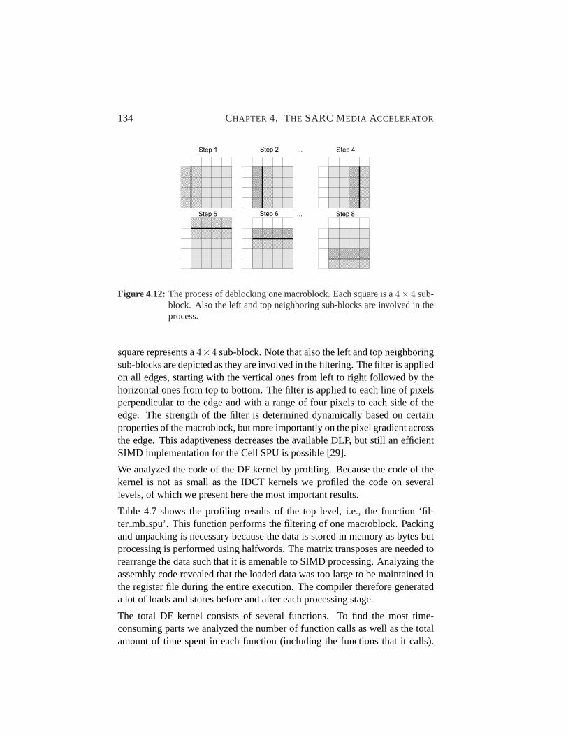
134 CHAPTER 4. THE SARC MEDIA ACCELERATOR
Figure 4.12: The process of deblocking one macroblock. Each square is a4× 4 sub-block. Also the left and top neighboring sub-blocks are involved in theprocess.
square represents a4×4 sub-block. Note that also the left and top neighboringsub-blocks are depicted as they are involved in the filtering. The filter is appliedon all edges, starting with the vertical ones from left to right followed by thehorizontal ones from top to bottom. The filter is applied to each line of pixelsperpendicular to the edge and with a range of four pixels to each side of theedge. The strength of the filter is determined dynamically based on certainproperties of the macroblock, but more importantly on the pixel gradient acrossthe edge. This adaptiveness decreases the available DLP, but still an efficientSIMD implementation for the Cell SPU is possible [29].
We analyzed the code of the DF kernel by profiling. Because the code of thekernel is not as small as the IDCT kernels we profiled the code on severallevels, of which we present here the most important results.
Table 4.7 shows the profiling results of the top level, i.e., the function ‘fil-ter mb spu’. This function performs the filtering of one macroblock. Packingand unpacking is necessary because the data is stored in memory as bytes butprocessing is performed using halfwords. The matrix transposes are needed torearrange the data such that it is amenable to SIMD processing. Analyzing theassembly code revealed that the loaded data was too large to be maintained inthe register file during the entire execution. The compiler therefore generateda lot of loads and stores before and after each processing stage.
The total DF kernel consists of several functions. To find the most time-consuming parts we analyzed the number of function calls as well as the totalamount of time spent in each function (including the functions that it calls).

4.5. PERFORMANCEEVALUATION 135
Table 4.7: Top-level profiling of the DF kernel for one macroblock. Both the originaland the optimized version are depicted. No architectural enhancements areincluded.
Original Optimizedcycles % cycles %
Initialize variables 22 0% 22 0%Load & unpack data 761 10% 761 10%First transpose 451 6% 451 6%Filter horizontal 2741 34% 2539 34%Second transpose 448 6% 448 6%Filter vertical 2748 34% 2546 34%Pack and store data 806 10% 806 11%
Total 7977 100% 7573 100%
Table 4.8: Profiling of the functions of the DF kernel when filtering4 × 4 mac-roblocks. The number of function calls and the time spent in the functionis mentioned. Functions of levelx only call functions of levelx + 1.
Calls Time Levelfilter mb spu 16 100% 1filter mb edgeh 240 53% 2filter mb edgecv 112 18% 2h264v loop filter luma c 192 19% 3h264 loop filter chroma 64 5% 3h264 loop filter chromaintra 48 1% 3clip 704 5% 3clip altivec 640 4% 4clip uint8 altivec 512 3% 4
The results are depicted in Table 4.8 which also states the level of each func-tion. Functions of levelx only call functions of levelx + 1. For this analysiswe filtered an area of4× 4 macroblocks of the top-left corner of a frame.
A large amount of time is spent in the ‘filtermb edgeh’ function which mainlycalls ‘h264v loop filter luma c’. The latter, however, is only 19% of the totalexecution time while the first is 53%. Further profiling revealed that in the firsta lot of time is taken by table lookups which are time-consuming on the SPUbecause of alignment issues.

136 CHAPTER 4. THE SARC MEDIA ACCELERATOR
Table 4.8 also shows that 12% is spent in clip functions. The ‘clip’ and‘clip altivec’ functions are used to set the index of table lookups within therange of the table (mainly between 0 and 51). The ‘clipuint8 altivec’ functionis used to saturate a halfword between 0 and 255. This is necessary becausethe SPU does not support saturating arithmetic.
While analyzing the kernel we also looked for non-optimal code. In this kernelwe did not find much to optimize. We did change some code that generatedconstants. The code was written in normal C and the compiler generated non-optimal assembly code. We rewrote the code using SPU intrinsics. The rightside of Table 4.7 shows the profiling results of the optimized kernel. As withthe previous kernels, we chose the optimized version as the baseline for evalu-ating architectural enhancements.
We identified a number of deficiencies in the execution of the DF kernel. Be-low they are presented and we show how the proposed architectural enhance-ments, proposed in Section 4.4, resolve these issues.
• Matrix transpositions: In order to utilize the SIMD capabilities eachdata matrix has to be transposed twice. This rearrangement overheadtakes up about 12% of the total execution time of the DF kernel. Asargued before, matrix transposition can be accelerated using the swapoeinstructions.
• Data size: The total data size of the baseline kernel exceeds the sizeof the register file and therefore a lot of intermediate loads and storesare required. The main cause of the large data size is that the matrixtransposes require twice as many registers: one set of registers for theoriginal and one for the transposed. The swapoe instructions performa matrix transpose in place and thus require half as many of registers.Simulation showed that using the swapoe instructions the entire data setfits in the register file and thus many loads and stores are prevented.
• Scalar operations: As with the previous kernels, scalar operations turnout to be very costly. In the DF kernel this manifests in the table lookups.Listing 4.1 of Section 4.4.1 shows that a table lookup costs five instruc-tions because of alignment issues. Using the lds instructions a tablelookup takes only two instructions.
• Lack of saturating function/arithmetic: The output of the DF kernel con-sists of unsigned bytes. Thus, the result of the filtering has to be satu-rated between 0 and 255. Many SIMD architectures offer saturating

4.5. PERFORMANCEEVALUATION 137
arithmetic which performs saturation automatically after each arithmeticoperation. In the DF kernel, however, halfwords are needed for the in-termediate results anyway, and thus one saturate at the end suffices. Im-plementing many saturating instructions is costly in terms of opcodes.The clip instruction is in that sense a good solution as it provides a fastsaturation with only one instruction per data type. Moreover, the clip in-struction can also be used for other purposes such as limiting the indexof a table lookup to the size of the table.
• Pack & unpack: In the SPE architecture, packing and unpacking has tobe performed explicitly and is done using shuffle instructions. The asp orsatpack instructions are of no help in the DF kernel as the saturate andthe pack are not coupled together. Automatic (un)pack at load and storewould be beneficial. As others have investigated this before [143, 42],we do not include this technique in our architectural enhancements.
• SIMDimization: Because of the adaptiveness of the filter, limited DLPis available. Five different filter strengths are applied depending on thesmoothness of the edge. That means that across the SIMD slots dif-ferent filters might be required. The SIMDimization strategy applied isto compute all five filters and to select the right result for each SIMDslot. Off course this requires extra computation. None of the proposedarchitectural enhancements resolves this issue.
Table 4.9 presents the speedup and instruction count reduction of the DF ker-nel using the proposed architectural enhancements. For this analysis we alsoapplied the DF to the top left4 × 4 macroblocks of a frame from a real videosequence. In contrast to the IDCT, for this kernel, the swapoe instructionshave a large impact on the execution time, mainly due to avoiding loads andstores. To achieve this some modifications to the code were required such thatthe compiler could ascertain all data accesses at compiler time. These mod-ifications included loop unrolling, substituting pointers for array indices, andinlining of functions.
Both the lds and clip instructions provide a moderate speedup separately butsignificant when all enhancements are applied concurrently. When combiningall three enhancements, again a synergistic effect happens as the total speedupis larger than the multiplication of the separate speedups. The reduction inthe number of instructions is proportional to the speedups. Combining all en-hancements the number of instructions is reduced with a factor 1.75.

138 CHAPTER 4. THE SARC MEDIA ACCELERATOR
Table 4.9: Speedup and reduction in instruction count of the DF kernel using the pro-posed architectural enhancements. The effect of each separate enhance-ment is listed as well as the aggregate effect.
Enhancement Cycles InstructionsBaseline Enhanced Speedup Baseline Enhanced Reduction
Swapoe 122135 90518 1.35 101480 74504 1.36Lds 122135 108995 1.12 101480 89692 1.13Clip 122135 114755 1.06 101480 96312 1.05All 122135 66334 1.84 101480 58088 1.75
For the DF kernel the speedup is larger than the reduction in instructions forthe following reason. When using the swapoe instructions it is possible to keepthe entire macroblock in the register file. To achieve this some modificationsto the code were required, such as the replacement of functions by macros.This reduces the number of branches significantly and with that the number ofbranch miss stall cycles. Specifically, in the baseline kernel there were 15,341branch miss stall cycles, while for the enhanced kernel this was only 4,529.
4.5.4 Results for the Luma/Chroma Interpolation Kernel
The Luma and Chroma interpolation kernels together perform the motion com-pensation. The kernels are applied to blocks of16× 16, 16× 8, 8× 16, 8× 8,8 × 4, 4 × 8, or 4 × 4 pixels. Note that there is only one chroma sample per2× 2 pixels. Otherwise the two kernels are identical and thus we focus on theLuma kernel only.
The accuracy of the motion compensation is a quarter of the distance betweenluma samples. If the motion vector points to an integer position, the predictedblock consists of the samples the motion vector points to in the referenceframe. If the motion vector points to a half-sample position, the predictedblock is obtained by interpolating the surrounding pixels. This is done by ap-plying a one-dimensional 6-tap FIR filter, which is given by:
p[0]′ = (p[−2]−5p[−1]+20p[0]+20p[1]−5p[2]+p[3])+16) >> 5. (4.1)
This filter is applied horizontally and/or vertically. Prediction values at quarter-sample positions are generated by averaging samples at integer- and half-sample positions. For more information on the motion compensation of H.264the reader is referred to [165].

4.5. PERFORMANCEEVALUATION 139
Table 4.10:Profiling results of the baseline Luma kernel. Both the original and theoptimized version are depicted. No architectural enhancements are in-cluded.
Original Optimizedcycles % cycles %
Initialization of variables 44 1% 27 1%Loop overhead 752 16% 896 21%Loading, aligning, and unpacking 1630 36% 1546 37%Computing interpolation filter 1024 23% 976 23%Saturating and pack 512 11% 416 10%Storing result 592 13% 368 9%
Total 4554 100% 4229 100%
The code of the Luma kernel contains many functions as there are many possi-ble combinations of block sizes and quarter sample positions. For the analysisin this work we chose an input block size of16× 16 and a quarter sample pre-diction position that requires both horizontal and vertical interpolation. Thisfilter function is one of the most compute intensive ones. The name of thisfilter function in the FFmpeg code isput h264 qpel16 mc11 spu . Theinput for this kernel is one macroblock and thus the filter function is run once.
We analyzed the code of the Luma kernel by profiling it using CellSim. Thefilter function calls three subfunctions:put h264 qpel v lowpass spuperforms vertical interpolation and consumes 33% of the total time,put h264 qpel h lowpass spu (52%) performs horizontal interpola-tion, andput pixels 16 l2 spu (16%) averages the result of the first twofunctions and stores it at the destination address. We divided the functions intothe six parts shown in Table 4.10 and measured how many cycles were spent ineach part combined for all three functions. Only 22.5% of the cycles is spenton actual computation of the interpolation. Most of the time is taken by load-ing/storing and the corresponding rearrangement of data to make it amenableto SIMD processing.
While analyzing the kernel we also looked for code optimization possibili-ties. We performed three optimizations. The first optimization is in the hor-izontal and vertical interpolation functions. The original code used only thespu madd intrinsic, which multiplies the odd elements only, and used shuf-fles to multiply even elements. We used thespu mule andspu mulo in

140 CHAPTER 4. THE SARC MEDIA ACCELERATOR
places where they are beneficial and thereby avoided some of the shuffles. Wealso developed a version that employed thespu mhhadd instruction, whichmultiply-adds the even elements. It turned out not to provide any speedup.
The second code optimization was performed in theput pixels 16 l2 spu function. The function computes the aver-age of two16 × 16 matrices of which it assumes that they are stored inmemory at a non quadword aligned address. Therefore this function contains alot of alignment overhead. In only a few cases, however, the input matrices areindeed stored non quadword aligned. In most cases the alignment overheadcan be avoided. For the filter function that we chose as subject of this analysisthis is always the case. Thus we created another version of this function calledput pixels 16 l2 spu aligned and used that one in our filter function.
The third optimization was performed on all three functions mentioned. Allthese functions contain a loop that iterates over all the rows of the block beingprocessed. The height of the block is a parameter of the function. Therefore,the loop count cannot be determined at compile time and thus the compilerdoes not perform loop unrolling optimizations. The loop bodies, however, arerather small and some contain very little ILP. Thus without loop unrolling alot of dependency stalls occur. The height of the block can take only twovalues, however. Thus, we created two versions of each function, one for eachblock height. We applied this enhancement to the three functions only whenbeneficial. For example, for the baseline kernel we applied this optimizationto the smallest subfunction only.
The two rightmost columns of Table 4.10 show the profiling results of theoptimized kernel. The third code optimization, however, is not reflected inthese results. The ILP increase it obtained was destroyed by the insertion of thevolatile profiler commands. In total the optimized version is about 33% fasterthan the original one. As with the previous kernels, we chose the optimizedversion as the baseline for evaluating architectural enhancements.
We identified a number of deficiencies in the execution of the Luma kernel. Be-low we present them and show how the proposed architectural enhancementsof Section 4.4 can resolve these issues.
• Unaligned loads: The Luma kernel loads the sub-block where the mo-tion vector is pointing to. In most cases by far this motion vector pointsto a non-quadword aligned memory address. To load such a misalignedmatrix into the register file, a lot of overhead is required. This main de-ficiency of the Luma kernel was resolved by using the unaligned loadinstructions.

4.5. PERFORMANCEEVALUATION 141
• Multiplication overhead: The input and output of the Luma kernel is amatrix of bytes while computations are performed on halfwords in ordernot to lose precision. When a multiplication is performed, the instruc-tions produce 32-bit results although the actual value never exceeds 15bits. Thus a multiplication of one vector is performed as a multiplicationof the odd elements, a multiplication of the even elements, and a shuffleto merge the odd and even elements back into one vector. This overheadcan be avoided by either using the mpytr instructions or the mpybyteinstructions.
The mpytr instructions multiply vectors of halfwords and produce vec-tors of halfwords. The mpybyte instructions multiply vectors of bytesand produce vectors of halfwords. The mpybyte instructions, therefore,allow performing the multiplication on the input data directly, which isin bytes. In general that will not always be possible, but for the Lumakernel it is. The additional benefit of the mpybyte instructions is thatthey unpack the input data automatically, making the explicit unpackssuperfluous.
In the horizontal interpolation function the mpybyte instructions pro-vided highest speedup while in the vertical interpolation function thempytr instructions did. Due to the way these functions are SIMDimized,the horizontal interpolation function contains many more unpack oper-ations which are performed automatically by the mpybyte instructions.The vertical interpolation function requires few unpack operations anddoes not benefit that much from the auto unpack of the mpybyte in-structions. Moreover, using the mpybyte instructions more instructionsare required for the vertical interpolation.
• Lack of saturation function/arithmetic: Just as the other kernels the re-sult of the Luma kernel has to be saturated between 0 and 255 andpacked to bytes. The clip instruction can be used for this purpose but thesatpack instruction provides more benefit to the overall performance.
• Pack & unpack: Packing and unpacking has to be performed explicitlyand is implemented using shuffle instructions. Automatic (un)pack dur-ing load and store would be beneficial, but is not investigated in thiswork, as mentioned before. The satpack instruction provides speedupas it combines a saturate and a pack.
Besides the architectural enhancements mentioned above, also the sfxsh in-structions are beneficial to the Luma kernel, although very little. Table 4.11

142 CHAPTER 4. THE SARC MEDIA ACCELERATOR
Table 4.11:Speedup and instruction count reduction of the Luma kernel using theproposed architectural enhancements. The effect of each separate en-hancement is listed as well as the aggregate effect.
Enhancement Cycles InstructionsBaseline Enhanced Speedup Baseline Enhanced Reduction
Mpytr 2461 2238 1.10 2473 2163 1.14Mpy byte 2461 2175 1.13 2473 2056 1.20Clip 2461 2333 1.05 2473 2311 1.07Satpack 2461 2065 1.19 2473 2212 1.12Sfxsh 2461 2375 1.04 2473 2409 1.03Unaligned L/S 2461 1915 1.29 2473 1936 1.28All (but Clip) 2461 1068 2.30 2473 1059 2.34
presents the speedup and instruction count reduction of the Luma kernel usingthe proposed architectural enhancements. For this analysis we run the Lumakernel on one entire macroblock.
The mpytr, mpybyte, and satpack instructions provide a moderate speedup.The clip and sfxsh instructions are used only a few times in the Luma kerneland therefore also provide a small speedup. The unaligned L/S instructionsprovide the highest speedup as loading, storing, and alignment consumes alarge part of the total execution time of the baseline kernel. Combining allenhancements, the clip instruction is not used as the saturation it performs isdone by the satpack instructions. The total speedup achieved is 2.30, whilethe instruction count is reduced by a factor of 2.34.
4.5.5 Summary and Discussion
To summarize, Figure 4.13 and Table 4.12 provide an overview of all architec-tural enhancements and modifications and the effect on the execution time andinstruction count of all the kernels. For each kernel a significant speedup wasobtained using a handful of specialized instructions only.
The performance improvements come at the cost of additional area. Most in-structions require a few additions to the data path of existing pipelines andthe corresponding control logic. For example, the as2ve (Add Scalar to Vec-tor Element) instructions require the scalar to be replicated among the SIMDslots, while the control logic selects which slot adds the scalar input to thevector input. The satpack (Saturate & Pack) and asp (Add, Saturate, & Pack)

4.5. PERFORMANCEEVALUATION 143
0
0.5
1
1.5
2
2.5
3
LumaDFIDCT4IDCT8
SpeedupReduction instructions
Figure 4.13: Speedup and instruction count reduction achieved on the H.264 kernels.
instructions require the pipeline to be extended with logic for saturation andpack.
The swapoe (Swap Odd-Even) instructions have two output operands. Thesecould be written in the register file serially, if one port is available. To writethe results to the register file in one cycle, two ports are needed. Either the portof the other pipeline is used, or an additional port is implemented. In any case,the forwarding network has to be extended, requiring significant area.
The IDCT8 and IDCT4 instructions most likely implemented in a special intra-vector unit. In the next chapter this is described in more detail.
Finally, two instructions require some modifications to the local store. First,the unaligned L/S instructions require the local store to shift the data into theright position. Furthermore, the required data might be stored across two mem-ory lines. This required more logic to handle. The lds (LoaD Scalar) instruc-tion requires similar shift operations. Thus, the logic required for these twoinstructions possibly can be combined.

144 CHAPTER 4. THE SARC MEDIA ACCELERATOR
Table4.12:O
verviewof
theeffect
ofallarchitecturalenhancem
entsand
modifications
onthe
executiontim
eand
instructioncount
ofthe
kernels.
Speedup
Reduction
instructionsID
CT
8ID
CT
4D
FLum
aID
CT
8ID
CT
4D
FLum
a
As2ve
1.041.05
1.031.06
Asp
1.151.11
1.191.23
Clip
1.061.05
1.051.07
IDC
T4
1.231.42
IDC
T8
1.391.46
Lds1.12
1.13M
pytr1.10
1.14M
pybyte
1.131.20
Satpack
1.191.12
Sfxsh
1.071.04
1.121.03
Sw
apoe0.99
1.351.12
1.36U
nalignedL/S
1.211.29
1.081.28
Total1.84
2.371.84
2.302.26
2.671.75
2.34

4.6. CONCLUSIONS 145
4.6 Conclusions
In this chapter we described the specialization of the Cell SPE for H.264 de-coding. The SPE architecture is an excellent starting point for this specializa-tion as it has a large register file, a local store, and a DMA-style of accessingglobal memory. This is very suitable for H.264 decoding because most dataaccesses it performs are know in advance. We enhanced the architecture withtwelve instruction classes, most of which have not been reported before, andwhich can be divided in five groups. First, we added instructions to enableefficient scalar-vector operations, because the SPE has a SIMD only archi-tecture. Second, we added several instructions that perform saturation andpacking as needed by the H.264 kernels. Third, we added theswapoe in-structions to perform fast matrix transposition, which is needed by many me-dia kernels. Fourth, we added specialized arithmetic instructions that collapsefrequently used simple arithmetic operations. Finally, we added support fornon-quadword aligned access to the local store, which is especially neededfor motion compensation. The speedup achieved on the H.264 kernels is be-tween 1.84x and 2.37x, while the dynamic instruction count is reduced by afactor between 1.75x and 2.67x. The largest performance improvements areachieved by theswapoe instructions because it allowed more efficient usageof the register file, by theIDCT instructions because they completely avoidmatrix transposes, and by the unaligned load/store instructions because of thelarge overhead reduction.
The IDCT instructions proposed in this chapter perform intra-vector opera-tions. In general SIMD instructions perform inter-vector operations, i.e., theyperform an operation on elements that are in the same slot, but in differentvectors. The next chapter investigates if such intra-vector SIMD instructionsare beneficial for other kernels and other application domains as well.


Chapter 5
Intra-Vector Instructions
In the previous chapter we proposed the SARC Media accelerator to achieveperformance scalability by specialization. Among the newly proposed in-structions were two intra-vector instructions. Those instructions operate
on data elements within a vector, in contrast to normal SIMD operations thatperform operations among elements that are in the same SIMD slot of differ-ent vectors. Those intra-vector instructions were designed because we noticedthat two-dimensional kernels often cannot fully exploit the DLP offered bythe SIMD unit. For vertical processing, the data is aligned in a fashion thatfits SIMD processing. Horizontal processing, though, requires significant datarearrangement before SIMD processing can be applied. This overhead was re-duced by using intra-vector instructions that break with the strict separation ofSIMD lanes.
Intra-vector instructions can be found in several commercial processors. Mostgeneral purpose SIMD extensions, such as SSE and AltiVec, have some limitedform of intra-vector instructions. They range from non-arithmetic operationssuch as permute, pack, unpack, and merge, to arithmetic operations such as dotproduct, sum across, and extract minimum. Intra-vector instructions are morecommon in the DSP area. NXP’s EVP [160, 115] has intra-vector process-ing capabilities that allows, for example, arbitrary reordering of data within avector as needed for FFT butterflies, pilot channel removal, and other compu-tations common in communication signal processing. The Sandblaster archi-tecture [117] has several intra-vector reduction operations, such as the multiplyand sum operations. Furthermore, there are intra-vector instructions for Viterbiand Turbo decoding. More general intra-vector permutations are provided inthe CEVA-XC [8], Lucent’s 16210 [163], and SODA [101] architectures.
147
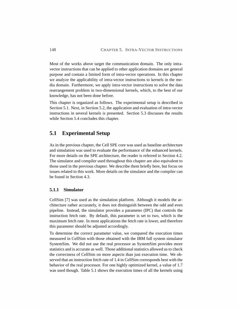
148 CHAPTER 5. INTRA-VECTOR INSTRUCTIONS
Most of the works above target the communication domain. The only intra-vector instructions that can be applied to other application domains are generalpurpose and contain a limited form of intra-vector operations. In this chapterwe analyze the applicability of intra-vector instructions to kernels in the me-dia domain. Furthermore, we apply intra-vector instructions to solve the datarearrangement problem in two-dimensional kernels, which, to the best of ourknowledge, has not been done before.
This chapter is organized as follows. The experimental setup is described inSection 5.1. Next, in Section 5.2, the application and evaluation of intra-vectorinstructions in several kernels is presented. Section 5.3 discusses the resultswhile Section 5.4 concludes this chapter.
5.1 Experimental Setup
As in the previous chapter, the Cell SPE core was used as baseline architectureand simulation was used to evaluate the performance of the enhanced kernels.For more details on the SPE architecture, the reader is referred to Section 4.2.The simulator and compiler used throughout this chapter are also equivalent tothose used in the previous chapter. We describe them briefly here, but focus onissues related to this work. More details on the simulator and the compiler canbe found in Section 4.3.
5.1.1 Simulator
CellSim [7] was used as the simulation platform. Although it models the ar-chitecture rather accurately, it does not distinguish between the odd and evenpipeline. Instead, the simulator provides a parameter (IPC) that controls theinstruction fetch rate. By default, this parameter is set to two, which is themaximum fetch rate. In most applications the fetch rate is lower, and thereforethis parameter should be adjusted accordingly.
To determine the correct parameter value, we compared the execution timesmeasured in CellSim with those obtained with the IBM full system simulatorSystemSim. We did not use the real processor as SystemSim provides morestatistics and is accurate as well. Those additional statistics allowed us to checkthe correctness of CellSim on more aspects than just execution time. We ob-served that an instruction fetch rate of 1.4 in CellSim corresponds best with thebehavior of the real processor. For one highly optimized kernel, a value of 1.7was used though. Table 5.1 shows the execution times of all the kernels using

5.1. EXPERIMENTAL SETUP 149
Table 5.1: Validation of CellSim.
IPC CyclesKernel (fetch rate) SystemSim CellSim Error
IDCT8 1.4 917 896 -2.3%IDCT4 1.4 2571 2524 -1.9%DF 1.4 121465 122122 0.5%IPol 1.4 2534 2598 2.5%MatMul 1.7 84180 85894 2.0%DWT 1.4 962640 994541 3.2%
both SystemSim and CellSim. It shows that the difference in execution time isat most 3.2%. Comparison of other statistics generated by the two simulatorsalso showed that CellSim is well suitable for its purpose.
5.1.2 Compiler
The compiler used throughout this work is spu-gcc version 4.1.1. The im-plemented intra-vector instructions were made available to the programmerthrough intrinsics or inline assembly in case intrinsics would require complexmodifications. The modifications assured that the compiler can handle the newinstructions, but not necessarily in an optimized way. Optimizing the compilerfor the new instructions is beyond the scope of this project.
5.1.3 Benchmark
We used six different kernels to demonstrate the effectiveness of intra-vectorinstructions. The kernels we used were either develop in-house before orwere taken from CellBench [5], which is a collection of publicly availableCell kernels. We examined all kernels available, searching for opportunitiesto apply intra-vector instructions. That is, we looked at inefficiencies of theSIMDimization and inefficiencies in the implementation of the algorithm. De-vising intra-vector instructions for a kernel requires a thorough understandingof the algorithm the kernel implements. Six kernels seemed amenable to theintra-vector paradigm, but we expect experts to be able to implement intra-vector instructions in many more kernels. The kernels used throughout thiswork are IDCT8, IDCT4, IPol (InterPolation), and DF (Deblocking Filter),originating from the FFmpeg H.264 video decoder [58]. Furthermore, we

150 CHAPTER 5. INTRA-VECTOR INSTRUCTIONS
+ + + +
SIMD Vector
(a)
+ + + +
(b)
Figure 5.1: Example of vertical processing of a matrix. Adding the elements of eachcolumn (a) can efficiently be performed with traditional SIMD instruc-tions, such as thevector-add instruction (b).
used the matrix multiply (MatMul) kernel from the Cell SDK. The last ker-nel is DWT (Discrete Wavelet Transform), taken from JasPer JPEG-2000 forCell [6].
5.2 The Intra-Vector SIMD Instructions
The principle of intra-vector instructions is well explained by the simple ex-ample of Figures 5.1 and 5.2. In both figures the elements of a matrix areprocessed. The matrix is stored in row-major order and, in this case but notnecessarily, one row fits in one SIMD vector. Figure 5.1(a) shows a verti-cal processing, i.e., the elements of each column are added. Such a compu-tation can efficiently be performed by traditional SIMD instructions, as thevector-add depicted in Figure 5.1(b).
In Figure 5.2(a), the matrix is processed in horizontal mode, i.e., the elementsof each row are added. To perform this computation using traditional SIMDinstructions, the data has to be rearranged, for example by a matrix transposi-tion. To avoid this overhead, intra-vector instructions can be used, such as theAltiVec sum-across instruction depicted in Figure 5.2(b).
Intra-vector instructions are not limited to matrix oriented kernels. The ex-ample shows however, that kernels that operate on matrices and perform bothvertical and horizontal processing are most likely to be amenable to the intra-vector paradigm. Also, the benefit of intra-vector instructions is not onlyavoiding rearrangement overhead as we will show in this section. Finally, weremark that the intra-vector instructions presented in this work are purposely
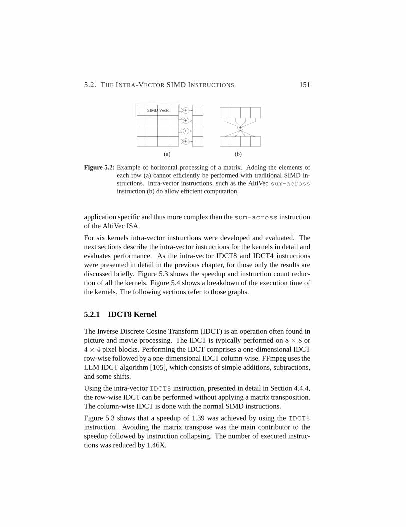
5.2. THE INTRA-VECTORSIMD INSTRUCTIONS 151
++
++SIMD Vector
(a)
+
(b)
Figure 5.2: Example of horizontal processing of a matrix. Adding the elements ofeach row (a) cannot efficiently be performed with traditional SIMD in-structions. Intra-vector instructions, such as the AltiVecsum-acrossinstruction (b) do allow efficient computation.
application specific and thus more complex than thesum-across instructionof the AltiVec ISA.
For six kernels intra-vector instructions were developed and evaluated. Thenext sections describe the intra-vector instructions for the kernels in detail andevaluates performance. As the intra-vector IDCT8 and IDCT4 instructionswere presented in detail in the previous chapter, for those only the results arediscussed briefly. Figure 5.3 shows the speedup and instruction count reduc-tion of all the kernels. Figure 5.4 shows a breakdown of the execution time ofthe kernels. The following sections refer to those graphs.
5.2.1 IDCT8 Kernel
The Inverse Discrete Cosine Transform (IDCT) is an operation often found inpicture and movie processing. The IDCT is typically performed on8 × 8 or4 × 4 pixel blocks. Performing the IDCT comprises a one-dimensional IDCTrow-wise followed by a one-dimensional IDCT column-wise. FFmpeg uses theLLM IDCT algorithm [105], which consists of simple additions, subtractions,and some shifts.
Using the intra-vectorIDCT8 instruction, presented in detail in Section 4.4.4,the row-wise IDCT can be performed without applying a matrix transposition.The column-wise IDCT is done with the normal SIMD instructions.
Figure 5.3 shows that a speedup of 1.39 was achieved by using theIDCT8instruction. Avoiding the matrix transpose was the main contributor to thespeedup followed by instruction collapsing. The number of executed instruc-tions was reduced by 1.46X.

152 CHAPTER 5. INTRA-VECTOR INSTRUCTIONS
0
0.5
1
1.5
2
DWTMatMulDFIPolIDCT4IDCT8
SpeedupReduction instructions
Figure 5.3: Speedup and instruction count reduction achieved using intra-vector in-structions.
0
0.2
0.4
0.6
0.8
1
IDCT8 IDCT4 IPol DF MatMul DWT
dependency stall cyclebranch stall cyclefetch stall cyclesingle issue cycledual issue cycle
Figure 5.4: Breakdown of the execution cycles normalized to the baseline kernel. Foreach kernel, the left is the baseline while the right is the enhanced versionusing intra-vector instructions.

5.2. THE INTRA-VECTORSIMD INSTRUCTIONS 153
5.2.2 IDCT4 Kernel
The IDCT4 kernel is similar to the IDCT8 kernel but operates on a4× 4 pixelblock. The computational structure of the one-dimensional IDCT4 is evensimpler than that of the IDCT8. Moreover, as a4 × 4 matrix of halfwordscompletely fits in two registers of 128-bits, the entire two-dimensional IDCT4could be performed using one instruction with two operands. This intra-vectorIDCT4 instruction reads the matrix from its two operand registers, performsthe arithmetic operations, and stores the result back in the two registers. Stor-ing the result could be done in one cycle if the the register file has two writeports, or otherwise two cycles are required. TheIDCT4 instruction is de-scribed in detail in Section 4.4.4.
Figure 5.3 shows that a speedup of 1.22 was achieved. Again, avoiding the ma-trix transposition was the main contributor to the speedup followed by instruc-tion collapsing. The number of executed instructions was reduced by 1.42X.Compared to theIDCT8 instruction, a significant lower speedup is obtained,although the instruction count reduction has only decreased a bit. This is be-cause the speedup of the IDCT4 kernel was limited by dependencies. Theinner loop of the kernel is small and by replacing multiple instructions withthe idct4 intra-vector instruction, the few instructions left were highly de-pending. Figure 5.4 shows that the dependency stall cycles nearly doubled.
5.2.3 Interpolation Kernel (IPol)
Motion compensation in H.264 has quarter pixel accuracy. In case a motionvector points to an integer position, the corresponding pixel is the predictedvalue. Otherwise, the prediction is obtained by interpolation of the neighboringpixels. Figure 5.5 illustrates this interpolation process. Pixels at half sampleposition are obtained by applying a 6-tap FIR filter as follows:
b = (20(G + H)− 5(F + I) + E + J + 16) >> 5 (5.1)
h = (20(G + M)− 5(C + R) + A + T + 16) >> 5 (5.2)
The result of the filter is clipped between 0 and 255. Pixels at quarter sampleposition are obtained by averaging the nearest half and full sample pixels. Thusfor every non integer motion vector, at least one 6 tap FIR filter has to beapplied.
This filter is one of the most time-consuming parts of the motion compensationkernel. Both the horizontal and the vertical filter can be SIMDimized to exploit

154 CHAPTER 5. INTRA-VECTOR INSTRUCTIONS
HG
M N
T U
R S
K L
E F
A
C
B
D
I J
QPNM s
n p q r
mkjih
d e f g
G a b c H
Figure 5.5: Pixels at fractional sample position (lower case letters) are determinedby applying an interpolation filter on the full sample pixels (upper case).Picture taken from [165].
FIR FIR FIR FIR FIR FIR FIR FIR
Figure 5.6: The ipol instruction computes eight FIR filters in parallel.
DLP, however, the first incurs considerable more overhead. When applying thehorizontal filter, the six input elements are located consecutive in memory andthus and intra-vector instruction could compute the entire filter at once.
Therefore, we propose theipol instruction. It computes eight 6 tap FIRfilters as indicated in Figure 5.6. Both the input and output operands are bytes.The computational structure of each FIR filter is depicted in Figure 5.7. Themultiplications are exchanged for shifts and additions to decrease latency. Theresult of the filter is also saturated between 0 and 255 in order to be able tostore the results as bytes. Note, that although the input and output operands ofthe instruction are bytes, internally halfwords have to be used in order not tolose precision.
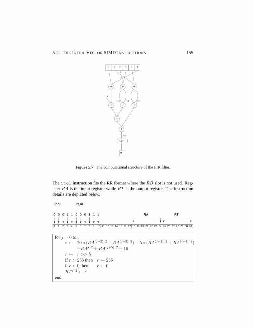
5.2. THE INTRA-VECTORSIMD INSTRUCTIONS 155
+ + +
+ + +
+
+
0 1 2 3 4 5
<<2 <<4 <<1
16
SAT
>>5
0
Figure 5.7: The computational structure of the FIR filter.
The ipol instruction fits the RR format where theRB slot is not used. Reg-isterRA is the input register whileRT is the output register. The instructiondetails are depicted below.
313029282726252423222120191817161514131211109876543210
RT0000 1 1 RA
rt,ra
0 1 1 1
ipol
0
for j = 0 to 5r ← 20 ∗ (RA(j+2)::2 + RA(j+3)::2)− 5 ∗ (RA(j+1)::2 + RA(j+4)::2)
+RAj::2 + RA(j+5)::2 + 16r ← r >> 5if r > 255 then r ← 255if r < 0 then r ← 0RT j::2 ← r
end
156 CHAPTER 5. INTRA-VECTOR INSTRUCTIONS
Table 5.2: Speedup and instruction count reduction obtained with theipol instruc-tion in the IPol kernel.
Baseline Enhanced ImprovementCycles 2390 1523 867 1.57Instructions 2473 1402 1071 1.76
The ipol instruction was made available to the programmer through an in-trinsic. The instruction was added to the simulator and the latency was set toten cycles for the following reason. Fixed point operations take two cyclesin the SPU architecture. Theipol instruction performs four steps of simplefixed point operations. We added another two cycles for the final shift andsaturation, making a total of ten.
We applied theipol instruction to the IPol kernel. This kernel consists ofmany functions, each for a different combination of block size and quartersample position. Theipol instruction can be used in any of those functionswhere a horizontal filter is applied, irrespective of the block size. We evaluatedthe ipol instruction with the function that computes the predicted value fora block of16 × 16 pixels with a motion vector at quarter sample position forboth the x and y coordinates. This function computes both a horizontal andvertical filter and is a good representative.
The speedup and instruction count reduction for the IPol kernel is shown inTable 5.2. A speedup of 1.57 is achieved, on the total two-dimensional kernel.This speedup is mainly achieved by reducing the number of instructions by1.76 times. Eachipol instruction replaces 67 instructions from the baselinekernel, including the following:
• Creation of auxiliary variables, such as vector of constants and masksfor shuffling.
• Aligning 6 input vectors (requiring some branches), instead of one.
• Unpack from bytes to halfwords and pack vice versa.
• Computation: 8 multiply-adds (each requiring a pack from words tohalfwords), 8 additions, 2 subtractions, 2 shifts, and 8 instructions forsaturation.

5.2. THE INTRA-VECTORSIMD INSTRUCTIONS 157
Figure 5.8: The process of deblocking one macroblock. Each square is a4 × 4 sub-block. Also the left and top neighboring sub-blocks are involved in theprocess.
Note that theipol instruction is only applied in the horizontal mode, andtherefore replacing 67 instructions with one, results in an instruction countreduction of 1.76 and not higher.
The speedup of the IPol kernel is lower than the instruction count reduction,which is the case for all but one kernel. The reason is the following. Multi-ple instructions are replaced by one. This decreases the code size but also theaverage distance between dependent instructions. Thus, there is less opportu-nity to schedule two instructions in the same cycle, or dependency stalls mighteven occur. This is reflected in Figure 5.4 which shows a breakdown of theexecution cycles. It shows that the enhanced IPol kernel has much less dualissue cycles than the baseline.
5.2.4 Deblocking Filter Kernel (DF)
The deblocking filter kernel is applied to remove an artifact introduced by theIDCT. The latter operates on4 × 4 or 8 × 8 sub-blocks and as a result squareareas might become visible in the decoded picture, which is called the ‘block-ing’ artifact. The DF kernel smoothes these block edges and thus improves theappearance of the decoded picture.
The process of deblocking a macroblock is depicted in Figure 5.8. Each squarerepresents a4× 4 sub-block. Also the left and top neighboring sub-blocks aredepicted as they are involved in the filtering. The filter is applied on all edges,starting with the vertical ones from left to right followed by the horizontal ones

158 CHAPTER 5. INTRA-VECTOR INSTRUCTIONS
Listing 5.1: Serial code of the dfy1 filter function of the DF kernel.
1 i f ( abs ( p0− q0 ) < a l p h a &&2 abs ( p1− p0 ) < b e t a &&3 abs ( q1− q0 ) < b e t a ) {45 i f ( abs ( p0− q0 ) < ( ( a l p h a >> 2 ) + 2 ) ){6 i f ( abs ( p2− p0 ) < b e t a ) {7 p0 = ( p2 + 2∗ p1 + 2∗ p0 + 2∗ q0 + q1 + 4 ) >> 3 ;8 p1 = ( p2 + p1 + p0 + q0 + 2 )>> 2 ;9 p2 = ( 2∗ p3 + 3∗ p2 + p1 + p0 + q0 + 4 )>> 3 ;
10 } e l s e {11 p0 = ( 2∗ p1 + p0 + q1 + 2 )>> 2 ;12 }13 i f ( abs ( q2− q0 ) < b e t a ) {14 q0 = ( p1 + 2∗ p0 + 2∗ q0 + 2∗ q1 + q2 + 4 ) >> 3 ;15 q1 = ( p0 + q0 + q1 + q2 + 2 )>> 2 ;16 q2 = ( 2∗ q3 + 3∗ q2 + q1 + q0 + p0 + 4 )>> 3 ;17 } e l s e {18 q0 = ( 2∗ q1 + q0 + p1 + 2 )>> 2 ;19 }20 } e l s e{21 p0 = ( 2∗ p1 + p0 + q1 + 2 )>> 2 ;22 q0 = ( 2∗ q1 + q0 + p1 + 2 )>> 2 ;23 }24 }
from top to bottom. The filter is applied to each line of pixels perpendicularto the edge and with a range of four pixels to each side of the edge. Thestrength of the filter is determined dynamically based on certain properties ofthe macroblock, but more importantly on the pixel gradient across the edge.
Listing 5.1 depicts the serial code of one of the two filter functions (referredto as dfy1) for the luma components. The DF kernel also contains two filterfunctions for the chroma components. The function of which the code is de-picted is the most complex one. Loading and storing of data is not included.The variablesalpha andbeta are inputs of the filter function. The pixelsare denoted as{p3,p2,p1,p0,q0,q1,q2,q3} , wherepx is a pixel onthe left (top) side of the edge, whileqx is a pixel on the right (bottom) side ofthe edge, assuming vertical (horizontal) filtering.

5.2. THE INTRA-VECTORSIMD INSTRUCTIONS 159
An efficient SIMD implementation for the Cell SPU was created byAzevedo [29]. The SIMDimized version only performs filtering in horizontalmode, thus the macroblock had to be transposed in order to perform verticalfiltering. The transposition overhead is approximately 12% of the executiontime of the kernel. The procedure using the SIMD implementation is as fol-lows: transpose all sub blocks involved, perform horizontal filtering, transposeall sub blocks back, perform horizontal filtering again.
Using intra-vector instructions for the vertical filtering, this transposition over-head can be avoided. Furthermore, instruction collapsing can be applied, re-ducing the time spent in computation. The procedure for the DF kernel usingintra-vector instructions is the following: perform vertical filtering using intra-vector instructions, perform horizontal filtering using the SIMDimized filterfunctions.
We implemented several intra-vector instructions for the DF kernel. As saidbefore, the kernel contains two filter functions for the luma components andtwo for the chroma components. All functions are similar although these forthe luma components are a bit more complex. We started implementing intra-vector instructions for the luma filter functions and, as we show later, foundout that those do not provide any speedup. Therefore, we did not implementintra-vector instructions for the chroma functions. We do report on those forthe luma functions as it provides insight in conditions for effective usage ofintra-vector instructions.
The two luma filter functions are referred to as dfy1 and dfy2.The corresponding ffmpeg function names are ‘filtermb edgeh’ and‘h264 loop filter luma c’, respectively. The functions differ to much to utilizethe same intra-vector instructions. Separate instructions were implemented in-stead, with the beginning of its mnemonic indicating for which function it canbe used.
The computation structure of the dfy1 function is depicted in Figure 5.9. Thisentire set of operations could be implemented in one instruction, but at the costof area and latency. Moreover, the latency might be larger than the depth ofthe current SPU pipeline. In such case, the number of forwarding stages willhave to be increased, again at the cost of area. Instead of using one instructionfor the entire filter function, the set of operations could be split in parts andimplemented in different instructions. We decided to explore both options,referring to the first as ‘complex’ and the latter as ‘simple’.
Using the complex intra-vector instructions, the code of the filter functionsbecomes rather simple and short, although some overhead is introduced to

160 CHAPTER 5. INTRA-VECTOR INSTRUCTIONS
+ + + + +
+ +
p3 p2 p1 p0 q0 q1 q2 q3
< <<<
+
p3 p2 p1 p0 q0 q1 q2 q3
+
+
+ +
+ +
+++
+
+
2
p1_1
+ +
+
+
+ +++
+
+
+ +
<<
p0_2 q0_2
4
2
q1_1
4
q2_1
alpha beta
diff diff diffbeta beta alpha
alpha 2
&
p0_1
2 2
2
+
p2_1
2
q0_1
diffbeta
diffbeta
Figure 5.9: Computational structure of the dfy1 filter function. Thedf y1c instruc-tion implements this entire computation. An arrow done means a shiftright by one bit while arrows up represent shifts left. A dotted line meansthe two input operands are the same.
rearrange the input data amenable to the new instructions. As a clarification,the code the of the dfy1 function is presented in Listing 5.2. Pixels are stored,in this case, as vectors of halfwords. As each vector contains eight pixels, datais stored in memory as8 × 8 matrices and the functions filter eight rows or

5.2. THE INTRA-VECTORSIMD INSTRUCTIONS 161
columns. In half of the cases, the pixels needed are stored within one8 × 8matrix (pointed to by*pix1 ). In the other cases, however, the pixels arestored across two matrices (pointed to by*pix1 and *pix2 ) and shufflesare required to combine the input pixels for each row into one vector and splitthe output pixels to store them in the original position. As the evaluation willshow, this overhead is large.
The df_y1c anddf_y2c instructions both fit the RR instructions format.OperandRA contains the pixels, whileRB contains the parametersalphaandbeta . The details of thedf_y1c instruction are depicted below.
313029282726252423222120191817161514131211109876543210
RT000 1 1 RA10
rt,ra,rb
RB0011
df_y1c
t ← RB0::4
u ← RB5::4
if( abs(RA6::2 −RA8::2) < t &&abs(RA4::2 −RA6::2) < u &&abs(RA10::2 −RA8::2) < u) thenif(abs(RA6::2 −RA8::2) < ((t >> 2) + 2)) then
if(abs(RA2::2 −RA6::2) < u) thenRT 6::2 ← (RA2::2 + 2 ∗RA4::2 + 2 ∗RA6::2 + 2 ∗RA8::2
+RA10::2 + 4) >> 3RT 4::2 ← (RA2::2 + RA4::2 + RA6::2 + RA8::2 + 2) >> 2RT 2::2 ← (2 ∗RA0::2 + 3 ∗RA2::2 + RA4::2 + RA6::2
+RA8::2 + 4) >> 3elseRT 6::2 ← (2 ∗RA4::2 + RA6::2 + RA10::2 + 2) >> 2if(abs(RA12::2 −RA8::2) < u) then
RT 8::2 ← (RA4::2 + 2 ∗RA6::2 + 2 ∗RA8::2 + 2 ∗RA10::2
+RA12::2 + 4) >> 3RT 10::2 ← (RA6::2 + RA8::2 + RA10::2 + RA12::2 + 2) >> 2RT 12::2 ← (2 ∗RA14::2 + 3 ∗RA12::2 + RA10::2 + RA8::2
+RA6::2 + 4) >> 3elseRT 8::2 ← (2 ∗RA10::2 + RA8::2 + RA4::2 + 2) >> 2
elseRT 6::2 ← (2 ∗RA4::2 + RA6::2 + RA10::2 + 2) >> 2;RT 8::2 ← (2 ∗RA10::2 + RA8::2 + RA4::2 + 2) >> 2;

162 CHAPTER 5. INTRA-VECTOR INSTRUCTIONS
Listing 5.2: Code of the dfy1 filter functions of the DF kernel using the complex DFintra-vector instruction.
1 cons t v u i n t 8 t combine =2 {0 x08 , 0 x09 , 0 x0a , 0 x0b , 0 x0c , 0 x0d , 0 x0e , 0 x0f ,3 0x10 , 0 x11 , 0 x12 , 0 x13 , 0 x14 , 0 x15 , 0 x16 , 0 x17} ;4 cons t v u i n t 8 t s p l i t l o w =5 {0 x10 , 0 x11 , 0 x12 , 0 x13 , 0 x14 , 0 x15 , 0 x16 , 0 x17 ,6 0x00 , 0 x01 , 0 x02 , 0 x03 , 0 x04 , 0 x05 , 0 x06 , 0 x07} ;7 cons t v u i n t 8 t s p l i t h i g h =8 {0 x08 , 0 x09 , 0 x0a , 0 x0b , 0 x0c , 0 x0d , 0 x0e , 0 x0f ,9 0x18 , 0 x19 , 0 x1a , 0 x1b , 0 x1c , 0 x1d , 0 x1e , 0 x1f} ;
10 v s i n t 3 2 t params = (v s i n t 3 2 t ) a l p h a ;11 params = s p ui n s e r t ( b e t a , params , 1 ) ;1213 f o r ( i = 0 ; i < 8 ; i + + ) {14 v u i n t 1 6 t p i x e l s ;15 i f ( do combine ){16 / / l oad & rea r range i n p u t da ta17 p i x e l s = s p u s h u f f l e (∗ ( p ix1 + i ) , ∗ ( p ix2 + i ) , combine ) ;1819 / / compute f i l t e r20 v u i n t 1 6 t r e s u l t = s p u d f y 1 c ( p i x e l s , params ) ;2122 / / r ea r range and s t o r e o u t p u t da ta23 ∗ ( p ix1 + i ) = s p u s h u f f l e ( r e s u l t 1 , ∗ ( p ix1 + i ) ,24 s p l i t l o w ) ;25 ∗ ( p ix2 + i ) = s p u s h u f f l e ( r e s u l t 1 , ∗ ( p ix2 + i ) ,26 s p l i t h i g h ) ;27 } e l s e {28 / / l oad da ta29 p i x e l s = ∗ ( p ix1 + i ) ;3031 / / compute f i l t e r32 v u i n t 1 6 t r e s u l t = s p u d f y 1 c ( p i x e l s , params ) ;3334 / / s t o r e da ta35 ∗ ( p ix1 + i ) = ( v s i n t 1 6 t ) r e s u l t 1 ;36 }37 }

5.2. THE INTRA-VECTORSIMD INSTRUCTIONS 163
Table 5.3: Speedup and instruction count reduction obtained with the complex DFinstructions in the DF kernel.
Baseline Enhanced ImprovementCycles 122135 120876 1259 1.01
Instructions 101480 86376 15104 1.17
The new instructions were made available to the programmer through intrin-sics (see also Listing 5.2). The instructions were added to the simulator andthe latency of both was set to 14 cycles. There are five stages of fixed pointoperations, each accounted for by two cycles. The 3-bit AND operation andthe three stages of muxes are accounted for by another two cycles. Finally,we added two more cycles for the complex routing in the first two stages (seeFigure 5.9). The complexity of thedf_y2c instruction is similar and thus hasthe same latency.
The simple DF intra-vector instructions implement only part of the computa-tional structure of Figure 5.9. Thedf_y1_p1 instructions computes the val-ues {p2_1,p1_1,p0_1,q0_1,q1_1,q2_1} , while df_y1_p2 com-putes the values{p0_2,q0_2} . To select the proper values for each pixel,two masks are created by instructionsdf_y1_m1 anddf_y1_m2 . Listing 5.3shows how these new functions work together to compute the dfy1 filter func-tion. For the dfy2 function a similar approach was used.
All the simple DF intra-vector instructions fit the RR instruction format. Theywere added to the simulator and made available to the programmer by intrin-sics. Considering the latency, the instructions were divided in two groups.Those that create a mask were assigned a latency of four cycles, just as anyother instruction in the SPU ISA that creates a mask. The other instructionswere assigned a latency of seven cycles. They mostly have three stages offixed point operations, each accounted for by two cycles. Further, we addedone cycles for the complex routing of the input values.
Table 5.3 and 5.4 present the speedup and reduction of the instruction countusing the complex and simple DF instructions, respectively. In both cases theenhanced kernel performs worse than the baseline kernel. To understand this,we summarize all the effects of using intra-vector instructions.
First, two transpositions of the pixel data are avoided, having a positive impacton the performance. On the other hand, new data rearrangement has beenintroduced as in half of the cases the input data is not aligned within one vector.

164 CHAPTER 5. INTRA-VECTOR INSTRUCTIONS
Listing 5.3: Code of the dfy1 filter functions of the DF kernel using the simple DFintra-vector instructions.
1 / / i n i t i a l i z a t i o n o m i t t e d due t o space c o n s t r a i n t s23 f o r ( i = 0 ; i < 8 ; i + + ) {4 v u i n t 1 6 t p i x e l s ;5 i f ( do combine ){6 / / l oad & rea r range i n p u t da ta7 p i x e l s = s p u s h u f f l e (∗ ( p ix1 + i ) , ∗ ( p ix2 + i ) , combine ) ;89 / / compute t h e f i l t e r
10 v u i n t 8 t mask1 , mask2 ;11 mask1 = spud f y1 m1 ( p i x e l s , params ) ;12 mask2 = spud f y1 m2 ( p i x e l s , params ) ;13 v u i n t 1 6 t r e s u l t 1 = s p ud f y 1 p 1 ( p i x e l s ) ;14 v u i n t 1 6 t r e s u l t 2 = s p ud f y 1 p 2 ( p i x e l s ) ;15 r e s u l t 1 = s p u s h u f f l e ( r e s u l t 1 , r e s u l t 2 , mask2 ) ;16 r e s u l t 1 = s p u s h u f f l e ( r e s u l t 1 , p i x e l s , mask1 ) ;1718 / / r ea r range & s t o r e o u t p u t da ta19 ∗ ( p ix1 + i ) = s p u s h u f f l e ( r e s u l t 1 , ∗ ( p ix1 + i ) ,20 s p l i t l o w ) ;21 ∗ ( p ix2 + i ) = s p u s h u f f l e ( r e s u l t 1 , ∗ ( p ix2 + i ) ,22 s p l i t h i g h ) ;23 } e l s e {24 / / l oad da ta25 p i x e l s = ∗ ( p ix1 + i ) ;2627 / / compute t h e f i l t e r28 v u i n t 8 t mask1 , mask2 ;29 mask1 = spud f y1 m1 ( p i x e l s , params ) ;30 mask2 = spud f y1 m2 ( p i x e l s , params ) ;31 v u i n t 1 6 t r e s u l t 1 = s p ud f y 1 p 1 ( p i x e l s ) ;32 v u i n t 1 6 t r e s u l t 2 = s p ud f y 1 p 2 ( p i x e l s ) ;33 r e s u l t 1 = s p u s h u f f l e ( r e s u l t 1 , r e s u l t 2 , mask2 ) ;34 r e s u l t 1 = s p u s h u f f l e ( r e s u l t 1 , p i x e l s , mask1 ) ;3536 / / s t o r e da ta37 ∗ ( p ix1 + i ) = ( v s i n t 1 6 t ) r e s u l t 1 ;38 }39 }

5.2. THE INTRA-VECTORSIMD INSTRUCTIONS 165
Table 5.4: Speedup and instruction count reduction obtained with the simple DF in-structions in the DF kernel.
Baseline Enhanced ImprovementCycles 122135 120596 1539 1.01
Instructions 101480 89704 11776 1.13
The latter rearrangement requires some shuffles but also additional loads andstores. For example, the code of Listing 5.2 performs 33 loads and 16 stores.That is an overhead of 4 loads and two stores per intra-vector instruction.
Second, the resulting code has many dependencies within few instructions. Forexample, the code of Listing 5.2 has the following instruction order: loads (2),shuffle, dfy1c, loads (2), shuffles (2), stores (2). Only the instructions that aregrouped within this list are independent. Consecutive groups are dependentand cause pipeline stalls. Even when applying loop unrolling this functiontakes more than three times the number of cycles compared to the SIMD ver-sion. The latter takes 77 cycles and 97 instructions while the enhanced takes275 cycles and 107 instructions. In total 131 cycles are dependency stalls,while most other cycles are single issue. From these numbers we concludethat dependencies are the main cause of the loss of performance.
Third, the DLP exploited by the DF intra-vector instructions is smaller thanin the SIMD version. Some of the intra-vector instructions compute only twooutputs, while the SIMD version always computes eight outputs. This loss ofDLP is compensated by the instruction collapsing, especially in the complexintra-vector instructions.
Finally, applying intra-vector instructions on the DF kernel, introduced somebranches, which are costly in the SPE architecture. For example, the code ofListing 5.2 incurs 30 branch stall cycles in half the cases.
We conclude the following from the experiments with this kernel. First, intra-vector instructions are likely not to be efficient if data is not naturally alignedwithin vectors. Second, performance gains obtained by intra-vector instruc-tions are likely to be proportional to the number of its output elements.
5.2.5 Matrix Multiply Kernel (MatMul)
Dense matrix-matrix multiplication is used in many scientific applications. Asthe matrices are often large (M=1024 or larger) and the algorithm has a time

166 CHAPTER 5. INTRA-VECTOR INSTRUCTIONS
B1
B2
B3
B4A4
A3
A2
A1
C3
C4
C1
C2+= X
Figure 5.10: Data layout of the baseline4× 4 matrix multiply. The vectors of matrixA have to be broken down in order to compute the matrix multiply.
complexity ofO(M3), fast execution of the matrix multiply (in short Matmul)kernel is of vital importance.
An efficient implementation using the multicore and SIMD capabilities of theCell processor was provided with SDK 3.0. The matrix multiplication is bro-ken down into multiplications of64 × 64 matrices, which fit in the SPE localstore size. Within the SPE this multiplication is broken down into smaller partsin two steps, such that in the end matrices of4× 4 are multiplied. The SIMDwidth of the SPU is four slots of single precision floats, and thus one row of the4× 4 matrix is contained within one SIMD vector as depicted in Figure 5.10.A 4 × 4 matrix multiply is part of a larger matrix multiplication, and thusthe result has to be added to the intermediate value in the output matrix, i.e.,C+ = A×B.
In order to utilize the SIMD capabilities, the elements of matrix A have to beextracted and splatted. For example, the first row of matrix C is computed as:
C1+ = a1 1 ∗B1 + a1 2 ∗B2 + a1 3 ∗B3 + a1 4 ∗B4, (5.3)
wherea1x is the xth element of vector A1. Listing 5.4 shows the SPU codethat performs this computation. The maskssplatx are used multiple timesand do not constitute a large overhead. Extracting and splatting the elementsof matrix A does constitute a significant overhead, although in the optimizedimplementation of the64 × 64 matrix multiplication the result is reused fourtimes, decreasing the total overhead.
Using the intra-vector paradigm, the matrix multiplication could be brokendown into blocks of2 × 2. A 2 × 2 block contains four floats which fit inone SIMD vector. Thus a2 × 2 matrix multiply can be done in one instruc-tion. We propose thefmatmul rt,ra,rb (Floating MATrix MULtiply)andfmma rt,ra,rb,rc (Floating Matrix Multiply Add) instructions thatmultiply the 2 × 2 matrices contained inra and rb and stores the result inregisterrt . Thefmma instructions also adds the matrix contained inrc to theresult.

5.2. THE INTRA-VECTORSIMD INSTRUCTIONS 167
Listing 5.4: Example code that computes the first output row of a4× 4 matrix multi-ply.
1 v e c t o r uchar s p l a t 0 ={ 0 , 1 , 2 , 3 , 1 6 , 1 7 , 1 8 , 1 9 ,2 0 , 1 , 2 , 3 , 1 6 , 1 7 , 1 8 , 1 9} ;3 v e c t o r uchar s p l a t 1 , s p l a t 2 , s p l a t 3 ;45 s p l a t 1 = s p uo r ( s p l a t 0 , 4 ) ;6 s p l a t 2 = s p uo r ( s p l a t 0 , 8 ) ;7 s p l a t 3 = s p uo r ( s p l a t 0 , 1 2 ) ;89 a1 1 = s p u s h u f f l e (A1 , A1 , s p l a t 0 ) ;
10 a1 2 = s p u s h u f f l e (A1 , A1 , s p l a t 1 ) ;11 a1 3 = s p u s h u f f l e (A1 , A1 , s p l a t 2 ) ;12 a1 4 = s p u s h u f f l e (A1 , A1 , s p l a t 3 ) ;1314 C1 = spu madd ( a1 1 , B1 , C1 ) ;15 C1 = spu madd ( a1 2 , B2 , C1 ) ;16 C1 = spu madd ( a1 3 , B3 , C1 ) ;17 C1 = spu madd ( a1 4 , B4 , C1 ) ;
X+=
C1 C2
C3
A1
A3
A2 B1 B2
B3C4 A4 B4
Figure 5.11: Data layout of the enhanced4×4 matrix multiply using2×2 sub blocks.Each2× 2 block is located within one SIMD vector.
Assuming the data of a4×4 matrix is rearranged such that the four2×2 blocksare located within SIMD vectors (as indicated in Figure 5.11), one block of theoutput can be computed with two instructions only, as shown in Listng 5.5.Usually the input data is not arranged in such a way, and therefore additionalconversion overhead is required. As we show later, the overhead does notcounterbalance the benefits.
The fmatmul instruction fits the RR instruction format. The instruction de-tails are depicted below. Theffma instruction fits the RRR instruction format.Only a few opcodes for this instruction format are available in the SPU. Op-tionally, the RR format could be used if registerrt is used for both input andoutput. The instruction details as we implemented it, are depicted below.

168 CHAPTER 5. INTRA-VECTOR INSTRUCTIONS
Listing 5.5: The code of Listing 5.4 can be replaced by the following when using theintra-vectorfmma instruction.
1 C1 = spu fmma (A1 , B1 , C1 ) ;2 C1 = spu fmma (A2 , B3 , C1 ) ;
313029282726252423222120191817161514131211109876543210
RT00 1 RA1
rt,ra,rb
RB01
fmatmul
0 1 1 0 1
RT 0::4 ← RA0::4 ∗RB0::4 +RA4::4 ∗RB8::4
RT 4::4 ← RA0::4 ∗RB4::4 +RA4::4 ∗RB12::4
RT 8::4 ← RA8::4 ∗RB0::4 +RA12::4 ∗RB8::4
RT 12::4 ← RA8::4 ∗RB4::4 +RA12::4 ∗RB12::4
313029282726252423222120191817161514131211109876543210
RTRARB
rt,ra,rb,rc
RC1 0
fmma
0 1
RT 0::4 ← RA0::4 ∗RB0::4 +RA4::4 ∗RB8::4 +RC0::4
RT 4::4 ← RA0::4 ∗RB4::4 +RA4::4 ∗RB12::4 +RC4::4
RT 8::4 ← RA8::4 ∗RB0::4 +RA12::4 ∗RB8::4 +RC8::4
RT 12::4 ← RA8::4 ∗RB4::4 +RA12::4 ∗RB12::4 +RC12::4
The fmatmul and fmma instruction were made available to theprogrammer trough the intrinsicsd = spu_fmma(a,b,c); andd = spu_fmatmul(a,b); . The instructions were added to the sim-ulator and the compiler. The latency of thefmatmul instruction was setto six cycles. A normal floating point multiply-add takes six cycles. Thefmatmul performs twice the number of multiplies, but those can be done inparallel. Thefmatmul instruction performs an addition, just like the normalmultiply add. Thus the latencies of those two are the same. The final additionof the fmma instruction, though, has three inputs instead of two and weaccount for this by adding two cycles to the latency. This is rather pessimistic,but on the safe side.

5.2. THE INTRA-VECTORSIMD INSTRUCTIONS 169
Table 5.5: Speedup and instruction count reduction obtained with thefmatmul in-struction in the Matmul kernel.
Baseline Enhanced ImprovementCycles 85894 69094 16800 1.24Instructions 136585 111048 25537 1.23
Table 5.6: Speedup and instruction count reduction obtained with thefmma instruc-tion in the Matmul kernel.
Baseline Enhanced ImprovementCycles 85894 41735 44159 2.06Instructions 136585 63239 73346 2.16
We applied the intra-vector instructions to the Matmul kernel taken from theCell SDK. The kernel contains several versions of the SPU code that multipliesthe64 × 64 blocks, each with a higher degree of optimization. We used theoptimized SIMD version, which is written in C code. There is also an evenmore optimized version written in assembly. We will indicate the expectedperformance of our enhanced kernel when written in assembly.
We did not change the general strategy of the64 × 64 multiply function, butonly changed the code at the subblock-level. We measured the time of one64 × 64 matrix multiply add only. The Matmul kernel uses double bufferingand is computation bound, and thus this measure is representative for the entirekernel. In the measurement results presented here we do not include the over-head cost for rearranging the data. This rearrangement has time a complexityof O(M2) and is fully data parallel. The matrix multiplication itself has a timecomplexity ofO(M3) and thus the overhead cost decreases exponentially forincreasing matrix sizes. ForM = 64 the overhead is 19.1%, but forM = 1024(which is a more realistic matrix size) the overhead is only 1.2%.
Table 5.5 shows the results obtained with thefmatmul instruction. A speedupof 1.24 is achieved and a similar reduction in the number of executed instruc-tions. The speedup is significant but limited. Everyfmatmul instruction isfollowed by an addition, mitigating much of the benefits. This is confirmed bythe results of thefmma instruction, depicted in Table 5.6. A speedup of 2.06 isachieved which is much larger than the former because many add instructionsare collapsed into thefmma instruction.
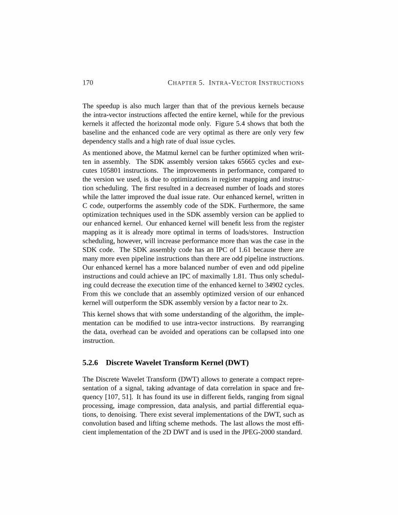
170 CHAPTER 5. INTRA-VECTOR INSTRUCTIONS
The speedup is also much larger than that of the previous kernels becausethe intra-vector instructions affected the entire kernel, while for the previouskernels it affected the horizontal mode only. Figure 5.4 shows that both thebaseline and the enhanced code are very optimal as there are only very fewdependency stalls and a high rate of dual issue cycles.
As mentioned above, the Matmul kernel can be further optimized when writ-ten in assembly. The SDK assembly version takes 65665 cycles and exe-cutes 105801 instructions. The improvements in performance, compared tothe version we used, is due to optimizations in register mapping and instruc-tion scheduling. The first resulted in a decreased number of loads and storeswhile the latter improved the dual issue rate. Our enhanced kernel, written inC code, outperforms the assembly code of the SDK. Furthermore, the sameoptimization techniques used in the SDK assembly version can be applied toour enhanced kernel. Our enhanced kernel will benefit less from the registermapping as it is already more optimal in terms of loads/stores. Instructionscheduling, however, will increase performance more than was the case in theSDK code. The SDK assembly code has an IPC of 1.61 because there aremany more even pipeline instructions than there are odd pipeline instructions.Our enhanced kernel has a more balanced number of even and odd pipelineinstructions and could achieve an IPC of maximally 1.81. Thus only schedul-ing could decrease the execution time of the enhanced kernel to 34902 cycles.From this we conclude that an assembly optimized version of our enhancedkernel will outperform the SDK assembly version by a factor near to 2x.
This kernel shows that with some understanding of the algorithm, the imple-mentation can be modified to use intra-vector instructions. By rearrangingthe data, overhead can be avoided and operations can be collapsed into oneinstruction.
5.2.6 Discrete Wavelet Transform Kernel (DWT)
The Discrete Wavelet Transform (DWT) allows to generate a compact repre-sentation of a signal, taking advantage of data correlation in space and fre-quency [107, 51]. It has found its use in different fields, ranging from signalprocessing, image compression, data analysis, and partial differential equa-tions, to denoising. There exist several implementations of the DWT, such asconvolution based and lifting scheme methods. The last allows the most effi-cient implementation of the 2D DWT and is used in the JPEG-2000 standard.
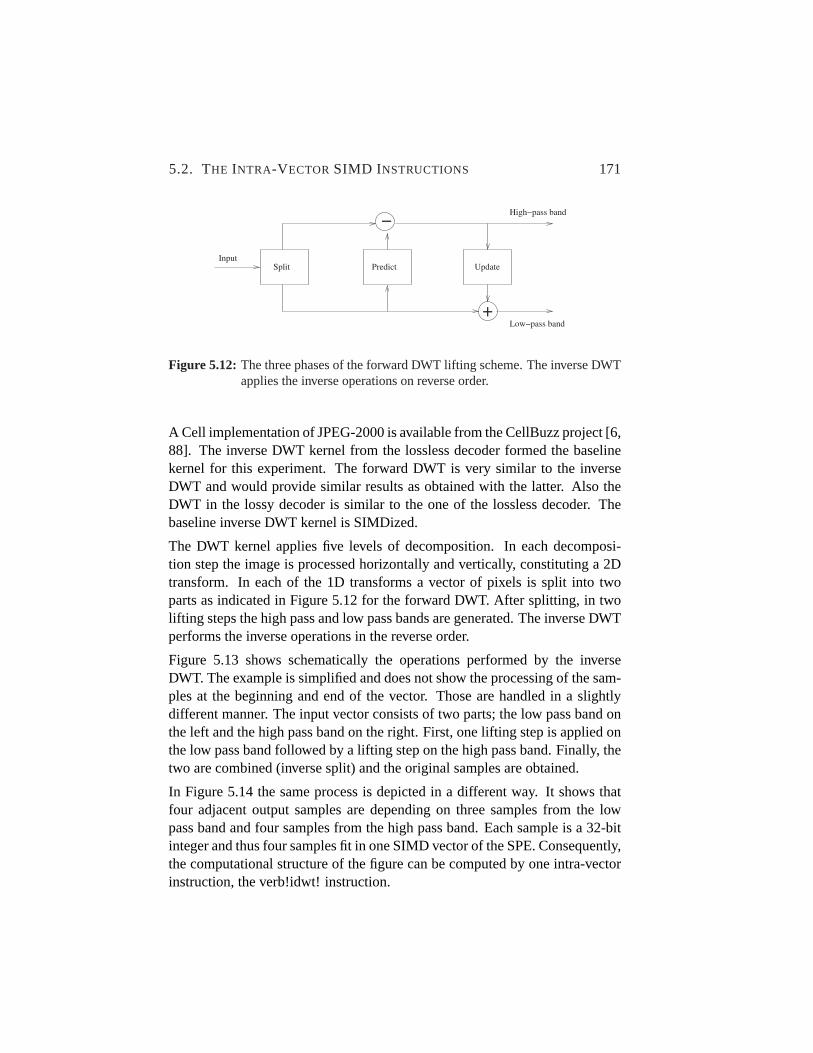
5.2. THE INTRA-VECTORSIMD INSTRUCTIONS 171
InputUpdateSplit Predict
Low−pass band
High−pass band
+
−
Figure 5.12: The three phases of the forward DWT lifting scheme. The inverse DWTapplies the inverse operations on reverse order.
A Cell implementation of JPEG-2000 is available from the CellBuzz project [6,88]. The inverse DWT kernel from the lossless decoder formed the baselinekernel for this experiment. The forward DWT is very similar to the inverseDWT and would provide similar results as obtained with the latter. Also theDWT in the lossy decoder is similar to the one of the lossless decoder. Thebaseline inverse DWT kernel is SIMDized.
The DWT kernel applies five levels of decomposition. In each decomposi-tion step the image is processed horizontally and vertically, constituting a 2Dtransform. In each of the 1D transforms a vector of pixels is split into twoparts as indicated in Figure 5.12 for the forward DWT. After splitting, in twolifting steps the high pass and low pass bands are generated. The inverse DWTperforms the inverse operations in the reverse order.
Figure 5.13 shows schematically the operations performed by the inverseDWT. The example is simplified and does not show the processing of the sam-ples at the beginning and end of the vector. Those are handled in a slightlydifferent manner. The input vector consists of two parts; the low pass band onthe left and the high pass band on the right. First, one lifting step is applied onthe low pass band followed by a lifting step on the high pass band. Finally, thetwo are combined (inverse split) and the original samples are obtained.
In Figure 5.14 the same process is depicted in a different way. It shows thatfour adjacent output samples are depending on three samples from the lowpass band and four samples from the high pass band. Each sample is a 32-bitinteger and thus four samples fit in one SIMD vector of the SPE. Consequently,the computational structure of the figure can be computed by one intra-vectorinstruction, the verb!idwt! instruction.

172 CHAPTER 5. INTRA-VECTOR INSTRUCTIONS
+
2
−
+
0 1 2 3 4 5 6 7
0 1 2 3 4 5 6 7
0 1 2 3 4 5 6 7
++
+ +
0 1 2 3 4 5 6 7
−
2
High−pass bandLow−pass band
Figure 5.13: Schematic overview of the computational structure of the inverse DWTon an example vector of eight samples. An arrow indicates a shift rightby one bit (two bits for a double arrow). The edges of the two sub bandsare processed slightly different and not shown in this diagram.
The idwt instruction is efficient in the horizontal inverse DWT as both theinput and output vector have elements in consecutive memory locations. Toapply theidwt instruction in the vertical DWT a lot of rearrangement over-head is required. Moreover, conventional SIMDimization is efficient in thevertical DWT, and therefore there is no need to apply the intra-vector instruc-tion to the vertical DWT.
As mentioned above, processing the first and last samples of a vector are doneslightly different. Therefore, theidwt instruction can only be applied to thebody of the vector. The head, consisting of four output samples, is performedusing scalar operations as well as the tail, consisting of at least one sample.The size of the vectors is usually large. Assuming an image of512 × 512pixels, the vector sizes for the DWT are 32, 64, 128, 256, and 512.

5.2. THE INTRA-VECTORSIMD INSTRUCTIONS 173
+ + +
+
++
+
2*i 2*i+1 2*i+2 2*i+3
High−pass bandLow−pass band
mid+i−1 mid+i mid+i+1 mid+i+2i i+1 i+2 i+3
2 2 2
−− −
Figure 5.14: A different representation of the computational structure of the inverseDWT. This time a larger vector is assumed and only partially displayed.All stages are combined in one step. The computations depicted can beperformed with theidwt intra-vector instruction.
The idwt instruction fits the RR instruction format. The instruction detailsare depicted below. The corresponding intrinsicd = spu_idwt(a,b) wasadded to the compiler. The latency of the instruction in the simulator was setto eight cycles. The critical path contains four simple fixed point operations,each taking two cycles and adding up to eight. We assume the latency of theshifts can be neglected.
We evaluated theidwt intra-vector instruction using the Cell implementationof JPEG-2000. The DWT kernel in this application is a cooperation betweenthe PPU and the SPUs. The first divides the work while the SPUs DMA in thedata and perform the actual DWT. We decoded a picture of512 × 512 pixelsand measured the actual time spent on the DWT in the SPUs. The results aredepicted in Table 5.7 and show that a significant speedup of 1.59 is obtained.Interestingly, the speedup is larger than the instruction count reduction. Fig-ure 5.4 shows that the baseline kernel suffered severely from dependency andbranch stalls. The new method of processing the array, enabled by intra-vectorinstructions, proves to be more efficient as both types of stall cycles are sub-stantially reduced. The DWT can also be applied to a one-dimensional dataarray. In that case the speedup achieved will even be larger. We obtained aspeedup of 2.53 on an array of 512 pixels.

174 CHAPTER 5. INTRA-VECTOR INSTRUCTIONS
Table 5.7: Speedup and instruction count reduction obtained with theidwt instruc-tion in the inverse DWT kernel.
Baseline Enhanced ImprovementCycles 10948039 6893905 4054134 1.59
Instructions 5117073 3685579 1431494 1.39
313029282726252423222120191817161514131211109876543210
RT000 1 1 RA10
rt,ra,rb
RB01
idwt
0 1
t0 ← RA0::4 − ((RB0::4 + RB4::4 + 2) >> 2)t2 ← RA4::4 − ((RB4::4 + RB8::4 + 2) >> 2)t ← RA8::4 − ((RB8::4 + RB12::4 + 2) >> 2)t1 ← RB4::4 + ((t0 + t2) >> 1)t3 ← RB8::4 + ((t2 + t) >> 1)
RT 0::4 ← t0RT 4::4 ← t1RT 8::4 ← t2RT 12::4 ← t3
Whereas the inner loop of all other kernels operate on small sub-blocks, in theDWT kernel entire rows and columns are processed. Therefore, the speedupof the kernel is depending on the input size. So far, an input image of512 ×512 pixels was assumed. Figure 5.15 shows that for smaller input sizes, thespeedup and instruction count reductions are actually larger. For smaller inputsizes, the startup overhead (processing the edges, initializing variables, etc.)dominates. This overhead is larger in the baseline kernel than is the case inthe enhanced kernel. Therefore, the speedup is larger for small input sizes andflattens out for larger sizes.
The DWT kernel is another example of how large speedups can be achievedby intra-vector instructions. It shows that they can enable a more efficient pro-cessing of the data. The DWT kernel also shows that intra-vector instructioncan be applied to one-dimensional kernels.
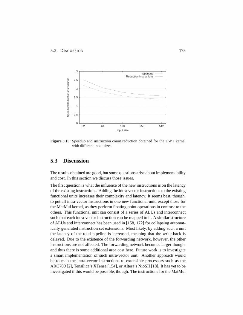
5.3. DISCUSSION 175
0
0.5
1
1.5
2
2.5
3
32 64 128 256 512
Spe
edup
/Red
uctio
n in
stru
ctio
ns
Input size
SpeedupReduction instructions
Figure 5.15: Speedup and instruction count reduction obtained for the DWT kernelwith different input sizes.
5.3 Discussion
The results obtained are good, but some questions arise about implementabilityand cost. In this section we discuss those issues.
The first question is what the influence of the new instructions is on the latencyof the existing instructions. Adding the intra-vector instructions to the existingfunctional units increases their complexity and latency. It seems best, though,to put all intra-vector instructions in one new functional unit, except those forthe MatMul kernel, as they perform floating point operations in contrast to theothers. This functional unit can consist of a series of ALUs and interconnectsuch that each intra-vector instruction can be mapped to it. A similar structureof ALUs and interconnect has been used in [158, 172] for collapsing automat-ically generated instruction set extensions. Most likely, by adding such a unitthe latency of the total pipeline is increased, meaning that the write-back isdelayed. Due to the existence of the forwarding network, however, the otherinstructions are not affected. The forwarding network becomes larger though,and thus there is some additional area cost here. Future work is to investigatea smart implementation of such intra-vector unit. Another approach wouldbe to map the intra-vector instructions to extensible processors such as theARC700 [2], Tensilica’s XTensa [154], or Altera’s NioSII [18]. It has yet to beinvestigated if this would be possible, though. The instructions for the MatMul

176 CHAPTER 5. INTRA-VECTOR INSTRUCTIONS
kernel probably are best added to the existing single precision unit. Similarlythis would increase the latency of the pipeline.
A second issue is the area cost of the intra-vector instructions. Without anactual hardware implementation, some back of the envelope calculations arethe best we can do. The intra-vector unit needs five levels of simple fixedpoint operations (no multiplication) and interconnect in between. The fixedpoint unit of the SPE performs these operations and from the floor plan wedetermined that the area of the fixed point unit is 3% of the total SPE. Thisfixed point unit can perform much more diverse operations as needed by theintra-vector unit, and also can operate on 32-bit values, while the intra-vectorunit needs to operate on 8 and 16-bit values only. On the other hand, the intra-vector unit requires more ALUs per level and additional interconnect. Weestimate that the area taken per level is 1.5 times that of the fixed point unit.Therefore, adding the intra-vector unit to the SPE requires approximately anadditional 5× 3× 1.5= 22.5% of area. Addition of the MatMul instructionsto the single precision pipeline is expected to double its size, requiring 10% ofadditional area.
Another question might be whether the latencies of the instructions are correct.Discussion with experts showed us that our methodology of determining thelatencies is on the safe side. We also analyzed the speedups for larger latencies,however. Figure 5.16 shows that the average speedup only drops from 1.45 to1.31 in the unlikely case when the latencies would be twice as large.
The speedups achieved seems to be worth the area cost. The average speedupis obtained on kernels only, though. The speedup on complete applicationswill be lower, although in the signal processing domain generally the kernelsdominate the execution time. Application specific processors targeted at sig-nal processing therefore seem to be most suitable for specialized intra-vectorinstructions as we presented them.
5.4 Conclusions
In this chapter we have shown that intra-vector SIMD instructions are an ef-fective technique for the specialization of cores, especially in the signal pro-cessing domain. For six kernels intra-vector instructions have been developedand simulations have shown that a speedup of up to 2.06 was achieved, withan average of 1.45.
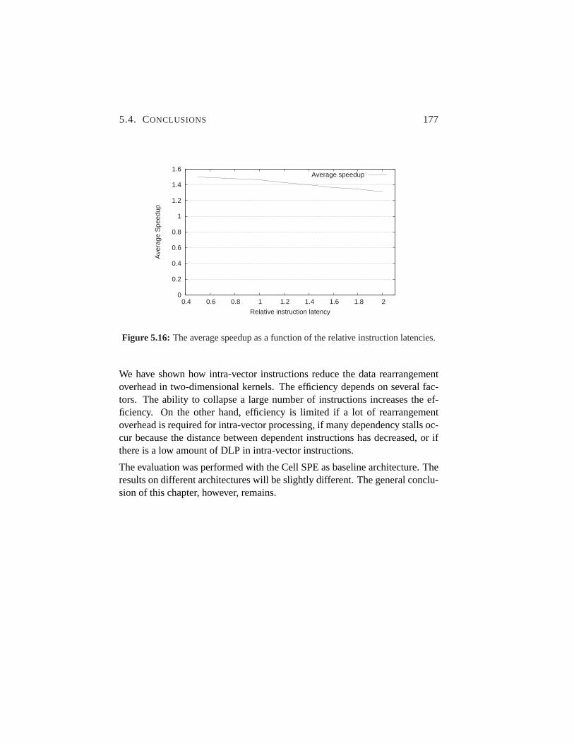
5.4. CONCLUSIONS 177
0
0.2
0.4
0.6
0.8
1
1.2
1.4
1.6
0.4 0.6 0.8 1 1.2 1.4 1.6 1.8 2
Ave
rage
Spe
edup
Relative instruction latency
Average speedup
Figure 5.16: The average speedup as a function of the relative instruction latencies.
We have shown how intra-vector instructions reduce the data rearrangementoverhead in two-dimensional kernels. The efficiency depends on several fac-tors. The ability to collapse a large number of instructions increases the ef-ficiency. On the other hand, efficiency is limited if a lot of rearrangementoverhead is required for intra-vector processing, if many dependency stalls oc-cur because the distance between dependent instructions has decreased, or ifthere is a low amount of DLP in intra-vector instructions.
The evaluation was performed with the Cell SPE as baseline architecture. Theresults on different architectures will be slightly different. The general conclu-sion of this chapter, however, remains.


Chapter 6
Hardware Task ManagementSupport for the StarSSProgramming Model: theNexus System
Successfuldeployment of many-core chips depends on the availabilityof parallel applications. Creating efficient parallel applications, though,is currently cumbersome and complicated as, besides parallelization, it
requires task scheduling, synchronization, programming or optimizing datatransfers, etc. Our experiences with the implementation of parallel H.264 de-coding for several platforms, as described in Chapter 3, confirm this statement.
Currently there are several efforts to solve the programmability issues of mul-ticores. Among these is the task-based StarSS programming model [129]. Itrequires the programmer only to indicate functions, referred to as tasks, that areamenable to parallel execution and to specify the input and output operands.All the other issues, such as determining task dependencies, scheduling, pro-gramming and issuing data transfers, etc., are automatically handled by StarSS.
The task management performed by the StarSS runtime system is rather labo-rious. This overhead affects the scalability and performance, and potentiallylimits the applicability of StarSS applications. In this chapter we study thebenefits of accelerating task management with hardware support. We showthat for fine-grained tasks, the runtime overhead greatly reduces performanceand severely limits scalability. Through extensive analysis of the current sys-
179

180 CHAPTER 6. HARDWARE TASK MANAGEMENT SUPPORT
tem’s bottlenecks, we specify the requirements of a hardware support system.
As an example of such a system, we present Nexus: a hardware task man-agement support system compliant with the StarSS programming model. Wepresent the design of the hardware, as well as the software interface. TheNexus system is evaluated by means of simulation, which shows that the re-quirements are met. By using the Nexus system, StarSS can be efficiently usedwith much smaller task sizes.
Some other works have proposed hardware support for task management.Most are limited, however, to scheduling of independent tasks leaving it up tothe programmer to deliver tasks at the appropriate time. Carbon [94] provideshardware task queuing enabling low latency task retrieval. In [79] a TriMedia-based multicore system is proposed containing a centralized task schedulingunit based on Carbon. For a multicore media SoC, Ou et al. [122] propose ahardware interface to manage tasks on the DSP, mainly to avoid OS interven-tion. Architectural support for the Cilk programming model has been proposedin [106], mainly focusing on cache coherency.
A few works include hardware task dependency resolution. In [142] a lookahead task management unit has been proposed reducing the task retrieval la-tency. It uses task dependencies in a reversed way to predict due availabletasks. Because of the programmable nature, its latency is rather large. The lat-ter issue has been resolved in [17] at the cost of generality: the proposed hard-ware is specific for H.264 decoding. For System-on-Chips (SoCs), an Appli-cation Specific Instruction set Processor (ASIP) has been proposed to speedupsoftware task management [35]. Independently, Etsion et al. [57] have also de-veloped hardware support for the StarSS programming model. They observea similarity between input and output dependencies of tasks and instructionsand have proposed task management hardware that works similar to an out-of-order instruction scheduler.
A different approach called Decoupled Thread Architecture (DTA) has beenproposed by Giorgi et al. [64] and is based on thread level data-flow. Threadscan be as small as functions and thus their approach is applicable to fine-grained parallelization. Data is sent from a producer to a consumer threaddirectly by distributed hardware units. This data communication also functionsas synchronization. In [65] an implementation of DTA for the Cell processorhas been described. Also based on the data-flow principle is the approach thathas been proposed by Stavrou et al. [146]. In contrast to DTA, this approach iscoarse grained, especially the scheduling among cores. A programming modelfor these two data-flow approaches has been presented in [147].
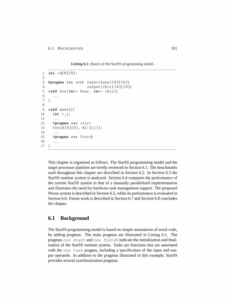
6.1. BACKGROUND 181
Listing 6.1: Basics of the StarSS programming model.
1 i n t ∗A[N] [N ] ;23 #pragma c s s t a s k i n p u t ( base [ 1 6 ] [ 1 6 ] )4 o u t p u t ( t h i s [ 1 6 ] [ 1 6 ] )5 vo id foo ( i n t ∗ base , i n t ∗ t h i s ){6 . . .7 }89 vo id main ( ){
10 i n t i , j ;11 . . .12 #pragma c s s s t a r t13 foo (A [ 0 ] [ 0 ] , A[ i ] [ j ] ) ;14 . . .15 #pragma c s s f i n i s h16 . . .17 }
This chapter is organized as follows. The StarSS programming model and thetarget processor platform are briefly reviewed in Section 6.1. The benchmarksused throughout this chapter are described in Section 6.2. In Section 6.3 theStarSS runtime system is analyzed. Section 6.4 compares the performance ofthe current StarSS system to that of a manually parallelized implementationand illustrates the need for hardware task management support. The proposedNexus system is described in Section 6.5, while its performance is evaluated inSection 6.6. Future work is described in Section 6.7 and Section 6.8 concludesthe chapter.
6.1 Background
The StarSS programming model is based on simple annotations of serial code,by adding pragmas. The main pragmas are illustrated in Listing 6.1. Thepragmascss start andcss finish indicate the initialization and final-ization of the StarSS runtime system. Tasks are functions that are annotatedwith the css task pragma, including a specification of the input and out-put operands. In addition to the pragmas illustrated in this example, StarSSprovides several synchronization pragmas.

182 CHAPTER 6. HARDWARE TASK MANAGEMENT SUPPORT
The current implementation of StarSS uses one core with two threads to controlthe application, while the others (worker cores) execute the parallel tasks. Asource-to-source compiler processes the annotated serial code and generatesthe codes for the control and worker cores. The first thread of the controlcore runs the main program code that adds tasks and the corresponding part ofthe runtime system. The second thread handles the communication with theworker cores and performs the scheduling of tasks.
Tasks are added dynamically to the runtime system, which builds the task de-pendency graph based on the addresses of input and output operands. Tasks,whose dependencies are met, are scheduled for execution on the worker cores.Furthermore, the runtime system manages data transfers between main mem-ory and local scratchpad memories, if applicable. It tries to minimize the exe-cution time by applying a few optimizations. First, it creates groups of tasks,referred to as bundles within StarSS. Using bundles reduces the per-task over-head for scheduling. In addition, the runtime system optimizes for data localityby assigning chains within the task graph to bundles. Within such bundles, dataproduced by one task is used by a next, and thus locality is exploited.
Throughout this chapter, we use the StarSS instantiation for the Cell Broad-band Engine, which is called CellSS. We use CellSS version 2.2 [4], which isthe latest release at time of writing. It has an improved runtime system withsignificantly lower overhead than prior releases.
CellSS has several configuration parameters that can be used to tune the be-havior of the runtime system. Three of these significantly affect the execu-tion of the benchmarks we use: (scheduler.mintasks, scheduler.initialtasks,scheduler.maxstrandsize), of which the default values are(16, 128, 8). Allthree relate to assigning ready tasks to the worker cores, which is referred toas scheduling in CellSS. Scheduler.mintasks defines the minimum number ofready tasks that should be available to start the scheduling process. Sched-uler.initial tasks is a similar threshold, but only used for the first time schedul-ing is applied. Scheduler.maxstrandsize defines the maximum bundle size.
Measuring the execution time of the benchmarks using CellSS includes onlythe parallel section. The startup and finish phase of CellSS are relativelylarge compared to the small benchmark program. Therefore, these phasesare excluded from the measurements. In practice this means that the timingis started directly after the#pragma css start and stopped just beforethe #pragma css finish , but after a#pragma css barrier (seeListing 6.2 in the next section). Putting the measurement points outside thesepragmas would include the startup and finish phase.
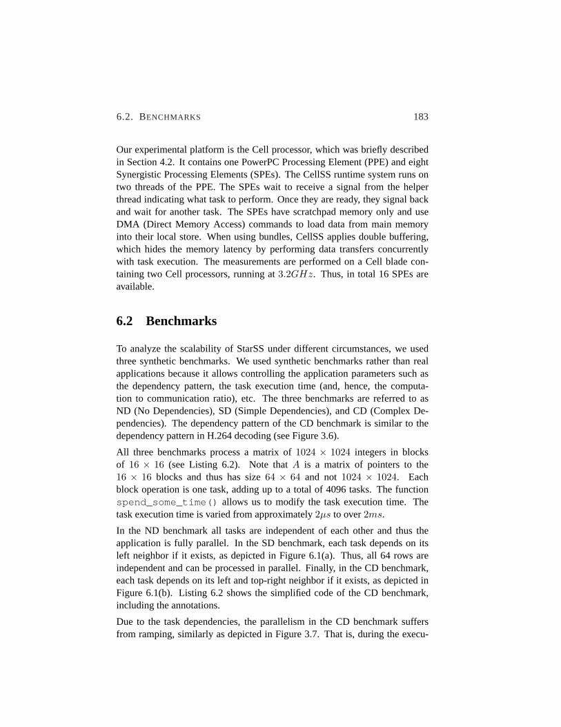
6.2. BENCHMARKS 183
Our experimental platform is the Cell processor, which was briefly describedin Section 4.2. It contains one PowerPC Processing Element (PPE) and eightSynergistic Processing Elements (SPEs). The CellSS runtime system runs ontwo threads of the PPE. The SPEs wait to receive a signal from the helperthread indicating what task to perform. Once they are ready, they signal backand wait for another task. The SPEs have scratchpad memory only and useDMA (Direct Memory Access) commands to load data from main memoryinto their local store. When using bundles, CellSS applies double buffering,which hides the memory latency by performing data transfers concurrentlywith task execution. The measurements are performed on a Cell blade con-taining two Cell processors, running at3.2GHz. Thus, in total 16 SPEs areavailable.
6.2 Benchmarks
To analyze the scalability of StarSS under different circumstances, we usedthree synthetic benchmarks. We used synthetic benchmarks rather than realapplications because it allows controlling the application parameters such asthe dependency pattern, the task execution time (and, hence, the computa-tion to communication ratio), etc. The three benchmarks are referred to asND (No Dependencies), SD (Simple Dependencies), and CD (Complex De-pendencies). The dependency pattern of the CD benchmark is similar to thedependency pattern in H.264 decoding (see Figure 3.6).
All three benchmarks process a matrix of1024 × 1024 integers in blocksof 16 × 16 (see Listing 6.2). Note thatA is a matrix of pointers to the16 × 16 blocks and thus has size64 × 64 and not1024 × 1024. Eachblock operation is one task, adding up to a total of 4096 tasks. The functionspend_some_time() allows us to modify the task execution time. Thetask execution time is varied from approximately2µs to over2ms.
In the ND benchmark all tasks are independent of each other and thus theapplication is fully parallel. In the SD benchmark, each task depends on itsleft neighbor if it exists, as depicted in Figure 6.1(a). Thus, all 64 rows areindependent and can be processed in parallel. Finally, in the CD benchmark,each task depends on its left and top-right neighbor if it exists, as depicted inFigure 6.1(b). Listing 6.2 shows the simplified code of the CD benchmark,including the annotations.
Due to the task dependencies, the parallelism in the CD benchmark suffersfrom ramping, similarly as depicted in Figure 3.7. That is, during the execu-

184 CHAPTER 6. HARDWARE TASK MANAGEMENT SUPPORT
Listing 6.2: The simplified code of the CD benchmark including StarSS annotations.
1 i n t ∗A[ 6 4 ] [ 6 4 ] ;23 t ypede f s t r u c t params{4 i n t y ;5 i n t x ;6 } p a r a m s t ;78 #pragma c s s t a s k i n p u t ( prms , l e f t [ 1 6 ] [ 1 6 ] ,9 t o p r i g h t [ 1 6 ] [ 1 6 ] )
10 i n o u t ( t h i s [ 1 6 ] [ 1 6 ] )11 vo id t a s k ( p a r a m st ∗ prms , i n t ∗ l e f t , i n t ∗ t o p r i g h t ,12 i n t ∗ t h i s ){13 . . .14 / / compute15 . .16 spend some t ime ( ) ;17 re turn ;18 }1920 vo id main ( ){21 i n t i , j ;22 p a r a m s t my params ;2324 i n i t m a t r i x (A ) ;2526 #pragma c s s s t a r t27 / / s t a r t measurement28 f o r ( i = 0 ; i <64; i ++){29 f o r ( j = 0 ; j <64; j ++){30 my params . y = i ;31 my params . x = j ;32 t a s k (&my params , A[ i ] [ j−1 ] , A[ i −1][ j + 1 ] , A[ i ] [ j ] ) ;33 }34 }35 #pragma c s s b a r r i e r36 / / s t o p measurement37 #pragma c s s f i n i s h38 }

6.3. SCALABILITY OF THE STARSS RUNTIME SYSTEM 185
(a) SD (b) CD
Figure 6.1: The task dependency patterns of the SD and CD benchmarks. The NDbenchmark has no task dependencies.
tion the number of available parallel tasks gradually increases, until halfway,after which the available parallelism similarly decreases back to one. There-fore, the amount of available parallelism at the start and end of the benchmarkis lower than the number of cores. Due to this ramping effect in the CD bench-mark, the maximum obtainable parallelism is 14.5 using 16 cores. The otherbenchmarks do not suffer from this ramping effect and have a maximum ob-tainable parallelism of 16 when using 16 cores.
6.3 Scalability of the StarSS Runtime System
The main purpose of this section is to quantify the task management overheadof the StarSS runtime system. One of the main metrics is scalability, which isdefined as the speedup of a parallel execution onN SPEs compared to execu-tion using one SPE. Besides measuring performance and scalability, we havealso generated Paraver traces [12] to study the runtime behavior in more detail.
First, we study the CD benchmark in detail, especially for small task sizes, asit resembles H.264 decoding, which has an average task size of approximately20µs.
6.3.1 CD Benchmark
Using the default(16, 128, 8) configuration of StarSS, which represents(scheduler.mintasks, scheduler.initialtasks, scheduler.maxstrandsize), amaximum scalability of 7.3 is obtained for the CD benchmark using 16 SPEs.

186 CHAPTER 6. HARDWARE TASK MANAGEMENT SUPPORT
0
2
4
6
8
10
12
14
16
2 4 6 8 10 12 14 16
Sca
labi
lity
Number of SPEs
2373 us636 us241 us66.7 us19.1 us11.2 us1.92 us
(a)
0
2
4
6
8
10
12
14
16
1 10 100 1000
Sca
labi
lity
Task size (us)
16 SPEs8 SPEs4 SPEs2 SPEs1 SPE
(b)
Figure 6.2: Scalability of StarSS with the CD benchmark and using the default con-figuration.
Figure 6.2 shows the scalability of the CD benchmark with the default config-uration for several task sizes.
Even when very large tasks of2373µs are used, the SPEs are mostly idle andwaiting for tasks, as illustrated in Figure 6.4, which shows a part of the trace.The colored parts indicate the execution phases, of which the legend is depictedin Figure 6.3. The first and second row of the trace corresponds to the mainand helper thread, respectively. The other rows correspond to the 16 SPEs.The yellow markers indicate communication events, where the direction of thearrow indicates whether it is a receive or a send. In Figure 6.4 only the receivesare depicted.
Figure 6.3: Legend of the StarSS Paraver traces.

6.3. SCALABILITY OF THE STARSS RUNTIME SYSTEM 187
Fig
ure
6.4:
Par
tialP
arav
ertr
ace
ofth
eC
Dbe
nchm
ark
with
16S
PE
s,a
task
size
of23
73µs,
and
the
defa
ultc
onfig
urat
ion.

188 CHAPTER 6. HARDWARE TASK MANAGEMENT SUPPORT
0
2
4
6
8
10
12
14
16
2 4 6 8 10 12 14 16
Sca
labi
lity
Number of SPEs
2373 us636 us241 us66.7 us19.1 us11.2 us1.92 us
(a)
0
2
4
6
8
10
12
14
16
1 10 100 1000
Sca
labi
lity
Task size (us)
16 SPEs8 SPEs4 SPEs2 SPEs1 SPE
(b)
Figure 6.5: Scalability of StarSS with the CD benchmark and the(1, 1, 1) configura-tion.
The reason for the low scalability is found in the configuration. The runtimesystem waits for 16 tasks to be ready before it schedules them to SPEs. Asthere is a limited amount of parallelism available, cores are left idle, waitingfor the runtime system to schedule tasks. Therefore, immediate scheduling ofready tasks is required, which is attained with a(1, y, z) configuration.
Furthermore, the runtime system tries to group up to 8 tasks to a single SPE.Again, because of the limited amount of available parallelism, cores are leftidle because the load is not properly balanced. Disallowing large groups, byusing an(x, y, 1) configuration, forces the runtime system to balance the loadamong the SPEs. Furthermore, the absolute performance is improved by im-mediate start of scheduling at the beginning of the application, enforced byusing a(x, 1, z) configuration. Scalability is not affected by this modification.
Summarizing, the optimal configuration for this benchmark and with largetasks is(1, 1, 1). The default configuration is only beneficial for situationswith ample parallelism. With the optimal settings, finally, a scalability of 14.2is obtained for large tasks, as shown in the graphs of Figure 6.5. This scala-bility is very close to the maximum obtainable parallelism of 14.5. Figure 6.6depicts a part of the Paraver trace. It shows that indeed all SPEs are almostcontinuously busy.
This configuration, however, stresses the runtime system, especially for smalltasks, as every single task is treated separately. Figure 6.7 depicts a part ofthe Paraver trace of the CD benchmark with a task size of19µs, for which ascalability of 4.2 is obtained. The yellow lines connecting the rows indicatecommunication. The helper thread signals to the SPEs what task to execute.The SPEs, in turn, signal back when the task execution is finished.

6.3. SCALABILITY OF THE STARSS RUNTIME SYSTEM 189
Fig
ure
6.6:
Par
tialP
arav
ertr
ace
ofth
eC
Dbe
nchm
ark
with
16S
PE
s,a
task
size
of23
73µs,
and
the(
1,1,
1)co
nfigu
ratio
n.

190 CHAPTER 6. HARDWARE TASK MANAGEMENT SUPPORT
Figure
6.7:PartialP
aravertrace
oftheC
Dbenchm
arkw
ith16
SP
Es,a
tasksize
of19
µs,and
the(1,1,1)
configuration.

6.3. SCALABILITY OF THE STARSS RUNTIME SYSTEM 191
The second row of the trace shows that scheduling (yellow), preparing (red),and submitting a bundle (green) takes approximately6µs, while removing atask (magenta) takes approximately5.8µs. As the total task size, includingtask stage in, wait for DMA, task execution, task stage out, and task finishednotification, is22.5µs, the helper thread can simply not keep up with the SPEs.Before the helper thread has launched the sixth task, the first one has alreadyfinished. However, its ready signal (yellow line) is processed much later, andbefore this SPE receives a new task, even more time is spent.
For such small tasks, the performance can be improved by using the(1, 1, 4)configuration. Grouping 4 tasks in a bundle reduces the scheduling time with45%, the preparation and submission of tasks with 73%, and the removal oftasks with 50%. In total, the per-task overhead is reduced from11.6µs to5.5µs resulting in an overall performance improvement of 20%.
Despite this improvement in the runtime system’s performance, the scalabil-ity is only 5.2. Both the helper thread and main thread remain bottlenecks.Although using the(1, 1, 4) configuration the per-task overhead in the helperthread is reduced to5.5µs, it is far from sufficient to leverage 16 SPEs effi-ciently. For that, at most a per-task overhead of22.5/16 = 1.4µs is required.
The main reason for the bottleneck in the main thread is very subtle. Althoughthe benchmark exhibits sufficient parallelism, due to the order in which themain thread spawns tasks (from left to right and top to bottom), at least 16“rows of tasks” (corresponding to 1/4th of the matrix) have to be added to thedependency graph before 16 independent tasks are available that can keep allcores busy. Thus, to exploit the parallelism available in the benchmark, theaddition of tasks in the main thread must therefore run ahead of the parallelexecution. The trace reveals that the main thread can only keep up with theparallel execution, and thus it limits the scalability of the system.
Figure 6.8 depicts the scalability of StarSS with the CD benchmark using the(1, 1, 4) configuration. Although this configuration outperforms the(1, 1, 1)configuration for small task sizes, for large task sizes it limits the scalabilityto less than 10. To obtain a high scalability, the(1, 1, 1) configuration must beused in combination with a medium task size. More specifically, Figure 6.5shows that in order to obtain a scalability efficiency of 80% when using 16SPEs, which is a scalability of 12.8, at least a task size of approximately100µsis required. Similarly, for 8 SPEs a task size of50µs is required.

192 CHAPTER 6. HARDWARE TASK MANAGEMENT SUPPORT
0
2
4
6
8
10
12
14
16
2 4 6 8 10 12 14 16
Sca
labi
lity
Number of SPEs
2373 us636 us241 us66.7 us19.1 us11.2 us1.92 us
(a)
0
2
4
6
8
10
12
14
16
1 10 100 1000
Sca
labi
lity
Task size (us)
16 SPEs8 SPEs4 SPEs2 SPEs1 SPE
(b)
Figure 6.8: Scalability of StarSS with the CD benchmark and the(1, 1, 4) configura-tion.
6.3.2 SD Benchmark
In the SD benchmark, tasks corresponding to different rows are completelyindependent of each other, because tasks only depend on their left neighbor.The difference in dependency pattern has several effects on the runtime system.First, this greatly simplifies the task dependency graph, which in turn mightlead to decreased runtime overhead. Second, the dependency pattern enablesthe runtime system to create efficient bundles, further reducing the overhead.Our measurements, however, show only a small improvement in scalabilitycompared to the CD benchmark.
Analysis of the scalability of the SD benchmark with the(1, 1, 1) configurationshows hardly any difference with the CD benchmark. The creation of bundlesimproves scalability a little. The(1, 1, 8) configuration is optimal in termsof performance and scalability and provides a maximum scalability of 14.5.Allowing larger bundles does not improve performance. Figure 6.9 depicts thescalability of the SD benchmark for different task sizes.
For a task size of19µs a scalability of 5.6 is obtained. Analysis of the Paravertrace, depicted in Figure 6.10, shows that the main thread is the bottleneck.It is continuously busy with user code (26.6%), adding tasks (50.9%), andremoving tasks (20.6%). On average per task these phases take2.0µs, 3.8µs,and1.5µs, respectively. This indicates that the time taken by building andmaintaining the task dependency graph is not much affected by the dependencypattern, unlike expected.
The stress on the helper thread, on the other hand, is significantly reduced bythe use of bundles. On average, the time spent on scheduling, preparation of
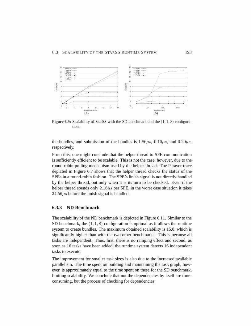
6.3. SCALABILITY OF THE STARSS RUNTIME SYSTEM 193
0
2
4
6
8
10
12
14
16
2 4 6 8 10 12 14 16
Sca
labi
lity
Number of SPEs
2372 us634 us240 us66.4 us19.1 us11.3 us1.85 us
(a)
0
2
4
6
8
10
12
14
16
1 10 100 1000
Sca
labi
lity
Task size (us)
16 SPEs8 SPEs4 SPEs2 SPEs1 SPE
(b)
Figure 6.9: Scalability of StarSS with the SD benchmark and the(1, 1, 8) configura-tion.
the bundles, and submission of the bundles is1.86µs, 0.10µs, and0.20µs,respectively.
From this, one might conclude that the helper thread to SPE communicationis sufficiently efficient to be scalable. This is not the case, however, due to theround-robin polling mechanism used by the helper thread. The Paraver tracedepicted in Figure 6.7 shows that the helper thread checks the status of theSPEs in a round-robin fashion. The SPE’s finish signal is not directly handledby the helper thread, but only when it is its turn to be checked. Even if thehelper thread spends only2.16µs per SPE, in the worst case situation it takes34.56µs before the finish signal is handled.
6.3.3 ND Benchmark
The scalability of the ND benchmark is depicted in Figure 6.11. Similar to theSD benchmark, the(1, 1, 8) configuration is optimal as it allows the runtimesystem to create bundles. The maximum obtained scalability is 15.8, which issignificantly higher than with the two other benchmarks. This is because alltasks are independent. Thus, first, there is no ramping effect and second, assoon as 16 tasks have been added, the runtime system detects 16 independenttasks to execute.
The improvement for smaller task sizes is also due to the increased availableparallelism. The time spent on building and maintaining the task graph, how-ever, is approximately equal to the time spent on these for the SD benchmark,limiting scalability. We conclude that not the dependencies by itself are time-consuming, but the process of checking for dependencies.

194 CHAPTER 6. HARDWARE TASK MANAGEMENT SUPPORT
Figure
6.10:Partial
Paraver
traceof
theS
Dbenchm
arkw
itha
tasksize
of19
µs
andthe(1
,1,8)configuration.
The
main
threadbottlenecks
thesystem
.

6.4. A CASE FORHARDWARE SUPPORT 195
0
2
4
6
8
10
12
14
16
2 4 6 8 10 12 14 16
Sca
labi
lity
Number of SPEs
1586 us425 us162 us45.5 us13.8 us8.6 us
1.75 us
(a)
0
2
4
6
8
10
12
14
16
1 10 100 1000
Sca
labi
lity
Task size (us)
16 SPEs8 SPEs4 SPEs2 SPEs1 SPE
(b)
Figure 6.11: Scalability of StarSS with the ND benchmark and the(1, 1, 8) configu-ration.
6.4 A Case for Hardware Support
In the previous section we analyzed the StarSS system and showed that thecurrent runtime system has a low scalability for fine-grained tasks. To show thepotential gains of accelerating the runtime system, in this section we compareStarSS to manually parallelized implementations of the benchmarks using adynamic task pool. Based on the analysis presented in this and the previoussection, we identify the bottlenecks in the StarSS runtime system. Those leadto a set of requirements that hardware support for task management shouldcomply with.
6.4.1 Comparison with Manually Parallelized Benchmarks
The benchmarks are also manually parallelized. The task functions were off-loaded to SPE code. On the PPE, tasks are added to a task pool, which dy-namically keeps track of task dependencies. An interface between the SPEsand the PPE was implemented, such that the task pool, running on the PPE,assigns tasks to SPEs. As for each task the dependencies are predetermined,the process of dependency resolution has become very simple and fast. A sim-ple Last-In-First-Out (LIFO) buffer is used to minimize the scheduling latency.The implementation of these manually parallelized benchmarks took a lot oftime compared to the implementations of the StarSS benchmarks. Especially,building and optimizing the task pool took significant effort [43].
The scalability of the benchmarks with the manually coded task pool is shownin Figures 6.12, 6.13, and 6.14. The first figure shows that for a task size of

196 CHAPTER 6. HARDWARE TASK MANAGEMENT SUPPORT
0
2
4
6
8
10
12
14
16
2 4 6 8 10 12 14 16
Sca
labi
lity
Number of SPEs
2373 us636 us241 us66.7 us19.1 us11.2 us1.92 us
(a)
0
2
4
6
8
10
12
14
16
1 10 100 1000
Sca
labi
lity
Task size (us)
16 SPEs8 SPEs4 SPEs2 SPEs1 SPE
(b)
Figure 6.12: Scalability of the manually parallelized CD benchmark.
0
2
4
6
8
10
12
14
16
2 4 6 8 10 12 14 16
Sca
labi
lity
Number of SPEs
2372 us634 us240 us66.4 us19.1 us11.3 us1.85 us
(a)
0
2
4
6
8
10
12
14
16
1 10 100 1000
Sca
labi
lity
Task size (us)
16 SPEs8 SPEs4 SPEs2 SPEs1 SPE
(b)
Figure 6.13: Scalability of the manually parallelized SD benchmark.
0
2
4
6
8
10
12
14
16
2 4 6 8 10 12 14 16
Sca
labi
lity
Number of SPEs
1586 us425 us162 us45.5 us13.8 us8.6 us
1.75 us
(a)
0
2
4
6
8
10
12
14
16
1 10 100 1000
Sca
labi
lity
Task size (us)
16 SPEs8 SPEs4 SPEs2 SPEs1 SPE
(b)
Figure 6.14: Scalability of the manually parallelized ND benchmark.

6.4. A CASE FORHARDWARE SUPPORT 197
1
10
100
2 4 8 16
Tas
k si
ze (
us)
Number of SPEs
StarSS (CD)StarSS (SD)StarSS (ND)Manual (CD)Manual (SD)Manual (ND)
Figure 6.15: The iso-efficiency lines of the StarSS and Manual systems (80% effi-ciency).
19µs, the scalability of the CD benchmark using 16 SPEs is almost 12. Thisis much higher than the scalability of 4.8 obtained with StarSS. Similarly, thescalability of the other two benchmarks for small task sizes is significantlyhigher compared to StarSS.
Although the scalability of the manually parallelized benchmarks is much bet-ter than the scalability obtained with StarSS, for small task sizes it is still lim-ited. Similar to StarSS, these benchmarks suffer from the round-robin pollingmechanism used by the PPE to handle mailbox messages from the SPEs. ThePPE spends3.5µs per task on updating the dependency table, submitting tasksto the ready queue, and submitting a new task to the SPE. As SPEs have to waittheir turn, typically they are waiting16µs before receiving the new task. Asignificant performance improvement can be made when the hardware wouldprovide faster synchronization primitives.
Figure 6.15 compares the scalability of the StarSS system to that of the man-ually parallelized (Manual) system. It displays the iso-efficiency lines, whichrepresent the minimal task size required for a certain system in order to obtaina specific scalability efficiency. Scalability efficiency is defined asS/N , whereS is the scalability andN is the number of cores. As scalability is defined rel-ative to one SPE, in this case we defineN as the number of SPEs, ignoringthe PPE. In Figure 6.15 the iso-efficiency graph for an efficiency of 80% is de-picted. Table 6.1 lists the values of the iso-efficiency function. For the Manual

198 CHAPTER 6. HARDWARE TASK MANAGEMENT SUPPORT
Table 6.1: The iso-efficiency values of the StarSS and Manual systems (80% effi-ciency).
Task size (µs)no. SPEs StarSS Manual
ND SD CD ND SD CD
2 6.3 7.4 6.34 9.7 9 10.8 3.98 32.8 38.6 46.9 6.6 7 8.1
16 59 62.6 134.4 26 32.9 50.1
system and a small number of SPEs, an efficiency of 80% is always obtained,irrespective the task size. Therefore, the corresponding iso-efficiency pointsdo not exist and are not displayed in the graph and table.
From the iso-efficiency graph it is clear that the Manual system achieves anefficiency of 80% for much smaller task sizes than StarSS does. For eightSPEs the difference in task size is between a factor of 5 and 6, while for 16SPEs the difference is between 2 and 3 times. The main cause for this dif-ference is the dependency resolution process of the StarSS runtime system.The iso-efficiency lines of both system increase with the number of SPEs.This is expected as the overhead increases with the number of SPEs, and thuslonger tasks are required to hide the task management latency on the PPE.Especially the polling mechanism used to synchronize incurs increasing over-head for larger core counts. For the Manual system this is the main reason forthe line increase. Furthermore, increasing the core count beyond eight requiresoff-chip communication, increasing the synchronization latency and reducingscalability.
Besides a lower scalability, also the absolute performance of StarSS is lower,up to four times, than that of the Manual System for fine-grained tasks. Ta-ble 6.2 depicts the execution times of the three benchmarks. For larger tasksizes the difference diminishes as the task management overhead becomesnegligible compared to the task execution time. The task sizes used in theND benchmark are slightly different from those used in the other benchmarks.This is due to the way thespend_some_time() function is implemented.
6.4.2 Requirements for Hardware Support
From the prior analysis, we conclude that the StarSS runtime system currentlydoes not scale well for fine-grained task parallelism. The manually parallelized

6.4. A CASE FORHARDWARE SUPPORT 199
Table 6.2: Absolute execution times, inms, for different task sizes, inµs, of the threebenchmarks for the StarSS and Manual systems, and using 8 SPEs.
Benchmark System Execution time per task size
1.92 11.2 19.1 66.7 241 636 2373CD StarSS 23 23 23 41 132 340 1250
Manual 6.0 10 13 39 130 337 1250
1.85 11.3 19.1 66.4 240 634 2372SD StarSS 17 17 18 39 128 330 1230
Manual 4.1 9.4 13 37 126 327 1210
1.75 8.6 13.8 45.5 162 425 1586ND StarSS 18 19 18 26 86 221 818
Manual 4.5 7.0 10 26 86 221 813
benchmarks, though, showed that it is possible to achieve a much higher scal-ability, while using dynamic task management.
The main bottleneck of the StarSS runtime system is the dependency resolutionprocess. Irrespective of the actual dependency pattern, determining whetherthere are task dependencies is a laborious process that cannot keep up withthe parallel task execution. In order to efficiently utilize 8 or 16 SPEs forH.264 decoding, roughly corresponding to the CD benchmark with a task sizeof 20µs, the process of building and maintaining the task dependency graphshould be reduced from9.1µs to 2.5µs and1.3µs, respectively. Therefore,we describe the first requirement for task management hardware support asfollows:
Requirement 1 The hardware support system should accelerate the task de-pendency resolution process by at least a factor of 3.6 and 7.3, when using 8and 16 SPEs, respectively.
Preferably, this process is accelerated even more, such that it can run ahead ofexecution in order to reveal more parallelism. As such a large speedup is re-quired we expect that some hardware acceleration, such as special instructions,will not be sufficient. Instead, we propose to perform this process completelyin hardware.
The second bottleneck is the scheduling, preparation, and submission of tasks,performed by the helper thread in StarSS. In total this per-task overhead is5.5µs, where at most a latency of2.8µs and1.4µs is required, for 8 and 16SPEs, respectively.

200 CHAPTER 6. HARDWARE TASK MANAGEMENT SUPPORT
Requirement 2 The hardware support system should accelerate scheduling,preparation, and submission of tasks by at least a factor of 2.0 and 3.9, whenusing 8 and 16 SPEs, respectively.
The scheduler tries to minimize the overhead by creating bundles of tasks,and tries to exploit data locality by grouping a dependency chain within onebundle. For small tasks, however, the scheduling costs more than the benefitsit provides. A rudimentary, yet fast, scheduling approach might therefore bemore efficient than a sophisticated one.
The latency of synchronization on the Cell processor is too long due to thepolling mechanism. Interrupts are more scalable than the polling mechanism,but still need to execute a software routine. Instead, SPEs should be able toretrieve a new task themselves instead of waiting for one to be assigned. Hard-ware task queues, such as Carbon [94], is an example of such an approach.Each core can read a task from the queue autonomously, avoiding off-chipcommunication and execution of a software routine. This approach does notonly provide benefit for the Cell processor, but also using a more conventionalmulticore [94]. Assuming a 5% overhead for synchronization is acceptable,the synchronization latency should be at most1µs, irrespective of the numberof cores.
Requirement 3 The hardware support system should provide synchronizationprimitives for retrieving tasks, with a latency of at most1µs, irrespective of thenumber of cores.
When compliant with these three requirements, a hardware support systemwill effectively improve the scalability of StarSS, while maintaining its easeof programming. In the next section we propose the Nexus system, which isdeveloped based on this set of requirements.
6.5 Nexus: a Hardware Task Management SupportSystem
In this section we present the design of the Nexus system, which provides therequired hardware support for task management in order to efficiently exploitfine-grained task parallelism with StarSS. Nexus can be incorporated in anymulticore architecture. In this section, as an example, we present a Nexusdesign for the Cell processor.

6.5. NEXUS: A HARDWARE TASK MANAGEMENT SUPPORTSYSTEM 201
SPE
SPESPE
LS SPU
MFC
SPE
MEM
PPE
TPU
TC
ELEMENT INTERCONNECT BUS
Figure 6.16: Overview of the Nexus system (in bold) implemented in the Cell pro-cessor. The depicted architecture could be one tile of a larger system.
First, we provide an overview of the Nexus system and explain its main oper-ation based on the life cycle of a task. Second, we present the design of theTask Pool Unit (TPU), which is the main hardware unit of the Nexus system.Finally, we present the Nexus API.
6.5.1 Nexus System Overview
The Nexus system contains two types of hardware units (see Figure 6.16). Thefirst and main unit is the Task Pool Unit (TPU). It receives tasks descriptorsfrom the PPE, which contain the meta data of the tasks, such as the function toperform and the location of the operands. It resolves dependencies, enqueuesready tasks to a memory mapped hardware queue, and updates the internal taskpool for every task that finishes. The TPU is designed for high throughput andtherefore it is deeply pipelined. It is directly connected to the bus to allow fastaccess from any core.
The second unit in the system is the Task Controller (TC), which can be placedat individual cores. The TC fetches tasks from the TPU, issues the DMAs ofinput and output operands, and implements double buffering. While the firsttask is executed, the inputs of the next are loaded. TCs are optional as the TPUis memory mapped and thus can be accessed by any core directly. No design ofthe TC has been developed as of yet. In the future work section of this chapterwe discuss some implementation details, though.

202 CHAPTER 6. HARDWARE TASK MANAGEMENT SUPPORT
Process taskdescriptor;fill the tables
Read readyqueue;load task descriptor;execute task;write task idto finish buffer
Load task descriptor totask storage
Create task
in buffer
descriptor;write to
Phase 4Phase 3 Phase 5 Phase 6
Handle finishbuffer;process kick−offlists
Phase 2Phase 1
PPE SPE
Add ready tasksto ready queue
TPU
loaderdescriptor
handlerdescriptor
TPU
handler
TPU TPU
readyqueue
finish
Figure 6.17: The phases of the task life cycle and the corresponding hardware units.
Storing all tasks in a central unit provides low latency dependency resolutionand scheduling. The hardware queues ensure fast synchronization. Such acentralized approach, however, eventually creates a scalability bottleneck forincreasing core count. In such a case, a clustered approach can be used. Tasksare distributed among TPUs such that inter-TPU communication is low whiletask stealing allows system-wide load balancing.
6.5.2 The Task Life Cycle
The main operation of the Nexus system is described by the task life cycle il-lustrated in Figure 6.17. The life cycle of tasks starts at the PPE which preparesthe task descriptors dynamically. It sends a task descriptor pointer, as well asthe size of the task descriptor, to the TPU. In the second phase, the TPU loadsthe descriptor into a task storage, where it remains until the task is completelyfinished. The task storage can be thought of as the local store of the TPU.
Once the task descriptor is loaded, in the third phase, the information in thedescriptor is processed. The new task is added to the task graph, by checkingfor dependencies on other tasks. The TPU performs this dependency resolutionby using three tables, as explained in the next section. This phase, therefore,consists of filling the tables with the required information, which consumesonly little time as will be shown.
The task resides in the tables until its dependencies are resolved. This processis handled by the TPU in the fourth phase. It maintains the dependency graphthroughout the execution, detects when the task can be executed, and then addsthe task to a ready queue.

6.5. NEXUS: A HARDWARE TASK MANAGEMENT SUPPORTSYSTEM 203
In the fifth phase, the task is executed. First, the SPE reads the task id from theready queue. This process can be performed by either its TC or by softwarerunning on the SPU. The task descriptor is loaded from the task storage afterwhich the task operands are loaded into the local store using DMA commands.When execution is finished and the task output is written back to main memory,the task id is signaled to the TPU.
Finally, in the sixth phase, the TPU handles the finish signal sent by the SPE.Based on the id of the task, it updates the tables, which thereafter indicatewhich tasks have no dependencies left. It then adds these tasks to the readyqueue. Thus, the sixth phase of the current task equals the fourth phase of thetasks that are added to the ready queue.
6.5.3 Design of the Task Pool Unit
The block diagram of the Nexus TPU is depicted in Figure 6.18. Its main fea-tures are the following. The task life cycle is pipelined to increase throughput.Dependency resolution consists of table lookups only, and therefore has lowlatency. All task descriptors are stored in the task storage to avoid off-chipcommunication. These three features are described in detail below.
Pipelining
The task life cycle is pipelined using the phases described in the previous sec-tion. For example, while the TPU is loading the descriptor of the first task, thePPE prepares the descriptor of the second task. Similarly, the other phases arepipelined. As a consequence, the TPU contains separate units for phases 2, 3,and 4/6 that operate concurrently. As explained in the previous section, phases4 and 6 belong to the same operation and therefore are mapped to a single unit.
Phase 2 is performed by thedescriptor loader. It reads thein buffer and issuesa DMA to load the task descriptor into thetask storage. All ports are memorymapped and can be accessed from anywhere in the system. Thedescriptorhandleris responsible for phase 3. It reads the task descriptor from thetaskstorageand performs the dependency resolution process, as described below.Finally, phases 4 and 6 are performed by thefinish handler. It reads task idsfrom thefinish bufferand updates the tables.
The three tables, the two buffers, theready queue, and thetask storageallhave a fixed size. Thus, they can be full in which case the pipeline stalls. Forexample, if thetask storageis full, the descriptor loaderstalls. If no entry

204 CHAPTER 6. HARDWARE TASK MANAGEMENT SUPPORT
ptr size
in buffer
descriptor
descriptor
handler
loader
id *descriptor
finishhandler
....
registerstatus
task storage
descriptor 1
descriptor 2
address kick−off list
ready queue
id
finish buffer
id *descriptor status #deps
task table
producers table
address #deps kick−off list
consumers table
Figure 6.18: Block diagram of the Nexus TPU. The ports are memory mapped andcan be accessed anywhere from the system.
of the task storageis removed, thein buffer will quickly be full too, whichstalls the process of adding tasks by the PPE. Deadlock cannot occur, however,because in the StarSS programming model tasks are added in serial executionorder. That means that if tasks are processed in this order sequentially, theexecution will be correct.
Dependency Resolution
Generally, task dependencies are expressed by using a task dependency graph.Building such a task dependency graph, however, is very time-consuming. Inthe TPU, dependencies are resolved by using three tables. Thus, the depen-dency resolution process can be performed fast, as it consists of simple lookups

6.5. NEXUS: A HARDWARE TASK MANAGEMENT SUPPORTSYSTEM 205
only. There is no need to search through the tables to find the correct item.
The task tablecontains all tasks in the system and records their status and thenumber of tasks it depends on. Tasks with a dependency count of zero areready for execution and added to theready queue. Thetask tableis indexed bythe task id.
The consumers tableis used to prevent write-after-read hazards. It containsthe addresses of data that is going to be produced by a pending task. Any taskthat requires that data can subscribe itself to that entry by adding its id to thekick-off list and increasing its own dependency count in thetask table. When atask finishes, thefinish handlerprocesses the kick-off lists of the entries in theconsumers tablecorresponding to the addresses of the output operands of thetask. That is, for each task id in the kick-off lists, it decreases the dependencycount of that task in thetask table.
As example, assume taskT1 writes to addressA, and taskT2 reads fromaddressA. Thus, taskT2 depends on taskT1. When taskT1 is added by thedescriptor handler, an entry for addressA is generated in theconsumers table,with an empty kick-off list. TaskT1 is also added to thetask table. When taskT2 is added, theconsumers tableis checked for addressA. As it is present, idT2 is added to the kick-off list of that entry. Further, taskT2 is added to thetask tablewith a dependency count of one. Once taskT1 finishes, thefinishhandlerreads the entry of addressA in the consumers table. In the kick-offlist, it finds the id of taskT2 and decreases the dependency count of taskT2 inthe task table. As the dependency count is zero, taskT2 is added to thereadyqueue.
Similarly, the consumers table prevents read-after-write hazards. This tablecontains the addresses of data that are going to be read by pending tasks. Anynew task that will write to these locations can subscribe itself to the kick-offlist.
As example, assume taskT1 reads from addressA while taskT2 writes toaddressA. In this case taskT2 is indirectly depending on taskT1. TaskT2does not need the output of taskT1, but it should not write to addressA beforetaskT1 has read from it. This read-after-write hazard is handles as follows.When taskT1 is added by thedescriptor handler, an entry for addressA isgenerated in the consumers table. The dependency count of that entry is setto one, while the kick-off list remains empty. In case an entry for addressAalready exists only the dependency count of that entry is increased by one.Further, taskT1 is added to thetask table. When taskT2 is added by thedescriptor handler, the consumers table is checked for addressA. As the entry

206 CHAPTER 6. HARDWARE TASK MANAGEMENT SUPPORT
is found, the id of taskT2 is added to the kick-off list of that entry. Further,taskT2 is added to thetask tablewith a dependency count of one. When taskT1 finishes, thefinish handlerdecreases the dependency count of entryA inthe consumers table. If it reaches zero, all consumers of addressA have readthe data, and thus the kick-off list is processed. The id of taskT2 is found inthe kick-off list and thus its dependency count in thetask tableis decreased byone. It reaches zero, and thus it is added to theready queue.
Finally, write-after-write hazards are handled by theproducers table. A taskwriting to a particular address that is already in theproducers table, subscribesitself to the corresponding entry. This subscription, however, is performed in adifferent manner, as explained in Section 6.5.3.
The lookups in the producers and consumers tables are address-based. As thelists are much smaller than the address space, a hashing function is used togenerate the index.
Task Storage
Thetask storagecontains only task descriptors. The amount of data maintainedwithin a task descriptor depends on the number of task operands. Thus variablesized task descriptors might be used to optimally utilize the available memory.That requires complicated memory management, however.
Instead, fixed-size task descriptors are used. Typically, tasks have a fewoperands only. Assuming a maximum of five operands, the task descriptoris 64 bytes large. Thetask storageis divided in slots of 64 bytes. For eachslot one bit is required to indicate if it is occupied. Task ids correspond to theslot of its task descriptor in thetask storageand are assigned by the descriptorloader.
Note that the source-to-source compiler can detect tasks with more than fiveoperands. It can warn the programmer or schedule the tasks to the PPU withoutintervention of the TPU.
Kick-off List Barriers
Theconsumers tablecontains one kick-off list per address. This is sufficientas long as there is only one producer per address. If multiple tasks write to thesame address, multiple kick-off lists for that address are required.

6.5. NEXUS: A HARDWARE TASK MANAGEMENT SUPPORTSYSTEM 207
1
A
A
A
2
3
4
5
(a)
1
2
3
4
5
war
war
raw
raw
waw
waw
(b)
Figure 6.19: (a) An example of tasks writing to and reading from the same addressAand (b) the corresponding task dependency graph.
Consider the example depicted in Figure 6.19. The left side of the figure de-picts the data that is produced or consumed by tasksT1 throughT5. The rightside of the figure illustrates the dependencies. First, taskT1 writes to locationA, after which taskT2 reads from locationA. Adding taskT1 by thedescrip-tor handler, adds the address ofA to theconsumers table. Adding taskT2 addsid 2 to kick-off list of addressA in the consumers table. Next, taskT3 alsowrites to locationA, after which taskT4 reads the new value from locationA. Addition of taskT3 does not change the producer table. Addition of taskT4, however, adds id4 to the kick-off list of addressA in the producer table,assuming one kick-off list per address is maintained. If now taskT1 finishes,the kick-off list of addressA in the producer table is processed and both taskT2 andT4 are put in theready queue. TaskT4, however, is depending ontaskT3 which has not been executed. Similarly, taskT5 is kicked-off fromthe consumers table before taskT4 is executed.
We solved this issue by using barriers in the kick-off lists. Barriers divide kick-off lists in multiple parts, as if they are separate lists. A task that writes to anaddress that is already in theproducers table, adds a barrier to the kick-off listof the corresponding entry. Similarly, a task that reads from an address alreadyin theconsumers table, and which entry has a non-empty kick-off list, adds abarrier to that kick-off list.
This process is illustrated in Figure 6.20 for the example of Figure 6.19. Eachrow shows the changes in the relevant entries of the three tables for a particularstep. In the top five rows, the tasks1 through5 are added to the system, whichis done by thedescriptor handler. The bottom five rows show how thefinishhandlerupdates the tables when it processes ids1 through5.
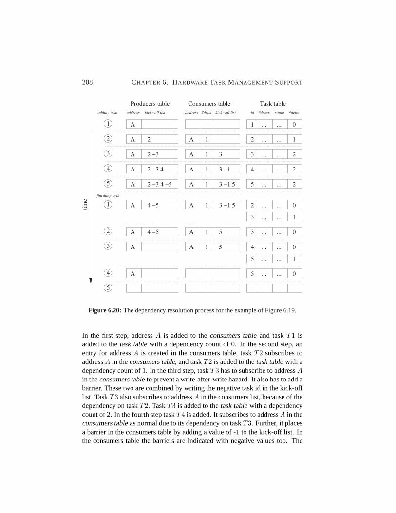
208 CHAPTER 6. HARDWARE TASK MANAGEMENT SUPPORT
5 2 −3 4 −5A A 3 −1 51 ... ... 25
... ... 24
adding task
Producers table
address kick−off list
Consumers table
address #deps kick−off list
Task table
id *descr. status #deps
A A 1
A A 1 ... ... 2
A A 1 ... ...
A 1 ... ...1
2
3
4
0
2
3
12
2 −3
2 −3 4
3
3 −1
finishing task
A A 1 ... ...
A A 3 −1 51 ... ...
... ...
1
2
2 0
3 1
4 −5
4 −5 5 3 0
A A 1 ... ...3 5 4 0
... ... 15
tim
e
5
A ... ...54 0
Figure 6.20: The dependency resolution process for the example of Figure 6.19.
In the first step, addressA is added to theconsumers tableand taskT1 isadded to thetask tablewith a dependency count of 0. In the second step, anentry for addressA is created in the consumers table, taskT2 subscribes toaddressA in theconsumers table, and taskT2 is added to thetask tablewith adependency count of 1. In the third step, taskT3 has to subscribe to addressAin theconsumers tableto prevent a write-after-write hazard. It also has to add abarrier. These two are combined by writing the negative task id in the kick-offlist. TaskT3 also subscribes to addressA in the consumers list, because of thedependency on taskT2. TaskT3 is added to thetask tablewith a dependencycount of 2. In the fourth step taskT4 is added. It subscribes to addressA in theconsumers tableas normal due to its dependency on taskT3. Further, it placesa barrier in the consumers table by adding a value of -1 to the kick-off list. Inthe consumers table the barriers are indicated with negative values too. The

6.5. NEXUS: A HARDWARE TASK MANAGEMENT SUPPORTSYSTEM 209
absolute value of the barrier indicates the number of tasks that need to readthe data in the corresponding address. Thus, it is similar to the dependencycount value in the entries of the consumer table. If another task that reads fromaddressA would be added now, the barrier would be decremented instead ofadding another barrier. The addition of taskT5 in the fifth step is similar tothe third step.
When taskT1 finishes, thefinish handlerprocesses the kick-off list in the pro-ducer table for addressA up to and including the barrier. Thus, the dependencycounts of both taskT2 andT3 are decremented. The dependency count of thefirst reaches zero, and thus taskT2 is added to theready queue. Further, taskT1 is removed from thetask table. The consumers table is unaltered. WhentaskT2 finishes, the entry for addressA in the consumers table is processed.The dependency count in that entry is decremented and becomes zero. Thusthe kick-off list is processed up to the barrier, which adds taskT3 to thereadyqueue. The barrier itself is negated and becomes the new dependency countof that entry. Similarly, in the final three steps the tables are updated until alltasks have completed and the tables are empty.
6.5.4 The Nexus API
In this section the software interface to the Nexus system is described. Itshows the relation between the programming model, the runtime system, andthe TPU.
Initialization
The Cell processor works with virtual addresses and physical addresses, re-ferred to as effective and real addresses, respectively. The real address spaceis the set of all addressable bytes in physical memory and on memory mappeddevices, such as the TPU. Programs, though, use effective addresses only, andthus a translation is always necessary.
The real address of the TPU is fixed and known a priori. Its mapping to theeffective address space is a runtime issue, and requires anmmapsystem call.Therefore, before any program can use the TPU, an initialization must takeplace, in which the effective address of the TPU is retrieved. Listing 6.3 showshow the TPU can be initialized. The functioninit_tpu() is part of libtpu,which is the runtime system of Nexus.
210 CHAPTER 6. HARDWARE TASK MANAGEMENT SUPPORT
Listing 6.3: Initialization retrieves the effective address of the TPU from the OS.
1 # inc lude < l i b t p u . h>23 t p u h a n d l e t t p u h a n d l e ;45 i n t main ( ){6 t p u h a n d l e = i n i t t p u ( ) ;7 . . .8 }
Adding Tasks
The user specifies tasks with pragmas as shown in Listing 6.2, while the TPUrequires a task descriptor. The source-to-source compiler analyzes the usercode and transforms it into code that creates and initializes the task descriptor.For example, the code of Listing 6.2 would be translated into that of List-ing 6.4.
The task descriptor has a header and body, which contains the parameter infor-mation. The header specifies the task function and the number of parameters ittakes. In this case the functiontask was assigned number 1 by the source-to-source compiler. This number is used by the SPEs to call the correct function.These functions are extracted from the source code by the source-to-sourcecompiler and put in the SPE code with an automatic generated main function.For each task parameter several fields are specified in the task descriptor. Theio type can be IN, OUT, or INOUT, which are defined in libtpu. The other fourentries specify the location and size of the parameter, which can be stored in astrided fashion.
Once the task descriptor is filled, thetpu_add_task runtime system func-tion is called. It requires as arguments the tpu handle, a pointer to the taskdescriptor, and its size, although the last parameter is not necessary for thecurrent TPU implementation. The runtime system copies the pointer and thesize to thein buffer of the TPU, and not the descriptor itself. If thein bufferis full, it overwrites the last item. Thus, the function first checks the statusregister of the TPU. The implementation of thetpu_add_task function isshown in Listing 6.5. The status register is a 32-bit value, of which the firstbyte contains the number of empty elements in thein buffer, and the secondbyte contains the state of the TPU. The other two bytes are currently not used.

6.5. NEXUS: A HARDWARE TASK MANAGEMENT SUPPORTSYSTEM 211
Listing 6.4: Preparation of the task descriptor and submission of it to the TPU.
1 t a s k d e s c r i p t o r t ∗ t a s k d l i s t = ma l loc ( . . . . ) ;23 t a s k d e s c r i p t o r t ∗ t d p t r = t a s k d l i s t ;4 f o r ( i = 0 ; i <64; i ++){5 f o r ( j = 0 ; j <64; j ++){6 t a s k d e s c r i p t o r t t d ;7 t d p t r−>t a s k f u n c = 1 ;8 t d p t r−>no params = 4 ;9 t d p t r−>p 1 i o t y p e = IN ;
10 t d p t r−>p 1 s t a r t p t r = & my params ;11 t d p t r−>p 1 x l e n g t h = s i z e o f( p a r a m s t ) ;12 t d p t r−>p 1 y l e n g t h = 1 ;13 t d p t r−>p 1 y s t r i d e = 0 ;14 t d p t r−>p 2 i o t y p e = IN ;15 t d p t r−>p 2 s t a r t p t r = A[ i ] [ j −1];16 t d p t r−>p 2 x l e n g t h = 1 6∗ s i z e o f( i n t ) ;17 t d p t r−>p 2 y l e n g t h = 1 6 ;18 t d p t r−>p 2 y s t r i d e = 1 6∗ s i z e o f( i n t ) ;19 t d p t r−>p 3 i o t y p e = IN ;20 t d p t r−>p 3 s t a r t p t r = A[ i −1][ j + 1 ] ;21 t d p t r−>p 3 x l e n g t h = 1 6∗ s i z e o f( i n t ) ;22 t d p t r−>p 3 y l e n g t h = 1 6 ;23 t d p t r−>p 3 y s t r i d e = 1 6∗ s i z e o f( i n t ) ;24 t d p t r−>p 4 i o t y p e = INOUT ;25 t d p t r−>p 4 s t a r t p t r = A[ i ] [ j ] ;26 t d p t r−>p 4 x l e n g t h = 1 6∗ s i z e o f( i n t ) ;27 t d p t r−>p 4 y l e n g t h = 1 6 ;28 t d p t r−>p 4 y s t r i d e = 1 6∗ s i z e o f( i n t ) ;2930 t p u a d d t a s k ( t p u h a n d l e , t d p t r ,31 s i z e o f( t a s k d e s c r i p t o r t ) ) ;32 t d p t r ++;33 } }
The Nexus library also provides thetpu_add_task_do_while . It tries toadd a task to the TPU. If thein buffer is full, instead of waiting it retrieves tasksfrom theready queueto execute in the mean time. Once there is a empty placein the in buffer, it adds the task and returns. In this way, the PPE is utilizedoptimally and performance can be improved.

212 CHAPTER 6. HARDWARE TASK MANAGEMENT SUPPORT
Listing 6.5: Thetpu add task runtime system function implementation.
1 vo id t p u a d d t a s k ( t p u h a n d l e t tpu , vo id ∗ d e s c r i p t o r ,2 s i z e t s i z e ){3 t p u s t a t u s t s t a t u s ;45 a s s e r t ( tpu ) ;67 do {8 memcpy(& s t a t u s , ( tpu + STATUSREGISTER ) , 4 ) ;9 } whi le ( s t a t u s . i n < = 0 ) ;
1011 memcpy ( ( tpu + INBUFFER ) , & d e s c r i p t o r , 4 ) ;12 memcpy ( ( tpu + INBUFFER + 4 ) , & s i z e , 4 ) ;13 }
Listing 6.6: The runtime system provides a wait function which returns once all taskshave finished.
1 i n t main ( ){23 . . .4 t p u w a i t ( t p u h a n d l e ) ;5 re turn ;6 }
Finalization
After the PPE has added all tasks to the TPU it has to wait for them to finishbefore continuing with the shutdown or next phase of the program. The run-time system provides a blocking wait, which continuously checks the status ofthe TPU and returns once it indicates that all tasks are finished. Listing 6.6shows the utilization of this function.
The Nexus runtime system also provides the functionality for the PPE to ex-ecute tasks while it is waiting for the parallel execution to finish, as shown inListing 6.7. The functiontpu_finished returns true if all tasks are fin-ished. The functiontpu_try_get_task returns the task id if there was atask in theready queue, else it returns zero. The functionexecute_task isprovided by the source-to-source compiler. It calls the task function, indicatedby the function number in the descriptor, with the operands, which are also
6.6. EVALUATION OF THE NEXUS SYSTEM 213
Listing 6.7: The PPE can also obtain tasks from the TPU to execute them.
1 i n t main ( ){23 . . .4 whi le ( ! t p u f i n i s h e d ( t p u h a n d l e ) ){5 t a s k d e s c r i p t o r t t d ;6 i n t t a s k i d ;7 i f ( t p u t r y g e t t a s k ( t p u h a n d l e , & t d , & t a s k i d ) ) {8 e x e c u t e t a s k (& t d ) ;9 t p u f i n i s h t a s k ( t p u h a n d l e , t a s k i d ) ;
10 }11 }12 re turn ;13 }
indicated in the descriptor. Finally, withtpu_finish_task the task id issent to thefinish bufferof the TPU.
So far the API concerned the PPE side of the code. The SPE side is dependingon whether a TC is included in the system or not. For now, we assume there isno TC. Instead, runtime system functions are used to obtain and finish a task.
Listing 6.8 shows an example of the SPEs main function. With thetpu_get_task function, the SPE receives a task descriptor. The functionfirst reads from theready queue, until it finds a task there. Next, it DMAs inthe task descriptor and returns. Thetpu_finish_task is equal to that onthe PPE, except for its internal implementation. The SPE code never returns.Instead, the SPEs are stopped by the PPE once all tasks have finished.
The function load_and_execute_task is provided by the source-to-source compiler. It reads the task descriptor, DMAs in all the input parameters,calls the proper task function, and finally DMAs back the output operands. Ex-cept for the task functions, all SPE code is generated automatically.
6.6 Evaluation of the Nexus System
In the previous section we have presented the design of the Nexus system. Inthis section we evaluate the implementation of Nexus for the Cell processor.First, we describe the experimental setup. Second, we present the performanceand scalability analysis of the Nexus system.

214 CHAPTER 6. HARDWARE TASK MANAGEMENT SUPPORT
Listing 6.8: The SPE main code retrieving tasks from the TPU.
1 # inc lude < t p u s p u . h>23 vo id main (unsigned long long i d , unsigned long long argp ) {4 mm ptr tpu = argp ;56 t a s k d e s c r i p t o r t t d a t t r i b u t e ( ( a l i g n e d ( 1 6 ) ) ) ;7 i n t t a s k i d ;8 whi le ( 1 ){9 i f ( t p u g e t t a s k ( tpu , & t d , & t a s k i d ) ) {
10 l o a d a n d e x e c u t e t a s k (& t d ) ;11 t p u f i n i s h t a s k ( tpu , t a s k i d ) ;12 }13 }14 }
6.6.1 Experimental Setup
Similar to Chapters 4 and 5, we use CellSim as evaluation platform (see alsoSection 4.3.3). In these previous chapters, however, we were only interestedin the SPE, while in this chapter, the entire Cell processor is of importance.Therefore, the configuration of the PPE, cache, memory, and bus modules arevalidated, to ensure these simulator models are accurate.
In contrast to previous chapters, we validated CellSim against a real Cell pro-cessor, instead of validating against SystemSim, for the following reason. Theadditional information provided by SystemSim was not needed for this vali-dation, while execution on the simulator is much slower than using the realprocessor. Although the Cell blade provides 16 SPEs, we used only 8 for thisvalidation. CellSim can simulate 16 SPEs, but connects all of them to thesame on-chip bus. As on the Cell blade these 16 SPEs are divided betweentwo chips, the two architectures would be different. There is one architecturaldifference between the simulator and the real Cell processor that was not re-solved. The real processor contains both an L1 and L2 cache on the chip. Inthe simulator only the L1 cache is available. We account for this difference inthe configuration of CellSim.
We adjusted the configuration parameters to match the real processor. As Cell-Sim is not cycle-accurate, an empirical methodology was used to determinethe correct parameter values. More precisely, we measured several properties

6.6. EVALUATION OF THE NEXUS SYSTEM 215
Table 6.3: CellSim configuration parameters.
L1-latency 10mem-latency 45dma-latency 900bus-latency 8bus-width 16ppu-fetch-rate 1.4spu-fetch-rate 1.4
on both the real Cell processor and on the simulator. The corresponding pa-rameters were adjusted until the properties measured on the simulator matchedthese of the real processor. For example, the latency of DMA transfers was ad-justed with the parameters ‘dma-latency’, ‘bus-latency’, ‘bus-bandwidth’, and‘mem-latency’. The properties that we measured are the following:
• Mailbox round-trip time: The round-trip time of a mailbox signal fromthe PPE to the SPE and back.
• DMA latency: The time spent on issuing and waiting for DMAs.
• SPU execution time:The execution time of one task on the SPE. Thisdoes not include any DMAs, mailbox signals, or other communications.
• PPE execution time: The execution time of the serial CD benchmarkrunning on the PPE.
• Cell execution time:The execution time of the parallel CD benchmark,when it is executed on the PPE and eight SPEs.
• Cell scalability: The scalability of the parallel CD benchmark, when itis executed on the PPE and eight SPEs. The scalability is relative to theparallel execution time on one SPE.
Most of the configuration parameters influence several properties resulting ina multi-dimensional matching problem. The most accurate configuration, pre-sented in Table 6.3, was determined by performing many measurements. Thememory access latency in the simulator is 45 cycles only, while using the realprocessor, off-chip memory accesses take in the order of a thousand cycles.As mentioned before, the simulator does not model the L2 cache. Thus a missin the L1 cache goes directly to main memory while in the real processor it

216 CHAPTER 6. HARDWARE TASK MANAGEMENT SUPPORT
Table 6.4: Validation of CellSim by comparing several properties of the simulatoragainst those measured on the real Cell processor. All measures are incycles, except scalability.
Cell CellSim Error
Mailbox round-trip 1,248 1,216 -2.6%DMA latency 7,048 6,524 -7.4%SPU ex. time 61,446 61,898 0.7%PPE ex. time 559,184 546,097 -2.3%Cell ex. time 41,996,703 41,471,514 -1.3%Cell scalability 7.4 7.0 -5.5%
goes to the L2 cache first. A memory access latency of 45 cycles correspondsto the average L1 miss penalty of the real processor. The memory access la-tency parameter, however, also affects the memory access time of DMAs. Thiswas compensated by increasing the dma-latency parameter (an MFC moduleparameter) to 900 cycles, whereas the default value is 50 cycles.
Table 6.4 compares the properties of CellSim to that of the real Cell processor.Most properties are modeled within 3% accuracy. The DMA latency, however,has an error of 7.4%. This error can be lowered by increasing the dma-latencyparameter. This would, however, negatively affect the scalability, which is5.5% off in the current configuration. The current trade-off seems reasonable.Overall, the simulator accuracy is fairly well and sufficient for its purpose.
The TPU is implemented as one module in CellSim. Although the size of thetables and the storage is still subject to research, we use the following valuesin the experiments. Thetask tableand thetask storagehave 1024 entries. Thisis the minimum size needed for the CD benchmark to detect 16 independenttasks. It is much less, though, than the total number of tasks (4096) in thebenchmarks. Thus, the process of adding tasks is stalled once thetask tableandtask storageare full.
The producersand consumers tableseach have 4096 entries. This is suffi-cient to contain all inputs and outputs of the 1024 tasks in thetask table. Asignificant number of hash collisions, however, happen. A coalesced hash al-gorithm [164] is used to resolve hash collisions. It allows the tables to be filledefficiently to a high density, while maintaining low latency table lookups.
The latencies of the TPU are determined as follows. The TPU functionalityconsists mainly of accessing the tables and the storage. In the real processor,

6.6. EVALUATION OF THE NEXUS SYSTEM 217
Table 6.5: Execution time of the CD benchmark, with a task size19µs, for the threesystems. Three configurations of the Nexus runtime system are analyzed.
Nexus Execution Time (ms) Speedup StarSS + Nexusconfiguration StarSS + Nexus StarSS Manual vs StarSS vs Manual
8 SPEs 11.1 22.3 13.0 2.02 1.178 SPEs - PPE 10.8 22.3 13.0 2.06 1.208 SPEs - PPE+ 10.4 22.3 13.0 2.14 1.24
accessing the local store, which is 256 kB large, takes six cycles. Thus, itis reasonable to assume that thetask storage, which is 64 kB large, can beaccessed in two cycles. Similarly, the three tables, which are smaller thanthe task storage, were assigned a latency of one cycle. Theproducersandconsumers tableare accessed several times per lookup, due to hash collisions.Measurements showed that on average one lookup takes six cycles. Per taskseveral lookups are required, depending on the number of parameters.
The latencies of the handlers are mainly based on the latencies of the tablesand storages. Also cycles for control logic and arithmetic operations are addedto the handler latencies. The total latency of the handlers, for each operationthey perform, is depending on the actual input and the state of the tables. Inthe next section, which presents the performance evaluation, these latenciesare analyzed for the benchmark.
6.6.2 Performance Evaluation
In this section we analyze the performance and the scalability of the Nexussystem. We present results for the CD benchmark. Analysis for the other twobenchmarks has yet to be performed. When comparing to the StarSS systemthat uses the software task management, we refer to that system as ‘StarSS’,while the system using the Nexus hardware task management is referred to as‘StarSS + Nexus’.
The execution time of the CD benchmark, with a task size of19µs is shownin Table 6.5. Three configurations of the Nexus runtime system are analyzed.The first (8 SPEs) uses only the eight SPEs to execute tasks. In the secondconfiguration (8 SPEs - PPE), the PPE also executes tasks, but only after it hasadded all tasks to the TPU. Finally, in the third configuration (8 SPEs - PPE+),the PPE also executes tasks while the addition of tasks to the TPU is stalledbecause thein-buffer is full.

218 CHAPTER 6. HARDWARE TASK MANAGEMENT SUPPORT
The table compares the StarSS + Nexus system to the StarSS and the Manualsystems. The execution of the benchmark using the StarSS system is measuredon the Cell blade, as the code generated by the StarSS compiler cannot be exe-cuted on the simulator. Thus, for this particular analysis we used the hardwareconfiguration for which the simulator was validated, i.e., we used eight SPEs.
The table shows that using the Nexus hardware instead of the software taskmanagement, a speedup of more than 2x is obtained, when using eight SPEs.As shown in Figure 6.8, for this task size and number of cores, the scalabil-ity of the StarSS system is 5.2. Section 6.3 showed that task managementoverhead limits the scalability and performance. As the performance has beenimproved by a factor of over 2x, the Nexus system has successfully removedthe performance bottleneck for this case.
More details on the parallel execution of the benchmark are provided in Fig-ure 6.22, which shows a part of the Paraver trace. The legend for this traceis depicted in Figure 6.21. The x-scale of the trace is in cycles, although thefigure statesns. This is due to a mismatch in the metrics used in the simulatorand the visualization tool. The trace shows that the SPEs are almost contin-uously executing tasks. The time it takes for an SPE to obtain a new task isextremely short when compared to the trace of the StarSS system (Figure 6.7).It takes 985 cycles, which is0.3µs, for the SPEs to read from theready-queueof the TPU.
Figure 6.21: Legend of the StarSS + Nexus Paraver traces.

6.6. EVALUATION OF THE NEXUS SYSTEM 219
Fig
ure
6.22
:Par
tialP
arav
ertr
ace
ofth
eC
Dbe
nchm
ark
with
8S
PE
s,a
task
size
of19
µs,
and
usin
gth
eN
exus
syst
em.
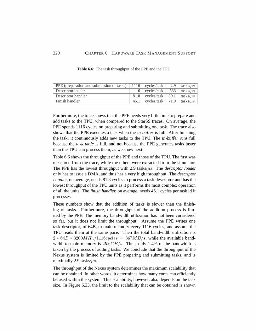
220 CHAPTER 6. HARDWARE TASK MANAGEMENT SUPPORT
Table 6.6: The task throughput of the PPE and the TPU.
PPE (preparation and submission of tasks)1116 cycles/task 2.9 tasks/µsDescriptor loader 6 cycles/task 533 tasks/µsDescriptor handler 81.8 cycles/task 39.1 tasks/µsFinish handler 45.1 cycles/task 71.0 tasks/µs
Furthermore, the trace shows that the PPE needs very little time to prepare andadd tasks to the TPU, when compared to the StarSS traces. On average, thePPE spends 1116 cycles on preparing and submitting one task. The trace alsoshows that the PPE executes a task when thein-buffer is full. After finishingthe task, it continuously adds new tasks to the TPU. Thein-buffer runs fullbecause thetask tableis full, and not because the PPE generates tasks fasterthan the TPU can process them, as we show next.
Table 6.6 shows the throughput of the PPE and those of the TPU. The first wasmeasured from the trace, while the others were extracted from the simulator.The PPE has the lowest throughput with 2.9 tasks/µs. Thedescriptor loaderonly has to issue a DMA, and thus has a very high throughput. Thedescriptorhandler, on average, needs 81.8 cycles to process a task descriptor and has thelowest throughput of the TPU units as it performs the most complex operationof all the units. Thefinish handler, on average, needs 45.1 cycles per task id itprocesses.
These numbers show that the addition of tasks is slower than the finish-ing of tasks. Furthermore, the throughput of the addition process is lim-ited by the PPE. The memory bandwidth utilization has not been consideredso far, but it does not limit the throughput. Assume the PPE writes onetask descriptor, of 64B, to main memory every 1116 cycles, and assume theTPU reads them at the same pace. Then the total bandwidth utilization is2 ∗ 64B ∗ 3200MHz/1116cycles = 367MB/s, while the available band-width to main memory is25.6GB/s. Thus, only 1.4% of the bandwidth istaken by the process of adding tasks. We conclude that the throughput of theNexus system is limited by the PPE preparing and submitting tasks, and ismaximally 2.9 tasks/µs.
The throughput of the Nexus system determines the maximum scalability thatcan be obtained. In other words, it determines how many cores can efficientlybe used within the system. This scalability, however, also depends on the tasksize. In Figure 6.23, the limit to the scalability that can be obtained is shown

6.6. EVALUATION OF THE NEXUS SYSTEM 221
0
50
100
150
200
250
300
0 20 40 60 80 100
Sca
labi
lity
limit
Task size (us)
Figure 6.23: The limit to the obtainable scalability using the Nexus system, based onthe maximum throughput.
for several task sizes. For example, for tasks of20µs, the scalability limit is20 × 2.9 = 58. The figure shows that the scalability limit increases with thetask size.
The TPU latencies are modeled as accurately as possible. As no real hardwarehas been developed, however, they might be incorrect to some extent. There-fore, we analyze the impact of increased TPU latencies on the performance.We use the CD benchmark with a task size of19µs, and only SPEs are execut-ing tasks. The result is shown in Figure 6.24. The performance is normalizedto that using the default latencies. The x-axis is the normalized TPU latency.A value of 10 indicates that all latencies of the TPU are multiplied by a factorof 10.
The figure shows that the performance is hardly influenced for up to a normal-ized latency of 100. This is explained as follows. Eight SPEs are used andthe task size of20µs. Therefore, the execution rate is0.4 tasks/µs. Within theTPU, thedescriptor handlerhas the lowest throughput, which is39.1 tasks/µsand which is directly related to the TPU latencies. When the latencies are in-creased with a factor of 100, the throughput increases also with a factor of 100and becomes equal to the execution rate. When the latencies increase further,the throughput of thedescriptor handlerlimits the throughput of the entiresystem and the performance decreases as shown in the figure.

222 CHAPTER 6. HARDWARE TASK MANAGEMENT SUPPORT
0.1
1
1 10 100 1000
Nor
mal
ized
per
form
ance
Normalized TPU latency
Figure 6.24: Impact of the TPU latency on the performance for a task size of20µsand using eight SPEs.
The point in Figure 6.24, from where the performance drops, therefore dependson the task size and the number of SPEs used. The minimum value, however, is13.5 because the performance is limited by the throughput of the PPE, which is13.5 times larger than that of thedescriptor handler. From this experiment weconclude that the claimed performance improvements, which can be obtainedwith the Nexus system, are reliable.
So far we have considered the single case of the CD benchmark with a tasksize of19µs and using 8 SPEs. We have shown that the Nexus hardware pro-vides large performance improvements and that the throughput of the Nexussystem potentially allows scaling to large number of cores. Figure 6.25 showsthe measured scalability of the StarSS + Nexus system, for several task sizesand up to 16 SPEs. The maximum scalability obtained is 14.3, which is veryclose to the theoretical scalability limit of 14.5 for the benchmark. The figureshows that for task sizes of11.2µs and larger, the scalability is almost perfect.Therefore, using the Nexus system, large speedups can be obtained comparedto StarSS without hardware task management support. For example, for a tasksize of11.2µs and using 16 SPEs, the StarSS + Nexus system is 5.3 timesfaster than the StarSS system (measured on real hardware). In case 32 SPEswould be used and the application exhibits sufficient parallelism, the speedupwould double approximately, as for that task size, the StarSS system does notscale beyond 4 cores, while the StarSS + Nexus system theoretically scales up

6.6. EVALUATION OF THE NEXUS SYSTEM 223
0
2
4
6
8
10
12
14
16
2 4 6 8 10 12 14 16
Sca
labi
lity
Number of SPEs
66.7 us19.1 us11.2 us1.92 us
(a)
0
2
4
6
8
10
12
14
16
1 10 100
Sca
labi
lity
Task size (us)
16 SPEs8 SPEs4 SPEs2 SPEs1 SPE
(b)
Figure 6.25: Scalability of the StarSS + Nexus system with the CD benchmark.
to approximately 30 cores. For a task size of1.92µs and using 16 SPEs, theStarSS + Nexus system is 7.4 times faster than the StarSS system (measuredon real hardware), although both system have a very limited scalability of 5.7and 1.9, respectively.
The scalability of the StarSS + Nexus system is compared to that of the StarSSand the Manual systems, in Figure 6.26 and Table 6.7. They show the iso-efficiency function of the three systems, for a scalability efficiency of 80%.The StarSS + Nexus system obtains an 80% efficiency for much smaller tasksizes than the StarSS system. The scalability of StarSS was limited by thetask management overhead, which we successfully accelerated with the Nexushardware.
The task size, required to obtain an 80% efficiency for the StarSS + Nexus sys-tem, is even lower than that required for the Manual system. The scalability ofthe Manual system was limited by the polling mechanism used to synchronize,which scaled very poorly. The difference between the line labeled StarSS +Nexus in Figure 6.26 and the line labeled Manual, shows the benefits of fasthardware synchronization primitives. The Manual line is much steeper, indi-cating the scalability difference.
To conclude this evaluation, we compare the measurements to the requirementsthat have been formulated in Section 6.4.2. The first requirement, states thatthe task dependency resolution process must be accelerated by a factor of 3.6and 7.3, when using 8 and 16 SPEs respectively. In the StarSS system, thedependency resolution process takes9.1µs. The most time-consuming part ofthe TPU is thedescriptor handler, which takes on average 81.81 cycles pertask, which is0.026µs per task. Therefore, the dependency resolution processis accelerated by a factor of 356.

224 CHAPTER 6. HARDWARE TASK MANAGEMENT SUPPORT
1
10
100
2 4 8 16
Tas
k si
ze (
us)
Number of SPEs
StarSSManual
StarSS + Nexus
Figure 6.26: The iso-efficiency lines of the three systems for the CD benchmark (80%efficiency).
Table 6.7: The iso-efficiency values of the three systems for the CD benchmark (80%efficiency).
no. SPEs Task size (µs)StarSS Manual StarSS + Nexus
2 6.34 10.88 46.9 8.1 5.116 134.4 50.1 10.0
The second requirement is that scheduling, preparation, and submission oftasks to the SPEs, should be accelerated by a factor of 2.0 and 3.9, when us-ing 8 and 16 SPEs, respectively. These processes, which can be viewed as theback-end of the task pool, were executed by the helper thread of the StarSSsoftware task management system. Using the Nexus hardware, this back-endprocess of retrieving tasks from the task pool and bringing them to the SPEs forexecution, is performed differently. Scheduling is currently performed by sim-ply writing to a FIFO queue. Preparation of tasks is not needed anymore, as allthe necessary information is in thetask storagealready. Submission of tasks toSPEs is replaced by SPEs reading tasks from theready queuethemselves. Thebest to compare the back-end of the StarSS software task management system

6.7. FUTURE WORK 225
to is the process of thefinish handler. It takes0.014µs per task, which is 390times faster than the back-end process of the StarSS system.
Finally, the third requirement is that the hardware should provide synchroniza-tion primitives for retrieving tasks, with a latency of at most1µs, irrespectiveof the number of cores. As mentioned before, it takes 985 cycles (0.3µs) forthe SPE to read an item from the ready queue. This latency is independent ofthe number of cores used, neglecting contention on the bus and the queue. Inour experiments, however, we have not detected any contention effects. An-other effect not considered here, is the increasing bus (or NoC) latency for anincreasing size of the on-chip system.
All three requirements are met by the Nexus system. Therefore, by using theNexus system, the StarSS programming model can efficiently be used for muchsmaller tasks and more cores. Provided the application exhibits sufficient par-allelism, task sizes as small as10µs can efficiently be used on a multicorecontaining approximately 30 cores.
6.7 Future Work
The research described in this chapter is work in progress at the time of writing.In this section we describe the future work, consisting of features that yet haveto be implemented, issues that have to be resolved, analyses that have to beperformed, and bottlenecks that have to be removed.
6.7.1 Dependency Resolution
The TPU resolves dependencies by means of three tables. This system, how-ever, is based on the start address of a piece of data. This puts certain restric-tions on the application, which are not always met.
As long as data is divided into fixed elementary blocks, the system works well.For example, if a matrix is divided in blocks of16 × 16 , the address of thetop-left element is all that is needed to refer to the entire block. This assumesthe system is aware of the block width, height, and stride. In the benchmarkprograms this is the case.
In some applications or kernels, such as motion compensation, the data blockshave an unknown alignment. Thus, blocks can partially overlap as depicted onthe left side of Figure 6.27. Computing the overlap is very laborious and eas-ily annihilates the gains of task level parallelism. Imagine, the input operand

226 CHAPTER 6. HARDWARE TASK MANAGEMENT SUPPORT
������������������������������������������������������������������������������������������������������������������������������������
������������������������������������������������������������������������������������������������������������������������������������
������������������������������������������
������������������������������������������
������������������������������������������
������������������������������������������
������������������������������������������
������������������������������������������
����������������
����������������
������������
������������
Figure 6.27: Calculating task dependencies through overlapping memory ranges(left) is laborious. Only the addresses of left-top corners have to bechecked, if all blocks are translated into several blocks that are alignedwith the grid.
of a task has to be compared against a thousand output operands of blocksinside the TPU. There is no clear solution to this issue as of yet, but we areinvestigating a few directions.
The first solution direction is to map at runtime blocks that are not aligned witha grid onto several aligned blocks and maintain the current hardware depen-dency resolution scheme. The source-to-source compiler can extract certaininformation from the annotated code and pass it on to the runtime system. Theruntime system checks the operands for their alignment by computing the startaddresses of the blocks it is overlapping and adds those to the task descrip-tor. If data is maintained within matrices, this computation can be performedquickly by checking the matrix indices.
Take for example the right-hand side of Figure 6.27. All blocks are16 × 16elements large and assume the matrix is namedframe . In this case the blockframe[24:39][24:39] is accessed which overlaps four aligned blocks.The system knows the block size, and thus the alignment can be checked bycomputing the x and y index, modulus the block width and height, respectively.If the modulus is not zero, it computes the start addresses of the blocks it over-laps, i.e., frame[16:31][16:31], frame[32:47][16:31], frame[16:31][32:47],frame[32:47][32:47].
These computations are rather simple and have to be performed only once permisaligned block. The TPU can check the dependencies among other tasksby using the lookup mechanisms as described before. This method, though,stresses the runtime system, and it has to be investigated what the impact of iton the performance and scalability will be.

6.7. FUTURE WORK 227
A second solution direction is to accelerate the overlap detection in hardware.Such a solution is not as much tied to a particular runtime system and program-ming model, and thus can be more general applicable. We are collaboratingwith Yoav Etsion and Alex Ramirez from the Barcelona Supercomputer Center(BSC) to investigate such hardware.
6.7.2 Task Controller
In the current implementation, the SPE has to read a task from the TPU, loadthe descriptor, issue DMAs to fetch the input operands, execute the task, issueDMAs to write back the output operands, and finally signal to the TPU. Perfor-mance can be improved by exploiting concurrency on a single SPE. Possiblya software double buffering strategy can be deployed. A hardware unit, how-ever, could increase concurrency even more. Therefore, we will investigate thebenefits of adding a Task Controller (TC) to each SPE.
Exploiting double buffering allows hiding the latency of access to main mem-ory. This is done through the MFC, which works autonomously and concur-rently with the SPU. Similarly, the TC could perform local task management inan autonomous and concurrent way. For example, while the SPU is executinga task, the TC could read a new task id from theready queueof the TPU, loadthe task descriptor, and program the MFC to load the input operands into thelocal store. Similarly, the TC could issue DMAs to store the output of a taskback to main memory and write the task id to thefinish buffer. All informationneeded to perform these operations is contained within the task descriptor.
To apply such a double buffering scheme, twice as many tasks should be avail-able. For applications with limited available parallelism, the double bufferingscheme might provide little performance improvement. For such situations,the Nexus system can be extended with task scheduling that exploits data lo-cality. For example, a tail-submit strategy (see Section 3.7.2) can be deployed.We will investigate how the TC and TPU have to be modified to support suchtask scheduling.
6.7.3 Other Features
Currently, the Nexus system is using a fixed size task descriptor. Althoughthis eases the implementation of the TPU, quite some memorytask storageiswaisted. We intend to investigate in future work the trade-offs of using variablesized task descriptors instead.

228 CHAPTER 6. HARDWARE TASK MANAGEMENT SUPPORT
To scale the Nexus system to the many-core area, a clustered approach can beused. We will investigate how to best implement the clusterization. A TPU-to-TPU interface has to be designed, allowing efficient task stealing. Applicationscheduling is typically managed by the OS. We will investigate an OS interfacethat allows such management.
StarSS is one of the task based programming models, currently being devel-oped. We will investigate compatibility of the Nexus system with other pro-gramming models.
6.7.4 Evaluation of Nexus
An important evaluation that has yet to be performed is the area and powerconsumption of the Nexus system. For both the TPU and the TC, the costs haveto be compared against the benefits. The TPU consists of mainly memory, andmight consume a significant amount of area and power. On the other hand, ifadditional cores cannot be deployed efficiently because of limited applicationscalability, the area and power is better spent on the Nexus system.
Related is the question what the proper size is for the storage and the tablesof the TPU. These are depending on the amount of available parallelism in theapplications, the dependency patterns, and the number of cores in the system.We will investigate the relation between these sizes, the performance, and thearea and power consumption.
Finally, we will evaluate the benefits of the Nexus system for several otherbenchmarks. We will take benchmarks from several domains and with varyingtask sizes.
6.8 Conclusions
The task-based StarSS programming model is a promising approach to sim-plify parallel programming. In this chapter we evaluated the StarSS runtimesystem. It was shown that for fine-grained task parallelism, the task manage-ment overhead significantly limits the scalability. Specifically, for a task sizeof approximately20µs, as used in task based parallel H.264 decoding, the scal-ability is limited to five cores. In order to efficiently utilize 8 or 16 cores forsuch a task size, the runtime system should be accelerated by at least a factorof 3.6 and 7.3, respectively. Mainly the task dependency resolution process istoo laborious to perform in software. Furthermore, the scheduling, prepara-

6.8. CONCLUSIONS 229
tion, and submission of tasks to cores take too much time to supply more thanfour cores continuously with tasks. Finally, we observed that the lack of fastsynchronization primitives causes many unnecessary stalls.
We proposed the Nexus system for hardware task management support. It per-forms dependency resolution in hardware using simple table lookups. Hard-ware queues are used for fast scheduling and synchronization. The Nexussystem was evaluated by means of simulation. It was shown that the depen-dency resolution process is accelerated by a factor of 356. Furthermore, thebottleneck of scheduling, preparation, and submission of tasks to the SPEswas removed. Scheduling is performed by writing to a hardware FIFO queue,preparation of tasks is not needed anymore, and the submission of tasks was re-placed with a distributed mechanism, in which SPEs read tasks from the queuethemselves. This mechanism using the hardware queue also provides the fastsynchronization primitive that was necessary.
Simulations showed that when using 16 SPEs, for the CD benchmark a nearoptimal scalability is obtained for task sizes of approximately10µs and larger.For such a task size, the scalability limit, based on the task throughput, is 29and increases with the task size.
The Nexus system is currently still work in progress. The optimal parametersof the Nexus hardware, such as the size of the tables, the queues, and the stor-age, have yet to be determined. Also additional features, such as dependencydetection of potentially overlapping memory regions, will be developed. Fur-ther, the area and power consumption of the Nexus hardware will be analyzed.Finally, several other benchmarks will be used to evaluate the performance andscalability of the Nexus system.


Chapter 7
Conclusions
In this dissertation, we have addressed several challenges in the multicore area.The overall aim of this work was to improve the scalability of multicore sys-tems, with a focus on H.264 video decoding. More specifically, the followingfour objectives were targeted. First, to analyze the H.264 decoding application,to find new ways to parallelize the code in a scalable fashion, and to analyzethe parallelization strategies and determine bottlenecks in current parallel sys-tems. Second, to specialize the cores of the Cell processor for H.264 in orderto obtain performance and power benefits. Third, to design hardware mech-anism to reduce the overhead of managing the parallel execution. Finally, toenhance efforts in improving programmability by providing hardware support.
In this final chapter, we first summarize the research presented in this thesisand show how the objectives have been met. Further we specify the maincontributions of this work. Second, we discuss possible directions for futureresearch.
7.1 Summary and Contributions
This dissertation started in Chapter 2 with an analysis of the power wall prob-lem for multicores. Specifically, we investigated the limits to performancegrowth of multicores due to technology improvements with respect to powerconstraints. As a case study we modeled a multicore consisting of Alpha 21264cores, scaled to future technology nodes according to the ITRS roadmap. Anal-ysis showed that the power budget significantly limits the performance growth.Despite this, the power constrained performance can double every three years
231

232 CHAPTER 7. CONCLUSIONS
due to technology improvements.
When taking Amdahl’s Law into account, a serial fraction of 1% decreases thepower constrained performance by up to a factor of 10, assuming a symmet-ric multicore. For an asymmetric multicore, where the serial code is executedon a core that runs at a higher clock frequency, 1% of serial code reducesthe achievable speedup by a factor of up to 2. This confirms that serial perfor-mance remains a challenge. On the other hand, there is Gustafson’s Law whichassumes that the input size grows equally with increasing number of proces-sors. Using Gustafson’s Law, for a serial fraction of 10% the performance lossis maximally 11%. Whether Amdahl’s or Gustafson’s Law is applicable to acertain application domain remains to be determined.
The contributions made in Chapter 2 can be summarized as follows:
• It was shown, based on the ITRS roadmap predictions, that technologyimprovements allow the performance of multicores to double every threeyears, despite being limited by the power budget.
• Our model confirms that in case Amdahl’s Law is applicable, the powerconstrained multicore performance can significantly be improved by us-ing an asymmetric architecture.
The first objective of this dissertation is met in Chapter 3, which investigatesthe parallelization of H.264 video decoding. Most promising is macroblock-level parallelism, of which it has been proven before that it can be exploitedinside a frame in a diagonal wavefront manner. We have observed that mac-roblocks (MBs) in different frames are only dependent through motion vectors.Therefore, we have proposed a novel parallelization strategy, called the Dy-namic 3D-Wave, which combines intra-frame and inter-frame MB-level paral-lelism.
Using this new parallelization strategy we have performed a limit study of theamount of MB-level parallelism available in H.264. We modified the FFmpegH.264 decoder and analyzed real movies. The results have revealed that motionvectors are typically small on average. As a result a large amount of parallelismis available. For FHD resolution the total number of parallel MBs ranges from4000 to 7000.
Finally, we have discussed a few implementations of the 2D-Wave and 3D-Wave strategy. Using the 3D-Wave parallelization strategy, a scalability of 55was obtained on a 64 core system, whereas the scalability of the 2D-Wave satu-rates around 15. Experiences with these implementations have shown that low

7.1. SUMMARY AND CONTRIBUTIONS 233
latency synchronization is essential for fine-grained parallelism as exploited inthese macroblock-level parallelizations of H.264.
The contributions made in Chapter 3 can be summarized as follows:
• A novel parallelization strategy for H.264 has been proposed, which ismore scalable than any previous parallelization.
• We have performed a limit study of the amount of macroblock-level par-allelism available in H.264, which has shown that for a FHD resolutionthe total number of parallel macroblocks ranges from 4000 to 7000.
• Analysis of parallel implementations of H.264 has shown that low la-tency synchronization is essential for efficient fine-grained paralleliza-tion.
• Although H.264 was assumed to be hard to parallelize, we were able tocreate a scalable implementation. This suggests that many other appli-cations can be parallelized in a scalable fashion.
A specialization of the Cell SPE architecture was presented in Chapter 4, withwhich the second objective was met. We enhanced the architecture with twelveinstruction classes, most of which have not been proposed before. These in-struction classes can be divided in five groups. First, we added instructionsto enable efficient scalar-vector operations, because the SPE has a SIMD onlyarchitecture. Second, we added several instructions that perform saturationand packing as needed by the H.264 kernels. Third, we added the swapoe in-structions to perform fast matrix transposition, which is needed by many me-dia kernels. Fourth, we added specialized arithmetic instructions that collapsefrequently used simple arithmetic operations. Finally, we added support fornon-quadword aligned access to the local store, which is especially needed formotion compensation. The speedup achieved on the H.264 kernels is between1.84x and 2.37x, while the dynamic instruction count is reduced by a factorbetween 1.75x and 2.67x.
The contributions made in Chapter 4 can be summarized as follows:
• We have identified the bottlenecks in the execution of the H.264 kernelson the Cell SPE architecture.
• We have proposed novel application specific instructions for H.264video decoding, of which several are applicable to other media appli-cations as well.
234 CHAPTER 7. CONCLUSIONS
• We have shown that a speedup of approximately 2x can be obtainedon the H.264 kernels by adding about a dozen of application specificinstructions.
One of the proposed instruction classes performs intra-vector operations. Byusing these intra-vector instructions, the matrix transpositions, generally re-quired in two-dimensional kernels, were avoided. In Chapter 5 it has beeninvestigated what the benefits of such intra-vector SIMD instructions for otherkernels are. For six kernels intra-vector instructions have been developed andsimulations have shown that a speedup of up to 2.06 was achieved. We havediscussed the results and have shown how the characteristics of the kernelsaffect the applicability of intra-vector instructions.
The contributions made in Chapter 5 can be summarized as follows:
• We have proposed intra-vector SIMD instructions to avoid matrix trans-position in two-dimensional kernels.
• We have shown that intra-vector SIMD instructions can speed up kernelsby a factor of up to 2.06.
The last two objectives are met in Chapter 6. In this chapter we have firstevaluated the runtime system of the task-based StarSS programming model. Itwas shown that for fine-grained task parallelism, the task management over-head significantly limits the scalability of StarSS applications. Specifically,for a task size of approximately20µs, as used in task based parallel H.264decoding, the scalability is limited to five cores.
We have contributed by proposing the Nexus system for hardware task man-agement support. It performs dependency resolution in hardware using simpletable lookups. Hardware queues are used for fast scheduling and synchroniza-tion. The Nexus system was evaluated by means of simulation. It was shownthat the dependency resolution process is accelerated by a factor of 356. As aresult, the StarSS programming model can be efficiently used for much smallertask sizes than was possible before. Simulations have shown that when using16 SPEs, a near optimal scalability is obtained for task sizes of approximately10µs and larger. For such a task size, the scalability limit, based on the taskthroughput, is 29 and increases with the task size.
The contributions made in Chapter 6 can be summarized as follows:
• The StarSS runtime system was analyzed, and it was shown that thetask management overhead is too large to efficiently exploit fine-grainedparallelism for more than five cores.

7.2. POSSIBLEDIRECTIONS FORFUTURE WORK 235
• We have proposed the Nexus system for hardware task management sup-port.
• We have proposed a novel dependency resolution scheme, based on lowlatency table lookups.
• We have shown that the Nexus system can greatly reduce the task man-agement overhead, as a result of which the StarSS programming modelcan efficiently be used for much smaller task sizes (down to10µs).
7.2 Possible Directions for Future Work
In Chapter 3, the limit study has shown that thousands of parallel macroblocksare available, when using the 3D-Wave parallelization strategy. The imple-mentation based on the TriMedia multicore, showed a speedup of 55 using 64cores. The scalability curve, however, indicates that this implementation scalesto higher core counts. Future work could investigate the scalability limit of the3D-Wave implementation. Furthermore, it would be interesting to study theperformance of the 3D-Wave on different architectures. Especially, the impactof the memory hierarchy would be interesting research topic. Such research,however, requires a large scale system. Potentially, such system could be basedon the Tilera’s Tile-GX processor, or on a second generation Cell processor.Finally, the integration of slice-level parallel entropy decoding into a 3D-Waveimplementation, could be analyzed.
The work presented in Chapter 4 could be extended with a thorough analysisof the power consumption. It was shown that the specialization of the CellSPEs improves performance and decreases the dynamic instruction count forthe H.264 kernels. This indicates that the power efficiency has been improved,although it has not been quantified. To perform such a power analysis, toolsand/or power models are needed. Such tools and models exist, but require alower level implementation than we provide. With modern large scale systemson chip, containing billions of transistors, it should be able to estimate thepower consumption in an early design stage, where a low-level implementa-tion is not yet available. Therefore, new power models and tools are needed.Such power tools could also be used to evaluate the power consumption of thehardware proposed in Chapters 5 and 6.
It was suggested in Chapter 5, that the proposed intra-vector instructions can beimplemented by mapping them to a special functional unit. Such a functionalunit, could consist of a series of ALUs and interconnect, as has been used

236 CHAPTER 7. CONCLUSIONS
in [158, 172]. Future work can include the design of such a functional unit. Itcan also be investigated if the proposed intra-vector instructions can be mappedto extensible processors, such as the ARC700 [2], Tensilica’s XTensa [154], orAltera’s NioSII [18].
The Nexus hardware support for task management, proposed in Chapter 6, isongoing work at the time of writing and many issues remain to be investigated.The most interesting are dependency detection of overlapping memory regions,the implementation of the task controller (including task scheduling), analysisof the area and power consumption, evaluation with several other benchmarks,and investigation of the applicability of the Nexus hardware to other emergingprogramming models.
Throughout Chapters 4 to 6, we used the CellSim simulator. The simulator isnot very fast, but for the benchmarks that were used, it was not a very largeproblem. Simulations took at most 10 hour. One of the limitations that we en-countered was that the simulator cannot execute normal Cell binaries. As thesimulator does not run an OS, the code has to be recompiled with special li-braries. For applications such as FFmpeg this is not feasible within reasonabletime, and individual kernels or synthetic benchmarks had to be used instead.For future multicore research, the current development of multicore simulatorsis of great importance.

Bibliography
[1] AMD Phenom Processors. http://www.amd.com/uk/products/desktop/processors/phenom/Pages/AMD-phenom-processor-X4-X3-at-home.aspx.
[2] ARC 700 Core Family. http://www.arc.com/configurablecores/arc700/.
[3] ARM Cortex-A9 MPCore. http://www.arm.com/products/CPUs/ARMCortex-A9 MPCore.html.
[4] Cell Superscalar. http://www.bsc.es/plantillaG.php?catid=179.
[5] CellBench. https://gso.ac.upc.edu/projects/cellbench/.
[6] CellBuzz: Georgia Tech Cell BE Software. http://sourceforge.net/projects/cellbuzz.
[7] CellSim: Modular Simulator for Heterogeneous Multiprocessor Archi-tectures. http://pcsostres.ac.upc.edu/cellsim/doku.php/.
[8] CEVA-XC Communication Processor. www.ceva-dsp.com/products/cores/ceva-xc.php.
[9] DaVinci Digital Media Processors - Texas Instruments. http://www.ti.com/.
[10] Intel CE 2110 Media Processor. http://www.intel.com/design/celect/2110/.
[11] Intel Core i7 Processor. http://www.intel.com/cd/products/services/emea/eng/processors/corei7/overview/405796.htm.
[12] Paraver - trace visualization tool. http://www.bsc.es/plantillaA.php?catid=485.
237

238 BIBLIOGRAPHY
[13] Six-Core AMD Opteron Processor. http://www.amd.com/uk/products/server/processors/six-core-opteron/Pages/six-core-opteron.aspx.
[14] Tensilica Technology Helps Power Worlds FastestRouter. http://www.tensilica.com/news/110/330/Tensilica-Technology-Helps-Power-World-s-Fastest-Router.htm.
[15] Tensilica’s Diamond 388VDO Video Engine. http://www.tensilica.com/products/video/videoarch.htm.
[16] Intel Itanium Architecture Software Developer’s Manual - Revision 2.2,2006. http://download.intel.com/design/Itanium/manuals/24531905.pdf.
[17] Ghiath Al-Kadi and Andrei Terechko. A Hardware Task Scheduler forEmbedded Video Processing. InProc. High Performance EmbeddedArchitectures and Compilers (HiPEAC) Conference, 2009.
[18] Altera. Nios II Processor: The World’s Most Versatile Embedded Pro-cessor. http://www.altera.com/products/ip/processors/nios2/ni2-index.html.
[19] M. Alvarez, A. Ramirez, A. Azevedo, C.H. Meenderinck, B.H.H. Ju-urlink, and M. Valero. Scalability of Macroblock-level Parallelism forH.264 Decoding. InProc. Int. Conf. on Parallel and Distributed Systems(ICPADS), 2009.
[20] M. Alvarez, A. Ramirez, M. Valero, A. Azevedo, C.H. Meenderinck,and B.H.H. Juurlink. Performance Evaluation of Macroblock-level Par-allelization of H.264 Decoding on a cc-NUMA Multiprocessor Archi-tecture.Avances en Sistemas e Informtica, 2009.
[21] M. Alvarez, E. Salami, A. Ramirez, and M. Valero. A PerformanceCharacterization of High Definition Digital Video Decoding usingH.264/AVC. In Proc. IEEE Int. Workload Characterization Symp.,2005.
[22] M. Alvarez, E. Salami, A. Ramirez, and M. Valero. HD-VideoBench:A Benchmark for Evaluating High Definition Digital Video Applica-tions. In Proc. IEEE Int. Workload Characterization Symp., 2007.http://personals.ac.upc.edu/alvarez/hdvideobench/index.html.

BIBLIOGRAPHY 239
[23] M. Alvarez, E. Salami, A. Ramirez, and M. Valero. Performance Impactof Unaligned Memory Operations in SIMD Extensions for Video CodecApplications. InProc. Int. Symp. on Performance Analysis of Systems& Software, 2007.
[24] G.M. Amdahl. Validity of the Single Processor Approach to AchievingLarge Scale Computing Capabilities. InProc. AFIPS Conf., 1967.
[25] AnandTech. Lab Update: SSDs, Nehalem Mac Pro, Nehalem EX,Bench and More. http://anandtech.com/weblog/showpost.aspx?i=603.
[26] Marnix Arnold and Henk Corporaal. Automatic Detection of Recur-ring Operation Patterns. InProc. Int. workshop on Hardware/softwarecodesign (CODES), 1999.
[27] K. Asanovic, R. Bodik, B.C. Catanzaro, J.J. Gebis, P. Husbands,K. Keutzer, D.A. Patterson, W.L. Plishker, J. Shalf, S.W. Williams, et al.The Landscape of Parallel Computing Research: A View from Berkeley.Technical Report UCB/EECS-2006-183, EECS Department Universityof California, Berkeley, 2006.
[28] A. Azevedo, B.H.H. Juurlink, C.H. Meenderinck, A. Terechko,J. Hoogerbrugge, M. Alvarez, A. Ramirez, and M. Valero. AHighly Scalable Parallel Implementation of H.264.Trans. on High-Performance Embedded Architectures and Compilers (HiPEAC), 2009.
[29] A. Azevedo, C.H. Meenderinck, B.H.H. Juurlink, M. Alvarez, andA. Ramirez. Analysis of Video Filtering on the Cell Processor. InProc.Int. Symp. on Circuits and Systems, 2008.
[30] P. Bellens, JM Perez, RM Badia, and J. Labarta. CellSs: a ProgrammingModel for the Cell BE Architecture. InProc. Supercomputing Conf.(SC), 2006.
[31] M. Berekovic, H.J. Stolberg, M.B. Kulaczewski, P. Pirsch, H. Moller,H. Runge, J. Kneip, and B. Stabernack. Instruction Set Extensions forMPEG-4 Video.Journal of VLSI Signal Processing, 23(1), 1999.
[32] S. Borkar. Thousand core chips: a technology perspective. InProc.Design Automation Conference, 2007.
[33] M. Briejer, C.H. Meenderinck, and B.H.H. Juurlink. Extending the CellSPE with Energy Efficient Branch Prediction. InProc. Int. Euro-ParConf., 2010.

240 BIBLIOGRAPHY
[34] Jeffery A. Brown, Rakesh Kumar, and Dean Tullsen. Proximity-AwareDirectory-Based Coherence for Multi-Core Processor Architectures. InProc. Symp. on Parallel Algorithms and Architectures, 2007.
[35] J. Castrillon, D. Zhang, T. Kempf, B. Vanthournout, R. Leupers, andG. Ascheid. Task Management in MPSoCs: an ASIP Approach. InProc. Int. Conf. on Computer-Aided Design, 2009.
[36] Cavium Networks. OCTEON Multi-Core Processor Family. http://www.caviumnetworks.com/OCTEONMIPS64.html.
[37] D. Chandra, F. Guo, S. Kim, and Y. Solihin. Predicting Inter-ThreadCache Contention on a Chip Multi-Processor Architecture. InProc.IEEE Int. Symp. on High-Performance Computer Architecture (HPCA),2005.
[38] H. Chang and W. Sung. Efficient Vectorization of SIMD Programswith Non-aligned and Irregular Data Access Hardware. InProc. Int.Conf. on Compilers, Architectures and Synthesis for Embedded Systems(CASES), 2008.
[39] J.W. Chen, C.R. Chang, and Y.L. Lin. A Hardware Accelerator forContext-Based Adaptive Binary Arithmetic Decoding in H. 264/AVC.In Proc. Int. Symp. Circuits and Systems (ISCAS), 2005.
[40] Y.K. Chen, E.Q. Li, X. Zhou, and S. Ge. Implementation of H. 264Encoder and Decoder on Personal Computers.Journal of Visual Com-munications and Image Representation, 17, 2006.
[41] Y.K. Chen, X. Tian, S. Ge, and M. Girkar. Towards Efficient Multi-Level Threading of H.264 Encoder on Intel Hyper-Threading Architec-tures. InProc. Int. Parallel and Distributed Processing Symp., 2004.
[42] D. Cheresiz, B.H.H. Juurlink, S. Vassiliadis, and H. A. G. Wijshoff.The CSI Multimedia Architecture.IEEE Trans. on Very Large ScaleIntegration (VLSI) Systems, 2005.
[43] C.C. Chi. Parallel H.264 Decoding Strategies for Cell Broadband En-gine, 2009. Msc thesis - ce.et.tudelft.nl.
[44] C.C. Chi, B.H.H. Juurlink, and C.H. Meenderinck. Evaluation of Paral-lel H.264 Decoding Strategies for the Cell Broadband Engine. InProc.Int. Conf. on Supercomputing (ICS), 2010.
BIBLIOGRAPHY 241
[45] J. Chong, N.R. Satish, B. Catanzaro, K. Ravindran, and K. Keutzer.Efficient Parallelization of H.264 Decoding with Macro Block LevelScheduling. InProc. IEEE Int. Conf. on Multimedia and Expo, 2007.
[46] ClearSpeed. The CSX600 Processor. http://www.clearspeed.com.
[47] ClearSpeed. The CSX700 Processor. http://www.clearspeed.com/products/csx700.php.
[48] J. Corbal, R. Espasa, and M. Valero. MOM: a Matrix SIMD Instruc-tion Set Architecture for Multimedia Applications. InProc. ACM/IEEEConf. on Supercomputing (ICS), 1999.
[49] T.L. da Silva, C.M. Diniz, J.A. Vortmann, L.V. Agostini, A.A. Susin,S. Bampi, and B. Pelotas-RS. A Pipelined 8x8 2-D Forward DCT Hard-ware Architecture for H. 264/AVC High Profile Encoder. InProc. Sec-ond Pacific Rim Symp. on Advances in Image and Video Technology(PSIVT), 2007.
[50] M.A. Daigneault, J.M. Pierre Langlois, and J.-P. David. ApplicationSpecific Instruction Set Processor Specialized for Block Motion Esti-mation. InProc. IEEE Int. Conf. on Computer Design, 2008.
[51] I. Daubechies and W. Sweldens. Factoring Wavelet Transforms intoLifting Steps.Journal of Fourier Analysis and Applications, 4(3), 1998.
[52] Advanced Micro Devices.3DNow! Technology Manual. AdvancedMicro Devices, Inc, 2000.
[53] K. Diefendorff, PK Dubey, R. Hochsprung, and H. Scale. AltiVec Ex-tension to PowerPC Accelerates Media Processing.IEEE Micro, 20(2),2000.
[54] EE Times. IBM’s Power7 Heats up Server Competition atHot Chips. http://www.eetimes.com/news/semi/showArticle.jhtml?articleID=219400955.
[55] EE Times. Sun, IBM Push Multicore Boundaries. http://www.eetimes.com/news/semi/showArticle.jhtml?articleID=219500130.
[56] J.O. Eklundh. A Fast Computer Method for Matrix Transposing.IEEETrans. on Computers, 100(21), 1972.

242 BIBLIOGRAPHY
[57] Y. Etsion, A. Ramirez, R.M. Badia, and J. Labarta. Cores as FunctionalUnits: A Task-Based, Out-of-Order, Dataflow Pipeline. InProc. Int.Summer School on Advanced Computer Architecture and Compilationfor Embedded Systems.
[58] The FFmpeg Libavcoded. http://ffmpeg.mplayerhq.hu/.
[59] B. Flachs, S. Asano, S.H. Dhong, H.P. Hofstee, G. Gervais, R. Kim,T. Le, P. Liu, J. Leenstra, J. Liberty, et al. The Microarchitecture ofthe Synergistic Processor for a CELL Processor. InProc. IEEE Int.Solid-State Circuits Conference, 2005.
[60] M. Flierl and B. Girod. Generalized B Pictures and the DraftH.264/AVC Video-Compression Standard.IEEE Trans. on Circuits andSystems for Video Technology, 13(7), July 2003.
[61] Freescale. MPC8641D: High-performance Dual Core Proces-sor. http://www.freescale.com/webapp/sps/site/prodsummary.jsp?code=MPC8641D.
[62] Freescale. QorIQ Communications Platforms. http://www.freescale./webapp/sps/site/overview.jsp?nodeId=02VS0l25E4.
[63] T. Fujiyoshi, S. Shiratake, S. Nomura, T. Nishikawa, Y. Kitasho,H. Arakida, Y. Okuda, Y. Tsuboi, M. Hamada, H. Hara, et al. A 63-mWH. 264/MPEG-4 Audio/Visual Codec LSI with Module-Wise DynamicVoltage/Frequency Scaling.IEEE Journal of Solid-State Circuits, 41(1),2006.
[64] R. Giorgi, Z. Popovic, and N. Puzovic. DTA-C: A Decoupled Multi-Threaded Architecture for CMP Systems. Inproc. Int. Symp. on Com-puter Architecture and High Performance Computing, 2007.
[65] R. Giorgi, Z. Popovic, and N. Puzovic. Introducing Hardware TLP Sup-port in the Cell Processor. InInt. Workshop on Multi-Core ComputingSystems (MuCoCoS), 2009.
[66] D. Gong, Y. He, and Z. Cao. New Cost-Effective VLSI Implementationof a 2-D Discrete Cosine Transform and its Inverse.IEEE Trans. onCircuits and Systems for Video Technology, 14(4), 2004.
[67] S. Gordon, D. Marpe, and T. Wiegand. Simplified use of 8x8Transforms–Updated Proposal & Results. Joint Video Team (JVT) of
BIBLIOGRAPHY 243
ISO/IEC MPEG and ITU-T VCEG, doc. JVT–K028, Munich, Germany,March 2004.
[68] A. Gulati and G. Campbell. Efficient Mapping of the H.264 EncodingAlgorithm onto Multiprocessor DSPs. InProc. Embedded Processorsfor Multimedia and Communications II, 2005.
[69] J.I. Guo, R.C. Ju, and J.W. Chen. An Efficient 2-D DCT/IDCT CoreDesign Using Cyclic Convolution and Adder-Based Realization.IEEETrans. on Circuits and Systems for Video Technology, 14(4), 2004.
[70] J.L. Gustafson. Reevaluating Amdahl’s Law.Communications of theACM, 31(5), 1988.
[71] L. Gwennap. Digital, MIPS add Multimedia Extensions.Microproces-sor Report, 10(15), 1996.
[72] B. Hanounik and X.S. Hu. Linear-time Matrix Transpose AlgorithmsUsing Vector Register File With Diagonal Registers. InProc. Int. Par-allel & Distributed Processing Symp., 2001.
[73] J.L. Hennessy and D.A. Patterson.Computer Architecture - A Quanta-tive Approach. Morgan Kaufman Publishers, 4th edition, 2007. page3.
[74] M.D. Hill and M.R. Marty. Amdahl’s Law in the Multicore Era.IEEEComputer, 41(7), 2008.
[75] M.D. Hill and M.R. Marty. Amdahl’s law in the multicore era.Com-puter, 41(7), 2008.
[76] HirooHayashi. SpursEngine - Architecture Overview & Imple-mentation, 2008. http://www.ksrp.or.jp/fais/sec/cell/fais/news/pdf/kenkyutheme/hayashiworkshop2008v2.pdf.
[77] H.P. Hofstee. Power-Constrained Microprocessor Design. InProc.IEEE Int. Conf. on Computer Design: VLSI in Computers and Proces-sors, 2002.
[78] H.P. Hofstee. Power Efficient Processor Architecture and the Cell Pro-cessor. InProc. Int. Symp. on High-Performance Computer Architecture(HPCA), 2005.

244 BIBLIOGRAPHY
[79] J. Hoogerbrugge and A. Terechko. A Multithreaded Multicore Systemfor Embedded Media Processing.Trans. on High-Performance Embed-ded Architectures and Compilers, 3(2), 2008.
[80] IBM. Cell Broadband Engine Programming Handbook, 2006. http://www.bsc.es/plantillaH.php?catid=326.
[81] IBM. Synergistic Processor Unit Instruction Set Architecture, 2007.http://www.bsc.es/plantillaH.php?cat\ id=326.
[82] Intel. Single-chip Cloud Computer . http://techresearch.intel.com/articles/Tera-Scale/1826.htm.
[83] Intel Integrated Performance Primitives. http://www.intel.com/cd/software/products/asmo-na/eng/perflib/ipp/302910.htm.
[84] ITRS. Int. Technology Roadmap for Semiconductors, 2007 Edition.http://www.itrs.net.
[85] ITRS. Int. Technology Roadmap for Semiconductors, 2009 Edition.http://www.itrs.net.
[86] ITU-T and ISO/IEC JTC 1. Generic Coding of Moving Pictures andAssociated Audio Information - Part 2: Video (ITU-T RecommendationH.262 - ISO/IEC 13818-2 (MPEG-2)), 1994.
[87] ISO/IEC JTC1. ISO/IEC 14496-2 - Information Technology - Codingof Audio-Visual Objects - Part 2: Visual, 1999.
[88] S. Kang and D.A. Bader. Optimizing JPEG2000 Still Image Encodingon the Cell Broadband Engine. InProc. Int. Conf. on Parallel Process-ing, 2008.
[89] R.E. Kessler. The Alpha 21264 Microprocessor.IEEE Micro, 19(2),1999.
[90] B. Khailany, W.J. Dally, U.J. Kapasi, P. Mattson, J. Namkoong, J.D.Owens, B. Towles, A. Chang, and S. Rixner. Imagine: Media Process-ing with Streams.IEEE Micro, 21(2), 2001.
[91] J. Kim and D.S. Wills. Quantized Color Instruction Set for Media-on-Demand Applications. InProc. Int. Conf. on Multimedia and Expo(ICME), 2003.

BIBLIOGRAPHY 245
[92] K.D. Kissell. MIPS MT: A Multithreaded RISC Architecture for Em-bedded Real-Time Processing. In”Proc. High Performance EmbeddedArchitectures and Compilers (HiPEAC) Conf.”, 2008.
[93] C.E. Kozyrakis and D.A. Patterson. Scalable, Vector Processors forEmbedded Systems.IEEE Micro, 23(6), 2003.
[94] S. Kumar, C.J. Hughes, and A. Nguyen. Carbon: Architectural Supportfor Fine-Grained Parallelism on Chip Multiprocessors. InProc. Int.Symp. on Computer Architecture (ISCA), 2007.
[95] B. Lee and D. Brooks. Effects of Pipeline Complexity on SMT/CMPPower-Performance Efficiency. InProc. Workshop on Complexity Ef-fective Design, 2005.
[96] J. Lee, S. Moon, and W. Sung. H.264 Decoder Optimization ExploitingSIMD Instructions. InProc. Asia-Pacific Conf. on Circuits and Systems,2004.
[97] R. Lee and J. Huck. 64-bit and Multimedia Extensions in the PA-RISC2.0 Architecture. InProc. Compcon Conf., 1996.
[98] S.M. Lee, J.H. Chung, and M.M.O. Lee. High-Speed and Low-PowerReal-Time Programmable Videomulti-Processor for MPEG-2 Multime-dia Chip on 0.6µm TLM CMOS Technology. InProc. Asia and SouthPacific Design Automation Conf. (ASP-DAC), 1999.
[99] L. Li, Y. Song, S. Li, T. Ikenaga, and S. Goto. A Hardware Architec-ture of CABAC Encoding and Decoding with Dynamic Pipeline for H.264/AVC. Journal of Signal Processing Systems, 50(1), 2008.
[100] H. Liao and A. Wolfe. Available Parallelism in Video Applications. InProc. Int. Symp. on Microarchitecture (Micro), 1997.
[101] Y. Lin, H. Lee, M. Woh, Y. Harel, S. Mahlke, T. Mudge, C. Chakrabarti,and K. Flautner. SODA: A High-Performance DSP Architecture forSoftware-Defined Radio.IEEE Micro, 27(1), 2007.
[102] P. List, A. Joch, J. Lainema, G. Bjntegaard, and M. Karczewicz. Adap-tive Deblocking Filter.IEEE Trans. on Circuits and Systems for VideoTechnology, 13(7), 2003.

246 BIBLIOGRAPHY
[103] L. Liu, S. Kesavarapu, J. Connell, A. Jagmohan, L. Leem,B. Paulovicks, V. Sheinin, L. Tang, and H. Yeo. Video Analysis andCompression on the STI Cell Broadband Engine Processor. Technicalreport, IBM T.J. Watson Research Center, 2006.
[104] Y. Liu and S. Oraintara. Complexity Comparison of fast Block-Matching Motion Estimation Algorithms. InProc. IEEE Int. Conf. onAcoustics, Speech, and Signal Processing, 2004.
[105] C. Loeffler, A. Ligtenberg, and G. S. Moschytz. Practical Fast 1-D DCTAlgorithms With 11 Multiplications. InProc. Int. Conf. on Acousticaland Speech and Signal Processing, 1989.
[106] G. Long, D. Fan, and J. Zhang. Architectural Support for Cilk Com-putations on Many-Core Architectures.ACM SIGPLAN Notices, 44(4),2009.
[107] S.G. Mallat. A Theory for Multiresolution Signal Decomposition: theWavelet Representation.IEEE Trans. on Pattern Analysis and MachineIntelligence, 11(7), 1989.
[108] H. Malvar, A. Hallapuro, M. Karczewicz, and L. Kerofsky. Low-complexity Transform and Quantization with 16-bit Arithmetic for H.26L. In Proc. IEEE Int. Conf. on Image Processing (ICIP), 2002.
[109] H.S. Malvar, A. Hallapuro, M. Karczewicz, and L. Kerofsky. Low-Complexity Transform and Quantization in H. 264/AVC.IEEE Trans.on Circuits and Systems for Video Technology, 13(7), 2003.
[110] D. Marpe, H. Schwarz, and T. Wiegand. Context-Based Adaptive Bi-nary Arithmetic Coding in the H.264/AVC Video Compression Stan-dard.IEEE Trans. on Circuits and Systems for Video Technology, 13(7),2003.
[111] C.H. Meenderinck. Implementing SPU instructions in CellSim. http://pcsostres.ac.upc.edu/cellsim/doku.php/.
[112] C.H. Meenderinck, A. Azevedo, B.H.H. Juurlink, M. Alvarez, andA. Ramirez. Parallel Scalability of Video Decoders. Technical re-port, Delft University of Technology, April 2008. http://ce.et.tudelft.nl/publications.php.

BIBLIOGRAPHY 247
[113] C.H. Meenderinck, A. Azevedo, B.H.H. Juurlink, M. Alvarez, andA. Ramirez. Parallel Scalability of Video Decoders.Journal of Sig-nal Processing Systems, 2008.
[114] A. Mendelson. How Many Cores are too Many Cores? Presentation at3rd HiPEAC Industrial Workshop.
[115] K. Moerman. NXP’s Embedded Vector Processor can Tune intoSoftware-Defined Radio. 2007. http://www.eetimes.eu/germany/202403704.
[116] G.E. Moore. Cramming More Components onto Integrated Circuits.Electronics, 1965.
[117] M. Moudgill, J. Glossner, S. Agrawal, and G. Nacer. The Sandblaster2.0 Architecture and SB3500 Implementation. InProc. Software De-fined Radio Technical Forum, 2008.
[118] T. Nishikawa, M. Takahashi, M. Hamada, T. Takayanagi, H. Arakida,N. Machida, H. Yamamoto, T. Fujiyoshi, Y. Maisumoto, O. Yamag-ishi, et al. A 60 MHz 240 mW MPEG-4 Video-Phone LSI with 16 MbEmbedded DRAM. InProc. IEEE Int. Solid-State Circuits Conference(ISSCC), 2000.
[119] T. Oelbaum, V. Baroncini, T.K. Tan, and C. Fenimore. Subjective Qual-ity Assessment of the Emerging AVC/H.264 Video Coding Standard. InInt. Broadcast Conference (IBC), 2004.
[120] Joint Video Team (JVT) of ISO/IEC MPEG and ITU-T VCEG. Int.Standard of Joint Video Specification (ITU-T Rec. H. 264— ISO/IEC14496-10 AVC), 2005.
[121] R.R. Osorio and J.D. Bruguera. An FPGA Architecture for CABAC De-coding in Many-core Systems. InProc. IEEE Int. Conf. on Application-Specific Systems, Architectures and Processors (ASAP), 2008.
[122] S.H. Ou, T.J. Lin, X.S. Deng, Z.H. Zhuo, and C.W. Liu. MultithreadedCoprocessor Interface for Multi-Core Multimedia SoC. InProc. Asiaand South Pacific Design Automation Conference (ASPDAC), 2008.
[123] Y. Pang, L. Sun, S. Guo, and S. Yang. Spatial and temporal data paral-lelization of multi-view video encoding algorithm. InProc. IEEE Work-shop on Multimedia Signal Processing (MMSP), 2007.

248 BIBLIOGRAPHY
[124] S. Park, S. Kim, K. Byeon, J. Cha, and H. Cho. An Area EfficientVideo/Audio Codec for Portable Multimedia Applications. InProc.IEEE Int. Symp. on Circuits and Systems (ISCAS), 2000.
[125] A. Peleg, S. Wilkie, and U. Weiser. Intel MMX for Multimedia PCs.Communications of the ACM, 40(1), 1997.
[126] H. Peters, R. Sethuraman, A. Beric, P. Meuwissen, S. Balakrishnan,C.A.A. Pinto, W. Kruijtzer, F. Ernst, G. Alkadi, J. van Meerbergen, et al.Application Specific Instruction-Set Processor Template for Motion Es-timation in Video Applications.IEEE Trans. on Circuits and Systemsfor Video Technology, 15(4), 2005.
[127] D. Pham, S. Asano, M. Bolliger, M.N. Day, H.P. Hofstee, C. Johns,J. Kahle, A. Kameyama, J. Keaty, Y. Masubuchi, et al. The Design andImplementation of a First-Generation CELL Processor. InProc. IEEEInt. Solid-State Circuits Conference (ISSCC), 2005.
[128] PicoChip. PC205 High Performance Signal Processor. http://www.picochip.com/page/76/.
[129] J. Planas, R.M. Badia, E. Ayguade, and J. Labarta. Hierarchical Task-Based Programming With StarSs.Int. Journal of High PerformanceComputing Applications, 23(3), 2009.
[130] Plurality. Hypercore Processor. http://www.plurality.com/hypercore.html.
[131] S.K. Raman, V. Pentkovski, and J. Keshava. Implementing StreamingSIMD Extensions on the Pentium III Processor.IEEE Micro, 2000.
[132] A. Rodriguez, A. Gonzalez, and M.P. Malumbres. Hierarchical Par-allelization of an H.264/AVC Video Encoder. InProc. Int. Symp. onParallel Computing in Electrical Engineering, 2006.
[133] M. Roitzsch. Slice-Balancing H.264 Video Encoding for ImprovedScalability of Multicore Decoding. InProc. IEEE Real-Time SystemsSymp., 2006.
[134] R. Sasanka, M.L. Li, S.V. Adve, Y.K. Chen, and E. Debes. ALP: Ef-ficient Support for all Levels of Parallelism for Complex Media Appli-cations. ACM Trans. on Architecture and Code Optimization (TACO),4(1), 2007.

BIBLIOGRAPHY 249
[135] K. Schoffmann, M. Fauster, O. Lampl, and L. Boszormenyi. AnEvaluation of Parallelization Concepts for Baseline-Profile CompliantH.264/AVC Decoders. InProc. Euro-Par Conf., 2007.
[136] A. Shahbahrami, B.H.H. Juurlink, and S. Vassiliadis. Performance Im-pact of Misaligned Accesses in SIMD Extensions. InProc. Workshopon Circuits, Systems, and Signal Processing (ProRISC), 2006.
[137] A. Shahbahrami, B.H.H. Juurlink, and S. Vassiliadis. Implementingthe 2D Wavelet Transform on SIMD-Enhanced General-Purpose Pro-cessors.IEEE Trans. on Multimedia, 10(1), 2008.
[138] Z. Shen, H. He, Y. Zhang, and Y. Sun. VS-ISA: A Video Specific In-struction Set Architecture for ASIP Design. InProc. Int. Conf. on Intel-ligent Information Hiding and Multimedia Signal Processing, 2006.
[139] Y. Shi. Reevaluating Amdahl’s Law and Gustafson’s Law, 1996. http://www.cis.temple.edu/∼shi/docs/amdahl/amdahl.html.
[140] H. Shojania, S. Sudharsanan, and Chan Wai-Yip. Performance Improve-ment of the H.264/AVC Deblocking Filter Using SIMD Instructions. InProc. IEEE Int. Symp. on Circuits and Systems (ISCAS), 2006.
[141] M. Sima, S. D. Cotofana, J. T. J. van Eijndhoven, S. Vassiliadis, andK. A. Vissers. An 8x8 IDCT Implementation on an FPGA-augmentedTriMedia. InProc. IEEE Symp. on Field-Programmable Custom Com-puting Machines (FCCM), 2001.
[142] Magnus Sjalander, Andrei Terechko, and Marc Duranton. A Look-Ahead Task Management Unit for Embedded Multi-Core Architectures.In Proc. EUROMICRO Conf. on Digital System Design Architectures,Methods and Tools (DSD), 2008.
[143] N. Slingerland and A.J. Smith. Measuring the Performance of Multi-media Instruction Sets.IEEE Trans. on Computers, 2002.
[144] Sony. BCU-100 Computing Unit with Cell/B.E. and RSX. http://pro.sony.com/bbsccms/ext/ZEGO/files/BCU-100Whitepaper.pdf.
[145] Sony. Media Backbone. http://pro.sony.com/bbsccms/ext/BroadcastandBusiness/minisites/NAB2010/docs/prodbrochmedbacksol.pdf.

250 BIBLIOGRAPHY
[146] K. Stavrou, C. Kyriacou, P. Evripidou, and P. Trancoso. Chip Multi-processor Based on Data-Driven Multithreading Model.Int. Journal ofHigh Performance Systems Architecture, 1(1), 2007.
[147] K. Stavrou, D. Pavlou, M. Nikolaides, P. Petrides, P. Evripidou, P. Tran-coso, Z. Popovic, and R. Giorgi. Programming Abstractions andToolchain for Dataflow Multithreading Architectures. InProc. IEEEInt. Symp. on Parallel and Distributed Computing (ISPDC), 2009.
[148] P. Stenstrom. Chip-Multiprocessing and Beyond. InProc. Int. Symp. onHigh-Performance Computer Architecture (HPCA), 2006.
[149] G.J. Sullivan, P.N. Topiwala, and A. Luthra. The H.264/AVC Ad-vanced Video Coding Standard: Overview and Introduction to the Fi-delity Range Extensions. InProc. SPIE Conference on Applications ofDigital Image Processing, 2004.
[150] K. Suzuki, M. Daito, T. Inoue, K. Nadehara, M. Nomura, M. Mizuno,T. Iima, S. Sato, T. Fukuda, T. Arai, et al. A 2000-MOPS EmbeddedRISC Processor with a Rambus DRAM Controller.IEEE Journal ofSolid-State Circuits, 34(7), 1999.
[151] H. Takata, T. Watanabe, T. Nakajima, T. Takagaki, H. Sato, A. Mohri,A. Yamada, T. Kanamoto, Y. Matsuda, S. Iwade, et al. TheD30V/MPEG Multimedia Processor.IEEE Micro, 19(4), 1999.
[152] D. Talla and L.K. John. Cost-Effective Hardware Acceleration of Mul-timedia Applications. InProc. Int. Conf. on Computer Design (ICCD),2001.
[153] A. Tamhankar and K.R. Rao. An Overview of H. 264/MPEG-4 Part 10.In Proc. EURASIP Conference focused on Video/Image Processing andMultimedia Communications, 2003.
[154] Tensilica Inc. Product Brief - Xtensa LX3 Customizable DPU. http://www.tensilica.com/uploads/pdf/LX3.pdf.
[155] Texas Instruments. OMAP Applications Processors. http://focus.ti.com/paramsearch/docs/parametricsearch.tsp?family=dsp§ionId=2&tabId=2218&familyId=1525¶mCriteria=no.
[156] Tilera. TILE-Gx Processors Family. http://www.tilera.com/products/TILE-Gx.php.

BIBLIOGRAPHY 251
[157] Tilera. TILE64 Processor Family. http://www.tilera.com.
[158] N. Topham. EnCore: A Low-power Extensible Embedded Processor.In Presentation at HiPEAC Industrial Workshop, 2009. http://groups.inf.ed.ac.uk/pasta/pub/hipeac-wroclaw.pdf.
[159] M. Tremblay, JM O’Connor, V. Narayanan, S.M. Inc, and CA Moun-tain View. VIS Speeds new Media Processing.IEEE Micro, 16(4),1996.
[160] K. van Berkel, P. Meuwissen, N. Engin, and S. Balakrishnan. CVP: AProgrammable Co Vector Processor for 3G Mobile Baseband Process-ing. In Proc. World Wireless Congress, 2003.
[161] J.W. van de Waerdt, K. Kalra, P. Rodriguez, H. van Antwerpen, S. Vas-siliadis, S. Das, S. Mirolo, C. Yen, B. Zhong, C. Basto, et al. TheTM3270 Media-Processor. InProc. IEEE/ACM Int. Symp. on Microar-chitecture, 2005.
[162] E.B. van der Tol, E.G. Jaspers, and R.H. Gelderblom. Mapping of H.264Decoding on a Multiprocessor Architecture. InProc. SPIE Conf. onImage and Video Communications and Processing, 2003.
[163] I. Verbauwhede and C. Nicol. Low Power DSP’s for Wireless Commu-nications. InProc. Int. Symp. on Low Power Electronics and Design,2000.
[164] J.S. Vitter. Implementations for Coalesced Hashing.Communicationsof the ACM, 25(12), 1982.
[165] T. Wiegand, G. J. Sullivan, G. Bjontegaard, and A.Luthra. Overview ofthe H.264/AVC Video Coding Standard.IEEE Trans. on Circuits andSystems for Video Technology, 13(7), 2003.
[166] M. Wien. Variable Block-Size Transforms for H. 264/AVC.IEEE Trans.on Circuits and Systems for Video Technology, 13(7), 2003.
[167] D.H. Woo and H.H.S. Lee. Extending Amdahls Law for Energy-Efficient Computing in the Many-Core Era.IEEE Computer, 41(12),2008.
[168] X264. A Free H.264/AVC Encoder. http://developers.videolan.org/x264.html.

252 BIBLIOGRAPHY
[169] X264-devel – Mailing list for x264 developers, July-August 2007. Sub-ject: Out-of-Range Motion Vectors.
[170] Z. Zhao and P. Liang. Data Partition for Wavefront Parallelization ofH.264 Video Encoder. InIEEE Int. Symp. on Circuits and Systems (IS-CAS), 2006.
[171] X. Zhou, E. Q. Li, and Y.K. Chen. Implementation of H.264 Decoderon General-Purpose Processors with Media Instructions. InProc. SPIEConf. on Image and Video Communications and Processing, 2003.
[172] M. Zuluaga and N. Topham. Resource Sharing in Custom InstructionSet Extensions. InProc. IEEE Symp. on Application Specific Processors(SASP), 2008.

List of Publications
International Journals
1. C.H. Meenderinck, A. Azevedo, B.H.H. Juurlink, M. Alvarez, A.Ramirez,Parallel Scalability of Video Decoders, Journal of Signal Pro-cessing Systems, Volume 57, Issue 2, 2009.
2. A. Azevedo, B.H.H. Juurlink,C.H. Meenderinck, A. Terechko, J.Hoogerbrugge, M. Alvarez, A. Ramirez, M. Valero,A Highly ScalableParallel Implementation of H.264, Transactions on High-PerformanceEmbedded Architectures and Compilers (HiPEAC), Volume 4, Issue 2,2009.
3. M. Alvarez, A. Ramirez, M. Valero, A. Azevedo,C.H. Meenderinck,B.H.H. Juurlink, Performance Evaluation of Macroblock-level Paral-lelization of H.264 Decoding on a cc-NUMA Multiprocessor Architec-ture, Avances en Sistemas e Informtica, Volume 6, Number 1, 2009,ISSN 1657-7663.
International Conferences
4. C.H. Meenderinck, B.H.H. Juurlink,A Case for Hardware Task Man-agement Support for the StarSS Programming Model, Proceedings of theEuromicro Conference on Digital System Design Architectures, Meth-ods and Tools (DSD), 2010.
5. M. Briejer, C.H. Meenderinck, B.H.H. Juurlink,Extending the CellSPE with Energy Efficient Branch Prediction, Proceedings of the Inter-national Euro-Par Conference, 2010.
6. C.C. Chi, B.H.H. Juurlink,C.H. Meenderinck, Evaluation of ParallelH.264 Decoding Strategies for the Cell Broadband Engine, Proceedingsof the International Conference on Supercomputing (ICS), 2010.
253

254 L IST OF PUBLICATIONS
7. C.H. Meenderinck, B.H.H. Juurlink, Intra-Vector SIMD Instructionsfor Core Specialization, Proceedings of the IEEE International Confer-ence on Computer Design (ICCD), 2009.
8. C.H. Meenderinck, B.H.H. Juurlink,Specialization of the Cell SPE forMedia Applications, Proceedings of the IEEE International Conferenceon Application-Specific Systems, Architectures and Processors (ASAP),2009.
9. M. Alvarez, A. Ramirez, M. Valero,C.H. Meenderinck, A. Azevedo,B.H.H. Juurlink, Performance Evaluation of Macroblock-level Paral-lelization of H.264 Decoding on a cc-NUMA Multiprocessor Architec-ture, Proceedings of the 4th Colombian Computing Conference (4CCC),2009.
10. Azevedo,C.H. Meenderinck, B.H.H. Juurlink, A. Terechko, J. Hooger-brugge, M. Alvarez, A. Ramirez, M. Valero,Parallel H.264 Decoding onan Embedded Multicore Processor, Proceedings of High-PerformanceEmbedded Architectures and Compilers Conference (HiPEAC), 2009.
11. M. Alvarez, A. Ramirez, A. Azevedo,C.H. Meenderinck, B.H.H. Ju-urlink, M. Valero,Scalability of Macroblock-level Parallelism for H.264Decoding, Proceedings of International Conference on Parallel and Dis-tributed Systems (ICPADS), 2009.
12. C.H. Meenderinck, B.H.H. Juurlink,(When) Will CMPs hit the PowerWall?, Proceedings of Euro-Par Workshops - Highly Parallel Processingon a Chip (HPPC), 2008.
13. C.H. Meenderinck, A. Azevedo, M. Alvarez, B.H.H. Juurlink, A.Ramirez,Parallel Scalability of H.264, Proceedings of Workshop onProgrammability Issues for Multi-Core Computers (MULTIPROG),2008.
14. Azevedo, C.H. Meenderinck, B.H.H. Juurlink, M. Alvarez, A.Ramirez,Analysis of Video Filtering on the Cell Processor, Proceedingsof International Symposium on Circuits and Systems (ISCAS), 2008.
15. M. Alvarez, A. Azevedo,C.H. Meenderinck, B.H.H. Juurlink, A.Terechko, J. Hoogerbrugge, A. Ramirez,Analyzing scalability limits ofH.264 decoding due to TLP overhead, HiPEAC Industrial Workshop,2008.

L IST OF PUBLICATIONS 255
Local Conferences
16. M Briejer, C.H. Meenderinck, B.H.H. Juurlink, Energy EfficientBranch Prediction on the Cell SPE, Proceedings Workshop on Circuits,Systems and Signal Processing (ProRISC), 2009.
17. C.H. Meenderinck, B.H.H. Juurlink,A Chip MultiProcessor Acceler-ator for Video Decoding, Proceedings Workshop on Circuits, Systemsand Signal Processing (ProRISC), 2008.
18. C.H. Meenderinck, B.H.H. Juurlink,(When) Will CMPs hit the PowerWall?, Proceedings Workshop on Circuits, Systems and Signal Process-ing (ProRISC), 2007.
19. Azevedo, C.H. Meenderinck, B.H.H. Juurlink, M. Alvarez, A.Ramirez,Analysis of Video Filtering on the Cell Processor, Proceed-ings Workshop on Circuits, Systems and Signal Processing (ProRISC),2007.
Reports
20. C.H. Meenderinck, B.H.H. Juurlink,The SARC Media Accelerator -Specialization of the Cell SPE for Media Acceleration, CE technical re-port, 2009, CE-TR-2009-01.
21. C.H. Meenderinck, B.H.H. Juurlink,(When) Will CMPs hit the PowerWall?, CE technical report, 2008, CE-TR-2008-04.
22. C.H. Meenderinck, A. Azevedo, B.H.H. Juurlink, M. Alvarez, A.Ramirez,Parallel Scalability of Video Decoders, CE technical report,2008, CE-TR-2008-03.
Tutorials & Manuals
23. C.H. Meenderinck, Implementing SPU instructions in CellSim, http://pcsostres.ac.upc.edu/cellsim/doku.php/, 2007.
24. C.H. Meenderinck, CellSim/SarcSim Profiling Tool Manual, 2008.

256 L IST OF PUBLICATIONS
International Journals (not directly related to this thesis)
25. C.H. Meenderinck, S. D. Cotofana,Computing Division Using Single-Electron Tunneling Technology, IEEE Transactions on Nanotechnology,Volume 6, Number 4, 2007.
26. C.H. Meenderinck, S. D. Cotofana,An Analysis of Basic Structures forEffective Computation in Single Electron Tunneling Technology, Roma-nian Journal of Information Science and Technology, Volume 10, num-ber 1, 2007.
Conferences (not directly related to this thesis)
27. C.H. Meenderinck, S. D. Cotofana,Basic Building Blocks for EffectiveSingle Electron Tunneling Technology Based Computation, Proceedingsof International Semiconductor Conference (CAS), 2006.
28. C.H. Meenderinck, S. D. Cotofana,Computing Division in the Elec-tron Counting Paradigm using Single Electron Tunneling Technology,Proceedings of IEEE Conference on Nanotechnology, 2006.
29. C.H. Meenderinck, S. D. Cotofana, High-Radix Addition and Multipli-cation in the Electron Counting Paradigm Using Single Electron Tun-neling Technology, Proceedings of International Workshop on ComputerSystems: Architectures, Modelling, and Simulation (SAMOS), 2006.
30. C.H. Meenderinck, S. D. Cotofana,Electron Counting based High-Radix Multiplication in Single Electron Tunneling Technology, Pro-ceedings of IEEE International Symposium on Circuits and Systems(ISCAS), 2006.
31. C.H. Meenderinck, C. R. Lageweg, S. D. Cotofana,Design Method-ology for Single Electron Based Building Blocks, Proceedings of IEEEConference on Nanotechnology, 2005.
32. C.H. Meenderinck, S. D. Cotofana, C. R. Lageweg,High Radix Ad-dition Via Conditional Charge Transport in Single Electron TunnelingTechnology, Proceedings of International Conference on Application-Specific Systems, Architectures and Processors, 2005.
33. C.H. Meenderinck, S. D. Cotofana,Periodic Symmetric Functions andAddition Related Arithmetic Operations in Single Electron TunnelingTechnology, Proceedings of Workshop on Circuits, Systems and SignalProcessing (ProRisc) 2005.

L IST OF PUBLICATIONS 257
34. C.H. Meenderinck, S. D. Cotofana,Computing Periodic Symmet-ric Functions in Single Electron Tunneling Technology, Proceedingsof International Semiconductor Conference (CAS), 2005,Best paperaward.


259
Samenvatting
De zoektocht naar steeds krachtigere procesoren heeft ertoe geleidt datsteeds vaker multicore architecturen worden toegepast. Omdat de klokfrequentie niet meer hard steeg, en omdat ILP technieken steeds min-
der opleverden, was het vermeerderen van het aantal cores per chip een natu-urlijke keuze. Het transistorbudget groeit nog steeds, en het is daarom teverwachten dat binnen tien jaar een chip honderd krachtige cores kan bevatten.Maar het opschalen van het aantal cores vertaalt zich niet noodzakelijkerwijs ineen gelijke opschaling van de prestaties. In dit proefschrift presenteren wij eenaantal technieken om de schaalbaarheid van de prestaties van multicore syste-men te verbeteren. Met deze technieken gaan wij in op een aantal belangrijkeuitdagingen op het gebied van multicores.
Ten eerste onderzoeken wij het effect van depower wallop de architectuur vantoekomstige multicores. Ons model bevat een voorspelling van technologischeverbeteringen, een analyse van symmetrische en asymmetrische multicores,alsmede de invloed van de wet van Amdahl.
Ten tweede onderzoeken wij de parallellisatie van een H.264 video decoder-ingsapplicatie, waarmee we ingaan op de schaalbaarheid van applicaties.Bestaande parallellisatiemethodes worden besproken en een nieuwe strategiewordt gepresenteerd. Analyse laat zien dat met het gebruik van de nieuweparallellisatiestrategie de hoeveelheid beschikbare parallellisme in de orde vanduizend is. Verscheidene implementaties van de strategie worden besproken,welke de moeilijkheden en de mogelijkheden laten zien van het benutten vanhet beschikbare parallellisme.
Ten derde presenteren wij een Applicatie Specifieke Instructie Set (ASIP) pro-cessor voor H.264 decodering, welke gebaseerd is op de Cell SPE. ASIPs zijnenergiezuinig en maken het mogelijk om de prestatie op te schalen in systemenwaar energieverbruik een beperkende factor is.
Ten slotte presenteren wij hardware ondersteuning voor taak management,waarvan de voordelen tweevoudig zijn. In de eerste plaats ondersteunt het hetSARC programmeermodel, welke een taak gebaseerde dataflow programmeer-model is. Door te voorzien in hardwarematige ondersteuning voor de meesttijdrovende onderdelen van het runtime systeem, wordt de schaalbaarheid ver-beterd. In de tweede plaats vermindert het de parallellisatieoverhead, zoalssynchronisatie, door te voorzien in snelle hardware primitieven.


Curriculum Vitae
Cor Meenderinck was born in Amsterdam, the Nether-lands, on January 29th 1978. From 1990 he took thesecondary education at the Herbert Vissers College inNieuw-Vennep, where he graduated in 1996. In the sameyear he became a student at the Electrical Engineering,Mathematics, and Computer Science Faculty of DelftUniversity of Technology. He obtained a BSc degree inelectrical engineering and later an MSc degree, with hon-ors, in Computer Engineering.
In 2005, Cor started working as a PhD student with the Computer EngineeringLaboratory of Delft University of Technology. The first year he worked on sin-gle electron tunneling based arithmetic operations, under supervision of SorinCotofana. From 2006 on he worked on the SARC project under supervision ofBen Juurlink. He was actively involved in this European project (16 partners)as well as in research clusters of the HiPEAC network of excellence. He hasclosely worked together with researchers from several universities and paid along term visit to the Barcelona Supercomputer Center (BSC) twice.
His research interests include computer architecture, multicores, media accel-erators, parallelization, design for power efficiency, task management, pro-gramming models, and runtime systems.
261
Copyright © 2022 FDOKUMEN