Monitoring vegetation changes in the Shawnigan Watershed with remote sensing: A study in support of...
73
1 MONITORING VEGETATION CHANGES IN THE SHAWNIGAN WATERSHED WITH REMOTE SENSING: A STUDY IN SUPPORT OF ADAPTIVE MANAGEMENT AND ECOLOGICAL GOVERNANCE By MARÍA DEL MAR MARTÍNEZ DE SAAVEDRA ÁLVAREZ B.Sc., Universidad de la Laguna, Tenerife, España, 1985 A Research Paper submitted in partial fulfillment of the requirements for the degree of MASTER OF SCIENCES IN ENVIRONMENTAL PRACTICE We accept this paper as conforming to the required standard .......................................................... Dr. Liza Ireland Research Coordinator School of Environment and Sustainability ROYAL ROADS UNIVERSITY March 2015 © María del Mar Martínez de Saavedra Álvarez, 2015
-
Upload
independent -
Category
Documents
-
view
0 -
download
0
Transcript of Monitoring vegetation changes in the Shawnigan Watershed with remote sensing: A study in support of...
1
MONITORING VEGETATION CHANGES IN THE SHAWNIGAN WATERSHED WITH
REMOTE SENSING: A STUDY IN SUPPORT OF ADAPTIVE MANAGEMENT AND
ECOLOGICAL GOVERNANCE
By
MARÍA DEL MAR MARTÍNEZ DE SAAVEDRA ÁLVAREZ
B.Sc., Universidad de la Laguna, Tenerife, España, 1985
A Research Paper submitted in partial fulfillment of
the requirements for the degree of
MASTER OF SCIENCES IN ENVIRONMENTAL PRACTICE
We accept this paper as conforming
to the required standard
..........................................................
Dr. Liza Ireland
Research Coordinator
School of Environment and Sustainability
ROYAL ROADS UNIVERSITY
March 2015
© María del Mar Martínez de Saavedra Álvarez, 2015

MONITORING CHANGES AT SHAWNIGAN WITH REMOTE SENSING 2
“We are trying to piece back together our culture, our language, our economy
and most important of all our community, so that
we can leave footprints on this Earth that our children will be proud to walk in”
(Chief Delores Alex, Nazko First Nation, January 25, 2007)
MONITORING CHANGES AT SHAWNIGAN WITH REMOTE SENSING 3
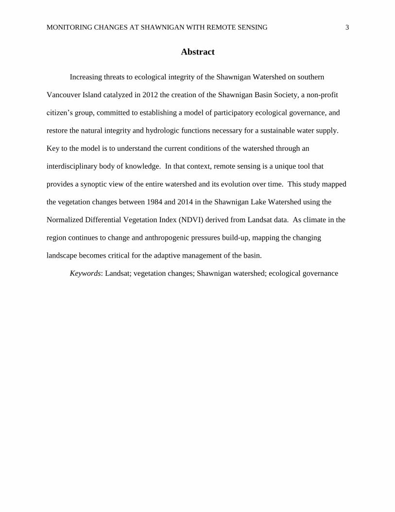
Abstract
Increasing threats to ecological integrity of the Shawnigan Watershed on southern
Vancouver Island catalyzed in 2012 the creation of the Shawnigan Basin Society, a non-profit
citizen’s group, committed to establishing a model of participatory ecological governance, and
restore the natural integrity and hydrologic functions necessary for a sustainable water supply.
Key to the model is to understand the current conditions of the watershed through an
interdisciplinary body of knowledge. In that context, remote sensing is a unique tool that
provides a synoptic view of the entire watershed and its evolution over time. This study mapped
the vegetation changes between 1984 and 2014 in the Shawnigan Lake Watershed using the
Normalized Differential Vegetation Index (NDVI) derived from Landsat data. As climate in the
region continues to change and anthropogenic pressures build-up, mapping the changing
landscape becomes critical for the adaptive management of the basin.
Keywords: Landsat; vegetation changes; Shawnigan watershed; ecological governance

MONITORING CHANGES AT SHAWNIGAN WITH REMOTE SENSING 4
Acknowledgements
I want to thank all the people in my life who have guided me during this journey, shared
their knowledge, inspired me to dig deeper, fed me dinners and made me laugh.
Special gratitude to my parents, Carmina and Antonio, for their constant encouragement,
and my son, Thomas Antonio, for he always inspires me to be a better person.
From ASL Environmental Sciences Inc., I want to thank David Fissel and the rest of the
Board of Directors at ASL Inc. for the generous support, and Keath Borg for his thorough review
and helpful comments. A big thanks to the instructors at Royal Roads University (RRU),
especially to Dr. Liza Ireland, for her passionate teaching and her continued efforts to focus my
enthusiasm; to Dr. Tom Green, for opening a window to the complexities of ecological
economics and reinforcing my belief that we cannot put a price on nature; and to Dr. Bob Kull,
for the reaffirmation of my worldview and values. I also want to thank to my friends Sarah
Roberts, Ralph Roberts and Ellen Simmons for their helpful reviews and friendship.
I am immensely grateful to Kelly Musselwhite, Dr. Bruce Fraser, and David Hutchinson
from the Shawnigan Basin Society, and Barry Gates of the Shawnigan Ecological Design Panel,
for sharing their knowledge and dedication, giving me an opportunity to collaborate in such an
interesting study and reviewing this paper.
Last but not least, I want to remember my two grandmothers, Carmen and Julia, and my
great aunt Isabel, three strong, brave and perseverant women, always present in my heart.

MONITORING CHANGES AT SHAWNIGAN WITH REMOTE SENSING 5
Glossary
AOI Area Of Interest
BCLSS British Columbia Lake Stewardship Society
CVRD Cowichan Valley Regional District
in situ “on the ground” - in the document refers to field work
ETM + Enhanced Thematic Mapper Plus (Landsat 7)
GIS Geographic Information Systems
GLOVIS USGS Global Visualization viewer
MOE Ministry of Environment (British Columbia government)
NDVI Normalized Difference Vegetation Index
NIR Near Infra-red
OLI Operational Land Imager (Landsat 8)
ROI Region Of Interest
SBA Shawnigan Basin Authority
SBS Shawnigan Basin Society
SWR Shawnigan Watershed Roundtable
TEV Total Economic Valuation
TM Thematic Mapper (Landsat 5)
TOA Top-Of -Atmosphere (reflectance)
USGS United States Geological Service
UTM Universal Transverse Mercator (map projection)
WGS World Geodetic System
WMP Watershed Management Plan
MONITORING CHANGES AT SHAWNIGAN WITH REMOTE SENSING 6
Table of Contents
Abstract ........................................................................................................................................... 3
Acknowledgements ......................................................................................................................... 4
Glossary .......................................................................................................................................... 5
Table of Contents ............................................................................................................................ 6
List of Figures ................................................................................................................................. 8
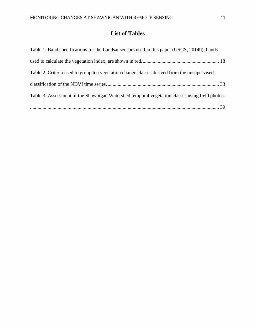
List of Tables ................................................................................................................................ 11
Introduction ................................................................................................................................... 12
Background on the Study Area ............................................................................................... 13
Research Objectives and Question.......................................................................................... 15
Methodology ................................................................................................................................. 16
Acquisition and Processing of Landsat Data .......................................................................... 16
The Normalized Difference Vegetation Index (NDVI) .......................................................... 20
Caveat............................................................................................................................... 21
Seasonality. ...................................................................................................................... 22
Temporal Changes of the Vegetation Cover ........................................................................... 22
Reflectance RGB Composite. ......................................................................................... 23
NDVI trends. ................................................................................................................... 23
Unsupervised classification of NDVI change. ............................................................... 23
CVRD Vectors ........................................................................................................................ 24
Field Survey ............................................................................................................................ 25
Results and Discussion ................................................................................................................. 26
Seasonality Analysis ............................................................................................................... 26
Vegetation Changes in Southern Cowichan Watersheds ........................................................ 27
Reflectance RGB three-year composite map. ............................................................... 27
NDVI difference map. ..................................................................................................... 28
Long-Term Vegetation Changes in the Shawnigan Watershed .............................................. 30
MONITORING CHANGES AT SHAWNIGAN WITH REMOTE SENSING 7
Trends in Average NDVI................................................................................................ 30
Unsupervised classification of vegetation changes. ...................................................... 33
Field Data ................................................................................................................................ 36
Conclusions ................................................................................................................................... 45
Remote Sensing Data and Results. ......................................................................................... 45
Beyond Remote Sensing: Is Sustainability Possible in the Shawnigan Lake Watershed? ..... 47
Future Directions. ........................................................................................................... 51
References ..................................................................................................................................... 53
Appendix A: Shawnigan Watershed Management Plan ............................................................... 67
Appendix B: Greater Victoria Watersheds ................................................................................... 68
Appendix C: Overview of the Overall Remote Sensing Processing & Analyses ......................... 69
Appendix D: Landsat Scenes for 22 Aug – 11 Oct 1984-2014 .................................................... 70
Appendix E: NDVI Images for 15-30 September 1984-2014 ...................................................... 71
Appendix F: Areal Distribution of NDVI-year Trends in the CVRD Parcels .............................. 72
Appendix G: Areal Distribution of Temporal Classes in the CVRD Parcels ............................... 73
MONITORING CHANGES AT SHAWNIGAN WITH REMOTE SENSING 8
List of Figures
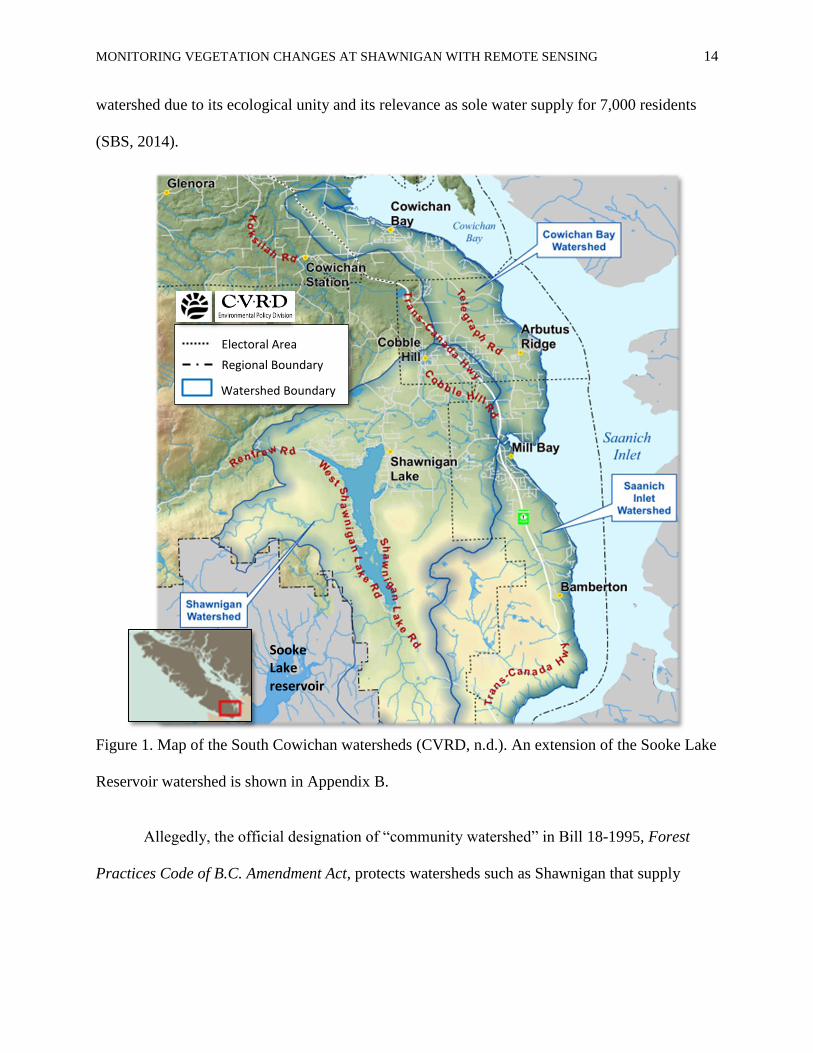
Figure 1. Map of the South Cowichan watersheds (CVRD, n.d.). An extension of the Sooke Lake
Reservoir watershed is shown in Appendix B. ............................................................................. 14
Figure 2. GLOVIS browser showing an overview of Landsat scenes covering southern
Vancouver Island: The area of interest is encompassed by both paths between the yellow and the
red areas. ....................................................................................................................................... 17
Figure 3. Near true colour composite (NTC) of 15 September 2014 L5TM (A). Insets show
subscenes for southern Vancouver Island (B), and Shawnigan Watershed (C) – the watershed
boundaries are shown in red in B and C. ...................................................................................... 19
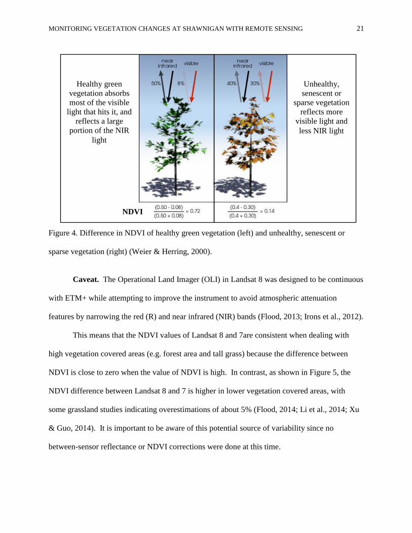
Figure 4. Difference in NDVI of healthy green vegetation (left) and unhealthy, senescent or
sparse vegetation (right). (Weier & Herring, 2000). ..................................................................... 21
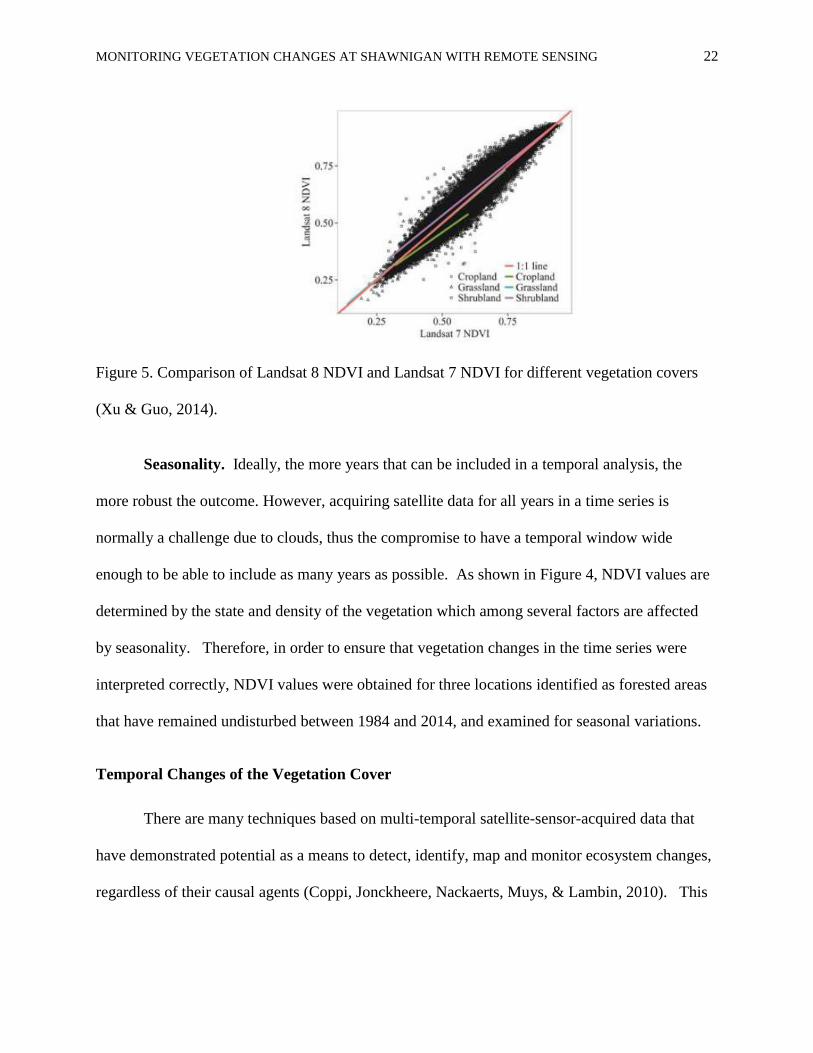
Figure 5. Comparison of Landsat 8 NDVI and Landsat 7 NDVI for different vegetation covers
(Xu & Guo, 2014). ........................................................................................................................ 22
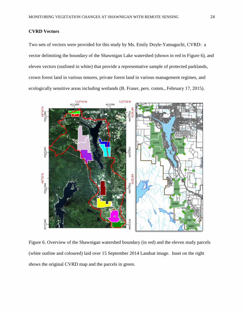
Figure 6. Shawnigan watershed boundary (in red), and the eleven study parcels (white outline
and coloured) laid over 15 September 2014 Landsat image. Inset on the right shows the original
CVRD map and the parcels in green............................................................................................. 24
Figure 7. NDVI values at three locations derived from 33 NDVI images between 21 August (JD
233) and 11 October (JD 284) 1984 to 2014. Seasonality is noted by the decreasing trends. ...... 26
Figure 8. Overview of RGB composite for southern Vancouver Island (Red: 15Sep 2014; Green:
26 Sep 1998, Blue: 28 Sep. 1984). The watershed boundary is shown in in yellow. .................. 27
Figure 9. Map of vegetation changes derived from the difference NDVI2014 - NDVI1984. The
watershed boundary is shown in red. ............................................................................................ 29
Figure 10. Examples of NDVI trends for the change classes shown in Figure 11. ...................... 30
MONITORING CHANGES AT SHAWNIGAN WITH REMOTE SENSING 9
Figure 11. Map of 1984-2014 vegetation trends in the Shawnigan Watershed superimposed over
the 15 Sep 2014 red band (0.65 μm). Plots show the distributions and areas (ha) of each trends
class for the entire watershed (A) and for each of the CVRD parcels (B), which are presented
from the most to the least changed. Areal details for each parcel (ha) are in Appendix F. ......... 32
Figure 12.Temporal classification of the Shawnigan Basin superimposed over the 15 Sep 2014
red band (0.65 μm). ....................................................................................................................... 34
Figure 13. Representative contributions of each temporal class in the entire watershed with areas
(ha) in italics (A), and for each of the CVRD parcels (B), sorted from the most disturbed to the
least; further details for each parcel are included in Appendix G. ................................................ 35
Figure 14. Overview of the GoogleEarth file showing the classification map for Shawnigan basin
north, the watershed boundary in yellow, CVRD parcels in white, February phot-locations (P1-
P23) with yellow pins, and March locations (PI-PM) in blue. ..................................................... 37
Figure 15. Overview of the GoogleEarth file showing the classification map for Shawnigan basin
south, the watershed boundary in yellow, CVRD parcels in white, February phot-locations (P1-
P23) with yellow pins, and March locations (PI-PM) in blue. ..................................................... 38
Figure 16. March 2015 photos of Shawnigan lake shoreline. Insets show hardhack in bloom
(top) and bulrush in full growth (bottom) (E-Flora BC, 2014). ................................................... 40
Figure 17. February 2015 photos illustrating weakly varying classes 4 and 5. Parcel and photo
number are indicated at the bottom of each picture. ..................................................................... 41
Figure 18. February 2015 photos of sites disturbed and not recovered by 2014 (Class 6). Parcel
number and photo number are indicated at the bottom of each picture. ....................................... 42
Figure 19. February 2015 photos of disturbed sites and recovered by 2014 (Class 7 and 8).
Parcel number and photo number are indicated at the bottom of each picture. ............................ 43
MONITORING CHANGES AT SHAWNIGAN WITH REMOTE SENSING 10
Figure 20. February 2015 photos for Classes 9 and 10 classified as fast growth with 2014 NDVIs
> 0.5. ............................................................................................................................................. 44
Figure 21. At the Shawnigan Basin Society watershed planning office, 1 February 2014. Left to
right: Barry Gates (ecoforester- responsible for the forest management design of the Living
Forest Community in the Elkington Forest), myself, Dr. Bruce Fraser (President of the
Shawnigan Basin Society), and Kelly Musselwhite (RRU colleague and executive director of the
SBS). ............................................................................................................................................. 47
Figure 22. Map with yellow pin showing the location of South Island Aggregates toxic soil
remediation site; the red pin indicates location for 4 March photo showing contaminated material
flowing into Shawnigan Creek (photos by D. Hutchinson) .......................................................... 49
MONITORING CHANGES AT SHAWNIGAN WITH REMOTE SENSING 11
List of Tables
Table 1. Band specifications for the Landsat sensors used in this paper (USGS, 2014b); bands
used to calculate the vegetation index, are shown in red. ............................................................. 18
Table 2. Criteria used to group ten vegetation change classes derived from the unsupervised
classification of the NDVI time series. ......................................................................................... 33
Table 3. Assessment of the Shawnigan Watershed temporal vegetation classes using field photos.
....................................................................................................................................................... 39
MONITORING VEGETATION CHANGES AT SHAWNIGAN WITH REMOTE SENSING 12
Introduction
The Shawnigan Watershed, located on southern Vancouver Island, British Columbia,
feeds the Shawnigan Lake, the second largest lake within the Cowichan Valley Regional District
(CVRD) and the sole domestic water source for a community of presently over 7,000 people
(CVRD, 2010; Fraser, 2014a; Rieberger, Epps, & Wilson, 2004). The basin’s land base is highly
fragmented among private ownerships, with crown land parcels mostly allocated by the province
as woodlots, and significant park areas owned by the Regional District (Fraser, 2014b;
Kemshaw, 2006). The governance of land and water resources in the basin has been fragmented
among federal, provincial and local government agencies resulting in unresolved environmental
problems derived from decades of intense industrial practices and increasing subdivision
development (Fraser, 2014b; Nordin, Zu, & Mazumder, 2007). The cumulative impact is high,
leading to significant threats to the public water supply that will be amplified by the progressing
consequences of climate change (CVRD, 2014a,b).
The mounting risks to the ecological integrity of the basin raised the concerns of a
community that increasingly knows and cares about its watershed and water security (Bainas,
2014; Cullington & Associates, 2012a,b; Desmond, 2012). In February 2012 the Shawnigan
community established the Shawnigan Watershed Roundtable (SWR) to promote active
ecological stewardship of the watershed. In 2013 this initiative led to the creation of the
Shawnigan Basin Society (SBS), a non-profit citizen’s group committed to establishing a model
of participatory ecological governance of the Shawnigan Community Watershed, and to gain and
account for public funds for watershed management (Fraser, 2012a). A third initiative, presently
in progress and being addressed collaboratively with the CVRD, is the Shawnigan Basin
Authority (SBA). The SBA aims to attain some decision making power from the government
MONITORING VEGETATION CHANGES AT SHAWNIGAN WITH REMOTE SENSING 13
agencies and achieve locally collaborative ecological governance of the watershed, though this is
expected to take several years to be accomplished (Fraser, 2014b; Rusland, 2013). The overall
objective is to develop and execute the Watershed Management Plan (WMP), shown in
Appendix A, which addresses the ecological risks to the basin, engages the many relevant senior
and local government jurisdictional agencies and involves the public and the Málexet1 First
Nations of the region (Fraser, 2013).
Basic to the ecosystem based conservation planning model is the acquisition of a strong
scientific base of geographic, ecological and hydrological information, aimed to establish a
baseline of the basin ecosystems; assembly of some of this knowledge is under way (Cullington
& Associates, 2012b; Rieberg et al., 2004). However, there have not been systematic ground
observations in the area over time, except for private managed forest land parcels. There are
presently still no accurate maps of our source streams, filtering wetlands and forest ecosystems,
which are critical to understanding the present state of ecological integrity and help focusing
efforts to restore the natural hydrologic functions of the watershed required for sustainable water
supplies into the future (B. Fraser, pers. comm., February 7, 2015).
Background on the Study Area
South Cowichan, home to the Cowichan, Shawnigan and Saanich Inlet watersheds
(Figure 1), was inhabited by Coastal Salish First Nations over 8,000 years ago who were
displaced as a result of the E&N Railway land grant in the late 1800’s. Since then, the area has
been heavily impacted by industrial logging, mining, recreation and urban sprawl (CVRD, 2010).
Although the Shawnigan watershed boundaries expand to the northeast towards Cobble Hill and
east into Mill Bay, the SBS has focused their preliminary efforts on the Shawnigan Lake
1 Malahat
MONITORING VEGETATION CHANGES AT SHAWNIGAN WITH REMOTE SENSING 14
watershed due to its ecological unity and its relevance as sole water supply for 7,000 residents
(SBS, 2014).
Figure 1. Map of the South Cowichan watersheds (CVRD, n.d.). An extension of the Sooke Lake
Reservoir watershed is shown in Appendix B.
Allegedly, the official designation of “community watershed” in Bill 18-1995, Forest
Practices Code of B.C. Amendment Act, protects watersheds such as Shawnigan that supply
Electoral Area Boundary Regional Boundary
Watershed Boundary
Sooke Lake reservoir
MONITORING VEGETATION CHANGES AT SHAWNIGAN WITH REMOTE SENSING 15
drinking water from harmful industrial practices (BC MOE2, 2004). However, the reality is quite
different (Cullington & Associates, 2012a,b; Desmond, 2012; The Council of Canadians, 2014).
There are concerns for surface water quality due to impacts of human activities in the upper
watershed, around the lake and on the lake itself (Fraser, 2012b). The watershed upland forests
were harvested in the early 1900s; additional ongoing harvesting continues to impact the
ecological integrity of the basin and the conditions in the lake (CVRD, 2010).
Shawnigan Lake is considered oligotrophic3, but algal patterns changes and hypoxia
events recorded in the past have been associated with intensive logging and settlement (Gregory,
2014; Nordin & McKean, 1984). Water quality was reported to remain within Provincial
guidelines a decade ago (Rieberger et al., 2004), but recent studies point to a trend of increasing
concentrations of chemicals and human feces (Mazumder, 2012; McGillivar, 2009). In addition,
for the last two years, the Shawnigan community has been fighting a permit granted by the MOE
that allows South Island Aggregates (SIA)4 to dump five million tons of toxic soil directly above
Shawnigan Lake’s main feeder creek (Fraser, 2012b; McCulloch, 2014).
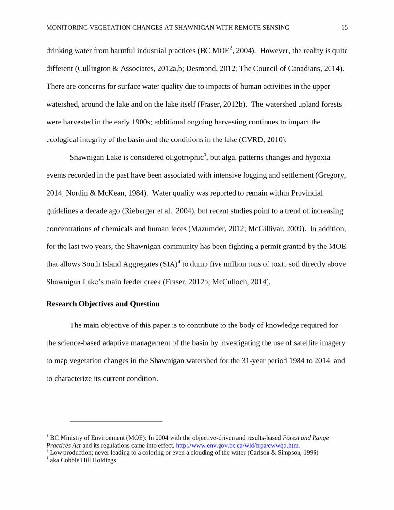
Research Objectives and Question
The main objective of this paper is to contribute to the body of knowledge required for
the science-based adaptive management of the basin by investigating the use of satellite imagery
to map vegetation changes in the Shawnigan watershed for the 31-year period 1984 to 2014, and
to characterize its current condition.
2 BC Ministry of Environment (MOE): In 2004 with the objective-driven and results-based Forest and Range
Practices Act and its regulations came into effect. http://www.env.gov.bc.ca/wld/frpa/cwwqo.html 3 Low production; never leading to a coloring or even a clouding of the water (Carlson & Simpson, 1996)
4 aka Cobble Hill Holdings
MONITORING VEGETATION CHANGES AT SHAWNIGAN WITH REMOTE SENSING 16
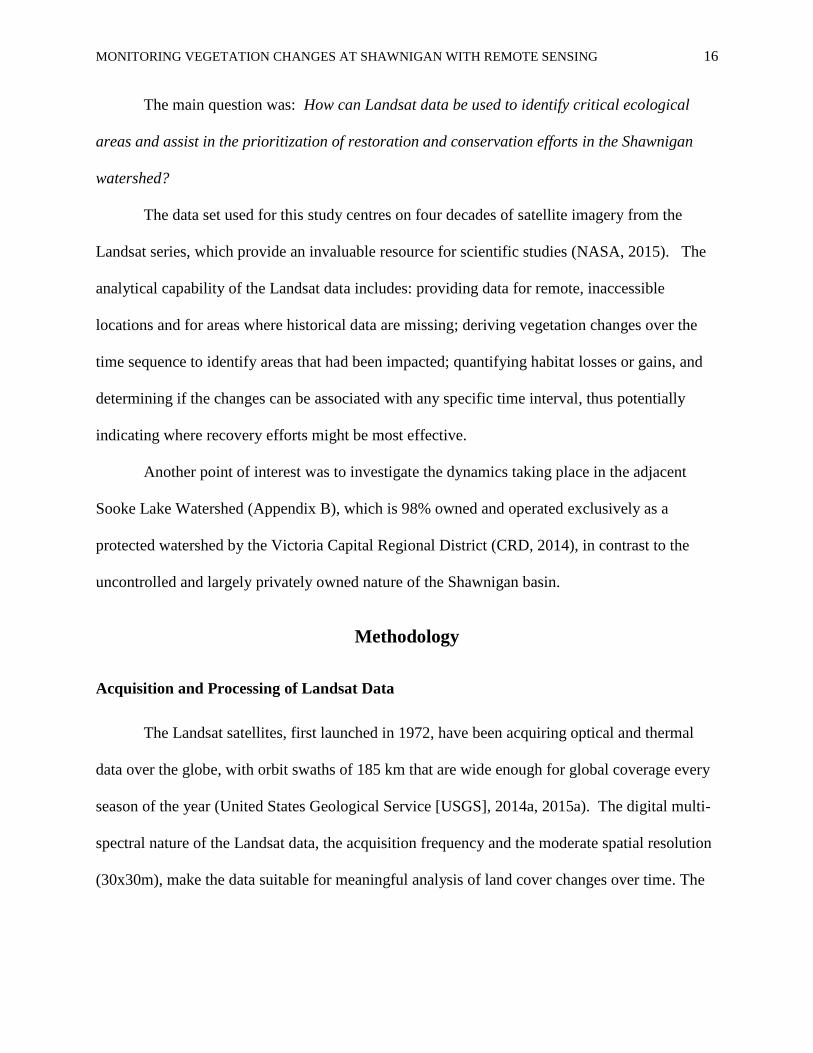
The main question was: How can Landsat data be used to identify critical ecological
areas and assist in the prioritization of restoration and conservation efforts in the Shawnigan
watershed?
The data set used for this study centres on four decades of satellite imagery from the
Landsat series, which provide an invaluable resource for scientific studies (NASA, 2015). The
analytical capability of the Landsat data includes: providing data for remote, inaccessible
locations and for areas where historical data are missing; deriving vegetation changes over the
time sequence to identify areas that had been impacted; quantifying habitat losses or gains, and
determining if the changes can be associated with any specific time interval, thus potentially
indicating where recovery efforts might be most effective.
Another point of interest was to investigate the dynamics taking place in the adjacent
Sooke Lake Watershed (Appendix B), which is 98% owned and operated exclusively as a
protected watershed by the Victoria Capital Regional District (CRD, 2014), in contrast to the
uncontrolled and largely privately owned nature of the Shawnigan basin.
Methodology
Acquisition and Processing of Landsat Data
The Landsat satellites, first launched in 1972, have been acquiring optical and thermal
data over the globe, with orbit swaths of 185 km that are wide enough for global coverage every
season of the year (United States Geological Service [USGS], 2014a, 2015a). The digital multi-
spectral nature of the Landsat data, the acquisition frequency and the moderate spatial resolution
(30x30m), make the data suitable for meaningful analysis of land cover changes over time. The

MONITORING VEGETATION CHANGES AT SHAWNIGAN WITH REMOTE SENSING 17
data are freely available and can be downloaded from the USGS Global Visualization Viewer
(GLOVIS) historical archive (USGS, 2015b).
The area of interest (AOI) for this study, the Shawnigan Watershed, is entirely captured
by Landsat path 47 and row 26 (48.9 deg Latitude, -122.8 deg Longitude), as shown in Figure 2.
Figure 2. USGS GLOVIS browser showing an overview of Landsat scenes covering southern
Vancouver Island: The area of interest is encompassed by both paths between the yellow and the
red areas.
The selection of images in GLOVIS focused on cloud-free scenes for the month of
September from 1984 to 2014; no data were available for Shawnigan before 1984. For years
with no suitable scene for September, the search expanded to include the end of August and
beginning of October. Cloud-free scenes out of that period were also downloaded and archived
for potential future analyses.
MONITORING VEGETATION CHANGES AT SHAWNIGAN WITH REMOTE SENSING 18
A total of 218 Level 15 images were downloaded and reviewed using ENVI
TM image
processing software property of ASL Environmental Sciences Inc. (processing flow summarized
in Appendix C). A total of 51 images were found suitable for the study period, and included 39
Landsat 5 Thematic Mapper ™, nine Landsat 7 Enhanced Thematic Mapper Plus (ETM+) and
three Landsat 8 Operational Land Imager (OLI) (Appendix C). Band specifications are shown in
Table 1 which shows the differences between OLI and the previous sensors.
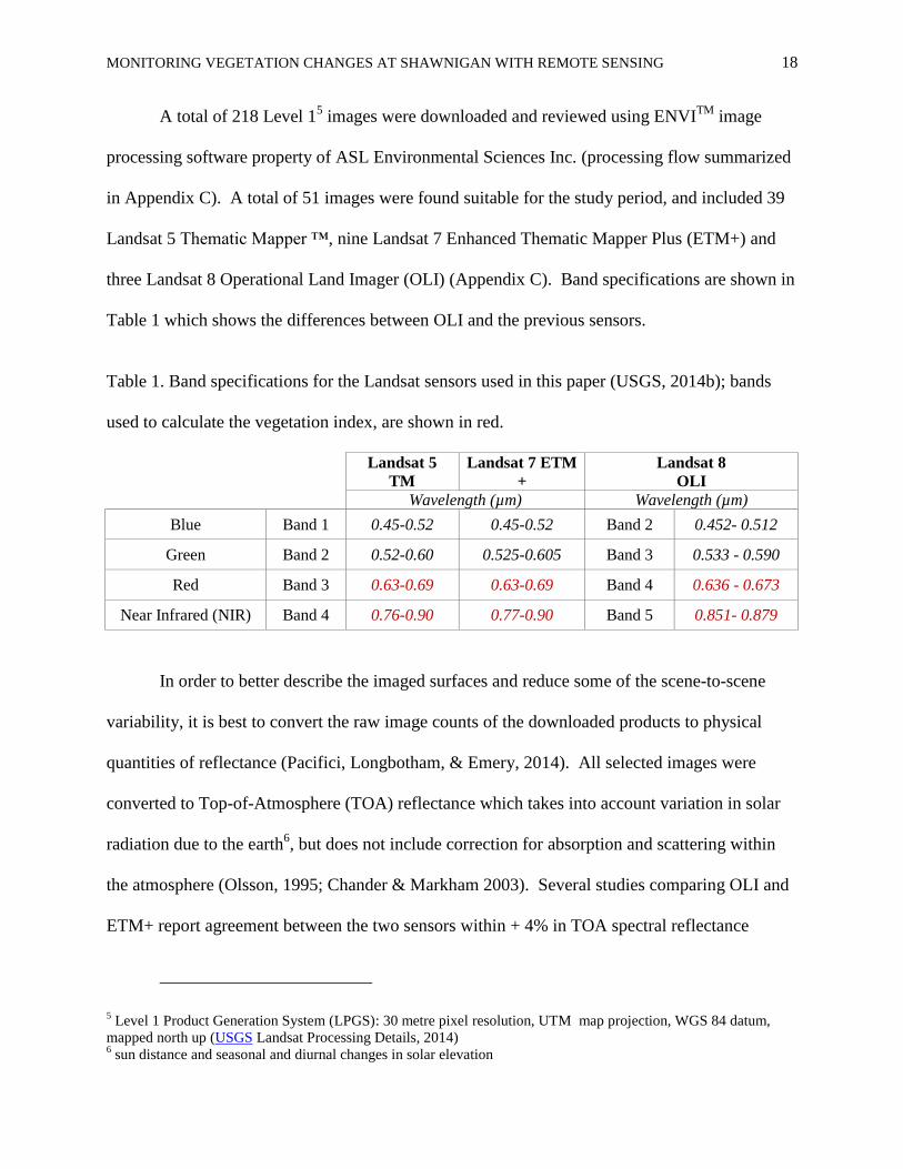
Table 1. Band specifications for the Landsat sensors used in this paper (USGS, 2014b); bands
used to calculate the vegetation index, are shown in red.
Landsat 5
TM
Landsat 7 ETM
+
Landsat 8
OLI
Wavelength (µm) Wavelength (µm)
Blue Band 1 0.45-0.52 0.45-0.52 Band 2 0.452- 0.512
Green Band 2 0.52-0.60 0.525-0.605 Band 3 0.533 - 0.590
Red Band 3 0.63-0.69 0.63-0.69 Band 4 0.636 - 0.673
Near Infrared (NIR) Band 4 0.76-0.90 0.77-0.90 Band 5 0.851- 0.879
In order to better describe the imaged surfaces and reduce some of the scene-to-scene
variability, it is best to convert the raw image counts of the downloaded products to physical
quantities of reflectance (Pacifici, Longbotham, & Emery, 2014). All selected images were
converted to Top-of-Atmosphere (TOA) reflectance which takes into account variation in solar
radiation due to the earth6, but does not include correction for absorption and scattering within
the atmosphere (Olsson, 1995; Chander & Markham 2003). Several studies comparing OLI and
ETM+ report agreement between the two sensors within + 4% in TOA spectral reflectance
5 Level 1 Product Generation System (LPGS): 30 metre pixel resolution, UTM map projection, WGS 84 datum,
mapped north up (USGS Landsat Processing Details, 2014) 6 sun distance and seasonal and diurnal changes in solar elevation
MONITORING VEGETATION CHANGES AT SHAWNIGAN WITH REMOTE SENSING 19
(Czapla-Myers et al., 2015; Irons, Dywer, & Barsi, 2012). Further discussion on the spectral
differences between the Landsat series is addressed in the next section. While it would be
preferable to use atmospherically corrected data7, adequate surface reflectance corrections of the
Landsat 8 data could not be generated with the available processing software, thus only TOA
calibration was done at this time.
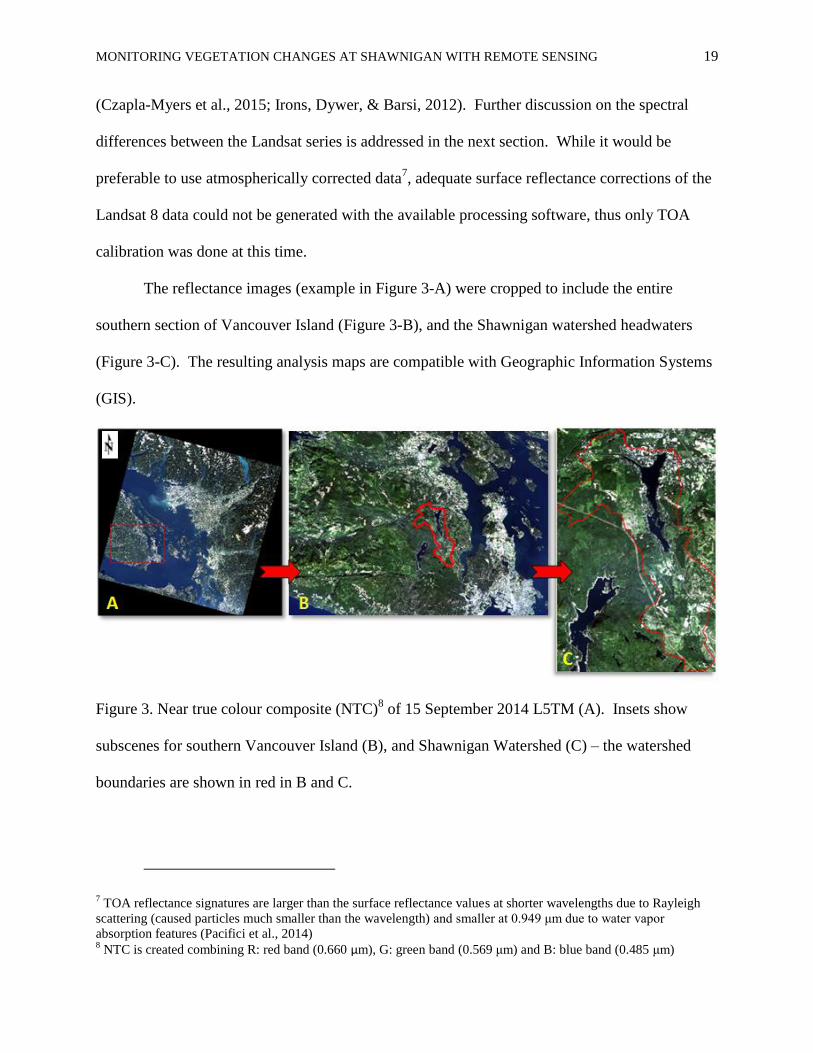
The reflectance images (example in Figure 3-A) were cropped to include the entire
southern section of Vancouver Island (Figure 3-B), and the Shawnigan watershed headwaters
(Figure 3-C). The resulting analysis maps are compatible with Geographic Information Systems
(GIS).
Figure 3. Near true colour composite (NTC)8 of 15 September 2014 L5TM (A). Insets show
subscenes for southern Vancouver Island (B), and Shawnigan Watershed (C) – the watershed
boundaries are shown in red in B and C.
7 TOA reflectance signatures are larger than the surface reflectance values at shorter wavelengths due to Rayleigh
scattering (caused particles much smaller than the wavelength) and smaller at 0.949 μm due to water vapor
absorption features (Pacifici et al., 2014) 8 NTC is created combining R: red band (0.660 μm), G: green band (0.569 μm) and B: blue band (0.485 μm)

MONITORING VEGETATION CHANGES AT SHAWNIGAN WITH REMOTE SENSING 20
The Normalized Difference Vegetation Index (NDVI)
There are many remote sensing vegetation indices intended to characterize the type
amount and condition of vegetation for each pixel in a satellite image (Baret & Guyot, 1991;
Jackson & Huete, 1991; Li, Jiang, & Feng, 2014; Silleos, Alexandridis, Gitas, & Perakis, 2006).
The chosen index was the Normalized Difference Vegetation Index (NDVI), a surrogate for
photosynthetic capacity based on the principle that chlorophyll in healthy plants strongly absorbs
incoming sunlight in the visible blue and red regions of the electromagnetic spectrum to fuel
photosynthesis and create chlorophyll, whereas the cell structure of the leaves scatters the near-
infrared (NIR) wavelengths back into the sky (Rouse, Haas, Schell, & Deering, 1974; Tucker,
1979; Lyon, Yuan, Lunetta, & Elvidge 1998).
NDVI for each pixel of each TOA reflectance image was calculated using the formula:
NDVI = (Near Infrared- Red) / (Near Infrared + Red)
where the red band is generally centered near 0.65 µm, and the NIR band varies over a broader
range between about 0.76 and 0.88 µm.
As shown in Figure 4, vigorously growing healthy vegetation with low red reflectance
and high infrared reflectance will exhibit high NDVI values greater than 0.5, sparse vegetation
such as shrubs and grasslands or senescing crops result in moderate NDVI values (approximately
0.2 to 0.5), and non-vegetated features, such as barren rock, soil, and water will have NDVI
values 0.1 or less (USGS, 2015c).
MONITORING VEGETATION CHANGES AT SHAWNIGAN WITH REMOTE SENSING 21
Figure 4. Difference in NDVI of healthy green vegetation (left) and unhealthy, senescent or
sparse vegetation (right) (Weier & Herring, 2000).
Caveat. The Operational Land Imager (OLI) in Landsat 8 was designed to be continuous
with ETM+ while attempting to improve the instrument to avoid atmospheric attenuation
features by narrowing the red (R) and near infrared (NIR) bands (Flood, 2013; Irons et al., 2012).
This means that the NDVI values of Landsat 8 and 7are consistent when dealing with
high vegetation covered areas (e.g. forest area and tall grass) because the difference between
NDVI is close to zero when the value of NDVI is high. In contrast, as shown in Figure 5, the
NDVI difference between Landsat 8 and 7 is higher in lower vegetation covered areas, with
some grassland studies indicating overestimations of about 5% (Flood, 2014; Li et al., 2014; Xu
& Guo, 2014). It is important to be aware of this potential source of variability since no
between-sensor reflectance or NDVI corrections were done at this time.
Healthy green
vegetation absorbs
most of the visible
light that hits it, and
reflects a large
portion of the NIR
light
Unhealthy,
senescent or
sparse vegetation
reflects more
visible light and
less NIR light
NDVI
MONITORING VEGETATION CHANGES AT SHAWNIGAN WITH REMOTE SENSING 22
Figure 5. Comparison of Landsat 8 NDVI and Landsat 7 NDVI for different vegetation covers
(Xu & Guo, 2014).
Seasonality. Ideally, the more years that can be included in a temporal analysis, the
more robust the outcome. However, acquiring satellite data for all years in a time series is
normally a challenge due to clouds, thus the compromise to have a temporal window wide
enough to be able to include as many years as possible. As shown in Figure 4, NDVI values are
determined by the state and density of the vegetation which among several factors are affected
by seasonality. Therefore, in order to ensure that vegetation changes in the time series were
interpreted correctly, NDVI values were obtained for three locations identified as forested areas
that have remained undisturbed between 1984 and 2014, and examined for seasonal variations.
Temporal Changes of the Vegetation Cover
There are many techniques based on multi-temporal satellite-sensor-acquired data that
have demonstrated potential as a means to detect, identify, map and monitor ecosystem changes,
regardless of their causal agents (Coppi, Jonckheere, Nackaerts, Muys, & Lambin, 2010). This
MONITORING VEGETATION CHANGES AT SHAWNIGAN WITH REMOTE SENSING 23
paper explored several methods illustrated in Appendix C and described hereafter to assess the
changes in the Shawnigan watershed vegetation cover between 1984 and 2014.
Reflectance RGB Composite. The TOA reflectance green bands (0.56 μm) of three
years in the time series were used to create a three-layer Red-Green-Blue (RGB) composite in
ENVITM
, where Red: 15 September 2014, Green: 26 September 1998, and Blue: 28 September
1984. This method makes it easier to see the history of vegetation cover in the area.
NDVI trends. The analysis of vegetation changes using the NDVI images (Appendix E)
were based on two methods (Borstad, Martínez de Saavedra Álvarez, Hines, & Dufour, 2008,
2010; Martínez de Saavedra Álvarez, Brown, Ersahin, & Henley, 2013):
(1) the difference between 1984 NDVI and 2014 NDVI (beginning and end of the time
series); this was done only for the southern Vancouver Island scene, and
(2) analysis of the NDVI time series (“cube”) to determine the areal extent of change
over the 31-year study period (1984-2014); this was done only for the Shawnigan Basin. The
cube was then used to carry out a linear regression of NDVI versus year on a pixel-by-pixel
basis. This analysis generates images of slope that allow valuable mapping of the rate and
direction of change (gains or losses) and its significance (p< 0.05).
Unsupervised classification of NDVI change. Trends analysis does not provide
information of when changes happen, or if the vegetation cover shows signs of recovery after a
disturbance (characterized by a decreasing slope).
To obtain that information, and generate maps of habitat change over the entire watershed
a pixel-by-pixel temporal land cover classification was done using the unsupervised algorithm
ISODATA in ENVI 5.0TM
, which generated seventy groups of pixels with similar NDVI
histories. The classification included the watershed uplands only, and excluded the lake.
MONITORING VEGETATION CHANGES AT SHAWNIGAN WITH REMOTE SENSING 24
CVRD Vectors
Two sets of vectors were provided for this study by Ms. Emily Doyle-Yamaguchi, CVRD: a
vector delimiting the boundary of the Shawnigan Lake watershed (shown in red in Figure 6), and
eleven vectors (outlined in white) that provide a representative sample of protected parklands,
crown forest land in various tenures, private forest land in various management regimes, and
ecologically sensitive areas including wetlands (B. Fraser, pers. comm., February 17, 2015).
Figure 6. Overview of the Shawnigan watershed boundary (in red) and the eleven study parcels
(white outline and coloured) laid over 15 September 2014 Landsat image. Inset on the right
shows the original CVRD map and the parcels in green.
MONITORING VEGETATION CHANGES AT SHAWNIGAN WITH REMOTE SENSING 25
The vectors for the eleven CVRD parcels were converted in ENVITM
to digital regions of
interest (ROIs) in preparation for the multi-temporal analyses. Since sections of some of the
parcels fall outside of the watershed boundary (as shown in Figure 6), the parts were excluded
from the generated ROIs before the analyses. Changes in the vegetation cover were estimated
for all the CVRD parcels using the methods described in the previous section.
Field Survey
A GoogleEarth compatible KML file9 was created in ENVI
TM with the multi-temporal
NDVI classification map described earlier, and the boundaries for the eleven CVRD parcels in
the watershed. The objective was to direct a field survey and acquire some photos to assist with
interpretation of the vegetation change classes. A total of 42 locations were chosen inside the
CVRD parcels, carefully positioned in the center of large homogenous classes to avoid
inaccurate information caused by positional error (Stehamn, & Czaplewski, 1998; Zăvoianu,
Caramizoiub, & Badeaa, 2004). The KML file was sent to Mr. David Hutchinson (IT specialist
and Board Member of the SBS), and Mr. Barry Gates (ecological forester manager and Board
Member of the Ecological Design Panel for Shawnigan Lake) to assist in their field planning.
The photo survey was carried on between 15th
February and 4th
March 2015; 14 more locations
were added during the survey, though eight of the initially planned sites were not accessed at the
time. All the photographs were taken by Mr. Hutchinson, and made available with no
restrictions on their use via google sharing.
9 KML is a file format used to display geographic data in an Earth browser such as Google Earth (Google
Developers, 2013)
MONITORING VEGETATION CHANGES AT SHAWNIGAN WITH REMOTE SENSING 26
Results and Discussion
Seasonality Analysis
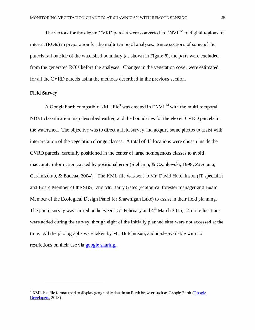
Seasonal changes have marked impacts on the spectral characteristics of vegetation,
especially in grasslands and deciduous forest (Vogelmann, Xian, Homer, & Tolk, 2012). NDVI
values for three locations in the Shawnigan basin identified as ‘forested and undisturbed between
1984 and 2014’ were extracted in ENVITM
. When the NDVI values were plotted by Julian Day
(JD) in Excel, it became evident that there was a seasonal effect (Figure 7), in particular affecting
Pt2 (shown in red), with NDVI values greater in 21 August (JD233) than in 11 October (JD 284).
Figure 7. NDVI values at three locations derived from 33 NDVI images between 21 August (JD
233) and 11 October (JD 284) 1984 to 2014. Seasonality is noted by the decreasing trends.
In order to ensure that the changes observed in the temporal analyses were not caused by
different seasonality patterns of “green-up” and senescence, only NDVI images from 15 to 30
September (Appendix E) were chosen at this time.
MONITORING VEGETATION CHANGES AT SHAWNIGAN WITH REMOTE SENSING 27
Vegetation Changes in Southern Cowichan Watersheds
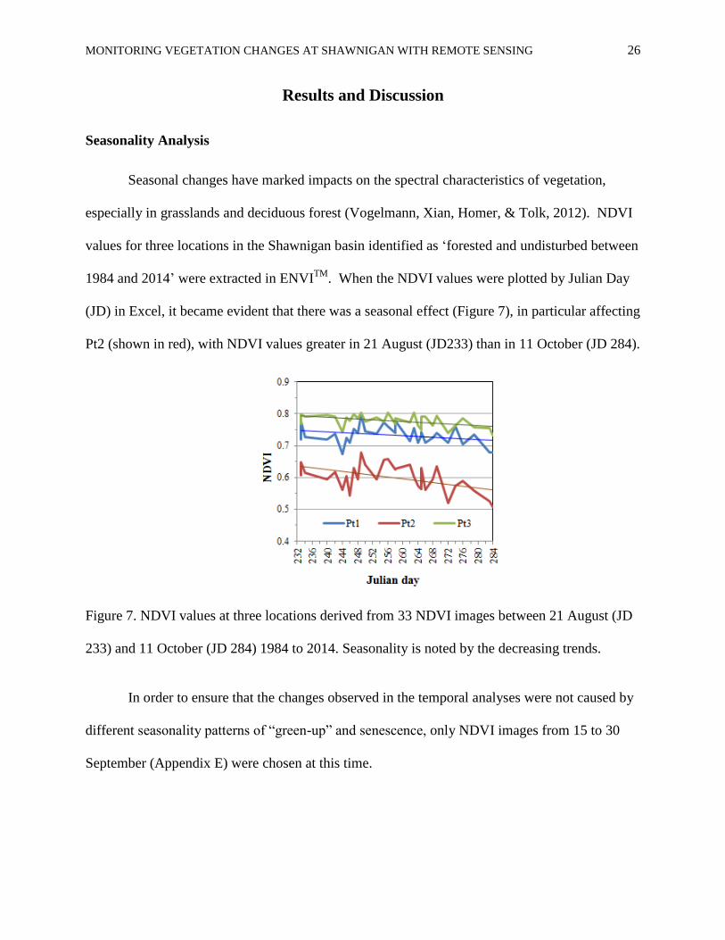
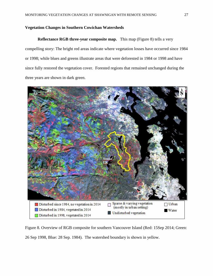
Reflectance RGB three-year composite map. This map (Figure 8) tells a very
compelling story: The bright red areas indicate where vegetation losses have occurred since 1984
or 1998; while blues and greens illustrate areas that were deforested in 1984 or 1998 and have
since fully restored the vegetation cover. Forested regions that remained unchanged during the
three years are shown in dark green.
Figure 8. Overview of RGB composite for southern Vancouver Island (Red: 15Sep 2014; Green:
26 Sep 1998, Blue: 28 Sep. 1984). The watershed boundary is shown in yellow.
MONITORING VEGETATION CHANGES AT SHAWNIGAN WITH REMOTE SENSING 28
This visual narrative illustrates the contrast between the recent forest conservation
management strategy (old growth restoration) in the Sooke Lake watershed. This has led to
forest recovery (green and blue areas southwest from Shawnigan) compared to the Shawnigan
Watershed, where industrial forestry, mining, soil dumping and urban pressures have led to
extensive forest losses, as indicated by the bright red coloured areas.
The contrast in this map paints a clear picture of the scale of the challenge that lies ahead
for the Shawnigan Lake community. Also worth mentioning is the striking vegetation losses in
the adjacent Saanich Inlet Watershed and the dense development in the Cowichan Bay
Watershed.
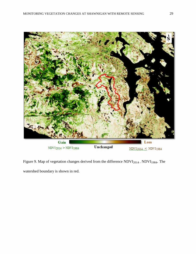
NDVI difference map. The map derived from the difference in 2014 and 1984 NDVIs
(Figure 9) uses a three-colour scheme: loss of vegetation cover occurred when NDVI2014 <
NDVI1984 (shown in brown); increase in vegetation when NDVI2014 > NDVI1984 (in green).
Areas were considered “unchanged” (shown in white) when the NDVI differences between 2014
and 1984 were less + 0.1.
This analysis corroborated the same message of losses and gains in the area shown in the
composite map (Figure 8).
MONITORING VEGETATION CHANGES AT SHAWNIGAN WITH REMOTE SENSING 29
Figure 9. Map of vegetation changes derived from the difference NDVI2014 - NDVI1984. The
watershed boundary is shown in red.
MONITORING VEGETATION CHANGES AT SHAWNIGAN WITH REMOTE SENSING 30
Long-Term Vegetation Changes in the Shawnigan Watershed
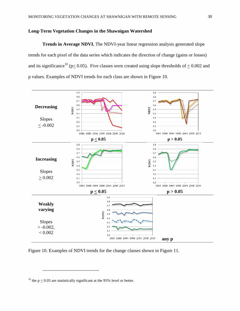
Trends in Average NDVI. The NDVI-year linear regression analysis generated slope
trends for each pixel of the data series which indicates the direction of change (gains or losses)
and its significance10
(p< 0.05). Five classes were created using slope thresholds of + 0.002 and
p values. Examples of NDVI trends for each class are shown in Figure 10.
Decreasing
Slopes
< -0.002
p < 0.05
p > 0.05
Increasing
Slopes
> 0.002
p < 0.05
p > 0.05
Weakly
varying
Slopes
> -0.002,
< 0.002
any p
Figure 10. Examples of NDVI trends for the change classes shown in Figure 11.
10 the p < 0.05 are statistically significant at the 95% level or better.
MONITORING VEGETATION CHANGES AT SHAWNIGAN WITH REMOTE SENSING 31
Trends were considered ‘unchanged or weakly varying’ when slopes ranged between -
0.002 and 0.002, regardless of p; ‘decreasing’ (vegetation loss), when slope values <-0.002; and
‘increasing’ (vegetation gains) when slope values > 0.002.
It is important to mention that while changes in the slope might not be statistically
significant they are still ecologically meaningful: Steady changes in slope will have p < 0.05,
while abrupt slope changes will exhibit p> 0.05. Abrupt changes are the result of landscape-
transforming events, such as those related to logging, agricultural expansion, urbanization, and
fire, which alter the spectral properties of the imaged surface (Vogelmann, Xian, Homer, & Tolk,
2012). One important limitation of the trend analysis is that while decreasing slopes technically
represent vegetation losses, as shown in Figure 10 some examples show (regardless of p) a
recovery of the vegetation cover with NDVI values close to or above 0.5 in 2014. Another
drawback is the ‘weakly varying’ class since it pools NDVI histories with very different
thresholds, thus a densely forested area and water are included in the class. Nonetheless, trends
are useful because they provide a synoptic view of long-term changes of the vegetation cover.
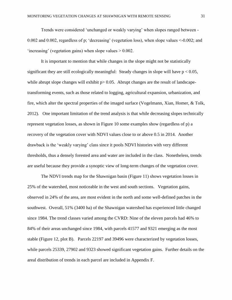
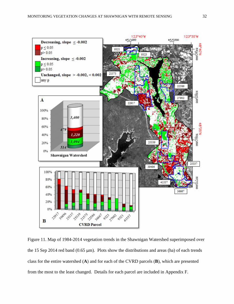
The NDVI trends map for the Shawnigan basin (Figure 11) shows vegetation losses in
25% of the watershed, most noticeable in the west and south sections. Vegetation gains,
observed in 24% of the area, are most evident in the north and some well-defined patches in the
southwest. Overall, 51% (3400 ha) of the Shawnigan watershed has experienced little changed
since 1984. The trend classes varied among the CVRD: Nine of the eleven parcels had 46% to
84% of their areas unchanged since 1984, with parcels 41577 and 9321 emerging as the most
stable (Figure 12, plot B). Parcels 22197 and 39496 were characterized by vegetation losses,
while parcels 25339, 27902 and 9323 showed significant vegetation gains. Further details on the
areal distribution of trends in each parcel are included in Appendix F.
MONITORING VEGETATION CHANGES AT SHAWNIGAN WITH REMOTE SENSING 32
Figure 11. Map of 1984-2014 vegetation trends in the Shawnigan Watershed superimposed over
the 15 Sep 2014 red band (0.65 μm). Plots show the distributions and areas (ha) of each trends
class for the entire watershed (A) and for each of the CVRD parcels (B), which are presented
from the most to the least changed. Details for each parcel are included in Appendix F.
MONITORING VEGETATION CHANGES AT SHAWNIGAN WITH REMOTE SENSING 33
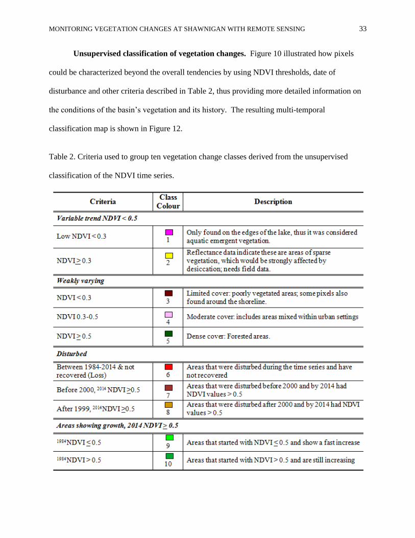
Unsupervised classification of vegetation changes. Figure 10 illustrated how pixels
could be characterized beyond the overall tendencies by using NDVI thresholds, date of
disturbance and other criteria described in Table 2, thus providing more detailed information on
the conditions of the basin’s vegetation and its history. The resulting multi-temporal
classification map is shown in Figure 12.
Table 2. Criteria used to group ten vegetation change classes derived from the unsupervised
classification of the NDVI time series.
MONITORING VEGETATION CHANGES AT SHAWNIGAN WITH REMOTE SENSING 34
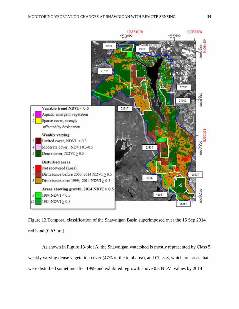
Figure 12.Temporal classification of the Shawnigan Basin superimposed over the 15 Sep 2014
red band (0.65 μm).
As shown in Figure 13-plot A, the Shawnigan watershed is mostly represented by Class 5
weakly varying dense vegetation cover (47% of the total area), and Class 8, which are areas that
were disturbed sometime after 1999 and exhibited regrowth above 0.5 NDVI values by 2014
MONITORING VEGETATION CHANGES AT SHAWNIGAN WITH REMOTE SENSING 35
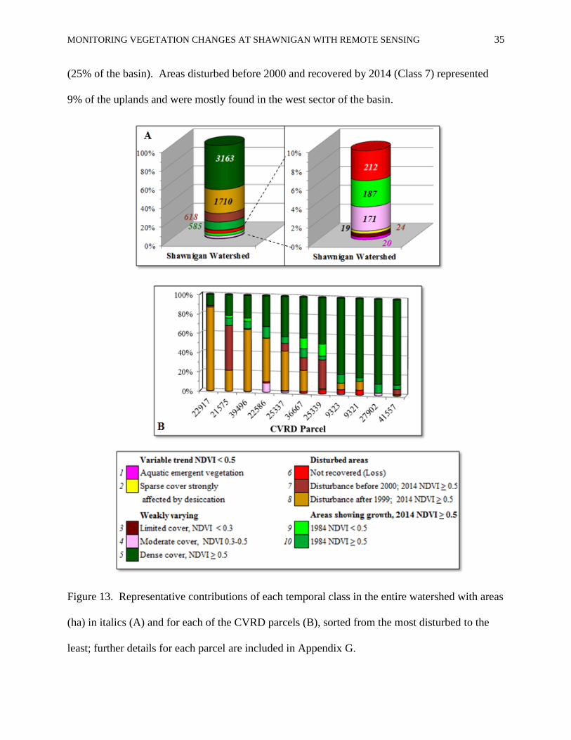
(25% of the basin). Areas disturbed before 2000 and recovered by 2014 (Class 7) represented
9% of the uplands and were mostly found in the west sector of the basin.
Figure 13. Representative contributions of each temporal class in the entire watershed with areas
(ha) in italics (A) and for each of the CVRD parcels (B), sorted from the most disturbed to the
least; further details for each parcel are included in Appendix G.
MONITORING VEGETATION CHANGES AT SHAWNIGAN WITH REMOTE SENSING 36
Vegetation loss (Class 6, 3% of the area) was found mostly in the southern section of the
basin. Vegetation growth trends were observed in areas that already had a vegetation cover with
NDVI > 0.5 in 1984 (Class 10, 9%), and patches that showed NDVI < 0.5 in 1984, probably due
to disturbance, and had NDVI values >0.5 in 2014 (Class 9, 3%). The moderate cover Class 4
represented approximately 3% of the basin and was found mostly in the northeast, within the
urban settings. The variable and low NDVI Class 5 (0.3% of the entire area) was found in a few
isolated patches that are probably disturbed areas covered with sparse vegetation. Aquatic
vegetation (Class 1) was found along the shoreline of the lake with NDVI trends consistently
below 0.1 values; similarly, the limited cover (Class 3) was mostly found sparsely distributed
along the lake. Both classes account for 0.3% and 0.4% of the studied area.
The distribution of the temporal classes varied greatly among the CVRD parcels (Figure
13-plot B). Parcels 9323, 9321, 27902 and 41557 were the most unchanged, showing a dense
vegetation cover (Class 5) since 1984 between 79% and 88% of their areas. Other parcels were
mostly composed represented by early disturbances and regrowth by 2014 with NDVI>0.5:
Class 7 (disturbed before 2000) was most predominant in parcel 21575 (47% of the parcel), and
Class 8 (disturbed after 1999) in parcel 22917 (87% of the parcel).
Field Data
The purpose of the February and March surveys was to acquire photos to assist with the
interpretation and assessment of the classification map shown in Figure 12. All photos were
taken by Dave Hutchinson11
, and have been used with his permission. The surveys’ sites are
indicated in Figures 14 and 15.
11 Board Member of the Shawnigan Basin Society
MONITORING VEGETATION CHANGES AT SHAWNIGAN WITH REMOTE SENSING 37
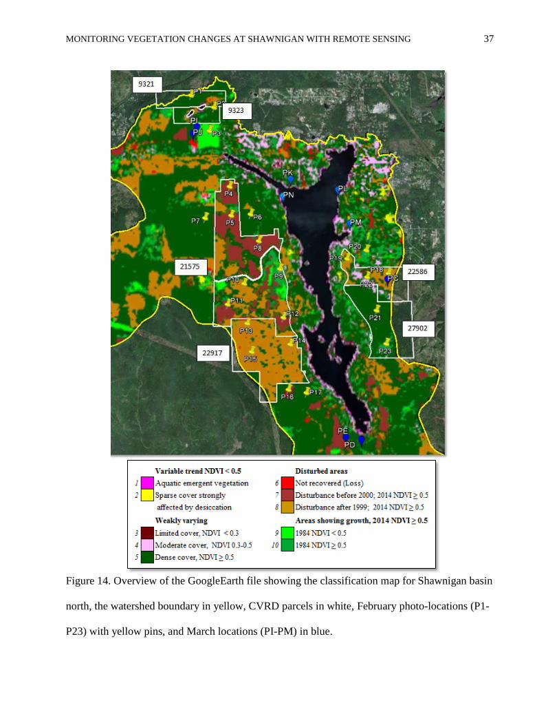
Figure 14. Overview of the GoogleEarth file showing the classification map for Shawnigan basin
north, the watershed boundary in yellow, CVRD parcels in white, February photo-locations (P1-
P23) with yellow pins, and March locations (PI-PM) in blue.
MONITORING VEGETATION CHANGES AT SHAWNIGAN WITH REMOTE SENSING 38
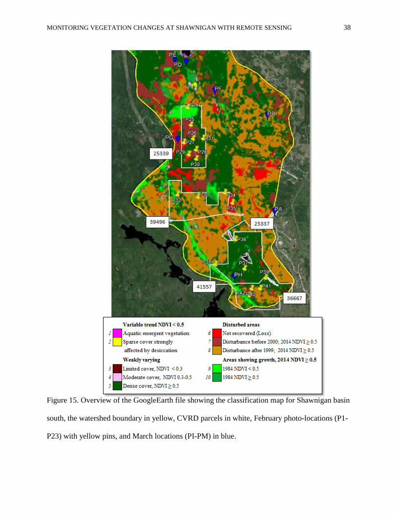
Figure 15. Overview of the GoogleEarth file showing the classification map for Shawnigan basin
south, the watershed boundary in yellow, CVRD parcels in white, February photo-locations (P1-
P23) with yellow pins, and March locations (PI-PM) in blue.
MONITORING VEGETATION CHANGES AT SHAWNIGAN WITH REMOTE SENSING 39
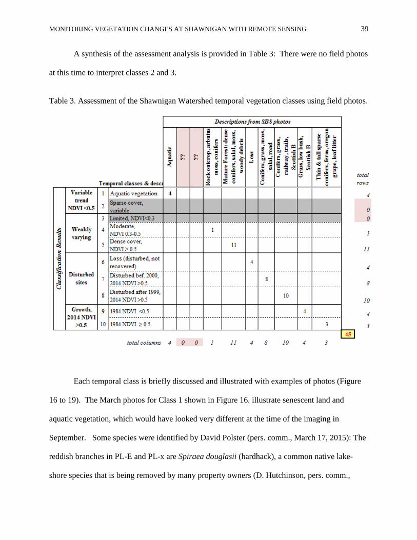
A synthesis of the assessment analysis is provided in Table 3: There were no field photos
at this time to interpret classes 2 and 3.
Table 3. Assessment of the Shawnigan Watershed temporal vegetation classes using field photos.
Each temporal class is briefly discussed and illustrated with examples of photos (Figure
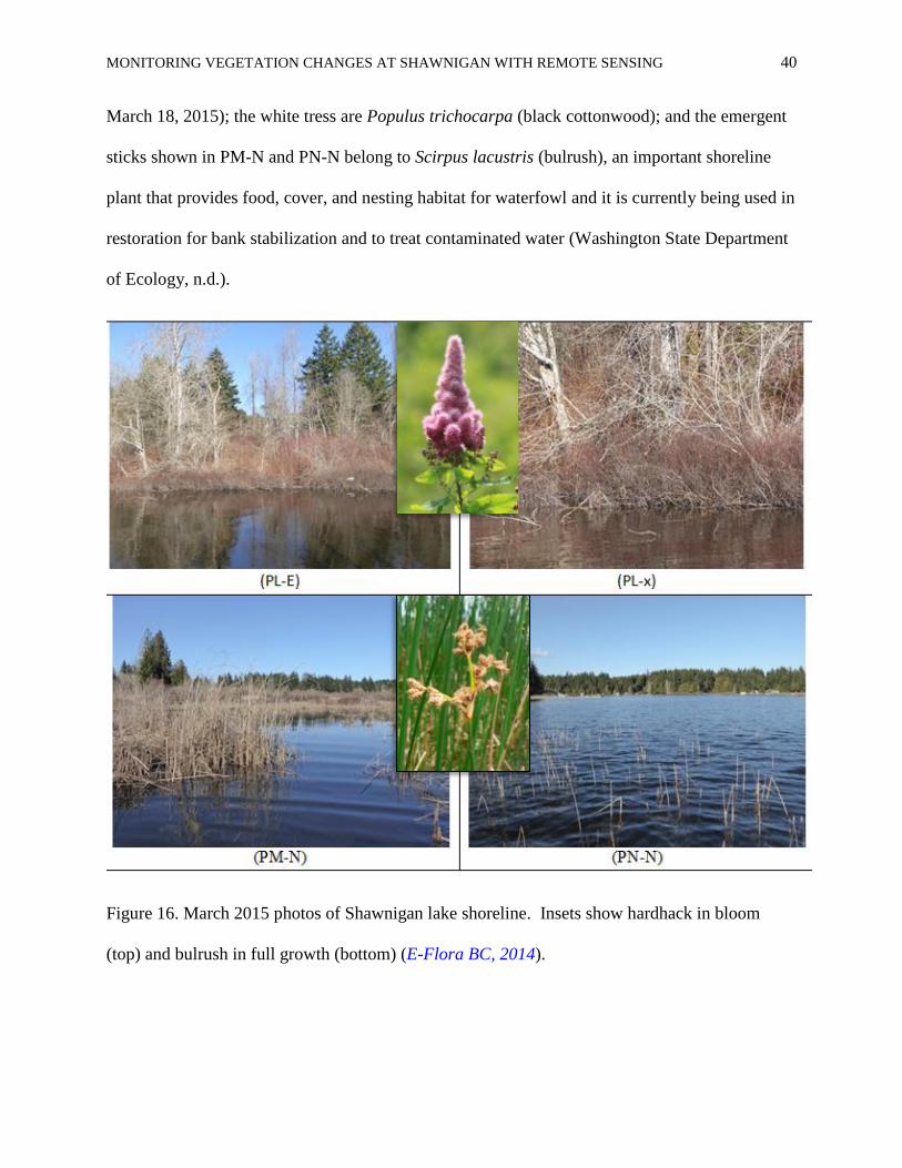
16 to 19). The March photos for Class 1 shown in Figure 16. illustrate senescent land and
aquatic vegetation, which would have looked very different at the time of the imaging in
September. Some species were identified by David Polster (pers. comm., March 17, 2015): The
reddish branches in PL-E and PL-x are Spiraea douglasii (hardhack), a common native lake-
shore species that is being removed by many property owners (D. Hutchinson, pers. comm.,
MONITORING VEGETATION CHANGES AT SHAWNIGAN WITH REMOTE SENSING 40
March 18, 2015); the white tress are Populus trichocarpa (black cottonwood); and the emergent
sticks shown in PM-N and PN-N belong to Scirpus lacustris (bulrush), an important shoreline
plant that provides food, cover, and nesting habitat for waterfowl and it is currently being used in
restoration for bank stabilization and to treat contaminated water (Washington State Department
of Ecology, n.d.).
Figure 16. March 2015 photos of Shawnigan lake shoreline. Insets show hardhack in bloom
(top) and bulrush in full growth (bottom) (E-Flora BC, 2014).
MONITORING VEGETATION CHANGES AT SHAWNIGAN WITH REMOTE SENSING 41
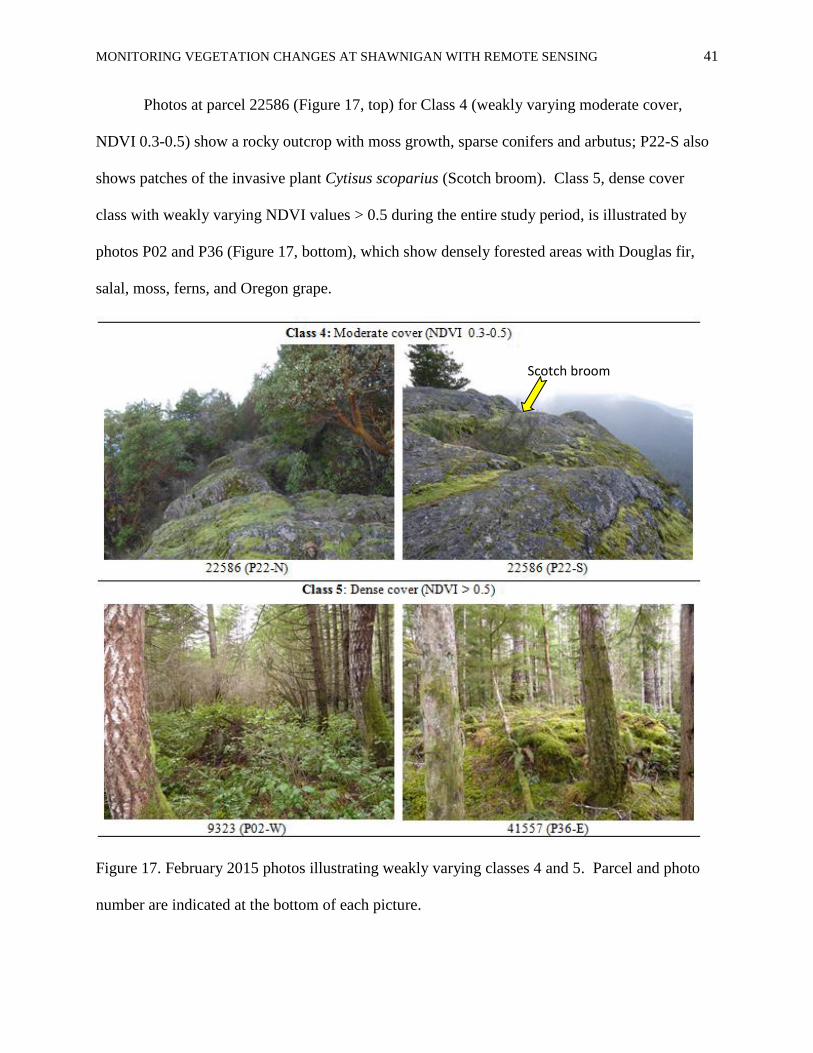
Photos at parcel 22586 (Figure 17, top) for Class 4 (weakly varying moderate cover,
NDVI 0.3-0.5) show a rocky outcrop with moss growth, sparse conifers and arbutus; P22-S also
shows patches of the invasive plant Cytisus scoparius (Scotch broom). Class 5, dense cover
class with weakly varying NDVI values > 0.5 during the entire study period, is illustrated by
photos P02 and P36 (Figure 17, bottom), which show densely forested areas with Douglas fir,
salal, moss, ferns, and Oregon grape.
Figure 17. February 2015 photos illustrating weakly varying classes 4 and 5. Parcel and photo
number are indicated at the bottom of each picture.
Scotch broom
MONITORING VEGETATION CHANGES AT SHAWNIGAN WITH REMOTE SENSING 42
Salal (Gaultheria shallon) is an important indigenous evergreen, beneficial as a soil
stabilizer after site disturbances. However, the dominant proliferation of salal after logging or
burning has been reported to render a replanting operation unsuccessful, as the plant recolonizes
sites rapidly and completely both above-ground and below-ground from rhizomes present before
the disturbance, and can resist invasion by other species (including authoctonous species) by pre-
emptying resources (Dorwoth, Sieber, & Woods, 2001).
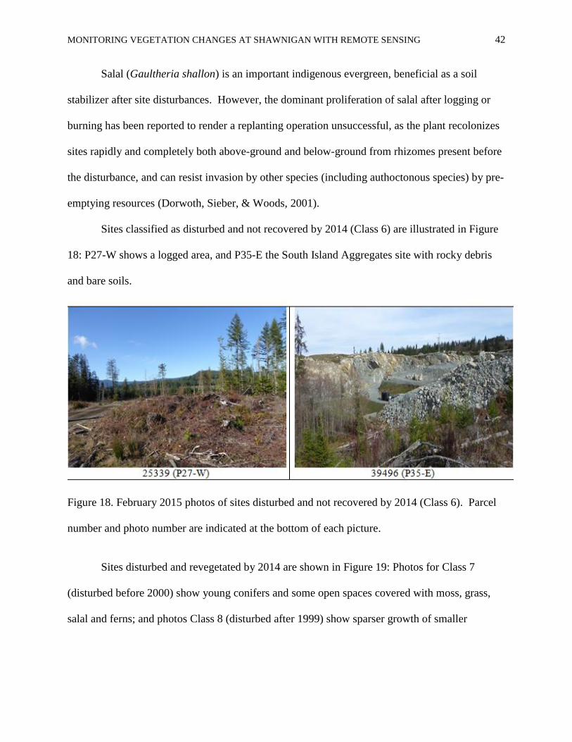
Sites classified as disturbed and not recovered by 2014 (Class 6) are illustrated in Figure
18: P27-W shows a logged area, and P35-E the South Island Aggregates site with rocky debris
and bare soils.
Figure 18. February 2015 photos of sites disturbed and not recovered by 2014 (Class 6). Parcel
number and photo number are indicated at the bottom of each picture.
Sites disturbed and revegetated by 2014 are shown in Figure 19: Photos for Class 7
(disturbed before 2000) show young conifers and some open spaces covered with moss, grass,
salal and ferns; and photos Class 8 (disturbed after 1999) show sparser growth of smaller
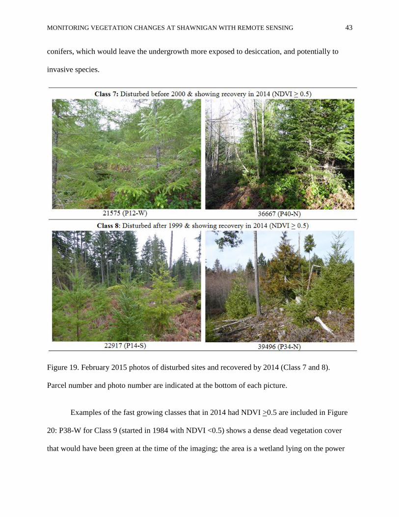
MONITORING VEGETATION CHANGES AT SHAWNIGAN WITH REMOTE SENSING 43
conifers, which would leave the undergrowth more exposed to desiccation, and potentially to
invasive species.
Figure 19. February 2015 photos of disturbed sites and recovered by 2014 (Class 7 and 8).
Parcel number and photo number are indicated at the bottom of each picture.
Examples of the fast growing classes that in 2014 had NDVI >0.5 are included in Figure
20: P38-W for Class 9 (started in 1984 with NDVI <0.5) shows a dense dead vegetation cover
that would have been green at the time of the imaging; the area is a wetland lying on the power
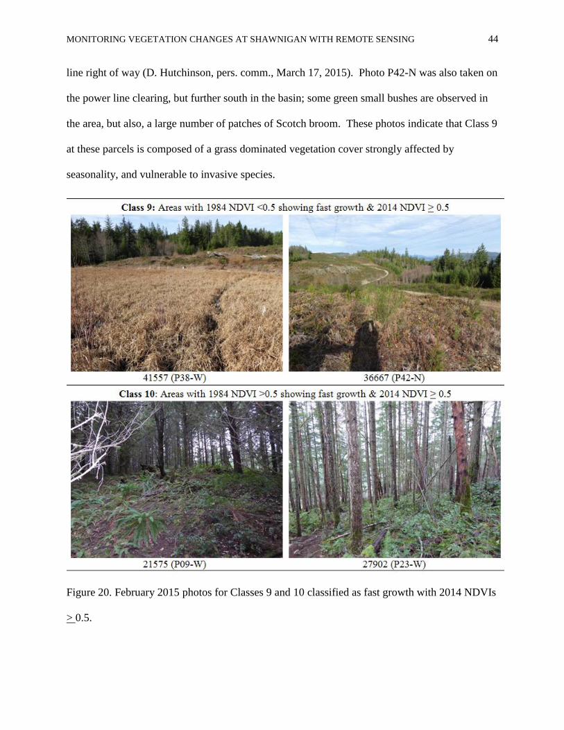
MONITORING VEGETATION CHANGES AT SHAWNIGAN WITH REMOTE SENSING 44
line right of way (D. Hutchinson, pers. comm., March 17, 2015). Photo P42-N was also taken on
the power line clearing, but further south in the basin; some green small bushes are observed in
the area, but also, a large number of patches of Scotch broom. These photos indicate that Class 9
at these parcels is composed of a grass dominated vegetation cover strongly affected by
seasonality, and vulnerable to invasive species.
Figure 20. February 2015 photos for Classes 9 and 10 classified as fast growth with 2014 NDVIs
> 0.5.
MONITORING VEGETATION CHANGES AT SHAWNIGAN WITH REMOTE SENSING 45
Photos for Class 10 (started in 1984 with NDVI >0.5) show areas with tall and thin
sparse conifers, large open spaces with ferns, and Oregon grape; if left undisturbed, these areas
will regenerate naturally.
In summary, the photos taken during this preliminary survey, even though out of
temporal sync with the imagery (survey was done in February and March 2015, and the images
were acquired in September), have validated the temporal vegetation classes that were created
solely on the basis of the NDVI histories.
Conclusions
Remote Sensing Data and Results.
This study has proven successful to meet the SBS needs to map the vegetation changes in
the Shawnigan watershed since 1984, and has made a significant contribution to characterize its
current condition.
Although remote sensing methodology is not a silver bullet, it has delivered much more
than pretty pictures. It has provided a synoptic view of the watershed dynamics in context with
the adjacent watershed, the long-term vegetation trends and classification maps of the Shawnigan
basin. Remote sensing methodology has provided a tool to be used in conjunction with land
based information, and a cost-effective means to focus restoration and conservation efforts on
specific locations most needing it. This is particularly critical for community-based initiatives,
such as the Watershed Management Plan at Shawnigan, that face the daunting challenge to
address highly degraded ecosystems with limited financial resources.
The main limitation with Landsat imagery, as with any other satellite data, is the cloud
coverage, which often limits the number of scenes available. As well, Landsat’s moderate
MONITORING VEGETATION CHANGES AT SHAWNIGAN WITH REMOTE SENSING 46
spatial resolution and the low number of spectral bands limit the use of more refined algorithms
that can be calculated using other satellites (such as WorldView-3). In addition, the accuracy of
land characterization due to signal mixing in the 30x30m pixel size is another limitation.
However, the freely-available 40-year data archive is still unmatched by any other satellite
archives, and its scientific value is incalculable as it provides the longest record of remote
sensing data (Campbell & Miller, 2013; NASA, 2015).
It is also important to understand the limitations of the methods: the NDVI works very
well to identify trends, but it identifies pixels in the imagery that are green- regardless of the
species. This is important because increased vegetation growth does not imply it is the right
ecological type of vegetation for the area (Polster, 2010, 2014): restoration of the watershed
requires rebuilding the ecosystem’s resilience by helping natural processes re-establish the areas
with autochthonous vegetation and successional sequences lying within the natural range of
variation, and avoiding the proliferation of invasive species or reliance on planted monocultures.
Species discrimination and on-the ground restoration is the strength of in situ work. In
combination, remote sensing and in situ based-data provide the interdisciplinary tools to generate
a comprehensive understanding required to undertake the complex adaptive management of
watersheds.
The remote sensing maps generated with this work have already been used to direct a
preliminary field survey in early 2015, and for a public meeting:
“We have already used the remote sensing images to illustrate the immensity of
the challenge to the Shawnigan public. The maps were presented at a public
meeting on 10th
December 2014 and now reside in the Watershed Planning
MONITORING VEGETATION CHANGES AT SHAWNIGAN WITH REMOTE SENSING 47
Office of the Authority in Shawnigan Village” (B. Fraser, pers. comm.,
December, 10 2014).
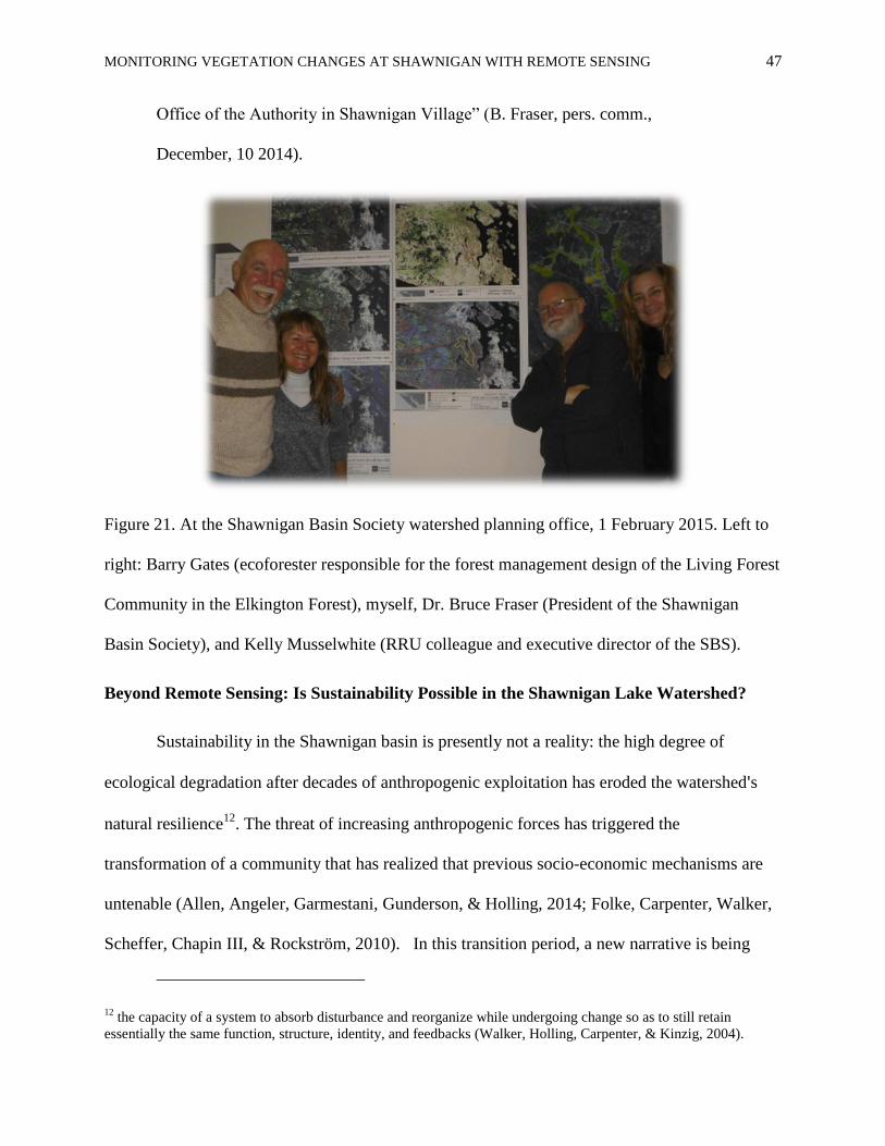
Figure 21. At the Shawnigan Basin Society watershed planning office, 1 February 2015. Left to
right: Barry Gates (ecoforester responsible for the forest management design of the Living Forest
Community in the Elkington Forest), myself, Dr. Bruce Fraser (President of the Shawnigan
Basin Society), and Kelly Musselwhite (RRU colleague and executive director of the SBS).
Beyond Remote Sensing: Is Sustainability Possible in the Shawnigan Lake Watershed?
Sustainability in the Shawnigan basin is presently not a reality: the high degree of
ecological degradation after decades of anthropogenic exploitation has eroded the watershed's
natural resilience12
. The threat of increasing anthropogenic forces has triggered the
transformation of a community that has realized that previous socio-economic mechanisms are
untenable (Allen, Angeler, Garmestani, Gunderson, & Holling, 2014; Folke, Carpenter, Walker,
Scheffer, Chapin III, & Rockström, 2010). In this transition period, a new narrative is being
12 the capacity of a system to absorb disturbance and reorganize while undergoing change so as to still retain
essentially the same function, structure, identity, and feedbacks (Walker, Holling, Carpenter, & Kinzig, 2004).
MONITORING VEGETATION CHANGES AT SHAWNIGAN WITH REMOTE SENSING 48
written: the community Watershed Management Plan is a collaborative effort, with the goal of
restoring ecological resilience and attain water security. The SBS vision (appendix A) is to
purposely reduce the ecological uncertainty derived from the lack of knowledge about the
watershed ecosystem by bridging across disciplines, and within a broader social, political and
institutional framework, thus evolving into adaptive governance (Folke, Hahn, Olsson, &
Norberg, 2005; Rist, Felton, Samuelsson, Sandström, & Rosvall, 2013).
While the SBS is striving to create an ecological governance model for the Shawnigan
Lake watershed, fragmentation of knowledge and planning is obvious when a larger socio-
economic system is considered. It appears that politicians from adjacent municipalities are not
as proactive or are resistant to accepting that an ecological governance model is critical to
preserving the watershed. The lake water that drains into Shawnigan Creek flows to Mill Bay
and then to the Saanich Inlet. Both the lake and sea become heavily contaminated by urban and
agricultural runoffs with deleterious effects on the marine ecosystems. At this time, there are no
known studies of actual downstream effects (Fraser, pers. comm., March 10, 2015). Shawnigan
Lake’s water flow is controlled by a weir installed in 2008 which accounts for the recorded
differences of 2.9 m between the dry season and the wet winter months (Hutchinson, 2011).
Additionally, the water levels during the summer in Shawnigan Creek are so low that they are
considered detrimental to aquatic ecosystems (CVRD, 2010; Riebergeg et al 2004). It is clear
that the South Cowichan communities need to work together and follow the SBS’s leadership in
order to restore the ecological resilience of the complex system that includes the lake, creeks and
sea. Ecological balance will not be achieved without a concerted and collaborative effort among
neighbouring municipalities. Furthermore, as long as the detrimental mindset that accepts the
discharge of refuse into the ground and effluent to run into an ephemeral stream that flows into
MONITORING VEGETATION CHANGES AT SHAWNIGAN WITH REMOTE SENSING 49
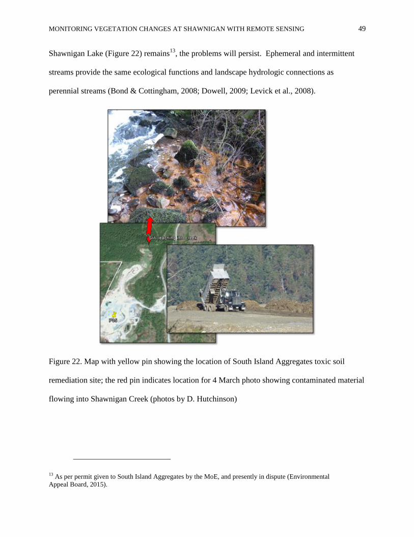
Shawnigan Lake (Figure 22) remains13
, the problems will persist. Ephemeral and intermittent
streams provide the same ecological functions and landscape hydrologic connections as
perennial streams (Bond & Cottingham, 2008; Dowell, 2009; Levick et al., 2008).
Figure 22. Map with yellow pin showing the location of South Island Aggregates toxic soil
remediation site; the red pin indicates location for 4 March photo showing contaminated material
flowing into Shawnigan Creek (photos by D. Hutchinson)
13 As per permit given to South Island Aggregates by the MoE, and presently in dispute (Environmental
Appeal Board, 2015).
MONITORING VEGETATION CHANGES AT SHAWNIGAN WITH REMOTE SENSING 50
If the last 20 years are any indication of our planet’s rate of changes, the next 20 years
will bring more change than the last 100 years. While restoring and monitoring ecosystems,
science-based decision models, public engagement and roundtable discussions may be costly,
they are necessary. It is imperative to build local ecological and social resilience to withstand
the rapid changes and maintain livable communities (Meadows, 2012; Olsson, Folke, & Berkes,
2004).
From an Ecological Economics perspective, it is possible to understand the limitations of
complex biophysical systems, and the urgency to conserve their integrity for the social wellbeing
of present and future generations. In that context, total economic valuation can be a powerful
tool in conjunction with the SBS adaptive management plan which will put into perspective the
true cost of not valuing the environment that we depend on (Max-Neef, 2005; Olewiler, 2010).
Theoretically, by estimating the ‘monetized value’ of the Shawnigan Watershed, legislation can
be adapted to address urgent issues by creating adequate timely policies (Mickwitz, 2003). As
well, tax incentives, such as the Natural Area Protection Tax Exemption Program (NAPTEP)
promoted by Islands Trust (2014), can be explored at the Shawnigan Lake Watershed to
stimulate private land-owners collaboration.
A vision of a future with resilient communities requires creating a new narrative,
radically changing our mindset, and challenging the dominant worldview –which invariably
implies uncomfortable confrontation, collective political engagement, and an involved
community (Fielding, MacDonald, & Louis, 2005; Lacasse, 2013). Trying to change the world
at large is a daunting task, but by focusing our efforts at a local scale, such as the SBS Watershed
Management Plan, communities can foster participatory and integrative frameworks to guide
adaptive strategies and policies that address the restoration of local resilience. Furthermore, this

MONITORING VEGETATION CHANGES AT SHAWNIGAN WITH REMOTE SENSING 51
focus can ensure the preservation of its integrity, and the rational use of the ecological goods and
services the ecosystems make available to the communities, present and future (Dale, 2001; Stelk
and Christie, 2014; Westley, 2002). This, in turn, might help the communities develop a
collective ‘sense of place’ and stewardship pride that will hopefully lead to a paradigm shift in
which the natural world is not simply viewed as ‘natural capital,’ and the Shawnigan Lake
Watershed simply as a ‘tradable asset’ (Monbiot, 2014).
Future Directions. It is recommended to continue, if possible, the existing Landsat time
series in order to maintain ongoing monitoring of the evolution of the watershed, and perhaps
explore what other analyses can be carried out as the Watershed Management Plan evolves. For
example, vegetation indices other than NDVI could be tested, and regression analyses using
variables such as precipitation, and temperature could be explored for a thorough understanding
of ecological resilience variability in the basin. The extent of the Scotch broom invasion can be
mapped if the imagery is acquired when the plants are in bloom (flowers are yellow and easily
detected with satellite data). Trends in water level fluctuations as well as water quality studies
(for sporadic events of turbidity and algal blooms) can also be done successfully with Landsat
data. It is important to acquire ground truth for all the classes created and for the same period as
the images, in order to generate an accuracy assessment and validate the work done to date. In
addition, a detailed land-cover inventory can be created using the most recent Landsat data,
though it would be preferably to acquire higher spatial and spectral resolution data, such as
World-View 3 (1.5m pixel resolution). This could be the baseline for a future high resolution
time series.
Visualization techniques can be improved using Digital Elevation Model drapes, to assist
interpretation, especially for public demonstrations. Bridging the scientific information to the
MONITORING VEGETATION CHANGES AT SHAWNIGAN WITH REMOTE SENSING 52
general public is critical to help bring understanding and promote collaboration. Public talks on
the results of this study (as requested by Dr. Fraser) are planned for 2015. I would like to
explore the possibility of training community volunteers and field specialists on the use of
remote sensing maps as tools for watershed management. It would be valuable to transfer the
remote sensing maps into iPad tablets for integration in a multi-layer GIS style database that
would also include field data, First Nations knowledge, and any other available information
relevant to the area.
It is important to share the results of the studies prepared for the SBS’s Watershed
Management Plan in platforms such as the British Columbia Lake Stewardship Society (BSLSS)
forum, and the 2016 conference of the Society for Ecological Restoration (SER).
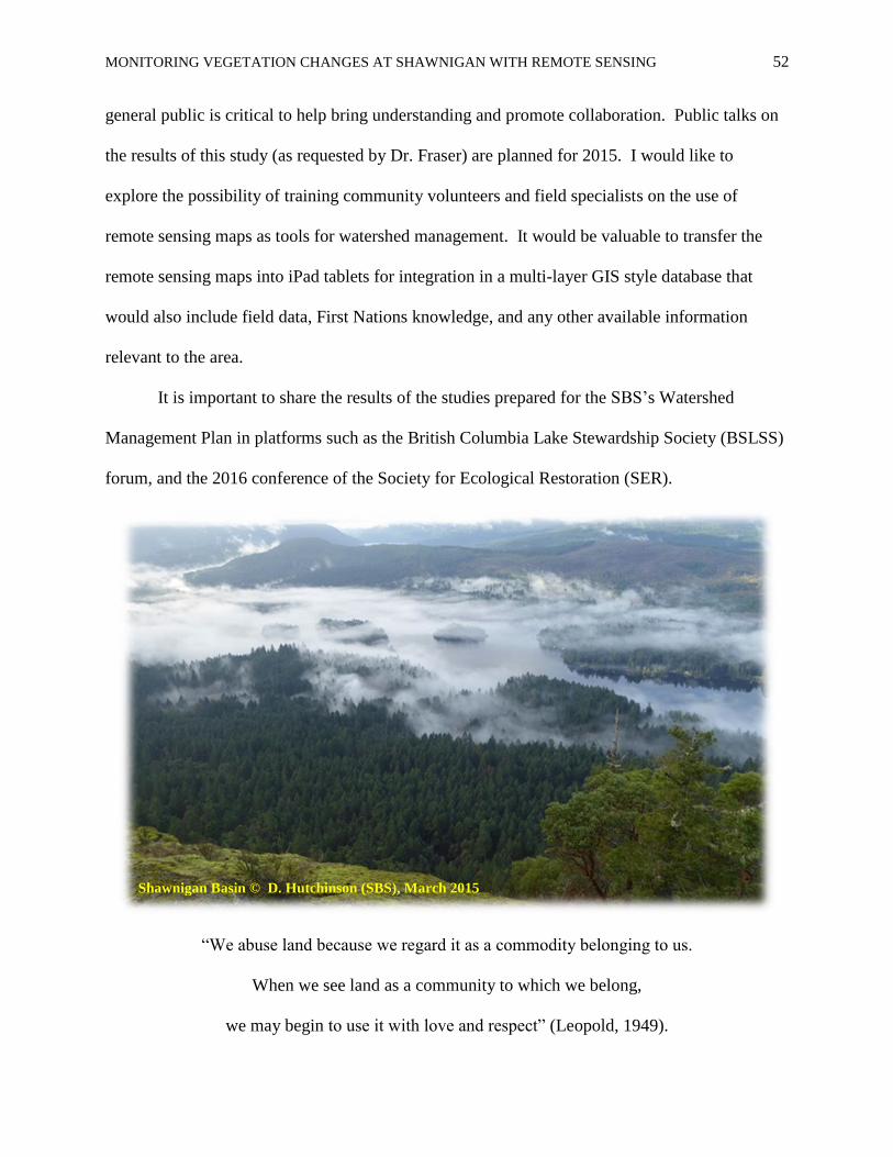
“We abuse land because we regard it as a commodity belonging to us.
When we see land as a community to which we belong,
we may begin to use it with love and respect” (Leopold, 1949).
Shawnigan Basin © D. Hutchinson (SBS), March 2015
MONITORING CHANGES AT SHAWNIGAN WITH REMOTE SENSING 53
References
Alex, D. (January 25, 2007). Nazco: Building a future together. In: Treaty Commission update-
the independent voice of treaty making in British Columbia, p4-5. Retrieved from
http://www.bctreaty.net/files/pdf_documents/April07update.pdf
Allen, C.R., Angeler, D.G., Garmestani, A.S., Gunderson, L.H., & Holling, C.S. (2014).
Panarchy: Theory and application. Ecosystems,17(4): 578-589. Retrieved from
http://snr.unl.edu/necoopunit/downloads/Publications/Craig%20Allen/Panarchy.pdf
Bainas, L. (2014, Nov 7). Conservation takes step forward in Shawnigan with living mat.
Cowichan Valley Citizen. Retrieved from
http://www.cowichanvalleycitizen.com/news/conservation-takes-step-forward-in-
shawnigan-with-living-mat-1.1528548
Baret, F., & Guyot, G. (1991). Potentials and limits of vegetation indices for LAI and APAR
assessment. Remote Sensing of the Environment, 35(2-3): 161-173. Retrieved from
http://www.sciencedirect.com/science/article/pii/003442579190009U
Bond N.R. and Cottingham P. 2008. Ecology and hydrology of temporary streams: Implications
for sustainable water management. eWater Technical Report. eWater Cooperative
Research Centre, Canberra. Retrieved from
http://ewatercrc.com.au/reports/Bond_Cottingham-2008-Temporary_Streams.pdf
Borstad G. A., Martínez de Saavedra Álvarez, M., Hines, J. E., & Dufour, J.F. (2008). Reduction
in vegetation cover at the Anderson River Delta, Northwest Territories, identified by
LANDSAT imagery, 1972 2003. Canadian Wildlife Service. Environment Canada.
Technical Report Series Number 496. Retrieved from
http://www.aslenv.com/Borstad/documents/E%20Rukiya%20-
MONITORING CHANGES AT SHAWNIGAN WITH REMOTE SENSING 54
CWS%20tech%20report%20anderson%20river%20vegetation%20%20-
%20rev%20morton%20August%2015.pdf
Borstad, G.A., Akenhead, S., Brown, L., Braun, D.C., Irvine, J.R., Martínez, M., & Kerr, R.
(2010). “How green is your valley? Remote sensing of large watershed change for
ecosystem management. Report for the 2009 Fraser Salmon and Watersheds Program. 31
March 2010. 46p. Retrieved from
http://www.thinksalmon.com/reports/FSWP_09_LR_HWRS_96_Final_Report.TS_.pdf
BC Environmental Appeal Board. (2015). Shawnigan Residents Association vs Cobble Hill
Holdings Ltd. (South Islands Aggregates). Retrieved from
http://www.eab.gov.bc.ca/ema/2013ema015c_019d_020b_021b.pdf
BC Ministry of Environment [MOE]. (2004). Ministry of Environment Authorities under the
Forest and Range Practices Act: Community Watersheds and Water Quality Objectives.
Retrieved from http://www.env.gov.bc.ca/wld/frpa/cwwqo.html
Campbell, J., & Miller, H. (2013). Landsat users confirm its unique value. USGS Newsroom.
Retrieved from http://www.usgs.gov/newsroom/article.asp?ID=3738#.VPPwhWd0zIU
Capital Regional District [CRD] (2012). Map of drinking water supply systems for Greater
Victoria. Retrieved from https://www.crd.bc.ca/docs/default-source/Partnerships-
PDF/image-download/map---greater-victoria-drinking-water-supply-system.jpg?sfvrsn=0
CRD (2014). Facts and Figures: Greater Victoria Water Supply Area. Retrieved from
https://www.crd.bc.ca/docs/default-source/Partnerships-
PDF/2014_iws_highschooltour_factsandfigures.pdf?sfvrsn=2
MONITORING CHANGES AT SHAWNIGAN WITH REMOTE SENSING 55
Carlson, R.E., & Simpson, J. (1996). A Coordinator’s Guide to Volunteer Lake Monitoring
Methods. North American Lake Management Society. 96 pp. Retrieved from
http://www.secchidipin.org/trophic_state.htm
Chander, G., & Markham, B.L. (2003). Revised Landsat 5 TM radiometric calibration
procedures and pos-calibration dynamic ranges. IEEE Transactions on Geoscience and
Remote Sensing 41(11): 2674-2677. Retrieved from
http://landsat.usgs.gov/resources/files/L5_TM_Cal_2003.pdf
Cowichan Valley Regional District [CVRD] (n.d.). Water water (almost) everywhere in south
Cowichan communities. Retrieved from
http://www.cvrd.bc.ca/DocumentCenter/Home/View/8949
CVRD (2010, June 9). 2010 State of the Environment. 219p + iv + Appendices. Retrieved from
http://www.12things.ca/12things/uploads/FinalSoEReport.pdf
CVRD (2014a). Official Community Plan No. 3510. Cowichan Valley Regional District: South
Cowichan – Schedule A. 216p. Retrieved from
http://www.cvrd.bc.ca/DocumentCenter/Home/View/7621
CVRD (2014b). Regional surface and ground water management and governance study:
Workshop 1 –Dialogue Summary. Retrieved from
http://www.fraserforshawnigan.ca/Governance%20-
%20CVRD/First%20Workshop%20SummaryWater%20Mngt%20May%202014.pdf
Coppi, P., Jonckheere, I., Nackaerts, K., Muys, B., & Lambin, E. (2004). Digital change
detection methods in ecosystem monitoring: a review. International Journal of Remote
Sensing, 25 (9), 1565-1596, DOI: 10.1080/0143116031000101675. Retrieved from
http://dx.doi.org/10.1080/0143116031000101675
MONITORING CHANGES AT SHAWNIGAN WITH REMOTE SENSING 56
Cullington, J., & Associates (2012a). South Cowichan Water Community Consultation 2012.
Summary of Community Input. 48p. Retrieved from
http://www.cvrd.bc.ca/DocumentCenter/Home/View/9058
Cullington, J., & Associates (2012b). Water Matters: Report on Public Consultations on Water
in South Cowichan Communities. Retrieved from
http://www.cvrd.bc.ca/DocumentCenter/Home/View/9677
Czapla-Myers, J., McCorkel, J., Anderson, N., Thome, K., Biggar, S., Helder, D.,…Mishra, N.
(2015). The ground-based absolute radiometric calibration of Landsat 8 OLI. Remote
Sensing, 7(1):600-626. Retrieved from http://www.mdpi.com/2072-4292/7/1/600
Dale, A. (2001). Ecological Imperatives. In: At the edge: sustainable development in the 21st
century (pp 44-58). Vancouver, BC: UBC Press Vancouver, BC: UBC Press.
Desmond, M. (2012, Aug 12). Clearcut Logging Diminishes Shawnigan Lake Watershed.
Watershed Sentinel. Retrieved from http://www.watershedsentinel.ca/content/clearcut-
logging-deminishes-shawnigan-lake-watershed
Dorwoth, C.E., Sieber, T.N., & Woods, T.A.D. (2001). Early growth performance of salal
(Gaultheria shallon) from various North American west-coast locations. Annals of Forest
Science, 58: 597–606. Retrieved from https://hal.archives-ouvertes.fr/hal-
00881939/document
Dowell, W.H. (2009). Ecology and Role of Headwater Streams. In: River ecosystem ecology: A
global perspective. G.E. Likens (Ed.). p173-181. San Diego, CA: Elsevier. Retrieved
from
https://books.google.ca/books?id=v5VHWWrK_SsC&pg=PA173&lpg=PA173&dq=ecol
ogical+importance+of+ephemeral+streams&source=bl&ots=AzdjD27g94&sig=09-
MONITORING CHANGES AT SHAWNIGAN WITH REMOTE SENSING 57
D9jS8CuuDKbnusWGZOaXx9tU&hl=en&sa=X&ei=mcUTVcOVIMywogS_7IG4Bw&
ved=0CFIQ6AEwCQ#v=onepage&q=ecological%20importance%20of%20ephemeral%2
0streams&f=false
E-Flora BC (2014). Electronic Atlas of the Plants of British Columbia [eflora.bc.ca]. Lab for
advanced spatial analysis, Department of Geography, University of British Columbia,
Vancouver. Retrieved from http://linnet.geog.ubc.ca/DB_Query/QueryForm.aspx
Fielding K.S., MacDonald, R., & Louis, W. (2005). Working Hard for the Environment: When
Will Citizens Engage in Environmental Activism? Paper presented at the International
Conference of Engaging Communities: Brisbane, Australia. Retrieved from
https://publications.qld.gov.au/storage/f/2014-01-30T06%3A32%3A05.023Z/fielding-
kelly-final.pdf
Flood, N. (2014). Continuity of reflectance data between Landsat-7 ETM+ and Landsat-8 OLI,
for both top-of-atmosphere and surface reflectance: A study in the Australian landscape.
Remote Sensing, 6: 7952-7970. Retrieved from
http://article.sciencepublishinggroup.com/pdf/10.11648.j.ajrs.20140202.11.pdf
Folke, C., Hahn, T., Olsson, P., & Norberg, J. (2005). Adaptive governance of social–ecological
systems. Annual Review of Environment and Resources 30:441-473. Retrieved from
http://dx.doi.org/10.1146/annurev.energy.30.050504.144511
Folke, C., Carpenter, S. R., Walker, B. H., Scheffer, M., Chapin III, F. S., & Rockström, J.
(2010). Resilience thinking: integrating resilience, adaptability and transformability.
Ecology and Society 15(4): 20. Retrieved from
http://www.ecologyandsociety.org/vol15/iss4/art20
MONITORING CHANGES AT SHAWNIGAN WITH REMOTE SENSING 58
Fraser, B. (2012a). Shawnigan Lake Watershed Roundtable. Retrieved from
http://www.fraserforshawnigan.ca/index%20April%2017%202012with%20search.html
Fraser, B. (2012b). Dumping in the Shawnigan Watershed. Retrieved from
http://www.fraserforshawnigan.ca/Watershed.html
Fraser, B. (2013). A Shawnigan Basin Authority. Retrieved from
http://www.shawniganfocus.ca/Vault/June%202013/A%20Shawnigan%20Basin%20Aut
hority.pdf
Fraser, B. (2014a). Shawnigan’s Quiet Progress. Retrieved from
http://www.fraserforshawnigan.ca/index%20Feb%2011,%202014.html
Fraser, B. (2014b). Restoring the Shawnigan watershed. Document sent by Dr. Bruce Fraser on
12 December 2014.
Gregory, L. (2014). Summary of the Available Information on Shawnigan Lake, with an
Emphasis on Water Quality. Prepared for the Shawnigan Basin Society. Retrieved from
http://www.shawniganfocus.ca/Vault/Shawnigan%20Focus%20December%202014/Sha
wnigan%20Focus%20Dec%202014.pdf
Hutchinson, D. (2011). The Shawnigan Weir. Shawnigan Focus September, 2011. Retrieved
from
http://www.shawniganfocus.ca/Vault/September%20Focus/September%20Focus.pdf
Irons, J.R., Dywer, J.L., & Barsi, J. (2012). The next Landsat satellite: the Landsat data
continuity mission. Retrieved from
http://www.sciencedirect.com.ezproxy.royalroads.ca/science/article/pii/S0034425712000
363
also http://www.nasa.gov/pdf/716684main_LDCMFactSheet.pdf
MONITORING CHANGES AT SHAWNIGAN WITH REMOTE SENSING 59
Islands Trust Fund. (2014). Ways to Protect your Land: Register a NAPTEP Covenant. Retrieved
from http://www.islandstrustfund.bc.ca/initiatives/privateconservation/naptep.aspx
Jackson, R.D., & Huete, A.R. (1991). Interpreting vegetation indices. Preventive Veterinary
Medicine, 11 (3–4): 185–200. Retrieved from
http://afrsweb.usda.gov/SP2UserFiles/Place/53442010/RemoteSensing/WCLPUB-1569-
Jackson.pdf
Kemshaw, M. (2006). Watersheds: A sip of life. Watershed Sentinel, March-April 2006, p 15.
http://watershedsentinel.ca/files/archives/WSMarApr2006.pdf
Lacasse, K. (2013). Policy analysis: Addressing the “go green” debate: policies that encourage
small green behaviors and their political spillover effects. The Journal of Science Policy
and Governance, 3(1): 1-33. Retrieved from:
http://www.sciencepolicyjournal.org/uploads/5/4/3/4/5434385/go_green_debate.pdf
Leopold, A. (1949). The Land Ethic. In: A Sand County Almanac. New York: Oxford University
Press.
Levick, L., Fonseca, J., Goodrich, D., Hernández, M., Semmens, D., Stromberg, J., … & Kepner,
W. (2008). The ecological and hydrological significance of ephemeral and intermittent
streams in the arid and semi-arid American southwest. U.S. Environmental Protection
Agency and USDA/ARS Southwest Watershed Research Center, EPA/600/R-08/134,
ARS/233046, 116 pp. Retrieved from http://www.epa.gov/esd/land-
sci/pdf/EPHEMERAL_STREAMS_REPORT_Final_508-Kepner.pdf
Li, P., Jiang, L., & Feng, Z. (2014). Cross-comparison of vegetation indices derived from
Landsat-7 Enhanced Thematic Mapper Plus (ETM+) and Landsat-8 Operational Land
MONITORING CHANGES AT SHAWNIGAN WITH REMOTE SENSING 60
Imager (OLI) sensors. Remote Sensing, 6(1), 310-329. Retrieved from
http://www.mdpi.com/2072-4292/6/1/310
Lyon, J.G., Yuan, D., Lunetta, R.S., & Elvidge, C.D. (1998). A change detection experiment
using vegetation indices. Photogrammetic Engineering & Remote Sensing, 64(2), 143-
150. Retrieved from
http://www.asprs.org/a/publications/pers/98journal/february/1998_feb_143-150.pdf
Martínez de Saavedra Álvarez, M., Borstad, G., Brown, L., Ersahin, K., & Henley, M. (2013).
Remote sensing in vegetation monitoring: More than just a pretty picture. Presented at the
38th
CLRA/ACRSD Annual Meeting and Northern Latitudes Mining Reclamation
Workshop "Overcoming Northern Challenges," Whitehorse, Yukon, September 9-12,
2013. Retrieved from http://remote-sensing.aslenv.com/documents/RemSensing-CLRA-
2013.pdf
Max-Neef, M.A. (2005). Foundations of transdisciplinarity (Commentary). Ecological
Economics, 53: 5-16. Retrieved from
http://artsci.unsw.wikispaces.net/file/view/max_neef_foundations_of_transdisciplinarity.
pdf/340979004/max_neef_foundations_of_transdisciplinarity.pdf
Mazumder, A. (2012). Characterizing and Modelling Impacts of Climate and Land Use
Variability on Water Quality. Shawnigan Lake Community Water System and
Watershed. Retrieved from http://www.cvrd.bc.ca/DocumentCenter/Home/View/63712
McCulloch, S. (2014, Feb. 14). Company defends soil dumping in Shawnigan. Cowichan Valley
Citizen. Retrieved from http://www.cowichanvalleycitizen.com/news/company-defends-
soil-dumping-in-shawnigan-1.854674
MONITORING CHANGES AT SHAWNIGAN WITH REMOTE SENSING 61
McGillivar, P. (May, 2009). Flushing out unsettling truths about water quality. The Ring,
University of Victoria. Retrieved from http://ring.uvic.ca/09may07/mazumder.html also
in http://www.uvic.ca/knowledge/assets/issues/2009/v9n04_apr09.pdf
Meadows, D. (2012). Perspectives on the Limits of Growth: It is too late for sustainable
development Video File. Smithsonian Institute Series. Retrieved from
https://www.youtube.com/watch?v=f2oyU0RusiA
Mickwitz, P. (2003). A Framework for Evaluating Environmental Policy Instruments.
Evaluation, 9(4): 415–436. Retrieved from
http://202.154.59.182/ejournal/files/A%20Framework%20for%20Evaluating%20Environ
mental%20Policy-2003.pdf
Monbiot, G. (2014). The Pricing of Everything. Transcript of G. Monbiot`s SPERI Annual
Lecture, hosted by the Sheffield Political Economy Research Institute at the University of
Sheffield. Retrieved from http://www.monbiot.com/2014/07/24/the-pricing-of-
everything/
NASA (2015). Landsat Science: Landsat seen as stunning return on public investment. Retrieved
from http://landsat.gsfc.nasa.gov/?page_id=2295 and
http://landsat.gsfc.nasa.gov/?p=9654
Nordin, R.N., & McKean, C.J.P. (1984). Shawnigan Lake water quality study. British Columbia
Ministry of Environment, Waste Management Branch. File 64.080301. 117p. Retrieved
from http://www.env.gov.bc.ca/wat/wq/studies/shawnigan84.pdf
Nordin, R.N., Zu, Z., & Mazumder, A. (2007). Ion Export from a Small British Columbia
Watershed After Forest Harvesting. Water Qual. Res. J. Canada, 42 (3), 138-152.
Retrieved from http://web.uvic.ca/water/publications/Nordinetal2007.pdf
MONITORING CHANGES AT SHAWNIGAN WITH REMOTE SENSING 62
Olewiler, N. (2010). What's My Lake Worth? Valuing the Ecosystem Goods & Services. School
of Public Policy, Simon Fraser University. BCLSS Community Forum Presentation.
Retrieved from http://www.bclss.org/library/cat_view/106-2010-community-forum-
presentations.html also available at
http://www.southchilcotin.ca/gunlake/pdf/What's%20My%20Lake%20Worth.pdf
Olsson, H. (1995). Reflectance calibration of Thematic Mapper data for forest change detection.
International Journal of Remote Sensing, 16(1): 81–96. Retrieved from
http://www.tandfonline.com/doi/abs/10.1080/01431169508954373?journalCode=tres20#.
VQdPAmd0zIU
Olsson, P., Folke, C., & Berkes, F. (2004). Adaptive comanagement for building resilience in
social–ecological systems. Environmental Management, 34(1): 75-90. Retrieved from
http://link.springer.com.ezproxy.royalroads.ca/article/10.1007%2Fs00267-003-0101-7
Olsson, P., Gunderson, L.H., Carpenter, S.R., Ryan, P., Lebel, L., Folke, C., & Holling, C. S.
(2006). Shooting the rapids: Navigating transitions to adaptive governance of social-
ecological systems. Ecology and Society, 11(1): 18-
Pacifici, F., Longbotham, N., & Emery, W.J. (2014). The importance of physical quantities for
the analysis of multitemporal and multiangular optical very high spatial resolution
images. IEEE Transactions on Geoscience and Remote Sensing, 52(10): 6241-6256.
Retrieved from http://ieeexplore.ieee.org/stamp/stamp.jsp?arnumber=6737293
Polster, D. (2010). Natural processes for riparian restoration: Part 1 & Part 2. BCLSS
Community Forum Presentation. Retrieved from
http://www.bclss.org/library/cat_view/106-2010-community-forum-presentations.html
MONITORING CHANGES AT SHAWNIGAN WITH REMOTE SENSING 63
Polster, D. (2014). Ecological restoration: Building resilience in the Cowichan Valley. A
presentation to the Cowichan Watershed Waterboard, October 2014. (provided by author)
Rieberger, K., Epps, D., & Wilson, J. (2004). Shawnigan Lake Water Quality Assessment 1976-
2004. BC Government report. Retrieved from
http://www.env.gov.bc.ca/wat/wq/studies/shawnigan2004.pdf
Rist, L., Felton, A., Samuelsson, L., Sandström, C., & Rosvall, O. (2013). A new paradigm for
adaptive management. Ecology and Society, 18(4): 63-72. Retrieved from
http://www.ecologyandsociety.org/vol18/iss4/art63/
Rouse, J.J., Haas, R.H., Schell, J.A., & Deering, D.W. (1974). Monitoring vegetation systems in
the Great Plains with ERTS. Proceedings of the Third Earth resources Satellite-1
Symposium 1(Sect. A), 309-317, Maryland, NASA SP-351. Retrieved from
http://www.researchgate.net/publication/246866091_Monitoring_vegetation_systems_in_
the_Great_Plains_with_ERTS
Rusland, P. (Aug 9, 2013). Shawnigan Basin Authority pitched to protect area's water. Retrieved
from http://www.cowichannewsleader.com/news/217803091.html
Shawnigan Basin Society [SBS] (2014). Ecological Watershed Governance. Retrieved from
http://www.shawniganwater.org/watershed_governance
Silleos, N.G., Alexandridis, T.K., Gitas, I.Z., & Perakis, K. (2006). Vegetation indices:
Advances made in biomass estimation and vegetation monitoring in the last 30 years.
Geocarto International, 21(4): 21-28. Retrieved from
http://www.tandfonline.com/doi/abs/10.1080/10106040608542399#.VPJ_W2d0yP8

MONITORING CHANGES AT SHAWNIGAN WITH REMOTE SENSING 64
Stehamn, V.S., & Czaplewski, R.L. (1998). Design and analysis for thematic map accuracy
assessment: Fundamental principles. Remote Sensing of Environment, 64(3): 331-344.
Retrieved from http://www.sciencedirect.com/science/article/pii/S0034425798000108
Stelk, M.J. & Christie, J. (2014). Ecosystem Service Valuation for Wetland Restoration: What It
Is, How To Do It, and Best Practice Recommendations. Association of State Wetland
Managers, Windham, Maine. 74p. Retrieved from
http://www.aswm.org/state_meeting/2014/ecosystem_service_valuation_for_wetland_res
toration.pdf
The Council of Canadians. (2014, April 28). Is Our Community Watershed Protected? Retrieved
from http://midislandcanadians.org/is-our-community-watershed-protected/
Tucker, C.J. (1979). Red and photographic infrared linear combinations for monitoring
vegetation. Remote Sensing of the Environment, 8 (2): 127-150. Retrieved from
http://www.sciencedirect.com/science/article/pii/0034425779900130
United States Geological Service [USGS]. (2014a). Landsat Missions Timeline. Retrieved from
http://landsat.usgs.gov/about_mission_history.php
USGS. (2014b). Landsat Satellites: Band Designations. Retrieved from
http://landsat.usgs.gov/band_designations_landsat_satellites.php
USGS. (2015a). Landsat Missions: Project Descriptions. Retrieved from
http://landsat.usgs.gov/about_project_descriptions.php
USGS. (2015b). GLOVIS: The USGS Global Visualization Viewer. Retrieved from
www.glovis.usgs.gov
USGS. (2015c). NDVI, the Foundation for Remote Sensing Phenology. Retrieved from
http://phenology.cr.usgs.gov/ndvi_foundation.php
MONITORING CHANGES AT SHAWNIGAN WITH REMOTE SENSING 65
Vogelmann, J.E., Xian, G., Homer, C., & Tolk, B. (2012). Monitoring gradual ecosystem change
using Landsat time series analyses: Case studies in selected forest and rangeland
ecosystems. Remote Sensing of Environment, 122: 92-105. Retrieved from
http://www.sciencedirect.com.ezproxy.royalroads.ca/science/article/pii/S0034425712000
429
Walker, B., Holling, C. S., Carpenter, S. R., & Kinzig, A. (2004). Resilience, adaptability and
transformability in social–ecological systems. Ecology and Society 9(2): 5. Retrieved
from http://www.ecologyandsociety.org/vol9/iss2/art5/
Washington State Department of Ecology (n.d.). Aquatic plants, algae & lakes: Shoreline plants.
Retrieved from
http://www.ecy.wa.gov/programs/wq/plants/plantid2/descriptions/sci.html
Weier, J., & Herring, D. (2000). Measuring NDVI & EVI. Retrieved from
http://earthobservatory.nasa.gov/Features/MeasuringVegetation/measuring_vegetation_1.
php
Westley, F. (2002). The devil in the dynamics: adaptive management on the front lines. In L.H
Gunderson, and C.S. Holling (Eds.), Panarchy: understanding transformations in human
and natural systems (pp. 333 – 360). Washington, DC: Island Press. Retrieved from
http://books.google.ca/books?id=DHcjtSM5TogC&pg=PA333&lpg=PA333&dq=Westle
y+Adaptive+Management+on+the+Front+Lines&source=bl&ots=xgsZOHn_17&sig=eq
1qzGYYM8SpubdxSXhDzcNxWhc&hl=en&sa=X&ei=oLt3T5evJ6mkiQLhuOCnDg&v
ed=0CDgQ6AEwAg#v=onepage&q=Westley%20Adaptive%20Management%20on%20t
he%20Front%20Lines&f=false
MONITORING CHANGES AT SHAWNIGAN WITH REMOTE SENSING 66
Xu, D., & Guo, X. (2104). Compare NDVI extracted from Landsat 8 imagery with that from
Landsat 7 imagery. American Journal of Remote Sensing, 2(2): 10-14. Retrieved from
http://article.sciencepublishinggroup.com/pdf/10.11648.j.ajrs.20140202.11.pdf
Zăvoianu a, F., Caramizoiub, A., & Badeaa, D. (2004). study and accuracy assessment of remote
sensing data for environmental change detection in Romanian coastal zone of the Black
Sea. Proceedings of the XXXV Conference of the International Sociey for
Photogrammetry and Remote Sensing, Istanbul, Turkey. Retrieved from
http://www.isprs.org/proceedings/XXXV/congress/comm7/papers/153.pdf
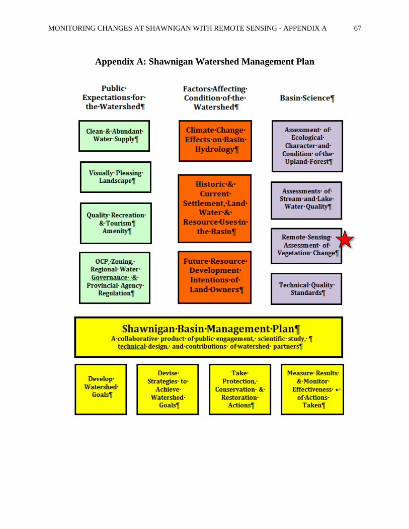
MONITORING CHANGES AT SHAWNIGAN WITH REMOTE SENSING - APPENDIX A 67
Appendix A: Shawnigan Watershed Management Plan
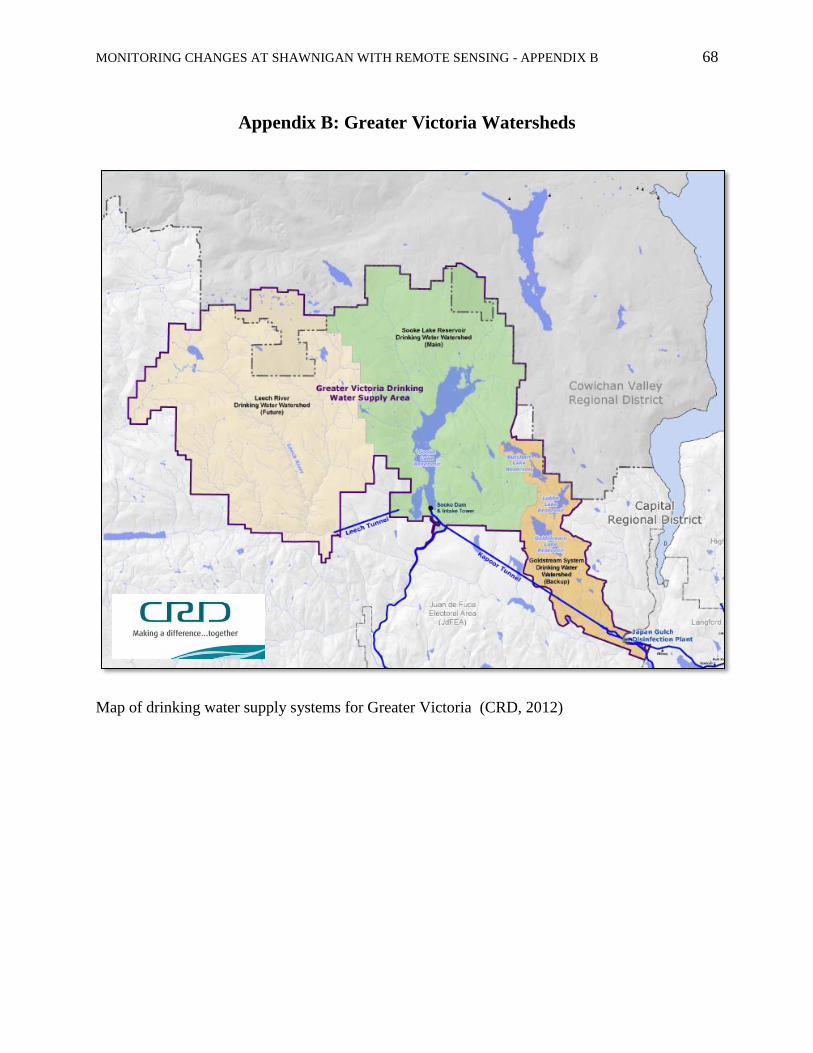
MONITORING CHANGES AT SHAWNIGAN WITH REMOTE SENSING - APPENDIX B 68
Appendix B: Greater Victoria Watersheds
Map of drinking water supply systems for Greater Victoria (CRD, 2012)
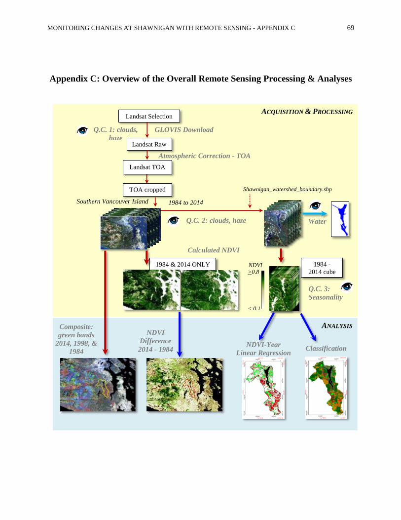
MONITORING CHANGES AT SHAWNIGAN WITH REMOTE SENSING - APPENDIX C 69
ACQUISITION & PROCESSING
Shawnigan_watershed_boundary.shp TOA cropped
Calculated NDVI
1984 -
2014 cube
ANALYSIS
Classification NDVI-Year
Linear Regression
1984 to 2014 Southern Vancouver Island
Composite:
green bands
2014, 1998, &
1984
1984 & 2014 ONLY
NDVI
Difference
2014 - 1984
Water
Appendix C: Overview of the Overall Remote Sensing Processing & Analyses
NDVI
>0.8
< 0.1
Atmospheric Correction - TOA
Landsat TOA
Landsat Raw
Landsat Selection
GLOVIS Download Q.C. 1: clouds,
haze
Q.C. 2: clouds, haze
Q.C. 3:
Seasonality
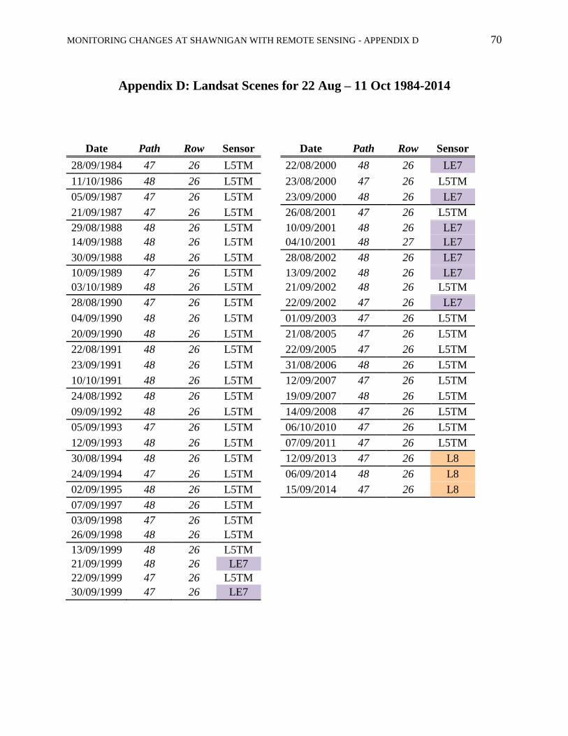
MONITORING CHANGES AT SHAWNIGAN WITH REMOTE SENSING - APPENDIX D 70
Appendix D: Landsat Scenes for 22 Aug – 11 Oct 1984-2014
Date Path Row Sensor
Date Path Row Sensor
28/09/1984 47 26 L5TM
22/08/2000 48 26 LE7
11/10/1986 48 26 L5TM
23/08/2000 47 26 L5TM
05/09/1987 47 26 L5TM
23/09/2000 48 26 LE7
21/09/1987 47 26 L5TM
26/08/2001 47 26 L5TM
29/08/1988 48 26 L5TM
10/09/2001 48 26 LE7
14/09/1988 48 26 L5TM
04/10/2001 48 27 LE7
30/09/1988 48 26 L5TM
28/08/2002 48 26 LE7
10/09/1989 47 26 L5TM
13/09/2002 48 26 LE7
03/10/1989 48 26 L5TM
21/09/2002 48 26 L5TM
28/08/1990 47 26 L5TM
22/09/2002 47 26 LE7
04/09/1990 48 26 L5TM
01/09/2003 47 26 L5TM
20/09/1990 48 26 L5TM
21/08/2005 47 26 L5TM
22/08/1991 48 26 L5TM
22/09/2005 47 26 L5TM
23/09/1991 48 26 L5TM
31/08/2006 48 26 L5TM
10/10/1991 48 26 L5TM
12/09/2007 47 26 L5TM
24/08/1992 48 26 L5TM
19/09/2007 48 26 L5TM
09/09/1992 48 26 L5TM
14/09/2008 47 26 L5TM
05/09/1993 47 26 L5TM
06/10/2010 47 26 L5TM
12/09/1993 48 26 L5TM
07/09/2011 47 26 L5TM
30/08/1994 48 26 L5TM
12/09/2013 47 26 L8
24/09/1994 47 26 L5TM
06/09/2014 48 26 L8
02/09/1995 48 26 L5TM
15/09/2014 47 26 L8
07/09/1997 48 26 L5TM
03/09/1998 47 26 L5TM 26/09/1998 48 26 L5TM
13/09/1999 48 26 L5TM 21/09/1999 48 26 LE7 22/09/1999 47 26 L5TM 30/09/1999 47 26 LE7
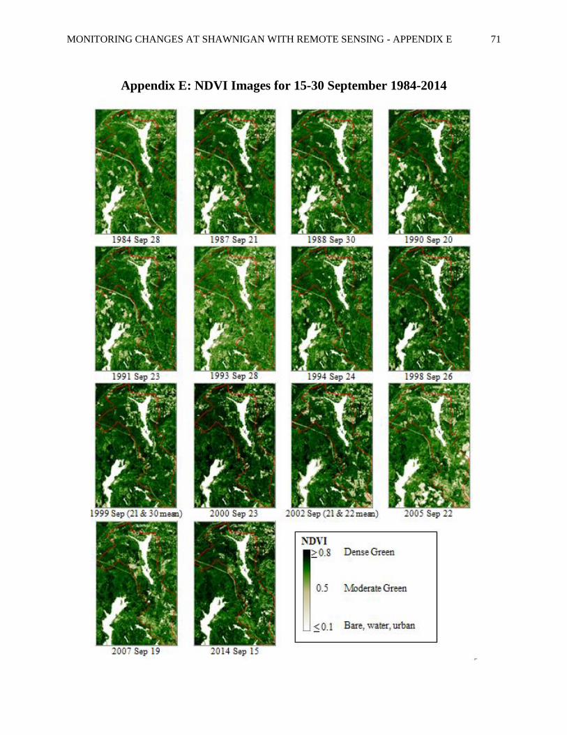
MONITORING CHANGES AT SHAWNIGAN WITH REMOTE SENSING - APPENDIX E 71
Appendix E: NDVI Images for 15-30 September 1984-2014
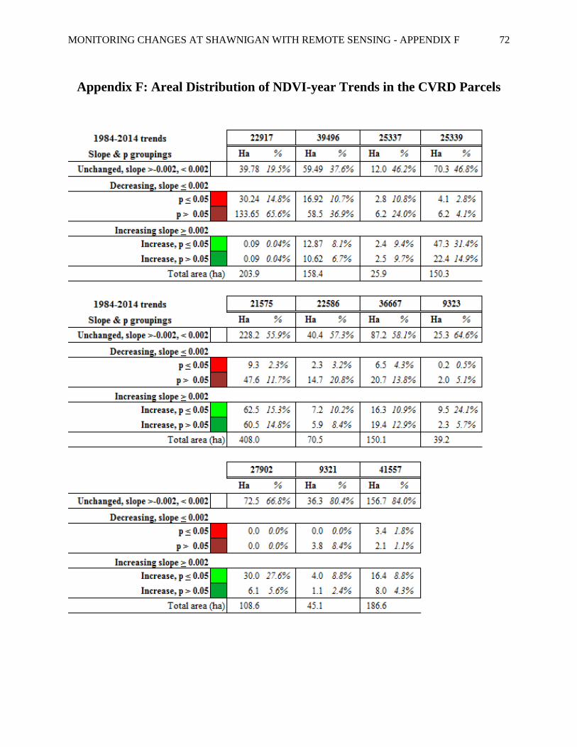
MONITORING CHANGES AT SHAWNIGAN WITH REMOTE SENSING - APPENDIX F 72
Appendix F: Areal Distribution of NDVI-year Trends in the CVRD Parcels
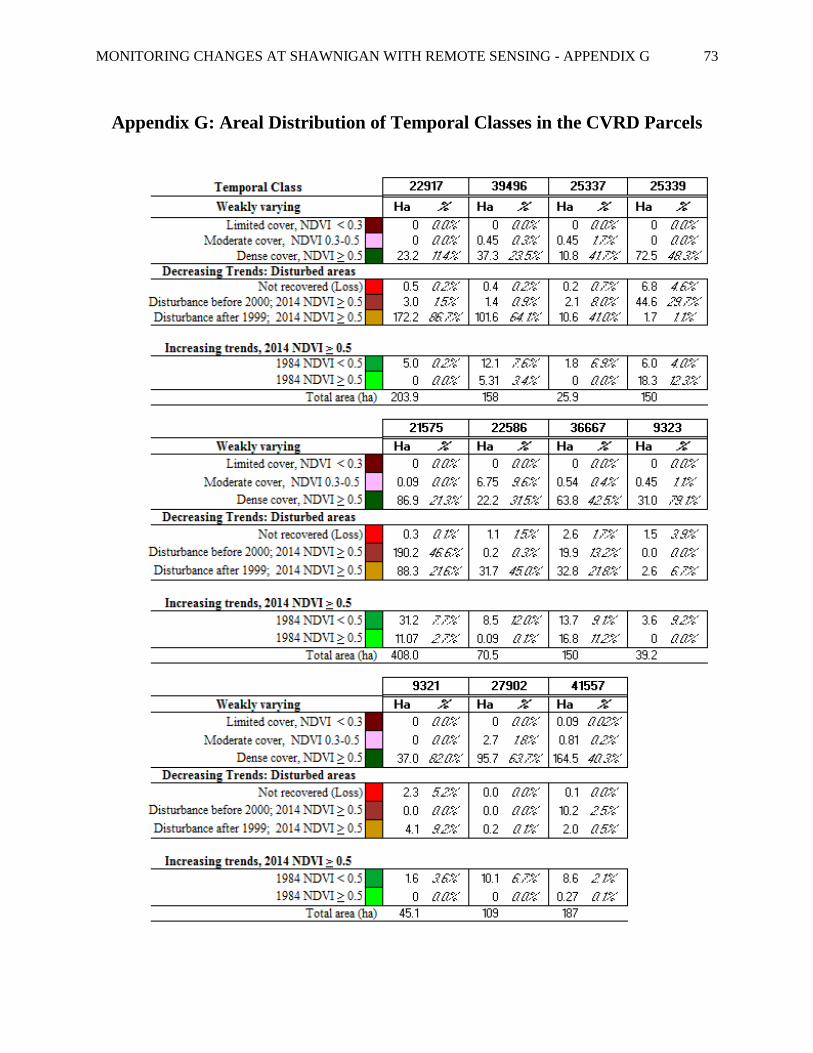
MONITORING CHANGES AT SHAWNIGAN WITH REMOTE SENSING - APPENDIX G 73
Appendix G: Areal Distribution of Temporal Classes in the CVRD Parcels