Seasonality of vegetation fires in Africa from remote sensing data and application to a global...

JOURNAL OF GEOPHYSICAL RESEARCH, VOL. 101, NO. D15, PAGES 21,051-21,065, SEPTEMBER 20, 1996

Seasonality of vegetation fires in Africa from remote sensing data and application to a global chemistry model W. F. Cooke •

Environment Institute, European Commission, Joint Research Center, Ispra, Italy

B. Kotti and J.-M. Grdgoire Space Applications Institute, European Commission, Joint Research Center, Ispra, Italy

Abstract. This paper sets out to show the potential use of remote sensing of active vegetation fires for continental- to global-scale modeling of biomass burning studies. It focuses on the analysis of the seasonality of vegetation fires for the African continent, as derived from NOAA-AVHRR-GAC-5km satellite data. These data are ideally suited for savanna fires, which constitute between 60 and 80% of the biomass burnt in Africa. Monthly counts of fire pixels, within 1 ø latitude x 1 ø longitude grid cells, over continental Africa have been calculated from November 1984 through October 1989. These 1 ø grid cells are summated to a 5 ø x 5 ø grid to enable comparison with previous studies and are analyzed at this resolution to show various features of the fire season. The analysis shows that previous attempts to characterize the seasonality of biomass burning have tended to underestimate the intensity of the peak months of burning or have predicted too long a fire season in certain areas. It also shows that there can be, for a given area, a temporal shift in the timing of the fire season from year to year. Such an interannual variability of fire seasonality makes satellite data more appropriate than statistical data for the modeling of atmospheric transport of vegetation fire products and the comparison with experimental measurements. Modeled values of black carbon mass concentration from a global transport model (MOGUNTIA), using the seasonality of biomass burning as an independent variable, are compared with measurements taken at Amsterdam Island (38ø30'S, 77ø30'E) and Lamto, Ivory Coast (6øN, 5øW). Although 5-year averaged satellite data were used, the seasonality as derived from satellite data determined in this paper gives modeled values of black carbon mass concentration that are in good agreement with the measurements.

1. Introduction

Tropical areas are continually under the influence of seasonal biomass burning, which in most cases is caused by fires deliberately lit by humans during the dry season. Because of deforestation by burning, shifting cultivation, hunting, range- land management, fuel wood use, and clearing of agricultural residues, such burning practices may result in global-scale and long lasting atmospheric, climatic, and biospheric implications [Crutzen and Andreae, 1990; Levine, 1991]. Global geographical distribution of biomass burning was first discussed in some detail in a review by Seiler and Crutzen [1980]. More recent studies, using statistical data (demographic data, land use, and forest inventories) and global vegetation and cultivation maps of tropical regions, were carried out during the last decade [Crutzen and Andreae, 1990; Andreae, 1991; Hao et al., 1991; Hao and Liu, 1994]. These studies all agree on the predomi- nance of Africa in global biomass burning due to the large area of savanna in both hemispheres. However, large quantitative and seasonality uncertainties in biomass estimates remain, as

•Now at Department of Experimental Physics, University College, Galway, Ireland.

Copyright 1996 by the American Geophysical Union.

Paper number 96JD01835. 0148-0227/96/96JD-01835509.00

significant differences between the estimates of the biomass burned from various sources are reported [Andreae, 1991; Hao and Liu, 1994]. There is therefore an increased request by the scientific community for a systematic documentation of continental and global biomass burning, in both experimental and modeling fields, especially by scientists involved in fire emission, land cover changes and tropical tropospheric chemistry studies. Data provided by the advanced very high resolution radiometers (AVHRR) onboard the NOAA satellites have been collected at continental and global scale for more than 10 years now and these data can be processed to allow an estimation of the seasonal changes in burning patterns. This method is more desirable, as it estimates the seasonality of biomass burning from the observation of the actual cause of the emissions (the fires) rather than an indirect effect of the emissions (photochemical production of ozone [Hao and Liu, 1994]). The present study, which focuses on tropical Africa, shows the potential use of remote sensing of vegetation fires for the characterization of biomass burning patterns at the continental scale and the use that can be made of these patterns with relation to atmospheric chemistry studies.

2. Remote Sensing of Active Fires The data presented here have been processed using daily

global area coverage (GAC) images, from the AVHRR of NOAA satellites, from November 1984 through October 1989.

21,051

21,052 COOKE ET AL.: SATELLITE FIRE SEASONALITY FOR CHEMISTRY MODEL

These 5-km-resolution data are known to provide a good description of the fire calendar and the geographical distribution of biomass burning at subcontinental scale [Belward et al., 1994; Koffi et al., 1995, 1996]. The method applied in this study to detect active fires is based on a combination of four thresh-

olds in the near, medium, and thermal infrared region of the spectrum. Three of these thresholds [Kaufman et al., 1990] are based on the brightness temperatures in AVHRR channels 3 (3.75 mm) and 4 (10.8 mm): (1) channel 3 brightness temperature of the candidate fire pixel must be above a specified value, (2) channel 3 must be hotter than channel 4 brightness temperature in order to discriminate between fire pixels and warm surfaces, and (3) channel 4 brightness temperature must itself exceed a specified value to avoid the detection of pixels that contain strongly reflective clouds, which can also saturate the sensor in channel 3. The method also includes "top of atmosphere" reflectance data from channel 2 (0.72-1.10 mm), where fire and recently burned areas will tend to have low reflectance due to the presence of ash cover [Kennedy et al., 1994]. Because of the dependance of the spectral responses of pixels conta!ning active fires on ecological factors, for example, soil and vegetation cover types, or the period within the fire season, no universal threshold values can be applied for fire detection [Kennedy, 1992; Gr•goire et al., 1993; Belward et al., 1994; Franca et al., 1995; Kennedy et al., 1994; Koffi et al., 1995 ]. Therefore the threshold values used in this study were defined on a monthly basis from a statistical study of fire pixels observed on the daily images by the presence of associated visible smoke. The fire detection method and the threshold values

applied in this study are fully documented by Koffi et al. [1996]. Moreover, because of the spatial sampling [Kidwell, 1990], the GAC data appear to be useful only for savanna and open woodland fires. In fact, fires in savanna and forest areas are quite different in nature. While forest fires may persist for many days, the fronts move slowly and the fires tend to occupy a small area. Savanna fires, which generally occur as a line fire where the burning front is some meters wide but several hun- dred meters long, are far more likely to be detected by satellite [Belward et al., 1994]. In this paper we concentrate on the African continent, where approximately 60-80% of the biomass burned is savanna [Delmas et al., 1991; Hao et al., 1991], so this limitation is not so important. In other regimes like South America or Asia, where savanna accounts for 50% and 8% of the biomass burned, respectively [Hao et al., 1991; Hao and Liu, 1994], higher-resolution satellite data such as the data provided by AVHRR local area coverage (LAC) at 1-km resolution may be necessary to provide good-quality seasonality data for subcontinental- and continental-scale areas. Ten-day and monthly syntheses of the African continental fire pixel maps, as derived from the daily GAC images, were made. These data were the subject of previous studies on multiannual monitoring of active vegetation fires in Africa at regional and continental scales [Koffi et al., 1995, 1996]. Care has been taken to assemble and format this fire-related information in consis-

tent data sets adapted to the modeling of trace gases and particulate matter. These data can be used to provide the seasonality for databases of biomass burning [Cooke and Wil- son, 1996] on the 1 ø x 1 ø scale or can be used to scale emissions on a larger scale (5 ø x 5 ø or 10 ø x 10 ø) if necessary. In this paper we sum the fire pixel count to 5 ø x 5 ø to enable us to compare our results with the data of Hao et al. [1991] and Hao and Liu [1994].

2.1. General Description of Seasonality of Biomass Burning in Africa as Derived From Remote Sensing Data

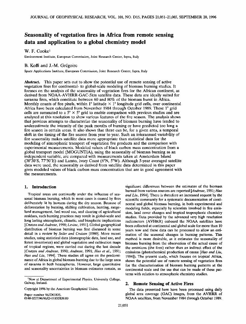
Savanna and open woodland burning during the dry season is widespread in Africa, where it is part of the agricultural policy for clearing the land of old grass, for shifting cultivation and hunting. Averaging over a 5 ø x 5 ø grid box needs to be treated with caution, as this can lead to averaging fire seasons from different biomass regimes, where the fire seasons may vary. For instance, the region of 5øW to 0 ø and 5øN to 10øN changes from rain forest to humid savanna to dry savanna. At present, global chemistry models are not advanced enough to allow for resolutions of better than 5 ø, so this averaging process is necessary to provide seasonality data for these models. The total fire pixel count for the period November 1984 through October 1989 on a scale of 1 ø x 1 ø is shown in Figure 1 where the letters A through H refer to the specific 5 ø x 5 ø areas of Figures 4a through 4h.

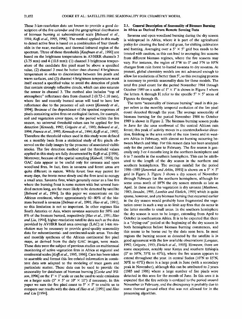
The term "seasonality of biomass burning" used in this paper refers to the monthly temporal evolution of the fire pixel count detected through the year. The average seasonality of biomass burning for the period November 1984 to October 1989 is shown in Figure 2. The biomass burning season peaks in June for the area southwest of the central African rain

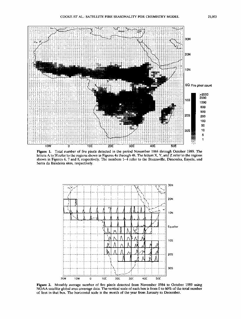
forest; this peak of activity moves in a counterclockwise direc- tion, finishing in the area north of the rain forest and in western Africa in February, with almost no burning occurring between March and May. For this reason data has been analyzed only for the period June to February. The fire season is generally only 3 or 4 months long in the northern hemisphere and 6 to 7 months in the southern hemisphere. This can be attributed to the length of the dry season in the northern and southern hemispheres. The average rainfall for the period 1986-1989 [Janowiak and Arkin, 1991] is shown on a 5 ø x 5 ø grid in Figure 3. Figure 3 shows a dry season of November through February for the northern hemisphere, although for some areas north of 10øN the dry season extends as late as April. In these areas the vegetation is dry savanna [Matthews, 1983; Janodet, 1995, Lambin and Ehrlich, 1995] which is quite sparse, however, and any biomass burning that occurred earlier in the dry season would probably have fragmented the vegetation cover in such a way as to limit any fires that do occur in the latter months to small areas. In the southern hemisphere the dry season is seen to be longer, extending from April to October in southeastern Africa. It is to be expected that there is a "drying-out" period at the beginning of the dry season in both hemispheres before biomass burning commences, and this seems to be borne out by the data seen here. In most regions the burning season as detected by the satellite is in good agreement with the few available observations [Langaas, 1992; Gr•goire, 1993; Ehrlich et al., 1995]. However, there are some exceptions, notably near Kenya and southern Ethiopia (0 ø to 10øN, 35øE to 40øE), where the fire season appears to extend throughout the year. In central Sudan (10øN to 15øN, 30øE to 40øE) there is a large peak in June (with a secondary peak in November), although this can be attributed to 2 years (1985 and 1986) where a large number of fire pixels were detected in this area for the month of June. In this area it is

expected that the fire activity is confined to the period around November to February, and the discrepancy is probably due to some thermal ground effect that was not allowed for in the processing algorithm.

COOKE ET AL.: SATELLITE FIRE SEASONALITY FOR CHEMISTRY MODEL 21,053

30N

10N

..........

•-•-t-•-•-1-I-•--:--:--:--:--:--:--7-•-•-•-•-•-•-•-I-•-•-•-... -•-•-•-•-•-•-•.;.;.;.;..:..;..:..•:• .......

,-,-,--,--,--,--,--,--.

,.,.,_,.,.,.,.,..,..,..,..,..,..,..,.,.,.,.,.,.,.,.,.,.,.,..,..,..,..,..,.

,.,.,.,.,.,.,.,..,..,..,..,..,..,..,.,.,.,.,.,.,.,.,.,.,.,..,..,..,..,..,.

,_,_,.,.,_,_,.,........,_.._.._..._,.,.,_,_,_,.,.,_,_,.,.,._,._,__,__.__._

20N

:::::::::::::::::::::::::::::::::::::::::::::::::::::::::::::::::::::::::::::::::::::::::: :,.E-•:-,.;;4:.';;•:?, ,:;:•:•:'i:'i:•:•:•:•:•;:,'::i::':::i::i::.::•::•:•:;:•:;:•:•:• "'"":J."•*' 5 .................

:-- .'-- .'-- •- •- 4- 4- -.'- -:- -:- -:--:--:--:--:--':- ',- ',- ',- .'-- •- •- •- •- 4- 4- -:- -:- -:--:--:--:-- :-- '•- .'-- ;- •- •~ •- •- 4- 4- -.'- -:- -:. -.:--:--:- ß :-- :-- .'-- .'-- .'-- -'.- •- •- -'.- 4- -.'- -:- 4- -:- -:- -:--:--:--:-- ',- :-- .'- - •- •- •- • :::::::::::::::::::::::::::::

....... ;...<;

:•:.;

ß -;-;-;-;-;-;-;

-;-;-;-;-:-;-:o;-;-; EQ Fire pixel count L-:- -:--:-~;-:--;-; - ;- ;- ;-

t' ............. >2000

':":--:--:--:--:'-:":" •-'•- •- •' •' • 10S 2000 80O

. :• 500

lOO --,-

10W 0 10E 20E 30E 40E 50E

Figure 1. Total number of fire pixels detected in the period November 1984 through October 1989. The letters A to H refer to the regions shown in Figures 4a through 4h. The letters X, Y, and Z refer to the regions shown in Figures 6, 7 and 8, respectively. The numbers 1-4 refer to the Brazzaville, Dimonika, Enyele, and Serra da Bandeira sites, respectively.

20W 10W 0 10E 20E 30E 40E 50E

30N

20N

1ON

Equator

1 os

20S

30S

Figure 2. Monthly average number of fire pixels detected from November 1984 to October 1989 using NOAA satellite global area coverage data. The vertical scale of each box is from 0 to 60% of the total number of fires in that box. The horizontal scale is the month of the year from January to December.


20W lOW 0 10E 20E 30E 40E 50E

30N

20N

1ON

Equotor

1 os

2os

30S

Figure 3. Seasonal variation of the rainfall in each 5 ø x 5 ø grid box. The vertical scale of each box is from 0 to 500 mm/month. The horizontal scale is the month of the year from January to December. After Janowiak and Arkin [1991].

2.2. Description of Specific Areas of Biomass Burning as Derived From NOAA Satellite Imagery

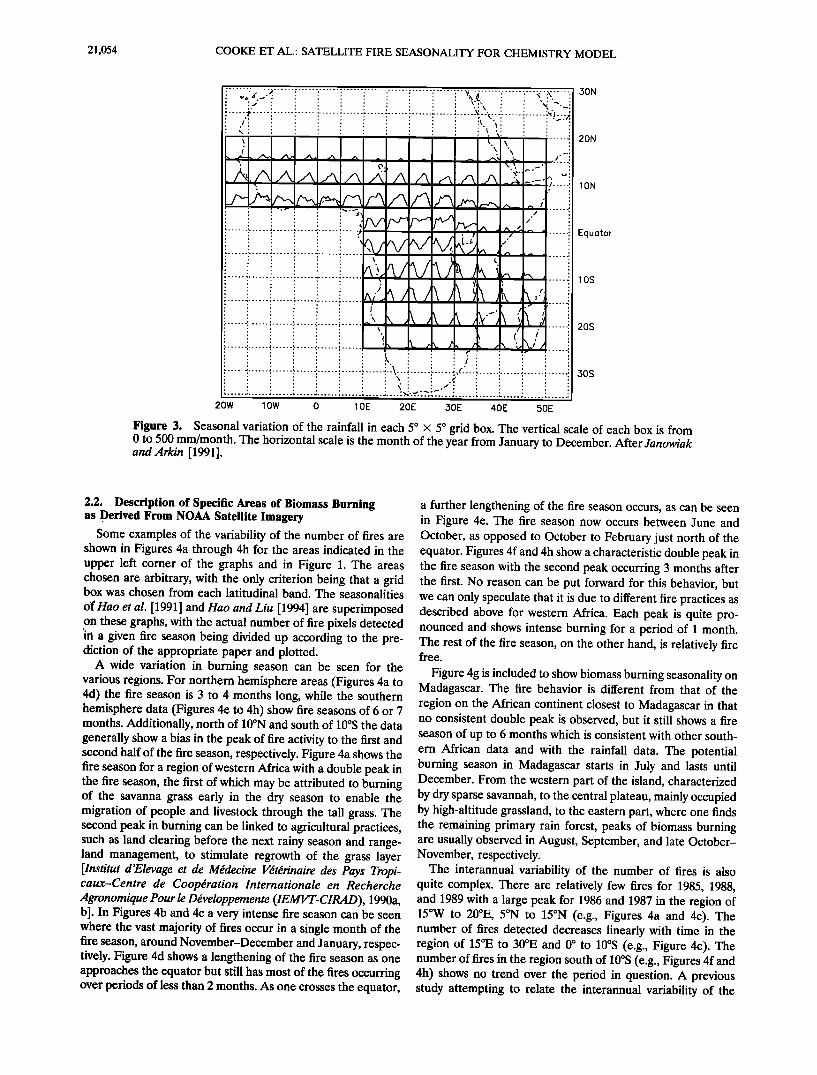
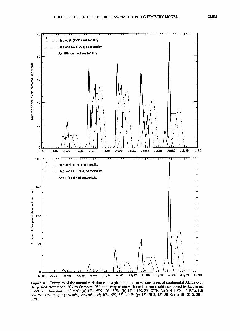
Some examples of the variability of the number of fires are shown in Figures 4a through 4h for the areas indicated in the upper left corner of the graphs and in Figure 1. The areas chosen are arbitrary, with the only criterion being that a grid box was chosen from each latitudinal band. The seasonalities ot• Hao et al. [1991] and Hao and Liu [1994] are superimposed on these graphs, with the actual number of fire pixels detected 'in a given fire season being divided up according to the pre- diction of the appropriate paper and plotted.

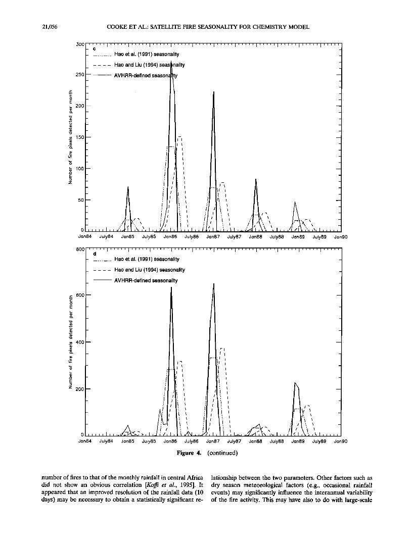
A wide variation in burning season can be seen for the various regions. For northern hemisphere areas (Figures 4a to 4d) the fire season is 3 to 4 months long, while the southern hemisphere data (Figures 4e to 4h) show fire seasons of 6 or 7 months. Additionally, north of 10øN and south of 10øS the data generally show a bias in the peak of fire activity to the first and second half of the fire season, respectively. Figure 4a shows the fire season for a region of western Africa with a double peak in the fire season, the first of which may be attributed to burning of the savanna grass early in the dry season to enable the migration of people and livestock through the tall grass. The second peak in burning can be linked to agricultural practices, such as land clearing before the next rainy season and range- land management, to stimulate regrowth of the grass layer [lnstitut d'Elevage et de M•decine V•t•rinaire des Pays Tropi- caux-Centre de Coopgration Internationale en Recherche Agronomique Pour le Dgveloppemente (IEMVT-CIRAD ), 1990a, b]. In Figures 4b and 4c a very intense fire season can be seen where the vast majority of fires occur in a single month of the fire season, around November-December and January, respectively. Figure 4d shows a lengthening of the fire season as one approaches the equator but still has most of the fires occurring over periods of less than 2 months. As one crosses the equator,

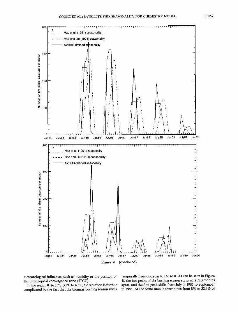
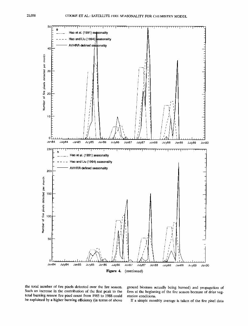
a further lengthening of the fire season occurs, as can be seen in Figure 4e. The fire season now occurs between June and October, as opposed to October to February just north of the equator. Figures 4f and 4h show a characteristic double peak in the fire season with the second peak occurring 3 months after the first. No reason can be put forward for this behavior, but we can only speculate that it is due to different fire practices as described above for western Africa. Each peak is quite pronounced and shows intense burning for a period of 1 month. The rest of the fire season, on the other hand, is relatively fire free.

Figure 4g is included to show biomass burning seasonality on Madagascar. The fire behavior is different from that of the region on the African continent closest to Madagascar in that no consistent double peak is observed, but it still shows a fire season of up to 6 months which is consistent with other southern African data and with the rainfall data. The potential burning season in Madagascar starts in July and lasts until December. From the western part of the island, characterized by dry sparse savannah, to the central plateau, mainly occupied by high-altitude grassland, to the eastern part, where one finds the remaining primary rain forest, peaks of biomass burning are usually observed in August, September, and late October- November, respectively.

The interannual variability of the number of fires is also quite complex. There are relatively few fires for 1985, 1988, and 1989 with a large peak for 1986 and 1987 in the region of 15øW to 20øE, 5øN to 15øN (e.g., Figures 4a and 4c). The number of fires detected decreases linearly with time in the region of 15øE to 30øE and 0 ø to 10øS (e.g., Figure 4e). The number of fires in the region south of 10øS (e.g., Figures 4f and 4h) shows no trend over the period in question. A previous study attempting to relate the interannual variability of the


lOO

80

'• 60

.•_

• 40

z

20

0

Jan84

- __ Hao et al. (1991) seasonality _ - - - Hao and Liu (1994) seasonality

- --- AVHRR-defined seasonality

Ill,'!',! li,I',! I,tA,:," "i"", • /!1 '1 '

,...,,,, ,•,,., ,,,,:, /,,• ', /•I• •', - ". • i I • , ..... ,,,/,..'•l,,,•,/,/,,',,I,•,,J,';,I,•,,,/,/,,'.,I • /,'/,•,,•,', .....

July84 J•n85 July85 Jen86 July86 J•n87 July87 Jen88 July88 Jon89 July89 Jen90

200

- Hao et al. (1991) seasonality _

- Hao and Liu (1994) seasonality _ - AVHRR-defined seasonality _

_(: 150 I

•o - E

N - • - • _

• 100 I

• _

•_ -

• "•1 I _

z 50 - i ,.. , -

• i II i • - -

_ /"•,,' ^ I/.--.,. •, I t." ,"• , li - 0 • •,, I,, ,•_•-•<.•,, i.•,,

J•n84 July84 J•n85 July85 J•n86 July86 J•n87 July87 J•n88 July88 J•n89 July89 J•n90

•i[ure 4. [xamples of the the peTiod NovembeT ]984 to OctobeT ]989 a•d compaTiso• with the •Te seaso•ali• pToposed by N•o et •l. []99]] a•d N•o • Li• []994]: (a) ]0ø-]5øN, ]0ø-]5øW; (b) ]0ø-]5øN, 20ø-25øE; (c) 5øN-]0øN, 5ø-]0øE; (d) oø-søN, •0ø-•sø[; (•) sø-]0øs, 2sø-•0ø[; (0 ]0ø-Isøs, •sø-•0ø[; (•) ]sø-20øs, •sø-s0ø[; (•) 20•-2søs, •øø- 35ø[.


300

250

E

200

• '150

'•..

.• •00 z

5O

0

Jan84

_ _ Hao et al. (1991) seasonality

- - Hao and Liu (1994) seastnality -- - AVHRR-defined season

I- /t--• ,•, i/,' I! , !/; I • ,, /'l,r.. , , • I-, .... ,,, •..:•l•I': , , , . , , ./,',., I,,,,,, i1,:, L;,,,, ,•..•',',•'.,,,, .... t•.,,..,,,,,,,,,

July84 Jan85 July85 Jan86 July86 Jan87 July87 Jan88 July88 Jan89 July89 Jan90

8OO

. Hao et al. (1991) seasonality

Hao and Liu (1994) seasonality

AVHRR-defined seasonality

,-- 600

E

• 400

/!.1.,' li, i'

Jon84 July84 Jan85 July85 Jan86 July86 Jan87 July87 Jan88 July88 Jan89 July89 Jan90

Figure 4. (continued)

number of fires to that of the monthly rainfall in central Africa did not show an obvious correlation [Koj• et al., 1995]. It appeared that an improved resolution of the rainfall data (10 days) may be necessary to obtain a statistically significant re-

lationship between the two parameters. Other factors such as dry season meteorological factors (e.g., occasional rainfall events) may significantly influence the interannual variability of the fire activity. This may have also to do with large-scale


200

•- 15o

o

E

• 100

x ._

,_

E

z 50

.... Hao et al. (1991) seasonality


AVHRR-defined sonality

i i

I i i i ,,i

I

o

don84 July84 don85 July85 don86 July86 don87 July87 don88 July88 don89 July89 don90

4OO

,- 300

• 200

'F,

z 100

0

don84

_- .... Hao et al. (1991 ) seasonality

_- - - Hao and Liu (1994) seasonality

; ---- AVHRR-defined seasonality

- I •

- : i • :

- •A'/',/, /l,'•,I• I,, ,-•,/• ..'/,'I. - •/,'• •,1', /)' "• I', ,'"L"•I, ...,/1 ..... I ..... I,,, L.//I,,,•t,,,;/I,,,tM .... .•.•',,,'.,bl,,, /.•4 ....... I ..... -

July84 Jan85 July85 Jan86 July86 Jan87 July87 Jan88 July88 Jan89 July89 Jan90


meteorological influences such as humidity or the position of the intertropical convergence zone (ITCZ).

In the region 0 ø to 15øS, 30øE to 40øE, the situation is further complicated by the fact that the biomass burning season shifts

temporally from one year to the next. As can be seen in Figure 4f, the two peaks of the burning season are generally 3 months apart, and the first peak shifts from July in 1985 to September in 1988. At the same time it contributes from 8% to 32.4% of


5O

g

- ....... Hao et al. (1991 ) se• •sonality -

- ...... Hao and Liu (1994)/Ieasonality 40 - ..... AVHRR-defined s onality

: i-- • , 30-- r--. "•

OF ..... i,,,,,i,,ie',l,,•,N,,/,4i,,",•,,l•l,,:,,/i,, ;,•,:;,il ..... i .... ,--I Jon84 July84 Jori85 July85 Jan86 July86 Jon87 July87 Jon88 July88 Jon89 July89 Jan90

2501 ..... I ..... I ..... I ..... I ..... I ..... I ..... I ..... I ..... I ..... I ..... I'''''

....... Hao et al. (1991) seasonality -

L .... Hao and Liu (1994) seasonality I - 2oo • AVHRR-defined seasonality -

•5o _

•- r'"l/ • i - I / i' I', I II i I -

: i" : ,,I -

- ;I,1,,I ',1 / ',•1!1 : ,',1',1 / ' : ,i i ' i -

- / '/,, .. • ! I / : / ,, - 0-,,,,,I,,,,,I .... '1"'14/' ''\:•' , / ,,, ,,,I,,,, ,- Jan84 July84 Jan85 July85 Jan86 July86 Jan87 July87 Jan88 July88 Jan89 July89 Jan90


the total number of fire pixels detected over the fire season. Such an increase in the contribution of the first peak to the total burning season fire pixel count from 1985 to 1988 could be explained by a higher burning efficiency (in terms of above

ground biomass actually being burned) and propagation of fires at the beginning of the fire season because of drier vegetation conditions.

If a simple monthly average is taken of the fire pixel data


5O

4O

• 3o

.x

.•-

• 2o

lO

Jan

I I

Feb Mar

Modified for first peak seasonality

Simple average seasonality

/

//

Apr May Jun Jul Aug Sep Oct. Nov Dec

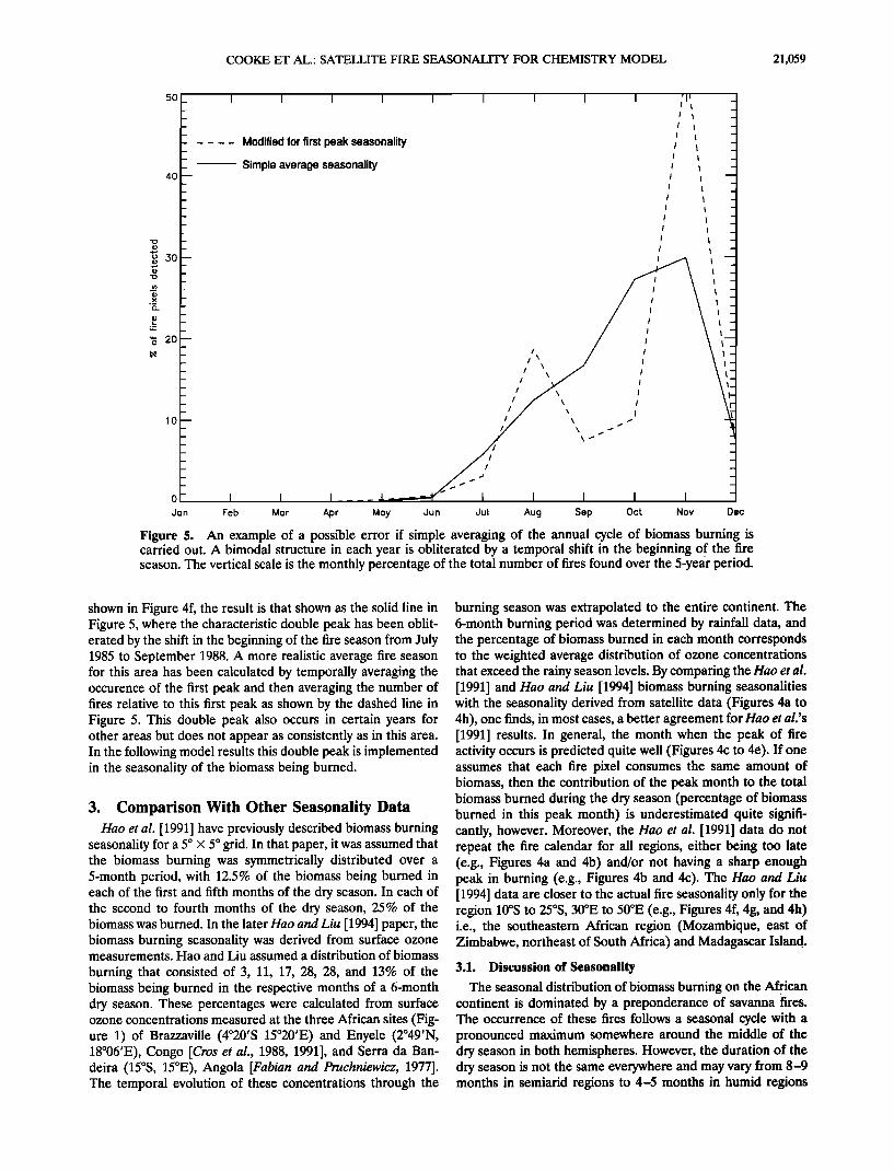
Figure 5. An example of a possible error if simple averaging of the annual cycle of biomass burning is carried out. A bimodal structure in each year is obliterated by a temporal shift in the beginning of the fire season. The vertical scale is the monthly percentage of the total number of fires found over the 5-year period.

shown in Figure 4f, the result is that shown as the solid line in Figure 5, where the characteristic double peak has been obliterated by the shift in the beginning of the fire season from July 1985 to September 1988. A more realistic average fire season for this area has been calculated by temporally averaging the occurence of the first peak and then averaging the number of fires relative to this first peak as shown by the dashed line in Figure 5. This double peak also occurs in certain years for other areas but does not appear as consistently as in this area. In the following model results this double peak is implemented in the seasonality of the biomass being burned.

3. Comparison With Other Seasonality Data Hao et al. [1991] have previously described biomass burning

seasonality for a 5 ø x 5 ø grid. In that paper, it was assumed that the biomass burning was symmetrically distributed over a 5-month period, with 12.5% of the biomass being burned in each of the first and fifth months of the dry season. In each of the second to fourth months of the dry season, 25% of the biomass was burned. In the later Hao and Liu [1994] paper, the biomass burning seasonality was derived from surface ozone measurements. Hao and Liu assumed a distribution of biomass

burning that consisted of 3, 11, 17, 28, 28, and 13% of the biomass being burned in the respective months of a 6-month dry season. These percentages were calculated from surface ozone concentrations measured at the three African sites (Fig- ure 1) of Brazzaville (4ø20'S 15ø20'E) and Enyele (2ø49'N, 18ø06'E), Congo [Cros et al., 1988, 1991], and Serra da Ban- deira (15øS, 15øE), Angola [Fabian and Pruchniewicz, 1977]. The temporal evolution of these concentrations through the

burning season was extrapolated to the entire continent. The 6-month burning period was determined by rainfall data, and the percentage of biomass burned in each month corresponds to the weighted average distribution of ozone concentrations that exceed the rainy season levels. By comparing the Hao et al. [1991] and Hao and Liu [1994] biomass burning seasonalities with the seasonality derived from satellite data (Figures 4a to 4h), one finds, in most cases, a better agreement for Hao et al.'s [1991] results. In general, the month when the peak of fire activity occurs is predicted quite well (Figures 4c to 4e). If one assumes that each fire pixel consumes the same amount of biomass, then the contribution of the peak month to the total biomass burned during the dry season (percentage of biomass burned in this peak month) is underestimated quite significantly, however. Moreover, the Hao et al. [1991] data do not repeat the fire calendar for all regions, either being too late (e.g., Figures 4a and 4b) and/or not having a sharp enough peak in burning (e.g., Figures 4b and 4c). The Hao and Liu [1994] data are closer to the actual fire seasonality only for the region 10øS to 25øS, 30øE to 50øE (e.g., Figures 4f, 4g, and 4h) i.e., the southeastern African region (Mozambique, east of Zimbabwe, northeast of South Africa) and Madagascar Island.

3.1. Discussion of Seasonality

The seasonal distribution of biomass burning on the African continent is dominated by a preponderance of savanna fires. The occurrence of these fires follows a seasonal cycle with a pronounced maximum somewhere around the middle of the dry season in both hemispheres. However, the duration of the dry season is not the same everywhere and may vary from 8-9 months in semiarid regions to 4-5 months in humid regions


5O

4O

•o 30

._x

._

'- 20 o

lo

i i i i

1986

1985

1986 ozone data

1985 Ozone data

o I 30 Jan Feb Mar Apr May Jun Jul Aug Sep Oct Nov Dec

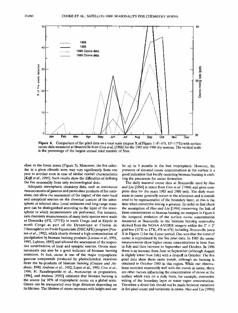
Figure 6. Comparison of fire pixel data on a local scale (region X of Figure 1: 4ø-6øS, 15ø-17øE) with surface ozone data measured at Brazzaville from Cros et al. [1988] for the 1985 and 1986 dry seasons. The vertical scale is the percentage of the largest annual total number of fires.

close to the forest zones (Figure 3). Moreover, the fire calendar in a given climatic zone may vary significantly from one year to another even in case of similar rainfall characteristics [Koffi et al., 1995]. Such results show the difficulties of defining the fire seasonality from only meteorological data.

Adequate atmospheric chemistry data, such as continuous measurements of gaseous and particulate products of fire emissions, can allow the assessment of the impact of the main local and synoptical sources on the chemical content of the atmosphere at selected sites. Local emissions and long-range transport can be distinguished according to the layer of the atmosphere in which measurements are performed. For instance, rain chemistry measurements of many ionic species were made at Dimonika (4øS, 12ø3'E) in south Congo and at Enyele in north Congo as part of the Dynamique et Chimie de l'Atmosph•re en For6t Equatoriale (DECAFE) program [Fort- tan et al., 1992], which clearly showed a high contamination of precipitation by biomass burning products [Lacaux et al., 1991, 1992; Lefeivre, 1993] and allowed the assessment of the respective contributions of local and synoptic sources. Ozone measurements can also be a good indicator of biomass burning emissions. In fact, ozone is one of the major tropospheric gaseous compounds produced by photochemical reactions from the by-products of biomass burning [Crutzen and An- dreae, 1990; Andreae et al., 1992; Lopez et al., 1992; Cros et al., 1996; H. Razafimpanilo et al., manuscript in preparation, 1996], and Andreae [1991] estimates that biomass burning is the source for 38% of tropospheric ozone on a global scale. Ozone can be transported over large distances depending on its lifetime. The lifetime of ozone increases with height and can

be up to 3 months in the free troposphereß However, the presence of elevated ozone concentrations at the surface is a good indication that locally occurring biomass burning is emit- ting the precursors for ozone formation.

The daily maximal ozone data at Brazzaville used by Hao and Liu [1994] is taken from Cros et al. [1988] and gives complete data for the years 1985 and 1986 only. The daily maximum in ozone generally occurs in the afternoon and is consid- ered to be representative of the boundary layer, as this is the time when convective mixing is greatest. In order to first check the assumption of Hao and Liu [1994] concerning the link of these concentrations to biomass burning, we compare in Figure 6 the temporal evolution of the surface ozone concentration measured at Brazzaville to the biomass burning seasonality derived from the NOAA AVHRR imagery within the 2 ø x 2 ø grid box (15øE to 17øE, 4øS to 6øS) including Brazzaville (area X in Figure 1) for the 2-year period. One sees that the trend of ozone is reproduced by the fire pixel data. In 1985 the ozone measurements show higher ozone concentrations in June than in July and then increase to September and October. In 1986 there is an increase from June to September (although August is slightly lower than July) with a dropoff in October. The fire pixel data show these same trends, although no burning is obtained in October 1985 in this region. While our observations correlate reasonably well with the trends in ozone, there are other factors influencing the concentration of ozone at the surface which vary on a daily basis, for example, convective mixing of the boundary layer or water vapor concentration. Therefore a direct link should not be made between variations

in fire pixel count and variations in ozone. Hao and Liu [1994]

COOKE ET AL.' SATELLITE FIRE SEASONALITY FOR CHEMISTRY MODEL 21,061

7O

6O

5O

• 40

._

'• 30

2O

10

1989

1988

1987

1986

1985

Hao and Liu (1994)

•-•'•ø I I' •"--• Jan Feb Mar

I I

\ \

\ \

\ \

\ \

\ \

Apr May Jun Jul Aug Sep Oct Nov Dec

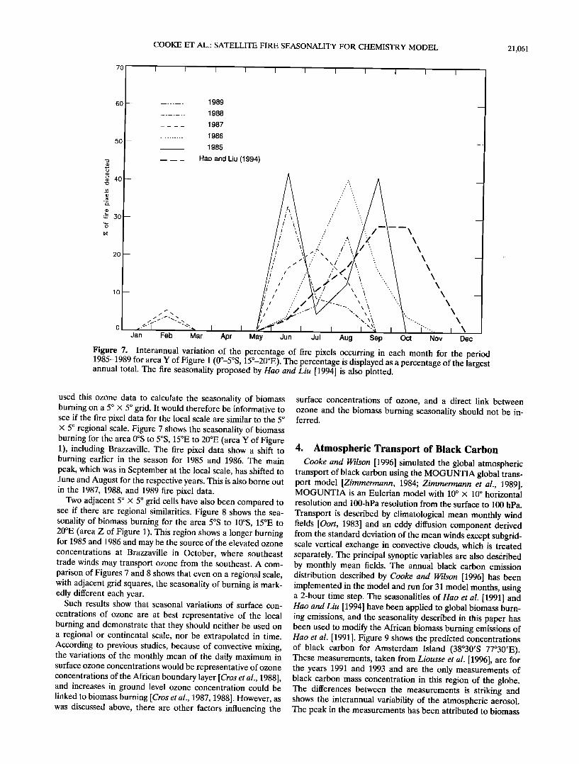
Figure 7. Interannual variation of the percentage of fire pixels occurring in each month for the period ß o o o o

1985-1989 for area Y of F•gure 1 (0 -5 S, 15 -20 E). The percentage is displayed as a percentage of the largest annual total. The fire seasonality proposed by Hao and Liu [1994] is also plotted.

used this ozone data to calculate the seasonality of biomass burning on a 5 ø x 5 ø grid. It would therefore be informative to see if the fire pixel data for the local scale are similar to the 5 ø x 5 ø regional scale. Figure 7 shows the seasonality of biomass burning for the area 0øS to 5øS, 15øE to 20øE (area Y of Figure 1), including Brazzaville. The fire pixel data show a shift to burning earlier in the season for 1985 and 1986. The main peak, which was in September at the local scale, has shifted to June and August for the respective years. This is also borne out in the 1987, 1988, and 1989 fire pixel data.

Two adjacent 5 ø x 5 ø grid cells have also been compared .to see if there are regional similarities. Figure 8 shows the seasonality of biomass burning for the area 5øS to 10øS, 15øE to 20øE (area Z of Figure 1). This region shows a longer burning for 1985 and 1986 and may be the source of'the elevated ozone concentrations at Brazzaville in October, where southeast trade winds may transport ozone from the southeast. A comparison of Figures 7 and 8 shows that even on a regional scale, with adjacent grid squares, the seasonality of burning is mark- edly different each year.

Such results show that seasonal variations of surface concentrations of ozone are at best representative of the local burning and demonstrate that they should neither be used on a regional or continental scale, nor be extrapolated in time. According to previous studies, because of convective mixing, the variations of the monthly mean of the daily maximum in surface ozone concentrations would be representative of ozone concentrations of the African boundary layer [Cros et al., 1988], and increases in ground level ozone concentration could be linked to biomass burning [Cros et al., 1987, 1988]. However, as was discussed above, there are other factors influencing the

surface concentrations of ozone, and a direct link between ozone and the biomass burning seasonality should not be in- ferred.

4. Atmospheric Transport of Black Carbon Cooke and Wilson [1996] simulated the global atmospheric

transport of black carbon using the MOGUNTIA global transport model [Zimmermann, 1984; Zimmermann et al., 1989]. MOGUNTIA is an Eulerian model with 10 ø x 10 ø horizontal resolution and 100-hPa resolution from the surface to 100 hPa. Transport is described by climatological mean monthly wind fields [Oort, 1983] and an eddy diffusion component derived from the standard deviation of the mean winds except subgrid- scale vertical exchange in convective clouds, which is treated separately. The principal synoptic variables are also desiSribed by monthly mean fields. The annual black carbon emission distribution described by Cooke and Wilson [1996] has been implemented in the model and run for 31 model months, using a 2-hour time step. The seasonalities of Hao et al. [1991] and Hao and Liu [1994] have been applied to global biomass burning emissions, and the seasonality described in this paper has been used to modify the African biomass burning emissions of Hao et al. [1991]. Figure 9 shows the predicted concentrations of black carbon for Amsterdam Island (38ø30'S 77ø30'E). These measurements, taken from Liousse et al. [1996], are for the years 1991 and 1993 and are the only measurements of black carbon mass concentration in this region of the globe. The differences between the measurements is striking and shows the interannual variability of the atmospheric aerosol. The peak in the measurements has been attributed to biomass


7O

6O

5O

• 4o

.--

2O

10

1989

1988

1987

1986

1985

Hao and Liu (1994)

L--- • I I Jan Feb Mar Apr

'""',•,,• i I-- -- --\\ -- //• \\

\\\\ _ May Jun Jul Aug Sep Oct Nov Dec

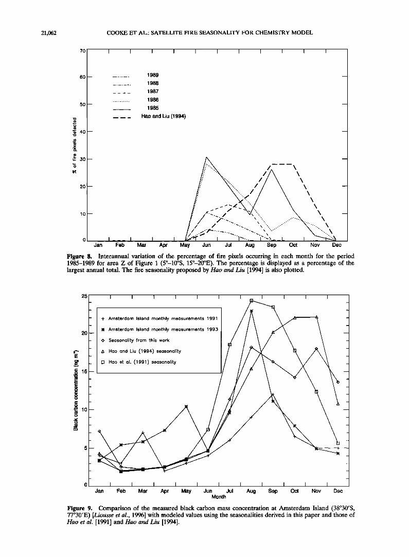
Figure 8. Interannual variation of the percentage of fire pixels occurring in each month for the period 1985-1989 for area Z of Figure 1 (5ø-10øS, 15ø-20øE). The percentage is displayed as a percentage of the largest annual total. The fire seasonality proposed by Hao and Liu [1994] is also plotted.

25

2O

c 15 .m

• 10

Amsterdam Island monthly measurements 1991

Amsterdam Island monthly measurements 1993

Seasonality from this work


Hao et al. (1991) seasonality

Jan Feb Mar Apr May Jun Jul Aug Sep Oct Nov Dec Month

Figure 9. Comparison of the measured black carbon mass concentration at Amsterdam Island (38ø30'S, 77ø30'E) [Liousse et al., 1996] with modeled values using the seasonalities derived in this paper and those of Hao et al. [1991] and Hao and Liu [1994].


6ooo I

4000

2000

+ Lamto monthly measurements

O Seasonality from this work

A Hao and Liu (1994) seasonality

[] Hao et al. (1991) seasonality

Jan Feb Mar Apr May Jun Jul Aug Sep Oct Nov Dec Month

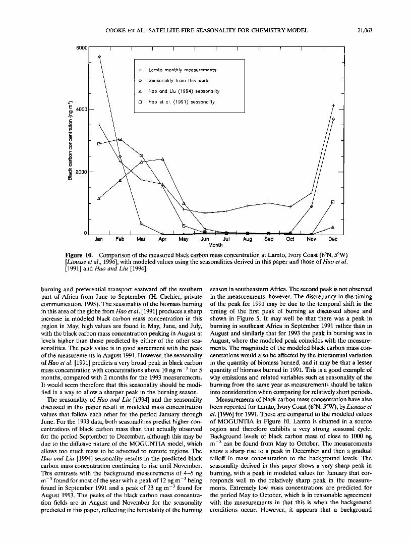
Figure 10. Comparison of the measured black carbon mass concentration at Lamto, Ivory Coast (6øN, 5øW) [Liousse et al., 1996], with modeled values using the seasonalities derived in this paper and those of Hao et al. [1991] and Hao and Liu [1994].

burning and preferential transport eastward off the southern part of Africa from June to September (H. Cachier, private communication, 1995). The seasonality of the biomass burning in this area of the globe from Hao et al. [1991] produces a sharp increase in modeled black carbon mass concentration in this

region in May; high values are found in May, June, and July, with the black carbon mass concentration peaking in August at levels higher than those predicted by either of the other seasonalities. The peak value is in good agreement with the peak of the measurements in August 1991. However, the seasonality ofHao et al. [1991] predicts a very broad peak in black carbon mass concentration with concentrations above 10 ng m --• for 5 months, compared with 2 months for the 1993 measurements. It would seem therefore that this seasonality should be modified in a way to allow a sharper peak in the burning season.

The seasonality of Hao and Liu [1994] and the seasonality discussed in this paper result in modeled mass concentration values that follow each other for the period January through June. For the 1993 data, both seasonalities predict higher concentrations of black carbon mass than that actually observed for the period September to December, although this may be due to the diffusive nature of the MOGUNTIA model, which allows too much mass to be advected to remote regions. The Hao and Liu [1994] seasonality results in the predicted black carbon mass concentration continuing to rise until November. This contrasts with the background measurements of 4-5 ng m -3 found for most of the year with a peak of 12 ng m -3 being found in September 1991 and a peak of 23 ng m -3 found for August 1993. The peaks of the black carbon mass concentration fields are in August and November for the seasonality predicted in this paper, reflecting the bimodality of the burning

season in southeastern Africa. The second peak is not observed in the measurements, however. The discrepancy in the timing of the peak for 1991 may be due to the temporal shift in the timing of the first peak of burning as discussed above and shown in Figure 5. It may well be that there was a peak in burning in southeast Africa in September 1991 rather than in August and similarly that for 1993 the peak in burning was in August, where the modeled peak coincides with the measurements. The magnitude of the modeled black carbon mass concentrations would also be affected by the interannual variation in the quantity of biomass burned, and it may be that a lesser quantity of biomass burned in 1991. This is a good example of why emissions and related variables such as seasonality of the burning from the same year as measurements should be taken into consideration when comparing for relatively short periods.

Measurements of black carbon mass concentration have also

been reported for Lamto, Ivory Coast (6øN, 5øW), by Liousse et al. [1996] for 1991. These are compared to the modeled values of MOGUNTIA in Figure 10. Lamto is situated in a source region and therefore exhibits a very strong seasonal cycle. Background levels of black carbon mass of close to 1000 ng m -3 can be found from May to October. The measurements show a sharp rise to a peak in December and then a gradual falloff in mass concentration to the background levels. The seasonality derived in this paper shows a very sharp peak in burning, with a peak in modeled values for January that corresponds well to the relatively sharp peak in the measurements. Extremely low mass concentrations are predicted for the period May to October, which is in reasonable agreement with the measurements in that this is when the background conditions occur. However, it appears that a background


source of black carbon is absent in the Cooke and Wilson [1996] emission data set. This background is probably wood burning for heating and cooking. The seasonality of Hao et al. [1991] predicts a much wider peak in mass concentrations, with mass concentrations of over 1000 ng m -3 for the months December through April. The mass concentrations predicted by the seasonality of Hao and Liu [1994] do not start to rise until Janu- ary, and they peak in April, when the measurements are almost back to background levels.

5. Conclusions

Special care needs to be taken when using proxy data to predict biomass burning seasonality on a continental scale. Satellite data, on the other hand, can be used to monitor on-site fire activity on the continental scale. Work has been carried out to determine the seasonality of biomass burning on this continental scale. A complex variation has been found for various regions of Africa with fire seasons varying from 3 to 6 months according to the dry season and in some areas having a bimodal structure to the fire season. Care must be taken in

these areas of bimodal fire structure to ensure that the tem-

poral variation of the fires are calculated correctly. In some regions, an important interannual variability of the fire seasonality is also shown. Trends in fire activity may also be seen, although the present data set is probably insufficient to make any firm conclusions.

A comparison has been made between the variations in burning as seen by satellite and ground measurements of ozone. A local-scale (2 ø x 2 ø) comparison has shown a reasonable correlation. A comparison of the local-scale measurements of ozone with more regional (5 ø x 5 ø) scale fire pixel data shows less agreement, indicating that local-scale surface ozone measurements are not indicative of regional-scale biomass burning and therefore cannot be used to derive temporal patterns for vegetation fires at such a spatial scale.

Variations in concentration of emitted black carbon from

biomass burning due to the variations in the seasonality of burning have been investigated, and significant differences have been found in both remote (Amsterdam Island) and source (Lamto) regions. The modeled values calculated using the average biomass burning seasonality defined from 5 years of satellite data show a good agreement with the measured concentrations. However, future studies using satellite derived fire data and measurements from the same period are needed to support these encouraging results. The seasonality of Hao et al. [1991] gives reasonable agreement with the peak in the burning period but appears to underestimate the intensity of the peak month of burning. For areas where there are no data available on the seasonality of biomass burning, it would be recommended that the Hao et al. [1991] data be modified to have more burning in the peak month of the fire season. A more complete analysis of the seasonality of biomass burning combining ground-based observations and remote sensing data would be a significant step forward in demonstrating the ca- pability of remote sensing methods to provide data on biomass burning seasonality. This would allow us to explain if, for example, the double peak found in the seasonality of southeastern Africa is due to agricultural practices as hypothesized here or whether there is some other explanation such as meteorological factors.

Acknowledgments. We would like to thank H. Cachier and C. Liousse for supplying the measurement data of black carbon at

Amsterdam Island and Lamto, respectively, and C. Davi and H. Eva for their help in processing the remote sensing data. We would also like to thank F. Raes, B. Cros, and S. G. Jennings for their useful comments. W. C., as a grantholder, would like to acknowledge the sponsorship of the European Commission in this work.

References

Andreae, M. O., Biomass burning: Its history, use and distribution and its impact on environmental quality and global climate, in Global Biomass Burning: Atmospheric, Climatic and Biospheric Implications, edited by J. S. Levine, pp. 1-21, MIT Press, Cambridge, Mass., 1991.

Andreae, M. O., A. Chapuis, B. Cross, J. Fontan, G. Hdlas, C. Justice, Y. J. Kaufman, A. Minga, and D. Nganga, Ozone and Aitken nuclei over equatorial Africa: Airborne observations during DECAFE 88, J. Geophys. Res., 97, 6137-6148, 1992.

Belward, A. S., P. J. Kennedy, and J.-M. Grdgoire, The limitations and potential of AVHRR GAC data for continental scale fire studies, Int. J. Remote Sens., 15, 2215-2234, 1994.

Cooke, W. F., and J. J. N. Wilson, A global black carbon aerosol model, J. Geophys. Res., in press, 1996.

Cros, B., R. Delmas, B. Clairac, J. Loemba-Ndembi, and J. Fontan, Survey of ozone concentration in an equatorial region during the rainy season, J. Geophys. Res., 92, 9772-9778, 1987.

Cros, B., R. Delmas, D. Nganga, B. Clairac, and J. Fontan, Seasonal trends of ozone in equatorial Africa: Experimental evidence of photochemical formation, J. Geophys. Res., 93, 8355-8366, 1988.

Cros, B., D. Nganga, R. A. Delmas, and J. Fontan, Tropospheric ozone and biomass burning in intertropical Africa, in Global Biomass Burn- ing.' Atmospheric, Climatic and Biospheric Implications, edited by J. S. Levine, pp. 143-146, MIT Press, Cambridge, Mass., 1991.

Cros, B., B. Ahoua, D. Orange, M. Dimbele, and J.P. Lacaux, Tro- pospheric ozone on both sides of the equator in Africa, in Biomass Burning and Global Change, edited by J. S. Levine, MIT Press, Cambridge, Mass., in press, 1996.

Crutzen, P. J., and M. O. Andreae, Biomass burning in the tropics: Impact on atmospheric chemistry and biogeochemical cycles, Sci- ence, 250, 1669-1678, 1990.

Delmas, R. A., P. Loudjani, A. Podaire, and J. C. Menaut, Biomass burning in Africa: An assessment of annually burned biomass, in Global Biomass Burning: Atmospheric, Climatic and Biospheric Im- plications, edited by J. S. Levine, pp. 126-132, MIT Press, Cam- bridge, Mass., 1991.

Ehrlich, D., J.-M. Grdgoire, H. Eva, E. Janodet, and B. Koffi, Fire detection, land cover characterization and burnt area estimation in the savannah-forest transition zone of central Africa, Publ. EUR 16314 EN, 72 pp., Luxembourg, Eur. Communities, 1995.

Fabian, P., and P. G. Pruchniewicz, Meridional distribution of ozone in the troposphere and its seasonal variations, J. Geophys. Res., 82, 2063-2073, 1977.

Fontan, J., A. Druilhet, B. Benech, and R. Lyra, The DECAFE experiments: Overview and meteorology, J. Geophys. Res., 97, 6123- 6136, 1992.

Franca, J. R. A., J. M. Brustet, and J. Fontan, A multi-spectral remote sensing of biomass burning in west Africa, J. ,4tmos. Chem., 22, 81-110, 1995.

Grdgoire, J.-M., Description quantitative des rdgimes de feu en zone soudanienne d'Afrique de l'ouest, Secheresse, 4, 37-45, 1993.

Grdgoire, J.-M., A. S. Belward, and P. Kennedy, Dynamique de satu- ration du signal dans la bande 3 du senseur AVHRR: Handicap majeur ou source d'information pour la surveillance de l'environnement en milieu soudano-guinden d'Afrique de l'ouest?, Int. J. Remote Sens., 14, 2079-2095, 1993.

Hao, W. M., and M. H. Liu, Spatial and temporal distribution of tropical biomass burning, Global Biogeochem. Cycles, 8, 495-503, 1994.

Hao, W. M., M. H. Liu, and P. J. Crutzen, Estimates of annual and regional releases of CO2 and other trace gases to the atmosphere from fires in the tropics, based on the FAO statistics for the period 1975-1980, in Fire in the Tropical Biota--Ecosystems, Processes and Global Challenges, Ecol. Stud., vol. 84, edited by J. G. Goldammer, pp. 440-462, Springer-Verlag, New York, 1991.

Institut d'Elevage et de Mddecine Vdtdrinaire des Pays Tropicaux- Centre de Coopdration Internationale en Recherche Agronomique Pour le Ddveloppement (IEMVT-CIRAD), Les feux de brousse, Fiches Tech. d'Elevage Trop., 3, 11 pp., Paris, March 1990a.


Institut d'Elevage et de M6decine V6t6rinaire des Pays Tropicaux- Centre de Coop6ration Internationale en Recherche Agronomique Pour le D6veloppement (IEMVT-CIRAD), Les feux de brousse, Fiches Tech. d'Elevage Trop., 6, 7 pp., Paris, June 1990b.

Janodet, E., Stratification saisonni•,re de l'Afrique continentale et car- tographie fonctionnelle des 6cosyst•,mes forestiers africains, final report, contract CCR 10350-94-07 FlED ISP F, 72 pp., Eur. Comm., Luxembourg, 1995.

Janowiak, J. E., and P. A. Arkin, Rainfall variations in the tropics during 1986-1989, as estimated from observations of cloud-top temperatures, J. Geophys. Res., 96, suppl., 3359-3373, 1991.

Kaufman, Y., C. J. Tucker, and I. Fung, Remote sensing of biomass burning in the tropics, J. Geophys. Res., 95, 9927-9939, 1990.

Kennedy, P., Biomass burning studies: The use of remote sensing, Ecol. Bull., 42, 133-148, 1992.

Kennedy, P. J., A. S. Belward, and J.-M. Gr6goire, An improved approach to fire monitoring in west Africa using AVHRR data, Int. J. Remote Sens., 15, 2235-2255, 1994.

Kidwell, K. B., Global vegetation index users guide, technical report, Natl. Clim. Cent., Natl. Oceanic and Atmos. Admin., Washington, D.C., 1990.

Koffi, B., J. M. Gr6goire, G. Mah6, and J.P. Lacaux, Remote sensing of bush fire dynamics in central Africa from 1984 to 1988: Analysis in relation to regional vegetation and pluviometric patterns, Atmos. Res., 39, 179-200, 1995.

Koffi, B., J.-M. Gr6goire, and H. D. Eva, Satellite monitoring of vegetation fires on a multiannual basis and a continental scale in Africa, in Biomass Burning and Global Change, edited by J. S. Levine, MIT Press, Cambridge, Mass., in press, 1996.

Lacaux, J.-P., R. Delmas, B. Cros, B. Lefeivre, and M. O. Andreae, Influence of biomass burning emissions on precipitation chemistry in the equatorial forests of Africa, in Global Biomass Burning; Atmo- spheric, Climatic and Biospheric Implications, edited by J. S. Levine, pp. 167-174, MIT Press, Cambridge, Mass., 1991.

Lacaux, J.-P., J. Loemba-Ndembi, B. Lefeivre, B. Cros, and R. Delmas, Biogenic emissions and biomass burning influences on the chemistry of the fog water and stratiform precipitation in the African equatorial forest, Atmos. Environ., Part A, 26, 541-551, 1992.

Lambin, E. F., and D. Ehrlich, Combining vegetation indices and surface temperature for land cover mapping at broad spatial scales, Int. J. Remote Sens., 16, 573-579, 1995.

Langaas, S., Temporal and spatial distribution of savanna fires in Senegal and the Gambia, west Africa, 1989-90, derived from multi- temporal AVHRR night images, Int. J. Wildland Fire, 2(1), 21-36, 1992.

Lefeivre, B., Etude exp6rimentale et par mod61isation des caract6ris- tiques physiques et chimiques des pr6cipitations collect6es en for6t 6quatoriale Africaine, Ph.D. thesis, 308 pp., Univ. Paul Sabatier, Toulouse, France, 1993.

Levine, J. S., Introduction: Global biomass burning: Atmospheric, climatic and biospheric implications, in Global Biomass Burning: Atmospheric, Climatic and Biospheric Implications, edited by J. S. Levine, pp. XXV-XXX, MIT Press, Cambridge, Mass., 1991.

Liousse, C., J. E. Penner, C. Chuang, J. J. Walton, H. Eddieman, and H. Cachier, A global three-dimensional model study of carbona- ceous aerosols, J. Geophys. Res., in press, 1996.

Lopez, A., M. L. Huertas, and J. M. Lacome, A numerical simulation of the ozone chemistry observed over forested tropical areas during DECAFE experiments, J. Geophys. Res., 97, 6149-6158, 1992.

Matthews, E., Global vegetation and land use: New high-resolution data bases for climate studies, J. Clim. Appl. Meteorol., 22, 474-487, 1983.

Oort, A. H., Global atmospheric circulation statistics, 1958-1973, NOAA Prof. Pap., 14, U.S. Govt. Print. Off., Washington, D.C., 1983.

Seller, W., and P. J. Crutzen, Estimates of gross and netfluxes of carbon between the biospheres and the atmosphere from biomass burning, Clim. Change, 2, 207-247, 1980.

Zimmermann, P. H., Ein dreidimensionales numerisches Transport- modell ftir atmosphfirische Spurenstoffe, Ph.D. thesis, Univ. of Mainz, Mainz, Germany, 1984.

Zimmermann, P. H., J. Feichter, H. K. Rath, P. J. Crutzen, and W. Weiss, A global three-dimensional source-receptor model investiga- tion using 85Kr, Atmos. Environ., 23, 25-35, 1989.

W. F. Cooke, Department of Experimental Physics, University Col- lege, Galway, Ireland. (e-mail: [email protected])

J.-M. Gr6goire and B. Koffi, T. P. 440, Space Applications Institute, European Commission, Joint Research Center, Ispra, 1-21020, Italy.

(Received January 10, 1996; revised May 23, 1996; accepted June 4, 1996.)

Seasonality of vegetation fires in Africa from remote sensing data and application to a global...

Documents

Transcript of Seasonality of vegetation fires in Africa from remote sensing data and application to a global...