land

Article

Monitoring of Urban Landscape Ecology Dynamics ofIslamabad Capital Territory (ICT), Pakistan,Over Four Decades (1976–2016)

Hammad Gilani 1,*, Sohail Ahmad 1, Waqas Ahmed Qazi 1, Syed Muhammad Abubakar 2

and Murtaza Khalid 1

1 Geospatial Research & Education Lab (GREL), Department of Space Science, Institute of Space Technology,Islamabad 44000, Pakistan; sohailahmedsings@gmail.com (S.A.); waqas.qazi@grel.ist.edu.pk (W.A.Q.);murtazakhalid96@gmail.com (M.K.)

2 Freelance Journalist, Lahore 54000, Pakistan; s.m.abubakar@hotmail.com* Correspondence: hammad.gilani@grel.ist.edu.pk; Tel.: +92-51-907-5767

Received: 25 March 2020; Accepted: 16 April 2020; Published: 20 April 2020�����������������

Abstract: In the late 1960s, the Islamic Republic of Pakistan’s capital shifted from Karachi toIslamabad, officially named Islamabad Capital Territory (ICT). In this aspect, the ICT is a young city,but undergoing rapid expansion and urbanization, especially in the last two decades. This studyreports the measurement and characterization of ICT land cover change dynamics using Landsatsatellite imagery for the years 1976, 1990, 2000, 2010, and 2016. Annual rate of change, landscapemetrics, and urban forest fragmentation spatiotemporal analyses have been carried out, along withthe calculation of the United Nations Sustainable Development Goal (SDG) indicator 11.3.1 LandConsumption Rate to the Population Growth Rate (LCRPGR). The results show consistent increase inthe settlement class, with highest annual rate of 8.79% during 2000–2010. Tree cover >40% and <40%canopy decreased at an annual rate of 0.81% and 0.77% between 1976 to 2016, respectively. Forestfragmentation analysis reveals that ‘core forests of >500 acres’ class decreased from 392 km2 (65.41%)to 241 km2 (55%), and ‘patch forest’ class increased from 15 km2 (2.46%) to 20 km2 (4.54%), from 1976to 2016. The LCRPGR ratio was 0.62 from 1976 to 2000, increasing to 1.36 from 2000 to 2016.

Keywords: forest fragmentation; sustainable development goal (SDG); land consumption rate to thepopulation growth rate (LCRPGR)

1. Introduction

The conversion of one land cover type to another is one of the most visible and rapid changes thatthe earth is experiencing and these conversions have profound social and environmental impacts atmultiple scales. In the past, the drivers of land cover changes have been classified into two categories:proximate and distant, or indirect [1]. Recently, the phenomenon of tele-coupling between places hasbeen recognized as key to understanding how distant drivers relate to proximate drivers and influencelocal landscape changes [2–4]. Some of the key drivers of landscape changes include economic,technological, institutional and policy, cultural, and demographic factors [5].

The growth of urban areas leads to land cover change in many parts of the world, especiallyin developing countries [3,6]. Intense urbanization and increase in anthropogenic activities reflectthe scope, intensity, and frequency of human interference, and the changes they cause in ecologicalprocesses and systems in the urbanized areas [7]. The urban areas consist of only 1–6% of the earth’sland surface, yet they have enormous impacts on the functioning and service of local and globalecosystems, by modifying local climate conditions, eliminating and fragmenting native habitats,generating anthropogenic pollutants, etc. [8]. The spatial pattern of an urban landscape is a result of the

Land 2020, 9, 123; doi:10.3390/land9040123 www.mdpi.com/journal/land

Land 2020, 9, 123 2 of 23

interaction between various driving forces including natural and socioeconomic factors [9]. Increasingtrends in industrialization and urbanization, along with the migration from rural to urban areas, are themost dominant factors influencing the land cover transformation. In the rural areas, employmentopportunities and income are insufficient, which contributes to large differences in income and facilitylevels between urban and rural areas [10]. In developing countries, new cities are being developed dueto human migration, infrastructure development, and growing job opportunities [10,11].

The United Nations (UN) Sustainable Development Goals (SDGs) are a collection of 17 globalgoals, which include 232 indicators set by the UN General Assembly for the year 2030. These goalsare an urgent call for action by all countries—developed and developing—in a global partnership.Pakistan is a signatory to the UN SDGs, and this study analyzes the land use change dynamics ofIslamabad Capital Territory (ICT) in the context of the relevant SDGs and indicators. The Goal 11of the SDGs, “Make cities and human settlements inclusive, safe, resilient and sustainable”, withindicator number 11.3.1 “Ratio of Land Consumption Rate to Population Growth Rate (LCRPGR)” [12]is an important parameter for analyzing sustainability of land use and land change with populationgrowth. The LCRPGR parameter is actually based on the previously defined parameters of LCR [13,14]and PGR [15], and several studies of urban areas have been carried out before on the basis of theseparameters. The LCRPGR parameter and terminology has been given prime importance now afterbeing linked with the UN defined SDGs. LCRPGR is vital to understand the rate of land changeas compared to the population boom, to understand historical land consumption traditions, and toguide decision and policy makers on the planned expansion of the city along with the protection ofenvironmental, social, and economic assets. Another SDG, Goal 15, “Protect, restore and promotesustainable use of terrestrial ecosystems, sustainably manage forests, combat desertification, and haltand reverse land degradation and halt biodiversity loss” emphasizes the protection of tree cover andsustainable management of forests. The SDG indicator number 15.2.1, "Progress towards sustainableforest management" [16] calls for sustainable management strategies for conserving the forest cover,enhancing environmental education, and engaging a wide range of stakeholder institutions, policies,regulations, and considerations that promote sustainability and utilization of natural resources atmultiple spatial scales [17].

Assessment and monitoring of land cover dynamics is essential for the sustainable managementof natural resources, environmental protection, biodiversity conservation, and developing sustainablelivelihoods. Therefore, the development of applicable and systematic methods for producing andupdating land cover databases are considered an urgent need [18]. Around the globe, urban landexpansion rates are higher than or equal to urban population growth rates [19–21]. Many researchstudies focus on big cities and metropolises, where increase in population through analysis of censusstatistics is directly linked with the urban land expansion; however, these statistics do not provideinformation regarding spatial distribution, pattern, and scale of urban land use change. Multi-temporalland cover change analysis and simulation based on coarse to very high resolution satellite remotesensing images is becoming a well established technique for quantifying changes occurring on theearth’s surface, and multi-temporal aerial and satellite datasets are now widely and continuously beingused for urban growth mapping, monitoring, and modeling with a focus on the spatial dimension andstructures [22–25]. In urban expansion studies, spatiotemporal analysis of land cover and land usechanges has helped towards understanding the underlying natural and socio-economic factors anddrivers. For instance, Seto et al. [26] have presented a meta-analysis of 326 studies which used temporalsatellite images to map urban land conversion. A total of 58,000 km2 increase in urban land area wasreported in thirty years (1970 to 2000) and by 2030, global urban land cover is expected to increasebetween 430,000 km2 and 12,568,000 km2, with an estimate of 1,527,000 km2 more likely. According toSeto et al. [26], across all regions and for all three decades, urban land expansion rates are higher thanor equal to urban population growth rates. Yang et al. [27] studied and reported the evidence of urbanagglomerations through satellite images in four major bay areas of US (San Francisco and New York),China (Hong Kong-Macau), and Japan (Tokyo), from 1987 to 2017.

Land 2020, 9, 123 3 of 23

Clarke et al. [28] proposed a framework to combine remote sensing and spatial metrics for improvedunderstanding and representation of urban dynamics to come up with alternative conceptions of urbanspatial structure and change. Particularly with regards to urban forestry, a few studies have focusedtowards the assessment, mapping, and monitoring of urban forest parameters in fast-growing cities ofdeveloping countries. For example, Gong et al. [29] carried out a 30-year forest fragmentation studyover Shenzhen Special Economic Zone (SEZ), a city which was established in 1979 in Southern China.Huang et al. [30] utilized satellite images of 77 metropolitan areas in Asia, US, Europe, Latin America,and Australia to calculate and analyze seven spatial metrics (area weighted mean shape, area weightedmean patch fractal dimension index, centrality, compactness index, compactness index of the largestpatch, ratio of open space, and density). According to their analysis, the compactness, density, andregularity of urban areas in developing regions generally exceeded the levels reported throughoutdeveloped countries [30]. Dewan et al. [31] studied the dynamics of land use/cover changes thoughlandscape fragmentation analysis in Dhaka Metropolitan, Bangladesh, computing and analyzing thefollowing metrics: Number of patches, Patch density, Landscape shape index, Largest patch index,Mean patch size, Area-weighted mean fractal dimension, Interspersion and juxtaposition, Contagion,and Shannon’s diversity index.

In Pakistan, like other developing countries, most urban development is haphazard, typicallylacking appropriate planning strategies [10]. Pakistan’s urbanization rate is the highest in SouthAsia, and by 2030, Pakistan will have more people in cities than in rural areas. Growing populationand rapid development is causing prime agricultural land to be encroached and also causing loss oftree cover [32–36]. In the late 1960s, the capital of the Islamic Republic of Pakistan was shifted fromKarachi to Islamabad (officially named Islamabad Capital Territory (ICT)). The masterplan of ICT wasdeveloped by the famous Greek architect and town planner C. A. Doxiadis [37]. In terms of a plannednew capital, ICT is similar to planned new post-colonial capitals/relocations as in the cases of Brasilia(Brazil), Nur-Sultan (named as Astana from 1998 to 2019, and Akmola previously) in Kazakhstan, andCanberra (Australia) [38–40]. In the recent decades, with various ongoing development activities,ICT has been struggling with rapid urbanization and gigantic levels of pollution from industrial,residential, and transportation sources. In terms of population, ICT is considered as the most diversecity of Pakistan with a large percentage of immigrants and foreigner population [41]. Unprecedentedinflux of migrants and population increase has resulted in urban sprawl and conversion of fertileagricultural land and green cover into concrete—a clear deviation from the original ICT masterplan [39,40]. Uncontrolled population growth in ICT due to rapid urbanization has deteriorated theliving environment, and increased the adverse ecological impacts on human health, flora, and fauna [42].

1.1. Literature Review—ICT Mapping and Monitoring

In the last 20 years, several studies have been conducted on the ICT, regarding land cover change,biomass estimation, water quality monitoring, and temperature increase using satellite datasets. In thissection, we present a synthesis of published work regarding land cover change dynamics in the ICT.

Adeel [43] identified urban growth potential through land use for ICT zone IV (Figure 1), basedon SPOT-5 2.5 m panchromatic dataset and population census data, and found that nearly 63% of zoneIV carries a ’High’ to ’Very High’ future growth potential, which is mainly located close to IslamabadExpressway. This work uses satellite imagery and field data from one year (2007) and does notreport spatiotemporal change dynamics. Butt et al. [35] studied the metropolitan development in ICT,based on growth direction and expansion trends from the city center, for the period 1972–2009 usingLandsat satellite images. Using Principal Components Analysis (PCA), band ratios, and supervisedclassification methods, they found that the urban development had expanded by 87.31 km2 in 38 years.Butt et al. [44] conducted a study on land cover change analysis over Simly dam watershed, ICT; theresults derived from maximum likelihood supervised classification showed tree cover loss of up to26% and 6% increase in settlements from 1992–2012, based on Landsat 5 TM and SPOT-5 imagery,respectively. Similarly, the watershed analysis of Rawal dam, ICT using Landsat 5 TM imagery, showed

Land 2020, 9, 123 4 of 23

3% degradation of tree cover and 2% gain of settlement from 1992–2012 [45]. Another ICT land coverchange dynamics study conducted by Hassan et al. [46] utilized 30 m Landsat 5 TM data for 1992 and2.5 m SPOT-5 data for 2012, using the maximum likelihood algorithm for image classification. Thestudy revealed a decrease in forest cover of approximately 49% and over 213% gain of settlement areafrom 1992–2012. Sohail et al. [47] conducted a study to assess the water quality index and analyze themajor change in land cover types, vegetation cover, rate of urbanization and its possible impact ongroundwater resources, vegetation, and barren land. They used Landsat images for the years 1993,1997, 2002, 2007, 2013, and 2017 for the assessment and mapping of land cover dynamics; according totheir findings, from 1993 to 2017, vegetation areas decreased by 101.77 km2, surface water was reducedby 1.10 km2, barren land was reduced by 2.90 km2, while built-up lands expanded by 105.77 km2.

A comparison of Beijing, China and ICT for the role of vegetation in “controlling the ecoenvironmental conditions for sustainable urban environment” was performed by Naeem et al. [42],where they used Gaofen-1 (GF-1) and Landsat-8 Operational Land Imager (OLI) satellite imagery with8 m and 30 m spatial resolution, respectively. They evaluated various scenarios and models for futuredevelopment to predict future spatial patterns in both cities. Another study was conducted by Naeemet al. [48] to study the association between green space characteristics, analyzed through landscapemetrics, and land surface temperature for sustainable urban environments comparing Beijing, Chinaand ICT.

Khalid et al. [49] conducted a study to quantify the decline of forest reserves and associatedtemperature variations in a relatively unexplored biodiversity hotspot of ICT, the Margalla HillsNational Park (MHNP). In this work, Landsat satellite imagery from 1992, 2000, and 2011 was usedto monitor the changes in forest cover and statistical significance tests were used to determine thesignificance of temperature variation associated with a shift in land cover classes. The study findsthat deforestation and forest degradation by local communities is an ongoing practice in MHNP; thisnecessitates the promotion of conservation practices to minimize ecological disturbances here [49].Batool and Javaid [50] carried out a study on the assessment of Margalla Hills forest by using Landsatimagery for years 2000 and 2018, and report that the forest cover has decreased from 87% in 2000to 74% in 2018, whereas built-up area has increased from 5% in 2000 to 7% in 2018, and open landin the study area increased from 2% in 2000 to 7% in 2018. Mannan et al. [51] conducted a studyusing Landsat imagery, Markov Chain, and Cellular Automata on Margalla Hills, focusing on thequantitative assessment of spatiotemporal land use and land cover changes during 1998, 2008, 2018,and a simulation of 2028. In addition, a forest inventory survey was conducted for biomass and carbonsink estimations. This work shows that the forest area has reduced from 409.36 km2 to 392.31 km2

and settlement area has increased from 14.97 km2 to 39.66 km2 from 1998 to 2018. The average yearlybiomass and carbon losses were 50.34 Gg/ha/yr and 31.33 Gg C/ha/yr, respectively.

The ICT is a relatively new and spatially heterogeneous city surrounded by the Himalayamountainous dense forest as compared to other fast growing and expanding cities like Dhaka,Bangladesh [31,52–55], New Delhi, India [56], Beijing, China [42,48,57,58], Shanghai, China [59–61],Tokyo, Japan [27,62], etc. Based on the literature review, we observed that most studies of the ICT landcover dynamics have used different remotely sensed data, methods, definitions, and classificationschemes, and have provided diverse results. Most studies which have analyzed the land changedynamics in the ICT focus on the overall analysis of land-cover and land-use change, and a detailedanalysis of the landscape ecology and urban forestry characteristics is missing. There has further beenvery little focus in these studies towards urban landscape metrics and indicators of sustainable urbangrowth such as LCRPGR.

1.2. Study Objectives

In this paper, well established, proven, and articulated research methodology, satellite datasets,and definitions of features were adopted with the goal to systematically achieve the following definedobjectives:

Land 2020, 9, 123 5 of 23

• Detection, measurement, and characterization of land cover features using Landsat mediumresolution freely available satellite data (1976, 1990, 2000, 2010, and 2016) and determine theannual rate of change in land cover classes at 10 years interval.

• Landscape metrics and forest fragmentation spatiotemporal analysis, to estimate and reportchanges in the ICT urban ecosystem over forty years.

• Calculation of SDG indicator number 11.3.1 “Land Consumption Rate to the Population GrowthRate (LCRPGR).”

2. Study Area

The ICT is the capital city of Islamic Republic of Pakistan (Figure 1) located in the Potohar plateau.It comprises an area of 906 km2 including mountains and uneven plains exceeding 1,175 m in heightabove the mean sea level [63]. According to the 2017 national population census, the total population ofICT is approximately two million, which makes it the ninth largest city of Pakistan. It has a humid andsub-tropical climate with four distinct seasons: autumn, spring, summer, and winter. The temperaturesvary from 13 ◦C in January to 38 ◦C in June. ICT consists of five planning zones: Zone I, II, and V arereserved for planned urban development, while the remaining two zones, III and IV, are managed asNational Park and the rural fringes. Marble and chemical factories, steel mills, flour mills, oil units,pigments, paints, and pharmaceutical manufacturing plants are some of the main industries in thecity [34].

Land 2020, 9, x 5 of 24

1.2. Study Objectives

In this paper, well established, proven, and articulated research methodology, satellite datasets,

and definitions of features were adopted with the goal to systematically achieve the following

defined objectives:

Detection, measurement, and characterization of land cover features using Landsat medium

resolution freely available satellite data (1976, 1990, 2000, 2010, and 2016) and determine the

annual rate of change in land cover classes at 10 years interval.

Landscape metrics and forest fragmentation spatiotemporal analysis, to estimate and report

changes in the ICT urban ecosystem over forty years.

Calculation of SDG indicator number 11.3.1 “Land Consumption Rate to the Population

Growth Rate (LCRPGR).”

2. Study Area

The ICT is the capital city of Islamic Republic of Pakistan (Figure 1) located in the Potohar

plateau. It comprises an area of 906 km2 including mountains and uneven plains exceeding 1,175 m

in height above the mean sea level [63]. According to the 2017 national population census, the total

population of ICT is approximately two million, which makes it the ninth largest city of Pakistan. It

has a humid and sub-tropical climate with four distinct seasons: autumn, spring, summer, and

winter. The temperatures vary from 13 °C in January to 38 °C in June. ICT consists of five planning

zones: Zone I, II, and V are reserved for planned urban development, while the remaining two

zones, III and IV, are managed as National Park and the rural fringes. Marble and chemical factories,

steel mills, flour mills, oil units, pigments, paints, and pharmaceutical manufacturing plants are

some of the main industries in the city [34].

Figure 1. Study area map—Islamabad Capital Territory (ICT), Pakistan. The bounded box inset

covering Zone I and Zone II partially is representing the area shown in the Figure in Section 5.

Figure 1. Study area map—Islamabad Capital Territory (ICT), Pakistan. The bounded box insetcovering Zone I and Zone II partially is representing the area shown in the Figure in Section 5.

Land 2020, 9, 123 6 of 23

3. Materials and Methods

3.1. Datasets

To study the land cover dynamics and spatial analysis of ICT, various datasets have been collectedfrom primary and secondary sources. The data collected from the primary sources include Landsatmedium resolution satellite imagery and field observations using Geographical Positioning System(GPS) receiver, while the secondary or ancillary data consist of population census and ground truthdata from Very High Resolution Satellite (VHRS) imagery.

3.1.1. Landsat Satellite and Digital Elevation Model (DEM) Data

For land cover mapping, we used 30 m spatial resolution orthorectified and cloud free LandsatMultispectral Scanner System (MSS), Thematic Mapper (TM), Enhanced Thematic Mapper Plus (ETM+),and Operational Land Image (OLI) sensor images. The TM, ETM+, and OLI sensors have the same30 m spatial resolution, while the MSS has a spatial resolution of 57 m. The overall ICT region iscovered within one Landsat scene (185 × 185 km). A total of five images for years 1976, 1990, 2000,2010, and 2016 were downloaded from the United States Geological Survey (USGS) Earth ResourcesObservation and Science (EROS) archive. All satellite data was collected for the months of October andNovember, to avoid cloud cover (Table 1).

Table 1. Landsat images used for land cover mapping.

Acquisition Date Satellite Sensor Path/Row Spatial Resolution

19 October 1976 Landsat 3 MSS 161/37 57 m01 October 1990 Landsat 5 TM 150/37 30 m05 November 2000 Landsat 7 ETM+ 150/37 30 m09 November 2010 Landsat 5 TM 150/37 30 m24 October 2016 Landsat 8 OLI 150/37 30 m

A 30 m spatial resolution Shuttle Radar Topography Mission (SRTM) Digital Elevation Model(DEM) from USGS was used to understand the topography of the area and to prepare the studyarea maps.

3.1.2. Population Census Data

For the calculation of SDG Goal 11 indicator 11.3.1 LCRPGR, we used the data collected fromsecondary sources including demographic data (primary census abstracts for the year 1972, 1998,and 2017) from the Pakistan Bureau of Statistics. We used actual census data of 1972 and 1998to determine the shape of the population curve, which was exponential, as expected. Using thefitted exponential regression function, we derived the growth rate through the exponential functionderivative—Equation (1), and then Equation (2) was utilized to determine the approximate populationfor the year 1976. The population data used for the calculation of LCRPGR is given in Table 2.

Growth rate = (ab)eac (1)

Pop1976 = Pop1972 + 4 × Growth rate (2)

where a and b are regression coefficients, c represents the population variable, POP1976 = EstimatedPopulation in 1976, and POP1972 = Past Population in 1972.

Table 2. Population data of ICT for 1972, 1976, 1998/2000, and 2016/2017.

Year 1972 1976 1998/2000 2016/2017

Population 238,000 291,888 805,235 2,006,572

Land 2020, 9, 123 7 of 23

3.1.3. Ground Truth Data

In this study, we collected ground truth data from two sources: the primary ground data wascollected using a Global Positioning System (GPS) receiver in October 2016 during field survey atvarious locations of ICT, while for the secondary ground data we relied on sub-meter VHRS imageryfrom Google Earth. A total of 205 samples were gathered, which were utilized as reference datafor the satellite image classification and accuracy assessment of results. Using the Google Earthtemporal VHRS data, we visually identified and geo-tagged the sites witnessing land degradation,urban development, and tree loss. The geo-tagged dataset helped to validate Landsat-based landcover changes.

3.2. Methodology

Our methodology (Figure 2) on land cover assessment and spatial analysis of ICT consists of(i) pre-processing of Landsat images, (ii) classification of Landsat images, (iii) accuracy assessmentof land cover products, (iv) temporal land cover assessment, (v) urban landscape metrics analysis,(vi) urban forest fragmentation analysis, and (vii) LCRPGR calculation.

Land 2020, 9, x 7 of 24

3.1.3. Ground Truth Data

In this study, we collected ground truth data from two sources: the primary ground data was

collected using a Global Positioning System (GPS) receiver in October 2016 during field survey at

various locations of ICT, while for the secondary ground data we relied on sub-meter VHRS imagery

from Google Earth. A total of 205 samples were gathered, which were utilized as reference data for

the satellite image classification and accuracy assessment of results. Using the Google Earth

temporal VHRS data, we visually identified and geo-tagged the sites witnessing land degradation,

urban development, and tree loss. The geo-tagged dataset helped to validate Landsat-based land

cover changes.

3.2. Methodology

Our methodology (Figure 2) on land cover assessment and spatial analysis of ICT consists of (i)

pre-processing of Landsat images, (ii) classification of Landsat images, (iii) accuracy assessment of

land cover products, (iv) temporal land cover assessment, (v) urban landscape metrics analysis, (vi)

urban forest fragmentation analysis, and (vii) LCRPGR calculation.

Figure 2. Methodological flow chart.

3.2.1. Pre-Preprocessing Landsat Images

Pre-processing steps for Landsat images included Top of Atmosphere (ToA) reflectance

conversion, terrain illumination correction, and layer stacking of spectral bands. A reduction in

between-scenes variability was accomplished through normalization for solar irradiance with a

two-step process. First, we converted all pixels’ Digital Numbers (DNs) to radiance values using the

bias and gain values, which were scene-specific and given in the metadata file of the respective

scene. Second, we converted radiance data to ToA reflectance [64]. Terrain illumination correction

Figure 2. Methodological flow chart.

3.2.1. Pre-Preprocessing Landsat Images

Pre-processing steps for Landsat images included Top of Atmosphere (ToA) reflectance conversion,terrain illumination correction, and layer stacking of spectral bands. A reduction in between-scenesvariability was accomplished through normalization for solar irradiance with a two-step process. First,we converted all pixels’ Digital Numbers (DNs) to radiance values using the bias and gain values,which were scene-specific and given in the metadata file of the respective scene. Second, we converted

Land 2020, 9, 123 8 of 23

radiance data to ToA reflectance [64]. Terrain illumination correction was conducted using an empiricalrotation model proposed by Tan et al. [65]. Layer stacking was performed to construct multi-spectralimages at 30 m spatial resolution. The false color composite (FCC) of bands 542 from the multi-spectralimages was used to visually interpret land cover features.

3.2.2. Classification of Landsat Satellite Images

The image classification procedure is to instinctively categorize all pixels in an image into landcover classes [66]. In this study, the maximum likelihood classification method was used for landcover-mapping from Landsat images. The maximum likelihood classification method is a supervisedclassification technique, which works on the basis of multivariate normal probability density functionof categories, and utilizes both the variance and co-variance of the spectral response of each unknownpixel to assign it to a particular category [67,68]. In this study, five land cover classes were specified:Tree cover >40% canopy, Tree cover <40% canopy, Settlement, Soil, and Water. Almost 35 trainingsamples were collected for each land cover class to classify the various Landsat images. The classifiedobjects with an area smaller than the Minimum Mapping Unit (MMU) (i.e., 1 ha ~ 3 × 3 pixels) werefused with the neighboring land cover classes [69]. We adopted on-scene digitization technique forland cover change detection. First, we overlaid 2016 base land cover map on the multi-spectral Landsatimage of 2010. We traced patches where land changes had occurred, leaving unchanged patchesunmodified for consistency [70]. We followed the similar approach to detect land cover change between2000 and 2010, using 2010 land cover map as a base layer. This process was repeated to generate landcover change maps between 1976–1990, 1990–2000, 2000–2010, and 2010–2016.

3.2.3. Accuracy Assessment of Land Cover Products

Assessment of classification accuracy of 1976, 1990, 2000, 2010, and 2016 land cover mapswas carried out to determine the quality of information derived from the data. Random samplingmethod was adopted to assess the accuracy of satellite derived land cover products. Accuracy wasassessed using 125 reference points, based on ground truth data and satellite visual interpretation.The comparison of classification results and reference data was carried out statistically using errormatrices. In addition, the non-parametric kappa statistic was computed for each classified map tomeasure the accuracy of results, as it not only accounts for diagonal elements but also for all elementsin the confusion matrix [71].

3.2.4. Temporal Land Cover Assessment

In this study, within the 906 km2 total area of ICT, the land cover maps (1976, 1990, 2000, 2010, and2016) were compared in terms of the area. According to Puyravaud [72], the annual rate of change isbased on the compound interest law, considering non-linear change across the timeline to estimate thepercentage change per year. In this study, the annual rate of change was calculated using Equation (3)proposed by Puyravaud [72].

r =(

1t2 − t1

)× (ln

A2

A1

)× 100 (3)

where r is the annual rate of change in percentage, and A1 and A2 is the area at earlier time t1 and latertime t2, respectively, and ln denotes the natural logarithm function.

3.2.5. Urban Landscape Metrics Analysis

Landscape metrics are used in this study to quantify the spatial patterns of land cover categories.The landscape metrics can be defined as quantitative and comprehensive measurements showingspatial diversity at a specific scale and resolution [73,74]. In this study, landscape metrics analysis wasperformed at land cover class level to quantitatively analyze spatial structures and patterns of thetopographically and biophysically heterogeneous and diverse landscape of the ICT [74].

Land 2020, 9, 123 9 of 23

Under the three habitat categories Patch Density and Size, Shape and Edge, and Proximity/Isolation,a total of nine landscape metrics were used to quantify structural changes: Number of patches (NP),Mean Patch Size (MPS), Largest Patch Index (LPI), Mean Radius of Gyration (MRG), Mean Shape Index(MSI), Edge Density (ED), Mean Perimeter to Area Ratio (MPAR), Mean Euclidean Nearest NeighborDistance (MED), and Mean Proximity Index (MPI) (Table 3). The landscape metrics were calculatedusing the FRAGSTATS v4 software tool. The output of the landscape metric analysis depends uponthe spatial resolution of the data [75]; in this particular study, 30 m spatial resolution data has beenchosen from 1990 to 2015 and 60 m spatial resolution for 1976.

Table 3. Land cover class level description of landscape metrics used in this study.

Category Metrics Unit Description

Patch size anddensity

Number of Patches (NP) Gives the total number of patches in thelandscape of a particular category.

Largest Patch Index (LPI) Percentage (%) Ratio of area of largest patch to totallandscape area.

Mean Patch Size (MPS) Square Kilometer(km2)

Sum of area of all the patches divided bythe number of patches of the class.

Mean Radius ofGyration (MRG) Meter (m)

Mean distance for each cell in one patch tothe patch centroid. It measures connectivity

inside habitat patches.

Shape and edge

Edge Density (ED) Meter per SquareKilometer (m/km2)

Measures total length of edge per unit area.It explains complexity of patch shape.

Mean Shape Index (MSI)

Measures complexity of patch shapecompared to a standard shape of the samesize. Its value increases with complexity

of shape.

Mean Perimeter to AreaRatio (MPAR)

Patch shape complexity, based on perimeterlength to patch area. It explains shape

complexity without standardization to astandard Euclidean shape (square).

Proximity/Isolation

Mean Proximity Index(MPI)

Measure of connectedness of a habitat class.Considers size and proximity of all patches

with the same habitat type inside aspecified search radius.

Mean Euclidean NearestNeighbor Distance

(MED)Meter (m)

Measures minimum edge-to-edge distanceto the nearest neighboring patch of thesame type. It explains connectedness orisolation in landscape or habitat class.

3.2.6. Urban Forest Fragmentation Analysis

Forest fragmentation is the splitting up of large contiguous forest fields into smaller or lesscontiguous areas. A number of events or activities can lead to forest fragmentation including roadformations, woodcutting, forest conversion to agriculture, forest fires, and human conflict overforest patches [25]. To assess forest fragmentation in ICT, the land cover map is divided into twomajor categories: forest and non-forest. Forest class consists of tree cover greater and less than40% canopy cover while non-forest class comprises of settlement, soil, and water land cover classes.The outcome of forest fragmentation analysis was represented into six categories: Patch, Edge,Perforated, Core (<250 acres), Core (250–500 acres), and Core (>500 acres). These categories are signsof forest ecosystem quality and can be used to estimate the amount of fragmentation present in alandscape and the potential habitat impacts [25,76].

3.2.7. Ratio of Land Consumption Rate to the Population Growth Rate (LCRPGR) Calculation

One of the goals of this study is the calculation of the SDGs indicator 11.3.1 Land ConsumptionRate to the Population Growth Rate (LCRPGR), which aims at monitoring and measuring urbandevelopment by comparing the urban expansion rate with the population growth rate on similar

Land 2020, 9, 123 10 of 23

temporal and spatial scales [12,77]. If the LCRPGR ratio value lies between 0 ≤ LCRPGR ≤ 1, it showsthe simultaneous increase of population growth rate (PGR) and land consumption rate (LCR), but theland consumption rate is much slower than the population growth rate. On the other hand, if LCRPGR> 1, it reflects the simultaneous increase of PGR and LCR, with a faster LCR than the PGR. To estimatethe LCRPGR, satellite data derived land cover maps were used for the years 1976, 1998/2000 and2016/2017, and census data was used for the specific years (Table 2). The indicator 11.3.1 was assessedat the local level for ICT using the mathematical expressions currently proposed by UN-Habitat, givenbelow in Equations (4)–(6) [77]:

LCRPGR =Land Consumption RatePopulation Growth Rate

(4)

Land Consumption Rate =ln(Urbt+n

Urbt)

n(5)

Population Growth Rate =ln(

Popt+nPopt

)

n(6)

where, ln = Natural logarithm, Urbt+n = Surface occupied by urban areas at the final year (t + n). Urbt

= Surface occupied by urban area at the initial year (t), Popt+n = Population living in urban areas atthe final year (t + n), Popt = Population living in urban areas at the initial year (t), and n = Number ofyears between the two time intervals.

4. Results

4.1. Accuracy Assessment of Land Cover Products

According to the confusion matrix analysis, 90% overall accuracy and kappa coefficient value of0.85 was attained for the 2016 classified map. Similarly, overall classification accuracy levels of 88%with kappa coefficient of 0.84 for 2010, 86% with kappa coefficient of 0.82 for 2000, 85% with kappacoefficient of 0.81 for 1990, and 83% with kappa coefficient of 0.79 for 1976 image classifications wereachieved (Table A1 in Appendix A).

4.2. Temporal Land Cover Assessment

The overall settlement in the ICT increased while tree cover classes (greater and less than 40%tree canopies) decreased in forty years (1976 to 2016). The estimated land cover area for each image issummarized in Table 4 and spatial distributions are presented in Figure 3.

Table 4. Land cover 1976, 1990, 2000, 2010, and 2016 assessment based on satellite images.

Land Cover Classes 1976 1990 2000 2010 2016

km2 (%)

Tree cover >40% canopy 182.87 (20.18) 192.19 (21.21) 178.56 (19.70) 140.76 (15.53) 132.27 (10.86)Tree cover <40% canopy 417.03 (46.02) 342.94 (37.85) 399.31 (44.07) 360.79 (39.82) 306.53 (35.72)

Settlement 29.99 (3.31) 44.51 (4.91) 59.73 (6.60) 143.82 (15.87) 170.40 (18.80)Soil 270.27 (29.83) 317.91 (35.08) 257.00 (28.37) 254.34 (28.02) 289.45 (33.82)

Water 5.86 (0.65) 8.44 (0.94) 10.51 (1.16) 6.29 (0.69) 6.51 (0.76)Total 906 (100)

Land 2020, 9, 123 11 of 23Land 2020, 9, x 11 of 24

Figure 3. Land cover maps for 1976, 1990, 2000, 2010, and 2016.

The settlement class in ICT increased from 29.99 km2 (3.31%) in 1976 to 170.40 km2 (18.80%) in

2016. The tree cover >40% canopy class showed a slight increase, 182.87 km2 (20.18%) in 1976 to

192.19 km2 (21.21%) in 1990 and then declined to 132.27 km2 (14.59%) in 2016. Tree cover <40%

canopy land cover class faced overall decline from 1976 to 2016: 417.03 km2 (46.02%) in 1976 to 342.94

km2 (37.85%) in 1990, increase from 1990 to 2000 to 399.31 km2 (44.07%), while again decreased from

2000 to 2016 to 306.53 km2 (35.72%). The other two land cover classes, soil and water, observed

fluctuating trends in the forty year period. The soil area of 270.27 km2 (29.83%) in 1976 increased to

317.91 km2 (35.08%) in 1990 and then reduced to 257 km2 (28.37%) in 2000, then further decreased to

254.34 (28.02%) in 2010, and again increased to 289.45 km2 (33.82%) in 2016. The change in water area

was not significant though it has shown fluctuations during the study period; it increased from 5.86

km2 (0.64%) in 1976 to 8.44 km2 (0.94%) in 1990, and to 10.51km2 (1.16%) in 2000, then decreased to

6.29 km2 (0.69%) in 2010, and then increased slightly to 6.51 km2 (0.76%) in 2016 (Table 4).

Based on the temporal land cover data in the ICT, urban landscape settlement increased at an

annual rate of 4.34% since 1976, with the highest annual rate of 8.79% during 2000–2010. The tree

cover >40% canopy decreased at an annual rate of 0.81% between 1976 to 2016 and tree cover >40%

canopy declined at an annual rate of 0.77% in forty years (1976–2016). The tree cover >40% canopy

witnessed the highest loss rate at 2.38% per annum between 2000–2010, and tree cover <40% canopy

experienced tree cover loss at 2.72% during 2010–2016 (Table 5).

Figure 3. Land cover maps for 1976, 1990, 2000, 2010, and 2016.

The settlement class in ICT increased from 29.99 km2 (3.31%) in 1976 to 170.40 km2 (18.80%) in 2016.The tree cover >40% canopy class showed a slight increase, 182.87 km2 (20.18%) in 1976 to 192.19 km2

(21.21%) in 1990 and then declined to 132.27 km2 (14.59%) in 2016. Tree cover <40% canopy land coverclass faced overall decline from 1976 to 2016: 417.03 km2 (46.02%) in 1976 to 342.94 km2 (37.85%) in1990, increase from 1990 to 2000 to 399.31 km2 (44.07%), while again decreased from 2000 to 2016 to306.53 km2 (35.72%). The other two land cover classes, soil and water, observed fluctuating trends inthe forty year period. The soil area of 270.27 km2 (29.83%) in 1976 increased to 317.91 km2 (35.08%)in 1990 and then reduced to 257 km2 (28.37%) in 2000, then further decreased to 254.34 (28.02%) in2010, and again increased to 289.45 km2 (33.82%) in 2016. The change in water area was not significantthough it has shown fluctuations during the study period; it increased from 5.86 km2 (0.64%) in 1976 to8.44 km2 (0.94%) in 1990, and to 10.51km2 (1.16%) in 2000, then decreased to 6.29 km2 (0.69%) in 2010,and then increased slightly to 6.51 km2 (0.76%) in 2016 (Table 4).

Based on the temporal land cover data in the ICT, urban landscape settlement increased at anannual rate of 4.34% since 1976, with the highest annual rate of 8.79% during 2000–2010. The tree cover>40% canopy decreased at an annual rate of 0.81% between 1976 to 2016 and tree cover >40% canopydeclined at an annual rate of 0.77% in forty years (1976–2016). The tree cover >40% canopy witnessedthe highest loss rate at 2.38% per annum between 2000–2010, and tree cover <40% canopy experiencedtree cover loss at 2.72% during 2010–2016 (Table 5).

Table 5. Land cover annual rate of change (% change per year) from 1976–1990, 1990–2000, 2000–2010,2010–2016, and 1976–2016.

Land Cover Classes 1976–1990 1990–2000 2000–2010 2010–2016 1976–2016

Tree cover >40% canopy 0.36 −0.74 −2.38 −1.04 −0.81Tree cover <40% canopy −1.40 1.52 −1.01 −2.72 −0.77

Settlements 2.82 2.94 8.79 2.83 4.34Soil 1.16 −2.09 −0.14 2.16 0.17

Water 2.61 2.19 −5.13 1.59 0.42

4.3. Urban Landscape Matrix Analysis

Landscape matrix analysis was performed at class level, and the results for each class are reportedin Figure 4 and Table A2 in Appendix A. The parameters Number of patches (NP), Largest Patch Index

Land 2020, 9, 123 12 of 23

(LPI), Edge Density (ED), and Mean Proximity Index (MPI) for the settlement class overall increasedfrom 1976 to 2016. Largest Patch Index (LPI) increased to 16% in 1990 from 13% in 1976, and thenreduced to less than 10% in 2000, 2010, and 2016. For tree cover greater than and less than 40% canopy,Number of patches (NP) and Edge Density (ED) initially increased from 1976 to 2000, and then declinedfrom 2000–2016. For tree cover greater than and less than 40% canopy, soil, and settlement classes, theMean Patch Size (MPS) and Mean Euclidean Nearest Neighbor Distance (MED) sharply declined from1976 to 1990 and remained lower. In the Mean Euclidean Nearest Neighbor Distance (MED), tree covergreater than and less than 40% canopy, soil and settlement classes remained less than 250 m throughoutfrom 1976 to 2016. From 1976 to 2010, the Mean Radius of Gyration (MRG) decreased for tree covergreater than and less than 40% canopy, and then slightly increased during the years 2010 to 2016. Fortree cover >40%, the canopy Mean Proximity Index (MPI) slightly increased between 1976 to 2016while for tree cover >40%, the canopy MPI decreased from 1976 to 1990, grew between 1990 to 2010,and then again sharply reduced from 2010 to 2016. In all the land cover classes, the Mean Shape Index(MSI) value remained greater than 1 with slight fluctuations. In the Mean Perimeter to Area Ratio(MPAR), the settlement class increased from 640 in 1976 to 1000 in 1990 with slight increase till 2016.

Land 2020, 9, x 12 of 24

Table 5. Land cover annual rate of change (% change per year) from 1976–1990, 1990–2000, 2000–

2010, 2010–2016, and 1976–2016.

Land cover classes 1976–1990 1990–2000 2000–2010 2010–2016 1976–2016

Tree cover >40% canopy 0.36 −0.74 −2.38 −1.04 −0.81

Tree cover <40% canopy −1.40 1.52 −1.01 −2.72 −0.77

Settlements 2.82 2.94 8.79 2.83 4.34

Soil 1.16 −2.09 −0.14 2.16 0.17

Water 2.61 2.19 −5.13 1.59 0.42

4.3. Urban Landscape Matrix Analysis

Landscape matrix analysis was performed at class level, and the results for each class are

reported in Figure 4 and Table A2 in Appendix A. The parameters Number of patches (NP), Largest

Patch Index (LPI), Edge Density (ED), and Mean Proximity Index (MPI) for the settlement class

overall increased from 1976 to 2016. Largest Patch Index (LPI) increased to 16% in 1990 from 13% in

1976, and then reduced to less than 10% in 2000, 2010, and 2016. For tree cover greater than and less

than 40% canopy, Number of patches (NP) and Edge Density (ED) initially increased from 1976 to

2000, and then declined from 2000–2016. For tree cover greater than and less than 40% canopy, soil,

and settlement classes, the Mean Patch Size (MPS) and Mean Euclidean Nearest Neighbor Distance

(MED) sharply declined from 1976 to 1990 and remained lower. In the Mean Euclidean Nearest

Neighbor Distance (MED), tree cover greater than and less than 40% canopy, soil and settlement

classes remained less than 250 m throughout from 1976 to 2016. From 1976 to 2010, the Mean Radius

of Gyration (MRG) decreased for tree cover greater than and less than 40% canopy, and then slightly

increased during the years 2010 to 2016. For tree cover >40%, the canopy Mean Proximity Index

(MPI) slightly increased between 1976 to 2016 while for tree cover >40%, the canopy MPI decreased

from 1976 to 1990, grew between 1990 to 2010, and then again sharply reduced from 2010 to 2016. In

all the land cover classes, the Mean Shape Index (MSI) value remained greater than 1 with slight

fluctuations. In the Mean Perimeter to Area Ratio (MPAR), the settlement class increased from 640

Figure 4. Land cover class level landscape matrix parameters graphs for 1976, 1990, 2000, 2010, and

2016. Figure 4. Land cover class level landscape matrix parameters graphs for 1976, 1990, 2000, 2010,and 2016.

4.4. Urban Forest Fragmentation Analysis

The forest fragmentation analysis results are presented in Figures 5 and 6, and Table A3 inAppendix A. The analysis shows that the overall core forests of >500 acres decreased from 391.98 km2

(65.41%) in 1976 to 241.44 km2 (40.29%) in 2016. In the forty years’ time span, the patch class increasedto 20 km2 (4.54%) in 2016 from 14.74 km2 (2.46%) in 1976. The perforated forest fragmentation classwas 35.21 km2 (5.88%) in 1976, which increased 41.79 km2 (7.23%) in 2000, and then again declined to22.74 km2 (5.18%) in 2016. For the edge class, a minor increase was observed from 1976 to 2000 andthen a drop in 2016.

Land 2020, 9, 123 13 of 23

Land 2020, 9, x 13 of 24

4.4. Urban Forest Fragmentation Analysis

The forest fragmentation analysis results are presented in Figure 5, Figure 6, and Table A3 in

Appendix A. The analysis shows that the overall core forests of >500 acres decreased from 391.98

km2 (65.41%) in 1976 to 241.44 km2 (40.29%) in 2016. In the forty years’ time span, the patch class

increased to 20 km2 (4.54%) in 2016 from 14.74 km2 (2.46%) in 1976. The perforated forest

fragmentation class was 35.21 km2 (5.88%) in 1976, which increased 41.79 km2 (7.23%) in 2000, and

then again declined to 22.74 km2 (5.18%) in 2016. For the edge class, a minor increase was observed

from 1976 to 2000 and then a drop in 2016.

Figure 5. Forest fragmentation maps for 1976, 1990, 2000, 2010, and 2016.

Figure 6. Forest fragmentation graphs for 1976, 1990, 2000, 2010, and 2016.

Figure 5. Forest fragmentation maps for 1976, 1990, 2000, 2010, and 2016.

Land 2020, 9, x 13 of 24

4.4. Urban Forest Fragmentation Analysis

The forest fragmentation analysis results are presented in Figure 5, Figure 6, and Table A3 in

Appendix A. The analysis shows that the overall core forests of >500 acres decreased from 391.98

km2 (65.41%) in 1976 to 241.44 km2 (40.29%) in 2016. In the forty years’ time span, the patch class

increased to 20 km2 (4.54%) in 2016 from 14.74 km2 (2.46%) in 1976. The perforated forest

fragmentation class was 35.21 km2 (5.88%) in 1976, which increased 41.79 km2 (7.23%) in 2000, and

then again declined to 22.74 km2 (5.18%) in 2016. For the edge class, a minor increase was observed

from 1976 to 2000 and then a drop in 2016.

Figure 5. Forest fragmentation maps for 1976, 1990, 2000, 2010, and 2016.

Figure 6. Forest fragmentation graphs for 1976, 1990, 2000, 2010, and 2016.

Figure 6. Forest fragmentation graphs for 1976, 1990, 2000, 2010, and 2016.

4.5. Ratio of Land Consumption Rate to the Population Growth Rate (LCRPGR)

For the years 1976–2000, the LCRPGR ratio (SDG indicator 11.3.1) was obtained to be 0.62, whichhighlights the simultaneous increase of Population Growth Rate (PGR) and Land Consumption Rate(LCR), but the LCR is much slower than the PGR. For the years 2000–2016, the LCRPGR ratio wasobtained to be 1.36, which reflects the simultaneous increase of PGR and LCR, with a faster LCRthan PGR.

5. Discussion

The present study was conducted in order to quantitatively analyze the landscape changedynamics in the ICT from 1976 to 2016 using medium spatial resolution Landsat images. In this study,we observed an increase in settlements over the last forty years. The dramatic land cover change in

Land 2020, 9, 123 14 of 23

settlements is exerting severe pressure on other land cover classes, particularly tree cover and soil.Already existing urban areas can be seen expanding through rapid construction of residential blocks inthe form of housing societies, industrial blocks and road expansions, leading to horizontal and verticaldevelopments in the city and development of lavish farm houses in the vicinity areas (Figure 7). Thisrapid increase in urbanization is linked also with migrations. Urban growth may have positive ornegative impacts on the environment but unplanned growth of urban areas has negative effects. Forthe economic development of the country, necessary planning is required to make urbanization helpful,as social, health, and environmental issues often accompany the process of urbanization.

In the time span of forty years, an overall decrease has been observed in the area of tree coverclasses (i.e., greater than and less than 40% tree canopy) in the ICT, and most of the tree loss hasoccurred after the year 2000 with a corresponding increase in built-up areas. Apart from tree cutting,another important reason behind rapid tree loss or degradation is forest fires. In the Margalla Hills,forest fires usually take place during dry hot climate conditions when there is no rain for months andtemperature goes up to 45 ◦C. According to Khalid and Ahmad [78], a total of 320 forest fires wererecorded from 2002 to 2012 and approximately 8 km2 area got burnt as a result. In the ICT, due touncontrolled urbanization and lack of awareness, huge tree loss has been observed in the last sixteenyears, i.e., 2000–2016. Another factor for forest degradation is uncontrolled grazing of livestock [78].As such, there are no adequate plans or manageable methods to stop grazing activities. For ecotourismand public awareness drives, a number of jogging and hiking trails have been formed in MargallaHills National Park, and a large number of visitors has severely affected the Margalla Hills NationalPark by dumping waste. These illegal and unmonitored activities in the forested area cause threats tothe forest ecosystem [50,79].

Massive migrations have occurred over the past few years from rural to urban areas, mostly dueto low cultivated land output, landlessness, sub-division of land, poor economy, and better educationaland health opportunities in urban areas. The rapid increase in population has contributed towardsnatural resource depletion and rapid deforestation close to settlements [80].

The LCRPGR parameter is an indicator of urban sustainable development, whether urbanexpansion is in balance with population growth or not. According to literature review, limited scientificpeer reviewed studies have been reported on the monitoring and mapping of LCRPGR. Under eachSDG, a number of targets and indicators have been defined, which countries have to quantify, but mostof the developing countries do not have comprehensive databases through which they can compute,quantify, and report the SDGs indicators. To the best of the authors’ knowledge, only Nicolau et al. [77]and Wang et al. [81] have computed and reported scientific results of SDG proposed LCRPGR overurban areas. Nicolau et al. [77] based their study over the mainland of Portugal, while Wang et al. [81]carried out their study over mainland China, using earth observation and population census data, andreported the increase of LCRPGR value from 1.69 in 1990–2000 to 1.78 in 2000–2010. The LCRPGRrelated research findings from these studies show that in most cities, both horizontal and vertical urbanexpansions are carried out in an unplanned manner which has already effected the equilibrium of landconsumption versus population increase to attain effective development goals by 2030 [77,81]. In thisstudy over the ICT, the LCRPGR ratio was 0.62 from 1976 to 2000, which increased to 1.36 from 2000 to2016. Based on studies conducted on the global scale, in the most of the cases LCR is higher than orequal to PGR due to high demand of luxurious occupancies in the urban areas [26,30].

Land 2020, 9, 123 15 of 23

Land 2020, 9, x 15 of 24

from 1976 to 2000, which increased to 1.36 from 2000 to 2016. Based on studies conducted on the

global scale, in the most of the cases LCR is higher than or equal to PGR due to high demand of

luxurious occupancies in the urban areas [26,30].

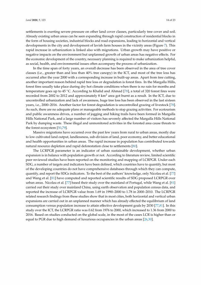
Figure 7. Temporal Landsat satellite images of 1976, 2000, and 2016 in standard False Color

Composite (FCC), illustrating an overall increase in built-up areas over the years in the ICT. The area

of the ICT shown here represents the bounded box inset covering Zone I and Zone II partially in

Figure 1.

The Shenzhen SEZ and ICT cities were both developed in late 1970s. In terms of urban forest

cover change, Shenzhen SEZ had been restored to ~85% (1973–2005) [29] while in this study, we

detected urban forest loss of ~27% (1976–2016) in the ICT. In both cities (SEZ and ICT), urban forest

fragmentation results revealed losses in forest patches. In South Asia, the landscape of the ICT

Figure 7. Temporal Landsat satellite images of 1976, 2000, and 2016 in standard False Color Composite(FCC), illustrating an overall increase in built-up areas over the years in the ICT. The area of the ICTshown here represents the bounded box inset covering Zone I and Zone II partially in Figure 1.

The Shenzhen SEZ and ICT cities were both developed in late 1970s. In terms of urban forestcover change, Shenzhen SEZ had been restored to ~85% (1973–2005) [29] while in this study, wedetected urban forest loss of ~27% (1976–2016) in the ICT. In both cities (SEZ and ICT), urban forestfragmentation results revealed losses in forest patches. In South Asia, the landscape of the ICTresembles strongly with the cities of Kathmandu (the capital of Nepal) and Thimphu (the capital ofBhutan), as they are all cities topographically surrounded by the pine trees. As compared to ICT,Kathmandu and Thimphu cities are older but highly migrant resident populated, vastly encroached,and over grazed. Although many studies have investigated the land cover dynamics of Kathmandu

Land 2020, 9, 123 16 of 23

and Thimphu cities using temporal satellite data [82–85], detailed analysis using parameters such aslandscape metrics, forest fragmentation, and LCRPGR has not been performed. In this aspect, thisstudy serves as a methodological framework for application and analysis over other similar cities indeveloping countries.

Due to rapid tree loss and urbanization, the ICT has observed rapid spells of dust storms andsoil erosion [86]. Soil erosion, dry temperatures, and consequent dust storms have a negative impactin the form of air pollution [87] and land degradation. The soil in ICT and the surrounding areas isshallow and has a clay composition [63]. The alluvial lands and terraces in the area tend to have lowagricultural productivity and in the southern and western parts of the Potohar plateau, the soil is thinand infertile [88]. Streams and ravines cut the loose plain and cause erosion and steep slopes. Thisland is generally unsuitable for cultivation. However, large patches of deep, fertile soil are found in thedepressions and sheltered parts of the plateau and these support small forests and agriculture [89].Butt et al. [45] described the most significant land degradation issues in the Rawal watershed as soilerosion and loss of soil nutrients. They further showed that, between 1992 to 2012, the majority of landthat was previously vegetation, bare soil, or water bodies was converted to agriculture and settlements,suggesting increased pressure on natural resources in the Rawal watershed [45].

The results of landscape analysis in this study reveal that the ICT urban landscape has become moreheterogeneous, disproportional and diverse, and tree patches have declined. Alarmingly, core forests of>500 acres have declined almost 15% in forty years. Although at the individual level, the residents of ICT,civil society, and the local government are trying to recover tree cover loss by planting trees, but theseinitiatives should be continuous and ongoing on a regular basis to monitor the growth of trees withoutdamaging the existing mature standing trees. The temporal forest fragmentation analysis shows thatdue to tree cover loss, the three categories of core forest fragmentations (i.e., <250 acres, 250–500 acres,and >500 acres) have decreased in forty years (1976–2016). The loss in forest fragmentation negativelyinfluences the habitat and terrestrial biodiversity of ICT [79,90,91]. Based on landscape metrics analysisover the Dhaka metropolitan, a similar Asian developing city, Dewan et al. [31] revealed that cultivatedareas and vegetated lands became highly fragmented with increasing anthropogenic disturbances andurban built up category became aggregated and convoluted.

While our analysis of ICT land cover change dynamics in this study is important and unique,there are a few caveats which are worth mentioning. First of all, for the 1976 land cover map, we haverelied on approximately 57 m spatial resolution Landsat 3 Multispectral Scanner System (MSS) sensordata which is relatively coarser spatially as compared to Landsat 5 and 8 (i.e., 30 m), which may affectthe spatial heterogeneity and accuracy of developed land cover maps. Second, as Landsat is a pioneerEarth Observation (EO) satellite program initiated in 1972, so acquiring remote sensing imagery of theyears before that is not possible, and thus we cannot derive land cover maps before the 1960s, whenthe Islamic Republic of Pakistan’s capital shifted from Karachi to Islamabad. Third, from Landsat 30 mmedium spatial resolution satellite data, we cannot detect and delineate the boundaries of built-upareas as well as can be done from sub-meter VHRS images available from the 2000s onward. However,the VHRS datasets come with a high cost, especially when acquisitions at multiples times have to beacquired, and may not be therefore feasible for study sites in developing countries. Of course, researchin this domain is ongoing with regards to utilization of VHRS data for study of urban areas, usingmethods like object-based image analysis, machine learning, etc. Fourth, there may be some level ofuncertainty for the field measurement data, as there is always a potential for human error especiallywhen ground truth is collected over larger areas. Fifth, in this study, we utilized only temporal opticalsatellite data, which may cause optical signal saturation in closed canopy forests, and atmosphericeffects (i.e., cloud coverage, haze, and smog).

6. Conclusions

This study sheds new light on systematic land cover dynamics of ICT over the period of fourdecades, underlining a major decrease in tree cover along with significant increase in settlements and

Land 2020, 9, 123 17 of 23

soil. The findings from the analysis of land cover changes, landscape metrics, forest fragmentation,and LCRPGR, are aligned well and agree overall with previous published work on the regional andglobal scales. The computation of LCRPGR is vital to understand the rate of land change as comparedto the population boom, to understand historical land consumption traditions, and to guide decisionand policy makers on planned urban expansion while ensuring the protection of environmental, social,and economic assets. It is indeed a scientifically accepted phenomenon that in most of the cities, theland consumption rate overall is much faster than the population growth rate, due to high demand ofluxurious occupancies in the urban areas.

Both natural and anthropogenic activities are responsible for land cover changes in ICT. In termsof landscape and fragmentations, the ICT urban landscape ecology is continuously under threatdue to the encroachment of housing societies, and influential business community. The findingsfrom urban landscape matrix and forest fragmentation analysis in this study could help ICT CapitalDevelopment Authority (CDA) and Islamabad Wildlife Management Board (IWMB) in making strategicdecisions to prevent tree loss, forest degradation, and encroachment in the urban landscape of ICT,and also plan future urban growth keeping with the use of remote sensing imagery and geospatialanalysis. The methodology outlined in this study is cost-effective and could be easily replicable to othercountries/regions, especially in developing countries, through integrating freely available satelliteimages with a 5–10 years interval.

Author Contributions: Conceptualization, H.G., W.A.Q.; data analysis, S.A., M.K.; supervision, H.G., visualization,H.G., W.A.Q., S.A., M.K.; writing—original draft preparation, H.G., S.A., W.A.Q., S.M.A.; writing—review andediting, H.G., W.A.Q., S.M.A. All authors have read and approved the final version of this paper. All authors haveread and agreed to the published version of the manuscript.

Funding: This research received no external funding.

Acknowledgments: This work is an extension of an Undergraduate Final Year Project, which was completed in2018, and we would like to express our thanks to Institute of Space Technology (IST) management and academicstaff for their support. The authors also would like to acknowledge the editors and three anonymous reviewersfor their extensive and critical comments on the paper, which helped to improve the paper immensely.

Conflicts of Interest: The authors declare no conflict of interest. The views and interpretations in this publicationare those of the authors, and they are not necessarily attributable to their organizations.

Appendix A

Table A1. Accuracy assessment of land covers classification for 1976, 1990, 2000, 2010, and 2016.

2016’s Land cover accuracy assessment report

Tree cover > 40% canopy Tree cover < 40% canopy Settlement Soil Water Total User’s accuracy (%)Tree cover >40% canopy 22 3 0 0 0 25 88Tree cover <40% canopy 3 21 0 1 0 25 84

Settlement 0 0 23 3 0 26 88Soil 0 1 2 21 0 24 88

Water 0 0 0 0 25 25 100Total 25 25 25 25 25 125

Producer’s accuracy (%) 88 84 92 84 100Overall accuracy: 0.90, Kappa: 0.85

2010’s Land cover accuracy assessment reportTree cover >40% canopy 22 5 0 0 1 28 79Tree cover <40% canopy 3 20 0 0 0 23 87

Settlement 0 0 23 4 0 27 85Soil 0 0 2 21 0 23 91

Water 0 0 0 0 24 24 100Total 25 25 25 25 25

Producer’s accuracy (%) 88 80 92 84 96Overall accuracy: 0.88, Kappa: 0.84

2000’s Land cover accuracy assessment reportTree cover >40% canopy 22 3 0 0 2 27 81Tree cover <40% canopy 3 20 1 1 0 25 80

Settlement 0 0 22 3 0 25 88Soil 0 2 2 21 0 25 84

Water 0 0 0 0 23 23 100Total 25 25 25 25 25 125

Producer’s accuracy (%) 88 80 88 84 92Overall accuracy: 0.86, Kappa: 0.82

Land 2020, 9, 123 18 of 23

Table A1. Cont.

1990’s Land cover accuracy assessment reportTree cover >40% canopy 21 2 0 0 1 24 88Tree cover <40% canopy 4 20 1 1 0 26 77

Settlement 0 0 21 4 0 25 84Soil 0 3 3 20 0 26 77

Water 0 0 0 0 24 24 100Total 25 25 25 25 25 125

Producer’s accuracy (%) 84 80 84 80 96Overall accuracy: 0.85, Kappa: 0.81

1976’s Land cover accuracy assessment reportTree cover >40% canopy 21 3 0 0 1 25 84Tree cover <40% canopy 4 21 1 2 0 28 75

Settlement 0 0 20 5 0 25 80Soil 0 1 4 18 0 23 78

Water 0 0 0 0 24 24 100Total 25 25 25 25 25 125

Producer’s accuracy (%) 84 84 80 72 96Overall accuracy: 0.83, Kappa: 0.79

Table A2. Land cover class level landscape matrix parameters results for 1976, 1990, 2000, 2010,and 2016.

Land Cover Class YearPatch Density and Size Shape and Edge Proximity/Isolation

NP LPI (%) MPS (km2) MRG (m) ED (m/km2) MSI MPAR ×103 MPI MED (m)

Tree cover >40% canopy

1976 1072 12.50 16.98 71.58 21.08 1.27 0.55 869.65 228.471990 5590 9.95 3.44 34.13 44.78 1.24 1.05 1233.12 109.632000 8195 10.31 2.18 26.89 54.25 1.19 1.14 1247.77 98.592010 6121 8.59 2.30 27.34 41.94 1.20 1.15 1401.38 104.152016 2223 7.10 5.95 40.30 23.54 1.28 1.03 1407.03 99.17

Tree cover <40% canopy

1976 1872 30.62 22.29 75.52 66.35 1.32 0.53 4809.76 145.761990 8856 5.89 3.87 40.00 125.30 1.35 1.02 1837.19 77.202000 10145 16.92 3.94 31.18 146.14 1.26 1.11 7773.81 73.002010 9253 29.83 3.89 31.39 122.42 1.23 1.06 18114.32 79.522016 8728 14.97 3.51 36.00 107.08 1.28 1.02 5386.70 83.08

Settlement

1976 4296 0.02 0.70 35.83 17.73 1.09 0.64 1.06 193.661990 7752 0.22 0.57 22.92 26.69 1.13 1.16 12.70 116.022000 6310 0.30 0.95 28.28 30.58 1.19 1.09 33.80 115.142010 11694 5.16 1.23 27.39 68.28 1.20 1.11 784.86 86.702016 12754 8.07 1.34 25.56 71.35 1.18 1.14 1382.81 87.29

Soil

1976 2180 13.76 12.40 65.86 50.43 1.29 0.54 1763.86 159.371990 9271 15.94 3.42 32.34 102.90 1.25 1.06 6172.97 81.382000 12060 3.15 2.13 33.12 103.57 1.27 1.05 564.47 80.482010 8885 4.02 2.86 33.49 84.81 1.26 1.05 530.05 85.992016 12436 5.72 2.33 30.23 107.68 1.26 1.1 1197.42 76.53

Water

1976 8 0.60 68.27 154.90 0.25 1.15 0.54 162.66 2192.651990 242 0.62 3.49 55.79 1.90 1.39 1.02 29.98 362.052000 449 0.61 2.35 43.54 2.93 1.25 1.07 26.36 322.782010 34 0.59 18.51 69.64 0.47 1.21 0.97 65.20 1230.492016 120 0.58 5.43 36.36 0.71 1.18 1.09 46.78 620.00

Table A3. Forest fragmentation results for 1976, 1990, 2000, 2010, and 2016 and percentage assessmentbased on satellite images).

Forest Fragmentation Classes 1976 1990 2000 2010 2016

km2

Patch 14.74 (2.46) 15.67 (2.93) 15.46 (2.68) 17.84 (3.56) 19.92 (4.54)Edge 105.58 (17.62) 119.48 (22.33) 123.42 (21.36) 94.06 (18.75) 96.83 (22.07)

Perforated 35.21 (5.88) 31.52 (5.89) 41.79 (7.23) 24.39 (4.86) 22.74 (5.18)Core (<250 acres) 41.4 (6.91) 79.94 (14.94) 68.04 (11.77) 52.05 (10.38) 52.24 (11.91)

Core (250–500 acres) 10.99 (1.83) 17.18 (3.21) 15.74 (2.72) 5.54 (1.10) 5.63 (1.28)Core (>500 acres) 391.98 (65.41) 271.34 (50.71) 313.42 (54.24) 307.67 (61.34) 241.44 (55.02)

Total 585.16 (100) 535.13 (100) 577.87 (100) 501.55 (100) 438.80 (100)

Land 2020, 9, 123 19 of 23

References

1. Lambin, E.F.; Meyfroidt, P. Land use transitions: Socio-ecological feedback versus socio-economic change.Land Use Policy 2010, 27, 108–118. [CrossRef]

2. Balooni, K.; Lund, J.F. Forest rights: The hard currency of REDD+. Conserv. Lett. 2014, 7, 278–284. [CrossRef]3. Belal, A.A.; Moghanm, F.S. Detecting urban growth using remote sensing and GIS techniques in Al Gharbiya

governorate, Egypt. Egypt. J. Remote Sens. Sp. Sci. 2011, 14, 73–79. [CrossRef]4. Congalton, R.; Gu, J.; Yadav, K.; Thenkabail, P.; Ozdogan, M. Global Land Cover Mapping: A Review and

Uncertainty Analysis. Remote Sens. 2014, 6, 12070–12093. [CrossRef]5. Rasul, G. Ecosystem services and agricultural land-use practices: A case study of the Chittagong Hill Tracts

of Bangladesh. Sustain. Sci. Pract. Policy 2009, 5, 15–27. [CrossRef]6. Addae, B.; Oppelt, N. Land-Use/Land-Cover Change Analysis and Urban Growth Modelling in the Greater

Accra Metropolitan Area (GAMA), Ghana. Urban Sci. 2019, 3, 26. [CrossRef]7. Redman, C.L. Human Dimensions of Ecosystem Studies. Ecosystems 1999, 2, 296–298. [CrossRef]8. Xu, C.; Liu, M.; Zhang, C.; An, S.; Yu, W.; Chen, J.M. The spatiotemporal dynamics of rapid urban growth in

the Nanjing metropolitan region of China. Landsc. Ecol. 2007, 22, 925–937. [CrossRef]9. Burgi, M.; Hersperger, A.M.; Schneeberger, N. Driving forces of landscape change - current and new

directions. Landsc. Ecol. 2005, 19, 857–868. [CrossRef]10. Bilsborrow, R.E.; McDevitt, T.M.; Kossoudji, S.; Fuller, R. The Impact of Origin Community Characteristics

on Rural-Urban Out-Migration in a Developing Country. Demography 1987, 24, 191–210. [CrossRef]11. Magidi, J.; Ahmed, F. Assessing urban sprawl using remote sensing and landscape metrics: A case study of

City of Tshwane, South Africa (1984–2015). Egypt. J. Remote Sens. Sp. Sci. 2019, 22, 335–346. [CrossRef]12. Melchiorri, M.; Pesaresi, M.; Florczyk, A.J.; Corbane, C.; Kemper, T. Principles and applications of the global

human settlement layer as baseline for the land use efficiency indicator—SDG 11.3.1. ISPRS Int. J. Geo-Inf.2019, 8, 96. [CrossRef]

13. Sharma, L.; Pandey, P.C.; Nathawat, M.S. Assessment of land consumption rate with urban dynamics changeusing geospatial techniques. J. Land Use Sci. 2012, 7, 135–148. [CrossRef]

14. Salvati, L.; Carlucci, M. Distance matters: Land consumption and the mono-centric model in two southernEuropean cities. Landsc. Urban Plan. 2014, 127, 41–51. [CrossRef]

15. Sibly, R.M.; Hone, J. Population growth rate and its determinants: An overview. Philos. Trans. R. Soc. B Biol.Sci. 2002, 357, 1153–1170. [CrossRef]

16. Philippe, D.; Jean-Marie, O.-B.; Marta, G.-D.; Thomas, C. Global immunization: Status, progress, challengesand future. BMC Int. Health Hum. Rights 2009, 9, S2. [CrossRef]

17. Ghazanfari, H.; Namiranian, M.; Sobhani, H.; Mohajer, R.M. Traditional forest management and its applicationto encourage public participation for sustainable forest management in the northern Zagros mountains ofKurdistan Province, Iran. Scand. J. For. Res. Suppl. 2004, 19, 65–71. [CrossRef]

18. Turner, A.B.L.; Meyer, W.B.; Skole, D.L. Global land-use/land-cover change: Towards an integrated study.Ambio 1994, 23, 91–95.

19. Seto, K.C.; Guneralp, B.; Hutyra, L.R. Global forecasts of urban expansion to 2030 and direct impacts onbiodiversity and carbon pools. Proc. Natl. Acad. Sci. 2012, 109, 16083–16088. [CrossRef] [PubMed]

20. Grimm, N.B.; Faeth, S.H.; Golubiewski, N.E.; Redman, C.L.; Wu, J.; Bai, X.; Briggs, J.M. Global Change andthe Ecology of Cities. Science. 2008, 319, 756–760. [CrossRef] [PubMed]

21. Angel, S.; Parent, J.; Civco, D.L.; Blei, A.; Potere, D. The dimensions of global urban expansion: Estimatesand projections for all countries, 2000–2050. Prog. Plann. 2011, 75, 53–107. [CrossRef]

22. Boggs, G.S. Assessment of SPOT 5 and QuickBird remotely sensed imagery for mapping tree cover insavannas. Int. J. Appl. Earth Obs. Geoinf. 2010, 12, 217–224. [CrossRef]

23. Wulder, M.A.; Coops, N.C.; Roy, D.P.; White, J.C.; Hermosilla, T. Land cover 2.0. Int. J. Remote Sens. 2018, 39,4254–4284. [CrossRef]

24. Dong, J.; Xiao, X.; Menarguez, M.A.; Zhang, G.; Qin, Y.; Thau, D.; Biradar, C.; Moore, B. Mapping paddy riceplanting area in northeastern Asia with Landsat 8 images, phenology-based algorithm and Google EarthEngine. Remote Sens. Environ. 2016, 185, 142–154. [CrossRef]

Land 2020, 9, 123 20 of 23

25. Uddin, K.; Shrestha, H.L.H.L.; Murthy, M.S.R.S.R.; Bajracharya, B.; Shrestha, B.; Gilani, H.; Pradhan, S.;Dangol, B. Development of 2010 national land cover database for the Nepal. J. Environ. Manage. 2015, 148,82–90. [CrossRef]

26. Seto, K.C.; Fragkias, M.; Güneralp, B.; Reilly, M.K. A Meta-Analysis of Global Urban Land Expansion.PLoS ONE 2011, 6, e23777. [CrossRef]

27. Yang, C.; Li, Q.; Hu, Z.; Chen, J.; Shi, T.; Ding, K.; Wu, G. Spatiotemporal evolution of urban agglomerationsin four major bay areas of US, China and Japan from 1987 to 2017: Evidence from remote sensing images.Sci. Total Environ. 2019, 671, 232–247. [CrossRef]

28. Herold, M.; Couclelis, H.; Clarke, K.C. The role of spatial metrics in the analysis and modeling of urban landuse change. Comput. Environ. Urban Syst. 2005, 29, 369–399. [CrossRef]

29. Gong, C.; Yu, S.; Joesting, H.; Chen, J. Determining socioeconomic drivers of urban forest fragmentation withhistorical remote sensing images. Landsc. Urban Plan. 2013, 117, 57–65. [CrossRef]

30. Huang, J.; Lu, X.X.; Sellers, J.M. A global comparative analysis of urban form: Applying spatial metrics andremote sensing. Landsc. Urban Plan. 2007, 82, 184–197. [CrossRef]

31. Dewan, A.M.; Yamaguchi, Y.; Ziaur Rahman, M. Dynamics of land use/cover changes and the analysis oflandscape fragmentation in Dhaka Metropolitan, Bangladesh. GeoJournal 2012, 77, 315–330. [CrossRef]

32. Mandelas, E. A fuzzy cellular automata based shell for modeling urban growth–a pilot application inMesogia area. In Proceedings of the 10th AGILE International Conference on Geographic InformationScience, Allborg, Denmark, 8–11 May 2007; pp. 1–9.

33. Farhat, K.; Waseem, L.A.; Khan, A.A.; Baig, S. Spatiotemporal Demographic Trends and Land Use Dynamicsof Metropolitan Lahore. J. Hist. Cult. Art Res. 2018, 7, 92. [CrossRef]

34. Shah, M.H.; Shaheen, N. Seasonal behaviours in elemental composition of atmospheric aerosols collected inIslamabad, Pakistan. Atmos. Res. 2010, 95, 210–223. [CrossRef]

35. Butt, M.J.; Waqas, A.; Iqbal, M.F.; Muhammad, G.; Lodhi, M.A.K. Assessment of Urban Sprawl of IslamabadMetropolitan Area Using Multi-Sensor and Multi-Temporal Satellite Data. Arab. J. Sci. Eng. 2012, 37, 101–114.[CrossRef]

36. Shahzad, N.; Saeed, U.; Gilani, H.; Ahmad, S.R.; Ashraf, I.; Irteza, S.M. Evaluation of state andcommunity/private forests in Punjab, Pakistan using geospatial data and related techniques. For. Ecosyst.2015, 2, 7. [CrossRef]

37. Doxiadis, C.A. Islamabad, the creation of a new capital. Town Plan. Rev. 1965, 36, 1. [CrossRef]38. Stephenson, G.V. Two Newly Created Capitals: Islamabad and Brasilia. Town Plan. Rev. 1970, 41, 317.

[CrossRef]39. Kreutzmann, H. Islamabad, living the plan. Südasien-Chronik-South Asia Chron. 2013, 3, 2013.40. Beacco, D. Urban Planning in Islamabad: From the Modern Movement to the Contemporary Urban

Development Between Formal and Informal Settlements. In Sustainable Urban Development and Globalization;Springer: Cham, Switzerland, 2018; pp. 65–74.

41. Bokhari, S.A.; Saqib, Z.; Ali, A.; Haq, M.Z. Perception of Residents about Urban Vegetation: A ComparativeStudy of Planned Versus Semi-Planned Cities of Islamabad and Rawalpindi, Pakistan. J. Ecosyst. Ecography2018, 8, 1–8. [CrossRef]

42. Naeem, S.; Cao, C.; Waqar, M.M.; Wei, C.; Acharya, B.K. Vegetation role in controlling the ecoenvironmentalconditions for sustainable urban environments: A comparison of Beijing and Islamabad. J. Appl. Remote Sens.2018, 12, 016013. [CrossRef]

43. Adeel, M. Methodology for identifying urban growth potential using land use and population data: A casestudy of Islamabad Zone IV. Procedia Environ. Sci. 2010, 2, 32–41. [CrossRef]

44. Butt, A.; Shabbir, R.; Ahmad, S.S.; Aziz, N. Land use change mapping and analysis using Remote Sensingand GIS: A case study of Simly watershed, Islamabad, Pakistan. Egypt. J. Remote Sens. Sp. Sci. 2015, 18,251–259. [CrossRef]

45. Butt, A.; Shabbir, R.; Ahmad, S.S.; Aziz, N.; Nawaz, M.; Shah, M.T.A. Land cover classification and changedetection analysis of Rawal watershed using remote sensing data. J Biodivers Env. Sci 2015, 6, 236–248.

46. Hassan, Z.; Shabbir, R.; Ahmad, S.S.; Malik, A.H.; Aziz, N.; Butt, A.; Erum, S. Dynamics of land use and landcover change (LULCC) using geospatial techniques: A case study of Islamabad Pakistan. Springerplus 2016,5, 812. [CrossRef] [PubMed]

Land 2020, 9, 123 21 of 23

47. Sohail, M.T.; Mahfooz, Y.; Azam, K.; Yat, Y.; Genfu, L.; Fahad, S. Impacts of urbanization and land coverdynamics on underground water in Islamabad, Pakistan. Desalin. WATER Treat. 2019, 159, 402–411.[CrossRef]

48. Naeem, S.; Cao, C.; Qazi, W.; Zamani, M.; Wei, C.; Acharya, B.; Rehman, A. Studying the association betweengreen space characteristics and land surface temperature for sustainable urban environments: An analysis ofBeijing and Islamabad. ISPRS Int. J. Geo-Inf. 2018, 7, 38. [CrossRef]

49. Khalid, N.; Ullah, S.; Ahmad, S.S.; Ali, A.; Chishtie, F. A remotely sensed tracking of forest cover andassociated temperature change in Margalla hills. Int. J. Digit. Earth 2019, 12, 1133–1150. [CrossRef]

50. Batool, R.; Javaid, K. Spatio-temporal assessment of Margalla hills forest by using Landsat imagery foryear 2000 and 2018. In Proceedings of the International Archives of the Photogrammetry, Remote Sensingand Spatial Information Sciences, ISPRS TC III Mid-term Symposium “Developments, Technologies andApplications in Remote Sensing”, Beijing, China, 7–10 May 2018; Volume XLII–3, pp. 69–72.

51. Mannan, A.; Liu, J.; Zhongke, F.; Khan, T.U.; Mukete, B.; Chaoyong, S.; Saeed, S.; Yongxiang, F.; Ahmad, A.;Amir, M.; et al. Application of land-use/land cover changes in monitoring and projecting forest biomasscarbon loss in Pakistan. Glob. Ecol. Conserv. 2019, 17, e00535. [CrossRef]

52. Dewan, A.M.; Yamaguchi, Y. Land use and land cover change in Greater Dhaka, Bangladesh: Using remotesensing to promote sustainable urbanization. Appl. Geogr. 2009, 29, 390–401. [CrossRef]

53. Dewan, A.M.; Yamaguchi, Y. Using remote sensing and GIS to detect and monitor land use and land coverchange in Dhaka Metropolitan of Bangladesh during 1960–2005. Environ. Monit. Assess. 2009, 150, 237–249.[CrossRef]

54. Pramanik, M.M.A.; Stathakis, D. Forecasting urban sprawl in Dhaka city of Bangladesh. Environ. Plan. BPlan. Des. 2016, 43, 756–771. [CrossRef]

55. Gruebner, O.; Sachs, J.; Nockert, A.; Frings, M.; Khan, M.M.H.; Lakes, T.; Hostert, P. Mapping the Slums ofDhaka from 2006 to 2010. Dataset Pap. Sci. 2014, 2014, 1–7. [CrossRef]

56. Sharma, R.; Joshi, P.K. Monitoring Urban Landscape Dynamics Over Delhi (India) Using Remote Sensing(1998–2011) Inputs. J. Indian Soc. Remote Sens. 2013, 41, 641–650. [CrossRef]

57. Naeem, S.; Cao, C.; Fatima, K.; Najmuddin, O.; Acharya, B.K. Landscape greening policies-based landuse/land cover simulation for Beijing and Islamabad—An implication of sustainable urban ecosystems.Sustainability 2018, 10, 1049. [CrossRef]

58. Huang, H.; Chen, Y.; Clinton, N.; Wang, J.; Wang, X.; Liu, C.; Gong, P.; Yang, J.; Bai, Y.; Zheng, Y.; et al.Mapping major land cover dynamics in Beijing using all Landsat images in Google Earth Engine. RemoteSens. Environ. 2017, 202, 166–176. [CrossRef]

59. Cui, L.; Shi, J. Urbanization and its environmental effects in Shanghai, China. Urban Clim. 2012, 2, 1–15.[CrossRef]

60. Zhao, S.; Da, L.; Tang, Z.; Fang, H.; Song, K.; Fang, J. Ecological consequences of rapid urban expansion:Shanghai, China. Front. Ecol. Environ. 2006, 4, 341–346.

61. Yue, W.; Fan, P.; Wei, Y.D.; Qi, J. Economic development, urban expansion, and sustainable development inShanghai. Stoch. Environ. Res. Risk Assess. 2014, 28, 783–799. [CrossRef]

62. Bagan, H.; Yamagata, Y. Landsat analysis of urban growth: How Tokyo became the world’s largest megacityduring the last 40 years. Remote Sens. Environ. 2012, 127, 210–222. [CrossRef]

63. Sheikh, I.M.; Pasha, M.K.; Williams, V.S.; Raza, S.Q.; Khan, K.S.A.A. Environmental Geology of theIslamabad-Rawalpindi Area. In Regional Studies of the Potwar Plateau Area, Northern Pakistan; 2007; pp. 1–32.Available online: https://pubs.usgs.gov/bul/2078/ (accessed on 5 February 2020).

64. Teillet, P.; Barker, J.; Markham, B.; Irish, R.; Fedosejevs, G.; Storey, J. Radiometric cross-calibration of theLandsat-7 ETM+ and Landsat-5 TM sensors based on tandem data sets. Remote Sens. Environ. 2001, 78,39–54. [CrossRef]

65. Tan, B.; Masek, J.G.; Wolfe, R.; Gao, F.; Huang, C.; Vermote, E.F.; Sexton, J.O.; Ederer, G. Improved forestchange detection with terrain illumination corrected Landsat images. Remote Sens. Environ. 2013, 136,469–483. [CrossRef]

66. Congalton, R.G. Remote Sensing and Image Interpretation. 7th Edition. Photogramm. Eng. Remote Sens. 2015,81, 615–616. [CrossRef]

Land 2020, 9, 123 22 of 23

67. Kasereka, K. Remote Sensing and Geographic Information System for Inferring Land Cover and Land UseChange in Wuhan (China), 1987-2006. J. Sustain. Dev. 2010, 3, 221–229. [CrossRef]

68. Khatami, R.; Mountrakis, G.; Stehman, S.V. A meta-analysis of remote sensing research on supervisedpixel-based land-cover image classification processes: General guidelines for practitioners and futureresearch. Remote Sens. Environ. 2016, 177, 89–100. [CrossRef]

69. Saura, S. Effects of minimum mapping unit on land cover data spatial configuration and composition. Int. J.Remote Sens. 2002, 23, 4853–4880. [CrossRef]

70. Roy, P.S.; Roy, A.; Joshi, P.K.; Kale, M.P.; Srivastava, V.K.; Srivastava, S.K.; Dwevidi, R.S.; Joshi, C.; Behera, M.D.;Meiyappan, P.; et al. Development of decadal (1985-1995-2005) land use and land cover database for India.Remote Sens. 2015, 7, 2401–2430. [CrossRef]

71. Rosenfield, G.H.; Fitzpatrick-Lins, K. A coefficient of agreement as a measure of thematic classificationaccuracy. Photogramm. Eng. Remote Sens. 1986, 52, 223–227.

72. Puyravaud, J.P. Standardizing the calculation of the annual rate of deforestation. For. Ecol. Manage. 2003,177, 593–596. [CrossRef]

73. McGarigal, K. Landscape Pattern Metrics. In Wiley StatsRef: Statistics Reference Online; John Wiley & Sons,Ltd.: Chichester, UK, 2014; Volume 45, pp. 1–18.

74. Nichol, J.E.; Abbas, S.; Fischer, G.A. Spatial patterns of degraded tropical forest and biodiversity restorationover 70-years of succession. Glob. Ecol. Conserv. 2017, 11, 134–145. [CrossRef]

75. McGarigal, K.; Marks, B.J. FRAGSTATS: Spatial pattern analysis program for quantifying landscapes structure.Gen. Tech. Rep. PNW-GTR-351. U.S. Dep. Agric. For. Serv. Pacific Northwest Res. Station. Portland, OR 1994,97331, 134.

76. Vogt, P.; Riitters, K.; Estreguil, C.; Kozak, J.; Wade, T.; Wickham, J. Mapping spatial patterns with morphologicalimage processing. Landsc. Ecol. 2007, 22, 171–177. [CrossRef]

77. Nicolau, R.; Caetano, M.; David, J.; Caetano, M.; Pereira, J. Ratio of Land Consumption Rate to PopulationGrowth Rate—Analysis of Different Formulations Applied to Mainland Portugal. ISPRS Int. J. Geo-Inf. 2018,8, 10. [CrossRef]

78. Khalid, N.; Saeed Ahmad, S. Monitoring Forest cover change of Margalla Hills over a period of two decades(1992-2011): A spatiotemporal perspective. J. Ecosyst. Ecography 2016, 06, 1–8. [CrossRef]

79. Malik, I.U.; Faiz, A.H.; -i- Abbas, F. Biodiversity Assessment and its Effect on the Environment of ShakarparianForest. J. Bioresour. Manag. 2014, 1, 4. [CrossRef]

80. Ahmed, K.; Jatoo, W.; Jing, F.C.; Saengkrod, W.; Mastoi, A.G. Urbanization in Pakistan: Challenges and WayForward (Options) For Sustainable Urban Development. In Proceedings of the 4th International Conferenceon Energy, Environment and Sustainable Development, Jamshoro, Pakistan, 1–3 November 2016.

81. Wang, Y.; Huang, C.; Feng, Y.; Zhao, M.; Gu, J. Using Earth Observation for Monitoring SDG 11.3.1- Ratioof Land Consumption Rate to Population Growth Rate in Mainland China. Remote Sens. 2020, 12, 357.[CrossRef]

82. Rimal, B. Application of remote sensing and GIS, land use/land cover change in Kathmandu MetropolitanCity, Nepal. J. Theor. Appl. Inf. Technol. 2011, 23, 80–86.

83. Thapa, B.R.; Ishidaira, H.; Pandey, V.P.; Shakya, N.M. A multi-model approach for analyzing water balancedynamics in Kathmandu Valley, Nepal. J. Hydrol. Reg. Stud. 2017, 9, 149–162. [CrossRef]

84. Giri, N.; Singh, O.P. Urban growth and water quality in Thimphu, Bhutan. J. Urban Environ. Eng. 2013, 7,82–95. [CrossRef]

85. Khanal, N.; Uddin, K.; Matin, M.; Tenneson, K. Automatic Detection of Spatiotemporal Urban ExpansionPatterns by Fusing OSM and Landsat Data in Kathmandu. Remote Sens. 2019, 11, 2296. [CrossRef]

86. Ellis, S.; Taylor, D.; Masood, K.R. Land degradation in northern Pakistan. Geography 1993, 78, 84–87.87. Cavanaugh, R. Increased pollution and problems in respiratory health menace Pakistan’s soaring population.

Lancet Respir. Med. 2018, 6, 175–176. [CrossRef]88. Rashid, K.; Rasul, G. Rainfall variability and maize production over the Potohar plateau of Pakistan. Pakistan

J. Meteorol. 2011, 8, 63–74.89. Pandey, V.P.; Manandhar, S.; Kazama, F. Climate change vulnerability assessment. In Climate Change and

Water Resources; CRC Press: Boca Raton, FL, USA, 2014; pp. 183–208. ISBN 9781466594678.

Land 2020, 9, 123 23 of 23

90. Akram, A.; Rais, M.; Asadi, M.A.; Jilani, M.J.; Balouch, S.; Anwar, M.; Saleem, A. Do habitat variablescorrelate anuran abundance in arid terrain of Rawalpindi–Islamabad Areas, Pakistan? J. King Saud Univ. Sci.2015, 27, 278–283. [CrossRef]

91. Shabbir, A.; Bajwa, R. Distribution of parthenium weed (Parthenium hysterophorus L.), an alien invasiveweed species threatening the biodiversity of Islamabad. Weed Biol. Manag. 2006, 6, 89–95. [CrossRef]

© 2020 by the authors. Licensee MDPI, Basel, Switzerland. This article is an open accessarticle distributed under the terms and conditions of the Creative Commons Attribution(CC BY) license (http://creativecommons.org/licenses/by/4.0/).