Temporal Extensions of Landscape Ecology Theory and Practice: Examples from the Peruvian Amazon

Temporal Extensions of Landscape Ecology Theory andPractice: Examples from the Peruvian Amazon*

Kelley A. Crews-MeyerUniversity of Texas

The growing overlap between geographic information science (GIScience) and landscape ecology for landscapecharacterization has led to increasingly sophisticated measures of landscape site and situation. Scale, bothtemporal and spatial, has been injected into methodologies to improve our ability to derive process from patternwith the hope of defining, monitoring, and modeling ecological landscape function. This article addresses anevolving methodology of longitudinal or panel analysis designed to test the relative importance of thematicversus structural landscape configuration as well as interannual versus intra-annual change. Landscapetypologies for both temporal signature and dominant structural trajectories are offered as guideposts for re-thinking dynamic landscape characterization. A case study from the Peruvian Amazon is provided to illustrateinterpretive advances available via panel methods that allow for disentangling inter- and intra-annual shifts aswell as separating changes in composition versus configuration for improved understanding of landscape dy-namics and dynamism. Key Words: change detection, landuse/landcover change (LULCC), pattern metrics,temporal analysis.

It might be said that landscapes are the unit offascination for all geographers and many

ecologists (Allen 1998). A more accurate andtelling description might be that landscapechange is what holds their rapt attention.Whether it is change among landscapes orchange in a given landscape over time, we seemcompelled by the dynamic, not the static. Asevidence, note the (re)surgence of ‘‘process’’models that, by definition, examine the natureof change rather than the nature of stability. Al-though we might bicker as to the temporal res-olution of these statements (what a geographerstudying geomorphology considers long termobviously varies by many orders of magnitudeover what a geographer studying urbanizationconsiders long term), we appear to have at leasttemporarily settled on a second premise to ge-ography beyond the importance of the spatialperspective: change, rather than stability, isoften what motivates our analyses.

Geographers, and in particular geographicinformation science (GIScience) practicioners,are adept at identifying some types of landscapechange, and are moving toward greater fluencyin explaining and predicting those changes withboth empirically fitted and dynamic process

models, respectively (Brown et al. 2004). Thefocus in most of these studies is landscapedynamics: the detection, attribution, andprediction of the mechanics of change. ThisGIScience-like approach is mechanistic andconnotes assessing patterns of change, growth,and activity. What we have not yet adequatelyexplored is a landscape ecology–like versionI shall call landscape dynamism: a more gestalticconnotation of continuous change, activity, orprogress. Our epistemology derives fromthese definitions and implementations of proc-ess. Bringing these views together is criticalfor the commensurability of landscape studiesacross scales (temporal and spatial, grainand extent), across processes (abiotic, biotic,human, and disturbance—after Turner, Gard-ner, and O’Neill 2001), across ecosystems, andperhaps most important across disciplinaryboundaries.

The theory and practice of scale-pattern-process1 entails that the scale of observation inpart determines our ability to identify the pat-terns used to infer process. The longer rangehope is that we can thereby understand andpredict function. This perspective has requiredthe inference of the dynamic from the static, and

*The author is indebted to the University of Texas Population Research Center, Karl Butzer, the Leon family, and Kenneth R. Young for both theirwilling and unwitting contributions to this research.

The Professional Geographer, 58(4) 2006, pages 421–435 r Copyright 2006 by Association of American Geographers.Initial submission, March 2005; revised submission, January 2006; final acceptance, April 2006.

Published by Blackwell Publishing, 350 Main Street, Malden, MA 02148, and 9600 Garsington Road, Oxford OX4 2DQ, U.K.

underscores the need for a landscape scale ofanalysis as much as a landscape level of analysis(Allen 1998). The paradigmatic overlap be-tween GIScience and landscape ecology lies inquantifying meaningful landscape change, re-quiring clearance of the hurdles of scale de-pendency of observation and ecological fallacy,to name only two. Here I discuss one path forinfusing landscape ecology principles intoGIScience practice for better assessment of thetemporal component of landscape change: mov-ing to dynamism from dynamics.

Phase I: From-To Change Detection

The simplest version of communicating change,and one that nongeographic disciplines still use,summarizes aspatial inventories from two timeperiods. These ‘‘statistics’’ are often used innews reporting, as in: The Antarctic ice sheethas decreased by 10 percent in the last thirtyyears, or Amazonian forested lands have de-creased by 40 percent over the last ten years.These soundbites of change detection, whileeasy to communicate quickly, do little to in-crease understanding of why and how thesephenomena have occurred or why and how theyhave occurred in some places and not others.This approach lacks two critical pieces of infor-mation: where did those changes occur (and bycorollary, where did they not occur) and whatlanduse or landcover replaced the ice sheet orthe forests.

Geographers tackle the issue of communi-cating change by moving into a spatialcontext to look at whole areas and describe thenature of thematic change or stability usingsatellite imagery, aerial photography, or mapsderived from surveying or remotely sensed data.In the 1960s Ian McHarg, whom many regard asthe grandfather of GIS (geographic informationsystems), proposed a technique now referred toin GIS as overlay analysis (McHarg 1969;Chrisman 1997), in which he printed on ace-tate rather than on paper several maps of dif-ferent types of information from the same timeperiod. He then stacked (overlaid) and aligned(registered) these acetate layers of informationand thereby easily demonstrated the spatialco-occurrence of phenomena. This innovationallowed the creation of new (and spatial) infor-mation, the hallmark of a GIS (Burrough andMcDonnell 1998).

Consider examining a map of Amazonianforests, noting where the most dense forestsremain. Now imagine a map of transportationinfrastructure, showing the roads and riverwaysof the area. By overlaying the two maps the cor-relation between, for example, roads and de-graded forests becomes clear, and we are able tohypothesize a causal connection between trans-portation infrastructure and the presence, ab-sence, and quality of forested lands. The newinformation gleaned from this analysis is notjust the locations of forests or the locations ofroads but the locations (or co-occurrence) offorests within a certain distance of roads, forestswithin a certain distance from waterways, orforests remote from all infrastructure. And themore data layers we add, the more new infor-mation we are able to extract. That this abilitynow seems commonplace is a tribute to geog-raphy as a discipline that has assimilated theideas of spatial co-occurrence so quickly and sothoroughly that to not use this approach seemsodd. But forty years ago it was not odd; it was thestandard—and in many disciplines it still isthe standard (Robinson et al. 1984; Duckham,Goodchild, and Worboys 2003).

The extension of overlay analysis to air pho-tos and satellite images is important for hy-pothesis testing, but even more critical forunderstanding change. Overlay analysis can beperformed with multiple layers from one date ordates. The 1970s witnessed the advent of satel-lite sensor systems whose data were available toresearchers; at the same time, research and de-velopment in computer processing power anddata storage offered a platform for working withlarge digital datasets ( Jensen 2005). Remotesensing analysts were able to implement whatthey termed from-to change detection, a wall-to-wall mapping approach that provided thespatially and thematically explicit informationneeded to better assess landscape change.Change maps were created illustrating precise-ly where landscape classes of interest were andhow they changed. Returning to the forest ex-ample, we could now measure not only whatpercentage of forests had been lost over, say, aten-year period but also to what those forestedlands were lost: urbanization, agricultural ext-ensification, ranching, logging, and so forth.Moreover we also could know where each ofthose from-to change categories existed. Wemight observe that logging activities tended to

422 Volume 58, Number 4, November 2006

be located closer to rivers, agricultural ext-ensification tended to be located closer to roads,and the most dense or unfragmented forestswere more remote and at higher elevations.With this array of information available, it be-came feasible to promote better-specified hy-potheses of landscape change over areas largerthan field sampling alone could accommodate.

From-to change detection was first imple-mented with only two dates of imagery (e.g.,1975 and 1985). But images are only snapshotsof the landscape, and the longer the interveningtime between dates the more difficult it is toattribute landscape change (or lack thereof ) to aparticular process or set of processes. As moresatellite sensor systems provided information,deeper time-series could be archived and analy-zed. Remote sensing analysts very soon beganusing multiple images in their time-series anal-yses, sometimes extending the range of tempo-ral coverage and sometimes increasing thefrequency of observation. In the preceding ex-ample, an intervening image from 1980 mightbe added to the time-series, with analyses ofthose three dates of imagery typically done inpairwise combination: 1975 and 1980, 1980 and1985, and 1975 and 1985. As the time-series ofimagery expands to include more dates, thenumber of possible pairwise combinations goesup considerably, and so too does the complexityof interpreting and reporting those results.

Meanwhile, remote sensing analysts were alsoincreasingly able to explore different temporaltypes of thematic change. The examples thus farhave focused on interannual change detection,and an implicit assumption of some early workwas that interannual change was likely longerterm, if not permanent. Therefore, one of themost stringent rules of change detection workwas the challenge to find anniversary-date im-agery: images collected years apart but collectedon as close to the same day of the year as pos-sible. By doing so one could better control forthe shorter-term or cyclic changes associatedwith seasonal, phenological, or crop calendar

differences artificially called ‘‘landscapechange.’’ Soon after, researchers realized thatthe error or noise in nonanniversary-date pairswas valuable for understanding intra-annualchanges such as monsoonal flooding, deciduousphenological cycles, or planting/harvesting cy-cles (Walsh et al. 2001). Since the 1980s, re-searchers have been comparing interannual andintra-annual change to determine the relativeimpacts of each, contextualizing the thematicnature of change as shown in Table 1.

Of the four types of combinatorial change il-lustrated in Table 1, the ‘‘stable landscapes’’ areoften the least analyzed by the geographic re-mote sensing community. There is a normativebias toward understanding the nature of land-scape change; therefore unchanging (or slightlychanging) landscapes are often of less interest.Nonchange is considered to be a nonresult (ex-cept when strong change is hypothesized butnot found). In terms of change detection, then,stable landscapes, which do not experience sea-sonal, cyclic, or longer-term change (given thetemporal grain and extent associated with re-motely sensed data), are often overlooked. Sea-sonal change (or rather, landscapes dominatedby intra-annual change and with very littlelonger-term change) has been less of a researchfocus than longer-term change, though therehas been a shift to some extent in the past decadeor so to studies centered on agriculture andflooding, or strong snow/ice seasonality as inAlaska (Eva and Lambin 1998; Smith 1998;Oechel et al. 2000; Walsh et al. 2001). Longer-term change can be observed in areas that arechanging over time but have little seasonal fluc-tuation: many urban areas without strong cli-mate changes and with no farming within theirbounds (e.g., Atlanta, Georgia) fall under thiscategory (Yang and Lo 2002).

Multiphase change is the most complicated toassess in this rubric, and too often the lack ofavailable quality imagery does not support theinvestigation of multitemporal trends. An ex-ample of this type of landscape is the Mississippi

Table 1 Temporal landscape typologies

Low intra-annual change High intra-annual change

Low interannual change Stable landscapes:e.g., the Mojave Desert

Seasonal change:e.g., Denali Park, Alaska

High interannual change Longer-term change:e.g., Atlanta, Georgia

Multiphase change:e.g., the Mississippi River floodplain

Temporal Extensions of Landscape Ecology: Examples from the Peruvian Amazon 423

River floodplain (cf. Smith 1998), where agri-cultural extensification and urbanization havecontributed to longer-term change while flood-ing cycles change the landscape both seasonally(flooding levels depending on precipitation) andlonger-term (meanders). One difficulty in ex-amining this type of landscape is that many areaswith strong seasonal pulses experience rainyseasons with associated cloud cover so spatiallyand temporally dominant that obtaining cloud-free [optical] imagery for that season is nearlyimpossible. As the availability of image time-series grows, the ability to search for trendswith different time stamps increases. Now, withmore than thirty years of Landsat data, inves-tigators can begin to look for decadal trends inaddition to interannual and seasonal changes.Separating out cyclic change from longer-termchange remains a vital research focus in remotesensing of environment. However, this changecomparison is still rooted in a pairwiseapproach.

Phase II: Panel Analysis

Working with more than two images simulta-neously in time series analysis can become com-putationally and conceptually burdensome.Advances in signal processing came with coars-er spatial resolution imagery because thesesensor systems/orbits (such as AVHRR andMODIS) were designed to offer better returntime or frequency of imaging the same place onthe ground. These projects necessarily focusedon more automated approaches for extractingchange, and they resulted in advances in land-scape assessment of fire and fire scar detection aswell as flood mapping (Zhan et al. 2002). Themethods developed for this process relied ontime series with sometimes hundreds ofimages—for example, Fourier transforms usedto extract dominant frequencies in the order ofmost importance (see, e.g., Schowengerdt1997). But such methods are not supported forworking with the typical five to fifteen imagesthat many landuse/landcover (LULC) projectsarchived given the minimum requirements ofimagery observations and complications of us-ing multiple thematic classes rather than binary(e.g., burn, no burn) classes. Environmental re-mote sensing in the landscape or geographictradition therefore faced a middle-numbersproblem: too many images to analyze ‘‘manu-

ally’’ and too few images to import into a signal-processing approach.

That middle ground was staked in the late1990s and early 2000s, as a method referred to aslongitudinal or panel analysis was applied to imagetime series. Panel analysis is borrowed fromquantitative sociology (see, e.g., Rindfuss,Swicegood, and Rosenfeld 1987) and is bestillustrated by considering demographic tech-niques. In many countries a census is conductedperiodically in order to inventory the relativelocation and demographic profile of a country’spopulation. In the United States, the Census hashistorically been conducted every ten years. Thelong form typically is administered to approxi-mately 20 percent of the population, such that in1990 20 percent of the population completedthat form and in 2000 another 20 percent ofthe population completed it (some people mayhave participated in that exercise both years, butfor the most part a different pool of people wasused each time). One might then talk about thechanging demographics of the country between1990 and 2000, but that would only be talkingabout the difference in how the population ingeneral had changed; one would not explicitlyknow the from-to information as discussedabove. To create that dataset one would needto revisit in 2000 all the same people whoparticipated in 1990, keep their records explicitsuch that we would know how each person sur-veyed changed, and then discuss the broaderfrom-to demographic changes. This method isreferred to as panel analysis (Crews-Meyer 2000,2001) or, in sociology, as the life course method(Rindfuss, Swicegood, and Rosenfeld 1987;Thomas, Herring, and Horton 1994; Haywardand Gorman 2004).

Applied to a landscape, panel analysis meanstracking the change for each piece of the land-scape; in remote sensing this would mean track-ing each instantaneous field of view (IFOV) onthe ground associated with each pixel in theraster imagery. Typically these pixel valuesrepresent landuse, landcover, or LULC classes,though such tracking can be extended to othercategorizations (such as classes binned fromvegetation indices or calculations of imperviouscover). Thus, one can record the entire patternor trajectory of change for each pixel and thenexamine the observed frequencies (pixel count)of each pattern to assess the dominant trajecto-ries across time. Most geographers were


introduced to this method in late 2000 byMertens and Lambin, who explored landscapechange in Cameroon utilizing a three-member(or three-image) panel—three images being thesmallest number of observations required tomove out of a from-to change approach into apanel change approach.

Why was this approach novel and importantwhen three images had easily been handled inpairwise comparisons previously? The answerlies in the perspective that the approach offers,one of looking at the life course of a pixel. Con-sider a binary representation or classification ofthe landscape that defines the landscape of in-terest as either forest (F) or nonforest (N). Withtwo images ( presume 1970 and 1990), four pos-sible change classes are observable: F–F (‘‘per-manently’’ forested), F–N (deforestation), N–F(either afforestation or reforestation), and N–N(‘‘permanently’’ nonforested). Now considerthe addition of a classified image from 1980; apairwise or from-to approach would mean wecould observe those exact four classes from 1970to 1980, from 1980 to 1990, and from 1970 to1990. But if we use a panel approach, we sud-denly can observe not four but eight changeclasses (Table 2).

Adding one intervening image to a two-classworld doubles the discernible classes. The two‘‘permanent’’ classes ( forest observed through-out or nonforest observed throughout) are thesame regardless of the number of images used(though with increasing image frequency thepercentage of this type class compared toall possible classes decreases substantially).Three images enable identification of cyclicforest and cyclic nonforest. Here is the primarystrength of a panel approach: greater specificityabout temporally dynamic classes. A secondarystrength of this method is the increased ability

to pinpoint the timing of classes that arethematically correct but temporally inexplicit(early versus late period deforestation, affores-tation, or reforestation). This benefit is helpfulthough perhaps intuitive: in general the moreobservations we have the better we are able topinpoint the timing of processes in question.Thus a panel perspective offers temporally rich-er, and in some cases more accurate, explana-tions of landscape phenomena even with onlyone additional image. It bears mentioning thatwith a more realistic classification scheme (e.g.,ten to twenty classes) and a richer time series thenumber of possible observable classes increasesdramatically, raising issues of how to handlethematic datasets exceeding the bit capacity ofmany programs. Nonetheless, panel analysis atthe pixel level represented a shift in thinkingabout the way we envision change and thequantitative expression of landscape history.

Phase III: Paneled Pattern Metrics

Simultaneous with developments in detectionand analysis of temporal patterns, the ability toadequately quantify spatial patterns grew withthe advent of pattern metrics. Landscape ecol-ogy, inspired from Carl Troll’s (1939) observa-tion of landscape configuration revealed inaerial photography, offered ways of measuringthe spatial co-occurrence and configuration ofecological patches. A patch, defined most simply asan area with the same landcover (or landuse)type, can be identified via ground-based meas-urements, aerial photography, or satellite im-agery. Once an area’s patches are delimited andclassified (attributed), we can measure the areathey cover, how much edge they have, their fre-quency of occurrence, their proximity to differ-ent types of neighbors, and so forth. Field-based

Table 2 Improvements to classification via panel analysis

Change trajectory Description Previousdescription

Detectablewithout panel

F–F–F ‘‘Permanent’’ forest ‘‘Permanent’’ forest Yes

F–N–F Cyclic forest No

F–F–N Late period deforestation Deforestation Partially

F–N–N Early period deforestation

N–F–F Early period afforestation or reforestation Afforestation or reforestation Partially

N–N–F Late period afforestation or reforestation

N–F–N Cyclic nonforest ‘‘Permanent’’ nonforest No

N–N–N ‘‘Permanent’’ nonforest Yes

Note: F¼ forest, N¼ nonforest.


studies of smaller areas may indeed considereach patch as worth exploring, however mostprojects based on remotely sensed data (oflarger areas than allowed for in even the mostexhaustive field studies) aggregate patch meas-urements or statistics to either the class or land-scape level (Frohn 1998). One could measure,for example, the ratio of edge to total area of apatch to get an idea of how much core area apatch has compared to how much of it bordersother kinds of patches (thereby offering thechance for exchange of materials and energybetween patches). One could then calculate thetypical (or average or weighted average) edge-to-area ratio for forest compared to forest, or forforest compared to agriculture compared to ur-ban area (the class level of analysis or aggrega-tion), or simply describe the entire area’s typicaledge-to-area ratio (the landscape level of anal-ysis or aggregation). Pattern metrics are calcu-lated from thematic (categorized, though lessfrequently ordinated) classes. In addition to theobvious and purposive advantage of quantifyingaspects of shape, dominance, juxtaposition, andinterspersion, this approach provides an eco-logically meaningful unit of analysis (the patch),standing in sharp contrast to the vast majority ofremote sensing studies using an arbitrary unit ofanalysis (the pixel, or, more correctly, theIFOV).

The definition of an appropriate unit of anal-ysis is critical for any type of study, and isespecially difficult in interdisciplinary studiesbringing together social, biophysical, and geo-graphical landscape components. ‘‘Natural’’units of analysis are offered as more meaning-ful and less likely to arbitrarily obscure results(Fox et al. 2003). In studies of water quality, forexample, watershed-type units ( facets, water-sheds, drainage basins) may be the most appro-priate unit of analysis (depending on spatialscale). In sociological studies a more appropri-ate unit of analysis could be based on dwelling/work arrangements (household, village or town,city, state or department, etc). Ecological andenvironmental studies are often interdiscipli-nary and include components of vegetation,hydrology, geomorphology, and populationstudies. Patches defined from a meaningfulclassification scheme may therefore offer themost theoretically consistent unit of analysis forassessing landscape configuration at a givenscale. The extension of patches into panel anal-

ysis was a likely, if not inevitable, evolution inlandscape change assessment.

In the raster data model, patches are com-posed of agglomerations of pixels, leaving rag-ged edges and tiny perforations within the patchitself. Pattern metrics can be run on either vec-tor or raster datasets, but as most image analysisremains in the native raster format, our exam-ples focus on the raster methodology for pane-led pattern metrics.2 Once an image has beenclassified (and possibly smoothed, filtered, orsieved, depending on the spatial resolution ofthe dataset compared to the spatial footprint ofthe landscape phenomena of interest), patternmetrics can be calculated at either the pixel levelor the patch level. Pixel-based metrics are lesscommonly used and are essentially filter meas-ures of neighborhood variation. Patch-basedmetrics require the definition of patches fromthe classified imagery, and statistics are thencalculated at the patch level. For panel analysis,those results are exported back to the pixel levelwhere pixel histories can be created. The re-sulting time series creates change maps not ofthematic landcover or landuse but of landscapeconfiguration.

Consider, as an example, the ratio of patchedge (the area of a patch within a user-specifiedbuffer of the edge—the area of likely interactionwith neighboring patch energy and materialsand more exposed to those conditions) to patchinterior (the area further into the patch core andoutside the edge buffer). This ratio can be cal-culated for every patch on the landscape, andthen exported to the pixel level as a represen-tation of, perhaps, potential interaction. Theresulting map would show the level of potentialinteraction (PI) across the landscape without re-gard to the thematic class itself. The map can be leftas is with a continuous range of PI or, for pan-elization, it can be grouped into categories orclasses of PI such as low, low-medium, medium,medium-high, and high. Once in thematic for-mat3 a panel of PI observations across time canbe stacked into layers to evaluate pixel-levelhistories of PI or fractal dimension.4 These tra-jectories can be mapped at the pixel-level for theentire area, or they can be reported at the patchlevel. Typically reporting at the patch levelmeans using either patch boundaries from theearliest (or baseline) image or from the latestimage. Reporting at the patch level is mostanalogous to the life-course method from


whence the approach came, as we are then fol-lowing an ecological patch through time: wehave paneled a meaningful unit of analysis toexamine its structural change in addition toits more typically measured thematic change(Crews-Meyer 2002).

What, more specifically, the paneled patternmetric process offers is the ability to separatelytest hypotheses regarding structural versusthematic change. Typically, change is change ischange, though from landscape ecology weknow that changing cover type and changingcover configuration have possibly different im-pacts and certainly different landscape manifes-tations. Consider a landscape that may havestructural change, thematic change, both typesof change, or neither type of change as inTable 3.5

For different landscapes or ecosystems facingdifferent biophysical, social, and geographicconditions, we could begin to assess the relativeimportant of thematic versus structural change.It may be that in some landscapes, ecologicalprocess is driven not by what is there but by howit is arranged and therefore how it can interact.This hypothesis is not to suggest that thematicchange is unimportant, only that rarely in thepast have structural and thematic changes beenassessed separately to determine their relativeexplanatory power as well as their potentialconfounding and interactive effects (see, e.g.,Crews-Meyer 2002, 2004).

A Case Study from the PeruvianAmazon

To illustrate the types of insights available fromusing the paneled LULC and paneled patternmetric methods, data from Iquitos, Peru (31510

S, 731130 W), in the northern Peruvian Amazonwere analyzed as above. The Peruvian Amazonprovides a compelling example for this work,owing to its relatively strong seasonality, spatialheterogeneity of soils and landforms, varying

dependence by indigenous, riberenos, and col-onist populations on rivers and roads for acces-sibility and livelihoods, and the increasing reachand impact of the largest city in the PeruvianAmazon (Iquitos has roughly 400,000 people)as urbanization reaches into areas of globallyrecognized biodiversity. The panel approachto LULCC (LULC change) can be used toassess interannual or longer-term change(Mertens and Lambin 2000; Crews-Meyer2001), and can be extended to intra-annualanalysis as well, a critical input in areas whereseasonal pulses impact landscapes with spatialfootprints and intensities matching or evengreater than those presented by long-termLULCC (Walsh et al. 2001). The impact ofseasonality in the Peruvian Amazon was recent-ly assessed using a panel approach, and the re-sults indicate that systematic errors more likelywhen seasonality is not explicitly incorporated,and the inclusion of multiseason data allows ex-traction of LULC classes not otherwise possible(Norman 2005). Paneled pattern metrics cansimilarly be used to address both inter- and in-tra-annual landscape change, though they haveprimarily been applied in interannual research(Crews-Meyer 2004).

To recognize and accommodate both of thesetemporal analysis goals, a combined inter- andintra-annual panel was constructed using Land-sat TM and ETM imagery for the area includ-ing and immediately to the west of Iquitos forthe dates 1 November 1987, 12 March 2001, 31May 2001, and 20 September 2001. For context,March represents the rainier but low-water sea-son, May represents peak flooding, and by mid-September water levels have dropped backdown and precipitation is slightly lower (thePeruvian Amazon does not experience the moremarked precipitation changes observed in theeastern Amazon, and seasonality has more to dowith annual Amazonian flooding from Andeandischarge). This time-series allowed for infer-ring longer-term change while controlling forseasonality (e.g., by comparing November 1987

Table 3 Structural/thematic landscape typologies

Low structural change High structural change

Low thematic change Stable landscapes:e.g., ‘‘Climax’’ communities

Reconfiguration:e.g., Successional vegetation

High thematic change Reconstitution:e.g., Mutually exclusive competition

Reconstruction:e.g., Deforestation/agricultural extensification


and September 2001), assessing intra-annualchange (by comparing March, May, and Sep-tember 2001), and discerning the differences inlonger-term change that could be observed ifseasonality were not held constant (by compar-ing the differences in LULCC between each ofthe 2001 dates and the 1987 image).

Previously, panel analysis has been based onusing LULC classifications, but a valid criticismof the approach is concern that the data re-quirements (a minimum of three LULC classi-fications) may well discourage testing of theapproach in other areas given the time requiredto produce and validate LULC products. Tooffer an example easier to test elsewhere, thisanalysis instead used as input class maps madeof Normalized Difference Vegetation Index(NDVI) classes, easily extractable from appro-priately preprocessed imagery and less suscep-tible to errors resulting from atmosphericdifferences than are fully scaled NDVI mapsdue to the binning process (Song et al. 2001).Using the May 2001 image as master, all re-maining imagery was rectified with each havinga total root mean square error of under 15 m.NDVI was calculated as float output then runthrough an iterative self-organizing data anal-ysis technique (ISODATA) clustering algo-rithm in Erdas Imagine (effectively here asimple binning process) to output eight NDVIclasses.6

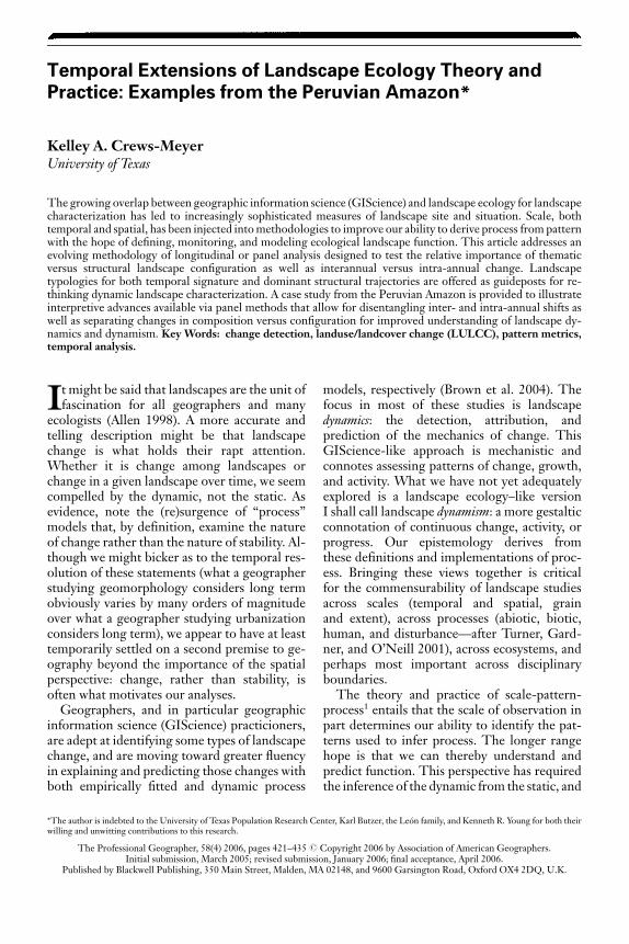
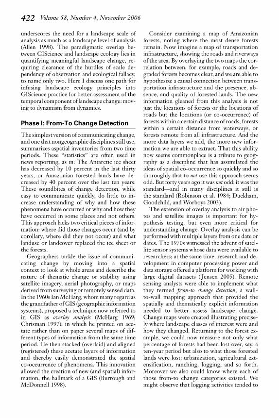
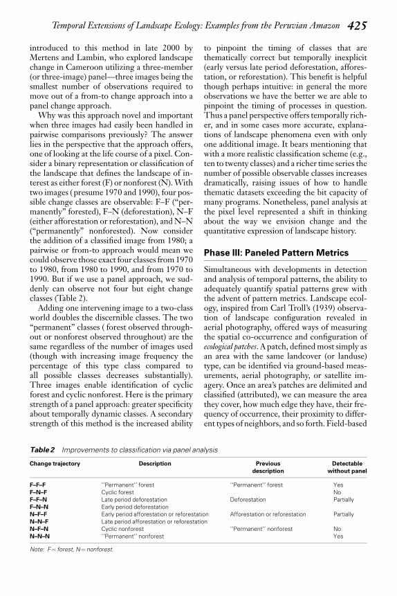
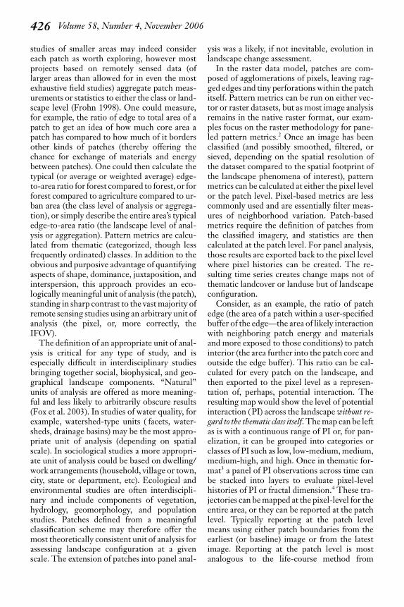
Figure 1 displays the study area, an approx-imately 10 km � 12 km, using a 432 compositeof the May 2001 image. Figure 2 shows the inputNDVI classes for each of the four images, andboth inter- and intra-annual shifts in NDVI classare visually discernible. Figures 3 and 4 illustrateproducts derived from the paneled NDVI anal-ysis, and Figures 5 and 6 exhibit sample deriv-ative products from the paneled pattern metricmethod. Typically, multiple metrics are run inthe paneled pattern metric method (here, usingFRAGSTATS freeware; McGarigal and Marks1993); for exploring proof of concept here, onlyspatial dominance (percentage of landscape)metric derivatives are used given the ease of in-terpretation for those less familiar with patternmetric analysis since spatial dominance tends tobe more easily conceptualized and observed byhumans (Turner, Gardner, and O’Neill 2001).7

For both the paneled NDVI and paneled patternmetric results, all trajectories (in the case ofpaneled NDVI) or patches (in the case ofpaneled pattern metrics) with membership/sizeof o500 pixels (0.45 km2) were removed fromthe analysis.8

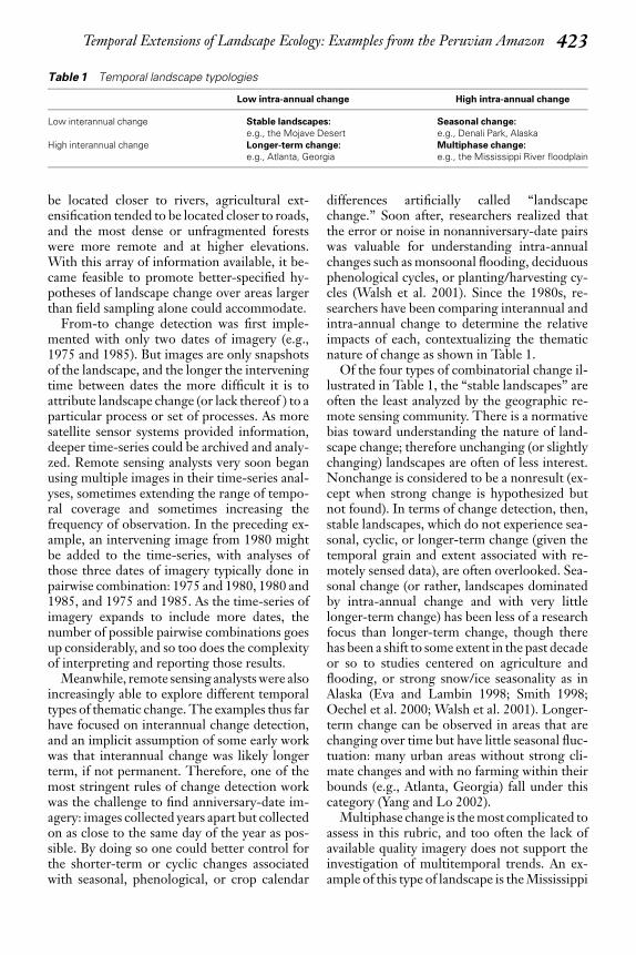
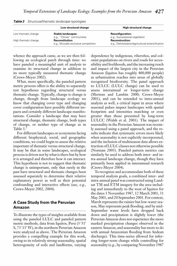
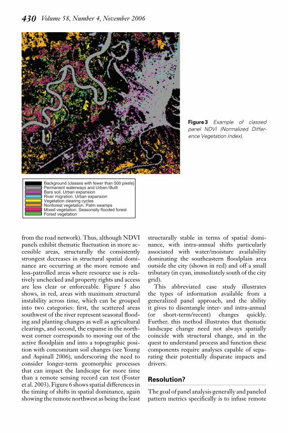
Paneled NDVI presents a expedient buteffective multitemporal product with more sea-sonally accurate class descriptions than are typ-ically obtainable via indices alone (Figure 3).Here, vegetated classes in particular are moredistinguishable from each other in terms of

Figure 1 Landsat ETM 432 com-

posite of Iquitos, Peru. Urban grid

of Iquitos apparent in cyan in the

northeastern portion of the image

and extending along the primary

roadway out of the city to the

southwest. Vegetation appears

red, and most water appears black

(northwestern portion), dark

green (southeastern portion), or

cyan (shallow water, most north-

eastern extent).


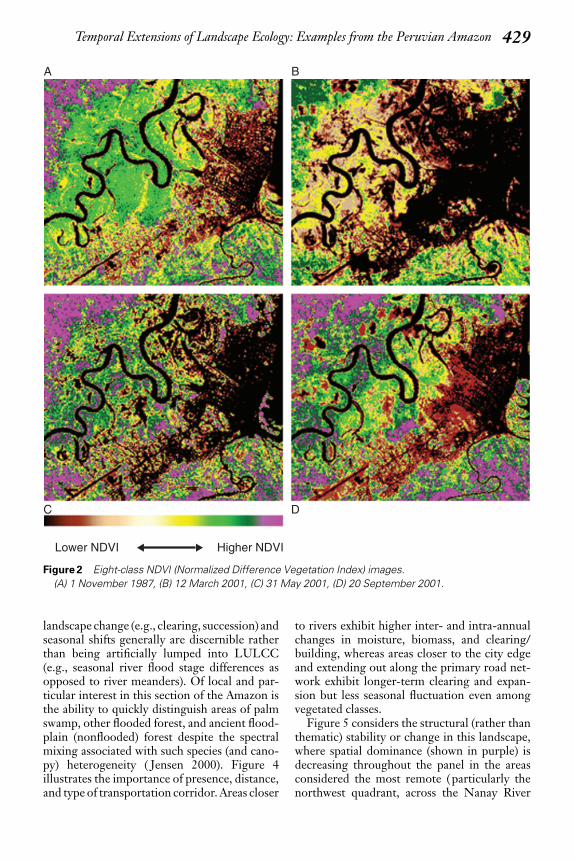
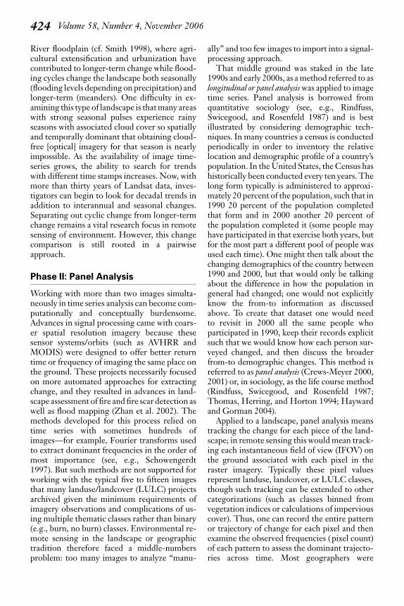
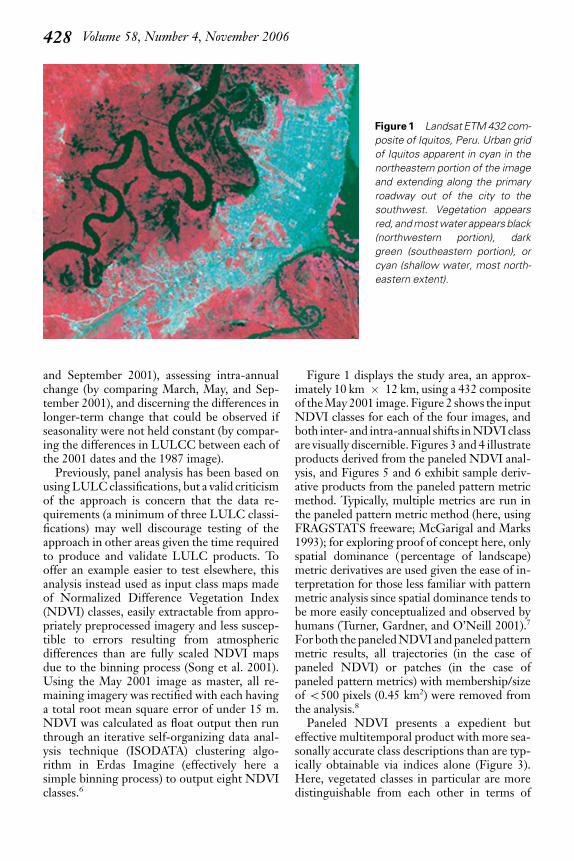
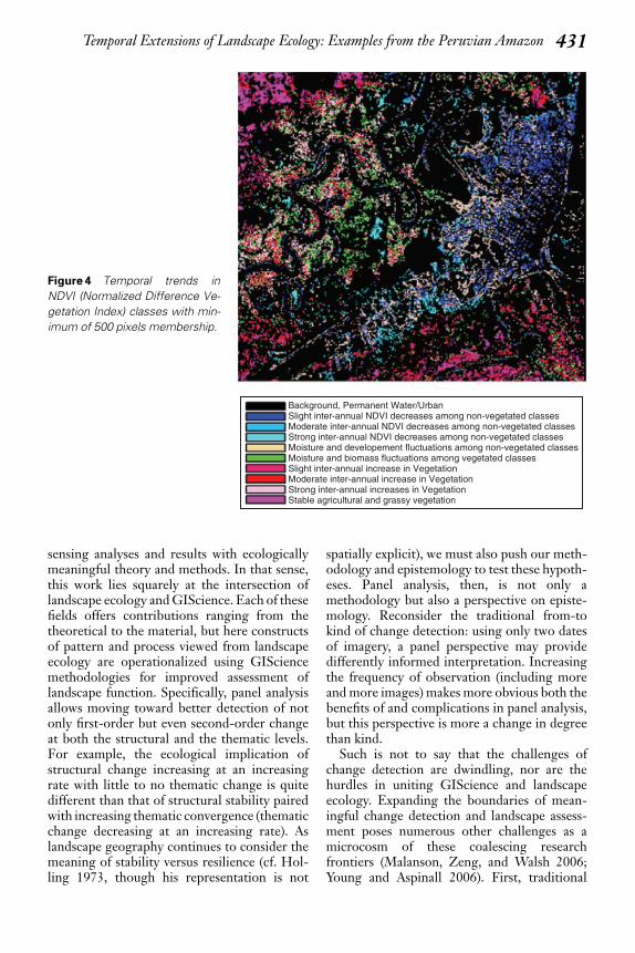
landscape change (e.g., clearing, succession) andseasonal shifts generally are discernible ratherthan being artificially lumped into LULCC(e.g., seasonal river flood stage differences asopposed to river meanders). Of local and par-ticular interest in this section of the Amazon isthe ability to quickly distinguish areas of palmswamp, other flooded forest, and ancient flood-plain (nonflooded) forest despite the spectralmixing associated with such species (and cano-py) heterogeneity ( Jensen 2000). Figure 4illustrates the importance of presence, distance,and type of transportation corridor. Areas closer

to rivers exhibit higher inter- and intra-annualchanges in moisture, biomass, and clearing/building, whereas areas closer to the city edgeand extending out along the primary road net-work exhibit longer-term clearing and expan-sion but less seasonal fluctuation even amongvegetated classes.

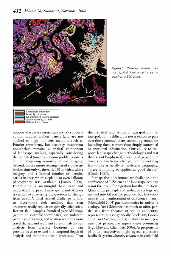
Figure 5 considers the structural (rather thanthematic) stability or change in this landscape,where spatial dominance (shown in purple) isdecreasing throughout the panel in the areasconsidered the most remote (particularly thenorthwest quadrant, across the Nanay River

C D

A B

Lower NDVI Higher NDVI

Figure 2 Eight-class NDVI (Normalized Difference Vegetation Index) images.

(A) 1 November 1987, (B) 12 March 2001, (C) 31 May 2001, (D) 20 September 2001.


from the road network). Thus, although NDVIpanels exhibit thematic fluctuation in more ac-cessible areas, structurally the consistentlystrongest decreases in structural spatial domi-nance are occurring at the more remote andless-patrolled areas where resource use is rela-tively unchecked and property rights and accessare less clear or enforceable. Figure 5 alsoshows, in red, areas with maximum structuralinstability across time, which can be groupedinto two categories: first, the scattered areassouthwest of the river represent seasonal flood-ing and planting changes as well as agriculturalclearings, and second, the expanse in the north-west corner corresponds to moving out of theactive floodplain and into a topographic posi-tion with concomitant soil changes (see Youngand Aspinall 2006), underscoring the need toconsider longer-term geomorphic processesthat can impact the landscape for more timethan a remote sensing record can test (Fosteret al. 2003). Figure 6 shows spatial differences inthe timing of shifts in spatial dominance, againshowing the remote northwest as being the least

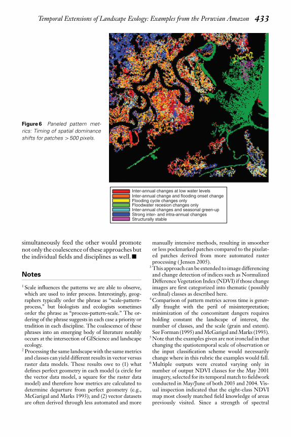
structurally stable in terms of spatial domi-nance, with intra-annual shifts particularlyassociated with water/moisture availabilitydominating the southeastern floodplain areaoutside the city (shown in red) and off a smalltributary (in cyan, immediately south of the citygrid).

This abbreviated case study illustratesthe types of information available from ageneralized panel approach, and the abilityit gives to disentangle inter- and intra-annual(or short-term/recent) changes quickly.Further, this method illustrates that thematiclandscape change need not always spatiallycoincide with structural change, and in thequest to understand process and function thesecomponents require analyses capable of sepa-rating their potentially disparate impacts anddrivers.

Resolution?

The goal of panel analysis generally and paneledpattern metrics specifically is to infuse remote

Background (classes with fewer than 500 pixels)Permanent waterways and Urban/BuiltBare soil. Urban expansionRiver migration. Urban expansionVegetation clearing cyclesNonforest vegetation. Palm swampsMixed vegetation. Seasonally flooded forestForest vegetation

Figure 3 Example of classed

panel NDVI (Normalized Differ-

ence Vegetation Index).


sensing analyses and results with ecologicallymeaningful theory and methods. In that sense,this work lies squarely at the intersection oflandscape ecology and GIScience. Each of thesefields offers contributions ranging from thetheoretical to the material, but here constructsof pattern and process viewed from landscapeecology are operationalized using GISciencemethodologies for improved assessment oflandscape function. Specifically, panel analysisallows moving toward better detection of notonly first-order but even second-order changeat both the structural and the thematic levels.For example, the ecological implication ofstructural change increasing at an increasingrate with little to no thematic change is quitedifferent than that of structural stability pairedwith increasing thematic convergence (thematicchange decreasing at an increasing rate). Aslandscape geography continues to consider themeaning of stability versus resilience (cf. Hol-ling 1973, though his representation is not

spatially explicit), we must also push our meth-odology and epistemology to test these hypoth-eses. Panel analysis, then, is not only amethodology but also a perspective on episte-mology. Reconsider the traditional from-tokind of change detection: using only two datesof imagery, a panel perspective may providedifferently informed interpretation. Increasingthe frequency of observation (including moreand more images) makes more obvious both thebenefits of and complications in panel analysis,but this perspective is more a change in degreethan kind.

Such is not to say that the challenges ofchange detection are dwindling, nor are thehurdles in uniting GIScience and landscapeecology. Expanding the boundaries of mean-ingful change detection and landscape assess-ment poses numerous other challenges as amicrocosm of these coalescing researchfrontiers (Malanson, Zeng, and Walsh 2006;Young and Aspinall 2006). First, traditional

Background, Permanent Water/UrbanSlight inter-annual NDVI decreases among non-vegetated classesModerate inter-annual NDVI decreases among non-vegetated classesStrong inter-annual NDVI decreases among non-vegetated classesMoisture and developement fluctuations among non-vegetated classesMoisture and biomass fluctuations among vegetated classesSlight inter-annual increase in VegetationModerate inter-annual increase in VegetationStrong inter-annual increases in VegetationStable agricultural and grassy vegetation

Figure 4 Temporal trends in

NDVI (Normalized Difference Ve-

getation Index) classes with min-

imum of 500 pixels membership.


notions of accuracy assessment are not support-ed for middle-numbers panels (and are notapplied to high numbers methods such asFourier transform), but accuracy assessmentnonetheless remains a critical componentof landscape analysis, especially consideringthe potential (mis)registration problems inher-ent in comparing remotely sensed imagery.Second, most remote sensing–based studies goback in time only to the early 1970s with satelliteimagery, and a limited number of decadesearlier in areas where airplane (or even balloon)photography was available ( Jensen 2000).Establishing a meaningful base year andunderstanding prior landscape manifestationsis critical to answering the question of changefrom what. A third related challenge is howto incorporate rich ancillary data thatare not spatially explicit or spatially exhaustive.Recent field samples, hundred-year-old maps(without discernible coordinates), or landscapepaintings, drawings, and written accounts fromtravel diaries, and sediment cores or palynologyanalysis from discrete locations all canprovide ways to extend the temporal depth ofanalysis and thought about a landscape. That

their spatial and temporal extrapolation orinterpolation is difficult is not a reason to passover those sources but instead is the grounds forincluding them as more than simply contextualor anecdotal information. Our ability to im-prove landscape change methodologies and testtheories of biophysical, social, and geographicdrivers of landscape change requires nothingless—most especially in landscape geography,‘‘there is nothing so applied as good theory’’(Gould 1985).

Perhaps the more immediate challenge in theconfluence of GIScience and landscape ecologyis not the level of integration but the direction.Quite often principles of landscape ecology aremelded into GIScience practice, but less com-mon is the manifestation of GIScience theory(Goodchild 2004) put into practice in landscapeecology. Yet GIScience has much to offer, par-ticularly from theories of scaling and entityrepresentation (see generally Duckham, Good-child, and Worboys 2003). Efforts to incorpo-rate that perspective appear quite promising(e.g., Mast and Chambers 2006). As proponentsof both perspectives might agree, a positivefeedback system whereby advances in each field

Consistent decreaseMajority decreaseNo change throughout panelStable majority of timeDifferent each time

Figure 5 Paneled pattern met-

rics: Spatial dominance trends for

patches 4500 pixels.


simultaneously feed the other would promotenot only the coalescence of these approaches butthe individual fields and disciplines as well.’

Notes

1 Scale influences the patterns we are able to observe,which are used to infer process. Interestingly, geog-raphers typically order the phrase as ‘‘scale-pattern-process,’’ but biologists and ecologists sometimesorder the phrase as ‘‘process-pattern-scale.’’ The or-dering of the phrase suggests in each case a priority ortradition in each discipline. The coalescence of thesephrases into an emerging body of literature notablyoccurs at the intersection of GIScience and landscapeecology.

2 Processing the same landscape with the same metricsand classes can yield different results in vector versusraster data models. These results owe to (1) whatdefines perfect geometry in each model (a circle forthe vector data model, a square for the raster datamodel) and therefore how metrics are calculated todetermine departure from perfect geometry (e.g.,McGarigal and Marks 1993); and (2) vector datasetsare often derived through less automated and more

manually intensive methods, resulting in smootheror less pockmarked patches compared to the pixelat-ed patches derived from more automated rasterprocessing ( Jensen 2005).

3 This approach can be extended to image differencingand change detection of indices such as NormalizedDifference Vegetation Index (NDVI) if those changeimages are first categorized into thematic (possiblyordinal) classes as described here.

4 Comparison of pattern metrics across time is gener-ally fraught with the peril of misinterpretation;minimization of the concomitant dangers requiresholding constant the landscape of interest, thenumber of classes, and the scale (grain and extent).See Forman (1995) and McGarigal and Marks (1993).

5 Note that the examples given are not ironclad in thatchanging the spatiotemporal scale of observation orthe input classification scheme would necessarilychange where in this rubric the examples would fall.

6 Multiple outputs were created varying only innumber of output NDVI classes for the May 2001imagery, selected for its temporal match to fieldworkconducted in May/June of both 2003 and 2004. Vis-ual inspection indicated that the eight-class NDVImap most closely matched field knowledge of areaspreviously visited. Since a strength of spectral

Inter-annual changes at low water levelsInter-annual change and flooding onset changeFlooding cycle changes onlyFloodwater recesion changes onlyInter-annual changes and seasonal green-upStrong inter- and intra-annual changesStructurally stable

Figure 6 Paneled pattern met-

rics: Timing of spatial dominance

shifts for patches 4500 pixels.


enhancements generally is that they do not explicitlyrequire field knowledge ( Jensen 2005), we recom-mend that others testing this approach select an out-put class number based on how many vegetative andnonvegetative classes they wish to extract. In mostvegetated landscapes, at least two classes are requiredto accommodate nonvegetated entities (water, soil,built environments) and three for vegetative classes(two for varying density of vascular species and onefor herbaceous/agricultural vegetation). Note thatbit-depth requirements in the concatenation processrender using more than nine classes (reserving oneclass for background/shadow/cloud/no observation)more difficult in terms of data volume and thematicprocessing capabilities.

7 For this analysis, the metrics double-log fractal di-mension, mean patch fractal dimension, and inter-spersion-juxtaposition index were run as well.

8 Though the paneled pattern metric method inher-ently runs at multiple ‘‘levels,’’ the author stronglyencourages running the analysis at multiple extentswith varying associated minimum membershipthresholding levels. Here, all four metrics were runfor three extents of the area: (1) full TM/ETM scene(roughly 185 km � 175 km) with 5,000 pixel or4.5-km2 threshold used, (2) present extent of roughly12 km � 10 km with 500 pixel or 0.45-km2 thresholdused, and (3) an inset of area 2 located in the southerncentral portion of the image dominated by smallerpatches, total extent approximately 1 km � 2 kmwith a minimum threshold of 50 pixels or 0.045 km2.Ultimately the selection of threshold is made itera-tively with number of output patches to be kept foranalysis; as a starting point, changing extents andthresholds on roughly order of magnitude scales isappropriate.

Literature Cited

Allen, T. F. H. 1998. The landscape ‘‘level’’ is dead:Persuading the family to take it off the respirator. InEcological scale: Theory and applications, ed. D. Peter-son and V. T. Parker, 35–54. New York: ColumbiaUniversity Press.

Brown, D. G., R. Walker, S. Manson, and K. Seto.2004. Modeling land-use and land-cover change. InLand change science: Observing, monitoring, and un-derstanding trajectories of change on the land surface, ed.G. Gutmann, A. C. Janetos, C. O. Justice, E. F.Moran, J. F. Mustard, R. R. Rindfuss, D. Skole,B. L. Turner II, and M. A. Cochrane, 395–409.Dordrecht, the Netherlands: Kluwer.

Burrough, P. A., and R. A. McDonnell. 1998. Principlesof geographical information systems. Oxford, U.K.:Oxford University Press.

Chrisman, N. 1997. Exploring geographic informationsystems. New York: Wiley.

Crews-Meyer, K. A. 2000. Integrated landscape char-acterization via landscape ecology and GIScience:A policy ecology of Northeast Thailand.Ph.D. diss., University of North Carolina atChapel Hill.

———. 2001. Assessing landscape change and pop-ulation-environment interactions via panel analy-sis. Geocarto International 16 (4): 69–79.

———. 2002. Characterizing landscape dynamism viapaneled-pattern metrics. Photogrammetric Engineer-ing and Remote Sensing 68 (10): 1031–40.

———. 2004. Agricultural landscape change and sta-bility in northeast Thailand: Historical patch-levelanalysis. Agriculture, Ecosystems and Environment101:155–69.

Duckham, M., M. F. Goodchild, and M. F. Worboys,eds. 2003. Foundations of geographic informationscience. New York: Taylor and Francis.

Eva, H., and E. F. Lambin. 1998. Remote sensing ofbiomass burning in tropical regions: Samplingissues and multisensor approach. Remote Sensing ofEnvironment 64 (3): 292–315.

Forman, R. T. T. 1995. Land mosaics: The ecology andlandscapes and regions. Cambridge, U.K.: CambridgeUniversity Press.

Foster, D., F. Swanson, J. Aber, I. Burke, N. Brokaw,D. Tilman, and A. Knapp. 2003. The importance ofland-use legacies to ecology and conservation.BioScience 53 (1): 77–88.

Fox, J., R. R. Rindfuss, S. J. Walsh, and V. Mishra, eds.2003. People and the environment: Approaches for link-ing household and community surveys to remote sensingand GIS. Dordrecht, the Netherlands: Kluwer.

Frohn, R. C. 1998. Remote sensing for landscapeecology: New metric indicators for monitoring,modeling, and assessment of ecosystems. Boca Raton,FL: Lewis.

Goodchild, M. F. 2004. The validity and usefulness oflaws in geographic information science and geog-raphy. Annals of the Association of American Geogra-phers 94:300–03.

Gould, P. 1985. The geographer at work. London:Routledge.

Hayward, M. D., and B. K. Gorman. 2004. The longarm of childhood: The influence of early-life socialconditions on men’s mortality. Demography 41:87–107.

Holling, C. S. 1973. Resilience and stability of eco-logical systems. Annual Review of Ecology andSystematics 4:1–23.

Jensen, J. R. 2000. Remote sensing of environment.Upper Saddle River, NJ: Prentice-Hall.

———. 2005. Digital image processing, 3rd ed. UpperSaddle River, NJ: Prentice-Hall.

Malanson, G. P., Y. Zeng, and S. J. Walsh. 2006.Landscape frontiers, geography frontiers: Lessonsto be learned. The Professional Geographer 58:383–96.


Mast, J. N., and C. L. Chambers. 2006. Integratedapproaches, multiple scales: Snag dynamics inburned versus unburned landscapes. The Profession-al Geographer 58:397–405.

McGarigal, K., and B. J. Marks. 1993. FRAGSTATS:Spatial pattern analysis program for quantifying land-scape structure. Corvallis, OR: Forest Science De-partment, Oregon State University. McHarg, I. L.1969. Design with nature. Garden City, NY: NaturalHistory Press.

Mertens, B., and E. F. Lambin. 2000. Land-cover-change trajectories in Southern Cameroon. Annalsof the Association of American Geographers 90:467–94.

Norman, A. L. 2005. Isolating seasonal variation inlanduse/landcover change using multi-temporalclassification of Landsat ETM Data in the Peruvi-an Amazon. Masters thesis, University of Texas,Austin.

Oechel, W. C., G. L. Vourlitis, J. Verfaillie Jr., T.Crawford, S. Brooks, E. Dumas, A. Hope, D. Stow,B. Boynton, V. Nosov, and R. Zulueta. 2000. Ascaling approach for quantifying the net CO2 flux ofthe Kuparuk River Basin, Alaska. Global ChangeBiology 6 (S1): 160–73.

Rindfuss, R. R., C. G. Swicegood, and R. A. Rosen-feld. 1987. Disorder in the life course: How com-mon and does it matter? American Sociological Review52 (6): 785–801.

Robinson, A. H., J. L. Morrison, P. C. Muehrcke, A. J.Kimerling, and S. C. Guptill. 1984. Elements of car-tography, 5th ed. New York: Wiley.

Schowengerdt, R. A. 1997. Remote sensing, models, andmethods for remote sensing. Burlington, MA: Aca-demic Press.

Smith, L. 1998. Satellite remote sensing of riverinundation area, stage, and discharge: A review.Hydrological Processes 11 (10): 1427–39.

Song, C., C. E. Woodcock, K. C. Seto, M. P. Lenney,and S. A. Macomber. 2001. Classification andchange detection using Landsat TM data: Whenand how to correct atmospheric effects? RemoteSensing of Environment 75:230–44.

Thomas, M. E., C. Herring, and H. D. Horton. 1994.Discrimination over the life course: A synthetic co-hort analysis of earnings differences between blackand white males, 1940–1990. Social Problems 41 (4):608–28.

Troll, C. 1939. Luftbildplan und okologische Boden-forschung [Aerial photography and ecological stud-ies of the earth]. Zeitschrift der Gesellschaft furErdkund 241–98.

Turner, M. G., R. H. Gardner, and R. V. O’Neill.2001. Landscape ecology in theory and practice: Patternand process. New York: Springer.

Walsh, S. J., K. A. Crews-Meyer, T. W. Crawford, W.F. Welsh, B. Entwisle, and R. R. Rindfuss. 2001.Patterns of change in LULC and plant biomass:Separating intra- and inter-annual signals in mon-soon-driven northeast Thailand. In Remote sensingand GIS applications in biogeography and ecology, ed.A. C. Millington, S. J. Walsh, and P. E. Osborne,91–108. Boston: Kluwer.

Yang, X., and C. P. Lo. 2002. Using a time series ofsatellite imagery to detect land use and land coverchanges in the Atlanta, Georgia metropolitan area.International Journal of RemoteSensing 23 (9):1775–98.

Young, K. R., and R. Aspinall. 2006. Kaleidoscopinglandscapes, shifting perspectives. The ProfessionalGeographer 58:436–47.

Zhan, X., R. A. Sohlberg, J. R. G. Townshend, C.DiMiceli, M. L. Carroll, J. C. Eastman, M. C.Hansen, and R. S. DeFries. 2002. Detection of landcover changes using MODIS 250 m data. RemoteSensing of Environment 83:336–50.

KELLEY A. CREWS-MEYER is an Associate Pro-fessor in the Department of Geography & the Envi-ronment at the University of Texas, Austin, TX 78712,and Director of the GIScience Center. E-mail:[email protected]. Her research interests in-clude spatiotemporal scaling thresholds and policyrelevant analyses in the global tropics.


Temporal Extensions of Landscape Ecology Theory and Practice: Examples from the Peruvian Amazon

Documents

Transcript of Temporal Extensions of Landscape Ecology Theory and Practice: Examples from the Peruvian Amazon