Ecological Indicators 2 (2002) 3–15

Applicability of landscape metrics for the monitoring of landscapechange: issues of scale, resolution and interpretability

A. Lausch∗, F. HerzogUFZ Centre for Environmental Research, P.O. Box 2, D-04301 Leipzig, Germany

Abstract

In most parts of the world, land-use/land cover can be considered an interface between natural conditions and anthropogenicinfluence. Indicators are being sought which reflect landscape conditions, pressures and related societal responses. Landscapemetrics, which are based on the number, size, shape and arrangement of patches of different land-use/land cover types, areused-together with areal statistics-to quantify landscape structure and composition.

The applicability of landscape metrics for landscape monitoring has been investigated in a 700 km2 test region in easternGermany, where open cast coal mining has caused far reaching land-use changes in the course of this century. Time series ofmaps (1912–2020) have been elaborated from various data sources (topographic maps, aerial photography, satellite images,prospective planning material). Landscape metrics have been calculated for the entire test region and for ecologically definedsubregions at the landscape, class and patch level.

The results are presented and methodological issues are addressed, namely the impact of scale, spatial and temporalresolution on the interpretability of landscape metrics. Critical issues are:

• the application of remote sensing methods, which is a pre-requisite for the area-wide monitoring of land-use change;• standardised data processing techniques, which are vital for the spatial and temporal comparability of results;• the selection of a manageable set of indicators which embraces the structural properties of landscapes;• the choice of appropriate spatial units which allow for an integration of landscape indicators (which tend to relate to

cross-border phenomena) and socio-economic indicators (which are usually available for administrative entities or areas).

These issues are discussed in relation to the application of landscape indices in environmental monitoring.© 2002 Elsevier Science Ltd. All rights reserved.

Keywords: Environmental monitoring; Remote sensing; GIS; Land-use; Land cover; Landscape pattern

1. Introduction

Land-use is one of the main factors throughwhich man influences the environment. Historically,the most important land-use change imposed byman was the clearing of forest land for agricultural

∗ Corresponding author. Tel.:+49-341-235-20-98;fax: +49-341-235-25-11.E-mail address: lausch@alok.ufz.de (A. Lausch).

purposes and for the establishment of settlements.Subsequent technical developments in the 19th and20th centuries, together with the growing humanpopulation, have increased man’s need and abilityto shape the environment according to his require-ments. The control of the hydrological regime oflandscapes (melioration, irrigation), industrialisedagricultural production methods and large-scale in-frastructure works interfere more and more with ourlandscapes.

1470-160X/02/$ – see front matter © 2002 Elsevier Science Ltd. All rights reserved.PII: S1470-160X(02)00053-5

4 A. Lausch, F. Herzog / Ecological Indicators 2 (2002) 3–15

The importance of land-use as an environmentalparameter is reflected by the attention it receives inthe actual discussion on environmental index develop-ment. The Organisation for Economic Co-operationand Development proposes a core set of 50 envi-ronmental indicators (OECD, 1998). Of these, eightrelate to land cover/land-use (irrigated areas; areaof forests; land-use changes; land cover conver-sion; land-use and conservation; biodiversity, wildlifehabitats, landscape; road infrastructure; habitat frag-mentation). However, values are presented only forindicators which can be derived from broad categoriesof land-use statistics (OECD, 1999). More advancedlandscape indicators such as indicators for culturallandscapes, agriculture and wildlife habitats, agricul-tural landscapes are discussed and their importanceis stressed, but no operational indicators have beenpresented to date (OECD, 2001). This also appliesto a recent publication of the Statistical Office of theEuropean Communities (EUROSTAT, 1998), wherethree levels of landscape indicators are mentioned: (1)statistical data on land cover and use (basically arealstatistics); (2) trends in land cover (relating mostly tolandscape pattern) and (3) landscape elements witha strong impact on the user’s perception. Whereasvalues are available for the conventional level 1 indi-cators, level 2 and 3 indicators are yet to be developedby national initiatives.

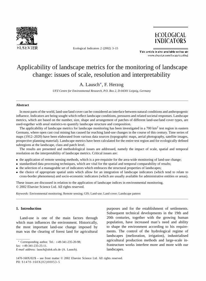
Fig. 1. The application of landscape metrics.

Indicators which address landscape pattern andwhich are based on landscape geometry may proveto be helpful in this context. There has been a con-siderable research effort in this field in the last twodecades, enabled by the rapid development of remotesensing and geographic information systems (GIS).Correlations between landscape metrics and variouslandscape functions are sought (Fig. 1). In the par-ticular field of landscape monitoring, the applicationof landscape metrics has been tested in a number ofstudies representing a wide range of test areas andmethods of data acquisition and treatment (Table 1).There are considerable variations in the size of thetest areas, the spatial and temporal resolutions, thenumber of different land-use/land cover types (LT),and the kind of raw data used. The most frequentlyapplied landscape indices belong to the broad cate-gory of edge and shape metrics. They quantify theoccurrence of ecotones, and are often related to patcharea, the fractal dimension, or the discrepancy be-tween actual and isodiametric shapes. Diversity mea-sures are usually derived from information theory andoften involve the use of Shannon’s diversity index.The number and size of patches (patch area) are alsooften measured, whereas metrics for landscape con-figuration (contagion indices) were seldom applied.

The study presented here was carried out in a land-scape which has been subject to particularly profound

A. Lausch, F. Herzog / Ecological Indicators 2 (2002) 3–15 5

Table 1Range of characteristics of 13 investigations (published in variouspapers) which applied landscape metrics for landscape monitoring;frequency of application of categories of metrics (Herzog et al.,2001)

Parameter Range

Area of test regions (km2) 3.2–9678Source of data Aerial

photography/topographicmaps—satellite images

Type of data (spatial resolution) Vector-Raster (2–200 m)Number of land-use/land

cover classes2–17

Temporal resolution (a) 8–30Landscape metrics employed

Patch area 58% of studiesEdge and shape 75%Diversity 75%Configuration 8%

modifications by means of surface lignite mining. Thistype of landscape is well suited for developing andtesting methods of landscape monitoring because thelandscape changes occur very rapidly. Preliminary re-sults have been presented bySteinhardt et al. (1999)who proposed the ‘Hemeroby Index’ as a human im-pact indicator. In this paper methodological questionsrelated to the selection of a set of landscape metricsfor landscape monitoring are addressed.

2. Materials and methods

2.1. Leipzig South

The Leipzig lowland bay is a flat basin, which wasfilled up in the Tertiary period with sediments. Whenthe basin lowered itself during the Tertiary period, thegroundwater level rose and the area became swampy.This resulted in the formation of several lignite seamsof 5–20 m in diameter. Today, the landscape consistsof even ice-age deposits, interspersed by large, flatvalleys. Topography is essentially flat with a steadyrise from the southern edge of the city of Leipzig(110 m above sea level) to Borna town (160 m abovesea level) (Eissmann, 1975). Until the early 20th cen-tury, Leipzig South was an agricultural region withcomparatively intensive arable production and grass-land in the river plains (Herzog and Heinrich, 1997).

Large-scale lignite mining started in the 1920s andculminated in the 1980s. By 1990, surface mining hadoccurred on almost 40% of the area and about 90km2 were awaiting recultivation (RPW, 1998). LeipzigSouth had been transformed into an industrial regionwith numerous environmental problems caused by themining itself, by the artificial modifications of theregion’s hydrological regime (lowering of the ground-water table, dislocations of riverbeds) and by the asso-ciated carbo-chemical and brown coal industry. About60 settlements have been destroyed since 1928 andabout 23,000 inhabitants re-located (Berkner, 1995;Kabisch, 1997). After the German re-unification in the1990s, mining was drastically reduced and the indus-trial plants closed. Today, sanitation, reclamation andthe regeneration of the landscape’s regulatory func-tions are the main issues. Novel landscape structuresestablish, often spontaneously, and there are large ar-eas with a high potential for nature protection (e.g.Durka and Altmoos, 1997).

2.2. Data acquisition

For Leipzig South, Spot-XS images from 1990,1994 and 1996 were analysed with a hierarchical clas-sification procedure based on maximum-likelihood,resulting in eleven LT for each image. In addition, thelandscape development concept of the regional plan-ning authority (RPW, 1996) for 2020 was digitisedand included in the analysis in order to allow for theevaluation of future developments. The spatial resolu-tion of multispectral SPOT-XS of 20 m/pixel allowedonly visual recognition of the traffic network but noproper classification. Because the values of landscapemetrics depend to a large extent on linear landscapeelements (Lausch and Menz, 1999), the traffic net-work was extracted from the digital biotope map ofSaxony, which is based on CIR aerial photography(Frietsch, 1997). It was transformed to raster format(10 m/pixel) and merged with the classified satelliteimages, which had beforehand been transformed tothe raster cell size of 10 m/pixel as well.

Leipzig South was subdivided into 50 landscapeunits at the meso scale (2–36 km2) based on a clas-sification of the Saxony Academy of Science (Haaseand Mannsfeld, 1987). Three major landscape typesare present: (1) valleys of large rivers and riverplains,(2) plains on loose rocks and (3) mosaics in technical

6 A. Lausch, F. Herzog / Ecological Indicators 2 (2002) 3–15

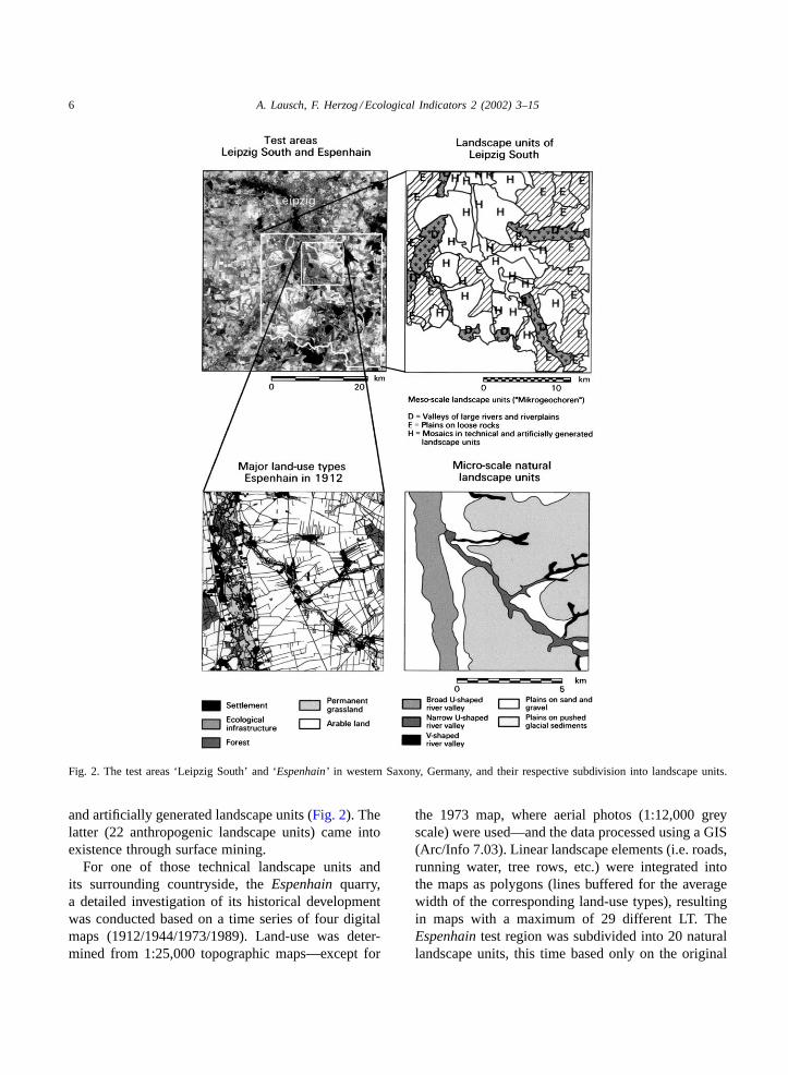
Fig. 2. The test areas ‘Leipzig South’ and ‘Espenhain’ in western Saxony, Germany, and their respective subdivision into landscape units.

and artificially generated landscape units (Fig. 2). Thelatter (22 anthropogenic landscape units) came intoexistence through surface mining.

For one of those technical landscape units andits surrounding countryside, theEspenhain quarry,a detailed investigation of its historical developmentwas conducted based on a time series of four digitalmaps (1912/1944/1973/1989). Land-use was deter-mined from 1:25,000 topographic maps—except for

the 1973 map, where aerial photos (1:12,000 greyscale) were used—and the data processed using a GIS(Arc/Info 7.03). Linear landscape elements (i.e. roads,running water, tree rows, etc.) were integrated intothe maps as polygons (lines buffered for the averagewidth of the corresponding land-use types), resultingin maps with a maximum of 29 different LT. TheEspenhain test region was subdivided into 20 naturallandscape units, this time based only on the original

A. Lausch, F. Herzog / Ecological Indicators 2 (2002) 3–15 7

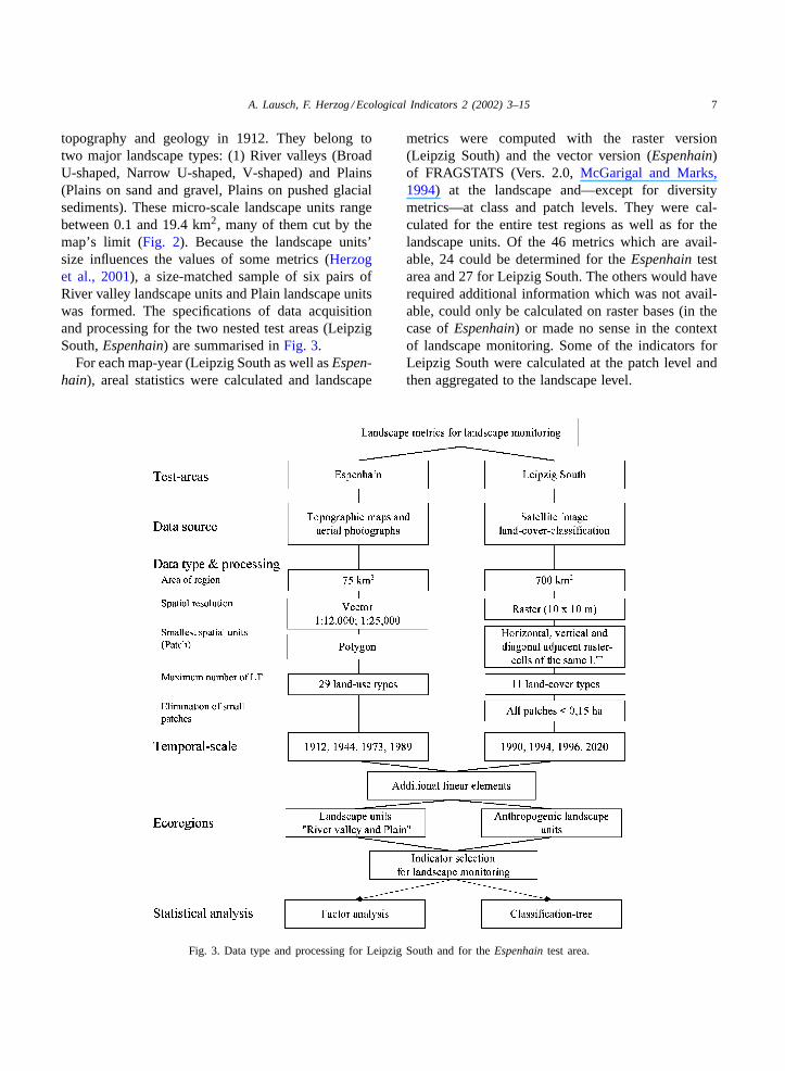
topography and geology in 1912. They belong totwo major landscape types: (1) River valleys (BroadU-shaped, Narrow U-shaped, V-shaped) and Plains(Plains on sand and gravel, Plains on pushed glacialsediments). These micro-scale landscape units rangebetween 0.1 and 19.4 km2, many of them cut by themap’s limit (Fig. 2). Because the landscape units’size influences the values of some metrics (Herzoget al., 2001), a size-matched sample of six pairs ofRiver valley landscape units and Plain landscape unitswas formed. The specifications of data acquisitionand processing for the two nested test areas (LeipzigSouth,Espenhain) are summarised inFig. 3.

For each map-year (Leipzig South as well asEspen-hain), areal statistics were calculated and landscape

Fig. 3. Data type and processing for Leipzig South and for theEspenhain test area.

metrics were computed with the raster version(Leipzig South) and the vector version (Espenhain)of FRAGSTATS (Vers. 2.0,McGarigal and Marks,1994) at the landscape and—except for diversitymetrics—at class and patch levels. They were cal-culated for the entire test regions as well as for thelandscape units. Of the 46 metrics which are avail-able, 24 could be determined for theEspenhain testarea and 27 for Leipzig South. The others would haverequired additional information which was not avail-able, could only be calculated on raster bases (in thecase ofEspenhain) or made no sense in the contextof landscape monitoring. Some of the indicators forLeipzig South were calculated at the patch level andthen aggregated to the landscape level.

8 A. Lausch, F. Herzog / Ecological Indicators 2 (2002) 3–15

Statistical analysis was conducted with STATIS-TICA 5.1 StatSoft Inc. (1997).

3. Results and discussion

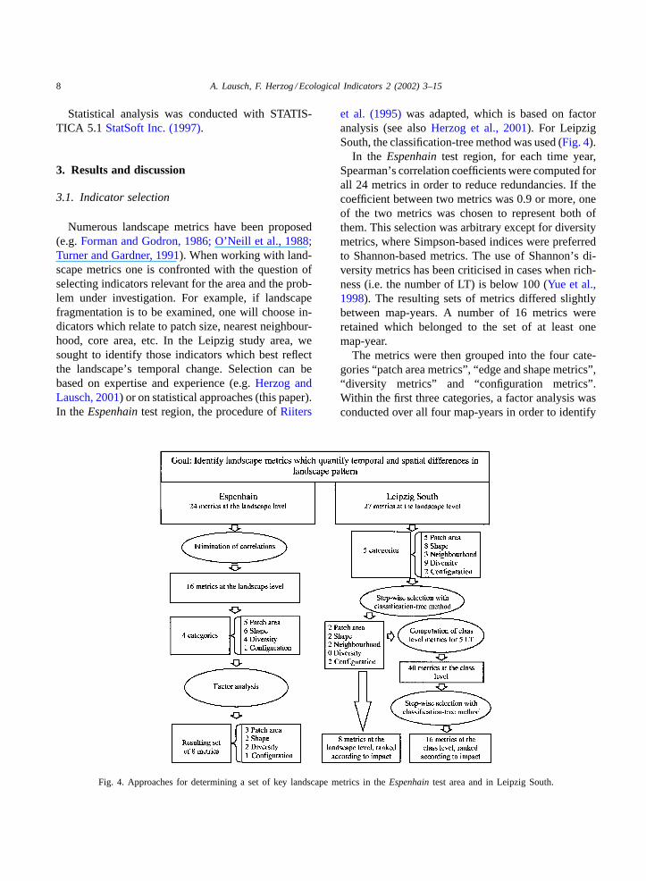
3.1. Indicator selection

Numerous landscape metrics have been proposed(e.g.Forman and Godron, 1986; O’Neill et al., 1988;Turner and Gardner, 1991). When working with land-scape metrics one is confronted with the question ofselecting indicators relevant for the area and the prob-lem under investigation. For example, if landscapefragmentation is to be examined, one will choose in-dicators which relate to patch size, nearest neighbour-hood, core area, etc. In the Leipzig study area, wesought to identify those indicators which best reflectthe landscape’s temporal change. Selection can bebased on expertise and experience (e.g.Herzog andLausch, 2001) or on statistical approaches (this paper).In the Espenhain test region, the procedure ofRiiters

Fig. 4. Approaches for determining a set of key landscape metrics in theEspenhain test area and in Leipzig South.

et al. (1995)was adapted, which is based on factoranalysis (see alsoHerzog et al., 2001). For LeipzigSouth, the classification-tree method was used (Fig. 4).

In the Espenhain test region, for each time year,Spearman’s correlation coefficients were computed forall 24 metrics in order to reduce redundancies. If thecoefficient between two metrics was 0.9 or more, oneof the two metrics was chosen to represent both ofthem. This selection was arbitrary except for diversitymetrics, where Simpson-based indices were preferredto Shannon-based metrics. The use of Shannon’s di-versity metrics has been criticised in cases when rich-ness (i.e. the number of LT) is below 100 (Yue et al.,1998). The resulting sets of metrics differed slightlybetween map-years. A number of 16 metrics wereretained which belonged to the set of at least onemap-year.

The metrics were then grouped into the four cate-gories “patch area metrics”, “edge and shape metrics”,“diversity metrics” and “configuration metrics”.Within the first three categories, a factor analysis wasconducted over all four map-years in order to identify

A. Lausch, F. Herzog / Ecological Indicators 2 (2002) 3–15 9

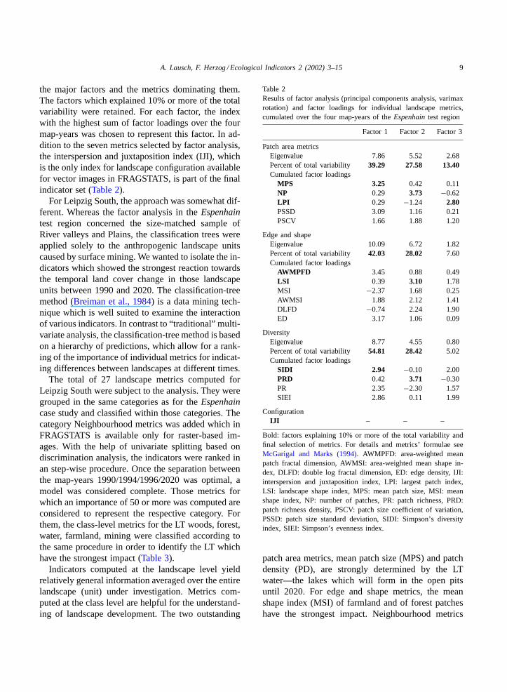
the major factors and the metrics dominating them.The factors which explained 10% or more of the totalvariability were retained. For each factor, the indexwith the highest sum of factor loadings over the fourmap-years was chosen to represent this factor. In ad-dition to the seven metrics selected by factor analysis,the interspersion and juxtaposition index (IJI), whichis the only index for landscape configuration availablefor vector images in FRAGSTATS, is part of the finalindicator set (Table 2).

For Leipzig South, the approach was somewhat dif-ferent. Whereas the factor analysis in theEspenhaintest region concerned the size-matched sample ofRiver valleys and Plains, the classification trees wereapplied solely to the anthropogenic landscape unitscaused by surface mining. We wanted to isolate the in-dicators which showed the strongest reaction towardsthe temporal land cover change in those landscapeunits between 1990 and 2020. The classification-treemethod (Breiman et al., 1984) is a data mining tech-nique which is well suited to examine the interactionof various indicators. In contrast to “traditional” multi-variate analysis, the classification-tree method is basedon a hierarchy of predictions, which allow for a rank-ing of the importance of individual metrics for indicat-ing differences between landscapes at different times.

The total of 27 landscape metrics computed forLeipzig South were subject to the analysis. They weregrouped in the same categories as for theEspenhaincase study and classified within those categories. Thecategory Neighbourhood metrics was added which inFRAGSTATS is available only for raster-based im-ages. With the help of univariate splitting based ondiscrimination analysis, the indicators were ranked inan step-wise procedure. Once the separation betweenthe map-years 1990/1994/1996/2020 was optimal, amodel was considered complete. Those metrics forwhich an importance of 50 or more was computed areconsidered to represent the respective category. Forthem, the class-level metrics for the LT woods, forest,water, farmland, mining were classified according tothe same procedure in order to identify the LT whichhave the strongest impact (Table 3).

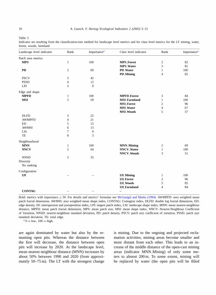
Indicators computed at the landscape level yieldrelatively general information averaged over the entirelandscape (unit) under investigation. Metrics com-puted at the class level are helpful for the understand-ing of landscape development. The two outstanding

Table 2Results of factor analysis (principal components analysis, varimaxrotation) and factor loadings for individual landscape metrics,cumulated over the four map-years of theEspenhain test region

Factor 1 Factor 2 Factor 3

Patch area metricsEigenvalue 7.86 5.52 2.68Percent of total variability 39.29 27.58 13.40Cumulated factor loadings

MPS 3.25 0.42 0.11NP 0.29 3.73 −0.62LPI 0.29 −1.24 2.80PSSD 3.09 1.16 0.21PSCV 1.66 1.88 1.20

Edge and shapeEigenvalue 10.09 6.72 1.82Percent of total variability 42.03 28.02 7.60Cumulated factor loadings

AWMPFD 3.45 0.88 0.49LSI 0.39 3.10 1.78MSI −2.37 1.68 0.25AWMSI 1.88 2.12 1.41DLFD −0.74 2.24 1.90ED 3.17 1.06 0.09

DiversityEigenvalue 8.77 4.55 0.80Percent of total variability 54.81 28.42 5.02Cumulated factor loadings

SIDI 2.94 −0.10 2.00PRD 0.42 3.71 −0.30PR 2.35 −2.30 1.57SIEI 2.86 0.11 1.99

ConfigurationIJI – – –

Bold: factors explaining 10% or more of the total variability andfinal selection of metrics. For details and metrics’ formulae seeMcGarigal and Marks (1994). AWMPFD: area-weighted meanpatch fractal dimension, AWMSI: area-weighted mean shape in-dex, DLFD: double log fractal dimension, ED: edge density, IJI:interspersion and juxtaposition index, LPI: largest patch index,LSI: landscape shape index, MPS: mean patch size, MSI: meanshape index, NP: number of patches, PR: patch richness, PRD:patch richness density, PSCV: patch size coefficient of variation,PSSD: patch size standard deviation, SIDI: Simpson’s diversityindex, SIEI: Simpson’s evenness index.

patch area metrics, mean patch size (MPS) and patchdensity (PD), are strongly determined by the LTwater—the lakes which will form in the open pitsuntil 2020. For edge and shape metrics, the meanshape index (MSI) of farmland and of forest patcheshave the strongest impact. Neighbourhood metrics

10 A. Lausch, F. Herzog / Ecological Indicators 2 (2002) 3–15

Table 3Indicator set resulting from the classification-tree method for landscape level metrics and for class level metrics for the LT mining, water,forest, woods, farmland

Landscape level indicator Rank Importancea Class level indicator Rank Importancea

Patch area metricsMPS 1 100 MPS Forest 2 82

MPS Water 3 81PD 2 69 PD Water 1 100

PD Mining 4 65PSCV 3 42PSSD 4 12LPI 5 9

Edge and shapeMPFD 1 100 MPFD Forest 3 84MSI 2 59 MSI Farmland 1 100

MSI Forest 2 96MSI Water 4 67MSI Woods 5 57

DLFD 3 25AWMPFD 4 21ED 5 15AWMSI 6 13LSI 7 9TE 8 3

NeighbourhoodMNN 1 100 MNN Mining 2 69NNCV 2 64 NNCV Water 1 100

NNCV Woods 3 51NNSD 3 35

DiversityNo ranking

ConfigurationIJI – – IJI Mining 1 100

IJI Forest 2 96IJI Woods 3 85IJI Farmland 4 84

CONTAG – – –

Bold: metrics with importance≥ 50. For details and metrics’ formulae seeMcGarigal and Marks (1994). AWMPFD: area weighted meanpatch fractal dimension, AWMSI: area weighted mean shape index, CONTAG: Contagion index, DLFD: double log fractal dimension, ED:edge density, IJI: interspersion and juxtaposition index, LPI: largest patch index, LSI: landscape shape index, MNN: mean nearest-neighbourdistance, MPFD: mean patch fractal dimension, MPS: mean patch size, MSI: mean shape index, NNCV: Nearest-Neighbour Coefficientof Variation, NNSD: nearest-neighbour standard deviation, PD: patch density, PSCV: patch size coefficient of variation, PSSD: patch sizestandard deviation, TE: total edge.

a 0 = low, 100= high.

are again dominated by water but also by the re-maining open pits. Whereas the distance betweenthe first will decrease, the distance between openpits will increase by 2020. At the landscape level,mean nearest neighbour distance (MNN) increases byabout 50% between 1990 and 2020 (from approxi-mately 50–75 m). The LT with the strongest change

is mining. Due to the ongoing and projected recla-mation activities, mining areas become smaller andmore distant from each other. This leads to an in-crease of the middle distance of the open-cast miningareas (indicator MNNMining) of only some me-ters to almost 200 m. To some extent, mining willbe replaced by water (the open pits will be filled

A. Lausch, F. Herzog / Ecological Indicators 2 (2002) 3–15 11

up by rising ground water) and there will be waterbodies dispersed all over Leipzig South by 2020.This leads to a decrease of the variation of the dis-tance between lakes, reflected by a decrease of theNearest-Neighbour Coefficient of Variation (NNCV)of the LT water (NNCVWater), which dominatesNNCV at the landscape level.

The classification-tree method failed to rank diver-sity metrics because the differences between the ninediversity metrics were too small over the period un-der investigation. Also, it was not possible to rank thetwo configuration metrics at the landscape level. Atthe class level, however, IJI for four out of the five LTdiffer strongly between the map-years. The ContagionIndex (CONTAG) is not computed for individual LT.

3.2. Analysis and interpretation

Areal statistics of the historicalEspenhain analysisshow that, at the beginning of this century, LeipzigSouth was a rural area with farmland being the dom-inating land-use type (Fig. 5). Arable land prevailedon the plains, permanent grassland in the river valleysand floodplains. There was a considerable share of“ecological infrastructure” (tree rows, hedges, ripar-ian woods, waterbodies, etc.) but only relatively smallpatches of forest. By the end of the 1980s, the situa-tion had changed drastically. Mining and settlementsexpanded at the expense of, mainly, arable land andgrassland. Farmland (arable land, grassland) remains

Fig. 5. Areal statistics of theEspenhain test area (1912–1989) and of Leipzig South (1990–2020) (Herzog and Lausch, 2001).

the dominating LT, inEspenhain as well as in LeipzigSouth in general, but about one quarter of the LeipzigSouth farmland in 1990 is reclaimed dumps. Landcover changes between 1990 and 1996 mainly con-cerned the reduction of mining per ground, which is in-creasingly covered by pioneer plant species. By 2020,the planned reclamation activities will further reducemining, but also spontaneous vegetation. Forest willbecome an important land cover type, together withwater due to the lakes which will form in the aban-doned open pits.

To what extent are those obvious landscape changesreflected by landscape metrics? As an example, thisis investigated for two metrics which were part of theselected indicator sets forEspenhain as well as forLeipzig South: mean patch size (MPS) and intersper-sion and juxtaposition index (IJI). MPS is computedby dividing the total landscape (or class) areaA by thenumber of patchesN (McGarigal and Marks, 1994):

MPS= A

N

(1

10, 000

)(1)

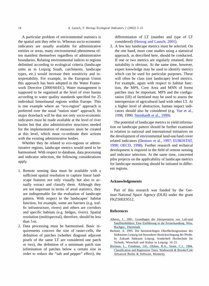
The arrangement of patches and LT in the landscape(landscape composition) is assessed via the intersper-sion and juxtaposition index (IJI). It is calculated fromthe relationship between the length of each edge typeeik and total edge of the landscapeE (at the landscapelevel)/the length of the respective edge type involvedeik (at the class level) divided by a term based on thenumber of LTm′:

12 A. Lausch, F. Herzog / Ecological Indicators 2 (2002) 3–15

Fig. 6. Evolution of mean patch size (MPS) at the landscape level (a) and for selected LT at the class level (b) for theEspenhain testregion (1912–1989) and for Leipzig South (1990–2020) (Herzog and Lausch, 2001).

Landscape level :

IJI = −∑m′i=1

∑m′k=i+1[(eik/E) × ln(eik/E)]

ln(1/2[m′(m′ − 1)])(100)

(2)

Fig. 7. Evolution of the Interspersion-juxtaposition Index (IJI) in theEspenhain test area (1912–1989) and in Leipzig South (1990–2020)at the landscape level (a) and for selected LT (b).

Class level :

IJI = −∑m′k=1[(eik/

∑m′k=1eik) × ln(eik/

∑m′k=1eik)]

ln(m′ − 1)

× (100) (3)

A. Lausch, F. Herzog / Ecological Indicators 2 (2002) 3–15 13

IJI approaches 0 when adjacencies are unevenly dis-tributed; IJI = 100 if all patch types are equally ad-jacent to all other patch types (McGarigal and Marks,1994).

In Figs. 6 and 7the evolution of MPS and IJI at thelandscape level (Figs. 6a and 7a) and for selected LT(Figs. 6b and 7b) is shown for theEspenhain test area(1912–1989) and for Leipzig South (1990–2020).The modifications of the indicators’ values can beexplained by increase in surface mining from the1940s onwards, the resulting re-arrangement of trafficand ecological infrastructure (also influenced by agri-cultural intensification) and the projected landscapewhich will be dominated by a series of lakes form-ing in the former open pits (seeHerzog and Lausch,2001; Herzog et al., 2001). From a methodologicalpoint of view, two observations are of interest.

1. Indicator values forEspenhain and Leipzig Southare at different levels. MPS computed for LeipzigSouth was generally lower, IJI was slightly higher.Although small patches<0.15 ha were removedduring the process of satellite image classificationand analysis—raster satellite images still containfar more small pixels than vector images which, tosome extent, are generalised in the process of map-ping and interpretation. This leads to an overalllower level of mean patch size and its distributionappears to be more uniform due to comparativelyhigher spatial differentiation of raster-based satel-lite images (higher values of IJI).

2. Class level indicators (Figs. 6b and 7b) are helpfulin understanding general trends appearing at thelandscape level (Figs. 6a and 7a). For example,MPS Lignite pit, IJI Lignite pit, MPSWater andIJI Water reflect the development of lignite pitslater becoming water bodies.

4. Conclusions

The Leipzig mining region proved well suited fortesting the application of landscape metrics for land-scape monitoring. The findings ofRiiters et al. (1995);Cain et al. (1997)were confirmed that relatively fewmetrics suffice to capture landscape pattern. Bothmethods applied (factor analysis, tree-classificationmethod) resulted in sets of a manageable size. Theactual indicators selected, however, differed to a large

extent. This is not surprising because data models andscales of theEspenhain and Leipzig South studieswere not the same and because different initial groupsof indices were available before the selection. Still,there are some similarities. MPS was retained in bothstudies to represent Patch area metrics. For edge andshape metrics, fractal indices (MPFD—mean patchfractal dimension, AWMPFD—area weighted meanpatch fractal dimension) ranked particularly high inboth studies. And landscape configuration can becaptured by IJI—if not at the landscape then at theclass level. This outcome is congruent with the resultsof similar investigations—although, due to differingdata sets and indicator computation, comparability islimited. Still, patch characteristics such as averagesize and shape (measured by MPS, LSI—landscapeshape index in our case) were retained byCain et al.(1997) and Riiters et al. (1995). Landscape com-position (IJI, CONTAG—contagion index) and—tosome extent—the largest patch index (LPI) and patchdensity (PD) are comparable to indicators for ‘im-age texture’ (contagion index, seeLi and Reynolds,1993) and ‘large-patch density-area scaling’ selectedby Riiters et al. (1995).

The metrics ‘actual values’ however, were at dif-ferent levels (Figs. 6 and 7) for Espenhain and forLeipzig South. This is basically due to the differ-ent data models used (vector/raster). The digitising ofmaps or aerial photographs, which results in vectordata, encompasses more than just making analogousdata digitally available. In the digitising process, thespatial information is interpreted and generalised (inthe case of map based work, a similar interpretationwas already done by the cartographer). Digital satel-lite images, on the other hand, are raster based. Dur-ing their interpretation, generalisation is usually lessand spatial information is conserved. Also, classifica-tion errors of individual pixels can never be avoidedcompletely and accuracy levels of more than 80–85%can hardly be achieved for SPOT-XS images (Albertz,1991; Hildebrandt, 1996).

This dependence upon the data model and process-ing limits the comparability of the results of individualstudies and consists a major drawback for the applica-tion of landscape metrics. If they were to be applied ata larger scale and enter policy relevant sets of environ-mental indicators such asOECD (1998), there wouldbe a need for standardisation at this level.

14 A. Lausch, F. Herzog / Ecological Indicators 2 (2002) 3–15

A particular problem of environmental statistics isthe spatial unit they refer to. Whereas socio-economicindicators are usually available for administrativeentities or areas, many environmental phenomena of-ten manifest themselves regardless of administrativeboundaries. Relating environmental indices to regionsdelimited according to ecological criteria (landscapeunits as in Leipzig South, catchments, landscapetypes, etc.) would increase their sensitivity and in-terpretability. For example, in the European Unionthis approach has been adopted in the Water Frame-work Directive (2000/60/EC). Water management issupposed to be organised at the level of river basinsaccording to water quality standards specified for 25individual limnofaunal regions within Europe. Thisis one example where an “eco-region” approach ispreferred over the usual “nation state” approach. Itsmajor drawback will be that not only socio-economicindicators must be made available at the level of riverbasins but that also administrative structures neededfor the implementation of measures must be createdat this level, which must co-ordinate their actionswith the existing administrative bodies.

Whether they be related to eco-regions or admin-istrative regions, landscape metrics would need to beharmonised. With respect to database, data processingand indicator selection, the following considerationsapply.

1. Remote sensing data must be available with asufficient spatial resolution to capture linear land-scape features not only visually but also to ac-tually extract and classify them. Although theyare not important in terms of areal statistics, theyare indispensable for the evaluation of landscapepattern. With respect to the landscapes’ habitatfunction, for example, some are barriers (e.g. traf-fic infrastructure, rivers) and others are corridorsand specific habitats (e.g. hedges, rivers). Spatialresolution (multispectral), therefore, should be lessthan 5 m.

2. Data processing must be harmonised. Basic re-quirements concern the size of raster-cells, thedefinition of patches (whether diagonal adjacentpixels of the same LT are considered one patchor two), the definition of a minimum patch size(elimination of patches below a certain size inorder to reduce the “salt and pepper” effect), the

differentiation of LT (number and type of LTconsidered) (Herzog and Lausch, 2001).

3. A few key landscape metrics must be selected. Onthe one hand, more case studies using a statisticalapproach, as described here, should be conducted.If one or two metrics are regularly retained, theirsuitability is obvious. At the same time, however,expert knowledge may be used to identify metricswhich can be used for particular purposes. Thesewill often be class (not landscape) level metrics.For example, again with respect to habitat func-tion, the MPS, Core Area and MNN of forestpatches may be important. MPS and the configu-ration (IJI) of farmland may be used to assess theinterspersion of agricultural land with other LT. Ata higher level of abstraction, human impact indi-cators should also be considered (e.g.Yue et al.,1998, 1990;Steinhardt et al., 1999).

The potential of landscape metrics to yield informa-tion on landscape pattern should be further examinedin relation to national and international initiatives onthe development of environmental land-use/land coverrelated indicators (Denisov et al., 1997; EUROSTAT,1998; OECD, 1998). Further research and technicaldevelopment is required in the field of remote sensingand indicator selection. At the same time, concertedpilot projects on the applicability of landscape metricsfor landscape monitoring should be initiated in differ-ent regions.

Acknowledgements

Part of this research was funded by the Ger-man National Space Agency (DLR) under the grantFKZ50EE9512.

References

Albertz, J., 1991. Grundlagen der Interpretation von Luft-undSatellitenbildern: Eine Einführung in die Fernerkundung. Wiss.Buchges., Darmstadt.

Berkner, A. 1995. Die beeinträchtigen Oberflächengewässer desSüdraumes Leipzig mit besonderer Berücksichtigung der Pleiße.In: Zukunft Südraum Leipzig. Sonderheft Hochschule fürTechnik, Wirtschaft und Kultur in Leipzig: 10–21.

Breiman, L., Friedman, J.H., Olshen, R.A., Stone, C.J., 1984.Classification and Regression Trees. Wadsworth & Brooks/ColeAdvanced Books & Software, Monterey.

A. Lausch, F. Herzog / Ecological Indicators 2 (2002) 3–15 15

Cain, D.H., Riiters, K., Orvis, K., 1997. A multi-scale analysis oflandscape statistics. Landsc. Ecol. 122, 199–212.

Denisov, N.B., Mnatsakanian, R.A., Semichaevsky, A.V., 1997.Environmental Reporting in Central and Eastern Europe:A Review of Selected Publications and Frameworks.UNEP/DEIA/TR.97-6, GA/205031-97/1 and CEU/50-97.1.

Durka, W., Altmoos, M., 1997. Naturschutz in der Bergbaufol-gelandschaft als Teil einer nachhaltigen Landschaftsent-wicklung. In: Ring B.G.I. (Ed.), Nachhaltige Entwicklung inIndustrie-und Bergbauregion–Eine Chance für den SüdraumLeipzig? Teubner Verlagsgesellschaft, Stuttgart, Leipzig, pp.52–72.

Eissmann, L., 1975. Das Quartiär der Leipziger Tieflandsbuchtund angrenzender Gebiete um Saale und Elbe. Schriftenreihefür geologische Wissenschaften, Heft 2.

EUROSTAT, 1998. European landscapes: Farmers maintain morethan half of the territory. Statistics in Focus—Agriculture.(EUROSTAT online document athttp://europa.eu.int/en/comm/eurostat/serven/pdf/sb-land.pdf).

Forman, R.T.T., Godron, M., 1986. Landscape Ecology, Wiley,New York.

Frietsch, G., 1997. Ergebnisse der CIR-Biotoptypen-und Landnut-zungskartierung und ihre Anwendungsmöglichkeiten in derNaturschutzpraxis–Einführungsvortrag. Sächsische Akademiefür Natur und Umwelt 3/97, pp. 7–11.

Haase, G., Mannsfeld, K., 1987. Konzeption und Beispielarbeitenfür eine Naturraumtypen-Karte der DDR im mittleren Maßstab1: 500000/1: 200000 (Projekt NTK). In Naturraumerkundungund Landnutzung, Heinzmann G. (Ed.), Beiträge zur Geo-graphie, Akademie Verlag, Bd. 34, pp. 143–191.

Herzog, F., Lausch, A., 2001. Supplementing land-use statisticswith landscape metrics: some methodological considerations.Environmental Monitoring and Assessment 72, 37–50.

Herzog, F., Lausch, A., Müller, E., Thulke, H.H., Steinhardt,U., Lehmann, S., 2001. Landscape metrics for the assessmentof landscape destruction and rehabilitation. Environ. Manage.27 (1), 91–107.

Herzog, F., Heinrich, K., 1997. Die Landwirtschaft im SüdraumLeipzig–Nachhaltig geschädigt. In: Ring, I., Teubner, B.G.(Eds.), Nachhaltige Entwicklung in Industrie-und Bergbaure-gion—Eine Chance für den Südraum Leipzig? Verlagsge-sellschaft, Stuttgart, Leipzig, pp. 191–220.

Hildebrandt, G., 1996. Fernerkundung und Luftbildmessung.Herbert Wichmann Verlag, Heidelberg.

Kabisch, S., 1997. Siedlungsstrukturelle Einschnitte infolgedes Braunkohlenbergbaus. In: Nachhaltige Entwicklung in

Industrie-und Bergbauregionen-Eine Chance für den SüdraumLeipzig? Ring B.G.I. (Ed.), Teubner Verlagsgesellschaft,Stuttgart, Leipzig, pp. 113–137.

Lausch, A., Menz, G., 1999. Bedeutung der Integration linearerElemente in Fernerkundungsdaten zur Berechnung von Land-schaftsstrukturmaßen. PFG 3, 185–194.

Li, H., Reynolds, J.F., 1993. A new contagion index to quantifyspatial patterns of landscapes. Landsc. Ecol. 8 (3), 155–162.

McGarigal, K., Marks, B., 1994. Fragstats—Spatial PatternAnalysis Program for Quantifying Landscape Structure. ForestScience Department, Oregon State University, Corvallis.

OECD, 1998. Environmental Indicators: Towards SustainableDevelopment. Organisation for Economic Co-operation andDevelopment, Paris.

OECD, 1999. OECD Environmental Data—Compendium 1999edition. Organisation for Economic Co-operation and Develop-ment, Paris.

OECD, 2001. Environmental Indicators for Agriculture, vol. 3.Methods and Results. Organisation for Economic Co-operationand Development, Paris.

O’Neill, R.V., Krummel, J.R., Gardner, R.H., Sugihara, G.,Jackson, B., DeAngelis, D.L., Milne, B.T., Turner, M.G.,Zygmunt, B., Christensen, S.W., Dale, V.H., Graham, R.L.,1988. Indices of landscape pattern. Landsc. Ecol. 1 (3), 153–162.

Riiters, K.H., O’Neill, R.V., Hunsacker, C.T., Wickham, J.D.,Yankee, D.H., Timmins, S.P., Jones, K.B., Jackson, B.L., 1995.A factor analysis of landscape pattern and structure metrics.Landsc. Ecol. 10 (1), 23–39.

RPW, 1996. Regionalplanung in Westsachsen. Regionaler Planu-ngsverband Westsachsen Grimma, Karte EntwicklungskonzeptLandschaft, Stand Januar 1995, Entwurf vom 09.08.1996,Maßstab 1: 75 000.

RPW, 1998. Braunkohlenplanung in Westsachsen. RegionalerPlanungsverband Westsachsen, Leipzig.

StatSoft, Inc. 1997. STATISTICA für Windows. Tulsa.Steinhardt, U., Herzog, F., Lausch, A., Müller, E., Lehmann,

S., 1999. The hemeroby index for landscape monitoring andevaluation, 16. In: Pykh, Y.A., Hyatt D.E., Lenz., R.J.M., (Eds.),Environmental Indices—Systems Analysis Approach, EOLSSPubl. Oxford, pp. 237–254.

Turner, M.G., Gardner, R.H. (Eds.), 1991. Quantitative Methodsin Landscape Ecology. Springer-Verlag, New York.

Yue, T.X., Haber, W., Herzog, F., Cheng, T., Zhang, H.Q., Wu,Q.H., 1998. Models for DLU strategy and their applications.Ekológia (Bratislava) 17 (Suppl. 1), 118–128.