APPLICABILITY OF THE MATHEWS STABILITY METHOD TO ...
200
APPLICABILITY OF THE MATHEWS STABILITY METHOD TO OPEN STOPE STABILITY ASSESSMENT AT OLYMPIC DAM MINE A thesis submitted in partial fulfilment of the requirements for the Degree of Master of Science in Engineering Geology at the University of Canterbury by Jacqueline Emily U’Ren Sharp 2011
-
Upload
khangminh22 -
Category
Documents
-
view
3 -
download
0
Transcript of APPLICABILITY OF THE MATHEWS STABILITY METHOD TO ...

APPLICABILITY OF THE MATHEWS
STABILITY METHOD TO OPEN STOPE
STABILITY ASSESSMENT AT OLYMPIC DAM
MINE
A thesis submitted in partial fulfilment of the requirements for the
Degree of
Master of Science in Engineering Geology
at the
University of Canterbury
by
Jacqueline Emily U’Ren Sharp
2011

II
Abstract
Olympic Dam underground mine is located in South Australia approximately 520km
north-north-west of Adelaide. The copper-gold-uranium deposit is extracted by open
stope mining. The empirical Mathews stability method has been applied to open stope
stability forecasting at Olympic Dam for the more than 20 years. This method adjusts
the rock tunneling quality index (Q‟) to allow for a rock stress factor, the orientation
of any discontinuity and the orientation of the geometric surface formed by the
excavation.
The applicability of the Mathews stability method at Olympic Dam was analysed by
assessing the volume of over break outside the stope design profile. It was found that
41% of all stope surface predictions were correct, and that 59% (by difference) of all
predictions were therefore incorrect. This was found to be primarily due to the
method as applied at Olympic Dam, rather than the inherent errors of the Mathews
stability method. However there are a number of weaknesses in the Mathews stability
method including the inability to identify structural weaknesses in the rock mass, to
allow for different stress concentrations around irregular shaped stopes and to account
for stope relaxation.
A high resolution non-linear, Hoek Brown, numerical model is capable of providing
displacement, velocity and strain rates for points within a rock mass. Velocity is the
modelled rate of displacement of the points within the rock mass relative to the stope
profile. An existing numerical model of this sort at Olympic Dam was used to
investigate the relationship of the velocity of points moving toward a stope, and the
probability of them becoming over break. It was found that with increasing rates of
velocity the probability of a point becoming over break increased.
The identified limitations of the application of the Mathews stability method are not
enough to justify removing the method from the stope design process at Olympic
Dam. With the implementation of recommended improvements such as, increasing
the frequency of window mapping collection, live stress measurements and detailed
post-mining assessment of stopes, an increase in the methods reliability can be
expected. These improvements should be incorporated in conjunction with the
continued trial of velocity as a stope performance indicator at Olympic Dam.

III
Table of Contents
Abstract ........................................................................................................................ II
List of Figures .............................................................................................................. V List of Tables .......................................................................................................... VIII Acknowledgements ................................................................................................... IX Chapter 1 . Introduction ............................................................................................. 1
1.1 Overview ........................................................................................................... 1 1.2 Scope for thesis ................................................................................................. 4
1.3 Olympic Dam Mine .......................................................................................... 4 1.4 Mining Method and Equipment ...................................................................... 10 1.5 Thesis methodology ........................................................................................ 14 1.6 Thesis format .................................................................................................. 15
Chapter 2 . Mathews stability method at Olympic Dam ........................................ 17 2.1 Introduction ..................................................................................................... 17
2.2 Geotechnical Data Collection ......................................................................... 19
2.3 In situ stress fields – Granite ........................................................................... 25 2.4 Intact rock strength at Olympic Dam .............................................................. 28 2.5 Rock mass Quality Classification ................................................................... 29 2.6 Design process ................................................................................................ 33
2.8 Evolution of the stability graph....................................................................... 39 2.9 Application of the Mathews stability method at Olympic Dam ..................... 43
2.10 Stope stability history at Olympic Dam .......................................................... 46 2.11 Synthesis ......................................................................................................... 48
Chapter 3 . Validating the Mathews stability method application at Olympic
Dam ............................................................................................................................. 49 3.1 Introduction ..................................................................................................... 49
3.2 Quantifying Mathews stability applicability at Olympic Dam ....................... 50
3.3 Results ............................................................................................................. 55
3.4 Discussion of the Mathews stability method evaluation................................. 57 3.5 Statistical Analysis .......................................................................................... 66 3.6 Failed surfaces ................................................................................................ 67 3.7 Limitations and bias of back analysis ............................................................. 69
3.8 Synthesis ......................................................................................................... 70
Chapter 4 . Discussion of the Mathews stability method application at Olympic
Dam ............................................................................................................................. 72 4.1 Back analysis results ....................................................................................... 72 4.2 Limitations of the Mathews stability method use at Olympic Dam ............... 73
4.3 Improvements in stope stability forecasting ................................................... 79 4.4 New stope stability analysis tool for Olympic Dam ....................................... 87 4.5 Summary ............................................................................................................ 88
Chapter 5 . Numerical model for stope design at Olympic Dam ........................... 90 5.1 Introduction ..................................................................................................... 90 5.2 Mechanics of instability .................................................................................. 90 5.3 Method for applying velocity as a stability indicator ..................................... 94
5.4 Application at Olympic Dam .......................................................................... 98 5.5 Conditions and limitations of results ............................................................ 106 5.6 Possible Improvements and Recommendations ............................................ 107 5.7 Success of velocity as a stability indicator at Olympic Dam ........................ 109 5.8 Synthesis ....................................................................................................... 109
Chapter 6 . Summary and Conclusions ................................................................. 110

IV
6.1 Thesis objectives ........................................................................................... 110
6.2 Mathews stability method ............................................................................ 111 6.3 Velocity as a stability indicator..................................................................... 112 6.4 Recommendations for future work ............................................................... 113 6.5 Conclusions ................................................................................................... 114
References ................................................................................................................. 115 Appendices ................................................................................................................ 119
Appendix A: Olympic Dam Geological and Geotechnical literature review. ....... 119 Appendix B: Classification of Q value input parameters ...................................... 148 Appendix C: OD intact rock properties ................................................................. 151
Appendix D: OD joint properties ........................................................................... 155 Appendix E: Explanation of failed surfaces .......................................................... 159 Appendix F: Rock property data provided to BE for use in LR2 .......................... 191
V
List of Figures
Figure 1.1: Map displaying recent, present and upcoming Uranium mines in Australia
(WealthMinerals 2002) .......................................................................................... 1
Figure .1.2:Mathews stability chart applied at Olympic Dam for supported surfaces -
walls (Hutchinson 1996) ........................................................................................ 2 Figure 1.3: Schematic diagram of a basic stope shape and its five surfaces ................. 3 Figure 1.4: Regional geological map showing interpreted subsurface geology of the
Gawler Craton, (Daly 1998)and (Reynolds 2000) ................................................. 6
Figure 1.5: Cross section the ODBC showing the variations within the ore
body(Reynolds 2000). ............................................................................................ 7 Figure 1.6: Simplified geological plan of the ODBC showing the general distribution
of major breccia types. Note the broad zonation from the host granite at the
margins of the complex to progressively more hematite-rich lithologies at the
center (Reynolds 2000). ......................................................................................... 8
Figure 1.7:Plan of Olympic Dam ore body and the underground workings, with mined
and planned stopes highlighted by the colour of which mine area they fall within
(Geotechnical 2010) ............................................................................................. 11 Figure 1.8: Schematic diagram showing the steps of SLOS mining method from
drilling to extraction. ............................................................................................ 12
Figure 1.9: Schematic diagram of an ideal stoping sequence, the numbers on each
stope indicate the order of extraction while the red lines represent stoping sub-
levels (drill levels) and the blue is the production level (extraction level). A) is in
early in the sequence. B) Near the end of the sequence. ...................................... 13 Figure 2.1:Window mapping template used for data rock mass characterisation
collection at Olympic Dam .................................................................................. 21 Figure 2.2:The Geotechnical Blockiness Index (GBI) defined for Olympic Dam
(SRK 2000) .......................................................................................................... 22
Figure 2.3: Photograph of HI Cell equipment used to obtain in situ stress
measurements at Olympic Dam, a) the equipment set in resin inside the drill
hole, b) measuring equipment out o the hole. ...................................................... 23 Figure 2.4:Location of in situ stress measurements using CSIRO HI cells at the
Olympic Dam Mine, (Bridges 2007). .................................................................. 24
Figure 2.5: A: Magnitude of principal stress versus depth. B: Estimated principal
stress orientations (Bridges 2007) ....................................................................... 26 Figure 2.6: Screen shot example of stress modeling undertaken at Olympic Dam prior
to the production of stopes displaying expected principal and horizontal stress
before and after the firing of each blast packet. ................................................... 28
Figure 2.7: Intact rock properties for differing rock types at Olympic Dam. The
number of uniaxial compression tests undertaken to achieve the result is noted on
the x axis. ............................................................................................................. 29
Figure 2.8: Stereographic plots of joint set data (Oddie 2004) .................................... 30 Figure 2.9: Plotted RQD values for mine areas represented in the key by the different
letter combinations. .............................................................................................. 31 Figure 2.10: Screen shot of a) the input table for the Mathews stability charts in Excel.
b) Mathews chart used at Olympic Dam for crowns and c) Mathews chart used
for stope walls at Olympic Dam. ......................................................................... 34 Figure 2.11: The stability graph method plot, the hatched section through the centre of
the chart represents the transition zone between the stable zone (above the
transition) and the caving zone (below the transition). The points plotted on the
chart are mined stopes from the North American case histories, their actual

VI
performacne is represented by the shap of the point as depicted in the key
(Potvin 1988b). .................................................................................................... 36 Figure 2.12: Input parameters for the Mathews stability number (Diederichs & Kaiser
1999) .................................................................................................................... 38 Figure 2.13: Simplified two-dimensional diagram showing the width and height
inputs for a) stope walls and b) stope crowns ...................................................... 39 Figure 2.14 Comparison of the different stability graphs (Stewart & Forsyth 1995) .. 42 Figure 2.15: Unsupported case histories stability chart used for stope wall stability
assessment at Olympic Dam (Hutchinson, 1996). ............................................... 44 Figure 2.16: Supported case histories stability chart used for stope crown stability
assessment at Olympic Dam (Hutchinson, 1996). ............................................... 45 Figure 2.17: Chart used to assist in cablebolt reinforcement requirements at Olympic
Dam. The red dot represents an example crown (Hutchinson, 1996). ................. 46 Figure 3.1: Simplified two-dimensional diagram of over break area on a stope surface
.............................................................................................................................. 52 Figure 3.2: Simplified two-dimensional explanation of ELOS. .................................. 52 Figure 3.3: A) Stope design wireframe in Datamine. B) cavity monitoring survey
wireframe (green) overlain stope design. C) Perpendicular slices through cavity
monitoring survey and design wireframe for measuring ELOS inputs. .............. 54
Figure 3.4: The overall performances for all surfaces (crowns and walls) .................. 57 Figure 3.5: The performance of surfaces as a percentage within there forecasted
category. Plot shows the majority of forecasted categories performed better than
expected with stable (lilac) surfaces dominating each category. ......................... 57 Figure 3.6: Crown surfaces actual performance plotted on the supported case histories
chart...................................................................................................................... 58 Figure 3.7: Stope walls actual performance plotted on the un-supported case histories
chart...................................................................................................................... 59
Figure 3.8: Chart showing the relationship between the increase in HR values and
increase in instability for stope walls ................................................................... 60 Figure 3.9: Pie chart showing the distribution of stopes included in the study in each
area of the mine. ................................................................................................... 61
Figure 3.10: Chart displaying the performance of stopes in each mine area ............... 61 Figure 3.11: Crown (left) and wall (right) plots for the FN mine area. ....................... 62
Figure 3.12: Crown (left) and wall (right) plots for the F mine area. .......................... 62 Figure 3.13: Crown (left) and wall (right) plots for the DSE mine area. ..................... 62
Figure 3.14: Crown (left) and wall (right) plots for the DCN mine area. .................... 63 Figure 3.15: Chart showing the breakdown of surfaces included in the study. ........... 63 Figure 3.16: Chart displaying performance by stope surface orientation. ................... 64 Figure 3.17: Chart displaying the number of inconsistencies from each mine area .... 65 Figure 3.18: Chart displaying the number of inconsistencies from each surface
orientation. ........................................................................................................... 65 Figure 3.19: Chart displays the predicted performance (1=Stable, 2=unstable,
3=Failed) with the ELOS (actual performance) the red circles around the data
represent the estimated areas which all points would fall in if the predictions
were 100% correct according to ELOS classification at Olympic Dam .............. 67 Figure 3.20: View looking North showing crown over break caused by close
proximity to the unconformity. ............................................................................ 68
Figure 4.1: The poor correlation between the stability number (N') and the percentage
of performance of the wall surfaces. .................................................................... 73
VII
Figure 4.2: Screen shot looking south at a stope design shape (red and white) with the
cavity monitoring survey shape (green) showing structurally controlled over
break. The ground below the structure has over broken. ..................................... 75 Figure 4.3: Schematic diagram showing how the back fill status of adjacent stopes can
affect the crown HR value. .................................................................................. 76
Figure 4.4: Screen shot of stress analysis showing the variation in stress
concentrations around different shaped excavations ........................................... 77 Figure 4.5: Chart by AMC authors showing stope stability deterioration over time at
Olympic Dam (Oddie, 2004) ............................................................................... 78 Figure 4.6: Fault-related sloughage of a hangingwall at Kidd Mine, Canada (Suorineni
et al. 2001a) .......................................................................................................... 80 Figure 4.7: The predicted dilution from the numerical analysis compared to measured
results (Martin et al. 1999). .................................................................................. 81 Figure 4.8: Mt Charlotte site-specific stable-failure boundary compared to the generic
boundary after logistic regression (Stewart 2001). .............................................. 82 Figure 4.9: Inverse - velocity versus time relationships preceding slope failure
(Fukuzono, 1985) ................................................................................................. 85 Figure 4.10: Percentage of unstable points (left hand y-axis) versus a)velocity and b)
plastic strain for two different stoping areas from the Kanowna Belle gold mine
case study (Cepuritis 2010) .................................................................................. 86 Figure 4.11: The actual performance of a) crowns and b) walls defined by their HR
and N' values, showing a poor correlation between stope performance prediction
and performance at Olympic Dam. ...................................................................... 87 Figure 5.1: Schematic showing any points within the numerical model which fall
within the shape of the mined stope (cavity monitoring survey outline) are
classed as unstable and any points which remain in place (outside cavity
monitoring survey outline) are stable. ................................................................. 95
Figure 5.2: An example of how the arrangement and distribution of points may look
in the numerical model, this one is from KBGM using Abaqus software. Each of
these points has a value for plastic strain, velocity and displacement (Cepuritis
2010) .................................................................................................................... 96
Figure 5.3: Instability criteria based on velocity only for Kanowna Belle mine. The
measurements were taken in one month steps (Cepuritis 2010). ........................ 97
Figure 5.4: a) Cross section showing design and cavity monitoring survey geometries
together with modelled velocity (m/step) and b) long section of a section of
stopes showing the probability of hangingwall instability, estimated from the
velocity instability criteria at Kanowna Belle mine (Cepuritis 2010). ................ 98 Figure 5.5: Simple logistic regression to estimate far-field stress inputs for the model
(Beck 2009). ......................................................................................................... 99 Figure 5.6: Approximate location of the three sub-models on the mine plan............ 100
Figure 5.7: Screen shot of point arrangement above stope (design shapes) crowns in
Voxler 2. ............................................................................................................ 101
Figure 5.8: Initial plot comparing the modelled velocity and probability of rock mass
instability at these velocities. ............................................................................. 102 Figure 5.9: Screen shot from Voxler showing the cavity monitoring shape of a mined
stope from SM02, the coloured points represent the % probability of sloughing
as quantified by the scale shown. The probability scale was defined from the
initial plot of unstable points and there modelled velocity from the mined stopes
at Olympic Dam. ................................................................................................ 104

VIII
Figure 5.10: Screen shot from Voxler where the crown of the lower stope remained
stable despite the percentage probability of sloughing being around 30% ........ 104 Figure 5.11: Screen shot from Voxler where stope crown behaviour reflects the
expected performance based on velocity values. The block shapes represented
stope design and the mesh represents the cavity monitoring survey shape. ...... 105
Figure 5.12: Screen shot from Voxler, the designed stope shapes are the solid blocks
while the actual performance (cavity monitoring data) is displayed by the mesh.
............................................................................................................................ 106
List of Tables Table 1.1: Olympic Dam ore body rock types and descriptions .................................... 9 Table 2.1:Principal in-situ stresses in the granite at Olympic Dam ............................. 25 Table 2.2: Estimated depth-stress relationship at each of the mean principal stresses 26 Table 2.3:Rock mass quality Properties for Olympic Dam (BHPBilliton 2010) ........ 29
Table 2.4:Orientations of the five prominent joint sets ............................................... 30 Table 2.5: Summary block size for Olympic Dam mine (Oddie 2004) ....................... 31
Table 2.6: Summary joint surface conditions for Olympic Dam rock mass (Oddie
2004) .................................................................................................................... 32 Table 3.1: Quantification of ELOS values ................................................................... 53 Table 3.2:Mine areas and the number of stopes from each included in the study ....... 56
Table 4.1: Major limitations of the application of the Mathews stability method at
Olympic Dam and possible solutions and improvements .................................... 89
Table 5.1: Sub-model naming convention and coordinates (mine plan grid) ............ 100 Table 6.1: Classification of stope performance based on ELOS values .................... 110

IX
Acknowledgements This thesis would not have been possible without the help of many people. Firstly I
would like to thank my supervisor David Bell, for guidance and numerous edits.
Getting started would not have been possible without Josh Bryant providing me with
the opportunity to visit and eventually work at Olympic Dam. Big thanks to Glenton
Mungur and Don Grant from BHP Billiton who gave up time out of their busy
schedules to track my progress and provide any support I needed.
A huge thank you to David Beck, without your extraordinary wealth of knowledge
and innovative thinking this thesis would still be in the making. Your passion for your
work is inspiring.
To my grammar savvy sister Katherine and her partner Hamish, thanks for spending
your weekend proof reading my work.
All my colleagues, friends and family thank you for listening to my worries and
whines over the past two years and assuring me that it isn‟t impossible to write a
thesis and that I will eventually get there. In saying that a special mention must go to
Josh, he has been through all the highs and lows of studying part-time with me. You
have been truly patient and always there to put things into perspective for me, for that
I am extremely grateful.
Mum and Dad your consistent encouragement has been one of the main drives for me
to finish this thesis, thank you.

Chapter 1. Introduction
1.1 Overview
Olympic Dam mine is an underground operation located in South Australia (Figure
1.1), where a copper-gold-uranium deposit is exploited via open stope mining. Stope
stability is of primary importance at Olympic Dam, without it there is no way of
achieving reliable and predictable production. By maintaining stable stopes there are
fewer threats to the safety of personnel and a greater chance of reaching production
targets.
As part of the preliminary open stope design process at Olympic Dam, a version of
the Mathews stability method is utilised. The Mathews stability method is an
empirical design tool commonly applied during preliminary design of open stopes as
a guide to stability.
Figure 1.1: Map displaying recent, present and upcoming Uranium mines in Australia
(WealthMinerals 2002)

2
Built from a database of case studies, the method graphically relates two calculated
parameters, the Mathews stability number (N‟) and the hydraulic radius (HR) (Figure
1.2). The stability number represents the competency of the rock while the hydraulic
radius accounts for the geometry of the surface by dividing the area of the stope
surface by the perimeter of the stope surface. When plotted together the location of
the point on the chart provides the user with an indication of the likely performance.
The Mathews method is generally undertaken for five surfaces of each stope. This
number will vary if the stope has any mined adjacencies. The five surfaces include the
crown, this is the top, or roof of the stope. The remaining surfaces are the four walls
(Figure 1.3).
Experience with the Mathews stability method at Olympic Dam has raised concerns
with the validity of its application and its usefulness as part of the design process.
This is due to the inconsistency between the method‟s predicted performance and the
actual performance of stope surfaces.
Figure .1.2:Mathews stability chart applied at Olympic Dam for supported
surfaces - walls (Hutchinson 1996)

3
The stability of each stope surface for this study is measured using the amount of
over-break. Over break is any unplanned inclusion of un-blasted material from the
walls and crown of the stope which fall into the void. Although stopes at Olympic
Dam generally have few stability issues, any unpredicted stope fall off or over break
that exists is of concern because it presents potential safety hazards and impacts on
future production.
This inconsistency between stope design and performance means there is little trust
remaining in the model. This means for example, if a stope surface is plotted in the
“caving” zone on the chart the result is disregarded and the stope design will remain
unchanged. Instead, designers have begun to rely solely on the experience of the
engineer conducting the analysis. The engineer takes into account a range of other
stability controls alongside the Mathews plot including, structures and in situ stress
patterns in and around the stope. This means the geotechnical analysis of each stope is
left to the subjective interpretation of the individual engineer. This is an inefficient
and inconsistent approach to mine design and leads to significant variance between
engineers.
Although there is a strong belief at Olympic Dam that the Mathews stability method
is inaccurate in its predictions there has been no recent study has tested this belief and
examined the Mathews stability method against stope performance at Olympic Dam
mine. This thesis has undertaken this examination and from the results has identified
Crown
East WallWest Wall
South Wall
North Wall
Crown
East WallWest Wall
South Wall
North Wall
Figure 1.3: Schematic diagram of a basic stope
shape and its five surfaces

4
some potential improvements to the application of the Mathews stability method at
Olympic Dam. An alternative stope surface stability predictive tool for Olympic Dam
has also been explored.
1.2 Scope for thesis
There are two primary objectives for this thesis. The first objective is to validate the
applicability of the Mathews Stability method to the preliminary stope design at
Olympic Dam mine. The second objective is to devise an alternative method to
replace the Mathews stability method as the preliminary stope design tool at Olympic
Dam.
The subsidiary objectives of this thesis are:
To define the stability of mined stopes
To explore what local parameters have an impact or control on failed stope
surfaces
To identify possible improvements to the application of the Mathews stability
method at Olympic Dam.
To gain an understanding of the mechanics of instability including stability
indicators.
1.3 Olympic Dam Mine
1.3.1 Location and Reserves
OD underground mine is located in South Australia approximately 520km north-
north-west of Adelaide city, close to the township of Roxby Downs. The ~1,600
million year old deposit commonly known as the Olympic Dam Breccia Complex
(ODBC) was discovered in 1975 by the Western Mining Company. Hosted by the
Roxby Downs granite, the hydrothermal breccia deposit is host to several iron-oxide
associated copper-uranium-gold ore bodies. The ore reserves is one of the largest
discovered deposits in the world (3,810 Mt at 1.0% Cu, 0.5 g/t Au, 0.04 U308, and 3.6
g/t Ag; (Williams 2005)).

5
OD mine is located in an arid environment where the average annual rainfall is
around 200mm, with temperatures reaching as high as 48ºC in the summer months.
1.3.2 Regional Geology
The Olympic Dam deposit is located on the eastern margin of the Gawler Craton
(Figure 1.4). It is unconformably overlain by 300 to 350m of Late Proterozoic to
Cambrian age flat-lying sedimentary rocks of the Stuart shelf geological province
(Reynolds 2000). The deposit is hosted by the Roxby Downs granite which is part of
a Hiltaba Suite batholith. This batholith involved the intrusion of deformed granitoids
and metasediments of the Hutchinson Group into the Olympic Dam and Andamooka
region. The batholith sub-crops over an expansive area of around 50 by 35 km, with a
composition range from syenogranite to quartz monzodiorites (Flint 1993). Campbell
et al. (1998) has constrained the intrusion ages of the granites through U-Pb zircon
dating. The ages range between 1598 and 1588 million years ago with a plus or minus
two error bracket. The Roxby Downs granite is a pink to red coloured, un-deformed,
un-metamorphosed, coarse to medium grained, quartz-poor syenogranite (Creaser
1989). The upper parts of the deposit and the Roxby Downs granite were eroded
during the Meso to Neoproterozoic (Reeve. 1990). Following this the sedimentary
rocks of the Stuart Shelf were deposited. These sediments now have a minimum
thickness of 260 meters.
A further literature review, by the author, of South Australian regional geological
setting and the Olympic Dam ore body is located in Appendix A.

6
Figure 1.4: Regional geological map showing interpreted subsurface geology of the Gawler Craton,
(Daly 1998)and (Reynolds 2000)

7
1.3.3 Olympic Dam Breccia Complex (ODBC)
The ODBC primarily consists of a funnel-shaped, barren, hematite-quartz breccia
core surrounded by an irregular array of variably mineralised and broadly zoned
hematite-granite breccia bodies with localised dykes and diatremes (Reynolds 2000).
A variety of lithologies are displayed by the breccia body including those which are
granite-dominated on the periphery of the complex to those which are intensely
hematised equivalents.
Aspects of the deposits origins are still debated, although the most recent models
regard the ODBC as stemming from hydrothermal activity. Reeve et al. (1990) and
Haynes et al. (1995) concluded that the origin involved the mixing of hot saline water
and cooler meteoric water interacting with basaltic and granitic wall rock.
A general increase in hematite content is witnessed in the cross section of the deposit
from the margins of the complex to the core (Figure 1.5). A halo of weakly altered
and brecciated granite extends out around 5 to 7 km from the core in all directions. In
total, hematitic-rich breccias occupy an area of approximately 3 by 3.5 km.
Figure 1.5: Cross section the ODBC showing the variations within the ore body(Reynolds
2000).

8
Further a 300 to 500 m wide belt extends approximately 3 km to the northwest. The
outer and lower boundaries of breccias and alteration have not been accurately located
due to a progression into granite host. It has a relatively long and narrow extension to
the NW. The limbs extend approximately 1,500 m north-south, 2,000 m east-west,
and the limbs are seen to taper with distance from the centre (Figure 1.6). The shape
of the deposit is often referred to as a fry pan or a sting ray. The ODBC is poorly
explored below 800 m. However exploration drilling has shown that the complex
exceeds depths of 1.4 km.
The unconformity which marks the boundary between the ODBC and the overlying
sediments is around 260 m below the surface. The unconformity has historically
attributed to the unraveling of stope crowns that are within close proximity.
Figure 1.6: Simplified geological plan of the ODBC showing the general distribution of major
breccia types. Note the broad zonation from the host granite at the margins of the complex to
progressively more hematite-rich lithologies at the center (Reynolds 2000).

9
As mentioned earlier there are several lithologies found within the Olympic Dam ore
body, with the two most prominent types being granite and hematite. Other than the
volcanic and sub-volcanic breccias and the dykes the rock types are classified by the
dominance of either granite or hematite within them (Table 1.1). There are no sharp
boundaries between these rock types. Instead there are gradual transitions throughout
the ore body with the principle copper-bearing minerals chalcopyrite, bornite,
chalcocite and native copper as well as uranite being present throughout the ore body.
GRNB: Brecciated & Unaltered granite as well as fragmental
rocks consisting of unaltered granite-derived components.
Granite is made up of alkali feldspar (50%, plagioclase (20%),
quartz (25%) and mafic minerals (5%).
GRNH: The majority of the unit should be intact, but hematite
has either started to crackle brecciate the unit, or the unit is clast
supported (predominantly granite). Hematite can replace some of
the feldspars, leaving a Ņtexturally retentive Ó rock type.
GRNL: Typically a matrix supported breccia, with the
matrix/infill being hematite +/- rock flour components.
However, majority of clasts are granitic in composition.
HEMH : Typically a matrix supported breccia (as per GRNL)
with the matrix/infill being hematite matrix/replacement, but
the clasts are predominantly hematite with a lower proportion
of granite.
HEM: Textured or massive; breccias, precipitates,
metasomatites . The similarity between hematite clasts and
matrix, and the strong hematite replacement/alteration can make
individual omponents difficult to recognize.
HEMQ : Classic hematite-quartz breccia. Barren, locally
vughy, porous or silicified. No sulphide, sericite or fluorite .
HEMV/VHEM: Breccia containing hematite + um-m volc clasts
GRNV/VGRN: Breccia containing granite + um-m volc clasts
EVD/UMD/FVD: Generic dyke; volcanic/sub-volcanic textures.
Often chlorite or hematite altered. The more mafic dykes have
undergone intense texturally destructive sericite and hematite
alteration. Felsic dykes commonly have preserved porphyritic
textures.
Table 1.1: Olympic Dam ore body rock types and descriptions

10
1.4 Mining Method and Equipment
At Olympic Dam the ore-bearing zone lies approximately 340m below the surface,
with all mining activities occurring 8-250m below this level. The extensive Olympic
Dam deposit is exploited by mechanised underground mining operations. All ore is
processed on site, utilizing the onsite facilities including an autogenous mill,
concentrator, hydrometallurgical plant, smelter and refinery to produce a marketable
product.
Annual production capacity of the mine is around 10 million tonnes (t) of ore,
recovering approximately 200,000 t of refined copper, 4,300 t of uranium product
(U3O8), 80,000 oz gold (Au) and 800,000 oz silver (Ag) (Reynolds 2000).
There is approximately 300 km of tunnelling development extending to depths of
around 800m below the surface at Olympic Dam (Figure 1.). Each development
heading is completed at a general rate of approximately 20km per annum or 5m per
day. The underground is accessed either down the 1.5 km portal in a vehicle or down
to the 420 m platform via an electronic personnel cage.
Sub Level Open Stoping (SLOS) is used to extract ore at Olympic Dam, with up to 20
stopes active at any one point in time around different areas of the mine. SLOS
mining methods are used to extract large, massive or tabular steeply dipping
competent ore bodies. These are surrounded by competent host rocks, which generally
have few constraints regarding the shape, size and continuity of mineralisation
(Villaescusa 2000).
The development of perimeter drives allows access to the ore zones. The front
(footwall) perimeter is primarily used for ore handling systems while the rear
(hangingwall) perimeter drive forms the exhaust for the ventilation circuit. This
ventilation system is particularly important for controlling the radiation levels in the
mine.

11
N
Figure 1.7:Plan of Olympic Dam ore body and the underground workings, with mined
and planned stopes highlighted by the colour of which mine area they fall within
(Geotechnical 2010) A large copy of this plan is located in the cover of this thesis (Map 1)

12
Once the access to a stope area has been developed the slot is created. This provides
access to the void, and the area that the stope will blast into. The initial void which the
slot fills is created by an underground raise (UGR) drilled by a raise drilling rig.
These raises are 1.4m in diameter and extend the entire height of the stope. The
remainder of the stope is drilled by Simba drill rigs which bore 102mm downholes in
the slot, 102mm uphole and 115mm downhole rings on the various drill levels for the
stope. The number of drill levels varies from 2 to 6 depending on the size of the stope.
The blast packages are progressively blasted and extracted level by level starting at
the bottom. Packages are taken as either full level firings or as undercuts. Using this
progressive technique minimizes the exposure of personnel to the open void.
Extraction of the fired rock is carried out by front end loaders from the drawpoints.
There is a minimum of two drawpoints per stope (Figure 1.8). Once the dirt is within
the brow of the drawpoint, tele-remote machinery bogs the stope for the void.
Between each stope firing, the stope must be bogged to create enough void to fire
into, preventing the stope from becoming blocked and therefore being unable to be
bogged.
Drill Drive
Slot
Raise Bore Machine
Slot Raise
Vertical charged holes
Undercut
Drawpoint
Drilled Rings
Bogging drawpoint
Figure 1.8: Schematic diagram showing the steps of SLOS mining method from drilling to extraction.
13
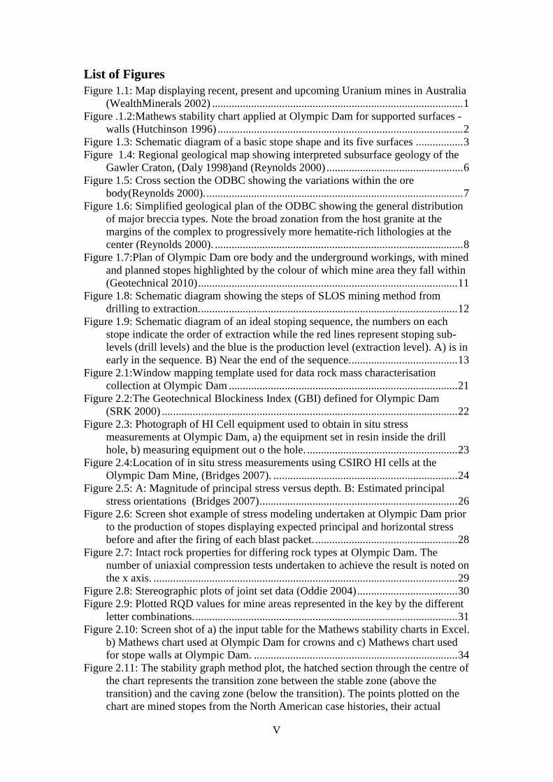
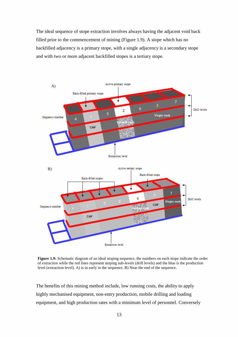
The ideal sequence of stope extraction involves always having the adjacent void back
filled prior to the commencement of mining (Figure 1.9). A stope which has no
backfilled adjacency is a primary stope, with a single adjacency is a secondary stope
and with two or more adjacent backfilled stopes is a tertiary stope.
The benefits of this mining method include, low running costs, the ability to apply
highly mechanised equipment, non-entry production, mobile drilling and loading
equipment, and high production rates with a minimum level of personnel. Conversely
A)
B)
Figure 1.9: Schematic diagram of an ideal stoping sequence, the numbers on each stope indicate the order
of extraction while the red lines represent stoping sub-levels (drill levels) and the blue is the production
level (extraction level). A) is in early in the sequence. B) Near the end of the sequence.

14
the downsides of the method include a significant amount of pre-production
development requiring a high inherent capital, stopes design requiring regular
boundaries for ideal extraction, dilution may occur consisting of waste or mine-fill
material, and the risk of insufficient breakage leading to ore production losses
(Villaescusa 2004).
Part of the SLOS mining method requires the backfilling of stopes following
extraction. At Olympic Dam this is done with cemented aggregate fill (CAF) and
waste rock individually, or a combination of both. There are two onsite batch plants
which apply specific recipes to define mixes of strengths varying from 0.5MPa to
4.5MPa.
The ingredients involved in batching CAF include:
Aggregate which is mined from the onsite quarry
Cement and flyash imported onto site
De-slimed tailings from the hydromet plant or dune sand (mined locally)
Water from an onsite dam.
1.5 Thesis methodology
At present there is no process at Olympic Dam, quantifying the performance of a
stope in comparison to its designed parameters, unless there was an issue with the
stope during production e.g. major over break, under break or freezing. In order to
quantify stope performance it needs to be clear what is expected of a stope for it to be
considered a success. As this thesis is focused on the Mathews stability method, it is
only concerned with the dimension of the final stope surfaces in comparison with the
design surfacee. This definition of instability is further discussed in Chapter Three.
To gauge the extent of inconsistency between the Mathews method predictions and
stope performance at Olympic Dam, all stopes completed prior to February 2009 that
met the data availability requirements had their performance reviewed. The
performance was quantified by the application of equivalent linear over break/slough

15
(ELOS) and classed as stable, unstable or failed. From the stability value a
comparison between design stability and actual was undertaken followed by an
investigation into some controls of stability specific to Olympic Dam.
There were 124 stopes included in the study; data for these stopes was collected from
the mine technical services department at Olympic Dam, using Datamine three
dimensional (3D) software, stope dimensions and final cavity survey data, combined
with the ELOS quantitative method to measure the performance of each surface of
each of stopes. The results of the back analysis lead to the classification of each
surface of the 124 stopes as stable, unstable or failed.
Part two of the study was focused on the generation of a possible new preliminary
stope design tool for Olympic Dam. The proposed solution applied the understanding
of stability indicators with an existing numerical model to forecast stope stability. The
method uses well defined criteria for instability and allows a series of points on each
stope surface to be considered as opposed to an overall stability classification for the
stope surface.
1.6 Thesis format
The outline of the thesis is as follows:
Chapter Two summarises the geotechnical characteristics of the Olympic Dam
ore body and earlier studies, followed by a literature review of the Mathews
stability method.
Chapter Three defines stope surface stability for the purpose of this study, and
the details of the methodology and results of investigating the Mathews
applicability at Olympic Dam.
Chapter Four discussed the results of the investigation, other alternative stope
surface design methods and possible improvements for the application of the
Mathews stability method at Olympic Dam.
Chapter Five discusses the mechanics of stability in regard to stability
indicators and introduces the application of modeled velocity as a stability
indicator to forecast stope surface stability at both Olympic Dam and other
mines.

16
Chapter Six summarises and concludes the thesis, including a section of
recommendations and subsequent work necessary to achieve an ideal outcome
at Olympic Dam.

17
Chapter 2. Mathews stability method at Olympic Dam
2.1 Introduction
Historically rock mass classification systems have been used to assist engineers
during feasibility and preliminary design stages of a project. As a whole they have
been evolving for over 100 years to achieve the most accurate result possible. Several
of the systems are based on civil engineering case studies and are continually being
adapted to incorporate underground mining case studies. As different systems use
differing combinations and have varying motives, it is important that the appropriate
system be applied for the project or problem at hand. Some of the common
classification systems, including the Mathews stability method, are briefly discussed
below.
2.1.1 Mathews Stability Method
The Mathews stability method has been applied for stope stability forecasting at
Olympic Dam throughout the mine‟s operational history. As stated in Chapter One the
Mathews stability method is an empirical measurement to forecast an open stopes
stability and is found by measuring a surface‟s material competency (N) and
hydraulic radius (HR).
As described by Barton et al (1974), the stability number N‟ is determined by
adjusting the rock tunnelling quality index (Q) value to allow for induced stresses,
discontinuity orientation and the orientation of the excavation surface (Equation 2.1):
N‟ = Q‟ x A x B x C Equation 2.1
where Q‟ is the modified Q-Value, A is the stress factor, B is the joint orientation
factor and C is the surface orientation factor.
The hydraulic radius (HR) is the consideration of the surface geometry, and is
calculated by dividing the area of a stopes surface by the length of its perimeter
(Mawdesley 2004). The N‟ and HR values form the two axes of a chart which has its

18
area divided into three categories (stable, transition, caving), showing the predicted
performance of a stope surface.
2.1.2 Rock Quality Index
The Tunnelling Quality Index (Q) is of particular relevance in this study as it forms
the basis of the Mathews stability number. From a growing underground excavations
database Barton et al. (1974) generated the Q index for the determination of rock
mass characteristics and tunnel support requirements.
The index considers geological, geometric and design/engineering parameters (Hoek.
E. 1997). The resulting values range on a logarithmic scale from 0.001 to 1,000, as
defined by (Equation 2.2) (Hoek 2006):
Q = RQD/Jn x Jr/Ja x Jw/SRF Equation 2.2
Where
RQD is the Rock Quality Designation
Jn is the joint set number
Jr is the joint roughness number
Ja is the joint alteration number
Jw is the joint water reduction factor
SRF is the stress reduction factor
Once the Q value is calculated it can be used to assess the overall condition of the
rock mass and assist in choosing a basic support system. The classification of the
individual parameters used to define Q is located in Appendix B.
2.1.3 Other classification systems
A descriptive classification system was first developed by Terzaghi (1946). This is
based on a rock load concept whereby loads are transferred from crown to sidewalls,
and it was initially developed for steel set supports in tunnels. It recognises seven
classes of rock (intact, stratified, moderately jointed, blocky and seamy, crushed,
squeezing and swelling) and briefly describes the appearance of each.

19
In 1967, Deere et al (1967) developed the rock quality designation (RQD) to
quantitatively estimate rock mass quality from drill cores. This defined RQD as the
percentage of intact pieces of core that are longer than 100mm in the total length of
the core (Deere 1967). RQD has since been integrated in other classification systems
and is applied as part of rock mass classification at Olymic Dam.
One classification utilising RQD in its calculation is the Geomechanics Classification,
or more commonly known as the rock mass rating (RMR) system. Initially created in
1973, the system is based on the strength of the material, RQD, spacing condition and
orientation of discontinuities, and groundwater conditions. A value is allocated to
each of these parameters and the final result is the sum of the values. The original
system was not well regarded by the mining industry, resulting in several
modifications, as summarised by Bieniawski (1989). The mining version of the
Geomechanics classification, mining rock mass rating (MRMR) system is commonly
applied to underground caving operations.
Other well-known classification systems include the Rock Structure Rating (RSR)
and Lauffer‟s stand-up time concept (Hoek 2006).
2.2 Geotechnical Data Collection
2.2.1 Rock mass data collection
The Olympic Dam ore body rock mass characteristics have been determined through
a combination of underground data collection, laboratory examination and computer
analysis. The primary underground data collection method is window mapping.
Window mapping is conducted underground by members of the Geotechnical
Department and SRK consultants (SRK) who were employed to generate a database
of the rock mass conditions at Olympic Dam. The windows are undertaken on
stretches of rock around 20 to 30m long. A window is generally located close to an
upcoming stope, providing data for the stope note analysis.

20
The mapping utilises a template log sheet (Figure 2.1) to observe and record the
structures within the rock mass. The data collected as part of this process includes:
Prominent rock types
Extent of alteration
Presence of any weathering
Groundwater conditions
Blockiness values
Estimates of intact material strength
Any blasting effects
Potential mode of failure
Installed ground support
Rock mass discontinuity data
Any other relevant or interesting comments
As is often found in data collection, there is an element if subjectivity in the
classification of the rock mass. The data which is recorded is dependent on the
experience and opinnion of the engineer. However the template log provides a process
in order to minimise the degree of subjectivity.
SRK has developed a blockiness index to describe in general terms the rock mass
conditions. This index has been developed from approximately 300 completed
windows and gives areas of rock a numeric classification between 1a and 8a (Figure
2.2).

21
Mapped By:
Window length: Face Orientation: 90 / (dd)
Rock Type: RQD (%):
Dip Dip Dir Dip Dip Dir
Alteration: Mineralized: Y / N
Weathering: Groundwater Conditions:
Blockiness: Min (m 3 )
Intact Material Strength (IRS)% Weak: IRS (MPa): Material:
% Strong: IRS (MPa): Material:
Blasting Effects:
Mode of Failure: (eg. Hor/Sub-Hor/Vert Slabbing vs Blocks & Wedges)
Support:
Comments:
Dip Dip Dir Min (m)
Length (m) Ends
Dip / Strike Dip / Strike
Avg (m 3) Max (m 3 )
Type
ONLY IF DISTINCTLY DIFFERENT
Set
No
Orientations Orientations
Thickness
(mm)
Set
No
Type
FIELD LOG FOR ROCK FACE MAPPING (Olympic Dam)
Set No
Set
No
Site Location:
Roughness
Blocky
SpacingAv. Orientation
Str/Mod/Wk
Massive
Micro:
Date:
Joint Wall Strength:
Rock Mass Discontinuities:
Continuity Range
Friable
Max (m)Mean (m)
PLANAR:
UNDULATING:
Joint InfillingJoint Wall
Hardness
Macro:
Micro Macro
STEPPED / IRREGULAR:
EXPOSED LENGTH100mm (SEE FIGURE)
1:Polished 2:Smooth 3 :Rough
4:Slickensided 5:Smooth 6 :Rough
7:Slickensided 8:Smooth 9 :Rough 3: Jt wall hardness < Rock hardness
1-Straight 2 -Slight undulation
3 -Curved 4-Uni directional wavy
5-Multi directional wavy
1: Jt wall hardness = Rock hardness
2: Jt wall hardness > Rock hardness
Convention:
Figure 2.1:Window mapping template used for data rock mass characterisation collection at
Olympic Dam

22
Figure 2.2:The Geotechnical Blockiness Index (GBI) defined for Olympic Dam (SRK
2000)

23
2.2.2 Stress measurements
Stress measurements have been conducted at Olympic Dam since the commencement
of mining, with the most recent measurements being those undertaken by Australian
mining consultants (AMC) in 2007. The database consists of 17 measurements that
were collected using a CSIRO Hollow Inclusion (HI) Cell (Figure 2.3). 16 of the
measurements were taken in the granite and one in the overlying sediments (Figure
2.4). The HI Cell consists of an array of strain gauges encapsulated in the wall of a
hollow pipe with a known elastic modulus. The cell is epoxy grouted into a borehole
and monitored for strain response during over-coring.
The AMC report, “In situ stress field for Olympic Dam mine” (Bridges 2007) stated
there is no evidence of any sectors within the mine where directions of principal stress
are significantly different from the estimated mean orientations by either northing or
by depth. This allows the 17 measurements to provide the generic stress
measurements for the mine. The present study only discusses the 16 readings from
within the granite because there is no current mining undertaken in the sedimentary
rock.
a)
b)
a)
b)
Figure 2.3: Photograph of HI Cell equipment used to
obtain in situ stress measurements at Olympic Dam, a)
the equipment set in resin inside the drill hole, b)
measuring equipment out o the hole.

24
Figure 2.4:Location of in situ stress measurements using CSIRO HI cells at the Olympic Dam
Mine, (Bridges 2007).

25
2.3 In situ stress fields – Granite
2.3.1 Principal in-situ stress field
Directions of intermediate and minor principal stresses spread around a great circle
normal towards the mean direction of the cluster of major principal stresses. Using the
small clusters and the results from vector summations, allowing for orthogonality,
AMC estimated mean directions for principal stresses for granite. For the granite
breccia complex the estimated in situ stresses are detailed in Table 2.1.
In table 2.1 the in-situ stress directions are represented as a bearing and plunge, as
referenced to the mine-planning grid. The mine grid north is 57.5 degrees west of
AMG north. AMG north is 1 degree west of true north. Plunges are positive
downwards (right handed system).
At Olympic Dam, the granite-breccia lies at a minimum depth of 330m below the
ground surface. AMC estimated the depth-stress relationship at each of the mean
directions of principal stresses, as shown in Table 2.2 (Figure 2.5).
037/72 Minor principal stress
224/18 Intermediate principal stress
133/02 Major principal stress
Table 2.1:Principal in-situ stresses in the granite at Olympic Dam

26
0+0.033*D MPaMinor principal stress
2+0.036*D MPaIntermediate principal stress
6+0.041*D MPaMajor principal stress
Table 2.2: Estimated depth-stress relationship at each of the mean principal stresses
Where D is the depth in metres below the ground surface, and respective directions of the major,
intermediate and minor principal stresses are the mean directions above (Table 2.1).
Figure 2.5: A: Magnitude of principal stress versus depth. B: Estimated principal stress orientations
(Bridges 2007)
A B

27
2.3.2 Effect of Mining Induced Stress in Excavation stability
A stope blasting has the potential to increase the stope dimensions and subsequently
reduce the rock pillar to a neighbouring stope. Stress concentration through the
remaining rock is then vulnerable to elevation. This can potentially result in drill drive
deterioration, stope over break and fall-off, longhole squeezing and an increased
likelihood of requiring re-drilling.
After the 2007 stress measurements were collected and analysed it was noted on a
mine-wide scale that there is a clear inter-relationship between stress and geologic
structures in the natural state of the rock prior to disturbance by mining. As mining
occurs, the interaction between stress and geologic structures redistributes those
stresses sometimes with serious adverse outcomes to stoping activity. The rock mass
around these structures will potentially become unstable.
At Olympic Dam, mining induced stress change is modelled with Map3D (Figure 2.6)
via stope note and pre-production reporting. However there is no instrumentation in
place to physically measure this stress change.Although not directly measured,
engineers often look at deformation or damage around voids and interpret them as
being caused by mining induced stress changes. They then use the location of the
damage to make an “educated guess” as to how the stress field is changing. Although
not ideal, this method appears valid on a broad scale.
It is difficult for Olympic Dam to verify the success of educated guesses. This is as
there is no investigation of the stress and mining induced changes except for where
problems are encountered during the stoping process. Such problems include over
break in a stope wall, or damage in a drive near a stope stress analysis. When these
occur stress analysis is undertaken as part of the investigation into the stope
performance.

28
Figure 2.6: Screen shot example of stress modeling undertaken at Olympic Dam
prior to the production of stopes displaying expected principal and horizontal
stress before and after the firing of each blast packet.
2.4 Intact rock strength at Olympic Dam
During the feasibility stages of the Olympic Dam operations it was determined
through a series of laboratory and in situ strength examinations, that the majority of
the granite breccia rock types have an average UCS50 of around 150MPa with a
standard deviation of 75MPa. The large standard deviation suggests a high percentage
of the samples tested must have failed by shearing on microstructures or weaknesses
that pervade the Olympic Dam intact rock. It can be inferred that similar behaviour
will occur around openings throughout the mine, particularly in the small Granite-
volcaniclastic (GRNV) deposit portion. Rock strength properties for all Olympic Dam
lithologies are located in Appendix D.

29
Figure 2.7: Intact rock properties for differing rock types at Olympic Dam. The number of uniaxial
compression tests undertaken to achieve the result is noted on the x axis.
Table 2.3:Rock mass quality Properties for Olympic Dam (BHPBilliton 2010)
2.5 Rock mass Quality Classification
Rock mass quality has been determined using the geotechnical underground window
mapping information, assisted by underground observations, with the rock tunnelling
quality index (Q index) applied to allocate a value to the rock mass. From the window
mapping and blockiness index analysis, Olympic Dam was found to have a range of
characteristics.
As described earlier the Q index is based on block size and the joint and stress
conditions of the rock. The Q factor values for Olympic Dam are summarized in
Table 2.3.
The Q-system parameters are discussed below in regard to Olympic Dam specific
values.
30
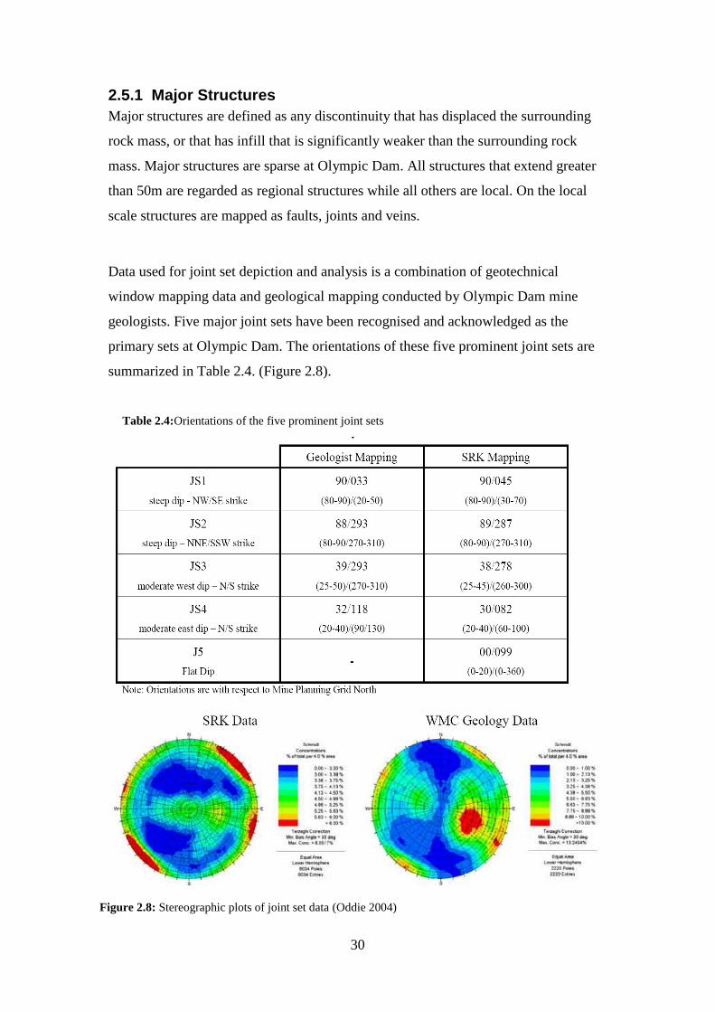
2.5.1 Major Structures
Major structures are defined as any discontinuity that has displaced the surrounding
rock mass, or that has infill that is significantly weaker than the surrounding rock
mass. Major structures are sparse at Olympic Dam. All structures that extend greater
than 50m are regarded as regional structures while all others are local. On the local
scale structures are mapped as faults, joints and veins.
Data used for joint set depiction and analysis is a combination of geotechnical
window mapping data and geological mapping conducted by Olympic Dam mine
geologists. Five major joint sets have been recognised and acknowledged as the
primary sets at Olympic Dam. The orientations of these five prominent joint sets are
summarized in Table 2.4. (Figure 2.8).
Figure 2.8: Stereographic plots of joint set data (Oddie 2004)
Table 2.4:Orientations of the five prominent joint sets

31
Figure 2.9: Plotted RQD values for mine areas represented in the key by the different letter combinations.
Table 2.5: Summary block size for Olympic Dam mine (Oddie 2004)
2.5.2 Block size
Block size at Olympic Dam is calculated using the volumetric joint count (Jv)
method. This represents the number of joints per unit length for all joint sets and is
detailed in Appendix E. A slight variation in RQD values exists across the mine, with
the Northern mine end having a wider spread of values than the southern end (Figure
2.9). This variance is not significant enough to suggest that individual RQD values
should be used for each section of the mine in analysis.
The joint set number (Jn) is a measurement of joint orientation in a rockmass that is
judged to influence the stability of an opening. In order to provide a rating system for
the rock quality throughout the mine a summary of the different qualities is
summarised in Table 2.5.

32
2.5.3 Joint surface condition
Joint roughness (Jr) and Joint alteration (Ja) are the two controlling parameters that
describe the shape and integrity of the joint surface. They are used to quantify the
joint surfaces resistance to shearing.
The joint shapes at Olympic Dam are predominantly “rough planar” but range from
“rough undulating” to “smooth planar”. The surfaces are generally unaltered,
although with some “surface staining” of sericite, chlorite or salt build up.
Occasionally they have a thin coating of less than 5mm of non-softening infill
material. A summary of the joint characteristics of each of the five major joint sets is
further detailed in Appendix E.
The roughness and level of alteration have been quantified. This showed all joint sets
have similar properties with the only difference being in the joint alteration. Joint
roughness values average between 1 and 1.5 while the worst joint alterations were
around 3 and 4 (Table 2.6).
Table 2.6: Summary joint surface conditions for Olympic Dam rock mass (Oddie 2004)

33
2.6 Design process
A rigorous design process is critical for safe and successful sub level open stope
(SLOS) mining, with input required from Geological, Geotechnical, Survey and
Engineering departments. The stope design process at Olympic Dam involves
numerous reviews and assessments in order to ensure adequate stability coupled with
maximum production.
There are various stages in the design process involving geotechnical input. Initially a
front review is conducted. This evaluates the effectiveness of the sequence in order to
produce a workable plan for a mine area. This is followed by the preliminary stope
design where the conceptual design of the stope is revised. At this stage it is critical to
correctly size and shape the stope based on the areas mining sequence.
The next stage involves the most significant amount of quantitative analysis of the
rock mass. This analysis is done both in and adjacent to the stope with results driving
the stope design. At this stage the Stability Graph Method is used to assess the
stability of the stope spans all the data is entered into an Excael spreadsheet which
returns a Mathews plot for the crown and one for the walls (Figure 2.10).
The stability graph method works by applying all of the above collected geotechnical
properties. Prior to the commencement of production drilling a pre-ring preview and
pre-production assessment are undertaken. These review any recent ground control
issues and identify any geological structures that have potential to influence interim or
final stability. At this stage a stress model is run, analysing the potential influence of
structures on each of the blast packets. This influence is investigated by visual
analysis.Any changes to stope design identified through the above analysis are
processed at this point. The stope assessment is then closed out, allowing production
to commence.

34
a)
b)
c)
Figure 2.10: Screen shot of a) the input table for the Mathews stability charts in Excel. b) Mathews
chart used at Olympic Dam for crowns and c) Mathews chart used for stope walls at Olympic Dam.
All of the above stages and the associated information are compiled into a document
called a “stope note”. A stope note details the entire process and includes the
preliminary study. Other aspects include the geological background, geotechnical
parameters, development design, services design, ventilation plan, drilling and
blasting, and backfilling notes.

35
2.7 Mathews stability method
2.7.1 Background of the Mathews stability method
Historically empirical civil engineering tools have been applied to open stopes, often
resulting in a conservative design. This design is predominantly due to stopes being
non-entry areas that allow for a limited amount of fall off . Over time it became clear
that no single index is an adequate indicator of the complex behaviour of a rock mass
surrounding an underground excavation (Hoek 1990).
Initially designed in 1980, the Mathews method answered the requirement for a more
lenient tool for large excavations. It soon became a popular choice, particularly in
metaleferous mines, as a preliminary guide to stope dimensioning. The Mathews
stability method is an empirical design tool with the original version being based on a
restricted data collection from case studies based primarily in North America. It has
been revised numerous times since its creation, resulting in the addition of further
data now making up the graph. The principal concept of the method is that the size of
an excavation surface can be related to the rock mass competence. This gives an
indication of stability or instability of a rock mass(Stewart 2001).
The Mathews method provides users with an indication of the likely performance of
underground excavations by plotting them on a chart. It is based on a stability graph
which relates two calculated factors; the Mathews stability number (N‟) and the
hydraulic radius (HR). The Mathews stability number is a function of rockmass
quality, stress, structural orientation and the likely mode of failure, while the
hydraulic radius accounts for the size and shape of the surface. For a typical
rectangular excavation there will be five surfaces, four sidewalls and the crown/back.
The stability graph deals with each of these individually, allowing the five surfaces to
fall within different predicted stability zones.
The differing zones on the graph were initially devised by Mathews from 50 case
histories compiled from North American mining data (Figure 2.11). The stability of a

36
planned excavation was then represented by where it was plotted on the graph. The
original three zones were stable, potentially unstable and potential caving. Each zone
was divided by transitional zones, reflecting the transition and uncertainties of the
boundaries.
2.7.2 Modified stability number N’
The stability graph uses the modified stability number, N‟, as described by Potvin
(1988b,1992), Bawden (1993) and Hutchinson (1996) to classify the rock mass.The
Modified stability number is a modified version of the rock tunnelling quality index
value (Q), as discussed earlier. The Mathews stability number is generated by
adjusting the Q‟ value to allow for induced stresses, discontinuity orientation, and the
orientation of the excavation surface.
Figure 2.11: The stability graph method plot, the hatched section through the centre of the chart
represents the transition zone between the stable zone (above the transition) and the caving zone
(below the transition). The points plotted on the chart are mined stopes from the North American
case histories, their actual performacne is represented by the shap of the point as depicted in the
key (Potvin 1988b).

37
The stability number (N‟) is defined by Equation 2.1:
N’ = Q’ x A x B x C (Equation 2.1)
where;
Q’ is the modified Q-value,
A is the rock stress factor,
B is the joint orientation adjustment factor,
C is the gravity adjustment factor.
(Hutchinson 1996)
The rock stress factor, A, is a measure of the ratio of intact rock strength to the
surrounding stress. As the maximum compressive stress acting parallel to a free stope
face approaches the uniaxial strength of the rock, factor A reflects the related
instability due to rock yield.
Factor B measures the relative orientation of the primary joint set in relation to the
excavation surface. Those forming an oblique angle with the free face are most likely
to become unstable. Conversely joints that are perpendicular to the free face are taken
to have the least influence on stability.
The gravity adjustment factor C, represents the potential influence of gravity on the
stability of the face. Crowns (backs) or unfavourably oriented structural weaknesses
have the maximum influence on potential instability (Hutchinson 1996) (Figure
2.12).

38
2.7.3 Hydraulic radius
The hydraulic radius (HR) measures the combined influence of the size and shape of
the face on excavation stability. The HR is calculated by dividing the area of the stope
face by the perimeter of that face, shown by Equation 2.3;
HR = Area (m²) = w x h (Equation 2.3)
Perimeter (m) 2(w + h)
where
w is the width of the surface
h is the height of the surface (Figure 2.13)
Figure 2.12: Input parameters for the Mathews stability number (Diederichs & Kaiser 1999)

39
This calculation differs from those used in other classification systems particularly
those of tunnels as it is calibrated for open stopes with finite dimensions and lower
priority for safety. It should be remembered that the shape factor of the hydraulic
radius is not dimensionless but is expressed in metres (Stewart & Forsyth 1995).
2.8 Evolution of the stability graph
The origins of rock mass classifications lie primarily in civil engineering, and in
particular tunnel engineering. It has become evident to many in the industry that a
mining specific excavation design tool was needed to replace the tools designed
primarily for civil and tunnel engineering. A mining-specific tool was seen as being
able to minimise cost and maximise production in underground mines.
In 1980, Mathews, Hoek and Wyllie devised the original stability zones and graph.
This empirical solution was published as part of a CANMET report on stope stability
in deep Canadian mines. During the initial stages of the method‟s application in
underground excavation projects, it became apparent that there was limited field data
supporting the method. This was a result of its design being based on only 50 case
histories.
The period since 1980 has allowed the tool to be tested for varying depths and rock
mass conditions by numerous authors .This has significantly extended the validity of
the tool. Such tests include those by Potvin (1988b), Stewart & Forsyth (1995),
Trueman et al.(2000) and Mawdesley (2001). As the method became more widely
Figure 2.13: Simplified two-dimensional diagram showing the width and
height inputs for a) stope walls and b) stope crowns

40
applied the database was expanded allowing adjustments to be made to the overall
layout of the zones, thereby reducing an element of the method‟s subjectivity.
The stability graph is defined by zones originally determined by visually fitting
boundaries between clusters of data representing stable and unstable stope surfaces,
and between the unstable and caved stope surfaces. The mined stope surfaces are
defined as stable or unstable after they have been emptied by examining final cavity
monitoring survey data with repsect to the designed stope shape. The zone enclosed
by the boundaries contains a mixture of stable, unstable and caved stopes. This is
labelled the transition zone (Suorineni et al. 2001a).
Subsequent studies have resulted in considerable change to the placement of the
original boundaries. These changes are due to the accumulation of additional data,
through the re-definition of the stability number, by calibrating boundaries to mine
site specific data, the mixing of data from differing versions of the stability number
and through human bias.
Potvin (1988b) expanded the original database from 50 to 175 case histories. The
enlarged database resulted in the re-calibration of factors A, B and C. Accompanying
this was a redefinition of the boundaries between stability states.
Literature subsequent to these changes, such as that by Stewart & Forsyth (1995) and
Trueman et al.(2000) noted that the modifications to the calculation of the stability
number resulted in no appreciable difference in the methods predictive capability.
Consequently the advances were not universally adopted. Note that there is a
distinction between those databases based on Potvin‟s definition of the stability
number and those based on the original Mathews factors. This is as the different
definitions varying transition boundaries between stability states.
Amongst other changes made by Potvin, the number of zones plotted on the graph
was reduced. Potvin‟s changes left the graph with simply a stable and a caved zone,

41
with a transition zone separating the two zones. Nickson (1992) later extended this
transition zone to incorporate a larger area of the plot.
The choice of the term „caved‟ has been subjected to much criticism Stewart &
Forsyth (1995) noted that the term has a definite meaning in the mining sense that is
not consistent with what it represents in Potvin‟s modified graph. They also noted that
the graph implies too great a level of accuracy as it only uses two zones. Stewart and
Forsyth (1995) suggested that new zones be allocated to the graph. These zones were
potentially stable, potentially unstable, potential major collapse and potential caving.
The zone of potential caving by Stewart and Forsyth was based on Laubscher‟s
caving stability graph (Laubscher 1990). They had no data themselves to validate this
zone, instead relying on Laubscher‟s work (Figure 2.14). Recognising this, Stewart
and Forsyth recommended that the user build their own experience and define their
own site-specific zones on the graph, rather than arranging data to arrange it to fit the
provided zones.
Historically simply visually identifying where the zones should lie was the used to
define the location of stability zones on the Mathews graph. These zones were
modified with the addition of new data. As the position of these zones on the graph is
crucial in the reliability of the method, an alternate method was sought to optimise the
locations of the zones.
Mathematical calculations were found to be a satisfactory alternative to visually
defining the location of the stability zones. Mathematical calculations were used to
identify the zones widths and positions. This is further discussed in Chapter Four. It
must be noted that the stability graph method remains a non-rigorous method.

42
The focus of these developments is in defining the stability graph boundaries and
recalibrating existing factors. There is no longer any justification in the use of the
original method. As has been shown to be the case with Mathews, empirical design
methods can evolve and improve over time with the availability of additional data and
increased experience with the method.
Figure 2.14 Comparison of the different stability graphs (Stewart & Forsyth 1995)

43
2.9 Application of the Mathews stability method at Olympic Dam
The Mathews stability method has been applied to stope design at Olympic Dam since
the mine was first commissioned. The method is used to provide the underlying
stability analysis for future stopes and is based on where surfaces plot on the relevant
charts. The version applied at Olympic Dam is obtained from “Cablebolting in
Underground Mines” (Hutchinson 1996). This particular model differs between un-
supported walls, supported crowns and unsupported crowns.
As explained the stope design process at Olympic Dam is compiled into a package
called “stope notes”. The package includes geological data and interpretation,
geotechnical parameters, adjacent development, firing design and sequence along
with ventilation and services plans. The modified stability graph is a key part of the
geotechnical investigation.
The walls are plotted on the unsupported case histories chart, while the crown is
plotted on the supported case histories chart. In the past the crown was plotted on both
the unsupported and supported charts to determine whether crown cable bolt support
was required. As crown cable support is now mandatory at Olympic Dam the
unsupported plot is no longer performed. There is little variation in the parameters
applied across the mine area with this technique.
The unsupported chart (Figure 2.15), published in “Cablebolting in Underground
Mines”, is calibrated from a study of 175 case histories by Potvin (1988a) and another
13 by Nickson (1992). They plotted stopes whose performance was already known as
stable, those which exhibited little or no deterioration during their service life,
unstable stopes which exhibited limited wall failure and/or block fallout involving
less than 30% of the face area, and caved stopes which suffered unacceptable failure.
From these plotted case studies they were able to generate the boundaries between the
stable, transition and caving zone. The upper boundary of the transition zone is
recommended as the “no support” limit for design (Hutchinson 1996).

44
Potvin (1988a) and Potvin & Milne (1992)also collected 66 case histories of open
stopes in which cablebolt support had been used. Nickson (1992) added another 46
case studies to the supported case histories chart (Figure 2.16). Similar to the
unsupported wall open stope case history chart, this displays a transition zone with the
upper curve represents the limit of reliable cablebolt performance. The lower
boundary reflects the reduction in confidence until cables can no longer be assumed to
be providing any degree of useful support (Hutchinson 1996).
Figure 2.15: Unsupported case histories stability chart used for stope
wall stability assessment at Olympic Dam (Hutchinson, 1996).

45
Other charts presented in “Cablebolting for Underground Mines” which are used at
Olympic Dam assist with the determination of cablebolt reinforcement requirements
(Figure 2.17). The chart allows the user to determine, from a calculated value or range
of N‟, the maximum recommended stope size and shape for an unsupported or
supported case. With non-entry conditions applying if a stope plots well above the left
or uppermost design curve, it is predicted to remain stable without the assistance of
support. Conversely a stope which plots far into the right hand section of the graph is
likely to undergo serious instability issues. The cablebolt design zone indicates the
need and effectiveness of cablebolt application (Hutchinson 1996).
Figure 2.16: Supported case histories stability chart used for stope crown
stability assessment at Olympic Dam (Hutchinson, 1996).
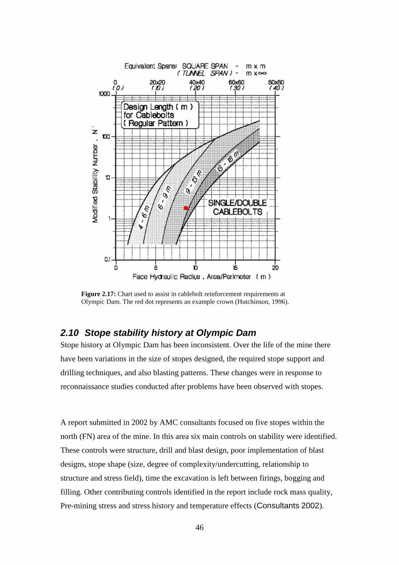
46
2.10 Stope stability history at Olympic Dam
Stope history at Olympic Dam has been inconsistent. Over the life of the mine there
have been variations in the size of stopes designed, the required stope support and
drilling techniques, and also blasting patterns. These changes were in response to
reconnaissance studies conducted after problems have been observed with stopes.
A report submitted in 2002 by AMC consultants focused on five stopes within the
north (FN) area of the mine. In this area six main controls on stability were identified.
These controls were structure, drill and blast design, poor implementation of blast
designs, stope shape (size, degree of complexity/undercutting, relationship to
structure and stress field), time the excavation is left between firings, bogging and
filling. Other contributing controls identified in the report include rock mass quality,
Pre-mining stress and stress history and temperature effects (Consultants 2002).
Figure 2.17: Chart used to assist in cablebolt reinforcement requirements at
Olympic Dam. The red dot represents an example crown (Hutchinson, 1996).

47
In November 2004 AMC consultants performed a Stability Graph Back Analysis with
similarities to the basis of this study. The performance of 92 stopes was used to
investigate the confidence that can be placed in the Mathews stability method for the
design of open spans at Olympic Dam. Of the 271 stope wall surfaces included in the
study 176 (65%) were stable, 78 (29%) unstable and 17 (6%) had failed.
To determine stope effectiveness performance was compared with predicted stability.
In relation to the wall surfaces it was concluded that only 10% of the stope walls were
in the recommended design zone (unsupported stable zone). 65% of walls were
deemed stable, 29% unstable and 6% failed. The performance was based on the
examination of the final cavity survey and the design shape of the stope. The design
limit of N‟ = 0.03xHR3 should give an 80% chance of stability, a 20% chance of
minor over break and no chance of failure. It was concluded that more stope history in
the stable and transition zones were needed to increase confidence in this line.
(Consultants 2004).
When looking at crown surfaces, AMC concluded that 95% of the stope crowns were
designed in the stable zone and only 50% remained stable. They found 40% of the
crowns to be influenced by major structures or the unconformity. Of these only 17%
remained stable. Of the 52 acceptable case histories, 28 were supported (cablebolted)
and 24 unsupported. The supported crowns were stable in 83% of cases.
The AMC report contained various other general conclusions. They found that
calculating the rock stress factor A using methods that consider the influence of low
stress did not improve the reliability of the Stability Graph method. They found some
existence of time-dependent stope failure at Olympic Dam, but decided further
investigations would be required to define this relationship.
In their conclusions AMC stated that Eastern walls have a higher rate of instability,
while stopes in the FN have shown poorer performance than other areas of the mine.

48
There was no strong correlation between rock type or alteration with surface
performance. However there appears to be threshold at which low HR values indicate
stope surfaces displaying improved stability. For walls this threshold was HR = 10
and for supported crowns HR = 6.
AMC also conducted a further study at Olympic Dam to determine the design
practices having a significant influence on the stability of crowns, those determining
the length and support capacity requirements for crown cablebolts and recommending
design guidelines to help achieve stable stope crowns. These aims were addressed by
reviewing the performance of 87 stope crowns at Olympic Dam. This report reiterates
that the three main controlling factors on stope crown stability are the distance from
the unconformity, cablebolting and crown shape.
The unconformity at Olympic Dam which separates the cover sequence and the
breccia lies at 240mRL. If the distance between the unconformity and the crown of
the stope is less than the width of the stope, the distance is considered to affect the
stability of the crown. The shape of the crown was also determined to be a key
influence in the stability of the crown. A crown with an arch shape was found to be
the most stable, while those that were stepped in/out being more likely to result in
failure.
2.11 Synthesis
The Mathews stability method has been applied during the preliminary design process
at Olympic Dam for over twenty years. The version of the method which is currently
applied is sourced from Hutchinson‟s (1996) “Cablebolting for Underground Mines”.
The database of rock mass characteristics at Olympic Dam that provides the input
parameters for the Mathews stability method is continually developing with window
mapping data collection an ongoing process.
Previous studies at Olympic Dam have indicated there are inconsistencies between the
Mathews stability method predictions and the actual performance of stope surfaces. In
order to validate this, the next Chapter compares the predictions and performances of
individual stope surfaces.

49
Chapter 3. Validating the Mathews stability method
application at Olympic Dam
3.1 Introduction
Open stope performance is measured by the ability to achieve maximum extraction
with minimum dilution (Villaescusa 2004). The following stope performance review
focuses only on the shape of the final excavation. The size and quality of ore
reporting to the draw points is not in the scope of this thesis.
Since commencing extraction at Olympic Dam, it has been acknowledged there are
significant issues with the accuracy of the Mathews stability method. This is generally
the case with any empirical method. This has implications for both safety and
production. These inconsistencies were not previously quantified and therefore the
extent of the problem was unknown. Predicted stope surface performance needs to be
calibrated against actual performance to understand the validity of the predictive
method.
This study is concerned with the performance of the individual surfaces of each stope.
This includes the crown and the side walls. The performance is quantified solely on
the amount of over break on each surface. For open stopes, over break can be thought
of as any unplanned sloughing or loss of rock from the stope walls or crown. This is
not to measure further or potential instability but the performance of the stope at the
time of the cavity monitoring survey. Over break is any point inside the actual mined
void which is outside the design shape of the stope.
Because it is likely that most surfaces will have over break to some extent, over break
has been quantified using the equivalent linear over break/slough (ELOS) method.
This method provides a simple number categorising the extent of over break. This is
further discussed in the Methodology section of this Chapter.

50
3.2 Quantifying Mathews stability applicability at Olympic Dam
3.2.1 Methodology
The first objective of this study was to validate the accuracy of the Mathews stability
method at Olympic Dam. This is done by completing a back analysis study on mined
stopes that were designed and blasted prior to February 2009. These results have then
been compared with the Mathews stability analysis component of the stope design.
Once this validation was complete any existing relationships between stability and
selected parameters, such as the area of the mine the stope is located in, the size of the
stope were considered.
The validation involved the following steps:
1) Selection of appropriate stope case histories
2) Data collection and measurement
3) Analysis of the data collected
These steps enabled the effectiveness of the Mathews stability method to be
quantified at Olympic Dam. Quantifying the effectiveness is a key step in being able
to define the major controls of stope over break and collapse. Quantification also
enables the identification of trends in stope performance and helps determine what
improvements are required.
All data was collected from the Olympic Dam working database. This included the
preliminary stope assessment, production tracking data and the post-production cavity
monitoring survey.
A poor correlation between the Mathews stability method‟s predictions and actual
stope performance was expected.

51
3.2.2 Stope case selection
The stopes analysed were obtained from a database provided by the Production-
Tracking Department at Olympic Dam. The names and dates of all stopes developed
since January of 1997 were provided. The requirements for a stope to be included in
the study were:
1) Stope completed and backfilled prior to February 2009
2) Crown cablebolted
3) All digital wire frames available
4) Stope note data available
5) Final cavity monitoring survey available
For inclusion in the study the stopes must have been completed prior to February
2009. This is the date the present study was commenced. Crowns are also required to
be cablebolted prior to this date as this has become a mandatory practice at Olympic
Dam. The remainder of the inclusion requirements represent data availability.
The stopes which met the selection included:
124 crown surfaces;
396 rock wall surfaces; and
100 CAF adjacent wall surfaces
3.2.3 Data collection
The stope notes were a primary source of information. These provided Mathews
stability method information on the stope as well as other background material.
Datamine, a 3D design software package, was applied to look at each stope. This
provided a 3D image giving the geometry of each surface.
Each surface of each of the 124 stopes was individually examined. The performance
of each surface was then classified as stable, unstable or failed. To ensure consistency
across the data range over break was calculated using ELOS, as described by Pakanis
(1996).

52
Figure 3.2: Simplified two-dimensional explanation of ELOS.
Adequate stope performance from a stability perspective is difficult to define. ELOS
is a simple method for expressing volumetric over break. It works by converting the
actual over break, usually varying depths over a well defined portion of the stope face
(Figure 3.2), into an average depth spread equally over the entire stope face (Figure
3.1). The following equation (Equation 3.1) displays how the ELOS of a stope surface
is calculated.
ELOS = Volume of Over break / Area of stope face Equation 3.1
= (Average depth of over break x Area of over break) / Area of stope face
Stope design shape
Over break
Figure 3.1: Simplified two-dimensional diagram of over break area on a stope surface

53
To quantify the ELOS results, the criteria listed in Table 3.1 were used:
Table 3.1: Quantification of ELOS values
ELOS Stability Rating Explanation
0 – 0.75 Stable Little or no deterioration
0.75 – 2.0 Unstable Minor failure
> 2.0 Failed Unacceptable failure
It is important the use of the word “failed” is not miss-interpreted. For the use in this
study the meaning is not that the stope or stope surface has entirely collapsed and is
un-usable. Instead the word represents the stope surfaces that have over break that has
an ELOS value greater than two.
This stability rating discounts the tonnage and grade of the final stope. It simply
quantifies the volume of rock over broken.
At Olympic Dam, a cavity monitoring survey is taken of all stopes once they have
been bogged for void and prior to the commencement of CAF backfilling. This is an
effective diagnostic tool that provides a 3D image of the “actual” shape of the stope.
The cavity monitor is a laser device that computes a 3D shape for the void with high
precision, allowing a direct comparison of the actual achieved shape with the planned
shape.
To calculate the ELOS for each stope surface, the cavity monitoring survey wire
frame was overlain the stope design wire frame in Datamine, allowing a comparison
between the two. Following this, slices were taken along the face to determine the
area of the stope face and the area of the over break. Slices taken perpendicular to the
face, along a plane indicating a fair cross section of the over break depths, were used
to measure the average over break over an average face cross section gives indicative
over break values (Figure 3.3). These values were then manipulated using the ELOS

54
calculation to provide a final over break value for each surface of the stope.
Calculations were also completed for CAF faces, although there is no pre production
assessment to compare these results with.
All ELOS values were calculated using the same technique, and judgment, to
maintain consistency. The standard design of wire frames in the database has a
control on the consistency of the analysis. Some were a combination of blast packets
while others were the full design. Stopes that were not simple shapes proved more
difficult to measure.
ELOS was used as to quantify over break, due to its straight forward nature and easily
comparable results. Its only drawback is that it does not make the distinction between
localised versus widespread over break. It is important to remembre ELOS is
representing the stope surface over break not its stability.
A
C
B
Figure 3.3: A) Stope design wireframe in Datamine. B) cavity monitoring
survey wireframe (green) overlain stope design. C) Perpendicular slices
through cavity monitoring survey and design wireframe for measuring
ELOS inputs.
55
3.2.4 Analysis
The shape of a mined stope is a function of its design, drilling, blasting, local rock
characteristics and over break. Analysis of a stope attempts to understand the over
break component. Once all the 124 stopes were analysed, other information on each
of surfaces was collected. This information came from stope notes, production
tracking and survey. The information was then included in the analysis of all the data.
The analysis was performed in Microsoft Excel by plotting relationships in a attempt
to identify any correlations in stope performance at Olympic Dam. The Excel
spreadsheet containing the raw data for the analysis is saved on disk 1 provided with
this thesis.
The 124 crown surfaces were analysed separately from the walls. This is because the
crowns at Olympic Dam are supported with cablebolts while the walls are
unsupported. The two are therefore not comparable.
The relationships considered during the analysis were:
1) The correlation between the predicted supported and unsupported charts
with the completed surfaces stability
2) The Mathews stability number with performance
3) HR with maximum over break
4) HR with performance
5) Mine area with performance
6) Surface orientation with performance
7) Time left open with performance
8) Volume of void with performance
3.3 Results
The data collected generated a database of 124 stopes with 619 surfaces. The raw data
is included in Appendix F. Of the 619 surfaces, there were 495 walls. Of these walls
100 were adjacent to CAF backfill and subsequently excluded from the analysis.

56
The Olympic Dam is divided into 13 areas represented by various letter, such as F,
FN, DSE etcetera. These areas are then subdivided into colour groups. For example
„FN‟ is host to Cyan and Amber. The sample included surfaces from all the primary
areas of the mine, although some of the smaller and newer colour groups, such as
Green, are not represented in the data (Table 3.1). Further, the data included surfaces
with HR measurements ranging between 3 and 20 and N‟ values from 0.6 to over 160.
Table 3.2:Mine areas and the number of stopes from each included in the study
Mine
Area
Number of stopes
Amber 10
Blue 12
Brown 2
Cyan 23
Jade 12
Olive 10
Orange 17
Pink 3
Purple 21
Red 1
Scarlet 11
Yellow 2
Of the 124 crowns included in the graph back analysis, 68 were stable, 34 were
unstable and 22 failed. 395 of the stope walls in the database remained valid once all
CAF adjacent walls had been removed. Of these the performance of 293 was stable,
that of 84 was unstable and 22 walls failed (Figure 3.3).
Overall there were 304 inconsistencies between the predicted and actual performance
(Figure 3.4). This includes all surfaces which had ELOS values and therefore
performances that differed from the Mathews stability method prediction for that
stope.

57
3.4 Discussion of the Mathews stability method evaluation
From the above results, further analysis was completed to identify the underlying
relationships and trends within the database. This included considering the results of
different areas of the mine and examining surface orientation.
Supported graph analysis (Crown):
There is no correlation when the HR and N‟ values of crown data is plotted with
actual performance on the supported case histories chart (Figure 3.6). A majority of
Percentage of surface performance within the predicted performance
0%
10%
20%
30%
40%
50%
60%
70%
80%
90%
100%
Stable Tran sitio n Cav in g
Pre dicte d pe rfo rm a nce
Per
cent
age
of
sur
face
s
Failed
Uns table
Stable
Figure 3.5: The performance of surfaces as a percentage within there forecasted category. Plot shows
the majority of forecasted categories performed better than expected with stable (lilac) surfaces
dominating each category.
Overall performance
Stable
71%
Unstable
22%
Failed
7%
Figure 3.4: The overall performances for all surfaces
(crowns and walls)

58
points fall within the stable zone as expected. This is as the crown is designed
generally to be a stable surface with the assistance of cablebolts. However as
demonstrated by the number of failed and unstable points, it is obvious the predictions
hold little validity. That said, there are a number of points that lie well within the
stable zone yet have actually failed or are unstable.
Un-supported graph analysis (Stope walls):
There is a loose correlation when the HR and N‟ values of wall data is plotted with
actual performance on the unsupported case histories chart (Figure 3.7). Actual failed
surfaces are scattered throughout the three zones. Actual stable walls are also spread
throughout the three zones, although they do have a concentration in the transition
zone. This concentration means the current design method may be too conservative
for the rock type at Olympic Dam. Actual unstable walls have the strongest
correlation with actual performance. These are concentrated in and around the
boundaries of the transition zone.
Stable
Unstable
Failed
Figure 3.6: Crown surfaces actual performance plotted on the
supported case histories chart

59
N’
There was no relationship between the performance of each surface and their
calculated Mathews stability number (N‟). This was unexpected as the N‟ number is
one of the two inputs of the stability chart.
HR
HR values were separately plotted against the maximum over break of each wall and
crown. This did not expose any relationship. However when HR was plotted against
wall surface performance there was a loose correlation between an increase in
instability and greater HR values (Figure 3.8). This was not displayed with the crown
values.
Stable
Unstable
Failed
Figure 3.7: Stope walls actual performance plotted on the un-supported
case histories chart
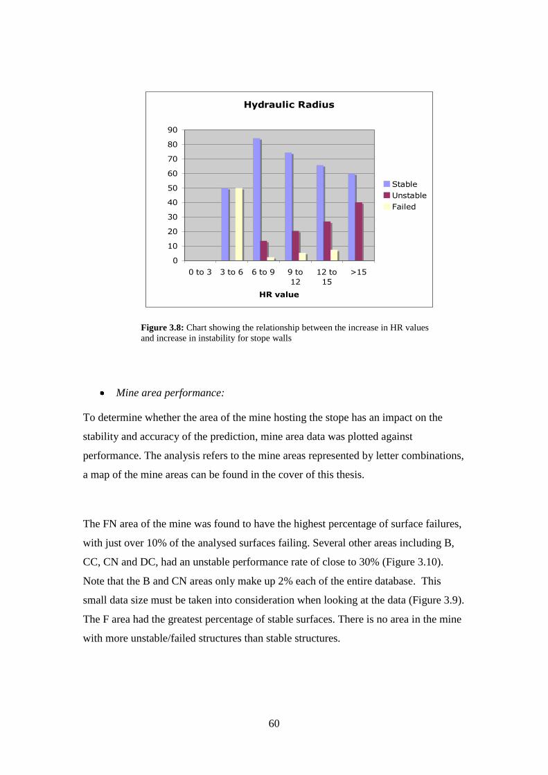
60
Mine area performance:
To determine whether the area of the mine hosting the stope has an impact on the
stability and accuracy of the prediction, mine area data was plotted against
performance. The analysis refers to the mine areas represented by letter combinations,
a map of the mine areas can be found in the cover of this thesis.
The FN area of the mine was found to have the highest percentage of surface failures,
with just over 10% of the analysed surfaces failing. Several other areas including B,
CC, CN and DC, had an unstable performance rate of close to 30% (Figure 3.10).
Note that the B and CN areas only make up 2% each of the entire database. This
small data size must be taken into consideration when looking at the data (Figure 3.9).
The F area had the greatest percentage of stable surfaces. There is no area in the mine
with more unstable/failed structures than stable structures.
Hydraulic Radius
0
10
20
30
40
50
60
70
80
90
0 to 3 3 to 6 6 to 9 9 to
12
12 to
15
>15
HR value
% o
f w
alls
Stable
Unstable
Failed
Figure 3.8: Chart showing the relationship between the increase in HR values
and increase in instability for stope walls

61
Based on the above analysis, the mine area comparison is inconclusive. However it
does support anecdotal evidence of the FN area being prone to poorly behaving
stopes. This is assumed to be due to the area‟s ground conditions. The rock is
notoriously broken up prooving difficult to develop, drill and fire.
Figure 3.9: Pie chart showing the distribution of stopes included in the study in each area of the mine.
Figure 3.10: Chart displaying the performance of stopes in each mine area
Data from the four largest mine area data sets (FN, F, DSE and DCN) were plotted
separately on the supported and un-supported case history charts (Figure 3.11, 3.12,
3.13 and 3.14). As with the combined plot, there was no consistency between the
placements of the surfaces on the chart and their final performance.
Percentage of Surfaces in Each Mine AreaB
2%CC
8%CN
2%
DC
10%
DCN
14%
DSE
19%
F
19%
FN
26%
Percentage of Surface Performance by Mine Area
0%
10%
20%
30%
40%
50%
60%
70%
80%
90%
100%
B CC CN DC DCN DSE F FN
Mine Area
Perc
ent
of
surfa
ces
Unstable
Stable
Failed

62
Figure 3.11: Crown (left) and wall (right) plots for the FN mine area.
Figure 3.12: Crown (left) and wall (right) plots for the F mine area.
Figure 3.13: Crown (left) and wall (right) plots for the DSE mine area.
Stable
Unstable
Failed
Stable
Unstable
Failed
Stable
Unstable
Failed
Stable
Unstable
Failed
Stable
Unstable
Failed
Stable
Unstable
Failed

63
Figure 3.14: Crown (left) and wall (right) plots for the DCN mine area.
Surface orientation:
When looking at the impact of surface orientation on stability there is only sufficient
data to look at the five main orientations (being the crown, north, south, east and
west) (Figure 3.15). All of the orientations had a majority of the faces that were
stable. The crown surfaces show the greatest percentage of failed surfaces with 18%
of the crowns failing. The remaining surfaces a fail rate of less than 8%. Southern
walls had the greatest percentage of stable surfaces (80%), and no failed surfaces
(Figure 3.16).
Stable
Unstable
Failed
Stable
Unstable
Failed
Breakdown of surface orientations
Crown
20%
E Wall
18%
EW Wall
0%
N Wall
18%
S Wall
18%
SE Wall
2%
SW Wall
2%
W Wall
18%
NE Wall
2%
NW Wall
2%
Figure 3.15: Chart showing the breakdown of surfaces
included in the study.

64
Time left open
The impact on stability of the time a void is left open on was also analysed. In
performing this analysis, crowns and walls were looked at separately. The time
between the completion of a stope‟s bogging and the commencement of backfilling
was calculated.
There is little correlation until a time span of approximately 300 days. At this point
the percentage of unstable and failed surfaces and crowns rise. Possible time
dependent effects include regional fault movement, stress re-distribution, production
blasting, and backfill drainage from adjacent stopes. Blast damage and the effects of
water from backfill have potential to move along common structures that truncate a
number of stopes.
Tonnes bogged
The volume of tonnes bogged was used to represent the final volume of void. This
displayed no trend with stope stability.
Surfaces inconsistent with their prediction
The above analysis does not adequately consider whether performance was consistent
with prediction. Of the 519 surfaces included in the analysis, there were 304 (59%)
performances inconsistent with their prediction. 216 of these inconsistencies reflected
the surface performing better than predicted, while the remaining 88 performed worse
than predicted.
Performance by surface orientation
0
10
20
30
40
50
60
70
80
Crown E Wall EW Wall N Wall NE Wall NW Wall S Wall SE Wall SW Wall W Wall
surface orientation
nu
mb
er o
f su
rfa
ce
s
Stable
Unstable
Failed
Figure 3.16: Chart displaying performance by stope surface orientation.

65
The FN mine area had the greatest number of inconsistencies with 92. The area with
the least inconsistent predictions was Yellow with 8. However there were only 10
surfaces from this mine area included in the analysis meaning the analysis may not be
truly representative of the area (Figure 3.17). Each mine area had greater than 50%
probability of their surface‟s performances predicted incorrectly.
With reference to surface orientations, western walls had the smallest number of
inconsistencies with 66 (50%) of the walls being inconsistent with predictions. South
eastern walls had the greatest percentage of inconsistencies with 90% of all surfaces
being incorrectly predicted (Figure 3.18).
Number of Inconsistencies by Surface Orientation
Crown, 62
E Wall, 53
N Wall, 50
S Wall, 46
SE Wall, 5
SW Wall, 9
W Wall, 66
NE Wall, 10
NW Wall, 4
Figure 3.18: Chart displaying the number of inconsistencies from each
surface orientation.
Number of inconsistencies from each mine area
B, 8 CC, 22
CN, 9
DC, 30
DCN, 37
DSE, 49F, 58
FN, 92
Figure 3.17: Chart displaying the number of inconsistencies from
each mine area

66
Inconsistency was broken into “conservative” inconsistency, where performance was
better than predicted, and “underestimation” inconsistency where the performance
was worse than the prediction. Of the inconsistencies 71% were conservative, leaving
29% underestimations.
3.5 Statistical Analysis
The apparent error rate (APER), as discussed in (Suorineni et al. 2001a), was used to
quantify the reliability of the stability graph for stope performance. Higher values of
APER reflected a better correlation between stability graph stope prediction and
actual performance.
APER is calculated using the confusion matrix. This is based on the data
classification, or alternatively the discriminate rule was used (Suorineni et al. 2001a).
This displays the percentage of incorrect predictions by the stability graph. The
method differs slightly from that applied by Suorineni (2001) to include all three
predicted zones on the chart. The APER is calculated by applying Equation 3.2:
(Equation 3.2)
Where nsm = the number of stable surfaces misclassified as failed, num = the number
of unstable surfaces misclassified as stable, nfm = the number of failed surfaces
misclassified as stable, ns = the number of stable surfaces, nu= number of unstable
surfaces, and nf= number of failed surfaces.
The present study produces an APER value of 41%. As stated, a high APER value
indicates a strong correlation between the predicted data and actual performance. This
low APER value in the present study emphasises the need to have the Mathews
stability method calibrated to Olympic Dam and adjusted to allow for other controls
to effectively assist with stope design at Olympic Dam.
APER = nsm + num + nfm
ns + nu + nf ( ) 100%

67
It is important to acknowledge that the 215 correct predictions were not spread across
the three stability zones. Of those surfaces that were predicted to be stable 71% were,
22% of all unstable predictions were correct and only 6% of all surfaces expected to
fail actually did. This is distribution is displayed by the plot of The plot of predicted
performance of the surfaces, as represented by values from 1 to 3 (stable =1, unstable
= 2 and fail = 3) with the actual performance of the stope, as represented by ELOS
(Figure 3.19).
The majority of the points are clustered in the lower part of the plot, indicating the
surfaces were primarily stable despite there Mathews stability predicted performance.
3.6 Failed surfaces
Each of the stopes displaying failure on at least one surface were individually
examined in order to discover the failure control mechanism. The individual reports
are included in Appendix G.
Figure 3.19: Chart displays the predicted performance (1=Stable, 2=unstable, 3=Failed) with
the ELOS (actual performance) the red circles around the data represent the estimated areas
which all points would fall in if the predictions were 100% correct according to ELOS
classification at Olympic Dam

68
In summary of the 32 stopes that were examined:
17 had some structural influence on the failure
9 had high a sericite alteration which may have contributed to the failure
10 had adjacent development which has been have attributed to the failure
1 crown failure was attributed to the close proximity of the unconformity
(Figure 3.20)
27 stopes were either secondary or tertiary stopes.
Structure and the presence of adjacent stopes are the two most common parameters
present in the 32 failed stopes. Neither of these controls are considered in the
Mathews stability graph calculation.
Figure 3.20: View looking North showing crown over break caused
by close proximity to the unconformity.
69
3.7 Limitations and bias of back analysis
The most significant limitation or bias within back analysis is the interpretation of the
above data and its associated results. That is, it is important to consider whether a
„correct‟ stability prediction is in fact correct, or whether the surface‟s stability is
simply the result of a non-event such as failure did not occur (or alternatively non-
failure).
Such scenarios have a strong control on results. If stability is due to a non-event, the
only predictions that can be classed as truly correct are those that predicted an event
that actually occurred. Therefore a correct prediction can only be one where a surface
was predicted to fail and the surface did indeed fail.
There are several other limitations within the above analysis that must also be
acknowledged. Firstly each stope‟s parameter data used in the calculation of N‟ is
based on mine wide models. Although the data may be accurate for some areas of, or
stopes in, the mine, other areas or stopes may have inaccurate data. Due to the type of
deposit at Olympic Dam, it is extremely difficult to produce an accurate model
without reducing the scale upon which the model is created.
The results may contain bias as only stopes meeting the required recommendations
were included in the analysis, thereby omitting certain stopes from the study. Such
stopes are generally from early Olympic Dam production. At that time cablebolting
was not mandatory and consequently all required information was not successfully
archived.
The ELOS calculation also has numerous limitations. Firstly, as part of the
calculation involves human judgment it is unavoidably subject to bias. Further, the
method uses the inclusion of drill drives (above the crown surface) as a definition of
failure. As the drill drives are not encompassed by the stope design wireframe they
become measured as over break. Error in drilling and charging of the stope must also
be considered as a factor of over break. Since there is no way of accounting for this,
the analysis must assume it is due to poor ground performance. Finally, it must also

70
be acknowledged that ELOS and the Mathews method were not created in
conjunction and therefore the ELOS values determining the stability category may
need reviewing.
There are an inconsistent number of stopes included in the study from each area of the
mine. This may have contributed to further bias in some of the analysis results.
For completeness, it is also necessary to acknowledge that there are several other
factors contributing to stope stability issues that have not been examined. Amongst
others, these include stope alteration, pillar adjacencies and previous blast damage.
3.8 Synthesis
The aim of the back analysis was to determine the effectiveness of the Mathews
stability method for stope stability forecasting at Olympic Dam. This analysis found
that only 41% of the stability predictions were correct. Of the incorrect predictions,
216 were due to the surface displaying less instability than predicted, while 88
showing more instability than expected. Of 124 crown surfaces, 55% were stable,
while 18 failed. Of the 395 wall surfaces, 74% were stable and only 6% failed.
Each of the mine areas had greater than 50% of its surfaces incorrectly predicted. The
FN mine area had the greatest number of inconsistent predictions as well the greatest
number of failed surfaces in the entire study. This indicates that the input values
applied in the Mathews stability predictions may not be correct for the surfaces in this
mine area.
While 41% of all surfaces conformed to their predicted performance, the analysis
discovered the existence of time dependent stability. It also discovered a loose
correlation between the increased HR value and increased instability.
The results from the refreshed database in this back analysis showed little variation
from the results contained in the 2004 AMC report. The poor correlation and a lack of

71
improvement confirm that the Mathews stability method is not effectively applied to
stope stability forecasting at Olympic Dam.
The limitations of the application of the Mathews stability method at Olympic Dam
are discussed in Chapter Four.

72
Chapter 4. Discussion of the Mathews stability
method application at Olympic Dam
4.1 Back analysis results
The results of the previous Chapter support the initial problem statement. That is the
application of the stability model at Olympic Dam does not accurately predict stope
surface performance. The current rate of correct predictions is around 4 out of 10, the
ideal rate of correct predictions would be more like 8 out of 10.
Applying the Matthews stability method at Olympic Dam is problematic as
Stope performance varies from that forecasted by the stability method
A large part of the method‟s application is subjective
Its successful application relies on engineer experience and expertise
Design is often conservative reducing the tonnes achieved
When critiquing the Mathews stability method it must be kept in mind that it is an
empirical tool. It is not a rigorous method and is only intended to provide a guide to
preliminary stope design. However this does not justify the inaccuracy of its
application at Olympic Dam, meaning further improvement to the method and its
application is necessary.
Calibration of the Mathews stability method to the rock type at Olympic Dam may
increase the model‟s accuracy and efficiency. This can be achieved through altering
the relative weighting of the parameters, or through altering the location of the zone
boundaries. Alternatively the accuracy of the input data could be improved by
reviewing each of the models and increasing the frequency of the mine‟s window
mapping. Further, correlation between actual and predicted stope performance could
be increased through the implementation of a new design tool specifically created for
application at Olympic Dam.

73
The following section highlights the limitations of the Mathews stability method and
of how it is applied at Olympic Dam and discusses alterations to the method
suggested by other authors. Possible improvements for the how the Matthews stability
method is applied at Olympic Dam are also identified.
4.2 Limitations of the Mathews stability method use at Olympic Dam
4.2.1 Quality of stability number input parameters
The popularity of the Matthews stability method is attributable largely to its simple
application. However as with any method that relies strongly on the subjective
interpretation of the user it has several limitations. The limitations are involved in
both the method itself and its application at Olympic Dam.
There is a poor correlation between the performance of stope surfaces and their N‟
value (Figure 4.1). It would be expected that there would be a clear trend between the
increase in the N‟ value and the increase in the stability of stope surfaces. It is
difficult to determine whether the poor correlation is due to the accuracy of the input
data or the stability number‟s suitability at Olympic Dam.
Data input accuracy is determined by the subjective judgements of the geologist or
geotechnical engineer collecting the data during the window mapping process. The
collected data is used during the stope note process. Due to the inconsistent coverage
of window mapping at Olympic Dam for some stopes this will mean only one
Matthews stability number (N') - Walls
0
10
20
30
40
50
60
70
80
90
0 to 20 20 to 40 40 to 60 60 to 80 80 to 100 >100
N'
% o
f w
alls
Stable
Unstable
Failed
Figure 4.1: The poor correlation between the stability number (N') and the percentage of
performance of the wall surfaces.

74
window from a level is entered, which could be as far as 80m away from the actual
stope. With an ore body such as the one at Olympic Dam, there can be significant
changes in the rock mass characteristics over this distance.
Engineer subjectivity is also involved when applying strength to the rock mass. The
average lithology and average extent of sericite alteration are used to define the
strength. Each lithology has a designated strength which is reduced to give the final
value depending on the extent of alteration. For example, HEMH has a set strength of
235MPa. If the face had a low alteration the HEMH set strength would be reduced by
10% to a final UCS strength of 212MPa. Considering this unavoidable variability in
the data inputs, it can be assumed that the poor correlation between the stability
number and performance is primarily a result of rock mass data inaccuracy.
4.2.2 Structural influence on stope performance
As mentioned by numerous authors a notable limitation of the Mathews stability
method is the absence of any attempt to incorporate the influence of discrete major
structures including faults, shears, joints and folds. As the stability graph is designed
for a moderately structured rock mass with a distributed or ubiquitous structure, the
influence of the structure was not considered as a primary control of instability.
Structural influence must therefore be considered separately to prevent unexpected
structurally controlled instability.
Ore bodies containing numerous regional and local structures, including faults and
joints, are often associated with the SLOS mining method. It is important that while in
production the stope remains stable. The intersection of any single structure with the
stope can lead to severe unravelling, having detrimental effects on the closing out of
the stope (Figure 4.2). The impact of structures on a stope emphasise the importance
of considering all structures in stope stability analysis. Other authors have attempted
to incorporate such factors into the stability number (as discussed later in this
Chapter). No such attempt has been made at Olympic Dam, structural influences are
individually considered by visual analysis at the stope note and pre production stage.
Because it is unlikely that every single structure has been successfully mapped this is
analysis is not always accurate.

75
Various other factors may lead to stope misclassification. These include rolls or folds
located in foliated rocks that may lead to undercutting of structures not anticipated by
mapping. This is a risk when the structure was not identified as having the potential to
cause failure, whereas if the underlying formation had been identified it would have
been. Strength deterioration due to weathering or bias of RQD calculation due to
relative orientations of the critical joint sets and drill cores may also lead to
misclassification (Stewart & Forsyth 1995). Because Olympic Dam is an underground
mine the exposure to weathering is minimal but the possibility of bias in RQD
measurements is possible. This bias is difficult to identify and acknowledge.
Struct
ure
Struct
ure
Figure 4.2: Screen shot looking south at a stope design shape (red and white)
with the cavity monitoring survey shape (green) showing structurally controlled
over break. The ground below the structure has over broken.

76
4.2.3 Adjacent stopes
Another issue relevant to Olympic Dam is the application of the Mathews stability
method when designing secondary and tertiary stopes. During the design of secondary
or tertiary stope it is assumed the adjacent stopes have been successfully and wholly
filled. The surrounding fill must be tight to the walls and the back of the stopes in
order for the fill to be considered supporting a element. If this is not the case the
assumed span used in the analysis may be much greater than the nominal stope panel.
Consequently the stability graph will not appropriately classify the surfaces predicted
stability. It is the responsibility of the user to ensure that backfilling of adjacent stopes
is completed to tight fill.
At Olympic Dam the Mathews plot is not used for stope surfaces that have direct CAF
adjacencies. However it is assumed that a neighbouring mined stope has been tight
filled. This assumption may impact the accuracy of the crown surface prediction
(Figure 4.3). The only apparent means of eliminating this error is for the user to check
back filling reports of adjacent stopes. Any incomplete or incorrect backfilling must
be allowed for in the HR calculation of the concerned surface.
Width of crown if stope B
is tight back-filled
Width of crown if stope B
is NOT tight back-filled
Width x Height
2(Width + Height)HR=
Stope A
(Design)
Stope B
(Mined &
Back-filled )
Figure 4.3: Schematic diagram showing how the back fill status
of adjacent stopes can affect the crown HR value.

77
The HR calculation is an improvement on simply accounting for span. However the
Mathews curves do not take into account the various stope shapes that could exist
with the same HR values (Vongpaisal et al. 2009). This has the potential to be
misleading as stress concentrations develop in different formations around different
shapes of void.
4.2.4 In situ stresses
As a general practice in SLOS mining, regular shaped stope surfaces are desired for
ease of both design and production of the stopes. A rectangular shape stope surface
with a “funnel” shaped bottom, or as commonly explained as an “upside down milk
carton”, cannot always be achieved. This means surfaces take on irregular shapes and
therefore have different patterns of stress acting on them (Figure 4.4). The orientation
of the stopes relative to this stress field has little influence on the predicted stope
performance in the Mathews stability method. At Olympic Dam a stress model is run
to identify any of these stress concentrations during the pre-production process. This
is as a result of the aspect not being accounted for in the stability number calculation.
Figure 4.4: Screen shot of stress analysis showing the variation in stress concentrations around
different shaped excavations

78
Another stress-related assumption included in the Mathews stability method is the
inability of the stress factor to account for tension. The rock stress factor (A) in the
stability number calculation represents the ratio between the intact rock strength to the
surrounding compressive strength. Tension is of relevance in areas where there has
been a lot of previous excavation with closure pillars, secondary and tertiary stopes
particularly as the strength of CAF is not equivalent to that of the rock mass.
4.2.5 Operational impacts on stope performance
There are two production related limitations in the Mathews stability method that can
affect the accuracy of predictions. Firstly there is no consideration of blasting effects
in the Mathews stability method. Blasting often leads to the degradation of the rock
mass by blasting-induced fractures that are likely to cause over break at stope
boundaries. Secondly there is an absence of any time factor in the method. It is widely
acknowledged that rock mass deterioration increases with exposure time as is seen at
Olympic Dam where the number of stable stopes reduced as they remained open
longer and the number of failed stopes increased.(Figure 4.5). Accordingly it is
preferable to have a stope open for the least time possible.
Figure 4.5: Chart by AMC authors showing stope stability deterioration over time at Olympic
Dam (Oddie, 2004)

79
4.2.6 Site specific influences on stope performance
It must be remembered that the Mathews stability method was based on a series of
case studies from North American mines. Due to this the stability zones of the graph
are unable to allow for differences in site specifics. The requirement for site-specific
calibration of the Mathews stability method has long been recognised.
In 2003 Stewart and Trueman looked at the application of the method to narrow-vein
stoping. They stated that a reliable stable-failure boundary requires at least 150 case
histories. Of these a minimum of 10% should be unstable stope surfaces (Stewart
2003). This requirement is not feasible at new mine sites coming online. Accordingly
new sites are forced to rely on clusters of non-continuous data. These define the
segments of the graph as the basis for preliminary stope design.
Although the Mathews stability method has some underlying limitations these cannot
be assumed the cause of the poor correlation between predicted and actual stope
performance at Olympic Dam. For this to be done the method must first be calibrated
to Olympic Dam and the database of input parameters for the method must be
reviewed.
4.3 Improvements in stope stability forecasting
It is widely acknowledged that despite its wide spread popularity the Mathews
stability method has significant shortcomings in the effective application to open
stope design including those experienced at Olympic Dam discussed above. As a
result, there have been various attempts at making additions or alterations to the
method. These have attempted to account for local conditions and other known
excavation stability problems.
4.3.1 Incorporation of a fault factor
Suorineni et al. (1999) explored the limitations of the application of Mathew‟s
stability method. They worked toward the incorporation of a fault factor into the
stability method. This was intended to account for fault controlled sloughage (Figure
4.6). The fault factor is an adjustment to the stability number that can be applied when
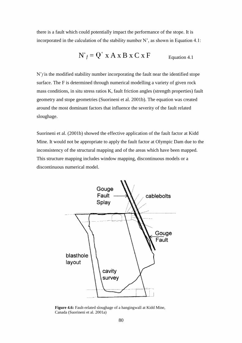
80
there is a fault which could potentially impact the performance of the stope. It is
incorporated in the calculation of the stability number N‟, as shown in Equation 4.1:
Equation 4.1
N‟f is the modified stability number incorporating the fault near the identified stope
surface. The F is determined through numerical modelling a variety of given rock
mass conditions, in situ stress ratios K, fault friction angles (strength properties) fault
geometry and stope geometries (Suorineni et al. 2001b). The equation was created
around the most dominant factors that influence the severity of the fault related
sloughage.
Suorineni et al. (2001b) showed the effective application of the fault factor at Kidd
Mine. It would not be appropriate to apply the fault factor at Olympic Dam due to the
inconsistency of the structural mapping and of the areas which have been mapped.
This structure mapping includes window mapping, discontinuous models or a
discontinuous numerical model.
Figure 4.6: Fault-related sloughage of a hangingwall at Kidd Mine,
Canada (Suorineni et al. 2001a)
N „ f = Q „ x
A x
B x
C x
F

81
4.3.2 Influence of confining stress
Martin et al (1999) discussed the application of confining stress as an indicator for
predicting the amount of dilution to be expected around mine openings. It is well
known that the behaviour of a jointed rock mass is predominantly controlled by its
confinement. As confining stress approaches zero, the potential for new crack growth
increases significantly. This is coupled with the belief that as stress becomes tensile
the potential for crack growth grows. From these conclusions a new approach to stope
hangingwall stability was presented by Martin et al. (1999). This considered the
stress path of stope experiences and the effect of low confinement (Martin et al.
1999).
The hypothesis Martin et al. (1999) study was that confining stress may be an
indicator for predicting the amount of dilution around mine openings. To test this, a
series of 3D elastic analyses were carried out on stopes of different width and height.
The depth at which the confining stress was equal to zero for the hanging wall at mid
height was used for the analysis. The results were then expressed as percent of
potential dilution. The results were in agreement with both the hypothesis and field
observations and found that stope stability is sensitive to the orientation of the stopes
relative stress field (Figure 4.7). Although this method was tested with narrow-vein
mining the general concept may be applied to open stoping.
Figure 4.7: The predicted dilution from the numerical analysis compared to
measured results (Martin et al. 1999).

82
4.3.3 Site-specific effects
Despite significant advances in experience and data related to the stability graph,
there is substantial evidence that site-specific effects may result in erroneous stability
predictions (Stewart & Forsyth 1995). The Mathews stability curves have been based
on bias data collected primarily from North America typically representing strong
rocks of medium to good quality. The method provides a starting point for design but
should be calibrated on site at all mining environments. To do this requires an up to
date database of stope dimensions, rock mass parameters and of stope performance.
On site calibration allows a more accurate model suited to the local conditions to
determine performance and ground support.
A case study completed at Mt Charlotte mine by Stewart and Trueman (2001) used
logistic regression to generate site-specific zone plots on the graph. These displayed
higher accuracy as a prediction tool than the generic stability graph (Figure 4.8). The
performance of stope surfaces at Mt Charlotte mine were represented by the stable,
failure and major failure. These are the equivalent of the stable, unstable and failed
used at Olympic Dam.
Caution must be used when undertaking a site-specific model with a database that is
adequate to make changes to the boundaries. Such changes must avoid the reflecting a
Figure 4.8: Mt Charlotte site-specific stable-failure boundary compared to the generic
boundary after logistic regression (Stewart 2001).

83
short-term operational condition rather than a relevant site-specific controlling factor.
Stewart and Trueman (2001) recommend a site-specific database of at least 150 case
histories of which at least 10 percent must be unstable. This number of case histories
must be obtained to minimize variance in a stable-failure boundary. The authors note
that these requirements apply only within the range of the current database.
The primary aim of underground excavation design should be to utilize the in situ
rock for its structural properties without relying on the installation of rock and surface
support to assist stability. The Mathews stability method has been validated as an
appropriate empirical design tool for the preliminary design of stopes. This means it
has been recognised as a helpful guide to stope stability during the early stages of
design. Over time experience with the model, the increased size of the database across
a broad range of surface geometries and rock mass conditions, and the use of
statistical analysis has resulted in minimal associated variability when it is correctly
applied to a mine site. This has optimised the method as a prediction tool. The
method is recommended as a useful open stope design tool, but it must be recognized
that it is not a rigorous design method.
4.3.4 Statistical improvements
With the use of logistic regression the risks associated with using the Matthews
technique has been quantified and applied. This is as has been recommended by
several authors (Trueman & Mawdesley 2003). Optimising the placement of the
stability zones on the stability graph is a critical to improving the reliability and
minimising the inherent subjectivity of the Mathews stability method (Mawdesley
2004).
Stability graphs are a simple, non-rigorous design approach based on case histories
and logistic regression. They can be applied to reduce the subjectivity through
statistical delineation, placement optimisation, and through calculating the accuracies
and probabilities of stability boundaries (Mawdesley 2004). The process also allows
isoprobability contours to be calculated and drawn on the stability graph. This is a
valuable design tool in quantifying the uncertainties of the Mathews design tool.

84
Although the zones can be determined by visual placement based on the scatter of
site-specific case studies, human bias and unknown errors are introduced when there
is no statistical guidance.
Mawdesley (2004) states logistic regression is used due to the failure of traditional
regression techniques to appropriately deal with binary or categorical outcomes. A
key benefit of this technique is its capability to allow the user to quantify the accuracy
of a given model. Applying regression techniques to a sufficiently large database is
currently the best option for minimising the influence of subjective data (Mawdesley
2004).
It is important to remember that the proceeding statistical analysis does not justify the
use of the stability graph as a rigorous design tool. Logistic regression enables the
engineer to allow for site specific calibration. However logistic regression is nothing
more than a short-term solution to the shortcomings of the Matthews method and the
application at Olympic Dam. To improve stope stability forecasting in the long-term,
the methods discussed in the previous section are preferable.
4.3.5 Applying numerical modelling
Rose & Hungr (2007) apply varying rates of velocity with the inverse-velocity
method to forecast potential slope failure in open pit mines. The inverse-velocity
method, developed by Fukuzono (1985) uses surface displacement measurement data
to determine the onset of failure. Based on laboratory tests during the development of
his method, Fukuzono simulated a rain-induced landslide. This landside indicated
that the logarithm of surface displacement acceleration increased in proportion to the
logarithm of surface velocity. When the inverse-velocity was plotted the values
approached zero. This allowed a prediction of time of failure to be determined
(Figure 4.9).
The method was applied successfully to the three slope case studies in 2001 by Rose
and Hungr (2007). This was the first time it had been tested in an open pit mining
environment. They concluded that the inverse-velocity plot often approaches linearity,
especially during the final stages before failure, which enhances the utility of the

85
method as a instability indicator (Rose & Hungr 2007). They stated that the method
could be extended to the forecasting of any unstable phenomena.
The application of velocity and plastic strain as stability indicators was investigated
by Cepuritis et al (2010) at the Kanowna Belle gold mine. They used back analysis of
over-break to investigate non-linear elasto-plastic relationships and stability. Their
modelling was done in Abaqus Explicit, a 3D analysis product, and selected velocity
and plastic strain as their stability indicators. Velocity and plastic strain were plotted
against points which had been classified as either stable or unstable (Figure 4.10). The
point‟s classification was determined by their location relative to the void boundary.
The results showed a clear relationship between an increase in velocity and the
increased likelihood of instability.
Figure 4.9: Inverse - velocity versus time relationships preceding slope failure
(Fukuzono, 1985)
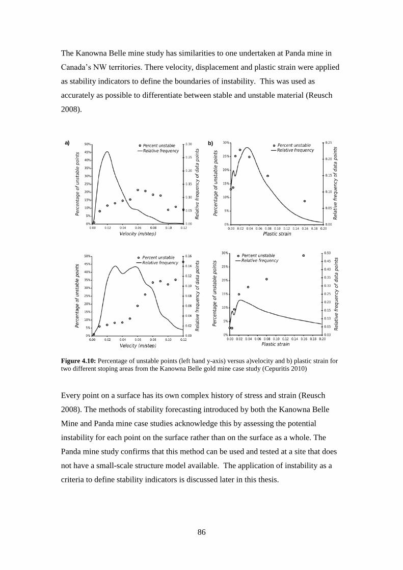
86
The Kanowna Belle mine study has similarities to one undertaken at Panda mine in
Canada‟s NW territories. There velocity, displacement and plastic strain were applied
as stability indicators to define the boundaries of instability. This was used as
accurately as possible to differentiate between stable and unstable material (Reusch
2008).
Every point on a surface has its own complex history of stress and strain (Reusch
2008). The methods of stability forecasting introduced by both the Kanowna Belle
Mine and Panda mine case studies acknowledge this by assessing the potential
instability for each point on the surface rather than on the surface as a whole. The
Panda mine study confirms that this method can be used and tested at a site that does
not have a small-scale structure model available. The application of instability as a
criteria to define stability indicators is discussed later in this thesis.
a) b)a) b)
Figure 4.10: Percentage of unstable points (left hand y-axis) versus a)velocity and b) plastic strain for
two different stoping areas from the Kanowna Belle gold mine case study (Cepuritis 2010)

87
The preceding section is merely a summary of the works completed in this field.
There are numerous other authors and topics which have not been mentioned due to
the vast collection of work available.
4.4 New stope stability analysis tool for Olympic Dam
The relationship between the actual performance of stope surfaces at Olympic Dam
does not correlate with the predictions of the Mathews method (Figure 4.11)
Historically it has been recommended that the zones on the chart be altered to suit the
Olympic Dam ore body. This recommendation alone is not enough to entirely correct
the Mathews model.
The results from Chapter Three indicate that the Mathews stability method is not
effectively applied at Olympic Dam. For the successful application of the method it is
required that it is calibrated to the Olympic Dam ore body. If the Mathews method is
continued to be used at Olympic Dam there are some recommendations which should
be adhered to in order to improve the methods application:
1) Implement a detailed quality assurance quality control (QAQC) system to
track the performance of mined stopes with reference to the design.
2) When applying ELOS during the QAQC process add another category to the
classification of surface performance. Currently any stope surface which has
over break with an ELOS value of two or over is classified as failed. Another
Stable
Unstable
Failed
Stable
Unstable
Failed
a) b)
Stable
Unstable
Failed
Stable
Unstable
Failed
Stable
Unstable
Failed
Stable
Unstable
Failed
a) b)
Figure 4.11: The actual performance of a) crowns and b) walls defined by their HR and N' values, showing
a poor correlation between stope performance prediction and performance at Olympic Dam.

88
catrgory should be added to separate the surfaces with catastrophic failures
from those which have extensive over break.
3) Undertake more window mapping close to upcoming stopes to strengthen the
accuracy of the database.
4) Install a series of live stress measuring stations around the mine. With
particular focus on stress relaxation around mined stopes.
5) Attempt to incorporate structures into the Mathews stability number.
6) Perform statistical analysis such as logistic regression to ensure the zones on
the Mathews chart are the best fit possible to Olympic Dam.
4.5 Summary
After working through both the results of the analysis in Chapter Three and the
discussion in this Chapter it is clear the issues with the Mathews stability method as a
design tool at Olympic Dam appear to primarily result from how the method is
applied. One limitation that exists within the method itself which is worth noting is
the lack of acknowledgement of structurally controlled failure.
There are several ways the application method at Olympic Dam could be improved to
achieve more accurate stability predictions. The main limitations with the application
at Olympic Dam and possible solutions are shown in Table 4.1
In the following chapter, a new method is devised that appears to provide accurate
forecasts of stope surface stability at Olympic Dam. Before the development of this
new method it is important to understand the mechanics and criteria of instability, as
well as the indicators most suited to forecasting this.

89
Table 4.1: Major limitations of the application of the Mathews stability method at Olympic Dam and
possible solutions and improvements
Limitations of application at
Olympic Dam
Possible solutions
The quality and coverage of the
database of stability number
input parameters.
Increased frequency of window
mapping, particularly in and
near upcoming stopes.
Lack of incorporation of
structural influence on stability
in the stability number
Attempt to incorporate
structures into the Mathews
stability number specific to the
Olympic Dam rock mass.
Insufficient in situ stress data Install a series of live stress
measuring stations around the
mine or increase the regularity
of measurements. Also increase
the number of measuring
stations. Particular focus should
be placed on stress relaxation
around mined stopes.
Unknown status of adjacent
stopes
A detailed QAQC process
should be undertaken for all
stopes not only those which do
not perform as expected to
develop a detailed database of
stope performance history.
No site-specific calibration Perform Logistic Regression on
the current stope histories to
determine the relocation of the
stability zones on the stability
chart to best fit the Olympic
Dam conditions.

90
Chapter 5. Numerical model for stope design at Olympic Dam
5.1 Introduction
At Olympic Dam, a high resolution non-linear numerical model of stoping already
exists. This model is able to replicate the extent and magnitude of damage well and
utilises a 3D discontinuum, Hoek Brown, strain softening and explicit finite element
modeling. This encapsulates a majority of completed stopes at Olympic Dam. The
data represented in these models includes displacement, velocity and plastic strain.
This chapter develops a new stability prediction tool to improve the non-linear
numerical model currently in use at Olympic Dam. This new model is based on
velocity, or incremental displacement, as a stability criterion. Note that stress and
strain-based approaches were not investigated as the estimate of velocity, or
incremental displacement, is predetermined by stress and strain.
The suggested new tool uses the existing numerical model to examine trends in the
movement of individual points, otherwise known as material instability. Completed
stopes were investigated to determine their material instability. From this a model for
future application at Olympic Dam has been produced. Cepuritis et al (2010) has
previously utilised similar numerical modelling and analysis at Kanowna Belle Gold
Mine .There the ore body is simultaneously mined in underground and open pit
operations.
The application of velocity as a stability indicator is incomparable to the Mathews
stability method. It is based on a numerical model and is not geologically based. The
use of the terms stable and unstable in this section should not be confused with the
use of the terms in regard to the Mathews stability method.
5.2 Mechanics of instability
Over break arises from rock mass instability at the excavation surface due to a
number of mechanisms. These include:
Wedges and blocks formed by existing discontinuities
Rock mass comminution (crushing and disassembly of rock mass)

91
Unstable volumes bound by a combination of existing discontinuities and induced
damage surfaces.
Estimating the potential for kinematic instability, that is the dislodging of block or
wedges formed solely by discontinuities, requires an understanding of the distribution
of discontinuities. This understanding is not usually complete but rather is a function
of geometry. The mechanics of this geometry are simple and well understood.
Sloughing by this mechanism is not the focus of this thesis.
Over break due to rock mass damage, or alternatively combined damage and
structure, is more relevant to this thesis. This requires consideration of both material
and kinematic instability. Material instability refers to the stability of a point within a
material (a comparison of stress and strength to estimate the accumulated yield),
while kinematic instability refers to the freedom of a volume within a mass to
displace and fail.
5.2.1 Empirical stability indicators
In the past the application of mechanistic analysis tools to rock mass was thought of
as a difficult task. To simplify this complexity rock empirical rock mass classification
systems were introduced. Most empirical classifications originally applied in mining
were based on civil engineering case studies. These case studies included rock quality
designation (RQD), rock mass classification (RMR), Q and the modified rock mass
classification (MRMR). These were in addition to the Mathews stability method.
The application of the empirical indicators has altered over time as more case
histories have been applied, testing and calibrating the indicators. It is usually
recommended that the methods be calibrated to each site, because they rely on local
rockmass patterns to be effective, but this is rarely done, and few of them account
well for the 3D geometry of the mine or the excavation, the stress history, structure or
interactions between multiple voids. The most commonly employed empirical
stability method is the Mathews Method, or the Modified Stability Graph.
5.2.2 Physics based stability indicators
The purpose of stability indicators is to identify the timing, magnitude and extent of
instability. The criteria for instability are generally defined by a certain critical limit

92
of a chosen parameter. The criteria will be applied to analyse results over a certain
timeframe. For open stoping this timeframe is typically between the completion of the
stope‟s production firing and back filling (Cepuritis 2010). As discussed in Chapter
Three the Olympic Dam criteria, volume of over broken rock, is measured at the time
of the cavity monitoring survey (after bogging, before back-filling).
For an engineering assessment of the potential for 'combination' mechanisms of
instability several criteria are frequently used. These are classified as the lower or
upper bounds, depending on whether they infer potential for instability, or whether
they constitute explicit instability. Stress is lower bound, because highly stressed rock
may or may not be unstable, while high velocities are upper bounds as something
which is accelerating is by definition not at equilibrium.
The stress criterion is generally applied for the assessment of excavation performance.
This is typically expressed as a ratio between peak strength and an elastic model‟s
estimate for stress. This ration is the strength Factor of Safety Factor (FOS). The
criterion states that there is a level of stress above which instability will occur. The
approach is qualitatively simple but limited in excavation stability assessments. This
is because stress is poorly correlated with kinematic permissibility for failure. Further,
rock mass damage is not simply correlated with any single component of stress,
because stope failures generally occur in de-stressed parts of an excavation rather than
in the highly stressed parts.
There are also practical considerations for the estimate of stress. As materials yield
the capacity to bear load reduces and stresses are redistributed. Analysis that does not
capture this softening, the subsequent redistribution of stress or the ultimate
equilibrium accounting for damaged parts of the rock mass will not properly estimate
the stress field. That is the stress estimate for FOS calculations may be invalid if the
mechanism of yield and instability are not sufficiently captured. Around stopes a
single safety factor for strength or stress does not meet the needs of an operator
(Martin et al. 1999).
Critical strain criteria are frequently applied in the assessment of instability. This
assessment uses the magnitude of damage or deformation to estimate the likelihood of

93
instability. Critical strain criteria are most often used when the kinematic constraints
are easily accounted for. Such circumstances occur where there are known
unfavourable geometric intersections with structure, for pillars, or where the level of
strain in the pillar core directly indicates the residual strength. The level of residual
strength is the level of strain where pillar strength reduces significantly and the pillar
will continue to deform even at constant or reducing load.
The main limitations of the critical strain criteria are the sufficiency requirements for
reliable non-linear analysis to compute strain values. It is also a lower bound on
instability in most cases as a rock mass may be damaged but still stable. This is as it
may not be kinematically capable of sloughing, or may retain sufficient strength to be
able to reach a stable equilibrium. This is in terms of the particular stress
configuration, strain, strength and structure. For example on the floor where the
damage can be deep but there is no issue with the rock remaining at rest.
Despite the limitations if the extent and magnitude of the damage and deformation is
sufficiently forecast, critical strain criteria are more satisfactory than stress criteria.
This is as the accounting for stress, strain and strength in the structure is implicit,
when in stress criterion additional assumptions are needed.
Any point within the rock body that is moving at a high velocity is unstable. The
velocity and acceleration of a point within a mass can therefore be considered an
upper bound criterion for instability. The velocity value represents the rate of
movement within the rock mass, generally measured relative to some point. In the
case of stope stability it is toward the void or designed void, for example points above
the crown that are moving in a downward vertical movement toward the crown have
positive modelled velocity values.
The load factor derived from a kinematically admissible velocity field is an upper
bound on the true collapse load factor (Yu 2006). Thus, the velocity criteria is
applicable for estimating the stability of all mechanisms including unstable blocks
bound by structures that have low levels of internal comminution, and high levels of
comminution (Cepuritis 2010).
94
In terms of velocity, instability in a rock mass can be divided into three phases:
An unstable phase: during this phase velocity increases at a constant or near constant
rate
Active failure: during this phase there is an onset of more rapid accelerations leading
to failure.
Failure: this phase is signified by collapse.
Beck (2009), when discussing slope failure forecasting in open-pit mines, said the
displacement rate (velocity) is commonly considered the best indicator of the failure
process. There is no doubt that it is the simplest criterion to understand. In open pits
for example radar are used to monitor slope movements and alarms are triggered
using velocity criteria, not stress or strain.
Numerical models estimate the movements in the rock mass. From one point in time
to another, from these values the distance they movies divided by the time passed.
The outcome is the velocity of the point the modelled velocity is the modelled
distance that any point moves in real time.
When applied to the result of numerical analysis, the main limitations of velocity
based stability criteria are the very high level of model similitude required before the
velocity estimates can be considered reliable. Essentially the displacements, and
therefore the extent and magnitude of damage modelled, must be a sufficient
representation of the real problem for the modelled velocities to correlate well with
actual measurements. It is only recently that the most sophisticated physics based
models have been considered to have high enough resolution and precision for this
task.
5.3 Method for applying velocity as a stability indicator
The method uses commercial modelling packages and should be easily applied at
most mine sites. The basic requirements to apply the stability indicators at different
sites are:
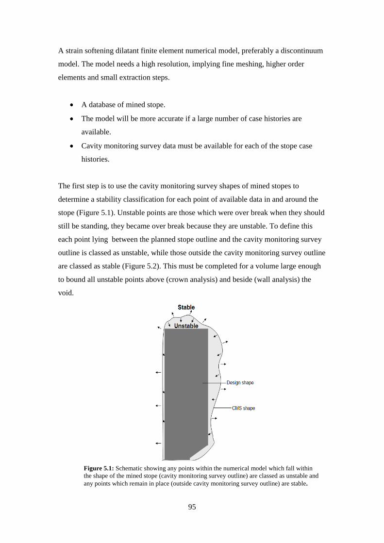
95
A strain softening dilatant finite element numerical model, preferably a discontinuum
model. The model needs a high resolution, implying fine meshing, higher order
elements and small extraction steps.
A database of mined stope.
The model will be more accurate if a large number of case histories are
available.
Cavity monitoring survey data must be available for each of the stope case
histories.
The first step is to use the cavity monitoring survey shapes of mined stopes to
determine a stability classification for each point of available data in and around the
stope (Figure 5.1). Unstable points are those which were over break when they should
still be standing, they became over break because they are unstable. To define this
each point lying between the planned stope outline and the cavity monitoring survey
outline is classed as unstable, while those outside the cavity monitoring survey outline
are classed as stable (Figure 5.2). This must be completed for a volume large enough
to bound all unstable points above (crown analysis) and beside (wall analysis) the
void.
Figure 5.1: Schematic showing any points within the numerical model which fall within
the shape of the mined stope (cavity monitoring survey outline) are classed as unstable and
any points which remain in place (outside cavity monitoring survey outline) are stable.
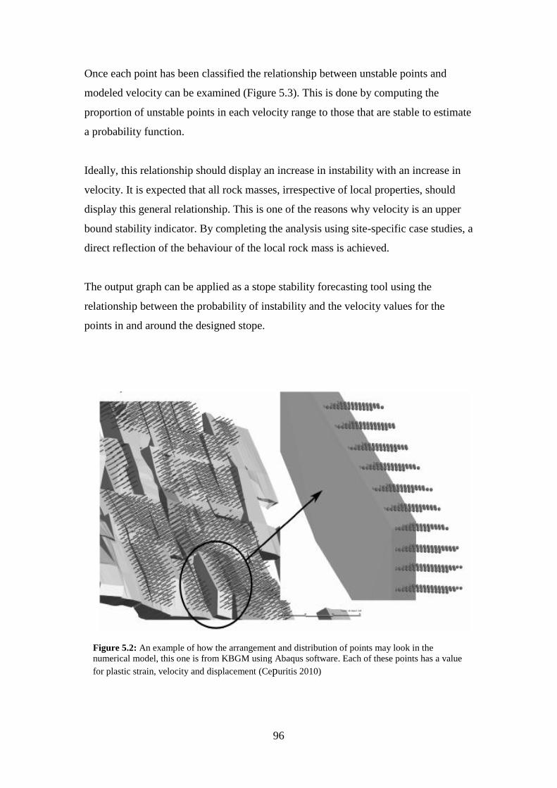
96
Once each point has been classified the relationship between unstable points and
modeled velocity can be examined (Figure 5.3). This is done by computing the
proportion of unstable points in each velocity range to those that are stable to estimate
a probability function.
Ideally, this relationship should display an increase in instability with an increase in
velocity. It is expected that all rock masses, irrespective of local properties, should
display this general relationship. This is one of the reasons why velocity is an upper
bound stability indicator. By completing the analysis using site-specific case studies, a
direct reflection of the behaviour of the local rock mass is achieved.
The output graph can be applied as a stope stability forecasting tool using the
relationship between the probability of instability and the velocity values for the
points in and around the designed stope.
Figure 5.2: An example of how the arrangement and distribution of points may look in the
numerical model, this one is from KBGM using Abaqus software. Each of these points has a value
for plastic strain, velocity and displacement (Cepuritis 2010)

97
The Kanowna Belle mine case study (Cepuritis 2010) provides examples of the
analysis possibilities. This includes plotting the rate of velocity with the probability of
instability (Figure 5.3). The probability of a stopes surface‟s instability can be
visualised (Figure 5.4) in a cross section allows the potential shape of any over break
to be estimated (Figure5.4).
As further mined stope case histories become available they will be added to the
database. This helps calculate the probability of instability and the velocity
relationship. The mine is then able to improve accuracy and ensure the model remains
up to date with the mines conditions.
Figure 5.3: Instability criteria based on velocity only for Kanowna Belle mine. The
measurements were taken in one month steps (Cepuritis 2010).

98
5.4 Application at Olympic Dam
The relationship between velocity and unstable points has been investigated at
Olympic Dam to generate a guide for forecasting stope surface stability. Although
there are still areas for improvement the initial trial as discussed below, has produced
excellent results. This method is completely separate from the Mathews stability
method.
5.4.1 Numerical modelling
The existing numerical model of stoping at Olympic Dam was created by Beck
Engineering. It was generated using Abaqus Explicit, a general purpose, 3D, non-
linear, continuum or discontinuum finite element analysis software.
The Levkovitch Reusch (LR2) model was used by Beck Engineering. In the model
softening, weakening and changes in other material properties are all described as a
function of strain. This enables softening to occur gradually and simulates, as closely
as possible, what is observed in „real‟ rock (Beck 2009). As all of the parameters in
Figure 5.4: a) Cross section showing design and cavity monitoring survey geometries together
with modelled velocity (m/step) and b) long section of a section of stopes showing the
probability of hangingwall instability, estimated from the velocity instability criteria at
Kanowna Belle mine (Cepuritis 2010).

99
the model can vary at different rates, with respect to the strain changes, approximation
of complex stress-strain behaviour can occur.
Initially a global model was created. This incorporated all mined and planned stope
geometries, access development and mapped mine-scale structures. There were no
new measurements taken for the rock mass model, instead relying on existing
information. The stress field that was used is based on the measurements from AMC‟s
report “In situ stress field for Olympic Dam mine” (as discussed in Chapter Two)
(Figure 5.5).
The Olympic Dam Geotechnical Department provided the material properties. A copy
of the table provided is given in Appendix I. The softening parameters were estimated
using conventional ratios for moderate strength rocks.
Figure 5.5: Simple logistic regression to estimate far-field stress
inputs for the model (Beck 2009).

100
From the global model, three smaller more detailed sub-models were created. These
incorporate the main areas of mining activity in the Olympic Dam ore body (Table
5.1) (Figure 5.6). Strain outputs and tractions of the global model defined the
boundary conditions of the sub-models for each extraction step. The evaluation points
in the sub-model used for stability function calculations are spaced between one and
two metres apart. The steps in
model are one month apart (plus
or minus one week).
5.4.2 Velocity analysis at Olympic Dam
The workflow, as outlined in the previous section, was undertaken at Olympic Dam
with the assistance of David Beck of BE. The 3D visualisation was undertaken using
Voxler 2. All further analysis was completed using Microsoft Excel.
Table 5.1: Sub-model naming convention and coordinates
(mine plan grid)
35500mN to 36150mNSM03
34500mN to 35000mNSM02
33000mN to 33800mNSM01
Approximate coordinatesSub-Model
35500mN to 36150mNSM03
34500mN to 35000mNSM02
33000mN to 33800mNSM01
Approximate coordinatesSub-Model
SM03
SM02
SM01
SM03
SM02
SM01
Figure 5.6: Approximate location of the three sub-
models on the mine plan.

101
The stopes included in the numerical modeling at Olympic Dam had to meet two
criteria. Firstly they needed to be included in the back analysis undertaken in Chapter
Three and secondly to fall within one of the three stope sub-models. This provided a
database of 42 completed stopes; 11 stopes from sub-model 1(SM01), 15 from sub-
model 2 (SM02) and 16 from sub-model 3 (SM03).
To categorise the stability of points in and above the crown of each of the stopes, the
cavity monitoring survey data for each stope was opened with each of the points
surrounding the mined stope being classed as either stable or unstable. This
classification was dependent on whether they fell within or without the confinement
of the cavity monitoring survey void. Unstable points were allocated a number 1 and
stable points a number 2. The volume of the points above the crown varied for each
stope. This ensured all unstable points were included (Figure 5.7).
The reason why the points became unstable is because the balance of
stress/strain/strength/structure wasn't sufficient for them to stay connected to the rest
of the rock. The numerical model applied in to the rock mass simulates this exact
same balance.
Figure 5.7: Screen shot of point arrangement above stope (design shapes) crowns in Voxler 2.

102
Once the points had their stability classification (stable or unstable) they were then
plotted with their modeled velocity values. The velocity is the rate of downwards
movements in a stope crown (Figure 5.8). The velocity value for each point was
derived from the sub-model data, allowing a probability relationship to be derived
based on the value of velocity and the likelihood of the points instability. This is
simply comparing modelled velocity for points that fell off, to points that didn't fall
off.
In the initial plot, 42,822 points from within and above the 42 stope crowns provided
a strong correlation with a R2 value of 0.8299 (Figure 5.8). A clear relationship can be
seen with the increase of velocity and the increase of the likelihood of instability. That
is if a single point moves 100mm in a single step (1 month) it is expected that the
point will become unstable greater than 40% of the time. In other words the rock mass
which that point represents has a probability of around 40% of becoming over break.
The strong relationship between velocity and the likelihood of instability was in some
respects unexpected due to the absence of a small scale structure component in the
numerical model. This may suggest that rock mass damage combined with structure is
the dominant mechanism of over break. That is to say a continuum representation
captures much of the over break. It is only instability which is solely structurally
controlled which cannot be captured by a continuum model.
Figure 5.8: Initial plot comparing the modelled velocity and probability of rock mass instability at
these velocities.

103
In order to ensure the relationship accurately reflects the behaviour of the rock mass
at Olympic Dam on a stope by stope basis, the velocity rates were compared with the
actual over break of a range of stopes from across the three sub-models. A majority of
the mined stopes with cavity monitoring survey shapes conformed to the probability
of instability relationship while others showed a weaker relationship.
Above the crown of a stope located near the centre of SM02 (Figure 5.9), the only
points remaining located outside of the cavity monitoring survey shape have velocity
values that reflect a low (0 – 25%) probability of instability. If the model was
incorrect, it would display a series of points remaining stable (outside the cavity
monitoring survey shape) with high percentages of probability of sloughing. This
scenario was witnessed in another stope from SM02 (Figure 5.10). Although the
probability values do not exceed 30% they are still significant. If this stope had been
designed using the new method a more conservative design may have been adopted in
recognition of the probability percentage.
There are numerous explanations for why or how these points remained stable. One
such explanation is that an error may have occurred with the sequencing in the model,
resulting in incorrect values being displayed. Another explanation is that crown
cablebolts effectively held the ground in place, particularly as the final crown shape is
uniform across the crown with very little over-break across the entire surface.
Further, under-break around the corner of the stope would not have been picked up in
the model. This is of particular relevance with this stope due to its previously mined,
backfilled adjacency. Other possibilities include good design and rigid
implementation of drilling and blasting procedures. Advantageous ground conditions
may also have contributed.

104
The majority of the stopes loaded with cavity monitoring survey having a percentage
probability of sloughing reflected the expected relationship. This indicates that the
method will be adequate as a stability indicator for stope crowns. Around 60% of the
sample stopes clearly reflected the relationship (Figure 5.11). Less than 15% of the
stopes were a poor match. The remainders were a strong qualitative match, falling
inside the general category of over break (for instance high or low).
Figure 5.9: Screen shot from Voxler showing the cavity monitoring shape of a mined stope
from SM02, the coloured points represent the % probability of sloughing as quantified by the
scale shown. The probability scale was defined from the initial plot of unstable points and
there modelled velocity from the mined stopes at Olympic Dam.
Figure 5.10: Screen shot from Voxler where the crown of the lower stope
remained stable despite the percentage probability of sloughing being around 30%

105
5.4.3 Applying velocity as a stability forecasting tool
The initial modelled velocity and instability probability plot infers that the larger the
modeled velocity value for a point within the material surrounding a stope, the more
likely that point is to become over break. This strong correlation can be utilised as a
tool to predict stope stability. It can be concluded that a stope crown‟s probability of
instability can be estimated using the rate of modeled velocity (as computed by a
model).
The most effective way of applying this relationship is visually. By opening the stope
design shape in Voxler, or other similar software and applying the percentage of
probability scale. The final crown shape can be estimated or the overall stability of the
crown can be determined (Figure 5.12). The engineer can then consider factors not
accounted for by the model, such as better or worse than normal blasting practice and
the influence of structures.
Figure 5.11: Screen shot from Voxler where stope crown behaviour reflects the expected
performance based on velocity values. The block shapes represented stope design and the mesh
represents the cavity monitoring survey shape.
Mesh
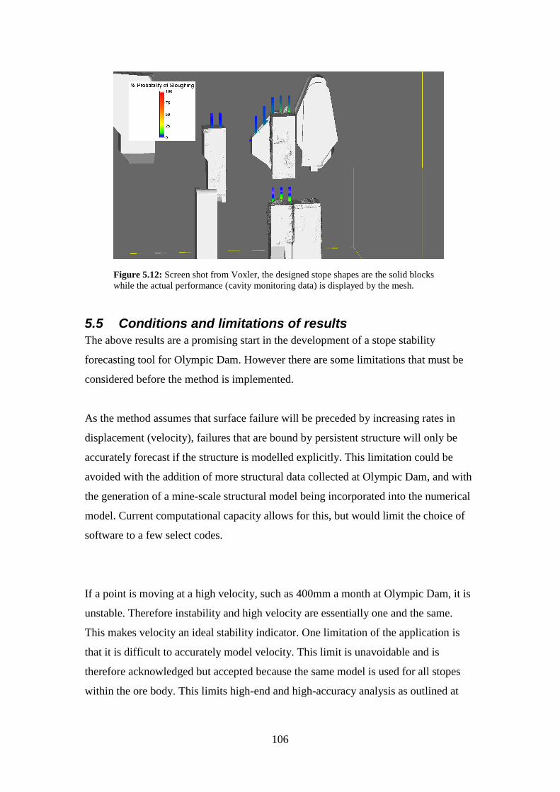
106
5.5 Conditions and limitations of results
The above results are a promising start in the development of a stope stability
forecasting tool for Olympic Dam. However there are some limitations that must be
considered before the method is implemented.
As the method assumes that surface failure will be preceded by increasing rates in
displacement (velocity), failures that are bound by persistent structure will only be
accurately forecast if the structure is modelled explicitly. This limitation could be
avoided with the addition of more structural data collected at Olympic Dam, and with
the generation of a mine-scale structural model being incorporated into the numerical
model. Current computational capacity allows for this, but would limit the choice of
software to a few select codes.
If a point is moving at a high velocity, such as 400mm a month at Olympic Dam, it is
unstable. Therefore instability and high velocity are essentially one and the same.
This makes velocity an ideal stability indicator. One limitation of the application is
that it is difficult to accurately model velocity. This limit is unavoidable and is
therefore acknowledged but accepted because the same model is used for all stopes
within the ore body. This limits high-end and high-accuracy analysis as outlined at
Figure 5.12: Screen shot from Voxler, the designed stope shapes are the solid blocks
while the actual performance (cavity monitoring data) is displayed by the mesh.

107
Olympic Dam. This is becoming more commonplace, but is not currently standard in
Australian mines.
Only current sub-model stopes were included in the calibration of this model. Future
stopes, particularly new stoping areas, will require the extension of the sub-models in
order to use this method.
Although the general idea of the model may be applied at other mines, the model
developed in this thesis will only be suitable for application at Olympic Dam. This is
of particular importance as the mine has significantly harder rock and an unusual lack
of prominent structures. This is unlike most other SLOS method mines. To be
accurately applied at other sites the workflow depicted earlier will need to be
emulated in local conditions.
As mentioned in the discussion of the results the crown cablebolts contribute to
conservative analysis. In some cases as they support material that otherwise may be
unstable. Allowing for this support during the design stage of the stope will assist
avoiding conservative design.
5.6 Possible Improvements and Recommendations
After experimentation with modelled velocity as a stability indicator at Olympic Dam,
it can be concluded that the model can be effectively utilised during crown stability
forecasting. Due to the rate of design and the turnover of stopes at Olympic Dam, a
period of at least five years is required to truly assess and calibrate the proposed new
model. It is recommended a five year trial be implemented. This trial period would
allow the model to be applied in the design of new stopes and for the final results to
be compared with the predicted stability. This testing would be performed through a
back analysis the same as or similar to the one completed in Chapter Three.
A major improvement, as identified earlier would be the incorporation of a mine-scale
structural model into the model. Although the current model is adequate for long term
planning, the addition would allow potential structurally controlled failure to be

108
identified and mitigated prior to production. Neither the Mathews method nor the new
method are currently capable of this. More structure would also allow detailed local
scale analysis. This would allow the assessment of sequencing options for an
individual stope.
In addition, the numerical model applied in the Olympic Dam case study was not
generated with over break analysis in mind. Improvements may be seen if the model
was re-run, incorporating the entire mine and with a better reconciliation with current
schedule and design data. Once the model is up and running, the periodical addition
of new data would ensure that the conditions at Olympic Dam are reflected as
accurately as possible.
The instability relationship identified by velocity or the probability of instability has
the potential to indicate the amount of over break that can be expected from a
designed stope surface. Using an agglomerate of points with known velocity values,
the likelihood of instability of a geometric failure can be defined. By combining the
likelihood of a point being unstable with the known tones of a designed stope, the
final surface may be estimated. Therefore the volume of over break can be estimated.
Crown cables are designed to mark the top of the stope. They ensure material cannot
continue to unravel into the void and become over break. They are intended to aid
potentially unstable material to remain stable. Incorporating this as a factor in the
model would assist in avoiding overly conservative crown design.
The velocity analysis should be undertaken not only for the crown of the stope but
also the walls. There is a possibility the results would be similar. Therefore one scale
percentage of sloughing probability could be used for all five stope surfaces. However
the workflow completed in this study in relation to the crowns needs to be repeated
for walls. This would develop the most accurate relationship possible.
It is worthwhile determining whether one relationship could be used for the design of
all walls despite their orientation and location. Alternatively a series of guidelines
could be developed for each of the stope walls. Such guidelines would define the
relationship for each wall individually and then compare the variance in results.

109
5.7 Success of velocity as a stability indicator at Olympic Dam
As a stability indicator, velocity allows the user to consider what the material will do,
rather than what the excavation‟s behaviour will be. While the Mathews method gives
an aggressive and broad yes or no type answer for each surface, the velocity based
model determines whether each individual point within the material is stable or
unstable. From this, a percentage of the surface can be deemed as stable or unstable.
There is no apparent reason why the velocity method could not also be successfully
applied to the wall surfaces. With some fine tuning the method has the potential to be
effectively applied at Olympic Dam.
5.8 Synthesis
As noted in the introduction to this Chapter the application of modelled velocity as an
indicator of stability and the Mathews stability method are very different and
completely separate approaches to stope stability forecasting.
The Mathews stability method is based on a series of parameters based on rock mass
characteristics. The final method was calibrated based on a series of case history
mined stopes. The application of modeled velocity is based on material stability and
the recommended relationship is derived from the behaviour of previously mined
stopes at Olympic Dam.
While both methods have their own strengths and short comings one similarity the
two methods have is the inability to predict structurally controlled failure. The
remainder of the limitations in the application of the Mathews stability method at
Olympic Dam that were acknowledged in this thesis are primarily related to how it is
applied, rather than within the method itself.
It is difficult to identify all of the limitations of applying modeled velocity as a
stability indicator until it is applied during the design of stopes and is validated. Ideal
validation would be similar to the analysis undertaken on the Mathews stability
method in Chapter Two, Recommendations for the effective implementation of the
modeled velocity method at Olympic Dam are made in Chapter Six.

110
Chapter 6. Summary and Conclusions
6.1 Thesis objectives
This thesis was focused on the application of the Mathews stability method at
Olympic Dam mine. The empirical method is based on a modified version of Barton
et al. (1974) tunnelling quality index. The modified tunneling quality index is
incorporated with a hydraulic radius value which accounts for the geometry of the
stope surfaces.
There were two primary objectives for this thesis.
1) To validate the applicability of the Mathews stability method at Olympic
Dam.
2) To investigate an alternative stope stability forecasting tool at Olympic Dam.
This thesis was undertaken at the request of the Geotechnical Department at Olympic
Dam due to ongoing concern with the inconsistency between Mathews stability
method predictions and stope performance.
The applicability of the Mathews stability method at Olympic Dam was investigated
by classifying the performance of mined stope surfaces, specifically the crown and
sidewalls. The performance was classified by comparing the shape of the mined void
with the stope design shape. Any rock within the mined void which was outside the
design shape was classed as over break. This over break was quantified by equivalent
linear over break./slough (ELOS) which calculates a numerical value by dividing the
volume of over break by the area of the stope face. The performance of each surface
was classified dependent on the amount of over break as shown in Table 6.1:
Table 6.1: Classification of stope performance based on ELOS values
ELOS Performance
<0.75 Stable
0.75 - 2 Unstable
>2 Failed

111
From the results and subsequent analysis it was discovered the inaccuracy of the
Mathews stability method predictions at Olympic Dam is primarily a result of the
quality of input data and the application, not the method itself.
6.2 Mathews stability method
The Olympic Dam Breccia Complex is host to a copper-gold-uranium ore body, this
ore is extracted by sub level open stoping (SLOS). The validity of the application of
the Mathews stability method at Olympic Dam was quantified by performing a back
analysis study of open stope performance. The performance was quantified solely on
the amount of over break on each surface.
This analysis of stope performance at Olympic Dam confirmed there are
inconsistencies between the Mathews stability method classification of stope surfaces
and their performance. The results showed 41% of all the Mathews predictions were
correct and the remaining 59% were incorrect. Of all the predictions 42% were
conservative. Only 6% of failed predictions were correct, 22% of unstable predictions
were correct and 71% of stable predictions were correct.
The hypothesis assumed that the Mathews stability method was not suited to the
Olympic Dam rock mass, however the majority of the identified limitations were a
result of how the method is applied not the method itself. Some possible solutions to
these limitations were identified:
1) Implement a detailed quality assurance quality control (QAQC) system to
track the performance of mined stopes with reference to the design.
2) When applying ELOS during the QAQC process add another category to the
classification of surface performance. Another catrgory would separate the
surfaces with catastrophic failures from those which have extensive over
break.
3) Undertake more window mapping close to upcoming stopes.
4) Install a series of live stress measuring stations around the mine.
5) Attempt to incorporate structures into the Mathews stability number.

112
6) Perform statistical analysis such as logistic regression to ensure the zones on
the Mathews chart are the best fit possible to Olympic Dam.
6.3 Velocity as a stability indicator
Alternative methods to the Mathews stability method which could potentially be
implemented at Olympic Dam for stope stability forecasting were researched.
Velocity was selected and successfully trialled as a stability indicator at Olympic
Dam. The method is based on a high resolution non-linear numerical model where
modelled values of displacement, strain and velocity are allocated to evenly spaced
points within the rock mass. The modelled velocity value represents the rate of
movement of the points within the rock mass, relative to the designed stope.
The method of applying velocity as a stability indicator was trialled at Olympic Dam
using an existing high resolution non-linear numerical model. The points from the
model, were allocated a stability classification. They were classed as unstable if they
fell within the mined void but outside the design shape of the stope. These unstable
points were then used to depict the relationship between modeled velocity and the
probability of instability. A strong correlation between the increase in modelled
velocity and the increased probability of instability was achieved, for example a point
which is being displaced at a velocity of 0.2m/month has a 60% probability of
becoming unstable.
Velocity is an upper bound stability indicator, therefore there are advantages of
applying it to stope surface stability forecasting. The velocity method does not rely on
the broad model but specific points. Because the Olympic Dam ore body is
heterogeneous relying on one generic model to cover the entire mine in regards to
rock properties and behaviours is unrealistic.
Some limitations of the velocity have been identified, such as the inability of the
method to predict structurally controlled instability. The relationship that was defined
in this study only depicts the behaviour of the Olympic Dam rock mass. It should not
be generically applied to other rock masses.

113
. For effective application at other mine sites these recommendations are made:
1) Must have a non-linear elasto-plastic finite element numerical model
available, inclusion of a small-scale structure model is preferred particularly at
a mine where structurally controlled failure is dominant.
2) Perform a back analysis study to ensure the model is accurately predicting
stope surface performance.
3) Allow for a trial period so the stopes which are analysed with the new method
during their design period to be examined after mining to validate the methods
applicability.
6.4 Recommendations for future work
These improvements will allow modeled velocity to be confidently applied as a stope
stability indicator at Olympic Dam mine:
1) This study has successfully applied velocity as stability indicator. However it
is recommended that a five year trial is instilled giving the mine technical
services department the opportunity to apply the model in design of stopes
and see the results once stopes completed.
2) The creation of a discontinuum model for Olympic Dam. Discontinuum
models are approximately 15% more expensive than a continuum model but
much more effective in prediction than continuum by providing a small-scale
structural model. Structure needs to be explicitly represented to accurately
forecast overbreak.
3) In order to best learn through experience, it is important to have a thorough
and consistent stope performance-monitoring schedule. This should be done
by implementing a thorough quality assurance quality control (QAQC)
program. The details of the stope design and it‟s underlying assumptions and
the history of the stopes performance from initial firing through to backfilling
should be included as part of a stope record. The stope record should include
notes from throughout the design and production as well as a back analysis.
4) Drill hole deviation should be recorded and controlled.
5) Live or more regular stress measurements should be undertaken.

114
6) The LR2 model should be updated regularly to ensure data is parallel with the
mines current conditions.
6.5 Conclusions
The Mathews stability method correctly predicted the performance of 41% of the
surfaces from 124 stopes included in this study at Olympic Dam. To be classed as a
reliable predictive tool this percentage should be the order of 80%. There were several
improvements that could be made to the application of the method at Olympic dam to
achieve this. All of the recommended improvements are achievable. Therefore it is
not recommended that the Mathews stability method be completely removed from the
stope design process at Olympic Dam.
It is recommended that the application of modeled velocity as a stope stability
indicator is trialled over a five year period to gain a comprehensive understanding of
its applicability. This should be undertaken in conjunction with the improvements to
the Mathews stability method. This may be a permanent arrangement or only carried
out until one method can be justified as more applicable to stope design at Olympic
Dam than the other.

115
References
Barton N., LR, Lunde J. 1974, 'Engineering classificationof rock masses for the
design of tunnel support', Rock Mechanics, vol. 6, pp. 188-236.
Bawden, WF 1993, 'The use of rock mechanics principles in Canadian underground
hard rock mine design', in Hudson (ed.), Comprehensive Rock Engineering:
Principles, Practice and Projects, vol. 5, Pergamon Press, Oxford, pp. 247-90.
Beck, D 2009, Olympic Dam, Global Open Pit and Underground Interaction.
BHPBilliton 2010, Olympic Dam Underground Control Management Plan, BHP
Billiton, Olympic Dam 4814.
Bieniawski, ZT 1989, 'Engineering rock mass classifications: a complete manual for
engineers and geologists in mining, civil, and petroleum engineering',
Engineering rock mass classifications: a complete manual for engineers and
geologists in mining, civil, and petroleum engineering.
Bridges, MC 2007, In situ stress field for Olympic Dam, Australian Mining
Consultants.
Campbell, IH, Compston, DM, Richards, JP, Johnson, JP & Kent, AJR 1998, 'Review
of the application of isotopic studies to the genesis of Cu-Au mineralisation at
Olympic Dam and Au mineralisation at Porgera, the Tennant Greek district
and Yilgarn Craton', Australian Journal of Earth Sciences, vol. 45, no. 2, pp.
201-18.
Cepuritis, PM, Villaescusa,E., Beck, D., Varden., R. 2010, 'Back analysis of Over-
break in Longhole Open Stope Operation using Non-Linear Elasto-Plastic
Numerical Modelling', in 44th US Rock Mechanics Symposium and 5th US.-
Canada Rock Mechanics Symposium, Salt Lake City, UT, June 27-30 2010.
Consultants, A 2002, Review of Stope Performance Issues, 202014.
Consultants, A 2004, Olympic Dam Operations, Stability Graph Back Analysis,
104078.
Creaser, R. A. 1989 The geology and petrology of Middle Proterozoic felsic
magmatism of the Stuart Shelf, South Australia.Ph.D. Thesis, Melbourne, La
Trobe University.Unpublished
Daly, SJ, Fanning, C.M., Fairclough, M.C. 1998, 'Tectonic evolution and exploration
potential of the Gawler Craton, South Australia', AGSO J. Australian Geol.
Geophys., vol. 17, no. 3, pp. 145 - 68.

116
Deere, DU, Hendron, A.J., Patton, F.D., Cording, E.J. 1967, 'Design of surface and
near surface construction in rock', Failure and breakage of rock, proceedings
8th U.S symp, rock mech., ed. C.Fairhurst, Society of Min.Engrs, Am. Inst
Min.Metall. Petrolm Engrs, New York, pp. 237 - 302.
Diederichs, MS & Kaiser, PK 1999, 'Tensile strength and abutment relaxation as
failure control mechanisms in underground excavations', International Journal
of Rock Mechanics and Mining Sciences, vol. 36, no. 1, pp. 69-96.
Fukuzono, TA 1985, 'A new method for predicting the failure time of a slope.', Fourth
international conference and field workshop on landslides., Japan Landslide
Society, Tokoyo, Japan, pp. 145-50.
Haynes, DW, Cross, KC, Bills, RT & Reed, MH 1995, 'Olympic dam ore genesis: a
fluid-mixing model', Economic Geology, vol. 90, no. 2, pp. 281-307.
Hoek, E, Brown, E.T. 1990, Underground excavations in rock, Taylor & Francis,
Abingdon, Oxon.
Hoek. E., KPK, Bawden. W.F. 1997, Support of Underground Excavations in Hard
Rock, 1st edn, A.A.Balkema Publishers, Rotterdam.
Hoek, E 2006, 'Practical Rock Engineering'. Evert Hoek Consulting Engineering Inc,
North Vancouver, Notes.
Hutchinson, DJ, Diederich, M.S 1996, Cablebolting in Underground Mines, BiTech
Publisher Ltd, British Columbia.
Laubscher, DH 1990, 'A geomechanics classification system for the rating of rock
mass in mine design', Journal of South African Institue of Mining and
Mettalurgy, vol. 90, no. 10, p. 16.
Martin, CD, Kaiser, PK, Tannant, DD & Yazici, S 1999, 'Stress path and instability
around mine openings', 20th Century Lessons, 21st Century Challenges., pp.
311-5.
Mawdesley, C, Trueman, R & Whiten, WJ 2001, 'Extending the Mathews stability
graph for open-stope design', Mining Technology: Transactions of the Institute
of Mining & Metallurgy, Section A, vol. 110, no. 1, p. 27.
Mawdesley, CA 2004, 'Using logistic regression to investigate and improve an
empirical design method', International Journal of Rock Mechanics and
Mining Sciences, vol. 41, no. SUPPL. 1, pp. 3A 07 1-6.
Nickson, SD 1992, Cable support guidelines for underground hard rock mine
operations, University of British Columbia.
Oddie, ME 2004, Minimum Ground Support Requirements for Development Headings
at Olympic Dam, Australian Mining Consultants, Melbourne.

117
Pakanis. R., NS, Lunder. P., Clark. l., Milne. D., Mah. P. 1996, 'Emperical Methods
for the design of Mine Structures', in Colleque en controle de terrain de
l'Association Miniere Quebec, 12 March 2006..
Potvin, Y 1988a, Emperical Stope design in Canada, University of British Columbia,
Canada.
Potvin, Y, Hudyma, M., Miller, H.D.M.S. 1988b, 'The stability graph for open stope
design', in 90th CIM AGM, Edmonton.
Potvin, Y, Milne, D. 1992, Emperical cable bolt support design, Rotterdam
Reeve., ea 1990, 'Olympic Dam copper-uranium-gold-silver deposit', in Hughes (ed.),
Geology of the mineral deposits of Australian and Papua New Guinea.
Australasian Institute of Mining and Metallurgy, pp. 1009 - 10035.
Reusch, F, Beck, D., Tyler, D. 2008, Quantitative forecasting of sidewall stability and
dilution in Sub-level Caves.
Reynolds, LJ 2000, 'Geology of Olympic Dam Cu-U-Au-Ag-REE Deposit', in Porter
(ed.), Hydrothermal Iron Oxide Copper-Gold & Related Deposits: A Global
perspective, vol. 1, PGC publishing, Adelaide, pp. 93-104.
Rose, ND & Hungr, O 2007, 'Forecasting potential rock slope failure in open pit
mines using the inverse-velocity method', International Journal of Rock
Mechanics and Mining Sciences, vol. 44, no. 2, pp. 308-20.
Stewart, PC, Trueman, R. 2001, 'The extended Mathews stability graph: Quantifying
case history requirements and site-specific effects', in International
Symposium of Mining Techniques. CIM, Quebec, p. 9, 2001, Conference
paper.
Stewart, PC, Trueman, R. 2003, 'Applying the Extended Mathews stability graph to
stress relaxation, site-specific effects and narrow-vein stoping', in Ground
Control in Mining, ed. BK Hebblewhite. UNSW School of Mining
Engineering, Scientia, UNSW, p. 7, 2003, Conference paper.
Stewart, SBV & Forsyth, WW 1995, 'The Mathew's method for open stope design',
CIM Bulletin, vol. 88, no. 992, pp. 45-53.
Suorineni, FT, Tannant, DD & Kaiser, PK 1999, 'Determination of fault-related
sloughage in open stopes', International Journal of Rock Mechanics and
Mining Sciences, vol. 36, no. 7, pp. 891-906.
Suorineni, FT, Kaiser, PK & Tannant, DD 2001a, 'Likelihood statistic for
interpretation of the stability graph for open stope design', International
Journal of Rock Mechanics and Mining Sciences, vol. 38, no. 5, pp. 735-44.

118
Suorineni, FT, Tannant, DD & Kaiser, PK 2001b, 'Incorporation of a fault factor into
the stability graph method: Kidd mine case studies', Mineral Resources
Engineering, vol. 10, no. 1, pp. 3-37.
Terzaghi, K 1946, 'Rock defects and loads on tunnel supports', in RV Proctor, White,
T.L. (ed.), Rock tunneling with steel supports, vol. 1, Commercial Shearing
and Stamping company, Youngstown, OH, pp. 17-99.
Trueman, R & Mawdesley, C 2003, 'Predicting cave initiation and propagation', CIM
Bulletin, vol. 96, no. 1071, pp. 54-9.
Trueman, R, Mikula, P, Mawdesley, C & Harries, N 2000, 'Experience in Australia
with the application of the Mathews' method for open stope design', CIM
Bulletin, vol. 93, no. 1036, pp. 162-7.
Villaescusa, E 2000, 'A review of sublevel stoping', Australasian Institute of Mining
and Metallurgy Publication Series, 7 edn, pp. 577-90.
Villaescusa 2004, 'Quantifying open stope performance', in MassMin, Santiago Chile,
August 2004.
Vongpaisal, S, Li, G, Pakalnis, R & Brady, T 2009, 'New 3D engineering curves for
predicting stope stability and mining dilution in longitudinal blasthole mining
operations', International Journal of Mining, Reclamation and Environment,
vol. 23, no. 2, pp. 92-102.
WealthMinerals 2002, Wealth mining, Wealth minerals Ltd, Vancouver. Retrieved
10/01/2011, from www.wealthminerals.com/s/UraniumMining.asp
Williams, PJ, Barton, M.D., Fontbote, L., de Haller, A., Mark, G., Oliver, N.H.S.,
Marschik, R. 2005, 'Iron oxide-copper gold deposits: Geology, space-time
distribution, and possible modes of origin', Economic Geology, vol. 100, pp.
371 - 405.
Yu, HS 2006, Plasticity and Geotechnics, Springer Science+Business Media, LLC,
New York.

119
Appendices
Appendix A: Olympic Dam Geological and Geotechnical
literature review.
Introduction to Olympic Dam Geological and Geotechnical
Background
1. Introduction
The Olympic Dam Cu-U-Au-Ag-REE deposit is located in the Stuart Shelf
geological province of South Australia, on the eastern most margin of the Gawler
Craton. The deposits lie wholly within the Olympic Dam Breccia Complex (ODBC)
populating only a small portion of the breccias volume with mineralised ore. In the
following summary the geological framework of South Australia was explored and
reviewed by accumulating information from a variety of sources. Rockmass quality
explored includes the identification and investigation of the five major joint sets at
Olympic Dam. The block size analysis aspect showed RQD values ranging from 55
(worst) to 100 (best). Further investigation of joint surface conditions showed a
variety in roughness between rough undulating and planar smooth exists with little in
the way of surface alteration, very rarely low friction clay minerals were identified
(worst).
The Olympic Dam deposit is a giant iron-oxide associated copper-uranium-gold-
silver-REE deposit in barren South Australia, near the township of Roxby Downs
around 520 km north-north-west of Adelaide (Hitzman, 2005). Discovered in 1975 by
exploration studies conducted by Western Mining Company (WMC) the deposit
contains ore reserves in excess of 600 Mt averaging 1.8% Cu, 0.5 kg/t U3O8, 0.5 g/t
Au and 3.6 g/t Ag (Reynolds, 2000). The ore is exploited by underground open stope

120
extraction methods at a rate of around 9 million tones of ore per annum, with all the
ore being processed to a marketable product on site.
2. South Australian Geological Framework
Modern South Australia is a tectonically stable region of the crust, punctuated
only by relatively minor epirogenic movements highlighting the unique setting of the
island continent Australia. There are no modern mountain ranges related to crustal or
intercrustal collisional zones and no volcanic or seismic activity.
A little over a million years ago the island continent of Australia was attached
to Antarctica along its present southern margin. It was a component of the much
larger Gondwana „super-continent‟. South Australia was adjacent to Wilkes Land and
George V Land; as a result the state shares many of the same geological units with
these land masses. Comparable units such as late Archaen to earliest Proterozoic
hypersthene Gneiss, amphibolite and granitoid gneisses can be seen in both South
Australia and Commonwealth Bay (Parker, 1983).
Prior to separation from Antarctica the southern margin of Australia was
dramatically thinned by extension of the crust offshore from mainland South
Australia. The zone of extension was related with the eruption of Jurassic Basalts (e.g.
Kangaroo Island) and the commencement of thick sediment accumulation, including
the Otway, Duntroon and Bight Basins. The basement and younger rocks of Australia
represent over 80 percent of the entire geological history of the earth, with sediments,
lavas and igneous and metamorphic complexes as old as Archaen (more than 2,300
million years old). This divergence of Australia and Antarctica occurred about 95
million years ago
Deep crustal structure
The composition of the mantle underlying South Australia is not well defined
but is assumed to be like the mantle under most stable crustal plates. Deep crustal
structures below Australia are limited as there are no actively subducting plates, no
major zones of upwelling mantle and no intracontinental rift zones; this is reflected in
the absence of any ridge related volcanism on the surface. A deep root crustal

121
Fig 2.1: Geological units of Australia ( Ludbrook, 1980)
structure lies beneath the main uplands of Mount Lofty and the Flinders Ranges and
irregularities can be seen in the Moho topography below the prominent Adelaide
geosyncline structure generated by extensional faulting. All depressions or
geosynclines appear to have displayed continual activity throughout geological time.
The Precambrian crystalline basement
Knowledge of the Precambrian rocks is still inadequate, but geological
mapping, isotopic dating and geophysical surveys have increased this knowledge
significantly in decades passed. The Australian Precambrian shield rock mass, forms a
basement beneath
a relatively
unaltered younger
cover rock
sequence. High
grade
metamorphism in
the eastern area of
the state due to
folding and granite
intrusions
interferes with the
interpretation of
basement rock.
There are differing views on the subdivision of the Precambrian, the scheme
discussed here is based around the stratigraphic positioning and layering of volcanic
units and there isotopic derived ages. Three major sedimentary basins appear to have
preserved complete Proterozoic records with the Adelaide Geosyncline being the only
one located in South Australia.
Tectonic framework
The crustal rock movements of the South Australian region can be divided
into three parts; the Gawler Platform, Adelaide Geosyncline orogen and the great

122
Fig 2.2: Gawler craton and neighbouring sedimentary basins
(Havilah Resources, 1992)
Musgrave Block. An array of major faults, shears and hinge lines reflects the shields
fragmentation, wide extremes of pressure and temperature and variations of fold
patterns show the shield has undergone more than one cycle of folding and
metamorphism. As much as 80,000 feet of sediment was accumulated in this area in
the time interval 1,400 and 600 million years ago. An overall northeasterly trend is
abundant in many of the fold belts in South Australia. Some basement areas are
discussed in more detail below, particular emphasis is based on the Grawler Craton.
Grawler Craton
Through geological mapping, geophysical surveys and exploratory drilling it
has been determined that a vast
partly buried basement of
Precambrian metamorphic,
intrusive or extrusive crystalline
rocks extend over the majority of
South Australia. This shield
extends northward and westward
most probably to the Continental
shelf. Individual basement areas
have been identified, the Grawler
craton is the prominent of these
discrete areas in the state.
Comprised of Archaean to
Mesoproterozoic rocks mantled in
part by thin platformal sediments and regoliths of Neoproterozoic to Cainozoic age
(Parker, 1983). The craton is a stable crystalline basement with little evidence of
deformation and remobilization, it is essentially the extension of the great shield of
Western Australia interrupted by the depressed area of Eucla Basin. The eastern and
southern boundaries are clearly defined while the north, northwest and west are
difficult to pin point due to thick Neoproterozoic and Phanerozoic cover, however it
has been confirmed the craton basement extends far into Western Australia under the
Nullarbor Plain.

123
The craton is subdivided in to several tectonic sub-domains, these
differentiations are based on metamorphic, structural and stratigraphic properties.
Because boundaries are often difficult to depict they are located along prominent
linear structures for convenience. The Grawler ranges are an important sub-domain of
the craton which display little to no deformational history and an irregular
distribution. The volcanics and sediments which compile the sub-domain are
relatively flat-lying.
The Musgrave Block
Compiled of crystalline basement terrain which extends into the Northern
Territory and Western Australia is a deep crustal rock which is now exposed after a
complex series of tectonic events. Rotation in the trend of foliation and layering of
granulites, granites and gneisses can be witnessed as the Northern Territory is
approached related to global shear systems. The shear system in the Musgrave Block
appears to be responsible for a chain of basic and ultrabasic intrusives which compile
the Giles Intrusive Complex (Sprigg and Wilson, 1958).
A belt of well layered metamorphic rocks form the Musgrave-Mann
Metamorphics which compile the region. Granulite facies are the dominant members,
the rocks are generally completely free of hydrous minerals due to distressing.
Locally intruded coarse grained feldspathic gneisses suggest certain layers were
converted magma, overall the layers appear to be in there original order.
Adelaide Geosyncline
Extending from beyond Kangaroo Island in the south to the Barrier Ranges at
the northern most past of the Flinders Ranges, The Adelaide Geosyncline is a
Neoproterozoic to Middle Cambrian complex of rift and sag basins flanking the
eastern margin of the Gawler Craton (Parker, 1990). The trough is host to more than
50,000 feet in thickness of sediment deposits from Proterozoic times. The sediments
were stripped from the shield to the west as the geosyncline was sinking during a
period of lithospheric stretching (Parkin, 1969). Investigations have shown that the
vast thicknesses of sediment were deposited in a shallow water environment, Glacial
debris is amongst the accumulated sediments.

124
The deeply subsident sedimentary basin underwent at least four main phases
of rifting in
the Adelaidean (Neoproterozoic) and one in the Early Cambrian; 12 major
transgressive–regressive cycles (sequence sets) in the Adelaidean and three in the
Early to Middle Cambrian. Break up of the geosynclinal trough commenced in the
early Paleozoic, when plate movements changed and the area experienced the
Delamerian Orogeny (~500Ma). The orogeny is one of the four major tectonic periods
disrupting sedimentation in the trough, it was related to major folding, mountain
building and the intrusion of granites. Newly formed structures proceeded to undergo
a long period of stripping but there is o evidence of these sediments in the area
preceding the Permian only the debris from the Permian glaciation period.
The ancient geosynclinal trough is represented by the Great Artesian Basin,
the Murray Basin and the Eucla Basin in the modern day. Permian marine sediments
line the bases of these areas. These basins continued to sink throughout the Mesozoic
and Tertiary, evidence of their mobility is identified up to reasonably recent times.
However not the entire geosyncline has been disturbed deposits can still be seen on
the Stuart Shelf today.
The Adelaide Geosyncline records the formation of the eastern margin of the
Australian continent, to which juvenile crustal elements were subsequently accreted to
during the Palaeozoic in the Tasman orogenic system. The North Flinders Zone and
Nackara Arc may have faced an opening ocean at least during the later stages of
evolution, but continental crust is likely to have extended at least as far ast as the
South Australia and Victoria border.
Precambrian Basement Cover
At its thickest in the Adelaide geosyncline this great belt of relatively
unaltered Precambrian sediments is the cover sequence of the crystalline basement.
The term Adelaidean has been allocated to sediments of this time interval in respect to
the colossal exposures seen in the Flinders ranges section of the shield. The rock
sections preserved in the Adelaide geosyncline represent a time span from about 560

125
million years back to approximately 1,400 millions years, these dates are based on
sparse isotopic dating but persistent markers throughout the shield support these ages.
The rocks of the geosyncline have been subdivided into four major units. The
oldest of these units is the Callanna, associated with basic volcanic rocks including
basalts and andesites as well as altered limestones. Cast structures in within the unit
infer a evaporative deposition environment. Some of the recognised formations
recognised in the Callanna unit include the Paralana Quartzite, the Wyawyana
formation, Wooltan and Roopean volcanics.
The Burra group overlies the Callanna unit, it marks the commencement of a
major sedimentary cycle of dominantly carbonate siltstones. The depostional
environment of these successions was mainly lagoonal to shallow marine. This
particular unit reaches thicknesses of up to 20,000 feet in the depression of the
geosyncline. The age of the oldest member of this unit is around 1 million years, the
Rhynie sandstone. Other members include the Skillogalee Dolomite, Woolshed Flat
formation, Undalya Quartzite and the Auburn Dolomite.
The Umberatana group is associated with cycles of sedimentation related to
tillites. The unit clearly indicates that two major late Precambrian ice ages occurred in
South Australia. These events were also registered not only in adjacent states but in
other continents around the globe including Central Africa, minimum ages of these
glacial periods have been placed at around 750 million years. Thicknesses of the unit
fluctuate between 12,000 and 20, thousand feet across the extent of the unit. Members
of the unit include the Yudnamutana Sub-Group, the Farina Sub-Group, the Tarcowie
Siltstone, the Angepena formation, the Elatina formation and the WIllohra sub-group.
The uppermost of the Precambrian units is the Wilpena group, deposited as a
result of sea-level rise these shallow water and continental sediment deposits have
generated an extensive blanket across the geosyncline. A transition from carbonate-
sandstone-siltstone to siltstone occurs with time. In some regions the top sequence of
the unit is missing meaning the deposits become 10,000 feet thick while in other areas
they are 20.000 feet thick. In the Woomera area the unit is around 13,000 feet thick
and appears to be thickening northward. Brachina formation, ABC Range Quartzite,

126
Bunyeroo formation, Wonoka formation and the Pound Quartzite are several of the
Wilpena unit members.
Paleozoic Era
The onset of the Paleozoic era is characterized by the appearance of animals
with external skeletons which could be preserved as fossils in sedimentary rocks. The
period extends from about 580 million years to 225 million years before the present
including Cambrian, Ordovician, Silurian, Devonian, Carboniferous and Permian
periods. Only those sediments from the Cambrian and Permian periods are
extensively preserved in South Australia.
The Cambrian Period
The Adelaide geosyncline is host to the most prominent deposition of
Cambrian sediments in South Australia. The sediments are highly exposed in surface
outcrops extending from Kangaroo Island to the northern Flinders Ranges. Cambrian
sediments are also found in the Cooper Basin, but here they underlie Permian
sediments at great depths and are not exposed as surface outcrops.
Much of the Flinders ranges are capped with Cambrian deposits, directly
overlying the earlier mentioned Permian Pound Quartzite. In the trough these
sediments mark the last deposition prior to the final deformation event.
Basal Cambrian units are characterized by a thick succession of dark coloured
carbonates and shales. The remainders of the Cambrian sediments were deposited in
evaporite “red-bed” and carbonate environments. The mobile behaviour of the
Adelaide Geosyncline means Cambrian deposits are characterized by regular
fluctuations in thicknesses and facies resulting in interbedded units, these sediments
are collectively referred to as the Hawker Group (Parkin, 1969). Rock groups
included in this collaboration include the Parachilna Formation, Kulpara Limestone,
Bunkers Sandstone and the Oraparinna Shale.
The beginning of the middle Cambrian is marked by a brief interval of basin-
wide shallow water deposition occurred. This is now seen as an excellent marker
horizon in the Flinders Ranges. The marker is the last of carbonate deposits and is
followed by red and green clastics which extend into the upper Cambrian.

127
The Ordovician period
Outcrops of Ordovician period rocks are limited in South Australia but can be
seen in the northwest in the Mount John and Indulkana Ranges. In some regions
Ordovician sediments rest on a sharp angular unconformity on steeply dipping
Precambrian tillites whereas in other localitites they are underlain conformably by
Cambrian greywacke siltstones and conglomerates.
At the surface outcrops the Ordovician deposits are compiled of lower and
upper sandstone units separated by about 150 feet of marls and calcareous siltstones.
The lower sandstone unit is medium grained quartz sandstone, with occasional lenses
of conglomerate. The overlying marl beds are poorly exposed but tend to be finely
micaceous. The upper sandstone is fine to medium grained with low angle current
bedding. Bedding in this unit is thinner than in the lower sandstone with frequent
changes in the apparent current direction.
The Silurian and Devonian Periods
Devonian period rocks have only recently been identified in the deep basins of
South Australia while those of a Silurian age are yet to be reliably identified.
Sandstones, conglomerates and some red beds of the Devonian period are known to
underlie the west-central Simpson Desert.
Overall it has been discovered by several authors that there is very little
sediments of Silurian and Devonian age in South Australia.
The Permian period
Early in this period much of South Australia was covered by ice, striated and
grooved rock was discovered in 1859 by a geologist by the name of Selwyn. The
discovery of marine foraminifera in Permian rocks has significantly enhanced the
understanding of the nature and duration of Permian sedimentation. The Gulf St.
Vincent Region, Murray Basin, Great Artesian basin and Eucla Basin are all host to
Permian deposits.
Mesozoic Era

128
The Mesozoic era covers around 160 million years, commencing around 225
million years ago. The era comprises the Triassic, Jurassic and Cretaceous periods, in
South Australia these periods represent large-scale down warping of the earths crust.
At the beginning or the era South Australia‟s was tectonically stable, the negative
movements related to the crustal down warping reached their maximum in the
Cretaceous period reflected in the development of most of the states major
sedimentary basins.
The Triassic period
Rocks of this period exist in only the Cooper and Great Artesia Basins and do
not outcrop, but are often intersected in oil exploration drilling. The rocks are
generally dolomitic sandstones and siltstones with a complete absence of marine
fossils, the specific age of these sediments has not been pin pointed.
Other South Australian Triassic deposits are small and rare fresh water
sediments, the most well known being the Leigh Creek Coal Measures. All Triassic
sediments have been affected by post-depositional tectonic movements, resulting in
the faulting, tilting and folding of the strata. This tectonic activity may explain the
sparse remaining deposits of Triassic sediments in South Australia.
The Jurassic period
These sediments represent a terrestrial fresh water depositional cycle which
may have exceeded the Jurassic period, the resulting sediments can be found
reasonably consistently through the entire South Australian segment of the Great
Artesian Basin.
These sediments provide the aquifers for the pressure water of the Great
Artesian basement making them of great economic importance.
The Cretaceous period
Cretaceous rocks cover the entire South Australian portion of the Great
Artesian Basin making the most extensive deposits of the Mesozoic era. Sediments
were deposited following a major marine transgression at a time of stable basin

129
conditions. A clear transition can be seen from the terrestrial-freshwater deposits of
the Jurassic to the marine environment in the lower Cretaceous.
Sediments deposited in the Cretaceous period are also present in the Murray
Basin, Eucla Basin and the Otway Basin.
The Tertiary period
The beginning of the tertiary period in South Australia saw the development
of much of the southern part of the state and several of the major sedimentary basins
including the Murray, St. Vincent and Eucla basins. These depressions were formed
by subsidence counteracting the tectonic uplift in the region.
The best Tertiary exposures can be seen in St. Vincent Basin, Kangaroo
Island, Murray Basin and Eucla Basin. Rocks ascend from carbonaceous sands and
silts with lignite beds to marine limestones and marls, rich in fossils predominantly
molluscs.
The Quaternary period
Extending back around only two years the Quaternary period is comprised of
the Pleistocene and Holocene epochs, representing a small pocket of time on the
geological scale. Due to there adolescence Quaternary deposits are well preserved
providing a vast insight to the past two million years and displays these development
of most modern day geomorphological features.
The tectonic processes which resulted in the break up of the South Australian
Tertiary basins carried to through to the Quaternary, there is no doubt that in areas
such as the Flinders Ranges this tectonic uplift is continuing. Volcanic activity which
occurred south of Kangaroo Island and in the south east of the state appeared to occur
in two separate phases. The younger phase is aged at about 1,700 years ago while the
older of the events is around 4,700 years old.
There is no evidence of Quaternary glaciation in South Australia on the
resultant climatic effects represented in shell fragments and dune preservation.
130
3. The Olympic Dam Cu-U-Au-Ag-REE Deposit
The ~150 million year old deposit more commonly known as the Olympic
Dam Breccia Complex has been the focus of several studies since its discovery in
1975 by the Western Mining Company. The majority of existing literature on the
deposit has been published as a component of exploration studies. The geological
interpretation and genesis of the Olympic Dam deposit has been the subject of
considerable discussion and debate predominantly due to its potential economic value.
In the case of Olympic Dam, a number of factors, in particular the unique nature of
the deposit and its deep burial beneath unrelated rocks, have resulted in considerable
changes in geological thinking over few decades since its discovery.
Geology
Regional setting
The Olympic Dam deposit is located on the eastern margin of the Gawler
Craton, and is unconformably overlain by 300 to 350 meters of Late Proterozoic to
Cambrian age flat-lying sedimentary rocks of the Stuart shelf geological province
(Reynolds, 2000). The deposit is hosted by the Roxby Downs granite which is part of
a Hiltaba Suite batholith which involved the intrusion of deformed granitoids and
metasediments of the Hutchinson Group into the Olympic Dam and Andamooka
region. The batholith sub-crops over an expansive area of around 50 by 35 km, with a
composition range from syenogranite to quartz monzodiorites (Cross, Daly, Flint,
1993). Cooper et al has constrained the intrusion ages of the granites through U-Pb
zircon dating, ages ranging between 1598 and 1588 million years ago, with plus or
minus two error bracket. The Roxby Downs granite is a pink to red coloured,
undeformed, unmetamorphosed, coarse to medium grained, quartz-poor syenogranite
(Creaser 1989).
The upper parts of the deposit and the Roxby Downs Granite were eroded
during the Meso- to Neoproterozoic (Reeve et al 1990). Afterwards the sedimentary

131
Fig 3.1: Map of Australia showing the location of the Olympic Dam
(Campbell et al. 1998)
rocks of the Stuart Shelf were deposited. These sediments now have a minimum
thickness of 260 meters.
Olympic Dam is one of the several coincident magnetic-gravity anomalies on
the Stuart Shelf, most probably caused by hydrothermal iron-oxide alteration in the
basement. The breccia complex and surrounding granite form a local basement high
on a broader regional uplift.

132
Deposit Host Rocks
Fig 3.2: Geological units of the Gawler Craton, South Australia.

133
Fig 3.3: Simplified geological plan of the ODBC showing the general distribution of major breccia
types. Note the broad zonation from the host granite at the margins of the complex to progressively
more hematite-rich lithologies at the center (Reynolds 2001)
Olympic Dam Breccia Complex (ODBC)
The complex primarily consists of a funnel-shaped, barren, hematite-quartz breccia
core surrounded by an irregular array of variably mineralised and broadly zoned
hematite-granite breccia bodies with localised dykes and diatremes. A variety of
lithologies are displayed by the breccia bodies including those which are granite-
dominated on the periphery of the complex to those which are intensely hematised
equivalents. (Reynolds, 2000)
A general progressive increase in hematite content is witnessed from the
margins of the complex to the core. A halo of weakly altered and brecciated granite
extends out around 5 to 7 km from the core in all directions. In total, hematitic-rich
breccias occupy an area of around 3 by 3.5 km, and a 300 to 500 meter wide belt
extends around 3 km to the northwest (Cross, Daly, Flint, 1993). The outer and lower
boundaries of breccias and alteration have not been accurately located due to
progression into granite host. it has relatively long and narrow extension to the NW.
The limbs extend around 1,500 meters north-south and 2,000 meters east-west, limbs
are seen to taper with (Cross, Daly, Flint, 1993). The ODBC is poorly explored below

134
Fig 3.4: Schematic east–west cross-section through the ODBC (after Reeve et al., 1990).
800 meters, but exploration drilling has shown that the complex exceeds depths of 1.4
km.
Other Lithologies
The hematite breccia bodies within the ODBC show very little pattern in terms of
shape and size, they are however generally elongate and steeply dipping. Variability
in mineralization can be seen within single breccia as well as between adjacent
breccias. Reeve et al interpreted the formation of the breccias to be related to five
processes; tectonic faulting, hydraulic fracturing, chemical corrosion,
phreatomagmatism and gravity collapse.

135
Fig 3.5: Photos from top to bottom:
Weakly brecciated Roxby Downs Granite. The breccia
matrix primarily consists of sericite and hematite, and
occupies steep dilated joints and cross-cutting fractures.
Typical granite-rich breccia with abundant hematite-rich
matrix. Note the partial disaggregation of the larger granite
clasts. Heterolithic hematite breccia containing a variety of
hematite-rich,granitic and transitional clast types.
Hematite-quartz breccia containing hematite as clasts and
matrix.Minor white disseminations are barite.
(Reynolds 2000).
When inspected in detail the
breccia zones often display the same
grading outward trend; hematite rich
cores grading out to fractured granite
that can be seen on the larger scale
complex (Reynolds, 2000).
The porphyritic felsic
volcanic clasts within the ODBC
may be derived from coherent
extrusive lava flows correlated with
the Gawler Range Volcanics‟
(Reynolds 2001). Reeve et al. (1990)
interpreted that these rocks lay above
the Roxby Downs Granite and
intruded during the development of
the hydrothermal system into the
breccia complex or, rather, that they
were epiclastic in origin. The Dykes
within the ODBC intrude
mineralized and barren breccias. In
the
northwest section brecciated aplitic
and microgranitic types prevail but
in the other parts ultramafic, mafic,
and felsic types are dominant. The
laster specified units indicate that
shattering and alteration occurred in
wet, poorly lithified sediments and
breccias. (Haynes et al. 1995)
There are a lot of veins within the ODBC and in the surrounding granite.
These narrow mono- or polymineralic veins are made up of haematite, sericite,

136
chlorite, siderite, barite, fluorite, quartz, sulphides or pitchblende in a variety of
combinations. These minerals are the prevailing alteration and mineralisation phases
throughout the breccia complex. (Reynolds 2001) The degree of alteration intensity
can immediately linked to the abundance of brecciation (Reynolds 2001). Fig. 3.6
shows the systematic patterns of alteration and mineralisation within the ODBC. „The
characteristic hydrothermal alteration mineralogy at Olympic Dam is sericite-
haematite, with less abundant chlorite, silica, carbonate (siderite) and magnetite‟
(Reynolds 2001).
Alteration
In general the degree of alteration intensity is associated with the amount of
brecciation, leaving the weakly brecciated granite halo only very slightly altered. All
publications confirm the characteristic hydrothermal alteration at Olympic Dam is
sericite-hematite, with less abundant chlorite, silica, carbonate (siderite) and
magnetite.
Fig 3.6: Generalised alteration and mineralisation patterns within the ODBC with some typical mineral assemblages. More
common components of the ODBC shown in solid lines; neither absolute nor relative abundances are implied. mt=magnetite,
haem=haematite, ser=sericite, chl=chlorite, sid=siderite, flu=fluorite, bar=barite, sil=silicification, py=pyrite, cp=chalcopyrite,
bn=bornite, cc=chalcocite, Cuo=native copper, Auo=free gold, ura=uraninite, bra=brannerite, cof=coffinite, REE=lanthanum
and cerium. (Reynolds 2000).

137
Table 3.1: Silicate Alteration (after Reynolds 2001)
In the breccia complex two iron oxide alteration product minerals exist,
magnetite and hematite. Magnetite is in good condition at depth and within the
breccia on the frontier of the ODBC, which are obviously not well developed.
(Reynolds 2001). Reynolds (2001) suggests that magnetite could be „the earliest
phase of iron oxide alteration within the breccia complex‟ and that it has been signed
over by hematite alteration. Hematite occurs mainly in the center of the deposit and
regional represents >95% of the rock whereas magnetite make up 20% of the rock in
strongly altered breccia zones. Reeve et al. (1990) documented that hematite generally
displays „pre-existing minerals, including primary granitic components, dykes and
secondary hydrothermal or vein minerals‟. But it can also „precipitated from solution
in veins and vugs‟ (Reynolds 2001). Hematite is closely connected with copper
mineralisation at all scales. (Reynolds 2001) Apart from the magnetite and hematite
alteration there is silicate alteration. Table 3.1 provides more information about the
original minerals, their alteration products and their appearances within the ODBC.
It should also be noted that „chlorite and siderite alteration is more abundant at
depth and on the periphery of the breccia zones‟ (Reynolds 2001). It is also connected
with „more magnetite-dominated alteration and chalcopyrite mineralisation‟
(Reynolds 2001). The boundary of the central core of hematite-quartz breccias
possesses a high silicification and these zones are expected to have a higher gold
mineralisation.

138
Mineralisation
Olympic Dam ore body is a complex mixture of more than 40 minerals
(Pickers, 2005). The principle copper-bearing minerals are chalcopyrite, bornite and
chalcocite accompanied by a small amount of native copper (Reynolds, 2000). The
primary uranium bearing mineral is uranite, while gold and silver are related to the
copper sulfides. Oreskes & Einaudi (1990) have determined bastnaesite to be the main
REE-bearing mineral and this conclusion has remained throughout exploration.
Haynes et al. (1995) publicized „three distinctive mineral associations in the orebody‟.
Association I, which is paragenetically the first of these three, is magnetite ±
hematite, chlorite, sericite, siderite, pyrite, chalcopyrite, and pitchblende. The
appearance of association II contains partially or almost totally the oxidized minerals
of association I and is „more characteristic of the middle to late stages of
mineralisation episodes‟ (Haynes et al. 1995). Association II is hematite, sericite,
chalcopyrite, bornite, pitchblende, barite, fluorite, and chlorite. The greatest amount
of chlorite and sericite exist in association I an II, and the hydrothermal quartz in
association II is regionally defined and unusually in combination with sulphides. The
third association is composed of „porous, vuggy, or massive hematite, granular quartz,
and vein barite, with localized zones of silification ± quartz veining‟ (Haynes et al.
1995). The quartz veining is in general brecciated. Association III mainly belongs to
the later stage of mineralisation and seldom contains fluorite and silicates except for
quartz. These three associations coincide more or less in temporal and spatial regard.
It exists „a gross vertical zonation from III at higher levels, to I at depth‟ (Haynes et
al. 1995). Reeve et al. (1990) observed that the cone- or wedge-shaped sectors of
association III acuminate to lower levels into II and in this area subsist „a lateral
zonation outward from III to II‟ (Haynes et al. 1995). But sporadic spikes of II
protrude upward into association III. (Haynes et al. 1995)
Beyond the classification after Haynes (1995) it is important to know that
massive
Ore is seldom in the ODBC that means the mineralisation basically appears within the
matrix of the breccias. Copper ore minerals are found as „disseminated grains,
veinlets and fragments within the breccia zones‟ (Reynolds 2001). Gold, silver and
uranium always occur with sulphides, for example the uranium mineral pitchblende
(uraninite) mainly appears as „fine-grained disseminations within hematitic breccias,

139
Fig 3.7: Diamond drill core samples from Olympic Dam displaying from left to right Chalcocite mineralisation, Bornite
mineralisation and Chalcopyrite mineralisation.
intergrown with sulphides and hematite‟ (Reynolds 2001). Silver mostly is present „in
solid solution with the sulphide minerals‟ (Reynolds 2001) and gold appears as
strongly bound particles within and in connection with
copper sulphide grains. The rare earth elements mainly La and Ce are found all over
the breccia zones and especially in the central hematite quartz core its concentration is
commonly higher (Reynolds 2001). In addition a sulphide zonation has developed. At
depth pyrite is the prevailing sulphide mineral, „grading upward into chalcopyrite-
dominant zones‟ (Campbell et al. 1998) and finally passing into bornite, chalcocite
and bornite + chalcocite zones (Oreskes & Einaudi 1990, Reeve et al. 1990). In
defined and complex zones within and around the silicified borders of the hematite
quartz core exist gold zones that are of a higher grade (Reynolds 2001).
.
Cross, Flint and Reynolds all exclaim only minor portions of the entire ODBC
volume are populated by ore zones. Within these ore zones there is a general
correlation between higher grade copper-uranium mineralisation and more hematitic
altered rocks (Reynolds, 2000). However it has recently been noted by several
publications that the central hematite-quartz breccia zone is essentially barren of
copper-uranium mineralisation.
Variations exist within the publicized copper grades; this is due to the process
of averaging the values across the ore zones. Cross et al determined that the grades of
delineated copper ore commonly vary between 1 and 5%, while gold varies from
between 0.3 and 1.0 g/t in 1993, these values have varied only very slightly in
Reynolds more recent summary. Reynolds suggests copper grades between 1 and 6%
and average gold grades of 0.6 g/t. The areas of ore within the ODBC are displayed in
the map below.

140
Common rock types found at Olympic Dam
GRNB: Brecciated & Unaltered granite as well as fragmental rocks consisting of
unaltered granite-derived components. Granites is made up of alkali feldspar (50%) ,
plagioclase (20%), quartz (25%) and mafic minerals (5%).
GRNH: The majority of the unit should be intact, but hematite has either started to
crackle brecciate the unit, or the unit is clast supported (predominantly granite).
Hematite can replace some of the feldspars, leaving a “texturally tentative” rock type.
GRNL: Typically a matrix supported breccia, with the matrix/infill being hematite +/-
rock flour components. However, majority of clasts are Granitic in composition.
HEMH: Typically a matrix supported breccia (as per GRNL) with the matrix/infill
being hematite matrix/replacement, but the clasts are predominantly hematite with
lower proportion of granite.
HEM: Textured or massive; breccias, precipitates, metasomatites. The similarity
between hematite clasts and matrix, and the strong hematite replacement/alteration
can make individual components difficult to recognize.
HEMQ: Classic hematite-quartz breccia. Barren, locally vughy, porous or silicified.
No sulphide, Sericite or fluorite.
HEMV/VHEM: Breccia containing hematite and volcanic clasts.
GRNV/VGRN: Breccia containing granite and volcanic clasts.
EVD/UMD/FVD: Generic dyke; volcanic/sub-volcanic textures. Often chlorite or
hematite altered. The more mafic dykes have undergone intense texturally destructive
Sericite and hematite alteration. Felsic dykes commonly have preserved porphyritic
textures.

141
Fig 3.8: Olympic Dam resource outline at the 41 Level + 100 m, showing distribution of ore zones.
A basal conglomerate directly overlies the unconformity, it is a clast support pebble
conglomerate containing rounded clasts of hematite and granite in a granular hematite
and quartz matrix. Overlying the conglomerate there is a transition in sediments from
shale, sandstone, quartzite and limestone.
Structure
The majority of publications refer to summaries of the deposits structures by
Sugden & Cross (1991). They observe the general north-west to north-north-west
trend which the ore bodies generally display. Early structures and controls on
structure have probably been obliterated during the on-going processes of brecciation
and alteration (Reeve et al, 1990; Sugden & Cross, 1991).
O‟Driscoll (1985) suggested the pattern of breccia bodies within the deposit
may represent an en-echelon fault zone, however further literature has questioned that
those faults presumed to be the bounding faults and whether they are just surficial. On
the mine scale the deposit is criss-crossed by a complex array of brittle faults and

142
veins of variable orientations and magnitudes. Sugden & Cross (1991) indicated it is
evident that most of these structures post date breccia-forming events, there study also
subdivided them into syn-hydrothermal structures, early strike-slip faults, reverse
faults, and late-stage conjugate arrays. Late stage conjugate arrays have been
interpreted to have formed during the Delamarian Orogeny (Sugden & Cross, 1991;
Reynolds, 2000)
Individual faults are generally minor structures with small displacements,
generally less than ten meters, these minor features are often hard to trace due to short
strikes. There are a few structures however which display displacements of up to
100m and display cataclastic zones (Reynolds, 2001).
4. Olympic Dam ground surface characteristics
Before commencing this section of the review it is important to note that the
following rock strength and stabilisation data is relevant for the current environment
at Olympic Dam, these characteristics should be reviewed regularly to allow for
change. The main source for the proceeding information is a document produced by
AMC consultants, spreadsheet rock strength data from the Olympic Dam database
and Rock Technology Pty Ltd regarding rock strength. Little other studies of the kind
have been conducted.
General
The underground mining operations at Olympic Dam are highly mechanized
including automated rail transportation and underground crushing. The primary
method of ore extraction is long-hole open stoping, this process involves the firing of
a slot followed by the progressive blasting of the stope through ring drill and blasting,
stopes vary greatly in volume generally averaging around 150m tall. The ore is then
bogged from an extraction point and the open stope is refilled with a cement
aggregate fill known as CAF, which is produced at the onsite CAF plant. The open
stoping method allows for large equipment to achieve high productivity and
maximum ore recovery.

143
On the base level (rail level) of the mine an automated rail transports the ore to
the crushers, where the ore is crushed and then hoisted to the surface via the main
Clark shaft or the Wheenan shaft.
Once at the surface the ore is fed into two grinding circuits by a conveyor
system. After grinding, the resultant slurry passes to a flotation circuit where a series
of flotation stages and further grinding activity produces a copper concentrate. This
concentrate is then passed through a leaching circuit which is principally designed to
extract uranium from the copper minerals. Uranium is extracted in a solvent
extraction plant, producing yellow-cake, which is subsequently calcined to produce
uranium oxide concentrate, this is the product which is package and exported. The
remaining copper concentrate is then fed through a flash furnace smelter to produce a
slag. The remainder of the process involves the copper being transferred into anodes
which are transported to the refinery to produce cathodes. Residual slimes are then
further processed to extract gold and silver.
Underground development
There is approximately 300 km of tunneling development extending to depths
of around 800m below the surface at Olympic Dam. Development of these tunnels is
done at a general rate of around 20kn per annum or 5m per day. Underground is
accessed either down the 1.5 km portal in a vehicle or down to the 420 metre platform
via an electronic cage. Around 20 stopes are being operated at one point in different
areas of the mine. The mine has been divided into the sub-areas displayed on the
following map of mine development.

144
Fig 4.1: Mine area map and stope blocks

145
References
AMC Consultants, 2007a In Situ stress field for Olympic Dam Mine. Unpublished
AMC Consultants report 106113 to BHPBilliton August.
AMC Consultants, 2007b OD seismic Pillars – Phase 1. Unpublished AMC
Consultants report 107090 to BHPBilliton December.
BHP Billiton 2006 Olympic Dam Underground Control Management Plan. BHP
Billiton, Unpublished Internal Report, April.
Baldwin, G. & Grice, A. Engineering the new Olympic Dam Backfill System.
MassMin 200. Brisbane, QLD, Australia. Oct 2000. Pp 721-734.
Campbell I H, Compston D M, Richards J P, Johnson J P, Kent A J R (1998) Review
of the
application of isotopic studies to the genesis of Cu-Au mineralisation at
Olympic Dam
an Au mineralisation at Porgera, the Tennant Creek district and Yilgarn
Craton. AustralianJournal of Earth Sciences 45: 210-218
Creaser, R.A., 1989. The geology and petrology of Middle Proterozoic felsic
magmatism of the Stuart Shelf, South Australia. Umpublished Ph.D, thesis, La
Trobe University, Melbourne, Australia.
Enghardt, J. 2004. The Olympic Dam Cu-U-Au-Ag-REE deposit, South Australia.
Institute of Geology, University of Mining and Technology Freiberg, Germany
Flint, R.B, (Comp), 1993. Mesoproterozoic. In: Drexel, J.F., Preiss, W.V. &Parker,
A.J. (eds), The geology of South Australia, v 1, The Precambrian, Geological
Survey of South Australia, Bulletin 54.
Grice, A et al. Reports to Olympic Dam on Backfilling. Consultancy reports from
AMC.
Haynes, D.W., Cross,K.C.,Bills, R.T., & Reed, M.H., 1995. Olympic Dam ore
genesis: A fluid mixing model. Economic Geology v. 90, pp 63-74
Hitzman, M.W., Oreskes, N., & Einauddi, M.T., 1992. Geological characteristics and
tectonic setting of Proterozoic iron oxide (Cu-U-Au-REE) deposits.
Precambrian Research v 58, pp 241-287
Hitzman, M.W & Valenta R.K., 2005. Uranium in iron oxide-copper-gold (IOCG)
systems. Economic Geology v. 100, pp 1657-1661.

146
Johns, R.K. 1968. “Geology and Mineral Resources of the Andamooka-Torrens
Area”, Bulletin No 41, Geological Survey of South Australia, Adelaide, pp 7 –
46.
Ludbrook, N.H. 1980. A guide to the geology and mineral resources of South
Australia, D.J Woolman government printer, South Australia.
O’Driscoll, E.S.T., 1985. The application of lineament tectonics in the discovery of
the Olympic Dam Cu-U-Au deposit at Roxby Downs, South Australia. Global
Tectonics and Metallogeny 3 (1), pp 43-57
Olympic Dam: Some developments in geological understanding over nearly two
decades, 1993,
Conference Series - Australasian Institute of Mining & Metallurgy,
Australasian Inst of Mining & Metallurgy, Parkville, pp 113-118
Oreskes, N. & Einaudi, M.T., 1990. Origin of rare earth element-enriched hematite
breccias at the Olympic Dam Cu-U-Au-Ag deposit, Roxby Downs, South
Australia. Economic Geology 85, pp 1-28.
Oreskes, N. & Einaudi, M.T., 1992. Origin of hydrothermal fluids at Olympic Dam:
Preliminary results from fluid inclusions and stable isotopes. Economic Geology v.
87, 64-90.
Parkin, L.W. (ed) 1969, Handbook of South Australian Geology, Geological Survey
of South Australia, Adelaide, Australia.
Pickers, N. & Maturana, F. Mineral Resource Report and Estimation Procedure,
August 2005.
Reeve et al. (1990) Olympic Dam copper-uranium-gold-silver deposit. In: Hughes
(Ed.), Geology of the mineral deposits of Australian and Papua New Guinea.
Australasian Institute of Mining and Metallurgy. Monograph Series 14: 1009-
10035
Reynolds, L.J. 2000. Geology of Olympic Dam Cu-U-Au-Ag-REE Deposit; in Porter
(Ed.), Hydrothermal Iron Oxide Copper-Gold & Related Deposits: A Global
perspective, v. 1; PGC publishing Adeaidelaide, pp 93-104.
Sugden, T.J. & Cross, K.C., 1991. Significance of overprinting fault systems in the
Olympic Dam Breccia Complex. Structural Geology in Mining and Exploration,
extended abstracts, University of Western Australia, Publication No. 25, 93-98.
WMC Resources, Olympic Dam Numerical Modelling of Stoping Schedule,
September 2005. AMC document number 105018.

147
WMC Resources, Olympic Dam Operations – Geotechnical Review – September
2003. AMC document number 103099.
WMC Resources, Olympic Dam Operations – Geotechnical Review – May 2004.
AMC document number 104035.
WMC Resources, Olympic Dam Operations Stability of Stope Crowns, February
2005. AMC document number 104028.
WMC Resources, Olympic Dam Operations Stability Graph Back Analysis,
November 2004. AMC document number 104078.

148
Appendix B: Classification of Q value input parameters
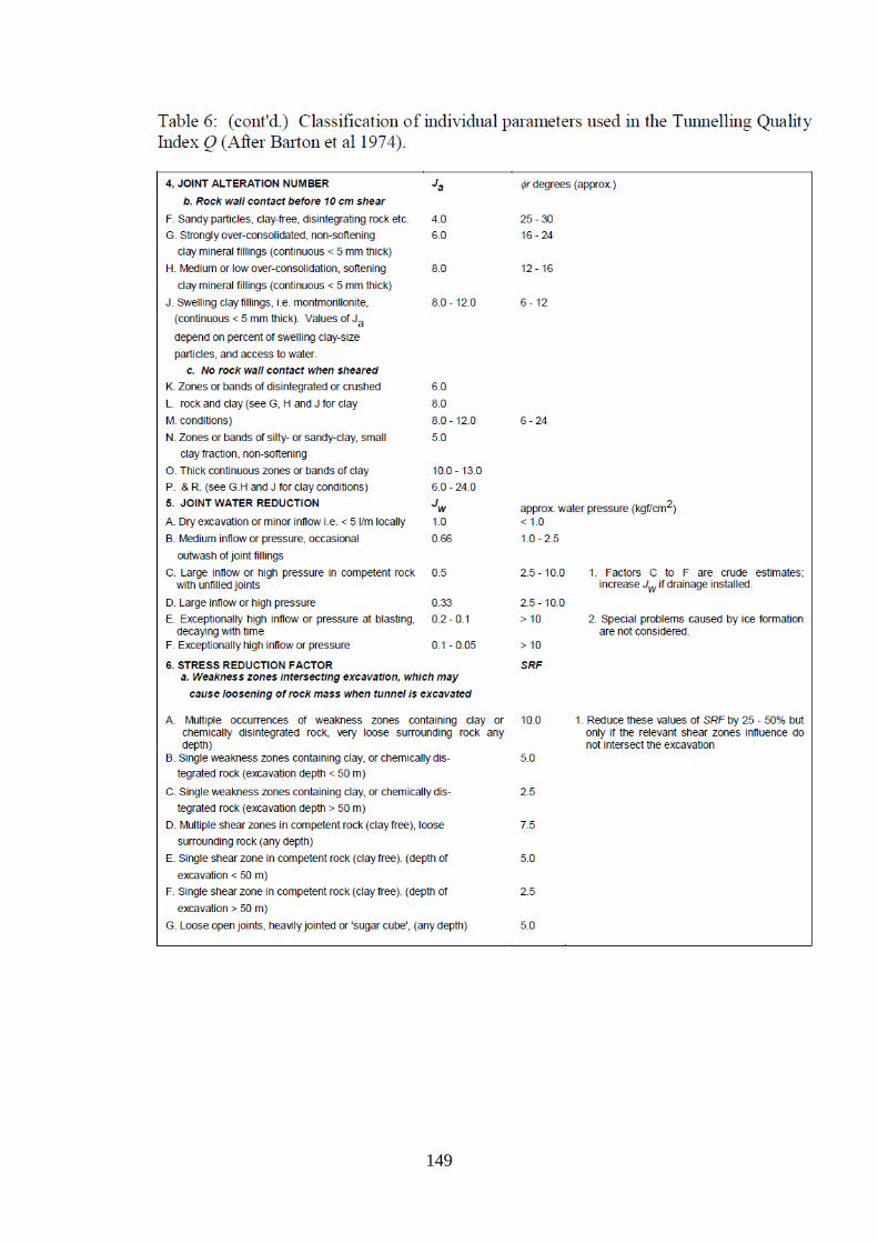
149

150

151
Appendix C: OD intact rock properties
D.1 Summary of rock property data for OD

152
C.2 UCS and UCS Vs sample diameter plots for different rock types at OD
Unconfined Compressive Strength
GRNB <10% Haemetite
0
20
40
60
80
100
1.5 to 3 3 to 10 10 to 25 25 to 80 80 to
250
>250
Unconfined Compressive Strength
Fre
qu
en
cy %
UCS Versus Sample Diameter
GRNB
0
100
200
300
400
500
0 20 40 60 80 100 120 140 160
Sample Diameter
UC
S i
n M
Pa
UCS Versus % Sericite
GRNB
y = -57.884Ln(x) + 330.28
R2 = 0.4066
0
100
200
300
400
500
0 10 20 30 40 50 60 70
% Sericite
UC
S i
n M
Pa
Unconfined Compressive Strength
GRNH 10 to 30% Haemetite
0
20
40
60
80
100
1.5 to 3 3 to 10 10 to 25 25 to 80 80 to
250
>250
Unconfined Compressive Strength
Fre
qu
en
cy %
UCS Versus Sample Diameter
GRNH
0
100
200
300
400
500
0 20 40 60 80 100 120 140 160
Sample Diameter
UC
S i
n M
Pa
UCS Versus % Sericite
GRNH
y = -94.669Ln(x) + 452.05
R2 = 0.4409
0
100
200
300
400
500
0 10 20 30 40 50 60 70
% Sericite
UC
S i
n M
Pa

153
Unconfined Compressive Strength
GRNL 30 to 60% Haemetite
0
20
40
60
80
100
1.5 to 3 3 to 10 10 to 25 25 to 80 80 to
250
>250
Unconfined Compressive Strength
Fre
qu
en
cy %
UCS VersusSample Diameter
GRNL
y = -46.913Ln(x) + 337.32
R2 = 0.0913
0
100
200
300
400
500
0 20 40 60 80 100 120 140 160
Sample Diameter
UC
S i
n M
Pa
UCS Versus % Sericite
GRNL
y = -26.312Ln(x) + 243.44
R2 = 0.1385
0
100
200
300
400
500
0 10 20 30 40 50 60 70
% Sericite
UC
S i
n M
Pa
Unconfined Compressive Strength
HEMH
0
20
40
60
80
100
1.5 to 3 3 to 10 10 to 25 25 to 80 80 to
250
>250
Unconfined Compressive Strength
Fre
qu
en
cy %
UCS Versus Sample Diameter
HEMH
0
100
200
300
400
500
0 20 40 60 80 100 120 140 160
Sample Diameter
UC
S i
n M
Pa
UCS Versus % Sericite
HEMH
y = -7.0066x + 346.88
R2 = 0.6158
0
100
200
300
400
500
0 10 20 30 40 50 60 70
% Sericite
UC
S i
n M
Pa

154
Unconfined Compressive Strength
HEM >90% Haemetite
0
20
40
60
80
100
1.5 to 3 3 to 10 10 to 25 25 to 80 80 to
250
>250
Unconfined Compressive Strength
Fre
qu
en
cy %
UCS Versus Sample Diameter
HEM
y = -85.828Ln(x) + 508.6
R2 = 0.1323
0
100
200
300
400
500
0 20 40 60 80 100 120 140 160
Sample Diameter
UC
S i
n M
Pa
Unconfined Compressive Strength
HEMQ >90% Haemetite & Quartz
0
20
40
60
80
100
1.5 to 3 3 to 10 10 to 25 25 to 80 80 to
250
>250
Unconfined Compressive Strength
Fre
qu
en
cy %
UCS Versus Sample Diameter
HEM
0
100
200
300
400
500
0 20 40 60 80 100 120 140 160
Sample Diameter
UC
S i
n M
Pa
Unconfined Compressive Strength
GRNV
0
20
40
60
80
100
1.5 to 3 3 to 10 10 to 25 25 to 80 80 to
250
>250
Unconfined Compressive Strength
Fre
qu
en
cy %
UCS Versus Sample Diameter
GRNV
y = -39.227Ln(x) + 261.08
R2 = 0.1377
0
100
200
300
400
500
0 20 40 60 80 100 120 140 160
Sample Diameter
UC
S i
n M
Pa

155
Appendix D: OD joint properties
E.1 Joint roughness and orientation

156

157
D.2 Mine area joint orientations
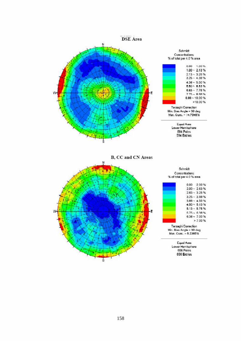
158
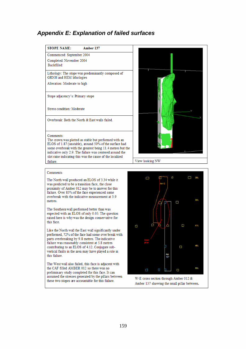
159
Appendix E: Explanation of failed surfaces

160

161

162

163

164
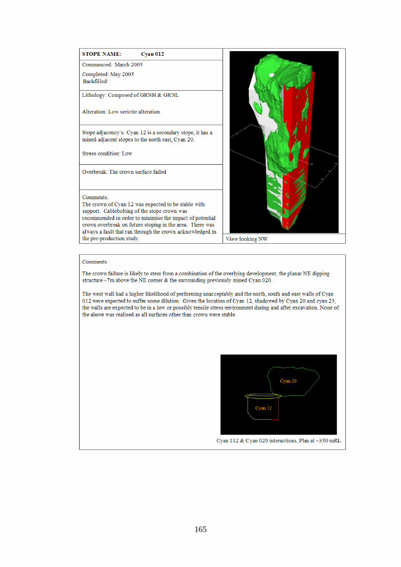
165

166

167

168

169

170

171

172

173

174

175

176

177

178

179

180

181

182

183

184

185

186

187

188

189

190
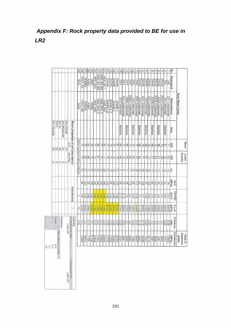
191
Appendix F: Rock property data provided to BE for use in
LR2