Applicability of non-invasively collected matrices for human biomonitoring
Upload
khangminh22Category
view
2download
0
Assessment of the applicability of XFEM in Abaqusfor modeling crack growth in rubber
Luigi Gigliotti
Supervisor: Dr. Martin Kroon
Master Thesis
Stockholm, Sweden 2012
KTH School of Engineering SciencesDepartment of Solid MechanicsRoyal Institute of Technology
SE-100 44 Stockholm - Sweden


Abstract
The eXtended Finite Element Method is a partition of unity based method, particularly suitable for modellingcrack propagation phenomena, without knowing a priori the crack path. Its numerical implementation is mostlyachieved with stand-alone codes.
The implementation of the eXtended Finite Element Method in commercial FEA softwares is still limited,and the most famous one including such capabilities is AbaqusTM. However, due to its relatively recent intro-duction, XFEM technique in Abaqus has been proved to provide trustable results only in few simple benchmarkproblems involving linear elastic material models.
In this work, we present an assessment of the applicability of the eXtendend Finite Element Method inAbaqus, to deal with fracture mechanics problems of rubber-like materials. Results are provided for bothNeo-Hookean and Arruda-Boyce material models, under plane strain conditions.
In the first part of this work, a static analysis for the pure Mode-I and for a 45o mixed-Mode load condition,whose objective has been to evaluate the ability of the XFEM technique in Abaqus, to correctly model the stressand displacement fields around a crack tip, has been performed. Outcomes from XFEM analysis with coarsemeshes have been compared with the analogous ones obtained with highly refined standard FEM discretizations.
Noteworthy, despite the remarkable level of accuracy in analyzing the displacement field at the crack tip,concerning the stress field, the adoption of the XFEM provides no benefits, if compared to the standard FEMformulation. The only remarkable advantage is the possibility to discretize the model without the mesh con-forming the crack geometry.
Furthermore, the dynamic process of crack propagation has been analyzed by means of the XFEM. A 45o
mixed-Mode and a 30o mixed-Mode load condition are analyzed. In particular, three fundamental aspects ofthe crack propagation phenomenon have been investigated, i.e. the instant at which a pre-existing crack startsto propagate within the body under the applied boundary conditions, the crack propagation direction and thepredicted crack propagation speeds.
According to the obtained results, the most influent parameters are thought to be the elements size at thecrack tip h and the applied displacement rate v. Severe difficulties have been faced to attain convergence. Somereasonable motivations of the unsatisfactory convergence behaviour are proposed.
Keywords: Fracture Mechanics; eXtended Finite Element Method; Rubber-like materials; Abaqus

Acknowledgements
Now that my master thesis work is completed, there are many people whom I wish to acknowledge.First of all, my deepest gratitude goes to my supervisor Dr. Martin Kroon for his guidance, interesting cues
and for giving me the possibility to work with him.Secondly, I am grateful to Dr. Artem Kulachenko for his suggestions and stimulating discussions.My ”big brother” PhD student Jacopo Biasetti deserves a special thanks for being my scientific mentor and,
most of all my friend, during my period at the Solid Mechanics Department of the Royal Institute of Technology(KTH).
Last but not least, I will never be sufficiently thankful to my family for their constant support and encour-agement during my studies.
Stockholm, June 2012
Luigi Gigliotti

Contents
Abstract . . . . . . . . . . . . . . . . . . . . . . . . . . . . . . . . . . . . . . . . . . . . . . . . . . . . . iAcknowledgements . . . . . . . . . . . . . . . . . . . . . . . . . . . . . . . . . . . . . . . . . . . . . . . iiMotivation and outline . . . . . . . . . . . . . . . . . . . . . . . . . . . . . . . . . . . . . . . . . . . . . iv
1 Fundamentals: literature review and basic concepts 11.1 Rubber elasticity . . . . . . . . . . . . . . . . . . . . . . . . . . . . . . . . . . . . . . . . . . . . . 1
1.1.1 Kinematics of large displacements . . . . . . . . . . . . . . . . . . . . . . . . . . . . . . . 11.1.2 Hyperelastic materials . . . . . . . . . . . . . . . . . . . . . . . . . . . . . . . . . . . . . . 71.1.3 Isotropic Hyperelastic material models . . . . . . . . . . . . . . . . . . . . . . . . . . . . . 9
1.2 Fracture Mechanics of Rubber . . . . . . . . . . . . . . . . . . . . . . . . . . . . . . . . . . . . . . 111.2.1 Fracture mechanics approach . . . . . . . . . . . . . . . . . . . . . . . . . . . . . . . . . . 111.2.2 Stress around the crack tip . . . . . . . . . . . . . . . . . . . . . . . . . . . . . . . . . . . 131.2.3 Tearing energy . . . . . . . . . . . . . . . . . . . . . . . . . . . . . . . . . . . . . . . . . . 141.2.4 Qualitative observation of the tearing process . . . . . . . . . . . . . . . . . . . . . . . . . 151.2.5 Tearing energy for different geometries . . . . . . . . . . . . . . . . . . . . . . . . . . . . . 15
1.3 eXtended Finite Element Method . . . . . . . . . . . . . . . . . . . . . . . . . . . . . . . . . . . . 181.3.1 Introduction . . . . . . . . . . . . . . . . . . . . . . . . . . . . . . . . . . . . . . . . . . . 181.3.2 Partition of unity . . . . . . . . . . . . . . . . . . . . . . . . . . . . . . . . . . . . . . . . . 191.3.3 eXtended Finite Element Method . . . . . . . . . . . . . . . . . . . . . . . . . . . . . . . . 201.3.4 XFEM implementation in ABAQUS . . . . . . . . . . . . . . . . . . . . . . . . . . . . . . 271.3.5 Limitations of the use of XFEM within Abaqus . . . . . . . . . . . . . . . . . . . . . . . . 27
2 Problem formulation 292.1 Geometrical model . . . . . . . . . . . . . . . . . . . . . . . . . . . . . . . . . . . . . . . . . . . . 292.2 Solution procedure . . . . . . . . . . . . . . . . . . . . . . . . . . . . . . . . . . . . . . . . . . . . 292.3 Static Analysis . . . . . . . . . . . . . . . . . . . . . . . . . . . . . . . . . . . . . . . . . . . . . . 302.4 Dynamic Analysis . . . . . . . . . . . . . . . . . . . . . . . . . . . . . . . . . . . . . . . . . . . . 312.5 Damage parameters . . . . . . . . . . . . . . . . . . . . . . . . . . . . . . . . . . . . . . . . . . . 32
3 Numerical results - Static Analysis 353.1 Stress field around the crack tip . . . . . . . . . . . . . . . . . . . . . . . . . . . . . . . . . . . . . 36
3.1.1 Pure Mode-I loading condition . . . . . . . . . . . . . . . . . . . . . . . . . . . . . . . . . 363.1.2 Mixed-Mode loading condition . . . . . . . . . . . . . . . . . . . . . . . . . . . . . . . . . 38
3.2 Displacement field around the crack tip . . . . . . . . . . . . . . . . . . . . . . . . . . . . . . . . 393.2.1 Pure Mode-I loading condition . . . . . . . . . . . . . . . . . . . . . . . . . . . . . . . . . 393.2.2 Mixed-Mode loading condition . . . . . . . . . . . . . . . . . . . . . . . . . . . . . . . . . 41
4 Numerical results - Dynamic Analysis 454.1 Convergence criteria for nonlinear problems . . . . . . . . . . . . . . . . . . . . . . . . . . . . . . 45
4.1.1 Line search algorithm . . . . . . . . . . . . . . . . . . . . . . . . . . . . . . . . . . . . . . 474.2 Crack propagation instant . . . . . . . . . . . . . . . . . . . . . . . . . . . . . . . . . . . . . . . . 474.3 Crack propagation angle . . . . . . . . . . . . . . . . . . . . . . . . . . . . . . . . . . . . . . . . . 504.4 Crack propagation speed . . . . . . . . . . . . . . . . . . . . . . . . . . . . . . . . . . . . . . . . . 534.5 Remarks on convergence behaviour . . . . . . . . . . . . . . . . . . . . . . . . . . . . . . . . . . . 62
5 Summary 65
Bibliography 67

Motivation and outline
The aim of the study in the present master thesis has been to assess the applicability of the XFEM implementation inthe commercial FEA software Abaqus, to handle fracture mechanics problems in rubber-like materials. In particular,we focus on the capabilities of XFEM analyses with coarse meshes, to correctly model the stress and displacement fieldsaround the crack tip under pure Mode-I and under a 45o mixed-Mode load condition in static problems. Such abilitieshave been investigated in crack growth processes as well, and the effects of the most relevant parameters are emphasized.
The introduction of the eXtended Finite Element Method (XFEM) represents undoubtedly, the major breakthroughin the computational fracture mechanics field, made in the last years. It is a suitable method to model the propagationof strong and weak discontinuities. The concept behind such technique is to enrich the space of standard polynomialbasis functions with discontinuous basis functions, in order to represent the presence of the discontinuity, and withsingular basis functions in order to capture the singularity in the stress field. By utilizing such method, the remeshingprocedure of conventional finite element methods, is no more needed. Therefore, the related computational burdenand results projection errors are avoided. For moving discontinuities treated with the XFEM, the crack will follow asolution-dependent path. Despite these advantages, the XFEM are numerically implemented mostly by means of stand-alone codes. However, during the last years an increasing number of commercial FEA software are adopting the XFEMtechnique; among these, the most famous and widely employed is Abaqus, produced by the Dassault Systemes S.A..
The implementation of XFEM in Abaqus is a work in progress and its applicability has been still evaluated only forparticularly simple fracture mechanics problems in plane stress conditions and for isotropic linear elastic materials. Noattempts have been made in considering more complex load conditions and/or material models. This work aims, at leastto some extent, at limiting the lack of knowledge in this field. For these reasons, the application of XFEM in Abaqus tomodel crack growth phenomena in rubber-like materials, has been investigated.
This report is organized as follows. In Chapter 1, a background of the arguments closely related to the present work,is provided. A short review of the continuum mechanics approach for rubber elasticity, along with concepts of fracturemechanics for rubber is given. Both theoretical and practical foundations of the eXtended Finite Element Method arepresented. In conclusion of this chapter, the application of such method to large strains problems and the main featuresof its implementation in Abaqus are discussed.
In Chapter 2, the problem formulation at hand is presented. Furthermore, details about the performed numericalsimulations are provided.
Numerical results of the static analysis are summarized in Chapter 3. The outcomes from coarse XFEM discretiza-tions are compared to those obtained with the standard FEM approach, in order to evaluate their ability to deal withfracture mechanics problems in rubber-like materials.
In conclusion, numerical results of the crack growth phenomenon in rubber, analyzed by means of the XFEM techniquein Abaqus are presented and discussed in Chapter 4. Three fundamental aspects of the crack propagation process areinvestigated, i.e. the instant in which the pre-existing crack starts to propagate under the prescribed loading conditions,the direction of crack propagation and its speed. At the end of this chapter, conclusive remarks on the convergencebehaviour in numerical simulations of crack growth phenomena by utilizing the eXtended Finite Element Method are,indicated.
iv

Chapter 1
Fundamentals: literature review andbasic concepts
1.1 Rubber elasticity
Rubber-like materials, such as rubber itself, soft tissues etc, can be appropriately described by virtue of a well-knowtheory in the continuum mechanics framework, named Hyperelasticity Theory. For this purpose, in this section thefundamental aspects of this theory - albeit limited to the case of isotropic and incompressible material - as well asfinite displacements and deformations theory will be expounded [1]. Lastly, a description of the hyperelastic constitutivemodels adopted in this work is proposed.
1.1.1 Kinematics of large displacements
The main goal of the kinematics theory, is to study and describe the motion of a deformable body, i.e to determine itssuccessive configurations under a general defined load condition, as function of the pseudo-time t.
A deformable body, within the framework of 3D Euclidean space, R3, can be regarded as a set of interacting particlesembedded in the domain Ω ∈ R3 (see Fig. 1.1). The boundary of this latter, often referred to as Γ = ∂Ω is split up in twodifferent parts, Γu along which the displacement values are prescribed and Γσ where the stress component values have tobe imposed. A problem is said to be well-posed if these two different boundary conditions are not applied simultaneouslyon the same portion of frontier. Moreover, the boundary Γ should be characterized by a sufficient smoothness (at leastpiece-wise), in order to define uniquely the outward unit normal vector n; last but not least, it must be highlighted that,a unique solution of the boundary value problem is achievable only if Γu 6= ∅, such that all the rigid body motions areeliminated.
Figure 1.1: Initial and deformed configurations of a solid deformable body in 3D Euclidean space.
Among all possible configurations assumed by a deformable body during its motion, of particular importance is thereference (or undeformed) configuration Ω, defined at a fixed reference time and depicted in Fig. 1.1 with thedashed line. With excess of meticulousness, it is worth noting that a so-called initial configuration at initial time t = 0,can be defined and that, whilst for static problems such configuration coincides with the reference one, in dynamics theinitial configuration is often not chosen as the reference configuration. In the reference configuration, every particles of
1

2 L. Gigliotti CHAPTER 1. FUNDAMENTALS: LITERATURE REVIEW AND BASIC CONCEPTS
the deformable body are solely identified by the position vector (or referential position) x defined as follows
x = xiei 7→ x =
x1
x2
x3
(1.1)
where ei represent the basis vectors of the employed coordinate system. The motion of a body from its referenceconfiguration is easily interpretable as the evolution of its particles and its resulting position at the instant of time t isgiven by the relation
xϕ = ϕt(x) (1.2)
At this point, the major difference with respect to the case of small displacements starts to play a significant role.Indeed, in case of deformable body, it is required to take account of two sets of coordinates for two different configurations,i.e. the initial configuration Ω and the so-called current (or deformed) configuration Ωϕ(” = ϕ(Ω)”). Under theseassumptions, it is now straightforward to write the position vectors for any particles constituting the deformable bodyin both its reference and current configurations:
x = xiei ; xϕ = xϕi eϕi (1.3)
being ei and eϕi the unit base vectors in reference and current configuration, respectively. Within the framework ofgeometrically nonlinear theory, in which large displacements and large displacement gradients are involved, the simpli-fication used in the linear theory, namely that not only the two base vectors are coincident, but also the two sets ofcoordinates in both reference and current configurations, can no longer be exploited. In this regard, it is then requiredto uniquely define the configuration with respect to which, the boundary value problem will be formulated.
For this aim, the choice has to be made between the Lagrangian formulation in which all the unknowns are referredto the coordinates xi
1 in the reference configuration and the Eulerian formulation, in which specularly, the unknownsare supposed to depend upon the coordinates xϕi
2 in the deformed configuration. In fluid mechanics problems the mostappropriate formulation is the Eulerian one, simply because the only configuration of interest is the deformed one and, atleast for Newtonian fluids, the constitutive behaviour is not dependent upon the deformation trajectory; on the contrary,the Lagrangian formulation appears to be better suitable for solid mechanics problems since it refers to the currentconfiguration. Furthermore, as it is necessary to consider the complete deformation trajectory, it is hence possible todefine the corresponding evolution of internal variables and resulting values of stress within solid materials. Of particularinterest is a mixed formulation called arbitrary Eulerian-Lagrangian formulation, especially well suitable for interactionproblems, such as fluid-structure interaction; in this case, the fluid motion will be described by the Eulerian formulationwhile the solid evolution by the Lagrangian one.
1.1.1.1 Deformation gradient
The motion of all particles of a deformable body might be described by means of the point transformation xϕ = ϕ(x); ∀x ∈Ω.
Let x = Φ(ξ) ⊂ Ω with ξ representing the parametrization shown in Fig. 1.2, a material (or undeformed)curve independent with respect to time. This latter is deformed into a spatial or deformed curve xϕ = Φϕ(ξ, t) =ϕ(Φ(ξ), t) ⊂ Ωϕ at any time t. At this point, it is useful to define a material tangent vector dx to the material curve
Figure 1.2: Deformation of a material curve Φ ∈ Ω into a spatial curve Φϕ ∈ Ωϕ.
and a spatial tangent vector dxϕ to the spatial curve.
dxϕ =∂Φϕ
∂ξ(ξ, t)dξ ; dx =
∂Φ
∂ξ(ξ)dξ (1.4)
1Often coordinates xi are labelled as the material (or referential) coordinates.2As above, usually with xϕi are referred to as spatial (or current) coordinates.
KTH Royal Institute of Technology - Solid Mechanics Department

1.1. RUBBER ELASTICITY L. Gigliotti 3
The tangent vectors dx and dxϕ are usually labelled as material (or undeformed) line element and spatial (ordeformed) line element, respectively. Furthermore, for any motion taking place in the Euclidean space, a largedisplacement vector can be introduced as follows
d(x) = xϕ ⇔ di(x) = ϕjδij − xi (1.5)
According to Fig. 1.3, and by means of basic notions of algebra of tensors, it is possible to infer that:
Figure 1.3: Total displacement field.
xϕ + dxϕ = x + dx + d(x + dx) =⇒ dxϕ = dx + d(x + dx)− d(x) (1.6)
The term d(x + dx) can be computed by exploiting Taylor series formula, and truncating them after the linear term:
d(x + dx) = d(x) +∇d(x)dx + o(‖dx‖) (1.7)
where, ∇d is the large displacement gradient, or in index notation
di(x + dx) = di(x) +∂di∂xi
(x)dxi + o(‖dx‖) (1.8)
At this point, it is sufficient to compare Eq. 1.6 and Eq. 1.7, to express the spatial tangent vector dxϕ as function of itscorresponding material tangent vector and of the two-point tensor F named as deformation gradient tensor:
dxϕ = (I +∇d)︸ ︷︷ ︸F
dx⇒ dxϕ = Fdx ; [F]ij :=∂xi∂xj
+∂di∂xj
=∂ϕi∂xj
(1.9)
or alternatively,
F =∂ϕi∂xj
eϕi ⊗ ej ; F = ϕ⊗∇ (1.10)
with the gradient operator ∇ = ∂∂xj
ei.
It is a painless task to demonstrate how the deformation gradient, not only provides the mapping of a generic(infinitesimal) material tangent vector into the relative spatial tangent vector, but also controls the transformation of aninfinitesimal surface element or an infinitesimal volume element (see Fig. 1.4).
Figure 1.4: Transformation of infinitesimal surface and volume elements between initial and deformedconfiguration.
KTH Royal Institute of Technology - Solid Mechanics Department

4 L. Gigliotti CHAPTER 1. FUNDAMENTALS: LITERATURE REVIEW AND BASIC CONCEPTS
Let dA be an infinitesimal surface element, constructed as the vector product of two infinitesimal reciprocally orthog-onal vectors, dx and dy; the outward normal vector is, as usual, defined as n = (dx× dy)/ ‖dx× dy‖. By means of thedeformation gradient F, the new extension and orientation in the space of the surface element can be easily determined
dAϕnϕ := dxϕ × dyϕ = (Fdx)× (Fdy) = (det [F] F−T )(dx× dy)︸ ︷︷ ︸dAn
= dA(cof [F])n (1.11)
which is often referred to as Nanson’s formula.
Once the Nanson’s formula has been derived, it is straightforward to obtain the analogous relation for the change of aninfinitesimal volume element occurring between the initial and the deformed configuration. Describing the infinitesimalvolume element in the material configuration as the scalar product between an infinitesimal surface element dAϕ andthe infinitesimal vector dzϕ and exploiting results in Eq. 1.11, the following relation holds
dV ϕ := dzϕ · dAnϕ = Fdz · JF−TdAn = Jdz · dAn = JdA (1.12)
in which J = det [F ] is well-known as the Jacobian determinant (or volume ratio).
As stated in Eq. 1.9, the deformation gradient F, is a linear transformation of an infinitesimal material vector dx intoits relative spatial dxϕ; such transformation affects all parameters characterizing a vector, its modulus, direction andorientation. However, the deformation is related only to the change in length of an infinitesimal vector, and therefore,it results to be handy to consider the so-called polar decomposition , by virtue of which the deformation gradient canbe written as a multiplicative split between an orthogonal tensor R, an isometric transformation which only changes thedirection and orientation of a vector, and a symmetric, positive-definite stretch tensor U that provides the measure oflarge deformation.
F = RU ; RT = R−1 ; UT = U ; ‖dxϕ‖ = ‖Ux‖ (1.13)
In other words, the symmetric tensor U, yet referred in literature to as the right (or material) stretch tensor,produces a deformed vector that remains in the initial configuration (no large rotations). In index notation, the largerotations tensor R, and the right stretch tensor U, can be respectively expressed as follows
R = Rijeϕi ⊗ ej ; U = Uijei ⊗ ej (1.14)
An alternative form of the polar decomposition can be provided, by simply inverting the order of the above mentionedtransformations and introducing the so-called left(or spatial) stretch tensor V
F = VR ; V = Vijeϕi ⊗ eϕj (1.15)
In such case, a large rotation, represented by R, is followed by a large deformation (tensor V).
1.1.1.2 Strain measures
Theoretically, apart form the right and the left stretch tensors U and V, an infinite number of other deformation measurescan be defined; indeed, unlike displacements, which are measurable quantities, strains are based on a concept that isintroduced as a simplification for the large deformation analysis.
From a computational point of view, the choice or U or V to calculate the stress values is not the most appropriateone, as it requires, first, to perform the polar decomposition of the deformation gradient. Hence, it is necessary tointroduce deformation measures that can directly, without any further computations, provide information about thedeformation state.
We may consider two neighbouring points defined by their position vectors x and y in the material description; withreference to Fig. 1.5 on the next page, it is possible to describe the relation between these two, sufficiently close points,i.e.
y = y + (x− x) = x +∣∣y − x
∣∣ y − x∣∣y − x∣∣ = x + dx (1.16)
dx = dεa and dε =∣∣y − x
∣∣ , a =y − x∣∣y − x
∣∣ (1.17)
In the above equations, it is clear that the length of the material line element dx is denoted by the scalar value dεand that the unit vector a, with
∣∣a∣∣ = 1, represents the direction of the aforesaid vector at the given position in thereference configuration. As stated in Eq. 1.9, the deformation gradient F allows to linearly approximate a vector dx inthe material description, with its corresponding vector dxϕ in the spatial description. The smaller the vector dx, thebetter the approximation.
At this point, it is then possible to define the stretch vector λa, in the direction of the unit vector a and at the pointx ∈ Ω as
λa(x, t) = F(x, t)a (1.18)
with its modulus λ known as stretch ratio or just stretch. This latter is a measure of how much the unit vector a hasbeen stretched. In relation to its value, λ < 1, λ = 1 or λ > 1, the line element is said to be compressed, unstretched
KTH Royal Institute of Technology - Solid Mechanics Department

1.1. RUBBER ELASTICITY L. Gigliotti 5
Figure 1.5: Deformation of a material line element with length dε into a spatial element with lengthλdε.
or extended, respectively. Computing the square of the stretch ratio λ, the definition of the right Cauchy-Greentensor C is introduced
λ2 = λa · λa = Fa · Fa = a · FTFa = a ·Ca ,
C = FTF or CIJ = FiIFiJ
(1.19)
Often the tensor C is also referred to as the Green deformation tensor and it should be highlighted that, since thetensor C operate solely on material vectors, it is denoted as a material deformation tensor. Moreover, C is symmetricand positive definite ∀x ∈ Ω:
C = FTF = (FTF)T = CT and u ·Cu > 0 ∀u 6= 0 (1.20)
The inverse of the right Cauchy-Green tensor is the well-known Piola deformation tensor B, i.e. B = C−1.To conclude the roundup of material deformation tensors, the definition of the commonly used Green-Lagrange
strain tensor E, is here provided:
12
[(λdε)2 − dε2
]= 1
2
[(dεa) · FTF (dεa)− dε2
]= dx ·Edx ,
E = 12
(FTF− I
)= 1
2(C− I) or EIJ = 1
2(FiIFiJ − δIJ)
(1.21)
whose symmetrical nature is obvious, given the symmetry of C and I. In an analogous manner of the one shown above,it is possible to describe deformation measures in spatial configuration, too; the stretch vector λaϕ in the direction ofaϕ, for each xϕ ∈ Ω might thus be define as:
λ−1aϕ (xϕ, t) = F−1(xϕ, t)aϕ (1.22)
where, the norm of the inverse stretch vector λ−1aϕ is called inverse stretch ratio λ−1 or simply inverse stretch.
Moreover, the unit vector aϕ may be interpreted as a spatial vector, characterizing the direction of a spatial line elementdxϕ. By virtue of Eq. 1.22, computing the square of the inverse stretch ratio, i.e.
λ−2 = λ−1aϕ · λ
−1aϕ = F−1a · F−1a = a · F−TF−1a = a · b−1a (1.23)
where b is the left Cauchy-Green tensor, sometimes referred to as the Finger deformation tensor
b = FFT or bij = FiIFjI (1.24)
Like its corresponding tensor in the material configuration, the Green deformation tensor, the left Cauchy-Green tensorb is symmetric and positive definite ∀xϕ ∈ Ω:
b = FFT = (FTF)T = bT and u · bu > 0 ∀u 6= 0 (1.25)
Last but not least, the well-known symmetric Euler-Almansi strain tensor e is here introduced:
1
2[dε2 − (λ−1dε)2] =
1
2[dε2 − (dεa) · F−TF−1(dεa)] = dxϕ · edxϕ ,
e =1
2(I− F−TF−1) or eij =
1
2(δij − F−1
Ki F−1Kj )
(1.26)
where the scalar value dε is the (spatial) length of a spatial line element dxϕ = xϕ − yϕ.
KTH Royal Institute of Technology - Solid Mechanics Department

6 L. Gigliotti CHAPTER 1. FUNDAMENTALS: LITERATURE REVIEW AND BASIC CONCEPTS
1.1.1.3 Stress measures
During a particular transformation, the motion and deformation which take place, make a portion of material interactwith the rest of the interior part of the body. These interactions give rise to stresses, physically forces per unit area,which are responsible of the deformation of material.
Given a deformable body occupying an arbitrary region Ω in the Euclidean space, whose boundary is the surface∂Ω at the specific time t, let us assume that two types of arbitrary forces, somehow distributed, act respectively on theboundary surface (external forces) and on an imaginary internal surface (internal forces).
Let the body be completely cut by a plane surface; thereby the interaction between the two different portions of thebody is represented by forces transmitted across the (internal) plane surface. Under the action of this system of forces,
Figure 1.6: Traction vectors acting on infinitesimal surface elements with outward unit normals.
the body results to be in equilibrium conditions but, once the body is cut in two parts, both of them are no more underthese equilibrium conditions and thus, an equivalent force distribution along the faces created by the cutting process hasto be considered, in order to represent the interaction between the two parts of the body. The infinitesimal resultant(actual) force acting on a surface element df, is defined as
df = tdAϕ = TdA (1.27)
Here, t = t(xϕ, t,nϕ) is known in the literature as the Cauchy (or true) traction vector (force measured per unitsurface area in the current configuration), while the (pseudo) traction vector T = T(x, t,n) represents the first Piola-Kirchhoff (or nominal) traction vector (force measured per unit surface area in the reference configuration).
In literature Eq. 1.27 is referred to as the Cauchy’s postulate. Moreover, the vectors t and T acting across surfaceelements dA and dAϕ with the corresponding normals n and nϕ, can be also defined as surface tractions or, accordingto other texts, as contact forces or just loads.
The so-called Cauchy’s stress theorem claims the existence of tensor fields σ and P so that
t(xϕ, t,nϕ) = σ(xϕ, t)nϕ or ti = σijnϕj
T(x, t,n) = P(x, t)n or Ti = PiInI
(1.28)
where the tensor σ denotes the symmetric3 Cauchy (or true) stress tensor (or simply the Cauchy stress) and P isreferred to as the first Piola-Kirchhoff (or nominal) stress tensor (or simply the Piola stress.)
The relation linking the above defined stress tensors is the so-called Piola transformation, obtained by merging Eq.1.27 and Eq. 1.28 and exploiting the Nanson’s formula:
P = JσF−T ; PiI = JσijF−1Ij (1.29)
or in its dual expressionσ = J−1PFT ; σij = J−1PiIFjI = σji (1.30)
Along with the stress tensors given above, many others have been presented in literature; in particular, the majorityof them have been proposed in order to ease numerical analyses for practical nonlinear problems. One of the mostconvenient is the Kirchhoff stress tensor τ , which is a contravariant spatial tensor defined by:
τ = Jσ ; τij = Jσij (1.31)
3Symmetry of the Cauchy stress is satisfied only under the assumption (typical of the classical formulation of continuummechanics) that resultant couples can be neglected.
KTH Royal Institute of Technology - Solid Mechanics Department

1.1. RUBBER ELASTICITY L. Gigliotti 7
In addition, the so-called second Piola-Kirchhoff stress tensor S has been proposed, especially for its noticeableusefulness in the computational mechanics field, as well as for the formulation of constitutive equations; this contravariantmaterial tensor does not have any physical interpretation in terms of surface tractions and it can be easily computed byapplying the pull-back operation on the contravariant spatial tensor τ :
S = F−1τF−T or SIJ = F−1Ii F
−1Jj τij (1.32)
The second Piola-Kirchhoff stress tensor S can be, moreover, related to the Cauchy stress tensor by exploiting Eqs.1.29, 1.32 and 1.31:
S = JF−1σF−T = F−1P = ST or SIJ = JF−1Ii F
−1Jj σij = F−1
Ii PiJ = SJI (1.33)
as consequence, the fundamental relationship between the first Piola-Kirchhoff stress tensor P and the symmetric secondPiola-Kirchhoff stress tensor S is found, i.e.
P = FS or PiI = FiJSJI (1.34)
A plethora of other stress tensors can be found in literature; among them the Biot stress tensor TB , the symmetryccorotated Cauchy stress tensor σu and the Mandel stress tensor Σ deserve to be mentioned [2].
1.1.2 Hyperelastic materials
The correct formulation of constitutive theories for different kinds of material, is a very important matter in continuummechanics, in particular with regards to the description of nonlinear materials, such as rubber-like ones.
The branch of continuum mechanics, which provides the formulation of constitutive equations for that category of ma-terials which can sustain to large deformations, is called finite (hyper)elasticity theory or just finite (hyper)elasticity.In this theory, the existence of the so-called Helmoltz free-energy function Ψ, defined per unit reference volume oralternately per unit mass, is postulated. In the most general case, the Helmoltz free-energy function is a scalar-valued function of the tensor F and of the position of the particular point within the body. Restricting the analysisto the case of homogeneous material, the energy solely depends on the deformation gradient F, and as such, it is oftenreferred to as strain-energy function or stored-energy function Ψ = Ψ(F). By virtue of what has been shown inthe previous section, the strain energy function Ψ can be expressed as function of several other deformation tensors, e.g.the right Cauchy-Green tensor C, the left Cauchy-Green tensor b.
A hyperelastic material, or Green-elastic material, is a subclass of elastic materials for which the relation expressedin Eq. 1.35 holds
P = G(F) =∂Ψ(F)
∂For PiI =
∂Ψ
∂FiI(1.35)
Many other reduced forms of constitutive equations, equivalent to the latter, for hyperelastic materials at finite strainscan be derived; while not wishing to report here all the different forms available in literature, consider for this purpose,the derivative with respect to time of the strain energy function Ψ(F):
Ψ = tr
[(∂Ψ(F)
∂F
)T
F
]= tr
[(∂Ψ(C)
∂C
)C
]=
= tr
[∂Ψ(C)
∂C
(FTF + FTF
)]= 2tr
(∂Ψ(C)
∂CFTF
)(1.36)
Given the symmetry of the tensor C, and the resulting symmetry of the tensor valued scalar function Ψ(C), it followsimmediately that: (
∂Ψ(F)
∂F
)T
= 2∂Ψ(C)
∂CFT (1.37)
1.1.2.1 Isotropic hyperelastic materials
Within the context of hyperelasticity, a typology of materials of unquestionable importance, of which rubber is one ofthe most representative examples, consists of the so-called isotropic materials. From a physical point of view, theproperty of isotropy is nothing more than the independence in the response of the material, in terms of stress-strainrelations, with respect to the particular direction considered.
Let us consider a point within an elastic, deformable body occupying the region Ω and identified by its positionvector x. Furthermore, let the body, in the reference configuration, undergo a translational motion represented by thevector c and rotated through the orthogonal tensor Q (see Fig. 1.7 on the following page):
x∗ = c + Qx (1.38)
The deformation gradient F that links the material configuration Ω∗, to the spatial configuration Ωϕ∗ might be computed
KTH Royal Institute of Technology - Solid Mechanics Department

8 L. Gigliotti CHAPTER 1. FUNDAMENTALS: LITERATURE REVIEW AND BASIC CONCEPTS
Figure 1.7: Rigid-body motion superimposed on the reference configuration.
by making use of the chain rule and Eq. 1.38, leading to
F =∂xϕ
∂x=∂xϕ
∂x∗Q = F∗Q or FiI =
∂xϕi∂xI
=∂xϕi∂x∗J
QJI = F ∗iJQJI (1.39)
A material is said to be isotropic if, and only if, the strain energies defined with respect to the deformation gradients Fand F∗ are the same for all orthogonal vectors Q; thus, it might be written that:
Ψ(F) = Ψ(F∗) = Ψ(FQT ) (1.40)
which is the unavoidable condition to refer to a material as isotropic.
Ψ(C) = Ψ(F∗TF∗) = Ψ(QFTFQT ) = Ψ(C∗) (1.41)
Hence, if this latter relation is valid for all symmetric tensors C and all orthogonal tensors Q, the strain energy functionΨ(C), is a scalar-valued isotropic tensor function solely of the tensor C. Under these assumption, the strain energymight be expressed in terms of its invariants, i.e. Ψ = Ψ [I1 (C) , I2 (C) I3 (C)] or, equivalently, of its principal stretchesΨ = Ψ (C) = Ψ [λ1, λ2, λ3].
1.1.2.2 Incompressible hyperelastic materials
A category of rubber-like materials widely used in practical applications and therefore particularly attractive, especiallywith regard to the corresponding computational analysis by means of numerical codes, are the so-called incompressiblematerials, which can sustain finite strains without show any considerable volume changes. In reference to Eq. 1.12, itmight to be stated that, the incompressibility constraint can be expressed as:
J = 1 (1.42)
The incompressibility constraint is widely known in literature as an internal constraint and a material subjected tosuch constraint is called constrained material. In order to derive constitutive equations for a general incompressiblematerial, it is necessary to postulate the existence of a particular strain energy function:
Ψ = Ψ(F)− p(J − 1) (1.43)
defined exclusively for J = det(F) = 1. In such expression, the scalar parameter p, is referred to as Lagrange multiplier,whose value can be determined by solving the equations of equilibrium. As proven in the previous sections, it is sufficient,assuming that this is possible, to differentiate the strain energy function in Eq. 1.43 with respect to the deformationgradient F, to obtain the three fundamental constitutive equations in terms of the first and the second Piola-Kirchhoffstresses, i.e. P and S, and of the Cauchy stress tensor σ. For the particular case of incompressible materials, they maybe written as
P = −pP−T +∂Ψ(F)
∂F
S = −pF−1F−T + F−1 ∂Ψ(F)
∂F= −pC−1 + 2
∂Ψ(C)
∂C
σ = −pI +∂Ψ(F)
∂FFT = −pI + F
(∂Ψ(F)
∂F
)T
(1.44)
KTH Royal Institute of Technology - Solid Mechanics Department

1.1. RUBBER ELASTICITY L. Gigliotti 9
Additionally, it has been demonstrated formerly that, in the case of isotropic material, the strain energy function canbe expressed as function of the right Cauchy Green tensor C, the left Cauchy-Green tensor b and their invariants.However, if the material is at the same time incompressible and isotropic, it is also true that I3 = det C = det b = 1and consequently, the third invariant is no longer an independent deformation variable like I1 and I2. Consequently, therelation stated in 1.43 can be reformulated as follows
Ψ = Ψ [I1(C), I2(C)]− 1
2p(I3 − 1) = Ψ [I1(b), I2(b)]− 1
2p(I3 − 1) (1.45)
Thus, the associated constitutive equations are written as
S = 2∂Ψ(I1, (I1)
∂C− ∂[p(I3 − 1)]
∂C= −pC−1 + 2
(∂Ψ
∂I1+ I1
∂Ψ
∂I2
)I− 2
∂Ψ
∂I2C
σ = −pI + 2
(∂Ψ
∂I1+ I1
∂Ψ
∂I2
)b− 2
∂Ψ
∂I2b2 = −pI + 2
∂Ψ
∂I1b− 2
∂Ψ
∂I2b−1
(1.46)
Lastly, if the strain energy function is expressed as a function of the three principal stretches λi, it holds that
Si = − 1
λ2i
p+1
λi
∂Ψ
∂λi, i = 1, 2, 3 (1.47)
Pi = − 1
λip+
∂Ψ
∂λi, i = 1, 2, 3 (1.48)
σi = −p+ λi∂Ψ
∂λi, i = 1, 2, 3 (1.49)
for whom the constraint of incompressibility, i.e. J = 1 takes the following form:
λ1λ3λ3 = 1 (1.50)
1.1.3 Isotropic Hyperelastic material models
Due to the greater difficulty in the mathematical treatment of hyperelastic materials, there are several examples inliterature about possible forms of strain energy functions for compressible, as well as for incompressible materials.
In the following sections, the two models adopted in the present work, i.e. the Arruda-Boyce and the Neo-Hookean model, will be described. It must be stressed however that, exclusively isotropic incompressible materialmodels under isothermal regime have been treated. Many other models have been proposed in literature, e.g. Ogdenmodel [4, 5] , Mooney-Rivlin model, [11], Yeoh model [16], Kilian-Van der Waals model [20] among the mostfamous.
1.1.3.1 Neo-Hookean model
The Neo-Hookean model [6] can be referred to as a particular case of the Ogden model. Its mathematical expression isthe following one
Ψ = c1(λ2
1 + λ22 + λ2
3 − 3)
= c1 (I1 − 3) (1.51)
By virtue of the consistency condition [7], it follows that
Ψ =µ
2
(λ2
1 + λ22 + λ2
3 − 3)
(1.52)
where µ indicates the shear modulus in the reference configuration.The neo-Hookean model, firstly proposed by Ronald Rivlin in 1948, is similar to the Hooke’s law adopted for linear
materials; indeed, the stress-strain relationship is initially linear while at a certain point the curve will level out. Theprincipal drawback of such model is its inability to predict accurately the behaviour of rubber-like materials for strainslarger then 20% and for biaxal stress states.
It can now be proven that, even if from a mathematical point of view, the Neo-Hookean model may be seen as thesimplest case of the Ogden model, it might be also justified within the context of the Gaussian statistical theory[8, 9]of elasticity, which is based on the assumption that only small strains will be involved in the course of the deformation4.Briefly, rubber-like materials are made up of long-chain molecules, producing one giant molecule, referred to as molecular
4This fact is a further validation of the adequacy of neo-Hookean model for strains up to 20%; the more refined non-Gaussianstatistical theory, of which an example is based on the Langevin distribution function is needed, in order to obtain a moreaccurate model for large strains.
KTH Royal Institute of Technology - Solid Mechanics Department

10 L. Gigliotti CHAPTER 1. FUNDAMENTALS: LITERATURE REVIEW AND BASIC CONCEPTS
network [10]; starting from the Boltzmann principle, and under the assumptions of incompressible material and affinemotion, the entropy change of this network, generated by the motion, can be readily computed as function of the numberN of chains in a unit volume of the network itself and of the principal stretches λi, i = 1, 2, 3
∆η = −1
2Nκ
r20in
r2out
(λ2
1 + λ22 + λ2
3 − 3)
(1.53)
where κ = 1.38 · 10−23Nm/K is the well-known Boltzmann’s constant; at the same time, the parameter r2out and
r20in are the mean square value of the end-to-end distance of detached chains and of the end-to-end distance of cross-
linked chains in the network, respectively. For isothermal processes(
Θ = 0)
, the Legendre transformation leads to
the following expression for the Helmholtz free-energy function
Ψ =1
2NκΘ
r20in
r2out
(λ2
1 + λ22 + λ2
3 − 3)
(1.54)
In conclusion, if the shear modulus µ is expressed as proportional to the concentration of chains N, it holds that:
µ = NκΘr20in
r2out
(1.55)
By virtue of this latter result, the equivalence between Eqs. 1.51 and 1.54 is demonstrated.
1.1.3.2 Arruda-Boyce model
The second material model adopted in this work for modeling the response of rubber-like materials is the Arruda-Boycemodel [14], proposed in 1993; in this model, also known as the eight-chain model, the assumption that the molecularnetwork structure can be regarded as a representing cubic unit volume in which, eight chains are distributed along thediagonal directions towards its eight corners, is made. The Arruda-Boyce model is particularly suitable to characterizeproperties of carbon-black filled rubber vulcanizates; such a notable category of elastomers are reinforced with fillers likecarbon black or silica obtaining thus, a significant improvement in terms of tensile and tear strength, as well as abrasionresistance. By virtue of these reasons, the stress-strain relation is tremendously nonlinear (stiffening effect) at the largestrains.
Unlike the neo-Hookean model, the Arruda-Boyce model is based on the non-Gaussian statistical theory [15]and consequently is adequate to approximate the finite extensibility of rubber-like materials as well as the upturn effectat higher strain levels. The strain energy function for the model considered herein, may be presented as
Ψ = NκΘ√n
[βλchain −
√n ln
(sinhβ
β
)](1.56)
The coefficients in the above written equation, are easily defined as follows
λchain =√I1/3 and β = L−1
(λchain√
n
)(1.57)
where, L is known as Langevin function; obviously, for computational reasons the latter function is approximatedwith a Taylor series expansion. By making use of the first five terms of the Taylor expansion of the Langevin function,a different analytical expression is given by
Ψ = c1
[1
2(I1 − 3)
1
20λ2m
(I21 − 9
)+
11
1050λ4m
(I31 − 27
)+
19
7000λ6m
(I41 − 81
)+
519
673750λ8m
(I51 − 243
)](1.58)
where λm is referred to as locking stretch, representing the stretch value at which the slope of the stress-strain curvewill rise significantly and thus, where the polymer chain network becomes locked. The consistency condition allows todefine the constant c1 as
c1 =µ(
1 + 35λ2m
+ 99175λ4
m+ 513
875λ6m
+ 4203967375λ8
m
) (1.59)
Lastly, it ought to be stressed that the strain energy function in the Arruda-Boyce model depends only upon thefirst invariant I1; from a physical point of view, this means that the eight chains stretch uniformly along all directionswhen subjected to a general deformation state.
A comparison of the quality of approximation for different material models is depicted in Fig. 1.8 on the next page;according to this plot, it is inferable that not all material models show the same level of accuracy in predicting thestress-strain behavior of rubber-like materials. In particular, some models, i.e. Neo-Hookean model and Mooney-Rivlinmodel, exhibit the incapacity to model the stiffening effect at the high strains.
KTH Royal Institute of Technology - Solid Mechanics Department

1.2. FRACTURE MECHANICS OF RUBBER L. Gigliotti 11
Figure 1.8: Stress-strain curves for uniaxial extension conditions - Comparison among various hypere-lastic material models.
1.2 Fracture Mechanics of Rubber
The extension of fracture mechanics concepts to elastomers has always represented a problem of major interest, sincethe first work in this field has been presented by Rivlin and Thomas in 1952 [21]. In this cornerstone work the authorshave shown how large deformations of rubber render the solution of the boundary value problem of a cracked bodymade of rubber, a quite compounded task. By virtue of the aforementioned nonlinear nature of constitutive modelsand due to the capacity of rubber-like materials to undergo finite deformations, LEFM results cannot be, without priormodifications, extended to this category of materials and thus, a slightly different approach has to be adopted. In thissection, some of the most relevant results achieved in the fracture mechanics of elastomers field, along with experimentalresults, are briefly described and discussed.
1.2.1 Fracture mechanics approach
The introduction of fracture mechanics concepts goes back to Griffith’s experimental work on the strength of glass [22].Griffith noticed that the characteristic tensile strength of the material was highly affected by the dimensions of thecomponent; by virtue of these observations, he pointed out that the variability of tensile strength should be related tosomething different than a simple inherent material property. Previously, Inglis had demonstrated that the commondesign procedure based on the theoretical strength of solid, was no longer adapt and that this material property shouldhave been reduced, in order to take into account the presence of flaws within the component5.
Griffith [22] hypothesized that, in an analogous manner of liquids, solid surfaces are characterized by surface tension.Having this borne in mind, for the propagation of a crack, or in order to increase its surface area, it is necessary thatthe surface tension, related to the new propagated surface, is less than the energy furnished from the external loads, orinternally released. Alternatively, the Griffith-Irwin-Orowan theory [24] [25] [26] claims that a crack will run through asolid deformable body, as soon as the input energy-rate surmounts the dissipated plastic-energy; denoting with W thework done by the external forces, with Ues and Ups the elastic and the plastic part of the total strain energy, respectively,and with UΓ the surface tension energy, we may write thus
∂W
∂a=∂Ues∂a
+∂Ups∂a
+∂UΓ
∂a(1.60)
This expression might then be rewritten in terms of the potential energy Π = Ues −W , i.e.
−∂Π
∂a=∂Ups∂a
+∂UΓ
∂a(1.61)
5In other words, the comparison ought to be made between the theoretical tensile strength and the concentrated stress and notwith the average stress computed by using the usual solid mechanics theory, based on the assumption of the absence of internaldefects.
KTH Royal Institute of Technology - Solid Mechanics Department

12 L. Gigliotti CHAPTER 1. FUNDAMENTALS: LITERATURE REVIEW AND BASIC CONCEPTS
which represents a stability criterion stating that, the decreasing rate of potential energy during crack growth mustequal the rate of dissipated energy in plastic deformation and crack propagation. Furthermore, Irwin demonstratedthat the input energy rate for an infinitesimal crack propagation, is independent of the load application modalities, e.g.fixed-grip condition or fixed-force condition, and it is referred to as strain-energy release rate G, for a unit length increasein the crack extension.
For the particular case of brittle materials, the plastic term Ups vanishes and the following expression might bededuced:
G = −∂Π
∂a= 2γs (1.62)
where γs is the surface energy and the term 2 is easily justified given the presence of two crack surfaces.
In one of his successive works, Griffith computed, in the case of an infinite plate with a central crack of length 2asubjected to uniaxial tensile load (see Fig. 1.9), the strain energy needed to propagate the crack, showing that it is equalto the energy needed to close the crack under the action of the acting stress
Figure 1.9: Infinite plate with central crack of length 2a, subjected to an uniaxial stress state.
Π = 4
∫ a
0
σuy (x) dx =πσ2a2
2E′⇒ G = −∂Π
∂a=πaσ2
E′(1.63)
where the coefficient E′
is defined below
E′
=
E Plane stress
E1−ν2 Plane strain
(1.64)
being E the Young’s modulus.
Combining Eqs. 1.62 and 1.63 it is straightforward to obtain the critical stress for cracking as
σcr =
√2E′γsπa
(1.65)
and the critical stress intensity factor KC6 is given by
KC = σcr√πa (1.66)
The crack growth stability may be assessed by simply considering the second derivative of (Π + UΓ); namely, thecrack propagation will be unstable or stable, when the energy at equilibrium assumes its maximum or minimum value,respectively [27]
∂2 (Π + UΓ)
∂a2=
< 0 unstable fracture
= 0 stable fracture
> 0 neutral equilibrium
(1.67)
With certain modifications, in order to consider their different behaviour, e.g. the plastic deformation area in thevicinity of the crack tip, Griffith theory has been extended to fracture processes of metallic materials. Hence, LEFMbecame a powerful tool for post-mortem analysis to predict metals fracture, to characterize fatigue crack extension rate,along with the identification of the threshold or lower bound below which fatigue and stable crack growth will not occur.
6According to some authors KC is referred to as fracture toughness.
KTH Royal Institute of Technology - Solid Mechanics Department
1.2. FRACTURE MECHANICS OF RUBBER L. Gigliotti 13
1.2.2 Stress around the crack tip
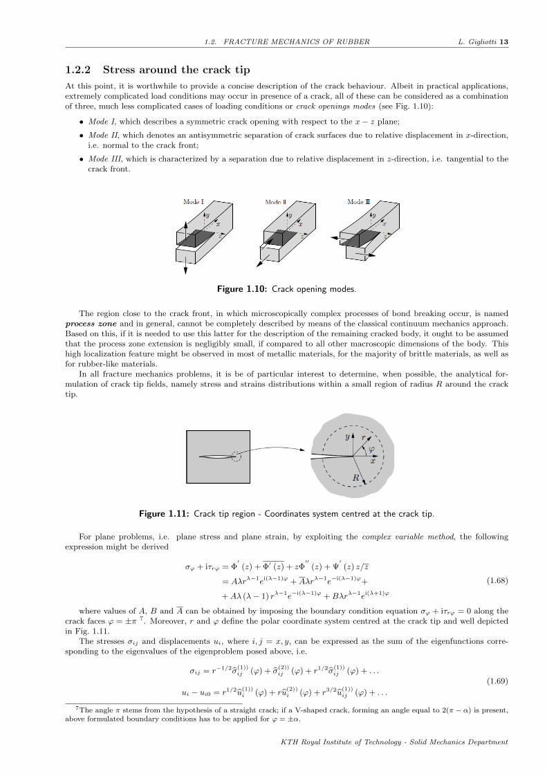
At this point, it is worthwhile to provide a concise description of the crack behaviour. Albeit in practical applications,extremely complicated load conditions may occur in presence of a crack, all of these can be considered as a combinationof three, much less complicated cases of loading conditions or crack openings modes (see Fig. 1.10):
• Mode I, which describes a symmetric crack opening with respect to the x− z plane;
• Mode II, which denotes an antisymmetric separation of crack surfaces due to relative displacement in x-direction,i.e. normal to the crack front;
• Mode III, which is characterized by a separation due to relative displacement in z-direction, i.e. tangential to thecrack front.
Figure 1.10: Crack opening modes.
The region close to the crack front, in which microscopically complex processes of bond breaking occur, is namedprocess zone and in general, cannot be completely described by means of the classical continuum mechanics approach.Based on this, if it is needed to use this latter for the description of the remaining cracked body, it ought to be assumedthat the process zone extension is negligibly small, if compared to all other macroscopic dimensions of the body. Thishigh localization feature might be observed in most of metallic materials, for the majority of brittle materials, as well asfor rubber-like materials.
In all fracture mechanics problems, it is be of particular interest to determine, when possible, the analytical for-mulation of crack tip fields, namely stress and strains distributions within a small region of radius R around the cracktip.
Figure 1.11: Crack tip region - Coordinates system centred at the crack tip.
For plane problems, i.e. plane stress and plane strain, by exploiting the complex variable method, the followingexpression might be derived
σϕ + iτrϕ = Φ′(z) + Φ′ (z) + zΦ
′′(z) + Ψ
′(z) z/z
= Aλrλ−1ei(λ−1)ϕ +Aλrλ−1e−i(λ−1)ϕ+
+Aλ (λ− 1) rλ−1e−i(λ−1)ϕ +Bλrλ−1ei(λ+1)ϕ
(1.68)
where values of A, B and A can be obtained by imposing the boundary condition equation σϕ + iτrϕ = 0 along thecrack faces ϕ = ±π 7. Moreover, r and ϕ define the polar coordinate system centred at the crack tip and well depictedin Fig. 1.11.
The stresses σij and displacements ui, where i, j = x, y, can be expressed as the sum of the eigenfunctions corre-sponding to the eigenvalues of the eigenproblem posed above, i.e.
σij = r−1/2σ(1))ij (ϕ) + σ
(2))ij (ϕ) + r1/2σ
(1))ij (ϕ) + . . .
ui − ui0 = r1/2u(1))i (ϕ) + ru
(2))i (ϕ) + r3/2u
(1))ij (ϕ) + . . .
(1.69)
7The angle π stems from the hypothesis of a straight crack; if a V-shaped crack, forming an angle equal to 2(π − α) is present,above formulated boundary conditions has to be applied for ϕ = ±α.
KTH Royal Institute of Technology - Solid Mechanics Department
14 L. Gigliotti CHAPTER 1. FUNDAMENTALS: LITERATURE REVIEW AND BASIC CONCEPTS
Here, ui0 represents an eventual rigid body motion while, for r → 0, the dominating term is the first one and thusa singularity in the stress field is obtained at the crack tip. A widely adopted procedure is to split the symmetric sin-gular field, corresponding to Mode-I crack opening, from the antisymmetric one, related to the Mode-II crack opening.According to this latter consideration, stress and displacement fields at the crack tip for both Mode-I and Mode-II canbe written as follows
Mode-I : σxσyτxy
= KI√2πr
cos (ϕ/2)
1− sin(ϕ/2) sin(3ϕ/2)1 + sin(ϕ/2) sin(3ϕ/2)
sin(ϕ/2) cos(3ϕ/2)
uv
= KI
2G
√r
2π(κ− cos (ϕ))
cos(ϕ/2)sin(ϕ/2)
(1.70)
Mode-II : σxσyτxy
= KII√2πr
− sin(ϕ/2)[2 + cos(ϕ/2) cos(3ϕ/2)]
sin(ϕ/2) cos(ϕ/2) cos(3ϕ/2)cos(ϕ/2)[1− sin(ϕ/2) sin(3ϕ/2)]
uv
= KII
2G
√r
2π
sin(ϕ/2)[κ+ 2 + cos(ϕ)]cos(ϕ/2)[κ− 2 + cos(ϕ)]
(1.71)
where
plane stress : κ = 3− 4ν, σz = 0
plane strain : κ = (3− ν)/(1 + ν), σz = ν(σx + σy)(1.72)
According to Eqs. 1.70 and 1.71, the amplitude of the crack tip fields is controlled by the stress-intensity factorsKI and KII ; their values depend on the geometry of the body, including the crack geometry, and on its load conditions.Indeed, provided the stresses and deformations are known, it is possible to determine the K-values: for example, fromEqs. 1.70 and 1.71 one might infer that
KI = limr→0
√2πrσy (ϕ = 0) , and KII = limr→0
√2πrτxy (ϕ = 0) (1.73)
In conclusion, it ought to be stressed that for larger distances from the crack tip, the higher terms in Eq. 1.69 cannotbe neglected and the effect of remaining eigenvalues has to be taken into account. Moreover, it has been observed that,in most of the crack problems the characteristic stress singularity is of the order r−1/2; however,different singularity
orders for the stress field might also come to light. As general remark, the stress singularities are of the type σij ∼ rλ−1,having denoted with λ the smallest eigenvalue in the eigenproblem formulated in Eq. 1.68.
1.2.3 Tearing energy
Theoretically, Griffith’s approach is suitable to predict the fracture mechanics behaviour of elastomers, since no limitationsto small strains or linear elastic material response have been made in its derivation. Many attempts have been carriedout throughout the years, to find a criterion for the crack propagation in rubber-like materials; however this task ischaracterized by overwhelming mathematical difficulties in determining the stress field in a cracked body made of anelastic material, due to large deformations at the crack tip prior failure. In addition, since high stresses developed arebounded within a limited region surrounding the crack tip, their experimental measurements cannot be promptly carriedout.
Based on thermodynamic considerations, Griffith theory describes the quasi-static crack propagation as a reversibleprocess; on the other hand, for rubber-like materials the decrease of elastic strain energy is balanced not only by theincrease of the surface free energy of the cracked body, as hypothesized for brittle materials, but it is also partiallyconverted into other forms of energy, i.e. irreversible deformations of the material. Such other forms of dissipated energyappear to be relevant only in proximity of the crack tip, i.e. in portions of material, relatively small if compared to theoverall dimensions of the component. It has been observed that, for a thin sheet of a rubber-like material, in which theinitial crack length is large if compared to its thickness, such energy losses are proportional to the rise of crack length.
In addition, they are readily computable just as function of the deformation state in the neighbourhood of the cracktip at the tearing instant, while basically independent of the specimen type and geometry, and of the particular mannerin which the deforming forces are applied to the cracked body. Even if a slight dependence with the shape of the cracktip is observed, such energy is a characteristic property of the tearing process of rubber-like materials.
Let us deform, under fixed-grip conditions, a thin sheet of rubber-like material cut by a crack of length a and whosethickness is t. In order to observe the crack length increases of da, a work Tcr t da has to be done, where Tcr is thecritical energy for tearing and is a characteristic property of the material:
KTH Royal Institute of Technology - Solid Mechanics Department
1.2. FRACTURE MECHANICS OF RUBBER L. Gigliotti 15
Tcr = −1
t
(∂Us∂a
)l
(1.74)
In the above expression, the suffix l indicates that the differentiation is performed with constant displacement ofthe portions of the boundary which are not force-free. Physically, the critical energy for tearing Tcr represents thewhole dissipated energy as result of fracture propagation (of which, in certain cases, surface tension may be a minorcomponent). Therefore, this critical energy has to be compared with the tearing energy calculated from the deformationstate at the crack tip and whose value, as function of the notch tip diameter d is written as
T = d
∫ π2
0
U0s cos (θ) dθ (1.75)
where, the term U0s is the strain energy density at the notch tip for θ = 0.
Lastly, if the average strain energy density Ubs is introduced, Eq. 1.75 is simplified as follows
T ∼= dUbs (1.76)
where the linear correlation of T with the notch diameter d is proven.Concerning the physical meaning of Ubs , this can be interpreted as the energy required to fracture a unit volume undersimple tension conditions and therefore, it is an intrinsic material property.
1.2.4 Qualitative observation of the tearing process
In [21], a formidable number of experiments have been carried out, in order to assess the effectiveness of the tearingcriterion expressed in Eq. 1.74; further information regarding vulcanizate materials adopted and experimental modalitiesare given in the cited work. Irreversible behaviour is observed exclusively within the neighbourhood region of the cracktip, where the material undergoes large deformations; in addition, if experimental tests are performed at a sufficientlyslow rate of deformation, these are not affected by the test speed.
To present a qualitative description of the tearing process, we may now consider a thin sheet of vulcanizate in which apre-existent crack is present. Experimental observations show how, even relatively small forces lead to considerable valuesof the tearing energy and, in addition, the tearing process ceases as soon as the deformation process is interrupted. Thecrack propagation process can be readily described since its earlier stages: as the deformation continues, the crack growsup to a few hundredths of millimetres. Once this condition is reached, catastrophic failure occurs and the crack lengthabruptly grows by a few millimetres. Such propagation mechanism is repeated as the deformation further increases,leading to a catastrophic rupture of the cracked body.
As always, in fracture mechanics analysis, noticeable information might be deduced from the observation of the cracktip geometry. In the process of crack growth in elastomers, during the stages preceding the catastrophic rupture, thecrack tip is initially blunted, whilst, as the tragic rupture occurs, the crack tip assumes an increasingly irregular shape.
Last but not least, it has to be stressed that the instant at which the catastrophic rupture commences, is by definition,taken as the tearing point .
1.2.5 Tearing energy for different geometries
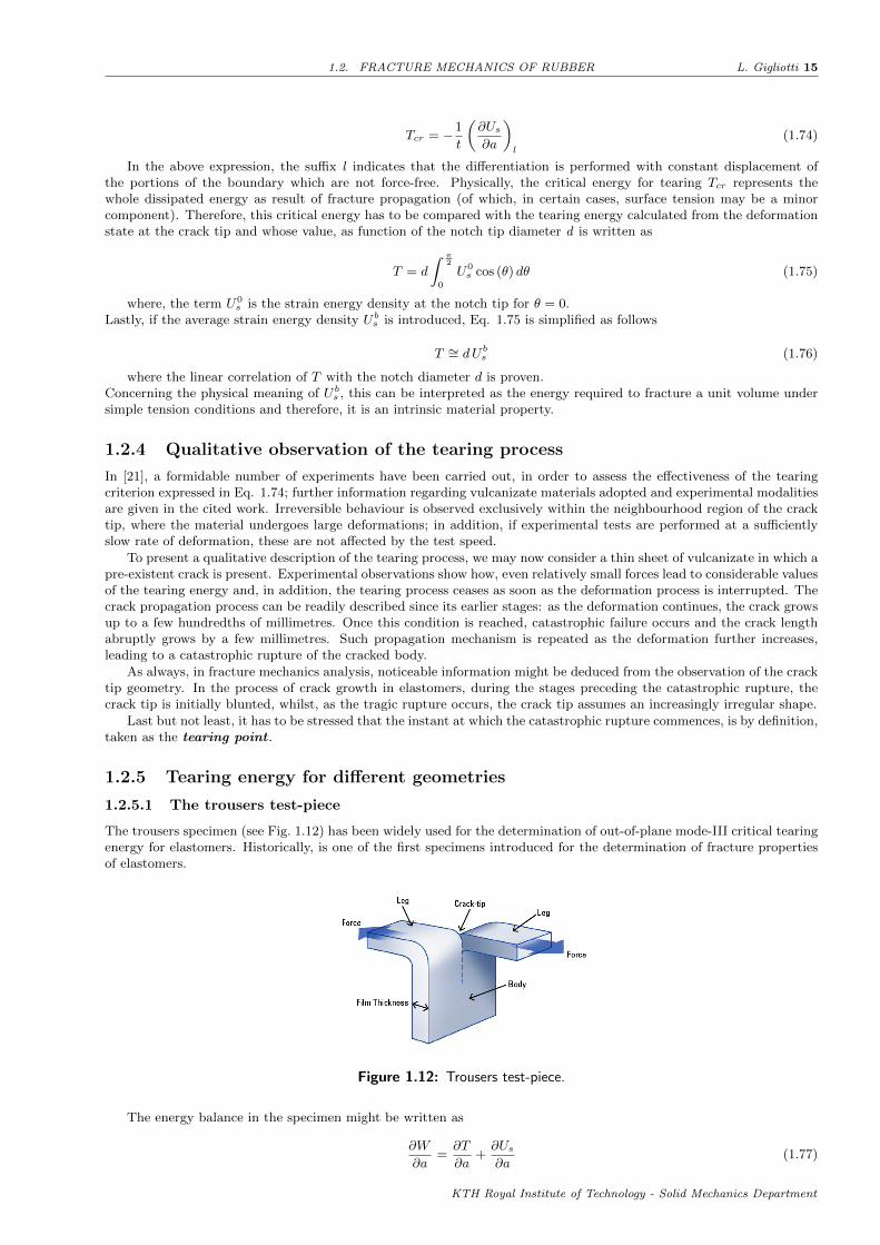
1.2.5.1 The trousers test-piece
The trousers specimen (see Fig. 1.12) has been widely used for the determination of out-of-plane mode-III critical tearingenergy for elastomers. Historically, is one of the first specimens introduced for the determination of fracture propertiesof elastomers.
Figure 1.12: Trousers test-piece.
The energy balance in the specimen might be written as
∂W
∂a=∂T
∂a+∂Us∂a
(1.77)
KTH Royal Institute of Technology - Solid Mechanics Department

16 L. Gigliotti CHAPTER 1. FUNDAMENTALS: LITERATURE REVIEW AND BASIC CONCEPTS
where W is the work done by the applied forces, T is the energy required for tearing and Us is the total internalstrain energy.
Next, assuming that the stretch ratio λ in the specimen, whose thickness is indicated with t and the width with w,is equal to λ = 1 + (u/L) ≥ 1 under the applied force F , Eq. 1.77 can be reformulated as follows
2Fλ = Tt+ Ψwt (1.78)
In addition, since λ = 1 in the reference configuration, according to the normalization condition, the strain energyΨ vanishes; therefore, the following expression of the tearing energy T may be inferred
T =2F
t(1.79)
showing the linear dependence of the tearing energy on the applied force F.
1.2.5.2 The constrained tension (shear) specimen
This specimen, also called pure shear test-piece [28], is constituted of a long strip of (rubber-like) materials which containsa symmetrically located cut (see Fig. 1.13). Let the strip be clamped along its parallel sides, and make them move apartof a distance v0 in the y-direction, in correspondence of which the material starts to crack and then held at this position.
Figure 1.13: Constrained tension (shear) specimen.
If both the strip and the crack are sufficiently long, three different regions are distinguished, namely:
• Region 1, which remains unstressed and whose related strain energy U1s vanishes;
• Region 2, the region containing the crack-tip and in which the strain energy U2s is an unknown complicated function
of x and y;
• Region 3, characterized by an uniform stress distribution and within which, the strain energy U3s = U0
s is constant.
The constant strain energy U0s might be computed as function of the relative clamp displacement v0 and of constitutive
material properties. At this point, it is worthwhile remarking on that, as the crack propagates by a certain length da,Region 2 simply moves with the crack tip while the strain energy value U2
s remains constant. In other words, theextension of the unstressed Region 1 grows whereas contemporary, Region 2 becomes larger as the crack propagates.The net variation of the overall strain energy Us is given by
dUs = −U0s h t da (1.80)
By virtue of Eq. 1.74, together with Eq. 1.80, the expression of the tearing energy expression in the case of constrainedtension (shear) specimen is obtained
T = −1
t
(∂Us∂a
)l
= U0s h (1.81)
1.2.5.3 The tensile strip specimen
Another well-known specimen adopted for the characterization of fracture mechanics properties of rubber-like materials,is the tensile strip specimen. This specimen, consists in a thin sheet of rubber, containing a crack, whose length a issmall if compared to the length L of the test piece. The strain distribution in a small region surrounding the crack tipis inhomogeneous, while in the center of the sheet, far from the crack tip, the specimen might be reasonably assumed tobe in simple extension conditions. In addition, the region indicated in Fig. 1.14 on the next page with A, namely thearea at the intersection of the cut and the free edge of the specimen, results to be unstretched.
Given the complexity of the strain distribution around the crack tip, in [21] dimensional considerations allow us tostate that, if a test piece is cut by an ideally sharp crack in its undeformed configuration, the variation in the elasticallystored energy due to its presence, will be proportional to a2. Such evidence is strictly valid only for ideally sharp crackand semi-infinite sheet, but it can be easily extended for other practical cases, provided that the radius of curvature atthe notch is small if compared with the crack length a. The variation of such elastically stored energy, caused by theintroduction of the crack in the specimen is expressed by the following relation
KTH Royal Institute of Technology - Solid Mechanics Department

1.2. FRACTURE MECHANICS OF RUBBER L. Gigliotti 17
Figure 1.14: Tensile strip specimen with a crack of length a.
U′s − Us = k
′a2t (1.82)
where the elastically stored energy in the absence of the crack is denoted by U′s and the constant of proportionality
k′
is function of the extension rate λ. The proportionality between U′s −Us and the thickness t holds only if plane stress
conditions are employed, i.e. t a.
At this point, it is straightforward to observe that, given the proportionality of the specimen elongation with λ− 1,the energy variation U
′s−Us will be proportional to (λ−1)2 or, in other words, to the strain energy density Ψ. By virtue
of the above considerations, Eq. 1.82 can be reformulated as
U′s − Us = ka2tΨ (1.83)
where k is a function of λ.
By differentiating Eq. 1.83 with respect to the crack length a, finally the expression of the tearing energy for thetensile strip specimen get the form
−(∂Us∂a
)l
= 2kΨat⇒ T = −1
t
(∂Us∂a
)l
= 2kΨa (1.84)
Concerning the dependance of the constant k with the extension rate λ, several experiments and FEA simulationshave been performed [30, 31] showing the proportionality of k with the inverse of the square root of λ, through theconstant π, i.e.
k =3√λ
(1.85)
Although the three test specimens presented so far, are widely used in experimental procedures, compression andshear are encountered much more often in engineering applications, because under these load conditions rubber-likematerials can be fully used without risks of crack growth.
1.2.5.4 The simple shear test-piece
A mathematically simple expression for the tearing energy T in simple shear specimens (see Fig. 1.15) has the form
T = kΨh (1.86)
Figure 1.15: Simple shear test-piece with an edge crack.
KTH Royal Institute of Technology - Solid Mechanics Department

18 L. Gigliotti CHAPTER 1. FUNDAMENTALS: LITERATURE REVIEW AND BASIC CONCEPTS
In such case, the constant of proportionality k, commonly assumes the value of 0.4, but its range of variation isbetween 0.2 and 1.0, depending on the configuration and size of the crack. In practical situations, it is really demandingto carry out simple shear experiments since, as the crack grows, it tends to change direction to Mode-I crack opening. Inaddition, relation Eq. 1.80 holds only if the crack is short, and this implies difficulties in the determination of the stressconcentration.
1.2.5.5 The uniaxial compression test piece
Uniaxial compression specimen slightly differs from those discussed in the previous sections; indeed, the strain distributionis highly inhomogeneous even without cracks within the component. For the strain energy Ψ of such test-piece, providedstrains are often small enough, the following linear approximation holds
Ψ =1
2Ece
2c (1.87)
where e2c is the compressive strain, while the compression modulus Ec is defined as
Ec = 2G(1 + 2S2) (1.88)
where G is the small strain shear modulus.The factor S in Eq. 1.88 referred to as a shape factor , is the ratio between the loaded area and the force-free
surface, i.e.
S =πD2/4
πDh=D
4h(1.89)
According to [29], when a bonded rubber unit is cyclically loaded in compression, an approximately parabolic surfaceis generated and the crack initiates at the intersection of such surface with the core of the specimen (see Fig. 1.16)
Figure 1.16: Typical stages of crack growth in compression: a) unstrained b) compressed - crackinitiation at bond edges c) compressed - bulge separate from core d) unstrained - showing paraboliccrack locus.
Under these assumptions, the tearing energy for uniaxial compression test-piece is given by the approximated ex-pression, valid for S > 0.5 and strains below 50%
T =1
2Ψh =
1
4Ece
2ch (1.90)
1.3 eXtended Finite Element Method
1.3.1 Introduction
Results presented in the previous section, concerning the analytical treatments of fracture mechanics problems areaffected by certain limitations, among which the most constraining are undoubtedly the following ones:
• The material domain is always considered infinite, in order to neglect edge effects in the mathematical derivationof stress and displacement distributions;
• In the majority of cases, the material is assumed to be homogeneous and isotropic;
• Only simple boundary conditions are considered.
However, it is easy to guess that in practical problems of complex structures, containing defects of finite sizes, subjectto complicated boundary conditions and whose material properties are much more complicated than those related to theideal linear, homogeneous and isotropic material model, a satisfactory fracture mechanics analysis can be carried outexclusively by means of numerical methods. Among these, the most widely adopted in practical engineering applicationsis the finite element method [33]; for this reason, several software packages based on the FEM technique have beendeveloped throughout the years [34]. Although the finite element method has shown to be particularly well-suited forfracture mechanics problems [35, 36, 37], the non-smooth crack tip fields in terms of stresses and strains can be captured
KTH Royal Institute of Technology - Solid Mechanics Department
1.3. EXTENDED FINITE ELEMENT METHOD L. Gigliotti 19
only by a locally refined mesh. This leads to an abrupt increase of the number of degrees of freedom and such defect isworsened in 3D-problems. Concerning the crack propagation analysis, it still remains a challenge for several industrialmodelling problems. Indeed, since it is required to the FEM discretization to conform the discontinuity, for modellingevolving discontinuities, the mesh has to be regenerated at each time step. This means that the solution has to be re-projected for each time step on the updated mesh, causing a dramatic rise in terms of computational costs and to a lossof the quality of results [38]. Because of these limitations, several numerical approaches to analyze fracture mechanicsproblems have been proposed during last years. The method based on the quarter-point finite element method [39], theenriched finite element method [40, 41], the integral equation method [42], the boundary collocation method [43], thedislocation method [44, 45], the boundary finite element method [46], the body force method [47] and mesh-free methods[48, 49], e.g. free-element Galerkin method [50, 51], represent the most valuable examples. In order to overcome the needof remeshing, different techniques have been introduced over the last decades, e.g. the incorporation of a discontinuousmode on an element level [52], a moving mesh technique [53] and an enrichment technique, based on the partition ofunity, later referred to as the eXtended Finite Element Method (XFEM) [54, 56, 55].
1.3.2 Partition of unity
Given a C∞ manifold M , with an open cover Ui, a partition of unity subject this latter, is a collection of n nonnegative,smooth functions fi such that, their support is included in Ui and the following relation holds
n∑i=1
fi(x) = 1 (1.91)
Often it is required that, the cover Ui have compact closure, which can be interpreted as finite, or bounded, opensets. If this condition is locally verified, any point x in M has only finitely many i with fi(x) 6= 0. It can be easilydemonstrated that, the sum in Eq. 1.91 does not have to be identically unity to work; indeed, for any arbitrary functionψ(x) it is verified that
n∑i=1
fi(x)ψ(x) = ψ(x) (1.92)
Furthermore, it might be inferred that the partition of unity property is also satisfied by the set of isoparametricfinite element shape functions Nj . i.e.
m∑j=1
Nj(x) = 1 (1.93)
1.3.2.1 Partition of unity finite element method
To increase the order of completeness of a finite element approximation, the so-called enrichment procedure may beexploited. In other words, the accuracy of solution can be ameliorated, by simply including in the finite elementdiscretization, the a priori analytical solution of the problem. For instance, in fracture mechanics problems, an improve-ment in predicting crack tip fields is achieved, if the analytical crack tip solution is included in the framework of theisoparametric finite element discretization. Computationally, this involves an increase in number of the nodal degrees offreedom.
The partition of unity finite element method (PUFEM) [57] [58], using the concept of enrichment functions alongwith the partition of unity property in Eq. 1.93, allows to obtain the following approximation of the displacement withina finite element
uh(x) =
m∑j=1
Nj(x)
(uj +
n∑i=1
pi(x)aji
)(1.94)
where, pi(x) are the enrichment functions and aji are the additional unknowns or degrees of freedom associated tothe enriched solution. With m and n the total number of nodes of each finite element and the number of enrichmentfunctions pi, are indicated.
By virtue of Eqs.1.92 and 1.93, for an enriched node xk, Eq. 1.94 might be written as
uh(xk) =
(uk +
n∑i=1
pi(xk)aji
)(1.95)
which is clearly not a plausible solution. To overcome this defect and satisfy interpolation at nodal point, i.e.uh(xi) = ui, a slightly modified expression for the enriched displacement field is proposed below
uh(x) =
m∑j=1
Nj(x)
[uj +
n∑i=1
(pi(x)− pi(xj)) aji
](1.96)
KTH Royal Institute of Technology - Solid Mechanics Department

20 L. Gigliotti CHAPTER 1. FUNDAMENTALS: LITERATURE REVIEW AND BASIC CONCEPTS
1.3.2.2 Generalized finite element method
A breakthrough in increasing the order of completeness of a finite element discretization is provided by the so-calledgeneralized finite element method (GFEM) [59, 60], in which two separate shape functions are employed for the ordinaryand for the enriched part of the finite element approximation, i.e.
uh(x) =
m∑j=1
Nj(x)uj +
m∑j=1
N j(x)
(n∑i=1
pi(x)aji
)(1.97)
where N j(x) are the shape functions associated with the enrichment basis functions pi(x).For the reason explained in the previous section, Eq. 1.97 should be modified as follows
uh(x) =
m∑j=1
Nj(x)uj +
m∑j=1
N j(x)
[n∑i=1
(pi(x)− pi(xj)) aji
](1.98)
1.3.3 eXtended Finite Element Method
The eXtended Finite Element Method is a partition of unity based method in which, as for PUFEM and GFEM, theclassical finite element approximation is enhanced by means of enrichment functions. However, in PUFEM and GFEM,the enrichment procedure involves the entire domain, whilst it is employed on a local level for the XFEM. Thus, onlynodes close to the crack tip, as well as the ones required for the correct localization of the crack, are enriched. Thisevidently entails a tremendous computational advantage.
The XFEM method was firstly introduced by Belytsckho and Black in 1999 [61]. Their work, in which a method forenriching finite element approximation in such a way that crack growth problems can be solved with minimal remeshing,represents a milestone in the XFEM history. Later on, much more elegant formulations, including the asymptotic near-tipfield and the Heaviside function H(x) in the enrichment scheme, have been proposed [62, 63, 64]8. The eXtended FiniteElement method, furthermore, has been demonstrated to be well suited for three dimensional crack modelling [65]. Inthis latter work, geometric issues associated with the representation of the crack and the enrichment of the finite elementapproximation have been addressed. A major step forward has been then achieved when a generalized methodology forrepresenting discontinuities, located within the domain indipendetely from the mesh grid, has been proposed [66, 62]. Insuch manner, the eXtended Finite Element Method allows to alleviate much of the burden related to the mesh generation,as the finite element mesh is not supposed to conform the crack geometry anymore. This represents certainly, one of themajor advantages provided by the XFEM usage. The XFEM capabilities can be extended if employed in conjunctionwith the Level Set Method (LSM) [67, 68, 69]. Such method permits to represent the crack position, as well as thelocation of crack tips. Within this context, the XFEM has also been employed in concert with a particular type of levelset method named Fast Marching Method [70, 71]. Accuracy, stability and convergence of XFEM, along with difficultiesin using the standard Gaussian quadrature have been investigated [72, 73]; a solution to this latter drawback has beenproposed in [74].
1.3.3.1 Enrichment functions
In two-dimensional problems, crack modelling is obtained by means of two different types of enrichment functions:
• The Heaviside function
The Heaviside function H(x), is employed to enrich elements completely cut by the crack. The splitting of thedomain by the crack, causes a jump in the displacement field and the Heaviside function provides a tremendouslysimple mathematical tool to model such behaviour.
Given a continuous curve Γ, representing a crack within the deformable body Ω, let us consider a point x (x, y) ∈ Ω.The whole aim is to determine the position of such point with respect to the crack location. In this context, if theclosest point belonging to Γ is denoted with x (x, y) and the outward normal vector to Γ in x with n (see Fig. 1.17on the facing page), the Heaviside function might be defined as follows
H (x, y) =
1 for (x− x) · n > 0
−1 for (x− x) · n < 0(1.99)
If no unique normal is defined, then the H(x) function will assume a positive value if (x− x) belong to the con ofnormals in x (see Fig. 1.17 on the next page)
• Asymptotic near-tip field functions
In case of not completely cracked element, the Heaviside function cannot be used to approximate the displacementfield over the entire element domain, since the element contains the crack tip. In [51] it has been proven thatthe displacement field from LEFM theory in Eqs. 1.70 and 1.71, is included within the span of the following fourfunctions, expressed in terms of the local crack tip coordinate system (r, θ)
Fi(r, θ)4i=1 =√
r cos(θ2
),√r sin
(θ2
),√r sin
(θ2
)sin (θ)
√r cos
(θ2
)sin (θ)
(1.100)
8In [64], the name eXtended Finite Element Method has been used for the first time.
KTH Royal Institute of Technology - Solid Mechanics Department

1.3. EXTENDED FINITE ELEMENT METHOD L. Gigliotti 21
(a) Smooth crack. (b) Kink crack.
Figure 1.17: Evaluation of the Heaviside function.
By using the enrichment functions in Eq. 1.100, four different additional degrees of freedom in each directionfor each node are added to those related to the standard finite element discretization. It should be stressed thatamong the aforementioned enriching functions (see Fig. 1.18), only the second term
√r sin
(θ2
)is discontinuous
along crack surfaces and hence, is responsible of the discontinuity in the approximation along the crack. Theremaining three functions are used to enhance the solution approximation in the neighborhood of the crack tip.
(a)√r cos
(θ2
). (b)
√r sin
(θ2
).
(c)√r sin
(θ2
)sin (θ). (d)
√r cos
(θ2
)sin (θ)
Figure 1.18: Near-tip enrichment functions.
Lastly, it should be highlighted that, referring to Eq. 1.100, the required singularity in the stress field, of order1√r
is, therefore, readily introduced.
By virtue of the above discussed enrichment functions, the following expression for the XFEM approximation mightbe formulated
uh (x) = uFEM (x) + uENR (x) =
=∑i∈I
Ni (x) ui +∑j∈J
Nj [H (x)] aj +∑k∈K1
Nk (x)
[4∑l=1
bl1k F1l (x)
]+
+∑k∈K2
Nk (x)
[4∑l=1
bl2k F2l (x)
] (1.101)
or, to eliminate the lack of interpolation property
KTH Royal Institute of Technology - Solid Mechanics Department

22 L. Gigliotti CHAPTER 1. FUNDAMENTALS: LITERATURE REVIEW AND BASIC CONCEPTS
uh (x) =∑i∈I
Ni (x) ui +∑j∈J
Nj [H (x)−H (xj)] aj +
+∑k∈K1
Nk (x)
[4∑l=1
bl1k[F 1l (x)− F 1
l (xk)]]
+∑k∈K2
Nk (x)
[4∑l=1
bl2k[F 2l (x)− F 2
l (xk)]] (1.102)
where, J indicates the set of nodes whose support domain is completely cut by the crack and thus enriched withthe Heaviside function H (x), K1 and K1 are the sets of nodes associated with the crack tips 1 and 2 in their influencedomain, respectively, and whose respective crack tip enrichment functions are F 1
l (x) and F 2l (x). Moreover, ui are
the standard degrees of freedom, while aj , bl1k and bl2k indicate the vectors of additional nodal degrees of freedom formodelling crack faces and the two crack tips, respectively.
1.3.3.2 Level set method for modelling discontinuities
In several cases, numerical simulations involve time-varying objects, like curves and surfaces on a fixed cartesian grid, e.g.interfaces, discontinuities, etc. Their modelling and tracking is particularly cumbersome and is based on the complexmathematical procedure denominated parametrization .
The Level Set Method [68] (often abbreviated as LSM) is an elegant numerical technique that allows to get overthese difficulties. The key-point of such method is to represent discontinuities as a zero level set function. For thispurpose, to fully characterize a crack, two different level set functions are defined
1. A normal level set function, ϕ (x)
2. A tangential level function, ψ (x).
At this point, for the evaluation of the signed distance functions, let Γc be the crack surface (see Fig. 1.19) and x thepoint in which it is sought to evaluate the ϕ (x) function. In an analogous manner of what done in the foregoing section,the normal level set function might be defined as
ϕ = (x− x) · n (1.103)
where x and n assume the previously stated meanings (see Fig. 1.17 on the preceding page) 9.
Figure 1.19: Construction of level set functions.
In Fig. 1.20 on the next page, the plot of the normal signed function ϕ (x) for an interior crack is provided.The tangential level set function ψ (x) is computed by finding the minimum signed distance to the normal at the
crack tip; in case of an interior crack, two different functions can be individuated. However, a unique tangential level setfunction can be defined as
ψ (x) = max ψ1 (x) , ψ2 (x) (1.104)
In conclusion, referring to Fig. 1.19, it may be written what followsfor x ∈ Γcr ϕ (x = 0) and ψ (x ≤ 0)
for x ∈ Γtip ϕ (x = 0) and ψ (x = 0)(1.105)
9According to the definition given in Eq.1.103, in case of interior crack, the normal level set function is computable only withinthe region delimited by the normals to the crack tips; in order to define ϕ (x) over the whole domain, both crack tips should bevirtually extended.
KTH Royal Institute of Technology - Solid Mechanics Department
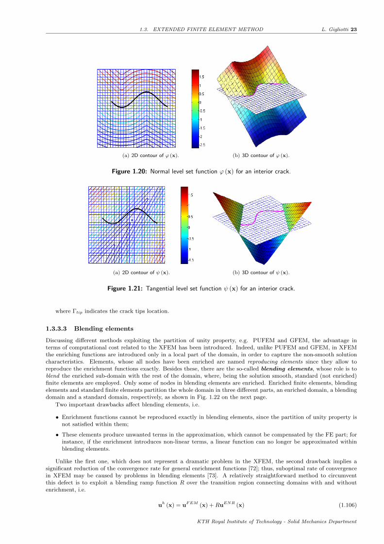
1.3. EXTENDED FINITE ELEMENT METHOD L. Gigliotti 23
(a) 2D contour of ϕ (x). (b) 3D contour of ϕ (x).
Figure 1.20: Normal level set function ϕ (x) for an interior crack.
(a) 2D contour of ψ (x). (b) 3D contour of ψ (x).
Figure 1.21: Tangential level set function ψ (x) for an interior crack.
where Γtip indicates the crack tips location.
1.3.3.3 Blending elements
Discussing different methods exploiting the partition of unity property, e.g. PUFEM and GFEM, the advantage interms of computational cost related to the XFEM has been introduced. Indeed, unlike PUFEM and GFEM, in XFEMthe enriching functions are introduced only in a local part of the domain, in order to capture the non-smooth solutioncharacteristics. Elements, whose all nodes have been enriched are named reproducing elements since they allow toreproduce the enrichment functions exactly. Besides these, there are the so-called blending elements, whose role is toblend the enriched sub-domain with the rest of the domain, where, being the solution smooth, standard (not enriched)finite elements are employed. Only some of nodes in blending elements are enriched. Enriched finite elements, blendingelements and standard finite elements partition the whole domain in three different parts, an enriched domain, a blendingdomain and a standard domain, respectively, as shown in Fig. 1.22 on the next page.
Two important drawbacks affect blending elements, i.e.
• Enrichment functions cannot be reproduced exactly in blending elements, since the partition of unity property isnot satisfied within them;
• These elements produce unwanted terms in the approximation, which cannot be compensated by the FE part; forinstance, if the enrichment introduces non-linear terms, a linear function can no longer be approximated withinblending elements.
Unlike the first one, which does not represent a dramatic problem in the XFEM, the second drawback implies asignificant reduction of the convergence rate for general enrichment functions [72]; thus, suboptimal rate of convergencein XFEM may be caused by problems in blending elements [73]. A relatively straightforward method to circumventthis defect is to exploit a blending ramp function R over the transition region connecting domains with and withoutenrichment, i.e.
uh (x) = uFEM (x) +RuENR (x) (1.106)
KTH Royal Institute of Technology - Solid Mechanics Department

24 L. Gigliotti CHAPTER 1. FUNDAMENTALS: LITERATURE REVIEW AND BASIC CONCEPTS
Figure 1.22: Standard, enriched and blending elements.
where R is set equal to 1 on the enrichment boundary, and equal to 0 on the standard finite element discretizationboundary. This linear blending function R ensures the continuity in the displacement field but not in the strain field. Toachieve this latter, higher order blending functions should be used. Other approaches prescribe to use enhanced straintechniques or p-refinement in blending elements [75], or to adjust the order of the FE shape functions depending on theenrichment [76]. Recently, an interesting solution has been proposed in [77]; in particular, in this work the enrichmentfunctions have been modified such that they vanish in standard elements, unchanged in elements with all their nodesbeing enriched and continuously varying within blending elements. In such approach all nodes of blending elements areenriched.
1.3.3.4 XFEM discretization
Consider a regular region Ω bounded by a smooth curve ∂Ω in the reference configuration, and let this latter be splitin two portions, namely ∂Ωt and ∂Ωu. Essential boundary conditions are imposed on ∂Ωu while traction boundaryconditions are applied along ∂Ωt. Let the region Ω be cut by a crack, whose surfaces ∂Ωcr are traction free. The strongform of the initial boundary value problem can be written as
DivP + Bf = ρ0u in Ωu = u on ∂Ωu
PN = o on ∂ΩcrPN = T on ∂Ωt
(1.107)
where Bf and ρ0u denote the reference body force and the inertia force per unite reference volume, respectively, Nthe outward unit normal to ∂Ω, u the prescribed displacement vector and T the prescribed first Piola-Kirchhoff tractionvector.
The displacement field u must satisfy all the essential boundary conditions and the smoothness property, so that uis continuous
(C0)
in Ω, i.e.
u ∈ U , U =u|u ∈ C0 except on ∂Ωcr , u = u on ∂Ωu
(1.108)
At the same time, test functions δv are defined by
δv ∈ U0, U0 =δv|δv ∈ C0 except on ∂Ωcr , δv = 0 on ∂Ωu
(1.109)
Thus, using the above concepts, the weak form of the equilibrium equation and traction boundary conditions mightbe formulated as ∫
Ω
S : δE dV =
∫Ω
(Bf − ρ0u) · δu dV +
∫∂Ωt
T · δu dA (1.110)
In engineering problems, the nonlinear boundary-value problem in Eq. 1.110 is numerically solved by means ofthe iterative procedure known as Newton-Raphson method. The main idea behind such method is to linearize allquantities associated with the problem at hand, replacing it with a series of linear problems, whose resolution is muchmore undemanding. The linearization procedure is the foundation of finite element methods [33, 78]. Here we present theXFEM discretization of problem in Eq. 1.110 for the particular case of hybrid elements and incompressible hyperelasticmaterial model. Hybrid elements use the well-known in computational mechanics field Hu-Washizu mixed form [79, 80].The resulting elements exhibit the capabilities to overcome the locking effects. In such elements the strain and/or stressfield is interpolated independently of the displacement field. The utilization of mixed forms is particularly profitablefor constrained problems. In addition, the incompressibility constrained is modeled by making use of the Lagrangemultipliers (Cfr. Sec. 1.1.2.2).
The resulting linearized equations, may be expressed as follows
KTH Royal Institute of Technology - Solid Mechanics Department
1.3. EXTENDED FINITE ELEMENT METHOD L. Gigliotti 25
[J GT
G 0
]δuh
δp
=
−rv −GTpv
−GT∆uhv
(1.111)
In the above matrix relation, the Jacobian matrix J, and the matrix G can be respectively written as
J =sD
β∆t2M + Kint + Kext , G =
∂g
∂u(1.112)
We first consider the J matrix. In the first term on the RSH, which is present only in dynamic problems, β is theparameter of the Newmark β-method, M is the mass matrix and ∆t is the time step increment. The second and thethird term are respectively the tangent stiffness matrices for internal and external nodal forces; this latter can be
easily expressed as Kext = ∂fext
∂u.
In the supposition that only one crack tip is present within the body, the vector of nodal parameters uh is definedas follows
uh = u a b1 b2 b3 b4T (1.113)
Concerning the global tangent stiffness matrix for internal forces Kint and the global vector of external forces f ext,these are obtained by assembling the tangent stiffness matrix for internal forces Kint e
ij and the vector of external forcesf ext ei for each element e of the XFEM discretization, i.e.
Kint eij =
Kuuij Kua
ij Kubij
Kauij Kaa
ij Kabij
Kbuij Kba
ij Kbbij
(1.114)
f ext ei =
fui fai fb1
i fb2i fb3
i fb4i
T
(1.115)
with
Krsij =
∫Ωe
[(Bri )
T : CSE : Bsj + I(Br
i )T : (S− pC−1) : Bs
j ]dΩ , r, s = u,a,b (1.116)
fui =∫∂Ωet
NiftdA +
∫ΩetNif
bdV
fai =∫∂Ωet
NiHf tdA +∫
ΩetNiHf bdV
fbαi =∫∂Ωet
NiFαf tdA +∫
ΩetNiFαf bdV , α = 1, 2, 3 and 4
(1.117)
In Eq. 1.116, CSE is a forth order tensor often referred to as tangent modulus tensor defined through the relationS = CSE : E, while B is the shape function derivatives matrix, i.e.
Bui =
Ni,x 00 Ni,y
Ni,y Ni,x
(1.118)
Bai =
[Ni(H(ξ)−H(ξi))],x 0
0 [Ni(H(ξ)−H(ξi))],y[Ni(H(ξ)−H(ξi))],y [Ni(H(ξ)−H(ξi))],x
(1.119)
Bbi =
[Bb1i Bb2
i Bb3i Bb4
i
]Bbαi =
[Ni (Fα − Fαi)],x 0
0 [Ni (Fα − Fαi)],y[Ni (Fα − Fαi)],y [Ni (Fα − Fαi)],x
, α = 1, 2, 3 and 4
(1.120)
where ξ is the local curvilinear (mapping) coordinate system. In addition, B represents the column matrix ofderivatives of shape functions I given by [B]iI = ∂NI
∂xiin the reference configuration.
Furthermore, in Eq. 1.111, p is the Lagrangian multipliers vector, δuh is the incremental displacement in the iterativeNewton procedure, ∆uh the step increment and δp the virtual pressure field. Concerning the Lagrange multipliersmethod, G is the matrix of material derivatives of constraints, i.e. G = ∂g
∂u. In conclusion, r is the residual column
matrix and the subscript v represent the iteration number. In this formulation the Lagrange multiplier p can be regardedas the physical hydrostatic pressure.
The above discussed formulation leads to a two-fields mixed finite element implementation in which the displacementfield and the hydrostatic pressure are treated as independent field variables. Lastly, it is fundamental to highlightthat such formulation requires to consider an additional numbers of unknown, i.e. equal to the number of Lagrangemultipliers sought. Along with the additional DOFs introduced by the XFEM technique, this renders the treatment ofincompressible materials with such method, extremely costly from a computational perspective.
KTH Royal Institute of Technology - Solid Mechanics Department

26 L. Gigliotti CHAPTER 1. FUNDAMENTALS: LITERATURE REVIEW AND BASIC CONCEPTS
1.3.3.5 Numerical integration and convergence
Though the Gauss quadrature has been proven to be exact for polynomial integrands, for non-polynomial ones it maycause a reduction in the accuracy of results. Introducing an arbitrary oriented discontinuity in the finite elementdiscretization transforms displacements and stresses into highly non-linear fields which cannot be correctly integrated.To circumvent such problems, a subtriangulation procedure (see Fig. 1.23), in which elements edges conform the crackfaces has been proposed [62]; within these elements the standard Gauss integration procedure might be exploited.
Figure 1.23: Subtriangulation of elements cut by a crack.
It has to be highlighted that, for elements containing the crack, therefore including the singular stress field at thecrack tip, this procedure might result to be inaccurate if Gauss points of sub-triangles are too close at the crack tip.
Crack modeling with the standard finite element method, is performed by re-meshing the domain so that elementsboundaries match the crack geometry; furthermore, new created elements have to be well conditioned and not badlyshaped. Accordingly, re-meshing procedure is a cumbersome and computationally costly operation. On the contrary,since the sub-triangulation is performed only for integration purposes, no additional degrees of freedom are added to thesystem and, sub-triangles are not forced to be well shaped.
It is worth mentioning that an alternative method based on the elimination of quadrature sub-elements has beenrecently proposed [74]. In such approach, rather then partition elements cut by a crack, discontinuous non-differentiablefunctions are replaced with equivalent polynomial functions and consequently the Gauss quadrature can be carried outover the whole element. Although this method would allow a sensible reduction in terms of computational costs, it isstill affected by some drawbacks, e.g. it is limited to element completely cut by a straight crack, no additional rulesare prescribed for elements containing the crack tip and even if the solution is accurate for triangular and tetrahedralelements, difficulties are still encountered in dealing with quadrilateral elements.
In conclusion, as previously stated, the XFEM method ensures more accurate results than classical FEM one.However, the rate of convergence does not improve as the mesh parameter h goes to zero due to the presence of thesingularity [73] and it is lower than the one expected by using the classical FEM method in smooth problems10. Severalmethods have been proposed during last decades to achieve an optimal rate of convergence, e.g. XFEM with a fixedenrichment area, high-order XFEM [72, 81] as well as a modified construction of blending elements. In [82] the robustnessof the method has been enhanced by means of a new integration quadrature for asymptotic functions and implementinga preconditioning scheme adapted to enrichment functions.
1.3.3.6 XFEM for finite strain fracture mechanics
Numerical methods based of the Finite Element Method, devoted to the computational analysis of crack propagationphenomena in non-linear fracture mechanics is still an open problem [83, 84].
Even more cumbersome is the application of the eXtended Finite Element Method to large strain problems; indeed,very few works have been intended to extend the XFEM capabilities to materials exhibiting a nonlinear behaviourand able to undergo large deformations, especially if associated with the volumetric incompressibility constraint. Thesatisfaction of such constraint within the enriched approximation is thought to be, in this context, the most difficultissue and requires to be further investigated. For this purpose, the enrichment of a standard biquadratic-displacementbilinear pressure for node quadrilateral element has been proposed [85]. Nevertheless, even if very good results have beenachieved in terms of stress and displacement fields prediction, the extent to which the incompressibility limit has beensatisfied ought to be better examined. A procedure to model the crack growth with a cohesive law on the discontinuitysurfaces has been developed, for compressible hyperelastic materials, in [86]. The incompressibility limit, along with thehigh stress localization at the crack tip, has been proven to lead to severe problems of mesh locking. In [88] a methodto circumvent this drawback has been proposed. More in detail, in such work, shear locking in Mindlin-Reissner platefracture has been reduced, but not completely eliminated, by enriching the four-node T1 element of Hughes and Tezduyar[87]. An enhanced assumed strain method to circumvent locking issue occurring in plane strain problems and eliminatethe spurious stress oscillations along the failure surface in nearly incompressible materials has been developed in [90].
The analysis of the asymptotic displacement field near the crack tip in plane stress conditions for a Neo-Hookeanmaterial model has been performed in [89], where the importance of the right choice for the singularity enriching functions
10It has been proven that the rate of convergence is of order√h.
KTH Royal Institute of Technology - Solid Mechanics Department
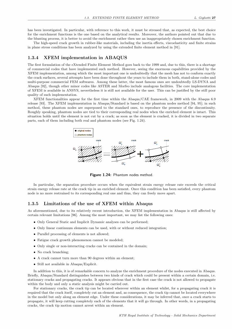
1.3. EXTENDED FINITE ELEMENT METHOD L. Gigliotti 27
has been investigated. In particular, with reference to this work, it must be stressed that, as expected, the best choicefor the enrichment functions is the one based on the analytical results. Moreover, the authors pointed out that due tothe blunting process, it is better to avoid the enrichment rather then use an inappropriately chosen enrichment function.
The high-speed crack growth in rubber-like materials, including the inertia effects, viscoelasticity and finite strainsin plane stress conditions has been analyzed by using the extended finite element method in [91].
1.3.4 XFEM implementation in ABAQUS
The first formulation of the eXtended Finite Element Method goes back to the 1999 and, due to this, there is a shortageof commercial codes that have implemented such method. However, seeing the enormous capabilities provided by theXFEM implementation, among which the most important one is undoubtedly that the mesh has not to conform exactlythe crack surfaces, several attempts have been done throughout the years to include them in both, stand-alone codes andmulti-purpose commercial FEM softwares. Among these latter, the most famous ones are undoubtedly LS-DYNA andAbaqus [92], though other minor codes like ASTER and Morfeo include analogous facilities. The core implementationof XFEM is available in ANSYS, nevertheless it is still not available for the user. This can be justified by the still poorquality of such implementation.
XFEM functionalities appear for the first time within the Abaqus/CAE framework, in 2009 with the Abaqus 6.9release [93]. The XFEM implementation in Abaqus/Standard is based on the phantom nodes method [94, 95]; in suchmethod, these phantom nodes are superposed to the standard ones, to reproduce the presence of the discontinuity.Roughly speaking, phantom nodes are tied to their corresponding real nodes when the enriched element is intact. Thissituation holds until the element is not cut by a crack; as soon as the element is cracked, it is divided in two separateparts, each of them including both real and phantom nodes (see Fig. 1.24).
Figure 1.24: Phantom nodes method.
In particular, the separation procedure occurs when the equivalent strain energy release rate exceeds the criticalstrain energy release rate at the crack tip in an enriched element. Once this condition has been satisfied, every phantomnode is no more restrained to its corresponding real one and thus, they can freely move apart.
1.3.5 Limitations of the use of XFEM within Abaqus
As aforementioned, due to its relatively recent introduction, the XFEM implementation in Abaqus is still affected bycertain relevant limitations [96]. Among the most important, we may list the following ones:
• Only General Static and Implicit Dynamic analyses can be performed;
• Only linear continuum elements can be used, with or without reduced integration;
• Parallel processing of elements is not allowed;
• Fatigue crack growth phenomenon cannot be modeled;
• Only single or non-interacting cracks can be contained in the domain;
• No crack branching;
• A crack cannot turn more than 90 degrees within an element;
• Still not available in Abaqus/Explicit.
In addition to this, it is of remarkable concern to analyze the enrichment procedure of the nodes executed in Abaqus.Briefly, Abaqus/Standard distinguishes between two kinds of crack which could be present within a certain domain, i.e.stationary cracks and propagating cracks. It appears obvious that in the first case the crack is not allowed to propagatewithin the body and only a static analysis might be carried out.
For stationary cracks, the crack tip can be located wherever within an element whilst, for a propagating crack it isrequired that the crack itself, completely cut an element and, as consequence, the crack tip cannot be located everywherein the model but only along an element edge. Under these considerations, it may be inferred that, once a crack starts topropagate, it will keep cutting completely each of the elements that it will go through. In other words, in a propagatingcracks, the crack tip motion cannot arrest within an element.
KTH Royal Institute of Technology - Solid Mechanics Department

28 L. Gigliotti CHAPTER 1. FUNDAMENTALS: LITERATURE REVIEW AND BASIC CONCEPTS
(a) Propagating cracks. (b) Stationary cracks.
Figure 1.25: Enrichment procedure in Abaqus/Standard.
The main difference between the aforementioned cases of propagating and stationary cracks, is in the enrichmentprocedure; more in detail, it is different the number of enriched nodes and the enrichment functions adopted.
For the propagating cracks typology, the asymptotic near-tip singularity functions are not included in the enrichmentscheme and only the Heaviside function is used; in this way, as seen before, the crack can be located everywhere in themodel while the crack tip is forced to lie on an element edge11. On the other hand, for a stationary crack both Heavisideand crack tip singularity functions are included in the XFEM discretization. According to what depicted in Fig. 1.25,the nodes of the elements completely cut by the crack are enriched only with the Heaviside function, while the singleelement containing the crack tip has its nodes enriched with both the Heaviside function and the asymptotic near-tipsingularity functions. In order to improve the accuracy of results, it is possible to enrich, logically only with the near-tipsingularity functions, also a certain number of elements within the distance named as enrichment radius Renr anddefined by the user. The higher the number of elements included within the enrichment area, the higher the accuracyand the computational cost. It ought to be stressed that, all nodes of all elements included within Renr are enriched.
In [97], an analysis of the accuracy of results provided by Abaqus for an isotropic linear elastic material and fordifferent enrichment discretizations has been performed; in particular, this work has been devoted to investigate theeffects of the asymptotic near-tip field functions on the quality of the results.
Unfortunately, analyses including stationary cracks can be performed only with linear elastic material models inAbaqus/Standard. For all other kinds of material models, including then, hyperelastic ones as well, only propagatingcracks can be used.
In conclusion, the crack surfaces and the crack tip location in Abaqus are indentified with a numerical procedurebased on the Level Set Method (Cfr. Sec. 1.3.3.2). Once the mesh discretization has been created, each node of the finiteelement grid is characterized with its three coordinates with respect the global coordinate system and two additionalparameters, called PHILSM and PSILSM. These parameters are nonzero only for the enriched elements and theymight be easily interpreted as the nodal coordinates of the enriched nodes in a coordinate system centred at the cracktip and whose axes are, respectively, tangent and normal to the crack surfaces at the crack tip. If the crack surfaces liealong element edges, it might result, for an enriched node, that the PSILSM coordinate is equal to zero; since this wouldimply that the node would have not to be enriched, by default, Abaqus slightly shifts the location of the crack surfacesin order to maintain the enrichment scheme unchanged, without excessively modify the problem formulation 12.
11Referring to the Abaqus’s User Manual, this is justified by the fact that, including the crack tip singularity functions also forpropagating cracks, would require to keep tracking for every instant the exact location of the crack tip, leading therefore, to anabnormal computational cost.
12For the Abaqus 6.10 release used in this work, the crack is shifted of a distance equal to one thousandth of the characteristicelement length at the crack tip.
KTH Royal Institute of Technology - Solid Mechanics Department

Chapter 2
Problem formulation
2.1 Geometrical model
In the present work, a single edge notched specimen, whose geometrical scheme is proposed in Fig. 2.1 has been employedto perform the numerical analyses. It consists of a sheet of rubber-like material and its dimensions are indicated inTab. 2.1. The specimen is subjected to a prescribed displacement u, applied to both its bottom and top edges and in allsimulations carried out, the model is assumed to be under plane strain condition.
SINGLE EDGE NOTCHED SPECIMEN
a w h
(m) (m) (m)
0.5 1 1
Table 2.1: Dimension of the geometrical model.
(a) Mode-I crack opening. (b) 45o mixed-Mode crack opening.
Figure 2.1: Geometrical model and crack opening modes for the static analysis.
2.2 Solution procedure
Firstly, a static analysis devoted to the evaluation of the capabilities of XFEM in Abaqus to determine the correct stressand displacement fields around the crack tip has been performed. For this purpose, the reference solutions has beenobtained by means of a standard FEM analysis with a sufficiently refined mesh. Then, this has been compared withthe outcomes of the XFEM analysis with a coarse mesh to evaluate the accuracy of results. Successively, in the secondpart of this work, instead, the aim has been to assess the applicability of XFEM in Abaqus for modelling crack growthprocesses in rubber-like materials. In particular, the XFEM capabilities have been evaluated in terms of their ability topredict the instant of crack propagation, the crack propagation angle and crack speeds.
29
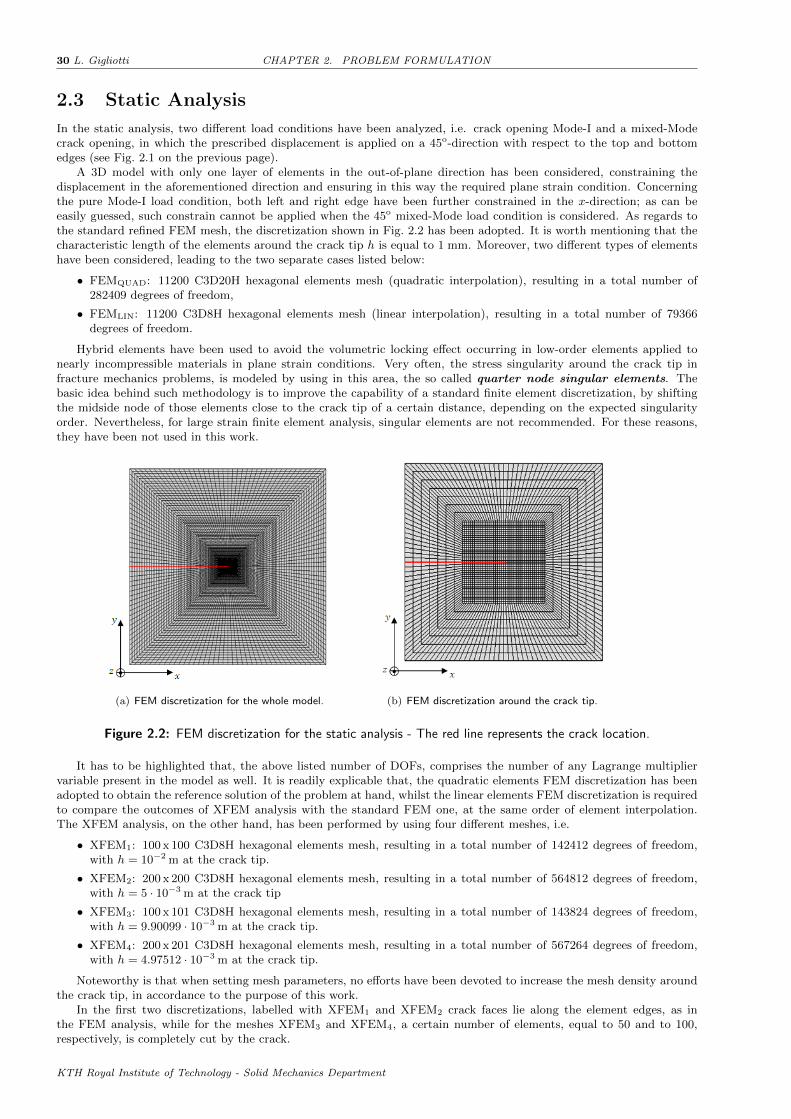
30 L. Gigliotti CHAPTER 2. PROBLEM FORMULATION
2.3 Static Analysis
In the static analysis, two different load conditions have been analyzed, i.e. crack opening Mode-I and a mixed-Modecrack opening, in which the prescribed displacement is applied on a 45o-direction with respect to the top and bottomedges (see Fig. 2.1 on the previous page).
A 3D model with only one layer of elements in the out-of-plane direction has been considered, constraining thedisplacement in the aforementioned direction and ensuring in this way the required plane strain condition. Concerningthe pure Mode-I load condition, both left and right edge have been further constrained in the x-direction; as can beeasily guessed, such constrain cannot be applied when the 45o mixed-Mode load condition is considered. As regards tothe standard refined FEM mesh, the discretization shown in Fig. 2.2 has been adopted. It is worth mentioning that thecharacteristic length of the elements around the crack tip h is equal to 1 mm. Moreover, two different types of elementshave been considered, leading to the two separate cases listed below:
• FEMQUAD: 11200 C3D20H hexagonal elements mesh (quadratic interpolation), resulting in a total number of282409 degrees of freedom,
• FEMLIN: 11200 C3D8H hexagonal elements mesh (linear interpolation), resulting in a total number of 79366degrees of freedom.
Hybrid elements have been used to avoid the volumetric locking effect occurring in low-order elements applied tonearly incompressible materials in plane strain conditions. Very often, the stress singularity around the crack tip infracture mechanics problems, is modeled by using in this area, the so called quarter node singular elements. Thebasic idea behind such methodology is to improve the capability of a standard finite element discretization, by shiftingthe midside node of those elements close to the crack tip of a certain distance, depending on the expected singularityorder. Nevertheless, for large strain finite element analysis, singular elements are not recommended. For these reasons,they have been not used in this work.
(a) FEM discretization for the whole model. (b) FEM discretization around the crack tip.
Figure 2.2: FEM discretization for the static analysis - The red line represents the crack location.
It has to be highlighted that, the above listed number of DOFs, comprises the number of any Lagrange multipliervariable present in the model as well. It is readily explicable that, the quadratic elements FEM discretization has beenadopted to obtain the reference solution of the problem at hand, whilst the linear elements FEM discretization is requiredto compare the outcomes of XFEM analysis with the standard FEM one, at the same order of element interpolation.The XFEM analysis, on the other hand, has been performed by using four different meshes, i.e.
• XFEM1: 100 x 100 C3D8H hexagonal elements mesh, resulting in a total number of 142412 degrees of freedom,with h = 10−2 m at the crack tip.
• XFEM2: 200 x 200 C3D8H hexagonal elements mesh, resulting in a total number of 564812 degrees of freedom,with h = 5 · 10−3 m at the crack tip
• XFEM3: 100 x 101 C3D8H hexagonal elements mesh, resulting in a total number of 143824 degrees of freedom,with h = 9.90099 · 10−3 m at the crack tip.
• XFEM4: 200 x 201 C3D8H hexagonal elements mesh, resulting in a total number of 567264 degrees of freedom,with h = 4.97512 · 10−3 m at the crack tip.
Noteworthy is that when setting mesh parameters, no efforts have been devoted to increase the mesh density aroundthe crack tip, in accordance to the purpose of this work.
In the first two discretizations, labelled with XFEM1 and XFEM2 crack faces lie along the element edges, as inthe FEM analysis, while for the meshes XFEM3 and XFEM4, a certain number of elements, equal to 50 and to 100,respectively, is completely cut by the crack.
KTH Royal Institute of Technology - Solid Mechanics Department

2.4. DYNAMIC ANALYSIS L. Gigliotti 31
Two different material models have been considered, the Arruda-Boyce model and the Neo-Hookean model. Materialcoefficients of both the hyperelastic models may be computed directly in Abaqus/Standard, providing experimentalstress-strain data. Results obtained from three different experimental tests, i.e. uniaxial, equibiaxial and planar test, canbe provided in the Abaqus/Standard environment; material constants will then be calculated by means of a nonlinearleast-square procedure, which minimizes the relative error in stress. Here, experimental uniaxial test data in [12] areused, and the result of such fitting procedure is depicted in Fig. 2.3.
Figure 2.3: Fitting of uniaxial test data with the Arruda-Boyce and Neo-Hookean model in Abaqus.
2.4 Dynamic Analysis
The dynamic analysis has been carried out, with the same geometric model adopted for the static analysis. The assumedmaterial model is the Arruda-Boyce, whose parameters are the ones computed in previous section. Two different loadingconditions have been examined in the dynamic analysis; however, in this case, the pure crack opening Mode-I has notbeen taken into account, but in addition to the 45o mixed-Mode, a 30o mixed-Mode has been analyzed (see Fig. 2.4).
Figure 2.4: 30o mixed-Mode crack opening.
In order to evaluate the mesh-dependence of the solution, five different discretizations, with decreasing characteristicelement dimension h at the crack tip, have been used, i.e.
• XFEMD1: 2541 C3D8H hexagonal elements mesh, resulting in a total number of 36090 degrees of freedom, withh = 4.76193 · 10−3 m at the crack tip,
• XFEMD2: 4061 C3D8H hexagonal elements mesh, resulting in a total number of 57610 degrees of freedom, h =3, 22580 · 10−3 m at the crack tip,
KTH Royal Institute of Technology - Solid Mechanics Department

32 L. Gigliotti CHAPTER 2. PROBLEM FORMULATION
• XFEMD3: 5781 C3D8H hexagonal elements mesh, resulting in a total number of 81930 degrees of freedom, h =2, 43902 · 10−3 m at the crack tip,
• XFEMD4: 7701 C3D8H hexagonal elements mesh, resulting in a total number of 109050 degrees of freedom,h = 1, 96078 · 10−3 m at the crack tip,
• XFEMD5: 20301 C3D8H hexagonal elements mesh, resulting in a total number of 286650 degrees of freedom,h = 0, 99009 · 10−3 m at the crack tip.
For graphical reasons, only the first discretization is shown herein in Fig. 2.5; in all other cases, the discretizationscheme is analogous, while the level of refinement at the crack tip is different.
(a) XFEM discretization for the whole model. (b) XFEM discretization around the crack tip.
Figure 2.5: XFEM discretization for the dynamic analysis.
2.5 Damage parameters
In order to observe the expected crack growth phenomenon, damage initiation and propagation criteria had to be defined.For the prediction of damage initiation in the enriched region, the Abaqus/Standard User’s Manual suggests to use eitherthe Maximum principal stress damage criterion or the Maximum principal strain damage criterion ; in thiswork, the first criterion has been adopted. More in detail, it assumes that a crack will nucleate within the body as soonas the ratio
f =
〈σmax〉σomax
(2.1)
reaches a value equal to 1. In Eq. 2.1, σomax represents the maximum allowable principal stress, while the symbol〈〉 indicates the Macaulay brackets, used to signify that a purely compressive stress state does not lead to any damageinitiation. Such criteria, define the conditions at which an internal defect will nucleate within the body. However, inthe geometric model adopted, an internal defect is already present. As consequence, under these conditions, the value ofthe principal stress does not play a relevant role for the crack propagation analysis. For this reason, its value has beenset equal to 5.57 MPa, corresponding to the highest stress value observed in the stress-strain relation in Fig. 2.3 on thepreceding page. In this way, the remote possibility that another crack had nucleated under the applied loads is avoided.
Much more important is the damage propagation criterion in the case of pre-existing cracks. In such criterion, a scalarvariable D is introduced to represent the overall damage in the material, due to all the active deformation mechanisms.Its value evolves monotonically from 0 up to 1, where the failure process is completed. For the characterization of thedamage evolution, it is required to define, firstly, the dissipated energy due to failure GC and afterwards, the damagevariable D evolution, between the initiation of damage and the final complete failure.
The energy-based model for the damage evolution here considered, is based on the calculation of the energy dissipatedduring the damage process, named as fracture energy. In case of mixed-Mode loading conditions, several models havebeen proposed to calculate the equivalent fracture energy. In the present work, the BK mixed-mode fracture criterion,presented by Benzeggagh and Kenane in [98] has been adopted. According to such model, particularly suitable whenthe critical fracture energies during separation purely along the first and the second shear directions are the same, theequivalent fracture energy is equal to
GCequiv = GCn +(GCs −GCn
)[GSGT
]η(2.2)
where, GS = Gs +Gt, GT = Gn +GS , while η is a material parameter. As clear, the fracture energy (per unit area)is computed as function of the fracture energy in the normal mode GCn , in the first shear mode GCs and in the second
KTH Royal Institute of Technology - Solid Mechanics Department

2.5. DAMAGE PARAMETERS L. Gigliotti 33
shear mode GCt ; under the assumption of isotropic material model, these components have been considered, all of them,equal to 5 kJ/m2.
Concerning the damage variable D, an exponential model to describe its evolution has been adopted. In particular,according to such model, the following relation holds
D =
∫ δfm
δom
TeffGC −Go
dδ (2.3)
in which, Teff indicates the effective traction, as well as the δ is the effective displacement. In addition, Go representsthe elastic energy at damage initiation, while δom and δfm are the effective displacement at complete failure and the effectivedisplacement at damage initiation, respectively (see Fig. 2.6).
Figure 2.6: Exponential damage evolution.
The fracture energy can thus, be regarded as a property of the cohesive interaction and it is equal to the area underthe traction-separation curve depicted in Fig. 2.6.
The last step to complete the description of damage evolution model, is to specify the crack propagation direction,once that the fracture criterion has been satisfied. In this work, the crack propagation has been thought to occur,normally to the maximum tangential stress direction. The unstable nature of the crack propagation in rubber-likematerial, along with the nonlinearity of the Arruda-Boyce material model, often leads to severe convergence difficultiesin Abaqus/Standard, especially due to the stiffness degradation associated with the damage. For these reasons, a localizeddamping might be readily included in the numerical model by using the viscous regularization technique, obtaining thatthe positiveness of the tangent stiffness matrix is ensured for small enough time increments. Such regularization process,predicts to adopt a so-called viscous stiffness degradation variable Dv, defined as
Dv =1
µ(D −Dv) (2.4)
where µ is the relaxation time of the viscous system, while D, as stated above, is the damage variable computed inthe inviscid model (Cfr. Eq. 2.3). Having borne in mind that an excessive viscous stabilization might have a negativeinfluence on the solution, leading in the worst cases to non-physically admissible results, the key-rule for the choice of afeasible value of the viscosity coefficient µ, is to limit as far as possible the approximated amount of energy associated withthe viscous regularization over the whole model1. A value of µ = 10−5 s is thought to do not strongly affect the solutionwith respect to case with no stabilization, and to guarantee a significant improvement in the analysis performance, interms of reduction of the CPU-time, wall clock time and number of increments required to complete the analysis2.
1The energy associated with the viscous regularization is available with the output variable ALLVD in Abaqus/Standard.2The CPU-time, the wall clock time and the number of increments required to perform an entire simulation are provided in the
.dat and in the .sta files.
KTH Royal Institute of Technology - Solid Mechanics Department

34 L. Gigliotti CHAPTER 2. PROBLEM FORMULATION
KTH Royal Institute of Technology - Solid Mechanics Department

Chapter 3
Numerical results - Static Analysis
In the present work, a static analysis is devoted to the determination of the stress and displacement fields around thecrack tip for a stationary crack, within a rubber-like material. These have been evaluated along two different directions,coincident with the x and y-axis of the coordinate system centred at the crack tip in the reference configuration (seeFig. 3.1).
Figure 3.1: Local coordinate system centred at the crack tip.
In particular, the stress component along the y-direction σy, and the in-plane displacements ux and uy have beenconsidered as outcomes of such analysis. The prescribed displacement at the top and bottom edges has been set equalto u = 10−2 m for the crack opening Mode-I, while for the 45o mixed-Mode crack opening, a displacement of u = 10−2 mhas been applied in both x and y-direction.
It is worthwhile noting that analyses with discontinuities, like those involving fracture mechanics problems, arenumerically cumbersome in Abaqus/Standard and the default time integration scheme may lead to premature cutbacksand terminations, requiring thus to be treated with special carefulness. Fortunately, the Abaqus User’s Manual providesclear information and useful hints to avoid the majority of these drawbacks. More in detail, to speed the convergencerate up, time incrementation parameters are thought to be the first ones to be modified. These improve the convergencebehaviour in those cases in which the convergence is nonquadratic or when it is initially nonmonotonic. Nonmonoticallydecreasing residuals are the result of several interacting nonlinearities, e.g., nonlinear material behavior, high stresslocalization and friction. In addition, if the Jacobian is not exact, due to complex material models, nonquadraticconverge rates may appear. Whether residuals increase in two consecutive iterations after I0 equilibrium iterations, asdefault configuration, Abaqus/Standard interrupts the iterative process and reduces the time step increment. A furthercheck is performed on the so-called logarithmic convergence rate after IR equilibrium iterations. Furthermore, it mightresult useful to increase the maximum possible number of attempts for each iteration IA. In Tab. 3.1 default values,together with modified ones of such parameters, are listed.
I0 IR IA
Abaqus Default 4 8 5
Discontinuous analysis 8 10 20
Table 3.1: Time incrementation scheme controls.
A further remedy exploited to avoid nonquadratic rate of convergence, is to utilize the unsymmetric equation solverfor the step.
35

36 L. Gigliotti CHAPTER 3. NUMERICAL RESULTS - STATIC ANALYSIS
3.1 Stress field around the crack tip
3.1.1 Pure Mode-I loading condition
A comparison between results obtained by means of the XFEM analysis and the FEM one, might readily be performedwith reference to Fig. 3.2. Here the stress component σy, as function of the distance from the crack tip in the referenceconfiguration is provided in the case of Arruda-Boyde material model. It is worthwhile noting that for all results shownin this work, distances has to be intended in the reference configuration, unless otherwise specified. Qualitatively, itis observable that, along both x and y-direction, by using the XFEM, it is not possible to properly describe the stresssingularity at the crack tip, even if compared to the FEM analysis with first-order elements.
(a) Stress component σy evaluated along the x-direction startingfrom the crack tip.
(b) Stress component σy evaluated along the y-directionstarting from the crack tip.
Figure 3.2: XFEM and standard FEM analysis of the stress field around the crack tip - Pure Mode-I.
Interestingly, it might be inferred that crack tip position within the mesh grid seems to play an important role.Indeed, whether a node is located in correspondence of the crack tip, a better evaluation of the stress singularity andof the highest stress value is attainable. Such consideration holds for both analyzed directions. Furthermore, when thecrack tip is not located at any vertex, the stress distribution along the normal direction to the crack surfaces, experiencesa plateau once the distance from the crack tip is less then the half of the characteristic element dimension h. These lastremarks are strictly connected to the Abaqus/standard limits in performing the required computations to visualize theresults stored in the output database, as well as in the averaging results procedure.
In the Abaqus/CAE environment, similarly to all the Finite Element commercial softwares, results stored in theoutput database are conveniently divided in node-based quantities, e.g. displacements, velocities, and element-basedquantities like stresses and strains. The visualization of node-based quantities is quite simple, since it does not requireanything more than the values of such variables at the specified nodes, along with the global coordinate system or anuser-defined one. Quite more demanding is instead, the situation for the element-based field output variables. Theseare stored in the output file in correspondence of the element nodes, centroid of integration points and, to perform theplotting procedure, results are read for all the elements connected to all required nodes. Thus, if a node is shared bytwo or more elements, an appropriate averaging procedure is required. For this aim, a user-defined threshold value hasto be compared to a relative node variation over the active region, defined as follows
Relative nodal variation =Maximum at a node − Minimum at a node
Maximum over active regions − Minimum over active regions(3.1)
If the relative nodal variation in correspondence of a node is less than the specified averaging threshold, values ofcontributing elements are averaged at the considered node, otherwise, no averaging occurs. The higher the thresholdvalue, the more the discontinuities relative to results across the model are smoothen out. Once the averaging processhas been completed, in order to obtain the results along paths including points whose location does not coincide withany nodes, Abaqus/CAE computes their values by means of an interpolation procedure. The values at the nodesare interpolated to the required locations through a geometric approximation of the element’s shape. Such numericalprocedures may not be controlled or modified by the user. It is never overemphasized that the averaging process stronglyinfluence the correct visualization of results. Indeed, path points at nodal locations receive multiple contributionsproducing then multiple data pairs if an inadequate value of the averaging threshold is set. Intuitively, such behaviourleads to a dramatic loss of accuracy, especially in those regions characterized by discontinuities and high gradients of the
KTH Royal Institute of Technology - Solid Mechanics Department

3.1. STRESS FIELD AROUND THE CRACK TIP L. Gigliotti 37
field outputs. Having the above considerations borne in mind, and given the symmetry of the stress field with respectto the crack surface, the plateau experienced along the y-direction might be easily justified.
Figure 3.3: Stress values interpolation across the crack surfaces.
Abaqus/CAE linearly interpolates the stress values between the two closest nodes to the crack tip, but since thesevalues are equal, the interpolation returns a constant stress value. Thus, the addition of a node exactly located at thecrack tip improves such interpolation procedure. Nevertheless, as suggested in [100], for coarse meshes, the conditionnumber of the system grows if compared to the case where the fracture surfaces do not lie along the edges of the elements.
Lastly, referring to Fig. 3.2 on the facing page, it should be highlighted that, for the direction parallel to cracksurfaces, the XFEM analysis results, strongly deviate from those provided by the FEM analysis at a distance from thecrack tip of 10−2 m. Such distance is halved for the direction normal to the crack tip.
Even if the results discussed above concern the Arruda-Boyce material model, exactly the same considerations arevalid for the case of Neo-Hookean material model.
According to Eq. 1.69, the stress field can be expresses as function of the distance in the reference configurationfrom the crack tip r, i.e. σij ∼ r−α. Based on this, a quantitative analysis of the ability of XFEM to describe thestress field around the crack tip can be carried out. In fact, the correct evaluation of the exponent in the stress-distancerelation might be used as indicator of quality of the analysis. The closer the numerically evaluated exponent to theanalytical value, i.e. 0.5, the higher is the approximation accuracy1. Results of such analysis are listed in Tab. 3.2 forthe Arruda-Boyce material model and in Tab. 3.3 for the Neo-Hookean model.
ARRUDA-BOYCE
x-direction y-direction
FEM1 FEM2 XFEM1 XFEM2 XFEM3 XFEM4 FEM1 FEM2 XFEM1 XFEM2 XFEM3 XFEM4
α 0.5 0.446 0.312 0.357 0.239 0.331 0.5 0.451 0.356 0.399 0.27 0.352
R2 (0.9963) (0.9914) (0.842) (0.9089) (0.7876) (0.8843) (0.9964) (0.9735) (0.8903) (0.8081) (0.7351) (0.8462)
Table 3.2: Fitting procedure of the σy stress results for the Arruda-Boyce material model along bothx and y-direction - Pure Mode-I.
NEO-HOOKEAN
x-direction y-direction
FEM1 FEM2 XFEM1 XFEM2 XFEM3 XFEM4 FEM1 FEM2 XFEM1 XFEM2 XFEM3 XFEM4
α 0.5 0.459 0.323 0.338 0.251 0.345 0.499 0.470 0.362 0.403 0.289 0.367
R2 (0.9975) (0.9911) (0.8519) (0.9089) (0.7752) (0.8917) (0.9981) (0.9819) (0.8957) (0.8074) (0.7637) (0.8571)
Table 3.3: Fitting procedure of the σy stress results for the Neo-Hookean material model along bothx and y-direction - Pure Mode-I.
1For the incompressible plane strain case, theoretical results can be found in [101].
KTH Royal Institute of Technology - Solid Mechanics Department

38 L. Gigliotti CHAPTER 3. NUMERICAL RESULTS - STATIC ANALYSIS
In both Tabs. 3.2 on the previous page and 3.3 on the preceding page, in addition to the exponent α, the squareof the Pearson product-moment correlation coefficient R is provided. According to such numerical results, all theabove mentioned considerations are confirmed. Note that the approximation of the stress field obtained by using theNeo-Hookean material model is slightly better than the one obtained with the Arruda-Boyce model. As seen before, oneof the main drawbacks of the XFEM analysis is the excessive inaccuracy to predict the highest stress values at the cracktip. In Fig. 3.4, a comparison between results obtained with a standard FEM discretization and a XFEM one in termsof such quantity, is given.
Figure 3.4: Evaluation of the σy values at the crack tip.
Once again, the advantage to have the crack tip located in correspondence of a node, is highlighted.
3.1.2 Mixed-Mode loading condition
The analysis of results executed in the previous section, is readily extended to the case of 45o mixed-Mode crack openingconditions. Similarly to above, the stress component σy distribution with respect to the distance from the crack tip,is represented in Fig. 3.5 on the facing page. Actually, even if the XFEM with coarse meshes still do not represent areliable tool for modelling the singular stress field at the crack tip, a slightly better approximation respect to the pureMode-I case is obtained. If the highest stresses computed at the crack tip are analyzed (see Fig. 3.5 on the next page), asdone for the pure Mode-I condition, it is straightforward to point out that values provided by the XFEM discretizationsare closer, in this case, to those obtained by means of the first-order FEM analysis.
Furthermore, the evaluation of the exponent in the stress-distance relation has been performed also in this case (seeTab. 3.4 and Tab. 3.5 on the next page).
ARRUDA-BOYCE
x-direction y-direction
FEM1 FEM2 XFEM1 XFEM2 XFEM3 XFEM4 FEM1 FEM2 XFEM1 XFEM2 XFEM3 XFEM4
α 0.499 0.441 0.356 0.4012 0.247 0.339 0.5 0.443 0.358 0.399 0.252 0.344
R2 (0.9961) (0.9907) (0.863) (0.9089) (0.7869) (0.8834) (0.9957) (0.9699) (0.8911) (0.8074) (0.7362) (0.8501)
Table 3.4: Fitting procedure of the σy stress results for the Arruda-Boyce material model along bothx and y-direction - 45o mixed-Mode.
It is clear for results presented in this section that using the XFEM no enhancements in terms of approximation ofthe stress field at the crack tip are achieved. In particular, the inability of coarse meshes to adequately model sharpgradients is evident. However, for structures including geometrically complex defects, the possibility to locate themindependently from the underlying discretization is unquestionable.
KTH Royal Institute of Technology - Solid Mechanics Department

3.2. DISPLACEMENT FIELD AROUND THE CRACK TIP L. Gigliotti 39
(a) Stress component σy evaluated along the x-direction startingfrom the crack tip.
(b) Stress component σy evaluated along the y-direction start-ing from the crack tip.
Figure 3.5: XFEM and standard FEM analysis of the stress field around the crack tip - 45o mixed-Mode.
NEO-HOOKEAN
x-direction y-direction
FEM1 FEM2 XFEM1 XFEM2 XFEM3 XFEM4 FEM1 FEM2 XFEM1 XFEM2 XFEM3 XFEM4
α 0.5 0.455 0.367 0.410 0.264 0.358 0.501 0.468 0.369 0.415 0.285 0.362
R2 (0.99685) (0.9924) (0.8508) (0.9112) (0.8002) (0.9112) (0.9979) (0.9723) (0.8956) (0.8135) (0.7602) (0.8346)
Table 3.5: Fitting procedure of the σy stress results for the Neo-Hookean material model along bothx and y-direction - 45o mixed-Mode.
3.2 Displacement field around the crack tip
3.2.1 Pure Mode-I loading condition
In Fig. 3.6 on the following page, we plot the uy displacement along the horizontal direction, for the Arruda-Boycematerial model. Notable is that, in this case, position the crack tip in correspondence of a node is not anymore the mostconvenient choice. Indeed, although discretizations XFEM3 and XFEM4 provide an extremely accurate approximationof the displacement field, whether the crack tip is located in correspondence of a node, severe oscillations can be observedand the predicted displacement at the crack tip is completely uncorrect. In addition, also for larger distances from thecrack, discretizations XFEM1 and XFEM2 are not able to correctly calculate displacement values2. The higher qualityof the displacement approximation obtained by using discretizations XFEM3 and XFEM4 is indisputable.Furthermore, even if only the two cases in which the crack surfaces cut the elements edges, are compared with the FEMapproximations, spurious oscillations in the displacement values at the crack tip are still present (see Fig. 3.7 on the nextpage).Nevertheless, their magnitude is significatively small if compared with those estimated the previous case. Such oscillationsalong with the difficulties in predicting the correct value of uy displacement at the crack tip, render the XFEM analysisa non-reliable tool to model the displacement field in such area, if compared to the standard FEM analysis.
In Tab. 3.6 on the following page, the uy displacements at the crack tip are listed for both Arruda-Boyce andNeo-Hookean models; it deserves to be mentioned that, the maximum predicted displacement value, and thus the lessaccurate one, provided that the exact solution is zero, is about nine orders of magnitude larger than the displacementvalue calculated with the second-order FEM analysis.
Next, the ux displacement along the horizontal direction is analyzed is plotted in Fig. 3.8 on page 41. From thisfigure one can see that, despite the overall trend is extremely well described by means of the XFEM analyses, such
2Such behaviour is completely unexpected; indeed, given the high distance from the crack tip, the effect of XFEM enriched areawas not thought to be so relevant.
KTH Royal Institute of Technology - Solid Mechanics Department

40 L. Gigliotti CHAPTER 3. NUMERICAL RESULTS - STATIC ANALYSIS
Figure 3.6: uy displacement along the x-direction starting from the crack tip - Arruda-Boyce materialmodel - Pure Mode-I.
Figure 3.7: uy displacement along the x-direction starting from the crack tip - Comparison betweenthe FEM analysis and the discretizations XFEM3 and XFEM4 - Arruda-Boyce material model - PureMode-I.
uy DISPLACEMENT AT THE CRACK TIP.
ARRUDA-BOYCE
FEM1 FEM2 XFEM1 XFEM2 XFEM3 XFEM4
3.963 · 10−13 m 7.3039 · 10−12 m −1.9298 · 10−4 m −1.24231 · 10−4 m 2.0373 · 10−9 m 3.7835 · 10−9 m
NEO-HOOKEAN
FEM1 FEM2 XFEM1 XFEM2 XFEM3 XFEM4
−1.6512 · 10−13 m −2.8277 · 10−12 m −1.9307 · 10−4 m −1.2453 · 10−4 m −2.0372 · 10−9 m 3.7544 · 10−9 m
Table 3.6: uy displacement at the crack tip for the Arruda-Boyce and Neo-Hookean material model -Pure Mode-I.
accuracy decreases when the length scale considered is reduced. It may be highlighted that, in case of crack tip locatedin correspondence of a node, an overestimation of the horizontal displacement at the crack tip itself is observed. Contem-porarily, an exactly specular behaviour is noticed when the crack tip lies along an element edge. Moreover, in this case aseverely discontinuous trend is observed. Again, the linear interpolation within elements of coarse XFEM discretizations,strongly affects the accuracy of results. Noteworthy is that, with the finer discretizations, i.e. XFEM2 and XFEM4, thedisplacement at the crack tip is really close to that computed by means of the FEM analysis. For the actual values of
KTH Royal Institute of Technology - Solid Mechanics Department

3.2. DISPLACEMENT FIELD AROUND THE CRACK TIP L. Gigliotti 41
computed displacements at the crack tip, refer to Tab. 3.7.
(a) ux displacement evaluated along the x-directionstarting from the crack tip.
(b) Detail of ux displacement field along the x-directionwithin the region close to the crack tip.
Figure 3.8: XFEM and standard FEM analysis of the ux displacement around the crack tip - PureMode-I.
uy DISPLACEMENT AT THE CRACK TIP.
ARRUDA-BOYCE
FEM1 FEM2 XFEM1 XFEM2 XFEM3 XFEM4
6.252 · 10−3 m 6.196 · 10−3 m −6.004 · 10−3 m 6.131 · 10−3 m 6.485 · 10−3 m 6.316 · 10−3 m
NEO-HOOKEAN
FEM1 FEM2 XFEM1 XFEM2 XFEM3 XFEM4
6.273 · 10−3 m −6.208 · 10−3 m −6.004 · 10−3 m −6.132 · 10−3 m −6.486 · 10−3 m −6.318 · 10−3 m
Table 3.7: ux displacement at the crack tip for the Arruda-Boyce and Neo-Hookean material model -Pure Mode-I.
Furthermore, the uy displacement as function of the distance from the crack tip along the vertical direction isdiscussed. What claimed about the uy displacement along the horizontal direction holds in this case, too. Indeed, bymeans of the XFEM analysis, even if with a coarse mesh, it is possible to predict the correct trend of the displacement.Again, in the area close to the crack tip and thus, where the presence of the enriched elements is more relevant, asignificant loss of accuracy is predicted (see Fig. 3.9 on the next page).
According to Eq. 1.69, the displacement field around the crack tip may be expressed as function of the distancefrom the crack tip itself in the reference configuration, i.e. ui ∼ rβ . As done in the previous section, we may considerthe computed exponent β as an index of the approximation quality. Numerical results are gathered in Tab. 3.8 on thefollowing page for the Arruda-Boyce and Neo-Hookean material models.
Clearly, what has been inferred by referring to Fig. 3.9 on the next page, is confirmed by numerical results. A pooraccuracy, represented by lower values of the correlation factors is obtained with coarser mesh. Notwithstanding this,the above discussed limits, finer XFEM discretizations provides highly accurate results. Furthermore, discretizationsXFEM1 and XFEM2 tend to overestimate the singular behaviour of the displacement field.
3.2.2 Mixed-Mode loading condition
In this section, we focus the attention, on the ux and uy displacements for the crack opening mixed-Mode, along thevertical direction. Firstly, in Fig. 3.10 on page 43 the ux displacement in case of Arruda Boyce material model is shown.
KTH Royal Institute of Technology - Solid Mechanics Department

42 L. Gigliotti CHAPTER 3. NUMERICAL RESULTS - STATIC ANALYSIS
(a) uy displacement evaluated along the y-directionstarting from the crack tip.
(b) Detail of uy displacement field along the y-directionwithin the region close to the crack tip.
Figure 3.9: XFEM and standard FEM analysis of the uy displacement around the crack tip - PureMode-I.
uy DISPLACEMENT - VERTICAL DIRECTION
ARRUDA-BOYCE NEO-HOOKEAN
FEM1 FEM2 XFEM1 XFEM2 XFEM3 XFEM4 FEM1 FEM2 XFEM1 XFEM2 XFEM3 XFEM4
α 0.4989 0.4917 0.5212 0.5115 0.4872 0.4901 0.5003 0.4952 0.5203 0.5132 0.4876 0.4908
R2 (0.9994) (1) (0.8116) (0.9559) (0.8741) (0.9983) (0.9991) (0.9985) (0.7956) (0.9275) (0.8874) (0.9991)
Table 3.8: Fitting procedure of the uy displacement results along the y-direction starting from thecrack tip - Pure Mode-I.
In an analogous manner of above, the overall trend of the displacement field is accurately approximate even with coarsermeshes while, the presence of the enriched elements along with a non-appropriate elements dimensions, leads to someapproximation difficulties at the crack tip. In order to confirm this, in Tab. 3.9, values of displacements at the cracktip evaluated with the different discretizations are given. Particularly noteworthy is that discretizations XFEM1 andXFEM2 overestimate the displacement value at the crack tip, while, if discretizations XFEM3 and XFEM4 are used, anunderestimation of this quantity is observed.
ux DISPLACEMENT AT THE CRACK TIP
ARRUDA-BOYCE
FEM1 FEM2 XFEM1 XFEM2 XFEM3 XFEM4
−1.2057 · 10−3 m −1.2211 · 10−3 m −1.3918 · 10−3 m −1.3352 · 10−3 m −9.1760 · 10−4 m −1.0339 · 10−3 m
NEO-HOOKEAN
FEM1 FEM2 XFEM1 XFEM2 XFEM3 XFEM4
−1.2031 · 10−3 m −1.2198 · 10−3 m −1.3918 · 10−3 m −1.3352 · 10−3 m −9.1750 · 10−4 m −1.0338 · 10−3 m
Table 3.9: ux displacement at the crack tip for the Arruda-Boyce and Neo-Hookean material model -45o mixed-Mode.
Furthermore, referring to Fig. 3.10 on the facing page, a peak is observed in the ux displacement distribution at
KTH Royal Institute of Technology - Solid Mechanics Department
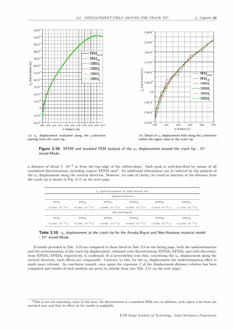
3.2. DISPLACEMENT FIELD AROUND THE CRACK TIP L. Gigliotti 43
(a) ux displacement evaluated along the y-directionstarting from the crack tip.
(b) Detail of ux displacement field along the y-directionwithin the region close to the crack tip.
Figure 3.10: XFEM and standard FEM analysis of the ux displacement around the crack tip - 45o
mixed-Mode.
a distance of about 5 · 10−2 m from the top edge of the rubber-sheet. Such peak is well-described by means of allconsidered discretizations, including coarser XFEM ones3. No additional information can be inferred by the analysis ofthe ux displacement along the vertical direction. However, for sake of clarity, its trend as function of the distance fromthe crack tip is shown in Fig. 3.11 on the next page.
uy DISPLACEMENT AT THE CRACK TIP
ARRUDA-BOYCE
FEM1 FEM2 XFEM1 XFEM2 XFEM3 XFEM4
−6.1644 · 10−4 m −6.1421 · 10−4 m −6.6488 · 10−4 m −6.6676 · 10−4 m −4.7410 · 10−4 m −5, 2175 · 10−4 m
NEO-HOOKEAN
FEM1 FEM2 XFEM1 XFEM2 XFEM3 XFEM4
−6.1582 · 10−4 m −6.1392 · 10−3 m −6.6487 · 10−4 m −6.6653 · 10−4 m −4.7396 · 10−4 m −5.2163 · 10−4 m
Table 3.10: uy displacement at the crack tip for the Arruda-Boyce and Neo-Hookean material model- 45o mixed-Mode.
If results provided in Tab. 3.10 are compared to those listed in Tab. 3.9 on the facing page, both the underestimationand the overestimation of the crack tip displacement, obtained with discretizations XFEM3-XFEM4 and with discretiza-tions XFEM1-XFEM2 respectively, is confirmed. It is nevertheless true that, concerning the ux displacement along thevertical direction, such effects are comparable. Contrary to this, for the uy displacement the underestimation effect ismuch more relevant. As conclusive remark, once again the exponent β of the displacement-distance relation has beencomputed and results of such analysis are given in tabular form (see Tab. 3.11 on the next page).
3This is not not surprising, since in this area, the discretization is a standard FEM one; in addition, such region is far from theenriched zone and thus its effect on the results is negligible.
KTH Royal Institute of Technology - Solid Mechanics Department

44 L. Gigliotti CHAPTER 3. NUMERICAL RESULTS - STATIC ANALYSIS
(a) uy displacement evaluated along the y-directionstarting from the crack tip.
(b) Detail of uy displacement field along the y-directionwithin the region close to the crack tip.
Figure 3.11: XFEM and standard FEM analysis of the uy displacement around the crack tip - 45o
mixed-Mode.
uy DISPLACEMENT - VERTICAL DIRECTION
ARRUDA-BOYCE NEO-HOOKEAN
FEM1 FEM2 XFEM1 XFEM2 XFEM3 XFEM4 FEM1 FEM2 XFEM1 XFEM2 XFEM3 XFEM4
α 0.4985 0.4901 0.5198 0.5128 0.4847 0.4914 0.5006 0.4937 0.5154 0.5102 0.4896 0.4939
R2 (0.9991) (1) (0.8109) (0.9543) (0.8798) (0.9857) (0.9998) (0.9954) (0.8016) (0.9312) (0.8943) (0.9898)
Table 3.11: Fitting procedure of the uy displacement results along the y-direction starting from thecrack tip - 45o mixed-Mode.
KTH Royal Institute of Technology - Solid Mechanics Department

Chapter 4
Numerical results - Dynamic Analysis
In this second part of the present work, the capabilities of the XFEM in Abaqus have been investigated. The analysis ofthe crack propagation phenomenon in rubber-like materials, by using the XFEM technique, has proved to be an arduoustask. This is thought to be mainly due, to the still poor implementation of the XFEM capabilities, along with thewell-established numerical difficulties encountered when fracture mechanics problems are analyzed by using numericalmethods. In particular, tremendous convergence difficulties have been faced and still unsatisfactory results in performingnumerical simulations of the crack growth process have been obtained. Only few elements can be cracked before thesimulation is aborted and there seems to be no correlation with the crack length; in other words, the highest number ofcracked elements does not depend on the level of refinement at the crack tip.
Notwithstanding these problems, three fundamental aspects of the crack propagation phenomenon have been inves-tigated, i.e. the instant at which, under the applied boundary conditions, the pre-existing crack starts to propagate, thecrack propagation angle and the crack propagation speed. For this aim, the above discussed discretizations have beenemployed (Cfr. Sec. 2.4). The choice to use discretizations in which the crack is not aligned with the elements edges, hasbeen somehow forced. Indeed, even with extreme modifications (sometimes almost non-realistic) of the time integrationscheme and of convergence parameters, it has been impossible to observe any crack growth in case of crack surfaces lyingalong elements edges. Likely, this stems from the presence of the node in correspondence of the crack tip and thus, fromthe resulting poorly conditioned problem (Cfr. Sec. 3.1.1). Furthermore, both the effects of the applied displacementand of the applied displacement rate have been taken into account.
4.1 Convergence criteria for nonlinear problems
As first attempt, the crack propagation phenomenon has been analyzed by means of a Static stress/displacement analysis.However, likely due to the unstable nature of the crack propagation process, by utilizing such typology of analysis it hasbeen not possible to observe any crack propagation and furthermore, no simulations have been successfully completed.
The Newton-Raphson method employed in Abaqus/Standard, when unstable processes are considered, often showssevere problems in reaching the convergence. However, these shortcomings are partially enhanced in dynamic problemsby the introduction of the mass matrix M, which is an additional positive term to the Jacobian. In such way, the Jacobianis thus slightly more positive and inertia effects help to regularize unstable behaviours1. Based on these considerations,an implicit dynamic analysis has been performed2.
Interestingly, what has been regarded as a limit, i.e. the possibility to use only linear elements, in this case istransformed into an advantage. Indeed, in large-deformation problems higher-order elements are affected by a rapid lossof accuracy, since the Jacobian determinant can be easily become negative at quadrature points, causing the abortionof calculations and high local inaccuracies. Thus, the implementation of higher-order XFEM could not lead to anysignificant enhancement.
Noteworthy is that, for all simulations performed, the maximum time step increment has been set equal to 0.1% ofthe whole simulation time3. By starting from zero, the applied displacement is linearly ramped over the step, until theprescribed value at the bottom ant top edge has not been reached.
In Abaqus/Standard, dynamic problems might be classified within three categories, i.e. transient fidelity applications,moderate dissipation applications and quasi-static applications. The Hilbert-Hughes-Taylor time integration method[102] is used for transient fidelity and moderate dissipation applications while the backward Euler operator is employedif the application is identified as quasi-static. Concerning this latter, it should be stressed that its application in Abaqus,requires a particular carefulness, because it automatically induces a 5% numerical damping and this value cannot bemodified by the user. Especially for this last reason, the Hilbert-Hughes-Taylor method has been used and its coefficientshave been tuned to attain a moderate numerical damping, which should help convergence and at the same time, not
1The density of rubber-like material has been set equal to 1000 kg/m3.2The principal advantage of this method is that it is unconditionally stable and thus no limitations exist on the size of time
increment used for the integration.3Comprehensive discussion on the correct choice of the maximum time step increment is provided on the Abaqus User’s Manual
(Cfr. Sec. 7.1.1).
45

46 L. Gigliotti CHAPTER 4. NUMERICAL RESULTS - DYNAMIC ANALYSIS
overly affect the physical formulation of the problem at hand 4. The HHT method provides for the definition of threedifferent parameters, α, β and γ. In order to let the method satisfy the stability and order properties [103], theseparameters are not independent of each other, but the following relationships hold
γ = 1−2α2
; β = (1−α)2
4(4.1)
Consequently, it is sufficient to modify only the parameter α to obtain different levels of numerical damping. Thechoice of α equal to 0, leads to the simple trapezoidal method and therefore, no numerical damping is introduced. Onthe other hand, the maximum numerical damping, i.e. 6%, is obtained for α = −1/3. For a comprehensive discussion onthe appropriate values of HHT-method parameters, refer to [104]. The values of such coefficients, utilized in this workare listed in Tab. 4.1.
HILBERT-HUGHES-TAYLOR METHOD COEFFICIENTS
β γ α
0.3025 0.6 −0.1
Table 4.1: Modified parameters for the Hilbert-Hughes-Taylor operator.
In addition to the introduction of numerical damping, the time implementation scheme has been adjusted analogouslyto the static analysis discussed in the previous chapter. Furthermore, the Criterion for residual forces for nonlinearproblems and the Criterion for displacement correction in nonlinear problems have been modified. In order toexplain these latter modifications, let us denote with α the characteristic field related to a particular problem, e.g. thedisplacement field in stress analyses. The parameters commonly used to determine whether an increment has convergedor not, are the following ones:
rαmax , the largest residual for the equilibrium equation of the field α;
∆uαmax , the maximum variation of the nodal variable during the increment;
cαmax , the largest correction executed during the current Newton iteration on any variable of type α;
ej , the greatest error in the particular j-constraint type, e.g. volumetric strain compatibility in problems involvinghybrid elements;
qα (t) , the magnitude of the conjugate flux to the field α, e.g. force flux for the displacement field, at any time t; itrepresents a spatial average flux over the entire domain, and it is defined a follows
qα (t)def=
(∑Ee=1
∑Nene=1
∑Nαnei=1 |q|
αi,ne
+∑i=1Nαef|q|α,efi
)∑Ee=1
∑Nene=1 N
αne +Nα
ef
(4.2)
where E is number of elements of the whole model, Ne is the number of nodes of the element e, Nαne indicates the
number of α-DOFs at the node ne of the element e, |q|αi,ne represents the magnitude of the flux that the elemente applies at its i-th α-DOF at its ne-th node at the specified time t, Nα
ef denotes the number of external fluxes for
the α-field and lastly, |q|α,efi is the amplitude of the i-th external flux for the α-field;
qα (t) , the overall time-averaged value of the conjugate flux to the field α; such averaging is performed over the wholestep, i.e.
qα (t)def=
1
Nt
Nt∑i=1
qα (ti) (4.3)
in which Nt indicates the total number of increments made hitherto in the step, including the current one as well.
For many practical applications, the following condition on the error in the residuals is introduced
rαmax ≤ Rαn qα (4.4)
Once the Eq. 4.4 is satisfied, the solution is accepted as converged if the largest correction to the solution cαmax issmaller than the greatest variation in the solution variable ∆uαmax, i.e.
cαmax ≤ Cαn∆uαmax. (4.5)
Coefficients Rαn and Cαn control the criterion for residual forces for nonlinear problems and the criterion for displace-ment correction in nonlinear problems, respectively, provided that the considered displacement field α, is the displacementone. In Tab. 4.2 on the next page, both default and updated values of such parameters are given.
4The HHT method is an extension of the Newmark β method.
KTH Royal Institute of Technology - Solid Mechanics Department

4.2. CRACK PROPAGATION INSTANT L. Gigliotti 47
Rαn Cαn
Abaqus Default 5 · 10−3 10−2
User controls 10−2 2 · 10−2
Table 4.2: Criteria for nonlinear problems controls.
4.1.1 Line search algorithm
Apart from modifying the aforementioned coefficients, in order to ameliorate the convergence and increase the robustnessof Newton-Raphson method, the line search algorithm has been included in the analysis. The main idea behind suchalgorithm is that, although the direction predicted by the ordinary Newton-Raphson method ∆d often is a good onetowards the correct solution, the step size ‖∆d‖ frequently is not the optimal one.
In the line search algorithm, the minimization of a measure of residuals, along the line d = dold +λ∆d, is sought. Theparameter λ defines the position along the line d, while dold is the last iterate. In nonlinear problems characterized bysharp discontinuities in the solution, the line search method represents a powerful tool to reduce the number of iterationsand cutbacks, resulting thus in a reduction of computational cost.
An aggressive line searching has been utilized in this work. In particular, the maximum number of line searchiterations allowed, N ls, is 10, while the accuracy in the line scale factor ηls employed, has been considered equal to 10−2.
4.2 Crack propagation instant
In this section, the instant at which the pre-existing crack starts to propagate within the structure is studied by usingthe XFEM technique. As previously stated, in Abaqus/Standard a crack can propagate only by completely cutting eachelement that it goes through. Based on this, the crack propagation instant tcrack is defined as the instant at whichthe first element is cut by the advancing crack. Such value has been calculated with a precision up to a thousandth ofsecond5.
First of all, an iterative procedure has been devoted to identify the value of displacement which causes the crack topropagate only within a single element. The instant of time at which this occurs is referred to as a reference crackpropagation instant tcrack. Such procedure has been performed by utilizing the discretization XFEMD5. Furthermore,it has been observed that, whether the crack crosses just one element, the simulations are able to terminate reaching theconvergence. Provided this, the calculated value of the reference crack propagation instant can be correctly evaluated.
Difficulties are encountered when the applied displacement rises and when coarser mesh at the crack tip are employed.Concerning the applied displacement, five different values have been considered, starting from 3 · 10−2 m up to a valueof 5 · 10−2 m, while keeping the velocity at which it is applied, at the constant value of v = 10−3 m/s. The fulfillment ofquasi-static conditions, has been kept under control by verifying the value of the total kinematic energy of the model6.In order to assess the influence of the applied displacement as well as of the element size at the crack tip, on the correctdetermination of the parameter at hand, the percent error, defined as follows, has been exploited
Error [%] =tcrack − tcrack
tcrack· 100 (4.6)
Such quantity is shown in Fig. 4.1 on the following page as function of the applied displacement u and for differentelements sizes h at the crack tip.
It can be easily seen that, in this case, the effect of the applied displacement is almost inexistent since the percentageerror remains constant with the applied displacement.
As expected, it is noted that the element size, on the contrary, strongly affects the results. Such statement is furtherconfirmed referring to Fig. 4.2 on the next page. Here, the percentage of error as function of the element size at thecrack tip h is depicted for both mixed-Mode load conditions analyzed. An almost linear trend can be easily noticed,although a slight deviation is observed in correspondence of intermediate values, i.e. for h ≈ 2 · 10−2 m. In both cases,a portion of the graph has been shown with an higher level of detail, in order to visualize the, albeit slight, influence ofthe applied displacement.
So far, we have considered a constant applied displacement velocity of 10−3 m/s. We may now analyze the effect ofsuch quantity on the evaluation of the crack propagation instant. In Fig. 4.3 on page 49 the evolution of the percentageerror defined above, is presented. In all cases, the applied displacement rate v is, on purpose, higher than v. Comparesuch figure with the analogous one regarding the influence of the applied displacement. Note that although the results arealmost identical, a slight dependence on the applied displacement rate v is detected. Especially for coarser discretizationsat the crack tip, the higher the applied displacement rate v, the higher the percentage error.
5The small size of the time step increments during the crack propagation process allow us to achieve such high level of accuracy.6Furthermore, information indicating whether the quasi-static conditions are satisfied or not, are provided in the .dat
Abaqus/CAE file.
KTH Royal Institute of Technology - Solid Mechanics Department

48 L. Gigliotti CHAPTER 4. NUMERICAL RESULTS - DYNAMIC ANALYSIS
Figure 4.1: Crack propagation instant tcrack as function of the applied displacement at the top andbottom edges. Data relative to the 45o mixed-Mode are depicted with solid lines while the dotted onesrepresent the data for the 30o mixed-Mode - Applied displacement rate equal to 10−3 m/s.
(a) 45o mixed-Mode. (b) 30o mixed-Mode.
Figure 4.2: Influence of the element size at the crack tip h on the correct determination of the crackpropagation instant - Applied displacement rate equal to 10−3 m/s.
The percentage error in the determination of tcrack as function of the elements size at the crack tip is plotted inFig. 4.4 on page 49. The trend is equivalent to the one observed so far. Furthermore, the slightly more relevant influenceof the applied displacement rate v with respect to the applied displacement u, on the percentage error, is clearer.
KTH Royal Institute of Technology - Solid Mechanics Department

4.2. CRACK PROPAGATION INSTANT L. Gigliotti 49
Figure 4.3: Crack propagation instant tcrack as function of the applied displacement rate. Data relativeto the 45o mixed-Mode are depicted with solid lines while dotted ones represent the data for the 30o
mixed-Mode - Applied displacement rate equal to 10−3 m/s.
(a) 45o mixed-Mode. (b) 30o mixed-Mode.
Figure 4.4: Influence of the element size at the crack tip h on the correct determination of the crackpropagation instant.
KTH Royal Institute of Technology - Solid Mechanics Department

50 L. Gigliotti CHAPTER 4. NUMERICAL RESULTS - DYNAMIC ANALYSIS
4.3 Crack propagation angle
Once the crack has started, the direction in which it will propagate is of tremendous interest in practical engineeringapplications. In this case, no reference solution exists since, as already stated, simulations in which the convergenceis achieved are those where just a single element as been cracked. One single element cracked has been thought to donot provide any valuable information about the correct direction of crack propagation. Thus, in this section, results areprovided in terms of real angles. In order to uniquely identify the crack growth direction, the local coordinate systemadopted and how the crack angle has been defined, is depicted in Fig. 4.5.
Figure 4.5: Local coordinate system centred at the crack tip and crack propagation angle α.
In Fig. 4.6, the crack propagation angle α, as function of the applied displacement is shown. Clearly, no dependanceon this latter is observed and such remark is valid for both examined loading conditions. On the contrary, the mesh sizeat the crack tip seems to strongly affect the correct prediction of the crack propagation angle. Coarser discretizationstend to overestimate it, if compared to the denser ones.
Figure 4.6: Crack propagation angle as function of the applied displacement for several elements size atthe crack tip. Solid lines are relative to the 45o mixed-Mode while dashed ones, to the 30o mixed-Mode- Applied displacement rate equal to 10−3 m/s.
A more detailed description of the dependance of α on the mesh size at the crack tip is depicted in Fig. 4.7 onthe facing page. A roughly linear trend is observed and the overestimation of the crack propagation angle with coarserdiscretizations is confirmed.
As last observation, it might be pointed out that the influence of the mesh size is comparable for the 45o mixed-Modeand for the 30o mixed-Mode. Indeed, the crack propagation angles predicted with the discretization XFEMD1 and withthe XFEMD5 one, differ at the most, of the 20.21% and 20.34% for the 45o mixed-Mode and for the 30o mixed-Mode,respectively.
We may now plot the predicted crack propagation angle as function of the applied displacement rate v. It can be
KTH Royal Institute of Technology - Solid Mechanics Department

4.3. CRACK PROPAGATION ANGLE L. Gigliotti 51
Figure 4.7: Crack propagation angle as function of the elements size at the crack tip h for severalvalues of the applied displacement. At the top, crack propagation angles for the 45o mixed-Mode whileat the bottom for the 30o mixed-Mode - Applied displacement rate equal to 10−3 m/s.
seen that the even in this case, the direction of the crack propagation is almost independent from the velocity at whichbottom and top edges are moved.In addition, a linear trend with respect to the mesh size at the crack tip is predicted, in this case as well (see Fig. 4.9 onthe next page). Lastly, for excess of meticulousness, it is observed that the characteristic knee in the crack angle - meshsize relation is located in correspondence of two different values of elements size at the crack tip h. In particular, it ispositioned at h ≈ 2 · 10−2 m when different values of the applied displacement are considered and at h ≈ 2.5 · 10−2 m,when, on the other hand, different values of the applied displacement rate are considered. Such behaviour would needto be further investigated.
Interestingly, the applied displacement rate, the more pronounced the influence of the mesh size at the crack tip on thepredicted crack propagation angle. By referring to Tab. 4.3, it may be readily noticed that, if the applied displacementrate is increased, the percentage difference between results obtained with the most dense discretization, XFEMD1, andwith the most coarse one, XFEMD5, also augments.
MESH SIZE EFFECT ON THE COMPUTED CRACK PROPAGATION ANGLE
45o mixed-Mode
10−3 m/s 1.15 · 10−3 m/s 1.35 · 10−3 m/s 1.54 · 10−3 m/s 1.73 · 10−3 m/s 1.92 · 10−3 m/s
20.21% 20.56% 20.98% 22.03% 23.87% 25.91%
30o mixed-Mode
10−3 m/s 1.15 · 10−3 m/s 1.35 · 10−3 m/s 1.54 · 10−3 m/s 1.73 · 10−3 m/s 1.92 · 10−3 m/s
20.34% 20.86% 21.12% 22.37% 23.43% 25.51%
Table 4.3: Percentage difference between the computed crack propagation angle with the XFEMD1 andXFEMD5 discretizations, for both 45o mixed-Mode and 30o mixed-Mode. In both case, an incrementof roughly 5% is obtained if the applied displacement rate is almost doubled.
KTH Royal Institute of Technology - Solid Mechanics Department

52 L. Gigliotti CHAPTER 4. NUMERICAL RESULTS - DYNAMIC ANALYSIS
Figure 4.8: Crack propagation angle as function of the applied displacement rate for several elementssize at the crack tip. Solid lines are relative to the 45o mixed-Mode while dashed ones, to the 30o
mixed-Mode.
Figure 4.9: Crack propagation angle as function of the elements size at the crack tip h for seral valuesof the applied displacement rate. At the top, crack propagation angles for the 45o mixed-Mode whileat the bottom for the 30o mixed-Mode.
KTH Royal Institute of Technology - Solid Mechanics Department

4.4. CRACK PROPAGATION SPEED L. Gigliotti 53
4.4 Crack propagation speed
Along with the triggering instant and the crack propagation direction, the third parameter of interest when crack growthphenomena are analyzed, is the speed at which the crack propagates within the component. In this section, the evaluationof such parameter has been studied for the 45o mixed-Mode loading condition and, as seen previously, the effects of theapplied displacement, applied displacement rate and mesh size at the crack tip have been investigated.
Since the crack can propagate only by cutting completely each element, the crack propagation phenomenon can beregarded as a discrete process. Based on this consideration, it is fundamental to clearly identify in which points and/orinstants the crack propagation speeds are evaluated.
For this purpose, consider Fig. 4.10. Here the value of the equivalent von Mises stress at the crack tip, as functionof the current value of the applied displacement, is depicted.
Figure 4.10: Equivalent von Mises stress at the crack tip as the applied displacement at the bottomand top edges varies. Note the sharp drop representing the instant at which the crack starts to advance.
The equivalent von Mises stress increases with the applied displacement as far as the fracture criterion defined so far(Cfr. Sec. 2.5) is not satisfied. At this point, the stress value sharply decreases within one single time step increment;such sudden drop clearly represents the triggering instant of the crack propagation. Thus, the crack propagation processmight be observed in terms of the evolution of the equivalent stress at the crack tip. Every time the von-Mises stressexperiences a decrement analogous to that one shown in Fig. 4.10, it represents that the crack has gone through onemore element. As example of what stated in the previous lines, we may now plot the evolution of the von-Mises stressat the crack tip as function of the current applied displacement during the load process (see Fig. 4.11 on page 55).
Particularly noteworthy is the fact that, whenever the defect is propagated through the next element, in terms ofstress-state at the crack tip, it is like if the structure was undamaged but with a pre-existing defect, whose geometry isdetermined by the previous load history. Such crack, however, is no longer, as before, initially stress-free, but subjectedto a stress level equal to that one present at the instant in which the crack has gone through the previous element alongits path. It can be easily seen that the load history in subsequent time steps is completely independent of what occurredin the previous stages, except with regard to the initial value of the equivalent stress at the crack tip. In addition, it isevident (see Fig. 4.11 on page 55) as, the evolution of the stress state at the crack tip is a particularly smooth function ofthe current applied displacement and no glaring deviations from the main trend are detectable. The analysis devoted tothe evaluation of the propagation speed of the crack through the structure is of major concern. Such analysis, however,as already stressed, is strongly limited by the small number of elements that can be cracked before simulations fail. Thespeed at which an element has been crossed by the defect, is defined as the ratio between the length of the crack in theelement itself, and the time interval between the relative minimum and maximum, of the portion of the loading curve,corresponding to the cracked element at hand (see Fig. 4.12 on page 56).
In Fig. 4.13 on page 57, the crack propagation speed vcrack as function of the current applied displacement fordifferent mesh sizes at the crack tip is presented.
In accordance with numerical results shown in the previous sections, in the present analysis the effect of the applieddisplacement has been considered to be negligible small. Interestingly, with the increase of the applied displacement alongboth the top and the bottom edge, the value of crack propagation speed increases quite abruptly. In these conditions, itis intuitive to perceive that the process of crack propagation becomes rapidly unstable.
The effect of the elements size at the crack tip, can be further investigated by analyzing the crack propagation speedvalues after the crack itself has crossed n elements. In Fig. 4.14 on page 58, the trend of vcrack after n = 2, 3, 4, 5 crackedelements, as function of the mesh size at the crack tip, is displayed.
KTH Royal Institute of Technology - Solid Mechanics Department

54 L. Gigliotti CHAPTER 4. NUMERICAL RESULTS - DYNAMIC ANALYSIS
One can clearly deduce that in all cases analyzed, coarser meshes tend to underestimate the value of the crack propagationspeed. This effect is much more pronounced as the lower vcrack itself, i.e. when the crack is starting to propagate. Thepercentage variation, between the values calculated by using the most dense mesh XFEMD5 or the most coarse oneXFEMD1, is given in Tab. 4.4.
MESH SIZE INFLUENCE ON vcrack
n = 2 n = 3 n = 4 n = 5
48.56% 40.54% 32.17% 19.02%
Table 4.4: Influence of the mesh size on vcrack. The percentage differences listed are relative to thevariation of the crack propagation speeds predicted with discretizations XFEMD1 and XFEMD5.
Observe that the crack propagation speed has not exceeded in any case the velocity of 50 m/s. This latter isconsidered a threshold value above which, the effects of inertia can no longer be neglected [105]. As conclusion ofthe present work, the influence of the applied displacement rate on the estimated crack propagation speed is studied.Following the same procedure adopted so far, consider the evolution of the equivalent von-Mises stress at the crack tipas function of the applied current displacement (see Fig. 4.15 on page 59) for a value of the applied displacement rateequal to 1.92 · 10−3 m/s and for five different element sizes at the crack tip7. Compare this result with that one shownin Fig. 4.11 on the facing page. In this case, one can observe how the trend is not completely uniform, showing on thecontrary, a highly irregular behaviour.Therefore, increasing the applied displacement rate, an additional source of instability of the model is introduced. Likely,this is due to the fact that, if the specimen is loaded with a higher velocity, the inertia effects ca no longer be neglected.
In order to better characterize such unstable behaviour, it is sufficient to evaluate the kinetic energy of the wholemodel and compare it to its total internal energy. To fulfil the quasi-static conditions, the kinetic energy should remainbelow the 5% of the internal energy during the majority of the analysis. Such condition, as already stated, is completelysatisfied for an applied displacement rate equal to 10−3 m/s. However, when higher values are considered, even if thiscondition continues to be met, the threshold value of 5% becomes progressively closer during some steps, and suchsituation is thought to lead to a further model instability.
Nevertheless, in Fig. 4.16 on page 60 the crack propagation speed as function of the current applied displacementand for five different element sizes at the crack tip, is presented. It is confirmed that, as the displacement at the bottomand top edge increases, the vcrack rises dramatically up to values higher then those observed in the previous case, for anapplied displacement rate of 10−3 m/s. These higher values are obviously ascribable to the increased applied displacementrate. Also in this case, the coarser the mesh the lower the computed crack propagation speed.
In conclusion, we present the evolution of the crack propagation speed as function of the applied displacement rate.This is shown in Fig. 4.17 on page 61 for four different time steps, namely, after that 2,3,4 and 5 elements have beencompletely cracked. As expected, increasing the applied displacement rate, we observe a growth in terms of crackpropagation speed. Moreover, the higher the number of cracked elements and therefore, the predicted propagationspeed, the more pronounced this effect. It seems to be not possible to extrapolate a common trend in all four depictedcases, however, a nearly parabolic relationship between the applied displacement rate and the crack propagation speed,is thought to be the most reasonable.
In confirmation of what stated above, regarding the no longer negligible inertia effects, note that for applied displace-ment rate values equal to 1.73 · 10−3 m/s and 1.92 · 10−3 m/s, the threshold value of 50 m/s for the crack propagationspeed has been exceeded, i.e. 57.691 m/s and 66.043 m/s respectively. In case of applied displacement rate equal to1.54 · 10−3 m/s, a very close value, equal to 48.021 m/s, is obtained.
7Exactly as above, only a particular example has been shown for graphical reasons.
KTH Royal Institute of Technology - Solid Mechanics Department

4.4. CRACK PROPAGATION SPEED L. Gigliotti 55
(a) XFEMD5. (b) XFEMD4.
(c) XFEMD3. (d) XFEMD2.
(e) XFEMD1.
Figure 4.11: Equivalent von Mises stress at the crack tip as the applied displacement at the bottomand top edges varies, for five different element sizes at the crack tip - Applied displacement rate equalto 10−3 m/s.
KTH Royal Institute of Technology - Solid Mechanics Department

56 L. Gigliotti CHAPTER 4. NUMERICAL RESULTS - DYNAMIC ANALYSIS
Figure 4.12: Evaluation of the crack propagation speed. The time period during which the crack shouldprogressively propagate through the element, is highlighted in the circle boxes - Applied displacementrate equal to 10−3 m/s.
KTH Royal Institute of Technology - Solid Mechanics Department
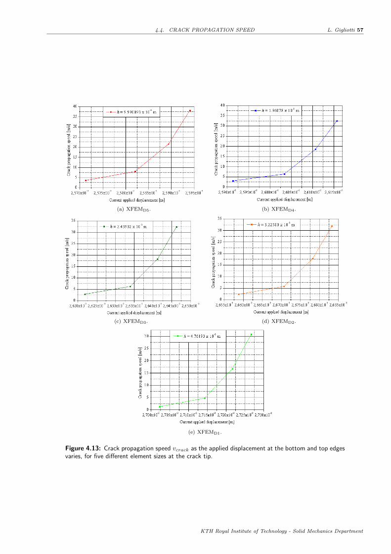
4.4. CRACK PROPAGATION SPEED L. Gigliotti 57
(a) XFEMD5. (b) XFEMD4.
(c) XFEMD3. (d) XFEMD2.
(e) XFEMD1.
Figure 4.13: Crack propagation speed vcrack as the applied displacement at the bottom and top edgesvaries, for five different element sizes at the crack tip.
KTH Royal Institute of Technology - Solid Mechanics Department

58 L. Gigliotti CHAPTER 4. NUMERICAL RESULTS - DYNAMIC ANALYSIS
Figure 4.14: Crack propagation speed as function of the element size at the crack tip. Speed valuesafter 4 and 5 cracked elements are depicted in dashed lines while solid lines represent speed values for2 and 3 cracked elements - Applied displacement rate equal to 10−3 m/s.
KTH Royal Institute of Technology - Solid Mechanics Department

4.4. CRACK PROPAGATION SPEED L. Gigliotti 59
(a) XFEMD5. (b) XFEMD4.
(c) XFEMD3. (d) XFEMD2.
(e) XFEMD1.
Figure 4.15: Equivalent von Mises stress at the crack tip as the applied displacement at the bottomand top edges varies, for five different element sizes at the crack tip - Applied displacement rate equalto 1.92 · 10−3 m/s.
KTH Royal Institute of Technology - Solid Mechanics Department

60 L. Gigliotti CHAPTER 4. NUMERICAL RESULTS - DYNAMIC ANALYSIS
(a) XFEMD5. (b) XFEMD4.
(c) XFEMD3. (d) XFEMD2.
(e) XFEMD1.
Figure 4.16: Crack propagation speed vcrack as the applied displacement at the bottom and topedges varies, for five different element sizes at the crack tip - Applied displacement rate equal to1.92 · 10−3 m/s.
KTH Royal Institute of Technology - Solid Mechanics Department

4.4. CRACK PROPAGATION SPEED L. Gigliotti 61
Figure 4.17: Crack propagation speed as function of the applied displacement rate. Speed values after4 and 5 cracked elements are depicted in dashed lines while, solid ones represent speed values for 2 and3 cracked elements - Discretization XFEMD5.
KTH Royal Institute of Technology - Solid Mechanics Department
62 L. Gigliotti CHAPTER 4. NUMERICAL RESULTS - DYNAMIC ANALYSIS
4.5 Remarks on convergence behaviour
As conclusion, it is worthwhile to comment on the convergence behaviour of the performedsimulations. The scenario is thefollowing one. The complete convergence is achieved only when the finest discretization is used, the applied displacementrate is maintained equal to 10−3 m/s and the displacement is such that only one element has been completely cracked,namely 2.8 · 10−2 m and 2.6 · 10−2 m, for the 45o mixed-Mode and for the 30o mixed-Mode, respectively. In all othercases, it has been not possible to complete the simulations successfully. Moreover, the analysis of residuals, clearlyreveals that the time step increments remain constant to their initial value until the crack propagation criterion (Cfr.Sec. 2.5) is not satisfied. At this point, the time step increments sharply decrease for two reasons: firstly, it can happensthat convergence is not obtained within the maximum number of iterations allowed for a single step or, secondly, thecomputed rate of convergence is too low and the convergence is judged unlikely.
Successively, the appropriate value of the time step increment is reached and thus the simulation can proceed. Ithas to be stressed that this value is much smaller than those observed before the crack starts to propagate. Duringthe crack growth process, the aforementioned time-length of the step increment is kept almost constant and no relevantvariations are observed. Such condition holds until, suddenly, a second sharp decrease in terms of time step incrementoccurs. However, at this point this latter is already small enough and a further reduction makes the simulation to exitautomatically with an error. The one described above, is the list of subsequent events occurring in all the carried outsimulations, with no exceptions.
Such difficulties might stem from the limited capacity of most of the elements to sustain distortion without causinga degradation of performance or failure. These limitations to deal with large distortions are particularly evident in thecase of nonlinear analyses, including large deformations and material nonlinearities, performed with Lagrangian meshes.Thus, the XFEM implementation is thought to further reduce the element capabilities to tolerate large distortions.
An efficient method to circumvent such shortcomings, or at least to reduce them, is to extend the XFEM capabilitiesto the Arbitrary Lagrangian Eulerian formulation [106, 107, 108, 109]. Often, the main cause of the failure of simulationsis the excessive value of distortion of the elements nearby the crack tip; this would require a remeshing procedure,which is not permitted when XFEM technique is used8. Meanwhile material motions does not lead to any distortionin Eulerian finite elements. However, the treatment of constitutive equations and of moving boundaries and interfaces,e.g. crack surfaces is cumbersome with pure Eulerian finite elements. The ALE formulation is an hybrid technique inwhich the advantages of both Lagrangian and Eulerian formulations are combined, while trying to limit as far as possibletheir relative disadvantages. It is opinion of the author of this thesis that, the extension of XFEM capabilities to theALE formulation in Abaqus/Standard could represent a major step forward to enhance the capabilities of the XFEMtechnique to model the crack growth process in materials that can undergo large deformations.
Furthermore, consider the convergence behaviour of iterations performed with the Newton-Raphson method. Roughlyspeaking, fundamental conditions for a quadratic rate of convergence ought to be satisfied, i.e. a sufficient smoothnessof the Jacobian matrix J as function of u is needed and, moreover, J should be regular and well conditioned over thewhole domain in the displacement space of the iterative procedure.
It is straightforward to observe that, both such conditions are not met in the problem at hand. In particular, it isevident that the Jacobian matrix is not only a non-smooth function of u but actually is a discontinuous one within theenriched elements9. Therefore, the regularity condition is also not satisfied for the enriched elements. Such considerationsare thought to be among the principal reasons of the lack of convergence faced for the crack propagation analysis.
It has been verified that the Arruda-Boyce material model employed in this section, is stable over the entire consideredrange of strains. However, material instabilities may rise also in presence of a localized growth of deformation, as that oneoccurring at the crack tip during crack propagation processes. Such phenomenon is known in literature as localization.This localization phenomenon, results in the formation of slender bands of intense deformation called shear bands10,which can be interpreted as the result of material instability in the shear component. Analogously, fracture can beseen as the result of material instability in the normal direction to the discontinuity surfaces in pure Mode-I or in thetangential direction in pure Mode-II.
As highlighted in [37], fracture cannot be numerically modeled without difficulties. Indeed, such phenomenon includesmost of the shortcoming related to material instabilities, i.e. localization to a set of measure for rate-independent materialmodels, zero energy dissipation11 as well as absence of a length scale. The Abaqus/Standard implementation of XFEMis thought to be still not able to handle such problems.
Analogous convergence difficulties to those encountered in this work, have been faced in [91]. However, in such work,these shortcoming have been circumvented by adopting a modified scheme of the Newton-Raphson method. It stands toreason, given the purpose of the present work, such approach has not be here employed.
In [72], has been observed that the convergence rate for the classical XFEM method is of the order√h. In addition
to this, in [110] and [111] detailed analyses of the convergence of assumed strain methods have been performed, in thecases of compressible and incompressible materials. The established a priori error estimate for displacements leads toa linear rate of convergence. Further works dealing with the rate of convergence for hybrid elements can be found inliterature [112] [113].
All in all, the severe convergence difficulties encountered are reasonably ascribable to the coexistence of severalfactors, i.e. fracture mechanics problem, high level of deformation, plane strain conditions, complex material model,
8In addition, the main peculiarity of the XFEM technique would be not exploited.9Recall Eq. 1.102 and that
dH(x)dx
= δ(x), where δ(x) is the Dirac delta function.10The name shear bands stems from the fact that often the deformation mode in these bands of high deformation is shear.11This, in particular, is thought to be the most relevant drawback, since fracture process leads to significant energy dissipation.
KTH Royal Institute of Technology - Solid Mechanics Department

4.5. REMARKS ON CONVERGENCE BEHAVIOUR L. Gigliotti 63
incompressibility constraint along with the still poor implementation of the XFEM technique in Abaqus.
KTH Royal Institute of Technology - Solid Mechanics Department

64 L. Gigliotti CHAPTER 4. NUMERICAL RESULTS - DYNAMIC ANALYSIS
KTH Royal Institute of Technology - Solid Mechanics Department
Chapter 5
Summary
The work presented in this thesis aims at assessing the capabilities of the XFEM implementation in the commercial FEAsoftware Abaqus for modelling crack growth phenomena in rubber-like materials.
The ability of the eXtended Finite Element Method in Abaqus to evaluate the correct displacement and stress fieldsat the crack tip in a single edge notched specimen of rubber in plane strain conditions has been assessed. For thispurpose, a comparison between results obtained by means of a standard FEM analysis with an highly refined mesh atthe crack tip and the outcomes of an XFEM analysis performed with coarser discretizations, has been carried out.TheArruda-Boyce and the Neo-Hookean material models have been considered. The analysis has been performed for twodifferent load conditions, a pure Mode-I load condition and a 45o mixed-Mode one.
Results of such analysis, clearly reveal the inaccuracy of the XFEM used with coarse meshes, in predicting thesingularity in the stress field at the crack tip. Such limit is readily attributable to the non-refined discretization at thecrack tip and to the visualization procedures performed in Abaqus for element-based variables in first-order continuumelements. Furthermore, it is not overemphasized that both the stress distribution around the crack tip and its highestvalues cannot be correctly predicted by means of an XFEM analysis performed with coarse meshes.
It has been highlighted the apparently major role played by the location of the crack tip within the discretizationgrid. Locate the tip in correspondence of a node guarantees an higher level of accuracy with respect to the case in whichit is positioned along an element edge in terms of stress values.
Relevant shortcomings are still observed concerning the displacement field prediction at the crack tip. However, muchmore accurate results than those related to the stress field can be obtained. In this case, the displacement trend can bepredict with an high level of accuracy and no glaring deviations with respect to the standard FEM analysis results aredetectable.
As seen for the previous case, the position of the crack tip within the mesh grid is of major concern for the determi-nation of the displacement field, as well. Noteworthy is that in this case, if a node is located at the crack tip, due to thesubsequent high condition number of the system, oscillatory trends are observed especially within the area close to thecrack tip. Such behaviour requires to be further investigated.
In addition, it ought to be emphasized that, for both stress and displacement fields, slightly more accurate resultsare obtained when the Neo-Hookean material model is adopted.
All in all, results of the static analysis here briefly summarized, allow to draw the following conclusion. In orderto correctly model the stress and displacement fields around the crack tip, the XFEM technique in Abaqus does notrepresent, at the moment, an advantage if compared to the standard FEM approach. Although, the possibility to locatethe crack within the structure, independently from the underlying discretization grid, is an unquestionable benefit.
The capabilities of the eXtended Finite Element Method implementation in Abaqus for modelling crack propagationphenomena in rubber-like materials have analyzed in terms of the three fundamental aspects of the crack propagationprocess, i.e. the instant at which the pre-existing crack will start to propagate, the crack propagation path and thespeed at which the crack will propagate. Two different mixed-mode load conditions have been analyzed, namely a 45o
mixed-Mode and a 30o mixed-Mode. Concerning the hyperelastic material model, in the dynamic analysis only theArruda-Boyce one has been considered.
Severe convergence difficulties have been encountered and the complete convergence has been attained only if theapplied displacement at the top and bottom edges, is such that one single element is cut by the propagating crack. Inaddition, very few elements can be cut by the advancing crack before simulations are aborted because of the inability ofthe solution to converge. The major causes of these difficulties may be related to the inadequacy of the Newton-Raphsonmethod to deal with sharp gradients and discontinuities in the displacement field, to the suboptimal rate of convergenceof the XFEM and to the coexistence of several factors, plane strain conditions, incompressibility constraint, high strainlocalization, complex material models among the most relevant.
Results of this analysis show that the applied displacement rate v has a slight influence on the correct prediction ofboth the crack propagation angle and crack propagation instant. On the contrary, these latter exhibit an almost lineardependance with the elements size at the crack tip.
Much more demanding has been the analysis of the crack propagation speed. Due to the enrichment procedureperformed in Abaqus, the crack can propagate within the structure, only by completely cutting each element that it
65

66 L. Gigliotti CHAPTER 5. SUMMARY
encounters on its path. Hence, the crack propagation can be regarded as a discrete process and it has been analyzedwith reference to the time evolution of the equivalent von Mises stress at the crack tip.
The applied displacement rate has proven, together with the inertia effects for crack propagation speed higher than50 m/s, to be of remarkable concern for the analysis stability.
Noteworthy, as expected, increasing the applied displacement rate, the crack propagation speed rises as well. It isworthwhile to mention that, the higher the crack propagation speed, the more evident is the effect of such parameter.
In addition, regarding the influence of the elements size at the crack tip, an underestimation of the crack propagationspeed is observed if coarser meshes are used. For lower values of the crack propagation speed, the influence of thediscretization refinement at the crack tip is much more pronounced and an almost linear trend with respect to theelements size might be observed.
Bearing in mind what presented in this work, it is possible to claim that the implementation of the eXtended FiniteElement Method in Abaqus is still too poor for providing an acceptable level of accuracy in the analysis of fracturemechanics problems involving rubber-like materials. Such limitations are emphasized when dynamic fracture mechanicsphenomena are investigated.
Major shortcomings related to the use of the XFEM technique within the framework of a multi-purpose commercialFEA software are detectable and even worsened by factors that are known to entail enormous difficulties in numericalanalyses.
For these reasons, further enhancements of the XFEM implementation in Abaqus are considered essential to suc-cessfully extend the enormous capabilities of such technique to the numerical analysis of fracture mechanics problems inrubber-like materials.
KTH Royal Institute of Technology - Solid Mechanics Department

Bibliography
[1] Ibrahimbegovic, A., Nonlinear Solid Mechanics: Theoretical Formulation and Finite Element Solution Methods,Springer, 2008.
[2] Holzapfel, G.A., Nonlinear Solid Mechanics: A Continuum Approach for Engineering, John Wiley & Sons Ltd,Chichester, 2000.
[3] Treloar, L.R.G., The Physics of rubber elasticity, 3rd edition, Clarendon Press, Oxford,1975.
[4] Ogden, R.W., Large Deformation Isotropic Elasticity - On the Correlation of Theory and Experiment for Incom-pressible Rubberlike Solids, Proceedings of the Royal Society of London. Series A, Mathematical and PhysicalSciences, 1972, A326 (1567), 565-584.
[5] Ogden, R.W., The elasticity of a network of long chain molecules. I and II, Transactions of the Faraday Society,1943, 39, 36-41 and 241-246.
[6] Rivlin, R.S., Large elastic deformations of isotropic materials. IV. Further developments of the general theory,Philosophical Transactions of the Royal Society of London, 1948, A241 (835), 379-397.
[7] Ogden, R.W., Non-linear elastic Deformations, Dover, New York, 1997.
[8] Flory, P.J., Principles of Polymer Chemistry, Cornell University Press, Ithaca, 1953.
[9] Flory, P.J., Statistical Mechanics of Chain Molecules, Interscience, 1969.
[10] Kuhn, R.S., Grun, F., Beziehungen zwischen elastischen Konstanten und Dehnungsdoppelbrechung hochelastischerStoffe, Kolloid-Zeitschrift, 1942, 101, 248-271.
[11] Mooney, M., A theory of large elastic deformation, Journal of Applied Physics, 1940, 11(9), 582-592.
[12] Treloar, L.R.G., A theory of large elastic deformation, Transaction of Faraday Society, 1944, 40, 59-70.
[13] Jones, D.F., Treloar, L.R.G., The properties of rubber in pure homogeneous strain, Journal of Physics D: AppliedPhysics, 1944, 8 (11), 007, 1285-1304.
[14] Arruda, E.M., Boyce, M.C., A three-dimensional constitutive model for the large stretch behaviour of rubber elasticmaterials, Journal of the Mechanics and Physics of Solids, 1993, 41 (2), 389-412.
[15] Mark, J.E., Erman, B., Rubberlike Elasticity a Molecular Primer, John Wiley & Sons Ltd, New York, 1993.
[16] Yeoh, O.H, Characterization of elastic properties of carbon black-filled rubber vulcanizates, Rubber Chemistry andTechnology, 1990, 63 , 792-805.
[17] Kawabata, S., Kawai, H., Strain energy density functions of rubber vulcanizates from biaxial extension, Advancesin Polymer Science, 1977, 24, Springer-Verlag, Berlin, 90-124.
[18] Seki, W., Fukahori, Y., Iseda, Y., Matsunaga, T., Large-deformation finite-element analysis for multilayer elas-tomeric bearings, Rubber Chemistry and Technology, 1987, 60, 856-869.
[19] Gent, A.N., A new constitutive relation for rubber, Rubber Chemistry and Technology, 1996, 69, 59-61.
[20] Kilian, H.G., Equation of State of Real Networks, Polymer, 1981, 22, 209-216.
[21] Rivlin, R.S., Thomas, A.G., Rupture of rubber I. Characteristic energy for tearing, Journal of Polymer Science1952, 10(3), 291-318.
[22] Griffith, A.A., The phenomena of rupture and flow in solids, Philosophical Transactions of the Royal Society A:Mathematical, Physical and Engineering, Delft, 1921, 221, 163-197.
[23] Griffith, A.A., The theory of rupture, Proceedings of First International Congress of Applied Mechanics, Eds.Biezeno and Burgers, Waltman, 1924, 55-63.
[24] Irwin, G.R., Kies, J., Fracturing and fracture dynamics, Welding Journal Research Supplement, 1952.
[25] Orowan, E., Fundamentals of brittle behaviour of metals, Fatigue and Fracture of Metals, John Wiley & Sons Ltd,New York, 1993, 139-167.
[26] Irwin, G.R. Fracture, Handbook of Physics, 1958, 6, 551-590.
[27] Gdoutos, E.E., Daniel, I.M., Schubel, P., Fracture mechanics of rubber, Mechanics, Automatic controls andRobotics, Facta Universitatis 2003, 3(13), 497-510.
67

68 L. Gigliotti BIBLIOGRAPHY
[28] Procedures of Army Symposium on Solid Mechanics - Case Studies on Structural Integrity and Reliability, AMMRCMS 78-3 1978, Army Materials and Mechanic Research Center.
[29] Stevenson, A., A fracture mechanics study of the fatigue of rubber in compression, International Journal ofFracture, 1983, 23, 47-59.
[30] Greensmith, H.W., Rupture of Rubber. Part 8: Comparisons of Tear and Tensile Rupture Measurements, Journalof applied Polymer Science, 1960, 21, 175.
[31] Lindley, P.B., Engineering Design with Natural Rubber, MRPRA, 1974.
[32] Lindley, P.B., Fatigue and Fracture of Elastomers, Master Thesis Report TVSM-5078, University of Lund 1998.
[33] Zienkiewicz, O.C., Taylor, R.L., The Finite Element Method, Vols. 1-3, Butterworth-Heinemann, Oxford 2000.
[34] http://homepage.usask.ca/~ijm451/finite/fe_resources/node139.html
[35] Atluri, S.N., Computational methods in mechanics - Vol.2 Computational methods in the mechanics of fracture,Mechanics and Mathematics Methods, North-Holland 1986.
[36] Liebowitz, H., Sandhu, J.S., Lee, J.D. Menandro, F.C.M., Computational fracture mechanics: research and ap-plication, Engineering fracture mechanics, 1995, 50, 653-670.
[37] Belytschko, T., Liu, W.K., Moran, B., Nonlinear Finite Element methods for Continua and Structures, JohnWiley & Sons Ltd, Chichester 2000.
[38] Tong, P., Pian, T.H., On the convergence of finite element method for problems with singularities, InternationalJournal of Solid Structures, 1973, 9, 313-321.
[39] Henshell, R., Shaw, K., Crack tip finite elements are unnecessary, International journal of numerical methods inengineering, 1975, 9, 495-507.
[40] Benzley, S.E., Representation of singularities with isoparametric finite elements, International journal of numericalmethods in engineering, 1975, 8, 537-545.
[41] Gifforrd, J., Hilton, P., Stress intesity factors by enriched finite elements, Engineering Fracture Mechanics, 1978,10, 485-496.
[42] Sneddon, I., Integral transform methods, Method of analysis adn solutions of crack problems,Nordho International, Leyden, 1973.
[43] Newman, J., An improved method of collocation for the stress analysis of cracked plates with various shapedboundaries, Technical Report TN D-6376, NASA, 1971.
[44] Obata, M., Nemat-Nasser, S., Gata, Y., Branched cracks in anisotropic elastic solids, Journal of applied mechanicstransactions ASME, 1989, 56(4), 858-864.
[45] Chen, Y., Hasebe, N., New integration scheme for the branch crack problem, Engineering Fracture Mechanics,1995, 52(2), 791-801.
[46] Cruse, T., Boundary element analysis in computational mechanics, Kluwer, Dordrecht, 1988.
[47] Nisitani, H., Body force method for determination of the stress intensity factor, Journal of Aeronutical Society ofIndia, 1997, 37, 21-41 [Special Issue in Fracture Mechanics].
[48] Babuska, I., Banerjee, U., Osborne, E.J., Survey of meshless and generalized finte element methods: A unifiedapproach, Acta Numerica, 2003.
[49] Belytschko, T., Krongauz, Y., Organ, D., Fleming, M., Krysl, P., Meshless method: An overview and recentedevelopments,Computer Methods for Applied Mechanical Engineering, 1996, 139, 3-47.
[50] Belytschko, T., Lu, Y., Gu, L., Element-free Galerkin methods, International journal of numerical methods inengineering, 1994, 37, 229-256.
[51] Fleming, M., Chu, Y.A., Moran, B., Belytschko, T., Enriched element-free Galerkin methods for crack tip fieldsElement-free Galerkin methods,International journal for numerical methods in engineering, 1997, 40(8), 1483-1504.
[52] Oliver, J., Continuum modeling of strong discontinuities in solid mechanics using damage models, ComputationalMechanics Journal, 1995, 17, 49-61.
[53] Rashid, M., The arbitrary local mesh refinement method: an alternative to remeshing for crack propagationanalysis, Computational methods for applied mechanical engineering, 1998, 154, 133-150.
[54] Mohammadi, S., Extended Finite Element Method for Fracture Analysis of Structures, Blackwell Publishing Ltd,Oxford, 2008.
[55] Abdelaziz, Y., Hamouine, A., A survey of the extended finite element method, Computers and Structures, 2007,86, 1141-1151.
[56] Karihaloo, B.L., Xiao, Q.Z., Modelling of stationary and growing cracks in FE framework wothout remeshing: astate-of-the-art review, Computers and Structures, 2003, 81, 119-129.
[57] Melenk, J.M., Babusska, I., The partition of unity finite element method: basic theory and applications, Compu-tational methods for applied mechanical engineering, 1996, 139, 289-314.
KTH Royal Institute of Technology - Solid Mechanics Department

BIBLIOGRAPHY L. Gigliotti 69
[58] Gasser, T.C., Holzapfel, G.A., Modeling 3D crack propagation in unreinforced concrete using PUFEM, Computa-tional methods for applied mechanical engineering, 2005, 194, 2859-2896.
[59] Strouboulis, T., Copps, K., The generalized finite element method, Computational methods for applied mechanicalengineering, 2001, 190, 4081-4193.
[60] Duarte, C., Babuska, I., Pden, J., Generalized finite element methods for three dimensional structural mechanicsproblems, Computers and structures, 2000, 77, 215-232.
[61] Belytschko, T., Black, T., Elastic crack growth in finite elements with minimal remeshing, International Journalfor Numerical Methods in Engineering, 1999, 45, 601-620.
[62] Dolbow, J., An extended finite element method with discontinuous enrichment for applied mechanics, PhD Thesis,Northwestern University, 1999.
[63] Dolbow, J., Moes, N., Belytschko, T., Discontinuous enrichment infinite elements with a partition of unity method,Finite Elements in Analysis and Design, 2000, 36(3-4), 235-260.
[64] Moes, N., Dolbow, J., Belytschko, T., A finite element method for crack growth without remeshing, InternationalJournal for Numerical Methods in Engineering, 1999, 46, 131-150.
[65] Sukumar, N., Moes, N., Moran, B., Belytschko, T., Extended finite element method for three dimensional crackmodelling, International Journal for Numerical Methods in Engineering, 2000, 48, 1549-1570.
[66] Belytschko, T., Moes, N., Usui, S., Parimi, C., Arbitrary discontinuities in finite elements, International Journalfor Numerical Methods in Engineering, 2001, 50, 993-1013.
[67] Stolarska, M., Chopp, D.L., Moes, N., Belytschko, T., Modelling crack growth by level sets in the extended finiteelement method, International Journal for Numerical Methods in Engineering, 2001, 51, 943-960.
[68] Osher, S., Sethian, J., Fronts propagating with curvature dependent speed: algorithms based on Hamilton-Jacobiformulations, Journal of Computational Physics, 1988, 89(1), 12-49.
[69] Ventura, G., Budyn, E., Belytschko, T., Vector level sets for description of propagating crack in finite elements,International Journal for Numerical Methods in Engineering, 2003, 58, 1571-1592.
[70] Sukumar, N., Chopp, D.L., Moran, B., Extended finite element method and fast marching method for three-dimensional fatigue crack propagation, Engineering Fracture Mechanics, 2003, 70, 29-48.
[71] Chopp, D.L., Sukumar, N., Fatigue crack propagation of multiple coplanar cracks with the coupled extended finiteelement/fast marching method, International Journal for Engineering Science, 2003, 41, 845-869.
[72] Laborde, P., Pommier, J., Renard, Y., Salaun, M., High-order finite element method for cracked domains, Inter-national Journal for Numerical Methods in Engineering, 2005, 64, 354-381.
[73] Stazi, F.L., Budyn, E., Chessa, J., Belytschko, T., An extended finite element method for crack problems withcurvature, Computational Mechanics, 2003, 31, 38-48.
[74] Ventura, G., On elimination of quadrature subcells for discontinuous functions in the extended finite elementmethod, International Journal for Numerical Methods in Engineering, 2006, 66, 761-795.
[75] Chessa, J., Wang, H., Belytschko, T., On the construction of blending elements for local partition of unity enrichedfinite elements, International Journal for Numerical Methods in Engineering, 2003, 57, 1015-1038.
[76] Chessa, J., The XFEM for free surface and two phases flow problems, Dissertation, Northwestern University,2003.
[77] Fries, T.P., A corrected XFEM approximation without problems in blending elements, International Journal forNumerical Methods in Engineering, 2008, 75, 503-532.
[78] Bathe, K.J., Finite Element Procedures, Prentice-Hall, Englewood Cliffs, NJ, 1996.
[79] Hu, H., On some variational principles in the theory of elasticiy and the theory of plasticity, Scientia Sinica, 1955,4, 33-54.
[80] Washizu, K., Variational methods in elasticity and plasticity, Pergamon Press, 3rd Ed., 1982.
[81] Xiao, Q.Z., Karihaloo, B.L., Improving the accuracy of XFEM crack tip fields using higher order quadratureand statically admissible stress recovery, International Journal for Numerical Methods in Engineering, 2008, 66,1378-1410.
[82] Bechet, E., Minnebo, H., Moes, N., Burgardt, B., Improved implementation and robustness study of the XFEMmethod for stress analysis around crack, International Journal for Numerical Methods in Engineering, 2008, 64(8),1033-1056.
[83] Charrier, P., Kuczynski, E.O., Verron, E., Marckmann, G., Gornet, L., Chagnon, G., Theoretical and numeri-cal limitations for the simulation of crack propagation in natural rubber componenents, Constitutive Models forRubber III, Busfield & Muhr (Eds) 2003.
[84] Timbrell, C., Wiehahn, M., Cook, G., Simulation of crack propagation in rubber, Constitutive Models for RubberIII, Busfield & Muhr (Eds) 2003.
KTH Royal Institute of Technology - Solid Mechanics Department

70 L. Gigliotti BIBLIOGRAPHY
[85] Wagner, G.J., Moes, N., Liu, W.K., Belytschko T., The extended finite element method for rigid particles in Stokesflow, International Journal for Numerical Methods in Engineering, 2001, 51, 293-313.
[86] Wells, G.N., de Borst, R., Sluys, L.J., A consistent geometrically non-linear approach for delamination, Interna-tional Journal for Numerical Methods in Engineering, 2002, 54(9), 1333-1355.
[87] Hughes, T.J.R., Tezduyar, T.E., Finite elements based upon Midlin plate-theory with particular reference to the4-node bilinear isoparametric element, Journal of Applied Mechanics, 1981, 48(3), 587-596.
[88] Dolbow, J., Moes, N., Belytsckho, T., Modeling fracture in Midlin-Reissner plates with the extended finite elementmethod, International Journal of Solids and Structures, 2000, 37, 587-596.
[89] Legrain, G., Moes, N., Verron, E., Stress analysis around crack tips in finite strain problems using the eXtendedfinite element method, International Journal for Numerical Methods in Engineering, 2005, 63, 290-314.
[90] Dolbow, J.E., Devan, A., Enrichment of enhanced assumed strain approximations for representing strong dis-continuities: addressing volumetric incompressibility and the discontinuous patch test, International Journal forNumerical Methods in Engineering, 2004, 59, 47-67.
[91] Kroon, M., Dynamic steady-state analysis of crack propagation in rubber-like solids using an extended finiteelement method., Computational Mechanics, 2012, 49(1), 73-86.
[92] Hibbit, D., Karlsson, B., Sorensen, P., Inc. ABAQUS/Standard User’s Manual, Ver. 6.10, Pawtucket, RhodeIsland, 2004.
[93] Dassault Systemes, Abaqus 6.9 Overview - June 2009, 2009, available at http://abaqusdoc.ucalgary.ca/v6.9/books/rnb/default.htm
[94] Hansbo, A., Hansbo, P., A finite element method for the dimulations of strong and weak discontinuities in solidmechanics, Computer Methods in Applied Mechanics and Engineering, 2004, 193, 3524-3540.
[95] Song, J.H., Areias, P.M.A., Belytsckho, T., A method for dynamic crack and shear band propagation with phantomnodes, International Journal for Numerical Methods in Engineering, 2006, 67, 868-893.
[96] http://www.matthewpais.com/abaqus
[97] Giner, E., Sukumar, N., Tarancon, J., Fuenmayor, F., An Abaqus implementation of the eXtended Dinite ElementMethod, Engineering Fracture Mechanics, 2009, 76(3), 347-368.
[98] Benzeggagh, M.L., Kenane, M., Measurement of Mixed-Mode delamination Fracture Toughness UnidirectionalGlass/Epoxy composites with Mixed-Mode bending apparatus, Composites Science and Technology, 1996, 56, 439-449.
[99] Krueger, R., The Virtual Crack Closure Technique: History, Approach and Applications, NASA/CR-2002-211628,ICASE Report No.2002-10, 2002.
[100] Pais, M.J., Variable amplitude fatigue analysis using surrogate models and exact XFEM analysis, PhD Disserta-tion, University of Florida, 2011.
[101] Stephenson, R.A., The equilibrium field near the tip of a crack for finite plane strain of incompressible elasticmaterials, Journal of Elasticity, 1982, 12(1), 65-99.
[102] Hilbert, H.M., Hughes, T.J.R., Taylor, R.L., Improved numerical dissipation for time integration algorithms nstructural dynamics, Easrthquake Engineering and Structural Dynamics, 1977, 5, 283-292.
[103] Grossberg, R., Lessmann, O., Remarks on local stability and the local order property, Department of MathematicalSciences, Carnegie Mellon University, 1988, Reserch report No. 98-220., available at http://repository.cmu.
edu/math/626
[104] Czekanski, A., El-Abbasi, N., Meguid, S.A., Optimal time integration parameters for elastodynamic contact prob-lems, Communications in Numerical Methods in Engineering, 2001, 17, 379-384.
[105] Kroon, M., Stedy-state crack growth in rubber-like solids, International Journal of Fracture, 2011, 169, 49-60.
[106] Belytschko, T., Kennedy, J.M., Computer models for subassembly simulation, Nuclear Engineering Design, 1978,49, 17-38.
[107] Hughes, T.J.R., Liu, W.K., Zimmerman, T.K., Lagrangian-Eulerian finite element formulation for incompressibleviscous flows, Computer Methods in Applied Mechanics and Engineering, 1981, 29, 329-349.
[108] Liu, W.K., Belytschko, T., Chang, H., An arbitrary Lagrangian-Eulerian finite element method for path-dependentmaterials, Computer Methods in Applied Mechanics and Engineering, 1986, 58, 227-246.
[109] Benson, D.J., An efficient, accurate simple ALE method for nonlinear finite element programs, Computer Methodsin Applied Mechanics and Engineering, 1989, 72, 205-350.
[110] Reddy, B.D., Simo, J.C., Stability and convergence of a class of enhanced strain methods, SIAM Journal onNumerical Analysis, 1995, 32, 1705-1728.
[111] Simo, J.C., Rifai, M.S., A class of assumed strain methods and the method of incompatible nodes, InternationalJournal for Numerical Methods in Engineering, 1990, 29, 1595-1638.
[112] Lamichhane, P., Reddy, B.D., Wohlmuth, I., Convergence in the incompressible limit of finite element approxi-mations based on the Hu-Washizu formulation, Journal Numerische Mathematik, 2006, 104(2), 151-175.
[113] Fortin, M., An analysis of the convergence of mixed finite element methods, RAIRO - Analyse numerique, 1977,11(4), 341-354.
KTH Royal Institute of Technology - Solid Mechanics Department
Copyright © 2022 FDOKUMEN