On Extended Finite Element Method (XFEM) for Modelling of Organ Deformations Associated with...

On Extended Finite Element Method (XFEM)for Modelling of Organ Deformations

Associated with Surgical Cuts

Lara M. Vigneron1, Jacques G. Verly1, and Simon K. Warfield2

1 Signal Processing GroupDepartment of Electrical Engineering and Computer Science

University of Liege, Belgium2 Surgical Planning Laboratory

Brigham and Women’s Hospital and Harvard Medical SchoolBoston, USA

Abstract. The Extended Finite Element Method (XFEM) is a tech-nique used in fracture mechanics to predict how objects deform as cracksform and propagate through them. Here, we propose the use of XFEMto model the deformations resulting from cutting through organ tissues.We show that XFEM has the potential for being the technique of choicefor modelling tissue retraction and resection during surgery. Candidatesapplications are surgical simulators and image-guided surgery. A keyfeature of XFEM is that material discontinuities through FEM meshescan be handled without mesh adaptation or remeshing, as would be re-quired in regular FEM. As a preliminary illustration, we show the resultof XFEM calculation for a simple 2D shape in which a linear cut wasmade.

1 Introduction

Neurosurgeons plan surgery from patients’ structural and functional images.During surgery, neuronavigation systems display the positions of surgical ins-truments in preoperative images. However, the brain deforms in the course ofa surgery. These deformations occurs principally following the opening of thedura, the drainage of the cerebrospinal fluid (CSF), the retraction of tissues andthe successive resections of, say, a tumor [5]. The usefulness of neuronavigationsystems is then limited: the current brain shape no longer corresponds to that ofthe preoperative images. Intraoperative image acquisition can partially circum-vent this limitation by capturing the new configuration of the brain, but suchimage acquisition is limited in signal-to-noise ratio and spatial resolution by thetime constraints of the surgical procedure. Additionally, not all imaging moda-lities (particularly functional ones) are available intraoperatively. Consequently,intraoperative monitoring and surgical navigation can be significantly improvedby estimating the deformation of the brain and projecting preoperative imagingdata into alignment with the subject brain.

S. Cotin and D. Metaxas (Eds.): ISMS 2004, LNCS 3078, pp. 134–143, 2004.c© Springer-Verlag Berlin Heidelberg 2004

On Extended Finite Element Method (XFEM) 135

Nonrigid registration techniques are numerous. One approach is to use biome-chanical models to encapsulate the mechanical properties and behavior of thebrain. We use intraoperative MRI images in order to compute the displacementsof the cortical and ventricular surfaces of the brain. The displacement field thendrives the brain model in place of the forces. Deformations throughout the brainare calculated using the finite element method (FEM) with a linear elastic be-havior law [18]. Our approach and implementation are similar to those of Ferrant[5][7][6].

Virtually all past studies on brain deformation modelling have focused onthe brain shift at an early stage of the procedure, before significant resectionhas taken place. The precision achieved in the prediction of displacements inthis particular context are good, with for instance, landmark matching errorsof 0.8 ± 0.4 mm at the surface of the brain and 1.1 ± 0.7 mm for the interior(mean±standard deviation) [7], which is comparable to the size of the voxels.

In comparison, modelling of retraction and resection is still in its infancy.There have been limited investigations of the forces involved in these two sur-gical tasks [10]. There has also been an effort to create a so-called “smart re-tractor” capable of measuring forces intraoperatively; this device has alreadyshown promising results [1]. Intraoperative images will be very useful when usedin conjunction with this device. Ferrant et al. [6] has used intraoperative MRIand captured brain deformation in the presence of resection, but the model ofresection simply consisted of clipping the deformed brain with the resection cav-ity.

Conventional FEM has serious limitations for modelling the tissue disconti-nuities associated with the resection of a tumor. The displacement field thatis the solution of the finite-element (FE) calculation must be continuous insideeach FE. Furthermore, the displacement at any node may take on only onevalue. Consequently, the modelling of a discontinuity requires that discontinuityboundaries be aligned with boundaries of the elements and that nodes lying onthese boundaries be duplicated.

Extensive work has been performed in the domain of surgical simulation onthe problem of cutting of a FE mesh [13][3]. Most of the proposed solutions andalgorithms are based on a subdivision method [2][9][12][8][13]. All elements inter-sected by the cut are divided into sub-elements in order to create a boundary offinite elements aligned with the cut. The subdivision is subject to the constraintof a good aspect ratio for the new elements.

The main drawback of this method is the rapid growth of the numbers ofnodes and elements in the mesh. In addition to the subdivision calculation, thelarger mesh size increases the computation time, and it is challenging to maintaincomputationally efficient parallel data structures as the mesh evolves. Of course,it is important to keep in mind that real-time performance is absolutely essentialfor surgical navigation and simulation.

Alternative methods have been evaluated to avoid these dramatic changes inthe mesh. For example, the mesh may be adapted to the geometry of the cut:some nodes are selected, and they are then relocated to cling as best as possible

136 Lara M. Vigneron, Jacques G. Verly, and Simon K. Warfield

to the cut geometry. However, an offset can remain between the boundary formedby these relocated nodes and the cut. Element degeneracies can also happen [14].Depending on the method used, the distortion of the mesh can produce elementswith unacceptably large aspect ratios. One solution is a remeshing, but this willin turn lead to an increase in the computation time [15].

We propose a new method for cutting meshes in arbitrary ways without meshadaptation or remeshing, thereby avoiding all of the above drawbacks. Thismethod allows the object to be modeled by finite elements without explicitlymeshing the cut surfaces. Discontinuities can then be arbitrary located with res-pect to the underlying FE mesh. In addition, no remeshing is required when thediscontinuity changes shape. Other appealing features of the method are thatthe FE framework and its advantages (sparsity and symmetry) are retained andthat a single-field (displacement) variational principle is used. This method iscalled “extended finite element method (XFEM)” and was introduced in 1999 inthe field of fracture mechanics for the study of crack and related failures, suchas for bridges and airplanes [11].

The paper is organized as follows. In Section 2, we review the basic principlesof FEM. In Section 3, we discuss the theory of XFEM. In Section 4, we providea proof-of-concept simulation for a simple 2D object. Finally, in Section 5, wediscuss the role and benefits of XFEM for handling the deformation of the brainin surgery, especially in the presence of significant retraction and resection.

2 Review of Basic FEM Principles

The problem of finding the displacement field u(x) such that the weak formof the equations of linear elasticity is satisfied is equivalent to determining thedisplacement field which minimizes the total deformation energy E

E =12

∫Ω

σ ε dΩ −∫

Ω

b u dΩ −∫

Γt

t u dΓ. (1)

The quantities in (1) are as follows. ε(x) and σ(x) are the strain tensor and thestress tensor, respectively. b(x) is the body force applied to the solid, while t(x)is the traction force applied to its surface. Ω represent the volume of the solidand Γt represents the surface of the solid on which traction is applied.

To solve the linear elastic problem, we need to discretize the equations. Inparticular, we need an approximation uh for the displacement field u. The FEMapproximation is defined by

uh(x) =N∑

i=1

ϕi(x)ui, (2)

where the ui’s are the discrete unknowns to be determined and the ϕi’s arebasis functions, called shape functions. These functions must obey 2 conditions.First, ϕi has a compact support ωi, which corresponds to the union of elementsubdomains connected to node i. Second, we have


ϕi(xj) =

1 if i = j0 if i = j

on ωi, (3)

where the xi’s, i = 1, ..., N , are the coordinates of the nodes.

Equations (2) and (3) yield the following property

uh(xi) =N∑

i=1

ϕi(xi)ui = ui. (4)

The FEM unknown ui can be shown to be the displacement field value at thenode xi. The FEM displacement field interpolates nodal displacements.

Finally, the introduction of the FE approximation (2) in the minimizationof (1) leads to the following system of linear equations

Ku = f or Kijui = fi i, j = 1, ..., n, (5)

where

Kij =∫

Ω

BTi HBj dΩ with Bi =

∂ϕi

∂x 0 00 ∂ϕi

∂y 00 0 ∂ϕi

∂z∂ϕi

∂y∂ϕi

∂x 00 ∂ϕi

∂z∂ϕi

∂y∂ϕi

∂z 0 ∂ϕi

∂x

, (6)

fi =∫

Ω

bϕi dΩ +∫

Γt

tϕi dΓ (7)

and H is Hooke’s tensor. The final step is to solve (5) for the displacement ui.One can then use (2) to align preoperative and intraoperative images.

3 Introduction to Basic XFEM Principles

3.1 Fundamental Equations

This section introduces the fundamental ideas of XFEM. For details regardingthe theory and various implementation issues, the reader should consult, e.g.,[11][17][4][16].

The key of this method is to create a new displacement-field approximationby enriching the FE approximation (2), that is by multiplying some of the FEnodal shape functions by discontinuous functions. This enrichment can be madeto take local form by only enriching those nodes whose support intersect a regionof interest. We have

uh(x) =∑iεI

ϕi(x)ui +∑iεJ

ϕi(x)nEi∑j=1

gj(x)aji. (8)


The quantities in (8) are as follow. The ϕi’s are the FE shape functions andthe gj ’s are the XFEM enrichment functions. We denote by I the set of all Nnodes in the domain, and by J the subset of I corresponding to the nE enrichednodes. ui and aji are nodal DOFs and nEi denotes the number of enrichmentfunctions for node i. The additional DOFs aji are associated with nodes thatare enriched.

An important consequence of the XFEM function enrichment is that theapproximation does not interpolate nodal displacements for enriched nodes xi,i.e.,

uh(xi) =∑iεI

ϕi(xi)ui +∑iεJ

ϕi(xi)nEi∑j=1

gj(xi)aji = ui +nEi∑j=1

gj(xi)aji = ui. (9)

3.2 Choice of Enrichment Functions and Enriched Nodes

We denote by Γd the crack surface. Any function that is discontinuous across Γd

can be used to model an arbitrary discontinuity in uh(x). The simplest choice is apiecewise-constant function that changes sign at the boundary Γd, the Heavisidefunction

H(x) =

1 for (x − x∗).en > 0−1 for (x − x∗).en < 0 (10)

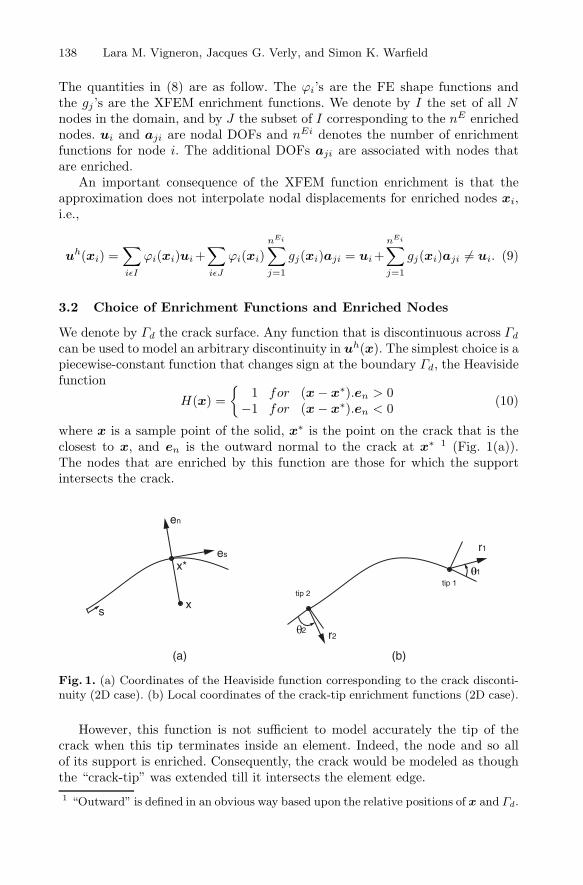
where x is a sample point of the solid, x∗ is the point on the crack that is theclosest to x, and en is the outward normal to the crack at x∗ 1 (Fig. 1(a)).The nodes that are enriched by this function are those for which the supportintersects the crack.

r1

r2

1

2

tip 1tip 2

s

es

en

x

x*

(a) (b)

Fig. 1. (a) Coordinates of the Heaviside function corresponding to the crack disconti-nuity (2D case). (b) Local coordinates of the crack-tip enrichment functions (2D case).

However, this function is not sufficient to model accurately the tip of thecrack when this tip terminates inside an element. Indeed, the node and so allof its support is enriched. Consequently, the crack would be modeled as thoughthe “crack-tip” was extended till it intersects the element edge.1 “Outward” is defined in an obvious way based upon the relative positions of x and Γd.


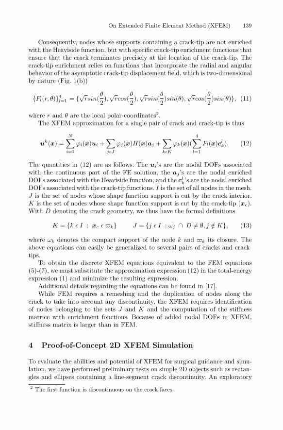
Consequently, nodes whose supports containing a crack-tip are not enrichedwith the Heaviside function, but with specific crack-tip enrichment functions thatensure that the crack terminates precisely at the location of the crack-tip. Thecrack-tip enrichment relies on functions that incorporate the radial and angularbehavior of the asymptotic crack-tip displacement field, which is two-dimensionalby nature (Fig. 1(b))

Fl(r, θ)4l=1 = √rsin(

θ

2),√

rcos(θ

2),√

rsin(θ

2)sin(θ),

√rcos(

θ

2)sin(θ), (11)

where r and θ are the local polar-coordinates2.The XFEM approximation for a single pair of crack and crack-tip is thus

uh(x) =N∑

i=1

ϕi(x)ui +∑jεJ

ϕj(x)H(x)aj +∑kεK

ϕk(x)(4∑

l=1

Fl(x)clk). (12)

The quantities in (12) are as follows. The ui’s are the nodal DOFs associatedwith the continuous part of the FE solution, the aj ’s are the nodal enrichedDOFs associated with the Heaviside function, and the cl

k’s are the nodal enrichedDOFs associated with the crack-tip functions. I is the set of all nodes in the mesh.J is the set of nodes whose shape function support is cut by the crack interior.K is the set of nodes whose shape function support is cut by the crack-tip (xc).With D denoting the crack geometry, we thus have the formal definitions

K = k ε I : xc ε k J = j ε I : ωj ∩ D = ∅, j /∈ K, (13)

where ωk denotes the compact support of the node k and k its closure. Theabove equations can easily be generalized to several pairs of cracks and crack-tips.

To obtain the discrete XFEM equations equivalent to the FEM equations(5)-(7), we must substitute the approximation expression (12) in the total-energyexpression (1) and minimize the resulting expression.

Additional details regarding the equations can be found in [17].While FEM requires a remeshing and the duplication of nodes along the

crack to take into account any discontinuity, the XFEM requires identificationof nodes belonging to the sets J and K and the computation of the stiffnessmatrice with enrichment fonctions. Because of added nodal DOFs in XFEM,stiffness matrix is larger than in FEM.

4 Proof-of-Concept 2D XFEM Simulation

To evaluate the abilities and potential of XFEM for surgical guidance and simu-lation, we have performed preliminary tests on simple 2D objects such as rectan-gles and ellipses containing a line-segment crack discontinuity. An exploratory

2 The first function is discontinuous on the crack faces.


(a) (b)

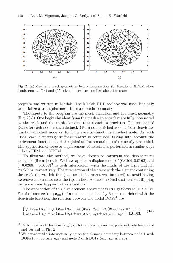
Fig. 2. (a) Mesh and crack geometries before deformation. (b) Results of XFEM whendisplacements (14) and (15) given in text are applied along the crack.

program was written in Matlab. The Matlab PDE toolbox was used, but onlyto initialize a triangular mesh from a domain boundary.

The inputs to the program are the mesh definition and the crack geometry(Fig. 2(a)). One begins by identifying the mesh elements that are fully intersectedby the crack and the mesh elements that contain a crack-tip. The number ofDOFs for each node is then defined: 2 for a non-enriched node, 4 for a Heaviside-function-enriched node or 10 for a near-tip-functions-enriched node. As withFEM, each elementary stiffness matrix is computed, taking into account theenrichment functions, and the global stiffness matrix is subsequently assembled.The application of force or displacement constraints is performed in similar waysin both FEM and XFEM.

To illustrate the method, we have chosen to constrain the displacementalong the (linear) crack. We have applied a displacement of (0.0266, 0.0103) and(−0.0266, −0.0103)3 to each intersection, with the mesh, of the right and leftcrack lips, respectively. The intersection of the crack with the element containingthe crack tip was left free (i.e., no displacement was imposed) to avoid havingexcessive constraints near the tip. Indeed, we have noticed that element flippingcan sometimes happen in this situation.

The application of this displacement constraint is straightforward in XFEM.For the intersection (xint) of an element defined by 3 nodes enriched with theHeaviside fonction, the relation between the nodal DOFs4 are

ϕ1(xint) ux1 + ϕ1(xint) ax1 + ϕ2(xint) ux2 + ϕ2(xint) ax2 = 0.0266ϕ1(xint) uy1 + ϕ1(xint) ay1 + ϕ2(xint) uy2 + ϕ2(xint) ay2 = 0.0103,

(14)

3 Each point is of the form (x, y), with the x and y axes being respectively horizontaland vertical in Fig. 2.

4 We consider the intersection lying on the element boundary between node 1 withDOFs (ux1, uy1, ax1, ay1) and node 2 with DOFs (ux2, uy2, ax2, ay2).


for the right lip where the Heaviside function (10) is equal to 1. Similarly, wehave

ϕ1(xint) ux1 − ϕ1(xint) ax1 + ϕ2(xint) ux2 − ϕ2(xint) ax2 = −0.0266ϕ1(xint) uy1 − ϕ1(xint) ay1 + ϕ2(xint) uy2 − ϕ2(xint) ay2 = −0.0103,

(15)

for the left lip where the Heaviside function (10) is equal to −1. The result ofthese displacement constraints is an opening of the crack, which is illustrated inFig. 2(b).

This example confirms that XFEM can elegantly and efficiently take into ac-count (crack) discontinuities in the study of the mechanical properties of objects.In particular, remember that no mesh adaptation or remeshing is required. Incontrast with FEM, solution displacement fields can now contain discontinuitiesinside the finite elements. Observe that the triangles that appear to have beenadded in Fig. 2(b) were added for display purposes only. They are needed toshow the new boundary of the crack. However, none of these additional nodesor elements are involved in the XFEM calculation.

5 Conclusions and Perspectives

XFEM is particularly well adapted to deal with the general problem of cuttingthrough a 2D or 3D finite-element mesh. This is required to deal with disconti-nuities, i.e., cracks or cuts. The main feature of XFEM is that it can deal withdiscontinuities without having to perform computationally-expensive mesh adap-tation or remeshing. Note that the technique applies to multiple discontinuitiesthat have arbitrary locations and shapes.

The implication for surgical guidance and simulation are clear and signifi-cant. In surgery, XFEM could be very useful in the modelling of retraction andresection, each of these surgical procedures inducing discontinuities in tissues.The pieces of information we need are the discontinuity geometry and the dis-placement contraints along the organ surfaces and the discontinuity boundary.The incision surface allowing the insertion of the retractor can be determinedby tracking. It can also be inferred from an intraoperative MRI image show-ing the retraction pathway. The displacements caused by the retractor can becalculated from distances between segmented brain boundaries along the retrac-tion path and the calculated incision surface. The modelling of resection is morecomplicated given that the brain can swell during this surgical procedure andthat this swelling is not visible in intraoperative images. However, the difficulttask of removing finite elements according to the boundary of resected areascan be done accurately with XFEM. Indeed, all elements falling entirely in theresected area can be removed. With the remaining elements, we can preciselyspecify the boundary of the resected cavity by adding discontinuous functionsto nodes located along this boundary, which allows us to cancel the presence ofthe elements on the resected side of the boundary.

The next step in our XFEM work will be the application and evaluation ofthe ideas and techniques proposed above to MRI images of a phantom submittedto retraction and resection.


References

On Extended Finite Element Method (XFEM) for Modelling of Organ Deformations Associated with...

Documents

Transcript of On Extended Finite Element Method (XFEM) for Modelling of Organ Deformations Associated with...