INTERNATIONAL JOURNAL FOR NUMERICAL METHODS IN ENGINEERINGInt. J. Numer. Meth. Engng 2000; 00:1–6 Prepared using nmeauth.cls [Version: 2002/09/18 v2.02]

Electrostatic Simulation using XFEM for Conductor andDielectric Interfaces

Veronique Rochus1, Daniel Rixen1, Laurent Van Miegroet2, Pierre Duysinx2

1Delft University of Technology, Faculty 3mE, Dpt. of Precision and Microsystems Engineering, EngineeringDynamics, Mekelweg 2, 2628 CD Delft, The Netherlands

2University of Liege, Aerospace and Mechanical Engineering Department, Chemin des chevreuils, 1, 4000Liege, Belgium.

SUMMARY

Many Micro-Electro-Mechanical Systems (e.g. RF-switches, micro-resonators and micro-rotors) involvemechanical structures moving in an electrostatic field. For this type of problems, it is required toevaluate accurately the electrostatic forces acting on the devices. Extended Finite Element (X-FEM)approaches can easily handle moving boundaries and interfaces in the electrostatic domain and seemtherefore very suitable to model Micro-Electro-Mechanical Systems. In this study we investigatedifferent X-FEM techniques to solve the electrostatic problem when the electrostatic domain isbounded by a conducting material. Preliminary studies in one-dimension have shown that one canobtain good results in the computation of electrostatic potential using X-FEM. In this paper theextension of these preliminary studies to 2D problem is presented. In particular a new type ofenrichment functions is proposed in order to treat accurately Dirichlet boundary conditions on theinterface.

Copyright c© 2000 John Wiley & Sons, Ltd.

key words: Extended Finite Elements (X-FEM); Dirichlet Boundary Conditions, Electrostatic

Forces; Moving Boundaries; MEMS

1. INTRODUCTION

Accurately predicting the electrostatic force appearing on (dielectric or conducting) movingstructures is primordial in the modeling and simulation of advanced micro sensors andactuators, and even in nano-devices where, for instance, dielectrophoresis is used to manipulatecells or nanotubes [1]. In [8] a consistent variational approach was introduced to derivea monolithically coupled electromechanical Finite Element approach allowing accuratecomputation of pull-in [27] limits and dynamic behaviours. The coupled simulation proposedin [8] is particularly efficient to compute electrostatic forces appearing around corners [12].

∗Correspondence to: V. Rochus, University of Liege, Aerospace and Mechanical Engineering Department,Chemin des chevreuils, 1, 4000 Liege, Belgium.

Contract/grant sponsor: Publishing Arts Research Council; contract/grant number: 98–1846389

Received 2008Copyright c© 2000 John Wiley & Sons, Ltd. Revised

2 V. ROCHUS

However, in the standard Finite Element techniques applied to coupled electro-mechanicalmodels, one often has to face some serious limitations when the structure undergoes largedisplacements: the electric mesh around the structure is strongly deformed in order to follow thedisplacement of the structure. In this process, the electrostatic mesh may be severely distorted,and might, in the limit case of contact, rapidly degenerate. To overcome this bottleneck, onecan apply re-meshing or use Boundary Elements in the electrostatic domain. Here howeverwe investigate the possibility to represent the shape modification of the electrostatic domainusing a fixed mesh method and apply the Extended Finite Elements (X-FEM) to account forboundaries and interfaces traveling across the fixed mesh.

In the electromechanical problem under consideration, the moving interface appears at theboundary between the electrical and mechanical domains while the latter undergoes largedisplacements through the fixed global electrostatic domain. The coupling occurring betweenelectrical and mechanical fields comes from electrostatic forces acting on the structure. Thoseforces being themselves depending on the deformation of the structure.

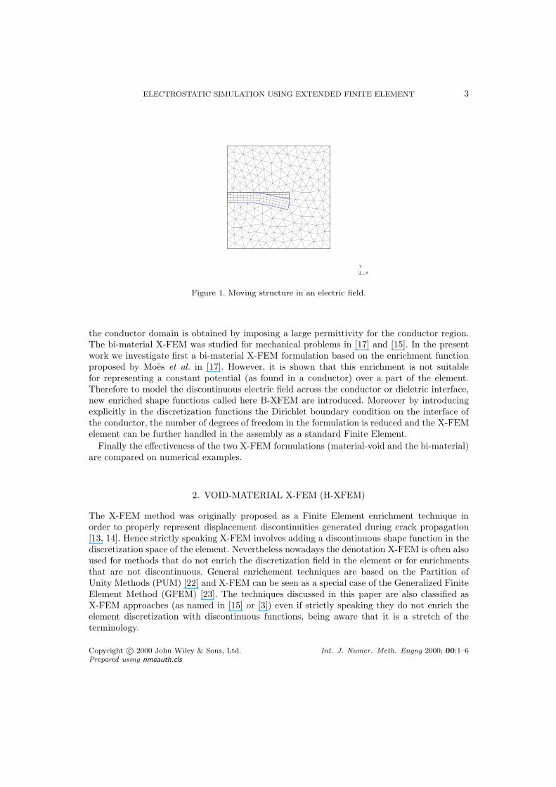
The extended finite element method is a novel approach tailored to simulate problemsinvolving moving discontinuities. Initially this methodology was introduced for the analysisof crack propagation [13, 14]. However this method has been quickly applied to several othertypes of problems such as elastic problems involving inclusions [15], fluid-structure interaction[4, 25] and phase changes problems [10]. In this paper, the X-FEM method is used to modelmoving the structural boundary problem arising in electro-mechanical coupled devices. Theelectrostatic analysis is carried out by an Eulerian-like description while the mechanical oneis treated by a Lagrangian description. When the structure is deformed, the electric field ismodified by the displacement of the discontinuity which is in our case the interface betweenthe mechanical and the electrostatic domain. The electrostatic problem is then recomputedtaking the displacement into account without remeshing the electrostatic domain as shownin figure 1. In such an approach, the challenge is obviously to properly handle the fact thatsome elements of the electrostatic domain are crossed by the interface between two differentmaterials. That interface can even be considered as a boundary condition for the electrostaticdomain if the moving structure is a perfect conductor (hence having an imposed constantpotential). In this paper we focus on this particular application in which we have to computeaccurately the electrostatic field around conductor structure. Indeed in the case of RF-switches[5] and micro-resonators [6], the moving interface appears between a conductive material and adielectric one. On the conductive part, the electrical voltage remains constant and only needsto be evaluated on its boundary. However in the dielectric part of the domain, the electricfield has to be computed accurately to provide precisely the electrostatic forces acting on themechanical structure. To deal with this problem, two different approaches, which have beencompared on a one-dimensional problem in [16], are considered here and later extended to 2D.

The first approach is similar to the modeling of material-void interfaces with X-FEM [15]in which classical FEM shape functions are used and the integration is only carried out onthe dielectric part. The simulation of an electric conductor is modeled by imposing a Dirichletboundary condition at the electromechanical interface with a penalty method. This techniqueis presented for two-dimensional electrostatic problems in section 2. In this paper we will referthe material void approach to H-XFEM.

In section 3 we outline the second approach, namely, the bi-material X-FEM methodwhere the interface between a conductive and a dielectric domain is modelled as an interfacebetween two electrostatic domains with different properties. An equi-potential condition in

Copyright c© 2000 John Wiley & Sons, Ltd. Int. J. Numer. Meth. Engng 2000; 00:1–6Prepared using nmeauth.cls

ELECTROSTATIC SIMULATION USING EXTENDED FINITE ELEMENT 3

Y

XZ

Figure 1. Moving structure in an electric field.

the conductor domain is obtained by imposing a large permittivity for the conductor region.The bi-material X-FEM was studied for mechanical problems in [17] and [15]. In the presentwork we investigate first a bi-material X-FEM formulation based on the enrichment functionproposed by Moes et al. in [17]. However, it is shown that this enrichment is not suitablefor representing a constant potential (as found in a conductor) over a part of the element.Therefore to model the discontinuous electric field across the conductor or dieletric interface,new enriched shape functions called here B-XFEM are introduced. Moreover by introducingexplicitly in the discretization functions the Dirichlet boundary condition on the interface ofthe conductor, the number of degrees of freedom in the formulation is reduced and the X-FEMelement can be further handled in the assembly as a standard Finite Element.

Finally the effectiveness of the two X-FEM formulations (material-void and the bi-material)are compared on numerical examples.

2. VOID-MATERIAL X-FEM (H-XFEM)

The X-FEM method was originally proposed as a Finite Element enrichment technique inorder to properly represent displacement discontinuities generated during crack propagation[13, 14]. Hence strictly speaking X-FEM involves adding a discontinuous shape function in thediscretization space of the element. Nevertheless nowadays the denotation X-FEM is often alsoused for methods that do not enrich the discretization field in the element or for enrichmentsthat are not discontinuous. General enrichement techniques are based on the Partition ofUnity Methods (PUM) [22] and X-FEM can be seen as a special case of the Generalized FiniteElement Method (GFEM) [23]. The techniques discussed in this paper are also classified asX-FEM approaches (as named in [15] or [3]) even if strictly speaking they do not enrich theelement discretization with discontinuous functions, being aware that it is a stretch of theterminology.

Copyright c© 2000 John Wiley & Sons, Ltd. Int. J. Numer. Meth. Engng 2000; 00:1–6Prepared using nmeauth.cls

4 V. ROCHUS

The first method investigated consists in considering that the electrostatic energy existsonly in the dielectric domain as shown in figure 2. In order to exclude the conductor from the

Dielectric Material

Figure 2. Hole XFEM.

electric domain the expression of the energy is defined as

We =1

2

∫

Ω

DTEHdV (1)

where H is the Heaviside function (or characteristic function) equal to 1 on the dielectricdomain Ωd and equal to 0 on the conductor, D the electric displacement and E the electricfield. In this approach the conductor is represented as a hole in the electrostatic domain.

The electric field and displacement are related by the constitutive relation:

D = εE (2)

where ε is the matrix of electric permittivity coefficients (or a scalar in case of isotropicpermittivity). The issues of constructing the discretized matrices and imposing Dirichletboundary conditions on the interface is discussed in the following.

2.1. Discretisation

The shape function used to interpolate the electrostatic potential φ is defined on the entireelement P1, P2, P3 of figure 2 by:

φ(x, t) =∑

i

Ni(x)Φi(t) (3)

where Ni are the standard linear shape functions defined on the element [24] and Φi are theelectric potential of the nodes i.

Calling B the shape functions gradients matrix, the electrostatic stiffness matrix is computedsolely on the dielectric domain Ωd as:

Kφφ =

∫

Ωd

BT εdBdV (4)

where Ωd is the dielectric domain and εd is its permittivity. To integrate on a part of theelement, this one is divided into sub-triangles and a second mapping is used to integrate onthe basic sub-elements as depicted in figure 3.

Copyright c© 2000 John Wiley & Sons, Ltd. Int. J. Numer. Meth. Engng 2000; 00:1–6Prepared using nmeauth.cls

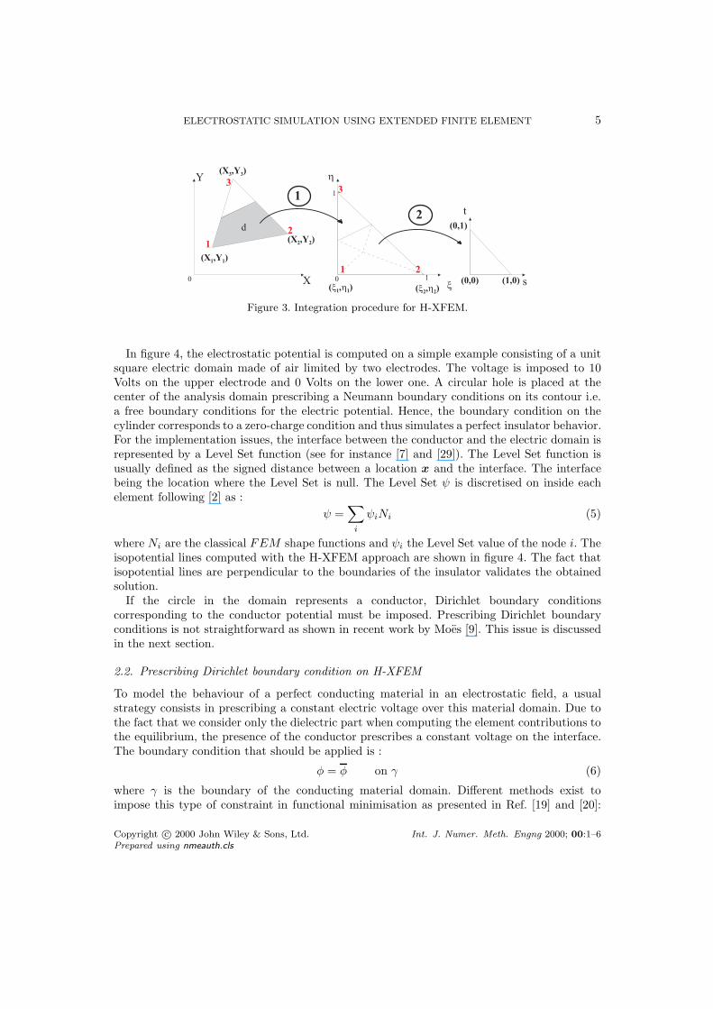
ELECTROSTATIC SIMULATION USING EXTENDED FINITE ELEMENT 5

0 1

1

x

h

0

d

X

Y 3

12

s

t

( X 3 , Y 3 )

( X 2 , Y 2 )( X 1 , Y 1 )

3

1 2( x 1 , h 1 ) ( x 2 , h 2 )

( 0 , 0 ) ( 1 , 0 )

( 0 , 1 )

12

Figure 3. Integration procedure for H-XFEM.

In figure 4, the electrostatic potential is computed on a simple example consisting of a unitsquare electric domain made of air limited by two electrodes. The voltage is imposed to 10Volts on the upper electrode and 0 Volts on the lower one. A circular hole is placed at thecenter of the analysis domain prescribing a Neumann boundary conditions on its contour i.e.a free boundary conditions for the electric potential. Hence, the boundary condition on thecylinder corresponds to a zero-charge condition and thus simulates a perfect insulator behavior.For the implementation issues, the interface between the conductor and the electric domain isrepresented by a Level Set function (see for instance [7] and [29]). The Level Set function isusually defined as the signed distance between a location x and the interface. The interfacebeing the location where the Level Set is null. The Level Set ψ is discretised on inside eachelement following [2] as :

ψ =∑

i

ψiNi (5)

where Ni are the classical FEM shape functions and ψi the Level Set value of the node i. Theisopotential lines computed with the H-XFEM approach are shown in figure 4. The fact thatisopotential lines are perpendicular to the boundaries of the insulator validates the obtainedsolution.

If the circle in the domain represents a conductor, Dirichlet boundary conditionscorresponding to the conductor potential must be imposed. Prescribing Dirichlet boundaryconditions is not straightforward as shown in recent work by Moes [9]. This issue is discussedin the next section.

2.2. Prescribing Dirichlet boundary condition on H-XFEM

To model the behaviour of a perfect conducting material in an electrostatic field, a usualstrategy consists in prescribing a constant electric voltage over this material domain. Due tothe fact that we consider only the dielectric part when computing the element contributions tothe equilibrium, the presence of the conductor prescribes a constant voltage on the interface.The boundary condition that should be applied is :

φ = φ on γ (6)

where γ is the boundary of the conducting material domain. Different methods exist toimpose this type of constraint in functional minimisation as presented in Ref. [19] and [20]:

Copyright c© 2000 John Wiley & Sons, Ltd. Int. J. Numer. Meth. Engng 2000; 00:1–6Prepared using nmeauth.cls

6 V. ROCHUS

10.0 VV

0.000

2.00

4.00

6.00

8.00

Figure 4. Isopotential lines computed by the H-FEM method for a perfect isolator.

the constraint elimination (or minimum dof-set) approach, the Lagrange multipliers method,the augmented Lagrange method, the penalty function method and the perturbed Lagrangemethod.

Since the elements considered here are linear, it is not always possible to strongly imposethe potential along the interface element without introducing locking [9]. For instance if thedielectric part of a linear triangular element is quadrangular as shown in figure 5, imposing zerovolt on the side P1, P2 and φ 6= 0 along the interface γ is not possible in every configuration.Indeed the discretization becomes:

φ = N3φ3 = ηφ3 (7)

which illustrates that a constant potential may be obtained only if the interface γ is parallelto the edge P1, P2 of the element.

Hence since the interface orientation may take any direction in simulations, the Dirichletboundary condition must be imposed weakly in a variational way in order to avoid locking.Please note also that different stabilisation strategies have been proposed to apply thisboundary condition such as [26] and [11]. Here one can apply the Lagrange multipliers method(augmented or not) with a reduced representation space for the multipliers, or by the penaltyand perturbation methods. Moes et al. in [9] proposed strategy to select a variable set ofLagrange multipliers depending on the mesh to avoid instabilities.

In order to avoid the complexity of introducing the additional field of Lagrange multiplier,we will investigate the penalty method, noting that it is mathematically equivalent to theperturbed Lagrange method (see for instance [21]).

Let us write the constraint as:

Γ =

[

φ|C − φ

φ|D − φ

]

= 0 (8)

Copyright c© 2000 John Wiley & Sons, Ltd. Int. J. Numer. Meth. Engng 2000; 00:1–6Prepared using nmeauth.cls

ELECTROSTATIC SIMULATION USING EXTENDED FINITE ELEMENT 7

x

h

F

F3

gC D

P3

P1

P2

g

Figure 5. Imposing a Dirichlet boundary condition on an interface parallel to an edge of the H-XFEM.

with C and D the intersection points between the interface and the edges of the element.The penalty method [20] introduces quadratic penalty terms in the original energy (1) of theelement:

Wep = We +1

2pΓT Γ (9)

where p is the penalty factor. Finally the imposition of the constraint consists only in addinga term to the stiffness matrix and external loads (charges in our case) to the element. Herethe penalty method is applied to the constraints collocated on the intersection points C andD. One can also apply a penalty on the constraint over the continuous interface in which casethe energy is enriched by the compatibility contribution

∫

γpΓT Γdγ. This does however not

significantly modify the conclusions of this section.The imposition of the potential with the penalty method is illustrated on a reference problem

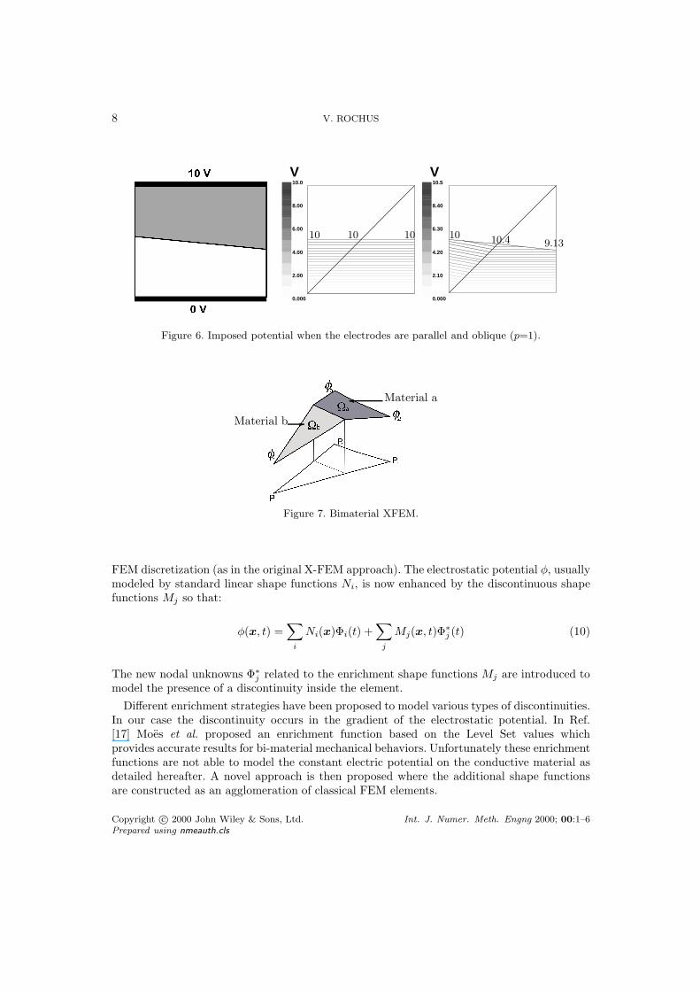
consisting of two electrodes between which a voltage difference of 10 V is applied. One canobserve in figure 6 that the potential is accurately prescribed at the interface when this one isparallel to the bottom electrode. Note that in this configuration, the condition can be stronglyimposed. However when the electrodes are not parallel or, more generally, when the interfaceis not parallel to an element edge, a constant potential at the interface can not be obtained(see figure 6 right).

Hence even when imposed weakly, prescribing a Dirichlet boundary condition inside a H-XFEM will lead to a bad approximation of the potential field, and then to an even worseapproximation of the electric field (and thus in turn of the electrostatic force). For that reason inthe next section a second methodology to model material interfaces in electrostatic is proposed.

3. BIMATERIAL XFEM (B-XFEM)

To circumvent the locking problem observed in the X-FEM approach, we investigate a secondapproach which is derived from the bimaterial X-FEM proposed by Moes et al [17]. In thepresent approach, both parts of the element are considered when computing the energy andthe matrices of the system. We assume that one part of the element is filled with material ’a’and the other with material ’b’ (figure 7) with different permittivities.

The discretization of the potential field uses additional shape functions to enrich the classical

Copyright c© 2000 John Wiley & Sons, Ltd. Int. J. Numer. Meth. Engng 2000; 00:1–6Prepared using nmeauth.cls

8 V. ROCHUS

10.0

8.00

6.00

4.00

2.00

0.000

V

10 10 10

10.5

8.40

6.30

4.20

2.10

0.000

V

10 10.4 9.13

Figure 6. Imposed potential when the electrodes are parallel and oblique (p=1).

Material a

-Material b

Figure 7. Bimaterial XFEM.

FEM discretization (as in the original X-FEM approach). The electrostatic potential φ, usuallymodeled by standard linear shape functions Ni, is now enhanced by the discontinuous shapefunctions Mj so that:

φ(x, t) =∑

i

Ni(x)Φi(t) +∑

j

Mj(x, t)Φ∗

j (t) (10)

The new nodal unknowns Φ∗

j related to the enrichment shape functions Mj are introduced tomodel the presence of a discontinuity inside the element.

Different enrichment strategies have been proposed to model various types of discontinuities.In our case the discontinuity occurs in the gradient of the electrostatic potential. In Ref.[17] Moes et al. proposed an enrichment function based on the Level Set values whichprovides accurate results for bi-material mechanical behaviors. Unfortunately these enrichmentfunctions are not able to model the constant electric potential on the conductive material asdetailed hereafter. A novel approach is then proposed where the additional shape functionsare constructed as an agglomeration of classical FEM elements.

Copyright c© 2000 John Wiley & Sons, Ltd. Int. J. Numer. Meth. Engng 2000; 00:1–6Prepared using nmeauth.cls

ELECTROSTATIC SIMULATION USING EXTENDED FINITE ELEMENT 9

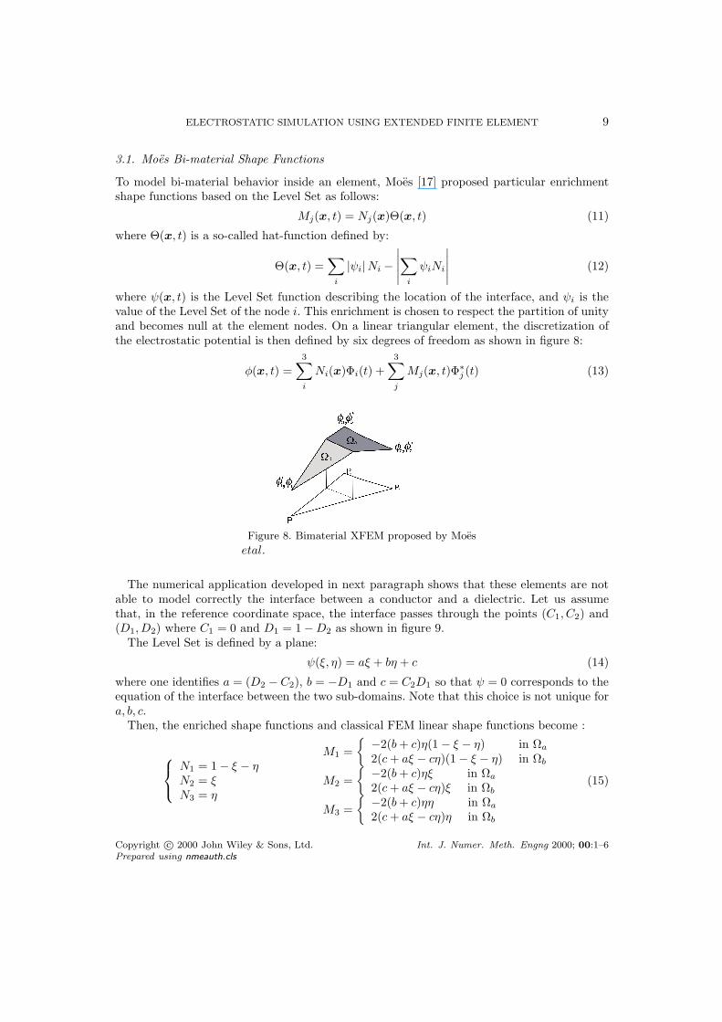
3.1. Moes Bi-material Shape Functions

To model bi-material behavior inside an element, Moes [17] proposed particular enrichmentshape functions based on the Level Set as follows:

Mj(x, t) = Nj(x)Θ(x, t) (11)

where Θ(x, t) is a so-called hat-function defined by:

Θ(x, t) =∑

i

|ψi|Ni −

∣

∣

∣

∣

∣

∑

i

ψiNi

∣

∣

∣

∣

∣

(12)

where ψ(x, t) is the Level Set function describing the location of the interface, and ψi is thevalue of the Level Set of the node i. This enrichment is chosen to respect the partition of unityand becomes null at the element nodes. On a linear triangular element, the discretization ofthe electrostatic potential is then defined by six degrees of freedom as shown in figure 8:

φ(x, t) =3

∑

i

Ni(x)Φi(t) +3

∑

j

Mj(x, t)Φ∗

j (t) (13)

Figure 8. Bimaterial XFEM proposed by Moes

etal.

The numerical application developed in next paragraph shows that these elements are notable to model correctly the interface between a conductor and a dielectric. Let us assumethat, in the reference coordinate space, the interface passes through the points (C1, C2) and(D1, D2) where C1 = 0 and D1 = 1 −D2 as shown in figure 9.

The Level Set is defined by a plane:

ψ(ξ, η) = aξ + bη + c (14)

where one identifies a = (D2 − C2), b = −D1 and c = C2D1 so that ψ = 0 corresponds to theequation of the interface between the two sub-domains. Note that this choice is not unique fora, b, c.

Then, the enriched shape functions and classical FEM linear shape functions become :

N1 = 1 − ξ − ηN2 = ξN3 = η

M1 =

−2(b+ c)η(1 − ξ − η) in Ωa

2(c+ aξ − cη)(1 − ξ − η) in Ωb

M2 =

−2(b+ c)ηξ in Ωa

2(c+ aξ − cη)ξ in Ωb

M3 =

−2(b+ c)ηη in Ωa

2(c+ aξ − cη)η in Ωb

(15)

Copyright c© 2000 John Wiley & Sons, Ltd. Int. J. Numer. Meth. Engng 2000; 00:1–6Prepared using nmeauth.cls

10 V. ROCHUS

Figure 9. Extended finite element in 2D.

xh

Figure 10. Enrichment hat function Θ.

The hat function

Θ =

3∑

i

Mi

modelling the discontinuity is plotted in figure 10. We can observe that the line of discontinuityis not horizontal, which indicates that these extended formulation might not be suitable toimpose a constant value along the interface (as needed for a conductor interface for instance).

Let us check if this extended shape functions are suitable for the electrostatic problem. Thepotential is discretized on each domain by:

φa = N1Φ1 +N2Φ2 +N3Φ3 +M1aΦ∗

1 +M2aΦ∗

2 +M3aΦ∗

3

φb = N1Φ1 +N2Φ2 +N3Φ3 +M1bΦ∗

1 +M2bΦ∗

2 +M3bΦ∗

3(16)

• Considering that the potential is constant on the quadrangular domain Ωa (see Figure10), we impose

∂φa

∂ξ= 0 and

∂φa

∂η= 0

for all values of ξ and η on the domain Ωa. After development we obtain the followingconstraints:

Φ1 = Φ2 and Φ∗

1 = Φ∗

2 = Φ∗

3 = −(Φ1 − Φ3)

2(b+ c)(17)

Only two unknowns are left, as expected, the potential Φ3 and Φ1 = Φ2.• We now consider that the potential is constant on the triangular domain Ωb so that

∂φb

∂ξ= 0 and

∂φb

∂η= 0

Copyright c© 2000 John Wiley & Sons, Ltd. Int. J. Numer. Meth. Engng 2000; 00:1–6Prepared using nmeauth.cls

ELECTROSTATIC SIMULATION USING EXTENDED FINITE ELEMENT 11

for all values of ξ and η on the domain Ωb. The conditions to have a constant potentialon this domain are

Φ∗

1 = Φ∗

2 = Φ∗

3 andΦ∗

1 =Φ1 − Φ2

2a

Φ∗

1 =Φ3 − Φ1

2c

(18)

In this case, setting the triangular domain Ωb to a constant potential Φ3 implies a relationbetween Φ1 and Φ2. This can be understood as follows. The condition Φ∗

1 = Φ∗

2 = Φ∗

3

enforces the linearity of the discretization field on domain Ωb and as a consequence, alsothe linearity of the field on the quadrangular domain Ωa. The relation between Φ1 andΦ2 implied by the second set of constraints in (18) imposes that the values of the electricpotential at the nodes “1”, “2”, “C” and “D” are coplanar. So the situation where Φ3

is set to a potential V (higher electrode) and Φ1 and Φ2 are on the grounded lowerelectrode, is possible only if the interface is parallel to the lower electrode.

Therefore it is impossible to impose a constant potential inside the triangular part of theextended element and a linear field on the quadrangular part. We must therefore concludethat the shape functions proposed in [17] are not suitable for electro-mechanical modeling inthe vicinity of conductors. It was shown in [18] that arbitrary Dirichlet boundary conditionscan be imposed along an arbitrary contour using a regularisation. In the following section, adifferent extended field is build to circumvent this shortcoming.

3.2. Enriched Shape Functions by Finite Element combination

The underlying idea of this new approach can be understood by observing that if the extendedelement was build out of two finite elements (one for the conductor and one for the non-conducting part), it would be straightforward to simulate the behavior of electro-mechanicalproblem. So, we use quadrangular shape functions for the quadrangular part and triangularshape functions for the triangular part.

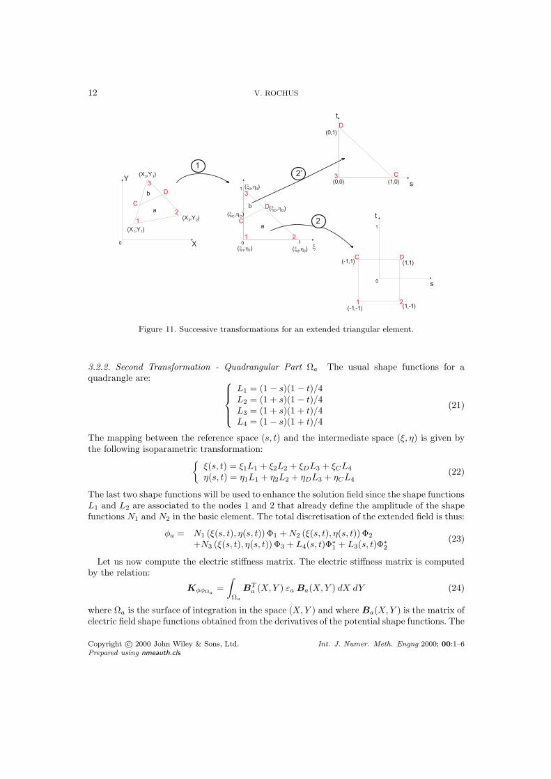
Therefore we will introduce two successive changes of variables corresponding to twoisoparametric transformation of the physical space: a first one between (X,Y ) and (ξ, η),and a second one between (ξ, η) and (s, t), as sketched in figure 11. Note that the secondtransformation is defined separately for the triangular and the quadrangular part of thepartitioned element.

3.2.1. First change of variables The first change of variables is identical for both domainsΩa and Ωb and may be expressed by the relation:

X = N1X1 +N2X2 +N3X3

Y = N1Y1 +N2Y2 +N3Y3

N1 = (1 − ξ − η)N2 = ξN3 = η

(19)

The coordinates of the point C and D are obtained by computing the intersections betweenthe zero Level Set and the edge of the triangle. In the (ξ, η) space, the position of these pointsare:

ξC = 0

ηC = (XC−X1)(X3−X1)

ξD = (X3−XD)(X3−X2)

ηD = (XD−X2)(X3−X2)

(20)

Copyright c© 2000 John Wiley & Sons, Ltd. Int. J. Numer. Meth. Engng 2000; 00:1–6Prepared using nmeauth.cls

12 V. ROCHUS

0 1

1

x

a

b

0

a

b

X

Y

0

1

s

t

3

1

2

s

t

C

D

(X3,Y3)

(X2,Y2)

(X1,Y1)

3

1 2

C

D

C

D

3

1 2

C D

(x1,h1) (x2,h2)

(x3,h3)

(xC,hC)(xD,hD)

(-1,-1) (1,-1)

(-1,1) (1,1)

(0,0) (1,0)

(0,1)

1

2

2’

Figure 11. Successive transformations for an extended triangular element.

3.2.2. Second Transformation - Quadrangular Part Ωa The usual shape functions for aquadrangle are:

L1 = (1 − s)(1 − t)/4L2 = (1 + s)(1 − t)/4L3 = (1 + s)(1 + t)/4L4 = (1 − s)(1 + t)/4

(21)

The mapping between the reference space (s, t) and the intermediate space (ξ, η) is given bythe following isoparametric transformation:

ξ(s, t) = ξ1L1 + ξ2L2 + ξDL3 + ξCL4

η(s, t) = η1L1 + η2L2 + ηDL3 + ηCL4(22)

The last two shape functions will be used to enhance the solution field since the shape functionsL1 and L2 are associated to the nodes 1 and 2 that already define the amplitude of the shapefunctions N1 and N2 in the basic element. The total discretisation of the extended field is thus:

φa = N1 (ξ(s, t), η(s, t)) Φ1 +N2 (ξ(s, t), η(s, t)) Φ2

+N3 (ξ(s, t), η(s, t)) Φ3 + L4(s, t)Φ∗

1 + L3(s, t)Φ∗

2(23)

Let us now compute the electric stiffness matrix. The electric stiffness matrix is computedby the relation:

KφφΩa=

∫

Ωa

BTa (X,Y ) εa Ba(X,Y ) dX dY (24)

where Ωa is the surface of integration in the space (X,Y ) and where Ba(X,Y ) is the matrix ofelectric field shape functions obtained from the derivatives of the potential shape functions. The

Copyright c© 2000 John Wiley & Sons, Ltd. Int. J. Numer. Meth. Engng 2000; 00:1–6Prepared using nmeauth.cls

ELECTROSTATIC SIMULATION USING EXTENDED FINITE ELEMENT 13

change of variables between the space (X,Y ) and the reference space (s, t) may be obtained bythe relations (19) and (22) which allow us to write X(s, t), Y (s, t) and the Jacobian J of thistransformation. The electric stiffness matrix may then be computed on the reference space by:

KφφΩa=

∫

Ωa

BTa (s, t) J

−T εa J−1

Ba(s, t) det(J) ds dt (25)

where

Ba(s, t) =

∂N1

∂s∂N2

∂s∂N3

∂s∂L4

∂s∂L3

∂s

∂N1

∂t∂N2

∂t∂N3

∂t∂L4

∂t∂L3

∂t

(26)

3.2.3. Second Transformation - Triangular Part Ωb The shape functions for the triangulardomain are the same as the initial change of variables:

G1 = (1 − s− t)G2 = sG3 = t

(27)

and the isoparametric transformation becomes:

ξ(s, t) = ξ3G1 + ξCG2 + ξDG3

η(s, t) = η3G1 + ηCG2 + ηDG3(28)

As for the quadrangular part only the shape functions that are not associated to the basicnodes (here G2 and G3) define the enrichment field. The total enhanced shape functions arethus, for domain b

φb = N1 (ξ(s, t), η(s, t)) Φ1 +N2 (ξ(s, t), η(s, t)) Φ2

+N3 (ξ(s, t), η(s, t)) Φ3 +G2(s, t)Φ∗

1 +G3(s, t)Φ∗

2(29)

Obviously since the added degrees of freedom Φ∗

1 and Φ∗

2 used here and used in the discretizedfield (23) in domain Ωa are identical, along the interface C,D, the continuity of the potentialfield is guarantied while the electric field (gradient of the potential) can be discontinuous dueto the enrichment field.

The electric stiffness matrix is computed by the relation

KφφΩb=

∫

Ωb

BTb (X,Y ) εb Bb(X,Y ) dX dY (30)

where Ωb is the surface of integration in the space (X,Y ). Using (19) and (28) the electricstiffness matrix may be computed on the reference space (s, t) by

KφφΩb=

∫

Ωb

BTb (s, t) J

−T εb J−1

Bb(s, t) det(J) ds dt (31)

where

Bb(s, t) =

∂N1

∂s

∂N2

∂s

∂N3

∂s

∂G2

∂s

∂G3

∂s

∂N1

∂t

∂N2

∂t

∂N3

∂t

∂G2

∂t

∂G3

∂t

(32)

Copyright c© 2000 John Wiley & Sons, Ltd. Int. J. Numer. Meth. Engng 2000; 00:1–6Prepared using nmeauth.cls

14 V. ROCHUS

3.2.4. Resulting Discretisation Finally both discretisation can be summarised in a triangleelement in the following way:

φa = N1Φ1 +N2Φ2 +N3Φ3 +M1aΦ∗

1 +M2aΦ∗

2

φb = N1Φ1 +N2Φ2 +N3Φ3 +M1bΦ∗

1 +M2bΦ∗

2(33)

where the shape functions are defined as the following:

N1 = (1 − ξ − η)N2 = ξN3 = η

M1a = (1 − s)(1 + t)/4M2a = (1 + s)(1 + t)/4M1b = sM2b = t

(34)

and presented in figure 13.

0

0.1

0.2

0.3

0.4

0.5

0.6

0.7

0.8

0.9

1

00.1

0.20.3

0.40.5

0.60.7

0.80.9

1

0

0.5

1

M1a

M1b

0

0.1

0.2

0.3

0.4

0.5

0.6

0.7

0.8

0.9

1

00.1

0.20.3

0.40.5

0.60.7

0.80.9

1

0

0.5

1

M2a

M2b

Figure 12. New Enriched Shape functions.

The stiffness matrix of this type of element is divided in two parts :

Kφφ =

∫

Ωa

BTa εaBadV +

∫

Ωb

BTb εbBbdV (35)

where Ωa is the quadrangular part and Ωb is the triangular part of the element.It is easy to verify that the hat function Θ is retrieved on domain Ωa and Ωb when Φ∗

1 = Φ∗

2:

Θ =

L3 + L4 in Ωa

G2 +G3 in Ωb(36)

This is depicted in figure 13.

h

x

Figure 13. Enrichment of domain a.

Copyright c© 2000 John Wiley & Sons, Ltd. Int. J. Numer. Meth. Engng 2000; 00:1–6Prepared using nmeauth.cls

ELECTROSTATIC SIMULATION USING EXTENDED FINITE ELEMENT 15

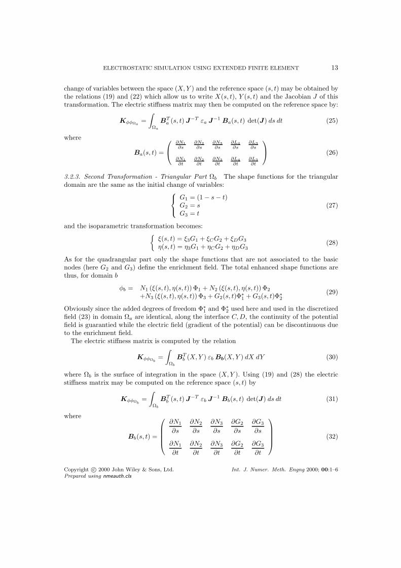
3.2.5. Numerical Validation of the Extended Finite Element The novel extended electrostaticfinite element is validated first on a simple test case. A unit square domain is subject to a 1 Voltdifference of voltage between the lower edge (ground) and the top domain (conducting domain)as shown in figure 14. The domain is modeled with 2 triangular extended finite elements asbuilt in the previous section.

First the interface between conductor and the vacuum is taken parallel to the groundelectrode. The computed electric potential is plotted in figure 14: it is observed that thepotential is constant on the conductor and decreases linearly between the electrodes asexpected. The upper part of the problem has a permittivity of ε1 and the lower one ε2.Three different situations are simulated and compared to the analytical solutions. The firstone is when ε1 ≫ ε2, this situation appears when part 1 is a conductive material. The electricpotential is nearly constant over this area as shown in figure 14. The second simulation is inthe case where ε1 = 2ε2. The potential at the middle point corresponds to the analytical value.Finally the last case show that a constant electrostatic field may be simulated if ε1 = ε2.

V = 0 V

V = 1 V

e 1

e 20

0.20.4

0.60.8

1

0

0.5

10

0.2

0.4

0.6

0.8

1

For ε1 ≫ ε2

00.2

0.40.6

0.81

0

0.5

10

0.2

0.4

0.6

0.8

1

For ε1 = 2ε2

00.2

0.40.6

0.81

0

0.5

10

0.2

0.4

0.6

0.8

1

For ε1 = ε2

Figure 14. Potential for different values of ε.

The electric potential is also recovered for the case where the interface is not parallel tothe extremities as shown in figures 15 for the same material properties. As shown in figure 15the potential isovalues are again piecewise linear and clearly the new shape functions of theeXtended Finite Elements can properly handle the computation of the electric potential evenif the interface is oblique.

Copyright c© 2000 John Wiley & Sons, Ltd. Int. J. Numer. Meth. Engng 2000; 00:1–6Prepared using nmeauth.cls

16 V. ROCHUS

V = 0 V

V = 1 V

00.2

0.40.6

0.81

0

0.5

10

0.2

0.4

0.6

0.8

1

For ε1 ≫ ε2

00.2

0.40.6

0.81

0

0.2

0.4

0.6

0.8

10

0.2

0.4

0.6

0.8

1

For ε1 = 2ε2

00.2

0.40.6

0.81

0

0.2

0.4

0.6

0.8

10

0.2

0.4

0.6

0.8

1

For ε1 = ε2

Figure 15. Potential for different values of ε.

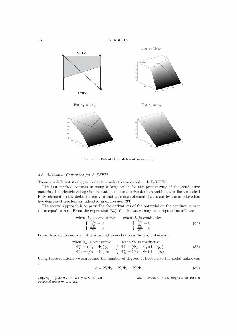
3.3. Additional Constraint for B-XFEM

There are different strategies to model conductive material with B-XFEM.The first method consists in using a large value for the permittivity of the conductive

material. The electric voltage is constant on the conductive domain and behaves like a classicalFEM element on the dielectric part. In that case each element that is cut by the interface hasfive degrees of freedom as indicated in expression (33).

The second approach is to prescribe the derivatives of the potential on the conductive partto be equal to zero. From the expression (33), the derivative may be computed as follows:

when Ωa is conductive

∂φa

∂s= 0

∂φa

∂t= 0

when Ωb is conductive

∂φb

∂s= 0

∂φb

∂t= 0

(37)

From these expressions we obtain two relations between the five unknowns.

when Ωa is conductive when Ωb is conductive

Φ∗

C = (Φ1 − Φ3)ηC

Φ∗

D = (Φ1 − Φ3)ηD

Φ∗

C = (Φ3 − Φ1)(1 − ηC)Φ∗

D = (Φ3 − Φ2)(1 − ηD)(38)

Using these relations we can reduce the number of degrees of freedom to the nodal unknowns:

φ = N∗

1 Φ1 +N∗

2 Φ2 +N∗

3 Φ3 (39)

Copyright c© 2000 John Wiley & Sons, Ltd. Int. J. Numer. Meth. Engng 2000; 00:1–6Prepared using nmeauth.cls

ELECTROSTATIC SIMULATION USING EXTENDED FINITE ELEMENT 17

where N∗

i are new shape functions taking the enrichment into account. If domain Ωa is aperfect conductor, we retrieve the shape function of the triangle:

N∗

1 = sN∗

2 = tN∗

3 = 1 − s− ton the domain Ωb (40)

and if domain b is conductor, the shape functions becomes:

N∗

1 = (1 − s)(1 − t)/4N∗

2 = (1 + s)(1 − t)/4N∗

3 = (1 + t)/2on the domain Ωa (41)

These new conductive extended finite elements are denoted here by C-XFEM. The potentialon the reference problem presented previously is illustrated in figure 16. In that case theprescribed voltage on the interface is strongly imposed even if the electrodes and the interfaceare not parallel.

10.0

8.00

6.00

4.00

2.00

0.000

V

10 10 10

10.0

8.00

6.00

4.00

2.00

0.000

V

10 1010

Figure 16. Imposed potential when the electrodes are parallel and oblique.

4. COMPARISON BETWEEN H-XFEM and C-XFEM

The two methods are compared on the problem defined in figure 17. In this example thepotential difference is imposed between the upper and the lower plate. The structure definedby the Level Set is now conductive and set to 6 Volts. The problem is meshed by triangularelements.

4.1. H-XFEM with penalty terms

Two parameters influence the behavior of the model: the size of the element h and the penaltyfactor p. Figure 18 shows the total electrostatic energy of the problem for different valuesof p and h. For smaller element size, the total energy becomes more accurate for differentvalues of penalty. For a fine mesh (h = 0.2) the energy seems to be nearly constant for each

Copyright c© 2000 John Wiley & Sons, Ltd. Int. J. Numer. Meth. Engng 2000; 00:1–6Prepared using nmeauth.cls

18 V. ROCHUS

Figure 17. Reference problem.

penalty factor. This indicates that the mesh has to be fine enough to properly model thecurved interface along the circle.

00.02

0.040.06

0.080.1

−12

−10

−8

−6

−42

4

6

8

10

12

14

x 10−10

Element Size [m]Log(Penalty Factor)

Ene

rgy

Figure 18. Total electrostatic energy for different value of element size and penalty.

In figure 19 the isopotential and the distribution of the electrostatic energy are plotted fordifferent penalty factors, taking h = 0.2. For a large penalty factor (p=1e-4), the potential isstrongly imposed on the boundary but the energy distribution shows that the field around itis not well modeled. For a very low penalty (p=1e-13), the potential is not well imposed on theinterface and the solution is not accurate even if the energy densities look smooth. To obtain amore realistic solution, a good penalty value has to be chosen. For p=1e-9, the distribution ofthe energy density looks smooth and the energy distribution seems to be correct. This exampleshows that it is tricky to properly choose the penalty value to impose a Dirichlet condition ina H-XFEM approach. This is the main drawback of this method.

Copyright c© 2000 John Wiley & Sons, Ltd. Int. J. Numer. Meth. Engng 2000; 00:1–6Prepared using nmeauth.cls

ELECTROSTATIC SIMULATION USING EXTENDED FINITE ELEMENT 19

10.0 V

0.000

2.00

4.00

6.00

8.00

10.0 V

0.000

2.00

4.00

6.00

8.00

10.0 V

0.000

2.00

4.00

6.00

8.00

p=1e-4 p=1e-9 p=1e-13

Figure 19. Isopotential and energy density for different values of penalty.

4.2. Conductive XFEM (C-XFEM)

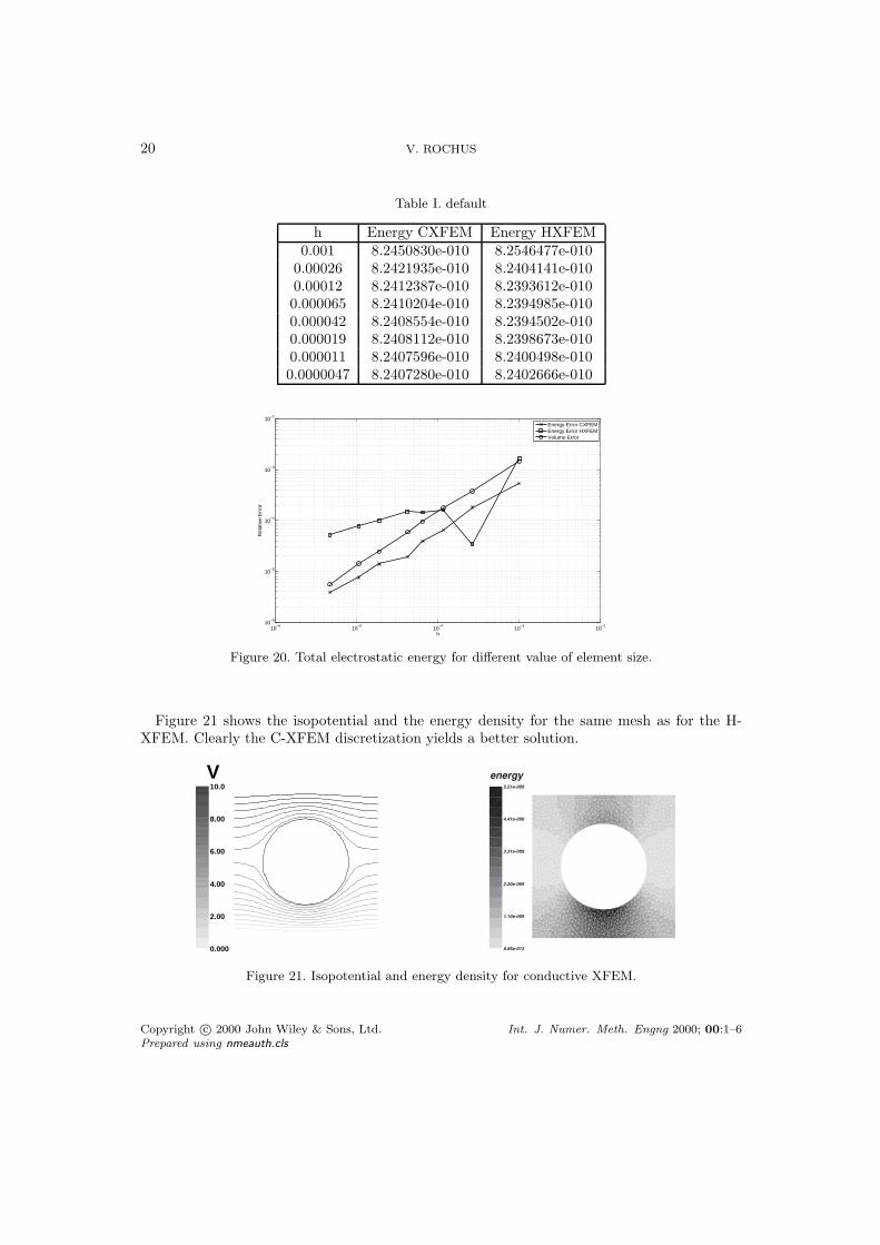
In the conductive Extended Finite Element (C-XFEM), the boundary condition is embeddedin the discretization. The only parameter influencing the model is the mesh refinement h. Thefigure 20 compares the electrostatic energy of the H-XFEM discretization (see above) with apenalty of 1e-9 and the C-XFEM. The relative error on the total energy is unstable with respectto the solution found by Finite Element method after mesh convergence. When the elementsize is small enough, the total energy is retrieved for both models but the convergence of the C-XFEM is faster. In the same figure we also indicate the relative error of the surface computationdue to the mesh discretisation, suggesting the error due to the geometrical approximation ofthe interface by the linear elements is not the main source of the error.

The relative errors are computed by:

εV =‖VXFEM − Vexact‖

‖Vexact‖εE =

‖EXFEM − EFEM‖

‖EFEM‖(42)

where Vexact is computed analytically and EFEM is the converged solution of the equivalentFEM model.

Copyright c© 2000 John Wiley & Sons, Ltd. Int. J. Numer. Meth. Engng 2000; 00:1–6Prepared using nmeauth.cls

20 V. ROCHUS

Table I. default

h Energy CXFEM Energy HXFEM0.001 8.2450830e-010 8.2546477e-010

0.00026 8.2421935e-010 8.2404141e-0100.00012 8.2412387e-010 8.2393612e-0100.000065 8.2410204e-010 8.2394985e-0100.000042 8.2408554e-010 8.2394502e-0100.000019 8.2408112e-010 8.2398673e-0100.000011 8.2407596e-010 8.2400498e-0100.0000047 8.2407280e-010 8.2402666e-010

10−6

10−5

10−4

10−3

10−2

10−6

10−5

10−4

10−3

10−2

h

Rel

ativ

e E

rror

Energy Error CXFEMEnergy Error HXFEMVolume Error

Figure 20. Total electrostatic energy for different value of element size.

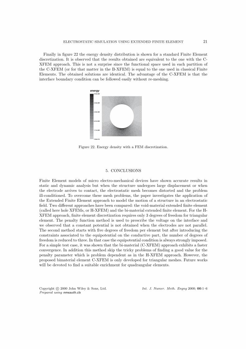
Figure 21 shows the isopotential and the energy density for the same mesh as for the H-XFEM. Clearly the C-XFEM discretization yields a better solution.

10.0 VV

0.000 0.000

2.00 2.00

4.00 4.00

6.00 6.00

8.00 8.00

Figure 21. Isopotential and energy density for conductive XFEM.

Copyright c© 2000 John Wiley & Sons, Ltd. Int. J. Numer. Meth. Engng 2000; 00:1–6Prepared using nmeauth.cls

ELECTROSTATIC SIMULATION USING EXTENDED FINITE ELEMENT 21

Finally in figure 22 the energy density distribution is shown for a standard Finite Elementdiscretization. It is observed that the results obtained are equivalent to the one with the C-XFEM approach. This is not a surprise since the functional space used in each partition ofthe C-XFEM (or for that matter in the B-XFEM) is equal to the one used in classical FiniteElements. The obtained solutions are identical. The advantage of the C-XFEM is that theinterface boundary condition can be followed easily without re-meshing.

Figure 22. Energy density with a FEM discretization.

5. CONCLUSIONS

Finite Element models of micro electro-mechanical devices have shown accurate results instatic and dynamic analysis but when the structure undergoes large displacement or whenthe electrode arrives to contact, the electrostatic mesh becomes distorted and the problemill-conditioned. To overcome these mesh problems, the paper investigates the application ofthe Extended Finite Element approach to model the motion of a structure in an electrostaticfield. Two different approaches have been compared: the void-material extended finite element(called here hole XFEMs, or H-XFEM) and the bi-material extended finite element. For the H-XFEM approach, finite element discretization requires only 3 degrees of freedom for triangularelement. The penalty function method is used to prescribe the voltage on the interface andwe observed that a constant potential is not obtained when the electrodes are not parallel.The second method starts with five degrees of freedom per element but after introducing theconstraints associated to the equipotential on the conductive part, the number of degrees offreedom is reduced to three. In that case the equipotential condition is always strongly imposed.For a simple test case, it was shown that the bi-material (C-XFEM) approach exhibits a fasterconvergence. In addition this method skip the tricky problems of finding a good value for thepenalty parameter which is problem dependent as in the H-XFEM approach. However, theproposed bimaterial element C-XFEM is only developed for triangular meshes. Future workswill be devoted to find a suitable enrichment for quadrangular elements.

Copyright c© 2000 John Wiley & Sons, Ltd. Int. J. Numer. Meth. Engng 2000; 00:1–6Prepared using nmeauth.cls

22 V. ROCHUS

REFERENCES

1. A. Vijayaraghavan and S. Blatt and D. Weissenberger and M. Oron-Carl and F. Hennrich and D. Gerthsenand H. Hahn and R. Krupke, Ultra-Large-Scale Directed Assembly of Single-Walled Carbon NanotubeDevices, Nano Letters, Vol. 7, 6, pp. 1556-1560, 2007

2. M. Stolarska, D. L. Chopp, N. Moes, T. Belytschko, Modellinf crack growth by Level Sets in the extendedfinite element method, International Journal for Numerical Methods in Engineering,2001, 51:943-960

3. C. Daux, N. Moes, J. Dolbow, N. Sukumar and T. Belytschko, Arbitrary branched and intersectingcracks with the extended finite element method, International Journal for Numerical Methods inEngineering,2000, 48:1741-1760

4. A. Legay and J. Chessa and T. Belytschko, An Eulerian-Lagrangian Method for Fluid Structure InteractionBased on Level Sets, Computer Methods in Applied Mechanical Engineering, Vol. 195, pp. 2070-2087, 2006

5. H. A. C. Tilmans and W. De Readt and E. Beyne, MEMS for Wireless Communications: from RF-MEMSComponents to RF-MEMS-SiP Journal of Micromechanical and Microengineering 2003 Vol. 13 4 pp. 139-163

6. G. Stemme, Resonant Silicon Sensors Journal of Micromechanical and Microengineering 1991 Vol. 1 pp.113-125

7. J. A. Sethian, Level Set Methods and Fast Marching Methods: Evolving Interfaces in ComputationalGeometry, Fluid Mechanics, Computer Vision and Materials Science Cambridge University Press,1999

8. V.Rochus, D.J. Rixen and J.C. Golinval Monolithic modelling of electro-mechanical coupling in micro-structures, International Journal for Numerical Methods in Engineering 2006, 65:461–493

9. N. Moes, E. Bechet and M. Tourbier, Imposing Dirichlet Boundary Conditions in the Extended finite elementmethod (article) International Journal for Numerical Methods in Engineering 6712, pp. 1646-1669

10. J. Chessa, P. Smolinski and T. Belytschko, The extended finite element method (XFEM) for solidificationproblems. International Journal for Numerical Methods in Engineering 2002,53:1959-1977.

11. J. Haslinger, Y. Renard, A new fictitious domain approach inspired by the extended finite element method.Siam J. on Numer. Anal. to appear.

12. S. Hannot and D.J Rixen and V. Rochus, Electromechanical FEM Models and Electrostatic Forces NearSharp and Rounded Corners Journal of Microelectromechanical Systems, to appear

13. T. Belytschko and T. Black, Elastic crack growth in finite elements with minimal remeshing InternationalJournal for Numerical Methods in Engineering 1999, 45 5:601-620

14. N. Moes, J. Dolbow and T. Belytschko A finite element method for crack growth without remeshing,International Journal for Numerical Methods in Engineering 1999, 46:131-150

15. N. Sukumar, D. L. Chopp, N. Moes, and T. Belytschko Modeling Holes and Inclusions by Level Sets in theExtended Finite Element Method Computer Methods in Applied Mechanics and Engineering, 2001 190

16. V. Rochus and A. Andreykiv and D.J. Rixen, Modelling Strategies for Microstructures moving in anelectric Field Int. Conference on Computational Methods for Coupled Problems in Science and Engineering:Coupled Problems 2007 Ibiza

17. N. Moes, M. Cloirec, P. Cartraud and J.F. Remacle, A computational approach to handle complexmicrostructure geometries Computer Methods in Applied Mechanics and Engineering,2003 192(28):3163–3177

18. Valance, S. and de Borst, R. and Rethore, J. and Coret, M., A partition-of-unity-based finite elementmethod for level sets, International Journal for Numerical Methods in Engineering, 2008, 76(10), JohnWiley & Sons, Ltd. Chichester, UK

19. D. Bertsekas, Constrained Optimization and Lagrange Multipliers methods Computer Science andScientific Computing Series, Academic Press 1982

20. M. Geradin and A. Cardona Flexible Multibody Dynamics - a Finite Element Approach (book)John Wileyand Sons,2001

21. D. Rixen, Substructuring and Dual Methods in Structural Analysis, PhD.Thesis, University of Liege,199722. I. Babuska, J. M. Melenk, The partition of unity method International Journal for Numerical Methods in

Engineering, 1997 40(4):727-75823. T. Strouboulis, K. Copps and I. Babuscaronka, The generalized finite element method: an example of

its implementation and illustration of its performance International Journal for Numerical Methods inEngineering,2000 47(8):1401-1417

24. R. Cook, D. Malkus, M. Plesha, Concepts and Applications of Finite Element Analysis, 3rd Edition, Wileyand Sons, 1989

25. A. Gerstenberger, W. A. Wall, An eXtended Finite Element Method/Lagrange multiplier based approachfor fluidstructure interaction Computer Methods in Applied Mechanics and Engineering, 2008 197 (19-20):1699-1714

26. H. M. Mourad, J. Dolbow, I. Harari, A bubble-stabilized finite element method for Dirichlet constraintson embedded interfaces International Journal for Numerical Methods in Engineering,2007 69 (4): 772-793

Copyright c© 2000 John Wiley & Sons, Ltd. Int. J. Numer. Meth. Engng 2000; 00:1–6Prepared using nmeauth.cls

ELECTROSTATIC SIMULATION USING EXTENDED FINITE ELEMENT 23

27. S. Senturia, Microsystem Design Kluwer Academic Publishers, 200128. A. Andreykiv and D. Rixen, Simulation of Electrostatic- Structural Coupling using Fictitious Domain and

Level Set methods 9th US National Congress on Computational Mechanics 200729. T. Belytschko, C. Parimi, N. Moes and N. Sukumar and S. Usui, Structured extended finite element methods

for solids defined by implicit surfaces International Journal for Numerical Methods in Engineering, 200356:609-635

Copyright c© 2000 John Wiley & Sons, Ltd. Int. J. Numer. Meth. Engng 2000; 00:1–6Prepared using nmeauth.cls