energies

Article

Optimal Conductor Size Selection in DistributionNetworks with High Penetration of DistributedGeneration Using Adaptive Genetic Algorithm

Zhenghui Zhao * and Joseph Mutale

School of Electrical & Electronic Engineering, University of Manchester, Sackville Street, Manchester M13 9PL,UK; j.mutale@manchester.ac.uk* Correspondence: zhenghui.zhao@postgrad.manchester.ac.uk

Received: 15 April 2019; Accepted: 28 May 2019; Published: 30 May 2019

Abstract: The widespread deployment of distributed generation (DG) has significantly impactedthe planning and operation of current distribution networks. The environmental benefits and thereduced installation cost have been the primary drivers for the investment in large-scale wind farmsand photovoltaics (PVs). However, the distribution network operators (DNOs) face the challengeof conductor upgrade and selection problems due to the increasing capacity of DG. In this paper,a hybrid optimization approach is introduced to solve the optimal conductor size selection (CSS)problem in the distribution network with high penetration of DGs. An adaptive genetic algorithm(AGA) is employed as the primary optimization strategy to find the optimal conductor sizes fordistribution networks. The aim of the proposed approach is to minimize the sum of life-cycle cost(LCC) of the selected conductor and the total energy procurement cost during the expected operationperiods. Alternating current optimal power flow (AC-OPF) analysis is applied as the secondaryoptimization strategy to capture the economic dispatch (ED) and return the results to the primaryoptimization process when a certain conductor arrangement is assigned by AGA. The effectiveness ofthe proposed algorithm for optimal CSS is validated through simulations on modified IEEE 33-busand IEEE 69-bus distribution systems.

Keywords: distributed power system; power system economic; optimal power flow; distributedgeneration (DG); genetic algorithm (GA)

1. Introduction

Nowadays, the large-scale installation of distribution generation (DG) of different types, includingwind and photovoltaic (PV) farms, has significantly impacted the operation and planning of low voltagenetworks. The International Renewable Energy Agency (IRENA) reported that global renewableenergy prices would be reduced to the cost range of traditional fossil fuels generation [1]. Mostdeveloped countries have launched their plans to support the development of renewable energies dueto their environmental benefits. In the UK, for instance, a contract for difference (CfD) mechanismwas introduced to improve the economic competitiveness of renewable resources in the electricitymarket [2]. However, increasing investment in DGs introduces new challenges to the distributionnetwork operators (DNOs) due to the natural characteristic of PV and wind resources, namely, poorpredictability and variability of output. Power losses, voltage profiles and frequency of the powersystem are often considered as the major impacts and factors in distribution networks with highpenetration of DGs [3,4]. The rapid decline in the cost of renewable technologies has promotedthe rapid integration of DGs at the distribution level. The maximum current carrying capacity ofconductors is expected to satisfy the potential output of installed DGs and the increasing load demands.

Energies 2019, 12, 2065; doi:10.3390/en12112065 www.mdpi.com/journal/energies

Energies 2019, 12, 2065 2 of 20

Meanwhile, the life-cycle cost (LCC) of the chosen conductors is also a significant factor that needs to beassessed since the objective of the DNOs is to provide a cost-effective service in the competitive market.Therefore, a judicious choice is that the selected conductors can satisfy the long-term load growth inthe networks and achieve the optimal economic balance between the infrastructure investment and theenergy procurement saving from consuming the installed DGs (the PV and wind DGs are commonlyconsidered as zero marginal cost generation plants).

The common conductor size selection (CSS) problems have been widely researched andinvestigated in the past decades. Funkhouser and Huber [5] firstly introduced the approach fordetermining economical conductor sizes for distribution networks. The approach found the minimizedinvestment of the conductor combination in a 13 kV distribution network and considered the voltageregulation and short-circuit current safety requirement. The economic model of conductors wascarefully established in the approach, where the labour cost, material cost and installation cost werefully considered in the paper. However, most of the costs such as the annual costs of energy lossesand energy price applied in the papers were fixed, thereby failing to reflect operating scenarios inreal power systems. In [6], a practical approach to the CSS was proposed for utility engineers. Theapproach considered the maximum allowable voltage drop and load growth as the objective in thecable selection and can achieve the optimal results quickly by a heuristic method. However, the methodignored the economic objective and can only be applied in pure radial distribution networks due to thesimplified power flow analysis strategy. In [7], the authors maximized the total financial saving inconductor material and energy losses. However, the proposed approach used the same conductortype for each branch in the networks. The judicious CSS approach is expected to allocate the optimalconductor type to different branches in the networks since the various load profiles at each feederresults in different burdens to each branch. A Mixed-Integer LP Approach was applied to solve the CSSproblems by Franco et al. [8]. The approach used a linearization method to simplify the optimizationprocess and guaranteed the accuracy and convergence speed. Recently, several studies [9–16] usedheuristic and evolution algorithm to solve the CSS problems. In [9,10], particle swarm optimization(PSO) was introduced to minimize the overall cost of power losses and the investment of selectedconductors and reference [11–14] applied genetic algorithm (GA). In [15], a novel approach based oncrow search algorithm (CSA) was proposed for optimal CSS problems in low voltage networks. Theharmony search algorithm with a differential operator was applied in [16] to solve the optimal CSSproblems and minimize the total capital investment in conductors and the energy losses cost.

The majority of the previous research of optimal CSS problems focused on minimizing the total costof investment of conductors and the total energy losses. Various approaches and innovative algorithmshave been introduced to improve the efficiency and accuracy of the same problems. However, fewpapers considered the participation of DGs in the optimal CSS problems. The large-scale installationof DGs and the declined levelized cost of renewable generation challenge the traditional optimalCSS strategy. Installed DGs in the distribution systems are often considered as zero marginal costenergy resources in the power operation analysis. In the distribution systems with high penetration ofrenewable generations, DNOs need to allocate suitable conductors to different branches to consume theavailable output of DGs, thus maximizing the economic benefits from renewable resources. Therefore,the selected conductors are expected to have enough current carrying capacity to satisfy the peak outputof the installed DGs. On the other hand, the investment of conductors is also an important economicfactor that needs to be considered. Therefore, DNOs find it difficult to identify the optimal conductorarrangement for the distribution system with high penetration DGs. During the CSS process, DNOsoften face two opposite results: (1) excessive investment on the conductor selection; and (2) the selectedconductors have insufficient capacity to consume available renewable resources, thus increasing thetotal energy procurement cost.

In this paper, we propose a hybrid optimization algorithm to solve the CSS problems in distributionsystems with high penetration DGs. Adaptive genetic algorithm (AGA) and alternating current optimalpower flow (AC-OPF) are employed together to find the optimal sizing of conductors to minimize

Energies 2019, 12, 2065 3 of 20

the sum of the LCC of selected cables and the total energy procurement cost from traditional fossilfuels generation. The AGA in the proposed approach is designed to improve the convergencespeed and avoid falling into the local optimum point of the CSS problems in distribution systems.This innovative GA restricts the initial population to satisfy the network operation constraints such avoltage regulation and conductors’ maximum current carrying capacity in distribution systems, thusallowing an improved efficiency of the optimization process. The adaptive function in the proposedGA provides a dynamic mutation and crossover strategies to avoid a low convergence speed or fallingin local optimum points. The AC-OPF is applied as a secondary optimization tool in the proposedapproach to finding the optimal economic dispatch (ED) when the primary optimization assigns theselected conductor size at each branch. The proposed framework considers for the first time thepotential cost conflict between the conductor LCCs and the costs of renewable resources curtailmentwhen dealing with the CSS problems at distribution level, by using an improved AGA that specificallydesigns for the CSS problem. Moreover, a precise conductor investment and O&M cost model isintroduced in this paper to ensure the accuracy of the proposed framework.

The remaining parts of the paper are organized as follows. Section 2 presents the objectivefunctions and constraints as well as the overall methodology. The network and data that are preparedfor verifying the proposed algorithm are presented in Section 3, and numerical test results are alsopresented. Section 4 provides the main conclusions and future search plan.

2. Problems Formulation

The objective function of the proposed optimal CSS problem and the related mathematicformulations are presented in this section.

2.1. Objective Function

The aim of the optimal CSS problem is to allocate the suitable conductor type from the giveninventories to each branch in the network, thus minimizing the sum of all conductor’s LCCs, powerlosses costs and the total energy procurement costs during the expected operation years of theconductors. The optimal process is subject to common power system operation constraints suchas voltage limits, thermal limits and power balance. LCC of a certain conductor LCCl includes theinvestment cost, operation cost and maintenance cost. In particular, the investment cost includesthe purchasing costs of fixed assets, purchasing costs of accessories (such as towers, wood poles andinsulators), design and installation costs and other costs (such as land acquisition fee). The operationcost of a certain distribution line in this paper is considered as the total power losses costs of this feederduring its whole life cycle. The maintenance cost of a certain distribution line in this paper includesinspection cost and recondition cost (recondition the conductors to eliminate the hidden trouble andensure the stability of the conductors).

In this paper, we propose a lump sum payment of total asset purchasing costs to simplify theformulation, where the annual discount rate is not applied in the objective function. The investmentcosts ICl, operation cost OCl and maintenance cost MCl of a certain conductor l can be expressed byEquations (1)–(3), then the LCC of this conductor can be expressed by Equation (4).

ICl = APl + ACl + INl (1)

OCl =T∑t

PLtl × EPt (2)

MCl = (ISPl × IST + RECl ×RET) × T (3)

LCCl = APl + ACl + INl +T∑t

PLtl × EPt + (ISPl × IST + RECl ×RET) × T (4)

Energies 2019, 12, 2065 4 of 20

where APl is the asset purchasing cost of the conductor l, ACl is the accessories purchasing cost of theconductor l, INl is the installation cost of the conductor l, PLt

l is the total power losses of the conductorl in the operation year t, OCl is the operation cost of the conductor l, PLt

l is the power losses of theconductor l in the operation year t, EPt is the average energy procurement costs in operation year tand T is the expected life span of the conductor. MCl represents the life-cycle maintenance cost of theconductor l, ISPl is the inspection cost of the conductor l, ISP (times/year) is per year inspection timesof the conductor l, RECl is the recondition cost of the conductor l, RET (times/year) is the per yearrecondition times of the conductor l.

Since we consider the full life span economic performance of the conductors, the existing loadsin the networks are expected to have an accepted load growth rate lg. Instead of the fixed energyprice that is applied in the majority of earlier research, we use a quadratic cost function to establish adynamic energy price curve. The load at each bus i with load growth lg and the generator cost functionare expressed by Equations (5)–(7).

PtDi = PDi × (1 + lg)(t−1) (5)

QtDi = QDi × (1 + lg)(t−1) (6)

GCgi = αgi × PG2gi + βgi × PGgi + γgi (7)

where PtDi and Qt

Di are active and reactive load at feeder i in the operation year t. Pi and Qi are activeand reactive load at bus i in the first operation year. αgi, βgi and γgi are cost coefficients for generator gi.GCgi and PGgi are generator cost and corresponding power output of generator gi.

AC-OPF analysis can be employed to obtain the energy procurement costs and confirm theprecise power losses when each branch of the network is allocated with a particular type of conductor.Therefore, the objective function of the proposed CSS problems can be expressed by Equation (8).

minT∑t

G∑g

GCtg +

L∑l

APl + ACl + INl +T∑t

PLtl × EPt + (ISPl × IST + RECl ×RET) × T

(8)

subject to:

Pti = Vt

i

n∑j=1

VtjYi j cos

(θt

i j + δtj − δ

ti

)(9)

Qti = Vt

i

n∑j=1

VtjYi j sin

(θt

i j + δtj − δ

ti

)(10)

Ptgi − Pt

Di = Pti (11)

Qtgi −Qt

Di = Qti (12)∑

i

Ptgi −

∑i

PtDi = Pt

loss (13)

∑i

Qtgi −

∑i

QtDi = Qt

loss (14)

Vmin ≤ Vti ≤ Vmax (15)

Pgi,min ≤ Ptgi ≤ Pgi,max (16)

Qgi,min ≤ Qtgi ≤ Qgi,max (17)∣∣∣δi − δ j

∣∣∣ ≤ ∣∣∣δi − δ j∣∣∣max (18)

Energies 2019, 12, 2065 5 of 20

where, Pti and Qt

i are the active and reactive power injected at bus i at operation year t, Yi j is theadmittance parameter of the distribution line between bus i and bus j. θt

i j, δtj and δt

i are relevant phaseangles. Expressions (15)–(18) indicate that voltage at each bus, power generation and phase angles areconstrained by relevant limitations.

2.2. Adaptive Genetic Algorithm

GAs are one of the most popular optimization algorithms that are applied to solve complexoptimization and adaptation problems. The basic principles of the GA technique are based on naturalselection and were initially introduced by Holland in [17]. Traditional GA approach includes theprocess of creating initial population, selection, crossover and mutation. The best fitness value and itscorresponding individual are obtained when the maximum number of iterations is reached, or theconvergence criterion is satisfied. However, the performance of GA largely depends on presupposedcontrol parameters such as crossover rate and mutation rate, where a poor choice of parametersmay result in a premature convergence solution or low convergence speed [18–20]. The AGA withself-controlled parameters is widely researched and proved as one of the best solutions to dealwith the problem of falling into the local optimum result or low convergence speed in common GAapproach [21–23]. The proposed AGA in this paper is specifically designed for the aim of optimalCSS in the distribution power systems. Similar to the standard GA approach, a set of the initialpopulation with Np chromosomes are created at the beginning of the approach. Each chromosome canbe represented as Ci = [c1, c2, c3, . . . , cD], where D is the number of genes in the chromosome Ci. In thispaper, we assume the number of branches in the network is Nb and the available types of conductorsin the inventory is Nc. In the proposed AGA approach, ci ∈ [1, Nc] and the value of ci represents theCSS of branch i. Therefore, each chromosome represents one solution of CSS in the network, whereeach gene of chromosome related to the selection of its corresponding branch. For example, in a CSSproblem, it is assumed that the system has ten branches and four different available types of conductorsin the inventory. Then, based on the previous definitions, the number of branches Nb equals to 10 andthe number of available conductor types Nc equals to 4. For a random individual, it will have thechromosome like this “3 1 2 2 4 2 4 4 3 2 1”, and each gene in the chromosome represents a choice ofconductor type for the corresponding branch. In particular, the first gene in this chromosome indicatesthat the branch c1 will be allocated as the type 3 conductor.

Double adaptive crossover rates, hybrid fitness value and self-adaptive mutation operator areinnovatively introduced in this approach. Instead of the normal single fitness value structure in thestandard GA approach, a hybrid fitness value is designed for the SSC problems since the individualwho has the optimal fitness value is also required to satisfy the network constraints at the same time. Weassume f (Ci) is the fitness value of individual Ci and V(Ci) is the auxiliary fitness value of individualCi. If the individual Ci can satisfy the network constraints such as the voltage constraints and thermalconstraints in the optimal power flow analysis, then V(Ci) = 1; otherwise V(Ci) = 0. The individualsthat cannot survive in the network constraints test will be replaced by a new random individual thatcan satisfy the network constraints test. In the crossover operator, we assume two crossover rates: elitecrossover rate crelite and standard crossover rate crsta. The individual who has the best fitness value inthe iteration t is marked as Cb f (t), where this individual can generate offspring with other individuals inthe population with the probability PCelite prior. Then, the rest of the individuals will generate offspringfollowing the standard GA crossover process with the probability PCsta. In self-adaptive mutationoperator, two adaptive factors σn and σm are introduced to achieve the function of self-adaptive GA,and the factors are expressed by Equations (19)–(22).

σn(t) = ρ×(1− 10(

−1µ(t) )

)(19)

µ(t) =

∣∣∣∣∣∣ ave f itness(t) − ave f itness(t− 1)ave f itness(t− 1) − ave f itness(t− 2)

∣∣∣∣∣∣ (20)

Energies 2019, 12, 2065 6 of 20

σm(t) = ε× 10( ω

Ntole(t))

(21)Ntole(t) = Ntole(t− 1) + 1; if objevtive function maintain the same

best fitbess value at iteration t + 1Ntole(t) = 0; if objevtive function obtain better fitness vaule

at iteration t + 1

(22)

where ave f itness(t) is the average fitness value of all population at iteration t, Ntole is the count numberof iterations above which the GA process cannot achieve a better fitness value and ω, ε, ρ are auxiliaryfactors supporting the adaptive factors. σn(t) represents the stability of overall population and the isapplied to the adapt the number of genes that need to be mutated in next iteration. σm(t) is used hereto help the proposed GA approach to escape the local optimum point, where this factor is related to themutation rate in next iteration. The genes that are required to mutate in iteration t and the mutationrate in iteration t are expressed by Equations (23) and (24).

Nmut(t) = Nb × σn(t) (23)

Pmut(t) = σm(t) (24)

Equations (21) and (22) indicate that the mutation rate will continually increase when the proposedGA approach falls into a local optimum point and cannot generate better fitness value. However,the increasing mutation rate will reach the presupposed auxiliary index ε (ε ∈ (0,1)) to maintain thestability of the mutation operator. Further, the index ω in Equation (21) is designed as a presupposedindex to control the variation speed of the mutation rate. Based on Equation (22), it is noted that themutation rate will reset to the initial value when a better fitness value is captured. This function canefficiently secure the new best fitness value and allow the corresponding chromosome or genes to fullyintegrate to the population through the elite crossover process.

2.3. Methodology

The proposed hybrid CSS optimization approach contains two main mechanisms: AC-OPF studyand AGA. AGA is applied as the primary optimization mechanism which is responsible for collectingthe simulation results from the AC-OPF, exploring the best individual and updating the evolutionstrategy of the approach. AC-OPF is responsible for accessing the minimum energy costs of eachindividual in the population of every iteration. The detailed flow chart of the approach is shown inFigure 1. In particular, the framework follows the steps below:

(1) AGA module generates the initial population with the required number of the individuals.(2) AGA module decodes the individuals and applies the decoded information to allocate the CSS. It

is noted that each individual represents a unique CSS plan for the chosen distribution network.(3) The CSS of each individual is captured and loaded to the AC-OPF optimization module and the

LCC assessment module.(4) The AC-OPF optimization module processes the power flow study of each individual by the

relevant CSS plan. In order to capture the change of power losses due to the increasing loaddemand, the power flow study is operated N times for each individual, where N represents theexpected operation years of the conductors. It is noted that the individuals that cannot survive inthe requirement of minimal voltage constraints or thermal constraints are eliminated immediatelyand replaced by the one who can satisfy the relevant constraints. This process is prior to the fitnessvalue calculation. Finally, for each survived individual in the current iteration, the sum of thepower losses and the energy procurement costs during the expected operation years are obtained.

(5) For each individual in the current iteration, the LCC assessment module evaluates the LCC ofeach conductor and provides a system level LCCs data. The system level conductor LCCs hererepresent the sum of each conductor’s life cycle cost in the network.

Energies 2019, 12, 2065 7 of 20

(6) After the power flow analysis and calculation in the AC-OPF module and the LCC assessmentmodule, the fitness value of each individual (sum of the system level conductor LCC, the totalenergy procurement costs and energy losses costs) is confirmed.

(7) After all individuals in the current iteration are assessed, the selection module is expected to findthe best fitness value in this iteration and compare it with the present best fitness value.

(8) AGA module generates the adaptive crossover factor and adaptive mutation factor for the nextiteration, where the factors are evaluated and decided by all individuals’ fitness value of currentand last iteration (explained in Section 2.2 already).

(9) Move to the next iteration or stop the process since the maximum number of iterations is reachedor the convergence criterion is satisfied.

Energies 2019, 12, x 7 of 20

(7) After all individuals in the current iteration are assessed, the selection module is expected to find

the best fitness value in this iteration and compare it with the present best fitness value.

(8) AGA module generates the adaptive crossover factor and adaptive mutation factor for the next

iteration, where the factors are evaluated and decided by all individuals’ fitness value of current

and last iteration (explained in Section 2.2 already).

(9) Move to the next iteration or stop the process since the maximum number of iterations is reached

or the convergence criterion is satisfied.

Figure 1. Flow chart of the proposed hybrid conductor size selection (CSS) optimization algorithm.

3. Numerical Results

The proposed hybrid optimal CSS approach is tested on the a 33-bus distribution network and

a 69-bus distribution network in the numerical tests. In each test network, three distributed wind

turbines with different available outputs are allocated at selected branches. The relevant parameters

of the AGA used in this numerical test are summarized in Table 1.

In order to identify the efficiency and the performance of the proposed AGA, the standard

generic algorithm is applied in this paper for the aim of comparison, and the parameters used for the

standard GA are shown in Table 2.

The available conductor types in the inventory and the relevant specifications are listed in Table

3. It is noted that the data of the conductors are different between manufactories and the unit price

of the conductors vary between different markets. We refer to several papers [7,16,24] to provide this

data.

start

Generate initial population randomly

Decoding the chromosome and transfer the information to conductor size selection

Run AC-OPF to assess energy costs and results of load flow study

evaluate conductors life-cycle costs by conductor types and energy losses

Generate total costs and fitness value

Replace the individual if it fails to satisfy network constraints

Apply adaptive crossover and mutation process (from second iteration)

End criteria reached?

Output the final results and the best conductor size selection arrangement in the neworks

YES

NO

Decide the new best fitness value and individual

Generate adaptive factors

All individuals evaluated?

YES

NO

Select next individual

Figure 1. Flow chart of the proposed hybrid conductor size selection (CSS) optimization algorithm.

3. Numerical Results

The proposed hybrid optimal CSS approach is tested on the a 33-bus distribution network anda 69-bus distribution network in the numerical tests. In each test network, three distributed windturbines with different available outputs are allocated at selected branches. The relevant parameters ofthe AGA used in this numerical test are summarized in Table 1.

Energies 2019, 12, 2065 8 of 20

Table 1. Parameter of adaptive generic algorithm.

Parameter Value

Initial population 100Length of chromosome 32

Initial elite crossover rate 3%Initial standard crossover rate 85%

Initial mutation rate 5%Initial mutation genes 1

Auxiliary factor ρ 6Auxiliary factor ε 0.5Auxiliary factor ω 2.2

Maximum iterations 300

In order to identify the efficiency and the performance of the proposed AGA, the standard genericalgorithm is applied in this paper for the aim of comparison, and the parameters used for the standardGA are shown in Table 2.

Table 2. Parameter of the standard generic algorithm.

Parameter Value

Crossover rate 80%Mutation rate 5%

Mutation genes 1Maximum iterations 300

The available conductor types in the inventory and the relevant specifications are listed in Table 3.It is noted that the data of the conductors are different between manufactories and the unit price of theconductors vary between different markets. We refer to several papers [7,16,24] to provide this data.

Table 3. Specifications of proposed aluminum-conductor steel-reinforced (ACSR) conductors.

Conductor Type R (Ω/km) X (Ω/km) Imax (A) UP ($/km)

Mole 2.718 0.3740 70 90Squirrel 1.376 0.3896 115 170Gopher 1.098 0.3100 138 210Weasel 0.9108 0.3797 150 260Ferret 0.6795 0.2980 180 340Rabbit 0.5441 0.3973 208 420Mink 0.4546 0.2850 226 500

Beaver 0.3841 0.2795 250 590Raccoon 0.3675 0.3579 260 630

Otter 0.3434 0.3280 270 770

The parameters used to evaluate the LCC of the conductors are shown in Table 4. It is difficult toidentify the precise installation and accessories costs of each conductor. However, we link those relevantcosts with the unit wire purchase cost of conductors with different sizes. The detailed evaluationapproach has been explained in Section 2.1. For example, if one of the branches in the network isallocated by the conductor with type Gopher, the LCC can be evaluated by express: 210($/km) ×

length of conductor(km) × (450% + 100% + 50%) × [1 + (75% + 8%× 12 + 5%) × operation year].

Energies 2019, 12, 2065 9 of 20

Table 4. Cost parameters of conductor investment.

Parameter Value

Planning operation period 20 yearsAccessories cost 450% wire cost

Design and Installation cost 100% wire costInspection cost 75% wire costs (per year)

Recondition costs 8% wire cost (per month)Annual operation cost 5% of total investment

(1) Case study of the 33-bus distribution network

The proposed CCS optimization approach is tested on a 33-bus network in this section, wherethree wind generators are connected to the network at branch 9, branch 18 and branch 26. The singleline diagram of this 33-bus distribution network is shown in Figure 2, and the relevant operation dataand network constraints are listed in Table 5.

Energies 2019, 12, x 9 of 20

line diagram of this 33-bus distribution network is shown in Figure 2, and the relevant operation data

and network constraints are listed in Table 5.

Figure 2. Single line diagram of the 33-bus distribution network.

Table 5. Parameters of the 33-bus network.

Parameter Value

Maximum voltage 1.1 (p.u.)

Minimum voltage 0.94 (p.u.)

Initial total active demand 3.72 MW

Initial total reactive demand 1.16 MVar

Load growth rate 5%/year

Operation year 20 years

Total branches 32

Maximum available output of wind farm at node 9 1.2 MW

Maximum available output of wind farm at node 18 1.0 MW

Maximum available output of wind farm at node 26 0.6 MW

The quadratic generation cost function of the main generator connected at node 1 is expressed

in Equation (25) and it is noted that we consider the wind farm as a zero marginal cost generator in

this approach.

𝑒𝑛𝑐𝑜𝑠𝑡($/𝑀𝑊ℎ) = 0.78 × 𝑃𝐺2 − 2.1 × 𝑃𝐺 + 10.4 (25)

where 𝑃𝐺 is the power output of this generator and is within the limitation of its generation output

(0 ≤ 𝑃𝐺 ≤ 10 MW).

A hybrid termination condition approach is used to identify the end of iterations. In particular,

the algorithm will be terminated when either of the conditions is reached: (1) when there has been no

improvement in the population for 100 iterations; or (2) when the GA reaches 300 generations.

However, the results of 300 iterations are provided in all cases to ensure the continuity of the

simulation by different cases.

The overall results of the proposed AGA optimal CSS for the selected 33-bus distribution

network are shown in Figure 3. It is observed that the best fitness can be achieved after approximately

150 iterations. The mutation rate is self-adaptive during the process of the AGA, which is shown in

Figure 4. It can be observed that the mutation rate is increased when the AGA cannot provide better

fitness value and resets to zero when a better fitness value is achieved.

MG

1 2 3 4 5 6 7 8 9 10 11 12 13 14 15

23 24 25

19 20 21 22

16 17 18

26 27 28 29 30 31 32 33

WFWF

WF WF

Figure 2. Single line diagram of the 33-bus distribution network.

Table 5. Parameters of the 33-bus network.

Parameter Value

Maximum voltage 1.1 (p.u.)Minimum voltage 0.94 (p.u.)

Initial total active demand 3.72 MWInitial total reactive demand 1.16 MVar

Load growth rate 5%/yearOperation year 20 yearsTotal branches 32

Maximum available output of wind farm at node 9 1.2 MWMaximum available output of wind farm at node 18 1.0 MWMaximum available output of wind farm at node 26 0.6 MW

The quadratic generation cost function of the main generator connected at node 1 is expressedin Equation (25) and it is noted that we consider the wind farm as a zero marginal cost generator inthis approach.

encost($/MWh) = 0.78× PG2− 2.1× PG + 10.4 (25)

where PG is the power output of this generator and is within the limitation of its generation output(0 ≤ PG ≤ 10 MW).

Energies 2019, 12, 2065 10 of 20

A hybrid termination condition approach is used to identify the end of iterations. In particular,the algorithm will be terminated when either of the conditions is reached: (1) when there has beenno improvement in the population for 100 iterations; or (2) when the GA reaches 300 generations.However, the results of 300 iterations are provided in all cases to ensure the continuity of the simulationby different cases.

The overall results of the proposed AGA optimal CSS for the selected 33-bus distribution networkare shown in Figure 3. It is observed that the best fitness can be achieved after approximately150 iterations. The mutation rate is self-adaptive during the process of the AGA, which is shown inFigure 4. It can be observed that the mutation rate is increased when the AGA cannot provide betterfitness value and resets to zero when a better fitness value is achieved.Energies 2019, 12, x 10 of 20

Figure 3. Overall results of the best fitness value and average fitness value (case 33-bus network).

Figure 4. Adaptive mutation rate in each iteration (case 33-bus network).

The detailed optimum results of CSS by two different approaches are shown in Table 6. After

the decoding process, the best conductor type of each branch in the 33-bus network can be checked

on this table.

Table 3 indicates that the expensive conductor has a relatively lower value of resistance, thus

allowing lower energy losses when the system has the same load condition. Therefore, there is a

potential conflict between the total life span energy losses costs and the total LCCs of all conductors

in the network. Figure 5 reveals this conflict and proves the proposed algorithm can successfully

achieve the balance between these two conflicting costs. On the other hand, even though the wind

farm in the network is considered as a zero marginal cost generator, attempting to fully consume all

available output of the renewable resources in the demand side may result in high conductor

Figure 3. Overall results of the best fitness value and average fitness value (case 33-bus network).

Energies 2019, 12, x 10 of 20

Figure 3. Overall results of the best fitness value and average fitness value (case 33-bus network).

Figure 4. Adaptive mutation rate in each iteration (case 33-bus network).

The detailed optimum results of CSS by two different approaches are shown in Table 6. After

the decoding process, the best conductor type of each branch in the 33-bus network can be checked

on this table.

Table 3 indicates that the expensive conductor has a relatively lower value of resistance, thus

allowing lower energy losses when the system has the same load condition. Therefore, there is a

potential conflict between the total life span energy losses costs and the total LCCs of all conductors

in the network. Figure 5 reveals this conflict and proves the proposed algorithm can successfully

achieve the balance between these two conflicting costs. On the other hand, even though the wind

farm in the network is considered as a zero marginal cost generator, attempting to fully consume all

available output of the renewable resources in the demand side may result in high conductor

Figure 4. Adaptive mutation rate in each iteration (case 33-bus network).

Energies 2019, 12, 2065 11 of 20

The detailed optimum results of CSS by two different approaches are shown in Table 6. After thedecoding process, the best conductor type of each branch in the 33-bus network can be checked onthis table.

Table 6. Best CSS for 33-bus distribution network. GA: genetic algorithm; and AGA: adaptivegenetic algorithm.

Branch From Node To NodeInitial Demand at Branch

Ending Node (kW)Selected ConductorType Via Standard

GA

Selected ConductorType Via AGA

P Q

1 1 2 100 30 Rabbit Raccoon2 2 3 90 20 Mole Mole3 3 4 120 30 Ferret Ferret4 4 5 60 30 Mink Raccoon5 5 6 60 20 Gopher Mole6 6 7 200 50 Otter Weasel7 7 8 200 50 Otter Gopher8 8 9 60 20 Weasel Mole9 9 10 60 20 Weasel Gopher

10 10 11 45 30 Otter Gopher11 11 12 60 35 Mole Mole12 12 13 60 35 Mole Mole13 13 14 120 30 Ferret Gopher14 14 15 60 20 Ferret Weasel15 15 16 60 20 Mole Weasel16 16 17 60 20 Squirrel Rabbit17 17 18 90 40 Mole Rabbit18 2 19 90 40 Mole Mole19 19 20 90 40 Squirrel Mole20 20 21 90 40 Gopher Mole21 21 22 90 40 Weasel Beaver22 3 23 90 50 Squirrel Ferret23 23 24 420 100 Mole Mole24 24 25 420 100 Mole Squirrel25 6 26 60 25 Mole Mole26 26 27 60 25 Mink Gopher27 27 28 60 20 Gopher Gopher28 28 29 200 50 Beaver Mole29 29 30 200 50 Mole Mole30 30 31 150 50 Mole Mole31 31 32 210 50 Mole Squirrel32 32 33 60 20 Weasel Mole

Total life cycle costs $2,404,475.17 $1,804,009.74Net cost saving - $600,465.43

Cost saving percentage - 25%

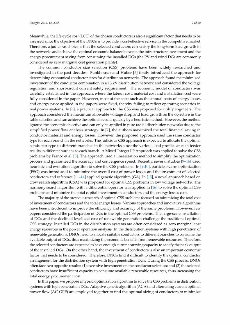
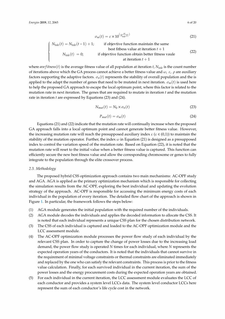
Table 3 indicates that the expensive conductor has a relatively lower value of resistance, thusallowing lower energy losses when the system has the same load condition. Therefore, there is apotential conflict between the total life span energy losses costs and the total LCCs of all conductors inthe network. Figure 5 reveals this conflict and proves the proposed algorithm can successfully achievethe balance between these two conflicting costs. On the other hand, even though the wind farm inthe network is considered as a zero marginal cost generator, attempting to fully consume all availableoutput of the renewable resources in the demand side may result in high conductor investment costsor high energy losses costs. Figure 6 shows that the optimum power consumption of the wind farmin each iteration. From the results in Figure 6, it is observed that parts of the available capacity arecurtailed to achieve the minimum total costs (including total energy losses costs, energy purchase costsand conductor investment costs). Based on the proposed approach, the conductor sizes that cannotsatisfy the minimum and maximum voltage constraints are eliminated and replaced by the new onesthat can satisfy the constraints. Figures 7 and 8 illustrate that the minimum and maximum voltageoccur in each iteration and proves that the proposed approach can successfully ensure that all theconductors satisfy the voltage constraints (0.94 to 1.1 p.u.).

Energies 2019, 12, 2065 12 of 20

Energies 2019, 12, x 12 of 20

Figure 5. Conflict of the life cycle costs of conductors and energy losses costs (case 33-bus network).

Figure 6. Wind farm output at each iteration (case 33-bus network).

Figure 5. Conflict of the life cycle costs of conductors and energy losses costs (case 33-bus network).

Energies 2019, 12, x 12 of 20

Figure 5. Conflict of the life cycle costs of conductors and energy losses costs (case 33-bus network).

Figure 6. Wind farm output at each iteration (case 33-bus network). Figure 6. Wind farm output at each iteration (case 33-bus network).

Energies 2019, 12, 2065 13 of 20Energies 2019, 12, x 13 of 20

Figure 7. Minimum voltage at each iteration (case 33-bus network).

Figure 8. Maximum voltage in each iteration (case 33-bus network).

(2) Case study of the IEEE 69-bus distribution network

The proposed CCS optimization approach is tested on an IEEE 69-bus network in this section,

where three wind generators are connected to the network at branch 6, branch 36 and branch 53. The

single line diagram of this 69-bus distribution network is shown in Figure 9, and the relevant

operation data and network constraints are listed in Table 7.

Figure 7. Minimum voltage at each iteration (case 33-bus network).

Energies 2019, 12, x 13 of 20

Figure 7. Minimum voltage at each iteration (case 33-bus network).

Figure 8. Maximum voltage in each iteration (case 33-bus network).

(2) Case study of the IEEE 69-bus distribution network

The proposed CCS optimization approach is tested on an IEEE 69-bus network in this section,

where three wind generators are connected to the network at branch 6, branch 36 and branch 53. The

single line diagram of this 69-bus distribution network is shown in Figure 9, and the relevant

operation data and network constraints are listed in Table 7.

Figure 8. Maximum voltage in each iteration (case 33-bus network).

(2) Case study of the IEEE 69-bus distribution network

The proposed CCS optimization approach is tested on an IEEE 69-bus network in this section,where three wind generators are connected to the network at branch 6, branch 36 and branch 53. Thesingle line diagram of this 69-bus distribution network is shown in Figure 9, and the relevant operationdata and network constraints are listed in Table 7.

Energies 2019, 12, 2065 14 of 20Energies 2019, 12, x 14 of 20

Figure 9. Single line diagram of the IEEE 69-bus distribution network.

Table 7. Parameters of the 69-bus network.

Parameter Value

Maximum voltage 1.1 (p.u.)

Minimum voltage 0.94 (p.u.)

Initial total active demand 3.22 MW

Initial total reactive demand 1.78 MVar

Load growth rate 3%/year

Operation year 20 years

Total branches 68

Maximum available output of wind farm at node 6 1.2 MW

Maximum available output of wind farm at node 36 1.0 MW

Maximum available output of wind farm at node 53 0.6 MW

Same as the case of IEEE 33-bus network, the quadratic generation cost function of the main

generator connected at node 1 is expressed in Equation (25) and the wind farm is also considered as

a zero marginal cost generator in the case of 69-bus network.

The overall results of the proposed AGA optimal CSS for the selected 69-bus distribution

network are shown in Figure 10. It is observed that the best fitness can be achieved after

approximately 160 iterations. The mutation rate is self-adaptive during the process of the AGA, which

is shown in Figure 11. It can be observed that the mutation rate is increased when the AGA cannot

provide a better fitness value and resets to zero when a better fitness value is achieved. Further, it is

noted that the best fitness value is captured after 250 iterations since the 69-bus system is more

complicated than the 33-bus system.

MG

1 2 3 4 5 6 7 8 9 10 11 12 13 14 15

47 48 49 50

16 17 18

36 37 38 39 40 41 42 43

WF

44 45 46

51 52 68 69

66 67

53 54 55 56 57 58 59 60 61 62 63

28 29 30 31 32 33 34 35

64 65

19 22 23 24 25 26 27

WF

WF

Figure 9. Single line diagram of the IEEE 69-bus distribution network.

Table 7. Parameters of the 69-bus network.

Parameter Value

Maximum voltage 1.1 (p.u.)Minimum voltage 0.94 (p.u.)

Initial total active demand 3.22 MWInitial total reactive demand 1.78 MVar

Load growth rate 3%/yearOperation year 20 yearsTotal branches 68

Maximum available output of wind farm at node 6 1.2 MWMaximum available output of wind farm at node 36 1.0 MWMaximum available output of wind farm at node 53 0.6 MW

Same as the case of IEEE 33-bus network, the quadratic generation cost function of the maingenerator connected at node 1 is expressed in Equation (25) and the wind farm is also considered as azero marginal cost generator in the case of 69-bus network.

The overall results of the proposed AGA optimal CSS for the selected 69-bus distribution networkare shown in Figure 10. It is observed that the best fitness can be achieved after approximately160 iterations. The mutation rate is self-adaptive during the process of the AGA, which is shown inFigure 11. It can be observed that the mutation rate is increased when the AGA cannot provide a betterfitness value and resets to zero when a better fitness value is achieved. Further, it is noted that thebest fitness value is captured after 250 iterations since the 69-bus system is more complicated than the33-bus system.

Energies 2019, 12, 2065 15 of 20

Energies 2019, 12, x 15 of 20

Figure 10. Overall results of the best fitness value and average fitness value (case 69-bus network).

Figure 11. Adaptive mutation rate in each iteration (case 69-bus network).

Similar to the results of the 33-bus system, Figure 12 reveals the conflict between total energy

losses and the life cycle costs of all conductors in the 69-bus network, thus proving that the proposed

algorithm can successfully achieve the balance between these two contrary costs. Figure 13 indicates

the optimum power consumption of the wind farm generations in each iteration in the case of the 69-

bus system. Similar to the results in the 33-bus system, parts of the available capacity are curtailed

for achieving the minimum total costs (including total energy losses costs, energy purchase costs and

conductor’s investment costs).

Figure 10. Overall results of the best fitness value and average fitness value (case 69-bus network).

Energies 2019, 12, x 15 of 20

Figure 10. Overall results of the best fitness value and average fitness value (case 69-bus network).

Figure 11. Adaptive mutation rate in each iteration (case 69-bus network).

Similar to the results of the 33-bus system, Figure 12 reveals the conflict between total energy

losses and the life cycle costs of all conductors in the 69-bus network, thus proving that the proposed

algorithm can successfully achieve the balance between these two contrary costs. Figure 13 indicates

the optimum power consumption of the wind farm generations in each iteration in the case of the 69-

bus system. Similar to the results in the 33-bus system, parts of the available capacity are curtailed

for achieving the minimum total costs (including total energy losses costs, energy purchase costs and

conductor’s investment costs).

Figure 11. Adaptive mutation rate in each iteration (case 69-bus network).

Similar to the results of the 33-bus system, Figure 12 reveals the conflict between total energylosses and the life cycle costs of all conductors in the 69-bus network, thus proving that the proposedalgorithm can successfully achieve the balance between these two contrary costs. Figure 13 indicatesthe optimum power consumption of the wind farm generations in each iteration in the case of the69-bus system. Similar to the results in the 33-bus system, parts of the available capacity are curtailedfor achieving the minimum total costs (including total energy losses costs, energy purchase costs andconductor’s investment costs).

Energies 2019, 12, 2065 16 of 20

Energies 2019, 12, x 16 of 20

Figure 12. Conflict of the life cycle costs of conductors and energy losses costs (case 69-bus network).

Figure 13. Wind farm outputs at each iteration (case 69-bus network).

Similar to the results in the case study of the 33-bus network, the individuals that cannot satisfy

the minimum and maximum voltage constraints are eliminated and replaced by the new individuals

that can satisfy the constraints. Figures 14 and 15 illustrate that the minimum and maximum voltage

occur in each iteration and proves that the proposed approach can successfully ensure all the

individuals satisfy the voltage constraints (0.94 to 1.1 p.u.).

Figure 12. Conflict of the life cycle costs of conductors and energy losses costs (case 69-bus network).

Energies 2019, 12, x 16 of 20

Figure 12. Conflict of the life cycle costs of conductors and energy losses costs (case 69-bus network).

Figure 13. Wind farm outputs at each iteration (case 69-bus network).

Similar to the results in the case study of the 33-bus network, the individuals that cannot satisfy

the minimum and maximum voltage constraints are eliminated and replaced by the new individuals

that can satisfy the constraints. Figures 14 and 15 illustrate that the minimum and maximum voltage

occur in each iteration and proves that the proposed approach can successfully ensure all the

individuals satisfy the voltage constraints (0.94 to 1.1 p.u.).

Figure 13. Wind farm outputs at each iteration (case 69-bus network).

Similar to the results in the case study of the 33-bus network, the individuals that cannot satisfy theminimum and maximum voltage constraints are eliminated and replaced by the new individuals thatcan satisfy the constraints. Figures 14 and 15 illustrate that the minimum and maximum voltage occurin each iteration and proves that the proposed approach can successfully ensure all the individualssatisfy the voltage constraints (0.94 to 1.1 p.u.).

Energies 2019, 12, 2065 17 of 20

Energies 2019, 12, x 17 of 20

Figure 14. Minimum voltage at each iteration (case 69-bus network).

Figure 15. Maximum voltage in each iteration (case 69-bus network).

The detailed optimum results of CSS by two different approaches are shown in Table 8. After

the decoding process, the best conductor type of each branch in the 69-bus network can be checked

on this table.

(3) Summary and discussion

The study results of the 33-bus network and the 69-bus network indicate that the proposed AGA

has the capability to provide a more efficient and effective way to solve the new challenge in the CSS

problem than the standard GA. In particular, 25% and 29% total costs saving are achieved separately

by the proposed approach in two different distribution networks. More importantly, the potential

economic conflict between the investment of conductors and the renewable recourses curtailment

Figure 14. Minimum voltage at each iteration (case 69-bus network).

Energies 2019, 12, x 17 of 20

Figure 14. Minimum voltage at each iteration (case 69-bus network).

Figure 15. Maximum voltage in each iteration (case 69-bus network).

The detailed optimum results of CSS by two different approaches are shown in Table 8. After

the decoding process, the best conductor type of each branch in the 69-bus network can be checked

on this table.

(3) Summary and discussion

The study results of the 33-bus network and the 69-bus network indicate that the proposed AGA

has the capability to provide a more efficient and effective way to solve the new challenge in the CSS

problem than the standard GA. In particular, 25% and 29% total costs saving are achieved separately

by the proposed approach in two different distribution networks. More importantly, the potential

economic conflict between the investment of conductors and the renewable recourses curtailment

Figure 15. Maximum voltage in each iteration (case 69-bus network).

The detailed optimum results of CSS by two different approaches are shown in Table 8. After thedecoding process, the best conductor type of each branch in the 69-bus network can be checked onthis table.

Energies 2019, 12, 2065 18 of 20

Table 8. Best CSS for 69-bus distribution network.

Branch From To

SelectedConductorType via

Standard GA

SelectedConductor

Type via AGABranch From To

SelectedConductorType via

Standard GA

SelectedConductor

Type via AGA

1 1 2 Gopher Mink 35 3 36 Squirrel Squirrel2 2 3 Weasel Ferret 36 36 37 Squirrel Otter3 3 4 Mole Otter 37 37 38 Gopher Ferret4 4 5 Ferret Otter 38 38 39 Mole Gopher5 5 6 Gopher Ferret 39 39 40 Beaver Raccoon6 6 7 Mole Beaver 40 40 41 Gopher Mole7 7 8 Rabbit Beaver 41 41 42 Squirrel Ferret8 8 9 Gopher Otter 42 42 43 Ferret Rabbit9 9 10 Weasel Mink 43 43 44 Rabbit Mink10 10 11 Mink Otter 44 44 45 Gopher Weasel11 11 12 Gopher Rabbit 45 45 46 Mink Gopher12 12 13 Mole Beaver 46 4 47 Ferret Ferret13 13 14 Rabbit Rabbit 47 47 48 Rabbit Beaver14 14 15 Squirrel Mink 48 48 49 Weasel Mink15 15 16 Gopher Beaver 49 49 50 Gopher Gopher16 16 17 Mole Raccoon 50 8 81 Gopher Rabbit17 17 18 Gopher Rabbit 51 51 52 Beaver Squirrel18 18 19 Squirrel Mole 52 9 53 Gopher Raccoon19 19 20 Squirrel Squirrel 53 53 54 Mink Beaver20 20 21 Squirrel Weasel 54 54 55 Mole Mink21 21 22 Mink Raccoon 55 55 56 Squirrel Raccoon22 22 23 Mole Mink 56 56 57 Mole Beaver23 23 24 Gopher Weasel 57 57 58 Rabbit Otter24 24 25 Beaver Mole 58 58 59 Mole Otter25 25 26 Rabbit Squirrel 59 59 60 Rabbit Raccoon26 26 27 Weasel Weasel 60 60 61 Weasel Otter27 3 28 Weasel Mole 61 61 62 Mole Ferret28 28 29 Beaver Ferret 62 62 63 Weasel Otter29 29 30 Mole Rabbit 63 63 64 Gopher Otter30 30 31 Ferret Ferret 64 64 53 Mole Rabbit31 31 32 Mole Mole 65 53 54 Squirrel Gopher32 32 33 Otter Squirrel 66 66 67 Gopher Squirrel33 33 34 Weasel Squirrel 67 12 68 Mole Mole34 34 35 Mole Weasel 68 68 69 Mole Squirrel

Total life-cycle costs of two approaches Standard GA $39,054,123.9Proposed AGA $27,617,228.5

Net cost saving - $11,436,895.4

Cost saving percentage - 29%

(3) Summary and discussion

The study results of the 33-bus network and the 69-bus network indicate that the proposed AGAhas the capability to provide a more efficient and effective way to solve the new challenge in the CSSproblem than the standard GA. In particular, 25% and 29% total costs saving are achieved separatelyby the proposed approach in two different distribution networks. More importantly, the potentialeconomic conflict between the investment of conductors and the renewable recourses curtailmentcosts is firstly considered in the CCS problem. On the other hand, the proposed approach employs acomprehensive conductor investment and O&M pricing model to provide precise and practical studyresults. The simulation times of the proposed AG and the standard GA used in the framework aresummarized in Table 9 to identify the efficiency of these two approaches. The results indicate thatthe calculation time is slightly increased when the proposed AGA is applied. However, the proposedAGA has the capability to provide a better solution to the CSS problem. In addition, the informationabout our computing platform used to assess the simulation results is listed below.

Table 9. Simulation times of standard GA and proposed AGA.

Simulation Times Standard GA Proposed AGA

Case 33-bus network 669.42 s 720.35 sCase 69-bus network 1548.76 s 2078.81 s

Energies 2019, 12, 2065 19 of 20

The computing platform used in this paper:

CPU: i5-8600k (Max Turbo Frequency 4.30 GHz)Memory: 32 GB (2400 MHz)Graphic card: Nvidia RTX 2080

4. Conclusions

A hybrid optimization algorithm to deal with the CSS problems in distribution systems withhigh penetration of DG has been proposed in this paper. An AGA that has a dynamic mutation rateand a dynamic number of mutated genes has been introduced as the main optimization mechanism.The proposed AGA mechanism is responsible for finding the optimal CSS for the chosen networkand the objective function is to minimize the sum of the LCC of selected conductors, the total energyprocurement costs and energy losses costs. It is noted that the total energy procurement costs andenergy losses costs of each individual are provided by the AC-OPF, which is employed as the auxiliaryoptimization tool in the approach.

The numerical results have demonstrated an ability to provide accurate and feasible solutions forsolving the optimal CSS problem and ensured that the results satisfy the network constraints. Differentfrom the majority of earlier research of the CSS problem, this approach comprehensively considersthe ED problems of the traditional fossil fuel generator and the renewable resources. Instead of theobjective function of minimum energy losses costs, the minimum system level costs are considered asthe main target in this approach.

The development of the high capacity electric vehicle charging stations and electrical storagesystem significantly affect the planning of the distribution networks. The CSS problem is expected tobe considered by those technologies. On the other hand, the high penetration of DGs will significantlychange the short-circuit currents through the distribution systems. This feature may affect the selectionof conductors when the DNOs consider a network upgrading plan. Indeed, several approaches areable to deal with this potential problem when the DNOs design or upgrade their distribution networkssuch as application of the superconducting fault current limiter (SFCL) or installing the second circuitbreak (CBs) in the proper place. However, the potential conflict between the costs of a second circuitbreak or superconducting fault current limiter and the costs of conductors upgrading requires carefulinvestigation. Therefore, the potential problem of increasing short-circuit currents caused by highpenetration of DGs will also be incorporated in future research.

Author Contributions: Writing and original draft preparation, Z.Z.; Review and editing, J.M.

Funding: This research received no external funding.

Conflicts of Interest: The authors declare no conflict of interest.

References

1. Gielen, D.; Boshell, F.; Saygin, D.; Bazilian, M.D.; Wagner, N.; Gorini, R. The role of renewable energy in theglobal energy transformation. Energy Strateg. Rev. 2019, 24, 38–50. [CrossRef]

2. Fan, A.; Huang, L.; Lin, S.; Chen, N.; Zhu, L.; Wang, X. Performance Comparison Between RenewableObligation and Feed-in Tariff with Contract for Difference in UK. In Proceedings of the 2018 China InternationalConference on Electricity Distribution (CICED), Tianjin, China, 17–19 September 2018; pp. 2761–2765.

3. Pandey, R.R.; Arora, S. Distributed generation system: A review and its impact on India. Int. Res. J. Eng.Technol. 2016, 3, 758–765.

4. Kamaruzzaman, Z. Effect of grid-connected photovoltaic systems on static and dynamic voltage stabilitywith analysis techniques—A review. Prz. Elektrotechniczny 2015, 1, 136–140. [CrossRef]

5. Funkhouser, A.W.; Huber, R.P. A Method for Determining Economical ACSR Conductor Sizes for DistributionSystems [includes discussion]. Trans. Am. Inst. Electr. Eng. Part III Power Appar. Syst. 1955, 74, 479–484.[CrossRef]

Energies 2019, 12, 2065 20 of 20

6. Wang, Z.; Liu, H.; Yu, D.C.; Wang, X.; Song, H. A practical approach to the conductor size selection inplanning radial distribution systems. IEEE Trans. Power Deliv. 2000, 15, 350–354. [CrossRef]

7. Sivanagaraju, S.; Sreenivasulu, N.; Vijayakumar, M.; Ramana, T. Optimal conductor selection for radialdistribution systems. Electr. Power Syst. Res. 2002, 63, 95–103. [CrossRef]

8. Franco, J.F.; Rider, M.J.; Lavorato, M.; Romero, R. Optimal Conductor Size Selection and Reconductoring inRadial Distribution Systems Using a Mixed-Integer LP Approach. IEEE Trans. Power Syst. 2013, 28, 10–20.[CrossRef]

9. Legha, M.M. Combination of optimal conductor selection and capacitor placement in radial distributionsystems using PSO method. Iraqi J. Electr. Electron. Eng. 2014, 10, 33–41.

10. Haidar, S.; Legha, M.M. Optimal Conductor Selection in Radial Distribution Using Imperialism CompetitiveAlgorithm and Comparison with PSO Method. In Proceedings of the 6th International Conference forScientific Computing to Computational Engineering, Athenes, Greece, 9–12 July 2014.

11. Devi, A.L.; Shereen, A. Optimal conductor selection for radial distribution networks using genetic algorithmin SPDCL, AP—A case study. J. Theor. Appl. Inf. Technol. 2009, 6, 674–685.

12. Vahid, M.; Hossein, A.A.; Kazem, M. Maximum loss reduction applying combination of optimal conductorselection and capacitor placement in distribution systems with nonlinear loads. In Proceedings of the 200843rd International Universities Power Engineering Conference, Padova, Italy, 1–4 September 2008; pp. 1–5.

13. Falaghi, H.; Singh, C. Optimal Conductor Size Selection in Distribution Systems with Wind Power Generation.In Wind Power Systems: Applications of Computational Intelligence; Wang, L., Singh, C., Kusiak, A., Eds.; Springer:Berlin/Heidelberg, Germany, 2010; pp. 25–51.

14. Thenepalle, M. A comparative study on optimal conductor selection for radial distribution network usingconventional and genetic algorithm approach. Int. J. Comput. Appl. 2011, 6, 6–13. [CrossRef]

15. Abdelaziz, A.Y.; Fathy, A. A novel approach based on crow search algorithm for optimal selection ofconductor size in radial distribution networks. Eng. Sci. Technol. An Int. J. 2017, 20, 391–402. [CrossRef]

16. Rao, R.S.; Satish, K.; Narasimham, S.V.L. Optimal Conductor Size Selection in Distribution Systems Usingthe Harmony Search Algorithm with a Differential Operator. Electr. Power Compon. Syst. 2011, 40, 41–56.[CrossRef]

17. Holland, J.H. Adaptation in Natural and Artificial Systems: An Introductory Analysis with Applications to Biology,Control and Artificial Intelligence; MIT Press: Cambridge, MA, USA, 1992; p. 228.

18. Liu, J.; Cai, Z.; Liu, J. Premature convergence in genetic algorithm: Analysis and prevention based on chaosoperator. In Proceedings of the 3rd World Congress on Intelligent Control and Automation, Hefei, China,26 June–2 July 2000; Volume 491, pp. 495–499.

19. Hrstka, O.; Kucerová, A. Improvements of real coded genetic algorithms based on differential operatorspreventing premature convergence. Adv. Eng. Softw. 2004, 35, 237–246. [CrossRef]

20. Pandey, H.M.; Chaudhary, A.; Mehrotra, D. A comparative review of approaches to prevent prematureconvergence in GA. Appl. Soft Comput. 2014, 24, 1047–1077. [CrossRef]

21. Queiroz, L.M.O.; Lyra, C. Adaptive Hybrid Genetic Algorithm for Technical Loss Reduction in DistributionNetworks under Variable Demands. IEEE Trans. Power Syst. 2009, 24, 445–453. [CrossRef]

22. Eiben, A.E.; Hinterding, R.; Michalewicz, Z. Parameter control in evolutionary algorithms. IEEE Trans. Evol.Comput. 1999, 3, 124–141. [CrossRef]

23. Mahmoodabadi, M.J.; Nemati, A.R. A novel adaptive genetic algorithm for global optimization ofmathematical test functions and real-world problems. Eng. Sci. Technol. Int. J. 2016, 19, 2002–2021.[CrossRef]

24. Ismael, S.M.; Abdel Aleem, S.H.E.; Abdelaziz, A.Y.; Zobaa, A.F. Optimal Conductor Selection of RadialDistribution Feeders: An Overview and New Application Using Grasshopper Optimization Algorithm. InClassical and Recent Aspects of Power System Optimization; Zobaa, A.F., Abdel Aleem, S.H.E., Abdelaziz, A.Y.,Eds.; Academic Press: Cambridge, MA, USA, 2018; Chapter 8, pp. 185–217.

© 2019 by the authors. Licensee MDPI, Basel, Switzerland. This article is an open accessarticle distributed under the terms and conditions of the Creative Commons Attribution(CC BY) license (http://creativecommons.org/licenses/by/4.0/).