
technical-specification-of-acsr-conductor-for-transmission ...
Upload
khangminh22Category
view
2download
0
Physics -1 Laboratory Manual (PH-191 / PH – 291)
Department of Applied Sciences : Physical Science Unit : HIT : Haldia : W.B. : India 1
Experiment No. : 01(Group-1)
DETERMINATION OF THERMAL CONDUCTIVITY OF A
GOOD CONDUCTOR BY SEARLE’S METHOD
I. Objective(s):
To determine the thermal conductivity of a good conductor by Searle‟s method.
II. Apparatus:
Searle‟s set-up, Thermometers, Measuring cylinder, Steam source, Continuous water
flow system etc.
III. Theory:
Thermal conductivity of a material is defined as “the amount of heat flowing per unit
time across one square unit of cross sectional area of one unit thickness (length) with
one degree temperature difference between the faces across which heat is assumed to
flow perpendicularly”.
In steady state condition, the amount of heat passing across the material normally per
unit time is given by-
d
KAdQ 21
………………….(1)
Where d is the thickness (length) of the good conductor, A is the cross sectional area
of the good conductor, θ1 and θ2 are the temperature recorded by the thermometers
T1 and T2 respectively. K is the thermal conductivity of the given good conductor.
If „m’ grams of water flows through the good conductor per seconds and θ3 and θ4 are
the stady state temperatures recorded for out flowing and inflowing water respectively,
the amount of heat „dQ’ taken by water per unit time is given by
dQ = m(θ3 – θ4)…………………….(2)
By equation (1) and (2), we get
21
43
A
dmK or,
21
2
434
D
dmK
………………….(3)
Where, cross sectional area of the good conductor bar4
2DA
, D is the diameter. In
C.G.S. the unit of Thermal conductivity is Cal/cm/sec/0C.
Physics -1 Laboratory Manual (PH-191 / PH – 291)
Department of Applied Sciences : Physical Science Unit : HIT : Haldia : W.B. : India 2
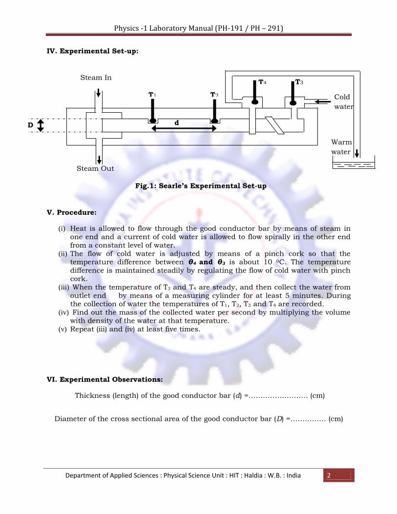
IV. Experimental Set-up:
V. Procedure:
(i) Heat is allowed to flow through the good conductor bar by means of steam in one end and a current of cold water is allowed to flow spirally in the other end from a constant level of water.
(ii) The flow of cold water is adjusted by means of a pinch cork so that the temperature difference between θ4 and θ3 is about 10 0C. The temperature difference is maintained steadily by regulating the flow of cold water with pinch cork.
(iii) When the temperature of T3 and T4 are steady, and then collect the water from outlet end by means of a measuring cylinder for at least 5 minutes. During the collection of water the temperatures of T1, T2, T3 and T4 are recorded.
(iv) Find out the mass of the collected water per second by multiplying the volume with density of the water at that temperature.
(v) Repeat (iii) and (iv) at least five times.
VI. Experimental Observations:
Thickness (length) of the good conductor bar (d) =……………………. (cm)
Diameter of the cross sectional area of the good conductor bar (D) =…………… (cm)
T1 T2 T3 T4 Steam In
Steam Out
Warm
water
Out
Cold
water
In D
Fig.1: Searle’s Experimental Set-up
d
Physics -1 Laboratory Manual (PH-191 / PH – 291)
Department of Applied Sciences : Physical Science Unit : HIT : Haldia : W.B. : India 3
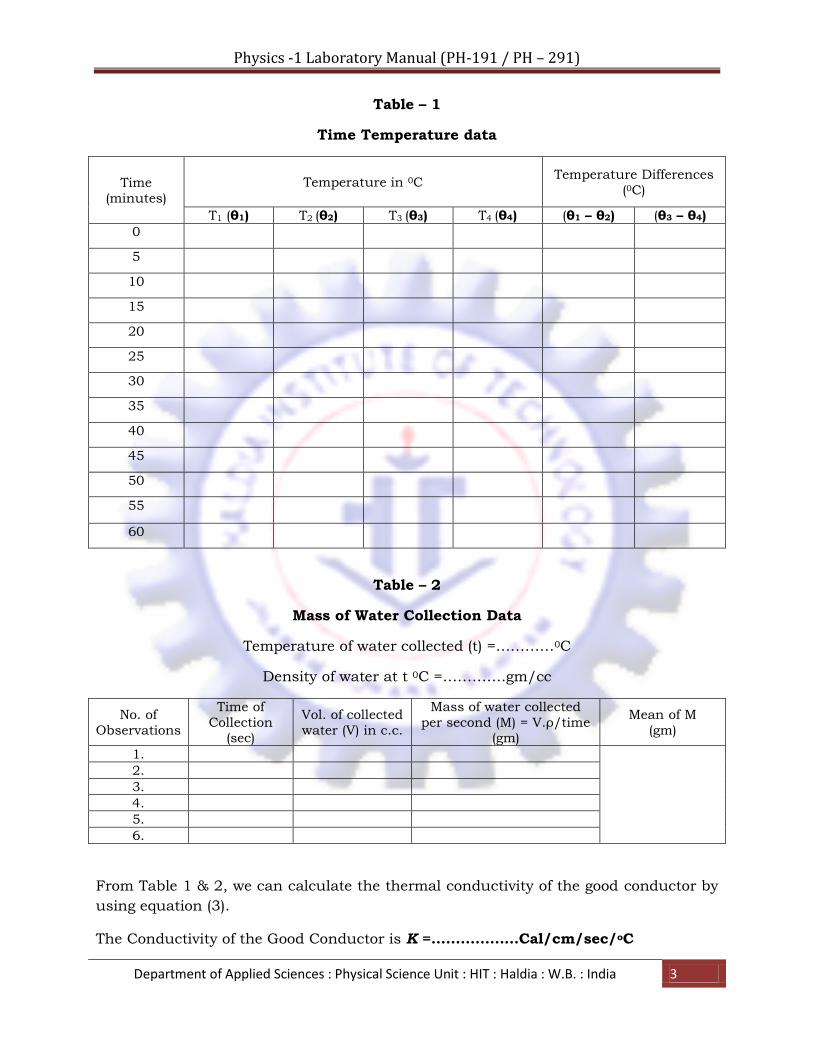
Table – 1
Time Temperature data
Time
(minutes)
Temperature in 0C Temperature Differences
(0C)
T1 (θ1) T2 (θ2) T3 (θ3) T4 (θ4) (θ1 – θ2) (θ3 – θ4)
0
5
10
15
20
25
30
35
40
45
50
55
60
Table – 2
Mass of Water Collection Data
Temperature of water collected (t) =…………0C
Density of water at t 0C =………….gm/cc
No. of
Observations
Time of
Collection (sec)
Vol. of collected
water (V) in c.c.
Mass of water collected
per second (M) = V.ρ/time (gm)
Mean of M
(gm)
1.
2.
3.
4.
5.
6.
From Table 1 & 2, we can calculate the thermal conductivity of the good conductor by
using equation (3).
The Conductivity of the Good Conductor is K =………………Cal/cm/sec/oC
Physics -1 Laboratory Manual (PH-191 / PH – 291)
Department of Applied Sciences : Physical Science Unit : HIT : Haldia : W.B. : India 4
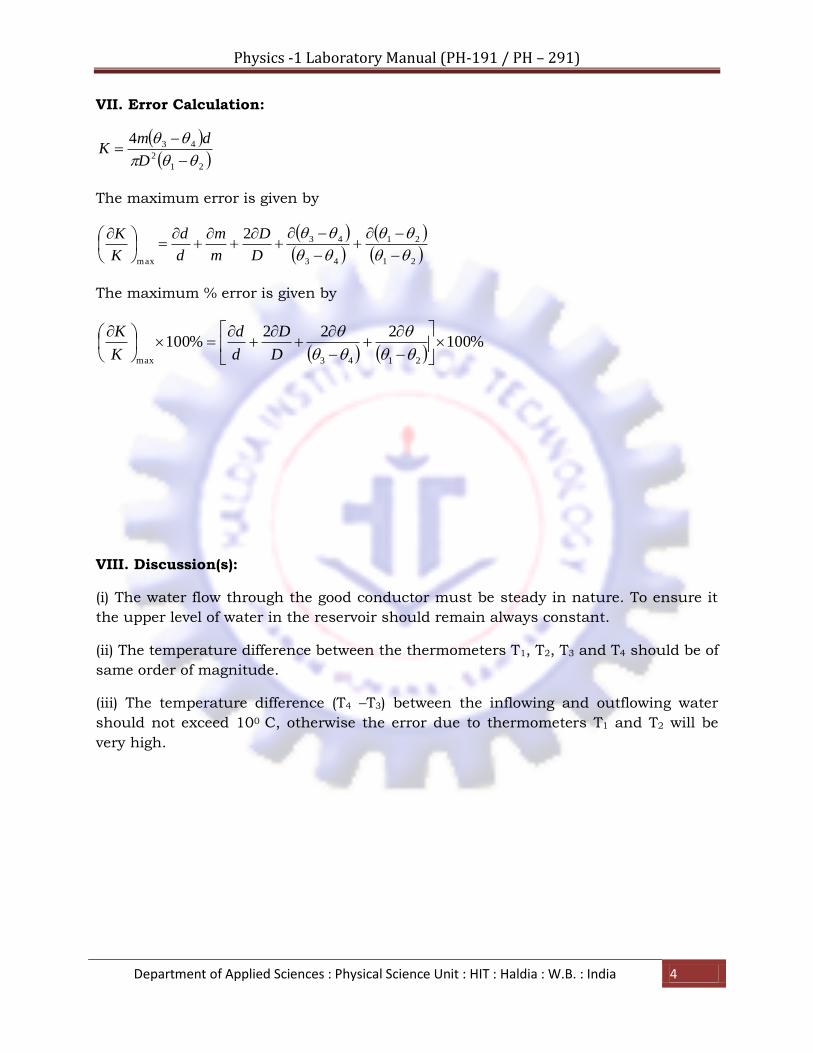
VII. Error Calculation:
21
2
434
D
dmK
The maximum error is given by
21
21
43
43
max
2
D
D
m
m
d
d
K
K
The maximum % error is given by
%100
222%100
2143max
D
D
d
d
K
K
VIII. Discussion(s):
(i) The water flow through the good conductor must be steady in nature. To ensure it
the upper level of water in the reservoir should remain always constant.
(ii) The temperature difference between the thermometers T1, T2, T3 and T4 should be of
same order of magnitude.
(iii) The temperature difference (T4 –T3) between the inflowing and outflowing water
should not exceed 100 C, otherwise the error due to thermometers T1 and T2 will be
very high.

Physics -1 Laboratory Manual (PH-191 / PH – 291)
Department of Applied Sciences : Physical Science Unit : HIT : Haldia : W.B. : India 5
Experiment No. : 02 (Group-1)
DETERMINATION OF THERMAL CONDUCTIVITY OF A
BAD CONDUCTOR IN THE FORM OF DISC BY LEE’S
AND CHORLTON’S METHOD
I. Objective:
To determine the thermal conductivity of a bad conductor by Lee‟s and Chorlton‟s
method
II. Apparatus:
Lee‟s apparatus, steam chamber, two thermometer, Bunsen burner, circular disc of
bad conductor (rubber, wood) etc.
III. Theory:
Let 1 and 2 be the steady state temperatures recorded by the thermometers T1 and T2
respectively (see Fig.1) and K be the thermal conductivity of the bad conducting disc
S. If d is the thickness and A is the cross sectional area of the disc S, then the
quantity of heat conducted through the disc per second is given by
Q = KA (1-2)/d
If m is the mass, s is the specific heat and d/dt is the rate of cooling at 2 of the lower
metal slab B, then
Q = ms d/dt at 2
So, KA (1-2)/d = ms d/dt at 2
Or, …………………………………(1)
This is the working formula.
If m is measured in gm, d/dt in 0C per sec and s is given in cal/gm. 0C then Q is
obtained in cal per sec. Again, when d is measured in cm, A in cm2, 1 and 2 in 0C
then K is given in cal. sec-1.cm-1 .0C-1.
[Note: In the present method, the rate of cooling of the lower disc B is determined
without the experimental disc S on it. So to obtain the correct value of d/dt at 2
under the condition of experiment, the quantity d/dt should be multiplied by a factor
f given by f = (r+2d1) / (2r+2d1). Where r and d1 are the radius and thickness of the
metal disc B respectively. This correction is called the Bedford correction. Thus -

Physics -1 Laboratory Manual (PH-191 / PH – 291)
Department of Applied Sciences : Physical Science Unit : HIT : Haldia : W.B. : India 6
…………………………(2)
IV. Schematic Diagram:
V. Procedure:
1. Connect the chamber to a distant boiler. Record the temperatures of C and B at
intervals of 5 minutes until the thermometers show steady state temperature for a
period of at least 10 to 15 minutes, and note the steady state temperatures 1 and 2.
2. Remove the steam chamber and experimental disc. Heat the metal slab B slowly by
means of a heat source and simultaneously observe the temperature. Raise the
temperature to a value which is about 120 C higher than the steady value 2 noted in
step 1. Do not raise the temperature beyond the upper limit of the thermometer T2.
3. Remove the heating source. Temperature of B will start decreasing. When the
temperature reaches a value roughly 100 C above its steady temperature 2, record the
temperature with time by means of a stop watch at intervals of quarter a minute until
temperature falls below 2 by about 100 C.
4. Draw a graph by plotting the temperature of cooling (in 0C) of B along Y -axis and
the corresponding time (sec.) along X -axis. The graph will be a non-linear curve line.
Draw a tangent to the curve around 2 and then find d/dt around 2.
B S
C
T1
T2
Steam In
Steam
Out
Fig.1: Bad Conductor Experimental Set-up

Physics -1 Laboratory Manual (PH-191 / PH – 291)
Department of Applied Sciences : Physical Science Unit : HIT : Haldia : W.B. : India 7
VI. Experimental Observations:
Mass (m) of the lower disc B = …………. gm
Specific heat (s) of B = …………….cal/gm. 0C
Radius (r) and the cross sectional area (A) of the disc S: r = …………..cm, A =
…………….cm2
Thickness (length) (d) of S = ………………..cm
Table 1
Temperature of C and B with time and the values of steady state temperatures 1
and 2
Time in
minutes
0 5 10 15 20 25 30 35 40
Temp.
of C (0C)
Temp.
of B (0C)
Table 2
Record of temperature of B with time during cooling
Time
in
Sec.
0 15 30 45 60 75 90 105 120 135 150 165 180 195
Temp.
of C
(0C)
Graph Plotting:
Draw a graph with t along X-axis and along Y-axis. Find d/dt at 2 from the graph.

Physics -1 Laboratory Manual (PH-191 / PH – 291)
Department of Applied Sciences : Physical Science Unit : HIT : Haldia : W.B. : India 8
Fig.2: Temperature vs. time curve to determine d/dt.
Table 3
Determination of K from graph
m
(gm)
s (cal.gm-1
.cm-1
d (cm) d/dt at 2
(0C.sec)
A (cm2) 1 -2
(0C)
K (cal.sec.cm-1
.0C-1)
VII. Computation of percentage error:
We have, K = ms d/dt (at 2).d/A(1 -2)
If the lower disc B cools by radiation from ′ 0C to ″ 0C through in time t, we can write
d/dt (at 2) = (′ - ″)/t. Also A = πr2. Hence
K = [msd (’ - ’’)/t/ πr2(1 -2)]
The maximum proportional error in K is, therefore,
δK/K = δm/m + δd/d + δ(’ - ’’)/ (’ - ’’) + δt/t + 2δr/r + δ(1 -2)/ (1 -2) + δs/s
Since m, r, d and s are supplied, thus δm = δd = δs = δr = 0
Thus, the maximum percentage error is given by
(δK/K) × 100 % = [δ(′ - ″)/ (′ - ″) + δt/t + δ(1 -2)/ (1 -2)] × 100%
VIII. Discussions:
Write discussions in your word in points.

Physics -1 Laboratory Manual (PH-191 / PH – 291)
Department of Applied Sciences : Physical Science Unit : HIT : Haldia : W.B. : India 9
Experiment No. : 04 (Group-1)
MEASUREMENT OF RESISTACE PER UNIT LENGTH OF
THE BRIDGE WIRE BY CARRY FOSTER’S METHOD AND
HENCE TO DETERMINE THE UNKNOWN RESISTANCE
I. Objectives:
To determine the resistance per unit length of the bridge wire by Carey Foster method
and hence to determine the unknown resistance.
II. Apparatus:
1. A meter bridge with four gaps (Carey Foster Bridge)
2. Two equal resistances (say 1 ohm each)
3. A fractional resistance box (0.10 to 10.00 ohm).
4. A DC power supply (apply 2 V only).
5. A table galvanometer (range 30-30 mV,1 smallest div=…….mV).
6. A plug commutator.
7. Connecting wire.
8. Unknown resistance (in ohm).
III. Circuit diagram:
Figure-1: Circuit connection of a Carey Foster’s bridge

Physics -1 Laboratory Manual (PH-191 / PH – 291)
Department of Applied Sciences : Physical Science Unit : HIT : Haldia : W.B. : India 10
[Here P & Q are two nearly equal resistances (each of one ohm); S is a metal strip
having zero resistance, R is the fractional resistance box; E is a D.C regulated power
supply: C is a Commutator, Rl is a rheostat in the battery circuit; G is a galvanometer]
IV. Theory:
When the Carry Foster‟s bridge is balanced condition, let the null point be
cm from the left end of the bridge wire, then from Wheatstone bridge principle, we
can write -
(1)
Where and are the end connections at the two ends of the bridge wire
and is the resistance per unit length of the bridge wire.
If by interchanging R & S in the circuit, the null point is obtained at cm from the
same end, then
(2)
Solving these two equations, we get
(3)
Since the strip has almost zero resistance (i.e. S=0), then
(4)
Again ,if the fractional resistance box „R‟ is inserted in the extreme right gap and strip
„S‟ in the extreme left gap at first and their positions are interchanged, giving and
as the null point lengths, then
(5)
Therefore in general the working formula of this experiment is
(6)
Physics -1 Laboratory Manual (PH-191 / PH – 291)
Department of Applied Sciences : Physical Science Unit : HIT : Haldia : W.B. : India 11
Determination of the unknown resistance: Let the given metal strip S be replaced
by a known resistance r and R be replaced by the given wire whose resistance is
unknown. Suppose that the unknown resistance of the given wire is and that is
the distance of the null point from the left end of the bridge wire obtained with this
circuit. Let be the distance of the null point from the same end obtained with circuit,
when r and are interchanged. Then using equation (3) we get -
(7)
Equation (6) and (7) are the working formulas of the experiment.
V. Procedure:
1. Make the circuit connections as shown in the figure 1. The fractional resistance
box is connected in the extreme left gap and strip in the extreme right gap.
Close tightly all the plugs of the box and observe the null point. The null point
should be obtained near middle of the bridge wire; if not, the resistance P & Q
are unequal.
2. Take out a plug to insert a small resistance (say 1 ohm) from the box R. Note
the null point readings for both direct and reverse currents. The null point
should be located towards the left end of the bridge wire. Increase gradually the
resistance R (say,1.2Ω,1.4Ω,1.6Ω etc) and each time record the null points for
both direct and reverse currents till end of the bridge wire approached.
3. Interchanged the copper strip „S‟ and resistance box R. Put those resistance
serially from the box which were used before, i.e. in step(ii) and record the null
points in the previous manner. In this case, the null points will be located
between the midpoint and right end of the bridge.
4. Find the value of ρ of the bridge wire from each set of reading using equation (6)
and obtain the mean ρ.
5. Repeat the same with replacing R by and S by r (known resistance).
VI. Experimental Observation(s):
Physics -1 Laboratory Manual (PH-191 / PH – 291)
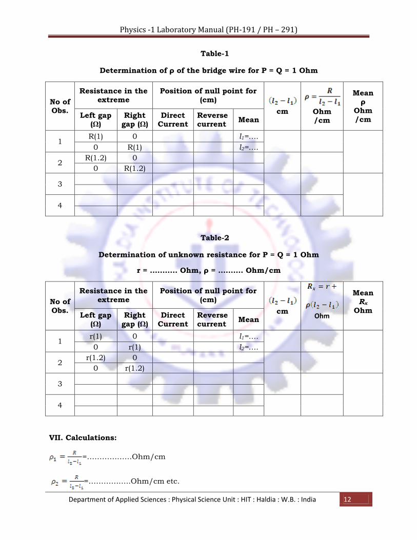
Department of Applied Sciences : Physical Science Unit : HIT : Haldia : W.B. : India 12
Table-1
Determination of ρ of the bridge wire for P = Q = 1 Ohm
No of Obs.
Resistance in the extreme
Position of null point for (cm)
cm
Ohm /cm
Mean ρ
Ohm /cm
Left gap (Ω)
Right gap (Ω)
Direct Current
Reverse current
Mean
1 R(1) 0 l1=….
0 R(1) l2=….
2 R(1.2) 0
0 R(1.2)
3
4
Table-2
Determination of unknown resistance for P = Q = 1 Ohm
r = ……….. Ohm, ρ = ………. Ohm/cm
No of Obs.
Resistance in the extreme
Position of null point for (cm)
cm
Ohm
Mean Rx
Ohm
Left gap (Ω)
Right gap (Ω)
Direct Current
Reverse current
Mean
1 r(1) 0 l1=….
0 r(1) l2=….
2 r(1.2) 0
0 r(1.2)
3
4
VII. Calculations:
=………………Ohm/cm
=……………..Ohm/cm etc.
Physics -1 Laboratory Manual (PH-191 / PH – 291)
Department of Applied Sciences : Physical Science Unit : HIT : Haldia : W.B. : India 13
Mean = ……………….. Ohm/cm
= ……………………………….Ohm
VIII. Result(s):
The resistance per unit length of the bridge wire (ρ) =………………..Ohm/cm
The resistance of the unknown wire =………………..Ohm
IX. Error Calculation:
Hence
Since, R is not been measured and = 1 smallest division of the measuring scale.
Thus maximum percentage of error,
X. Discussion(s):
(i). Before proceeding with the measurements, ensure that there is no loose contact
anywhere in the circuit.
(ii). At the beginning, it should be seen whether with S = R = 0, the null point is
obtained at a point very near at 50 cm mark (i.e. the midpoint of the bridge wire). If the
null point is obtained more on the right of 50 cm mark, the resistance P is defective. If
on the other hand, the null point is more on the left of the of 50 cm mark, the
resistance Q is defective.

Physics -1 Laboratory Manual (PH-191 / PH – 291)
Department of Applied Sciences : Physical Science Unit : HIT : Haldia : W.B. : India 14
Experiment No. : 05 (Group-2)
DETERMINATION OF YOUNG’S MODULUS BY FLEXURE
METHOD AND CALCULATION OF BENDING MOMENT
AND SHEAR FORCE AT A POINT ON THE BEAM
I. Objective(s): To determine the Young‟s Modulus by Flexure method and calculation
of Bending Moment and Shear Force at a point on the beam.
II. Apparatus:
A solid bar, Two stout iron stands, Rectangular stirrup with a knife- edge and a
vertical pointer, A traveling microscope, Standard weights, Spirit level, Meter scale, A
slide calipers.
III. Theory:
A uniform rectangular bar supported symmetrically on two horizontal and parallel
knife-edges is depressed by a load of mass M, suspended from the beam midway
between the knife-edges. Then the depression of the middle of the bar is given by
Or,
Where, Young‟s Modulus, Length of the bar between the two knife-edges,
Breadth of the bar, Depth of the bar, Acceleration due to gravity at laboratory,
Load suspended at the middle point of the bar, and depression at the middle
point of the bar,
IV. Experimental Set-up:
Fig.1: Schematic diagram of Young’s Modulus Experiment.
POINTER
KNIFE
EDGES
BAR
STAND
S
LOADS
Physics -1 Laboratory Manual (PH-191 / PH – 291)
Department of Applied Sciences : Physical Science Unit : HIT : Haldia : W.B. : India 15
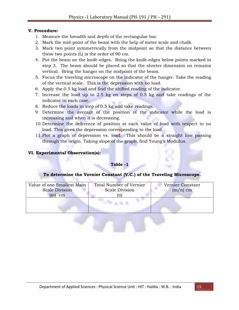
V. Procedure:
1. Measure the breadth and depth of the rectangular bar.
2. Mark the mid-point of the beam with the help of meter scale and chalk.
3. Mark two point symmetrically from the midpoint so that the distance between
these two points (L) is the order of 90 cm.
4. Put the beam on the knife-edges. Bring the knife-edges below points marked in
step 3. The beam should be placed so that the shorter dimension on remains
vertical. Bring the hanger on the midpoint of the beam.
5. Focus the traveling microscope on the indicator of the hanger. Take the reading
of the vertical scale. This is the depression with no load.
6. Apply the 0.5 kg load and find the shifted reading of the indicator.
7. Increase the load up to 2.5 kg on steps of 0.5 kg and take readings of the
indicator in each case.
8. Reduce the loads in step of 0.5 kg and take readings.
9. Determine the average of the position of the indicator while the load is
increasing and when it is decreasing.
10. Determine the deference of position at each value of load with respect to no
load. This gives the depression corresponding to the load.
11. Plot a graph of depression vs. load. This should be a straight line passing
through the origin. Taking slope of the graph, find Young‟s Modulus.
VI. Experimental Observation(s):
Table -1
To determine the Vernier Constant (V.C.) of the Traveling Microscope.
Value of one Smallest Main Scale Division
(m) cm
Total Number of Vernier Scale Division
(n)
Vernier Constant (m/n) cm
Physics -1 Laboratory Manual (PH-191 / PH – 291)
Department of Applied Sciences : Physical Science Unit : HIT : Haldia : W.B. : India 16
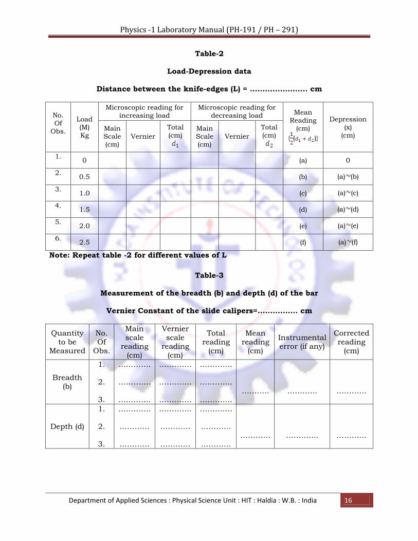
Table-2
Load-Depression data
Distance between the knife-edges (L) = ………………….. cm
No.
Of
Obs.
Load
(M)
Kg
Microscopic reading for
increasing load
Microscopic reading for
decreasing load Mean
Reading (cm)
( )
Depression
(x)
(cm) Main Scale
(cm)
Vernier
Total
(cm)
Main Scale
(cm)
Vernier
Total
(cm)
1.
0 (a) 0
2.
0.5 (b) (a) (b)
3.
1.0 (c) (a) (c)
4.
1.5 (d) (a) (d)
5.
2.0 (e) (a) (e)
6.
2.5 (f) (a) (f)
Note: Repeat table -2 for different values of L
Table-3
Measurement of the breadth (b) and depth (d) of the bar
Vernier Constant of the slide calipers=……………. cm
Quantity to be
Measured
No. Of
Obs.
Main scale
reading (cm)
Vernier scale
reading (cm)
Total reading
(cm)
Mean reading
(cm)
Instrumental error (if any)
Corrected reading
(cm)
Breadth (b)
1.
2.
3.
………….
………….
………….
………….
………….
………….
………….
………….
………….
………..
…………
…………
Depth (d)
1.
2.
3.
………….
…………
…………
………….
…………
…………
………….
…………
…………
…………
………….
…………

Physics -1 Laboratory Manual (PH-191 / PH – 291)
Department of Applied Sciences : Physical Science Unit : HIT : Haldia : W.B. : India 17
Graph(s): Plot a graph of depression (x) vs. load (M) as shown in Fig.2.
Fig.2: Load-depression curves.
Table-4
Determination of from Load –Depression graph
Chosen value of Load(M) on the
Graph (kg)
Length of the bar Between the knife-
Edges (L) meter
Depression (x) From the graph
(meter)
Value of
Table-5
Determination of Y
Value of
From table-4
Value of “b” From table-3
(meter)
Value of “d” From table-3
(meter)
Value of “g
Value of “Y”
Hence, the measured value of Young‟s Modulus (Y) of the material of the given bar is
=……………………………………………

Physics -1 Laboratory Manual (PH-191 / PH – 291)
Department of Applied Sciences : Physical Science Unit : HIT : Haldia : W.B. : India 18
VII. Maximum proportional error:
The measured quantities in this experiment are L, b, d, x.
The maximum proportional error in “ Y ” due to errors in the measurement of L, b, d,
x. is given by
Where = one smallest division of the meter scale by which the length of the bar
between two knife edges is measured.
the vernier constant of the slide calipers.
Vernier constant of the traveling microscope.
Now, multiply by 100 to obtain the maximum percentage error.
VIII. Discussion(s):
(i) In the working formula, Young‟s modulus Y is the function of the cube of length (L)
and depth (d), they should be measured very carefully, otherwise a large error will
occur in the value of Y.
(ii) The beam should be made horizontal and the loading should be made exactly at
the middle of the bar.
(iii) As the breaking load of the bar is very high, the maximum load on the hanger is
usually far below the breaking load. Hence it is unnecessary to find the breaking
load of the bar.
(iv) To minimize the error in measuring Y, it is available to find Y for three different
lengths of the bar and the length of the bar should not be below 80 cm.
(v) While measuring depression, to avoid back-lash error the microscope screw should
allows be rotated in the same direction.
(vi) After adding a load to the hanger, reading is to be taken after waiting for sometime
show that the depression is complete.
Physics -1 Laboratory Manual (PH-191 / PH – 291)
Department of Applied Sciences : Physical Science Unit : HIT : Haldia : W.B. : India 19
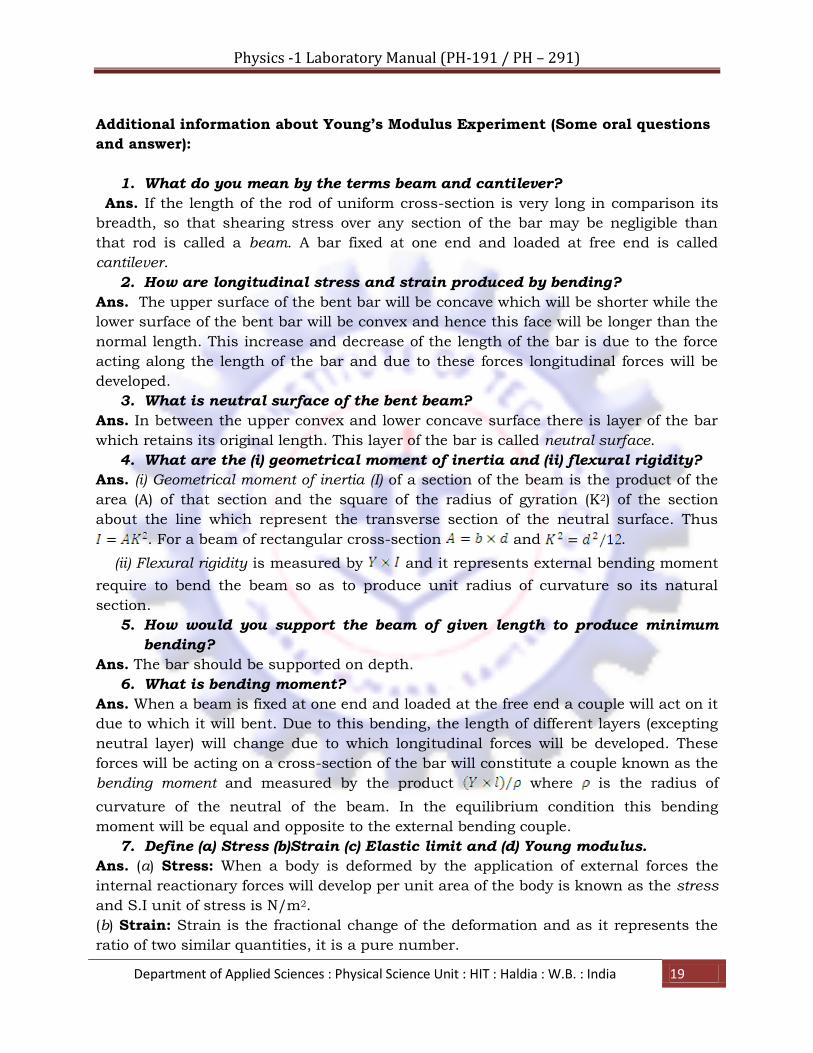
Additional information about Young’s Modulus Experiment (Some oral questions
and answer):
1. What do you mean by the terms beam and cantilever?
Ans. If the length of the rod of uniform cross-section is very long in comparison its
breadth, so that shearing stress over any section of the bar may be negligible than
that rod is called a beam. A bar fixed at one end and loaded at free end is called
cantilever.
2. How are longitudinal stress and strain produced by bending?
Ans. The upper surface of the bent bar will be concave which will be shorter while the
lower surface of the bent bar will be convex and hence this face will be longer than the
normal length. This increase and decrease of the length of the bar is due to the force
acting along the length of the bar and due to these forces longitudinal forces will be
developed.
3. What is neutral surface of the bent beam?
Ans. In between the upper convex and lower concave surface there is layer of the bar
which retains its original length. This layer of the bar is called neutral surface.
4. What are the (i) geometrical moment of inertia and (ii) flexural rigidity?
Ans. (i) Geometrical moment of inertia (I) of a section of the beam is the product of the
area (A) of that section and the square of the radius of gyration (K2) of the section
about the line which represent the transverse section of the neutral surface. Thus
. For a beam of rectangular cross-section and .
(ii) Flexural rigidity is measured by and it represents external bending moment
require to bend the beam so as to produce unit radius of curvature so its natural
section.
5. How would you support the beam of given length to produce minimum
bending?
Ans. The bar should be supported on depth.
6. What is bending moment?
Ans. When a beam is fixed at one end and loaded at the free end a couple will act on it
due to which it will bent. Due to this bending, the length of different layers (excepting
neutral layer) will change due to which longitudinal forces will be developed. These
forces will be acting on a cross-section of the bar will constitute a couple known as the
bending moment and measured by the product where is the radius of
curvature of the neutral of the beam. In the equilibrium condition this bending
moment will be equal and opposite to the external bending couple.
7. Define (a) Stress (b)Strain (c) Elastic limit and (d) Young modulus.
Ans. (a) Stress: When a body is deformed by the application of external forces the
internal reactionary forces will develop per unit area of the body is known as the stress
and S.I unit of stress is N/m2.
(b) Strain: Strain is the fractional change of the deformation and as it represents the
ratio of two similar quantities, it is a pure number.
Physics -1 Laboratory Manual (PH-191 / PH – 291)
Department of Applied Sciences : Physical Science Unit : HIT : Haldia : W.B. : India 20
(c) Elastic limit: The range of deformation over which the body return to its original
state when deforming forces are withdrawn, is called elastic limit.
(d) Young’s Modulus(Y): It is the ratio of the longitudinal stress and longitudinal
strain and its unit in S.I system is N/m2.
8. Will the value of Y change if l, b or d is change?
Ans. No. Y is the property of the material only.
9. Why don’t you take into account the depression due to the hanger?
Ans. Depression caused by the weight of hanger cancels out because we measure
depression by taking difference of the two readings.
10. Why do you support the beam with smaller dimension (d) in the
vertical direction?
Ans. Since depression , it causes greater depression. If b and d are interchanged
will be very small.
11. Does the weight of the beam have any effect in the result?
Ans. The weight causes some depression, but since depressions for difference loads
are calculated by taking difference of the two readings, the initial depression cancels
out. So the weight of the bar does not affects the results.
12. State the Hooke’s law.
Ans. Within elastic limit stress is proportional to strain.
i.e.
Here k is known as coefficient of elasticity.

Physics -1 Laboratory Manual (PH-191 / PH – 291)
Department of Applied Sciences : Physical Science Unit : HIT : Haldia : W.B. : India 21
Experiment No. : 06 (Group-2)
DETERMINATION OF RIGIDITY MODULUS OF THE
MATERIAL OF A WIRE BY DYNAMICAL METHOD
I. Objective(s): To determine the rigidity modulus of the material of a wire by
dynamical method.
II. Apparatus: A screw gauge, measuring tape, stop watch, slide calipers, rigidity
modulus experimental set-up etc..
III. Theory:
Within the elastic limit of a body, the ratio of tangential stress to the shearing strain is
called rigidity modulus of elasticity. The period (T) with which the bob of a torsion
pendulum oscillates with its suspension wire as axis, is given by-
T=
2
2
42 ,
I IorC
C T
(i)
Where, I is the moment of inertia of the suspended cylinder about its own axis and is
given by
I=1
2 (Mass). (Radius)2 (ii)
Here C represents the restoring couple exerted by the suspension wire of length l for
one radian twist at its free end and is given by,
C=
4
2
n r
l
(iii)
Where n is the rigidity of the material of the wire, while l and r are respectively the
length and radius of the suspension wire.
From (i) and (iii) we get
4
2
n r
l
=
2
2
4 I
T
or, n= 2 4
8 Il
T r
(iv)
Calculating I from the relation (ii) and by measuring l, r and T experimentally, we can
find the rigidity (n) of the wire by employing the relation (iv). If l and r are put in
meters, I in kg.m2 then n will be in N/m2.

Physics -1 Laboratory Manual (PH-191 / PH – 291)
Department of Applied Sciences : Physical Science Unit : HIT : Haldia : W.B. : India 22
IV. Experimental set-up:
Fig.1: Schematic diagram of Rigidity modulus experimental set-up.
V. Procedure:
(i) If the cylinder is detachable from the suspension wire, then it should be detached
from the suspension wire and its mass (M) is to be found out either by a rough balance
or by a spring balance, [if this cylinder is not detachable from the suspension wire
then its mass (M) should be supplied].
(ii) The diameter D of the cylinder is to be determined by a slide calipers at least in six
different places and at each place, the diameter in two perpendicular directions should
be found out. The mean of these diameters when halved we get the radius (R) of the
cylinder. Thus R=D/2. Knowing the mass M and the radius R of the cylinder, its
moment of inertia I about its own axis is calculated by using the formulae I= 1
2MR2.
(iii) The cylinder is then attached to the lower end of the suspension wire (provided the
cylinder is detachable from the suspension wire) and the length l of wire, from its

Physics -1 Laboratory Manual (PH-191 / PH – 291)
Department of Applied Sciences : Physical Science Unit : HIT : Haldia : W.B. : India 23
point of suspension to the point where the cylinder is attached, is measured by a scale
thrice and its mean value is found out.
(iv) The diameter of the suspension wire is measured by a screw gauge at least in eight
different places and at each place this diameter is found out in two perpendicular
directions. When the mean of these diameters (d) is halved and corrected for the
instrumental error of the screw gauge we get the mean corrected radius r = d/2 of the
suspension wire.
(v) To find the time period T of a chalk-mark is given on the circular scale just below
the pointer when the cylinder is at rest. (if there is no pointer, a vertical line N is
marked on the cylinder and is focused by a telescope from a distance such that the
line coincides with the vertical cross-wire of the telescope). The cylinder is then twisted
by a certain angle and is released to perform torsional oscillations about the vertical
axis. The pendulum linear oscillation (if any) should be stopped by leveling the base of
the pendulum stand. When the pointer is going towards right by crossing the chalk
mark (or when the vertical line of the cross-wire of the telescope) a stop-clock is
started and note the total time for 30 complete oscillations. The time for 30 complete
oscillations is noted thrice independently and the mean of this time when divided by
30, we get the period (T) of oscillation of the cylinder.
(vi) The value of the rigidity n is then calculated by putting the values of I, l, r and T
in the relation (iv).
Physics -1 Laboratory Manual (PH-191 / PH – 291)
Department of Applied Sciences : Physical Science Unit : HIT : Haldia : W.B. : India 24
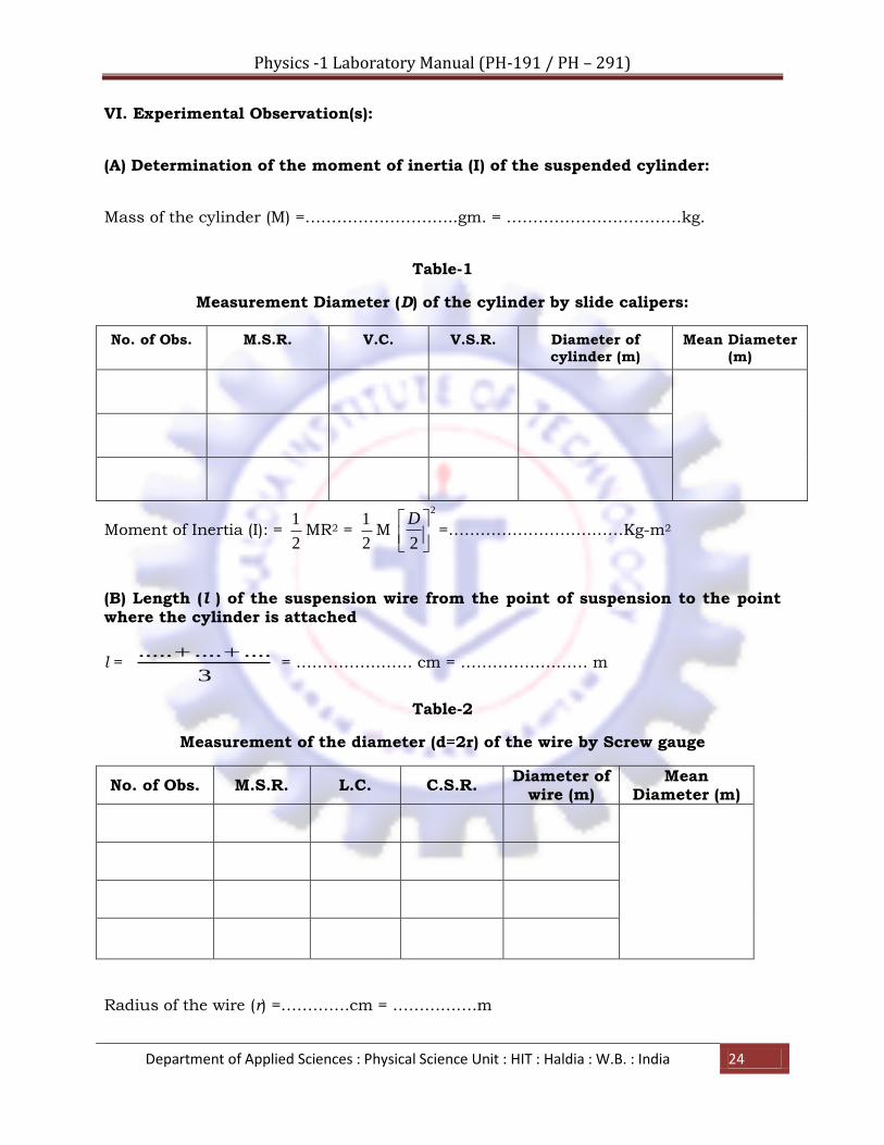
VI. Experimental Observation(s):
(A) Determination of the moment of inertia (I) of the suspended cylinder:
Mass of the cylinder (M) =………………………..gm. = ……………………………kg.
Table-1
Measurement Diameter (D) of the cylinder by slide calipers:
No. of Obs. M.S.R. V.C. V.S.R. Diameter of
cylinder (m)
Mean Diameter
(m)
Moment of Inertia (I): = 1
2MR2 =
1
2M
2
2
D
=……………………………Kg-m2
(B) Length (l ) of the suspension wire from the point of suspension to the point
where the cylinder is attached
l = ..... .... ....
3
= …………………. cm = …………………… m
Table-2
Measurement of the diameter (d=2r) of the wire by Screw gauge
No. of Obs. M.S.R. L.C. C.S.R. Diameter of
wire (m) Mean
Diameter (m)
Radius of the wire (r) =………….cm = …………….m
Physics -1 Laboratory Manual (PH-191 / PH – 291)
Department of Applied Sciences : Physical Science Unit : HIT : Haldia : W.B. : India 25
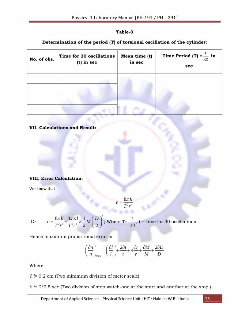
Table-3
Determination of the period (T) of torsional oscillation of the cylinder:
No. of obs. Time for 30 oscillations
(t) in sec
Mean time (t)
in sec
Time Period (T) =30
t in
sec
VII. Calculations and Result:
VIII. Error Calculation:
We know that-
2 4
8 Iln
T r
Or
2
2 4 2 4
8 8 1
2 2
Il l Dn M
T r T r
; Where T=
30
t, t = time for 30 oscillations
Hence maximum proportional error is
max
2 24
n l t r M D
n l t r M D
Where
l= 0.2 cm (Two minimum division of meter scale)
t= 2*0.5 sec (Two division of stop watch-one at the start and another at the stop.)
Physics -1 Laboratory Manual (PH-191 / PH – 291)
Department of Applied Sciences : Physical Science Unit : HIT : Haldia : W.B. : India 26
r= 0.001 cm (L.C of screw gauge)
D=0.01 cm (V.C of slide calipers)
As M is large M
M
can be neglected. Now putting a typical set of observed data for l,t,r
and D we can calculate
max
n
n
Next multiplying it by 100, we get % error of „n’.
IX. Discussion(s):
(i) The pendulum oscillation of the cylinder (if any) should be stopped.
(ii) Care is to be taken to see that the suspension wire may coincide with the axis of
the cylinder.
(iii) The radius r of the suspension wire occurs in 4th power and hence it should be
measured very carefully otherwise a small error in the measurement of r will increase
the error in the determination of n by four times.
(iv)The period (T) of the oscillation should also be measured very carefully for it occurs
in the second power in the expression of n.
********
Additional information:
Different Moduli of Elasticity are given below-
1. Young's modulus (Y): Within the elastic limit of a body, the ratio between the
longitudinal stress and the longitudinal strain is called the Young's modulus of
elasticity.
Y = longitudinal stress
longitudinal strain =
F l
A l (N/m2)
Where F is the force acting on the surface of area A, Δl is the increase in length in a
Physics -1 Laboratory Manual (PH-191 / PH – 291)
Department of Applied Sciences : Physical Science Unit : HIT : Haldia : W.B. : India 27
length l of the wire.
2. Rigidity modulus (n): Within the elastic limit of a body, the ratio of tangential
stress to the shearing strain is called rigidity modulus of elasticity. The rigidity
modulus
n =tangential stress
shearing strain =
/
/
F A
l x =
F x
Al
(N/m2)
Where F/A is the tangential stress, Δx the displacement in a length l in the
perpendicular direction
3. Bulk modulus (K): It is defined as the ratio of stress to volumetric strain.
K = stress
bulk strain =
P V
V
(N/m2)
Where P is the pressure, V is the original volume and ΔV is the change in volume of
the material
4. Compressibility: The reciprocal of the bulk modulus is called compressibility.
Compressibility = 1/K
Poisson's ratio: When a sample of material is stretched in one direction, it tends to
get thinner in the other two directions. Poisson's ratio (ν), is a measure of this
tendency. Poisson's ratio is the ratio of the relative contraction strain, or transverse
strain (normal to the applied load), divided by the relative extension strain, or axial
strain (in the direction of the applied load). For a perfectly incompressible material
deformed elastically at small strains, the Poisson's ratio would be exactly 0.5. Most
practical engineering materials have between 0.0 and 0.5. Cork is close to 0.0, most
steels are around 0.3, and rubber is almost 0.5.

Physics -1 Laboratory Manual (PH-191 / PH – 291)
Department of Applied Sciences : Physical Science Unit : HIT : Haldia : W.B. : India 28
Standard values of different elastic constants are listed below-
Possible Questions:
1) Define rigidity modulus and state its unit.
2) The formulae for rigidity involves length and radius of the wire, how do they
influence rigidity modulus?
3) Which quantity would you measure very accurately and why?
4) How rigidity modulus (n) is related to Young‟s modulus (Y)?
5) What is the effect of increase of temperature on the rigidity of the wire?
6) Does the period of oscillation depend on the amplitude of oscillation of the cylinder?
7) What is the difference between simple rigidity and torsional rigidity?
8) How will the period of oscillation of a torsional pendulum be affected when the
length and diameter of the suspension wire is increased?
9) How will be the period of oscillation be affected if the bob of the pendulum be made
heavy?
10) Will the period be affected by the change in the acceleration due to gravity?
11) Why do you call the method a dynamical method?
12) Is the motion simple harmonic?
Material Rigidity Modulus
(1010 N/m2) Young‟s Modulus
(1010 N/m2) Poisson‟s Ratio
Steel 7.9 - 8.9 19.5 - 20.6 0.28
Aluminium 2.67 7.50 0.34
Copper 4.55 12.4 - 12.9 0.34
Iron (Wrought) 7.7 - 8.3 19.9 - 20.0 0.27
Brass 3.5 9.7-10.2 0.34 - 0.38
Physics -1 Laboratory Manual (PH-191 / PH – 291)
Department of Applied Sciences : Physical Science Unit : HIT : Haldia : W.B. : India 29
Experiment No. : 07 (Group-2)
DETERMINATION OF COEFFICIENT OF VISCOSITY OF
WATER BY POISEULLE’S METHOD
I. Objective: The aim of this experiment is to determine the coefficient of viscosity of
water by Poiseulle‟s method.
II. Theory:
When water is allowed to flow in a stream line manner through a uniform capillary
tube of length and radius , volume of water flowing per second is given by-
(i)
Where P is the pressure difference between the two ends of the capillary tube, is the
coefficient of viscosity of water.
If the pressure difference be measure by type water manometer then
(ii)
Where be the difference of water levels in two arms of the tube and is the density
of water. Hence
(iii)
If is expressed in , in cm and in then will be in
or .
In order to be sure that the motion of the liquid is in streamline the value of should
be kept below the critical height . By finding one nominal value of from relation
(iii) the critical value can be found out from the relation
(iv)
Where is the Reynold‟s number (k ≈ 1000 for narrow tube) and is the density of the
liquid.

Physics -1 Laboratory Manual (PH-191 / PH – 291)
Department of Applied Sciences : Physical Science Unit : HIT : Haldia : W.B. : India 30
III. Experimental Set up:
Fig.1:
Experimental arrangement to show the necessary apparatus for this experiment.
IV. Experimental Procedure:
Step 1: Set up the apparatus as shown in figure
Step 2: Control the pinch cock „S‟ so that water flows through the capillary at slow
rate and collects in the beaker, drop by drop. When the columns of water in the
manometer tubes „E‟ & „F‟ are in steady, note the levels of water in „E‟& „F‟. Designate
the reading by R1 and R2 respectively, the difference (R1 ~ R2) of the two readings gives
i.e. pressure difference in terms of the height of the liquid column.
Step 3: Note the temperature (t in 0C) of the liquid in the beaker by a thermometer.
Take the value of the density ρ of the liquid at this temperature from physical table.
Step 4: When the flow of water through the capillary tube T has been steady, put a
clean & dry glass beaker below the exit tube at the end B, As soon as water starts
collecting in beaker, start a stop watch. Allow the water to collect a little more than
half volume of the beaker. When the collection is over, remove the beaker and stop the
stop watch.
Step 5: (rate of flow of water) may be determined the measuring the volume of the
liquid collected in t sec. with the help of a measuring cylinder and dividing by t.
Step 6: Measure several other value of . Each value of should be so chosen that
the liquid flows in the capillary tube in stream lines.
Step 7: Draw a graph by plotting (cm) along X-axis and the corresponding (cm3/
sec) along Y-axis. The graph will be straight line and passing through the origin (0,0).
Physics -1 Laboratory Manual (PH-191 / PH – 291)
Department of Applied Sciences : Physical Science Unit : HIT : Haldia : W.B. : India 31
Step 8: On the graph choose a point and obtain the corresponding values of and .
Calculate the value of from the relation, . Compute the co-efficient of
viscosity by using equation (iii).
V. Experimental Observations:
a. Length of the capillary tube =…………………………..cm
b. Radius of the capillary tube =………………………………..cm
c. Critical height: =……………………….. cm
Table- 1
Pressure difference in terms of height from manometer readings:
Temperature of water = ………………0C
Density of water at that temperature (ρ) = …………..gm/cc.
Value of g = 980cm/sec2
No. of observation
Height of water level in 1st arm (R1)
in cm
Height of water level in 2nd arm (R2)
in cm
Difference height
Pressure difference
dyne/cm2

Physics -1 Laboratory Manual (PH-191 / PH – 291)
Department of Applied Sciences : Physical Science Unit : HIT : Haldia : W.B. : India 32
Table-2
Measurement of Rate of flow of water:
No. of observation
Pressure difference from
Table-1
Volume of the collected water (vt) in
cc
Time for collection of
water (t) (sec)
Rate of flow of water
V=vt/t (c.c./sec)
VI. Calculation and Result:
Table-3
Data for graph:
No. of observation
from Table-1 (cm) Corresponding V (from Table-2) (cm3/sec)
Fig.2: h vs. V graph

Physics -1 Laboratory Manual (PH-191 / PH – 291)
Department of Applied Sciences : Physical Science Unit : HIT : Haldia : W.B. : India 33
Table-4
Calculation of Co-efficient of viscosity (η) of water at t 0C from graph:
from
graph
from
graph
Slope of the graph
length
in cm in cm4
(Poise)
Hence, Co-efficient of viscosity at temperature ..…..0C = …..……dyne. Sec/cm2
or Poise
VII. Error calculation:
We know ;
Where, represents the volume of the liquid collected in time t. the maximum
proportional error in the measurement of is given by
Since, , g, r & l are not measured (supplied). Then
Therefore maximum proportional error
Physics -1 Laboratory Manual (PH-191 / PH – 291)
Department of Applied Sciences : Physical Science Unit : HIT : Haldia : W.B. : India 34
VIII. Precaution &Discussions:
1. Since radius r occurs in the fourth power, the radius of the capillary tube
should be uniform and measured it very carefully.
2. Due to capillary action the out-flowing liquid from the end of the tube may
run back along the outside of the tube. To prevent this, a little vaseline
should be smeared on the outside of the tube near its free end.
3. The height difference of the two arms of manometer should below the critical
height; otherwise flow of water through capillary tube would be turbulent.
4. You should check the beaker in which you will collect the water is
completely dry or not. If not then first dry it as much as possible and then
collect water for a known interval of time until the beaker is greater than
half full.
5. The temperature of the water should be noted carefully as the value of the
coefficient of viscosity changes rapidly with temperature.
Additional information:
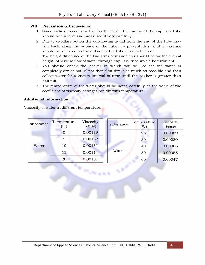
Viscosity of water at different temperature:
substance Temperature
(0C) Viscosity (Poise)
Water
0 0.00179
5 0.00152
10 0.00131
15 0.00114
20 0.00101
substance Temperature
(0C) Viscosity (Poise)
Water
25 0.00089
30 0.00080
40 0.00066
50 0.00055
60 0.00047

Physics -1 Laboratory Manual (PH-191 / PH – 291)
Department of Applied Sciences : Physical Science Unit : HIT : Haldia : W.B. : India 35
Experiment No.: 08 (Group-3)
DETERMINATION OF WAVELENGTH OF LIGHT BY
NEWTON’S RINGS METHOD
I. Objective: The objective of this experiment is to determine the wavelength of
sodium light by forming Newton‟s rings.
II. Apparatus: Sodium Vapour Lamp, Newton‟s rings set-up.
III. Ray diagram:
A thin wedge shaped air film is created by placing a plano-convex lens on a flat glass
plate. A monochromatic (sodium vapour lamp) beam of light is made to fall at almost
normal incidence on the arrangement. Ring like interference fringes (fig.2) are
observed through eyepiece due to reflected light.
Fig.1: Ray diagram of Newton’s Rings Experiment
A horizontal beam of light falls on the glass plate G at an angle of 450. The reflected
beam from the air film is viewed with a microscope. Interference takes place and dark
and bright circular fringes are produced. This is due to the interference between the
light reflected at the lower surface of the lens and the upper surface of the plate G by
division of amplitude.
Physics -1 Laboratory Manual (PH-191 / PH – 291)
Department of Applied Sciences : Physical Science Unit : HIT : Haldia : W.B. : India 36
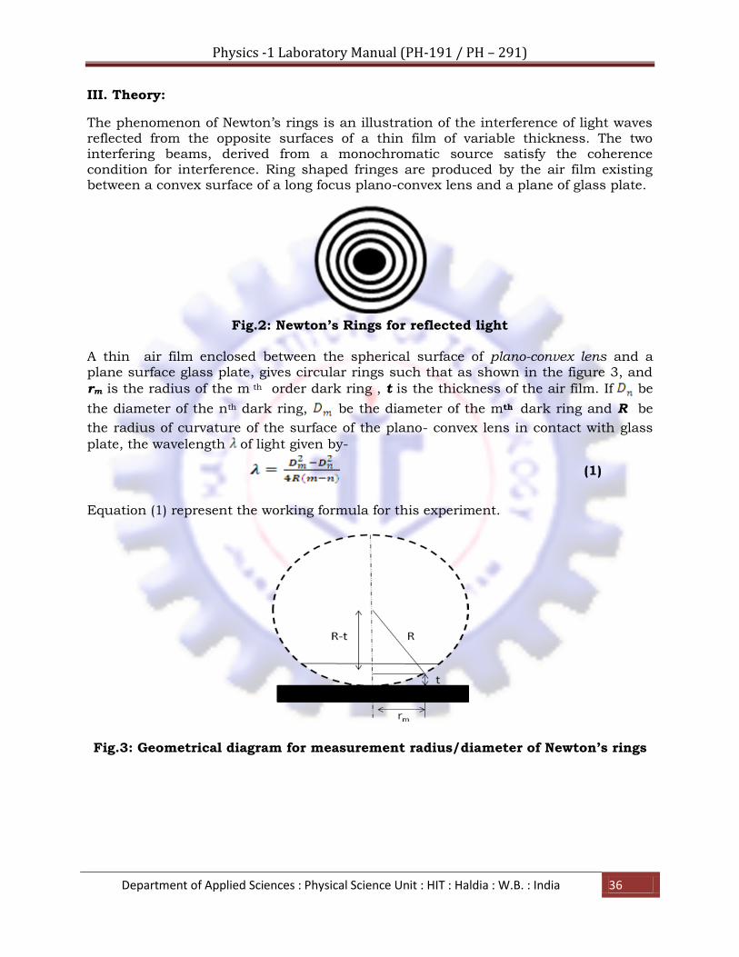
III. Theory:
The phenomenon of Newton‟s rings is an illustration of the interference of light waves reflected from the opposite surfaces of a thin film of variable thickness. The two interfering beams, derived from a monochromatic source satisfy the coherence condition for interference. Ring shaped fringes are produced by the air film existing between a convex surface of a long focus plano-convex lens and a plane of glass plate.
Fig.2: Newton’s Rings for reflected light
A thin air film enclosed between the spherical surface of plano-convex lens and a plane surface glass plate, gives circular rings such that as shown in the figure 3, and
rm is the radius of the m th order dark ring , t is the thickness of the air film. If be
the diameter of the nth dark ring, be the diameter of the mth dark ring and R be
the radius of curvature of the surface of the plano- convex lens in contact with glass
plate, the wavelength of light given by-
(1)
Equation (1) represent the working formula for this experiment.
Fig.3: Geometrical diagram for measurement radius/diameter of Newton’s rings

Physics -1 Laboratory Manual (PH-191 / PH – 291)
Department of Applied Sciences : Physical Science Unit : HIT : Haldia : W.B. : India 37
V. Procedure:
1. Determine the least count of the circular scale associated with the apparatus.
2. Switch on the sodium vapour lamp. Wait till it turns yellow. Adjust the mirror
such that light is reflected on the lens. Focus the microscope to see sharp
circular fringes. Adjust the mirror if necessary to increase the contrast in the
fringes.
3. Adjust the screws to bring the central dark spot at the crosswire. Now, move
horizontally to a dark ring of large diameter, say the 20th ring. Place the
crosswire tangentially to the ring. Take the horizontal main scale and the
circular scale readings.
4. Move the crosswire towards the centre to another ring skipping 4 rings. Note
the ring number and the microscope reading.
5. Repeat the step 4 till the smallest distinct circular ring is reached (i.e. 16th, 12th,
8th and 4th). Continue towards the other direction and take readings for the
order ends of the same rings as before (i.e. 4th, 8th, 12th, 16th and 20th).
6. Repeat the step 4 and step 5 but this time moving in opposite direction. Thus,
the diameters of each ring will be measured twice.
7. Draw a graph with in the coordinate and m in the abscissa, where m is the
order number of the ring. Determine the slope of this straight line with integer
values of m. This will yield the value of in the working formula for
wavelength.
VI. Experimental Observations:
Table 1
To determine the least count of the circular scale
No of div. in the circular scale (n)
Screw Pitch (x) in mm
Least Count L.C=x/n in mm

Physics -1 Laboratory Manual (PH-191 / PH – 291)
Department of Applied Sciences : Physical Science Unit : HIT : Haldia : W.B. : India 38
Table 2
Experimental data to measure the diameter of Newton’s Rings
Graph Plotting: A graph will be plotted between (along Y axis) vs. m (along X axis)
and then find λ from this graph considering m-n=6.
Fig.4: vs. m plot for Newton’s rings.
Movin
g r
igh
t to
left
No o
f ri
ngs
Microscopic reading
Dm=X
~Y
( cm
)
Avg D
m
Dm
2 i
n
cm
2
m-n
Left (X)
Right(Y)
M..S.R
(cm
)
L.C
.
C.S
.R
(cm
)
Tota
l
M.S
.R
(cm
)
L.C
.
C.S
.R
(cm
)
Tota
l
(cm
)
Movin
g left
to
righ
t
0 2 4 6 8 10 12 14 160
10
20
30
40
50
60
70
80
90
100
Sq
uare o
f th
e d
iam
ete
r (
Dm
2)
(mm
2)
Order number of the ring (m)
Central dark
Central bright

Physics -1 Laboratory Manual (PH-191 / PH – 291)
Department of Applied Sciences : Physical Science Unit : HIT : Haldia : W.B. : India 39
VII. Calculations and Result:
=
VIII. Maximum Percentage of Error:
The Maximum Percentage of Error can be calculated by using this relation
× 100%
IX. Discussions: Notice that, as you go away from the central dark spot, the fringe width decreases. In order to minimize the errors in measurement of the diameter of the rings the following precautions should be taken:
i) The microscope should be parallel to the edge of the glass plate. ii) If you place the cross wire tangential to the outer side of a perpendicular ring
on one side of the central spot then the cross wire should be placed tangential to the inner side of the same ring on the other side of the central spot.
iii) The traveling microscope should move to and fro only in one direction.

Physics -1 Laboratory Manual (PH-191 / PH – 291)
Department of Applied Sciences : Physical Science Unit : HIT : Haldia : W.B. : India 40
Experiment No. : 09 (Group-3)
DETERMINATION OF THE WAVELENGTH OF A
MONOCHROMATIC LIGHT BY FRESNEL’S BI-PRISM
METHOD
I. Objectives: To determine the wavelength of a monochromatic light by Fresnel‟s bi-
prism method.
II. Apparatus: Fresnel‟s bi-prism, source of monochromatic light (Sodium vapour lamp),
a slit, a micrometer eyepiece, a convex lens, an optical bench with four stands.
III. Theory and Working Formula:
A bi-prism may be regarded as made up of two prisms of very small refracting
angles placed base to base. In actual practice a single glass plate is suitably grinded
and polished to give a single prism of obtuse angle 179° leaving remaining two acute
angles of 30′ each. If monochromatic light of wavelength λ from a point source S is
made emergent on the two halves of the bi-prism LMN then the emergent beam from
the bi-prism appears to diverge from two virtual images S1 and S2 (Fig. 1). Thus two
coherent sources have been formed (S1 and S2) from a single source (S) by the division
of wavefront with the help of the bi-prism. Fig. 1 shows ray diagram of the
experimental arrangement to determine the wavelength of monochromatic light using
Fresnel‟s bi-prism. Rays from the two virtual sources interfere with each other and
form alternating dark and bright bands. The fringes are hyperbolic, but due to high
eccentricity they appear to be straight lines in the focal plane of the eyepiece (E). The
Fringe width (β) is given by-
(1)
Where, λ is the wavelength of the monochromatic light, d is the apparent distance
between the two coherent virtual sources S1 and S2. D denotes the distance between
the slit and the focal plane of the eyepiece.
If β1 and β2 represent fringe width at distances D1 and D2 respectively, then the
wavelength is given by,
(2)
However, d cannot be directly measured as the sources are virtual. To find out the
value of d, a convex lens of focal length f (so that, D1 or D2 > 4f) is placed between the
bi-prism and the eyepiece so that for its two positions L1 and L2 real images of S1 and
S2 may be focused at the focal plane of the eyepiece. If d1 and d2 are the separations

Physics -1 Laboratory Manual (PH-191 / PH – 291)
Department of Applied Sciences : Physical Science Unit : HIT : Haldia : W.B. : India 41
between the two real images of S1 and S2 for the two positions L1 and L2 of the lens,
then d is obtained from the relation,
(3)
Thus the wavelength of the monochromatic light can be expressed as,
(4)
Equation (4) is the working formula for this experiment. By measuring the fringe width
(β1 and β2), the separation between the two virtual sources (d1 and d2) and the
distance between the slit and the eyepiece (D1 and D2) the wavelength of
monochomatic light can be determined.
Fig. 1: Ray diagram of the experimental arrangement to determine the
wavelength of monochromatic light using Fresnel’s bi-prism
IV. Procedure:
1. Set the slit vertical and bright by adjusting the source. Set the bi-prism edge
vertical with flat side facing the slit. Adjust the height so that the centre of the slit
and the centre of the bi-prism are in the same height. Bring both of them in the
middle of the bench.
2. Bring the eyepiece close to the bi-prism. Look through it. Move the eyepiece in the
direction perpendicular to the length of the optical bench until its axis passes
through the centre of the bi-prism and the slit. Focus the eyepiece so that the
D
S1
S
S2
L
M
N
L1 L2
P
Q
d
E

Physics -1 Laboratory Manual (PH-191 / PH – 291)
Department of Applied Sciences : Physical Science Unit : HIT : Haldia : W.B. : India 42
fringes can be seen. If not turn the bi-prism using the transverse and tangent
screws.
3. Replace the sodium (Na) light by white light. A coloured fringe with a white centre
will be visible. Move the eyepiece near and farther to the bi-prism, always keeping
the central white line on the cross-wire by adjusting the micrometer screw of the
eyepiece at all positions.
4. Bring the Na lamp back. Move the eyepiece at a certain distance. Note down the
position of the slit and the eyepiece on the optical bench. Look through the
eyepiece. Go to the extreme right white band. Note the position of the eyepiece on
the micrometer scale. Go to the bright band on the left side keeping 2 to 3 lines.
Note eyepiece position. If you have skipped 3 lines then the difference between
these two successive readings will give you 4 times the fringe width. Repeat this
step unless you reach the left extreme. Now start moving in the opposite direction
each time noting the position of the eyepiece.
5. Move the eyepiece to another distance and repeat step 4.
6. Place a convex lens between the eyepiece and the bi-prism. Move the eyepiece to a
distance slightly more than four times the focal length of the lens. Look through
the eyepiece and change the position of the lens. For two positions of the lens two
images of the slit can be seen. Go to one of the positions. Find the separation (d1)
between the images by bringing each of the images on the cross-wire by rotating
the micrometer screw and noting the reading in each case. Go to the second
position and find the separation (d2) between the images.
V. Experimental Observations:
Table-1
Determination of Least Count of the micrometer
Screw Pitch (x) in mm No. of divisions on the circular scale (n)
Least Count (x/n) in mm
Physics -1 Laboratory Manual (PH-191 / PH – 291)
Department of Applied Sciences : Physical Science Unit : HIT : Haldia : W.B. : India 43
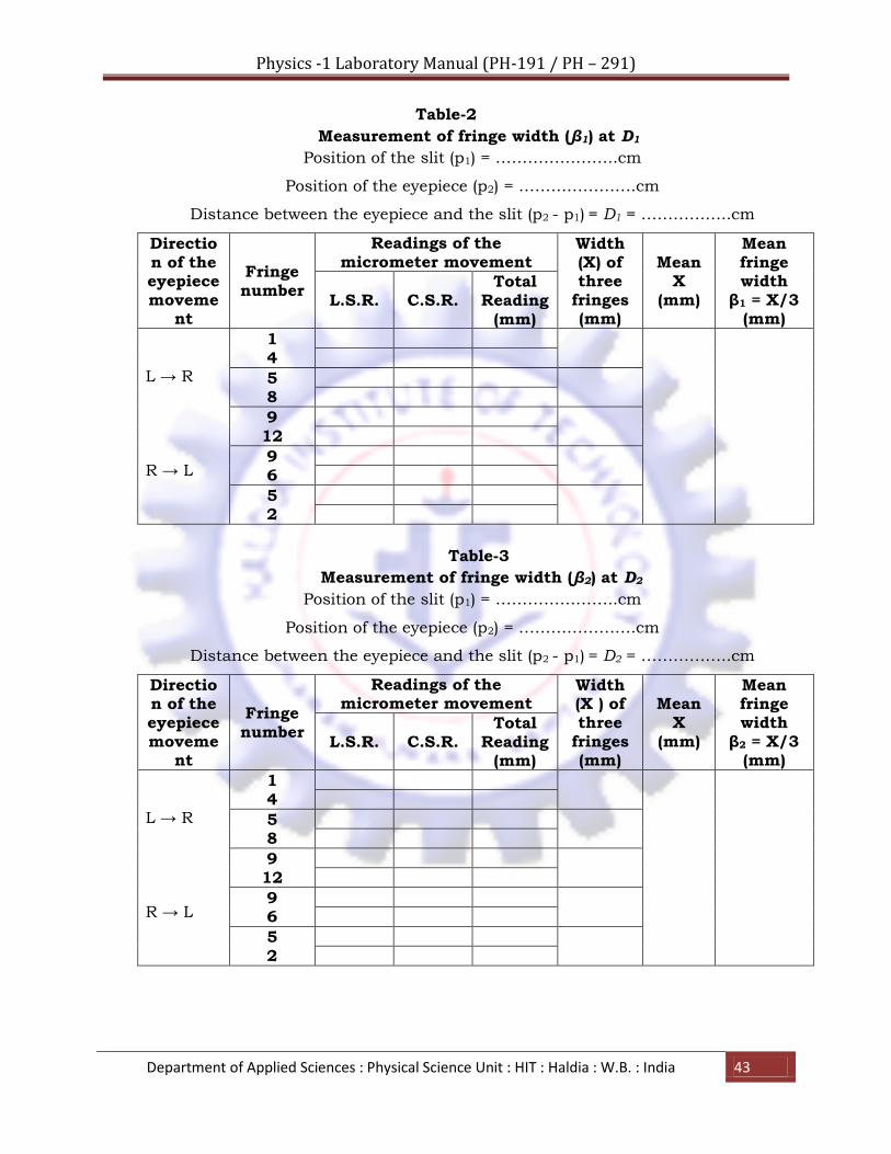
Table-2
Measurement of fringe width (β1) at D1
Position of the slit (p1) = …………………..cm
Position of the eyepiece (p2) = ………………….cm
Distance between the eyepiece and the slit (p2 - p1) = D1 = ……………..cm
Direction of the eyepiece moveme
nt
Fringe number
Readings of the micrometer movement
Width (X) of three
fringes (mm)
Mean X
(mm)
Mean fringe width
β1 = X/3 (mm)
L.S.R. C.S.R. Total
Reading (mm)
L → R R → L
1 4
5 8
9 12
9 6
5 2
Table-3
Measurement of fringe width (β2) at D2
Position of the slit (p1) = …………………..cm
Position of the eyepiece (p2) = ………………….cm
Distance between the eyepiece and the slit (p2 - p1) = D2 = ……………..cm
Direction of the eyepiece moveme
nt
Fringe number
Readings of the micrometer movement
Width (X ) of three
fringes (mm)
Mean X
(mm)
Mean fringe width
β2 = X/3 (mm)
L.S.R. C.S.R. Total
Reading (mm)
L → R R → L
1 4
5 8
9 12
9 6
5 2

Physics -1 Laboratory Manual (PH-191 / PH – 291)
Department of Applied Sciences : Physical Science Unit : HIT : Haldia : W.B. : India 44
Table-4
Measurement of d1 and d2 and hence d
Position of the slit = …………………cm
Position of the bi-prism = ……………….cm
Position of the eyepiece = ……………….cm
Focal length of the lens = ………………… cm
No. of
Obs.
Lens positi
on (cm)
Direction of
eyepiece
movement
Reading of the micrometer (mm) Separati
on between
the images r1~r2 (mm)
Mean
separa-
tion (mm)
d =
(mm)
For Left image For Right image
L.S.R
C.S.R
Total Reading(r1)
L.S.R
C.S.R
Total Reading (r2)
1.
L → R d1=
2. R → L
1.
L → R d2 =
2. R → L
Table-5
Determination of wavelength (λ) of monochromatic light
Distance (D) between the slit and the eyepiece
in mm
Fringe width (β) in mm
Value of d in mm
Value of λ in Ǻ
D1 =
D2 =
β1 =
β2 =

Physics -1 Laboratory Manual (PH-191 / PH – 291)
Department of Applied Sciences : Physical Science Unit : HIT : Haldia : W.B. : India 45
VI. Percentage error:
The working formula is-
Therefore the maximum proportional error can be represented as,
where, δβ = δd1 = δd2 = smallest measuring distance (least count) of the
micrometer.
Hence the maximum percentage error is,
VII. Discussions:
(i) The fringe width (β) can be made smaller by increasing the distance between
the slit and the bi-prism. Again β can be increased by increasing the
distance between the slit and the eyepiece. Hence these distances should be
judiciously adjusted to make fringes neither too wide nor too narrow.
(ii) The convex lens employed to focus the real images of the virtual sources at
the focal plane of the eyepiece should be of such focal length (f) so that D >
4f.
(iii) The displacement of the lens to get the real images of the virtual sources at
its two positions should not be very large, otherwise proportional error in
measuring d would be greater.
(iv) The measurement of the fringe width is to be done very carefully as it has
the maximum contribution in the error calculation.
(v) The instrument should be properly aligned so that there may not be any
relative shift between the fringe and the cross-wires, as the eyepiece is
moved along the optical bench.
(vi) The strongly illuminated part of the source must be placed behind the slit. If
necessary, a convex lens may be used to concentrate the light on the slit.

Physics -1 Laboratory Manual (PH-191 / PH – 291)
Department of Applied Sciences : Physical Science Unit : HIT : Haldia : W.B. : India 46
Experiment No. : 10 (Group-3)
DETERMINATION OF THE WAVELENGTH OF He-Ne LASER BY
STUDYING THE DIFFRACTION OF MONOCHROMATIC LIGHT BY
PLANE TRANSMISSION GRATING
I. Objective: To determine the wavelength of He-Ne Laser by studying the diffraction
of monochromatic light by plane transmission grating.
II. Apparatus:
1. Meter Scale
2. He-Ne Laser
3. Plane transmission Grating
4. Optical Bench
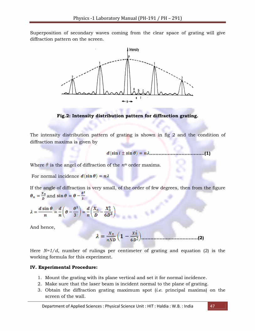
III. Theory: When a wavefront is incident on a grating surface, light is transmitted through the
slits and obstructed by the opaque portions. The secondary waves from the positions
of the slit interface with one another similar to the interference of waves in Young‟s
experiment. If the spacing between the lines is of the order of the wavelength of light
then an appreciable deviation of the light is produced.
We consider a grating of N slits per centimeter having clear space of width a each are
separated by opaque space b placed on the optical bench. A parallel beam of laser
incident on it at an angle i with the normal to the grating surface.
Fig.1: Laser diffraction from a grating of grating element (d = a+b).
Physics -1 Laboratory Manual (PH-191 / PH – 291)
Department of Applied Sciences : Physical Science Unit : HIT : Haldia : W.B. : India 47
Superposition of secondary waves coming from the clear space of grating will give
diffraction pattern on the screen.
Fig.2: Intensity distribution pattern for diffraction grating.
The intensity distribution pattern of grating is shown in fig 2 and the condition of
diffraction maxima is given by
………………………………(1)
Where is the angel of diffraction of the nth order maxima.
For normal incidence
If the angle of diffraction is very small, of the order of few degrees, then from the figure
and
And hence,
……………………………….(2)
Here N=1/d, number of rulings per centimeter of grating and equation (2) is the
working formula for this experiment.
IV. Experimental Procedure:
1. Mount the grating with its plane vertical and set it for normal incidence.
2. Make sure that the laser beam is incident normal to the plane of grating.
3. Obtain the diffraction grating maximum spot (i.e. principal maxima) on the
screen of the wall.
Physics -1 Laboratory Manual (PH-191 / PH – 291)
Department of Applied Sciences : Physical Science Unit : HIT : Haldia : W.B. : India 48
4. Measure . and D by meter scale.
5. Calculate the value of for each order on both sides and obtain the mean value.
6. Repeat it for another D value.
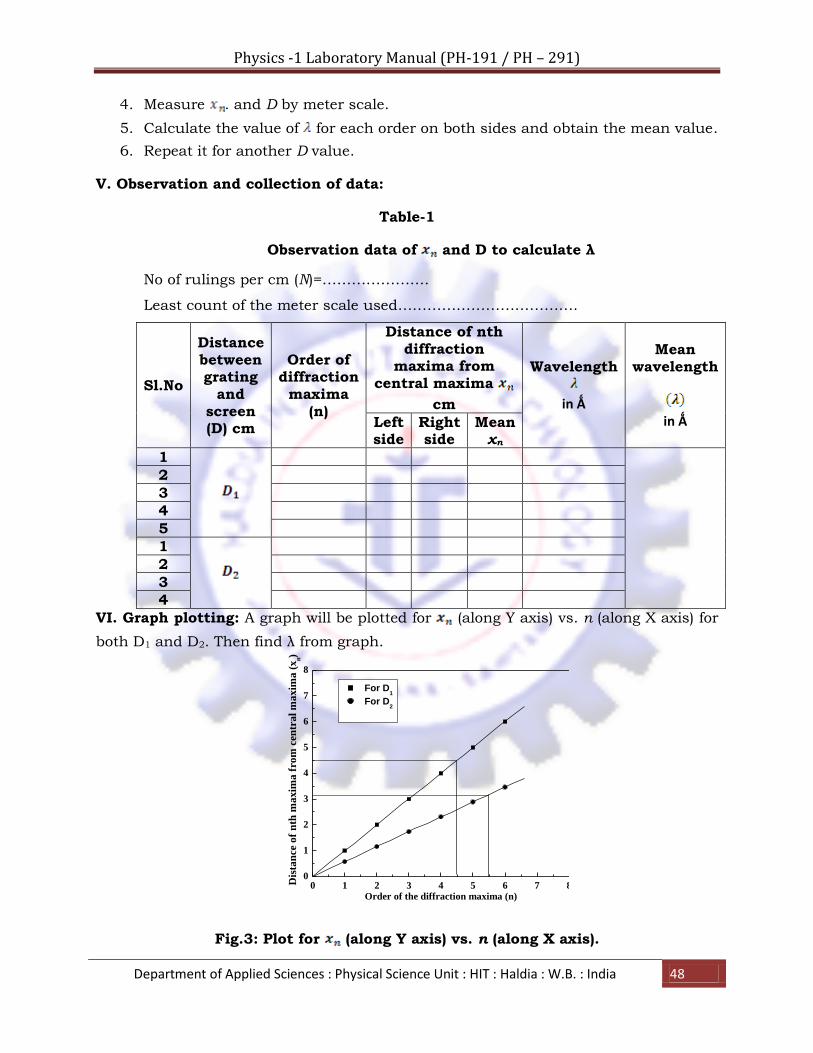
V. Observation and collection of data:
Table-1
Observation data of and D to calculate λ
No of rulings per cm (N)=………………….
Least count of the meter scale used……………………………….
Sl.No
Distance between grating
and screen (D) cm
Order of diffraction maxima
(n)
Distance of nth diffraction
maxima from central maxima
cm
Wavelength
in Ǻ
Mean wavelength
in Ǻ Left
side Right side
Mean xn
1
2
3
4
5
1
2
3
4
VI. Graph plotting: A graph will be plotted for (along Y axis) vs. n (along X axis) for
both D1 and D2. Then find λ from graph.
Fig.3: Plot for (along Y axis) vs. n (along X axis).
0 1 2 3 4 5 6 7 80
1
2
3
4
5
6
7
8
Dis
tan
ce o
f n
th m
axim
a f
rom
cen
tra
l m
axim
a (
xn)
Order of the diffraction maxima (n)
For D1
For D2
Physics -1 Laboratory Manual (PH-191 / PH – 291)
Department of Applied Sciences : Physical Science Unit : HIT : Haldia : W.B. : India 49
VII. Error calculation:
Working formula is
Here, the maximum proportional error is introduced due to third power of . and D
Hence
VIII. Result and Discussions:
(i) From the study of diffraction of monochromatic light beam by plane
transmission grating we obtain the wavelength of He-Ne laser and it is……..
(ii) If we plot a graph for against n, then we find for lower values of the plot is
nearly a straight line. We can obtain by equating the slope of that straight
line with and compare it with the mean values of .
(iii) LASER light is dangerous, so it should be careful that LASER light can‟t fall
into eye.

Physics -1 Laboratory Manual (PH-191 / PH – 291)
Department of Applied Sciences : Physical Science Unit : HIT : Haldia : W.B. : India 50
Experiment No. : 11 (Group-3)
DETERMINATION OF NUMERICAL APERTURE,
ANGLE OF ACCEPTANCE AND BENDING ENERGY
LOSSES OF AN OPTICAL FIBRE
I. Objective(s): To determine the numerical aperture, angle of acceptance and bending
energy losses of an optical fibre.
II. Theory:
Numerical aperture is a basic descriptive characteristics of a specific fibre. This
represents the „size of openness‟ of the input acceptance cone. Mathematically,
numerical aperture (NA) is defined as the Sine of the half angle of the acceptance cone.
The light gathering power or flux carrying capacity of a fibre is numerically equal to
the sequence of the aperture, which is the ratio between the area of a unit sphere with
the acceptance cone and the area of the hemisphere (2П solid angle).
Snell‟s law can be used to calculate the maximum angle within which light will be
accepted into and conducted through the fibre.
NA = Sin θa = (n12 – n2
2)1/2
Where Sin θa is the numerical aperture and n1 & n2 are the refractive indices of the
core and the cladding. The semi angle θa (determined) of the acceptance cone for a
step index fibre is determine by the critical angle ( θc ), where θc = Sin - 1 (n1 / n2).
Fig. 1: Propagation of light beam through the fibre.
n1
n2
θa
Physics -1 Laboratory Manual (PH-191 / PH – 291)
Department of Applied Sciences : Physical Science Unit : HIT : Haldia : W.B. : India 51
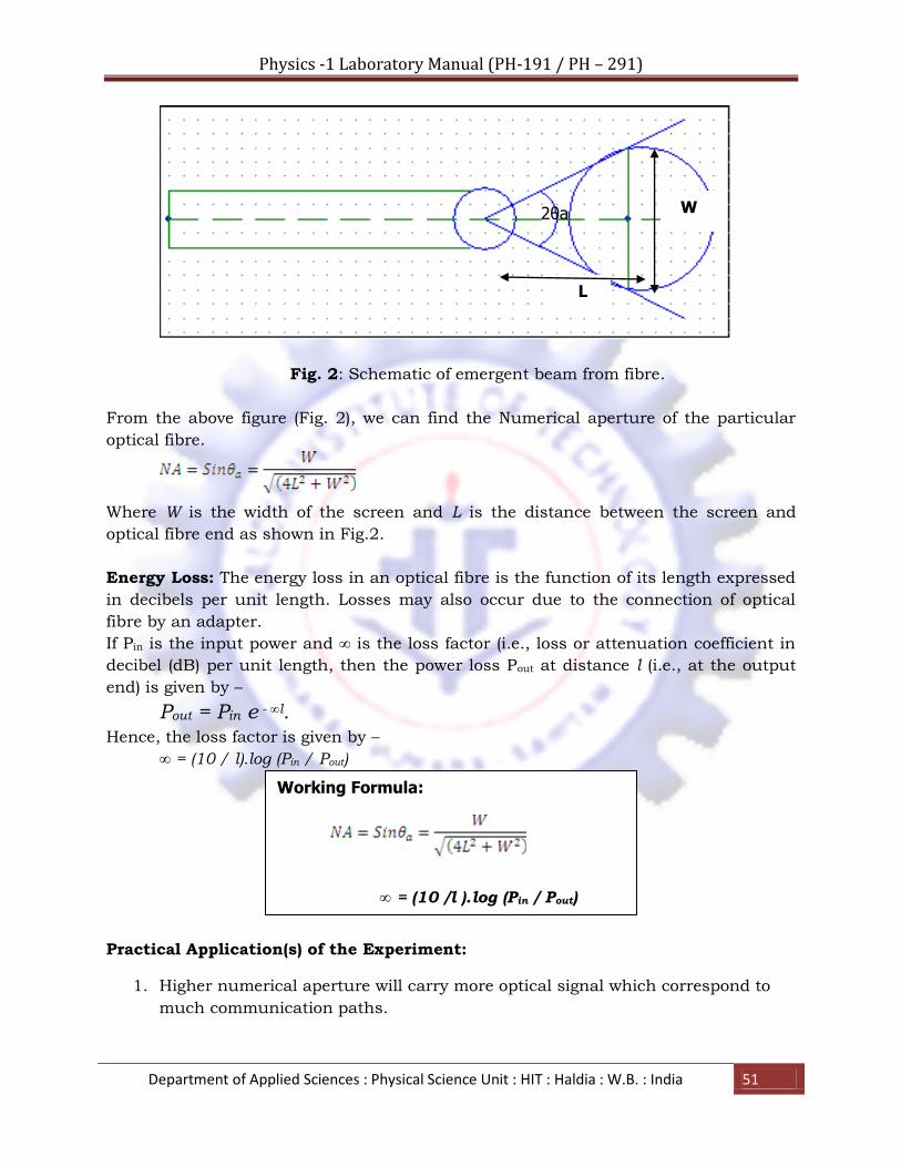
Fig. 2: Schematic of emergent beam from fibre.
From the above figure (Fig. 2), we can find the Numerical aperture of the particular
optical fibre.
Where W is the width of the screen and L is the distance between the screen and
optical fibre end as shown in Fig.2.
Energy Loss: The energy loss in an optical fibre is the function of its length expressed
in decibels per unit length. Losses may also occur due to the connection of optical
fibre by an adapter.
If Pin is the input power and ∞ is the loss factor (i.e., loss or attenuation coefficient in
decibel (dB) per unit length, then the power loss Pout at distance l (i.e., at the output
end) is given by –
Pout = Pin e - ∞l. Hence, the loss factor is given by –
∞ = (10 / l).log (Pin / Pout)
Practical Application(s) of the Experiment:
1. Higher numerical aperture will carry more optical signal which correspond to
much communication paths.
2θa
L
W
Working Formula:
∞ = (10 /l ).log (Pin / Pout)
Physics -1 Laboratory Manual (PH-191 / PH – 291)
Department of Applied Sciences : Physical Science Unit : HIT : Haldia : W.B. : India 52
2. Higher numerical aperture carries maximum number of optical mode which
causes dispersion of signal. This is the disadvantage of higher NA.
III. Apparatus:
Fibre optic transmission kit, Fibre optic receiver kit, Optical fibre, Screen, Measuring
scale.
Function of Each Instrument and Component:
Fibre Optic Transmission Kit:- To produce and transmit laser light through an
optical fibre of which we measure the numerical aperture of the fibre.
Fibre Optic Receiver Kit:- To accept the transmitted laser light through an optical
fibre of which we measure the loss factor of the fibre.
Screen:- It is simply a graph paper upon which the laser light fallen and measuring
distance from screen to fibre & diameter of cone, we can find out the numerical
aperture of the fibre.
Optical Fibre:- It is a core tube through we passes the laser beam and of which we
measure the numerical aperture.
IV. Experimental Procedure:
1. In a dark room connect the optical fibre with the LED port of transmission kit from
which laser light may enter into the fibre. Insert the other end of the fibre through the
hole of L – shaped numerical aperture measurement kit. Place the calibrated screen
paper vertically on the marked scale of L – shaped kit. Switch on the transmission kit.
Make a bright circle on the vertical paper by adjusting the intensity knob. Note down
the value of L. Adjust the vertical paper so that the bright circle is symmetrical with
respect to scales drawn on it. Measure the value of the diameter of the circle.
2. Move the vertical screen to several other values of L. Note down the value of W in
each case.
3. Take out the previous optical fibre cable and connect one end of a long optical fibre
cable to the LED port of the transmission kit again. Connect the other end of the
optical fibre cable to LED port of the receiver kit. Apply the input voltage / power by
turning Pin knob of transmission kit. Make the optical fibre cable bended with several
coiling. Measure the input power (Pin) and output power (Pout) with the help of
Physics -1 Laboratory Manual (PH-191 / PH – 291)
Department of Applied Sciences : Physical Science Unit : HIT : Haldia : W.B. : India 53
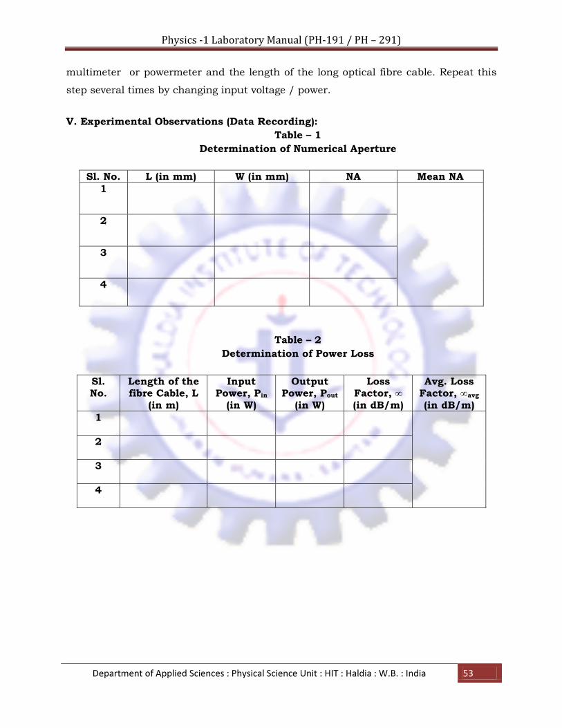
multimeter or powermeter and the length of the long optical fibre cable. Repeat this
step several times by changing input voltage / power.
V. Experimental Observations (Data Recording):
Table – 1
Determination of Numerical Aperture
Sl. No. L (in mm) W (in mm) NA Mean NA
1
2
3
4
Table – 2
Determination of Power Loss
Sl. No.
Length of the fibre Cable, L
(in m)
Input Power, Pin
(in W)
Output Power, Pout
(in W)
Loss Factor, ∞ (in dB/m)
Avg. Loss Factor, ∞avg (in dB/m)
1
2
3
4

Physics -1 Laboratory Manual (PH-191 / PH – 291)
Department of Applied Sciences : Physical Science Unit : HIT : Haldia : W.B. : India 54
VI. Results:
VII. % Error Calculations:
VIII. Discussions:
1. In determination of the diameter of the circular spot formed on the screen we
used graph paper of mm division. If the diameter is measure using the main
scale and the circular scale much accurate result must obtained.
2. The initial error of the screw gauge has been added with all subsequent
reading of the distance of the fibre from the screen.
3. As the value of both L and W are very small much accurate measurement
has to be taken to achieve the nearly accurate value of the numerical aperture.
4. The distance between the screen and the fibre should be small enough for
eye estimation.
5. The end of the fibre must be placed perpendicular to the screen values.
Otherwise it is difficult to measure the diameter.
6. For the measurement of loss factor input and output power should be
measured by digital multimeter.
7. LASER light is dangerous, so it should be careful that LASER light can‟t fall
into eye.
Numerical Aperture, NA = Sin θa = ………………………………
Angle of Acceptance, 2θa = …………….., θa =………………………
Loss Factor (∞) = …………………………………….
Copyright © 2022 FDOKUMEN