INTERNATIONAL JOURNAL FOR NUMERICAL METHODS IN ENGINEERINGInt. J. Numer. Meth. Engng (2007)Published online in Wiley InterScience (www.interscience.wiley.com). DOI: 10.1002/nme.2196

A regularized XFEMmodel for the transition from continuousto discontinuous displacements

E. Benvenuti1,∗,†, A. Tralli1 and G. Ventura2

1Dipartimento di Ingegneria, Universita di Ferrara, via Saragat 1, I-44100 Ferrara, Italy2Politecnico di Torino, Corso Duca degli Abruzzi 24, I-10129 Torino, Italy

SUMMARY

This work focuses on the modelling through the extended finite element method of structural problemscharacterized by discontinuous displacement. As a model problem, an elastic isotropic domain characterizedby a displacement discontinuity across a surface is studied. A regularization of the displacement field isintroduced depending on a scalar parameter. The regularized solution is defined in a layer. The emergingstrain and stress fields are independently modelled using specific constitutive assumptions. In particular, itis shown that the mechanical work spent within the regularization layer can be interpreted as an interfacework provided that a spring-like constitutive law is adopted. The accuracy of the integration proceduresadopted for the stiffness matrix is assessed, as highly non-linear terms appear. Standard Gauss quadratureis compared with adaptive quadrature and with a new technique, based on an equivalent polynomialapproach. One- and two-dimensional results are reported for varying discretization size, regularizationparameter, and constitutive parameters. Copyright q 2007 John Wiley & Sons, Ltd.

Received 2 November 2006; Revised 13 August 2007; Accepted 22 August 2007

KEY WORDS: discontinuous displacement; extended finite element method; numerical quadrature

1. INTRODUCTION

Finite element procedures that efficiently handle discontinuities of the displacement fields aredecisive in structural mechanics problems dominated by the possible emergence of cracks andinterfaces. This motivated the noticeable amount of contributions that appeared in the last decades.For instance, the extended finite elements method (XFEM) is based on the nodal enrichment of the

∗Correspondence to: E. Benvenuti, Dipartimento di Ingegneria, Universita di Ferrara, via Saragat 1, I-44100 Ferrara,Italy.

†E-mail: elena.benvenuti@unife.it, ebenvenuti@ing.unife.it

Contract/grant sponsor: Research fund ‘Interfacial resistance and failure in materials and structural systems’ PRIN2005Contract/grant sponsor: ‘Nanotribology’ PRIN 2004

Copyright q 2007 John Wiley & Sons, Ltd.

E. BENVENUTI, A. TRALLI AND G. VENTURA

finite element approximation of the displacement field with discontinuous functions (e.g. [1, 2]). Onthe basis of the local partition of unity property of finite element shape functions, the XFEM stemsfrom the partition of unity finite element method [3], a variant of which is often referred to as thegeneralized finite element method [4–7]. Besides being robust and general, the XFEM requires nomesh adaptivity to adequately capture strong discontinuities, gives a conforming approximation ofthe displacement, and, generally, leads to symmetric stiffness matrices [8]. After early applicationsin elastic–brittle materials [1], the XFEM has been combined with cohesive crack models to thepurpose of simulating fracture in quasi-brittle heterogeneous materials [9, 10]. In this context,Wells and Sluys [11] developed a cohesive XFEM formulation, where the mechanical work relatedto the cohesive stress–strain law is recovered through a limit process.

A considerable number of alternative methods for modelling discontinuities is available. Amongall, the embedded element technique was proposed in the eighties by Belytschko et al. [12] for shearband modelling, motivated by Ortiz et al. [13], and later extended to crack modelling by Oliveret al. (e.g. [14]). The embedded enhanced approach introduces the discontinuity at the elementlevel. The displacement is approximated by making use of discontinuous or regularized functionsthat, however, introduce non-compatible modes: the strain can be discontinuous within and acrosselement boundaries [8]. A detailed classification of embedded enhanced formulations can be foundin Reference [15]. Comparative analyses of the XFEM versus the embedded discontinuity methodwere given by Jirasek and Belytschko [8], and Oliver et al. [16]. Recently, a new approach formodelling discontinuities of displacement and strain has been derived from Nitsche’s method byHansbo and Hansbo [17], and extended to finite strain elasticity by Mergheim and Steinmann [18].Areias and Belytschko [19] showed that this model can be recast as a special case of extendedfinite element formulation.

Displacement regularization is a well-known procedure that naturally leads to localization bandswith finite width: for instance, the discontinuous Heaviside function used as enrichment of thedisplacement representation of cracks can be replaced by a continuous function that depends ona regularization parameter. This type of displacement regularization has been previously adoptedin several types of embedded discontinuity approaches for elasto-plastic and elasto-damagingmaterials. For instance, the displacement discontinuity has been approximated through a linearramp function by Simo et al. [20], and Oliver et al. [14, 16] in softening plasticity, and by Larssonet al. [21] in a model for embedded localization band in undrained soil. Similarly, Iarve [22]proposed a mesh-independent scheme for crack modelling where the discontinuous function isapproximated with splines. In a model for non-local elasto-damaging materials, Patzak and Jirasek[23] enriched the displacement field with regularized Heaviside functions for the purpose ofimproving the computational resolution of highly localized strains in narrow damage process zones.Recently, a two-scale method for shear band evolution was presented by Areias and Belytschko [24],where the local displacement enrichment is a regularized version of the Heaviside function, similarto the homologous function employed in Reference [23].

In the present work, a class of displacement regularization is employed, which is based on theadoption of a regularized Heaviside function, analogous to the regularization proposed by Patzakand Jirasek [23]. As in the contributions by Pietruszczak and Mroz [25] and Belytschko et al. [12],the regularization length � is assumed ab initio as a model parameter. The regularized layer ismodelled as an isotropic elastic equivalent continuum. The stress field associated with the ‘bulk’strain field and the stress field corresponding to the ‘localized’ strain field that is activated in theregularization layer are assumed mechanically uncoupled. The minimal requisite is that a standardXFEM formulation for displacement discontinuities can be recovered as the regularization ceases to

Copyright q 2007 John Wiley & Sons, Ltd. Int. J. Numer. Meth. Engng (2007)DOI: 10.1002/nme

REGULARIZED XFEM

be active. Distinguishing features are that (i) the bulk strain field and the localized strain field, andthe associated stress fields, are assumed to govern distinct mechanically uncoupled mechanismsand (ii) a bounded spring-like constitutive model for the localized stress–strain law is adopted,which ensures convergence of the inherent mechanical work to the traction–separation work whenthe regularization parameter vanishes. To the authors’ knowledge, the present approach to boththe constitutive modelling and the variational formulation differs from the procedures followed inprevious models based either on similar displacement regularization, such as [23], or on analogousvariational statements, such as [11].

The discretization procedure naturally leads to an extended finite element formulation. Accordingto the classification adopted by Belytschko et al. [12], the adopted approach makes it possibleto perform sub-h, iso-h, and super-h regularization, where h is the element representative size,because the width of the regularization parameter can be varied. While integration sub-domainsare usually adopted in XFEM formulations with discontinuous enrichment functions [9, 11, 26],here, all fields are continuous and differentiable. Hence, standard quadrature can be used. Owingto the presence of strong spatial gradients of both the regularization function and its derivative,standard Gauss quadrature with a fixed grid of Gauss points may lead to inaccurate results. Forthis reason, a new integration technique is presented that is based on the replacement of theregularization function with continuous polynomials that exactly integrate the stiffness coefficients.It is an extension of the method proposed by Ventura [27] to avoid quadrature subcells in XFEMfor strong discontinuities. This method conjugates the simplicity of implementation of standardGauss quadrature with the accuracy ensured by adaptive quadrature. Furthermore, comparisonswith standard Gauss quadrature and adaptive quadrature have been carried out.

1.1. Outline

In Section 2, an isotropic elastic domain first characterized by a discontinuity surface, Section 2.1,and then by a soft layer, Section 2.2, is analyzed. In the latter case, a regularized function isconsidered in the displacement expression that approaches the discontinuous Heaviside functionas the regularization parameter � vanishes. The strain is obtained as the sum of a bulk partand a contribution localized in the regularization layer (Section 2.2). The variational formulationassociated with the present model is analyzed in Section 3. In particular, mechanical uncouplingof the stress fields associated with the distinct strains is considered (Section 3.1). The limit ofthe mechanical work for vanishing � is studied in Section 3.3.1. In Section 4, the discrete finiteelement formulation is introduced as a typical extended finite elements formulation. The stiffnessmatrix is obtained by applying the principle of virtual work. Moreover, a new integration procedurebased on the use of equivalent polynomials is described in Section 5, which extends the methodintroduced by Ventura [27]. In Sections 6.1.1 and 6.1.2, classic Gauss quadrature, exact adaptivequadrature, and the equivalent-polynomials procedure elaborated for the formulation are comparedfor a wide range of parameters. In Sections 7.1 and 7.2, one- and two-dimensional results areshown, which display the aptitude of the regularized XFEM to actually capture the transition fromcontinuous to discontinuous displacement.

A bold-face notation is adopted to denote vector-valued functions w of components wi ,i=1, . . . ,n as well as second-order tensors r. The blackboard symbol S indicates a fourth-ordertensor. Application of r to a vector n is indicated by rn. The symbol |w| denotes the norm of wwhile its symmetric gradient is indicated by ∇sw. The scalar product and the tensor product ofvectors, w1 and w2, are written as w1 ·w2, and w1⊗w2, respectively.

Copyright q 2007 John Wiley & Sons, Ltd. Int. J. Numer. Meth. Engng (2007)DOI: 10.1002/nme

E. BENVENUTI, A. TRALLI AND G. VENTURA

2. KINEMATICS

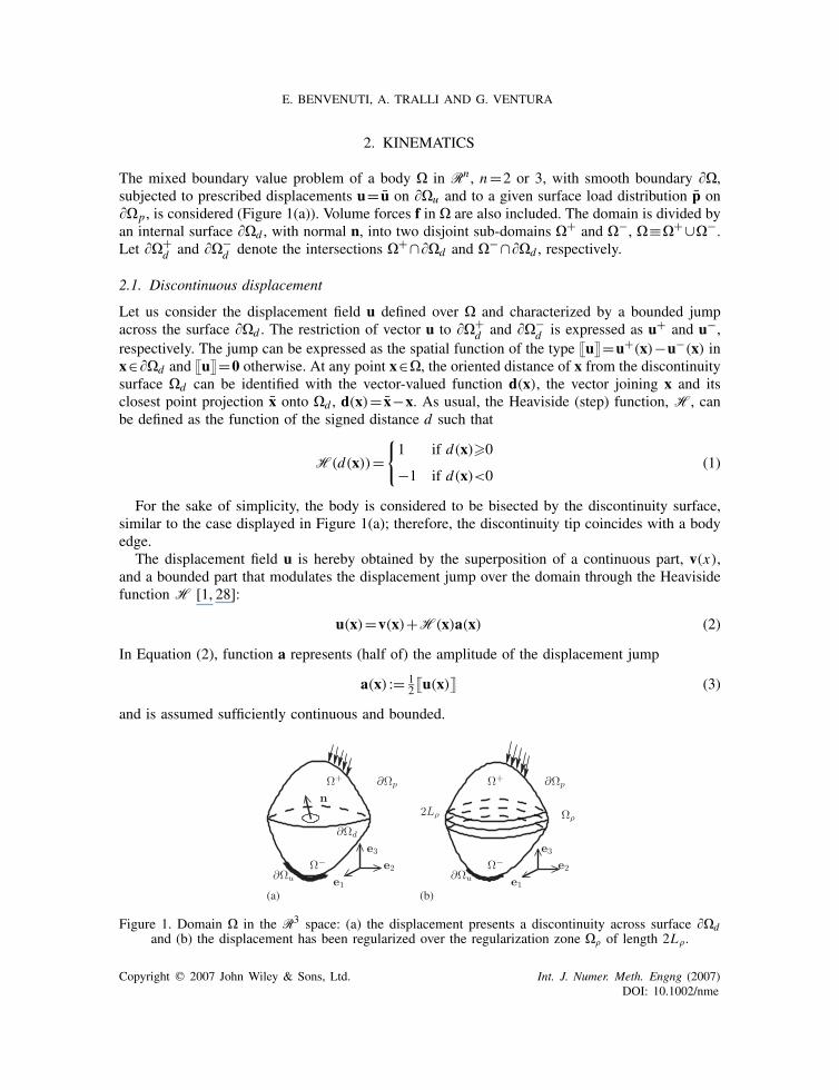
The mixed boundary value problem of a body � in Rn , n=2 or 3, with smooth boundary ��,subjected to prescribed displacements u= u on ��u and to a given surface load distribution p on��p, is considered (Figure 1(a)). Volume forces f in � are also included. The domain is divided byan internal surface ��d , with normal n, into two disjoint sub-domains �+ and �−, �≡�+∪�−.Let ��+

d and ��−d denote the intersections �+∩��d and �−∩��d , respectively.

2.1. Discontinuous displacement

Let us consider the displacement field u defined over � and characterized by a bounded jumpacross the surface ��d . The restriction of vector u to ��+

d and ��−d is expressed as u+ and u−,

respectively. The jump can be expressed as the spatial function of the type �u�=u+(x)−u−(x) inx∈��d and �u�=0 otherwise. At any point x∈�, the oriented distance of x from the discontinuitysurface �d can be identified with the vector-valued function d(x), the vector joining x and itsclosest point projection x onto �d , d(x)= x−x. As usual, the Heaviside (step) function, H, canbe defined as the function of the signed distance d such that

H(d(x))={1 if d(x)�0

−1 if d(x)<0(1)

For the sake of simplicity, the body is considered to be bisected by the discontinuity surface,similar to the case displayed in Figure 1(a); therefore, the discontinuity tip coincides with a bodyedge.

The displacement field u is hereby obtained by the superposition of a continuous part, v(x),and a bounded part that modulates the displacement jump over the domain through the Heavisidefunction H [1, 28]:

u(x)=v(x)+H(x)a(x) (2)

In Equation (2), function a represents (half of) the amplitude of the displacement jump

a(x) := 12�u(x)� (3)

and is assumed sufficiently continuous and bounded.

(a) (b)

Figure 1. Domain � in the R3 space: (a) the displacement presents a discontinuity across surface ��dand (b) the displacement has been regularized over the regularization zone �� of length 2L�.

Copyright q 2007 John Wiley & Sons, Ltd. Int. J. Numer. Meth. Engng (2007)DOI: 10.1002/nme

REGULARIZED XFEM

The strain associated with displacement (2) writes

ε(x)=∇su=∇sv(x)+H(x)∇sa+(a(x)⊗d(xd))s (4)

where the distributional derivative

d(x) :=∇H(x) (5)

is the Dirac’s delta distribution such that, for any bounded second-order tensor field u∫�u(x)d(x)

d�=∫��du(x)ndS [29]. Note that vector d has the dimension of the inverse of a length, [L−1].

Strain (4) is the sum of the contribution

εb(x) :=∇sv(x)+H(x)∇sa(x) (6)

which is bounded, and the contribution

εc(x) :=(a(x)⊗d(x))s (7)

which is defined in a distributional sense, as it is governed by the (formal) function Dirac delta d.

2.2. Regularized displacement

Let us replace the discontinuous Heaviside function H(x) (1) with a regularized function H�(x)that depends on a positive regularization parameter �. FunctionH�(x) will be assumed continuous,with continuous derivatives, and reproducing the Heaviside function H(x) as � vanishes. Thelength over which the regularization is active is the decaying length L�, which is related to theregularization parameter � and depends on the type of function H� that is adopted, as manypossibilities are available (Section 2.2.1).

Let ��+� and ��−

� be the surfaces obtained by shifting the surface ��d of the quantity L� indirections n+ and n−, and let �+

� and �−� be the two volume domains spanned in the directions n+

and n−. Hence, the regularization introduces a layer of finite width 2L�, which will be hereafterdenoted ��, such that �� ≡�+

� ∪�−� . A pictorial representation is given in Figure 1(b).

Consequently, the displacement field can be reproposed as the following continuous function:

u�(x)=v(x)+H�(x)a(x) (8)

The strain associated with displacement u� can be expressed as

ε�(x) :=∇sv(x)+H�(x)∇sa(x)+(a(x)⊗∇(H�(x)))s (9)

Two different strain terms can be identified: the bulk strain εb

εb(x) :=∇sv(x)+H�(x)∇s(a(x)) (10)

and the ‘localization’ strain εc

εc(x) :=(a(x)⊗d�(x))s (11)

that is governed by the derivative

d�(x) :=∇H�(x) (12)

Copyright q 2007 John Wiley & Sons, Ltd. Int. J. Numer. Meth. Engng (2007)DOI: 10.1002/nme

E. BENVENUTI, A. TRALLI AND G. VENTURA

The former term (10) is bounded for any value of the parameter �, and entails the deformation ofthe entire body. Term (11) is different from zero only at points x∈��, and can reach values thatare several orders of magnitude larger than εb. It can be drawn that strains εb(x) and εc(x) arerepresentative of different deformation mechanisms.

Note again that the term d� possesses the dimension of the inverse of a length, [L−1]. Usingthe chain rule, d� can be expressed as a function of the normal n in the form

d� =∇H(d(x))= �H�

�d∇d=��n (13)

where �� :=|d�|. Replacement of Equation (13) in Equation (11) yields

εc(x) :=��(x)(a(x)⊗n(x))s (14)

The numerical treatment of large derivatives related to singular terms is discussed, for instance,in References [30, 31].

2.2.1. Examples of regularized Heaviside functions. Several choices are available for constructingsmooth approximations of the Heaviside function, as described, for instance, in Reference [32].A simple example is the piecewise polynomial function derived from the bell function

H�(d(x))=

⎧⎪⎪⎪⎪⎪⎨⎪⎪⎪⎪⎪⎩

0 if d(x)<0

1

V�(x)

∫ d(x)

0

(1− �2

�2

)p

d� if −��d(x)��

1 if d(x)>�

(15)

where the reference volume V� is V� =16�/15 for p=2 and V� =256�/315 for p=4. In this case,the decaying length L� =�. Function (15) was used, for instance, by Patzak and Jirasek [23].

A different expression can be obtained from the Gauss function as

H�(d(x))= 1

V�(x)

∫ d(x)

−∞e−|�|2/�2 d� (16)

where V� =(�√2�)n in Rn .

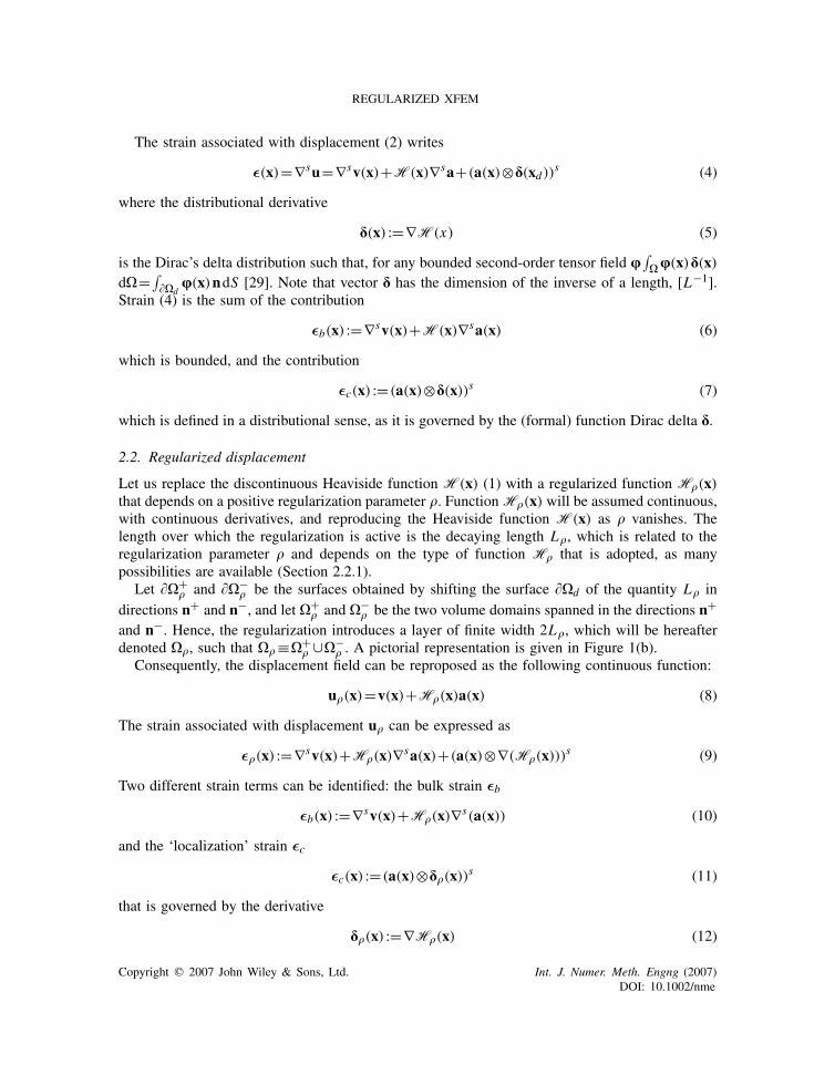
A further choice is represented by the regularization function

H�(d(x))= 1

V�

∫ d(x)

0e−|�|/� d�=sign(d(x))(1−e−|d(x)|/�) (17)

where |�| denotes the absolute value of � and V� =�.Figure 2(a) shows different profiles of the regularized Heaviside function (17) for different

values of the regularization parameter �. The corresponding derivative d� is displayed inFigure 2(b).

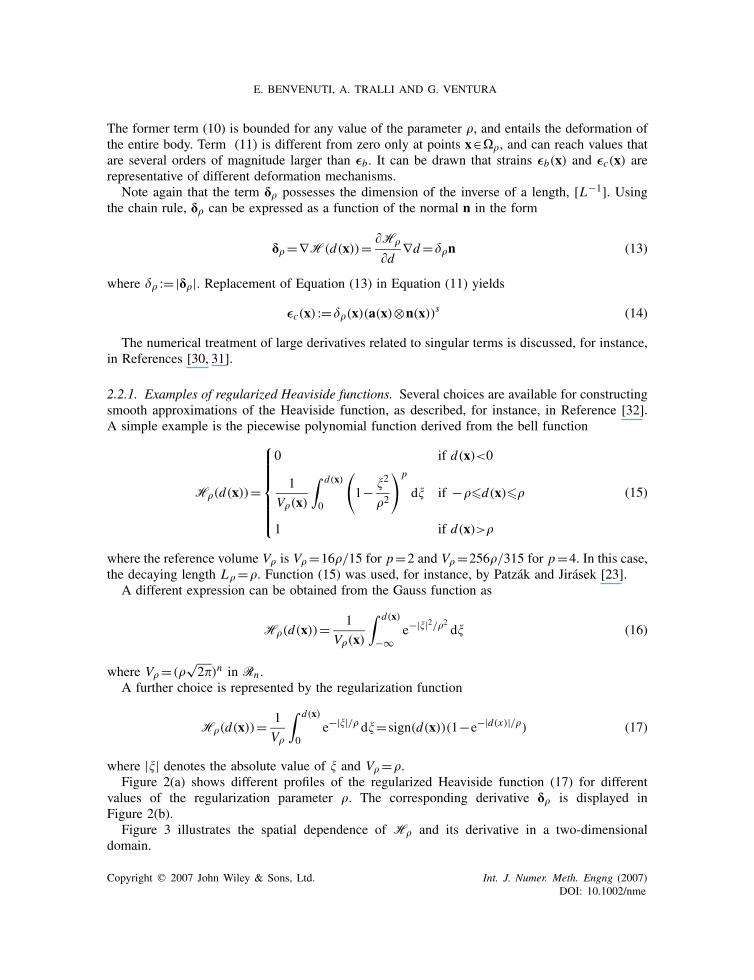
Figure 3 illustrates the spatial dependence of H� and its derivative in a two-dimensionaldomain.

Copyright q 2007 John Wiley & Sons, Ltd. Int. J. Numer. Meth. Engng (2007)DOI: 10.1002/nme

REGULARIZED XFEM

Figure 2. One-dimensional spatial representation of function H� (17) and itsderivative �� for �=0.01,0.02,0.03,0.04.

Figure 3. Functions H� and �� over the regularization layer of width 2L� as a function of the signeddistance from the discontinuity line in a two-dimensional quadrilateral domain.

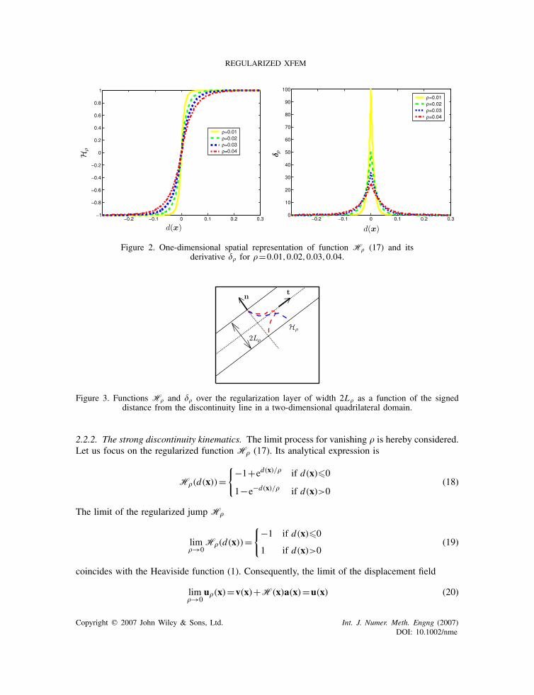
2.2.2. The strong discontinuity kinematics. The limit process for vanishing � is hereby considered.Let us focus on the regularized function H� (17). Its analytical expression is

H�(d(x))={−1+ed(x)/� if d(x)�0

1−e−d(x)/� if d(x)>0(18)

The limit of the regularized jump H�

lim�→0

H�(d(x))={−1 if d(x)�0

1 if d(x)>0(19)

coincides with the Heaviside function (1). Consequently, the limit of the displacement field

lim�→0

u�(x)=v(x)+H(x)a(x)=u(x) (20)

Copyright q 2007 John Wiley & Sons, Ltd. Int. J. Numer. Meth. Engng (2007)DOI: 10.1002/nme

E. BENVENUTI, A. TRALLI AND G. VENTURA

coincides with the non-regularized displacement (2). Analogously, the limit of the ε� strain

lim�→0

ε� =∇sv(x)+H(x)∇sa(x)+(a(x)⊗d(x))s =ε (21)

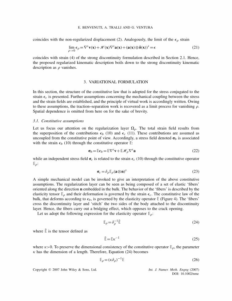
coincides with strain (4) of the strong discontinuity formulation described in Section 2.1. Hence,the proposed regularized kinematic description boils down to the strong discontinuity kinematicdescription as � vanishes.

3. VARIATIONAL FORMULATION

In this section, the structure of the constitutive law that is adopted for the stress conjugated to thestrain εc is presented. Further assumptions concerning the mechanical coupling between the stressand the strain fields are established, and the principle of virtual work is accordingly written. Owingto these assumptions, the traction–separation work is recovered as a limit process for vanishing �.Spatial dependence is omitted from here on for the sake of brevity.

3.1. Constitutive assumptions

Let us focus our attention on the regularization layer ��. The total strain field results fromthe superposition of the contributions εb (10) and εc (11). These contributions are assumed asuncoupled from the constitutive point of view. Accordingly, a stress field denoted rb is associatedwith the strain εb (10) through the constitutive operator E:

rb=Eεb=E∇sv+EH�∇sa (22)

while an independent stress field rc is related to the strain εc (10) through the constitutive operatorE�:

rc=��E�(a⊗n)s (23)

A simple mechanical model can be invoked to give an interpretation of the above constitutiveassumptions. The regularization layer can be seen as being composed of a set of elastic ‘fibers’oriented along the direction n embedded in the bulk. The behavior of the ‘fibers’ is described by theelasticity tensor E� and their deformation is governed by the strain εc. The constitutive law of thebulk, that deforms according to εb, is governed by the elasticity operator E (Figure 4). The ‘fibers’cross the discontinuity layer and ‘stitch’ the two sides of the body attached to the discontinuitylayer. Hence, the fibers carry out a bridging effect, which opposes to the crack opening.

Let us adopt the following expression for the elasticity operator E�:

E� =�−1� E (24)

where E is the tensor defined as

E=E�−1 (25)

where �>0. To preserve the dimensional consistency of the constitutive operator E�, the parameter� has the dimension of a length. Therefore, Equation (24) becomes

E� =(���)−1E (26)

Copyright q 2007 John Wiley & Sons, Ltd. Int. J. Numer. Meth. Engng (2007)DOI: 10.1002/nme

REGULARIZED XFEM

Figure 4. Domain � in the R3 space with regularized displacement: mechanicalinterpretation of the regularization layer.

Moreover, let us assume that ��1; for �=1, the constitutive operator E coincides with the consti-tutive operator E; otherwise the constitutive operator E corresponds to a material that is softer thanthe elastic bulk. By replacing expressions (24) in Equation (23), the stress rc yields

rc= Eεc= E(a⊗n)s (27)

According to Equation (27), the stress rc is proportional to a through the elasticity operator E,bounded and independent of the distribution d�, and, consequently, of the regularization param-eter �. Moreover, stress rc has non-vanishing components along the normal direction, while itstangential components vanish. Hence, an analogy with some expressions for the interface stressassumed in adhesive joints emerges [33]. The expression of E� (24) is analogous to the expressionof the softening modulus used by Simo et al. [20] and by Oliver et al. [16] in the context ofregularized embedded discontinuities in plasticity. Note that it has been here, assuming that thestress fields rc and rb do not perform mechanical work for the strain fields εb and εc, respectively.This assumption will be shown in the next section to make it possible to establish a precise linkbetween the present formulation and standard formulations for strong discontinuities.

3.2. The principle of virtual work

The primal fields of the present formulation are (v,a). Virtual variations of the unknown fields(v, a) are considered within the space of bounded sufficiently continuous functions that satisfyhomogeneous boundary conditions on ��u . Correspondingly, virtual variations εb and εc of thestrain fields εb=∇s v+H�∇s a and εc=�� (a⊗n)s arise.‡

As explained in Section 3.1, the strain components, εb and εc, are assumed to be mechanicallyuncoupled within the regularization layer ��. Therefore, the internal work of the stresses rb andrc conjugated to the above strains can be written as

Li :=∫

�\��

rb · εb d�+∫

��

rb · εb d�+∫

��

rc · εc d� (28)

‡The proper functional space for the class of deformations that are investigated here is the Bounded Deformationspace. A rigorous mathematical treatment of this matter can be found, for instance, in Reference [34].

Copyright q 2007 John Wiley & Sons, Ltd. Int. J. Numer. Meth. Engng (2007)DOI: 10.1002/nme

E. BENVENUTI, A. TRALLI AND G. VENTURA

The principle of virtual work states that, for any virtual admissible variations (v, a), the internalvirtual work Li must be equal to the external virtual work∫

�rb · εb d�+

∫��

rc · εc d�=∫

�f ·(v+H�a)d�+

∫��p

p· vdS (29)

where it has been assumed that a vanishes on ��p and the additivity of the integral operator hasbeen exploited. After application of the divergence theorem, by the arbitrariness and independencyof the virtual variations v and a, the principle of virtual work implies the following set of weakequilibrium equations: ∫

�(divrb+f) · vd� = 0 (30)

∫��p

(rbn− p) · vdS = 0 (31)

∫�rb ·H�∇s ad�+

∫��

��rc ·(a⊗n)s d� =∫

�f ·H�ad� (32)

for any virtual admissible variation v and a.

3.3. Convergence to the strong discontinuity case

In this section, the transition from continuous to discontinuous displacement is considered. To thispurpose, the attention is focused on the limit process where the domain �� collapses into a surface�d as the regularization parameter � vanishes. An expression for the stress rc was adopted inSection 3.1 that makes the work of the stress rc by the ‘localization’ strain εc converge to the workof the traction vector at the discontinuity by the displacement jump at the discontinuity surface,as shown in the next section.

3.3.1. The traction–separation work. Owing to the property of the regularized Heaviside functionH� to converge in a classical sense to the Heaviside function H as � vanishes, it is possible towrite that the limit of the first term on the left-hand side of Equation (28) becomes

lim�→0

∫�rb · εb d�=

∫�

E(∇sv+H∇sa) ·(∇s v+H∇s a)d� (33)

where the fact that the argument is bounded for any � has also been exploited. Hence, this termconverges to a bounded quantity that is �-independent, and represents the work of the stress rbfor the strain associated with a displacement field characterized by a strong discontinuity. Thework appearing on the right-hand side of Equation (33) is typical of standard strong discontinuitiesformulations [11, 27].

By replacing the relationship (a⊗d�)s =∇s(H�a)−H�∇sa, and applying the divergencetheorem, the work of the stress rc by its conjugated strain εc can be reformulated as∫

��

rc ·(a⊗d�)s d�=∫

��

−divrc ·H�a+rc ·H�∇s ad�+∫

���

rcn·H�adS (34)

Copyright q 2007 John Wiley & Sons, Ltd. Int. J. Numer. Meth. Engng (2007)DOI: 10.1002/nme

REGULARIZED XFEM

Let the volume �� have sufficiently smooth boundaries, and a and ∇sa be bounded for anyvalue of �. It can be proved that the internal work of rc (27) for its conjugated strain εc convergesto the work of the traction t=rcn for the jump �u� at the discontinuity surface ��d as � vanishes:

lim�→0

∫��

rc ·εc d�=∫

��d

t ·�u�dS (35)

ProofBy hypothesis, a and ∇a are continuous bounded functions. Consequently, by Equation (27), rcand divrc are continuous bounded function as well [35, p. 30]. Moreover, H� is a continuousbounded function as −1�H��1 for any �. The measure of ��, meas(��), is proportional to themeasure of the discontinuity surface meas(��d)

meas(��)=2n�meas(��d) (36)

as the decaying length can be set as L� =n� with n a positive real number.Let us consider the first term on the right-hand side of Equation (34). Then, by hypothesis, it

is possible to write

Hi�divrc ·H�a�Hs (37)

where Hi :=ess inf(divrc ·H�a) and Hs :=ess sup(divrc ·H�a), and ess sup, ess inf denote theessential supremum and infimum of the work. This implies that (e.g. [29]):

Hi2n�meas(��d)�∫

��

divrc ·H�ad��Hs2n�meas(��d) (38)

Analogously, let us consider the second term on the right-hand side of Equation (34). Again, it ispossible to write

Ki�rc ·H�∇sa�Ks (39)

where Ki :=ess inf(rc ·H�∇sa) and Ks :=ess sup(rc ·H�∇sa). Therefore, we get

Ki2n�meas(��d)�∫

��

rc ·H�∇sad��Ks2n�meas(��d) (40)

If � vanishes, then, in view of Equations (38) and (40), the following result holds [29]:

lim�→0

∫��

divrc ·H�ad�= lim�→0

∫��

rc ·H�∇sad�=0 (41)

Let us focus on the surface integral in the internal work (34). It is convenient to split the boundary��� into the external lateral boundary ��l

� and the internal surfaces ��+� and ��−

� with normal

n+ and n−, respectively, ��� ≡��l�∪��+

� ∪��−� . Moreover, in view of the hypotheses done on

the shape of ��, ��+� =��−

� =��d and thus the measures of ��+� and ��−

� are independent of �.The surface integral can be written as [29]∫

���

rcn·H�adS=∫

��l�

t ·H�adS+∫

��+d

t ·H�adS+∫

��−d

t ·H�adS dS (42)

Copyright q 2007 John Wiley & Sons, Ltd. Int. J. Numer. Meth. Engng (2007)DOI: 10.1002/nme

E. BENVENUTI, A. TRALLI AND G. VENTURA

where the traction t

t=rcn= E(a⊗n)sn (43)

is independent of the value of � and is bounded when � vanishes.The same arguments used for proving Equation (41) can be exploited to prove that the first two

integrals on the right-hand side of Equation (42) vanish as � vanishes, because the measure of ��l�

vanishes. Owing to the constitutive relationship (27), the limit can be brought within the integral[29]

lim�→0

(∫��+

d

t ·H�adS+∫

��−d

t ·H�adS

)

=∫

��+d

lim�→0

(t ·H�a)dS+∫

��−d

lim�→0

(t ·H�a)dS=∫

��+d

t ·HadS+∫

��−d

t ·HadS (44)

Now, it is convenient to exploit the fact that, by construction, 2a=�u�. Moreover, accordingto [9, 10], it is possible to write t= t+ =rcn+ =−t− =−rcn−. Then Equation (44) can be refor-mulated as ∫

��+d

t ·HadS+∫

��−d

t ·HadS =∫

��+d

t+ ·adS−∫

��−d

t− ·adS

=∫

��d

2t ·adS=∫

��d

t ·�u�dS (45)

where Ha=a on ��+d and Ha=−a on ��−

d . Therefore, the limit of the work carried out by thestress rc for the localized strain εc in the volume ��

lim�→0

∫��

rc ·εc d�=∫

��d

t ·�u�dS (46)

actually converges to the work of the traction vector of the stress rc by the jump �u� at thediscontinuity surface. �

3.4. Remarks

The proof relies on the assumption of a �-independent bounded expression of the stress rc and onthe mechanical uncoupling between the single stress components. Otherwise, convergence of thework localized over the regularization layer to the traction–separation work is not possible. Note,however, that the the constitutive law (27) is a sufficient but not a necessary condition for the workof rc by εc to actually converge to the traction–separation work. It is, however, the simplest typeof constitutive law that preserves rc bounded for any value of �.

It is worth noting that, here, all strain terms consistently contribute to the mechanical work, whilein other references the strain energy contributions associated with the derivative of the polynomialsthat approximate the Heaviside function are not taken into account (e.g. [22]).

In the extended finite element formulation with a cohesive crack model developed by Wells andSluys [11], the cohesive stress–strain law emerges in the principle of virtual work. However, in

Copyright q 2007 John Wiley & Sons, Ltd. Int. J. Numer. Meth. Engng (2007)DOI: 10.1002/nme

REGULARIZED XFEM

this work, the requirements that the stress and the strain fields should satisfy in order to obtain avariationally consistent model were not discussed.

4. FINITE ELEMENT FORMULATION

Let domain � be discretized into M non over-lapping finite elements

�≡M⋃i=1

�i (47)

connected at N nodes [36]. The primal fields, v and a, are approximated over the set of N nodalvalues vI , aI through the same polynomial shape functions NI , I =1, . . . ,N:

v≈ ∑I∈N

NI (x)vI (48)

a≈ ∑I∈N

NI (x)aI (49)

Therefore, the displacement field becomes

u�(x)= ∑I∈N

NI (x)(vI +aIH�(x)) (50)

Equation (50) satisfies the local partition of unity approximation.For the sake of brevity, let N collect the shape functions of the displacement field over the single

element. According to this notation, the displacement u� can be written as

u� =Nv+H�Na (51)

while the approximations of the strains εb and εc can be expressed as

εb =Bv+H�Ba (52a)

εc = ��Na (52b)

Matrix B is the symmetric compatibility matrix such that

Bv=∇sNv (53)

and N is the operator such that

Na=(Na⊗n)s (54)

Note that, from Equation (51) on, the vectors v and a will indicate the nodal values, not thefunctions v(x) and a(x). The stresses are approximated as

rb = Eεb=EBv+H�EBa (55a)

rc = E�εc=E���Na= ENa (55b)

where the fact that E� = E�−1� has been exploited, (Equation (24), Section 3.1).

Copyright q 2007 John Wiley & Sons, Ltd. Int. J. Numer. Meth. Engng (2007)DOI: 10.1002/nme

E. BENVENUTI, A. TRALLI AND G. VENTURA

4.1. Discrete form of the principle of virtual work

According to the Galerkin approach, primal fields and their virtual variations are interpolatedthrough the same shape functions. The internal virtual work is given by∫

�rb ·εb+rc ·εc d� =

∫�(EBv+H�EBa) ·(Bv+H�Ba)d�+

∫�(ENa) ·(��Na)d�

=∫

�BtEBd�v ·v+

∫�H�BtEBd�a ·v+

∫�H�BtEBd�v ·a

+∫

�H2

�BtEBd�a ·a+

∫��

�� Nt ENd�a ·a (56)

The previous equation can be written in a more compact form as∫�r ·εd�=

∫�u·kud� (57)

where the stiffness matrix

k=(kvv kva

kav kaa

)(58)

collects the submatrices:

kvv =BtEB (59a)

kva =H�BtEB (59b)

kav =H�BEBt (59c)

kaa = ��Nt EN+H2�B

tEB (59d)

Because kva =ktav , a symmetric stiffness matrix is obtained. The expression of the components ofthe stiffness matrix (59) shows that the equations of equilibrium are characterized by a couplingbetween the unknowns v and a, and that, the value of � enters the evaluation of the degrees offreedom v and a.

4.2. Equivalence to strong discontinuity XFEM

Standard XFEM models for strong discontinuity in the displacement field can be recovered byassuming that E vanishes. In this case, the internal virtual work is expressed as∫

�rb ·εb+rc ·rc d� =

∫�BtEBd�v ·v+

∫�HBtEBd�a ·v

+∫

�BtEHBd�v ·a+

∫�H2BtEBd�a ·a (60)

Copyright q 2007 John Wiley & Sons, Ltd. Int. J. Numer. Meth. Engng (2007)DOI: 10.1002/nme

REGULARIZED XFEM

and the components of the stiffness matrix are

kvv =BtEB (61a)

kva =BtEHB=ktav (61b)

kaa =H2BtEB (61c)

Equations (61) coincide with standard extended finite element formulation for strong discontinuity.They can be directly obtained starting from the expressions of the displacement and the strain field

u=Nv+HNa (62)

e=Bv+HBa (63)

that are usually employed in XFEM context [27].

5. INTEGRATION OF THE STIFFNESS MATRIX BY EQUIVALENT POLYNOMIALS

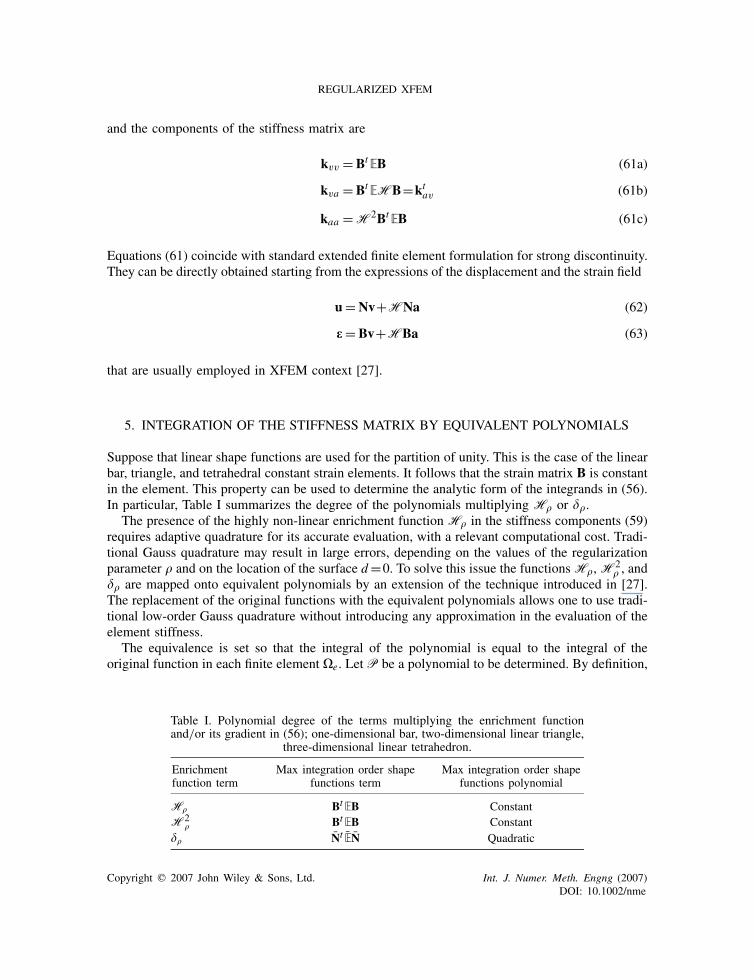
Suppose that linear shape functions are used for the partition of unity. This is the case of the linearbar, triangle, and tetrahedral constant strain elements. It follows that the strain matrix B is constantin the element. This property can be used to determine the analytic form of the integrands in (56).In particular, Table I summarizes the degree of the polynomials multiplying H� or ��.

The presence of the highly non-linear enrichment function H� in the stiffness components (59)requires adaptive quadrature for its accurate evaluation, with a relevant computational cost. Tradi-tional Gauss quadrature may result in large errors, depending on the values of the regularizationparameter � and on the location of the surface d=0. To solve this issue the functionsH�, H2

� , and�� are mapped onto equivalent polynomials by an extension of the technique introduced in [27].The replacement of the original functions with the equivalent polynomials allows one to use tradi-tional low-order Gauss quadrature without introducing any approximation in the evaluation of theelement stiffness.

The equivalence is set so that the integral of the polynomial is equal to the integral of theoriginal function in each finite element �e. Let P be a polynomial to be determined. By definition,

Table I. Polynomial degree of the terms multiplying the enrichment functionand/or its gradient in (56); one-dimensional bar, two-dimensional linear triangle,

three-dimensional linear tetrahedron.

Enrichmentfunction term

Max integration order shapefunctions term

Max integration order shapefunctions polynomial

H� BtEB ConstantH2

� BtEB Constant�� Nt EN Quadratic

Copyright q 2007 John Wiley & Sons, Ltd. Int. J. Numer. Meth. Engng (2007)DOI: 10.1002/nme

E. BENVENUTI, A. TRALLI AND G. VENTURA

it must be ∫�e

kva d� =∫

�e

H�BtEBd�=∫

�e

PH�BtEBd� (64a)

∫�e

kaa d� =∫

�e

(��Nt EN+H2�B

tEB)d�=∫

�e

(P��Nt EN+PH2

�BtEB)d� (64b)

so that three equivalent polynomials PH� , PH2�, and P�� are to be determined.

Observing that the equivalent polynomials multiply a generic polynomial integrand whose degreeis reported in Table I, Equations (64) are satisfied if each of the following equations is satisfiedindependently:

• in the one-dimensional case, � being the abscissa in the parent reference axis

◦ for the equivalent polynomial PH� :∫�e

H� d�=∫

�e

PH� d� (65)

◦ for the equivalent polynomial PH2�:

∫�e

H2� d�=

∫�e

PH2�d� (66)

◦ for the equivalent polynomial P�� :∫�e

�� d� =∫

�e

P�� d� (67a)

∫�e

���d� =∫

�e

P���d� (67b)

∫�e

���2 d� =

∫�e

P���2 d� (67c)

• in the two-dimensional case, (�,�) being the parent coordinate axes

◦ for the equivalent polynomial PH� :∫�e

H� d�=∫

�e

PH� d� (68)

◦ for the equivalent polynomial PH2�:

∫�e

H2� d�=

∫�e

PH2�d� (69)

Copyright q 2007 John Wiley & Sons, Ltd. Int. J. Numer. Meth. Engng (2007)DOI: 10.1002/nme

REGULARIZED XFEM

◦ for the equivalent polynomial P�� :

∫�e

�� d� =∫

�e

P�� d� (70a)

∫�e

���d� =∫

�e

P���d� (70b)

∫�e

���d� =∫

�e

P���d� (70c)

∫�e

���2 d� =

∫�e

P���2 d� (70d)

∫�e

���2 d� =

∫�e

P���2 d� (70e)

∫�e

����d� =∫

�e

P����d� (70f)

Letting PH� and PH2�as constants (0th degree polynomial) and P�� as a complete quadratic

polynomial, Equations (65)–(70) can be evaluated analytically and yield linear systems in thecolumn vector of variables c (polynomial coefficients) of the form

Ac=b (71)

The analytic expressions of the matrix of coefficients A and of the column vector of solutionsb in the cases of linear bar and triangular constant strain elements are given in Appendix A.

Note that, because of (65)–(70), replacing the functions H�, H2� , and �� with the equivalent

polynomials PH� , PH2�, and P�� has the consequence that the integrands become all polynomial

functions. These can be integrated exactly by low-order Gauss quadrature. This procedure, bydefinition of equivalent polynomials, does not introduce any approximation.

The equivalence equations (65)–(70) do not take into account the effect of the Jacobian in theintegration. When transforming the element stiffness from the parent to the global domain, theelement shape function derivatives are multiplied by the inverse of the Jacobian matrix and theintegrand function by the determinant of the Jacobian. Consequently, the proposed methodology isexact only when the Jacobian matrix is given by constant terms. This is always true for linear shapefunctions elements as the terms in the Jacobian matrix are the shape functions derivatives. Theseare the one-dimensional bar and the triangular and tetrahedral constant strain elements. For thetwo-dimensional quadrilateral, having bilinear shape functions, the Jacobian matrix has constantelements only when the opposite sides are parallel.

In a general setting the effect of the Jacobian terms has been examined in [27], but its effectcan be reduced to be negligible by a proper choice of the degree of the equivalent polynomials.The details of this procedure are outside the scope of the present paper and are fully discussedin [27].

Copyright q 2007 John Wiley & Sons, Ltd. Int. J. Numer. Meth. Engng (2007)DOI: 10.1002/nme

E. BENVENUTI, A. TRALLI AND G. VENTURA

6. NUMERICAL INTEGRATION

The focus of the analysis is restricted to the assessment of the influence of the numerical integrationprocedure on the evaluation of the stiffness matrix. As in References and [12, 25], prefixed valuesof � are assumed as model parameters.

For the sake of a comparison, the bell function (15) and the exponential function (17) have beenadopted. However, the homologous regularized Heaviside function based on the Gaussian (16) canbe alternatively used.

For numerical purposes, the decaying length, L�, is identified as the value of the signed distanced that fulfils the following condition:

L� =d such that|H�−H|

H<0.001 (72)

For instance, in the case of regularized function H� (17), it has been found that L� ∼=10�, whilein the case of compact support regularized function (15), the decaying length coincides with theregularization parameter itself, L� =�.

Since the regularization length can be larger than the element size, all nodes whose distance from��d is smaller than L� are enriched. The set of enriched nodes across the discontinuity increasesfor increasing �. Therefore, the number of components of the stiffness matrix corresponding tothe enriched nodes does depend on the value of �.

6.1. Integration procedures

The element stiffness has been computed with the following methods:

• adaptive numerical quadrature based on the Gauss–Lobatto method [37];• standard Gauss quadrature with Ng Gauss points without subdomains subdivision;• equivalent integration procedure as described in Section 5.

The first non-vanishing eigenvalues of the stiffness matrix obtained with the Gauss and the equiv-alent polynomial technique have been compared with the corresponding eigenvalues obtained withthe adaptive quadrature. In particular, the relative error obtained with the Gauss quadrature relativeto the eigenvalue e j is defined as

Tjstd= |estj −eadj |

eadj(73)

and the homologous error for the equivalent polynomial procedure is expressed as

Tjequiv= |eeqj −eadj |

eadj(74)

The equivalent integration procedure has been employed for values of �, which prevents possiblemachine overflow related to the presence of the exponential term e1/� in the equivalent polynomials.

Standard Gaussian quadrature is a simple integration rule which is independent of the valueof � and of the discontinuity position. On the one hand, this is an advantage, as there is noneed to perform element sub-quadrature; on the other hand, more refined quadrature proceduresmight be used so as to improve the computational accuracy. For instance, following Areias and

Copyright q 2007 John Wiley & Sons, Ltd. Int. J. Numer. Meth. Engng (2007)DOI: 10.1002/nme

REGULARIZED XFEM

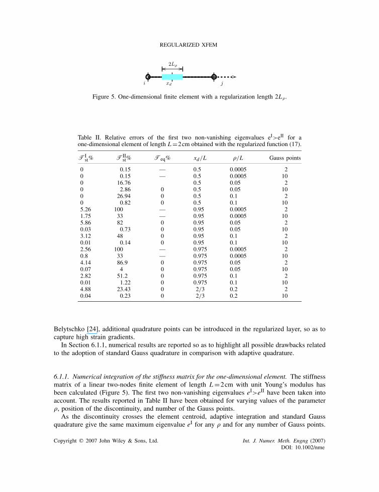
Figure 5. One-dimensional finite element with a regularization length 2L�.

Table II. Relative errors of the first two non-vanishing eigenvalues eI>eII for aone-dimensional element of length L=2cm obtained with the regularized function (17).

TIst% TII

st% Teq% xd/L �/L Gauss points

0 0.15 — 0.5 0.0005 20 0.15 — 0.5 0.0005 100 16.76 0.5 0.05 20 2.86 0 0.5 0.05 100 26.94 0 0.5 0.1 20 0.82 0 0.5 0.1 105.26 100 — 0.95 0.0005 21.75 33 — 0.95 0.0005 105.86 82 0 0.95 0.05 20.03 0.73 0 0.95 0.05 103.12 48 0 0.95 0.1 20.01 0.14 0 0.95 0.1 102.56 100 — 0.975 0.0005 20.8 33 — 0.975 0.0005 104.14 86.9 0 0.975 0.05 20.07 4 0 0.975 0.05 102.82 51.2 0 0.975 0.1 20.01 1.22 0 0.975 0.1 104.88 23.43 0 2/3 0.2 20.04 0.23 0 2/3 0.2 10

Belytschko [24], additional quadrature points can be introduced in the regularized layer, so as tocapture high strain gradients.

In Section 6.1.1, numerical results are reported so as to highlight all possible drawbacks relatedto the adoption of standard Gauss quadrature in comparison with adaptive quadrature.

6.1.1. Numerical integration of the stiffness matrix for the one-dimensional element. The stiffnessmatrix of a linear two-nodes finite element of length L=2cm with unit Young’s modulus hasbeen calculated (Figure 5). The first two non-vanishing eigenvalues eI>eII have been taken intoaccount. The results reported in Table II have been obtained for varying values of the parameter�, position of the discontinuity, and number of the Gauss points.

As the discontinuity crosses the element centroid, adaptive integration and standard Gaussquadrature give the same maximum eigenvalue eI for any � and for any number of Gauss points.

Copyright q 2007 John Wiley & Sons, Ltd. Int. J. Numer. Meth. Engng (2007)DOI: 10.1002/nme

E. BENVENUTI, A. TRALLI AND G. VENTURA

Figure 6. A constant strain triangle with the regularization zone of width 2L�.

Figure 7. Gauss quadrature in the parent triangular element: set of 13 Gauss points (‘∗’), set of threeGauss points (‘+’); the dashed lines correspond to the discontinuity positions xd =0.1 and 0.9.

In this particular case, the contributions to the matrix kav (59b) in the domains �+ and �− areopposite: ∫

��+H�BEBt d�=−

∫��−

H�BEBt d� (75)

so that any error cancels out.

6.1.2. Numerical integration of the CST stiffness matrix. A triangular three-nodes finite element inits parent domain has been considered crossed by a vertical discontinuity whose distance from theorigin is equal to xd (Figure 6). Standard Gauss quadrature was performed by adopting a coarsegrid consisting of three Gauss points and a refined grid consisting of 13 Gauss points (Figure 7).The errors TI,TII,TIII,TIV relative to the first four non-vanishing eigenvalues eI,eII,eIII,eIV

have been compared in Table III for varying �, regularization function, and position of thediscontinuity.

Copyright q 2007 John Wiley & Sons, Ltd. Int. J. Numer. Meth. Engng (2007)DOI: 10.1002/nme

REGULARIZED XFEM

Table III. Relative errors of the first four non-vanishing eigenvalues eI>eII>eIII>eIV of atwo-dimensional CST element in the parent domain.

TIst% TII

st% TIIIst % TIV

st % Teq% xd � Type Gauss points

5.89 5.88 5.87 21.3 0 0.5 0.1 bell 3<0.01 0.02 <0.01 9.77 0 0.5 0.1 bell 135.8 5.8 5.8 12 — 0.5 0.001 bell 32.28 2.28 2.28 10 — 0.5 0.001 bell 13

<0.01 <0.01 <0.01 100 — 0.9 0.001 bell 3<0.01 <0.01 <0.01 100 — 0.9 0.001 bell 1316.3 16 16 100 — 0.1 0.001 bell 35.73 5.7 5.7 32 — 0.1 0.001 bell 13

16.13 16.1 16.1 87 0 0.1 0.1 bell 33.98 3.9 4 31 0 0.1 0.1 bell 132.77 2.74 46.1 2.79 0 0.5 0.1 exp 30.87 0.87 1.92 0.9 0 0.5 0.1 exp 13

11 5 13 12 — 0.5 0.001 exp 35.54 5.54 14 3 — 0.5 0.001 exp 131 1 1 100 — 0.9 0.001 exp 31 1 1 100 — 0.9 0.001 exp 13

23.49 23.5 23.5 100 — 0.1 0.001 exp 38.72 8.72 20.2 4.3 — 0.1 0.001 exp 132.24 2 2.15 74 0 0.1 0.1 exp 30.44 0.44 0.5 10 0 0.1 0.1 exp 13

6.1.3. Discussion. The equivalent polynomial procedure proposed in Section 5 gives the sameresults of the adaptive quadrature. For small values of �, the presence of the exponential term e1/�

in the polynomials, see the Appendix, can attain values of several orders of magnitude larger thanthe other terms.

In the coarse grid, 10 points in the one-dimensional case and 13 points in the two-dimensionaltriangle can give satisfying results for a large range of values of � and position of the discontinuity.

In regard to the type of regularization function, it can be deduced from the analysis of Table IIIthat the errors relative to the regularized function with compact support (15) are slightly smallerthan the corresponding errors that are detected when the regularized function (17) is exploited.

The position of the discontinuity influences the accuracy. The largest error is met when thediscontinuity crosses the element very close to the boundary.

For what concerns the influence of the parameter �, there are two essential circumstances: thecase where L� is too small and the case where L� is sufficiently large in comparison with thedistance between the Gauss points. When L� is too small, the formulation can reproduce thesame drawbacks of classic XFEM models when � vanishes, and the highest errors are achieved.Otherwise, the error decreases, because the function H� is continuous within the element anda unique integration domain can be successfully employed. The largest errors are detected inthe calculus of the smallest eigenvalue, precisely the second eigenvalue in the one-dimensionalelement, and the fourth eigenvalue in the CST, which, however, is at least two to three orders ofmagnitude smaller than the others.

In XFEM models for strong discontinuities, when the discontinuity line crosses the elementclose to the boundary, the Heaviside function cannot be distinguished from a constant function:the resulting system of equation can become linearly dependent [1, 11, 27]. Here, the regularized

Copyright q 2007 John Wiley & Sons, Ltd. Int. J. Numer. Meth. Engng (2007)DOI: 10.1002/nme

E. BENVENUTI, A. TRALLI AND G. VENTURA

function H� is not constant within the layer of width 2L�, whose width can attain large values asin the case of Equation (17), where 2L� ≈20�. Hence, if a sufficiently fine grid is assumed, lineardependency of the equilibrium equation can be avoided, as a certain number of Gauss points iswithin the regularization layer.

In synthesis, two conclusions can be drawn:

• the superiority in accuracy of adaptive quadrature and of the equivalent polynomial procedurehas been confirmed, the latter being much faster;

• when a sufficiently large value of � and the open support function H� (17) are used, areasonably fine grid of Gauss points makes it possible to calculate the first significativeeigenvalues of the stiffness matrix with an acceptable level of accuracy and to avoid lineardependency of the equilibrium equations.

7. EXAMPLES

A number of one- and two-dimensional examples are reported for the purpose of verifying whethermechanically consistent results are obtained, especially when the smallest regularization lengthwith respect to the mesh resolution is adopted. The regularization width is comparable or largerwith respect to the element size (Sections 7.1–7.2). Moreover, a double cantilever beam test hasbeen analyzed, where a thin elastic interface is inserted within an elastic body (Section 7.3).Finally, an edge-notched specimen subjected to a mode I loading is considered in Section 7.4.The stress intensity factor is determined from the finite element results for varying values of theregularization parameter �.

7.1. One-dimensional examples

A one-dimensional bar of length L=2cm is considered subjected to imposed displacement u=0.1cm at the free end and clamped at the other end. A discontinuity at the center, x=1, hasbeen considered. The results that are reported in the following figures have been obtained byusing adaptive quadrature based on the Gauss–Lobatto algorithm [37] and adopting the regularizedHeaviside function (17).

In Figure 8, the dependency of the displacement profiles on the value of the parameter � isillustrated for a discretization of 55 finite elements. In particular, the profiles corresponding to�=0.05L , 0.1L , and 0.15L have been obtained by setting E=E/� with �=10, while the perfectstep profile corresponding to the strong discontinuity solution has been obtained by setting �=0.0005L and E=E/� with �=1012. As expected, the slope of the displacement profile decreases,and the displacement profile becomes smoother when � increases.

Furthermore, Figure 9(a) and (b) shows the influence of the stiffness E and the stiffness reductionparameter � on the one-dimensional displacement field u�. In Figure 9(a), the parameter �=0.05Lis fixed while � varies in the range [1,5,10,1012]. Figure 9(a) clearly illustrates that the length ofthe regularization zone depends on the value of � and thus the perfect step profile cannot be reachedwhen � is large. Figure 9(b) displays the way � and � influence the regularized displacement u�.The dashed-line profiles correspond to �=0.0005L while the continuous-line profiles have beencomputed by setting �=0.05L . For each value of �, two extremal values of � have been tested:�=1 and 1012, corresponding to E=E and E≈0, respectively. As E decreases, the slope tendsto the horizontal asymptote. Hence, it can be drawn that a strong discontinuous solution can be

Copyright q 2007 John Wiley & Sons, Ltd. Int. J. Numer. Meth. Engng (2007)DOI: 10.1002/nme

REGULARIZED XFEM

Figure 8. One-dimensional bar discretized with 55 finite elements with discontinuity at x=1cm usingthe function H� (17): comparison of the displacement obtained with �=0.05,0.1,0.15L and �=10; the

step function has been obtained with �=0.0005L and �=1012.

(a) (b)

Figure 9. One-dimensional bar discretized with 55 finite elements with discontinuity at x=1cm using thefunction H� (17): (a) displacements obtained with �=1,5,10,10000 and �=0.05L and (b) displacements

obtained by setting �=0.0005L and �=1,10000, and �=0.05L and �=1,10000.

obtained by setting � sufficiently small and choosing a vanishing value of E . When a non-vanishingE is adopted, the slope of u� outside 2L� is not horizontal as the regularized zone still possessesa residual stiffness. It emerges that

• � influences the width of the regularization zone;• E governs the slope of u� in the zone outside the regularization layer 2L�.

Figure 10(a) and (b) illustrates the mesh independency of the finite element results for �=0.1cm.The mesh was subdivided into 3,55, and 255 elements. The result with the coarsest mesh isindicated with a dashed line, while the other profiles are indistinguishable as they practically

Copyright q 2007 John Wiley & Sons, Ltd. Int. J. Numer. Meth. Engng (2007)DOI: 10.1002/nme

E. BENVENUTI, A. TRALLI AND G. VENTURA

(a) (b)

Figure 10. Comparison of the displacement (a) and strain (b) profiles for a one-dimensional bar withdiscontinuity at x=1cm with �=10, �=0.05L , by using the function H� (17) obtained with 3 (dashed

line), 55,255 (continuous lines) finite elements.

coincide. Figure 10(b) displays the profiles of the localized strain εc corresponding to the samevalues that have been adopted in Figure 10(a). The characteristic shape of the strain peak dependson the choice of the regularized function H�, as illustrated in Figures 2(a) and (b).

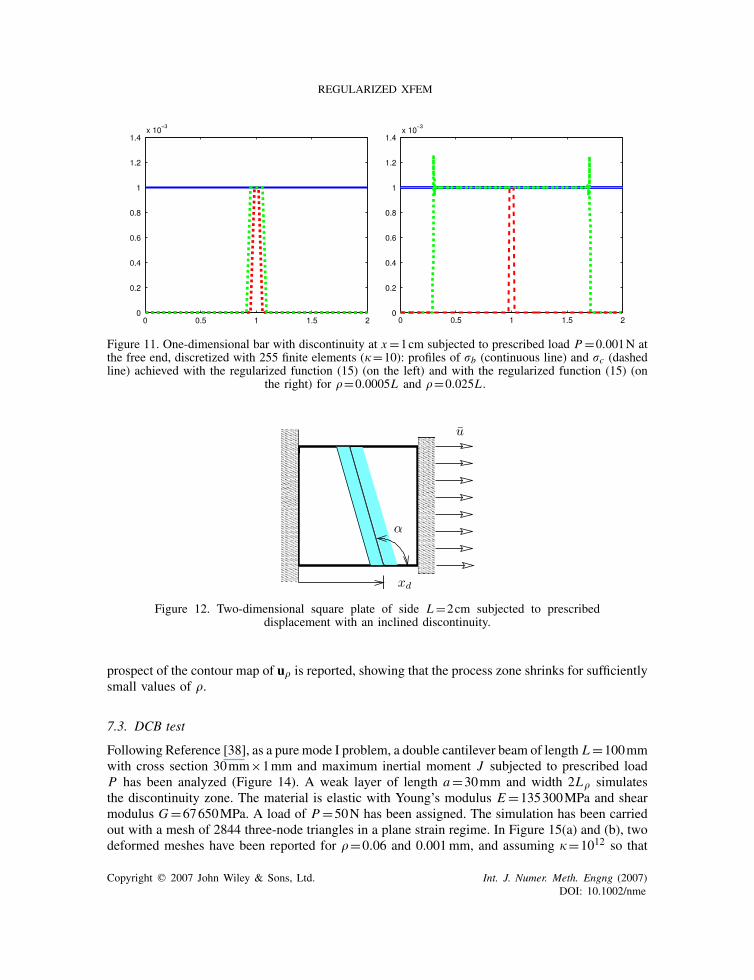
The same bar has been analyzed subjected to the load P=0.001N at the free end and discretizedwith 255 finite elements. The corresponding profiles of �b, continuous line, and �c, dashed line,have been reported in Figure 11(a) and (b) for �=0.0005L (dashed line) and �=0.025L (dottedline). The results in Figure 11(a) have been obtained by using the regularized function H� (15),while those in Figure 11(b) have been achieved by using the regularized function H� (17). Notethat the equilibrium conditions �b= P/A along the bar axis and �b=�c over the regularizationzone are fulfilled.

When the regularization function (17) is used, a decaying length as large as possible shouldbe considered in order for the equilibrium condition to be satisfied with accuracy. Some weakoscillations of rc can arise at the boundary of the regularization zones, as discussed, for instance,in Reference [23].

7.2. Two-dimensional examples

In all the following examples, Gauss quadrature with 13 points within three node triangles hasbeen adopted.

7.2.1. Square plate. A square plate of side 20mm subjected to assigned displacement at the rightend and clamped at the opposite side is studied in plane strain (Figure 12(a)). Young’s modulusE=20000MPa and a shear modulus G=E/2 have been adopted. A straight discontinuity layerof width 2L� with slope �=26◦ has been modelled with 1156 finite elements.

For this test, the displacement profiles have been reported in Figure 13 for different values of theparameter �. The transition from a regularized displacement profile to the strong discontinuity issimulated by choosing �=0.025L and 0.001L . On the left, the x-component of the displacementvector u� is displayed on the z-axis versus the coordinate axes x and y. On the right, a frontal

Copyright q 2007 John Wiley & Sons, Ltd. Int. J. Numer. Meth. Engng (2007)DOI: 10.1002/nme

REGULARIZED XFEM

Figure 11. One-dimensional bar with discontinuity at x=1cm subjected to prescribed load P=0.001N atthe free end, discretized with 255 finite elements (�=10): profiles of �b (continuous line) and �c (dashedline) achieved with the regularized function (15) (on the left) and with the regularized function (15) (on

the right) for �=0.0005L and �=0.025L .

Figure 12. Two-dimensional square plate of side L=2cm subjected to prescribeddisplacement with an inclined discontinuity.

prospect of the contour map of u� is reported, showing that the process zone shrinks for sufficientlysmall values of �.

7.3. DCB test

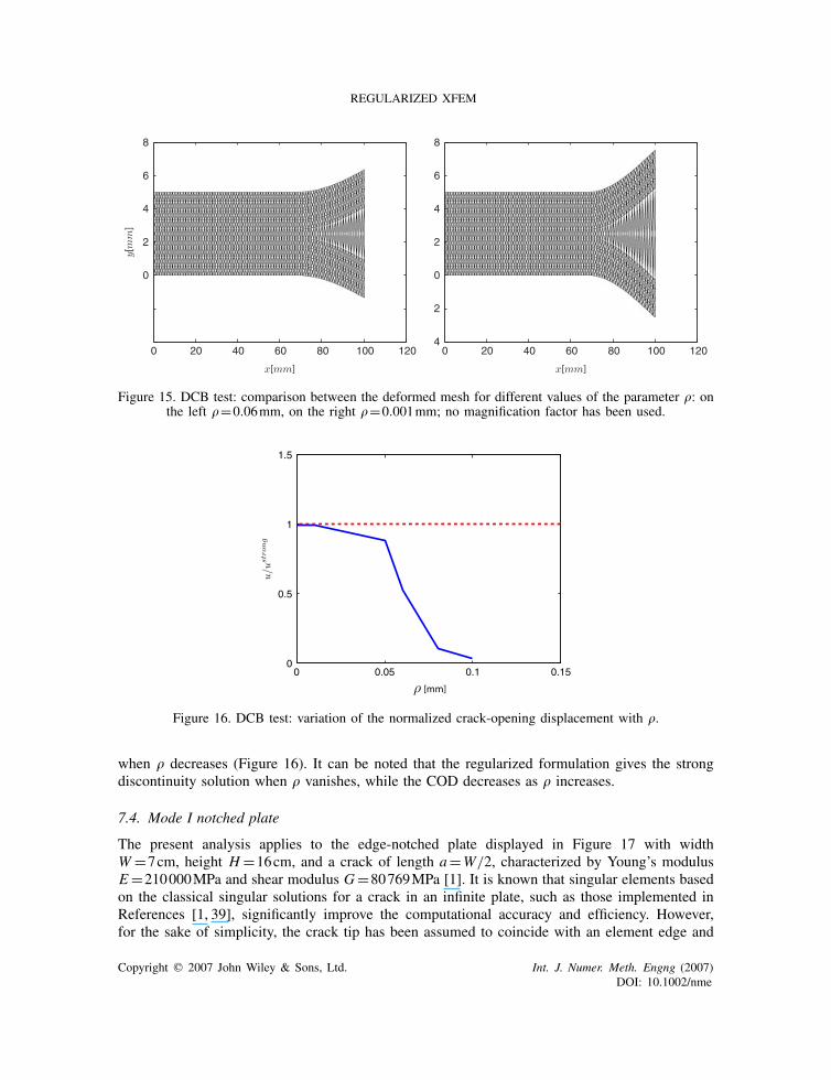
Following Reference [38], as a pure mode I problem, a double cantilever beam of length L=100mmwith cross section 30mm×1mm and maximum inertial moment J subjected to prescribed loadP has been analyzed (Figure 14). A weak layer of length a=30mm and width 2L� simulatesthe discontinuity zone. The material is elastic with Young’s modulus E=135300MPa and shearmodulus G=67650MPa. A load of P=50N has been assigned. The simulation has been carriedout with a mesh of 2844 three-node triangles in a plane strain regime. In Figure 15(a) and (b), twodeformed meshes have been reported for �=0.06 and 0.001mm, and assuming �=1012 so that

Copyright q 2007 John Wiley & Sons, Ltd. Int. J. Numer. Meth. Engng (2007)DOI: 10.1002/nme

E. BENVENUTI, A. TRALLI AND G. VENTURA

0

0.51

1.52

0

0.5

1

1.5

20

0.02

0.04

0.06

0.08

0.1

0

(a) (b)

(c) (d)

0.01

0.02

0.03

0.04

0.05

0.06

0.07

0.08

0.09

0.1

0 0.5 1 1.5 20

0.2

0.4

0.6

0.8

1

1.2

1.4

1.6

1.8

2

00.5

11.5

2

0

0.5

1

1.5

20

0.02

0.04

0.06

0.08

0.1

0

0.01

0.02

0.03

0.04

0.05

0.06

0.07

0.08

0.09

0.1

0 0.5 1 1.5 20

0.2

0.4

0.6

0.8

1

1.2

1.4

1.6

1.8

2

Figure 13. Two-dimensional square plate of side L=2cm subjected to prescribed displacement:x-component of u� plotted in the z-axis versus the deformed mesh: (a) perspective and (b) front for

�=0.025L; (c) perspective and (d) front for �=0.0005L .

La

h

P

Figure 14. DCB test: L=100mm, a=30mm, h=5mm, width=1mm.

the stiffness E vanishes. Figure 15(b) shows that the strong discontinuity solution can be recoveredfor vanishing � and vanishing E.

The reference value ustrong= Pa3/3EJ=2.55mm corresponding to the crack-opening displace-ment of the fully discontinuous solution is compared with the crack-opening displacement obtained

Copyright q 2007 John Wiley & Sons, Ltd. Int. J. Numer. Meth. Engng (2007)DOI: 10.1002/nme

REGULARIZED XFEM

x[mm] x[mm]

y[m

m]

0 20 40 60 80 100 120

0

2

4

6

8

0 20 40 60 80 100 1204

2

0

2

4

6

8

Figure 15. DCB test: comparison between the deformed mesh for different values of the parameter �: onthe left �=0.06mm, on the right �=0.001mm; no magnification factor has been used.

Figure 16. DCB test: variation of the normalized crack-opening displacement with �.

when � decreases (Figure 16). It can be noted that the regularized formulation gives the strongdiscontinuity solution when � vanishes, while the COD decreases as � increases.

7.4. Mode I notched plate

The present analysis applies to the edge-notched plate displayed in Figure 17 with widthW =7cm, height H =16cm, and a crack of length a=W/2, characterized by Young’s modulusE=210000MPa and shear modulus G=80769MPa [1]. It is known that singular elements basedon the classical singular solutions for a crack in an infinite plate, such as those implemented inReferences [1, 39], significantly improve the computational accuracy and efficiency. However,for the sake of simplicity, the crack tip has been assumed to coincide with an element edge and

Copyright q 2007 John Wiley & Sons, Ltd. Int. J. Numer. Meth. Engng (2007)DOI: 10.1002/nme

E. BENVENUTI, A. TRALLI AND G. VENTURA

a

y

x

p

W

H

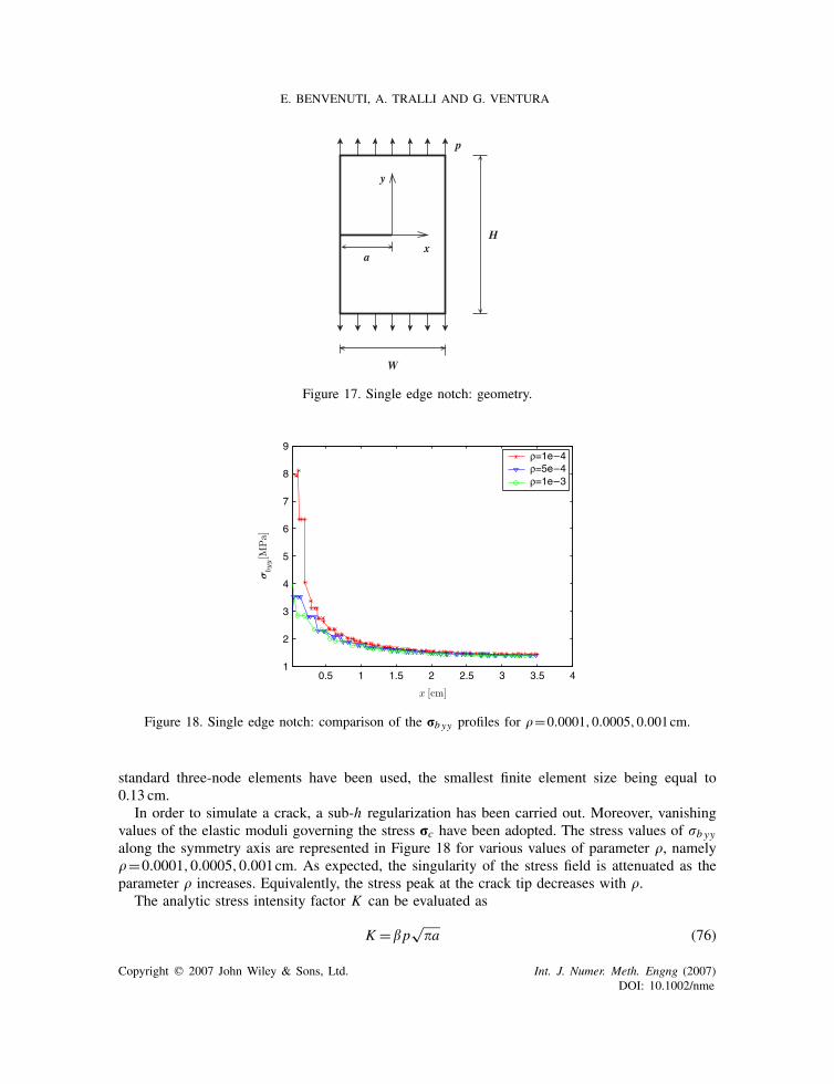
Figure 17. Single edge notch: geometry.

Figure 18. Single edge notch: comparison of the rb yy profiles for �=0.0001,0.0005,0.001cm.

standard three-node elements have been used, the smallest finite element size being equal to0.13 cm.

In order to simulate a crack, a sub-h regularization has been carried out. Moreover, vanishingvalues of the elastic moduli governing the stress rc have been adopted. The stress values of �b yyalong the symmetry axis are represented in Figure 18 for various values of parameter �, namely�=0.0001,0.0005,0.001cm. As expected, the singularity of the stress field is attenuated as theparameter � increases. Equivalently, the stress peak at the crack tip decreases with �.

The analytic stress intensity factor K can be evaluated as

K =p√

�a (76)

Copyright q 2007 John Wiley & Sons, Ltd. Int. J. Numer. Meth. Engng (2007)DOI: 10.1002/nme

REGULARIZED XFEM

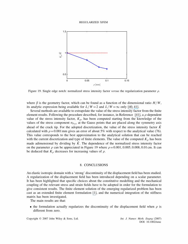
Figure 19. Single edge notch: normalized stress intensity factor versus the regularization parameter �.

where is the geometry factor, which can be found as a function of the dimensional ratio H/W ,its analytic expression being available for L/W =2 and L/W =∞ only [40, 41].

Several methods are available to extrapolate the value of the stress intensity factor from the finiteelement results. Following the procedure described, for instance, in Reference [41], a �-dependentvalue of the stress intensity factor, K�, has been computed starting from the knowledge of thevalues of the stress component �b yy at the Gauss points that are placed along the symmetry axisahead of the crack tip. For the adopted discretization, the value of the stress intensity factor Kcalculated with �=0.001mm gives an error of about 5% with respect to the analytical value (76).This value corresponds to the best approximation to the analytical solution that can be reachedwith the current discretization and type of finite elements. The value of the computed K� has beenmade adimensional by dividing by K . The dependence of the normalized stress intensity factoron the parameter � can be appreciated in Figure 19 where �=0.001,0.005,0.008,0.01cm. It canbe deduced that K� decreases for increasing values of �.

8. CONCLUSIONS

An elastic isotropic domain with a ‘strong’ discontinuity of the displacement field has been studied.A regularization of the displacement field has been introduced depending on a scalar parameter.It has been highlighted that specific choices about the constitutive modelling and the mechanicalcoupling of the relevant stress and strain fields have to be adopted in order for the formulation togive consistent results. The finite element solution of the emerging regularized problem has beencast as an extended finite element formulation [1], and the numerical integration of the stiffnessmatrix has been investigated.

The main results are that:

• the formulation actually regularizes the discontinuity of the displacement field when � isdifferent from zero.

Copyright q 2007 John Wiley & Sons, Ltd. Int. J. Numer. Meth. Engng (2007)DOI: 10.1002/nme

E. BENVENUTI, A. TRALLI AND G. VENTURA

• For vanishing �, the formulation contains, as special cases, XFEM models for strong discon-tinuity with a bridging cohesive stress.

• Standard quadrature techniques or, as an alternative, a new polynomial technique, alreadyproposed for strong discontinuities in [27], can be used without the need of subdividing theenriched elements into integration subdomains.

The formulation can be applied to all the cases where a finite width of the process zone mustbe accounted for, such as the transition from strain localization bands to interfaces with finitethickness. In this case, the regularization parameter indeed acquires the precise physical meaningof a characteristic length of the process zone [42].

Fundamental issues still need to be addressed, such as the formulation of a law of variationof the parameter � that is mechanically consistent with the width of the process zone [23], theimplementation of non-linear cohesive stress within non-local formulations such as [43], and thedefinition of crack-propagation criteria. All these developments are the subject of an undergoingresearch.

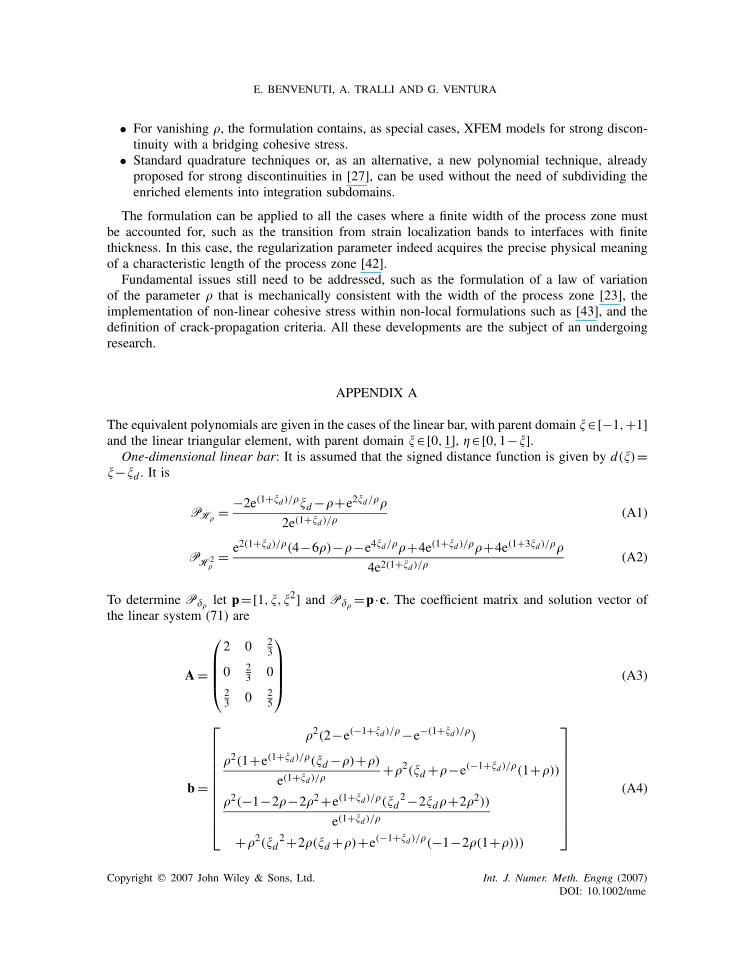
APPENDIX A

The equivalent polynomials are given in the cases of the linear bar, with parent domain �∈[−1,+1]and the linear triangular element, with parent domain �∈[0,1], �∈[0,1−�].

One-dimensional linear bar: It is assumed that the signed distance function is given by d(�)=�−�d . It is

PH� = −2e(1+�d )/��d −�+e2�d/��

2e(1+�d )/�(A1)

PH2�

= e2(1+�d )/�(4−6�)−�−e4�d/��+4e(1+�d )/��+4e(1+3�d )/��

4e2(1+�d )/�(A2)

To determine P�� let p=[1,�,�2] and P�� =p·c. The coefficient matrix and solution vector ofthe linear system (71) are

A=

⎛⎜⎜⎜⎝2 0 2

3

0 23 0

23 0 2

5

⎞⎟⎟⎟⎠ (A3)

b=

⎡⎢⎢⎢⎢⎢⎢⎢⎢⎢⎣

�2(2−e(−1+�d )/�−e−(1+�d )/�)

�2(1+e(1+�d )/�(�d −�)+�)

e(1+�d )/�+�2(�d +�−e(−1+�d )/�(1+�))

�2(−1−2�−2�2+e(1+�d )/�(�d2−2�d�+2�2))

e(1+�d )/�

+�2(�d2+2�(�d +�)+e(−1+�d )/�(−1−2�(1+�)))

⎤⎥⎥⎥⎥⎥⎥⎥⎥⎥⎦

(A4)

Copyright q 2007 John Wiley & Sons, Ltd. Int. J. Numer. Meth. Engng (2007)DOI: 10.1002/nme

REGULARIZED XFEM

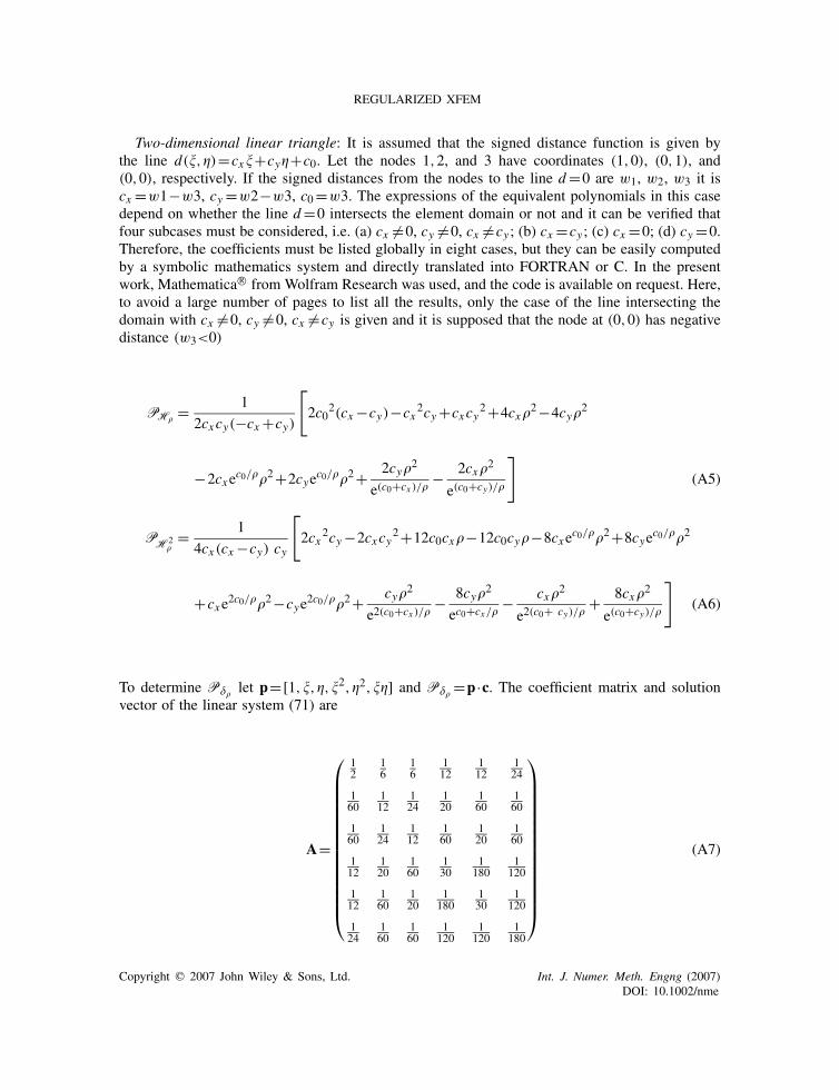
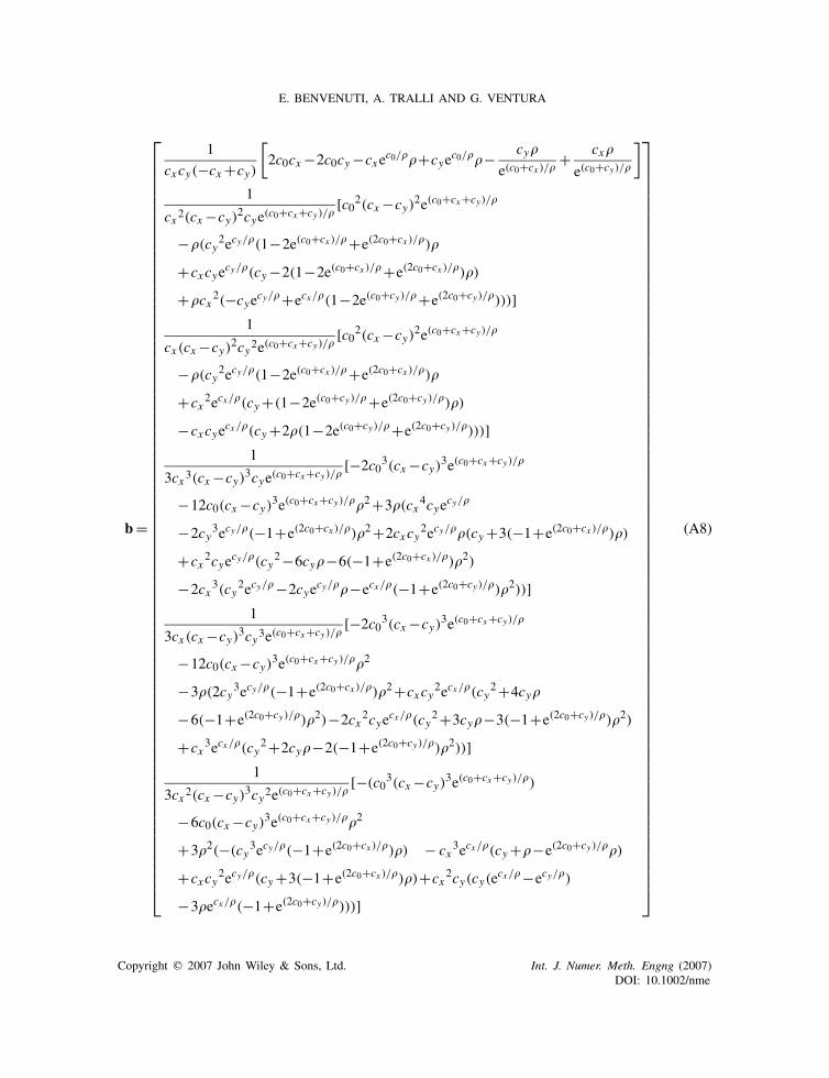
Two-dimensional linear triangle: It is assumed that the signed distance function is given bythe line d(�,�)=cx�+cy�+c0. Let the nodes 1,2, and 3 have coordinates (1,0), (0,1), and(0,0), respectively. If the signed distances from the nodes to the line d=0 are w1, w2, w3 it iscx =w1−w3, cy =w2−w3, c0=w3. The expressions of the equivalent polynomials in this casedepend on whether the line d=0 intersects the element domain or not and it can be verified thatfour subcases must be considered, i.e. (a) cx �=0, cy �=0, cx �=cy ; (b) cx =cy ; (c) cx =0; (d) cy =0.Therefore, the coefficients must be listed globally in eight cases, but they can be easily computedby a symbolic mathematics system and directly translated into FORTRAN or C. In the presentwork, Mathematica R© from Wolfram Research was used, and the code is available on request. Here,to avoid a large number of pages to list all the results, only the case of the line intersecting thedomain with cx �=0, cy �=0, cx �=cy is given and it is supposed that the node at (0,0) has negativedistance (w3<0)

PH� = 1

2cxcy(−cx +cy)

[2c0

2(cx −cy)−cx2cy+cxcy

2+4cx�2−4cy�

2

−2cxec0/��2+2cye

c0/��2+ 2cy�2

e(c0+cx )/�− 2cx�2

e(c0+cy)/�

](A5)

PH2�

= 1

4cx (cx −cy) cy

[2cx

2cy−2cxcy2+12c0cx�−12c0cy�−8cxe

c0/��2+8cyec0/��2

+cxe2c0/��2−cye

2c0/��2+ cy�2

e2(c0+cx )/�− 8cy�2

ec0+cx/�− cx�2

e2(c0+ cy)/�+ 8cx�2

e(c0+cy)/�

](A6)

To determine P�� let p=[1,�,�,�2,�2,��] and P�� =p·c. The coefficient matrix and solutionvector of the linear system (71) are

A=

⎛⎜⎜⎜⎜⎜⎜⎜⎜⎜⎜⎜⎜⎜⎜⎝

12

16

16

112

112

124

160

112

124

120

160

160

160

124

112

160

120

160

112

120

160

130

1180

1120

112

160

120

1180

130

1120

124

160

160

1120

1120

1180

⎞⎟⎟⎟⎟⎟⎟⎟⎟⎟⎟⎟⎟⎟⎟⎠

(A7)

Copyright q 2007 John Wiley & Sons, Ltd. Int. J. Numer. Meth. Engng (2007)DOI: 10.1002/nme

E. BENVENUTI, A. TRALLI AND G. VENTURA

b=

⎡⎢⎢⎢⎢⎢⎢⎢⎢⎢⎢⎢⎢⎢⎢⎢⎢⎢⎢⎢⎢⎢⎢⎢⎢⎢⎢⎢⎢⎢⎢⎢⎢⎢⎢⎢⎢⎢⎢⎢⎢⎢⎢⎢⎢⎢⎢⎢⎢⎢⎢⎢⎢⎢⎢⎢⎢⎢⎢⎢⎢⎢⎢⎢⎢⎢⎢⎢⎢⎢⎢⎢⎢⎢⎢⎢⎢⎢⎢⎢⎢⎣

1

cxcy(−cx +cy)

[2c0cx −2c0cy−cxe

c0/��+cyec0/��− cy�

e(c0+cx )/�+ cx�

e(c0+cy)/�

]1

cx 2(cx −cy)2cye(c0+cx+cy)/�[c02(cx −cy)

2e(c0+cx+cy)/�

−�(cy2ecy/�(1−2e(c0+cx )/�+e(2c0+cx )/�)�

+cxcyecy/�(cy−2(1−2e(c0+cx )/�+e(2c0+cx )/�)�)

+�cx2(−cye

cy/�+ecx/�(1−2e(c0+cy)/�+e(2c0+cy)/�)))]1

cx (cx −cy)2cy2e(c0+cx+cy)/�[c02(cx −cy)

2e(c0+cx+cy)/�

−�(cy2ecy/�(1−2e(c0+cx )/�+e(2c0+cx )/�)�

+cx2ecx/�(cy+(1−2e(c0+cy)/�+e(2c0+cy)/�)�)

−cxcyecx/�(cy+2�(1−2e(c0+cy)/�+e(2c0+cy)/�)))]

1

3cx 3(cx −cy)3cye(c0+cx+cy)/�[−2c0

3(cx −cy)3e(c0+cx+cy)/�

−12c0(cx −cy)3e(c0+cx+cy)/��2+3�(cx

4cyecy/�

−2cy3ecy/�(−1+e(2c0+cx )/�)�2+2cxcy

2ecy/��(cy+3(−1+e(2c0+cx )/�)�)

+cx2cye

cy/�(cy2−6cy�−6(−1+e(2c0+cx )/�)�2)

−2cx3(cy

2ecy/�−2cyecy/��−ecx/�(−1+e(2c0+cy)/�)�2))]

1

3cx (cx −cy)3cy3e(c0+cx+cy)/�[−2c0

3(cx −cy)3e(c0+cx+cy)/�

−12c0(cx −cy)3e(c0+cx+cy)/��2

−3�(2cy3ecy/�(−1+e(2c0+cx )/�)�2+cxcy

2ecx/�(cy2+4cy�

−6(−1+e(2c0+cy)/�)�2)−2cx2cye

cx/�(cy2+3cy�−3(−1+e(2c0+cy)/�)�2)

+cx3ecx/�(cy

2+2cy�−2(−1+e(2c0+cy)/�)�2))]1

3cx 2(cx −cy)3cy2e(c0+cx+cy)/�[−(c0

3(cx −cy)3e(c0+cx+cy)/�)

−6c0(cx −cy)3e(c0+cx+cy)/��2

+3�2(−(cy3ecy/�(−1+e(2c0+cx )/�)�) − cx

3ecx/�(cy+�−e(2c0+cy)/��)

+cxcy2ecy/�(cy+3(−1+e(2c0+cx )/�)�)+cx

2cy(cy(ecx/�−ecy/�)

−3�ecx/�(−1+e(2c0+cy)/�)))]

⎤⎥⎥⎥⎥⎥⎥⎥⎥⎥⎥⎥⎥⎥⎥⎥⎥⎥⎥⎥⎥⎥⎥⎥⎥⎥⎥⎥⎥⎥⎥⎥⎥⎥⎥⎥⎥⎥⎥⎥⎥⎥⎥⎥⎥⎥⎥⎥⎥⎥⎥⎥⎥⎥⎥⎥⎥⎥⎥⎥⎥⎥⎥⎥⎥⎥⎥⎥⎥⎥⎥⎥⎥⎥⎥⎥⎥⎥⎥⎥⎥⎦

(A8)

Copyright q 2007 John Wiley & Sons, Ltd. Int. J. Numer. Meth. Engng (2007)DOI: 10.1002/nme

REGULARIZED XFEM

ACKNOWLEDGEMENTS

E. Benvenuti and A. Tralli acknowledge the financial support of the PRIN 2005 research fund ‘Interfacialresistance and failure in materials and structural systems’. G. Ventura acknowledges the financial supportof the PRIN 2004 research fund ‘Nanotribology’.

REFERENCES

1. Moes N, Dolbow J, Belytschko T. A finite element method for crack growith without remeshing. InternationalJournal for Numerical Methods in Engineering 1999; 46:131–150.

2. Chessa J, Smolinski P, Belytschko T. The extended finite element method (XFEM) for solidification problems.International Journal for Numerical Methods in Engineering 2002; 53:1959–1977.

3. Melenk JM, Babuska I. The partition of unity finite element method: basic theory and applications. ComputerMethods in Applied Mechanics and Engineering 1996; 39:289–314.

4. Babuska I, Stroubulis T, Copps K. The design and analysis of the generalized finite element method. ComputerMethods in Applied Mechanics and Engineering 2000; 181:43–69.

5. Menouillard T, Rethore J, Combescure A, Bung H. Efficient explicit time stepping for the extended finite elementmethod (X-FEM). International Journal for Numerical Methods in Engineering 2006; 68:911–939.

6. Gracie R, Ventura G, Belytschko T. A new fast finite element method for dislocations based on interiordiscontinuities. International Journal for Numerical Methods in Engineering 2007; 69:423–441.

7. Simone A, Duarte CA, Van der Giessen EA. A generalized finite element method for polycrystals withdiscontinuous grain boundaries. International Journal for Numerical Methods in Engineering 2006; 67:1122–1145.

8. Jirasek M, Belytschko T. Computational resolution of strong discontinuities. In Fifth World Congress onComputational Mechanics, 7–12 July 2002, Wien, Austria, Mang HA et al. (eds). 2002; 20p. on CD.

9. Moes N, Belytschko T. Extended finite element method for cohesive crack growth. Engineering Fracture Mechanics2002; 69:813–833.

10. Mariani S, Perego U. Extended finite element method for quasi brittle fracture. International Journal for NumericalMethods in Engineering 2003; 58:103–126.

11. Wells GN, Sluys LJ. A new method for modelling cohesive cracks using finite elements. International Journalfor Numerical Methods in Engineering 2001; 50:2667–2682.

12. Belytschko T, Fish J, Engelmann BE. A finite element method with embedded localization zones. ComputerMethods in Applied Mechanics and Engineering 1988; 70:59–89.

13. Ortiz M, Leroy Y, Needleman A. A finite element method for localized failure analysis. Computer Methods inApplied Mechanics and Engineering 1987; 61:189–214.

14. Oliver J, Huespe AE, Pulido MDG, Chaves E. From continuum mechanics to fracture mechanics: the strongdiscontinuity approach. Engineering Fracture Mechanics 2002; 69:113–136.

15. Jirasek M. Comparative study on finite elements with embedded discontinuities. Computer Methods in AppliedMechanics and Engineering 2000; 188:307–330.

16. Oliver J, Huespe AE, Sanchez PJ. Comparative study on finite elements for capturing strong discontinuities:E-FEM vs X-FEM. Computer Methods in Applied Mechanics and Engineering 2006; 195:4732–4752.

17. Hansbo A, Hansbo P. A finite element method for the simulation of strong and weak discontinuities in solidmechanics. Computer Methods in Applied Mechanics and Mathematics 2004; 193:3523–3540.

18. Mergheim J, Steinmann P. A geometrically non-linear FE approach for the simulation of strong and weakdiscontinuities. Computer Methods in Applied Mechanics and Engineering 2006; 195:5037–5052.

19. Areias PMA, Belytschko T. A comment on the article ‘A finite element method for simulation of strong andweak discontinuities in solid mechanics’ by A. Hansbo and P. Hansbo [Comput. Methods Appl. Mech. Engrg.193 (2004) 3523–3540]. Computer Methods in Applied Mechanics and Engineering 2006; 195(9–12):1275–1276.

20. Simo JC, Oliver J, Armero F. An analysis of strong discontinuities induced by strain-softening in rate-independentinelastic solids. Computational Mechanics 1993; 12:277–296.

21. Larsson R, Runesson K, Sture S. Embedded localization band in undrained soil based on regularized strongdiscontinuity—theory and fe-analysis. International Journal of Solids and Structures 1996; 20–22:3081–3101.

22. Iarve EV. Mesh independent modelling of cracks by using higher order shape functions. International Journalfor Numerical Methods in Engineering 2003; 56:869–882.

23. Patzak B, Jirasek M. Process zone resolution by extended finite elements. Engineering Fracture Mechanics 2003;70:957–977.

Copyright q 2007 John Wiley & Sons, Ltd. Int. J. Numer. Meth. Engng (2007)DOI: 10.1002/nme

E. BENVENUTI, A. TRALLI AND G. VENTURA

24. Areias PMA, Belytschko T. Two-scale shear band evolution by local partition of unity. International Journal forNumerical Methods in Engineering 2006; 66:878–910.

25. Pietruszczak S, Mroz Z. Finite element analysis of deformation of strain softening materials. International Journalfor Numerical Methods in Engineering 1981; 17:327–334.

26. Simone A. Partition of unity-based discontinuous elements for interface phenomena: computational issues.Computer Methods in Applied Mechanics and Engineering 2004; 20:465–478.

27. Ventura G. On the elimination of quadrature subcells for discontinuous functions in the extended finite-elementmethod. International Journal for Numerical Methods in Engineering 2006; 66(5):761–795.

28. Ventura G, Budyn E, Belytschko T. Vector level sets for description of propagating cracks in finite elements.International Journal for Numerical Methods in Engineering 2003; 58:1571–1592.

29. Kolmogorov AN, Fomin SV. Introductory Real Analysis. Dover: New York, 1970.30. Belytschko T, Chen H, Xu JX, Zi G. Dynamic crack propagation based on loss of hyperbolicity and a new

discontinuous enrichment. International Journal for Numerical Methods in Engineering 2003; 58:1873–1905.31. Belytschko T, Parimi C, Moes N, Sukumar N, Usui S. Structured extended finite element methods for solids

defined by implicit surfaces. International Journal for Numerical Methods in Engineering 2003; 56:609–635.32. Oh H-S, Kim JG, Jeong J. The smooth piecewise polynomial particle shape functions corresponding to patch-wise

non-uniformly spaced particles for meshfree particle methods. International Journal for Numerical Methods inEngineering 1991; 36(5):765–781.

33. Klarbring A. Derivation of a model of adhesively bonded joints by the asymptotic expansion method. InternationalJournal of Engineering Science 1991; 29:493–512.

34. Braides A. Gamma—Convergence for Beginners. Oxford University Press: Oxford, 2002.35. Gurtin M. An Introduction to Continuum Mechanics. Academic Press: New York, 1981.36. Bathe KJ. Finite Element Procedures. Prentice-Hall: Englewood Cliffs, NJ, 1996.37. Gander W, Gautschi W. Adaptive quadrature revisited. Report ETH, Zurich, 1998.38. Alfano G, Crisfield MA. Finite element interface models for the delamination analysis of laminated composites:

mechanical and computational issues. International Journal for Numerical Methods in Engineering 2001; 50:1701–1736.

39. Belytschko T, Black T. Elastic crack growth in finite element with minimal remeshing. International Journal forNumerical Methods in Engineering 1999; 45:133–150.

40. Kanninen MF, Popelar CH. Advanced Fracture Mechanics. Oxford University Press: Oxford, 1985.41. Broek D. The Practical use of Fracture Mechanics. Kluwer Academic Publishers: Dordrecht, 1988.42. Tvergaard V, Hutchinson JW. The relation between crack growth resistance and fracture process parameters in

elastic–plastic solids. Journal of the Mechanics and Physics of Solids 1992; 40:1377–1397.43. Benvenuti E, Borino G, Tralli A. A thermodynamically consistent non-local model for elasto-damaging materials.

European Journal of Mechanics – A/Solids 2002; 21:535–553.

Copyright q 2007 John Wiley & Sons, Ltd. Int. J. Numer. Meth. Engng (2007)DOI: 10.1002/nme