Petr Krysl

Finite ElementModelingwith Abaqusand Pythonfor Thermal andStress Analysis

Pressure Cooker PressSan Diego© 2017-2021 Petr Krysl

Contents

1 Introduction . . . . . . . . . . . . . . . . . . . . . . . . . . . . . . . . . . . . . . . . . . . . . . . . . . . . . . . . . . . . . . . . . . 11.1 Goals and Approach . . . . . . . . . . . . . . . . . . . . . . . . . . . . . . . . . . . . . . . . . . . . . . . . . . . . . . . . 11.2 Coverage . . . . . . . . . . . . . . . . . . . . . . . . . . . . . . . . . . . . . . . . . . . . . . . . . . . . . . . . . . . . . . . . . . 11.3 Organization of the book . . . . . . . . . . . . . . . . . . . . . . . . . . . . . . . . . . . . . . . . . . . . . . . . . . . . 21.4 Software . . . . . . . . . . . . . . . . . . . . . . . . . . . . . . . . . . . . . . . . . . . . . . . . . . . . . . . . . . . . . . . . . . 2

1.4.1 Abaqus software . . . . . . . . . . . . . . . . . . . . . . . . . . . . . . . . . . . . . . . . . . . . . . . . . . . . . 31.4.2 Cloud computing . . . . . . . . . . . . . . . . . . . . . . . . . . . . . . . . . . . . . . . . . . . . . . . . . . . . . 31.4.3 Local Python environment . . . . . . . . . . . . . . . . . . . . . . . . . . . . . . . . . . . . . . . . . . . . . 31.4.4 Running Python in Abaqus . . . . . . . . . . . . . . . . . . . . . . . . . . . . . . . . . . . . . . . . . . . 41.4.5 Standing assumptions for Python code . . . . . . . . . . . . . . . . . . . . . . . . . . . . . . . . . . 4

1.5 Units . . . . . . . . . . . . . . . . . . . . . . . . . . . . . . . . . . . . . . . . . . . . . . . . . . . . . . . . . . . . . . . . . . . . . 51.6 Abbreviations . . . . . . . . . . . . . . . . . . . . . . . . . . . . . . . . . . . . . . . . . . . . . . . . . . . . . . . . . . . . . . 6

2 Getting acquainted with the FEM . . . . . . . . . . . . . . . . . . . . . . . . . . . . . . . . . . . . . . . . . . . . 72.1 High-level explanation of the principles of FEM . . . . . . . . . . . . . . . . . . . . . . . . . . . . . . . . 72.2 Thermally driven micro-actuator . . . . . . . . . . . . . . . . . . . . . . . . . . . . . . . . . . . . . . . . . . . . . 102.3 The heat transfer problem . . . . . . . . . . . . . . . . . . . . . . . . . . . . . . . . . . . . . . . . . . . . . . . . . . . 112.4 Concrete column . . . . . . . . . . . . . . . . . . . . . . . . . . . . . . . . . . . . . . . . . . . . . . . . . . . . . . . . . . . 13

2.4.1 Boundary value problem solved . . . . . . . . . . . . . . . . . . . . . . . . . . . . . . . . . . . . . . . . 152.4.2 What are finite elements? . . . . . . . . . . . . . . . . . . . . . . . . . . . . . . . . . . . . . . . . . . . . . 16

2.5 Hexahedral elements . . . . . . . . . . . . . . . . . . . . . . . . . . . . . . . . . . . . . . . . . . . . . . . . . . . . . . . . 182.6 Using symmetry . . . . . . . . . . . . . . . . . . . . . . . . . . . . . . . . . . . . . . . . . . . . . . . . . . . . . . . . . . . . 192.7 More symmetry: axisymmetric model . . . . . . . . . . . . . . . . . . . . . . . . . . . . . . . . . . . . . . . . . 202.8 Even more symmetry: 2-D model in the cross-section . . . . . . . . . . . . . . . . . . . . . . . . . . . . 212.9 Modeling with film condition . . . . . . . . . . . . . . . . . . . . . . . . . . . . . . . . . . . . . . . . . . . . . . . . . 222.10 Bird’s-eye view of FEA . . . . . . . . . . . . . . . . . . . . . . . . . . . . . . . . . . . . . . . . . . . . . . . . . . . . . . 23

2.10.1 Phase 1: Formulate objectives, scope, deliverables . . . . . . . . . . . . . . . . . . . . . . . . 232.10.2 Phase 2: Choose mathematical model and idealizations . . . . . . . . . . . . . . . . . . . . 232.10.3 Phase 3: Set up FE model(s) . . . . . . . . . . . . . . . . . . . . . . . . . . . . . . . . . . . . . . . . . . . 242.10.4 Phase 4: Verification and validation . . . . . . . . . . . . . . . . . . . . . . . . . . . . . . . . . . . . . 242.10.5 Phase 5: Error control . . . . . . . . . . . . . . . . . . . . . . . . . . . . . . . . . . . . . . . . . . . . . . . . 242.10.6 Phase 6: Interpret results, make predictions . . . . . . . . . . . . . . . . . . . . . . . . . . . . . . 25

2.11 Background, explanations, details . . . . . . . . . . . . . . . . . . . . . . . . . . . . . . . . . . . . . . . . . . . . 25

3 FEA for 2-D Heat conduction with Triangles . . . . . . . . . . . . . . . . . . . . . . . . . . . . . . . . . 333.1 Model in two coordinates . . . . . . . . . . . . . . . . . . . . . . . . . . . . . . . . . . . . . . . . . . . . . . . . . . . . 333.2 The discrete model: Method of Weighted Residuals . . . . . . . . . . . . . . . . . . . . . . . . . . . . . 343.3 Weighted residual method for the heat conduction problem . . . . . . . . . . . . . . . . . . . . . . 383.4 Test and trial functions and finite elements . . . . . . . . . . . . . . . . . . . . . . . . . . . . . . . . . . . . 393.5 The standard triangle . . . . . . . . . . . . . . . . . . . . . . . . . . . . . . . . . . . . . . . . . . . . . . . . . . . . . . . 40

4 Contents

3.6 Interpolation over the x, y triangle . . . . . . . . . . . . . . . . . . . . . . . . . . . . . . . . . . . . . . . . . . . . 433.7 Elementwise calculations . . . . . . . . . . . . . . . . . . . . . . . . . . . . . . . . . . . . . . . . . . . . . . . . . . . . 453.8 Derivatives of the basis functions; Jacobian . . . . . . . . . . . . . . . . . . . . . . . . . . . . . . . . . . . . 493.9 Jacobian matrix for the triangle . . . . . . . . . . . . . . . . . . . . . . . . . . . . . . . . . . . . . . . . . . . . . . 503.10 Bookkeeping . . . . . . . . . . . . . . . . . . . . . . . . . . . . . . . . . . . . . . . . . . . . . . . . . . . . . . . . . . . . . . . 503.11 Concrete-column example continued . . . . . . . . . . . . . . . . . . . . . . . . . . . . . . . . . . . . . . . . . . 51

3.11.1 Element 1 . . . . . . . . . . . . . . . . . . . . . . . . . . . . . . . . . . . . . . . . . . . . . . . . . . . . . . . . . . . 52Elementwise conductivity matrix . . . . . . . . . . . . . . . . . . . . . . . . . . . . . . . . . . . . . . . 53Elementwise heat load . . . . . . . . . . . . . . . . . . . . . . . . . . . . . . . . . . . . . . . . . . . . . . . . 55

3.11.2 Element 2 . . . . . . . . . . . . . . . . . . . . . . . . . . . . . . . . . . . . . . . . . . . . . . . . . . . . . . . . . . . 55Elementwise conductivity matrix . . . . . . . . . . . . . . . . . . . . . . . . . . . . . . . . . . . . . . . 56Elementwise heat load . . . . . . . . . . . . . . . . . . . . . . . . . . . . . . . . . . . . . . . . . . . . . . . . 57

3.11.3 Element 3 . . . . . . . . . . . . . . . . . . . . . . . . . . . . . . . . . . . . . . . . . . . . . . . . . . . . . . . . . . . 57Elementwise conductivity matrix . . . . . . . . . . . . . . . . . . . . . . . . . . . . . . . . . . . . . . . 57Elementwise heat load . . . . . . . . . . . . . . . . . . . . . . . . . . . . . . . . . . . . . . . . . . . . . . . . 57

3.11.4 Assembled equations . . . . . . . . . . . . . . . . . . . . . . . . . . . . . . . . . . . . . . . . . . . . . . . . . . 583.12 Concrete-column example: nonzero boundary temperature . . . . . . . . . . . . . . . . . . . . . . . 58

3.12.1 Treatment of nonzero boundary conditions . . . . . . . . . . . . . . . . . . . . . . . . . . . . . . 583.12.2 Application of the partitioning method to the heat conduction problem . . . . . 603.12.3 Natural boundary conditions . . . . . . . . . . . . . . . . . . . . . . . . . . . . . . . . . . . . . . . . . . . 62

3.13 Layered wall example . . . . . . . . . . . . . . . . . . . . . . . . . . . . . . . . . . . . . . . . . . . . . . . . . . . . . . . 623.14 Prescribed heat flux on the boundary . . . . . . . . . . . . . . . . . . . . . . . . . . . . . . . . . . . . . . . . . 66

3.14.1 The L2 element . . . . . . . . . . . . . . . . . . . . . . . . . . . . . . . . . . . . . . . . . . . . . . . . . . . . . . 683.14.2 Using the L2 element . . . . . . . . . . . . . . . . . . . . . . . . . . . . . . . . . . . . . . . . . . . . . . . . . 683.14.3 Layered wall: Heat flux boundary condition . . . . . . . . . . . . . . . . . . . . . . . . . . . . . . 693.14.4 Layered wall: Heat flux boundary conditions only . . . . . . . . . . . . . . . . . . . . . . . . . 72

3.15 Concrete column with film boundary condition . . . . . . . . . . . . . . . . . . . . . . . . . . . . . . . . . 763.16 Background, explanations, details . . . . . . . . . . . . . . . . . . . . . . . . . . . . . . . . . . . . . . . . . . . . 793.17 Code listings . . . . . . . . . . . . . . . . . . . . . . . . . . . . . . . . . . . . . . . . . . . . . . . . . . . . . . . . . . . . . . . 88

4 FEA for 2-D Heat conduction with Quadrilaterals . . . . . . . . . . . . . . . . . . . . . . . . . . . . 1034.1 Quadrilateral element . . . . . . . . . . . . . . . . . . . . . . . . . . . . . . . . . . . . . . . . . . . . . . . . . . . . . . . 1034.2 Example: using Gaussian quadrature for a rectangle . . . . . . . . . . . . . . . . . . . . . . . . . . . . 1054.3 Concrete column example again . . . . . . . . . . . . . . . . . . . . . . . . . . . . . . . . . . . . . . . . . . . . . . 108

4.3.1 Conductivity matrix . . . . . . . . . . . . . . . . . . . . . . . . . . . . . . . . . . . . . . . . . . . . . . . . . . 1084.3.2 Heat load vector and solution . . . . . . . . . . . . . . . . . . . . . . . . . . . . . . . . . . . . . . . . . . 1104.3.3 Postprocessing . . . . . . . . . . . . . . . . . . . . . . . . . . . . . . . . . . . . . . . . . . . . . . . . . . . . . . . 111

4.4 Effects of element distortion . . . . . . . . . . . . . . . . . . . . . . . . . . . . . . . . . . . . . . . . . . . . . . . . . 1124.5 Effects of the choice of the numerical quadrature rule . . . . . . . . . . . . . . . . . . . . . . . . . . . 1134.6 Example finite element program . . . . . . . . . . . . . . . . . . . . . . . . . . . . . . . . . . . . . . . . . . . . . . 1154.7 Background, explanations, details . . . . . . . . . . . . . . . . . . . . . . . . . . . . . . . . . . . . . . . . . . . . 1174.8 Code listings . . . . . . . . . . . . . . . . . . . . . . . . . . . . . . . . . . . . . . . . . . . . . . . . . . . . . . . . . . . . . . . 122

5 FEA for 2-D Stress Analysis . . . . . . . . . . . . . . . . . . . . . . . . . . . . . . . . . . . . . . . . . . . . . . . . . . 1315.1 Bracket plane-stress model . . . . . . . . . . . . . . . . . . . . . . . . . . . . . . . . . . . . . . . . . . . . . . . . . . . 1315.2 Bookkeeping for plane stress FE models . . . . . . . . . . . . . . . . . . . . . . . . . . . . . . . . . . . . . . . 1355.3 Weighted residual equation for plane stress . . . . . . . . . . . . . . . . . . . . . . . . . . . . . . . . . . . . 1365.4 Elementwise quantities for the three-node triangle . . . . . . . . . . . . . . . . . . . . . . . . . . . . . . 137

5.4.1 Strains from displacements . . . . . . . . . . . . . . . . . . . . . . . . . . . . . . . . . . . . . . . . . . . . 1375.4.2 Stiffness matrix . . . . . . . . . . . . . . . . . . . . . . . . . . . . . . . . . . . . . . . . . . . . . . . . . . . . . . 1405.4.3 Singularity . . . . . . . . . . . . . . . . . . . . . . . . . . . . . . . . . . . . . . . . . . . . . . . . . . . . . . . . . . 142

5.5 Quadratic triangle T6 . . . . . . . . . . . . . . . . . . . . . . . . . . . . . . . . . . . . . . . . . . . . . . . . . . . . . . . 1435.5.1 Basis function gradients and strains . . . . . . . . . . . . . . . . . . . . . . . . . . . . . . . . . . . . . 144

5.6 Quadratic curve element L3 . . . . . . . . . . . . . . . . . . . . . . . . . . . . . . . . . . . . . . . . . . . . . . . . . . 146

Contents 5

5.6.1 Distributed traction on the boundary . . . . . . . . . . . . . . . . . . . . . . . . . . . . . . . . . . . 1475.7 Case study: applying boundary conditions . . . . . . . . . . . . . . . . . . . . . . . . . . . . . . . . . . . . . 148

5.7.1 Free-floating structure . . . . . . . . . . . . . . . . . . . . . . . . . . . . . . . . . . . . . . . . . . . . . . . . 1485.7.2 Point supports . . . . . . . . . . . . . . . . . . . . . . . . . . . . . . . . . . . . . . . . . . . . . . . . . . . . . . . 1495.7.3 Reduction using symmetry . . . . . . . . . . . . . . . . . . . . . . . . . . . . . . . . . . . . . . . . . . . . 1505.7.4 Graded mesh . . . . . . . . . . . . . . . . . . . . . . . . . . . . . . . . . . . . . . . . . . . . . . . . . . . . . . . . 152

5.8 Boundary conditions of the “Contact” type . . . . . . . . . . . . . . . . . . . . . . . . . . . . . . . . . . . . 1525.8.1 Prescribed displacement of the circumference of the hole A . . . . . . . . . . . . . . . . 1535.8.2 Rigid-body constraint applied to the hole A . . . . . . . . . . . . . . . . . . . . . . . . . . . . . 1545.8.3 Modeling the contact of the hole A with the pin . . . . . . . . . . . . . . . . . . . . . . . . . . 1545.8.4 Summary. . . . . . . . . . . . . . . . . . . . . . . . . . . . . . . . . . . . . . . . . . . . . . . . . . . . . . . . . . . . 155

5.9 Thermal loading . . . . . . . . . . . . . . . . . . . . . . . . . . . . . . . . . . . . . . . . . . . . . . . . . . . . . . . . . . . . 1565.9.1 Thermal loads example . . . . . . . . . . . . . . . . . . . . . . . . . . . . . . . . . . . . . . . . . . . . . . . 1575.9.2 Thermal strains in a bimetallic assembly . . . . . . . . . . . . . . . . . . . . . . . . . . . . . . . . 157

5.10 Background, explanations, details . . . . . . . . . . . . . . . . . . . . . . . . . . . . . . . . . . . . . . . . . . . . 1595.11 Code listings . . . . . . . . . . . . . . . . . . . . . . . . . . . . . . . . . . . . . . . . . . . . . . . . . . . . . . . . . . . . . . . 190

6 How to deal with errors . . . . . . . . . . . . . . . . . . . . . . . . . . . . . . . . . . . . . . . . . . . . . . . . . . . . . . 1936.1 Where is this applicable? . . . . . . . . . . . . . . . . . . . . . . . . . . . . . . . . . . . . . . . . . . . . . . . . . . . . 1936.2 Simple examples . . . . . . . . . . . . . . . . . . . . . . . . . . . . . . . . . . . . . . . . . . . . . . . . . . . . . . . . . . . 193

6.2.1 Uniformly heated wall . . . . . . . . . . . . . . . . . . . . . . . . . . . . . . . . . . . . . . . . . . . . . . . . 1946.3 Interpolation errors . . . . . . . . . . . . . . . . . . . . . . . . . . . . . . . . . . . . . . . . . . . . . . . . . . . . . . . . . 196

6.3.1 Interpolation error of temperature . . . . . . . . . . . . . . . . . . . . . . . . . . . . . . . . . . . . . . 1976.3.2 Interpolation error of temperature gradient . . . . . . . . . . . . . . . . . . . . . . . . . . . . . . 198

6.4 Estimation of True Solution . . . . . . . . . . . . . . . . . . . . . . . . . . . . . . . . . . . . . . . . . . . . . . . . . . 1996.4.1 The uses of the element-size control . . . . . . . . . . . . . . . . . . . . . . . . . . . . . . . . . . . . . 200

6.5 Richardson extrapolation . . . . . . . . . . . . . . . . . . . . . . . . . . . . . . . . . . . . . . . . . . . . . . . . . . . . 2016.6 Graded meshes . . . . . . . . . . . . . . . . . . . . . . . . . . . . . . . . . . . . . . . . . . . . . . . . . . . . . . . . . . . . . 203

6.6.1 Thin aluminium slab: estimation of maximum tensile stress . . . . . . . . . . . . . . . . 2046.7 Meshes and Mesh generation . . . . . . . . . . . . . . . . . . . . . . . . . . . . . . . . . . . . . . . . . . . . . . . . . 208

6.7.1 Mesh generation . . . . . . . . . . . . . . . . . . . . . . . . . . . . . . . . . . . . . . . . . . . . . . . . . . . . . 2096.7.2 Element distortions . . . . . . . . . . . . . . . . . . . . . . . . . . . . . . . . . . . . . . . . . . . . . . . . . . . 2106.7.3 Interior mesh and Boundary mesh . . . . . . . . . . . . . . . . . . . . . . . . . . . . . . . . . . . . . . 211

6.8 Lumping: How the FEM works . . . . . . . . . . . . . . . . . . . . . . . . . . . . . . . . . . . . . . . . . . . . . . . 2126.9 Background, explanations, details . . . . . . . . . . . . . . . . . . . . . . . . . . . . . . . . . . . . . . . . . . . . 2146.10 Code listings . . . . . . . . . . . . . . . . . . . . . . . . . . . . . . . . . . . . . . . . . . . . . . . . . . . . . . . . . . . . . . . 219

7 Further Developments of FEA for General Stress Analysis . . . . . . . . . . . . . . . . . . . . 2237.1 Stress analysis in three dimensions . . . . . . . . . . . . . . . . . . . . . . . . . . . . . . . . . . . . . . . . . . . . 2237.2 Weighted residual equation for three dimensions . . . . . . . . . . . . . . . . . . . . . . . . . . . . . . . . 2247.3 Tetrahedra . . . . . . . . . . . . . . . . . . . . . . . . . . . . . . . . . . . . . . . . . . . . . . . . . . . . . . . . . . . . . . . . 225

7.3.1 Tetrahedron T4 . . . . . . . . . . . . . . . . . . . . . . . . . . . . . . . . . . . . . . . . . . . . . . . . . . . . . . 2257.3.2 Simplex elements . . . . . . . . . . . . . . . . . . . . . . . . . . . . . . . . . . . . . . . . . . . . . . . . . . . . . 2277.3.3 Tetrahedron T10 . . . . . . . . . . . . . . . . . . . . . . . . . . . . . . . . . . . . . . . . . . . . . . . . . . . . . 227

7.4 Hexahedra . . . . . . . . . . . . . . . . . . . . . . . . . . . . . . . . . . . . . . . . . . . . . . . . . . . . . . . . . . . . . . . . . 2287.4.1 Eight-node hexahedron (H8) . . . . . . . . . . . . . . . . . . . . . . . . . . . . . . . . . . . . . . . . . . . 2287.4.2 Thin simply-supported square plate with uniform distributed load . . . . . . . . . . 2297.4.3 Shear locking . . . . . . . . . . . . . . . . . . . . . . . . . . . . . . . . . . . . . . . . . . . . . . . . . . . . . . . . 2297.4.4 Quadratic element H20 . . . . . . . . . . . . . . . . . . . . . . . . . . . . . . . . . . . . . . . . . . . . . . . . 2317.4.5 Quadratic element Q8. . . . . . . . . . . . . . . . . . . . . . . . . . . . . . . . . . . . . . . . . . . . . . . . . 233

7.5 Model reduction for plane strain . . . . . . . . . . . . . . . . . . . . . . . . . . . . . . . . . . . . . . . . . . . . . 2347.6 Model reduction for axial symmetry . . . . . . . . . . . . . . . . . . . . . . . . . . . . . . . . . . . . . . . . . . 2357.7 Free vibration (frequency) analysis . . . . . . . . . . . . . . . . . . . . . . . . . . . . . . . . . . . . . . . . . . . . 238

7.7.1 Modal analysis of a circular clamped plate . . . . . . . . . . . . . . . . . . . . . . . . . . . . . . . 239

6 Contents

7.8 Principle of equivalent loads (Saint-Venant’s principle) . . . . . . . . . . . . . . . . . . . . . . . . . . 2407.9 Supports applied to nodes . . . . . . . . . . . . . . . . . . . . . . . . . . . . . . . . . . . . . . . . . . . . . . . . . . . 241

7.9.1 Metal strip: example of free-floating structure . . . . . . . . . . . . . . . . . . . . . . . . . . . . 2427.10 Advanced three-dimensional elements . . . . . . . . . . . . . . . . . . . . . . . . . . . . . . . . . . . . . . . . . 2447.11 Analyzing shell structures with hexahedra and tetrahedra . . . . . . . . . . . . . . . . . . . . . . . 2457.12 Harmonic Forced Vibration Analysis . . . . . . . . . . . . . . . . . . . . . . . . . . . . . . . . . . . . . . . . . . 246

7.12.1 Response of a thin plate . . . . . . . . . . . . . . . . . . . . . . . . . . . . . . . . . . . . . . . . . . . . . . . 2487.13 Analysis of a composite plate . . . . . . . . . . . . . . . . . . . . . . . . . . . . . . . . . . . . . . . . . . . . . . . . 249

7.13.1 Strain-displacement matrix for anisotropic materials . . . . . . . . . . . . . . . . . . . . . . 2507.13.2 Cross-ply plate results . . . . . . . . . . . . . . . . . . . . . . . . . . . . . . . . . . . . . . . . . . . . . . . . 251

7.14 Background, explanations, details . . . . . . . . . . . . . . . . . . . . . . . . . . . . . . . . . . . . . . . . . . . . 252

8 Interpretation of FEA Results . . . . . . . . . . . . . . . . . . . . . . . . . . . . . . . . . . . . . . . . . . . . . . . . 2618.1 Singularities . . . . . . . . . . . . . . . . . . . . . . . . . . . . . . . . . . . . . . . . . . . . . . . . . . . . . . . . . . . . . . . 2618.2 Interpretation of stresses . . . . . . . . . . . . . . . . . . . . . . . . . . . . . . . . . . . . . . . . . . . . . . . . . . . . 2638.3 Stress concentrations . . . . . . . . . . . . . . . . . . . . . . . . . . . . . . . . . . . . . . . . . . . . . . . . . . . . . . . . 2668.4 Errors, validation, and verification . . . . . . . . . . . . . . . . . . . . . . . . . . . . . . . . . . . . . . . . . . . . 266

8.4.1 Verification and Prediction . . . . . . . . . . . . . . . . . . . . . . . . . . . . . . . . . . . . . . . . . . . . 2688.4.2 Validation . . . . . . . . . . . . . . . . . . . . . . . . . . . . . . . . . . . . . . . . . . . . . . . . . . . . . . . . . . . 2698.4.3 Errors . . . . . . . . . . . . . . . . . . . . . . . . . . . . . . . . . . . . . . . . . . . . . . . . . . . . . . . . . . . . . . 2698.4.4 Using modeling to make predictions . . . . . . . . . . . . . . . . . . . . . . . . . . . . . . . . . . . . 2698.4.5 Using benchmarks . . . . . . . . . . . . . . . . . . . . . . . . . . . . . . . . . . . . . . . . . . . . . . . . . . . . 270

8.5 Writing FEA reports . . . . . . . . . . . . . . . . . . . . . . . . . . . . . . . . . . . . . . . . . . . . . . . . . . . . . . . . 2718.6 Background, explanations, details . . . . . . . . . . . . . . . . . . . . . . . . . . . . . . . . . . . . . . . . . . . . 272

References . . . . . . . . . . . . . . . . . . . . . . . . . . . . . . . . . . . . . . . . . . . . . . . . . . . . . . . . . . . . . . . . . . . . . . . . 287

Index . . . . . . . . . . . . . . . . . . . . . . . . . . . . . . . . . . . . . . . . . . . . . . . . . . . . . . . . . . . . . . . . . . . . . . . . . . . . . 289

1

Introduction

1.1 Goals and Approach

The goal of the present textbook is to introduce the basics of the finite element analysis for thermaland deformation problems that can be analyzed with linear models.

In this book we focus on the following aspects of which we believe the user of finite elementanalysis must have a basic understanding:

1. Understanding of the mathematical models: what are the underlying assumptions, how is themodel properly defined, what are the solutions of elementary models.

2. How is the finite element model related to the mathematical model: what is the effect of theconversion of the continuous mathematical model to the discrete finite element model, what isthe accuracy, how to control the accuracy.

3. How to use results from finite element modeling: interpretation of results, estimation of errors,verification and validation, proper formulation of reports.

In this respect the present textbook differs from the current popular engineering textbooks on finiteelements. The mathematics is also presented as simply as possible, so that the present textbook isalso quite different from state of the art the mathematical treatments of the finite element method.

1.2 Coverage

The finite element models are in this book derived from the method of weighted residuals (theGalerkin form). This has the advantage of being very general and applicable, not only in linearmodeling but also in nonlinear modeling.

Only linear models are discussed. The thermal analysis will not consider radiation boundaryconditions. These conditions leads to a nonlinear model which is outside of the scope of this book.In stress analysis we will not consider contact conditions, which are again a nonlinearity-generatingboundary condition.

The finite element method is developed for the so-called continuum finite elements. Structuralfinite elements are not considered: beams, shells, and various types of discrete elements (connectors,dampers, ...) are not used in our examples and they are not discussed at all. The structural finiteelements are reduced versions of the continuum finite elements, but contrary to expectations, thismakes the structural elements much more complicated to describe and use. They are probably bestleft to an advanced finite element course. (The trivial structural elements— two-node truss elementsand two-dimensional beams— are an exception to the rule: they are simple. They are also quitelimited in what they can do.)

2 FEM for Thermal and Stress Analysis

1.3 Organization of the book

Important bits of information are boxed:

This is how important information will be set off. For instance, here is an importantequation

exp iϕ = cosϕ+ i sinϕ

At times there will be a warning:

This is a common mistake!

The electronic book has built-in links to additional information and resources. This is likely toprove useful when searching for text or code. The external links lead to a website storing the PDFtutorials, Python scripts, Abaqus model files, and other resources. Use a capable PDF viewer thatwill allow you to control how to open these files. Some browsers will attempt to display the Abaqusmodel files, with useless results. In that case attempt to make them save the file to the hard drive.

The material in the regular sections presents the basic information. At the end of eachchapter, there is a special section with detailed background information, additionalexplanations, tables, and such. This is not required reading at the basic level: if youneed it or if you are plain interested, go for it; otherwise you can leave it till it becomesuseful.

1.4 Software

The software used in this textbook consists of a finite element program with a graphical user interface,Abaqus/CAE, and the open-source object-oriented language Python.

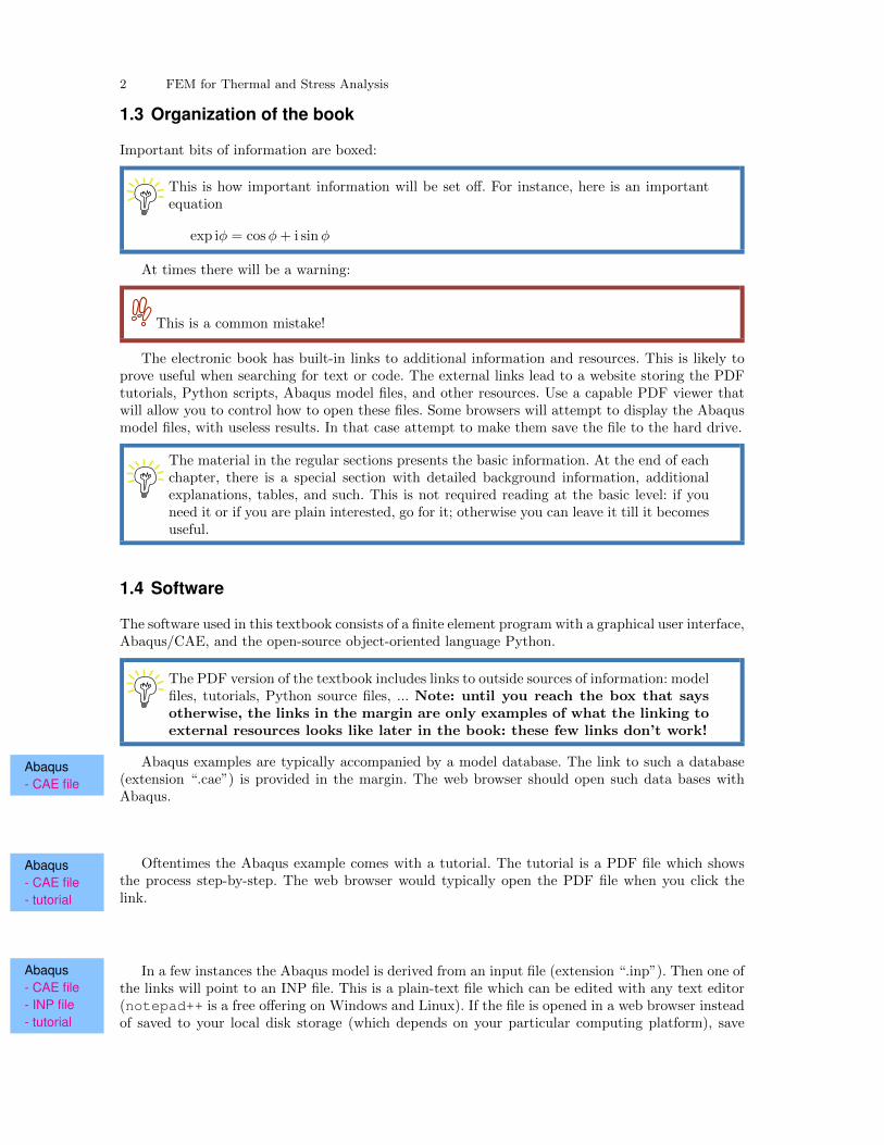
The PDF version of the textbook includes links to outside sources of information: modelfiles, tutorials, Python source files, ... Note: until you reach the box that saysotherwise, the links in the margin are only examples of what the linking toexternal resources looks like later in the book: these few links don’t work!

Abaqus- CAE file

Abaqus examples are typically accompanied by a model database. The link to such a database(extension “.cae”) is provided in the margin. The web browser should open such data bases withAbaqus.

Abaqus- CAE file- tutorial

Oftentimes the Abaqus example comes with a tutorial. The tutorial is a PDF file which showsthe process step-by-step. The web browser would typically open the PDF file when you click thelink.

Abaqus- CAE file- INP file- tutorial

In a few instances the Abaqus model is derived from an input file (extension “.inp”). Then one ofthe links will point to an INP file. This is a plain-text file which can be edited with any text editor(notepad++ is a free offering on Windows and Linux). If the file is opened in a web browser insteadof saved to your local disk storage (which depends on your particular computing platform), save

1.4 Software 3

the file with the “.inp” extension. As an example, in the Chrome browser, right-click on the textdisplayed in the browser and select “Save as...”. In the selection box “Save as type” choose“All Files”, and make sure to delete the “.txt” extension, if there is one attached to the name.Then in the folder where the file was saved you have the “.inp” file which can be now edited withany text editor. The tutorials will explain how to use the INP file.

Python- script

Some detailed finite element calculations are carried out with Python. Links to the Pythonscript files (extension .py) are available in the margin. Save the file and then load it in developmentenvironment of choice (see Section 1.4).

Animation- video

Some points are illustrated with animations. Links to video files are available in the margin, andare typically opened in a web browser. If that is not the case, locate the file in your Downloadsfolder and drag it to a browser window. (There are also specialized applications that can displayvideo files.)

Links to outside resources from this box on should all work. If you find a problem withthe downloads, please let the author know (pkrysl@ucsd.edu).

1.4.1 Abaqus software

Abaqus is a suite of commercial finite element codes. It consists of Abaqus Standard, which is ageneral purpose finite element software, and Abaqus Explicit for dynamic analysis. It is now ownedby Dassault Systemes and is part of the SIMULIA range of products, see

www.simulia.com/products/unified fea.html

In this book we will interact with the finite element analysis in Abaqus Standard through theAbaqus/CAE, a graphical user interface. Abaqus® is a registered trade mark of Dassault Systemes.For product information, please refer to the website http://www.3ds.com. This book has beentested with the Abaqus/CAE Teaching Edition and the Student Edition, as they were current in2020.

Abaqus is tightly coupled to Python, a very popular and widely used scripting language. TheAbaqus software can be driven by scripts, which makes it a very flexible and powerful tool. Inaddition, many exercises in this book will be supported by numerical or symbolic computations withPython in the form of script files.

1.4.2 Cloud computing

The easiest way of running most Python examples from the textbook (except those that requireAbaqus/CAE) may well be provided by the cloud computing environment try.jupyter.org. Selectfrom the “New” menu to create “Python 2” or “Python 3” notebook, and then paste blocks of codeor in fact the entire code of an example into the first cell of the notebook and select for instance“Run all” or “Run Cells”. This will create an output cell, with printouts and graphics.

The programming environment at repl.it is also very easy to use. Simply copy the text of thePython program into the main.py window and click on Run. Registration is free (as of 2020).

1.4.3 Local Python environment

The examples in this book were written with modules from the so-called SciPy stack (SciPy =Scientific Python). For those interested in having a local Python environment, a good option is tovisit www.scipy.org/install.html. At the top of the page there is a list of comprehensive packagesfor Linux, Windows and Mac (“Scientific Python Distributions”). All come with free versions, andas of 2020 there were these:

4 FEM for Thermal and Stress Analysis

1. Anaconda: A free distribution for the SciPy stack. Supports Linux, Windows and Mac.2. Enthought Canopy: The free and commercial versions include the core SciPy stack packages.

Supports Linux, Windows and Mac.3. WinPython: A free distribution including the SciPy stack. Windows only.

The two at the top require registration, the one at the end of the list is really the most straightforwardto get. Download, install, and run the provided Integrated Development Environment (IDE) (calledSpyder). Then download the script file by clicking one of the links in this textbook, open the filein the IDE, and run it.

1.4.4 Running Python in Abaqus

The examples in this book are worked with the Abaqus/CAE program. This program can be drivenby a Python script. When the user operates the Graphical User Interface (GUI), for instance topartition a face, Abaqus/CAE writes the commands to accomplish this to a few files: the main onesbeing the replay file, abaqus.rpy, the journal file (with extension .jnl), and the recovery file (withextension .rec). These are all Python scripts that can be executed from the “File” menu.

Abaqus/CAE Student Edition does not write the replay file and the journal file. Also,the recovery file is erased once the user quits the GUI.

These Python scripts can be edited by the user to accomplish slightly modified tasks, for instancethe dimensions of the part may be changed, or the material properties can be defined to work withuser inputs, etc.

The Abaqus Scripting Interface is an application programming interface (API) to the modelingand model data. The scripting interface is an extension of the Python object-oriented programminglanguage: the interface scripts are Python scripts. One can (a) create and modify the componentsof an Abaqus model (including, but not limited to, parts, materials, loads, and steps); (b) manageanalysis jobs; (c) manage output databases; (d) postprocess the results of an analysis.

An even nicer facility is part of Abaqus/CAE: the “Macro Manager”. Invoke the “MacroManager” from the “File” menu, and start recording the macro. Then execute a few Abaqus com-mands, such as create a sketch and extrude it into a part. Then stop the recording of the macro,and voila: the file called abaqusMacros.py appears in the working folder (typically c:\temp). Themacro is named, and its name should now appear on the list of the “Macro Manager”. Should it notappear automatically, feel free to click “Reload”. The contents of the abaqusMacros.py script filemay now be inspected with an editor of your choice. It consists essentially of definitions of Pythonfunctions. Each function is a macro.

As an example, here’s a link to a sample macros file. When this file is copied to the workingPython- script

folder, and the “Macro Manager” is opened, two macros should be listed:

� MakeCylinderPart to create a cylindrical solid part; and� MakeUsefulMaterials to create several material models.

1.4.5 Standing assumptions for Python code

Working with arrays and linear algebra in Python is best done with the array module numpy. Thefunctions array, dot, and so on are part of this module, as is the submodule linalg for linear-algebra operations. When we present Python code we usually don’t state that explicitly, but theseobjects need to be imported, for instance as

from numpy import array, dotfrom numpy import linalg

Similarly, when we work with the symbolic-math module sympy, we import the objects we needfrom this module

1.5 Units 5

from sympy import symbols, simplify, Matrix, diff

or, alternatively, we can import the module and then refer to the objects as for instance

import sympyA, B = sympy.symbols(’A, B’)

Some modules are not installed for the Abaqus Python environment. Code referencedin this book which relies on these modules will not run in the Abaqus command line.For instance neither sympy, nor matplotlib are available. It is easiest to use thesemodules in the cloud (in a Jupyter notebook), or with a local Python installation.

1.5 Units

Abaqus puts the onus of inputting the data in consistent units on the user. It is not alone in this, astypical finite element programs do not allow for explicit provision of physical units. This means thatinput data is only typed in as numbers, without any indication of the physical units. The programwill assume that the numbers that were input by the user were all in consistent units.

In thermomechanical problems one must choose four units, for example for length, mass, time,and temperature. For instance, in SI units for these quantities, we use m for length, kg for mass, sfor time and oK for temperature; then the units for forces will be in N, the stresses and the pressurewill be in Pa, the mass density will be in kg ·m−3, the thermal conductivity in W ·m−1 · oK−1 , andthe specific heat in J · kg−1 · oK−1.

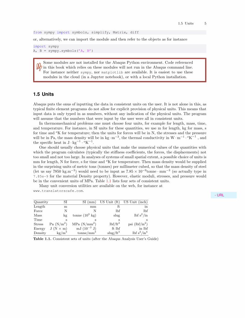
One should usually choose physical units that make the numerical values of the quantities withwhich the program calculates (typically the stiffness coefficients, the forces, the displacements) nottoo small and not too large. In analyses of systems of small spatial extent, a possible choice of units ismm for length, N for force, s for time and oK for temperature. Then mass density would be suppliedin the surprising units of metric tons (tonnes) per millimeter cubed, so that the mass density of steel(let us say 7850 kg.m−3) would need to be input as 7.85 × 10−9tonne ·mm−3 (so actually type in7.85e-9 for the material Density property). However, elastic moduli, stresses, and pressure wouldbe in the convenient units of MPa. Table 1.1 lists four sets of consistent units.

Many unit conversion utilities are available on the web, for instance atwww.translatorscafe.com.

- URL

Quantity SI SI (mm) US Unit (ft) US Unit (inch)

Length m mm ft inForce N N lbf lbfMass kg tonne (103 kg) slug lbf s2/inTime s s s sStress Pa (N/m2) MPa (N/mm2) lbf/ft2 psi (lbf/in2)Energy J (N × m) mJ (10−3 J) ft lbf in lbfDensity kg/m3 tonne/mm3 slug/ft3 lbf s2/in4

Table 1.1. Consistent sets of units (after the Abaqus Analysis User’s Guide)

6 FEM for Thermal and Stress Analysis

1.6 Abbreviations

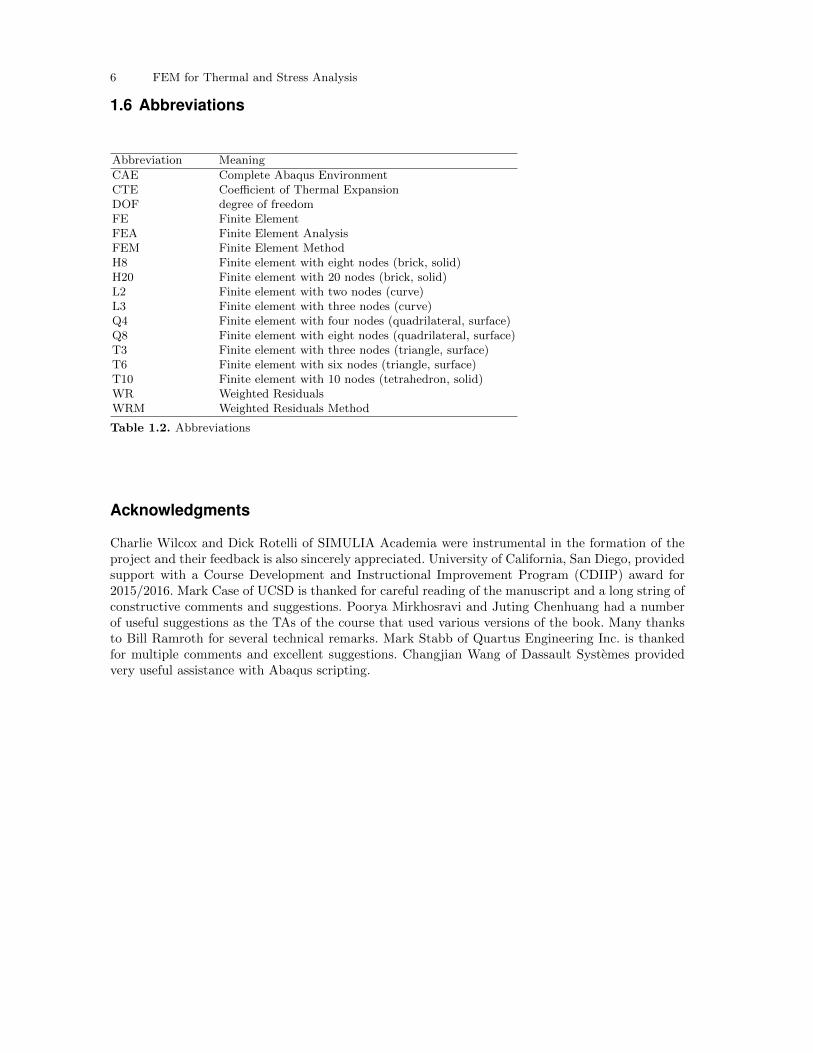
Abbreviation Meaning

CAE Complete Abaqus EnvironmentCTE Coefficient of Thermal ExpansionDOF degree of freedomFE Finite ElementFEA Finite Element AnalysisFEM Finite Element MethodH8 Finite element with eight nodes (brick, solid)H20 Finite element with 20 nodes (brick, solid)L2 Finite element with two nodes (curve)L3 Finite element with three nodes (curve)Q4 Finite element with four nodes (quadrilateral, surface)Q8 Finite element with eight nodes (quadrilateral, surface)T3 Finite element with three nodes (triangle, surface)T6 Finite element with six nodes (triangle, surface)T10 Finite element with 10 nodes (tetrahedron, solid)WR Weighted ResidualsWRM Weighted Residuals Method

Table 1.2. Abbreviations

Acknowledgments

Charlie Wilcox and Dick Rotelli of SIMULIA Academia were instrumental in the formation of theproject and their feedback is also sincerely appreciated. University of California, San Diego, providedsupport with a Course Development and Instructional Improvement Program (CDIIP) award for2015/2016. Mark Case of UCSD is thanked for careful reading of the manuscript and a long string ofconstructive comments and suggestions. Poorya Mirkhosravi and Juting Chenhuang had a numberof useful suggestions as the TAs of the course that used various versions of the book. Many thanksto Bill Ramroth for several technical remarks. Mark Stabb of Quartus Engineering Inc. is thankedfor multiple comments and excellent suggestions. Changjian Wang of Dassault Systemes providedvery useful assistance with Abaqus scripting.

2

Getting acquainted with the FEM

2.1 High-level explanation of the principles of FEM

Consider the mechanical part of the heavy-duty ball bearing housing of Figure 2.1. Without doubtAbaqus- CAE file

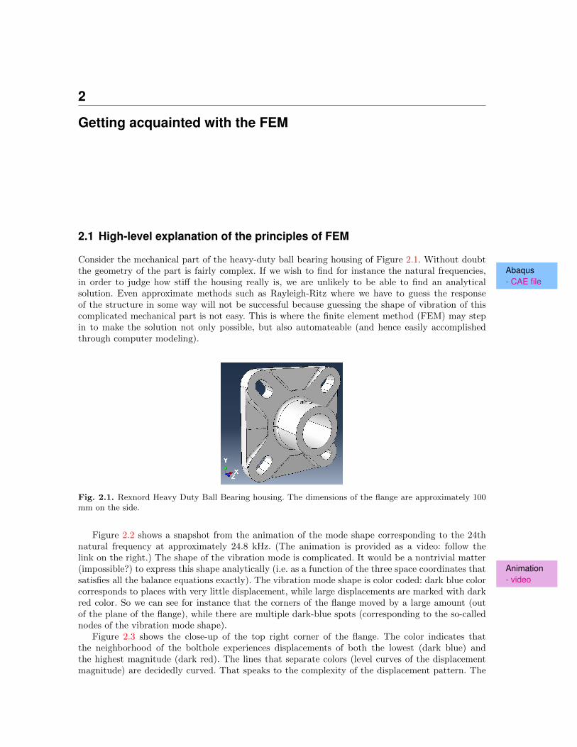
the geometry of the part is fairly complex. If we wish to find for instance the natural frequencies,in order to judge how stiff the housing really is, we are unlikely to be able to find an analyticalsolution. Even approximate methods such as Rayleigh-Ritz where we have to guess the responseof the structure in some way will not be successful because guessing the shape of vibration of thiscomplicated mechanical part is not easy. This is where the finite element method (FEM) may stepin to make the solution not only possible, but also automateable (and hence easily accomplishedthrough computer modeling).

Fig. 2.1. Rexnord Heavy Duty Ball Bearing housing. The dimensions of the flange are approximately 100mm on the side.

Figure 2.2 shows a snapshot from the animation of the mode shape corresponding to the 24thnatural frequency at approximately 24.8 kHz. (The animation is provided as a video: follow thelink on the right.) The shape of the vibration mode is complicated. It would be a nontrivial matter

Animation- video

(impossible?) to express this shape analytically (i.e. as a function of the three space coordinates thatsatisfies all the balance equations exactly). The vibration mode shape is color coded: dark blue colorcorresponds to places with very little displacement, while large displacements are marked with darkred color. So we can see for instance that the corners of the flange moved by a large amount (outof the plane of the flange), while there are multiple dark-blue spots (corresponding to the so-callednodes of the vibration mode shape).

Figure 2.3 shows the close-up of the top right corner of the flange. The color indicates thatthe neighborhood of the bolthole experiences displacements of both the lowest (dark blue) andthe highest magnitude (dark red). The lines that separate colors (level curves of the displacementmagnitude) are decidedly curved. That speaks to the complexity of the displacement pattern. The

8 FEM for Thermal and Stress Analysis

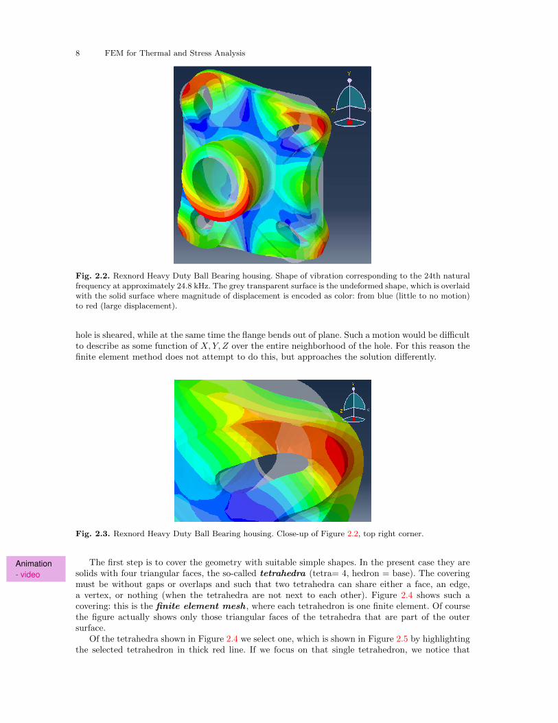
Fig. 2.2. Rexnord Heavy Duty Ball Bearing housing. Shape of vibration corresponding to the 24th naturalfrequency at approximately 24.8 kHz. The grey transparent surface is the undeformed shape, which is overlaidwith the solid surface where magnitude of displacement is encoded as color: from blue (little to no motion)to red (large displacement).

hole is sheared, while at the same time the flange bends out of plane. Such a motion would be difficultto describe as some function of X,Y, Z over the entire neighborhood of the hole. For this reason thefinite element method does not attempt to do this, but approaches the solution differently.

Fig. 2.3. Rexnord Heavy Duty Ball Bearing housing. Close-up of Figure 2.2, top right corner.

Animation- video

The first step is to cover the geometry with suitable simple shapes. In the present case they aresolids with four triangular faces, the so-called tetrahedra (tetra= 4, hedron = base). The coveringmust be without gaps or overlaps and such that two tetrahedra can share either a face, an edge,a vertex, or nothing (when the tetrahedra are not next to each other). Figure 2.4 shows such acovering: this is the finite element mesh , where each tetrahedron is one finite element. Of coursethe figure actually shows only those triangular faces of the tetrahedra that are part of the outersurface.

Of the tetrahedra shown in Figure 2.4 we select one, which is shown in Figure 2.5 by highlightingthe selected tetrahedron in thick red line. If we focus on that single tetrahedron, we notice that

2.1 High-level explanation of the principles of FEM 9

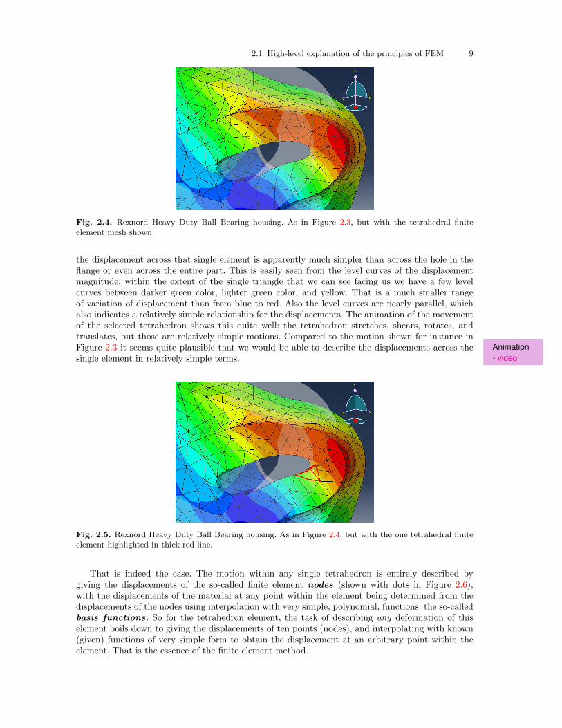
Fig. 2.4. Rexnord Heavy Duty Ball Bearing housing. As in Figure 2.3, but with the tetrahedral finiteelement mesh shown.

the displacement across that single element is apparently much simpler than across the hole in theflange or even across the entire part. This is easily seen from the level curves of the displacementmagnitude: within the extent of the single triangle that we can see facing us we have a few levelcurves between darker green color, lighter green color, and yellow. That is a much smaller rangeof variation of displacement than from blue to red. Also the level curves are nearly parallel, whichalso indicates a relatively simple relationship for the displacements. The animation of the movementof the selected tetrahedron shows this quite well: the tetrahedron stretches, shears, rotates, andtranslates, but those are relatively simple motions. Compared to the motion shown for instance in

Animation- video

Figure 2.3 it seems quite plausible that we would be able to describe the displacements across thesingle element in relatively simple terms.

Fig. 2.5. Rexnord Heavy Duty Ball Bearing housing. As in Figure 2.4, but with the one tetrahedral finiteelement highlighted in thick red line.

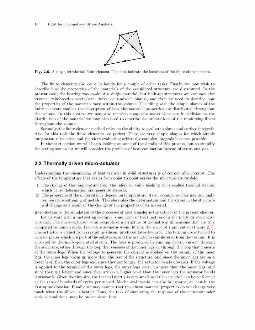
That is indeed the case. The motion within any single tetrahedron is entirely described bygiving the displacements of the so-called finite element nodes (shown with dots in Figure 2.6),with the displacements of the material at any point within the element being determined from thedisplacements of the nodes using interpolation with very simple, polynomial, functions: the so-calledbasis functions. So for the tetrahedron element, the task of describing any deformation of thiselement boils down to giving the displacements of ten points (nodes), and interpolating with known(given) functions of very simple form to obtain the displacement at an arbitrary point within theelement. That is the essence of the finite element method.

10 FEM for Thermal and Stress Analysis

Fig. 2.6. A single tetrahedral finite element. The dots indicate the locations of the finite element nodes.

The finite elements also come in handy for a couple of other tasks. Firstly, we may wish todescribe how the properties of the materials of the considered structure are distributed. In thepresent case, the bearing was made of a single material, but built-up structures are common (forinstance reinforced-concrete/steel decks, or sandwich plates), and then we need to describe howthe properties of the materials vary within the volume. The tiling with the simple shapes of thefinite elements enables the description of how the material properties are distributed throughoutthe volume. In this context we may also mention composite materials where in addition to thedistribution of the material we may also need to describe the orientations of the reinforcing fibersthroughout the volume.

Secondly, the finite element method relies on the ability to evaluate volume and surface integrals.Also for this task the finite elements are perfect. They are very simple shapes for which simpleintegration rules exist, and therefore evaluating arbitrarily complex integrals becomes possible.

In the next section we will begin looking at some of the details of this process, but to simplifythe setting somewhat we will consider the problem of heat conduction instead of stress analysis.

2.2 Thermally driven micro-actuator

Understanding the phenomena of heat transfer in solid structures is of considerable interest. Theeffects of the temperature that varies from point to point across the structure are twofold:

1. The change of the temperature from the reference value leads to the so-called thermal strains,which cause deformation and generate stresses.

2. The properties of the material may depend on temperature. As an example we may mention high-temperature softening of metals. Therefore also the deformation and the stress in the structurewill change as a result of the change of the properties of its material.

Introduction to the simulation of the processes of heat transfer is the subject of the present chapter.Let us start with a motivating example: simulation of the function of a thermally driven micro-

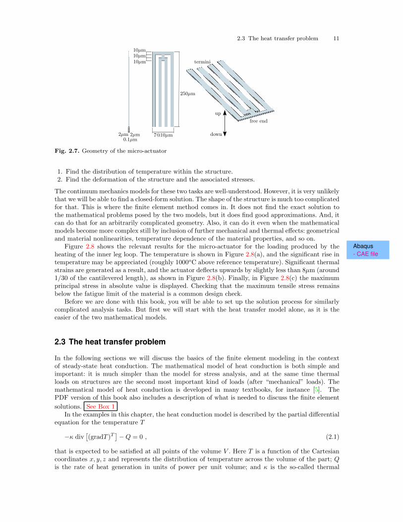
actuator. The micro-actuator is an example of a structure of geometrical dimensions that are tinycompared to human scale. The entire actuator would fit into the space of 1 mm cubed (Figure 2.7).The actuator is etched from crystalline silicon, produced layer-by-layer. The termini are attached tocontact plates which are part of the substrate, and the actuator is cantilevered from the termini. It isactuated by thermally-generated strains. The heat is produced by running electric current throughthe structure, either through the loop that consists of the inner legs, or through the loop that consistsof the outer legs. When the voltage to generate the current is applied on the termini of the innerlegs, the inner legs warm up more than the rest of the structure, and since the inner legs are on alower level then the outer legs and since they get longer, the actuator bends upwards. If the voltageis applied to the termini of the outer legs, the outer legs warm up more than the inner legs, andsince they get longer and since they are on a higher level than the inner legs the actuator bendsdownwards. Given the tiny size, the thermal inertia is very small, and the actuation can be performedat the rate of hundreds of cycles per second. Mechanical inertia can also be ignored, at least in thefirst approximation. Finally, we may assume that the silicon material properties do not change verymuch when the silicon is heated. Thus, the task of simulating the response of the actuator undervarious conditions, may be broken down into

2.3 The heat transfer problem 11

Fig. 2.7. Geometry of the micro-actuator

1. Find the distribution of temperature within the structure.2. Find the deformation of the structure and the associated stresses.

The continuum mechanics models for these two tasks are well-understood. However, it is very unlikelythat we will be able to find a closed-form solution. The shape of the structure is much too complicatedfor that. This is where the finite element method comes in. It does not find the exact solution tothe mathematical problems posed by the two models, but it does find good approximations. And, itcan do that for an arbitrarily complicated geometry. Also, it can do it even when the mathematicalmodels become more complex still by inclusion of further mechanical and thermal effects: geometricaland material nonlinearities, temperature dependence of the material properties, and so on.

Abaqus- CAE file

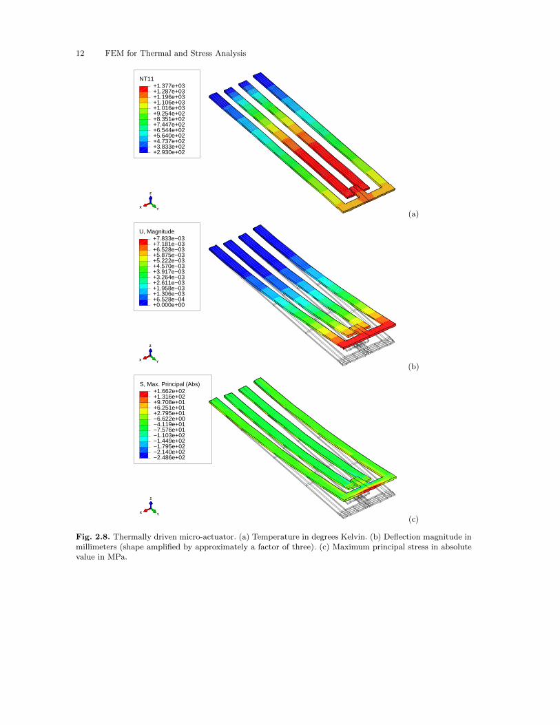
Figure 2.8 shows the relevant results for the micro-actuator for the loading produced by theheating of the inner leg loop. The temperature is shown in Figure 2.8(a), and the significant rise intemperature may be appreciated (roughly 1000oC above reference temperature). Significant thermalstrains are generated as a result, and the actuator deflects upwards by slightly less than 8µm (around1/30 of the cantilevered length), as shown in Figure 2.8(b). Finally, in Figure 2.8(c) the maximumprincipal stress in absolute value is displayed. Checking that the maximum tensile stress remainsbelow the fatigue limit of the material is a common design check.

Before we are done with this book, you will be able to set up the solution process for similarlycomplicated analysis tasks. But first we will start with the heat transfer model alone, as it is theeasier of the two mathematical models.

2.3 The heat transfer problem

In the following sections we will discuss the basics of the finite element modeling in the contextof steady-state heat conduction. The mathematical model of heat conduction is both simple andimportant: it is much simpler than the model for stress analysis, and at the same time thermalloads on structures are the second most important kind of loads (after “mechanical” loads). Themathematical model of heat conduction is developed in many textbooks, for instance [5]. ThePDF version of this book also includes a description of what is needed to discuss the finite element

solutions. See Box 1In the examples in this chapter, the heat conduction model is described by the partial differential

equation for the temperature T

−κ div[(gradT )T

]−Q = 0 , (2.1)

that is expected to be satisfied at all points of the volume V . Here T is a function of the Cartesiancoordinates x, y, z and represents the distribution of temperature across the volume of the part; Qis the rate of heat generation in units of power per unit volume; and κ is the so-called thermal

12 FEM for Thermal and Stress Analysis

NT11

+2.930e+02+3.833e+02+4.737e+02+5.640e+02+6.544e+02+7.447e+02+8.351e+02+9.254e+02+1.016e+03+1.106e+03+1.196e+03+1.287e+03+1.377e+03

X Y

Z

(a)

U, Magnitude

+0.000e+00+6.528e−04+1.306e−03+1.958e−03+2.611e−03+3.264e−03+3.917e−03+4.570e−03+5.222e−03+5.875e−03+6.528e−03+7.181e−03+7.833e−03

X Y

Z

(b)

S, Max. Principal (Abs)

−2.486e+02−2.140e+02−1.795e+02−1.449e+02−1.103e+02−7.576e+01−4.119e+01−6.622e+00+2.795e+01+6.251e+01+9.708e+01+1.316e+02+1.662e+02

X Y

Z

(c)

Fig. 2.8. Thermally driven micro-actuator. (a) Temperature in degrees Kelvin. (b) Deflection magnitude inmillimeters (shape amplified by approximately a factor of three). (c) Maximum principal stress in absolutevalue in MPa.

2.4 Concrete column 13

conductivity, which is a property of the concrete material; the material is assumed to be the sameeverywhere within V (i.e. homogeneous). The div and grad are the divergence and gradient operators.Explicitly we write

−κ(∂2T

∂x2+∂2T

∂y2+∂2T

∂z2

)−Q = 0 . (2.2)

This equation expresses the balance of heat energy, and if we find a solution, it will hold at everysingle point in the volume V .

The boundary conditions are the decisive part of the mathematical model: they can make thesolution unique, and they are crucial in deciding whether or not the solution exists in the first place.Physically the boundary conditions are an expression of the interaction of the world with a subsetof it that we wish to model. We always limit ourselves to a simple three-dimensional body. Theinteraction of this modeled three-dimensional body with the environment in which it exists (otherthree-dimensional bodies, the ambient media, and so on) is expressed through the interactions thatthe modeled body has with the not-modeled rest of the world. This interaction occurs across theboundaries.

In the first example we will consider the two simplest kinds of boundary condition, namely thetemperature being known and the zero heat flux condition.(For a thorough discussion of boundary

conditions see See Box 2 .)

2.4 Concrete column

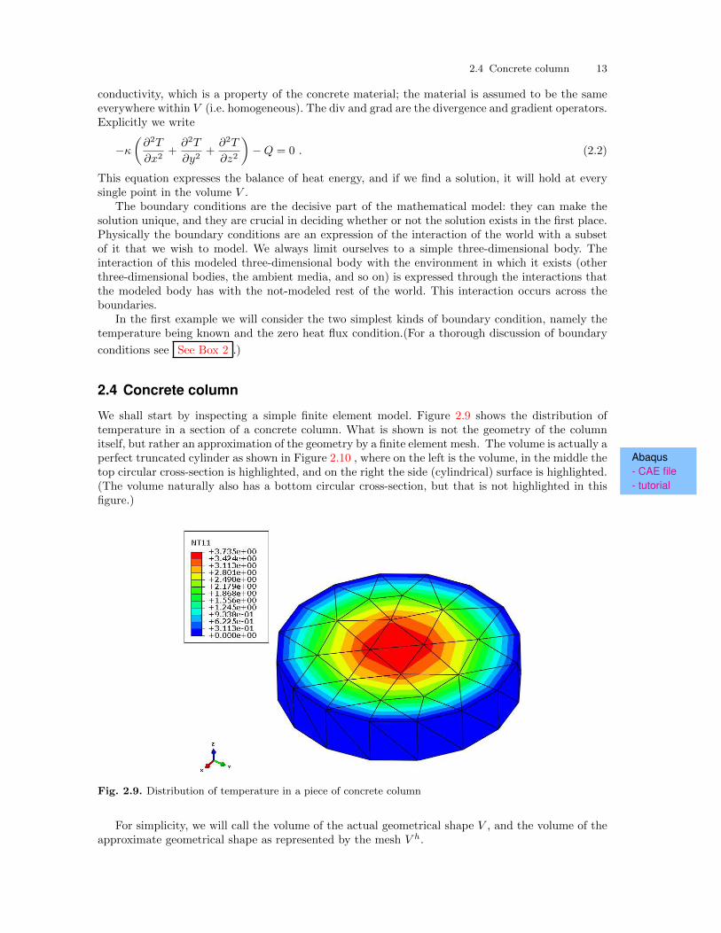
We shall start by inspecting a simple finite element model. Figure 2.9 shows the distribution oftemperature in a section of a concrete column. What is shown is not the geometry of the columnitself, but rather an approximation of the geometry by a finite element mesh. The volume is actually a

Abaqus- CAE file- tutorial

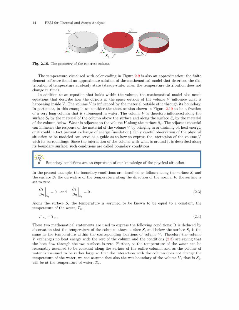
perfect truncated cylinder as shown in Figure 2.10 , where on the left is the volume, in the middle thetop circular cross-section is highlighted, and on the right the side (cylindrical) surface is highlighted.(The volume naturally also has a bottom circular cross-section, but that is not highlighted in thisfigure.)

Fig. 2.9. Distribution of temperature in a piece of concrete column

For simplicity, we will call the volume of the actual geometrical shape V , and the volume of theapproximate geometrical shape as represented by the mesh V h.

14 FEM for Thermal and Stress Analysis

Fig. 2.10. The geometry of the concrete column

The temperature visualized with color coding in Figure 2.9 is also an approximation: the finiteelement software found an approximate solution of the mathematical model that describes the dis-tribution of temperature at steady state (steady-state: when the temperature distribution does notchange in time).

In addition to an equation that holds within the volume, the mathematical model also needsequations that describe how the objects in the space outside of the volume V influence what ishappening inside V . The volume V is influenced by the material outside of it through its boundary.In particular, in this example we consider the short section shown in Figure 2.10 to be a fractionof a very long column that is submerged in water. The volume V is therefore influenced along thesurface St by the material of the column above the surface and along the surface Sb by the materialof the column below. Water is adjacent to the volume V along the surface Ss. The adjacent materialcan influence the response of the material of the volume V by bringing in or draining off heat energy,or it could in fact prevent exchange of energy (insulation). Only careful observation of the physicalsituation to be modeled can serve as a guide as to how to express the interaction of the volume Vwith its surroundings. Since the interaction of the volume with what is around it is described alongits boundary surface, such conditions are called boundary conditions.

Boundary conditions are an expression of our knowledge of the physical situation.

In the present example, the boundary conditions are described as follows: along the surface St andthe surface Sb the derivative of the temperature along the direction of the normal to the surface isset to zero

∂T

∂n

∣∣∣∣St

= 0 and∂T

∂n

∣∣∣∣Sb

= 0 . (2.3)

Along the surface Ss the temperature is assumed to be known to be equal to a constant, thetemperature of the water, Tw,

T |Ss= Tw . (2.4)

These two mathematical statements are used to express the following conditions: It is deduced byobservation that the temperature of the columns above surface St and below the surface Sb is thesame as the temperature within the corresponding locations of volume V . Therefore the volumeV exchanges no heat energy with the rest of the column and the conditions (2.3) are saying thatthe heat flow through the two surfaces is zero. Further, as the temperature of the water can bereasonably assumed to be constant along the surface of the entire column, and as the volume ofwater is assumed to be rather large so that the interaction with the column does not change thetemperature of the water, we can assume that also the wet boundary of the volume V , that is Ss,will be at the temperature of water, Tw.

2.4 Concrete column 15

2.4.1 Boundary value problem solved

Equations (2.1), (2.3) , and (2.4) are a package that together defines the mathematical model. Themathematical model is known as a boundary value problem. The significance of the boundaries isclearly indicated in the name!

Some of these boundary value problems can be solved exactly by clever tricks and sophisticatedmathematical techniques. The point of finite element methods is that they are applicable when noanalytical techniques exist to solve these problems.

The analytical solution can be derived in cylindrical coordinates See Box 3 as T (r) = Q4κ

(a2 − r2

).

For the temperature distribution in a concrete column of circular cross-section of radius a = 2.5m,immersed in water at Tw = 0o C, where the concrete gives off hydration heat at the rate ofQ = 4.5 W/m3, and the thermal conductivity of concrete is taken at κ = 1.8W/m/oK, the tem-perature at the axis of the cylinder is 3.906oC. The temperature varies only in the radial direction,not in the circumferential direction and not in the axial direction. Therefore the gradient of thetemperature points directly to the axis of the cylinder (the temperature increases from the circum-ference towards the center). The maximum temperature gradient value obtains at the circumference,∂T (r = a)/∂r = Q

2κa = 3.125oC/m. The quantity that is used in thermal analyses to measure theflow of energy per unit area is the heat flux. By definition, the radial component of the heat fluxwould in this case be

qr(r) = −κ∂T (r)∂r

. (2.5)

The radial component of the heat flux at the circumference of the column would be qr(r = a) =5.625W/m2.

X Y

Z

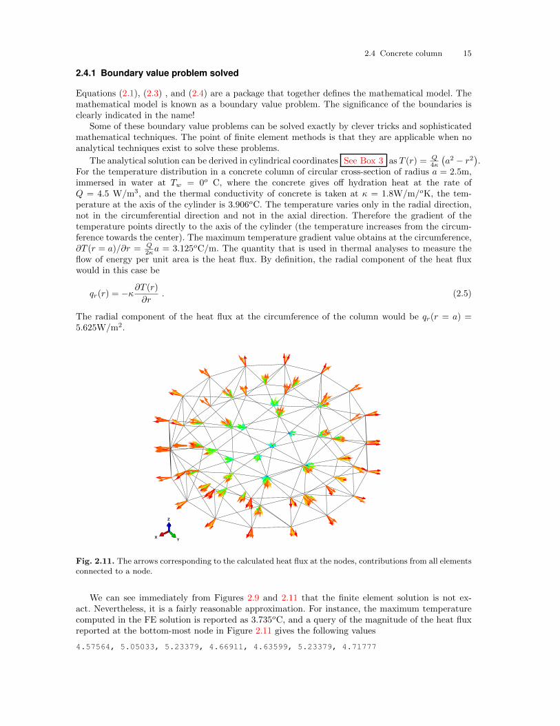
Fig. 2.11. The arrows corresponding to the calculated heat flux at the nodes, contributions from all elementsconnected to a node.

We can see immediately from Figures 2.9 and 2.11 that the finite element solution is not ex-act. Nevertheless, it is a fairly reasonable approximation. For instance, the maximum temperaturecomputed in the FE solution is reported as 3.735oC, and a query of the magnitude of the heat fluxreported at the bottom-most node in Figure 2.11 gives the following values

4.57564, 5.05033, 5.23379, 4.66911, 4.63599, 5.23379, 4.71777

16 FEM for Thermal and Stress Analysis

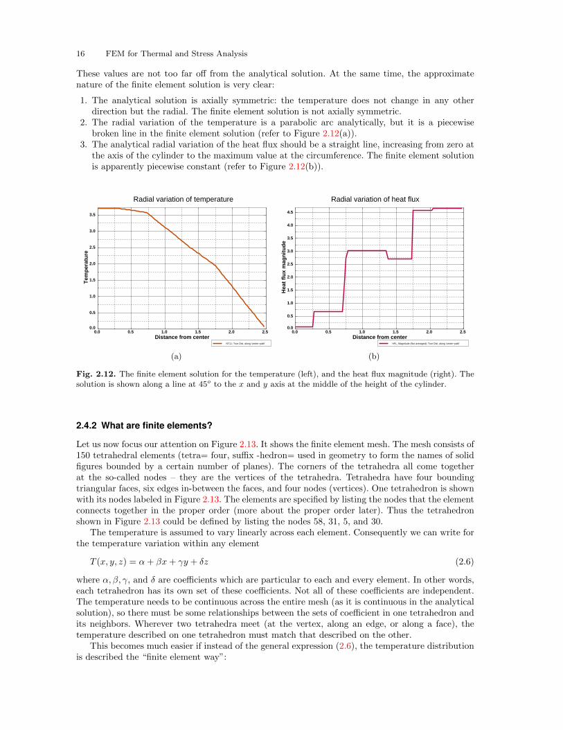
These values are not too far off from the analytical solution. At the same time, the approximatenature of the finite element solution is very clear:

1. The analytical solution is axially symmetric: the temperature does not change in any otherdirection but the radial. The finite element solution is not axially symmetric.

2. The radial variation of the temperature is a parabolic arc analytically, but it is a piecewisebroken line in the finite element solution (refer to Figure 2.12(a)).

3. The analytical radial variation of the heat flux should be a straight line, increasing from zero atthe axis of the cylinder to the maximum value at the circumference. The finite element solutionis apparently piecewise constant (refer to Figure 2.12(b)).

Radial variation of temperature

Distance from center0.0 0.5 1.0 1.5 2.0 2.5

Tem

per

atu

re

0.0

0.5

1.0

1.5

2.0

2.5

3.0

3.5

NT11: True Dist. along ’center−path’

Radial variation of heat flux

Distance from center0.0 0.5 1.0 1.5 2.0 2.5

Hea

t fl

ux

mag

nit

ud

e

0.0

0.5

1.0

1.5

2.0

2.5

3.0

3.5

4.0

4.5

HFL, Magnitude (Not averaged): True Dist. along ’center−path’

(a) (b)

Fig. 2.12. The finite element solution for the temperature (left), and the heat flux magnitude (right). Thesolution is shown along a line at 45o to the x and y axis at the middle of the height of the cylinder.

2.4.2 What are finite elements?

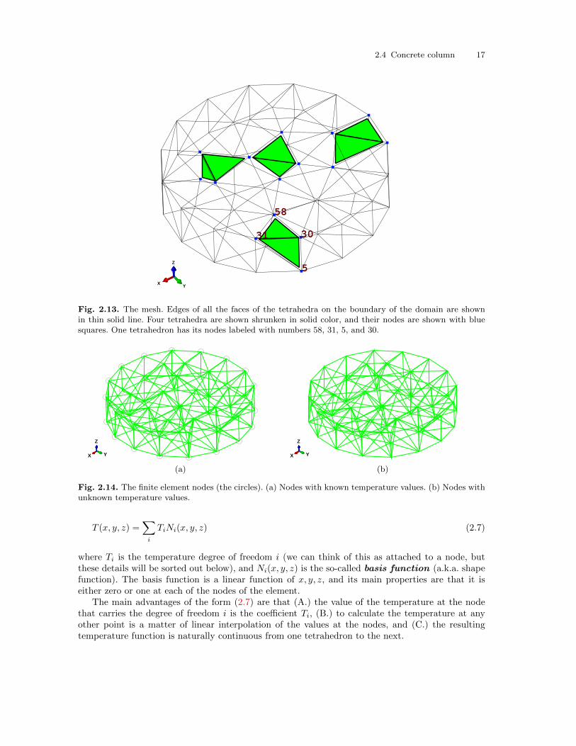
Let us now focus our attention on Figure 2.13. It shows the finite element mesh. The mesh consists of150 tetrahedral elements (tetra= four, suffix -hedron= used in geometry to form the names of solidfigures bounded by a certain number of planes). The corners of the tetrahedra all come togetherat the so-called nodes – they are the vertices of the tetrahedra. Tetrahedra have four boundingtriangular faces, six edges in-between the faces, and four nodes (vertices). One tetrahedron is shownwith its nodes labeled in Figure 2.13. The elements are specified by listing the nodes that the elementconnects together in the proper order (more about the proper order later). Thus the tetrahedronshown in Figure 2.13 could be defined by listing the nodes 58, 31, 5, and 30.

The temperature is assumed to vary linearly across each element. Consequently we can write forthe temperature variation within any element

T (x, y, z) = α+ βx+ γy + δz (2.6)

where α, β, γ, and δ are coefficients which are particular to each and every element. In other words,each tetrahedron has its own set of these coefficients. Not all of these coefficients are independent.The temperature needs to be continuous across the entire mesh (as it is continuous in the analyticalsolution), so there must be some relationships between the sets of coefficient in one tetrahedron andits neighbors. Wherever two tetrahedra meet (at the vertex, along an edge, or along a face), thetemperature described on one tetrahedron must match that described on the other.

This becomes much easier if instead of the general expression (2.6), the temperature distributionis described the “finite element way”:

2.4 Concrete column 17

58

31 30

5X Y

Z

Fig. 2.13. The mesh. Edges of all the faces of the tetrahedra on the boundary of the domain are shownin thin solid line. Four tetrahedra are shown shrunken in solid color, and their nodes are shown with bluesquares. One tetrahedron has its nodes labeled with numbers 58, 31, 5, and 30.

X Y

Z

X Y

Z

(a) (b)

Fig. 2.14. The finite element nodes (the circles). (a) Nodes with known temperature values. (b) Nodes withunknown temperature values.

T (x, y, z) =∑i

TiNi(x, y, z) (2.7)

where Ti is the temperature degree of freedom i (we can think of this as attached to a node, butthese details will be sorted out below), and Ni(x, y, z) is the so-called basis function (a.k.a. shapefunction). The basis function is a linear function of x, y, z, and its main properties are that it iseither zero or one at each of the nodes of the element.

The main advantages of the form (2.7) are that (A.) the value of the temperature at the nodethat carries the degree of freedom i is the coefficient Ti, (B.) to calculate the temperature at anyother point is a matter of linear interpolation of the values at the nodes, and (C.) the resultingtemperature function is naturally continuous from one tetrahedron to the next.

18 FEM for Thermal and Stress Analysis

For the four node tetrahedron the basis function is linear in x, y, z. The value of a basisfunction at a node is either zero or one— this is referred to as having the Kroneckerdelta property. The derivatives of the basis function with the respect to x, y, z areconstant within the element.

For the tetrahedron it is relatively straightforward to calculate the form of such linear basis

functions from the Kronecker delta property See Box 4 , but there is a more natural way which willbe discussed later.

Figure 2.14 shows two sets of nodes. (a) The temperature is known for nodes that are located onthe boundary where the temperature value is prescribed (the cylindrical side surface Ss); and (b)the temperature is unknown at all the other nodes. The quantities that are associated with nodesare called the degrees of freedom. The degrees of freedom at nodes that are at the boundary arecalled fixed, because their value is determined, before the calculation even starts, from the boundaryconditions. The degrees of freedom that are unknown until the calculation finishes are the free degreesof freedom. Here “free” is used as the opposite of “fixed”.

The degrees of freedom (DOFs) are the values of the temperature at the nodes. SomeDOFs are fixed by the boundary conditions, others needs to be calculated from thefinite element equations: these are free (as opposed to fixed).

The expressions for the basis functions can be also easily differentiated to obtain the gradientof temperature at any point. For instance, the temperature values at the nodes 30, 31, and 5 areknown to be zero because of the boundary condition (see Figure 2.13). The temperature at node 58

is 2.07121o C as we find by querying the temperature in the Abaqus model. See Box 5 FurthermoreAbaqus- CAE file

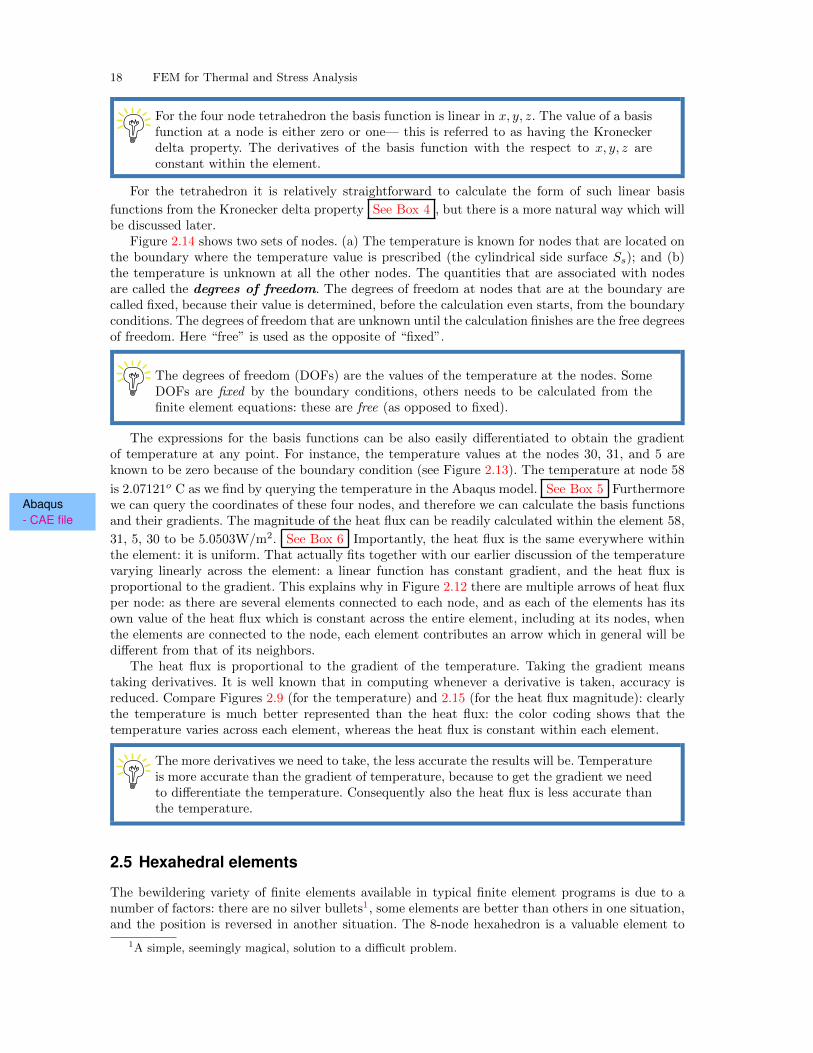
we can query the coordinates of these four nodes, and therefore we can calculate the basis functionsand their gradients. The magnitude of the heat flux can be readily calculated within the element 58,

31, 5, 30 to be 5.0503W/m2. See Box 6 Importantly, the heat flux is the same everywhere withinthe element: it is uniform. That actually fits together with our earlier discussion of the temperaturevarying linearly across the element: a linear function has constant gradient, and the heat flux isproportional to the gradient. This explains why in Figure 2.12 there are multiple arrows of heat fluxper node: as there are several elements connected to each node, and as each of the elements has itsown value of the heat flux which is constant across the entire element, including at its nodes, whenthe elements are connected to the node, each element contributes an arrow which in general will bedifferent from that of its neighbors.

The heat flux is proportional to the gradient of the temperature. Taking the gradient meanstaking derivatives. It is well known that in computing whenever a derivative is taken, accuracy isreduced. Compare Figures 2.9 (for the temperature) and 2.15 (for the heat flux magnitude): clearlythe temperature is much better represented than the heat flux: the color coding shows that thetemperature varies across each element, whereas the heat flux is constant within each element.

The more derivatives we need to take, the less accurate the results will be. Temperatureis more accurate than the gradient of temperature, because to get the gradient we needto differentiate the temperature. Consequently also the heat flux is less accurate thanthe temperature.

2.5 Hexahedral elements

The bewildering variety of finite elements available in typical finite element programs is due to anumber of factors: there are no silver bullets1, some elements are better than others in one situation,and the position is reversed in another situation. The 8-node hexahedron is a valuable element to

1A simple, seemingly magical, solution to a difficult problem.

2.6 Using symmetry 19

42, 5.05033

HFL, Magnitude

+8.611e−02+5.279e−01+9.698e−01+1.412e+00+1.853e+00+2.295e+00+2.737e+00+3.179e+00+3.621e+00+4.063e+00+4.504e+00+4.946e+00+5.388e+00

X Y

Z

Fig. 2.15. The heat flux magnitude displayed with color coding for the entire mesh, and with annotationlabel for the element with nodes [58, 31, 5, 30] (heat flux magnitude 5.0503).

NT11

+0.000e+00+3.222e−01+6.444e−01+9.666e−01+1.289e+00+1.611e+00+1.933e+00+2.256e+00+2.578e+00+2.900e+00+3.222e+00+3.544e+00+3.867e+00

X Y

Z

HFL, Magnitude

+3.313e−01+7.356e−01+1.140e+00+1.544e+00+1.949e+00+2.353e+00+2.757e+00+3.161e+00+3.566e+00+3.970e+00+4.374e+00+4.779e+00+5.183e+00

X Y

Z

(a) (b)

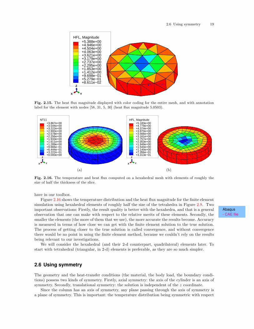
Fig. 2.16. The temperature and heat flux computed on a hexahedral mesh with elements of roughly thesize of half the thickness of the slice.

have in our toolbox.Figure 2.16 shows the temperature distribution and the heat flux magnitude for the finite element

simulation using hexahedral elements of roughly half the size of the tetrahedra in Figure 2.9. TwoAbaqus- CAE file

important observations: Firstly, the result quality is better with the hexahedra, and that is a generalobservation that one can make with respect to the relative merits of these elements. Secondly, thesmaller the elements (the more of them that we use), the more accurate the results become. Accuracyis measured in terms of how close we can get with the finite element solution to the true solution.The process of getting closer to the true solution is called convergence, and without convergencethere would be no point in using the finite element method, because we couldn’t rely on the resultsbeing relevant to our investigations.

We will consider the hexahedral (and their 2-d counterpart, quadrilateral) elements later. Tostart with tetrahedral (triangular, in 2-d) elements is preferable, as they are so much simpler.

2.6 Using symmetry

The geometry and the heat-transfer conditions (the material, the body load, the boundary condi-tions) possess two kinds of symmetry. Firstly, axial symmetry: the axis of the cylinder is an axis ofsymmetry. Secondly, translational symmetry: the solution is independent of the z coordinate.

Since the column has an axis of symmetry, any plane passing through the axis of symmetry isa plane of symmetry. This is important: the temperature distribution being symmetric with respect

20 FEM for Thermal and Stress Analysis

to the plane of symmetry means that the gradient of temperature through the plane of symmetryis zero. This means that the heat flux through the plane of symmetry is known to be zero. Thus weget a natural boundary condition that we can use, we only have to be able to identify a plane ofsymmetry.

Since any plane passing through the axis is a symmetry plane, which one of the infinitely manyplanes do we pick? We can pick a single plane, effectively slicing the column in half. This is nice, thesize of the problem is immediately reduced with a factor of two. But we can do better, we can picktwo planes. The pie slice generated in this way could be of any interior angle. The smaller the anglethe smaller the model (the fewer the elements in the mesh). However, we should not make the angletoo small: small angle means poorly shaped elements, and poorly shaped elements lead to errors. Solet us make it 15o.

Abaqus- CAE file- tutorial

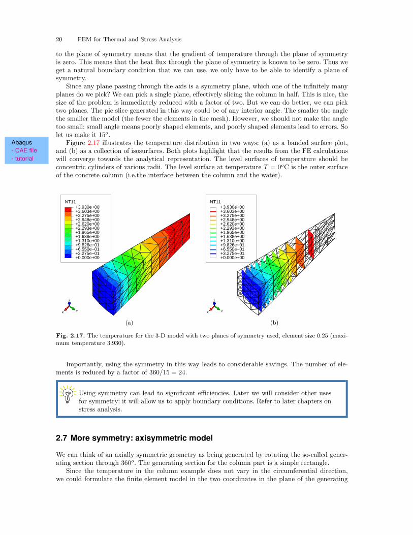
Figure 2.17 illustrates the temperature distribution in two ways: (a) as a banded surface plot,and (b) as a collection of isosurfaces. Both plots highlight that the results from the FE calculationswill converge towards the analytical representation. The level surfaces of temperature should beconcentric cylinders of various radii. The level surface at temperature T = 0oC is the outer surfaceof the concrete column (i.e.the interface between the column and the water).

NT11

+0.000e+00+3.275e−01+6.550e−01+9.826e−01+1.310e+00+1.638e+00+1.965e+00+2.293e+00+2.620e+00+2.948e+00+3.275e+00+3.603e+00+3.930e+00

X Y

Z

NT11

+0.000e+00+3.275e−01+6.550e−01+9.826e−01+1.310e+00+1.638e+00+1.965e+00+2.293e+00+2.620e+00+2.948e+00+3.275e+00+3.603e+00+3.930e+00

X Y

Z

(a) (b)

Fig. 2.17. The temperature for the 3-D model with two planes of symmetry used, element size 0.25 (maxi-mum temperature 3.930).

Importantly, using the symmetry in this way leads to considerable savings. The number of ele-ments is reduced by a factor of 360/15 = 24.

Using symmetry can lead to significant efficiencies. Later we will consider other usesfor symmetry: it will allow us to apply boundary conditions. Refer to later chapters onstress analysis.

2.7 More symmetry: axisymmetric model

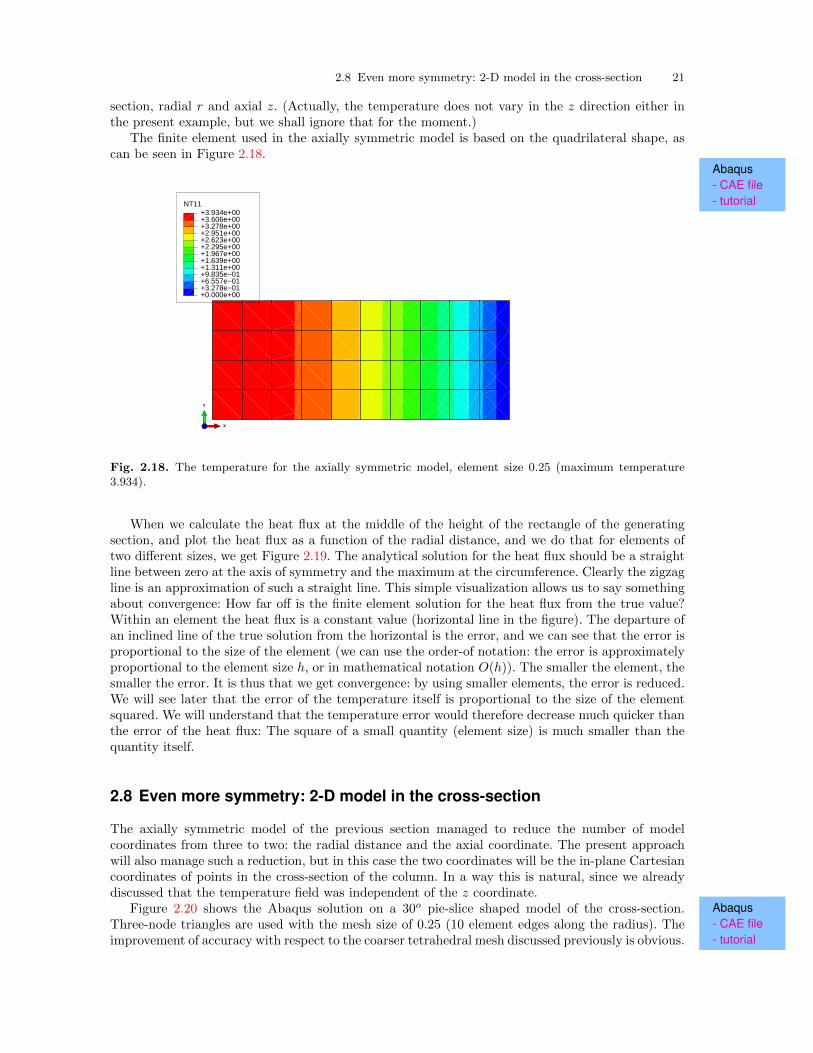
We can think of an axially symmetric geometry as being generated by rotating the so-called gener-ating section through 360o. The generating section for the column part is a simple rectangle.

Since the temperature in the column example does not vary in the circumferential direction,we could formulate the finite element model in the two coordinates in the plane of the generating

2.8 Even more symmetry: 2-D model in the cross-section 21

section, radial r and axial z. (Actually, the temperature does not vary in the z direction either inthe present example, but we shall ignore that for the moment.)

The finite element used in the axially symmetric model is based on the quadrilateral shape, ascan be seen in Figure 2.18.

Abaqus- CAE file- tutorialNT11

+0.000e+00+3.278e−01+6.557e−01+9.835e−01+1.311e+00+1.639e+00+1.967e+00+2.295e+00+2.623e+00+2.951e+00+3.278e+00+3.606e+00+3.934e+00

X

Y

Z

Fig. 2.18. The temperature for the axially symmetric model, element size 0.25 (maximum temperature3.934).

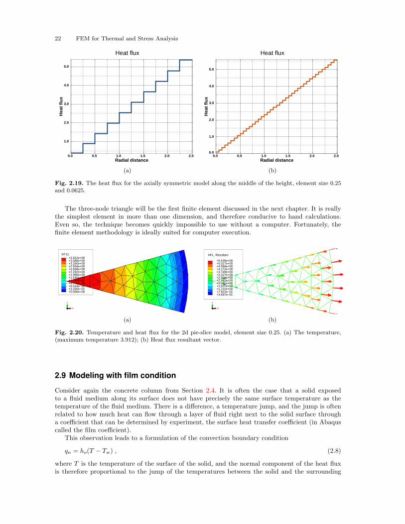
When we calculate the heat flux at the middle of the height of the rectangle of the generatingsection, and plot the heat flux as a function of the radial distance, and we do that for elements oftwo different sizes, we get Figure 2.19. The analytical solution for the heat flux should be a straightline between zero at the axis of symmetry and the maximum at the circumference. Clearly the zigzagline is an approximation of such a straight line. This simple visualization allows us to say somethingabout convergence: How far off is the finite element solution for the heat flux from the true value?Within an element the heat flux is a constant value (horizontal line in the figure). The departure ofan inclined line of the true solution from the horizontal is the error, and we can see that the error isproportional to the size of the element (we can use the order-of notation: the error is approximatelyproportional to the element size h, or in mathematical notation O(h)). The smaller the element, thesmaller the error. It is thus that we get convergence: by using smaller elements, the error is reduced.We will see later that the error of the temperature itself is proportional to the size of the elementsquared. We will understand that the temperature error would therefore decrease much quicker thanthe error of the heat flux: The square of a small quantity (element size) is much smaller than thequantity itself.

2.8 Even more symmetry: 2-D model in the cross-section

The axially symmetric model of the previous section managed to reduce the number of modelcoordinates from three to two: the radial distance and the axial coordinate. The present approachwill also manage such a reduction, but in this case the two coordinates will be the in-plane Cartesiancoordinates of points in the cross-section of the column. In a way this is natural, since we alreadydiscussed that the temperature field was independent of the z coordinate.

Abaqus- CAE file- tutorial

Figure 2.20 shows the Abaqus solution on a 30o pie-slice shaped model of the cross-section.Three-node triangles are used with the mesh size of 0.25 (10 element edges along the radius). Theimprovement of accuracy with respect to the coarser tetrahedral mesh discussed previously is obvious.

22 FEM for Thermal and Stress Analysis

Heat flux

Radial distance0.0 0.5 1.0 1.5 2.0 2.5

Hea

t fl

ux

1.0

2.0

3.0

4.0

5.0

Heat flux

Radial distance0.0 0.5 1.0 1.5 2.0 2.5

Hea

t fl

ux

0.0

1.0

2.0

3.0

4.0

5.0

(a) (b)

Fig. 2.19. The heat flux for the axially symmetric model along the middle of the height, element size 0.25and 0.0625.

The three-node triangle will be the first finite element discussed in the next chapter. It is reallythe simplest element in more than one dimension, and therefore conducive to hand calculations.Even so, the technique becomes quickly impossible to use without a computer. Fortunately, thefinite element methodology is ideally suited for computer execution.

NT11

+0.000e+00+3.260e−01+6.519e−01+9.779e−01+1.304e+00+1.630e+00+1.956e+00+2.282e+00+2.608e+00+2.934e+00+3.260e+00+3.586e+00+3.912e+00

X

Y

Z

HFL, Resultant

+3.697e−01+7.921e−01+1.215e+00+1.637e+00+2.060e+00+2.482e+00+2.904e+00+3.327e+00+3.749e+00+4.172e+00+4.594e+00+5.017e+00+5.439e+00

X

Y

Z

(a) (b)

Fig. 2.20. Temperature and heat flux for the 2d pie-slice model, element size 0.25. (a) The temperature,(maximum temperature 3.912); (b) Heat flux resultant vector.

2.9 Modeling with film condition

Consider again the concrete column from Section 2.4. It is often the case that a solid exposedto a fluid medium along its surface does not have precisely the same surface temperature as thetemperature of the fluid medium. There is a difference, a temperature jump, and the jump is oftenrelated to how much heat can flow through a layer of fluid right next to the solid surface througha coefficient that can be determined by experiment, the surface heat transfer coefficient (in Abaquscalled the film coefficient).

This observation leads to a formulation of the convection boundary condition

qn = ho(T − Tw) , (2.8)

where T is the temperature of the surface of the solid, and the normal component of the heat fluxis therefore proportional to the jump of the temperatures between the solid and the surrounding

2.10 Bird’s-eye view of FEA 23

medium. See Box 2 In this example the convection boundary condition is applied on the sidecylindrical surface. The ambient temperature is again taken as 0oC, and the surface heat transfer

Abaqus- CAE file- tutorial

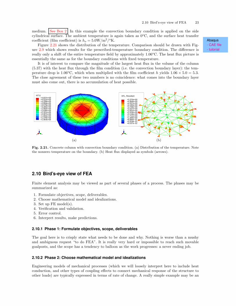
coefficient (film coefficient) is ho = 5.0W/m2/oK.Figure 2.21 shows the distribution of the temperature. Comparison should be drawn with Fig-

ure 2.9 which shows results for the prescribed-temperature boundary condition. The difference isreally only a shift of the entire temperature field by approximately 1.06oC. The heat flux picture isessentially the same as for the boundary conditions with fixed temperature.

It is of interest to compare the magnitude of the largest heat flux in the volume of the column(5.37) with the heat flux through the film condition (i.e. the convection boundary layer): the tem-perature drop is 1.06oC, which when multiplied with the film coefficient h yields 1.06 × 5.0 = 5.3.The close agreement of these two numbers is no coincidence: what comes into the boundary layermust also come out, there is no accumulation of heat possible.

NT11

+1.064e+00+1.378e+00+1.693e+00+2.007e+00+2.321e+00+2.636e+00+2.950e+00+3.265e+00+3.579e+00+3.894e+00+4.208e+00+4.522e+00+4.837e+00

X Y

Z

HFL, Resultant

+8.537e−02+4.919e−01+8.984e−01+1.305e+00+1.711e+00+2.118e+00+2.524e+00+2.931e+00+3.337e+00+3.744e+00+4.150e+00+4.557e+00+4.964e+00+5.370e+00

X Y

Z

(a) (b)

Fig. 2.21. Concrete column with convection boundary condition. (a) Distribution of the temperature. Notethe nonzero temperature on the boundary. (b) Heat flux displayed as symbols (arrows).

2.10 Bird’s-eye view of FEA

Finite element analysis may be viewed as part of several phases of a process. The phases may besummarized as:

1. Formulate objectives, scope, deliverables.2. Choose mathematical model and idealizations.3. Set up FE model(s).4. Verification and validation.5. Error control.6. Interpret results, make predictions.

2.10.1 Phase 1: Formulate objectives, scope, deliverables

The goal here is to crisply state what needs to be done and why. Nothing is worse than a mushyand ambiguous request “to do FEA”. It is really very hard or impossible to reach such movablegoalposts, and the scope has a tendency to balloon as the work progresses: a never ending job.

2.10.2 Phase 2: Choose mathematical model and idealizations

Engineering models of mechanical processes (which we will loosely interpret here to include heatconduction, and other types of coupling effects to connect mechanical response of the structure toother loads) are typically expressed in terms of rate of change. A really simple example may be an

24 FEM for Thermal and Stress Analysis

axial member in a truss structure: the rate of change of the displacement (strain) produces stress.The balance of the structure is expressed in terms of the rate of change of the stress. Other modelshave similar characteristics. For instance in heat conduction the balance of power is expressed interms of the rate of the flow of power (heat flux). And so on.

Mathematical models are chosen as compromises. They need to be simple enough to allow usto compute solutions, yet sufficiently complicated to capture the physics of the response of thestructure. An example of a mathematical model in common use is linear elasticity: In this simplecouple of words we can express the basic parameters of the model. We are saying that the responseof the material is elastic (reversible), and the displacements and strains are small. Other types ofmodels in common use include, for instance, linear thermoelasticity (linear elasticity with effectsof thermal strains), or linear elastodynamics (linear elasticity of dynamic response). These verbalstatements can also be provided by listing the mathematical equations that describe the models.Evidently, we can be as precise as necessary in this way.

Since the models need to be sufficiently simple, one usually needs to adopt idealizations. Thesemay include choosing the dimension of the model (beam, shell, solid), material response (reversibleor irreversible, such as plasticity), simplification of geometry, and, importantly, choice of the so-calledboundary and initial conditions.

2.10.3 Phase 3: Set up FE model(s)

Once the mathematical models and the idealizations have been selected, we need to concern ourselveswith how to obtain the approximate solutions of these models (exact, analytical solutions are notavailable, in general). The finite element method (FEM) is one of the tools that can be used, andthere are others. However, FEM is a quite common approach: in analyses of structures it is at leastan order of magnitude more likely to be used than anything else.

The finite element model needs to respect the peculiarities of the mathematical model and thestructure to be modeled. We need to consider geometry, the expected response of the structure,which features of the structure and the loading are important versus unimportant, the response ofthe material, connections to adjacent parts, and other aspects.

2.10.4 Phase 4: Verification and validation

It is important to realize that the finite element model is solved with a computer program orprograms. The solution relies on multiple layers of software: from the bottom where basic instructionsfor manipulating binary data is executed, through layers of linear algebra and other libraries, tothe finite element program and to layers of dialogues and graphical displays exposed to the user.The task of ascertaining that the finite element model was solved correctly is called verification.Any reputable finite element program would come with extensive verification suites, which wouldcompare the solution obtained with the software to other independent solutions.

The task of validation is then to try to address the question whether the physical situation athand was solved in a way that provides relevant and reliable answers. In other words, was the correctmodel used?

2.10.5 Phase 5: Error control

In the process of obtaining some quantitative answers in this way there will always be errors. Theerrors we need to concern ourselves with are the discretization error, the solver (a.k.a. computerarithmetic) error, the modeling error, the error due to the inputs, and the experimental error.

In this course we will be mostly concerned with the discretization error: error due to the use ofthe finite element method to solve the mathematical model. However, in general all sources of errorneeds to be considered when entering the last phase of the process, the interpretation of results.

2.11 Background, explanations, details 25

2.10.6 Phase 6: Interpret results, make predictions

Provided we have gained some control over the errors, we can try to undertake interpretations ofthe quantitative data resulting from the solution process. We can make predictions of performanceof a structure which doesn’t exist yet, explain the performance of an existing structure, and so on.

Iteration

It is important to realize that we may need to cycle back to previous phases. For instance, in orderto control the modeling error, we may have to choose a better mathematical model. We will findout whether or not the model is good enough in Phase 4, so in order to change the mathematicalmodel we need to come back to Phase 2. Multiple such iterative changes may be required, includingrefining the statement of purpose in Phase 1. At some point we will accept the limitations of thecurrent models, and the report and deliverables will be written and submitted as the result of themodeling process. It is necessary to realize that the result will never be perfect, but it needs to begood enough.

How to do good FEA?

� Success is conditioned on an in-depth knowledge of the principles.� It is necessary to have a feel (understanding) of the physical artifact or process in order to model

it. FEA requires creativity and imagination.� Modeling is by necessity an iteration.� FEA is just one part of the entire process, and understanding the whole process is essential.� Bad FEA is easy; to do FEA well requires know-how, time, and effort.

2.11 Background, explanations, details

Box 1. Heat conduction PDEThe excellent thermal analysis textbook by Lienhard and Lienhard [5] has all the details one mightrequire to supplement the treatment that follows.

Our first goal is to derive the balance equation that describes heat conduction in solids as a partialdifferential equation (PDE). To begin, we pick a control volume, and we keep track of the heat energywithin that volume. The control volume may be the whole structure, part of the structure, or just avery small chunk of material surrounding a given point in space (Figure Box 1(a)). The amount ofheat energy in the control volume U is expressed as an integral of the volume density of heat energy,u

U =

∫V

u dV (2.9)

The amount of heat energy within the control volume may change by outflow (inflow) of heatenergy via the boundaries, and heat generation (or loss) within the volume. These quantities willbe expressed in terms of rates. Therefore, the amount of energy flowing out of the control volumethrough its bounding surface S per unit time is∫

S

n · q dS , (2.10)

where n is the outer normal to the surface S, and q is the heat flux (amount of heat flowing througha unit area per unit time). The amount of energy generated within the control volume per unit timeis

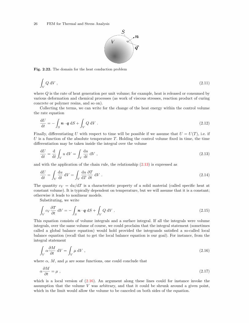
26 FEM for Thermal and Stress Analysis

Fig. 2.22. The domain for the heat conduction problem

∫V

Q dV , (2.11)

where Q is the rate of heat generation per unit volume; for example, heat is released or consumed byvarious deformation and chemical processes (as work of viscous stresses, reaction product of curingconcrete or polymer resins, and so on).

Collecting the terms, we can write for the change of the heat energy within the control volumethe rate equation

dU

dt= −

∫S

n · q dS +

∫V

Q dV . (2.12)

Finally, differentiating U with respect to time will be possible if we assume that U = U(T ), i.e. ifU is a function of the absolute temperature T . Holding the control volume fixed in time, the timedifferentiation may be taken inside the integral over the volume

dU

dt=

d

dt

∫V

u dV =

∫V

du

dtdV , (2.13)

and with the application of the chain rule, the relationship (2.13) is expressed as

dU

dt=

∫V

du

dtdV =

∫V

du

dT

∂T

∂tdV . (2.14)

The quantity cV = du/dT is a characteristic property of a solid material (called specific heat atconstant volume). It is typically dependent on temperature, but we will assume that it is a constant;otherwise it leads to nonlinear models.

Substituting, we write∫V

cV∂T

∂tdV = −

∫S

n · q dS +

∫V

Q dV . (2.15)

This equation consists of volume integrals and a surface integral. If all the integrals were volumeintegrals, over the same volume of course, we could proclaim that the integral statement (sometimescalled a global balance equation) would hold provided the integrands satisfied a so-called localbalance equation (recall that to get the local balance equation is our goal). For instance, from theintegral statement∫

V

α∂M

∂tdV =

∫V

µ dV , (2.16)

where α, M , and µ are some functions, one could conclude that

α∂M

∂t= µ , (2.17)

which is a local version of (2.16). An argument along these lines could for instance invoke theassumption that the volume V was arbitrary, and that it could be shrunk around a given point,which in the limit would allow the volume to be canceled on both sides of the equation.

2.11 Background, explanations, details 27

To execute this program for equation (2.15), we have to convert the surface integral to a volumeintegral. We have the needed tool in the celebrated divergence theorem (also known as the Gausstheorem)∫

V

divq dV =

∫S

n · q dS , (2.18)

where the divergence of the flux vector is defined in Cartesian coordinates as

divq =∂qx∂x

+∂qy∂y

+∂qz∂z

.

Consequently, Eq. (2.15) may be rewritten∫V

cV∂T

∂tdV = −

∫V

divq dV +

∫V

Q dV , (2.19)

and grouping the terms as∫V

[cV∂T

∂t+ divq −Q

]dV = 0 . (2.20)

we may conclude that the inside of the bracket has to vanish since the volume could be entirelyarbitrary. Therefore, we arrive at the local balance equation

cV∂T

∂t+ divq −Q = 0 . (2.21)

Equation (2.21) contains too many variables: both temperature and heat flux. Since it is a scalarequation, the logical step is to express the heat flux in terms of temperature. That is the contentof the Fourier model: heat flows opposite to the gradient of the temperature (downhill). In matrixform

q = −κ(gradT )T . (2.22)

The matrix κ is the conductivity matrix of the material. The most common forms of κ are

κ = κ1 (2.23)

for the so-called thermally isotropic material, and

κ =

κx 0 00 κy 00 0 κz

, (2.24)

for materials that have three orthogonal directions of different thermal conductivities (orthotropicmaterial); κ is the isotropic thermal conductivity coefficient, 1 is the identity matrix, and κx, κy,and κz are the orthotropic thermal conductivities. To explain the orthotropic conductivity modelwe note that some materials have preferred directions in which heat would like to flow, for instancealong the fibers in a composite. Visually, we can imagine a corrugated steel roof, with the channelsrunning not directly downhill, but tilted away from the slope – the water would run preferentiallyin the channels, but generally downhill.

The funny looking transpose of the temperature gradient follows from the definition: the gradientof the scalar is a row matrix

gradT =

[∂T

∂x,∂T

∂y,∂T

∂z

]. (2.25)

With the constitutive equation, the balance equation (2.21) is now expressed purely in terms ofthe absolute temperature,

cV∂T

∂t− div

[κ(gradT )T

]−Q = 0 . (2.26)

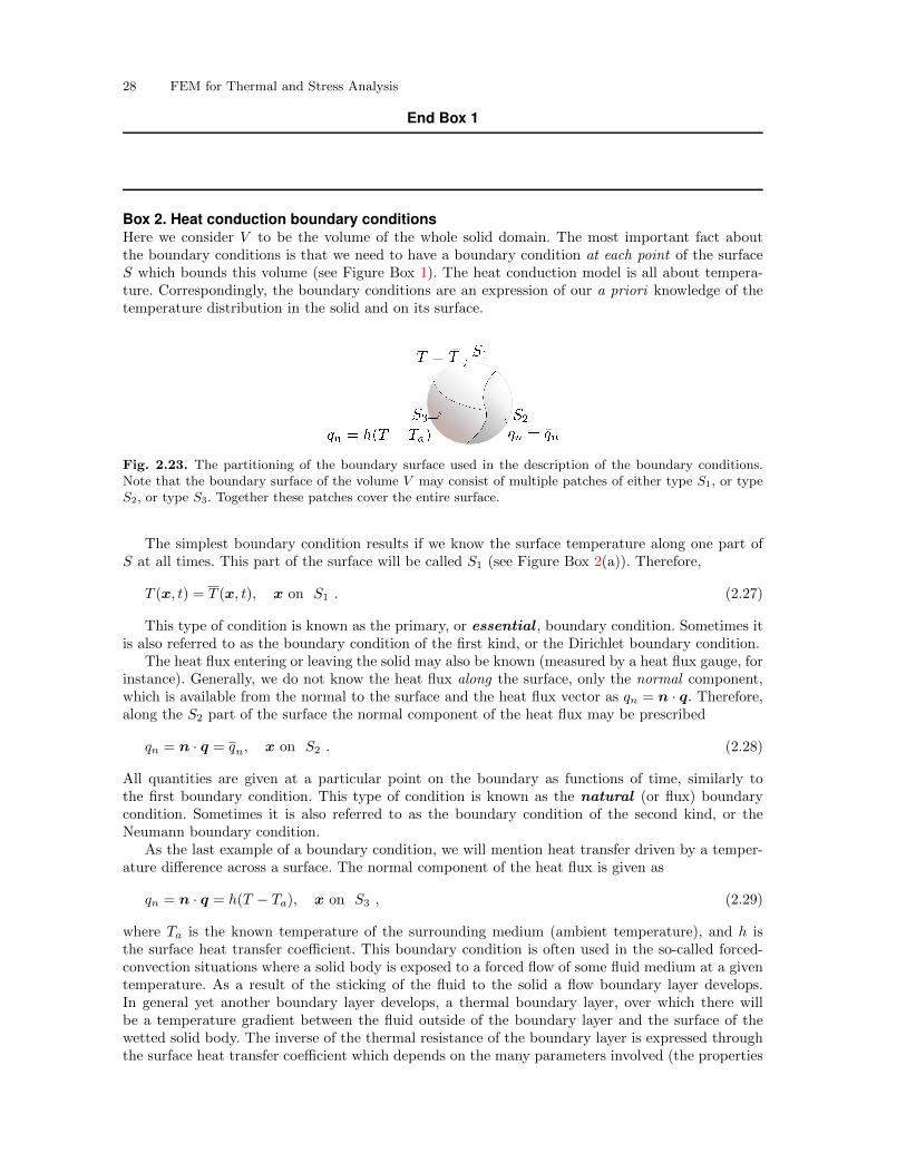
28 FEM for Thermal and Stress Analysis

End Box 1

Box 2. Heat conduction boundary conditionsHere we consider V to be the volume of the whole solid domain. The most important fact aboutthe boundary conditions is that we need to have a boundary condition at each point of the surfaceS which bounds this volume (see Figure Box 1). The heat conduction model is all about tempera-ture. Correspondingly, the boundary conditions are an expression of our a priori knowledge of thetemperature distribution in the solid and on its surface.

Fig. 2.23. The partitioning of the boundary surface used in the description of the boundary conditions.Note that the boundary surface of the volume V may consist of multiple patches of either type S1, or typeS2, or type S3. Together these patches cover the entire surface.

The simplest boundary condition results if we know the surface temperature along one part ofS at all times. This part of the surface will be called S1 (see Figure Box 2(a)). Therefore,

T (x, t) = T (x, t), x on S1 . (2.27)

This type of condition is known as the primary, or essential , boundary condition. Sometimes itis also referred to as the boundary condition of the first kind, or the Dirichlet boundary condition.

The heat flux entering or leaving the solid may also be known (measured by a heat flux gauge, forinstance). Generally, we do not know the heat flux along the surface, only the normal component,which is available from the normal to the surface and the heat flux vector as qn = n · q. Therefore,along the S2 part of the surface the normal component of the heat flux may be prescribed

qn = n · q = qn, x on S2 . (2.28)

All quantities are given at a particular point on the boundary as functions of time, similarly tothe first boundary condition. This type of condition is known as the natural (or flux) boundarycondition. Sometimes it is also referred to as the boundary condition of the second kind, or theNeumann boundary condition.

As the last example of a boundary condition, we will mention heat transfer driven by a temper-ature difference across a surface. The normal component of the heat flux is given as

qn = n · q = h(T − Ta), x on S3 , (2.29)

where Ta is the known temperature of the surrounding medium (ambient temperature), and h isthe surface heat transfer coefficient. This boundary condition is often used in the so-called forced-convection situations where a solid body is exposed to a forced flow of some fluid medium at a giventemperature. As a result of the sticking of the fluid to the solid a flow boundary layer develops.In general yet another boundary layer develops, a thermal boundary layer, over which there willbe a temperature gradient between the fluid outside of the boundary layer and the surface of thewetted solid body. The inverse of the thermal resistance of the boundary layer is expressed throughthe surface heat transfer coefficient which depends on the many parameters involved (the properties

2.11 Background, explanations, details 29

of the surface of the body, the properties of the fluid, the properties of the convection flow, etc.).Sometimes it is also referred to as the boundary condition of the third kind, or the Newton boundarycondition. In Abaqus this boundary condition is known as the convective film condition. Since thiskind of boundary condition has application also in other situations such as modeling of the thermalresistance of contact between two solid bodies, or modeling of thin insulation layers, as surfaceswith thermal gradients across them, we will refer to this condition as the surface heat transferboundary condition.

End Box 2

Box 3. Analytical solution for the cylindrical domainConsider a cylinder of radius a. In cylindrical coordinates, where r is the radial distance from the axisof symmetry, ϕ is the circumferential angle, and z is the coordinate along the axis of the cylinder,the differential equation

1

r

∂

∂r

(κr∂T

∂r

)+Q = 0 (2.30)

describes the variation of temperature in the radial direction. The solution for uniform heat gener-ation rate Q and homogeneous material κ, with the two boundary conditions

∂T (r = 0)

∂r= 0, T (r = a) = Tw = 0 , (2.31)

is

T (r) =Q

4κ

(a2 − r2

)(2.32)

End Box 3

Box 4. Basis function for the tetrahedronThe basis functions for the T4 tetrahedron KLMP are linear functions with four coefficients, forinstance

NK(x, y, z) = aKx+ bKy + cKz + dK

The interpolation conditions are written

NK(xJ , yJ , zJ) = aKxJ + bKyJ + cKzJ + dK = δKJ ,

where δKJ is the Kronecker Delta,

δik =

{1, if i = k;0, otherwise.

The relationship written for all four nodes results inxK , yK , zK , 1xL, yL, zL, 1xM , yM , zM , 1xP , yP , zP , 1

︸ ︷︷ ︸

X

aK , aL, aM , aPbK , bL, bM , bPcK , cL, cM , cPdK , dL, dM , dP

︸ ︷︷ ︸

A

=

1, 0, 0, 00, 1, 0, 00, 0, 1, 00, 0, 0, 1

︸ ︷︷ ︸

1

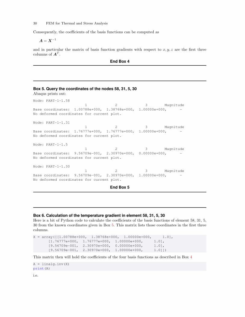
30 FEM for Thermal and Stress Analysis

Consequently, the coefficients of the basis functions can be computed as

A = X−1

and in particular the matrix of basis function gradients with respect to x, y, z are the first threecolumns of AT .

End Box 4

Box 5. Query the coordinates of the nodes 58, 31, 5, 30Abaqus prints out:

Node: PART-1-1.581 2 3 Magnitude

Base coordinates: 1.00788e+000, 1.38768e+000, 1.00000e+000, -No deformed coordinates for current plot.

Node: PART-1-1.311 2 3 Magnitude

Base coordinates: 1.76777e+000, 1.76777e+000, 1.00000e+000, -No deformed coordinates for current plot.

Node: PART-1-1.51 2 3 Magnitude

Base coordinates: 9.56709e-001, 2.30970e+000, 0.00000e+000, -No deformed coordinates for current plot.

Node: PART-1-1.301 2 3 Magnitude

Base coordinates: 9.56709e-001, 2.30970e+000, 1.00000e+000, -No deformed coordinates for current plot.

End Box 5

Box 6. Calculation of the temperature gradient in element 58, 31, 5, 30Here is a bit of Python code to calculate the coefficients of the basis functions of element 58, 31, 5,30 from the known coordinates given in Box 5. This matrix lists those coordinates in the first threecolumns.

X = array([[1.00788e+000, 1.38768e+000, 1.00000e+000, 1.0],[1.76777e+000, 1.76777e+000, 1.00000e+000, 1.0],[9.56709e-001, 2.30970e+000, 0.00000e+000, 1.0],[9.56709e-001, 2.30970e+000, 1.00000e+000, 1.0]])

This matrix then will hold the coefficients of the four basis functions as described in Box 4

A = linalg.inv(X)print(A)

i.e.

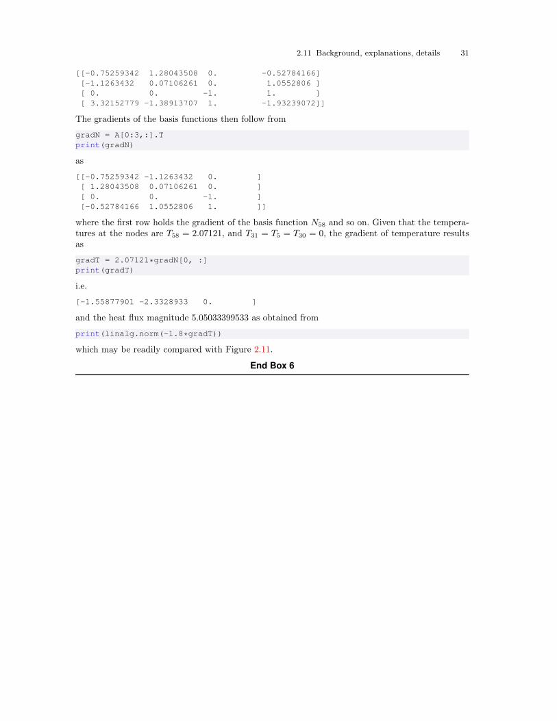
2.11 Background, explanations, details 31

[[-0.75259342 1.28043508 0. -0.52784166][-1.1263432 0.07106261 0. 1.0552806 ][ 0. 0. -1. 1. ][ 3.32152779 -1.38913707 1. -1.93239072]]

The gradients of the basis functions then follow from

gradN = A[0:3,:].Tprint(gradN)

as

[[-0.75259342 -1.1263432 0. ][ 1.28043508 0.07106261 0. ][ 0. 0. -1. ][-0.52784166 1.0552806 1. ]]

where the first row holds the gradient of the basis function N58 and so on. Given that the tempera-tures at the nodes are T58 = 2.07121, and T31 = T5 = T30 = 0, the gradient of temperature resultsas

gradT = 2.07121*gradN[0, :]print(gradT)

i.e.

[-1.55877901 -2.3328933 0. ]

and the heat flux magnitude 5.05033399533 as obtained from

print(linalg.norm(-1.8*gradT))

which may be readily compared with Figure 2.11.

End Box 6

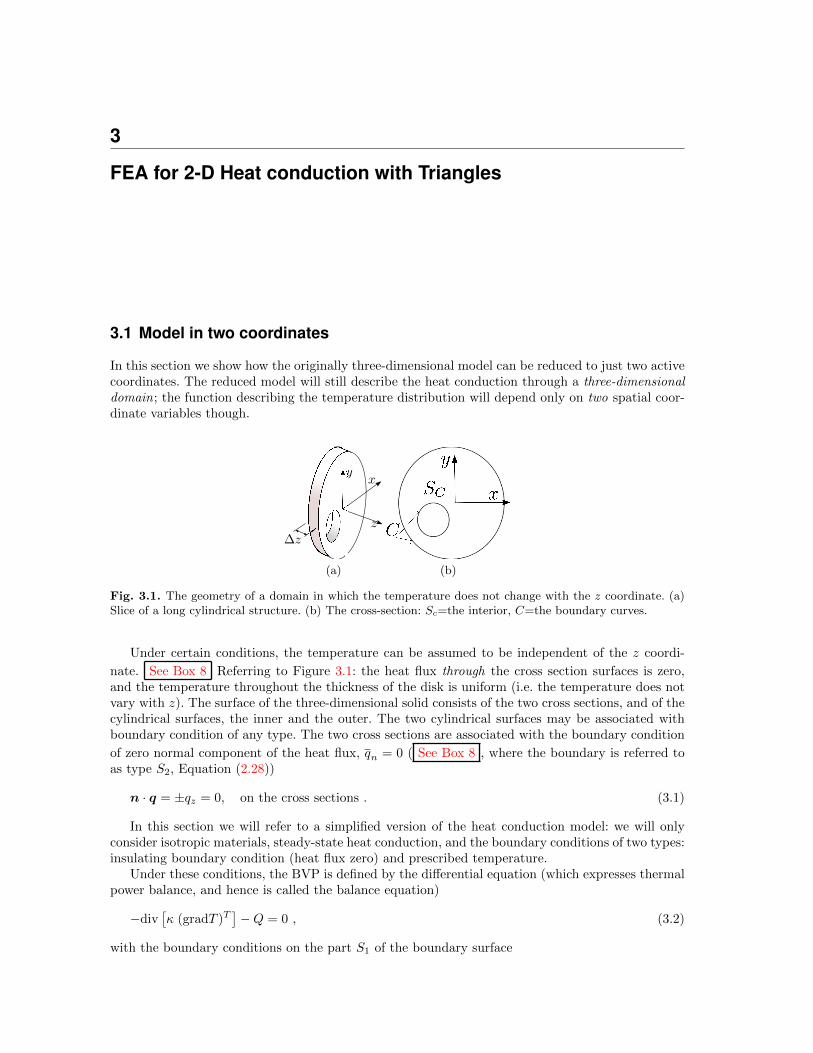
3

FEA for 2-D Heat conduction with Triangles

3.1 Model in two coordinates

In this section we show how the originally three-dimensional model can be reduced to just two activecoordinates. The reduced model will still describe the heat conduction through a three-dimensionaldomain; the function describing the temperature distribution will depend only on two spatial coor-dinate variables though.

(a) (b)

Fig. 3.1. The geometry of a domain in which the temperature does not change with the z coordinate. (a)Slice of a long cylindrical structure. (b) The cross-section: Sc=the interior, C=the boundary curves.

Under certain conditions, the temperature can be assumed to be independent of the z coordi-

nate. See Box 8 Referring to Figure 3.1: the heat flux through the cross section surfaces is zero,and the temperature throughout the thickness of the disk is uniform (i.e. the temperature does notvary with z). The surface of the three-dimensional solid consists of the two cross sections, and of thecylindrical surfaces, the inner and the outer. The two cylindrical surfaces may be associated withboundary condition of any type. The two cross sections are associated with the boundary condition

of zero normal component of the heat flux, qn = 0 ( See Box 8 , where the boundary is referred toas type S2, Equation (2.28))

n · q = ±qz = 0, on the cross sections . (3.1)

In this section we will refer to a simplified version of the heat conduction model: we will onlyconsider isotropic materials, steady-state heat conduction, and the boundary conditions of two types:insulating boundary condition (heat flux zero) and prescribed temperature.

Under these conditions, the BVP is defined by the differential equation (which expresses thermalpower balance, and hence is called the balance equation)

−div[κ (gradT )T

]−Q = 0 , (3.2)

with the boundary conditions on the part S1 of the boundary surface

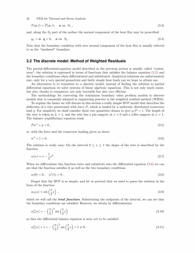
34 FEM for Thermal and Stress Analysis

T (x, t) = T (x, t), x on S1 , (3.3)

and, along the S2 part of the surface the normal component of the heat flux may be prescribed

qn = n · q = 0, x on S2 . (3.4)

Note that the boundary condition with zero normal component of the heat flux is usually referredto as the “insulated” boundary.

3.2 The discrete model: Method of Weighted Residuals

The partial-differential-equation model described in the previous section is usually called “contin-uous”: the solution is expressed in terms of functions that satisfies the balance equation (3.2) andthe boundary conditions when differentiated and substituted. Analytical solutions are unfortunatelyrare: only for a very special geometries and fairly simple heat loads can we hope to obtain one.

An alternative is to transition to a discrete model: instead of finding the solution to partialdifferential equations we solve systems of linear algebraic equations. This is not only much easier,but also, thanks to computers, not only tractable but also very efficient.

The methodology for converting the continuous boundary value problem models to discretemodels that is commonly adopted in engineering practice is the weighted residual method (WRM).

To explain the basics we will discuss in this section a really simple BVP model that describes thedeflection of a wire prestressed with force P , which is loaded by a uniformly distributed transverseload q. For simplicity we shall consider these two quantities chosen to give q/P = 1. The length ofthe wire is taken as L = 1, and the wire has a pin support at x = 0 and a roller support at x = 1.The balance (equilibrium) equation reads

Pw′′ + q = 0 , (3.5)

or, with the force and the transverse loading given as above

w′′ + 1 = 0 . (3.6)

The solution is really easy: On the interval 0 ≤ x ≤ 1 the shape of the wire is described by thefunction

w(x) = x− 1

2x2 . (3.7)

When we differentiate this function twice and substitute into the differential equation (3.6) we cansee that the function satisfies it as well as the two boundary conditions

w(0) = 0 , w′(1) = 0 . (3.8)

Forget that the BVP is so simple, and let us pretend that we need to guess the solution in theform of the function

wh(x) = sin(π2x), (3.9)

which we will call the trial function . Substituting the endpoints of the interval, we can see thatthe boundary conditions are satisfied. However, we obtain by differentiation

w′′h(x) = −

(π2

)2sin(π2x)

(3.10)

so that the differential balance equation is seen not to be satisfied

w′′h(x) + 1 = −

(π2

)2sin(π2x)+ 1 = 0 . (3.11)

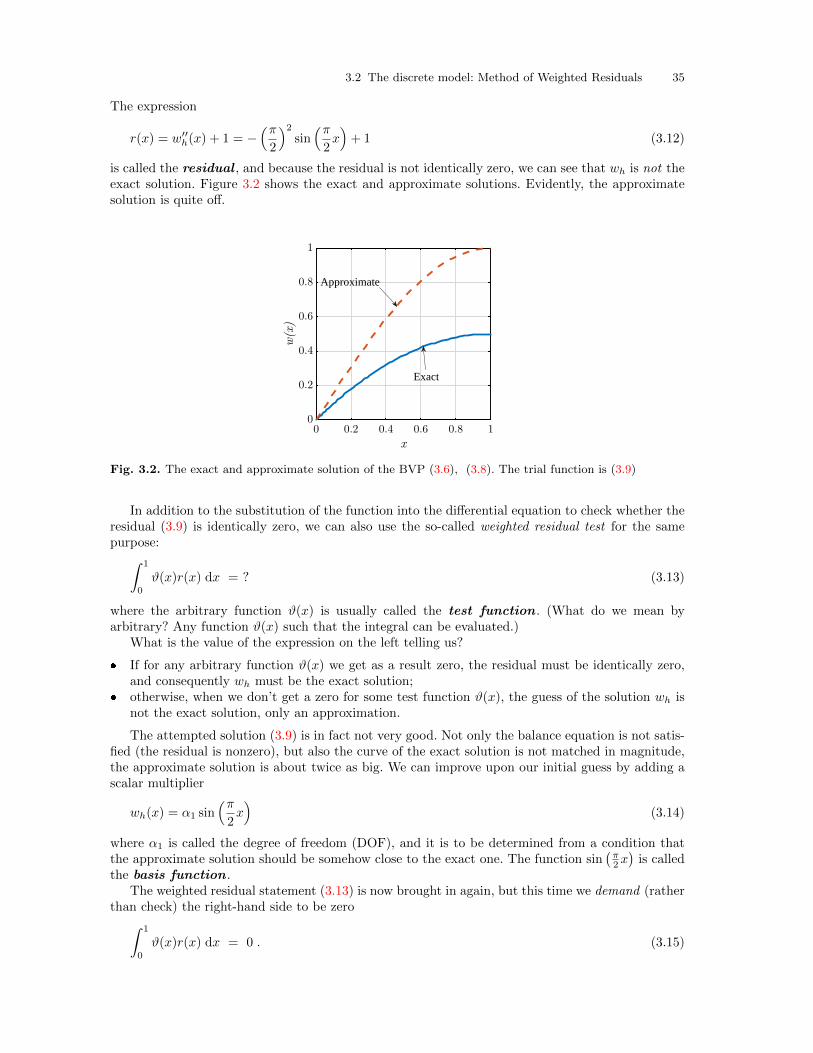
3.2 The discrete model: Method of Weighted Residuals 35

The expression

r(x) = w′′h(x) + 1 = −

(π2

)2sin(π2x)+ 1 (3.12)

is called the residual , and because the residual is not identically zero, we can see that wh is not theexact solution. Figure 3.2 shows the exact and approximate solutions. Evidently, the approximatesolution is quite off.

x0 0.2 0.4 0.6 0.8 1

w(x)

0

0.2

0.4

0.6

0.8

1

Approximate

Exact

Fig. 3.2. The exact and approximate solution of the BVP (3.6), (3.8). The trial function is (3.9)

In addition to the substitution of the function into the differential equation to check whether theresidual (3.9) is identically zero, we can also use the so-called weighted residual test for the samepurpose:∫ 1

0

ϑ(x)r(x) dx = ? (3.13)

where the arbitrary function ϑ(x) is usually called the test function . (What do we mean byarbitrary? Any function ϑ(x) such that the integral can be evaluated.)

What is the value of the expression on the left telling us?

� If for any arbitrary function ϑ(x) we get as a result zero, the residual must be identically zero,and consequently wh must be the exact solution;

� otherwise, when we don’t get a zero for some test function ϑ(x), the guess of the solution wh isnot the exact solution, only an approximation.

The attempted solution (3.9) is in fact not very good. Not only the balance equation is not satis-fied (the residual is nonzero), but also the curve of the exact solution is not matched in magnitude,the approximate solution is about twice as big. We can improve upon our initial guess by adding ascalar multiplier

wh(x) = α1 sin(π2x)

(3.14)

where α1 is called the degree of freedom (DOF), and it is to be determined from a condition thatthe approximate solution should be somehow close to the exact one. The function sin

(π2x)is called

the basis function .The weighted residual statement (3.13) is now brought in again, but this time we demand (rather

than check) the right-hand side to be zero∫ 1

0

ϑ(x)r(x) dx = 0 . (3.15)

36 FEM for Thermal and Stress Analysis

If we now substitute our guess (trial) (3.14), equation (3.15) can be solved for α1, and voila, thereis our approximate solution.

One more tweak: In order to improve our chances of finding a good trial function, the weightedresidual statement (3.15) is replaced with a simple modification. If we substitute the trial func-tion (3.14) into (3.15) we see that the trial function must be twice differentiable∫ 1

0

ϑ(x)r(x) dx =

∫ 1

0

ϑ(x) [w′′h(x) + 1] dx =

∫ 1

0

ϑ(x)w′′h(x) dx +

∫ 1

0

ϑ(x) dx = 0 (3.16)

which is easy here, but considerably more difficult for real situations in two or three dimensions.Therefore, we use integration by parts to reduce the number of derivatives needed for the weightedresidual statement as∫ 1

0

ϑ(x)w′′h(x) dx = −

∫ 1

0

ϑ′(x)w′h(x) dx+ [ϑ(x)w′

h(x)]10 (3.17)

So the weighted residual statement (3.16) will be rewritten as∫ 1

0

ϑ(x)r(x) dx = −∫ 1

0

ϑ′(x)w′h(x) dx+ [ϑ(x)w′

h(x)]10 +

∫ 1

0

ϑ(x) dx = 0 (3.18)

Notice that we haven’t changed the rules of the game: this is still the original weighted residualstatement, but now we are allowed to pick a trial function with only one derivative, and in exchangewe now also require the test function to be differentiable. The test function is typically taken inthe same form as the trial function, meaning we would take the test function here to be the basisfunction sin

(π2x). When we do that, the weighted residual statement (3.18) yields

−∫ 1

0

[sin(π2x)]′ [

α1 sin(π2x)]′

dx

+sin(π2× 1)α1

π

2cos(π2× 1)

︸ ︷︷ ︸0

− sin(π2× 0)

︸ ︷︷ ︸0

[α1π

2cos(π2× 0)]

+

∫ 1

0

sin(π2x)

dx = 0

(3.19)

and in numbers

−α1π2

8+

2

π= 0 , ⇒ α1 =

16

π3≈ 0.516 (3.20)

Figure 3.3 shows the approximate solution (3.14) for the calculated value of α1: clearly theapproximate solution now hugs the exact solution fairly closely.

If we wanted to improve the approximate solution further, we could use for instance this function

wh(x) = α1 sin(π2x)+ α2 sin

(3π

2x

)(3.21)

with two degrees of freedom, which we can write using the notation ϕ1(x) = sin(π2x)and ϕ2(x) =

sin(3π2 x)as

wh(x) = α1ϕ1(x) + α2ϕ2(x) (3.22)

Now we need two equations, because we have two unknown degrees of freedom. So we write theweighted residual equation once, for ϑ = ϕ1,

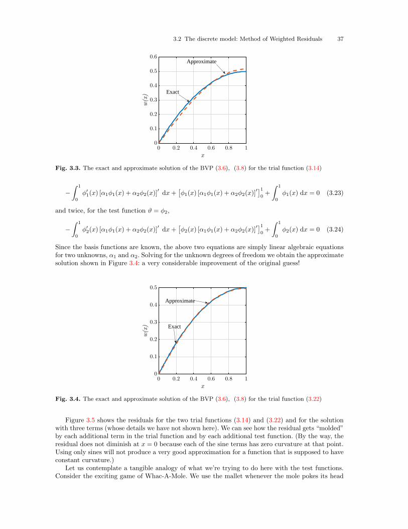
3.2 The discrete model: Method of Weighted Residuals 37

x0 0.2 0.4 0.6 0.8 1

w(x)

0

0.1

0.2

0.3

0.4

0.5

0.6Approximate

Exact

Fig. 3.3. The exact and approximate solution of the BVP (3.6), (3.8) for the trial function (3.14)

−∫ 1

0

ϕ′1(x) [α1ϕ1(x) + α2ϕ2(x)]′dx+

[ϕ1(x) [α1ϕ1(x) + α2ϕ2(x)]

′]10+

∫ 1

0

ϕ1(x) dx = 0 (3.23)

and twice, for the test function ϑ = ϕ2,

−∫ 1

0

ϕ′2(x) [α1ϕ1(x) + α2ϕ2(x)]′dx+

[ϕ2(x) [α1ϕ1(x) + α2ϕ2(x)]

′]10+

∫ 1

0

ϕ2(x) dx = 0 (3.24)

Since the basis functions are known, the above two equations are simply linear algebraic equationsfor two unknowns, α1 and α2. Solving for the unknown degrees of freedom we obtain the approximatesolution shown in Figure 3.4: a very considerable improvement of the original guess!

x0 0.2 0.4 0.6 0.8 1

w(x)

0

0.1

0.2

0.3

0.4

0.5

Exact

Approximate

Fig. 3.4. The exact and approximate solution of the BVP (3.6), (3.8) for the trial function (3.22)

Figure 3.5 shows the residuals for the two trial functions (3.14) and (3.22) and for the solutionwith three terms (whose details we have not shown here). We can see how the residual gets “molded”by each additional term in the trial function and by each additional test function. (By the way, theresidual does not diminish at x = 0 because each of the sine terms has zero curvature at that point.Using only sines will not produce a very good approximation for a function that is supposed to haveconstant curvature.)

Let us contemplate a tangible analogy of what we’re trying to do here with the test functions.Consider the exciting game of Whac-A-Mole. We use the mallet whenever the mole pokes its head

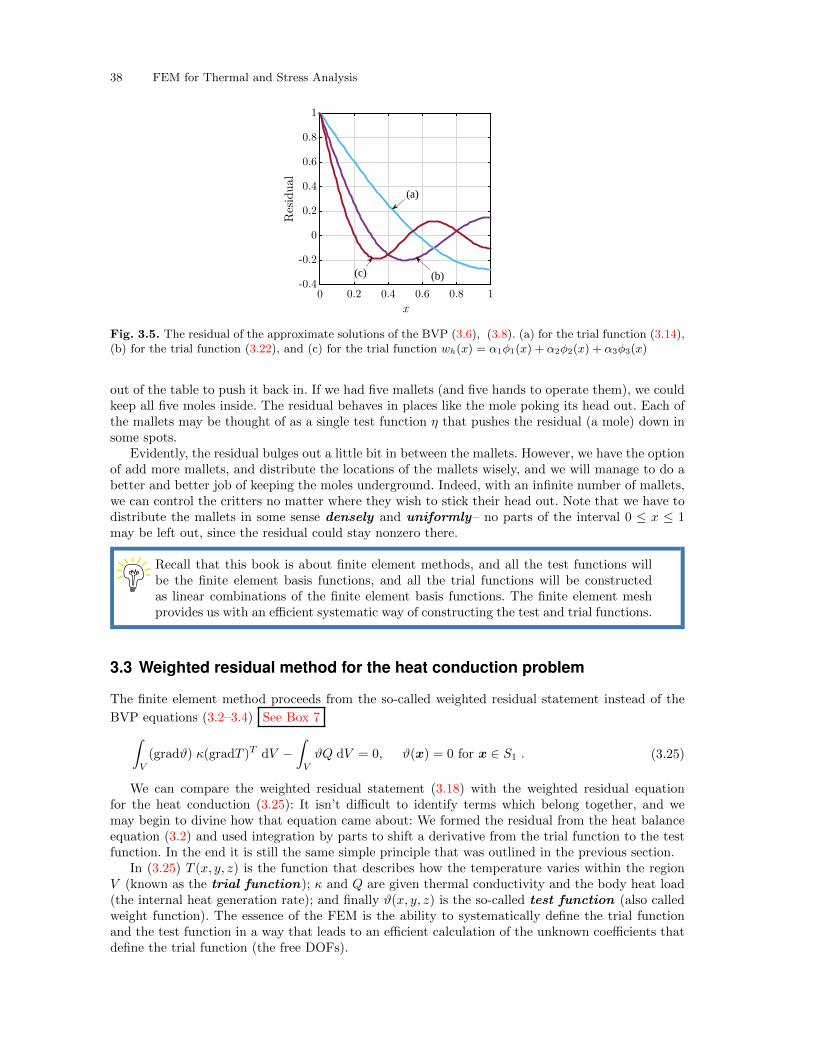
38 FEM for Thermal and Stress Analysis

x

0 0.2 0.4 0.6 0.8 1Residual

-0.4

-0.2

0

0.2

0.4

0.6

0.8

1

(c) (b)

(a)

Fig. 3.5. The residual of the approximate solutions of the BVP (3.6), (3.8). (a) for the trial function (3.14),(b) for the trial function (3.22), and (c) for the trial function wh(x) = α1ϕ1(x) + α2ϕ2(x) + α3ϕ3(x)

out of the table to push it back in. If we had five mallets (and five hands to operate them), we couldkeep all five moles inside. The residual behaves in places like the mole poking its head out. Each ofthe mallets may be thought of as a single test function η that pushes the residual (a mole) down insome spots.

Evidently, the residual bulges out a little bit in between the mallets. However, we have the optionof add more mallets, and distribute the locations of the mallets wisely, and we will manage to do abetter and better job of keeping the moles underground. Indeed, with an infinite number of mallets,we can control the critters no matter where they wish to stick their head out. Note that we have todistribute the mallets in some sense densely and uniformly– no parts of the interval 0 ≤ x ≤ 1may be left out, since the residual could stay nonzero there.

Recall that this book is about finite element methods, and all the test functions willbe the finite element basis functions, and all the trial functions will be constructedas linear combinations of the finite element basis functions. The finite element meshprovides us with an efficient systematic way of constructing the test and trial functions.

3.3 Weighted residual method for the heat conduction problem

The finite element method proceeds from the so-called weighted residual statement instead of the

BVP equations (3.2–3.4) See Box 7∫V

(gradϑ) κ(gradT )T dV −∫V

ϑQ dV = 0, ϑ(x) = 0 for x ∈ S1 . (3.25)

We can compare the weighted residual statement (3.18) with the weighted residual equationfor the heat conduction (3.25): It isn’t difficult to identify terms which belong together, and wemay begin to divine how that equation came about: We formed the residual from the heat balanceequation (3.2) and used integration by parts to shift a derivative from the trial function to the testfunction. In the end it is still the same simple principle that was outlined in the previous section.

In (3.25) T (x, y, z) is the function that describes how the temperature varies within the regionV (known as the trial function); κ and Q are given thermal conductivity and the body heat load(the internal heat generation rate); and finally ϑ(x, y, z) is the so-called test function (also calledweight function). The essence of the FEM is the ability to systematically define the trial functionand the test function in a way that leads to an efficient calculation of the unknown coefficients thatdefine the trial function (the free DOFs).

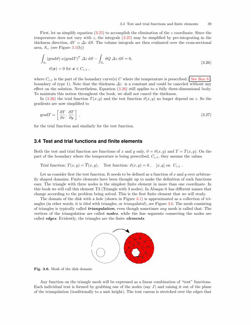
3.4 Test and trial functions and finite elements 39

First, let us simplify equation (3.25) to accomplish the elimination of the z coordinate. Since thetemperature does not vary with z, the integrals (3.25) may be simplified by pre-integrating in thethickness direction, dV = ∆z dS. The volume integrals are then evaluated over the cross-sectionalarea, Sc, (see Figure 3.1(b))∫

Sc

(gradϑ) κ(gradT )T ∆z dS −∫Sc

ϑQ ∆z dS = 0,

ϑ(x) = 0 for x ∈ Cc,1 ,

(3.26)

where Cc,1 is the part of the boundary curve(s) C where the temperature is prescribed ( See Box 8 ,boundary of type 1). Note that the thickness ∆z is a constant and could be canceled without anyeffect on the solution. Nevertheless, Equation (3.26) still applies to a fully three-dimensional body.To maintain this notion throughout the book, we shall not cancel the thickness.

In (3.26) the trial function T (x, y) and the test function ϑ(x, y) no longer depend on z. So thegradients are now simplified to

gradT =

[∂T

∂x,∂T

∂y

], (3.27)

for the trial function and similarly for the test function.

3.4 Test and trial functions and finite elements

Both the test and trial function are functions of x and y only, ϑ = ϑ(x, y) and T = T (x, y). On thepart of the boundary where the temperature is being prescribed, Cc,1, they assume the values

Trial function: T (x, y) = T (x, y), Test function: ϑ(x, y) = 0 , [x, y] on Cc,1 .

Let us consider first the test function. It needs to be defined as a function of x and y over arbitrar-ily shaped domains. Finite elements have been thought up to make the definition of such functionseasy. The triangle with three nodes is the simplest finite element in more than one coordinate. Inthis book we will call this element T3 (Triangle with 3 nodes). In Abaqus it has different names thatchange according to the problem being solved. This is the first finite element that we will study.

The domain of the disk with a hole (shown in Figure 3.1) is approximated as a collection of tri-angles (in other words, it is tiled with triangles, or triangulated), see Figure 3.6. The mesh consistingof triangles is typically called triangulation, even though sometimes any mesh is called that. Thevertices of the triangulation are called nodes, while the line segments connecting the nodes arecalled edges. Evidently, the triangles are the finite elements.

Fig. 3.6. Mesh of the disk domain

Any function on the triangle mesh will be expressed as a linear combination of “tent” functions.Each individual tent is formed by grabbing one of the nodes (say J) and raising it out of the planeof the triangulation (traditionally to a unit height). The tent canvas is stretched over the edges that

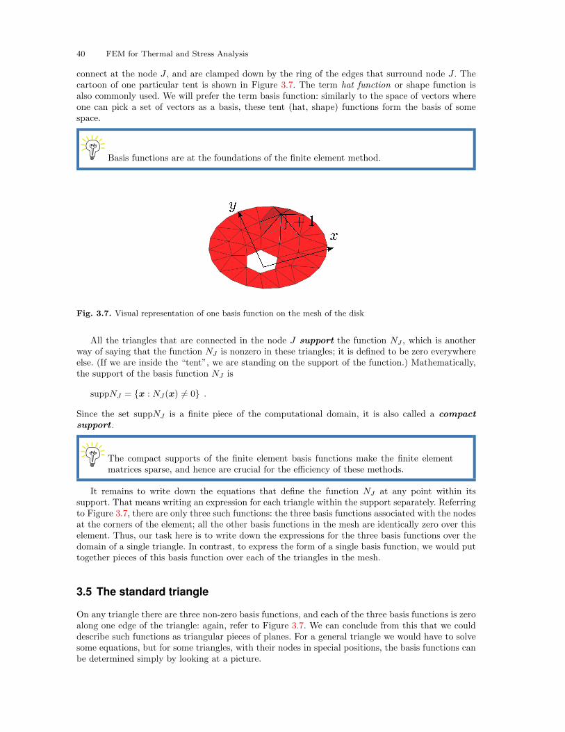
40 FEM for Thermal and Stress Analysis

connect at the node J , and are clamped down by the ring of the edges that surround node J . Thecartoon of one particular tent is shown in Figure 3.7. The term hat function or shape function isalso commonly used. We will prefer the term basis function: similarly to the space of vectors whereone can pick a set of vectors as a basis, these tent (hat, shape) functions form the basis of somespace.

Basis functions are at the foundations of the finite element method.

Fig. 3.7. Visual representation of one basis function on the mesh of the disk

All the triangles that are connected in the node J support the function NJ , which is anotherway of saying that the function NJ is nonzero in these triangles; it is defined to be zero everywhereelse. (If we are inside the “tent”, we are standing on the support of the function.) Mathematically,the support of the basis function NJ is

suppNJ = {x : NJ(x) = 0} .

Since the set suppNJ is a finite piece of the computational domain, it is also called a compactsupport .

The compact supports of the finite element basis functions make the finite elementmatrices sparse, and hence are crucial for the efficiency of these methods.

It remains to write down the equations that define the function NJ at any point within itssupport. That means writing an expression for each triangle within the support separately. Referringto Figure 3.7, there are only three such functions: the three basis functions associated with the nodesat the corners of the element; all the other basis functions in the mesh are identically zero over thiselement. Thus, our task here is to write down the expressions for the three basis functions over thedomain of a single triangle. In contrast, to express the form of a single basis function, we would puttogether pieces of this basis function over each of the triangles in the mesh.

3.5 The standard triangle

On any triangle there are three non-zero basis functions, and each of the three basis functions is zeroalong one edge of the triangle: again, refer to Figure 3.7. We can conclude from this that we coulddescribe such functions as triangular pieces of planes. For a general triangle we would have to solvesome equations, but for some triangles, with their nodes in special positions, the basis functions canbe determined simply by looking at a picture.

3.5 The standard triangle 41

This is the idea behind the isoparametric formulation: the expressions for the basis functions arederived for elements of particularly simple shapes, such as a right triangle or a square. These arecalled standard shapes, hence we will be talking about the standard triangle here. The standardtriangle is described in coordinates ξ, η, and these are not the physical coordinates in which theBVP is described. These are coordinates used only to describe the standard shape, and they will bereferred to as the parametric coordinates. Refer to Figure 3.8.

Nodes of a single element will be shown with an underline, and are always between1 and n , where n is the number of nodes of the element (three for the three-nodetriangle). Global node numbers (that is numbers within the entire mesh) will alwaysbe shown without an underline (like this: K).

The basis functions associated with nodes 2 and 3 are simply

N2(ξ, η) = ξ , (3.28)

and

N3(ξ, η) = η . (3.29)

As is easily verified, N2 is zero along the edge [3, 1], and assumes value +1 at node 2; analogousproperties hold for N3. If N1 should be equal to +1 at the origin, it must be written as

N1(ξ, η) = 1− ξ − η . (3.30)

Clearly, N1 vanishes at the edge [2,3] opposite node 1. Thus, we see that the three functions we justformulated satisfy the Kronecker delta property,

Ni(ξk, ηk) = δik , (3.31)

where the symbol δik is known as the Kronecker delta

δik =

{1, if i = k;0, otherwise.

In words: basis function Ni associated with node i assumes the value of either 1.0 or 0.0 at node k,depending on whether it is the same node (i = k) or not.

Fig. 3.8. Standard triangle

Now that we have the three basis functions we can use them to describe functions within thestandard triangle. We simply write

a(ξ, η) =

3∑i=1

Ni(ξ, η)ai , (3.32)

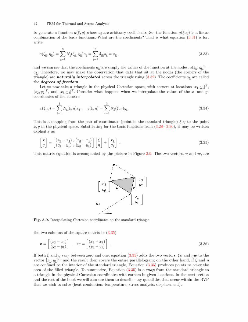
42 FEM for Thermal and Stress Analysis

to generate a function a(ξ, η) where ai are arbitrary coefficients. So, the function a(ξ, η) is a linearcombination of the basis functions. What are the coefficients? That is what equation (3.31) is for:write

a(ξk, ηk) =

3∑i=1

Ni(ξk, ηk)ai =

3∑i=1

δikai = ak , (3.33)

and we can see that the coefficients ak are simply the values of the function at the nodes, a(ξk, ηk) =ak. Therefore, we may make the observation that data that sit at the nodes (the corners of thetriangle) are naturally interpolated across the triangle using (3.32). The coefficients ak are calledthe degrees of freedom .

Let us now take a triangle in the physical Cartesian space, with corners at locations [x1, y1]T ,

[x2, y2]T , and [x3, y3]

T . Consider what happens when we interpolate the values of the x- and y-coordinates of the corners:

x(ξ, η) =

3∑i=1

Ni(ξ, η)xi , y(ξ, η) =

3∑i=1

Ni(ξ, η)yi . (3.34)

This is a mapping from the pair of coordinates (point in the standard triangle) ξ, η to the pointx, y in the physical space. Substituting for the basis functions from (3.28– 3.30), it may be writtenexplicitly as[

xy

]=

[(x2 − x1) , (x3 − x1)(y2 − y1) , (y3 − y1)

] [ξη

]+

[x1y1

]. (3.35)

This matrix equation is accompanied by the picture in Figure 3.9. The two vectors, v and w, are

Fig. 3.9. Interpolating Cartesian coordinates on the standard triangle

the two columns of the square matrix in (3.35):

v =

[(x2 − x1)(y2 − y1)

], w =

[(x3 − x1)(y3 − y1)

]. (3.36)

If both ξ and η vary between zero and one, equation (3.35) adds the two vectors, ξv and ηw to thevector [x1, y1]

T , and the result then covers the entire parallelogram; on the other hand, if ξ and ηare confined to the interior of the standard triangle, Equation (3.35) produces points to cover thearea of the filled triangle. To summarize, Equation (3.35) is a map from the standard triangle toa triangle in the physical Cartesian coordinates with corners in given locations. In the next sectionand the rest of the book we will also use them to describe any quantities that occur within the BVPthat we wish to solve (heat conduction: temperature, stress analysis: displacement).

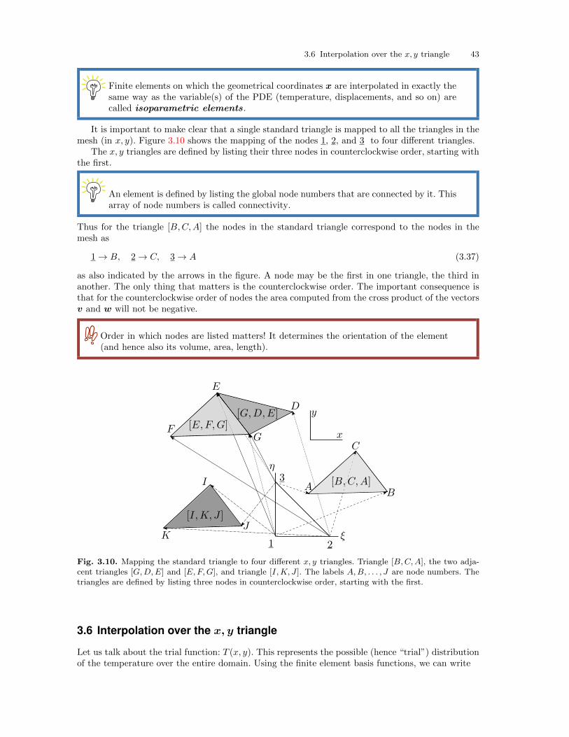
3.6 Interpolation over the x, y triangle 43

Finite elements on which the geometrical coordinates x are interpolated in exactly thesame way as the variable(s) of the PDE (temperature, displacements, and so on) arecalled isoparametric elements.

It is important to make clear that a single standard triangle is mapped to all the triangles in themesh (in x, y). Figure 3.10 shows the mapping of the nodes 1, 2, and 3 to four different triangles.

The x, y triangles are defined by listing their three nodes in counterclockwise order, starting withthe first.

An element is defined by listing the global node numbers that are connected by it. Thisarray of node numbers is called connectivity.

Thus for the triangle [B,C,A] the nodes in the standard triangle correspond to the nodes in themesh as

1 → B, 2 → C, 3 → A (3.37)

as also indicated by the arrows in the figure. A node may be the first in one triangle, the third inanother. The only thing that matters is the counterclockwise order. The important consequence isthat for the counterclockwise order of nodes the area computed from the cross product of the vectorsv and w will not be negative.

Order in which nodes are listed matters! It determines the orientation of the element(and hence also its volume, area, length).

Fig. 3.10. Mapping the standard triangle to four different x, y triangles. Triangle [B,C,A], the two adja-cent triangles [G,D,E] and [E,F,G], and triangle [I,K, J ]. The labels A,B, . . . , J are node numbers. Thetriangles are defined by listing three nodes in counterclockwise order, starting with the first.

3.6 Interpolation over the x, y triangle

Let us talk about the trial function: T (x, y). This represents the possible (hence “trial”) distributionof the temperature over the entire domain. Using the finite element basis functions, we can write

44 FEM for Thermal and Stress Analysis

T (x, y) =

N∑i=1

Ni(x, y)Ti (3.38)

provided we knew the expressions for the basis functions in the coordinates x, y, i.e. Ni(x, y). Atthis point we don’t, we know Nj(ξ, η), j = 1, 2, 3 instead. But let us pretend we do. How would weactually use it to describe T (x, y)? Have a look at Figure 3.7: each basis function has a differentdescription over each triangle in its support (i.e. over each triangle where it is nonzero). So to describeT (x, y) we must do it triangle-by-triangle. The function T (x, y) looks like triangular facets on thesurface of the diamond! It is piecewise linear.

What are the is in (3.38)? They are degree of freedom numbers. Simply put, a degree of freedomis a number (coefficient) that we use to describe the temperature, as opposed to the basis functionwhich is not a number but, as its name implies, a function. The basis functions are determined bythe mesh, the degrees of freedom will determine the solution. The basis functions Ni are labeledwith i as the degree of freedom number, and so are the Ti degrees of freedom.

The basis function Ni is to be understood as the basis function associated with thenode that carries the degree of freedom i.

At this point we know how to write the basis functions over the standard triangle (3.28– 3.30),and we know that any triangle in the mesh in the coordinates x, y is an image of the standard triangleobtained from (3.34). And now we also realize that the describe T (x, y) we have to do it one triangleat a time. Therefore a perfectly reasonable approach to the expression of the trial function (3.38) isto express

T (x, y) =

N∑i=1

Ni(x(ξ, η), y(ξ, η))Ti =

N∑i=1

Ni(ξ, η)Ti (3.39)

That is, for any point x, y we can say what the value T (x, y) is obtained by finding the correspondingpoint ξ, η in the standard triangle, calculating the values of the basis functions at that point, andplugging them into (3.39). If it seems awkward, it is because it is awkward. But we never actuallyneed to go through with this to express T (x, y) for a given x, y. Rather, all operations that we willneed will be expressed on the standard triangle, so that we actually know ξ, η (which allows us tocalculate x, y, should we be interested).

In any given triangle of the mesh, the trial functions are expressed for any point x, ywithin that triangle by writing

T (x, y) =

N∑i=1

Ni(ξ, η)Ti

where it is understood that ξ, η is such a point in the standard triangle that is mappedto x, y by (3.34).

The test function is actually a lot simpler than the trial function. Our choice for a test function willbe a single basis function

ϑ(x, y) = Nj(ξ, η) (3.40)

We will explain how to arrive at the degree of freedom number j below. In brief, each degree offreedom that is free (i. e. an actual unknown) will be associated with one test function. The reasonis that for each unknown in the problem we need one equation: Nf unknowns leads to Nf coupledequations.

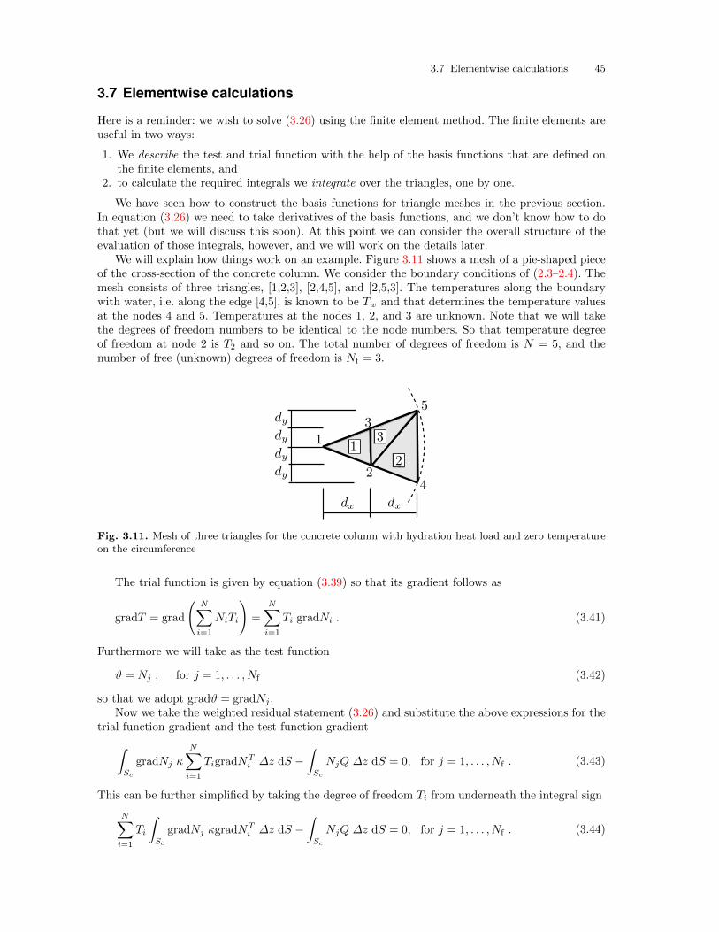
3.7 Elementwise calculations 45

3.7 Elementwise calculations

Here is a reminder: we wish to solve (3.26) using the finite element method. The finite elements areuseful in two ways:

1. We describe the test and trial function with the help of the basis functions that are defined onthe finite elements, and

2. to calculate the required integrals we integrate over the triangles, one by one.

We have seen how to construct the basis functions for triangle meshes in the previous section.In equation (3.26) we need to take derivatives of the basis functions, and we don’t know how to dothat yet (but we will discuss this soon). At this point we can consider the overall structure of theevaluation of those integrals, however, and we will work on the details later.

We will explain how things work on an example. Figure 3.11 shows a mesh of a pie-shaped pieceof the cross-section of the concrete column. We consider the boundary conditions of (2.3–2.4). Themesh consists of three triangles, [1,2,3], [2,4,5], and [2,5,3]. The temperatures along the boundarywith water, i.e. along the edge [4,5], is known to be Tw and that determines the temperature valuesat the nodes 4 and 5. Temperatures at the nodes 1, 2, and 3 are unknown. Note that we will takethe degrees of freedom numbers to be identical to the node numbers. So that temperature degreeof freedom at node 2 is T2 and so on. The total number of degrees of freedom is N = 5, and thenumber of free (unknown) degrees of freedom is Nf = 3.

Fig. 3.11. Mesh of three triangles for the concrete column with hydration heat load and zero temperatureon the circumference

The trial function is given by equation (3.39) so that its gradient follows as

gradT = grad

(N∑i=1

NiTi

)=

N∑i=1

Ti gradNi . (3.41)

Furthermore we will take as the test function

ϑ = Nj , for j = 1, . . . , Nf (3.42)

so that we adopt gradϑ = gradNj .Now we take the weighted residual statement (3.26) and substitute the above expressions for the

trial function gradient and the test function gradient∫Sc

gradNj κ

N∑i=1

TigradNTi ∆z dS −

∫Sc

NjQ ∆z dS = 0, for j = 1, . . . , Nf . (3.43)

This can be further simplified by taking the degree of freedom Ti from underneath the integral sign

N∑i=1

Ti

∫Sc

gradNj κgradNTi ∆z dS −

∫Sc

NjQ ∆z dS = 0, for j = 1, . . . , Nf . (3.44)

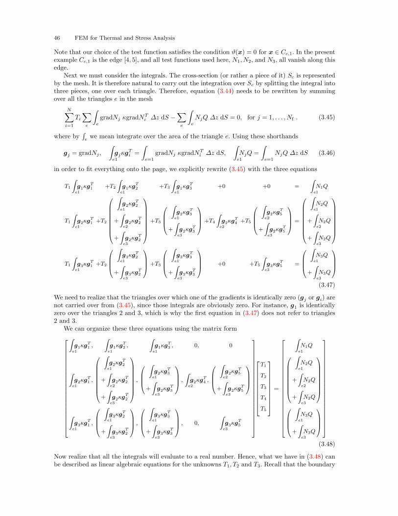
46 FEM for Thermal and Stress Analysis

Note that our choice of the test function satisfies the condition ϑ(x) = 0 for x ∈ Cc,1. In the presentexample Cc,1 is the edge [4, 5], and all test functions used here, N1, N2, and N3, all vanish along thisedge.

Next we must consider the integrals. The cross-section (or rather a piece of it) Sc is representedby the mesh. It is therefore natural to carry out the integration over Sc by splitting the integral intothree pieces, one over each triangle. Therefore, equation (3.44) needs to be rewritten by summingover all the triangles e in the mesh

N∑i=1

Ti∑e

∫e

gradNj κgradNTi ∆z dS −

∑e

∫e

NjQ ∆z dS = 0, for j = 1, . . . , Nf . (3.45)

where by∫ewe mean integrate over the area of the triangle e. Using these shorthands

gj = gradNj ,

∫e1

gjκgTi =

∫e=1

gradNj κgradNTi ∆z dS,

∫e1

NjQ =

∫e=1

NjQ ∆z dS (3.46)

in order to fit everything onto the page, we explicitly rewrite (3.45) with the three equations

T1

∫e1

g1κgT1 +T2

∫e1

g1κgT2 +T3

∫e1

g1κgT3 +0 +0 =

∫e1

N1Q

T1

∫e1

g2κgT1 +T2

∫e1

g2κgT2

+

∫e2

g2κgT2

+

∫e3

g2κgT2

+T3

∫e1

g2κgT3

+

∫e3

g2κgT3

+T4

∫e2

g2κgT4 +T5

∫e2

g2κgT5

+

∫e3

g2κgT5

=

∫e1

N2Q

+

∫e2

N2Q

+

∫e3

N2Q

T1

∫e1

g3κgT1 +T2

∫e1

g3κgT2

+

∫e3

g3κgT2

+T3

∫e1

g3κgT3

+

∫e3

g3κgT3

+0 +T5

∫e3

g3κgT5 =

∫e1

N3Q

+

∫e3

N3Q

(3.47)

We need to realize that the triangles over which one of the gradients is identically zero (gj or gi) arenot carried over from (3.45), since those integrals are obviously zero. For instance, g1 is identicallyzero over the triangles 2 and 3, which is why the first equation in (3.47) does not refer to triangles2 and 3.

We can organize these three equations using the matrix form

∫e1

g1κgT1 ,

∫e1

g1κgT2 ,

∫e1

g1κgT3 , 0, 0

∫e1

g2κgT1 ,

∫e1

g2κgT2

+

∫e2

g2κgT2

+

∫e3

g2κgT2

,

∫e1

g2κgT3

+

∫e3

g2κgT3

,

∫e2

g2κgT4 ,

∫e2

g2κgT5

+

∫e3

g2κgT5

∫e1

g3κgT1 ,

∫e1

g3κgT2

+

∫e3

g3κgT2

,

∫e1

g3κgT3

+

∫e3

g3κgT3

, 0,

∫e3

g3κgT5

T1

T2

T3

T4

T5

=

∫e1

N1Q

∫e1

N2Q

+

∫e2

N2Q

+

∫e3

N2Q

∫e1

N3Q

+

∫e3

N3Q

(3.48)

Now realize that all the integrals will evaluate to a real number. Hence, what we have in (3.48) canbe described as linear algebraic equations for the unknowns T1, T2 and T3. Recall that the boundary

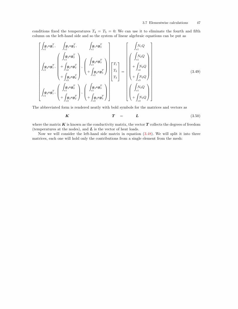
3.7 Elementwise calculations 47

conditions fixed the temperatures T4 = T5 = 0: We can use it to eliminate the fourth and fifthcolumn on the left-hand side and so the system of linear algebraic equations can be put as

∫e1

g1κgT1 ,

∫e1

g1κgT2 ,

∫e1

g1κgT3

∫e1

g2κgT1 ,

∫e1

g2κgT2

+

∫e2

g2κgT2

+

∫e3

g2κgT2

,

∫e1

g2κgT3

+

∫e3

g2κgT3

∫e1

g3κgT1 ,

∫e1

g3κgT2

+

∫e3

g3κgT2

,

∫e1

g3κgT3

+

∫e3

g3κgT3

T1

T2

T3

=

∫e1

N1Q

∫e1

N2Q

+

∫e2

N2Q

+

∫e3

N2Q

∫e1

N3Q

+

∫e3

N3Q

(3.49)

The abbreviated form is rendered neatly with bold symbols for the matrices and vectors as

K T = L (3.50)

where the matrixK is known as the conductivity matrix, the vector T collects the degrees of freedom(temperatures at the nodes), and L is the vector of heat loads.

Now we will consider the left-hand side matrix in equation (3.48). We will split it into threematrices, each one will hold only the contributions from a single element from the mesh:

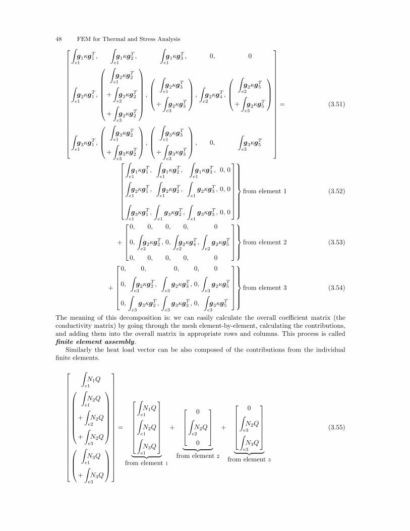
48 FEM for Thermal and Stress Analysis

∫e1

g1κgT1 ,

∫e1

g1κgT2 ,

∫e1

g1κgT3 , 0, 0

∫e1

g2κgT1 ,

∫e1

g2κgT2

+

∫e2

g2κgT2

+

∫e3

g2κgT2

,

∫e1

g2κgT3

+

∫e3

g2κgT3

,

∫e2

g2κgT4 ,

∫e2

g2κgT5

+

∫e3

g2κgT5

∫e1

g3κgT1 ,

∫e1

g3κgT2

+

∫e3

g3κgT2

,

∫e1

g3κgT3

+

∫e3

g3κgT3

, 0,

∫e3

g3κgT5

= (3.51)

∫e1

g1κgT1 ,

∫e1

g1κgT2 ,

∫e1

g1κgT3 , 0, 0∫

e1

g2κgT1 ,

∫e1

g2κgT2 ,

∫e1

g2κgT3 , 0, 0∫

e1

g3κgT1 ,

∫e1

g3κgT2 ,

∫e1

g3κgT3 , 0, 0

from element 1 (3.52)

+

0, 0, 0, 0, 0

0,

∫e2

g2κgT2 , 0,

∫e2

g2κgT4 ,

∫e2

g2κgT5

0, 0, 0, 0, 0

from element 2 (3.53)

+

0, 0, 0, 0, 0

0,

∫e3

g2κgT2 ,

∫e3

g2κgT3 , 0,

∫e3

g2κgT5

0,

∫e3

g3κgT2 ,

∫e3

g3κgT3 , 0,

∫e3

g3κgT5

from element 3 (3.54)

The meaning of this decomposition is: we can easily calculate the overall coefficient matrix (theconductivity matrix) by going through the mesh element-by-element, calculating the contributions,and adding them into the overall matrix in appropriate rows and columns. This process is calledfinite element assembly .

Similarly the heat load vector can be also composed of the contributions from the individualfinite elements.

∫e1

N1Q

∫e1

N2Q

+

∫e2

N2Q

+

∫e3

N2Q

∫e1

N3Q

+

∫e3

N3Q

=

∫e1

N1Q∫e1

N2Q∫e1

N3Q

︸ ︷︷ ︸

from element 1

+

0∫

e2

N2Q

0

︸ ︷︷ ︸

from element 2

+

0∫

e3

N2Q∫e3

N3Q

︸ ︷︷ ︸

from element 3

(3.55)

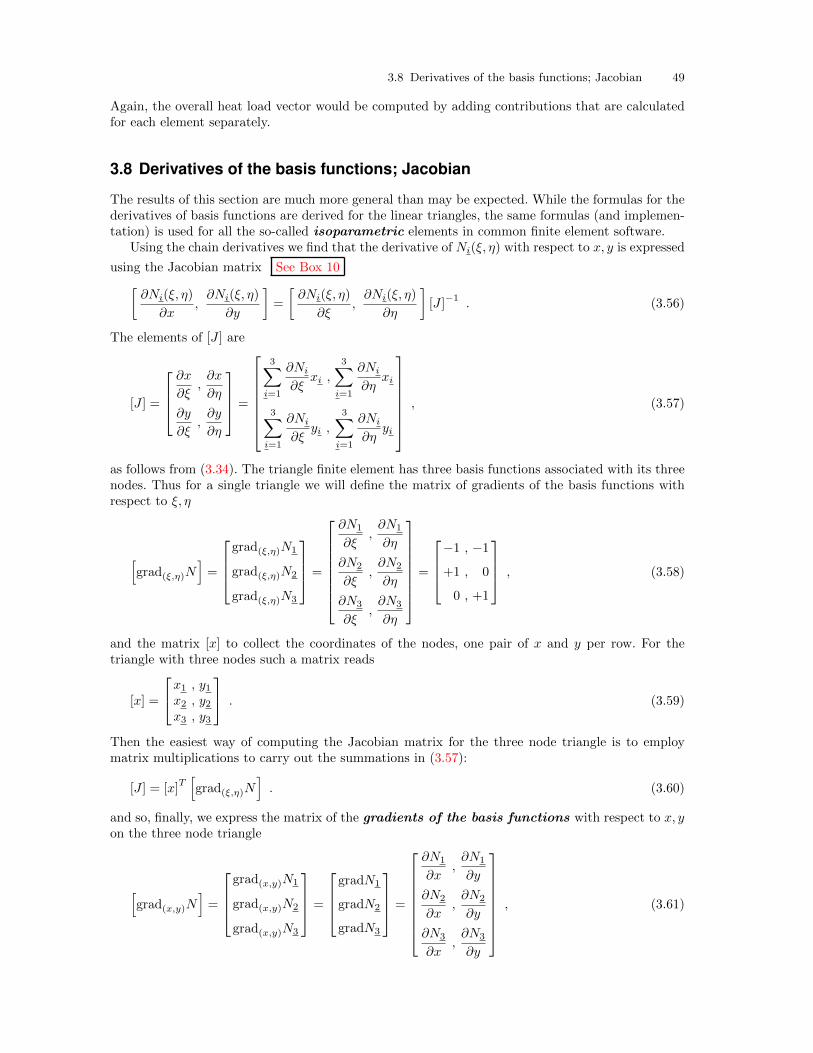
3.8 Derivatives of the basis functions; Jacobian 49

Again, the overall heat load vector would be computed by adding contributions that are calculatedfor each element separately.

3.8 Derivatives of the basis functions; Jacobian

The results of this section are much more general than may be expected. While the formulas for thederivatives of basis functions are derived for the linear triangles, the same formulas (and implemen-tation) is used for all the so-called isoparametric elements in common finite element software.

Using the chain derivatives we find that the derivative of Ni(ξ, η) with respect to x, y is expressed

using the Jacobian matrix See Box 10[∂Ni(ξ, η)

∂x,∂Ni(ξ, η)

∂y

]=

[∂Ni(ξ, η)

∂ξ,∂Ni(ξ, η)

∂η

][J ]

−1. (3.56)

The elements of [J ] are

[J ] =

∂x

∂ξ,∂x

∂η

∂y

∂ξ,∂y

∂η

=

3∑i=1

∂Ni

∂ξxi ,

3∑i=1

∂Ni

∂ηxi

3∑i=1

∂Ni

∂ξyi ,

3∑i=1

∂Ni

∂ηyi

, (3.57)

as follows from (3.34). The triangle finite element has three basis functions associated with its threenodes. Thus for a single triangle we will define the matrix of gradients of the basis functions withrespect to ξ, η

[grad(ξ,η)N

]=

grad(ξ,η)N1

grad(ξ,η)N2

grad(ξ,η)N3

=

∂N1

∂ξ,∂N1

∂η

∂N2

∂ξ,∂N2

∂η

∂N3

∂ξ,∂N3

∂η

=

−1 , −1

+1 , 0

0 , +1

, (3.58)

and the matrix [x] to collect the coordinates of the nodes, one pair of x and y per row. For thetriangle with three nodes such a matrix reads

[x] =

x1 , y1x2 , y2x3 , y3

. (3.59)

Then the easiest way of computing the Jacobian matrix for the three node triangle is to employmatrix multiplications to carry out the summations in (3.57):

[J ] = [x]T[grad(ξ,η)N

]. (3.60)

and so, finally, we express the matrix of the gradients of the basis functions with respect to x, yon the three node triangle

[grad(x,y)N

]=

grad(x,y)N1

grad(x,y)N2

grad(x,y)N3

=

gradN1

gradN2

gradN3

=

∂N1

∂x,∂N1

∂y

∂N2

∂x,∂N2

∂y

∂N3

∂x,∂N3

∂y

, (3.61)

50 FEM for Thermal and Stress Analysis

from (3.56) using (3.58)[grad(x,y)N

]=[grad(ξ,η)N

][J ]

−1. (3.62)

The right-hand side is readily evaluated: the matrix[grad(ξ,η)N

]is easily computed from the defini-

tion of the basis functions on the standard element (for the triangle from (3.30), (3.28), and (3.29)),and the Jacobian matrix follows from the definition (3.60). When there is no possibility of confusion

we could use the simplified notation gradNj = grad(x,y)Nj and [gradN ] =[grad(x,y)N

].

3.9 Jacobian matrix for the triangle

The computation of the gradient of the basis functions critically depends on the Jacobian matrix. TheJacobian (determinant of the Jacobian matrix) should be positive. The Jacobian matrix will thenbe invertible. The Jacobian matrix for the three-node triangle can be directly obtained from (3.35)

[J ] =

[(x2 − x1) , (x3 − x1)(y2 − y1) , (y3 − y1)

]. (3.63)

It really consists of the two vectors shown in Figure 3.9. This can be readily used to see whichconditions guarantee the determinant of the Jacobian matrix (i.e. the Jacobian) to be positive.Thinking about the geometrical meaning of the cross product in two dimensions, we can see thatthe cross product of v and w is in fact equal to the Jacobian, and so as long as these two vectorsare not co-linear the Jacobian will be nonzero.

Another way of thinking about the Jacobian is in terms of area. By inspection of Figure 3.9 wecan conclude that the Jacobian is twice the area of the triangle, to which we will refer to in thefollowing as Se,

det[J ] = 2Se . (3.64)

3.10 Bookkeeping

The following rules will apply in all hand calculations done in this book (such rules do not necessarilyneed to apply in all finite element programs: the developers are free to do whatever they want, aslong as the result is correct).

The nodes of the mesh may be numbered arbitrarily. Each node will be associated with a degreeof freedom. This information will be given in a table. For our example of Section 3.7 such a tablewould be trivial:

Node numbers 1 2 3 4 5DOF numbers 1 2 3 4 5

It simply says that the degree of freedom numbers are the same as the node numbers. In general,they will not be.

We will assume that all degrees of freedom are numbered sequentially from 1 to N . First thefree degrees of freedom will be numbered 1, 2, ..., Nf (those degrees of freedom that are actuallyunknown and need to be solved for), and only then the degrees of freedom that are given as data(known from the boundary conditions) will be numbered Nf+1, ..., N . In our example the free DOFsreside at nodes 1, 2, and 3. That’s why these three nodes have the first 3 degrees of freedom.

All elements connect some nodes. In a three-node triangle mesh each element connects threenodes. The so-called element connectivity are the numbers of the nodes, given in a counterclockwiseorder. Again, the connectivity of the triangles will be given by a table. For our example of Section 3.7

3.11 Concrete-column example continued 51

Element Node 1 Node 2 Node 31 1 2 32 2 4 53 2 5 3

For each element we can therefore find out the degrees of freedom at its three nodes. We look atthe row of the element connectivity table, and we pick out the degrees of freedom from the node-DOFtable. The so-called element degree of freedom array (we will be abbreviating it as edof array) isthe result. For instance, for element 3 the edof array reads [2, 5, 3] (which is the same as the thirdrow in the connectivity table, because in this particular example the node numbers are the same asthe degree of freedom numbers).

There is another way we can account for the degrees of freedom. In the context of a singleelement, we can consider the degrees of freedom at the three nodes of the triangle. They are alwaysnumbered the same way as the three nodes of the triangle: 1, 2, and 3. We can call these “local”numbers as opposed to the global numbers that are counted in the entire mesh. The global degreeof freedom numbers change from triangle to triangle (the edof array is different for each triangle),the local numbers are always the same.

3.11 Concrete-column example continued

Now that we know how to calculate the derivatives of the basis functions, we can continue theexample from Section 3.7. The radius of the circular cross-section is a = 2.5m, and we take theinternal angle of the pie-shaped domain as 15o. The dimensions in Figure 3.11 are then dx = 1.2074mand dy = 0.3235m. We consider the boundary conditions of (2.3–2.4). The mesh consists of threetriangles, [1,2,3], [2,4,5], and [2,5,3]. The temperature along the boundary with water, i.e. along theedge [4,5], is known and that determines the temperature at the nodes 4 and 5. Temperatures atthe nodes 1, 2, and 3 are unknown. We will associate the degrees of freedom with the nodes as

Node numbers 1 2 3 4 5DOF numbers 3 1 2 5 4

The total number of degrees of freedom is N = 5, and the number of free (unknown) degrees offreedom is Nf = 3.

As shown in Section 3.7, we will proceed by computing contributions to the algebraic equationselement-by-element. The goal is to evaluate integrals such as∫

e

gradNj κgradNTi ∆z dS (3.65)

But rather than iterate i = 1, . . . , N and j = 1, . . . , Nf and compute the integral for all such pairs,we will calculate the elementwise conductivity matrix for the local degrees of freedom k and m,where k = 1, 2, 3, m = 1, 2, 3, and when the matrix is calculated we will decide to which DOFs i andj it should contribute and assemble the appropriate numbers to the global (systemwide) quantities.

How do we evaluate the integral in the first place? Let us inspect one of the terms, for instance∫e=1

gradNk κgradNTm ∆z dS (3.66)

By inspecting the individual terms in the expression for the gradients of the basis functions (3.62),we can see that the gradients of the basis functions with respect to x, y are constant on eachthree-node triangle, since they are the product of two position-independent matrices, the gradientmatrix (3.58), and the inverse of the Jacobian matrix (3.63). But that means that the integrandin (3.66) is a constant number since everything else, κ and ∆z are also uniform on each triangle.That makes the integral trivial∫

e=1

gradNk κgradNTm ∆z dS = gradNk κgradN

Tm ∆z

∫e=1

dS = gradNk κgradNTm ∆zSe1

52 FEM for Thermal and Stress Analysis

(3.67)

where Se1 =∫e=1

dS is the area of the triangle e = 1. Also recall (3.64) so that∫e=1

gradNk κgradNTm ∆z dS = (det[J ]/2)gradNk κgradN

Tm ∆z (3.68)

The actual calculating will be performed here with the help of Python. Evidently, it can also bePython- script

done with a calculator or by hand. To begin, some required functions are imported from the modulesmath and numpy. We define some input quantities with obvious meanings (page 88):

20 a = 2.5 # radius of the column21 dy = a/2*math.sin(15./180*math.pi)22 dx = a/2*math.cos(15./180*math.pi)23 Q = 4.5 # internal heat generation rate24 k = 1.8 # thermal conductivity25 Dz = 1.0 # thickness of the slice

The matrix of the gradients of the basis functions with respect to the parametric coordinates isdefined as

28 gradNpar = array([[-1, -1], [1, 0], [0, 1]])

Note that an array is defined row-by-row, for instance [-1, -1] is the first row of gradNpar, and[1, 0] and [0, 1] are the second and third row.

The locations of the nodes are defined with an array of coordinates of the nodes, one node perrow.

30 xall = array([[0, 0], [dx, -dy], [dx, dy], [2*dx, -2*dy], [2*dx, 2*dy]])

and the definition of the degrees of freedom

31 # Numbers of the degrees of freedom32 dof = array([3, 1, 2, 5, 4])33 # Number of free degrees of freedom34 N_f = 335 # Number of all degrees of freedom36 N = 5

3.11.1 Element 1

And now we are ready to evaluate the expressions we need for the first element. The element isdefined by listing its three nodes.

43 conn = array([1, 2, 3]) # The definition of the element, listing its nodes

We can then use this list to extract the coordinates of the three nodes that are connected by element1. But we need to take into account the Python zero-based indexing: arrays rows and columns arepointed to by numbers 0 to n-1 (where n is the number of rows or columns). Figure 3.12 illustratesthe indexing of the entries of a matrix (an array), both when working with the matrix in handcalculations and when indexing the matrix in Python code. To recap: Python works with offsets ofthe rows and columns, whereas in hand calculation we refer to the index of the row or column.

So the node number 3 is stored in row 2 of the array xall and so on. Therefore, we can createan appropriate array of Python indexes by subtracting 1 from conn (page 88).

44 zconn =conn - 1 # zero-based node indexes

Then the coordinates of the three nodes of element 1 can be retrieved as

45 x = xall[zconn, :]# The coordinates of the three nodes

to give

3.11 Concrete-column example continued 53

Fig. 3.12. Indexing a 2 × 6 matrix A. Numbers at the top and along the left side: one-based indexing, ofthe kind that would be used when working with the matrix by hand. Numbers along the bottom and theright-hand side: zero-based indexing. Python uses this way of referring to the matrix entries by specifyingthe offset of the left-hand side or the top boundary of the entry’s box from the top-left corner of the matrix.So the offset of the box of column 3 of the matrix from the top-left corner is 2. Similar scheme is used torefer to the rows of the matrix: the offset of the second row is 1. So for instance the entry in row 2 andcolumn 3 of this matrix is referred to as A23 in hand calculations, and A[1, 2] in Python code.

x= [[ 0. 0. ][ 1.20740728 -0.32352381][ 1.20740728 0.32352381]]

Now we calculate the Jacobian matrix from (3.60)

47 J = dot(x.T, gradNpar) # Compute the Jacobian matrix48 Se = linalg.det(J)/2 # The area of the triangle49 print(’Se = ’, Se)

The area of the triangle prints as Se= 0.390625.Note the use of the dot function to compute the dot product of two matrices, and the use of the

.T attribute to transpose a matrix. In the above we have also used the numpy.linalg linear algebramodule, namely the function det to compute the determinant of the Jacobian matrix. Elementarygeometry confirms that the area is correct: we calculate 0.390625 from the dimensions as dx*dy.

Elementwise conductivity matrix

Next we calculate the gradients of the basis functions on the first triangle with the respect to thex, y coordinates from (3.62). We will again use the linear algebra module, numpy.linalg, for theinverse of the Jacobian matrix (page 88).

51 gradN = dot(gradNpar, linalg.inv(J))52 print(’gradN=’, gradN)

gradN = [[-0.82822094 0. ][ 0.41411047 -1.54548132][ 0.41411047 1.54548132]]

The first row of this matrix is the gradient gradN1 and so on. Now we can calculate for instance∫e=1

gradN1 κgradNT1 ∆z dS (3.69)

as

54 print(Se*dot(gradN[0,:], gradN[0,:].T)*k*Dz)

which yields 0.482308546376, or∫e=1

gradN1 κgradNT2 ∆z dS (3.70)

as

55 print(Se*dot(gradN[0,:], gradN[1,:].T)*k*Dz)

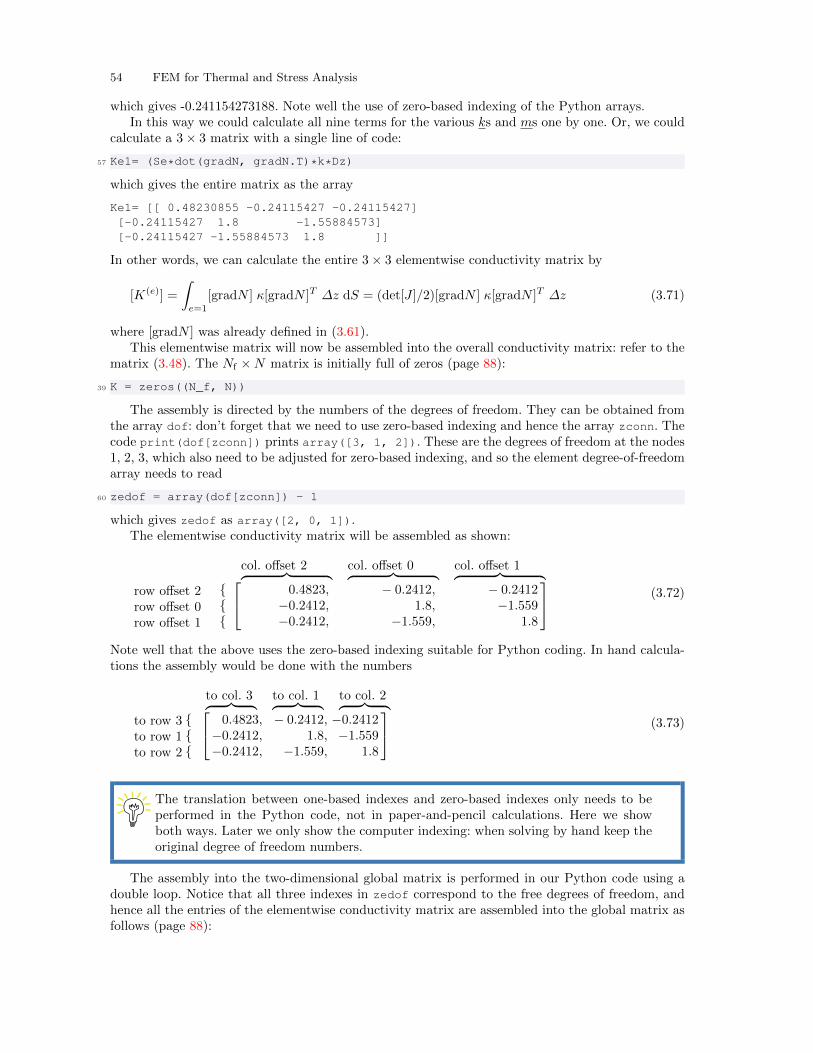
54 FEM for Thermal and Stress Analysis

which gives -0.241154273188. Note well the use of zero-based indexing of the Python arrays.In this way we could calculate all nine terms for the various ks and ms one by one. Or, we could

calculate a 3× 3 matrix with a single line of code:

57 Ke1= (Se*dot(gradN, gradN.T)*k*Dz)

which gives the entire matrix as the array

Ke1= [[ 0.48230855 -0.24115427 -0.24115427][-0.24115427 1.8 -1.55884573][-0.24115427 -1.55884573 1.8 ]]

In other words, we can calculate the entire 3× 3 elementwise conductivity matrix by

[K(e)] =

∫e=1

[gradN ] κ[gradN ]T ∆z dS = (det[J ]/2)[gradN ] κ[gradN ]T ∆z (3.71)

where [gradN ] was already defined in (3.61).This elementwise matrix will now be assembled into the overall conductivity matrix: refer to the

matrix (3.48). The Nf ×N matrix is initially full of zeros (page 88):

39 K = zeros((N_f, N))

The assembly is directed by the numbers of the degrees of freedom. They can be obtained fromthe array dof: don’t forget that we need to use zero-based indexing and hence the array zconn. Thecode print(dof[zconn]) prints array([3, 1, 2]). These are the degrees of freedom at the nodes1, 2, 3, which also need to be adjusted for zero-based indexing, and so the element degree-of-freedomarray needs to read

60 zedof = array(dof[zconn]) - 1

which gives zedof as array([2, 0, 1]).The elementwise conductivity matrix will be assembled as shown:

col. offset 2︷ ︸︸ ︷ col. offset 0︷ ︸︸ ︷ col. offset 1︷ ︸︸ ︷row offset 2 {row offset 0 {row offset 1 {

0.4823, − 0.2412, − 0.2412−0.2412, 1.8, −1.559−0.2412, −1.559, 1.8

(3.72)

Note well that the above uses the zero-based indexing suitable for Python coding. In hand calcula-tions the assembly would be done with the numbers

to col. 3︷ ︸︸ ︷ to col. 1︷ ︸︸ ︷ to col. 2︷ ︸︸ ︷to row 3 {to row 1 {to row 2 {

0.4823, − 0.2412, −0.2412−0.2412, 1.8, −1.559−0.2412, −1.559, 1.8

(3.73)

The translation between one-based indexes and zero-based indexes only needs to beperformed in the Python code, not in paper-and-pencil calculations. Here we showboth ways. Later we only show the computer indexing: when solving by hand keep theoriginal degree of freedom numbers.

The assembly into the two-dimensional global matrix is performed in our Python code using adouble loop. Notice that all three indexes in zedof correspond to the free degrees of freedom, andhence all the entries of the elementwise conductivity matrix are assembled into the global matrix asfollows (page 88):

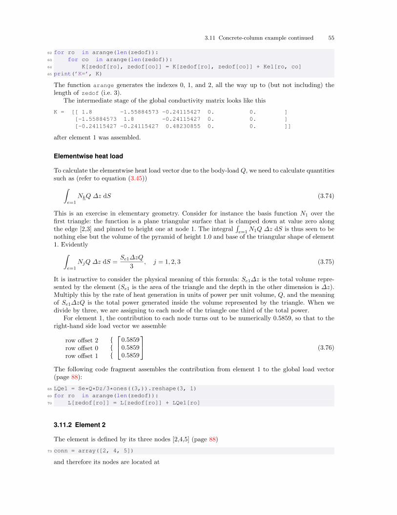
3.11 Concrete-column example continued 55

62 for ro in arange(len(zedof)):63 for co in arange(len(zedof)):64 K[zedof[ro], zedof[co]] = K[zedof[ro], zedof[co]] + Ke1[ro, co]65 print(’K=’, K)

The function arange generates the indexes 0, 1, and 2, all the way up to (but not including) thelength of zedof (i.e. 3).

The intermediate stage of the global conductivity matrix looks like this

K = [[ 1.8 -1.55884573 -0.24115427 0. 0. ][-1.55884573 1.8 -0.24115427 0. 0. ][-0.24115427 -0.24115427 0.48230855 0. 0. ]]

after element 1 was assembled.

Elementwise heat load

To calculate the elementwise heat load vector due to the body-load Q, we need to calculate quantitiessuch as (refer to equation (3.45))∫

e=1

NkQ ∆z dS (3.74)

This is an exercise in elementary geometry. Consider for instance the basis function N1 over thefirst triangle: the function is a plane triangular surface that is clamped down at value zero alongthe edge [2,3] and pinned to height one at node 1. The integral

∫e=1

N1Q ∆z dS is thus seen to benothing else but the volume of the pyramid of height 1.0 and base of the triangular shape of element1. Evidently∫

e=1

NjQ ∆z dS =Se1∆zQ

3, j = 1, 2, 3 (3.75)

It is instructive to consider the physical meaning of this formula: Se1∆z is the total volume repre-sented by the element (Se1 is the area of the triangle and the depth in the other dimension is ∆z).Multiply this by the rate of heat generation in units of power per unit volume, Q, and the meaningof Se1∆zQ is the total power generated inside the volume represented by the triangle. When wedivide by three, we are assigning to each node of the triangle one third of the total power.

For element 1, the contribution to each node turns out to be numerically 0.5859, so that to theright-hand side load vector we assemble

row offset 2 {row offset 0 {row offset 1 {

0.58590.58590.5859

(3.76)

The following code fragment assembles the contribution from element 1 to the global load vector(page 88):

68 LQe1 = Se*Q*Dz/3*ones((3,)).reshape(3, 1)69 for ro in arange(len(zedof)):70 L[zedof[ro]] = L[zedof[ro]] + LQe1[ro]

3.11.2 Element 2

The element is defined by its three nodes [2,4,5] (page 88)

73 conn = array([2, 4, 5])

and therefore its nodes are located at

56 FEM for Thermal and Stress Analysis

74 zconn = conn - 1 # zero-based node indexes75 x = xall[zconn, :]# The coordinates of the three nodes

which gives

array([[ 1.20740728, -0.32352381],[ 2.41481457, -0.64704761],[ 2.41481457, 0.64704761]])

The Jacobian matrix reads

array([[ 1.20740728, 1.20740728],[-0.32352381, 0.97057142]])

and the triangle area is 0.78125.

Elementwise conductivity matrix

For element 2 the procedure proceeds precisely as for element 1. This is why the finite elementmethod is so well suited to the computer age: it is very easy to program, the procedure is justrepeated for one more element, and the computer doesn’t care whether it needs to compute thesame thing 1000 or 1001 times. The elementwise conductivity matrix for element 2 results as

array([[ 0.96461709, -0.72346282, -0.24115427],[-0.72346282, 1.38230855, -0.65884573],[-0.24115427, -0.65884573, 0.9 ]])

The element degree of freedom array of element 2 obtains from the dof map as

84 zedof = array(dof[zconn]) - 1

i.e. array([0, 4, 3]). Notice that the global conductivity matrix is of dimension Nf ×N = 3× 5,and therefore in zero-based indexing we ignore any row offsets with value ≥ 3. Hence from theconductivity matrix of element 2

col. offset 0︷ ︸︸ ︷ col. offset 4︷ ︸︸ ︷ col. offset 3︷ ︸︸ ︷row offset 0 {row offset 4 {row offset 3 {

0.9646, − 0.7235, − 0.2412−0.7235, 1.382, −0.6588− 0.2412, −0.6588, 0.9

(3.77)

the only assembled values will go to row 0.In order to implement the assembly in Python code, we need to test the contents of the element

degree-of-freedom array: when both the row index and the column index fall within the boundariesof the conductivity matrix, the corresponding entries from the elementwise matrix are added to theglobal matrix; otherwise they are simply ignored (page 88).

86 for ro in arange(len(zedof)):87 for co in arange(len(zedof)):88 if (zedof[ro] < N_f):89 K[zedof[ro], zedof[co]] = K[zedof[ro], zedof[co]] + Ke2[ro, co]

For easy reference we also give here the variant of the above algorithm that could be used in handcalculations. In pseudocode:

for r in 1, 2, 3for c in 1, 2, 3

if (edof[r] <= N_f)K[edof[r], edof[c]] = K[edof[r], edof[c]] + Ke2[r, c]

for edof=[1, 5, 4], where edof[2] is 5 and so on.

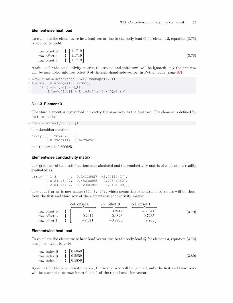
3.11 Concrete-column example continued 57

Elementwise heat load

To calculate the elementwise heat load vector due to the body-load Q for element 2, equation (3.75)is applied to yield

row offset 0 {row offset 4 {row offset 3 {

1.17191.17191.1719

(3.78)

Again, as for the conductivity matrix, the second and third rows will be ignored; only the first rowwill be assembled into row offset 0 of the right-hand side vector. In Python code (page 88):

91 LQe2 = Se*Q*Dz/3*ones((3,)).reshape(3, 1)92 for ro in arange(len(zedof)):93 if (zedof[ro] < N_f):94 L[zedof[ro]] = L[zedof[ro]] + LQe2[ro]

3.11.3 Element 3

The third element is dispatched in exactly the same way as the first two. The element is defined byits three nodes

99 conn = array([2, 5, 3])

The Jacobian matrix is

array([[ 1.20740728 0. ][ 0.97057142 0.64704761]])

and the area is 0.390625.

Elementwise conductivity matrix

The gradients of the basis functions are calculated and the conductivity matrix of element 3 is readilyevaluated as

array([[ 1.8 , 0.24115427, -2.04115427],[ 0.24115427, 0.48230855, -0.72346282],[-2.04115427, -0.72346282, 2.76461709]])

The zedof array is now array([0, 3, 1]), which means that the assembled values will be thosefrom the first and third row of the elementwise conductivity matrix.

col. offset 0︷ ︸︸ ︷ col. offset 3︷ ︸︸ ︷ col. offset 1︷ ︸︸ ︷row offset 0 {row offset 3 {row offset 1 {

1.8, 0.2412, − 2.0410.2412, 0.4823, − 0.7235−2.041, −0.7235, 2.765

(3.79)

Elementwise heat load

To calculate the elementwise heat load vector due to the body-load Q for element 3, equation (3.75)is applied again to yield

row index 0 {row index 3 {row index 1 {

0.58590.58590.5859

(3.80)

Again, as for the conductivity matrix, the second row will be ignored; only the first and third rowswill be assembled to rows index 0 and 1 of the right-hand side vector.

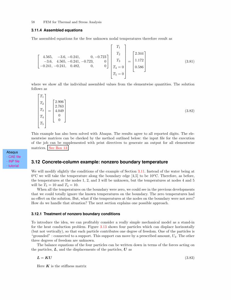
58 FEM for Thermal and Stress Analysis

3.11.4 Assembled equations

The assembled equations for the free unknown nodal temperatures therefore result as

4.565, −3.6, −0.241, 0, −0.723−3.6, 4.565, −0.241, −0.723, 0

−0.241, −0.241, 0.482, 0, 0

T1

T2

T3

T4 = 0

T5 = 0

=

2.344

1.172

0.586

(3.81)

where we show all the individual assembled values from the elementwise quantities. The solutionfollows as

T1

T2

T3

T4

T5

=

2.9062.7634.04900

(3.82)

This example has also been solved with Abaqus. The results agree to all reported digits. The ele-mentwise matrices can be checked by the method outlined below: the input file for the executionof the job can be supplemented with print directives to generate an output for all elementwise

matrices. See Box 13Abaqus- CAE file- INP file- tutorial

3.12 Concrete-column example: nonzero boundary temperature

We will modify slightly the conditions of the example of Section 3.11. Instead of the water being at0oC we will take the temperature along the boundary edge [4,5] to be 10oC. Therefore, as before,the temperatures at the nodes 1, 2, and 3 will be unknown, but the temperatures at nodes 4 and 5will be T5 = 10 and T4 = 10.

When all the temperatures on the boundary were zero, we could see in the previous developmentsthat we could totally ignore the known temperatures on the boundary. The zero temperatures hadno effect on the solution. But, what if the temperatures at the nodes on the boundary were not zero?How do we handle that situation? The next section explains one possible approach.

3.12.1 Treatment of nonzero boundary conditions

To introduce the idea, we can profitably consider a really simple mechanical model as a stand-infor the heat conduction problem. Figure 3.13 shows four particles which can displace horizontally(but not vertically), so that each particle contributes one degree of freedom. One of the particles is“grounded” : connected to a support. This support can move by a prescribed amount, U4. The otherthree degrees of freedom are unknown.

The balance equations of the four particles can be written down in terms of the forces acting onthe particles, L, and the displacements of the particles, U as

L = KU (3.83)

Here K is the stiffness matrix

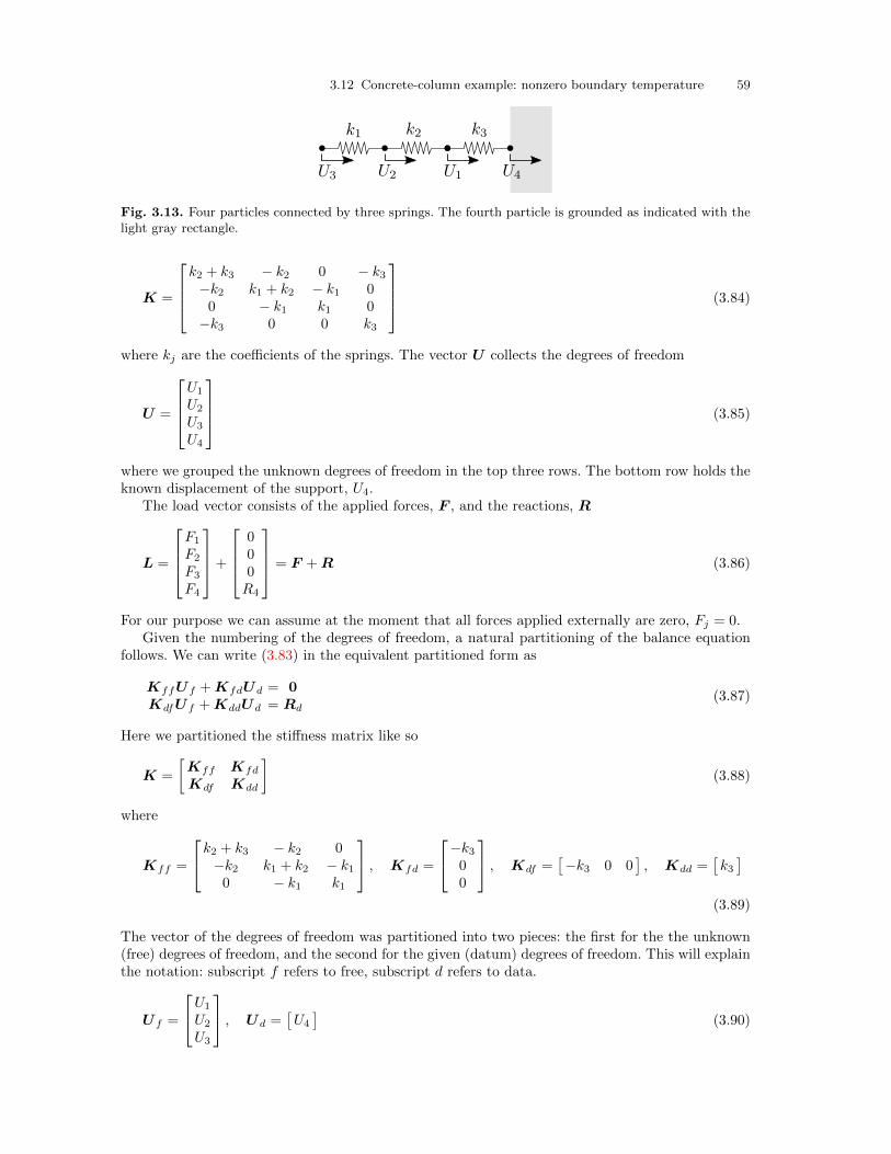
3.12 Concrete-column example: nonzero boundary temperature 59

Fig. 3.13. Four particles connected by three springs. The fourth particle is grounded as indicated with thelight gray rectangle.

K =

k2 + k3 − k2 0 − k3−k2 k1 + k2 − k1 00 − k1 k1 0

−k3 0 0 k3

(3.84)

where kj are the coefficients of the springs. The vector U collects the degrees of freedom

U =

U1

U2

U3

U4

(3.85)

where we grouped the unknown degrees of freedom in the top three rows. The bottom row holds theknown displacement of the support, U4.

The load vector consists of the applied forces, F , and the reactions, R

L =

F1

F2

F3

F4

+

000R4

= F +R (3.86)

For our purpose we can assume at the moment that all forces applied externally are zero, Fj = 0.Given the numbering of the degrees of freedom, a natural partitioning of the balance equation

follows. We can write (3.83) in the equivalent partitioned form as

KffUf +KfdUd = 0KdfUf +KddUd = Rd

(3.87)

Here we partitioned the stiffness matrix like so

K =

[Kff Kfd

Kdf Kdd

](3.88)

where

Kff =

k2 + k3 − k2 0−k2 k1 + k2 − k10 − k1 k1

, Kfd =

−k300

, Kdf =[−k3 0 0

], Kdd =

[k3]

(3.89)

The vector of the degrees of freedom was partitioned into two pieces: the first for the the unknown(free) degrees of freedom, and the second for the given (datum) degrees of freedom. This will explainthe notation: subscript f refers to free, subscript d refers to data.

Uf =

U1

U2

U3

, Ud =[U4

](3.90)

60 FEM for Thermal and Stress Analysis

The reaction vector was also partitioned, and the first part is omitted since it is identically zero.

Rd =[R4

](3.91)

We note that the first of the equations (3.87) can be written in the usual form where the coefficientmatrix and the vector of unknowns are on the left-hand side, and everything on the right-hand sideis known.

KffUf = −KfdUd (3.92)

The coefficient matrix Kff is square and invertible (its determinant is (k2+ k3)k21 +((k2+ k3)(k2+

k1) + k22)k1 = 0). Therefore we can solve from (3.92) for the unknown displacements Uf . If we wishto find the reaction, we use the second equation (3.87) to solve for the reactions

Rd = KdfUf +KddUd (3.93)

We call the term −KfdUd the load due to support settlement. More generally, this is the loadvector produced by nonzero essential boundary conditions. In the present case this is explicitly

−KfdUd =

−k3U4

00

(3.94)

Note that if we are not interested in the reactions, which is typically the case in heat conductionanalysis, since the reactions are difficult to interpret in that case, we can simply work with only thematrices in (3.92), Kff , and Kfd. In other words, the second row in (3.87) corresponding to theknown displacement does not need to be calculated.

3.12.2 Application of the partitioning method to the heat conduction problem

Our method still works with the same equation, the weighted residual statement (3.45), but theterms multiplied with T5 and T4 do not drop out anymore. We will indicate this by splitting thesum over the degrees of freedom in (3.45) (which is for your convenience reproduced again here)

N∑i=1

Ti∑e

∫e

gradNj κgradNTi ∆z dS −

∑e

∫e

NjQ ∆z dS = 0, for j = 1, . . . , Nf . (3.95)

into

Nf∑i=1

Ti∑e

∫e

gradNj κgradNTi ∆z dS︸ ︷︷ ︸

free degrees of freedom i = 1, 2, 3

+

N∑i=Nf+1

Ti∑e

∫e

gradNj κgradNTi ∆z dS︸ ︷︷ ︸

datum degrees of freedom i = 4, 5

−∑e

∫eNjQ ∆z dS = 0, for j = 1, . . . , Nf .

(3.96)

The first line of this equation are the unknown degrees of freedom Ti multiplied with the entriesof the conductivity matrix (which are the integrals). The second line of this equation contains onlyknown quantities. The first line is the left-hand side, and the second line is the right-hand side ofthe algebraic equations from which we need to solve for the free degrees of freedom. So a good wayof rewriting the above is

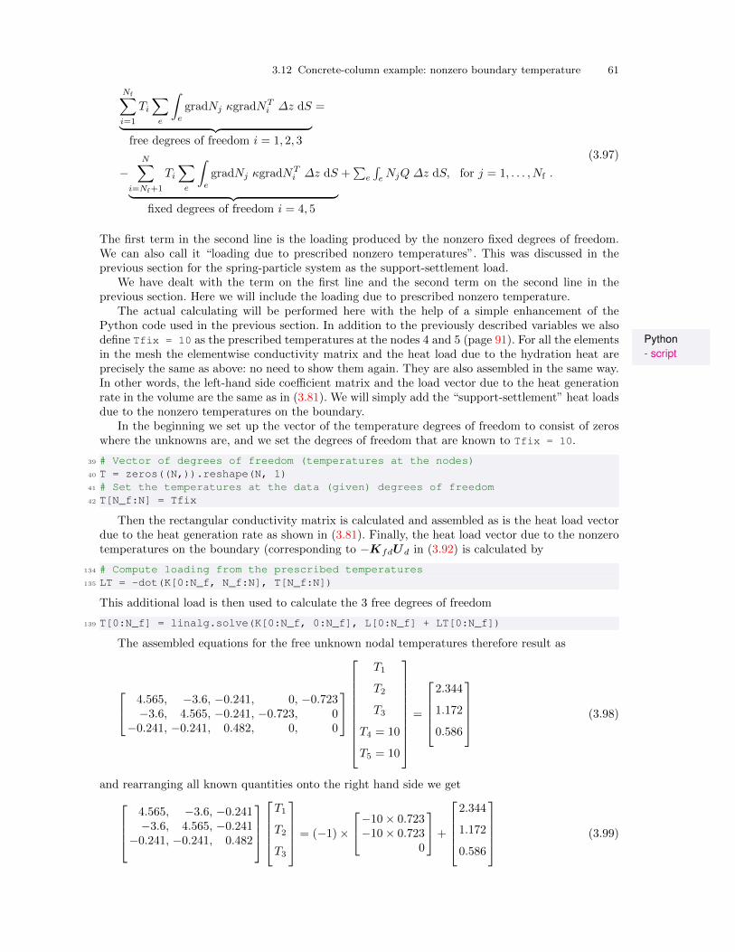
3.12 Concrete-column example: nonzero boundary temperature 61

Nf∑i=1

Ti∑e

∫e

gradNj κgradNTi ∆z dS︸ ︷︷ ︸

free degrees of freedom i = 1, 2, 3

=

−N∑

i=Nf+1

Ti∑e

∫e

gradNj κgradNTi ∆z dS︸ ︷︷ ︸

fixed degrees of freedom i = 4, 5

+∑

e

∫eNjQ ∆z dS, for j = 1, . . . , Nf .

(3.97)

The first term in the second line is the loading produced by the nonzero fixed degrees of freedom.We can also call it “loading due to prescribed nonzero temperatures”. This was discussed in theprevious section for the spring-particle system as the support-settlement load.

We have dealt with the term on the first line and the second term on the second line in theprevious section. Here we will include the loading due to prescribed nonzero temperature.

The actual calculating will be performed here with the help of a simple enhancement of thePython code used in the previous section. In addition to the previously described variables we also

Python- script

define Tfix = 10 as the prescribed temperatures at the nodes 4 and 5 (page 91). For all the elementsin the mesh the elementwise conductivity matrix and the heat load due to the hydration heat areprecisely the same as above: no need to show them again. They are also assembled in the same way.In other words, the left-hand side coefficient matrix and the load vector due to the heat generationrate in the volume are the same as in (3.81). We will simply add the “support-settlement” heat loadsdue to the nonzero temperatures on the boundary.

In the beginning we set up the vector of the temperature degrees of freedom to consist of zeroswhere the unknowns are, and we set the degrees of freedom that are known to Tfix = 10.

39 # Vector of degrees of freedom (temperatures at the nodes)40 T = zeros((N,)).reshape(N, 1)41 # Set the temperatures at the data (given) degrees of freedom42 T[N_f:N] = Tfix

Then the rectangular conductivity matrix is calculated and assembled as is the heat load vectordue to the heat generation rate as shown in (3.81). Finally, the heat load vector due to the nonzerotemperatures on the boundary (corresponding to −KfdUd in (3.92) is calculated by

134 # Compute loading from the prescribed temperatures135 LT = -dot(K[0:N_f, N_f:N], T[N_f:N])

This additional load is then used to calculate the 3 free degrees of freedom

139 T[0:N_f] = linalg.solve(K[0:N_f, 0:N_f], L[0:N_f] + LT[0:N_f])

The assembled equations for the free unknown nodal temperatures therefore result as

4.565, −3.6, −0.241, 0, −0.723−3.6, 4.565, −0.241, −0.723, 0

−0.241, −0.241, 0.482, 0, 0

T1

T2

T3

T4 = 10

T5 = 10

=

2.344

1.172

0.586

(3.98)

and rearranging all known quantities onto the right hand side we get4.565, −3.6, −0.241−3.6, 4.565, −0.241

−0.241, −0.241, 0.482

T1

T2

T3

= (−1)×

−10× 0.723−10× 0.723

0

+

2.344

1.172

0.586

(3.99)

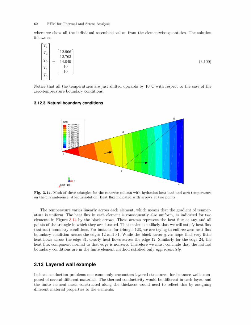
62 FEM for Thermal and Stress Analysis

where we show all the individual assembled values from the elementwise quantities. The solutionfollows as

T1

T2

T3

T4

T5

=

12.90612.76314.0491010

(3.100)

Notice that all the temperatures are just shifted upwards by 10oC with respect to the case of thezero-temperature boundary conditions.

3.12.3 Natural boundary conditions

NT11

+0.000e+00+3.375e−01+6.749e−01+1.012e+00+1.350e+00+1.687e+00+2.025e+00+2.362e+00+2.700e+00+3.037e+00+3.375e+00+3.712e+00+4.049e+00

X

Y

Z

1

3

2

4

5

Text−10

Fig. 3.14. Mesh of three triangles for the concrete column with hydration heat load and zero temperatureon the circumference. Abaqus solution. Heat flux indicated with arrows at two points.

The temperature varies linearly across each element, which means that the gradient of temper-ature is uniform. The heat flux in each element is consequently also uniform, as indicated for twoelements in Figure 3.14 by the black arrows. These arrows represent the heat flux at any and allpoints of the triangle in which they are situated. That makes it unlikely that we will satisfy heat flux(natural) boundary conditions. For instance for triangle 123, we are trying to enforce zero-heat-fluxboundary condition across the edges 12 and 31. While the black arrow gives hope that very littleheat flows across the edge 31, clearly heat flows across the edge 12. Similarly for the edge 24, theheat flux component normal to that edge is nonzero. Therefore we must conclude that the naturalboundary conditions are in the finite element method satisfied only approximately.

3.13 Layered wall example

In heat conduction problems one commonly encounters layered structures, for instance walls com-posed of several different materials. The thermal conductivity would be different in each layer, andthe finite element mesh constructed along the thickness would need to reflect this by assigningdifferent material properties to the elements.

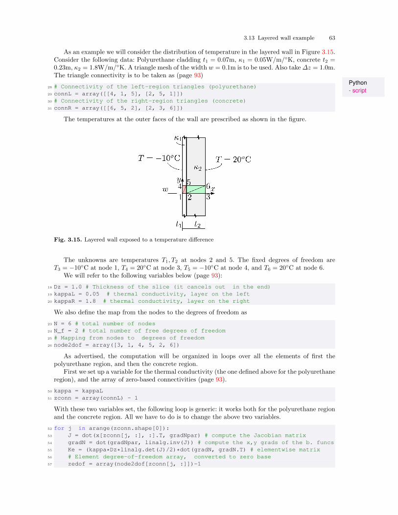
3.13 Layered wall example 63

As an example we will consider the distribution of temperature in the layered wall in Figure 3.15.Consider the following data: Polyurethane cladding t1 = 0.07m, κ1 = 0.05W/m/◦K, concrete t2 =0.23m, κ2 = 1.8W/m/◦K. A triangle mesh of the width w = 0.1m is to be used. Also take∆z = 1.0m.The triangle connectivity is to be taken as (page 93)

Python- script

28 # Connectivity of the left-region triangles (polyurethane)29 connL = array([[4, 1, 5], [2, 5, 1]])30 # Connectivity of the right-region triangles (concrete)31 connR = array([[6, 5, 2], [2, 3, 6]])

The temperatures at the outer faces of the wall are prescribed as shown in the figure.

Fig. 3.15. Layered wall exposed to a temperature difference

The unknowns are temperatures T1, T2 at nodes 2 and 5. The fixed degrees of freedom areT3 = −10◦C at node 1, T4 = 20◦C at node 3, T5 = −10◦C at node 4, and T6 = 20◦C at node 6.

We will refer to the following variables below (page 93):

18 Dz = 1.0 # Thickness of the slice (it cancels out in the end)19 kappaL = 0.05 # thermal conductivity, layer on the left20 kappaR = 1.8 # thermal conductivity, layer on the right

We also define the map from the nodes to the degrees of freedom as

23 N = 6 # total number of nodes24 N_f = 2 # total number of free degrees of freedom25 # Mapping from nodes to degrees of freedom26 node2dof = array([3, 1, 4, 5, 2, 6])

As advertised, the computation will be organized in loops over all the elements of first thepolyurethane region, and then the concrete region.

First we set up a variable for the thermal conductivity (the one defined above for the polyurethaneregion), and the array of zero-based connectivities (page 93).

50 kappa = kappaL51 zconn = array(connL) - 1

With these two variables set, the following loop is generic: it works both for the polyurethane regionand the concrete region. All we have to do is to change the above two variables.

52 for j in arange(zconn.shape[0]):53 J = dot(x[zconn[j, :], :].T, gradNpar) # compute the Jacobian matrix54 gradN = dot(gradNpar, linalg.inv(J)) # compute the x,y grads of the b. funcs55 Ke = (kappa*Dz*linalg.det(J)/2)*dot(gradN, gradN.T) # elementwise matrix56 # Element degree-of-freedom array, converted to zero base57 zedof = array(node2dof[zconn[j, :]])-1

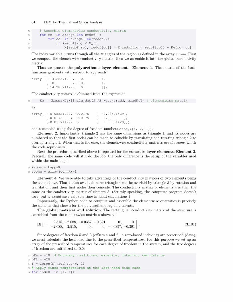
64 FEM for Thermal and Stress Analysis

58 # Assemble elementwise conductivity matrix59 for ro in arange(len(zedof)):60 for co in arange(len(zedof)):61 if (zedof[ro] < N_f):62 K[zedof[ro], zedof[co]] = K[zedof[ro], zedof[co]] + Ke[ro, co]

The index variable j runs through all the triangles of the region as defined in the array zconn. Firstwe compute the elementwise conductivity matrix, then we assemble it into the global conductivitymatrix.

Thus we process the polyurethane layer elements: Element 1. The matrix of the basisfunctions gradients with respect to x, y reads

array([[-14.28571429, 10. ],[ 0. , -10. ],[ 14.28571429, 0. ]])

The conductivity matrix is obtained from the expression

55 Ke = (kappa*Dz*linalg.det(J)/2)*dot(gradN, gradN.T) # elementwise matrix

as

array([[ 0.05321429, -0.0175 , -0.03571429],[-0.0175 , 0.0175 , 0. ],[-0.03571429, 0. , 0.03571429]])

and assembled using the degree of freedom numbers array([4, 2, 1]).Element 2: Importantly, triangle 2 has the same dimensions as triangle 1, and its nodes are

numbered so that the first nodes can be made to coincide by translating and rotating triangle 2 tooverlap triangle 1. When that is the case, the elementwise conductivity matrices are the same, whichthe code reproduces.

Next the procedure described above is repeated for the concrete layer elements: Element 3.Precisely the same code will still do the job, the only difference is the setup of the variables usedwithin the main loop:

65 kappa = kappaR66 zconn = array(connR)-1

Element 4: We were able to take advantage of the conductivity matrices of two elements beingthe same above. That is also available here: triangle 4 can be overlaid by triangle 3 by rotation andtranslation, and their first nodes then coincide. The conductivity matrix of elements 4 is then thesame as the conductivity matrix of element 3. (Strictly speaking, the computer program doesn’tcare, but it would save valuable time in hand calculations.)

Importantly, the Python code to compute and assemble the elementwise quantities is preciselythe same as that shown for the polyurethane region elements.

The global matrices and solution: The rectangular conductivity matrix of the structure isassembled from the elementwise matrices above as

[K] =

[2.515, −2.088, −0.0357, −0.391, 0., 0.

−2.088, 2.515, 0., 0., −0.0357, −0.391

]. (3.101)

Since degrees of freedom 5 and 3 (offsets 4 and 2, in zero-based indexing) are prescribed (data),we must calculate the heat load due to the prescribed temperatures. For this purpose we set up anarray of the prescribed temperatures for each degree of freedom in the system, and the free degreesof freedom are initialized to 0.0:

32 pTe = -10 # Boundary conditions, exterior, interior, deg Celsius33 pTi = +2034 T = zeros(N).reshape(N, 1)35 # Apply fixed temperatures at the left-hand side face36 for index in [1, 4]:

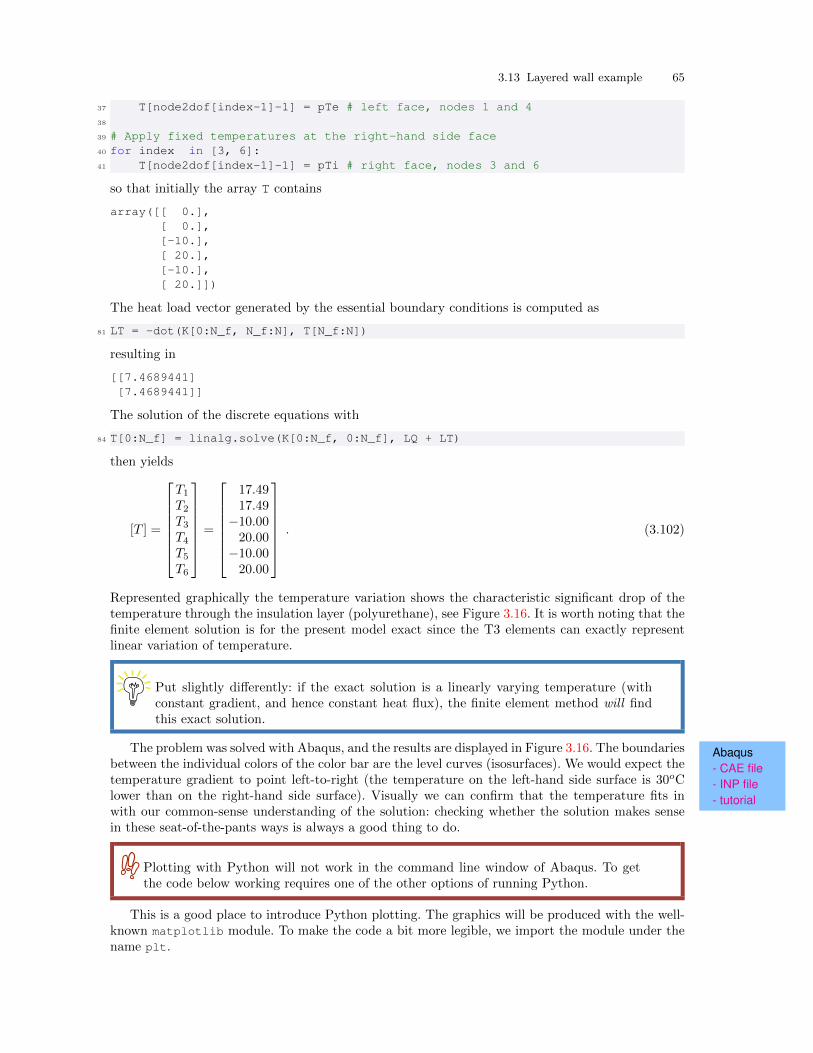
3.13 Layered wall example 65

37 T[node2dof[index-1]-1] = pTe # left face, nodes 1 and 438

39 # Apply fixed temperatures at the right-hand side face40 for index in [3, 6]:41 T[node2dof[index-1]-1] = pTi # right face, nodes 3 and 6

so that initially the array T contains

array([[ 0.],[ 0.],[-10.],[ 20.],[-10.],[ 20.]])

The heat load vector generated by the essential boundary conditions is computed as

81 LT = -dot(K[0:N_f, N_f:N], T[N_f:N])

resulting in

[[7.4689441][7.4689441]]

The solution of the discrete equations with

84 T[0:N_f] = linalg.solve(K[0:N_f, 0:N_f], LQ + LT)

then yields

[T ] =

T1T2T3T4T5T6

=

17.4917.49

−10.0020.00

−10.0020.00

. (3.102)

Represented graphically the temperature variation shows the characteristic significant drop of thetemperature through the insulation layer (polyurethane), see Figure 3.16. It is worth noting that thefinite element solution is for the present model exact since the T3 elements can exactly representlinear variation of temperature.

Put slightly differently: if the exact solution is a linearly varying temperature (withconstant gradient, and hence constant heat flux), the finite element method will findthis exact solution.

Abaqus- CAE file- INP file- tutorial

The problem was solved with Abaqus, and the results are displayed in Figure 3.16. The boundariesbetween the individual colors of the color bar are the level curves (isosurfaces). We would expect thetemperature gradient to point left-to-right (the temperature on the left-hand side surface is 30oClower than on the right-hand side surface). Visually we can confirm that the temperature fits inwith our common-sense understanding of the solution: checking whether the solution makes sensein these seat-of-the-pants ways is always a good thing to do.

Plotting with Python will not work in the command line window of Abaqus. To getthe code below working requires one of the other options of running Python.

This is a good place to introduce Python plotting. The graphics will be produced with the well-known matplotlib module. To make the code a bit more legible, we import the module under thename plt.

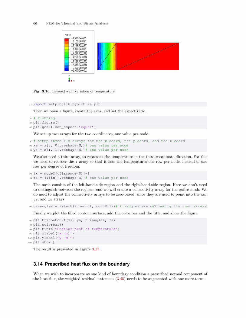
66 FEM for Thermal and Stress Analysis

NT11

−1.000e+01−7.500e+00−5.000e+00−2.500e+00+0.000e+00+2.500e+00+5.000e+00+7.500e+00+1.000e+01+1.250e+01+1.500e+01+1.750e+01+2.000e+01

X

Y

Z

Fig. 3.16. Layered wall: variation of temperature

16 import matplotlib.pyplot as plt

Then we open a figure, create the axes, and set the aspect ratio.

87 # Plotting88 plt.figure()89 plt.gca().set_aspect(’equal’)

We set up two arrays for the two coordinates, one value per node.

90 # setup three 1-d arrays for the x-coord, the y-coord, and the z-coord91 xs = x[:, 0].reshape(N,)# one value per node92 ys = x[:, 1].reshape(N,)# one value per node

We also need a third array, to represent the temperature in the third coordinate direction. For thiswe need to reorder the T array so that it lists the temperatures one row per node, instead of onerow per degree of freedom.

93 ix = node2dof[arange(N)]-194 zs = (T[ix]).reshape(N,)# one value per node

The mesh consists of the left-hand-side region and the right-hand-side region. Here we don’t needto distinguish between the regions, and we will create a connectivity array for the entire mesh. Wedo need to adjust the connectivity arrays to be zero-based, since they are used to point into the xs,ys, and zs arrays.

95 triangles = vstack((connL-1, connR-1))# triangles are defined by the conn arrays

Finally we plot the filled contour surface, add the color bar and the title, and show the figure.

96 plt.tricontourf(xs, ys, triangles, zs)97 plt.colorbar()98 plt.title(’Contour plot of temperature’)99 plt.xlabel(’x (m)’)

100 plt.ylabel(’y (m)’)101 plt.show()

The result is presented in Figure 3.17.

3.14 Prescribed heat flux on the boundary

When we wish to incorporate as one kind of boundary condition a prescribed normal component ofthe heat flux, the weighted residual statement (3.45) needs to be augmented with one more term:

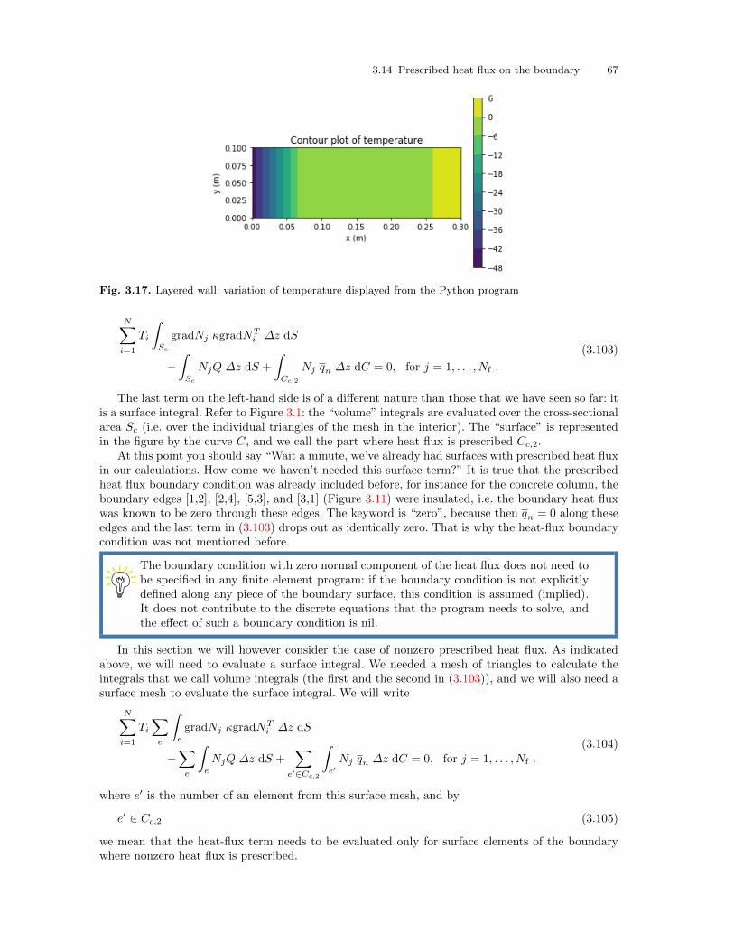
3.14 Prescribed heat flux on the boundary 67

Fig. 3.17. Layered wall: variation of temperature displayed from the Python program

N∑i=1

Ti

∫Sc

gradNj κgradNTi ∆z dS

−∫Sc

NjQ ∆z dS +

∫Cc,2

Nj qn ∆z dC = 0, for j = 1, . . . , Nf .

(3.103)

The last term on the left-hand side is of a different nature than those that we have seen so far: itis a surface integral. Refer to Figure 3.1: the “volume” integrals are evaluated over the cross-sectionalarea Sc (i.e. over the individual triangles of the mesh in the interior). The “surface” is representedin the figure by the curve C, and we call the part where heat flux is prescribed Cc,2.

At this point you should say “Wait a minute, we’ve already had surfaces with prescribed heat fluxin our calculations. How come we haven’t needed this surface term?” It is true that the prescribedheat flux boundary condition was already included before, for instance for the concrete column, theboundary edges [1,2], [2,4], [5,3], and [3,1] (Figure 3.11) were insulated, i.e. the boundary heat fluxwas known to be zero through these edges. The keyword is “zero”, because then qn = 0 along theseedges and the last term in (3.103) drops out as identically zero. That is why the heat-flux boundarycondition was not mentioned before.

The boundary condition with zero normal component of the heat flux does not need tobe specified in any finite element program: if the boundary condition is not explicitlydefined along any piece of the boundary surface, this condition is assumed (implied).It does not contribute to the discrete equations that the program needs to solve, andthe effect of such a boundary condition is nil.

In this section we will however consider the case of nonzero prescribed heat flux. As indicatedabove, we will need to evaluate a surface integral. We needed a mesh of triangles to calculate theintegrals that we call volume integrals (the first and the second in (3.103)), and we will also need asurface mesh to evaluate the surface integral. We will write

N∑i=1

Ti∑e

∫e

gradNj κgradNTi ∆z dS

−∑e

∫e

NjQ ∆z dS +∑

e′∈Cc,2

∫e′Nj qn ∆z dC = 0, for j = 1, . . . , Nf .

(3.104)

where e′ is the number of an element from this surface mesh, and by

e′ ∈ Cc,2 (3.105)

we mean that the heat-flux term needs to be evaluated only for surface elements of the boundarywhere nonzero heat flux is prescribed.

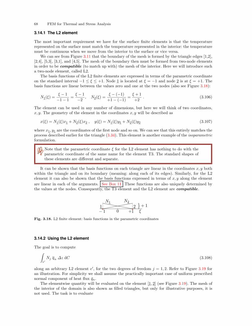
68 FEM for Thermal and Stress Analysis

3.14.1 The L2 element

The most important requirement we have for the surface finite elements is that the temperaturerepresented on the surface must match the temperature represented in the interior: the temperaturemust be continuous when we move from the interior to the surface or vice versa.

We can see from Figure 3.11 that the boundary of the mesh is formed by the triangle edges [1,2],[2,4], [5,3], [3,1], and [4,5]. The mesh of the boundary then must be formed from two-node elementsin order to be compatible (to match up with) the mesh of the interior. Here we will introduce sucha two-node element, called L2.

The basis functions of the L2 finite elements are expressed in terms of the parametric coordinateon the standard interval −1 ≤ ξ ≤ +1. Node 1 is located at ξ = −1 and node 2 is at ξ = +1. Thebasis functions are linear between the values zero and one at the two nodes (also see Figure 3.18):

N1(ξ) =ξ − 1

−1− 1=ξ − 1

−2, N2(ξ) =

ξ − (−1)

+1− (−1)=ξ + 1

+2. (3.106)

The element can be used in any number of dimensions, but here we will think of two coordinates,x, y. The geometry of the element in the coordinates x, y will be described as

x(ξ) = N1(ξ)x1 +N2(ξ)x2 , y(ξ) = N1(ξ)y1 +N2(ξ)y2 (3.107)

where x1, y1 are the coordinates of the first node and so on. We can see that this entirely matches theprocess described earlier for the triangle (3.34). This element is another example of the isoparametricformulation.

Note that the parametric coordinate ξ for the L2 element has nothing to do with theparametric coordinate of the same name for the element T3. The standard shapes ofthese elements are different and separate.

It can be shown that the basis functions on each triangle are linear in the coordinates x, y bothwithin the triangle and on its boundary (meaning: along each of its edges). Similarly, for the L2element it can also be shown that the basis functions expressed in terms of x, y along the element

are linear in each of the arguments. See Box 11 These functions are also uniquely determined bythe values at the nodes. Consequently, the T3 element and the L2 element are compatible .

Fig. 3.18. L2 finite element: basis functions in the parametric coordinates

3.14.2 Using the L2 element

The goal is to compute∫e′Nj qn ∆z dC (3.108)

along an arbitrary L2 element e′, for the two degrees of freedom j = 1, 2. Refer to Figure 3.19 foran illustration. For simplicity we shall assume the practically important case of uniform prescribednormal component of heat flux qn.

The elementwise quantity will be evaluated on the element [1, 2] (see Figure 3.19). The mesh ofthe interior of the domain is also shown as filled triangles, but only for illustrative purposes, it isnot used. The task is to evaluate

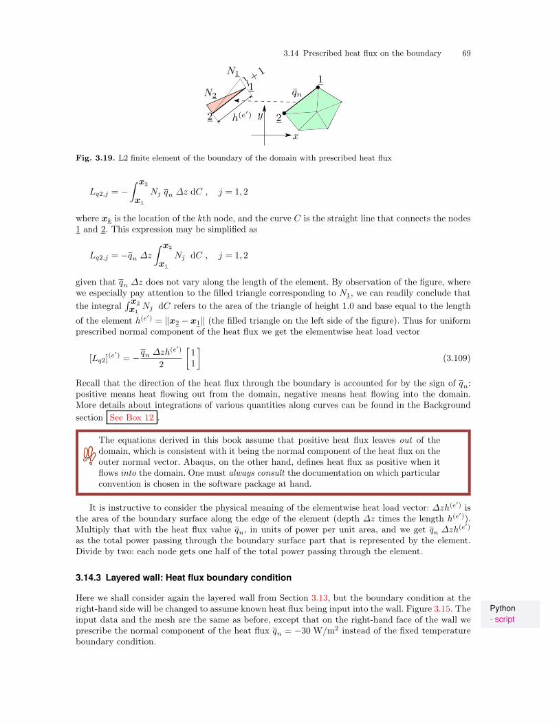
3.14 Prescribed heat flux on the boundary 69

Fig. 3.19. L2 finite element of the boundary of the domain with prescribed heat flux

Lq2,j = −∫ x2

x1

Nj qn ∆z dC , j = 1, 2

where xk is the location of the kth node, and the curve C is the straight line that connects the nodes1 and 2. This expression may be simplified as

Lq2,j = −qn ∆z∫ x2

x1

Nj dC , j = 1, 2

given that qn ∆z does not vary along the length of the element. By observation of the figure, wherewe especially pay attention to the filled triangle corresponding to N1, we can readily conclude that

the integral∫x2

x1Nj dC refers to the area of the triangle of height 1.0 and base equal to the length

of the element h(e′) = ∥x2 − x1∥ (the filled triangle on the left side of the figure). Thus for uniform

prescribed normal component of the heat flux we get the elementwise heat load vector

[Lq2](e′) = −qn ∆zh

(e′)

2

[11

](3.109)

Recall that the direction of the heat flux through the boundary is accounted for by the sign of qn:positive means heat flowing out from the domain, negative means heat flowing into the domain.More details about integrations of various quantities along curves can be found in the Background

section See Box 12 .

The equations derived in this book assume that positive heat flux leaves out of thedomain, which is consistent with it being the normal component of the heat flux on theouter normal vector. Abaqus, on the other hand, defines heat flux as positive when itflows into the domain. One must always consult the documentation on which particularconvention is chosen in the software package at hand.

It is instructive to consider the physical meaning of the elementwise heat load vector: ∆zh(e′) is

the area of the boundary surface along the edge of the element (depth ∆z times the length h(e′)).

Multiply that with the heat flux value qn, in units of power per unit area, and we get qn ∆zh(e′)

as the total power passing through the boundary surface part that is represented by the element.Divide by two: each node gets one half of the total power passing through the element.

3.14.3 Layered wall: Heat flux boundary condition

Here we shall consider again the layered wall from Section 3.13, but the boundary condition at thePython- script

right-hand side will be changed to assume known heat flux being input into the wall. Figure 3.15. Theinput data and the mesh are the same as before, except that on the right-hand face of the wall weprescribe the normal component of the heat flux qn = −30 W/m2 instead of the fixed temperatureboundary condition.

70 FEM for Thermal and Stress Analysis

In the convention of our model negative value means the heat flux enters into thedomain (the component on the outer normal is negative because the heat flux pointsopposite the normal); in Abaqus a negative value of the heat flux means the heat fluxleaves the domain.

Importantly, we have to renumber the degrees of freedom, since now the degrees of freedom atthe nodes 3 and 6 are also unknown. So in addition to the unknowns T1, T2 at nodes 2, 5, we alsoinclude unknowns T3, T4 at nodes 3 and 6. The fixed degrees of freedom are T5 = −10◦C at node 1,and T6 = −10◦C at node 4. We define (page 95)

25 N = 6 # total number of nodes26 N_f = 4 # total number of free degrees of freedom27 # Mapping from nodes to degrees of freedom28 node2dof = array([5, 1, 3, 6, 2, 4])

The elementwise conductivity matrices of the four elements are precisely the same as for theprevious example. They just need to be reassembled into a new overall conductivity matrix (fourrows this time). The same code that computed the conductivity matrix above still works and yields

[K] =

2.515, −2.088, −0.391, 0., −0.0357, 0.

−2.088, 2.515, 0., −0.391, 0., −0.0357−0.391, 0., 2.461, −2.07, 0., 0.

0., −0.391, −2.07, 2.461, 0., 0.

(3.110)

For the heat load vector contribution from the prescribed heat flux we need a surface mesh. Inthe present example the surface mesh consists of a single L2 element, connecting the nodes [3, 6].We define

34 # Connectivity of the boundary L2 element on the right35 connRbdry = array([[3, 6]])

The elementwise heat load vector due to the prescribed heat flux follows from (3.109)

[Lq2](e′) = −qn ∆zh

(e′)

2

[11

]= −−30× 1.0× 0.1

2

[11

]= 1.5

[11

](3.111)

to be assembled to degrees of freedom 3 and 4 (at the nodes 3 and 6). The code to compute theelementwise heat load vector due to the prescribed heat flux reads (page 95)

79 qnbar = qnbarR80 zconn = connRbdry - 181 for j in arange(zconn.shape[0]):82 he = linalg.norm(diff(x[zconn[j, :], :], axis=0))83 # Element degree-of-freedom array, converted to zero base84 zedof = array(node2dof[zconn[j, :]])-185 Leq = -qnbar*he*Dz/2*array([[1], [1]])

The first two lines again define variables used inside the loop. The loop itself is generic: it will workwith any number of boundary finite elements with any numbering.

Here the diff function computes the difference of the locations of the two endpoints of theelement (row-wise difference, note the axis=0): we have x[zconn[j, :], :],

array([[ 0.3, 0. ],[ 0.3, 0.1]])

and therefore diff(x[zconn[j, :], :], axis=0) computes

array([[ 0. , 0.1]])

and linalg.norm evaluates the norm (Euclidean length) of this vector as 0.1.The elementwise load vector due to the applied heat flux is assembled in standard way as (page

95)

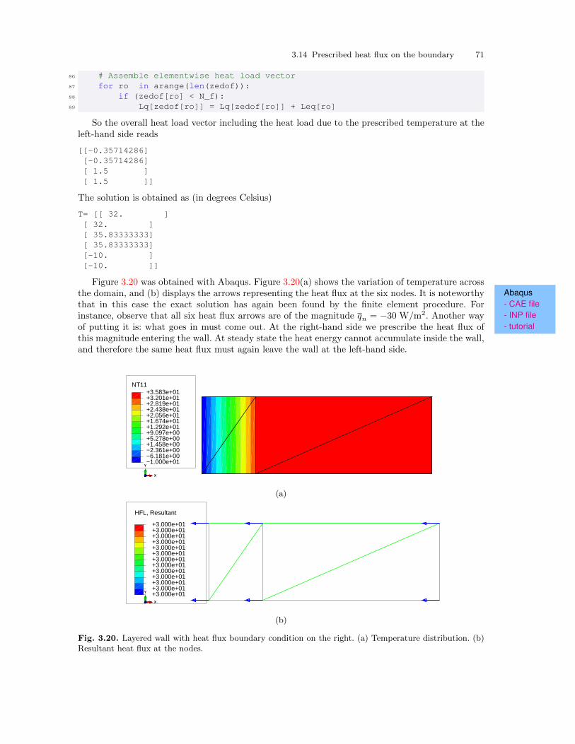
3.14 Prescribed heat flux on the boundary 71

86 # Assemble elementwise heat load vector87 for ro in arange(len(zedof)):88 if (zedof[ro] < N_f):89 Lq[zedof[ro]] = Lq[zedof[ro]] + Leq[ro]

So the overall heat load vector including the heat load due to the prescribed temperature at theleft-hand side reads

[[-0.35714286][-0.35714286][ 1.5 ][ 1.5 ]]

The solution is obtained as (in degrees Celsius)

T= [[ 32. ][ 32. ][ 35.83333333][ 35.83333333][-10. ][-10. ]]

Figure 3.20 was obtained with Abaqus. Figure 3.20(a) shows the variation of temperature acrossAbaqus- CAE file- INP file- tutorial

the domain, and (b) displays the arrows representing the heat flux at the six nodes. It is noteworthythat in this case the exact solution has again been found by the finite element procedure. Forinstance, observe that all six heat flux arrows are of the magnitude qn = −30 W/m2. Another wayof putting it is: what goes in must come out. At the right-hand side we prescribe the heat flux ofthis magnitude entering the wall. At steady state the heat energy cannot accumulate inside the wall,and therefore the same heat flux must again leave the wall at the left-hand side.

NT11

−1.000e+01−6.181e+00−2.361e+00+1.458e+00+5.278e+00+9.097e+00+1.292e+01+1.674e+01+2.056e+01+2.438e+01+2.819e+01+3.201e+01+3.583e+01

X

Y

Z

(a)

HFL, Resultant

+3.000e+01+3.000e+01+3.000e+01+3.000e+01+3.000e+01+3.000e+01+3.000e+01+3.000e+01+3.000e+01+3.000e+01+3.000e+01+3.000e+01+3.000e+01

X

Y

Z

(b)

Fig. 3.20. Layered wall with heat flux boundary condition on the right. (a) Temperature distribution. (b)Resultant heat flux at the nodes.

72 FEM for Thermal and Stress Analysis

3.14.4 Layered wall: Heat flux boundary conditions only

Here we shall consider again the layered wall from Section 3.13, but the boundary condition on bothPython- script

sides will be changed to assume known heat flux. The heat flux will be assumed to go in at theright-hand side of the wall and to come out at the left-hand side. The input data and the meshare the same as before (Figure 3.15), except that on the right-hand face of the wall we prescribethe normal component of the heat flux qn = −30 W/m2 instead of the fixed temperature boundarycondition, and on the left-hand side of the wall we prescribe the normal component of the heat fluxqn = +30 W/m2 (take note of the changed sign).

All nodes now have unknown degrees of freedom, and we take unknowns T1, T2 at nodes 2, 5,unknowns T3, T4 at nodes 3 and 6, unknowns T5, T6 at nodes 4 and 1 (page 97).

24 N = 6 # total number of nodes25 N_f = 6 # total number of free degrees of freedom26 # Mapping from nodes to degrees of freedom27 node2dof=array([6, 1, 3, 5, 2, 4])

As in the previous section, the elementwise conductivity matrices of the four elements do notneed to be recalculated. They just need to be reassembled into a new overall 6 × 6 conductivitymatrix:

[K] =

2.515, −2.087, −0.3913, 0, 0, −0.03571

−2.087, 2.515, 0, −0.3913, −0.03571, 0−0.3913, 0, 2.461, −2.07, 0, 0

0, −0.3913, −2.07, 2.461, 0, 00, −0.03571, 0, 0, 0.05321, −0.0175

−0.03571, 0, 0, 0, −0.0175, 0.05321

(3.112)

The global heat load vector is assembled from the heat-flux contributions from the two surfaceelements: In the present example the surface mesh consists of two L2 elements, the first on theright-hand side surface, connecting the nodes [3, 6] (degrees of freedom [3,4]), and the second on theleft-hand side surface, connecting nodes [4, 1] (degrees of freedom [5,6]). The global heat load vectorthen reads

[L] =

00

1.51.5

−1.5−1.5

(3.113)

We can clearly appreciate that each degree of freedom at the boundary node gets half of the powerpassing through the surface.

The solution in Python is produced as

Tg= [[ -3.17647059][ -3.17647059][ 0.65686275][ 0.65686275][-45.17647059][-45.17647059]]

which means temperatures at the nodes (1, 2, ..., 6) are -45.17647059, -3.17647059, 0.65686275, -45.17647059, -3.17647059, 0.65686275.

The solution was also calculated with Abaqus, with the results shown in Figure 3.21. This timeAbaqus- CAE file- INP file- tutorial

the calculated temperatures at the nodes do not match our solution. The temperatures at the nodes(1, 2, ..., 6) are reported as -42, 0, 3.83, -42, 0, 3.83.

To locate the source of this discrepancy, we must pay attention to the properties of the resultingsystem of algebraic equations. In fact, Abaqus complained about the system conductivity matrix: inthe file with the extension .msg we find

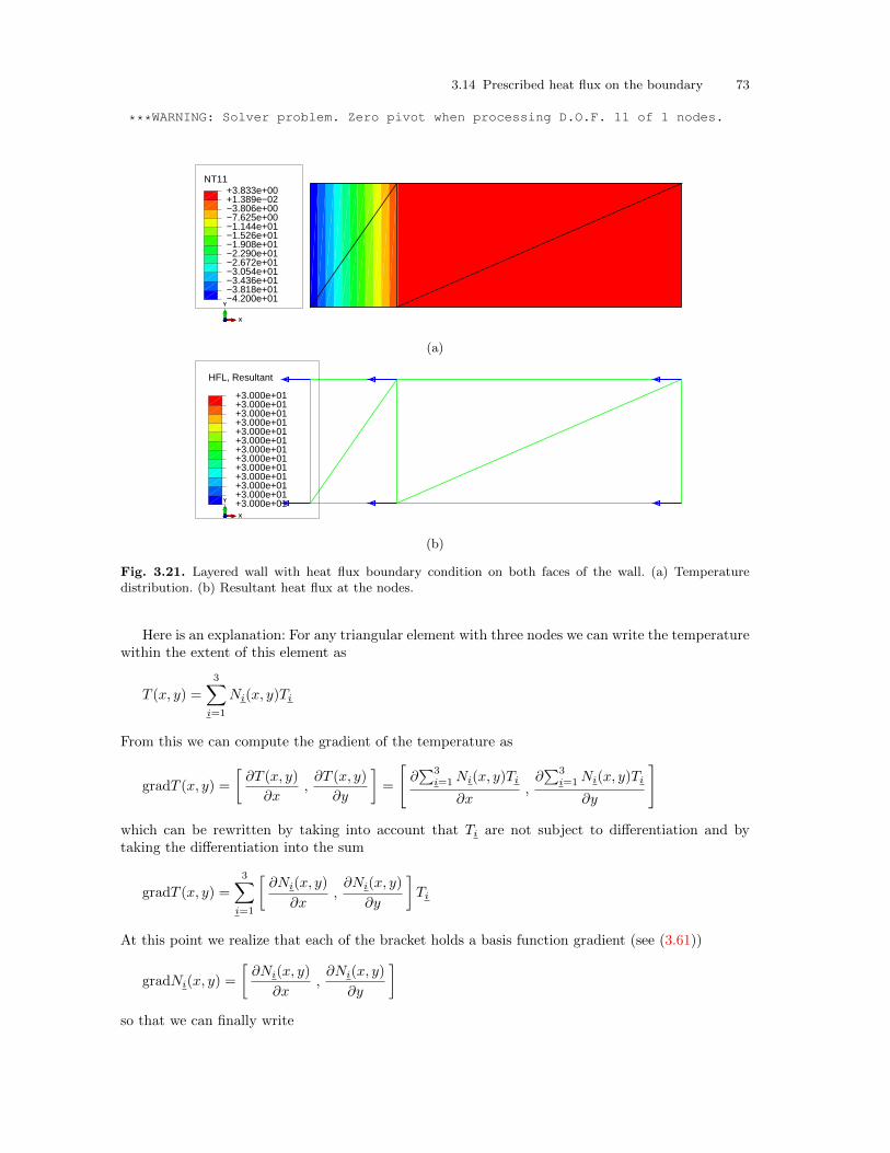
3.14 Prescribed heat flux on the boundary 73

***WARNING: Solver problem. Zero pivot when processing D.O.F. 11 of 1 nodes.

NT11

−4.200e+01−3.818e+01−3.436e+01−3.054e+01−2.672e+01−2.290e+01−1.908e+01−1.526e+01−1.144e+01−7.625e+00−3.806e+00+1.389e−02+3.833e+00

X

Y

Z

(a)

HFL, Resultant

+3.000e+01+3.000e+01+3.000e+01+3.000e+01+3.000e+01+3.000e+01+3.000e+01+3.000e+01+3.000e+01+3.000e+01+3.000e+01+3.000e+01+3.000e+01

X

Y

Z

(b)

Fig. 3.21. Layered wall with heat flux boundary condition on both faces of the wall. (a) Temperaturedistribution. (b) Resultant heat flux at the nodes.

Here is an explanation: For any triangular element with three nodes we can write the temperaturewithin the extent of this element as

T (x, y) =

3∑i=1

Ni(x, y)Ti

From this we can compute the gradient of the temperature as

gradT (x, y) =

[∂T (x, y)

∂x,∂T (x, y)

∂y

]=

[∂∑3

i=1Ni(x, y)Ti

∂x,∂∑3

i=1Ni(x, y)Ti

∂y

]

which can be rewritten by taking into account that Ti are not subject to differentiation and bytaking the differentiation into the sum

gradT (x, y) =

3∑i=1

[∂Ni(x, y)

∂x,∂Ni(x, y)

∂y

]Ti

At this point we realize that each of the bracket holds a basis function gradient (see (3.61))

gradNi(x, y) =

[∂Ni(x, y)

∂x,∂Ni(x, y)

∂y

]so that we can finally write

74 FEM for Thermal and Stress Analysis

gradT (x, y) =

3∑i=1

gradNi(x, y)Ti =

3∑i=1

Ti gradNi(x, y)

This can be also written as a handy matrix expression

gradT (x, y) =[T1, T2, T3

] [gradN1(x, y)]

[gradN2(x, y)]

[gradN3(x, y)]

or, even more succinctly

gradT (x, y) = [T (e)]T[gradN (e)(x, y)

]where [T (e)] is the vector of the three nodal temperatures, and

[gradN (e)(x, y)

]is the matrix of the

gradients of the three basis functions of the triangle (3.61). Now we recall the conductivity matrixfor the single-element mesh (3.71) and we write the product of the elementwise conductivity matrixand the elementwise vector of temperatures

[K(e)][T (e)] =((det[J ]/2)[gradN ] κ[gradN ]T ∆z

)[T (e)] (3.114)

Reshuffling results in

[K(e)][T (e)] = ∆z(det[J ]/2)[gradN ] κ([gradN ]T [T (e)]

)and we realize

[gradN ]T [T (e)] = (gradT )T

so that the above may be rewritten

[K(e)][T (e)] = ∆z(det[J ]/2)[gradN ] κ(gradT )T (3.115)

Now, if all the nodal temperatures are the same, T1 = T2 = T3, the gradient of the temperatureis identically zero, gradT = [0, 0], and we have

[K(e)][T (e)] = ∆z(det[J ]/2)[gradN ] κ

[00

]=

000

(3.116)

The elementwise conductivity matrix produces zero output when all the nodes havethe same temperature.

Equation (3.116) is stating that the vector [T (e)] is a solution of a system of linear algebraic equationswhere the right-hand side consists of zeros. Such a matrix [K(e)] is singular.

The elementwise conductivity matrix will always have rank of (n− 1) where n is thenumber of nodes of the element. That is, it will be singular . This is true not only forthe three node triangle, but for any finite element applied to heat conduction.

So now we take the vector of the temperatures at the nodes to consist of the same numbers in eachentry, for simplicity we pick 1.0

3.14 Prescribed heat flux on the boundary 75T(e)1

T(e)2

T(e)3

=

1.01.01.0

(3.117)

Then the product of the elementwise conductivity matrix and the vector of temperatures will giveK(e)11 , K

(e)12 , K

(e)13

K(e)21 , K

(e)22 , K

(e)23

K(e)31 , K

(e)32 , K

(e)33

T

(e)1

T(e)2

T(e)3

=

K(e)11 , K

(e)12 , K

(e)13

K(e)21 , K

(e)22 , K

(e)23

K(e)31 , K

(e)32 , K

(e)33

111

=

K(e)11 +K

(e)12 +K

(e)13

K(e)21 +K

(e)22 +K

(e)23

K(e)31 +K

(e)32 +K

(e)33

=

000

(3.118)

In words, the values of the entries in each row of the elementwise conductivity matrix sum to zero!Now comes the crucial observation: if we take any number of finite elements and assemble theirentire elementwise conductivity matrices into the global matrix, the entries in each row of the globalconductivity matrix will also sum to zero. That means that the global conductivity matrix will alsobe singular. And that is why we are having trouble inverting it. The software does its best, probablyby setting some entry of the solution to some arbitrary number.

If we take as the solution the numbers reported by Python and add +3.17647059, we will obtainthe solution reported by Abaqus. Both of those solutions satisfy all the conditions (in particular theboundary conditions), and so since both of them are solutions, we must conclude that the solution isnot unique. We can arbitrarily add some constant temperature and get another solution. The heatflux in the solution will not feel this added constant value of temperature, because as we pointed outearlier, constant temperature produces zero gradient of temperature and therefore zero heat flux.

This argument can be firmed up with just a few equations. We know that for a given element wecan write the balance equation as

[K(e)][T (e)] = [L(e)] (3.119)

where [L(e)] is a vector of heat loads at the nodes. At the same time, we know that the conductivity

matrix of the element is singular and therefore there is some nonzero vector of temperatures [T (e)]that follows as solution to the system of equations

[K(e)][T (e)] = [0] (3.120)

with a zero heat load vector on the right-hand side. In fact, the solution is an arbitrary multiple ofthe vector [T (e)]

[K(e)][αT (e)] = [0] (3.121)

where α = 0. Adding together the left-hand sides and the right-hand sides of equations (3.119)and (3.121) yields

[K(e)][T (e)] + [K(e)][αT (e)] = [L(e)] + [0] . (3.122)

As a result we have

[K(e)]([T (e)] + α[T (e)]

)= [L(e)] (3.123)

which states that since the conductivity matrix of the element is singular, the solution to its balanceequation for an arbitrary load vector [L(e)] is not unique: it is [T (e)] plus an arbitrary multiple of

the eigenvector corresponding to the zero eigenvalue [T (e)].

76 FEM for Thermal and Stress Analysis

Heat conduction problems where all the boundary conditions are only of the heat-fluxkind do not have unique solutions. The global conductivity matrix is singular.

In fact, it is possible that when the conductivity matrix is singular, there is no solution. In orderto understand this, think of it this way: imagine that for the wall we would require for the heatflux to go in on either side of the wall. Would a steady-state solution be possible then? The answermust be no: it is not possible for heat to be continuously pumped into the wall without the totalcontent of heat energy inside the wall continually increasing, and hence the temperature changingas a result. (There is no heat sink inside the wall to swallow that added heat.) The applied heatfluxes along the boundary must balance, what goes in must come out.

Unless the heat fluxes balance (possibly with sources of heat and heat sinks), thesolution to a problem with heat-flux boundary conditions only will not exist.

If we change both boundary conditions in Abaqus to list the normal heat flux as the same number(either +30 or -30), the solver will report an error and the solution will fail.

Job Job-1: Abaqus/Standard aborted due to errors.Error in job Job-1: Abaqus/Standard Analysis exited with an error - Pleasesee the message file for possible error messages if the file exists.

For these loads the solution could not be found (it does not exist!).

3.15 Concrete column with film boundary condition

In Section 3.14 the weighted residual statement to use in formulating a finite element model incor-porated both a volume integral (for the conductivity matrix and the heat source loading) and asurface integral (for the flux boundary condition). In order to incorporate the third kind of bound-ary condition, the convection boundary condition (or the “surface film” boundary condition, as it iscalled in Abaqus), we need to include one more surface integral. (For the derivation please consult

the Background material. See Box 7 ) Equation (3.104) is augmented to read

N∑i=1

Ti∑e

∫e

gradNj κgradNTi ∆z dS

−∑e

∫e

NjQ ∆z dS +∑

e′∈Cc,2

∫e′Nj qn ∆z dC

−∑

e′∈Cc,3

∫e′Nj hTa ∆z dC

+

N∑i=1

Ti∑

e′∈Cc,3

∫e′Nj h Ni ∆z dC = 0, for j = 1, . . . , Nf .

(3.124)

Equation (3.124) is the most general form of the steady-state heat-conduction modelconsidered in this book. All the terms are included: conduction and internal heatgeneration rate in the volume, and prescribed temperatures, prescribed heat flux, andthe surface film condition on the boundary.

We shall assume for simplicity that along each element on the boundary the heat surface transfercoefficient h (the surface film coefficient), and the ambient temperature Ta are constant. This is

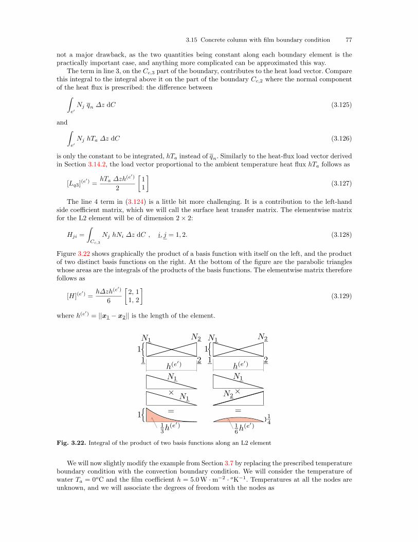
3.15 Concrete column with film boundary condition 77

not a major drawback, as the two quantities being constant along each boundary element is thepractically important case, and anything more complicated can be approximated this way.

The term in line 3, on the Cc,3 part of the boundary, contributes to the heat load vector. Comparethis integral to the integral above it on the part of the boundary Cc,2 where the normal componentof the heat flux is prescribed: the difference between∫

e′Nj qn ∆z dC (3.125)

and∫e′Nj hTa ∆z dC (3.126)

is only the constant to be integrated, hTa instead of qn. Similarly to the heat-flux load vector derivedin Section 3.14.2, the load vector proportional to the ambient temperature heat flux hTa follows as

[Lq3](e′) =

hTa ∆zh(e′)

2

[11

](3.127)

The line 4 term in (3.124) is a little bit more challenging. It is a contribution to the left-handside coefficient matrix, which we will call the surface heat transfer matrix. The elementwise matrixfor the L2 element will be of dimension 2× 2:

Hji =

∫Cc,3

Nj hNi ∆z dC , i, j = 1, 2. (3.128)

Figure 3.22 shows graphically the product of a basis function with itself on the left, and the productof two distinct basis functions on the right. At the bottom of the figure are the parabolic triangleswhose areas are the integrals of the products of the basis functions. The elementwise matrix thereforefollows as

[H](e′) =

h∆zh(e′)

6

[2, 11, 2

](3.129)

where h(e′) = ||x1 − x2|| is the length of the element.

Fig. 3.22. Integral of the product of two basis functions along an L2 element

We will now slightly modify the example from Section 3.7 by replacing the prescribed temperatureboundary condition with the convection boundary condition. We will consider the temperature ofwater Ta = 0oC and the film coefficient h = 5.0W ·m−2 · oK−1. Temperatures at all the nodes areunknown, and we will associate the degrees of freedom with the nodes as

78 FEM for Thermal and Stress Analysis

Node numbers 1 2 3 4 5DOF numbers 3 1 2 5 4

The total number of degrees of freedom is N = 5, and the number of free (unknown) degrees offreedom is Nf = 5.

In addition to the triangles in the interior of the domain, we also have to consider the boundarymesh: a single L2 element along the edge [4,5]. The elementwise conductivity matrices of the threetriangles are assembled fully into the global conductivity matrix (all degrees of freedom are free).Recall Section 3.14.4 — the global conductivity matrix will be singular. There it is, produced byprint(K):

Python- script

array([[ 4.56462e+00, -3.60000e+00, -2.41154e-01, 8.32667e-17, -7.23463e-01],[ -3.60000e+00, 4.56462e+00, -2.41154e-01, -7.23463e-01, 0.00000e+00],[ -2.41154e-01, -2.41154e-01, 4.82309e-01, 0.00000e+00, 0.00000e+00],[ 8.32667e-17, -7.23463e-01, 0.00000e+00, 1.38231e+00, -6.58846e-01],[ -7.23463e-01, 0.00000e+00, 0.00000e+00, -6.58846e-01, 1.38231e+00]])

As the sums of the rows and columns we don’t get precisely zeros, given the limited number of digits,but in double precision we get very small numbers indeed: the matrix is practically singular. Usingnumpy.sum(Kg, axis=1) (which means sum across the columns), we obtain

array([ -6.66133815e-16, -8.88178420e-16, 0.00000000e+00,1.11022302e-16, 0.00000000e+00])

However, we are not done yet, there remain the surface terms. There is no prescribed heat flux:the second term on the second line of (3.124) may be ignored. The term on the third line is also zero,since Ta is zero. The surface heat transfer matrix, however, needs to be computed and assembled(page 99). The L2 element on the boundary has connectivity

42 connbdry = array([[4, 5]])

With the definition of the zero-based connectivity

67 zconn = connbdry - 1

we can compute the length of the finite element as

69 he = linalg.norm(diff(x[zconn[j, :], :], axis=0))

This yields 1.2941. In terms of the local degrees of freedom, the surface heat transfer elementwisematrix for the L2 element [4,5] is computed as

72 He = h * Dz * he / 6 * array([[2, 1], [1, 2]])

The matrix reads

array([[ 2.15683, 1.07841],[ 1.07841, 2.15683]])

It will get assembled to the degrees of freedom 5 and 4 and therefore the assembled surface heattransfer matrix Hg (refer to the code below)

74 for ro in arange(len(zedof)):75 for co in arange(len(zedof)):76 if (zedof[ro] < N_f) and (zedof[co] < N_f):77 Hg[zedof[ro], zedof[co]] = Hg[zedof[ro], zedof[co]] + He[ro, co]

reads

array([[ 0. , 0. , 0. , 0. , 0. ],[ 0. , 0. , 0. , 0. , 0. ],[ 0. , 0. , 0. , 0. , 0. ],[ 0. , 0. , 0. , 2.15683, 1.07841],[ 0. , 0. , 0. , 1.07841, 2.15683]])

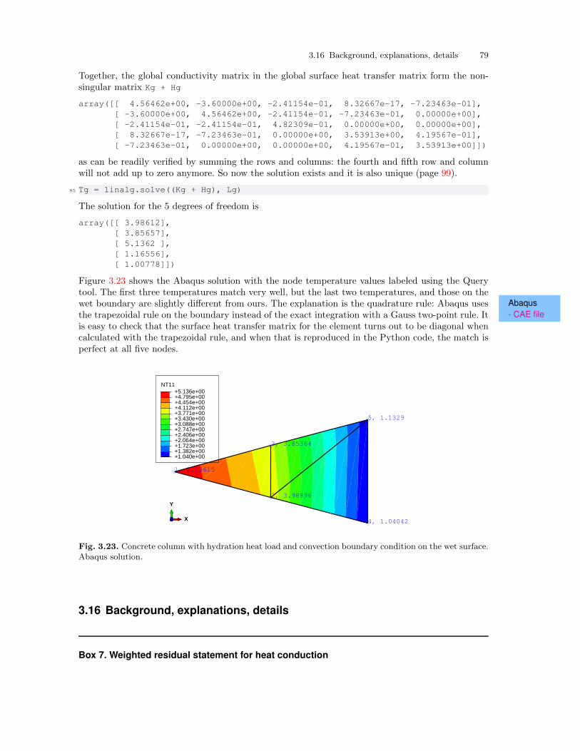
3.16 Background, explanations, details 79

Together, the global conductivity matrix in the global surface heat transfer matrix form the non-singular matrix Kg + Hg

array([[ 4.56462e+00, -3.60000e+00, -2.41154e-01, 8.32667e-17, -7.23463e-01],[ -3.60000e+00, 4.56462e+00, -2.41154e-01, -7.23463e-01, 0.00000e+00],[ -2.41154e-01, -2.41154e-01, 4.82309e-01, 0.00000e+00, 0.00000e+00],[ 8.32667e-17, -7.23463e-01, 0.00000e+00, 3.53913e+00, 4.19567e-01],[ -7.23463e-01, 0.00000e+00, 0.00000e+00, 4.19567e-01, 3.53913e+00]])

as can be readily verified by summing the rows and columns: the fourth and fifth row and columnwill not add up to zero anymore. So now the solution exists and it is also unique (page 99).

85 Tg = linalg.solve((Kg + Hg), Lg)

The solution for the 5 degrees of freedom is

array([[ 3.98612],[ 3.85657],[ 5.1362 ],[ 1.16556],[ 1.00778]])

Figure 3.23 shows the Abaqus solution with the node temperature values labeled using the Querytool. The first three temperatures match very well, but the last two temperatures, and those on the

Abaqus- CAE file

wet boundary are slightly different from ours. The explanation is the quadrature rule: Abaqus usesthe trapezoidal rule on the boundary instead of the exact integration with a Gauss two-point rule. Itis easy to check that the surface heat transfer matrix for the element turns out to be diagonal whencalculated with the trapezoidal rule, and when that is reproduced in the Python code, the match isperfect at all five nodes.

5, 1.1329

4, 1.04042

3, 3.85364

2, 3.98896

1, 5.13615

NT11

+1.040e+00+1.382e+00+1.723e+00+2.064e+00+2.406e+00+2.747e+00+3.088e+00+3.430e+00+3.771e+00+4.112e+00+4.454e+00+4.795e+00+5.136e+00

X

Y

Z

Fig. 3.23. Concrete column with hydration heat load and convection boundary condition on the wet surface.Abaqus solution.

3.16 Background, explanations, details

Box 7. Weighted residual statement for heat conduction

80 FEM for Thermal and Stress Analysis

The goal is to formulate an equation that will allow the finite element method to calculate anapproximate solution to the heat conduction boundary value problem (BVP). The PDE was derivedin Box 1 and the boundary conditions are discussed in Box 2.

The method chosen here is the weighted residual statement. The statement is derived in the formof an integral, so that the BVP is satisfied in an “average” sense.

In what follows, T is the so-called trial function, and ϑ is a weight function. The major steps are:satisfy the essential boundary conditions by designing the trial function, shift the derivatives in thebalance equation residual, and combine the balanced equation residual with the natural boundarycondition into one residual equation.

The essential boundary condition is satisfied by restricting possible trial functions to only thosethat conform to the essential boundary conditions a priori

T (x, t)− T (x, t) = 0, x on S1 , (3.130)

The next step equalizes the number of derivatives on the test and trial functions. The balanceequation (2.1) yields the balance residual as

rB = cV∂T

∂t− div

[κ(gradT )T

]−Q . (3.131)

so that the weighted balance residual reads∫V

ϑ(x)rB(x, t) dV =

∫V

ϑ

(cV∂T

∂t− div

[κ(gradT )T

]−Q

)dV . (3.132)

The first term (ϑcV∂T∂t ) and the third term (ϑQ) are kept without change, but in the second term

−ϑdiv[κ(gradT )T

]the test function ϑ multiplies an expression that contains the second derivatives of temperature (thediv[κ(gradT )T

]term). Balancing the order of differentiation by shifting one derivative from the

temperature to the test function ϑ will be beneficial: we will be able to use basis functions that needto be less smooth since the second derivatives would not need to be taken, and also we will be ableto satisfy the natural boundary conditions without having to include them as a separate residual(naturally!). As before, the price to pay is the need to place some restrictions on the test function.

For the moment, it will be convenient to work with the expression

−ϑ div[κ(gradT )T

]= ϑ divq ,

that is, we work with the flux variable q = −κ(gradT )T .The integration by parts in the case of a multidimensional integral is generalized in the divergence

theorem (2.18). We may anticipate that ϑ divq is the result of the chain rule applied to the vectorϑ q. That is indeed the case, as we have

div (ϑ q) = ϑ divq + (gradϑ) q , (3.133)

which is easily verified by working out the equality in components. Therefore, we may start byinspecting the integral∫

V

ϑ divq dV

where we substitute from (3.133)∫V

ϑ divq dV =

∫V

div (ϑ q) dV −∫V

(gradϑ) q dV . (3.134)

The divergence theorem may be applied to the first integral on the right to give the identity

3.16 Background, explanations, details 81∫V

ϑ divq dV =

∫S

ϑ q · n dS −∫V

(gradϑ) q dV . (3.135)

Since q · n is known on some parts of the boundary, but unknown on the others – see Eqs. (2.28)and (2.29), we will split the surface integral into one for each sub-surface,∫

V

ϑ divq dV =∫S1

ϑ q · n dS +

∫S2

ϑ q · n dS +

∫S3

ϑ q · n dS −∫V

(gradϑ) q dV . (3.136)

The integral over the part of the surface S1 is troublesome, because q ·n is unknown there. However,we have the option of making ϑ vanish along S1, making∫

S1

ϑ q · n dS = 0 ,

where the test function now must satisfy ϑ(x) = 0 for x ∈ S1. Now we switch back from q to−κ(gradT )T to obtain from (3.136)∫

V

ϑ divq dV = −∫V

ϑ div[κ(gradT )T

]dV =∫

S2

ϑ (q · n) dS +

∫S3

ϑ (q · n) dS +

∫V

(gradϑ) κ(gradT )T dV . (3.137)

The heat flux passing through the surface S2 is known: see the boundary condition (2.28). Therefore,if we attempt to satisfy this boundary condition in a weighted residual sense we write∫

S2

ϑ[qn − (q · n)

]dS = 0 (3.138)

where we test with the function ϑ because we anticipate a possible cancellation with a term in (3.137).Note that the underlined term is present with the opposite sign in (3.136). Similarly, on the boundarysurface S3 we might attempt to satisfy the boundary condition with a weighted residual equation∫

S3

ϑ[h(T − Ta)− (q · n)

]dS = 0 (3.139)

Finally we have all the pieces ready. We take as the weighted residual statement for the heat conduc-tion problem the weighted balance residual (3.132) to which we add the natural boundary conditionresiduals (3.138) and (3.139).∫

V

ϑ

(cV∂T

∂t− div

[κ(gradT )T

]−Q

)dV︸ ︷︷ ︸

(3.132)

+

∫S2

ϑ[qn − (q · n)

]dS︸ ︷︷ ︸

(3.138)

+

∫S3

ϑ[h(T − Ta)− (q · n)

]dS︸ ︷︷ ︸

(3.139)

= 0 . (3.140)

Expression (3.137) is introduced to replace the second volume term.∫V

ϑcV∂T

∂tdV +

∫V

(gradϑ) κ(gradT )T dV −∫V

ϑQ dV

+

∫S2

ϑ (q · n) dS +

∫S3

ϑ (q · n) dS

+

∫S2

ϑ[qn − (q · n)

]dS +

∫S3

ϑ[h(T − Ta)− (q · n)

]dS = 0,

where ϑ(x) = 0 for x ∈ S1 .

(3.141)

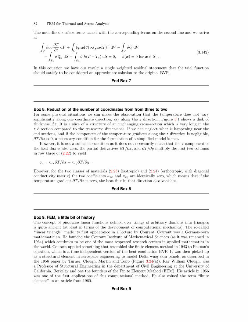
82 FEM for Thermal and Stress Analysis

The underlined surface terms cancel with the corresponding terms on the second line and we arriveat ∫

V

ϑcV∂T

∂tdV +

∫V

(gradϑ) κ(gradT )T dV −∫V

ϑQ dV

+

∫S2

ϑ qn dS +

∫S3

ϑ h(T − Ta) dS = 0, ϑ(x) = 0 for x ∈ S1 .(3.142)

In this equation we have our result: a single weighted residual statement that the trial functionshould satisfy to be considered an approximate solution to the original BVP.

End Box 7

Box 8. Reduction of the number of coordinates from from three to twoFor some physical situations we can make the observation that the temperature does not varysignificantly along one coordinate direction, say along the z direction. Figure 3.1 shows a disk ofthickness ∆z. It is a slice of a structure of an unchanging cross-section which is very long in thez direction compared to the transverse dimensions. If we can neglect what is happening near theend sections, and if the component of the temperature gradient along the z direction is negligible,∂T/∂z ≈ 0, a necessary condition for the formulation of a simplified model is met.

However, it is not a sufficient condition as it does not necessarily mean that the z component ofthe heat flux is also zero: the partial derivatives ∂T/∂x, and ∂T/∂y multiply the first two columnsin row three of (2.22) to yield

qz = κzx∂T/∂x+ κzy∂T/∂y .

However, for the two classes of materials (2.23) (isotropic) and (2.24) (orthotropic, with diagonalconductivity matrix) the two coefficients κzx and κzy are identically zero, which means that if thetemperature gradient ∂T/∂z is zero, the heat flux in that direction also vanishes.

End Box 8

Box 9. FEM, a little bit of historyThe concept of piecewise linear functions defined over tilings of arbitrary domains into trianglesis quite ancient (at least in terms of the development of computational mechanics). The so-called“linear triangle” made its first appearance in a lecture by Courant. Courant was a German-bornmathematician. He founded the Courant Institute of Mathematical Sciences (as it was renamed in1964) which continues to be one of the most respected research centers in applied mathematics inthe world. Courant applied something that resembled the finite element method in 1943 to Poisson’sequation, which is a time-independent version of the heat conduction BVP. It was then picked upas a structural element in aerospace engineering to model Delta wing skin panels, as described inthe 1956 paper by Turner, Clough, Martin and Topp (Figure 3.24(a)). Ray William Clough, wasa Professor of Structural Engineering in the department of Civil Engineering at the University ofCalifornia, Berkeley and one the founders of the Finite Element Method (FEM). His article in 1956was one of the first applications of this computational method. He also coined the term “finiteelement” in an article from 1960.

End Box 9

3.16 Background, explanations, details 83

Fig. 3.24. The famous 1956 paper by Turner, Clough, Martin and Topp

Box 10. Derivatives of the basis functionsTo evaluate the derivatives of the basis functions with respect to x and y we need the chain rule.Equations (3.28–3.30) define the functions over the standard triangle in terms of ξ and η. Therefore,to express ∂Ni/∂x we use the chain rule

∂Ni

∂x=∂Ni

∂ξ

∂ξ

∂x+∂Ni

∂η

∂η

∂x,

∂Ni

∂y=∂Ni

∂ξ

∂ξ

∂y+∂Ni

∂η

∂η

∂y.

For the purpose of this discussion, the function that is being differentiated does not really matter.We will replace it with a ♡, while we arrange the above equation into a matrix expression

[∂♡∂x

,∂♡∂y

]=

[∂♡∂ξ

,∂♡∂η

]∂ξ

∂x

∂ξ

∂y

∂η

∂x

∂η

∂y

=

[∂♡∂ξ

,∂♡∂η

] [J]. (3.143)

The derivatives are arranged in row matrices because these objects are gradients of the ♡ function[compare with (2.25)]. The row matrix[

∂♡∂ξ

,∂♡∂η

]is the gradient of the function ♡ with respect to the coordinates ξ, η and this is the gradient of thesame function with respect to coordinates x, y[

∂♡∂x

,∂♡∂y

].

The matrix

[J]=

∂ξ

∂x

∂ξ

∂y

∂η

∂x

∂η

∂y

, (3.144)

84 FEM for Thermal and Stress Analysis

is the Jacobian matrix of the mapping ξ = ξ(x, y), η = η(x, y), which is the inverse of the mapx = x(ξ, η), y = y(ξ, η) of Eq. (3.35). The question is how to evaluate the partial derivatives of thetype ∂ξ/∂x, since the inverse of the map (3.35) is not known (at least not in general).

Here is an idea: If we start the chain rule from the other end (switching the role of the variables),we obtain

[∂♡∂ξ

,∂♡∂η

]=

[∂♡∂x

,∂♡∂y

]∂x

∂ξ

∂x

∂η

∂y

∂ξ

∂y

∂η

, (3.145)

and inverting the Jacobian matrix[J]in equation (3.143) we get[

∂♡∂ξ

,∂♡∂η

]=

[∂♡∂x

,∂♡∂y

] [J]−1

. (3.146)

Comparing (3.145) and (3.146) yields

[J ] =

∂x

∂ξ

∂x

∂η

∂y

∂ξ

∂y

∂η

=[J]−1

, (3.147)

where [J ] is the Jacobian matrix of the map (3.35).Hence, the derivatives of the basis functions with respect to the coordinates x, y are evaluated

as [∂Ni(ξ, η)

∂x,∂Ni(ξ, η)

∂y

]=

[∂Ni(ξ, η)

∂ξ,∂Ni(ξ, η)

∂η

][J ]

−1. (3.148)

End Box 10

Box 11. Form of the basis functions for the T3 triangle and the L2 line elementTriangle T3: When we map the point from the standard triangle ξ, η to the point x, y using (3.34)or, explicitly, (3.35), we obtain a linear relationship between those two pairs of coordinates, x, yexpressed in terms of ξ, η. Therefore, inverting this relationship will result in a linear dependenceof ξ, η on x, y. Substituting ξ, η in the expressions for the basis functions (3.28–3.30) will expressthe basis functions as linear functions of x, y. This will make perfect sense, since a linear functionin x, y is uniquely determined by the values of three coefficients, and we have three nodes that eachdetermine the basis function through the Kronecker delta property (3.31).

Line L2: Expanding (3.107) in terms of the basis functions, we obtain

x(ξ) =x1 + x2

2+ ξ

x2 − x12

, y(ξ) =y1 + y2

2+ ξ

y2 − y12

(3.149)

This is clearly have linear relationship between each of x and y and ξ. The same reasoning as aboveleads us to conclude that the basis functions are in fact linear functions of x, y.

End Box 11

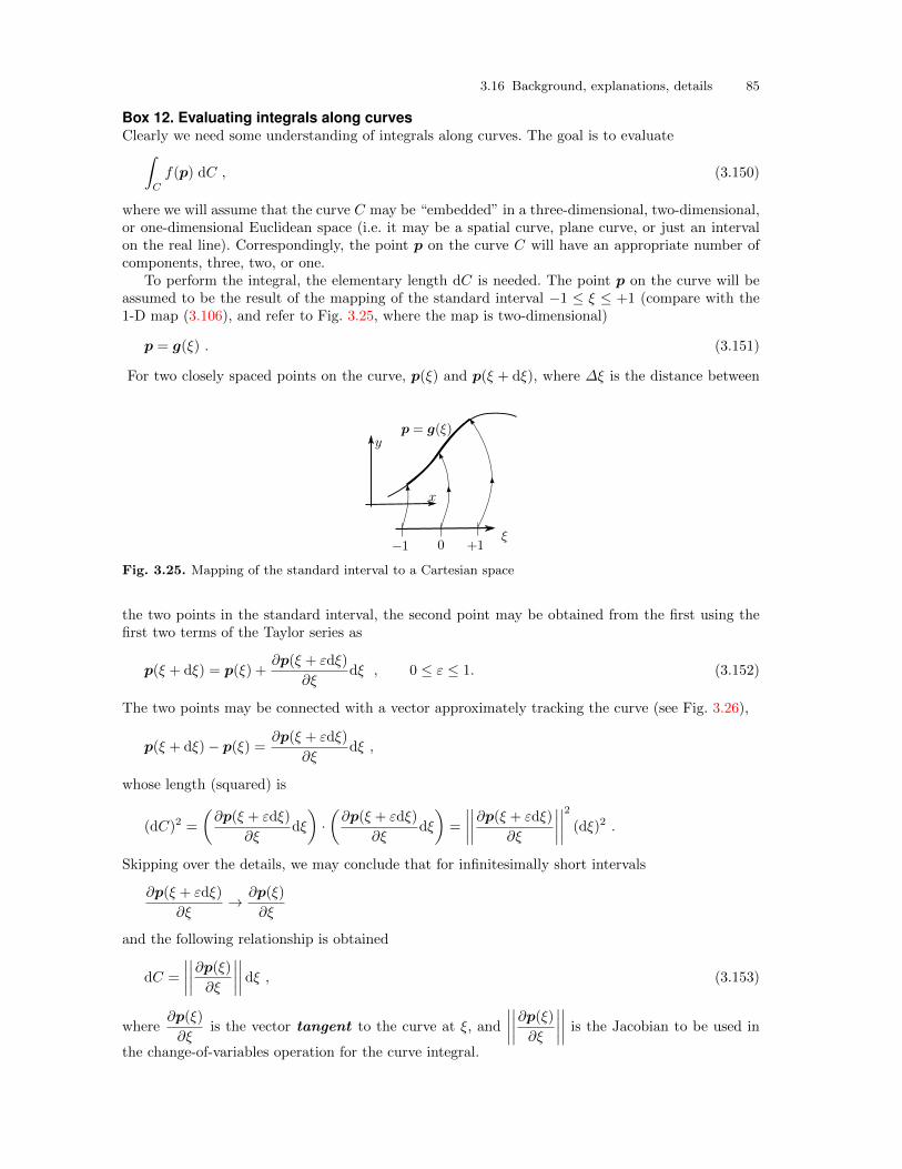
3.16 Background, explanations, details 85

Box 12. Evaluating integrals along curvesClearly we need some understanding of integrals along curves. The goal is to evaluate∫

C

f(p) dC , (3.150)

where we will assume that the curve C may be “embedded” in a three-dimensional, two-dimensional,or one-dimensional Euclidean space (i.e. it may be a spatial curve, plane curve, or just an intervalon the real line). Correspondingly, the point p on the curve C will have an appropriate number ofcomponents, three, two, or one.

To perform the integral, the elementary length dC is needed. The point p on the curve will beassumed to be the result of the mapping of the standard interval −1 ≤ ξ ≤ +1 (compare with the1-D map (3.106), and refer to Fig. 3.25, where the map is two-dimensional)

p = g(ξ) . (3.151)

For two closely spaced points on the curve, p(ξ) and p(ξ + dξ), where ∆ξ is the distance between

Fig. 3.25. Mapping of the standard interval to a Cartesian space

the two points in the standard interval, the second point may be obtained from the first using thefirst two terms of the Taylor series as

p(ξ + dξ) = p(ξ) +∂p(ξ + εdξ)

∂ξdξ , 0 ≤ ε ≤ 1. (3.152)

The two points may be connected with a vector approximately tracking the curve (see Fig. 3.26),

p(ξ + dξ)− p(ξ) =∂p(ξ + εdξ)

∂ξdξ ,

whose length (squared) is

(dC)2 =

(∂p(ξ + εdξ)

∂ξdξ

)·(∂p(ξ + εdξ)

∂ξdξ

)=

∣∣∣∣∣∣∣∣∂p(ξ + εdξ)

∂ξ

∣∣∣∣∣∣∣∣2 (dξ)2 .Skipping over the details, we may conclude that for infinitesimally short intervals

∂p(ξ + εdξ)

∂ξ→ ∂p(ξ)

∂ξ

and the following relationship is obtained

dC =

∣∣∣∣∣∣∣∣∂p(ξ)∂ξ

∣∣∣∣∣∣∣∣dξ , (3.153)

where∂p(ξ)

∂ξis the vector tangent to the curve at ξ, and

∣∣∣∣∣∣∣∣∂p(ξ)∂ξ

∣∣∣∣∣∣∣∣ is the Jacobian to be used in

the change-of-variables operation for the curve integral.

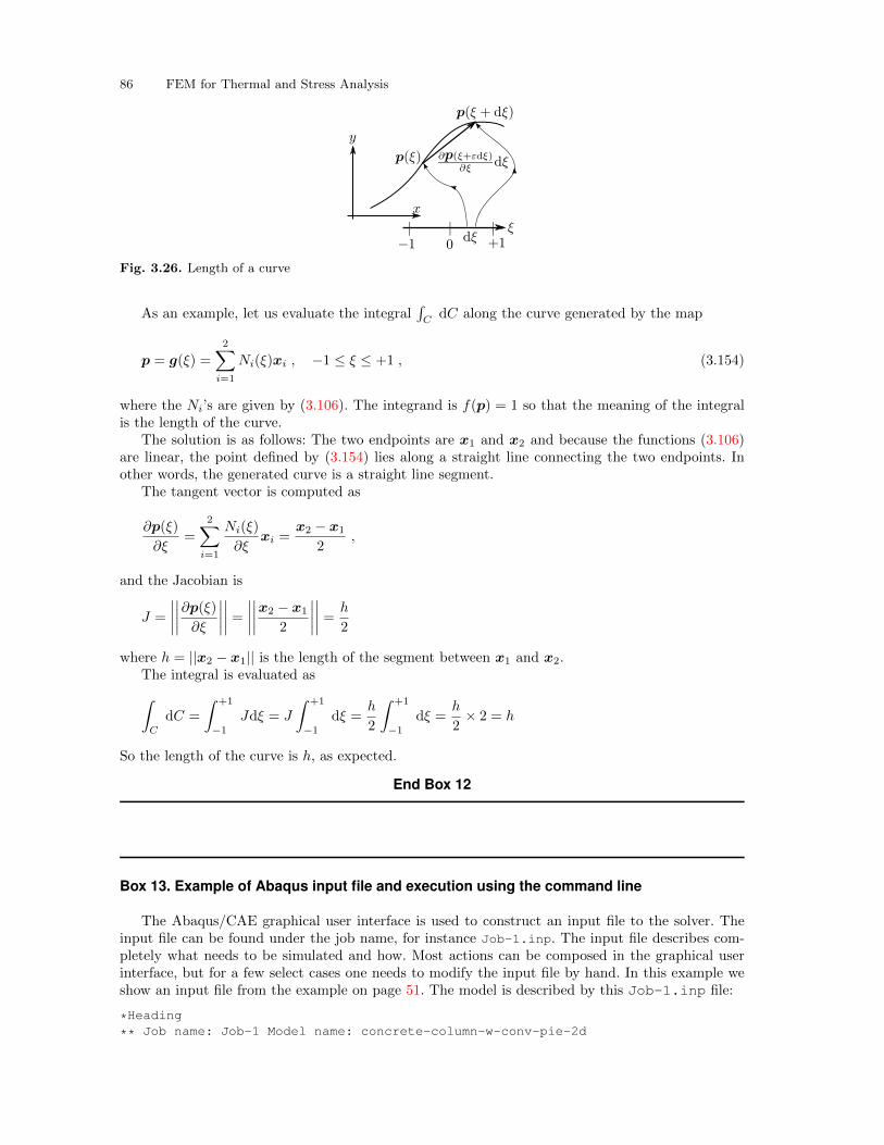
86 FEM for Thermal and Stress Analysis

Fig. 3.26. Length of a curve

As an example, let us evaluate the integral∫C

dC along the curve generated by the map

p = g(ξ) =

2∑i=1

Ni(ξ)xi , −1 ≤ ξ ≤ +1 , (3.154)

where the Ni’s are given by (3.106). The integrand is f(p) = 1 so that the meaning of the integralis the length of the curve.

The solution is as follows: The two endpoints are x1 and x2 and because the functions (3.106)are linear, the point defined by (3.154) lies along a straight line connecting the two endpoints. Inother words, the generated curve is a straight line segment.

The tangent vector is computed as

∂p(ξ)

∂ξ=

2∑i=1

Ni(ξ)

∂ξxi =

x2 − x1

2,

and the Jacobian is

J =

∣∣∣∣∣∣∣∣∂p(ξ)∂ξ

∣∣∣∣∣∣∣∣ = ∣∣∣∣∣∣∣∣x2 − x1

2

∣∣∣∣∣∣∣∣ = h

2

where h = ||x2 − x1|| is the length of the segment between x1 and x2.The integral is evaluated as∫C

dC =

∫ +1

−1

Jdξ = J

∫ +1

−1

dξ =h

2

∫ +1

−1

dξ =h

2× 2 = h

So the length of the curve is h, as expected.

End Box 12

Box 13. Example of Abaqus input file and execution using the command line

The Abaqus/CAE graphical user interface is used to construct an input file to the solver. Theinput file can be found under the job name, for instance Job-1.inp. The input file describes com-pletely what needs to be simulated and how. Most actions can be composed in the graphical userinterface, but for a few select cases one needs to modify the input file by hand. In this example weshow an input file from the example on page 51. The model is described by this Job-1.inp file:

*Heading

** Job name: Job-1 Model name: concrete-column-w-conv-pie-2d

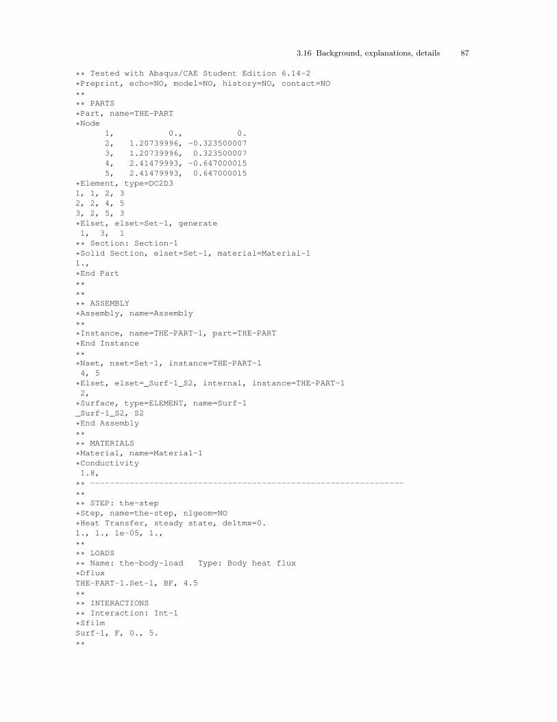
3.16 Background, explanations, details 87

** Tested with Abaqus/CAE Student Edition 6.14-2

*Preprint, echo=NO, model=NO, history=NO, contact=NO

**** PARTS

*Part, name=THE-PART

*Node1, 0., 0.2, 1.20739996, -0.3235000073, 1.20739996, 0.3235000074, 2.41479993, -0.6470000155, 2.41479993, 0.647000015

*Element, type=DC2D31, 1, 2, 32, 2, 4, 53, 2, 5, 3

*Elset, elset=Set-1, generate1, 3, 1

** Section: Section-1

*Solid Section, elset=Set-1, material=Material-11.,

*End Part

****** ASSEMBLY

*Assembly, name=Assembly

***Instance, name=THE-PART-1, part=THE-PART

*End Instance

***Nset, nset=Set-1, instance=THE-PART-14, 5

*Elset, elset=_Surf-1_S2, internal, instance=THE-PART-12,

*Surface, type=ELEMENT, name=Surf-1_Surf-1_S2, S2

*End Assembly

**** MATERIALS

*Material, name=Material-1

*Conductivity1.8,

** ----------------------------------------------------------------

**** STEP: the-step

*Step, name=the-step, nlgeom=NO

*Heat Transfer, steady state, deltmx=0.1., 1., 1e-05, 1.,

**** LOADS

** Name: the-body-load Type: Body heat flux

*DfluxTHE-PART-1.Set-1, BF, 4.5

**** INTERACTIONS

** Interaction: Int-1

*SfilmSurf-1, F, 0., 5.

**

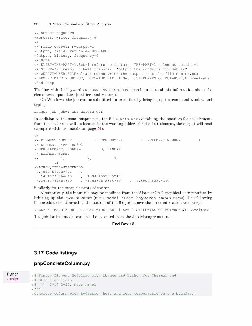
88 FEM for Thermal and Stress Analysis

** OUTPUT REQUESTS

*Restart, write, frequency=0

**** FIELD OUTPUT: F-Output-1

*Output, field, variable=PRESELECT

*Output, history, frequency=0

** Note:

** ELSET=THE-PART-1.Set-1 refers to instance THE-PART-1, element set Set-1

** STIFF=YES means in heat transfer "output the conductivity matrix"

** OUTPUT=USER,FILE=elmats means write the output into the file elmats.mtx

*ELEMENT MATRIX OUTPUT,ELSET=THE-PART-1.Set-1,STIFF=YES,OUTPUT=USER,FILE=elmats

*End Step

The line with the keyword *ELEMENT MATRIX OUTPUT can be used to obtain information about theelementwise quantities (matrices and vectors).

On Windows, the job can be submitted for execution by bringing up the command window andtyping

abaqus job=job-1 ask_delete=off

In addition to the usual output files, the file elmats.mtx containing the matrices for the elementsfrom the set Set-1 will be located in the working folder. For the first element, the output will read(compare with the matrix on page 54):

**** ELEMENT NUMBER 1 STEP NUMBER 1 INCREMENT NUMBER 1

** ELEMENT TYPE DC2D3

*USER ELEMENT, NODES= 3, LINEAR

** ELEMENT NODES

** 1, 2, 311

*MATRIX,TYPE=STIFFNESS0.48227599129621 ,-.24113799564810 , 1.8001052273240-.24113799564810 , -1.5589672316759 , 1.8001052273240

Similarly for the other elements of the set.Alternatively, the input file may be modified from the Abaqus/CAE graphical user interface by

bringing up the keyword editor (menu Model->Edit keywords->model name). The followingline needs to be attached at the bottom of the file just above the line that states *End Step:

*ELEMENT MATRIX OUTPUT,ELSET=THE-PART-1.Set-1,STIFF=YES,OUTPUT=USER,FILE=elmats

The job for this model can then be executed from the Job Manager as usual.

End Box 13

3.17 Code listings

pnpConcreteColumn.py

Python- script

1 # Finite Element Modeling with Abaqus and Python for Thermal and2 # Stress Analysis3 # (C) 2017-2020, Petr Krysl4 """5 Concrete column with hydration heat and zero temperature on the boundary.

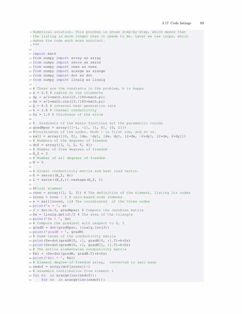
3.17 Code listings 89

6 Numerical solution. This process is shown step-by-step, which means that7 the listing is much longer than it needs to be. Later we use loops, which8 makes the code much more succinct.9 """

10

11 import math12 from numpy import array as array13 from numpy import zeros as zeros14 from numpy import ones as ones15 from numpy import arange as arange16 from numpy import dot as dot17 from numpy import linalg as linalg18

19 # These are the constants in the problem, k is kappa20 a = 2.5 # radius on the columnthe21 dy = a/2*math.sin(15./180*math.pi)22 dx = a/2*math.cos(15./180*math.pi)23 Q = 4.5 # internal heat generation rate24 k = 1.8 # thermal conductivity25 Dz = 1.0 # thickness of the slice26

27 # Gradients of the basis functions wrt the parametric coords28 gradNpar = array([[-1, -1], [1, 0], [0, 1]])29 #Coordinates of the nodes. Node 1 in first row, and so on.30 xall = array([[0, 0], [dx, -dy], [dx, dy], [2*dx, -2*dy], [2*dx, 2*dy]])31 # Numbers of the degrees of freedom32 dof = array([3, 1, 2, 5, 4])33 # Number of free degrees of freedom34 N_f = 335 # Number of all degrees of freedom36 N = 537

38 # Global conductivity matrix and heat load vector.39 K = zeros((N_f, N))40 L = zeros((N_f,)).reshape(N_f, 1)41

42 #First element43 conn = array([1, 2, 3]) # The definition of the element, listing its nodes44 zconn = conn - 1 # zero-based node indexes45 x = xall[zconn, :]# The coordinates of the three nodes46 print(’x = ’, x)47 J = dot(x.T, gradNpar) # Compute the Jacobian matrix48 Se = linalg.det(J)/2 # The area of the triangle49 print(’Se = ’, Se)50 # Compute the gradient with respect to X, Y51 gradN = dot(gradNpar, linalg.inv(J))52 print(’gradN = ’, gradN)53 # Some terms of the conductivity matrix54 print(Se*dot(gradN[0, :], gradN[0, :].T)*k*Dz)55 print(Se*dot(gradN[0, :], gradN[1, :].T)*k*Dz)56 # The entire elementwise conductivity matrix57 Ke1 = (Se*dot(gradN, gradN.T)*k*Dz)58 print(’Ke1 = ’, Ke1)59 # Element degree-of-freedom array, converted to zero base60 zedof = array(dof[zconn])-161 # Assemble contribution from element 162 for ro in arange(len(zedof)):63 for co in arange(len(zedof)):

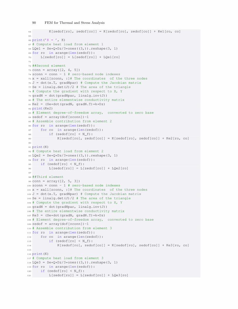
90 FEM for Thermal and Stress Analysis

64 K[zedof[ro], zedof[co]] = K[zedof[ro], zedof[co]] + Ke1[ro, co]65

66 print(’K = ’, K)67 # Compute heat load from element 168 LQe1 = Se*Q*Dz/3*ones((3,)).reshape(3, 1)69 for ro in arange(len(zedof)):70 L[zedof[ro]] = L[zedof[ro]] + LQe1[ro]71

72 ##Second element73 conn = array([2, 4, 5])74 zconn = conn - 1 # zero-based node indexes75 x = xall[zconn, :]# The coordinates of the three nodes76 J = dot(x.T, gradNpar) # Compute the Jacobian matrix77 Se = linalg.det(J)/2 # The area of the triangle78 # Compute the gradient with respect to X, Y79 gradN = dot(gradNpar, linalg.inv(J))80 # The entire elementwise conductivity matrix81 Ke2 = (Se*dot(gradN, gradN.T)*k*Dz)82 print(Ke2)83 # Element degree-of-freedom array, converted to zero base84 zedof = array(dof[zconn])-185 # Assemble contribution from element 286 for ro in arange(len(zedof)):87 for co in arange(len(zedof)):88 if (zedof[ro] < N_f):89 K[zedof[ro], zedof[co]] = K[zedof[ro], zedof[co]] + Ke2[ro, co]90

91 print(K)92 # Compute heat load from element 293 LQe2 = Se*Q*Dz/3*ones((3,)).reshape(3, 1)94 for ro in arange(len(zedof)):95 if (zedof[ro] < N_f):96 L[zedof[ro]] = L[zedof[ro]] + LQe2[ro]97

98 ##Third element99 conn = array([2, 5, 3])

100 zconn = conn - 1 # zero-based node indexes101 x = xall[zconn, :]# The coordinates of the three nodes102 J = dot(x.T, gradNpar) # Compute the Jacobian matrix103 Se = linalg.det(J)/2 # The area of the triangle104 # Compute the gradient with respect to X, Y105 gradN = dot(gradNpar, linalg.inv(J))106 # The entire elementwise conductivity matrix107 Ke3 = (Se*dot(gradN, gradN.T)*k*Dz)108 # Element degree-of-freedom array, converted to zero base109 zedof = array(dof[zconn])-1110 # Assemble contribution from element 3111 for ro in arange(len(zedof)):112 for co in arange(len(zedof)):113 if (zedof[ro] < N_f):114 K[zedof[ro], zedof[co]] = K[zedof[ro], zedof[co]] + Ke3[ro, co]115

116 print(K)117 # Compute heat load from element 3118 LQe3 = Se*Q*Dz/3*ones((3,)).reshape(3, 1)119 for ro in arange(len(zedof)):120 if (zedof[ro] < N_f):121 L[zedof[ro]] = L[zedof[ro]] + LQe3[ro]

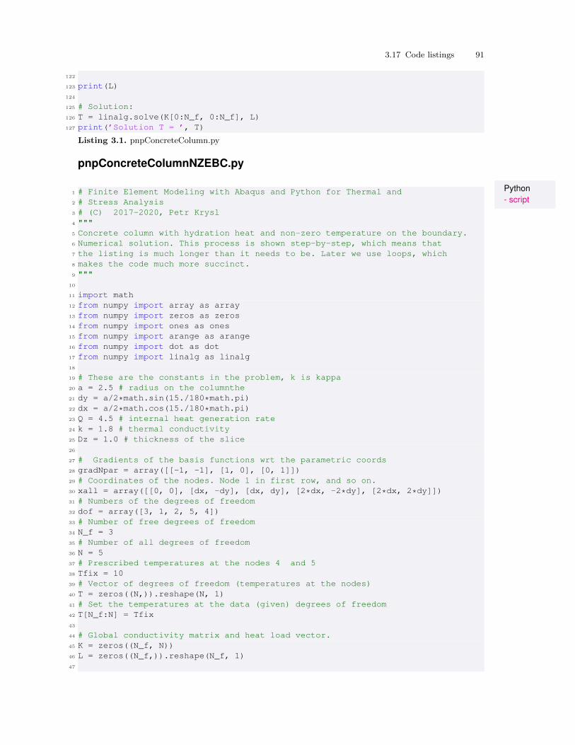
3.17 Code listings 91

122

123 print(L)124

125 # Solution:126 T = linalg.solve(K[0:N_f, 0:N_f], L)127 print(’Solution T = ’, T)

Listing 3.1. pnpConcreteColumn.py

pnpConcreteColumnNZEBC.py

Python- script

1 # Finite Element Modeling with Abaqus and Python for Thermal and2 # Stress Analysis3 # (C) 2017-2020, Petr Krysl4 """5 Concrete column with hydration heat and non-zero temperature on the boundary.6 Numerical solution. This process is shown step-by-step, which means that7 the listing is much longer than it needs to be. Later we use loops, which8 makes the code much more succinct.9 """

10

11 import math12 from numpy import array as array13 from numpy import zeros as zeros14 from numpy import ones as ones15 from numpy import arange as arange16 from numpy import dot as dot17 from numpy import linalg as linalg18

19 # These are the constants in the problem, k is kappa20 a = 2.5 # radius on the columnthe21 dy = a/2*math.sin(15./180*math.pi)22 dx = a/2*math.cos(15./180*math.pi)23 Q = 4.5 # internal heat generation rate24 k = 1.8 # thermal conductivity25 Dz = 1.0 # thickness of the slice26

27 # Gradients of the basis functions wrt the parametric coords28 gradNpar = array([[-1, -1], [1, 0], [0, 1]])29 # Coordinates of the nodes. Node 1 in first row, and so on.30 xall = array([[0, 0], [dx, -dy], [dx, dy], [2*dx, -2*dy], [2*dx, 2*dy]])31 # Numbers of the degrees of freedom32 dof = array([3, 1, 2, 5, 4])33 # Number of free degrees of freedom34 N_f = 335 # Number of all degrees of freedom36 N = 537 # Prescribed temperatures at the nodes 4 and 538 Tfix = 1039 # Vector of degrees of freedom (temperatures at the nodes)40 T = zeros((N,)).reshape(N, 1)41 # Set the temperatures at the data (given) degrees of freedom42 T[N_f:N] = Tfix43

44 # Global conductivity matrix and heat load vector.45 K = zeros((N_f, N))46 L = zeros((N_f,)).reshape(N_f, 1)47

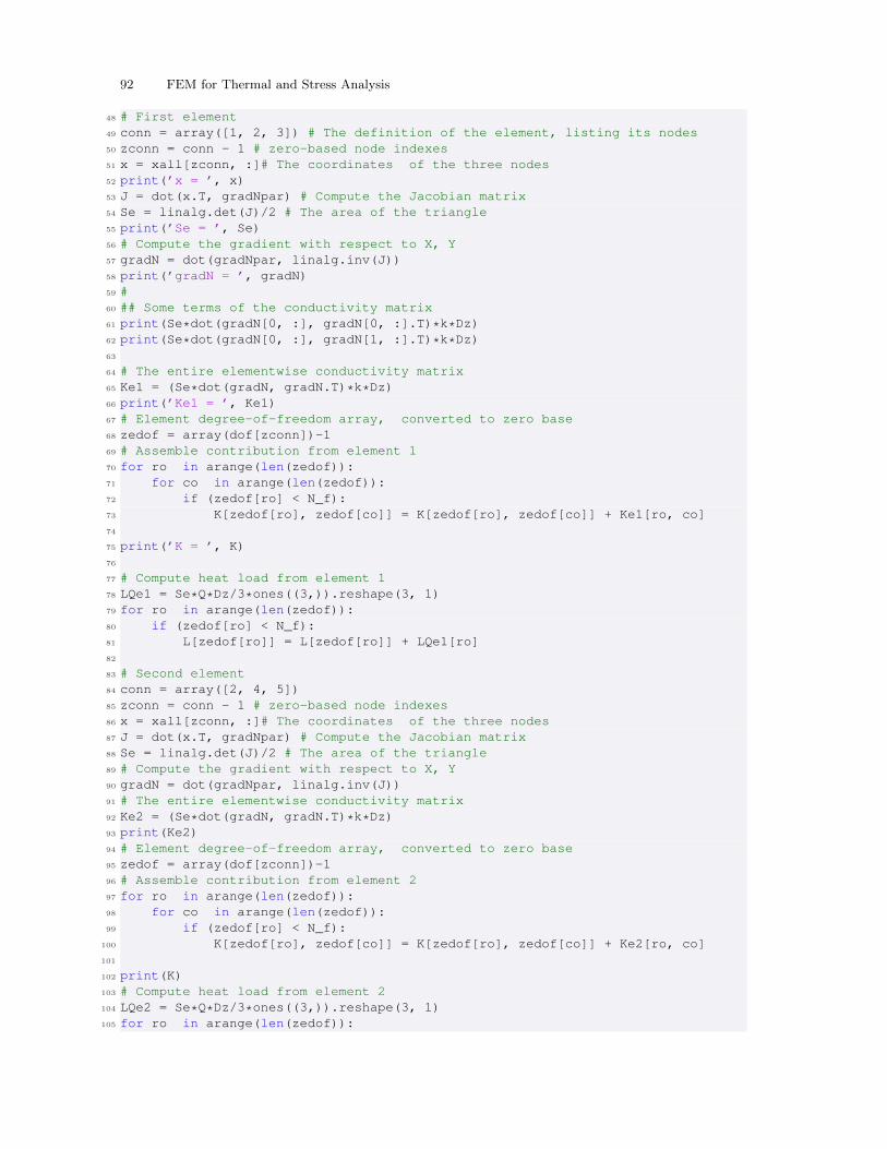
92 FEM for Thermal and Stress Analysis

48 # First element49 conn = array([1, 2, 3]) # The definition of the element, listing its nodes50 zconn = conn - 1 # zero-based node indexes51 x = xall[zconn, :]# The coordinates of the three nodes52 print(’x = ’, x)53 J = dot(x.T, gradNpar) # Compute the Jacobian matrix54 Se = linalg.det(J)/2 # The area of the triangle55 print(’Se = ’, Se)56 # Compute the gradient with respect to X, Y57 gradN = dot(gradNpar, linalg.inv(J))58 print(’gradN = ’, gradN)59 #60 ## Some terms of the conductivity matrix61 print(Se*dot(gradN[0, :], gradN[0, :].T)*k*Dz)62 print(Se*dot(gradN[0, :], gradN[1, :].T)*k*Dz)63

64 # The entire elementwise conductivity matrix65 Ke1 = (Se*dot(gradN, gradN.T)*k*Dz)66 print(’Ke1 = ’, Ke1)67 # Element degree-of-freedom array, converted to zero base68 zedof = array(dof[zconn])-169 # Assemble contribution from element 170 for ro in arange(len(zedof)):71 for co in arange(len(zedof)):72 if (zedof[ro] < N_f):73 K[zedof[ro], zedof[co]] = K[zedof[ro], zedof[co]] + Ke1[ro, co]74

75 print(’K = ’, K)76

77 # Compute heat load from element 178 LQe1 = Se*Q*Dz/3*ones((3,)).reshape(3, 1)79 for ro in arange(len(zedof)):80 if (zedof[ro] < N_f):81 L[zedof[ro]] = L[zedof[ro]] + LQe1[ro]82

83 # Second element84 conn = array([2, 4, 5])85 zconn = conn - 1 # zero-based node indexes86 x = xall[zconn, :]# The coordinates of the three nodes87 J = dot(x.T, gradNpar) # Compute the Jacobian matrix88 Se = linalg.det(J)/2 # The area of the triangle89 # Compute the gradient with respect to X, Y90 gradN = dot(gradNpar, linalg.inv(J))91 # The entire elementwise conductivity matrix92 Ke2 = (Se*dot(gradN, gradN.T)*k*Dz)93 print(Ke2)94 # Element degree-of-freedom array, converted to zero base95 zedof = array(dof[zconn])-196 # Assemble contribution from element 297 for ro in arange(len(zedof)):98 for co in arange(len(zedof)):99 if (zedof[ro] < N_f):

100 K[zedof[ro], zedof[co]] = K[zedof[ro], zedof[co]] + Ke2[ro, co]101

102 print(K)103 # Compute heat load from element 2104 LQe2 = Se*Q*Dz/3*ones((3,)).reshape(3, 1)105 for ro in arange(len(zedof)):

3.17 Code listings 93

106 if (zedof[ro] < N_f):107 L[zedof[ro]] = L[zedof[ro]] + LQe2[ro]108

109 # Third element110 conn = array([2, 5, 3])111 zconn = conn - 1 # zero-based node indexes112 x = xall[zconn, :]# The coordinates of the three nodes113 J = dot(x.T, gradNpar) # Compute the Jacobian matrix114 Se = linalg.det(J)/2 # The area of the triangle115 # Compute the gradient with respect to X, Y116 gradN = dot(gradNpar, linalg.inv(J))117 # The entire elementwise conductivity matrix118 Ke3 = (Se*dot(gradN, gradN.T)*k*Dz)119 # Element degree-of-freedom array, converted to zero base120 zedof = array(dof[zconn])-1121 # Assemble contribution from element 2122 for ro in arange(len(zedof)):123 for co in arange(len(zedof)):124 if (zedof[ro] < N_f):125 K[zedof[ro], zedof[co]] = K[zedof[ro], zedof[co]] + Ke3[ro, co]126

127 print(K)128 # Compute heat load from element 3129 LQe3 = Se*Q*Dz/3*ones((3,)).reshape(3, 1)130 for ro in arange(len(zedof)):131 if (zedof[ro] < N_f):132 L[zedof[ro]] = L[zedof[ro]] + LQe3[ro]133

134 # Compute loading from the prescribed temperatures135 LT = -dot(K[0:N_f, N_f:N], T[N_f:N])136 print(LT)137

138 # Solution:139 T[0:N_f] = linalg.solve(K[0:N_f, 0:N_f], L[0:N_f] + LT[0:N_f])140 print(’Solution T=’, T)

Listing 3.2. pnpConcreteColumnNZEBC.py

pnpLayeredWall1v3.py

Python- script

1 # Finite Element Modeling with Abaqus and Python for Thermal and2 # Stress Analysis3 # (C) 2017-2020, Petr Krysl4 """5 Layered wall. Temperature boundary conditions.6 """7

8 import math9 from numpy import array as array

10 from numpy import zeros as zeros11 from numpy import ones as ones12 from numpy import arange as arange13 from numpy import dot as dot14 from numpy import linalg as linalg15 from numpy import vstack as vstack16 import matplotlib.pyplot as plt17

18 Dz = 1.0 # Thickness of the slice (it cancels out in the end)

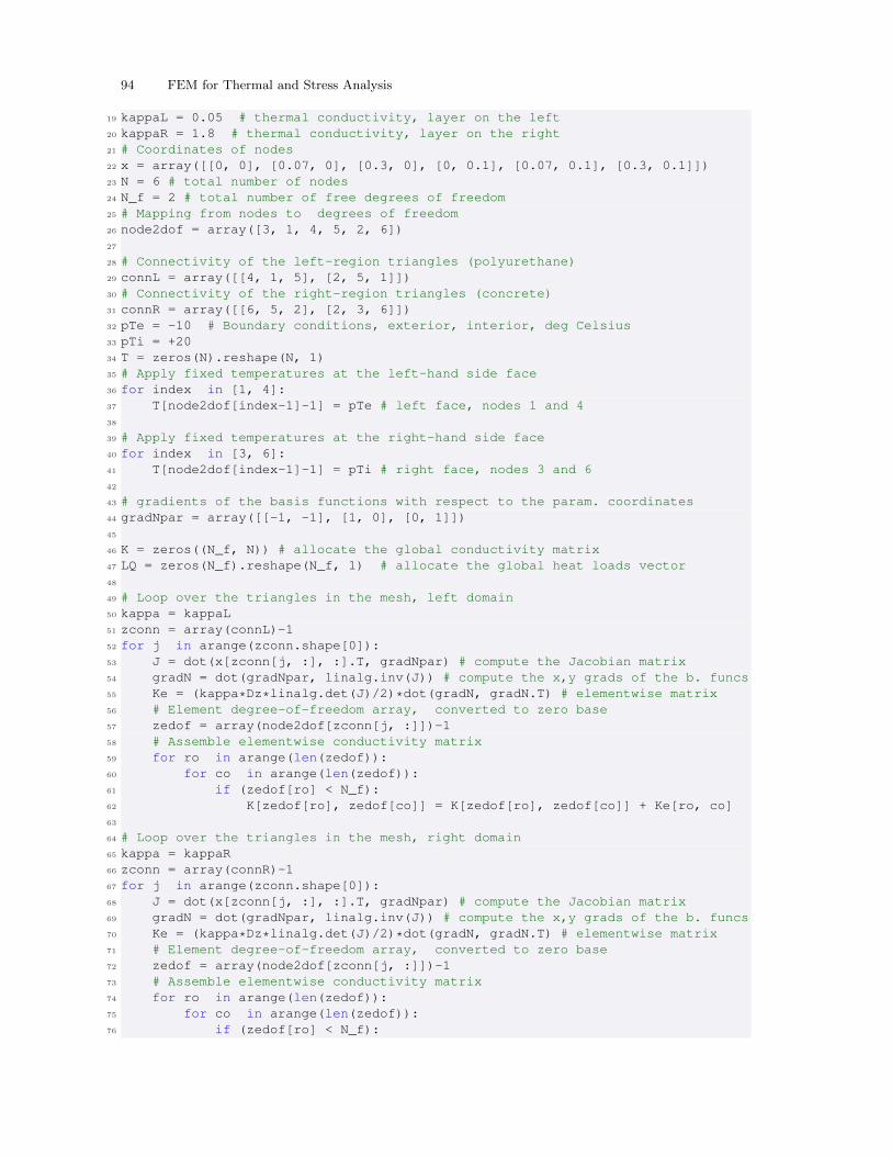
94 FEM for Thermal and Stress Analysis

19 kappaL = 0.05 # thermal conductivity, layer on the left20 kappaR = 1.8 # thermal conductivity, layer on the right21 # Coordinates of nodes22 x = array([[0, 0], [0.07, 0], [0.3, 0], [0, 0.1], [0.07, 0.1], [0.3, 0.1]])23 N = 6 # total number of nodes24 N_f = 2 # total number of free degrees of freedom25 # Mapping from nodes to degrees of freedom26 node2dof = array([3, 1, 4, 5, 2, 6])27

28 # Connectivity of the left-region triangles (polyurethane)29 connL = array([[4, 1, 5], [2, 5, 1]])30 # Connectivity of the right-region triangles (concrete)31 connR = array([[6, 5, 2], [2, 3, 6]])32 pTe = -10 # Boundary conditions, exterior, interior, deg Celsius33 pTi = +2034 T = zeros(N).reshape(N, 1)35 # Apply fixed temperatures at the left-hand side face36 for index in [1, 4]:37 T[node2dof[index-1]-1] = pTe # left face, nodes 1 and 438

39 # Apply fixed temperatures at the right-hand side face40 for index in [3, 6]:41 T[node2dof[index-1]-1] = pTi # right face, nodes 3 and 642

43 # gradients of the basis functions with respect to the param. coordinates44 gradNpar = array([[-1, -1], [1, 0], [0, 1]])45

46 K = zeros((N_f, N)) # allocate the global conductivity matrix47 LQ = zeros(N_f).reshape(N_f, 1) # allocate the global heat loads vector48

49 # Loop over the triangles in the mesh, left domain50 kappa = kappaL51 zconn = array(connL)-152 for j in arange(zconn.shape[0]):53 J = dot(x[zconn[j, :], :].T, gradNpar) # compute the Jacobian matrix54 gradN = dot(gradNpar, linalg.inv(J)) # compute the x,y grads of the b. funcs55 Ke = (kappa*Dz*linalg.det(J)/2)*dot(gradN, gradN.T) # elementwise matrix56 # Element degree-of-freedom array, converted to zero base57 zedof = array(node2dof[zconn[j, :]])-158 # Assemble elementwise conductivity matrix59 for ro in arange(len(zedof)):60 for co in arange(len(zedof)):61 if (zedof[ro] < N_f):62 K[zedof[ro], zedof[co]] = K[zedof[ro], zedof[co]] + Ke[ro, co]63

64 # Loop over the triangles in the mesh, right domain65 kappa = kappaR66 zconn = array(connR)-167 for j in arange(zconn.shape[0]):68 J = dot(x[zconn[j, :], :].T, gradNpar) # compute the Jacobian matrix69 gradN = dot(gradNpar, linalg.inv(J)) # compute the x,y grads of the b. funcs70 Ke = (kappa*Dz*linalg.det(J)/2)*dot(gradN, gradN.T) # elementwise matrix71 # Element degree-of-freedom array, converted to zero base72 zedof = array(node2dof[zconn[j, :]])-173 # Assemble elementwise conductivity matrix74 for ro in arange(len(zedof)):75 for co in arange(len(zedof)):76 if (zedof[ro] < N_f):

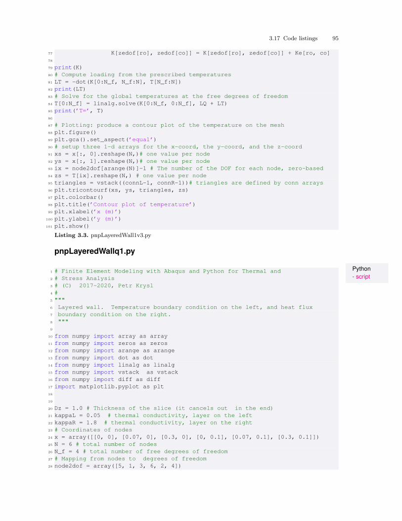
3.17 Code listings 95

77 K[zedof[ro], zedof[co]] = K[zedof[ro], zedof[co]] + Ke[ro, co]78

79 print(K)80 # Compute loading from the prescribed temperatures81 LT = -dot(K[0:N_f, N_f:N], T[N_f:N])82 print(LT)83 # Solve for the global temperatures at the free degrees of freedom84 T[0:N_f] = linalg.solve(K[0:N_f, 0:N_f], LQ + LT)85 print(’T=’, T)86

87 # Plotting: produce a contour plot of the temperature on the mesh88 plt.figure()89 plt.gca().set_aspect(’equal’)90 # setup three 1-d arrays for the x-coord, the y-coord, and the z-coord91 xs = x[:, 0].reshape(N,)# one value per node92 ys = x[:, 1].reshape(N,)# one value per node93 ix = node2dof[arange(N)]-1 # The number of the DOF for each node, zero-based94 zs = T[ix].reshape(N,) # one value per node95 triangles = vstack((connL-1, connR-1))# triangles are defined by conn arrays96 plt.tricontourf(xs, ys, triangles, zs)97 plt.colorbar()98 plt.title(’Contour plot of temperature’)99 plt.xlabel(’x (m)’)

100 plt.ylabel(’y (m)’)101 plt.show()

Listing 3.3. pnpLayeredWall1v3.py

pnpLayeredWallq1.py

Python- script

1 # Finite Element Modeling with Abaqus and Python for Thermal and2 # Stress Analysis3 # (C) 2017-2020, Petr Krysl4 #5 """6 Layered wall. Temperature boundary condition on the left, and heat flux7 boundary condition on the right.8 """9

10 from numpy import array as array11 from numpy import zeros as zeros12 from numpy import arange as arange13 from numpy import dot as dot14 from numpy import linalg as linalg15 from numpy import vstack as vstack16 from numpy import diff as diff17 import matplotlib.pyplot as plt18

19

20 Dz = 1.0 # Thickness of the slice (it cancels out in the end)21 kappaL = 0.05 # thermal conductivity, layer on the left22 kappaR = 1.8 # thermal conductivity, layer on the right23 # Coordinates of nodes24 x = array([[0, 0], [0.07, 0], [0.3, 0], [0, 0.1], [0.07, 0.1], [0.3, 0.1]])25 N = 6 # total number of nodes26 N_f = 4 # total number of free degrees of freedom27 # Mapping from nodes to degrees of freedom28 node2dof = array([5, 1, 3, 6, 2, 4])

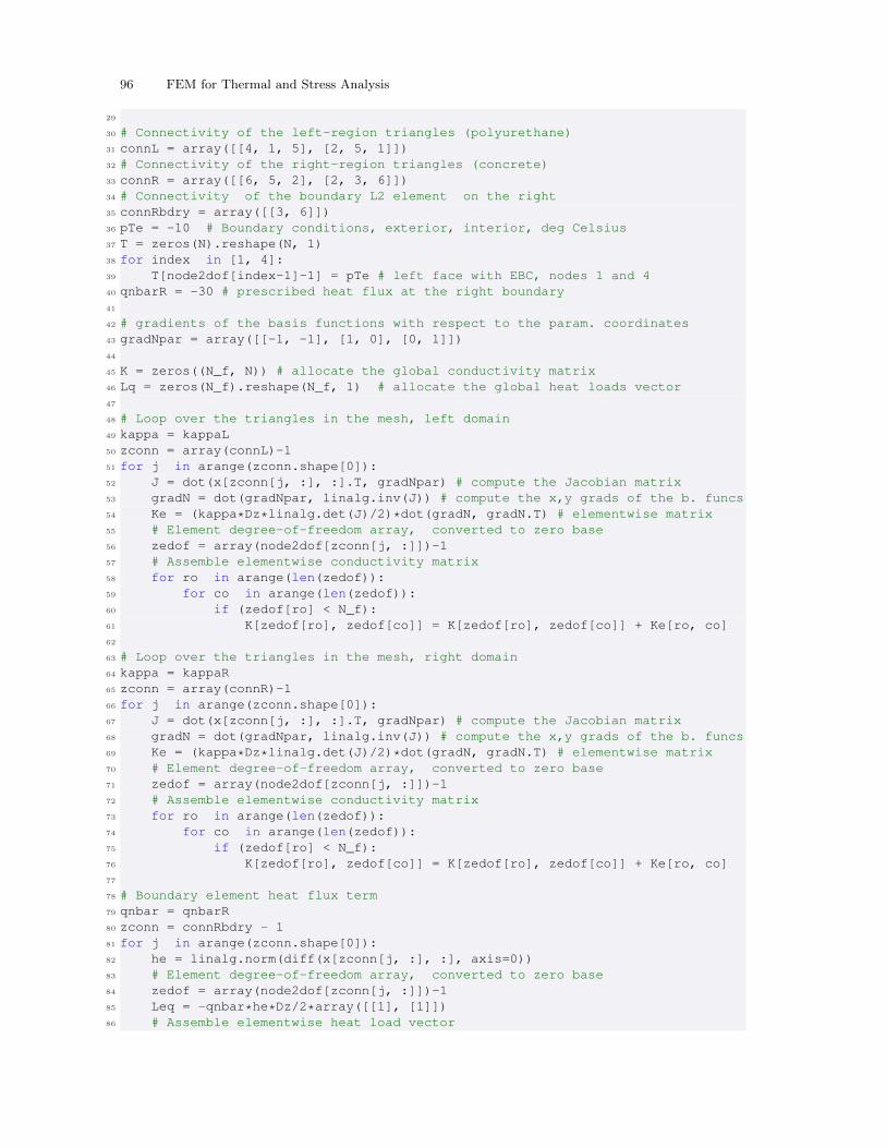
96 FEM for Thermal and Stress Analysis

29

30 # Connectivity of the left-region triangles (polyurethane)31 connL = array([[4, 1, 5], [2, 5, 1]])32 # Connectivity of the right-region triangles (concrete)33 connR = array([[6, 5, 2], [2, 3, 6]])34 # Connectivity of the boundary L2 element on the right35 connRbdry = array([[3, 6]])36 pTe = -10 # Boundary conditions, exterior, interior, deg Celsius37 T = zeros(N).reshape(N, 1)38 for index in [1, 4]:39 T[node2dof[index-1]-1] = pTe # left face with EBC, nodes 1 and 440 qnbarR = -30 # prescribed heat flux at the right boundary41

42 # gradients of the basis functions with respect to the param. coordinates43 gradNpar = array([[-1, -1], [1, 0], [0, 1]])44

45 K = zeros((N_f, N)) # allocate the global conductivity matrix46 Lq = zeros(N_f).reshape(N_f, 1) # allocate the global heat loads vector47

48 # Loop over the triangles in the mesh, left domain49 kappa = kappaL50 zconn = array(connL)-151 for j in arange(zconn.shape[0]):52 J = dot(x[zconn[j, :], :].T, gradNpar) # compute the Jacobian matrix53 gradN = dot(gradNpar, linalg.inv(J)) # compute the x,y grads of the b. funcs54 Ke = (kappa*Dz*linalg.det(J)/2)*dot(gradN, gradN.T) # elementwise matrix55 # Element degree-of-freedom array, converted to zero base56 zedof = array(node2dof[zconn[j, :]])-157 # Assemble elementwise conductivity matrix58 for ro in arange(len(zedof)):59 for co in arange(len(zedof)):60 if (zedof[ro] < N_f):61 K[zedof[ro], zedof[co]] = K[zedof[ro], zedof[co]] + Ke[ro, co]62

63 # Loop over the triangles in the mesh, right domain64 kappa = kappaR65 zconn = array(connR)-166 for j in arange(zconn.shape[0]):67 J = dot(x[zconn[j, :], :].T, gradNpar) # compute the Jacobian matrix68 gradN = dot(gradNpar, linalg.inv(J)) # compute the x,y grads of the b. funcs69 Ke = (kappa*Dz*linalg.det(J)/2)*dot(gradN, gradN.T) # elementwise matrix70 # Element degree-of-freedom array, converted to zero base71 zedof = array(node2dof[zconn[j, :]])-172 # Assemble elementwise conductivity matrix73 for ro in arange(len(zedof)):74 for co in arange(len(zedof)):75 if (zedof[ro] < N_f):76 K[zedof[ro], zedof[co]] = K[zedof[ro], zedof[co]] + Ke[ro, co]77

78 # Boundary element heat flux term79 qnbar = qnbarR80 zconn = connRbdry - 181 for j in arange(zconn.shape[0]):82 he = linalg.norm(diff(x[zconn[j, :], :], axis=0))83 # Element degree-of-freedom array, converted to zero base84 zedof = array(node2dof[zconn[j, :]])-185 Leq = -qnbar*he*Dz/2*array([[1], [1]])86 # Assemble elementwise heat load vector

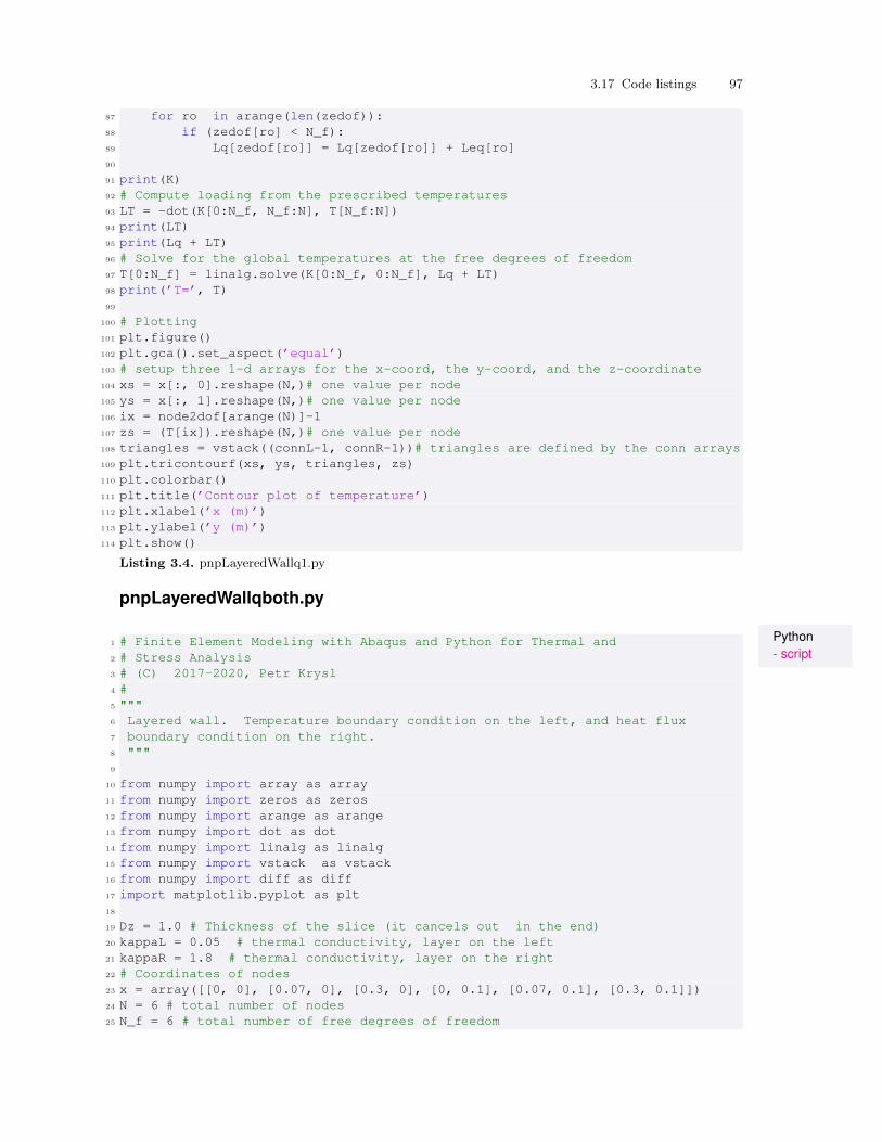
3.17 Code listings 97

87 for ro in arange(len(zedof)):88 if (zedof[ro] < N_f):89 Lq[zedof[ro]] = Lq[zedof[ro]] + Leq[ro]90

91 print(K)92 # Compute loading from the prescribed temperatures93 LT = -dot(K[0:N_f, N_f:N], T[N_f:N])94 print(LT)95 print(Lq + LT)96 # Solve for the global temperatures at the free degrees of freedom97 T[0:N_f] = linalg.solve(K[0:N_f, 0:N_f], Lq + LT)98 print(’T=’, T)99

100 # Plotting101 plt.figure()102 plt.gca().set_aspect(’equal’)103 # setup three 1-d arrays for the x-coord, the y-coord, and the z-coordinate104 xs = x[:, 0].reshape(N,)# one value per node105 ys = x[:, 1].reshape(N,)# one value per node106 ix = node2dof[arange(N)]-1107 zs = (T[ix]).reshape(N,)# one value per node108 triangles = vstack((connL-1, connR-1))# triangles are defined by the conn arrays109 plt.tricontourf(xs, ys, triangles, zs)110 plt.colorbar()111 plt.title(’Contour plot of temperature’)112 plt.xlabel(’x (m)’)113 plt.ylabel(’y (m)’)114 plt.show()

Listing 3.4. pnpLayeredWallq1.py

pnpLayeredWallqboth.py

Python- script

1 # Finite Element Modeling with Abaqus and Python for Thermal and2 # Stress Analysis3 # (C) 2017-2020, Petr Krysl4 #5 """6 Layered wall. Temperature boundary condition on the left, and heat flux7 boundary condition on the right.8 """9

10 from numpy import array as array11 from numpy import zeros as zeros12 from numpy import arange as arange13 from numpy import dot as dot14 from numpy import linalg as linalg15 from numpy import vstack as vstack16 from numpy import diff as diff17 import matplotlib.pyplot as plt18

19 Dz = 1.0 # Thickness of the slice (it cancels out in the end)20 kappaL = 0.05 # thermal conductivity, layer on the left21 kappaR = 1.8 # thermal conductivity, layer on the right22 # Coordinates of nodes23 x = array([[0, 0], [0.07, 0], [0.3, 0], [0, 0.1], [0.07, 0.1], [0.3, 0.1]])24 N = 6 # total number of nodes25 N_f = 6 # total number of free degrees of freedom

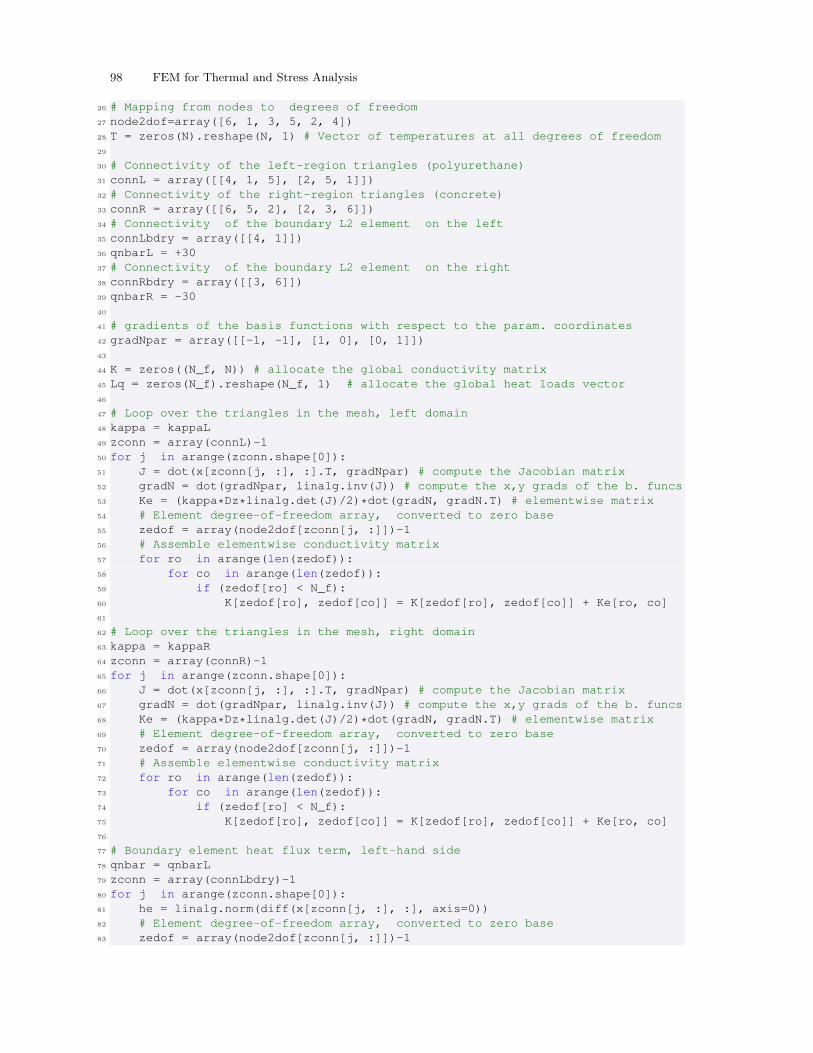
98 FEM for Thermal and Stress Analysis

26 # Mapping from nodes to degrees of freedom27 node2dof=array([6, 1, 3, 5, 2, 4])28 T = zeros(N).reshape(N, 1) # Vector of temperatures at all degrees of freedom29

30 # Connectivity of the left-region triangles (polyurethane)31 connL = array([[4, 1, 5], [2, 5, 1]])32 # Connectivity of the right-region triangles (concrete)33 connR = array([[6, 5, 2], [2, 3, 6]])34 # Connectivity of the boundary L2 element on the left35 connLbdry = array([[4, 1]])36 qnbarL = +3037 # Connectivity of the boundary L2 element on the right38 connRbdry = array([[3, 6]])39 qnbarR = -3040

41 # gradients of the basis functions with respect to the param. coordinates42 gradNpar = array([[-1, -1], [1, 0], [0, 1]])43

44 K = zeros((N_f, N)) # allocate the global conductivity matrix45 Lq = zeros(N_f).reshape(N_f, 1) # allocate the global heat loads vector46

47 # Loop over the triangles in the mesh, left domain48 kappa = kappaL49 zconn = array(connL)-150 for j in arange(zconn.shape[0]):51 J = dot(x[zconn[j, :], :].T, gradNpar) # compute the Jacobian matrix52 gradN = dot(gradNpar, linalg.inv(J)) # compute the x,y grads of the b. funcs53 Ke = (kappa*Dz*linalg.det(J)/2)*dot(gradN, gradN.T) # elementwise matrix54 # Element degree-of-freedom array, converted to zero base55 zedof = array(node2dof[zconn[j, :]])-156 # Assemble elementwise conductivity matrix57 for ro in arange(len(zedof)):58 for co in arange(len(zedof)):59 if (zedof[ro] < N_f):60 K[zedof[ro], zedof[co]] = K[zedof[ro], zedof[co]] + Ke[ro, co]61

62 # Loop over the triangles in the mesh, right domain63 kappa = kappaR64 zconn = array(connR)-165 for j in arange(zconn.shape[0]):66 J = dot(x[zconn[j, :], :].T, gradNpar) # compute the Jacobian matrix67 gradN = dot(gradNpar, linalg.inv(J)) # compute the x,y grads of the b. funcs68 Ke = (kappa*Dz*linalg.det(J)/2)*dot(gradN, gradN.T) # elementwise matrix69 # Element degree-of-freedom array, converted to zero base70 zedof = array(node2dof[zconn[j, :]])-171 # Assemble elementwise conductivity matrix72 for ro in arange(len(zedof)):73 for co in arange(len(zedof)):74 if (zedof[ro] < N_f):75 K[zedof[ro], zedof[co]] = K[zedof[ro], zedof[co]] + Ke[ro, co]76

77 # Boundary element heat flux term, left-hand side78 qnbar = qnbarL79 zconn = array(connLbdry)-180 for j in arange(zconn.shape[0]):81 he = linalg.norm(diff(x[zconn[j, :], :], axis=0))82 # Element degree-of-freedom array, converted to zero base83 zedof = array(node2dof[zconn[j, :]])-1

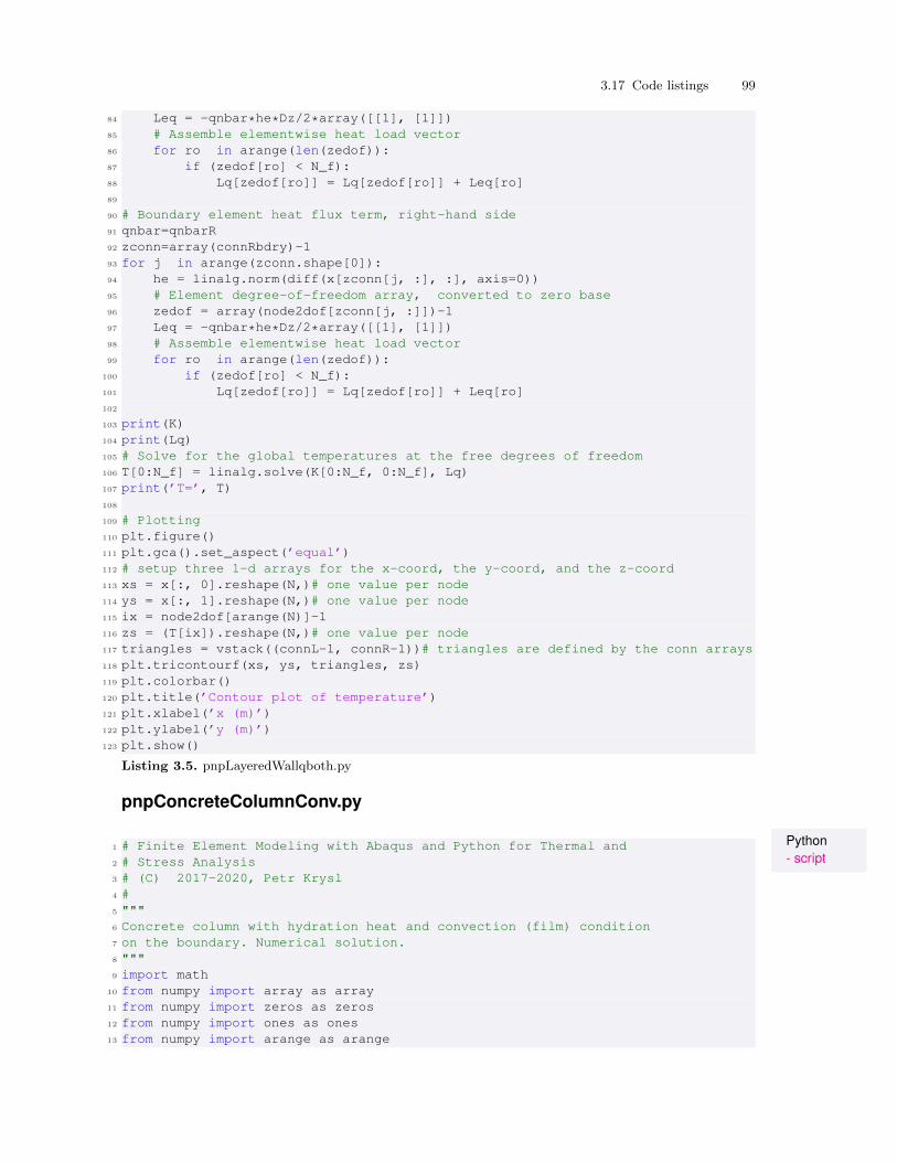
3.17 Code listings 99

84 Leq = -qnbar*he*Dz/2*array([[1], [1]])85 # Assemble elementwise heat load vector86 for ro in arange(len(zedof)):87 if (zedof[ro] < N_f):88 Lq[zedof[ro]] = Lq[zedof[ro]] + Leq[ro]89

90 # Boundary element heat flux term, right-hand side91 qnbar=qnbarR92 zconn=array(connRbdry)-193 for j in arange(zconn.shape[0]):94 he = linalg.norm(diff(x[zconn[j, :], :], axis=0))95 # Element degree-of-freedom array, converted to zero base96 zedof = array(node2dof[zconn[j, :]])-197 Leq = -qnbar*he*Dz/2*array([[1], [1]])98 # Assemble elementwise heat load vector99 for ro in arange(len(zedof)):

100 if (zedof[ro] < N_f):101 Lq[zedof[ro]] = Lq[zedof[ro]] + Leq[ro]102

103 print(K)104 print(Lq)105 # Solve for the global temperatures at the free degrees of freedom106 T[0:N_f] = linalg.solve(K[0:N_f, 0:N_f], Lq)107 print(’T=’, T)108

109 # Plotting110 plt.figure()111 plt.gca().set_aspect(’equal’)112 # setup three 1-d arrays for the x-coord, the y-coord, and the z-coord113 xs = x[:, 0].reshape(N,)# one value per node114 ys = x[:, 1].reshape(N,)# one value per node115 ix = node2dof[arange(N)]-1116 zs = (T[ix]).reshape(N,)# one value per node117 triangles = vstack((connL-1, connR-1))# triangles are defined by the conn arrays118 plt.tricontourf(xs, ys, triangles, zs)119 plt.colorbar()120 plt.title(’Contour plot of temperature’)121 plt.xlabel(’x (m)’)122 plt.ylabel(’y (m)’)123 plt.show()

Listing 3.5. pnpLayeredWallqboth.py

pnpConcreteColumnConv.py

Python- script

1 # Finite Element Modeling with Abaqus and Python for Thermal and2 # Stress Analysis3 # (C) 2017-2020, Petr Krysl4 #5 """6 Concrete column with hydration heat and convection (film) condition7 on the boundary. Numerical solution.8 """9 import math

10 from numpy import array as array11 from numpy import zeros as zeros12 from numpy import ones as ones13 from numpy import arange as arange

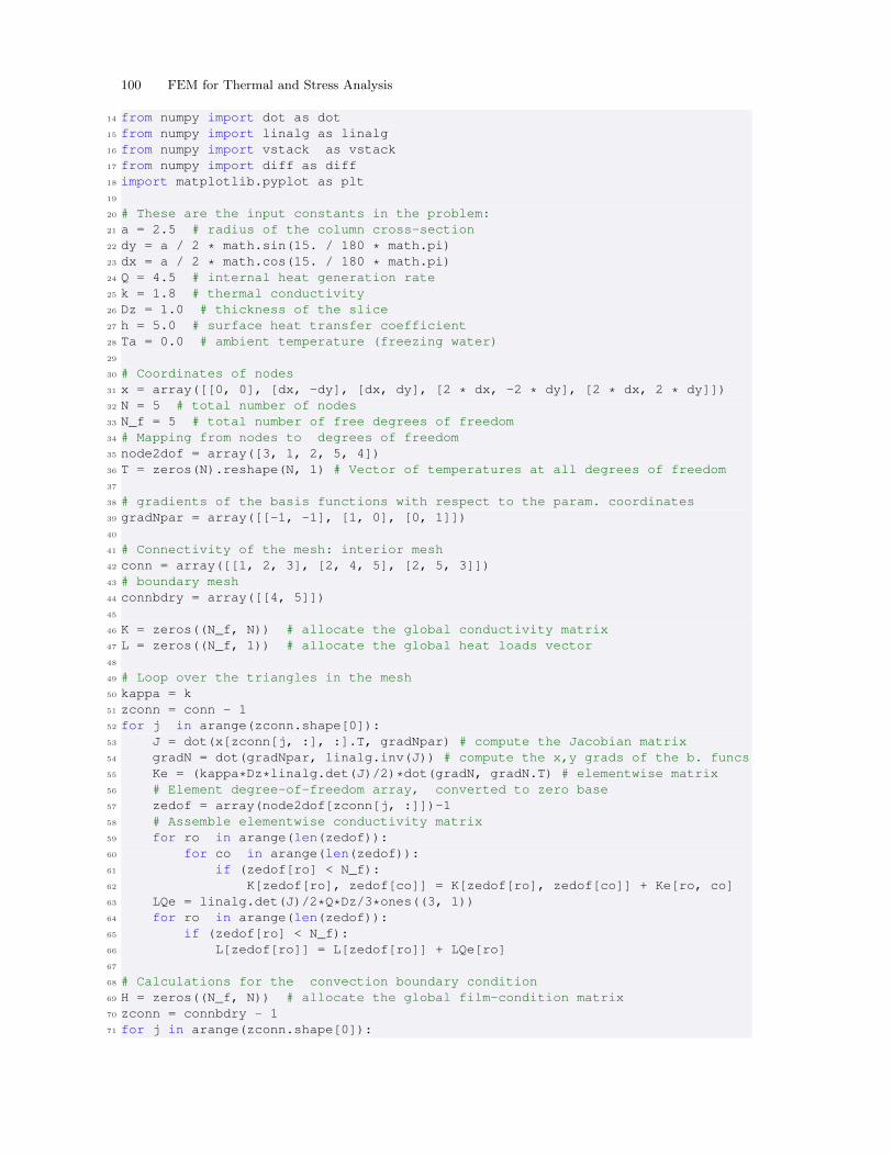
100 FEM for Thermal and Stress Analysis

14 from numpy import dot as dot15 from numpy import linalg as linalg16 from numpy import vstack as vstack17 from numpy import diff as diff18 import matplotlib.pyplot as plt19

20 # These are the input constants in the problem:21 a = 2.5 # radius of the column cross-section22 dy = a / 2 * math.sin(15. / 180 * math.pi)23 dx = a / 2 * math.cos(15. / 180 * math.pi)24 Q = 4.5 # internal heat generation rate25 k = 1.8 # thermal conductivity26 Dz = 1.0 # thickness of the slice27 h = 5.0 # surface heat transfer coefficient28 Ta = 0.0 # ambient temperature (freezing water)29

30 # Coordinates of nodes31 x = array([[0, 0], [dx, -dy], [dx, dy], [2 * dx, -2 * dy], [2 * dx, 2 * dy]])32 N = 5 # total number of nodes33 N_f = 5 # total number of free degrees of freedom34 # Mapping from nodes to degrees of freedom35 node2dof = array([3, 1, 2, 5, 4])36 T = zeros(N).reshape(N, 1) # Vector of temperatures at all degrees of freedom37

38 # gradients of the basis functions with respect to the param. coordinates39 gradNpar = array([[-1, -1], [1, 0], [0, 1]])40

41 # Connectivity of the mesh: interior mesh42 conn = array([[1, 2, 3], [2, 4, 5], [2, 5, 3]])43 # boundary mesh44 connbdry = array([[4, 5]])45

46 K = zeros((N_f, N)) # allocate the global conductivity matrix47 L = zeros((N_f, 1)) # allocate the global heat loads vector48

49 # Loop over the triangles in the mesh50 kappa = k51 zconn = conn - 152 for j in arange(zconn.shape[0]):53 J = dot(x[zconn[j, :], :].T, gradNpar) # compute the Jacobian matrix54 gradN = dot(gradNpar, linalg.inv(J)) # compute the x,y grads of the b. funcs55 Ke = (kappa*Dz*linalg.det(J)/2)*dot(gradN, gradN.T) # elementwise matrix56 # Element degree-of-freedom array, converted to zero base57 zedof = array(node2dof[zconn[j, :]])-158 # Assemble elementwise conductivity matrix59 for ro in arange(len(zedof)):60 for co in arange(len(zedof)):61 if (zedof[ro] < N_f):62 K[zedof[ro], zedof[co]] = K[zedof[ro], zedof[co]] + Ke[ro, co]63 LQe = linalg.det(J)/2*Q*Dz/3*ones((3, 1))64 for ro in arange(len(zedof)):65 if (zedof[ro] < N_f):66 L[zedof[ro]] = L[zedof[ro]] + LQe[ro]67

68 # Calculations for the convection boundary condition69 H = zeros((N_f, N)) # allocate the global film-condition matrix70 zconn = connbdry - 171 for j in arange(zconn.shape[0]):

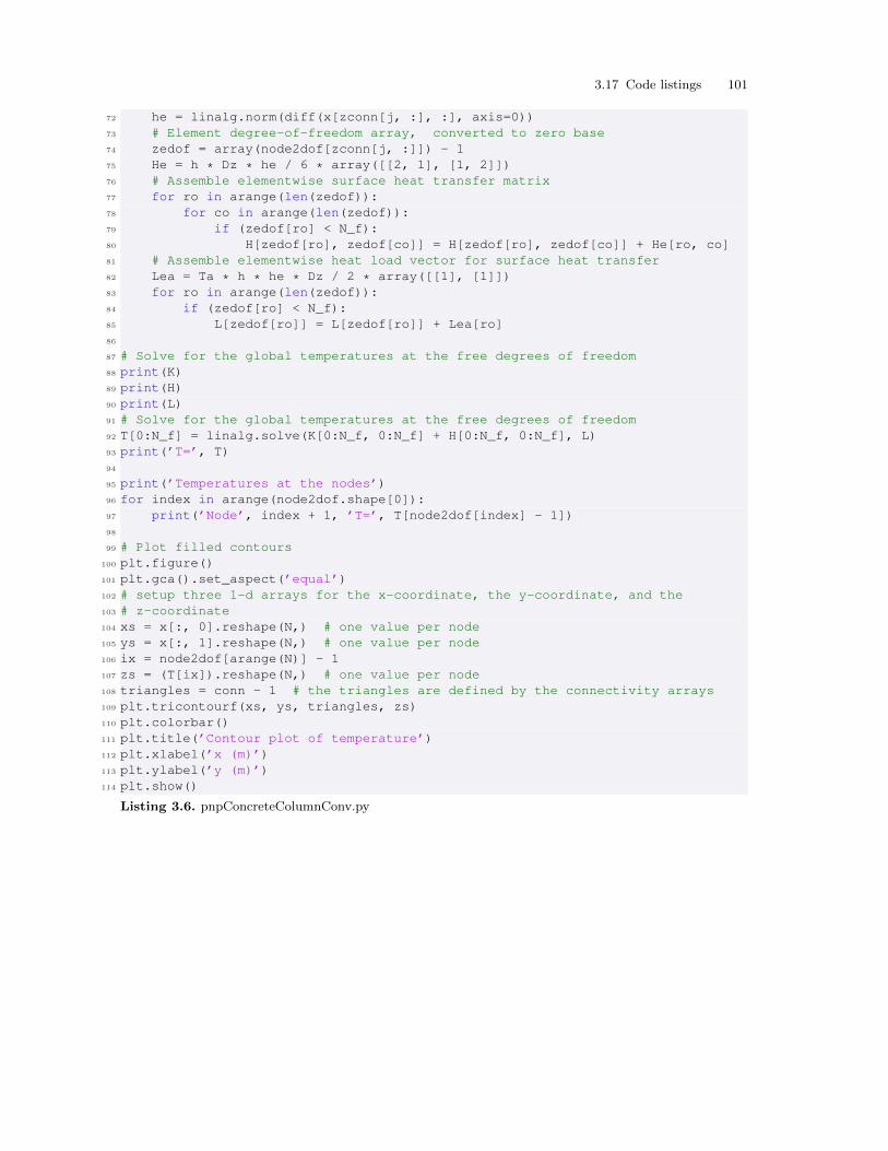
3.17 Code listings 101

72 he = linalg.norm(diff(x[zconn[j, :], :], axis=0))73 # Element degree-of-freedom array, converted to zero base74 zedof = array(node2dof[zconn[j, :]]) - 175 He = h * Dz * he / 6 * array([[2, 1], [1, 2]])76 # Assemble elementwise surface heat transfer matrix77 for ro in arange(len(zedof)):78 for co in arange(len(zedof)):79 if (zedof[ro] < N_f):80 H[zedof[ro], zedof[co]] = H[zedof[ro], zedof[co]] + He[ro, co]81 # Assemble elementwise heat load vector for surface heat transfer82 Lea = Ta * h * he * Dz / 2 * array([[1], [1]])83 for ro in arange(len(zedof)):84 if (zedof[ro] < N_f):85 L[zedof[ro]] = L[zedof[ro]] + Lea[ro]86

87 # Solve for the global temperatures at the free degrees of freedom88 print(K)89 print(H)90 print(L)91 # Solve for the global temperatures at the free degrees of freedom92 T[0:N_f] = linalg.solve(K[0:N_f, 0:N_f] + H[0:N_f, 0:N_f], L)93 print(’T=’, T)94

95 print(’Temperatures at the nodes’)96 for index in arange(node2dof.shape[0]):97 print(’Node’, index + 1, ’T=’, T[node2dof[index] - 1])98

99 # Plot filled contours100 plt.figure()101 plt.gca().set_aspect(’equal’)102 # setup three 1-d arrays for the x-coordinate, the y-coordinate, and the103 # z-coordinate104 xs = x[:, 0].reshape(N,) # one value per node105 ys = x[:, 1].reshape(N,) # one value per node106 ix = node2dof[arange(N)] - 1107 zs = (T[ix]).reshape(N,) # one value per node108 triangles = conn - 1 # the triangles are defined by the connectivity arrays109 plt.tricontourf(xs, ys, triangles, zs)110 plt.colorbar()111 plt.title(’Contour plot of temperature’)112 plt.xlabel(’x (m)’)113 plt.ylabel(’y (m)’)114 plt.show()

Listing 3.6. pnpConcreteColumnConv.py

4

FEA for 2-D Heat conduction with Quadrilaterals

Quadrilateral elements are an alternative to the triangles discussed in Chapter 3. The triangularelements are in a way too simple: the variation of temperature they can represent is not sufficientlyrich. We say that the triangles are “stiff”, which makes more sense when they are applied to stressanalysis, but the intuitive insight this word attempts to generate is hopefully clear.

Quadrilateral elements address the excessive stiffness of the triangular elements by coupling to-gether a larger number of nodes (four instead of three), which in the end leads to basis functionswhich are more than just linear polynomials. This endowes the finite element with that little some-thing that makes it more accurate.

4.1 Quadrilateral element

The element Q4 has four nodes, and its standard shape is a bi-unit square. This square is to beunderstood as the Cartesian product of two standard intervals (refer to Section 3.14.1). Therefore,the basis functions of Q4 may also be formed as products of the basis functions on the standardinterval L2 (3.106). Assuming the numbering of the nodes as shown in Figure 4.1, the basis functionN1 may be written as the product of the basis function on the interval −1 ≤ ξ ≤ +1 and thebasis function on the interval −1 ≤ η ≤ +1 where both functions correspond to the left-hand sideendpoint (ξ = −1, η = −1)

N1(ξ, η) =ξ − 1

−1− 1× η − 1

−1− 1=

(ξ − 1)(η − 1)

4. (4.1)

Similarly, for the remaining three functions we have

N2(ξ, η) =(ξ + 1)(η − 1)

−4, N3(ξ, η) =

(ξ + 1)(η + 1)

4, (4.2)

and

N4(ξ, η) =(ξ − 1)(η + 1)

−4. (4.3)

As all basis functions are linear in ξ and η, the shape that they represent when raised as a surfaceabove the standard square is a hyperbolic paraboloid.

The derivatives of the basis functions (i.e. the gradients of the basis functions) are computedin the standard way using equations (3.62). All we need is the gradient of the basis functions withrespect to the parametric coordinates

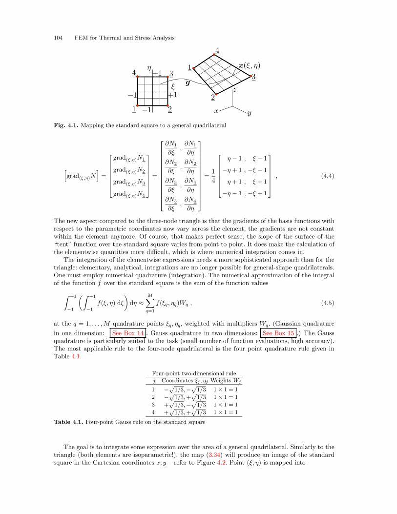
104 FEM for Thermal and Stress Analysis

Fig. 4.1. Mapping the standard square to a general quadrilateral

[grad(ξ,η)N

]=

grad(ξ,η)N1

grad(ξ,η)N2

grad(ξ,η)N3

grad(ξ,η)N4

=

∂N1

∂ξ,∂N1

∂η

∂N2

∂ξ,∂N2

∂η

∂N3

∂ξ,∂N4

∂η

∂N3

∂ξ,∂N4

∂η

=

1

4

η − 1 , ξ − 1

−η + 1 , −ξ − 1

η + 1 , ξ + 1

−η − 1 , −ξ + 1

, (4.4)

The new aspect compared to the three-node triangle is that the gradients of the basis functions withrespect to the parametric coordinates now vary across the element, the gradients are not constantwithin the element anymore. Of course, that makes perfect sense, the slope of the surface of the“tent” function over the standard square varies from point to point. It does make the calculation ofthe elementwise quantities more difficult, which is where numerical integration comes in.

The integration of the elementwise expressions needs a more sophisticated approach than for thetriangle: elementary, analytical, integrations are no longer possible for general-shape quadrilaterals.One must employ numerical quadrature (integration). The numerical approximation of the integralof the function f over the standard square is the sum of the function values∫ +1

−1

(∫ +1

−1

f(ξ, η) dξ

)dη ≈

M∑q=1

f(ξq, ηq)Wq , (4.5)

at the q = 1, . . . ,M quadrature points ξq, ηq, weighted with multipliers Wq. (Gaussian quadrature

in one dimension: See Box 14 . Gauss quadrature in two dimensions: See Box 15 .) The Gaussquadrature is particularly suited to the task (small number of function evaluations, high accuracy).The most applicable rule to the four-node quadrilateral is the four point quadrature rule given inTable 4.1.

Four-point two-dimensional rulej Coordinates ξj , ηj Weights Wj

1 −√

1/3,−√

1/3 1× 1 = 1

2 −√

1/3,+√

1/3 1× 1 = 1

3 +√

1/3,−√

1/3 1× 1 = 1

4 +√

1/3,+√

1/3 1× 1 = 1

Table 4.1. Four-point Gauss rule on the standard square

The goal is to integrate some expression over the area of a general quadrilateral. Similarly to thetriangle (both elements are isoparametric!), the map (3.34) will produce an image of the standardsquare in the Cartesian coordinates x, y – refer to Figure 4.2. Point (ξ, η) is mapped into

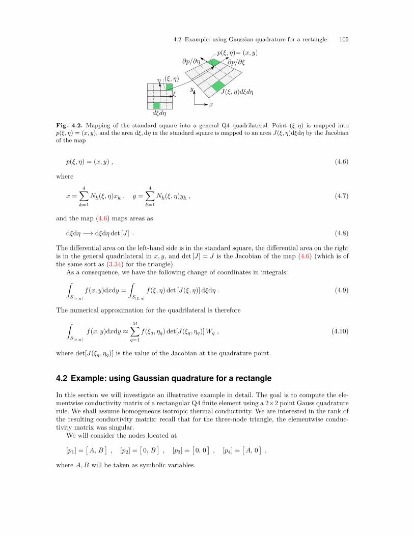
4.2 Example: using Gaussian quadrature for a rectangle 105

Fig. 4.2. Mapping of the standard square into a general Q4 quadrilateral. Point (ξ, η) is mapped intop(ξ, η) = (x, y), and the area dξ,dη in the standard square is mapped to an area J(ξ, η)dξdη by the Jacobianof the map

p(ξ, η) = (x, y) , (4.6)

where

x =

4∑k=1

Nk(ξ, η)xk , y =

4∑k=1

Nk(ξ, η)yk , (4.7)

and the map (4.6) maps areas as

dξdη −→ dξdη det [J ] . (4.8)

The differential area on the left-hand side is in the standard square, the differential area on the rightis in the general quadrilateral in x, y, and det [J ] = J is the Jacobian of the map (4.6) (which is ofthe same sort as (3.34) for the triangle).

As a consequence, we have the following change of coordinates in integrals:∫S[x,y]

f(x, y)dxdy =

∫S[ξ,η]

f(ξ, η) det [J(ξ, η)] dξdη . (4.9)

The numerical approximation for the quadrilateral is therefore∫S[x,y]

f(x, y)dxdy ≈M∑q=1

f(ξq, ηq) det[J(ξq, ηq)]Wq , (4.10)

where det[J(ξq, ηq)] is the value of the Jacobian at the quadrature point.

4.2 Example: using Gaussian quadrature for a rectangle

In this section we will investigate an illustrative example in detail. The goal is to compute the ele-mentwise conductivity matrix of a rectangular Q4 finite element using a 2×2 point Gauss quadraturerule. We shall assume homogeneous isotropic thermal conductivity. We are interested in the rank ofthe resulting conductivity matrix: recall that for the three-node triangle, the elementwise conduc-tivity matrix was singular.

We will consider the nodes located at

[p1] =[A, B

], [p2] =

[0, B

], [p3] =

[0, 0

], [p4] =

[A, 0

],

where A,B will be taken as symbolic variables.

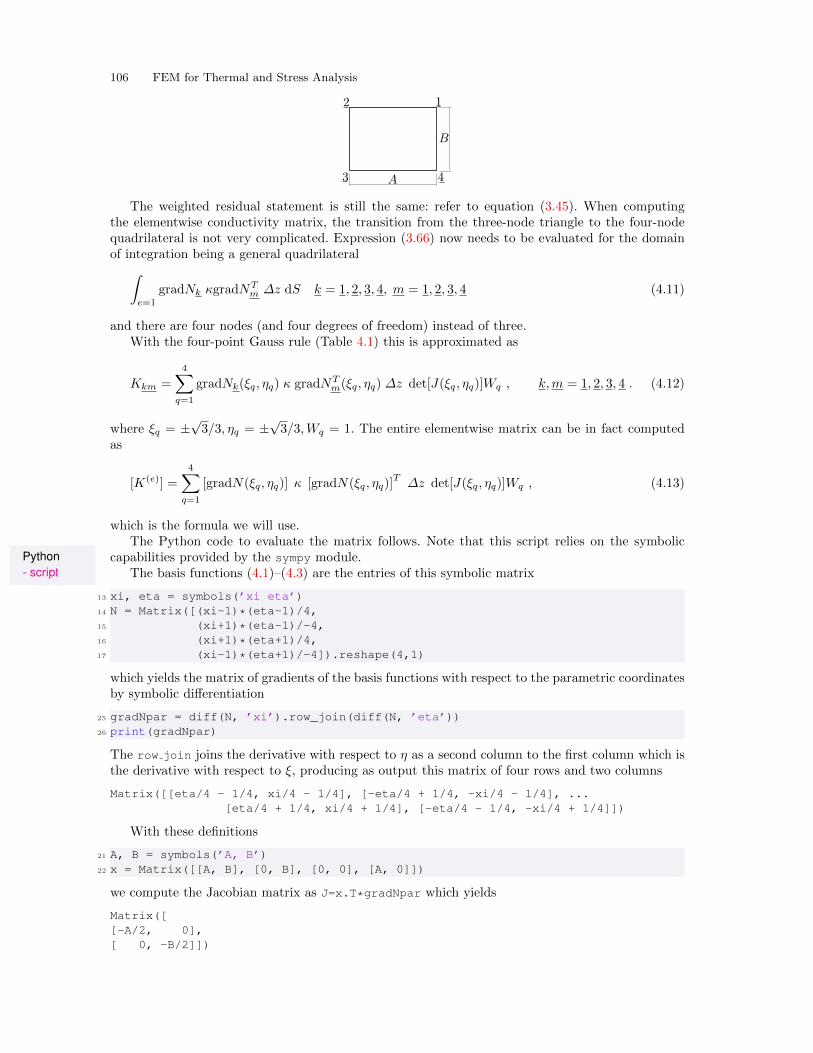
106 FEM for Thermal and Stress Analysis

The weighted residual statement is still the same: refer to equation (3.45). When computingthe elementwise conductivity matrix, the transition from the three-node triangle to the four-nodequadrilateral is not very complicated. Expression (3.66) now needs to be evaluated for the domainof integration being a general quadrilateral∫

e=1

gradNk κgradNTm ∆z dS k = 1, 2, 3, 4, m = 1, 2, 3, 4 (4.11)

and there are four nodes (and four degrees of freedom) instead of three.With the four-point Gauss rule (Table 4.1) this is approximated as

Kkm =

4∑q=1

gradNk(ξq, ηq) κ gradNTm(ξq, ηq) ∆z det[J(ξq, ηq)]Wq , k,m = 1, 2, 3, 4 . (4.12)

where ξq = ±√3/3, ηq = ±

√3/3,Wq = 1. The entire elementwise matrix can be in fact computed

as

[K(e)] =

4∑q=1

[gradN(ξq, ηq)] κ [gradN(ξq, ηq)]T∆z det[J(ξq, ηq)]Wq , (4.13)

which is the formula we will use.The Python code to evaluate the matrix follows. Note that this script relies on the symbolic

Python- script

capabilities provided by the sympy module.The basis functions (4.1)–(4.3) are the entries of this symbolic matrix

13 xi, eta = symbols(’xi eta’)14 N = Matrix([(xi-1)*(eta-1)/4,15 (xi+1)*(eta-1)/-4,16 (xi+1)*(eta+1)/4,17 (xi-1)*(eta+1)/-4]).reshape(4,1)

which yields the matrix of gradients of the basis functions with respect to the parametric coordinatesby symbolic differentiation

25 gradNpar = diff(N, ’xi’).row_join(diff(N, ’eta’))26 print(gradNpar)

The row join joins the derivative with respect to η as a second column to the first column which isthe derivative with respect to ξ, producing as output this matrix of four rows and two columns

Matrix([[eta/4 - 1/4, xi/4 - 1/4], [-eta/4 + 1/4, -xi/4 - 1/4], ...[eta/4 + 1/4, xi/4 + 1/4], [-eta/4 - 1/4, -xi/4 + 1/4]])

With these definitions

21 A, B = symbols(’A, B’)22 x = Matrix([[A, B], [0, B], [0, 0], [A, 0]])

we compute the Jacobian matrix as J=x.T*gradNpar which yields

Matrix([[-A/2, 0],[ 0, -B/2]])

4.2 Example: using Gaussian quadrature for a rectangle 107

and the Jacobian Jac=det(J) as A*B/4. We may note that the Jacobian is constant, which is whatwe would expect since the standard square is mapped into a rectangle: All right angles stay rightangles, and horizontal lines stretch by the same amount, and vertical lines also stretch by the sameamount everywhere.

The basis function gradients with respect to x, y may be evaluated from the general formula (3.62)

38 gradN = simplify(gradNpar*(J**-1))39 print(gradN)

resulting in

Matrix([[-(eta - 1)/(2*A), (-xi + 1)/(2*B)],[ (eta - 1)/(2*A), (xi + 1)/(2*B)],[-(eta + 1)/(2*A), -(xi + 1)/(2*B)],[ (eta + 1)/(2*A), (xi - 1)/(2*B)]])

We glean from the above that the x, y basis function gradients vary from point to point within theelement.

The conductivity matrix can be now evaluated. First we simplify by noting that κ,∆z, Wk = 1,and det[J(ξk, ηk)] = (AB)/4 are all constants and therefore may be taken out of the sum of thenumerical quadrature . The four-point integration needs to be carried out only on the product ofthe gradients, which change from quadrature point to quadrature point, and yields the intermediateresult (note the use of subs() to evaluate the basis function gradient expressions for particularvalues of ξ, η)

50 gN = gradN.subs(xi, -0.577350269189626).subs(eta, -0.577350269189626)51 K1 = kap*Dz*Jac*gN*gN.T # term 1 of the sum52 gN = gradN.subs(xi, -0.577350269189626).subs(eta, +0.577350269189626)53 K2 = kap*Dz*Jac*gN*gN.T # term 2 of the sum54 gN = gradN.subs(xi, +0.577350269189626).subs(eta, -0.577350269189626)55 K3 = kap*Dz*Jac*gN*gN.T # term 3 of the sum56 gN = gradN.subs(xi, +0.577350269189626).subs(eta, +0.577350269189626)57 K4 = kap*Dz*Jac*gN*gN.T # term 4 of the sum

and further adding together the intermediate results from the for quadrature points

59 K = simplify(K1+K2+K3+K4)60 print(K)

(note the use of simplify() to produce an uncluttered expression) gives, with a little bit of manualediting,

kap*Dz/(A*B)/6*Matrix([[ 2*(A**2 + B**2), (*A**2 - 2*B**2), -(A**2 + B**2), (-2*A**2 + B**2)],[ (A**2 - 2*B**2), 2*(A**2 + B**2), (-2*A**2 + B**2), -(A**2 + B**2)],[ -(A**2 + B**2), (-2*A**2 + B**2), 2*(A**2 + B**2), (A**2 - 2*B**2)],[(-2*A**2 + B**2), -(A**2 + B**2), (A**2 - 2*B**2), 2*(A**2 + B**2)]])

where we have shortened the output by hand by replacing 0.333333333333333 with 1/3, and0.166666666666667 with 1/6. This can be cleaned up as

[K(e)

]=κ∆z

6AB

2A2 + 2B2, A2 − 2B2, −A2 −B2, B2 − 2A2

A2 − 2B2, 2A2 + 2B2, B2 − 2A2, −A2 −B2

−A2 −B2, B2 − 2A2, 2A2 + 2B2, A2 − 2B2

B2 − 2A2, −A2 −B2, A2 − 2B2, 2A2 + 2B2

(4.14)

The elementwise conductivity matrix[K(e)

]has a rank equal to the number of nonzero eigen-

values. With Python we find the eigenvalues of this matrix as K.eigenvals() which yields

{B*Dz*kap/A: 1, A*Dz*kap/B: 1, (A**2*Dz*kap + B**2*Dz*kap)/(3*A*B): 1, 0: 1}

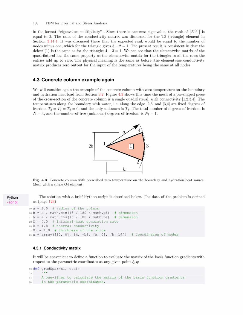
108 FEM for Thermal and Stress Analysis

in the format “eigenvalue: multiplicity” . Since there is one zero eigenvalue, the rank of[K(e)

]is

equal to 3. The rank of the conductivity matrix was discussed for the T3 (triangle) element inSection 3.14.4. It was discussed there that the expected rank would be equal to the number ofnodes minus one, which for the triangle gives 3− 2 = 1. The present result is consistent in that thedefect (1) is the same as for the triangle: 4− 3 = 1. We can see that the elementwise matrix of thequadrilateral has the same property as the elementwise matrix for the triangle: in all the rows theentries add up to zero. The physical meaning is the same as before: the elementwise conductivitymatrix produces zero output for the input of the temperatures being the same at all nodes.

4.3 Concrete column example again

We will consider again the example of the concrete column with zero temperature on the boundaryand hydration heat load from Section 3.7. Figure 4.3 shows this time the mesh of a pie-shaped pieceof the cross-section of the concrete column is a single quadrilateral, with connectivity [1,2,3,4]. Thetemperatures along the boundary with water, i.e. along the edge [2,3] and [3,4] are fixed degrees offreedom T2 = T3 = T4 = 0, and the only unknown is T1. The total number of degrees of freedom isN = 4, and the number of free (unknown) degrees of freedom is Nf = 1.

Fig. 4.3. Concrete column with prescribed zero temperature on the boundary and hydration heat source.Mesh with a single Q4 element.

Python- script

The solution with a brief Python script is described below. The data of the problem is definedas (page 123)

19 a = 2.5 # radius of the column20 b = a * math.sin(15 / 180 * math.pi) # dimension21 h = a * math.cos(15 / 180 * math.pi) # dimension22 Q = 4.5 # internal heat generation rate23 k = 1.8 # thermal conductivity24 Dz = 1.0 # thickness of the slice25 x = array([[0, 0], [h, -b], [a, 0], [h, b]]) # Coordinates of nodes

4.3.1 Conductivity matrix

It will be convenient to define a function to evaluate the matrix of the basis function gradients withrespect to the parametric coordinates at any given point ξ, η:

32 def gradNpar(xi, eta):33 """34 A one-liner to calculate the matrix of the basis function gradients35 in the parametric coordinates.

4.3 Concrete column example again 109

36 """37 return array([38 [eta / 4 - 1. / 4, xi / 4 - 1. / 4],39 [1. / 4 - eta / 4, - xi / 4 - 1. / 4],40 [eta / 4 + 1. / 4, xi / 4 + 1. / 4],41 [- eta / 4 - 1. / 4, 1. / 4 - xi / 4]])

The 2×2 Gauss rule (Table 4.1) will be used for the elementwise quantities. It is the default for thistype of element in Abaqus. The locations and the weights are defined as

52 xe = array([[-0.577350269189626, -0.577350269189626],53 [-0.577350269189626, +0.577350269189626],54 [+0.577350269189626, -0.577350269189626],55 [+0.577350269189626, +0.577350269189626]])56 W = array([1, 1, 1, 1])

The task is to compute the elementwise conductivity matrix

[K(e)] =

∫e=1

[gradN ] κ[gradN ]T ∆z dS (4.15)

which is an expression analogous to (3.71) but of dimension 4 × 4, using the numerical approxi-mation (4.13). This will be accomplished in the integration loop over the four quadrature pointsof the Gauss rule. Inside the loop we will be building up the elementwise conductivity matrix onequadrature point at a time, and therefore we need a preallocated array to which the intermediateresults will be added (page 123).

60 Ke = zeros((4, 4))

In the loop we start by setting the parametric coordinates of the quadrature point, and calculatingthe Jacobian matrix at that point from (3.60).

63 for qp in arange(xe.shape[0]):64 xi = xe[qp, 0]65 eta = xe[qp, 1]66 # Compute the Jacobian matrix67 J = dot(x.T, gradNpar(xi, eta))

From the Jacobian matrix, we calculate the Jacobian. It varies from quadrature point to quadraturepoint, with the minimum value of 0.1868 (at the fourth quadrature point) and the maximum valueof 0.6220 (at the first quadrature point).

69 detJ = linalg.det(J)

The gradient of the basis functions is calculated using the standard expression (3.62)

71 gradN = dot(gradNpar(xi, eta), linalg.inv(J))

Now we can add the contribution from the quadrature point to the preallocated elementwise matrixKe.

73 Ke = Ke + k * Dz * dot(gradN, gradN.T) * detJ * W[qp]

The interior of the loop is executed four times, once for each quadrature point. The finished elemen-twise conductivity matrix is

array([[ 0.46772756, -0.02719481, -0.41333794, -0.02719481],[-0.02719481, 2.13771962, -0.77091145, -1.33961336],[-0.41333794, -0.77091145, 1.95516084, -0.77091145],[-0.02719481, -1.33961336, -0.77091145, 2.13771962]])

110 FEM for Thermal and Stress Analysis

4.3.2 Heat load vector and solution

Now analogously to the heat load vector calculation in Section 3.11 we need to evaluate (3.74), whichcan be written as a matrix expression∫

e=1

[N ]Q ∆z dS (4.16)

where [N ] is the matrix that consists of the four basis functions on the quadrilateral in the rows. Ofcourse, the integral will again be approximated with numerical quadrature∫

e=1

[N ]Q ∆z dS ≈4∑

q=1

[N(ξq, ηq)]Q ∆z det[J(ξq, ηq)]Wq , (4.17)

This little helper function will evaluate the column array of the basis function values at any quadra-ture point:

82 def N(xi, eta):83 """84 A one-liner to calculate the matrix of the basis function values.85 """86 return array([(xi - 1) * (eta - 1) / 4,87 (xi + 1) * (eta - 1) / -4,88 (xi + 1) * (eta + 1) / 4,89 (xi - 1) * (eta + 1) / -4]).reshape(4, 1)

Now we are ready to start the quadrature point loop. Again, the load vector is preallocated in thecorrect size, Le=zeros(4).reshape(4,1). We will need the Jacobian (the first few lines of this looplook precisely like the ones for the conductivity matrix above), and then according to the formulawe need to add the contribution from (4.17)

104 Le = Le + Q * Dz * N(xi, eta) * detJ * W[qp]

for each quadrature point qp. The result of the integration is the elementwise load vector

array([[ 2.38508927],[ 1.81982141],[ 1.25455355],[ 1.81982141]])

Notice that the largest contribution of the heat load density Q is to the degree of freedom at thefirst node, and the smallest is to the degree of freedom at the third node. This corresponds to themagnitudes of the Jacobians we inspected above: the quadrature point closest to node 1 has thelargest value of the Jacobian, and the quadrature point closest to node 3 has the smallest value ofthe Jacobian.

Because of the simplicity of the present FE mesh, the entry K[0,0] of the elementwise conduc-tivity matrix is the entire free-free global conductivity matrix, and the entry L[0] of the elementwiseload vector is the entire global load vector. The solution for the only degree of freedom then followsas

114 T = zeros((4, 1))115 # Solve the global equations116 T[0] = (1 / K[0, 0]) * L[0]

which results in the temperature 5.0993 for the only free degree of freedom. Clearly, compared tothe exact value, the solution is not very good. But the mesh is not very good, so we cannot ask toomuch of it.

4.3 Concrete column example again 111

4.3.3 Postprocessing

In this section we will evaluate the heat flux at the quadrature points. This is often called thepostprocessing step: the solution has already been obtained, we will merely process it to extractsome more information.

The gradient of the temperature at any quadrature point can be calculated using the definitionof the interpolated temperature within the element:

T (ξ, η) =

N∑i=1

Ni(ξ, η)Ti (4.18)

as

gradT (ξ, η) = grad

(N∑i=1

Ni(ξ, η)Ti

)=

N∑i=1

Ti gradNi(ξ, η) = [T ]T[gradN(ξ, η)] (4.19)

where the last expression is a matrix multiplication, of the matrix of the degrees of freedom valuesand the matrix of the basis function gradients. Note that the matrix of the basis function gradientsdepends on where in the element the gradients are evaluated. The postprocessing for the heat fluxvectors is again performed in a loop (page 123)

124 for qp in arange(xe.shape[0]):125 xi = xe[qp, 0]126 eta = xe[qp, 1]127 # Compute the location of the quadrature point128 qploc = dot(N(xi, eta).T, x)

where the location of the quadrature point in the global coordinates qploc also calculated to allowus to plot the results.

We need the gradients of the basis functions:

130 J = dot(x.T, gradNpar(xi, eta))131 # The gradient of the basis functions with respect to x, y132 gradN = dot(gradNpar(xi, eta), linalg.inv(J))

It remains to calculate the gradient of the temperature and the heat flux, and to print out theresults:

134 gradT = dot(T.T, gradN)135 # Heat flux vector136 q = -k * gradT.T137 print(’Heat flux at’, qploc, ’ = ’, q)

For the four quadrature points we get the following output:

Heat flux at [[ 0.91658369 0. ]] = [[ 3.76543041][-0. ]]Heat flux at [[ 2.02654304 0.37357311]] = [[ 3.67150541][ 0.27906968]]Heat flux at [[ 2.02654304 -0.37357311]] = [[ 3.67150541][-0.27906968]]Heat flux at [[ 2.35995936 0. ]] = [[ 3.35882447][-0. ]]

The calculated heat flux vectors are visualized in Figure 4.4. Notice that the results are relativelycrude: we would expect the heat flux vectors to become shorter towards the center whereas theopposite is true for this very coarse mesh.

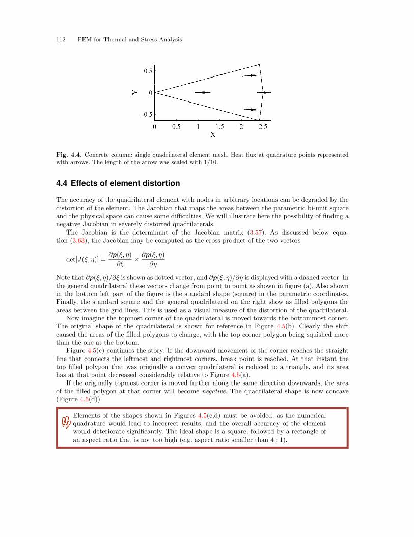
112 FEM for Thermal and Stress Analysis

Fig. 4.4. Concrete column: single quadrilateral element mesh. Heat flux at quadrature points representedwith arrows. The length of the arrow was scaled with 1/10.

4.4 Effects of element distortion

The accuracy of the quadrilateral element with nodes in arbitrary locations can be degraded by thedistortion of the element. The Jacobian that maps the areas between the parametric bi-unit squareand the physical space can cause some difficulties. We will illustrate here the possibility of finding anegative Jacobian in severely distorted quadrilaterals.

The Jacobian is the determinant of the Jacobian matrix (3.57). As discussed below equa-tion (3.63), the Jacobian may be computed as the cross product of the two vectors

det[J(ξ, η)] =∂p(ξ, η)

∂ξ× ∂p(ξ, η)

∂η

Note that ∂p(ξ, η)/∂ξ is shown as dotted vector, and ∂p(ξ, η)/∂η is displayed with a dashed vector. Inthe general quadrilateral these vectors change from point to point as shown in figure (a). Also shownin the bottom left part of the figure is the standard shape (square) in the parametric coordinates.Finally, the standard square and the general quadrilateral on the right show as filled polygons theareas between the grid lines. This is used as a visual measure of the distortion of the quadrilateral.

Now imagine the topmost corner of the quadrilateral is moved towards the bottommost corner.The original shape of the quadrilateral is shown for reference in Figure 4.5(b). Clearly the shiftcaused the areas of the filled polygons to change, with the top corner polygon being squished morethan the one at the bottom.

Figure 4.5(c) continues the story: If the downward movement of the corner reaches the straightline that connects the leftmost and rightmost corners, break point is reached. At that instant thetop filled polygon that was originally a convex quadrilateral is reduced to a triangle, and its areahas at that point decreased considerably relative to Figure 4.5(a).

If the originally topmost corner is moved further along the same direction downwards, the areaof the filled polygon at that corner will become negative. The quadrilateral shape is now concave(Figure 4.5(d)).

Elements of the shapes shown in Figures 4.5(c,d) must be avoided, as the numericalquadrature would lead to incorrect results, and the overall accuracy of the elementwould deteriorate significantly. The ideal shape is a square, followed by a rectangle ofan aspect ratio that is not too high (e.g. aspect ratio smaller than 4 : 1).

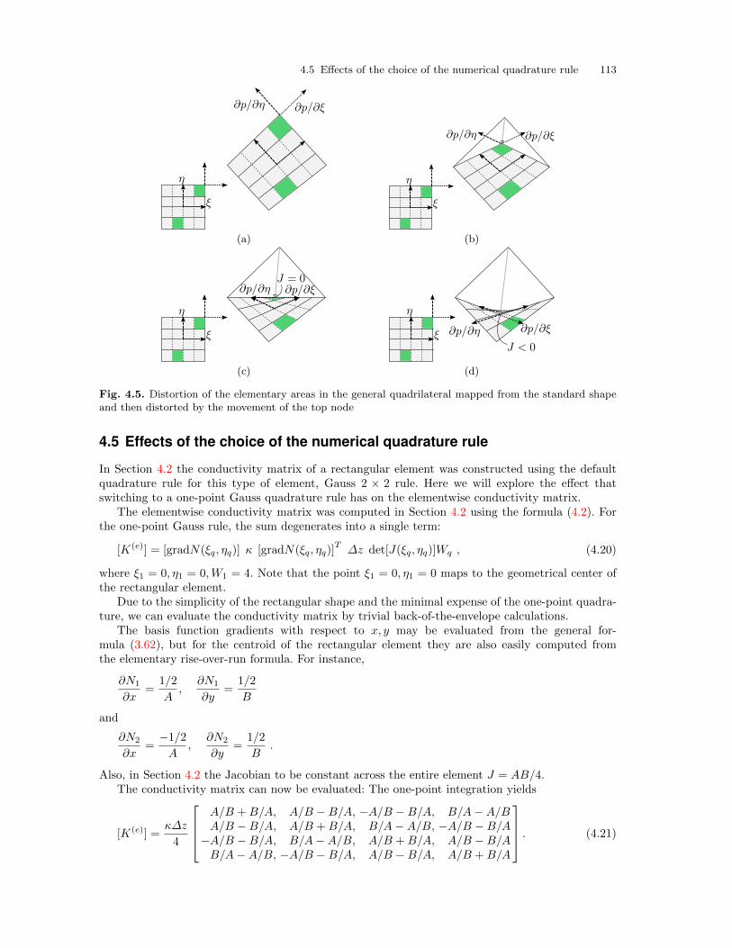
4.5 Effects of the choice of the numerical quadrature rule 113

(a) (b)

(c) (d)

Fig. 4.5. Distortion of the elementary areas in the general quadrilateral mapped from the standard shapeand then distorted by the movement of the top node

4.5 Effects of the choice of the numerical quadrature rule

In Section 4.2 the conductivity matrix of a rectangular element was constructed using the defaultquadrature rule for this type of element, Gauss 2 × 2 rule. Here we will explore the effect thatswitching to a one-point Gauss quadrature rule has on the elementwise conductivity matrix.

The elementwise conductivity matrix was computed in Section 4.2 using the formula (4.2). Forthe one-point Gauss rule, the sum degenerates into a single term:

[K(e)] = [gradN(ξq, ηq)] κ [gradN(ξq, ηq)]T∆z det[J(ξq, ηq)]Wq , (4.20)

where ξ1 = 0, η1 = 0,W1 = 4. Note that the point ξ1 = 0, η1 = 0 maps to the geometrical center ofthe rectangular element.

Due to the simplicity of the rectangular shape and the minimal expense of the one-point quadra-ture, we can evaluate the conductivity matrix by trivial back-of-the-envelope calculations.

The basis function gradients with respect to x, y may be evaluated from the general for-mula (3.62), but for the centroid of the rectangular element they are also easily computed fromthe elementary rise-over-run formula. For instance,

∂N1

∂x=

1/2

A,

∂N1

∂y=

1/2

B

and

∂N2

∂x=

−1/2

A,

∂N2

∂y=

1/2

B.

Also, in Section 4.2 the Jacobian to be constant across the entire element J = AB/4.The conductivity matrix can now be evaluated: The one-point integration yields

[K(e)] =κ∆z

4

A/B +B/A, A/B −B/A, −A/B −B/A, B/A−A/BA/B −B/A, A/B +B/A, B/A−A/B, −A/B −B/A

−A/B −B/A, B/A−A/B, A/B +B/A, A/B −B/AB/A−A/B, −A/B −B/A, A/B −B/A, A/B +B/A

. (4.21)

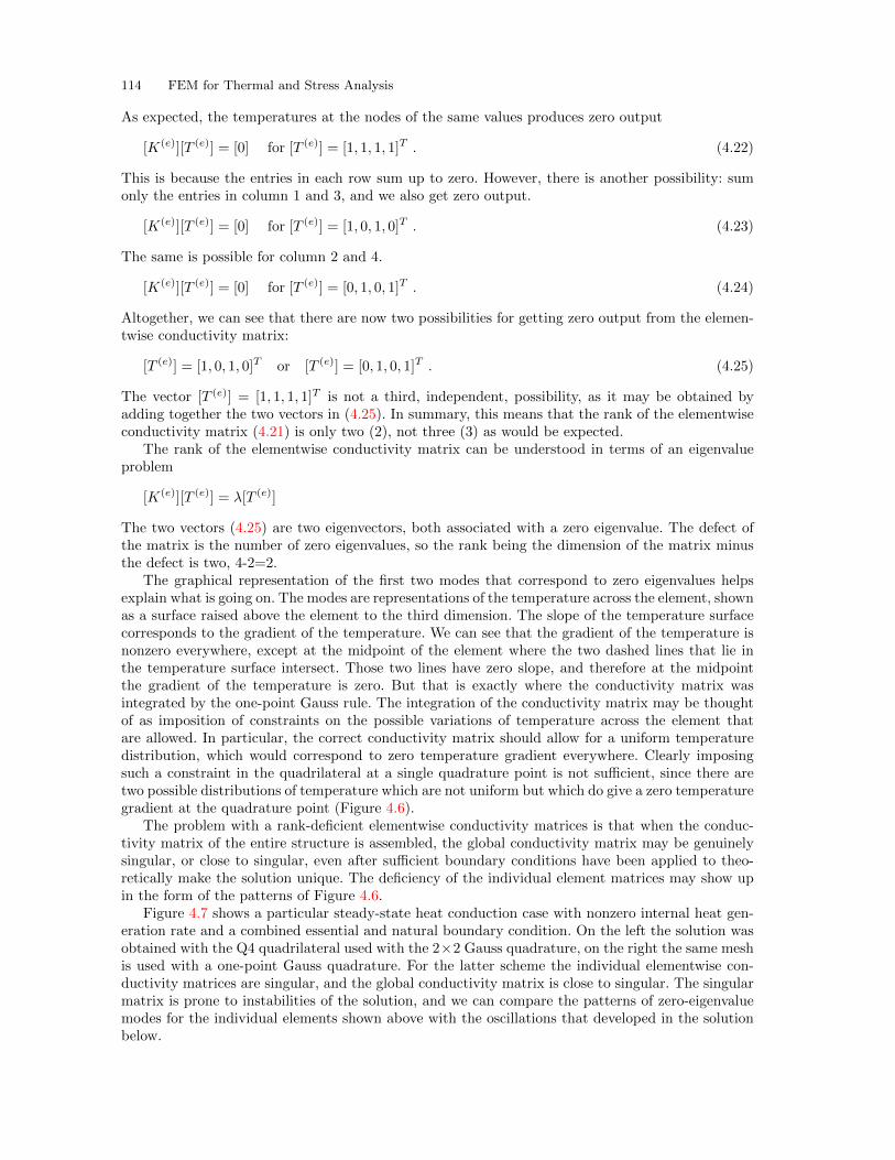
114 FEM for Thermal and Stress Analysis

As expected, the temperatures at the nodes of the same values produces zero output

[K(e)][T (e)] = [0] for [T (e)] = [1, 1, 1, 1]T . (4.22)

This is because the entries in each row sum up to zero. However, there is another possibility: sumonly the entries in column 1 and 3, and we also get zero output.

[K(e)][T (e)] = [0] for [T (e)] = [1, 0, 1, 0]T . (4.23)

The same is possible for column 2 and 4.

[K(e)][T (e)] = [0] for [T (e)] = [0, 1, 0, 1]T . (4.24)

Altogether, we can see that there are now two possibilities for getting zero output from the elemen-twise conductivity matrix:

[T (e)] = [1, 0, 1, 0]T or [T (e)] = [0, 1, 0, 1]T . (4.25)

The vector [T (e)] = [1, 1, 1, 1]T is not a third, independent, possibility, as it may be obtained byadding together the two vectors in (4.25). In summary, this means that the rank of the elementwiseconductivity matrix (4.21) is only two (2), not three (3) as would be expected.

The rank of the elementwise conductivity matrix can be understood in terms of an eigenvalueproblem

[K(e)][T (e)] = λ[T (e)]

The two vectors (4.25) are two eigenvectors, both associated with a zero eigenvalue. The defect ofthe matrix is the number of zero eigenvalues, so the rank being the dimension of the matrix minusthe defect is two, 4-2=2.

The graphical representation of the first two modes that correspond to zero eigenvalues helpsexplain what is going on. The modes are representations of the temperature across the element, shownas a surface raised above the element to the third dimension. The slope of the temperature surfacecorresponds to the gradient of the temperature. We can see that the gradient of the temperature isnonzero everywhere, except at the midpoint of the element where the two dashed lines that lie inthe temperature surface intersect. Those two lines have zero slope, and therefore at the midpointthe gradient of the temperature is zero. But that is exactly where the conductivity matrix wasintegrated by the one-point Gauss rule. The integration of the conductivity matrix may be thoughtof as imposition of constraints on the possible variations of temperature across the element thatare allowed. In particular, the correct conductivity matrix should allow for a uniform temperaturedistribution, which would correspond to zero temperature gradient everywhere. Clearly imposingsuch a constraint in the quadrilateral at a single quadrature point is not sufficient, since there aretwo possible distributions of temperature which are not uniform but which do give a zero temperaturegradient at the quadrature point (Figure 4.6).

The problem with a rank-deficient elementwise conductivity matrices is that when the conduc-tivity matrix of the entire structure is assembled, the global conductivity matrix may be genuinelysingular, or close to singular, even after sufficient boundary conditions have been applied to theo-retically make the solution unique. The deficiency of the individual element matrices may show upin the form of the patterns of Figure 4.6.

Figure 4.7 shows a particular steady-state heat conduction case with nonzero internal heat gen-eration rate and a combined essential and natural boundary condition. On the left the solution wasobtained with the Q4 quadrilateral used with the 2×2 Gauss quadrature, on the right the same meshis used with a one-point Gauss quadrature. For the latter scheme the individual elementwise con-ductivity matrices are singular, and the global conductivity matrix is close to singular. The singularmatrix is prone to instabilities of the solution, and we can compare the patterns of zero-eigenvaluemodes for the individual elements shown above with the oscillations that developed in the solutionbelow.

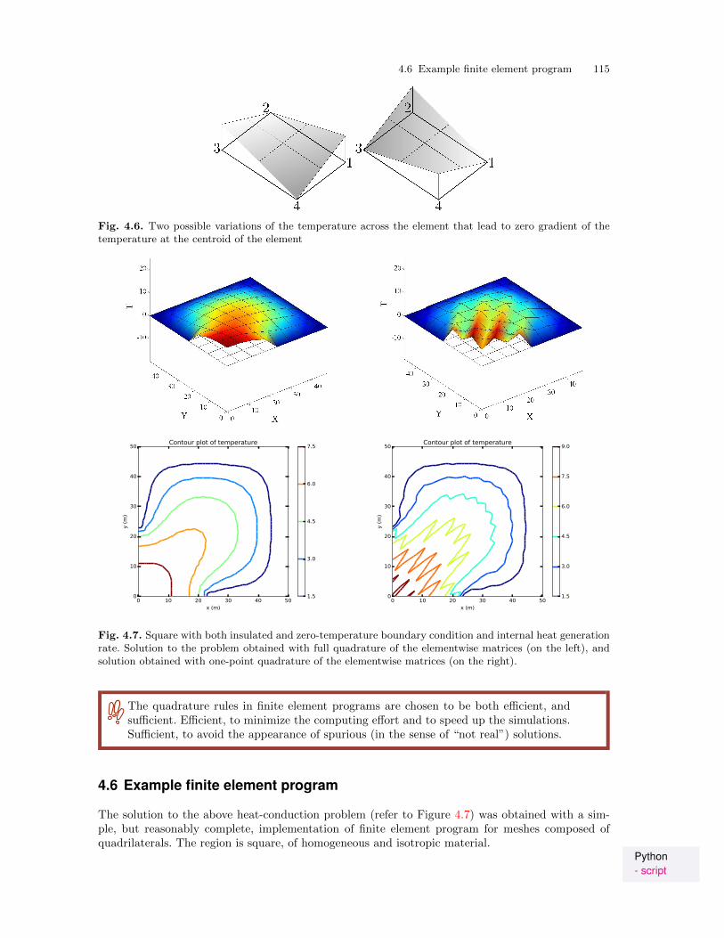
4.6 Example finite element program 115

Fig. 4.6. Two possible variations of the temperature across the element that lead to zero gradient of thetemperature at the centroid of the element

0 10 20 30 40 50x (m)

0

10

20

30

40

50

y (m)

Contour plot of temperature

1.5

3.0

4.5

6.0

7.5

0 10 20 30 40 50x (m)

0

10

20

30

40

50

y (m)

Contour plot of temperature

1.5

3.0

4.5

6.0

7.5

9.0

Fig. 4.7. Square with both insulated and zero-temperature boundary condition and internal heat generationrate. Solution to the problem obtained with full quadrature of the elementwise matrices (on the left), andsolution obtained with one-point quadrature of the elementwise matrices (on the right).

The quadrature rules in finite element programs are chosen to be both efficient, andsufficient. Efficient, to minimize the computing effort and to speed up the simulations.Sufficient, to avoid the appearance of spurious (in the sense of “not real”) solutions.

4.6 Example finite element program

The solution to the above heat-conduction problem (refer to Figure 4.7) was obtained with a sim-ple, but reasonably complete, implementation of finite element program for meshes composed ofquadrilaterals. The region is square, of homogeneous and isotropic material.

Python- script

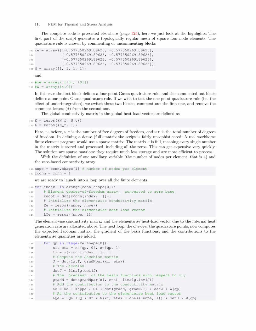
116 FEM for Thermal and Stress Analysis

The complete code is presented elsewhere (page 125), here we just look at the highlights: Thefirst part of the script generates a topologically regular mesh of square four-node elements. Thequadrature rule is chosen by commenting or uncommenting blocks

103 xe = array([[-0.577350269189626, -0.577350269189626],104 [-0.577350269189626, +0.577350269189626],105 [+0.577350269189626, -0.577350269189626],106 [+0.577350269189626, +0.577350269189626]])107 W = array([1, 1, 1, 1])

and

110 #xe = array([[+0., +0]])111 #W = array([4.0])

In this case the first block defines a four point Gauss quadrature rule, and the commented-out blockdefines a one-point Gauss quadrature rule. If we wish to test the one-point quadrature rule (i.e. theeffect of underintegration), we switch these two blocks: comment out the first one, and remove thecomment letters (#) from the second one.

The global conductivity matrix in the global heat load vector are defined as

109 K = zeros((N_f, N_t))110 L = zeros((N_f, 1))

Here, as before, N f is the number of free degrees of freedom, and N t is the total number of degreesof freedom. In defining a dense (full) matrix the script is fairly unsophisticated. A real workhorsefinite element program would use a sparse matrix. The matrix K is full, meaning every single numberin the matrix is stored and processed, including all the zeros. This can get expensive very quickly.The solution are sparse matrices: they require much less storage and are more efficient to process.

With the definition of one auxiliary variable (the number of nodes per element, that is 4) andthe zero-based connectivity array

116 nnpe = conn.shape[1] # number of nodes per element117 zconn = conn - 1

we are ready to launch into a loop over all the finite elements

118 for index in arange(conn.shape[0]):119 # Element degree-of-freedom array, converted to zero base120 zedof = dof[zconn[index, :]]-1121 # Initialize the elementwise conductivity matrix.122 Ke = zeros((nnpe, nnpe))123 # Initialize the elementwise heat load vector124 LQe = zeros((nnpe, 1))

The elementwise conductivity matrix and the elementwise heat-load vector due to the internal heatgeneration rate are allocated above. The next loop, the one over the quadrature points, now computesthe expected Jacobian matrix, the gradient of the basis functions, and the contributions to theelementwise quantities are added.

126 for qp in range(xe.shape[0]):127 xi, eta = xe[qp, 0], xe[qp, 1]128 lx = x[zconn[index, :], :]129 # Compute the Jacobian matrix130 J = dot(lx.T, gradNpar(xi, eta))131 # The Jacobian132 detJ = linalg.det(J)133 # The gradient of the basis functions with respect to x,y134 gradN = dot(gradNpar(xi, eta), linalg.inv(J))135 # Add the contribution to the conductivity matrix136 Ke = Ke + kappa * Dz * dot(gradN, gradN.T) * detJ * W[qp]137 # At the contribution to the elementwise heat load vector138 LQe = LQe + Q * Dz * N(xi, eta) * ones((nnpe, 1)) * detJ * W[qp]

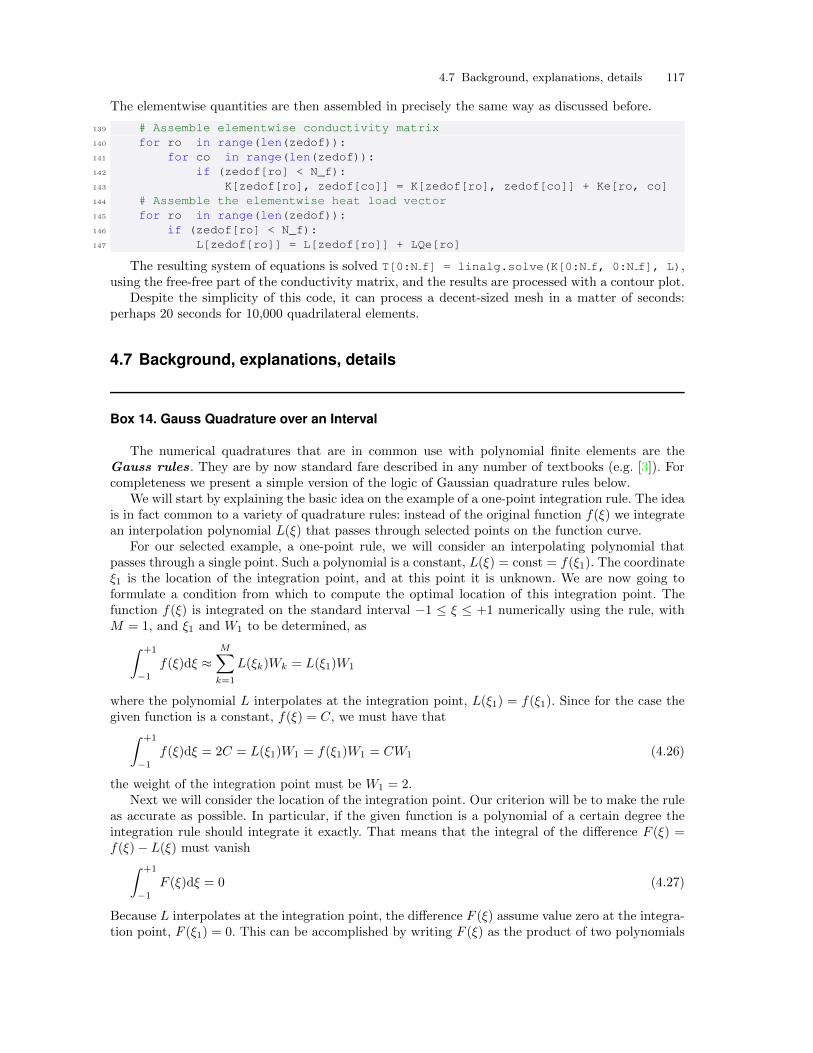
4.7 Background, explanations, details 117

The elementwise quantities are then assembled in precisely the same way as discussed before.

139 # Assemble elementwise conductivity matrix140 for ro in range(len(zedof)):141 for co in range(len(zedof)):142 if (zedof[ro] < N_f):143 K[zedof[ro], zedof[co]] = K[zedof[ro], zedof[co]] + Ke[ro, co]144 # Assemble the elementwise heat load vector145 for ro in range(len(zedof)):146 if (zedof[ro] < N_f):147 L[zedof[ro]] = L[zedof[ro]] + LQe[ro]

The resulting system of equations is solved T[0:N f] = linalg.solve(K[0:N f, 0:N f], L),using the free-free part of the conductivity matrix, and the results are processed with a contour plot.

Despite the simplicity of this code, it can process a decent-sized mesh in a matter of seconds:perhaps 20 seconds for 10,000 quadrilateral elements.

4.7 Background, explanations, details

Box 14. Gauss Quadrature over an Interval

The numerical quadratures that are in common use with polynomial finite elements are theGauss rules. They are by now standard fare described in any number of textbooks (e.g. [3]). Forcompleteness we present a simple version of the logic of Gaussian quadrature rules below.

We will start by explaining the basic idea on the example of a one-point integration rule. The ideais in fact common to a variety of quadrature rules: instead of the original function f(ξ) we integratean interpolation polynomial L(ξ) that passes through selected points on the function curve.

For our selected example, a one-point rule, we will consider an interpolating polynomial thatpasses through a single point. Such a polynomial is a constant, L(ξ) = const = f(ξ1). The coordinateξ1 is the location of the integration point, and at this point it is unknown. We are now going toformulate a condition from which to compute the optimal location of this integration point. Thefunction f(ξ) is integrated on the standard interval −1 ≤ ξ ≤ +1 numerically using the rule, withM = 1, and ξ1 and W1 to be determined, as∫ +1

−1

f(ξ)dξ ≈M∑k=1

L(ξk)Wk = L(ξ1)W1

where the polynomial L interpolates at the integration point, L(ξ1) = f(ξ1). Since for the case thegiven function is a constant, f(ξ) = C, we must have that∫ +1

−1

f(ξ)dξ = 2C = L(ξ1)W1 = f(ξ1)W1 = CW1 (4.26)

the weight of the integration point must be W1 = 2.Next we will consider the location of the integration point. Our criterion will be to make the rule

as accurate as possible. In particular, if the given function is a polynomial of a certain degree theintegration rule should integrate it exactly. That means that the integral of the difference F (ξ) =f(ξ)− L(ξ) must vanish∫ +1

−1

F (ξ)dξ = 0 (4.27)

Because L interpolates at the integration point, the difference F (ξ) assume value zero at the integra-tion point, F (ξ1) = 0. This can be accomplished by writing F (ξ) as the product of two polynomials

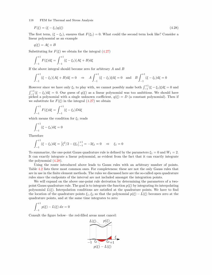
118 FEM for Thermal and Stress Analysis

F (ξ) = (ξ − ξ1)q(ξ) (4.28)

The first term, (ξ − ξ1), ensures that F (ξ1) = 0. What could the second term look like? Consider alinear polynomial as an example

q(ξ) = Aξ +B

Substituting for F (ξ) we obtain for the integral (4.27)∫ +1

−1

F (ξ)dξ =

∫ +1

−1

(ξ − ξ1)(Aξ +B)dξ

If the above integral should become zero for arbitrary A and B∫ +1

−1

(ξ − ξ1)(Aξ +B)dξ = 0 ⇒ A

∫ +1

−1

(ξ − ξ1)ξdξ = 0 and B

∫ +1

−1

(ξ − ξ1)dξ = 0

However since we have only ξ1 to play with, we cannot possibly make both∫ +1

−1(ξ − ξ1)ξdξ = 0 and∫ +1

−1(ξ − ξ1)dξ = 0. Our guess of q(ξ) as a linear polynomial was too ambitious. We should have

picked a polynomial with a single unknown coefficient, q(ξ) = D (a constant polynomial). Then ifwe substitute for F (ξ) in the integral (4.27) we obtain∫ +1

−1

F (ξ)dξ =

∫ +1

−1

(ξ − ξ1)Ddξ

which means the condition for ξ1 reads∫ +1

−1

(ξ − ξ1)dξ = 0

Therefore∫ +1

−1

(ξ − ξ1)dξ =[ξ2/2− ξξ1

]+1

−1= −2ξ1 = 0 ⇒ ξ1 = 0

To summarize, the one-point Gauss quadrature rule is defined by the parameters ξ1 = 0 andW1 = 2.It can exactly integrate a linear polynomial, as evident from the fact that it can exactly integratethe polynomial (4.28).

Using the route introduced above leads to Gauss rules with an arbitrary number of points.Table 4.2 lists three most common ones. For completeness: these are not the only Gauss rules thatare in use in the finite element methods. The rules we discussed here are the so-called open quadraturerules since the endpoints of the interval are not included amongst the integration points.

We will expand on the above one-point rule derivation by determining the parameters of a two-point Gauss quadrature rule. The goal is to integrate the function p(ξ) by integrating its interpolatingpolynomial L(ξ). Interpolation conditions are satisfied at the quadrature points. We have to findthe location of the quadrature points ξ1, ξ2 so that the polynomial p(ξ)− L(ξ) becomes zero at thequadrature points, and at the same time integrates to zero∫ +1

−1

p(ξ)− L(ξ) dx = 0

Consult the figure below– the red-filled areas must cancel:

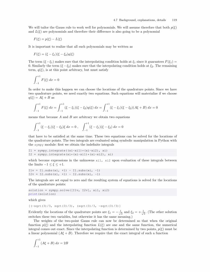
4.7 Background, explanations, details 119

We will tailor the Gauss rule to work well for polynomials. We will assume therefore that both p(ξ)and L(ξ) are polynomials and therefore their difference is also going to be a polynomial

F (ξ) = p(ξ)− L(ξ)

It is important to realize that all such polynomials may be written as

F (ξ) = (ξ − ξ1)(ξ − ξ2)q(ξ)

The term (ξ−ξ1) makes sure that the interpolating condition holds at ξ1 since it guarantees F (ξ1) =0. Similarly the term (ξ−ξ2) makes sure that the interpolating condition holds at ξ2. The remainingterm, q(ξ), is at this point arbitrary, but must satisfy∫ +1

−1

F (ξ) dx = 0

In order to make this happen we can choose the locations of the quadrature points. Since we havetwo quadrature points, we need exactly two equations. Such equations will materialize if we chooseq(ξ) = Aξ +B as∫ +1

−1

F (ξ) dx =

∫ +1

−1

(ξ − ξ1)(ξ − ξ2)q(ξ) dx =

∫ +1

−1

(ξ − ξ1)(ξ − ξ2)(Aξ +B) dx = 0

means that because A and B are arbitrary we obtain two equations∫ +1

−1

(ξ − ξ1)(ξ − ξ2)ξ dx = 0 ,

∫ +1

−1

(ξ − ξ1)(ξ − ξ2) dx = 0

that have to be satisfied at the same time. These two equations can be solved for the locations ofthe quadrature points. The two integrals are evaluated using symbolic manipulation in Python withthe sympy module: first we obtain the indefinite integrals

I1 = sympy.integrate((xi-xi1)*(xi-xi2), xi)I2 = sympy.integrate(xi*(xi-xi1)*(xi-xi2), xi)

which become expressions in the unknowns xi1, xi2 upon evaluation of these integrals betweenthe limits −1 ≤ ξ ≤ +1.

I1v = I1.subs(xi, +1) - I1.subs(xi, -1)I2v = I2.subs(xi, +1) - I2.subs(xi, -1)

The integrals are set equal to zero and the resulting system of equations is solved for the locationsof the quadrature points:

solution = sympy.solve([I1v, I2v], xi1, xi2)print(solution)

which gives

[(-sqrt(3)/3, sqrt(3)/3), (sqrt(3)/3, -sqrt(3)/3)]

Evidently the locations of the quadrature points are ξ1 = − 1√3and ξ2 = + 1√

3. (The other solution

switches these two variables, but otherwise it has the same meaning.)The weights of the two-point Gauss rule can now be determined so that when the original

function p(ξ) and the interpolating function L(ξ) are one and the same function, the numericalintegral comes out exact. Since the interpolating function is determined by two points, p(ξ) must bea linear polynomial (Aξ +B). Therefore we require that the exact integral of such a function∫ +1

−1

(Aξ +B) dx = 2B

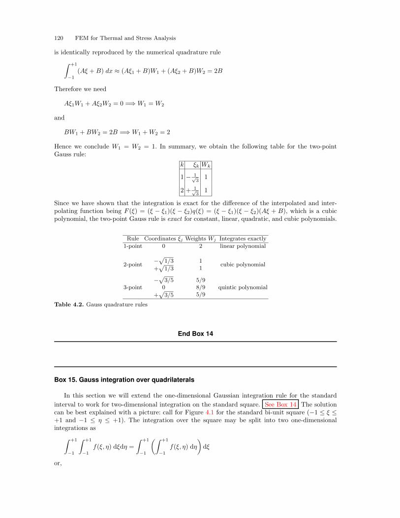
120 FEM for Thermal and Stress Analysis

is identically reproduced by the numerical quadrature rule∫ +1

−1

(Aξ +B) dx ≈ (Aξ1 +B)W1 + (Aξ2 +B)W2 = 2B

Therefore we need

Aξ1W1 +Aξ2W2 = 0 =⇒W1 =W2

and

BW1 +BW2 = 2B =⇒W1 +W2 = 2

Hence we conclude W1 = W2 = 1. In summary, we obtain the following table for the two-pointGauss rule:

k ξk Wk

1 − 1√3

1

2 + 1√3

1

Since we have shown that the integration is exact for the difference of the interpolated and inter-polating function being F (ξ) = (ξ − ξ1)(ξ − ξ2)q(ξ) = (ξ − ξ1)(ξ − ξ2)(Aξ + B), which is a cubicpolynomial, the two-point Gauss rule is exact for constant, linear, quadratic, and cubic polynomials.

Rule Coordinates ξj Weights Wj Integrates exactly

1-point 0 2 linear polynomial

2-point−√

1/3

+√

1/3

11

cubic polynomial

3-point−√

3/50

+√

3/5

5/98/95/9

quintic polynomial

Table 4.2. Gauss quadrature rules

End Box 14

Box 15. Gauss integration over quadrilaterals

In this section we will extend the one-dimensional Gaussian integration rule for the standard

interval to work for two-dimensional integration on the standard square. See Box 14 The solutioncan be best explained with a picture: call for Figure 4.1 for the standard bi-unit square (−1 ≤ ξ ≤+1 and −1 ≤ η ≤ +1). The integration over the square may be split into two one-dimensionalintegrations as∫ +1

−1

∫ +1

−1

f(ξ, η) dξdη =

∫ +1

−1

(∫ +1

−1

f(ξ, η) dη

)dξ

or,

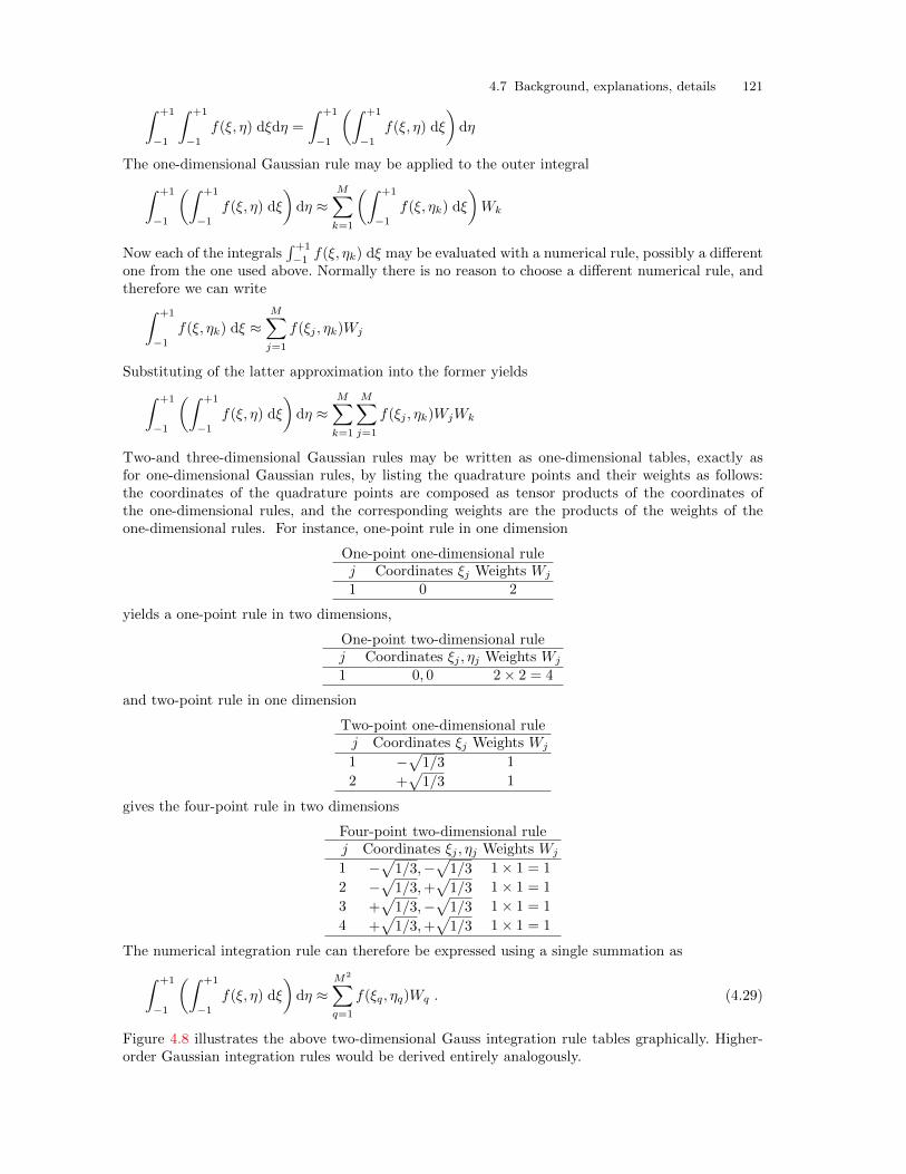
4.7 Background, explanations, details 121∫ +1

−1

∫ +1

−1

f(ξ, η) dξdη =

∫ +1

−1

(∫ +1

−1

f(ξ, η) dξ

)dη

The one-dimensional Gaussian rule may be applied to the outer integral∫ +1

−1

(∫ +1

−1

f(ξ, η) dξ

)dη ≈

M∑k=1

(∫ +1

−1

f(ξ, ηk) dξ

)Wk

Now each of the integrals∫ +1

−1f(ξ, ηk) dξ may be evaluated with a numerical rule, possibly a different

one from the one used above. Normally there is no reason to choose a different numerical rule, andtherefore we can write∫ +1

−1

f(ξ, ηk) dξ ≈M∑j=1

f(ξj , ηk)Wj

Substituting of the latter approximation into the former yields∫ +1

−1

(∫ +1

−1

f(ξ, η) dξ

)dη ≈

M∑k=1

M∑j=1

f(ξj , ηk)WjWk

Two-and three-dimensional Gaussian rules may be written as one-dimensional tables, exactly asfor one-dimensional Gaussian rules, by listing the quadrature points and their weights as follows:the coordinates of the quadrature points are composed as tensor products of the coordinates ofthe one-dimensional rules, and the corresponding weights are the products of the weights of theone-dimensional rules. For instance, one-point rule in one dimension

One-point one-dimensional rulej Coordinates ξj Weights Wj

1 0 2

yields a one-point rule in two dimensions,

One-point two-dimensional rulej Coordinates ξj , ηj Weights Wj

1 0, 0 2× 2 = 4

and two-point rule in one dimension

Two-point one-dimensional rulej Coordinates ξj Weights Wj

1 −√

1/3 1

2 +√

1/3 1

gives the four-point rule in two dimensions

Four-point two-dimensional rulej Coordinates ξj , ηj Weights Wj

1 −√1/3,−

√1/3 1× 1 = 1

2 −√1/3,+

√1/3 1× 1 = 1

3 +√1/3,−

√1/3 1× 1 = 1

4 +√1/3,+

√1/3 1× 1 = 1

The numerical integration rule can therefore be expressed using a single summation as∫ +1

−1

(∫ +1

−1

f(ξ, η) dξ

)dη ≈

M2∑q=1

f(ξq, ηq)Wq . (4.29)

Figure 4.8 illustrates the above two-dimensional Gauss integration rule tables graphically. Higher-order Gaussian integration rules would be derived entirely analogously.

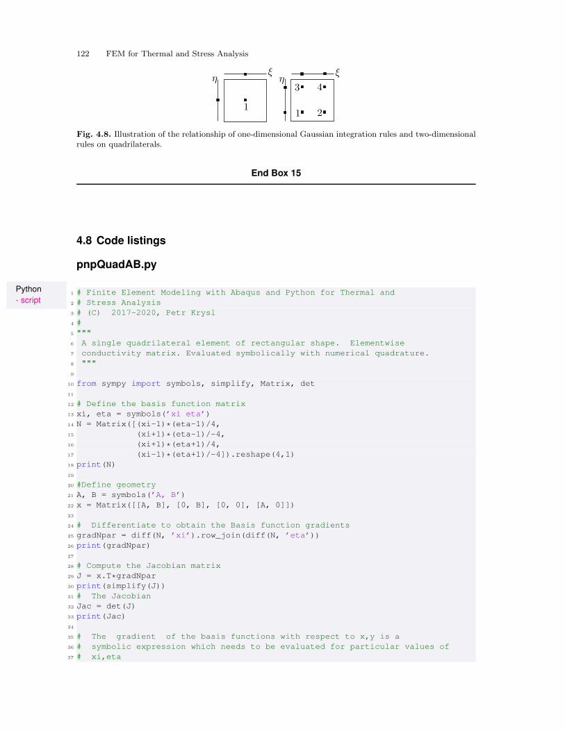
122 FEM for Thermal and Stress Analysis

Fig. 4.8. Illustration of the relationship of one-dimensional Gaussian integration rules and two-dimensionalrules on quadrilaterals.

End Box 15

4.8 Code listings

pnpQuadAB.py

Python- script

1 # Finite Element Modeling with Abaqus and Python for Thermal and2 # Stress Analysis3 # (C) 2017-2020, Petr Krysl4 #5 """6 A single quadrilateral element of rectangular shape. Elementwise7 conductivity matrix. Evaluated symbolically with numerical quadrature.8 """9

10 from sympy import symbols, simplify, Matrix, det11

12 # Define the basis function matrix13 xi, eta = symbols(’xi eta’)14 N = Matrix([(xi-1)*(eta-1)/4,15 (xi+1)*(eta-1)/-4,16 (xi+1)*(eta+1)/4,17 (xi-1)*(eta+1)/-4]).reshape(4,1)18 print(N)19

20 #Define geometry21 A, B = symbols(’A, B’)22 x = Matrix([[A, B], [0, B], [0, 0], [A, 0]])23

24 # Differentiate to obtain the Basis function gradients25 gradNpar = diff(N, ’xi’).row_join(diff(N, ’eta’))26 print(gradNpar)27

28 # Compute the Jacobian matrix29 J = x.T*gradNpar30 print(simplify(J))31 # The Jacobian32 Jac = det(J)33 print(Jac)34

35 # The gradient of the basis functions with respect to x,y is a36 # symbolic expression which needs to be evaluated for particular values of37 # xi,eta

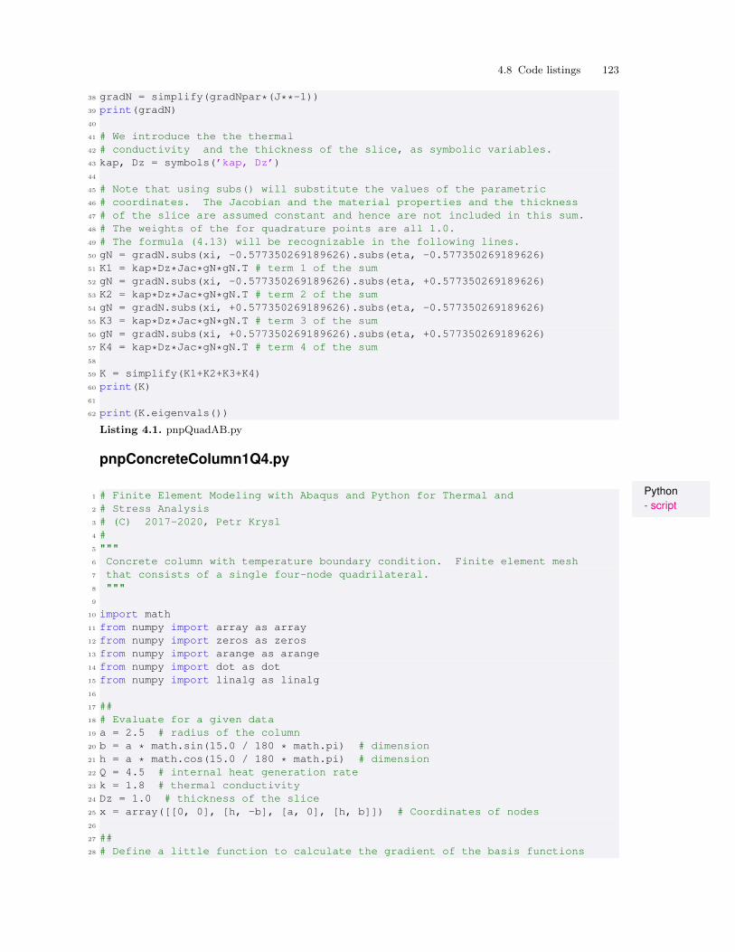
4.8 Code listings 123

38 gradN = simplify(gradNpar*(J**-1))39 print(gradN)40

41 # We introduce the the thermal42 # conductivity and the thickness of the slice, as symbolic variables.43 kap, Dz = symbols(’kap, Dz’)44

45 # Note that using subs() will substitute the values of the parametric46 # coordinates. The Jacobian and the material properties and the thickness47 # of the slice are assumed constant and hence are not included in this sum.48 # The weights of the for quadrature points are all 1.0.49 # The formula (4.13) will be recognizable in the following lines.50 gN = gradN.subs(xi, -0.577350269189626).subs(eta, -0.577350269189626)51 K1 = kap*Dz*Jac*gN*gN.T # term 1 of the sum52 gN = gradN.subs(xi, -0.577350269189626).subs(eta, +0.577350269189626)53 K2 = kap*Dz*Jac*gN*gN.T # term 2 of the sum54 gN = gradN.subs(xi, +0.577350269189626).subs(eta, -0.577350269189626)55 K3 = kap*Dz*Jac*gN*gN.T # term 3 of the sum56 gN = gradN.subs(xi, +0.577350269189626).subs(eta, +0.577350269189626)57 K4 = kap*Dz*Jac*gN*gN.T # term 4 of the sum58

59 K = simplify(K1+K2+K3+K4)60 print(K)61

62 print(K.eigenvals())

Listing 4.1. pnpQuadAB.py

pnpConcreteColumn1Q4.py

Python- script

1 # Finite Element Modeling with Abaqus and Python for Thermal and2 # Stress Analysis3 # (C) 2017-2020, Petr Krysl4 #5 """6 Concrete column with temperature boundary condition. Finite element mesh7 that consists of a single four-node quadrilateral.8 """9

10 import math11 from numpy import array as array12 from numpy import zeros as zeros13 from numpy import arange as arange14 from numpy import dot as dot15 from numpy import linalg as linalg16

17 ##18 # Evaluate for a given data19 a = 2.5 # radius of the column20 b = a * math.sin(15.0 / 180 * math.pi) # dimension21 h = a * math.cos(15.0 / 180 * math.pi) # dimension22 Q = 4.5 # internal heat generation rate23 k = 1.8 # thermal conductivity24 Dz = 1.0 # thickness of the slice25 x = array([[0, 0], [h, -b], [a, 0], [h, b]]) # Coordinates of nodes26

27 ##28 # Define a little function to calculate the gradient of the basis functions

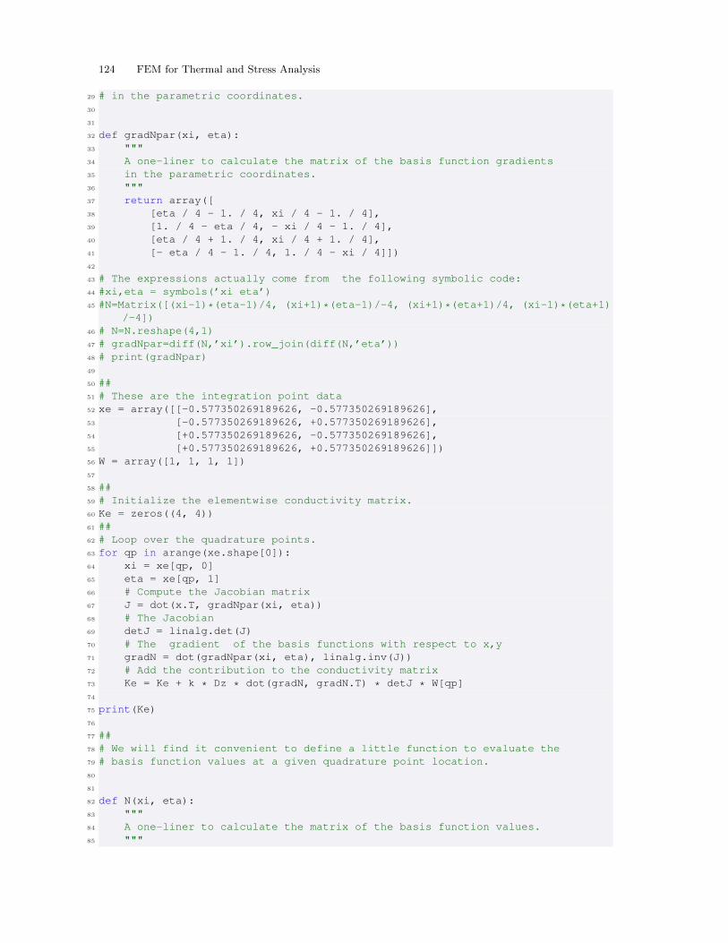
124 FEM for Thermal and Stress Analysis

29 # in the parametric coordinates.30

31

32 def gradNpar(xi, eta):33 """34 A one-liner to calculate the matrix of the basis function gradients35 in the parametric coordinates.36 """37 return array([38 [eta / 4 - 1. / 4, xi / 4 - 1. / 4],39 [1. / 4 - eta / 4, - xi / 4 - 1. / 4],40 [eta / 4 + 1. / 4, xi / 4 + 1. / 4],41 [- eta / 4 - 1. / 4, 1. / 4 - xi / 4]])42

43 # The expressions actually come from the following symbolic code:44 #xi,eta = symbols(’xi eta’)45 #N=Matrix([(xi-1)*(eta-1)/4, (xi+1)*(eta-1)/-4, (xi+1)*(eta+1)/4, (xi-1)*(eta+1)

/-4])46 # N=N.reshape(4,1)47 # gradNpar=diff(N,’xi’).row_join(diff(N,’eta’))48 # print(gradNpar)49

50 ##51 # These are the integration point data52 xe = array([[-0.577350269189626, -0.577350269189626],53 [-0.577350269189626, +0.577350269189626],54 [+0.577350269189626, -0.577350269189626],55 [+0.577350269189626, +0.577350269189626]])56 W = array([1, 1, 1, 1])57

58 ##59 # Initialize the elementwise conductivity matrix.60 Ke = zeros((4, 4))61 ##62 # Loop over the quadrature points.63 for qp in arange(xe.shape[0]):64 xi = xe[qp, 0]65 eta = xe[qp, 1]66 # Compute the Jacobian matrix67 J = dot(x.T, gradNpar(xi, eta))68 # The Jacobian69 detJ = linalg.det(J)70 # The gradient of the basis functions with respect to x,y71 gradN = dot(gradNpar(xi, eta), linalg.inv(J))72 # Add the contribution to the conductivity matrix73 Ke = Ke + k * Dz * dot(gradN, gradN.T) * detJ * W[qp]74

75 print(Ke)76

77 ##78 # We will find it convenient to define a little function to evaluate the79 # basis function values at a given quadrature point location.80

81

82 def N(xi, eta):83 """84 A one-liner to calculate the matrix of the basis function values.85 """

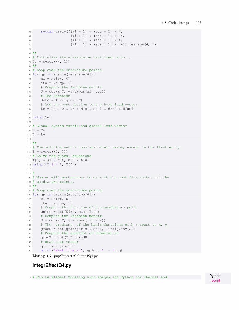
4.8 Code listings 125

86 return array([(xi - 1) * (eta - 1) / 4,87 (xi + 1) * (eta - 1) / -4,88 (xi + 1) * (eta + 1) / 4,89 (xi - 1) * (eta + 1) / -4]).reshape(4, 1)90

91 ##92 # Initialize the elementwise heat-load vector .93 Le = zeros((4, 1))94 ##95 # Loop over the quadrature points.96 for qp in arange(xe.shape[0]):97 xi = xe[qp, 0]98 eta = xe[qp, 1]99 # Compute the Jacobian matrix

100 J = dot(x.T, gradNpar(xi, eta))101 # The Jacobian102 detJ = linalg.det(J)103 # Add the contribution to the heat load vector104 Le = Le + Q * Dz * N(xi, eta) * detJ * W[qp]105

106 print(Le)107

108 # Global system matrix and global load vector109 K = Ke110 L = Le111

112 ##113 # The solution vector consists of all zeros, except in the first entry.114 T = zeros((4, 1))115 # Solve the global equations116 T[0] = (1 / K[0, 0]) * L[0]117 print(’T_1 = ’, T[0])118

119 #120 # Now we will postprocess to extract the heat flux vectors at the121 # quadrature points.122 ##123 # Loop over the quadrature points.124 for qp in arange(xe.shape[0]):125 xi = xe[qp, 0]126 eta = xe[qp, 1]127 # Compute the location of the quadrature point128 qploc = dot(N(xi, eta).T, x)129 # Compute the Jacobian matrix130 J = dot(x.T, gradNpar(xi, eta))131 # The gradient of the basis functions with respect to x, y132 gradN = dot(gradNpar(xi, eta), linalg.inv(J))133 # Compute the gradient of temperature134 gradT = dot(T.T, gradN)135 # Heat flux vector136 q = -k * gradT.T137 print(’Heat flux at’, qploc, ’ = ’, q)

Listing 4.2. pnpConcreteColumn1Q4.py

IntegrEffectQ4.py

Python- script

1 # Finite Element Modeling with Abaqus and Python for Thermal and

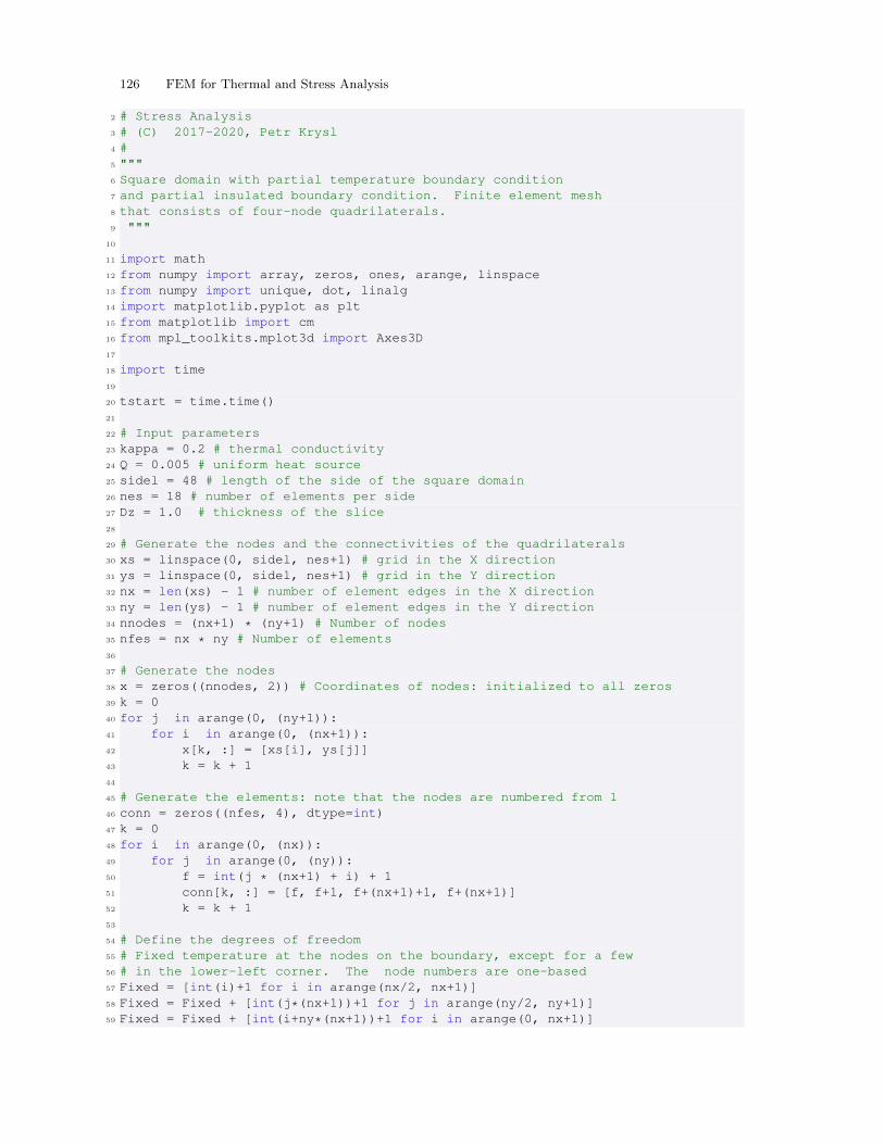
126 FEM for Thermal and Stress Analysis

2 # Stress Analysis3 # (C) 2017-2020, Petr Krysl4 #5 """6 Square domain with partial temperature boundary condition7 and partial insulated boundary condition. Finite element mesh8 that consists of four-node quadrilaterals.9 """

10

11 import math12 from numpy import array, zeros, ones, arange, linspace13 from numpy import unique, dot, linalg14 import matplotlib.pyplot as plt15 from matplotlib import cm16 from mpl_toolkits.mplot3d import Axes3D17

18 import time19

20 tstart = time.time()21

22 # Input parameters23 kappa = 0.2 # thermal conductivity24 Q = 0.005 # uniform heat source25 sidel = 48 # length of the side of the square domain26 nes = 18 # number of elements per side27 Dz = 1.0 # thickness of the slice28

29 # Generate the nodes and the connectivities of the quadrilaterals30 xs = linspace(0, sidel, nes+1) # grid in the X direction31 ys = linspace(0, sidel, nes+1) # grid in the Y direction32 nx = len(xs) - 1 # number of element edges in the X direction33 ny = len(ys) - 1 # number of element edges in the Y direction34 nnodes = (nx+1) * (ny+1) # Number of nodes35 nfes = nx * ny # Number of elements36

37 # Generate the nodes38 x = zeros((nnodes, 2)) # Coordinates of nodes: initialized to all zeros39 k = 040 for j in arange(0, (ny+1)):41 for i in arange(0, (nx+1)):42 x[k, :] = [xs[i], ys[j]]43 k = k + 144

45 # Generate the elements: note that the nodes are numbered from 146 conn = zeros((nfes, 4), dtype=int)47 k = 048 for i in arange(0, (nx)):49 for j in arange(0, (ny)):50 f = int(j * (nx+1) + i) + 151 conn[k, :] = [f, f+1, f+(nx+1)+1, f+(nx+1)]52 k = k + 153

54 # Define the degrees of freedom55 # Fixed temperature at the nodes on the boundary, except for a few56 # in the lower-left corner. The node numbers are one-based57 Fixed = [int(i)+1 for i in arange(nx/2, nx+1)]58 Fixed = Fixed + [int(j*(nx+1))+1 for j in arange(ny/2, ny+1)]59 Fixed = Fixed + [int(i+ny*(nx+1))+1 for i in arange(0, nx+1)]

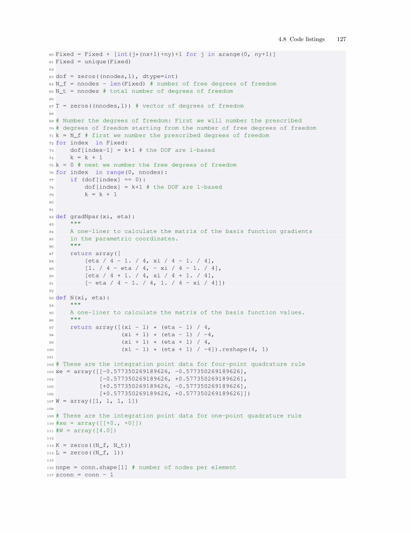
4.8 Code listings 127

60 Fixed = Fixed + [int(j*(nx+1)+ny)+1 for j in arange(0, ny+1)]61 Fixed = unique(Fixed)62

63 dof = zeros((nnodes,1), dtype=int)64 N_f = nnodes - len(Fixed) # number of free degrees of freedom65 N_t = nnodes # total number of degrees of freedom66

67 T = zeros((nnodes,1)) # vector of degrees of freedom68

69 # Number the degrees of freedom: First we will number the prescribed70 # degrees of freedom starting from the number of free degrees of freedom71 k = N_f # first we number the prescribed degrees of freedom72 for index in Fixed:73 dof[index-1] = k+1 # the DOF are 1-based74 k = k + 175 k = 0 # next we number the free degrees of freedom76 for index in range(0, nnodes):77 if (dof[index] == 0):78 dof[index] = k+1 # the DOF are 1-based79 k = k + 180

81

82 def gradNpar(xi, eta):83 """84 A one-liner to calculate the matrix of the basis function gradients85 in the parametric coordinates.86 """87 return array([88 [eta / 4 - 1. / 4, xi / 4 - 1. / 4],89 [1. / 4 - eta / 4, - xi / 4 - 1. / 4],90 [eta / 4 + 1. / 4, xi / 4 + 1. / 4],91 [- eta / 4 - 1. / 4, 1. / 4 - xi / 4]])92

93 def N(xi, eta):94 """95 A one-liner to calculate the matrix of the basis function values.96 """97 return array([(xi - 1) * (eta - 1) / 4,98 (xi + 1) * (eta - 1) / -4,99 (xi + 1) * (eta + 1) / 4,

100 (xi - 1) * (eta + 1) / -4]).reshape(4, 1)101

102 # These are the integration point data for four-point quadrature rule103 xe = array([[-0.577350269189626, -0.577350269189626],104 [-0.577350269189626, +0.577350269189626],105 [+0.577350269189626, -0.577350269189626],106 [+0.577350269189626, +0.577350269189626]])107 W = array([1, 1, 1, 1])108

109 # These are the integration point data for one-point quadrature rule110 #xe = array([[+0., +0]])111 #W = array([4.0])112

113 K = zeros((N_f, N_t))114 L = zeros((N_f, 1))115

116 nnpe = conn.shape[1] # number of nodes per element117 zconn = conn - 1

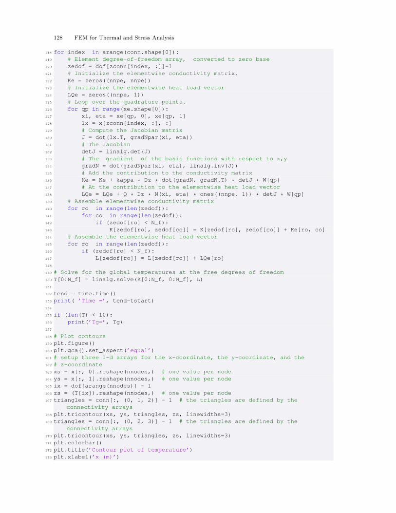
128 FEM for Thermal and Stress Analysis

118 for index in arange(conn.shape[0]):119 # Element degree-of-freedom array, converted to zero base120 zedof = dof[zconn[index, :]]-1121 # Initialize the elementwise conductivity matrix.122 Ke = zeros((nnpe, nnpe))123 # Initialize the elementwise heat load vector124 LQe = zeros((nnpe, 1))125 # Loop over the quadrature points.126 for qp in range(xe.shape[0]):127 xi, eta = xe[qp, 0], xe[qp, 1]128 lx = x[zconn[index, :], :]129 # Compute the Jacobian matrix130 J = dot(lx.T, gradNpar(xi, eta))131 # The Jacobian132 detJ = linalg.det(J)133 # The gradient of the basis functions with respect to x,y134 gradN = dot(gradNpar(xi, eta), linalg.inv(J))135 # Add the contribution to the conductivity matrix136 Ke = Ke + kappa * Dz * dot(gradN, gradN.T) * detJ * W[qp]137 # At the contribution to the elementwise heat load vector138 LQe = LQe + Q * Dz * N(xi, eta) * ones((nnpe, 1)) * detJ * W[qp]139 # Assemble elementwise conductivity matrix140 for ro in range(len(zedof)):141 for co in range(len(zedof)):142 if (zedof[ro] < N_f):143 K[zedof[ro], zedof[co]] = K[zedof[ro], zedof[co]] + Ke[ro, co]144 # Assemble the elementwise heat load vector145 for ro in range(len(zedof)):146 if (zedof[ro] < N_f):147 L[zedof[ro]] = L[zedof[ro]] + LQe[ro]148

149 # Solve for the global temperatures at the free degrees of freedom150 T[0:N_f] = linalg.solve(K[0:N_f, 0:N_f], L)151

152 tend = time.time()153 print( ’Time =’, tend-tstart)154

155 if (len(T) < 10):156 print(’Tg=’, Tg)157

158 # Plot contours159 plt.figure()160 plt.gca().set_aspect(’equal’)161 # setup three 1-d arrays for the x-coordinate, the y-coordinate, and the162 # z-coordinate163 xs = x[:, 0].reshape(nnodes,) # one value per node164 ys = x[:, 1].reshape(nnodes,) # one value per node165 ix = dof[arange(nnodes)] - 1166 zs = (T[ix]).reshape(nnodes,) # one value per node167 triangles = conn[:, (0, 1, 2)] - 1 # the triangles are defined by the

connectivity arrays168 plt.tricontour(xs, ys, triangles, zs, linewidths=3)169 triangles = conn[:, (0, 2, 3)] - 1 # the triangles are defined by the

connectivity arrays170 plt.tricontour(xs, ys, triangles, zs, linewidths=3)171 plt.colorbar()172 plt.title(’Contour plot of temperature’)173 plt.xlabel(’x (m)’)

4.8 Code listings 129

174 plt.ylabel(’y (m)’)175 plt.show()

Listing 4.3. IntegrEffectQ4.py

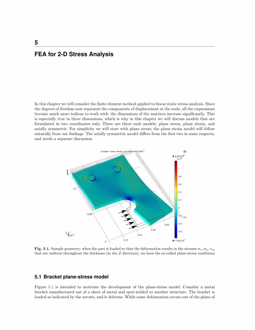
5

FEA for 2-D Stress Analysis

In this chapter we will consider the finite element method applied to linear static stress analysis. Sincethe degrees of freedom now represent the components of displacement at the node, all the expressionsbecome much more tedious to work with: the dimensions of the matrices increase significantly. Thisis especially true in three dimensions, which is why in this chapter we will discuss models that areformulated in two coordinates only. There are three such models: plane stress, plane strain, andaxially symmetric. For simplicity we will start with plane stress; the plane strain model will follownaturally from our findings. The axially symmetric model differs from the first two in some respects,and needs a separate discussion.

Fig. 5.1. Sample geometry: when the part is loaded so that the deformation results in the stresses σx, σy, τxythat are uniform throughout the thickness (in the Z direction), we have the so-called plane-stress conditions

5.1 Bracket plane-stress model

Figure 5.1 is intended to motivate the development of the plane-stress model. Consider a metalbracket manufactured out of a sheet of metal and spot-welded to another structure. The bracket isloaded as indicated by the arrows, and it deforms. While some deformation occurs out of the plane of

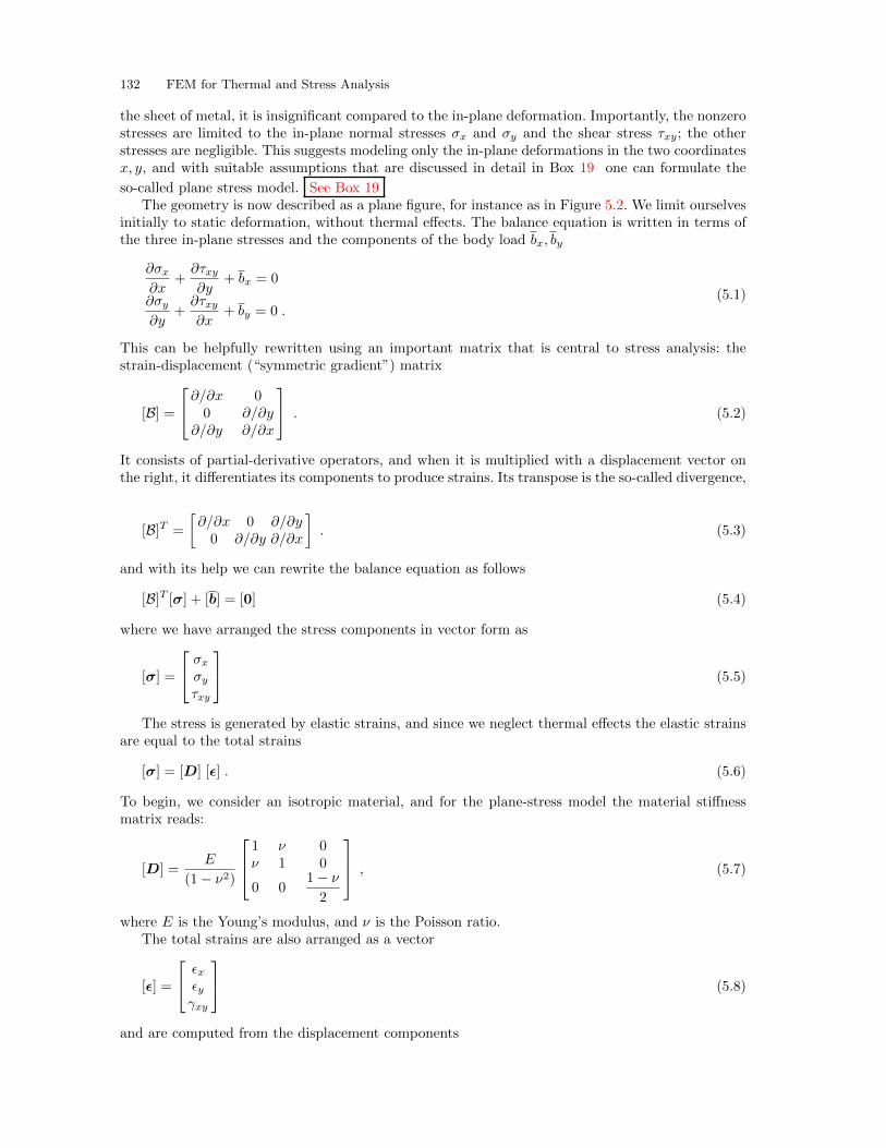
132 FEM for Thermal and Stress Analysis

the sheet of metal, it is insignificant compared to the in-plane deformation. Importantly, the nonzerostresses are limited to the in-plane normal stresses σx and σy and the shear stress τxy; the otherstresses are negligible. This suggests modeling only the in-plane deformations in the two coordinatesx, y, and with suitable assumptions that are discussed in detail in Box 19 one can formulate the

so-called plane stress model. See Box 19The geometry is now described as a plane figure, for instance as in Figure 5.2. We limit ourselves

initially to static deformation, without thermal effects. The balance equation is written in terms ofthe three in-plane stresses and the components of the body load bx, by

∂σx∂x

+∂τxy∂y

+ bx = 0

∂σy∂y

+∂τxy∂x

+ by = 0 .(5.1)

This can be helpfully rewritten using an important matrix that is central to stress analysis: thestrain-displacement (“symmetric gradient”) matrix

[B] =

∂/∂x 00 ∂/∂y

∂/∂y ∂/∂x

. (5.2)

It consists of partial-derivative operators, and when it is multiplied with a displacement vector onthe right, it differentiates its components to produce strains. Its transpose is the so-called divergence,

[B]T =

[∂/∂x 0 ∂/∂y0 ∂/∂y ∂/∂x

]. (5.3)

and with its help we can rewrite the balance equation as follows

[B]T [σ] + [b] = [0] (5.4)

where we have arranged the stress components in vector form as

[σ] =

σxσyτxy

(5.5)

The stress is generated by elastic strains, and since we neglect thermal effects the elastic strainsare equal to the total strains

[σ] = [D] [ϵ] . (5.6)

To begin, we consider an isotropic material, and for the plane-stress model the material stiffnessmatrix reads:

[D] =E

(1− ν2)

1 ν 0ν 1 0

0 01− ν

2

, (5.7)

where E is the Young’s modulus, and ν is the Poisson ratio.The total strains are also arranged as a vector

[ϵ] =

ϵxϵyγxy

(5.8)

and are computed from the displacement components

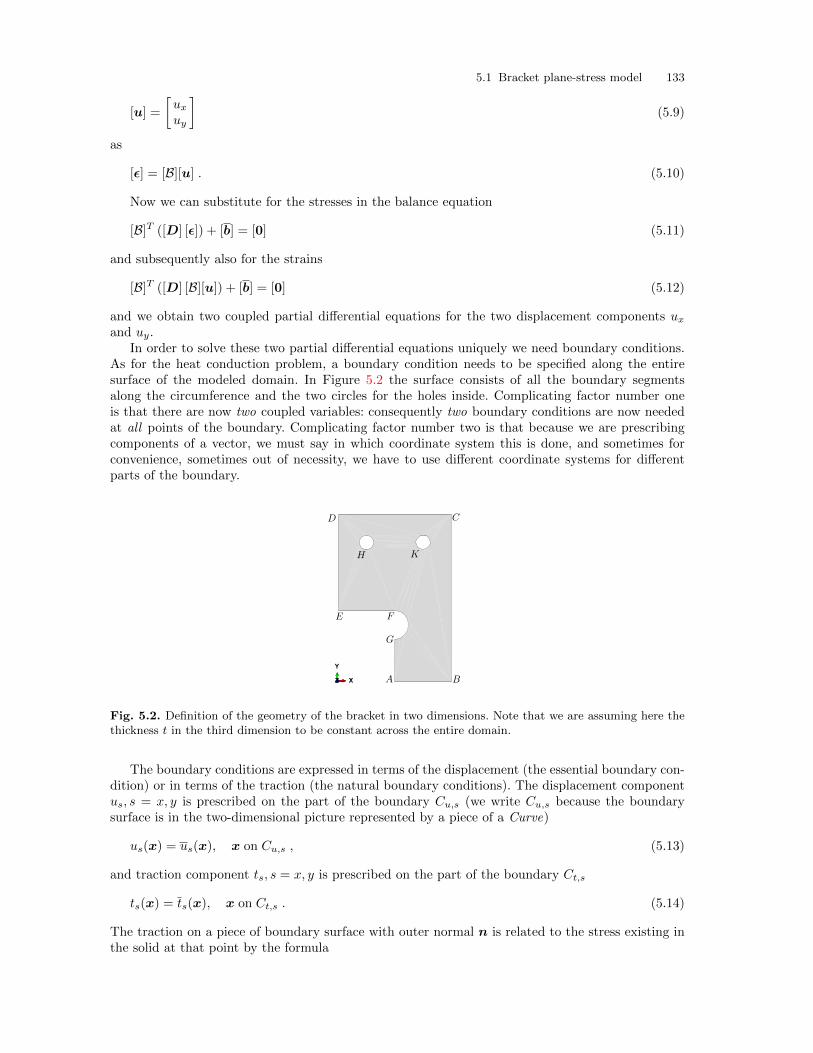
5.1 Bracket plane-stress model 133

[u] =

[uxuy

](5.9)

as

[ϵ] = [B][u] . (5.10)

Now we can substitute for the stresses in the balance equation

[B]T ([D] [ϵ]) + [b] = [0] (5.11)

and subsequently also for the strains

[B]T ([D] [B][u]) + [b] = [0] (5.12)

and we obtain two coupled partial differential equations for the two displacement components uxand uy.

In order to solve these two partial differential equations uniquely we need boundary conditions.As for the heat conduction problem, a boundary condition needs to be specified along the entiresurface of the modeled domain. In Figure 5.2 the surface consists of all the boundary segmentsalong the circumference and the two circles for the holes inside. Complicating factor number oneis that there are now two coupled variables: consequently two boundary conditions are now neededat all points of the boundary. Complicating factor number two is that because we are prescribingcomponents of a vector, we must say in which coordinate system this is done, and sometimes forconvenience, sometimes out of necessity, we have to use different coordinate systems for differentparts of the boundary.

X

Y

Z

Fig. 5.2. Definition of the geometry of the bracket in two dimensions. Note that we are assuming here thethickness t in the third dimension to be constant across the entire domain.

The boundary conditions are expressed in terms of the displacement (the essential boundary con-dition) or in terms of the traction (the natural boundary conditions). The displacement componentus, s = x, y is prescribed on the part of the boundary Cu,s (we write Cu,s because the boundarysurface is in the two-dimensional picture represented by a piece of a Curve)

us(x) = us(x), x on Cu,s , (5.13)

and traction component ts, s = x, y is prescribed on the part of the boundary Ct,s

ts(x) = ts(x), x on Ct,s . (5.14)

The traction on a piece of boundary surface with outer normal n is related to the stress existing inthe solid at that point by the formula

134 FEM for Thermal and Stress Analysis[Pn(x)σ(x)

]s= ts(x), (5.15)

where the matrix “vector-stress vector dot product” operator is defined as

Pn =

[nx 0 ny0 ny nx

]. (5.16)

With these pieces of information about the boundary conditions in the plane-stress analysis wecan compare usefully with the heat conduction model from the previous chapters:

The boundary condition expressed in terms of the displacement component is equiva-lent to prescribed temperature; the boundary condition expressed in terms of the heatflux component normal to the boundary is equivalent to prescribed traction compo-nent. This is well worth understanding: temperature and displacement are equivalentquantities, and heat flux and stress are equivalent quantities.

For the bracket of Figure 5.2 the boundary conditions are relatively simple to describe—refer toFigure 5.3. In Figure 5.3(a) the thick-line highlighted part of the boundary is where we prescribetraction components. The ty component is zero along this entire part of the boundary, and the txcomponent is zero everywhere along the boundary except for the segment GA, where it is prescribedas nonzero. Figure 5.3(b) shows that the displacement components are both prescribed along the

Abaqus- CAE file

circles that represents the holes, ux = uy = 0 (clamped or “encastre” condition).

X

Y

Z X

Y

Z

(a) (b)

Fig. 5.3. Partitioning of the surface of the bracket for the application of the boundary conditions. (a)Part of the boundary where both traction components are prescribed. (b) Part of the boundary where bothdisplacement components are prescribed.

There is a simple systematic way (algorithm) for applying boundary conditions in stress analysis.It relies on the simple observation that at any given point of the boundary for each of the componentss = x, y one of the quantities us and ts, must be known and the other one must be unknown. Thekey is to choose an appropriate coordinate system in which to work. Often such a system will haveorientation that places one of the coordinate directions normal to the surface.

For each of the coordinate directions s = x, y then do:

1. Consider both us and ts: If one of these is known (prescribed), the boundary condition is decided;otherwise if one of these is definitely unknown, the other one must be known, and if not explicitlygiven, then it will be equal to zero.

2. If the decision could not be reached above, restart by selecting a different coordinate system.

As an example, consider the circular arc FG in Figure 5.3. The appropriate coordinate systemin this case will be in a cylindrical coordinate system with origin at the center of the arc. Since

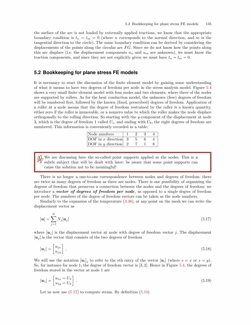
5.2 Bookkeeping for plane stress FE models 135

the surface of the arc is not loaded by externally applied tractions, we know that the appropriateboundary condition is tn = tm = 0 (where n corresponds to the normal direction, and m is thetangential direction to the circle). The same boundary condition can be derived by considering thedisplacements of the points along the circular arc FG. Since we do not know how the points alongthis arc displace (i.e. the displacement components un and um are unknown), we must know thetraction components, and since they are not explicitly given we must have tn = tm = 0.

5.2 Bookkeeping for plane stress FE models

It is necessary to start the discussion of the finite element model by gaining some understandingof what it means to have two degrees of freedom per node in the stress analysis model. Figure 5.4shows a very small finite element model with four nodes and two elements, where three of the nodesare supported by rollers. As for the heat conduction model, the unknown (free) degrees of freedomwill be numbered first, followed by the known (fixed, prescribed) degrees of freedom. Application ofa roller at a node means that the degree of freedom restrained by the roller is a known quantity,either zero if the roller is immovable, or a nonzero value to which the roller makes the node displaceorthogonally to the rolling direction. So starting with the y-component of the displacement at node3, which is the degree of freedom 1 called U1, and ending with U8, the eight degrees of freedom arenumbered. This information is conveniently recorded in a table:

Node numbers 1 2 3 4DOF in x direction 3 5 6 4DOF in y direction 2 7 1 8

We are discussing here the so-called point supports applied at the nodes. This is asubtle subject that will be dealt with later: be aware that some point supports cancause the solution not to be meaningful!

There is no longer a one-to-one correspondence between nodes and degrees of freedom: thereare twice as many degrees of freedom as there are nodes. There is one possibility of organizing thedegrees of freedom that preserves a connection between the nodes and the degrees of freedom: weintroduce a vector of degrees of freedom per node , as opposed to a single degree of freedomper node. The numbers of the degree of freedom vectors can be taken as the node numbers.

Similarly to the expansion of the temperature (3.38), at any point on the mesh we can write thedisplacement vector as

[u] =

N∑j=1

Nj [uj ] (5.17)

where [uj ] is the displacement vector at node with degree of freedom vector j. The displacement[uj ] is the vector that consists of the two degrees of freedom

[uj ] =

[ujxujy

]. (5.18)

We will use the notation [ui]s to refer to the sth entry of the vector [ui] (where s = x or s = y).So, for instance for node 1, the degree of freedom vector is [3, 2]. Hence in Figure 5.4, the degrees offreedom stored in the vector at node 1 are

[u1] =

[u1x = U3

u1y = U2

]. (5.19)

Let us now use (5.17) to compute strain. By definition (5.10)

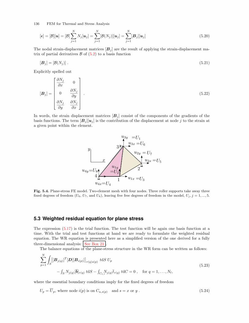
136 FEM for Thermal and Stress Analysis

[ϵ] = [B][u] = [B]N∑j=1

Nj [uj ] =

N∑j=1

[B(Nj)][uj ] =

N∑j=1

[Bj ][uj ] (5.20)

The nodal strain-displacement matrices [Bj ] are the result of applying the strain-displacement ma-trix of partial derivatives B of (5.2) to a basis function

[Bj ] = [B(Nj)] . (5.21)

Explicitly spelled out

[Bj ] =

∂Nj

∂x0

0∂Nj

∂y

∂Nj

∂y

∂Nj

∂x

. (5.22)

In words, the strain displacement matrices [Bj ] consist of the components of the gradients of thebasis functions. The term [Bj ][uj ] is the contribution of the displacement at node j to the strain ata given point within the element.

Fig. 5.4. Plane-stress FE model. Two-element mesh with four nodes. Three roller supports take away threefixed degrees of freedom (U6, U7, and U8), leaving five free degrees of freedom in the model, Uj , j = 1, ..., 5.

5.3 Weighted residual equation for plane stress

The expression (5.17) is the trial function. The test function will be again one basis function at atime. With the trial and test functions at hand we are ready to formulate the weighted residualequation. The WR equation is presented here as a simplified version of the one derived for a fully

three-dimensional analysis: See Box 21 .The balance equations of the plane-stress structure in the WR form can be written as follows:

N∑p=1

∫S

[[Bj(q)]

T [D][Bi(p)]]r(q)s(p)

tdS Up

−∫SNj(q)[b]r(q) tdS −

∫Ct,rNj(q)tr(q) tdC = 0 , for q = 1, . . . , Nf ,

(5.23)

where the essential boundary conditions imply for the fixed degrees of freedom

Up = Up, where node i(p) is on Cu,s(p) and s = x or y . (5.24)

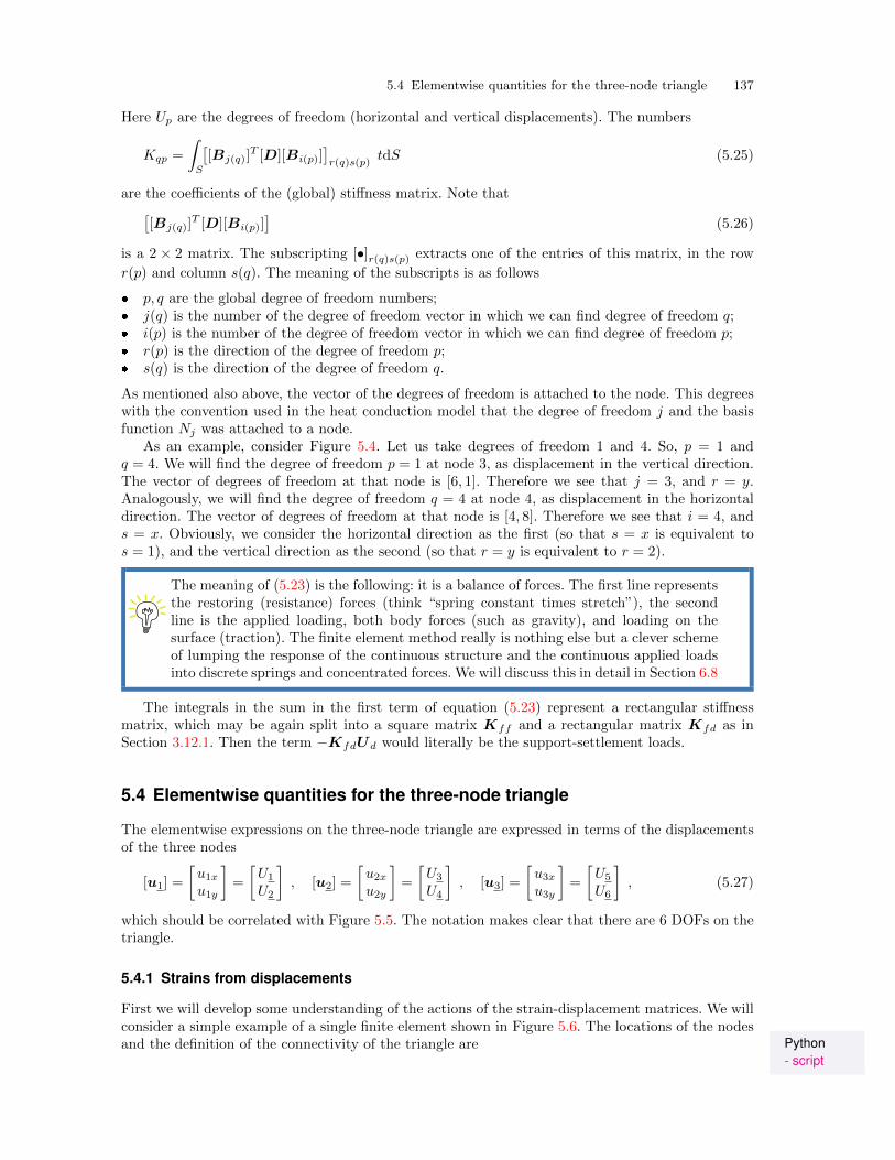
5.4 Elementwise quantities for the three-node triangle 137

Here Up are the degrees of freedom (horizontal and vertical displacements). The numbers

Kqp =

∫S

[[Bj(q)]

T [D][Bi(p)]]r(q)s(p)

tdS (5.25)

are the coefficients of the (global) stiffness matrix. Note that[[Bj(q)]

T [D][Bi(p)]]

(5.26)

is a 2 × 2 matrix. The subscripting [•]r(q)s(p) extracts one of the entries of this matrix, in the row

r(p) and column s(q). The meaning of the subscripts is as follows

� p, q are the global degree of freedom numbers;� j(q) is the number of the degree of freedom vector in which we can find degree of freedom q;� i(p) is the number of the degree of freedom vector in which we can find degree of freedom p;� r(p) is the direction of the degree of freedom p;� s(q) is the direction of the degree of freedom q.

As mentioned also above, the vector of the degrees of freedom is attached to the node. This degreeswith the convention used in the heat conduction model that the degree of freedom j and the basisfunction Nj was attached to a node.

As an example, consider Figure 5.4. Let us take degrees of freedom 1 and 4. So, p = 1 andq = 4. We will find the degree of freedom p = 1 at node 3, as displacement in the vertical direction.The vector of degrees of freedom at that node is [6, 1]. Therefore we see that j = 3, and r = y.Analogously, we will find the degree of freedom q = 4 at node 4, as displacement in the horizontaldirection. The vector of degrees of freedom at that node is [4, 8]. Therefore we see that i = 4, ands = x. Obviously, we consider the horizontal direction as the first (so that s = x is equivalent tos = 1), and the vertical direction as the second (so that r = y is equivalent to r = 2).

The meaning of (5.23) is the following: it is a balance of forces. The first line representsthe restoring (resistance) forces (think “spring constant times stretch”), the secondline is the applied loading, both body forces (such as gravity), and loading on thesurface (traction). The finite element method really is nothing else but a clever schemeof lumping the response of the continuous structure and the continuous applied loadsinto discrete springs and concentrated forces. We will discuss this in detail in Section 6.8

The integrals in the sum in the first term of equation (5.23) represent a rectangular stiffnessmatrix, which may be again split into a square matrix Kff and a rectangular matrix Kfd as inSection 3.12.1. Then the term −KfdUd would literally be the support-settlement loads.

5.4 Elementwise quantities for the three-node triangle

The elementwise expressions on the three-node triangle are expressed in terms of the displacementsof the three nodes

[u1] =

[u1xu1y

]=

[U1

U2

], [u2] =

[u2xu2y

]=

[U3

U4

], [u3] =

[u3xu3y

]=

[U5

U6

], (5.27)

which should be correlated with Figure 5.5. The notation makes clear that there are 6 DOFs on thetriangle.

5.4.1 Strains from displacements

First we will develop some understanding of the actions of the strain-displacement matrices. We willconsider a simple example of a single finite element shown in Figure 5.6. The locations of the nodes

Python- script

and the definition of the connectivity of the triangle are

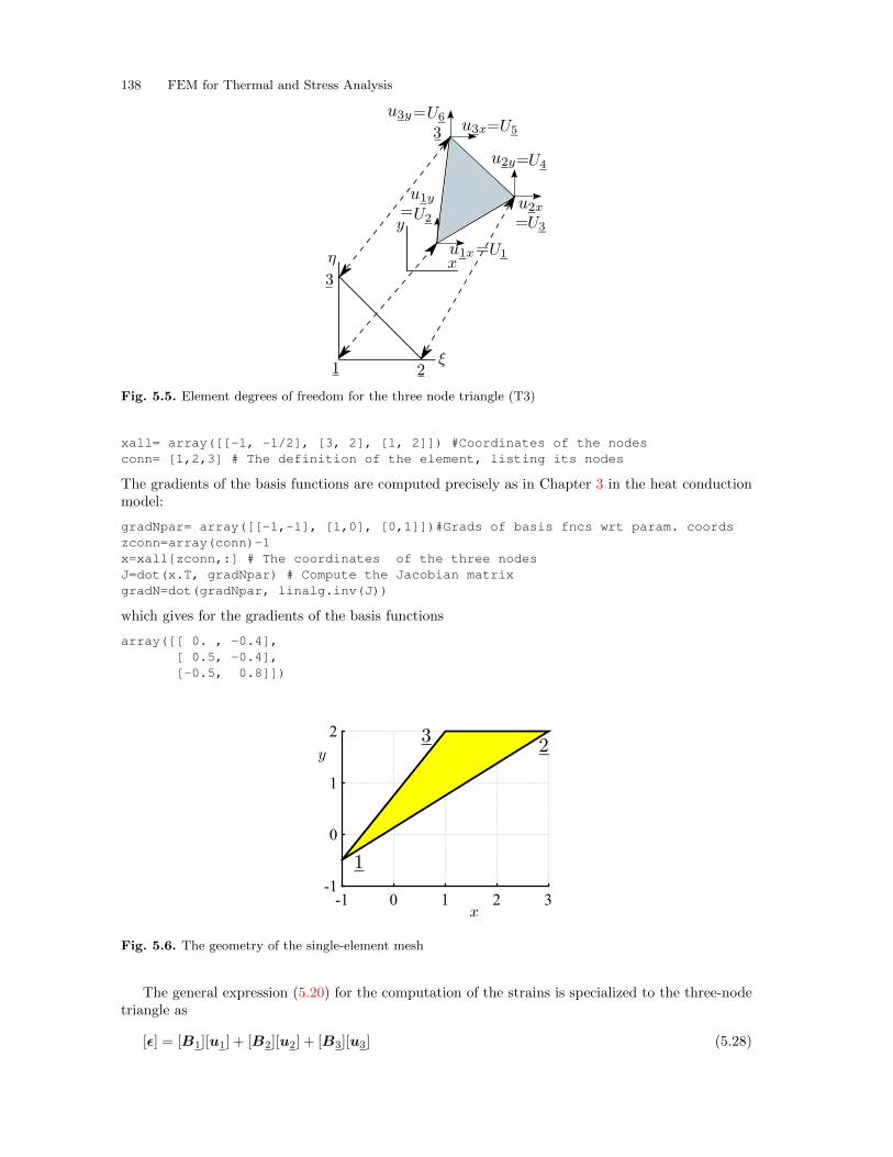
138 FEM for Thermal and Stress Analysis

Fig. 5.5. Element degrees of freedom for the three node triangle (T3)

xall= array([[-1, -1/2], [3, 2], [1, 2]]) #Coordinates of the nodesconn= [1,2,3] # The definition of the element, listing its nodes

The gradients of the basis functions are computed precisely as in Chapter 3 in the heat conductionmodel:

gradNpar= array([[-1,-1], [1,0], [0,1]])#Grads of basis fncs wrt param. coordszconn=array(conn)-1x=xall[zconn,:] # The coordinates of the three nodesJ=dot(x.T, gradNpar) # Compute the Jacobian matrixgradN=dot(gradNpar, linalg.inv(J))

which gives for the gradients of the basis functions

array([[ 0. , -0.4],[ 0.5, -0.4],[-0.5, 0.8]])

x

-1 0 1 2 3

y

-1

0

1

2

Fig. 5.6. The geometry of the single-element mesh

The general expression (5.20) for the computation of the strains is specialized to the three-nodetriangle as

[ϵ] = [B1][u1] + [B2][u2] + [B3][u3] (5.28)

5.4 Elementwise quantities for the three-node triangle 139

where the three nodal strain-displacement matrices are calculated from the gradients of the basisfunctions (see (5.22)) by defining a little helper Python function

def Bn(gradNn):return array([[gradNn[0], 0],

[0, gradNn[1]],[gradNn[1], gradNn[0]]])

Here gradNn is a 1 × 2 array of the components of the basis function gradients: gradNn[0] meansderivative ∂Nn/∂x and gradNn[1] corresponds to derivative ∂Nn/∂y. Let us inspect the strainsthat are produced by the motion of each of the three nodes individually (one moves, the other twostay fixed). For node 1 we obtain (gradN[0,:] is the gradient of the first basis function) usingB1=Bn(gradN[0,:])

array([[ 0. , 0. ],[ 0. , -0.4],[-0.4, 0. ]])

Note the strains we get when this strain-displacement matrix is multiplied with u1x, in the firstcolumn and u1y in the second column:

ϵx = 0 , ϵy = −0.4u1y , γxy = −0.4u1x (5.29)

The x displacement of node 1 produces only shear strain, and in particular no strain ϵx is pro-duced by the motion of node 1. Similarly, for node 2 we obtain the strain-displacement matrix asB2=Bn(gradN[1,:])

array([[ 0.5, 0. ],[ 0. , -0.4],[-0.4, 0.5]])

Now we can see that the displacement u2x contributes to the strain ϵx (just consider that theelement side [2,3] changes length when node 2 moves). We get the contribution to the strain withinthe element from the motion of node 2

ϵx = 0.5u2x , ϵy = −0.4u2y , γxy = −0.4u2x + 0.5u2y (5.30)

And, for node 3

array([[-0.5, 0. ],[ 0. , 0.8],[ 0.8, -0.5]])

ϵx = −0.5u3x , ϵy = 0.8u3y , γxy = 0.8u3x − 0.5u3y . (5.31)

Therefore (5.28) turns out to be explicitly ϵx = 0.5u2x − 0.5u3xϵy = −0.4u1y − 0.4u2y + 0.8u3yγxy = −0.4u1x − 0.4u2x + 0.5u2y + 0.8u3x − 0.5u3y

(5.32)

This is the complete description of how strains are produced for this particular triangular finiteelement by the motion of all and any of its three nodes.

An important observation should be made here:

Note that the strain components are uniform across the entire triangle. The three-nodetriangle is therefore usually called the CST (constant strain triangle).

140 FEM for Thermal and Stress Analysis

Consider now a special type of displacement: let us take all the x components of the nodedisplacements to be some value, the same at all three nodes, and similarly for the y components:u1x = u2x = u3x = a and u1y = u2y = u2y = b. The strain will then become ϵx = 0.5a− 0.5a = 0

ϵy = −0.4b− 0.4b+ 0.8b = 0γxy = −0.4a− 0.4a+ 0.5b+ 0.8a− 0.5b = 0

(5.33)

This displacement pattern is the so-called rigid-body translation, and the strains are all zero! Thatis the correct element response, there should be no strain when the element moves as a rigid body.

There is in fact one more displacement pattern where the element moves as a rigid body: rotation.The rotation about some point xc, yc can be described by the displacements

ux = −(y − yc)ψ , uy = (x− xc)ψ (5.34)

where the scalar ψ stands for the magnitude of the rotation angle. The displacements at the nodesare then obtained by substituting their coordinates to yield

u1x = −(y1 − yc)ψ , u2x = −(y2 − yc)ψ , u3x = −(y3 − yc)ψ ,u1y = (x1 − xc)ψ , u2y = (x2 − xc)ψ , u3y = (x3 − xc)ψ.

(5.35)

The strains are thenϵx = 0.5[−(y2 − yc)ψ]− 0.5[−(y3 − yc)ψ] = 0ϵy = −0.4[(x1 − xc)ψ]− 0.4[(x2 − xc)ψ] + 0.8[(x3 − xc)ψ] = 0γxy = −0.4[−(y1 − yc)ψ]− 0.4[−(y2 − yc)ψ] + 0.5[(x2 − xc)ψ]

+0.8[−(y3 − yc)ψ]− 0.5[(x3 − xc)ψ] = 0

(5.36)

where ψ can be totally arbitrary.

The strains for the three node triangle are all zero for the displacement patterns thatcorresponds to the two rigid body translations and the rigid body rotation.

5.4.2 Stiffness matrix

Now we will develop the stiffness matrix of the three node triangle. The starting point is the firstterm of (5.23). For a row degree of freedom q (the displacement at node j in the direction r) andcolumn p (the displacement at node i in the direction s), the entry qp of the stiffness matrix reads

Kqp =

∫S

[[Bj(q)]

T [D][Bi(p)]]r(q)s(p)

tdS (5.37)

Since the two indexes r, s take on values x, y (which are equivalent to 1, 2), the matrix∫S

[[Bj(q)]

T [D][Bi(p)]]tdS (5.38)

is of dimension 2×2. As the degrees of freedom of the three-node triangle are organized into a vector

[u(e)] =[u1x, u1y, u2x, u2y, u3x, u3y

]T=[U1, U2, U3, U4, U5, U6

]T, (5.39)

we realize that the entire stiffness matrix of the triangle consists of the 2× 2 submatrices (5.38)

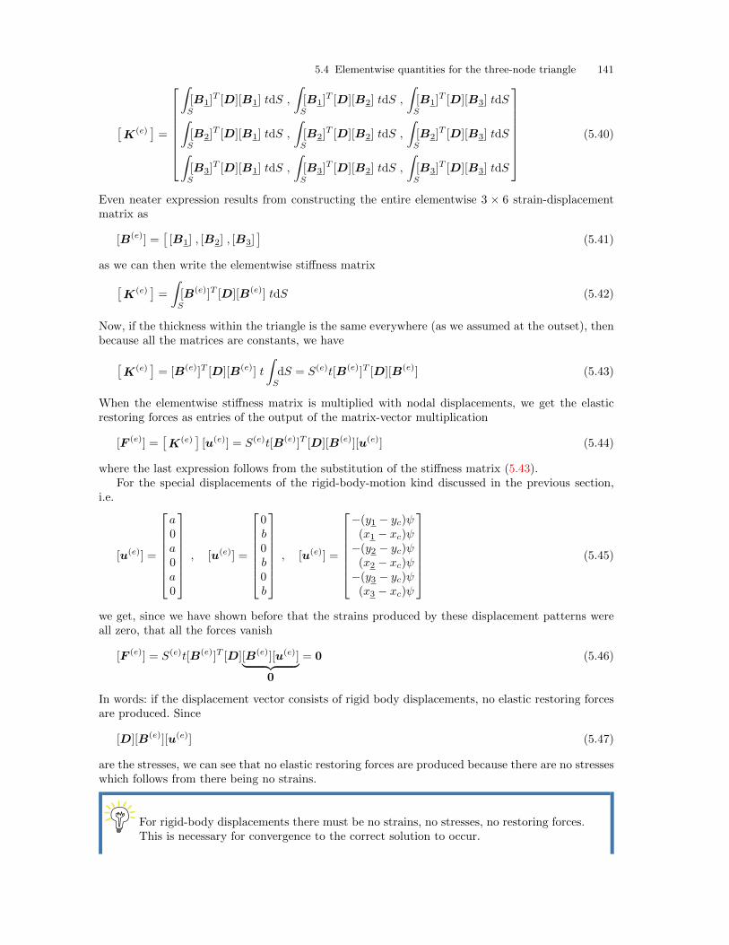
5.4 Elementwise quantities for the three-node triangle 141

[K(e)

]=

∫S

[B1]T [D][B1] tdS ,

∫S

[B1]T [D][B2] tdS ,

∫S

[B1]T [D][B3] tdS∫

S

[B2]T [D][B1] tdS ,

∫S

[B2]T [D][B2] tdS ,

∫S

[B2]T [D][B3] tdS∫

S

[B3]T [D][B1] tdS ,

∫S

[B3]T [D][B2] tdS ,

∫S

[B3]T [D][B3] tdS

(5.40)

Even neater expression results from constructing the entire elementwise 3 × 6 strain-displacementmatrix as

[B(e)] =[[B1] , [B2] , [B3]

](5.41)

as we can then write the elementwise stiffness matrix[K(e)

]=

∫S

[B(e)]T [D][B(e)] tdS (5.42)

Now, if the thickness within the triangle is the same everywhere (as we assumed at the outset), thenbecause all the matrices are constants, we have[

K(e)]= [B(e)]T [D][B(e)] t

∫S

dS = S(e)t[B(e)]T [D][B(e)] (5.43)

When the elementwise stiffness matrix is multiplied with nodal displacements, we get the elasticrestoring forces as entries of the output of the matrix-vector multiplication

[F (e)] =[K(e)

][u(e)] = S(e)t[B(e)]T [D][B(e)][u(e)] (5.44)

where the last expression follows from the substitution of the stiffness matrix (5.43).For the special displacements of the rigid-body-motion kind discussed in the previous section,

i.e.

[u(e)] =

a0a0a0

, [u(e)] =

0b0b0b

, [u(e)] =

−(y1 − yc)ψ(x1 − xc)ψ

−(y2 − yc)ψ(x2 − xc)ψ

−(y3 − yc)ψ(x3 − xc)ψ

(5.45)

we get, since we have shown before that the strains produced by these displacement patterns wereall zero, that all the forces vanish

[F (e)] = S(e)t[B(e)]T [D][B(e)][u(e)]︸ ︷︷ ︸0

= 0 (5.46)

In words: if the displacement vector consists of rigid body displacements, no elastic restoring forcesare produced. Since

[D][B(e)][u(e)] (5.47)

are the stresses, we can see that no elastic restoring forces are produced because there are no stresseswhich follows from there being no strains.

For rigid-body displacements there must be no strains, no stresses, no restoring forces.This is necessary for convergence to the correct solution to occur.

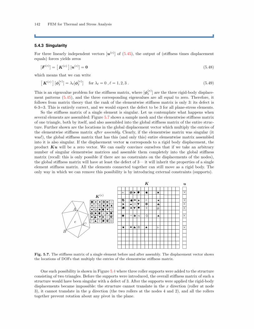
142 FEM for Thermal and Stress Analysis

5.4.3 Singularity

For three linearly independent vectors [u(e)] of (5.45), the output of (stiffness times displacementequals) forces yields zeros

[F (e)] =[K(e)

][u(e)] = 0 (5.48)

which means that we can write[K(e)

][ϕ

(e)ℓ ] = λℓ[ϕ

(e)ℓ ] for λℓ = 0 , ℓ = 1, 2, 3 . (5.49)

This is an eigenvalue problem for the stiffness matrix, where [ϕ(e)ℓ ] are the three rigid-body displace-

ment patterns (5.45), and the three corresponding eigenvalues are all equal to zero. Therefore, itfollows from matrix theory that the rank of the elementwise stiffness matrix is only 3: its defect is6-3=3. This is entirely correct, and we would expect the defect to be 3 for all plane-stress elements.

So the stiffness matrix of a single element is singular. Let us contemplate what happens whenseveral elements are assembled: Figure 5.7 shows a sample mesh and the elementwise stiffness matrixof one triangle, both by itself, and also assembled into the global stiffness matrix of the entire struc-ture. Further shown are the locations in the global displacement vector which multiply the entries ofthe elementwise stiffness matrix after assembly. Clearly, if the elementwise matrix was singular (itwas!), the global stiffness matrix that has this (and only this) entire elementwise matrix assembledinto it is also singular. If the displacement vector u corresponds to a rigid body displacement, theproduct Ku will be a zero vector. We can easily convince ourselves that if we take an arbitrarynumber of singular elementwise matrices and assemble them completely into the global stiffnessmatrix (recall: this is only possible if there are no constraints on the displacements of the nodes),the global stiffness matrix will have at least the defect of 3— it will inherit the properties of a singleelement stiffness matrix. All the elements connected together can still move as a rigid body. Theonly way in which we can remove this possibility is by introducing external constraints (supports).

Fig. 5.7. The stiffness matrix of a single element before and after assembly. The displacement vector showsthe locations of DOFs that multiply the entries of the elementwise stiffness matrix.

One such possibility is shown in Figure 5.4 where three roller supports were added to the structureconsisting of two triangles. Before the supports were introduced, the overall stiffness matrix of such astructure would have been singular with a defect of 3. After the supports were applied the rigid-bodydisplacements became impossible: the structure cannot translate in the x direction (roller at node3), it cannot translate in the y direction (the two rollers at the nodes 4 and 2), and all the rollerstogether prevent rotation about any pivot in the plane.

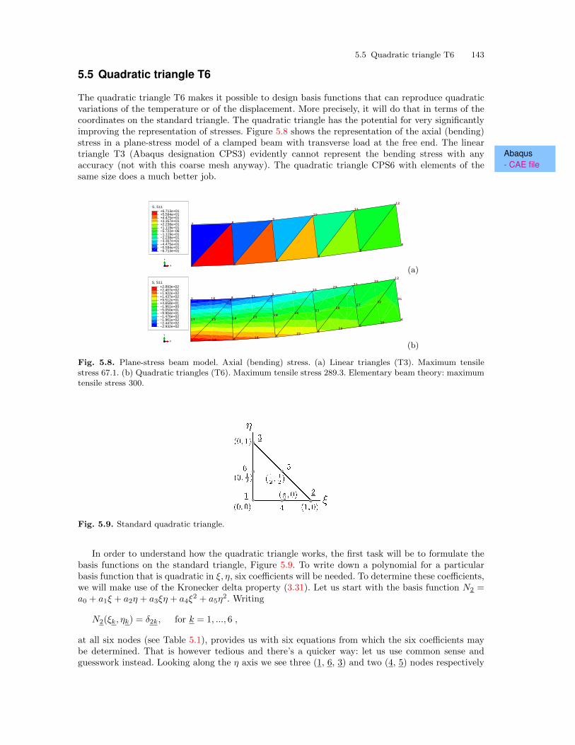
5.5 Quadratic triangle T6 143

5.5 Quadratic triangle T6

The quadratic triangle T6 makes it possible to design basis functions that can reproduce quadraticvariations of the temperature or of the displacement. More precisely, it will do that in terms of thecoordinates on the standard triangle. The quadratic triangle has the potential for very significantlyimproving the representation of stresses. Figure 5.8 shows the representation of the axial (bending)stress in a plane-stress model of a clamped beam with transverse load at the free end. The linear

Abaqus- CAE file

triangle T3 (Abaqus designation CPS3) evidently cannot represent the bending stress with anyaccuracy (not with this coarse mesh anyway). The quadratic triangle CPS6 with elements of thesame size does a much better job.

12

11

109

87

6

5

43

21

S, S11

−6.713e+01−5.594e+01−4.475e+01−3.357e+01−2.238e+01−1.119e+01−5.722e−06+1.119e+01+2.238e+01+3.357e+01+4.475e+01+5.594e+01+6.713e+01

X

Y

Z

(a)33

3231

30

29

2827

26

25

2423

22

21

20 19

18

17

16

15 14

13

12

11

109

87

6

5

43

21

S, S11

−2.932e+02−2.447e+02−1.961e+02−1.476e+02−9.904e+01−5.050e+01−1.961e+00+4.658e+01+9.512e+01+1.437e+02+1.922e+02+2.407e+02+2.893e+02

X

Y

Z

(b)

Fig. 5.8. Plane-stress beam model. Axial (bending) stress. (a) Linear triangles (T3). Maximum tensilestress 67.1. (b) Quadratic triangles (T6). Maximum tensile stress 289.3. Elementary beam theory: maximumtensile stress 300.

Fig. 5.9. Standard quadratic triangle.

In order to understand how the quadratic triangle works, the first task will be to formulate thebasis functions on the standard triangle, Figure 5.9. To write down a polynomial for a particularbasis function that is quadratic in ξ, η, six coefficients will be needed. To determine these coefficients,we will make use of the Kronecker delta property (3.31). Let us start with the basis function N2 =a0 + a1ξ + a2η + a3ξη + a4ξ

2 + a5η2. Writing

N2(ξk, ηk) = δ2k, for k = 1, ..., 6 ,

at all six nodes (see Table 5.1), provides us with six equations from which the six coefficients maybe determined. That is however tedious and there’s a quicker way: let us use common sense andguesswork instead. Looking along the η axis we see three (1, 6, 3) and two (4, 5) nodes respectively

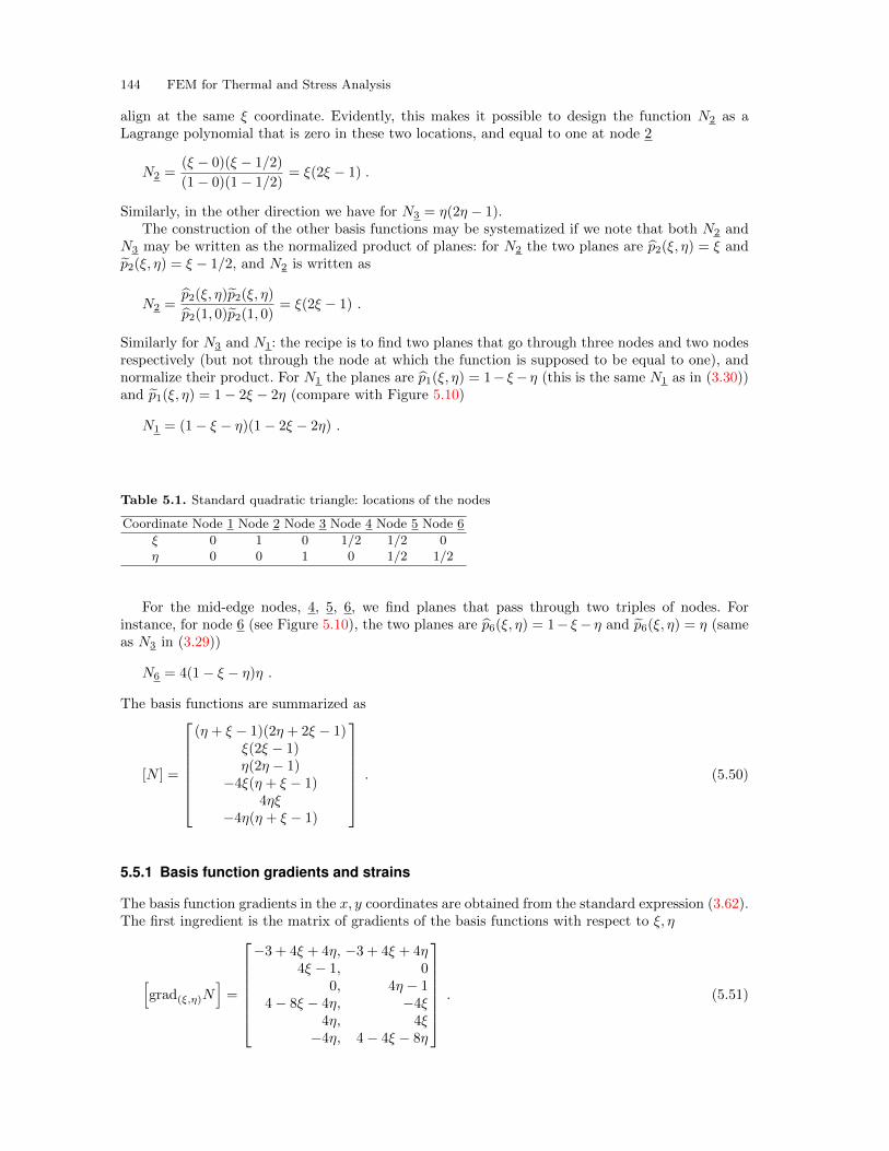
144 FEM for Thermal and Stress Analysis

align at the same ξ coordinate. Evidently, this makes it possible to design the function N2 as aLagrange polynomial that is zero in these two locations, and equal to one at node 2

N2 =(ξ − 0)(ξ − 1/2)

(1− 0)(1− 1/2)= ξ(2ξ − 1) .

Similarly, in the other direction we have for N3 = η(2η − 1).The construction of the other basis functions may be systematized if we note that both N2 and

N3 may be written as the normalized product of planes: for N2 the two planes are p2(ξ, η) = ξ andp2(ξ, η) = ξ − 1/2, and N2 is written as

N2 =p2(ξ, η)p2(ξ, η)

p2(1, 0)p2(1, 0)= ξ(2ξ − 1) .

Similarly for N3 and N1: the recipe is to find two planes that go through three nodes and two nodesrespectively (but not through the node at which the function is supposed to be equal to one), andnormalize their product. For N1 the planes are p1(ξ, η) = 1− ξ− η (this is the same N1 as in (3.30))and p1(ξ, η) = 1− 2ξ − 2η (compare with Figure 5.10)

N1 = (1− ξ − η)(1− 2ξ − 2η) .

Table 5.1. Standard quadratic triangle: locations of the nodes

Coordinate Node 1 Node 2 Node 3 Node 4 Node 5 Node 6

ξ 0 1 0 1/2 1/2 0η 0 0 1 0 1/2 1/2

For the mid-edge nodes, 4, 5, 6, we find planes that pass through two triples of nodes. Forinstance, for node 6 (see Figure 5.10), the two planes are p6(ξ, η) = 1− ξ− η and p6(ξ, η) = η (sameas N3 in (3.29))

N6 = 4(1− ξ − η)η .

The basis functions are summarized as

[N ] =

(η + ξ − 1)(2η + 2ξ − 1)

ξ(2ξ − 1)η(2η − 1)

−4ξ(η + ξ − 1)4ηξ

−4η(η + ξ − 1)

. (5.50)

5.5.1 Basis function gradients and strains

The basis function gradients in the x, y coordinates are obtained from the standard expression (3.62).The first ingredient is the matrix of gradients of the basis functions with respect to ξ, η

[grad(ξ,η)N

]=

−3 + 4ξ + 4η, −3 + 4ξ + 4η

4ξ − 1, 00, 4η − 1

4− 8ξ − 4η, −4ξ4η, 4ξ

−4η, 4− 4ξ − 8η

. (5.51)

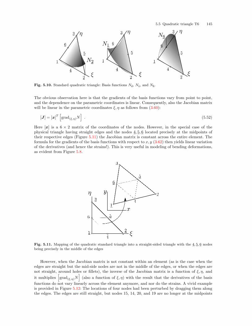
5.5 Quadratic triangle T6 145

Fig. 5.10. Standard quadratic triangle: Basis functions N2, N1, and N6.

The obvious observation here is that the gradients of the basis functions vary from point to point,and the dependence on the parametric coordinates is linear. Consequently, also the Jacobian matrixwill be linear in the parametric coordinates ξ, η as follows from (3.60):

[J ] = [x]T[grad(ξ,η)N

]. (5.52)

Here [x] is a 6 × 2 matrix of the coordinates of the nodes. However, in the special case of thephysical triangle having straight edges and the nodes 4, 5, 6 located precisely at the midpoints oftheir respective edges (Figure 5.11) the Jacobian matrix is constant across the entire element. Theformula for the gradients of the basis functions with respect to x, y (3.62) then yields linear variationof the derivatives (and hence the strains!). This is very useful in modeling of bending deformations,as evident from Figure 5.8.

Fig. 5.11. Mapping of the quadratic standard triangle into a straight-sided triangle with the 4, 5, 6 nodesbeing precisely in the middle of the edges

However, when the Jacobian matrix is not constant within an element (as is the case when theedges are straight but the mid-side nodes are not in the middle of the edges, or when the edges arenot straight, around holes or fillets), the inverse of the Jacobian matrix is a function of ξ, η, and

it multiplies[grad(ξ,η)N

](also a function of ξ, η) with the result that the derivatives of the basis

functions do not vary linearly across the element anymore, and nor do the strains. A vivid exampleis provided in Figure 5.12: The locations of four nodes had been perturbed by dragging them alongthe edges. The edges are still straight, but nodes 15, 14, 20, and 19 are no longer at the midpoints

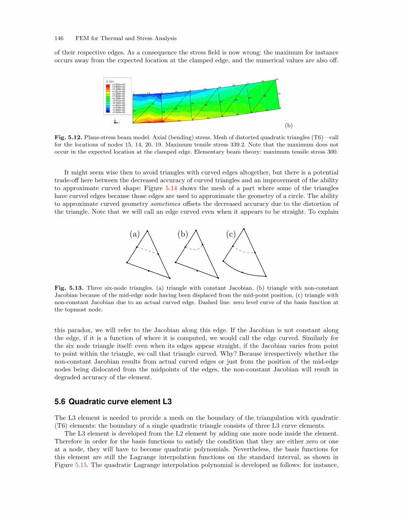
146 FEM for Thermal and Stress Analysis

of their respective edges. As a consequence the stress field is now wrong: the maximum for instanceoccurs away from the expected location at the clamped edge, and the numerical values are also off.

33

3231

30

29

2827

26

25

24

23

22

21

20

19

18

17

16

15

14

13

12

11

109

87

6

5

43

21

S, S11

−2.932e+02−2.405e+02−1.878e+02−1.351e+02−8.240e+01−2.971e+01+2.299e+01+7.568e+01+1.284e+02+1.811e+02+2.338e+02+2.865e+02+3.392e+02

X

Y

Z

(b)

Fig. 5.12. Plane-stress beam model. Axial (bending) stress. Mesh of distorted quadratic triangles (T6)—callfor the locations of nodes 15, 14, 20, 19. Maximum tensile stress 339.2. Note that the maximum does notoccur in the expected location at the clamped edge. Elementary beam theory: maximum tensile stress 300.

It might seem wise then to avoid triangles with curved edges altogether, but there is a potentialtrade-off here between the decreased accuracy of curved triangles and an improvement of the abilityto approximate curved shape: Figure 5.14 shows the mesh of a part where some of the triangleshave curved edges because those edges are used to approximate the geometry of a circle. The abilityto approximate curved geometry sometimes offsets the decreased accuracy due to the distortion ofthe triangle. Note that we will call an edge curved even when it appears to be straight. To explain

Fig. 5.13. Three six-node triangles. (a) triangle with constant Jacobian, (b) triangle with non-constantJacobian because of the mid-edge node having been displaced from the mid-point position, (c) triangle withnon-constant Jacobian due to an actual curved edge. Dashed line: zero level curve of the basis function atthe topmost node.

this paradox, we will refer to the Jacobian along this edge. If the Jacobian is not constant alongthe edge, if it is a function of where it is computed, we would call the edge curved. Similarly forthe six node triangle itself: even when its edges appear straight, if the Jacobian varies from pointto point within the triangle, we call that triangle curved. Why? Because irrespectively whether thenon-constant Jacobian results from actual curved edges or just from the position of the mid-edgenodes being dislocated from the midpoints of the edges, the non-constant Jacobian will result indegraded accuracy of the element.

5.6 Quadratic curve element L3

The L3 element is needed to provide a mesh on the boundary of the triangulation with quadratic(T6) elements: the boundary of a single quadratic triangle consists of three L3 curve elements.

The L3 element is developed from the L2 element by adding one more node inside the element.Therefore in order for the basis functions to satisfy the condition that they are either zero or oneat a node, they will have to become quadratic polynomials. Nevertheless, the basis functions forthis element are still the Lagrange interpolation functions on the standard interval, as shown inFigure 5.15. The quadratic Lagrange interpolation polynomial is developed as follows: for instance,

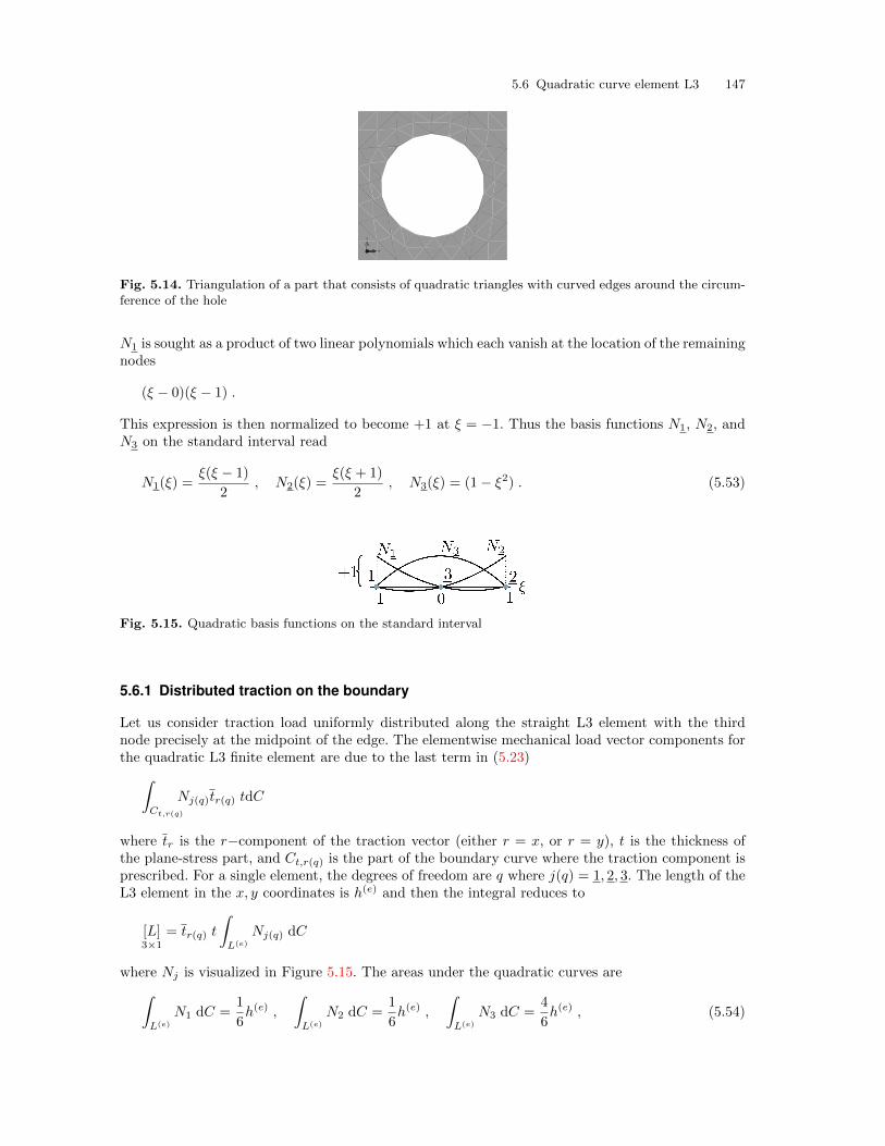
5.6 Quadratic curve element L3 147

X

Y

Z

Fig. 5.14. Triangulation of a part that consists of quadratic triangles with curved edges around the circum-ference of the hole

N1 is sought as a product of two linear polynomials which each vanish at the location of the remainingnodes

(ξ − 0)(ξ − 1) .

This expression is then normalized to become +1 at ξ = −1. Thus the basis functions N1, N2, andN3 on the standard interval read

N1(ξ) =ξ(ξ − 1)

2, N2(ξ) =

ξ(ξ + 1)

2, N3(ξ) = (1− ξ2) . (5.53)

Fig. 5.15. Quadratic basis functions on the standard interval

5.6.1 Distributed traction on the boundary

Let us consider traction load uniformly distributed along the straight L3 element with the thirdnode precisely at the midpoint of the edge. The elementwise mechanical load vector components forthe quadratic L3 finite element are due to the last term in (5.23)∫

Ct,r(q)

Nj(q)tr(q) tdC

where tr is the r−component of the traction vector (either r = x, or r = y), t is the thickness ofthe plane-stress part, and Ct,r(q) is the part of the boundary curve where the traction component isprescribed. For a single element, the degrees of freedom are q where j(q) = 1, 2, 3. The length of theL3 element in the x, y coordinates is h(e) and then the integral reduces to

[L]3×1

= tr(q) t

∫L(e)

Nj(q) dC

where Nj is visualized in Figure 5.15. The areas under the quadratic curves are∫L(e)

N1 dC =1

6h(e) ,

∫L(e)

N2 dC =1

6h(e) ,

∫L(e)

N3 dC =4

6h(e) , (5.54)

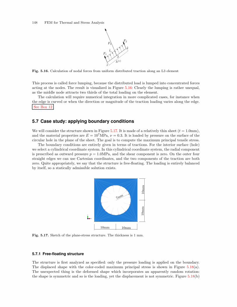
148 FEM for Thermal and Stress Analysis

Fig. 5.16. Calculation of nodal forces from uniform distributed traction along an L3 element

This process is called force lumping, because the distributed load is lumped into concentrated forcesacting at the nodes. The result is visualized in Figure 5.16: Clearly the lumping is rather unequal,as the middle node attracts two thirds of the total loading on the element.

The calculation will require numerical integration in more complicated cases, for instance whenthe edge is curved or when the direction or magnitude of the traction loading varies along the edge.

See Box 12

5.7 Case study: applying boundary conditions

We will consider the structure shown in Figure 5.17. It is made of a relatively thin sheet (t = 1.0mm),and the material properties are E = 107MPa, ν = 0.3. It is loaded by pressure on the surface of thecircular hole in the plane of the sheet. The goal is to compute the maximum principal tensile stress.

The boundary conditions are entirely given in terms of tractions. For the interior surface (hole)we select a cylindrical coordinate system. In this cylindrical coordinate system, the radial componentis prescribed as outward pressure p = 1.0MPa, and the shear component is zero. On the outer fourstraight edges we can use Cartesian coordinates, and the two components of the traction are bothzero. Quite appropriately, we say that the structure is free-floating. The loading is entirely balancedby itself, so a statically admissible solution exists.

Z

Y

X

X

Y

Z

Z

Y

X

X

Y

Z

Fig. 5.17. Sketch of the plane-stress structure. The thickness is 1 mm.

5.7.1 Free-floating structure

The structure is first analyzed as specified: only the pressure loading is applied on the boundary.The displaced shape with the color-coded maximum principal stress is shown in Figure 5.18(a).The unexpected thing is the deformed shape which incorporates an apparently random rotation:the shape is symmetric and so is the loading, yet the displacement is not symmetric. Figure 5.18(b)

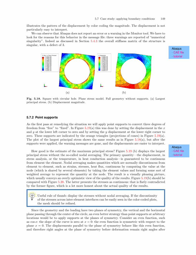
5.7 Case study: applying boundary conditions 149

illustrates the pattern of the displacement by color coding the magnitude. The displacement is notparticularly easy to interpret.

We can observe that Abaqus does not report an error or a warning in the Monitor tool. We have tolook for the reasons for this behavior in the message file: three warnings are reported of “numericalsingularity”. Indeed as discussed in Section 5.4.3 the overall stiffness matrix of the structure issingular, with a defect of 3.

Abaqus- CAE file- tutorialS, Max. In−Plane Principal

−8.203e−02+2.036e−01+4.892e−01+7.748e−01+1.060e+00+1.346e+00+1.632e+00+1.917e+00+2.203e+00+2.489e+00+2.774e+00+3.060e+00+3.345e+00

X

Y

Z

U, Magnitude

+8.956e−07+1.160e−06+1.425e−06+1.689e−06+1.953e−06+2.218e−06+2.482e−06+2.747e−06+3.011e−06+3.276e−06+3.540e−06+3.805e−06+4.069e−06

X

Y

Z

(a) (b)

Fig. 5.18. Square with circular hole. Plane stress model. Full geometry without supports. (a) Largestprincipal stress. (b) Displacement magnitude.

5.7.2 Point supports

As the first pass at remedying the situation we will apply point supports to convert three degrees offreedom from “free” to “fixed”. In Figure 5.19(a) this was done by setting the displacement in the xand y at the lower left corner to zero and by setting the y displacement at the lower right corner tozero. These supports are indicated by the orange triangles (projections of cones) in Figure 5.19(a).The plot of the largest principal stress shows the same results as in Figure 5.18(a), but after thesupports were applied, the warning messages are gone, and the displacements are easier to interpret.

Abaqus- CAE file- tutorial

How good is the estimate of the maximum principal stress? Figure 5.19 (b) displays the largestprincipal stress without the so-called nodal averaging. The primary quantity—the displacement, instress analysis, or the temperature, in heat conduction analysis—is guaranteed to be continuousfrom element the element. Nodal averaging makes quantities which are normally discontinuous fromelement to element, such as strains, stresses, heat flux, continuous by computing the value at thenode (which is shared by several elements) by taking the element values and forming some sort ofweighted average to represent the quantity at the node. The result is a visually pleasing picture,which usually conveys an overly optimistic view of the quality of the results. Figure 5.19(b) should becompared with Figure 5.20. The latter presents the stresses as continuous: that is flatly contradictedby the former figure, which is a lot more honest about the actual quality of the results.

Useful rule of thumb: display the stresses without nodal averaging. If the discontinuityof the stresses across inter-element interfaces can be easily seen in the color-coded plots,the mesh should be refined.

Since the geometry and the loading have two planes of symmetry, the vertical and the horizontalplane passing through the center of the circle, an even better strategy than point supports at arbitrarylocations would be to apply supports at the planes of symmetry. Consider an even function, suchas cosx: the slope of the curve is zero at x = 0: the even function is symmetric with respect to theplane x = 0. The displacements parallel to the plane of symmetry behave like this even function,and therefore right angles at the plane of symmetry before deformation remain right angles after

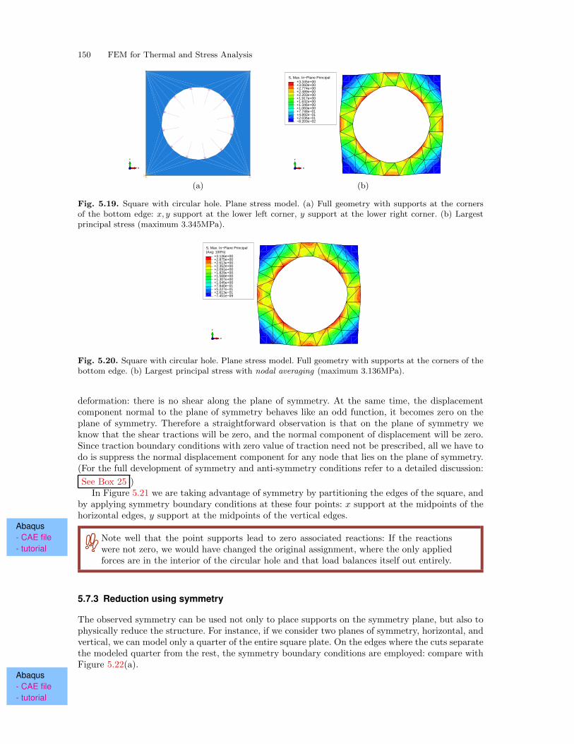
150 FEM for Thermal and Stress Analysis

Z

Y

X

X

Y

Z

S, Max. In−Plane Principal

−8.203e−02+2.036e−01+4.892e−01+7.748e−01+1.060e+00+1.346e+00+1.632e+00+1.917e+00+2.203e+00+2.489e+00+2.774e+00+3.060e+00+3.345e+00

X

Y

Z

(a) (b)

Fig. 5.19. Square with circular hole. Plane stress model. (a) Full geometry with supports at the cornersof the bottom edge: x, y support at the lower left corner, y support at the lower right corner. (b) Largestprincipal stress (maximum 3.345MPa).

(Avg: 100%)S, Max. In−Plane Principal

−7.451e−09+2.613e−01+5.227e−01+7.840e−01+1.045e+00+1.307e+00+1.568e+00+1.829e+00+2.091e+00+2.352e+00+2.613e+00+2.875e+00+3.136e+00

X

Y

Z

Fig. 5.20. Square with circular hole. Plane stress model. Full geometry with supports at the corners of thebottom edge. (b) Largest principal stress with nodal averaging (maximum 3.136MPa).

deformation: there is no shear along the plane of symmetry. At the same time, the displacementcomponent normal to the plane of symmetry behaves like an odd function, it becomes zero on theplane of symmetry. Therefore a straightforward observation is that on the plane of symmetry weknow that the shear tractions will be zero, and the normal component of displacement will be zero.Since traction boundary conditions with zero value of traction need not be prescribed, all we have todo is suppress the normal displacement component for any node that lies on the plane of symmetry.(For the full development of symmetry and anti-symmetry conditions refer to a detailed discussion:

See Box 25 )In Figure 5.21 we are taking advantage of symmetry by partitioning the edges of the square, and

by applying symmetry boundary conditions at these four points: x support at the midpoints of thehorizontal edges, y support at the midpoints of the vertical edges.

Abaqus- CAE file- tutorial

Note well that the point supports lead to zero associated reactions: If the reactionswere not zero, we would have changed the original assignment, where the only appliedforces are in the interior of the circular hole and that load balances itself out entirely.

5.7.3 Reduction using symmetry

The observed symmetry can be used not only to place supports on the symmetry plane, but also tophysically reduce the structure. For instance, if we consider two planes of symmetry, horizontal, andvertical, we can model only a quarter of the entire square plate. On the edges where the cuts separatethe modeled quarter from the rest, the symmetry boundary conditions are employed: compare withFigure 5.22(a).

Abaqus- CAE file- tutorial

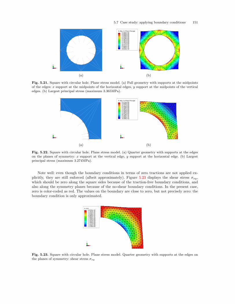
5.7 Case study: applying boundary conditions 151

Z

Y

X

X

Y

Z

S, Max. In−Plane Principal

+8.616e−03+2.883e−01+5.680e−01+8.477e−01+1.127e+00+1.407e+00+1.687e+00+1.967e+00+2.246e+00+2.526e+00+2.806e+00+3.085e+00+3.365e+00

X

Y

Z

(a) (b)

Fig. 5.21. Square with circular hole. Plane stress model. (a) Full geometry with supports at the midpointsof the edges: x support at the midpoints of the horizontal edges, y support at the midpoints of the verticaledges. (b) Largest principal stress (maximum 3.365MPa).

X

Y

Z

S, Max. In−Plane Principal

−6.494e−03+2.669e−01+5.402e−01+8.136e−01+1.087e+00+1.360e+00+1.634e+00+1.907e+00+2.180e+00+2.454e+00+2.727e+00+3.000e+00+3.274e+00

X

Y

Z

(a) (b)

Fig. 5.22. Square with circular hole. Plane stress model. (a) Quarter geometry with supports at the edgeson the planes of symmetry: x support at the vertical edge, y support at the horizontal edge. (b) Largestprincipal stress (maximum 3.274MPa).

Note well: even though the boundary conditions in terms of zero tractions are not applied ex-plicitly, they are still enforced (albeit approximately). Figure 5.23 displays the shear stress σxy,which should be zero along the square sides because of the traction-free boundary conditions, andalso along the symmetry planes because of the no-shear boundary conditions. In the present case,zero is color-coded as red. The values on the boundary are close to zero, but not precisely zero: theboundary condition is only approximated.

S, S12

−2.140e+00−1.958e+00−1.777e+00−1.595e+00−1.413e+00−1.232e+00−1.050e+00−8.682e−01−6.865e−01−5.048e−01−3.231e−01−1.414e−01+4.034e−02

X

Y

Z

Fig. 5.23. Square with circular hole. Plane stress model. Quarter geometry with supports at the edges onthe planes of symmetry: shear stress σxy

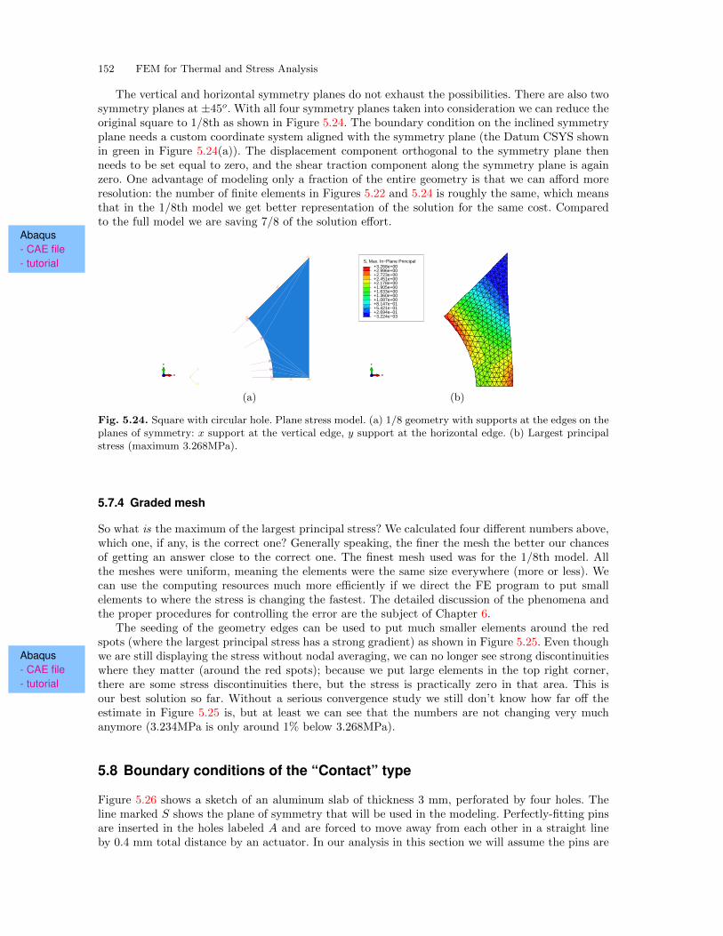
152 FEM for Thermal and Stress Analysis

The vertical and horizontal symmetry planes do not exhaust the possibilities. There are also twosymmetry planes at ±45o. With all four symmetry planes taken into consideration we can reduce theoriginal square to 1/8th as shown in Figure 5.24. The boundary condition on the inclined symmetryplane needs a custom coordinate system aligned with the symmetry plane (the Datum CSYS shownin green in Figure 5.24(a)). The displacement component orthogonal to the symmetry plane thenneeds to be set equal to zero, and the shear traction component along the symmetry plane is againzero. One advantage of modeling only a fraction of the entire geometry is that we can afford moreresolution: the number of finite elements in Figures 5.22 and 5.24 is roughly the same, which meansthat in the 1/8th model we get better representation of the solution for the same cost. Comparedto the full model we are saving 7/8 of the solution effort.

Abaqus- CAE file- tutorial

Z

Y

X

X

Y

Z

S, Max. In−Plane Principal

−3.224e−03+2.694e−01+5.421e−01+8.147e−01+1.087e+00+1.360e+00+1.633e+00+1.905e+00+2.178e+00+2.451e+00+2.723e+00+2.996e+00+3.268e+00

X

Y

Z

(a) (b)

Fig. 5.24. Square with circular hole. Plane stress model. (a) 1/8 geometry with supports at the edges on theplanes of symmetry: x support at the vertical edge, y support at the horizontal edge. (b) Largest principalstress (maximum 3.268MPa).

5.7.4 Graded mesh

So what is the maximum of the largest principal stress? We calculated four different numbers above,which one, if any, is the correct one? Generally speaking, the finer the mesh the better our chancesof getting an answer close to the correct one. The finest mesh used was for the 1/8th model. Allthe meshes were uniform, meaning the elements were the same size everywhere (more or less). Wecan use the computing resources much more efficiently if we direct the FE program to put smallelements to where the stress is changing the fastest. The detailed discussion of the phenomena andthe proper procedures for controlling the error are the subject of Chapter 6.

The seeding of the geometry edges can be used to put much smaller elements around the redspots (where the largest principal stress has a strong gradient) as shown in Figure 5.25. Even though

Abaqus- CAE file- tutorial

we are still displaying the stress without nodal averaging, we can no longer see strong discontinuitieswhere they matter (around the red spots); because we put large elements in the top right corner,there are some stress discontinuities there, but the stress is practically zero in that area. This isour best solution so far. Without a serious convergence study we still don’t know how far off theestimate in Figure 5.25 is, but at least we can see that the numbers are not changing very muchanymore (3.234MPa is only around 1% below 3.268MPa).

5.8 Boundary conditions of the “Contact” type

Figure 5.26 shows a sketch of an aluminum slab of thickness 3 mm, perforated by four holes. Theline marked S shows the plane of symmetry that will be used in the modeling. Perfectly-fitting pinsare inserted in the holes labeled A and are forced to move away from each other in a straight lineby 0.4 mm total distance by an actuator. In our analysis in this section we will assume the pins are

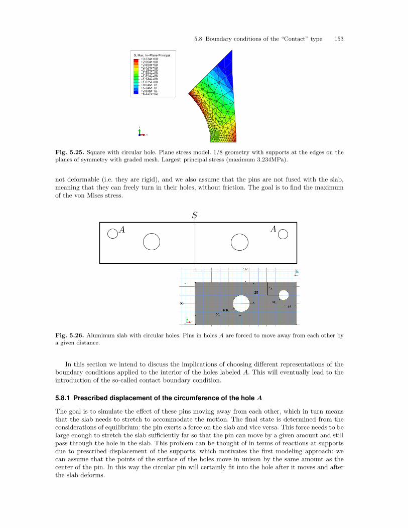
5.8 Boundary conditions of the “Contact” type 153

S, Max. In−Plane Principal

−5.317e−03+2.646e−01+5.346e−01+8.046e−01+1.075e+00+1.344e+00+1.614e+00+1.884e+00+2.154e+00+2.424e+00+2.694e+00+2.964e+00+3.234e+00

X

Y

Z

Fig. 5.25. Square with circular hole. Plane stress model. 1/8 geometry with supports at the edges on theplanes of symmetry with graded mesh. Largest principal stress (maximum 3.234MPa).

not deformable (i.e. they are rigid), and we also assume that the pins are not fused with the slab,meaning that they can freely turn in their holes, without friction. The goal is to find the maximumof the von Mises stress.

Fig. 5.26. Aluminum slab with circular holes. Pins in holes A are forced to move away from each other bya given distance.

In this section we intend to discuss the implications of choosing different representations of theboundary conditions applied to the interior of the holes labeled A. This will eventually lead to theintroduction of the so-called contact boundary condition.

5.8.1 Prescribed displacement of the circumference of the hole A

The goal is to simulate the effect of these pins moving away from each other, which in turn meansthat the slab needs to stretch to accommodate the motion. The final state is determined from theconsiderations of equilibrium: the pin exerts a force on the slab and vice versa. This force needs to belarge enough to stretch the slab sufficiently far so that the pin can move by a given amount and stillpass through the hole in the slab. This problem can be thought of in terms of reactions at supportsdue to prescribed displacement of the supports, which motivates the first modeling approach: wecan assume that the points of the surface of the holes move in unison by the same amount as thecenter of the pin. In this way the circular pin will certainly fit into the hole after it moves and afterthe slab deforms.

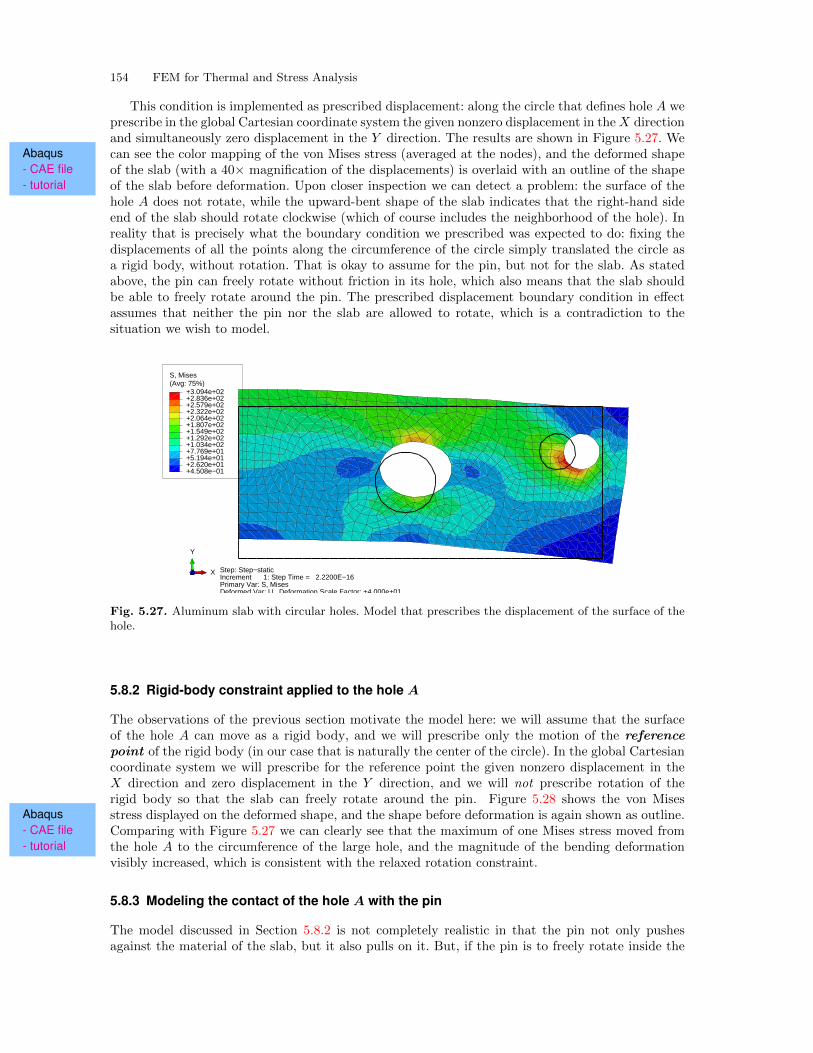
154 FEM for Thermal and Stress Analysis

This condition is implemented as prescribed displacement: along the circle that defines hole A weprescribe in the global Cartesian coordinate system the given nonzero displacement in theX directionand simultaneously zero displacement in the Y direction. The results are shown in Figure 5.27. We

Abaqus- CAE file- tutorial

can see the color mapping of the von Mises stress (averaged at the nodes), and the deformed shapeof the slab (with a 40× magnification of the displacements) is overlaid with an outline of the shapeof the slab before deformation. Upon closer inspection we can detect a problem: the surface of thehole A does not rotate, while the upward-bent shape of the slab indicates that the right-hand sideend of the slab should rotate clockwise (which of course includes the neighborhood of the hole). Inreality that is precisely what the boundary condition we prescribed was expected to do: fixing thedisplacements of all the points along the circumference of the circle simply translated the circle asa rigid body, without rotation. That is okay to assume for the pin, but not for the slab. As statedabove, the pin can freely rotate without friction in its hole, which also means that the slab shouldbe able to freely rotate around the pin. The prescribed displacement boundary condition in effectassumes that neither the pin nor the slab are allowed to rotate, which is a contradiction to thesituation we wish to model.

(Avg: 75%)S, Mises

+4.508e−01+2.620e+01+5.194e+01+7.769e+01+1.034e+02+1.292e+02+1.549e+02+1.807e+02+2.064e+02+2.322e+02+2.579e+02+2.836e+02+3.094e+02

Step: Step−staticIncrement 1: Step Time = 2.2200E−16Primary Var: S, MisesDeformed Var: U Deformation Scale Factor: +4.000e+01

X

Y

Z

Fig. 5.27. Aluminum slab with circular holes. Model that prescribes the displacement of the surface of thehole.

5.8.2 Rigid-body constraint applied to the hole A

The observations of the previous section motivate the model here: we will assume that the surfaceof the hole A can move as a rigid body, and we will prescribe only the motion of the referencepoint of the rigid body (in our case that is naturally the center of the circle). In the global Cartesiancoordinate system we will prescribe for the reference point the given nonzero displacement in theX direction and zero displacement in the Y direction, and we will not prescribe rotation of therigid body so that the slab can freely rotate around the pin. Figure 5.28 shows the von Mises

Abaqus- CAE file- tutorial

stress displayed on the deformed shape, and the shape before deformation is again shown as outline.Comparing with Figure 5.27 we can clearly see that the maximum of one Mises stress moved fromthe hole A to the circumference of the large hole, and the magnitude of the bending deformationvisibly increased, which is consistent with the relaxed rotation constraint.

5.8.3 Modeling the contact of the hole A with the pin

The model discussed in Section 5.8.2 is not completely realistic in that the pin not only pushesagainst the material of the slab, but it also pulls on it. But, if the pin is to freely rotate inside the

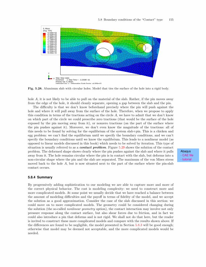
5.8 Boundary conditions of the “Contact” type 155

(Avg: 75%)S, Mises

+5.330e−01+2.254e+01+4.455e+01+6.655e+01+8.856e+01+1.106e+02+1.326e+02+1.546e+02+1.766e+02+1.986e+02+2.206e+02+2.426e+02+2.646e+02

Step: Step−staticIncrement 1: Step Time = 2.2200E−16Primary Var: S, MisesDeformed Var: U Deformation Scale Factor: +4.000e+01

X

Y

Z

Fig. 5.28. Aluminum slab with circular holes. Model that ties the surface of the hole into a rigid body.

hole A, it is not likely to be able to pull on the material of the slab. Rather, if the pin moves awayfrom the edge of the hole, it should cleanly separate, opening a gap between the slab and the pin.

The difficulty is that we don’t know beforehand precisely where the pin will push against thehole and where it will pull away from the surface of the hole. Therefore, when we propose to applythis condition in terms of the tractions acting on the circle A, we have to admit that we don’t knowon which part of the circle we could prescribe zero tractions (that would be the surface of the holeexposed by the pin moving away from it), or nonzero tractions (on the part of the surface wherethe pin pushes against it). Moreover, we don’t even know the magnitude of the tractions: all ofthis needs to be found by solving for the equilibrium of the system slab+pin. This is a chicken andegg problem: we can’t find the equilibrium until we specify the boundary conditions, and we can’tspecify the boundary conditions until we know the equilibrium. This leads to a nonlinear model (asopposed to linear models discussed in this book) which needs to be solved by iteration. This type ofsituation is usually referred to as a contact problem . Figure 5.29 shows the solution of the contact

Abaqus- CAE file- tutorial

problem. The deformed shape shows clearly where the pin pushes against the slab and where it pullsaway from it. The hole remains circular where the pin is in contact with the slab, but deforms into anon-circular shape where the pin and the slab are separated. The maximum of the von Mises stressmoved back to the hole A, but is now situated next to the part of the surface where the pin-slabcontact occurs.

5.8.4 Summary

By progressively adding sophistication to our modeling we are able to capture more and more ofthe correct physical behavior. The cost is modeling complexity: we need to construct more andmore complicated models. At some point we usually decide that we have reached a balance betweenthe amount of modeling difficulties and the payoff in terms of fidelity of the model, and we acceptthe solution as a good approximation. Consider the case of the slab discussed in this section: wecould move on to more complicated models. The geometry could be considered changing duringthe solution (the so-called nonlinear geometry option), the contact interaction may involve not onlypressure response along the contact surface, but also shear forces due to friction, and in fact wecould also introduce a pin that deforms and is not rigid. We shall not do that here, but the readeris invited to construct these more complicated models and compare with the results shown above. Ifthe differences are found to be negligible, the model presented in Section 5.8.3 will be good enough;otherwise that model may be deemed not acceptable, and the more complicated models would beneeded.

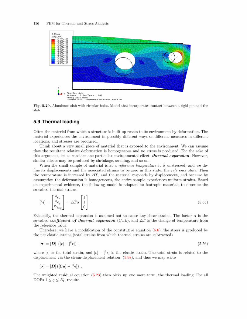
156 FEM for Thermal and Stress Analysis

(Avg: 75%)S, Mises

+1.561e+00+2.839e+01+5.522e+01+8.205e+01+1.089e+02+1.357e+02+1.625e+02+1.894e+02+2.162e+02+2.430e+02+2.698e+02+2.967e+02+3.235e+02

Step: Step−staticIncrement 1: Step Time = 1.000Primary Var: S, MisesDeformed Var: U Deformation Scale Factor: +4.000e+01

X

Y

Z

Fig. 5.29. Aluminum slab with circular holes. Model that incorporates contact between a rigid pin and theslab.

5.9 Thermal loading

Often the material from which a structure is built up reacts to its environment by deformation. Thematerial experiences the environment in possibly different ways or different measures in differentlocations, and stresses are produced.

Think about a very small piece of material that is exposed to the environment. We can assumethat the resultant relative deformation is homogeneous and no stress is produced. For the sake ofthis argument, let us consider one particular environmental effect: thermal expansion . However,similar effects may be produced by shrinkage, swelling, and so on.

When the small sample of material is at a reference temperature it is unstressed, and we de-fine its displacements and the associated strains to be zero in this state: the reference state. Thenthe temperature is increased by ∆T , and the material responds by displacement, and because byassumption the deformation is homogeneous, the entire sample experiences uniform strains. Basedon experimental evidence, the following model is adopted for isotropic materials to describe theso-called thermal strains

[θϵ] =

θϵxθϵyθγxy

= ∆Tα

110

. (5.55)

Evidently, the thermal expansion is assumed not to cause any shear strains. The factor α is theso-called coefficient of thermal expansion (CTE), and ∆T is the change of temperature fromthe reference value.

Therefore, we have a modification of the constitutive equation (5.6): the stress is produced bythe net elastic strains (total strains from which thermal strains are subtracted)

[σ] = [D]([ϵ]− [θϵ]

), (5.56)

where [ϵ] is the total strain, and [ϵ] − [θϵ] is the elastic strain. The total strain is related to thedisplacement via the strain-displacement relation (5.98), and thus we may write

[σ] = [D]([Bu]− [θϵ]

).

The weighted residual equation (5.23) then picks up one more term, the thermal loading: For allDOFs 1 ≤ q ≤ Nf , require

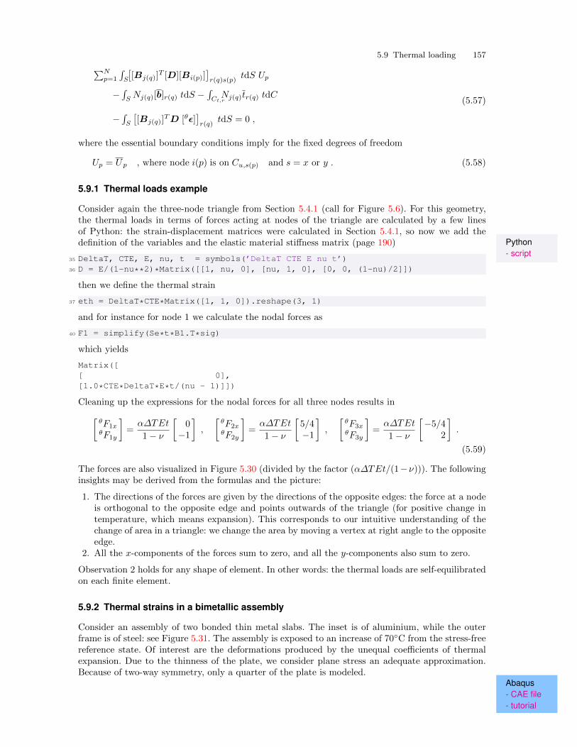
5.9 Thermal loading 157∑Np=1

∫S

[[Bj(q)]

T [D][Bi(p)]]r(q)s(p)

tdS Up

−∫SNj(q)[b]r(q) tdS −

∫Ct,rNj(q)tr(q) tdC

−∫S

[[Bj(q)]

TD [θϵ]]r(q)

tdS = 0 ,

(5.57)

where the essential boundary conditions imply for the fixed degrees of freedom

Up = Up , where node i(p) is on Cu,s(p) and s = x or y . (5.58)

5.9.1 Thermal loads example

Consider again the three-node triangle from Section 5.4.1 (call for Figure 5.6). For this geometry,the thermal loads in terms of forces acting at nodes of the triangle are calculated by a few linesof Python: the strain-displacement matrices were calculated in Section 5.4.1, so now we add the

Python- script

definition of the variables and the elastic material stiffness matrix (page 190)

35 DeltaT, CTE, E, nu, t = symbols(’DeltaT CTE E nu t’)36 D = E/(1-nu**2)*Matrix([[1, nu, 0], [nu, 1, 0], [0, 0, (1-nu)/2]])

then we define the thermal strain

37 eth = DeltaT*CTE*Matrix([1, 1, 0]).reshape(3, 1)

and for instance for node 1 we calculate the nodal forces as

40 F1 = simplify(Se*t*B1.T*sig)

which yields

Matrix([[ 0],[1.0*CTE*DeltaT*E*t/(nu - 1)]])

Cleaning up the expressions for the nodal forces for all three nodes results in[θF1xθF1y

]=α∆TEt

1− ν

[0

−1

],

[θF2xθF2y

]=α∆TEt

1− ν

[5/4−1

],

[θF3xθF3y

]=α∆TEt

1− ν

[−5/4

2

].

(5.59)

The forces are also visualized in Figure 5.30 (divided by the factor (α∆TEt/(1−ν))). The followinginsights may be derived from the formulas and the picture:

1. The directions of the forces are given by the directions of the opposite edges: the force at a nodeis orthogonal to the opposite edge and points outwards of the triangle (for positive change intemperature, which means expansion). This corresponds to our intuitive understanding of thechange of area in a triangle: we change the area by moving a vertex at right angle to the oppositeedge.

2. All the x-components of the forces sum to zero, and all the y-components also sum to zero.

Observation 2 holds for any shape of element. In other words: the thermal loads are self-equilibratedon each finite element.

5.9.2 Thermal strains in a bimetallic assembly

Consider an assembly of two bonded thin metal slabs. The inset is of aluminium, while the outerframe is of steel: see Figure 5.31. The assembly is exposed to an increase of 70◦C from the stress-freereference state. Of interest are the deformations produced by the unequal coefficients of thermalexpansion. Due to the thinness of the plate, we consider plane stress an adequate approximation.Because of two-way symmetry, only a quarter of the plate is modeled.

Abaqus- CAE file- tutorial

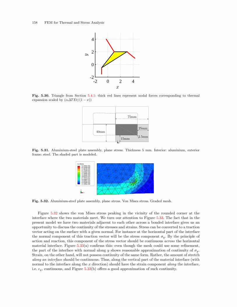
158 FEM for Thermal and Stress Analysis

x

-2 0 2 4y

-2

0

2

4

Fig. 5.30. Triangle from Section 5.4.1: thick red lines represent nodal forces corresponding to thermalexpansion scaled by (α∆TEt/(1− ν))

X

Y

Z

Fig. 5.31. Aluminium-steel plate assembly, plane stress. Thickness 5 mm. Interior: aluminium, exteriorframe: steel. The shaded part is modeled.

S, Mises

+1.335e+00+2.034e+01+3.935e+01+5.836e+01+7.737e+01+9.637e+01+1.154e+02+1.344e+02+1.534e+02+1.724e+02+1.914e+02+2.104e+02+2.294e+02

X

Y

Z

Fig. 5.32. Aluminium-steel plate assembly, plane stress. Von Mises stress. Graded mesh.

Figure 5.32 shows the von Mises stress peaking in the vicinity of the rounded corner at theinterface where the two materials meet. We turn our attention to Figure 5.33. The fact that in thepresent model we have two materials adjacent to each other across a bonded interface gives us anopportunity to discuss the continuity of the stresses and strains. Stress can be converted to a tractionvector acting on the surface with a given normal. For instance at the horizontal part of the interfacethe normal component of this traction vector will be the stress component σy. By the principle ofaction and reaction, this component of the stress vector should be continuous across the horizontalmaterial interface. Figure 5.33(a) confirms this: even though the mesh could use some refinement,the part of the interface with normal along y shows reasonable approximation of continuity of σy.Strain, on the other hand, will not possess continuity of the same form. Rather, the amount of stretchalong an interface should be continuous. Thus, along the vertical part of the material interface (withnormal to the interface along the x direction) should have the strain component along the interface,i.e. ϵy, continuous, and Figure 5.33(b) offers a good approximation of such continuity.

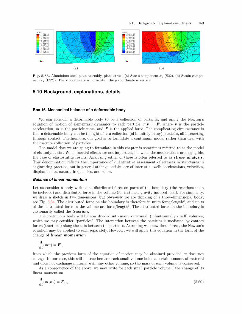
5.10 Background, explanations, details 159

S, S22

−4.526e+01−3.116e+01−1.705e+01−2.941e+00+1.117e+01+2.527e+01+3.938e+01+5.349e+01+6.760e+01+8.170e+01+9.581e+01+1.099e+02+1.240e+02

X

Y

Z

E, E22

+5.009e−04+6.092e−04+7.175e−04+8.258e−04+9.342e−04+1.042e−03+1.151e−03+1.259e−03+1.367e−03+1.476e−03+1.584e−03+1.692e−03+1.801e−03

X

Y

Z

(a) (b)

Fig. 5.33. Aluminium-steel plate assembly, plane stress. (a) Stress component σy (S22). (b) Strain compo-nent ϵy (E22)). The x coordinate is horizontal, the y coordinate is vertical.

5.10 Background, explanations, details

Box 16. Mechanical balance of a deformable body

We can consider a deformable body to be a collection of particles, and apply the Newton’sequation of motion of elementary dynamics to each particle, mv = F , where v is the particleacceleration, m is the particle mass, and F is the applied force. The complicating circumstance isthat a deformable body can be thought of as a collection (of infinitely many) particles, all interactingthrough contact. Furthermore, our goal is to formulate a continuum model rather than deal withthe discrete collection of particles.

The model that we are going to formulate in this chapter is sometimes referred to as the modelof elastodynamics. When inertial effects are not important, i.e. when the accelerations are negligible,the case of elastostatics results. Analyzing either of these is often referred to as stress analysis.This denomination reflects the importance of quantitative assessment of stresses in structures inengineering practice, but in general other quantities are of interest as well: accelerations, velocities,displacements, natural frequencies, and so on.

Balance of linear momentum

Let us consider a body with some distributed force on parts of the boundary (the reactions mustbe included) and distributed force in the volume (for instance, gravity-induced load). For simplicity,we draw a sketch in two dimensions, but obviously we are thinking of a three-dimensional body;see Fig. 5.34. The distributed force on the boundary is therefore in units force/length2, and unitsof the distributed force in the volume are force/length3. The distributed force on the boundary iscustomarily called the traction .

The continuous body will be now divided into many very small (infinitesimally small) volumes,which we may consider “particles”. The interaction between the particles is mediated by contactforces (tractions) along the cuts between the particles. Assuming we know these forces, the Newton’sequation may be applied to each separately. However, we will apply this equation in the form of thechange of linear momentum

d

dt(mv) = F ,

from which the previous form of the equation of motion may be obtained provided m does notchange. In our case, this will be true because each small volume holds a certain amount of materialand does not exchange material with any other volume, so the mass of each volume is conserved.

As a consequence of the above, we may write for each small particle volume j the change of itslinear momentum

d

dt(mjvj) = F j , (5.60)

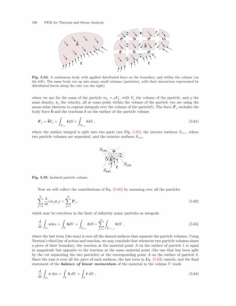
160 FEM for Thermal and Stress Analysis

Fig. 5.34. A continuous body with applied distributed force on the boundary, and within the volume (onthe left). The same body cut up into many small volumes (particles), with their interaction represented bydistributed forces along the cuts (on the right).

where we use for the mass of the particle mj = ρVj , with Vj the volume of the particle, and ρ themass density, vj the velocity, all at some point within the volume of the particle (we are using themean-value theorem to express integrals over the volume of the particle!). The force F j includes thebody force b and the tractions t on the surface of the particle volume

F j = bVj +

∫Sint

tdS +

∫Sext

tdS , (5.61)

where the surface integral is split into two parts (see Fig. 5.35): the interior surfaces Sint, wheretwo particle volumes are separated, and the exterior surfaces Sext.

Fig. 5.35. Isolated particle volume.

Now we will collect the contributions of Eq. (5.60) by summing over all the particles

N∑j=1

d

dt(mjvj) =

N∑j=1

F j , (5.62)

which may be rewritten in the limit of infinitely many particles as integrals

d

dt

∫m

vdm =

∫V

bdV +

∫Sext

tdS +

∞∑j=1

∫Sint,j

tdS , (5.63)

where the last term (the sum) is over all the shared surfaces that separate the particle volumes. UsingNewton’s third law of action and reaction, we may conclude that whenever two particle volumes sharea piece of their boundary, the traction at the material point A on the surface of particle 1 is equalin magnitude but opposite to the traction at the same material point (the one that has been splitby the cut separating the two particles) at the corresponding point A on the surface of particle 2.Since the sum is over all the pairs of such surfaces, the last term in Eq. (5.63) cancels, and the finalstatement of the balance of linear momentum of the material in the volume V reads

d

dt

∫m

v dm =

∫V

b dV +

∫S

t dS , (5.64)

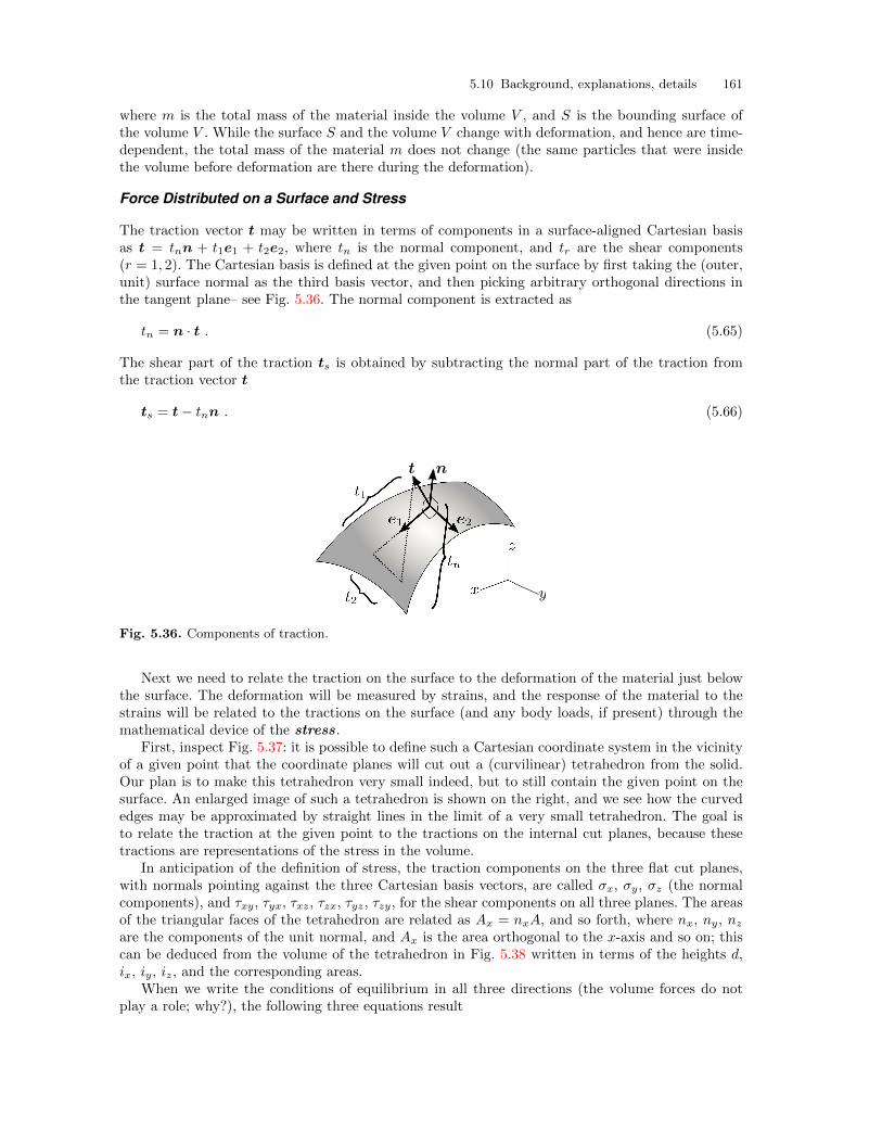
5.10 Background, explanations, details 161

where m is the total mass of the material inside the volume V , and S is the bounding surface ofthe volume V . While the surface S and the volume V change with deformation, and hence are time-dependent, the total mass of the material m does not change (the same particles that were insidethe volume before deformation are there during the deformation).

Force Distributed on a Surface and Stress

The traction vector t may be written in terms of components in a surface-aligned Cartesian basisas t = tnn + t1e1 + t2e2, where tn is the normal component, and tr are the shear components(r = 1, 2). The Cartesian basis is defined at the given point on the surface by first taking the (outer,unit) surface normal as the third basis vector, and then picking arbitrary orthogonal directions inthe tangent plane– see Fig. 5.36. The normal component is extracted as

tn = n · t . (5.65)

The shear part of the traction ts is obtained by subtracting the normal part of the traction fromthe traction vector t

ts = t− tnn . (5.66)

Fig. 5.36. Components of traction.

Next we need to relate the traction on the surface to the deformation of the material just belowthe surface. The deformation will be measured by strains, and the response of the material to thestrains will be related to the tractions on the surface (and any body loads, if present) through themathematical device of the stress.

First, inspect Fig. 5.37: it is possible to define such a Cartesian coordinate system in the vicinityof a given point that the coordinate planes will cut out a (curvilinear) tetrahedron from the solid.Our plan is to make this tetrahedron very small indeed, but to still contain the given point on thesurface. An enlarged image of such a tetrahedron is shown on the right, and we see how the curvededges may be approximated by straight lines in the limit of a very small tetrahedron. The goal isto relate the traction at the given point to the tractions on the internal cut planes, because thesetractions are representations of the stress in the volume.

In anticipation of the definition of stress, the traction components on the three flat cut planes,with normals pointing against the three Cartesian basis vectors, are called σx, σy, σz (the normalcomponents), and τxy, τyx, τxz, τzx, τyz, τzy, for the shear components on all three planes. The areasof the triangular faces of the tetrahedron are related as Ax = nxA, and so forth, where nx, ny, nzare the components of the unit normal, and Ax is the area orthogonal to the x-axis and so on; thiscan be deduced from the volume of the tetrahedron in Fig. 5.38 written in terms of the heights d,ix, iy, iz, and the corresponding areas.

When we write the conditions of equilibrium in all three directions (the volume forces do notplay a role; why?), the following three equations result

162 FEM for Thermal and Stress Analysis

Fig. 5.37. Relating the components of traction to stress.

Fig. 5.38. Components of traction.

tx = σxnx + τxyny + τxznz ,

ty = τyxnx + σyny + τyznz , (5.67)

tz = τzxnx + τzyny + σznz .

This equation relates the components of the traction on the surface with the components of thetraction on the special surfaces – coordinate planes – inside the volume. The components of thetraction on the internal surfaces are called normal stresses (σx, σy, σz), and shear stresses (τxy,τyx, τxz, τzx, τyz, τzy). The form of Eq. (5.67) suggests the matrix expression txty

tz

=

σx τxy τxzτyx σy τyzτzx τzy σz

nxnynz

, (5.68)

where all matrices hold components in the Cartesian basis. A component-free version would read

t = Σ · n ,

where Σ would be defined as a Cartesian tensor, the Cauchy stress tensor . The traction vectorand the normal would then also become tensors. However, in this book the tensor notation is avoided,and with a few exceptions tensors will not be needed. The two exceptions that may be mentionedhere are coordinate transformations and the calculation of the principal stresses which are theeigenvalues of the matrix of the stress components.

First we will consider transformation of vectors from one Cartesian coordinate system into an-other. The Cartesian coordinate axes are defined by a triple of orthonormal basis vectors, one bythe basis triple ex, ey, ez and the other by the basis triple ex, ey, ez. An arbitrary vector u may bewritten in terms of components and basis vectors in either coordinate system as

u = uxex + uyey + uzez = uxex + uyey + uzez . (5.69)

This may be written as a matrix expression, with the basis vectors as columns of matrices

5.10 Background, explanations, details 163

u =[ex, ey, ez

] uxuyuz

=[ex, ey, ez

] uxuyuz

. (5.70)

Now consider that the basis vectors themselves may be expressed in terms of their components onsome basis: we will pick ex, ey, ez as that basis. On this basis we can write the components of thevectors ex, ey, ez themselves as

[ex] =

100

, [ey] =

010

, [ez] =

001

We can now write, entirely in components,

[[ex], [ey], [ez]

] uxuyuz

=

100

010

001

uxuyuz

=

uxuyuz

.

The components of the vectors ex, ey, ez are

[ex] =

ex · exex · eyex · ez

, [ey] =

ey · exey · eyey · ez

, [ez] =

ez · exez · eyez · ez

,

where ex · ex is the cosine of the angle between the two vectors ex and ex, and so on, so that wecan write entirely in terms of components

[ex, ey, ez

] uxuyuz

=

ex · exex · eyex · ez

,ey · exey · eyey · ez

,ez · exez · eyez · ez

uxuyuz

= [Rm]

uxuyuz

.

where we have defined the transformation matrix

[Rm] =

ex · ex, ey · ex, ez · exex · ey, ey · ey, ez · eyex · ez, ey · ez, ez · ez

, (5.71)

composed of the direction cosines. In words, the columns of the transformation matrix consist ofthe components of the vectors ex, ey, ez on the basis vectors ex, ey, ez. The transformation matrixis recognized as an orthogonal matrix (rotation matrix), whose inverse is its transpose

[Rm]−1

= [Rm]T

Thus we have the transformation of vector componentsuxuyuz

= [Rm]

uxuyuz

and

uxuyuz

= [Rm]T

uxuyuz

. (5.72)

Now we take up again the relationship between the traction vector, the stress at a point, andthe normal to a surface through the point (5.68) txty

tz

=

σx τxy τxzτyx σy τyzτzx τzy σz

nxnynz

,

and we consider what happens when both vectors are expressed using components in a differentcoordinate system. We apply (5.72) as

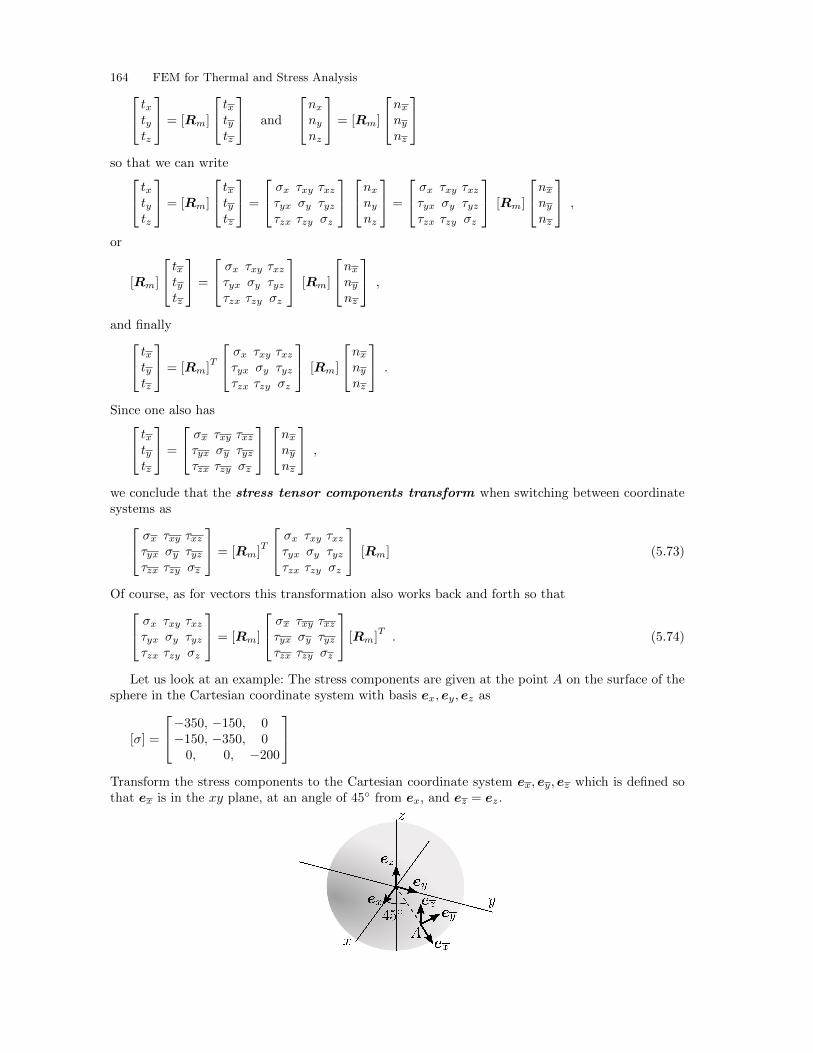
164 FEM for Thermal and Stress Analysis txtytz

= [Rm]

txtytz

and

nxnynz

= [Rm]

nx

nynz

so that we can write txty

tz

= [Rm]

txtytz

=

σx τxy τxzτyx σy τyzτzx τzy σz

nxnynz

=

σx τxy τxzτyx σy τyzτzx τzy σz

[Rm]

nx

nynz

,

or

[Rm]

txtytz

=

σx τxy τxzτyx σy τyzτzx τzy σz

[Rm]

nxnynz

,

and finally txtytz

= [Rm]T

σx τxy τxzτyx σy τyzτzx τzy σz

[Rm]

nx

nynz

.

Since one also has txtytz

=

σx τxy τxzτyx σy τyzτzx τzy σz

nxnynz

,

we conclude that the stress tensor components transform when switching between coordinatesystems as σx τxy τxz

τyx σy τyzτzx τzy σz

= [Rm]T

σx τxy τxzτyx σy τyzτzx τzy σz

[Rm] (5.73)

Of course, as for vectors this transformation also works back and forth so that σx τxy τxzτyx σy τyzτzx τzy σz

= [Rm]

σx τxy τxzτyx σy τyzτzx τzy σz

[Rm]T. (5.74)

Let us look at an example: The stress components are given at the point A on the surface of thesphere in the Cartesian coordinate system with basis ex, ey, ez as

[σ] =

−350, −150, 0−150, −350, 00, 0, −200

Transform the stress components to the Cartesian coordinate system ex, ey, ez which is defined sothat ex is in the xy plane, at an angle of 45◦ from ex, and ez = ez.

5.10 Background, explanations, details 165

Solution: The transformation (5.73) needs to be applied. Therefore, the transformation matrix[Rm] is needed. The basis vector ex and ez follow the definition

exb = array([math.sqrt(2.)/2, math.sqrt(2.)/2, 0])ezb = array([0, 0, 1.])

The third vector is obtained using the vector cross product

eyb = cross(ezb, exb)

Therefore we can write [Rm] with these three basis vectors as columns

# The vectors exb, eyb, ezb are going to become the rows# of RmT; to get the actual rotation matrix we need# to transposeRm = array([exb, eyb, ezb]).T

and the transformed stress components are obtained from the formula as

sigb = dot(Rm.T, sig).dot(Rm)

giving the resulting stress matrix

array([[-500., 0., 0.],[ 0., -200., 0.],[ 0., 0., -200.]])

This means that the shear stresses τxy, τxz, τyz are all zero, and the normal stresses are σx =−500, σy = −200, σz = −200. End of example.

The principal directions are normals to such special surfaces that the traction vector actingon the surface has only a normal component. We write this statement as txty

tz

= σ

nxnynz

. (5.75)

In words, the traction vector [t] has the same direction as the normal to the surface [n] and (signed)magnitude σ. Substituting for the traction vector from (5.68) leads to σx τxy τxz

τyx σy τyzτzx τzy σz

nxnynz

= σ

nxnynz

, (5.76)

This is a standard eigenvalue problem, and for the solution to exist one further equation must betrue

det

σx τxy τxzτyx σy τyzτzx τzy σz

− σ

1 0 00 1 00 0 1

= 0 . (5.77)

This equation is equivalent to the search for the roots of the cubic characteristic equation

−σ3 + C2σ2 + C1σ + C0 = 0

where C2 = (σx+σy+σz), C1 = (τ2xy+τ2xz+τ

2yz−σxσy−σxσz−σyσz), C0 = −σzτ2xy+2τxyτxzτyz−

σyτ2xz − σxτ

2yz + σxσyσz. Consequently, this being a cubic equation there must be three such roots

– principal stresses–which we denote

σj j = 1, 2, 3 ,

and three mutually orthogonal principal directions (eigenvectors)

166 FEM for Thermal and Stress Analysis nxnynz

j

j = 1, 2, 3 .

The matrix of the stress components being real and symmetric guarantees that the roots of thecharacteristic equation are always real, and also the existence of the three eigenvectors that areorthonormal is guaranteed.

As an example we will find the principal stresses of the stress matrix

[σ] =

−350, −150, 0−150, −350, 00, 0, −200

Solution: While there are formulas for the roots of cubic equations, in finite element programs

principal stresses are normally computed numerically and here we shall solve the eigenvalue problemusing numerical methods built-in into the Python linalg.eig solver: First we define the array ofthe stress components

sig = array([[-350.00, -150.00, 0],[-150.0, -350.00, 0],

[0, 0, -200.0000]])

which is subsequently passed to the solver

D, V = linalg.eig(sig)

The principal stresses are in the array D

[-200. -500. -200.]

Note that they are not sorted. The principal directions are the columns of the array V

[[ 0.70710678 0.70710678 0. ][-0.70710678 0.70710678 0. ][ 0. 0. 1. ]]

By convention in continuum mechanics the principal stresses should be ordered σ1 ≥ σ2 ≥ σ3.Therefore, we can sort the array D and then reorder both arrays, switching the columns of theprincipal-direction matrix (note that the sort is in ascending order, but we need the descendingorder; hence we use the order array reshuffled from last to first, order[::-1])

order = argsort(D)print(’Sorted principal stresses’)print(D[order[::-1]]) # reverse the order to make it descendingprint(’Sorted principal directions’)print(V[:, order[::-1]])

The code above prints

Sorted principal stresses[-200. -200. -500.]Sorted principal directions[[ 0. 0.70710678 0.70710678][ 0. -0.70710678 0.70710678][ 1. 0. 0. ]]

so that the principal stresses and principal directions are explicitly

σ1 = −200 ,

nxnynz

1

=

001

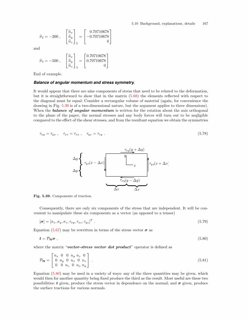
5.10 Background, explanations, details 167

σ2 = −200 ,

nxnynz

2

=

0.70710678−0.70710678

0

and

σ3 = −500 ,

nxnynz

3

=

0.707106780.707106780

End of example.

Balance of angular momentum and stress symmetry.

It would appear that there are nine components of stress that need to be related to the deformation,but it is straightforward to show that in the matrix (5.68) the elements reflected with respect tothe diagonal must be equal: Consider a rectangular volume of material (again, for convenience thedrawing in Fig. 5.39 is of a two-dimensional nature, but the argument applies to three dimensions).When the balance of angular momentum is written for the rotation about the axis orthogonalto the plane of the paper, the normal stresses and any body forces will turn out to be negligiblecompared to the effect of the shear stresses, and from the resultant equation we obtain the symmetries

τxy = τyx , τxz = τzx , τyz = τzy . (5.78)

Fig. 5.39. Components of traction.

Consequently, there are only six components of the stress that are independent. It will be con-venient to manipulate these six components as a vector (as opposed to a tensor)

[σ] = [σx, σy, σz, τxy, τxz, τyz]T . (5.79)

Equation (5.67) may be rewritten in terms of the stress vector σ as

t = Pnσ , (5.80)

where the matrix “vector-stress vector dot product” operator is defined as

Pn =

nx 0 0 ny nz 00 ny 0 nx 0 nz0 0 nz 0 nx ny

. (5.81)

Equation (5.80) may be used in a variety of ways: any of the three quantities may be given, whichwould then for another quantity being fixed produce the third as the result. Most useful are these twopossibilities: t given, produce the stress vector in dependence on the normal; and σ given, producethe surface tractions for various normals.

168 FEM for Thermal and Stress Analysis

Here is an illustration: Stress components at a point are given as

σx = 9 , σy = −3 , σz = 3 , τxy = −2 , τxz = 0 , τyz = 2

Find the magnitude of the normal and shear traction on the plane with normal [n] = [2, 1, 2]T /3.Solution: This can be done in two ways. Firstly we can organize the stress components in a square

matrix and use equation (5.68). Secondly we can use (5.80) with the stress vector form.The first approach: The traction vector is computed from the matrix representing the stress

sig = array([[9.00, -2.00, 0.00],[-2.00, -3.00, 2.00],[0.00, 2.00, 3.00]])

and the normal

n = array([2.0, 1.0, 2.0])n = n/linalg.norm(n)

as t = dot(sig, n)

array([ 5.33333333, -1. , 2.66666667])

The normal component of the traction is tn = dot(t, n), that is 5.0. The shear part of the tractionis the difference between the total traction vector and its normal part

ts = t - tn * n

and the shear traction vector is

array([ 2. , -2.66666667, -0.66666667])

The magnitude of the shear traction vector is linalg.norm(ts), i.e. 3.399346342.The second approach computes the projection matrix from the normal

Pn = array([[n[0], 0, 0, n[1], n[2], 0],[0, n[1], 0, n[0], 0, n[2]],[0, 0, n[2], 0, n[0], n[1]]])

and then from the stress vector

sigv = array([9.00, -3.00, 3.00, -2.00, 0.00, 2.00])sigv.shape = (6, 1)

evaluates, after the normal vector is made into a column n.shape = (3, 1) so that the matricesare compatible,

t = dot(Pn, sigv)tn = dot(t.T, n)ts = t - tn * nprint(linalg.norm(ts))

which results in the precisely the same results as before. End of example.Another example: Stress components at a point are given as

σx = 9 , σy = −3 , σz = 3 , τxy = −2 , τxz = 0 , τyz = 2

Find the largest possible shear stress at the given point. This means the maximum of the shearstress acting on all planes that can be passed through the point.

Solution: The maximum possible shear stress is computed from the principal stress values as

τmax =σ1 − σ3

2

i.e. as half the difference between the largest and the smallest principal stress. The principal stressvalues and the principal stress directions are computed from

5.10 Background, explanations, details 169

sig = array([[9.00, -2.00, 0.00],[-2.00, -3.00, 2.00],[0.00, 2.00, 3.00]])

princstrs, princdirs = linalg.eig(sig)

order = argsort(princstrs)print(’Sorted principal stresses’)princstrs = princstrs[order[::-1]]print(princstrs)print(’Sorted principal directions’)princdirs = princdirs[:, order[::-1]]print(princdirs)

which gives

Sorted principal stresses[ 9.34156488 3.54921973 -3.89078461]Sorted principal directions[[ 0.98434176 0.09670745 0.14737356][-0.16810829 0.26356552 0.94988042][-0.05301792 0.95978169 -0.27569587]]

and the maximum shear stress is therefore found as τmax = (9.342 − −3.891)/2 = 6.616. Notablythe maximum shear stress appears in the Tresca failure criterion

τmax ≤ σf2

where σf is the failure stress of the material in uniaxial tension. End of example.Ductile materials (such as metals) are often considered in failure analyses in relation to the stress

quantity that describes the distortion of the volume of the material (no change in volume), the vonMises equivalent stress.

One more example: Stress components at a point are given as

σx = 9 , σy = −3 , σz = 3 , τxy = −2 , τxz = 0 , τyz = 2

Find the Von Mises equivalent stress at the given point.Solution: The von Mises equivalent stress may be computed from the principal stresses as

σvm =1√2

√(σ1 − σ2)2 + (σ1 − σ3)2 + (σ3 − σ2)2

or directly from the components of the stress as

σvm =1√2

√(σx − σy)2 + (σx − σz)2 + (σz − σy)2 + 6(τ2xy + τ2xz + τ2yz)

Substituting given stress components we obtain σvm = 11.489. The von Mises equivalent stress iscompared in the von Mises failure criterion

σvm ≤ σf

with the failure stress of the material in uniaxial tension σf . End of example.

Equation of Local equilibrium

In complete analogy to the model of heat conduction, the global balance equation (5.63) (in this case,balance of linear momentum, for the heat conduction it was balance of heat energy (2.12)) needsto be converted to a local form. The local form expresses dynamic equilibrium of an infinitesimalparticle as an equation that holds at a point.

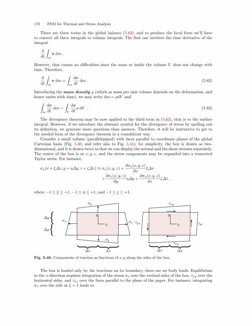
170 FEM for Thermal and Stress Analysis

There are three terms in the global balance (5.63), and to produce the local form we’ll haveto convert all three integrals to volume integrals. The first one involves the time derivative of theintegral

d

dt

∫m

v dm .

However, that causes no difficulties since the mass m inside the volume V does not change withtime. Therefore,

d

dt

∫m

v dm =

∫m

dv

dtdm . (5.82)

Introducing the mass density ρ (which as mass per unit volume depends on the deformation, andhence varies with time), we may write dm = ρdV and∫

m

dv

dtdm =

∫V

dv

dtρ dV . (5.83)

The divergence theorem may be now applied to the third term in (5.63), that is to the surfaceintegral. However, if we introduce the abstract symbol for the divergence of stress by spelling outits definition, we generate more questions than answers. Therefore, it will be instructive to get tothe needed form of the divergence theorem in a roundabout way.

Consider a small volume (parallelepiped) with faces parallel to coordinate planes of the globalCartesian basis (Fig. 5.40, and refer also to Fig. 5.34); for simplicity, the box is drawn as two-dimensional, and it is drawn twice so that we can display the normal and the shear stresses separately.The center of the box is at x, y, z, and the stress components may be expanded into a truncatedTaylor series. For instance,

σx(x+ ξ∆x, y + η∆y, z + ζ∆z) ≈ σx(x, y, z) +∂σx(x, y, z)

∂xξ∆x

+∂σx(x, y, z)

∂yη∆y +

∂σx(x, y, z)

∂zζ∆z ,

where −1 ≤ ξ ≤ +1, −1 ≤ η ≤ +1, and −1 ≤ ζ ≤ +1.

Fig. 5.40. Components of traction as functions of x, y along the sides of the box.

The box is loaded only by the tractions on its boundary, there are no body loads. Equilibriumin the x-direction requires integration of the stress σx over the vertical sides of the box, τxy over thehorizontal sides, and τxz over the faces parallel to the plane of the paper. For instance, integratingσx over the side at ξ = 1 leads to

5.10 Background, explanations, details 171

∆y∆z

∫ +1

−1

∫ +1

−1

σx(x+∆x, y + η∆y, z + ζ∆z) dηdζ ≈

∆y∆z

∫ +1

−1

∫ +1

−1

[σx(x, y, z) +

∂σx(x, y, z)

∂x∆x

+∂σx(x, y, z)

∂yη∆y +

∂σx(x, y, z)

∂zζ∆z

]dηdζ .

The terms with η and ζ integrate to zero, and the result is

4∆y∆z

[σx(x, y, z) +

∂σx(x, y, z)

∂x∆x

].

Next, integrating σx over the side at ξ = −1 leads to

∆y∆z

∫ +1

−1

∫ +1

−1

−σx(x+∆x, y + η∆y, z + ζ∆z) dηdζ ≈

∆y∆z

∫ +1

−1

∫ +1

−1

[−σx(x, y, z) +

∂σx(x, y, z)

∂x∆x

−∂σx(x, y, z)∂y

η∆y − ∂σx(x, y, z)

∂zζ∆z

]dηdζ .

The terms with η and ζ integrate to zero, and the result is

4∆y∆z

[−σx(x, y, z) +

∂σx(x, y, z)

∂x∆x

].

Adding these two together gives the total contribution of the stress σx as

8∆x∆y∆z∂σx(x, y, z)

∂x= ∆V

∂σx(x, y, z)

∂x,

with the elementary volume ∆V = 8∆x∆y∆z. The same exercise is now repeated for the stresscomponents τxy and τxz, giving the total force on the elementary volume in the x-direction

∆b∗x = ∆V

[∂σx(x, y, z)

∂x+∂τxy(x, y, z)

∂y+∂τxz(x, y, z)

∂z

], (5.84)

and analogously in the other two directions

∆b∗y = ∆V

[∂τyx(x, y, z)

∂x+∂σy(x, y, z)

∂y+∂τyz(x, y, z)

∂z

], (5.85)

and

∆b∗z = ∆V

[∂τzx(x, y, z)

∂x+∂τzy(x, y, z)

∂y+∂σz(x, y, z)

∂z

]. (5.86)

Now the same argument that was established around Eq. (5.61) will be pursued: put together thetotal force on the body by collecting the contributions from all the elementary volumes. This can bedone in two ways:

1. Add up all the tractions on the bounding faces of the elementary volumes. The tractions on theshared faces (internal surfaces) will cancel; only the tractions on the exterior surface will be left:∫

S

t dS

172 FEM for Thermal and Stress Analysis

2. Add up all the resultant equivalent volume forces (5.84-5.86), which in the limit will become avolume integral∫

V

b∗ dV

where the imaginary force b∗ has components on the Cartesian basis

[b∗] =

∂σx(x, y, z)

∂x+∂τxy(x, y, z)

∂y+∂τxz(x, y, z)

∂z

∂τyx(x, y, z)

∂x+∂σy(x, y, z)

∂y+∂τyz(x, y, z)

∂z

∂τzx(x, y, z)

∂x+∂τzy(x, y, z)

∂y+∂σz(x, y, z)

∂z

(5.87)

and may be recognized as the stress divergence.

These two forces are equal, and we have the following form of the divergence theorem∫V

b∗ dV =

∫S

t dS .

Using the template of the “vector-stress vector dot product” operator (5.81), we may write the stressdivergence as

b∗ = BTσ , (5.88)

where the stress-divergence operator BT is defined as

BT =

∂/∂x 0 0 ∂/∂y ∂/∂z 00 ∂/∂y 0 ∂/∂x 0 ∂/∂z0 0 ∂/∂z 0 ∂/∂x ∂/∂y

. (5.89)

This operator (un-transposed) will make its appearance shortly yet again as the symmetric gradi-ent operator to produce strains out of displacements. Using the definitions of both of these usefuloperators, the divergence theorem may be written in terms of stress as∫

V

BTσ dV =

∫S

Pnσ dS . (5.90)

Putting the three integrals from (5.63) into the volume-integral form leads to a pointwise expres-sion of local equilibrium:∫

V

ρdv

dtdV =

∫V

b dV +

∫V

BTσ dV ⇒ ρdv

dt= b+ BTσ . (5.91)

This is a statement of dynamic equilibrium of a point particle: On the left-hand side we havethe inertial force (mass times acceleration), on the right-hand side is the body load and the forcegenerated by a stress gradient across the particle. Analogously to the heat conduction problem, thislocal balance equation contains too many variables. The stress plays the role of the heat flux, andit also will be replaced by reference to measurable variables – the strains.

End Box 16

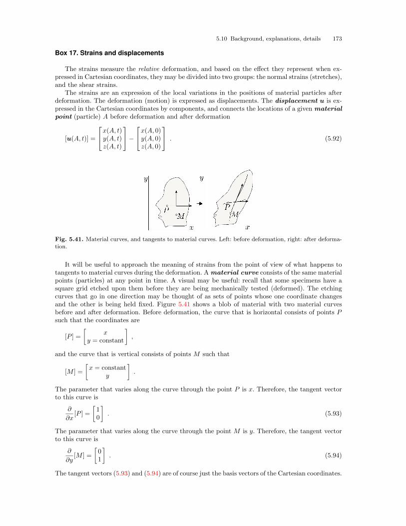
5.10 Background, explanations, details 173

Box 17. Strains and displacements

The strains measure the relative deformation, and based on the effect they represent when ex-pressed in Cartesian coordinates, they may be divided into two groups: the normal strains (stretches),and the shear strains.

The strains are an expression of the local variations in the positions of material particles afterdeformation. The deformation (motion) is expressed as displacements. The displacement u is ex-pressed in the Cartesian coordinates by components, and connects the locations of a given materialpoint (particle) A before deformation and after deformation

[u(A, t)] =

x(A, t)y(A, t)z(A, t)

−

x(A, 0)y(A, 0)z(A, 0)

. (5.92)

Fig. 5.41. Material curves, and tangents to material curves. Left: before deformation, right: after deforma-tion.

It will be useful to approach the meaning of strains from the point of view of what happens totangents to material curves during the deformation. A material curve consists of the same materialpoints (particles) at any point in time. A visual may be useful: recall that some specimens have asquare grid etched upon them before they are being mechanically tested (deformed). The etchingcurves that go in one direction may be thought of as sets of points whose one coordinate changesand the other is being held fixed. Figure 5.41 shows a blob of material with two material curvesbefore and after deformation. Before deformation, the curve that is horizontal consists of points Psuch that the coordinates are

[P ] =

[x

y = constant

],

and the curve that is vertical consists of points M such that

[M ] =

[x = constant

y

].

The parameter that varies along the curve through the point P is x. Therefore, the tangent vectorto this curve is

∂

∂x[P ] =

[10

]. (5.93)

The parameter that varies along the curve through the point M is y. Therefore, the tangent vectorto this curve is

∂

∂y[M ] =

[01

]. (5.94)

The tangent vectors (5.93) and (5.94) are of course just the basis vectors of the Cartesian coordinates.

174 FEM for Thermal and Stress Analysis

After deformation, the curve that used to be horizontal consists of points P such that

[P ] =

[x+ ux

(y = constant) + uy

],

and the curve that is vertical consists of points M such that

[M ] =

[(x = constant) + ux

y + uy

].

Since these are material curves, they are still parameterized by the same parameters as beforedeformation. Consequently, for the originally horizontal curve we have the tangent vector afterdeformation

∂

∂x[P ] =

1 +∂ux∂x

∂uy∂x

. (5.95)

The parameter that varies along the curve through the point M is y. Therefore, after deformationthe tangent vector to this curve is

∂

∂y[M ] =

∂ux∂y

1 +∂uy∂y

. (5.96)

The stretches measure the relative change in length of the tangent vectors at the same materialpoint before and after deformation. For instance, the tangent vector (5.93) is of unit length beforedeformation, and the vector (5.95) is of length√

(1 +∂ux∂x

)2 + (∂uy∂x

)2 =

√1 + 2

∂ux∂x

+ (∂ux∂x

)2 + (∂uy∂x

)2 .

If we now make the assumption that the derivatives of the displacement components are very smallin magnitude,

|∂uk∂j

| ≪ 1, k, j = x, y, z , (5.97)

the length of the tangent vector may be expressed as√1 + 2

∂ux∂x

+ (∂ux∂x

)2 + (∂uy∂x

)2 ≈ 1 +∂ux∂x

,

and the relative change in length (the stretch in the x direction) is

1 +∂ux∂x

− 1

1= ϵx .

The shears measure the change in the angle between originally orthogonal directions of pairsof the Cartesian axes. Therefore, we could measure the change in the angle between the tangents oftwo intersecting material curves before and after deformation. For the two curves in Fig. 5.41, theinitial angle is π/2; the cosine of the angle after the deformation is

∂

∂x[P ]T

∂

∂y[M ] = (1 +

∂ux∂x

)∂ux∂y

+∂uy∂x

(1 +∂uy∂y

)

5.10 Background, explanations, details 175

which, again using the assumption (5.97), gives for the change of the angle

∂ux∂y

+∂uy∂x

= γxy .

In this way we define all six strain components: three stretches, and three shears. In fact, wecould have defined nine strains (components of the strain tensor), which would correspond to thenine components of the Cauchy stress tensor. However, we will stick to the vector representation inthis book.

The six strain components are a mixture of the derivatives of the displacement components, andmay be expressed in an operator equation, using the definition (5.88)

ϵ = Bu , (5.98)

where B is called the symmetric gradient (or strain-displacement) operator.The components of the strain are

[ϵ]T = [ϵx, ϵy, ϵz, γxy, γxz, γyz]T (5.99)

Note the transpose, the strain vector has six rows and one column. The first three components arethe stretches, the last three components are the shears.

End Box 17

Box 18. Elastic constitutive equation

The stress now needs to be linked to the strains. Then we will be in a position to replace it inthe balance equation (5.91) by reference to the primary variable, the displacement. As for the heatconduction model, this link is the constitutive equation.

The constitutive equation that will be of interest in this book is the model of linear elasticity .It is expressed as a linear relationship between the strain and the stress, and since these are vectors,the linear relationship, the constitutive equation , is expressed as a matrix product

σ = Dϵ , (5.100)

where D is a 6× 6 matrix of the elastic coefficients (also known as the elasticities); D may be alsoreferred to as the material stiffness matrix. If the material stiffness matrix changes from point topoint, we call the material inhomogeneous; otherwise when the matrix is uniform across the material,we call the material homogeneous.

The total energy density stored in the material in the volume dV is

ϕ(ϵ) =1

2ϵTDϵ dV . (5.101)

Mathematically, the expression 12ϵ

TDϵ is known as a quadratic form. One interesting propertyof the quadratic form is that the unsymmetrical part of the matrix D does not contribute to theenergy:

1

2ϵTDϵ =

(1

2ϵTDϵ

)T

=1

2ϵTDT ϵ ⇒ 1

2ϵT (D −DT )ϵ = 0 .

Because the energy of deformation is a fundamental quantity, from physical principles, and fromthe point of view of mathematical modeling, this is a very good reason for postulating a priori thesymmetry of the material stiffness, D = DT .

176 FEM for Thermal and Stress Analysis

Material stiffness of linearly elastic materials

The strain displacement operator (symmetric gradient operator) (5.98) links displacements in termsof their components in the global Cartesian basis to strains. The strains could be expressed in thesame Cartesian basis, but need not be. In fact, it will be most useful not to express the strains inthe same global Cartesian coordinate system. The motivating factor is the constitutive equation:For some materials it will be important to keep track of the local orientation of the material volume.For instance, fiber reinforced materials will have very different stiffness properties along the fibersas opposed to orthogonally to the fibers.

The components of the material stiffness matrix (or the material compliance matrix) are to beunderstood as being expressed in the local coordinate system ex, ey, ez attached to the materialpoint in the form of the rotation matrix (5.71).

General anisotropic material. Because of the symmetry of the material stiffness, for the most generalelastic material the number of elastic coefficients is only 21 out of the total of 36 elements of thematerial stiffness matrix. Still, to identify all of these constants represents a major experimentaleffort, and few engineering materials are characterized as fully anisotropic.

Orthotropic material. If a material has three mutually orthogonal planes of symmetry, it is known asan orthotropic material. For instance wood is often characterized as such type of material, and fiber-reinforced composites are in more sophisticated analyses also treated as orthotropic. The compliancematrix

C = D−1 ,

has a pleasingly simple appearance

C =

E1−1 , −ν12

E1, −ν13

E1, 0 , 0 , 0

−ν12E1

, E2−1 , −ν23

E2, 0 , 0 , 0

−ν13E1

, −ν23E2

, E3−1 , 0 , 0 , 0

0 , 0 , 0 , G12−1 , 0 , 0

0 , 0 , 0 , 0 , G13−1 , 0

0 , 0 , 0 , 0 , 0 , G23−1

.

All nine coefficients are independent, and need to be provided as input [4]. The material stiffnessmatrix is a bit of a mess. The nonzero elements are

D11 =C22C33 − C23C23

C, D12 =

C13C23 − C12C33

C,

D13 =C12C23 − C13C22

C, D22 =

C33C11 − C13C13

C,

D23 =C12C13 − C23C11

C, D33 =

C11C22 − C12C12

C,

D44 = G12, D55 = G13, D66 = G23.

Here C = C11C22C33 − C11C23C23 − C22C13C13 − C33C12C12 + 2C12C23C13.

Transversely isotropic material. If a material has an infinite number of planes of symmetry passingthrough an axis (in this case, the local x-axis), and one plane of symmetry orthogonal to this axis, itis known as a transversely isotropic material. Unidirectionally reinforced composites are of this type,as are for instance muscles. The direction of the fibers is special (oriented along the local x-axis), butthe material behaves isotropically in the planes orthogonal to the fibers. Layered materials are alsomodeled as transversely isotropic: here the direction orthogonal to the layers is special. Figure 5.42offers an illustration of these two types.

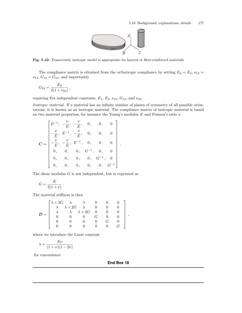
5.10 Background, explanations, details 177

Fig. 5.42. Transversely isotropic model is appropriate for layered or fiber-reinforced materials

The compliance matrix is obtained from the orthotropic compliance by setting E2 = E3, ν12 =ν13, G12 = G13, and importantly

G23 =E2

2(1 + ν23),

requiring five independent constants, E1, E2, ν12, G12, and ν23.

Isotropic material. If a material has an infinite number of planes of symmetry of all possible orien-tations, it is known as an isotropic material. The compliance matrix of isotropic material is basedon two material properties, for instance the Young’s modulus E and Poisson’s ratio ν

C =

E−1 , − ν

E, − ν

E, 0 , 0 , 0

− ν

E, E−1 , − ν

E, 0 , 0 , 0

− ν

E, − ν

E, E−1 , 0 , 0 , 0

0 , 0 , 0 , G−1 , 0 , 0

0 , 0 , 0 , 0 , G−1 , 0

0 , 0 , 0 , 0 , 0 , G−1

.

The shear modulus G is not independent, but is expressed as

G =E

2(1 + ν).

The material stiffness is then

D =

λ+ 2G λ λ 0 0 0λ λ+ 2G λ 0 0 0λ λ λ+ 2G 0 0 00 0 0 G 0 00 0 0 0 G 00 0 0 0 0 G

,

where we introduce the Lame constant

λ =Eν

(1 + ν)(1− 2ν)

for convenience.

End Box 18

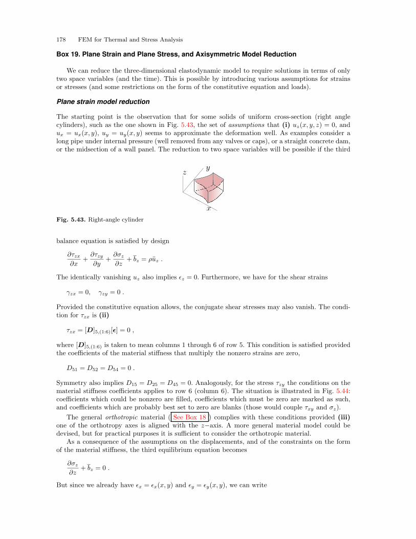
178 FEM for Thermal and Stress Analysis

Box 19. Plane Strain and Plane Stress, and Axisymmetric Model Reduction

We can reduce the three-dimensional elastodynamic model to require solutions in terms of onlytwo space variables (and the time). This is possible by introducing various assumptions for strainsor stresses (and some restrictions on the form of the constitutive equation and loads).

Plane strain model reduction

The starting point is the observation that for some solids of uniform cross-section (right anglecylinders), such as the one shown in Fig. 5.43, the set of assumptions that (i) uz(x, y, z) = 0, andux = ux(x, y), uy = uy(x, y) seems to approximate the deformation well. As examples consider along pipe under internal pressure (well removed from any valves or caps), or a straight concrete dam,or the midsection of a wall panel. The reduction to two space variables will be possible if the third

Fig. 5.43. Right-angle cylinder

balance equation is satisfied by design

∂τzx∂x

+∂τzy∂y

+∂σz∂z

+ bz = ρuz .

The identically vanishing uz also implies ϵz = 0. Furthermore, we have for the shear strains

γzx = 0, γzy = 0 .

Provided the constitutive equation allows, the conjugate shear stresses may also vanish. The condi-tion for τzx is (ii)

τzx = [D]5,(1:6)[ϵ] = 0 ,

where [D]5,(1:6) is taken to mean columns 1 through 6 of row 5. This condition is satisfied providedthe coefficients of the material stiffness that multiply the nonzero strains are zero,

D51 = D52 = D54 = 0 .

Symmetry also implies D15 = D25 = D45 = 0. Analogously, for the stress τzy the conditions on thematerial stiffness coefficients applies to row 6 (column 6). The situation is illustrated in Fig. 5.44:coefficients which could be nonzero are filled, coefficients which must be zero are marked as such,and coefficients which are probably best set to zero are blanks (those would couple τxy and σz).

The general orthotropic material ( See Box 18 ) complies with these conditions provided (iii)one of the orthotropy axes is aligned with the z−axis. A more general material model could bedevised, but for practical purposes it is sufficient to consider the orthotropic material.

As a consequence of the assumptions on the displacements, and of the constraints on the formof the material stiffness, the third equilibrium equation becomes

∂σz∂z

+ bz = 0 .

But since we already have ϵx = ϵx(x, y) and ϵy = ϵy(x, y), we can write

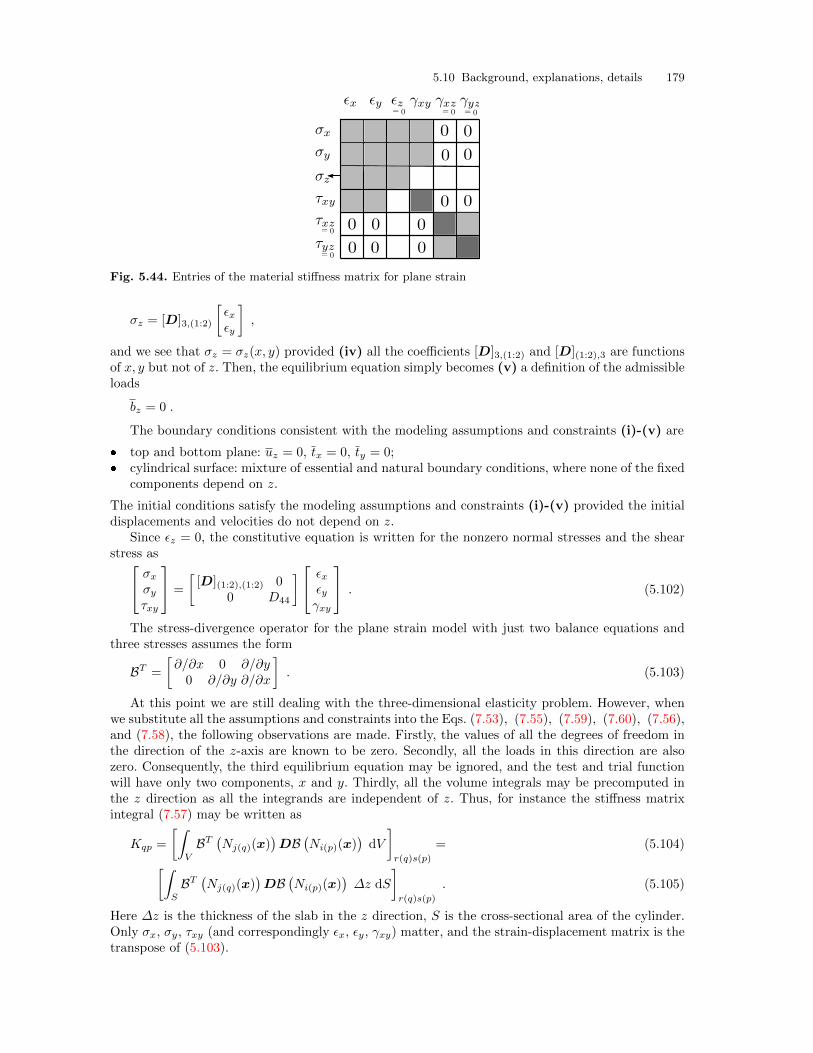
5.10 Background, explanations, details 179

Fig. 5.44. Entries of the material stiffness matrix for plane strain

σz = [D]3,(1:2)

[ϵxϵy

],

and we see that σz = σz(x, y) provided (iv) all the coefficients [D]3,(1:2) and [D](1:2),3 are functionsof x, y but not of z. Then, the equilibrium equation simply becomes (v) a definition of the admissibleloads

bz = 0 .

The boundary conditions consistent with the modeling assumptions and constraints (i)-(v) are

� top and bottom plane: uz = 0, tx = 0, ty = 0;� cylindrical surface: mixture of essential and natural boundary conditions, where none of the fixed

components depend on z.

The initial conditions satisfy the modeling assumptions and constraints (i)-(v) provided the initialdisplacements and velocities do not depend on z.

Since ϵz = 0, the constitutive equation is written for the nonzero normal stresses and the shearstress as σxσy

τxy

=

[[D](1:2),(1:2) 0

0 D44

] ϵxϵyγxy

. (5.102)

The stress-divergence operator for the plane strain model with just two balance equations andthree stresses assumes the form

BT =

[∂/∂x 0 ∂/∂y0 ∂/∂y ∂/∂x

]. (5.103)

At this point we are still dealing with the three-dimensional elasticity problem. However, whenwe substitute all the assumptions and constraints into the Eqs. (7.53), (7.55), (7.59), (7.60), (7.56),and (7.58), the following observations are made. Firstly, the values of all the degrees of freedom inthe direction of the z-axis are known to be zero. Secondly, all the loads in this direction are alsozero. Consequently, the third equilibrium equation may be ignored, and the test and trial functionwill have only two components, x and y. Thirdly, all the volume integrals may be precomputed inthe z direction as all the integrands are independent of z. Thus, for instance the stiffness matrixintegral (7.57) may be written as

Kqp =

[∫V

BT(Nj(q)(x)

)DB

(Ni(p)(x)

)dV

]r(q)s(p)

= (5.104)[∫S

BT(Nj(q)(x)

)DB

(Ni(p)(x)

)∆z dS

]r(q)s(p)

. (5.105)

Here ∆z is the thickness of the slab in the z direction, S is the cross-sectional area of the cylinder.Only σx, σy, τxy (and correspondingly ϵx, ϵy, γxy) matter, and the strain-displacement matrix is thetranspose of (5.103).

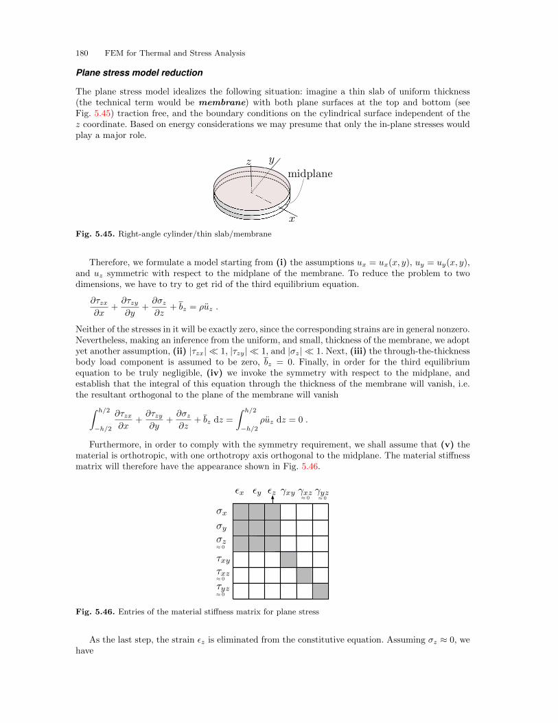
180 FEM for Thermal and Stress Analysis

Plane stress model reduction

The plane stress model idealizes the following situation: imagine a thin slab of uniform thickness(the technical term would be membrane) with both plane surfaces at the top and bottom (seeFig. 5.45) traction free, and the boundary conditions on the cylindrical surface independent of thez coordinate. Based on energy considerations we may presume that only the in-plane stresses wouldplay a major role.

Fig. 5.45. Right-angle cylinder/thin slab/membrane

Therefore, we formulate a model starting from (i) the assumptions ux = ux(x, y), uy = uy(x, y),and uz symmetric with respect to the midplane of the membrane. To reduce the problem to twodimensions, we have to try to get rid of the third equilibrium equation.

∂τzx∂x

+∂τzy∂y

+∂σz∂z

+ bz = ρuz .

Neither of the stresses in it will be exactly zero, since the corresponding strains are in general nonzero.Nevertheless, making an inference from the uniform, and small, thickness of the membrane, we adoptyet another assumption, (ii) |τzx| ≪ 1, |τzy| ≪ 1, and |σz| ≪ 1. Next, (iii) the through-the-thicknessbody load component is assumed to be zero, bz = 0. Finally, in order for the third equilibriumequation to be truly negligible, (iv) we invoke the symmetry with respect to the midplane, andestablish that the integral of this equation through the thickness of the membrane will vanish, i.e.the resultant orthogonal to the plane of the membrane will vanish∫ h/2

−h/2

∂τzx∂x

+∂τzy∂y

+∂σz∂z

+ bz dz =

∫ h/2

−h/2

ρuz dz = 0 .

Furthermore, in order to comply with the symmetry requirement, we shall assume that (v) thematerial is orthotropic, with one orthotropy axis orthogonal to the midplane. The material stiffnessmatrix will therefore have the appearance shown in Fig. 5.46.

Fig. 5.46. Entries of the material stiffness matrix for plane stress

As the last step, the strain ϵz is eliminated from the constitutive equation. Assuming σz ≈ 0, wehave

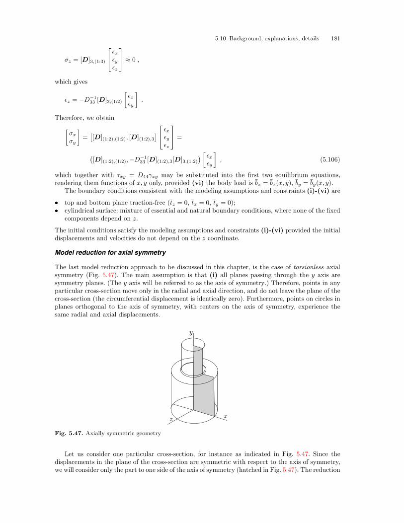
5.10 Background, explanations, details 181

σz = [D]3,(1:3)

ϵxϵyϵz

≈ 0 ,

which gives

ϵz = −D−133 [D]3,(1:2)

[ϵxϵy

].

Therefore, we obtain[σxσy

]=[[D](1:2),(1:2), [D](1:2),3

] ϵxϵyϵz

=

([D](1:2),(1:2),−D−1

33 [D](1:2),3[D]3,(1:2)) [ ϵx

ϵy

], (5.106)

which together with τxy = D44γxy may be substituted into the first two equilibrium equations,rendering them functions of x, y only, provided (vi) the body load is bx = bx(x, y), by = by(x, y).

The boundary conditions consistent with the modeling assumptions and constraints (i)-(vi) are

� top and bottom plane traction-free (tz = 0, tx = 0, ty = 0);� cylindrical surface: mixture of essential and natural boundary conditions, where none of the fixed

components depend on z.

The initial conditions satisfy the modeling assumptions and constraints (i)-(vi) provided the initialdisplacements and velocities do not depend on the z coordinate.

Model reduction for axial symmetry

The last model reduction approach to be discussed in this chapter, is the case of torsionless axialsymmetry (Fig. 5.47). The main assumption is that (i) all planes passing through the y axis aresymmetry planes. (The y axis will be referred to as the axis of symmetry.) Therefore, points in anyparticular cross-section move only in the radial and axial direction, and do not leave the plane of thecross-section (the circumferential displacement is identically zero). Furthermore, points on circles inplanes orthogonal to the axis of symmetry, with centers on the axis of symmetry, experience thesame radial and axial displacements.

Fig. 5.47. Axially symmetric geometry

Let us consider one particular cross-section, for instance as indicated in Fig. 5.47. Since thedisplacements in the plane of the cross-section are symmetric with respect to the axis of symmetry,we will consider only the part to one side of the axis of symmetry (hatched in Fig. 5.47). The reduction

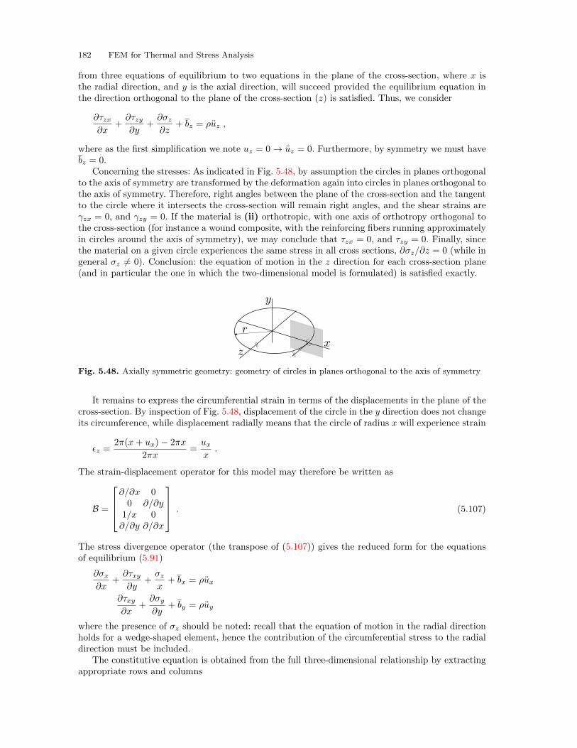
182 FEM for Thermal and Stress Analysis

from three equations of equilibrium to two equations in the plane of the cross-section, where x isthe radial direction, and y is the axial direction, will succeed provided the equilibrium equation inthe direction orthogonal to the plane of the cross-section (z) is satisfied. Thus, we consider

∂τzx∂x

+∂τzy∂y

+∂σz∂z

+ bz = ρuz ,

where as the first simplification we note uz = 0 → uz = 0. Furthermore, by symmetry we must havebz = 0.

Concerning the stresses: As indicated in Fig. 5.48, by assumption the circles in planes orthogonalto the axis of symmetry are transformed by the deformation again into circles in planes orthogonal tothe axis of symmetry. Therefore, right angles between the plane of the cross-section and the tangentto the circle where it intersects the cross-section will remain right angles, and the shear strains areγzx = 0, and γzy = 0. If the material is (ii) orthotropic, with one axis of orthotropy orthogonal tothe cross-section (for instance a wound composite, with the reinforcing fibers running approximatelyin circles around the axis of symmetry), we may conclude that τzx = 0, and τzy = 0. Finally, sincethe material on a given circle experiences the same stress in all cross sections, ∂σz/∂z = 0 (while ingeneral σz = 0). Conclusion: the equation of motion in the z direction for each cross-section plane(and in particular the one in which the two-dimensional model is formulated) is satisfied exactly.

Fig. 5.48. Axially symmetric geometry: geometry of circles in planes orthogonal to the axis of symmetry

It remains to express the circumferential strain in terms of the displacements in the plane of thecross-section. By inspection of Fig. 5.48, displacement of the circle in the y direction does not changeits circumference, while displacement radially means that the circle of radius x will experience strain

ϵz =2π(x+ ux)− 2πx

2πx=uxx.

The strain-displacement operator for this model may therefore be written as

B =

∂/∂x 00 ∂/∂y

1/x 0∂/∂y ∂/∂x

. (5.107)

The stress divergence operator (the transpose of (5.107)) gives the reduced form for the equationsof equilibrium (5.91)

∂σx∂x

+∂τxy∂y

+σzx

+ bx = ρux

∂τxy∂x

+∂σy∂y

+ by = ρuy

where the presence of σz should be noted: recall that the equation of motion in the radial directionholds for a wedge-shaped element, hence the contribution of the circumferential stress to the radialdirection must be included.

The constitutive equation is obtained from the full three-dimensional relationship by extractingappropriate rows and columns

5.10 Background, explanations, details 183σxσyσzτxy

=

[[D](1:3),(1:3) 0

0 D44

]ϵxϵyϵzγxy

. (5.108)

End Box 19

Box 20. Boundary conditions for stress analysis

The boundary conditions for general three-dimensional stress analysis may be expressed as(see (5.81))

ti = (Pnσ)i = ti on St,i for i = x, y, z (5.109)

as the traction (natural) boundary condition for the ith component, and

ui = ui on Su,i for i = x, y, z (5.110)

as the displacement (essential) boundary condition for the ith component. When setting upa finite element model, note that the natural boundary condition need only be specified explicitlywhen ti = 0; the case of ti = 0 is implicitly active when we say nothing. In particular, no boundarycondition needs to be explicitly defined for any component for a traction-free surface.

End Box 20

Box 21. Derivation of weighted residual equations for stress analysis

Incorporation of the natural boundary conditions

The natural boundary condition leads to the residual

rt,i = (Pnσ)i − ti on St,i for i = x, y, z , (5.111)

which will be incorporated into the balance residual equation, and the displacement boundary con-dition (5.110) gives the residual

ru,i = ui − ui on Su,i for i = x, y, z , (5.112)

that will be made zero by the choice of the trial functions (which takes care of the step 2).The weighted residual equations are integrals of the residuals over the corresponding surface.

Since the displacement boundary condition residual is identically zero, it may be ignored. Thetraction boundary condition residual equation reads∫

St,i

rt,iϑi dS ,

or, expanded,

184 FEM for Thermal and Stress Analysis∫St,i

rt,iϑi dS =

∫St,i

[(Pnσ)i − ti

]ϑi dS = 0 . (5.113)

Rearranging the balance equation (5.91) into the residual form leads to

rB = ρdv

dt− b− BTσ , (5.114)

which is a statement of imbalance when the force residual is nonzero.The balance weighted residual reads∫V

ϑ · rB dV =

∫V

ϑ ·(ρdv

dt− b− BTσ

)dV , (5.115)

where ϑ is a vector test function (with three components). At this point, we only require that thetest function be sufficiently smooth for the integral to exist. The dot product of the residual and thevector test function is written in the “dot” form; when the weighted residual equation is written interms of the components, transposes must be used as

∫V

ϑ · rB dV =

∫V

[rB ]T [ϑ] dV =

∫V

[ϑ]T [rB ] dV .

Shifting of derivatives

While the first two terms on the right-hand side of (5.114) present no difficulties, the stress termneeds to be treated similarly to the previous two models to move one derivative from the stress tothe test function. Therefore, in the next few paragraphs we focus on the integral∫

V

ϑ · BTσ dV .

It will be sought as one constituent of the chain-rule result (analogously to Eq. (3.133) for the heatconduction). The inner product of ϑ and σ may be expressed using the vector-stress vector dotproduct operator (5.81) in the form Pϑσ (which is a vector). Therefore, we need an identity for

the chain rule applied to the divergence div(Pϑσ

): in one

div(Pϑσ

)= (Bϑ) · σ + ϑ · BTσ . (5.116)

It may not be immediately clear why the right-hand side has this form, but to verify this formulais straightforward, albeit tedious. Expressing the rightmost term of (5.116) by the other two, weobtain

∫V

ϑ · BTσ dV =

∫V

div(Pϑσ

)dV −

∫V

(Bϑ) · σ dV .

The divergence theorem (2.18) may be applied to the first term on the right to yield

∫V

ϑ · BTσ dV =

∫S

(Pϑσ

)· n dS −

∫V

(Bϑ) · σ dV .

The traction boundary condition (5.109) references Pnσ. To extricate this form from(Pϑσ

)· n

we note that the result of this dot product is a scalar (a number). This indicates that the stress isinvolved in a double dot product: the stress tensor is dotted with one vector, which is subsequentlydotted with the second vector. Indeed, it is easily verified by multiplying through that(

Pϑσ)· n = (Pnσ) · ϑ .

5.10 Background, explanations, details 185

As a result we obtain∫V

ϑ · BTσ dV =

∫S

ϑ · (Pnσ) dS −∫V

(Bϑ) · σ dV .

It will be useful to summarize the balance weighted residual (5.115) now as∫V

ϑ · rB dV =

∫V

ϑ · ρdvdt

dV −∫V

ϑ · b dV

−∫S

ϑ · (Pnσ) dS +

∫V

(Bϑ) · σ dV . (5.117)

Boundary conditions

The surface will now be split, for each component, into the part where traction is known, and thepart where displacement is being fixed∫

S

ϑ · (Pnσ) dS =∑

i=x,y,z

∫St,i

ϑi (Pnσ)i dS +

∫Su,i

ϑi (Pnσ)i dS ,

where ϑi = (ϑ)i is the ith component of the test function. On the St,i subset the traction component

i is known from (5.109), but on the Su,i subset of the bounding surface, the component i of thetraction is not known, it represents the reaction. To be able to ignore the reactions, we will resortto the same trick as for the other PDE models, namely we will put in place the requirement

ϑi = 0 on Su,i .

Therefore, with the constraint on the trial function to satisfy the essential boundary conditions onSu,i, and a constraint on the test function to vanish on Su,i, we have the weighted balance residual∫

V

ϑ · ρdvdt

dV −∫V

ϑ · b dV −∑

i=x,y,z

∫St,i

ϑi (Pnσ)i dS +

∫V

(Bϑ) · σ dV (5.118)

To the weighted balance residual (5.118) we now add the weighted residuals of the natural boundarycondition (5.113) and set the result equal to zero.∫

V

ϑ · ρdvdt

dV −∫V

ϑ · b dV −∑

i=x,y,z

∫St,i

ϑi (Pnσ)i dS +

∫V

(Bϑ) · σ dV

+∑

i=x,y,z

∫St,i

ϑi[(Pnσ)i − ti

]dS = 0 (5.119)

We can see that the terms with ϑi (Pnσ)i cancel and we obtain the final form of the weightedresidual equation∫

V

ϑ · ρdvdt

dV −∫V

ϑ · b dV −∑

i=x,y,z

∫St,i

(ϑ)i ti dS +

∫V

(Bϑ) · σ dV = 0

ui = ui and (ϑ)i = 0 on Su,i for i = x, y, z .

(5.120)

So far we have been using the velocity and the stress vector for convenience and brevity, but toproduce a displacement-based computational model these will have to be replaced by references tothe displacement field. Using

v =du

dt⇒ dv

dt=

d2u

dt2= u ,

186 FEM for Thermal and Stress Analysis

and the constitutive equation (5.100) and the displacement-strain relation (5.98), the form that goesinto the discretization process reads∫

V

ϑ · ρu dV +

∫V

(Bϑ) ·DBu dV −∫V

ϑ · b dV −∑

i=x,y,z

∫St,i

(ϑ)i ti dS = 0 (5.121)

ui = ui and (ϑ)i = 0 on Su,i for i = x, y, z .

Box 22. Method of weighted residuals as the principle of virtual work

An alternative route to Eq. (5.120) is via the principle of virtual work. The test function isinterpreted as a virtual displacement . The constraint on the test function is postulated a priori:virtual displacement is kinematically admissible. The various terms in (5.120) are interpreted asthe virtual work of the inertial forces, applied body load, applied tractions, and internal forces.

This approach tends to seem somewhat arbitrary, since a number of concepts are postulated tobe taken on faith. In this book we therefore avoid this viewpoint. Nevertheless, it may be usefulto be aware of these possible interpretations of the various terms as virtual quantities (especiallywork).

End Box 22

Box 23. Integration for two-dimensional models

As discussed earlier, the volume integrals for plane strain, such as the one required for the stiffnessmatrix, incorporate the third dimension as a “thickness”. Integration through the third dimensionreduces to multiplication with the thickness.

Fig. 5.49. Volume integration for axisymmetric analysis

The volume integrals for the axial-symmetry model reduction approach differ from plane stressor plane strain in that the “gratis” integration in the third direction is performed along the circum-ference of the rotationally symmetric body, not “through the thickness”. For instance, the stiffnessmatrix integral (7.57) may be written as

Kqp =

[∫V

BT(Nj(q)(x)

)DB

(Ni(p)(x)

)dV

]r(q)s(p)

= (5.122)[∫S

BT(Nj(q)(x)

)DB

(Ni(p)(x)

)2πx dS

]r(q)s(p)

. (5.123)

where 2πx dS is the volume element of the ring generated by revolving the area dS around the axisof symmetry y—compare with Fig. 5.49. The volume integration may be performed by numericalquadrature over the area S but using a volume Jacobian

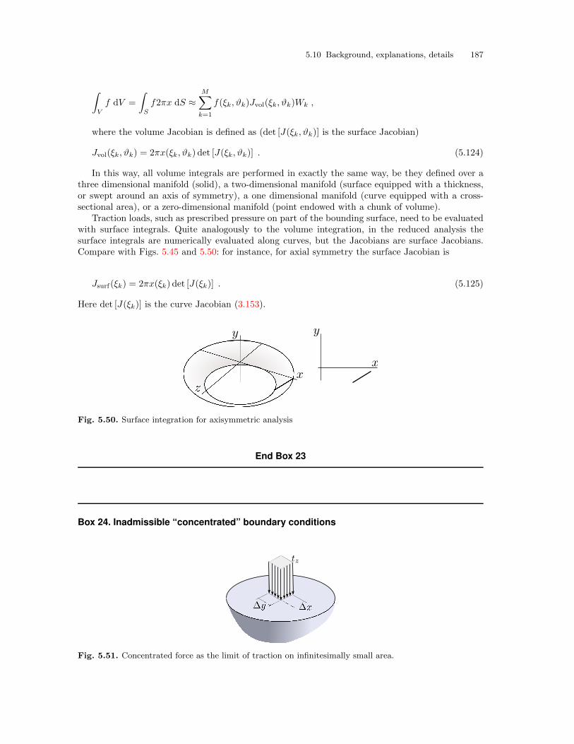
5.10 Background, explanations, details 187

∫V

f dV =

∫S

f2πx dS ≈M∑k=1

f(ξk, ϑk)Jvol(ξk, ϑk)Wk ,

where the volume Jacobian is defined as (det [J(ξk, ϑk)] is the surface Jacobian)

Jvol(ξk, ϑk) = 2πx(ξk, ϑk) det [J(ξk, ϑk)] . (5.124)

In this way, all volume integrals are performed in exactly the same way, be they defined over athree dimensional manifold (solid), a two-dimensional manifold (surface equipped with a thickness,or swept around an axis of symmetry), a one dimensional manifold (curve equipped with a cross-sectional area), or a zero-dimensional manifold (point endowed with a chunk of volume).

Traction loads, such as prescribed pressure on part of the bounding surface, need to be evaluatedwith surface integrals. Quite analogously to the volume integration, in the reduced analysis thesurface integrals are numerically evaluated along curves, but the Jacobians are surface Jacobians.Compare with Figs. 5.45 and 5.50: for instance, for axial symmetry the surface Jacobian is

Jsurf(ξk) = 2πx(ξk) det [J(ξk)] . (5.125)

Here det [J(ξk)] is the curve Jacobian (3.153).

Fig. 5.50. Surface integration for axisymmetric analysis

End Box 23

Box 24. Inadmissible “concentrated” boundary conditions

Fig. 5.51. Concentrated force as the limit of traction on infinitesimally small area.

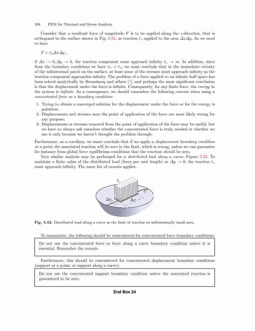
188 FEM for Thermal and Stress Analysis

Consider that a resultant force of magnitude F is to be applied along the z-direction, that isorthogonal to the surface shown in Fig. 5.51, as traction tz applied to the area ∆x∆y. As we needto have

F = tz∆x∆y ,

if ∆x → 0, ∆y → 0, the traction component must approach infinity tz → ∞. In addition, sincefrom the boundary conditions we have σz = tz, we must conclude that in the immediate vicinityof the infinitesimal patch on the surface, at least some of the stresses must approach infinity as thetraction component approaches infinity. The problem of a force applied to an infinite half space hasbeen solved analytically by Boussinesq and others [7], and perhaps the most significant conclusionis that the displacement under the force is infinite. Consequently, for any finite force, the energy inthe system is infinite. As a consequence, we should remember the following caveats when using aconcentrated force as a boundary condition:

1. Trying to obtain a converged solution for the displacement under the force or for the energy ispointless;

2. Displacements and stresses near the point of application of the force are most likely wrong forany purpose;

3. Displacements or stresses removed from the point of application of the force may be useful, butwe have to always ask ourselves whether the concentrated force is truly needed or whether weuse it only because we haven’t thought the problem through.

Furthermore, as a corollary, we must conclude that if we apply a displacement boundary conditionat a point, the associated reaction will be zero in the limit, which is wrong, unless we can guaranteefor instance from global force equilibrium conditions that the reaction should be zero.

Very similar analysis may be performed for a distributed load along a curve: Figure 5.52. Tomaintain a finite value of the distributed load (force per unit length) as ∆y → 0, the traction tzmust approach infinity. The same list of caveats applies.

Fig. 5.52. Distributed load along a curve as the limit of traction on infinitesimally small area.

To summarize, the following should be remembered for concentrated force boundary conditions:

Do not use the concentrated force or force along a curve boundary condition unless it isessential. Remember the caveats.

Furthermore, this should be remembered for concentrated displacement boundary conditions(support at a point, or support along a curve):

Do not use the concentrated support boundary condition unless the associated reaction isguaranteed to be zero.

End Box 24

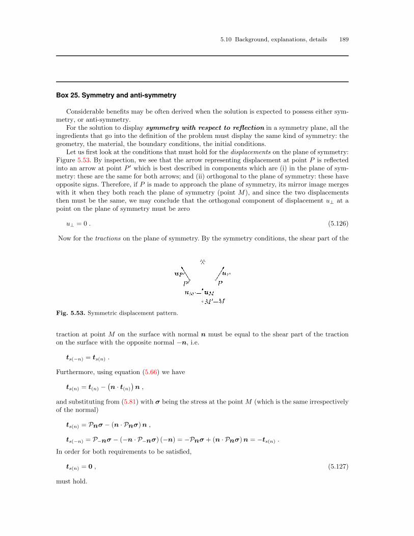
5.10 Background, explanations, details 189

Box 25. Symmetry and anti-symmetry

Considerable benefits may be often derived when the solution is expected to possess either sym-metry, or anti-symmetry.

For the solution to display symmetry with respect to reflection in a symmetry plane, all theingredients that go into the definition of the problem must display the same kind of symmetry: thegeometry, the material, the boundary conditions, the initial conditions.

Let us first look at the conditions that must hold for the displacements on the plane of symmetry:Figure 5.53. By inspection, we see that the arrow representing displacement at point P is reflectedinto an arrow at point P ′ which is best described in components which are (i) in the plane of sym-metry: these are the same for both arrows; and (ii) orthogonal to the plane of symmetry: these haveopposite signs. Therefore, if P is made to approach the plane of symmetry, its mirror image mergeswith it when they both reach the plane of symmetry (point M), and since the two displacementsthen must be the same, we may conclude that the orthogonal component of displacement u⊥ at apoint on the plane of symmetry must be zero

u⊥ = 0 . (5.126)

Now for the tractions on the plane of symmetry. By the symmetry conditions, the shear part of the

Fig. 5.53. Symmetric displacement pattern.

traction at point M on the surface with normal n must be equal to the shear part of the tractionon the surface with the opposite normal −n, i.e.

ts(−n) = ts(n) .

Furthermore, using equation (5.66) we have

ts(n) = t(n) −(n · t(n)

)n ,

and substituting from (5.81) with σ being the stress at the pointM (which is the same irrespectivelyof the normal)

ts(n) = Pnσ − (n · Pnσ)n ,

ts(−n) = P−nσ − (−n · P−nσ) (−n) = −Pnσ + (n · Pnσ)n = −ts(n) .

In order for both requirements to be satisfied,

ts(n) = 0 , (5.127)

must hold.

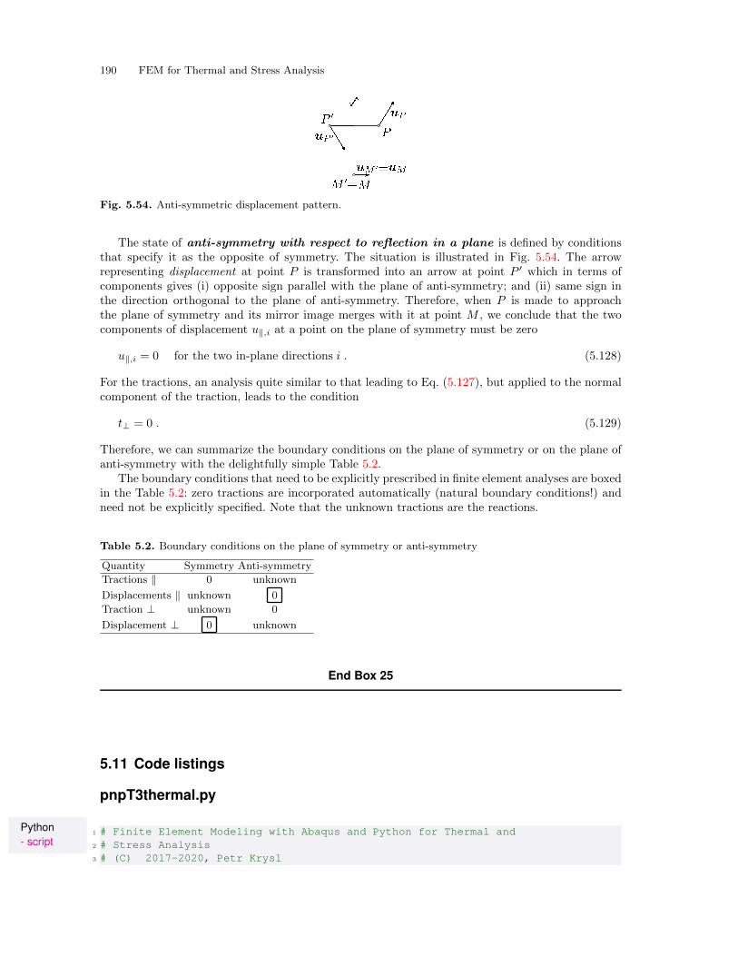
190 FEM for Thermal and Stress Analysis

Fig. 5.54. Anti-symmetric displacement pattern.

The state of anti-symmetry with respect to reflection in a plane is defined by conditionsthat specify it as the opposite of symmetry. The situation is illustrated in Fig. 5.54. The arrowrepresenting displacement at point P is transformed into an arrow at point P ′ which in terms ofcomponents gives (i) opposite sign parallel with the plane of anti-symmetry; and (ii) same sign inthe direction orthogonal to the plane of anti-symmetry. Therefore, when P is made to approachthe plane of symmetry and its mirror image merges with it at point M , we conclude that the twocomponents of displacement u∥,i at a point on the plane of symmetry must be zero

u∥,i = 0 for the two in-plane directions i . (5.128)

For the tractions, an analysis quite similar to that leading to Eq. (5.127), but applied to the normalcomponent of the traction, leads to the condition

t⊥ = 0 . (5.129)

Therefore, we can summarize the boundary conditions on the plane of symmetry or on the plane ofanti-symmetry with the delightfully simple Table 5.2.

The boundary conditions that need to be explicitly prescribed in finite element analyses are boxedin the Table 5.2: zero tractions are incorporated automatically (natural boundary conditions!) andneed not be explicitly specified. Note that the unknown tractions are the reactions.

Table 5.2. Boundary conditions on the plane of symmetry or anti-symmetry

Quantity Symmetry Anti-symmetry

Tractions ∥ 0 unknown

Displacements ∥ unknown 0

Traction ⊥ unknown 0

Displacement ⊥ 0 unknown

End Box 25

5.11 Code listings

pnpT3thermal.py

Python- script

1 # Finite Element Modeling with Abaqus and Python for Thermal and2 # Stress Analysis3 # (C) 2017-2020, Petr Krysl

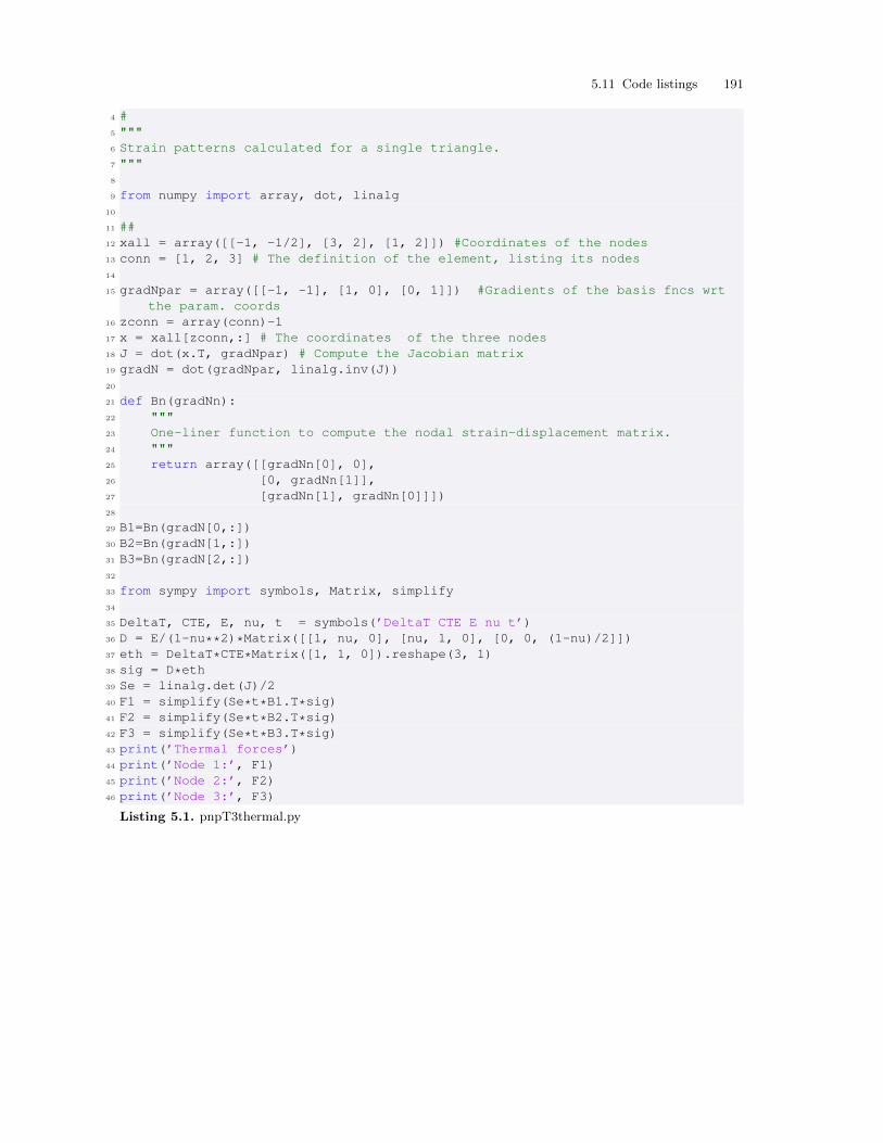
5.11 Code listings 191

4 #5 """6 Strain patterns calculated for a single triangle.7 """8

9 from numpy import array, dot, linalg10

11 ##12 xall = array([[-1, -1/2], [3, 2], [1, 2]]) #Coordinates of the nodes13 conn = [1, 2, 3] # The definition of the element, listing its nodes14

15 gradNpar = array([[-1, -1], [1, 0], [0, 1]]) #Gradients of the basis fncs wrtthe param. coords

16 zconn = array(conn)-117 x = xall[zconn,:] # The coordinates of the three nodes18 J = dot(x.T, gradNpar) # Compute the Jacobian matrix19 gradN = dot(gradNpar, linalg.inv(J))20

21 def Bn(gradNn):22 """23 One-liner function to compute the nodal strain-displacement matrix.24 """25 return array([[gradNn[0], 0],26 [0, gradNn[1]],27 [gradNn[1], gradNn[0]]])28

29 B1=Bn(gradN[0,:])30 B2=Bn(gradN[1,:])31 B3=Bn(gradN[2,:])32

33 from sympy import symbols, Matrix, simplify34

35 DeltaT, CTE, E, nu, t = symbols(’DeltaT CTE E nu t’)36 D = E/(1-nu**2)*Matrix([[1, nu, 0], [nu, 1, 0], [0, 0, (1-nu)/2]])37 eth = DeltaT*CTE*Matrix([1, 1, 0]).reshape(3, 1)38 sig = D*eth39 Se = linalg.det(J)/240 F1 = simplify(Se*t*B1.T*sig)41 F2 = simplify(Se*t*B2.T*sig)42 F3 = simplify(Se*t*B3.T*sig)43 print(’Thermal forces’)44 print(’Node 1:’, F1)45 print(’Node 2:’, F2)46 print(’Node 3:’, F3)

Listing 5.1. pnpT3thermal.py

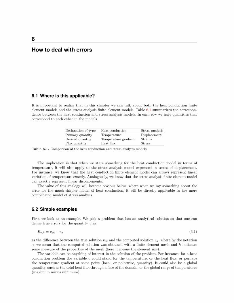
6

How to deal with errors

6.1 Where is this applicable?

It is important to realize that in this chapter we can talk about both the heat conduction finiteelement models and the stress analysis finite element models. Table 6.1 summarizes the correspon-dence between the heat conduction and stress analysis models. In each row we have quantities thatcorrespond to each other in the models.

Designation of type Heat conduction Stress analysis

Primary quantity Temperature DisplacementDerived quantity Temperature gradient StrainsFlux quantity Heat flux Stress

Table 6.1. Comparison of the heat conduction and stress analysis models

The implication is that when we state something for the heat conduction model in terms oftemperature, it will also apply to the stress analysis model expressed in terms of displacement.For instance, we know that the heat conduction finite element model can always represent linearvariation of temperature exactly. Analogously, we know that the stress analysis finite element modelcan exactly represent linear displacements.

The value of this analogy will become obvious below, where when we say something about theerror for the much simpler model of heat conduction, it will be directly applicable to the morecomplicated model of stress analysis.

6.2 Simple examples

First we look at an example. We pick a problem that has an analytical solution so that one candefine true errors for the quantity v as

Ev,h = vex − vh (6.1)

as the difference between the true solution vex and the computed solution vh, where by the notation·h we mean that the computed solution was obtained with a finite element mesh and h indicatessome measure of the properties of the mesh (here it means the element size).

The variable can be anything of interest in the solution of the problem. For instance, for a heatconduction problem the variable v could stand for the temperature, or the heat flux, or perhapsthe temperature gradient at some point (local, or pointwise, quantity). It could also be a globalquantity, such as the total heat flux through a face of the domain, or the global range of temperatures(maximum minus minimum).

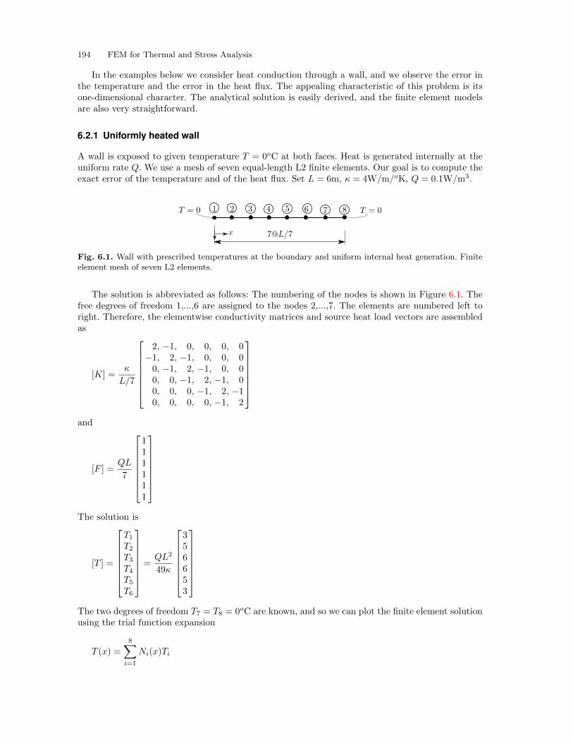
194 FEM for Thermal and Stress Analysis

In the examples below we consider heat conduction through a wall, and we observe the error inthe temperature and the error in the heat flux. The appealing characteristic of this problem is itsone-dimensional character. The analytical solution is easily derived, and the finite element modelsare also very straightforward.

6.2.1 Uniformly heated wall

A wall is exposed to given temperature T = 0oC at both faces. Heat is generated internally at theuniform rate Q. We use a mesh of seven equal-length L2 finite elements. Our goal is to compute theexact error of the temperature and of the heat flux. Set L = 6m, κ = 4W/m/oK, Q = 0.1W/m3.

Fig. 6.1. Wall with prescribed temperatures at the boundary and uniform internal heat generation. Finiteelement mesh of seven L2 elements.

The solution is abbreviated as follows: The numbering of the nodes is shown in Figure 6.1. Thefree degrees of freedom 1,...,6 are assigned to the nodes 2,...,7. The elements are numbered left toright. Therefore, the elementwise conductivity matrices and source heat load vectors are assembledas

[K] =κ

L/7

2, −1, 0, 0, 0, 0

−1, 2, −1, 0, 0, 00, −1, 2, −1, 0, 00, 0, −1, 2, −1, 00, 0, 0, −1, 2, −10, 0, 0, 0, −1, 2

and

[F ] =QL

7

111111

The solution is

[T ] =

T1T2T3T4T5T6

=QL2

49κ

356653

The two degrees of freedom T7 = T8 = 0oC are known, and so we can plot the finite element solutionusing the trial function expansion

T (x) =

8∑i=1

Ni(x)Ti

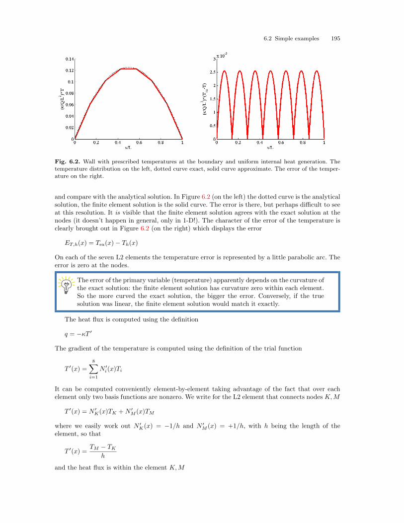
6.2 Simple examples 195

Fig. 6.2. Wall with prescribed temperatures at the boundary and uniform internal heat generation. Thetemperature distribution on the left, dotted curve exact, solid curve approximate. The error of the temper-ature on the right.

and compare with the analytical solution. In Figure 6.2 (on the left) the dotted curve is the analyticalsolution, the finite element solution is the solid curve. The error is there, but perhaps difficult to seeat this resolution. It is visible that the finite element solution agrees with the exact solution at thenodes (it doesn’t happen in general, only in 1-D!). The character of the error of the temperature isclearly brought out in Figure 6.2 (on the right) which displays the error

ET,h(x) = Tex(x)− Th(x)

On each of the seven L2 elements the temperature error is represented by a little parabolic arc. Theerror is zero at the nodes.

The error of the primary variable (temperature) apparently depends on the curvature ofthe exact solution: the finite element solution has curvature zero within each element.So the more curved the exact solution, the bigger the error. Conversely, if the truesolution was linear, the finite element solution would match it exactly.

The heat flux is computed using the definition

q = −κT ′

The gradient of the temperature is computed using the definition of the trial function

T ′(x) =

8∑i=1

N ′i(x)Ti

It can be computed conveniently element-by-element taking advantage of the fact that over eachelement only two basis functions are nonzero. We write for the L2 element that connects nodes K,M

T ′(x) = N ′K(x)TK +N ′

M (x)TM

where we easily work out N ′K(x) = −1/h and N ′

M (x) = +1/h, with h being the length of theelement, so that

T ′(x) =TM − TK

h

and the heat flux is within the element K,M

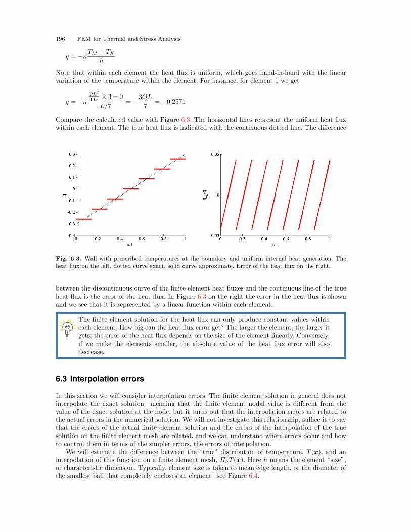
196 FEM for Thermal and Stress Analysis

q = −κTM − TKh

Note that within each element the heat flux is uniform, which goes hand-in-hand with the linearvariation of the temperature within the element. For instance, for element 1 we get

q = −κQL2

49κ × 3− 0

L/7= −3QL

7= −0.2571

Compare the calculated value with Figure 6.3. The horizontal lines represent the uniform heat fluxwithin each element. The true heat flux is indicated with the continuous dotted line. The difference

Fig. 6.3. Wall with prescribed temperatures at the boundary and uniform internal heat generation. Theheat flux on the left, dotted curve exact, solid curve approximate. Error of the heat flux on the right.

between the discontinuous curve of the finite element heat fluxes and the continuous line of the trueheat flux is the error of the heat flux. In Figure 6.3 on the right the error in the heat flux is shownand we see that it is represented by a linear function within each element.

The finite element solution for the heat flux can only produce constant values withineach element. How big can the heat flux error get? The larger the element, the larger itgets: the error of the heat flux depends on the size of the element linearly. Conversely,if we make the elements smaller, the absolute value of the heat flux error will alsodecrease.

6.3 Interpolation errors

In this section we will consider interpolation errors. The finite element solution in general does notinterpolate the exact solution– meaning that the finite element nodal value is different from thevalue of the exact solution at the node, but it turns out that the interpolation errors are related tothe actual errors in the numerical solution. We will not investigate this relationship, suffice it to saythat the errors of the actual finite element solution and the errors of the interpolation of the truesolution on the finite element mesh are related, and we can understand where errors occur and howto control them in terms of the simpler errors, the errors of interpolation.

We will estimate the difference between the “true” distribution of temperature, T (x), and aninterpolation of this function on a finite element mesh, ΠhT (x). Here h means the element “size”,or characteristic dimension. Typically, element size is taken to mean edge length, or the diameter ofthe smallest ball that completely encloses an element –see Figure 6.4.

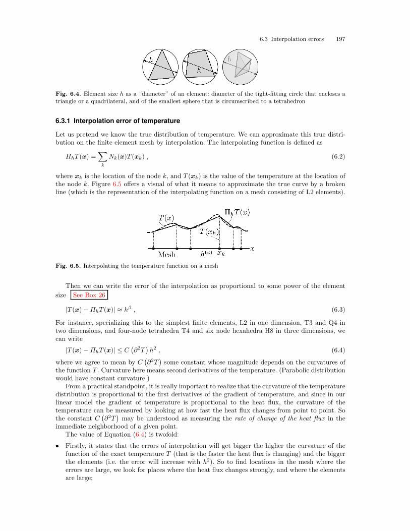
6.3 Interpolation errors 197

Fig. 6.4. Element size h as a “diameter” of an element: diameter of the tight-fitting circle that encloses atriangle or a quadrilateral, and of the smallest sphere that is circumscribed to a tetrahedron

6.3.1 Interpolation error of temperature

Let us pretend we know the true distribution of temperature. We can approximate this true distri-bution on the finite element mesh by interpolation: The interpolating function is defined as

ΠhT (x) =∑k

Nk(x)T (xk) , (6.2)

where xk is the location of the node k, and T (xk) is the value of the temperature at the location ofthe node k. Figure 6.5 offers a visual of what it means to approximate the true curve by a brokenline (which is the representation of the interpolating function on a mesh consisting of L2 elements).

Fig. 6.5. Interpolating the temperature function on a mesh

Then we can write the error of the interpolation as proportional to some power of the element

size See Box 26

|T (x)−ΠhT (x)| ≈ hβ , (6.3)

For instance, specializing this to the simplest finite elements, L2 in one dimension, T3 and Q4 intwo dimensions, and four-node tetrahedra T4 and six node hexahedra H8 in three dimensions, wecan write

|T (x)−ΠhT (x)| ≤ C(∂2T

)h2 , (6.4)

where we agree to mean by C(∂2T

)some constant whose magnitude depends on the curvatures of

the function T . Curvature here means second derivatives of the temperature. (Parabolic distributionwould have constant curvature.)

From a practical standpoint, it is really important to realize that the curvature of the temperaturedistribution is proportional to the first derivatives of the gradient of temperature, and since in ourlinear model the gradient of temperature is proportional to the heat flux, the curvature of thetemperature can be measured by looking at how fast the heat flux changes from point to point. Sothe constant C

(∂2T

)may be understood as measuring the rate of change of the heat flux in the

immediate neighborhood of a given point.The value of Equation (6.4) is twofold:

� Firstly, it states that the errors of interpolation will get bigger the higher the curvature of thefunction of the exact temperature T (that is the faster the heat flux is changing) and the biggerthe elements (i.e. the error will increase with h2). So to find locations in the mesh where theerrors are large, we look for places where the heat flux changes strongly, and where the elementsare large;

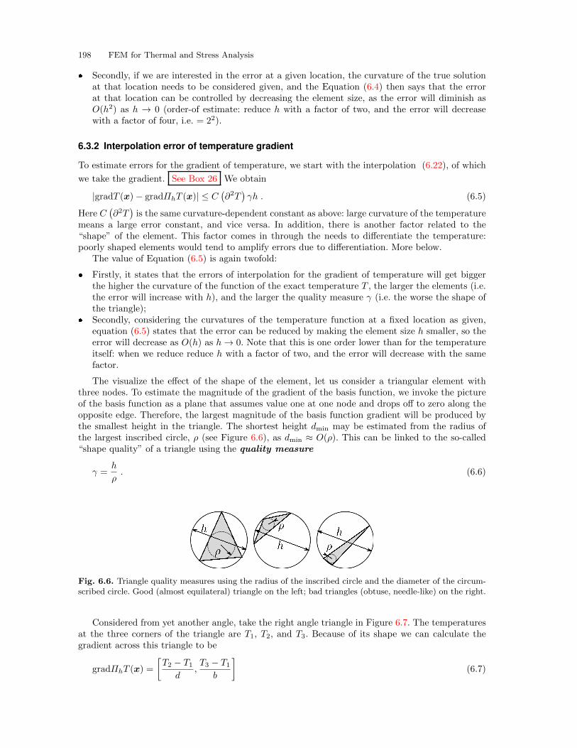
198 FEM for Thermal and Stress Analysis

� Secondly, if we are interested in the error at a given location, the curvature of the true solutionat that location needs to be considered given, and the Equation (6.4) then says that the errorat that location can be controlled by decreasing the element size, as the error will diminish asO(h2) as h → 0 (order-of estimate: reduce h with a factor of two, and the error will decreasewith a factor of four, i.e. = 22).

6.3.2 Interpolation error of temperature gradient

To estimate errors for the gradient of temperature, we start with the interpolation (6.22), of which

we take the gradient. See Box 26 We obtain

|gradT (x)− gradΠhT (x)| ≤ C(∂2T

)γh . (6.5)

Here C(∂2T

)is the same curvature-dependent constant as above: large curvature of the temperature

means a large error constant, and vice versa. In addition, there is another factor related to the“shape” of the element. This factor comes in through the needs to differentiate the temperature:poorly shaped elements would tend to amplify errors due to differentiation. More below.

The value of Equation (6.5) is again twofold:

� Firstly, it states that the errors of interpolation for the gradient of temperature will get biggerthe higher the curvature of the function of the exact temperature T , the larger the elements (i.e.the error will increase with h), and the larger the quality measure γ (i.e. the worse the shape ofthe triangle);

� Secondly, considering the curvatures of the temperature function at a fixed location as given,equation (6.5) states that the error can be reduced by making the element size h smaller, so theerror will decrease as O(h) as h→ 0. Note that this is one order lower than for the temperatureitself: when we reduce reduce h with a factor of two, and the error will decrease with the samefactor.

The visualize the effect of the shape of the element, let us consider a triangular element withthree nodes. To estimate the magnitude of the gradient of the basis function, we invoke the pictureof the basis function as a plane that assumes value one at one node and drops off to zero along theopposite edge. Therefore, the largest magnitude of the basis function gradient will be produced bythe smallest height in the triangle. The shortest height dmin may be estimated from the radius ofthe largest inscribed circle, ρ (see Figure 6.6), as dmin ≈ O(ρ). This can be linked to the so-called“shape quality” of a triangle using the quality measure

γ =h

ρ. (6.6)

Fig. 6.6. Triangle quality measures using the radius of the inscribed circle and the diameter of the circum-scribed circle. Good (almost equilateral) triangle on the left; bad triangles (obtuse, needle-like) on the right.

Considered from yet another angle, take the right angle triangle in Figure 6.7. The temperaturesat the three corners of the triangle are T1, T2, and T3. Because of its shape we can calculate thegradient across this triangle to be

gradΠhT (x) =

[T2 − T1

d,T3 − T1

b

](6.7)

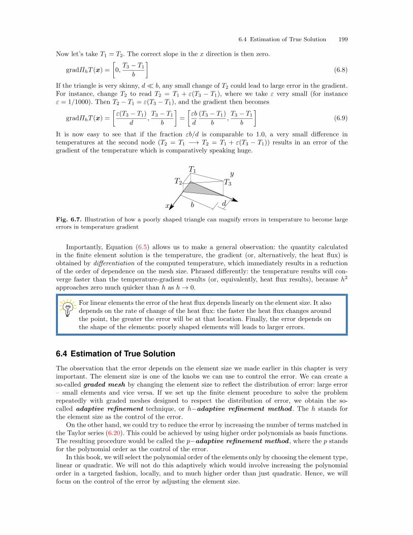
6.4 Estimation of True Solution 199

Now let’s take T1 = T2. The correct slope in the x direction is then zero.

gradΠhT (x) =

[0,T3 − T1

b

](6.8)

If the triangle is very skinny, d≪ b, any small change of T2 could lead to large error in the gradient.For instance, change T2 to read T2 = T1 + ε(T3 − T1), where we take ε very small (for instanceε = 1/1000). Then T2 − T1 = ε(T3 − T1), and the gradient then becomes

gradΠhT (x) =

[ε(T3 − T1)

d,T3 − T1

b

]=

[εb

d

(T3 − T1)

b,T3 − T1

b

](6.9)

It is now easy to see that if the fraction εb/d is comparable to 1.0, a very small difference intemperatures at the second node (T2 = T1 −→ T2 = T1 + ε(T3 − T1)) results in an error of thegradient of the temperature which is comparatively speaking huge.

Fig. 6.7. Illustration of how a poorly shaped triangle can magnify errors in temperature to become largeerrors in temperature gradient

Importantly, Equation (6.5) allows us to make a general observation: the quantity calculatedin the finite element solution is the temperature, the gradient (or, alternatively, the heat flux) isobtained by differentiation of the computed temperature, which immediately results in a reductionof the order of dependence on the mesh size. Phrased differently: the temperature results will con-verge faster than the temperature-gradient results (or, equivalently, heat flux results), because h2

approaches zero much quicker than h as h→ 0.

For linear elements the error of the heat flux depends linearly on the element size. It alsodepends on the rate of change of the heat flux: the faster the heat flux changes aroundthe point, the greater the error will be at that location. Finally, the error depends onthe shape of the elements: poorly shaped elements will leads to larger errors.

6.4 Estimation of True Solution

The observation that the error depends on the element size we made earlier in this chapter is veryimportant. The element size is one of the knobs we can use to control the error. We can create aso-called graded mesh by changing the element size to reflect the distribution of error: large error– small elements and vice versa. If we set up the finite element procedure to solve the problemrepeatedly with graded meshes designed to respect the distribution of error, we obtain the so-called adaptive refinement technique, or h−adaptive refinement method . The h stands forthe element size as the control of the error.

On the other hand, we could try to reduce the error by increasing the number of terms matched inthe Taylor series (6.20). This could be achieved by using higher order polynomials as basis functions.The resulting procedure would be called the p−adaptive refinement method , where the p standsfor the polynomial order as the control of the error.

In this book, we will select the polynomial order of the elements only by choosing the element type,linear or quadratic. We will not do this adaptively which would involve increasing the polynomialorder in a targeted fashion, locally, and to much higher order than just quadratic. Hence, we willfocus on the control of the error by adjusting the element size.

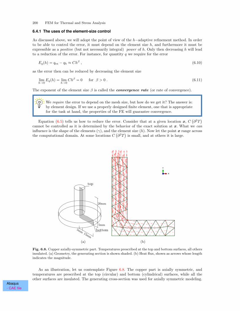
200 FEM for Thermal and Stress Analysis

6.4.1 The uses of the element-size control

As discussed above, we will adopt the point of view of the h−adaptive refinement method. In orderto be able to control the error, it must depend on the element size h, and furthermore it must beexpressible as a positive (but not necessarily integral) power of h. Only then decreasing h will leadto a reduction of the error. For instance, for quantity q we require for the error

Eq(h) = qex − qh ≈ Chβ , (6.10)

as the error then can be reduced by decreasing the element size

limh→0

Eq(h) = limh→0

Chβ = 0 for β > 0 . (6.11)

The exponent of the element size β is called the convergence rate (or rate of convergence).

We require the error to depend on the mesh size, but how do we get it? The answer is:by element design. If we use a properly designed finite element, one that is appropriatefor the task at hand, the properties of the FE will guarantee convergence.

Equation (6.5) tells us how to reduce the error. Consider that at a given location x, C(∂2T

)cannot be controlled as it is determined by the behavior of the exact solution at x. What we caninfluence is the shape of the elements (γ), and the element size (h). Now let the point x range acrossthe computational domain. At some locations C

(∂2T

)is small, and at others it is large.

X

Y

Z

(a) (b)

Fig. 6.8. Copper axially-symmetric part. Temperatures prescribed at the top and bottom surfaces, all othersinsulated. (a) Geometry, the generating section is shown shaded. (b) Heat flux, shown as arrows whose lengthindicates the magnitude.

As an illustration, let us contemplate Figure 6.8. The copper part is axially symmetric, andtemperatures are prescribed at the top (circular) and bottom (cylindrical) surfaces, while all theother surfaces are insulated. The generating cross-section was used for axially symmetric modeling.

Abaqus- CAE file

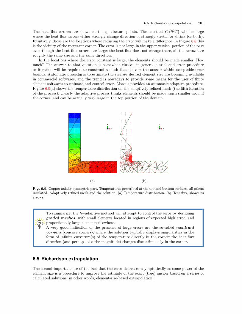
6.5 Richardson extrapolation 201

The heat flux arrows are shown at the quadrature points. The constant C(∂2T

)will be large

where the heat flux arrows either strongly change direction or strongly stretch or shrink (or both).Intuitively, those are the locations where reducing the error will make a difference. In Figure 6.8 thisis the vicinity of the reentrant corner. The error is not large in the upper vertical portion of the parteven though the heat flux arrows are large: the heat flux does not change there, all the arrows areroughly the same size and the same direction.

In the locations where the error constant is large, the elements should be made smaller. Howmuch? The answer to that question is somewhat elusive: in general a trial and error procedureor iteration will be required to construct a mesh that delivers the answer within acceptable errorbounds. Automatic procedures to estimate the relative desired element size are becoming availablein commercial softwares, and the trend is nowadays to provide some means for the user of finiteelement softwares to estimate and control error. Abaqus provides an automatic adaptive procedure.Figure 6.9(a) shows the temperature distribution on the adaptively refined mesh (the fifth iterationof the process). Clearly the adaptive process thinks elements should be made much smaller aroundthe corner, and can be actually very large in the top portion of the domain.

X

Y

Z X

Y

Z

(a) (b)

Fig. 6.9. Copper axially-symmetric part. Temperatures prescribed at the top and bottom surfaces, all othersinsulated. Adaptively refined mesh and the solution. (a) Temperature distribution. (b) Heat flux, shown asarrows.

To summarize, the h−adaptive method will attempt to control the error by designinggraded meshes, with small elements located in regions of expected high error, andproportionally large elements elsewhere.A very good indication of the presence of large errors are the so-called reentrantcorners (concave corners), where the solution typically displays singularities in theform of infinite curvature(s) of the temperature directly in the corner: the heat fluxdirection (and perhaps also the magnitude) changes discontinuously in the corner.

6.5 Richardson extrapolation

The second important use of the fact that the error decreases asymptotically as some power of theelement size is a procedure to improve the estimate of the exact (true) answer based on a series ofcalculated solutions: in other words, element-size-based extrapolation.

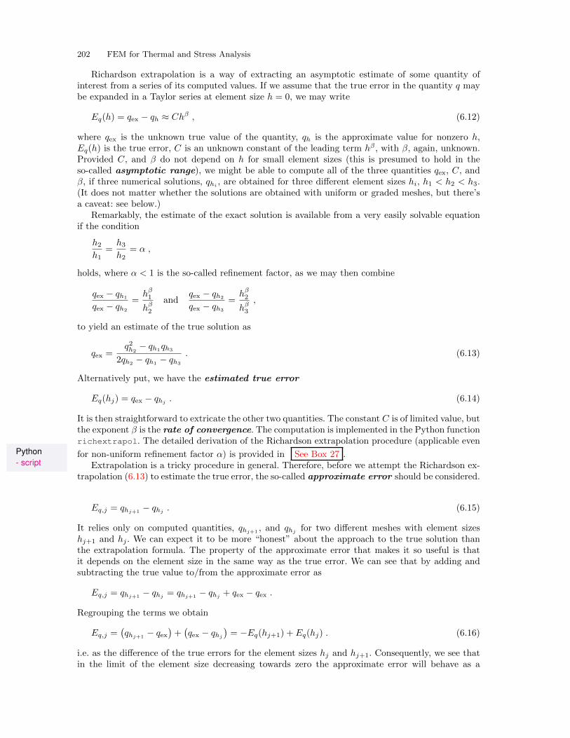
202 FEM for Thermal and Stress Analysis

Richardson extrapolation is a way of extracting an asymptotic estimate of some quantity ofinterest from a series of its computed values. If we assume that the true error in the quantity q maybe expanded in a Taylor series at element size h = 0, we may write

Eq(h) = qex − qh ≈ Chβ , (6.12)

where qex is the unknown true value of the quantity, qh is the approximate value for nonzero h,Eq(h) is the true error, C is an unknown constant of the leading term hβ , with β, again, unknown.Provided C, and β do not depend on h for small element sizes (this is presumed to hold in theso-called asymptotic range), we might be able to compute all of the three quantities qex, C, andβ, if three numerical solutions, qhi

, are obtained for three different element sizes hi, h1 < h2 < h3.(It does not matter whether the solutions are obtained with uniform or graded meshes, but there’sa caveat: see below.)

Remarkably, the estimate of the exact solution is available from a very easily solvable equationif the condition

h2h1

=h3h2

= α ,

holds, where α < 1 is the so-called refinement factor, as we may then combine

qex − qh1

qex − qh2

=hβ1

hβ2and

qex − qh2

qex − qh3

=hβ2

hβ3,

to yield an estimate of the true solution as

qex =q2h2

− qh1qh3

2qh2− qh1

− qh3

. (6.13)

Alternatively put, we have the estimated true error

Eq(hj) = qex − qhj . (6.14)

It is then straightforward to extricate the other two quantities. The constant C is of limited value, butthe exponent β is the rate of convergence. The computation is implemented in the Python functionrichextrapol. The detailed derivation of the Richardson extrapolation procedure (applicable even

Python- script

for non-uniform refinement factor α) is provided in See Box 27 .Extrapolation is a tricky procedure in general. Therefore, before we attempt the Richardson ex-

trapolation (6.13) to estimate the true error, the so-called approximate error should be considered.

Eq,j = qhj+1 − qhj . (6.15)

It relies only on computed quantities, qhj+1, and qhj

for two different meshes with element sizeshj+1 and hj . We can expect it to be more “honest” about the approach to the true solution thanthe extrapolation formula. The property of the approximate error that makes it so useful is thatit depends on the element size in the same way as the true error. We can see that by adding andsubtracting the true value to/from the approximate error as

Eq,j = qhj+1 − qhj = qhj+1 − qhj + qex − qex .

Regrouping the terms we obtain

Eq,j =(qhj+1

− qex)+(qex − qhj

)= −Eq(hj+1) + Eq(hj) . (6.16)

i.e. as the difference of the true errors for the element sizes hj and hj+1. Consequently, we see thatin the limit of the element size decreasing towards zero the approximate error will behave as a

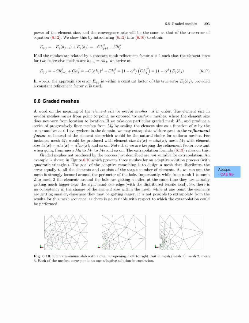
6.6 Graded meshes 203

power of the element size, and the convergence rate will be the same as that of the true error ofequation (6.12). We show this by introducing (6.12) into (6.16) to obtain

Eq,j = −Eq(hj+1) + Eq(hj) = −Chβj+1 + Chβj

If all the meshes are related by a constant mesh refinement factor α < 1 such that the element sizesfor two successive meshes are hj+1 = αhj , we arrive at

Eq,j = −Chβj+1 + Chβj = −C(αhj)β + Chβj =(1− αβ

) (Chβj

)=(1− αβ

)Eq(hj) (6.17)

In words, the approximate error Eq,j is within a constant factor of the true error Eq(hj), provideda constant refinement factor α is used.

6.6 Graded meshes

A word on the meaning of the element size in graded meshes is in order. The element size ingraded meshes varies from point to point, as opposed to uniform meshes, where the element sizedoes not vary from location to location. If we take one particular graded mesh M0, and produce aseries of progressively finer meshes from M0 by scaling the element size as a function of x by thesame number α < 1 everywhere in the domain, we may extrapolate with respect to the refinementfactor α, instead of the element size which would be the natural choice for uniform meshes. Forinstance, mesh M1 would be produced with element size h1(x) = αh0(x), mesh M2 with elementsize h2(x) = αh1(x) = α2h0(x), and so on. Note that we are keeping the refinement factor constantwhen going from mesh M0 to M1 to M2 and so on. The extrapolation formula (6.13) relies on this.

Graded meshes not produced by the process just described are not suitable for extrapolation. Anexample is shown in Figure 6.10 which presents three meshes for an adaptive solution process (withquadratic triangles). The goal of the adaptive remeshing is to design a mesh that distributes the

Abaqus- CAE file

error equally to all the elements and consists of the target number of elements. As we can see, themesh is strongly focused around the perimeter of the hole. Importantly, while from mesh 1 to mesh2 to mesh 3 the elements around the hole are getting smaller, at the same time they are actuallygetting much bigger near the right-hand-side edge (with the distributed tensile load). So, there isno consistency in the change of the element size within the mesh: while at one point the elementsare getting smaller, elsewhere they may be getting larger. It is not possible to extrapolate from theresults for this mesh sequence, as there is no variable with respect to which the extrapolation couldbe performed.

X

Y

Z X

Y

Z X

Y

Z

Fig. 6.10. Thin aluminium slab with a circular opening. Left to right: Initial mesh (mesh 1), mesh 2, mesh3. Each of the meshes corresponds to one adaptive solution in succession.

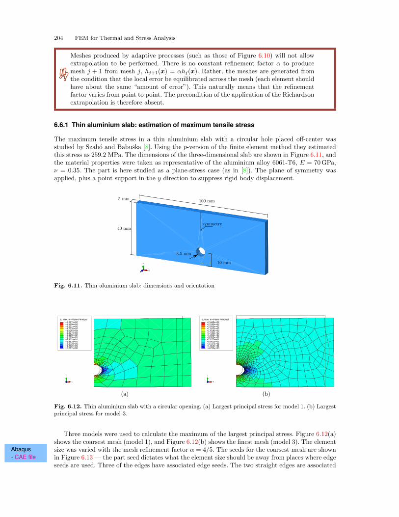
204 FEM for Thermal and Stress Analysis

Meshes produced by adaptive processes (such as those of Figure 6.10) will not allowextrapolation to be performed. There is no constant refinement factor α to producemesh j + 1 from mesh j, hj+1(x) = αhj(x). Rather, the meshes are generated fromthe condition that the local error be equilibrated across the mesh (each element shouldhave about the same “amount of error”). This naturally means that the refinementfactor varies from point to point. The precondition of the application of the Richardsonextrapolation is therefore absent.

6.6.1 Thin aluminium slab: estimation of maximum tensile stress

The maximum tensile stress in a thin aluminium slab with a circular hole placed off-center wasstudied by Szabo and Babuska [8]. Using the p-version of the finite element method they estimatedthis stress as 259.2 MPa. The dimensions of the three-dimensional slab are shown in Figure 6.11, andthe material properties were taken as representative of the aluminium alloy 6061-T6, E = 70GPa,ν = 0.35. The part is here studied as a plane-stress case (as in [8]). The plane of symmetry wasapplied, plus a point support in the y direction to suppress rigid body displacement.

Z

Y

X

X

Y

Z

Fig. 6.11. Thin aluminium slab: dimensions and orientation

S, Max. In−Plane Principal

−5.887e+00+1.392e+01+3.372e+01+5.352e+01+7.332e+01+9.313e+01+1.129e+02+1.327e+02+1.525e+02+1.723e+02+1.921e+02+2.119e+02+2.317e+02

X

Y

Z

S, Max. In−Plane Principal

−4.233e+00+1.652e+01+3.727e+01+5.802e+01+7.877e+01+9.953e+01+1.203e+02+1.410e+02+1.618e+02+1.825e+02+2.033e+02+2.240e+02+2.448e+02

X

Y

Z

(a) (b)

Fig. 6.12. Thin aluminium slab with a circular opening. (a) Largest principal stress for model 1. (b) Largestprincipal stress for model 3.

Three models were used to calculate the maximum of the largest principal stress. Figure 6.12(a)shows the coarsest mesh (model 1), and Figure 6.12(b) shows the finest mesh (model 3). The element

Abaqus- CAE file

size was varied with the mesh refinement factor α = 4/5. The seeds for the coarsest mesh are shownin Figure 6.13 — the part seed dictates what the element size should be away from places where edgeseeds are used. Three of the edges have associated edge seeds. The two straight edges are associated

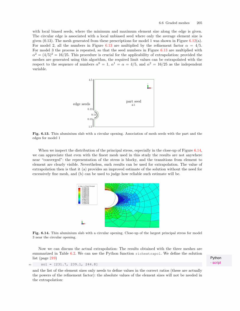
6.6 Graded meshes 205

with local biased seeds, where the minimum and maximum element size along the edge is given.The circular edge is associated with a local unbiased seed where only the average element size isgiven (0.13). The mesh generated from these prescriptions for model 1 was shown in Figure 6.12(a).For model 2, all the numbers in Figure 6.13 are multiplied by the refinement factor α = 4/5.For model 3 the process is repeated, so that the seed numbers in Figure 6.13 are multiplied withα2 = (4/5)2 = 16/25. This procedure is crucial for the applicability of extrapolation: provided themeshes are generated using this algorithm, the required limit values can be extrapolated with therespect to the sequence of numbers α0 = 1, α1 = α = 4/5, and α2 = 16/25 as the independentvariable.

X

Y

Z

Fig. 6.13. Thin aluminium slab with a circular opening. Association of mesh seeds with the part and theedges for model 1

When we inspect the distribution of the principal stress, especially in the close-up of Figure 6.14,we can appreciate that even with the finest mesh used in this study the results are not anywherenear “converged”: the representation of the stress is blocky, and the transitions from element toelement are clearly visible. Nevertheless, such results can be used for extrapolation. The value ofextrapolation then is that it (a) provides an improved estimate of the solution without the need forexcessively fine mesh, and (b) can be used to judge how reliable such estimate will be.

S, Max. In−Plane Principal

−4.233e+00+1.652e+01+3.727e+01+5.802e+01+7.877e+01+9.953e+01+1.203e+02+1.410e+02+1.618e+02+1.825e+02+2.033e+02+2.240e+02+2.448e+02

X

Y

Z

Fig. 6.14. Thin aluminium slab with a circular opening. Close-up of the largest principal stress for model3 near the circular opening.

Now we can discuss the actual extrapolation: The results obtained with the three meshes aresummarized in Table 6.2. We can use the Python function richextrapol. We define the solution

Python- script

list (page 219)

86 sol = [231.7, 239.1, 244.8]

and the list of the element sizes only needs to define values in the correct ratios (these are actuallythe powers of the refinement factor): the absolute values of the element sizes will not be needed inthe extrapolation:

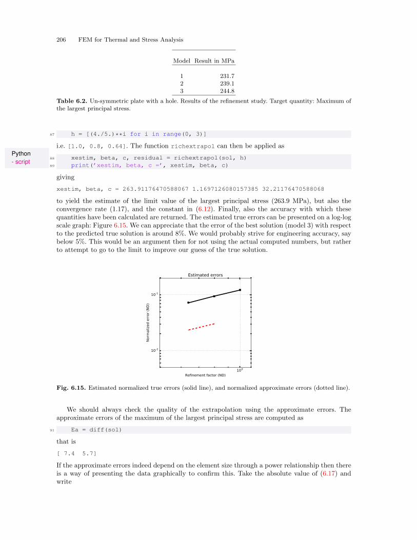
206 FEM for Thermal and Stress Analysis

Model Result in MPa

1 231.72 239.13 244.8

Table 6.2. Un-symmetric plate with a hole. Results of the refinement study. Target quantity: Maximum ofthe largest principal stress.

87 h = [(4./5.)**i for i in range(0, 3)]

i.e. [1.0, 0.8, 0.64]. The function richextrapol can then be applied asPython- script

88 xestim, beta, c, residual = richextrapol(sol, h)89 print(’xestim, beta, c =’, xestim, beta, c)

giving

xestim, beta, c = 263.91176470588067 1.1697126080157385 32.21176470588068

to yield the estimate of the limit value of the largest principal stress (263.9 MPa), but also theconvergence rate (1.17), and the constant in (6.12). Finally, also the accuracy with which thesequantities have been calculated are returned. The estimated true errors can be presented on a log-logscale graph: Figure 6.15. We can appreciate that the error of the best solution (model 3) with respectto the predicted true solution is around 8%. We would probably strive for engineering accuracy, saybelow 5%. This would be an argument then for not using the actual computed numbers, but ratherto attempt to go to the limit to improve our guess of the true solution.

100

Refinement factor (ND)

10-2

10-1

Norm

alized error (N

D)

Estimated errors

Fig. 6.15. Estimated normalized true errors (solid line), and normalized approximate errors (dotted line).

We should always check the quality of the extrapolation using the approximate errors. Theapproximate errors of the maximum of the largest principal stress are computed as

91 Ea = diff(sol)

that is

[ 7.4 5.7]

If the approximate errors indeed depend on the element size through a power relationship then thereis a way of presenting the data graphically to confirm this. Take the absolute value of (6.17) andwrite

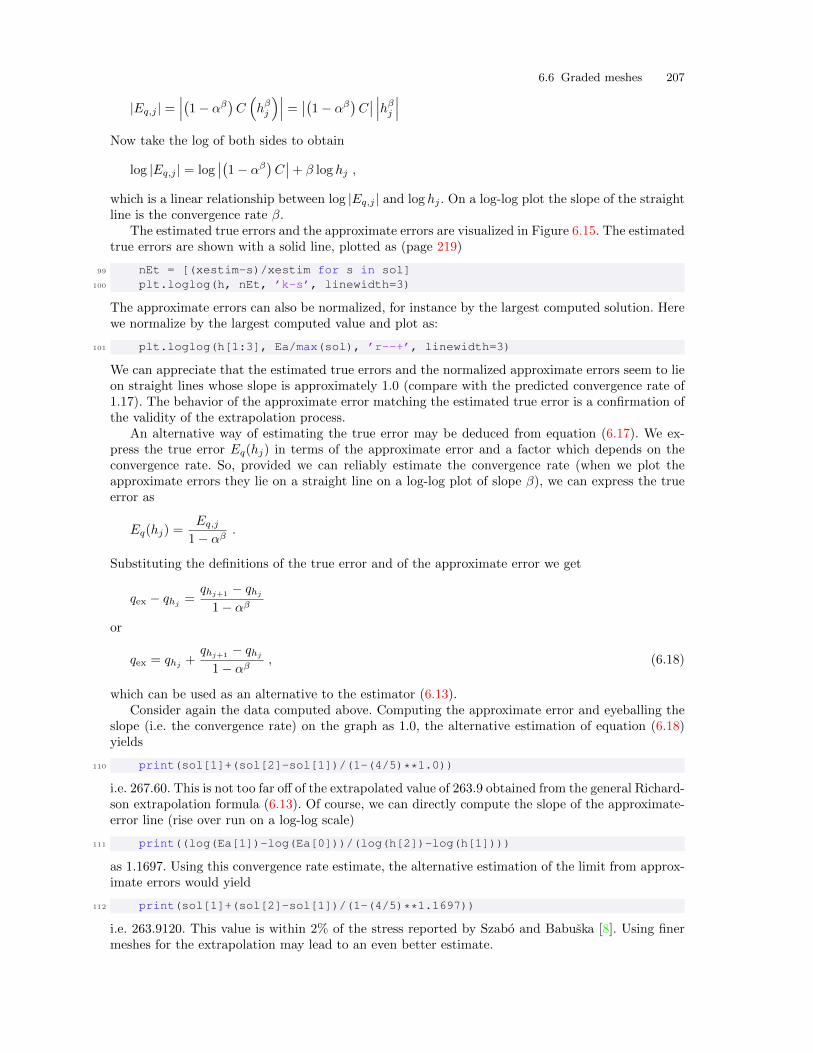
6.6 Graded meshes 207

|Eq,j | =∣∣∣(1− αβ

)C(hβj

)∣∣∣ = ∣∣(1− αβ)C∣∣ ∣∣∣hβj ∣∣∣

Now take the log of both sides to obtain

log |Eq,j | = log∣∣(1− αβ

)C∣∣+ β log hj ,

which is a linear relationship between log |Eq,j | and log hj . On a log-log plot the slope of the straightline is the convergence rate β.

The estimated true errors and the approximate errors are visualized in Figure 6.15. The estimatedtrue errors are shown with a solid line, plotted as (page 219)

99 nEt = [(xestim-s)/xestim for s in sol]100 plt.loglog(h, nEt, ’k-s’, linewidth=3)

The approximate errors can also be normalized, for instance by the largest computed solution. Herewe normalize by the largest computed value and plot as:

101 plt.loglog(h[1:3], Ea/max(sol), ’r--+’, linewidth=3)

We can appreciate that the estimated true errors and the normalized approximate errors seem to lieon straight lines whose slope is approximately 1.0 (compare with the predicted convergence rate of1.17). The behavior of the approximate error matching the estimated true error is a confirmation ofthe validity of the extrapolation process.

An alternative way of estimating the true error may be deduced from equation (6.17). We ex-press the true error Eq(hj) in terms of the approximate error and a factor which depends on theconvergence rate. So, provided we can reliably estimate the convergence rate (when we plot theapproximate errors they lie on a straight line on a log-log plot of slope β), we can express the trueerror as

Eq(hj) =Eq,j

1− αβ.

Substituting the definitions of the true error and of the approximate error we get

qex − qhj =qhj+1

− qhj

1− αβ

or

qex = qhj+qhj+1

− qhj

1− αβ, (6.18)

which can be used as an alternative to the estimator (6.13).Consider again the data computed above. Computing the approximate error and eyeballing the

slope (i.e. the convergence rate) on the graph as 1.0, the alternative estimation of equation (6.18)yields

110 print(sol[1]+(sol[2]-sol[1])/(1-(4/5)**1.0))

i.e. 267.60. This is not too far off of the extrapolated value of 263.9 obtained from the general Richard-son extrapolation formula (6.13). Of course, we can directly compute the slope of the approximate-error line (rise over run on a log-log scale)

111 print((log(Ea[1])-log(Ea[0]))/(log(h[2])-log(h[1])))

as 1.1697. Using this convergence rate estimate, the alternative estimation of the limit from approx-imate errors would yield

112 print(sol[1]+(sol[2]-sol[1])/(1-(4/5)**1.1697))

i.e. 263.9120. This value is within 2% of the stress reported by Szabo and Babuska [8]. Using finermeshes for the extrapolation may lead to an even better estimate.

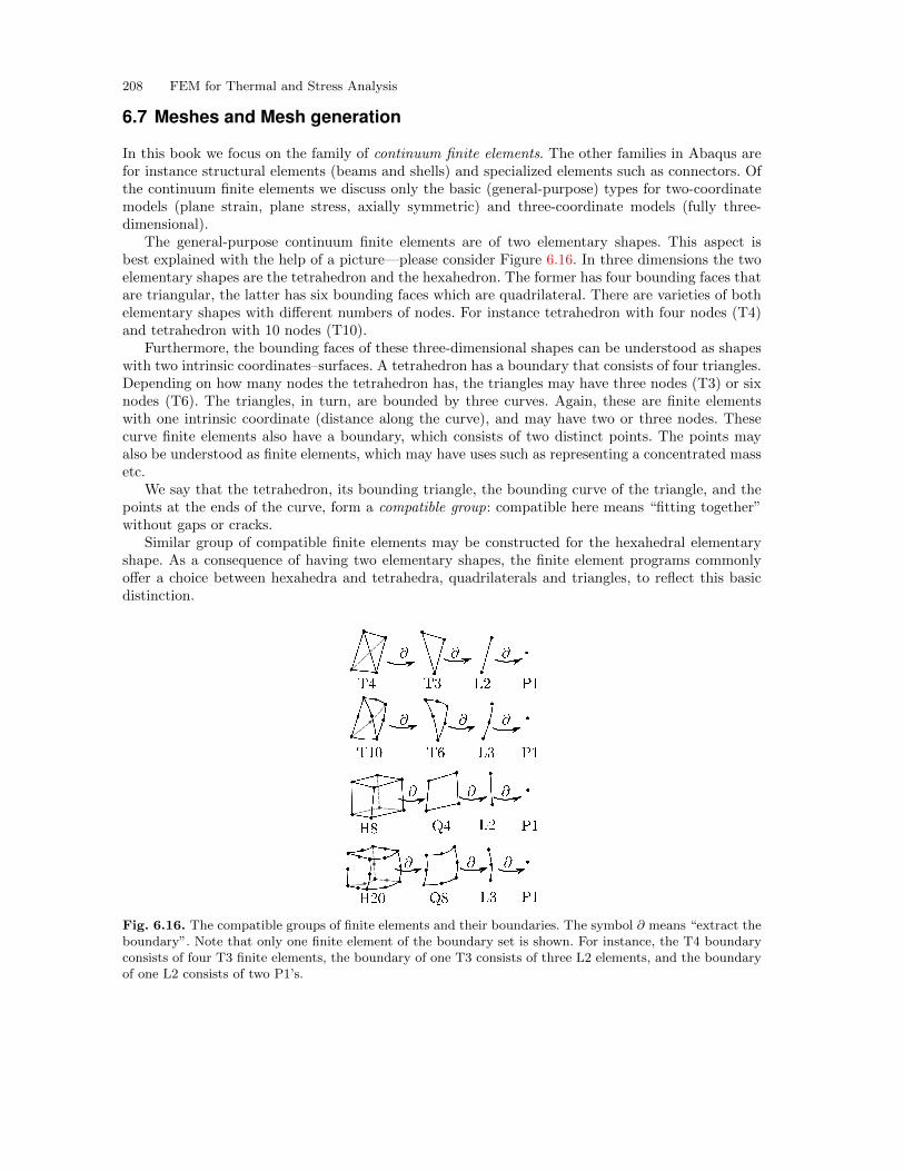
208 FEM for Thermal and Stress Analysis

6.7 Meshes and Mesh generation

In this book we focus on the family of continuum finite elements. The other families in Abaqus arefor instance structural elements (beams and shells) and specialized elements such as connectors. Ofthe continuum finite elements we discuss only the basic (general-purpose) types for two-coordinatemodels (plane strain, plane stress, axially symmetric) and three-coordinate models (fully three-dimensional).

The general-purpose continuum finite elements are of two elementary shapes. This aspect isbest explained with the help of a picture—please consider Figure 6.16. In three dimensions the twoelementary shapes are the tetrahedron and the hexahedron. The former has four bounding faces thatare triangular, the latter has six bounding faces which are quadrilateral. There are varieties of bothelementary shapes with different numbers of nodes. For instance tetrahedron with four nodes (T4)and tetrahedron with 10 nodes (T10).

Furthermore, the bounding faces of these three-dimensional shapes can be understood as shapeswith two intrinsic coordinates–surfaces. A tetrahedron has a boundary that consists of four triangles.Depending on how many nodes the tetrahedron has, the triangles may have three nodes (T3) or sixnodes (T6). The triangles, in turn, are bounded by three curves. Again, these are finite elementswith one intrinsic coordinate (distance along the curve), and may have two or three nodes. Thesecurve finite elements also have a boundary, which consists of two distinct points. The points mayalso be understood as finite elements, which may have uses such as representing a concentrated massetc.

We say that the tetrahedron, its bounding triangle, the bounding curve of the triangle, and thepoints at the ends of the curve, form a compatible group: compatible here means “fitting together”without gaps or cracks.

Similar group of compatible finite elements may be constructed for the hexahedral elementaryshape. As a consequence of having two elementary shapes, the finite element programs commonlyoffer a choice between hexahedra and tetrahedra, quadrilaterals and triangles, to reflect this basicdistinction.

Fig. 6.16. The compatible groups of finite elements and their boundaries. The symbol ∂ means “extract theboundary”. Note that only one finite element of the boundary set is shown. For instance, the T4 boundaryconsists of four T3 finite elements, the boundary of one T3 consists of three L2 elements, and the boundaryof one L2 consists of two P1’s.

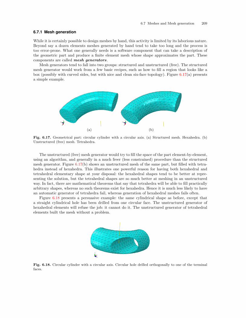
6.7 Meshes and Mesh generation 209

6.7.1 Mesh generation

While it is certainly possible to design meshes by hand, this activity is limited by its laborious nature.Beyond say a dozen elements meshes generated by hand tend to take too long and the process istoo error-prone. What one generally needs is a software component that can take a description ofthe geometric part and produce a finite element mesh whose shape approximates the part. Thesecomponents are called mesh generators.

Mesh generators tend to fall into two groups: structured and unstructured (free). The structuredmesh generator would work from a few basic recipes, such as how to fill a region that looks like abox (possibly with curved sides, but with nice and clean six-face topology). Figure 6.17(a) presentsa simple example.

X

YZ

X

YZ

(a) (b)

Fig. 6.17. Geometrical part: circular cylinder with a circular axis. (a) Structured mesh. Hexahedra. (b)Unstructured (free) mesh. Tetrahedra.

The unstructured (free) mesh generator would try to fill the space of the part element-by-element,using an algorithm, and generally in a much freer (less constrained) procedure than the structuredmesh generator. Figure 6.17(b) shows an unstructured mesh of the same part, but filled with tetra-hedra instead of hexahedra. This illustrates one powerful reason for having both hexahedral andtetrahedral elementary shape at your disposal: the hexahedral shapes tend to be better at repre-senting the solution, but the tetrahedral shapes are so much better at meshing in an unstructuredway. In fact, there are mathematical theorems that say that tetrahedra will be able to fill practicallyarbitrary shapes, whereas no such theorems exist for hexahedra. Hence it is much less likely to havean automatic generator of tetrahedra fail, whereas generation of hexahedral meshes fails often.

Figure 6.18 presents a persuasive example: the same cylindrical shape as before, except thata straight cylindrical hole has been drilled from one circular face. The unstructured generator ofhexahedral elements will refuse the job: it cannot do it. The unstructured generator of tetrahedralelements built the mesh without a problem.

X

Y

Z

Fig. 6.18. Circular cylinder with a circular axis. Circular hole drilled orthogonally to one of the terminalfaces.

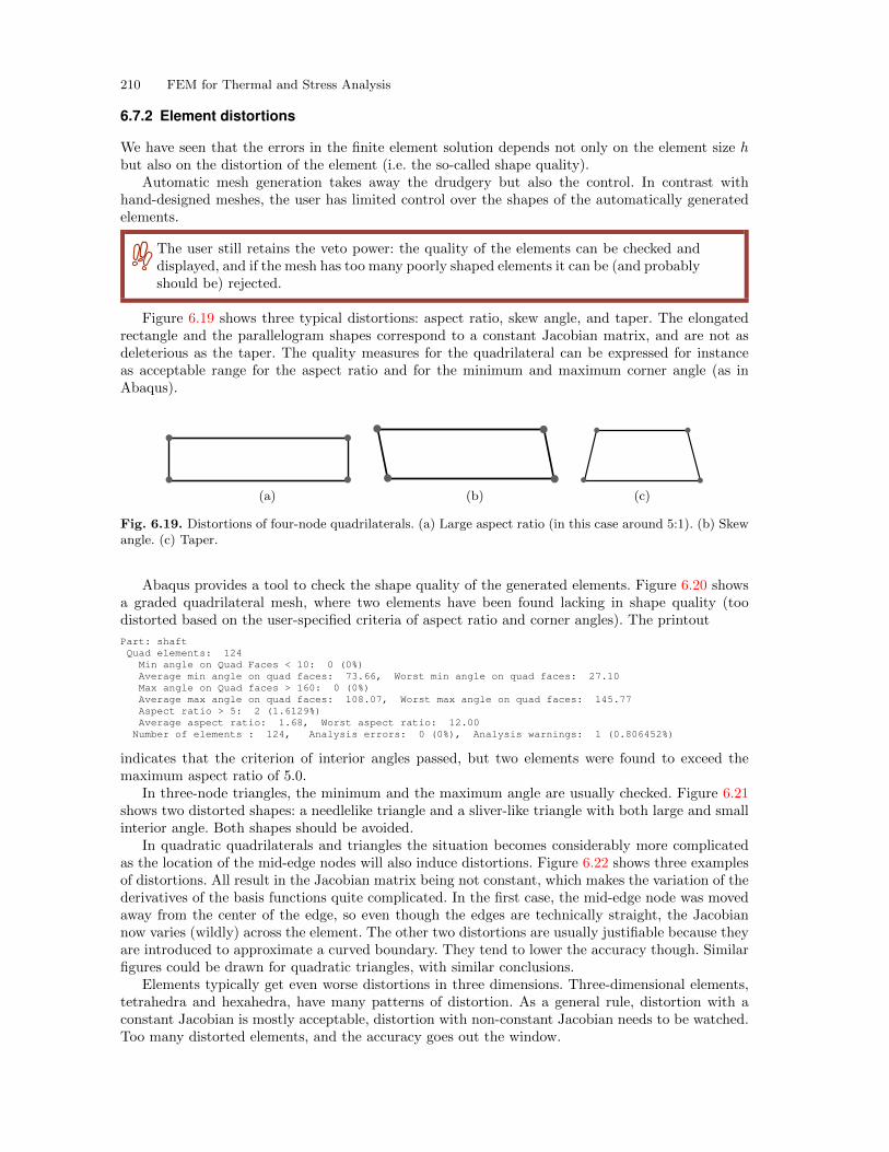
210 FEM for Thermal and Stress Analysis

6.7.2 Element distortions

We have seen that the errors in the finite element solution depends not only on the element size hbut also on the distortion of the element (i.e. the so-called shape quality).

Automatic mesh generation takes away the drudgery but also the control. In contrast withhand-designed meshes, the user has limited control over the shapes of the automatically generatedelements.

The user still retains the veto power: the quality of the elements can be checked anddisplayed, and if the mesh has too many poorly shaped elements it can be (and probablyshould be) rejected.

Figure 6.19 shows three typical distortions: aspect ratio, skew angle, and taper. The elongatedrectangle and the parallelogram shapes correspond to a constant Jacobian matrix, and are not asdeleterious as the taper. The quality measures for the quadrilateral can be expressed for instanceas acceptable range for the aspect ratio and for the minimum and maximum corner angle (as inAbaqus).

(a) (b) (c)

Fig. 6.19. Distortions of four-node quadrilaterals. (a) Large aspect ratio (in this case around 5:1). (b) Skewangle. (c) Taper.

Abaqus provides a tool to check the shape quality of the generated elements. Figure 6.20 showsa graded quadrilateral mesh, where two elements have been found lacking in shape quality (toodistorted based on the user-specified criteria of aspect ratio and corner angles). The printout

Part: shaftQuad elements: 124

Min angle on Quad Faces < 10: 0 (0%)Average min angle on quad faces: 73.66, Worst min angle on quad faces: 27.10Max angle on Quad faces > 160: 0 (0%)Average max angle on quad faces: 108.07, Worst max angle on quad faces: 145.77Aspect ratio > 5: 2 (1.6129%)Average aspect ratio: 1.68, Worst aspect ratio: 12.00

Number of elements : 124, Analysis errors: 0 (0%), Analysis warnings: 1 (0.806452%)

indicates that the criterion of interior angles passed, but two elements were found to exceed themaximum aspect ratio of 5.0.

In three-node triangles, the minimum and the maximum angle are usually checked. Figure 6.21shows two distorted shapes: a needlelike triangle and a sliver-like triangle with both large and smallinterior angle. Both shapes should be avoided.

In quadratic quadrilaterals and triangles the situation becomes considerably more complicatedas the location of the mid-edge nodes will also induce distortions. Figure 6.22 shows three examplesof distortions. All result in the Jacobian matrix being not constant, which makes the variation of thederivatives of the basis functions quite complicated. In the first case, the mid-edge node was movedaway from the center of the edge, so even though the edges are technically straight, the Jacobiannow varies (wildly) across the element. The other two distortions are usually justifiable because theyare introduced to approximate a curved boundary. They tend to lower the accuracy though. Similarfigures could be drawn for quadratic triangles, with similar conclusions.

Elements typically get even worse distortions in three dimensions. Three-dimensional elements,tetrahedra and hexahedra, have many patterns of distortion. As a general rule, distortion with aconstant Jacobian is mostly acceptable, distortion with non-constant Jacobian needs to be watched.Too many distorted elements, and the accuracy goes out the window.

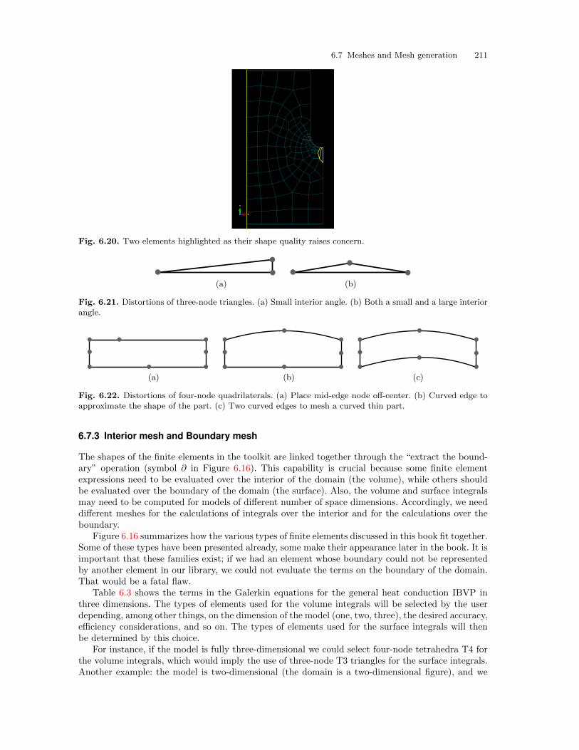
6.7 Meshes and Mesh generation 211

X

Y

Z

Fig. 6.20. Two elements highlighted as their shape quality raises concern.

(a) (b)

Fig. 6.21. Distortions of three-node triangles. (a) Small interior angle. (b) Both a small and a large interiorangle.

(a) (b) (c)

Fig. 6.22. Distortions of four-node quadrilaterals. (a) Place mid-edge node off-center. (b) Curved edge toapproximate the shape of the part. (c) Two curved edges to mesh a curved thin part.

6.7.3 Interior mesh and Boundary mesh

The shapes of the finite elements in the toolkit are linked together through the “extract the bound-ary” operation (symbol ∂ in Figure 6.16). This capability is crucial because some finite elementexpressions need to be evaluated over the interior of the domain (the volume), while others shouldbe evaluated over the boundary of the domain (the surface). Also, the volume and surface integralsmay need to be computed for models of different number of space dimensions. Accordingly, we needdifferent meshes for the calculations of integrals over the interior and for the calculations over theboundary.

Figure 6.16 summarizes how the various types of finite elements discussed in this book fit together.Some of these types have been presented already, some make their appearance later in the book. It isimportant that these families exist; if we had an element whose boundary could not be representedby another element in our library, we could not evaluate the terms on the boundary of the domain.That would be a fatal flaw.

Table 6.3 shows the terms in the Galerkin equations for the general heat conduction IBVP inthree dimensions. The types of elements used for the volume integrals will be selected by the userdepending, among other things, on the dimension of the model (one, two, three), the desired accuracy,efficiency considerations, and so on. The types of elements used for the surface integrals will thenbe determined by this choice.

For instance, if the model is fully three-dimensional we could select four-node tetrahedra T4 forthe volume integrals, which would imply the use of three-node T3 triangles for the surface integrals.Another example: the model is two-dimensional (the domain is a two-dimensional figure), and we

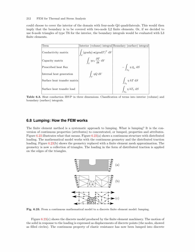
212 FEM for Thermal and Stress Analysis

could choose to cover the interior of the domain with four-node Q4 quadrilaterals. This would thenimply that the boundary is to be covered with two-node L2 finite elements. Or, if we decided touse 6-node triangles of type T6 for the interior, the boundary integrals would be evaluated with L3finite elements.

Term Interior (volume) integral Boundary (surface) integral

Conductivity matrix

∫V

(gradη) κ(gradT )T dV

Capacity matrix

∫V

ηcV∂T

∂tdV

Prescribed heat flux −∫S2

η qn dS

Internal heat generation

∫V

ηQ dV

Surface heat transfer matrix

∫S3

η hT dS

Surface heat transfer load

∫S3

η hTa dS

Table 6.3. Heat conduction IBVP in three dimensions. Classification of terms into interior (volume) andboundary (surface) integrals.

6.8 Lumping: How the FEM works

The finite element method is a systematic approach to lumping. What is lumping? It is the con-version of continuous properties (attributes) to concentrated, or lumped, properties and attributes.Figure 6.23 illustrates what that means. Figure 6.23(a) shows a continuous structure with distributedloading. The mathematical model works with the continuous geometry and the distributed tractionloading. Figure 6.23(b) shows the geometry replaced with a finite element mesh approximation. Thegeometry is now a collection of triangles. The loading in the form of distributed traction is appliedon the edges of the triangles.

Fig. 6.23. From a continuous mathematical model to a discrete finite element model: lumping.

Figure 6.23(c) shows the discrete model produced by the finite element machinery. The motion ofthe solid in response to the loading is expressed as displacements of discrete points (the nodes, showedas filled circles). The continuous property of elastic resistance has now been lumped into discrete

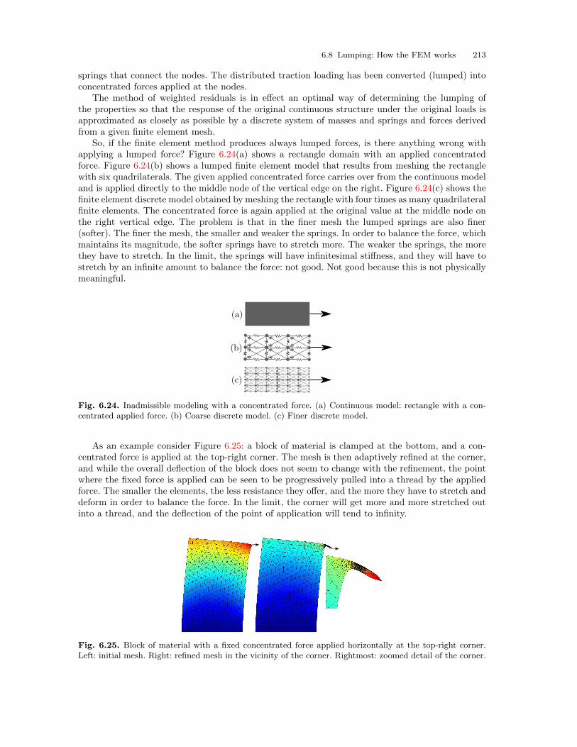
6.8 Lumping: How the FEM works 213

springs that connect the nodes. The distributed traction loading has been converted (lumped) intoconcentrated forces applied at the nodes.

The method of weighted residuals is in effect an optimal way of determining the lumping ofthe properties so that the response of the original continuous structure under the original loads isapproximated as closely as possible by a discrete system of masses and springs and forces derivedfrom a given finite element mesh.

So, if the finite element method produces always lumped forces, is there anything wrong withapplying a lumped force? Figure 6.24(a) shows a rectangle domain with an applied concentratedforce. Figure 6.24(b) shows a lumped finite element model that results from meshing the rectanglewith six quadrilaterals. The given applied concentrated force carries over from the continuous modeland is applied directly to the middle node of the vertical edge on the right. Figure 6.24(c) shows thefinite element discrete model obtained by meshing the rectangle with four times as many quadrilateralfinite elements. The concentrated force is again applied at the original value at the middle node onthe right vertical edge. The problem is that in the finer mesh the lumped springs are also finer(softer). The finer the mesh, the smaller and weaker the springs. In order to balance the force, whichmaintains its magnitude, the softer springs have to stretch more. The weaker the springs, the morethey have to stretch. In the limit, the springs will have infinitesimal stiffness, and they will have tostretch by an infinite amount to balance the force: not good. Not good because this is not physicallymeaningful.

Fig. 6.24. Inadmissible modeling with a concentrated force. (a) Continuous model: rectangle with a con-centrated applied force. (b) Coarse discrete model. (c) Finer discrete model.

As an example consider Figure 6.25: a block of material is clamped at the bottom, and a con-centrated force is applied at the top-right corner. The mesh is then adaptively refined at the corner,and while the overall deflection of the block does not seem to change with the refinement, the pointwhere the fixed force is applied can be seen to be progressively pulled into a thread by the appliedforce. The smaller the elements, the less resistance they offer, and the more they have to stretch anddeform in order to balance the force. In the limit, the corner will get more and more stretched outinto a thread, and the deflection of the point of application will tend to infinity.

Fig. 6.25. Block of material with a fixed concentrated force applied horizontally at the top-right corner.Left: initial mesh. Right: refined mesh in the vicinity of the corner. Rightmost: zoomed detail of the corner.

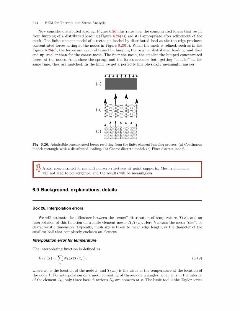
214 FEM for Thermal and Stress Analysis

Now consider distributed loading. Figure 6.26 illustrates how the concentrated forces that resultfrom lumping of a distributed loading (Figure 6.26(a)) are still appropriate after refinement of themesh. The finite element model of a rectangle loaded by distributed load at the top edge producesconcentrated forces acting at the nodes in Figure 6.26(b). When the mesh is refined, such as in theFigure 6.26(c), the forces are again obtained by lumping the original distributed loading, and theyend up smaller than for the coarse mesh. The finer the mesh, the smaller the lumped concentratedforces at the nodes. And, since the springs and the forces are now both getting “smaller” at thesame time, they are matched. In the limit we get a perfectly fine physically meaningful answer.

Fig. 6.26. Admissible concentrated forces resulting from the finite element lumping process. (a) Continuousmodel: rectangle with a distributed loading. (b) Coarse discrete model. (c) Finer discrete model.

Avoid concentrated forces and nonzero reactions at point supports. Mesh refinementwill not lead to convergence, and the results will be meaningless.

6.9 Background, explanations, details

Box 26. Interpolation errors

We will estimate the difference between the “exact” distribution of temperature, T (x), and aninterpolation of this function on a finite element mesh, ΠhT (x). Here h means the mesh “size”, orcharacteristic dimension. Typically, mesh size is taken to mean edge length, or the diameter of thesmallest ball that completely encloses an element.

Interpolation error for temperature

The interpolating function is defined as

ΠhT (x) =∑k

Nk(x)T (xk) , (6.19)

where xk is the location of the node k, and T (xk) is the value of the temperature at the location ofthe node k. For interpolation on a mesh consisting of three-node triangles, when x is in the interiorof the element ∆e, only three basis functions Nk are nonzero at x. The basic tool is the Taylor series

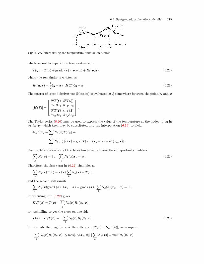
6.9 Background, explanations, details 215

Fig. 6.27. Interpolating the temperature function on a mesh

which we use to expand the temperature at x

T (y) = T (x) + gradT (x) · (y − x) +R1(y,x) , (6.20)

where the remainder is written as

R1(y,x) =1

2(y − x) ·H(T )(y − x) . (6.21)

The matrix of second derivatives (Hessian) is evaluated at ξ somewhere between the points y and x

[H(T )] =

∂2T (ξ)

∂x1∂x1

∂2T (ξ)

∂x1∂x2

∂2T (ξ)

∂x2∂x1

∂2T (ξ)

∂x2∂x2

.

The Taylor series (6.20) may be used to express the value of the temperature at the nodes– plug inxk for y– which then may be substituted into the interpolation (6.19) to yield

ΠhT (x) =∑k

Nk(x)T (xk) =∑k

Nk(x) [T (x) + gradT (x) · (xk − x) +R1(xk,x)] .

Due to the construction of the basis functions, we have these important equalities∑k

Nk(x) = 1 ,∑k

Nk(x)xk = x . (6.22)

Therefore, the first term in (6.22) simplifies as∑k

Nk(x)T (x) = T (x)∑k

Nk(x) = T (x) ,

and the second will vanish∑k

Nk(x)gradT (x) · (xk − x) = gradT (x) ·∑k

Nk(x)(xk − x) = 0 .

Substituting into (6.22) gives

ΠhT (x) = T (x) +∑k

Nk(x)R1(xk,x) ,

or, reshuffling to get the error on one side,

T (x)−ΠhT (x) = −∑k

Nk(x)R1(xk,x) . (6.23)

To estimate the magnitude of the difference, |T (x)−ΠhT (x)|, we compute

|∑k

Nk(x)R1(xk,x)| ≤ max|R1(xk,x)| |∑k

Nk(x)| = max|R1(xk,x)| ,

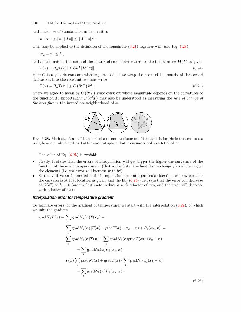
216 FEM for Thermal and Stress Analysis

and make use of standard norm inequalities

|v ·Av| ≤ ∥v∥∥Av∥ ≤ ∥A∥∥v∥2 .This may be applied to the definition of the remainder (6.21) together with (see Fig. 6.28)

∥xk − x∥ ≤ h ,

and an estimate of the norm of the matrix of second derivatives of the temperature H(T ) to give

|T (x)−ΠhT (x)| ≤ Ch2∥H(T )∥ . (6.24)

Here C is a generic constant with respect to h. If we wrap the norm of the matrix of the secondderivatives into the constant, we may write

|T (x)−ΠhT (x)| ≤ C(∂2T

)h2 , (6.25)

where we agree to mean by C(∂2T

)some constant whose magnitude depends on the curvatures of

the function T . Importantly, C(∂2T

)may also be understood as measuring the rate of change of

the heat flux in the immediate neighborhood of x.

Fig. 6.28. Mesh size h as a “diameter” of an element: diameter of the tight-fitting circle that encloses atriangle or a quadrilateral, and of the smallest sphere that is circumscribed to a tetrahedron

The value of Eq. (6.25) is twofold:

� Firstly, it states that the errors of interpolation will get bigger the higher the curvature of thefunction of the exact temperature T (that is the faster the heat flux is changing) and the biggerthe elements (i.e. the error will increase with h2);

� Secondly, if we are interested in the interpolation error at a particular location, we may considerthe curvatures at that location as given, and the Eq. (6.25) then says that the error will decreaseas O(h2) as h→ 0 (order-of estimate: reduce h with a factor of two, and the error will decreasewith a factor of four).

Interpolation error for temperature gradient

To estimate errors for the gradient of temperature, we start with the interpolation (6.22), of whichwe take the gradient

gradΠhT (x) =∑k

gradNk(x)T (xk) =∑k

gradNk(x) [T (x) + gradT (x) · (xk − x) +R1(xk,x)] =∑k

gradNk(x)T (x) +∑k

gradNk(x)gradT (x) · (xk − x)

+∑k

gradNk(x)R1(xk,x) =

T (x)∑k

gradNk(x) + gradT (x) ·∑k

gradNk(x)(xk − x)

+∑k

gradNk(x)R1(xk,x) .

(6.26)

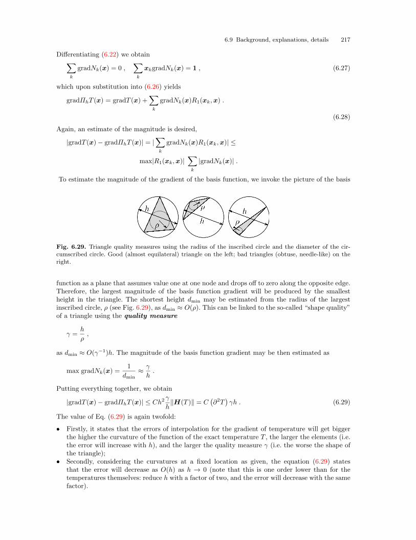
6.9 Background, explanations, details 217

Differentiating (6.22) we obtain∑k

gradNk(x) = 0 ,∑k

xkgradNk(x) = 1 , (6.27)

which upon substitution into (6.26) yields

gradΠhT (x) = gradT (x) +∑k

gradNk(x)R1(xk,x) .

(6.28)

Again, an estimate of the magnitude is desired,

|gradT (x)− gradΠhT (x)| = |∑k

gradNk(x)R1(xk,x)| ≤

max|R1(xk,x)|∑k

|gradNk(x)| .

To estimate the magnitude of the gradient of the basis function, we invoke the picture of the basis

Fig. 6.29. Triangle quality measures using the radius of the inscribed circle and the diameter of the cir-cumscribed circle. Good (almost equilateral) triangle on the left; bad triangles (obtuse, needle-like) on theright.

function as a plane that assumes value one at one node and drops off to zero along the opposite edge.Therefore, the largest magnitude of the basis function gradient will be produced by the smallestheight in the triangle. The shortest height dmin may be estimated from the radius of the largestinscribed circle, ρ (see Fig. 6.29), as dmin ≈ O(ρ). This can be linked to the so-called “shape quality”of a triangle using the quality measure

γ =h

ρ,

as dmin ≈ O(γ−1)h. The magnitude of the basis function gradient may be then estimated as

max gradNk(x) =1

dmin≈ γ

h.

Putting everything together, we obtain

|gradT (x)− gradΠhT (x)| ≤ Ch2γ

h∥H(T )∥ = C

(∂2T

)γh . (6.29)

The value of Eq. (6.29) is again twofold:

� Firstly, it states that the errors of interpolation for the gradient of temperature will get biggerthe higher the curvature of the function of the exact temperature T , the larger the elements (i.e.the error will increase with h), and the larger the quality measure γ (i.e. the worse the shape ofthe triangle);

� Secondly, considering the curvatures at a fixed location as given, the equation (6.29) statesthat the error will decrease as O(h) as h → 0 (note that this is one order lower than for thetemperatures themselves: reduce h with a factor of two, and the error will decrease with the samefactor).

218 FEM for Thermal and Stress Analysis

Importantly, Eq. (6.29) allows us to make a general observation: the quantity calculated in thefinite element solution is the temperature, the gradient (or, alternatively, the heat flux) is obtained bydifferentiation of the computed temperature, which immediately results in a reduction of the orderof dependence on the mesh size. Phrased differently: the temperature results will converge fasterthan the temperature-gradient results (or, equivalently, heat flux results), because h2 approacheszero much quicker than h as h→ 0.

End Box 26

Box 27. Richardson extrapolation

If we assume that the true error in the quantity q may be expanded in a Taylor series at elementsize h = 0, we may write Eq(h) as the true error of the quantity q for some nonzero element size hin the form

Eq(h) = qex − qh = Chβ +R , (6.30)

where qex is the true solution, qh is the approximate solution obtained with element size h, C issome constant which does not depend on the element size, β > 0 is the so-called convergence rate,and R is the remainder term. If the remainder term R is negligible compared to Chβ , we may write

Eq(h) = Chβ . (6.31)

Then, provided we obtain the solution of the finite element problem for three different elementsize values h1 < h2 < h3, so that we have a sequence of solutions qhj

, we can write the so-calledapproximate error as the difference of two successive solutions

Eq,j = qhj+1− qhj

. (6.32)

Replacing the approximate solutions with the true errors and the true solution qhj= qex − Eq(hj),

we obtain

Eq,j = −Eq(hj+1) + Eq(hj) . (6.33)

Substituting from (6.31), we get

Eq,j = −Chj+1β + Chj

β = C(−hj+1

β + hjβ). (6.34)

This equation may be written twice, for two successive approximate errors,

Eq,1 = C(−h2β + h1

β)

and Eq,2 = C(−h3β + h2

β), (6.35)

which may be readily solved for C to yield

Eq,1

−h2β + h1β=

Eq,2

−h3β + h2β. (6.36)

This nonlinear equation may be solved for the convergence rate β. Then the constant C follows as

C =Eq,1

−h2β + h1β=

Eq,2

−h3β + h2β, (6.37)

and the estimate of the true error for any element size then follows from (6.31). Obviously, with theestimate of the true error we also have the estimate of the true solution qex.

End Box 27

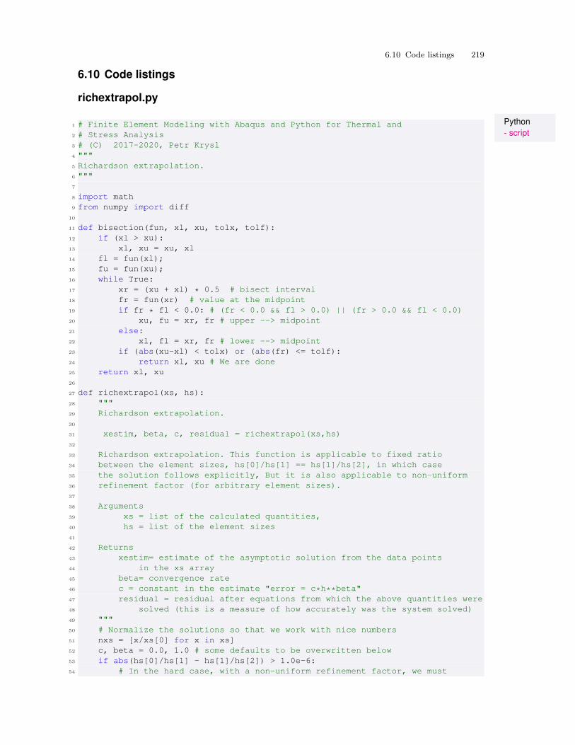
6.10 Code listings 219

6.10 Code listings

richextrapol.py

Python- script

1 # Finite Element Modeling with Abaqus and Python for Thermal and2 # Stress Analysis3 # (C) 2017-2020, Petr Krysl4 """5 Richardson extrapolation.6 """7

8 import math9 from numpy import diff

10

11 def bisection(fun, xl, xu, tolx, tolf):12 if (xl > xu):13 xl, xu = xu, xl14 fl = fun(xl);15 fu = fun(xu);16 while True:17 xr = (xu + xl) * 0.5 # bisect interval18 fr = fun(xr) # value at the midpoint19 if fr * fl < 0.0: # (fr < 0.0 && fl > 0.0) || (fr > 0.0 && fl < 0.0)20 xu, fu = xr, fr # upper --> midpoint21 else:22 xl, fl = xr, fr # lower --> midpoint23 if (abs(xu-xl) < tolx) or (abs(fr) <= tolf):24 return xl, xu # We are done25 return xl, xu26

27 def richextrapol(xs, hs):28 """29 Richardson extrapolation.30

31 xestim, beta, c, residual = richextrapol(xs,hs)32

33 Richardson extrapolation. This function is applicable to fixed ratio34 between the element sizes, hs[0]/hs[1] == hs[1]/hs[2], in which case35 the solution follows explicitly, But it is also applicable to non-uniform36 refinement factor (for arbitrary element sizes).37

38 Arguments39 xs = list of the calculated quantities,40 hs = list of the element sizes41

42 Returns43 xestim= estimate of the asymptotic solution from the data points44 in the xs array45 beta= convergence rate46 c = constant in the estimate "error = c*h**beta"47 residual = residual after equations from which the above quantities were48 solved (this is a measure of how accurately was the system solved)49 """50 # Normalize the solutions so that we work with nice numbers51 nxs = [x/xs[0] for x in xs]52 c, beta = 0.0, 1.0 # some defaults to be overwritten below53 if abs(hs[0]/hs[1] - hs[1]/hs[2]) > 1.0e-6:54 # In the hard case, with a non-uniform refinement factor, we must

220 FEM for Thermal and Stress Analysis

55 # solve a nonlinear equation 1st.56 nea1 = nxs[1]-nxs[0]57 nea2 = nxs[2]-nxs[1]58 tol = 0.00000000159 h0, h1, h2 = hs[0], hs[1], hs[2]60 eqn = lambda b: nea1 - nea2 * ((-h1**b+h0**b) / (-h2**b+h1**b))61 lo = tol # lower bound on the convergence rate62 hi = 10.063 b1, b2 = bisection(eqn, lo, hi, tol, tol)64 beta = (b1 + b2) / 2.065 c = xs[0]*nea1/(-hs[1]**beta+hs[0]**beta)66 xestim = xs[2] + c * hs[2]**beta67 else:68 # In the easy case, with a uniform refinement factor, the solution69 # is obtained explicitly.70 xestim = ((-(nxs[0]*nxs[2]-nxs[1]**2)/(2*nxs[1]-nxs[0]-nxs[2])))*xs[0]71 if (xestim-xs[0]) <= 0:72 beta = math.log((xestim-xs[1])/(xestim-xs[2]))/math.log(hs[1]/hs[2])73 else:74 beta = math.log((xestim-xs[0])/(xestim-xs[2]))/math.log(hs[0]/hs[2])75 c = (xestim-xs[0])/hs[0]**beta76 #77 # just to check things, calculate the residual78 residual = [0, 0, 0]79 for I in range(0, 3):80 residual[I] = (xestim-xs[I])-c*hs[I]**beta# this should be close to zero81 #82 return xestim, beta, c, residual83

84 def _test():85 """86 Test of Richardson extrapolation.87 """88 xs = [93.0734, 92.8633, 92.7252]89 hs = [0.1000, 0.0500, 0.0250]90 xestim, beta, c, residual = richextrapol(xs, hs)91 print(’xestim, beta, c, residual =’, xestim, beta, c, residual)92 print(’to be compared with ’, 92.46031652777476, 0.6053628424093497,

-2.471055221256022, \93 [0.0, 5.534461777756405e-13, 3.6376457401843254e-13])94 #95 xs = [13.124299546191557, 12.192464513175167, 12.026065694522512]96 hs = [1.0, 0.5, 0.25]97 xestim, beta, c, residual = richextrapol(xs, hs)98 print(’xestim, beta, c, residual =’, xestim, beta, c, residual)99 print(’to be compared with ’, 11.989892116202842, 2.485429379525128,

-1.1344074299887144, \100 [0.0, -8.93729534823251e-15, -1.5959455978986625e-15])101 #102 xs = [18.279591331058882, 18.260877354949294, 18.255333231883284]103 hs = [0.25, 0.125, 0.0625]104 xestim, beta, c, residual = richextrapol(xs, hs)105 print(’xestim, beta, c, residual =’, xestim, beta, c, residual)106 print(’to be compared with ’, 18.25299931817398, 1.7550849296401745,

-0.3029825595040225, \107 [0.0, -3.975153539670373e-13, -1.1776647365624449e-13])108 #109 sol = [231.7, 239.1, 244.8]

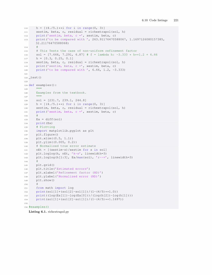
6.10 Code listings 221

110 h = [(4./5.)**i for i in range(0, 3)]111 xestim, beta, c, residual = richextrapol(sol, h)112 print(’xestim, beta, c =’, xestim, beta, c)113 print(’to be compared with ’, 263.91176470588067, 1.1697126080157385,

32.21176470588068)114 #115 # This Tests the case of non-uniform refinement factor116 sol = [7.446, 7.291, 6.87] # f = lambda h: -3.333 * h**1.2 + 6.66117 h = [0.3, 0.25, 0.1]118 xestim, beta, c, residual = richextrapol(sol, h)119 print(’xestim, beta, c =’, xestim, beta, c)120 print(’to be compared with ’, 6.66, 1.2, -3.333)121

122 _test()123

124 def examples():125 """126 Examples from the textbook.127 """128 sol = [231.7, 239.1, 244.8]129 h = [(4./5.)**i for i in range(0, 3)]130 xestim, beta, c, residual = richextrapol(sol, h)131 print(’xestim, beta, c =’, xestim, beta, c)132 #133 Ea = diff(sol)134 print(Ea)135 # Plotting136 import matplotlib.pyplot as plt137 plt.figure()138 plt.xlim((0.5, 1.1))139 plt.ylim((0.005, 0.2))140 # Normalized true error estimate141 nEt = [(xestim-s)/xestim for s in sol]142 plt.loglog(h, nEt, ’k-s’, linewidth=3)143 plt.loglog(h[1:3], Ea/max(sol), ’r--+’, linewidth=3)144 #145 plt.grid()146 plt.title(’Estimated errors’)147 plt.xlabel(’Refinement factor (ND)’)148 plt.ylabel(’Normalized error (ND)’)149 plt.show()150 #151 from math import log152 print(sol[1]+(sol[2]-sol[1])/(1-(4/5)**1.0))153 print((log(Ea[1])-log(Ea[0]))/(log(h[2])-log(h[1])))154 print(sol[1]+(sol[2]-sol[1])/(1-(4/5)**1.1697))155

156 #examples()

Listing 6.1. richextrapol.py

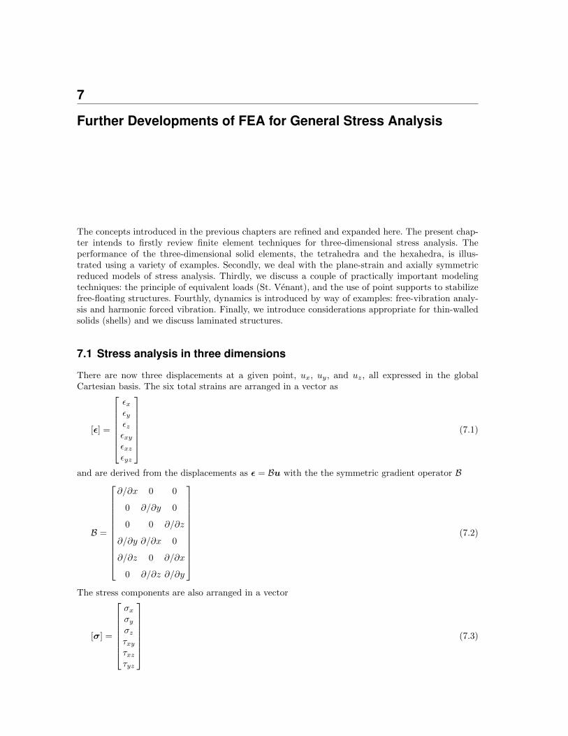
7

Further Developments of FEA for General Stress Analysis

The concepts introduced in the previous chapters are refined and expanded here. The present chap-ter intends to firstly review finite element techniques for three-dimensional stress analysis. Theperformance of the three-dimensional solid elements, the tetrahedra and the hexahedra, is illus-trated using a variety of examples. Secondly, we deal with the plane-strain and axially symmetricreduced models of stress analysis. Thirdly, we discuss a couple of practically important modelingtechniques: the principle of equivalent loads (St. Venant), and the use of point supports to stabilizefree-floating structures. Fourthly, dynamics is introduced by way of examples: free-vibration analy-sis and harmonic forced vibration. Finally, we introduce considerations appropriate for thin-walledsolids (shells) and we discuss laminated structures.

7.1 Stress analysis in three dimensions

There are now three displacements at a given point, ux, uy, and uz, all expressed in the globalCartesian basis. The six total strains are arranged in a vector as

[ϵ] =

ϵxϵyϵzϵxyϵxzϵyz

(7.1)

and are derived from the displacements as ϵ = Bu with the the symmetric gradient operator B

B =

∂/∂x 0 0

0 ∂/∂y 0

0 0 ∂/∂z

∂/∂y ∂/∂x 0

∂/∂z 0 ∂/∂x

0 ∂/∂z ∂/∂y

(7.2)

The stress components are also arranged in a vector

[σ] =

σxσyσzτxyτxzτyz

(7.3)

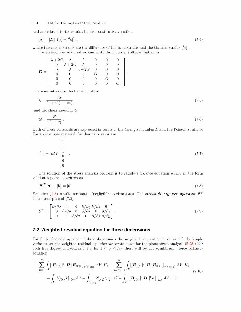
224 FEM for Thermal and Stress Analysis

and are related to the strains by the constitutive equation

[σ] = [D]([ϵ]− [θϵ]

), (7.4)

where the elastic strains are the difference of the total strains and the thermal strains [θϵ].For an isotropic material we can write the material stiffness matrix as

D =

λ+ 2G λ λ 0 0 0λ λ+ 2G λ 0 0 0λ λ λ+ 2G 0 0 00 0 0 G 0 00 0 0 0 G 00 0 0 0 0 G

,

where we introduce the Lame constant

λ =Eν

(1 + ν)(1− 2ν)(7.5)

and the shear modulus G

G =E

2(1 + ν). (7.6)

Both of these constants are expressed in terms of the Young’s modulus E and the Poisson’s ratio ν.For an isotropic material the thermal strains are

[θϵ] = α∆T

111000

. (7.7)

The solution of the stress analysis problem is to satisfy a balance equation which, in the formvalid at a point, is written as

[B]T [σ] +[b]= [0] . (7.8)

Equation (7.8) is valid for statics (negligible accelerations). The stress-divergence operator BT

is the transpose of (7.2)

BT =

∂/∂x 0 0 ∂/∂y ∂/∂z 00 ∂/∂y 0 ∂/∂x 0 ∂/∂z0 0 ∂/∂z 0 ∂/∂x ∂/∂y

. (7.9)

7.2 Weighted residual equation for three dimensions

For finite elements applied in three dimensions the weighted residual equation is a fairly simplevariation on the weighted residual equation we wrote down for the plane-stress analysis (5.23): Foreach free degree of freedom q, i.e. for 1 ≤ q ≤ Nf , there will be one equilibrium (force balance)equation

Nf∑p=1

∫V

[[Bj(q)]

T [D][Bi(p)]]r(q)s(p)

dV Up +

N∑p=Nf+1

∫V

[[Bj(q)]

T [D][Bi(p)]]r(q)s(p)

dV Up

−∫V

Nj(q)[b]r(q) dV −∫St,r(q)

Nj(q)tr(q) dS −∫V

[[Bj(q)]

TD [θϵ]]r(q)

dV = 0.

(7.10)

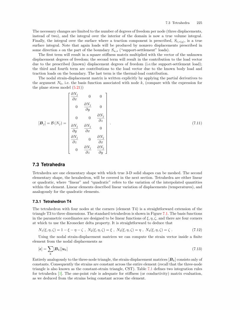
7.3 Tetrahedra 225

The necessary changes are limited to the number of degrees of freedom per node (three displacements,instead of two), and the integral over the interior of the domain is now a true volume integral.Finally, the integral over the surface where a traction component is prescribed, St,r(q), is a truesurface integral. Note that again loads will be produced by nonzero displacements prescribed insome direction s on the part of the boundary Su,s (“support-settlement” loads).

The first term will result in a square stiffness matrix multiplied with the vector of the unknowndisplacement degrees of freedom; the second term will result in the contribution to the load vectordue to the prescribed (known) displacement degrees of freedom (i.e.the support-settlement load);the third and fourth term are contributions to the load vector due to the known body load andtraction loads on the boundary. The last term is the thermal-load contribution.

The nodal strain-displacement matrix is written explicitly by applying the partial derivatives tothe argument Nk, i.e. the basis function associated with node k, (compare with the expression forthe plane stress model (5.21))

[Bj ] = B (Nj) =

∂Nj

∂x0 0

0∂Nj

∂y0

0 0∂Nj

∂z

∂Nj

∂y

∂Nj

∂x0

∂Nj

∂z0

∂Nj

∂x

0∂Nj

∂z

∂Nj

∂y

. (7.11)

7.3 Tetrahedra

Tetrahedra are one elementary shape with which true 3-D solid shapes can be meshed. The secondelementary shape, the hexahedron, will be covered in the next section. Tetrahedra are either linearor quadratic, where “linear” and “quadratic” refers to the variation of the interpolated quantitieswithin the element. Linear elements described linear variation of displacements (temperatures), andanalogously for the quadratic elements.

7.3.1 Tetrahedron T4

The tetrahedron with four nodes at the corners (element T4) is a straightforward extension of thetriangle T3 to three dimensions. The standard tetrahedron is shown in Figure 7.1. The basis functionsin the parametric coordinates are designed to be linear functions of ξ, η, ζ, and there are four cornersat which to use the Kronecker delta property. It is straightforward to deduce that

N1(ξ, η, ζ) = 1− ξ − η − ζ , N2(ξ, η, ζ) = ξ , N3(ξ, η, ζ) = η , N4(ξ, η, ζ) = ζ . (7.12)

Using the nodal strain-displacement matrices we can compute the strain vector inside a finiteelement from the nodal displacements as

[ϵ] =∑k

[Bk][uk] (7.13)

Entirely analogously to the three-node triangle, the strain-displacement matrices [Bk] consists only ofconstants. Consequently the strains are constant across the entire element (recall that the three-nodetriangle is also known as the constant-strain triangle, CST). Table 7.1 defines two integration rulesfor tetrahedra [3]. The one-point rule is adequate for stiffness (or conductivity) matrix evaluation,as we deduced from the strains being constant across the element.

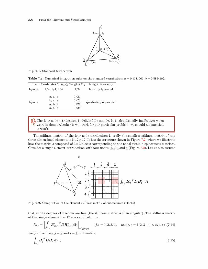
226 FEM for Thermal and Stress Analysis

Fig. 7.1. Standard tetrahedron

Table 7.1. Numerical integration rules on the standard tetrahedron; a = 0.1381966, b = 0.5854102.

Rule Coordinates ξj , ηj , ζj Weights Wj Integrates exactly

1-point 1/4, 1/4, 1/4 1/6 linear polynomial

4-point

a, a, ab, a, aa, b, aa, a, b

1/241/241/241/24

quadratic polynomial

The four-node tetrahedron is delightfully simple. It is also dismally ineffective: whenwe’re in doubt whether it will work for our particular problem, we should assume thatit won’t.

The stiffness matrix of the four-node tetrahedron is really the smallest stiffness matrix of anythree-dimensional element, it is 12×12. It has the structure shown in Figure 7.2, where we illustratehow the matrix is composed of 3×3 blocks corresponding to the nodal strain-displacement matrices.Consider a single element, tetrahedron with four nodes, 1, 2, 3 and 4 (Figure 7.2). Let us also assume

Fig. 7.2. Composition of the element stiffness matrix of submatrices (blocks)

that all the degrees of freedom are free (the stiffness matrix is then singular). The stiffness matrixof this single element has 12 rows and columns.

Kqp =

[∫Ve

Bej(q)

TDBei(s) dV

]r(q)s(p)

, j, i = 1, 2, 3, 4 , and r, s = 1, 2, 3 (i.e. x, y, z) .(7.14)

For j, i fixed, say j = 2 and i = 4, the matrix∫Ve

BejTDBe

i dV , (7.15)

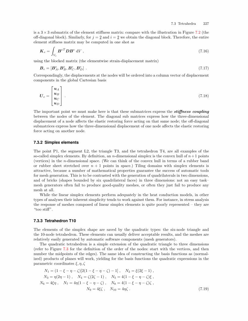
7.3 Tetrahedra 227

is a 3× 3 submatrix of the element stiffness matrix: compare with the illustration in Figure 7.2 (theoff-diagonal block). Similarly, for j = 2 and i = 2 we obtain the diagonal block. Therefore, the entireelement stiffness matrix may be computed in one shot as

Ke =

∫Ve

BeTDBe dV , (7.16)

using the blocked matrix (the elementwise strain-displacement matrix)

Be = [BeA,B

eB ,B

eC ,B

eD] . (7.17)

Correspondingly, the displacements at the nodes will be ordered into a column vector of displacementcomponents in the global Cartesian basis

U e =

uA

uB

uC

uD

. (7.18)

The important point we must make here is that these submatrices express the stiffness couplingbetween the nodes of the element. The diagonal sub matrices express how the three-dimensionaldisplacement of a node affects the elastic restoring force acting on that same node; the off-diagonalsubmatrices express how the three-dimensional displacement of one node affects the elastic restoringforce acting on another node.

7.3.2 Simplex elements

The point P1, the segment L2, the triangle T3, and the tetrahedron T4, are all examples of theso-called simplex elements. By definition, an n-dimensional simplex is the convex hull of n+1 points(vertices) in the n-dimensional space. (We can think of the convex hull in terms of a rubber bandor rubber sheet stretched over n + 1 points in space.) Tiling domains with simplex elements isattractive, because a number of mathematical properties guarantee the success of automatic toolsfor mesh generation. This is to be contrasted with the generation of quadrilaterals in two dimensions,and of bricks (shapes bounded by six quadrilateral faces) in three dimensions: not an easy task–mesh generators often fail to produce good-quality meshes, or often they just fail to produce anymesh at all.

While the linear simplex elements perform adequately in the heat conduction models, in othertypes of analyses their inherent simplicity tends to work against them. For instance, in stress analysisthe response of meshes composed of linear simplex elements is quite poorly represented – they are“too stiff”.

7.3.3 Tetrahedron T10

The elements of the simplex shape are saved by the quadratic types: the six-node triangle andthe 10-node tetrahedron. These elements can usually deliver acceptable results, and the meshes arerelatively easily generated by automatic software components (mesh generators).

The quadratic tetrahedron is a simple extension of the quadratic triangle to three dimensions(refer to Figure 7.3 for the definition of the order of the nodes: start with the vertices, and thennumber the midpoints of the edges). The same idea of constructing the basis functions as (normal-ized) products of planes will work, yielding for the basis functions the quadratic expressions in theparametric coordinates ξ, η, ζ

N1 = (1− ξ − η − ζ)[2(1− ξ − η − ζ)− 1] , N2 = ξ(2ξ − 1) ,

N3 = η(2η − 1) , N4 = ζ(2ζ − 1) , N5 = 4(1− ξ − η − ζ)ξ ,

N6 = 4ξη , N7 = 4η(1− ξ − η − ζ) , N8 = 4(1− ξ − η − ζ)ζ ,

N9 = 4ξζ , N10 = 4ηζ . (7.19)

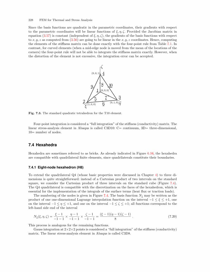
228 FEM for Thermal and Stress Analysis

Since the basis functions are quadratic in the parametric coordinates, their gradients with respectto the parametric coordinates will be linear functions of ξ, η, ζ. Provided the Jacobian matrix inequation (3.57) is constant (independent of ξ, η, ζ), the gradients of the basis functions with respectto x, y, z as computed from (3.56) are going to be linear in the x, y, z coordinates. Hence, computingthe elements of the stiffness matrix can be done exactly with the four-point rule from Table 7.1. Incontrast, for curved elements (when a mid-edge node is moved from the mean of the locations of thecorners) the four-point rule will not be able to integrate the stiffness matrix exactly. However, whenthe distortion of the element is not excessive, the integration error can be accepted.

Fig. 7.3. The standard quadratic tetrahedron for the T10 element.

Four-point integration is considered a “full integration” of the stiffness (conductivity) matrix. Thelinear stress-analysis element in Abaqus is called C3D10: C= continuum, 3D= three-dimensional,10= number of nodes.

7.4 Hexahedra

Hexahedra are sometimes referred to as bricks. As already indicated in Figure 6.16, the hexahedraare compatible with quadrilateral finite elements, since quadrilaterals constitute their boundaries.

7.4.1 Eight-node hexahedron (H8)

To extend the quadrilateral Q4 (whose basic properties were discussed in Chapter 4) to three di-mensions is quite straightforward: instead of a Cartesian product of two intervals on the standardsquare, we consider the Cartesian product of three intervals on the standard cube (Figure 7.4).The Q4 quadrilateral is compatible with the discretization on the faces of the hexahedron, which isessential for the implementation of the integrals of the surface terms (heat flux or traction loads).

The numbering of the nodes is given in Figure 7.4. The basis function N1 may be written as theproduct of one one-dimensional Lagrange interpolation function on the interval −1 ≤ ξ ≤ +1, oneon the interval −1 ≤ η ≤ +1, and one on the interval −1 ≤ ζ ≤ +1; all functions correspond to theleft-hand side end of the interval

N1(ξ, η, ζ) =ξ − 1

−1− 1× η − 1

−1− 1× ζ − 1

−1− 1=

(ξ − 1)(η − 1)(ζ − 1)

8. (7.20)

This process is analogous for the remaining functions.Gauss integration at 2×2×2 points is considered a “full integration” of the stiffness (conductivity)

matrix. The linear stress-analysis element in Abaqus is called C3D8.

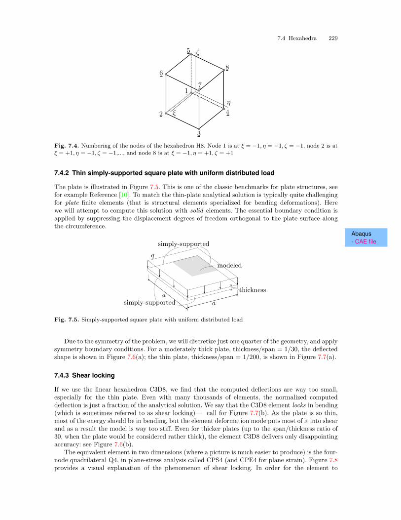
7.4 Hexahedra 229

Fig. 7.4. Numbering of the nodes of the hexahedron H8. Node 1 is at ξ = −1, η = −1, ζ = −1, node 2 is atξ = +1, η = −1, ζ = −1,..., and node 8 is at ξ = −1, η = +1, ζ = +1

7.4.2 Thin simply-supported square plate with uniform distributed load

The plate is illustrated in Figure 7.5. This is one of the classic benchmarks for plate structures, seefor example Reference [10]. To match the thin-plate analytical solution is typically quite challengingfor plate finite elements (that is structural elements specialized for bending deformations). Herewe will attempt to compute this solution with solid elements. The essential boundary condition isapplied by suppressing the displacement degrees of freedom orthogonal to the plate surface alongthe circumference.

Abaqus- CAE file

Fig. 7.5. Simply-supported square plate with uniform distributed load

Due to the symmetry of the problem, we will discretize just one quarter of the geometry, and applysymmetry boundary conditions. For a moderately thick plate, thickness/span = 1/30, the deflectedshape is shown in Figure 7.6(a); the thin plate, thickness/span = 1/200, is shown in Figure 7.7(a).

7.4.3 Shear locking

If we use the linear hexahedron C3D8, we find that the computed deflections are way too small,especially for the thin plate. Even with many thousands of elements, the normalized computeddeflection is just a fraction of the analytical solution. We say that the C3D8 element locks in bending(which is sometimes referred to as shear locking)— call for Figure 7.7(b). As the plate is so thin,most of the energy should be in bending, but the element deformation mode puts most of it into shearand as a result the model is way too stiff. Even for thicker plates (up to the span/thickness ratio of30, when the plate would be considered rather thick), the element C3D8 delivers only disappointingaccuracy: see Figure 7.6(b).

The equivalent element in two dimensions (where a picture is much easier to produce) is the four-node quadrilateral Q4, in plane-stress analysis called CPS4 (and CPE4 for plane strain). Figure 7.8provides a visual explanation of the phenomenon of shear locking. In order for the element to

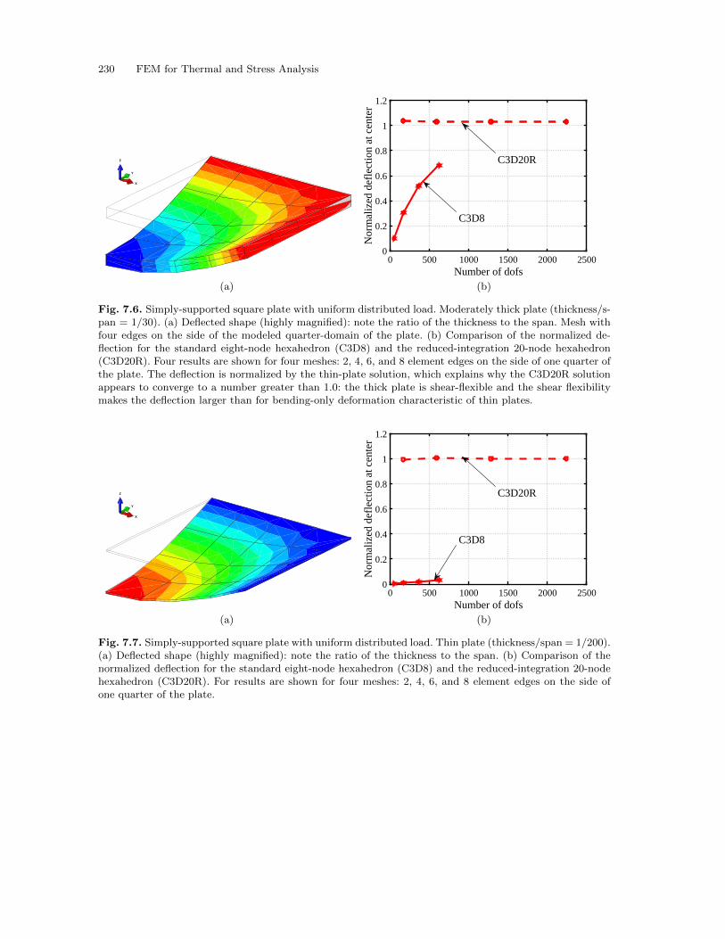
230 FEM for Thermal and Stress Analysis

X

Y

Z

Number of dofs0 500 1000 1500 2000 2500

Nor

mal

ized

def

lect

ion

at c

ente

r

0

0.2

0.4

0.6

0.8

1

1.2

C3D8

C3D20R

(a) (b)

Fig. 7.6. Simply-supported square plate with uniform distributed load. Moderately thick plate (thickness/s-pan = 1/30). (a) Deflected shape (highly magnified): note the ratio of the thickness to the span. Mesh withfour edges on the side of the modeled quarter-domain of the plate. (b) Comparison of the normalized de-flection for the standard eight-node hexahedron (C3D8) and the reduced-integration 20-node hexahedron(C3D20R). Four results are shown for four meshes: 2, 4, 6, and 8 element edges on the side of one quarter ofthe plate. The deflection is normalized by the thin-plate solution, which explains why the C3D20R solutionappears to converge to a number greater than 1.0: the thick plate is shear-flexible and the shear flexibilitymakes the deflection larger than for bending-only deformation characteristic of thin plates.

X

Y

Z

Number of dofs0 500 1000 1500 2000 2500

Nor

mal

ized

def

lect

ion

at c

ente

r

0

0.2

0.4

0.6

0.8

1

1.2

C3D20R

C3D8

(a) (b)

Fig. 7.7. Simply-supported square plate with uniform distributed load. Thin plate (thickness/span = 1/200).(a) Deflected shape (highly magnified): note the ratio of the thickness to the span. (b) Comparison of thenormalized deflection for the standard eight-node hexahedron (C3D8) and the reduced-integration 20-nodehexahedron (C3D20R). For results are shown for four meshes: 2, 4, 6, and 8 element edges on the side ofone quarter of the plate.

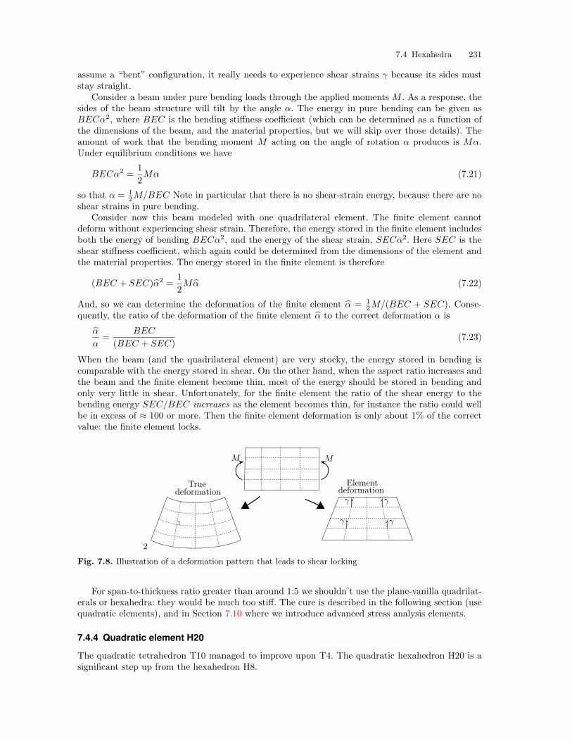
7.4 Hexahedra 231

assume a “bent” configuration, it really needs to experience shear strains γ because its sides muststay straight.

Consider a beam under pure bending loads through the applied moments M . As a response, thesides of the beam structure will tilt by the angle α. The energy in pure bending can be given asBECα2, where BEC is the bending stiffness coefficient (which can be determined as a function ofthe dimensions of the beam, and the material properties, but we will skip over those details). Theamount of work that the bending moment M acting on the angle of rotation α produces is Mα.Under equilibrium conditions we have

BECα2 =1

2Mα (7.21)

so that α = 12M/BEC Note in particular that there is no shear-strain energy, because there are no

shear strains in pure bending.Consider now this beam modeled with one quadrilateral element. The finite element cannot

deform without experiencing shear strain. Therefore, the energy stored in the finite element includesboth the energy of bending BECα2, and the energy of the shear strain, SECα2. Here SEC is theshear stiffness coefficient, which again could be determined from the dimensions of the element andthe material properties. The energy stored in the finite element is therefore

(BEC + SEC)α2 =1

2Mα (7.22)

And, so we can determine the deformation of the finite element α = 12M/(BEC + SEC). Conse-

quently, the ratio of the deformation of the finite element α to the correct deformation α is

α

α=

BEC

(BEC + SEC)(7.23)

When the beam (and the quadrilateral element) are very stocky, the energy stored in bending iscomparable with the energy stored in shear. On the other hand, when the aspect ratio increases andthe beam and the finite element become thin, most of the energy should be stored in bending andonly very little in shear. Unfortunately, for the finite element the ratio of the shear energy to thebending energy SEC/BEC increases as the element becomes thin, for instance the ratio could wellbe in excess of ≈ 100 or more. Then the finite element deformation is only about 1% of the correctvalue: the finite element locks.

2

Fig. 7.8. Illustration of a deformation pattern that leads to shear locking

For span-to-thickness ratio greater than around 1:5 we shouldn’t use the plane-vanilla quadrilat-erals or hexahedra: they would be much too stiff. The cure is described in the following section (usequadratic elements), and in Section 7.10 where we introduce advanced stress analysis elements.

7.4.4 Quadratic element H20

The quadratic tetrahedron T10 managed to improve upon T4. The quadratic hexahedron H20 is asignificant step up from the hexahedron H8.

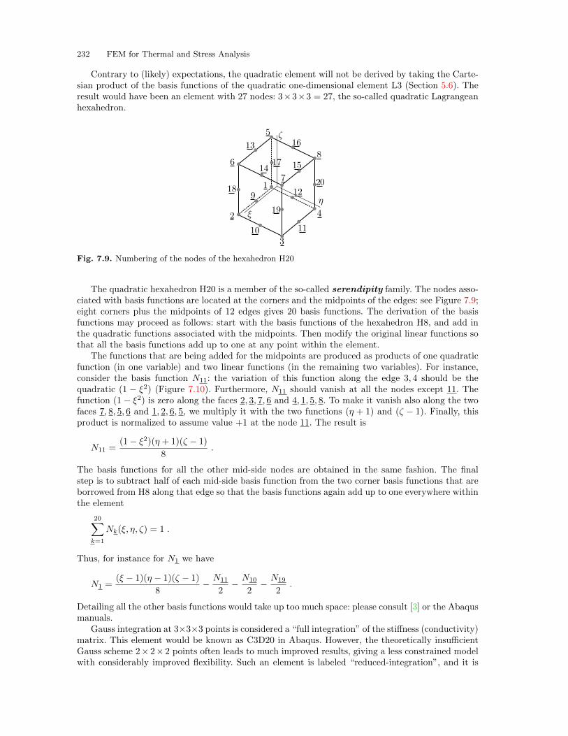
232 FEM for Thermal and Stress Analysis

Contrary to (likely) expectations, the quadratic element will not be derived by taking the Carte-sian product of the basis functions of the quadratic one-dimensional element L3 (Section 5.6). Theresult would have been an element with 27 nodes: 3×3×3 = 27, the so-called quadratic Lagrangeanhexahedron.

Fig. 7.9. Numbering of the nodes of the hexahedron H20

The quadratic hexahedron H20 is a member of the so-called serendipity family. The nodes asso-ciated with basis functions are located at the corners and the midpoints of the edges: see Figure 7.9;eight corners plus the midpoints of 12 edges gives 20 basis functions. The derivation of the basisfunctions may proceed as follows: start with the basis functions of the hexahedron H8, and add inthe quadratic functions associated with the midpoints. Then modify the original linear functions sothat all the basis functions add up to one at any point within the element.

The functions that are being added for the midpoints are produced as products of one quadraticfunction (in one variable) and two linear functions (in the remaining two variables). For instance,consider the basis function N11: the variation of this function along the edge 3, 4 should be thequadratic (1 − ξ2) (Figure 7.10). Furthermore, N11 should vanish at all the nodes except 11. Thefunction (1− ξ2) is zero along the faces 2, 3, 7, 6 and 4, 1, 5, 8. To make it vanish also along the twofaces 7, 8, 5, 6 and 1, 2, 6, 5, we multiply it with the two functions (η + 1) and (ζ − 1). Finally, thisproduct is normalized to assume value +1 at the node 11. The result is

N11 =(1− ξ2)(η + 1)(ζ − 1)

8.

The basis functions for all the other mid-side nodes are obtained in the same fashion. The finalstep is to subtract half of each mid-side basis function from the two corner basis functions that areborrowed from H8 along that edge so that the basis functions again add up to one everywhere withinthe element

20∑k=1

Nk(ξ, η, ζ) = 1 .

Thus, for instance for N1 we have

N1 =(ξ − 1)(η − 1)(ζ − 1)

8− N11

2− N10

2− N19

2.

Detailing all the other basis functions would take up too much space: please consult [3] or the Abaqusmanuals.

Gauss integration at 3×3×3 points is considered a “full integration” of the stiffness (conductivity)matrix. This element would be known as C3D20 in Abaqus. However, the theoretically insufficientGauss scheme 2× 2× 2 points often leads to much improved results, giving a less constrained modelwith considerably improved flexibility. Such an element is labeled “reduced-integration”, and it is

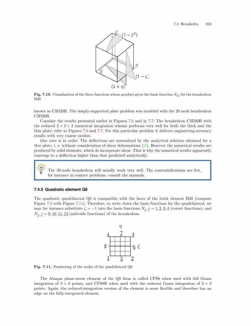
7.4 Hexahedra 233

Fig. 7.10. Visualization of the three functions whose product gives the basis function N11 for the hexahedronH20

known as C3D20R. The simply-supported plate problem was modeled with the 20 node hexahedronC3D20R.

Consider the results presented earlier in Figures 7.6 and in 7.7: The hexahedron C3D20R withthe reduced 2 × 2 × 2 numerical integration scheme performs very well for both the thick and thethin plate: refer to Figures 7.6 and 7.7. For this particular problem it delivers engineering-accuracyresults with very coarse meshes.

One note is in order: The deflections are normalized by the analytical solution obtained for athin plate, i. e. without consideration of shear deformations [10]. However the numerical results areproduced by solid elements, which do incorporate shear. That is why the numerical results apparentlyconverge to a deflection higher than that predicted analytically.

The 20-node hexahedron will usually work very well. The contraindications are few,for instance in contact problems: consult the manuals.

7.4.5 Quadratic element Q8

The quadratic quadrilateral Q8 is compatible with the faces of the brick element H20 (compareFigure 7.9 with Figure 7.11). Therefore, to write down the basis functions for the quadrilateral, wemay for instance substitute ζ = −1 into the basis functions Nj , j = 1, 2, 3, 4 (corner functions), and

Nj , j = 9, 10, 11, 12 (mid-side functions) of the hexahedron.

Fig. 7.11. Numbering of the nodes of the quadrilateral Q8

The Abaqus plane-stress element of the Q8 form is called CPS8 when used with full Gaussintegration of 3 × 3 points, and CPS8R when used with the reduced Gauss integration of 2 × 2points. Again, the reduced-integration version of the element is more flexible and therefore has anedge on the fully-integrated element.

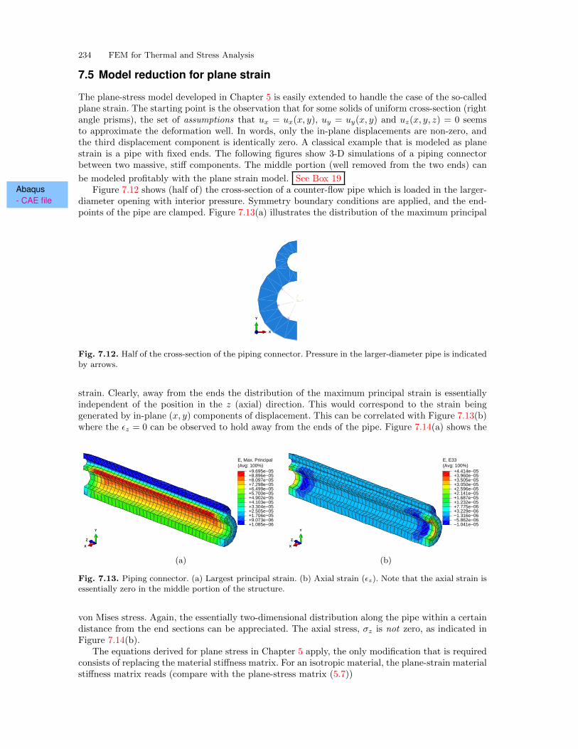
234 FEM for Thermal and Stress Analysis

7.5 Model reduction for plane strain

The plane-stress model developed in Chapter 5 is easily extended to handle the case of the so-calledplane strain. The starting point is the observation that for some solids of uniform cross-section (rightangle prisms), the set of assumptions that ux = ux(x, y), uy = uy(x, y) and uz(x, y, z) = 0 seemsto approximate the deformation well. In words, only the in-plane displacements are non-zero, andthe third displacement component is identically zero. A classical example that is modeled as planestrain is a pipe with fixed ends. The following figures show 3-D simulations of a piping connectorbetween two massive, stiff components. The middle portion (well removed from the two ends) can

be modeled profitably with the plane strain model. See Box 19Abaqus- CAE file

Figure 7.12 shows (half of) the cross-section of a counter-flow pipe which is loaded in the larger-diameter opening with interior pressure. Symmetry boundary conditions are applied, and the end-points of the pipe are clamped. Figure 7.13(a) illustrates the distribution of the maximum principal

Z

Y

X

X

Y

Z

Fig. 7.12. Half of the cross-section of the piping connector. Pressure in the larger-diameter pipe is indicatedby arrows.

strain. Clearly, away from the ends the distribution of the maximum principal strain is essentiallyindependent of the position in the z (axial) direction. This would correspond to the strain beinggenerated by in-plane (x, y) components of displacement. This can be correlated with Figure 7.13(b)where the ϵz = 0 can be observed to hold away from the ends of the pipe. Figure 7.14(a) shows the

(Avg: 100%)E, Max. Principal

+1.085e−06+9.073e−06+1.706e−05+2.505e−05+3.304e−05+4.103e−05+4.902e−05+5.700e−05+6.499e−05+7.298e−05+8.097e−05+8.896e−05+9.695e−05

X

Y

Z

(Avg: 100%)E, E33

−1.041e−05−5.862e−06−1.316e−06+3.229e−06+7.775e−06+1.232e−05+1.687e−05+2.141e−05+2.596e−05+3.050e−05+3.505e−05+3.960e−05+4.414e−05

X

Y

Z

(a) (b)

Fig. 7.13. Piping connector. (a) Largest principal strain. (b) Axial strain (ϵz). Note that the axial strain isessentially zero in the middle portion of the structure.

von Mises stress. Again, the essentially two-dimensional distribution along the pipe within a certaindistance from the end sections can be appreciated. The axial stress, σz is not zero, as indicated inFigure 7.14(b).

The equations derived for plane stress in Chapter 5 apply, the only modification that is requiredconsists of replacing the material stiffness matrix. For an isotropic material, the plane-strain materialstiffness matrix reads (compare with the plane-stress matrix (5.7))

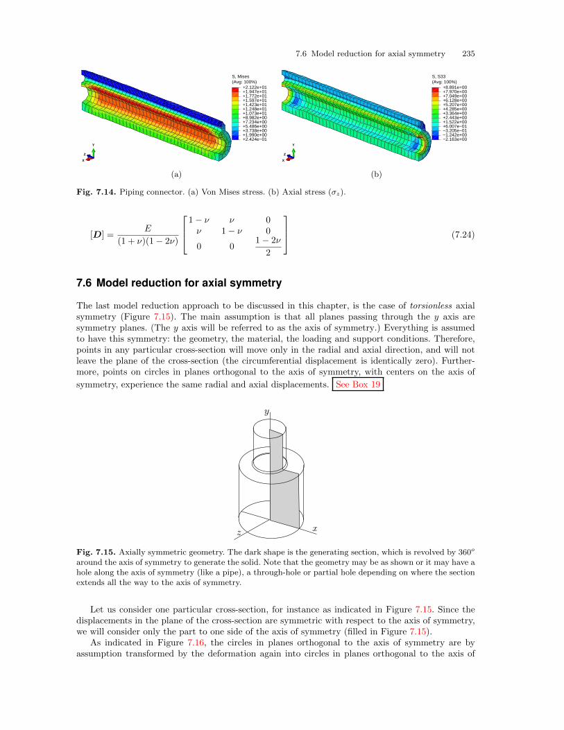
7.6 Model reduction for axial symmetry 235

(Avg: 100%)S, Mises

+2.424e−01+1.990e+00+3.738e+00+5.486e+00+7.234e+00+8.982e+00+1.073e+01+1.248e+01+1.423e+01+1.597e+01+1.772e+01+1.947e+01+2.122e+01

X

Y

Z

(Avg: 100%)S, S33

−2.163e+00−1.242e+00−3.205e−01+6.007e−01+1.522e+00+2.443e+00+3.364e+00+4.285e+00+5.207e+00+6.128e+00+7.049e+00+7.970e+00+8.891e+00

X

Y

Z

(a) (b)

Fig. 7.14. Piping connector. (a) Von Mises stress. (b) Axial stress (σz).

[D] =E

(1 + ν)(1− 2ν)

1− ν ν 0ν 1− ν 0

0 01− 2ν

2

(7.24)

7.6 Model reduction for axial symmetry

The last model reduction approach to be discussed in this chapter, is the case of torsionless axialsymmetry (Figure 7.15). The main assumption is that all planes passing through the y axis aresymmetry planes. (The y axis will be referred to as the axis of symmetry.) Everything is assumedto have this symmetry: the geometry, the material, the loading and support conditions. Therefore,points in any particular cross-section will move only in the radial and axial direction, and will notleave the plane of the cross-section (the circumferential displacement is identically zero). Further-more, points on circles in planes orthogonal to the axis of symmetry, with centers on the axis of

symmetry, experience the same radial and axial displacements. See Box 19

Fig. 7.15. Axially symmetric geometry. The dark shape is the generating section, which is revolved by 360o

around the axis of symmetry to generate the solid. Note that the geometry may be as shown or it may have ahole along the axis of symmetry (like a pipe), a through-hole or partial hole depending on where the sectionextends all the way to the axis of symmetry.

Let us consider one particular cross-section, for instance as indicated in Figure 7.15. Since thedisplacements in the plane of the cross-section are symmetric with respect to the axis of symmetry,we will consider only the part to one side of the axis of symmetry (filled in Figure 7.15).

As indicated in Figure 7.16, the circles in planes orthogonal to the axis of symmetry are byassumption transformed by the deformation again into circles in planes orthogonal to the axis of

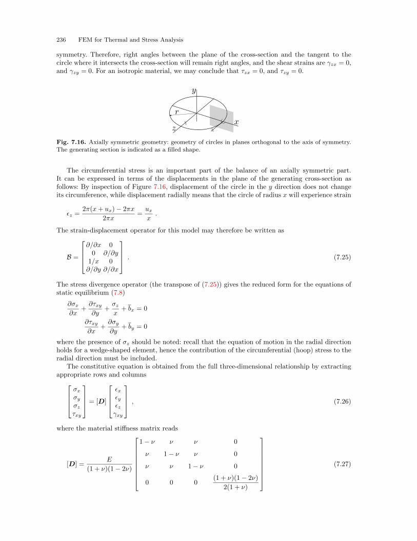
236 FEM for Thermal and Stress Analysis

symmetry. Therefore, right angles between the plane of the cross-section and the tangent to thecircle where it intersects the cross-section will remain right angles, and the shear strains are γzx = 0,and γzy = 0. For an isotropic material, we may conclude that τzx = 0, and τzy = 0.

Fig. 7.16. Axially symmetric geometry: geometry of circles in planes orthogonal to the axis of symmetry.The generating section is indicated as a filled shape.

The circumferential stress is an important part of the balance of an axially symmetric part.It can be expressed in terms of the displacements in the plane of the generating cross-section asfollows: By inspection of Figure 7.16, displacement of the circle in the y direction does not changeits circumference, while displacement radially means that the circle of radius x will experience strain

ϵz =2π(x+ ux)− 2πx

2πx=uxx.

The strain-displacement operator for this model may therefore be written as

B =

∂/∂x 00 ∂/∂y

1/x 0∂/∂y ∂/∂x

. (7.25)

The stress divergence operator (the transpose of (7.25)) gives the reduced form for the equations ofstatic equilibrium (7.8)

∂σx∂x

+∂τxy∂y

+σzx

+ bx = 0

∂τxy∂x

+∂σy∂y

+ by = 0

where the presence of σz should be noted: recall that the equation of motion in the radial directionholds for a wedge-shaped element, hence the contribution of the circumferential (hoop) stress to theradial direction must be included.

The constitutive equation is obtained from the full three-dimensional relationship by extractingappropriate rows and columns

σxσyσzτxy

= [D]

ϵxϵyϵzγxy

, (7.26)

where the material stiffness matrix reads

[D] =E

(1 + ν)(1− 2ν)

1− ν ν ν 0

ν 1− ν ν 0

ν ν 1− ν 0

0 0 0(1 + ν)(1− 2ν)

2(1 + ν)

(7.27)

7.6 Model reduction for axial symmetry 237

When a single part is not supported in any way, in the axially symmetric model it has one rigidbody mode, translation in the axial direction. Consider the piece of a steel cylindrical shaft with a

Abaqus- CAE file

filleted shoulder in Figure 7.17. The part is under self-equilibrated tensile loads, 20 ksi applied tothe top circular cross-section of radius 5/6 in, and an appropriately reduced distributed loading of(5/6)2 × 20 ksi is applied on the bottom circular cross-section of radius 1 in.

0.83

1.

1.

R0.15

H

H

0.83

1.

1.

R0.15

H

H

X

Y

Z

Z

T R

X

Y

Z

(a) (b)

Fig. 7.17. Shaft with cross-section transition. (a) Sketch. Units: inches. Note that the top radius is 5/6 in: thedimension shows rounding. (b) Loading by tension tractions, the loading is assumed to be in self-equilibrium.

When the solution is obtained without applying any displacement boundary conditions, thedisplacement in the direction along the axis of symmetry is huge, and depends on the mesh used.For instance, with the mesh in the linked model database, the displacement is on the order of 17,000inches. The reason is the (nearly) singular stiffness matrix and the following effect of numericalround off: the simulation is actually run off of a text file that describes the model, the “.inp” filethat the Job Manager writes out. Thus we find that distributed loading defined by these lines:

** Name: tension bottom Type: Surface traction

*Dsloadbottom, TRVEC, 13888.9, 0., -1., 0.

** Name: tension top Type: Surface traction

*Dsloadtop, TRVEC, 20000., 0., 1., 0.

where TRVEC, 13888.9 refers to the magnitude of the traction applied on the bottom face andTRVEC, 20000. refers to the magnitude of the traction applied on the top face. Using these numbers,the traction at the bottom is actually only approximately able to balance the traction applied atthe top. The total force applied at the top is (in lbf)

math.pi*(5./6.)**2*20000

i.e. 43633.231, which is to be compared to the total force applied on the bottom face

math.pi*(1.0)**2*13888.9

i.e. 43633.266. We can see that the two forces only agree to six decimal places, so a force on theorder of 10−2 lbf is the imbalance. However tiny this is compared to the applied forces, given thenear singularity of the stiffness matrix it is still able to produce a huge displacement.

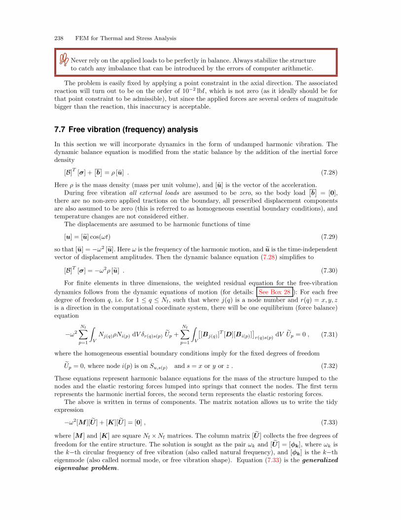
238 FEM for Thermal and Stress Analysis

Never rely on the applied loads to be perfectly in balance. Always stabilize the structureto catch any imbalance that can be introduced by the errors of computer arithmetic.

The problem is easily fixed by applying a point constraint in the axial direction. The associatedreaction will turn out to be on the order of 10−2 lbf, which is not zero (as it ideally should be forthat point constraint to be admissible), but since the applied forces are several orders of magnitudebigger than the reaction, this inaccuracy is acceptable.

7.7 Free vibration (frequency) analysis

In this section we will incorporate dynamics in the form of undamped harmonic vibration. Thedynamic balance equation is modified from the static balance by the addition of the inertial forcedensity

[B]T [σ] +[b]= ρ [u] . (7.28)

Here ρ is the mass density (mass per unit volume), and [u] is the vector of the acceleration.During free vibration all external loads are assumed to be zero, so the body load

[b]= [0],

there are no non-zero applied tractions on the boundary, all prescribed displacement componentsare also assumed to be zero (this is referred to as homogeneous essential boundary conditions), andtemperature changes are not considered either.

The displacements are assumed to be harmonic functions of time

[u] = [u] cos(ωt) (7.29)

so that [u] = −ω2 [u]. Here ω is the frequency of the harmonic motion, and u is the time-independentvector of displacement amplitudes. Then the dynamic balance equation (7.28) simplifies to

[B]T [σ] = −ω2ρ [u] . (7.30)

For finite elements in three dimensions, the weighted residual equation for the free-vibration

dynamics follows from the dynamic equations of motion (for details: See Box 28 ): For each freedegree of freedom q, i.e. for 1 ≤ q ≤ Nf , such that where j(q) is a node number and r(q) = x, y, zis a direction in the computational coordinate system, there will be one equilibrium (force balance)equation

−ω2Nf∑p=1

∫V

Nj(q)ρNi(p) dV δr(q)s(p) Up +

Nf∑p=1

∫V

[[Bj(q)]

T [D][Bi(p)]]r(q)s(p)

dV Up = 0 , (7.31)

where the homogeneous essential boundary conditions imply for the fixed degrees of freedom

Up = 0, where node i(p) is on Su,s(p) and s = x or y or z . (7.32)

These equations represent harmonic balance equations for the mass of the structure lumped to thenodes and the elastic restoring forces lumped into springs that connect the nodes. The first termrepresents the harmonic inertial forces, the second term represents the elastic restoring forces.

The above is written in terms of components. The matrix notation allows us to write the tidyexpression

−ω2[M ][U ] + [K][U ] = [0] , (7.33)

where [M ] and [K] are square Nf ×Nf matrices. The column matrix [U ] collects the free degrees of

freedom for the entire structure. The solution is sought as the pair ωk and [U ] = [ϕk], where ωk isthe k−th circular frequency of free vibration (also called natural frequency), and [ϕk] is the k−theigenmode (also called normal mode, or free vibration shape). Equation (7.33) is the generalizedeigenvalue problem .

7.7 Free vibration (frequency) analysis 239

7.7.1 Modal analysis of a circular clamped plate

As our first example, we consider the vibration of a moderately thick circular plate as shown in Fig-ure 7.18. The cylindrical surface is fully clamped (all displacements zero). The material is isotropic.The analytical solution has been analytically worked out in dependence on the number of “nodes”(locations of approximately zero displacement) radially and circumferentially [2]. Therefore, this isa very good example with which to test a finite element solver (a so-called benchmark).

Abaqus- CAE file

Fig. 7.18. Clamped circular plate (drum).

Step: modal analysisMode 1: Value = 10803. Freq = 16.542 (cycles/time)Primary Var: U, U3

X Y

Z

Step: modal analysisMode 2: Value = 49410. Freq = 35.377 (cycles/time)Primary Var: U, U3

X Y

Z

Step: modal analysisMode 3: Value = 51714. Freq = 36.193 (cycles/time)Primary Var: U, U3

X Y

Z

Step: modal analysisMode 4: Value = 1.46266E+05 Freq = 60.868 (cycles/time)Primary Var: U, U3

X Y

Z

Fig. 7.19. Mode shapes of thick clamped plate. The analytical solution for the natural frequencies yieldsfor these modes ω1 = 15.7511Hz, ω2 = ω3 = 32.7659Hz, ω4 = 53.757Hz

The finite element solution adopts the quadratic tetrahedron C3D10 (the quadratic T10). Thenatural frequencies obtained for a relatively coarse mesh are illustrated in Figure 7.19. Evidently,the element T10 produces estimates of the frequencies which are of good engineering accuracy.

The graph of Figure 7.20 may serve as a crude guide to the relative accuracy of the two tetrahedralelements, the linear T4 and the quadratic T10. The four natural frequencies are computed for finerand finer meshes (the analytical results are indicated with horizontal red lines). The quadraticelement solutions approach the reference values quickly. The linear tetrahedral element solutionsapproach the reference values very slowly. (Slow convergence is bad: a large number of elements, andhence large expense, are needed for acceptable accuracy.)

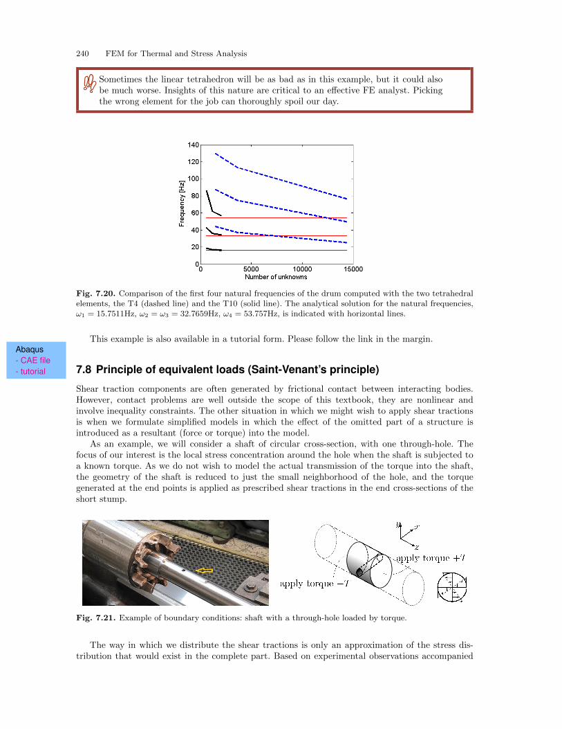
240 FEM for Thermal and Stress Analysis

Sometimes the linear tetrahedron will be as bad as in this example, but it could alsobe much worse. Insights of this nature are critical to an effective FE analyst. Pickingthe wrong element for the job can thoroughly spoil our day.

Fig. 7.20. Comparison of the first four natural frequencies of the drum computed with the two tetrahedralelements, the T4 (dashed line) and the T10 (solid line). The analytical solution for the natural frequencies,ω1 = 15.7511Hz, ω2 = ω3 = 32.7659Hz, ω4 = 53.757Hz, is indicated with horizontal lines.

This example is also available in a tutorial form. Please follow the link in the margin.Abaqus- CAE file- tutorial 7.8 Principle of equivalent loads (Saint-Venant’s principle)

Shear traction components are often generated by frictional contact between interacting bodies.However, contact problems are well outside the scope of this textbook, they are nonlinear andinvolve inequality constraints. The other situation in which we might wish to apply shear tractionsis when we formulate simplified models in which the effect of the omitted part of a structure isintroduced as a resultant (force or torque) into the model.

As an example, we will consider a shaft of circular cross-section, with one through-hole. Thefocus of our interest is the local stress concentration around the hole when the shaft is subjected toa known torque. As we do not wish to model the actual transmission of the torque into the shaft,the geometry of the shaft is reduced to just the small neighborhood of the hole, and the torquegenerated at the end points is applied as prescribed shear tractions in the end cross-sections of theshort stump.

Fig. 7.21. Example of boundary conditions: shaft with a through-hole loaded by torque.

The way in which we distribute the shear tractions is only an approximation of the stress dis-tribution that would exist in the complete part. Based on experimental observations accompanied

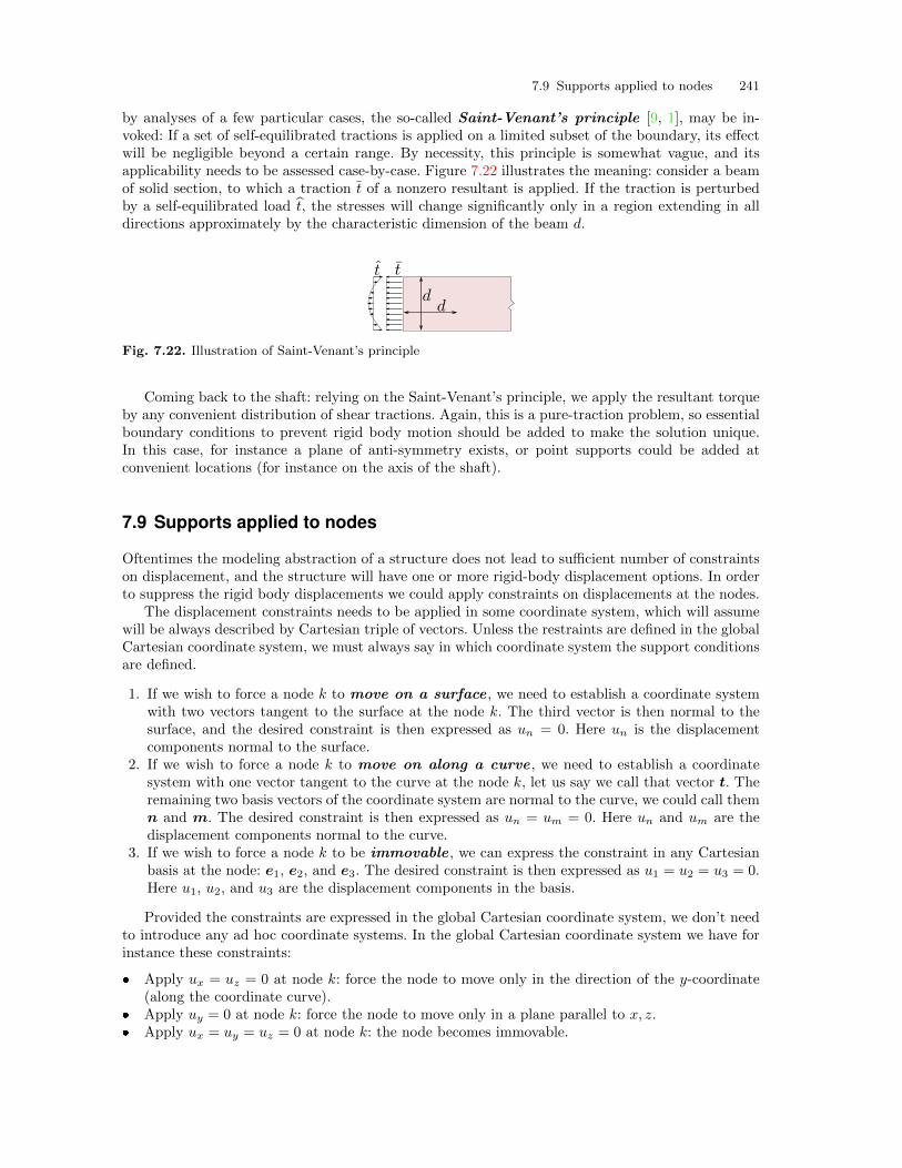
7.9 Supports applied to nodes 241

by analyses of a few particular cases, the so-called Saint-Venant’s principle [9, 1], may be in-voked: If a set of self-equilibrated tractions is applied on a limited subset of the boundary, its effectwill be negligible beyond a certain range. By necessity, this principle is somewhat vague, and itsapplicability needs to be assessed case-by-case. Figure 7.22 illustrates the meaning: consider a beamof solid section, to which a traction t of a nonzero resultant is applied. If the traction is perturbedby a self-equilibrated load t, the stresses will change significantly only in a region extending in alldirections approximately by the characteristic dimension of the beam d.

Fig. 7.22. Illustration of Saint-Venant’s principle

Coming back to the shaft: relying on the Saint-Venant’s principle, we apply the resultant torqueby any convenient distribution of shear tractions. Again, this is a pure-traction problem, so essentialboundary conditions to prevent rigid body motion should be added to make the solution unique.In this case, for instance a plane of anti-symmetry exists, or point supports could be added atconvenient locations (for instance on the axis of the shaft).

7.9 Supports applied to nodes

Oftentimes the modeling abstraction of a structure does not lead to sufficient number of constraintson displacement, and the structure will have one or more rigid-body displacement options. In orderto suppress the rigid body displacements we could apply constraints on displacements at the nodes.

The displacement constraints needs to be applied in some coordinate system, which will assumewill be always described by Cartesian triple of vectors. Unless the restraints are defined in the globalCartesian coordinate system, we must always say in which coordinate system the support conditionsare defined.

1. If we wish to force a node k to move on a surface , we need to establish a coordinate systemwith two vectors tangent to the surface at the node k. The third vector is then normal to thesurface, and the desired constraint is then expressed as un = 0. Here un is the displacementcomponents normal to the surface.

2. If we wish to force a node k to move on along a curve , we need to establish a coordinatesystem with one vector tangent to the curve at the node k, let us say we call that vector t. Theremaining two basis vectors of the coordinate system are normal to the curve, we could call themn and m. The desired constraint is then expressed as un = um = 0. Here un and um are thedisplacement components normal to the curve.

3. If we wish to force a node k to be immovable , we can express the constraint in any Cartesianbasis at the node: e1, e2, and e3. The desired constraint is then expressed as u1 = u2 = u3 = 0.Here u1, u2, and u3 are the displacement components in the basis.

Provided the constraints are expressed in the global Cartesian coordinate system, we don’t needto introduce any ad hoc coordinate systems. In the global Cartesian coordinate system we have forinstance these constraints:

� Apply ux = uz = 0 at node k: force the node to move only in the direction of the y-coordinate(along the coordinate curve).

� Apply uy = 0 at node k: force the node to move only in a plane parallel to x, z.� Apply ux = uy = uz = 0 at node k: the node becomes immovable.

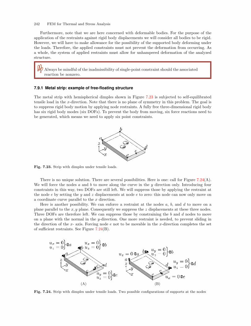
242 FEM for Thermal and Stress Analysis

Furthermore, note that we are here concerned with deformable bodies. For the purpose of theapplication of the restraints against rigid body displacements we will consider all bodies to be rigid.However, we will have to make allowance for the possibility of the supported body deforming underthe loads. Therefore, the applied constraints must not prevent the deformation from occurring. Asa whole, the system of applied restraints must allow for unhampered deformation of the analyzedstructure.

Always be mindful of the inadmissibility of single-point constraint should the associatedreaction be nonzero.

7.9.1 Metal strip: example of free-floating structure

The metal strip with hemispherical dimples shown in Figure 7.23 is subjected to self-equilibratedtensile load in the x-direction. Note that there is no plane of symmetry in this problem. The goal isto suppress rigid body motion by applying node restraints. A fully free three-dimensional rigid bodyhas six rigid body modes (six DOFs). To prevent the body from moving, six force reactions need tobe generated, which means we need to apply six point constraints.

Fig. 7.23. Strip with dimples under tensile loads.

There is no unique solution. There are several possibilities. Here is one: call for Figure 7.24(A).We will force the nodes a and b to move along the curve in the y direction only. Introducing fourconstraints in this way, two DOFs are still left. We will suppress those by applying the restraint atthe node e by setting the y and z displacements at node e to zero: this node can now only move ona coordinate curve parallel to the x direction.

Here is another possibility. We can enforce a restraint at the nodes a, b, and d to move on aplane parallel to the x, y plane. Consequently we suppress the z displacements at these three nodes.Three DOFs are therefore left. We can suppress those by constraining the b and d nodes to moveon a plane with the normal in the y-direction. One more restraint is needed, to prevent sliding inthe direction of the x- axis. Forcing node e not to be movable in the x-direction completes the setof sufficient restraints. See Figure 7.24(B).

(A) (B)

Fig. 7.24. Strip with dimples under tensile loads. Two possible configurations of supports at the nodes

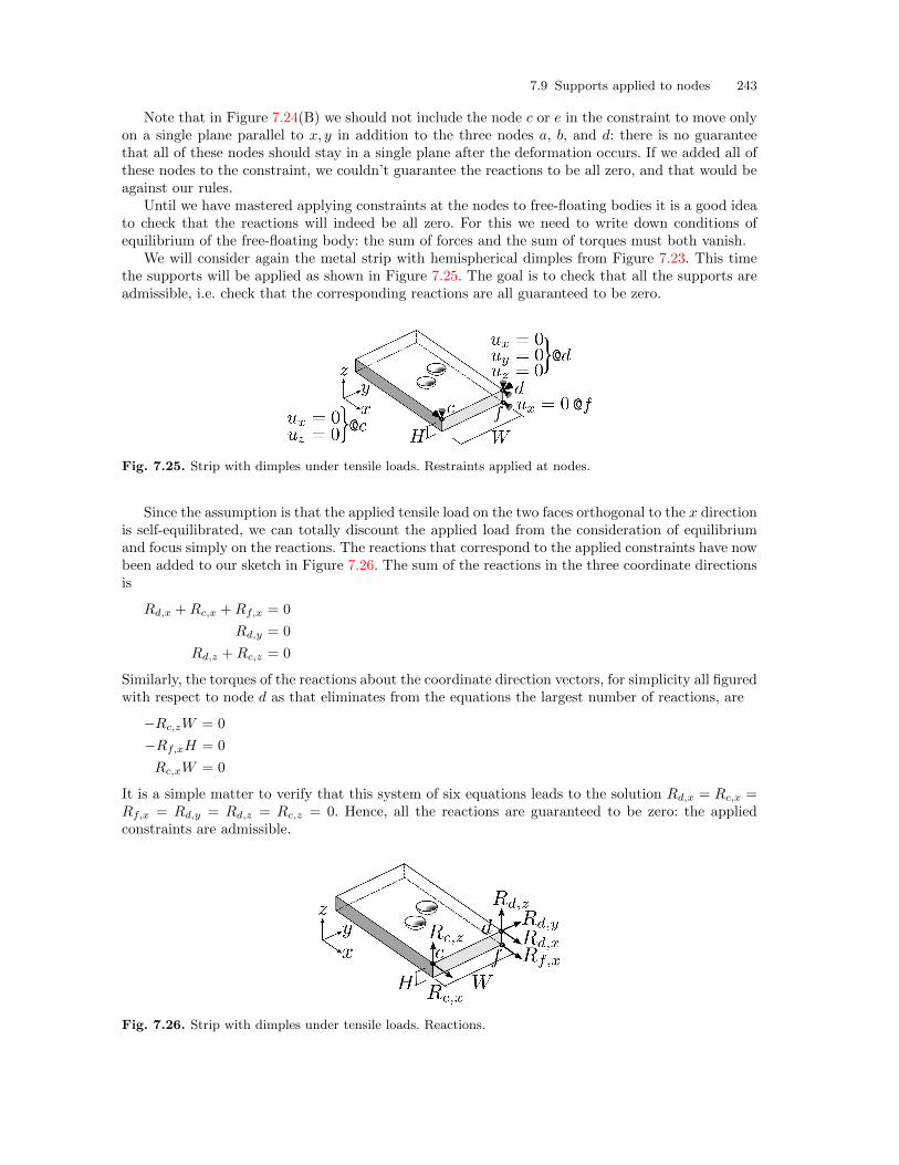
7.9 Supports applied to nodes 243

Note that in Figure 7.24(B) we should not include the node c or e in the constraint to move onlyon a single plane parallel to x, y in addition to the three nodes a, b, and d: there is no guaranteethat all of these nodes should stay in a single plane after the deformation occurs. If we added all ofthese nodes to the constraint, we couldn’t guarantee the reactions to be all zero, and that would beagainst our rules.

Until we have mastered applying constraints at the nodes to free-floating bodies it is a good ideato check that the reactions will indeed be all zero. For this we need to write down conditions ofequilibrium of the free-floating body: the sum of forces and the sum of torques must both vanish.

We will consider again the metal strip with hemispherical dimples from Figure 7.23. This timethe supports will be applied as shown in Figure 7.25. The goal is to check that all the supports areadmissible, i.e. check that the corresponding reactions are all guaranteed to be zero.

Fig. 7.25. Strip with dimples under tensile loads. Restraints applied at nodes.

Since the assumption is that the applied tensile load on the two faces orthogonal to the x directionis self-equilibrated, we can totally discount the applied load from the consideration of equilibriumand focus simply on the reactions. The reactions that correspond to the applied constraints have nowbeen added to our sketch in Figure 7.26. The sum of the reactions in the three coordinate directionsis

Rd,x +Rc,x +Rf,x = 0

Rd,y = 0

Rd,z +Rc,z = 0

Similarly, the torques of the reactions about the coordinate direction vectors, for simplicity all figuredwith respect to node d as that eliminates from the equations the largest number of reactions, are

−Rc,zW = 0

−Rf,xH = 0

Rc,xW = 0

It is a simple matter to verify that this system of six equations leads to the solution Rd,x = Rc,x =Rf,x = Rd,y = Rd,z = Rc,z = 0. Hence, all the reactions are guaranteed to be zero: the appliedconstraints are admissible.

Fig. 7.26. Strip with dimples under tensile loads. Reactions.

244 FEM for Thermal and Stress Analysis

Valuable insight can be gained by writing out the above relationships in terms of the matrixequation:

1 0 0 1 0 10 1 0 0 0 00 0 1 0 1 00 0 0 0 −W 00 0 0 0 0 −H0 0 0 W 0 0

Rd,x

Rd,y

Rd,z

Rc,x

Rc,z

Rf,x

=

000000

(7.34)

The coefficient matrix on the left is clearly non-singular, it is easy to see how we could get thismatrix in upper-triangular form with non-zero numbers on the diagonal by swapping rows six andfive and five and four, and therefore the only solution for a zero right-hand side is the homogeneousone (all unknowns zero). If the coefficient matrix was singular, the solution could consist of somenon-zero reactions, and we would have to conclude that the support conditions were inadmissible.

Furthermore, if the coefficient matrix was non-square (rectangular), it might be possible for thesolution of the equilibrium equations to include some nonzero reactions. For instance, let us saythere are more reactions then there are equations (the matrix is wider than it is tall). Then theequations are insufficient to determine the solution uniquely, and the support conditions may beinadmissible since some of the reactions may be non-zero. On the other hand, if there are fewerreactions than there are equations of equilibrium, the matrix is singular (there are more rows thanthere are columns), and we cannot guarantee the stability of the supported body: we need to addan appropriate number of additional supports.

7.10 Advanced three-dimensional elements

In professional finite element analysis work one straightaway perceives the need for using toolswell-suited to the purpose. It is difficult to be efficient when the tools are flawed. Consideringstress analysis of three-dimensional solids with hexahedral elements, the flaws of plain-vanilla finiteelements are inescapable: the isoparametric hexahedron is too stiff in bending, much too susceptibleto deterioration of performance in distorted configurations, especially when used with high aspectratio (such as for plates or shells), and finally, using isoparametric hexahedra for analyses with littlecompressibility, such as for elastomeric structures or when plasticity of metals is of concern, is afrustrating exercise as the element “locks” (there is much too little of the correct deformation).

To design a hexahedral element capable of good performance under all these requirements is not atrivial proposition. Abaqus implements at least two decent candidates, the element with incompatiblemodes and the mean-strain element. The standard isoparametric element is too stiff because it reactswith too much resistance to some strains. These two approaches attempt to improve the responseby either

� enhancing the representation of the strains so that the strains are correct, or� making the troublesome strains invisible to the element.

In the first approach, additional possible deformation patterns are added to the element as internaldegrees of freedom: If we make it possible for the element to represent bending deformation byincorporating the possibility of curving, it will not need to produce shear strains to deform. However,this will be in addition to the usual straight-edge mode of deforming. Since each element now hasits own way of curving that is not shared with its neighbors, the resulting displacement pattern inthe mesh is incompatible (the elements don’t fit together perfectly after deformation). The elementin Abaqus is called C3D8I, where the “I” stands for incompatible.

In the second approach, instead of the 2 × 2 × 2 Gauss quadrature, which is the logical choicefor the standard element, an alternative, reduced, integration scheme is used. For instance, if onlya single integration point was used, the element would be blind to its distortion in the form of abending pattern (see Figure 7.8). Unavoidably, not seeing this distortion means that “too much

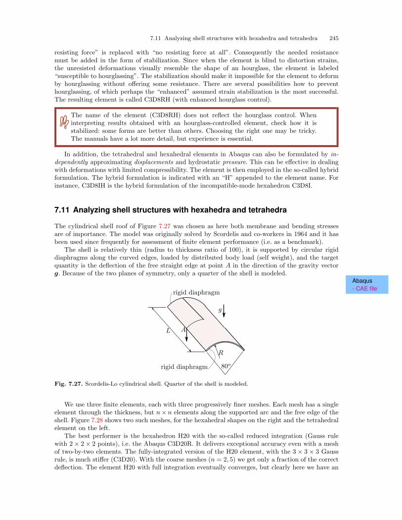
7.11 Analyzing shell structures with hexahedra and tetrahedra 245

resisting force” is replaced with “no resisting force at all”. Consequently the needed resistancemust be added in the form of stabilization. Since when the element is blind to distortion strains,the unresisted deformations visually resemble the shape of an hourglass, the element is labeled“susceptible to hourglassing”. The stabilization should make it impossible for the element to deformby hourglassing without offering some resistance. There are several possibilities how to preventhourglassing, of which perhaps the “enhanced” assumed strain stabilization is the most successful.The resulting element is called C3D8RH (with enhanced hourglass control).

The name of the element (C3D8RH) does not reflect the hourglass control. Wheninterpreting results obtained with an hourglass-controlled element, check how it isstabilized: some forms are better than others. Choosing the right one may be tricky.The manuals have a lot more detail, but experience is essential.

In addition, the tetrahedral and hexahedral elements in Abaqus can also be formulated by in-dependently approximating displacements and hydrostatic pressure. This can be effective in dealingwith deformations with limited compressibility. The element is then employed in the so-called hybridformulation. The hybrid formulation is indicated with an “H” appended to the element name. Forinstance, C3D8IH is the hybrid formulation of the incompatible-mode hexahedron C3D8I.

7.11 Analyzing shell structures with hexahedra and tetrahedra

The cylindrical shell roof of Figure 7.27 was chosen as here both membrane and bending stressesare of importance. The model was originally solved by Scordelis and co-workers in 1964 and it hasbeen used since frequently for assessment of finite element performance (i.e. as a benchmark).

The shell is relatively thin (radius to thickness ratio of 100), it is supported by circular rigiddiaphragms along the curved edges, loaded by distributed body load (self weight), and the targetquantity is the deflection of the free straight edge at point A in the direction of the gravity vectorg. Because of the two planes of symmetry, only a quarter of the shell is modeled.

Abaqus- CAE file

Fig. 7.27. Scordelis-Lo cylindrical shell. Quarter of the shell is modeled.

We use three finite elements, each with three progressively finer meshes. Each mesh has a singleelement through the thickness, but n× n elements along the supported arc and the free edge of theshell. Figure 7.28 shows two such meshes, for the hexahedral shapes on the right and the tetrahedralelement on the left.

The best performer is the hexahedron H20 with the so-called reduced integration (Gauss rulewith 2× 2× 2 points), i.e. the Abaqus C3D20R. It delivers exceptional accuracy even with a meshof two-by-two elements. The fully-integrated version of the H20 element, with the 3 × 3 × 3 Gaussrule, is much stiffer (C3D20). With the coarse meshes (n = 2, 5) we get only a fraction of the correctdeflection. The element H20 with full integration eventually converges, but clearly here we have an

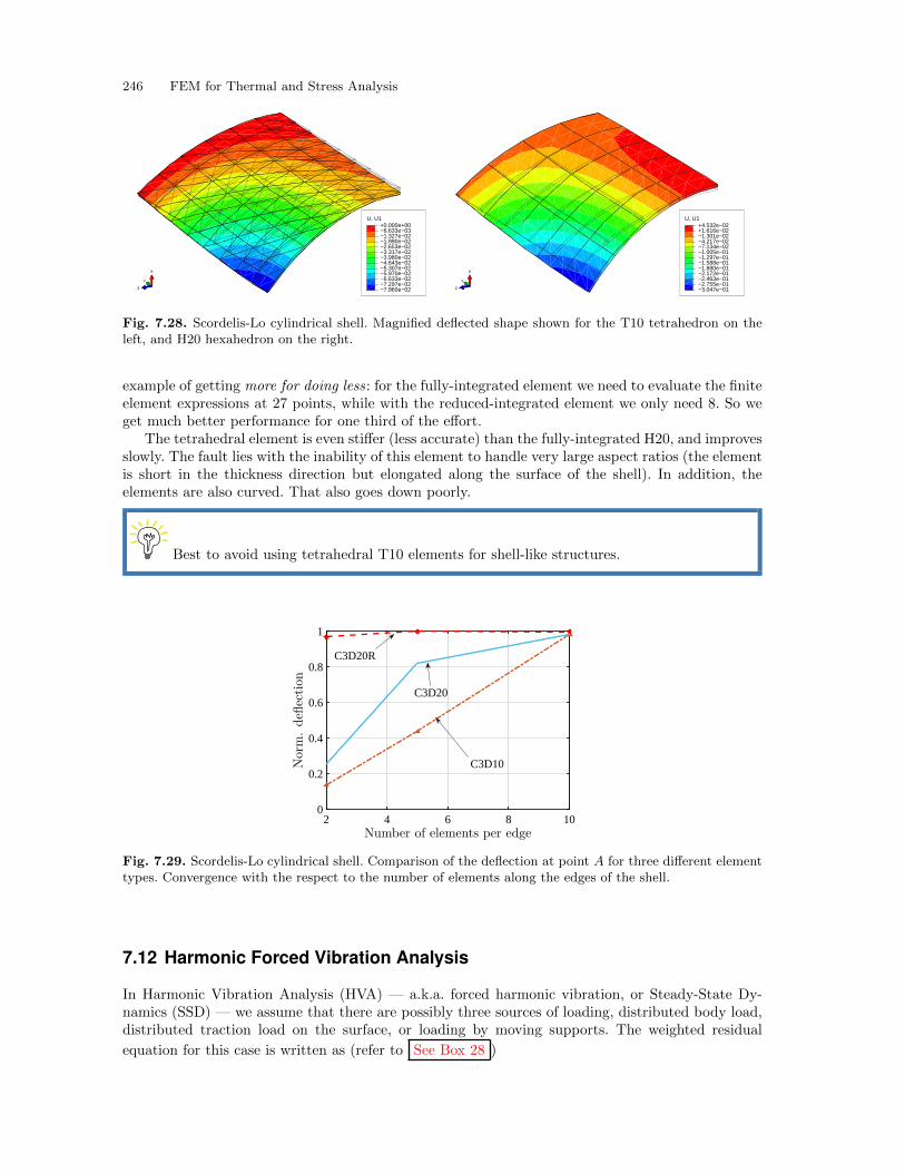
246 FEM for Thermal and Stress Analysis

U, U1

−7.960e−02−7.297e−02−6.633e−02−5.970e−02−5.307e−02−4.643e−02−3.980e−02−3.317e−02−2.653e−02−1.990e−02−1.327e−02−6.633e−03+0.000e+00

X

Y

Z

U, U1

−3.047e−01−2.755e−01−2.463e−01−2.172e−01−1.880e−01−1.588e−01−1.297e−01−1.005e−01−7.134e−02−4.217e−02−1.301e−02+1.616e−02+4.532e−02

X

Y

Z

Fig. 7.28. Scordelis-Lo cylindrical shell. Magnified deflected shape shown for the T10 tetrahedron on theleft, and H20 hexahedron on the right.

example of getting more for doing less: for the fully-integrated element we need to evaluate the finiteelement expressions at 27 points, while with the reduced-integrated element we only need 8. So weget much better performance for one third of the effort.

The tetrahedral element is even stiffer (less accurate) than the fully-integrated H20, and improvesslowly. The fault lies with the inability of this element to handle very large aspect ratios (the elementis short in the thickness direction but elongated along the surface of the shell). In addition, theelements are also curved. That also goes down poorly.

Best to avoid using tetrahedral T10 elements for shell-like structures.

Number of elements per edge2 4 6 8 10

Norm

.deflection

0

0.2

0.4

0.6

0.8

1

C3D20R

C3D20

C3D10

Fig. 7.29. Scordelis-Lo cylindrical shell. Comparison of the deflection at point A for three different elementtypes. Convergence with the respect to the number of elements along the edges of the shell.

7.12 Harmonic Forced Vibration Analysis

In Harmonic Vibration Analysis (HVA) — a.k.a. forced harmonic vibration, or Steady-State Dy-namics (SSD) — we assume that there are possibly three sources of loading, distributed body load,distributed traction load on the surface, or loading by moving supports. The weighted residual

equation for this case is written as (refer to See Box 28 )

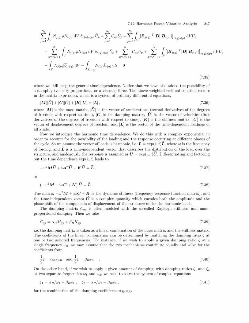
7.12 Harmonic Forced Vibration Analysis 247

Nf∑p=1

∫V

Nj(q)ρNi(p) dV δr(q)s(p) Up +

Nf∑p=1

CqpUp +

Nf∑p=1

∫V

[[Bj(q)]

T [D][Bi(p)]]r(q)s(p)

dV Up

+

N∑p=Nf+1

∫V

Nj(q)ρNj(q) dV δr(q)s(p) Up +

N∑p=Nf+1

CqpUp +

N∑p=Nf+1

∫V

[[Bj(q)]

T [D][Bi(p)]]r(q)s(p)

dV Up

−∫V

Nj(q)[b]r(q) dV −∫St,r(q)

Nj(q)tr(q) dS = 0

(7.35)

where we still keep the general time dependence. Notice that we have also added the possibility ofa damping (velocity-proportional or a viscous) force. The above weighted residual equation resultsin the matrix expression, which is a system of ordinary differential equations,

[M ][U ] + [C][U ] + [K][U ] = [L] , (7.36)

where [M ] is the mass matrix, [U ] is the vector of accelerations (second derivatives of the degreesof freedom with respect to time), [C] is the damping matrix, [U ] is the vector of velocities (firstderivatives of the degrees of freedom with respect to time), [K] is the stiffness matrix, [U ] is thevector of displacement degrees of freedom, and [L] is the vector of the time-dependent loadings ofall kinds.

Now we introduce the harmonic time dependence. We do this with a complex exponential inorder to account for the possibility of the loading and the response occurring at different phases ofthe cycle. So we assume the vector of loads is harmonic, i.e. L = exp(iωt)L, where ω is the frequency

of forcing, and L is a time-independent vector that describes the distribution of the load over thestructure, and analogously the response is assumed as U = exp(iωt)U . Differentiating and factoringout the time dependence exp(iωt) leads to

−ω2MU + iωCU +KU = L , (7.37)

or (−ω2M + iωC +K

)U = L . (7.38)

The matrix −ω2M + iωC +K is the dynamic stiffness (frequency response function matrix), and

the time-independent vector U is a complex quantity which encodes both the amplitude and thephase shift of the components of displacement of the structure under the harmonic loads.

The damping matrix Cqp is often modeled with the so-called Rayleigh stiffness- and mass-proportional damping. Then we take

Cqp = αRMqp + βRKqp , (7.39)

i.e. the damping matrix is taken as a linear combination of the mass matrix and the stiffness matrix.The coefficients of the linear combination can be determined by matching the damping ratio ζ atone or two selected frequencies. For instance, if we wish to apply a given damping ratio ζ at asingle frequency ω0, we may assume that the two mechanisms contribute equally and solve for thecoefficients from

1

2ζ = αR/ω0 and

1

2ζ = βRω0 . (7.40)

On the other hand, if we wish to apply a given amount of damping, with damping ratios ζ1 and ζ2at two separate frequencies ω1 and ω2, we need to solve the system of coupled equations

ζ1 = αR/ω1 + βRω1 , ζ2 = αR/ω2 + βRω2 , (7.41)

for the combination of the damping coefficients αR, βR.

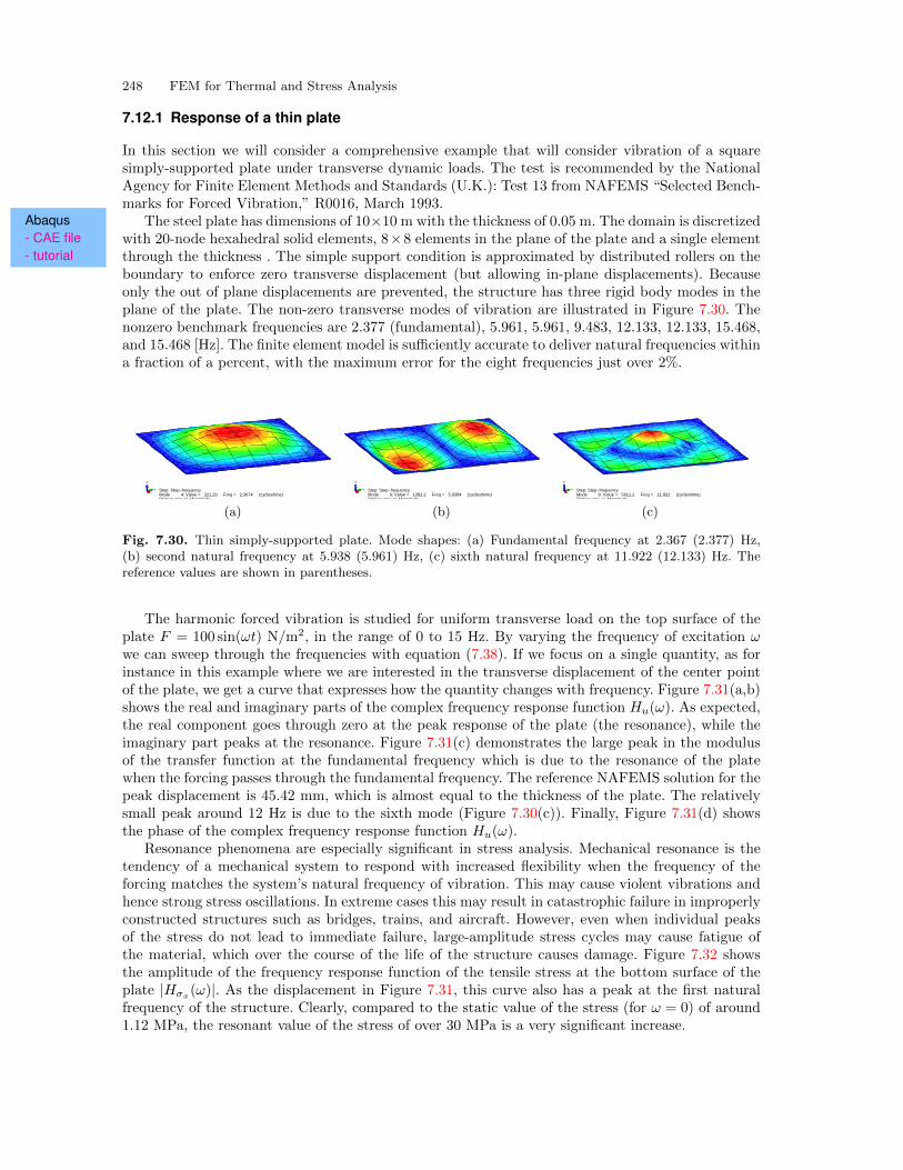
248 FEM for Thermal and Stress Analysis

7.12.1 Response of a thin plate

In this section we will consider a comprehensive example that will consider vibration of a squaresimply-supported plate under transverse dynamic loads. The test is recommended by the NationalAgency for Finite Element Methods and Standards (U.K.): Test 13 from NAFEMS “Selected Bench-marks for Forced Vibration,” R0016, March 1993.

Abaqus- CAE file- tutorial

The steel plate has dimensions of 10×10 m with the thickness of 0.05 m. The domain is discretizedwith 20-node hexahedral solid elements, 8×8 elements in the plane of the plate and a single elementthrough the thickness . The simple support condition is approximated by distributed rollers on theboundary to enforce zero transverse displacement (but allowing in-plane displacements). Becauseonly the out of plane displacements are prevented, the structure has three rigid body modes in theplane of the plate. The non-zero transverse modes of vibration are illustrated in Figure 7.30. Thenonzero benchmark frequencies are 2.377 (fundamental), 5.961, 5.961, 9.483, 12.133, 12.133, 15.468,and 15.468 [Hz]. The finite element model is sufficiently accurate to deliver natural frequencies withina fraction of a percent, with the maximum error for the eight frequencies just over 2%.

Step: Step−frequencyMode 4: Value = 221.26 Freq = 2.3674 (cycles/time)Primary Var: U, Magnitude

XY

Z

Step: Step−frequencyMode 6: Value = 1392.2 Freq = 5.9384 (cycles/time)Primary Var: U, Magnitude

XY

Z

Step: Step−frequencyMode 9: Value = 5611.2 Freq = 11.922 (cycles/time)Primary Var: U, Magnitude

XY

Z

(a) (b) (c)

Fig. 7.30. Thin simply-supported plate. Mode shapes: (a) Fundamental frequency at 2.367 (2.377) Hz,(b) second natural frequency at 5.938 (5.961) Hz, (c) sixth natural frequency at 11.922 (12.133) Hz. Thereference values are shown in parentheses.

The harmonic forced vibration is studied for uniform transverse load on the top surface of theplate F = 100 sin(ωt) N/m2, in the range of 0 to 15 Hz. By varying the frequency of excitation ωwe can sweep through the frequencies with equation (7.38). If we focus on a single quantity, as forinstance in this example where we are interested in the transverse displacement of the center pointof the plate, we get a curve that expresses how the quantity changes with frequency. Figure 7.31(a,b)shows the real and imaginary parts of the complex frequency response function Hu(ω). As expected,the real component goes through zero at the peak response of the plate (the resonance), while theimaginary part peaks at the resonance. Figure 7.31(c) demonstrates the large peak in the modulusof the transfer function at the fundamental frequency which is due to the resonance of the platewhen the forcing passes through the fundamental frequency. The reference NAFEMS solution for thepeak displacement is 45.42 mm, which is almost equal to the thickness of the plate. The relativelysmall peak around 12 Hz is due to the sixth mode (Figure 7.30(c)). Finally, Figure 7.31(d) showsthe phase of the complex frequency response function Hu(ω).

Resonance phenomena are especially significant in stress analysis. Mechanical resonance is thetendency of a mechanical system to respond with increased flexibility when the frequency of theforcing matches the system’s natural frequency of vibration. This may cause violent vibrations andhence strong stress oscillations. In extreme cases this may result in catastrophic failure in improperlyconstructed structures such as bridges, trains, and aircraft. However, even when individual peaksof the stress do not lead to immediate failure, large-amplitude stress cycles may cause fatigue ofthe material, which over the course of the life of the structure causes damage. Figure 7.32 showsthe amplitude of the frequency response function of the tensile stress at the bottom surface of theplate |Hσx(ω)|. As the displacement in Figure 7.31, this curve also has a peak at the first naturalfrequency of the structure. Clearly, compared to the static value of the stress (for ω = 0) of around1.12 MPa, the resonant value of the stress of over 30 MPa is a very significant increase.

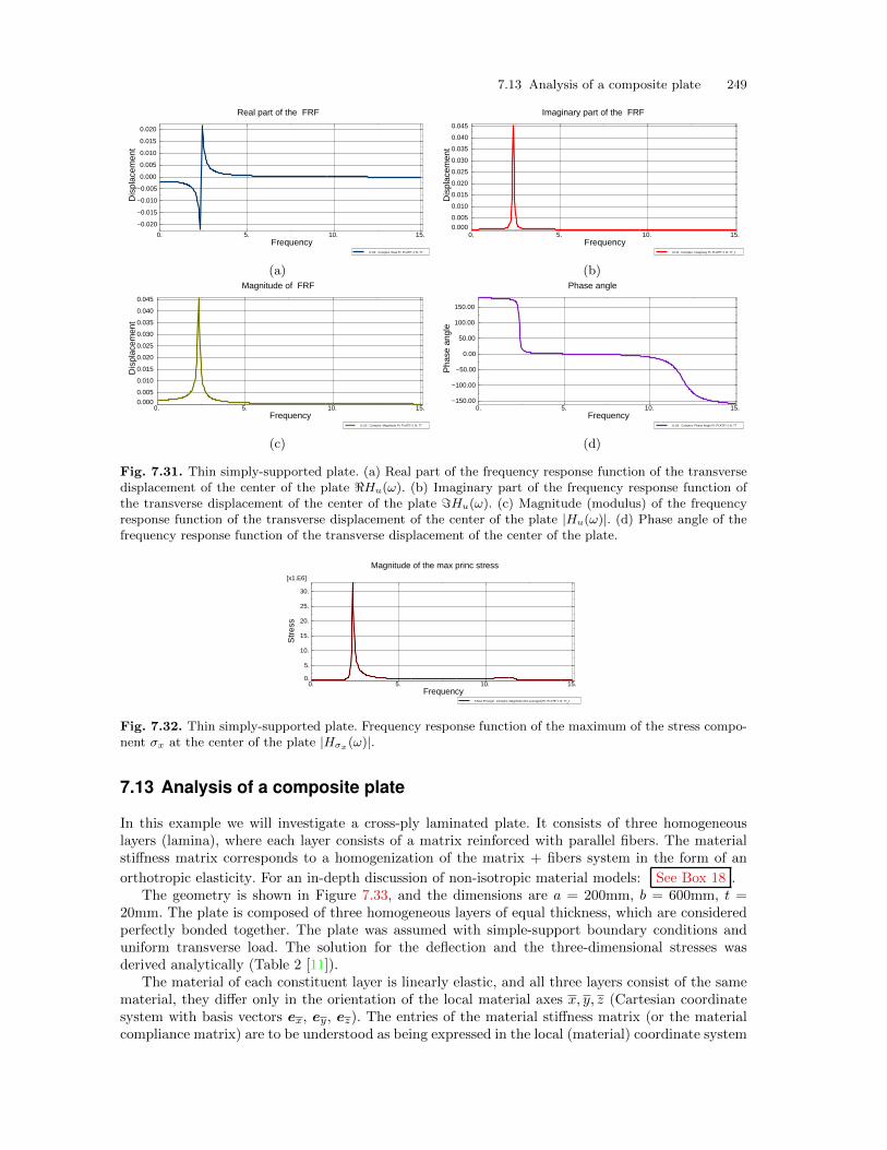
7.13 Analysis of a composite plate 249

Real part of the FRF

Frequency0. 5. 10. 15.

Dis

plac

emen

t

−0.020

−0.015

−0.010

−0.005

0.000

0.005

0.010

0.015

0.020

U:U3 Complex: Real PI: PLATE−1 N: 77

Imaginary part of the FRF

Frequency0. 5. 10. 15.

Dis

plac

emen

t

0.000

0.005

0.010

0.015

0.020

0.025

0.030

0.035

0.040

0.045

U:U3 Complex: Imaginary PI: PLATE−1 N: 77_1

(a) (b)Magnitude of FRF

Frequency0. 5. 10. 15.

Dis

plac

emen

t

0.000

0.005

0.010

0.015

0.020

0.025

0.030

0.035

0.040

0.045

U:U3 Complex: Magnitude PI: PLATE−1 N: 77

Phase angle

Frequency0. 5. 10. 15.

Pha

se a

ngle

−150.00

−100.00

−50.00

0.00

50.00

100.00

150.00

U:U3 Complex: Phase Angle PI: PLATE−1 N: 77

(c) (d)

Fig. 7.31. Thin simply-supported plate. (a) Real part of the frequency response function of the transversedisplacement of the center of the plate ℜHu(ω). (b) Imaginary part of the frequency response function ofthe transverse displacement of the center of the plate ℑHu(ω). (c) Magnitude (modulus) of the frequencyresponse function of the transverse displacement of the center of the plate |Hu(ω)|. (d) Phase angle of thefrequency response function of the transverse displacement of the center of the plate.

Magnitude of the max princ stress

Frequency0. 5. 10. 15.

Str

ess

0.

5.

10.

15.

20.

25.

30.

[x1.E6]

S:Max Principal Complex: Magnitude (Not averaged) PI: PLATE−1 N: 77_1

Fig. 7.32. Thin simply-supported plate. Frequency response function of the maximum of the stress compo-nent σx at the center of the plate |Hσx(ω)|.

7.13 Analysis of a composite plate

In this example we will investigate a cross-ply laminated plate. It consists of three homogeneouslayers (lamina), where each layer consists of a matrix reinforced with parallel fibers. The materialstiffness matrix corresponds to a homogenization of the matrix + fibers system in the form of an

orthotropic elasticity. For an in-depth discussion of non-isotropic material models: See Box 18 .The geometry is shown in Figure 7.33, and the dimensions are a = 200mm, b = 600mm, t =

20mm. The plate is composed of three homogeneous layers of equal thickness, which are consideredperfectly bonded together. The plate was assumed with simple-support boundary conditions anduniform transverse load. The solution for the deflection and the three-dimensional stresses wasderived analytically (Table 2 [11]).

The material of each constituent layer is linearly elastic, and all three layers consist of the samematerial, they differ only in the orientation of the local material axes x, y, z (Cartesian coordinatesystem with basis vectors ex, ey, ez). The entries of the material stiffness matrix (or the materialcompliance matrix) are to be understood as being expressed in the local (material) coordinate system

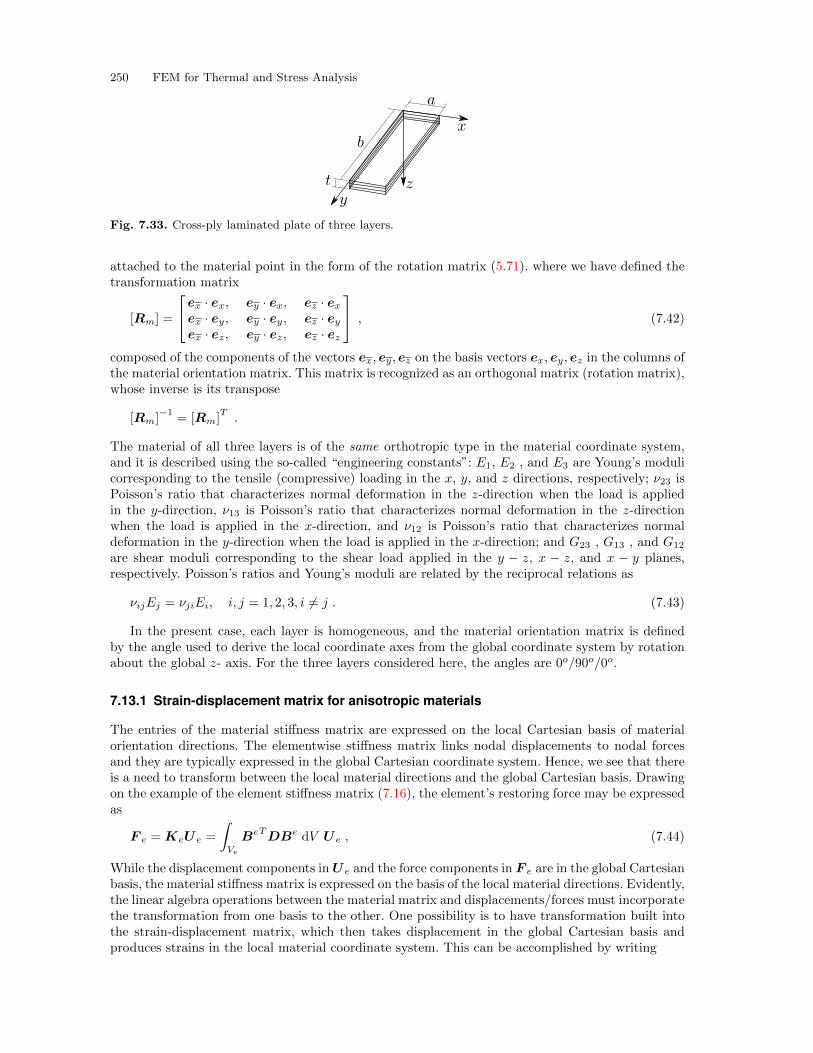
250 FEM for Thermal and Stress Analysis

Fig. 7.33. Cross-ply laminated plate of three layers.

attached to the material point in the form of the rotation matrix (5.71). where we have defined thetransformation matrix

[Rm] =

ex · ex, ey · ex, ez · exex · ey, ey · ey, ez · eyex · ez, ey · ez, ez · ez

, (7.42)

composed of the components of the vectors ex, ey, ez on the basis vectors ex, ey, ez in the columns ofthe material orientation matrix. This matrix is recognized as an orthogonal matrix (rotation matrix),whose inverse is its transpose

[Rm]−1

= [Rm]T.

The material of all three layers is of the same orthotropic type in the material coordinate system,and it is described using the so-called “engineering constants”: E1, E2 , and E3 are Young’s modulicorresponding to the tensile (compressive) loading in the x, y, and z directions, respectively; ν23 isPoisson’s ratio that characterizes normal deformation in the z-direction when the load is appliedin the y-direction, ν13 is Poisson’s ratio that characterizes normal deformation in the z-directionwhen the load is applied in the x-direction, and ν12 is Poisson’s ratio that characterizes normaldeformation in the y-direction when the load is applied in the x-direction; and G23 , G13 , and G12

are shear moduli corresponding to the shear load applied in the y − z, x − z, and x − y planes,respectively. Poisson’s ratios and Young’s moduli are related by the reciprocal relations as

νijEj = νjiEi, i, j = 1, 2, 3, i = j . (7.43)

In the present case, each layer is homogeneous, and the material orientation matrix is definedby the angle used to derive the local coordinate axes from the global coordinate system by rotationabout the global z- axis. For the three layers considered here, the angles are 0o/90o/0o.

7.13.1 Strain-displacement matrix for anisotropic materials

The entries of the material stiffness matrix are expressed on the local Cartesian basis of materialorientation directions. The elementwise stiffness matrix links nodal displacements to nodal forcesand they are typically expressed in the global Cartesian coordinate system. Hence, we see that thereis a need to transform between the local material directions and the global Cartesian basis. Drawingon the example of the element stiffness matrix (7.16), the element’s restoring force may be expressedas

F e = KeU e =

∫Ve

BeTDBe dV U e , (7.44)

While the displacement components inU e and the force components in F e are in the global Cartesianbasis, the material stiffness matrix is expressed on the basis of the local material directions. Evidently,the linear algebra operations between the material matrix and displacements/forces must incorporatethe transformation from one basis to the other. One possibility is to have transformation built intothe strain-displacement matrix, which then takes displacement in the global Cartesian basis andproduces strains in the local material coordinate system. This can be accomplished by writing

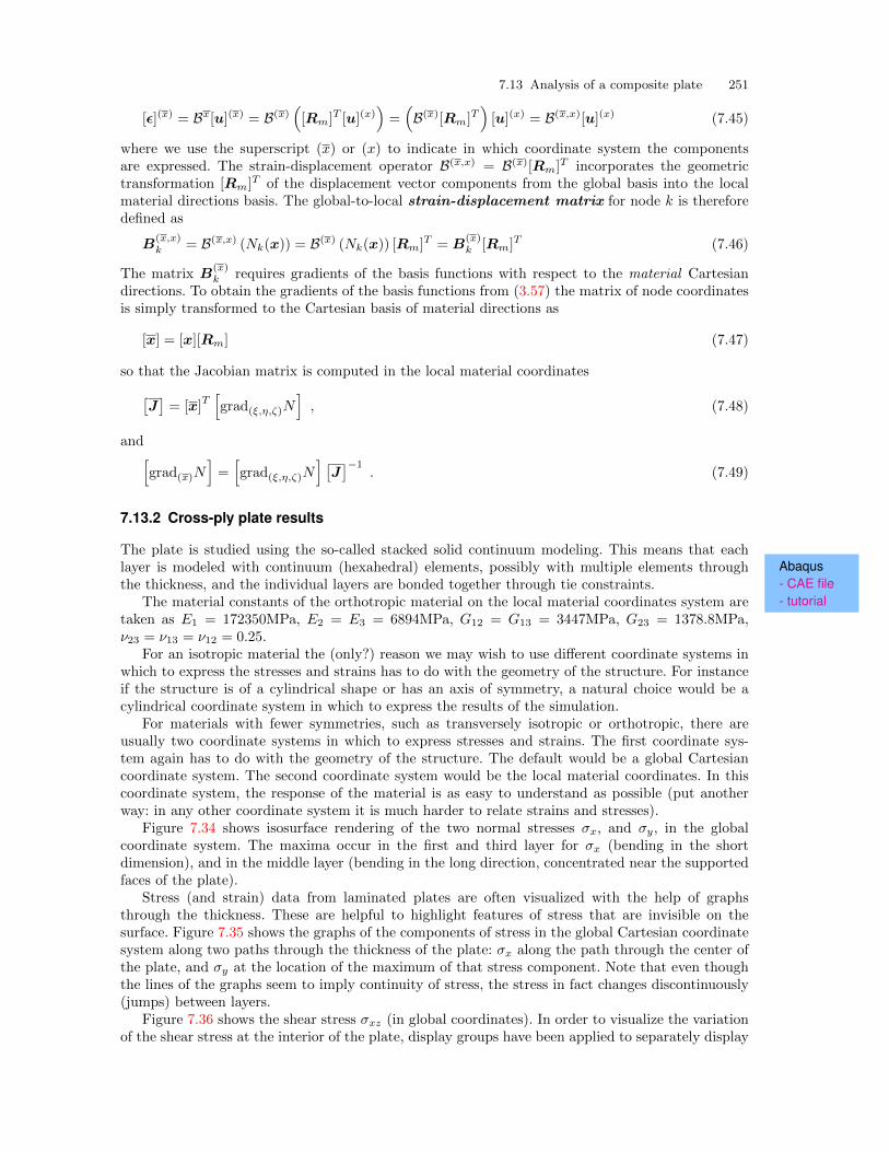
7.13 Analysis of a composite plate 251

[ϵ](x) = Bx[u](x) = B(x)([Rm]T [u](x)

)=(B(x)[Rm]T

)[u](x) = B(x,x)[u](x) (7.45)

where we use the superscript (x) or (x) to indicate in which coordinate system the componentsare expressed. The strain-displacement operator B(x,x) = B(x)[Rm]T incorporates the geometrictransformation [Rm]T of the displacement vector components from the global basis into the localmaterial directions basis. The global-to-local strain-displacement matrix for node k is thereforedefined as

B(x,x)k = B(x,x) (Nk(x)) = B(x) (Nk(x)) [Rm]T = B

(x)k [Rm]T (7.46)

The matrix B(x)k requires gradients of the basis functions with respect to the material Cartesian

directions. To obtain the gradients of the basis functions from (3.57) the matrix of node coordinatesis simply transformed to the Cartesian basis of material directions as

[x] = [x][Rm] (7.47)

so that the Jacobian matrix is computed in the local material coordinates[J]= [x]

T[grad(ξ,η,ζ)N

], (7.48)

and[grad(x)N

]=[grad(ξ,η,ζ)N

] [J]−1

. (7.49)

7.13.2 Cross-ply plate results

The plate is studied using the so-called stacked solid continuum modeling. This means that eachAbaqus- CAE file- tutorial

layer is modeled with continuum (hexahedral) elements, possibly with multiple elements throughthe thickness, and the individual layers are bonded together through tie constraints.

The material constants of the orthotropic material on the local material coordinates system aretaken as E1 = 172350MPa, E2 = E3 = 6894MPa, G12 = G13 = 3447MPa, G23 = 1378.8MPa,ν23 = ν13 = ν12 = 0.25.

For an isotropic material the (only?) reason we may wish to use different coordinate systems inwhich to express the stresses and strains has to do with the geometry of the structure. For instanceif the structure is of a cylindrical shape or has an axis of symmetry, a natural choice would be acylindrical coordinate system in which to express the results of the simulation.

For materials with fewer symmetries, such as transversely isotropic or orthotropic, there areusually two coordinate systems in which to express stresses and strains. The first coordinate sys-tem again has to do with the geometry of the structure. The default would be a global Cartesiancoordinate system. The second coordinate system would be the local material coordinates. In thiscoordinate system, the response of the material is as easy to understand as possible (put anotherway: in any other coordinate system it is much harder to relate strains and stresses).

Figure 7.34 shows isosurface rendering of the two normal stresses σx, and σy, in the globalcoordinate system. The maxima occur in the first and third layer for σx (bending in the shortdimension), and in the middle layer (bending in the long direction, concentrated near the supportedfaces of the plate).

Stress (and strain) data from laminated plates are often visualized with the help of graphsthrough the thickness. These are helpful to highlight features of stress that are invisible on thesurface. Figure 7.35 shows the graphs of the components of stress in the global Cartesian coordinatesystem along two paths through the thickness of the plate: σx along the path through the center ofthe plate, and σy at the location of the maximum of that stress component. Note that even thoughthe lines of the graphs seem to imply continuity of stress, the stress in fact changes discontinuously(jumps) between layers.

Figure 7.36 shows the shear stress σxz (in global coordinates). In order to visualize the variationof the shear stress at the interior of the plate, display groups have been applied to separately display

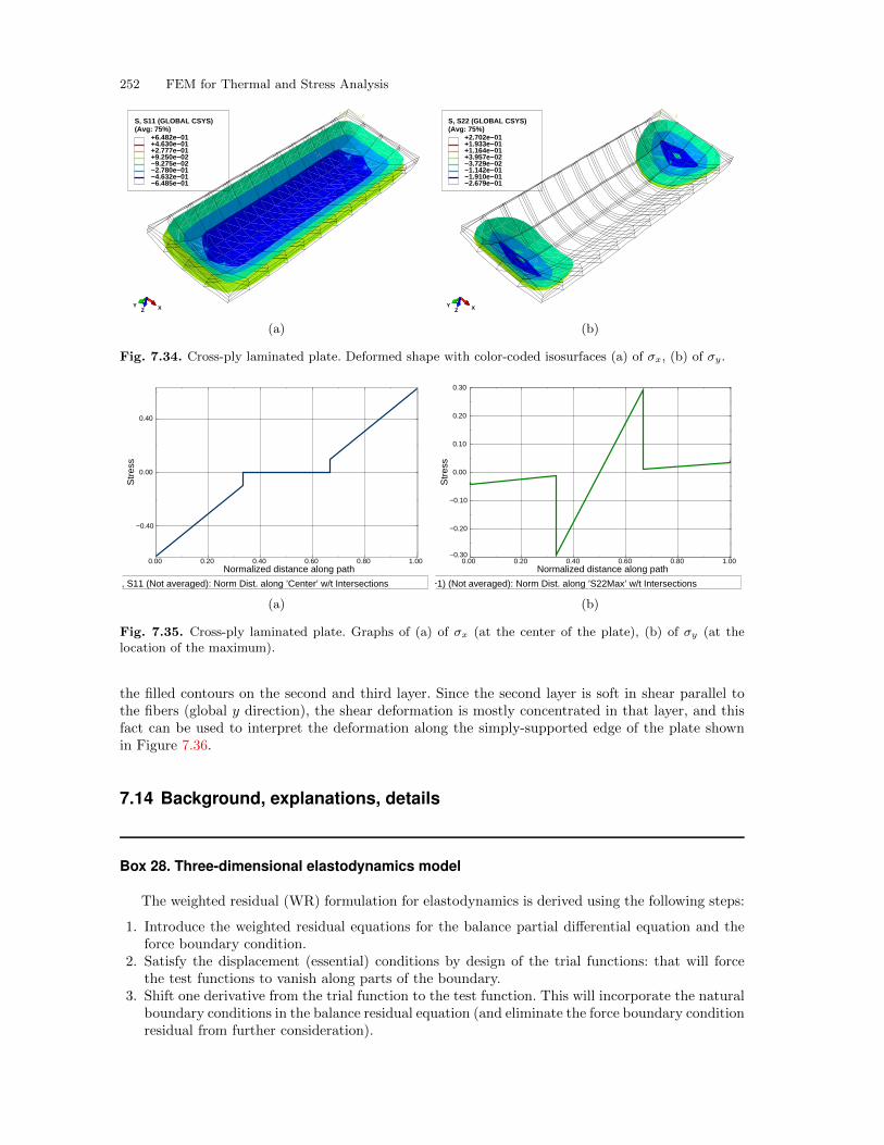
252 FEM for Thermal and Stress Analysis

ZX

Y

(Avg: 75%)S, S11 (GLOBAL CSYS)

−6.485e−01−4.632e−01−2.780e−01−9.275e−02+9.250e−02+2.777e−01+4.630e−01+6.482e−01

XYZ

ZX

Y

(Avg: 75%)S, S22 (GLOBAL CSYS)

−2.679e−01−1.910e−01−1.142e−01−3.729e−02+3.957e−02+1.164e−01+1.933e−01+2.702e−01

XYZ

(a) (b)

Fig. 7.34. Cross-ply laminated plate. Deformed shape with color-coded isosurfaces (a) of σx, (b) of σy.

Normalized distance along path0.00 0.20 0.40 0.60 0.80 1.00

Str

ess

−0.40

0.00

0.40

S, S11 (Not averaged): Norm Dist. along ’Center’ w/t Intersections

Normalized distance along path0.00 0.20 0.40 0.60 0.80 1.00

Str

ess

−0.30

−0.20

−0.10

0.00

0.10

0.20

0.30

S, S22 (ASSEMBLY_Layer 1−1_ORI−1) (Not averaged): Norm Dist. along ’S22Max’ w/t Intersections

(a) (b)

Fig. 7.35. Cross-ply laminated plate. Graphs of (a) of σx (at the center of the plate), (b) of σy (at thelocation of the maximum).

the filled contours on the second and third layer. Since the second layer is soft in shear parallel tothe fibers (global y direction), the shear deformation is mostly concentrated in that layer, and thisfact can be used to interpret the deformation along the simply-supported edge of the plate shownin Figure 7.36.

7.14 Background, explanations, details

Box 28. Three-dimensional elastodynamics model

The weighted residual (WR) formulation for elastodynamics is derived using the following steps:

1. Introduce the weighted residual equations for the balance partial differential equation and theforce boundary condition.

2. Satisfy the displacement (essential) conditions by design of the trial functions: that will forcethe test functions to vanish along parts of the boundary.

3. Shift one derivative from the trial function to the test function. This will incorporate the naturalboundary conditions in the balance residual equation (and eliminate the force boundary conditionresidual from further consideration).

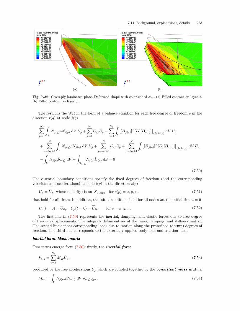
7.14 Background, explanations, details 253

(Avg: 75%)S, S13 (GLOBAL CSYS)

−5.367e−02−4.473e−02−3.578e−02−2.684e−02−1.789e−02−8.946e−03−5.588e−09+8.946e−03+1.789e−02+2.684e−02+3.578e−02+4.473e−02+5.367e−02

XY

Z

(Avg: 75%)S, S13 (GLOBAL CSYS)

−5.367e−02−4.473e−02−3.578e−02−2.684e−02−1.789e−02−8.946e−03−5.588e−09+8.946e−03+1.789e−02+2.684e−02+3.578e−02+4.473e−02+5.367e−02

XY

Z

(a) (b)

Fig. 7.36. Cross-ply laminated plate. Deformed shape with color-coded σxz. (a) Filled contour on layer 2.(b) Filled contour on layer 3.

The result is the WR in the form of a balance equation for each free degree of freedom q in thedirection r(q) at node j(q)

Nf∑p=1

∫V

Nj(q)ρNi(p) dV Up +

Nf∑p=1

CqpUp +

Nf∑p=1

∫V

[[Bj(q)]

T [D][Bi(p)]]r(q)s(p)

dV Up

+

N∑p=Nf+1

∫V

Nj(q)ρNj(q) dV Up +

N∑p=Nf+1

CqpUp +

N∑p=Nf+1

∫V

[[Bj(q)]

T [D][Bi(p)]]r(q)s(p)

dV Up

−∫V

Nj(q)br(q) dV −∫St,r(q)

Nj(q)tr(q) dS = 0

(7.50)

The essential boundary conditions specify the fixed degrees of freedom (and the correspondingvelocities and accelerations) at node i(p) in the direction s(p)

Up = Up, where node i(p) is on Su,s(p) for s(p) = x, y, z . (7.51)

that hold for all times. In addition, the initial conditions hold for all nodes iat the initial time t = 0

Up(t = 0) = U0p Up(t = 0) = U0p for s = x, y, z . (7.52)

The first line in (7.50) represents the inertial, damping, and elastic forces due to free degreeof freedom displacements. The integrals define entries of the mass, damping, and stiffness matrix.The second line defines corresponding loads due to motion along the prescribed (datum) degrees offreedom. The third line corresponds to the externally applied body load and traction load.

Inertial term: Mass matrix

Two terms emerge from (7.50): firstly, the inertial force

Fa,q =

Nf∑p=1

MqpUp , (7.53)

produced by the free accelerations Up which are coupled together by the consistent mass matrix

Mqp =

∫V

Nj(q)ρNi(p) dV δr(q)s(p) , (7.54)

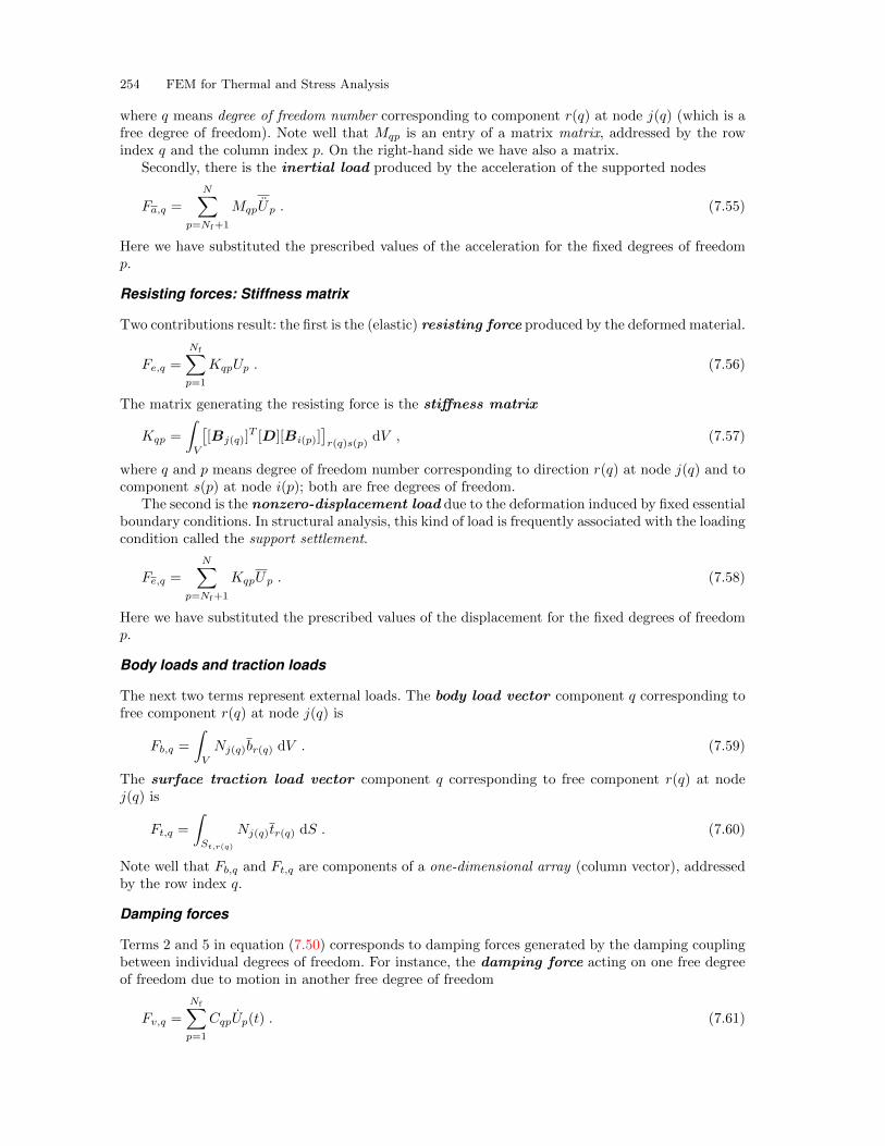
254 FEM for Thermal and Stress Analysis

where q means degree of freedom number corresponding to component r(q) at node j(q) (which is afree degree of freedom). Note well that Mqp is an entry of a matrix matrix, addressed by the rowindex q and the column index p. On the right-hand side we have also a matrix.

Secondly, there is the inertial load produced by the acceleration of the supported nodes

Fa,q =

N∑p=Nf+1

MqpUp . (7.55)

Here we have substituted the prescribed values of the acceleration for the fixed degrees of freedomp.

Resisting forces: Stiffness matrix

Two contributions result: the first is the (elastic) resisting force produced by the deformed material.

Fe,q =

Nf∑p=1

KqpUp . (7.56)

The matrix generating the resisting force is the stiffness matrix

Kqp =

∫V

[[Bj(q)]

T [D][Bi(p)]]r(q)s(p)

dV , (7.57)

where q and p means degree of freedom number corresponding to direction r(q) at node j(q) and tocomponent s(p) at node i(p); both are free degrees of freedom.

The second is the nonzero-displacement load due to the deformation induced by fixed essentialboundary conditions. In structural analysis, this kind of load is frequently associated with the loadingcondition called the support settlement.

Fe,q =

N∑p=Nf+1

KqpUp . (7.58)

Here we have substituted the prescribed values of the displacement for the fixed degrees of freedomp.

Body loads and traction loads

The next two terms represent external loads. The body load vector component q corresponding tofree component r(q) at node j(q) is

Fb,q =

∫V

Nj(q)br(q) dV . (7.59)

The surface traction load vector component q corresponding to free component r(q) at nodej(q) is

Ft,q =

∫St,r(q)

Nj(q)tr(q) dS . (7.60)

Note well that Fb,q and Ft,q are components of a one-dimensional array (column vector), addressedby the row index q.

Damping forces

Terms 2 and 5 in equation (7.50) corresponds to damping forces generated by the damping couplingbetween individual degrees of freedom. For instance, the damping force acting on one free degreeof freedom due to motion in another free degree of freedom

Fv,q =

Nf∑p=1

CqpUp(t) . (7.61)

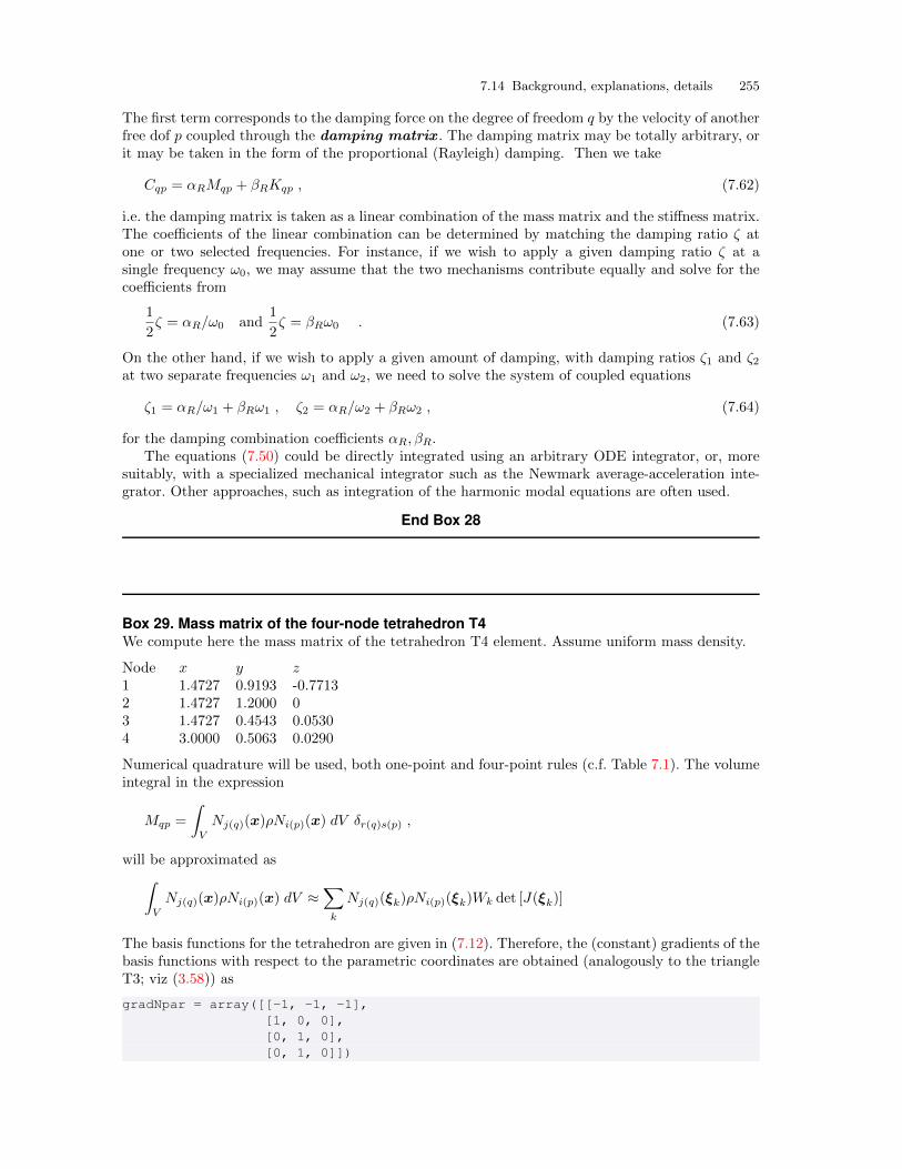
7.14 Background, explanations, details 255

The first term corresponds to the damping force on the degree of freedom q by the velocity of anotherfree dof p coupled through the damping matrix . The damping matrix may be totally arbitrary, orit may be taken in the form of the proportional (Rayleigh) damping. Then we take

Cqp = αRMqp + βRKqp , (7.62)

i.e. the damping matrix is taken as a linear combination of the mass matrix and the stiffness matrix.The coefficients of the linear combination can be determined by matching the damping ratio ζ atone or two selected frequencies. For instance, if we wish to apply a given damping ratio ζ at asingle frequency ω0, we may assume that the two mechanisms contribute equally and solve for thecoefficients from

1

2ζ = αR/ω0 and

1

2ζ = βRω0 . (7.63)

On the other hand, if we wish to apply a given amount of damping, with damping ratios ζ1 and ζ2at two separate frequencies ω1 and ω2, we need to solve the system of coupled equations

ζ1 = αR/ω1 + βRω1 , ζ2 = αR/ω2 + βRω2 , (7.64)

for the damping combination coefficients αR, βR.The equations (7.50) could be directly integrated using an arbitrary ODE integrator, or, more

suitably, with a specialized mechanical integrator such as the Newmark average-acceleration inte-grator. Other approaches, such as integration of the harmonic modal equations are often used.

End Box 28

Box 29. Mass matrix of the four-node tetrahedron T4We compute here the mass matrix of the tetrahedron T4 element. Assume uniform mass density.

Node x y z1 1.4727 0.9193 -0.77132 1.4727 1.2000 03 1.4727 0.4543 0.05304 3.0000 0.5063 0.0290

Numerical quadrature will be used, both one-point and four-point rules (c.f. Table 7.1). The volumeintegral in the expression

Mqp =

∫V

Nj(q)(x)ρNi(p)(x) dV δr(q)s(p) ,

will be approximated as∫V

Nj(q)(x)ρNi(p)(x) dV ≈∑k

Nj(q)(ξk)ρNi(p)(ξk)Wk det [J(ξk)]

The basis functions for the tetrahedron are given in (7.12). Therefore, the (constant) gradients of thebasis functions with respect to the parametric coordinates are obtained (analogously to the triangleT3; viz (3.58)) as

gradNpar = array([[-1, -1, -1],[1, 0, 0],[0, 1, 0],[0, 1, 0]])

256 FEM for Thermal and Stress Analysis

The array of the vertex locations given as

x = array([[1.4727, 0.9193, -0.7713],[1.4727, 1.2000, 0],[1.4727, 0.4543, 0.0530],[3.0000, 0.5063, 0.0290]])

the Jacobian matrix follows from (3.60), which is readily transcribed into Python code as J =

dot(x.T, gradNpar):

array([[ 0. , 0. , 1.5273],[ 0.2807, -0.465 , -0.413 ],[ 0.7713, 0.8243, 0.8003]])

The Jacobian is a constant, 0.90116, (i.e. independent of the integration point), computed as detJ= linalg.det(J).

The one-point rule evaluates the basis functions of the centroid of the tetrahedron. Therefore allthe basis functions assume the value of 1/4 at the quadrature point. For instance we get∫

V

N1(x)ρN1(x) dV ≈ N1(ξ1)ρN1(ξ1)W1 det [J(ξ1)] = (1/4)ρ(1/4)(1/6)0.9012 = 0.0094ρ

But a more descriptive expression will be obtained by keeping W1 det [J(ξ1)] = det [J(ξ1)] /6 = Vtetinstead of numbers, where Vtet is the volume of the tetrahedron element, so that the above may beput as∫

V

N1(x)ρN1(x) dV ≈ 1

16Vtetρ =

1

16mtet

where mtet is the mass of the tetrahedron. Since all basis functions have the same value of thequadrature point, the same expression is obtained for the one-point quadrature rule for all basisfunctions. The δrs represents a 3× 3 identity matrix, and the mass matrix therefore results as

M =1

16mtet

1 0 00 1 00 0 1

1 0 00 1 00 0 1

1 0 00 1 00 0 1

1 0 00 1 00 0 1

1 0 00 1 00 0 1

1 0 00 1 00 0 1

1 0 00 1 00 0 1

1 0 00 1 00 0 1

1 0 00 1 00 0 1

1 0 00 1 00 0 1

1 0 00 1 00 0 1

1 0 00 1 00 0 1

1 0 00 1 00 0 1

1 0 00 1 00 0 1

1 0 00 1 00 0 1

1 0 00 1 00 0 1

Note that there are four “1”’s in each row, which means that for the four nodes accelerating in eitherof the three directions with the same acceleration a (i.e. the element accelerates as a rigid body) thetotal inertial force is a mtet, as expected.

Now we will apply the four-point quadrature rule from Table 7.1. For instance we have∫V

N2(x)ρN3(x) dV ≈∑k

N2(ξk)ρN3(ξk)Wk det [J(ξk)] ≈ ρWk det [J(ξk)]∑k

N2(ξk)N3(ξk)

because ρWk det [J(ξk)] is constant. Substituting the definitions of the basis functions, N2 = ξ andN3 = η, yields∑

k

N2(ξk)N3(ξk) = aa+ aa+ ba+ ab = 2a(a+ b) = 1/5

7.14 Background, explanations, details 257

and hence∫V

N2(x)ρN3(x) dV ≈ 1

20Vtetρ =

1

20mtet

Therefore, the mass matrix will link the nodes 2 and 3 by the 3× 3 matrix

1

20mtet

1 0 00 1 00 0 1

Similarly∫

V

N3(x)ρN3(x) dV ≈∑k

N3(ξk)ρN3(ξk)Wk det [J(ξk)] ≈ ρWk det [J(ξk)]∑k

N3(ξk)N3(ξk)

and∑k

N3(ξk)N3(ξk) = aa+ aa+ aa+ bb = 2/5

and hence∫V

N3(x)ρN3(x) dV ≈ 1

10Vtetρ =

1

10mtet

M =1

20mtet

2 0 00 2 00 0 2

1 0 00 1 00 0 1

1 0 00 1 00 0 1

1 0 00 1 00 0 1

1 0 00 1 00 0 1

2 0 00 2 00 0 2

1 0 00 1 00 0 1

1 0 00 1 00 0 1

1 0 00 1 00 0 1

1 0 00 1 00 0 1

2 0 00 2 00 0 2

1 0 00 1 00 0 1

1 0 00 1 00 0 1

1 0 00 1 00 0 1

1 0 00 1 00 0 1

2 0 00 2 00 0 2

Again, to check the mass matrix we can consider the element accelerating as a rigid body in any oneof the three directions in the Cartesian coordinates. Since for any selected direction, for each nodethe sum of the row of the mass matrix is mtet/4, the total mass obtained by adding the contributionsfrom all four nodes is mtet, as expected.

Both of the above mass matrices are the so-called consistent mass matrices, but only the secondis integrated exactly. The first matrix is integrated inaccurately. As we have seen for the prestressedwire model, various tricks can be undertaken with integration rules for mass matrices to improvethe accuracy of the computed frequencies, so we can’t necessarily conclude that integrating the massmatrix inaccurately will produce a less accurate estimate of the natural frequencies (and vice versa).

End Box 29

Box 30. Body load on a T4 tetrahedron

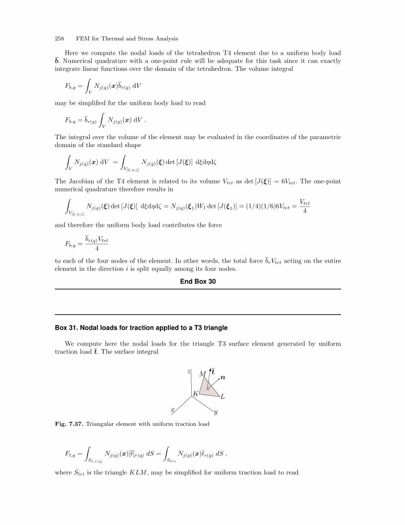
258 FEM for Thermal and Stress Analysis

Here we compute the nodal loads of the tetrahedron T4 element due to a uniform body loadb. Numerical quadrature with a one-point rule will be adequate for this task since it can exactlyintegrate linear functions over the domain of the tetrahedron. The volume integral

Fb,q =

∫V

Nj(q)(x)br(q) dV

may be simplified for the uniform body load to read

Fb,q = br(q)

∫V

Nj(q)(x) dV .

The integral over the volume of the element may be evaluated in the coordinates of the parametricdomain of the standard shape∫

V

Nj(q)(x) dV =

∫V[ξ,η,ζ]

Nj(q)(ξ) det [J(ξ)] dξdηdζ

The Jacobian of the T4 element is related to its volume Vtet as det [J(ξ)] = 6Vtet. The one-pointnumerical quadrature therefore results in∫

V[ξ,η,ζ]

Nj(q)(ξ) det [J(ξ)] dξdηdζ = Nj(q)(ξ1)W1 det [J(ξ1)] = (1/4)(1/6)6Vtet =Vtet4

and therefore the uniform body load contributes the force

Fb,q =br(q)Vtet

4

to each of the four nodes of the element. In other words, the total force brVtet acting on the entireelement in the direction i is split equally among its four nodes.

End Box 30

Box 31. Nodal loads for traction applied to a T3 triangle

We compute here the nodal loads for the triangle T3 surface element generated by uniformtraction load t. The surface integral

Fig. 7.37. Triangular element with uniform traction load

Ft,q =

∫St,r(q)

Nj(q)(x)[t]r(q) dS =

∫Stri

Nj(q)(x)tr(q) dS ,

where Stri is the triangle KLM , may be simplified for uniform traction load to read

7.14 Background, explanations, details 259

Ft,q = tr(q)

∫Stri

Nj(q)(x) dS

The task therefore reduces to the integration of basis functions over the surface of the triangle, whichmay be evaluated in the coordinates of the parametric domain of the standard triangle∫

Stri

Nj(q)(x) dS =

∫S[ξ,η]

Nj(q)(ξ) det [J(ξ)] dξdη

The Jacobian for the triangle is obtained as the cross product of the two tangent vectors

∂x(ξ, η)

∂ξ, and

∂x(ξ, η)

∂η,

and because the basis functions are linear in ξ, η the tangent vectors are constant (the same at allpoints of the triangle). It is also shown above that the Jacobian of the surface is equal to twice thearea of the triangle. Hence we get∫

S[ξ,η]

Nj(q)(ξ) det [J(ξ)] dξdη = det [J(ξ)]

∫S[ξ,η]

Nj(q)(ξ) dξdη = 2Stri

∫S[ξ,η]

Nj(q)(ξ) dξdη

Numerical quadrature with a one-point rule will be adequate, as Nj is linear in its arguments∫S[ξ,η]

Nj(q)(ξ) dξdη ≈ Nj(q)(ξ1)W1 = (1/3)(1/2) = 1/6

Thus we conclude that the uniform traction load contributes the force component

Ft,q = tr(q)

∫Stri

Nj(x) dS = tr(q) × 2Stri × (1/6) =trStri

3

to each of the three nodes j of the element. In words, the total force tr(q)Stri acting on the entireelement in the direction r(q) is split equally among its three nodes.

End Box 31

Box 32. Imposed (thermal) strains

Often the material from which a structure is built up reacts to the environment by deformation.The material experiences the environment in possibly different ways or different measures in differentlocations, and stresses are produced.

To get started, think about a very small piece of material that is exposed to the environmentso that we can assume that the resultant relative deformation is homogeneous and no stress isproduced. For the sake of this argument, let us consider one particular environmental effect: thermalexpansion . However, similar effects may be produced by shrinkage, swelling, piezoelectric effects,and so on.

When the small sample of material is at a reference temperature it is unstressed, and we de-fine its displacements and the associated strains to be zero in this state: the reference state. Thenthe temperature is increased by ∆T , and the material responds by displacement, and because byassumption the deformation is homogeneous, the entire sample experiences uniform strains. Basedon experimental evidence, the following model is adopted for orthotropic materials to describe thestrains in coordinates aligned with the material directions

260 FEM for Thermal and Stress Analysis

[θϵ] =

ϵxϵyϵzγxyγxzγyz

= ∆T

αx

αy

αz

000

. (7.65)

Evidently, the thermal expansion is assumed not to cause any shear strains. The factors αx, αy, αz

are the so-called coefficients of thermal expansion ; different in different directions, in general.In addition to the imposed strain ϵΘ, the sample is also exposed to stresses on its boundary,

again such that they result in uniform strain. The total strains that the sample experiences consistof the imposed strains to which the mechanical strains are added. Since the mechanical strains areavailable from the stresses through the constitutive equation, we write

ϵ = ϵtotal =θϵ+D−1σ , (7.66)

Therefore, we have a modification of the constitutive equation

σ = D(ϵ− θϵ

). (7.67)

The total strain is related to the displacement via the strain-displacement relation (5.98), and thuswe may write

σ = D(Bu− θϵ

).

As expected, the residual equation form that enters the discretization process needs to be aug-mented with respect to (5.121) to become∫

V

η · ρu dV −∫V

η · b dV −∑

i=x,y,z

∫St,i

(η)i ti dS +

∫V

(Bη) ·D(Bu− θϵ

)dV = 0 (7.68)

ui = ui and (η)i = 0 on Su,i for i = x, y, z

Clearly, there will be one more term to discretize

−∫V

(Bη) ·D θϵ dV , (7.69)

yielding the thermal strain load

FΘ,q =

[∫V

BT(Nj(q)(x)

)D θϵ dV

]r(q)

. (7.70)

End Box 32

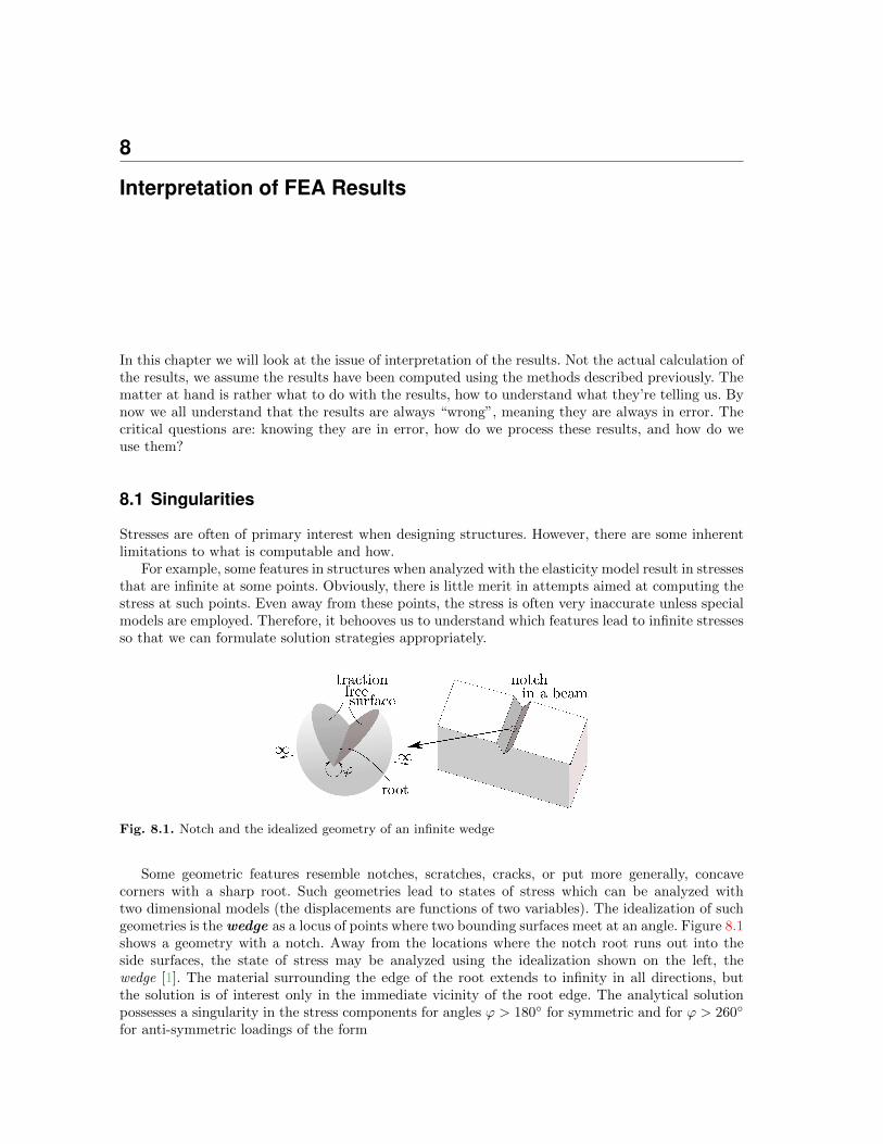
8

Interpretation of FEA Results

In this chapter we will look at the issue of interpretation of the results. Not the actual calculation ofthe results, we assume the results have been computed using the methods described previously. Thematter at hand is rather what to do with the results, how to understand what they’re telling us. Bynow we all understand that the results are always “wrong”, meaning they are always in error. Thecritical questions are: knowing they are in error, how do we process these results, and how do weuse them?

8.1 Singularities

Stresses are often of primary interest when designing structures. However, there are some inherentlimitations to what is computable and how.

For example, some features in structures when analyzed with the elasticity model result in stressesthat are infinite at some points. Obviously, there is little merit in attempts aimed at computing thestress at such points. Even away from these points, the stress is often very inaccurate unless specialmodels are employed. Therefore, it behooves us to understand which features lead to infinite stressesso that we can formulate solution strategies appropriately.

Fig. 8.1. Notch and the idealized geometry of an infinite wedge

Some geometric features resemble notches, scratches, cracks, or put more generally, concavecorners with a sharp root. Such geometries lead to states of stress which can be analyzed withtwo dimensional models (the displacements are functions of two variables). The idealization of suchgeometries is the wedge as a locus of points where two bounding surfaces meet at an angle. Figure 8.1shows a geometry with a notch. Away from the locations where the notch root runs out into theside surfaces, the state of stress may be analyzed using the idealization shown on the left, thewedge [1]. The material surrounding the edge of the root extends to infinity in all directions, butthe solution is of interest only in the immediate vicinity of the root edge. The analytical solutionpossesses a singularity in the stress components for angles φ > 180◦ for symmetric and for φ > 260◦

for anti-symmetric loadings of the form

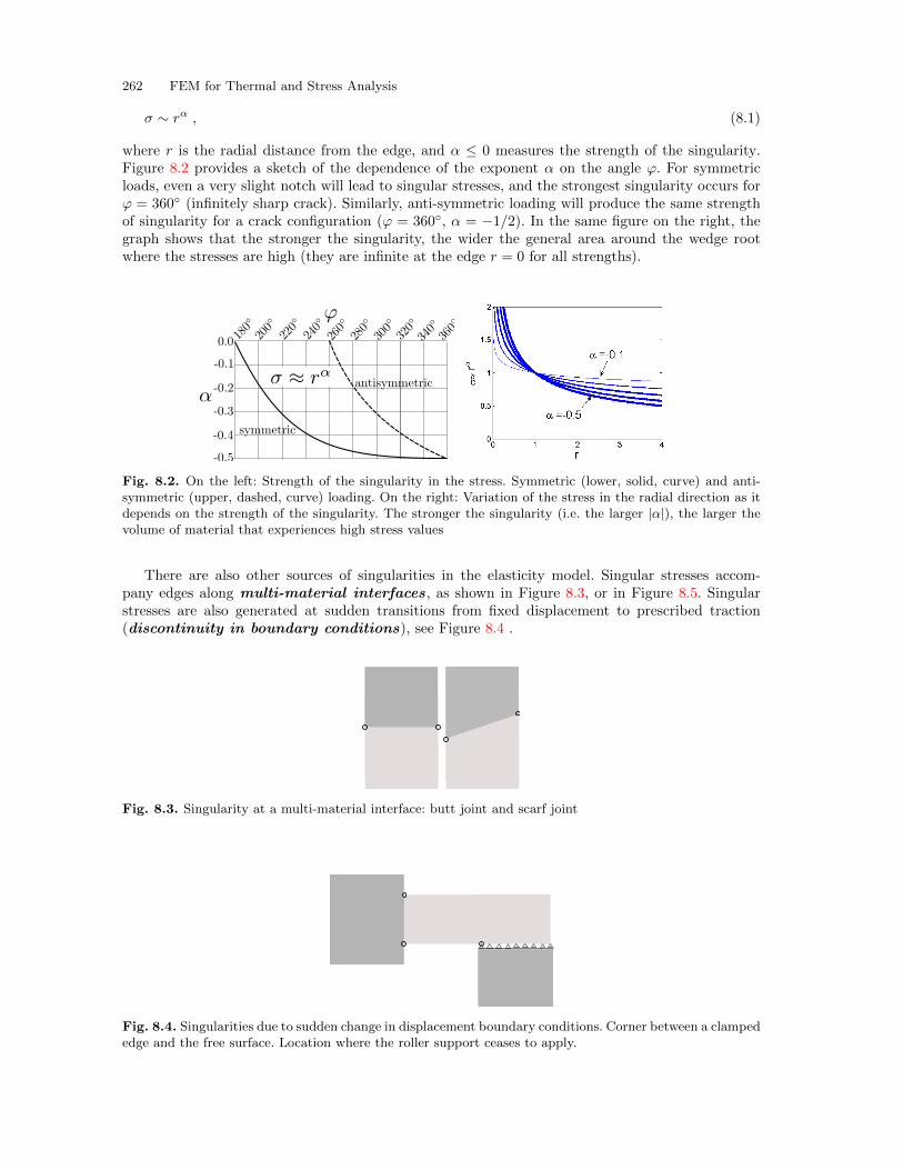
262 FEM for Thermal and Stress Analysis

σ ∼ rα , (8.1)

where r is the radial distance from the edge, and α ≤ 0 measures the strength of the singularity.Figure 8.2 provides a sketch of the dependence of the exponent α on the angle φ. For symmetricloads, even a very slight notch will lead to singular stresses, and the strongest singularity occurs forφ = 360◦ (infinitely sharp crack). Similarly, anti-symmetric loading will produce the same strengthof singularity for a crack configuration (φ = 360◦, α = −1/2). In the same figure on the right, thegraph shows that the stronger the singularity, the wider the general area around the wedge rootwhere the stresses are high (they are infinite at the edge r = 0 for all strengths).

Fig. 8.2. On the left: Strength of the singularity in the stress. Symmetric (lower, solid, curve) and anti-symmetric (upper, dashed, curve) loading. On the right: Variation of the stress in the radial direction as itdepends on the strength of the singularity. The stronger the singularity (i.e. the larger |α|), the larger thevolume of material that experiences high stress values

There are also other sources of singularities in the elasticity model. Singular stresses accom-pany edges along multi-material interfaces, as shown in Figure 8.3, or in Figure 8.5. Singularstresses are also generated at sudden transitions from fixed displacement to prescribed traction(discontinuity in boundary conditions), see Figure 8.4 .

Fig. 8.3. Singularity at a multi-material interface: butt joint and scarf joint

Fig. 8.4. Singularities due to sudden change in displacement boundary conditions. Corner between a clampededge and the free surface. Location where the roller support ceases to apply.

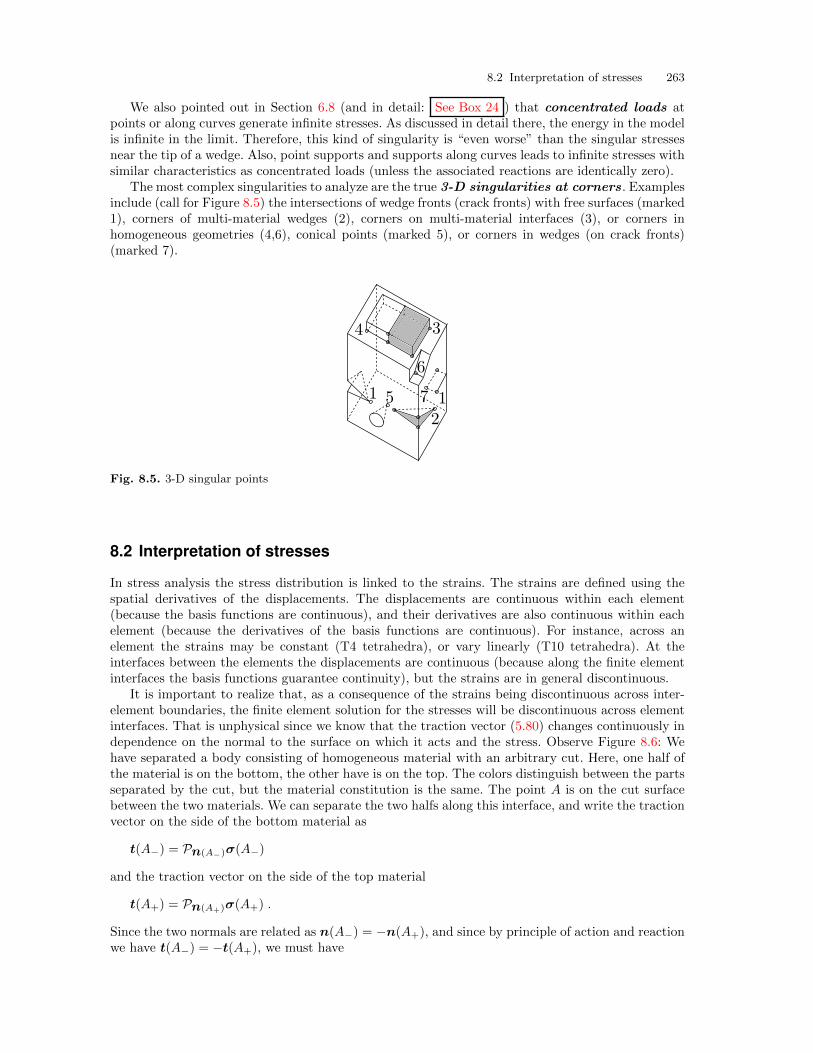
8.2 Interpretation of stresses 263

We also pointed out in Section 6.8 (and in detail: See Box 24 ) that concentrated loads atpoints or along curves generate infinite stresses. As discussed in detail there, the energy in the modelis infinite in the limit. Therefore, this kind of singularity is “even worse” than the singular stressesnear the tip of a wedge. Also, point supports and supports along curves leads to infinite stresses withsimilar characteristics as concentrated loads (unless the associated reactions are identically zero).

The most complex singularities to analyze are the true 3-D singularities at corners. Examplesinclude (call for Figure 8.5) the intersections of wedge fronts (crack fronts) with free surfaces (marked1), corners of multi-material wedges (2), corners on multi-material interfaces (3), or corners inhomogeneous geometries (4,6), conical points (marked 5), or corners in wedges (on crack fronts)(marked 7).

Fig. 8.5. 3-D singular points

8.2 Interpretation of stresses

In stress analysis the stress distribution is linked to the strains. The strains are defined using thespatial derivatives of the displacements. The displacements are continuous within each element(because the basis functions are continuous), and their derivatives are also continuous within eachelement (because the derivatives of the basis functions are continuous). For instance, across anelement the strains may be constant (T4 tetrahedra), or vary linearly (T10 tetrahedra). At theinterfaces between the elements the displacements are continuous (because along the finite elementinterfaces the basis functions guarantee continuity), but the strains are in general discontinuous.

It is important to realize that, as a consequence of the strains being discontinuous across inter-element boundaries, the finite element solution for the stresses will be discontinuous across elementinterfaces. That is unphysical since we know that the traction vector (5.80) changes continuously independence on the normal to the surface on which it acts and the stress. Observe Figure 8.6: Wehave separated a body consisting of homogeneous material with an arbitrary cut. Here, one half ofthe material is on the bottom, the other have is on the top. The colors distinguish between the partsseparated by the cut, but the material constitution is the same. The point A is on the cut surfacebetween the two materials. We can separate the two halfs along this interface, and write the tractionvector on the side of the bottom material as

t(A−) = Pn(A−)σ(A−)

and the traction vector on the side of the top material

t(A+) = Pn(A+)σ(A+) .

Since the two normals are related as n(A−) = −n(A+), and since by principle of action and reactionwe have t(A−) = −t(A+), we must have

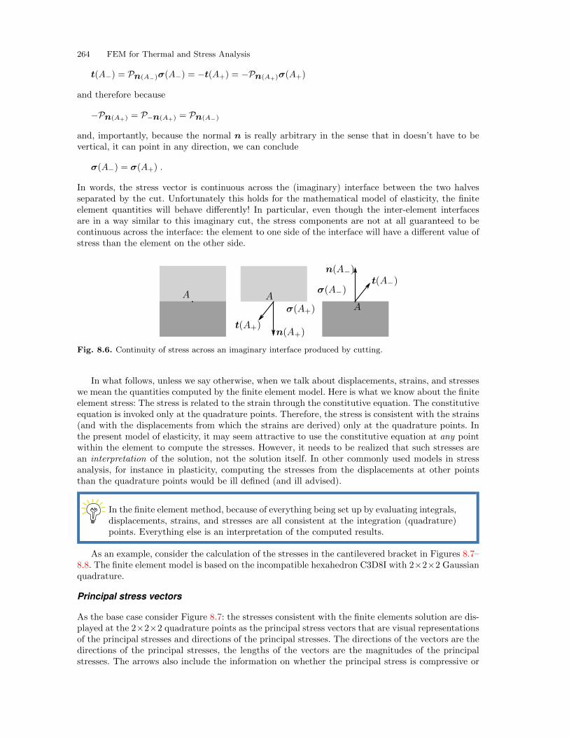
264 FEM for Thermal and Stress Analysis

t(A−) = Pn(A−)σ(A−) = −t(A+) = −Pn(A+)σ(A+)

and therefore because

−Pn(A+) = P−n(A+) = Pn(A−)

and, importantly, because the normal n is really arbitrary in the sense that in doesn’t have to bevertical, it can point in any direction, we can conclude

σ(A−) = σ(A+) .

In words, the stress vector is continuous across the (imaginary) interface between the two halvesseparated by the cut. Unfortunately this holds for the mathematical model of elasticity, the finiteelement quantities will behave differently! In particular, even though the inter-element interfacesare in a way similar to this imaginary cut, the stress components are not at all guaranteed to becontinuous across the interface: the element to one side of the interface will have a different value ofstress than the element on the other side.

Fig. 8.6. Continuity of stress across an imaginary interface produced by cutting.

In what follows, unless we say otherwise, when we talk about displacements, strains, and stresseswe mean the quantities computed by the finite element model. Here is what we know about the finiteelement stress: The stress is related to the strain through the constitutive equation. The constitutiveequation is invoked only at the quadrature points. Therefore, the stress is consistent with the strains(and with the displacements from which the strains are derived) only at the quadrature points. Inthe present model of elasticity, it may seem attractive to use the constitutive equation at any pointwithin the element to compute the stresses. However, it needs to be realized that such stresses arean interpretation of the solution, not the solution itself. In other commonly used models in stressanalysis, for instance in plasticity, computing the stresses from the displacements at other pointsthan the quadrature points would be ill defined (and ill advised).

In the finite element method, because of everything being set up by evaluating integrals,displacements, strains, and stresses are all consistent at the integration (quadrature)points. Everything else is an interpretation of the computed results.

As an example, consider the calculation of the stresses in the cantilevered bracket in Figures 8.7–8.8. The finite element model is based on the incompatible hexahedron C3D8I with 2×2×2 Gaussianquadrature.

Principal stress vectors

As the base case consider Figure 8.7: the stresses consistent with the finite elements solution are dis-played at the 2×2×2 quadrature points as the principal stress vectors that are visual representationsof the principal stresses and directions of the principal stresses. The directions of the vectors are thedirections of the principal stresses, the lengths of the vectors are the magnitudes of the principalstresses. The arrows also include the information on whether the principal stress is compressive or

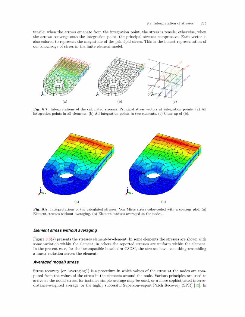
8.2 Interpretation of stresses 265

tensile: when the arrows emanate from the integration point, the stress is tensile; otherwise, whenthe arrows converge onto the integration point, the principal stresses compressive. Each vector isalso colored to represent the magnitude of the principal stress. This is the honest representation ofour knowledge of stress in the finite element model.

XY

Z

X XY

Z

(a) (b) (c)

Fig. 8.7. Interpretations of the calculated stresses. Principal stress vectors at integration points. (a) Allintegration points in all elements. (b) All integration points in two elements. (c) Close-up of (b).

XY

Z

XY

Z

(a) (b)

Fig. 8.8. Interpretations of the calculated stresses. Von Mises stress color-coded with a contour plot. (a)Element stresses without averaging. (b) Element stresses averaged at the nodes.

Element stress without averaging

Figure 8.8(a) presents the stresses element-by-element. In some elements the stresses are shown withsome variation within the element, in others the reported stresses are uniform within the element.In the present case, for the incompatible hexahedra C3D8I, the stresses have something resemblinga linear variation across the element.

Averaged (nodal) stress

Stress recovery (or “averaging”) is a procedure in which values of the stress at the nodes are com-puted from the values of the stress in the elements around the node. Various principles are used toarrive at the nodal stress, for instance simple average may be used, or a more sophisticated inverse-distance-weighted average, or the highly successful Superconvergent Patch Recovery (SPR) [12]. In

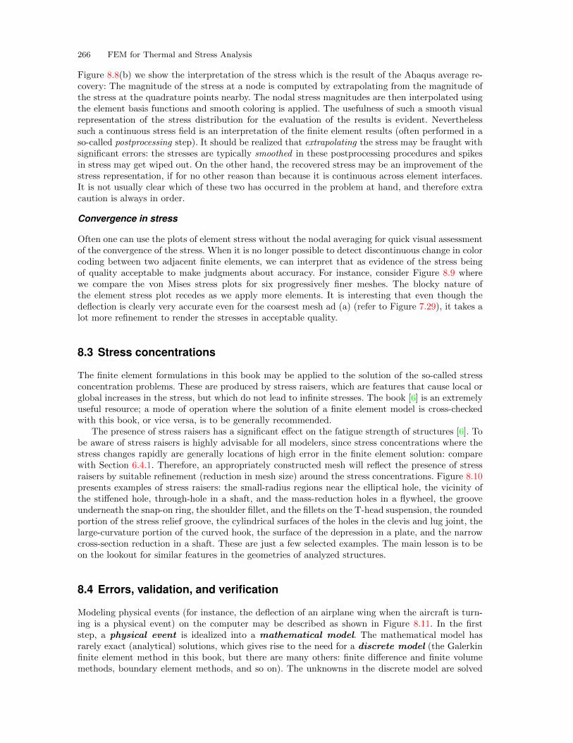
266 FEM for Thermal and Stress Analysis

Figure 8.8(b) we show the interpretation of the stress which is the result of the Abaqus average re-covery: The magnitude of the stress at a node is computed by extrapolating from the magnitude ofthe stress at the quadrature points nearby. The nodal stress magnitudes are then interpolated usingthe element basis functions and smooth coloring is applied. The usefulness of such a smooth visualrepresentation of the stress distribution for the evaluation of the results is evident. Neverthelesssuch a continuous stress field is an interpretation of the finite element results (often performed in aso-called postprocessing step). It should be realized that extrapolating the stress may be fraught withsignificant errors: the stresses are typically smoothed in these postprocessing procedures and spikesin stress may get wiped out. On the other hand, the recovered stress may be an improvement of thestress representation, if for no other reason than because it is continuous across element interfaces.It is not usually clear which of these two has occurred in the problem at hand, and therefore extracaution is always in order.

Convergence in stress

Often one can use the plots of element stress without the nodal averaging for quick visual assessmentof the convergence of the stress. When it is no longer possible to detect discontinuous change in colorcoding between two adjacent finite elements, we can interpret that as evidence of the stress beingof quality acceptable to make judgments about accuracy. For instance, consider Figure 8.9 wherewe compare the von Mises stress plots for six progressively finer meshes. The blocky nature ofthe element stress plot recedes as we apply more elements. It is interesting that even though thedeflection is clearly very accurate even for the coarsest mesh ad (a) (refer to Figure 7.29), it takes alot more refinement to render the stresses in acceptable quality.

8.3 Stress concentrations

The finite element formulations in this book may be applied to the solution of the so-called stressconcentration problems. These are produced by stress raisers, which are features that cause local orglobal increases in the stress, but which do not lead to infinite stresses. The book [6] is an extremelyuseful resource; a mode of operation where the solution of a finite element model is cross-checkedwith this book, or vice versa, is to be generally recommended.

The presence of stress raisers has a significant effect on the fatigue strength of structures [6]. Tobe aware of stress raisers is highly advisable for all modelers, since stress concentrations where thestress changes rapidly are generally locations of high error in the finite element solution: comparewith Section 6.4.1. Therefore, an appropriately constructed mesh will reflect the presence of stressraisers by suitable refinement (reduction in mesh size) around the stress concentrations. Figure 8.10presents examples of stress raisers: the small-radius regions near the elliptical hole, the vicinity ofthe stiffened hole, through-hole in a shaft, and the mass-reduction holes in a flywheel, the grooveunderneath the snap-on ring, the shoulder fillet, and the fillets on the T-head suspension, the roundedportion of the stress relief groove, the cylindrical surfaces of the holes in the clevis and lug joint, thelarge-curvature portion of the curved hook, the surface of the depression in a plate, and the narrowcross-section reduction in a shaft. These are just a few selected examples. The main lesson is to beon the lookout for similar features in the geometries of analyzed structures.

8.4 Errors, validation, and verification

Modeling physical events (for instance, the deflection of an airplane wing when the aircraft is turn-ing is a physical event) on the computer may be described as shown in Figure 8.11. In the firststep, a physical event is idealized into a mathematical model. The mathematical model hasrarely exact (analytical) solutions, which gives rise to the need for a discrete model (the Galerkinfinite element method in this book, but there are many others: finite difference and finite volumemethods, boundary element methods, and so on). The unknowns in the discrete model are solved

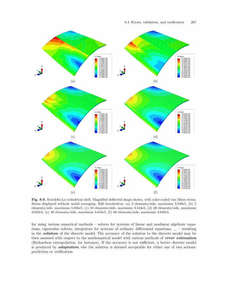
8.4 Errors, validation, and verification 267

S, Mises

+1.040e+04+3.494e+04+5.948e+04+8.403e+04+1.086e+05+1.331e+05+1.577e+05+1.822e+05+2.067e+05+2.313e+05+2.558e+05+2.804e+05+3.049e+05

X

Y

Z

S, Mises

+2.156e+03+2.994e+04+5.773e+04+8.551e+04+1.133e+05+1.411e+05+1.689e+05+1.967e+05+2.244e+05+2.522e+05+2.800e+05+3.078e+05+3.356e+05

X

Y

Z

(a) (b)

S, Mises

+7.825e+02+3.025e+04+5.972e+04+8.919e+04+1.187e+05+1.481e+05+1.776e+05+2.071e+05+2.365e+05+2.660e+05+2.955e+05+3.250e+05+3.544e+05

X

Y

Z

S, Mises

+3.920e+02+3.057e+04+6.074e+04+9.092e+04+1.211e+05+1.513e+05+1.814e+05+2.116e+05+2.418e+05+2.720e+05+3.022e+05+3.323e+05+3.625e+05

X

Y

Z

(c) (d)

S, Mises

+3.357e+02+3.068e+04+6.103e+04+9.138e+04+1.217e+05+1.521e+05+1.824e+05+2.128e+05+2.431e+05+2.735e+05+3.038e+05+3.342e+05+3.645e+05

X

Y

Z

S, Mises

+3.222e+02+3.070e+04+6.107e+04+9.145e+04+1.218e+05+1.522e+05+1.826e+05+2.129e+05+2.433e+05+2.737e+05+3.041e+05+3.345e+05+3.648e+05

X

Y

Z

(e) (f)

Fig. 8.9. Scordelis-Lo cylindrical shell. Magnified deflected shape shown, with color-coded von Mises stress.Stress displayed without nodal averaging. H20 hexahedron: (a) 3 elements/side, maximum 3.049e5, (b) 5elements/side, maximum 3.356e5, (c) 10 elements/side, maximum 3.544e5, (d) 20 elements/side, maximum3.625e5, (e) 40 elements/side, maximum 3.645e5, (f) 80 elements/side, maximum 3.648e5.

for using various numerical methods – solvers for systems of linear and nonlinear algebraic equa-tions, eigenvalue solvers, integrators for systems of ordinary differential equations, ... – resultingin the solution of the discrete model. The accuracy of the solution to the discrete model may bethen assessed with respect to the mathematical model with various methods of error estimation(Richardson extrapolation, for instance). If the accuracy is not sufficient, a better discrete modelis produced by adaptation, else the solution is deemed acceptable for either one of two actions:prediction or verification.

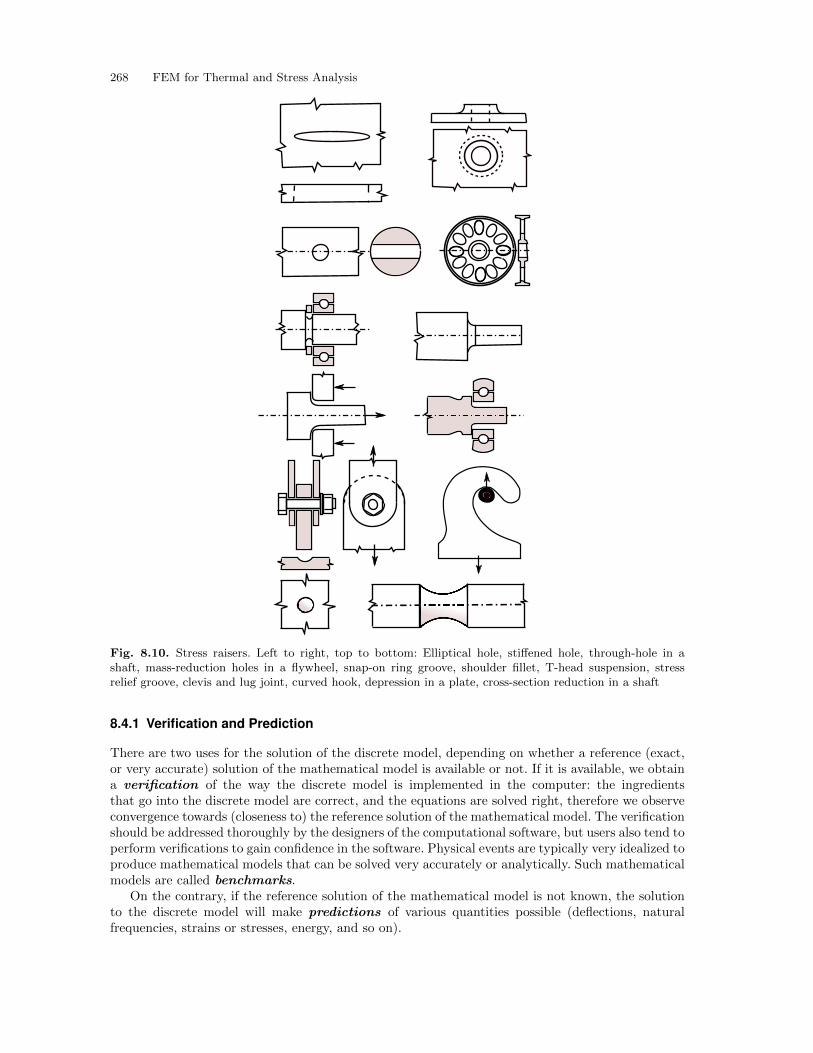
268 FEM for Thermal and Stress Analysis

Fig. 8.10. Stress raisers. Left to right, top to bottom: Elliptical hole, stiffened hole, through-hole in ashaft, mass-reduction holes in a flywheel, snap-on ring groove, shoulder fillet, T-head suspension, stressrelief groove, clevis and lug joint, curved hook, depression in a plate, cross-section reduction in a shaft

8.4.1 Verification and Prediction

There are two uses for the solution of the discrete model, depending on whether a reference (exact,or very accurate) solution of the mathematical model is available or not. If it is available, we obtaina verification of the way the discrete model is implemented in the computer: the ingredientsthat go into the discrete model are correct, and the equations are solved right, therefore we observeconvergence towards (closeness to) the reference solution of the mathematical model. The verificationshould be addressed thoroughly by the designers of the computational software, but users also tend toperform verifications to gain confidence in the software. Physical events are typically very idealized toproduce mathematical models that can be solved very accurately or analytically. Such mathematicalmodels are called benchmarks.

On the contrary, if the reference solution of the mathematical model is not known, the solutionto the discrete model will make predictions of various quantities possible (deflections, naturalfrequencies, strains or stresses, energy, and so on).

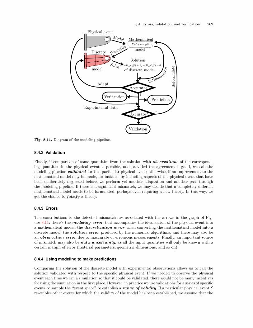
8.4 Errors, validation, and verification 269

Fig. 8.11. Diagram of the modeling pipeline.

8.4.2 Validation

Finally, if comparison of some quantities from the solution with observations of the correspond-ing quantities in the physical event is possible, and provided the agreement is good, we call themodeling pipeline validated for this particular physical event; otherwise, if an improvement to themathematical model may be made, for instance by including aspects of the physical event that havebeen deliberately neglected before, we perform yet another adaptation and another pass throughthe modeling pipeline. If there is a significant mismatch, we may decide that a completely differentmathematical model needs to be formulated, perhaps even requiring a new theory. In this way, weget the chance to falsify a theory.

8.4.3 Errors

The contributions to the detected mismatch are associated with the arrows in the graph of Fig-ure 8.11: there’s the modeling error that accompanies the idealization of the physical event intoa mathematical model, the discretization error when converting the mathematical model into adiscrete model, the solution error produced by the numerical algorithms, and there may also bean observation error due to inaccurate or erroneous measurements. Finally, an important sourceof mismatch may also be data uncertainty, as all the input quantities will only be known with acertain margin of error (material parameters, geometric dimensions, and so on).

8.4.4 Using modeling to make predictions

Comparing the solution of the discrete model with experimental observations allows us to call thesolution validated with respect to the specific physical event. If we needed to observe the physicalevent each time we ran a simulation so that it could be validated, there would not be many incentivesfor using the simulation in the first place. However, in practice we use validations for a series of specificevents to sample the “event space” to establish a range of validity. If a particular physical event Eresembles other events for which the validity of the model has been established, we assume that the

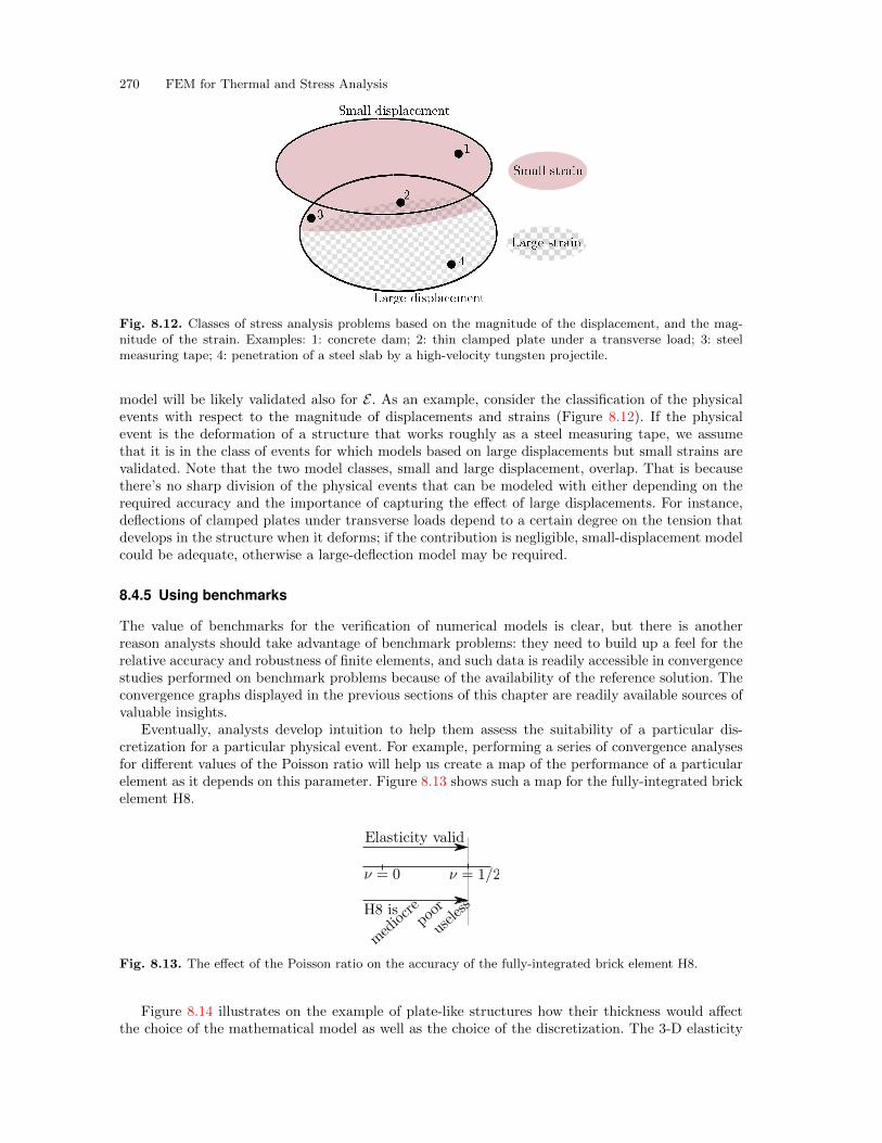
270 FEM for Thermal and Stress Analysis

Fig. 8.12. Classes of stress analysis problems based on the magnitude of the displacement, and the mag-nitude of the strain. Examples: 1: concrete dam; 2: thin clamped plate under a transverse load; 3: steelmeasuring tape; 4: penetration of a steel slab by a high-velocity tungsten projectile.

model will be likely validated also for E . As an example, consider the classification of the physicalevents with respect to the magnitude of displacements and strains (Figure 8.12). If the physicalevent is the deformation of a structure that works roughly as a steel measuring tape, we assumethat it is in the class of events for which models based on large displacements but small strains arevalidated. Note that the two model classes, small and large displacement, overlap. That is becausethere’s no sharp division of the physical events that can be modeled with either depending on therequired accuracy and the importance of capturing the effect of large displacements. For instance,deflections of clamped plates under transverse loads depend to a certain degree on the tension thatdevelops in the structure when it deforms; if the contribution is negligible, small-displacement modelcould be adequate, otherwise a large-deflection model may be required.

8.4.5 Using benchmarks

The value of benchmarks for the verification of numerical models is clear, but there is anotherreason analysts should take advantage of benchmark problems: they need to build up a feel for therelative accuracy and robustness of finite elements, and such data is readily accessible in convergencestudies performed on benchmark problems because of the availability of the reference solution. Theconvergence graphs displayed in the previous sections of this chapter are readily available sources ofvaluable insights.

Eventually, analysts develop intuition to help them assess the suitability of a particular dis-cretization for a particular physical event. For example, performing a series of convergence analysesfor different values of the Poisson ratio will help us create a map of the performance of a particularelement as it depends on this parameter. Figure 8.13 shows such a map for the fully-integrated brickelement H8.

Fig. 8.13. The effect of the Poisson ratio on the accuracy of the fully-integrated brick element H8.

Figure 8.14 illustrates on the example of plate-like structures how their thickness would affectthe choice of the mathematical model as well as the choice of the discretization. The 3-D elasticity

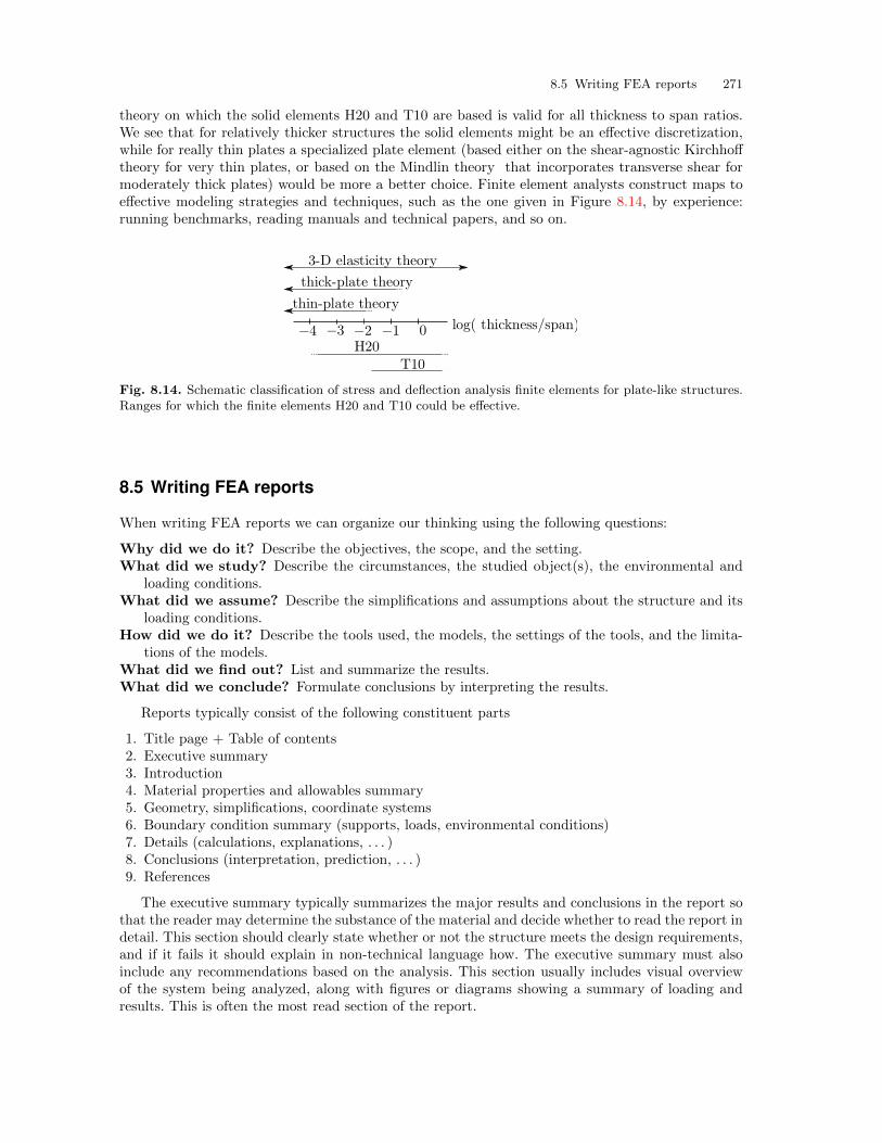
8.5 Writing FEA reports 271

theory on which the solid elements H20 and T10 are based is valid for all thickness to span ratios.We see that for relatively thicker structures the solid elements might be an effective discretization,while for really thin plates a specialized plate element (based either on the shear-agnostic Kirchhofftheory for very thin plates, or based on the Mindlin theory that incorporates transverse shear formoderately thick plates) would be more a better choice. Finite element analysts construct maps toeffective modeling strategies and techniques, such as the one given in Figure 8.14, by experience:running benchmarks, reading manuals and technical papers, and so on.

Fig. 8.14. Schematic classification of stress and deflection analysis finite elements for plate-like structures.Ranges for which the finite elements H20 and T10 could be effective.

8.5 Writing FEA reports

When writing FEA reports we can organize our thinking using the following questions:

Why did we do it? Describe the objectives, the scope, and the setting.What did we study? Describe the circumstances, the studied object(s), the environmental and

loading conditions.What did we assume? Describe the simplifications and assumptions about the structure and its

loading conditions.How did we do it? Describe the tools used, the models, the settings of the tools, and the limita-

tions of the models.What did we find out? List and summarize the results.What did we conclude? Formulate conclusions by interpreting the results.

Reports typically consist of the following constituent parts

1. Title page + Table of contents2. Executive summary3. Introduction4. Material properties and allowables summary5. Geometry, simplifications, coordinate systems6. Boundary condition summary (supports, loads, environmental conditions)7. Details (calculations, explanations, . . . )8. Conclusions (interpretation, prediction, . . . )9. References

The executive summary typically summarizes the major results and conclusions in the report sothat the reader may determine the substance of the material and decide whether to read the report indetail. This section should clearly state whether or not the structure meets the design requirements,and if it fails it should explain in non-technical language how. The executive summary must alsoinclude any recommendations based on the analysis. This section usually includes visual overviewof the system being analyzed, along with figures or diagrams showing a summary of loading andresults. This is often the most read section of the report.

272 FEM for Thermal and Stress Analysis

The FE analysis report is often the document that makes the study reproducible . Inother words, the report should allow someone else to perform the same study to verifyour own results. This aspect is very important indeed: if for no other reason, then tomeet our professional responsibilities.

An example of a report from a finite element analysis is provided in the next section. See Box 33The section also includes a list of reporting dos and don’ts, an incomplete list, but useful nonethe-

less. See Box 34

8.6 Background, explanations, details

Box 33. Strap analysis: Sample FEA report

The following pages show a sample report from an FE analysis. (The report pages are framedfor visual clarity.)

Investigation of the Tresca Stress in a SteelStrap

Petr Krysl

February 18, 2017

Contents

1 Executive Summary 1

2 Introduction 3

3 Material properties 3

4 Geometry 3

5 Boundary conditions 4

6 Detailed calculations 4

7 Conclusions 9

1 Executive Summary

The objective was to calculate accurately the Tresca stress, as a measure ofstress intensity, in a steel strap under tensile loads. The part was modeledusing the plane-stress idealization. Figure 1 shows graphically the bound-ary conditions (clamped edge at the left-hand side, edge with uniformly dis-tributed pressure on the right-hand side), and the six points of interest wherethe Tresca stress was to be computed.

1

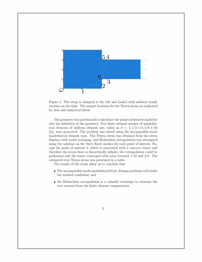
Z

Y

X

X

Y

Z

Figure 1: The strap is clamped at the left and loaded with uniform tensiletraction on the right. The output locations for the Tresca stress are indicatedby dots and numerical labels.

The geometry was partitioned to introduce the points of interest explicitlyinto the definition of the geometry. Five finite element meshes of quadrilat-eral elements of uniform element size, taken as h = 1, 1/2, 1/4, 1/8, 1/16[in], were generated. The problem was solved using the incompatible-modequadrilateral element type. The Tresca stress was obtained from the stressdisplays with nodal averaging, and Richardson extrapolation was attemptedusing the solution on the three finest meshes for each point of interest. Ex-cept for point of interest 5, which is associated with a concave corner andtherefore the stress there is theoretically infinite, the extrapolation could beperformed and the stress converged with rates between 1.12 and 2.8. Theestimated true Tresca stress was presented in a table.

The results of the study allow us to conclude that

• The incompatible-mode quadrilateral from Abaqus performs well underthe studied conditions; and

• the Richardson extrapolation is a valuable technique to estimate thetrue answers from the finite element computations.

2

2 Introduction

The goal of the present study is to illustrate calculation of accurate stressresults under nontrivial conditions. In the present case the geometry incor-porates several stress raisers: the concave corners where the narrower part ofthe strap transitions into the wide part, one with a fillet, and one with sharpinterior angle; further, where the wide part is clamped along the left-handside edge, the corners of that side are also locations of stress concentrations.

The procedure is to compute several solutions with uniform meshes ofdifferent resolutions (i.e. built up of elements of different sizes), and then toattempt extrapolation to the limit of the element size vanishing (h → 0).

The Abaqus/Standard, version 6.14.1, finite element program was adoptedin this study.

3 Material properties

The material was assumed to be steel, with Young’s modulus of 30 × 106 psiand Poisson ratio of 0.3.

4 Geometry

The geometry of the strap is shown in Figure 2. Note that one corner isleft sharp with a 90o interior angle, and one corner is rounded with a filletfeature.

Figure 3 illustrates the partitioning of the part into eight regions in orderto incorporate the points of interest into the geometry, and to make it possiblefor the mesher to succeed in building quadrilateral meshes. The six points ofinterest are indicated in the figure. Note that point 5 is located at the rootof the concave corner, and point 6 is located at the midpoint of the edge thatrepresents the fillet.

The strap is of uniform thickness of 0.25 in, which is a sufficiently smallthickness to allow for the plane-stress modeling to be used.

3

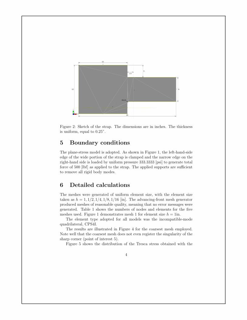
V

H

V

H

3.

12.

12.

1.5

R0.25

24.

6.

X

Y

Z

Figure 2: Sketch of the strap. The dimensions are in inches. The thicknessis uniform, equal to 0.25”.

5 Boundary conditions

The plane-stress model is adopted. As shown in Figure 1, the left-hand-sideedge of the wide portion of the strap is clamped and the narrow edge on theright-hand side is loaded by uniform pressure 333.3333 [psi] to generate totalforce of 500 [lbf] as applied to the strap. The applied supports are sufficientto remove all rigid body modes.

6 Detailed calculations

The meshes were generated of uniform element size, with the element sizetaken as h = 1, 1/2, 1/4, 1/8, 1/16 [in]. The advancing-front mesh generatorproduced meshes of reasonable quality, meaning that no error messages weregenerated. Table 1 shows the numbers of nodes and elements for the fivemeshes used. Figure 1 demonstrates mesh 1 for element size h = 1in.

The element type adopted for all models was the incompatible-modequadrilateral, CPS4I.

The results are illustrated in Figure 4 for the coarsest mesh employed.Note well that the coarsest mesh does not even register the singularity of thesharp corner (point of interest 5).

Figure 5 shows the distribution of the Tresca stress obtained with the

4

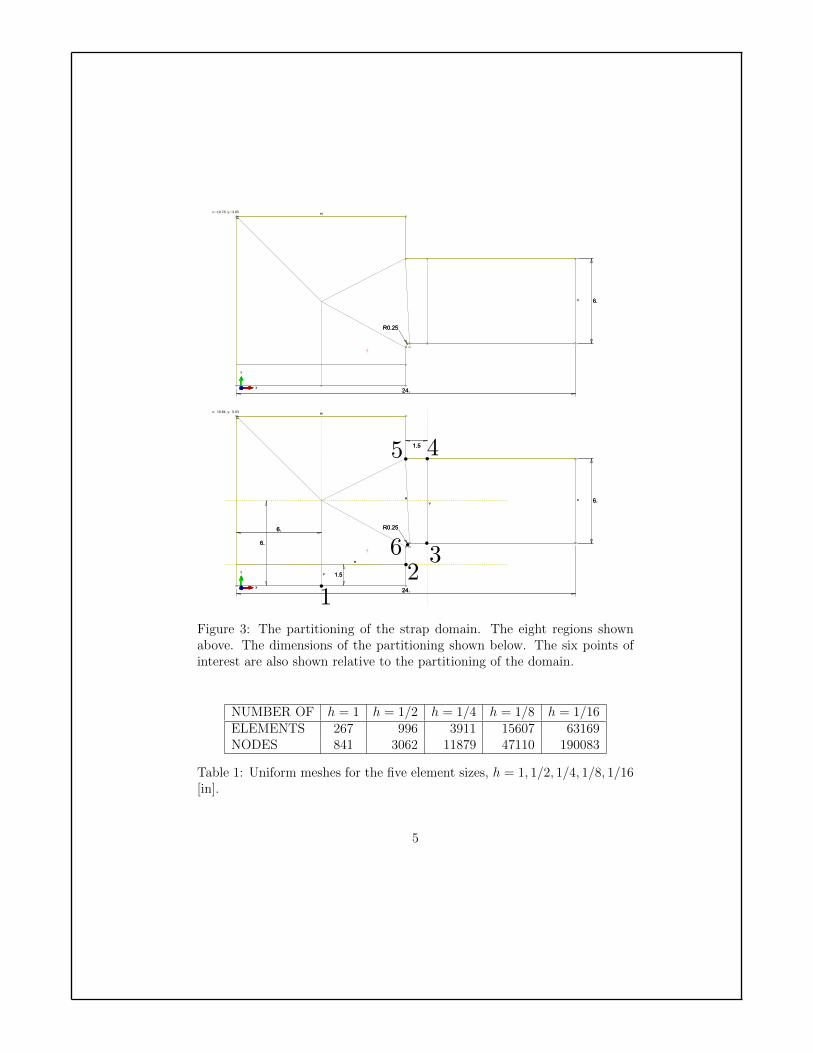
6.

24.

R0.25

H

V 6.

24.

R0.25

H

V

X

Y

Z

x:−10.78, y:−3.85

6.

24.

R0.25

1.5

6.

6.

1.5

H

V

V

H

V

H6.

24.

R0.25

1.5

6.

6.

1.5

H

V

V

H

V

H

X

Y

Z

x:�10.84, y:�0.03

Figure 3: The partitioning of the strap domain. The eight regions shownabove. The dimensions of the partitioning shown below. The six points ofinterest are also shown relative to the partitioning of the domain.

NUMBER OF h = 1 h = 1/2 h = 1/4 h = 1/8 h = 1/16ELEMENTS 267 996 3911 15607 63169NODES 841 3062 11879 47110 190083

Table 1: Uniform meshes for the five element sizes, h = 1, 1/2, 1/4, 1/8, 1/16[in].

5

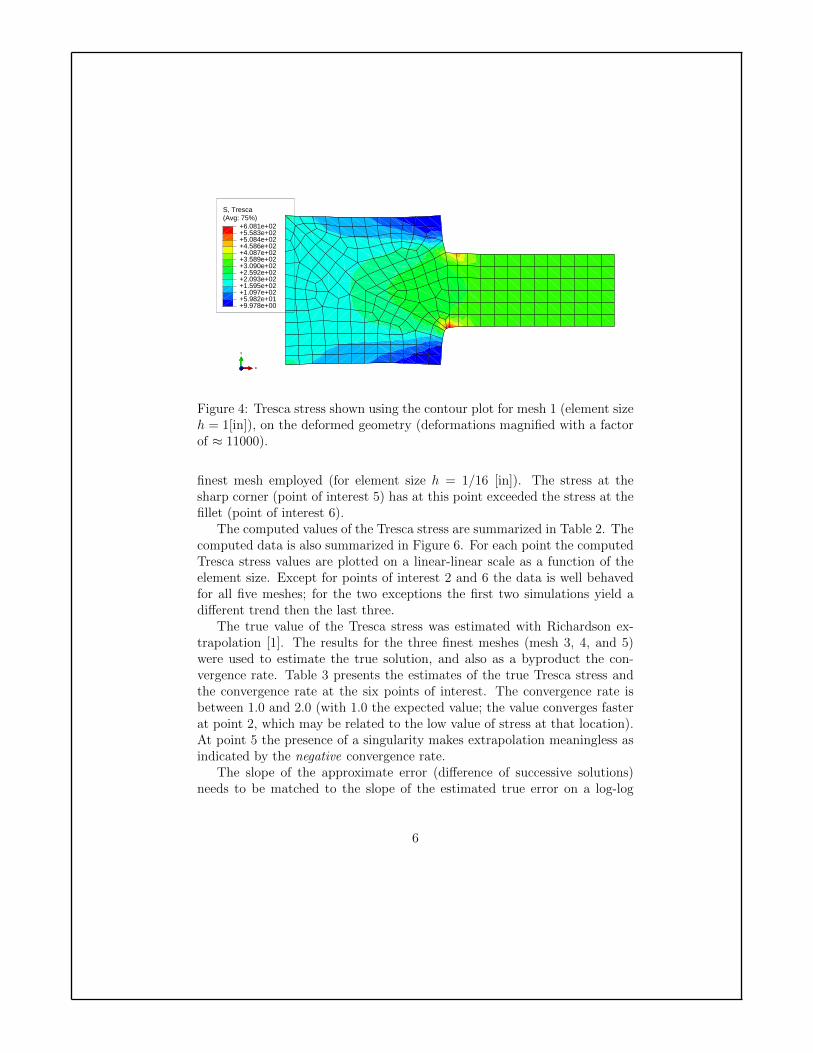
(Avg: 75%)S, Tresca

+9.978e+00+5.982e+01+1.097e+02+1.595e+02+2.093e+02+2.592e+02+3.090e+02+3.589e+02+4.087e+02+4.586e+02+5.084e+02+5.583e+02+6.081e+02

X

Y

Z

Figure 4: Tresca stress shown using the contour plot for mesh 1 (element sizeh = 1[in]), on the deformed geometry (deformations magnified with a factorof ≈ 11000).

finest mesh employed (for element size h = 1/16 [in]). The stress at thesharp corner (point of interest 5) has at this point exceeded the stress at thefillet (point of interest 6).

The computed values of the Tresca stress are summarized in Table 2. Thecomputed data is also summarized in Figure 6. For each point the computedTresca stress values are plotted on a linear-linear scale as a function of theelement size. Except for points of interest 2 and 6 the data is well behavedfor all five meshes; for the two exceptions the first two simulations yield adifferent trend then the last three.

The true value of the Tresca stress was estimated with Richardson ex-trapolation [1]. The results for the three finest meshes (mesh 3, 4, and 5)were used to estimate the true solution, and also as a byproduct the con-vergence rate. Table 3 presents the estimates of the true Tresca stress andthe convergence rate at the six points of interest. The convergence rate isbetween 1.0 and 2.0 (with 1.0 the expected value; the value converges fasterat point 2, which may be related to the low value of stress at that location).At point 5 the presence of a singularity makes extrapolation meaningless asindicated by the negative convergence rate.

The slope of the approximate error (difference of successive solutions)needs to be matched to the slope of the estimated true error on a log-log

6

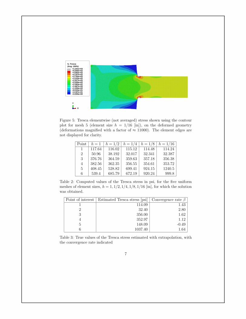
(Avg: 100%)S, Tresca

+0.000e+00+4.167e+01+8.333e+01+1.250e+02+1.667e+02+2.083e+02+2.500e+02+2.917e+02+3.333e+02+3.750e+02+4.167e+02+4.583e+02+5.000e+02+1.241e+03

X

Y

Z

Figure 5: Tresca elementwise (not averaged) stress shown using the contourplot for mesh 5 (element size h = 1/16 [in]), on the deformed geometry(deformations magnified with a factor of ≈ 11000). The element edges arenot displayed for clarity.

Point h = 1 h = 1/2 h = 1/4 h = 1/8 h = 1/161 117.64 116.02 115.12 114.48 114.242 50.96 38.192 32.017 32.341 32.3873 376.76 364.59 359.63 357.18 356.384 382.56 362.35 356.55 354.61 353.725 408.45 528.82 699.41 924.15 1240.56 539.4 685.79 672.19 920.24 999.8

Table 2: Computed values of the Tresca stress in psi, for the five uniformmeshes of element sizes, h = 1, 1/2, 1/4, 1/8, 1/16 [in], for which the solutionwas obtained.

Point of interest Estimated Tresca stress [psi] Convergence rate β1 114.09 1.432 32.40 2.803 356.00 1.624 352.97 1.125 148.09 -0.496 1037.40 1.64

Table 3: True values of the Tresca stress estimated with extrapolation, withthe convergence rate indicated

7

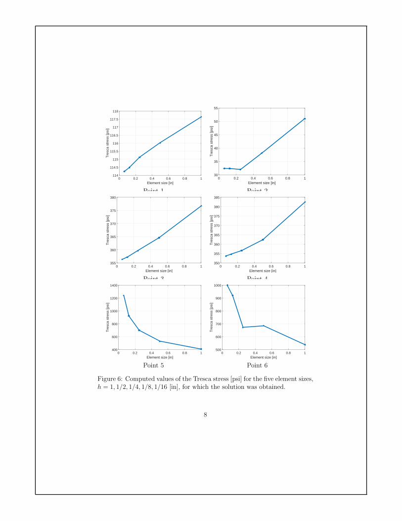
Element size [in]0 0.2 0.4 0.6 0.8 1

Tre

sca

stre

ss [p

si]

114

114.5

115

115.5

116

116.5

117

117.5

118

Element size [in]0 0.2 0.4 0.6 0.8 1

Tre

sca

stre

ss [p

si]

30

35

40

45

50

55

Point 1 Point 2

Element size [in]0 0.2 0.4 0.6 0.8 1

Tre

sca

stre

ss [p

si]

355

360

365

370

375

380

Element size [in]0 0.2 0.4 0.6 0.8 1

Tre

sca

stre

ss [p

si]

350

355

360

365

370

375

380

385

Point 3 Point 4

Element size [in]0 0.2 0.4 0.6 0.8 1

Tre

sca

stre

ss [p

si]

400

600

800

1000

1200

1400

Element size [in]0 0.2 0.4 0.6 0.8 1

Tre

sca

stre

ss [p

si]

500

600

700

800

900

1000

Point 5 Point 6

Figure 6: Computed values of the Tresca stress [psi] for the five element sizes,h = 1, 1/2, 1/4, 1/8, 1/16 [in], for which the solution was obtained.

8

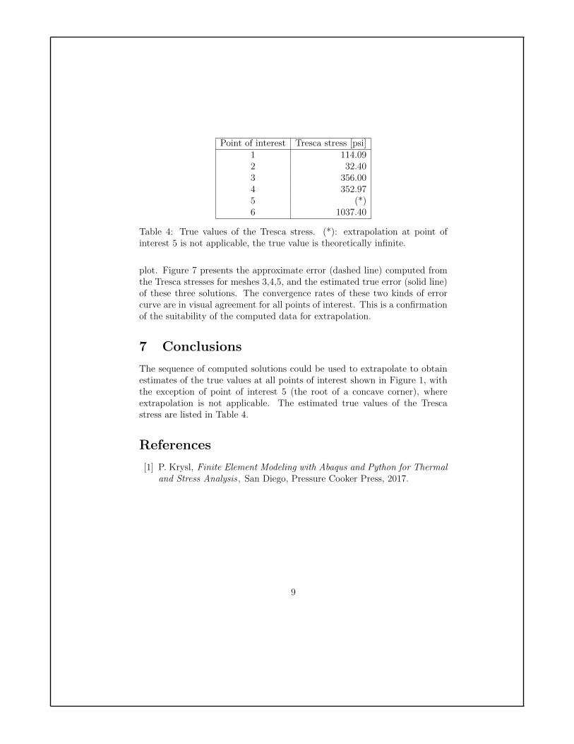
Point of interest Tresca stress [psi]1 114.092 32.403 356.004 352.975 (*)6 1037.40

Table 4: True values of the Tresca stress. (*): extrapolation at point ofinterest 5 is not applicable, the true value is theoretically infinite.

plot. Figure 7 presents the approximate error (dashed line) computed fromthe Tresca stresses for meshes 3,4,5, and the estimated true error (solid line)of these three solutions. The convergence rates of these two kinds of errorcurve are in visual agreement for all points of interest. This is a confirmationof the suitability of the computed data for extrapolation.

7 Conclusions

The sequence of computed solutions could be used to extrapolate to obtainestimates of the true values at all points of interest shown in Figure 1, withthe exception of point of interest 5 (the root of a concave corner), whereextrapolation is not applicable. The estimated true values of the Trescastress are listed in Table 4.

References

[1] P. Krysl, Finite Element Modeling with Abaqus and Python for Thermaland Stress Analysis , San Diego, Pressure Cooker Press, 2017.

9

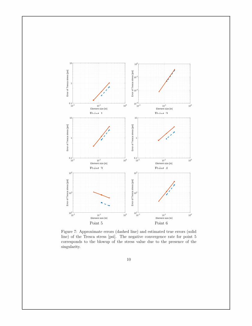
Element size [in]10-2 10-1 100

Err

or o

f Tre

sca

stre

ss [p

si]

0.1

1

10

Element size [in]10-2 10-1 100

Err

or o

f Tre

sca

stre

ss [p

si]

10-3

10-2

10-1

100

Point 1 Point 2

Element size [in]10-2 10-1 100

Err

or o

f Tre

sca

stre

ss [p

si]

0.1

1

10

Element size [in]10-2 10-1 100

Err

or o

f Tre

sca

stre

ss [p

si]

0.1

1

10

Point 3 Point 4

Element size [in]10-2 10-1 100

Err

or o

f Tre

sca

stre

ss [p

si]

102

103

104

Element size [in]10-2 10-1 100

Err

or o

f Tre

sca

stre

ss [p

si]

101

102

103

Point 5 Point 6

Figure 7: Approximate errors (dashed line) and estimated true errors (solidline) of the Tresca stress [psi]. The negative convergence rate for point 5corresponds to the blowup of the stress value due to the presence of thesingularity.

10

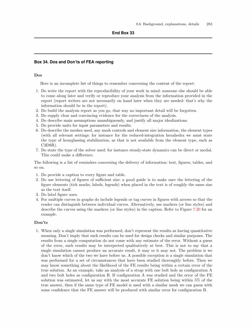
8.6 Background, explanations, details 283

End Box 33

Box 34. Dos and Don’ts of FEA reporting

Dos

Here is an incomplete list of things to remember concerning the content of the report:

1. Do write the report with the reproducibility of your work in mind: someone else should be ableto come along later and verify or reproduce your analysis from the information provided in thereport (report writers are not necessarily on hand later when they are needed: that’s why theinformation should be in the report).

2. Do build the analysis report as you go, that way no important detail will be forgotten.3. Do supply clear and convincing evidence for the correctness of the analysis.4. Do describe main assumptions unambiguously, and justify all major idealizations.5. Do provide units for input parameters and results.6. Do describe the meshes used, any mesh controls and element size information, the element types

(with all relevant settings: for instance for the reduced-integration hexahedra we must statethe type of hourglassing stabilization, as that is not available from the element type, such asC3D8R).

7. Do state the type of the solver used: for instance steady-state dynamics can be direct or modal.This could make a difference.

The following is a list of reminders concerning the delivery of information: text, figures, tables, andso on.

1. Do provide a caption to every figure and table.2. Do use lettering of figures of sufficient size: a good guide is to make sure the lettering of the

figure elements (tick marks, labels, legends) when placed in the text is of roughly the same sizeas the text itself.

3. Do label figure axes.4. For multiple curves in graphs do include legends or tag curves in figures with arrows so that the

reader can distinguish between individual curves. Alternatively, use markers (or line styles) anddescribe the curves using the markers (or line styles) in the caption. Refer to Figure 7.20 for anexample.

Don’ts

1. When only a single simulation was performed, don’t represent the results as having quantitativemeaning. Don’t imply that such results can be used for design checks and similar purposes. Theresults from a single computation do not come with any estimate of the error. Without a guessof the error, such results may be interpreted qualitatively at best. This is not to say that asingle simulation cannot produce an accurate result, it may or it may not. The problem is wedon’t know which of the two we have before us. A possible exception is a single simulation thatwas performed for a set of circumstances that have been studied thoroughly before. Then wemay know something about the likelihood of the FE results being within a certain error of thetrue solution. As an example, take an analysis of a strap with one bolt hole as configuration Aand two bolt holes as configuration B. If configuration A was studied and the error of the FEsolution was estimated, let us say with the most accurate FE solution being within 5% of thetrue answer, then if the same type of FE model is used with a similar mesh we can guess withsome confidence that the FE answer will be produced with similar error for configuration B.

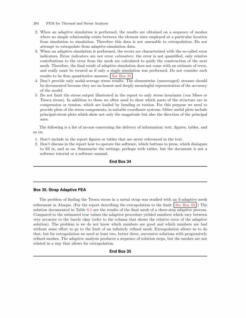
284 FEM for Thermal and Stress Analysis

2. When an adaptive simulation is performed, the results are obtained on a sequence of mesheswhere no simple relationship exists between the element sizes employed at a particular locationfrom simulation to simulation. Therefore this data is not amenable to extrapolation. Do notattempt to extrapolate from adaptive-simulation data.

3. When an adaptive simulation is performed, the errors are characterized with the so-called errorindicators. Error indicators are not error estimators: the error is not quantified, only relativecontributions to the error from the mesh are calculated to guide the construction of the nextmesh. Therefore, the final result of adaptive simulation does not come with an estimate of error,and really must be treated as if only a single simulation was performed. Do not consider such

results to be firm quantitative answers. See Box 354. Don’t provide only nodal-average stress results. The elementwise (unaveraged) stresses should

be documented because they are an honest and deeply meaningful representation of the accuracyof the model.

5. Do not limit the stress output illustrated in the report to only stress invariants (von Mises orTresca stress). In addition to these we often need to show which parts of the structure are incompression or tension, which are loaded by bending or torsion. For this purpose we need toprovide plots of the stress components, in suitable coordinate systems. Other useful plots includeprincipal-stress plots which show not only the magnitude but also the direction of the principalaxes.

The following is a list of no-nos concerning the delivery of information: text, figures, tables, andso on.

1. Don’t include in the report figures or tables that are never referenced in the text.2. Don’t discuss in the report how to operate the software, which buttons to press, which dialogues

to fill in, and so on. Summarize the settings, perhaps with tables, but the document is not asoftware tutorial or a software manual.

End Box 34

Box 35. Strap Adaptive FEA

The problem of finding the Tresca stress in a metal strap was studied with an h-adaptive mesh

refinement in Abaqus. (For the report describing the extrapolation to the limit: See Box 33 .) Thesolution documented in Table 8.1 are the results of the final mesh of a three-step adaptive process.Compared to the estimated true values the adaptive procedure yielded numbers which vary betweenvery accurate to the barely okay (refer to the column that shows the relative error of the adaptivesolution). The problem is we do not know which numbers are good and which numbers are badwithout some effort to go to the limit of an infinitely refined mesh. Extrapolation allows us to dothat, but for extrapolation we need at least two, better three, successive solutions with progressivelyrefined meshes. The adaptive analysis produces a sequence of solution steps, but the meshes are notrelated in a way that allows for extrapolation.

End Box 35

Point of interest Estimated true stressAdaptive simulation

stress

Relative error of theadaptive solution

1 114.09 113.70 0.30%2 32.40 40.84 21.66%3 356.00 368.02 3.27%4 352.97 367.47 3.95%5 (*) 2284.33 NA6 1037.40 1082.39 4.20%

Table 8.1. The Tresca stress in psi. Limit value prediction: (*) means extrapolation at point of interest 5is not applicable, the true value is theoretically infinite. Comparison with the final result from an adaptivesimulation.

References

1. J.R. Barber. Elasticity. Solid Mechanics and Its Applications. Springer, 2009.2. R. D. Blevins. Formulas for Natural Frequency and Mode Shape. Krieger publishing company, reprint

edition, 2001.3. T. J. R. Hughes. The Finite Element Method - Linear Static and Dynamic Finite Element Analysis.

Dover Publications, Inc., 2000.4. M. W. Hyer. Stress Analysis of Fiber-reinforced Composite Materials. WCB/McGraw-Hill, 1998.5. John H. Lienhard IV and John H. Lienhard V. A Heat Transfer Textbook.

http://web.mit.edu/lienhard/www/ahtt.html, 2005.6. W. D. Pilkey. Peterson’s Stress Concentration Factor. John Wiley & Sons, 2nd edition, 1997.7. I.S. Sokolnikoff. Mathematical Theory of Elasticity. Robert E. Krieger publishing Company, 1983.8. B. Szabo and I. Babuska. Introduction to Finite Element Analysis: Formulation, Verification and Vali-

dation. Wiley Series in Computational Mechanics. Wiley, 2011.9. S. P. Timoshenko. History of Strength of Materials. Dover, 1983.

10. W. Young and R. Budynas. Roark’s Formulas for Stress and Strain. McGraw Hill professional, 2001.11. Ashraf M. Zenkour. Three-dimensional elasticity solution for uniformly loaded cross-ply laminates and

sandwich plates. Journal of Sandwich Structures and Materials, 9(3):213–238, 2007.12. O.C. Zienkiewicz and R.L. Taylor. The Finite Element Method: The Basis. Oxford [etc.] : Butterworth

Heinemann, 2000.

Index

.inp file, 237edof array, 51

adaptation, 267adaptiveh−adaptive refinement method, 199p−adaptive refinement method, 199

adaptive refinement, 199anisotropic material, 176anti-symmetry, 189, 190approximate error, 202aspect ratio, 210assembly, 48asymptotic range, 202average element stress, 265averaged nodal stress, 265axial symmetry, 181, 235axial symmetry, 235axis of symmetry, 181, 235axisymmetric, 181, 235

balance equation, 33global, 26local, 26

balance of angular momentum, 167balance of linear momentum, 160basis function, 17, 35, 40gradient, 49, 73parametric coordinate, 68triangle T3, 41triangle T6, 144

benchmark, 239, 268, 270bi-unit square, 103body load, 254boundaryinsulated, 34

boundary conditionconvective film condition, 29displacement, 183essential, 28, 183

inadmissible, 187natural, 28, 183of the first kind, 28of the second kind, 28of the third kind, 29surface heat transfer, 29traction, 183

boundary conditions, 24essentialhomogeneous, 238

boundary element method, 266boundary layer, 28Boussinesq, 188brick, 228

Cauchy stress tensor, 162change of coordinates in integrals, 105characteristic equation, 165chicken and egg problem, 155circular frequency, 238Clough, 82Turner, Clough, Martin and Topp, 82

compact support, 40compatible, 68compliance matrix, 176concentrated force, 187, 213conductivity matrix, 27connectivity, 43, 50constitutive equation, 156, 175, 224, 260constraintsingle-point, 242tie, 251

contact, 153, 240contact problem, 155control volume, 25convective film condition, 29convergence, 268convergence rate, 200convex hull, 227Courant, 82

290 Index

CST, 139

damping, 247proportional, 247, 255

damping force, 254damping matrix, 247, 255damping ratio, 247, 255data uncertainty, 269degree of freedom, 42, 44fixed, 50free, 50given, data, 50

degree of freedom number, 254degrees of freedom, 18Dirichlet boundary condition, 28discrete model, 266displacement, 173rigid body, 241

displacement boundary condition, 183divergence, 13, 27stress, 172

divergence theorem, 27, 170, 172, 184DOFdegree of freedom, 50

dynamic equilibrium, 172dynamic stiffness, 247

edge seed, 204eigenmode, 238eigenvalue, 162eigenvalue problem, 114, 165generalized, 238

elastic coefficients, 175elastodynamics, 159elastostatics, 159elementdistortions, 210

element degree of freedom array, 51element distortion, 210element size, 196, 199errorapproximate, 202discretization, 269estimated true, 202estimation, 267modeling, 269observation, 269solution, 269true, 202

essential boundary condition, 28estimated true error, 202

factorrefinement, 203

fatigue, 248, 266fiber-reinforced composite, 176film coefficient, 22finite elementadvanced stress, 231C3D10, 7, 228, 239C3D20, 232C3D20R, 11, 229, 230, 233, 245C3D8, 228, 229C3D8I, 244C3D8IH, 245C3D8RH, 245continuum, 208CPE4, 229CPS3, 143CPS4, 229CPS6, 134, 143, 149CPS8, 233CPS8R, 233DC2D3, 20, 21, 58, 65, 71DC3D4, 13, 18DC3D8, 19DCAX4, 21DCAX6, 200edge, 39H8, 228incompatible, 244isoparametric, 49L3, 146node, 39Q4, 103Q8, 233T10, 227T4, 225T6, 143

finite volume method, 266flux boundary condition, 28forced-convection, 28Fourier model, 27free vibration, 238free vibration shape, 238free-floating structure, 148frequency response function, 247fundamental frequency, 248

gameWhac-A-Mole, 37

Gauss quadrature rule, 117Gauss rule, 121Gauss theorem, 27generalized eigenvalue problem, 238graded mesh, 199, 201, 203gradient, 13, 27basis function, 73

Index 291

hat function, 40heatconduction, 25diffusion, 25

heat energy, 25heat flux, 25heat loadambient-temperature, 77

Hessian, 215hexahedronquadratic Lagrangean, 232

homogeneous, 13homogeneous material, 175homogenization, 249hoop stress, 236hourglassing, 245hybrid formulation, 245

idealization, 24inadmissible boundary condition, 187incompatible, 244indexingzero-based, 52

inertial force, 172, 253inertial load, 254infinite half space, 188inhomogeneous material, 175initial conditions, 24, 253input file.inp, 237

integration ruleGauss, 121tetrahedron, 225

interpolation, 196, 214isoparametric element, 43, 49isoparametric formulation, 41isosurface, 65isotropic material, 27, 177

Jacobian, 50curve, 85, 187determinant, 50surface, 187volume, 186, 187

Jacobian matrix, 84invertibility, 50

kinematically admissible displacement, 186Kirchhoff theory, 271Kronecker Delta, 18Kronecker delta, 29, 41, 143

Lame constant, 177, 224Lame constant λ, 177, 224

lamina, 249laminated plate, 249level curve, 65linear elasticity, 175linear momentum, 159lockingshear, 229, 231

lumped, 212lumping, 137, 212

map, 42of areas, 105

mass density, 170mass matrixconsistent, 253, 257

materialcompliance matrix, 176, 249homogeneous, 175inhomogeneous, 175stiffness matrix, 176, 249

material curve, 173material orientation matrix, 176, 250, 251material point, 173material stiffness, 175mathematical model, 266matrixorthogonal, 163, 250rotation, 163, 250surface heat transfer, 77

membrane, 180mesh, 8mesh generator, 209mesh refinement factor, 203mesh size, 196, 214methodh−adaptive refinement, 199p−adaptive refinement, 199weighted residual, 35

Mindlin theory, 271modal equations, 255modelplane stress, 132

modeling pipeline, 267motion, 173

natural interpolation, 42natural boundary condition, 28natural frequency, 238Neumann boundary condition, 28Newmark average-acceleration integrator, 255Newton boundary condition, 29Newton’s equation of motion, 159nodal averaging, 149nodal strain-displacement matrix, 136

292 Index

nonlinear model, 26, 155nonzero-displacement load, 254normal mode, 238normal strain, 173normal stress, 162notch, 261numerical quadratureGauss, 121

observation, 269ODE integrator, 255order-of, 198, 216orthogonal matrix, 163, 250orthotropic elasticity, 249orthotropic material, 27, 176outer normal, 25

parametric coordinates, 41, 68part seed, 204particle, 159physical event, 267plane strain, 178, 234plane stress, 180plane stress model, 132plate, 229, 271Kirchhoff theory, 271Mindlin theory, 271

point support, 135, 187Poisson ratio, 132Poisson’s equation, 82Poisson’s ratio ν, 177prediction, 267principal direction, 165principal stress, 162, 264convention, 166

principle of virtual work, 186

quadratic form, 175quadrature ruleGauss, 117, 121

quality measuretriangle, 198, 217

range of validity, 269rank, 114elementwise conductivity, 74

rate of convergence, 200, 202rate of heat generation, 26Rayleigh damping, 247, 255reaction, 185recovered nodal stress, 265reductiondimension, 33

reentrant corner, 201

reference point, 154refinement factor, 202, 203reflection, 189residual, 35, 80balance, 80

resisting force, 254resonance, 248Richardson extrapolation, 202, 267rigid body, 154rigid body displacement, 241, 242rigid body rotation, 140rigid-body translation, 140rotation matrix, 163, 176, 250

Saint-Venant’s principle, 241seededge, 204part, 204

serendipity elements, 232shape function, 17, 40shape quality, 198, 210, 217shear locking, 229shear modulus, 177, 224shear strain, 173, 175shear stress, 162shear tractions, 240simplex element, 227singular, 74, 114singularity, 201strength, 262

skew angle, 210sparse, 40sparse matrix, 116specific heat, 26squarebi-unit, 103

standard cube, 228standard interval, 85, 103standard tetrahedron, 225standard triangle, 41, 143stiffness coupling, 227stiffness matrix, 254strain, 161, 225plane, 234vector components, 175

strain displacement operator, 176strain tensor, 175strain-displacement matrix, 251nodal, 136

strain-displacement operator, 175stress, 161average element, 265averaged, 265concentration, 266

Index 293

hoop, 236interpretation, 263maximum shear , 169normal, 162principal, 162, 165principal stress vectors, 264raiser, 266recovered nodal, 265shear, 162singular, 261von Mises, 266von Mises equivalent , 169

stress analysis, 159stress divergence, 172stress raiser, 266stress recovery, 265stress-divergence operator, 172, 179, 224stretch, 173, 175support, 40compact, 40

support-settlement loads, 137surface heat transfer, 29surface heat transfer coefficient, 28film coefficient, 22

surface heat transfer matrix, 77surface traction load, 254symmetric gradient, 132symmetric gradient operator, 172, 175, 176, 223symmetry, 189

tangent to material curve, 173tangent vector, 85taper, 210Taylor series, 214temperature gradient, 27tensor, 162tensor transformation, 164tent function, 40test function, 35, 38, 39, 184tetrahedron, 8linear, 225quadratic, 227standard, 225, 227

thermal conductivity, 27thermal expansion, 156, 259coefficient of, 156, 260

thermal strain, 156, 259

thermal strain load, 260tie constraint, 251traction, 159traction boundary condition, 183traction-freesurface, 183

transformationof vector components, 163tensor, 164

transformation matrix, 176, 250transversely isotropic material, 176Tresca, 169trial function, 34, 38, 39, 80trianglelinear, 49, 82needlelike, 210quadratic, 143sliver-like, 210standard, 143

triangulation, 39true error, 193, 202

uniform mesh, 203

validation, 24, 267vector cross product, 165vector-stress vector dot product operator, 134,

167, 184verification, 24, 267virtual displacement, 186virtual work, 186viscous, 247von Mises, 169von Mises equivalent stress, 169

wedge, 261weight function, 38weighted residual equationstress analysis, 185

weighted residual method, 34weighted residual statement, 38, 80WRM, 34

Young’s modulus, 132Young’s modulus E, 177

zero-based indexing, 52