
Abaqus/CAE User's Guide - HTML
1138
Abaqus/CAE User’s Guide Abaqus 6.13 Abaqus/CAE User’s Guide
-
Upload
khangminh22 -
Category
Documents
-
view
1 -
download
0
Transcript of Abaqus/CAE User's Guide - HTML

Abaqus/CAE User’s Guide
Abaqus ID:
Printed on:
Abaqus 6.13Abaqus/CAE User’s Guide


Abaqus/CAE
User’s Guide
Abaqus ID:
Printed on:

Legal NoticesCAUTION: This documentation is intended for qualified users who will exercise sound engineering judgment and expertise in the use of the Abaqus
Software. The Abaqus Software is inherently complex, and the examples and procedures in this documentation are not intended to be exhaustive or to apply
to any particular situation. Users are cautioned to satisfy themselves as to the accuracy and results of their analyses.
Dassault Systèmes and its subsidiaries, including Dassault Systèmes Simulia Corp., shall not be responsible for the accuracy or usefulness of any analysis
performed using the Abaqus Software or the procedures, examples, or explanations in this documentation. Dassault Systèmes and its subsidiaries shall not
be responsible for the consequences of any errors or omissions that may appear in this documentation.
The Abaqus Software is available only under license from Dassault Systèmes or its subsidiary and may be used or reproduced only in accordance with the
terms of such license. This documentation is subject to the terms and conditions of either the software license agreement signed by the parties, or, absent
such an agreement, the then current software license agreement to which the documentation relates.
This documentation and the software described in this documentation are subject to change without prior notice.
No part of this documentation may be reproduced or distributed in any form without prior written permission of Dassault Systèmes or its subsidiary.
The Abaqus Software is a product of Dassault Systèmes Simulia Corp., Providence, RI, USA.
© Dassault Systèmes, 2013
Abaqus, the 3DS logo, SIMULIA, CATIA, and Unified FEA are trademarks or registered trademarks of Dassault Systèmes or its subsidiaries in the United
States and/or other countries.
Other company, product, and service names may be trademarks or service marks of their respective owners. For additional information concerning
trademarks, copyrights, and licenses, see the Legal Notices in the Abaqus 6.13 Installation and Licensing Guide.
Abaqus ID:
Printed on:

Preface
This section lists various resources that are available for help with using Abaqus Unified FEA software.
Support
Both technical software support (for problems with creating a model or performing an analysis) and systems
support (for installation, licensing, and hardware-related problems) for Abaqus are offered through a global
network of support offices, as well as through our online support system. Regional contact information is
accessible from the Locations page at www.3ds.com/simulia. The online support system is accessible from
the Support page at www.3ds.com/simulia.
Online support
SIMULIA provides a knowledge database of answers and solutions to questions that we have answered, as
well as guidelines on how to use Abaqus, SIMULIA Scenario Definition, Isight, and other SIMULIA products.
The knowledge database is available from the Support page at www.3ds.com/simulia.
By using the online support system, you can also submit new requests for support. All support incidents
are tracked. If you contact us by means outside the system to discuss an existing support problem and you
know the support request number, please mention it so that we can query the database to see what the latest
action has been.
Anonymous ftp site
To facilitate data transfer with SIMULIA, an anonymous ftp account is available at ftp.simulia.com.Login as user anonymous, and type your e-mail address as your password. Contact support before placing
files on the site.
Training
All support offices offer regularly scheduled public training classes. The courses are offered in a traditional
classroom form and via the Web. We also provide training seminars at customer sites. All training classes
and seminars include workshops to provide as much practical experience with Abaqus as possible. For a
schedule and descriptions of available classes, see the Training page at www.3ds.com/simulia or call your
support office.
Feedback
We welcome any suggestions for improvements to Abaqus software, the support program, or documentation.
We will ensure that any enhancement requests you make are considered for future releases. If you wish to
make a suggestion about the service or products, refer to www.3ds.com/simulia. Complaints should be made
by contacting your support office or by visiting the Quality Assurance page at www.3ds.com/simulia.
Abaqus ID:
Printed on:

Abaqus ID:
Printed on:
CONTENTS
Contents
PART I INTERACTING WITH Abaqus/CAE
1. Using this guide
Overview of this guide 1.1
Typographical conventions 1.2
Basic mouse actions 1.3
2. The basics of interacting with Abaqus/CAE
Starting and exiting Abaqus/CAE 2.1
Overview of the main window 2.2
What is a module? 2.3
What is a toolset? 2.4
Using the mouse with Abaqus/CAE 2.5
Getting help 2.6
3. Understanding Abaqus/CAE windows, dialog boxes, and toolboxes
Using the prompt area during procedures 3.1
Interacting with dialog boxes 3.2
Understanding and using toolboxes and toolbars 3.3
Managing objects 3.4
Working with the Model Tree and the Results Tree 3.5
Understanding Abaqus/CAE GUI settings 3.6
4. Managing viewports on the canvas
Understanding viewports 4.1
Manipulating viewports and viewport annotations 4.2
5. Manipulating the view and controlling perspective
Understanding camera modes and view options 5.1
Understanding the view manipulation tools 5.2
The 3D compass 5.3
Customizing the view triad 5.4
Controlling perspective 5.5
i
Abaqus ID:usi-toc
Printed on: Wed January 23 -- 15:26:47 2013

CONTENTS
6. Selecting objects within the viewport
Understanding selection within viewports 6.1
Selecting objects within the current viewport 6.2
Using the selection options 6.3
7. Configuring graphics display options
Overview of graphics display options 7.1
8. Printing viewports
Understanding printing 8.1
PART II WORKING WITH Abaqus/CAE MODEL DATABASES, MODELS, AND FILES
9. Understanding and working with Abaqus/CAE models, model databases, and files
What is an Abaqus/CAE model database? 9.1
What is an Abaqus/CAE model? 9.2
Accessing an output database on a remote computer 9.3
Understanding the files generated by creating and analyzing a model 9.4
Abaqus/CAE command files 9.5
10. Importing and exporting geometry data and models
Importing files into and exporting files from Abaqus/CAE 10.1
Valid parts, precise parts, and tolerance 10.2
Controlling the import process 10.3
Understanding the contents of an IGES file 10.4
What can you import from a model? 10.5
A logical approach to successful import of IGES files 10.6
PART III CREATING AND ANALYZING A MODEL USING THE Abaqus/CAE MODULES
11. The Part module
Understanding the role of the Part module 11.1
Entering and exiting the Part module 11.2
What is feature-based modeling? 11.3
How is a part defined in Abaqus/CAE? 11.4
Copying a part 11.5
What are orphan nodes and elements? 11.6
ii
Abaqus ID:usi-toc
Printed on: Wed January 23 -- 15:26:47 2013

CONTENTS
Modeling rigid bodies and display bodies 11.7
The reference point and point parts 11.8
What types of features can you create? 11.9
Using feature-based modeling effectively 11.10
Capturing your design and analysis intent 11.11
What is part and assembly locking? 11.12
What are extruding, revolving, and sweeping? 11.13
What is lofting? 11.14
Using the Sketcher in conjunction with the Part module 11.15
Understanding toolsets in the Part module 11.16
Using the Part module toolbox 11.17
12. The Property module
Entering and exiting the Property module 12.1
Understanding properties 12.2
Which properties can I assign to a part? 12.3
Understanding the Property module editors 12.4
Using material libraries 12.5
Using the Property module toolbox 12.6
13. The Assembly module
Understanding the role of the Assembly module 13.1
Entering and exiting the Assembly module 13.2
Working with part instances 13.3
Working with model instances 13.4
Creating the assembly 13.5
Creating patterns of part instances 13.6
Performing Boolean operations on part instances 13.7
Understanding toolsets in the Assembly module 13.8
Using the Assembly module toolbox 13.9
14. The Step module
Understanding the role of the Step module 14.1
Entering and exiting the Step module 14.2
Understanding steps 14.3
Understanding output requests 14.4
Understanding integrated, restart, diagnostic, and monitor output 14.5
Understanding ALE adaptive meshing 14.6
How can I customize the Abaqus analysis controls? 14.7
Using the Step module toolbox 14.8
iii
Abaqus ID:usi-toc
Printed on: Wed January 23 -- 15:26:47 2013

CONTENTS
15. The Interaction module
Understanding the role of the Interaction module 15.1
Entering and exiting the Interaction module 15.2
Understanding interactions 15.3
Understanding interaction properties 15.4
Understanding constraints 15.5
Understanding contact and constraint detection 15.6
Understanding connectors 15.7
Understanding connector sections and functions 15.8
Understanding Interaction module managers and editors 15.9
Understanding symbols that represent interactions, constraints, and connectors 15.10
Using the Interaction module toolbox 15.11
16. The Load module
Understanding the role of the Load module 16.1
Entering and exiting the Load module 16.2
Managing prescribed conditions 16.3
Creating and modifying prescribed conditions 16.4
Understanding symbols that represent prescribed conditions 16.5
Transferring results between Abaqus analyses 16.6
Using the Load module toolbox 16.7
17. The Mesh module
Understanding the role of the Mesh module 17.1
Entering and exiting the Mesh module 17.2
Mesh module basics 17.3
Understanding seeding 17.4
Assigning Abaqus element types 17.5
Verifying and improving meshes 17.6
Understanding mesh generation 17.7
Structured meshing and mapped meshing 17.8
Swept meshing 17.9
Free meshing 17.10
Bottom-up meshing 17.11
Mesh-geometry association 17.12
Understanding adaptive remeshing 17.13
Advanced meshing techniques 17.14
Using the Mesh module toolbox 17.15
iv
Abaqus ID:usi-toc
Printed on: Wed January 23 -- 15:26:47 2013

CONTENTS
18. The Optimization module
Understanding the role of the Optimization module 18.1
Entering and exiting the Optimization module 18.2
Understanding optimization 18.3
Using the Optimization module toolbox 18.4
Viewing and troubleshooting an optimization 18.5
19. The Job module
Understanding the role of the Job module 19.1
Understanding analysis jobs 19.2
Understanding adaptivity processes 19.3
Understanding co-executions 19.4
Understanding optimization processes 19.5
Restarting an analysis 19.6
20. The Sketch module
Understanding the role of the Sketch module 20.1
Entering and exiting the Sketch module 20.2
Overview of the Sketch module 20.3
Basic Sketcher concepts 20.4
Sketcher geometry 20.5
Specifying precise geometry 20.6
Controlling sketch geometry 20.7
Modifying, copying, and offsetting objects 20.8
PART IV MODELING TECHNIQUES
21. Adhesive joints and bonded interfaces
Overview of adhesive joint and bonded interface modeling 21.1
Embedding cohesive elements in an existing three-dimensional mesh 21.2
Creating a model with cohesive elements using geometry and mesh tools 21.3
Defining tie constraints between the cohesive layer and the surrounding bulk material 21.4
Assigning cohesive modeling data 21.5
22. Bolt loads
Understanding bolt loads 22.1
v
Abaqus ID:usi-toc
Printed on: Wed January 23 -- 15:26:47 2013

CONTENTS
23. Composite layups
An overview of composite layups 23.1
Creating a composite layup 23.2
Understanding composite layups and orientations 23.3
Understanding composite layups and distributions 23.4
Requesting output from a composite layup 23.5
Viewing a composite layup 23.6
24. Connectors
Overview of connector modeling 24.1
What is a connector? 24.2
What is a connector section? 24.3
What is a CORM? 24.4
What are connector behaviors? 24.5
Creating the connector geometry, connector sections, and connector section assignments 24.6
What is the relationship between reference points and connectors? 24.7
Defining connector orientations in connector section assignments 24.8
Requesting output from connectors 24.9
Applying connector loads and connector boundary conditions 24.10
Displaying connectors in the Visualization module 24.11
25. Continuum shells
Overview of continuum shell modeling 25.1
Meshing parts with continuum shell elements 25.2
26. Co-simulation
Overview of co-simulation 26.1
What is a co-simulation? 26.2
Linking and excluding part instances for a co-simulation 26.3
Ensuring matching nodes at the interface regions 26.4
Specifying the interface region and coupling schemes 26.5
Identifying the models involved and specifying job parameters 26.6
Viewing the results of the co-simulation 26.7
27. Display bodies
What is a display body? 27.1
Should I mesh a display body? 27.2
Displaying display bodies in the Visualization module 27.3
vi
Abaqus ID:usi-toc
Printed on: Wed January 23 -- 15:26:47 2013

CONTENTS
28. Eulerian analyses
Overview of Eulerian analyses 28.1
Assembling coupled Eulerian-Lagrangian models in Abaqus/CAE 28.2
Defining contact in Eulerian-Lagrangian models 28.3
Assigning materials to Eulerian part instances 28.4
The volume fraction tool 28.5
Eulerian mesh motion 28.6
Viewing output from Eulerian analyses 28.7
29. Fasteners
About fasteners 29.1
Managing fasteners 29.2
30. Fluid dynamic analyses
Overview of fluid dynamic analyses 30.1
Modeling the fluid domain 30.2
Defining the fluid material properties 30.3
Specifying prescribed conditions for a fluid model 30.4
Meshing a fluid model 30.5
Running a fluid analysis 30.6
Using Abaqus/CFD for co-simulation 30.7
Viewing fluid analysis results 30.8
31. Fracture mechanics
Seam cracks 31.1
Using contour integrals to model fracture mechanics 31.2
Using the extended finite element method to model fracture mechanics 31.3
Using the virtual crack closure technique to model crack propagation 31.4
Managing cracks 31.5
32. Gaskets
Overview of gasket modeling 32.1
Defining materials for gaskets 32.2
Assigning gasket elements to a region 32.3
33. Inertia
Defining inertia 33.1
Managing inertia 33.2
vii
Abaqus ID:usi-toc
Printed on: Wed January 23 -- 15:26:47 2013

CONTENTS
34. Load cases
What is a load case? 34.1
Managing load cases 34.2
Load case editors 34.3
Viewing load case output 34.4
35. Midsurface modeling
Understanding midsurface modeling 35.1
Understanding the reference representation 35.2
Creating shell faces for the midsurface model 35.3
Examples of creating a midsurface model 35.4
36. Skin and stringer reinforcements
Defining skin reinforcements 36.1
Defining stringer reinforcements 36.2
Managing skin and stringer reinforcements 36.3
Generating elements on a skin or stringer reinforcement 36.4
Assigning element types to skin or stringer reinforcements 36.5
Using offset meshes to create skin reinforcements 36.6
Assigning surface properties to skins and stringers 36.7
37. Springs and dashpots
Defining springs and dashpots 37.1
Managing springs and dashpots 37.2
38. Submodeling
Analyzing the global model 38.1
Creating a submodel 38.2
Removing regions 38.3
Creating the submodel boundary condition 38.4
Creating the submodel load 38.5
Modifying the submodel 38.6
Analyzing the submodel 38.7
Checking the results from the submodel 38.8
39. Substructures
Overview of substructures in Abaqus/CAE 39.1
Generating a substructure 39.2
Specifying the retained nodal degrees of freedom and load cases for a substructure 39.3
Importing a substructure into Abaqus/CAE 39.4
viii
Abaqus ID:usi-toc
Printed on: Wed January 23 -- 15:26:47 2013

CONTENTS
Using substructure part instances in an assembly 39.5
Activating load cases during substructure usage 39.6
Recovering field output for substructures 39.7
Visualizing substructure output 39.8
PART V VIEWING RESULTS
40. Visualization module basics
Understanding the role of the Visualization module 40.1
Entering and exiting the Visualization module 40.2
Understanding plot states and plot customization 40.3
Understanding toolsets in the Visualization module 40.4
Understanding Visualization module performance 40.5
41. Viewing diagnostic output
Overview of job diagnostics 41.1
Generating diagnostic information 41.2
Interpreting diagnostic information 41.3
42. Selecting model data and analysis results to plot
Overview of results selection from an output database 42.1
Overview of results selection from the current model database 42.2
Selecting the results step and frame 42.3
Customizing the display of steps and frames in the results 42.4
Selecting the field output to display 42.5
Selecting result options 42.6
Creating new field output 42.7
Creating coordinate systems during postprocessing 42.8
43. Plotting the undeformed and deformed shapes
Understanding undeformed shape plotting 43.1
Understanding deformed shape plotting 43.2
Overview of common plot options 43.3
44. Contouring analysis results
Understanding contour plotting 44.1
Overview of contour plot options 44.2
ix
Abaqus ID:usi-toc
Printed on: Wed January 23 -- 15:26:47 2013

CONTENTS
45. Plotting analysis results as symbols
Understanding symbol plotting 45.1
Overview of symbol plot options 45.2
46. Plotting material orientations
Understanding material orientation plotting 46.1
Overview of material orientation plot options 46.2
47. X–Y plotting
Understanding X–Y plotting 47.1
Specifying and saving X–Y data objects 47.2
Producing an X–Y plot 47.3
Operating on saved X–Y data objects 47.4
Customizing X–Y plot axes 47.5
Customizing X–Y curve appearance 47.6
Customizing X–Y plot appearance 47.7
Customizing the X–Y plot title 47.8
Customizing the appearance of the X–Y plot legend 47.9
Customizing border and fill colors for an X–Y plot 47.10
48. Viewing results along a path
Understanding results along a path 48.1
49. Animating plots
Understanding animation 49.1
Producing and customizing an object-based animation 49.2
Saving an animation file 49.3
Controlling animation playback 49.4
50. Querying the model in the Visualization module
Overview of Query toolset in the Visualization module 50.1
51. Probing the model
Understanding probing 51.1
52. Calculating linearized stresses
Understanding stress linearization 52.1
Stress linearization example 52.2
x
Abaqus ID:usi-toc
Printed on: Wed January 23 -- 15:26:47 2013
CONTENTS
53. Viewing a ply stack plot
Overview of ply stack plots 53.1
54. Generating tabular data reports
Producing a tabular report 54.1
Overview of tabular report options 54.2
55. Customizing plot display
Overview of plot display customization 55.1
Customizing render style, translucency, and fill color 55.2
Customizing element and surface edges 55.3
Customizing model shape 55.4
Customizing model labels 55.5
Displaying multiple plot states 55.6
Displaying element and surface normals 55.7
Customizing the appearance of display bodies 55.8
Customizing camera movement 55.9
Controlling the display of model entities 55.10
Controlling the display of constraints in the Visualization module 55.11
Customizing general model display 55.12
56. Customizing viewport annotations
Customizing the legend 56.1
Customizing the title block 56.2
Customizing the state block 56.3
PART VI USING TOOLSETS
57. The Amplitude toolset
Understanding the role of the Amplitude toolset 57.1
Understanding the amplitude editors 57.2
58. The Analytical Field toolset
Using the Analytical Field toolset 58.1
Using analytical expression fields 58.2
Using analytical mapped fields 58.3
Displaying symbols for interactions and prescribed conditions that use analytical fields 58.4
Displaying symbols to visualize mapping source data 58.5
xi
Abaqus ID:usi-toc
Printed on: Wed January 23 -- 15:26:47 2013

CONTENTS
59. The Attachment toolset
Understanding attachment points and lines 59.1
Understanding the projection methods 59.2
60. The CAD Connection toolset
Creating a CAD connection 60.1
Updating geometry parameters in an imported model 60.2
61. The Customize toolset
Configuring the visibility of toolbars 61.1
Configuring keyboard shortcuts 61.2
Custom toolbars 61.3
Configuring icons in custom toolbars 61.4
62. The Datum toolset
Understanding the role of datum geometry 62.1
Using the Datum toolset 62.2
Why are datum coordinate systems so important? 62.3
Understanding a datum as a feature 62.4
An overview of datum creation techniques 62.5
63. The Discrete Field toolset
Using the Discrete Field toolset 63.1
64. The Edit Mesh toolset
What can I do with the Edit Mesh toolset? 64.1
What is the difference between editing an orphan mesh, a meshed part, and a meshed
part instance in the assembly? 64.2
Meshing strategies and mesh editing techniques 64.3
65. The Feature Manipulation toolset
Using the Feature Manipulation toolset 65.1
Using the Model Tree to manage features 65.2
Tuning feature regeneration 65.3
66. The Filter toolset
Filtering field and history data 66.1
Applying bounding values to field and history data 66.2
xii
Abaqus ID:usi-toc
Printed on: Wed January 23 -- 15:26:47 2013

CONTENTS
67. The Free Body toolset
Resultant forces and moments on free body cuts in Abaqus/CAE 67.1
68. The Options toolset
Customizing memory limits and regeneration options 68.1
Using view manipulation shortcuts 68.2
Scaling the size of icons 68.3
69. The Geometry Edit toolset
Using the Geometry Edit toolset 69.1
An overview of editing techniques 69.2
What is stitching? 69.3
A strategy for repairing geometry 69.4
Creating a part from orphan elements 69.5
70. The Partition toolset
Understanding the role of partitions 70.1
Using the Partition toolset 70.2
Understanding partitions 70.3
An overview of partitioning techniques 70.4
71. The Query toolset
Understanding the role of the Query toolset 71.1
72. The Reference Point toolset
What is a reference point? 72.1
What is a reference point used for? 72.2
73. The Set and Surface toolsets
Understanding the role of the Set and Surface toolsets 73.1
Understanding sets and surfaces 73.2
74. The Stream toolset
Understanding stream display 74.1
75. The Virtual Topology toolset
What is virtual topology? 75.1
What can I do with the Virtual Topology toolset? 75.2
What can I do with a part or a part instance containing virtual topology? 75.3
xiii
Abaqus ID:usi-toc
Printed on: Wed January 23 -- 15:26:47 2013

CONTENTS
Why repair a part if I can use virtual topology? 75.4
Creating virtual topology based on geometric parameters 75.5
PART VII CUSTOMIZING MODEL DISPLAY
76. Customizing geometry and mesh display
Overview of geometry and mesh display options 76.1
Choosing a render style 76.2
Controlling edge visibility 76.3
Controlling curve refinement 76.4
Defining mesh feature edges 76.5
Controlling translucency for substructure parts 76.6
Controlling beam profile display 76.7
Controlling shell thickness display 76.8
Controlling datum display 76.9
Controlling the display of individual coordinate systems 76.10
Controlling reference point display 76.11
Customizing mesh display 76.12
Controlling model lighting 76.13
Controlling instance visibility 76.14
Controlling the display of attributes 76.15
Saving your display options settings 76.16
77. Color coding geometry and mesh elements
Understanding color coding 77.1
78. Using display groups to display subsets of your model
Understanding display groups 78.1
Managing display groups 78.2
79. Overlaying multiple plots
Understanding how to overlay plots 79.1
80. Cutting through a model
Understanding view cuts 80.1
xiv
Abaqus ID:usi-toc
Printed on: Wed January 23 -- 15:26:47 2013
CONTENTS
PART VIII USING PLUG-INS
81. The Plug-in toolset
What is a plug-in? 81.1
Where can I get plug-ins? 81.2
How can I get information about a plug-in? 81.3
A. Keyword support
B. Special element types
C. Special graphical symbols
Symbols used to represent prescribed conditions C.1
Symbols used to represent interactions, constraints, and connectors C.2
Symbols used to represent special engineering features C.3
Symbols used in the Visualization module C.4
D. Element and output variable support
xv
Abaqus ID:usi-toc
Printed on: Wed January 23 -- 15:26:47 2013


Part I: Interacting with Abaqus/CAEThis guide is the main reference document for Abaqus/CAE, including Abaqus/Viewer.
Abaqus/CAE
Abaqus/CAE is a complete Abaqus environment that provides a simple, consistent interface for creating,
submitting, monitoring, and evaluating results from Abaqus/Standard and Abaqus/Explicit simulations.
Abaqus/CAE is divided into modules, where each module defines a logical aspect of the modeling
process; for example, defining the geometry, defining material properties, and generating a mesh. As
you move from module to module, you build the model from which Abaqus/CAE generates an input
file that you submit to the Abaqus/Standard or Abaqus/Explicit analysis product. The analysis product
performs the analysis, sends information to Abaqus/CAE to allow you to monitor the progress of the
job, and generates an output database. Finally, you use the Visualization module of Abaqus/CAE (also
licensed separately as Abaqus/Viewer) to read the output database and view the results of your analysis.
Abaqus/Viewer
Abaqus/Viewer provides graphical display of Abaqus finite element models and results. Abaqus/Viewer
is incorporated into Abaqus/CAE as the Visualization module.
This part of the guide introduces you to the Abaqus/CAE working environment. The following topics
are covered:
• Chapter 1, “Using this guide”
• Chapter 2, “The basics of interacting with Abaqus/CAE”
• Chapter 3, “Understanding Abaqus/CAE windows, dialog boxes, and toolboxes”
• Chapter 4, “Managing viewports on the canvas”
• Chapter 5, “Manipulating the view and controlling perspective”
• Chapter 6, “Selecting objects within the viewport”
• Chapter 7, “Configuring graphics display options”
• Chapter 8, “Printing viewports”
Abaqus ID:
Printed on:

OVERVIEW OF THIS GUIDE
1. Using this guide
This guide is a complete reference to using Abaqus/CAE. The portable document format (PDF) version
of this guide provides basic information about the capabilities of Abaqus/CAE in a printer-friendly form.
The HTML version of this guide contains the same information as the PDF version as well as detailed,
step-by-step instructions for using each of the Abaqus/CAE functions. The detailed instructions are also
available as context-sensitive help. For information on displaying the online information, see “Getting
help,” Section 2.6.
This chapter provides information about the contents of this guide and the typographical conventions
used. The following topics are covered:
• “Overview of this guide,” Section 1.1
• “Typographical conventions,” Section 1.2
• “Basic mouse actions,” Section 1.3
1.1 Overview of this guide
This guide is a complete reference to using Abaqus/CAE (including Abaqus/Viewer, a subset
of Abaqus/CAE that contains only the Visualization module). In general, any references to the
Visualization module throughout this guide apply equally to Abaqus/Viewer.
The Abaqus/CAE user interface is very intuitive and allows you to begin working without a great
deal of preparation. However, you may find it useful to read through the tutorials at the end of the HTML
version of the Getting Started with Abaqus: Interactive Edition guide before using the product for the
first time. Only Appendix D, “Viewing the Output from Your Analysis,” of Getting Started with Abaqus:
Interactive Edition applies if you are running Abaqus/Viewer.
This guide is divided into the following parts:
• Part I, “Interacting with Abaqus/CAE,” contains general information on the user interface
• Part II, “Working with Abaqus/CAE model databases, models, and files,” contains information on
the various files created by and used with Abaqus/CAE
• Part III, “Creating and analyzing a model using the Abaqus/CAE modules,” discusses each of the
Abaqus/CAE modules in detail, except the Visualization module
• Part IV, “Modeling techniques,” discusses how to define special engineering features in an
Abaqus/CAE model and discusses modeling techniques that span multiple Abaqus/CAE modules.
• Part V, “Viewing results,” discusses the Visualization module (Abaqus/Viewer) in detail
• Part VI, “Using toolsets,” contains information on the toolsets in all Abaqus/CAE modules except
the Visualization module (discussed in Part V, “Viewing results”)
1–1
Abaqus ID:
Printed on:

BASIC MOUSE ACTIONS
• Part VII, “Customizing model display,” contains customization information
• Part VIII, “Using plug-ins,” discusses how you can use plug-ins and the Plug-in toolset to extend
the capabilities of Abaqus/CAE.
Appendix A, “Keyword support,” provides tables that you can use to determine which Abaqus/CAE
module embodies the functionality of a particular Abaqus keyword, as well as whether a particular
keyword is supported. Appendix B, “Special element types,” lists element types used in Abaqus for
model features that are not part of the mesh. Appendix C, “Special graphical symbols,” explains how to
interpret the special graphical symbols used by Abaqus/CAE. Appendix D, “Element and output variable
support,” lists the Abaqus output variables that are not supported by the Visualization module.
1.2 Typographical conventions
This guide adheres to a set of typographical conventions so that you can recognize actions and items.
The following list illustrates each of the conventions:
• Text you enter from the keyboard or that Abaqus/CAE outputs: crankshaft_steel, 1.35E10
• Labels of items on the screen: Job Manager
• Keyboard actions: [Shift]
• Keystroke combinations (two keys that must be pressed simultaneously): [Alt]+F
• Compound keyboard/mouse actions: [Shift]+Click
• Text indicating that the user has a choice: odb_file, Options→plot state
• Menu selections and tabs within dialog boxes:
View→Graphics Options→Hardware
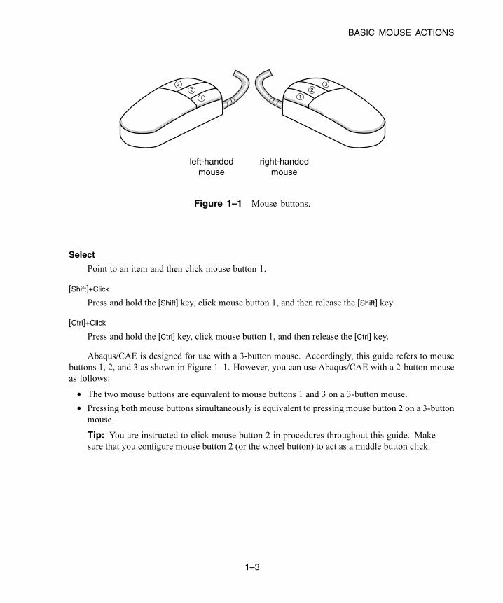
1.3 Basic mouse actions
Figure 1–1 shows the mouse button orientation for a left-handed and a right-handed 3-button mouse.The
following terms describe actions you perform using the mouse:
Click
Press and quickly release the mouse button. Unless otherwise specified, the instruction “click”
means that you should click mouse button 1.
Drag
Press and hold down mouse button 1 while moving the mouse.
Point
Move the mouse until the cursor is over the desired item.
1–2
Abaqus ID:
Printed on:
BASIC MOUSE ACTIONS
right-handedmouse
left-handedmouse
12
3
1
23
Figure 1–1 Mouse buttons.
Select
Point to an item and then click mouse button 1.
[Shift]+Click
Press and hold the [Shift] key, click mouse button 1, and then release the [Shift] key.
[Ctrl]+Click
Press and hold the [Ctrl] key, click mouse button 1, and then release the [Ctrl] key.
Abaqus/CAE is designed for use with a 3-button mouse. Accordingly, this guide refers to mouse
buttons 1, 2, and 3 as shown in Figure 1–1. However, you can use Abaqus/CAE with a 2-button mouse
as follows:
• The two mouse buttons are equivalent to mouse buttons 1 and 3 on a 3-button mouse.
• Pressing both mouse buttons simultaneously is equivalent to pressing mouse button 2 on a 3-button
mouse.
Tip: You are instructed to click mouse button 2 in procedures throughout this guide. Make
sure that you configure mouse button 2 (or the wheel button) to act as a middle button click.
1–3
Abaqus ID:
Printed on:


STARTING AND EXITING Abaqus/CAE
2. The basics of interacting with Abaqus/CAE
Before you can begin creating and analyzing a model or interpreting analysis results, it is helpful to
become familiar with the basics of interacting with Abaqus/CAE. This chapter introduces you to the
user interface. The following topics are covered:
• “Starting and exiting Abaqus/CAE,” Section 2.1
• “Overview of the main window,” Section 2.2
• “What is a module?,” Section 2.3
• “What is a toolset?,” Section 2.4
• “Using the mouse with Abaqus/CAE,” Section 2.5
• “Getting help,” Section 2.6
2.1 Starting and exiting Abaqus/CAE
This section explains how to start and how to exit Abaqus/CAE.
2.1.1 Starting Abaqus/CAE (or Abaqus/Viewer)When you create a model and analyze it, Abaqus/CAE generates a set of files containing the definition
of your model, the analysis input, and the results of the analysis. In addition, Abaqus/CAE and
Abaqus/Viewer generate replay files that reflect all your interactions with the application. Consequently,
before you run either product, you should move to a directory where you have permission to create files.
You execute Abaqus/CAE (or Abaqus/Viewer) by running the abaqus execution procedure and
specifying the cae (or viewer) parameter:
abaqus cae or viewer [database=database-file] [replay=replay-file] [recover=journal-file][startup=startup-file] [script=script-file] [noGUI=noGUI-file][noenvstartup] [noSavedOptions] [noSavedGuiOptions][noStartupDialog] [custom=script-file] [guiTester=[GUI-script] ][guiRecord] [guiNoRecord]
You can include the following options on the command line:
database
This option specifies the name of the model database file or output database file to open. You can
open either type of file in Abaqus/CAE; you can open only output database files in Abaqus/Viewer.
To specify a model database file, include either the .cae file extension or no file extension in
your file name. To specify an output database file when running Abaqus/CAE, include the .odb
2–1
Abaqus ID:
Printed on:

STARTING AND EXITING Abaqus/CAE
file extension in your file name. If you are running Abaqus/Viewer, you can omit the .odb file
extension.
replay
This option specifies the name of the file from which Abaqus/CAE commands are to be replayed.
The commands in replay-file will execute immediately upon startup of Abaqus/CAE. You cannot
use the replay option to execute a script with control flow statements. For more information, see
“Replaying an Abaqus/CAE session,” Section 9.5.1.
recover
This option specifies the name of the file from which a model database is to be rebuilt;
it is not available if you are running Abaqus/Viewer. The commands in journal-file
(model_database_name.jnl) will execute immediately upon startup of Abaqus/CAE. For
more information, see “Recreating a saved model database,” Section 9.5.2, and “Recreating an
unsaved model database,” Section 9.5.3.
startup
This option specifies the name of the file containing Python configuration commands to be run at
application startup. Commands in this file are run after any configuration commands that have been
set in the environment file. Abaqus/CAE does not echo the commands to the replay file when they
are executed.
script
This option specifies the name of the file containing Python configuration commands to be run at
application startup. Commands in this file are run after any configuration commands that have been
set in the environment file.
Arguments can be passed into the file by entering -- on the command line, followed by the
arguments separated by one or more spaces. These arguments will be ignored by the Abaqus/CAE
execution procedure, but they will be accessible within the script.
noGUI
This option specifies the name of a file containing Python scripts to be run without the graphical user
interface (GUI). This option is useful for automating pre- or post-analysis processing tasks without
the added expense of running a display. Since no interface is provided, the scripts cannot include
any user interaction. Abaqus/CAE runs the commands in the file and exits upon their completion. If
no file extension is given, the default extension is .py. If you use the noGUI option, Abaqus/CAE
ignores any other command line options that you provide.
Arguments can be passed into the file by entering -- on the command line, followed by the
arguments separated by one or more spaces. These arguments will be ignored by the Abaqus/CAE
execution procedure, but they will be accessible within the Python script. If you are using the
noGUI option, you can use an argument to pass in a variable that would otherwise be provided by
2–2
Abaqus ID:
Printed on:

STARTING AND EXITING Abaqus/CAE
a command line option. For example, you can pass in the name of a file that would otherwise be
specified by the script option.
A sample usage of the noGUI option is available in “Abaqus/CAE execution,” Section 3.2.6
of the Abaqus Analysis User’s Guide.
noenvstartup
This option specifies that all configuration commands in the environment files should not be run at
application startup. This option can be used in conjunction with the startup command to suppress
all configuration commands except for those in the startup file.
noSavedOptions
This option specifies that Abaqus/CAE should not apply the display options settings (for example,
the render style and the display of datum planes) stored in the abaqus_v6.13.gpr file. For
more information, see “Working with abaqus_v6.13.gpr files,” Section 2.1.3, and “Saving
your display options settings,” Section 76.16.
noSavedGuiOptions
This option specifies that Abaqus/CAE should not apply the GUI options settings (for example,
the size and location of the Abaqus/CAE main window or its dialog boxes) stored in the
abaqus_v6.13.gpr file.
noStartupDialog
This option specifies that the Start Session dialog box for Abaqus/CAE or Abaqus/Viewer should
not be displayed.
custom
This option specifies the name of the file containing Abaqus GUI Toolkit commands. This option
executes an application that is a customized version of Abaqus/CAE or Abaqus/Viewer. For more
information, see Chapter 1, “Introduction,” of the Abaqus GUI Toolkit User’s Guide.
guiTester
This option starts a separate user interface containing the Abaqus Python development environment
along with Abaqus/CAE or Abaqus/Viewer. The Abaqus Python development environment allows
you to create, edit, step through, and debug Python scripts. For more information, see Part III, “The
Abaqus Python development environment,” of the Abaqus Scripting User’s Guide.
You can specify a script as the argument for this option, which prompts Abaqus/CAE or
Abaqus/Viewer to run a GUI script. Abaqus/CAE or Abaqus/Viewer closes when the end of the
script is reached.
guiRecord
This option enables you to record your actions in the Abaqus/CAE or Abaqus/Viewer user interface
in a file named abaqus.guiLog. Creating a record of your actions in the GUI can help you
2–3
Abaqus ID:
Printed on:
STARTING AND EXITING Abaqus/CAE
capture and replay common activities in Abaqus/CAE or Abaqus/Viewer for demonstration or
training purposes. You can replicate all of the actions from a .guiLog file in Abaqus/CAE or
Abaqus/Viewer by running the file in the Abaqus Python Development Environment (PDE); for
more information, see “Running a script,” Section 7.3.2 of the Abaqus Scripting User’s Guide.
If desired, you can set guiRecord at startup by using the environment variable
ABQ_CAE_GUIRECORD. The guiRecord option cannot be used with the guiTester option.
guiNoRecord
This option enables you to disable user interface recording when the environment variable
ABQ_CAE_GUIRECORD is set.
Abaqus/CAE begins. If you do not include the database, replay, recover, or noStartupDialog
options, the Start Session dialog box appears. Choose one of the following session startup options:
Create Model Database: With Standard/Explicit Model
Use this option (not available if you are running Abaqus/Viewer) to begin a new Abaqus/Standard
or Abaqus/Explicit analysis (equivalent to choosing File→New Model Database→WithStandard/Explicit Model from the main menu bar).
Create Model Database: With CFD Model
Use this option (not available if you are running Abaqus/Viewer) to begin a new Abaqus/CFD
analysis (equivalent to choosing File→New Model Database→With CFD Model from the main
menu bar).
Create Model Database: With Electromagnetic Model
Use this option (not available if you are running Abaqus/Viewer) to begin an electromagnetic
analysis (equivalent to choosing File→New Model Database→With Electromagnetic Modelfrom the main menu bar).
Open Database
Use this option to open a previously saved model database or output database file (equivalent to
choosing File→Open from the main menu bar).
Run Script
Use this option to run a file containing Abaqus/CAE commands (equivalent to choosing File→RunScript from the main menu bar). For more information, see “Creating and running your own
scripts,” Section 9.5.4.
Start Tutorial
Use this option to begin an introductory tutorial from the online documentation (equivalent to
choosing Help→Getting Started from the main menu bar).
2–4
Abaqus ID:
Printed on:
STARTING AND EXITING Abaqus/CAE
Recent Files
Use this option to open one of the five model database files or output database files that were most
recently opened in Abaqus/CAE (equivalent to choosing one of the recent files listed under the Filemenu).
2.1.2 Exiting an Abaqus/CAE session
You can exit the Abaqus/CAE session at any time by selecting File→Exit from the main menu bar. If
you made any changes to the current model database, Abaqus/CAE asks if you want to save the changes
before exiting the session. Abaqus/CAE then closes the current model or output database and all windows
and exits the session.
Abaqus/CAE saves your GUI settings; for example, the size of the main window and the size
and location of dialog boxes. For more information, see “Working with abaqus_v6.13.gpr files,”
Section 2.1.3, and “Understanding Abaqus/CAE GUI settings,” Section 3.6. In addition, Abaqus/CAE
automatically creates a file called abaqus.rpy that records your operations during the session; you
can use this file to reproduce your operations. For more information on reproducing operations and on
recovering interrupted sessions, see “Recreating an unsaved model database,” Section 9.5.3.
2.1.3 Working with abaqus_v6.13.gpr files
The abaqus_v6.13.gpr file in your home directory stores GUI settings (such as the size of the main
window) as well as display options settings (such as the render style). You can also store display options
settings in an abaqus_v6.13.gpr file in a directory other than your home directory. If you start
Abaqus/CAE with noSavedOptions specified, Abaqus/CAE does not apply the display options settings
(for example, the render style and the display of datum planes) stored in the abaqus_v6.13.gpr file.
For more information, see “Starting Abaqus/CAE (or Abaqus/Viewer),” Section 2.1.1.
When you start Abaqus/CAE
• GUI settings are read from the abaqus_v6.13.gpr file in your home directory.
• Display options settings are read from the abaqus_v6.13.gpr file in the directory from
which you start Abaqus/CAE.
– If no abaqus_v6.13.gpr file is present but a .gpr file from an earlier release exists
in that directory, Abaqus/CAE attempts to apply the settings specified in that file and
creates an abaqus_v6.13.gpr file to store the settings.
– If no .gpr file is present in that directory, the display options settings are read from the
abaqus_v6.13.gpr file in your home directory.
2–5
Abaqus ID:
Printed on:

OVERVIEW OF THE MAIN WINDOW
During an Abaqus/CAE session
You can use File→Save Display Options to save display options settings to the
abaqus_v6.13.gpr file in your home directory or in the current directory. For more
information, see “Saving your display options settings,” Section 76.16. This save option does not
apply to GUI settings.
When you exit Abaqus/CAE
Your GUI settings are saved automatically to the abaqus_v6.13.gpr file in your home
directory. For more information, see “Understanding Abaqus/CAE GUI settings,” Section 3.6.
You can edit the abaqus_v6.13.gpr file using API commands in the Abaqus Scripting Interface;
for more information, see “Editing display preferences and GUI settings,” Section 8.4 of the Abaqus
ScriptingUser’s Guide. You can also delete the file to restore the default GUI and display options settings.
2.1.4 Saving model data from an inactive session
Abaqus/CAE and Abaqus/Viewer include an inactivity timer. If the applications are left inactive for an
extended period of time, the license tokens are returned to the server to make them available to other
users. Your session does not end if the server connection is lost or if new license tokens cannot be
acquired. Instead, when no licenses are available, a dialog box appears listing your options. For both
Abaqus/CAE and Abaqus/Viewer you can attempt to reacquire a license or you can exit the application.
For Abaqus/CAE you also have the option to save the current model database. Saving the model allows
you to preserve any completed model information that you did not already save; any partially completed
information, such as for a procedure that was active at the time the license was lost, is not saved. Once
you have saved the model database, only the reacquire and exit options remain in the dialog box. The
save option is not provided in Abaqus/Viewer since all changes that affect the output database are saved
immediately when you make them.
The default time limit is 60 minutes. You can change the time limit by using the cae_timeout
environment variable in the Abaqus environment file (abaqus_v6.env). For additional information
on the environment file, see “Using the Abaqus environment file,” Section 4.1 of the Abaqus Installation
and Licensing Guide.
2.2 Overview of the main window
This section provides an overview of the main window and explains how to operate and manipulate the
elements of the window during a session.
2–6
Abaqus ID:
Printed on:

OVERVIEW OF THE MAIN WINDOW
2.2.1 Components of the main windowYou interact with Abaqus/CAE through the main window, and the appearance of the window changes
as you work through the modeling process. Figure 2–1 shows the components that appear in the main
window.
Title bar
Model Tree / Results Tree
Menu bar Toolbars
Toolboxarea
Canvas anddrawing area
Viewport Promptarea
Message area orcommand line interface
Context bar
Figure 2–1 Components of the main window.
The components are:
Title bar
The title bar indicates the release of Abaqus/CAE you are running and the name of the current model
database.
2–7
Abaqus ID:
Printed on:

OVERVIEW OF THE MAIN WINDOW
Menu bar
The menu bar contains all the available menus; the menus give access to all the functionality in the
product. Different menus appear in the menu bar depending on which module you selected from
the context bar. For more information, see “Components of the main menu bar,” Section 2.2.2.
Toolbars
The toolbars provide quick access to items that are also available in the menus. For more
information, see “Components of the toolbars,” Section 2.2.3.
Context bar
Abaqus/CAE is divided into a set of modules, where each module allows you to work on one aspect
of your model; the Module list in the context bar allows you to move between these modules. Other
items in the context bar are a function of the module you are working in. For example, the context
bar allows you to retrieve an existing part while creating the geometry of the model or to change
the output database associated with the current viewport. Similarly, in the Mesh module you can
choose whether to display the assembly or a particular part. For more information, see “The context
bar,” Section 2.2.4.
Model Tree
The Model Tree provides you with a graphical overview of your model and the objects that it
contains, such as parts, materials, steps, loads, and output requests. In addition, the Model Tree
provides a convenient, centralized tool for moving between modules and for managing objects. If
your model database contains more than one model, you can use the Model Tree to move between
models. When you become familiar with the Model Tree, you will find that you can quickly perform
most of the actions that are found in the main menu bar, the module toolboxes, and the various
managers. For more information, see “An overview of the Model Tree,” Section 3.5.1.
Results Tree
The Results Tree provides you with a graphical overview of your output databases and other session-
specific data such as X–Y plots. If you have more than one output database open in your session, you
can use the Results Tree to move between output databases. When you become familiar with the
Results Tree, you will find that you can quickly perform most of the actions in the Visualization
module that are found in the main menu bar and the toolbox. For more information, see “An
overview of the Results Tree,” Section 3.5.2.
Toolbox area
When you enter a module, the toolbox area displays tools in the toolbox that are appropriate for that
module. The toolbox allows quick access to many of the module functions that are also available
from the menu bar. For more information, see “Understanding and using toolboxes and toolbars,”
Section 3.3.
2–8
Abaqus ID:
Printed on:

OVERVIEW OF THE MAIN WINDOW
Canvas and drawing area
The canvas can be thought of as an infinite screen or bulletin board on which you post viewports;
for more information, see Chapter 4, “Managing viewports on the canvas.” The drawing area is the
visible portion of the canvas.
Viewport
Viewports are windows on the canvas in which Abaqus/CAE displays your model. For more
information, see Chapter 4, “Managing viewports on the canvas.”
Prompt area
The prompt area displays instructions for you to follow during a procedure; for example, it asks you
to select the geometry as you create a set. In the Visualization module a set of buttons is displayed
in the prompt area that allow you to move between the steps and the frames of your analysis. For
more information, see “Using the prompt area during procedures,” Section 3.1.
Message area
Abaqus/CAE prints status information and warnings in the message area. To resize the message
area, drag the top edge; to see information that has scrolled out of the message area, use the scroll
bar on the right side. The message area is displayed by default, but it uses the same space occupied
by the command line interface. If you have recently used the command line interface, you must
click in the bottom left corner of the main window to activate the message area.
Note: If newmessages are added while the command line interface is active, Abaqus/CAE changes
the background color surrounding the message area icon to red. When you display the message area,
the background reverts to its normal color.
Command line interface
You can use the command line interface to type Python commands and evaluate mathematical
expressions using the Python interpreter that is built into Abaqus/CAE. The interface includes
primary (>>>) and secondary (...) prompts to indicate when you must indent commands to
comply with Python syntax. For more information on Python commands, see “The basics of
Python,” Section 4.5 of the Abaqus Scripting User’s Guide.
The command line interface is hidden by default, but it uses the same space occupied by the
message area. Click in the bottom left corner of the main window to switch from the message
area to the command line interface.
2.2.2 Components of the main menu barWhen you start a session, the menus listed below appear on the main menu bar. Abaqus/CAE displays
additional menu options and provides access to toolsets depending on the current module in use.
2–9
Abaqus ID:
Printed on:

OVERVIEW OF THE MAIN WINDOW
File
The items in the File menu allow you to create, open, and save model databases; open and close
output databases; import and export files; save and load session objects and options; run scripts;
manage macros; print viewports; and exit Abaqus/CAE. For more information, see “Using the File
menu,” Section 9.6, in the HTML version of this guide.
Model
The items in the Model menu allow you to open, copy, rename, and delete the models in the current
model database. For more information, see “Managing models,” Section 9.8, in the HTML version
of this guide.
Viewport
The items in the Viewport menu allow you to create or manipulate viewports and viewport
annotations. For more information, see Chapter 4, “Managing viewports on the canvas.”
View
The items in the View menu allow you to manipulate views, customize certain aspects of the
appearance of your model or plots, control display performance, and turn off the display of the
Model Tree, the Results Tree, and individual toolbars. Some of the operations available in the view
manipulation menu are also available in the View Manipulation toolbar. For more information,
see:
• “Working with the Model Tree and the Results Tree,” Section 3.5
• Chapter 5, “Manipulating the view and controlling perspective”
• Chapter 7, “Configuring graphics display options”
• Chapter 55, “Customizing plot display”
• Chapter 61, “The Customize toolset”
• Chapter 76, “Customizing geometry and mesh display”
Plug-ins
The items in the Plug-ins menu allow you to access the plug-ins distributed with Abaqus/CAE or
plug-ins that you have downloaded or created. For more information, see Chapter 81, “The Plug-in
toolset.”
Help
The items in the Help menu allow you to request context-sensitive help and to search or browse the
documentation. For more information, see “Getting help,” Section 2.6.
2.2.3 Components of the toolbarsThe toolbars contain convenient sets of tools for managing your files, filtering object selection, and
viewing your model. Items in a toolbar are shortcuts to functions that are also available from the main
2–10
Abaqus ID:
Printed on:

OVERVIEW OF THE MAIN WINDOW
menu bar. By default, Abaqus/CAE displays all of the toolbars in a row underneath the main menu bar.
Abaqus/CAE may place some toolbars in a second row depending on your display resolution and the
size of the main window. The toolbars are shown in the following figure:
File View Manipulation View Options
Render Style
QueryDisplay Group Color Code
Toolbar grip
Selection
Translucency
View CutVisible Objects
You can change the location of a toolbar using the toolbar’s grip, as indicated in the above figure.
Clicking and dragging the grip moves the toolbar around the main window. If you release the toolbar grip
while the toolbar is over one of the four available docking regions of the main window (see Figure 2–2),
Abaqus/CAE “docks” the toolbar; a docked toolbar has no title bar and does not obstruct any other
portion of the main window.
If you release the toolbar grip while the toolbar is not near a docking region, Abaqus/CAE creates
a floating toolbar with a title bar. A floating toolbar obstructs other items in the main window (see
Figure 2–3); however, a floating toolbar can be positioned outside of the Abaqus/CAE main window.
Clicking mouse button 3 on a toolbar grip displays a menu that lets you specify the location and
format of the toolbar:
• Select Top to dock the toolbar in the top docking region.
• Select Bottom to dock the toolbar in the bottom docking region.
• Select Left to dock the toolbar in the left docking region.
• Select Right to dock the toolbar in the right docking region.
• Select Float to change a docked toolbar into a floating toolbar; this option is available only for
docked toolbars.
• Select Flip to change the orientation of a floating toolbar from horizontal to vertical, or vice versa;
this option is available only for floating toolbars.
You can also hide toolbars and create custom toolbars that include shortcuts to additional functions.
For more information, see Chapter 61, “The Customize toolset.”
2–11
Abaqus ID:
Printed on:

OVERVIEW OF THE MAIN WINDOW
Bottom docking region
Left docking region
Top docking region
Rightdockingregion
Figure 2–2 Available docking regions for toolbars.
Figure 2–3 Floating toolbars.
To obtain a short description of a tool in a toolbar, place the cursor over that tool for a moment; a
small box containing a description, or “tooltip,” will appear. To obtain the name of a toolbar, place the
cursor over the toolbar grip for a moment.
2–12
Abaqus ID:
Printed on:

OVERVIEW OF THE MAIN WINDOW
The Abaqus/CAE toolbars contain the following functionality:
File
The File toolbar allows you to create, open, and save model databases; to open output databases; to
print viewports; and to save and load session objects and options. For more information, see Part II,
“Working with Abaqus/CAE model databases, models, and files”; Chapter 8, “Printing viewports”;
and “Managing session objects and session options,” Section 9.9, in the HTML version of this guide.
View Manipulation
The View Manipulation toolbar allows you to specify different views of the model or plot. For
example, you can pan, rotate, or zoom the model or plot using these tools. For more information,
see Chapter 5, “Manipulating the view and controlling perspective.”
View Options
The View Options toolbar allows you to specify whether or not perspective is applied to your
model. For more information, see “Controlling perspective,” Section 5.5.
Render Style
The Render Style toolbar allows you to specify whether the wireframe, hidden line, or shaded
render style will be used to display your model. In the Visualization module the Render Style
toolbar also includes the filled render style tool. For more information, see “Choosing a render
style,” Section 55.2.1.
Visible Objects
The Visible Objects toolbar allows you to switch between displaying the geometry of an
Abaqus/CAE native part and the meshed representation of the same part, to toggle the display of
2–13
Abaqus ID:
Printed on:

OVERVIEW OF THE MAIN WINDOW
seeds on and off, and to toggle the display of the reference representation on or off if the meshed
representation and reference representation exist. For more information, see “Displaying a native
mesh,” Section 17.3.11; “What are mesh seeds?,” Section 17.4.1; and “Understanding the reference
representation,” Section 35.2.
Selection
The Selection toolbar allows you to enable or disable object selection by toggling on the arrow
icon. You can use the list to the right of the arrow to limit the types of objects that you can select.
The Selection toolbar is available only when there are no active procedures running in a viewport.
For more information, see “Selecting objects before choosing a procedure,” Section 6.3.7.
Query
The Query toolbar allows you to obtain information about the geometry and features of your model,
to probe model and X–Y plots for output data, and to perform stress linearization on your results.
For more information, see Chapter 71, “The Query toolset”; Chapter 51, “Probing the model”; and
Chapter 52, “Calculating linearized stresses.”
Display Group
The Display Group toolbar allows you to selectively plot one or more model or output database
items. For example, you can create a display group that contains only the elements belonging to
specified sets in yourmodel. For more information, see Chapter 78, “Using display groups to display
subsets of your model.”
Color Code
The Color Code toolbar allows you to customize the colors of items in the viewport and change
the degree of their translucency.
For color coding, you can create color mappings that assign unique colors to different elements
of a display. For example, when using a part instance color mapping, each part instance in a model
2–14
Abaqus ID:
Printed on:

OVERVIEW OF THE MAIN WINDOW
will appear as a different color. For more information, see Chapter 77, “Color coding geometry and
mesh elements.”
For translucency, you can click the arrow to the right of the tool to reveal a slider, which
you can drag to make the display colors more transparent or more opaque. For more information,
see “Changing the translucency,” Section 77.3.
Field Output
The Field Output toolbar allows you to control two aspects of field output variable display:
• You can select the field output variable that you want to display in the current viewport.
Selections include the type of field output variable (Primary, Deformed, or Symbol), thevariable name, and if available, the invariants and components for the selected primary
variable.
• For changes in variable type, you can control whether Abaqus/CAE automatically
synchronizes the plot state in the current viewport with the new selection of variable type.
If the tool is toggled on, Abaqus/CAE synchronizes the plot state if the newly selected
field output variable requires a change in plot state; if this option is toggled off, Abaqus/CAE
still updates the output variable displayed in the viewport but does not change the plot state
in the current viewport.
The selections in the toolbar are limited, but the tool provides access to the Field Outputdialog box, if needed. For more information about the options in the toolbar, see “Using the field
output toolbar,” Section 42.5.2.
Viewport
The Viewport toolbar allows you to create and align viewports, link viewports, and create viewportannotations. For more information, see “Managing viewports and viewport annotations from the
Viewport toolbar,” Section 4.2.2. The Viewport toolbar is not displayed by default.
View Cut
2–15
Abaqus ID:
Printed on:

OVERVIEW OF THE MAIN WINDOW
The View Cut toolbar allows you to toggle the display of view cuts in modules other than the
Visualization module and to customize their definition and display. For more information, see
Chapter 80, “Cutting through a model.” The View Cut toolbar is displayed by default; in the
Visualization module, view cut options are available in the toolbox.
Views
The Views toolbar allows you to apply a custom view to the model in the viewport. For more
information, see “Custom views,” Section 5.2.8. The Views toolbar is not displayed by default.
2.2.4 The context barThe context bar is located above the canvas and drawing area; you can use it to do the following:
Select the current module
The Module list on the context bar allows you to move between modules. (For more information,
see “What is a module?,” Section 2.3.) Figure 2–4 shows the context bar. To move to a different
module, you can choose from the list (the arrow on the right) or click the up and down arrows (on
the left) to move to the previous or next module.
Figure 2–4 The context bar in the Part module.
Note: Abaqus/Viewer contains only the Visualization module.
Select module-specific items
As you move between modules, Abaqus/CAE displays additional items on the context bar that help
you select the context of your current operations. For example, when you are in the Part module or
Mesh module, Abaqus/CAE displays the Part list in the context bar. The Part list contains everypart in your model; you can use it to retrieve a particular part. These lists also include the up and
down navigation arrows that allow you to move to the previous or next item in the list.
The context bar also allows you to move between models in the model database or to change
the output database associated with the current viewport. The additional items in the context bar
are a function of the module in which you are working.
The items displayed in the context bar always refer to the current viewport, which is indicated by a
dark gray title bar. For example, if you have different parts displayed in different viewports, the context
bar indicates the name of the part displayed in the current viewport.
2–16
Abaqus ID:
Printed on:

OVERVIEW OF THE MAIN WINDOW
2.2.5 Components of the viewportFigure 2–5 shows the components of the viewport in the Visualization module.
Viewport: 1 ODB: C:/models/Plastic_lug_hard_tutorial.odb
(Avg: 75%)S, Mises
+3.540e+07+8.398e+07+1.326e+08+1.812e+08+2.297e+08+2.783e+08+3.269e+08+3.755e+08+4.241e+08+4.727e+08+5.213e+08+5.699e+08+6.184e+08
Step: LugLoad, Apply uniform pressure to the holeIncrement 4: Step Time = 1.000Primary Var: S, MisesDeformed Var: U Deformation Scale Factor: +1.527e+00
X
Y
Z
X
Y
Z
Compass
View orientation triadState Block
Legend Viewport title
Figure 2–5 Components of the viewport.
The viewport title and the border around the viewport are called the viewport decorations. The legend,
state block, title block, view orientation triad, and 3D compass are called the viewport annotations.
The view orientation triad and 3D compass indicate the orientation of the model currently being
displayed. You can change the view of the model by clicking and dragging on the 3D compass; the
three perpendicular axes on the view orientation triad rotate with the compass to indicate the current
view orientation. For more information, see “The 3D compass,” Section 5.3, and “Customizing the
2–17
Abaqus ID:
Printed on:

WHAT IS A MODULE?
view triad,” Section 5.4. The legend, state block, and title block identify results you display using the
Visualization module. For more information, see Chapter 56, “Customizing viewport annotations.”
2.3 What is a module?
Abaqus/CAE is divided into functional units called modules. Each module contains only those tools that
are relevant to a specific portion of the modeling task. For example, the Mesh module contains only the
tools needed to create finite element meshes, while the Job module contains only the tools used to create,
edit, submit, and monitor analysis jobs. Abaqus/Viewer is a subset of Abaqus/CAE that contains only
the Visualization module.
You can select a module from the Module list in the context bar. Alternatively, you can select a
module by switching to the context of a selected object in the Model Tree; for more information, see
“An overview of the Model Tree,” Section 3.5.1. The order of the modules in the menu and in the Model
Tree corresponds to the logical sequence you follow to create a model. In many circumstances you must
follow this natural progression to complete a modeling task; for example, you must create parts before
you create an assembly. Although the order of the modules follows a logical sequence, Abaqus/CAE
allows you to select any module at any time, regardless of the state of your model.
The following list of the modules available within Abaqus/CAE briefly describes the modeling tasks
you can perform in each module. The order of the modules in the list corresponds to the order of the
modules in the context bar’s Module list and in the Model Tree:
Part
Create individual parts by sketching or importing their geometry. For more information, see
Chapter 11, “The Part module.”
Property
Create section and material definitions and assign them to regions of parts. For more information,
see Chapter 12, “The Property module.”
Assembly
Create and assemble part instances. For more information, see Chapter 13, “TheAssemblymodule.”
Step
Create and define the analysis steps and associated output requests. For more information, see
Chapter 14, “The Step module.”
Interaction
Specify the interactions, such as contact, between regions of a model. For more information, see
Chapter 15, “The Interaction module.”
2–18
Abaqus ID:
Printed on:

WHAT IS A TOOLSET?
Load
Specify loads, boundary conditions, and fields. For more information, see Chapter 16, “The Load
module.”
Mesh
Create a finite element mesh. For more information, see Chapter 17, “The Mesh module.”
Optimization
Create and configure an optimization task. For more information, see Chapter 18, “The
Optimization module.”
Job
Submit a job for analysis and monitor its progress. For more information, see Chapter 19, “The Job
module.”
Visualization
View analysis results and selected model data. For more information, see Part V, “Viewing results.”
Sketch
Create two-dimensional sketches. For more information, see Chapter 20, “The Sketch module.”
Modules can be classified by the objects that are displayed in the viewport. Parts are displayed
when you are in the Part and Property modules; the assembly is displayed when you are in the Assembly,
Step, Interaction, Load, Mesh, and Job modules; and output database results are displayed when you are
in the Visualization module.
The contents of the main window change as you move between modules. Selecting a module from
the Module list on the context bar or by switching to the context of a selected object in the Model Tree
causes the context bar, module toolbox, and menu bar to change to reflect the functionality of the current
module.
When you move between modules, Abaqus/CAE associates the current viewport with the module
you select. You can have multiple viewports, and different viewports can be associated with different
modules. As you select a viewport and make it current, the module associated with the viewport becomes
the current module. For more information on moving between viewports, see “Selecting viewports,”
Section 4.3.2, in the HTML version of this guide.
2.4 What is a toolset?
When you enter most modules, a Tools menu appears in the main menu bar containing all of the toolsets
relevant to that module. A toolset is a functional unit that allows you to perform a specific modeling task.
2–19
Abaqus ID:
Printed on:
WHAT IS A TOOLSET?
In most cases the objects that you create with a toolset in one module are useful in other modules.
For example, you can use the Set toolset to create sets in the Assembly module and then apply boundary
conditions to those sets in the Load module. Most of the toolsets include manager menus and manager
dialog boxes that allow you to edit, copy, rename, and delete the objects you create with the toolset.
The following toolsets are available in Abaqus/CAE:
• The Amplitude toolset allows you to define arbitrary time or frequency variations of load,
displacement, and other prescribed variables. For more information, see Chapter 57, “The
Amplitude toolset.”
• The Analytical Field toolset allows you to create analytical fields that you can use to define spatially
varying parameters for selected interactions and prescribed conditions. For more information, see
Chapter 58, “The Analytical Field toolset.”
• The Attachment toolset allows you to create attachment points and lines that you can use to define
point-based and discrete fasteners, connector points for a connector, and regions for a coupling
definition, point mass, load, or boundary condition. For more information, see Chapter 59, “The
Attachment toolset.”
• The CAD Connection toolset allows you to create a connection that you can use for associative
import of parts into Abaqus/CAE from CATIA and third-party CAD systems. For more information,
see Chapter 60, “The CAD Connection toolset.”
• The Color Code toolset allows you to customize the edge and fill color of individual elements. For
more information, see Chapter 77, “Color coding geometry and mesh elements.”
• The Coordinate System toolset allows you to create local coordinate systems for use in
postprocessing. For more information, see “Creating coordinate systems during postprocessing,”
Section 42.8.
• The Create Field Output toolset allows you to perform operations on the field output available in an
output database. For more information, see “Creating new field output,” Section 42.7.
• The Customize toolset allows you to control the appearance of Abaqus/CAE toolbars, to create
customized toolbars, and to specify keyboard shortcuts for many Abaqus/CAE features. For more
information, see Chapter 61, “The Customize toolset.”
• The Datum toolset allows you to create datum points, axes, planes, and coordinate systems for a
variety of modeling tasks. For more information, see Chapter 62, “The Datum toolset.”
• The Discrete Field toolset allows you to create a spatially varying field where values are associated
with nodes or elements. For more information, see Chapter 63, “The Discrete Field toolset.”
• The Display Group toolset allows you to selectively plot one or more model or output database
items. For more information, see Chapter 78, “Using display groups to display subsets of your
model.”
• The Edit Mesh toolset allows you to modify a mesh to improve mesh quality. For more information,
see Chapter 64, “The Edit Mesh toolset.”
• The Feature Manipulation toolset allows you to modify and manage the existing features in your
model. For more information, see Chapter 65, “The Feature Manipulation toolset.”
2–20
Abaqus ID:
Printed on:
USING THE MOUSE WITH Abaqus/CAE
• The Filter toolset allows you to remove extraneous output data—noise—during the analysis of a
model without a loss of resolution in the desired data range. For more information, see Chapter 66,
“The Filter toolset.”
• The Free Body toolset allows you to create and customize free body cuts in the Visualization module
of Abaqus/CAE. For more information, see Chapter 67, “The Free Body toolset.”
• The Geometry Edit toolset allows you to repair invalid and imprecise imported parts. For more
information, see Chapter 69, “The Geometry Edit toolset.”
• The Partition toolset allows you to divide a part or assembly into regions. For more information,
see Chapter 70, “The Partition toolset.”
• The Path toolset allows you to specify a path through your model along which you can obtain and
view X–Y data. For more information, see Chapter 48, “Viewing results along a path.”
• The Query toolset allows you to obtain general information about your model and to probe model
and X–Y plots for output data. For more information, see Chapter 71, “The Query toolset.”
• The Reference Point toolset allows you to create reference points associated with a part or assembly.
For more information, see Chapter 72, “The Reference Point toolset.”
• The Set toolset and the Surface toolset allow you to define sets and surfaces from regions of a model.
For more information, see Chapter 73, “The Set and Surface toolsets.”
• The Stream toolset allows you to display streamlines to investigate velocity or vorticity in a fluid
flow analysis. For more information, see Chapter 74, “The Stream toolset.”
• The Virtual Topology toolset allows you to ignore details, such as very small faces and edges, when
you are meshing a part or a part instance. For more information, see Chapter 75, “The Virtual
Topology toolset.”
• The XY Data toolset allows you to create and operate on X–Y data objects. For more information,
see Chapter 47, “X–Y plotting.”
2.5 Using the mouse with Abaqus/CAE
Many of the procedures in the Abaqus/CAE documentation involve using one or more of the three
mouse buttons. The following list explains the importance of each mouse button when interacting with
Abaqus/CAE:
Mouse button 1
You use mouse button 1 to select objects in the viewport, to expand pull-down menus, and to select
items from menus. The instructions “click,” “select,” and “drag” in the documentation refer to
mouse button 1.
Mouse button 2
Clicking mouse button 2 in the viewport signifies that you have finished the current task. For
example:
2–21
Abaqus ID:
Printed on:

GETTING HELP
• Selecting entities from the model: when you create a node set, you select the nodes to include
in the set. Clicking mouse button 2 indicates that your selection is complete and you are ready
to create the set.
• Using a tool: click mouse button 2 to indicate that you have finished with a view manipulation
tool.
In addition, clicking mouse button 2 in the viewport is equivalent to clicking the highlighted button
in the prompt area. For example, if you tried to select nodes from your model and Abaqus/CAE
displayed the following prompt, clicking mouse button 2 would have the same effect as clicking
OK:
If your mouse has a wheel as mouse button 2, you can scroll the wheel vertically to manipulate
your view of the model or plot in the viewport. Scroll downward to magnify your view of the
contents of the viewport, or scroll upward to reduce your view of the contents of the viewport.
Mouse button 3
You press and hold mouse button 3 to access a popup menu that contains shortcuts to functions
related to the current procedure. For example, when you press mouse button 3 in a viewport while
creating a geometry set, Abaqus/CAE displays the following menu:
If you use mouse button 3 in a viewport, most of the items in the popupmenu duplicate the buttons in
the prompt area. The mouse button 3 shortcut is also available for selections from the Model Tree
and Results Tree, as described in “Using popup menus in the Model Tree and the Results Tree,”
Section 3.5.3.
2.6 Getting help
The Abaqus/CAE HTML documentation is available through the Help menu on the main menu bar. This
section provides a brief description of the HTML online documentation and explains how to use the Helpmenu to find information. For additional information, refer to Using Abaqus Online Documentation.
2–22
Abaqus ID:
Printed on:

GETTING HELP
The features described in this section apply only to the HTML documentation, not the PDF-format
guides.
Note:
• On Windows platforms, the help system uses your default web browser to display the online
documentation.
• On UNIX and Linux platforms, the help system searches the system path for Firefox. If the help
system cannot find Firefox, an error is displayed.
The browser_type and browser_path variables can be set in the environment file to modify
this behavior. For more information, see “System customization parameters,” Section 4.1.4 of the
Abaqus Installation and Licensing Guide.
2.6.1 Displaying context-sensitive help
You can use the help tool on the main menu bar to display detailed HTML help on any icon, menu,
or dialog box that you use in Abaqus/CAE. When you click the help tool and then click an item in the
Abaqus/CAE window, a help window appears containing the section from the online documentation that
is relevant to that item.
To display help on an item in the main window or in a dialog box:
1. Click the help tool on the main menu bar.
Tip: You can also select Help→On Context from the main menu bar.
The cursor changes to a question mark.
2. Position the cursor over the item about which you need help, and click mouse button 1.
A help window appears. The window contains the appropriate online documentation and links to
associated topics.
Alternatively, you can use the [F1] key to display help on a particular item. In most cases you
can gain access to context-sensitive help by using the Help menu, the help tool icon, or the [F1] key.However, you must use [F1] if you are seeking information about menu items or dialog boxes that do not
allow access to the help tool.
To display help using the [F1] key:
1. Click the feature in the Abaqus/CAE window that you want help with. If the feature is part of a
menu, do not release the mouse button.
2. Press [F1].
2–23
Abaqus ID:
Printed on:

GETTING HELP
A help window appears. The window contains the appropriate online documentation and links
to associated topics. If you selected a menu item without releasing the mouse button, that menu
disappears.
Note: Abaqus/CAE also provides brief “tooltips” that describe the function of tools in toolboxes and in
the toolbars. To see a “tooltip,” position the cursor over a tool and leave it stationary for a short time.
2.6.2 Browsing and searching the HTML guidesYou can browse and search the entire HTML collection by selecting Help→Search & Browse Guides.The collection window that appears contains a list of all the book titles in the documentation collection.
To view a particular guide, click the title of interest; the guide will appear in a new browser window.
(For detailed information, see Using Abaqus Online Documentation.)
To display and search an HTML guide:
1. From the main menu bar, select Help→Search & Browse Guides.
The collection window appears in your web browser with a list of all the book titles in the
documentation collection, grouped by category.
2. Click the book title of interest.
A book window containing the guide that you selected opens in a new browser window. The book
window contains four frames: the navigation frame, the table of contents control frame, the table
of contents frame, and the text frame, as shown in Figure 2–6.
3. Navigate through the guide’s contents using any of the following techniques:
Table of contents controls
Use the buttons in the table of contents control frame to vary the level of detail displayed in the
table of contents frame or change the size of the frame. Click to expand several levels in
the table of contents of an online book. Click to collapse all expanded sections in the table
of contents. Click and , respectively, to narrow or widen the table of contents frame.
Browsing
Use the and arrows in the text frame to navigate sequentially through the text. You
can also use the web browser functions to return to recently viewed pages.
Searching
Use the search panel located in the navigation frame to search for specific words or phrases.
For more information, see Chapter 4, “Searching the Abaqus HTML documentation,” of Using
Abaqus Online Documentation.
2–24
Abaqus ID:
Printed on:

GETTING HELP
list box
navigationframe
text frame
table of contentscontrol frame
table of contentsframe
search field
Figure 2–6 The book window.
Using hyperlinks
Use hyperlinks to move from one part of a book to another or from one book to another book.
2.6.3 Finding special sections of the online documentationThe following Help menu items allow you to display sections of the HTML documentation that you may
find useful:
On Module
Select Help→On Module to display the Abaqus/CAE User’s Guide opened to the beginning of the
chapter that describes the current module. If you have not yet entered a module, the guide will be
opened to a description of the module concept. In either case, you are then free to read additional
information as needed and to conduct text searches through the entire guide.
On Help
Select Help→On Help to display the Abaqus/CAE User’s Guide opened to the section that
describes how to use the help system. You are also free to read additional information as needed
and to conduct text searches through the entire guide.
Getting Started
Select Help→Getting Started to display a section that provides basic information on how to work
in the Abaqus/CAE window. This section also contains links to helpful tutorials in the Getting
Started with Abaqus: Interactive Edition guide.
2–25
Abaqus ID:
Printed on:
GETTING HELP
Release Notes
Select Help→Release Notes to display the Abaqus Release Notes. Release notes detail new
features of the software and provide a list of updates and enhancements.
About Abaqus
Select Help→About Abaqus to determine which release of Abaqus/CAE you are currently
using. Abaqus also provides the location of release information for open source software used by
Abaqus/CAE; for example, Python.
About Licensing
Select Help→About Licensing to determine product license information. Abaqus displays your
site identification and the name of your license server along with your license number and the total
number of licenses available from your site.
2.6.4 Finding information about keywords
The keyword browser is a scrollable table that contains the following information:
• The purpose of each keyword.
• The Abaqus/CAE module or toolset that contains the functionality associated with each keyword.
To view the keyword browser, select Help→Keyword Browser from the main menu bar. For example,
you could use the keyword browser to verify that the *ELASTIC option allows you to specify elastic
material properties and that the Property module is the Abaqus/CAE module associated with this
keyword.
The keyword browser also contains hyperlinks to relevant sections in the online documentation. You
can click a particular keyword in the table to display detailed information concerning the function of that
keyword. You can also click the name of a module or toolset in the table to view related documentation
in the Abaqus/CAE User’s Guide.
To display the keyword browser:
1. From the main menu bar, select Help→Keyword Browser.
The Abaqus/CAE User’s Guide is opened to a table of Abaqus keywords and their associated
modules.
2. In the Keyword column, click the keyword of interest to view online documentation describing that
keyword.
3. In the Module column, click the module or toolset name of interest to view online documentation
concerning that module or toolset.
2–26
Abaqus ID:
Printed on:

USING THE PROMPT AREA DURING PROCEDURES
3. Understanding Abaqus/CAE windows, dialog boxes,and toolboxes
This chapter explains how to interact with the various windows, dialog boxes, and toolboxes that appear
throughout the Abaqus/CAE application. The following topics are covered:
• “Using the prompt area during procedures,” Section 3.1
• “Interacting with dialog boxes,” Section 3.2
• “Understanding and using toolboxes and toolbars,” Section 3.3
• “Managing objects,” Section 3.4
• “Working with the Model Tree and the Results Tree,” Section 3.5
• “Understanding Abaqus/CAE GUI settings,” Section 3.6
3.1 Using the prompt area during procedures
This section explains how to make use of the procedural steps that Abaqus/CAE displays in the prompt
area.
3.1.1 What is a procedure?Many tasks within Abaqus/CAE are broken into step-by-step procedures. For example, creating an arc
in the Sketcher is a three-step procedure:
1. Pick the center point for the arc.
2. Pick the start point.
3. Pick the end point.
Abaqus/CAE displays each step of a procedure in the prompt area near the bottom of the main
window so that you do not need to remember all the steps and their order.
3.1.2 Following instructions and entering data in the prompt areaTo use a procedure, simply follow the directions that appear in the prompt area near the bottom of the
main window, as shown here:
3–1
Abaqus ID:
Printed on:

USING THE PROMPT AREA DURING PROCEDURES
The button marked X in the above figure is the Cancel button; click this button to cancel the entire
procedure at any time. The arrow to the left of the Cancel button is the Previous button; click it to abort
the current step of the procedure and return to the previous one. (The Previous button appears dimmed
during the first step of any procedure.) If you prefer, you can place the cursor over the canvas and press
mouse button 3; then select Previous Step or Cancel Procedure from the menu that appears.
A Stop button appears in the prompt area during certain time-consuming operations, such as part
healing or meshing or the extraction of X–Y data from history for large models. You can click Stop to
interrupt and cancel the operation.
Many procedures require textual or numeric data; for example, when creating a fillet using the
Sketch module, you must first specify the fillet radius. When textual or numeric data are required,
Abaqus/CAE displays a text field in the prompt area for you to fill in; usually the text box will already
contain a default value, as shown here:
Position your cursor over the viewport, and enter data into the text field as follows:
• To accept the default value, press either [Enter] or mouse button 2.
• To replace the default value, simply begin typing; you need not click the text field before typing.
The default value disappears as soon as you begin to type.
• To change a portion of the default value, first click the text field; then use the [Delete] key and the
other keys on your keyboard to change the value.
• To commit any changes, press [Enter] or mouse button 2.
• You can also enter an expression in a text field in the prompt area. For more information, see
“Entering expressions,” Section 3.2.2.
Some procedures require you to choose from a number of options. For example, the Datum toolset
may ask you to choose a principal axis. Such options are represented by buttons in the prompt area, as
shown here:
Click the appropriate button to select the desired option.
In some procedures a default option is indicated by a border around the corresponding button; in the
above example the border is drawn around the X-Axis button. To select the default option, click mouse
button 2.
3–2
Abaqus ID:
Printed on:
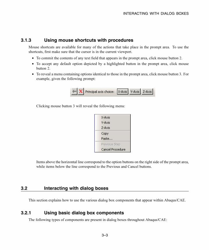
INTERACTING WITH DIALOG BOXES
3.1.3 Using mouse shortcuts with proceduresMouse shortcuts are available for many of the actions that take place in the prompt area. To use the
shortcuts, first make sure that the cursor is in the current viewport.
• To commit the contents of any text field that appears in the prompt area, click mouse button 2.
• To accept any default option depicted by a highlighted button in the prompt area, click mouse
button 2.
• To reveal a menu containing options identical to those in the prompt area, click mouse button 3. For
example, given the following prompt:
Clicking mouse button 3 will reveal the following menu:
Items above the horizontal line correspond to the option buttons on the right side of the prompt area,
while items below the line correspond to the Previous and Cancel buttons.
3.2 Interacting with dialog boxes
This section explains how to use the various dialog box components that appear within Abaqus/CAE.
3.2.1 Using basic dialog box componentsThe following types of components are present in dialog boxes throughout Abaqus/CAE:
3–3
Abaqus ID:
Printed on:
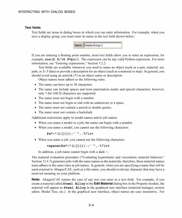
INTERACTING WITH DIALOG BOXES
Text fields
Text fields are areas in dialog boxes in which you can enter information. For example, when you
save a display group, you must enter its name in the text field shown below:
If you are entering a floating point number, most text fields allow you to enter an expression; for
example, cos(2.5/(4.9*pi)). The expression can be any valid Python expression. For more
information, see “Entering expressions,” Section 3.2.2.
Text fields are available whenever you need to name an object (such as a part, material, set,
path, or X–Y data) or provide a description for an object (such as a material or step). In general, you
should avoid using an asterisk (*) in an object name or description.
Object names must adhere to the following rules:
• The name can have up to 38 characters.
• The name can include spaces and most punctuation marks and special characters; however,
only 7-bit ASCII characters are supported.
• The name must not begin with a number.
• The name must not begin or end with an underscore or a space.
• The name must not contain a period or double quotes.
• The name must not contain a backslash.
Additional restrictions apply to model names and to job names.
• When you name a model or a job, the name can begin with a number.
• When you name a model, you cannot use the following characters:
$&*~!()[]{}|;'`”,.?/\><
• When you name a job, you cannot use the following characters:
<space>$&*~!()[]{}|:;'`”,.?/\><
In addition, a job name cannot begin with a dash -.
The material evaluation procedure (“Evaluating hyperelastic and viscoelastic material behavior,”
Section 12.4.7) generates jobs with the same names as the materials; therefore, these material names
must adhere to the same rules as job names. In general, when you are specifying a name that will be
used external to Abaqus/CAE, such as a file name, you should avoid any character that may have a
reserved meaning on your platform.
Note: Abaqus/CAE retains the case of any text you enter in a text field. For example, if you
create a material called Steel Alloy in the Edit Material dialog box in the Property module, the
material will appear as Steel Alloy in the graphical user interface (material manager, section
editor, Model Tree, etc.). In the graphical user interface, object names are case insensitive. For
3–4
Abaqus ID:
Printed on:

INTERACTING WITH DIALOG BOXES
example, you cannot create a second material called steel alloy. Conversely, Python (which
is used in the command line interface) is case sensitive, but you should not rely on this behavior to
distinguish between objects.
Numeric fields
Numeric fields are specialized text fields for integer input values. They have two opposing arrows
directly to the right of the text area. You can enter a numeric value into the text field, or you can
use the arrows to cycle up and down through a list of fixed values.
Unlike other text fields, numeric fields do not accept text or special characters.
Numeric fields often have upper and lower limits. If the value you enter exceeds the limits,
Abaqus/CAE changes the entry to the closest acceptable value when you move to another field or
try to apply the value.
Combo boxes
Combo boxes are fields having an arrow directly to the right of the field. If you click this arrow, a list
of the possible choices that you can enter in the field appears. For example, if you click the arrow
to the right of the Module field in the context bar, a list of all the Abaqus/CAE modules appears,
and you can select the module of your choice from the list.
3–5
Abaqus ID:
Printed on:
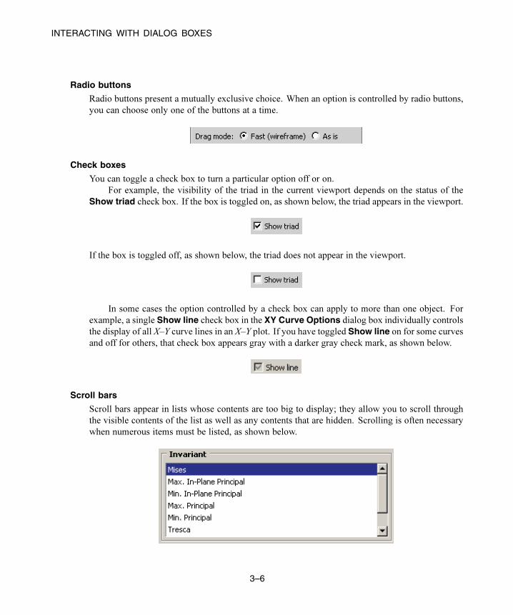
INTERACTING WITH DIALOG BOXES
Radio buttons
Radio buttons present a mutually exclusive choice. When an option is controlled by radio buttons,
you can choose only one of the buttons at a time.
Check boxes
You can toggle a check box to turn a particular option off or on.
For example, the visibility of the triad in the current viewport depends on the status of the
Show triad check box. If the box is toggled on, as shown below, the triad appears in the viewport.
If the box is toggled off, as shown below, the triad does not appear in the viewport.
In some cases the option controlled by a check box can apply to more than one object. For
example, a single Show line check box in the XY Curve Options dialog box individually controls
the display of all X–Y curve lines in an X–Y plot. If you have toggled Show line on for some curves
and off for others, that check box appears gray with a darker gray check mark, as shown below.
Scroll bars
Scroll bars appear in lists whose contents are too big to display; they allow you to scroll through
the visible contents of the list as well as any contents that are hidden. Scrolling is often necessary
when numerous items must be listed, as shown below.
3–6
Abaqus ID:
Printed on:

INTERACTING WITH DIALOG BOXES
Sliders
Sliders allow you to set the value of an option that has a continuous range of possible values. An
example of a slider is shown in the following figure:
3.2.2 Entering expressionsIf a field in a dialog box or in the prompt area is expecting a floating point number or a complex number,
you can enter an arithmetic expression, as shown in Figure 3–1.
Figure 3–1 An expression in a text field.
3–7
Abaqus ID:
Printed on:
INTERACTING WITH DIALOG BOXES
The expression is evaluated by the Python interpreter that is built into Abaqus/CAE. The arithmetic
expression is replaced by its value; if you reopen a dialog that contained expressions, only the values
are available. Variables like pi and functions like sin() are available because Abaqus/CAE imports
the Python math module when you start a session. As a result, you can enter any expression that can
be evaluated by Python’s built-in functions or by the Python math module. For more information, see
the documentation for built-in functions (http://www.python.org/doc/current/lib/built-in-funcs.html) and
the mathmodule (http://www.python.org/doc/current/lib/module-math.html) on the official Python home
page.
To make sure that your expression is evaluated as expected, you should be aware of the following:
• If you enter numbers as integers, Python will perform integer division and round down any
remainder. For example, Python will interpret 3/2 as 1 and 1/2 as 0. In contrast, Python
interprets 3./2 as 1.5 and 1/2. as 0.5.
• Python interprets numbers with leading zeros as octal numbers. For example, 0123 is interpreted
as 83.0.
• Python interprets e as the natural logarithm; for example, e equates to 2.71828182846 and e+2equates to 4.71828182846.
• If the “e” character is preceded by a number, Python interprets it as an exponent, not a natural
logarithm. For example, Python interprets 2e+2 as 2 × 10² and equates it to 200.
• Python interprets 2e+ as 2 × 100 and equates it to 2. Similarly, Python interprets 2e++11 as
2 × 100 + 11 and equates it to 13.
If you are unsure how Python will interpret your expression, you can enter the expression on the
command line; Abaqus/CAE will print the resulting interpreted value in the message area. To access the
command line interface, click in the bottom left corner of the main window. For more information,
see “Components of the main window,” Section 2.2.1.
You can also test how Abaqus/CAE interprets an expression by entering abaqus python at an
operating system prompt and entering the expression at the Python prompt that appears. The prompt
line and some dialog boxes do not allow you to enter an expression. As an alternative, you can enter the
expression on the command line or at the Python prompt and paste the resulting value in the prompt line
or dialog box.
3.2.3 Using dimmed dialog box and toolbox components
Some objects in dialog boxes and toolboxes are available only under certain circumstances. When an
object is unavailable, it appears dimmed in the dialog box. Items are usually dimmed as a result of some
other setting in the dialog box. For example, if Use settings below is not selected, the image size
options below it are not available and appear dimmed, as shown below.
3–8
Abaqus ID:
Printed on:

INTERACTING WITH DIALOG BOXES
Context-sensitive help is available even for dimmed options, although tooltips are not.
3.2.4 Disabling warning dialog boxesSome dialog boxes can be disabled so that they will not appear again during the current Abaqus/CAE
session. For example, if you submit a job for analysis and job files with the same name already exist,
Abaqus/CAE displays a dialog box asking if it is OK to overwrite the job files, as shown below.
If you toggle off Show this warning next time, the dialog box will be disabled for the remainder of
the current Abaqus/CAE session.
3.2.5 Understanding the OK, Apply, Defaults, Continue, Cancel, andDismiss buttons
When you are finished working with a dialog box, you can specify how to proceed by using different
action buttons. For example, if you enter data in a dialog box, you can save the data and apply them by
clicking OK. If the dialog box is part of an intermediate step of a procedure, you can click Continue to
move on to the next step.
The following action buttons can appear in a dialog box:
OK
Click OK to commit the current contents of a dialog box and to close the dialog box.
3–9
Abaqus ID:
Printed on:
INTERACTING WITH DIALOG BOXES
Apply
When you click Apply, any changes you have made in the dialog box take effect, but the dialog
box remains displayed. This button is useful if you make changes in a dialog box and would like to
see the effects of these changes before closing the dialog box.
Defaults
If you want to revert back to the predefined default values after entering data or specifying
preferences in a dialog box, you can click Defaults. This button affects only the information
entered in the dialog box. It does not apply your changes or close the dialog box; therefore, to see
the effect of reverting to the default values, you must click Apply or OK.
Cancel
Click Cancel to close a dialog box without applying any of the changes that you made. If the dialog
box appears in the middle of a procedure, clicking Cancel usually also cancels the procedure. In
some cases clicking Cancel returns you to the previous step in the procedure.
Continue
Dialog boxes that appear in the middle of a procedure contain Continue buttons. When you click
Continue, you indicate that you have finished entering data in the current dialog box and would
like to move on to the next step of the procedure. Continue causes the dialog box to be closed and
all data in it to be saved unless you click Cancel at some point later in the procedure.
Dismiss
Dismiss buttons appear in dialog boxes that contain data that you cannot modify. For example,
some managers contain lists of objects that exist but no fields in which you can enter data or specify
preferences. Dismiss buttons also appear in message dialog boxes. When you click Dismiss, thedialog box closes.
To close a toolbox or a dialog box that does not have a Cancel or Dismiss button, click the close
button in the upper right corner of the toolbox or dialog box. Alternatively, you can close an active
toolbox or dialog box by pressing [Esc].
Note: On Linux platforms, depending on your settings, [Esc] may be the only way to close a toolbox
or dialog box. For more information, see “Linux settings that affect Abaqus/CAE and Abaqus/Viewer,”
Section 5.1.3 of the Abaqus Installation and Licensing Guide.
3.2.6 Using dialog boxes separated by tabsFor the sake of organization and convenience, some dialog boxes are separated by tabs. Only one dialog
box is visible at a time. To view a particular dialog box, click its labeled tab.
For example, Figure 3–2 displays the Common Plot Options dialog boxes.
3–10
Abaqus ID:
Printed on:

INTERACTING WITH DIALOG BOXES
Figure 3–2 Dialog boxes separated by tabs.
If you click the Color & Style tab, the dialog box containing the color and edge attributes options comes
forward, obscuring the other four dialog boxes, as shown in Figure 3–3.
Figure 3–3 Using tabs to display particular dialog boxes.
3–11
Abaqus ID:
Printed on:
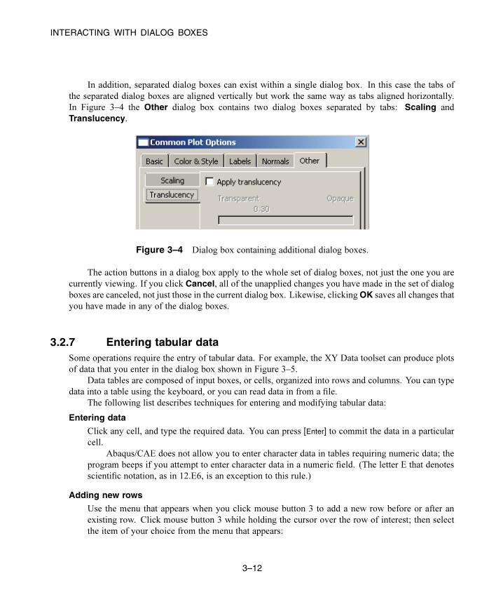
INTERACTING WITH DIALOG BOXES
In addition, separated dialog boxes can exist within a single dialog box. In this case the tabs of
the separated dialog boxes are aligned vertically but work the same way as tabs aligned horizontally.
In Figure 3–4 the Other dialog box contains two dialog boxes separated by tabs: Scaling and
Translucency.
Figure 3–4 Dialog box containing additional dialog boxes.
The action buttons in a dialog box apply to the whole set of dialog boxes, not just the one you are
currently viewing. If you click Cancel, all of the unapplied changes you have made in the set of dialog
boxes are canceled, not just those in the current dialog box. Likewise, clicking OK saves all changes that
you have made in any of the dialog boxes.
3.2.7 Entering tabular dataSome operations require the entry of tabular data. For example, the XY Data toolset can produce plots
of data that you enter in the dialog box shown in Figure 3–5.
Data tables are composed of input boxes, or cells, organized into rows and columns. You can type
data into a table using the keyboard, or you can read data in from a file.
The following list describes techniques for entering and modifying tabular data:
Entering data
Click any cell, and type the required data. You can press [Enter] to commit the data in a particular
cell.
Abaqus/CAE does not allow you to enter character data in tables requiring numeric data; the
program beeps if you attempt to enter character data in a numeric field. (The letter E that denotes
scientific notation, as in 12.E6, is an exception to this rule.)
Adding new rows
Use the menu that appears when you click mouse button 3 to add a new row before or after an
existing row. Click mouse button 3 while holding the cursor over the row of interest; then select
the item of your choice from the menu that appears:
3–12
Abaqus ID:
Printed on:
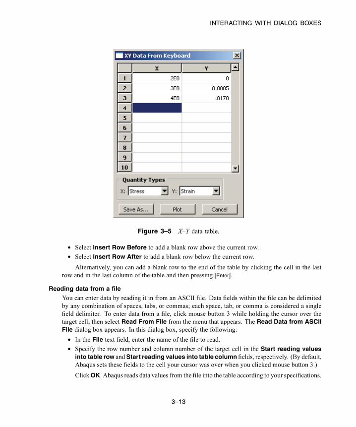
INTERACTING WITH DIALOG BOXES
Figure 3–5 X–Y data table.
• Select Insert Row Before to add a blank row above the current row.
• Select Insert Row After to add a blank row below the current row.
Alternatively, you can add a blank row to the end of the table by clicking the cell in the last
row and in the last column of the table and then pressing [Enter].
Reading data from a file
You can enter data by reading it in from an ASCII file. Data fields within the file can be delimited
by any combination of spaces, tabs, or commas; each space, tab, or comma is considered a single
field delimiter. To enter data from a file, click mouse button 3 while holding the cursor over the
target cell; then select Read From File from the menu that appears. The Read Data from ASCIIFile dialog box appears. In this dialog box, specify the following:
• In the File text field, enter the name of the file to read.
• Specify the row number and column number of the target cell in the Start reading valuesinto table row andStart reading values into table column fields, respectively. (By default,
Abaqus sets these fields to the cell your cursor was over when you clicked mouse button 3.)
ClickOK. Abaqus reads data values from the file into the table according to your specifications.
3–13
Abaqus ID:
Printed on:

INTERACTING WITH DIALOG BOXES
Moving from cell to cell
Use the [Enter] key to move from left to right between the cells in a row. When you have reached
the end of the row, press [Enter] to move the cursor to the first cell in the following row.
In addition, you can use a combination of the [Tab] key and the up and down arrow keys to
move from cell to cell. Use [Tab] to move to the right and [Shift]+[Tab] to move to the left; use the up
and down arrows to move up and down. You can also simply click the cell of interest.
Changing data
If a cell already contains data, clicking the cell highlights the data; as soon as you begin typing, the
highlighted contents of the cell disappear and are replaced by whatever you type. You can also use
the [Backspace] or [Delete] keys to delete highlighted data in a cell.
After clicking the cell once, you can click a second time to remove the highlighting and position
the cursor within the cell. Use the [Backspace] key and the other keys on your keyboard to modify
the data.
Cutting, copying, and pasting data
Use the menu that appears when you click mouse button 3 to cut, copy, and paste data from one
location in a table to another. You can cut or copy data in single cells, in rows or parts of rows, in
columns or parts of columns, and in series of consecutive rows or columns.
First, drag the mouse over the cells containing the data that you want to cut or copy. All of
the selected cells will become highlighted except the cell that you selected first. This cell becomes
highlighted when you move the cursor outside the data table window or if you click mouse button 3.
Once you have selected the cells of interest, click mouse button 3 while holding the cursor over
the selection; then select either Cut or Copy from the menu that appears. To paste the data, select
the target cell, click mouse button 3, and select Paste from the menu that appears.
Sorting data
Some data tables offer a sorting feature. (To determine if sorting is available for a particular table,
hold the cursor over the table; then click mouse button 3. If it is available, Sort is listed in the menu
that appears.)
To sort table data, click mouse button 3 while holding the cursor over the table; then click Sort.The Sort Table dialog box appears. In this dialog box, choose the following:
• In the Sort by text field, choose the column by which to sort.
• Choose Ascending or Descending sort order.
Click OK or Apply. Abaqus sorts all rows according to data values in the specified column.
Expanding and contracting columns
You can change the size of the columns in some tables. To expand or contract a column, move the
cursor to the line that divides the headings of the columns you want to resize; a resize cursor will
3–14
Abaqus ID:
Printed on:
INTERACTING WITH DIALOG BOXES
appear. Drag this cursor to the left or right to resize the two columns on either side of the dividing
line.
You can also resize the last column in some tables by horizontally enlarging the dialog box
that contains the table.
Viewing data that extend beyond the edge of the dialog box
Use the horizontal and vertical scroll bars to view portions of a table that are outside the boundaries
of the dialog box. In some cases scroll bars may not be available; instead, increase the size of the
dialog box to display more data.
Deleting rows of data
Click any cell within the row you want to delete, or select multiple cells in consecutive rows. Then,
while holding the cursor over the dialog box containing the table, click mouse button 3 and select
Delete Rows from the menu that appears. The row or rows disappear; if the rows are numbered,
Abaqus/CAE automatically renumbers the remaining rows.
You cannot delete rows from tables that display matrices or tensors of fixed size, such as those
used in the orthotropic or anisotropic elasticity data input forms in the Property module.
Creating X–Y data from table data
While you are creating a material in the Property module, you can use the data in a table to create
X–Y data. You can then use the Visualization module to plot the X–Y data and to visually check its
validity. To create an X–Y data object, click mouse button 3 while holding the cursor over the table;
then select Create XY Data from the menu that appears. The Create XY Data dialog box appears.
In this dialog box, do the following:
• Enter the name of the X–Y data to create.
• Specify the column number containing the X-values and the column number containing the
Y-values.
• Click OK. Abaqus reads the data values from the table into the X–Y data. Abaqus/CAE retains
saved X–Y data only for the duration of the session.
To view the X–Y data, do the following:
• From the module list on the context bar, select Visualization.
• From the main menu bar, select Tools→XY Data→Plot, and select the X–Y data from the
pull-right menu.
For more information, see Chapter 47, “X–Y plotting.”
Clearing the table
You can delete all data from a table. While holding the cursor over the table, click mouse button 3
and select Clear Table from the menu that appears. The table data disappear.
3–15
Abaqus ID:
Printed on:

INTERACTING WITH DIALOG BOXES
3.2.8 Customizing fonts
The Select Font dialog box allows you to customize the font of certain kinds of text; for example, you
can use this dialog box to customize the font that appears in viewport annotations. A similar dialog box
is used to customize the font of the Visualization module labels and titles.
The Select Font dialog box allows you to specify and preview the following:
• Proportional or fixed fonts.
• The font family.
• The font size, in points.
• Regular, bold, or italic font.
The available options vary depending on which fonts are installed on your system.
3.2.9 Customizing colors
The Select Color dialog box allows you to customize the color of many objects in Abaqus/CAE. For
more information about the objects that you can change, see the following sections:
• “Customizing the view triad,” Section 5.4
• “Choosing background colors,” Section 7.7, in the HTML version of this guide
• “Selecting overall element and surface edge color,” Section 55.3.3
• “Coloring elements with no results,” Section 55.12.4
• “Customizing the legend,” Section 56.1
• “Customizing the title block,” Section 56.2
• “Customizing the state block,” Section 56.3
The current color is displayed on the left side of the Select Color dialog box, below the eyedropper tool.
You can use the methods in the Select Color dialog box to update the displayed color. The color is not
updated elsewhere until you click OK to accept your changes and to close the Select Color dialog box.You can choose from the following methods of color selection:
Color palette
Twenty-four common colors are displayed in boxes along the bottom of the dialog box. Click a
color to select it; you cannot modify the palette to show different colors.
Eyedropper tool
The eyedropper tool is located on the left side of the dialog box. When you click the eyedropper
tool, the cursor changes to crosshairs. The next time you click mouse button 1 anywhere on the
computer screen, Abaqus/CAE selects the color at the cursor position.
3–16
Abaqus ID:
Printed on:

INTERACTING WITH DIALOG BOXES
Note: The cursor returns to its normal form if you move it outside the Abaqus/CAE application
window, but you can still select a color by clicking mouse button 1.
Color wheel
The color wheel and brightness control are located in the Wheel tab. A black dot indicates the
position of the currently selected color, regardless of the method that was used to select it. Click
anywhere on the wheel to select a new color. Move the vertical slider to change the brightness; as
you move the slider downward, Abaqus/CAE adds black to the selected color.
RGB controls
RGB (Red, Green, and Blue) controls are located in the RGB tab. The RGB settings match the
color displayed on the left side of the Select Color dialog box, regardless of the method that was
used to select it. You can move the sliders or enter values from 0 to 255 to mix the three colors of
light and produce the full color spectrum. 0, 0, 0 is black (no light); and 255, 255, 255 is white (full
intensity, full spectrum light).
HSV controls
HSV (Hue, Saturation, and Value) controls are located in the HSV tab. The HSV settings match
the color displayed on the left side of the Select Color dialog box, regardless of the method that
was used to select it. The Hue control ranges from 0 to 360, and changing the setting corresponds
to moving the black dot around the perimeter of the color wheel (0 and 360 are both red). The
Saturation control ranges from 0 to 100 and varies the amount of the selected color added to the
background color. The Value control indicates the background color; 0 is black, 100 is white.
CMY controls
CMY (Cyan, Magenta, and Yellow) controls are located in the CMY tab. The CMY settings match
the color displayed on the left side of the Select Color dialog box, regardless of the method that
was used to select it. You can move the sliders or enter values from 0 to 255 to mix the three colors
of tint and produce the full color spectrum. The CMY controls work like adding tint to paint; 0, 0,
0 is white (no tint), and 255, 255, 255 is black (all tint).
Color list
The color list is located in the List tab. You can choose from several hundred colors, including
shades of gray. The color list provides you with a more extensive range of colors than the color
palette, but it does not provide you with the full color spectrum.
3.2.10 Using file selection dialog boxes
File selection dialog boxes allow you to select files from lists that are filtered based on file type or location.
To use a file selection dialog box, you first choose the type of file to open and then specify the directory
3–17
Abaqus ID:
Printed on:

INTERACTING WITH DIALOG BOXES
to list. Abaqus/CAE refreshes the dialog box to list only files that meet your criteria. From this list, you
select the file to open.
The dialog box for selecting model databases or output databases is shown in Figure 3–6.
go up one directoryhome
work
bookmarknewdirectory
list icons
detailsshow hidden files
Figure 3–6 Selecting a model database or an output database.
Note: In Abaqus/Viewer you can open only output database files; therefore, Output Database (*.odb)is the only type available in the File Filter field.
Similar file selection dialog boxes appear when you perform other Filemenu functions, such as importing
a part or printing to a file.
Use the following techniques to select the file of your choice:
Filtering the file list according to file type
File selection dialog boxes contain File Filter fields, which allow you to select the file extension
of interest. For example, the File Filter selection in Figure 3–6 is Output Database (*.odb).Therefore, only files with the extension .odb appear in the list in the center of the dialog box.
3–18
Abaqus ID:
Printed on:

INTERACTING WITH DIALOG BOXES
Using wildcards to search for a file name
You can use a wildcard filter to search for partial names of files. A wildcard search is helpful when
you have a large number of files stored in the same directory. Wildcard searches also override the file
extensions (File Filter field, as described above), allowing you to open files saved with nonstandardfile extensions.
To use a wildcard search, enter a partial file name into the File Name field using one of the
following forms:
? matches a single character
* matches zero or more characters
[abc] matches a single character, but it must be one of the characters listed
[^abc] or [!abc] matches a single character, but it must not be one of the characters listed
[a-zA-Z] matches a single character, but it must be within the ranges provided
[^a-zA-Z] or [!a-zA-Z] matches a single character, but it must not be within the ranges provided
pat1|pat2 or pat1,pat2 matches either pat1 or pat2
(pat1|pat2) or (pat1,pat2) matches either pat1 or pat2, and the patterns may be nested
You can combine several wildcard filters to further narrow your search. For example, entering
[abc]*.(cae,odb) will list all files beginning with a, b, or c and having a .cae or .odb file
extension.
Specifying the directory from which to select a file
By default, the Directory field shows the directory in which you started Abaqus/CAE. If you want
to view a list of files from a different directory, you can click the directory name in the list to view
directories within the current path or you can click the arrow next to the Directory field to access
other paths that are available on your system. In addition, icons at the top of the dialog box allow
you to do the following (keyboard shortcuts are shown in parentheses when available):
• Go up one directory level ([Backspace]).
• Access your system default, or Home, directory ([Ctrl]+H).
• Access the Work directory ([Ctrl]+W). The work directory is the directory from which you
started Abaqus/CAE unless you specified the directory using File→Set Work Directory.
• Set or use Bookmarks to any directory on your system.
• Create a new directory ([Ctrl]+N).
The Directory field includes a Network connectors item. If you have created and started a
network ODB connector, you can use this item to access a remote directory and to open a remote
output database. For more information, see “Creating a network ODB connector,” Section 9.7.4, in
the HTML version of this guide.
3–19
Abaqus ID:
Printed on:

INTERACTING WITH DIALOG BOXES
Selecting a file
To select and open a file, double-click the file name of interest from the list. You can also begin
typing the file name; the cursor will reposition to the matching location in the file list, and the first file
starting with the letters you typed will be selected. Alternatively, you can enter the entire directory
path and file name of interest directly in the File Name field and then click OK. Icons at the top
of the dialog box allow you to change the displayed file format to one of the following (keyboard
shortcuts are shown in parentheses):
• A list ([Ctrl]+S).
• Icons ([Ctrl]+B).
• A detailed list ([Ctrl]+L).
The icon farthest to the right allows you to display or suppress “hidden” files.
3.2.11 Selecting multiple items from lists and tablesIn some Abaqus/CAE dialog boxes it is necessary to select an item from a list or a table before you can
perform certain functions. For example, if you want to plot X–Y data, you must first select the data object
of your choice from the list in the XY Data Manager, shown in Figure 3–7, and then click Plot.
Figure 3–7 Single item selected.
Some functions allow you to operate on more than one item. For example, if you wanted to delete
the first two data objects in the manager shown in Figure 3–7, you could select them both and then click
Delete.
3–20
Abaqus ID:
Printed on:

INTERACTING WITH DIALOG BOXES
To select a single item from a list, you need only click that item in the dialog box. To select a
single item from a table, click the table row heading. To select multiple items, you can use the following
techniques:
Selecting consecutive items from a list or table
Click the first item of interest from a list or row heading from a table and then, while continuing
to hold down mouse button 1, drag the cursor over the remaining items. Release the mouse button
when all of the items of interest are selected. For example, consecutive items are selected in
Figure 3–8.
Figure 3–8 Consecutive items selected.
Another way to select consecutive items is to click the first item of interest from a list or row
heading from a table and then [Shift]+Click the last item of interest. All items between the first and
the last are selected automatically.
Selecting nonconsecutive items from a list or table
Click the first item of interest from a list or row heading from a table and then [Ctrl]+Click any other
items you want to select. For example, nonconsecutive items are selected in Figure 3–9.
Canceling a selection
You can [Ctrl]+Click previously selected items to remove them from your selection. For example,
if you [Ctrl]+Click Displacement in the list shown in Figure 3–9, that data object is no longer
selected, as shown in Figure 3–10.
Certain functions in a dialog box may become unavailable when you select multiple items. For
example, the Edit, Copy, and Rename functions in the Data Manager shown in Figure 3–10 are valid
3–21
Abaqus ID:
Printed on:

INTERACTING WITH DIALOG BOXES
Figure 3–9 Nonconsecutive items selected.
Figure 3–10 Individual item removed from selection.
only for individual data objects. When you select multiple data objects, these three functions become
unavailable.
3–22
Abaqus ID:
Printed on:
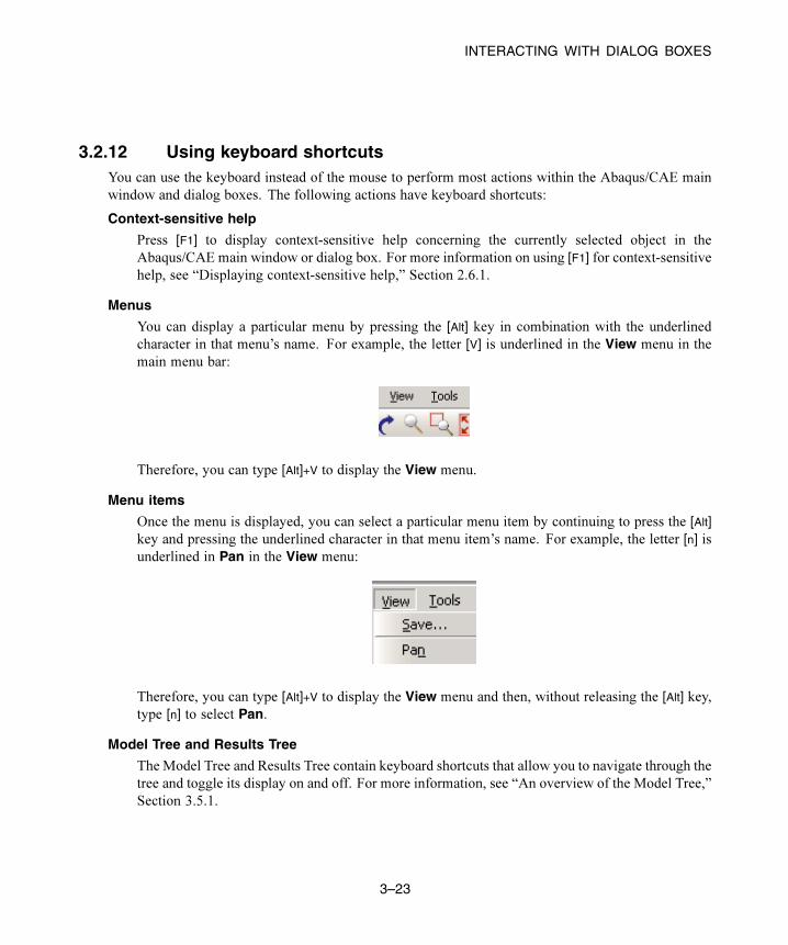
INTERACTING WITH DIALOG BOXES
3.2.12 Using keyboard shortcutsYou can use the keyboard instead of the mouse to perform most actions within the Abaqus/CAE main
window and dialog boxes. The following actions have keyboard shortcuts:
Context-sensitive help
Press [F1] to display context-sensitive help concerning the currently selected object in the
Abaqus/CAE main window or dialog box. For more information on using [F1] for context-sensitivehelp, see “Displaying context-sensitive help,” Section 2.6.1.
Menus
You can display a particular menu by pressing the [Alt] key in combination with the underlined
character in that menu’s name. For example, the letter [V] is underlined in the View menu in the
main menu bar:
Therefore, you can type [Alt]+V to display the View menu.
Menu items
Once the menu is displayed, you can select a particular menu item by continuing to press the [Alt]key and pressing the underlined character in that menu item’s name. For example, the letter [n] isunderlined in Pan in the View menu:
Therefore, you can type [Alt]+V to display the View menu and then, without releasing the [Alt] key,type [n] to select Pan.
Model Tree and Results Tree
The Model Tree and Results Tree contain keyboard shortcuts that allow you to navigate through the
tree and toggle its display on and off. For more information, see “An overview of the Model Tree,”
Section 3.5.1.
3–23
Abaqus ID:
Printed on:

UNDERSTANDING AND USING TOOLBOXES AND TOOLBARS
3.3 Understanding and using toolboxes and toolbars
This section explains how to use the toolbox windows and toolbars to perform common functions within
a module or toolset or on the canvas.
3.3.1 What are toolboxes and toolbars?
Toolboxes and toolbars are collections of icons that provide quick access to commonly used Abaqus/CAE
functions. For example, the Visualization module toolbox contains icons representing the tools used to
generate different kinds of plots. The Visualization module toolbox is shown in Figure 3–11. All module
toolboxes are available immediately to the left of the drawing area as soon as you enter the module.
Toolbars also contain collections of icons to access Abaqus/CAE functions. Toolbars provide access
to supporting functions that help you save, manipulate, and make selections from a model; whereas
toolboxes contain functions critical to creating or changing a model. In addition to tool icons, toolbars
may also contain lists of options related to a tool. For example, the color mapping list in the ColorCode toolbar contains various methods for coloring the objects displayed in the current viewport. You
can also customize toolbar contents, move toolbars to new locations, or close them (for more information,
see Chapter 61, “The Customize toolset”). Toolboxes cannot be moved or hidden.
To obtain a short description of a tool, place the cursor over that tool for a moment; a small box
containing a description, or “tooltip,” will appear. Tooltips are not available for icons that appear
dimmed; to get information on those icons, use context-sensitive help instead.
3.3.2 Using toolboxes and toolbars that contain hidden icons
In some toolboxes, such as the Job module toolbox, all tool icons are immediately visible; however, most
toolboxes contain hidden icons to conserve space. Since there is more space above the canvas, and since
you can move or hide toolbars to meet your needs, most toolbars do not contain hidden icons.
Any icon that includes a small triangle in its lower right corner conceals a group of icons whose
function is closely related to that of the visible icon.
To select tools whose icons are initially hidden:
1. Click and hold any icon that includes a triangle in its lower right corner.
Icons for all the tools that are closely related to the original icon appear. For example, Figure 3–12
shows the top portion of the Part module toolbox with all of the icons revealed that are used for
creating round or chamfered corners.
3–24
Abaqus ID:
Printed on:

UNDERSTANDING AND USING TOOLBOXES AND TOOLBARS
Figure 3–11 The Visualization module toolbox.
Create Chamfer tool
Figure 3–12 Part module toolbox with round and chamfer icons displayed.
3–25
Abaqus ID:
Printed on:
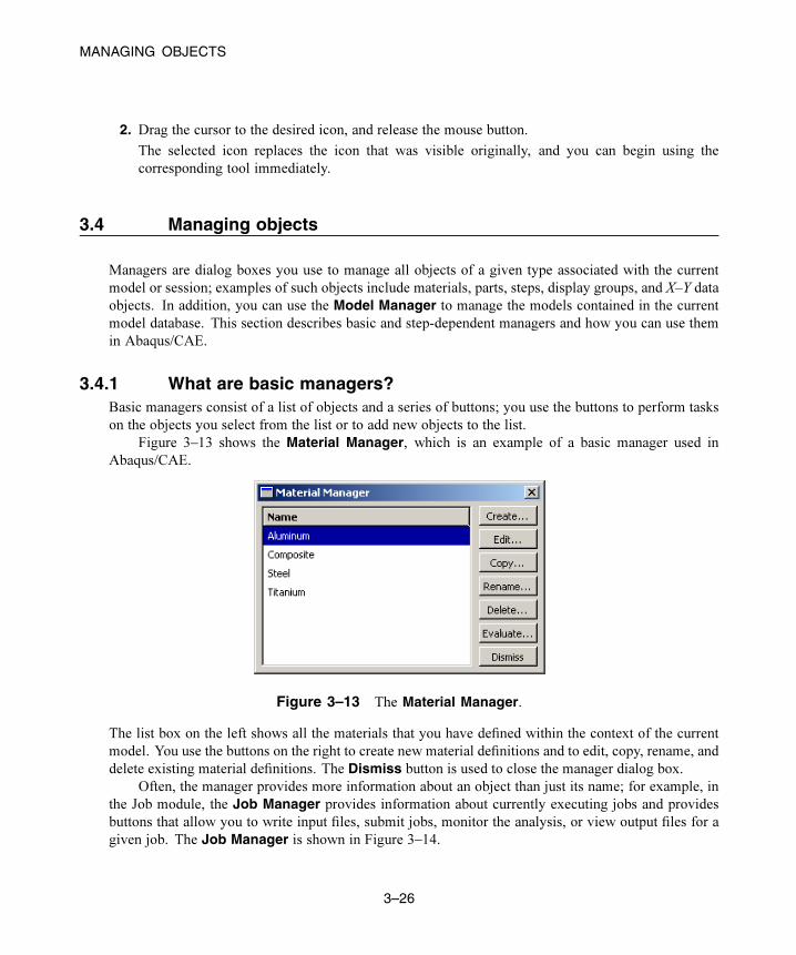
MANAGING OBJECTS
2. Drag the cursor to the desired icon, and release the mouse button.
The selected icon replaces the icon that was visible originally, and you can begin using the
corresponding tool immediately.
3.4 Managing objects
Managers are dialog boxes you use to manage all objects of a given type associated with the current
model or session; examples of such objects include materials, parts, steps, display groups, and X–Y data
objects. In addition, you can use the Model Manager to manage the models contained in the current
model database. This section describes basic and step-dependent managers and how you can use them
in Abaqus/CAE.
3.4.1 What are basic managers?Basic managers consist of a list of objects and a series of buttons; you use the buttons to perform tasks
on the objects you select from the list or to add new objects to the list.
Figure 3–13 shows the Material Manager, which is an example of a basic manager used in
Abaqus/CAE.
Figure 3–13 The Material Manager.
The list box on the left shows all the materials that you have defined within the context of the current
model. You use the buttons on the right to create new material definitions and to edit, copy, rename, and
delete existing material definitions. The Dismiss button is used to close the manager dialog box.
Often, the manager provides more information about an object than just its name; for example, in
the Job module, the Job Manager provides information about currently executing jobs and provides
buttons that allow you to write input files, submit jobs, monitor the analysis, or view output files for a
given job. The Job Manager is shown in Figure 3–14.
3–26
Abaqus ID:
Printed on:

MANAGING OBJECTS
Figure 3–14 The Job Manager.
Most tasks you can perform with a manager can also be performed using the pull-down menus
available from the main menu bar; for example, Figure 3–15 shows the menu items that correspond to
the Job Manager.
Figure 3–15 Menu items that correspond to the Job Manager.
After you select a management operation from the main menu bar, the procedure is exactly the same as
if you had clicked the corresponding button inside the manager dialog box. In addition, most of the tasks
3–27
Abaqus ID:
Printed on:
MANAGING OBJECTS
you can perform with a manager can be performed by clicking mouse button 3 on an object in the Model
Tree. For more information, see “Working with the Model Tree and the Results Tree,” Section 3.5.
The decision whether to use menus, dialog boxes, or the Model Tree is yours. In general, menus
are more convenient if you are performing isolated operations; the advantages of manager dialog boxes
become apparent when you are performing several operations in sequence, when you need to browse
through a long list of objects, or when you need quick access to the additional information that is
displayed by some managers. The Model Tree provides you with a graphical overview of your model
and allows you to perform operations without changing modules. In addition, the Model Tree allows
you to use drag-select to select multiple items; for example, you can select multiple sets to merge or
multiple parts to delete.
3.4.2 What are step-dependent managers?
Like the basic managers described in “What are basic managers?,” Section 3.4.1, step-dependent
managers contain a list of all of the objects of a certain type that you have created, as well as Create,Edit, Copy, Rename, and Delete buttons that you can use to manipulate existing objects and to create
new ones.
However, the types of objects that appear in step-dependent managers are those that you can create
and, in some cases, modify, suppress, and deactivate in particular analysis steps. Therefore, unlike basic
managers, step-dependent managers contain additional information concerning the history of each object
listed in the manager. Step-dependent managers display how these objects propagate from one step to
another during the course of an Abaqus analysis. (For information on steps and multiple-step analyses,
see “Defining an analysis,” Section 6.1.2 of the Abaqus Analysis User’s Guide.)
The following step-dependent managers exist in Abaqus/CAE:
In the Load module:
• Load Manager
• Boundary Condition Manager
• Predefined Field Manager
In the Interaction module:
• Interaction Manager
In the Step module:
• Field Output Requests Manager
• History Output Requests Manager
• Adaptive Mesh Constraint Manager
For example, the Load Manager is shown in Figure 3–16.
3–28
Abaqus ID:
Printed on:

MANAGING OBJECTS
Figure 3–16 The Load Manager.
This manager displays an alphabetical list of existing loads along the left side of the dialog box.
The names of all the steps in the analysis appear along the top of the dialog box in the order of execution.
The table formed by these two lists displays the status of each load in each step. (For information on
creating and deleting steps, see Chapter 14, “The Step module.”)
If you click one of the cells in the table, that cell becomes highlighted, and the following information
related to the cell appears in the legend at the bottom of the manager:
• The type of analysis procedure carried out in the step in that column.
• Information about the step-dependent object in that row.
• The status of the step-dependent object in that step (the same information that appears in the cells
of the table except in more detail in some cases).
You can use the icons in the column along the left side of the manager to suppress objects or to
resume previously suppressed objects for an analysis. For more information, see “Suppressing and
resuming objects,” Section 3.4.3.
The buttons along the right side of the manager allow you to manipulate objects in the steps that
you select. For example, if you click Edit in the Load Manager shown above, an editor appears in which
you could modify the load named Force in Step-1. The other buttons—Move Left, Move Right,Activate, and Deactivate—allow you to change the status of an object in a particular step.
Note: The Activate and Deactivate buttons are not available in the Predefined Field Manager.
For more information, see “Modifying the history of a step-dependent object,” Section 3.4.6; and, in the
HTML version of this guide, “Changing the status of an object in a step,” Section 3.4.12; and “Editing
step-dependent objects,” Section 3.4.13.
3–29
Abaqus ID:
Printed on:

MANAGING OBJECTS
You can resize the columns of the table by dragging the dividers between the column headings to
the right or left. You can also increase the size of the dialog box by dragging the sides of the box. If
the analysis includes many steps or many step-dependent objects, increasing the size of the dialog box
allows you to view more rows and columns without having to use the scroll bars.
3.4.3 Suppressing and resuming objectsWhen performing an analysis, you may want to study the effects of different combinations of objects,
such as loads, or you may want to temporarily exclude an object from the model, such as excluding
a boundary condition or a constraint in a design analysis. You can create a model that includes all of
the objects and then suppress the objects that you want to exclude from the model prior to the analysis.
Suppressed objects are not written to the input file and are treated as deleted objects. You should review
your model for any references to suppressed objects. For more information, see “What happens when
deleted objects are referred to?,” Section 3.4.8.
You can suppress step-dependent objects, constraints (in the Interaction module), section
assignments (in the Property module), and features. After you create a suppressible object, the manager
dialog box displays a green check mark in the column along the left side of the manager next to the
name of the object. You can suppress an object from the manager by clicking the green check mark next
to the object. For example, if you click the green check mark to the left of the load named Force in the
Load Manager shown in Figure 3–16, the icon changes to a red “X” and the cells displaying the status
of the load in each step are shaded gray to indicate that the load is suppressed, as shown in Figure 3–17.
Note: There is no manager associated with features; you can suppress or resume features using the
popup menus in the Model Tree.
Figure 3–17 The Load Manager indicates that the load named Force is suppressed.
3–30
Abaqus ID:
Printed on:

MANAGING OBJECTS
You can also select Suppress→object in the appropriate menu from the main menu bar to suppress
an object. For example, to suppress the load named Force shown in Figure 3–16, you would select
Load→Suppress→Force from the main menu bar of the Load module.
You cannot edit suppressed objects; however, you can copy, rename, and delete them. Symbols for
suppressed objects are not displayed in the viewport.
You can resume an object that was previously suppressed. If you attempt to resume an object that is
not valid for a given procedure type, Abaqus/CAE displays an error message. You can use the manager
or the Resume menu item from the main menu bar to resume the object. In the manager, click the red
“X” to change the icon back to a green check mark and to remove the cell shading. Symbols for resumed
objects are displayed in the viewport.
You can also use the Model Tree to suppress or resume an object by clicking mouse button 3 on the
object and selecting Suppress or Resume from the menu that appears. The Model Tree displays a red
“X” next to an object to indicate that it is suppressed. For more information, see “An overview of the
Model Tree,” Section 3.5.1.
3.4.4 Understanding the status of an object in a stepA model can contain a sequence of analysis steps. When you create an object in a step, that object may
or may not continue to be active in any of the following steps. The activity (or inactivity) of an object in
any particular step is called its “status” in that step.
For example, Figure 3–18 shows the status of a load in a series of general static analysis steps.
Step 1 Step 2 Step 3 Step 4 Step 5 Step 6
Created Propagated Propagated Inactive InactiveModifiedLoad 1
Load
1
Time
Figure 3–18 The analysis history of a load.
The load in this example is created in Step 1; therefore, the status of the load in Step 1 is Created.Since Step 1 is a general static step, the load’s magnitude is ramped up over the course of the step. If
the load continues to be active in Step 2, its status in Step 2 is Propagated and its magnitude remains
constant throughout that step. If you edit the load in Step 3, its status in Step 3 becomes Modified
3–31
Abaqus ID:
Printed on:

MANAGING OBJECTS
and its magnitude ramps to the new value over the course of the step. If the modified version of the
load continues to be active in Step 4, its status in Step 4 (as in Step 2) is Propagated and the value is
constant. If you deactivate the load in Step 5, its status in Step 5 is Inactive and its magnitude ramps
down to zero. The load remains inactive in Step 6.
For detailed explanations of the terms used to describe object status, see “Terms describing object
status,” Section 3.4.5.
3.4.5 Terms describing object statusAbaqus/CAE uses the following terms to describe the status of objects in particular steps:
Created
The object was created and becomes active in this step. The point in the step at which a prescribed
condition becomes active depends on the amplitude variation associated with that step. For more
information, see “Prescribed conditions” in “Defining an analysis,” Section 6.1.2 of the Abaqus
Analysis User’s Guide.
Computed
The analysis products will compute the value of the object in this step.
Modified
The definition of the object has been modified in this step. The variation of a prescribed condition
over the course of the step depends on the amplitude variation associated with that step.
Propagated
The object was created, modified, or computed in an earlier step of the analysis and continues to be
active in this step.
Inactive
The object has been deactivated in this step or in a previous step. It will remain deactivated in all
subsequent steps until you reactivate it. You cannot deactivate an object in the step in which it was
created. The point in the step at which a prescribed condition becomes inactive depends on the
amplitude variation associated with that step. For more information, see “Prescribed conditions” in
“Defining an analysis,” Section 6.1.2 of the Abaqus Analysis User’s Guide.
You cannot deactivate predefined fields; an inactive status for a predefined field means that the
field has been reset to the value specified in the initial step. The point in the step at which an object
resumes its initial value depends on the amplitude variation associated with that step. For more
information, see “Prescribed conditions” in “Defining an analysis,” Section 6.1.2 of the Abaqus
Analysis User’s Guide.
N/A
The object does not have any effect on the calculations for this step.
3–32
Abaqus ID:
Printed on:
MANAGING OBJECTS
The following terms apply only in linear perturbation steps:
Built into base state
Any active object created in a preceding general analysis step will be part of the base state and
cannot be changed during the linear perturbation step.
Propagated from base state
Objects created in a previous general step will be part of the base state for this procedure but can be
modified or deactivated by the user.
Deactivated from base state
Objects created in a previous general step are deactivated in this linear perturbation step. The
deactivated state applies only to the linear perturbation step and does not propagate to the remaining
steps.
For information on linear perturbation steps, see “General and linear perturbation procedures,”
Section 6.1.3 of the Abaqus Analysis User’s Guide.
The following term applies only in modal dynamics steps:
Built into modes
Boundary conditions that are active in a preceding frequency analysis step are used in the calculation
of modes and will therefore be built into the modes for mode-based linear perturbation procedures
and subspace dynamic procedures. During these mode-based and subspace dynamic procedures the
boundary condition cannot be changed.
For information on modal dynamics steps, see “Transient modal dynamic analysis,” Section 6.3.7 of the
Abaqus Analysis User’s Guide.
3.4.6 Modifying the history of a step-dependent objectYou can modify the analysis history of an object by using the five buttons aligned along the right
side of the step-dependent manager: Edit, Move Left, Move Right, Activate, and Deactivate. (Forinformation on how to use these buttons, see “Changing the status of an object in a step,” Section 3.4.12,
in the HTML version of this guide.) The use of these buttons may be restricted depending on the nature
of each step and the status of the object in the steps.
The following list describes the rules for modifying the history of a step-dependent object:
Changing the step in which an object becomes active
You can change the step in which an object becomes active by moving the Created status to that
step. You can move the Created status of an object to any previous general step, or you can move
the Created status to the following general step if its status in the following step is Propagated.For example, you could select the Created status of Load1 in the load manager table below.
3–33
Abaqus ID:
Printed on:

MANAGING OBJECTS
Step 1 Step 2 Step 3 Step 4 Step 5
Load1 Created Propagated Propagated Propagated
If you moved the Created status to Step 1, the table would change as shown below.
Step 1 Step 2 Step 3 Step 4 Step 5
Load1 Created Propagated Propagated Propagated Propagated
If you moved the Created status to Step 3, the table would change as shown below.
Step 1 Step 2 Step 3 Step 4 Step 5
Load1 Created Propagated Propagated
Note: If an object is created in a linear perturbation step, its Created status cannot be moved.
Modifying an object
You can modify an object when its status is Propagated; the object’s status in that step changes
to Modified.
Moving the modifications of an object to another step
You can transfer the modifications of an object to another step by moving the object’s modified
status to that step. You can move the Modified status of an object to the previous general step or
to the following general step if the status of the object in those steps is Propagated.For example, you could select the Modified status of Load1 in the loadmanager table below.
Step 1 Step 2 Step 3 Step 4 Step 5
Load1 Created Propagated Modified Propagated
If you moved the Modified status to Step 3, the table would change as shown below.
Step 1 Step 2 Step 3 Step 4 Step 5
Load1 Created Modified Propagated Propagated
If you moved the Modified status to Step 5, the table would change as shown below.
Step 1 Step 2 Step 3 Step 4 Step 5
Load1 Created Propagated Propagated Modified
Deactivating an object
You can deactivate an object when its status is Propagated or Modified; the object’s status inthat step and in any following steps changes to Inactive.
3–34
Abaqus ID:
Printed on:
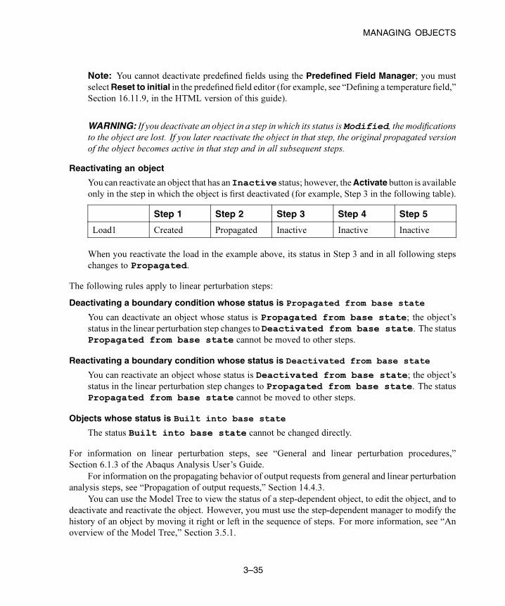
MANAGING OBJECTS
Note: You cannot deactivate predefined fields using the Predefined Field Manager; you must
selectReset to initial in the predefined field editor (for example, see “Defining a temperature field,”
Section 16.11.9, in the HTML version of this guide).
WARNING: If you deactivate an object in a step in which its status is Modified, the modificationsto the object are lost. If you later reactivate the object in that step, the original propagated version
of the object becomes active in that step and in all subsequent steps.
Reactivating an object
You can reactivate an object that has anInactive status; however, theActivate button is available
only in the step in which the object is first deactivated (for example, Step 3 in the following table).
Step 1 Step 2 Step 3 Step 4 Step 5
Load1 Created Propagated Inactive Inactive Inactive
When you reactivate the load in the example above, its status in Step 3 and in all following steps
changes to Propagated.
The following rules apply to linear perturbation steps:
Deactivating a boundary condition whose status is Propagated from base state
You can deactivate an object whose status is Propagated from base state; the object’s
status in the linear perturbation step changes to Deactivated from base state. The statusPropagated from base state cannot be moved to other steps.
Reactivating a boundary condition whose status is Deactivated from base state
You can reactivate an object whose status is Deactivated from base state; the object’sstatus in the linear perturbation step changes to Propagated from base state. The statusPropagated from base state cannot be moved to other steps.
Objects whose status is Built into base state
The status Built into base state cannot be changed directly.
For information on linear perturbation steps, see “General and linear perturbation procedures,”
Section 6.1.3 of the Abaqus Analysis User’s Guide.
For information on the propagating behavior of output requests from general and linear perturbation
analysis steps, see “Propagation of output requests,” Section 14.4.3.
You can use the Model Tree to view the status of a step-dependent object, to edit the object, and to
deactivate and reactivate the object. However, you must use the step-dependent manager to modify the
history of an object by moving it right or left in the sequence of steps. For more information, see “An
overview of the Model Tree,” Section 3.5.1.
3–35
Abaqus ID:
Printed on:
MANAGING OBJECTS
3.4.7 Understanding modified step-dependent objectsWhen you edit an object in the step in which it was created, you change the definition of the object in all
of the steps in which it is active. In some cases you can also edit an object in steps in which its status
is Propagated or Modified. In these cases the object’s definition varies according to the analysis
step.
The effects of editing a step-dependent object are summarized below.
If the status of the object is Created in the selected step:
• Modifications that you make to the object in this step become effective in this step and
propagate through all subsequent steps in which the condition is active unless you modify the
object again in a later step.
• The status of the object remains Created in the selected step and also remains unchanged
in all subsequent steps. For more information, see “Understanding the status of an object in a
step,” Section 3.4.4.
If the status of the object is Propagated or Modified in the selected step:
• Modifications that you make to the object in this step become effective in this step and
propagate through all subsequent steps in which the object is active.
• The status of the object becomes (or remains) Modified in this step and remains unchanged
in all other steps. (In other words, if the status of the object in the following step was
Propagated before modification, its status in the following step remains Propagatedafter modification.) For example, the load applied over a sequence of general static analysis
steps in Figure 3–18 has been modified in Step 3; the modifications remain in effect in Step 4
even though the status in Step 4 is Propagated. For more information, see “Understanding
the status of an object in a step,” Section 3.4.4.
• When youmodify the data in any editor other than the Interaction editor, Abaqus/CAE indicates
in the editor which data have been modified. These indications disappear if you change the
data in the editor back to their original values.
In some cases you cannot edit a particular aspect of an object’s definition because it must be
consistent for the analysis to proceed correctly. For example, although you can modify the magnitude
of a load in any analysis step, you cannot modify the region to which the load is applied. The areas in
an editor that specify this kind of restricted data are unavailable in all steps except the one in which the
object was created.
3.4.8 What happens when deleted objects are referred to?You should take care when deleting or renaming objects, such as materials and amplitudes, that may be
referred to by other objects. For example, if you delete or rename a material, the sections that refer to
3–36
Abaqus ID:
Printed on:

MANAGING OBJECTS
the material become inconsistent. To resolve the missing reference, you can edit the section and refer to
a new material, or you can create a new material with the same name as the deleted material.
Table 3–1 lists objects that are commonly referred to by other objects.
Table 3–1 Objects that are commonly referred to by other objects.
This object Can be referred to by these types of objects
Material Section
Profile Section, skin
Section Section assignment
Interaction Output request, contact controls
Interaction property Interaction
Amplitude Load, predefined field, boundary condition, interaction
Connector section Connector section assignment
Region (set or surface) Boundary condition, predefined field, load, interaction,
constraint, connector section assignment, output request,
section assignment, beam section orientation, material
orientation, output request, DOF monitor, adaptive mesh
domain
Load Load case, output request
Boundary condition Load case
Datum coordinate
system
Boundary condition, connector section assignment, material
orientation, constraint
Datum plane Load
Datum axis Load
Datum point Constraint
Part instance Constraint
Part Part instance
Parts and part instances behave slightly differently. If you delete a part after you have instanced the
part in the Assembly module, Abaqus/CAE suppresses the part instance in the assembly. You can delete
the instance from the assembly. Alternatively, if you then create a new part that uses the same name,
you can unsuppress the part instance to include it in the assembly. In addition, if you rename a part or a
datum, objects that refer to the part or datum refer to the new name; and, as a result, the reference does
not become inconsistent.
3–37
Abaqus ID:
Printed on:

WORKING WITH THE MODEL TREE AND THE RESULTS TREE
3.5 Working with the Model Tree and the Results Tree
The Model Tree and Results Tree are convenient tools for navigating and managing your models and
analysis results. You can use the Model Tree to view a model and the items that it contains, and you
can use the Results Tree to display analysis results from output databases as well as session-specific data
such as X–Y plots. Both trees provides shortcuts to much of the functionality of the main menu bar, the
module toolboxes, and the various managers. This section describes both the Model Tree and Results
Tree. The following topics are covered:
• “An overview of the Model Tree,” Section 3.5.1
• “An overview of the Results Tree,” Section 3.5.2
• “Using popup menus in the Model Tree and the Results Tree,” Section 3.5.3
• “Changing the view of the model,” Section 3.5.4
3.5.1 An overview of the Model Tree
The Model Tree provides a visual description of the hierarchy of items in a model. For example,
Figure 3–19 shows the appearance of the Model Tree after completing the online tutorial for a cantilever
beam in Appendix B, “Creating and Analyzing a Simple Model in Abaqus/CAE,” of Getting Started
with Abaqus: Interactive Edition. The Model Tree shares the left side of the Abaqus/CAE interface
with the Results Tree and, in the Property module only, a material library. You can click the Model,Results, or Material Library tab to toggle the display between the Model Tree, the Results Tree, and a
material library. See “An overview of the Results Tree,” Section 3.5.2, and “Using material libraries,”
Section 12.5, respectively, for more information about the Results Tree and material libraries. In
addition, the tip button at the top of the Model Tree provides a quick summary of the functionality
of the Model Tree and Results Tree along with a summary of the keyboard shortcuts described at the
end of this section.
A complete Abaqus/CAE model contains all of the information required to perform an analysis; for
example, all of the parts, materials, steps, and loads and the meshed representation of the assembly. A
model also contains the jobs that are submitted to the Abaqus analysis products. For more information,
see “What does an Abaqus/CAE model contain?,” Section 9.2.1. All of these items are represented in
the Model Tree.
Items in the Model Tree are represented by small icons; for example, the Steps icon,
. In addition, parentheses next to an item indicate that the item is a container, and the
number in the parentheses indicates the number of items in the container. You can click on the “plus”
and “minus” signs in the Model Tree to expand and collapse a container. The right and left arrow keys
perform the same operation.
3–38
Abaqus ID:
Printed on:
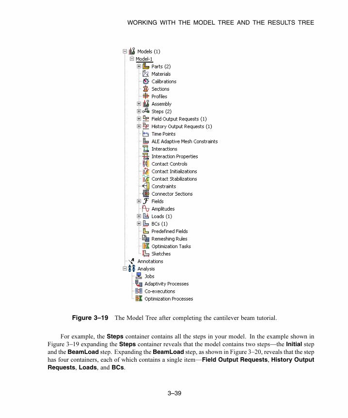
WORKING WITH THE MODEL TREE AND THE RESULTS TREE
Figure 3–19 The Model Tree after completing the cantilever beam tutorial.
For example, the Steps container contains all the steps in your model. In the example shown in
Figure 3–19 expanding the Steps container reveals that the model contains two steps—the Initial stepand the BeamLoad step. Expanding the BeamLoad step, as shown in Figure 3–20, reveals that the step
has four containers, each of which contains a single item—Field Output Requests, History OutputRequests, Loads, and BCs.
3–39
Abaqus ID:
Printed on:

WORKING WITH THE MODEL TREE AND THE RESULTS TREE
Figure 3–20 Containers in the BeamLoad step.
In addition, the step contains four empty containers—ALE Adaptive Mesh Constraints, Interactions,Predefined Fields, and Load Cases. You cannot delete an empty container from the Model Tree,
although you can hide empty containers from view (see “Changing the view of the model,” Section 3.5.4).
Finally, expanding the Loads container, as shown in Figure 3–21, reveals a single load called Pressurethat was created in this step.
Figure 3–21 The load in the Loads container.
The arrangement of the containers and items in the Model Tree reflects the order in which you are
likely to create yourmodel. A similar logic governs the order ofmodules in themodulemenu—you create
parts before you create the assembly, and you create steps before you create loads. This arrangement is
fixed—you cannot move items in the Model Tree. For more information, see “What is a module?,”
Section 2.3.
Abaqus/CAE underlines the current objects in the Model Tree and displays them in the context
bar. The model you are working on is a current object. The current part or the current step is also a
current object. When you select an item in the Model Tree, Abaqus/CAE highlights that item in the
current viewport if the selected item belongs to the current objects. For example, if you select a load,
Abaqus/CAE highlights the load in the current viewport if it was applied in the current step of the current
model. Containers are not highlighted.
You can select multiple items in the Model Tree, and Abaqus/CAE highlights each of those items
if they belong to the current objects. For example, you can select an interaction and a load in the current
step of the current model, and Abaqus/CAE highlights both the interaction and the load in the assembly.
3–40
Abaqus ID:
Printed on:

WORKING WITH THE MODEL TREE AND THE RESULTS TREE
As you move the cursor over an item, theModel Tree displays some information about the item, as shown
in Figure 3–22. In most cases the same information is available from the item’s manager.
Figure 3–22 The Model Tree displays information about the item under the cursor.
Pressing an alphabetic key (a–z) when the cursor is in the Model Tree selects the first item in the
tree with a name beginning with that character. Pressing subsequent keys continues to match characters
in an item’s name. Table 3–2 describes all of the keyboard shortcuts that are available for navigation in
the Model Tree; you can use these shortcuts to navigate in the Results Tree as well.
Table 3–2 Keyboard shortcuts in the Model Tree and Results Tree.
Keyboard shortcut Action
[Home] Go to top of Model Tree or Results Tree
[End] Go to bottom of Model Tree or Results Tree
Up arrow Move up one item
Down arrow Move down one item
Right arrow Expand branch or move down one item
Left arrow Collapse branch or move up one item
[Del] Delete item
[F2] Apply a filter to a container
3–41
Abaqus ID:
Printed on:

WORKING WITH THE MODEL TREE AND THE RESULTS TREE
The Model Tree provides most of the functionality of the main menu bar and the module managers.
For example, if you double-click on the Parts container, you can create a new part (the equivalent of
selecting Part→Create from the main menu bar). If you double-click on a part’s feature, you can edit
the feature (the equivalent of selecting Feature→Edit from the main menu bar).
You can drag the divider between the Model Tree and the canvas to change the width of the Model
Tree. In addition, you can toggle off the display of the Model Tree by selecting View→Show ModelTree from the main menu bar. Pressing [Ctrl]+T has the same effect. To switch to the Results Tree, click
the Results tab.
Step-dependent objects are objects that can be propagated between steps; for example, loads and
interactions. For more information, see “What are step-dependent managers?,” Section 3.4.2. Text next
to a step-dependent object in the Model Tree, such as (Created) and (Propagated), indicates the statusof the object. You can use the Model Tree to change the status of a step-dependent object by clicking
mouse button 3 on the object and selecting an action from the menu that appears. The actions correspond
to those available in the step-dependent managers. For more information, see “Understanding modified
step-dependent objects,” Section 3.4.7.
You can use the Model Tree to suppress a feature, a constraint (in the Interaction module), a section
assignment (in the Property module), or a step-dependent object by clicking mouse button 3 on the item
and selecting Suppress from the menu that appears. A red “X” appears next to the item in the Model
Tree to indicate that it is suppressed. You can resume the item by clicking mouse button 3 on the item
and selecting Resume. Abaqus/CAE removes the red “X” from the Model Tree to indicate that the item
is no longer suppressed. The same information is displayed in the managers. For more information, see
“Suppressing and resuming objects,” Section 3.4.3.
3.5.2 An overview of the Results Tree
The Results Tree provides a visual description of the output data available in your session, including
all open output databases and session-specific data such as X–Y data and X–Y plots. In addition, the
Results Tree enables you to navigate to viewable content in the current model database, such as the
loads specified in one step of a particular model. This tool shares the left side of the Abaqus/CAE
interface with the Model Tree and, in the Property module only, a material library. You can click the
Model, Results, or Material Library tab to toggle the display between the Model Tree, the Results
Tree, and a material library. (For more information on material libraries, see “Using material libraries,”
Section 12.5.) The Results Tree also uses all of the same keyboard and navigational shortcuts as the
Model Tree; see Table 3–2 for more information.
Figure 3–23 shows the appearance of the Results Tree after completing an analysis of the online
tutorial for the hinge model in Appendix C, “Using Additional Techniques to Create and Analyze a
Model in Abaqus/CAE,” of Getting Started with Abaqus: Interactive Edition. The Output Databasescontainer displays all the output database files that are currently open in your session. In the example
shown in Figure 3–23 the Output Databases container is expanded and reveals that only one output
database is open—the PullHinge output database.
3–42
Abaqus ID:
Printed on:

WORKING WITH THE MODEL TREE AND THE RESULTS TREE
Figure 3–23 The Results Tree after completing an analysis of the hinge model tutorial.
Expanding PullHinge, as shown in Figure 3–24, reveals that this output database has the followingcontainers: History Output, Steps, Instances, Materials, Sections, Element Sets, Node Sets, andSurface Sets. In addition, the output database contains two empty containers—Session CoordinateSystems andODB Coordinate Systems. You cannot delete an empty container from the Results Tree,
although you can hide empty containers from view (see “Changing the view of the model,” Section 3.5.4).
Figure 3–24 The containers in the PullHinge output database.
Expanding the History Output container, as shown in Figure 3–25, reveals the sixteen output
variables for which history output was requested in this analysis. Each variable listing also describes the
3–43
Abaqus ID:
Printed on:

WORKING WITH THE MODEL TREE AND THE RESULTS TREE
region for which history output was requested; in this example every history output request was made
for the whole model. You can click any of the history output variables in the Results Tree to plot the
selected variable in the current viewport.
Figure 3–25 The History Output container of the Results Tree.
Each output database also includes a Steps container, which includes containers for each step in
the output database and within the steps, every frame in the output database. You can use the Results
Tree to display the model at any frame of the analysis, to activate or deactivate steps or frames in the
analysis, or to display field output at the selected frame.
The Model Database container displays all the models in the current model database. You can
expand each model to select the step with data that you want to investigate and to display or hide
individual part instances. Figure 3–26 shows the hinge model with its Steps and Instances containers
expanded.
The other containers in the Results Tree provide shortcuts to data that persist only during your
session. By using these shortcuts, you can create and manage contour spectrums; create and edit X–Y data
and display X–Y plots, create and manage paths and display groups; and upload and display background
images and movies.
3–44
Abaqus ID:
Printed on:

WORKING WITH THE MODEL TREE AND THE RESULTS TREE
Figure 3–26 The Model Database container of the Results Tree.
3.5.3 Using popup menus in the Model Tree and the Results Tree
Much of the power of the Model Tree and Results Tree comes from the popup menu that appears when
you click mouse button 3 on an item. For example, Figure 3–27 shows the effect of clicking mouse
button 3 on the Parts container in the Model Tree.
The Create menu item appears in bold font in Figure 3–27 because it is the default action. Double-
clicking an item or selecting an item and pressing [Enter] invokes the default action. In most cases if
an item is a container, the default action is to create a new item in the container. Similarly, if an item
is not a container, the default action is to edit the item. For example, if you double-click the Partscontainer, Abaqus/CAE displays the Create Part dialog box and allows you to create a new part; if you
double-click one of the parts within the container, Abaqus/CAE displays the Edit Part dialog box and
allows you to edit the part you selected.
Some of the commands in the popup menu appear with all items in the Model Tree and Results Tree;
other commands appear only with specific items or with items in one of the two trees. For example,
the Switch Context command appears with all items in the Model Tree and Results Tree, including
containers. The following commands appear with all containers in the Model Tree and Results Tree:
Switch Context
If you select Switch Context, Abaqus/CAE makes the item current. In the Model Tree, where
appropriate, Abaqus/CAE also switches to the module in which you can edit the item. For example,
if you click mouse button 3 on the Materials container and select Switch Context, Abaqus/CAEswitches to the Property module. For more information, see “What is a module?,” Section 2.3. In
the Results Tree you can also switch the context to an item in another output database.
Selecting a container and pressing [Ctrl]+[Space] have the same effect as selecting SwitchContext from either tree.
3–45
Abaqus ID:
Printed on:

WORKING WITH THE MODEL TREE AND THE RESULTS TREE
Figure 3–27 Clicking mouse button 3 on the Parts container in the Model Tree.
Filter
When you select Filter, Abaqus/CAE prompts you for a string of characters next to the container’s
name. After you press [Enter], Abaqus/CAE filters the contents of the container and displays only
those items that match the specified character string. The filter is case-sensitive. For details on valid
filtering syntax, click the tip button at the top of the Model Tree or Results Tree. Figure 3–28
shows the effect of filtering a container.
Unfiltered Filtered
Figure 3–28 Filtering a container in the Model Tree.
Items that are hidden by a filter cannot be manipulated from the Model Tree or Results Tree;
however, these items are not removed from the model or output database. When a filter is in
3–46
Abaqus ID:
Printed on:

WORKING WITH THE MODEL TREE AND THE RESULTS TREE
effect, the numbers in parentheses next to the container name indicate the number of visible items
in the container followed by the total number of items (visible and hidden) in the container (see
Figure 3–28). The filter string appears to the right of these numbers. To remove a filter, select
Filter for the appropriate container, delete the filter string, and press [Enter].Filters can be applied only to individual containers and persist only during your session.
Selecting a container and pressing [F2] have the same effect as selecting Filter from either tree.
Set As Root
If you select Set As Root, Abaqus/CAE moves the container to the pull-down menu above
the Model Tree or Results Tree and displays everything under the selected container. For more
information, see “Changing the view of the model,” Section 3.5.4.
Expand All Under
If you select Expand All Under, Abaqus/CAE expands all of the containers and items inside the
selected container.
Collapse All Under
If you select Collapse All Under, Abaqus/CAE collapses all of the containers and items inside the
selected container.
Group Children
When a container includes more than 30 items, Abaqus/CAE automatically groups the items into
sets of 30. If you toggle off the Group Children option, Abaqus/CAE removes the groupings and
lists all of the items on the same level in the container.
Selecting a container and pressing [Ctrl]+[G] have the same effect as selecting Group Childrenfrom either tree.
Many popup menu commands appear only with specific items. In the Model Tree these commands
mirror the actions that you can perform with that item’s manager; for example, create, edit, delete,
rename, suppress, and resume. In the Results Tree some popup menus provide Boolean operators that
enable you to control the display of items in the current viewport. These Boolean operators are the same
five commands that are available for controlling display groups: replace, add, remove, intersect, and
either. See “Understanding display group Boolean operations,” Section 78.1.2, for more information.
Some menu commands are specific to one container in the Model Tree or Results Tree; for example,
clicking mouse button 3 on a step allows you to toggle the Nlgeom setting, clicking mouse button 3 on
a job allows you to submit the job for analysis, and clicking mouse button 3 on a history output variable
allows you to add another variable to the existing plot. When you become familiar with the Model Tree
and Results Tree, you will find that you can quickly perform most of the actions that are found in the
main menu bar, the module toolboxes, and the various managers.
3–47
Abaqus ID:
Printed on:

WORKING WITH THE MODEL TREE AND THE RESULTS TREE
3.5.4 Changing the view of the model
If you select Set As Root from a container’s popup menu, Abaqus/CAE displays everything under the
selected container in the Model Tree or Results Tree and displays the name of the container in the menu
above the tree. This option is useful if, for example, you have a complex model or output database and
correspondingly complex Model Tree or Results Tree. You can use Set As Root to simplify the Model
Tree or Results Tree by displaying only the portion that you are working on. For example, Figure 3–29
shows a view of the Model Tree on the left and contrasts it with the effect of setting the Materialscontainer as the root.
When you change the default root container, you can use the menu above theModel Tree and Results
Tree to move up through its levels. In addition, Abaqus/CAE activates two icons above the Model Tree
or Results Tree, as shown in Figure 3–29: the Set Root to Model Database icon in the Model Tree,
the Set Root to Session Data icon in the Results Tree, and the Up One Level icon in both trees.
• The Set Root to Model Database icon returns the Model Tree to the default view that shows
Model Database at the top of the tree. The Set Root to Session Data icon returns the
Results Tree to the default view that shows Session Data at the top of the tree.
• The Up One Level icon moves the root of the Model Tree or Results Tree up one level; for
example, from the Materials container up one level to the Beam model that contains the Materialscontainer.
If you click mouse button 3 on the background of the Model Tree or Results Tree, Abaqus/CAE displays
a popup menu with the following options:
Show Empty Containers
By default, Abaqus/CAE displays all of the containers in the Model Tree and Results Tree,
whether or not they have items in them. By turning off the Show Empty Containers option,
you can suppress the display of containers without any items in them. If you perform an action
in Abaqus/CAE that adds an item to a previously empty container (for example, creating an
interaction using the Interaction module toolbox), the container and item will reappear in the
Model Tree or Results Tree. For a container to be suppressed from view, it must be completely
empty; even if all items in a container are hidden because of a filter (see “Using popup menus in
the Model Tree and the Results Tree,” Section 3.5.3), that container is not suppressed by the ShowEmpty Containers option.
The state of the Show Empty Containers option persists between Abaqus/CAE sessions.
Expand All
If you select Expand All, Abaqus/CAE expands all of the containers and items in the Model Tree
or Results Tree.
3–48
Abaqus ID:
Printed on:

WORKING WITH THE MODEL TREE AND THE RESULTS TREE
up one levelset root to Model Database
tip
Figure 3–29 The effect of Set As Root on the Model Tree.
Collapse All
If you select Collapse All, Abaqus/CAE collapses all of the containers in the Model Tree or Results
tree, leaving only top-level containers and items visible.
3–49
Abaqus ID:
Printed on:

UNDERSTANDING Abaqus/CAE GUI SETTINGS
Set Root to Displayed Object
If you select Set Root to Displayed Object, the container corresponding to the part visible in thecurrent viewport becomes the root of the Model Tree (as described above). If an assembly is visible
in the current viewport, the Assembly container for the appropriate model becomes the root of the
Model Tree.
This option is available only in the Model Tree.
Set Root to Model Database
If you select Set Root to Model Database, Abaqus/CAE returns the Model Tree to the default
view that shows Model Database at the top of the tree. This option has the same effect as the Set
Root to Model Database icon .
This option is available only in the Model Tree.
Set Root to Session Data
If you select Set Root to Session Data, Abaqus/CAE returns the Results Tree to the default view
that shows Session Data at the top of the tree. This option has the same effect as the Set Root to
Session Data icon .
This option is available only in the Results Tree.
3.6 Understanding Abaqus/CAE GUI settings
GUI settings are always saved automatically to a binary file in your home directory called
abaqus_v6.13.gpr when you exit Abaqus/CAE. For more information, see “Working with
abaqus_v6.13.gpr files,” Section 2.1.3.
These GUI settings include the following:
• The size and location of the main window.
• The size and location of a particular dialog box; for example, the Open Database and Create Partdialog boxes.
• The location, orientation, and visibility of individual toolbars.
• Custom toolbars.
• Customized keyboard shortcuts.
• The size of the message area and command line interface.
• Whether the Model Tree and Results Tree are displayed. The width of the tree area is also stored.
• Bookmarks to directories that you created when opening a file.
You cannot edit the abaqus_v6.13.gpr file; however, you can delete it to restore the default GUI
and display options settings.
3–50
Abaqus ID:
Printed on:

UNDERSTANDING Abaqus/CAE GUI SETTINGS
WARNING: Deleting the abaqus_v6.13.gpr file resets all of the GUI settings listed above. You
cannot restore the settings from a deletedabaqus_v6.13.gpr file except by recreating themmanually
in Abaqus/CAE.
3–51
Abaqus ID:
Printed on:


UNDERSTANDING VIEWPORTS
4. Managing viewports on the canvas
The canvas can be thought of as an infinite screen or bulletin board on which you post viewports; you
can imagine the canvas extending beyond the main window and your monitor. The visible portion of
the canvas is called the drawing area, and you can increase its size by increasing the size of the main
window.
You can position viewports anywhere on the canvas, and you can drag them outside the drawing
area. When viewports are positioned outside the drawing area, you can cascade or tile the viewports to
bring them back into view. Viewports are not part of a model and are not saved between sessions.
This chapter explains how to create and manipulate viewports, text annotations, and arrow
annotations. The following topics are covered:
• “Understanding viewports,” Section 4.1
• “Manipulating viewports and viewport annotations,” Section 4.2
In addition, the following sections are available in the HTML version of this guide:
• “Working with viewports,” Section 4.3
• “Working with viewport arrow and text annotations,” Section 4.4
• “Linking viewports for view manipulation,” Section 4.5
• “Working with background images and movies in viewports,” Section 4.6
4.1 Understanding viewports
Viewports are areas on the canvas where you can display models or analysis results. You can add arrow
and text annotations to draw attention to or explain features within a viewport. You can create and
manipulate viewports, text, and arrows using the Viewport menu.
4.1.1 What is a viewport?While the canvas can be thought of as an infinite screen or bulletin board, viewports are simply display
areas posted onto that screen on which you can display models or analysis results. You can have many
viewports on the canvas. A viewport is similar to other windows on your workstation in that it can be
moved, resized, minimized, and maximized; and it can overlap other viewports on the canvas. For more
information, see “Working with viewports,” Section 4.3, in the HTML version of this guide.
You can easily create and delete viewports and control their size, position, and appearance.
Figure 4–1 illustrates how you might use several viewports to view the results from your analysis.
The view manipulation tools, such as zoom and rotate, operate on the viewport that contains the
cursor. Other operations interact with the current viewport or with all viewports on the canvas.
4–1
Abaqus ID:
Printed on:

UNDERSTANDING VIEWPORTS
Current viewport
Figure 4–1 Working with multiple viewports.
The current viewport
To change the contents of a viewport, you must first designate the desired viewport as current.
The current viewport is indicated by a dark gray title bar. All work takes place within the current
viewport. To choose another viewport as the current viewport, click on the border or title bar. The
selected viewport moves in front of other viewports on the canvas, and the title bar color changes
to blue. The title bar reverts to dark gray when you select an Abaqus/CAE tool or menu.
Note: On Windows platforms you can customize the colors used by Abaqus/CAE. For more
information, see “Common customizations on Windows platforms,” Section 5.1.2 of the Abaqus
Installation and Licensing Guide.
All viewports are associated with a certainmodel andmodule. When you create a newmodel or
open an existingmodel or output database, that model becomes associated with the current viewport.
You can create different viewports and associate each one with a different model, so designating
each viewport as current results in switching between the associated models. Similarly, you can
work in multiple modules simultaneously by designating a new viewport as current before entering
a different module.
For detailed instructions on working with viewports, see the following topics in the HTML version
of this guide:
• “Creating new viewports,” Section 4.3.1
4–2
Abaqus ID:
Printed on:
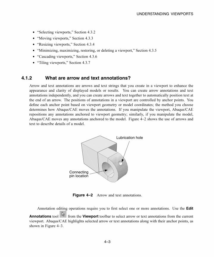
UNDERSTANDING VIEWPORTS
• “Selecting viewports,” Section 4.3.2
• “Moving viewports,” Section 4.3.3
• “Resizing viewports,” Section 4.3.4
• “Minimizing, maximizing, restoring, or deleting a viewport,” Section 4.3.5
• “Cascading viewports,” Section 4.3.6
• “Tiling viewports,” Section 4.3.7
4.1.2 What are arrow and text annotations?
Arrow and text annotations are arrows and text strings that you create in a viewport to enhance the
appearance and clarity of displayed models or results. You can create arrow annotations and text
annotations independently, and you can create arrows and text together to automatically position text at
the end of an arrow. The positions of annotations in a viewport are controlled by anchor points. You
define each anchor point based on viewport geometry or model coordinates; the method you choose
determines how Abaqus/CAE moves the annotations. If you manipulate the viewport, Abaqus/CAE
repositions any annotations anchored to viewport geometry; similarly, if you manipulate the model,
Abaqus/CAE moves any annotations anchored to the model. Figure 4–2 shows the use of arrows and
text to describe details of a model.
Lubrication hole
Connectingpin location
Figure 4–2 Arrow and text annotations.
Annotation editing operations require you to first select one or more annotations. Use the Edit
Annotations tool from the Viewport toolbar to select arrow or text annotations from the current
viewport. Abaqus/CAE highlights selected arrow or text annotations along with their anchor points, as
shown in Figure 4–3.
4–3
Abaqus ID:
Printed on:

UNDERSTANDING VIEWPORTS
handle/connectionpoints
Figure 4–3 Selected annotations: an arrow with no offsets, text with an offset, and an arrow
with gaps at both ends and an offset between the tail and its anchor point.
Anchor points are shown as a small dot with an anchor symbol placed nearby. Dashed lines indicate
an offset between the anchor point and the annotation; circular “handles” are the anchor connection
points—if there is no offset, the connection point and anchor point are the same.
Arrow annotations have two anchor points (you can use the same coordinates for both points). You
can add a gap between the arrow ends and the connection points. Adding a gap is comparable to leaving
a space between dimension lines and object lines in the Sketcher or in a CAD drawing; it can increase
the clarity of your annotation. Text annotations have a single anchor point. You can change the offsets
by dragging the connection points, or the entire annotation, in the viewport.
Do not confuse the viewport annotations that you can create with the viewport annotations generated
by Abaqus/CAE. The generated viewport annotations include the view orientation triad; the 3D compass;
and, in the Visualization module, the legend, the title block, and the state block. You can modify some
display aspects of the generated annotations, but you cannot modify their contents. For more information,
see Chapter 56, “Customizing viewport annotations.” In contrast, you have full control of all attributes
related to arrow and text annotations including their colors, line styles, line thicknesses, arrowheads,
fonts, anchor points, and any offsets between the anchor points and the annotations.
Abaqus/CAE saves arrow and text annotations in model and output databases; however, viewports
are not saved. As a result, the arrow and text annotations in a database are not associated with a viewport.
When you subsequently open a database that contains annotations, you must use the AnnotationManager to display a selected annotations in the current viewport. The Annotation Manager also
allows you to copy annotations from a model database to an output database and vice versa. You cannot
create annotations in a model database from the Visualization module; open the model database in a
different module if you want to create annotations for it.
Use the Viewport menu, the Viewport toolbox, or the Annotation Manager dialog box to create
or modify arrow and text annotations. For detailed instructions, see the following topics in the HTML
version of this guide:
• “Annotating viewports,” Section 4.4.1
• “Creating an arrow annotation,” Section 4.4.2
4–4
Abaqus ID:
Printed on:

MANIPULATING VIEWPORTS AND VIEWPORT ANNOTATIONS
• “Creating a text annotation,” Section 4.4.3
• “Creating combined arrow and text annotations,” Section 4.4.4
• “Manipulating annotations in the current viewport,” Section 4.4.5
• “Editing arrow annotation attributes,” Section 4.4.6
• “Editing text annotation attributes,” Section 4.4.7
• “Plotting annotations in the current viewport,” Section 4.4.8
• “Hiding annotations in the current viewport,” Section 4.4.9
• “Copying viewport annotations to another database,” Section 4.4.10
• “Rearranging the annotation list order,” Section 4.4.11
4.2 Manipulating viewports and viewport annotations
This section explains how to manipulate viewports and viewport annotations using the options provided
in the Viewport menu, the Viewport toolbar, and the Annotation Manager.
4.2.1 Managing viewports and viewport annotations from the mainmenu bar
Use the Viewport menu, located on the main menu bar, to create, delete, modify, or rearrange
viewports and to create or edit viewport annotations—both those that you create and those generated by
Abaqus/CAE. If you prefer, you can select View→Toolbars→Viewport from the main menu bar to
display a toolbar containing most of the functionality of the items in the Viewport menu.
The Viewport menu and toolbar allow you to do the following:
• Create a viewport.
• Edit options for generated viewport annotations (triad, legend, title block, and state block).
• Create an arrow annotation.
• Create a text annotation.
• Create a combined arrow and text annotation.
• Edit arrow and text annotations.
• Open the Annotation Manager to manipulate arrow and text annotations.
Note: The Annotation Manager provides several unique management functions; for more
information, see “The Annotation Manager,” Section 4.2.3.
• Open the Viewport Annotation Options to show or hide all annotations and to manipulate the
viewport annotations generated by Abaqus/CAE.
In addition, the Viewport menu lists all the viewports in the session and allows you to delete the current
viewport.
4–5
Abaqus ID:
Printed on:

MANIPULATING VIEWPORTS AND VIEWPORT ANNOTATIONS
4.2.2 Managing viewports and viewport annotations from the Viewporttoolbar
To display the Viewport toolbar, select View→Toolbars→Viewport from the main menu bar.
Figure 4–4 describes the tools available from the Viewport toolbar.
create
Viewport Tools Annotation Tools
cascade
tilehorizontal
tilevertical
linkedviewports
createarrowandtext
createarrow
createtext
edit
annotationmanager
viewportannotation
options
Figure 4–4 The Viewport toolbar.
4.2.3 The Annotation Manager
The Annotation Manager is similar to other manager dialog boxes in Abaqus/CAE. It allows you to
do the following:
• Create arrow, text, or combined arrow and text annotations.
• Edit an arrow or text annotation.
• Copy or rename an annotation.
• Delete annotations.
In addition, the Annotation Manager allows you to perform the following tasks that are not available
from the Viewport menu or toolbar:
• Select the source—model database (MDB) or output database (ODB)—of annotations to manage.
• Plot model database or output database annotations in the current viewport.
• Hide model database or output database annotations in the current viewport.
• Copy annotations from a model database to an output database and vice versa.
4–6
Abaqus ID:
Printed on:

MANIPULATING VIEWPORTS AND VIEWPORT ANNOTATIONS
• Highlight annotations in the viewport.
• Rearrange the order of arrow and text annotations in the list.
You can display the Annotation Manager by selecting Viewport→Annotation Manager from the
main menu bar or in the Viewport toolbar. The Annotation Manager is shown in Figure 4–5.
Figure 4–5 The Annotation Manager.
For detailed instructions on using the Annotation Manager to create, edit, and manipulate annotations,
see the following sections in the HTML version of this guide:
• “Annotating viewports,” Section 4.4.1
• “Editing arrow annotation attributes,” Section 4.4.6
• “Editing text annotation attributes,” Section 4.4.7
• “Plotting annotations in the current viewport,” Section 4.4.8
• “Copying viewport annotations to another database,” Section 4.4.10
• “Rearranging the annotation list order,” Section 4.4.11
4–7
Abaqus ID:
Printed on:


UNDERSTANDING CAMERA MODES AND VIEW OPTIONS
5. Manipulating the view and controlling perspective
This chapter describes the view options, the view manipulation tools, the 3D compass, and the
perspective tools, all of which control a camera that creates the view in a viewport. The view options
allow you to switch between two camera modes and numerically control some of their properties. The
view manipulation tools and 3D compass control the camera to position, orient, and magnify objects in
the view; you can also select custom views such as front and back, as well as define your own views.
The perspective tools control whether Abaqus/CAE displays your model with or without perspective;
using perspective gives a more realistic appearance for three-dimensional models. The following topics
are covered:
• “Understanding camera modes and view options,” Section 5.1
• “Understanding the view manipulation tools,” Section 5.2
• “The 3D compass,” Section 5.3
• “Customizing the view triad,” Section 5.4
• “Controlling perspective,” Section 5.5
In addition, the following sections are available in the HTML version of this guide:
• “Using the view manipulation tools,” Section 5.6
• “Using the 3Dconnexion motion controllers with Abaqus/CAE,” Section 5.7
5.1 Understanding camera modes and view options
This section describes the camera modes used to create views in Abaqus/CAE.
5.1.1 Camera modes and view terminologyA view is a two-dimensional representation—a camera image—of your model or analysis results,
displayed in a viewport. Abaqus/CAE uses a single camera to create the view in each viewport. You can
choose from two camera modes to create the desired view of your model or results. The default mode
allows you to position the camera anywhere outside the model. The movie mode allows you to position
the same camera inside the model as well as outside it. In addition, the movie mode provides you with
two clipping planes that you can use to eliminate objects from the view when they are too close to, or
too far from, the camera. The view depth is not limited in default mode; objects in the view may be
directly in front of the camera or at a distance that makes them too small for you to see in the viewport.
View manipulation tools are available so that you can fully utilize both camera modes. All
view manipulation tools can be used in either camera mode, but an “alternate mode” of some view
manipulation tools is intended primarily for use in movie mode. For example, the magnify tool allows
5–1
Abaqus ID:
Printed on:

UNDERSTANDING CAMERA MODES AND VIEW OPTIONS
you to magnify the current view without moving the camera; the alternate mode of this tool moves the
camera closer to the model. The effects of both view manipulations appear identical; but when used
in the default camera mode, the alternate mode stops working if the camera “hits” the outer edge of
the model. In movie mode you can use the alternate mode of the magnify tool to move the camera
into and through the model. The view manipulation tools are described in “Understanding the view
manipulation tools,” Section 5.2.
Figure 5–1 shows the two camera modes. The shaded areas in the figure represent the visible
space—the view—in each camera mode.
field-of-view angle
default mode movie mode
field-of-view angle
frustum
near plane far plane
Figure 5–1 The default mode and movie mode camera views.
The camera terms that follow are used to describe the view that you see in a viewport:
Camera target
The camera target is a point in space that controls how the camera moves during most view
manipulations. For all default views the camera target coincides with the center point of all objects
in the view. The camera target moves away from the center of all objects when you use the
alternate mode of the pan, rotate, and magnify view manipulation tools.
Frustum
The frustum is the three-dimensional space visible with the movie camera mode. The camera
position forms the apex of a pyramid created by a left, right, top, and bottom plane (the same as
it does in the default mode). To create the frustum, two additional planes are added to the default
view, the near plane and the far plane. Only those objects (or portions of objects) that are within the
frustum are visible in movie camera mode.
Field-of-view angle
The field-of-view angle is the larger of the angles between the left and right or the top and bottom
planes that form the sides of the view. The angle that is used depends on the shape of the frustum
5–2
Abaqus ID:
Printed on:

UNDERSTANDING CAMERA MODES AND VIEW OPTIONS
(effectively the shape of the viewport); in both images of Figure 5–1 the angle between the left and
right planes is larger; therefore, this angle is indicated as the field-of-view angle. The field-of-view
angle applies to both the default camera mode and the movie camera mode; changing the angle is
comparable to adjusting the zoom on a stationary camera to expand or shrink the camera image.
The magnify, box zoom, and auto-fit viewmanipulation tools all change the field-of-view angle
to resize the view in the viewport. See “Understanding the view manipulation tools,” Section 5.2,
for more information about these tools.
Near plane
The near plane lies perpendicular to the camera direction and is effective only in the movie camera
mode. The distance from the camera to the near plane is the closest distance that an object can be to
the camera and still remain in the view. The view from the default camera includes objects at any
distance, as if the near plane were positioned directly in front of the camera lens.
The near plane is a clipping plane; it removes model surfaces and edges from view without
cutting through the model. In the Visualization module you can cut the model such that interior
surfaces are visible; for more information, see Chapter 80, “Cutting through a model.”
Far plane
Like the near plane, the far plane lies perpendicular to the camera direction and is effective only in
the movie camera mode. The distance from the camera to the far plane is the farthest distance that
an object can be from the camera and still remain in the view. The view from the default camera
includes objects at any distance, as if the far plane were positioned an infinite distance from the
camera lens.
The far plane is a clipping plane; it removes model surfaces and edges from view without
cutting through the model. In the Visualization module you can cut the model such that interior
surfaces are visible; for more information, see Chapter 80, “Cutting through a model.”
You use the view options, view manipulation tools, and perspective tools to change the camera mode
settings or to change the relationship between the camera, the camera target, and the object that you are
viewing. The current settings of these tools and options define the current view.
5.1.2 Using view options to control the cameraUse the view options to control the current camera mode and other options that you cannot set using the
view manipulation tools.
Select View→View Options from the main menu bar to access the view options for the current
viewport, as shown in Figure 5–2. You can use the View Options dialog box to control:
• The field-of-view angle (effectively, the magnification of the current view).
• The camera mode (movie mode allows you to move the camera into and through the model).
• The distance from the movie mode camera to the near plane (the closest distance an object can be
to the camera while remaining in the view).
5–3
Abaqus ID:
Printed on:
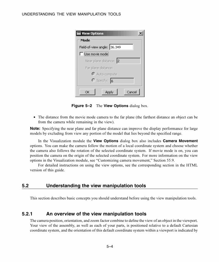
UNDERSTANDING THE VIEW MANIPULATION TOOLS
Figure 5–2 The View Options dialog box.
• The distance from the movie mode camera to the far plane (the farthest distance an object can be
from the camera while remaining in the view).
Note: Specifying the near plane and far plane distance can improve the display performance for large
models by excluding from view any portion of the model that lies beyond the specified range.
In the Visualization module the View Options dialog box also includes Camera Movementoptions. You can make the camera follow the motion of a local coordinate system and choose whether
the camera also follows the rotation of the selected coordinate system. If movie mode is on, you can
position the camera on the origin of the selected coordinate system. For more information on the view
options in the Visualization module, see “Customizing camera movement,” Section 55.9.
For detailed instructions on using the view options, see the corresponding section in the HTML
version of this guide.
5.2 Understanding the view manipulation tools
This section describes basic concepts you should understand before using the view manipulation tools.
5.2.1 An overview of the view manipulation toolsThe camera position, orientation, and zoom factor combine to define the view of an object in the viewport.
Your view of the assembly, as well as each of your parts, is positioned relative to a default Cartesian
coordinate system, and the orientation of this default coordinate system within a viewport is indicated by
5–4
Abaqus ID:
Printed on:

UNDERSTANDING THE VIEW MANIPULATION TOOLS
the view triad. By default, an isometric view is used when a module first displays a three-dimensional
part or assembly.
You can manipulate the view using the pan, rotate, magnify, box zoom, and auto-fit tools on the
View Manipulation toolbar to control the relative positions of the camera, the camera target, and the
model or results that you are viewing. For example, you might want to pan and zoom a contour plot to
view an area of stress concentration. The view manipulation tools allow you to perform the following
operations:
• Move the view horizontally and vertically; that is, pan the view.
• Rotate the view.
• Magnify or reduce the view.
• Zoom in to a selected area of the view.
• Rescale the view to fill the viewport; that is, auto-fit the view.
• Cycle through previous views.
Other types of view manipulations can be performed using the 3D compass; for more information, see
“The 3D compass,” Section 5.3.
You can click mouse button 3 to access the following view manipulation tools:
• Set As Rotation Center: Set the center of rotation at the position of the mouse click, which can
be at any location in the viewport.
• Use Default Rotation Center: Clear a previously set center of rotation.
• Center View: Center the view at the position of the mouse click.
When an X–Y plot is displayed in the viewport, you can use the view manipulation tools to change
the view of the X–Y curves. Because X–Y plots are two-dimensional, the rotate tool is disabled when the
current viewport displays an X–Y plot.
Clicking a view manipulation tool puts you into the corresponding view manipulation mode. You
then manipulate the view in a particular viewport by moving the cursor to that viewport and dragging or
clicking as necessary. In addition, the pan, rotate, and magnify tools have alternate modes that you can
access by holding the [Shift] key in conjunction with the normal use of these tools. The alternate modes
of these tools are intended for use in the movie camera mode, but they can also be used in the default
mode. For more information about camera terminology and the view modes, see “Understanding camera
modes and view options,” Section 5.1. To exit a view manipulation mode, do one of the following:
• Click mouse button 2.
• Click the cancel button in the prompt area.
• Click the view manipulation tool again.
• Click any other view manipulation tool.
5–5
Abaqus ID:
Printed on:

UNDERSTANDING THE VIEW MANIPULATION TOOLS
You can use the view manipulation tools as many times as necessary to reach the desired view,
and you can perform the view manipulation in any viewport, regardless of what is being displayed.
Abaqus/CAE stores the eight most recent views from each viewport, and you can use the cycle view
manipulation tool to cycle backward and forward through these views.
When you use the move, rotate, magnify, zoom, or rescale tools in a viewport that is linked to
other viewports, Abaqus/CAE manipulates the view of objects in the linked viewports as well. For more
information, see “Linking viewports for view manipulation,” Section 4.5, in the HTML version of this
guide.
By default, Abaqus/CAE displays the image using the current render style (wireframe, filled, hidden
line, or shaded) while you manipulate the view of an object. Alternatively, you can change the Dragmode in the Graphics Options dialog box to display the image as a simple wireframe while you
manipulate the view; this mode allows faster manipulation of very large models in the shaded render
style. The view reverts to the original render style when you complete a manipulation.
If you prefer to use menus rather than the tools on the View Manipulation toolbar, you can access
all of the view manipulation tools through the View menu on the main menu bar. In addition, you can
apply predefined and user-defined views using the Views toolbar, and you can numerically specify a
precise view using the dialog box that appears when you select View→Specify from the main menu bar.
For more information on custom and numerically specified views, see “Custom views,” Section 5.2.8,
and “Numerically specifying a view,” Section 5.2.9, respectively.
Alternatively, you can enter three of the view manipulation modes by using a combination of
keyboard and mouse actions.
• To rotate the view, press [Ctrl]+[Alt], and hold down mouse button 1.
• To pan the view, press [Ctrl]+[Alt], and hold down mouse button 2.
• To magnify or reduce the view, press [Ctrl]+[Alt], and hold down mouse button 3.
Add [Shift] to any of these combinations to access the alternate modes of these tools. For example, press
[Shift]+[Ctrl]+[Alt] and hold mouse button 3 to access the alternate mode of the magnify tool and move
the camera closer to or farther from the objects in the view. The [Shift] key has no effect on the view
manipulation tools when you are not using alternate modes. To exit a view manipulation mode after
using one of the preceding actions, simply release the mouse button.
You can reconfigure these keyboard and mouse combinations to mimic the view manipulation
interfaces used by five other common CAD applications by selecting Tools→Options from the main
menu bar. See “Using view manipulation shortcuts,” Section 68.2 in the HTML version of this guide,
for more information.
5.2.2 The pan view tool
When you select the pan tool and the viewport in which to work, Abaqus/CAE enters pan mode, as
indicated by the cursor.
5–6
Abaqus ID:
Printed on:

UNDERSTANDING THE VIEW MANIPULATION TOOLS
When a model is displayed in the viewport, the position of your view of the model changes as
you click and then drag the cursor, and a rubberband line indicates the amount of translation. Panning
the view is comparable to moving the camera over a snapshot of the model, as shown in Figure 5–3;
the snapshot moves in the viewport but any faces of the model that were hidden in the original camera
position remain hidden as you pan.
snapshot of the object
Figure 5–3 Panning the view.
The alternate mode of the pan tool, accessed by holding [Shift] while performing the manipulation,
creates a more realistic camera view. Instead of a snapshot of the model, you pan the camera over the
real model. Faces of the model that were hidden at the original camera position are exposed as you move
the camera over the model, as shown in Figure 5–4.
Figure 5–4 Panning the view in alternate mode.
Note: If perspective is not on, the alternate mode of pan works identically to the standard pan tool.
For both modes of the pan tool, the initial location of the cursor is not important, as long as you
place it within the viewport. Cursor motion is limited only by the physical bounds of your monitor, and
panning will continue even if you move the cursor outside the viewport or window.
5–7
Abaqus ID:
Printed on:
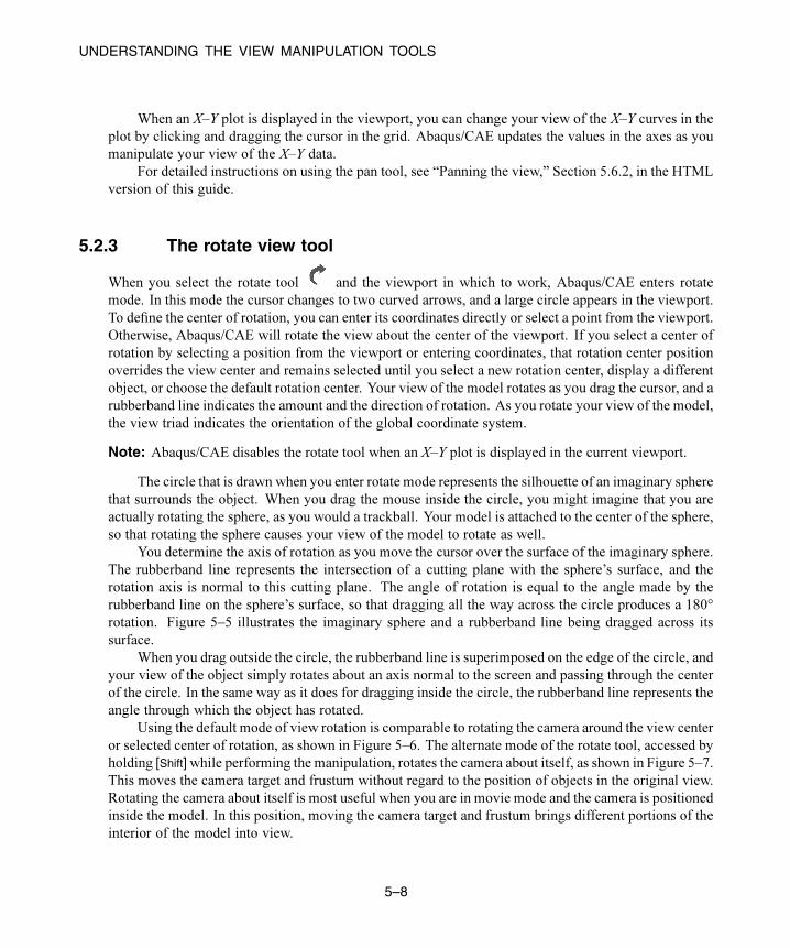
UNDERSTANDING THE VIEW MANIPULATION TOOLS
When an X–Y plot is displayed in the viewport, you can change your view of the X–Y curves in the
plot by clicking and dragging the cursor in the grid. Abaqus/CAE updates the values in the axes as you
manipulate your view of the X–Y data.
For detailed instructions on using the pan tool, see “Panning the view,” Section 5.6.2, in the HTML
version of this guide.
5.2.3 The rotate view tool
When you select the rotate tool and the viewport in which to work, Abaqus/CAE enters rotate
mode. In this mode the cursor changes to two curved arrows, and a large circle appears in the viewport.
To define the center of rotation, you can enter its coordinates directly or select a point from the viewport.
Otherwise, Abaqus/CAE will rotate the view about the center of the viewport. If you select a center of
rotation by selecting a position from the viewport or entering coordinates, that rotation center position
overrides the view center and remains selected until you select a new rotation center, display a different
object, or choose the default rotation center. Your view of the model rotates as you drag the cursor, and a
rubberband line indicates the amount and the direction of rotation. As you rotate your view of the model,
the view triad indicates the orientation of the global coordinate system.
Note: Abaqus/CAE disables the rotate tool when an X–Y plot is displayed in the current viewport.
The circle that is drawn when you enter rotate mode represents the silhouette of an imaginary sphere
that surrounds the object. When you drag the mouse inside the circle, you might imagine that you are
actually rotating the sphere, as you would a trackball. Your model is attached to the center of the sphere,
so that rotating the sphere causes your view of the model to rotate as well.
You determine the axis of rotation as you move the cursor over the surface of the imaginary sphere.
The rubberband line represents the intersection of a cutting plane with the sphere’s surface, and the
rotation axis is normal to this cutting plane. The angle of rotation is equal to the angle made by the
rubberband line on the sphere’s surface, so that dragging all the way across the circle produces a 180°
rotation. Figure 5–5 illustrates the imaginary sphere and a rubberband line being dragged across its
surface.
When you drag outside the circle, the rubberband line is superimposed on the edge of the circle, and
your view of the object simply rotates about an axis normal to the screen and passing through the center
of the circle. In the same way as it does for dragging inside the circle, the rubberband line represents the
angle through which the object has rotated.
Using the default mode of view rotation is comparable to rotating the camera around the view center
or selected center of rotation, as shown in Figure 5–6. The alternate mode of the rotate tool, accessed by
holding [Shift] while performing the manipulation, rotates the camera about itself, as shown in Figure 5–7.
This moves the camera target and frustum without regard to the position of objects in the original view.
Rotating the camera about itself is most useful when you are in movie mode and the camera is positioned
inside the model. In this position, moving the camera target and frustum brings different portions of the
interior of the model into view.
5–8
Abaqus ID:
Printed on:
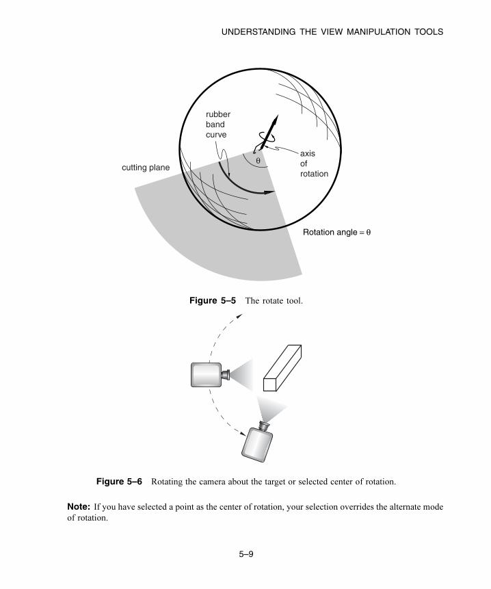
UNDERSTANDING THE VIEW MANIPULATION TOOLS
axis of rotation
θcutting plane
rubber band curve
Rotation angle = θ
Figure 5–5 The rotate tool.
Figure 5–6 Rotating the camera about the target or selected center of rotation.
Note: If you have selected a point as the center of rotation, your selection overrides the alternate mode
of rotation.
5–9
Abaqus ID:
Printed on:

UNDERSTANDING THE VIEW MANIPULATION TOOLS
Figure 5–7 Rotating the camera about itself.
In either mode, it is usually easier to obtain a desired rotation by performing a sequence of smaller
rotations rather than one large one. If you need to abandon the rotation and return to a known orientation,
use either the predefined views in the Views toolbar or the cycle view tool . Using any of the
predefined views will also reset the camera target to the center of the model.
Because X–Y plots are two-dimensional, Abaqus/CAE disables the rotate tool when an X–Y plot is
displayed in the current viewport.
For detailed instructions on using the rotate tool, see “Rotating the view,” Section 5.6.3, in the
HTML version of this guide.
5.2.4 The magnify tool
When you select the magnify tool and the viewport in which to work, Abaqus/CAE enters magnify
mode, as indicated by the magnify cursor . When you drag the cursor along the positive direction
while in magnify mode, your view of the model or plot expands within the viewport, and a rubberband
line indicates the relative magnification. Similarly, when you drag the cursor along the negative direction,
your view of the model or plot contracts, and a rubberband line indicates the relative reduction. The
positive and negative directions depend on your settings in the view manipulation options (see “Using
view manipulation shortcuts,” Section 68.2 in the HTML version of this guide). If you are using the
default Abaqus/CAE configuration for view manipulations, the positive direction is to the right and the
negative direction is to the left. If you are using a nondefault configuration for view manipulations, the
positive direction is upward and the negative direction is downward. To reflect the configuration settings,
the rubberband line is horizontal for the default configuration and vertical for nondefault configurations.
The dragging action must start in the viewport, but you can continue to drag within the limits of your
monitor. You can also drag repeatedly to achieve the desired view. The magnify tool recognizes only the
horizontal (for the default configuration) or vertical (for nondefault configurations) component of your
dragging motion, as indicated by the rubberband line. Consequently, you can achieve finer control by
dragging diagonally across the screen, since this results in a smaller component of the cursor’s motion
in the effective direction than dragging the same distance along the effective direction.
5–10
Abaqus ID:
Printed on:
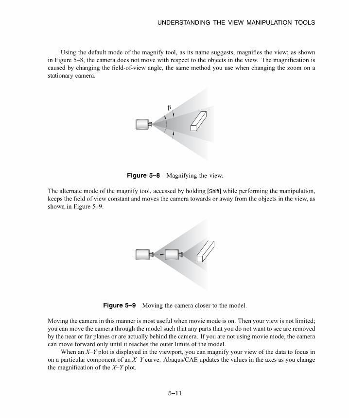
UNDERSTANDING THE VIEW MANIPULATION TOOLS
Using the default mode of the magnify tool, as its name suggests, magnifies the view; as shown
in Figure 5–8, the camera does not move with respect to the objects in the view. The magnification is
caused by changing the field-of-view angle, the same method you use when changing the zoom on a
stationary camera.
β
Figure 5–8 Magnifying the view.
The alternate mode of the magnify tool, accessed by holding [Shift] while performing the manipulation,
keeps the field of view constant and moves the camera towards or away from the objects in the view, as
shown in Figure 5–9.
Figure 5–9 Moving the camera closer to the model.
Moving the camera in this manner is most useful when movie mode is on. Then your view is not limited;
you can move the camera through the model such that any parts that you do not want to see are removed
by the near or far planes or are actually behind the camera. If you are not using movie mode, the camera
can move forward only until it reaches the outer limits of the model.
When an X–Y plot is displayed in the viewport, you can magnify your view of the data to focus in
on a particular component of an X–Y curve. Abaqus/CAE updates the values in the axes as you change
the magnification of the X–Y plot.
5–11
Abaqus ID:
Printed on:

UNDERSTANDING THE VIEW MANIPULATION TOOLS
If you lose track of your position, you can use the auto-fit tool to rescale the view to fit the
viewport. Using the auto-fit tool also resets the camera target to the center of the model.
For detailed instructions on using the magnify tool, see “Magnifying or reducing the view,”
Section 5.6.4, in the HTML version of this guide.
5.2.5 The box zoom tool
When you select the box zoom tool and the viewport in which to work, Abaqus/CAE enters box
zoom mode, as indicated by a crosshair-shaped cursor. You use this tool to select a rectangular area of
your model or plot; Abaqus/CAE enlarges your view of the selected portion of your model or plot to fill
the viewport. For X–Y plots, Abaqus/CAE enlarges your view of the selected X–Y curves and updates
the axis values to match the data that you select.
For detailed instructions on using the box zoom tool, see “Zooming in to a selected area of the
view,” Section 5.6.5, in the HTML version of this guide.
5.2.6 The auto-fit tool
Use the auto-fit tool from the View Manipulation toolbar to quickly adjust your view of the model
so that the model or model plot fills the viewport and is centered within it. When you fit a view of a
model, the orientation does not change, as indicated by the view triad.
When you auto-fit an X–Y plot, the auto-fit tool resets the values in the axes to their specified
minimum and maximum values; see “Customizing X–Y plot axes,” Section 47.5. The auto-fit tool
does not necessarily fill the viewport with the X–Y plot, because the chart options may dictate that the
plot occupy only part of the viewport; see “Customizing X–Y plot appearance,” Section 47.7, for more
information about the chart sizing and positioning options.
Auto-fitting occurs in the current viewport as soon as you click the auto-fit tool. If you have more
than one viewport, select the viewport that you want to rescale to make it the current viewport before
selecting the auto-fit tool.
A separate option, Auto-fit after rotations, is available when you select View→GraphicsOptions from the main menu bar. You use this option to control whether or not Abaqus/CAE
automatically rescales the view to fit the viewport as you rotate. For more information on using this
option, see “Rotating the view,” Section 5.6.3, in the HTML version of this guide.
For detailed instructions on using the auto-fit tool, see “Rescaling the view to fit the viewport,”
Section 5.6.6, in the HTML version of this guide.
5–12
Abaqus ID:
Printed on:

UNDERSTANDING THE VIEW MANIPULATION TOOLS
5.2.7 The cycle tool
When you select the cycle tool and the viewport in which to work, Abaqus/CAE enters cycle mode,
as indicated by a cursor in the form of a two-way arrow. You can cycle through the eight most recent
views in each viewport.
To cycle through previous views, click in the viewport whose view you want to change. To control
the direction of cycling, click Backward or Forward in the prompt area. The default is to cycle
backward. After you cycle backward to the oldest available view, continued clicking has no effect.
Similarly, after you cycle forward to the most recent view, continued clicking has no effect.
For detailed instructions on using the cycle tool, see “Cycling through views,” Section 5.6.7, in the
HTML version of this guide.
5.2.8 Custom views
The Views toolbar allows you to apply a custom view to the model in the selected viewport. (A view is
the combination of the position, orientation, and zoom factor of the model in the viewport.)
Note: The Views toolbar is not visible in the Abaqus/CAE main window by default. To display the
Views toolbar, select View→Toolbars→Views from the main menu.
Custom views include seven predefined views (such as front and back) and up to four user-defined
views.
Predefined views
Predefined views are based on the six faces of an imaginary cube and an isometric view. The view
triad indicates the orientation of this imaginary cube within a viewport. Figure 5–10 illustrates the
six predefined cube face views.
Note: Predefined views have no effect when an X–Y plot is displayed in the current viewport.
User-defined views
You can use the view manipulation tools to position your view of a model in a viewport and then
click in the Views toolbar to save the view as one of four user-defined views. You can use this
saved view to restore the object in the viewport to a known orientation, and you can apply a saved
view to other viewports. By default, saved views are not stored between sessions. If you want to
retain a saved view for subsequent sessions, save it to an XML file, to the model database, or to
an output database. For more information, see “Managing session objects and session options,”
Section 9.9, in the HTML version of this guide.
5–13
Abaqus ID:
Printed on:
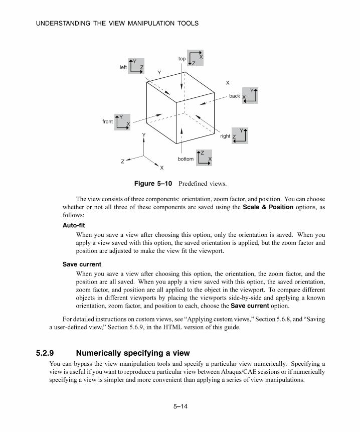
UNDERSTANDING THE VIEW MANIPULATION TOOLS
bottom
back
front
left
right
top X
ZY Z
X
X
Y
Y
Y
YX
X
XZ
Z
ZY
Figure 5–10 Predefined views.
The view consists of three components: orientation, zoom factor, and position. You can choose
whether or not all three of these components are saved using the Scale & Position options, as
follows:
Auto-fit
When you save a view after choosing this option, only the orientation is saved. When you
apply a view saved with this option, the saved orientation is applied, but the zoom factor and
position are adjusted to make the view fit the viewport.
Save current
When you save a view after choosing this option, the orientation, the zoom factor, and the
position are all saved. When you apply a view saved with this option, the saved orientation,
zoom factor, and position are all applied to the object in the viewport. To compare different
objects in different viewports by placing the viewports side-by-side and applying a known
orientation, zoom factor, and position to each, choose the Save current option.
For detailed instructions on custom views, see “Applying custom views,” Section 5.6.8, and “Saving
a user-defined view,” Section 5.6.9, in the HTML version of this guide.
5.2.9 Numerically specifying a viewYou can bypass the view manipulation tools and specify a particular view numerically. Specifying a
view is useful if you want to reproduce a particular view between Abaqus/CAE sessions or if numerically
specifying a view is simpler and more convenient than applying a series of view manipulations.
5–14
Abaqus ID:
Printed on:

UNDERSTANDING THE VIEW MANIPULATION TOOLS
Select View→Specify from the main menu bar to specify a view.
Tip: You can also specify a view by double-clicking the 3D compass.
You can use the following methods to specify your view:
Rotation Angles
Enter three angles ( , , ) representing the angles through which your view of the model rotates
about the screen or model 1-, 2-, and 3-axes, respectively. Rotations are interpreted in the order
( , , ), and a positive angle represents a right-handed rotation about the axis. If you previously
specified a nondefault center of rotation while using the rotate view tool (see “The rotate view tool,”
Section 5.2.3), the specified rotations will also be about this point. You must choose one of the
following modes to apply the rotation:
• Increment About Model Axes. When you choose Increment About Model Axes,Abaqus/CAE simply applies the rotation to the current view. Figure 5–11 shows the result of
applying an incremental model axes rotation of 90, 0, 0 from the isometric view.
13
1
2
3 2
Figure 5–11 Specifying an incremental model axes rotation angle.
• Increment About Screen Axes. The screen X-axis is horizontal, the Y-axis is vertical,
and the Z-axis is out of the screen. The origin of the screen axes is the camera target. In
most cases the camera target coincides with the center of the viewport, but some view
manipulation methods can move the camera target (for more information, see “Camera modes
and view terminology,” Section 5.1.1). When you choose Increment About Screen Axes,Abaqus/CAE simply applies the rotation to the current view. Figure 5–12 shows the result of
applying an incremental screen axes rotation of 90, 0, 0 from the isometric view.
5–15
Abaqus ID:
Printed on:

UNDERSTANDING THE VIEW MANIPULATION TOOLS
12312
3
Figure 5–12 Specifying an incremental screen axes rotation angle.
• Total Rotation From (0,0,1). When you choose Total Rotation From (0,0,1), Abaqus/CAEfirst rotates the view to the default position (a view looking down the 3-axis with the 1- and
2-axes in the plane of the screen) and then applies the desired rotation. Figure 5–13 shows the
result of applying a total rotation of 90, 0, 0 from the isometric view.
12
31
2
3
Figure 5–13 Specifying a total rotation angle.
Viewpoint
When you choose Viewpoint, you enter three values representing the 1-, 2-, and 3-position of an
observer. Abaqus/CAE constructs a vector from the origin of the model to the position that you
specify and rotates your view of the model so that this vector points out of the screen. Figure 5–14
shows the result of applying a viewpoint of 1, 1, 1 (an isometric view) and a viewpoint of 1, 0, 0.
5–16
Abaqus ID:
Printed on:

UNDERSTANDING THE VIEW MANIPULATION TOOLS
12
1
2
3 3
Figure 5–14 Specifying a viewpoint.
When you use the Viewpoint method to specify a view, you can also specify the Up vector.Abaqus/CAE positions your view of the model so that this vector points upward. Figure 5–15 shows
the result of applying an up vector of 0, 1, 0 and an up vector of 0, −1, 0 to an isometric view. The
Up vector must not equal the Viewpoint vector.
1
2
31
2
3
Figure 5–15 Specifying an Up vector.
Zoom
Enter a value representing a magnification factor. A value greater than 1 expands your view of the
model in the viewport; for example, a Zoom factor of 2 doubles the size of your view of the model.
A value between 0 and 1 contracts your view of the model in the viewport; for example, a value of
0.25 contracts your view of the model to a quarter of its original size. The value must be greater
than zero.
5–17
Abaqus ID:
Printed on:
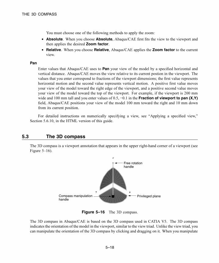
THE 3D COMPASS
You must choose one of the following methods to apply the zoom:
• Absolute. When you choose Absolute, Abaqus/CAE first fits the view to the viewport and
then applies the desired Zoom factor.
• Relative. When you choose Relative, Abaqus/CAE applies the Zoom factor to the current
view.
Pan
Enter values that Abaqus/CAE uses to Pan your view of the model by a specified horizontal and
vertical distance. Abaqus/CAE moves the view relative to its current postion in the viewport. The
values that you enter correspond to fractions of the viewport dimensions; the first value represents
horizontal motion and the second value represents vertical motion. A positive first value moves
your view of the model toward the right edge of the viewport, and a positive second value moves
your view of the model toward the top of the viewport. For example, if the viewport is 200 mm
wide and 100 mm tall and you enter values of 0.5, −0.1 in the Fraction of viewport to pan (X,Y)field, Abaqus/CAE positions your view of the model 100 mm toward the right and 10 mm down
from its current position.
For detailed instructions on numerically specifying a view, see “Applying a specified view,”
Section 5.6.10, in the HTML version of this guide.
5.3 The 3D compass
The 3D compass is a viewport annotation that appears in the upper right-hand corner of a viewport (see
Figure 5–16).
Compass manipulationhandle
Free rotationhandle
Privileged plane
Figure 5–16 The 3D compass.
The 3D compass in Abaqus/CAE is based on the 3D compass used in CATIA V5. The 3D compass
indicates the orientation of the model in the viewport, similar to the view triad. Unlike the view triad, you
can manipulate the orientation of the 3D compass by clicking and dragging on it. When you manipulate
5–18
Abaqus ID:
Printed on:

THE 3D COMPASS
the 3D compass, the viewport camera pans or rotates to change the viewport orientation accordingly.
The behavior of the compass view manipulations is identical to the compass view manipulation behavior
in CATIA V5.
The 3D compass is a helpful shortcut for certain view manipulation options since it is available in
all modules and during all procedures; you do not need to enter a view manipulation mode to change the
viewport orientation using the 3D compass.
This section describes the basic functions and features of the 3D compass.
5.3.1 Rotating the view using the 3D compass
The 3D compass allows you to rotate the view of a model using two different methods: you can rotate
freely in all directions, or you can constrain the manipulation to rotation about a specific axis. In both
cases the model view rotates about the current center of rotation for the viewport, as defined by the rotate
tool (see “The rotate view tool,” Section 5.2.3).
Free rotation
To rotate a model in any direction, click and drag the free rotation handle on the 3D compass:
Freerotationhandle
As you drag the mouse, the compass rotates about its pivot in the direction of the mouse motion
(the pivot point coincides with the compass manipulation handle). The rotation is dependent on
the direction of the mouse motion, not on the location of the pointer; in other words, the compass
continues to rotate as long as you continue to drag. As the orientation of the compass changes, the
view of the model changes accordingly.
Rotation about an axis
You can also rotate a model about a specified axis, thereby maintaining a constant orientation in a
particular direction during the manipulation. To rotate about an axis, click and drag one of the three
arcs along the perimeter of the 3D compass:
5–19
Abaqus ID:
Printed on:

THE 3D COMPASS
Rotate aboutan axis
As you drag the mouse, the compass rotates about the axis that is perpendicular to the plane
subtended by the selected arc (the X-axis in the above example). The rotation is dependent on the
location of the pointer. As you drag the mouse, the path of the pointer in the viewport is projected
onto the selected compass arc. The compass rotates according to this projected path. As the
orientation of the compass changes, the view of the model changes accordingly.
5.3.2 Panning the view using the 3D compass
The 3D compass allows you to pan the view of a model using two different methods: you can pan along
a specified axis, or you can pan within a specified plane.
The pan manipulations performed with the 3D compass are different than the manipulation
performed with the standard pan view tool (see “The pan view tool,” Section 5.2.2). The standard
pan tool moves the camera laterally in front of the model; the camera is constrained to move only in
a plane parallel to the viewport. The panning planes for the 3D compass are not necessarily parallel
to the viewport. As a result, panning with the compass behaves like a combination of the standard
pan and zoom tools in their alternate modes: the camera moves both laterally across the model and
perpendicularly toward or away from the model. The orientation of the compass and model view does
not change during pan manipulations.
Note: As with the alternate mode of the standard pan view tool, panning the view with the 3D compass
also translates the viewport’s center of rotation along with the camera. See “The rotate view tool,”
Section 5.2.3, for information about the center of rotation.
Panning along an axis
To pan the view along an axis, click and drag any of the straight axes on the 3D compass:
5–20
Abaqus ID:
Printed on:

THE 3D COMPASS
Pan alongan axis
As you drag the mouse, the path of the pointer in the viewport plane is projected onto the selected
compass axis (the Z-axis in the above example). The camera moves according to this projected
linear path.
Panning along a plane
To pan the view along a plane, click and drag any of the quarter-circular faces on the 3D compass:
Pan alonga plane
As you drag the mouse, the path of the pointer in the viewport plane is projected onto the selected
compass plane (theY–Z plane in the above example). The camera moves according to this projected
path.
5.3.3 Predefined views for the 3D compassYou can use the 3D compass to quickly set the viewpoint to one of six predefined views. You can also
access the Specify View dialog box through the compass.
Predefined views
The predefined views correspond to the three planes of the 3D compass. To apply a predefined view,
click the label for any of the axes on the 3D compass:
5–21
Abaqus ID:
Printed on:

THE 3D COMPASS
Apply a predefinedview
Z
The view is adjusted so that the selected axis (the Z-axis in the above example) is perpendicular
to the plane of the viewport. Clicking the same axis label again flips the view orientation to the
opposite side of the viewport plane. In other words, clicking the same axis label repeatedly oscillates
the view between the front and back side of the displayed model.
The six predefined views associated with the 3D compass are identical to the predefined views
in the Views toolbar.
Numerically specifying a view
Double-clicking anywhere on the 3D compass opens the Specify View dialog box. You can use
this method to numerically specify a viewpoint or camera location. See “Numerically specifying a
view,” Section 5.2.9, for more information.
5.3.4 Customizing the 3D compassTo customize the look and orientation of the 3D compass, click mouse button 3 on the compass and select
an option from the menu that appears. You can perform the following customizations:
Edit
Select Edit to display the Specify View dialog box and numerically specify a custom view
orientation. See “Numerically specifying a view,” Section 5.2.9, for details on specifying custom
view orientations.
Tip: You can also double click the 3D compass to display the Specify View dialog box.
Change the privileged plane
The base of the compass (which contains the compass manipulation handle) is called the privileged
plane. By default, the X–Z plane is the privileged plane in Abaqus/CAE. The privileged plane
can be helpful in determining the “correct” orientation of a model in the viewport. In the default
isometric orientation of the compass, the privileged plane appears at the bottom and the free rotation
handle appears at the top; the axis from the privileged plane to the free rotation handle in effect
indicates the “up” direction for the model.
5–22
Abaqus ID:
Printed on:

CUSTOMIZING THE VIEW TRIAD
If the Y-axis does not correspond to the “up” direction in a model, you can change the
privileged plane to any of the three major planes in the compass. For example, select Make XYthe Privileged Plane to set the X–Y plane as the privileged plane. Changing the privileged plane
only reconfigures the shape of the 3D compass, as indicated in Figure 5–17; the view orientation
and the predefined views in the Views toolbar are not changed.
Figure 5–17 Changing the privileged plane from the X–Z plane (left) to the X–Y plane (right).
Hide
Select Hide to remove the 3D compass from the viewport display. To resume the display of
the 3D compass, you must use the viewport annotation options (select Viewport→ViewportAnnotation Options from the main menu). For information on controlling the visibility of
viewport annotations, see “Overview of viewport annotation options,” Section 56.4, in the HTML
version of this guide.
Help
Select Help to display a help window with documentation on using the 3D compass.
5.4 Customizing the view triad
The view triad, shown below, is a set of three perpendicular axes that indicate the orientation of your view
of the model currently being displayed. TheX,Y, and Z labels correspond to the 1-, 2-, and 3-directions,
respectively. As you rotate your view of the model, the triad changes to indicate the new orientation.
X
Y
Z
5–23
Abaqus ID:
Printed on:

CONTROLLING PERSPECTIVE
The view triad and the 3D compass both indicate the view orientation, and they are always aligned
with each other. You can directly manipulate the 3D compass orientation in the viewport, thereby
changing the view of the model (see “The 3D compass,” Section 5.3). The view triad acts only as a
reference; it rotates with the 3D compass, but it cannot be directly manipulated.
You can use the Viewport→Viewport Annotation Options menu item to request or suppress the
display of the triad and to control the triad’s size, position, and appearance. You can also control the
triad’s labels, including their color and font.
For detailed instructions on customizing the view triad, see the corresponding section in the HTML
version of this guide.
5.5 Controlling perspective
Perspective representation accurately depicts the spatial relationship of three-dimensional objects in a
two-dimensional plane. In other words, a three-dimensional model on your screen appears more realistic
when perspective is turned on. Alternatively, parallel lines in the model appear parallel when perspective
is turned off. Perspective affects all plots except X–Y plots, applies in all modules, and is turned on by
default.
• To turn perspective on, select the icon located in the View Options toolbar or select
View→Perspective from the main menu bar.
• To turn perspective off, select the icon located in the View Options toolbar or select
View→Parallel from the main menu bar.
Your changes apply only to the current viewport and are saved for the duration of the session.
5–24
Abaqus ID:
Printed on:

UNDERSTANDING SELECTION WITHIN VIEWPORTS
6. Selecting objects within the viewport
This chapter explains how to select objects that appear within a viewport, such as nodes, elements,
vertices, edges, faces, and cells. The following topics are covered:
• “Understanding selection within viewports,” Section 6.1
• “Selecting objects within the current viewport,” Section 6.2
• “Using the selection options,” Section 6.3
Selecting dialog box options is discussed in “Interacting with dialog boxes,” Section 3.2. Selecting
viewports is discussed in “Selecting viewports,” Section 4.3.2, in the HTML version of this guide.
6.1 Understanding selection within viewports
This section describes the objects that you can select in a viewport and explains what these objects
represent.
6.1.1 What objects can you select from the viewport?Selecting an object within the current viewport is one of the most common tasks you have to perform
during the modeling process. In the course of various procedures you may need to select geometric
objects (vertices, edges, faces, cells, and datums) or discrete objects (nodes and elements) by picking
them directly from the viewport. Figure 6–1 shows these different object types.
You can select objects in the viewport during certain procedures, such as those listed below:
• Creating sets and surfaces
• Partitioning a part instance
• Editing a feature
• Seeding a part instance for meshing
• Creating or editing a display group composed of elements or nodes
• Color coding elements in your model
• Creating a node list path through your model
• Creating a load
You can also select objects in the viewport in advance of selecting a procedure. If you make selections
prior to selecting a procedure, Abaqus/CAE does not limit your selections. When you select a procedure,
Abaqus/CAE filters any selections that you made and keeps only those selections that are appropriate for
the procedure. For more information, see “Selecting objects before choosing a procedure,” Section 6.3.7.
6–1
Abaqus ID:
Printed on:

UNDERSTANDING SELECTION WITHIN VIEWPORTS
Cell
Datumplane
Vertex
Partition
Face
Edge
Element
Node
Geometric entities Discrete entities
Figure 6–1 Object types that you can select.
If you select objects as part of a procedure, in most circumstances Abaqus/CAE only allows you to
select objects that are appropriate for the current procedure. For example, the first step in partitioning
an edge is selecting the edge of interest. Therefore, at this point in the procedure you can select only an
edge; you cannot select a cell, a face, or a vertex. Messages in the prompt area guide you through the
steps of a procedure and indicate which types of objects are available for selection. You can select only
objects that are part of the current display group.
In some circumstances Abaqus/CAE cannot determine which objects are appropriate for selection
and does not limit your selection. For example, when you are creating a set, you can select from cells,
faces, edges, and vertices to include in the set and Abaqus/CAE allows you to select any of these objects.
If you make an ambiguous selection from the viewport during a procedure, Abaqus/CAE allows you
to cycle through the available objects until the desired object is selected. This ambiguity is described
in “Cycling through valid selections,” Section 6.2.10. You may find it easier to use the selection filters
to limit the type of object you can select. For more information, see “Using the selection options,”
Section 6.3.
Many procedures to define attributes (interactions, constraints, loads, boundary conditions,
predefined fields, and engineering features) allow you to select objects from the viewport to identify
the region on which to apply the attribute. The default behavior for these procedures is to create a set
or surface that contains the selected objects. You can change this behavior by toggling off the option to
create a set or surface in the prompt area. A default name is provided in the prompt area, but you can
enter a new name.
6–2
Abaqus ID:
Printed on:
UNDERSTANDING SELECTION WITHIN VIEWPORTS
6.1.2 What is a selection group?
You can copy entities (vertices, edges, faces, or cells) that are highlighted in the viewport into a temporary
storage area called a selection group. Abaqus/CAE saves the selection group for the duration of a session.
Rather thanmanually reselecting the same entities during a subsequent selection procedure, you can paste
the selection group into your selection. For example, you can copy all of the small faces highlighted by
the Geometry Diagnostics query tool into a selection group. You can then paste the same selection
group into your selection when you are using the Geometry Edit toolset to repair small faces.
When you paste a group into your selection, you can choose from selection groups and from display
groups. Selection groups are designed to be a temporary convenience for the user, and they do not appear
with display groups in the Display Groups toolset. You can create any number of display groups. In
contrast, Abaqus/CAE saves a maximum of five selection groups. Abaqus/CAE overwrites the existing
selection groups if you create more than five selection groups.
After you have selected the desired entities, you create a selection group by clicking mouse
button 3 in the viewport and selecting Copy from the menu that appears. Abaqus/CAE copies all of
the highlighted entities into a selection group. You paste a selection group to your current selection by
clicking mouse button 3 in the viewport and selecting Paste from the menu that appears. Abaqus/CAE
displays the Paste to Selection dialog box, and you can select one or more of the existing selection
groups to paste to your current selection. When you paste a group, Abaqus/CAE appends the entities in
the group to any other entities that you have already selected.
Note: You cannot create or use selection groups if you are selecting objects in advance of selecting a
procedure.
6.1.3 Understanding the correspondence between geometric andphysical objects
When you select geometric objects in a viewport, it is important to understand what physical
structure each object represents. The geometric objects that make up a model—cells, faces, edges,
and vertices—can represent different physical structures depending on the space in which they are
embedded.
For example, beams and other wire parts are represented by edges in the geometric model (see
Figure 6–2). The end surfaces of these parts are represented by the vertices on either side of the edge,
and the circumferential surface is represented by the line joining the vertices. To select a wire part, you
can click the edge, and, if necessary, Abaqus/CAE prompts you to specify the surface of interest.
Likewise, axisymmetric shells are also represented by edges in the geometric model (see
Figure 6–3). You can select the axisymmetric shell by clicking the edge in the viewport, and, if
necessary, Abaqus/CAE prompts you to specify either the inside surface or the outside surface of the
shell. You must select either the inside or the outside surface if you are applying a prescribed condition
6–3
Abaqus ID:
Printed on:

UNDERSTANDING SELECTION WITHIN VIEWPORTS
Geometric model Physical object
Edge Circumferential surface
End 2 surface
End 1 surface
Figure 6–2 Selecting wire parts.
Geometric model Physical part
Edge
Edge
Surface
Axis of symmetry Axis of symmetry
Vertex
Figure 6–3 Selecting axisymmetric shells.
or contact definition to the surface. For example, if you want to apply a pressure load to a shell, you
must specify which side of the shell should receive the load.
For more information on selecting surfaces, see “Specifying a particular side or end of a region,”
Section 73.2.5. For more information on modeling space, see “The relationship between parts and
features,” Section 11.3.1, and “Part modeling space,” Section 11.4.1.
6–4
Abaqus ID:
Printed on:

SELECTING OBJECTS WITHIN THE CURRENT VIEWPORT
6.2 Selecting objects within the current viewport
This section describes techniques that you can use for selecting one or more objects in the current
viewport.
6.2.1 Selecting and unselecting individual objects
Selecting and unselecting objects in the current viewport are straightforward operations that use standard
methods. For more information on selecting viewports, see “Selecting viewports,” Section 4.3.2, in the
HTML version of this guide.
Preselection highlighting allows you to preview which object Abaqus/CAE will select if you click
at the current cursor location. In addition, preselection in the Sketcher uses a secondary cursor to indicate
the exact position and type of entity that will be selected. (For more information on Sketcher preselection,
see “The Sketcher cursors and preselection,” Section 20.4.5.)
You will use the following three selection operations most frequently:
Click to select an object
To select a single object from the current viewport, move the cursor to the object and click mouse
button 1.
• To select a point, click the corresponding point marker. The point marker changes color when
selected. Vertices that you can select are marked by small, filled circles; and datum points
are marked by small, unfilled circles. (See “Understanding the role of datum geometry,”
Section 62.1, for information on datum points.) Edge midpoints and arc centers that you can
select are marked by small diamonds.
Note: Some of the selection markers that appear when you are using the Sketch module
are different from those described here. For information on selecting objects while using the
Sketch module, see “The Sketcher cursors and preselection,” Section 20.4.5.
• To select an edge, click the edge while positioning the cursor away from any vertex. Selected
edges are highlighted.
• To select a face, click the face while positioning the cursor away from any edge or vertex.
Selected faces are highlighted with a grid pattern. (The grid pattern is unrelated to mesh
element location.)
• To select a cell, click any of its faces. All edges of selected cells are highlighted.
If you are unable to select the desired objects, you can use the Selection toolbar to change the
selection behavior. For more information, see “Using the selection options,” Section 6.3.
Once you select an object, any objects previously selected in the current viewport are
unselected automatically.
6–5
Abaqus ID:
Printed on:

SELECTING OBJECTS WITHIN THE CURRENT VIEWPORT
If your current procedure, options, and cursor position do not clearly specify one object for
preselection, Abaqus/CAE highlights all of the potential selections and adds ellipsis marks (...) next
to the cursor arrow to indicate an ambiguous preselection. If you accept an ambiguous preselection
or otherwise make an ambiguous selection, use the buttons in the prompt area to make your final
selection. For more information, see “Cycling through valid selections,” Section 6.2.10.
[Shift]+Click to select additional objects
To select an additional object, move the cursor to the object and [Shift]+Click. Your original selection
remains highlighted, and the newly selected object becomes highlighted.
An alternative method for selecting multiple objects is to drag a rectangle around the objects.
For more information, see “Drag-selecting multiple objects,” Section 6.2.2.
[Ctrl]+Click to unselect objects
To unselect an object, move the cursor to the object and [Ctrl]+Click. To unselect all objects, click an
unused region of the current viewport.
When you have finished selecting and unselecting items in the viewport, click mouse button 2 to
confirm your selection. You can use the selection option tools to adjust the shape of the drag-select
region. You can also choose which objects are selected by the drag-select region. The selection option
tools are located in the Selection toolbar. For more information, see “Modifying the shape of the
drag-select region,” Section 6.3.5, and “Choosing which objects are selected by the drag-select region,”
Section 6.3.6.
6.2.2 Drag-selecting multiple objectsMost prompts ask you to select just one object from the current viewport. However, some tasks allow
you to select one or more objects; for example, the Set toolset allows you to select several objects of
the same type and group them into sets. You can select multiple objects using the [Shift]+Click method
described in “Selecting and unselecting individual objects,” Section 6.2.1. An additional method for
selecting multiple objects is to drag a rectangle around those objects. You can use the selection option
tools to adjust the shape of the drag-select region. You can also choose which objects are selected by the
drag-select region. The selection option tools are located in theSelection toolbar. For more information,
see “Modifying the shape of the drag-select region,” Section 6.3.5, and “Choosing which objects are
selected by the drag-select region,” Section 6.3.6.
To drag-select multiple objects:
1. Imagine a rectangle that encloses only the objects you want to select.
2. Click at one corner of the rectangle and, while continuing to press the mouse button, drag until you
have enclosed all the objects.
3. Release the mouse button.
All the valid objects inside or crossing the rectangle are highlighted.
6–6
Abaqus ID:
Printed on:

SELECTING OBJECTS WITHIN THE CURRENT VIEWPORT
4. Click mouse button 2 to indicate that you have finished selecting objects.
Sometimes it is convenient to use a combination of the [Shift]+Click and drag-select selection
techniques. For more information, see “Combining selection techniques,” Section 6.2.8.
Tip: If you select multiple objects and then want to unselect one or more of them, [Ctrl]+Click
the objects you want to unselect. To unselect all the objects, click in an unused area of the
viewport.
6.2.3 Using the angle and feature edge method to select multipleobjects
In complicated models selecting individual faces or edges from geometry or selecting element faces or
nodes from a mesh can be time consuming and prone to error. For example, when creating a surface from
a mesh, you must select the individual element faces that make up the surface and append them to your
selection. To speed up the selection process, Abaqus/CAE provides the angle and feature edge methods
for selecting multiple faces, edges, elements, element faces, or nodes.
When you are performing a task in which you must pick more than one face or edge from geometry
or more than one element, element face, or node from a mesh, Abaqus/CAE displays a field in the prompt
area. The field allows you to choose between three selection methods—individually, by angle, and byfeature edge, as shown in Figure 6–4.
Figure 6–4 Choose the selection method from the field in the prompt area.
Individually
Selecting individual objects is described in “Selecting and unselecting individual objects,”
Section 6.2.1.
By angle
Selecting objects using the angle method is a two-step process:
1. In the prompt area, you enter an angle (from 0° to 90°).
2. From the part or assembly, you select a face, edge, element face, or node.
The angle must be greater than the angle through which adjacent edges or faces must rotate to
create the geometry as if it was being formed by bending a straight wire or folding a series of faces.
6–7
Abaqus ID:
Printed on:
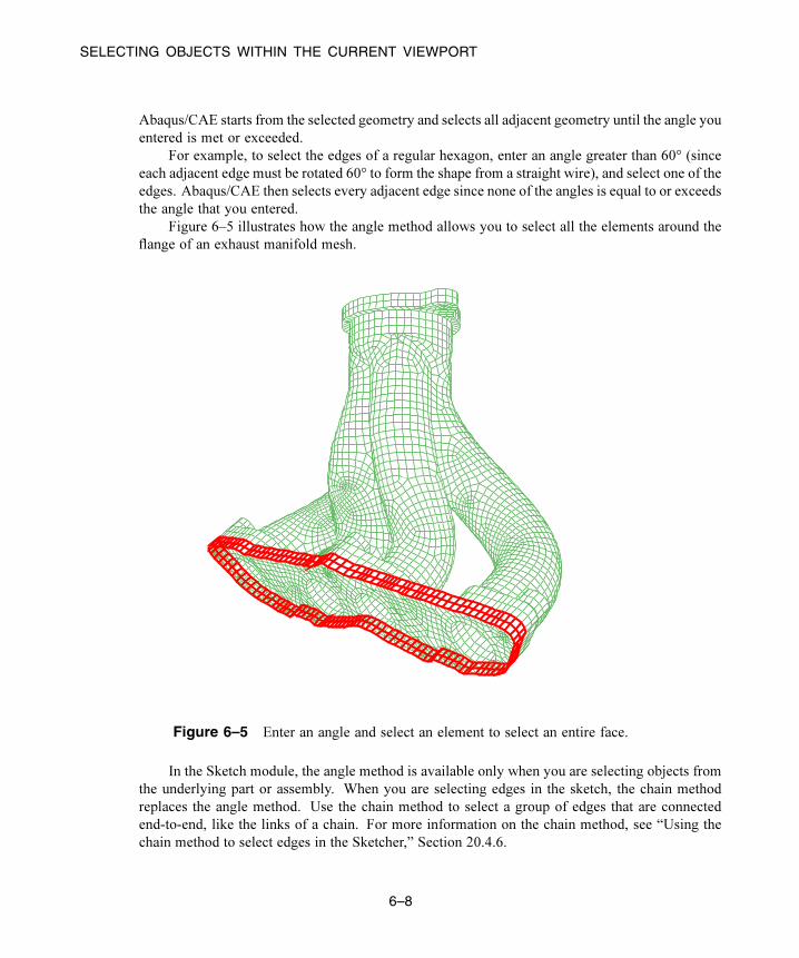
SELECTING OBJECTS WITHIN THE CURRENT VIEWPORT
Abaqus/CAE starts from the selected geometry and selects all adjacent geometry until the angle you
entered is met or exceeded.
For example, to select the edges of a regular hexagon, enter an angle greater than 60° (since
each adjacent edge must be rotated 60° to form the shape from a straight wire), and select one of the
edges. Abaqus/CAE then selects every adjacent edge since none of the angles is equal to or exceeds
the angle that you entered.
Figure 6–5 illustrates how the angle method allows you to select all the elements around the
flange of an exhaust manifold mesh.
Figure 6–5 Enter an angle and select an element to select an entire face.
In the Sketch module, the angle method is available only when you are selecting objects from
the underlying part or assembly. When you are selecting edges in the sketch, the chain method
replaces the angle method. Use the chain method to select a group of edges that are connected
end-to-end, like the links of a chain. For more information on the chain method, see “Using the
chain method to select edges in the Sketcher,” Section 20.4.6.
6–8
Abaqus ID:
Printed on:

SELECTING OBJECTS WITHIN THE CURRENT VIEWPORT
By feature edge
The feature edge method is also a multistep process:
1. In the prompt area, you enter an angle (from 0° to 90°).
2. Abaqus/CAE identifies all the feature edges in your model by finding all the element edges
where the angle between two adjacent element faces is greater than the angle specified.
3. From the mesh, you select an element edge or node.
4. Abaqus/CAE follows the feature edge that passes through the selected element edge or node.
The feature edge is truncated if another feature edge intersects it at an angle greater than the
angle specified in Step 1.
5. Abaqus/CAE selects all the elements or nodes along the feature edge.
Figure 6–6 illustrates how the feature edge method allows you to select all the nodes along the
edges of a flange of an exhaust manifold mesh.
Figure 6–6 Enter an angle and select a segment of an edge to select adjacent nodes.
6–9
Abaqus ID:
Printed on:

SELECTING OBJECTS WITHIN THE CURRENT VIEWPORT
After you use the angle or feature edge methods, you can click the individually method in the
prompt area and [Shift]+Click on individual faces, edges, elements, element faces, or nodes to append
them to your selection. You can also [Ctrl]+Click on items to unselect them. In addition, you can continue
to use the angle and feature edge methods and use [Shift]+Click to append faces, edges, elements, element
faces, or nodes to your selection. You can keep the same angle, or you can change the angle while you
continue to append items. For more information, see “Combining selection techniques,” Section 6.2.8.
6.2.4 Using the face curvature method to select multiple faces
In addition to selecting objects by the angle between them, you can select multiple faces from a part
based on the curvature of the faces. When you are performing a task that allows you to pick more than
one geometric face, Abaqus/CAE displays a field in the prompt area. The field allows you to choose
between the three selection methods—individually, by face angle, and by face curvature, as shownin Figure 6–7.
Figure 6–7 Choose the selection method from the field in the prompt area.
The angle selection method is described in “Using the angle and feature edge method to select multiple
objects,” Section 6.2.3.
The face curvature method is available during procedures that select faces. If a procedure accepts
object types other than faces, you can change the object type in the Selection toolbar to Faces to access
the face curvature method.
Select a face from the part or assembly. Abaqus/CAE selects all connected faces that have similar
curvature along both principal directions and are joined at an angle of less than 20°. If you select a
flat face, Abaqus/CAE adds any adjoining flat faces that lie in the same plane. Disconnected faces that
share similar curvature are not selected, nor are faces that share similar curvature but have significantly
different face normals at the edge where they meet. Figure 6–8 shows two rounded faces selected using
the face curvature method.
After you use the face curvature method, you can click the individually method in the prompt area
and [Shift]+Click on individual faces to append them to your selection. You can also [Ctrl]+Click on items
to unselect them. In addition, you can continue to use the face curvature method and use [Shift]+Click
to append faces to your selection. For more information, see “Combining selection techniques,”
Section 6.2.8.
6–10
Abaqus ID:
Printed on:

SELECTING OBJECTS WITHIN THE CURRENT VIEWPORT
Figure 6–8 Select a single curved face to select adjoining faces with similar curvature.
6.2.5 Using the topology method to select multiple elementsYou can select multiple elements based on the connection of a row or layer of elements. When you
are performing a task that allows you to pick more than one element, Abaqus/CAE displays a field in
the prompt area. The field allows you to choose between the four selection methods—individually, byangle, by feature edge, and by topology, as shown in Figure 6–9.
Figure 6–9 Choose the selection method from the field in the prompt area.
The angle and feature edge selection methods are described in “Using the angle and feature edge method
to select multiple objects,” Section 6.2.3.
The topology method is available during most procedures that select elements. If a procedure
accepts object types other than elements, you can change the object type in the Selection toolbar to
Elements to access the topology method.
The topology method is designed for use with two- and three-dimensional structured meshes. Select
an element face from the mesh, and Abaqus/CAE selects all the elements connected to it in a row through
the mesh. Select an element edge from the mesh, and Abaqus/CAE selects all the elements in a layer
6–11
Abaqus ID:
Printed on:

SELECTING OBJECTS WITHIN THE CURRENT VIEWPORT
starting with the element faces that share the selected edge. Figure 6–10 shows selection of an interior
row on the left and an interior layer on the right.
Figure 6–10 Using the topology method to select a row or a layer of elements.
You can use the topology method to select elements from other mesh types, but without the clearly
defined rows or layers of a structured mesh, the selections may be unpredictable. In some cases, such
as with a tetrahedral mesh, topology selection may be limited to only the elements that share the face or
edge you select.
After you use the topology method, you can select other methods in the prompt area and [Shift]+Click
to appendmore elements to your selection. You can also [Ctrl]+Click on items to unselect them. In addition,
you can continue to use the topology method and use [Shift]+Click to append elements to your selection.
For more information, see “Combining selection techniques,” Section 6.2.8.
6.2.6 Using the limiting angle, layer, and analytic methods to selectmultiple element faces
When you are selecting orphan element faces to create geometry (for more information, see “Create
face from element faces,” Section 69.7.10, in the HTML version of this guide), Abaqus/CAE displays a
field in the prompt area. The field allows you to choose between five selection methods—individually,by angle, by limiting angle, by layer, and by analytic, as shown in Figure 6–11. The angle
selection method is described in “Using the angle and feature edge method to select multiple objects,”
Section 6.2.3. The limiting angle, layer, and analytic methods are available only while selecting orphan
element faces to create new geometric faces.
6–12
Abaqus ID:
Printed on:

SELECTING OBJECTS WITHIN THE CURRENT VIEWPORT
Figure 6–11 Choose the selection method from the field in the prompt area.
By limiting angle
Selecting objects using a limiting angle is a two-step process:
1. In the prompt area, you enter an angle (from 0° to 90°).
2. From the part or assembly, you select an orphan element face.
The angle must be greater than the total angle between the selected element face and the element
faces connected to it. Abaqus/CAE starts from the selected geometry and selects all adjacent
geometry until the angle between the selected face and the last face in the series of adjacent faces
meets or exceeds the angle you entered. Figure 6–12 shows selection of element faces with a
limiting angle of 45°, and one of the vertical element faces below the rounded area is picked.
Figure 6–12 A limiting angle of 45° with a selected vertical face.
Increasing the limiting angle to its maximum of 90° would select the faces up to the top of the
rounded section. In contrast, using the angle method with an angle of 13° or more would continue
the selection around the rounded portion and down the far side since the angle between each adjacent
face is less than 13°.
By layer
Selecting objects using the layer method is a two-step process:
1. In the prompt area, you enter a number of layers.
6–13
Abaqus ID:
Printed on:
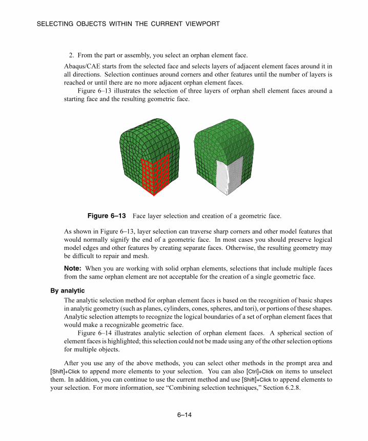
SELECTING OBJECTS WITHIN THE CURRENT VIEWPORT
2. From the part or assembly, you select an orphan element face.
Abaqus/CAE starts from the selected face and selects layers of adjacent element faces around it in
all directions. Selection continues around corners and other features until the number of layers is
reached or until there are no more adjacent orphan element faces.
Figure 6–13 illustrates the selection of three layers of orphan shell element faces around a
starting face and the resulting geometric face.
Figure 6–13 Face layer selection and creation of a geometric face.
As shown in Figure 6–13, layer selection can traverse sharp corners and other model features that
would normally signify the end of a geometric face. In most cases you should preserve logical
model edges and other features by creating separate faces. Otherwise, the resulting geometry may
be difficult to repair and mesh.
Note: When you are working with solid orphan elements, selections that include multiple faces
from the same orphan element are not acceptable for the creation of a single geometric face.
By analytic
The analytic selection method for orphan element faces is based on the recognition of basic shapes
in analytic geometry (such as planes, cylinders, cones, spheres, and tori), or portions of these shapes.
Analytic selection attempts to recognize the logical boundaries of a set of orphan element faces that
would make a recognizable geometric face.
Figure 6–14 illustrates analytic selection of orphan element faces. A spherical section of
element faces is highlighted; this selection could not be made using any of the other selection options
for multiple objects.
After you use any of the above methods, you can select other methods in the prompt area and
[Shift]+Click to append more elements to your selection. You can also [Ctrl]+Click on items to unselect
them. In addition, you can continue to use the current method and use [Shift]+Click to append elements to
your selection. For more information, see “Combining selection techniques,” Section 6.2.8.
6–14
Abaqus ID:
Printed on:

SELECTING OBJECTS WITHIN THE CURRENT VIEWPORT
Figure 6–14 Analytic geometry selection.
6.2.7 Adding adjacent objects to a selectionIf you have already selected one or more objects, you can expand your selection to include all adjacent
objects of the same type. Adding adjacent objects is an alternative to using drag-select or the angle
method (see “Drag-selecting multiple objects,” Section 6.2.2, and “Using the angle and feature edge
method to select multiple objects,” Section 6.2.3, respectively) to quickly select multiple objects.
Selecting adjacent objects allows you to expand your selection in all directions, regardless of the shape
of surrounding features or the angle at which objects are joined. It also allows you to pick multiple
areas of interest in a model and expand the selection set in each area at the same time.
To add adjacent objects to the current selection, click mouse button 3 over an existing selected
object and select Add Adjacent Entities. Abaqus/CAE expands your selections to all adjacent objects
of the same type, including objects that are not included in the current display. If necessary, Abaqus/CAE
adds the newly selected objects to the current display group to make them visible. Adjacent objects are
defined in terms of the currently selected entities as follows:
• Edges that share a common vertex with one or more selected edges
• Vertices that share a common edge with one or more selected vertices
• Faces that share a common vertex or edge with one or more selected faces
• Nodes that share a common edge with one or more selected nodes
• Elements that share a common element edge or node with a selected element
6.2.8 Combining selection techniquesThere are times when it is convenient to use a combination of the methods for selecting and unselecting
objects. For example, you can drag-select a group of nodes while creating a node set using the Set toolset.
6–15
Abaqus ID:
Printed on:
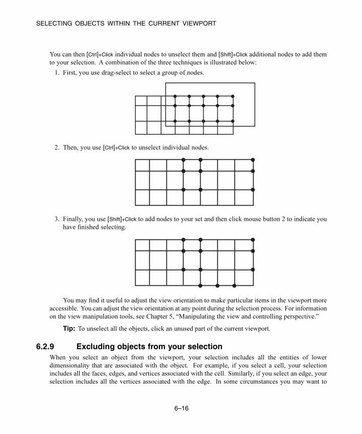
SELECTING OBJECTS WITHIN THE CURRENT VIEWPORT
You can then [Ctrl]+Click individual nodes to unselect them and [Shift]+Click additional nodes to add them
to your selection. A combination of the three techniques is illustrated below:
1. First, you use drag-select to select a group of nodes.
2. Then, you use [Ctrl]+Click to unselect individual nodes.
3. Finally, you use [Shift]+Click to add nodes to your set and then click mouse button 2 to indicate you
have finished selecting.
You may find it useful to adjust the view orientation to make particular items in the viewport more
accessible. You can adjust the view orientation at any point during the selection process. For information
on the view manipulation tools, see Chapter 5, “Manipulating the view and controlling perspective.”
Tip: To unselect all the objects, click an unused part of the current viewport.
6.2.9 Excluding objects from your selectionWhen you select an object from the viewport, your selection includes all the entities of lower
dimensionality that are associated with the object. For example, if you select a cell, your selection
includes all the faces, edges, and vertices associated with the cell. Similarly, if you select an edge, your
selection includes all the vertices associated with the edge. In some circumstances you may want to
6–16
Abaqus ID:
Printed on:

SELECTING OBJECTS WITHIN THE CURRENT VIEWPORT
exclude the entities of lower dimensionality from your selection. For example, if you select an edge to
include in a set, you may not want the set to contain the vertices at each end of the edge. Excluding
entities of lower dimensionality from your selection may solve any problems that you encounter with
overconstraints.
To exclude objects from your selection:
1. Select all the objects using a combination of select, drag-select, [Ctrl]+Click, and [Shift]+Click.
Abaqus/CAE highlights the selected objects in red.
2. [Ctrl]+Click an object to exclude it from your selection.
Abaqus/CAE highlights the excluded objects in purple.
6.2.10 Cycling through valid selections
In some cases Abaqus/CAE is unable to differentiate between the object you have selected and other
nearby or related objects. This ambiguity can arise as follows:
• Imagine a small square surrounding the cursor. When you click an object, any other valid objects of
the same type that fall inside this square are also considered to be possible selections. For example,
if you select an edge that is positioned very close to another edge, Abaqus/CAE may consider both
edges to be possible selections.
The size of the square is independent of the monitor size, the viewport size, and the dimensions
of the model. It also remains constant when you zoom in and out on your model. Therefore, you
can select a specific object in the viewport more precisely by zooming in on your model to increase
the distance between objects.
• If your model is three-dimensional, imagine a line that is perpendicular to the screen and that passes
through the cursor and into the model. When you select an object, any valid objects of the same type
that intersect this line are considered to be possible selections. (Rotating your model may remove
some of the ambiguity.)
Abaqus/CAE reduces the potential for ambiguity by filtering your selection against the current
procedure whenever possible. For example, if you are partitioning a cell, Abaqus/CAE prompts you
to select the cell to partition. When you make a selection, Abaqus/CAE considers only cells to be a
valid selection. Conversely, if you are creating a geometry set, Abaqus/CAE considers cells, faces,
edges, and vertices to be a valid selection and the potential for ambiguity is increased. In addition,
preselection highlighting allows you to see exactly which object would be selected before you make the
selection. Moving the cursor around the viewport may remove the ambiguity in the selection and result
in Abaqus/CAE highlighting the object of your choice. If the ambiguity remains, Abaqus/CAE changes
the cursor, adding ellipsis marks (...) to the right of the arrow, and highlights all the possible selections.
When your selection is ambiguous, Abaqus/CAE displays buttons in the prompt area that allow you
to cycle through all of the possible selections, as shown here:
6–17
Abaqus ID:
Printed on:

USING THE SELECTION OPTIONS
Use the Next and Previous buttons to cycle forward and backward through all of the objects in the
viewport that are possible selections; each object becomes highlighted in turn. When the object of your
choice is highlighted, click OK or click mouse button 2 to confirm your selection. (You can also click
mouse button 3 in the current viewport to reveal a menu of the options in the prompt area.)
6.2.11 Using groups while selecting entitiesYou can append groups of entities to your selection to speed up the process of selecting many entities
from the viewport. The group can be a display group, or it can be a temporary selection group. You can
click mouse button 3 on the viewport and do the following:
• Create a selection group by copying entities (vertices, edges, faces, or cells) that are highlighted in
the viewport into a selection group.
• Append to your selected entities by pasting the entities stored in a selection group or a display group
into your current selection.
6.2.12 Selecting interior surfacesYou can use the selection tools to select an interior surface of a model; for example, when you create a
surface or when you select a region using the solid offset mesh tool.
To select an interior surface:
1. In the Selection toolbar, toggle on the Select From Interior Entities tool .
Note: The Select From Interior Entities tool is hidden by default. For more information, see
“Using toolboxes and toolbars that contain hidden icons,” Section 3.3.2.
2. Select the interior surface from the viewport.
6.3 Using the selection options
Abaqus/CAE provides a set of tools that can make it easier and more efficient for you to select entities
from the viewport. The selection tools are located in the Selection toolbar. The available options depend
on the current selection procedure; some options can be used to preselect entities outside of a procedure.
6–18
Abaqus ID:
Printed on:

USING THE SELECTION OPTIONS
6.3.1 Overview of the selection optionsWhen you are prompted to select an object from the viewport, Abaqus/CAE provides selection tools that
can make it easier and more efficient for you to make the desired selection.
Use the Selection toolbar to configure the selection options. Figure 6–15 shows the layout of the
selection tools. Selection tools appear dimmed if they are not valid for the current procedure.
Figure 6–15 The Selection toolbar.
6.3.2 Filtering your selection based on the type of objectTo help you select the desired entities (vertices, edges, faces, cells, nodes, and elements) from the current
viewport, Abaqus/CAE provides a set of filters that you can use to limit your selection based on the type
of object. For example, if you are creating a set that contains only surfaces, you can limit your selection
to only faces—vertices, edges, and cells will not be selected.
The object filters are listed in the Selection toolbar. Abaqus/CAE configures the filter list based on
the current procedure. If you have not started a selection procedure, Abaqus/CAE lists some commonly
used filters (for more information on selecting objects outside of a procedure, see “Selecting objects
before choosing a procedure,” Section 6.3.7).
If the current viewport contains an Abaqus/CAE part or part instance, you can select one of the
following filters:
All
All objects except skins and stringers.
Vertices
All point objects, such as vertices, datum points, and nodes.
Edges
All edge objects, such as edges, datum axes, and element edges.
Faces
All planar objects, such as faces, datum planes, and element faces.
Cells
All volumes, such as cells and elements.
6–19
Abaqus ID:
Printed on:

USING THE SELECTION OPTIONS
Skins
All skin reinforcements.
Stringers
All stringer reinforcements.
Reference Points
All reference points.
By default, Abaqus/CAE selects from all vertices, edges, faces, cells, and reference points but excludes
skins and stringers. You can select a skin or stringer from the viewport only after you select the
appropriate filter. The list of available filters is updated as you change modules or selection procedures.
Similarly, if you are selecting orphan elements in the current viewport (to assign an element type,
for example), you can select one of the following filters:
• All
• Zero-dimensional elements
• One-dimensional elements
• Two-dimensional elements
• Three-dimensional elements
• Skins
• Stringers
By default, Abaqus/CAE selects from all elements except skins and stringers.
6.3.3 Filtering your selection based on the position of the objectThe selection tools allow you to choose from which objects to select, based on their positions in the
viewport. The Selection toolbar contains all of the selection tools. The following position-based
selection tools are available only after you start a procedure that requires object selection (position-based
selection is not available outside of a procedure):
Objects closest to the screen
Toggle on this tool to select only the objects closest to the front of the screen. This tool is
toggled on by default.
If you toggle off this tool, Abaqus/CAE allows you to cycle through all of the possible
selections. Use the Next and Previous buttons in the prompt area to cycle forward and backward
through all of the objects in the viewport that are possible selections; each object becomes
highlighted in turn. For more information, see “Cycling through valid selections,” Section 6.2.10.
This filter applies to native vertices, edges, faces, and cells and to orphan nodes and orphan
elements.
6–20
Abaqus ID:
Printed on:
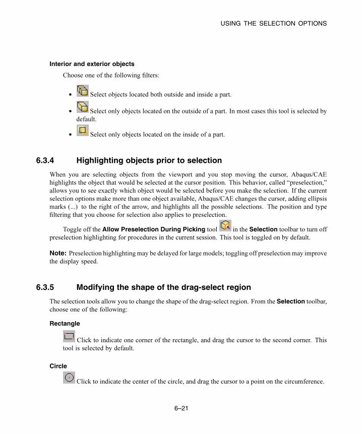
USING THE SELECTION OPTIONS
Interior and exterior objects
Choose one of the following filters:
• Select objects located both outside and inside a part.
• Select only objects located on the outside of a part. In most cases this tool is selected by
default.
• Select only objects located on the inside of a part.
6.3.4 Highlighting objects prior to selection
When you are selecting objects from the viewport and you stop moving the cursor, Abaqus/CAE
highlights the object that would be selected at the cursor position. This behavior, called “preselection,”
allows you to see exactly which object would be selected before you make the selection. If the current
selection options make more than one object available, Abaqus/CAE changes the cursor, adding ellipsis
marks (...) to the right of the arrow, and highlights all the possible selections. The position and type
filtering that you choose for selection also applies to preselection.
Toggle off the Allow Preselection During Picking tool in the Selection toolbar to turn off
preselection highlighting for procedures in the current session. This tool is toggled on by default.
Note: Preselection highlighting may be delayed for large models; toggling off preselection may improve
the display speed.
6.3.5 Modifying the shape of the drag-select region
The selection tools allow you to change the shape of the drag-select region. From the Selection toolbar,
choose one of the following:
Rectangle
Click to indicate one corner of the rectangle, and drag the cursor to the second corner. This
tool is selected by default.
Circle
Click to indicate the center of the circle, and drag the cursor to a point on the circumference.
6–21
Abaqus ID:
Printed on:

USING THE SELECTION OPTIONS
Polygon
Click to indicate one vertex of the polygon, and drag the cursor to the second vertex. You then
continue to click on each vertex of the polygon. Click mouse button 2 to indicate you have finished
entering vertices. There is no limit to the number of vertices in the polygon.
6.3.6 Choosing which objects are selected by the drag-select regionThe selection tools allow you to choose which objects are selected by the drag-select region. From the
Selection toolbar, choose one of the following:
Inside
Select only the objects that fall inside the drag-select region.
Inside and crossing
Select only the objects that fall inside or cross the drag-select region. This tool is selected by
default.
Crossing
Select only the objects that cross the drag-select region.
Outside and crossing
Select only the objects that fall outside or cross the drag-select region.
Outside
Select only the objects that fall outside the drag-select region.
6.3.7 Selecting objects before choosing a procedureYou can select objects from the current viewport before choosing a procedure to work with them. You
can use the Selection toolbar to toggle selection and
to limit viewport selections based on the type of object. The Selection tool is the first tool in the toolbar;
it is available only when there are no active procedures running in a viewport. By default, selection
is active and viewport object types are not limited. You can select multiple objects using any of the
methods described in “Combining selection techniques,” Section 6.2.8. Toggle off object selection to
prevent selecting objects when you are not in a procedure.
6–22
Abaqus ID:
Printed on:

USING THE SELECTION OPTIONS
Note: Preselection highlightingmay be delayed for large models; toggling off selectionmay improve the
display speed by preventing preselection and selection unless you first choose a procedure that requires
object selection.
When you select a procedure after selecting objects from the viewport, Abaqus/CAE applies the
selection filters for the procedure. For example, if you selected a vertex, a face, and an edge, then started
a procedure that can accept only vertices, Abaqus/CAE accepts the selected vertex, cancels the selection
of the face and edge, and begins the procedure with the second step. Similarly, if you select a procedure
that requires a single object selection and you have already selected multiple valid objects, Abaqus/CAE
accepts the first valid selection and cancels the remaining selections. If Abaqus/CAE cannot determine
which object you selected first, it will cancel all selections and begin the procedure at the first step.
If a procedure includes multiple selection steps, objects that you select before the procedure can be
used only to complete the first selection step. Any subsequent selection steps require you to select new
objects interactively from the viewport or, if applicable, use saved selection groups. You cannot save
selections made prior to the start of a procedure.
6–23
Abaqus ID:
Printed on:


OVERVIEW OF GRAPHICS DISPLAY OPTIONS
7. Configuring graphics display options
This chapter explains how you can configure the graphics display options in Abaqus/CAE. The following
topic is covered:
• “Overview of graphics display options,” Section 7.1
In addition, the following sections are available in the HTML version of this guide. (For information on
displaying the online documentation, see “Getting help,” Section 2.6.)
• “Using display lists,” Section 7.2
• “Using antialiasing,” Section 7.3
• “Choosing a highlight method,” Section 7.4
• “Choosing a translucency mode,” Section 7.5
• “Controlling drag mode,” Section 7.6
• “Choosing background colors,” Section 7.7
7.1 Overview of graphics display options
When you start a session, Abaqus detects the graphics hardware installed on your system and sets the
graphics options accordingly. If your graphics hardware is not supported by Abaqus/CAE or if you
wish to override the default graphics options, you can use the Graphics Options dialog box to tune
display performance. Abaqus/CAE applies the settings to all viewports and saves the settings for the
duration of the session. To use the customized settings each time you start an Abaqus/CAE session,
modify the environment file (abaqus_v6.env). For additional information on the environment file,
see the Abaqus Installation and Licensing Guide.
Note: Recommended settings for recently introduced graphics adapters are available from the Supportpage at www.3ds.com/simulia.
You can also use the Graphics Options dialog box to do the following:
• Choose the appearance of your model during rotation, pan, or zoom view manipulations. The
appearance is related to the render style and can be set to Fast (wireframe) or As is.
• Choose whether Abaqus/CAE will auto-fit the image to the current viewport after you rotate the
view. Automatically fitting the image to the viewport is equivalent to clicking the auto-fit tool
in the View Manipulation toolbar. Auto-fit adjusts your view of the model so that the model fills
the viewport and is centered within it. The orientation remains fixed, as indicated by the view triad.
• Choose whether Abaqus/CAE will optimize the display of translucent objects for performance, for
accuracy, or for a level in between.
7–1
Abaqus ID:
Printed on:

OVERVIEW OF GRAPHICS DISPLAY OPTIONS
• Choose the viewport background color. Your selected color will be applied to all viewports in the
current session of Abaqus/CAE.
To specify graphics display options:
From the main menu bar, select View→Graphics Options.
The Graphics Options dialog box appears with the following options:
• Tune performance using options for display lists, highlight method, and translucency mode.
• Choose the display mode while you drag objects in the viewport.
• Enable or disable the automatic fitting of your view to the viewport after rotations.
• Choose the background color of the viewports.
7–2
Abaqus ID:
Printed on:

UNDERSTANDING PRINTING
8. Printing viewports
This chapter describes how you send an image of selected viewports either directly to a printer or to a
file. The following topic is covered:
• “Understanding printing,” Section 8.1
For detailed instructions on printing, see “Controlling the destination and appearance of printed images,”
Section 8.2, in the HTML version of this guide.
For additional information on configuring printers, see the Abaqus Installation and LicensingGuide.
8.1 Understanding printing
Abaqus/CAE allows you to take a snapshot of one or more viewports and their contents and to send
the image either directly to a printer or to a file for later use; for example, to include in a presentation,
embed in a printed report, or display in an HTML document. Additional options allow you to select the
appearance of viewports in the resulting image, as well as the color, resolution, and size of the image.
This section describes basic concepts you should understand before sending output to a printer or
to a file.
8.1.1 Printed image formats
Abaqus/CAE allows you to print images directly to a Windows printer. The printer driver creates and
sends the necessary information to the printer in whatever format is required.
If Windows printer drivers are not available or if you are using another platform, you can use a print
command to create and send a PostScript file directly to a PostScript printer. You can also save images
in a PostScript (PS), Encapsulated PostScript (EPS), Tag Image File Format (TIFF), Portable Network
Graphics (PNG), or Scalable Vector Graphics (SVG) file. The following list describes these file formats:
PostScript
PostScript is the recognized standard for desktop publishing. PostScript is actually a programming
language whose instructions and data are usually stored in an ASCII format that can be transferred
easily between operating systems. The PostScript format is used when you use a print command
to print to a PostScript printer or when you save the image in a PostScript file. When you select
the PostScript format, Abaqus/CAE generates either a compressed raster representation or a vector
representation of your image. For efficiency when producing raster images, you should minimize
the size of your image and limit the resolution of the image to, at most, the resolution of the device
on which the image is to be printed or displayed.
8–1
Abaqus ID:
Printed on:
UNDERSTANDING PRINTING
Encapsulated PostScript
Encapsulated PostScript (EPS) is a variation of PostScript that describes a single graphic designed
to be included in a larger document without modification. EPS files are identical to PostScript files
except for some information that describes the size and positioning of the image. As a result, the
above discussion about vector and raster representations of your image applies equally to the EPS
format. Most word processing and graphics applications support the inclusion of EPS files.
TIFF
Tag Image File Format (TIFF) is a well-established raster image format that is recognized by many
software applications. The TIFF format supports both color and greyscale. By default, Abaqus/CAE
limits TIFF images of viewports to 8-bit color (256 colors). However, you can also use 24-bit color
(on Windows) or the system color setting (on Linux).
PNG
Portable Network Graphics (PNG) is an industry standard for storing raster images. The use of PNG
files has been popularized by the World Wide Web, and PNG images are displayed by most popular
web browsers running on a variety of operating systems. A PNG file consists of color information
and a compressed raster representation of the image. By default, Abaqus/CAE limits PNG images
of viewports to 8-bit color (256 colors). However, you can also use 24-bit color (on Windows) or
the system color setting (on Linux).
SVG
Scalable Vector Graphics (SVG) is an industry-standard vector graphics language written in XML.
8.1.2 Windows and PostScript image layout
When you print a snapshot of selected viewports directly to a Windows printer or to a PostScript printer
or file, the layout of the image is determined by the available page size, the orientation, and the aspect
ratio of the viewports:
Available page size
The available page size is calculated from the total page size and the margin information that you
supply, as illustrated by the sample dimensions shown in Figure 8–1.
The total page size is determined by the paper size. For a Windows printer, click the PrinterProperties button in the Print dialog box to open the Document Properties dialog box and
change the paper size. For a PostScript printer or file, click the Postscript Format Options button
in the Print dialog box to change the paper size.
Orientation
The orientation of your page can be either portrait or landscape.
8–2
Abaqus ID:
Printed on:
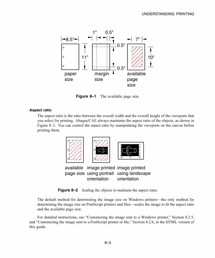
UNDERSTANDING PRINTING
������
11" 10"
8.5"
paper size
1"
0.5"
0.5"
0.5"
margin size
7"
availablepagesize
Figure 8–1 The available page size.
Aspect ratio
The aspect ratio is the ratio between the overall width and the overall height of the viewports that
you select for printing. Abaqus/CAE always maintains the aspect ratio of the objects, as shown in
Figure 8–2. You can control the aspect ratio by manipulating the viewports on the canvas before
printing them.
availablepage size
image printedusing portraitorientation
image printedusing landscapeorientation
Figure 8–2 Scaling the objects to maintain the aspect ratio.
The default method for determining the image size on Windows printers—the only method for
determining the image size on PostScript printers and files—scales the image to fit the aspect ratio
and the available page size.
For detailed instructions, see “Customizing the image sent to a Windows printer,” Section 8.2.5,
and “Customizing the image sent to a PostScript printer or file,” Section 8.2.6, in the HTML version of
this guide.
8–3
Abaqus ID:
Printed on:

UNDERSTANDING PRINTING
8.1.3 Windows printer image size
When you print a snapshot of selected viewports directly to a Windows printer, the image size is
determined by one of three methods:
Fit to page
Use this method to scale the printed image to fit within the available page size. This method is used
by default.
Use size on screen
Use this method to match the printed image size to the current size on the canvas. If the image
size exceeds the available page size, you must resize the image, change the page size or margins, or
select a different method to print your image.
Use settings
Use this method to specify the size of the printed image directly. You specify either the width or
the height, and Abaqus/CAE adjusts the other dimension to maintain the image aspect ratio. If the
image exceeds the available page size, you must resize the image, change the page size or margins,
or select a different method to print the image.
For detailed instructions, see “Customizing the image sent to a Windows printer,” Section 8.2.5, in the
HTML version of this guide.
8.1.4 EPS, TIFF, PNG, and SVG image size
When you print a snapshot of selected viewports to an Encapsulated PostScript (EPS), TIFF, PNG, or
SVG format file, Abaqus/CAE determines the size of the image based on the size you specify and the
overall aspect ratio of the viewports. You can control the aspect ratio by manipulating the viewports on
the canvas.
In the options dialog box (EPS Options, TIFF Options, PNG Options, or SVG Options) youcan choose one of the following methods to specify the size of the printed image:
• Use the size of the image on the screen. (Abaqus/CAE indicates the current image size in the options
dialog box.) This method is the default.
• Set the width or height. You specify only one dimension; Abaqus/CAE computes the other
dimension to maintain the aspect ratio of the viewports. When you are creating an EPS-format
file, you specify the width or height in either inches or millimeters. When you are creating a TIFF,
PNG, or SVG format file, you specify the width or height in screen pixels; increasing the number
of pixels increases the image size. The maximum image size allowed is 1280 × 1024 pixels.
8–4
Abaqus ID:
Printed on:

UNDERSTANDING PRINTING
For detailed instructions, see “Customizing the image saved in an Encapsulated PostScript file,”
Section 8.2.7, and “Customizing the image saved in TIFF, PNG, or SVG files,” Section 8.2.8, in the
HTML version of this guide.
8.1.5 Hard-copy image quality
When you print a snapshot of selected viewports directly to a PostScript printer or save it in a PostScript
or Encapsulated PostScript (EPS) file, Abaqus/CAE creates either a vector or raster representation of the
image (for more information, see “Printed image formats,” Section 8.1.1).
Vector representation images are resolution independent, so their quality depends only on the
resolution of your printer.
For PostScript and EPS images, you can use the Resolution field in the corresponding options
dialog box to specify the resolution of the image you save or print. At higher resolution, raster images
appear to be smoother and less jagged. Low-resolution vector images may have holes if scaled to a larger
size.
Although a higher resolution image has higher quality, more data are required to define the image;
the resulting file can consume a large amount of disk space. A lower resolution image will normally print
and display faster. In general, you should select the lowest resolution that still produces an acceptable
image. You may want to save a lower resolution image while you produce draft copies of your work and
switch to a higher resolution for the finished version.
The resolution of your printer sets an upper limit on the printed image resolution. For example, if
you save an image at a resolution of 600 dots per inch (dpi) and print it on a printer that has a resolution
of 300 dpi, the printed image will have a resolution of only 300 dpi.
Raster representation image quality may also be affected by changes you make to the image with
external software after the image has been created, such as scaling and rotation. Scaling and rotation may
distort a raster image. Consequently, before you print a raster representation of your image, you should
adjust the viewports on your canvas to match the dimensions and orientation that will appear in the final
application. Scaling and rotation do not distort or diminish the quality of vector representation images.
For vector representation PostScript and EPS images, you can use the Shading Quality field in the
corresponding options dialog box to specify the quality of the lighting on curved surfaces in the image.
This option does not affect the image resolution or the file size. A finer shading quality will produce
an image closer to the raster representation. A coarser shading quality will normally print and display
faster. Similar to the resolution for raster images, you should select the coarsest shading quality that still
produces an acceptable image.
Vector PostScript and EPS images do not support translucency; all translucent or transparent objects
will appear opaque when printed using vector PostScript or EPS format.
8–5
Abaqus ID:
Printed on:
UNDERSTANDING PRINTING
8.1.6 Importing Abaqus/CAE images into other software products
Many popular software applications, such as word processors, allow you to import files containing
graphic images generated by Abaqus/CAE; and most of these applications allow you to preview the
imported image. In addition, if you are using a Windows system, you can use [Ctrl]+C to copy the image
in the current viewport to the system clipboard and [Ctrl]+V to paste it into another application. Windows
stores the image in the clipboard in a bitmap (.bmp) format at the resolution of the screen. Although
the image quality will be satisfactory when viewed online, it may be unacceptable when printed. If you
expect to print an image, you should save it in PostScript or Encapsulated PostScript format.
8–6
Abaqus ID:
Printed on:

Part II: Working with Abaqus/CAE modeldatabases, models, and filesAlmost every modeling operation you perform while working in an Abaqus/CAE module contributes to the
definition of a model in a model database. This part describes Abaqus/CAE models and model databases, the
files created by the modeling process, and how you work with these models and files. The following topics
are covered:
• Chapter 9, “Understanding and working with Abaqus/CAE models, model databases, and files”
• Chapter 10, “Importing and exporting geometry data and models”
Abaqus ID:
Printed on:

WHAT IS AN Abaqus/CAE MODEL DATABASE?
9. Understanding and working with Abaqus/CAE models,model databases, and files
A finished model contains all the data that Abaqus/CAE needs to create and submit the analysis to
Abaqus/Standard or Abaqus/Explicit. Models are stored in a model database. This chapter discusses
models and model databases and describes the various files that Abaqus/CAE generates and reads. The
following topics are covered:
• “What is an Abaqus/CAE model database?,” Section 9.1
• “What is an Abaqus/CAE model?,” Section 9.2
• “Accessing an output database on a remote computer,” Section 9.3
• “Understanding the files generated by creating and analyzing a model,” Section 9.4
• “Abaqus/CAE command files,” Section 9.5
In addition, the following sections are available in the HTML version of this guide:
• “Using the File menu,” Section 9.6
• “Managing model and output databases,” Section 9.7
• “Managing models,” Section 9.8
• “Managing session objects and session options,” Section 9.9
• “Controlling the input file generated by Abaqus/CAE,” Section 9.10
• “Managing macros,” Section 9.11
9.1 What is an Abaqus/CAE model database?
A model database (file extension .cae) stores models and analysis jobs. (For more information on
analysis jobs, see “Understanding analysis jobs,” Section 19.2.) You can have multiple model databases
stored on your workstation or network, but Abaqus/CAE can work on only one of them at any time. A
model database can contain more than one model; if you plan to work onmultiple models simultaneously,
they must be stored in one model database. The model database in use is known as the current model
database; Abaqus/CAE displays the name of the current model database across the top of the main
window, as shown in Figure 9–1.
When you first start Abaqus/CAE, the Start Session dialog box allows you to either create a
new, empty model database or to open an existing model database. Anything you create or define
in Abaqus/CAE is stored in this model database. You save the contents by selecting File→Save or
File→Save As from the main menu bar.
Abaqus/CAE never saves the model database unless you perform an explicit save operation;
there is no timer-based automatic saving, for example. However, while you work on your model,
Abaqus/CAE maintains a record of all the operations that changed the model database. Although you
9–1
Abaqus ID:
Printed on:

WHAT IS AN Abaqus/CAE MODEL?
Figure 9–1 Abaqus/CAE displays the model database name and the model name.
may not have saved the model database, you can always replay the operations that replicate its current
state. For more information on recreating the model database, see “Recreating an unsaved model
database,” Section 9.5.3. Abaqus/CAE is backward compatible and can open model databases created
by previous releases of Abaqus/CAE.
After you begin an Abaqus/CAE session, you can open an existing model database by selecting
File→Open from the main menu bar, or you can create a newmodel database by selecting File→New. If
you open or create another model database after you have made changes to the current one, Abaqus/CAE
asks if you want to save the changes before it closes the current model database.
You can open a model database in the Visualization module to probe or query its nodes and elements
and to plot contours or symbols for selected attributes. For more information, see “Understanding the
role of the Visualization module,” Section 40.1.
For detailed instructions on creating and saving model databases, see “Managing model and output
databases,” Section 9.7, in the HTML version of this guide.
9.2 What is an Abaqus/CAE model?
This section describes an Abaqus/CAE model.
9–2
Abaqus ID:
Printed on:

WHAT IS AN Abaqus/CAE MODEL?
9.2.1 What does an Abaqus/CAE model contain?An Abaqus/CAE model contains the following kinds of objects:
• parts
• materials and sections
• assembly
• sets and surfaces
• steps
• loads, boundary conditions, and fields
• interactions and their properties
• meshes
A model database can contain any number of models so that you can keep all models related to a
single problem in one database. (For more information, see “What is an Abaqus/CAE model database?,”
Section 9.1.) You can open multiple models from the model database at the same time, and you can
work on different models in different viewports. The viewport title bar (if visible) displays the name of
the model associated with the viewport. The model associated with the current viewport is called the
current model, and there is only one current model. Figure 9–1 shows two viewports displaying two
different models (high-speed and low-speed) in the same model database (crankshaft.cae);the current viewport in Figure 9–1 is displaying the high-speed model.
You use the Model Manager or the Model menu items from the main menu bar to create and
manage your models. You use the Model list located in the context bar to switch to a different model in
the current model database.
You can create a copy of a model within a model database; in addition, you can copy the following
objects between models:
• Sketches
• Parts (part sets are also copied)
• Instances
• Materials
• Sections (including connector sections)
• Profiles
• Amplitudes
• Interaction properties
For detailed instructions, see “Manipulating models within a model database,” Section 9.8.1, and
“Copying objects between models,” Section 9.8.3, in the HTML version of this guide.
You can also import a model from another model database file, which creates a full copy of the model
in the current model database. For more information, see “Importing a model from an Abaqus/CAE
model database,” Section 10.5.1.
9–3
Abaqus ID:
Printed on:

WHAT IS AN Abaqus/CAE MODEL?
Abaqus/CAE checks that your model is complete when you submit it for analysis. For example, if
you request a dynamic analysis, you must specify the density of the materials so that the mass and inertia
properties of the model can be calculated. If you did not provide a material density in the Property
module, the Job module reports an error; for more information, see “Monitoring the progress of an
analysis job,” Section 19.2.6.
In some modules Abaqus/CAE does not support functionality from Abaqus/Standard,
Abaqus/Explicit, or Abaqus/CFD that you may want to include in the analysis. You may be able to
add such functionality by using the Keywords Editor to edit the Abaqus keywords associated with a
model. Select Model→Edit Keywords→model name from the main menu bar to start the KeywordsEditor. (You can review the keywords supported by Abaqus/CAE by selecting Help→KeywordBrowser from the main menu bar.)
You can specify that a model uses information from a previous analysis. When you submit the
model for analysis, Abaqus/CAE continues the analysis from a selected step. For more information,
see “Configuring restart output requests,” Section 14.13.2, in the HTML version of this guide, and
“Restarting an analysis,” Section 19.6.
9.2.2 What are the model attributes?The model attributes describe characteristics of a model and are stored with a model in the model
database. The following list describes the attributes of an Abaqus/CAE model:
• Description. If you have many similar models in a model database, you can use the description to
distinguish between the models. The description that you enter is stored with the model attributes;
the description is written above the header of the input file but is not written to the output database.
For more information, see “Adding descriptions to your Abaqus/CAE model,” Section 9.10.2.
• Type. You can choose between a Standard & Explicit model (the default), a CFD model, or an
Electromagnetic model. Once you select a model type, Abaqus/CAE filters the set of options
available in the main menu bar, toolboxes, and Model Tree so that they are appropriate to your
model type selection.
• Physical constants for the model. You can enter values for the Absolute zero temperature and the
Stefan-Boltzmann constant. These values are needed to specify surface emissivity and radiation
conditions in heat transfer analyses.
You can also enter a value for the Universal gas constant, and you can choose an option
from the Specify acoustic wave formulation list.
• Restart information that will start the analysis using data from a previous analysis. You can specify
the following:
– The name of the job from which Abaqus/CAE will read the restart information.
– The name of the step from which Abaqus/CAE will restart the analysis.
– The increment or the interval of the step from which Abaqus/CAE will restart the analysis.
For more information, see “Restarting an analysis,” Section 19.6, and “Restarting an analysis,”
Section 9.1.1 of the Abaqus Analysis User’s Guide.
9–4
Abaqus ID:
Printed on:

ACCESSING AN OUTPUT DATABASE ON A REMOTE COMPUTER
• Submodel information that will be used to drive submodel boundary conditions or loads in the
model. You can specify the following:
– The job from which the global solution will be used to drive the submodel boundary conditions
or loads.
– Whether a shell global model will be used to drive a solid submodel.
For more information, see Chapter 38, “Submodeling.”
Select Model→Edit Attributes→model name from the main menu bar to edit the attributes of the
selected model. For more information, see “Specifying model attributes,” Section 9.8.4, in the HTML
version of this guide.
9.3 Accessing an output database on a remote computer
This section describes how you can create and start a network connector. You can use the network
connector to navigate the directory structure on a remote host and to access a remote output database.
9.3.1 What is a network ODB connector?
A network ODB connector creates a connection to a remote machine and allows you to access a remote
output database. For example, you can submit an analysis to a high-performance UNIX system and view
the results on a local Windows workstation while the analysis is still running.
You can create a network ODB connector from any platform—Windows, UNIX, or Linux.
However, the network ODB server must reside on a UNIX or Linux platform; you cannot access
an output database that resides on a remote Windows system. You can access only a remote output
database; you cannot access a remote model database.
Select File→Network ODB Connector→Create from the main menu bar to create a connection
with a directory on a remote host. When you are creating a network ODB connector, you can use
Abaqus/CAE to automatically start the network ODB server and to establish the communication port
numbers on the host and remote systems. Alternatively, you can start the network ODB server manually
from the command line using the abaqus networkDBConnector execution procedure. If you start the
server from the command line, you enter the communication port number returned by the execution
procedure when you subsequently create the network ODB connector. For more information, see
“Network output database file connector,” Section 3.2.22 of the Abaqus Analysis User’s Guide.
After you create a network ODB connector, you must start it by selecting File→Network ODBConnector→Start→Connector name from the main menu bar. The remote system must have Abaqus
installed for Abaqus/CAE to establish the network connection. For more information, see “Creating a
network ODB connector,” Section 9.7.4, and “Managing network ODB connectors,” Section 9.7.6, in
the HTML version of this guide.
9–5
Abaqus ID:
Printed on:

ACCESSING AN OUTPUT DATABASE ON A REMOTE COMPUTER
After you create and start a network connector, you can use it to navigate the directory structure
on a remote host. When you select File→Open from the main menu bar to open a database from
Abaqus/CAE, a Network connectors entry appears under Directory in the file selection dialog box.
The entry appears regardless of whether you are trying to open an output database or a model database;
however, you cannot use a network connector when opening a model database. For more information,
see “Using file selection dialog boxes,” Section 3.2.10.
The network connector allows you to do the following:
• Open a remote output database in read-only mode, and view the contents of the output database
using the Visualization module. For more information, see “Opening a model database or an output
database,” Section 9.7.2, in the HTML version of this guide.
The behavior of the Visualization module does not change when the output database is remote;
for example, you can view the output database while the analysis is running on a remote machine,
and more than one user can view the output database. However, you cannot click Results in the
Job Manager to open the remote output database associated with a remote analysis.
• Import a part from a remote output database. For more information, see “Importing parts,”
Section 10.7.2, in the HTML version of this guide.
• Import a model from a remote output database. For more information, see “Importing a model from
an output database,” Section 10.5.3.
• Upgrade a remote output database.
After most Visualization module operations and during animations, Abaqus/CAE monitors the
output database for updated results and updates the current viewport accordingly. If you are displaying
data from a remote output database, the performance of Abaqus/CAE may be degraded if the time taken
to monitor the database over the network is significant. To increase the performance, you can reduce
the frequency with which Abaqus/CAE monitors the output database for updates or you can disable the
monitoring. For more information, see “Controlling results caching,” Section 42.6.10, in the HTML
version of this guide.
9.3.2 How secure is the access to a network ODB connector?
Abaqus/CAE maintains a secure connection to the network ODB connector by generating a key that
is passed back and forth between the server and the client. If a file called .abaqus_net_passwdis present in your home directory on the remote server, Abaqus/CAE uses the password in the file for
authentication instead of the key generated by Abaqus/CAE. Abaqus/CAE checks that you are the only
user with permission to read and write to the password file. In addition, you must update the file after 30
days, and the password must be at least eight characters long. Abaqus uses password files to authenticate
the connection between the client and the server if you start the network ODB server manually. These
files are described in “Network output database file connector,” Section 3.2.22 of the Abaqus Analysis
User’s Guide.
9–6
Abaqus ID:
Printed on:

ACCESSING AN OUTPUT DATABASE ON A REMOTE COMPUTER
9.3.3 Tuning the cache size to increase the performance of a networkODB
When you start an Abaqus/CAE session, a cache is created in the scratch file directory. Abaqus/CAE uses
this cache for local data storage when you use a network ODB connector to read from a remote output
database. The cache greatly increases the performance of the Visualizationmodule in Abaqus/CAEwhen
accessing data from the remote output database.
Abaqus/CAE allows the cache to grow to a size that is sufficient to contain all of the data in all of the
open remote output databases. However, Abaqus/CAE limits the cache size to 80% of the total free space
in the directory. For example, if the scratch directory has 35 gigabytes of unused space, Abaqus/CAE
will allow the cache to grow to 28 gigabytes. Alternatively, you can limit the size of the cache using
the nodb_cache_limit parameter in the Abaqus environment file, abaqus_v6.env. You must set the
nodb_cache_limit parameter to the number of megabytes to which the cache size will be limited. For
example,
nodb_cache_limit=20000
will set the maximum cache size to 20 gigabytes. Abaqus/CAE uses this cache space only as needed
during a session, and the actual cache size may be significantly less than the limit you specified. The
minimum value of nodb_cache_limit is 500, indicating that the cache size is limited to 500 megabytes.
If you set the maximum cache size to be greater than the available free space, Abaqus/CAE reduces it to
a value that is equal to the available free space.
Abaqus/CAE uses the cache to increase its performance when reading data from a remote output
database. The speed at which data can be accessed over a network is significantly lower than the speed
at which data can be accessed from a local disk drive. As a result, the performance of remote output
databases will be significantly slower than the performance of a local output database. The cache
reduces this performance difference by retaining data that have been transferred over the network,
thereby reducing the need for data transfer over the network. However, if the cache is not large enough,
Abaqus/CAE will have to transfer more data over the network and performance will suffer.
In most cases you will not have to tune the size of the cache using the nodb_cache_limit parameter.
However, you may have to reduce the size of the cache if it is consuming too much disk space and
reducing the speed of other applications on your system. Similarly, you may have to increase the size
of the cache if it is too small to support all of your remote output databases and the performance of
Abaqus/CAE is degraded. If you cannot increase the size of the cache, you should close some of your
remote output databases.
If the desired cache size is larger than the space available in the scratch file directory, you can move
the scratch file directory to a larger disk drive using the Abaqus scratch environment file parameter. For
more information, see “Using the Abaqus environment settings,” Section 3.3.1 of the Abaqus Analysis
User’s Guide, and “Managing memory and disk use in Abaqus,” Section 3.4.1 of the Abaqus Analysis
User’s Guide.
9–7
Abaqus ID:
Printed on:
UNDERSTANDING THE FILES GENERATED BY CREATING AND ANALYZING A MODEL
9.4 Understanding the files generated by creating and analyzing amodel
When you start a session and begin defining your model, Abaqus/CAE generates the following file:
The replay file (abaqus.rpy)
The replay file contains Abaqus/CAE commands that record almost every modeling operation
you perform during a session. For more information, see “Replaying an Abaqus/CAE session,”
Section 9.5.1.
When you select File→Save from the main menu bar and save the model database, Abaqus/CAE saves
the following files:
The model database file (model_database_ name.cae)
The model database file contains models and analysis jobs. For more information, see “What is an
Abaqus/CAE model database?,” Section 9.1.
The journal file (model_database_ name.jnl)
The journal file contains the Abaqus/CAE commands that will replicate the model database that was
saved to disk. For more information, see “Recreating a saved model database,” Section 9.5.2.
When you continue to work on your model, Abaqus/CAE continues to record your actions in the replay
file. In addition, Abaqus/CAE saves the following file:
The recover file (model_database_ name.rec)
The recover file contains the Abaqus/CAE commands that will replicate the version of the model
database in memory. The model database recovery file contains only the commands that changed
the model database since you last saved it. For more information, see “Recreating an unsaved model
database,” Section 9.5.3.
When you submit a job for analysis, Abaqus/Standard and Abaqus/Explicit create a set of files; for a
complete list of these files, see “File extensions used by Abaqus,” Section 3.6.1 of the Abaqus Analysis
User’s Guide. The following list describes some of the files that Abaqus/Standard and Abaqus/Explicit
create and their relationship to Abaqus/CAE:
Input files (job_name.inp)
Abaqus/CAE generates an input file that is read by Abaqus/Standard or Abaqus/Explicit when
you submit a job for analysis. For more information, see “Basic steps for analyzing a model,”
Section 19.2.1.
Output database files (job_name.odb)
Output database files contain the results from your analysis. You use the Step module’s output
request managers to choose which variables are written to the output database during the analysis
9–8
Abaqus ID:
Printed on:

UNDERSTANDING THE FILES GENERATED BY CREATING AND ANALYZING A MODEL
and at what rate. An output database is associated with the job you submit from the Job module; for
example, if you named your job FrictionLoad, the analysis creates an output database called
FrictionLoad.odb.When you open an output database, Abaqus/CAE loads the Visualization module and allows
you to view a graphical representation of the contents. You can also import a part from an output
database as a mesh. You can save X–Y data objects to an output database file if you open the file
with write permission; otherwise, you cannot modify the contents of the output database once it has
been created.
The output database lock file (job_name.lck)
The lock file (job_name.lck) is written whenever an output database file is opened with write
access, including when an analysis is running and writing output to an output database file. The lock
file prevents you from having simultaneous write permission to the output database from multiple
sources. It is deleted automatically when the output database file is closed or when the analysis that
creates it ends.
The restart file (job_name.res)
The restart file is used to continue an analysis that stopped before it was complete. You use the
Step module to specify which analysis steps should write restart information and how often. If you
are using Abaqus/Explicit, the restart information you supply in the Step module controls the data
written to the state file (job_name.abq). For more information, see “Configuring restart output
requests,” Section 14.13.2, in the HTML version of this guide.
The data file (job_name.dat)
The data file contains printed output from the analysis input file processor, as well as printed output
of selected results written during the analysis. Abaqus/CAE automatically requests that the default
printed output for the current analysis procedure be generated at the end of each step; you cannot
use Abaqus/CAE to exert any additional control over the contents of the data file.
The message file (job_name.msg)
The message file contains diagnostic or informative messages about the progress of the solution.
You can control the diagnostic information that is output to the message file using the Step module.
For more information, see “Diagnostic printing,” Section 14.5.3.
The status file (job_name.sta)
The status file (job_name.sta) contains information about the progress of the analysis. In addition,
you use the Step module to request that the value of a single degree of freedom at a single node
be output to the status file. For more information, see “Degree of freedom monitor requests,”
Section 14.5.4.
9–9
Abaqus ID:
Printed on:
Abaqus/CAE COMMAND FILES
The results file (job_name.fil)
The results file contains selected results from the analysis in a format that can be read by other
applications, such as postprocessing programs. A submodel analysis can read the global model
results from either an output database or a results file. By default, an analysis from Abaqus/CAE
does not create a results file. For more information, see “Submodeling,” Section 10.2 of the Abaqus
Analysis User’s Guide, and Chapter 38, “Submodeling.”
Note: The errors and warnings that Abaqus/Standard and Abaqus/Explicit write to the data, message,
and status files while analyzing a job can be monitored by the Job module; for more information, see
“Monitoring the progress of an analysis job,” Section 19.2.6.
When you open an output database file in the Visualization module and create new field output variables
(see “Creating new field output,” Section 42.7, for more information), Abaqus/CAE generates the
following file:
The scratch output database file (job_name.ods)
The scratch output database file (job_name.ods) contains a “session step” in which field output
variables that you create (by operating on either fields or frames) are saved. This file is deleted
automatically when the original output database file (fromwhich the field output originates) is closed
or when the Abaqus/CAE session ends.
In most cases the files generated by Abaqus/CAE are written to the work directory. The work
directory is the directory from which you started the Abaqus/CAE session unless you changed the
directory by selecting File→Set Work Directory from the main menu bar. For more information, see
“Setting the work directory,” Section 9.7.8.
9.5 Abaqus/CAE command files
This section describes the command files that you can use to reproduce your work and to customize
Abaqus/CAE.
9.5.1 Replaying an Abaqus/CAE sessionAlmost every operation that you perform in Abaqus/CAE is recorded automatically in the replay file
(abaqus.rpy) in the form of Abaqus Scripting Interface commands. Executing the replay file is
equivalent to replaying the original sequence of operations including any redundant procedures and any
mistakes and subsequent corrections that you made. The replay file also includes canvas operations, such
as creating a new viewport.
Abaqus/CAE retains the five most recent versions of the replay file. The most recent version of the
replay file is called abaqus.rpy; it is created when you start a session. The four older versions have a
9–10
Abaqus ID:
Printed on:
Abaqus/CAE COMMAND FILES
number appended to the end of the file name; the file name with the lowest number indicates the oldest
replay file, and the file name with the highest number indicates the second most recent replay file.
You can execute the commands in a replay file when you start Abaqus/CAE or during a session;
however, the result may be different if the replay file generates an error.
From the Abaqus execution procedure
To run a replay file from the Abaqus execution procedure, type abaqus cae (or abaqusviewer) replay=replay_file_name.rpy. If executing the replay file generates an error,
Abaqus/CAE ignores the error and continues to the next command in the replay file. As a result,
Abaqus/CAE always attempts to execute every command in the replay file. You cannot use the
replay option to execute a script with control flow statements. For more information, see
“Abaqus/CAE execution,” Section 3.2.6 of the Abaqus Analysis User’s Guide.
During an Abaqus/CAE session
To run a replay file during a session, select File→Run Script from the main menu bar. If the replay
file generates an error, Abaqus/CAE stops executing the replay file and displays an error message
in the command area. It is recommended that you run a replay file from the Abaqus execution
procedure.
You can also execute a replay file using the Abaqus Python development environment (Abaqus
PDE). The Abaqus Scripting Interface commands in the replay file must be run in the kernel workspace
in the Abaqus PDE. For more information on the Abaqus PDE, see Chapter 7, “Using the Abaqus Python
development environment,” of the Abaqus Scripting User’s Guide.
9.5.2 Recreating a saved model database
When you save a model database (by selecting File→Save or File→Save As from the main menu
bar), Abaqus/CAE also saves a model database journal file (model_database_name.jnl) containingthe Abaqus Scripting Interface commands that will recreate the model database. Should the saved model
database become corrupted, you can recreate it by starting Abaqus/CAE with the recover option. (Type
abaqus cae recover=model_database_name.jnl.) The recover option executes the commands
in the specified model database journal file.
The model database journal file differs from the replay file in that it does not contain every operation
performed during a session. The model database journal file contains only the commands that change the
saved model database; for example, commands that create or edit a part, change the time incrementation
of an analysis step, or modify the mesh. Operations that do not change the model database are not saved
in the journal file; for example, sending an image to a printer, creating a viewport, rotating the model, or
viewing results in the Visualization module.
As you continue to work on your model, the model database in memory will differ from the most
recently saved model database. The model database journal file is updated only when you perform an
explicit save of the model database using File→Save or File→Save As. If you copy the model database
9–11
Abaqus ID:
Printed on:

Abaqus/CAE COMMAND FILES
to a different location, you should also copy the associated model database journal file. Otherwise, you
will not be able to recreate the model database.
9.5.3 Recreating an unsaved model databaseWhen you start a new session and make changes to your model, Abaqus/CAE records those changes
to a model database recovery file (abaqusn.rec). If you subsequently save the model database,
Abaqus/CAE appends the commands in the recovery file to the journal file for that model database
(model_database_name.jnl) and deletes the recovery file. If you make further changes to your model,
Abaqus/CAE creates a new recovery file (model_database_name.rec) to record the changes since yourlast save. Upon your next save, the commands in the recovery file are appended to the journal file and the
recovery file is deleted. The journal file contains all the commands necessary to rebuild the entire model
database. For example, Table 9–1 shows the changes that Abaqus/CAE makes to the model database,
recovery, and journal files for a model named engine.
Table 9–1 Modeling changes and their effect on the model
database, recovery, and journal files.
User action Abaqus/CAE action Files
Start Abaqus/CAE
session
None None
Make model changes Record commands in recover file abaqus1.rec
Save the model database Create model database file
Copy recover commands to journal
file
Delete recover file
engine.caeengine.jnl
Make more changes to
the model
Record commands in recover file engine.recengine.cae (out of date)
engine.jnl (out of date)
Save model database Update model database file
Append recover commands to journal
file
Delete recover file
engine.cae (updated)
engine.jnl (updated)
If your Abaqus/CAE session aborts unexpectedly—for example, because of a power loss to your
computer—the recovery file will still be available to Abaqus/CAE for your next session. Abaqus/CAE
first checks for the presence of a recovery file of the form abaqusn.rec; if such a file exists, it may be
from a previous session that aborted unexpectedly, or it may be from another Abaqus/CAE session that
you started in the same directory. Because Abaqus/CAE cannot tell the difference between these two
9–12
Abaqus ID:
Printed on:

Abaqus/CAE COMMAND FILES
cases and cannot determine automatically whether you want to implement the changes, Abaqus/CAE
prompts you with three options: recover the changes and delete the recovery file, do not recover
changes and delete the recovery file, or disregard the recovery file because its changes belong to another
Abaqus/CAE session. When you recover changes, you can skip the last command in the recovery file if
you think the last command you issued caused the termination of the session.
If a recovery file belongs to a model database (model_database_name.rec), Abaqus/CAE will
not detect the recovery file until you attempt to open that model database. Upon your attempt to open
the model database, Abaqus/CAE prompts you to recover or disregard the changes. If you recover the
changes, Abaqus/CAE appends the changes in the database recovery file to the journal file and deletes
the database recovery file; if you choose to disregard the changes, Abaqus/CAE deletes the recovery file
and does not implement any of the model changes described in the file.
9.5.4 Creating and running your own scripts
Almost every operation that you perform during an Abaqus/CAE session can be duplicated by a script
(script_name.py) containing a set of Abaqus Scripting Interface commands. Conversely, running a
script from within Abaqus/CAE is equivalent to performing the corresponding operations using the
menus, toolboxes, and dialog boxes that Abaqus/CAE provides.
You can create scripts that duplicate operations you perform routinely during a session; for example,
you might write a script that defines the material properties of a commonly used material or one that
produces a contour plot of a particular variable shown in a particular view orientation.
Abaqus/CAE commands are written in the Python scripting language, and you can use Python to
enhance the scripts generated by Abaqus/CAE. Commands are stored as ASCII text in the replay, journal,
and recovery files and in Abaqus/CAE scripts that you create. As a result, you can use a standard text
editor to edit the contents of the files. For more information on commands, see the Abaqus Scripting
User’s Guide.
To run a script, select File→Run Script from the main menu bar, and select the script to run from
the Run Script dialog box.
Note: You should use the recover option from the Abaqus/CAE execution procedure to run a journal file
and recreate a saved model database. (Type abaqus cae recover=model_database_name.jnl.)Selecting File→Run Script to run a journal file may result in an incomplete model database.
You can also create and run scripts using the Abaqus Python development environment (Abaqus
PDE). The Abaqus Scripting Interface commands in the scripts must be run in the kernel workspace in
the Abaqus PDE. For more information on the Abaqus PDE, see Chapter 7, “Using the Abaqus Python
development environment,” of the Abaqus Scripting User’s Guide.
9–13
Abaqus ID:
Printed on:

Abaqus/CAE COMMAND FILES
9.5.5 Creating and running a macro
The Macro Manager allows you to record a sequence of Abaqus Scripting Interface commands in a
macro file while you interact with Abaqus/CAE. Each command corresponds to an interaction with
Abaqus/CAE, and replaying the macro reproduces the sequence of interactions. You can use a macro
to automate tasks that you find yourself performing repeatedly, such as printing the current viewport or
applying a predefined view. For more information on Abaqus Scripting Interface commands, see the
Abaqus Scripting User’s Guide.
Macros are stored in a file called abaqusMacros.py. Abaqus/CAE searches three directories
for abaqusMacros.py, in the following order:
• The site directory of the Abaqus installation.
• Your home directory.
• The current working directory.
The abaqusMacros.py file can exist in more than one of these directories. The Macro Managercontains a list of the existing macros that Abaqus/CAE detected in all of the abaqusMacros.py files.
If a macro uses the same name in more than one abaqusMacros.py file, Abaqus/CAE uses the last
macro encountered.
To create, delete, or run a macro, select File→Macro Manager from the main menu bar. For more
information, see “Managing macros,” Section 9.11, in the HTML version of this guide.
9.5.6 Customizing your Abaqus/CAE environment
You use the Abaqus environment file (abaqus_v6.env) to specify parameters that control
Abaqus/Standard and Abaqus/Explicit. In addition, you can use the environment file to specify a set
of commands that are executed when you start an Abaqus/CAE session. Examples of commands
that configure how you want a job to run on a remote host computer are given in “Submitting a job
remotely,” Section 19.2.7.
9–14
Abaqus ID:
Printed on:

IMPORTING FILES INTO AND EXPORTING FILES FROM Abaqus/CAE
10. Importing and exporting geometry data and models
This section describes the files that can be imported into and exported from Abaqus/CAE. The following
topics are covered:
• “Importing files into and exporting files from Abaqus/CAE,” Section 10.1
• “Valid parts, precise parts, and tolerance,” Section 10.2
• “Controlling the import process,” Section 10.3
• “Understanding the contents of an IGES file,” Section 10.4
• “What can you import from a model?,” Section 10.5
• “A logical approach to successful import of IGES files,” Section 10.6
In addition, the following sections are available in the HTML version of this guide:
• “Importing sketches and parts,” Section 10.7
• “Importing a model,” Section 10.8
• “Exporting geometry, model, and mesh data,” Section 10.9
10.1 Importing files into and exporting files from Abaqus/CAE
Abaqus/CAE can import part and assembly geometries from a variety of external sources and CAD
systems. The associative interfaces for Abaqus/CAE provide straightforward and powerful techniques
for importing geometry. More traditional techniques are also available for importing and exporting
geometry using standard CAD file formats. Understanding the capabilities of each format, as well as
the limitations of representing the geometry of a part in a file, will help you select the import or export
technique that is appropriate for your application.
10.1.1 What kinds of files can be imported and exported fromAbaqus/CAE?
Abaqus/CAE reads and writes geometry data stored in Abaqus file formats as well as non-Abaqus file
formats.
Abaqus file formats
Abaqus/CAE reads and writes geometry data stored in the following Abaqus file formats:
10–1
Abaqus ID:
Printed on:

IMPORTING FILES INTO AND EXPORTING FILES FROM Abaqus/CAE
Abaqus output database (output_database_name.odb)
An output database contains the data generated during an Abaqus/Standard or Abaqus/Explicit
analysis. You can import parts from an output database in the form of meshes. A mesh part contains
no feature information and is extracted from the output database as a collection of nodes, elements,
surfaces, and sets. If the output database contains multiple part instances, you can select the part
instances to import. Abaqus/CAE imports each part instance as a separate part. You can import
either the undeformed or the deformed shape. If you import the deformed shape, you can specify
the step and the frame from which to import.
To verify the quality of the mesh, you can display the part in the Mesh module and select
Mesh→Verify from the main menu bar. In addition, you can use the Mesh module to change the
element type assigned to the mesh and to edit the original mesh definition. For more information,
see “Importing a part from an output database,” Section 10.7.12, and “What can I do with the Edit
Mesh toolset?,” Section 64.1, in the HTML version of this guide; and “Assigning Abaqus element
types,” Section 17.5.
You can also import a model from an output database. The model that is imported will
contain parts representing each of the undeformed part instances in the output database along with
a mesh representation of the undeformed assembly. The model will also contain any sets, surfaces,
materials, section definitions, and beam profiles that were defined in the output database. For more
information, see “Importing a model from an output database,” Section 10.5.3.
Abaqus/CAE model database (model_database_name.cae)
Abaqus/CAE can import a model into the current model database from a different Abaqus/CAE
model database. For more information on importing model data from another model database, see
“Importing a model from an Abaqus/CAE model database,” Section 10.5.1.
Abaqus/Standard and Abaqus/Explicit input files
Abaqus/CAE generates an input file when you submit a job for analysis. You can import input
files into Abaqus/CAE. Abaqus/CAE translates the keywords and data lines in the imported input
file into a new model; however, a limited set of Abaqus/Standard and Abaqus/Explicit keywords is
supported, as described in “Importing a model from an Abaqus input file,” Section 10.5.2. For more
information on creating and submitting jobs, see “Basic steps for analyzing amodel,” Section 19.2.1.
Abaqus substructure files (substructure_name.sim)
Abaqus/CAE can import a substructure definition from a SIM database as a new part definition. The
.sim file you import must reside in the same directory as the supporting Abaqus files to which the
SIM database refers; these supporting files may include data in the formats .prt, .mdl, .stt,or .sup. For step-by-step instructions, see “Importing a substructure into a model database as a
part,” Section 10.7.13, in the HTML version of this guide.
Supported non-Abaqus file formats
Abaqus/CAE reads and writes geometry data stored in the following non-Abaqus file formats:
10–2
Abaqus ID:
Printed on:
IMPORTING FILES INTO AND EXPORTING FILES FROM Abaqus/CAE
3D XML (file_name.3dxml)
3D XML is an XML-based format developed by Dassault Systèmes for encoding three-dimensional
images and data. The format is open and extendable, allowing three-dimensional graphics to be
easily shared and integrated into existing applications and processes. 3D XML files can be many
times smaller than typical model database files. The 3D XML Player from Dassault Systèmes is
required to view 3D XML files or to integrate them into business applications. You can also view
3D XML files in CATIA V5.
You can export viewport data from Abaqus/CAE in 3D XML or compressed 3D XML format.
For more information, see “Exporting viewport data to a 3D XML-format file,” Section 10.9.5, in
the HTML version of this guide. You cannot import 3D XML into Abaqus/CAE.
ACIS (file_name.sat)
ACIS is a library of solid modeling functions developed by Spatial, and most CAD products can
generate ACIS-format parts. You can import ACIS-format parts, and you can export parts or the
assembly in ACIS format. In addition, you can import and export sketches in ACIS format. For
more information, see “Importing parts from an ACIS-format file,” Section 10.7.4; “Importing
sketches,” Section 10.7.1; and “Exporting geometry, model, and mesh data,” Section 10.9, in the
HTML version of this guide.
ANSYS input files (file_name.cdb)
ANSYS Mechanical and ANSYS Multiphysics software are computer-aided engineering products
that allow you to perform finite element analysis and computational fluid dynamics. You can
import models from files in ANSYS input file format into Abaqus/CAE. For more information,
see “Importing a model from an ANSYS input file,” Section 10.5.5, and “Importing a model,”
Section 10.8, in the HTML version of this guide.
Assembly files (file_name.eaf)
Assembly files are created by the associative interface applications, which are plug-ins for
third-party CAD systems that allow you to transfer models from the CAD system to Abaqus/CAE
using a technique called associative import (see “What can I do with the associative interfaces?,”
Section 10.1.2). The associative interface plug-ins save model information in the assembly file,
and you can use the assembly file to associatively import the model from the third-party CAD
system into Abaqus/CAE. For more information, see “Importing an assembly from an assembly
file,” Section 10.7.14, in the HTML version of this guide. You cannot export assemblies from
Abaqus/CAE in assembly file format.
AutoCAD (file_name.dxf)
Two-dimensional profiles stored in AutoCAD (.dxf) files can be imported as stand-alone sketches.
However, Abaqus/CAE supports only a limited number of AutoCAD entities, and you should use
this format only if no other formats are available. For more information and details on the AutoCAD
10–3
Abaqus ID:
Printed on:

IMPORTING FILES INTO AND EXPORTING FILES FROM Abaqus/CAE
entities supported by Abaqus/CAE, see “Importing sketches,” Section 10.7.1, in the HTML version
of this guide.
CATIA V4 (file_name.model, file_name.catdata, or file_name.exp)
You can import CATIA-format parts. You can also import an entire CATIA V4 assembly into
the Abaqus/CAE assembly, or you can choose to import only selected part instances. For more
information, see “Importing a part from a CATIA V4- or V5-format file,” Section 10.7.5; and
“Importing an assembly from a CATIA V4-format file,” Section 10.7.15, in the HTML version
of this guide. You cannot export parts from Abaqus/CAE in CATIA format.
CATIA V5 Elysium Neutral File (file_name.enf_abq)
Abaqus provides a translator plug-in for CATIA V5 that will generate a geometry file using the
Elysium Neutral File (.enf) format. You can use Elysium Neutral Files to import CATIA V5
parts. In addition, you can use Elysium Neutral Files to import an entire CATIA V5 assembly into
the Abaqus/CAE assembly, or you can choose to import only selected part instances. For more
information, see “Importing a part from an Elysium Neutral file,” Section 10.7.6, and “Importing
an assembly from an Elysium Neutral file,” Section 10.7.16, in the HTML version of this guide.
You cannot export parts or assemblies from Abaqus/CAE in Elysium Neutral File format.
CATIA V5 parts and assemblies (file_name.CATPart or .CATProduct)
With the optional CATIA V5 Associative Interface add-on feature for Abaqus/CAE, you can import
CATIAV5-format parts and assemblies. For more information, see “Importing a part from a CATIA
V4- or V5-format file,” Section 10.7.5, in the HTML version of this guide. You cannot export parts
from Abaqus/CAE in CATIA V5 format.
CATIA V6 parts and assemblies (file_name.CATPart or .CATProduct)
You use the SIMULIA Associative Interface for Abaqus/CAE to import CATIA V6-format parts
and assemblies. The CATIA V6 parts and assemblies are first converted to CATIA V5 format,
and Abaqus/CAE imports the resulting CATIA V5 CATPart or CATProduct files. For more
information, see “Importing a part from a CATIA V4- or V5-format file,” Section 10.7.5, in the
HTML version of this guide. You cannot export parts from Abaqus/CAE to CATIA V6.
IGES (file_name.igs or .iges)
The Initial Graphics Exchange Specification (IGES) is a neutral data format designed for graphics
exchange between computer-aided design (CAD) systems.
You can import IGES-format parts, and you can export parts in IGES format. In addition,
you can import and export sketches in IGES format. For more information, see “Importing a part
from an IGES-format file,” Section 10.7.7; “Importing sketches,” Section 10.7.1; and “Exporting
geometry, model, and mesh data,” Section 10.9, in the HTML version of this guide.
The IGES-format allows for many interpretations, and most of the parts that you import into
Abaqus/CAE using IGES-format will need to be repaired before you can use them. Thus, it is
recommended that you try to use another format, if possible.
10–4
Abaqus ID:
Printed on:

IMPORTING FILES INTO AND EXPORTING FILES FROM Abaqus/CAE
Nastran input files (file_name.bdf, file_name.dat, file_name.nas, file_name.nastran,file_name.blk, or file_name.bulk)
You can import Nastran model data from a Nastran input file into Abaqus/CAE, and you can export
data from an Abaqus/CAE model and job into Nastran bulk data file format. Imported and exported
models include many common entities in the Nastran bulk data. For more information on supported
entities for import of Nastran input files into Abaqus/CAE, see “TranslatingNastran bulk data files to
Abaqus input files,” Section 3.2.26 of the Abaqus Analysis User’s Guide. For more information on
supported entities for export of Abaqus/CAE jobs and models to Nastran, see “Translating Abaqus
files to Nastran bulk data files,” Section 3.2.27 of the Abaqus Analysis User’s Guide.
NX Elysium Neutral File (file_name.enf_abq)
Abaqus provides a translator plug-in for NX that will generate a geometry file using the Elysium
Neutral File (.enf) format. You can use Elysium Neutral Files to import NX parts. In addition,
you can use Elysium Neutral Files to import an entire NX assembly into the Abaqus/CAE assembly,
or you can choose to import only selected part instances from the assembly. For more information,
see “Importing a part from an Elysium Neutral file,” Section 10.7.6, and “Importing an assembly
from an Elysium Neutral file,” Section 10.7.16, in the HTML version of this guide. You cannot
export parts or assemblies from Abaqus/CAE in Elysium Neutral File format.
OBJ (file_name.obj)
OBJ is an open file format that describes the geometry in terms of the position of the vertices, the
edges between them, and the faces that comprise each polygon in the geometry. Data in OBJ format
are saved as a text file.
You can export geometry data or mesh data from Abaqus/CAE in OBJ format. For more
information, see “Exporting viewport data to an OBJ-format file,” Section 10.9.6, in the HTML
version of this guide. You cannot import OBJ-format data into Abaqus/CAE.
Parasolid (file_name.x_t, file_name.x_b, file_name.xmt_txt, or file_name.xmt_bin)
Parasolid is a library of solid modeling functions developed by UGS. A variety of CAD products can
generate Parasolid-format parts, such as NX, SolidWorks, Solid Edge, FEMAP, and MSC.Patran.
You can import Parasolid-format parts. You can also import an entire Parasolid assembly into
the Abaqus/CAE assembly, or you can choose to import only selected part instances. For more
information, see “Importing a part from a Parasolid-format file,” Section 10.7.9; and “Importing an
assembly from a Parasolid-format file,” Section 10.7.17, in the HTML version of this guide. You
cannot export parts or assemblies from Abaqus/CAE in Parasolid format.
Pro/ENGINEER Elysium Neutral File (file_name.enf_abq)
Abaqus provides a translator plug-in for Pro/ENGINEER that will generate a geometry file
using the Elysium Neutral File (.enf) format. You can use Elysium Neutral Files to import
Pro/ENGINEER parts. In addition, you can use Elysium Neutral Files to import an entire
Pro/ENGINEER assembly into the Abaqus/CAE assembly, or you can choose to import only
10–5
Abaqus ID:
Printed on:

IMPORTING FILES INTO AND EXPORTING FILES FROM Abaqus/CAE
selected part instances from the assembly. For more information, see “Importing a part from an
Elysium Neutral file,” Section 10.7.6, and “Importing an assembly from an Elysium Neutral file,”
Section 10.7.16, in the HTML version of this guide. You cannot export parts or assemblies from
Abaqus/CAE in Elysium Neutral File format.
STEP (file_name.stp or .step)
The STandard for the Exchange of Product model data (STEP ISO 10303–1) is designed as a high-
level replacement for IGES that attempts to overcome some of the shortcomings of IGES. The STEP
AP203 standard is designed to provide a computer-interpretable representation of a mechanical
product throughout its life cycle, independent of any particular system.
You can import STEP-format parts, and you can export parts in STEP format. In addition, you
can import and export sketches in STEP format. For more information, see “Importing a part from a
STEP-format file,” Section 10.7.10; and “Exporting geometry, model, and mesh data,” Section 10.9,
in the HTML version of this guide.
STEP-format parts are similar to IGES-format parts in that most of the parts that you import
into Abaqus/CAE using STEP-format will need to be repaired before you can use them. Thus, it is
recommended that you try to use another format, if possible.
VDA-FS (file_name.vda)
The Verband der Automobilindustrie Flächen Schnittstelle (VDA-FS) surface data format is a
geometry standard developed by the German automotive industry. Both VDA-FS and IGES files
contain a mathematical representation of the part in an ASCII format; however, the VDA-FS
standard concentrates on geometry information. Additional information covered by the IGES
standard, such as dimensions, text, and colors, is not stored in a VDA-FS file.
You can import VDA-FS-format parts, and you can export parts in VDA-FS format. For more
information, see “Importing a part from a VDA-FS-format file,” Section 10.7.11; and “Exporting
geometry, model, and mesh data,” Section 10.9, in the HTML version of this guide.
VDA-FS format parts are similar to IGES-format parts in that most of the parts that you import
into Abaqus/CAE using VDA-FS format will need to be repaired before you can use them. Thus,
it is recommended that you try to use another format, if possible.
VRML (file_name.wrl)
Virtual Reality Modeling Language (VRML) is the ISO standard for displaying three-dimensional
images in a web browser or a stand-alone VRML client. It is an open, platform-independent, vector-
based, three-dimensional modeling language that encodes computer-generated graphics to allow
them to be shared easily across a network. VRML files use meters for all lengths and distances.
VRML-format files can be many times smaller than typical model database files. A special plug-in
viewer, such as Cortona or Cosmo, is required to view VRML files.
You can export viewport data from Abaqus/CAE in VRML format or compressed
VRML format. For more information, see “Exporting viewport data to a VRML-format file,”
Section 10.9.4, in the HTML version of this guide.
10–6
Abaqus ID:
Printed on:

IMPORTING FILES INTO AND EXPORTING FILES FROM Abaqus/CAE
10.1.2 What can I do with the associative interfaces?The associative interfaces are optional add-on products that simplify the process of transferring model
data between CAD systems and Abaqus/CAE. The associative interfaces use the CAD Connection
toolset to create a connection between Abaqus/CAE and a CAD system running an associative interface
plug-in. Associative interface plug-ins are available for the following CAD systems:
• CATIA V6
• CATIA V5
• NX (Unigraphics)
• SolidWorks
• Pro/ENGINEER
The associative interfaces allow for associative import of models from a CAD system to
Abaqus/CAE. You can export an entire assembly from the CAD system into Abaqus/CAE with a
single mouse click, and you can modify your model in the CAD system and use the connection to
quickly update the model in Abaqus/CAE. Features that you created in Abaqus/CAE—such as loads,
boundary conditions, sets, and surfaces—are updated when you import the modified model. In addition
to modified parts, any changes that you make to the position of instances in the assembly will also be
exported to Abaqus/CAE.
Associative import is useful when you are running the CAD system and Abaqus/CAE on the same
computer and are iterating on the design of the model based on the results of the analysis. Figure 10–1
shows the connection between SolidWorks and Abaqus/CAE using associative import.
You can modify the model with either the CAD system or Abaqus/CAE while you iterate on the
design. If you import a model into Abaqus/CAE from the CAD system and then add features to the
model in Abaqus/CAE, Abaqus/CAE regenerates these features in the model the next time you import
it from the CAD system. Geometry modifications that you make in Abaqus/CAE (such as partitions,
fillets, etc.) are also regenerated each time you import the model from the CAD system. Abaqus/CAE
may fail to regenerate features if the changes that you make using the CAD system significantly change
the topology of the model. Geometry modifications made in Abaqus/CAE are not propagated to the
original CAD model, although the Pro/ENGINEER Associative Interface does provide a method for
revising certain geometric entities in the original Pro/ENGINEER model from within Abaqus/CAE (see
“Updating geometry parameters in an imported model,” Section 60.2).
The associative interfaces also allow you to save assemblies in a CAD system to an assembly file
format that can subsequently be imported to Abaqus/CAE at a later time. For example, the CATIA V5
Associative Interface saves your CATIA V5 Assembly (.CATProduct) in an assembly file (.eaf)format that you can manually import into Abaqus/CAE. Similarly, the SIMULIA Associative Interface
for Abaqus/CAE converts your CATIA V6 product to a CATIA V5 Assembly and then saves it in an
assembly file format that you can manually import into Abaqus/CAE.
For more information about creating a connection between Abaqus/CAE and CAD systems,
see Chapter 60, “The CAD Connection toolset.” For information about the versions of the CAD
10–7
Abaqus ID:
Printed on:

IMPORTING FILES INTO AND EXPORTING FILES FROM Abaqus/CAE
Abaqus/CAESolidWorks
Figure 10–1 Associative import using the SolidWorks Associative Interface.
software supported by the associative interfaces, see the Dassault Systèmes Knowledge Base at
www.3ds.com/support/knowledge-base.
10.1.3 What can I do with the Elysium plug-ins?You can use a Neutral File-based translator from Elysium, Inc., to import parts into Abaqus/CAE that
were created by the following CAD software:
• CATIA V4
• CAD software that creates Parasolid-format files, such as SolidWorks, NX, Solid Edge, FEMAP,
and MSC.Patran
You can also use the Elysium translator to import the entire assembly or only selected part instances from
the assembly.
In addition, you can import a part, the assembly, or selected part instances from the assembly into
Abaqus/CAE using the Elysium Neutral File format. Abaqus provides a translator plug-in from Elysium
10–8
Abaqus ID:
Printed on:

IMPORTING FILES INTO AND EXPORTING FILES FROM Abaqus/CAE
that will generate a geometry file using the Elysium Neutral File format. The plug-in is available for the
following products:
• CATIA V5
• NX
• Pro/ENGINEER
For information about the versions of the CAD software supported by the Elysium translators, see
the Dassault Systèmes Knowledge Base at www.3ds.com/support/knowledge-base.
10.1.4 Importing an assembly
Afile from aCAD system, such as CATIA, can contain a single part or an assembly of parts. Abaqus/CAE
allows you to select File→Import from the main menu bar and choose either Part or Assembly. Bothoptions allow you to import all of the parts in an assembly; however, the end result is slightly different.
Importing parts
If you choose to import parts from a file that contains an assembly of parts, you can import either
all of the parts from the file or only a specified part. If you import all of the parts, Abaqus/CAE
creates a group of parts that corresponds to each part instance in the original assembly. To recreate
the original assembly, you must use the Assembly module to instance each imported part. However,
the relationship between the parts and the part instances in the original assembly is lost during the
import process. For example, if the original assembly contained a bolt that was instanced nine
times, Abaqus/CAE creates nine identical parts. When you recreate the assembly in the Assembly
module, Abaqus/CAE creates a part instance for each of the nine bolts. Although the relationship
between the parts and part instances is lost, Abaqus/CAE does retain the position of the parts. As a
result, when you instance each part, it appears in the correct position in the assembly.
Importing an assembly
If you choose to import an assembly, you can import the entire assembly or you can import only
selected part instances. Abaqus/CAE appends your selection to the existing assembly and retains
the original positioning of the instances. In addition, Abaqus/CAE creates parts that correspond to
the imported part instances and maintains the relationship between the parts and their instances. For
example, if a bolt is instanced nine times in the assembly, Abaqus/CAE imports nine instances of
the bolt but creates only a single part.
Importing an assembly also offers the following advantages:
• In most cases Abaqus/CAE retains the names of the parts and the part instances from the
original file.
• If the parts and part instances in the original file were colored by the third-party CAD
system, Abaqus/CAE retains those colors during the import procedure. For information about
modifying the color coding, see Chapter 77, “Color coding geometry and mesh elements.”
10–9
Abaqus ID:
Printed on:

IMPORTING FILES INTO AND EXPORTING FILES FROM Abaqus/CAE
10.1.5 Know what you want as an end product
Many of the problems associated with importing a complex solid part into Abaqus/CAE can be alleviated
if you recognize what you want as an end product: a finite element mesh of the parts to be analyzed using
Abaqus/Standard or Abaqus/Explicit.
A small feature in the imported part will result in a fine mesh in the area of the detail. The fine mesh
will influence the mesh in adjacent regions and may dominate the time taken to perform the analysis. If
you are not interested in analyzing the feature, you should use the CAD system to remove the detail from
the part before you import the part into Abaqus/CAE. Removing small features may solve precision
errors in the imported part. Examples of small features include:
• Fillets
• Chamfers
• Holes
Simplifying a solid part will increase your chances of successfully importing it into Abaqus/CAE.
You must decide the level of detail that will produce meaningful results from the analysis.
Finally, you should consider the type of mesh required by the analysis. If you plan to mesh the part
with triangular or tetrahedral elements or with quadrilateral elements generated by the advancing front
algorithm, you can use the Virtual Topology toolset in the Mesh module to remove small details from
the part before you generate the mesh. For more information, see Chapter 75, “The Virtual Topology
toolset.”
10.1.6 Vendors interpret the standards differently
Using an accepted industry standard, such as IGES and VDA-FS, to exchange geometric information
between a CAD system and Abaqus/CAE is not a guarantee of success. When a CAD system exports a
part, the system maps its proprietary representation of the part into an array of entities available from the
standard. Similarly, when Abaqus/CAE imports the file, it converts the entities defined by the standard
into its internal representation—ACIS.
ACIS recognizes only some of the entities defined in the IGES and VDA-FS standards and also
expects a certain level of smoothness or continuity in the trimmed surfaces. Although the exporting
CAD system is not aware of the requirements of Abaqus/CAE, setting the correct export options will
increase your chance of success. For more information, see “How do solid modelers represent a solid?,”
Section 10.1.7, and “Understanding the contents of an IGES file,” Section 10.4.
In addition, you may experience problems because CAD systems interpret the industry standards
differently. In many cases there is more than one way to define a geometric entity, resulting in a particular
“flavor” of the file format. In more extreme cases, vendors violate the standard, especially when creating
trimmed surfaces.
10–10
Abaqus ID:
Printed on:

IMPORTING FILES INTO AND EXPORTING FILES FROM Abaqus/CAE
10.1.7 How do solid modelers represent a solid?Abaqus/CAE provides tools that allow you to import a sketch, a part, or an assembly into the current
model. When you import a sketch or a planar part or assembly, the process is usually straightforward.
However, when you import a solid, you may find that you have to perform some additional steps to obtain
a satisfactory result. To understand what the steps accomplish and why you need to perform them, you
need to understand how solids are represented by solid modelers.
As modeling systems have evolved during the last 30 years, the techniques used to represent a
solid body have also evolved. Each new generation of modelers incorporates more knowledge about the
construction of the body and relies less on the sheer volume of data points to describe a solid.
Wireframe
The original CAD systems used two-dimensional wireframes to replicate traditional mechanical
drawings. Later versions introduced three-dimensionality in the form of isometric views and
perspective views. In a wireframe a solid body is represented by a set of curves that define
the edges of the body; however, the system has no information about the surfaces between the
edges. A wireframe model defines an object by its edges and vertices; as a result the wireframe
representation of a solid has limited use. For example, you cannot calculate the volume of the
solid, and you cannot mesh the solid.
Trimmed surface
Later systems introduced the concept of trimmed surfaces, as shown in Figure 10–2.
trim curve
surface geometry
trim surface
Figure 10–2 A trimmed surface.
A trimmed surface is defined by a combination of surface geometry and trim curves. The surface
geometry is a general expression for the surface; the trim curves form a closed loop on the surface
geometry and define the boundary of the surface. A surface can also have multiple internal trim
curve surfaces. A solid is defined as a set of trimmed surfaces that form an enclosed volume.
10–11
Abaqus ID:
Printed on:

IMPORTING FILES INTO AND EXPORTING FILES FROM Abaqus/CAE
For example, a cylinder can be defined from three trimmed surfaces as shown in Figure 10–3.
trimmedsurfaces
A1
A 2
trimmed surfacesintersect to form an enclosedvolume
B1
B2
Figure 10–3 Three trimmed surfaces define a cylinder.
Each surface includes a set of edges that define the boundary of the surface. The flat trimmed surface
at the top of the cylinder contains trim curve A1 . The flat trimmed surface at the base of the cylinder
contains trim curve B1 . The cylindrical trimmed surface is bounded by two trim curves—A2 and
B2 . When two trimmed surfaces intersect, the definition of the resulting edge is duplicated by each
surface. There is no information to indicate that a group of trimmed surfaces comprise a solid.
The edges of the solid are well defined when the intersecting surfaces are planar, cylindrical,
or spherical. However, when more complex curves intersect, the resulting edge must be described
by a polynomial expression that approximates the intersection of the two faces. The accuracy of the
approximation depends on the order of the polynomial expression. If an edge does not lie on either
surface, a gap is created and the solid is considered invalid. Figure 10–4 illustrates a gap between
trimmed surfaces.
10–12
Abaqus ID:
Printed on:

IMPORTING FILES INTO AND EXPORTING FILES FROM Abaqus/CAE
When trimmed surfacesintersect, the definitionof the edges is duplicatedin the intersecting surfaces.A gap results when surfacesdo not intersect.
Overlapping (or duplicate) edges
Gap
Figure 10–4 A gap between trimmed surfaces.
You can use the Geometry Edit toolset to stitch gaps. For more information, see “What is stitching?,”
Section 69.3.
Both the IGES and VDA-FS standards use trimmed surfaces. Most of the problems that can
occur during import arise from the translation of a trimmed surface from the original file into a form
recognized by Abaqus/CAE.
B-rep
More recently, solid modelers have introduced the concept of a “boundary representation,” or “B-
rep,” to define a solid object. A B-rep solid is similar to a solid defined by a set of trimmed surfaces;
however, a B-rep solid includes additional information about the faces, edges, and vertices that are
generated when the surfaces intersect to form the solid. Abaqus/CAE uses ACIS to store geometric
entities, and ACIS uses the concept of B-reps. Figure 10–5 illustrates the cylinder defined as a B-rep
solid.
A B-rep solid knowsthat the edge definition is shared between the two surfaces.
Figure 10–5 A B-rep solid.
Unlike a solid represented by only trimmed surfaces, a B-rep solid does not duplicate edges
that are shared between two surfaces. In a B-rep solid one trimmed surface defines the shared edge
and the second edge refers to that definition. For the B-rep solid to be recreated correctly, it must
10–13
Abaqus ID:
Printed on:

VALID PARTS, PRECISE PARTS, AND TOLERANCE
be possible to duplicate the trim curve defined by the first surface along the geometry of the second
surface. In some cases ACIS will stitch adjacent edges to create the B-rep solid.
The IGES and STEP standards include the concept of B-reps, although IGES calls them
Manifold Solid B-rep Objects or MSBOs. If you import an IGES or STEP file containing two or
more trimmed surfaces that are close enough to be stitched together into a B-rep solid, Abaqus/CAE
groups the surfaces together as a single solid entity. The VDA-FS standard does not include the
concept of B-rep solids; VDA-FS uses only trimmed surfaces to define a solid.
10.2 Valid parts, precise parts, and tolerance
A part that you import into Abaqus/CAE must be valid if you wish to analyze the part with
Abaqus/Standard or Abaqus/Explicit. The following sections describe valid and precise parts and how
Abaqus/CAE uses imprecise modeling and tolerance to construct an imported part.
10.2.1 What is a valid and precise part?
When you import a solid part, Abaqus/CAE tries to create a closed solid part. Similarly, when you import
a shell part, Abaqus/CAE tries to create a connected shell part. If the part is imported successfully, the
part is considered valid and precise. However, if the precision of the original part is less than the precision
used by Abaqus/CAE, the part may be imprecise or invalid. In most cases you can continue working
with an imprecise part. You can also work with an invalid part if you repair it or choose to ignore the
invalid status.
The terms “imprecise” and “invalid” are described in more detail below.
Imprecise
A valid part can be either precise or imprecise. If Abaqus/CAE must use a looser tolerance in some
areas to recreate a closed volume from the imported part, the part is considered imprecise. You can
complete most modeling operations with imprecise parts.
You should try to work with an imprecise part. If Abaqus/CAE cannot proceed, you can
suppress the imprecise region or use the geometry edit tools to try and make the part precise.
However, if the part contains many complex surfaces, the geometry edit tools may not be able to
make the part precise and using the tools may be time consuming. If you cannot work with the
imprecise part and you cannot make the part precise, you should return to the CAD application that
generated the original file and increase the precision.
Invalid
If the errors are so large that Abaqus/CAE cannot recreate a closed volume from the imported part,
the part is considered to be invalid. For example, large gaps between edges cause a part to be invalid.
Similarly, points on edges that are far away from an underlying surface cause a part to be invalid.
10–14
Abaqus ID:
Printed on:

VALID PARTS, PRECISE PARTS, AND TOLERANCE
If the part is invalid, you can use the Geometry Edit toolset to try to make it valid. If you cannot
repair a part, you can indicate that you want to ignore the invalid part status and continue to use
the part as if it were valid (for more information, see “Working with invalid parts,” Section 10.2.3).
However, operations on invalid geometry may fail, give inconsistent results, or cause instabilities
in Abaqus/CAE. If you encounter problems with your model after ignoring the invalidity of a part,
consider attempting to fix the geometry in the CAD application that generated the original file.
If you do not repair or ignore the status of an invalid part, the only way that you can use it
in Abaqus/CAE is to apply a display body or a rigid body constraint to the part in the Interaction
module. A display body is included in the model for display purposes only. If you apply a display
body constraint, you do not have to mesh the instance and can continue to analyze your model. For
more information, see Chapter 27, “Display bodies.”
10.2.2 How are precision and tolerance related?
Precision and tolerance are important considerations for successfully importing a part into Abaqus/CAE.
For trimmed surfaces the tolerance defines the maximum allowable deviation between an edge and the
surface bounded by the edge. The accuracy of the polynomial defining an edge of a trimmed surface
depends on the tolerance of the CAD system. Abaqus/CAE uses ACIS to represent a part or the assembly.
ACIS uses a precision of 10−6 to define a geometric entity.
To successfully import a solid defined by trimmed surfaces or B-reps, the tolerance of the original
file and the tolerance of Abaqus/CAE must match within an acceptable limit. If the tolerance of the
original file is considerably looser than the tolerance of Abaqus/CAE, the import may fail because
Abaqus/CAE cannot reconstruct the solid from the trimmed surfaces and B-rep information.
After you import a part into Abaqus/CAE, the healing process is designed to improve the part’s
accuracy. Abaqus/CAE tries to change neighboring entities so that their geometry matches exactly.
Converting to a precise representation usually results in precise geometry. However, this can be a lengthy
operation that increases the complexity of the imported part. As a result, subsequent processing and
analysis of the part may be slower. Moreover, if the part contains many complex surfaces, converting
to a precise representation is likely to fail. If possible, you should return to the CAD application that
generated the original file and increase the precision.
You can use the Query toolset in the Part module to highlight regions of an imported part that have
geometry precision and validity errors. An imprecise vertex can be thought of as a vertex surrounded by
an imaginary sphere, where the diameter of the sphere is equal to the local precision. When you heal a
part, ACIS assumes that any point inside the imaginary sphere is coincident with the vertex, as shown in
Figure 10–6.
Similarly, an imprecise edge can be thought of as an edge surrounded by an imaginary tube, where
the diameter of the tube is equal to the local precision. When you heal a part, ACIS assumes that any
point inside the imaginary tube is lying on the edge, as shown in Figure 10–7.
10–15
Abaqus ID:
Printed on:
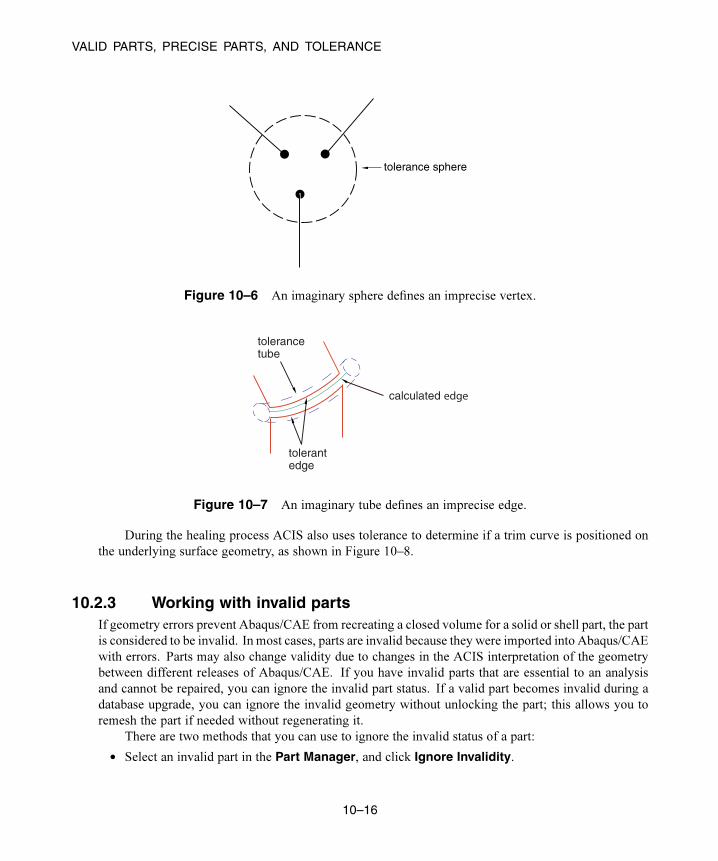
VALID PARTS, PRECISE PARTS, AND TOLERANCE
tolerance sphere
Figure 10–6 An imaginary sphere defines an imprecise vertex.
tolerancetube
calculated edge
tolerantedge
Figure 10–7 An imaginary tube defines an imprecise edge.
During the healing process ACIS also uses tolerance to determine if a trim curve is positioned on
the underlying surface geometry, as shown in Figure 10–8.
10.2.3 Working with invalid partsIf geometry errors prevent Abaqus/CAE from recreating a closed volume for a solid or shell part, the part
is considered to be invalid. In most cases, parts are invalid because they were imported into Abaqus/CAE
with errors. Parts may also change validity due to changes in the ACIS interpretation of the geometry
between different releases of Abaqus/CAE. If you have invalid parts that are essential to an analysis
and cannot be repaired, you can ignore the invalid part status. If a valid part becomes invalid during a
database upgrade, you can ignore the invalid geometry without unlocking the part; this allows you to
remesh the part if needed without regenerating it.
There are two methods that you can use to ignore the invalid status of a part:
• Select an invalid part in the Part Manager, and click Ignore Invalidity.
10–16
Abaqus ID:
Printed on:

VALID PARTS, PRECISE PARTS, AND TOLERANCE
trim curvesurface geometry
tolerancecylinder
edge
Figure 10–8 Tolerance determines if a trim curve lies on the underlying surface.
• Select an invalid part or an invalid independent part instance in theModel Tree, clickmouse button 3,
and select Ignore Invalidity.
When you choose to ignore the invalid status of a part or part instance, Abaqus/CAE displays a warning.
The warning indicates that while ignoring the invalidity of the part allows you to perform all geometry
and meshing functions, ignoring the invalidity may cause some part functions to fail or lead to other
undesirable behavior. If you accept this warning, Abaqus/CAE changes the part status to Invalid(ignored). The part status is displayed in the Part Manager and in the Model Tree. Table 10–1 shows
the icons and text used to indicate the status of invalid parts.
Table 10–1 Part status in the Model Tree and the Part Manager.
Model Treesymbol
Part Manager text Meaning
Invalid An unlocked invalid part.
Invalid (ignored) An unlocked invalid part with the invalid
status ignored.
Locked, Invalid A locked invalid part.
Locked, Invalid(ignored)
A locked invalid part with the invalid status
ignored.
Regardless of whether you are trying to repair the geometry or working with the invalid
status ignored, Abaqus/CAE does not always recompute the validity of parts as you make changes.
10–17
Abaqus ID:
Printed on:

CONTROLLING THE IMPORT PROCESS
Recomputing the validity, especially for complex parts, can take a substantial amount of time. To
recompute and update the validity of a part, select Update Validity in the Part Manager or in the menu
that appears when you click mouse button 3 on an invalid part or part instance in the Model Tree. You
can also use the Geometry diagnostics query to update validity. (For more information on geometry
diagnostics, see “Using the geometry diagnostic tools,” Section 71.2.4, in the HTML version of this
guide.)
10.3 Controlling the import process
When you import a part from a file generated by a third-party CAD system, Abaqus/CAE allows you to
control how it interprets the contents of the file. This section describes the options that are available to
you.
10.3.1 Repairing a part during import
You can import a part and subsequently use the Geometry Edit toolset in the Part module to apply any
repair operations that might be required to make the part usable by Abaqus/CAE; see Chapter 69, “The
Geometry Edit toolset,” for more information. Alternatively, you can import a part and repair the part
during the import process, as described in this section.
When you import a part, Abaqus/CAE scans the contents of the file and displays a dialog box with
a Name-Repair tabbed page that allows you to control the following:
Name
The name of the part.
Repair Options
For most of the file formats supported, Abaqus/CAE automatically repairs the part during the import
process. However, Abaqus/CAE provides the following additional options when you are importing
an IGES- or a VDA-FS-format file:
• Convert to analytical representation
• Stitch gaps
In most cases, the default settings for these options provide the best results. For more information,
see “An overview of editing techniques,” Section 69.2.
Topology
Abaqus/CAE selects the topology—solid, shell, or wire—based on the entities that it finds in the
file. In most cases you should accept the setting selected by Abaqus/CAE. However, if the topology
of the resulting part is not as expected, you can try importing the part again with a different topology
10–18
Abaqus ID:
Printed on:

CONTROLLING THE IMPORT PROCESS
selected. In addition, if you are importing an IGES-format file, you can click Entity List on the
IGES Options tabbed page to examine the type of entities found in the file.
Part Filter
The following file formats can include several parts in a single file:
• ACIS
• CATIA V4
• Elysium Neutral File (CATIA V5 or Pro/ENGINEER)
• Parasolid
• STEP
Abaqus/CAE imports all of the parts in the file by default. If you import all the parts in the file,
you can create individual Abaqus parts for each of them or you can combine them together into
a single Abaqus part; in addition, if you combine these parts, Abaqus/CAE enables you to stitch
these imported parts together using a user-specified stitching tolerance value. Alternatively, you
can toggle on Import part number and enter the number of a single part to import from the file.
Abaqus/CAE indicates if any of the parts have validity or precision problems.
In some cases when you import a part into Abaqus/CAE, the geometry of the part contains additional
edges and vertices that serve no purpose. The additional geometry splits faces into additional faces and
edges into additional edges, resulting in unnecessary complexity. The additional geometry will influence
your mesh unduly, and you should use the Geometry Edit toolset to remove the redundant edges and
vertices. You can also use virtual topology in the Mesh module to combine small faces and edges and
to ignore unnecessary vertices and edges; for more information, see Chapter 75, “The Virtual Topology
toolset.”
10.3.2 What are the part attributes?A part has the following attributes:
Modeling Space
When you import a part, Abaqus/CAE scans the file and tries to determine the modeling space of
the part being imported as follows:
• If Abaqus/CAE determines the part is three-dimensional, it sets the modeling space to three-
dimensional.
• If Abaqus/CAE determines the part is planar, you can choose whether the modeling space is
two- or three-dimensional.
• If Abaqus/CAE determines the part is planar and that its geometry does not cross the
Y-axis, you can choose whether the modeling space is axisymmetric, two-dimensional, or
three-dimensional. If you choose axisymmetric, the Y-axis is assumed to be the axis of
revolution, and you can add a twist degree of freedom.
10–19
Abaqus ID:
Printed on:

UNDERSTANDING THE CONTENTS OF AN IGES FILE
For more information, see “Part modeling space,” Section 11.4.1.
Type
Abaqus/CAE always assumes that the part type is deformable. Alternatively, you can select
Discrete rigid to import a discrete rigid part or select Eulerian to import an Eulerian part. For
more information, see “Part types,” Section 11.4.2.
Although you cannot define an imported part to be an analytical rigid part, you can import the
geometry of the analytical rigid part into a sketch. You can then create a new analytical rigid part
and copy the imported sketch into the Sketcher toolset.
10.3.3 Scaling a part during the import processWhen you import a part, you can choose to maintain the dimensions stored in the file, or you can change
the scale of the part during the import process. You can do the following:
• Enter a scale factor that Abaqus/CAE will apply to all of the coordinates in the file. Any offset from
the origin will be scaled accordingly.
• If you are importing a part from an ACIS file, you can read the scale factor, the rotation matrix, and
the translation matrix from the file.
You can also change the scale of a part while copying it to a new part. For more information, see “Copying
a part,” Section 11.5.
10.4 Understanding the contents of an IGES file
The IGES neutral file format is an international standard that allows you to transfer geometric data
between Abaqus/CAE and other CAD applications. You can use IGES-format files to import and export
sketches and parts. This section describes the IGES format and the options that are available to you when
importing and exporting IGES files.
For a detailed description of how to import and export IGES-format files, see “Importing a part from
an IGES-format file,” Section 10.7.7, and “Exporting geometry, model, and mesh data,” Section 10.9, in
the HTML version of this guide.
10.4.1 What are the IGES options in Abaqus/CAE?The IGES options allow you to control the following:
Trim Curve Preference
An IGES file can contain curves defined using real space, parameter space, or both. When you
import a part from an IGES file into Abaqus/CAE, the surface and the trim curves are converted
10–20
Abaqus ID:
Printed on:
UNDERSTANDING THE CONTENTS OF AN IGES FILE
into an internal representation of the part. By default, Abaqus/CAE uses the information stored in
the IGES file to decide how the trim curve is defined; alternatively, you can force Abaqus/CAE to
always use either real space or parameter space.
• As per IGES file. This is the default option. When this option is selected, Abaqus/CAE uses
either the Always use parametric data option or the Always use 3D data option to decide
how the trim curve is defined. Information in the IGES file determines which of the two options
is used.
• Always use parametric data. This option computes the trim curve parametrically using the
surface on which the curve is lying. Each of the data points on the trim curve is located by a
surface parameter (u, v). Abaqus/CAE evaluates the surface corresponding to the data point
and generates three-dimensional coordinates for the point.
If the underlying surface has too many sharp deflections that cannot be accurately defined
parametrically, the trim curve may not lie on the surface when Abaqus/CAE tries to reconstruct
the part. This produces a trimming error and may result in gaps between edges.
• Always use 3D data. This option computes the trim curve from the three-dimensional
coordinates in space—the part’s coordinate system—together with an indication that the trim
curve lies on the parametric surface. Each of the data points has its own three-dimensional
geometrical point; as a result the trim curve must be re-evaluated each time the surface is
moved. The trim curve can move only along the surface. The Always use 3D data option
should allow trim curves to stay with their underlying surface; however, this is not guaranteed.
If you select the Always use 3D data option, the import will take longer to complete.
MSBO
A Manifold Solid B-rep Object (MSBO, entity type 186) is an IGES term for a B-rep solid. Like
all B-rep solids, the MSBO entity indicates the overall topology of a solid entity by referencing all
the trimmed surfaces that define the solid. Abaqus/CAE sets the MSBO option automatically after
scanning an IGES-format file and finding the entity.
For an IGES file to contain anMSBO entity, the CAD package that created the file must include
the MSBO in the export procedure. CATIA V5 allows for the MSBO entity; SolidWorks does not.
Levels
CAD applications can store entities in an IGES-format file in a sequence of levels (also referred
to as layers). For example, different levels can contain geometry, dimensions, text annotations,
construction lines, notes, or a legend. When you import a part from an IGES-format file,
Abaqus/CAE scans the file and the Create Part from IGES File dialog box displays a list of the
levels that were found in the IGES file.
If a level contains something other than geometry, such as dimensions, Abaqus/CAE ignores
the level during the import. However, if a level does contain geometry, you can delete the level
from the list in the dialog box and Abaqus/CAE will not import the level. You must import at least
one level. As a result, if the IGES file contains only one level, the Level field is not available.
Abaqus/CAE ignores any levels that you enter that are not present in the IGES file.
10–21
Abaqus ID:
Printed on:

UNDERSTANDING THE CONTENTS OF AN IGES FILE
If you encounter problems during the import, you may want to modify the default settings.
10.4.2 What is an IGES entity?When you import an IGES-format file, Abaqus/CAE scans the contents of the file before displaying the
Create Part from IGES File dialog box. You can then use buttons on the IGES Options tabbed page
to view the following:
IGES HeaderThe IGES header information includes details about the application that wrote the IGES file. It also
includes information about the author of the file and the date when the file was written, along with
the scale, resolution, and units.
Entity ListAn entity can be a geometric entity, such as a point, an arc, or a line. Alternatively, an entity can
be separate from the geometry, such as a comment. IGES allocates a number to each entity; for
example, a circular arc is entity number 100. The IGES entity list displays a list of each type of
entity found in the file. The list includes the IGES entity number, a description of the entity, and the
number found in the file.
For a complete list of the IGES entities that can be imported into Abaqus/CAE, see “IGES entities
recognized by Abaqus/CAE when importing a part or a sketch,” Section 10.7.8, in the HTML version of
this guide.
10.4.3 What is in the IGES log file?When you import a part from an IGES file, Abaqus/CAE creates a file called
abaqus_read_iges.log in the directory from which you started the session. The
IGES log file contains information about the entities that were translated along with any problems
that were encountered.
Abaqus/CAE overwrites the abaqus_read_iges.log file after each IGES import. The
following information is written to the IGES log file:
• The global header information.
• A summary of the IGES entities found.
• IGES read options. The options displayed are the options used by the ACIS geometry engine in
Abaqus/CAE during the import. You can control only the following options:
– MSBO
– Read trim curves
• A conversion log.
• Errors.
10–22
Abaqus ID:
Printed on:

WHAT CAN YOU IMPORT FROM A MODEL?
10.4.4 Exporting to an IGES file
CAD applications store data in IGES-format files using their own interpretation of the IGES standard.
Abaqus/CAE is able to interpret IGES-format files generated by most applications. In addition, when
you export a part or assembly to an IGES-format file, Abaqus/CAE allows you to specify the application
that will be reading the file, and the data are written out in the appropriate tailored format or flavor. You
can choose one of the following flavors:
• Standard
• MSBO
• AutoCAD
• SolidWorks
• JAMA (Japanese Automotive Manufacturer’s Association)
By default, Abaqus/CAE exports data to an IGES file using a standard flavor. Abaqus/CAE writes the
geometry data to a single layer in the IGES file.
10.5 What can you import from a model?
You can import a model from an input file, an output database, or an Abaqus/CAE model database. You
can import the complete model from an input file or model database; however, you can import only parts,
section definitions, materials, and beam profiles from an output database.
The following sections describe how you can import a model. For a detailed description of how to
import a model, see “Importing a model,” Section 10.8, in the HTML version of this guide.
10.5.1 Importing a model from an Abaqus/CAE model database
You can import a model into the current Abaqus/CAE model database from a different model database
by selecting File→Import→Model from the main menu bar. Select a model database (.cae) file fromthe dialog box that appears, then select the model you want to import from the Import Model fromModel Database dialog box. Model databases from previous releases of Abaqus must be upgraded to
the current release before you can import their model data.
When you import a model from a model database, Abaqus/CAE creates a copy of that model that
includes all model data in the original version. However, this import excludes the following data present
in the original model database file but not directly related to the model:
• Job data
• Custom user data created using the Abaqus Scripting Interface
10–23
Abaqus ID:
Printed on:

WHAT CAN YOU IMPORT FROM A MODEL?
You can also prompt Abaqus/CAE to display the Copy Objects dialog box immediately after the
model is imported. This dialog box enables you to copy individual objects such as parts, sketches, or
materials between models in the current model database. For more information about copying objects,
see “Copying objects between models,” Section 9.8.3, in the HTML version of this guide.
Models imported from different model databases are not linked to their original models; any changes
to the original model that occur after the import are not propagated to the copy.
10.5.2 Importing a model from an Abaqus input file
You can use an Abaqus input file to import a model into Abaqus/CAE by selecting
File→Import→Model from the main menu bar. Abaqus keywords that are imported from the input
file are incorporated into a new model; for example, if the Young’s modulus was imported from the
*ELASTIC keyword, it will be available in the Property module. Keywords that are not supported
are ignored during import. Model component labels that differ only in case are not imported into
Abaqus/CAE consistently; therefore, you should not use case to distinguish between model components
of the same type. The input file does not have to be complete; for example, it may not contain any
history data. Because an input file is unable to store all of the data from an Abaqus/CAE model
database, you should not use input files to archive model data.
The following functionality can be imported into a model from an Abaqus input file:
• Nodes and elements
• Surfaces, node and element sets, and contact node sets
• Adaptive mesh controls
• Material, section, and orientation definitions
• Model and material descriptions
• Interactions and interaction properties
• Discrete fasteners (previously defined in Abaqus/CAE)
• Loads and boundary conditions (in the global coordinate system)
• Amplitudes
• Procedures, output requests, and monitor variables
Note: Importing models with a very large number of attributes, such as steps or predefined fields,
(on the order of 8000 or more) may take a significant amount of time.
See “Keyword support from the input file reader,” Section A.2, in the HTML version of this guide
for a complete list of the keywords that are supported by the input file reader. You can use the Keywords
Editor to include options that the input file reader does not support; for detailed instructions on using the
Keywords Editor, see “Adding unsupported keywords to your Abaqus/CAE model,” Section 9.10.1, in
the HTML version of this guide.
10–24
Abaqus ID:
Printed on:
WHAT CAN YOU IMPORT FROM A MODEL?
Importing parts
Parts are imported from an input file in the form of meshes; a mesh consists of node and element
definitions along with the type of element assigned. The input file reader can import a mesh containing
most of the commonly used element types. However, the input file reader cannot import a mesh
containing the following element types:
• Tube support elements (ITS*)
• User-defined elements (U*)
The following element types can be imported, but their section properties are not yet supported:
• Distributing coupling elements (DCOUP*)
• Drag chain elements (DRAG*)
• Frame elements (FRAME*)
• Gap contact stress/displacement elements (GAPCYL, GAPSPHER, and GAPUNI)
• Interface elements (INTER*, ISL*, IRS*, ISP*, ITT*, and DINTER*)
• Joint elements (JOINT*)
• Line spring elements (LS*)
Pore pressure cohesive elements can be imported, but you cannot view them in the Abaqus/CAE model.
However, you can view pore pressure cohesive elements in the Visualization module after an analysis is
complete.
You can use the Mesh module to change the element type assigned to elements imported from an
input file.
Importing sets and surfaces
The import capability creates sets based on any *ELSET or *NSET keywords, as well as any ELSET
or NSET parameters on other supported keywords. If the input file was written in terms of an assembly
of part instances, Abaqus/CAE preserves your intent when creating part and assembly sets. If a set was
defined within a part (deformable or rigid), Abaqus/CAE creates a part set. When you instance the part in
the Assembly module, you can refer to the part set; however, the assembly-related modules provide only
read-only access to part sets. If a set was defined within the assembly, Abaqus/CAE creates an assembly
set. For more information, see “How do part sets and assembly sets differ?,” Section 73.2.2.
In contrast, if the input file was not written in terms of an assembly of part instances, Abaqus/CAE
tries to minimize the number of sets created. In most cases, sets in the input file are imported as only
assembly sets. However, if a section assignment refers to a set, Abaqus/CAE imports the set as only a
part set.
Element-based surfaces can be imported; however, Abaqus/CAE imports a node-based surface as
a set of nodes, not as a surface. As a result, an imported node-based surface appears in the Set manager
and not in the Surface manager.
10–25
Abaqus ID:
Printed on:

WHAT CAN YOU IMPORT FROM A MODEL?
Importing descriptions
Model descriptions and material descriptions that appear as comment lines in input files are imported into
Abaqus/CAE. The comment lines that immediately precede the header of the input file store the model
description, which is available in theEdit Model Attributes dialog box upon import. The comment lines
that immediately precede the material and material behavior definitions store the material descriptions,
which are available in the Edit Material dialog box upon import.
The job description from the Edit Job dialog box appears as the data line for the header of the input
file. If desired, you can modify this data line to include more details about the job; however, this data
line is not imported into Abaqus/CAE.
Importing interactions, constraints, and fasteners
Abaqus/CAE imports reactivated contact pairs only if the contact pairs were deactivated in the first
analysis step.
Abaqus/CAE imports multi-point constraints as MPC connector sections and wire features or as
MPC constraints, depending on how the input file identifies the nodes involved.
A fully defined discrete fastener contains both an attachment line and a connector section
assignment. In order to recreate these discrete fasteners as originally modeled in Abaqus/CAE upon
import, Abaqus/CAE writes special comment lines to the input file when you submit a job for analysis.
These special comment lines immediately precede the Abaqus keyword used to define the discrete
fasteners, begin with **@ABQCAE, and are ignored by the Abaqus solvers.
Assembled fasteners and point-based (mesh-independent) fasteners cannot be imported from an
input file.
Analyzing a submodel
When you analyze a submodel using Abaqus/Standard or Abaqus/Explicit, you provide the name of the
output database or results file containing the global solution in the Abaqus execution procedure; the
file name does not appear in the input file. As a result, when you import an input file that analyzes a
submodel, you must specify the name of the output database or results file containing the global solution
that will drive the submodel. Select Model→Edit Attributes→Model Name and enter the name of the
file containing the global solution on the Submodel tabbed page.
10.5.3 Importing a model from an output databaseYou can use an output database to import a model into Abaqus/CAE by selecting File→Import→Modelfrom the main menu bar.
The following functionality can be imported into a model from an output database:
• Nodes and elements
• Surfaces, node and element sets, and contact node sets
10–26
Abaqus ID:
Printed on:

WHAT CAN YOU IMPORT FROM A MODEL?
• Materials and section definitions
• Beam profiles
Although sections are imported, the assignment of a section to the appropriate element set is not imported.
Similarly, the assignment of a beam profile to the appropriate beam section is not imported. When you
submit an input file for analysis, Abaqus does not write some material definitions to the output database.
As a result, if you import the output database into Abaqus/CAE, these materials will be missing from the
model. If this occurs, you can import the model from the input file instead of from the output database.
Abaqus/CAE imports a part from an output database by reading the nodes and elements that define
each part instance in the assembly. If the input file that created the output database was structured using
parts and assemblies, each part instance imported from the output database appears as a separate part in
Abaqus/CAE. In addition, the assembly appears in Abaqus/CAE along with each part instance. As a
result, the model imported into Abaqus/CAE contains a part and a part instance corresponding to each
part instance in the output database.
The nodes and elements that define a part instance in an output database have been translated and
rotated to their position in the assembly. The resulting part that is imported into Abaqus/CAE has the
same name as the original part instance in the output database, and its orientation reflects the orientation
of the part instance in the output database. As a result, the orientation of the imported part may be
different from the orientation of the part in the input file that created the output database.
If the input file that created the output database was not structured using parts and assemblies,
Abaqus/CAE writes the mesh definition to the output database as a single part and a single part instance.
If the single part in the output database includes an analytical rigid surface, the part that Abaqus/CAE
tries to import will contain an invalid combination of deformable parts and analytical rigid parts. As a
result the output database cannot be imported.
10.5.4 Importing a model from a Nastran input file
You can use a Nastran input file to import a model into Abaqus/CAE by selecting File→Import→Modelfrom the main menu bar. Abaqus/CAE imports many common entities in the Nastran bulk data into the
model you create; for more information on supported entities, see “Translating Nastran bulk data files to
Abaqus input files,” Section 3.2.26 of the Abaqus Analysis User’s Guide.
When you import a Nastran input file into Abaqus/CAE, you can control several aspects of the
Nastran-to-Abaqus conversion. These options include:
• Mapping of elements from Nastran to Abaqus element types.
• Selecting a method for converting Nastran section or membrane data into Abaqus sections. You
can create Abaqus sections corresponding to each Nastran PSHELL or PCOMP property ID, create
sections for all homogeneous elements referencing the same material, or create a separate shell or
membrane section for each combination of orientation, offset, and/or thickness in the Nastran input
file.
• Using pre-integrated shell sections.
10–27
Abaqus ID:
Printed on:
A LOGICAL APPROACH TO SUCCESSFUL IMPORT OF IGES FILES
• Applying a scaling multiplier for all density, mass, and rotary inertia values created in the
Abaqus/CAE model.
• Converting statements that use the Nastran libraries SOL 101, SOL 108, or SOL 111 into Abaqus
perturbation steps with load cases.
• Coupling of beam element offsets by creating new nodes at the offset locations, changing the beam
connectivity to the new nodes, and rigidly coupling the new and original nodes.
10.5.5 Importing a model from an ANSYS input fileYou can use an ANSYS input file to import a model into Abaqus/CAE by selecting
File→Import→Model from the main menu bar. Abaqus/CAE imports many common entities in
the ANSYS input file into the model you create; for more information on supported entities, see
“Translating ANSYS input files to Abaqus input files,” Section 3.2.28 of the Abaqus Analysis User’s
Guide.
10.6 A logical approach to successful import of IGES files
The following list describes the steps that you should follow if you experience problems importing a part
from an IGES file into Abaqus/CAE. The same approach can be applied to import other file types, but
the import options will vary based on the file type.
Defeature the part
Before you export a part from a CAD system, you should know what type of part you want to
analyze with Abaqus and what you expect from the analysis. For example, you may want to remove
excessive detail that will influence the mesh and dominate the time taken to perform the analysis.
For more information, see “Know what you want as an end product,” Section 10.1.5.
Modify the import options in Abaqus/CAE
If you are importing a part from an IGES file, you can choose the following options:
• Trim Curve Preference
• Scale
• MSBO
You can also specify the levels in the IGES file from which to import. For more information on the
effects of setting these options, see “What are the IGES options in Abaqus/CAE?,” Section 10.4.1.
Try to repair the part
If Abaqus/CAE requires a precise part to proceed (for example, if you need to partition the part),
you can use the Geometry Edit toolset in the Part module to edit the part. For more information,
see “An overview of editing techniques,” Section 69.2.
10–28
Abaqus ID:
Printed on:

A LOGICAL APPROACH TO SUCCESSFUL IMPORT OF IGES FILES
Diagnose and locate problems
If you are not sure why a part is still unusable by Abaqus/CAE, you can try the following:
• Look at the IGES Entity Filter list in the IGES Options dialog box for unsupported entities.
• Grey or lighter unconnected lines on a face are silhouette lines indicating undulations in the
surface that Abaqus/CAE introduced while attempting to make the surface more precise. You
should manually delete the face or import the part again without using the Convert to preciserepresentation automated repair option.
• Try to mesh the part. Faces that cannot be meshed by Abaqus/CAE are an indication of poor
geometry.
Try to reimport the part
If the repair tools fail to produce a valid part, the file describing the part may be invalid or contain
illegal statements. You should try to import the part back into the CAD system that created it. If
the part cannot be imported, you should check the export settings and regenerate the file. Entities in
the file that are not related to the part definition will cause the import to fail; for example, a border
around the part or a title block. Ideally, you should not try to import a part into Abaqus/CAE until
you know that it can be imported back into the CAD system that generated the part.
10–29
Abaqus ID:
Printed on:


Part III: Creating and analyzing a model using theAbaqus/CAE modulesThis part describes how to use the modules in Abaqus/CAE to define a model’s geometry and other physical
properties and then submit the model for analysis. The following topics are covered:
• Chapter 11, “The Part module”
• Chapter 12, “The Property module”
• Chapter 13, “The Assembly module”
• Chapter 14, “The Step module”
• Chapter 15, “The Interaction module”
• Chapter 16, “The Load module”
• Chapter 17, “The Mesh module”
• Chapter 18, “The Optimization module”
• Chapter 19, “The Job module”
• Chapter 20, “The Sketch module”
Abaqus ID:
Printed on:


THE PART MODULE
11. The Part module
Parts are the building blocks of an Abaqus/CAE model. You use the Part module to create each part,
and you use the Assembly module to assemble instances of the parts. The online tutorial in Appendix C,
“Using Additional Techniques to Create and Analyze a Model in Abaqus/CAE,” of Getting Started with
Abaqus: Interactive Edition contains examples of how you create, modify, and manipulate parts. This
chapter explains how you use the tools within the Part module to work with parts. The following topics
are covered:
• “Understanding the role of the Part module,” Section 11.1
• “Entering and exiting the Part module,” Section 11.2
• “What is feature-based modeling?,” Section 11.3
• “How is a part defined in Abaqus/CAE?,” Section 11.4
• “Copying a part,” Section 11.5
• “What are orphan nodes and elements?,” Section 11.6
• “Modeling rigid bodies and display bodies,” Section 11.7
• “The reference point and point parts,” Section 11.8
• “What types of features can you create?,” Section 11.9
• “Using feature-based modeling effectively,” Section 11.10
• “Capturing your design and analysis intent,” Section 11.11
• “What is part and assembly locking?,” Section 11.12
• “What are extruding, revolving, and sweeping?,” Section 11.13
• “What is lofting?,” Section 11.14
• “Using the Sketcher in conjunction with the Part module,” Section 11.15
• “Understanding toolsets in the Part module,” Section 11.16
• “Using the Part module toolbox,” Section 11.17
In addition, the following sections are available in the HTML version of this guide:
• “Managing parts,” Section 11.18
• “Using the Create Part dialog box,” Section 11.19
• “Adding a feature to a part,” Section 11.20
• “Adding a solid feature,” Section 11.21
• “Adding a shell feature,” Section 11.22
• “Adding a wire feature,” Section 11.23
• “Adding a cut feature,” Section 11.24
• “Using the Edit Feature dialog box,” Section 11.25
11–1
Abaqus ID:
Printed on:

UNDERSTANDING THE ROLE OF THE PART MODULE
• “Using the Edit Loft dialog box,” Section 11.26
• “Blending edges,” Section 11.27
• “Mirroring a part,” Section 11.28
11.1 Understanding the role of the Part module
There are several ways to create a part in Abaqus/CAE:
• Create the part using the tools available in the Part module.
• Import the part from a file containing geometry stored in a third-party format.
• Import the part mesh from an output database.
• Import a meshed part from an Abaqus input file.
• Merge or cut part instances in the Assembly module.
• Create a meshed part in the Mesh module.
A part created using the Part module tools is called a native part and has a feature-based representation.
A feature captures your design intent and contains geometry information as well as a set of rules that
govern the behavior of the geometry. For example, a circular through cut is a feature, and Abaqus/CAE
stores the diameter of the cut along with the information that it should pass all the way through the part.
If you increase the size of the part, Abaqus/CAE recognizes that the depth of the cut should increase so
that it continues to pass through the part.
You use the Part module to create, edit, and manage the parts in the current model. Abaqus/CAE
stores each part in the form of an ordered list of features. The parameters that define each
feature—extruded depth, hole diameter, sweep path, etc.—combine to define the geometry of the part.
The Part module allows you to do the following:
• Create deformable, discrete rigid, analytical rigid, or Eulerian parts. The part tools also allow you
to edit and manipulate the existing parts defined in the current model.
• Create the features—solids, shells, wires, cuts, and rounds—that define the geometry of the part.
• Use the Feature Manipulation toolset to edit, delete, suppress, resume, and regenerate a part’s
features.
• Assign the reference point to a rigid part.
• Use the Sketcher to create, edit, and manage the two-dimensional sketches that form the profile of a
part’s features. These profiles can be extruded, revolved, or swept to create part geometry; or they
can be used directly to form a planar or axisymmetric part.
• Use the Set toolset, the Partition toolset, and the Datum toolset. These toolsets operate on the part
in the current viewport and allow you to create sets, partitions, and datum geometry, respectively.
11–2
Abaqus ID:
Printed on:

WHAT IS FEATURE-BASED MODELING?
11.2 Entering and exiting the Part module
You can enter the Part module at any time during an Abaqus/CAE session by clicking Part in the Modulelist located in the context bar. The Part, Shape, Feature, and Tools menus appear on the main menu
bar, and the title bar of the current viewport displays the name of the current part, if one exists.
To exit the Part module, select any other module from the Module list. You need not take any
specific action to save your parts before exiting the module; they are saved automatically when you save
the entire model by selecting File→Save or File→Save As from the main menu bar.
11.3 What is feature-based modeling?
This section describes the feature-based modeling approach that Abaqus/CAE uses to define a part.
11.3.1 The relationship between parts and featuresA part created in Abaqus/CAE has a feature-based representation. A feature is a meaningful piece of the
design and provides the engineer with a convenient and natural way to build and modify a part. Parts
created in Abaqus/CAE are constructed from an ordered list of features and the parameters that define
the geometry of each feature. You select from the following shape features to build a part in the Part
module:
• Solids
• Shells
• Wires
• Cuts
• Blends
Using the tools in the Part module, you create and edit all the features necessary to describe each of
the parts in your model. Abaqus/CAE stores each feature and uses this information to define the entire
part, to regenerate the part if you modify it, and to generate an instance of the part in the Assembly
module. For more information on how parts are related to part instances, see “What is a part instance?,”
Section 11.3.4.
The following sequence illustrates how the three-dimensional part in Figure 11–1 would be
constructed using features available in Abaqus/CAE:
1. The first feature you create while building a part is called the base feature; you construct the
remainder of the part by adding more features that either modify or add detail to the base feature.
In this example the base feature is a U-shaped part; the user sketched a two-dimensional profile
and extruded it to form the base feature, as shown in Figure 11–2.
11–3
Abaqus ID:
Printed on:

WHAT IS FEATURE-BASED MODELING?
Figure 11–1 Part constructed using solid, shell, wire, cut, and blend features.
a
Figure 11–2 The base feature.
The sketch and the extrusion depth (a) are the modifiable parameters that define the base
feature. You can revisit the base feature and change its size or shape by using the Feature
Manipulation toolset to modify either the section sketch or the extrusion distance. If desired, you
can delete the base feature and sketch a new shape.
2. A stiffening web is added as a shell feature. The user sketched a line on one of the internal faces and
extruded the sketch to the opposite face, as shown in Figure 11–3. The sketch is the only modifiable
parameter that defines the shell feature.
3. Rods are added to the corners as wire features. The wire was created by connecting two points that
the user selected, as shown in Figure 11–4. Wires created in this way have nomodifiable parameters;
they must be deleted and recreated if you need to change them.
4. A blind cut is cut into the top of the clamp. The user sketched a two-dimensional profile, and the
profile was extruded into the clamp through a specified distance, as shown in Figure 11–5. The
sketch and the depth of the slot are the modifiable parameters that define the blind cut feature.
5. The edges of the cut are rounded. The user selected the edges to round and provided the radius of
the round, as shown in Figure 11–6. The radius is the modifiable parameter that defines the round
feature.
11–4
Abaqus ID:
Printed on:

WHAT IS FEATURE-BASED MODELING?
sketched profile
Figure 11–3 A shell feature.
Figure 11–4 Wire features.
If the geometry of a new feature depends on an existing feature, Abaqus/CAE creates a parent-child
relationship between the features. The new feature is the child, and the feature it depends on is the parent.
For example, in the part described above the round feature is a child of the cut feature. If you change the
position or size of the cut, the edges remain rounded. Similarly, if you delete the cut, Abaqus/CAE also
deletes the rounds.
If you modify a parent feature, the modification may invalidate children of the parent feature. For
example, in the part described above if you were to increase the depth of the cut so that it became a
through cut, you would lose the fillets along its edges; that is, the fillets would fail to regenerate after the
modification. Abaqus/CAE offers you the following two choices:
• Keep the changes to the parent feature but suppress the features that failed to regenerate. Children
of the suppressed features will also be suppressed.
• Abort the modification of the parent feature and return to the state of the last successful regeneration.
11–5
Abaqus ID:
Printed on:

WHAT IS FEATURE-BASED MODELING?
sketched profile
Figure 11–5 A cut feature.
Figure 11–6 Round features.
11.3.2 The base featureThe first feature you create while building a part is called the base feature; you construct the remainder
of the part by adding more features that either modify or add detail to the base feature. This process of
building an Abaqus/CAE native part using the tools in the Part module follows a sequence of operations
analogous to building a part in a machine shop. For example, you start with a piece of billet stock (the
base feature) and then you do the following:
• Attach additional pieces to the billet (apply a solid extrusion, a revolved shell, or a sketched wire).
11–6
Abaqus ID:
Printed on:
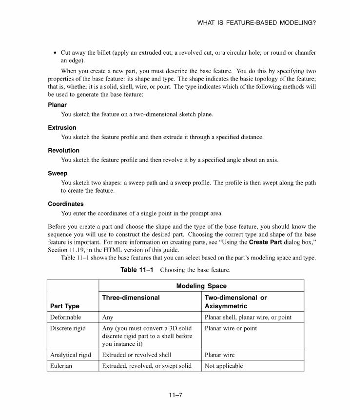
WHAT IS FEATURE-BASED MODELING?
• Cut away the billet (apply an extruded cut, a revolved cut, or a circular hole; or round or chamfer
an edge).
When you create a new part, you must describe the base feature. You do this by specifying two
properties of the base feature: its shape and type. The shape indicates the basic topology of the feature;
that is, whether it is a solid, shell, wire, or point. The type indicates which of the following methods will
be used to generate the base feature:
Planar
You sketch the feature on a two-dimensional sketch plane.
Extrusion
You sketch the feature profile and then extrude it through a specified distance.
Revolution
You sketch the feature profile and then revolve it by a specified angle about an axis.
Sweep
You sketch two shapes: a sweep path and a sweep profile. The profile is then swept along the path
to create the feature.
Coordinates
You enter the coordinates of a single point in the prompt area.
Before you create a part and choose the shape and the type of the base feature, you should know the
sequence you will use to construct the desired part. Choosing the correct type and shape of the base
feature is important. For more information on creating parts, see “Using the Create Part dialog box,”
Section 11.19, in the HTML version of this guide.
Table 11–1 shows the base features that you can select based on the part’s modeling space and type.
Table 11–1 Choosing the base feature.
Modeling Space
Part TypeThree-dimensional Two-dimensional or
Axisymmetric
Deformable Any Planar shell, planar wire, or point
Discrete rigid Any (you must convert a 3D solid
discrete rigid part to a shell before
you instance it)
Planar wire or point
Analytical rigid Extruded or revolved shell Planar wire
Eulerian Extruded, revolved, or swept solid Not applicable
11–7
Abaqus ID:
Printed on:

WHAT IS FEATURE-BASED MODELING?
Modeling Space
Part TypeThree-dimensional Two-dimensional or
Axisymmetric
Fluid Extruded, revolved, or swept solid Not applicable
Electromagnetic Extruded, revolved, or swept solid Planar shell
A part imported from a file containing third-party format geometry consists of a single feature that
you import into Abaqus/CAE as the base feature of a new part. You cannot modify this base feature, but
you can add additional features to it. Similarly, a mesh part is created in the Mesh module or imported
from an output database as the base feature of a new part. You can use the mesh editing tools to add and
delete nodes and elements from a mesh, or you can use the tools in the Part module to add geometric
features to the mesh.
The HTML version of this guide contains detailed instructions on creating and defining a new part
and managing the parts in your model. The following topics are covered:
• “Managing parts,” Section 11.18
• “Using the Create Part dialog box,” Section 11.19
11.3.3 Simplifying a part’s feature listWhen you copy a part to a new part, you can reduce all the feature and parameter information to a simple
definition. If you reduce the feature list, Abaqus/CAE will regenerate the part faster if you subsequently
modify it; however, you will no longer be able to modify any parameters of the part. You copy a part by
selecting Part→Copy→part name from the main menu bar.
Simplifying a part’s feature list is especially useful if you have spent a lot of time creating a part
and have iterated many times over the design. For example, if you created a slot and redimensioned the
slot before arriving at the final design, the original part contains features that define each variation of the
slot. If you copy the part and simplify the feature list, the new part will contain only one feature that
defines the final version of the slot.
11.3.4 What is a part instance?A part instance can be thought of as a representation of the original part. You create a part in the Part
module and define its properties in the Property module. However, when you assemble the model using
the Assembly module, you work only with instances of the part, not the part itself. The Interaction and
Load modules also operate on the assembly and, therefore, on part instances. In contrast, the Mesh
module enables you to operate on either the assembly or one or more of its component parts.
You create part instances in the Assembly module. You then position those instances relative to
each other in a global coordinate system to form the assembly. You can create and position multiple
instances of a single part. In addition, you can assemble instances of deformable, analytical rigid, and
11–8
Abaqus ID:
Printed on:

WHAT IS FEATURE-BASED MODELING?
discrete rigid parts when you are solving contact problems. For more information on the types of parts
you can create in Abaqus/CAE, see “Part types,” Section 11.4.2.
The following example illustrates the relationship between parts and part instances. A pump housing
is composed of three parts: the housing cover, a gasket, and a mounting bolt. In the Part module you
create each of the three parts shown in Figure 11–7:
• One housing cover
• One gasket
• One bolt
1. pump
2. gasket
3. bolt
Figure 11–7 The original parts.
In the Assembly module you assemble instances of each part:
• One instance of the body
• One instance of the gasket
• Eight instances of the bolt
You then position the instances relative to a common coordinate system, thereby creating the model of
the pump housing, as shown in Figure 11–8.
Now, suppose you want to change the length of the bolts. You return to the Part module and modify
the length of the bolt by editing the original part. When you return to the Assembly module, Abaqus/CAE
recognizes that the part was modified and automatically regenerates the eight instances of the bolt to
reflect the change in the length.
You cannot modify the geometry of a part instance directly; you can modify the part itself only
within the Part module. When you modify a part, Abaqus/CAE automatically regenerates all instances
11–9
Abaqus ID:
Printed on:
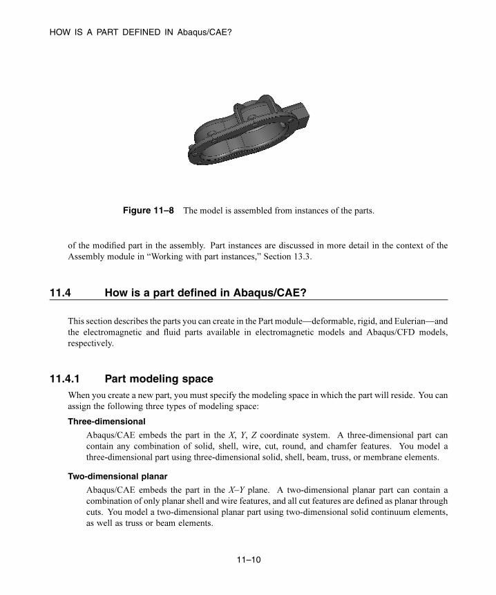
HOW IS A PART DEFINED IN Abaqus/CAE?
Figure 11–8 The model is assembled from instances of the parts.
of the modified part in the assembly. Part instances are discussed in more detail in the context of the
Assembly module in “Working with part instances,” Section 13.3.
11.4 How is a part defined in Abaqus/CAE?
This section describes the parts you can create in the Part module—deformable, rigid, and Eulerian—and
the electromagnetic and fluid parts available in electromagnetic models and Abaqus/CFD models,
respectively.
11.4.1 Part modeling spaceWhen you create a new part, you must specify the modeling space in which the part will reside. You can
assign the following three types of modeling space:
Three-dimensional
Abaqus/CAE embeds the part in the X, Y, Z coordinate system. A three-dimensional part can
contain any combination of solid, shell, wire, cut, round, and chamfer features. You model a
three-dimensional part using three-dimensional solid, shell, beam, truss, or membrane elements.
Two-dimensional planar
Abaqus/CAE embeds the part in the X–Y plane. A two-dimensional planar part can contain a
combination of only planar shell and wire features, and all cut features are defined as planar through
cuts. You model a two-dimensional planar part using two-dimensional solid continuum elements,
as well as truss or beam elements.
11–10
Abaqus ID:
Printed on:

HOW IS A PART DEFINED IN Abaqus/CAE?
Axisymmetric
Abaqus/CAE embeds the part in the X–Y plane with the Y-axis indicating the axis of revolution.
An axisymmetric part can contain a combination of only planar shell and wire features, and all cut
features are defined as planar through cuts. You model an axisymmetric part using axisymmetric
solid continuum elements or axisymmetric shell elements.
Modeling space refers to the space in which the part is embedded rather than to the topology of the part
itself. Thus, you can create a three-dimensional part using a topologically two-dimensional shell feature
or a one-dimensional wire feature. You can change the modeling space of a part after you have created it
by clicking mouse button 3 on the part in the Model Tree and selecting Edit from the menu that appears.
Abaqus/CAE uses the following methods to determine the modeling space of an imported part:
• When you import a part from a file containing geometry stored in a third-party format, you can
specify the part’s modeling space, provided that Abaqus/CAE does not determine it must be three-
dimensional.
• When you import a mesh from an output database, Abaqus/CAE determines the modeling space of
the new part from the information stored in the output database.
• When you import a mesh from an input file, Abaqus/CAE determines the modeling space of the
new part from the element type.
• When you create a mesh part in the Mesh module, the modeling space of the mesh part is the same
as the modeling space of the original part.
Detailed instructions on how to specify modeling space when creating and importing a part can be found
in “Choosing the modeling space of a new part,” Section 11.19.2, and “Importing sketches and parts,”
Section 10.7, in the HTML version of this guide. For instructions on using the online documentation,
see “Getting help,” Section 2.6.
11.4.2 Part types
When you create a new part or import a part from a file containing geometry stored in a third-party
format, you must choose the part’s type. The possible types for Abaqus/Standard and Abaqus/Explicit
are:
Deformable
Any arbitrarily shaped axisymmetric, two-dimensional, or three-dimensional part that you can
create or import can be specified as a deformable part. A deformable part represents a part that can
deform under load; the load can be mechanical, thermal, or electrical. By default, Abaqus/CAE
creates parts that are deformable.
11–11
Abaqus ID:
Printed on:

HOW IS A PART DEFINED IN Abaqus/CAE?
Discrete rigid
A discrete rigid part is similar to a deformable part in that it can be any arbitrary shape. However, a
discrete rigid part is assumed to be rigid and is used in contact analyses to model bodies that cannot
deform.
Analytical rigid
An analytical rigid part is similar to a discrete rigid part in that it is used to represent a rigid surface
in a contact analysis. However, the shape of an analytical rigid part is not arbitrary and must be
formed from a set of sketched lines, arcs, and parabolas.
Eulerian
Eulerian parts are used to define a domain in which material can flow for an Eulerian analysis.
Eulerian parts do not deform during an analysis; instead, the material within the part deforms
under load and can flow across the rigid element boundaries. For more information about Eulerian
analyses, see Chapter 28, “Eulerian analyses.”
Electromagnetic
The electromagnetic part type is used only in an electromagnetic model. For more information, see
“Eddy current analysis,” Section 6.7.5 of the Abaqus Analysis User’s Guide.
The part type available for Abaqus/CFD is:
Fluid
The fluid part type is used only in an Abaqus/CFD model.
You can assemble deformable bodies, discrete rigid parts, analytical rigid parts, Eulerian parts, fluid
parts, and electromagnetic parts in the Assembly module. If allowed, you can change the type of a part
after you have created it by clicking mouse button 3 on the part in the Model Tree and selecting Editfrom the menu that appears.
Abaqus/CAE uses the following methods to determine the type of an imported part:
• When you import a part from a file containing geometry stored in a third-party format, you can
specify the part’s type to be either deformable, discrete rigid, or Eulerian.
• When you import a mesh from an output database, Abaqus/CAE determines the type of the new
part from the information stored in the output database.
• When you import a mesh from an input file, Abaqus/CAE determines the type of the new part from
the element type.
• When you create a mesh part in the Mesh module, the type of the mesh part is the same as the type
of the original part.
For detailed instructions on how to set the type of a part when creating it, see “Choosing the type
of a new part,” Section 11.19.3, in the HTML version of this guide.
11–12
Abaqus ID:
Printed on:

COPYING A PART
11.4.3 Part size
When you create a new part, you must choose the part’s approximate size. The size that you enter is used
by Abaqus/CAE to calculate the size of the Sketcher sheet and the spacing of its grid. You should set the
approximate size of the part to match the largest dimension of the finished part. If you find subsequently
that the part exceeds the size of the Sketcher sheet, use the Sketch customization options to increase the
sheet size. You cannot change a part’s approximate size after you have created it. However, you can copy
the part to a new part and scale the part during the copy operation. For more information, see “Copying
a part,” Section 11.18.3, in the HTML version of this guide.
Abaqus/CAE uses a geometry engine to model parts and features. The recommended approximate
size limits are between 0.001 (10−3 ) and 1000 (104) units. This size range should prevent your model
from exceeding the limits of the geometry engine. For example, the minimum size supported by the
geometry engine is 10−6 , so maintaining geometry on the order of 10−3 will normally allow node and
element dimensions to remain above the minimum size. Parts that exceed the recommended limits may
exhibit geometric defects. If you find that you need to specify an approximate size that is outside the
suggested range, you should consider adopting a different set of units.
For detailed instructions on how to specify the approximate size of a part when creating it, see
“Setting the approximate size of the new part,” Section 11.19.5, in the HTML version of this guide.
11.5 Copying a part
Select Part→Copy→part name from the main menu bar to copy a part to a new part. You can create
an identical copy of the original part, or you can do the following during the copy operation:
Compress features
Abaqus/CAE reduces all the feature and parameter information to a simple definition of the part.
As a result, Abaqus/CAE will regenerate the part faster if you subsequently modify it; however, you
will no longer be able to modify any parameters of the part. For more information, see “Simplifying
a part’s feature list,” Section 11.3.3.
Scale part by
Abaqus/CAE scales the new part by the scale factor that you enter. If you choose to scale a part,
Abaqus/CAE also compresses its features. You can use scaling to correct imported parts. If the
scale of the imported part is incorrect, you can copy the part to a new part and scale it to the correct
dimensions in the process. In some cases you can produce a valid part by scaling the part down,
repairing the part, and then scaling the part back to its original dimensions. You can also scale an
imported part during the import process. For more information, see “Importing sketches and parts,”
Section 10.7, in the HTML version of this guide.
11–13
Abaqus ID:
Printed on:

WHAT ARE ORPHAN NODES AND ELEMENTS?
Mirror part about plane
Abaqus/CAE mirrors the part about the selected plane (X–Y, Y–Z, or X–Z). If you select the Mirrorpart about plane option, Abaqus/CAE selects the Compress features option.
To mirror a part about a plane other than one of the principal planes and without compressing
the features, use Shape→Transform→Mirror. For more information, see “Mirroring a part,”
Section 11.28, in the HTML version of this guide.
Separate disconnected regions into parts
In some cases when you import an IGES- or VDA-FS-format part and select the Stitch edgesrepair option, Abaqus/CAE imports separate parts as a single part. If you toggle on the Separatedisconnected regions into parts option and copy the imported part to a new part, Abaqus/CAE
will separate disconnected regions into separate parts. For more information, see “Controlling the
import process,” Section 10.3.
You can copy a mesh part and separate it into disconnected parts based on nodal connectivity.
Abaqus/CAE assumes that all connected nodes belong to a single part and does not take element
type into consideration. However, Abaqus/CAE ignores connectivity between axisymmetric solid
elements with nonlinear, asymmetric deformation (CAXA) and some line elements (connectors,
springs, dashpots, gap, and joint).
You can copy parts containing both geometry and orphan mesh features. The compress, scale, mirror,
and separate disconnected regions options can be used on any part.
Note: Reference points, point parts, and datums are not copied when you compress or mirror a part
during the copy operation.
11.6 What are orphan nodes and elements?
Orphan nodes and elements are components of a finite element mesh that exist without any associated
geometry. In effect, the mesh information has been orphaned from its parent geometry. Orphan nodes
and elements can be created in several ways; they can be:
• Imported from an output database (for more information, see “Importing a part from an output
database,” Section 10.7.12, in the HTML version of this guide)
• Imported from an Abaqus input file (for more information, see “Importing a model,” Section 10.8,
in the HTML version of this guide)
• Created as a mesh part (for more information, see “Creating a mesh part,” Section 17.20, in the
HTML version of this guide )
• Created in a bottom-up meshing procedure (for more information, see “Bottom-up meshing,”
Section 17.11)
• Created by certain mesh editing operations, such as create element and offset (for more information,
see “An overview of the mesh editing tools,” Section 64.4, in the HTML version of this guide)
11–14
Abaqus ID:
Printed on:
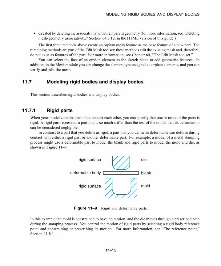
MODELING RIGID BODIES AND DISPLAY BODIES
• Created by deleting the associativity with their parent geometry (for more information, see “Deleting
mesh-geometry associativity,” Section 64.7.12, in the HTML version of this guide )
The first three methods above create an orphan mesh feature as the base feature of a new part. The
remaining methods are part of the Edit Mesh toolset; these methods edit the existing mesh and, therefore,
do not exist as features of the part. For more information, see Chapter 64, “The Edit Mesh toolset.”
You can select the face of an orphan element as the sketch plane to add geometric features. In
addition, in the Mesh module you can change the element type assigned to orphan elements, and you can
verify and edit the mesh.
11.7 Modeling rigid bodies and display bodies
This section describes rigid bodies and display bodies.
11.7.1 Rigid partsWhen your model contains parts that contact each other, you can specify that one or more of the parts is
rigid. A rigid part represents a part that is so much stiffer than the rest of the model that its deformation
can be considered negligible.
In contrast to a part that you define as rigid, a part that you define as deformable can deform during
contact with either a rigid part or another deformable part. For example, a model of a metal stamping
process might use a deformable part to model the blank and rigid parts to model the mold and die, as
shown in Figure 11–9.
������������
������������������������
rigid surface
rigid surface
deformable body
die
blank
mold
Figure 11–9 Rigid and deformable parts.
In this example the mold is constrained to have no motion, and the die moves through a prescribed path
during the stamping process. You control the motion of rigid parts by selecting a rigid body reference
point and constraining or prescribing its motion. For more information, see “The reference point,”
Section 11.8.1.
11–15
Abaqus ID:
Printed on:

MODELING RIGID BODIES AND DISPLAY BODIES
Computational efficiency is the principal advantage of rigid parts over deformable parts. During
the analysis element-level calculations are not performed for rigid parts. Although some computational
effort is required to update the motion of the rigid body and to assemble concentrated and distributed
loads, the motion of the rigid body is determined completely by the reference point. To change the type
of a part from deformable to rigid and vice versa, you can click mouse button 3 on the part in the Model
Tree and select Edit from the menu that appears. For more information, see “What is the difference
between a rigid part and a rigid body constraint?,” Section 11.7.3, and Chapter 27, “Display bodies.”
You can choose between two kinds of rigid parts:
Discrete rigid partsA part that you declared to be a discrete rigid part can be any arbitrary three-dimensional,
two-dimensional, or axisymmetric shape. Therefore, you can use all the Part module feature
tools—solids, shells, wires, cuts, and blends—to create a discrete rigid part. However, only
discrete rigid parts containing shells and wires can be meshed with rigid elements in the Mesh
module. If you try to create an instance of a solid discrete rigid part in the Assembly module,
Abaqus/CAE displays an error message; you must return to the Part module and convert the faces
of the solid to shells.
Analytical rigid parts
An analytical rigid part is similar to a discrete rigid part in that it is used to represent a rigid part in
a contact analysis. If possible, you should use an analytical rigid part when describing a rigid part
because it is computationally less expensive than a discrete rigid part. The shape of an analytical
rigid part is not arbitrary, and the profile must be smooth. You can use only the following methods
to create an analytical rigid part:
• You can sketch the two-dimensional profile of the part and revolve the profile around an axis of
symmetry to form a three-dimensional revolved analytical rigid part, as shown in Figure 11–10.
revolved
sketchedprofile
Figure 11–10 A revolved analytical rigid part.
• You can sketch the two-dimensional profile of the part and extrude the profile infinitely to form
a three-dimensional extruded analytical rigid part. Although Abaqus/CAE considers that the
11–16
Abaqus ID:
Printed on:

MODELING RIGID BODIES AND DISPLAY BODIES
extrusion extends to infinity, the Part module displays a three-dimensional extruded analytical
rigid part with a depth that you specify, as shown in Figure 11–11.
extruded
sketchedprofile
extruded
Figure 11–11 An extruded analytical rigid part.
• You can sketch the profile of a planar two-dimensional analytical rigid part, as shown in
Figure 11–12.
Figure 11–12 A planar analytical rigid part.
• You can sketch the profile of an axisymmetric two-dimensional analytical rigid part, as shown
in Figure 11–13.
You can import a part from a file containing geometry stored in a third-party format and define
it to be either a deformable or a discrete rigid part; however, you cannot define an imported part to
be an analytical rigid part. As an alternative, you can import the geometry of the analytical rigid
part into a sketch. You can then create a new analytical rigid part and copy the imported sketch into
the Sketcher toolset.
11–17
Abaqus ID:
Printed on:
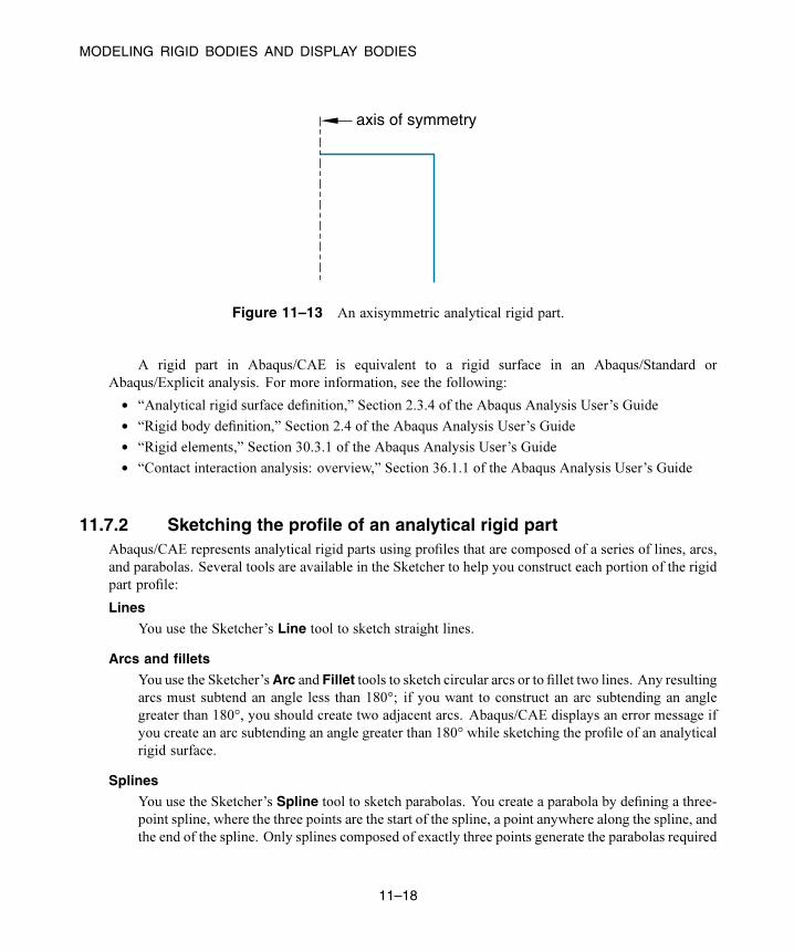
MODELING RIGID BODIES AND DISPLAY BODIES
axis of symmetry
Figure 11–13 An axisymmetric analytical rigid part.
A rigid part in Abaqus/CAE is equivalent to a rigid surface in an Abaqus/Standard or
Abaqus/Explicit analysis. For more information, see the following:
• “Analytical rigid surface definition,” Section 2.3.4 of the Abaqus Analysis User’s Guide
• “Rigid body definition,” Section 2.4 of the Abaqus Analysis User’s Guide
• “Rigid elements,” Section 30.3.1 of the Abaqus Analysis User’s Guide
• “Contact interaction analysis: overview,” Section 36.1.1 of the Abaqus Analysis User’s Guide
11.7.2 Sketching the profile of an analytical rigid partAbaqus/CAE represents analytical rigid parts using profiles that are composed of a series of lines, arcs,
and parabolas. Several tools are available in the Sketcher to help you construct each portion of the rigid
part profile:
Lines
You use the Sketcher’s Line tool to sketch straight lines.
Arcs and fillets
You use the Sketcher’s Arc and Fillet tools to sketch circular arcs or to fillet two lines. Any resultingarcs must subtend an angle less than 180°; if you want to construct an arc subtending an angle
greater than 180°, you should create two adjacent arcs. Abaqus/CAE displays an error message if
you create an arc subtending an angle greater than 180° while sketching the profile of an analytical
rigid surface.
Splines
You use the Sketcher’s Spline tool to sketch parabolas. You create a parabola by defining a three-
point spline, where the three points are the start of the spline, a point anywhere along the spline, and
the end of the spline. Only splines composed of exactly three points generate the parabolas required
11–18
Abaqus ID:
Printed on:
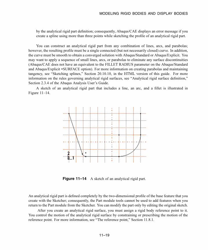
MODELING RIGID BODIES AND DISPLAY BODIES
by the analytical rigid part definition; consequently, Abaqus/CAE displays an error message if you
create a spline using more than three points while sketching the profile of an analytical rigid part.
You can construct an analytical rigid part from any combination of lines, arcs, and parabolas;
however, the resulting profile must be a single connected (but not necessarily closed) curve. In addition,
the curve must be smooth to obtain a converged solution with Abaqus/Standard or Abaqus/Explicit. You
may want to apply a sequence of small lines, arcs, or parabolas to eliminate any surface discontinuities
(Abaqus/CAE does not have an equivalent to the FILLET RADIUS parameter on the Abaqus/Standard
and Abaqus/Explicit *SURFACE option). For more information on creating parabolas and maintaining
tangency, see “Sketching splines,” Section 20.10.10, in the HTML version of this guide. For more
information on the rules governing analytical rigid surfaces, see “Analytical rigid surface definition,”
Section 2.3.4 of the Abaqus Analysis User’s Guide.
A sketch of an analytical rigid part that includes a line, an arc, and a fillet is illustrated in
Figure 11–14.
Figure 11–14 A sketch of an analytical rigid part.
An analytical rigid part is defined completely by the two-dimensional profile of the base feature that you
create with the Sketcher; consequently, the Part module tools cannot be used to add features when you
return to the Part module from the Sketcher. You can modify the part only by editing the original sketch.
After you create an analytical rigid surface, you must assign a rigid body reference point to it.
You control the motion of the analytical rigid surface by constraining or prescribing the motion of the
reference point. For more information, see “The reference point,” Section 11.8.1.
11–19
Abaqus ID:
Printed on:

MODELING RIGID BODIES AND DISPLAY BODIES
11.7.3 What is the difference between a rigid part and a rigid bodyconstraint?
You can create a rigid part in the Part module by creating a part and declaring its type to be discrete or
analytical rigid. You can create a reference point and assign it to the rigid body reference point. Motion
or constraints that you apply to the reference point are then applied to the entire rigid part.
Similarly, you can create a rigid body constraint in the Interaction module. Rigid body constraints
allow you to constrain the motion of regions of the assembly to the motion of a reference point. The
relative positions of the regions that are part of the rigid body remain constant throughout the analysis.
In addition, you can select regions from a part instance and use a rigid body constraint to specify an
isothermal rigid body for a fully coupled thermal-stress analysis. For detailed instructions on defining
rigid body constraints and assigning a rigid body reference point, see “Defining rigid body constraints,”
Section 15.15.2, in the HTML version of this guide.
You do not have to create a reference point for a part, even if the part type is discrete or analytical
rigid. However, if you do not create a reference point for a rigid part, every instance of the part in the
assembly must be included in a rigid body constraint.
Rigid parts are associated with parts; rigid body constraints are associated with regions of the
assembly. For example, if you define a part to be rigid, every instance of the part in the assembly is
rigid. In contrast, if you define a part to be deformable, you can use rigid body constraints to make only
some of the instances rigid. If you do not create a reference point in the Part module, you cannot create
a rigid body reference point by associating an instance of the rigid part with a reference point created
in the Assembly module. However, you can associate the instance with a rigid body constraint and a
reference point created in the Assembly module.
If you define a part to be rigid, you can use the Model Tree to change the part type to be deformable.
To check that your basic model is correct, you might run a quick analysis with a part defined as rigid and
then change the type to deformable. Similarly, if you define a part to be deformable and apply a rigid
body constraint to an instance of the part in the assembly, you can easily remove the constraint at a later
time. You can run your quick analysis with a rigid body constraint applied to the part instance and then
remove the constraint and run a full analysis with the part instance acting as a deformable body. The two
approaches are very similar.
11.7.4 What is a display body?
A display body is a part instance that will be used for display only. You do not have to mesh the part,
and the part is not included in the analysis; however, when you view the results of the analysis, the
Visualization module displays the part along with the rest of your model. If Abaqus/CAE reports that
an imported part is invalid, you can still include the part in your model as a display body. For more
information, see “What is a valid and precise part?,” Section 10.2.1.
11–20
Abaqus ID:
Printed on:

THE REFERENCE POINT AND POINT PARTS
You create a display body by applying a display body constraint in the Interaction module. You
can apply a display body constraint to both deformable and rigid parts, and you can apply a display
body constraint to parts containing both geometry and orphan elements. You can constrain the part
instance to be fixed in space, or you can constrain it to follow selected points. For more information, see
“Understanding constraints,” Section 15.5. For an example of a model that uses display body constraints,
see Chapter 27, “Display bodies.”
11.8 The reference point and point parts
This section describes how you can create a reference point that is associated with a part and how you
can create a part containing just a single point that is also the reference point.
11.8.1 The reference point
You can use the Reference Point toolset to create a reference point that is associated with a part by
selecting Tools→Reference Point from the main menu bar. A part can include only one reference
point, and Abaqus/CAE labels it RP. Abaqus/CAE asks you if you want to delete the original point if
you try to create a second point. A reference point on a part appears on all instances of the part in the
assembly. The assembly can include more than one reference point, and Abaqus/CAE labels them RP-1,RP-2, RP-3, etc. For more information about the reference point, see Chapter 72, “The Reference Point
toolset.”
Abaqus/CAE displays the reference point at the desired location along with its label. You can
change the reference point label by selecting Rename from the Model Tree. If desired, you can turn
off the display of the reference point symbol and the reference point label; for more information, see
“Controlling reference point display,” Section 76.11.
If the part is a discrete or analytical rigid part, you use the reference point to indicate the rigid body
reference point. When you create the assembly, the reference point appears on each instance of the part.
You use the Interaction module to apply constraints to the reference point or the Load module to define
the motion of the reference point using loads or boundary conditions. Motion or constraints that you
apply to the reference point are then applied to the entire rigid part.
11.8.2 Point parts
When you create a part, you can choose the shape of its base feature to be a solid, a shell, a wire, or a
point. If you select a point, you must specify the coordinates of the point and Abaqus/CAE creates a part
for which the base feature is a point at that location. In addition, the point is the reference point for the
part. The modeling space of a point part can be three-dimensional, two-dimensional, or axisymmetric.
The type of a point part can be either deformable or rigid.
11–21
Abaqus ID:
Printed on:

WHAT TYPES OF FEATURES CAN YOU CREATE?
You can continue to add features to a point part, such as datums and wires. More typically, you
will use a point part to simplify your model by replacing a rigid part with a point part that has mass and
inertia. You can add mass to a rigid point part; see Chapter 33, “Inertia.” In addition, you can attach a
display body to the point and use the display body to represent the original rigid part; see Chapter 27,
“Display bodies.” Finally, you can constrain the point part to your model by modeling a connector such
as JOIN or REVOLUTE; see Chapter 24, “Connectors.”
11.9 What types of features can you create?
After you select the type and shape of the part and sketch the two-dimensional profile of its base feature,
you add additional features or modify existing features to create the finished part.
11.9.1 Solid featuresTo create a solid feature, select Shape→Solid from the main menu bar or select one of the solid tools
in the Part module toolbox. Once you have sketched the initial profile, you perform one of the following
operations to create the feature:
• To create an extruded solid feature, you extrude the profile through a specified distance (d), as shown
in Figure 11–15.
solid elements
d
extruded depth
sketched profile
Figure 11–15 An extruded solid feature.
In addition, you can apply either draft or twist to the extrusion, as shown in Figure 11–16. You
define the draft angle for an extrusion with draft or the center of twist and the pitch (the extrusion
distance in which a 360° twist occurs) for an extrusion with twist. Select Shape→Solid→Extrudefrom the main menu bar to create this type of feature.
• To create a solid loft feature, you transition the shape from the initial loft section to an end section
of a different shape or orientation. Abaqus/CAE determines the shape between the start and end
sections using tangency constraints, intermediate sections, and a path curve. A simple loft (with
11–22
Abaqus ID:
Printed on:
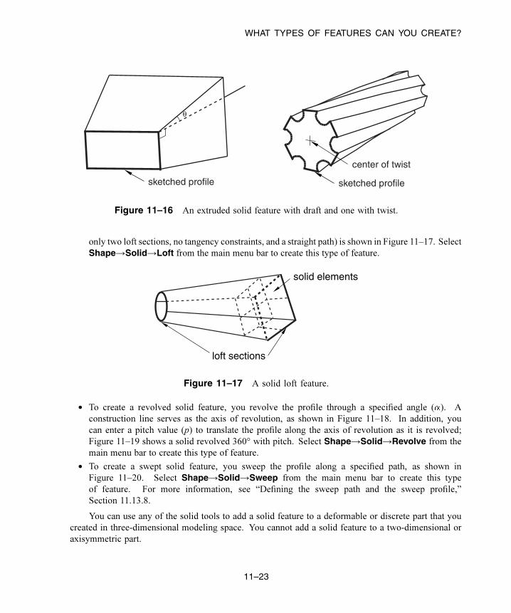
WHAT TYPES OF FEATURES CAN YOU CREATE?
θ
sketched profile sketched profile
center of twist
Figure 11–16 An extruded solid feature with draft and one with twist.
only two loft sections, no tangency constraints, and a straight path) is shown in Figure 11–17. Select
Shape→Solid→Loft from the main menu bar to create this type of feature.
solid elements
loft sections
Figure 11–17 A solid loft feature.
• To create a revolved solid feature, you revolve the profile through a specified angle ( ). A
construction line serves as the axis of revolution, as shown in Figure 11–18. In addition, you
can enter a pitch value (p) to translate the profile along the axis of revolution as it is revolved;
Figure 11–19 shows a solid revolved 360° with pitch. Select Shape→Solid→Revolve from the
main menu bar to create this type of feature.
• To create a swept solid feature, you sweep the profile along a specified path, as shown in
Figure 11–20. Select Shape→Solid→Sweep from the main menu bar to create this type
of feature. For more information, see “Defining the sweep path and the sweep profile,”
Section 11.13.8.
You can use any of the solid tools to add a solid feature to a deformable or discrete part that you
created in three-dimensional modeling space. You cannot add a solid feature to a two-dimensional or
axisymmetric part.
11–23
Abaqus ID:
Printed on:
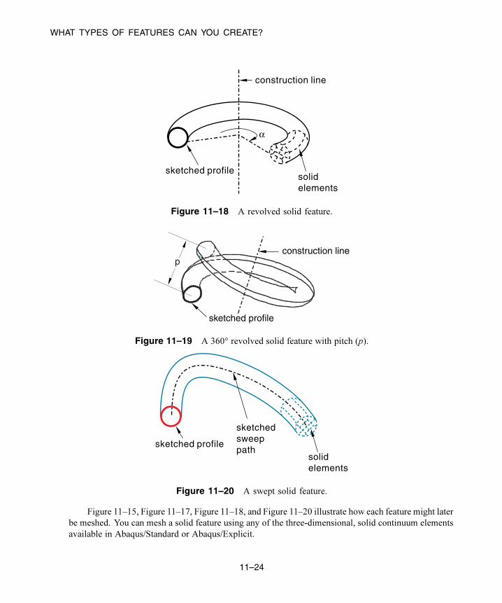
WHAT TYPES OF FEATURES CAN YOU CREATE?
solid elements
sketched profile
construction line
α
Figure 11–18 A revolved solid feature.
sketched profile
pconstruction line
Figure 11–19 A 360° revolved solid feature with pitch (p).
solid elements
sketched profile
sketchedsweeppath
Figure 11–20 A swept solid feature.
Figure 11–15, Figure 11–17, Figure 11–18, and Figure 11–20 illustrate how each feature might later
be meshed. You can mesh a solid feature using any of the three-dimensional, solid continuum elements
available in Abaqus/Standard or Abaqus/Explicit.
11–24
Abaqus ID:
Printed on:

WHAT TYPES OF FEATURES CAN YOU CREATE?
The HTML version of this guide contains detailed instructions on using the Part module tools to
add a solid feature to a three-dimensional solid part. The following topics are covered:
• “Adding an extruded solid feature,” Section 11.21.1
• “Adding a revolved solid feature,” Section 11.21.2
• “Adding a swept solid feature,” Section 11.21.3
• “Adding a solid loft feature,” Section 11.21.4
11.9.2 Shell featuresA shell feature is an idealization of a solid in which thickness is considered small compared to the width
and depth. To create a shell feature, select Shape→Shell from the main menu bar or select one of the
shell tools in the Part module toolbox. You create a shell feature by using the shell tools to do one of the
following:
• To create an extruded shell feature, you sketch a profile and extrude it through a specified distance
(d), as shown in Figure 11–21.
d extruded depth
sketchedprofile
shellelements
Figure 11–21 An extruded shell feature.
In addition, you can apply either draft or twist to the extrusion, as shown in Figure 11–22.
sketched profile
θ
sketched profile
Figure 11–22 An extruded shell feature with draft and one with twist.
11–25
Abaqus ID:
Printed on:

WHAT TYPES OF FEATURES CAN YOU CREATE?
You define the draft angle for an extrusion with draft or the center of twist and the pitch (the extrusion
distance in which a 360° twist occurs) for an extrusion with twist. Select Shape→Shell→Extrudefrom the main menu bar to create this type of feature.
• To create a shell loft feature, you transition the shape from the initial loft section to an end section
of a different shape or orientation. Abaqus/CAE determines the shape between the start and end
sections using tangency constraints, intermediate sections, and a path curve. A simple loft (with
only two loft sections, no tangency constraints, and a straight path) is shown in Figure 11–23. Select
Shape→Shell→Loft from the main menu bar to create this type of feature.
shell elements
loft sections
Figure 11–23 A shell loft feature.
• To create a revolved shell feature, you sketch a profile and revolve it through a specified angle (α).
A construction line serves as the axis of revolution, as shown in Figure 11–24.
sketchedprofile
shellelements
construction line
α
Figure 11–24 A revolved shell feature.
In addition, you can enter a pitch value to translate the profile along the axis of revolution as it is
revolved; Figure 11–25 shows a revolved shell with pitch.
11–26
Abaqus ID:
Printed on:

WHAT TYPES OF FEATURES CAN YOU CREATE?
sketchedprofileh
Figure 11–25 A revolved shell feature with pitch.
The dimension h represents the translation of the sketched profile due to pitch; h would be equal
to the pitch if the part was revolved a full 360°. Select Shape→Shell→Revolve from the main
menu bar to create this type of feature.
• To create a swept shell feature, you sketch a profile and sweep it along a specified path, as shown
in Figure 11–26.
sketchedprofile
sketchedsweep path
shellelements
Figure 11–26 A swept shell feature.
Select Shape→Shell→Sweep from the main menu bar to create this type of feature. For more
information, see “Defining the sweep path and the sweep profile,” Section 11.13.8.
• To create a planar shell feature, you sketch the outline of the shell on a selected planar face or
datum plane, as shown in Figure 11–27. When you sketch on a planar face (for example, the side
11–27
Abaqus ID:
Printed on:

WHAT TYPES OF FEATURES CAN YOU CREATE?
1
2
3
sketchedprofiles
selectedface
shell elements
Figure 11–27 A sketched shell feature.
of a cube), the shell feature is created only where it extends beyond the face; a shell feature cannot
overlap a face. A sketch on a planar face of a cube and the resulting shell feature are shown in
Figure 11–27. In this example the shell feature is a fin extending beyond the selected face of the
cube. Select Shape→Shell→Planar from the main menu bar to create this type of feature.
• To create a shell-from-solid feature, you convert the faces of a solid feature to shell features;
in effect, hollow out a solid. A shell-from-solid feature is shown in Figure 11–28. Select
Shape→Shell→From Solid from the main menu bar to create this type of feature.
You can use any of the shell tools to add a shell feature to a part that you created in three-dimensional
modeling space; however, when you are working on parts created in two-dimensional or axisymmetric
modeling space, you can use only the planar shell tool to add a shell feature. You use the Property
module to create a section prescribing the desired thickness and to assign the section to the shell feature.
For more information, see “Defining sections,” Section 12.2.3, and “Which properties can I assign to a
part?,” Section 12.3.
Many of the figures illustrate how the shell features might later be meshed. You can mesh a shell
feature using:
• Two-dimensional or axisymmetric continuum elements (limited to planar shell features)
• Three-dimensional shell elements
• Membrane elements
11–28
Abaqus ID:
Printed on:

WHAT TYPES OF FEATURES CAN YOU CREATE?
⇒
solid model
shell elements
Figure 11–28 A shell-from-solid feature.
The HTML version of this guide contains detailed instructions on using the Part module tools to
add a shell feature to a three-dimensional solid part, a two-dimensional planar part, or an axisymmetric
part. The following topics are covered:
• “Adding an extruded shell feature,” Section 11.22.1
• “Adding a revolved shell feature,” Section 11.22.2
• “Adding a swept shell feature,” Section 11.22.3
• “Adding a shell loft feature,” Section 11.22.4
• “Adding a planar shell feature,” Section 11.22.5
• “Adding a shell-from-solid feature,” Section 11.22.6
11.9.3 Wire featuresA wire is depicted as a line in Abaqus/CAE and is used to idealize a solid in which both its thickness and
depth are considered small compared to its length. To create a wire feature, select Shape→Wire from
the main menu bar or select one of the wire tools in the Part module toolbox. You create a wire feature
in the Part module using the wire tools to do one of the following:
• Sketch a wire on a selected planar face or datum plane to create a sketched wire feature, as shown
in Figure 11–29. Select Shape→Wire→Sketch from the main menu bar to create this type of
feature.
11–29
Abaqus ID:
Printed on:

WHAT TYPES OF FEATURES CAN YOU CREATE?
elements
sketched profile
Figure 11–29 A sketched wire feature.
When you sketch on a planar face (for example, the side of a cube), the wire feature is created only
where it extends beyond the face.
• Connect two or more points with straight lines, as shown in Figure 11–30, or with a spline curve, as
shown in Figure 11–31. Select Shape→Wire→Point to Point from the main menu bar to create
this type of feature. Select Polyline or Spline for the Geometry Type to create straight lines or a
spline curve, respectively. You can use the Merge wire with part geometry option to create only
those wire segments that are unique from existing part geometry, or turn this option off to create
all segments of the point-to-point wire. The rectangular solid feature in Figure 11–31 is shown for
reference. The image on the left shows the full length of the spline wire, while the image on the right
shows a spline wire connecting the same set of points using the Merge wire with part geometryoption. You can create geometry sets that include the wires and vertices defined in the wire feature.
elements
Figure 11–30 A wire feature connecting three points.
11–30
Abaqus ID:
Printed on:

WHAT TYPES OF FEATURES CAN YOU CREATE?
Figure 11–31 A wire feature connecting several points of a solid feature.
You can use the wire tools to add a wire feature to any deformable or discrete rigid part. You cannot
add a wire feature to an analytical rigid part; you can only modify the original sketch that defined that
part.
You use the Property module to create a section that prescribes the desired cross-sectional
geometry and to assign that section to the wire feature. (For more information, see “Defining sections,”
Section 12.2.3, and “Which properties can I assign to a part?,” Section 12.3.) You can model a wire
feature using any of the beam, truss, or axisymmetric shell elements available in Abaqus/Standard or
Abaqus/Explicit.
Note: Although you can create a mesh of beam elements, the current release of Abaqus/CAE allows
you to assign only the following sections to a wire:
• Beam section
• Truss section
The HTML version of this guide contains detailed instructions on using the Part module tools to
add a wire feature to a three-dimensional solid part, a two-dimensional planar part, or an axisymmetric
part. The following topics are covered:
• “Adding a sketched wire feature,” Section 11.23.1
• “Adding a point-to-point wire feature,” Section 11.23.2
11.9.4 Cut featuresA cut is a feature that removes material from a part. A cut can be a circular hole, or it can be any arbitrary
shape. The sketched profile of any cut must be closed. In many cases the entire profile will affect the
shape of the cut feature, even if it does not initially contact the surface being cut. To create a cut feature,
select Shape→Cut from the main menu bar or select one of the cut tools in the Part module toolbox.
11–31
Abaqus ID:
Printed on:

WHAT TYPES OF FEATURES CAN YOU CREATE?
Note: Most of the figures do not show a closed cut profile where it intersects with the part surface.
These lines have been removed to show the shape of the cut feature.
Once you have sketched the initial profile, you perform one of the following operations to create a
cut feature:
• To create an extruded cut, you extrude the profile through a specified distance (d), as shown in
Figure 11–32.
d
sketchedprofile
Figure 11–32 An extruded cut feature.
In addition, you can apply either draft or twist to the extruded cut, as shown in Figure 11–33.
You define the draft angle for an extruded cut with draft or the center of twist and the pitch
(the extrusion distance in which a 360° twist occurs) for an extruded cut with twist. Select
Shape→Cut→Extrude from the main menu bar to create this type of feature.
sketched profile
Figure 11–33 Extruded cut features with draft and twist.
• To create a cut loft feature, you transition the shape from the initial loft section to an end section
of a different shape or orientation, as shown in Figure 11–34. Abaqus/CAE determines the shape
11–32
Abaqus ID:
Printed on:
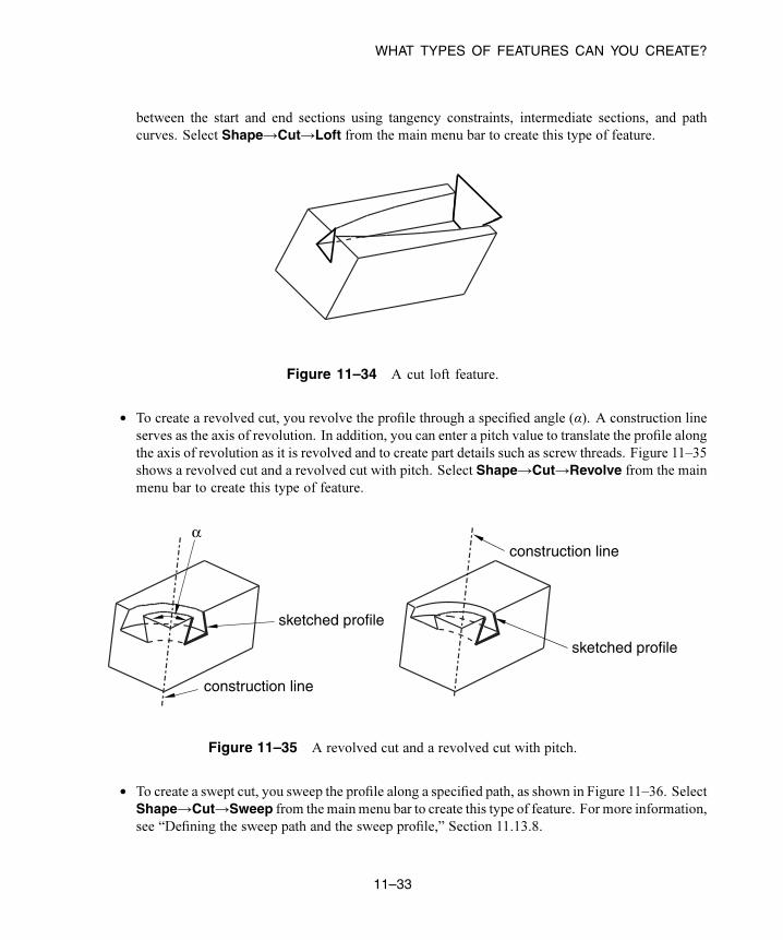
WHAT TYPES OF FEATURES CAN YOU CREATE?
between the start and end sections using tangency constraints, intermediate sections, and path
curves. Select Shape→Cut→Loft from the main menu bar to create this type of feature.
Figure 11–34 A cut loft feature.
• To create a revolved cut, you revolve the profile through a specified angle (α). A construction line
serves as the axis of revolution. In addition, you can enter a pitch value to translate the profile along
the axis of revolution as it is revolved and to create part details such as screw threads. Figure 11–35
shows a revolved cut and a revolved cut with pitch. Select Shape→Cut→Revolve from the main
menu bar to create this type of feature.
construction line
α
sketched profile
construction line
sketched profile
Figure 11–35 A revolved cut and a revolved cut with pitch.
• To create a swept cut, you sweep the profile along a specified path, as shown in Figure 11–36. Select
Shape→Cut→Sweep from the mainmenu bar to create this type of feature. For more information,
see “Defining the sweep path and the sweep profile,” Section 11.13.8.
11–33
Abaqus ID:
Printed on:

WHAT TYPES OF FEATURES CAN YOU CREATE?
sketched profile
Figure 11–36 A swept cut feature.
• To create a circular hole, you enter the diameter of a hole and the distance of its center from two
selected edges, as shown in Figure 11–37. Select Shape→Cut→Circular Hole from the main
menu bar to create this type of feature.
d1d
2
diameter
Figure 11–37 A circular hole feature.
When you are sketching the profile of an extruded, revolved, or swept cut, you can sketch multiple
profiles in a single sketch. Abaqus/CAE extrudes each of the profiles when you exit the Sketcher and
creates a cut corresponding to each profile as shown in Figure 11–38. The sequence of cuts is stored as
a single feature, and you can edit it only as a single feature. For example, if you change the extrusion
depth, the depth will change for all the cuts in the feature.
You can use the cut tools to add a cut feature to any deformable or discrete rigid part. You cannot
add a cut feature to an analytical rigid part; you can only modify the original sketch that defined that part.
The HTML version of this guide contains detailed instructions on using the Part module tools to
add a cut feature to a three-dimensional solid part, a two-dimensional planar part, or an axisymmetric
part. The following topics are covered:
• “Creating an extruded cut,” Section 11.24.1
• “Creating a loft cut,” Section 11.24.2
• “Creating a revolved cut,” Section 11.24.3
• “Creating a swept cut,” Section 11.24.4
11–34
Abaqus ID:
Printed on:

WHAT TYPES OF FEATURES CAN YOU CREATE?
Figure 11–38 Multiple profiles extruded from a single sketch.
• “Cutting a circular hole,” Section 11.24.5
11.9.5 Blend features
A blend feature smooths an edge of a three-dimensional solid part. To create a blend feature, select
Shape→Blend from the main menu bar or select one of the blend tools in the Part module toolbox. You
create a blend feature in the Part module using the blend tools to do one of the following:
• Smooth an edge with a circular blend of a specified radius, as shown in Figure 11–39. Select
Shape→Blend→Round/Fillet from the main menu bar to create this type of feature.
• Bevel an edge with a chamfered blend of a specified length, as shown in Figure 11–40. Select
Shape→Blend→Chamfer from the main menu bar to create this type of feature.
You can use the blend tools to blend edges of a deformable or discrete rigid part that you created in
three-dimensional modeling space. You cannot add a blend feature to a two-dimensional or axisymmetric
part; however, you can blend its corners by editing the sketch of the part.
The HTML version of this guide contains detailed instructions on using the Part module tools to
blend edges of a three-dimensional part. The following topics are covered:
• “Rounding edges,” Section 11.27.1
• “Chamfering edges,” Section 11.27.2
11–35
Abaqus ID:
Printed on:
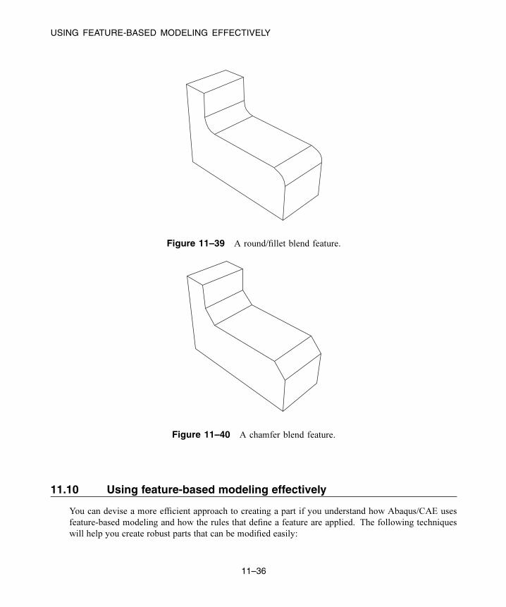
USING FEATURE-BASED MODELING EFFECTIVELY
Figure 11–39 A round/fillet blend feature.
Figure 11–40 A chamfer blend feature.
11.10 Using feature-based modeling effectively
You can devise a more efficient approach to creating a part if you understand how Abaqus/CAE uses
feature-based modeling and how the rules that define a feature are applied. The following techniques
will help you create robust parts that can be modified easily:
11–36
Abaqus ID:
Printed on:

USING FEATURE-BASED MODELING EFFECTIVELY
Plan a strategy
Feature-based modeling provides flexibility, but it can also add overhead to your model. For
example, you can suppress an extrusion using the suppress tool in the Feature Manipulation toolset.
Alternatively, you could effectively suppress the extrusion by removing it with a cut feature.
Although you could restore the extrusion subsequently by removing the cut feature, the resulting
part contains additional feature-based information that can slow down regeneration. Regeneration
speed can be improved by using the geometry cache to save parts in different states, but the cache
uses system memory that may be needed for other operations (for more information, see “Tuning
feature regeneration,” Section 65.3). In addition, dependencies may cause feature regeneration to
fail if you add more detail to the part; and, because the extrusion is no longer visible, the cause of
the failure to regenerate may be hard to determine.
Before you decide how to create a part, you should always consider if you will ever need to
modify the part in the future. If you decide that you might need to modify the part, you should
consider the techniques that you will use to create the features that define the part. The simplest
techniques may not provide the flexibility you need for modifying the features. You may find it
cumbersome to edit or suppress individual items of geometry, such as an extrusion, a fillet, or a
hole.
Alternatively, if you know that you will never change the final design, you may not need
the flexibility provided by feature-based modeling and can use the simplest and most convenient
techniques to define the part.
In general, you should try to finish creating your parts in the Part module before you start
creating part instances and positioning them in the assembly. You should try to finish creating all
your parts before you apply attributes to the assembly, such as sets, loads, and boundary conditions.
If you apply attributes to the assembly and then return to the Part module to modify the original part,
Abaqus/CAE may not be able to determine where the attribute should be applied. For example, if
you apply a pressure load to a face and then return to the Part module to partition the face into two
regions, Abaqus/CAE will apply the pressure to only one of the regions.
Use reference geometry
When you are adding a feature to a part, you should always use underlying reference geometry to
define the new feature’s location relative to existing features. While sketching a feature, you may
be able to select reference geometry directly; for example, if you are sketching a circle, you may be
able to select a vertex from the reference geometry to define its center. Alternatively, you may have
to add a dimension between reference geometry and the new feature. If you do not use reference
geometry to position the sketch of a new feature and you subsequently modify the part, the resulting
changes to the feature can be unpredictable.
Use dimensions
Dimensions add clarity to the sketches that define features and document your design intent for
future reference. Dimensions also add constraints to your sketches. You can modify dimensions in
the Sketcher, and the part and assembly will regenerate accordingly.
11–37
Abaqus ID:
Printed on:
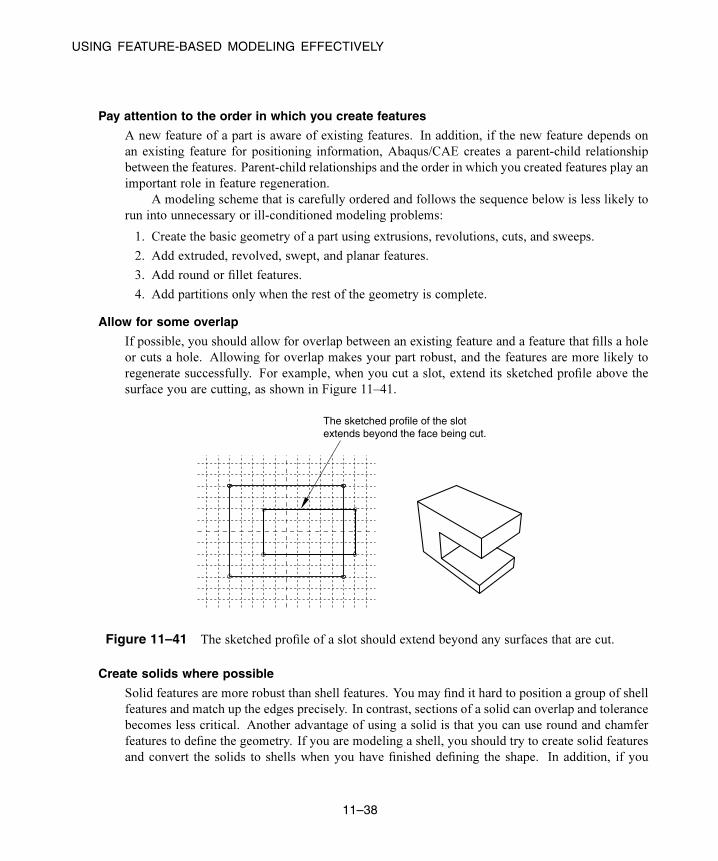
USING FEATURE-BASED MODELING EFFECTIVELY
Pay attention to the order in which you create features
A new feature of a part is aware of existing features. In addition, if the new feature depends on
an existing feature for positioning information, Abaqus/CAE creates a parent-child relationship
between the features. Parent-child relationships and the order in which you created features play an
important role in feature regeneration.
A modeling scheme that is carefully ordered and follows the sequence below is less likely to
run into unnecessary or ill-conditioned modeling problems:
1. Create the basic geometry of a part using extrusions, revolutions, cuts, and sweeps.
2. Add extruded, revolved, swept, and planar features.
3. Add round or fillet features.
4. Add partitions only when the rest of the geometry is complete.
Allow for some overlap
If possible, you should allow for overlap between an existing feature and a feature that fills a hole
or cuts a hole. Allowing for overlap makes your part robust, and the features are more likely to
regenerate successfully. For example, when you cut a slot, extend its sketched profile above the
surface you are cutting, as shown in Figure 11–41.
The sketched profile of the slotextends beyond the face being cut.
Figure 11–41 The sketched profile of a slot should extend beyond any surfaces that are cut.
Create solids where possible
Solid features are more robust than shell features. You may find it hard to position a group of shell
features and match up the edges precisely. In contrast, sections of a solid can overlap and tolerance
becomes less critical. Another advantage of using a solid is that you can use round and chamfer
features to define the geometry. If you are modeling a shell, you should try to create solid features
and convert the solids to shells when you have finished defining the shape. In addition, if you
11–38
Abaqus ID:
Printed on:

CAPTURING YOUR DESIGN AND ANALYSIS INTENT
subsequently want to add additional shell features to a shell part, where the shell part was generated
from a solid, you should do the following:
1. Delete the last solid-to-shell feature to convert the model back to a solid.
2. Add your new solid features.
3. Create a new solid-to-shell feature to convert the model back to a shell.
11.11 Capturing your design and analysis intent
If used carefully, the feature-based modeling approach used by Abaqus/CAE allows you to capture both
your design and analysis intent.
Design intent is the capability to make changes based on design considerations. For example, when
you add a cut feature, you can select either a through cut or a blind cut. If the cut feature represents a
bolt hole, you know that the hole must always pass completely through the part. As a consequence, you
should select a through cut, and Abaqus/CAE recognizes that the hole remains through even when you
change the thickness of the part.
Analysis intent is the capability to make changes based on analysis considerations. Although
Abaqus/CAE allows you to create parts with complex, detailed geometry, your final goal is usually
a finite element analysis of a meshed representation of the part. Excessive detail, such as fillets and
small holes, can lead to regions with a very fine mesh that will, in turn, dominate the time taken by
Abaqus/Standard or Abaqus/Explicit to reach a solution. The amount of detail you provide when you
create a part in the Part module should be a reflection of your goals. Alternatively, you can create a part
with detailed features but suppress them prior to meshing the assembly. For example, if a model takes
several hours to analyze, you may wish to simplify it by suppressing features; you could then submit an
analysis that runs faster and checks your basic modeling assumptions. If the simplified model behaves
as expected, you can unsuppress the features and resubmit a full analysis.
For an example of different feature-based design approaches based on design and analysis intent,
consider the cover plate shown in Figure 11–42.
Figure 11–42 A model of a cover plate.
11–39
Abaqus ID:
Printed on:

WHAT IS PART AND ASSEMBLY LOCKING?
You could create the three-dimensional shell that models the plate in several ways:
1. Sketch a base feature that includes the four holes.
2. Sketch a rectangular base feature, and add four separate cut features.
3. Sketch a rectangular base feature, and add a single cut feature that cuts all four holes.
Either of the three approaches would generate the same part, but your design intent and your analysis
intent govern the best approach. For example:
• Do you want to create and analyze plates of varying sizes with different sized holes for different
applications? If the diameter of all four holes is always identical, you should create all four holes
as a single cut feature. However, if the diameter of individual holes might differ, you should create
four separate cut features.
• Do you want to suppress features before you finalize your design? For example, you could perform
a series of analyses with the holes suppressed to determine the desired plate thickness. You could
then unsuppress the holes and analyze the finished model. In addition, suppressing features may
simplify the mesh that Abaqus/CAE generates, or suppressing features may make the assembly
sweep meshable.
If you want to suppress all four holes in the example of the rectangular cover plate, you should
create all four holes as a single cut feature. However, if you want to suppress individual holes, you
should create four separate cut features. If the analysis is straightforward and you do not need to
analyze a simplified model, you should sketch a base feature that includes the four holes.
11.12 What is part and assembly locking?
Part and assembly locking is an Abaqus/CAE function that prevents any changes to the features of a part
or to the features of the assembly. You can lock parts or the assembly to prevent accidental changes,
such as when sharing a model with other Abaqus users or when working on a model that contains many
similar parts. You must unlock a part or the assembly if you plan on modifying it.
Note: Part and assembly locking is not a security feature; any user can unlock and modify parts and
assemblies that were locked by another user.
You can click mouse button 3 on a part or on the assembly in the Model Tree and use the menu that
appears to lock and unlock the feature. A padlock before the feature name in the Model Tree indicates
that a part or the assembly has been locked by the user or by a database upgrade. For more information,
see “Using the Model Tree to manage features,” Section 65.2.
Alternatively, you can use the Part Manager to lock or unlock any part in a model. If the part is
unlocked, the Status field is empty in the Part Manager. If the part is locked, the Status field indicates
one of two conditions:
11–40
Abaqus ID:
Printed on:

WHAT ARE EXTRUDING, REVOLVING, AND SWEEPING?
Locked (Database upgrade)
Abaqus/CAE locked the part automatically while upgrading the model from a previous release of
Abaqus.
Locked
A user locked the part using the Model Tree or the Part Manager.
Abaqus/CAE automatically locks the assembly and all the parts in a model when it upgrades a
database from an older release of Abaqus. Locking the assembly and the parts allows Abaqus/CAE to
complete the upgrade faster than if the assembly and all the parts were also regenerated. If you unlock a
part that was locked by a database upgrade, Abaqus/CAE regenerates that part. Similarly, if you unlock
an assembly that was locked by a database upgrade, Abaqus/CAE regenerates the assembly.
WARNING: If a part is locked due to a database upgrade, you should unlock the part prior to making anychanges to set or property definitions. If you unlock the part after making modifications, your changes
can become invalid when Abaqus/CAE regenerates the part.
If you unlock a part that you locked with the Model Tree or the Part Manager, Abaqus/CAE does
not regenerate the part because it could not be modified while it was locked. Similarly, Abaqus/CAE
does not regenerate the assembly when you unlock it after locking it with the Model Tree. If a part
that you unlock fails to regenerate, both the locked version and the unlocked version are retained. You
can recreate missing features on the unlocked version of the part and use it to replace the locked part
throughout the model.
You can instance a locked part and use it in the assembly. In addition, you can add or delete set or
property definitions to a locked part or to a locked assembly. However, you must unlock a part or the
assembly before you can add features to it or edit existing features.
11.13 What are extruding, revolving, and sweeping?
The following sections describe the techniques you can use to extrude, revolve, and sweep a
two-dimensional sketch to create a three-dimensional part or feature.
11.13.1 Defining the extrusion distanceYou can sketch a two-dimensional profile and extrude it to create the following:
• A three-dimensional extruded solid feature.
• A three-dimensional extruded shell feature.
• A three-dimensional extruded cut feature.
11–41
Abaqus ID:
Printed on:

WHAT ARE EXTRUDING, REVOLVING, AND SWEEPING?
Abaqus/CAE provides the following methods for defining the extrusion distance:
Blind
Specify the distance over which Abaqus/CAE extrudes the sketch. The sketch and the distance
define the feature and can be edited using the Feature Manipulation toolset. You can use this method
when creating extruded solid, shell, and cut features. Figure 11–43 illustrates a blind extruded cut
in a solid part.
sketch plane
d
Figure 11–43 A blind extruded cut.
Up to Face
Select a single face to which Abaqus/CAE extrudes the sketch. The selected face does not have to be
parallel to the sketch plane. The selected face can be a nonplanar face; however, it must completely
contain the extruded section. If you select this method to define the extrusion distance, only the
sketch can be modified using the Feature Manipulation toolset; if you wish to extrude to a different
face, you must create a new extruded cut feature. You can use this method when creating extruded
solid, shell, and cut features. Figure 11–44 illustrates a sketch extruded to a nonplanar face.
extrude tothis face
sketchplane
Figure 11–44 A solid feature extruded up to a nonplanar face.
Through All
This method is available only for extruded cut features. Abaqus/CAE extrudes the sketch defining
the profile of the cut completely though the part. If you select this method to define the extrusion
11–42
Abaqus ID:
Printed on:

WHAT ARE EXTRUDING, REVOLVING, AND SWEEPING?
distance, only the sketch can be modified using the Feature Manipulation toolset. Figure 11–45
illustrates a through all cut in a solid part.
sketch plane
Figure 11–45 A through all extruded cut.
11.13.2 Controlling the direction of an extruded featureWhen you add an extruded feature to a three-dimensional part, Abaqus/CAE chooses a default direction
of extrusion from the sketched profile based on the type of feature you are creating. By default, a solid
or shell feature is extruded outward such that material is added to the existing base feature. Conversely,
a cut feature is extruded inward such that material is removed from the existing base feature.
You can control the direction of an extruded feature as follows:
Choosing the direction while adding an extruded feature
When you complete the sketch to add an extruded feature to an existing part, Abaqus/CAE displays
the new sketched profile on the original part. The sketched profile includes an arrow that indicates
the extrusion direction. Abaqus/CAE also displays the Edit Extrusion dialog box.
You can control the direction of extrusion by clicking in the Edit Extrusion dialog box.
The arrow in the viewport changes direction to show the new extrusion direction.
Editing the direction of an existing extruded feature
When you select an extruded feature to edit, Abaqus/CAE highlights the selected feature in the
viewport and the Edit Feature dialog box appears.
You can reverse the direction of extrusion by toggling Flip extrude direction in the EditFeature dialog box. Abaqus/CAE does not display an arrow that indicates the direction of
extrusion; however, you can click Apply to view your changes. When the direction is acceptable,
click OK to end the editing process.
You cannot change the direction of extrusion when you are creating a new part because the part would
be identical regardless of the direction.
11–43
Abaqus ID:
Printed on:

WHAT ARE EXTRUDING, REVOLVING, AND SWEEPING?
11.13.3 Including twist in an extrusionYou can choose to include twist during the creation of an extrusion. Twist can be used to create twisted
cables, helical gears, and other complex shapes that can be formed by passing a constant cross-section
through a sequence of parallel planes. Twist modifies an extrusion by rotating the sketched profile about
an axis parallel to the direction of extrusion. The center of twist is an isolated point in the sketched
profile; it is the point at which the axis used to twist the extrusion passes through the sketch plane. The
pitch defines the extrusion distance in which the profile would be twisted by 360°. You can modify the
extrusion profile, extrusion direction, center of twist, and pitch using the Feature Manipulation toolset.
You can add twist during the creation of extruded solid, shell, and cut features. Figure 11–46
illustrates a twisted extrusion.
sketched profile
center of twist
Figure 11–46 A solid feature extruded with twist.
If you want to create complex shapes in which the sketched profile is revolved rather than extruded,
such as screw threads or coil springs, you can include pitch in a revolved solid, shell, or cut feature.
See “What types of features can you create?,” Section 11.9, for basic information about all the available
feature types and “Defining the axis of revolution for axisymmetric parts and for revolved features,”
Section 11.13.5, for more information about revolved features.
11.13.4 Including draft in an extrusionYou can choose to create an extrusion with draft. Draft can be used to accurately represent the small
angle often applied to ease the removal of cast or molded parts from the tooling. Draft in an extrusion
can also be used to create tapered parts.
In a straight extrusion the draft angle is 0°, so all extruded surfaces are perpendicular to the original
profile. Draft modifies an extrusion by adjusting the angle between the extruded surfaces and the original
sketch plane. Abaqus/CAE reverses the application of draft angle from internal to external features. If
external loops in a sketched profile are expanding, internal ones are contracting; this behavior is expected
for draft and is required for part removal from tooling (all surfaces taper in the same direction).
11–44
Abaqus ID:
Printed on:

WHAT ARE EXTRUDING, REVOLVING, AND SWEEPING?
You can modify draft, along with the extrusion profile and direction, using the Feature Manipulation
toolset. You can add draft during the creation of extruded solid, shell, and cut features. Figure 11–47
illustrates an extruded cut with draft in a solid part.
sketched profile
Figure 11–47 A cut feature extruded with draft.
Note: The complete sketched profile for the cut in Figure 11–47 is a triangle, as shown. If the profile
were a trapezoid whose top edge coincided with the edge of the block, the cut would look very different.
As the profile was extruded, the application of draft made it smaller. The top face of a trapezoid profile
would immediately fall below the surface of the block instead of extending through the top surface.
Abaqus/CAE cannot mesh an extruded solid that includes draft with hexahedral elements unless
you partition the solid into structured regions.
11.13.5 Defining the axis of revolution for axisymmetric parts and forrevolved features
When you create an axisymmetric part and when you add a revolved feature to a part, the sketch of the
profile must include a construction line that defines the axis of rotation. The following rules apply to the
sketch and to the construction line:
Creating an axisymmetric part
You can create axisymmetric parts that are defined by either a shell or a wire along with an axis of
symmetry by selecting Part→Create from the main menu bar. Abaqus/CAE allows you to include
a twist degree of freedom in your model when you create an axisymmetric part.
When you sketch the part’s base feature, Abaqus/CAE displays a vertical construction line on
the Y-axis of the sketch representing the axis of symmetry. You must sketch only to the right of the
line. Your sketch can touch this line but cannot cross it.
You can add only shell and wire features to an axisymmetric base feature. Abaqus/CAE
displays the original sketch and construction line when you add a feature, and the same rules
apply—you cannot delete this construction line, and you must sketch only to the right of it.
11–45
Abaqus ID:
Printed on:

WHAT ARE EXTRUDING, REVOLVING, AND SWEEPING?
Creating revolved features
You can create three-dimensional parts with a revolved solid or a revolved shell base feature
by selecting Part→Create from the main menu bar. Similarly, you can add revolved solids,
shells, and cuts to three-dimensional solids and shells by selecting Shape→Solid→Revolve,Shape→Shell→Revolve, or Shape→Cut→Revolve from the main menu bar.
The sketch of a revolved feature must contain a construction line representing the axis of
revolution. When you create a new revolved part, Abaqus/CAE creates a vertical construction line
through the origin of the Sketcher grid. If desired, you can delete this construction line and redraw
it at a new angle and position. In contrast, when you add a revolved feature to an existing part, you
must sketch the construction line representing the axis of revolution. You can sketch to the right
or to the left of the construction line. Your sketch can touch this line but cannot cross it. If the
completed sketch contains more than one construction line, Abaqus/CAE prompts you to select the
line that will represent the axis of revolution.
When you are sketching the construction line that represents the axis of revolution, you can
position the construction line by selecting a datum axis from the underlying part if one exists. You
cannot select the datum axis directly; you must select a point from either end of the datum axis. You
can use the datum axis to create concentric features.
When you exit the Sketcher, Abaqus/CAE opens a dialog box to complete the definition of the
revolved feature. You enter the angle through which the profile will be revolved and the direction
of revolution, and you can choose whether to translate the profile along the axis of revolution by
including pitch. You can also specify the direction of translation. The pitch value is the distance
through which the profile would be translated during a rotation of 360°. Pitch allows the creation
of parts such as coil springs and part details such as screw threads.
If you want to create complex shapes in which the sketched profile is extruded rather than revolved,
such as twisted cables or helical gears, you can include twist in an extruded solid, shell, or cut feature.
See “What types of features can you create?,” Section 11.9, for basic information about all the available
feature types and “Defining the extrusion distance,” Section 11.13.1, for more information about extruded
features.
11.13.6 Controlling the direction of a revolved featureWhen you create a part with a revolved base feature or add a revolved feature to a three-dimensional
part, you can control the direction of revolution. If you include pitch in a revolved feature, you can also
control the direction of translation. The descriptions that follow provide the details of controlling both
the direction of revolution and, if applicable, the direction of translation for any revolved feature that
you create in Abaqus/CAE:
Choosing the direction while creating a revolved feature
When you complete the sketch to create a revolved feature, Abaqus/CAE displays the sketched
profile including an arrow that indicates the direction of revolution. If you are creating a part with
11–46
Abaqus ID:
Printed on:
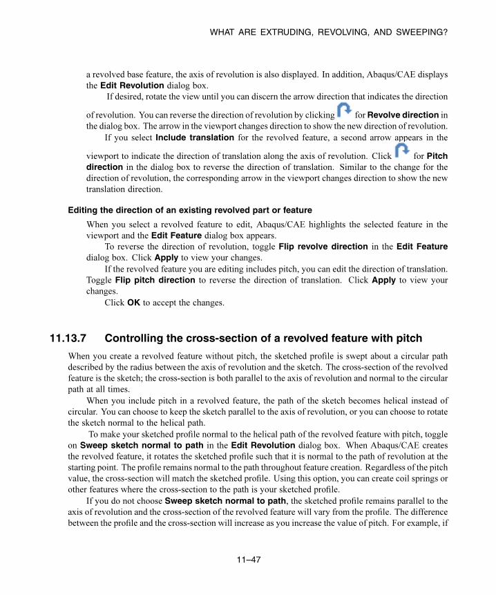
WHAT ARE EXTRUDING, REVOLVING, AND SWEEPING?
a revolved base feature, the axis of revolution is also displayed. In addition, Abaqus/CAE displays
the Edit Revolution dialog box.
If desired, rotate the view until you can discern the arrow direction that indicates the direction
of revolution. You can reverse the direction of revolution by clicking for Revolve direction in
the dialog box. The arrow in the viewport changes direction to show the new direction of revolution.
If you select Include translation for the revolved feature, a second arrow appears in the
viewport to indicate the direction of translation along the axis of revolution. Click for Pitchdirection in the dialog box to reverse the direction of translation. Similar to the change for the
direction of revolution, the corresponding arrow in the viewport changes direction to show the new
translation direction.
Editing the direction of an existing revolved part or feature
When you select a revolved feature to edit, Abaqus/CAE highlights the selected feature in the
viewport and the Edit Feature dialog box appears.
To reverse the direction of revolution, toggle Flip revolve direction in the Edit Featuredialog box. Click Apply to view your changes.
If the revolved feature you are editing includes pitch, you can edit the direction of translation.
Toggle Flip pitch direction to reverse the direction of translation. Click Apply to view your
changes.
Click OK to accept the changes.
11.13.7 Controlling the cross-section of a revolved feature with pitch
When you create a revolved feature without pitch, the sketched profile is swept about a circular path
described by the radius between the axis of revolution and the sketch. The cross-section of the revolved
feature is the sketch; the cross-section is both parallel to the axis of revolution and normal to the circular
path at all times.
When you include pitch in a revolved feature, the path of the sketch becomes helical instead of
circular. You can choose to keep the sketch parallel to the axis of revolution, or you can choose to rotate
the sketch normal to the helical path.
To make your sketched profile normal to the helical path of the revolved feature with pitch, toggle
on Sweep sketch normal to path in the Edit Revolution dialog box. When Abaqus/CAE creates
the revolved feature, it rotates the sketched profile such that it is normal to the path of revolution at the
starting point. The profile remains normal to the path throughout feature creation. Regardless of the pitch
value, the cross-section will match the sketched profile. Using this option, you can create coil springs or
other features where the cross-section to the path is your sketched profile.
If you do not choose Sweep sketch normal to path, the sketched profile remains parallel to the
axis of revolution and the cross-section of the revolved feature will vary from the profile. The difference
between the profile and the cross-section will increase as you increase the value of pitch. For example, if
11–47
Abaqus ID:
Printed on:

WHAT ARE EXTRUDING, REVOLVING, AND SWEEPING?
there is no pitch, a circular sketched profile creates a circular cross-section. If you increase the pitch, the
cross-section will become increasingly elliptical. You can create screw threads or other features where
the cross-section parallel to the axis of revolution is your sketched profile.
To change the cross-section behavior after the feature is created, you can toggle Move sketchnormal to path in the Edit Feature dialog box.
11.13.8 Defining the sweep path and the sweep profileTo create a swept feature, select Shape→Solid→Sweep, Shape→Shell→Sweep, or
Shape→Cut→Sweep from the main menu bar or select the equivalent tool from the Part module
toolbox. Abaqus/CAE displays the Create Solid Sweep, Create Shell Sweep, or Create CutSweep dialog box.
Sweeping is a two-part operation: first you define the sweep path, and then you define the sweep
profile. The profile is swept along the length of the path to form a three-dimensional solid, shell, or cut
feature. The sweep path can be any continuous path you can create with the Sketcher or any series of
connected edges or wires in your part. The latter option allows you to define a three-dimensional sweep
path, such as a point-to-point spline wire; the sketch method provides greater flexibility but supports only
two-dimensional paths. Figure 11–48 shows an example of a sweep path and a sweep profile.
sweeppath sweep
profile
Figure 11–48 An example of a sweep path and profile.
The feature created by sweeping the sweep profile along the above path is shown in Figure 11–49. The
sweep profile can be defined either in the Sketcher or by selecting components in the geometry. For solid
or cut swept features you can select one of the faces in your part to use as the sweep profile; for shell
swept features you can select one or more edges in your part to use as the sweep profile.
If you define your sweep path or sweep profile using the Sketcher, you can modify that feature
using the Feature Manipulation toolset. The sweep tools are available only when you are working on a
deformable or discrete part that you created in a three-dimensional modeling space.
You can define a swept solid, swept shell, or swept cut feature whose sweep profile is offset from
the sweep path. In this case Abaqus/CAE moves the sweep path to a parallel location that passes through
the sweep profile and creates the swept feature at that location.
11–48
Abaqus ID:
Printed on:

WHAT ARE EXTRUDING, REVOLVING, AND SWEEPING?
Figure 11–49 The resulting swept feature.
You can control whether the orientation of the sweep profile changes as it travels along the sweep
path. Applying a draft to a sweep feature works best when the sweep path is linear. If you toggle on
Keep profile normal constant, Abaqus/CAE does not change the sweep profile orientation and the
profile at the beginning of the sweep path will be parallel to the profile at the end of the sweep path.
If you toggle off this option, Abaqus/CAE adjusts the orientation of the sweep profile so that the angle
between the sweep path and the profile normal remains constant as the profile travels down the sweep
path. The draft option and Keep profile normal constant option are mutually exclusive; Abaqus/CAE
toggles off one of these options if you select the other.
The sweep profile must be closed when you are creating a swept solid or cut feature. However,
unlike the sweep profile, the sweep path can be open or closed regardless of whether you are creating
a swept solid, shell, or cut feature. If the sweep path is closed, the two ends of the path must meet
tangentially. For example, the closed sweep paths labeled “Bad” in Figure 11–50 are not allowed because
the ends of the path meet at an angle.
Bad Good Bad Good
Bad Good
= start and end of sweep path are coincident
Figure 11–50 Valid and invalid sweep paths.
11–49
Abaqus ID:
Printed on:

WHAT IS LOFTING?
As you define your sweep feature, you can apply a twist or draft. For more information about these
tools, see “What types of features can you create?,” Section 11.9. You can also toggle on Keep internalboundaries to maintain any faces or edges that are generated between the swept solid feature and the
existing part. The internal boundaries can create regions that can be structured or swept meshed without
having to resort to partitioning.
The HTML version of this guide contains detailed instructions on using the Part module tools to
add a swept feature to a three-dimensional part. The following topics are covered:
• “Adding a swept solid feature,” Section 11.21.3
• “Adding a swept shell feature,” Section 11.22.3
• “Creating a swept cut,” Section 11.24.4
11.14 What is lofting?
Lofting is a method that allows you to create complex three-dimensional features that cannot be created
by extruding, revolving, or sweeping. For example, you can use lofts to model an exhaust manifold that
would be difficult to create by other means due to varying cross-sections. You can create solid, shell, or
cut loft features in Abaqus/CAE. A loft feature transforms from a starting section shape and orientation
to an ending shape and orientation. You first create sections that define the shape of the loft as it passes
through an area in space. Then Abaqus/CAE can create the path between sections automatically, or you
can define one or more continuous paths connecting one point on each loft section to a corresponding
point on the next section. You can also choose from several tangency options to control the shape of
the loft as it leaves the starting section or as it approaches the ending section. This section describes
the options available for defining the loft sections, loft paths, and loft tangencies prior to creating a loft
feature and explains self-intersection.
11.14.1 Defining the loft sections
Loft sections represent the shape that the loft feature will have at a particular point along a loft path. At
least two sections are required to create a loft feature. You can create additional sections to control the
shape of the loft between the starting and ending sections. In a solid or cut loft, each loft section must be
a closed loop with no branches. In a shell loft, the loft sections can either all be open or all be closed. You
can define planar or nonplanar loft sections to create a loft feature. Once the loft is created, the number
of sections and their order within the loft cannot be changed.
You create loft sections by picking from existing edges on the part in the current viewport. Any
edges can be selected; for example:
• Edges that define extruded, revolved, or swept features.
11–50
Abaqus ID:
Printed on:

WHAT IS LOFTING?
• Edges that define planar wire or shell features.
• Spline wire features.
You can use individual edges from several features to define a single section. However, planar wires
sketched on datum planes are one of the simplest means you can use to define the loft sections. Using the
simplest means to define your loft sections will give you more control and will result in a more robust
loft feature.
You cannot modify loft sections directly. Once you create the loft feature, you can use the Feature
Manipulation toolset to edit features that created the edges used in the loft sections. Moving a vertex or
edge that is used in a loft section will change the shape of the section and the shape of the corresponding
loft feature.
11.14.2 Defining a loft pathEach loft feature that you create requires at least one loft path. When you have defined the loft sections,
you can choose to modify the loft path or paths. The paths of a loft feature connect a point on the
starting section to a point on the ending section. If more than two loft sections are defined, each path
also passes through a point on each intermediate section. You can define a loft path using the options on
the Transition tabbed page of the Edit Loft dialog box.
When you create a loft feature, you can choose from the following methods to define a loft path:
Specify tangencies
Specify tangencies is the default loft path definition. If you select Specify tangencies,Abaqus/CAE creates a single smooth path that passes through the center of each loft section, as
shown in Figure 11–51. You can apply tangency conditions that modify the shape of the loft near
the starting and ending loft sections. For more information on loft tangency, see “Defining loft
tangency,” Section 11.14.3.
Figure 11–51 A loft feature with a path defined by Abaqus/CAE.
11–51
Abaqus ID:
Printed on:

WHAT IS LOFTING?
Select path
If you choose Select path, you can select from existing edges to define a loft path. This method
also allows you to define multiple loft paths. The loft feature is created by following the loft paths
as they connect one loft section to the next, as shown in Figure 11–52. A loft feature with a
single selected path behaves similarly to a swept feature except that the cross-section of the loft
is constantly changing to match the position and shape of the next loft section along the path.
Figure 11–52 A loft feature with a single user-defined path.
You must pick from existing line segments in the viewport to create paths connecting all of the
loft sections. Each path must be a smooth curve, and it must connect the sections in the same order
that they will be connected when the loft is created. You can use the tool to create spline wires
that define the three-dimensional paths.
Once the loft feature is created, you cannot edit the paths directly, regardless of which path definition
you chose. However, if you used Select path, you can edit the points that created each spline wire by
using the Feature Manipulation toolset to edit the features that created the wire vertices.
11.14.3 Defining loft tangencyIf you accept the default Specify tangencies method for a loft, you can choose from several loft
tangency options. Loft tangency affects the angle at which the loft faces leave the first loft section and
approach the last section. The effect of tangency settings is transient, diminishing in proportion to the
distance from the start or end section. The shape of the loft feature between any intermediate sections is
unaffected by the loft tangency.
You can set all of the loft tangency options except None independently for the starting and ending
section. For example, you can set the start tangency to Normal and the end tangency to Radial. Youcan choose from the following options to define the loft tangency:
11–52
Abaqus ID:
Printed on:

WHAT IS LOFTING?
None
None is the default setting, and it is the only tangency setting that can be used with nonplanar
sections. If you choose None, you must use it for both the start and the end tangency. None applies
no conditions to the shape or direction of the loft. The edges of the loft feature will make a linear
approach from the starting section to the second section and from the next-to-last section to the last
section as shown in Figure 11–53.
Figure 11–53 A loft feature with no tangency.
Normal
The Normal setting forces the faces created by the lofted edges to be at 90° to the first loft section
as they are initially lofted toward the second section. Similarly, this setting forces the faces to be at
90° as they approach the last section of the loft feature. If you set Start Tangency to Normal, theinitial part of the lofted feature will be similar to a straight extrusion as shown in Figure 11–54.
Figure 11–54 A loft feature with normal tangency at both ends.
11–53
Abaqus ID:
Printed on:

WHAT IS LOFTING?
Radial
The Radial setting forces the faces created by the lofted edges to be at 0° to the first loft section as
they are initially lofted toward the second section. Similarly, this setting forces the faces to be at 0°
as they approach the last section of the loft feature. Thus, the faces initially radiate outward from the
starting loft section or inward toward the ending loft section. If you set Start Tangency to Radial,the initial part of the lofted feature will be similar to an extrusion with a draft angle approaching
90° as shown in Figure 11–55.
Figure 11–55 A loft feature with radial tangency at the left
end and normal tangency at the right end.
WARNING: If you attempt to create a loft feature with only two loft sections and a dissimilar
number of vertices, setting both Start Tangency and End Tangency to Radial may cause the loftfeature to fail.
Specify
The Specify setting allows you to control both the Angle applied to the lofted edges and the
Magnitude % that represents a relative distance through which the angle will affect the loft. If
you set Start Tangency to Specify, the initial part of the lofted feature will be similar to an
extrusion with a draft angle of Angle degrees as shown in Figure 11–56. Figure 11–56 shows a
Start Tangency angle of 45° (left) and an End Tangency angle of 135° (right), both applied with
magnitudes of 25%. For reference, a Normal tangency setting corresponds to specifying an angle
of 90° and a magnitude of 25% and a Radial tangency setting corresponds to specifying an angle
of 0° and a magnitude of 25%.
The angle of the loft faces at any point depends on the Angle and Magnitude % settings, the
distance between consecutive loft sections, and the severity of change between the loft sections.
Depending on these conditions, the requirement to make a smooth transition from one loft section
to the next may override some loft tangency effects. If you require greater control over the shape
of the loft, use the Select path method to define paths that the loft feature will follow exactly.
11–54
Abaqus ID:
Printed on:
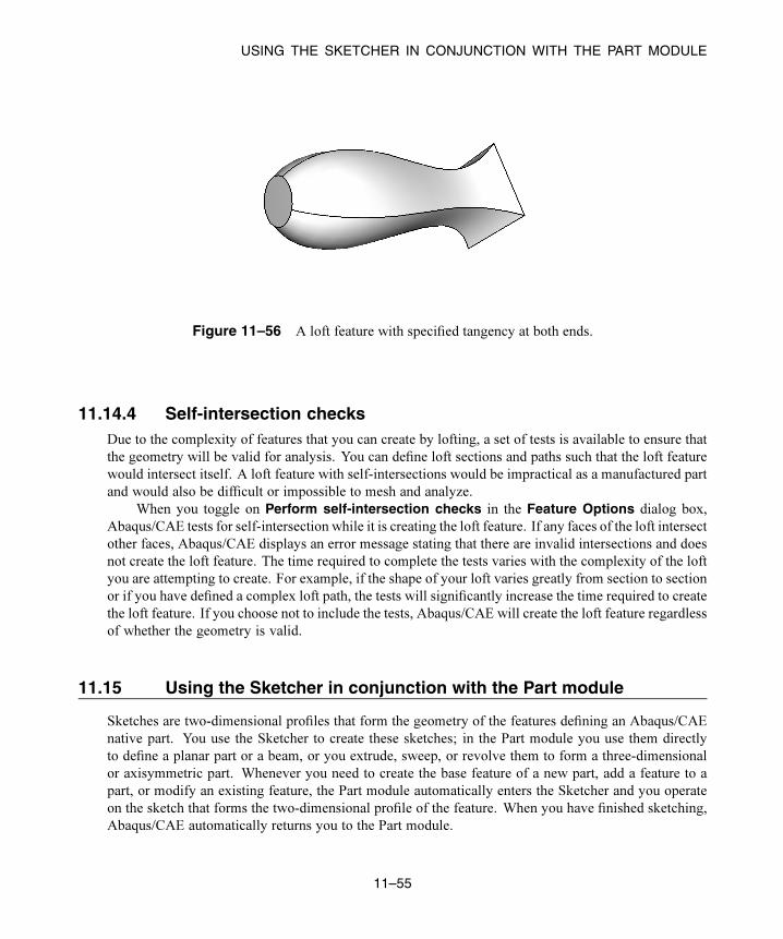
USING THE SKETCHER IN CONJUNCTION WITH THE PART MODULE
Figure 11–56 A loft feature with specified tangency at both ends.
11.14.4 Self-intersection checksDue to the complexity of features that you can create by lofting, a set of tests is available to ensure that
the geometry will be valid for analysis. You can define loft sections and paths such that the loft feature
would intersect itself. A loft feature with self-intersections would be impractical as a manufactured part
and would also be difficult or impossible to mesh and analyze.
When you toggle on Perform self-intersection checks in the Feature Options dialog box,
Abaqus/CAE tests for self-intersection while it is creating the loft feature. If any faces of the loft intersect
other faces, Abaqus/CAE displays an error message stating that there are invalid intersections and does
not create the loft feature. The time required to complete the tests varies with the complexity of the loft
you are attempting to create. For example, if the shape of your loft varies greatly from section to section
or if you have defined a complex loft path, the tests will significantly increase the time required to create
the loft feature. If you choose not to include the tests, Abaqus/CAE will create the loft feature regardless
of whether the geometry is valid.
11.15 Using the Sketcher in conjunction with the Part module
Sketches are two-dimensional profiles that form the geometry of the features defining an Abaqus/CAE
native part. You use the Sketcher to create these sketches; in the Part module you use them directly
to define a planar part or a beam, or you extrude, sweep, or revolve them to form a three-dimensional
or axisymmetric part. Whenever you need to create the base feature of a new part, add a feature to a
part, or modify an existing feature, the Part module automatically enters the Sketcher and you operate
on the sketch that forms the two-dimensional profile of the feature. When you have finished sketching,
Abaqus/CAE automatically returns you to the Part module.
11–55
Abaqus ID:
Printed on:

UNDERSTANDING TOOLSETS IN THE PART MODULE
If you are adding a feature or modifying an existing feature, you must choose the plane on which
to sketch. For a detailed description of how Abaqus/CAE determines the orientation of the part relative
to the sketch plane, see “How Abaqus/CAE orients your sketch,” Section 20.4.3.
11.16 Understanding toolsets in the Part module
The Part module provides a set of toolsets that allow you to add and modify the features that define a part.
This section describes how these toolsets are used within the Part module. For more detailed information
about each toolset, refer to:
• Chapter 62, “The Datum toolset”
• Chapter 64, “The Edit Mesh toolset”
• Chapter 65, “The Feature Manipulation toolset”
• Chapter 66, “The Filter toolset”
• Chapter 70, “The Partition toolset”
• Chapter 71, “The Query toolset”
• Chapter 72, “The Reference Point toolset”
• Chapter 69, “The Geometry Edit toolset”
• Chapter 73, “The Set and Surface toolsets”
The Display Group toolset is discussed in Chapter 78, “Using display groups to display subsets of your
model.”
11.16.1 Using the Datum toolset in the Part moduleA datum can be thought of as reference geometry or a construction aid that helps you create a feature
when the part does not contain the necessary geometry; you create datum geometry using the Datum
toolset. A datum is a feature of a part and is regenerated along with the rest of the part. Furthermore,
datum geometry is visible unless you toggle it off by selecting View→Part Display Options→Datumfrom the main menu bar. A datum created in the Part module appears with each instance of the part in
the Assembly module or any other assembly-based module.
Datum points are projected onto the Sketch plane in the Sketcher, and the projected point can be
selected. However, you cannot refer to datum axes or planes in the Sketcher. Examples of how you
might use datum planes and axes in the Part module are given below.
Datum plane
You can sketch directly on datum planes, and any features you sketch on a datum plane will be
projected onto the part. Projecting a sketch from a datum plane is useful if the part does not already
contain a convenient sketch plane.
11–56
Abaqus ID:
Printed on:
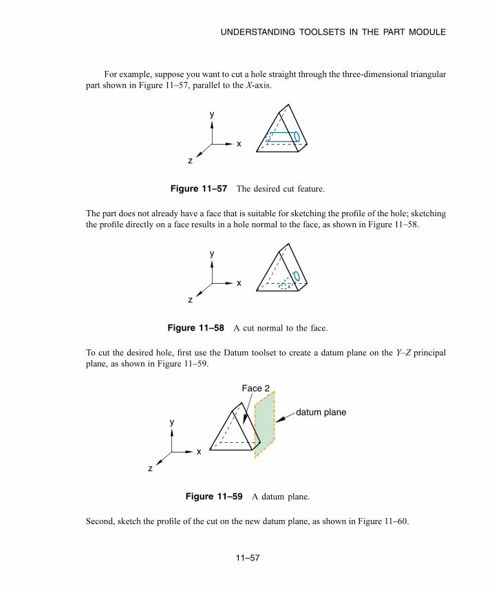
UNDERSTANDING TOOLSETS IN THE PART MODULE
For example, suppose you want to cut a hole straight through the three-dimensional triangular
part shown in Figure 11–57, parallel to the X-axis.
y
z
x
Figure 11–57 The desired cut feature.
The part does not already have a face that is suitable for sketching the profile of the hole; sketching
the profile directly on a face results in a hole normal to the face, as shown in Figure 11–58.
y
z
x
Figure 11–58 A cut normal to the face.
To cut the desired hole, first use the Datum toolset to create a datum plane on the Y–Z principal
plane, as shown in Figure 11–59.
datum plane
Face 2
y
z
x
Figure 11–59 A datum plane.
Second, sketch the profile of the cut on the new datum plane, as shown in Figure 11–60.
11–57
Abaqus ID:
Printed on:

UNDERSTANDING TOOLSETS IN THE PART MODULE
y
xz
projected imageof Face 2
Figure 11–60 A sketch on the datum plane.
When you exit the Sketcher, Abaqus/CAE cuts the sketched hole through the part, perpendicular to
the datum plane and parallel to the X-axis. This cut is illustrated in Figure 11–61.
y
z
x
Figure 11–61 The desired cut.
Datum axis
You can use the Datum toolset to create a datum axis. You can then select the datum axis to
control the orientation of the part on the Sketcher grid when adding or modifying a feature to a
three-dimensional solid. Creating a datum axis is useful when the part does not already contain the
necessary axis.
For example, suppose you want to cut a slot through the part as shown in Figure 11–62.
y
zx
desired slot
Figure 11–62 The desired slot.
Sketching the slot is difficult because selecting either of the two straight edges of the part as the
sketch’s vertical axis causes the sketch grid lines to align with the line you select, not with the X- or
11–58
Abaqus ID:
Printed on:

UNDERSTANDING TOOLSETS IN THE PART MODULE
Y-axis. To make it easier to create the slot with the desired orientation, first use the Datum toolset
to create a datum axis along the Y-axis, as shown in Figure 11–63.
datum axis
y
zx
Figure 11–63 The datum axis.
When you select the datum axis to appear vertical and on the right, the Sketcher starts, and its grid
is aligned with the part’s X- and Y-axes, as shown in Figure 11–64.
y
z x
datum axis
Figure 11–64 The resulting sketch orientation.
11.16.2 Using the Feature Manipulation toolset in the Part moduleThe following are considered to be features of a part:
• Geometric features, such as extruded solids, revolved shells, sketched wires, and rounded edges
• Repair operations
• Partitions
• Datum geometry
When the Feature Manipulation toolset asks you to select a feature, you can select it from the viewport.
Alternatively, you can select the feature from the Model Tree.
If you click mouse button 3 on a feature in the Model Tree, the menu that appears allows you to do
the following:
11–59
Abaqus ID:
Printed on:
UNDERSTANDING TOOLSETS IN THE PART MODULE
Edit
When you edit a feature, Abaqus/CAE displays the feature editor. You can either modify
the feature’s parameters directly or, if applicable, you can modify the sketch that forms the
two-dimensional profile or sweep path of a feature.
Regenerate
When you modify features in a complex part, it may be convenient to postpone regeneration
until you make all your changes, since regeneration can be time consuming. Select
Feature→Regenerate when you are ready to regenerate the part.
Rename
Rename a part.
Suppress
Suppressing a feature temporarily removes it from the definition of the part. A suppressed feature is
invisible, cannot be meshed, and is not included in the analysis of the model. You cannot suppress
the base feature, and suppressing a parent feature will suppress all of its child features.
Resume
Resuming a feature restores a suppressed feature to the part; resuming a parent feature restores
all of its child features. You can choose to resume all features, the set of features most recently
suppressed, or a selected feature.
Delete
Deleting a feature removes it from the part. You cannot resume a deleted feature.
Query
When you query a part, Abaqus/CAE displays information in the message area and writes the same
information to the replay file (abaqus.rpy) in the form of comments.
Options
The Feature Options dialog box allows you to tune the regeneration performance of the current
model.
11.16.3 Using the Partition toolset in the Part module
Within the Part module, you can use the Partition toolset to partition a part into additional regions. After
you partition a part, you can use the Property module to assign different sections to the resulting regions;
for example, you might use partitions to delineate regions of the part that are comprised of different
materials.
11–60
Abaqus ID:
Printed on:

UNDERSTANDING TOOLSETS IN THE PART MODULE
The partitions you create are features associated with the part, so that each instance of that part in the
assembly will contain all the partitions created in the Part module. You can use the regions when working
with the assembly in other modules; for example, you can apply a load over a region in the Load module.
If you do not want to associate the partitions with every instance of the part, create an independent
instance in the Assembly module and partition the independent instance. For more information, see
“Partitioning the assembly,” Section 13.8.3.
If you have created the assembly and applied attributes to it, such as loads, boundary conditions,
and sets, you should be careful if you subsequently decide to return to the Part module and partition one
of the original parts. The region to which the attribute is assigned may change unexpectedly if the region
is affected by the partition. In general, you should try to finish creating your parts in the Part module
before you start creating part instances and applying sets, loads, and meshes to the assembly. If you do
return to the Part module to create a partition, you should at least check that the regions in the assembly
to which attributes are assigned are still valid.
11.16.4 Using the Query toolset in the Part module
Select Tools→Query from the main menu bar, or click the tool in the Query toolbar to start the
Query toolset.
You can use the Query toolset to request either general information or module-specific information.
For a discussion of the information displayed by general queries, see “Obtaining general information
about the model,” Section 71.2.2, in the HTML version of this guide.
The following queries are specific to the Part module:
Part attributes
Abaqus/CAE displays the part name, modeling space, and type in the message area along with the
shape (solid, shell, wire, or point) and the number of entities (cells, faces, edges, and vertices).
Regeneration warnings
If any sets or surfaces in the selected part cannot be regenerated because their underlying geometry
has been modified or deleted, Abaqus/CAE displays the set or surface name, the original number
of faces, and the number of faces found during the query.
Substructure statistics
Abaqus/CAE displays the following information about the selected substructure part: the number
of retained nodes, eigenmodes, and substructure loads in the part; the availability of the recovery
matrix, gravity load vectors, reduced mass matrix, reduced structural damping matrix, and reduced
viscous damping matrix in the substructure; and mass properties of the substructure.
11–61
Abaqus ID:
Printed on:
USING THE PART MODULE TOOLBOX
11.16.5 Using the Reference Point toolset in the Part module
From the main menu bar, select Tools→Reference Point to create a reference point on a part. A part
can include only one reference point. For more information, see “The reference point and point parts,”
Section 11.8, and Chapter 72, “The Reference Point toolset.”
Abaqus/CAE displays the reference point at the desired location and labels it RP. You can change
the reference point label by clicking mouse button 3 on the feature in the Model Tree and selecting
Rename from the menu that appears. If desired, you can turn off the display of the reference point
symbol and the reference point label; for more information, see “Controlling reference point display,”
Section 76.11.
11.16.6 Using the Geometry Edit toolset in the Part module
You use the Geometry Edit toolset to repair regions of a part that contain invalid or imprecise geometry.
For more information, see “An overview of editing techniques,” Section 69.2. You can use the Query
toolset to locate regions that need repairing. For more information, see Chapter 71, “The Query toolset.”
11.16.7 Using the Set toolset in the Part module
Sets created by selecting geometry from a part are called part sets, and you use the Set toolset to create and
manage part sets. You can use part sets in the Part module to select regions that should be repaired by the
Geometry Edit toolset. In addition, in the Property module you can assign sections to regions specified
by part sets. When Abaqus/CAE prompts you to select a region, you can either select the region from
the part in the current viewport, or you can select a named part set.
Only part sets are visible in the Set Manager in the Part module. When you instance a part in
the Assembly module, Abaqus creates part instance sets that refer to any part sets that you previously
created. For more information, see “Understanding sets and surfaces,” Section 73.2, and “Using sets and
surfaces in the Assembly module,” Section 13.8.6.
11.17 Using the Part module toolbox
You can access all the Part module tools through either the main menu bar or the Part module toolbox.
Figure 11–65 shows the hidden icons for all the part tools in the Part module toolbox.
The HTML version of this guide contains detailed instructions on using each of the tools in the Part
module toolbox.
11–62
Abaqus ID:
Printed on:
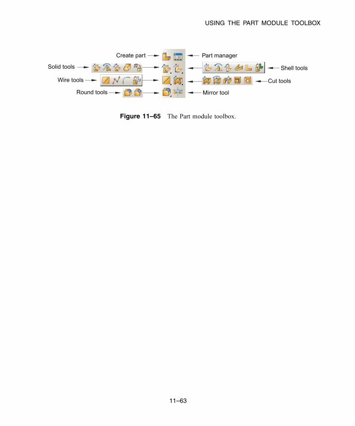
USING THE PART MODULE TOOLBOX
Solid tools Shell tools
Cut tools
Create part
Wire tools
Round tools
Part manager
Mirror tool
Figure 11–65 The Part module toolbox.
11–63
Abaqus ID:
Printed on:


THE PROPERTY MODULE
12. The Property module
You can use the Property module to perform the following tasks:
• Define materials.
• Define beam section profiles.
• Define sections.
• Assign sections, orientations, normals, and tangents to parts.
• Define composite layups.
• Define a skin reinforcement.
• Define inertia (point mass, rotary inertia, and heat capacitance) on a part.
• Define springs and dashpots between two points or between a point and ground.
• Define material calibrations.
This chapter covers the following topics:
• “Entering and exiting the Property module,” Section 12.1
• “Understanding properties,” Section 12.2
• “Which properties can I assign to a part?,” Section 12.3
• “Understanding the Property module editors,” Section 12.4
• “Using material libraries,” Section 12.5
• “Using the Property module toolbox,” Section 12.6
For information on defining inertia, see Chapter 33, “Inertia.” For information on defining skin
reinforcements, see Chapter 36, “Skin and stringer reinforcements.” For information on defining springs
and dashpots, see Chapter 37, “Springs and dashpots.” In addition, the following sections are available
in the HTML version of this guide:
• “Creating and editing materials,” Section 12.7
• “Defining general material data,” Section 12.8
• “Defining mechanical material models,” Section 12.9
• “Defining thermal material models,” Section 12.10
• “Defining electrical and magnetic material models,” Section 12.11
• “Defining other types of material models,” Section 12.12
• “Creating and editing sections,” Section 12.13
• “Creating and editing composite layups,” Section 12.14
• “Assigning sections, orientations, normals, and tangents to a part,” Section 12.15
• “Using discrete orientations for material orientations and composite layup orientations,”
Section 12.16
• “Creating material calibrations,” Section 12.17
12–1
Abaqus ID:
Printed on:

UNDERSTANDING PROPERTIES
• “Using the Special menu in the Property module,” Section 12.18
• “Using the Query toolset to obtain assignment information,” Section 12.19
12.1 Entering and exiting the Property module
You can enter the Property module at any time during an Abaqus/CAE session by clicking Property in
the Module list located in the context bar. When you enter the Property module, Material, Section,Profile, Assign, Special, Feature, and Tools menus appear in the main menu bar. A Part list appearsin the context bar that allows you to select the part to which you want to assign properties.
To exit the Property module, select another module from the Module list. You need not take any
specific action to save your material, section, and other definitions before exiting the module; they are
saved automatically when you save the entire model by selecting File→Save or File→Save As from
the main menu bar.
12.2 Understanding properties
You can specify the properties of a part or part region by creating a section and assigning it to the part.
In most cases, sections refer to materials that you have defined. Beam sections also refer to profiles
that you have defined. This section of the guide explains materials, profiles, sections, rebar, and section
assignment. You create materials, profiles, and sections using the Property module editors, as described
in “Understanding the Property module editors,” Section 12.4.
12.2.1 Defining materialsA material definition specifies all the property data relevant to a material. You specify a material
definition by including a set of material behaviors, and you supply the property data with each material
behavior you include. You use the material editor to specify all the information that defines each
material.
Each material that you create is assigned its own name and is independent of any particular section;
you can refer to a single material in as many sections as necessary. Abaqus/CAE assigns the properties
of a material to a region of a part when you assign a section referring to that material to the region.
12.2.2 Defining profilesA profile specifies the properties of a beam section that are related to its cross-sectional shape and size
(for example, cross-section area and moments of inertia). When you define a beam section, you must
include a reference to a profile in the section definition.
12–2
Abaqus ID:
Printed on:

UNDERSTANDING PROPERTIES
You can create the following types of profiles:
Shape-based profiles
Shape-based profiles define the specific shape and dimensions of the beam cross-section. Abaqus
uses the information provided by the shape-based profile to calculate the engineering properties of
the section.
You can create this type of profile by first selecting from a list of shape options and then
specifying that particular shape’s dimensions. For example, if you select a box shape, you must
then specify the height and width of the box as well as the thickness of the four walls. The shape
options are shown in Figure 12–1.
Arbitrary Box Circular
Hexagonal I L
Pipe Rectangular Trapezoidal
T
Figure 12–1 Available shape options.
For detailed information on each profile shape, see “Beam cross-section library,” Section 29.3.9 of
the Abaqus Analysis User’s Guide.
Generalized profiles
Generalized profiles specify the engineering properties of the section directly. You can create a
generalized profile by specifying values for the area, moments of inertia, torsional constant, and,
if applicable, sectorial moment and warping constant. For more information, see “Using a general
beam section to define the section behavior,” Section 29.3.7 of the Abaqus Analysis User’s Guide.
Each profile that you create has its own name and is independent of any particular beam section; you can
refer to a single profile in as many beam sections as necessary. After you have assigned the beam section
12–3
Abaqus ID:
Printed on:

UNDERSTANDING PROPERTIES
and beam orientation to the part, you can use the part display options to view an idealized representation
of the shape-based or generalized beam profile. Displaying beam profiles is useful for checking that the
correct profile has been assigned to a particular region and that the assigned beam orientation results in
the expected orientation of the profile. For more information, see “Controlling beam profile display,”
Section 76.7.
12.2.3 Defining sections
A section contains information about the properties of a part or a region of a part. The information
required in the definition of a section depends on the type of region in question. For example, if the
region is a deformable wire, shell, or two-dimensional solid, you must assign a section to that region
that provides information about the region’s cross-sectional geometry. Likewise, a rigid region requires
a section that describes its mass properties. Most sections must refer to a material name. Beam sections
must also refer to a profile name.
When you assign a section to a part, Abaqus/CAE automatically assigns that section to each instance
of the part. As a result, the elements that are created when you mesh those part instances will have the
properties specified in that section.
Sections are named and created independently of any particular region, part, or assembly. You can
assign a single section to as many different regions as necessary. You can use the Property module to
create solid sections, shell sections, beam sections, fluid sections, and other sections.
Solid sections
Solid sections define the section properties of two-dimensional, three-dimensional, and
axisymmetric solid regions.
• Homogeneous solid sections. Homogeneous solid sections consist of a material name. In
addition, if the section will be used with a two-dimensional region, you must also specify the
section thickness. (You have the option of specifying a plane stress or plane strain thickness
even if the section will be assigned to a three-dimensional region. Abaqus/CAE ignores the
thickness information if it is not needed for the region type.)
For more information, see “Creating homogeneous solid sections,” Section 12.13.1, in
the HTML version of this guide.
• Generalized plane strain sections. Generalized plane strain sections consist of a material
name, thickness, and wedge angles about the global 1- and 2-axes. You can assign generalized
plane strain sections only to two-dimensional planar regions.
For more information, see “Creating generalized plane strain sections,” Section 12.13.2,
in the HTML version of this guide.
• Eulerian sections. Eulerian sections consist of a list of material names. This list specifies all
of the materials that can be present in an Eulerian domain. You can assign Eulerian sections
only to Eulerian parts.
12–4
Abaqus ID:
Printed on:
UNDERSTANDING PROPERTIES
For more information, see “Creating Eulerian sections,” Section 12.13.3, in the HTML
version of this guide. For an overview of Eulerian analyses, see Chapter 28, “Eulerian
analyses.”
• Composite solid sections. Composite solid sections consist of layers of materials. For each
layer of material, you must specify a material name, thickness, and orientation.
For more information, see “Creating composite solid sections,” Section 12.13.4, in the
HTML version of this guide.
• Electromagnetic solid sections. Electromagnetic solid sections are valid for
electromagnetic models and consist of a material name. In addition, if the section will
be used with a two-dimensional region, you must also specify the section thickness. (You
have the option of specifying a plane stress or plane strain thickness even if the section will
be assigned to a three-dimensional region. Abaqus/CAE ignores the thickness information if
it is not needed for the region type.)
For more information, see “Creating electromagnetic solid sections,” Section 12.13.5, in
the HTML version of this guide.
Shell sections
Shell sections define the section properties of shell regions. Shells model structures in which
one dimension (the thickness) is significantly smaller than the other two dimensions and in
which the stresses in the thickness direction are negligible. You can define one or more layers of
reinforcement (rebar) in shell sections. For more information, see “Understanding rebar in shell
sections,” Section 12.2.5.
• Homogeneous shell sections. Homogeneous shell sections consist of a shell thickness,
material name, section Poisson’s ratio, and optional rebar layers. You can choose to provide
the section property data before the analysis or to have Abaqus calculate (integrate) the cross-
sectional behavior from section integration points during the analysis. If the latter is chosen,
options are provided to control the section integration and temperature variation through the
thickness.
For more information, see “Creating homogeneous shell sections,” Section 12.13.6, in the
HTML version of this guide.
• Composite shell sections. Composite shell sections consist of layers of materials, a section
Poisson’s ratio, and optional rebar layers. For each layer of material, you must specify a
material name, thickness, and orientation. You can choose to provide the section property
data before the analysis or to have Abaqus calculate (integrate) the cross-sectional behavior
from section integration points during the analysis. If the latter is chosen, options are provided
to control the section integration and temperature variation through the thickness.
For more information, see “Creating composite shell sections,” Section 12.13.7, in the
HTML version of this guide.
12–5
Abaqus ID:
Printed on:
UNDERSTANDING PROPERTIES
• Membrane sections. Membranes represent thin surfaces in space that offer strength in the
plane of the surface but have no bending stiffness. Membrane sections consist of a material
name, membrane thickness, section Poisson’s ratio, and optional rebar layers.
For more information, see “Creating membrane sections,” Section 12.13.8, in the HTML
version of this guide.
• Surface sections. Surface sections represent surfaces in space that have no inherent stiffnessand behave like membrane elements with zero thickness. Surface sections consist of optional
rebar layers.
For more information, see “Creating surface sections,” Section 12.13.9, in the HTML
version of this guide.
• General shell stiffness sections. General shell stiffness sections allow you to define a
shell’s mechanical response by directly specifying the stiffness matrix and thermal expansion
response. General shell stiffness sections consist of a section stiffness matrix and scaling
moduli. Optionally, you can also specify a thermal expansion coefficient and thermal stresses
in the section.
For more information, see “Creating general shell stiffness sections,” Section 12.13.10,
in the HTML version of this guide.
Beam sections
Beams are used in two and three dimensions to model slender, rod-like structures that provide axial
strength and bending stiffness. Beams represent structures in which the cross-section is assumed to
be small compared to the length. You can assign beam sections only to wire regions. In addition,
you must assign a beam section orientation to all regions with beam sections.
• Beam sections. Beam sections consist of a section Poisson’s ratio and a reference to a profile.
Additional information is required depending on whether you choose to calculate (integrate)
the section stiffness either before or during analysis.
For information on profiles, see “Defining profiles,” Section 12.2.2. For more information
on beam sections, see “Creating beam sections,” Section 12.13.11, in the HTML version of this
guide.
• Truss sections. Trusses, like beams, are used in two and three dimensions to model slender,
rod-like structures that provide axial strength but no bending stiffness. Truss sections consist
of a material name and cross-sectional area.
For more information, see “Creating truss sections,” Section 12.13.12, in the HTML
version of this guide.
You can use the part display options to view an idealized representation of the beam or truss
profile along the wire region. For more information, see “Controlling beam profile display,”
Section 76.7.
12–6
Abaqus ID:
Printed on:

UNDERSTANDING PROPERTIES
Fluid sections
Fluid sections define the material properties of three-dimensional fluid regions. These sections are
used only in Abaqus/CFD models.
• Homogeneous fluid sections. Homogeneous fluid sections consist of a material name. For
more information, see “Creating homogeneous fluid sections,” Section 12.13.13, in the HTML
version of this guide.
Other sections
Other sections you can create include gasket sections, cohesive sections, acoustic infinite sections,
and acoustic interface sections.
• Gasket sections (Abaqus/Standard analyses only). Gaskets model thin sealing components
that are positioned between structural components. Gasket sections are used to provide
pressure-closure behaviors for sealing components. Gasket sections consist of a material
name, initial gasket thickness, initial gap, initial void, and cross-sectional area.
For more information, see “Creating gasket sections,” Section 12.13.15, in the HTML
version of this guide, and Chapter 32, “Gaskets.”
• Cohesive sections. Cohesive sections are used to model finite thickness adhesives,
negligibly thin adhesive layers for debonding applications, as well as gaskets. No specialized
gasket behavior (typically defined in terms of pressure versus closure) is available. Cohesive
sections consist of a material name, response, initial thickness, and out-of-plane thickness.
For more information, see “Creating cohesive sections,” Section 12.13.16, in the HTML
version of this guide, and Chapter 21, “Adhesive joints and bonded interfaces.”
• Acoustic infinite sections. Acoustic infinite sections are used to model an acoustic medium
undergoing small pressure changes involving exterior domains. Acoustic infinite sections
consist of an acoustic medium material name. In addition, if the section will be used with
a two-dimensional region, you must also specify the section thickness. (You have the option
of specifying a plane stress or plane strain thickness even if the section will be assigned to a
three-dimensional region. Abaqus/CAE ignores the thickness information if it is not needed
for the region type.)
For more information, see “Creating acoustic infinite sections,” Section 12.13.17, in the
HTML version of this guide.
• Acoustic interface sections. Acoustic interface sections are used to couple an acoustic
medium to a structural model. Acoustic interface sections consist of an acoustic medium
material name. In addition, if the section will be used with a two-dimensional region, you
must also specify the section thickness. (You have the option of specifying a plane stress
or plane strain thickness even if the section will be assigned to a three-dimensional region.
Abaqus/CAE ignores the thickness information if it is not needed for the region type.)
For more information, see “Creating acoustic interface sections,” Section 12.13.18, in the
HTML version of this guide.
12–7
Abaqus ID:
Printed on:

WHICH PROPERTIES CAN I ASSIGN TO A PART?
WARNING: The type of section that you assign to a part must be consistent with the element type that
you assign to instances of that part in the Mesh module. For example, if you assign a truss section to a
wire part in the Property module, you should assign a truss element type (and not a beam element type)
to any instances of that part in the Mesh module.
12.2.4 Defining composite layupsYou use a composite layup to model a part that contains many plies, where each ply is defined by a
material, a thickness, and a reference orientation. Composite layups are similar to composite shell
or composite solid sections. A ply in a composite section is the same as a ply in a composite layup;
however, a composite section always contains the same number of plies. In contrast, a composite layup
can contain a different number of plies in different regions. Abaqus/CAE converts a composite layup to
its constituent composite sections when you analyze your model. Abaqus/CAE allows you to define three
types of composite layups—shells, continuum shells, and solids. For more information, see Chapter 23,
“Composite layups.”
12.2.5 Understanding rebar in shell sectionsYou can define one or more layers of reinforcement (rebar) in shell sections by specifying a unique layer
name for each rebar layer. You also select the name of the material forming each rebar layer and specify
the cross-sectional area per bar, spacing, and orientation of the rebar in each layer.
To define the orientation of each rebar layer, you can specify an orientation angle or an orientation
name. The angular orientation of a rebar layer is defined relative to the rebar reference orientation. You
use the Assign menu to assign a rebar reference orientation to shell regions. If you specify an orientation
name, you must supply the user subroutine ORIENT. For more information, see “Defining rebar layers,”
Section 12.13.19, and “Assigning a rebar reference orientation” in “Assigning a material orientation or
rebar reference orientation,” Section 12.15.4, in the HTML version of this guide.
In the Step module you must request output for rebar to include rebar output in the data that Abaqus
writes to the output database and to view plots of the rebar orientations in the Visualization module. In
the Visualization module Abaqus/CAE treats rebar layers as section points for output purposes, and you
can create material orientation plots to show the rebar orientation.
For more information on rebar, see “Defining reinforcement,” Section 2.2.3 of the Abaqus Analysis
User’s Guide.
12.3 Which properties can I assign to a part?
Once you have created a section, you can assign the following properties to a part:
12–8
Abaqus ID:
Printed on:

WHICH PROPERTIES CAN I ASSIGN TO A PART?
Section
You can assign the section to a region of a part. The Section Assignment Manager allows youto view, create, edit, suppress, resume, and delete section assignments. In the Property module,
Abaqus/CAE colors a region green to indicate that the region has a section assignment. If there are
overlapping section assignments, Abaqus/CAE colors the region yellow.
Beam Section Orientation
You can assign beam section orientations to wire regions. You assign an orientation to a beam
section by defining the approximate local 1-direction of the cross-section.
Material Orientation
You can assign material orientations to shell and solid regions. The global coordinate system
determines the default material orientation. You can define a material orientation by selecting an
existing datum coordinate system or discrete field or by defining a discrete orientation. For an
Abaqus/Standard analysis, you can define the material orientation in a user subroutine.
Rebar Reference Orientation
The angular orientation of a rebar layer is defined relative to the rebar reference orientation. You
can assign rebar reference orientations to shell regions. The global coordinate system determines
the default rebar reference orientation. You can define a rebar reference orientation by selecting
an existing datum coordinate system from the viewport and then selecting an axis on the datum
coordinate system that approximates the direction of the shell normal.
Element Normal
You can assign shell/membrane normal directions to orphan elements, shell and membrane
regions, and axisymmetric parts with wire regions. The shell/membrane normals affect the
material orientation assigned to the region. If you reverse the normal of a shell region, the material
2-direction will be reversed. The reversal of the material 2-direction has no effect on the analysis
results. However, you should use care when interpreting section point output for shells.
Element Tangent
You can assign beam/truss tangent directions to orphan elements and wire regions. Beam section
orientations depend on the beam tangent directions. If you reverse the tangent direction, the local
2-direction will be reversed, and you should use care when interpreting results, in particular when
you identify the beam section point locations.
You can use the Assign menu in the Property module main menu bar to assign properties to a part. You
can select the region to which to assign a property in the following ways:
• Select the region directly in the viewport.
• Select elements individually or using the angle method (to assign shell normals to orphan elements).
12–9
Abaqus ID:
Printed on:

UNDERSTANDING THE PROPERTY MODULE EDITORS
• Use the Set toolset to create a set consisting of regions of parts or orphan elements. (The Set toolset
is available from the Tools menu in the main menu bar.) You can then assign the property to the
region or elements defined by the set.
If you assign a section to a region and then rename or delete the section, that section is no longer
applied to the region. If a region of your model lacks section properties, your analysis job will fail and
the problem will be reported by the Job module.
However, the original names of renamed or deleted sections continue to be associated with the
regions to which they have been assigned until you take one of the following actions:
• Assign a different section to the region.
• Create a new section that has the original section name and is the appropriate type for the region
(for example, a shell section for a shell region); the properties defined in the new section are applied
to the region automatically.
• If you have renamed a section, change the name of the section back to its original name.
(You can use the Query toolset to determine the name of the section assigned to the region; for more
information, see “Understanding the role of the Query toolset,” Section 71.1.)
Similarly, if you refer to a material in a section definition and then rename or delete the material,
the section becomes invalid; properties defined in that section are no longer applied to regions to which
the section is assigned. However, the original names of renamed or deleted materials continue to be
associated with sections that refer to those materials; therefore, you can use techniques similar to the
ones listed above to restore sections.
For detailed instructions on assigning properties to a model and managing section assignments, see
the following sections in the HTML version of this guide:
• “Assigning a section,” Section 12.15.1
• “Managing section assignments,” Section 12.15.2
• “Assigning a beam orientation,” Section 12.15.3
• “Assigning a material orientation or rebar reference orientation,” Section 12.15.4
• “Assigning shell/membrane normal directions,” Section 12.15.5
• “Assigning beam/truss tangent directions,” Section 12.15.6
• “Using discrete orientations for material orientations and composite layup orientations,”
Section 12.16
12.4 Understanding the Property module editors
When you create or edit a material, profile, or section, you must enter data in the appropriate editor. For
example, when you create a material, you must enter data in the material editor. This section provides
information on each editor type.
12–10
Abaqus ID:
Printed on:

UNDERSTANDING THE PROPERTY MODULE EDITORS
12.4.1 Creating materialsTo create a material, select Material→Create from the main menu bar. An Edit Material dialog box
appears in which you can enter a name for the material and create or edit material properties. The material
editor is shown in Figure 12–2.
Note: Once you have created a material, it cannot be renamed using the material editor; you must use
Material→Rename to change the name of an existing material.
Figure 12–2 The material editor.
The material editor consists of the following:
12–11
Abaqus ID:
Printed on:

UNDERSTANDING THE PROPERTY MODULE EDITORS
Material Behaviors list
A list of the behaviors you have included in the material definition.
Behavior menu
A set of menus beneath the behavior list from which you select material behaviors.
Behavior definition area
The lower portion of the window in which the parameters, tabular data fields, and suboptions
associated with a selected behavior appear.
Note: You can display help on particular aspects of the editor that are not discussed here by selecting
Help→On Context from the main menu bar and then clicking the editor feature of interest.
12.4.2 Creating profilesTo create a profile, selectProfile→Create from themainmenu bar. ACreate Profile dialog box appears
in which you can enter a name for the profile and select the profile type. Once you have finished entering
this information, click Continue in the Create Profile dialog box to display the profile editor, which
allows you to create and edit profiles.
All profile editors display a diagram of the profile shape and text fields in which you can enter
all of the data necessary to define the profile. For example, the I-shaped profile editor is shown in
Figure 12–3. The editor contains a diagram of the I-shaped profile and data fields in which you can
enter each dimension.
Figure 12–3 The I-shaped profile editor.
12–12
Abaqus ID:
Printed on:

UNDERSTANDING THE PROPERTY MODULE EDITORS
Once you have created a profile, you can refer to that profile in a beam section definition. For
example, a box-shaped profile named SupportBeam is selected in the beam section editor shown in
Figure 12–4.
Figure 12–4 Specifying a profile name in the beam section editor.
For more information on profiles, see “Defining profiles,” Section 12.2.2.
12.4.3 Creating sectionsYou can use the Property module to create the following types of sections:
• Homogeneous solid sections
• Generalized plane strain sections
• Eulerian sections
• Composite solid sections
• Electromagnetic solid sections
• Homogeneous shell sections
• Composite shell sections
• Membrane sections
• Surface sections
• General shell stiffness sections
• Beam sections
• Truss sections
• Fluid sections
• Gasket sections
• Cohesive sections
• Acoustic infinite sections
• Acoustic interface sections
12–13
Abaqus ID:
Printed on:

UNDERSTANDING THE PROPERTY MODULE EDITORS
To create a section, select Section→Create from the main menu bar. A Create Section dialog
box appears in which you can name the section and specify the type of section that you want to create.
Once you have specified a section name and type, click Continue in the Create Section dialog box to
display the section editor, which allows you to create and edit sections.
The format of the section editor varies according to the type of section you are defining. For
example, the homogeneous shell section editor is shown in Figure 12–5.
Figure 12–5 The homogeneous shell section editor.
Note: You can display help on particular aspects of an editor that are not discussed here by selecting
Help→On Context from the main menu bar and then clicking the editor feature of interest. A help
window will appear containing a relevant section from this guide.
Some editors contain a Rebar Layers option ( icon), as shown in Figure 12–5. If you click
this icon, another dialog box appears in which you can enter data concerning rebar layers, as shown in
Figure 12–6.
Note: To display context-sensitive help for items in the Rebar Layers dialog box, you must select the
item of interest and then press [F1]. (The Help menu in the main menu bar is unavailable while the option
dialog box is displayed.)
Once you have entered all the data necessary to define the section, you can click OK to close the
section editor and to save the section.
12–14
Abaqus ID:
Printed on:

UNDERSTANDING THE PROPERTY MODULE EDITORS
Figure 12–6 The Rebar Layers dialog box.
For detailed instructions on using section editors, see the following sections in the HTML version
of this guide:
• “Creating homogeneous solid sections,” Section 12.13.1
• “Creating generalized plane strain sections,” Section 12.13.2
• “Creating Eulerian sections,” Section 12.13.3
• “Creating composite solid sections,” Section 12.13.4
• “Creating electromagnetic solid sections,” Section 12.13.5
• “Creating homogeneous shell sections,” Section 12.13.6
• “Creating composite shell sections,” Section 12.13.7
• “Creating membrane sections,” Section 12.13.8
• “Creating surface sections,” Section 12.13.9
• “Creating general shell stiffness sections,” Section 12.13.10
• “Creating beam sections,” Section 12.13.11
• “Creating truss sections,” Section 12.13.12
• “Creating homogeneous fluid sections,” Section 12.13.13
• “Creating fluid sections for porous media,” Section 12.13.14
• “Creating gasket sections,” Section 12.13.15
• “Creating cohesive sections,” Section 12.13.16
• “Creating acoustic infinite sections,” Section 12.13.17
• “Creating acoustic interface sections,” Section 12.13.18
• “Defining rebar layers,” Section 12.13.19
• “Creating profiles,” Section 12.13.20
12–15
Abaqus ID:
Printed on:

UNDERSTANDING THE PROPERTY MODULE EDITORS
12.4.4 Creating composite layupsYou can use the Property module to create the following types of composite layups:
• Shell
• Continuum shell
• Solid
To create a composite layup, select Composite→Create from the main menu bar. A CreateComposite Layup dialog box appears in which you can name the layup, specify the initial ply count,
and specify the type of composite layup that you want to create. Once you have finished entering this
information, click Continue in the Create Composite Layup dialog box to display the composite
layup editor, which allows you to create and edit layups.
The format of the composite layup editor varies according to the type of layup you are defining. For
example, the shell composite layup editor is shown in Figure 12–7.
Note: You can display help on particular aspects of an editor that are not discussed here by selecting
Help→On Context from the main menu bar and then clicking the editor feature of interest. A help
window will appear containing a relevant section from this guide.
Once you have entered all the data necessary to define the layup, you can click OK to close the
editor and to save the composite layup.
For detailed instructions on using composite layup editors, see the following sections in the HTML
version of this guide:
• “Creating conventional shell composite layups,” Section 12.14.2
• “Creating continuum shell composite layups,” Section 12.14.3
• “Creating solid composite layups,” Section 12.14.4
12.4.5 Selecting material behaviorsThe material editor contains several menus that allow you to add most of the material behaviors available
in Abaqus/Standard, Abaqus/Explicit, or Abaqus/CFD to a material definition. (For information on
which material behaviors are available in Abaqus/CAE, see Appendix A, “Keyword support,” in the
HTML version of this guide.)
Thematerial editormenus reflect the division of all material behaviors into five categories: General,Mechanical, Thermal, Electrical/Magnetic, and Other. Figure 12–8 shows the elasticity behaviors
available under the Mechanical menu.
The lists of behaviors do not change to exclude behaviors that are invalid for the type of analysis
you are running. In addition, Abaqus/CAE does not check that the data that you enter in the editor are
valid or that your materials are appropriate for your analysis type. For example, if you request a dynamic
analysis, Abaqus/Standard or Abaqus/Explicit requires that you specify the density of the materials used
12–16
Abaqus ID:
Printed on:

UNDERSTANDING THE PROPERTY MODULE EDITORS
Figure 12–7 The shell composite layup editor.
in the model so that it can calculate mass and inertia properties of the model. If you do not provide
a material density in the material definition, Abaqus/CAE allows you to create the material; however,
Abaqus/CAE will report an error when you submit your analysis job.
When you select a behavior, the name of the behavior appears in the Material Behaviors list at
the top of the editor, and the behavior becomes part of your material definition. For example, the list in
Figure 12–9 reflects that the Elastic and Plastic behaviors have been chosen, as well as the Fail Stresssuboption of the Elastic behavior.
Behaviors such as Elastic and Plastic are primary behaviors. Test data and suboptions such as FailStress appear beneath the corresponding primary behavior and are indented to indicate their subordinate
position.
12–17
Abaqus ID:
Printed on:

UNDERSTANDING THE PROPERTY MODULE EDITORS
Figure 12–8 Elasticity behaviors under the Mechanical menu.
Figure 12–9 The Material Behaviors list.
If you want to remove a behavior or suboption from a material definition, you can select that
behavior or suboption from the Material Behaviors list and then click .
If you are creating a new material, the selected behavior list is initially blank. As you select
behaviors, the behavior name appears in the list; if there are too many behaviors to see at once, a scroll
bar appears on the right side of the list.
12.4.6 Specifying material parameters and dataWhen you select a behavior, the behavior definition area changes to show all of the associated parameters
and data items for the currently selected behavior. The parameters are shown at the top of the behavior
description area and the data items at the bottom.
Depending on your analysis requirements, you choose to either accept or change the default
parameter values; for example, you choose whether to use isotropic elasticity by using the Type combo
box on the elasticity form, as shown in Figure 12–10.
12–18
Abaqus ID:
Printed on:

UNDERSTANDING THE PROPERTY MODULE EDITORS
Figure 12–10 The Type combo box.
A table containing fields for the remaining required material data appears beneath the parameter
area; for example, Figure 12–11 shows the table that appears when you choose isotropic elasticity.
Figure 12–11 The isotropic elasticity table.
Different fields become available depending upon how you have set the parameters. For example, when
you choose lamina elasticity rather than isotropic elasticity, the table in Figure 12–12 appears.
Figure 12–12 The lamina elasticity table.
You can enter data into the table using the keyboard. Alternatively, you can click mouse button 3
anywhere in the table to view a list of options for specifying tabular data. For example, an option exists
for automatically entering data from a file. Another option exists for creating an X–Y data object from
12–19
Abaqus ID:
Printed on:
UNDERSTANDING THE PROPERTY MODULE EDITORS
the data in the table; you can plot the X–Y data in the Visualization module and visually check its validity.
For detailed information on each option, see “Entering tabular data,” Section 3.2.7.
For detailed information on specific features in the material editor, see the following sections in the
HTML version of this guide:
• “Creating or editing a material,” Section 12.7.1
• “Browsing and modifying material behaviors,” Section 12.7.2
• “Entering strain-rate-dependent data,” Section 12.7.3
• “Entering temperature-dependent data,” Section 12.7.4
• “Specifying field variable dependence,” Section 12.7.5
• “Selecting and modifying suboptions or test data,” Section 12.7.6
• “Displaying X–Y plots of hyperelastic material behavior,” Section 12.7.7
• “Displaying X–Y plots of viscoelastic material behavior,” Section 12.7.8
12.4.7 Evaluating hyperelastic and viscoelastic material behavior
Abaqus/CAE provides a convenient Evaluate option that allows you to view the behavior predicted by
a hyperelastic or viscoelastic material and that allows you to choose a suitable material formulation. You
can evaluate any hyperelastic material, but a viscoelastic material can be evaluated only if it is defined
in the time domain and includes hyperelastic and/or elastic material data. The Evaluate option prompts
Abaqus/CAE to perform one or more standard tests using an existing material. (For information on
standard tests for hyperelastic and viscoelastic materials, see “Hyperelasticity,” Section 22.5 of the
Abaqus Analysis User’s Guide, and “Linear viscoelasticity,” Section 22.7 of the Abaqus Analysis User’s
Guide, respectively.) Once the standard tests are completed, Abaqus/CAE enters the Visualization
module and displays the test results in new viewports as X–Y plots. (For more information on X–Y plots,
see Chapter 47, “X–Y plotting.”) Abaqus/CAE also displays an informational dialog box containing
the stability limits and coefficients for each hyperelastic strain energy potential and the viscoelastic
material parameters for the viscoelastic response. The information from the evaluation is saved in the
material_name_i.dat file, where i starts at 1 and is incremented for subsequent evaluations of the
same material. You can review the evaluation results and adjust the material definition as necessary.
To initiate the evaluation procedure, select Material→Evaluate→material name from the
main menu bar. Alternatively, you can select the material of interest in the Material Manager and
then click Evaluate. The Evaluate Material dialog box appears in which you can specify how you
want Abaqus/CAE to perform the standard tests. For detailed instructions on evaluating hyperelastic
material behavior, see “Displaying X–Y plots of hyperelastic material behavior,” Section 12.7.7, in the
HTML version of this guide. For detailed instructions on evaluating viscoelastic material behavior, see
“Displaying X–Y plots of viscoelastic material behavior,” Section 12.7.8, in the HTML version of this
guide.
12–20
Abaqus ID:
Printed on:

UNDERSTANDING THE PROPERTY MODULE EDITORS
Note: The material evaluation procedure generates jobs with the same names as the materials;
therefore, these material names must adhere to the same rules as job names (see “Using basic dialog
box components,” Section 3.2.1, for more information on naming objects).
The Evaluate option is particularly useful in the following scenarios:
Comparing test data with the behavior predicted by a particular strain energy potential
When you define a hyperelastic material using experimental data, you also specify the strain energy
potential that you want to apply to the data. Abaqus uses the experimental data to calculate the
coefficients necessary for the specified strain energy potential. However, it is important to verify
that an acceptable correlation exists between the behavior predicted by the material definition and
the experimental data.
You can use the Evaluate option to calculate the material response based on the experimental
data using the strain energy potential that you have specified in the material definition. When the
tests are complete, Abaqus/CAE enters the Visualization module and displays X–Y plots of the
test results. Each plot includes the experimental data and a curve for each evaluated strain energy
potential. Abaqus/CAE also opens a dialog box containing the stability limits and coefficients for
each strain energy potential.
For example, the X–Y plot in Figure 12–13 shows the results of a planar test using the Ogden
N=3 strain energy potential.
Test_DataOGDEN_N3POLY_N2
Test_DataOGDEN_N3Test_DataOGDEN_N3REDUCED_POLYNOMIAL_N1REDUCED_POLYNOMIAL_N2REDUCED_POLYNOMIAL_N3REDUCED_POLYNOMIAL_N4REDUCED_POLYNOMIAL_N5REDUCED_POLYNOMIAL_N6
Test_DataOGDEN_N3
Figure 12–13 Results of a planar test.
12–21
Abaqus ID:
Printed on:

UNDERSTANDING THE PROPERTY MODULE EDITORS
In addition, the following information is reported to the data (.dat) file:
• The coefficients calculated for the strain energy potential.
• Any material instabilities that were detected during the tests.
The path to the data (.dat) file appears in the message area of the Abaqus/CAE main window once
the analysis has completed successfully.
Evaluating multiple strain energy potentials
If you are defining a hyperelastic material using experimental data and you are unsure which
strain energy potential to specify, you can select Unknown from the Strain energy potential listin the material editor. You can then use the Evaluate option to perform standard tests with the
experimental data using multiple strain energy potentials.
When the tests are complete, Abaqus/CAE enters the Visualization module and displays an
X–Y plot for each test and a dialog box containing the stability limits and coefficients for each strain
energy potential. Each plot includes the experimental data and a curve for each evaluated strain
energy potential. You can visually compare the strain energy potential curves and the experimental
data curve and select the strain energy potential that provides the best fit.
Once you have determined which strain energy potential provides the best fit with the
experimental data, you must return to the material editor in the Property module and change the
Strain energy potential selection from Unknown to the strain energy potential that you have
chosen.
Viewing behavior predicted by coefficients
If you have acquired coefficients for a particular strain energy potential (either by evaluating one or
more hyperelastic strain energy potentials, as described above, or from another source), you may
want to verify that the behavior predicted by the strain energy potential acceptably matches your
experimental data or meets other criteria.
You can use the Evaluate option to plot a curve of the strain energy potential using the
coefficients you provided in the material definition. If the material definition also includes
experimental data, a curve for that data also appears in the plot.
Viewing response curves for viscoelastic materials
If you have shear or volumetric test results, you may want to verify that the creep and relaxation
behavior predicted by Abaqus acceptably matches your experimental data or meets other criteria.
Likewise, if you have frequency data, you may want to verify that the predicted storage and loss
components of the shear and bulk moduli match your data.
You can use the Evaluate option to plot curves using the coefficients you provided in the
material definition. If the material definition includes experimental data, curves for those data also
appear in the plots. The types of curves produced depend on the material definition. For viscoelastic
materials defined using a Prony series, creep test data, or relaxation test data for time, you can
produce creep and relaxation plots versus time. For viscoelastic materials defined using frequency
12–22
Abaqus ID:
Printed on:

USING MATERIAL LIBRARIES
data for time, you can produce plots of the storage and loss components of the shear and bulk moduli
versus a logarithmic scale of frequencies.
Adjusting material data
If you are unsatisfied with the fit between the test data and the behavior predicted by the material,
you can return to the Property module and adjust the test data and then evaluate the material again.
You can repeat this process until you are satisfied with the material behavior. In some cases it may be
possible to use this approach to optimize the coefficient values included in a hyperelastic material
definition. For more information, see “Improving the accuracy and stability of the test data fit,”
in “Hyperelastic behavior of rubberlike materials,” Section 22.5.1 of the Abaqus Analysis User’s
Guide.
For detailed instructions on evaluating materials, see the following sections in the HTML version
of this guide:
• “Displaying X–Y plots of hyperelastic material behavior,” Section 12.7.7
• “Displaying X–Y plots of viscoelastic material behavior,” Section 12.7.8
For more information on the strain energy potentials available in Abaqus, see “Strain energy
potentials,” in “Hyperelastic behavior of rubberlike materials,” Section 22.5.1 of the Abaqus Analysis
User’s Guide.
12.5 Using material libraries
You can use a material library to maintain a consistent set of material property data for use in all
Abaqus/CAE analysis models. Material libraries are available only in the Property module.
This section provides information on accessing, using, and managing material libraries. To access
material libraries, click the Material Library tab that appears near the upper left corner of the main
window in the Property module, next to the Model and Results tabs.
12.5.1 An overview of material librariesMaterial library tools are located in the Model Tree area in the Property module. Material libraries
provide a convenient means of storing material property data for use in multiple analyses. You can
create one or more libraries to save and organize material data related to a project, a group of projects, or
an entire company. Use of material libraries allows you to maintain a consistent set of material properties
and to quickly add materials to your models.
Material libraries are considered plug-ins to Abaqus/CAE, although they are loaded automatically
without use of the Plug-ins menu. Material libraries have the file extension .lib and are stored in
the abaqus_plugins directories located within the Abaqus parent directory, your home directory,
or the current directory (the directory from which you launched Abaqus/CAE). You can also use the
12–23
Abaqus ID:
Printed on:
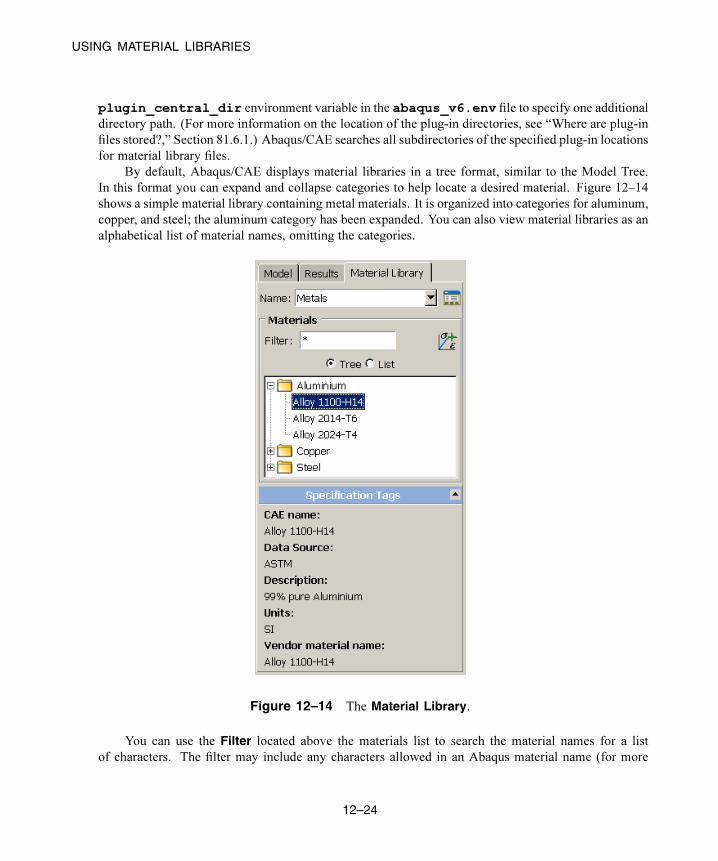
USING MATERIAL LIBRARIES
plugin_central_dir environment variable in the abaqus_v6.env file to specify one additional
directory path. (For more information on the location of the plug-in directories, see “Where are plug-in
files stored?,” Section 81.6.1.) Abaqus/CAE searches all subdirectories of the specified plug-in locations
for material library files.
By default, Abaqus/CAE displays material libraries in a tree format, similar to the Model Tree.
In this format you can expand and collapse categories to help locate a desired material. Figure 12–14
shows a simple material library containing metal materials. It is organized into categories for aluminum,
copper, and steel; the aluminum category has been expanded. You can also view material libraries as an
alphabetical list of material names, omitting the categories.
Figure 12–14 The Material Library.
You can use the Filter located above the materials list to search the material names for a list
of characters. The filter may include any characters allowed in an Abaqus material name (for more
12–24
Abaqus ID:
Printed on:

USING MATERIAL LIBRARIES
information on object naming, see “Using basic dialog box components,” Section 3.2.1). The filter is
not applied to category names, so filtering may result in “empty” categories.
The tool opens the Material Library Manager, where you can create, edit, rename,
and reorganize material libraries. You can also use the manager to create, edit, rename, and delete
Specification Tags to help identify materials in a library.
Figure 12–14 shows the predefined Specification Tags. The tool copies a selected material
from the library to the current model.
12.5.2 Managing material librariesThe Material Library Manager allows you create, edit, and rename material libraries, library
categories, and library materials. The default Specification Tags indicate the source of the material
data, a description, the units of measure, and a vendor material name. You can create, edit, rename, and
delete specification tags for each material in a library. Material properties and categories are presented
in alphabetical order, identical to the default view of the library in the main window of Abaqus/CAE;
material categories appear first, followed by materials that are not in a category. You can use the
manager to copy materials from a model to a library or from a library to a model. The Material LibraryManager is shown in Figure 12–15.
Figure 12–15 The Material Library Manager.
12–25
Abaqus ID:
Printed on:

USING THE PROPERTY MODULE TOOLBOX
When you work with material libraries, it is recommended that you carefully consider the material
and category names. You can create multiple categories and/or materials with exactly the same name.
For example, you could have identical entries for a standard grade of steel, each containing properties in
different sets of units. Using suitable category names, you can easily identify each material. However,
if you display the library in the list format, the identical entries will all appear in the list. Modifying the
material names to include the units information may make it easier to identify the desired material. For
example, you can name one material Steel 1020 US and another Steel 1020 SI. Alternatively,you can click Tags in the material library manager to indicate the units in the Specification Tags that
appear below the materials list in the main window. Renaming a material in the material library will
change the name only in the library and does not change the underlying material name copied from or to
the Abaqus/CAE model. A material added from the library to a model will still retain the old name.
You cannot view or edit material properties within the material library manager. To view or edit
the properties of a material, you must add the material to a model and use the Edit Material dialog box
(for more information, see “Creating or editing a material,” Section 12.7.1, in the HTML version of this
guide). For detailed instructions on using the Material Library Manager, see the corresponding sectionin the HTML version of this guide. Changes that you make in the Material Library Manager are visibleimmediately in the manager dialog box. However, they are not committed to the library file until you
click Save Changes. Abaqus/CAE does not update the library view in the main window until you
dismiss the material library manager.
12.5.3 Adding materials from a library to your modelTo viewmaterial libraries, select the Material Library tab in theModel Tree area of the Property module.
If more than one library is available, select one from the list at the top of the tabbed page. In the default
Tree view, expand categories to view the materials within each category. To hide the categories and view
an alphabetical list of all materials in the current library, select the List view.To add a material from a library to the current model, highlight the material name in the tree or list
view, and click the Add Material icon at the upper right corner of the Materials list. Alternatively,
you can double-click on a material name in the library to add it to the model.
For detailed instructions, see the corresponding section in the HTML version of this guide.
Once you have added a material to your model, use the Edit Material dialog box to view or edit the
material properties. Use the other tools in the Property module to associate the material with a section
and assign the section to part of your model.
12.6 Using the Property module toolbox
You can access all the Property module tools through either the main menu bar or the Property module
toolbox. Figure 12–16 shows the icons for all the property tools in the Property module toolbox.
12–26
Abaqus ID:
Printed on:

USING THE PROPERTY MODULE TOOLBOX
Create material Material manager
Profile manager
Section assignment manager
Create profile
Create composite layup
Create skin
Create stringer
Skin manager
Stringer manager
Composite layup manager
Section managerCreate section
Assign section
Assign materialand shell properties
Assign beam properties
Figure 12–16 The Property module toolbox.
12–27
Abaqus ID:
Printed on:


UNDERSTANDING THE ROLE OF THE ASSEMBLY MODULE
13. The Assembly module
You use the Assembly module to create and modify the assembly. A model contains one main assembly,
which is composed of instances of parts from the model as well as instances of other models. The online
tutorial in Appendix C, “Using Additional Techniques to Create and Analyze a Model in Abaqus/CAE,”
of Getting Started with Abaqus: Interactive Edition contains examples of how you use the Assembly
module to create part instances and position them relative to each other in a global coordinate system.
This chapter explains how you use the tools within the Assembly module to create the assembly. The
following topics are covered:
• “Understanding the role of the Assembly module,” Section 13.1
• “Entering and exiting the Assembly module,” Section 13.2
• “Working with part instances,” Section 13.3
• “Working with model instances,” Section 13.4
• “Creating the assembly,” Section 13.5
• “Creating patterns of part instances,” Section 13.6
• “Performing Boolean operations on part instances,” Section 13.7
• “Understanding toolsets in the Assembly module,” Section 13.8
• “Using the Assembly module toolbox,” Section 13.9
In addition, the following sections are available in the HTML version of this guide:
• “Creating and manipulating part and model instances,” Section 13.10
• “Applying constraints to part and model instances,” Section 13.11
• “Using the Query toolset to query the assembly,” Section 13.12
13.1 Understanding the role of the Assembly module
When you create a part, it exists in its own coordinate system, independent of other parts in the model.
In contrast, you use the Assembly module to create instances of your parts and to position the instances
relative to each other in a global coordinate system, thus creating the assembly. You position part
instances by sequentially applying position constraints that align selected faces, edges, or vertices or by
applying simple translations and rotations.
You can also create instances of other models in your main model, allowing you to add complete
subassemblies in addition to individual parts. Model instances are created in the exact same way as part
instances and can be positioned and manipulated in a similar fashion.
An instance maintains its association with the original part or model. If the geometry of a part or
model changes, Abaqus/CAE automatically updates all instances of the part or model to reflect these
changes. You cannot edit the geometry of an instance directly.
13–1
Abaqus ID:
Printed on:

WORKING WITH PART INSTANCES
Your main model can contain many parts and model subassemblies, and a part or model can be
instanced many times in the main model assembly; however, a model contains only one top-level
assembly. Loads, boundary conditions, predefined fields, and meshes are all applied to the complete
assembly. Even if your model consists of only a single part, you must still create an assembly that
consists of just a single instance of that part.
A part instance can be thought of as a representation of the original part. You can create either
independent or dependent part instances. An independent instance is effectively a copy of the part. A
dependent instance is only a pointer to the part, partition, or virtual topology; and as a result, you cannot
mesh a dependent instance. However, you can mesh the original part from which the instance was
derived, in which case Abaqus/CAE applies the same mesh to each dependent instance of the part.
A model instance is always dependent, not independent.
13.2 Entering and exiting the Assembly module
You can enter the Assembly module at any time during an Abaqus/CAE session by clicking Assemblyin the Module list located in the context bar. The Instance, Constraint, Feature, and Tools menus
appear on the main menu bar.
To exit the Assembly module, select any other module from the Module list. You need not save
your assembly before exiting the module; it will be saved automatically when you save the entire model
by selecting File→Save or File→Save As from the main menu bar.
13.3 Working with part instances
This section describes part instances, how they relate to the original part, how you link and exclude part
instances, and how you use them to create the assembly.
13.3.1 Understanding the relationship between models, parts, instances,and assemblies
A model can contain many parts; however, it can contain only one top-level assembly. The assembly
is composed of instances of the parts positioned relative to each other in a global coordinate system, as
described in “What is a part instance?,” Section 11.3.4. The top-level assembly can also contain model
instances that effectively create subassemblies from other models.
The concept of parts, part instances, and the assembly is carried throughout the Abaqus/CAE
modeling process:
13–2
Abaqus ID:
Printed on:

WORKING WITH PART INSTANCES
1. You create a part in the Part module; each part is a distinct entity that can be modified and
manipulated independently of other parts. Parts exist in their own coordinate system and have no
knowledge of other parts.
2. You define section properties in the Property module and also associate a material with a section.
You use the Property module to assign these section properties to a part or to a selected region of a
part.
3. You create instances of your parts in the Assembly module, and you position those instances relative
to each other in a global coordinate system to form the assembly. You can also add instances of other
models in the assembly.
Abaqus/CAE allows you to create either independent or dependent part instances, as described
in “What is the difference between a dependent and an independent part instance?,” Section 13.3.2.
Both independent and dependent part instances maintain their association with the original part.
When you modify the original part in the Part module, Abaqus/CAE updates any instances of that
part when you return to the Assembly module. You can instance a part many times and assemble
multiple instances of the same part. Each instance of the part is associated with the section properties
assigned to the part in the Property module.
4. You use the Interaction and Load modules to complete the definition of the model by, for example,
defining contact and applying items such as loads and boundary conditions. The Interaction and
Load modules operate on the assembly.
5. You use the Mesh module to mesh the assembly. You can do either of the following:
• Individually mesh each independent instance of a part in the assembly.
• Mesh the original part. Abaqus/CAE then associates the mesh with each dependent instance
of the part in the assembly.
The two meshing approaches are described in “What is the difference between a dependent and an
independent part instance?,” Section 13.3.2.
“Creating a part or model instance,” Section 13.10.3, in the HTML version of this guide contains
detailed instructions on creating part instances. For instructions on using the online documentation, see
“Getting help,” Section 2.6.
13.3.2 What is the difference between a dependent and an independentpart instance?
When you create a part instance, you can choose to create either a dependent part instance or an
independent part instance. You can also edit a part instance and change it from dependent to independent
or vice versa. When you create a model instance, it is always dependent.
Dependent part instances
By default, Abaqus/CAE creates a dependent instance of a part. A dependent instance is only a
pointer to the original part. In effect, a dependent instance shares the geometry and the mesh of the
13–3
Abaqus ID:
Printed on:
WORKING WITH PART INSTANCES
original part. As a result, you can mesh the original part, but you cannot mesh a dependent instance.
When you mesh the original part, Abaqus/CAE applies the same mesh to all dependent instances of
the part. Most modifications are not allowed on a dependent part instance; for example, you cannot
add partitions or create virtual topology. However, operations that do not modify the geometry of a
dependent part instance are still allowed; for example, you can create sets, apply loads and boundary
conditions, and define connector section assignments. If you have already meshed a part or added
virtual topology to the part, you can create only a dependent instance of the part.
If you apply an adaptive remeshing rule to a dependent part instance in the Mesh module,
Abaqus/CAE remeshes the original part and applies the new mesh to each dependent instance of
the part.
You cannot change the mesh attributes of an individual dependent part instance; for example,
the mesh seeds, mesh controls, and element types. However, you can change the mesh attributes
of the original part, and Abaqus/CAE propagates the changes to all dependent instances of the part.
Although you have already meshed the original part and applied the same mesh to its dependent
instances, the mesh is visible only in the Mesh module. You continue to work with the native
Abaqus/CAE geometry in the Assembly, Interaction, and Load modules. In general, you cannot
use the Edit Mesh toolset to edit the mesh of a dependent part instance; however, you can use the
Edit Mesh toolset to edit and project the nodes of a dependent part instance. Abaqus/CAE moves
the nodes of the original meshed part, and your modifications appear on all dependent instances of
the part.
The advantages of dependent part instances are that they consume fewer memory resources and
you need mesh the part only once. In addition, Abaqus/CAE instances a dependent part instance in
the input file by writing a single set of nodal coordinates and element connectivity to define the part
along with a transform to define each part instance.
Independent part instances
In contrast, an independent part instance is a copy of the geometry of the original part. You
cannot mesh a part from which you created an independent part instance; however, you can
mesh the independent instance. In addition to meshing, you can perform most other operations
on an independent instance; for example, you can add partitions and create virtual topology.
The disadvantages of independent instances are that they consume more memory resources,
and you must mesh each independent instance individually. In addition, Abaqus/CAE does not
take advantage of instantiation in the input file with independent part instances—sets of nodal
coordinates and element connectivity are written to the input file for each independent part instance.
You cannot create both a dependent and an independent instance of the same part. As a result, if you
create a dependent instance of a part, all subsequent instances must be dependent. The same argument
applies to independent instances. Instances of mesh parts are always dependent.
You can use the Model Tree to determine if an instance is dependent or independent. When you
mesh an independent part instance, the mesh appears in the Model Tree under the part instance container,
as shown in Figure 13–1. In addition, Figure 13–1 also illustrates that as you move the cursor over an
13–4
Abaqus ID:
Printed on:

WORKING WITH PART INSTANCES
instance, the information displayed by the Model Tree indicates whether the instance is dependent or
independent.
Figure 13–1 The Model Tree indicates whether a part instance is dependent or independent.
13.3.3 How do I decide whether to create a dependent or an independentpart instance?
If your assembly contains a few part instances that are unrelated, dependent instances have little
advantage over independent instances. Each part is different, and you must create an instance of each
part. In contrast, if your assembly contains identical part instances, you can save time by assembling
dependent instances of the part. When you subsequently mesh the original part, Abaqus/CAE applies
that mesh to each dependent instance of the part in the assembly. In addition, dependent instances
consume fewer memory resources and result in a smaller input file.
For example, Figure 13–2 illustrates an assembly of independent and dependent part instances. The
pump housing is an independent part instance, and the eight bolts are dependent part instances. The figure
on the left shows the assembly in the Assembly module. The figure on the right shows the assembly in
the Mesh module. The user has meshed the part representing the bolt, and Abaqus/CAE associated the
mesh with each dependent instance of the bolt.
13–5
Abaqus ID:
Printed on:
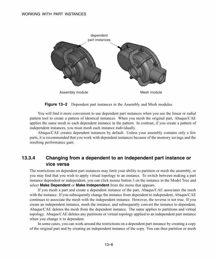
WORKING WITH PART INSTANCES
dependentpart instances
Assembly module Mesh module
Figure 13–2 Dependent part instances in the Assembly and Mesh modules.
You will find it more convenient to use dependent part instances when you use the linear or radial
pattern tool to create a pattern of identical instances. When you mesh the original part, Abaqus/CAE
applies the same mesh to each dependent instance in the pattern. In contrast, if you create a pattern of
independent instances, you must mesh each instance individually.
Abaqus/CAE creates dependent instances by default. Unless your assembly contains only a few
parts, it is recommended that you work with dependent instances because of the memory savings and the
resulting performance gain.
13.3.4 Changing from a dependent to an independent part instance orvice versa
The restrictions on dependent part instances may limit your ability to partition or mesh the assembly, or
you may find that you wish to apply virtual topology to an instance. To switch between making a part
instance dependent or independent, you can click mouse button 3 on the instance in the Model Tree and
select Make Dependent or Make Independent from the menu that appears.
If you mesh a part and create a dependent instance of the part, Abaqus/CAE associates the mesh
with the instance. If you subsequently change the instance from dependent to independent, Abaqus/CAE
continues to associate the mesh with the independent instance. However, the reverse is not true. If you
create an independent instance, mesh the instance, and subsequently convert the instance to dependent,
Abaqus/CAE deletes the mesh from the dependent instance. The same applies to partitions and virtual
topology. Abaqus/CAE deletes any partitions or virtual topology applied to an independent part instance
when you change it to dependent.
In some cases, you can work around the restrictions on a dependent part instance by creating a copy
of the original part and by creating an independent instance of the copy. You can then partition or mesh
13–6
Abaqus ID:
Printed on:
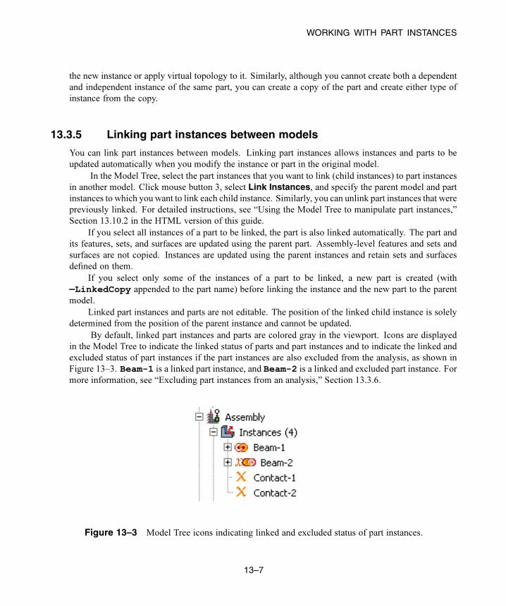
WORKING WITH PART INSTANCES
the new instance or apply virtual topology to it. Similarly, although you cannot create both a dependent
and independent instance of the same part, you can create a copy of the part and create either type of
instance from the copy.
13.3.5 Linking part instances between models
You can link part instances between models. Linking part instances allows instances and parts to be
updated automatically when you modify the instance or part in the original model.
In the Model Tree, select the part instances that you want to link (child instances) to part instances
in another model. Click mouse button 3, select Link Instances, and specify the parent model and part
instances to which you want to link each child instance. Similarly, you can unlink part instances that were
previously linked. For detailed instructions, see “Using the Model Tree to manipulate part instances,”
Section 13.10.2 in the HTML version of this guide.
If you select all instances of a part to be linked, the part is also linked automatically. The part and
its features, sets, and surfaces are updated using the parent part. Assembly-level features and sets and
surfaces are not copied. Instances are updated using the parent instances and retain sets and surfaces
defined on them.
If you select only some of the instances of a part to be linked, a new part is created (with
—LinkedCopy appended to the part name) before linking the instance and the new part to the parent
model.
Linked part instances and parts are not editable. The position of the linked child instance is solely
determined from the position of the parent instance and cannot be updated.
By default, linked part instances and parts are colored gray in the viewport. Icons are displayed
in the Model Tree to indicate the linked status of parts and part instances and to indicate the linked and
excluded status of part instances if the part instances are also excluded from the analysis, as shown in
Figure 13–3. Beam-1 is a linked part instance, and Beam-2 is a linked and excluded part instance. For
more information, see “Excluding part instances from an analysis,” Section 13.3.6.
Figure 13–3 Model Tree icons indicating linked and excluded status of part instances.
13–7
Abaqus ID:
Printed on:

WORKING WITH MODEL INSTANCES
13.3.6 Excluding part instances from an analysisYou can exclude part instances from the analysis so that they are not written to the input file when the
analysis job is submitted. An excluded part instance participates in all operations other than the analysis.
In the Model Tree, select the part instances that you want to exclude from the analysis. Click
mouse button 3, and select Exclude from Simulation. Similarly, you can include part instances that
were previously excluded by selecting Include in Simulation. Constraints on the part instances are
retained if you exclude the instances from the analysis and subsequently include them.
By default, part instances that are excluded from the analysis are colored dark gray in the viewport.
Icons are displayed in the Model Tree to indicate the excluded status of part instances and to indicate
the linked and excluded status of part instances if the part instances are also linked between models, as
shown in Figure 13–3. Contact-1 and Contact-2 are part instances that are excluded from the
analysis, and Beam-2 is a linked and excluded part instance. For more information, see “Linking part
instances between models,” Section 13.3.5.
13.3.7 Sets and part instancesPart sets are transferred when you create a part instance from a part. For example, you might create
a set from a region of a part and use the Property module to assign a section to that set. When you
instance the part in the Assembly module, Abaqus creates part instance sets that refer to any part sets
that you previously created. Abaqus provides read-only access to these part instance sets in assembly-
related modules. You cannot access a part instance set from the Set Manager; however, you can select
an eligible part instance set during a procedure by clicking the Set button and selecting the set from
the Region Selection dialog box that appears. For more information, see “Understanding sets and
surfaces,” Section 73.2.
13.4 Working with model instances
You can create instances of other models in your main model, allowing you to add complete
subassemblies in addition to individual parts. Model instances are created in the exact same way as part
instances and can be positioned and manipulated in a similar fashion.
When you create a new model instance, the main assembly of the referenced model is instantiated
in the assembly of the current working model. The instance produces a subassembly from the contents
of the other model. Since the referenced model assembly may in turn contain other model instances as
children, multiple levels of complex subassemblies are possible.
The external model to be instantiated must be included in the current model database (.cae) fileto be available. If the model you want to instantiate is contained in a different model database, use
13–8
Abaqus ID:
Printed on:

WORKING WITH MODEL INSTANCES
File→Import→Model to import it into the current model database. A model database file can always
contain multiple models.
Model instances have the following characteristics:
• A particular model can be instantiated multiple times, and you can instantiate as many different
models as desired.
• Model instances are always dependent, not independent.
• You can freely mix model instances with part instances.
• Model instance subassemblies can contain either geometric parts or orphan mesh parts.
• Model instances can be positioned and oriented in the main assembly by using transformations
(Translate, Translate To, Rotate) and positioning constraints. The transformations and
constraints must be applied to a complete model instance subassembly, not to any of its children. If
you select a child instance within a model instance, the transformation or constraint will be applied
to the entire parent model instance.
• Linear and radial patterns are not supported and cannot be used with model instances.
• Part instance commands such as Suppress/Resume, Hide/Show, Delete, and ShowParents/Children can also be used on model instances.
The Suppress and Delete commands cannot be used on the child instances of a model
instance, only on the model instance itself. If you suppress a child instance (part or model) in the
referenced model assembly, it will be suppressed in the main model as well. The child instance
must then be resumed in the original, referenced model.
• Replace, Switch Context, Exclude from Simulation, Merge/Cut, and Link Instances are not
supported and cannot be used on model instances.
• The Partition toolset is not supported and cannot be used with model instances.
• The Query toolset is supported and can be used to determine the position and attributes of model
instances.
• All sets and surfaces defined in the referenced model are brought into the model instance,
maintaining the Model Tree hierarchy of features. These sets and surfaces will be available in the
main model.
• History-level features defined in the referenced model such as steps, loads, boundary conditions,
interactions, and amplitudes are not brought into the model instance. Some model-level
features—connector assignments, fasteners, and other engineering features—defined in the
referenced model are not brought into the model instance.
• Model instances are supported and selectable in Display Groups and in the Instance tab of the
Assembly Display Options.
• The Virtual Topology toolset is not supported for model instances.
Any part-level attributes that are needed in your subassembly (referenced) model must be created
and assigned in that original model and cannot be created in the main model assembly. For example,
materials, sections, orientations, and skin/stringer assignments must be created in the original model.
13–9
Abaqus ID:
Printed on:
WORKING WITH MODEL INSTANCES
Meshing can be performed on the original independent part instances, and the meshes will appear in the
model instance.
When you create a model instance, all of the part instances of the referenced model assembly are
added to the main model assembly as child part instances. Any suppressed part instances or instances
that are excluded from the simulation will retain the same status in the subassembly.
If you modify or delete an existing part instance or model instance subassembly in the main model
assembly, Abaqus/CAE automatically regenerates the child instances from all parent instances (parts and
models) whenever you switch out of and back into the Assembly module of the main model.
If you try to create a new model instance from another model that in turn contains child model
instances, any problems with model referencing circularity will be prevented by Abaqus/CAE.
Abaqus/CAE will prevent you from creating this kind of problematic instance.
Abaqus/CAE ensures consistency of the modeling space for model instances—if all instances in the
main model are three-dimensional, any other models to be instantiated must also be three-dimensional.
13.4.1 Model instance data saved in input files
When Abaqus/CAE generates the input (.inp) file for a model assembly that contains model instances,
a single flattened assembly is generated. All model instance subassemblies are written as a flat list of
instances under the single assembly block.
Most features from the original model of a model instance are saved in the input file, with some
exceptions:
• None of the history-level features from a model instance subassembly is saved in the input file.
Model-level features from a model instance are saved in the input file; for example, materials,
section assignments, skins, stringers, and orientations. Materials and element controls defined
in a model instance are prepended with the model name in the main assembly; for example,
model-name#material-name. Other model-level data such as initial conditions and
amplitude definitions from a model instance are not saved in the input file.
• Engineering features such as mass and inertia elements, springs, and dashpots defined at the part
level in the model instance are saved to the input file, but engineering features defined at the
assembly level in the original model are not.
• Sets and surfaces from a model instance are saved in the input file. These set and surface names are
also prepended with the model instance name in the main assembly; for example:
model-instance-name#Set1
• Constraints, reference points, attachment points, attachment lines, and wires from a model instance
are saved in the input file.
• For constraints the model instance name will be prepended to the constraint name; for example:
model-instance-name#constraint-name
13–10
Abaqus ID:
Printed on:

CREATING THE ASSEMBLY
• Attachment points, attachment lines, and wires will be available through sets created in the
subassembly.
The following limitations exist:
• Generation of a flat input file is not supported for a model containing model instances.
• Restart analysis is not supported for a model containing model instances.
• Instances of models containing substructure instances are not supported.
• Instances of models containing assembled fasteners are not supported.
13.5 Creating the assembly
After you create a part instance or a model instance, you apply a succession of position constraints and
positioning operations to position it relative to other instances in the global coordinate system. This
section describes the tools that Abaqus/CAE provides to position and constrain part and model instances.
This section also describes how you can replace a part instance.
13.5.1 The position tools in the Assembly module
Each part exists in its own coordinate system in the Part module, and model instances are created in their
own coordinate system. You use the Assembly module to position and orient instances of these parts and
models relative to each other in a global coordinate system. Abaqus/CAE provides the following tools
for positioning part and model instances:
Auto-offset
When you create the first part or model instance in the Assembly module, Abaqus/CAE displays
a triad indicating the origin and the orientation of the global coordinate system. Abaqus/CAE
positions the first instance so that the origin of the part or model aligns with the origin of the
global coordinate system and the axes are aligned. If you create additional instances, Abaqus/CAE
continues to position the new instances such that their coordinate system aligns with the global
coordinate system. Since this usually results in new instances overlapping existing ones,
Abaqus/CAE allows you to apply an offset before it creates the instance. The offset is applied
along the X-axis for three-dimensional and two-dimensional instances and along the Y-axis
for axisymmetric instances. For detailed instructions, see “Creating a part or model instance,”
Section 13.10.3, in the HTML version of this guide.
Basic positioning tools
Abaqus/CAE provides the following basic methods for positioning part and model instances:
13–11
Abaqus ID:
Printed on:

CREATING THE ASSEMBLY
• You can translate selected instances along a vector by specifying the coordinates of the start
point and end point of the translation vector. You can use the following methods to determine
the distance moved by the selected instances:
– The selected instances move along the translation vector from the start point to the end
point.
– The selected instances move along the translation vector from the start point toward the
end point and continue to move until a selected face or edge is a specified distance from
a face or edge selected from the fixed instances. For more information, see “Positioning
a part or model instance using the Translate To tool,” Section 13.5.4.
• You can rotate selected instances about an axis. You specify the X-, Y-, and Z-coordinates of
the start point and end point of the axis of rotation and the angle of rotation.
Position constraint tools
A position constraint defines a relationship between two instances. Unlike a simple translation or
rotation, you do not specify the position directly. Position constraints define a set of rules that must
always be met by the part or model instances in the assembly; for example, a face that must be
parallel to another face.
Position constraints defined in the Assembly module create constraints only on the initial
positions of instances, whereas constraints defined in the Interaction module define constraints on
the analysis degrees of freedom. In the Assembly module constraints are stored as features of the
assembly. If you modify a part or move a part or model instance, Abaqus/CAE attempts to apply
all existing position constraints when it regenerates the assembly. Each of the position constraints
is described in “How the position constraint methods differ,” Section 13.5.2.
Creating the final assembly is an iterative process of creating instances, applying position
constraints, and applying translations and rotations. After each repositioning, Abaqus/CAE displays
a temporary image indicating the result of the operation. You can accept the new position, cancel the
operation, or step back through the repositioning procedure by clicking the Previous button in
the prompt area.
You can use the Query toolset to obtain the coordinates of a vertex and to measure the distance
between selected vertices. This may help you determine the vector along which you need to translate
instances or the angle through which you need to rotate them. “Using the Query toolset to query the
assembly,” Section 13.12, in the HTML version of this guide contains detailed instructions on how to
obtain information about the assembly.
13.5.2 How the position constraint methods differA position constraint defines a relationship between two part or model instances—one that will move (the
movable instance) and one that will remain stationary (the fixed instance). When you apply a position
constraint, Abaqus/CAE computes a position for the movable instance that satisfies this relationship; you
13–12
Abaqus ID:
Printed on:

CREATING THE ASSEMBLY
do not specify the position directly. You can apply the following position constraints to instances in the
Assembly module:
• Parallel face (three-dimensional instances only)
• Face to face (three-dimensional instances only)
• Parallel edge
• Edge to edge
• Coaxial (three-dimensional instances only)
• Coincident point
• Parallel coordinate systems
In general, applying a single position constraint is not sufficient to define the precise location of a
movable instance. You must apply several position constraints—usually three for a three-dimensional
assembly and two for a two-dimensional assembly—to position an instance in the desired location. Part
and model instances can overlap as a result of applying position constraints; Abaqus/CAE does not
prevent overclosure between edges, faces, or cells. Similarly, Abaqus/CAE does not prevent you from
overconstraining instances or duplicating a constraint.
The definition of a constraint feature includes all the faces and edges that you originally selected.
If you subsequently modify a part or move a part or model instance, Abaqus/CAE automatically
recalculates the constraint based on your original selection of faces and edges. As a result, one or
more instances may move after the assembly is regenerated. For example, different edges may become
parallel. For more information on features, see “Manipulating features in the Assembly module,”
Section 13.8.2, and Chapter 65, “The Feature Manipulation toolset.”
The following position constraints are provided by the Assembly module:
Parallel Face
A parallel face position constraint causes a selected face of the movable instance to become parallel
with a selected face of the fixed instance. However, the position constraint does not specify the
precise location of the movable instance, and the distance between the parallel faces is arbitrary. To
apply a parallel face position constraint between two instances, you do the following:
• Select the faces to be constrained to be parallel from the movable instance and the fixed
instance, as shown in Figure 13–4.
• Abaqus/CAE displays arrows normal to the selected faces. You prescribe the orientation
of the movable instance by selecting the direction of the arrow normal to its selected face.
Figure 13–5 illustrates the result of applying the position constraint and the effect on the
movable instance of reversing the direction of the arrow. Abaqus/CAE rotates the movable
instance until the two selected faces are parallel and the arrows are pointing in the same
direction.
13–13
Abaqus ID:
Printed on:

CREATING THE ASSEMBLY
Selected faces
Fixed part instance
Movable part instance
Figure 13–4 Select the faces to become parallel.
Figure 13–5 The result of applying a parallel face position constraint and the effect of changing
the direction of the arrow normal to the selected face of the movable instance.
The faces you select from the movable and fixed instances must be planar. The parallel face
position constraint can be applied only to three-dimensional instances. For detailed instructions,
see “Constraining two instances with parallel planar faces,” Section 13.11.2, in the HTML version
of this guide.
Face to Face
A face-to-face position constraint is similar to a parallel face position constraint except that you
define the clearance between the parallel faces. The clearance is measured between the two selected
faces, positive along the normal to the fixed instance. Other than this clearance, the precise location
of the movable instance is not constrained. Assuming that you selected the same two faces shown in
Figure 13–4, the effect of applying a face-to-face constraint is shown in Figure 13–6. Figure 13–6
also illustrates the effect on the movable instance of reversing the direction of the arrow normal to
its selected face.
13–14
Abaqus ID:
Printed on:

CREATING THE ASSEMBLY
d d
Plan viewPlan view
Figure 13–6 The result of applying a face-to-face constraint
and the effect of changing the direction of the arrow normal to
the selected face of the movable instance.
Abaqus/CAE rotates the movable instance until the two selected faces are parallel and the arrows
point in the same direction. In addition, the movable instance is translated to satisfy the clearance
specified. The faces you select from the movable and fixed instances must be planar. The
face-to-face position constraint can be applied only to three-dimensional instances. For detailed
instructions, see “Constraining two instances with parallel planar faces separated by a specified
distance,” Section 13.11.3, in the HTML version of this guide.
Parallel Edge
A parallel edge position constraint causes a selected edge of the movable instance to become parallel
with a selected edge of the fixed instance. However, the position constraint does not specify the
precise location of the movable instance, and the distance between the parallel edges is arbitrary.
To apply a parallel edge position constraint between two instances, you do the following:
13–15
Abaqus ID:
Printed on:

CREATING THE ASSEMBLY
• Select the edges to be constrained to be parallel from the movable and fixed instance, as shown
in Figure 13–7.
Selected edges
Fixed part instance
Movable part instance
Figure 13–7 Select the edges to become parallel.
• Abaqus/CAE displays arrows along the selected edges. You prescribe the orientation of the
movable instance by selecting the direction of the arrow along its selected edge. Figure 13–8
illustrates the result of applying the position constraint and the effect on the movable instance
of reversing the direction of the arrow. Abaqus/CAE rotates the movable instance until the two
selected edges are parallel and the arrows point in the same direction.
The edges you select from the movable and fixed instances must be straight. You can select an edge
from an instance, or you can select a datum axis or one of the axes of a datum coordinate system.
The parallel edge position constraint can be applied only to two-dimensional and three-dimensional
instances. It has no effect on axisymmetric instances. For detailed instructions, see “Constraining
two instances with parallel edges,” Section 13.11.4, in the HTML version of this guide.
Edge to Edge
An edge-to-edge position constraint is similar to a parallel edge position constraint except that the
clearance between the parallel edges is defined by the constraint. Assuming that you selected the
same two edges shown in Figure 13–7, the effect of applying an edge-to edge position constraint
to a two-dimensional assembly is shown in Figure 13–9. Figure 13–9 also illustrates the effect on
the movable instance of reversing the direction of the arrow along its selected edge. The modeling
space of the assembly determines the behavior of Abaqus/CAE after you apply an edge-to-edge
position constraint.
• If the assembly is three-dimensional, Abaqus/CAE positions the movable instance so that the
edges are coincident.
• If the assembly is two-dimensional, you can specify the clearance between the selected edges.
The clearance is measured between the two selected edges, positive along the normal to the
fixed instance.
Other than this behavior, the precise location of the movable instance is not constrained. The edge-
to-edge position constraint can be applied to two-dimensional, three-dimensional, and axisymmetric
instances; however, axisymmetric instances can move only parallel to the axis of revolution. For
13–16
Abaqus ID:
Printed on:

CREATING THE ASSEMBLY
Figure 13–8 The result of applying a parallel edge constraint
and the effect of changing the direction of the arrow along the
selected edge of the movable instance.
d d
Figure 13–9 The result of applying an edge-to-edge constraint
and the effect of changing the direction of the arrow along the
selected edge of the movable instance.
detailed instructions, see “Constraining two instances with parallel edges separated by a specified
distance,” Section 13.11.5, in the HTML version of this guide.
Coaxial
A coaxial position constraint causes a selected cylindrical or conical face of the movable instance
to become coaxial with a selected cylindrical or conical face of the fixed instance. However, the
coaxial position constraint does not constrain the precise location of the movable instance. To apply
a coaxial position constraint between two instances, you do the following:
13–17
Abaqus ID:
Printed on:

CREATING THE ASSEMBLY
• Select the cylindrical or conical faces to be constrained to be coaxial from the movable and
fixed instance, as shown in Figure 13–10.
Selected faces
Axis of revolution
Axis of revolution
Fixed part instance
Movable part instance
Figure 13–10 Select the faces to become coaxial.
• Abaqus/CAE displays arrows along the axis of revolution of the selected instances. You
prescribe the orientation of the movable instance by selecting the direction of the arrow along
its axis of revolution. Figure 13–11 illustrates the result of applying the coaxial position
constraint.
Abaqus/CAE rotates and translates the movable instance until the two selected faces are coaxial
and the arrows are pointing in the same direction. The coaxial position constraint can be applied
only to three-dimensional instances. For detailed instructions, see “Constraining two instances with
coaxial faces,” Section 13.11.6, in the HTML version of this guide.
Coincident Point
A coincident point constraint causes a selected point on the movable instance to coincide with a
selected point on the fixed instance. However, the coincident point constraint does not constrain the
orientation of the movable instance. The orientation of the movable instance does not change after
the constraint is applied, as shown in Figure 13–12. For detailed instructions, see “Constraining
two instances with coincident points,” Section 13.11.7, in the HTML version of this guide.
13–18
Abaqus ID:
Printed on:

CREATING THE ASSEMBLY
Figure 13–11 The effect of applying a coaxial constraint.
Maintain relativepositions usingCVJOINT connector.
2.Assemble instancesusing coincident points.
1.
Figure 13–12 The effect of applying a coincident point constraint.
Parallel CSYS
A parallel coordinate systems constraint causes the axes of a datum coordinate system on the
movable instance to become parallel with the axes of a datum coordinate system on the fixed
instance. However, the parallel coordinate systems constraint does not specify the precise location
of the movable instance. Figure 13–13 illustrates the effect of applying a parallel coordinate
systems constraint and a concident point constraint to two instances.
13–19
Abaqus ID:
Printed on:

CREATING THE ASSEMBLY
Coincident point
Maintain relativepositions with TRANSLATOR connector.
2.
Assemble instances using coincident point and parallel CSYS.
1.
eb
2
eb
3e
b
1e
a
2
ea
1
ea
3
Part b
Part a
Parallelcoordinatesystems
Figure 13–13 The effect of applying parallel coordinate
systems and coincident point constraints.
The coordinate systems can be either rectangular (X-, Y-, and Z-axes), cylindrical (R-, -, and Z-
axes), or spherical (R-, -, and -axes). For detailed instructions, see “Constraining two instances
with parallel coordinate systems,” Section 13.11.8, in the HTML version of this guide.
You can use datums to position part and model instances. When you are prompted to select a face,
you can also select a datum plane. When you are prompted to select an edge, you can also select a datum
axis or one of the axes of a datum coordinate system. You can select a datum that you created in the Part
module because the datum is associated with an instance of the part and moves with the part instance.
However, if the position constraint uses a datum that you created in the Assembly module by selecting
from a part instance (such as a face of a part instance), Abaqus/CAE changes its regeneration behavior
and regenerates features in the order that you created them. For more information, see “How are position
constraints regenerated?,” Section 65.3.5. You cannot select a datum as the movable part instance if you
created the datum in the Assembly module and it depends on more than one part instance; for example,
a datum axis that runs through vertices of two part instances.
13–20
Abaqus ID:
Printed on:

CREATING THE ASSEMBLY
13.5.3 How conflicts can arise between position constraints,translations, and rotations
In some situations attempting to apply a position constraint results in a conflict with existing position
constraints. If that is the case, Abaqus/CAE displays an error message, and you can either apply a
different position constraint or use the Feature Manipulation toolset to modify the existing position
constraints.
Similarly, attempting to translate or rotate a part or model instance may result in a conflict with
existing position constraints. If a conflict occurs, Abaqus/CAE does the following:
Translation
Abaqus/CAE applies the components of translation only along the unconstrained degrees of
freedom. If all of the degrees of freedom are constrained, Abaqus/CAE displays an error message
and the translation fails.
Rotation
Abaqus/CAE displays an error message, and the rotation fails.
If you experience conflicts with an existing position constraint, you can remove all the existing
position constraints without changing the position of the instances by using Instance→ConvertConstraints. You can then apply the new position constraint, translation, or rotation. You cannot
restore position constraints that were removed. Alternatively, you can delete a position constraint,
and Abaqus/CAE will move the instance back to its original position. For detailed instructions, see
“Converting constraints,” Section 13.10.10, in the HTML version of this guide.
13.5.4 Positioning a part or model instance using the Translate To tool
The Translate To tool positions two part or model instances by translating one instance along a user-
defined vector defining the direction of motion until selected faces or edges of the movable instance are
separated by a specified distance from selected faces or edges of the fixed instance.
When you use the Translate To tool to position instances in three-dimensional modeling space,
you select faces to come into contact; for instances in two-dimensional or axisymmetric modeling space,
you select edges to come into contact. In addition, when you use the Translate To tool to position
axisymmetric instances, the translation vector must be parallel to the axis of revolution.
When you use the Translate To positioning tool, you can select more than one face or edge from
both the fixed and the movable instances. Selecting multiple faces or edges is useful if you are not sure
what part of the model will come in contact when the movable instance moves along the selected vector.
However, for faster processing you should select as few faces or edges as possible.
To translate a movable part or model instance to a fixed instance, you do the following:
13–21
Abaqus ID:
Printed on:

CREATING THE ASSEMBLY
• Select faces or edges from the instance that will move and from the instance that will remain
stationary.
• Prescribe the motion of the movable instance by defining a translation vector. Figure 13–14
illustrates the selected edges and translation vector.
Selected edges
Translationvector
Figure 13–14 Select the edges to contact, and define the translation vector.
• Define the desired clearance between the selected faces or edges. Figure 13–15 shows the effect
of the contact constraint after specifying a clearance value of zero and a clearance value of d. To
measure the clearance d, Abaqus/CAE first moves the instance along the translation vector until
any pair of selected faces or edges come into contact. Abaqus/CAE then moves the instance along
the translation vector a distance specified by the clearance value. The clearance can be zero or a
positive or negative number; a negative value for the clearance results in overclosure between the
selected faces or edges. When you use the Translate To tool, Abaqus/CAE calculates the position
of the movable instance within a tolerance based on its size. If you want to avoid any possibility of
overclosure, you should specify a small clearance value, rather than simply specifying zero.
Abaqus/CAE displays an error message and does not move the instance if contact between the
selected faces or edges is not possible along the translation vector. For detailed instructions, see
“Translating a part or model instance to another instance,” Section 13.10.7, in the HTML version
of this guide.
Even though you translate the movable instances until contact occurs with a fixed instance, the
physical proximity of the selected surfaces is not enough to indicate any type of interaction between them.
You must use the Interaction module to specify mechanical contact between surfaces. The Translate Topositioning tool is satisfied only within a tolerance based on the size of your model. As a result, contact
may not be precise unless it is applied between two planar surfaces.
Abaqus/CAE approximates a curved face with a set of faceted faces. Likewise, Abaqus/CAE
approximates a curved edge with a set of faceted edges. The number of facets depends on the degree
13–22
Abaqus ID:
Printed on:

CREATING THE ASSEMBLY
d
Points ofcontact
Figure 13–15 The effect of applying a contact constraint and
specifying clearance values of zero and d.
of curve refinement that you specified when creating the part in the Part module. Use the box zoom
tool to view the faceting applied to curved faces or edges in the assembly. When you are
translating curved faces or curved edges, Abaqus/CAE computes the contact position using this faceted
representation. You may wish to set the curve refinement to a finer setting based on the curvature of
faces or edges that you know will be coming into contact. For more information, see “Controlling curve
refinement,” Section 76.4, in the HTML version of this guide.
13.5.5 Replacing a part instanceYou can replace a part instance with an instance of a second part. To be precise, you are replacing the
part from which the part instance is created. Abaqus/CAE positions the new part instance such that its
origin is located at the origin of the original part instance and their axes align. In addition, you can choose
whether the new part instance inherits all the constraints from the instance it replaced.
The replace operation does not change the attributes of the instance. For example, if the original
instance is dependent, the instance that replaces it will also be dependent. As a result, if an independent
instance of a part exists, you cannot use the replace procedure to create a dependent instance of the same
part.
Replacing a part instance is useful when you are replacing a part instance with one that has similar
geometry. For example, the new part instance might have additional detail that was not present in the
original part instance. You can also replace a geometry-based part with a mesh representation of the same
part. For example, you could replace a part with the mesh representation of the deformed part imported
from an output database. For detailed instructions, see “Replacing a part instance,” Section 13.10.9, in
the HTML version of this guide.
13–23
Abaqus ID:
Printed on:

CREATING PATTERNS OF PART INSTANCES
13.6 Creating patterns of part instances
You can create multiple copies of a selected part instance in either a linear or radial pattern. You can
specify the number of instances to create and the structure of the pattern, as described below. These
commands cannot be used on model instances.
Linear pattern
A linear pattern positions the new instances linearly along a direction; for example, the X-direction.
The origin of the selected part instance and the origins of the new part instances lie on the line
specified by the direction. You can specify the number of instances and the spacing between the
instances. In addition, you can change the orientation of the linear pattern by selecting a line from
the assembly that represents the new direction.
You can create a matrix of copied instances by creating copies in a second direction; for
example, the Y-direction. The options are the same as for the first direction; you can control the
number of copies, the spacing, and the orientation. By default, the first direction is the X-axis and
the second direction is the Y-axis. For example, Figure 13–16 illustrates how a part instance can
be patterned in both the X- and Y-axes.
Figure 13–16 Part instances patterned in two linear directions.
Radial pattern
A radial pattern positions the new instances in a circular pattern. You can specify the number of
instances, and you can specify the angle between the first and last copy, where a positive angle
corresponds to a counterclockwise direction. For example, Figure 13–17 illustrates a radial pattern
of the same part instances that appear in Figure 13–16. By default, Abaqus/CAE creates the radial
pattern about the Z-axis. Alternatively, you can select a line from the assembly that defines the axis
of the circular pattern.
If you create a pattern of instances that are touching and you want to treat the pattern as a single
part, you must use the Merge/Cut tool to merge all of the part instances in the pattern into a single part
instance. For example, the instances in the radial pattern illustrated in Figure 13–17 overlapped each
13–24
Abaqus ID:
Printed on:

PERFORMING BOOLEAN OPERATIONS ON PART INSTANCES
Figure 13–17 A radial pattern of part instances.
other and have been merged into a single part instance. For more information, see “Performing Boolean
operations on part instances,” Section 13.7. If you do not merge the part instances, the pattern may
include duplicate faces or nodes where the instances touch.
If a part contains part-level sets or surfaces, Abaqus/CAE creates separate assembly-level sets and
surfaces for each individual part instance in a pattern (see “How do part sets and assembly sets differ?,”
Section 73.2.2, for further discussion of part- and assembly-level sets and surfaces). For example, if
the top face of the original part in Figure 13–16 and Figure 13–17 is included in a part-level surface,
Abaqus/CAE initially creates individual assembly-level surfaces for the top face of each part instance
in the patterned assembly. It is often helpful to merge these repeated sets and surfaces into a single set
or surface. When you merge patterned part instances, Abaqus/CAE also merges any repeated sets or
repeated surfaces into a single set or surface on the merged part and part instance. If you do not merge
the patterned part instances, you can still merge sets or surfaces using the Boolean option in the Model
Tree (see “Performing Boolean operations on sets or surfaces,” Section 73.3.4, in the HTML version of
this guide, for instructions).
You will find it more convenient to use dependent part instances when you create a linear or radial
pattern of instances. When you mesh the original part, Abaqus/CAE applies the same mesh to each
instance in the pattern. In contrast, if you create a pattern of independent instances, you must mesh each
instance individually. For more information, see “What is the difference between a dependent and an
independent part instance?,” Section 13.3.2.
13.7 Performing Boolean operations on part instances
You can select instances of parts that you created using Abaqus/CAE and merge them into a single
instance. In addition, you can cut away the geometric portion of a part instance using the geometric
13–25
Abaqus ID:
Printed on:

PERFORMING BOOLEAN OPERATIONS ON PART INSTANCES
portion of other part instances to make the cut. You can also merge instances of parts containing both
geometry and orphan elements. For detailed instructions, see “Merging or cutting part instances,”
Section 13.10.11, in the HTML version of this guide. This section describes how you merge and cut
part instances.
13.7.1 Merging and cutting part instances
Select Instance→Merge/Cut from the main menu bar to merge multiple instances of parts. The parts
to be merged can contain any combination of geometry and orphan mesh nodes and elements; and there
are options for merging the geometry, the mesh (orphan and native), or both. In addition, you can cut the
geometric portion of a part instance using the geometric portion of one or more part instances to make
the cut. Both merge and cut operations create a new part instance and a new part. When you merge or
cut part instances, you can choose to suppress or delete the original part instances. The merge and cut
operations are described in more detail below.
Merge
You can select multiple part instances and merge them into a single part instance. For example,
Figure 13–18 shows two part instances that model a 15-pin connector. The two part instances are
positioned along a common face and then merged into a single part instance that can be meshed
and analyzed. You can merge part instances even if the instances are not touching or overlapping.
You can choose whether to remove or retain the intersecting boundaries between the merged part
instances, as shown in Figure 13–19. If desired, you can use the Part Copy dialog box to create a
mirror image of a part about one of the three principal planes. For more information, see “Copying
a part,” Section 11.5.
If you merge meshes, you can specify the Node merging tolerance, which is the maximum
distance between nodes that will be merged. Abaqus/CAE creates a compatible mesh by deleting
nodes that are closer than the specified distance and replacing them with a single new node. The
location of the new node is the average position of the deleted nodes. If the value that you entered
for the Node merging tolerance is too large, Abaqus/CAE may detect duplicate nodes from the
same element. Abaqus/CAE will not merge nodes from the same element. However, the large
tolerance can result in a distorted mesh, and Abaqus/CAE asks if you want to continue or end the
merging procedure. If no nodes are closer than the specified distance, Abaqus/CAE asks if you want
to cancel the procedure or to create a single instance from the selected instances.
When you merge meshed part instances that intersect, you can choose whether to create
duplicate elements as well as duplicate nodes. A duplicate element has the same connectivity
as another element. By default, Abaqus/CAE deletes duplicate elements, and in most cases you
should accept the default behavior. However, you must retain duplicate elements if you want to
model a material with a combination of material properties that are not supported by Abaqus, as
described in the discussion of stability in “No compression or no tension,” Section 22.2.2 of the
Abaqus Analysis User’s Guide.
You can choose between the following methods for merging the nodes:
13–26
Abaqus ID:
Printed on:

PERFORMING BOOLEAN OPERATIONS ON PART INSTANCES
Figure 13–18 Two part instances merged into a single part instance.
Figure 13–19 The effect of removing and retaining intersecting boundaries.
Boundary only
By default, Abaqus/CAE merges the meshed part instances only along their boundaries
(defined by free faces for three-dimensional instances and by free edges for two-dimensional
13–27
Abaqus ID:
Printed on:

PERFORMING BOOLEAN OPERATIONS ON PART INSTANCES
instances). Free faces and edges are those faces and edges that belong to only one geometric
entity or element. Using this setting, Abaqus/CAE does not check for duplicate nodes
in the interior of the parts, which speeds up the merging process. You should retain this
default setting if three-dimensional part instances intersect at only a common face or if
two-dimensional instances intersect at only a common edge.
All
If the part instances overlap, you may want to merge all the nodes in the selected part instances.
None
Alternatively, you can choose to merge none of the nodes, in which case Abaqus/CAE merges
the part instances into a single instance but retains all the original nodes.
In many cases you will be merging part instances that do not intersect but share a common
face; for example, the two part instances shown in Figure 13–20.
Figure 13–20 Two meshed part instances merged into a single meshed part instance.
You can also merge selected nodes of a meshed part using the Edit Mesh toolset; for more
information, see “Manipulating nodes,” Section 64.1.1.
Although the resulting merged mesh may appear acceptable in the viewport, the mesh may
contain small gaps between a node and an element face that are not readily apparent. The mesh
may also contain merged faces that have an incompatible mesh pattern. You can use the Meshgaps/intersections tool in the Query toolset to check for small gaps and incompatible faces. For
13–28
Abaqus ID:
Printed on:

PERFORMING BOOLEAN OPERATIONS ON PART INSTANCES
more information, see “Obtaining general information about the model,” Section 71.2.2, in the
HTML version of this guide.
When you merge part instances, any sets or surfaces on the original parts and part instances
are mapped to the new part and part instance. If sets or surfaces from different parts have the same
name, they are merged into a single set or surface on the merged part and part instance. If you
choose to remove intersecting boundaries between the merged part instances, portions of sets or
surfaces that lie on those boundary edges and faces are removed from the mapped sets and surfaces.
Section assignments from the original parts are also mapped to the new part. If parts in the
original assembly intersect, Abaqus/CAE can map only a single section in the intersecting regions.
Similarly, if parts are exactly touching or intersecting and the intersecting boundaries are removed
during the merge, Abaqus/CAE maps only a single section to the entire merged part. In these
intersecting situations, the section that gets mapped is dependent on a variety of factors and may not
match your modeling intent. When merging intersecting regions, you should retain the intersecting
boundaries; the boundaries preserve the original section assignments in nonintersecting regions
and make it easier to modify mapped section assignments if necessary (for details, see “Managing
section assignments,” Section 12.15.2, in the HTML version of this guide).
Note: Beam section assignments and rebar reference orientations are not mapped to the merged
part. You must recreate them and any associated properties after the merge.
You might want to merge part instances for the following reasons:
• If geometry in separate instances touches or overlaps but you do not merge the instances,
Abaqus/CAE creates a separate mesh for each instance and you must apply tie constraints
to effectively merge the nodes. In contrast, when you merge part instances, Abaqus/CAE
creates a single combined mesh and you do not need to apply computationally expensive tie
constraints. In effect, you have created a compatible mesh between the part instances. If you
want to retain the concept of separate part instances, you can create partitions at the common
interface of the merged instances.
• Merging part instances allows you to assign material properties to the single part created by
the merge operation instead of to each part individually.
• You can apply a display body constraint to a group of merged part instances instead of applying
the constraint to each part instance individually.
• When you import a complex assembly, the assembly may appear in Abaqus/CAE as a large
number of individual part instances that will be meshed individually. You can merge all the
part instances into a single part instance, or you can merge groups of part instances into several
separate part instances.
You have the following three options when merging part instances:
Geometry
Merge only the geometry. Any orphan mesh portions of the instances being merged are deleted
from the merged part and part instance.
13–29
Abaqus ID:
Printed on:

PERFORMING BOOLEAN OPERATIONS ON PART INSTANCES
Mesh
Merge all native and orphan mesh components. Any geometry of the instances being merged
is deleted from the merged part and part instance. The native mesh portion of the original parts
becomes part of the orphan mesh in the new part.
Both
Merge both the geometry and the orphan mesh. Any native meshes are deleted in the process
of merging the geometry.
Cut
You can select the geometric portion of a single part instance to be cut, and then you can select
the geometry of one or more part instances that are touching or overlapping the part instance to be
cut. Abaqus/CAE uses the geometry that will make the cut (the die) to cut away from the geometry
of the instance to be cut (the blank). Geometry must touch or overlap to create a cut part and part
instance. If the part instance being cut includes orphan mesh elements, they are unaffected by the
cut operation.
When you cut a part instance, sets, surfaces, and section assignments from the original part and
part instance are mapped to the new part and part instance. Portions of original sets and surfaces
that lie within cut portions of the original geometry are removed from the mapped sets and surfaces.
The cut operation is useful if you want to create a mold from a part or vice versa. Figure 13–21
shows a bottle and a rectangular blank and how the cut process creates the mold. You cannot make
a cut with a shell part instance. Therefore, before the cut operation was performed, the bottle was
converted from a shell to a solid part in the Part module. For more information, see “Creating a solid
feature from a shell,” Section 11.21.5, in the HTML version of this guide. In addition, the original
part instances (the blank and the die) were suppressed after the cut operation. The cut operation is
also useful for modeling a structure and an acoustic medium when you are performing an acoustic
or shock analysis.
Note: You cannot merge or cut part instances that contain virtual topology.
For detailed instructions, see “Merging or cutting part instances,” Section 13.10.11, in the HTML
version of this guide.
13.7.2 Merging and cutting independent and dependent part instancesMerging selected part instances results in a new part instance and a new part. If you merge independent
part instances, the resulting part instance is also independent. Similarly, if you merge dependent
part instances, the resulting part instance is also dependent. Finally, if you merge a combination of
independent and dependent part instances, the resulting part instance is dependent.
When you merge the meshes of meshed geometry and/or orphan mesh elements, the resulting part
instance is always an orphan mesh part and it is always dependent. When you merge both the meshes and
13–30
Abaqus ID:
Printed on:

UNDERSTANDING TOOLSETS IN THE ASSEMBLY MODULE
positionpart instances
cut
Figure 13–21 A mold created from a blank and a die using the cut operation.
geometry of parts containing geometry and orphan mesh nodes and elements, the resulting part instance
is a hybrid containing geometry and orphan nodes and elements, and it is always dependent.
Cutting the geometry of selected part instances also results in a new part instance and a new part.
The discussion of merging the geometry of independent and dependent part instances applies to cutting
the geometry of independent and dependent part instances; however, orphan mesh elements within a part
instance cannot be cut or used to cut the geometry of another instance.
13.8 Understanding toolsets in the Assembly module
The Assembly module provides several toolsets that allow you to modify the features that define the
assembly. This section describes how these toolsets are used within the Assembly module. For more
detailed information about each toolset, refer to:
• Chapter 62, “The Datum toolset”
13–31
Abaqus ID:
Printed on:

UNDERSTANDING TOOLSETS IN THE ASSEMBLY MODULE
• Chapter 65, “The Feature Manipulation toolset”
• Chapter 70, “The Partition toolset”
• Chapter 71, “The Query toolset”
• Chapter 72, “The Reference Point toolset”
• Chapter 73, “The Set and Surface toolsets”
The Display Group toolset is discussed in Chapter 78, “Using display groups to display subsets of your
model.”
13.8.1 Using datum geometry in the Assembly module
Within the Assembly module, you use the Datum toolset to provide additional reference geometry
(vertices, edges, and surfaces) that is not provided by the assembly. You use the reference geometry to
help you define position constraints and to position part or model instances. For example, you can use
a datum plane when creating a parallel face or face-to-face constraint if the desired surface does not
exist. Similarly, you can use a datum axis when creating a parallel edge or edge-to-edge constraint if
the desired edge does not exist. A datum is a parent feature of any constraint in which it was selected.
Datums do not modify the geometry of a part or model instance; as a result, you can create datums that
refer to both independent and dependent part instances.
Datum geometry that you create in the Part module is transferred along with the rest of the part’s
geometry when you create a part instance in the Assembly module. In addition, when you translate and
rotate a part instance in the Assembly module, a datum created in the Part module is translated and rotated
along with the instance. In contrast, a datum created in the Assembly module follows only the reference
points that were used to create the datum. As a result if you translate and rotate a part instance, the
behavior of the datum may not reflect your design intent. If you know that a datum should be associated
with a part, you should create the datum in the Part module.
Figure 13–22 illustrates a model in which a deformable curved shell will be compressed between
two rigid surfaces.
13–32
Abaqus ID:
Printed on:

UNDERSTANDING TOOLSETS IN THE ASSEMBLY MODULE
d
Fixed rigid partinstance
Rigid partinstance
Movabledeformablepart instance
Datum axis
Selected edge
Figure 13–22 An edge-to-edge constraint applied between a datum axis and a selected edge.
The shell is positioned easily by applying an edge-to-edge position constraint between a selected edge of
the lower rigid surface (the fixed part instance) and a datum axis associated with the shell (the movable
part instance). The datum axis was created with the deformable part in the Part module and moves
along with the movable part instance when the position constraint is applied. In contrast, Figure 13–23
illustrates an edge-to-edge position constraint applied between three movable part instances and a fixed
datum axis that provides reference geometry. In this example the datum axis was created along the
X-axis of the assembly and is not associated with any part instance. Applying three edge-to-edge position
constraints, one to each of the three part instances shown, would result in alignment of the three instances
along the datum axis.
A datum is a feature of the assembly and is regenerated along with the rest of the assembly. You can
make datum geometry invisible while still retaining it in the assembly by selecting View→AssemblyDisplay Options from the main menu bar. For more information, see “Controlling datum display,”
Section 76.9.
The triad indicating the origin and the orientation of the global coordinate system is a datum
coordinate system created by the Assembly module. You can suppress or delete it, but you cannot
modify it.
13.8.2 Manipulating features in the Assembly module
Along with datum geometry and partitions, the following are considered to be features of the assembly
and appear in the list of features in the Model Tree:
13–33
Abaqus ID:
Printed on:

UNDERSTANDING TOOLSETS IN THE ASSEMBLY MODULE
Selectededge
Fixeddatumaxis
d
Figure 13–23 Edge-to-edge constraints applied between multiple parts and a fixed datum axis.
Part instances
You can suppress, resume, and delete part instances. You can partition a part instance, but you
cannot edit its shape or its features. To modify a part instance, you must edit the original part in the
Part module; Abaqus/CAE automatically regenerates instances of a modified part when you return
to the Assembly module.
You can make a part instance invisible while still retaining it in the assembly by selecting
View→Assembly Display Options→Instance from the main menu bar. For more information,
see “Controlling instance visibility,” Section 76.14. This technique is not the same as suppressing
a part instance; a suppressed part instance is removed from the assembly until you resume it. You
can also use display groups to make part instances invisible; for more information, see Chapter 78,
“Using display groups to display subsets of your model.”
You can link part instances, and you can exclude part instances from an analysis; for more
information, see “Linking part instances between models,” Section 13.3.5, and “Excluding part
instances from an analysis,” Section 13.3.6.
Model instances
You can suppress, resume, and delete model instances. To modify a model instance, you must edit
the original model’s assembly.
You can make a model instance invisible while still retaining it in the assembly by selecting
View→Assembly Display Options→Instance from themainmenu bar. You can also use display
groups to make model instances invisible.
13–34
Abaqus ID:
Printed on:
UNDERSTANDING TOOLSETS IN THE ASSEMBLY MODULE
Position constraints
You can edit, suppress, resume, and delete position constraints. You can modify the following
parameters of a position constraint:
• The direction of the arrow normal to the selected face or along the selected edge of the movable
part instance.
• The clearance between the selected face or edge of the movable part instance and the selected
face or edge of the fixed part instance. The clearance parameter applies only to face-to-face,
edge-to-edge, and contact constraints.
Translations and rotations are not stored as features and cannot be edited, suppressed, resumed, or
deleted.
You can use the FeatureManipulation toolset to modify features of the assembly. When you are prompted
to select a feature to modify, you can select a visible feature such as a part instance, a datum, or a partition
from the viewport. However, to select a position constraint, you must select it from the Model Tree.
The following feature manipulation tools are available from the Feature Manipulation toolset:
Edit
When you edit a feature, Abaqus/CAE displays the Edit Feature dialog box and you can modify
the feature’s parameters or the sketch that defined the feature. You cannot edit part instances; you
must return to the Part module to modify the original part.
Regenerate
When you modify features in a complex assembly, it may be convenient to postpone
regeneration until you make all your changes, since regeneration can be time consuming.
Select Feature→Regenerate when you are ready to regenerate the assembly.
Rename
Rename a feature.
Suppress
Suppressing a feature temporarily removes it from the definition of the assembly. A suppressed
feature is invisible, cannot be meshed, and is not included in the analysis of the model. Suppressing
a parent feature will suppress all of its child features.
Resume
Resuming a feature restores a suppressed feature to the assembly. You can choose to resume all
features, the set of features most recently suppressed, or just a selected feature.
Delete
Deleting a feature removes it from the assembly; you cannot restore a deleted feature.
13–35
Abaqus ID:
Printed on:

UNDERSTANDING TOOLSETS IN THE ASSEMBLY MODULE
Query
When you query a feature, Abaqus/CAE displays information in the message area and writes the
same information to the replay file (abaqus.rpy) in the form of comments.
Options
The Feature Options dialog box allows you to control whether Abaqus/CAE performs
self-intersection checks and enables you to prioritize the regeneration of constraint features over
other assembly features.
For a more detailed explanation of the Feature Manipulation toolset, see Chapter 65, “The Feature
Manipulation toolset.”
13.8.3 Partitioning the assembly
Within the Assembly module, you can use the Partition toolset to partition the assembly into additional
regions. You can use vertices, edges, and faces from one part instance to create a partition that divides a
second part instance; for example, youmight use theExtend Facemethod to partition a cell by extending
a face of one part instance into a second part instance. Partitions cannot span part instances.
A partition in the assembly appears in every module that operates on the assembly. Partitions you
create in the Part module are transferred along with the rest of the part’s geometry when you create a
part instance in the Assembly module. Partitions are features of the assembly, and they are regenerated
along with the rest of the assembly. You cannot turn off the display of partitions. Partitions modify the
geometry of a part instance; as a result, you cannot partition a dependent part instance.
The Partition toolset is not supported and cannot be used with model instances.
13.8.4 Querying the assembly
You can use the Query toolset to request either general information or module-specific information. For
a discussion of the information displayed by general queries, see “Obtaining general information about
the model,” Section 71.2.2, in the HTML version of this guide.
In addition, you can use the Assembly module-specific queries to determine the following attributes
of a part instance or a model instance:
• Name, type, and modeling space
• Origin
• The sum of the translations and rotations applied to the instance
For more information, see “Using the Query toolset to query the assembly,” Section 13.12, in the HTML
version of this guide.
13–36
Abaqus ID:
Printed on:

USING THE ASSEMBLY MODULE TOOLBOX
13.8.5 Creating reference points
From the main menu bar, select Tools→Reference Point to create a reference point on a part instance
or a model instance. You can create multiple reference points on the assembly; Abaqus/CAE labels them
RP-1, RP-2, RP-3, etc. For more information, see Chapter 72, “The Reference Point toolset.”
Abaqus/CAE displays the reference point at the desired location alongwith its label. You can change
the reference point label by clicking mouse button 3 on the feature in the Model Tree and selecting
Rename from the menu that appears. If desired, you can turn off the display of the reference point
symbol and the reference point label; for more information, see “Controlling reference point display,”
Section 76.11.
13.8.6 Using sets and surfaces in the Assembly module
Sets created by selecting geometry from the assembly are called assembly sets, and you use the Set
toolset to create and manage assembly sets. For example, you can select an assembly set to indicate
where loads, boundary conditions, and interactions are applied. You can also use assembly sets to define
regions of the model from which Abaqus/CAE will generate output during the analysis; for example,
selected vertices or faces. Assembly sets can include regions from multiple part instances.
In contrast, part sets are created by selecting geometry from a part in the Part module or the Property
module. When you instance a part in the Assembly module, you can refer to any part sets that you
previously created; however, Abaqus provides only read-only access to these part sets in assembly-related
modules. In addition, you cannot access a part set from the Set Manager in assembly-related modules;
however, you can select an eligible part set during a procedure by clicking the Set button and selecting
the set from the Region Selection dialog box that appears. For more information, see “Understanding
sets and surfaces,” Section 73.2.
You create surfaces by selecting faces or edges from the assembly, and you use the Surface toolset
to create and manage surfaces. Typically you select a surface when a procedure is expecting a face;
for example, when you are applying distributed loads, such as pressure loads, and defining contact
interactions. For more information, see “What is a surface?,” Section 73.2.3.
For model instances, any sets or surfaces defined in the original model are brought into the model
instances, maintaining the Model Tree hierarchy of features.
13.9 Using the Assembly module toolbox
You can access all the Assembly module tools through either the main menu bar or through the Assembly
module toolbox. Figure 13–24 shows the hidden icons for all the Assembly module tools in the toolbox.
13–37
Abaqus ID:
Printed on:
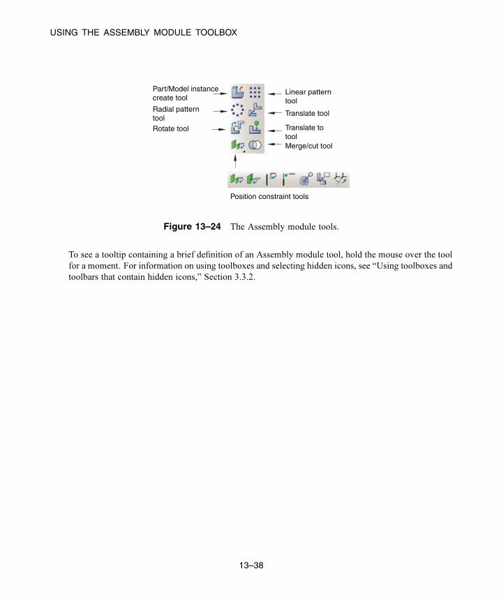
USING THE ASSEMBLY MODULE TOOLBOX
Part/Model instance create tool
Position constraint tools
Radial patterntoolRotate tool
Translate tool
Linear patterntool
Translate totoolMerge/cut tool
Figure 13–24 The Assembly module tools.
To see a tooltip containing a brief definition of an Assembly module tool, hold the mouse over the tool
for a moment. For information on using toolboxes and selecting hidden icons, see “Using toolboxes and
toolbars that contain hidden icons,” Section 3.3.2.
13–38
Abaqus ID:
Printed on:

UNDERSTANDING THE ROLE OF THE STEP MODULE
14. The Step module
You can use the Step module to perform the following tasks:
• Create analysis steps.
• Specify output requests.
• Specify adaptive meshing.
• Specify analysis controls.
This chapter covers the following topics:
• “Understanding the role of the Step module,” Section 14.1
• “Entering and exiting the Step module,” Section 14.2
• “Understanding steps,” Section 14.3
• “Understanding output requests,” Section 14.4
• “Understanding integrated, restart, diagnostic, and monitor output,” Section 14.5
• “Understanding ALE adaptive meshing,” Section 14.6
• “How can I customize the Abaqus analysis controls?,” Section 14.7
• “Using the Step module toolbox,” Section 14.8
In addition, the following sections are available in the HTML version of this guide:
• “Using the Step Manager,” Section 14.9
• “Using the step editor,” Section 14.10
• “Configuring analysis procedure settings,” Section 14.11
• “Defining output requests,” Section 14.12
• “Requesting specialized output,” Section 14.13
• “Customizing ALE adaptive meshing,” Section 14.14
• “Customizing the Abaqus analysis controls,” Section 14.15
For information on displaying the online documentation, see “Getting help,” Section 2.6.
14.1 Understanding the role of the Step module
You can use the Step module to perform the following tasks:
Create analysis steps
Within a model you define a sequence of one or more analysis steps. The step sequence provides a
convenient way to capture changes in the loading and boundary conditions of the model, changes in
the way parts of the model interact with each other, the removal or addition of parts, and any other
changes that may occur in the model during the course of the analysis. In addition, steps allow you
14–1
Abaqus ID:
Printed on:

UNDERSTANDING STEPS
to change the analysis procedure, the data output, and various controls. You can also use steps to
define linear perturbation analyses about nonlinear base states. You can use the replace function to
change the analysis procedure of an existing step.
Specify output requests
Abaqus writes output from the analysis to the output database; you specify the output by creating
output requests that are propagated to subsequent analysis steps. An output request defines which
variables will be output during an analysis step, from which region of the model they will be output,
and at what rate they will be output. For example, you might request output of the entire model’s
displacement field at the end of a step and also request the history of a reaction force at a restrained
point.
Specify adaptive meshing
You can define adaptive mesh regions and specify controls for adaptive meshing in those regions.
Specify analysis controls
You can customize general solution controls and solver controls.
14.2 Entering and exiting the Step module
You can enter the Stepmodule at any time during anAbaqus/CAE session by clickingStep in theModulelist located in the context bar. The Step, Output, Other, and Tools menus appear on the main menu
bar. If the current viewport contains something other than the assembly, the contents of the viewport
disappear when you start the Step module.
To exit the Step module, select any other module from the Module list. You need not save your
steps or output requests before exiting the module; they will be saved automatically when you save the
model database by selecting File→Save or File→Save As from the main menu bar.
14.3 Understanding steps
This section gives an overview of steps. For additional information on steps, see “Defining an analysis,”
Section 6.1.2 of the Abaqus Analysis User’s Guide.
14.3.1 What is a step?
An Abaqus/CAE model uses the following two types of steps:
14–2
Abaqus ID:
Printed on:
UNDERSTANDING STEPS
The initial step
Abaqus/CAE creates a special initial step at the beginning of the model’s step sequence and names
it Initial. Abaqus/CAE creates only one initial step for your model, and it cannot be renamed,
edited, replaced, copied, or deleted.
The initial step allows you to define boundary conditions, predefined fields, and interactions
that are applicable at the very beginning of the analysis. For example, if a boundary condition or
interaction is applied throughout the analysis, it is usually convenient to apply such conditions in the
initial step. Likewise, when the first analysis step is a linear perturbation step, conditions applied
in the initial step form part of the base state for the perturbation.
Analysis steps
The initial step is followed by one or more analysis steps. Each analysis step is associated with a
specific procedure that defines the type of analysis to be performed during the step, such as a static
stress analysis or a transient heat transfer analysis. You can change the analysis procedure from step
to step in any meaningful way, so you have great flexibility in performing analyses. Since the state
of the model (stresses, strains, temperatures, etc.) is updated throughout all general analysis steps,
the effects of previous history are always included in the response for each new analysis step.
There is no limit to the number of analysis steps you can define, but there are restrictions on
the step sequence. (For more information, see “Step sequence restrictions,” Section 14.3.3.)
You use items from the Step menu to create a step, to select and define the analysis procedure used
during the step, and to manage existing steps. Alternatively, you can select Step→Manager from the
main menu bar to display the Step Manager.
For example, consider the following analysis of a section of a piping system:
Initial Step:
Apply boundary conditions to fix the left end of the pipe and to allow only axial movement at the
right end.
Step 1: Compress
Apply a compressive force to the right end of the pipe. This step is a general analysis step.
Step 2: Eigenmodes
Calculate the frequencies and modes of vibration of the pipe in its compressed state. This step is a
linear perturbation step.
Figure 14–1 shows the Step Manager after you create these steps.
14–3
Abaqus ID:
Printed on:

UNDERSTANDING STEPS
Figure 14–1 The Step Manager.
The manager lists all of the steps in the analysis as well as a few salient details concerning each step.
Step 2, Eigenmodes, is indented to show that it is a linear perturbation step based on the state of the
model at the end of Step 1, Compress.For detailed information on creating, editing, and replacing steps, see the following sections in the
HTML version of this guide:
• “The Step Manager,” Section 14.9.1
• “Creating a step,” Section 14.9.2
• “Editing a step,” Section 14.9.3
• “Replacing a step,” Section 14.9.4
• “Resetting the default values in the step editor,” Section 14.9.5
• “The step editor,” Section 14.10.1
• “The Incrementation tab,” Section 14.10.2
14.3.2 Linear and nonlinear proceduresThe Step Manager distinguishes between general nonlinear steps and linear perturbation steps by
indenting the names and procedure descriptions of linear perturbation steps. General nonlinear analysis
steps define sequential events: the state of the model at the end of one general step provides the initial
state for the start of the next general step. Linear perturbation analysis steps provide the linear response
of the model about the state reached at the end of the last general nonlinear step. You use the Proceduretype field to choose between General and Linear perturbation steps when you select the procedure
in the Create Step dialog box.
For each step in the analysis the Step Manager also indicates whether Abaqus will account for
nonlinear effects from large displacements and deformations. If the displacements in a model due to
loading are relatively small during a step, the effects may be small enough to be ignored. However, in
cases where the loads on a model result in large displacements, nonlinear geometric effects can become
14–4
Abaqus ID:
Printed on:

UNDERSTANDING STEPS
important. The Nlgeom setting for a step determines whether Abaqus will account for geometric
nonlinearity in that step.
The Nlgeom setting is turned on by default for Abaqus/Explicit steps and turned off by default for
Abaqus/Standard steps. The sequence of steps and the current Nlgeom setting determine whether you
can change the Nlgeom setting in a particular step. For example, if Abaqus is already accounting for
geometric nonlinearity, the Nlgeom setting is toggled on for all subsequent steps, and you cannot toggle
it off. Where permissible, the following methods allow you to change the Nlgeom setting for a step:
• Click the Basic tab in the Step Editor, and toggle the Nlgeom setting.
• Select Step→Nlgeom from the main menu bar.
• Click Nlgeom in the Step Manager.
For more information, see “Accounting for geometric nonlinearity,” Section 14.9.6, in the HTML
version of this guide or see “General and linear perturbation procedures,” Section 6.1.3 of the Abaqus
Analysis User’s Guide.
14.3.3 Step sequence restrictionsWhen you select Step→Create from the main menu bar, a Create Step dialog box appears in which
you can specify the procedure type for the step that you are creating. Similarly, when you select
Step→Replace from the main menu bar, a Replace Step dialog box appears in which you can specify
a new procedure type for an existing step. The selection of procedure types in the Create Step and
Replace Step dialog boxes depends on the following:
• The model type.
• The procedures that you have already associated with existing steps.
• The position of the new or replaced step in the analysis step sequence.
For example, when you create the first step in an analysis, you can choose from a list of valid
procedure types; both Abaqus/Standard and Abaqus/Explicit procedure types appear in the list. However,
once you have created the first step, the list of valid procedure types in the Create Step dialog box will
change to include only those procedures that are compatible with the first step. For example, if the first
step is an Abaqus/Standard step, Abaqus/Explicit procedures no longer appear in the list.
14.3.4 What is step replacement?After you have defined your model and performed an analysis, you may want to run another analysis
using a different procedure without having to redefine objects in your model, such as loads, boundary
conditions, and interactions. You can use the replace function to replace the analysis procedure for an
existing step with any procedure that is allowed by Abaqus/Standard or Abaqus/Explicit; for example,
you can change from a Static, General procedure to a Dynamic, Explicit procedure or from a Static,General procedure to a Static, Riks procedure. After you select Step→Replace from the main menu
14–5
Abaqus ID:
Printed on:

UNDERSTANDING STEPS
bar, you select the step that you want to replace and the new analysis procedure for that step. The EditStep dialog box appears with default values for the new analysis procedure. You can modify the default
values and specify values for optional settings in the step editor.
When you replace a step, Abaqus/CAE copies all of the compatible step-dependent objects to the
new step. If objects are incompatible with the new step, Abaqus/CAE substitutes an equivalent object,
if possible, and suppresses or deletes the remaining objects. Therefore, you may want to copy the model
before you replace the step. Abaqus/CAE displays a list of the objects that were suppressed or deleted
during step replacement in the message area. For example, if you replace a Static, General procedurecontaining an Abaqus/Standard self-contact interaction, a pressure load, and an inertia relief load with a
Dynamic, Explicit procedure, Abaqus/CAE does the following:
• Substitutes an Abaqus/Explicit self-contact interaction for the Abaqus/Standard self-contact
interaction in the Dynamic, Explicit procedure.
• Copies the pressure load to the Dynamic, Explicit procedure.
• Suppresses the inertia relief load. Inertia relief loads apply only in Abaqus/Standard procedures.
After you replace a step, you should verify that previously defined properties, element types, jobs,
and boundary conditions and predefined fields in the initial step remain valid for the model. In the Job
module you can click Write Input in the Job Manager to write the input file and then check the input
file for errors.
You can use the replace function to reset step settings to their default values by replacing an existing
step with a step of the same procedure type.
14.3.5 Replacing an Abaqus/Standard procedure with an Abaqus/Explicitprocedure or vice versa
If you want to replace an Abaqus/Standard analysis procedure with an Abaqus/Explicit analysis
procedure or vice versa, you must have only one analysis step in the model for the desired procedure
type to appear in the Replace Step dialog box. If your model contains multiple steps, you can use
step-dependent managers to move objects to a single step. You can then delete the other steps and
replace the remaining step with the new analysis procedure.
For example, if you want to change a model that contains four Static, General procedures
from an Abaqus/Standard analysis to an Abaqus/Explicit analysis, you can use the Load Manager tomove all of the loads into one of the four steps. Similarly, you can use the Interaction Manager to
move the interactions. You can then delete the other three steps and replace the remaining step with a
Dynamic, Explicit procedure. If desired, you can create additional Abaqus/Explicit steps and use the
step-dependent managers to move objects that were copied during step replacement to the appropriate
Abaqus/Explicit procedures.
For more information, see “Modifying the history of a step-dependent object,” Section 3.4.6.
14–6
Abaqus ID:
Printed on:

UNDERSTANDING OUTPUT REQUESTS
14.4 Understanding output requests
This section gives an overview of output requests.
14.4.1 What is an output request?The Abaqus analysis products compute the values of many variables at every increment of a step. Usually
you are interested in only a small subset of all of this computed data. You can specify the data that
you want written to the output database by creating output requests. An output request consists of the
following information:
• The variables or variable components of interest.
• The region of the model and the integration points from which the values are written to the output
database.
• The rate at which the variable or component values are written to the output database.
When you create the first step, Abaqus/CAE selects a default set of output variables corresponding to
the step’s analysis procedure. By default, output is requested from every node or integration point in the
model and from default section points. In addition, Abaqus/CAE selects the default rate at which the
variables are written to the output database. You can edit these default output requests or create and edit
new ones.
Default output requests and output requests that you modified are propagated to subsequent steps in
the analysis. If you have a large model that includes the default output requests and requests output from
a large number of frames, the resulting output database will be very large. You can use a C++ program to
extract data from a large output database and copy only selected frames to a second output database. For
more information, see “Decreasing the amount of data in an output database by retaining data at specific
frames,” Section 10.15.4 of the Abaqus Scripting User’s Guide.
When your analysis is complete, you use the Visualization module to read the output database and
graphically display the data that were written to it.
For detailed instructions on creating and editing output requests, see the following sections in the
HTML version of this guide:
• “Creating an output request,” Section 14.12.1
• “Modifying field output requests,” Section 14.12.2
• “Modifying history output requests,” Section 14.12.3
14.4.2 What is the difference between field output and history output?When you create an output request, you can choose either field output or history output.
14–7
Abaqus ID:
Printed on:

UNDERSTANDING OUTPUT REQUESTS
Field output
Abaqus generates field output from data that are spatially distributed over the entire model or over
a portion of it. In most cases you use the Visualization module to view field output data using
deformed shape, contour, or symbol plots. The amount of field output generated by Abaqus during
an analysis is often large. As a result, you typically request that Abaqus write field data to the output
database at a low rate; for example, after every step or at the end of the analysis.
When you create a field output request, you can specify the output frequency in equally
spaced time intervals or every time a particular length of time elapses. For an Abaqus/Standard
analysis procedure, you can alternatively specify the output frequency in increments, request
output after the last increment of each step, or request output according to a set of time points. For
an Abaqus/Explicit analysis procedure, you can alternatively request field output for every time
increment or according to a set of time points. For an Abaqus/CFD analysis procedure, you can
alternatively specify the output frequency in increments.
When you create a field output request, Abaqus writes every component of the selected
variables to the output database. For example, if you were using solid elements to model a
cantilever beam with a load at the tip, you could request the stress (all six components) and the
displacement (all six components) data from the entire model after the last increment of the loading
step. You could then use the Visualization module to view a contour plot of stresses and deflections
in the final loaded state.
History output
Abaqus generates history output from data at specific points in a model. In most cases you use
the Visualization module to display history output using X–Y plots. The rate of output depends on
how you want to use the data that are generated by the analysis, and the rate can be very high. For
example, data generated for diagnostic purposes may be written to the output database after every
increment. You can also use history output for data that relate to the model or a portion of the model
as a whole; for example, whole model energies.
When you create a history output request, you can specify the output frequency in equally
spaced time intervals or every time a particular length of time elapses. For an Abaqus/Standard
analysis procedure, you can alternatively specify the output frequency in increments, request
output after the last increment of each step, or request output according to a set of time points.
For an Abaqus/Explicit analysis procedure, you can alternatively request history output in time
increments. For an Abaqus/CFD analysis procedure, you can alternatively specify the output
frequency in increments.
When you create a history output request, you can specify the individual components of the
variables that Abaqus/CAEwill write to the output database. For example, if youmodel the response
of a cantilever beam with a load applied to the tip, you might request the following output after each
increment of the loading step:
• The principal stress at a single node at the root of the beam.
• The vertical displacement at a single node at the tip of the beam.
14–8
Abaqus ID:
Printed on:

UNDERSTANDING OUTPUT REQUESTS
You could then use the Visualization module to view an X–Y plot of stress at the root versus
displacement at the tip with increasing load.
14.4.3 Propagation of output requests
When you create the first step in the analysis, Abaqus/CAE generates default field and history output
requests based on the analysis procedure that you selected for the step. These default output requests
are propagated to subsequent steps. The Field Output Requests Manager and the History OutputRequests Manager are step-dependent managers that display the propagation and the status of output
requests between steps.
The output requested in a general step is independent of the output requested in a linear perturbation
step. In addition, the propagation behavior of output requests varies between general steps and linear
perturbation steps.
General steps
Abaqus/CAE creates a default field output request for the first general step in your model, and that
default output request propagates to all subsequent general steps. Similarly, if you create a new
output request or modify the default output request, the new or modified request is propagated to
subsequent general steps.
If you insert a new general step into the sequence of steps, the output request from the previous
general step propagates to the new step.
Linear perturbation steps
Abaqus/CAE creates a default field output request for the first linear perturbation step in your model,
and that default output request propagates to all subsequent linear perturbation steps that use the
same analysis procedure; for example, all the frequency analyses. Similarly, if you create a new
output request or modify the default output request, the new or modified request is propagated to
subsequent steps that use the same analysis procedure.
If you insert a new linear perturbation step into the sequence of steps, the output request from
the previous linear perturbation step that uses the same analysis procedure propagates to the new
step. If you create a linear perturbation step that uses a different analysis procedure, Abaqus/CAE
creates a new default output request. The new default output request propagates to all subsequent
linear perturbation steps that use the same analysis procedure.
You should be aware of the following behavior:
• If you insert a new general step at the beginning of a sequence of existing general steps, Abaqus/CAE
does not create a default output request for the new step. Similarly, if you insert a new linear
perturbation step at the beginning of a sequence of existing linear perturbation steps of the same
procedure type, Abaqus/CAE does not create a default output request for the new step. In both
cases you must create a new output request for the new step. Alternatively, you can use the output
request managers to move the output request from the following step to the new step.
14–9
Abaqus ID:
Printed on:
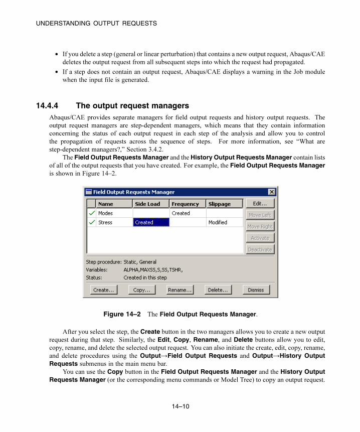
UNDERSTANDING OUTPUT REQUESTS
• If you delete a step (general or linear perturbation) that contains a new output request, Abaqus/CAE
deletes the output request from all subsequent steps into which the request had propagated.
• If a step does not contain an output request, Abaqus/CAE displays a warning in the Job module
when the input file is generated.
14.4.4 The output request managersAbaqus/CAE provides separate managers for field output requests and history output requests. The
output request managers are step-dependent managers, which means that they contain information
concerning the status of each output request in each step of the analysis and allow you to control
the propagation of requests across the sequence of steps. For more information, see “What are
step-dependent managers?,” Section 3.4.2.
The Field Output Requests Manager and the History Output Requests Manager contain listsof all of the output requests that you have created. For example, the Field Output Requests Manageris shown in Figure 14–2.
Figure 14–2 The Field Output Requests Manager.
After you select the step, the Create button in the two managers allows you to create a new output
request during that step. Similarly, the Edit, Copy, Rename, and Delete buttons allow you to edit,
copy, rename, and delete the selected output request. You can also initiate the create, edit, copy, rename,
and delete procedures using the Output→Field Output Requests and Output→History OutputRequests submenus in the main menu bar.
You can use the Copy button in the Field Output Requests Manager and the History OutputRequests Manager (or the corresponding menu commands or Model Tree) to copy an output request.
14–10
Abaqus ID:
Printed on:

UNDERSTANDING OUTPUT REQUESTS
You can copy an output request from any step to any valid step, with some restrictions. For more details,
see “Copying step-dependent objects using manager dialog boxes,” Section 3.4.11.
The Move Left, Move Right, Activate, and Deactivate buttons allow you to control the
propagation of output requests over the course of an analysis. For more information, see “Modifying
the history of a step-dependent object,” Section 3.4.6.
You can use the icons in the column along the left side of the managers to suppress output
requests or to resume previously suppressed output requests for an analysis. The suppress and resume
procedures are also available from the Output→Field Output Requests and Output→HistoryOutput Requests submenus in the main menu bar. For more information, see “Suppressing and
resuming objects,” Section 3.4.3.
14.4.5 Creating and modifying output requestsTo create an output request, select Output→Field Output Requests→Create or Output→HistoryOutput Requests→Create from the main menu bar. An editor appears in which you can enter all of
the information necessary to define the output request. The top of the editor displays the following:
• The name of the output request.
• The name of the step in which you are creating or modifying the output request.
• The name of the analysis procedure associated with the step.
For example, the Field Output Request editor is shown in Figure 14–3.
The Domain section of the editor allows you to choose the region from which output will be
generated. You can request that Abaqus write field data to the output database for the following:
• Whole model
• Whole model, only exterior nodes and elements (three-dimensional models in Abaqus/Standard or
Abaqus/Explicit analyses)
• A set
• A bolt load
• A skin
• A stringer
• A fastener
• An assembled fastener set
• An interaction
• A composite layup
• A substructure
Similarly, you can request that Abaqus write history data to the output database for the following:
• Whole model
14–11
Abaqus ID:
Printed on:

UNDERSTANDING OUTPUT REQUESTS
Figure 14–3 The Field Output Request editor.
• A set
• A bolt load
• A skin
• A stringer
14–12
Abaqus ID:
Printed on:

UNDERSTANDING OUTPUT REQUESTS
• A fastener
• An assembled fastener set
• A contour integral
• A general contact surface (Abaqus/Explicit steps only)
• An integrated output section (Abaqus/Explicit steps only)
• An interaction
• Springs/dashpots
• A composite layup
The Frequency section of the editor allows you to specify the frequency at which the output is
written to the output database. Choose one of the following:
• Last increment to request output only after the last increment of the step. This output frequency
is available only when you choose an Abaqus/Standard analysis procedure.
• Every n increments to request output after a specified number of increments. If you specify the
frequency in increments, Abaqus also writes output after the last increment of the step. This output
frequency is available when you choose an Abaqus/Standard or Abaqus/CFD analysis procedure.
• Every time increment to request output at every time increment. This output frequency is
available for field output when you choose an Abaqus/Explicit analysis procedure.
• Every n time increments to request output at a specified number of time increments. This output
frequency is available for history output when you choose an Abaqus/Explicit analysis procedure.
• Evenly spaced time intervals to request output at a number of evenly spaced time intervals.
• Every x units of time to request output after a particular length of time elapses.
• From time points to request output according to a set of time points that you specify. This output
frequency is available for field and history output when you choose an Abaqus/Standard analysis
procedure and for field output when you choose an Abaqus/Explicit analysis procedure.
The Output Variables section of the editor contains a list of the variable categories that are
applicable to the step procedure and the selected domain. Choose one of the following:
• Select from list below to request the variables from the list of check boxes below. You can click
the check box next to a category name to select all of the variables within that category, or you can
click the arrow next to a category name to display the list of variables in that category and then
select individual variables.
• Preselected defaults to request the default output variables for the procedure.
• All to request all output variables for the procedure.
• Edit variables to request variables from the text field below. You can manually edit this field and
type or delete variable names.
Note: In addition to the current analysis procedure, other aspects of the model may affect the preselected
default output variables. For example, if an output variable is valid for the analysis procedure but is not
valid for the element type used in the mesh, Abaqus will remove that variable during the analysis.
14–13
Abaqus ID:
Printed on:

UNDERSTANDING OUTPUT REQUESTS
If you use the Field Output Request editor to select a vector or tensor variable to be included in afield output request, Abaqus automatically writes all components of that variable to the output database
during the step. For example, if you select the vector U in a three-dimensional model, Abaqus outputs
the three displacement components U1, U2, and U3 to the output database along with the three rotation
components UR1, UR2, and UR3.
In contrast, if you use the History Output Request editor to select a vector or tensor variable to beincluded in a history output request, the History Output Request editor allows you to select individualcomponents of the variable. It is useful to specify individual components in a history output request
because these variables are typically output very frequently—possibly as often as every increment.
If yourmodel contains rebar, youmust toggle onOutput for rebar to include rebar output in the datathat Abaqus writes to the output database and to view plots of the rebar orientations in the Visualization
module. For more information, see “Understanding rebar in shell sections,” Section 12.2.5.
The editor also allows you to specify the section points from which output will be obtained. If
you request output from a composite layup, you can specify the section points from which output will
be obtained for each ply of the layup. For more information, see “Requesting output from a composite
layup,” Section 23.5.
For example, in Figure 14–3 the user is editing a field output request that is associated with a Static,General analysis procedure. The user has selected all of the variables in the Stresses category. These
variables will be included in the output request during the step named Side Load. Abaqus will writeoutput from the default section points at every increment.
For detailed instructions on selecting output variables and components, see the following sections
in the HTML version of this guide:
• “Modifying field output requests,” Section 14.12.2
• “Modifying history output requests,” Section 14.12.3
Once you have created an output request, you can modify it in the following ways:
• Select Output→Field Output Requests→Edit or Output→History Output Requests→Editto display the field or history output request editor.
• Select Output→Field Output Requests→Manager or Output→History OutputRequests→Manager to display the field or history output requests manager. Use the manager to
modify the stepwise history of the output request. (See “What are step-dependent managers?,”
Section 3.4.2, for more information.)
If you modify an output request during the step in which you created the request, you can modify
the domain, the output variables, the output for rebar option, the section points, and the output frequency.
However, if you modify an output request during a step into which it was propagated, you can modify
only the output variables and the output frequency.
When you request output from a contour integral, the History Output Request editor allows youto select only the frequency of output, the number of contour integrals, and the type of contour integral
calculation. For more information, see “Requesting contour integral output,” Section 31.2.11, in the
HTML version of this guide.
14–14
Abaqus ID:
Printed on:
UNDERSTANDING INTEGRATED, RESTART, DIAGNOSTIC, AND MONITOR OUTPUT
14.5 Understanding integrated, restart, diagnostic, and monitor output
This section explains the additional output controls available in the Step module.
14.5.1 Integrated output from Abaqus/Explicit
To obtain history output of variables such as the forces summed over an exterior surface in contact
or transmitted through a tie constraint between surfaces (see “Integrated output in Abaqus/Explicit” in
“Output to the output database,” Section 4.1.3 of the Abaqus Analysis User’s Guide; this type of output
is available only for Abaqus/Explicit steps), you must refer to an integrated output section to identify the
surface where output is needed. In addition, the integrated output section definition can provide a local
coordinate system in which to express the vector output quantities and/or a reference node as an anchor
point about which the total moment across the surface is computed.
By default, an integrated output section is anchored at the global origin and does not follow the
motion of the surface on which it is defined. You can define a reference point at which the output section
is anchored and specify how this reference point tracks with the average motion of the surface. The
reference point must not be connected to any other part of the finite element model.
Integrated output sections associated with a coordinate system and/or a reference node can be used
independent of integrated output requests to track the average motion of a surface.
You define integrated output sections by selecting Output→Integrated OutputSections→Create from the main menu bar. For detailed instructions, see “Defining integrated output
sections,” Section 14.13.1, in the HTML version of this guide. For information on requesting output
for an integrated output section, see “Modifying history output requests,” Section 14.12.3, in the
HTML version of this guide.
14.5.2 Restart output requests
You can use the restart files created by Abaqus to continue an analysis from a specified step of a previous
analysis. This section describes how you control the output of restart data. For a discussion of how you
use the restart data in a subsequent job, see “Restarting an analysis,” Section 19.6, and “What are the
model attributes?,” Section 9.2.2.
By default, no restart information is written for an Abaqus/Standard or an Abaqus/CFD analysis
and restart information is written only at the beginning and end of each step for an Abaqus/Explicit
analysis. However, default restart requests are created automatically for every step in an analysis. The
Edit Restart Requests dialog box, invoked by selecting Output→Restart Requests from the main
menu bar in the Step module, allows you to specify how often you want the restart information to be
written.
14–15
Abaqus ID:
Printed on:

UNDERSTANDING INTEGRATED, RESTART, DIAGNOSTIC, AND MONITOR OUTPUT
You can specify the frequency at which Abaqus writes data to the restart files; however, the behavior
of restart differs between analysis products.
Abaqus/Standard and Abaqus/CFD
You can request the frequency in increments or in time intervals. For an Abaqus/Standard step, you
can choose whether the output is written at the exact time interval or at the closest approximation.
Abaqus/Explicit
For an Abaqus/Explicit analysis, you specify the number of equally spaced time intervals at which
Abaqus writes data to the restart files. In addition, for an Abaqus/Explicit step you can choose
whether the output is written at the exact time interval or at the closest approximation. However,
you cannot avoid writing information to the restart files for Abaqus/Explicit steps; the number of
time intervals must be set to one or greater.
For an Abaqus/Standard or an Abaqus/Explicit analysis, you can request that data written to the
restart files overlay data from the previous increment. If you select this option, Abaqus retains the
information from only one increment of each step in the restart files, thus minimizing the size of the
files. By default, Abaqus does not overlay data.
For more information, see “Restarting an analysis,” Section 19.6, and “Restarting an analysis,”
Section 9.1.1 of the Abaqus Analysis User’s Guide. For detailed instructions on requesting restart output,
see “Configuring restart output requests,” Section 14.13.2, in the HTML version of this guide.
You can use the abaqus restartjoin execution procedure to extract data from the output database
created by a restart analysis and append the data to a second output database. For more information, see
“Joining output database (.odb) files from restarted analyses,” Section 3.2.19 of the Abaqus Analysis
User’s Guide.
14.5.3 Diagnostic printingIf the analysis of your model fails or produces unexpected results, you can examine its iteration-by-
iteration progress by looking at selected diagnostic information that is written to the following files:
For Abaqus/Standard analyses:
Diagnostic information is written to the message (.msg) file, and a subset of the information is
written to the output database (.odb) file. You can view the diagnostic information in the output
database in the Visualization module (for more information, see Chapter 41, “Viewing diagnostic
output”). By default, the information is written during every iteration; you can request that Abaqus
discontinue writing diagnostic information to the message file by specifying an output frequency of
zero.
For Abaqus/Explicit analyses:
Diagnostic information is written to the status (.sta) file. For information on the frequency at
which this information is written, see “Output,” Section 4.1.1 of the Abaqus Analysis User’s Guide.
14–16
Abaqus ID:
Printed on:

UNDERSTANDING ALE ADAPTIVE MESHING
You display the Edit Diagnostic Print dialog box by selecting Output→Diagnostic Print fromthe main menu bar.
For detailed instructions on requesting diagnostic printing, see “Configuring diagnostic printing,”
Section 14.13.3, in the HTML version of this guide.
Note: Changes to the diagnostic print requests do not affect the diagnostic information written to the
output database during Abaqus/Standard analyses.
14.5.4 Degree of freedom monitor requests
You can request that Abaqus write the values of a degree of freedom at one selected point to the status
(.sta) file and, for Abaqus/Standard analyses, to the message (.msg) file at specific increments during
the course of an analysis. In addition, a plot of the degree of freedom value over time appears in a
new viewport that is generated automatically when you submit the analysis. (For more information, see
“Monitoring the progress of an analysis job,” Section 19.2.6.) You can use this information to monitor
the progress of the solution.
You must specify the vertex or node you want to monitor by selecting an existing geometry or
node set or by selecting a point in the viewport. Once you have specified the point, you must indicate
which degree of freedom you want to monitor at that vertex or node, how often you want the information
displayed in a viewport, and how often you want it printed to the status and message files.
For detailed instructions on monitoring a degree of freedom, see “Configuring monitor requests,”
Section 14.13.4, in the HTML version of this guide.
14.6 Understanding ALE adaptive meshing
Arbitrary Lagrangian-Eulerian (ALE) adaptive meshing allows you to maintain a high-quality mesh
throughout an analysis, even when large deformations or losses of material occur, by allowing the mesh
to move independently of the material. Adaptive meshing moves only nodes; the mesh topology remains
unchanged. Adaptivemeshing is available only forCoupled temp-displacement; Dynamic, Explicit;Dynamic, Temp-disp, Explicit; Soils; and Static, General steps.
You can define regions of the model where you want adaptive meshing by selecting Other→ALEAdaptive Mesh Domain from the main menu bar. If necessary, you can select Other→ALE AdaptiveMesh Controls or Other→ALE Adaptive Mesh Constraint to customize the adaptive mesh controls
or to add regional adaptive mesh constraints, respectively. Currently, you can define only one ALE
adaptive mesh domain for any particular step.
For detailed information on adaptive meshing, see “ALE adaptive meshing,” Section 12.2 of the
Abaqus Analysis User’s Guide.
For detailed instructions on defining adaptive mesh regions, see the following sections in the HTML
version of this guide:
14–17
Abaqus ID:
Printed on:

HOW CAN I CUSTOMIZE THE Abaqus ANALYSIS CONTROLS?
• “Defining an ALE adaptive mesh region,” Section 14.14.1
• “Specifying ALE adaptive mesh constraints,” Section 14.14.2
• “Specifying controls for ALE adaptive meshing,” Section 14.14.3
14.7 How can I customize the Abaqus analysis controls?
This section explains how you can adjust the parameters that control the Abaqus analysis.
14.7.1 General solution controlsYou can customize the numerous variables that control the convergence and time integration accuracy
algorithms in Abaqus. The default solution controls usually work well, but customizing these controls
may result in a more cost-effective solution or help you to obtain a solution for particularly difficult
analyses.
Note: These options are available only for general Abaqus/Standard analysis steps.
You can access the solution controls by selecting Other→General Solution Controls from the
main menu bar. For more information, see “Analysis convergence controls,” Section 7.2 of the Abaqus
Analysis User’s Guide.
WARNING: Solution controls are intended for experienced analysts and should be used with great care.The default settings of these controls are appropriate for most nonlinear analyses. Changing these values
inappropriately may greatly increase the computational time of your analysis or produce inaccurate
results.
For detailed instructions on setting general solution controls, see “Customizing general solution
controls,” Section 14.15.1, in the HTML version of this guide.
14.7.2 Solver controlsYou can customize the variables that control the iterative linear equation solver.
Note: You can use the iterative linear equation solver only for Static, General; Static, Linearperturbation; Visco; Heat transfer; Geostatic; and Soils analysis steps.
You can access the solver controls by selecting Other→Solver Controls from the main menu bar.
For more information, see “Iterative linear equation solver,” Section 6.1.6 of the Abaqus Analysis User’s
Guide.
14–18
Abaqus ID:
Printed on:
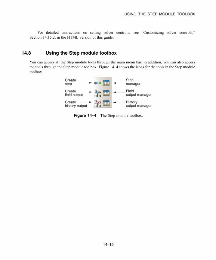
USING THE STEP MODULE TOOLBOX
For detailed instructions on setting solver controls, see “Customizing solver controls,”
Section 14.15.2, in the HTML version of this guide.
14.8 Using the Step module toolbox
You can access all the Step module tools through the main menu bar; in addition, you can also access
the tools through the Step module toolbox. Figure 14–4 shows the icons for the tools in the Step module
toolbox.
Createstep
Createfield output
Createhistory output
Stepmanager
Field output manager
Historyoutput manager
Figure 14–4 The Step module toolbox.
14–19
Abaqus ID:
Printed on:


THE INTERACTION MODULE
15. The Interaction module
You can use the Interaction module to define and manage the following objects:
• Mechanical and thermal interactions between regions of a model or between a region of a model
and its surroundings.
• The interface region and coupling schemes for an Abaqus/Standard to Abaqus/Explicit
co-simulation.
• The interface region and coupling step period for a fluid-structure co-simulation (between
Abaqus/CFD and Abaqus/Standard or Abaqus/Explicit).
• Analysis constraints between regions of a model.
• Assembly-level wire features, connector sections, and connector section assignments to model
connectors.
• Inertia (point mass, rotary inertia, and heat capacitance) on regions of the model.
• Cracks on regions of the model.
• Springs and dashpots between two points of a model or between a point of a model and ground.
This chapter covers the following topics:
• “Understanding the role of the Interaction module,” Section 15.1
• “Entering and exiting the Interaction module,” Section 15.2
• “Understanding interactions,” Section 15.3
• “Understanding interaction properties,” Section 15.4
• “Understanding constraints,” Section 15.5
• “Understanding contact and constraint detection,” Section 15.6
• “Understanding connectors,” Section 15.7
• “Understanding connector sections and functions,” Section 15.8
• “Understanding Interaction module managers and editors,” Section 15.9
• “Understanding symbols that represent interactions, constraints, and connectors,” Section 15.10
• “Using the Interaction module toolbox,” Section 15.11
The following sections are available in the HTML version of this guide:
• “Using the Interaction module,” Section 15.12
• “Using the interaction editors,” Section 15.13
• “Using the interaction property editors,” Section 15.14
• “Using the constraint editors,” Section 15.15
• “Using contact and constraint detection,” Section 15.16
• “Using the connector section editors,” Section 15.17
• “Using the Query toolset to obtain connector assignment information,” Section 15.18
15–1
Abaqus ID:
Printed on:

UNDERSTANDING THE ROLE OF THE INTERACTION MODULE
15.1 Understanding the role of the Interaction module
You can use the Interaction module to define the following:
• Contact interactions.
• Elastic foundations.
• Cavity radiation.
• Thermal film conditions.
• Radiation to and from the ambient environment.
• Abaqus/Standard to Abaqus/Explicit co-simulation interaction.
• Fluid-structure co-simulation interaction (between Abaqus/CFD and Abaqus/Standard or
Abaqus/Explicit).
• Pressure penetration.
• Incident waves.
• Acoustic impedance.
• Cyclic symmetry.
• A user-defined actuator/sensor interaction.
• Model change interactions.
• Tie constraints.
• Rigid body constraints.
• Display body constraints.
• Coupling constraints.
• Adjust points constraints.
• MPC constraints.
• Shell-to-solid coupling constraints.
• Embedded region constraints.
• Equation constraints.
• Connector section assignments.
• Inertia.
• Cracks.
• Springs and dashpots.
Interactions are step-dependent objects, which means that when you define them, you must indicate
in which steps of the analysis they are active. (For more information about step-dependent objects,
see “Understanding the status of an object in a step,” Section 3.4.4.) For example, you can define film
and radiation conditions on a surface only during a heat transfer, coupled temperature-displacement,
15–2
Abaqus ID:
Printed on:

UNDERSTANDING INTERACTIONS
or coupled thermal-electrical step. Similarly, you can define an interaction with a user-defined
actuator/sensor only during the initial step.
The Set and Surface toolsets in the Interaction module allow you to define and name regions of your
model to which you would like interactions and constraints applied. You can use the Amplitude toolset
to define variations in some interaction attributes over the course of the analysis. The Analytical Field
toolset allows you to create analytical fields that you can use to define spatially varying parameters for
selected interactions. The Reference Point toolset allows you to define reference points that are used in
constraints and creating assembly-level wire features.
Abaqus/CAE does not recognize mechanical contact between part instances or regions of an
assembly unless that contact is specified in the Interaction module; the mere physical proximity of two
surfaces in an assembly is not enough to indicate any type of interaction between the surfaces.
For information on defining cracks to study their initiation and propagation, see Chapter 31,
“Fracture mechanics.” For information on defining cracks for fluid-structure interaction, see “Defining
a fluid-structure co-simulation interaction,” Section 15.13.15, in the HTML version of this guide. For
information on defining inertia, see Chapter 33, “Inertia.” For information on defining springs and
dashpots, see Chapter 37, “Springs and dashpots.”
15.2 Entering and exiting the Interaction module
You can enter the Interaction module at any time during an Abaqus/CAE session by clicking Interactionin the Module list located in the context bar. Interaction, Constraint, Connector, Special, Feature,and Tools menus appear on the main menu bar; and a Step list appears under the context bar.
To exit the Interaction module, click another module in the Module list. You need not take any
specific action to save objects created in the Interaction module before exiting the module; they are
saved automatically when you save the entire model by selecting File→Save or File→Save As from
the main menu bar.
15.3 Understanding interactions
You can use the Interaction module to define the following types of interactions:
General contact
General contact interactions allow you to define contact between many or all regions of the model
with a single interaction. General contact is also used to define contact between Lagrangian
bodies and Eulerian materials in a coupled Eulerian-Lagrangian analysis (see “Defining contact
in Eulerian-Lagrangian models,” Section 28.3). Typically, general contact interactions are
defined for an all-inclusive surface that contains all exterior faces; feature edges; and—in
Abaqus/Explicit—analytical rigid surfaces, edges based on beams and trusses, and Eulerian
material boundaries. To refine the contact domain, you can include or exclude specific surface
pairs. Surfaces used in general contact interactions can span many disconnected regions of the
15–3
Abaqus ID:
Printed on:

UNDERSTANDING INTERACTIONS
model. Attributes, such as contact properties, surface properties, and contact formulation, are
assigned as part of the contact interaction definition but independently of the contact domain
definition, which allows you to use one set of surfaces for the domain definition and another set of
surfaces for the attribute assignments. For detailed instructions on creating this type of interaction,
see “Defining general contact,” Section 15.13.1, in the HTML version of this guide.
General contact interactions and surface-to-surface or self-contact interactions can be used
together in the same analysis. Only one general contact interaction can be active in a step during
an analysis.
For more information, see “Contact interaction analysis: overview,” Section 36.1.1 of the
Abaqus Analysis User’s Guide; “Defining general contact interactions in Abaqus/Standard,”
Section 36.2.1 of the Abaqus Analysis User’s Guide; “Defining general contact interactions in
Abaqus/Explicit,” Section 36.4.1 of the Abaqus Analysis User’s Guide; and “Eulerian analysis,”
Section 14.1.1 of the Abaqus Analysis User’s Guide. The assignment of a penalty stiffness scale
factor is not supported in Abaqus/CAE. In addition, node-based surfaces cannot be used in a
general contact interaction in Abaqus/CAE.
Surface-to-surface contact, self-contact, and pressure penetration
Surface-to-surface contact interactions describe contact between two deformable surfaces or
between a deformable surface and a rigid surface. Self-contact interactions describe contact
between different areas on a single surface. For detailed instructions on creating these
types of interactions, see “Defining surface-to-surface contact,” Section 15.13.7; “Defining
self-contact,” Section 15.13.8; and “Using contact and constraint detection,” Section 15.16,
in the HTML version of this guide. For more information, see “Defining contact pairs in
Abaqus/Standard,” Section 36.3.1 of the Abaqus Analysis User’s Guide, and “Defining contact
pairs in Abaqus/Explicit,” Section 36.5.1 of the Abaqus Analysis User’s Guide.
If your model includes complex geometries and numerous contact interactions, you may want
to customize the variables that control the contact algorithms to obtain cost-effective solutions.
These controls are intended for advanced users and should be used with great care. For more
information, see “Contact controls editors,” Section 15.9.4.
A pressure penetration interaction allows you to simulate the pressure of a fluid penetrating
between two surfaces involved in surface-to-surface contact. The fluid pressure is applied normal
to the surfaces. You must create a surface-to-surface contact interaction to specify the master and
slave surfaces for the pressure penetration. The bodies forming the joint can both be deformable, as
is the case with threaded connectors; or one can be rigid, as occurs when a soft gasket is used
as a seal between stiffer structures. A pressure penetration interaction can be used only in an
Abaqus/Standard analysis. For detailed instructions on creating pressure penetration interactions,
see “Defining pressure penetration,” Section 15.13.16, in the HTML version of this guide. For
more information, see “Pressure penetration loading,” Section 37.1.7 of the Abaqus Analysis User’s
Guide.
15–4
Abaqus ID:
Printed on:

UNDERSTANDING INTERACTIONS
Fluid cavity
A fluid cavity interaction allows you to select and assign properties to a liquid- or gas-filled fluid
cavity in the model. Fluid cavity selection includes a reference point and the surface that encloses
the cavity. The properties are defined in a fluid cavity interaction property (for more information,
see “Understanding interaction properties,” Section 15.4). You can define fluid cavity interactions
in the initial step of an Abaqus/Standard or an Abaqus/Explicit analysis. The fluid cavity interaction
remains constant throughout all steps of an analysis; you cannot modify or deactivate it after the
initial step. For detailed instructions on creating fluid cavity interactions, see “Defining a fluid
cavity interaction,” Section 15.13.11, in the HTML version of this guide.
Fluid exchange
A fluid exchange interaction allows you to define movement of fluid between a cavity and the
environment or between two cavities. To create a fluid exchange interaction, you must first select
an existing fluid cavity interaction for each cavity (one for exchange to environment or two for
exchange between cavities). Then you can select or create a fluid exchange interaction property (for
more information, see “Understanding interaction properties,” Section 15.4) and set the effective
exchange area. For detailed instructions on creating fluid exchange interactions, see “Defining a
fluid exchange interaction,” Section 15.13.12, in the HTML version of this guide.
XFEM crack growth
An XFEM crack growth interaction allows you to activate or deactivate growth of a crack created
using the extended finite element method. For detailed instructions on creating this type of
interaction, see “Deactivating and activating an XFEM crack growth,” Section 31.3.5, in the
HTML version of this guide.
Model change
A model change interaction allows you to remove and reactivate elements during an analysis. You
can use model change interactions in all Abaqus/Standard analysis procedures except for the static,
Riks procedure and linear perturbation procedures. For detailed instructions on creating this type of
interaction, see “Defining a model change interaction,” Section 15.13.13, in the HTML version of
this guide. For more information on removing and reactivating elements, see “Element and contact
pair removal and reactivation,” Section 11.2.1 of the Abaqus Analysis User’s Guide.
Cyclic symmetry (Abaqus/Standard only)
Cyclic symmetry enables you to model an entire 360° structure at considerably reduced
computational expense by analyzing only a single repetitive sector of a model. You can create
cyclic symmetry interactions only in the initial step. Once a cyclic symmetry interaction is
created, cyclic symmetry applies to the entire analysis history. If you deactivate a cyclic symmetry
interaction in a frequency step, Abaqus/CAE evaluates all possible nodal diameters being evaluated
for that step. For detailed instructions on creating this type of interaction, see “Defining cyclic
symmetry,” Section 15.13.19, in the HTML version of this guide. For more information about
15–5
Abaqus ID:
Printed on:
UNDERSTANDING INTERACTIONS
cyclic symmetry in Abaqus, see “Analysis of models that exhibit cyclic symmetry,” Section 10.4.3
of the Abaqus Analysis User’s Guide.
Elastic foundation (Abaqus/Standard only)
Elastic foundations allow you to model the stiffness effects of a distributed support on a surface
without actually modeling the details of the support. You can create elastic foundation interactions
only in the initial step. Once an elastic foundation is activated, you cannot deactivate it in
later analysis steps. For detailed instructions on creating this type of interaction, see “Defining
foundations,” Section 15.13.20, in the HTML version of this guide. For more information, see
“Element foundations,” Section 2.2.2 of the Abaqus Analysis User’s Guide.
Cavity radiation (Abaqus/Standard only)
Cavity radiation interactions describe heat transfer due to radiation in enclosures. Two cavity
radiation models are available in Abaqus/CAE: a fully implicit definition and an approximation.
The full version can be used for heat transfer without deformation in two-dimensional,
three-dimensional, and axisymmetric models. It can include open or closed cavities and accounts
for symmetries and surface blocking, but it does not support surface motion within cavities.
For detailed instructions on creating this type of interaction, see “Defining a cavity radiation
interaction,” Section 15.13.21, in the HTML version of this guide.
The cavity radiation approximation is defined using a surface radiation interaction. You can
approximate cavity radiation in any heat transfer analysis, with or without deformation. However,
approximate cavity radiation can be used only for closed cavities in three-dimensional models. The
approximation treats the cavity as a black body enclosure with a temperature equal to the average
temperature of the entire surface. Under these limited conditions, approximate cavity radiation
can save considerable computational expense. For detailed instructions on creating this type of
interaction, see “Defining a surface radiative interaction,” Section 15.13.24, in the HTML version
of this guide.
For more information on both types of cavity radiation, see “Cavity radiation,” Section 41.1.1
of the Abaqus Analysis User’s Guide.
Thermal film conditions
Film condition interactions define heating or cooling due to convection by surrounding fluids. Two
types of film condition interaction are available in Abaqus/CAE: surface film conditions define
convection from model surfaces, and concentrated film conditions define convection from nodes
or vertices. You can define film condition interactions only during a heat transfer, fully coupled
thermal-stress, or coupled thermal-electrical step. For detailed instructions on defining these types
of interactions, see “Defining a surface film condition interaction,” Section 15.13.22, and “Defining
a concentrated film condition interaction,” Section 15.13.23, respectively, in the HTML version
of this guide. For more information, see “Thermal loads,” Section 34.4.4 of the Abaqus Analysis
User’s Guide.
15–6
Abaqus ID:
Printed on:

UNDERSTANDING INTERACTIONS
Radiation to and from the ambient environment
Radiation interactions describe heat transfer to a nonreflecting environment due to radiation. Two
types of radiation interactions are available in Abaqus/CAE: surface radiation interactions describe
heat transfer with a nonconcave surface, and concentrated radiation interactions describe radiation
from nodes or vertices. You can define radiation interactions only during a heat transfer, fully
coupled thermal-stress, or coupled thermal-electrical step. For detailed instructions on creating
these types of interactions, see “Defining a surface radiative interaction,” Section 15.13.24, and
“Defining a concentrated radiative interaction,” Section 15.13.25, respectively, in the HTML
version of this guide. For more information, see “Thermal loads,” Section 34.4.4 of the Abaqus
Analysis User’s Guide.
Abaqus/Standard to Abaqus/Explicit co-simulation
For an Abaqus/Standard to Abaqus/Explicit co-simulation, you must specify the interface region
(region for exchanging data) and coupling schemes (time incrementation process and frequency of
data exchange) for the co-simulation. In each model, you create a Standard-Explicit co-simulation
interaction to define the co-simulation behavior; only one Standard-Explicit co-simulation
interaction can be active in a model. The settings in each co-simulation interaction must be the
same in the Abaqus/Standard model and the Abaqus/Explicit model.
A Standard-Explicit co-simulation interaction can be created only in a general static, implicit
dynamic, or explicit dynamic step. The interaction is valid only in the step in which it is created
and is not propagated to subsequent steps. For detailed instructions on creating this type of
interaction, see “Defining a Standard-Explicit co-simulation interaction,” Section 15.13.14, in the
HTML version of this guide. For more information, see “Structural-to-structural co-simulation,”
Section 17.3.1 of the Abaqus Analysis User’s Guide.
Fluid-structure co-simulation (between Abaqus/CFD and Abaqus/Standard orAbaqus/Explicit)
For a fluid-structure interaction (FSI) you must specify the interface boundary (region for
exchanging data) and coupling step period for the co-simulation. In each model you create a
fluid-structure co-simulation interaction to define the behavior; only one co-simulation interaction
can be active in a particular model.
Within the fluid model (Abaqus/CFD) the FSI co-simulation interaction can be created only in a
flow step. Within the structural model (Abaqus/Standard or Abaqus/Explicit), the FSI co-simulation
interaction can be created only in an implicit dynamic, explicit dynamic, or heat transfer step.
For detailed instructions on creating this type of interaction, see “Defining a fluid-structure co-
simulation interaction,” Section 15.13.15, in the HTML version of this guide. For more information,
see “Fluid-to-structural co-simulation and conjugate heat transfer,” Section 17.3.2 of the Abaqus
Analysis User’s Guide.
15–7
Abaqus ID:
Printed on:

UNDERSTANDING INTERACTION PROPERTIES
Incident waves
Incident wave interactions model incident wave loading due to external acoustic wave sources.
For detailed instructions on creating this type of interaction, see “Defining incident waves,”
Section 15.13.18, in the HTML version of this guide. For more information, see “Acoustic and
shock loads,” Section 34.4.6 of the Abaqus Analysis User’s Guide.
Acoustic impedanceAn acoustic impedance specifies the relationship between the pressure of an acoustic medium and
the normal motion at an acoustic-structural interface. For detailed instructions on creating this
type of interaction, see “Defining acoustic impedance,” Section 15.13.17, in the HTML version of
this guide. For more information, see “Acoustic and shock loads,” Section 34.4.6 of the Abaqus
Analysis User’s Guide.
Actuator/sensor (Abaqus/Standard only)An actuator/sensor interaction models a combination of sensors and actuators and, therefore,
allows for modeling control system components. Currently, this type of interaction allows sensing
and actuation at just one point. For detailed instructions on creating this type of interaction, see
“Defining an actuator/sensor interaction,” Section 15.13.26, in the HTML version of this guide.
The interaction definition and its optional associated property are used to define the basic
aspects of the interaction, but the user must provide user subroutine UEL to supply the specific
formulae for how actuation depends on sensor readings. You specify the name of the file containing
the user subroutine when you create the analysis job in the Job module.
WARNING: This feature is intended for advanced users only. Its use in all but the simplest
test examples will require considerable coding by the user/developer. “User-defined elements,”
Section 32.15.1 of the Abaqus Analysis User’s Guide, should be read before proceeding.
Actuator/sensor interactions are available only for Abaqus/Standard analyses. For more
information, see “User subroutines and utilities,” Section 18.1 of the Abaqus Analysis User’s
Guide.
15.4 Understanding interaction properties
You can define a set of data that is referred to by an interaction but is independent of the interaction;
for example, the coefficients that define friction during contact. This set of data is called an interaction
property. One interaction property can be referred to by many different interactions.
You can create the following types of interaction properties:
Contact
A contact interaction property can define tangential behavior (friction and elastic slip) and normal
behavior (hard, soft, or damped contact and separation). In addition, a contact property can contain
15–8
Abaqus ID:
Printed on:

UNDERSTANDING INTERACTION PROPERTIES
information about damping, thermal conductance, thermal radiation, and heat generation due to
friction. A contact interaction property can be referred to by a general contact, surface-to-surface
contact, or self-contact interaction. For detailed instructions on defining this type of interaction
property, see “Defining a contact interaction property,” Section 15.14.1, in the HTML version of
this guide.
Film condition
A film condition interaction property defines a film coefficient as a function of temperature and
field variables. A film condition interaction property can be referred to only by a film condition
interaction. For detailed instructions on defining this type of interaction property, see “Defining a
film condition interaction property,” Section 15.14.2, in the HTML version of this guide.
Cavity radiation
A cavity radiation interaction property defines emissivity for a cavity as a function of temperature
and field variables. A cavity radiation interaction property can be referred to only by a cavity
radiation interaction. For detailed instructions on defining this type of interaction property, see
“Defining a cavity radiation interaction property,” Section 15.14.3, in the HTML version of this
guide.
Fluid cavity
A fluid cavity interaction property defines the type of fluid occupying the cavity and the fluid
properties. You can choose either a hydraulic fluid or a pneumatic fluid. Hydraulic fluids
must include a fluid density; and they may include a fluid bulk modulus, thermal expansion
coefficients, and other temperature-dependent data. Pneumatic fluids must include an ideal gas
molecular weight, and they may include a molar heat capacity (Abaqus/Explicit only). For detailed
instructions on defining this type of interaction property, see “Defining a fluid cavity interaction
property,” Section 15.14.4, in the HTML version of this guide.
Fluid exchange
A fluid exchange interaction property defines the fluid flow between a cavity and the environment
or from one cavity to another. You can define a fluid exchange based on bulk viscosity, mass flux,
mass rate leakage, volume flux, or volume rate leakage. For detailed instructions on defining this
type of interaction property, see “Defining a fluid exchange interaction property,” Section 15.14.5,
in the HTML version of this guide.
Acoustic impedance
An acoustic impedance interaction property defines surface impedance or the proportionality
factors between the pressure and the normal components of surface displacement and velocity
in an acoustic analysis. An acoustic impedance interaction property can be referred to only by
an acoustic impedance interaction. For detailed instructions on defining this type of interaction
property, see “Defining an acoustic impedance interaction property,” Section 15.14.6, in the HTML
version of this guide.
15–9
Abaqus ID:
Printed on:

UNDERSTANDING CONSTRAINTS
Incident wave
An incident wave interaction property defines the speed of the incident wave and other
characteristics of the wave loading. An incident wave interaction property can be referred to only
by an incident wave interaction. For detailed instructions on defining this type of interaction
property, see “Defining an incident wave interaction property,” Section 15.14.7, in the HTML
version of this guide.
Actuator/sensor
An actuator/sensor interaction property provides the PROPS, JPROPS, NPROPS, and NJPROPSvariables that are passed into a UEL user subroutine used with an actuator/sensor interaction. For
detailed instructions on defining this type of interaction property, see “Defining an actuator/sensor
interaction property,” Section 15.14.8, in the HTML version of this guide.
15.5 Understanding constraints
Constraints defined in the Interaction module define constraints on the analysis degrees of freedom,
whereas constraints defined in the Assembly module define constraints only on the initial positions of
instances. In the Interaction module you can constrain the degrees of freedom between regions of a
model, and you can suppress and resume constraints to vary the analysis model. Currently, you can
create the following types of constraints:
Tie
A tie constraint allows you to fuse together two regions even though the meshes created on
the surfaces of the regions may be dissimilar. For detailed instructions on creating this type of
constraint, see “Defining tie constraints,” Section 15.15.1, and “Using contact and constraint
detection,” Section 15.16, in the HTML version of this guide. For more information, see “Mesh tie
constraints,” Section 35.3.1 of the Abaqus Analysis User’s Guide.
Rigid body
A rigid body constraint allows you to constrain the motion of regions of the assembly to the motion
of a reference point. The relative positions of the regions that are part of the rigid body remain
constant throughout the analysis. For detailed instructions on creating this type of constraint,
see “Defining rigid body constraints,” Section 15.15.2, in the HTML version of this guide. For
more information on reference points, see Chapter 72, “The Reference Point toolset.” For more
information, see “Rigid body definition,” Section 2.4.1 of the Abaqus Analysis User’s Guide.
Display body
A display body constraint allows you to select a part instance that will be used for display only.
You do not have to mesh the part instance, and it is not included in the analysis; however, when
you view the results of the analysis, the Visualization module displays the selected part instance.
15–10
Abaqus ID:
Printed on:

UNDERSTANDING CONSTRAINTS
You can constrain the part instance to be fixed in space, or you can constrain it to follow selected
nodes. You can apply a display body constraint to an instance of an Abaqus native part or to an
instance of an orphan mesh part. For detailed instructions on creating this type of constraint, see
“Defining display body constraints,” Section 15.15.3, in the HTML version of this guide. You can
customize the appearance of display bodies in the Visualization module; for more information, see
“Customizing the appearance of display bodies,” Section 55.8.
A display body constraint is especially useful for mechanism or multibody dynamic problems
where rigid parts interact with each other via connectors. In such cases you can create a simple
rigid part, such as a point part, and a display body that is more representative of the physical part.
For an example of a model that includes a display body constraint combined with connectors, see
Chapter 27, “Display bodies.” You can also use display bodies to model stationary objects that are
not involved in the analysis but that help you to visualize the results.
For more information, see “Display body definition,” Section 2.9.1 of the Abaqus Analysis
User’s Guide.
Coupling
A coupling constraint allows you to constrain the motion of a surface to the motion of a single
point. For detailed instructions on creating this type of constraint, see “Defining coupling
constraints,” Section 15.15.4, in the HTML version of this guide. For more information, see
“Coupling constraints,” Section 35.3.2 of the Abaqus Analysis User’s Guide.
Adjust points
An adjust points constraint allows you to move a point or points onto a specified surface. For
detailed instructions on creating this type of constraint, see “Defining adjust points constraints,”
Section 15.15.5, in the HTML version of this guide. For more information, see “Adjusting nodal
coordinates,” Section 2.1.6 of the Abaqus Analysis User’s Guide. This adjustment may be useful in
assembled fasteners and other applications; see “About assembled fasteners,” Section 29.1.3, and
“Creating assembled fasteners,” Section 29.5, in the HTML version of this guide.
MPC constraint
An MPC constraint allows you to constrain the motion of the slave nodes of a region to the motion
of a single point. For detailed instructions on creating this type of constraint, see “Defining MPC
constraints,” Section 15.15.6, in the HTML version of this guide. A multi-point constraint between
two points is defined using connectors. For detailed instructions, see Chapter 24, “Connectors.”
For more information, see “General multi-point constraints,” Section 35.2.2 of the Abaqus Analysis
User’s Guide.
Shell-to-solid coupling
A shell-to-solid coupling constraint allows you to couple the motion of a shell edge to the motion
of an adjacent solid face. For detailed instructions on creating this type of constraint, see “Defining
shell-to-solid coupling constraints,” Section 15.15.7, in the HTML version of this guide. For more
information, see “Shell-to-solid coupling,” Section 35.3.3 of the Abaqus Analysis User’s Guide.
15–11
Abaqus ID:
Printed on:

UNDERSTANDING CONTACT AND CONSTRAINT DETECTION
Embedded region
An embedded region constraint allows you to embed a region of the model within a “host” region of
the model or within the whole model. For detailed instructions on creating this type of constraint,
see “Defining embedded region constraints,” Section 15.15.8, in the HTML version of this guide.
For more information, see “Embedded elements,” Section 35.4.1 of the Abaqus Analysis User’s
Guide.
Equation
Equations are linear, multi-point equation constraints that allow you to describe linear constraints
between individual degrees of freedom. For detailed instructions on creating this type of constraint,
see “Defining equation constraints,” Section 15.15.9, in the HTML version of this guide. For more
information, see “Linear constraint equations,” Section 35.2.1 of the Abaqus Analysis User’s Guide.
15.6 Understanding contact and constraint detection
The contact detection tool in Abaqus/CAE provides a fast and easy way to define contact interactions and
tie constraints in a three-dimensional model. Instead of individually selecting surfaces and defining the
interactions between them, you can instruct Abaqus/CAE to automatically locate all surfaces in a model
that are likely to interact based on initial proximity. You can tune the proximity settings and specify
a variety of options that control the active search domain, the definitions of surfaces, and the default
interaction or constraint settings. The search works for both geometry and meshed models.
Each detected interaction or constraint involves two identified surfaces, also known as a contact pair
candidate. The contact detection dialog box lists each contact pair candidate and its default parameters
in a tabular format. The default contact pair candidate parameters are slightly different than the default
parameters used in the traditional Abaqus/CAE interaction editors; in particular, the contact detection
tool initially assigns surface-to-surface discretization to each contact pair candidate instead of node-to-
surface discretization.
Using the tabular interface, you can review the contact pair candidates to ensure that the surface
definitions are comprehensive, the master and slave assignments are appropriate, and the parameters
are correct. If necessary, you can modify parameters or surface assignments in the table, and you can
create new contact pairs where appropriate. Once the contact pair candidates are configured to your
specifications, Abaqus/CAE defines all of the contact interactions and tie constraints simultaneously.
For step-by-step instructions on using the contact detection dialog box, see “Using contact and
constraint detection,” Section 15.16, in the HTML version of this guide. The following topics describe
the general functionality of contact detection in Abaqus/CAE:
• “The contact detection dialog box,” Section 15.6.1
• “The contact detection algorithm,” Section 15.6.2
15–12
Abaqus ID:
Printed on:

UNDERSTANDING CONTACT AND CONSTRAINT DETECTION
• “Default interaction and constraint parameters,” Section 15.6.3
• “Tips for using the contact detection tool,” Section 15.6.4
15.6.1 The contact detection dialog boxTo use contact detection, select Interaction→Find contact pairs or Constraint→Find contact pairsfrom the main menu bar. The contact detection dialog box appears as shown in Figure 15–1. Initially
there are no identified contact pairs.
Figure 15–1 Initial view of the contact detection tool.
Using the contact detection tool is a two-step process: first Abaqus/CAE searches for surfaces in
the model that are likely to interact; then you have a chance to review the identified surfaces and modify
the default contact pair parameters before creating interactions and constraints. You provide some basic
criteria to guide the search. These criteria include the search domain and the distance between surfaces
that will likely be in contact.
15–13
Abaqus ID:
Printed on:

UNDERSTANDING CONTACT AND CONSTRAINT DETECTION
After entering the necessary search criteria, click Find Contact Pairs to begin the search.
Abaqus/CAE updates the contact pair candidates table, as illustrated in Figure 15–2.
Figure 15–2 The contact pair candidates table.
You can create either a contact interaction or a tie constraint for each contact pair candidate in the
table. You can also modify the parameters of the interaction or constraint definition by clicking on the
appropriate table cell (see Figure 15–3).
Figure 15–3 Changing cell values in the contact pair candidates table.
Clicking mouse button 3 on the table displays a menu of extended options and allows you to manually
add contact pairs to the table. When you toggle on Show previously created interactions and ties,any preexisting interactions and tie constraints are added to the contact pair candidates table; you can
modify existing contact pairs in the same manner as newly detected contact pair candidates.
The interactions and constraints shown in the contact pair candidates table do not become part of
the model until you click OK. When you have finished setting parameters for the contact pairs, click
OK. Abaqus/CAE simultaneously creates contact interactions and tie constraints for every contact pair
in the table according to the specified parameters. The created interactions and constraints are added to
the Model Tree and the Interaction Manager; you can review, modify, suppress, and delete the created
interactions using either of these interfaces.
For detailed instructions on using the automatic contact detection tool, see “Using contact and
constraint detection,” Section 15.16, in the HTML version of this guide.
15–14
Abaqus ID:
Printed on:

UNDERSTANDING CONTACT AND CONSTRAINT DETECTION
15.6.2 The contact detection algorithm
Surfaces must meet two requirements to be identified by the automatic contact detection tool:
• The surfaces must be separated by a distance less than or equal to the specified separation tolerance.
• The surfaces must be intuitively opposed, as defined below.
Abaqus/CAE defines the separation between two surfaces as the distance between the points of
closest approach on the surfaces. This distance is reported in the Separation column of the contact
pair candidates table. The separation tolerance is the primary input used during the contact detection
search. You should specify a separation tolerance that encompasses the separation distances between all
of the potentially contacting surfaces in your model. For more information, see “Choosing a separation
tolerance and extension angle” below.
Note: The value reported in the Separation column may not correspond exactly to the separation
used by Abaqus/Standard during an analysis. Certain automatic surface enhancements applied during
the analysis to improve contact robustness (such as master surface smoothing and surface extensions)
can lead to slight discrepancies between the separations calculated in the Abaqus/CAE preprocessor
and the Abaqus/Standard analysis. For more details on automatic surface enhancements and contact
formulations, refer to “Defining contact pairs in Abaqus/Standard,” Section 36.3 of the Abaqus Analysis
User’s Guide.
Two surfaces are considered intuitively opposed if the two surface normals constructed at the points
of closest approach lie between 135° and 225° of each other (see Figure 15–4). In other words, the
surfaces must be offset from each other by less than 45° at the points of closest approach. It is not
possible to adjust or ignore the surface orientation requirement.
Figure 15–5 illustrates a simple example of the contact pair requirements. The dashed line
represents the separation tolerance as calculated from surface X. Surface B, which is parallel to surface
X, is identified as part of a contact pair because it is both within the separation tolerance and intuitively
opposed to surface X. Similarly, surface C meets both of these criteria. Surface D, although it is
intuitively opposed to surface X, does not lie within the separation tolerance at any point; surface D is
not considered for inclusion in a contact pair. Surface A, although it is within the separation tolerance,
is not intuitively opposed to surface X; therefore, surface A is also excluded from any contact pair
definition. The connected surfaces (A, B, C, and D) do not form contact pairs with each other. By
default, Abaqus/CAE only searches for surfaces on separate part instances. However, even if you
were to enable searching within the same instance (see “Defining contact within the same instance and
self-contact” below), these surfaces would not meet the orientation requirements.
Additional criteria for defining contact pairs
After using the separation and orientation checks to compile a list of potential contact pairs, the contact
detection tool can perform a series of additional checks that adjust the surface definitions to make them
15–15
Abaqus ID:
Printed on:

UNDERSTANDING CONTACT AND CONSTRAINT DETECTION
Intuitively Opposed Not Intuitively Opposed
145°
180°205°
90°
280°
50°
Figure 15–4 The relative orientation of the normals determines whether or not
the surfaces are intuitively opposed.
A
BC
D170°
170°100°
B || X
Figure 15–5 Two bodies involved in potential contact. The bodies are rendered
in two dimensions for simplicity.
more useful and realistic. All three of these additional checks are optional, but they are enabled by
default.
Extending surfaces
By default, any surface identified by the contact detection tool is extended to include adjacent model
faces within 20°, even if the adjacent faces do not meet the separation and orientation requirements.
The 20° angle is measured as the offset between the normals of the detected surface and the adjacent
face at the common edge. You can modify the extension angle using the Extend each surfacefound by angle option. As faces are added to the surface definition, Abaqus/CAE also checks any
faces adjacent to the newly added faces. Abaqus/CAE eliminates any redundant definitions if an
extended surface incorporates a face from a separately defined contact pair. For example, consider
extending surfaces within 20° for the model in Figure 15–5. Abaqus/CAE creates a single contact
pair: one surface consists of face X, and the other surface consists of faces B, C, and D. Face D is
15–16
Abaqus ID:
Printed on:
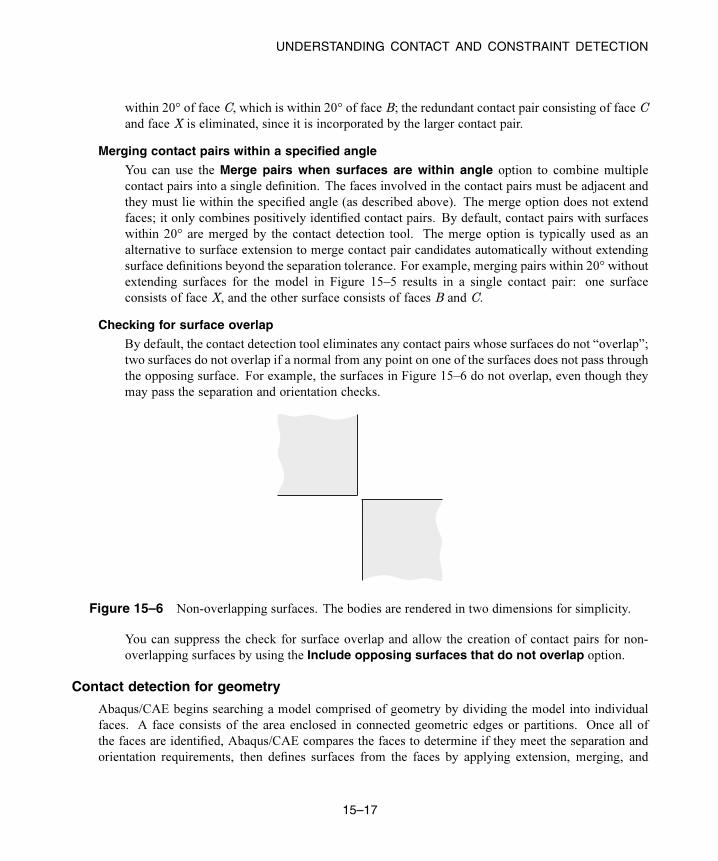
UNDERSTANDING CONTACT AND CONSTRAINT DETECTION
within 20° of face C, which is within 20° of face B; the redundant contact pair consisting of face C
and face X is eliminated, since it is incorporated by the larger contact pair.
Merging contact pairs within a specified angle
You can use the Merge pairs when surfaces are within angle option to combine multiple
contact pairs into a single definition. The faces involved in the contact pairs must be adjacent and
they must lie within the specified angle (as described above). The merge option does not extend
faces; it only combines positively identified contact pairs. By default, contact pairs with surfaces
within 20° are merged by the contact detection tool. The merge option is typically used as an
alternative to surface extension to merge contact pair candidates automatically without extending
surface definitions beyond the separation tolerance. For example, merging pairs within 20° without
extending surfaces for the model in Figure 15–5 results in a single contact pair: one surface
consists of face X, and the other surface consists of faces B and C.
Checking for surface overlap
By default, the contact detection tool eliminates any contact pairs whose surfaces do not “overlap”;
two surfaces do not overlap if a normal from any point on one of the surfaces does not pass through
the opposing surface. For example, the surfaces in Figure 15–6 do not overlap, even though they
may pass the separation and orientation checks.
Figure 15–6 Non-overlapping surfaces. The bodies are rendered in two dimensions for simplicity.
You can suppress the check for surface overlap and allow the creation of contact pairs for non-
overlapping surfaces by using the Include opposing surfaces that do not overlap option.
Contact detection for geometry
Abaqus/CAE begins searching a model comprised of geometry by dividing the model into individual
faces. A face consists of the area enclosed in connected geometric edges or partitions. Once all of
the faces are identified, Abaqus/CAE compares the faces to determine if they meet the separation and
orientation requirements, then defines surfaces from the faces by applying extension, merging, and
15–17
Abaqus ID:
Printed on:

UNDERSTANDING CONTACT AND CONSTRAINT DETECTION
overlap checks (see “Additional criteria for defining contact pairs” above). Any two surfaces that meet
all of the requirements are flagged as a contact pair candidate.
Abaqus/CAE automatically assigns the master and slave designations to surfaces in a detected
contact pair. Analytical rigid or discrete rigid surfaces are always assigned the master role; if the contact
pair involves two rigid surfaces, the assignment of master and slave roles is arbitrary. For contact
pairs involving two deformable surfaces, Abaqus/CAE first determines if the surface geometry has
been meshed and assigns the master role to the surface with the coarser mesh. If mesh information is
unavailable, the surface with the larger area becomes the master surface. The algorithm that assigns
master and slave roles does not account for dissimilar underlying stiffness or element assignments; if
these factors play a significant role in your contact interactions, you should review the master and slave
assignments before creating an interaction. For further discussion of master and slave assignments, see
“Selecting surfaces used in contact pairs” in “Defining contact pairs in Abaqus/Standard,” Section 36.3.1
of the Abaqus Analysis User’s Guide.
Contact detection for meshed models
Contact detection also works with mesh models. The search algorithm for meshed models works in
much the same way as with geometry, but it uses element faces instead of geometric faces. By default,
Abaqus/CAE only searches for contact pairs between separate part instances. Mesh models that are
imported into Abaqus/CAE often consist of only a single part instance; therefore, you should enable
searching within the same instance before using contact detection on these models (see “Defining contact
within the same instance and self-contact” below for more details).
WARNING: Unlike geometry-based searches, the reported separation between surfaces for mesh-basedsurfaces is not necessarily the distance between the exact points of closest approach, but rather a close
approximation. If the specified search tolerance is very large compared to the characteristic element
size, the accuracy of this approximation is greatly reduced.
Before defining surfaces on element faces, Abaqus/CAE applies the same extension, merging,
and overlap checks as with geometry faces (see “Additional criteria for defining contact pairs” above).
Because element faces are typically much smaller than geometric faces, you should always allow some
extension of the surfaces to get ample coverage from a surface definition; Figure 15–7 compares the
created surfaces for geometry and meshed geometry when no surface extension is allowed.
If you remesh your model, any surfaces defined on elements faces may become invalid. By
extension, the interactions and constraints based on these faces also become invalid.
When assigning master and slave designations to the mesh surfaces, rigid surfaces always become
the master; if the contact pair involves two rigid surfaces, the assignment of master and slave roles
is arbitrary. For contact pairs involving two deformable surfaces, Abaqus/CAE considers the mesh
densities on each surface; the surface with the coarser mesh becomes the master surface. If the mesh
densities on the two surfaces are equivalent, the assignment of master and slave roles is arbitrary. The
algorithm that assigns master and slave roles does not account for dissimilar underlying stiffness or
element types; if these factors play a significant role in your contact interactions, you should review
15–18
Abaqus ID:
Printed on:

UNDERSTANDING CONTACT AND CONSTRAINT DETECTION
Surfaces Surfaces
Figure 15–7 Discrepancies between created surfaces when no surface extension is
allowed for geometry (left) and meshed geometry (right).
the master and slave assignments before creating an interaction. For further discussion of master
and slave assignments, see “Selecting surfaces used in contact pairs” in “Defining contact pairs in
Abaqus/Standard,” Section 36.3.1 of the Abaqus Analysis User’s Guide.
The contact detection tool does not detect contact between geometry and orphan elements or
analytical surfaces and orphan elements. If your model includes part instances that have been meshed
from geometry, you can use the options on the Advanced tabbed page of the contact detection dialog
box to indicate whether these instances should be treated as geometry (the default) or an element mesh
during the search. If your model contains instances of both geometry and orphan mesh elements, you
should first mesh all of the geometries, then perform a mesh-based search to capture all possible contact
pairs.
In most cases the geometry is a more faithful representation of the object being modeled than
the meshed geometry. In addition, geometry-based interactions and constraints are not affected by
remeshing. However, the mesh is the geometry used in the analysis. Mesh discretization can lead to
slight disparities in separation distances between the two representations, which may become important
in precise analyses. After performing a search, you can check individual contact pairs for disparities
between the native and meshed geometry by using the Recalculate Separation option.
Detection of overclosed surfaces
If two faces in an assembly intersect at any point, the contact detection tool reports those faces as an
overclosed contact pair. Overclosed contact pairs that appear in the contact pair candidates table must
still meet the surface orientation requirements. A red zero in the Separation column indicates that the
two surfaces in the contact pair are intersecting.
Note: A black zero in the Separation column implies that the two surfaces are exactly touching at their
closest points. There is no overclosure or intersection in this situation.
If you extend or merge an overclosed surface to include faces that are not overclosed, Abaqus/CAE
reports the entire contact pair as overclosed.
You should visually inspect all overclosed surfaces before creating contact interactions. Models
with severe overclosures should be adjusted to remove the overclosures (or at least lessen their severity).
15–19
Abaqus ID:
Printed on:
UNDERSTANDING CONTACT AND CONSTRAINT DETECTION
Minor overclosures can be addressed by using the contact adjustment options (available in the contact
pair candidates table) or the interference fit options (available in the contact interaction editor).
Faces must intersect to be reported as overclosed. If a face is enclosed entirely within another part
instance, the automatic contact detection tool does not report that face as being overclosed. Such a
face may still meet the separation and orientation requirements with respect to an external face on the
enclosing instance. By default, Abaqus/CAE eliminates enclosed faces from the contact pair candidates
table because the surfaces do not “overlap” (see “Additional criteria for defining contact pairs”). If
you disable the overlap checks, Abaqus/CAE reports a contact pair candidate for enclosed faces, but
the contact pair candidates table does not provide any indication that the surfaces are overclosed
or penetrating. Because the contact detection tool does not recognize these faces as overclosed, the
adjustment options that are applied to overclosed surfaces by default (see “Default interaction and
constraint parameters,” Section 15.6.3) are not applied to this contact pair. If an enclosed face is
embedded deeper than the separation tolerance from any external face, the automatic contact detection
tool does not identify those faces as a contact pair candidate.
As an example, consider the model in Figure 15–8. The separation tolerance specified for this
search is 0.1. The circular face at the end of part instance B is within the separation tolerance and is
intuitively opposed to the rectangular face on part instance A, but there is no intersection. The contact
pair candidates table lists a normal contact pair consisting of the circular face and the rectangular face
separated by a distance of 0.06. The cylindrical side face of part instance B is listed as overclosed because
it intersects the rectangular face of part instance A.
Although the contact detection tool does not recognize completely enclosed surfaces as being
overclosed, such surfaces are still treated as overclosures during an analysis. Severe overclosures
commonly lead to convergence difficulties. When reviewing overclosed contact pairs in the contact pair
candidates table, check adjoining surfaces for fully enclosed faces.
Defining contact within the same instance and self-contact
You can use the contact detection tool to define contact between different areas of the same part instance.
This capability is particularly useful for complicated models that are imported into Abaqus/CAE as a
single part instance. If you enable the Include pairs with surfaces on the same instance option,
Abaqus/CAE checks different geometry or element faces on the same part instance to determine whether
or not they meet the separation and orientation requirements. Surfaces and contact pairs are defined on
any faces that meet the requirements.
In some situations, surface extension options cause the master and slave surfaces to overlap. If the
master surface and the slave surface consist of the same faces, Abaqus/CAE automatically adjusts the
contact pair to create a self-contact interaction, in which a surface contacts itself during deformation. A
single surface is created in this situation.
Considerations for shells
If a section definition has been assigned to a shell part, the contact detection tool accounts for the
thickness of the shell in separation calculations. The reported separation has been adjusted according
to the thickness and offset specified in the shell section assignment. You can use the Account for
15–20
Abaqus ID:
Printed on:

UNDERSTANDING CONTACT AND CONSTRAINT DETECTION
Part A
Part B
0.06
Figure 15–8 In this model, one end of the cylindrical part instance is entirely
enclosed within another part instance.
shell thickness and offset option to ignore shell section properties during a contact detection search.
Varying thickness distributions are never considered in the separation calculations.
The contact detection tool automatically selects a shell side on which to create a surface (see
“Specifying a particular side or end of a region,” Section 73.2.5, for more information). The side is
selected such that the surface normals at the points of closest approach are intuitively opposed.
When working with a model that includes orphan shell elements, make sure that the element
normal orientations are consistent between elements; that is, the positive element faces (SPOS) should
all be located on the same side of the shell structure (see “Shell elements: overview,” Section 29.6.1
of the Abaqus Analysis User’s Guide, for more information). If the element normal orientations are
inconsistent, Abaqus/CAE misinterprets the angles between the element faces, and the surface extension
and merge operations do not function appropriately.
For certain spline-based shells or faces, the same surface may interact with both sides of a shell (see
Figure 15–9, for example). Normally you would define a separate contact pair involving each side of
the shell. The contact detection tool, however, cannot create multiple contact pairs that involve the same
two faces; it will define a single contact pair and select the shell side according to the orientation at the
point of closest approach. You must manually define another contact pair for the other side of the shell.
The contact detection tool does not create any double-sided surfaces. If appropriate, you can edit the
definition of a created surface in the Model Tree to make it double-sided (see “Editing sets and surfaces,”
Section 73.3.5, in the HTML version of this guide).
15–21
Abaqus ID:
Printed on:

UNDERSTANDING CONTACT AND CONSTRAINT DETECTION
Figure 15–9 A spline-based shell.
15.6.3 Default interaction and constraint parametersAfter completing a search for potential contact pairs, Abaqus/CAE populates the contact pair candidates
table with all of the parameters necessary to create interactions. Names are provided for the contact pair
and any created surfaces. Table 15–1 outlines the naming algorithm.
Table 15–1 Algorithms used to create names in the contact detection tool.
Contact pairs Prefix-Contact_pair_number-Master_instance-Slave_instance
Master surfaces Prefix-Contact_pair_number-Master_instance
Slave surfaces Prefix-Contact_pair_number-Slave_instance
Merged master surface Prefix-All-m
Merged slave surface Prefix-All-s
Merged “all” surface Prefix-All
Use the Names tabbed page before performing a search to modify the naming prefix and control the
creation of surfaces. For details, see “Specifying naming options for contact detection” in “Specifying
search criteria for contact detection,” Section 15.16.1, in the HTML version of this guide.
The default parameters supplied to contact pairs by the contact detection tool are slightly different
than the defaults used in the traditional interaction or constraint editor. Most notably, the contact detection
tool initially assigns surface-to-surface discretization to each contact pair instead of node-to-surface
15–22
Abaqus ID:
Printed on:

UNDERSTANDING CONTACT AND CONSTRAINT DETECTION
discretization. See “Mesh tie constraints,” Section 35.3.1 of the Abaqus Analysis User’s Guide, and
“Contact formulations in Abaqus/Standard,” Section 38.1.1 of the Abaqus Analysis User’s Guide, for a
discussion of surface discretization and the associated constraint enforcement methods.
The default surface adjustment options depend on the separation between the surfaces in a contact
pair. You can use the Rules tabbed page before performing a search to control the default adjustment
options that are assigned to detected contact pairs. You can also use this page to specify a separation
tolerance within which all contact pairs default to tie constraints. For more information about the Rulespage, see “Defining default contact pair parameters” in “Specifying search criteria for contact detection,”
Section 15.16.1, in the HTML version of this guide.
Table 15–2 lists the default contact pair parameters supplied by Abaqus/CAE. You can edit each
parameter individually before creating interactions and constraints. For detailed instructions on editing
parameters and defaults, see “Reviewing and modifying detected contact pairs,” Section 15.16.3, in the
HTML version of this guide.
Table 15–2 Default contact pair parameters for the contact detection tool.
Parameter Default Value
Active/suppressed Active
Type1 Interaction
Sliding Finite sliding
Discretization Surface-to-surface
Interaction Property The first contact Interaction Property listed in the Interaction Property manager2 ;
if no Interaction Properties have been created, this parameter is blank
Adjust1 Off for contact interactions between nonintersecting surfaces; 0 for contact
interactions between intersecting surfaces; On for tie constraints
Creation step Initial
Surface smoothing Automatic
1Defaults for the Type and Adjust parameters are controlled by the Rules options.
2The Interaction Property manager lists all created Interaction Properties alphabetically by name.
Note: Some of the parameters discussed above are not visible in the contact pair candidates table by
default. Click mouse button 3 anywhere in the table, and select Edit Visible Columns to control which
parameters appear in the table.
For more information about interaction and constraint parameters, see “Mesh tie constraints,”
Section 35.3.1 of the Abaqus Analysis User’s Guide; “Defining contact pairs in Abaqus/Standard,”
Section 36.3.1 of the Abaqus Analysis User’s Guide; and “Defining contact pairs in Abaqus/Explicit,”
Section 36.5.1 of the Abaqus Analysis User’s Guide.
15–23
Abaqus ID:
Printed on:

UNDERSTANDING CONTACT AND CONSTRAINT DETECTION
15.6.4 Tips for using the contact detection toolThe contact detection tool is available for use in any three-dimensional model requiring the creation of
contact interactions and tie constraints. It quickly and thoroughly identifies and creates interactions and
ties based on minimal specifications. The tool greatly simplifies the contact definition process in models
for which a general contact definition is not applicable.
Some basic guidelines, outlined in the following sections, ensure the most effective and efficient
use of the tool:
• “Choosing a separation tolerance and extension angle”
• “Reviewing contact pair candidates”
• “Saving the search parameters”
• “Features that may cause difficulties for the contact detection tool”
• “Limitations of the contact detection tool”
Choosing a separation tolerance and extension angle
The specified separation tolerance is the primary driver of the contact pair search algorithm. Abaqus/CAE
supplies a default separation tolerance based on the relative size of the faces in your model. You may
need to modify this value depending on the expected response of your model during an analysis. To
effectively capture all significant contact pairs, the specified separation tolerance should be on the same
order as or greater than the expected displacements or deflections in your model.
Specifying a very large separation tolerance usually captures more contact pairs then are necessary
in an analysis. While extra contact pairs do not necessarily reduce the quality of a model, the extraneous
definitions are difficult to manage and can degrade performance.
When selecting an angle to control the extension of surfaces, you should consider the topology and
surface characteristics of the areas that are likely to come into contact. Surfaces should extend slightly
beyond the area of potential contact, so set the extension angle to capture any chamfers or soft corners
along the edges of a face. Indentations, grooves, or embossments can sometimes break up the definition
of a surface; the angle that these features make with the main face should dictate the extension angle.
For meshed models, you can preview the extension of surfaces before performing a search for
contact pairs by displaying only the feature edges on a model (see “Defining mesh feature edges,”
Section 76.5, in the HTML version of this guide). If the extension angle is equal to the feature angle,
the surface definition in a particular area extends as far as the nearest visible feature edge. Adjust the
feature angle until the visible edges enclose the area you want to capture, then set the extension angle
accordingly.
Reviewing contact pair candidates
You should always review contact pair candidates before creating interactions and constraints. Look for
any discontinuities in surface definitions. Discontinuities are often caused by small connecting faces that
are not intuitively opposed to the logical contacting surface in a contact pair (see Figure 15–10).
15–24
Abaqus ID:
Printed on:

UNDERSTANDING CONTACT AND CONSTRAINT DETECTION
Figure 15–10 The automatic contact detection tool will not identify the highlighted perpendicular face.
You may want to rerun the search using revised extension and merge options to incorporate the
discontinuities into larger surfaces. If necessary, add a contact pair manually using the Add option. You
can also combine discontinuous surfaces using the Merge option.
You should investigate any intersecting surfaces to verify that they match your modeling intent. A
contact pair with only a single overclosed nodewill be reported as intersecting, so slight discrepancies can
cause overclosures. Overclosed contact pairs without appropriate adjustment or interference fit options
can lead to convergence difficulties in an analysis. You should also check any faces or surfaces adjacent
to overclosed contact pairs to ensure they are not enclosed faces. See “Detection of overclosed surfaces”
in “The contact detection algorithm,” Section 15.6.2, for more information.
Saving the search parameters
By default, the search parameters that you specify in the Find Contact Pairs dialog box persist only as
long as the dialog box is open; if you close the dialog box, default search parameters are provided the
next time you access the contact detection tool.
If you click on the Advanced tabbed page, Abaqus/CAE sets the currently specified search
parameters as the default search parameters. These parameters are supplied as defaults in all future
sessions of Abaqus/CAE. The only parameter that is not saved is the search domain, which always uses
a default of Whole model.When you save the current search parameters, Abaqus/CAE asks if you want to save the current
separation tolerance as a default. Normally Abaqus/CAE recalculates the default separation tolerance
based on the current model; if you opt to save the separation tolerance, this calculation is skipped and
the same value is always provided as the default separation tolerance.
The default search parameters for the contact detection tool are saved in the abaqus_v6.13.gprfile; see “Understanding Abaqus/CAE GUI settings,” Section 3.6, for more information. To return the
default search parameters to their original settings, click on the Advanced tabbed page.
15–25
Abaqus ID:
Printed on:

UNDERSTANDING CONTACT AND CONSTRAINT DETECTION
Features that may cause difficulties for the contact detection tool
You may encounter difficulties using the contact detection tool with certain model features and designs.
These situations do not cause performance or stability problems, but the search results most often will
not match your modeling intent.
Stacked shells and thin layers
Models with layers of shells or thin plates stacked closely in parallel can lead to the definition
of extraneous contact pairs. The automatic contact detection tool can find contact pairs involving
surfaces separated by an intermediate layer, as long as these surfaces are intuitively opposed and
within the separation tolerance. In addition, if searching within the same instance is enabled and
the overlapping surface check is disabled, the contact detection tool may detect potential contact
between the top side and bottom side of a thin continuum plate. Abaqus/CAE creates contact pair
candidates for all of these surfaces, even though they will never be in contact. This problem is
most common when the layers or plates are a local feature of the model, since a larger separation
tolerance is required to capture surfaces in other areas of the model. To overcome this problem, limit
the search domain to a particular area of the model and use a separation tolerance that is appropriate
for that area. You may also be able to use the Entities tabbed page of the contact detection dialog
box to eliminate certain geometry or element types (shells, for example) from your search domain.
Otherwise, you should delete the extraneous contact pair candidates before creating interactions.
Concave surfaces
While the contact search algorithm effectively accounts for most appropriate surfaces, it can
misinterpret the relationship between a concave surface and a flat surface. Concave surfaces
create difficulties because their surface normal orientation can vary widely across the span of a
single surface, and the points of closest approach between surfaces is sometimes a poor reference.
Consider, for example, the situations in Figure 15–11. Even if the points of closest approach in
these models are within the separation tolerance, the surface normals at these points do not pass the
orientation test. The contact detection tool will not report these surfaces as contact pair candidates,
and adjusting the separation tolerance has no effect on this behavior. You can sometimes modify
the extension angle to capture the concave surface within another surface definition. Otherwise,
you must manually define the contact pair using the Add option.
Mechanisms involving large rotations
When modeling mechanisms that undergo large rotations, the contact detection tool often will not
effectively capture your modeling intent. In such mechanisms the intended contact surfaces initially
may be positioned far away from each other, while nearby surfaces never actually come into contact.
The Geneva mechanism depicted in Figure 15–12 is a typical example.
15–26
Abaqus ID:
Printed on:

UNDERSTANDING CONTACT AND CONSTRAINT DETECTION
Figure 15–11 The normals of the shaded surfaces are not
intuitively opposed at the points of closest approach.
Figure 15–12 Motion of a Geneva mechanism.
The important contact surfaces in this model are the pin on the right-hand body and the slots on the
left-hand body. In the initial configuration, the pin is relatively distant from any of the slots. The
neighboring surfaces, on the other hand, are insignificant to the contact conditions of the model.
Contact for such models is best defined manually using the interaction editor (see “Defining surface-
to-surface contact,” Section 15.13.7, in the HTML version of this guide).
Limitations of the contact detection tool
Contact detection cannot create contact pairs involving the following features:
• Two-dimensional models
• Axisymmetric models
• Beams and trusses
• Face-to-edge contact
• Edge-to-edge contact
• Contact between orphan mesh elements and analytical rigid surfaces
• Hybrid models containing both orphan mesh and unmeshed geometry
The minimum allowable separation tolerance is 1 × 10⁻⁵ . The maximum allowable separation
tolerance is 1 × 10⁵ . Abaqus/CAE cannot accurately calculate separations outside of this range. If your
model requires the use of a separation tolerance that does not meet these requirements, you should scale
the dimensions of the entire model so that they fall within the functional range.
15–27
Abaqus ID:
Printed on:

UNDERSTANDING CONNECTOR SECTIONS AND FUNCTIONS
15.7 Understanding connectors
Connectors allow you to model a connection between two points in an assembly or between a point in
an assembly and ground. To model a connector in Abaqus/CAE, you must create an assembly-level wire
feature, a connector section, and a connector section assignment that associates the connector section
with selected wires.
The wire feature contains one or more wires that define the underlying connector geometry. The
connector section specifies the type of connection, connector behaviors, and section data. Similar to
the manner in which you assign a section to a region of the model in the Property module, you create
a connector section assignment to assign a connector section to a region of the model; specifically, you
assign a connector section to wires. You also specify local orientations for the endpoints of the wires in
the connector section assignment definition.
For more information on connectors in Abaqus/CAE, including an overview and an example of
connector modeling, see Chapter 24, “Connectors.”
15.8 Understanding connector sections and functions
The connector section defines the connection type and may include connector behavior and section
data. For some complex coupled connector behaviors, additional functions describing the nature of the
coupling effects (connector derived components and connector potential) must be defined. A connector
section can be referred to by one or more different connector section assignments.
15.8.1 Connection typesTable 15–3 summarizes the connection types available when creating connector sections. You can define
basic, assembled, complex, and MPC connection types.
Table 15–3 Connection types.
Basic Types
Translational Rotational
Assembled/ComplexTypes
MPCTypes
Accelerometer Align Beam Beam
Axial Cardan Bushing Elbow
Cartesian Constant Velocity CV Joint Link
Join Euler Cylindrical Pin
15–28
Abaqus ID:
Printed on:

UNDERSTANDING CONNECTOR SECTIONS AND FUNCTIONS
Basic Types
Translational Rotational
Assembled/ComplexTypes
MPCTypes
Link Flexion-Torsion Hinge Tie
Proj. Cartesian Flow-Converter Planar User-defined
Radial-Thrust Proj. Flex-Tors. Retractor
Slide-Plane Revolute Slip Ring
Slot Rotation Translator
Rotation-Accelerometer U Joint
Universal Weld
Basic types
Basic connection types include translational types and rotational types. Translational types affect
translational degrees of freedom at both endpoints of the wires to which the connector section is
assigned and may affect rotational degrees of freedom at the first points of the wires. Rotational
types affect only rotational degrees of freedom at both endpoints of the wires. You can use a single
basic connection type (translational or rotational) or one translational and one rotational type.
Assembled types
Assembled connection types are predefined combinations of basic connection types.
Complex types
Complex connection types affect a combination of degrees of freedom in the connection and
cannot be combined with other connection types. They typically model highly coupled physical
connections.
MPC types
MPC connection types are used to define multi-point constraints between two points.
For a description of each connection type and the equivalent basic connection types that define the
kinematic constraints of assembled type connections, see “Connection-type library,” Section 31.1.5 of
the Abaqus Analysis User’s Guide, and “General multi-point constraints,” Section 35.2.2 of the Abaqus
Analysis User’s Guide.
15.8.2 Connector behaviors
You can apply connector behaviors to connection types that have available components of relative
motion. Available components of relative motion are displacements and rotations that are not
15–29
Abaqus ID:
Printed on:
UNDERSTANDING CONNECTOR SECTIONS AND FUNCTIONS
kinematically constrained. Multiple connector behaviors can be defined in a connector section. You can
specify the following connector behaviors:
• Elasticity: Define spring-like elastic behavior.
• Damping: Define dashpot-like damping behavior.
• Friction: Define Coulomb-like and hysteretic friction using predefined or user-defined friction
models.
• Plasticity: Define plastic behavior.
• Damage: Define damage initiation and evolution behavior.
• Stop: Define limit values of the admissible range of positions.
• Lock: Specify a user-defined locking criterion.
• Failure: Define limit values for force, moment, or position.
• Reference Length: Define the translational or angular positions at which constitutive forces and
moments are zero.
• Integration: Specify implicit or explicit time integration for elasticity, damping, and friction
(Abaqus/Explicit analyses only).
For detailed instructions on defining connector behaviors, see “Using the connector section editors,”
Section 15.17, in the HTML version of this guide. For more information on connector behaviors, see
“Connector behavior,” Section 31.2.1 of the Abaqus Analysis User’s Guide.
15.8.3 What types of friction models are available?
You can model predefined or user-defined friction behavior. In general, for predefined friction you
specify a set of geometric quantities that are characteristic of the connection type for which friction
is modeled. In addition, you can define internal contact force contributions, such as prestress from the
connection. Abaqus automatically defines the contact force contributions and the local tangent directions
along which friction occurs.
You can model predefined friction for the following connection types:
Assembled/Complex types
• Cylindrical (Slot + Revolute)
• Hinge (Join + Revolute)
• Planar (Slide-Plane + Revolute)
• Slip Ring (complex)
• Translator (Slot + Align)
• U Joint (Join + Universal)
15–30
Abaqus ID:
Printed on:

UNDERSTANDING INTERACTION MODULE MANAGERS AND EDITORS
Basic types
• Slide-Plane
• Slot
Predefined friction is also available if you define a combined translational and rotational connection
type that is equivalent to one of these assembled types. You can define only one friction behavior for a
given connection type if you are modeling predefined friction.
If a predefined friction model is not available or does not adequately describe the mechanism being
analyzed, you can specify a user-defined friction model (except in the case of the Slip Ring connection
type, which does not allow a user-defined friction model). You must specify slip direction information,
the friction-producing normal force or normal moment, and the friction law. You may use several
connector friction behaviors to represent the frictional effects in the connector.
For detailed instructions on defining friction, see “Defining friction,” Section 15.17.3, in the HTML
version of this guide. For more information, see “Connector friction behavior,” Section 31.2.5 of the
Abaqus Analysis User’s Guide.
15.8.4 Connector derived components and connector potentials
You can define complex coupled behavior for connectors using connector derived components and
connector potentials. Connector derived components are user-specified component definitions based on
a function of intrinsic connector components of relative motion. You can create derived components
to specify the friction-generating normal force in connectors as a complex combination of connector
forces and moments or to use as an intermediate result in a connector potential function.
Connector potentials are user-defined mathematical functions of intrinsic components of relative
motion or derived components. These functions can be quadratic, elliptical, or maximum norms. You
use connector potentials to define coupled friction, plasticity, and damage connector behaviors.
For detailed instructions on defining derived components and potentials, see “Specifying connector
derived components,” Section 15.17.15, and “Specifying potential terms,” Section 15.17.16. For more
information on connector functions, see “Connector functions for coupled behavior,” Section 31.2.4 of
the Abaqus Analysis User’s Guide.
15.9 Understanding Interaction module managers and editors
You can create and manage objects in the Interaction module using managers and editors.
15–31
Abaqus ID:
Printed on:

UNDERSTANDING INTERACTION MODULE MANAGERS AND EDITORS
15.9.1 Managing objects in the Interaction moduleThe Interaction module provides the following managers that you can use to organize and manipulate
objects associated with a given model:
• The Interaction Manager allows you to create and manage interactions.
• The Interaction Property Manager allows you to create and manage interaction properties.
• The Contact Controls Manager allows you to create and manage contact controls for surface-to-
surface contact and self-contact interactions.
• The Contact Initialization Manager allows you to create and manage contact initialization rules
for general contact interactions in Abaqus/Standard.
• The Constraint Manager allows you to create and manage constraints.
• The Connector Section Manager allows you to create and manage connector sections.
• The Connector Section Assignment Manager allows you to create and manage connector
section assignments.
For example, a list of interaction properties appears in the Interaction Property Manager shown in
Figure 15–13.
Figure 15–13 The Interaction Property Manager.
The Create, Edit, Copy, Rename, and Delete buttons in the managers allow you to create new
objects or to edit, copy, rename, and delete existing ones. In the Connector Section AssignmentManager, you can only create, edit, or delete connector section assignments. You can also
initiate these procedures using the Interaction, Interaction→Property, Interaction→ContactControls, Interaction→Contact Initialization, Constraint, Connector→Section, and
Connector→Assignment menus from the main menu bar. After you select a management
operation from the main menu bar, the procedure is exactly the same as if you had clicked the
corresponding button inside the manager dialog box.
You can use the Copy button in the Interaction Manager, the corresponding menu command, or
the Model Tree to copy an interaction. You can copy an interaction from any step to any valid step, with
15–32
Abaqus ID:
Printed on:

UNDERSTANDING INTERACTION MODULE MANAGERS AND EDITORS
some restrictions. For more details, see “Copying step-dependent objects using manager dialog boxes,”
Section 3.4.11.
The Interaction Manager is a step-dependent manager, which means that it contains additional
information on the history of each interaction through the analysis. The Interaction Manager is shownin Figure 15–14.
Figure 15–14 The Interaction Manager.
The Move Left, Move Right, Activate, and Deactivate buttons allow you to manipulate the
stepwise history of interactions. For more information, see “Modifying the history of a step-dependent
object,” Section 3.4.6.
You can suppress and resume previously defined interactions, constraints, and connector section
assignments from the managers. You can use the icons in the column along the left side of the manager
to suppress these attributes or to resume previously suppressed attributes for an analysis. The suppress
and resume procedures are also available from the Interaction, Constraint, and Connector menus in
the main menu bar. For more information, see “Suppressing and resuming objects,” Section 3.4.3.
For detailed instructions on creating interactions, interaction properties, constraints, connector
sections, and connector section assignments, see “Using the Interaction module,” Section 15.12, in the
HTML version of this guide.
15.9.2 Interaction editorsTo create interactions, select Interaction→Create from the main menu bar. A Create Interactiondialog box appears in which you can provide a name for the interaction, select the step in which the
interaction will be created, and choose the type of the interaction.
When you click Continue in the Create Interaction dialog box after selecting any interaction type
except general contact, you are prompted to select the regions to which to apply the interaction. Once
15–33
Abaqus ID:
Printed on:

UNDERSTANDING INTERACTION MODULE MANAGERS AND EDITORS
you have selected the region or regions, an interaction editor appears in which you can specify additional
information about the interaction, such as the interaction property that you want to associate with the
interaction. For general contact interactions, the interaction editor appears when you click Continue in
the Create Interaction dialog box. For example, the general contact editor for Abaqus/Explicit analyses
is shown in Figure 15–15.
Figure 15–15 The general contact editor.
Each interaction editor displays the current step and the name and type of the interaction that you
are defining in the top panel of the dialog box. The format of the rest of the editor varies depending on
the type of interaction you are defining.
Once you have created an interaction, you can modify the interaction in the following ways:
• You canmodify some or all of the data that you entered in the editor when you created the interaction.
• You can use the Interaction Manager to modify the stepwise history of the interaction. (For more
information, see “What are step-dependent managers?,” Section 3.4.2.)
15–34
Abaqus ID:
Printed on:

UNDERSTANDING INTERACTION MODULE MANAGERS AND EDITORS
You can display information on a particular editor feature by selecting Help→On Context fromthe main menu bar and then clicking the editor feature of interest.
15.9.3 Interaction property editors
To create interaction properties, select Interaction→Property→Create from the main menu bar. A
Create Interaction Property dialog box appears in which you can specify a name for the interaction
property and the type of interaction property that you want to create. Once you have specified this
information, click Continue in the Create Interaction Property dialog box to display the interaction
property editor.
The format of the interaction property editor depends on the type of interaction property you are
defining. For example, the film condition and actuator/sensor property editors display data fields in which
you can enter all of the information necessary to define the property. The film condition property editor
is shown in Figure 15–16.
Figure 15–16 The film condition property editor.
The format of the contact property editor, on the other hand, is identical to the material editor in
the Property module (see “Creating materials,” Section 12.4.1, for more information). Like the material
editor, the contact property editor contains menus from which you select options to include in the property
definition, as shown in Figure 15–17.
15–35
Abaqus ID:
Printed on:
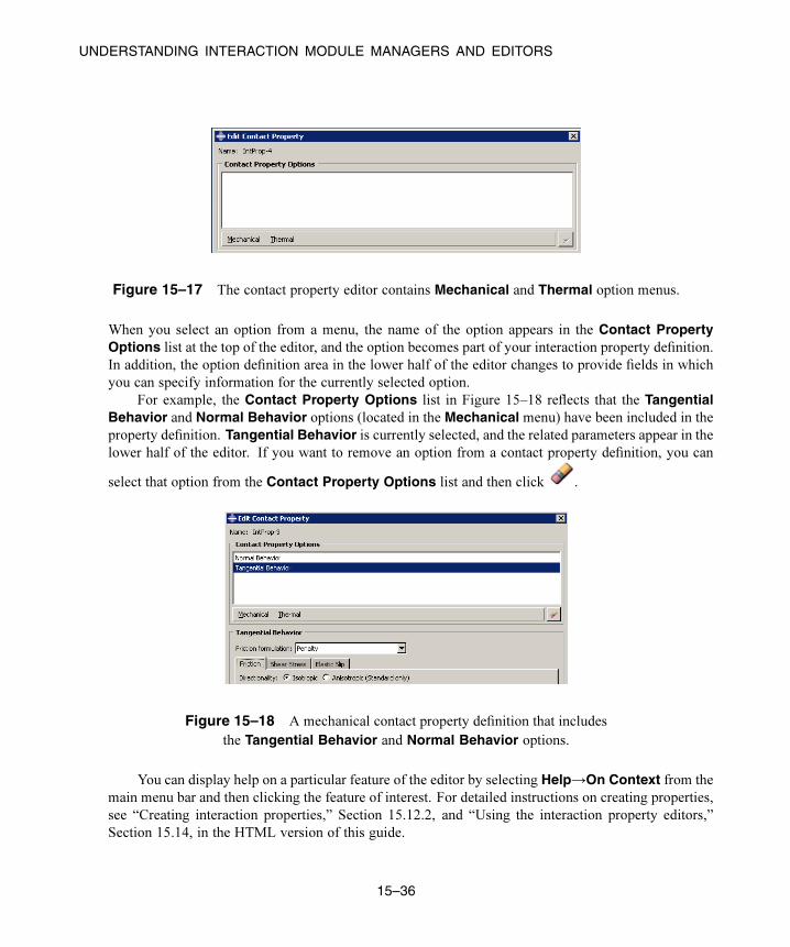
UNDERSTANDING INTERACTION MODULE MANAGERS AND EDITORS
Figure 15–17 The contact property editor contains Mechanical and Thermal option menus.
When you select an option from a menu, the name of the option appears in the Contact PropertyOptions list at the top of the editor, and the option becomes part of your interaction property definition.
In addition, the option definition area in the lower half of the editor changes to provide fields in which
you can specify information for the currently selected option.
For example, the Contact Property Options list in Figure 15–18 reflects that the TangentialBehavior and Normal Behavior options (located in the Mechanical menu) have been included in the
property definition. Tangential Behavior is currently selected, and the related parameters appear in the
lower half of the editor. If you want to remove an option from a contact property definition, you can
select that option from the Contact Property Options list and then click .
Figure 15–18 A mechanical contact property definition that includes
the Tangential Behavior and Normal Behavior options.
You can display help on a particular feature of the editor by selecting Help→On Context from the
main menu bar and then clicking the feature of interest. For detailed instructions on creating properties,
see “Creating interaction properties,” Section 15.12.2, and “Using the interaction property editors,”
Section 15.14, in the HTML version of this guide.
15–36
Abaqus ID:
Printed on:

UNDERSTANDING INTERACTION MODULE MANAGERS AND EDITORS
15.9.4 Contact controls editors
To create contact controls for surface-to-surface contact and self-contact interactions, select
Interaction→Contact Controls→Create from the main menu bar. A Create Contact Controlsdialog box appears in which you can specify a name for the contact controls and the type of contact
controls that you want to create. Once you have specified this information, click Continue to display
the contact controls editor.
WARNING: Contact controls are intended for advanced users. The default settings of these controls
are appropriate for most analyses. Using nondefault values of these controls may greatly increase
the computational time of the analysis or produce inaccurate results. Changing these settings in an
Abaqus/Standard analysis may also cause convergence problems.
Each contact controls editor displays the name and type of the contact controls that you are defining
in the top panel of the dialog box. The format of the rest of the editor varies depending on whether you
are defining controls for an Abaqus/Standard or an Abaqus/Explicit analysis.
You can display help on a particular feature of the editor by selecting Help→On Context fromthe main menu bar and then clicking the feature of interest. For more information, see “Specifying
contact controls in an Abaqus/Standard analysis,” Section 15.13.9, and “Specifying contact controls in
an Abaqus/Explicit analysis,” Section 15.13.10, in the HTML version of this guide.
15.9.5 Contact initialization editor
To create contact initialization rules for a general contact interaction in Abaqus/Standard, select
Interaction→Contact Initialization→Create from the main menu bar. The contact initialization
editor appears in which you can specify a name for the initialization definition and the rules associated
with that definition.
You can display help on the contact initialization editor by selecting Help→On Context from the
main menu bar and then clicking the editor. For more information, see “Creating contact initializations,”
Section 15.12.4, in the HTML version of this guide.
15.9.6 Constraint editors
To create constraints, select Constraint→Create from the main menu bar. A Create Constraint dialogbox appears in which you can specify the name and type of the constraint. Click Continue to specify the
regions to which to apply the constraint (if applicable) and to display the editor in which you can enter
the data necessary to define the constraint.
15–37
Abaqus ID:
Printed on:

UNDERSTANDING INTERACTION MODULE MANAGERS AND EDITORS
Each constraint editor displays the name and type of the constraint you are defining in the top panel
of the dialog box. The format of the rest of the editor varies depending on the type of constraint you are
defining. For example, the tie constraint editor is shown in Figure 15–19.
Figure 15–19 The tie constraint editor.
You can display information on a particular editor feature by selecting Help→On Context fromthe main menu bar and then clicking the editor feature of interest. For detailed instructions on creating
constraints, see “Using the constraint editors,” Section 15.15, in the HTML version of this guide.
15.9.7 Connector section editorsTo create connector sections, select Connector→Section→Create from the main menu bar. A
Create Connector Section dialog box appears in which you can specify a name, category, and
type for the connector section that you want to create. When you select a connection type from the
15–38
Abaqus ID:
Printed on:

UNDERSTANDING INTERACTION MODULE MANAGERS AND EDITORS
Assembled/Complex or Basic category, the available and constrained components of relative motion
(CORM) for that connection type are displayed in the dialog box. In addition, you can click to see
a schematic drawing of the connection type along with the Abaqus idealization of the connection. Once
you have specified the name, category, and type, click Continue in the Create Connector Sectiondialog box to display the connector section editor. For a connection type in the MPC category, select the
type and enter data, if required. Click OK to finish creating the MPC section and to close the CreateConnector Section dialog box.
The connector section editor allows you to add the connector behaviors available in
Abaqus/Standard and Abaqus/Explicit. When you click Add on the Behavior Options tabbed
page, a list of behaviors appears. After you select a behavior, the name of the behavior appears in the
Behavior Options list at the top of the editor, and the behavior becomes part of your connector section
definition. The option definition area in the lower half of the editor changes to provide fields in which
you can specify information for the currently selected behavior. If you want to remove a behavior from
a connector section definition, you can select it from the Behavior Options list and then click Delete.
Note: Abaqus/CAE does not perform any checks for dependencies on other behaviors; you should
ensure that all required behaviors are defined. For example, if you define a plasticity behavior, you must
also define an elasticity behavior.
You can define multiple behaviors of the same type, such as elasticity. Only forces or moments that
are consistent with the available components of relative motion for the chosen connection type can be
selected to define behaviors. For example, the Behavior Options list in Figure 15–20 reflects that two
Elasticity behaviors and a Reference Length behavior have been included in the connector section
definition. The highlighted Elasticity behavior defines elastic behavior in the same direction as the
selected moment.
On the Table Options tabbed page, you can specify behavior settings for the regularization
(Abaqus/Explicit analyses only) and the extrapolation of tabular data for all of the behavior options in a
connector section. Alternatively, you can specify behavior settings for individual behavior options by
clicking the Table Options button in the option definition area in the lower half of the editor. Behavior
settings for individual behavior options take precedence over the connector section behavior settings.
When section data are applicable for the specified connection type, you can enter the data on the
Section Data tabbed page.
You can display help on a particular feature of the editor by selecting Help→On Context from the
main menu bar and then clicking the feature of interest. For detailed instructions on creating connector
sections and defining behaviors and section data, see “Creating connector sections,” Section 15.12.11,
and “Using the connector section editors,” Section 15.17, in the HTML version of this guide.
15.9.8 Connector section assignment editorsTo create connector section assignments, select Connector→Assignment→Create from the main
menu bar. Select the wires to which you want to assign the connector section.
15–39
Abaqus ID:
Printed on:
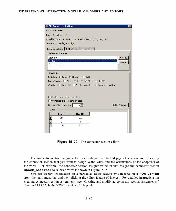
UNDERSTANDING INTERACTION MODULE MANAGERS AND EDITORS
Figure 15–20 The connector section editor.
The connector section assignment editor contains three tabbed pages that allow you to specify
the connector section that you want to assign to the wires and the orientations of the endpoints of
the wires. For example, the connector section assignment editor that assigns the connector section
Shock_Absorber to selected wires is shown in Figure 15–21.
You can display information on a particular editor feature by selecting Help→On Contextfrom the main menu bar and then clicking the editor feature of interest. For detailed instructions on
creating connector section assignments, see “Creating and modifying connector section assignments,”
Section 15.12.12, in the HTML version of this guide.
15–40
Abaqus ID:
Printed on:
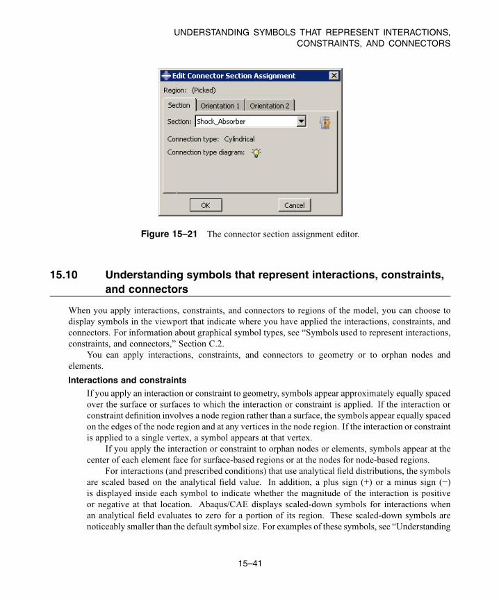
UNDERSTANDING SYMBOLS THAT REPRESENT INTERACTIONS,CONSTRAINTS, AND CONNECTORS
Figure 15–21 The connector section assignment editor.
15.10 Understanding symbols that represent interactions, constraints,and connectors
When you apply interactions, constraints, and connectors to regions of the model, you can choose to
display symbols in the viewport that indicate where you have applied the interactions, constraints, and
connectors. For information about graphical symbol types, see “Symbols used to represent interactions,
constraints, and connectors,” Section C.2.
You can apply interactions, constraints, and connectors to geometry or to orphan nodes and
elements.
Interactions and constraints
If you apply an interaction or constraint to geometry, symbols appear approximately equally spaced
over the surface or surfaces to which the interaction or constraint is applied. If the interaction or
constraint definition involves a node region rather than a surface, the symbols appear equally spaced
on the edges of the node region and at any vertices in the node region. If the interaction or constraint
is applied to a single vertex, a symbol appears at that vertex.
If you apply the interaction or constraint to orphan nodes or elements, symbols appear at the
center of each element face for surface-based regions or at the nodes for node-based regions.
For interactions (and prescribed conditions) that use analytical field distributions, the symbols
are scaled based on the analytical field value. In addition, a plus sign (+) or a minus sign (−)
is displayed inside each symbol to indicate whether the magnitude of the interaction is positive
or negative at that location. Abaqus/CAE displays scaled-down symbols for interactions when
an analytical field evaluates to zero for a portion of its region. These scaled-down symbols are
noticeably smaller than the default symbol size. For examples of these symbols, see “Understanding
15–41
Abaqus ID:
Printed on:

USING THE INTERACTION MODULE TOOLBOX
prescribed condition symbol type, color, and size,” Section 16.5.1, in the HTML version of this
guide. For more information, see “Using analytical expression fields,” Section 58.2.
Connectors
When you apply a connector to wires, squares appear at the first points of the wires and triangles
appear at the second points of the wires. If you specify an orientation other than the global coordinate
system for orientation 1, an orientation triad appears at the first points of the wires. For orientation 2,
an orientation triad appears at the second points of the wires only if you specify a coordinate system
by name; if you toggle on the option to Use orientation 1, the orientation triad does not appear at
the second points. The connection type label appears midway along a line between the endpoints of
the selected wires. You can also display the tag associated with the connector section assignment,
though this display is turned off by default.
For information about controlling the visibility of these symbols, see “Controlling the display of
attributes,” Section 76.15.
15.11 Using the Interaction module toolbox
You can access all the Interaction module tools through either the main menu bar or the Interaction
module toolbox. Figure 15–22 shows the icons for all the tools in the Interaction module toolbox.
Create interaction
Create interaction property
Create constraint
Find contact pairs
Create connector assignment
Create connector section
Create wire feature
Interaction manager
Interaction property manager
Constraint manager
Connector assignment manager
Connector section manager
Modify wire feature
Connector Builder
Create fastener Fastener manager
Figure 15–22 The Interaction module toolbox.
15–42
Abaqus ID:
Printed on:

UNDERSTANDING THE ROLE OF THE LOAD MODULE
16. The Load module
You use the Load module to define and manage the following prescribed conditions:
• Loads
• Boundary conditions
• Predefined fields
• Load cases (see Chapter 34, “Load cases”)
This chapter covers the following topics:
• “Understanding the role of the Load module,” Section 16.1
• “Entering and exiting the Load module,” Section 16.2
• “Managing prescribed conditions,” Section 16.3
• “Creating and modifying prescribed conditions,” Section 16.4
• “Understanding symbols that represent prescribed conditions,” Section 16.5
• “Transferring results between Abaqus analyses,” Section 16.6
• “Using the Load module toolbox,” Section 16.7
For information on modeling a bolt load, see Chapter 22, “Bolt loads.” In addition, the following
sections are available in the HTML version of this guide:
• “Using the Load module,” Section 16.8
• “Using the load editors,” Section 16.9
• “Using the boundary condition editors,” Section 16.10
• “Using the predefined field editors,” Section 16.11
16.1 Understanding the role of the Load module
Prescribed conditions in Abaqus/CAE are step-dependent objects, which means that you must specify
the analysis steps in which they are active. You can use the load, boundary condition, and predefined
field managers to view and manipulate the stepwise history of prescribed conditions. You can also use
the Step list located in the context bar to specify the steps in which new loads, boundary conditions, and
predefined fields become active by default.
You can use the Amplitude toolset in the Load module to specify complicated time or frequency
dependencies that can be applied to prescribed conditions. The Set and Surface toolsets in the Load
module allow you to define and name regions of your model to which you would like to apply prescribed
conditions. The Analytical Field toolset and the Discrete Field toolset allow you to create fields that you
can use to define spatially varying parameters for selected prescribed conditions.
16–1
Abaqus ID:
Printed on:

MANAGING PRESCRIBED CONDITIONS
Load cases are sets of loads and boundary conditions used to define a particular loading condition.
You can create load cases in static perturbation and steady-state dynamic, direct steps. For information
on load cases, see Chapter 34, “Load cases.”
16.2 Entering and exiting the Load module
You can enter the Load module at any time during an Abaqus/CAE session by clicking Load in the
Module list located in the context bar. The Load, BC, Predefined Field, Load Case, Feature, andTools menus appear on the main menu bar. A Step list appears in the context bar.
To exit the Load module, specify another module in the Module list in the context bar. You need
not take any specific action to save your prescribed conditions before exiting the module; they are saved
automatically when you save the entire model by selecting File→Save or File→Save As from the main
menu bar.
16.3 Managing prescribed conditions
Prescribed condition managers are dialog boxes that you use to organize and manipulate the prescribed
conditions associated with a given model. Each kind of prescribed condition that you can define in
the Load module has a separate manager. You access the managers by selecting Manager from the
appropriate menus on the main menu bar. The Load module provides the following managers:
• Load Manager
• Boundary Condition Manager
• Predefined Field Manager
Prescribed condition managers contain alphabetical lists of all the prescribed conditions of a certain
type that you have created. For example, the Load Manager shown in Figure 16–1 contains a list of
loads.
The Create, Edit, Copy, Rename, and Delete buttons in the managers allow you to create new
prescribed conditions or to edit, copy, rename, and delete existing ones. You can also initiate the create,
edit, copy, rename, and delete procedures by using the Load, BC, and Predefined Field menus in the
main menu bar. After you select a management operation from the main menu bar, the procedure is
exactly the same as if you had clicked the corresponding button inside the manager dialog box.
The prescribed condition managers are step-dependent managers, which means that they contain
additional information concerning the history of each load, boundary condition, and predefined field in
the model. You can use the icons in the column along the left side of the managers to suppress prescribed
conditions or to resume previously suppressed prescribed conditions for an analysis. The suppress and
resume procedures are also available from the Load, BC, and Predefined Field menus in the main
menu bar. For more information, see “Suppressing and resuming objects,” Section 3.4.3.
16–2
Abaqus ID:
Printed on:

CREATING AND MODIFYING PRESCRIBED CONDITIONS
Figure 16–1 The Load Manager.
You can use the Copy button in manager dialog boxes, the corresponding menu command, or the
Model Tree to copy a load, boundary condition, or predefined field. You can copy these objects from
any step to any valid step, with some restrictions. For more details, see “Copying step-dependent objects
using manager dialog boxes,” Section 3.4.11.
The Move Left, Move Right, Activate, and Deactivate buttons allow you to manipulate the
stepwise history of prescribed conditions. For more information, see “Modifying the history of a step-
dependent object,” Section 3.4.6.
Note: The Activate and Deactivate buttons are not available in the Predefined Field Manager.
For detailed instructions on creating, editing, and manipulating prescribed conditions, see the
following sections in the HTML version of this guide:
• “Using the Load module,” Section 16.8
• “Using the load editors,” Section 16.9
• “Using the boundary condition editors,” Section 16.10
• “Using the predefined field editors,” Section 16.11
16.4 Creating and modifying prescribed conditions
To create a load, boundary condition, or predefined field, select Create from the appropriate menu in the
main menu bar. A Create dialog box will appear in which you can provide a name for the prescribed
condition and choose the type of the prescribed condition that you want to create.
16–3
Abaqus ID:
Printed on:
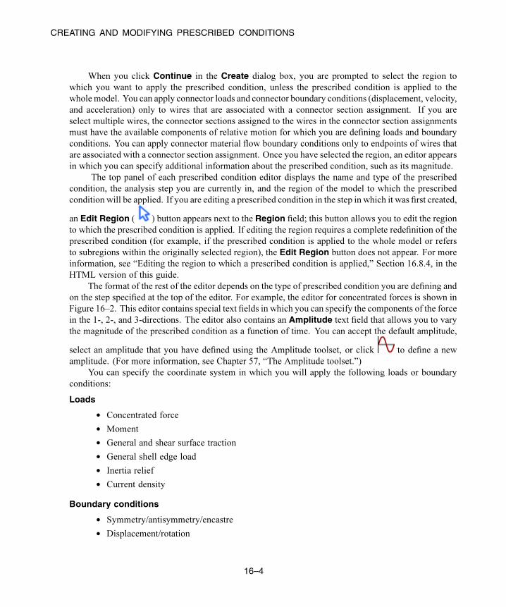
CREATING AND MODIFYING PRESCRIBED CONDITIONS
When you click Continue in the Create dialog box, you are prompted to select the region to
which you want to apply the prescribed condition, unless the prescribed condition is applied to the
whole model. You can apply connector loads and connector boundary conditions (displacement, velocity,
and acceleration) only to wires that are associated with a connector section assignment. If you are
select multiple wires, the connector sections assigned to the wires in the connector section assignments
must have the available components of relative motion for which you are defining loads and boundary
conditions. You can apply connector material flow boundary conditions only to endpoints of wires that
are associated with a connector section assignment. Once you have selected the region, an editor appears
in which you can specify additional information about the prescribed condition, such as its magnitude.
The top panel of each prescribed condition editor displays the name and type of the prescribed
condition, the analysis step you are currently in, and the region of the model to which the prescribed
condition will be applied. If you are editing a prescribed condition in the step in which it was first created,
an Edit Region ( ) button appears next to the Region field; this button allows you to edit the region
to which the prescribed condition is applied. If editing the region requires a complete redefinition of the
prescribed condition (for example, if the prescribed condition is applied to the whole model or refers
to subregions within the originally selected region), the Edit Region button does not appear. For more
information, see “Editing the region to which a prescribed condition is applied,” Section 16.8.4, in the
HTML version of this guide.
The format of the rest of the editor depends on the type of prescribed condition you are defining and
on the step specified at the top of the editor. For example, the editor for concentrated forces is shown in
Figure 16–2. This editor contains special text fields in which you can specify the components of the force
in the 1-, 2-, and 3-directions. The editor also contains an Amplitude text field that allows you to vary
the magnitude of the prescribed condition as a function of time. You can accept the default amplitude,
select an amplitude that you have defined using the Amplitude toolset, or click to define a new
amplitude. (For more information, see Chapter 57, “The Amplitude toolset.”)
You can specify the coordinate system in which you will apply the following loads or boundary
conditions:
Loads
• Concentrated force
• Moment
• General and shear surface traction
• General shell edge load
• Inertia relief
• Current density
Boundary conditions
• Symmetry/antisymmetry/encastre
• Displacement/rotation
16–4
Abaqus ID:
Printed on:

CREATING AND MODIFYING PRESCRIBED CONDITIONS
Figure 16–2 The editor for concentrated forces.
• Velocity/angular velocity
• Acceleration/rotational acceleration
• Eulerian mesh motion
• Magnetic vector potential
All other prescribed conditions use the global coordinate system, with the exception of pressures, which
are applied normal to the selected surfaces.
If the load or boundary condition allows you to specify the coordinate system, you can select an
existing datum coordinate system or you can accept the global coordinate system. If the desired datum
coordinate system does not exist, you can create it using the Datum toolset. (For more information, see
“Creating datum coordinate systems,” Section 62.9, in the HTML version of this guide.) Alternatively,
you can refer to an Abaqus/Standard user subroutine that defines the coordinate system (see “ORIENT,”
Section 1.1.15 of the Abaqus User Subroutines Reference Guide).
16–5
Abaqus ID:
Printed on:

UNDERSTANDING SYMBOLS THAT REPRESENT PRESCRIBED CONDITIONS
Note: If you delete or suppress the datum coordinate system, the orientation of the load or boundary
condition reverts to the global coordinate system.
The rules for creating and modifying predefined fields vary depending on the predefined field type:
• Some predefined fields require that you specify only the initial conditions. You can create and edit
this type of predefined field only in the initial step. Abaqus computes subsequent values for the
predefined field as the analysis progresses. The predefined fields of this type are initial velocity
specifications, hardening specifications, and material assignments (for Eulerian analyses). For more
information, see “Initial conditions in Abaqus/Standard and Abaqus/Explicit,” Section 34.2.1 of the
Abaqus Analysis User’s Guide.
• You can create predefined temperature fields for any step in the analysis. You can define the
temperatures for the current model either by entering the values for the desired steps or by reading
the temperature values computed by Abaqus in a previous analysis with thermal components.
For more information, see “Temperature,” in “Predefined fields,” Section 34.6.1 of the Abaqus
Analysis User’s Guide.
Note: If you do not define initial values for a predefined field, that field is assumed to have a value of
zero at the start of the analysis.
Once you have created a prescribed condition, you can modify the prescribed condition in the
following ways:
• You can modify some or all of the data that you entered in the editor when you created the prescribed
condition.
• You can use the managers to modify the stepwise history of the prescribed condition. (For more
information, see “What are step-dependent managers?,” Section 3.4.2.)
To display help on a particular manager or editor feature, select Help→On Context from the main
menu bar and then click the feature of interest.
16.5 Understanding symbols that represent prescribed conditions
When you apply prescribed conditions to a region, you can choose to display symbols in the viewport
that indicate the following:
• The regions to which you applied the prescribed condition.
• The type of the prescribed condition.
• If applicable, the degrees of freedom to which you applied the prescribed condition.
• If applicable, the direction (negative or positive) in which you applied the prescribed condition.
• If applicable, the spatial variation of the prescribed condition.
This section explains how to interpret the symbols. For information about controlling the visibility of
these symbols, see “Controlling the display of attributes,” Section 76.15.
16–6
Abaqus ID:
Printed on:

UNDERSTANDING SYMBOLS THAT REPRESENT PRESCRIBED CONDITIONS
16.5.1 Understanding prescribed condition symbol type, color, and size
The type, color, and size of the symbols that represent prescribed conditions can vary with
• the type of prescribed condition that the symbols represent,
• the degrees of freedom to which you apply the prescribed condition, and
• the spatial variation of the prescribed condition (for analytical field distributions).
Refer to “Symbols used to represent prescribed conditions,” Section C.1, for summaries of the
significance of the symbol types and colors.
Note: When a boundary condition fixes a degree of freedom in place, the arrow representing that
component lacks a stem.
In general, the size of the symbols is uniform and unrelated to the magnitude of the prescribed
condition. For prescribed conditions that use analytical field distributions, the symbols are scaled based
on the analytical field value. In addition, for symbols other than arrows, a plus sign (+) or a minus sign (−)
is displayed inside each symbol to indicate whether the magnitude of the prescribed condition is positive
or negative at that location. For information on controlling symbol size and scaling, see “Controlling the
display of attributes,” Section 76.15.
In some circumstances Abaqus/CAE displays scaled-down symbols for prescribed conditions, such
as when a specified prescribed condition has no effect on the analysis or when an analytical field evaluates
to zero for a portion of its region. These scaled-down symbols are noticeably smaller than the default
symbol size. For example, if you specify a shear surface traction load with a direction vector normal
to the surface, Abaqus/CAE cannot apply this type of load normal to the reference surface and displays
very small arrow symbols to represent the load in the viewport.
16.5.2 What do single-headed and double-headed arrows represent?
In many cases Abaqus/CAE uses arrows to represent prescribed conditions in the viewport. These arrows
represent each component of the prescribed condition (except for fluid boundary conditions, in which
case the arrows represent the resultant direction). For example, the arrows that appear in Figure 16–3
represent the three components of a concentrated force that is applied to two vertices.
An arrow with a single arrowhead represents a component of a prescribed condition that is applied
to a translational degree of freedom. For example, the three components of the concentrated force in
Figure 16–3 are applied to degrees of freedom 1 through 3; therefore, each arrow in the figure has a
single arrowhead.
When a component of a prescribed condition is applied to a rotational degree of freedom,
that component appears as a double-headed arrow. The arrows in Figure 16–4 indicate that a
Velocity/Angular Velocity boundary condition is applied to degrees of freedom 4 and 6 of the vertices.
A magnified view of the double-headed arrows appears in Figure 16–5.
16–7
Abaqus ID:
Printed on:

UNDERSTANDING SYMBOLS THAT REPRESENT PRESCRIBED CONDITIONS
12
3
Figure 16–3 A concentrated force with three components.
12
3
Figure 16–4 A boundary condition applied to rotational degrees of freedom.
12
3
Figure 16–5 Magnified double-headed arrows.
16–8
Abaqus ID:
Printed on:

UNDERSTANDING SYMBOLS THAT REPRESENT PRESCRIBED CONDITIONS
If you apply a prescribed condition to both translational and rotational degrees of freedom, both
the single-headed and the double-headed arrows appear. For example, a Velocity/Angular Velocityboundary condition is applied to degrees of freedom 1, 3, 4, and 6 of the vertex in Figure 16–6.
12
3
Figure 16–6 Magnified view of a boundary condition applied
to translational and rotational degrees of freedom.
In this figure the single-headed arrows indicate that degrees of freedom 1 and 3 of the vertex are fixed.
The double-headed arrows appear directly behind the single-headed arrows and indicate that degree of
freedom 4 and 6 of the vertex are fixed.
For information on arrow color, see “Understanding prescribed condition symbol type, color, and
size,” Section 16.5.1. For information on when to expect arrows to point toward or away from a region,
see “Understanding symbol location and direction,” Section 16.5.3.
16.5.3 Understanding symbol location and directionThe placement of symbols on a model can depend on the type of prescribed condition that the symbols
represent and the type of region to which the prescribed condition is applied. Table 16–1 indicates where
symbols appear on geometric models, and Table 16–2 indicates where symbols appear onmeshedmodels.
Table 16–1 Symbol location on geometry.
Region type to which theprescribed condition is applied
Location of symbols on the model
Vertex At the vertex
Edge Equally spaced along the edge
Assembly-level wire At the midpoint of the wire
Face Equally spaced over the interior of the face for directional
prescribed conditions (e.g., pressure load)
16–9
Abaqus ID:
Printed on:

UNDERSTANDING SYMBOLS THAT REPRESENT PRESCRIBED CONDITIONS
Region type to which theprescribed condition is applied
Location of symbols on the model
Equally spaced along the edges of the face for nondirectional
prescribed conditions (e.g., surface charge and boundary
conditions)
Cell Equally spaced along each edge of the cell
Whole model At the point required to define the rigid body motion (inertia
relief load only); otherwise, at the triad indicating the origin and
orientation of the global coordinate system
Table 16–2 Symbol location on meshes.
Region type to which theprescribed condition is applied
Location of symbols on the model
Node At the node
Element edge (for two-dimensional
meshes)
At the midpoint of the element edge
Element face (for three-dimensional
meshes)
At the centroid of the element face
Assembly-level wire At the midpoint of the wire
For example, Figure 16–7 shows a concentrated force applied to two vertices and a boundary condition
applied to a surface of a geometric model.
12
3
Figure 16–7 A concentrated force and a boundary condition.
16–10
Abaqus ID:
Printed on:

UNDERSTANDING SYMBOLS THAT REPRESENT PRESCRIBED CONDITIONS
Figure 16–8 shows a boundary condition applied to four nodes and a pressure load applied to several
element faces of a mesh.
12
3
Figure 16–8 A pressure load and a boundary condition.
Note: If you apply a pressure load to a planar geometry face where the surface area is small compared
to the enclosed area (such as a ring formed by two concentric circles), the load symbols may not be
distributed evenly, regardless of the symbol density settings in the Assembly Display Options dialog
box.
When a boundary condition fixes a degree of freedom in place, the arrow representing that
component points into the region and lacks a stem. For example, the boundary condition in Figure 16–9
fixes degrees of freedom 1, 2, and 3 in place.
12
3
Figure 16–9 A boundary condition fixing degrees of freedom in place.
16–11
Abaqus ID:
Printed on:

TRANSFERRING RESULTS BETWEEN Abaqus ANALYSES
Likewise, if a positive pressure load or an Eulerian inflow boundary condition is applied to a region,
the arrows representing that pressure load or boundary condition point into the region, as illustrated in
Figure 16–10.
1
2
3
Figure 16–10 A positive pressure load.
If a load is defined to have a complex magnitude and the real and imaginary parts have different signs
(for example, ), the load will appear as an arrow with two ends. Similarly, an Eulerian boundary
condition that includes both inflow and outflow components will appear as an arrow with two ends.
In all other cases, arrows representing components of a prescribed condition point out from the
region.
Note: When a component of a concentrated force is zero, no arrow appears for that component.
Likewise, when a boundary condition leaves a degree of freedom unconstrained, no arrow appears for
that component.
16.6 Transferring results between Abaqus analyses
You can select part instances from your model and associate an initial state field with the instances. An
initial state field applies a deformed mesh and its associated material state to the instances using data
imported from a previous Abaqus/Standard or Abaqus/Explicit analysis. Abaqus/CAE allows you to
select the job name corresponding to the analysis from which the initial state field is imported. You can
also specify the particular step and increment of the analysis from which to import data. Abaqus/CAE
imports data from several of the files created by the previous analysis. As a result, the files from the
analysis must reside in the directory from which you started the current Abaqus/CAE session.
You can use this capability to drive an Abaqus/Explicit analysis with the results of an
Abaqus/Standard analysis and vice versa. This is useful if your problem can be broken down into
different stages; for example, you can use Abaqus/Explicit to analyze a metal forming problem and
Abaqus/Standard to analyze the following springback. You can also use this capability to change the
16–12
Abaqus ID:
Printed on:

TRANSFERRING RESULTS BETWEEN Abaqus ANALYSES
model definition between steps. For more information, see “Transferring results between Abaqus
analyses: overview,” Section 9.2.1 of the Abaqus Analysis User’s Guide.
You can also transfer results and model information from an Abaqus/Standard analysis to a new
Abaqus/Standard analysis, where you can specify additional model definitions before continuing the
analysis. For example, you might first study the local behavior of a particular component during an
assembly process and then study the behavior of the assembled product. You can start by analyzing
the local behavior of the component in an Abaqus/Standard analysis. You can then transfer the model
information and results from this analysis to a second Abaqus/Standard analysis, where you can specify
additional model definitions for the other components and analyze the behavior of the entire product.
Abaqus/CAE always imports the material state along with the deformedmesh. If you want to import
only the deformedmesh, you can import a mesh from a selected step and increment of an output database.
For more information, see “What kinds of files can be imported and exported from Abaqus/CAE?,”
Section 10.1.1.
Abaqus uses the imported information when you submit a job for analysis; however, Abaqus/CAE
does not update the shape of the selected instances to reflect the applied deformed mesh. As a result, you
should be careful when adding new instances to the assembly and positioning them relative to existing
part instances. For example, a new part instance may appear to touch one of the instances associated with
the initial state field; however, when the analysis applies the imported deformed mesh, the instances may
become separated or overclosed.
To avoid this mismatch between the undeformed state and the imported state, you may want to
import the deformed mesh from the analysis instead of working with the undeformed part instance.
Even if you import the deformed mesh, you must take care that the frame from which you imported
the mesh is the same as the step and increment specified in the initial state field. For more information,
see “Importing a part from an output database,” Section 10.7.12, in the HTML version of this guide.
Alternatively, you can create the current model by copying it from the model that generated the previous
Abaqus/Standard or Abaqus/Explicit analysis. For more information, see “Manipulating models within
a model database,” Section 9.8.1, in the HTML version of this guide.
The reference configuration is the configuration of the model from which displacements (and
associated strains) are calculated. By default, Abaqus/CAE does not use the imported data to update
the reference configuration. As a result, displacements and strains are calculated as total values relative
to the reference configuration at the start of the original analysis, and the values will be continuous
between analyses. You can change the default behavior and configure Abaqus/CAE to update the
reference configuration to be the imported configuration. Abaqus/CAE now calculates displacements
and strains relative to the new imported reference configuration; for example, for a springback analysis.
Abaqus imposes many restrictions when you try to create an initial state field. For a detailed
discussion of these limitations, see “Transferring results between Abaqus analyses: overview,”
Section 9.2.1 of the Abaqus Analysis User’s Guide. For example, the mesh of the part instances that you
select from the current model must match the mesh of the part instances that you are importing. You
can then, for example, change the material definition, add loads and boundary conditions, and change
from an Abaqus/Standard to an Abaqus/Explicit step. However, you cannot perform an operation that
will change the mesh of a selected part instance; for example, you cannot partition the part instance.
16–13
Abaqus ID:
Printed on:
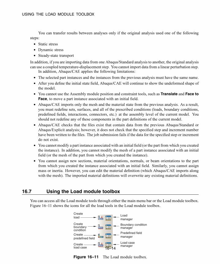
USING THE LOAD MODULE TOOLBOX
You can transfer results between analyses only if the original analysis used one of the following
steps:
• Static stress
• Dynamic stress
• Steady-state transport
In addition, if you are importing data from one Abaqus/Standard analysis to another, the original analysis
can use a coupled temperature-displacement step. You cannot import data from a linear perturbation step.In addition, Abaqus/CAE applies the following limitations:
• The selected part instances and the instances from the previous analysis must have the same name.
• After you define the initial state field, Abaqus/CAE will continue to show the undeformed shape of
the model.
• You cannot use the Assembly module position and constraint tools, such as Translate and Face toFace, to move a part instance associated with an initial field.
• Abaqus/CAE imports only the mesh and the material state from the previous analysis. As a result,
you must redefine sets, surfaces, and all of the prescribed conditions (loads, boundary conditions,
predefined fields, interactions, connectors, etc.) at the assembly level of the current model. You
should not redefine any of these components in the part definitions of the current model.
• Abaqus/CAE checks that the files exist that contain data from the previous Abaqus/Standard or
Abaqus/Explicit analysis; however, it does not check that the specified step and increment number
have been written to the files. The job submission fails if the data for the specified step or increment
do not exist.
• You cannot modify a part instance associated with an initial field (or the part from which you created
the instance). In addition, you cannot modify the mesh of a part instance associated with an initial
field (or the mesh of the part from which you created the instance).
• You cannot assign new sections, material orientations, normals, or beam orientations to the part
from which you created the instance associated with an initial field. Similarly, you cannot assign
mass or inertia. However, you can edit the material definition (which Abaqus/CAE imports along
with the mesh). The imported material definitions will overwrite any existing material definitions.
16.7 Using the Load module toolbox
You can access all the Load module tools through either the main menu bar or the Load module toolbox.
Figure 16–11 shows the icons for all the load tools in the Load module toolbox.
Loadmanager
Boundary conditionmanager
Predefined fieldmanager
Load casemanager
Createload
Createboundarycondition
Createpredefined field
Createload case
Figure 16–11 The Load module toolbox.
16–14
Abaqus ID:
Printed on:

UNDERSTANDING THE ROLE OF THE MESH MODULE
17. The Mesh module
The Mesh module contains tools that allow you to generate meshes on parts and assemblies created
within Abaqus/CAE. In addition, the Mesh module contains functions that verify an existing mesh. This
chapter covers the following topics:
• “Understanding the role of the Mesh module,” Section 17.1
• “Entering and exiting the Mesh module,” Section 17.2
• “Mesh module basics,” Section 17.3
• “Understanding seeding,” Section 17.4
• “Assigning Abaqus element types,” Section 17.5
• “Verifying and improving meshes,” Section 17.6
• “Understanding mesh generation,” Section 17.7
• “Structured meshing and mapped meshing,” Section 17.8
• “Swept meshing,” Section 17.9
• “Free meshing,” Section 17.10
• “Bottom-up meshing,” Section 17.11
• “Mesh-geometry association,” Section 17.12
• “Understanding adaptive remeshing,” Section 17.13
• “Advanced meshing techniques,” Section 17.14
• “Using the Mesh module toolbox,” Section 17.15
In addition, the following sections are available in the HTML version of this guide:
• “Seeding a model,” Section 17.16
• “Creating and deleting meshes,” Section 17.17
• “Controlling mesh characteristics,” Section 17.18
• “Obtaining mesh information and statistics,” Section 17.19
• “Creating a mesh part,” Section 17.20
• “Controlling adaptive remeshing,” Section 17.21
For information on editing orphan nodes and elements, see “What can I do with the Edit Mesh toolset?,”
Section 64.1.
17.1 Understanding the role of the Mesh module
The Mesh module allows you to generate meshes on parts and assemblies created within Abaqus/CAE.
Various levels of automation and control are available so that you can create a mesh that meets the needs
of your analysis. As with creating parts and assemblies, the process of assigning mesh attributes to the
17–1
Abaqus ID:
Printed on:

ENTERING AND EXITING THE MESH MODULE
model—such as seeds, mesh techniques, and element types—is feature based. As a result you canmodify
the parameters that define a part or an assembly, and the mesh attributes that you specified within the
Mesh module are regenerated automatically.
The Mesh module provides the following features:
• Tools for prescribing mesh density at local and global levels.
• Model coloring that indicates the meshing technique assigned to each region in the model.
• A variety of mesh controls, such as:
– Element shape
– Meshing technique
– Meshing algorithm
– Adaptive remeshing rule
• A tool for assigning Abaqus/Standard, Abaqus/Explicit, or Abaqus/CFD element types to mesh
elements. The elements can belong either to a model that you created or to an orphan mesh.
• A tool for verifying mesh quality.
• Tools for refining the mesh and for improving the mesh quality.
• A tool for saving the meshed assembly or selected part instances as a mesh part.
17.2 Entering and exiting the Mesh module
You can enter the Mesh module at any time during an Abaqus/CAE session by clicking Mesh in the
Module list located in the context bar. Upon entering the Mesh module, the Abaqus/CAE interface
changes in the following ways:
• The Seed, Mesh, Feature, and Tools menus appear on the main menu bar.
• The Object field that appears in the context bar allows you to display either a part or the assembly.
• Abaqus/CAE may change the color of the part instances in the assembly displayed in the viewport.
These color cues describe the meshability and dependence of each instance. Independent instances
appear in a color that describes their meshability, while dependent intances appear blue in the
Assembly context and white in the Part context. See “Meshing independent and dependent part
instances,” Section 17.3.10.
Note: Part instances are color coded according to their meshability and dependence only when
the Mesh defaults color mapping is selected. If you displayed the default color mapping in a
different module, Abaqus/CAE applies the Mesh defaults color mapping automatically upon your
entry to the Mesh module. If you selected a non-default color mapping such as Materials in a
different module, Abaqus/CAE continues color coding according to that color mapping (in this case,
by material type) when you enter the Mesh module.
17–2
Abaqus ID:
Printed on:
MESH MODULE BASICS
To exit the Mesh module, select any other module from the Module list. You need not save your
mesh before exiting the module; it will be saved automatically when you save the entire model by
selecting File→Save or File→Save As from the main menu bar.
17.3 Mesh module basics
This section provides brief explanations of terms and concepts that you must understand to use the Mesh
module effectively. It gives you an overview of the functions available and describes the role that each
function plays in the mesh creation process.
17.3.1 The meshing process
To create an acceptable mesh, you use the following process:
Assign mesh attributes and set mesh controls
TheMeshmodule provides a variety of tools that allow you to specify different mesh characteristics,
such as mesh density, element shape, and element type.
Generate the mesh
The Mesh module uses a variety of techniques to generate meshes. The different mesh techniques
provide you with different levels of control over the mesh.
Refine the mesh
The Mesh module provides a variety of tools that allow you to refine the mesh:
– The seeding tools allow you to adjust the mesh density in selected regions.
– The Partition toolset allows you to partition complex models into simpler subregions.
– The Virtual Topology toolset allows you to simplify your model by combining small faces and
edges with adjacent faces and edges.
– The Edit Mesh toolset allows you to make minor adjustments to your mesh.
Optimize the mesh
You can assign remeshing rules to regions of your model. Remeshing rules enable successive
refinement of your mesh where each refinement is based on the results of an analysis.
Verify the mesh
The verification tools provide you with information concerning the quality of the elements used in
a mesh.
17–3
Abaqus ID:
Printed on:

MESH MODULE BASICS
17.3.2 Mesh attributes and controlsAbaqus/CAE provides you with a variety of tools for controlling mesh characteristics:
• You can specify the density of a mesh by creating seeds along the edges of the model to indicate
where the corner nodes of the elements should be located. For example, Figure 17–1 displays a
model with biased seeding along the top and left edges.
Figure 17–1 A model with biased seeding.
For more information, see “Understanding seeding,” Section 17.4.
• You can select the shape of the mesh elements. For example, Figure 17–2 shows a model that has
been meshed first with quadrilateral elements and then with triangular elements.
Figure 17–2 Two meshes with different element shapes.
For more information, see “Assigning Abaqus element types,” Section 17.5.
• You can choose the meshing technique—free, structured, or swept—and, where applicable, you can
choose the meshing algorithm—medial axis or advancing front. For more information, see “Mesh
generation,” Section 17.3.3.
17–4
Abaqus ID:
Printed on:

MESH MODULE BASICS
• You can select the element type that is assigned to the mesh by choosing the element family,
geometric order, and shape along with specific element controls, such as hourglassing. For more
information, see “Understanding mesh generation,” Section 17.7.
17.3.3 Mesh generationAbaqus/CAE can use a variety of meshing techniques to mesh models of different topologies. In some
cases you can choose the technique used to mesh a model or model region. In other cases only one
technique is valid. The different meshing techniques provide varying levels of automation and user
control. There are two meshing methodologies available in Abaqus/CAE: top-down and bottom-up.
Top-down meshing generates a mesh by working down from the geometry of a part or region to
the individual mesh nodes and elements. You can use top-down meshing techniques to mesh one-, two-,
or three-dimensional geometry using any available element type. The resulting mesh exactly conforms
to the original geometry. The rigid conformance to geometry makes top-down meshing predominantly
an automated process but may make it difficult to produce a high-quality mesh on regions with complex
shapes.
Bottom-up meshing generates a mesh by working up from two-dimensional entities (geometric
faces, element faces, or two-dimensional elements) to create a three-dimensional mesh. You can use
bottom-up meshing techniques to mesh only solid three-dimensional geometry using all—or nearly
all—hexahedral elements. Generating a mesh using the bottom-up meshing technique is a manual
process, and the resulting mesh may vary significantly from the original geometry. However, allowing
the mesh to vary from geometry may allow you to produce a high quality hexahedral mesh on regions
with complex shapes.
17.3.4 Top-down meshingTop-down meshing relies on the geometry of a part to define the outer bounds of the mesh. The top-
down mesh matches the geometry; you may need to simplify and/or partition complex geometry so that
Abaqus/CAE recognizes basic shapes that it can use to generate a high-quality mesh. In some cases top-
down methods may not allow you to mesh portions of a complex part with the desired type of elements.
The top-down techniques—structured, swept, and free meshing—and their geometry requirements are
well-defined, and loads and boundary conditions applied to a part are associated automatically with the
resulting mesh.
Structured meshing
Structured meshing is the top-down technique that gives you the most control over your mesh
because it applies preestablished mesh patterns to particular model topologies. Most unpartitioned
solid models are too complex to be meshed using preestablished mesh patterns. However, you can
often partition complex models into simple regions with topologies for which structured meshing
patterns exist. Figure 17–3 shows an example of a structured mesh. For more information, see
“Structured meshing and mapped meshing,” Section 17.8.
17–5
Abaqus ID:
Printed on:

MESH MODULE BASICS
Figure 17–3 A structured mesh.
Swept meshing
Abaqus/CAE creates swept meshes by internally generating the mesh on an edge or face and
then sweeping that mesh along a sweep path. The result can be either a two-dimensional mesh
created from an edge or a three-dimensional mesh created from a face. Like structured meshing,
swept meshing is a top-down technique limited to models with specific topologies and geometries.
Figure 17–4 shows an example of a swept mesh. For more information, see “Swept meshing,”
Section 17.9.
sourceside
targetside
sweep path
Figure 17–4 A swept mesh.
17–6
Abaqus ID:
Printed on:

MESH MODULE BASICS
Free meshing
The free meshing technique is the most flexible top-down meshing technique. It uses no
preestablished mesh patterns and can be applied to almost any model shape. However, free
meshing provides you with the least control over the mesh since there is no way to predict the
mesh pattern. Figure 17–5 shows an example of a free mesh. For more information, see “Free
meshing,” Section 17.10.
Figure 17–5 A free mesh generated with tetrahedral elements.
17.3.5 Bottom-up meshingBottom-up meshing uses the part geometry as a guideline for the outer bounds of the mesh, but the mesh
is not required to conform to the geometry. Removing this restriction gives you greater control over
the mesh and allows you to create a hexahedral or hexahedral-dominated mesh on geometry that is too
complex for the structured or swept meshing techniques. Bottom-up meshing can be applied to any solid
model shape. It provides you with the most control over the mesh, since you select the method and the
parameters that drive the mesh. However, you must also decide whether the resulting mesh is a suitable
approximation of the geometry. If it is not, you can delete the mesh and try a different bottom-up meshing
method or partition the region and mesh the resulting smaller regions with either bottom-up or top-down
meshing techniques.
To mesh a single bottom-up region, you may have to apply several successive bottom-up meshes.
For example, you may use an extruded bottom-up mesh to generate part of a region, then use the element
faces of the extruded mesh as a starting point to generate a swept mesh for features that the extruded
mesh did not include.
17–7
Abaqus ID:
Printed on:

MESH MODULE BASICS
Loads and boundary conditions are applied to geometry. Unlike a top-down mesh, a bottom-up
mesh may not be fully associated with geometry. Therefore, you should check that the mesh is correctly
associated with the geometry in areas where loads or boundary conditions are applied. Proper mesh-
geometry association will ensure that the loads and boundary conditions are correctly transferred to the
mesh during the analysis. (For more information, see “Mesh-geometry association,” Section 17.12.)
Because of the extra effort required by the user to create a satisfactory mesh compared to the automated
top-down meshing processes, bottom-up meshing is recommended for use only when top-down meshing
cannot generate a suitable mesh.
Figure 17–6 shows an example of a bottom-up meshed part. Although this part is relatively simple,
it requires two regions and four bottom-up meshes to completely mesh the part. Abaqus/CAE displays
bottom-up meshed regions using a mixture of the region geometry color (light tan) and the mesh color
(light blue) to emphasize that the geometry and mesh may not be associated. Displaying both the
geometry and the mesh allows you to view and edit the mesh-geometry associativity.
Figure 17–6 A bottom-up hexahedral meshed part.
17.3.6 Mesh technique color codingWhen the Mesh defaults color mapping is selected, Abaqus/CAE uses different colors to indicate which
meshing technique, if any, is currently assigned to a region. For example, if a solid region is meshable
using the structured meshing technique, the region turns green when you enter the Mesh module; the
green color indicates that the structured meshing technique is assigned to that region. Yellow indicates
that the sweep meshing technique is applied to a region. If a region is unmeshable using the currently
17–8
Abaqus ID:
Printed on:
MESH MODULE BASICS
assigned element shape, the region turns orange when you enter the Mesh module. Regions that are pink
or light tan have been assigned the free and bottom-up meshing techniques, respectively.
Note: You must use the Mesh Controls dialog box to assign the bottom-up meshing technique to
a region. Abaqus/CAE does not automatically assign the bottom-up meshing technique and will not
indicate whether a region that is assigned the bottom-up technique can also be meshed using a top-down
technique. (For more information, see “Assigning mesh controls,” Section 17.18.1, in the HTML version
of this guide.)
You can change the applicable meshing techniques by partitioning the region into smaller regions
with simpler topology, by changing the element shape assigned to the region, or by using the Virtual
Topology toolset.
17.3.7 Mesh refinement
The Mesh module provides a set of tools that allow you to refine a mesh.
• You can use the Partition toolset to divide geometric regions into smaller regions. The resulting
partitions introduce new edges that you can seed; therefore, you can combine partitioning and
seeding to gain additional control over the mesh generation process. You can also use partitioning
to create regions to which you can assign different element types. For example, you might want to
assign reduced-integration elements to some portions of your model and fully integrated elements
to others. For more information, see Chapter 70, “The Partition toolset.”
• In some cases the geometry contains details such as very small faces and edges. The Virtual
Topology toolset allows you to remove these small details by combining a small face with an
adjacent face or by combining a small edge with an adjacent edge. Introducing virtual topology is a
convenient method for creating a clean, well-formed mesh. For more information, see Chapter 75,
“The Virtual Topology toolset.”
• You can use the Edit Mesh toolset to make minor adjustments to your mesh. For more information,
see “What can I do with the Edit Mesh toolset?,” Section 64.1.
17.3.8 Mesh optimization
You can assign remeshing rules to regions of your model. Remeshing rules enable successive refinement
of your mesh based on solution results. After each analysis, the Mesh module adjusts your mesh
with the aim of reducing selected error indicators in the solution results. For more information, see
“Understanding adaptive remeshing,” Section 17.13; “Advanced meshing techniques,” Section 17.14;
and “Creating, editing, and manipulating adaptivity processes,” Section 19.9, in the HTML version of
this guide.
17–9
Abaqus ID:
Printed on:

MESH MODULE BASICS
17.3.9 Mesh verification
The Mesh module provides a set of tools that allow you to verify a mesh and to obtain mesh statistics
and mesh information. The Mesh module also provides geometry diagnostic tools that will help you
determine why Abaqus/CAE cannot mesh a region. For more information, see “Verifying your mesh,”
Section 17.6.1; “Querying your mesh,” Section 17.6.2; and “Using the geometry diagnostic tools,”
Section 71.2.4, in the HTML version of this guide.
17.3.10 Meshing independent and dependent part instances
The approach to meshing independent and dependent instances is different. For more information, see
“What is the difference between a dependent and an independent part instance?,” Section 13.3.2.
Independent
To mesh an independent instance, use the context bar to change the Object to Assembly and mesh
the instance directly. You cannot mesh a part that you have used to create an independent instance.
Dependent
To mesh a dependent instance, use the context bar to change the Object to Part and select the part
with which the dependent instance is associated. You can then mesh the part, and Abaqus/CAE
applies the same mesh to each dependent instance in the assembly. Dependent instances are
convenient when you have a linear or radial pattern of part instances. You can mesh the original
part, and Abaqus/CAE applies the same mesh to each instance of the part in the pattern.
17.3.11 Displaying a native mesh
You can switch between displaying the geometry of the part instance and the meshed representation of
the same instance by clicking the Show native mesh icon located in the Visible Objects toolbar.
You can use the Show native mesh tool in any of the assembly-related modules to switch between
displaying the geometry of the assembly and a meshed representation of the assembly. Abaqus/CAE
displays the meshed representation of both independent and dependent part instances in the assembly
(assuming that you have created the appropriate meshes).
Toggling between the geometry of a part and its meshed representation using the Show nativemesh tool allows you to see how closely the mesh follows the geometry. The tool also allows you to
see how Abaqus/CAE incorporated virtual topology into the mesh. In addition, you may find it useful to
click on the Show native mesh tool in the Job module. You can then confirm that the entire assembly
has been meshed correctly before you submit a job for analysis.
17–10
Abaqus ID:
Printed on:

UNDERSTANDING SEEDING
The display of any orphan elements in the model is unaffected by this tool; orphan elements are
displayed regardless of whether you display the geometry or elements for the native portion of part
instances.
17.4 Understanding seeding
This section explains the concept of seeding and how to use seeding to improve meshes.
17.4.1 What are mesh seeds?Seeds are markers that you place along the edges of a region to specify the target mesh density in that
region. Both the mesh density along the boundary of the region and the mesh density in the interior of
the region are determined by the seeds along the edges of the region.
You can create and control seeds using the Seed menu in the Mesh module main menu bar.
Abaqus/CAE generates meshes that match your seeds as closely as possible. Abaqus/CAE can use the
following methods to control the distribution of the seeds:
• Position the seeds uniformly along all the edges of a part or part instance
• Position the seeds uniformly along an edge
• Position the seeds with a bias such that the mesh density increases toward one end of the edge
• Position the seeds with a bias such that the mesh density increases from each end toward the center
of the edge
• Position the seeds with a bias such that the mesh density increases from the center toward each end
of the edge
Figure 17–7 shows a combination of uniform seeding and bias seeding.
Figure 17–7 A model with uniform and bias seeding.
17–11
Abaqus ID:
Printed on:
UNDERSTANDING SEEDING
You should apply seeds to all edges. If a uniform seed distribution is sufficient, the recommended
approach is to seed the entire part or part instance. If you want more control over the mesh, you can
partition the region and then provide seeds along the partitions you have created. This technique is
described in greater detail in “Verifying and improving meshes,” Section 17.6.
Mesh seeds specify only a target mesh density. If you are using hexahedral or quadrilateral elements,
Abaqus/CAE often changes the element distribution so that the mesh can be generated successfully. You
can prevent such adjustments by constraining the number of seeds along an edge. When you constrain
seeds, you are prescribing mainly the number of elements along the edge, and, to a lesser extent, the
precise locations of the nodes; if necessary, Abaqus/CAE adjusts the locations of the nodes to reduce
element distortion. In addition, you should use such constraints with care, since they can make it more
difficult for the mesh generator to obtain a mesh.
By default, Abaqus/CAE displays seeds on a part or assembly only when you are defining or
modifying seed placement. You can enable persistent seed display if you want the seeds to appear while
you perform other operations in the Mesh module; toggle on in the Visible Objects toolbar to
maintain seed display.
17.4.2 Can I seed a face or a cell?
You can select edges, faces, or cells to seed; however, Abaqus/CAE creates seeds only along edges.
When you select faces or cells to seed, Abaqus/CAE creates seeds only along the edges of the faces or
cells. In addition, you can select a set or surface to seed; as a result, Abaqus/CAE creates seeds along
the edges of the geometry contained in the set or surface.
When you are applying uniform seeds, you can use a combination of the following methods to select
the region to which Abaqus/CAE will apply the seeds:
Individually/By angle
You can select edges, faces, or cells individually; or you can use the angle method to select a group
of edges or faces. For example, if you choose the angle method and select an edge, Abaqus/CAE
then selects every adjacent edge until the angle between the edges is equal to or exceeds the angle
that you entered. For more information, see “Using the angle and feature edge method to select
multiple objects,” Section 6.2.3.
Selection filters
You can use filters to choose the type of object to select—Edges, Faces, Cells, or All. By default,Abaqus/CAE allows you to select all types of object. The option to select by angle becomes
available only after you select Edges or Faces from the selection filters. For more information,
see “Filtering your selection based on the type of object,” Section 6.3.2.
17–12
Abaqus ID:
Printed on:

UNDERSTANDING SEEDING
Sets or surfaces
By default, Abaqus/CAE allows you to apply seeds to edges, faces, and cells that you select from
the viewport. Alternatively, you can click Sets/Surfaces on the right of the prompt area and select
from eligible sets (or surfaces). When you select a set (or surface), Abaqus/CAE applies seeds to
every edge in the set (or surface), including every edge of all the cells and faces. Abaqus/CAE
ignores any vertices in the set (or surface).
17.4.3 Controlling the seed density
You can use the following methods to control the seed density along selected edges:
• Specify the average element size for every edge of the entire part or part instance.
• Specify the number of elements desired along an edge.
• Specify the average element size along an edge. (If the edge length is not an integer multiple of the
element length, Abaqus/CAE will change the element length slightly to obtain an integer number
of elements along the edge.)
• Specify a nonuniform distribution of elements along an edge. The element density can increase
from one end of the edge to the other (single bias), or the element density can vary from the center
of the edge to each end (double bias). For a nonuniform distribution you can specify either of the
following:
– The number of elements desired along an edge and a bias ratio. The bias ratio is the ratio of
the largest element to the smallest element.
– The size of the smallest element and the size of the largest element.
If you select edges that you previously seeded using a combination of these methods, Abaqus/CAE
provides an As Is option that allows you to retain the seeding method. Abaqus/CAE provides a similar
option if you select edges with a mixture of curvature controls or seed constraints.
For detailed instructions on prescribing seed density, see the following sections in the HTMLversion
of this guide:
• “Defining seed density for an entire part or part instance,” Section 17.16.1
• “Seeding an edge by prescribing the number of elements,” Section 17.16.2
• “Seeding an edge by prescribing element size,” Section 17.16.3
• “Prescribing biased seeding along an edge,” Section 17.16.4
• “Applying constraints to edge seeds,” Section 17.16.5
• “Seeding previously meshed parts, part instances, or regions,” Section 17.16.6
• “Deleting part or instance seeds,” Section 17.16.7
• “Deleting edge seeds,” Section 17.16.8
17–13
Abaqus ID:
Printed on:

UNDERSTANDING SEEDING
Seeds created by specifying an average element size for the entire part or part instance are called
part seeds or instance seeds, respectively, and appear in white; seeds created using the other methods are
called edge seeds and appear in magenta. Edge seeds always override part or instance seeds; therefore,
when you specify the average element size for the entire part or part instance, part or instance seeds
appear only on edges of the region that do not already have edge seeds. New edges created by partitioning
are given part or instance seeds by default.
When you seed an edge of a region that is assigned the swept or revolved mesh technique, the
edge seeding tools automatically propagate seeds from the selected edge to the matching edges in the
region. In other words, the seeds on the face or edge at the beginning of the sweep path are propagated
automatically to the face or edge at the end of the sweep path. Likewise, the seeds created on one edge
along the sweep path are propagated automatically to the other edges along the sweep path. As a result,
even though you select a single edge of a face to seed, Abaqus/CAEwill propagate the seeds to additional
edges and faces. For more information, see “What is swept meshing?,” Section 17.9.1.
17.4.4 Applying curvature control to your seeding
The part seeding tool allows you to specify a target element size when you are seeding a part, a part
instance, or multiple edges. If the geometry is relatively regular, specifying a single target element size
can result in an acceptable mesh. However, if you specify a single target element size and the geometric
features that make up the part or edges vary in size, the resulting mesh may be too coarse to adequately
represent any small features, as shown in Figure 17–8.
Figure 17–8 Seeding and the resultingmeshwith no curvature control.
17–14
Abaqus ID:
Printed on:

UNDERSTANDING SEEDING
To avoid the problem of inadequate seeding around small curved features, Abaqus/CAE applies
curvature control when it seeds a part, a part instance, or edges. Curvature control allows Abaqus/CAE
to calculate the seed distribution based on the curvature of the edge along with the target element size.
Figure 17–9 shows the same part seeded and meshed with curvature control enabled.
Figure 17–9 Seeding and the resulting mesh with curvature control enabled.
You can configure the following to specify how curvature control will influence the seeding:
Deviation factor
The deviation factor is a measure of howmuch the element edges deviate from the original geometry,
as shown in Figure 17–10.
h = chordal deviationdeviation factor = h/L
h
L
Figure 17–10 Deviation factor.
To help you visualize the deviation factor, Abaqus/CAE displays the approximate number of
elements it would create around a circle corresponding to the setting that you enter. As you
17–15
Abaqus ID:
Printed on:

UNDERSTANDING SEEDING
reduce the deviation factor, the number of elements that Abaqus/CAE would create around a circle
increases. This number is only a visual aid; for example, if you are seeding a spline or an ellipse,
Abaqus/CAE creates a different number of elements, depending on the local curvature along the
edge.
Specify minimum size factor
Specifying a minimum size factor prevents Abaqus/CAE from creating very fine meshes in areas of
high curvature that you have no interest in modeling; for example, kinks in spline curves or fillets
with a very small radius. The number that you enter representing the minimum size is the fraction
of the global seed size. As a result, if you change the global seed size, you do not have to change
the minimum size factor.
For detailed instructions on applying curvature control, see “Defining seed density for an entire part or
part instance,” Section 17.16.1, in the HTML version of this guide.
17.4.5 Constraining seeds
By default, mesh seeds prescribe only a target mesh density. Abaqus/CAE generally matches the mesh
seeds exactly when you are using the free meshing technique to generate triangular- or tetrahedral-
shaped elements. However, in other cases Abaqus/CAE may alter the element distribution so that it
can successfully generate the mesh. If you want to prevent Abaqus/CAE from altering the element
distribution, you can fix a specific number of elements along an edge by constraining the seeds along
that edge. You can constrain only edge seeds, not part or instance seeds.
You can assign any one of the following three states to a group of seeds along an edge:
Unconstrained
This is the default setting. The number of elements along an edge can either increase or decrease
so that the mesh can become denser or coarser than is specified by the seeds. Unconstrained seeds
appear as open circles.
Partially constrained
The number of elements along an edge may be increased during mesh generation but cannot be
decreased. This constraint allows the mesh to become denser than is specified by the seeds but no
coarser. Partially constrained seeds appear as upward-pointing triangles.
Fully constrained
The number of elements specified by constrained seeds along an edge cannot be altered by the mesh
generation process. When the seeds are fully constrained, the mesh generation will attempt to allow
the location of the nodes to correspond exactly to the location of the seeds. However, an exact
match between the seeds and the nodal positions is not guaranteed. Fully constrained seeds appear
as squares.
17–16
Abaqus ID:
Printed on:

UNDERSTANDING SEEDING
Abaqus/CAE always creates a fully constrained seed at each geometric vertex of a region to
indicate that a finite element node will be positioned at each vertex.
In many cases the mesh generator must redistribute elements (and deviate from the number and
location of the seeds) to generate a mesh successfully. For the greatest likelihood of meshing success,
leave seeds unconstrained or at least avoid fully constraining large numbers of seeds in a given part or
part instance so that the mesh generator has as much freedom to redistribute seeds as possible.
For detailed instructions on constraining edge seeds, see the following sections in the HTML version
of this guide:
• “Applying constraints to edge seeds,” Section 17.16.5
• “Relaxing constraints using the error dialog box,” Section 17.16.9
17.4.6 Minimizing seed repositioningDuring the mesh generation process Abaqus/CAE uses the seeds that you create as target locations for
nodes along the edges of the mesh. However, if you are using quadrilateral- or hexahedral-shaped
elements, a close match between your seeds and nodes depends heavily on the following:
The element shapes you allow in transition regions
You will obtain a better match between your seeds and the nodes of the mesh if you allow triangular
elements in transition regions. The seeds and the nodes are less likely to match if you restrict your
mesh to including only quadrilateral elements.
The mesh transition setting
You will obtain a better match between your seeds and the nodes of the mesh if you allow for mesh
transition.
The meshing technique
The mesh generated using the advancing front meshing algorithm matches your seeding better than
the mesh generated using the medial axis algorithm.
The seed constraints
Fully constrained seeds closely match the generated nodes in both number and position. However,
you must fully constrain only a few edges of a part or part instance; otherwise, Abaqus/CAE will
not be able to generate a mesh.
How neighboring regions are seeded
When meshing multiple regions, Abaqus/CAE often redistributes the elements so that the mesh
is compatible between regions. Even though a single region’s seed arrangement may be adequate
for generating a mesh on that one region, the seed arrangement may need to be changed since the
number of elements must be compatible with neighboring regions along shared edges.
17–17
Abaqus ID:
Printed on:

UNDERSTANDING SEEDING
Note: Mesh compatibility between part instances is not guaranteed. In some simple cases seeding
can help achieve part-to-part mesh compatibility. Techniques for obtaining compatible meshes are
described in “Compatible meshes between part instances,” Section 17.14.3.
Abaqus/CAE tries to adhere as closely as possible to the number and location of seeds that you specified
when balancing the element redistribution for the entire model. If given a choice between making a large
change along a single seeded edge and making a small change to many edges, Abaqus/CAE will make
many small changes.
17.4.7 What is the relationship between vertices and nodes?
When you seed a model, Abaqus/CAE automatically places fully constrained seeds wherever vertices
appear along the model’s edges. Fully constrained seeds that appear at vertices always indicate that
nodes will appear at those vertices. (Fully constrained seeds that appear at other locations along an edge
of a region do not indicate the exact location of nodes; they indicate only the number of nodes along that
edge.) Therefore, when you sketch a part, you should keep in mind that the location of vertices in the
part influences the quality of the mesh that Abaqus/CAE can generate. (For information about altering
vertex locations, see “Dragging Sketcher objects,” Section 20.17.1, in the HTML version of this guide.)
For example, Figure 17–11 shows a sketch of a two-dimensional part.
Figure 17–11 Vertices on a two-dimensional part.
Note the locations of the nine vertices. These vertices were created by sketching several line segments
along the top and bottom edges rather than one continuous line segment along each edge.
When that part or an instance of the part is seeded, square-shaped, fully constrained seeds appear
at each vertex, as shown in Figure 17–12.
When the model is meshed, Abaqus/CAE always places nodes at the location of the fully constrained
seeds that are located at vertices, as shown in Figure 17–13.
Likewise, Figure 17–14 shows the sketch of two concentric circles that will be extruded to form a
hollow cylinder.
17–18
Abaqus ID:
Printed on:

UNDERSTANDING SEEDING
Figure 17–12 Fully constrained seeds appear at each vertex.
Figure 17–13 Nodes appear at the vertices.
Figure 17–14 Concentric circles with aligned vertices.
Note the location of the vertices, which the Sketcher creates at the locations you click to define the circles’
perimeters.
When the cylinder is seeded, square-shaped, fully constrained seeds appear at each vertex, as shown
in Figure 17–15.
17–19
Abaqus ID:
Printed on:

ASSIGNING Abaqus ELEMENT TYPES
Figure 17–15 Fully constrained seeds appear at each vertex.
When the model is meshed, nodes always appear at the location of the fully constrained seeds that
are located at vertices, as shown in Figure 17–16.
Figure 17–16 Nodes appear at the vertices.
If you do not align the two vertices when you sketch the cylinder, you risk generating a distorted
mesh. For example, the vertices of the two concentric circles are not aligned in Figure 17–17. As a
result, the mesh is slightly distorted on the right side, as shown in Figure 17–18.
17.5 Assigning Abaqus element types
This section explains how to assign Abaqus/Standard, Abaqus/Explicit, and Abaqus/CFD element types
to geometric regions and to orphan elements.
17–20
Abaqus ID:
Printed on:
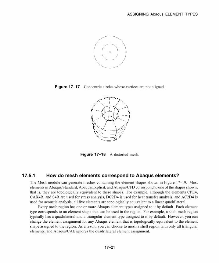
ASSIGNING Abaqus ELEMENT TYPES
Figure 17–17 Concentric circles whose vertices are not aligned.
Figure 17–18 A distorted mesh.
17.5.1 How do mesh elements correspond to Abaqus elements?The Mesh module can generate meshes containing the element shapes shown in Figure 17–19. Most
elements in Abaqus/Standard, Abaqus/Explicit, andAbaqus/CFD correspond to one of the shapes shown;
that is, they are topologically equivalent to these shapes. For example, although the elements CPE4,
CAX4R, and S4R are used for stress analysis, DC2D4 is used for heat transfer analysis, and AC2D4 is
used for acoustic analysis, all five elements are topologically equivalent to a linear quadrilateral.
Every mesh region has one or more Abaqus element types assigned to it by default. Each element
type corresponds to an element shape that can be used in the region. For example, a shell mesh region
typically has a quadrilateral and a triangular element type assigned to it by default. However, you can
change the element assignment for any Abaqus element that is topologically equivalent to the element
shape assigned to the region. As a result, you can choose to mesh a shell region with only all triangular
elements, and Abaqus/CAE ignores the quadrilateral element assignment.
17–21
Abaqus ID:
Printed on:
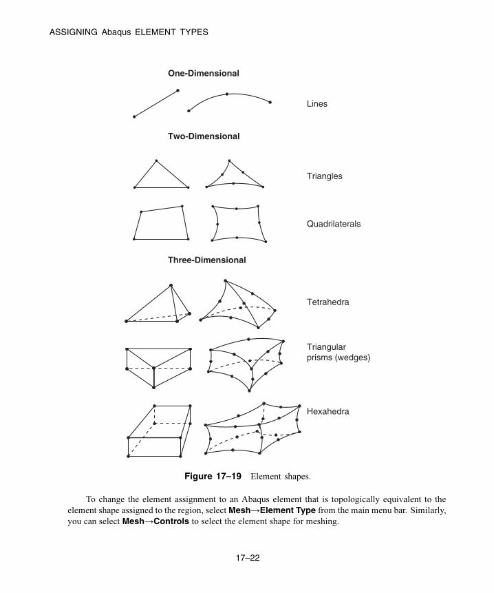
ASSIGNING Abaqus ELEMENT TYPES
One-Dimensional
Two-Dimensional
Three-Dimensional
Lines
Triangles
Quadrilaterals
Tetrahedra
Triangularprisms (wedges)
Hexahedra
Figure 17–19 Element shapes.
To change the element assignment to an Abaqus element that is topologically equivalent to the
element shape assigned to the region, select Mesh→Element Type from the main menu bar. Similarly,
you can select Mesh→Controls to select the element shape for meshing.
17–22
Abaqus ID:
Printed on:

ASSIGNING Abaqus ELEMENT TYPES
However, since no element type checking is done until you submit the analysis, it is possible
to choose an element that is inappropriate for the analysis you will be conducting. For example,
Abaqus/CAE does not prevent you from specifying heat transfer elements such as DC2D4, even though
you may be conducting a stress analysis.
17.5.2 What kinds of elements must be generated outside the Meshmodule?
Abaqus/CAE provides support for all Abaqus/CFD elements and most of the elements that are used
by Abaqus/Standard and Abaqus/Explicit. However, some elements are not supported and must be
generated outside the Mesh module. The following list describes the elements that are not supported
by Abaqus/CAE. If you want to assign these element types to a model, you must use a text editor to
add them to the input file generated in the Job module. For information on generating the input file, see
“Basic steps for analyzing a model,” Section 19.2.1.
• Acoustic interface element (ASI1)
• Axisymmetric elements with non-axisymmetric response (CAXA4N, CAXA8PN, etc.)
• Coupled temperature–pore pressure elements (C3D8PT, C3D8RPT, etc.)
• Coupled thermal-electrical-structural elements (Q3D4, Q3D6, etc.)
• Distributing coupling elements (DCOUP2D and DCOUP3D)
• Drag chain elements (DRAG2D and DRAG3D)
• Elastic-plastic joint elements (JOINT2D and JOINT3D)
• Frame elements (FRAME2D and FRAME3D)
• Gap elements, coupled temperature-displacement and heat transfer (GAPUNIT and DGAP)
• Infinite elements (CIN3D8, CINAX4, etc.)
• Line spring elements (LS3S and LS6)
• Membrane elements, 9-node quadrilateral (M3D9 and M3D9R)
• Membrane elements, cylindrical (MCL6 and MCL9)
• Particle element (PC3D)
• Pipe-soil interaction elements (PSI24, PSI34, etc.)
• Pore pressure cohesive elements (COH2D4P, COH3D6P, etc.)
• Slide line elements (ISL21A and ISL22A)
• Stress/displacement variable node elements (C3D15V, C3D27, etc.)
Note: After you submit the analysis for execution, Abaqus/Standard automatically converts any
C3D20(R)(H) element that is adjacent to a slave surface in a contact pair into the corresponding
C3D27(R)(H) element. (Neither element is available in Abaqus/Explicit.) Otherwise, there is no
way to generate variable node hexahedra with Abaqus/CAE.
17–23
Abaqus ID:
Printed on:

ASSIGNING Abaqus ELEMENT TYPES
• Surface elements, cylindrical (SFMCL6 and SFMCL9)
• Thin shell element, 9-node doubly curved (S9R5)
• Tube-to-tube contact elements (ITT21 and ITT31)
You cannot assign some elements, such as CONN2D2 and SPRING1 in the Mesh module; however,
you can create equivalent connectors in the Interaction module or engineering features in the Property
module or Interaction module as shown in Table 17–1:
Table 17–1 Abaqus/CAE support for connectors and engineering features.
Elements Abaqus/CAE support
CONN2D2, CONN3D2 Equivalent connector in Interaction module
Engineering feature in Property module
or Interaction module (linear behavior
independent of field variables)
DASHPOTA, DASHPOT1, DASHPOT2
Equivalent connector in Interaction module
GAPCYL, GAPSPHER, GAPUNI Equivalent connector in Interaction module
HEATCAP Engineering feature in Property module or
Interaction module
ITSCYL, ITSUNI Equivalent connector in Interaction module
JOINTC Equivalent connector in Interaction module
MASS Engineering feature in Property module or
Interaction module
ROTARYI Engineering feature in Property module or
Interaction module
Engineering feature in Property module
or Interaction module (linear behavior
independent of field variables)
SPRINGA, SPRING1, SPRING2
Equivalent connector in Interaction module
For more information, see “Understanding connectors,” Section 15.7; Chapter 33, “Inertia”; and
Chapter 37, “Springs and dashpots.”
17–24
Abaqus ID:
Printed on:

ASSIGNING Abaqus ELEMENT TYPES
17.5.3 Element type assignment
Element types can be assigned to the following:
• A region selected from geometry-based parts or part instances. The part instances must have come
from parts that you created in the Part module or from parts that you imported.
• A set that refers to a region selected from geometry-based parts or part instances. The set can also
refer to a skin reinforcement.
• An orphan element or element set.
All regions from geometry-based parts or part instances and all orphan elements have default
element type assignments. These assignments depend on the kind of part to which the region or element
belongs. You can view and change the Abaqus element types that are assigned using the Element Typedialog box, which you can display by selecting Mesh→Element Type. For example, the ElementType dialog box for a two-dimensional structural region is shown in Figure 17–20.
At the top of the dialog box, you enter your preferences for element library, geometric order, and
family. Then, you select a specific element type by clicking the tabs in the bottom half of the dialog box
and choosing from the options that appear. For more information on the element control options, see
“Section controls,” Section 27.1.4 of the Abaqus Analysis User’s Guide.
The dialog box can contain from one to three tabs depending on the dimensionality of the selected
region or regions:
• The Line tab allows you to choose an applicable element type and assign it to one-dimensional
mesh elements in the region.
• The Quad and Tri tabs allow you to choose an applicable element type and assign it to
two-dimensional mesh elements in the region.
• The Hex, Wedge, and Tet tabs allow you to assign three-dimensional element types to the three-
dimensional mesh elements in the region.
For example, in Figure 17–20 the options for a linear shell element from the Abaqus/Standard
element library are selected. After clicking the Quad tab, reduced integration and finite membrane
strains are selected. The name and a brief description of the quadrilateral shell element that meets all of
these criteria appear at the bottom of the tabbed page.
The Tri tab in this dialog box is shown in Figure 17–21. The name and a brief description of the
triangular shell element that meets all of the criteria specified in the dialog box appear at the bottom of the
Tri tabbed page in Figure 17–21. If the selected region in this example happens to contain a combination
of triangular and quadrilateral mesh elements:
• The quadrilateral mesh elements are assigned the S4R element type.
• The triangular mesh elements are assigned the S3 element type.
17–25
Abaqus ID:
Printed on:

ASSIGNING Abaqus ELEMENT TYPES
Figure 17–20 The Element Type dialog box for a two-dimensional structural
region in an Abaqus/Standard model.
Figure 17–21 The Tri tab.
17–26
Abaqus ID:
Printed on:

VERIFYING AND IMPROVING MESHES
If the region contains only quadrilateral elements, all of the elements are assigned the S4R element
type.
For detailed, step-by-step instructions for assigning element types to a mesh region, see
“Associating Abaqus elements with mesh regions,” Section 17.18.10, in the HTML version of this
guide. For lists of the element types that are available, see Section EI.1, “Abaqus/Standard Element
Index,” of the Abaqus Analysis User’s Guide, Section EI.2, “Abaqus/Explicit Element Index,” of
the Abaqus Analysis User’s Guide, and Section EI.3, “Abaqus/CFD Element Index,” of the Abaqus
Analysis User’s Guide. You can select most of these elements through the Element Type dialog box.
“What kinds of elements must be generated outside the Mesh module?,” Section 17.5.2, describes the
elements that cannot be selected.
17.6 Verifying and improving meshes
This section explains how you use the tools in the Mesh module to verify your mesh quality, to control
mesh generation, and to improve the mesh quality.
17.6.1 Verifying your meshUpon completion of a meshing operation, Abaqus/CAE highlights any bad elements in the mesh.
Abaqus/CAE also provides a set of tools in the Mesh module that allow you to verify the quality of
your mesh and to obtain information about the nodes and elements in the mesh. You can use these tools
to isolate regions where the mesh quality is poor and to guide you if you need to refine your mesh. To
verify the quality of the mesh, choose the Object from the context bar, and select Mesh→Verify from
the main menu bar. You can then select the part, part instances, geometric regions, or element to verify.
Abaqus/CAE allows you to choose between checking that your mesh will pass the quality tests in the
analysis products and checking that your mesh passes individual quality checks, such as checking for
elements with a large aspect ratio. Any elements that do not pass the specified criteria are highlighted
in the viewport, and you can choose to create and save a set containing the highlighted elements or, if
applicable, the cells, faces, or edges related to those elements. For detailed information on using the
mesh verify tools, see “Verifying element quality,” Section 17.19.1, in the HTML version of this guide.
You can use the Analysis checks to verify that the elements in your mesh will pass the element
quality checks that are included with the input file processor in Abaqus/Standard or Abaqus/Explicit.
Abaqus/CAE highlights any elements that fail the mesh quality tests and displays the number of elements
tested along with the number of errors and warnings in the message area. The mesh quality tests in the
input file processor are extensive and specific to each element type. At a minimum, the mesh quality
tests issue a warning for elements that seem inappropriately distorted, and the tests issue an error if
the distortion is severe. Abaqus/CAE does not support analysis checks for beam, gasket, or cohesive
elements.
17–27
Abaqus ID:
Printed on:

VERIFYING AND IMPROVING MESHES
You can use the Shape metrics to highlight elements of a selected shape that do not meet one of
the following selection criteria:
Shape factor
Abaqus/CAE highlights elements with a normalized shape factor smaller than a specified value.
The shape factor criterion is available only for triangular and tetrahedral elements. The shape
factor ranges from 0 to 1, with 1 indicating the optimal element shape and 0 indicating a degenerate
element.
• For triangular elements the normalized shape factor is defined as
Optimal element area is the area of an equilateral triangle with the same circumradius as the
element. (The circumradius is the radius of the circle passing through the three vertices of the
triangle.)
• For tetrahedral elements the normalized shape factor is defined as
Optimal element volume is the volume of an equilateral tetrahedron with the same circumradius
as the element. (The circumradius is the radius of the sphere passing through the four vertices
of the tetrahedron.)
Small face corner angle
Abaqus/CAE highlights elements containing faces where two edges meet at an angle smaller than
a specified angle.
Large face corner angle
Abaqus/CAE highlights elements containing faces where two edges meet at an angle larger than a
specified angle.
Aspect ratio
Abaqus/CAE highlights elements with an aspect ratio larger than a specified value. The aspect ratio
is the ratio between the longest and shortest edge of an element.
Table 17–2 shows the default limits for the selection criteria based on the element shape.
17–28
Abaqus ID:
Printed on:

VERIFYING AND IMPROVING MESHES
Table 17–2 Element shape selection criteria limits.
Selectioncriterion
Quadrilateral Triangle Hexahedra Tetrahedra Wedge
Shape factor N/A 0.01 N/A 0.0001 N/A
Smaller face
corner angle
10 5 10 5 10
Larger face
corner angle
160 170 160 170 160
Aspect ratio 10 10 10 10 10
You can use the Size metrics to highlight elements that do not meet one of the following selection
criteria:
Geometric deviation factor
Abaqus/CAE highlights elements with an edge whose geometric deviation factor is greater than the
specified value. The geometric deviation factor is a measure of how much an element edge deviates
from the original geometry, and Abaqus/CAE calculates this value by dividing the maximum gap
between an element edge and its parent geometric face or edge by the length of the element edge.
By default, Abaqus/CAE highlights elements whose geometric deviation factor is greater than 0.2.
Abaqus/CAE calculates the geometric deviation factor only for elements in a native mesh. If
you select a part that contains no geometry, Abaqus/CAE disables this option in the Verify Meshdialog box. If your selection includes both native and orphan elements, Abaqus/CAE considers
only the native elements for calculations of geometric deviation factor.
Short edge
Abaqus/CAE highlights elements with an edge shorter than a specified value.
Long edge
Abaqus/CAE highlights elements with an edge longer than a specified value.
Stable time increment
Abaqus/CAE highlights elements with a calculated stable time increment less than the specified
value. The stable time increment calculation requires a suitable material definition and section
assignment and is meaningful only for Abaqus/Explicit analyses.
The stable time increment calculation in Abaqus/CAE is an approximation of the initial stable
time increment calculation made by Abaqus/Explicit for an element-by-element formulation. It
does not account for any of the following conditions:
• Mass scaling
• Point mass
17–29
Abaqus ID:
Printed on:

VERIFYING AND IMPROVING MESHES
• Rotary inertia
• Nonstructural mass
• Reinforcement (rebar)
Material behaviors supported for the stable time increment calculation in Abaqus/CAE include
elastic, hyperelastic, hyperfoam (without user-defined test data), and acoustic medium. Composite
sections with multiple materials are not supported. For more information, see “Stability” in
“Explicit dynamic analysis,” Section 6.3.3 of the Abaqus Analysis User’s Guide.
Maximum allowable frequency for acoustic elements
Abaqus/CAE highlights finite acoustic elements that may not be valid for modal or steady-state
dynamic analyses in Abaqus/Standard above the specified frequency value. The maximum
allowable frequency calculation requires a suitable material definition and section assignment. The
calculation is a guideline based on approximately 10 elements per wavelength:
where P is the interpolation order (1 or 2), h is the size of the element bounding box, and is the
speed of sound .
In addition, for both shape and size metrics Abaqus/CAE displays the following information in the
message area for each selected part, part instance, or region:
• The name of the part or part instance.
• The total number of elements of the selected shape in the part instance or in the selected regions.
• The number of highlighted elements and the percentage of the elements being verified that these
elements comprise.
• The average value of the selection criterion. For the geometric deviation factor, Abaqus/CAE
calculates the average value by considering only elements along a curve or face; solid elements
in the center of a volume are excluded from this value.
• The “worst” value of the selection criterion—the value closest to the criterion if it is not exceeded
or the value farthest beyond the criterion if it is exceeded.
17.6.2 Querying your meshThe Query toolset in the Mesh module allows you to obtain information about the nodes and elements in
the mesh. In addition, you can select Tools→Query from the main menu bar to request the following
information about the mesh:
• The total number of nodes and elements in a selected part, part instance, or region along with the
number of elements of each element shape.
• The type and connectivity of a selected element.
17–30
Abaqus ID:
Printed on:

VERIFYING AND IMPROVING MESHES
• The positive and negative sides of shell and membrane faces.
• The direction of beam and truss tangents.
• The mesh stack orientation.
• Whether any edges of boundary faces have incompatible interfaces, cracks, or gaps and whether
any edges intersect other faces.
• The location of free or non-manifold edges—exterior shell or solid element edges that are not shared
by exactly two exterior elements.
• The location of any unmeshed regions.
For detailed information on using the Query toolset, see “Obtaining mesh information,” Section 17.19.2,
in the HTML version of this guide.
17.6.3 Why partition in the Mesh module?
You can use the Partition toolset to divide parts or independent part instances into smaller regions. There
are three reasons to create partitions in the Mesh module:
• To divide a complex, three-dimensional part or instance into simpler regions that Abaqus/CAE
can mesh using primarily hexahedral elements with the structured or swept meshing techniques.
(Almost all three-dimensional parts are meshable using the free meshing technique, but
three-dimensional free meshes can include only tetrahedral elements.)
• To gain more control over mesh generation.
• To obtain regions to which you can assign different element types.
See Chapter 70, “The Partition toolset,” for detailed information on how to use each tool in the Partition
toolset.
You can partition only parts or independent part instances. If you need to partition a dependent
instance, you can partition the original part fromwhich the dependent instance was created. Alternatively,
you can create a copy of the original part and then create an independent instance of the copy. You can
then replace the dependent instance with the new independent instance and partition the independent
instance. For more information, see “What is the difference between a dependent and an independent
part instance?,” Section 13.3.2.
By default, the free meshing technique with quadrilateral elements is applied to all two-dimensional
parts and part instances. When you create the mesh using this default technique, Abaqus/CAE implicitly
creates partitions that divide the part into regions that can be meshed using the structured meshing
technique. (For more information, see “Free meshing with quadrilateral and quadrilateral-dominated
elements,” Section 17.10.2.) Therefore, all two-dimensional parts are meshable without any manual
partitioning.
However, when a three-dimensional part or instance is unmeshable using hexahedral elements, you
must take one of the following steps:
17–31
Abaqus ID:
Printed on:

VERIFYING AND IMPROVING MESHES
• Change the element shape from hexahedra to tetrahedra so that the free meshing technique can be
applied.
• Partition into structured- or swept-meshable regions.
When the Mesh defaults color mapping is selected, Abaqus/CAE uses the color orange to indicate
that a three-dimensional region is unmeshable using the currently assigned element shape. For example,
Figure 17–22 illustrates a part that cannot be meshed with hexahedral elements.
Orange (cannot be meshed)
Figure 17–22 Unmeshable three-dimensional region.
With the addition of a partition, the part can be meshed with hexahedral elements, as shown in
Figure 17–23; the green region can be meshed using the structured meshing technique, and the yellow
regions can be meshed using the swept meshing technique.
Green (structured meshing technique)
Yellow (sweptmeshing technique)
Figure 17–23 The model is partitioned into three regions.
Even when a part or instance can be meshed without partitioning, you may still want to partition to
gain more control over mesh generation. Without partitions, the mesh is aligned only along the exterior
edges; with partitions, the resulting mesh will have rows or grids of elements aligned along the partitions.
That is, the mesh “flows” along the partitions. For example, in Figure 17–24 the partition that divides
the rectangle in two causes the mesh to flow at an angle along the partition.
17–32
Abaqus ID:
Printed on:
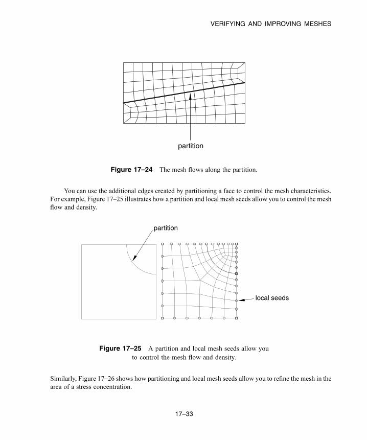
VERIFYING AND IMPROVING MESHES
partition
Figure 17–24 The mesh flows along the partition.
You can use the additional edges created by partitioning a face to control the mesh characteristics.
For example, Figure 17–25 illustrates how a partition and local mesh seeds allow you to control the mesh
flow and density.
partition
local seeds
Figure 17–25 A partition and local mesh seeds allow you
to control the mesh flow and density.
Similarly, Figure 17–26 shows how partitioning and local mesh seeds allow you to refine the mesh in the
area of a stress concentration.
17–33
Abaqus ID:
Printed on:

VERIFYING AND IMPROVING MESHES
Figure 17–26 Partitioning and local mesh seeds allow you to
refine the mesh in the area of a stress concentration.
In addition, you can apply different mesh controls, such as element shape, to the regions created by a
partition.
When partitioning, remember that partitions will become element boundaries. Therefore, try to
ensure that partitions make angles as close to 90° as possible with other partitions or edges. In addition,
you should avoid creating unwanted short edges that will distort the mesh.
17.6.4 How are seeds and other attributes affected by partitioning?
Seed distributions along edges you have seeded may change during the partitioning process;
Abaqus/CAE redistributes the seeds to accommodate any new vertices created by partitioning. For
example, the left and right edges of the part instance in Figure 17–27 are seeded with seven elements
per edge.
17–34
Abaqus ID:
Printed on:

VERIFYING AND IMPROVING MESHES
Figure 17–27 The left and right edges each have seven elements.
If you create a partition that splits the part instance into two regions, new vertices are created at the
midpoints of both edges. In Figure 17–28 you can see how Abaqus/CAE added seeds at the new vertices
so that nodes will exist at the corners of each region.
Figure 17–28 Redistribution of seeds.
Abaqus/CAE also redistributed the existing seeds to eliminate any overly small elements created by the
new partition. However, this redistribution can result in seeds that are not aligned. The top region has
one seed more on the left side than it does on the right, and the reverse is true for the bottom region. In
this example you could change the number of elements along the right and left edges to an even number
to ensure that the seeds align after partitioning.
Any other mesh attributes, such as element shape or element type, that you have applied are applied
automatically to each new region that you create with a partition. However, once you have created the
different regions, you can assign different mesh attributes to each region.
17–35
Abaqus ID:
Printed on:

VERIFYING AND IMPROVING MESHES
17.6.5 Regenerating partitions after modifying geometryPartitions are features associated with the part or part instance; therefore, you can modify and regenerate
them like any other feature.
For example, consider the partition on the right side of the part instance shown in Figure 17–29.
Figure 17–29 A partitioned part instance.
If you return to the Part module and widen the right side of the model, the partition also expands and
continues to divide the face into two regions, as shown in Figure 17–30.
Figure 17–30 The partition is regenerated.
Sometimes regeneration of a partition creates unmeshable regions. In this situation simply add,
modify, or delete partitions until the part instance becomes meshable again.
17.6.6 Using virtual topology to improve your meshIn some cases parts or independent part instances contain details such as very small faces and edges. The
Virtual Topology toolset allows you to remove these small details by combining a small face with an
17–36
Abaqus ID:
Printed on:

VERIFYING AND IMPROVING MESHES
adjacent face or by combining a small edge with an adjacent edge. You can also ignore selected edges
and vertices, which has the same effect as combining faces and edges. Introducing virtual topology is
a convenient method for creating a clean, well-formed mesh. The Virtual Topology toolset is available
only in the Mesh module.
However, adding virtual topology to a part instance can restrict your ability to subsequently mesh
the part instance. For example, you cannot mesh regions that contain virtual topology using the following
techniques:
• Two-dimensional free meshing with quadrilateral or quadrilateral-dominated elements using the
medial axis algorithm.
• Three-dimensional swept meshing using the medial axis algorithm.
• Two-dimensional structured meshing if the region to be meshed is not bounded by four corners.
• Three-dimensional structured meshing if the region to be meshed is not bounded by six sides.
For more information, see Chapter 75, “The Virtual Topology toolset.”
In addition, you can apply virtual topology only to independent instances. If you need to apply
virtual topology to a dependent instance, you can create a copy of the original part and then create an
independent instance of the copy. You can then replace the dependent instance with the new independent
instance and apply virtual topology to the independent instance. For more information, see “What is the
difference between a dependent and an independent part instance?,” Section 13.3.2.
17.6.7 Using adaptive remeshing to improve your mesh
In many cases you will not know the adequacy of your mesh refinement for your particular solution goal
until you have executed a number of analyses and evaluated the solution results. Mesh refinement studies
are typically performed in these cases, where a mesh is successively refined and key solution results
are confirmed to converge. You can automate this process by applying remeshing rules to regions of
interest in your model and using the Abaqus/CAE adaptive remeshing process to automatically perform
successive mesh refinement based on a series of executed analyses.
With a remeshing rule you can specify:
• The region where you want the mesh refined.
• The solution quality criteria (for example error indicators in the Mises stress) that mesh refinement
is based on.
• The analysis step or steps that refinement is based on.
• Minimum and maximum element size constraints.
• A sizing algorithm and parameters appropriate to your simulation.
For more information, see “Advanced meshing techniques,” Section 17.14; and “Creating, editing, and
manipulating adaptivity processes,” Section 19.9, in the HTML version of this guide.
17–37
Abaqus ID:
Printed on:

UNDERSTANDING MESH GENERATION
17.7 Understanding mesh generation
This section explains basic concepts and terminology related to meshes and mesh generation.
17.7.1 OverviewMost meshing in Abaqus/CAE is completed in a “top-down” fashion. This means that the mesh is created
to conform exactly with the geometry of a region and works down to the element and node positions.
Abaqus/CAE follows these basic steps to generate a mesh:
1. Generate a mesh on each top-down region using the meshing technique currently assigned to that
region. By default, Abaqus/CAE generates meshes with first-order line, quadrilateral, or hexahedral
elements throughout.
2. Merge the meshes of all regions into a single mesh. Typically, Abaqus/CAE merges the nodes along
the common boundaries of neighboring regions into a single set of nodes. However, in certain
cases Abaqus/CAE creates tied surface interactions instead of merging these nodes; for example,
along the common interface between hexahedral and tetrahedral meshes. For more information, see
“Meshing multiple three-dimensional solid regions,” Section 17.14.1.
Top-down meshes generated by Abaqus/CAE conform to the geometry of the part or part instance
they discretize, as shown in Figure 17–31:
• A node is generated at each geometric vertex.
• A connected set of element edges is generated along each geometric edge.
• A connected set of element faces is generated along each geometric face.
• Nodes that are on the boundary of the mesh (including the midside nodes of second-order elements)
are also on the boundary of the geometry.
• Midside nodes of internal second-order elements are centered between the end nodes of the element
edges.
For detailed, step-by-step instructions on creating a top-down mesh, see “Creating a mesh,”
Section 17.17.1, in the HTML version of this guide.
Relying directly on the geometry to form the outer mesh boundaries can impact mesh quality as
Abaqus/CAE creates elements to fill small details. In some cases you may not be able to implement
a partitioning strategy that allows you to apply a top-down swept or structured meshing technique on
a complex region. For solid regions, you can use the “bottom-up” meshing technique in place of the
automated top-downmeshing techniques to generate a hexahedral mesh. Bottom-upmeshing is amanual,
incremental meshing process that builds up a three-dimensional mesh from two-dimensional entities.
You define the regions that will be meshed using the bottom-up technique, control the meshing process,
decide whether the resulting mesh meets your needs, and—since the mesh is not required to conform to
17–38
Abaqus ID:
Printed on:

UNDERSTANDING MESH GENERATION
Node at each vertex
Element facesalong eachgeometric face
Element edgesalong eachgeometric edge
Boundary midside nodes conform to the geometric boundary
Internal midside nodescentered between corner nodes
Figure 17–31 The mesh conforms to the geometry of the part instance.
the geometry— control the associativity of the geometry to the mesh. For more information on bottom-up
meshing, see “Bottom-up meshing,” Section 17.11.
17.7.2 Preserving the precision of nodal coordinates
When you create a part in the Part module, it exists in its own coordinate system, independent of other
parts in the model. In contrast, when you create an instance of the part in the Assembly module and
position it relative to other part instances, you are working in the assembly’s global coordinate system.
To preserve precision, the Mesh module separates the positioning information of a part instance
from the geometry of the instance. As a result, when you generate a mesh, the nodal coordinates for the
part instance are computed relative to the coordinate system of the original part. (When the Job module
generates an input file, Abaqus/CAE writes the nodal coordinates for each instance relative to its own
coordinate system and passes the instance positioning and orientation information to the analysis product
via the *INSTANCE keyword.)
The Mesh module stores these nodal coordinates in single precision. If the geometry of the part
lies far from the origin of its coordinate system, some precision of the nodal coordinates will be lost. To
prevent this loss of precision, you should try to position a part close to the origin of its coordinate system.
For example, the origin of the coordinate system of an Abaqus/CAE native part is located at the origin
of the sketch that defined the base feature. Therefore, if possible, you should position the sketch of the
base feature over the origin of the sketcher grid.
17–39
Abaqus ID:
Printed on:

UNDERSTANDING MESH GENERATION
17.7.3 Determining which regions are meshableWhen the Mesh defaults color mapping is selected, the color of a region in the Mesh module indicates
the meshing technique currently assigned to that region. The color coding is as follows:
• Structured meshing technique: green
• Free meshing technique: pink
• Swept meshing technique: yellow
• Unmeshable: orange
• Bottom-up meshing technique: light tan
See “Structured meshing and mapped meshing,” Section 17.8; “Free meshing,” Section 17.10; “Swept
meshing,” Section 17.9; and “Bottom-up meshing,” Section 17.11, for information about each meshing
technique. See Chapter 77, “Color coding geometry and mesh elements,” for more information about
color mappings.
In many cases Abaqus/CAE can use more than one technique to mesh a region; in these cases
you can either accept the default technique, or you can use the Mesh Controls dialog box to select an
alternative technique. In addition, you can change the meshing techniques that are valid for a region
by adding partitions to the region or by assigning a different element shape to the region. For example,
if you change the element shape assignment of an unmeshable three-dimensional part instance from
hexahedra to tetrahedra, the part instance becomes meshable using the free-meshing technique. For
more information, see “Why partition in the Mesh module?,” Section 17.6.3.
Note: You must use the Mesh Controls dialog box to assign the bottom-up meshing technique to a
region. To unassign the bottom-up technique, you may select another technique or click Defaults in
the Mesh Controls dialog box to allow Abaqus/CAE to use the default element shape and meshing
technique for the region.
The default meshing technique for two-dimensional models is the free meshing technique. If you
are not satisfied with the quality of the mesh generated by the free meshing technique, or if you prefer
a more regular grid-like mesh pattern, you can assign structured meshing to the simpler regions of your
model. However, if your model is large and complex, identifying the simple regions where structured
meshing is applicable can be a time-consuming process. To make the process faster, you can apply the
structured meshing technique to the entire model, and Abaqus/CAE will do the following:
• Determine if any faces are too complex to be structured meshed and ask if you wish to remove them
from your selection.
• Determine if any faces are poorly shaped and will result in unacceptable mesh quality and ask if
you wish to remove them from your selection.
If Abaqus/CAE removed any faces from your selection, they are colored pink to indicate that they will
be meshed using free meshing. Remaining faces are colored green to indicate that Abaqus/CAE will
mesh them using structured meshing.
17–40
Abaqus ID:
Printed on:

UNDERSTANDING MESH GENERATION
For example, Figure 17–32 shows a shell model of an electrical connector. The user attempted to
assign structured meshing to the entire assembly, and Abaqus/CAE removed the indicated faces from
their selection.
These faces are too complex for structured meshing
Figure 17–32 Faces that cannot be structured meshed are removed from the selection.
If you are meshing a solid model, you must select one or more cells and use the Mesh Controls dialog
box to determine whether the structured technique can be applied to those cells. If you have a region
that will be meshed using free tetrahedral meshing, you can select boundary faces and use the MeshControls dialog box to determine whether the structured technique can be applied to create a triangular
boundary mesh prior to tetrahedral meshing of the solid.
For detailed information on controlling the mesh technique and element shape assigned to a region,
see the following sections in the HTML version of this guide:
• “Bottom-up meshing,” Section 17.11
• “Assigning mesh controls,” Section 17.18.1
• “Choosing an element shape,” Section 17.18.2
• “Selecting a meshing technique,” Section 17.18.3
• “Changing mesh controls for previously meshed regions,” Section 17.18.9
17–41
Abaqus ID:
Printed on:
UNDERSTANDING MESH GENERATION
17.7.4 What should I do if a region fails to mesh?
If a region fails to mesh, Abaqus/CAE displays an Error dialog box that explains why the meshing
failed. In most cases Abaqus/CAE highlights the region and allows you to save it in a set. You can create
a display group from the set and use the display group to study the region that failed to mesh.
Some of the more common reasons why a region fails to mesh and the associated solutions are as
follows:
Inadequate seeding
The region contains some small edges or the seed density is too coarse. You can use the Virtual
Topology toolset to merge small edges. Alternatively, if you save the region that failed to mesh in
a set, you can apply local seeds of a finer density to the saved set.
When you are creating a hexahedral mesh, a quadrilateral mesh, or a quadrilateral-dominated
mesh using the medial axis algorithm, Abaqus may need to alter seeds to generate the mesh. In
some cases, mesh generation may fail because the modified seeds density is too coarse. Meshing
may succeed if you incrementally mesh the regions of the part in a different order, or, as described
above, you can apply local seeds of a finer density and remesh the part.
Bad geometry
Bad geometry refers to small edges or faces or to part instances that are imprecise. You can use the
Query toolset to check the geometry. For more information, see “Using the geometry diagnostic
tools,” Section 71.2.4, in the HTML version of this guide.
Poor boundary triangles
When you are creating a free mesh with tetrahedral elements, Abaqus/CAE first creates a triangular
mesh on the faces of the region and then uses those triangles as faces of the boundary tetrahedral
elements. You can choose to preview the triangular mesh on the faces and decide if it is acceptable
before continuing with the time-consuming process of generating tetrahedral elements through
the interior of the region. For more information, see “What is a tetrahedral boundary mesh?,”
Section 17.10.4.
In some cases Abaqus/CAE cannot complete the conversion from triangles to tetrahedra and
highlights the nodes on the boundary mesh that cannot be inserted into the tetrahedral mesh. The
highlighted nodes serve as indicators of regions that require attention, and you can try the following:
– Use the seeding tools to increase the mesh density.
– Use the Virtual Topology toolset to combine small faces and edges with adjacent faces and
edges.
– Use the Partition toolset to partition regions into simpler subregions.
– Use the Edit Mesh toolset to improve the tetrahedral boundary mesh.
– Use mesh controls to change the mesh technique applied to faces of the solid region.
17–42
Abaqus ID:
Printed on:

UNDERSTANDING MESH GENERATION
Gasket regions
You can generate a gasket reinforcement mesh only on a region that contains a gasket mesh.
17.7.5 What is a mesh transition?
A mesh transition is an area where a mesh transitions from coarse (large elements) to fine (small
elements), as shown in Figure 17–33.Tr
ansi
tion
Figure 17–33 A mesh with a transition from coarse to fine elements.
Abaqus/CAE provides mesh transition controls for the following types of meshes:
• A two-dimensional, quadrilateral-only mesh that is created using the structured meshing technique
or the free meshing technique with the medial axis algorithm.
• A three-dimensional, hexahedral-only mesh that is created by sweeping a two-dimensional mesh.
For more information, see “What is swept meshing?,” Section 17.9.1.
When transition controls are applicable to the type of mesh you are creating, a toggle button appears
on the right side of the Mesh Controls dialog box that allows you to minimize the mesh transition. By
default, Abaqus/CAE minimizes the mesh transition, which in some cases will reduce mesh distortion.
Conversely, if you toggle off the option to minimize mesh transition, the mesh may move closer to the
specified mesh seeds. To display the Mesh Controls dialog box, select Mesh→Controls from the
main menu bar. For more information, see “Setting the mesh algorithm,” Section 17.18.5, in the HTML
version of this guide.
17–43
Abaqus ID:
Printed on:

UNDERSTANDING MESH GENERATION
17.7.6 What is the difference between the medial axis algorithm andthe advancing front algorithm?
The medial axis algorithm and the advancing front algorithm are two meshing schemes that Abaqus/CAE
can use to generate a mesh when you are doing the following:
• Meshing a surface with quadrilateral or quadrilateral-dominated elements using the free meshing
technique.
• Meshing a solid region with hexahedral or hexahedral-dominated elements using the swept meshing
technique. (Abaqus/CAE generates hexahedral and hexahedral-dominated meshes by sweeping the
quadrilateral and quadrilateral-dominated elements generated by the two algorithms from the source
side to the target side.)
The two algorithms are described as follows:
Medial axis
The medial axis algorithm first decomposes the region to be meshed into a group of simpler
regions. The algorithm then uses structured meshing techniques to fill each simple region with
elements. If the region being meshed is relatively simple and contains a large number of elements,
the medial axis algorithm generates a mesh faster than the advancing front algorithm. Minimizing
the mesh transition may improve the mesh quality. The mesh transition option is available only for
quadrilateral and hexahedral meshing. For more information, see “What is a mesh transition?,”
Section 17.7.5.
Advancing front
The advancing front algorithm generates quadrilateral elements at the boundary of the region and
continues to generate quadrilateral elements as it moves systematically to the interior of the region.
The elements generated by the advancing front algorithm will always follow the seeding
exactly for quadrilateral-dominated and hexahedral-dominated meshes (except when you are
creating a three-dimensional revolved mesh, and the profile being revolved touches the axis of
revolution). For other meshes the elements generated by the advancing front algorithm will always
follow the seeding more closely than those generated by the medial axis algorithm. If the region to
be meshed contains virtual topology, you can use only the advancing front algorithm to generate
the mesh.
If you select the advancing front algorithm, you can allowAbaqus/CAE to usemappedmeshing
where appropriate. (Mapped meshing is the same as structured meshing but applies to only four-
sided regions.) For more information, see “What is mapped meshing?,” Section 17.8.2, and “When
can Abaqus/CAE apply mapped meshing?,” Section 17.8.6.
17–44
Abaqus ID:
Printed on:

UNDERSTANDING MESH GENERATION
You may have to experiment with the two algorithms to obtain the optimal mesh. Figure 17–34
illustrates a simple shell region that was meshed with quadrilateral-dominated elements using the two
meshing algorithms. In this example both algorithms generate an acceptable mesh.
Medialaxis
Advancingfront
Figure 17–34 Both algorithms generate acceptable meshes.
Because the elements produced by the advancing front algorithm follow your seeds, the resulting mesh
may include some skew in the elements in narrow regions. Element skew is illustrated in Figure 17–35.
Medialaxis
Advancingfront
Elements with skew
Figure 17–35 In some cases the advancing front algorithm generates elements with some skew.
In contrast, the advancing front algorithm may generate elements of a more uniform size with a more
consistent aspect ratio, as shown in Figure 17–36. Uniform element size can play an important role in
the analysis; for example, if you are creating a mesh for an Abaqus/Explicit analysis, small elements in
the mesh can unduly control the size of the time step. In addition, if it is important that the elements
follow your seeds, the advancing front algorithm is preferable.
17–45
Abaqus ID:
Printed on:

UNDERSTANDING MESH GENERATION
Medialaxis
Advancingfront
Figure 17–36 In some cases the advancing front algorithm produces a more uniform mesh.
In some cases, when you mesh multiple regions, Abaqus/CAE generates a mesh with sheared
elements at the interface between regions. Nodes in one region may be positioned differently than
nodes in an adjacent region, which results in shear at the common boundary when Abaqus/CAE merges
the adjacent meshes. Figure 17–37 shows multiple swept regions and the resulting mesh generated by
the medial axis algorithm.
Figure 17–37 Mesh shear is significant between adjacent regions using the medial axis algorithm.
The advancing front algorithm positions the nodes on the source side at the same location as your seeds;
as a result, the mesh shear will be reduced. Figure 17–38 shows the same part meshed with the same
seeding using the advancing front algorithm. However, as stated earlier, you may have to experiment
with the two algorithms to obtain the optimal mesh.
17–46
Abaqus ID:
Printed on:

UNDERSTANDING MESH GENERATION
Figure 17–38 Mesh shear is reduced between adjacent regions using the advancing front algorithm.
For information on related topics, refer to the following section:
• “Setting the mesh algorithm,” Section 17.18.5, in the HTML version of this guide
17.7.7 What kinds of meshes cannot be generated automatically?
There are a few types of meshes that you cannot create using the mesh generator in the Mesh module:
Compatible meshes between part instances of the same assembly
Compatibility means that the element faces or element edges of the meshes of adjacent part
instances share the same nodes and have the same topology at the common interface. You cannot
prescribe mesh compatibility between instances. However, you can use the Merge/Cut tool inthe Assembly module to merge multiple instances into a single part instance. You can then create
a single compatible mesh from the single part instance. See “Compatible meshes between part
instances,” Section 17.14.3, for more information.
Symmetric meshes
You cannot ensure that Abaqus/CAE will generate a symmetric mesh for a symmetric part or part
instance.
17–47
Abaqus ID:
Printed on:

UNDERSTANDING MESH GENERATION
Bottom-up meshes
Bottom-up meshing is a manual process. You must set and apply the parameters to create the mesh
for each region to which you have assigned the bottom-up meshing technique.
17.7.8 When will Abaqus/CAE delete a mesh?The following attributes of a part, part instance, or region affect how the mesh will be generated:
• Seeding
• Element shape
• Meshing technique
• Meshing algorithm
• Logical corners of a two-dimensional structured region
• Transition control
• Sweep path of a swept region
If you change any of the attributes listed, the existing mesh will no longer be consistent with its attributes.
As a result, Abaqus/CAE deletes the mesh, and you can recreate a new mesh that matches the new
attributes. (Element order and element family are the only attributes that, when changed, do not require
the mesh to be deleted and recreated.)
Whenever you make a change that will affect any of these attributes for a top-down meshed region,
Abaqus/CAE displays a dialog box similar to the one shown in Figure 17–39.
Figure 17–39 The warning dialog box.
You can delete the mesh by clicking the Delete Meshes button, or you can keep your mesh and exit the
procedure by pressing the Cancel button.You can also avoid this warning message for the remainder of the current session by toggling
Automatically delete meshes invalidated by mesh control changes. The next time you attempt
17–48
Abaqus ID:
Printed on:

UNDERSTANDING MESH GENERATION
to change the attributes of a part, part instance, or region that already contains a mesh, the mesh will be
deleted immediately without any warning being displayed.
If you save your model to a model database before you delete the mesh, you can revert back to that
mesh if you are dissatisfied with later meshing attempts.
Since bottom-up meshes can be very time consuming to create, Abaqus/CAE attempts to preserve
them in many circumstances that would cause a top-down mesh to be deleted. Bottom-up meshes are
retained during changes to seeding, partitioning, and virtual topology. When you partition a region or
create a virtual topology feature the mesh will be retained, but associativity with the geometry effected
by the partition or virtual topology operation will be lost.
WARNING: There is no way to avoid deleting a top-down mesh when you change one of the meshing
attributes listed above. Likewise, if you change the part geometry, Abaqus/CAE always deletes both
top-down and bottom-up meshes without warning. Since remeshing can be time consuming for large or
complex models, you should use caution when changing these attributes.
For detailed, step-by-step instructions on deleting a mesh, see “Deleting a mesh,” Section 17.17.2,
in the HTML version of this guide.
17.7.9 Do I have to mesh the entire model in one operation?Abaqus/CAE allows you to mesh the model in an incremental fashion, where each meshing operation
meshes a different region of the model. You can use incremental meshing to fine-tune the mesh in a
selected region of your model without remeshing the entire model.
When you mesh a selected region, Abaqus/CAE tries to preserve the existing mesh in other regions
of the model if possible. However, incremental meshing may force the nodes on the boundaries of the
existing mesh to move and can reduce the mesh quality along the interfaces between the regions. In
some cases Abaqus/CAE cannot proceed with an incremental meshing operation and must delete all the
existing meshes before proceeding:
• Incremental meshing cannot proceed if the seeding between the existing mesh and the selected
region cannot be honored. You must allow Abaqus/CAE to delete the existing mesh and remesh the
original regions and the selected region.
For example, consider the part instance in Figure 17–40. The central region cannot be meshed
incrementally because one end has a mesh with 4 × 4 mesh pattern and the opposite end has a mesh
with a 3 × 3 mesh pattern. If you try to mesh only the central region, Abaqus/CAE will detect the
problem and allow you to choose between the following:
– Remesh the regions that are already meshed and the central region to generate a compatible
mesh.
– Cancel the operation to mesh the central region.
• Incremental meshing cannot proceed if the existing mesh needs to be derived from the mesh you are
trying to create. For example, consider the part instance in Figure 17–41. To create a compatible
17–49
Abaqus ID:
Printed on:

UNDERSTANDING MESH GENERATION
Figure 17–40 The central region cannot be meshed incrementally.
Region 1
Region 2
Region 3
Figure 17–41 The regions must be meshed in the correct sequence.
mesh between region 1 and region 2, the mesh of region 2 is derived from the mesh of the cylinder
in region 1. Similarly, the mesh of region 3 is derived from the mesh of region 2, which in turn was
derived from the mesh of the cylinder in region 1. As a consequence, if you mesh region 3 first,
Abaqus/CAE cannot incrementally mesh regions 1 and 2. You must allow Abaqus/CAE to mesh
region 1 prior to remeshing regions that were already meshed.
If incremental meshing cannot proceed, Abaqus/CAE displays a warning message prior to deleting an
existing mesh.
If you want to mesh the part or assembly incrementally, you can follow a strategy that will minimize
the number of times Abaqus/CAE has to delete the existing mesh. The meshing strategy depends on the
topology of the regions, the element shapes, the meshing technique, and the mesh seeding.
• Changes to the seeding always propagate out to the boundaries. As a result, you should start meshing
from the interior of the part or part instance and continue out to the boundaries of the part or instance.
• However, if you can identify a set of adjacent three-dimensional regions that will be meshed using
the swept method, you should start meshing on one side of the part or part instance and continue
the mesh through the interior to the other side of the part or instance.
17–50
Abaqus ID:
Printed on:

STRUCTURED MESHING AND MAPPED MESHING
• Regions that are meshed by triangles or tetrahedral elements will never force the entire mesh to
be deleted during incremental meshing. The same is also true for regions that are meshed by
quadrilateral-dominated elements using the advancing front algorithm. Abaqus/CAE can always
remesh these regions, and you can mesh them at any time.
17.7.10 Can I change the geometric order of the elements in a mesh?
If you have already meshed a part, a part instance, or a region, Abaqus/CAE allows you to change the
element order without having to recreate the entire mesh. If you change between linear and quadratic
elements, Abaqus/CAE simply adds or removes the midside nodes as required.
WARNING: If you change the order of the elements in adjacent regions of a part or part instance,
Abaqus/CAE cannot create tied contact between the linear nodes and the quadratic nodes at the boundary
of the two regions. You must create two separate part instances and create tied contact between them.
If the part or part instance contains orphan elements, you can change the order of all the elements or
you can change the order of only selected elements. Orphan elements contain no underlying geometry
information; therefore, you should take care when changing the order of the elements. If you change
orphan elements from quadratic to linear, all information on the location of the midside nodes is lost. As
a result, if you subsequently decide to change back from linear to quadratic elements, you will not be
able to return to the original mesh. For more information, see “What kinds of files can be imported and
exported from Abaqus/CAE?,” Section 10.1.1.
17.8 Structured meshing and mapped meshing
This section describes the structured and mapped meshing techniques and the types of regions to which
these techniques can be applied.
17.8.1 What is structured meshing?
The structured meshing technique generates structured meshes using simple predefined mesh topologies.
Abaqus/CAE transforms the mesh of a regularly shaped region, such as a square or a cube, onto the
geometry of the region you want to mesh. For example, Figure 17–42 illustrates how simple mesh
patterns for triangles, squares, and pentagons are applied to more complex shapes.
You can apply the structured meshing technique to simple two-dimensional regions (planar or
curved) or to simple three-dimensional regions that have been assigned the Hex or Hex-dominatedelement shape option. For more information about assigning element shapes to a region, see “Choosing
an element shape,” Section 17.18.2, in the HTML version of this guide.
17–51
Abaqus ID:
Printed on:

STRUCTURED MESHING AND MAPPED MESHING
Figure 17–42 Two-dimensional structured mesh patterns.
17.8.2 What is mapped meshing?The terms structured meshing and mapped meshing are used interchangeably in the finite element
analysis literature. However, Abaqus/CAE makes a subtle distinction between the two terms. Mapped
meshing is a subset of structured meshing. Mapped meshing refers only to structured meshing of
four-sided, two-dimensional regions—the square mesh pattern in Figure 17–42.
Some models that appear very complex actually contain faces with relatively simple geometry.
When you mesh such a model with free or swept meshing, the resulting element quality can be poor
on these faces. However, if you allow Abaqus/CAE to use the mapped meshing technique where the
geometry is appropriate, it often generates elements of good quality, especially if the region is a long,
thin rectangular face.
You cannot apply mapped meshing directly to a region. However, you can apply it indirectly by
meshing a region and allowing Abaqus/CAE to apply mapped meshing where appropriate. For example,
Figure 17–43 shows the effect of free meshing a part and allowing Abaqus/CAE to use mapped meshing
where appropriate.
By default, Abaqus/CAE uses mapped meshing where appropriate when you are doing the
following:
• Using the advancing front algorithm to sweep mesh a solid region with hexahedral or hexahedral-
dominated elements.
• Using the advancing front algorithm to free mesh a shell region with quadrilateral or quadrilateral-
dominated elements.
• Free meshing a solid region with tetrahedral elements.
• Free meshing a shell region with triangular elements.
17–52
Abaqus ID:
Printed on:

STRUCTURED MESHING AND MAPPED MESHING
12
3
12
3
Allow Abaqus/CAE to usemapped meshing where appropriate
Without mapped meshing
Figure 17–43 The effect of allowing mapped meshing.
17.8.3 Two-dimensional structured meshingA two-dimensional region can be meshed using the structured meshing technique if it has the following
characteristics:
• The region has no holes, isolated edges, or isolated vertices. Figure 17–44 shows regions that cannot
be structured meshed.
holesisolated edges
isolated vertex
Figure 17–44 Regions that cannot be structured meshed.
• The region is bounded by three to five logical sides, where each side is a connected set of edges.
In general, structuredmeshing gives you themost control over themesh that Abaqus/CAE generates.
If you are meshing a four-sided region with all quadrilateral elements, the total number of element edges
around the boundary must be even. For three- and five-sided regions, the constraint equations are more
complex. Abaqus/CAE respects seed distribution wherever possible when generating a structured mesh.
(Seed distribution describes the spacing of the seeds, not necessarily the number of seeds. For example,
17–53
Abaqus ID:
Printed on:
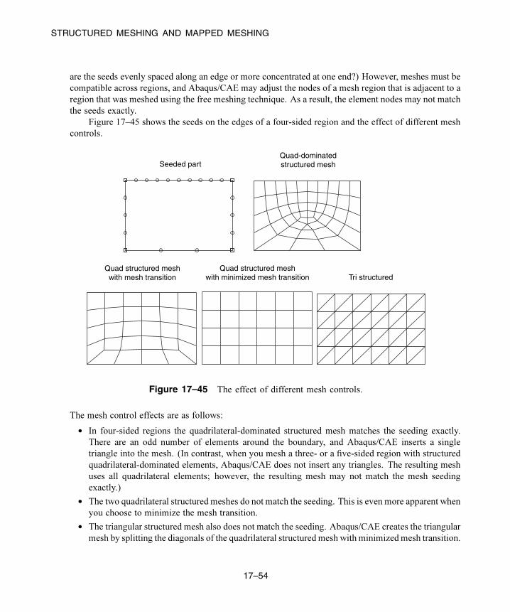
STRUCTURED MESHING AND MAPPED MESHING
are the seeds evenly spaced along an edge or more concentrated at one end?) However, meshes must be
compatible across regions, and Abaqus/CAE may adjust the nodes of a mesh region that is adjacent to a
region that was meshed using the free meshing technique. As a result, the element nodes may not match
the seeds exactly.
Figure 17–45 shows the seeds on the edges of a four-sided region and the effect of different mesh
controls.
Seeded partQuad-dominatedstructured mesh
Quad structured meshwith mesh transition
Quad structured meshwith minimized mesh transition Tri structured
Figure 17–45 The effect of different mesh controls.
The mesh control effects are as follows:
• In four-sided regions the quadrilateral-dominated structured mesh matches the seeding exactly.
There are an odd number of elements around the boundary, and Abaqus/CAE inserts a single
triangle into the mesh. (In contrast, when you mesh a three- or a five-sided region with structured
quadrilateral-dominated elements, Abaqus/CAE does not insert any triangles. The resulting mesh
uses all quadrilateral elements; however, the resulting mesh may not match the mesh seeding
exactly.)
• The two quadrilateral structured meshes do not match the seeding. This is even more apparent when
you choose to minimize the mesh transition.
• The triangular structured mesh also does not match the seeding. Abaqus/CAE creates the triangular
mesh by splitting the diagonals of the quadrilateral structured mesh with minimized mesh transition.
17–54
Abaqus ID:
Printed on:

STRUCTURED MESHING AND MAPPED MESHING
Abaqus/CAE combines edges into a logical side automatically if the edges subtend a shallow angle.
For example, each region in Figure 17–46 has five edges.
Figure 17–46 Edges subtending shallow angles.
However, since the top two edges in each region subtend a shallow angle, Abaqus/CAE considers these
two edges to be one logical side. Therefore, the mesh pattern for four-sided regions is applied to these
regions. If the region contains virtual topology, you can mesh the region using the structured meshing
technique only if the region is bounded by four sides. You cannot use structured meshing to mesh three-
or five-sided regions that contain virtual topology.
You can use the Redefine Region Corners button in the Mesh Controls dialog box to combine
edges yourself, regardless of the angle they subtend. (To display the Mesh Controls dialog box, select
Mesh→Controls from the main menu bar.) This technique allows you to control which structured mesh
pattern is applied to the two-dimensional region. (This technique is not available for three-dimensional
regions.) For more information, see “Redefining region corners,” Section 17.18.4, in the HTML version
of this guide.
The region that you plan to mesh with structured quadrilateral elements must be well shaped;
otherwise, Abaqus/CAE may create invalid elements as shown in Figure 17–47.
corner 1 corner 2 corner 3
corner 4
Figure 17–47 Regions must be well shaped.
If the mesh contains invalid elements, you can use several techniques to correct the mesh:
• Adjust the position of the mesh seeds.
• Redefine the region corners.
• Partition the face into smaller, better shaped regions.
17–55
Abaqus ID:
Printed on:

STRUCTURED MESHING AND MAPPED MESHING
The result of applying each technique is illustrated in Figure 17–48.
adjust seeds
redefine logical corners partition into two five-sided regions
corner 1 corner 2 corner 3
corner 4
corner 1 corner 2 corner 3 corner 4
corner 1
corner 2 corner 3
corner 4corner 5
Figure 17–48 Correcting a mesh that contains invalid elements.
17.8.4 Three-dimensional structured meshingFigure 17–49 illustrates examples of simple three-dimensional regions that can be meshed using the
structured meshing technique.
Meshing more complex regions with this technique may require manual partitioning. If you do not
partition a complex region, your only meshing option may be the free meshing technique with tetrahedral
elements. Meshes constructed using the structured meshing technique consist of hexahedral elements,
which are preferred over tetrahedral elements.
The characteristics described below are required to mesh a three-dimensional region successfully
using the structured meshing technique:
• The region cannot have any holes, isolated faces, isolated edges, or isolated vertices. For example,
the regions shown in Figure 17–50 cannot be meshed using the structured meshing technique.You
can eliminate holes (whether they pass all the way through the part instance or just part way through)
by partitioning their circumferences into halves, quarters, etc. For example, the four partitions in
Figure 17–51 convert the part instance from one region with a hole to four regions without holes.
17–56
Abaqus ID:
Printed on:

STRUCTURED MESHING AND MAPPED MESHING
Figure 17–49 Regions that can be meshed using the structured meshing technique.
holeisolated edges
isolated face
isolated vertices
Figure 17–50 Regions that cannot be meshed using the
structured meshing technique.
���
���
���
��� ��
��
�� ��
���
�
partitions
partitions
Figure 17–51 Partitions can make a part structured meshable.
17–57
Abaqus ID:
Printed on:

STRUCTURED MESHING AND MAPPED MESHING
• You should limit arcs to 90° or less to avoid concavities along sides and at edges. For example, the
part instance in Figure 17–52 has been partitioned so that the single region with 180° arcs becomes
two regions with 90° arcs.
���
��
partition
Figure 17–52 Limit arcs to 90° or less.
• All the faces of the region must have geometries that could be meshed using the two-dimensional
structured meshing technique. For example, without partitioning, the semicircles at either end of the
part in Figure 17–53 have only two sides each. (A face must have at least three sides to be meshed
using the structured meshing technique.) If you partition the part into two halves, each semicircle
is divided into two faces with three sides each.
���
�����
������
����
��
partition
Figure 17–53 Partitioning creates two faces with three sides.
• Exactly three edges of the region must meet at each vertex. For example, the vertex at the top of
an unpartitioned pyramid in Figure 17–54 is connected to four edges. However, if you partition the
pyramid into two tetrahedral regions, the vertex is connected to only three edges for each individual
region.
����������vertex
partition
Figure 17–54 After partitioning the vertex is connected to only three edges for each individual region.
17–58
Abaqus ID:
Printed on:

STRUCTURED MESHING AND MAPPED MESHING
• The region must be bounded by at least four sides (a tetrahedral region). If a region is bounded by
fewer than four sides, you can partition the region as necessary to create additional sides.
• If a region contains virtual topology, the region must be bounded by six sides.
• If a region cannot be meshed using the structured meshing technique, you can use virtual topology to
combine faces until the region is bounded by six sides. Figure 17–55 shows how you can use virtual
topology to create a six-sided region that can be meshed using the structured meshing technique.
3) Apply a structured mesh
2) Region contains virtual topology and is six-sided
1) Combine these three faces using virtual topology
Figure 17–55 Virtual topology can make a part structured meshable.
• The angles between sides should be as close to 90° as possible; you should partition to eliminate
angles greater than 150°.
• Each side of the region must match one of the following definitions:
– If the region is not a cube, a side must correspond to a single face; that is, the side must not
contain multiple faces.
– If the region is a cube, a side can be a connected set of faces that are on the same geometric
surface. However, each face must have four sides. In addition, the pattern of the faces must
allow rows and columns of hexahedral elements to be created in a regular grid pattern along
that entire side when the cube is meshed. For example, Figure 17–56 shows two acceptable
face patterns and the resulting regular grid pattern of elements created by meshing the cubes
using the structured meshing technique.
Figure 17–56 Acceptable face patterns and the resulting meshes.
17–59
Abaqus ID:
Printed on:
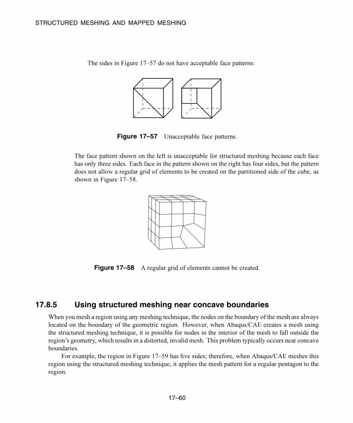
STRUCTURED MESHING AND MAPPED MESHING
The sides in Figure 17–57 do not have acceptable face patterns:
Figure 17–57 Unacceptable face patterns.
The face pattern shown on the left is unacceptable for structured meshing because each face
has only three sides. Each face in the pattern shown on the right has four sides, but the pattern
does not allow a regular grid of elements to be created on the partitioned side of the cube, as
shown in Figure 17–58.
Figure 17–58 A regular grid of elements cannot be created.
17.8.5 Using structured meshing near concave boundaries
When you mesh a region using any meshing technique, the nodes on the boundary of the mesh are always
located on the boundary of the geometric region. However, when Abaqus/CAE creates a mesh using
the structured meshing technique, it is possible for nodes in the interior of the mesh to fall outside the
region’s geometry, which results in a distorted, invalid mesh. This problem typically occurs near concave
boundaries.
For example, the region in Figure 17–59 has five sides; therefore, when Abaqus/CAE meshes this
region using the structured meshing technique, it applies the mesh pattern for a regular pentagon to the
region.
17–60
Abaqus ID:
Printed on:

STRUCTURED MESHING AND MAPPED MESHING
Figure 17–59 The mesh pattern for a regular pentagon is applied to the region.
However, if you seed the region so that the number of elements is reduced, as shown in Figure 17–60,
a distorted mesh results due to the concavity at the highly curved edge. Nodes from the interior of the
mesh pattern (indicated by closed circles in Figure 17–61) fall outside the region’s geometry, while nodes
on the boundary of the mesh (indicated by open circles in Figure 17–61) remain on the boundary of the
region’s geometry.
Figure 17–60 Seeds prescribing a coarser mesh.
When interior nodes fall outside the region’s geometry, you can try the following techniques to improve
the mesh:
• Change the mesh seeds and remesh. For example, the number of elements along the highly curved
edge in Figure 17–59 is greater than in Figure 17–61.
17–61
Abaqus ID:
Printed on:
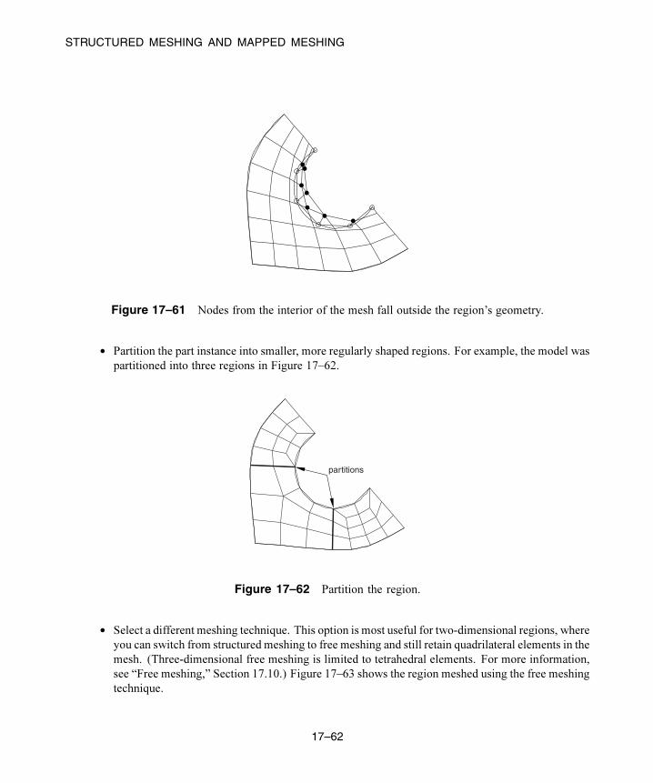
STRUCTURED MESHING AND MAPPED MESHING
Figure 17–61 Nodes from the interior of the mesh fall outside the region’s geometry.
• Partition the part instance into smaller, more regularly shaped regions. For example, the model was
partitioned into three regions in Figure 17–62.
partitions
Figure 17–62 Partition the region.
• Select a different meshing technique. This option is most useful for two-dimensional regions, where
you can switch from structured meshing to free meshing and still retain quadrilateral elements in the
mesh. (Three-dimensional free meshing is limited to tetrahedral elements. For more information,
see “Free meshing,” Section 17.10.) Figure 17–63 shows the region meshed using the free meshing
technique.
17–62
Abaqus ID:
Printed on:

STRUCTURED MESHING AND MAPPED MESHING
Figure 17–63 Mesh the region using the free meshing technique.
The mesh in Figure 17–63 is not symmetric, which is typical of free meshes.
17.8.6 When can Abaqus/CAE apply mapped meshing?
Abaqus/CAE decides that mapped meshing is appropriate in a four-sided region when:
• it is likely that a regular mesh pattern with reasonable quality can be generated, and
• any minor adjustments to the mesh seeding will not violate the user’s intent (as indicated by any
existing seed constraints).
When Abaqus/CAE applies mapped meshing, it makes small adjustments to the mesh seeding to
ensure that opposite sides of the rectangular region have the same number of seeds. If your model is large
and includes many simple regions, it may take slightly longer for Abaqus/CAE to check for rectangular
regions and adjust the seeds to produce a mapped mesh than to produce a mesh without mapped meshing.
However, for most models the time difference to include mapped meshing is not significant compared
to the improvement in mesh quality.
Figure 17–64 shows a shell part meshed with triangles using the following mesh techniques and
algorithms available in Abaqus/CAE:
• Free meshing
• Free meshing using mapped meshing where appropriate
• Structured meshing
17–63
Abaqus ID:
Printed on:

SWEPT MESHING
Originalshell part Free mesh
Free mesh withmapped meshingwhere appropriate
Structuredmesh
Figure 17–64 A shell part meshed with triangles in three different ways.
In many cases a free mesh of triangles with mapped meshing where appropriate will be the same as
a structured mesh of triangles. The meshes are different in Figure 17–64 because Abaqus/CAE honors
the original seeding and determines that mapped meshing is not appropriate on the side of the part. In
contrast, when Abaqus/CAE creates the structured mesh, it significantly adjusts the seeding to create the
structured mesh that was requested by the user.
17.9 Swept meshing
This section explains the swept meshing technique and describes the types of regions to which this
meshing technique can be applied.
17.9.1 What is swept meshing?Abaqus/CAE uses swept meshing to mesh complex solid and surface regions. The swept meshing
technique involves two phases:
• Abaqus/CAE creates a mesh on one side of the region, known as the source side.
• Abaqus/CAE copies the nodes of that mesh, one element layer at a time, until the final side, known
as the target side, is reached. Abaqus/CAE copies the nodes along an edge, and this edge is called
17–64
Abaqus ID:
Printed on:

SWEPT MESHING
the sweep path. The sweep path can be any type of edge—a straight edge, a circular edge, or a spline.
If the sweep path is a straight edge or a spline, the resulting mesh is called an extruded swept mesh.
If the sweep path is a circular edge, the resulting mesh is called a revolved swept mesh.
For example, Figure 17–65 shows an extruded swept mesh. To mesh this model, Abaqus/CAE
first creates a two-dimensional mesh on the source side of the model. Next, each of the nodes in the
two-dimensional mesh is copied along a straight edge to every layer until the target side is reached.
Target sideSource side
Nodes copied from the sourceside to each element layer andto the target side.
Figure 17–65 The swept meshing technique for an extruded solid.
To determine if a region is swept meshable, Abaqus/CAE tests if the region can be replicated by
sweeping a source side along a sweep path to a target side. In general, Abaqus/CAE selects the most
complex side (for example, the side that has an isolated edge or vertex) to be the source side. In some
cases you can use the mesh controls to select the sweep path. If some regions of a model are too complex
to be swept meshed, Abaqus/CAE asks if you want to remove these regions from your selection before
it generates a swept mesh on the remaining regions. You can use the free meshing technique to mesh
the complex regions, or you can partition the regions into simplified geometry that can be structured or
swept meshed.
When you assign mesh controls to a region, Abaqus/CAE indicates the direction of the sweep
path and allows you to control the direction. If the region can be swept in more than one direction,
Abaqus/CAE may generate a very different two-dimensional mesh on the faces that it can select as the
source side. As a result, the direction of the sweep path can influence the uniformity of the resulting
three-dimensional swept mesh, as shown in Figure 17–66. In addition, the sweep path controls the
default orientation of hexahedral and wedge elements that are used to model gaskets, continuum shells,
cylindrical regions using cylindrical elements, and adhesive joints using cohesive elements. For more
17–65
Abaqus ID:
Printed on:

SWEPT MESHING
sweepdirection
sweepdirection
Figure 17–66 The sweep direction can influence the uniformity of the swept mesh.
information, see “Assigning gasket elements to a region,” Section 32.3; “Meshing parts with continuum
shell elements,” Section 25.2; “Swept meshing of cylindrical solids,” Section 17.9.4; and “Creating a
model with cohesive elements using geometry and mesh tools,” Section 21.3.
17.9.2 Swept meshing of surfacesAbaqus/CAE can apply the swept meshing technique only to surface regions that can be replicated by
sweeping a source side along a sweep path to a target side. The sweep path is always an edge; however,
for a surface region the source and target sides are also edges. The surface region can be extruded,
revolved, swept, or planar. In addition, an extruded surface region can include twist, and a revolved
surface region can include translation. You can apply the swept meshing technique to surface regions
using either the Quad or Quad-dominated element shape options.
If you are creating a revolved swept mesh, Abaqus/CAE meshes the source side and revolves that
mesh around the axis of revolution to the source side. The sweep path can be revolved a full 360°. You
must use the Quad-dominated element shape option when the source side touches the axis of revolution
at a point, because a layer of triangular elements is generated at that point. Abaqus/CAE cannot generate
a revolved surface mesh when a single surface touches the axis of revolution at two points, unless the
revolved surface is a sphere.
For example, the source side touches the axis of revolution at the top of the model shown in
Figure 17–67 and a layer of triangular elements is generated at that point. (For more information on
assigning element shapes to a region, see “Choosing an element shape,” Section 17.18.2, in the HTML
version of this guide.)
17.9.3 Swept meshing of three-dimensional solidsAbaqus/CAE can apply the swept meshing technique to solid regions that can be replicated by sweeping
a source side along an edge to the target side. For a three-dimensional solid the sweep path is an edge, but
the source and target sides are faces. Figure 17–68 illustrates an extruded swept mesh—Abaqus/CAE
17–66
Abaqus ID:
Printed on:

SWEPT MESHING
Figure 17–67 A layer of triangular elements.
meshes the source side and extrudes that mesh along an edge to the target side. Figure 17–69 illustrates
a revolved swept mesh—Abaqus/CAE meshes the source side and revolves that mesh about the axis of
the circular edge to the target side.
sourceside
targetside
sweep path
Figure 17–68 The extruded swept meshing technique sweeps
the mesh on the source side along an edge.
If a region is swept meshable, Abaqus/CAE can generate the swept mesh on a region that has been
assigned the Hex, Hex-dominated, or Wedge element shape option. To generate the preliminary two-
17–67
Abaqus ID:
Printed on:

SWEPT MESHING
sourceside
targetside
sweep path
Figure 17–69 The revolved swept meshing technique sweeps
the mesh on the source side along a circular edge.
dimensional mesh on the source side, Abaqus/CAE uses the free meshing technique with the Quad,Quad-dominated, or Tri element shape option, respectively.
You can choose between the medial axis and advancing front meshing algorithms when you mesh
a solid region with hexahedral or hexahedral-dominated elements using the swept meshing technique.
(Abaqus/CAE generates hexahedral and hexahedral-dominated meshes by sweeping the quadrilateral
and quadrilateral-dominated elements generated by the two algorithms from the source side to the target
side.) However, if the region to be meshed contains virtual topology, you can use only the advancing
front algorithm to generate the swept mesh. For more information, see “What is the difference between
the medial axis algorithm and the advancing front algorithm?,” Section 17.7.6, and “Free meshing with
quadrilateral and quadrilateral-dominated elements,” Section 17.10.2.
If you select the advancing front algorithm, Abaqus/CAE will use mapped meshing, if it is
appropriate, to improve the mesh for some regions. (Mapped meshing is the same as structured meshing
but applies only to four-sided regions.) Abaqus/CAE determines whether it is appropriate to replace the
advancing front algorithm with mapped meshing on any of the faces that belong to the source side. For
more information, see “What is mapped meshing?,” Section 17.8.2, and “When can Abaqus/CAE apply
mapped meshing?,” Section 17.8.6. Abaqus/CAE uses mapped meshing to create quadrilateral and
quadrilateral-dominated elements on these appropriate boundary faces and then sweeps the elements
from the source side to the target side to create the hexahedral and hexahedral-dominated elements.
A three-dimensional region can be meshed using the swept meshing technique if it has the following
characteristics:
• Every side that connects the source side to the target side must have only a single face or be
comprised of four-sided combined faces that form a regular grid pattern. Figure 17–70 provides
two examples of acceptable connecting face patterns.
17–68
Abaqus ID:
Printed on:
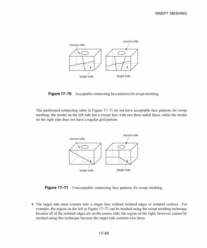
SWEPT MESHING
source side
target side
source side
target side
Figure 17–70 Acceptable connecting face patterns for swept meshing.
The partitioned connecting sides in Figure 17–71 do not have acceptable face patterns for swept
meshing; the model on the left side has a sweep face with two three-sided faces, while the model
on the right side does not have a regular grid pattern.
source side
target side
source side
target side
Figure 17–71 Unacceptable connecting face patterns for swept meshing.
• The target side must contain only a single face without isolated edges or isolated vertices. For
example, the region on the left in Figure 17–72 can be meshed using the swept meshing technique
because all of the isolated edges are on the source side; the region on the right, however, cannot be
meshed using this technique because the target side contains two faces.
17–69
Abaqus ID:
Printed on:

SWEPT MESHING
source side
target side
source side
target side
Figure 17–72 Only the region on the left can be meshed using the swept meshing technique.
Figure 17–73 illustrates a part that has been swept meshed along a varying cross-section. The
part appears to be relatively complex; for example, the source side is nonplanar, and the cross-
section of the part varies along the sweep path. However, the rules for generating a swept mesh still
apply.
– Every side that connects the source side to the target side contains only a single face.
– Although the source side contains two faces, the target side contains only a single face.
target side
sourceside
sweep path
Figure 17–73 Sweeping the mesh along a varying cross-section.
17–70
Abaqus ID:
Printed on:
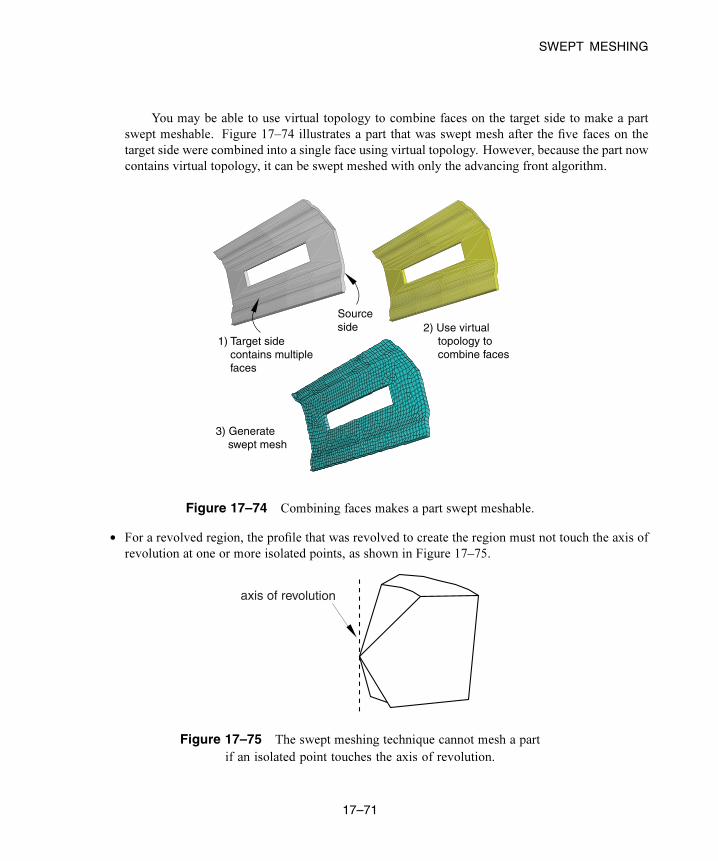
SWEPT MESHING
You may be able to use virtual topology to combine faces on the target side to make a part
swept meshable. Figure 17–74 illustrates a part that was swept mesh after the five faces on the
target side were combined into a single face using virtual topology. However, because the part now
contains virtual topology, it can be swept meshed with only the advancing front algorithm.
1) Target side contains multiple faces
2) Use virtual topology to combine faces
3) Generate swept mesh
Sourceside
Figure 17–74 Combining faces makes a part swept meshable.
• For a revolved region, the profile that was revolved to create the region must not touch the axis of
revolution at one or more isolated points, as shown in Figure 17–75.
axis of revolution
Figure 17–75 The swept meshing technique cannot mesh a part
if an isolated point touches the axis of revolution.
17–71
Abaqus ID:
Printed on:

SWEPT MESHING
• Similarly, Abaqus/CAE cannot mesh a region with hexahedral or wedge elements if one or more
edges lie along the axis of revolution, as shown in Figure 17–76.
axis of revolution
Figure 17–76 Abaqus/CAE cannot mesh a region with hexahedral elements if one
or more edges lie along the axis of revolution.
However, Abaqus/CAE can mesh the region with hexahedral-dominated elements by generating
layers of wedge elements along the axis, as shown in Figure 17–77.
wedgeelements
axis ofrevolution
Figure 17–77 Abaqus/CAE can mesh the region with hexahedral-dominated elements.
As a result, you must select the Hex-dominated element shape option before you mesh the region.
Alternatively, you can partition the region into simple structural mesh regions and select the Hexelement shape option to create the mesh using all hexahedral elements. For more information,
see “Sweep meshing a solid, revolved region whose profile touches the axis of revolution,”
Section 17.18.7, in the HTML version of this guide.
• A fully revolved region that does not touch the axis of revolution is meshable only if all the edges
that are associated with the profile being revolved exist. However, the edges that bound the profile
must not create a face. Figure 17–78 shows a meshable part instance where all of the edges of the
revolved profile exist. In this example the user sketched the profile, and Abaqus/CAE revolved the
profile to create the part; however, the edges that bound the profile do not form a face. In contrast,
Figure 17–79 shows a part instance that is not meshable because some of the edges of the revolved
profile are missing.
17–72
Abaqus ID:
Printed on:

SWEPT MESHING
all profileedges exist
Figure 17–78 All of the edges of the revolved profile exist;
hence, the part instance is meshable.
profile edgesare missing
Figure 17–79 Some of the edges of the revolved profile are
missing; hence, the part instance is not meshable.
• A fully revolved region that touches the axis of revolution is meshable only if all of the edges that
are associated with the profile being revolved exist except the edges along the axis of revolution.
Figure 17–80 shows a part instance that is meshable because all of the edges of the revolved profile
exist except for the edge along the axis of revolution. If the profile included the edge along the axis
of revolution, the part instance would not be meshable.
• If a revolved region was created by revolving a sketch that contains a spline, the region is meshable
only if the vertices at each end of the spline are not on the axis of revolution.
• If a part was created by sweeping a cross-section along a sweep path that is composed of a closed
spline, the resulting part is meshable only if it is split into two or more regions.
17–73
Abaqus ID:
Printed on:

SWEPT MESHING
edge alongaxis of revolutiondoes not exist
Figure 17–80 All of the edges of the revolved profile exist, except for the edge along
the axis of revolution; hence, the part instance is meshable.
17.9.4 Swept meshing of cylindrical solids
You can use swept meshing to create a mesh on cylindrical geometry with many types of solid elements,
including elements from the solid cylindrical element library. If you use solid cylindrical elements
for a native mesh, Abaqus/CAE uses the sweep path of the selected sweep/revolve region as the
circumferential direction for the generated cylindrical elements. You should confirm that the sweep
path is set correctly before creating the mesh.
Abaqus considers the following requirements for cylindrical elements when you attempt to mesh
solid geometry with cylindrical elements:
• The midside nodes on the circular edges of the cylindrical elements must be placed exactly halfway
between the edge nodes.
• All nodes on a cross-section must lie on the same radial plane.
• All the circular edges within an element must span the same angle.
• The centers of the circular arcs within an element must lie on a common axis.
• An element cannot span more than 180°.
These requirements mean that you can create valid cylindrical elements only on revolved parts or
parts that you can split into revolved domains. The S-shaped extrusion in Figure 17–81 can be meshed
with cylindrical elements after partitioning into revolved regions.
17–74
Abaqus ID:
Printed on:

SWEPT MESHING
Figure 17–81 Acceptable geometry for solid cylindrical meshing.
Figure 17–82 shows three types of geometry—a helical spring, a revolved part with cuts, and a tapered
part—that cannot be meshed with solid cylindrical elements because of these meshing requirements.
Figure 17–82 Forms of geometry that cannot be swept
meshed with cylindrical elements.
17–75
Abaqus ID:
Printed on:

SWEPT MESHING
If one of the connecting sides that connect the source face to the target face in a revolved region
is separated into multiple faces due to the internal edge or edges that constrain the mesh, the generated
elements are likely to be too distorted to be used as cylindrical elements. You must partition the solid
region into simpler revolved regions, as shown in the example on the right side of Figure 17–83.
Figure 17–83 A solid region that is unsuitable for meshing with
cylindrical elements (left) and the same region rendered suitable for
meshing with cylindrical elements through the use of a partition (right).
When you edit a mesh part by assigning cylindrical elements to it, Abaqus/CAE considers Face 1
and Face 2 of each cylindrical element to be the faces along its radial planes. Figure 17–84 indicates the
location of these faces for several types of cylindrical elements. You should orient the stack direction
for elements in your part before assigning a cylindrical element type to it; for more information, see the
descriptions in “Orienting the stack direction,” Section 64.6.4, in the HTML version of this guide.
17.9.5 Characteristics of the geometry can prevent a part from beingswept meshable
The characteristics of a region described in “Swept meshing of three-dimensional solids,” Section 17.9.3,
are referred to as “topological characteristics.” In some cases, all of the topological characteristics will
apply to a region; however, Abaqus/CAE will not allow the region to be swept meshed because some
“geometrical characteristics” are not satisfied. The geometric characteristics that Abaqus/CAE looks
for when determining if a region is swept meshable are hard to quantify. In general, a three-dimensional
region can be meshed using the swept meshing technique if it satisfies the following geometrical
characteristics:
• If the source side contains more than one face, the angle between the faces must be relatively flat
(close to 180°).
17–76
Abaqus ID:
Printed on:

SWEPT MESHING
4 3
12 111 2
8 79 10
5 6
315
4
2
13
1
6
17
5
7
19
8
1123
22
10
20
2124
9
12
14
16
12-node element12-node element 24-node element
1
3
2
7
4
8
5
9
6
9-node element
3
9
6
14
513
4
158
16
7
1 10
2
1211
1817
18-node element
18
Figure 17–84 Illustration of node ordering and face numbering
for cylindrical elements (with Faces 1 and 2 shaded).
• Each face that connects the source side to the target side (a connecting side) must have four corners.
The angle at each of the corners must be close to 90°.
• The angles between the source side and each of the connecting sides should be close to 90°.
Similarly, the angles between the target side and each of the connecting sides should be close to
90°.
For example, Figure 17–85 shows a part with three faces on the source side. When the angle decreases
between the faces that form the source side, the part no longer satisfies the geometric characteristics of
a swept meshable region.
You may be able to apply virtual topology to satisfy the geometrical characteristics and to make the
part swept meshable. For example, Figure 17–86 illustrates that the part becomes swept meshable when
the three faces on the source side are combined using virtual topology. However, the resulting mesh is
of poor quality.
17–77
Abaqus ID:
Printed on:

SWEPT MESHING
part cannotbe sweptmeshed
Figure 17–85 Swept meshing depends on geometrical characteristics.
virtualtopology
sweptmesh
Figure 17–86 Applying virtual topology can result in poor mesh quality.
17–78
Abaqus ID:
Printed on:

FREE MESHING
In some cases Abaqus/CAE will still allow you to create a swept mesh, even though the geometrical
characteristics are not satisfied. The intention is to allow you to create a swept mesh wherever possible.
However, the resulting mesh may be of poor quality, or it may be invalid. To ensure that your swept
mesh is acceptable, you should use the mesh verify tool to verify its quality. For more information, see
“Verifying element quality,” Section 17.19.1, in the HTML version of this guide.
17.10 Free meshing
This section explains how you can use the free meshing technique to mesh two- or three-dimensional
models.
17.10.1 What is free meshing?Unlike structured meshing, free meshing uses no preestablished mesh patterns. When you mesh a region
using the structured meshing technique, you can predict the pattern of the mesh based on the region
topology. In contrast, it is impossible to predict a free mesh pattern before creating the mesh.
Because it is unstructured, free meshing allows more flexibility than structured meshing. The
topology of regions that you mesh with the free mesh technique can be very complex.
You can use this technique to mesh a region with the Tri, Quad, or Quad-dominated element
shape options for two-dimensional regions or the Tet element shape option for three-dimensional
regions. For more information on assigning element shapes to a region, see “Choosing an element
shape,” Section 17.18.2, in the HTML version of this guide.
17.10.2 Free meshing with quadrilateral and quadrilateral-dominatedelements
Free meshing with quadrilateral elements is the default meshing technique for two-dimensional regions.
The free meshing technique with quadrilateral elements can be applied to any planar or curved surface.
An example of a mesh generated with this technique is shown in Figure 17–87. Free meshes are usually
not symmetric, even if the part or part instance itself is symmetric.
Abaqus/CAE allows you to choose between twomeshing algorithms when you create a quadrilateral
or quadrilateral-dominated mesh. For more information, see “What is the difference between the medial
axis algorithm and the advancing front algorithm?,” Section 17.7.6.
Medial axis
When you free mesh a complex region with quadrilateral elements using the medial axis algorithm,
Abaqus/CAE creates internal partitions that divide the region into simple structured mesh regions
and then seeds the smaller regions.
17–79
Abaqus ID:
Printed on:

FREE MESHING
Figure 17–87 A free mesh generated with quadrilateral elements.
If you use the medial axis algorithm to mesh a region and then remesh the region (for example,
after modifying the seeds), Abaqus/CAE stores the internal partitions, and the newmesh is generated
more quickly. In addition, the internal partitions allow Abaqus/CAE to generate a fine mesh in a
similar time to that required to generate a coarse mesh. You cannot use the medial axis algorithm
to mesh regions that contain virtual topology, and it does not work well with imprecise parts.
In general, a medial axis-based free mesh with quadrilateral elements does not match the mesh
seeds exactly for the following reasons:
• Abaqus/CAE tries to balance the seeds between adjacent regions and the smaller regions
created by the internal partitioning.
• Abaqus/CAE tries to minimize element distortions.
However, when you apply fixed seed constraints, Abaqus/CAEmatches the number of seeds exactly
and attempts to match the seed positions exactly. Figure 17–88 illustrates a two-dimensional plate
with fixed seeds and movable seeds and the resulting all quadrilateral mesh. You should specify
fixed seeds on only a few edges, or Abaqus/CAE may not be able to generate a mesh. For example,
if you specify fixed seeds around one of the holes in the plate shown in Figure 17–88, the global
seeding becomes overconstrained, and Abaqus/CAE cannot generate a mesh.
Using the medial axis algorithm, a free mesh generated with quadrilateral-dominated
elements is similar to a free mesh generated with all quadrilateral elements and without transition
minimization; however, Abaqus/CAE inserts a few isolated triangles in an effort to match the mesh
seeds more closely. Abaqus/CAE can generate a mesh with quadrilateral-dominated elements
faster than it can generate a mesh with all quadrilateral elements.
17–80
Abaqus ID:
Printed on:

FREE MESHING
Figure 17–88 Fixed and movable seeds and the medial axis meshing algorithm.
Advancing front
When you free mesh a complex region with quadrilateral elements using the advancing front
algorithm, Abaqus/CAE generates quadrilateral elements at the boundary of the region and
continues to generate quadrilateral elements as it moves systematically to the interior of the region.
When you choose the advancing front algorithm, Abaqus/CAE matches the seeds exactly
(except when you are creating a three-dimensional revolved mesh, and the profile being revolved
touches the axis of revolution). A quadrilateral mesh that matches the seeds exactly is shown in
Figure 17–89. In general, the mesh transitions generated with the advancing front algorithm are
more acceptable than the transitions generated by the medial axis algorithm; however, matching
the seeds exactly in narrow regions may compromise the mesh quality. In contrast with the medial
axis algorithm, you can use the advancing front algorithm in conjunction with imprecise parts and
on regions that contain virtual topology.
If you select the advancing front algorithm, Abaqus/CAE will also use mapped meshing
where appropriate. (Mapped meshing is the same as structured meshing but applies only to
four-sided regions.) For more information, see “What is mapped meshing?,” Section 17.8.2, and
“When can Abaqus/CAE apply mapped meshing?,” Section 17.8.6. When mapped meshing is
used, Abaqus/CAE makes minor adjustments to the mesh seeding. If you do not want the seeding
to change, you can use mesh controls to prevent the use of mapped meshing. For more information,
see “Assigning mesh controls,” Section 17.18.1, in the HTML version of this guide.
By default, Abaqus/CAE minimizes the mesh transition when it generates a free quadrilateral mesh
using the medial axis algorithm. Minimizing the mesh transition results in a better mesh that is generated
more quickly; however, the generated nodes deviate further from themesh seeds. Figure 17–90 illustrates
the same planar part instance meshed using the medial axis algorithm with and without minimizing the
mesh transition and meshed using the advancing front algorithm.
17–81
Abaqus ID:
Printed on:

FREE MESHING
Figure 17–89 Fixed and movable seeds and the advancing front meshing algorithm.
medial axisalgorithm
advancing frontalgorithm
minimize mesh transitiontoggled on (default)
minimize mesh transitiontoggled off
Figure 17–90 The effect of mesh transition and the meshing algorithm.
17–82
Abaqus ID:
Printed on:

FREE MESHING
17.10.3 Free meshing with triangular and tetrahedral elements
Free meshing with triangular elements can be applied to any planar or curved surface, and the part can
be precise or imprecise. For more information, see “What is a valid and precise part?,” Section 10.2.1.
A free mesh of triangular elements matches the mesh seeds exactly. This meshing technique can handle
large variations in element size, which is useful when you want to refine only part of a mesh. The time
taken for Abaqus/CAE to compute a free triangular mesh grows approximately linearly with the number
of elements and nodes. Figure 17–91 shows an example of a mesh generated using this technique.
Figure 17–91 A free mesh generated with triangular elements.
Free meshing with tetrahedral elements can be applied to almost any three-dimensional region; in
fact, very complex models can be meshed using this technique without the help of partitioning. Free
meshing with tetrahedral elements is similar to free meshing with triangular elements in that the part can
be precise or imprecise. In general, Abaqus/CAEmatches the mesh seeds exactly although the mesh may
be finer around small holes if the mesh seeds are not fully constrained. Figure 17–92 shows an example
of a free tetrahedral mesh. Free meshing of three-dimensional solids using hexahedral elements is not
supported.
You should use the Query toolset in the Part module or the Mesh module to check the geometry of
the parts or of the assembly before you try to generate a free mesh with tetrahedral elements. You should
check the following:
• There are no free edges in the solid.
• There are no short edges, small faces, or small face corner angles.
17–83
Abaqus ID:
Printed on:

FREE MESHING
Figure 17–92 A free mesh generated with tetrahedral elements.
For more information, see “Using the geometry diagnostic tools,” Section 71.2.4, in the HTML version
of this guide.
When you create a free mesh with tetrahedral elements, you can use the default mesh generation
algorithm, or toggle off the default algorithm to use the algorithm that was includedwith Abaqus/CAE 6.4
and earlier. The default algorithm is significantly more robust, particularly when meshing complex
shapes and thin solids. In addition, the default algorithm allows you to increase the size of the interior
elements. If the mesh density is adequate for the model being analyzed and the areas of interest are on the
mesh boundary, increasing the size of the interior elements will increase the computational efficiency.
When you are using free meshing to create triangular elements on a surface, Abaqus/CAE will
use mapped meshing for some regions if it is appropriate. (Mapped meshing is the same as structured
meshing but applies only to four-sided regions.) For more information, see “What is mapped meshing?,”
Section 17.8.2, and “When can Abaqus/CAE apply mapped meshing?,” Section 17.8.6. Abaqus/CAE
replaces free triangular meshing with mapped triangular meshing only when it is likely that the resulting
mesh quality will be improved. If desired, you can use mesh controls to prevent Abaqus/CAE from
allowing mapped meshing. For more information, see “Assigning mesh controls,” Section 17.18.1, in
the HTML version of this guide.
Similarly, when you are using free meshing to create tetrahedral elements, you can allow
Abaqus/CAE to decide whether mapped meshing is appropriate. After Abaqus/CAE determines that
the resulting mesh quality will be improved, it replaces free meshing with mapped meshing on simple
boundary faces and converts the resulting triangles into tetrahedral elements.
Figure 17–93 shows the effect of allowing mapped meshing where appropriate in a free mesh of
a solid part using tetrahedral elements. The mesh quality is improved in four-sided regions that can be
mapped meshed.
To view the internal tetrahedral elements generated by Abaqus/CAE, you can create a new mesh
part from the current mesh and use display groups to remove selected elements. You can also view the
internal elements after the analysis is complete by using view cuts in the Visualization module. For more
information, see Chapter 78, “Using display groups to display subsets of your model,” and Chapter 80,
“Cutting through a model.”
17–84
Abaqus ID:
Printed on:

FREE MESHING
Free meshing Free meshing with mapped meshing where appropriate
Figure 17–93 The effect of allowing mapped meshing.
17.10.4 What is a tetrahedral boundary mesh?When Abaqus/CAE generates a free mesh on a solid with tetrahedral elements, the meshing process
consists of two phases:
1. A boundary mesh of triangles is generated on the faces of the solid regions.
2. Abaqus/CAE generates a tetrahedral mesh using the triangles as faces of the tetrahedral elements.
The same process is used to create a quadrilateral boundary mesh and a hexahedral solid mesh for
geometric faces of bottom-up mesh regions (for more information, see “Creating the boundary mesh
for a bottom-up region,” Section 17.11.5).
If your part is complex, generating a free tetrahedral mesh can be time consuming. Previewing
the mesh on the boundary faces can help you identify problems before generating a mesh for the entire
part. You can preview the triangles on the boundary faces after the first phase of the meshing process by
toggling on Preview boundary mesh in the prompt area before you generate the mesh. If the mesh is
acceptable, you can continue meshing the interior of the region. If the mesh is not acceptable or if some
regions failed to mesh, Abaqus/CAE provides a variety of tools for correcting the problems. For more
information, see “What can I do with a boundary mesh?,” Section 17.10.5.
If you decide to preview the triangular boundary mesh for a region, Abaqus/CAE allows you to
select faces to mesh even though your final intent is to mesh a solid. When you toggle on Previewboundary mesh, Abaqus/CAE automatically changes the selection filter in the prompt area to select
Faces. For more information, see “Filtering your selection based on the type of object,” Section 6.3.2.
17–85
Abaqus ID:
Printed on:

FREE MESHING
When the Mesh defaults color mapping is selected, Abaqus/CAE displays a boundary mesh using
white to represent the boundary elements, which is in contrast to the cyan color that Abaqus/CAE uses
to represent the final mesh. When you query the tetrahedral boundary mesh, Abaqus/CAE refers to the
elements as Tri boundary elements. In contrast, when you query the final mesh, Abaqus/CAE refers
to the elements as Linear tetrahedral elements or Quadratic tetrahedral elements. The triangleson the boundary faces have no concept of geometric order.
17.10.5 What can I do with a boundary mesh?When Abaqus/CAE generates a free mesh on a solid with tetrahedral elements, it first generates a
boundary mesh of triangles on the exterior faces of the solid regions, as described in “What is a
tetrahedral boundary mesh?,” Section 17.10.4.
When you are creating a free tetrahedral mesh, Abaqus/CAE can create either a free mesh or a
mapped mesh on the boundary faces; two mechanisms control the mesh pattern for this triangular surface
mesh:
• Global mesh control associated with the three-dimensional region: Global controls
always exist. They are set when you assign the free tetrahedral meshing technique to the region.
You can use them to create a mapped mesh in areas where Abaqus/CAE determines that mapped
meshing is appropriate or to create a free mesh on all bounding faces.
• Local mesh controls specified on selected faces of the region: To assign local controls,
you select one or more faces of the region and specify whether Abaqus/CAE should create a free
mesh or a mapped or structured mesh on the selection. If you define local controls, they override
the global controls.
If you assign the structured technique to faces of solid regions that will be tetrahedral meshed, these faces
are colored green to show the technique assignment for the surface mesh. (For detailed instructions on
assigning mesh controls, see “Assigning mesh controls,” Section 17.18.1, in the HTML version of this
guide.)
Note: The green coloring is applied only while you are assigning mesh controls to the faces. When the
procedure ends, the global mesh control colors are displayed.
In addition, Abaqus/CAE highlights any faces on the boundary that failed to mesh. These failures
are usually due to mesh seeding that is too coarse or to tiny edges or faces. You can save the highlighted
faces in a set, and you can apply finer seeds to only the faces in the set. For more information about
seeding faces in a set, see “Can I seed a face or a cell?,” Section 17.4.2. You can use display groups to
display only the faces in the set. For more information, see “Plotting display groups,” Section 78.2.4, in
the HTML version of this guide.
You can query a boundary mesh using the Query toolset. In addition, you can check the quality of
a boundary mesh using the mesh verify tool. The mesh verify tool allows you to check the quality of all
boundary triangles, or you can use the selection filters to check the quality of the boundary triangles of
only selected faces.
17–86
Abaqus ID:
Printed on:

BOTTOM-UP MESHING
If tiny edges or faces prevent Abaqus/CAE from generating an acceptable tetrahedral mesh, you
can try the following:
• Use the geometry diagnostics tool to find small entities such as short edges, small faces, and faces
with small face corner angles that can affect the mesh quality. You can create a set containing these
small entities. For more information, see “Using the geometry diagnostic tools,” Section 71.2.4, in
the HTML version of this guide.
• Use the Geometry Edit toolset to remove redundant edges and vertices. You can also remove a face
and stitch over the resulting gap. For more information, see “An overview of editing techniques,”
Section 69.2.
• Use the Virtual Topology toolset to ignore tiny edges or faces. For more information, see “What
can I do with the Virtual Topology toolset?,” Section 75.2.
• Add partitions to reduce the aspect ratio of long, narrow faces or cells. For more information, see
Chapter 70, “The Partition toolset.”
• Use the Edit Mesh toolset to modify the preview mesh. You can do the following in the Mesh
module:
– Edit nodes
– Collapse element edges
– Swap the diagonal of a pair of adjacent triangular elements
– Split element edges
For more information, see “What can I do with the Edit Mesh toolset?,” Section 64.1.
In some cases you will not be able to mesh an imported solid part with tetrahedral elements because
of very thin triangular elements in the surface mesh or because some sliver faces cannot be meshed
with triangles. “Using a combination of tools to mesh an imported solid part with tetrahedral elements,”
Section 64.3.6, describes how you can use the Edit Mesh toolset and other tools in the Mesh module to
mesh the part successfully.
17.11 Bottom-up meshing
This section explains the bottom-up meshing technique and describes the types of regions to which
this meshing technique can be applied. The related topic of mesh associativity is also explained. The
following topics are covered:
• “What is bottom-up meshing?,” Section 17.11.1
• “The bottom-up meshing domain,” Section 17.11.2
• “Bottom-up meshing methods,” Section 17.11.3
• “Selecting parameters for a bottom-up mesh,” Section 17.11.4
• “Creating the boundary mesh for a bottom-up region,” Section 17.11.5
17–87
Abaqus ID:
Printed on:

BOTTOM-UP MESHING
• “Improving the quality of boundary meshes for a bottom-up region,” Section 17.11.6
• “Defining connecting sides for a bottom-up swept mesh,” Section 17.11.7
In addition, the following sections are available in the HTML version of this guide:
• “Creating a bottom-up mesh,” Section 17.11.8
• “An example including bottom-up meshing techniques,” Section 17.11.9
17.11.1 What is bottom-up meshing?Bottom-up meshing is a manual, incremental meshing process that allows you to build a hexahedral mesh
in any solid region. Structured, swept, and free meshing techniques all work in a top-downmanner—they
are tied directly to the geometry such that the resulting mesh fills the geometry. Bottom-up meshing
relaxes the constraint that ties the mesh to the geometry so that you can build a mesh that ignores some
geometric features. You can also use bottom-up meshing techniques to modify a mesh part, in which
case there are no geometric features to consider. If you work with geometry, the elements that you
create in a bottom-up mesh are always associated with the solid region that you meshed, but the mesh
boundaries may not be associated with the geometric boundaries of the region. This allows you to create
a mesh using only hexahedral elements where top-down meshing techniques might require extensive
partitioning or the use of tetrahedral elements to complete the mesh. However, the relaxed geometry
constraints also mean that you must carefully choose the parameters used to create the mesh, since it
can vary significantly from the geometry. Once Abaqus has generated a bottom-up mesh, you need to
evaluate whether it is suitable for the analysis and, if geometry is present, verify that the mesh is correctly
associated with it.
You can apply bottom-up meshing to any solid region, including regions that can be meshed using
the top-down techniques, and to meshes that do not have any associated geometry. Since bottom-up
meshing is a manual process that can be very time consuming, it is recommended that you use this method
only when the top-down methods fail to produce a satisfactory mesh.
Generating the desired mesh may require multiple applications of the bottom-upmeshing technique.
If multiple applications are required, each bottom-up mesh becomes an incremental building block for
the next mesh until you complete the mesh for the region. Each application of the bottom-up meshing
technique involves four phases:
1. You select the domain within which Abaqus/CAE will create the mesh. You can choose either a
three-dimensional geometry region or orphan elements.
2. You select the method that Abaqus/CAE will use to create the mesh. You can choose from the
following methods:
• Sweep
• Extrude
• Revolve
• Offset (available only for orphan element selections)
17–88
Abaqus ID:
Printed on:

BOTTOM-UP MESHING
3. You select the side, called the source side, that Abaqus/CAE will use to create a two-dimensional
mesh to be swept, extruded, or revolved to fill a three-dimensional region.
4. You select the remaining parameters to complete the definition of the bottom-upmesh. For example,
if you chose the sweep method, you can choose connecting sides and a target side.
In addition, you may need to edit bottom-up meshes or associate them with geometry before you can use
them to continue generating the region mesh. For more information, see Chapter 64, “The Edit Mesh
toolset.”
Figure 17–94 shows a part that cannot be meshed with hexahedral elements using top-down
techniques.
Figure 17–94 Complex geometry such as fillets can prevent top-down meshing.
The bottom-up sweep method was used to mesh the part in Figure 17–95. The user selected six faces
for the source side (magenta), selected the hidden rear face as the target side (white), and used the six
remaining sides as connecting sides (yellow), as indicated in the figure. In this example the selected
sides are all geometric faces; Abaqus/CAE also allows you to select element faces and two-dimensional
elements to define the source side and the connecting sides of a bottom-up mesh.
You can choose from the sweep, extrude, or revolve methods to mesh a selected geometric region,
and you can also choose the offset method if you are working with orphan elements. Depending on the
shape of the region and the analysis intent, more than one method may produce acceptable results. The
method that you select and the corresponding parameters will determine how well the mesh conforms to
the geometry, if applicable. For example, Figure 17–96 shows the same part as Figure 17–95; this time
the part is meshed with the extrude method. The parameters for the extrude method are a source side, an
extrusion vector, and a number of layers. As shown in Figure 17–96, the extruded mesh does not capture
the tapered sides and the rounded corners at the back of the model. If these details are not important,
this simplified mesh may be acceptable. Alternatively, you could edit the resulting mesh by modifying
17–89
Abaqus ID:
Printed on:

BOTTOM-UP MESHING
connectingsides
target side
connectingsides
sourceside
Figure 17–95 A bottom-up mesh using the sweep method.
Number of layers
Figure 17–96 A bottom-up mesh using the extrude method.
or removing the nodes and elements that extend beyond the original geometry. For more information on
editing a mesh, see Chapter 64, “The Edit Mesh toolset.”
If a resulting bottom-up mesh is not acceptable, you can delete it and try a different bottom-up
method for the same region or partition the region and mesh the resulting simpler regions. You can also
use the mesh Undo and Redo functions to undo steps in the bottom-up meshing procedure rather than
deleting the entire bottom-up mesh for the region and starting over.
Note: Undo and redo are not available after some operations, such as deleting a region mesh.
The undo and redo functions are the same as those used for the Edit Mesh toolset (for more information,
see “Undoing or redoing a change in the Edit Mesh toolset,” Section 64.9, in the HTML version of this
guide).
17–90
Abaqus ID:
Printed on:

BOTTOM-UP MESHING
17.11.2 The bottom-up meshing domain
When you begin creating a bottom-up mesh, the first requirement is to define the domain in which the
mesh will be created. The domain determines whether the bottom-up mesh is created as a native mesh or
as a collection of orphan nodes and elements. To create a native mesh, you choose a three-dimensional
geometric model region that has been assigned the bottom-up meshing technique in the Mesh Controlsdialog box. (For more information, see “Assigningmesh controls,” Section 17.18.1, in the HTMLversion
of this guide.) If there are no geometric regions with the bottom-up technique assigned, you must create
one or use the orphan element domain.
Selecting a three-dimensional region as the domain also indicates that you intend to fully associate
the bottom-up mesh with geometry. The association between mesh and geometry is necessary to transfer
loads, boundary conditions, and other information from the geometry to the mesh. Mesh-geometry
association is discussed in “Mesh-geometry association,” Section 17.12.
Selecting orphan elements as the domain indicates that the bottom-up mesh will not be fully
associated with geometry. The created elements may either have no association with geometry, or you
may associate the created orphan mesh entities with adjacent geometric faces. Associating the orphan
mesh faces with adjacent geometric faces allows Abaqus/CAE to create a compatible mesh when you
mesh the geometry.
17.11.3 Bottom-up meshing methods
The control parameters for each bottom-up method are similar to the parameters used internally by
Abaqus/CAE to create a comparable top-down swept mesh for a three-dimensional solid. The bottom-up
methods and associated parameters are defined as follows:
Sweep
The sweep method creates a three-dimensional mesh by moving a two-dimensional mesh along
a sweep path. The sweep method is illustrated in Figure 17–95. You should use the bottom-up
sweep meshing method when the region cross-section changes between the starting and ending
sides. To use the sweep method, you must first choose a Source side that defines the face or
faces on which Abaqus/CAE will create a two-dimensional mesh. The source side can be any
combination of geometric faces, element faces, and two-dimensional elements. You can define the
sweep path by selecting Connecting sides that define the sides of the desired sweep region. If
you define connecting sides, the mesh conforms closely to the geometry or mesh along the selected
sides. Alternatively, for geometry you can select a Target side and specify a Number of layersand allow Abaqus/CAE to create the sweep path by interpolating between the source and target
sides. The Target side is a single face that Abaqus/CAE uses to end the mesh. The number of
layers refers to the number of element layers that will be placed between the source and the target
sides—if you use connecting sides, the two-dimensional meshes of the connecting sides define the
17–91
Abaqus ID:
Printed on:

BOTTOM-UP MESHING
number of element layers. Abaqus/CAE sweeps the two-dimensional mesh from the source side
into the volume of the solid region to create the mesh.
Extrude
The extrude method is a special case of the sweep method with a linear path defined by a direction
and a distance. The extrude method is illustrated in Figure 17–96. You should use the extrude
method for regions with a constant cross-section and a linear sweep path. There are three required
parameters for a bottom-up extruded mesh. As with the sweep method, you choose the Sourceside that defines the area on which Abaqus/CAE will create a two-dimensional mesh. You then
select the starting and ending point of a Vector that defines the extrusion direction and can also
be used to define the extrusion distance. Finally, you indicate the Number of layers to define the
number of elements between the source side and the end of the extruded mesh. If you use the vector
to define the extrusion distance, the definition is complete. However, you can Specify a distance
or use Project to target and select a target side to define the extrusion distance. The target side
can be selected from any geometry, mesh, or datum plane in the viewport; it need not be part of
the same part instance as the source. Abaqus/CAE extrudes the two-dimensional mesh from the
source side in the direction of the extrusion vector. If you select a target side to define the extrusion
distance, Abaqus/CAE ends the extruded mesh at the target side. Figure 17–97 shows the source
side and target side on the left; the extrusion vector (not shown) extends from the center of the
rectangular source side to the center of the cylinder. The resulting extruded mesh is an extension of
the source side mesh. It closely matches the target side shape, but no attempt is made to match the
node positions of the mesh on the target side.
Figure 17–97 The optional target side (colored white) is used to define the extrusion distance.
The Bias ratio parameter defines a change in the element thickness between the source side
and the end of an extruded bottom-up mesh in which more than one layer is created. The bias ratio
17–92
Abaqus ID:
Printed on:

BOTTOM-UP MESHING
is the ratio of the thickness of the first layer of elements in the extruded mesh to the thickness of the
last layer of elements. The default bias ratio of 1.0 has equal thickness elements throughout the
extrusion distance.
Revolve
The revolve method is another special case of the sweep method. In this case the sweep path is a
circular path defined by an axis and an angle of revolution. The revolve method is illustrated in
Figure 17–98. You should use this method for regions with a constant cross-section and a circular
sweep path. As with the sweep and extrude methods, you choose the Source side that defines the
area on which Abaqus/CAE will create a two-dimensional mesh. The source side cannot intersect
the axis of revolution, but it may contain edges that coincide with the axis. If so, the elements
contacting the axis create a layer of wedge elements in the revolved mesh. The source side should
not include any triangular elements along the axis of revolution. You then select the starting and
ending point of an Axis that defines the axis of revolution. Finally, you indicate the Angle and
the Number of layers to define the number of elements between the source side and the end of
the revolved mesh. Abaqus/CAE revolves the two-dimensional mesh from the source side by the
specified angle and evenly divides the resulting region into the desired number of element layers.
The direction of revolution is clockwise if you look along the axis of revolution from the starting
point to the ending point.
Axis
Source side
Number of layers
Figure 17–98 The bottom-up revolve method sweeps the source side mesh by
the specified angle about the axis.
Offset
The offset method works the same as Offset (create solid layers) in the Edit Mesh toolset; it
creates one or more layers of solid elements by offsetting the selected elements. Offset is available
17–93
Abaqus ID:
Printed on:

BOTTOM-UP MESHING
only when you are working with orphan elements. To create an offset bottom-up mesh, you enter a
total thickness for the offset elements and the desired number of element layers. You can create an
element set or extend an existing set, but you cannot create top and bottom surfaces as you can with
the Edit Mesh toolset. If you select shell elements as the source, youmust indicate in the prompt area
the desired offset direction; you can offset shell elements in both directions. If your shell element
selection contains sharp corners, toggle on Constant thickness around corners to maintain the
same total thickness where the elements meet in the corner as in the rest of the selection. Using
this option can reduce element distortion and prevent collapsed elements, especially if elements are
offset to the inner side of a corner (for more information, see “Reducing element distortion and
collapse during mesh offsetting,” Section 64.3.3).
17.11.4 Selecting parameters for a bottom-up meshThe parameters that you use to create a bottom-up mesh are similar to those that Abaqus/CAE uses
to create a comparable top-down swept mesh. In the top-down meshing methods, Abaqus/CAE
automatically selects the required geometric sides for the region. Top-down swept meshes—including
extruded and revolved meshes—are discussed in “Swept meshing of three-dimensional solids,”
Section 17.9.3. The parameters used in the bottom-up mesh methods are described below.
Source side
The Source side is a required parameter that defines the face or faces on which Abaqus/CAE
will create a two-dimensional mesh that will be swept, extruded, or revolved to create a three-
dimensional mesh. The source side may be a combination of geometric faces, element faces, and
two-dimensional elements; you can also select saved surfaces instead of selecting from the viewport.
For a top-down mesh Abaqus/CAE limits the angularity between multiple faces that it selects as the
source side (for more information, see “Characteristics of the geometry can prevent a part from
being swept meshable,” Section 17.9.5). There is no limit on the angle between the faces that you
can select as the source side of a bottom-up mesh. However, increased angles between the source
side faces or between the sourcewill result in decreased quality in the three-dimensional elements.
Connecting sides
Connecting sides define the direction of a swept region. Connecting sides may be a combination
of geometric faces, element faces, and two-dimensional elements. Every connecting side must have
only a single four-sided geometric face or be comprised of four-sided combined geometric faces,
element faces, and two-dimensional elements that form a regular grid pattern.
In a top-down swept mesh Abaqus/CAE creates connecting sides along all edges of the source
side. The connecting sides extend completely from the source side to the target side. In a bottom-up
swept mesh connecting sides are optional for geometry, but it is recommended that you include as
many connecting sides as possible. Connecting sides help to control the mesh as it is swept through
the three-dimensional region and enforce associativity in the resulting mesh. Including connecting
sides reduces the amount of work needed to clean up and associate the bottom-up swept mesh with
the geometry. Connecting sides for a bottom-up mesh may extend completely from the source side
17–94
Abaqus ID:
Printed on:

BOTTOM-UP MESHING
to the target side or they may cover only part of the distance. They may also be used without a target
side, in which case the end of the connecting sides defines the end of the bottom-up swept mesh. For
more information, see “Defining connecting sides for a bottom-up swept mesh,” Section 17.11.7.
Target side
The Target side defines the end of a swept mesh or an extruded mesh. You cannot select a target
side for revolved or offset bottom-up meshes. The target side of a swept mesh must be a single
geometric face; the target side for an extruded mesh can be one or more geometric faces, a group of
element faces, or a datum plane. The target side is not required for a swept mesh unless you have
not included any connecting sides. However, including a target side helps you control the mesh
and, if applicable, enforce associativity of the mesh to geometry. Abaqus/CAE creates a mesh for
the target side by projecting the nodes from the source side if connecting sides are not used or from
the last layer of nodes if connecting sides are used. The projected nodes may be positioned outside
of the selected geometric target side. The target side is optional for an extruded mesh and is used
only to establish the extrusion distance; selection of mesh faces for a target side will not change the
extruded mesh to conform to the existing nodes and element faces.
Number of layers
The Number of layers parameter defines the number of layers of elements that Abaqus/CAE
generates along the sweep, extrude, or revolve direction. If you select the bottom-up sweep method
and select connecting sides, the number of element layers is driven by the mesh or seeding of the
connecting sides, similar to the top-down meshing techniques. If you do not select connecting sides
for the sweep method or if you choose the extrude or revolve methods, you must specify how many
element layers Abaqus/CAE should generate.
Vector
The Vector parameter defines the extrusion direction and, optionally, the distance for an extruded
mesh. You select an extrusion vector by picking a start point and an end point from the nodes,
vertices, datum points, and interesting points in the viewport. Abaqus/CAE extrudes the mesh from
the source side by the direction and, if applicable, distance of the vector regardless of where in the
viewport you define the vector.
Axis
The Axis parameter defines the axis of revolution for a revolved mesh. You can define the axis of
revolution by selecting two vertices, nodes, datum points, or interesting points from the viewport.
Angle
The Angle parameter defines the angle of revolution for a revolved mesh. You must specify the
angle of revolution for the bottom-up revolve technique to indicate where Abaqus/CAE should end
the revolved mesh.
17–95
Abaqus ID:
Printed on:

BOTTOM-UP MESHING
Bias ratio
The Bias ratio parameter defines a change in the element thickness between the source side and
the end of an extruded bottom-up mesh in which more than one layer is created. The bias ratio is
the ratio of the thickness of the first layer of elements in the extruded mesh to the thickness of the
last layer of elements. A bias ratio less than one creates thinner layers near the source side, a ratio
of exactly one has equal thickness layers throughout, and a ratio greater than one creates thicker
layers near the source side. Abaqus/CAE evenly distributes the bias through the number of layers
in the extrusion.
As you select the parameters to define a bottom-up mesh, consider not only the shape of the current
bottom-up mesh but also the desired final mesh shape. Many complex parts will require several bottom-
up meshing iterations to generate a complete mesh. For example, you may use connecting sides or
element faces of a bottom-up swept mesh as the source side of a bottom-up extruded mesh. If you
cannot completely mesh the selected region in the current iteration, consider how you can add another
bottom-up mesh or use the Edit Mesh toolset to complete the mesh. For a detailed, step-by-step example
of combining top-down and bottom-up techniques to mesh a part, see “An example including bottom-up
meshing techniques,” Section 17.11.9, in the HTML version of this guide.
17.11.5 Creating the boundary mesh for a bottom-up regionWhen you create a bottom-up mesh for a geometric region, the meshing process consists of two phases:
1. A boundary mesh of quadrilateral elements is generated on the source side—and on the connecting
sides of a swept mesh if they are included.
2. Abaqus/CAE generates a hexahedral mesh using the quadrilateral elements as faces of the
hexahedral elements.
Creating a boundary mesh allows you to preview the first phase of producing the bottom-up mesh.
Viewing the boundary elements can help you identify problems that may prevent generating a bottom-up
mesh. The boundary mesh functions for geometric faces of bottom-up mesh regions are identical to
the tetrahedral boundary mesh capabilities in Abaqus/CAE except that a bottom-up boundary mesh is
composed of quadrilateral elements instead of tetrahedral elements (for more information on tetrahedral
boundary meshes, see “What is a tetrahedral boundary mesh?,” Section 17.10.4, and “What can I do with
a boundary mesh?,” Section 17.10.5).
To create the boundary mesh for faces of a bottom-up region you must use the top-down region
meshing process.
Creating a boundary mesh:
1. From the main menu bar, select Mesh→Region.
2. Toggle on Preview boundary mesh in the prompt area.
17–96
Abaqus ID:
Printed on:

BOTTOM-UP MESHING
Abaqus/CAE automatically switches the default selection option from Regions to Faces.
3. Select the geometric faces of a bottom-up region for which you want to create the boundary mesh.
4. Click Done in the prompt area.
Abaqus/CAE creates a two-dimensional mesh on the selected faces.
When the Mesh defaults color mapping is selected, Abaqus/CAE displays a boundary mesh using
white to represent the quadrilateral elements, which is in contrast to the cyan color that Abaqus/CAE
uses to represent the final solid mesh. When you query the bottom-up boundary mesh, Abaqus/CAE
refers to the two-dimensional boundary elements as Quad boundary elements. In contrast, when youquery the final mesh, Abaqus/CAE refers to the three-dimensional solid elements as Linear hexahedralelements.
17.11.6 Improving the quality of boundary meshes for a bottom-up regionThe quality of the boundary mesh on the source and connecting sides is a major factor affecting the
quality of a swept mesh. Creating the boundary meshes allows you to improve their quality before you
use them to create a bottom-up mesh. For example, to use a combination of unassociated geometric and
unassociated element faces to create an acceptable source side, youmay need to create the boundary mesh
and merge the nodes of the two-dimensional mesh. Likewise, you cannot use a combination of geometric
and element faces to create a connecting side, but you can create a single boundary mesh and use a
combination of its two-dimensional elements and the element faces of an adjacent three-dimensional
mesh to create a connecting side.
You can query a boundary mesh using the Query toolset. In addition, you can check the quality of
a boundary mesh using the mesh verify tool. The mesh verify tool allows you to check the quality of all
the boundary elements, or you can use the selection filters to check the quality of the boundary elements
of only selected faces.
To improve the boundary meshes for a bottom-up region, you can try the following:
• Modify the mesh controls for the faces of a bottom-up region. For more information, see “Assigning
mesh controls,” Section 17.18.1, in the HTML version of this guide.
• Use the geometry diagnostics tool to find small entities such as short edges, small faces, and faces
with small face corner angles that can affect the mesh quality. You can create a set containing these
small entities. For more information, see “Using the geometry diagnostic tools,” Section 71.2.4, in
the HTML version of this guide.
• Use the Geometry Edit toolset to remove redundant edges and vertices. You can also remove a face
and stitch over the resulting gap. For more information, see “An overview of editing techniques,”
Section 69.2.
• Use the Virtual Topology toolset to ignore tiny edges or faces. For more information, see “What
can I do with the Virtual Topology toolset?,” Section 75.2.
• Add partitions to reduce the aspect ratio of long, narrow faces or cells. For more information, see
Chapter 70, “The Partition toolset.”
17–97
Abaqus ID:
Printed on:

BOTTOM-UP MESHING
• Use the Edit Mesh toolset to modify the boundary mesh. You can do the following in the Mesh
module:
– Edit nodes
– Collapse element edges
– Swap the diagonal of a pair of adjacent triangular elements
– Split element edges
For more information, see “What can I do with the Edit Mesh toolset?,” Section 64.1.
17.11.7 Defining connecting sides for a bottom-up swept mesh
Defining the connecting sides for a bottom-up swept mesh is a complex task. Connecting sides are
required only when creating a swept mesh that uses orphan element faces as the source side. However,
even when the connecting sides are not required, using them can save you a significant amount of time
after you create the mesh. Connecting sides help control the shape of the swept mesh, and they enforce
associativity between the mesh and geometry or force the mesh to match the existing mesh along the
connecting sides, depending on whether you are working with geometry or a mesh. In other words,
connecting sides force a bottom-up swept mesh to be more similar to a top-down swept mesh. Without
connecting sides, you may need to edit the mesh shape, merge nodes, or otherwise modify the mesh to
comply with adjacent geometry or meshes, and you will need to manually associate the mesh with the
surrounding sides if there are any loads or boundary conditions applied to those sides.
Connecting sides for a bottom-upmeshmay be a combination of geometric faces, element faces, and
two-dimensional elements. Elements or element faces must be quadrilaterals, and a single connecting
side cannot contain both mesh entities and geometric faces. The criteria below and the examples that
follow should help you select valid connecting sides or create valid connecting sides from sides that are
initially invalid:
• Each geometric face must have four logical sides.
• The corners of each geometric face must be consistent with the mesh sweeping operation.
• Connecting sides must share a common edge with the source side.
• Geometric faces or mesh entities must form a regular grid pattern.
Each geometric face must have four logical sides
In Figure 17–99 the top face contains a hole and the front face includes a triangular face. Neither
face can be used as a connecting side because of these additional features. If you select sides such
as these, Abaqus/CAE will display an error message indicating that the faces are topologically not
four-sided.
In addition to topological tests, Abaqus applies geometric tests to determine whether faces that
have four or more edges should be considered four-sided. The geometric tests evaluate the angles
at the vertices of the face and determine whether a good quality structured mesh can be generated.
17–98
Abaqus ID:
Printed on:

BOTTOM-UP MESHING
Figure 17–99 Connecting sides must have four logical sides.
You can override the geometric tests by using the mesh controls to assign the structured meshing
technique to these faces.
For example, in Figure 17–100 the front face is topologically four-sided; however, because
the sides meet the top edge along a curve, Abaqus/CAE does not recognize all four of the corners.
When you finish selecting connecting sides, Abaqus/CAE highlights faces that are not geometrically
four-sided and displays an error message. You can use the mesh controls to redefine the region’s
corners as highlighted in the figure so that the face can be used as a connecting side. For more
information on using mesh controls on the faces of bottom-up mesh regions, see “Improving the
quality of boundary meshes for a bottom-up region,” Section 17.11.6.
The corners of each geometric face must be consistent with the mesh sweeping operation
The four corners shown on the selected face in Figure 17–101 do not match the corners of the
adjacent source side (the bottom side of the part). In this case you can finish selecting the connecting
sides; but when you attempt to apply the bottom-up swept mesh, Abaqus/CAE indicates that it
cannot map the mesh on the connecting sides into a regular grid. If you use mesh controls to remove
the corner at the semicircular cut and add a corner at the bottom left corner of the side, you can use
the face as a connecting side.
Connecting sides must share a common edge with the source side
The common edge shared between the source side and connecting sides cannot extend beyond the
edges of the source side. In addition, if you use two-dimensional elements or element faces as the
source side and select geometric faces as a connecting side, or vice versa, the element edges must be
associated with the geometric edge or Abaqus will not recognize them as sharing a common edge.
17–99
Abaqus ID:
Printed on:

BOTTOM-UP MESHING
Figure 17–100 Faces with corner radii may require editing for use as connecting sides.
Figure 17–101 Four-sided faces whose corners do not match the corners of the source side.
As an alternative to associating the elements with the geometric edge, you can create a bottom-
up boundary mesh on the geometric face and manually merge the nodes of the source side and
17–100
Abaqus ID:
Printed on:

MESH-GEOMETRY ASSOCIATION
connecting side meshes (for more information, see “Creating the boundary mesh for a bottom-up
region,” Section 17.11.5). If a connecting side does not share a common edge with the source side,
Abaqus/CAE indicates that it cannot map the mesh on the connecting sides into a regular grid.
Geometric faces or mesh entities must form a regular grid pattern
The geometric faces or element faces and two-dimensional elements that you select must form a
regular grid pattern. Figure 17–102 provides two examples of acceptable connecting face patterns.
source side
target side
source side
target side
Figure 17–102 Acceptable connecting face patterns
for swept meshing.
The combination of the three four-sided faces in Figure 17–103 makes it unacceptable as a
connecting side. In this case when you indicate that you are done selecting connecting sides,
Abaqus/CAE displays an error message stating that the selected geometric faces do not form a grid
pattern.
If you are unable to create acceptable connecting sides, you can leave out the connecting sides. The
resulting mesh may still be acceptable for analysis. However, you should remember to associate the
elements along the sides of the region with the geometry, especially if there are loads or other analysis
attributes applied to the sides of the mesh. For more information, see “Mesh-geometry association,”
Section 17.12.
17.12 Mesh-geometry association
Abaqus/CAE automatically associates top-down meshes with the underlying geometry. Abaqus/CAE
can make this association since the mesh conforms exactly to the geometry. In contrast, a bottom-up
mesh does not have to conform to geometry and, therefore, Abaqus/CAE may not associate parts of
the mesh with the geometry. Similarly, orphan mesh entities are not associated with geometry because
they were either created independent of geometry or the geometry from which they were created is not
available in the current model.
17–101
Abaqus ID:
Printed on:

MESH-GEOMETRY ASSOCIATION
Figure 17–103 An unacceptable face pattern.
Creating an association between orphan or bottom-up mesh entities (elements, element faces,
element edges, and nodes) and adjacent geometry allows the transfer of loads, interactions, and
boundary conditions from the geometry to the mesh. If you fully associate orphan or bottom-up mesh
entities with an adjacent geometric face, you can use that face to create a native mesh for the geometry
region that is compatible with the orphan or bottom-up mesh with which you started. Full association
means that:
• The selected geometric face is associated with element faces that cover the entire face.
• All edges of the geometric face are associated with element edges that span the entire edge.
• All vertices of the face are associated with nodes.
Figure 17–104 shows an example of the use of mesh-geometry association between an two-dimensional
orphan element region and an adjoining geometric region. Associating the geometric edge—the yellow
line in the left image—between the two regions with the orphan element edges and nodes results in a
compatible hybrid mesh.
Figure 17–104 Associating an edge enforces creation of a compatible mesh.
17–102
Abaqus ID:
Printed on:

MESH-GEOMETRY ASSOCIATION
Conversely, if a model has a mesh that you need to preserve—because it includes extensive edits
or is ideally suited to an analysis—and you do not want to make an orphan mesh for the entire part, you
can delete the association between the mesh and selected entities to create orphan nodes and elements in
selected regions. Deleting mesh associativity prevents Abaqus/CAE from deleting the mesh of a region
when you edit the geometry. After making your edits, you can reestablish associativity between the
geometric faces and the surface entities of the mesh.
Note: If you delete the mesh-geometry associativity for a solid region, the only ways to reestablish a
native mesh are to use the Undo function in the Edit Mesh dialog box or to assign the bottom-up mesh
technique to the region and recreate the associativity.
The following rules apply to the association of bottom-up elements when you work with a region
of solid geometry:
• Abaqus/CAE always associates bottom-up elements with the selected region.
• When the underlying geometry is used to define the shape of the mesh, Abaqus/CAE associates the
mesh with that geometry.
• When portions of the geometry are not used to define the bottom-up mesh, Abaqus/CAE does not
associate them, even if the mesh and geometry are in the same location.
• You can edit the mesh-geometry association of any geometry-based bottom-up meshed region.
• Even if you edit a generated mesh so that it matches the geometry, you must still manually associate
the mesh with the geometry.
There are three considerations that make mesh-geometry association critical to creating a good analysis
model:
1. When you work with geometry, attributes such as loads and boundary conditions are applied to the
geometry. Proper mesh-geometry association ensures that these attributes are transferred correctly
to the mesh during the analysis.
2. If you select a geometric face as a source or connecting side of a bottom-up mesh, Abaqus reuses
the existing mesh entities on that face to create a compatible mesh only if the mesh entities are fully
associated with the selected face.
3. Abaqus tries to merge meshes that are associated with the same geometric entities. Unassociated
meshes may require you to merge nodes along mesh boundaries using the Edit Mesh toolset.
You should always check that the mesh-geometry associativity is correct when working with
bottom-up meshes or editing the associativity of any mesh. Abaqus/CAE will issue an error in the Job
module if you submit a job and attributes are applied to geometry with no associated mesh. However,
Abaqus/CAE cannot determine whether the association is correct. For example, if a load is applied to a
geometric face that should have several hundred elements but only one element is associated with that
face, Abaqus/CAE will attempt to analyze the model with the entire load applied at the single associated
element. Incorrect association produces incorrect analysis results.
17–103
Abaqus ID:
Printed on:

UNDERSTANDING ADAPTIVE REMESHING
You can use the mesh-geometry association and delete mesh associativity tools in the
Meshmodule toolbox to view and edit or to delete mesh-geometry associations. For detailed instructions,
see “Viewing and editing mesh-geometry associativity,” Section 64.7.11, and “Deleting mesh-geometry
associativity,” Section 64.7.12, in the HTML version of this guide.
17.13 Understanding adaptive remeshing
Adaptive remeshing is described in detail in “Adaptive remeshing,” Section 12.3 of the Abaqus
Analysis User’s Guide. This section describes how you perform adaptive remeshing in Abaqus/CAE.
The following topics are covered:
• “What are remeshing rules?,” Section 17.13.1
• “Which mesh controls can I use with adaptive remeshing?,” Section 17.13.2
• “Which procedures can I use with adaptive remeshing?,” Section 17.13.3
• “What is the difference between automatic adaptive remeshing and manual adaptive remeshing?,”
Section 17.13.4
• “When do I need to use manual adaptive remeshing?,” Section 17.13.5
17.13.1 What are remeshing rules?Remeshing rules enable Abaqus/CAE to adapt your mesh iteratively to meet error indicator goals that you
have specified. You can allow Abaqus/CAE to perform the iterative remeshing and analysis operations,
or you can remesh manually and study the effect of your remeshing rule on the mesh and the resulting
analysis. Abaqus/CAE remeshes the faces and cells to which you assigned an adaptivity rule and any
adjacent faces or cells; the mesh on other regions does not change. For more information, see “Adaptive
remeshing: overview,” Section 12.3.1 of the Abaqus Analysis User’s Guide.
A remeshing rule describes all aspects of your adaptive meshing specification:
• The region to which the remeshing rule is applied. You can apply a remeshing rule to the entire
model or to selected regions.
• A specific step during which Abaqus/CAE will apply the rule. The remeshing rule will be applied
only during this step; however, you can apply a different remeshing rule with the same settings to
another step in your model.
• The error indicator output variables—the output variables that will be used to calculate the error
estimate. For more information, see “Selection of error indicators influencing adaptive remeshing,”
Section 12.3.2 of the Abaqus Analysis User’s Guide.
• The sizing method—the method that Abaqus/CAE will use to calculate the size of the elements in
the mesh. For more information, see “Solution-based mesh sizing,” Section 12.3.3 of the Abaqus
Analysis User’s Guide.
17–104
Abaqus ID:
Printed on:

UNDERSTANDING ADAPTIVE REMESHING
• Any constraints on the remeshing calculations.
A remeshing rule works in combination with the edge seeding, element type, and meshing method to
determine the mesh at a particular adaptivity iteration. Remeshing rules are stored in the model database
and are maintained between sessions. To create a remeshing rule, select Adaptivity→RemeshingRule→Create from the main menu bar. For more information, see “Creating a remeshing rule,”
Section 17.21.1, in the HTML version of this guide.
You can define multiple remeshing rules over multiple regions of your model. If you apply
multiple remeshing rules to the same region of a model, Abaqus/CAE applies a conservative element
size specification, and the rule that defines a finer mesh at a particular point takes precedence. If you
assign a remeshing rule to a dependent instance, Abaqus/CAE remeshes the original part and each
dependent instance of the part inherits the same mesh.
Abaqus/CAE requests error indicator output variables in every job that you create while a remeshing
rule is active. The remeshing rule has no effect on the mesh during the first job. However, during the
first job Abaqus uses the remeshing rule to calculate the error indicator output variables. In subsequent
adaptive remesh iterations the remeshing rule augments your mesh size specification to produce a mesh
that attempts to optimize element size and placement to achieve the error indicator goals described in the
rule.
17.13.2 Which mesh controls can I use with adaptive remeshing?
Table 17–3 shows the mesh controls that must be assigned to a region that will use adaptive remeshing.
Table 17–3 Mesh controls and adaptive remeshing.
Dimensionality Element Shape Algorithm Technique
Two-dimensional Triangular n/a Free
Two-dimensional Quad-dominated Advancing front Free
Three-dimensional Tetrahedral n/a Free
In addition, you must assign the above supported mesh controls to any face or cell that is adjacent to a
region that is included in a remeshing rule.
When Abaqus/CAE generates a tetrahedral mesh, it first creates a boundary mesh of triangles on the
exterior faces of the solid region and then generates the tetrahedral mesh using the triangles as faces of
the exterior tetrahedral elements. When you assign adaptive remeshing to a solid region, Abaqus/CAE
applies adaptive remeshing to the boundarymesh of triangles on the exterior faces. For more information,
see “Free meshing with triangular and tetrahedral elements,” Section 17.10.3.
If Abaqus/CAE is using the mapped meshing technique in a region you have selected for adaptive
remeshing, the mesh resizing algorithm may be slow to converge and require more remeshing iterations
to achieve a given target error. To prevent Abaqus/CAE from using mapped meshing, you can toggle off
17–105
Abaqus ID:
Printed on:

UNDERSTANDING ADAPTIVE REMESHING
Use mapped meshing where appropriate in the Mesh Controls dialog box. For more information,
see “Setting the mesh algorithm,” Section 17.18.5, in the HTML version of this guide.
17.13.3 Which procedures can I use with adaptive remeshing?
Adaptive remeshing is available only for Abaqus/Standard. In addition, adaptive remeshing is available
only for the following Abaqus/Standard procedures:
• Static (general and linear perturbation)
• Quasi-static
• Heat transfer
• Fully coupled thermal-stress
• Coupled pore fluid diffusion-stress
• Coupled thermal-electrical
17.13.4 What is the difference between automatic adaptive remeshingand manual adaptive remeshing?
If you choose to allow Abaqus/CAE to remesh your model iteratively, the adaptivity process in the Job
module controls the adaptive remeshing for you. You need only define the remeshing rule in the Mesh
module and apply the rule to the regions in your model that you want to be remeshed.
Conversely, you can manually apply modified remeshing rules and view the impact of your
modifications on the generated mesh. When you are satisfied that your remeshing rule is producing the
desired mesh, you can use the rule to drive a sequence of iterative remeshing and analysis operations
that is controlled by Abaqus/CAE. Select Adaptivity→Manual Adaptive Remesh from the main
menu bar to apply the adaptive remesh rules manually. For more information, see “Manually resizing
and remeshing,” Section 17.21.6, in the HTML version of this guide.
When you apply manual adaptive remeshing, you must enter the name of the output database file
that was generated by a previous analysis of your model. This output database contains the error indicator
output variables that Abaqus/CAE uses to calculate the mesh sizing functions. The error indicator output
variables stored in the output database limit the changes that you can make to a remeshing rule. For
example, if your original rule specified energy density in a certain region, you will not be able to switch
the rule to use error in equivalent plastic strain without first rerunning the analysis. You can modify
the sizing method and the element size constraints in the remeshing rule and still use the output database
from a previous analysis. However, the output database cannot be used if you modify the step, the region,
or the error indicator output variables.
17–106
Abaqus ID:
Printed on:

ADVANCED MESHING TECHNIQUES
17.13.5 When do I need to use manual adaptive remeshing?You can use manual adaptive remeshing to do the following:
• To learn about the impact of various size function and error indicator output variables on the mesh
generated by Abaqus/CAE.
• If your analysis is expected to take a long time, you can close the Abaqus/CAE session and make the
license tokens available for another user or for a new session. However, to continue the adaptive
process, you must read the output database generated by the analysis and manually remesh the
model.
• If the analysis ended prematurely (for example, because of insufficient memory), you can use
manual remeshing to continue the adaptivity process.
17.14 Advanced meshing techniques
This section contains information about how to accomplish advanced meshing tasks that are not
straightforward.
17.14.1 Meshing multiple three-dimensional solid regionsAbaqus/CAE assigns a default meshing technique to each region depending on its geometry and topology.
However, sometimes the default meshing techniques applied to adjacent regions of a three-dimensional
part or part instance are not compatible, and Abaqus/CAE cannot generate a compatible mesh.
For example, Abaqus/CAE cannot generate a compatible mesh over the entire part instance in
Figure 17–105 using the default meshing techniques because the nodes from the structured mesh on
the left cannot be merged with the nodes of the swept mesh on the right. (The cube on the right side of
the part instance is a swept region because it is joined to the cylinder, which is also a swept region.) The
mismatch that would occur between the nodes of the structured region and the nodes of the swept region
is obvious if you mesh the two regions separately, as shown in Figure 17–106.
If you initiate the meshing procedure and Abaqus/CAE cannot generate a compatible mesh using
the default meshing techniques, Abaqus/CAE attempts to replace the default meshing techniques with
new meshing techniques. These new techniques are determined not only by the region’s geometry and
topology but also by the characteristics of neighboring regions in the part or part instance. Abaqus/CAE
evaluates the interfaces between regions and tries to minimize the number of incompatible interfaces.
For example, the default meshing technique for the cube on the left side of the part instance in
Figure 17–105 is structured, and the resulting incompatible mesh is shown in Figure 17–106. However,
this cube can also be meshed using the swept meshing technique. Therefore, Abaqus/CAE changes
the meshing technique assigned to this region from structured to swept, and a compatible mesh is
17–107
Abaqus ID:
Printed on:

ADVANCED MESHING TECHNIQUES
structured region swept region
shared target side
Figure 17–105 A compatible mesh is impossible using these default meshing techniques.
Figure 17–106 The structured region and the swept region meshed separately.
generated over the whole part instance. (The element shapes assigned to a region remain unchanged
when Abaqus/CAE changes the meshing technique assigned to the region.)
When you initiate the meshing procedure for a three-dimensional part or part instance, Abaqus/CAE
determines if a compatible mesh can be generated using the default techniques assigned to each region.
If a compatible mesh is possible, meshing proceeds. If a compatible mesh cannot be generated using
the default techniques, Abaqus/CAE checks to see if it can replace the default meshing techniques with
different techniques that will allow a compatible mesh to be generated.
• If different techniques will allow a compatible mesh, Abaqus/CAE highlights the incompatible
interfaces and prompts you to select one of the following options:
17–108
Abaqus ID:
Printed on:

ADVANCED MESHING TECHNIQUES
– Cancel the meshing procedure.
– Allow Abaqus/CAE to replace the default techniques as necessary and generate a compatible
mesh.
– Allow Abaqus/CAE to use the default meshing techniques and automatically generate
tie constraints across the incompatible interfaces. Abaqus/CAE automatically chooses
one side of the interface as the slave surface and the other as the master surface for the
automatically generated tie constraint but creates common (merged) nodes on the perimeter
of the incompatible interface. The nodes on the slave surface are constrained to have the same
value of displacement, temperature, pore pressure, or electrical potential as the point on the
master surface to which they are tied. Abaqus/CAE generally selects the surface with the finer
mesh to be the slave surface. The computation for the depth of the slave node adjustment
zone for the tie constraint is based on the bounding dimensions of the interfacing regions.
(For more information on tie constraints, see “Mesh tie constraints,” Section 35.3.1 of the
Abaqus Analysis User’s Guide.)
• If different techniques will still not allow a compatible mesh, Abaqus/CAE highlights the
incompatible interfaces and prompts you to select one of the following options:
– Cancel the meshing procedure.
– Automatically generate tied surface interactions across the incompatible interfaces, as
described above.
If a compatible mesh cannot be generated, you can try one of the following approaches:
• Partition as necessary to generate a compatible mesh.
• Use the free meshing technique to mesh the entire part or part instance.
In general, the following restrictions apply to generating a compatible mesh on a three-dimensional
solid part or part instance:
• A swept region cannot share its target side with a structured region. However, it can share a source
side or a connecting side with a structured region, as shown in Figure 17–107.
• In some situations Abaqus/CAE cannot mesh a part or part instance that contains multiple regions
that have all been assigned the swept meshing technique. For example, Abaqus/CAE cannot sweep
a mesh along the part instance shown in Figure 17–108 because a compatible mesh cannot be
generated on the shared target face. However, Figure 17–109 shows how you can use partitions
to produce a mesh that incorporates four swept regions.
Different regions of the same part or part instance can be meshed with hexahedral and tetrahedral
elements as shown in Figure 17–110. You can use the hexahedral elements where accuracy is important,
such as adjacent to contact surfaces or in areas of special interest that require a fine mesh. You can use
tetrahedral elements in other regions, and Abaqus/CAE creates tied surfaces where the regions connect.
When you mesh one region, Abaqus/CAE does not adjust an existing mesh on adjacent regions.
17–109
Abaqus ID:
Printed on:

ADVANCED MESHING TECHNIQUES
structured region swept region
shared connecting side
Figure 17–107 The connecting side of the swept region is shared with the structured region.
��������������������������������
sweepdirection
sweepdirection shared
target face
Figure 17–108 A compatible swept mesh cannot be generated along this part instance.
17.14.2 Meshing multiple two- and three-dimensional shell regions“Meshing multiple three-dimensional solid regions,” Section 17.14.1, describes how the default meshing
techniques applied to adjacent regions of a three-dimensional solid part or part instance may not allow
you to generate a mesh that is compatible across the regions. In contrast, adjacent regions of a two- or
three-dimensional shell part or part instance are always compatible.
17–110
Abaqus ID:
Printed on:
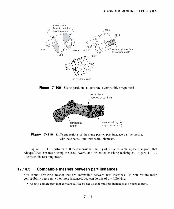
ADVANCED MESHING TECHNIQUES
the resulting mesh
cell 1
cell 2
cell 3
extend cylinder faceto partition cell 2
cell 4
cell 1
cell 2
cell 3
extend planarfaces to partitioninto three cells
Figure 17–109 Using partitions to generate a compatible swept mesh.
tied surfaceinserted at partition
tetrahedralregion
hexahedral region(region of interest)
Figure 17–110 Different regions of the same part or part instance can be meshed
with hexahedral and tetrahedral elements.
Figure 17–111 illustrates a three-dimensional shell part instance with adjacent regions that
Abaqus/CAE can mesh using the free, swept, and structured meshing techniques. Figure 17–112
illustrates the resulting mesh.
17.14.3 Compatible meshes between part instancesYou cannot prescribe meshes that are compatible between part instances. If you require mesh
compatibility between two or more instances, you can do one of the following:
• Create a single part that contains all the bodies so that multiple instances are not necessary.
17–111
Abaqus ID:
Printed on:

ADVANCED MESHING TECHNIQUES
freeregion
structuredregion swept
region
Figure 17–111 Adjacent regions of a three-dimensional shell part instance.
Figure 17–112 The resulting mesh.
• Assemble instances of the parts in the Assembly module and use the Merge/Cut tool to merge the
instances into a single instance. If you need to maintain the concept of separate part instances, you
can create a partition at the common interface of the merged instances.
Similarly, you can create a single part instance from multiple instances containing orphan
elements and nodes, using the Merge/Cut tool to merge duplicate nodes. For more information,
see “Performing Boolean operations on part instances,” Section 13.7.
• If you must use separate parts, you can use tied contact to avoid the issue of mesh compatibility.
Keep in mind that this is not true compatibility, and the accuracy of the solution may suffer. For
more information on tied contact, see “Understanding interactions,” Section 15.3.
17–112
Abaqus ID:
Printed on:

ADVANCED MESHING TECHNIQUES
17.14.4 Parametric modelingA useful feature of the Mesh module is the ability to regenerate partitions and mesh attributes—such as
element type assignments, seeds, and mesh controls—after a part has been modified. (You must always
recreate the mesh itself after modifying a model.)
For example, the model shown in Figure 17–113 has been partitioned into four regions and then
seeded to specify an approximate element size of 3.
Figure 17–113 Seeded model with small hole.
You can return to the Part module and modify the hole at the center of the model so that it is slightly
larger. When you return to the Mesh module, the partitions and the seeds are regenerated, as shown in
Figure 17–114.
Figure 17–114 Seeds are regenerated after the part is modified.
In addition, settings in the Mesh Controls andElement Type dialog boxes (such as element shape,
element type, and meshing technique) are also regenerated. (You can display these two dialog boxes by
selecting Mesh→Controls and Mesh→Element Type from the main menu bar.)
17–113
Abaqus ID:
Printed on:

ADVANCED MESHING TECHNIQUES
Note: If you drastically modify the part, the seeds and partitions may fail to regenerate. In these cases
you must create new seeds and partitions after reentering the Mesh module.
17.14.5 Meshing complex solids with hexahedral elementsYou can use the Part module to create complex solid revolved parts that include a translation along the
axis of revolution, and you can also create solid extruded parts that include a twist about a selected center
point. Free meshing allows you to mesh these parts with tetrahedral elements, as described in “Free
meshing with triangular and tetrahedral elements,” Section 17.10.3. In addition, you can use hexahedral
elements to mesh an extruded part that is twisted, as shown in Figure 17–115.
Figure 17–115 A hexahedral swept mesh on an extruded part with twist.
However, if you want to use hexahedral elements to mesh a revolved part that is translated, you will
probably have to introduce partitions to make the part swept meshable, as described in the following
paragraphs.
For the Mesh module to create a three-dimensional swept mesh of hexahedral elements, every side
that connects the source side to the target side must contain only a single face (see Figure 17–102 in
“Swept meshing of three-dimensional solids,” Section 17.9.3). However, when you create a part that
is revolved more than 180° and then translated along the axis of revolution, Abaqus/CAE inserts rings
along the length of the solid. These rings exist only on the surface of the part, and they do not create
faces that cut through the part. As a result, the side that connects the source side and the target side now
contains more than one face, and the part is not swept meshable with hexahedral elements unless you
introduce partitions.
For example, Figure 17–116 shows a part that represents a coil spring. The figure also shows the
rings that Abaqus/CAE inserted when the part was created. These rings divide the connecting face
between the source side and the target side; as a result, you cannot mesh an instance of the coil spring
with a swept mesh of hexahedral elements until you partition the part.
17–114
Abaqus ID:
Printed on:

ADVANCED MESHING TECHNIQUES
rings divide the main sweptsurface into several faces
Figure 17–116 Rings divide the coil into several segments.
The partitioning operation introduces partitions through the solid coil using N-sided patches to
define the new faces. You select the rings to define the N-sided patches, as shown in Figure 17–117.
N-sided patches partition the cell into multiple swept regions
Figure 17–117 N-sided patches partition the cell.
You can now seed the part instance and generate a swept mesh using hexahedral elements, as shown in
Figure 17–118.
17–115
Abaqus ID:
Printed on:
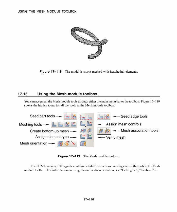
USING THE MESH MODULE TOOLBOX
Figure 17–118 The model is swept meshed with hexahedral elements.
17.15 Using the Mesh module toolbox
You can access all theMeshmodule tools through either the main menu bar or the toolbox. Figure 17–119
shows the hidden icons for all the tools in the Mesh module toolbox.
Seed part tools
Meshing tools
Assign element type
Create bottom-up mesh
Verify mesh
Mesh association tools
Assign mesh controls
Seed edge tools
Mesh orientation
Figure 17–119 The Mesh module toolbox.
The HTML version of this guide contains detailed instructions on using each of the tools in theMesh
module toolbox. For information on using the online documentation, see “Getting help,” Section 2.6.
17–116
Abaqus ID:
Printed on:

UNDERSTANDING THE ROLE OF THE OPTIMIZATION MODULE
18. The Optimization module
You use the Optimization module to create an optimization task that can be used to optimize the topology
or shape of your model given a set of objectives and a set of restrictions. For example, an optimization
can attempt to remove material from selected regions to satisfy a maximum weight objective while
maintaining a minimum stiffness. This chapter covers the following topics:
• “Understanding the role of the Optimization module,” Section 18.1
• “Entering and exiting the Optimization module,” Section 18.2
• “Understanding optimization,” Section 18.3
• “Using the Optimization module toolbox,” Section 18.4
• “Viewing and troubleshooting an optimization,” Section 18.5
In addition, the following sections are available in the HTML version of this guide:
• “Creating and configuring an optimization task,” Section 18.6
• “Configuring design responses,” Section 18.7
• “Creating objective functions,” Section 18.8
• “Creating constraints,” Section 18.9
• “Configuring geometric restrictions,” Section 18.10
• “Creating local stop conditions,” Section 18.11
For information on displaying the online documentation, see “Getting help,” Section 2.6.
18.1 Understanding the role of the Optimization module
You can use the Optimization module to perform the following tasks:
Create optimization tasks
An optimization task contains the definition of your optimization. You run an optimization in the
Job module using an optimization process. An optimization process refers to an optimization task.
Create design responses
A design response is a single scalar value that is extracted from an optimization. A design response
can be extracted directly from the output database, such as the volume of the model. Alternatively,
the Abaqus Topology Optimization Module can extract data from the output database and calculate
the design response, such as the total strain energy of the model, a measure of its flexibility.
18–1
Abaqus ID:
Printed on:

UNDERSTANDING OPTIMIZATION
Create objective functions
An objective function defines the objective of the optimization and refers to the value of a design
response or a combination of design responses. For example, the objective function of the
optimization can be to minimize the total strain energy in the model (maximize its stiffness).
Create constraints
Constraints define the changes that the Abaqus Topology Optimization Module can apply to the
topology or the shape of the model during the optimization. For example, the volume of the
optimized model can be constrained to be 50% of the original volume. If a constraint cannot be
satisfied, the optimization is not feasible. A constraint also refers to the value of a design response,
but it cannot refer to a combination of design responses.
Create geometric restrictions
A geometric restriction places restrictions on the changes that the Abaqus Topology Optimization
Module canmake to the topology of the model. Geometrical restrictions include frozen regions from
which material cannot be removed and manufacturing constraints, such as restrictions on cavities
and undercuts, that would prevent the optimized model from being removed from a mold.
Create stop conditions
A stop condition is an indicator that the optimization has converged to a solution. For example, an
optimization can be considered complete after a specified number of iterations or when the change
in an optimization function between iterations is less than a specified value.
18.2 Entering and exiting the Optimization module
You can enter the Optimization module at any time during an Abaqus/CAE session by clicking
Optimization in the Module list located in the context bar. The Task, Design Response, ObjectiveFunction, Constraint, Geometric Restriction, Stop Condition, and Tools menus appear on the
main menu bar. If the current viewport contains something other than the assembly, the contents of the
viewport disappear when you start the Step module.
To exit the Optimization module, select any other module from the Module list. You need not save
your optimization definition before exiting the module; it will be saved automatically when you save the
model database by selecting File→Save or File→Save As from the main menu bar.
18.3 Understanding optimization
An optimization is an iterative process that modifies the structure of your model while it searches
for an optimized solution given a set of objectives and constraints that must be satisfied.
This section briefly describes the components of an optimization that you can create with the
18–2
Abaqus ID:
Printed on:

UNDERSTANDING OPTIMIZATION
Abaqus Topology Optimization Module. For more detailed information, see “Structural optimization:
overview,” Section 13.1.1 of the Abaqus Analysis User’s Guide.
The following topics are covered:
• “About tasks,” Section 18.3.1
• “About design responses,” Section 18.3.2
• “About objective functions,” Section 18.3.3
• “About constraints,” Section 18.3.4
• “About geometric restrictions,” Section 18.3.5
• “About stop conditions,” Section 18.3.6
• “About optimization processes,” Section 18.3.7
18.3.1 About tasksAn optimization task contains the components that define your optimization, such as the design responses,
objectives, constraints, and geometric restrictions. To run an optimization, you execute an optimization
process. An optimization process refers to an optimization task.
For more information, see “Creating an optimization task,” Section 18.6.1.
18.3.2 About design responsesThe inputs to your optimization are called the design responses. Design responses can be read from
the Abaqus output database file; for example, stiffness, stresses, eigenfrequencies, and displacements.
Alternatively, the Abaqus Topology Optimization Module can extract the design responses from the
position of nodes or the layout of elements in your model; for example, its weight, center of mass, or
inertia.
A design response is associated with a region of your model; however, it consists of a single scalar
value, such as the maximum stress in a region or the total volume of the model. In addition, a design
response can be associated with a particular step or load case. For more information, see “Configuring
design responses,” Section 18.7, and “Design responses,” Section 13.2.1 of the Abaqus Analysis User’s
Guide.
18.3.3 About objective functionsThe objective functions define the objective of your optimization. The objective function is extracted
from a design response, such as the lowest eigenfrequencies or the minimum stress. The objective
function can be formulated from multiple design responses. If you specify that the objective functions
minimize or maximize the design responses, the Abaqus Topology Optimization Module calculates the
objective function by adding each of the values determined from the design responses. In addition, you
18–3
Abaqus ID:
Printed on:

UNDERSTANDING OPTIMIZATION
can specify a weighting factor (the default weighting factor is 1.0). For the most common optimization
formulations you do not need to change the default value of the weighting factor. However, in some
cases you may have to change the weighting factor to balance the effect of an objective function that
is dominating the optimization. You should be aware that changing the weighting factor can have a
significant impact on the final design. In addition, a design response that is dominant at the start of the
optimization may have less effect as the Abaqus Topology Optimization Module modifies your model.
For more information, see “Creating objective functions,” Section 18.8, and “Objectives and constraints,”
Section 13.2.2 of the Abaqus Analysis User’s Guide.
18.3.4 About constraints
Constraints are also extracted from the design responses. Constraints restrict the value of a design
response; for example, you can specify that the volume must be reduced by 45% or the absolute
displacement in a region must not exceed 1 mm. You can also apply manufacturing and geometric
constraints that are independent of the optimization; for example, a structure must be able to be cast or
stamped or the diameter of a bearing surface cannot be changed.
Satisfying the constraints has priority over the minimization or maximization of the objective
function. The optimization algorithms start to maximize or minimize the objectives only after the
constraints are satisfied.
You can specify only a volume constraint for a condition-based topology or shape optimization,
and the volume constraint must be either equal to a fixed value or a fraction of the value before
the optimization starts. If the requested volume differs greatly from the initial volume, the
Abaqus Topology Optimization Module may need several design cycles to satisfy the volume constraint.
A general topology optimization provides more flexibility; and you can select any of the design
responses as a constraint, except for the design response that calculates the eigenfrequencies with the
Kreisselmaier-Steinhauser formula. The constraint in a general topology optimization can be less than,
greater than, or equal to a fixed value or a fraction of the value before the optimization starts. For more
information, see “Creating constraints,” Section 18.9, and “Objectives and constraints,” Section 13.2.2
of the Abaqus Analysis User’s Guide.
18.3.5 About geometric restrictions
Geometric restrictions are manufacturing and geometric constraints that are independent of the
optimization; for example, a structure must be able to be cast or stamped or the diameter of a
bearing surface cannot be changed. For more information, see “Configuring geometric restrictions,”
Section 18.10, and “Objectives and constraints,” Section 13.2.2 of the Abaqus Analysis User’s Guide.
18–4
Abaqus ID:
Printed on:

USING THE OPTIMIZATION MODULE TOOLBOX
18.3.6 About stop conditionsA global stop condition defines the maximum number of iterations an optimization should perform. A
local stop condition specifies that the optimization should end when a local minimum (or maximum) has
been reached. For more information, see “Creating local stop conditions,” Section 18.11, and “Objectives
and constraints,” Section 13.2.2 of the Abaqus Analysis User’s Guide.
18.3.7 About optimization processesYou create optimization processes in the Job module. An optimization process reads an optimization task
that you defined in the Abaqus Topology Optimization Module and iteratively searches for an optimized
solution based on the objective functions and constraints that you defined in the optimization task. For
more information, see “What is an optimization process?,” Section 19.5.1. You can use a view cut in
the Visualization module to view the results of an optimization process. For more information, see
Chapter 80, “Cutting through a model.”
18.4 Using the Optimization module toolbox
You can access all the Optimization module tools through either the main menu bar or through the
Optimization module toolbox. Figure 18–1 shows the icons for all the Optimization module tools in
the toolbox.
Create optimization task
Create geometric restriction
Create constraint
Create objective function
Create design response
Create stop condition
Optimization task manager
Geometric restriction manager
Constraint manager
Objective function manager
Design response manager
Stop condition manager
Figure 18–1 The Optimization module tools.
To see a tooltip containing a brief definition of an Optimization module tool, hold the mouse over the
tool for a moment. For information on using toolboxes and selecting hidden icons, see “Using toolboxes
and toolbars that contain hidden icons,” Section 3.3.2.
18–5
Abaqus ID:
Printed on:

VIEWING AND TROUBLESHOOTING AN OPTIMIZATION
18.5 Viewing and troubleshooting an optimization
You can use the field and history output generated by Abaqus to view the results generated by your
optimization process. You can also use the output to diagnose any problems with the optimization;
for example, to determine if the optimization is converging on an objective or to study the rate of
convergence. You view the results by clicking Results in the Optimization Process Manager.When you submit an optimization process for analysis, Abaqus creates an output database
that contains data from each design cycle of the optimization. The output database is stored in the
jobname\ATOM_POST directory. The behavior of the Visualization module depends on whether the
output database was created from a topology optimization or a shape optimization.
Topology optimization
When you view the results of a topology optimization, Abaqus/CAE automatically displays
a view cut superimposed on the current view that represents the optimized design surface.
The isosurface variable of the view cut is the normalized material property that the
Abaqus Topology Optimization Module uses to “add” or “remove” elements from the analysis.
By default, Abaqus/CAE displays the view cut with the normalized material property set to 0.3.
You can use the view cut manager to modify the value of the isosurface variable and to view the
resulting boundary of the isosurface. Boundary conditions are not displayed while an optimization
view cut is active. For more information, see “Managing view cuts,” Section 80.2, in the HTML
version of this guide.
Shape optimization
When you view the results of a shape optimization, Abaqus/CAE displays the model in its optimized
shape using the new position of the surface nodes.
Each design cycle in the optimization process is saved as a frame in the output database, and you
can open the Step/Frame dialog box to display the results from each design cycle. You can view
the results of an optimization process while it is still in progress. As the optimization process moves
toward completion, the lists of completed steps and frames are updated every time you close and reopen
the Step/Frame dialog box. For more information, see “Selecting a specific results step and frame,”
Section 42.3.1, and “Stepping through frames,” Section 42.3.2.
You can perform a time history animation of a deformed or contour plot and view the progress of
the optimization as Abaqus attempts to satisfy the objective functions while respecting the constraints.
For a topology optimization you can view the progressive removal of elements from the analysis and the
resulting effect on the mechanical behavior of the model, such as the change in deformation or stress.
Turning on translucency allows you to see the progression of the optimization through interior elements;
for example, the removal of interior elements to create voids. For more information, see “Changing
the translucency,” Section 77.3. For a shape optimization you can view the incremental change in the
position of the surface nodes as the optimization progresses; and, similar to a topology optimization, you
can view the resulting effect on the mechanical behavior of the model.
18–6
Abaqus ID:
Printed on:

VIEWING AND TROUBLESHOOTING AN OPTIMIZATION
In addition, the optimization process writes history data in the ATOM_OPTIMIZATION that
you can use to track the design variables. As a result, you can create an X–Y plot showing how the
objective functions and constraints change after each design cycle. The resulting plot indicates how the
Abaqus Topology Optimization Module tries to meet the specified objective functions while satisfying
the constraints. You can use an X–Y plot of the objective functions and constraints as a diagnostic tool
to view the progression of the optimization after each design cycle and to determine if the optimization
is converging on a solution, as shown in Figure 18–2.
Design Cycle0. 5. 10. 15.
Vol
ume
0.50
0.60
0.70
0.80
0.90
Str
ain
Ene
rgy
0.26
0.28
0.30
0.32
0.34
0.36[x1.E6]
Strain EnergyVolume
Figure 18–2 The design objective and constraint
during an optimization.
The Abaqus Topology Optimization Module also saves output databases in the
jobname\SAVE.odb directory. These output databases contain the data generated by the Abaqus
analyses during each design cycle; however, they do not contain data related to the optimization, such
as the value of the normalized material property.
If you performed an eigenfrequency optimization, the output database stored in the
jobname\ATOM_POST directory contains only results corresponding to the first eigenfrequency.
However, the jobname\SAVE.odb output database contains results from the last optimization step for
all eigenfrequencies.
For information on related topics, refer to the following sections:
• “Understanding view cuts,” Section 80.1
• “Understanding X–Y plotting,” Section 47.1
18–7
Abaqus ID:
Printed on:


UNDERSTANDING THE ROLE OF THE JOB MODULE
19. The Job module
You can use the Job module to create and manage analysis jobs and to view a basic plot of the analysis
results. You can also use the Job module to create and manage adaptivity analyses and co-executions.
This chapter covers the following topics:
• “Understanding the role of the Job module,” Section 19.1
• “Understanding analysis jobs,” Section 19.2
• “Understanding adaptivity processes,” Section 19.3
• “Understanding co-executions,” Section 19.4
• “Understanding optimization processes,” Section 19.5
• “Restarting an analysis,” Section 19.6
In addition, the following sections are available in the HTML version of this guide:
• “Creating, editing, and manipulating jobs,” Section 19.7
• “Using the job editor,” Section 19.8
• “Creating, editing, and manipulating adaptivity processes,” Section 19.9
• “Using the adaptivity process editor,” Section 19.10
• “Creating, editing, and manipulating co-executions,” Section 19.11
• “Creating, editing, and manipulating optimization processes,” Section 19.12
See the online tutorial in Appendix B, “Creating and Analyzing a Simple Model in Abaqus/CAE,”
of Getting Started with Abaqus: Interactive Edition for examples of how to submit and monitor a job.
19.1 Understanding the role of the Job module
Once you have finished all of the tasks involved in defining a model (such as defining the geometry of the
model, assigning section properties, and defining contact), you can use the Job module to analyze your
model. The Job module allows you to create a job, to submit it for analysis, and to monitor its progress.
If desired, you can create multiple models and jobs and run and monitor the jobs simultaneously.
In addition, you have the option of creating only the analysis input file for your model. This option
allows you to view and edit the input file before submitting it for analysis. For an Abaqus/Standard or
Abaqus/Explicit analysis, you can also view and edit the analysis keywords for a model by selecting
Model→Edit Keywords→model name from the main menu bar.
You can create and submit a job based on an existing input file instead of an Abaqus/CAE model;
for example, if you have created an input file outside Abaqus/CAE but would like to run the analysis,
monitor its progress, and view the results in Abaqus/CAE. Jobs can be created only for input files that
do not contain references to other results files; for example, you cannot create a job based on an input
file that contains a restart analysis.
19–1
Abaqus ID:
Printed on:

UNDERSTANDING ANALYSIS JOBS
If you have defined adaptive remeshing rules in the Mesh module, you can submit a mesh adaptivity
process. Abaqus/CAE submits a succession of jobs, each of which attempts to improve solution accuracy
and reduce error indicators over the previous job.
For an Abaqus co-simulation, you can create a co-execution to execute two analysis jobs in
synchronization with one another.
19.2 Understanding analysis jobs
This section provides an overview of the Job module.
19.2.1 Basic steps for analyzing a modelAfter you have defined your model, you are ready to analyze it. Analyzing amodel involves the following
steps, each of which can be performed using either the Job menu on the main menu bar or the JobManager:
Create and configure an analysis job
You create an analysis job by selecting Job→Create from the main menu bar. Abaqus/CAE asks
you to name the new job and to associate it with a model selected from the model database or with
an existing input file. You can select any model that exists in the database; you are not limited to
the current model. The job editor allows you to configure the job settings.
Write the input file
When you submit a job associated with a model for analysis, Abaqus/CAE first generates an input
file representing your model and then Abaqus/Standard, Abaqus/Explicit, or Abaqus/CFD performs
the analysis using the contents of this file. Alternatively, you can ask Abaqus/CAE to generate only
the input file; Abaqus/CAE writes the input file in ASCII format, and you can view and edit it in
your working directory.
WARNING: If you edit the input file for a model using a text editor outside Abaqus/CAE and then
submit the job for that model in the Job module, your changes to the input file will be lost. Instead,
you must submit the modified input file directly for analysis by creating a new job and selecting
Input file as the job Source.However, if you use the Keywords Editor to modify the generated keywords for a model, those
modifications are retained in the model and apply to any jobs associated with that model.
Submit the job for analysis
You submit the job for analysis by selecting Job→Submit from the main menu bar. As the analysis
progresses, Abaqus/CAE displays information from the status, data, log, and message files in the job
19–2
Abaqus ID:
Printed on:

UNDERSTANDING ANALYSIS JOBS
monitor dialog box. After your job is completed, you can display results from the output database
in the Visualization module by selecting Job→Results from the main menu bar.
19.2.2 Entering and exiting the Job module
You can enter the Job module at any time during a session by clicking Job in the Module list located in
the context bar. The Job menu appears in the main menu bar.
To exit the Job module, select any other module from the main menu. If your job completed
successfully, you can also exit the Job module by selecting Job→Results from the main menu bar;
you will enter the Visualization module, and the output database for your analysis job will be opened
automatically.
You need not save your job before exiting the module; it will be saved automatically when you save
the entire model by selecting File→Save or File→Save As from the main menu bar.
19.2.3 The Job Manager
The Job Manager, which is similar to other managers in Abaqus/CAE, allows you to do the following:
• Create an analysis job and associate the new job with a selected model or input file.
• Edit the selected analysis job.
• Copy, rename, or delete the selected analysis job.
Note: A job associated with a model can be copied only to a job associated with a model. A job
associated with an input file can be copied only to a job associated with an input file.
In addition, the Job Manager allows you to do the following:
• Write an input file for a model-based job without submitting it for analysis.
• Perform a data check on a model.
• Submit a job for analysis.
• Continue an analysis to completion after performing a data check.
• Monitor the analysis as it progresses.
• View the results from a job.
• Kill a job that is currently running.
You can display the Job Manager by selecting Job→Manager from the main menu bar.
Figure 19–1 shows the layout of the Job Manager.
19–3
Abaqus ID:
Printed on:

UNDERSTANDING ANALYSIS JOBS
Figure 19–1 The Job Manager.
The four columns of the Job Manager display the following:
Name
The Name column displays the name of the job. Click Rename to rename the selected job.
Model
The Model column displays the name of the model or input file associated with the job.
Type
The Type column displays the job type that you selected when you configured the job using the job
editor. The job type can be one of the following:
• Full Analysis
• Recover
• Restart
(See “Selecting a job type,” Section 19.2.5, for more information.) You can use the job editor to
change the job type as long as the job is not running.
Status
The Status column displays the current status of the analysis job and is updated continually while
your job is running. The status can be one of the following:
None
The job has not been submitted for analysis.
19–4
Abaqus ID:
Printed on:
UNDERSTANDING ANALYSIS JOBS
Check Submitted
The input file has been written, and the model is being submitted for a data check.
Check Running
The data check of the model is running.
Check Completed
The data check of the model has completed successfully; you can now continue with the full
analysis.
Submitted
The input file has been written, and the job is being submitted for a full analysis.
Running
The job has been submitted for a full analysis and is running.
Completed
The analysis is complete. You can click Results to view the contents of the output database
and graphically verify your results.
Aborted
The job has been aborted due to problems such as fatal errors in the input file or lack of disk
space.
Terminated
The job has been killed by the user.
For detailed instructions on using the Job Manager to create, edit, and manipulate jobs, see the
following sections in the HTML version of this guide:
• “Creating a new analysis job,” Section 19.7.1
• “Writing the input file only,” Section 19.7.2
• “Performing a data check on a model,” Section 19.7.3
• “Submitting an analysis job,” Section 19.7.4
• “Continuing an analysis job after a data check,” Section 19.7.5
• “Terminating an analysis job,” Section 19.7.6
• “Viewing the results of your job,” Section 19.7.7
19–5
Abaqus ID:
Printed on:

UNDERSTANDING ANALYSIS JOBS
19.2.4 The job editorYou use the job editor to customize the settings for a new job or to edit the settings for an existing job.
You can display the job editor by selecting Job→Create or Job→Edit→job name from the main menu
bar. (You can also click Create or Edit in the job manager.)
The job editor contains the following tabbed pages:
Submission
Use the Submission tabbed page to configure the submission attributes of your job, such as job
type, run mode, and submit time. You can also use the submission tabbed page to specify that the
job is to be submitted to remote queues that have been configured by your local Abaqus environment
file or by your system administrator.
General
Use the General tabbed page to configure job settings such as the analysis input file processor
printout and the name of the directory used for scratch files.
Preprocessor printout options are not available for a job associated with an input file; you must
specify these options in the input file itself.
Memory
Use the Memory tabbed page to configure the amount of memory allocated to an Abaqus analysis.
Parallelization
Use the Parallelization tabbed page to configure the parallel execution of an Abaqus analysis job,
such as the number of processors to use and the parallelization method.
Precision
Use the Precision tabbed page to specify either single or double precision for Abaqus/Explicit
analyses. You can also choose the precision of nodal output that is written to the output database
during the analysis.
For detailed instructions on using the job editor to define jobs, see the following sections in the
HTML version of this guide:
• “Navigating the job customization options,” Section 19.8.1
• “Configuring job submission attributes,” Section 19.8.2
• “Choosing the job type,” Section 19.8.3
• “Choosing the job run mode,” Section 19.8.4
• “Setting the job submit time,” Section 19.8.5
• “Specifying general job settings,” Section 19.8.6
• “Controlling job memory settings,” Section 19.8.7
19–6
Abaqus ID:
Printed on:

UNDERSTANDING ANALYSIS JOBS
• “Controlling job parallel execution,” Section 19.8.8
• “Controlling job precision,” Section 19.8.9
19.2.5 Selecting a job typeThe Submission tabbed page in the job editor allows you to choose between the following job types:
Full analysis
Submit a job with this option selected to generate (or regenerate) the input file (if the job is associated
with a model), perform a complete analysis of your model, and write the results to the output
database. This option is the default.
Recover (Explicit)
This option is available only when you are running Abaqus/Explicit. Submit a job with this option
selected to complete your analysis after Abaqus/Explicit stopped unexpectedly; for example, after
filling a disk or after a network problem.
You cannot use this job type to recover an Abaqus/Standard job that terminated prematurely.
Instead, you should use the Abaqus/Standard restart capabilities as described in “Recovering an
Abaqus/Standard analysis,” Section 19.6.9.
Restart
Submit a job with this option selected to start the analysis using data from a previous analysis of a
specified model. You must use the Edit Model Attributes dialog box to specify the job to read data
from and to specify the step from which to restart the analysis. When you create a job that refers to
a model with restart data attributes, Abaqus/CAE by default selects the job type to be Restart.Restart analyses are described in more detail in “Restarting an analysis,” Section 19.6. You
cannot create a restart job for a job that was associated with an input file.
The Job Type settings are analogous to parameters of the Abaqus execution procedure; for more
information, see “Abaqus/Standard, Abaqus/Explicit, and Abaqus/CFD execution,” Section 3.2.2 of the
Abaqus Analysis User’s Guide. For detailed instructions on choosing a job type, see “Choosing the job
type,” Section 19.8.3, in the HTML version of this guide.
19.2.6 Monitoring the progress of an analysis jobThe Job Manager and Co-execution Manager continually update the status of analysis jobs in the
model database. In addition, Abaqus/CAE prints error messages from the analysis products to the
message area and creates diagnostic files in your current working directory.
You can monitor information concerning a submitted job by selecting Job→Monitor→job of yourchoice from the main menu bar or by selecting the job of your choice and clicking Monitor in the JobManager. The job monitor dialog box for that job appears, as shown in Figure 19–2. You can display
as many job monitors as necessary to view information on multiple jobs.
19–7
Abaqus ID:
Printed on:

UNDERSTANDING ANALYSIS JOBS
Figure 19–2 The job monitor.
The jobs submitted for a co-execution appear in the Model Tree in the Jobs container under the
co-execution in the Co-executions container. You can monitor these jobs by clicking mouse button 3
on the job in the Model Tree and selecting Monitor.The top half of the job monitor dialog box displays the information available in the status file that
Abaqus creates for the analysis. The table headings are customized for each job based on the settings
sent from the analysis. The bottom half of the dialog box displays the following information:
• Click the Log tab to display the start and end times that appear in the log file for the analysis.
• Click the Errors and Warnings tabs to display the errors or the warnings associated with the
analysis. Abaqus/CAE indicates the presence of errors or warnings by prepending an exclamation
point before the Errors and Warnings tab. If a particular region of the model is causing the error
or warning, a node or element set will be created automatically that contains that region. The name
of the node or element set appears with the error or warning message, and you can view the set
using display groups in the Visualization module. (For more information on display groups, see
Chapter 78, “Using display groups to display subsets of your model.”)
Abaqus/CAE may not perform all consistency checks when it creates an input file, which can
result in warnings or error messages during an analysis. If your analysis generates warning or
error messages, consider running a data check analysis (see “Performing a data check on a model,”
Section 19.7.3) to diagnose and fix possible problems in your model.
19–8
Abaqus ID:
Printed on:

UNDERSTANDING ANALYSIS JOBS
The number of error and warning messages that appear in the job monitor is limited by
the environment parameters cae_error_limit and cae_warning_limit, respectively (see “Job
customization parameters,” Section 4.1.3 of the Abaqus Installation and Licensing Guide, for
details). If the number of errors or warnings exceeds the job monitor limit, consult the data,
message, or status file for a complete list of messages.
• Click the Output tab to display a record of each output data entry as it is written to the output
database. In addition, if you requested that Abaqus monitor the values of a degree of freedom
of a particular node to the message and status files, the Output tabbed page records each time this
information is written and the value of the degree of freedom at that point of the analysis. (For more
information, see “Understanding output requests,” Section 14.4, and “Degree of freedom monitor
requests,” Section 14.5.4.)
• As the analysis proceeds, Abaqus creates the following files:
– Abaqus/Standard: Data file, message file, and status file
– Abaqus/Explicit: Data file, message file, and status file
– Abaqus/CFD: Data file and status file
Abaqus/CAE activates the Data File, Message File, and Status File tabs accordingly. You can
click any of these tabs to browse or search the corresponding file for additional error and warning
messages.
Note: Abaqus/CAE populates the Data File, Message File, and Status File tabbed pages only
for locally submitted analyses; this information will not be displayed in the job monitor for remote
jobs. In addition, although Abaqus/CAE updates the contents of these pages periodically as the
analysis runs, the data might not always be synchronized with the latest data in the files.
For detailed information on the different output files that Abaqus creates during an analysis, see “Output,”
Section 4.1.1 of the Abaqus Analysis User’s Guide.
You can search for specific error or warning messages within any of the files displayed in tabbed
pages in the job monitor. Select the desired file tab, enter a search string in the Text to find field, and
click Next or Previous to step through the file from one hit to the next. Toggle on Match case to
perform a case-sensitive search.
The information presented in the job monitor dialog box is updated continually as the analysis
progresses. If the job fails, the Errors tabbed page appears in front of the other tabbed pages
automatically to help you determine the cause of the failure. In addition, an exclamation point appears
on the tab if any error or warning messages are output.
If you start monitoring a job and then exit Abaqus/CAE, close the current model database, or open
a new model database, Abaqus/CAE will stop updating the job monitor. The job will continue to run;
however, the job monitor will not report the status of the job or update the increment information.
If you requested DOF Monitor output on a particular degree of freedom for a particular node,
Abaqus/CAE provides another opportunity to monitor the job by plotting the values of the degree of
freedom over time. The plot appears in a new viewport that is generated automatically when you submit
the job. If the visible part of the canvas is already filled with one or more viewports, the new viewport may
19–9
Abaqus ID:
Printed on:

UNDERSTANDING ANALYSIS JOBS
be placed on a part of the canvas that is not visible; in this case you should tile or cascade the viewports or
enlarge the canvas to bring the viewport into view. (For information on requesting output for a particular
degree of freedom for a particular node, see “Degree of freedom monitor requests,” Section 14.5.4.)
If necessary, you can terminate the analysis job by clicking Kill at the bottom of the job monitor
dialog box.
19.2.7 Submitting a job remotely
When you configure a job, you can request that Abaqus/CAE route the job to a specified queue on a
remote UNIX or Linux host computer. You can specify the remote queue by selecting an associated
queue name in the Submission tabbed page of the job editor.
Note: The job editor displays default settings for memory usage, parallelization, and precision based
on the environment files effective for the current session on the local machine. When you submit a job
to a remote machine, Abaqus replaces the default settings with those from the environment files on the
remote machine. Non-default settings in the job editor are saved with the job and will be used regardless
of where you run the analysis.
Each queue name that appears in the job editor refers to an entry in your Abaqus environment file
in which you specify how you want the job to be run on the host computer. In other words, when you
select a queue name in the job editor, you specify not only the desired queue on the host computer but
also other options, such as the directory on the host computer in which you want to run the job and the
files you want copied back to your local directory when the job is complete.
You can specify your preferences for running a job remotely by adding the following to your Abaqus
environment file:
def onCaeStartup():import os
def makeQueues(*args):session.Queue(name,
queueName,hostName,fileCopy,directory,driver,localPlatform,filesToCopy,description)
addImportCallback('job', makeQueues)
19–10
Abaqus ID:
Printed on:

UNDERSTANDING ANALYSIS JOBS
This entry is written using the Abaqus command language. The following list describes each argument
in the entry above.
name
The queue name that you want to appear in the job editor.
queueName
The name of an existing queue on the host computer. (For information on creating queues on the
host computer, refer to the Abaqus Installation and Licensing Guide.)
hostName
The name of the host computer. The default is the name of the local computer.
fileCopy
When the analysis is complete, the value of this argument determines whether or not the analysis
files will be copied back to the directory from which the job was submitted. The default value is ON.
directory
The name of the directory on the host computer where you want the job run. You must have write
privileges to this directory. The default is the local directory (the directory from which you are
submitting the job).
driver
The name of the command on the host computer to execute Abaqus/Standard or Abaqus/Explicit.
The default is abaqus.
localPlatform
The platform on the local computer. You can specify either UNIX or WINDOWS; UNIX is the default.
filesToCopy
The three-letter extensions of the analysis files that you want copied back to the local directory when
the job is complete. By default, the files with the following extensions are copied: log, dat, msg,sta, odb, res, abq, and pac.
Note: The restart (.res) file, the Abaqus/Explicit state (.abq) file, and the packaging (.pac)file are platform-dependent; if your local platform and remote platform settings differ, you will not
be able to copy and use these files without some kind of translation. All of the other files listed
above can be copied across platforms without any difficulty.
description
A short description of the queue.
19–11
Abaqus ID:
Printed on:

UNDERSTANDING ANALYSIS JOBS
The name and queueName arguments must be included in each queue definition. However, if you do
not include any of the other arguments in a queue definition, default values will be supplied automatically.
An example queue definition is shown below:
def onCaeStartup():import os
def makeQueues(*args):session.Queue(name='long',
queueName='aba_long',hostName='jobserver',directory='/scratch/' + os.environ['USER'])
addImportCallback('job', makeQueues)
The commands in the example above configure the following:
name
The queue name displayed in the job editor is long.
queueName
The queue name on the host computer is aba_long.
hostName
The name of the host computer is jobserver.
directory
The directory on the host computer where Abaqus will store the input file and all other files
associated with the job is /scratch/your user name.
Since the fileCopy, driver, localPlatform, and filesToCopy arguments have been left out of the entry
above, the default options for these parameters are assigned to this queue automatically.
If you want to create two or more queues, you can repeat the line containing the session.Queuecommand as many times as necessary. For example, the following Abaqus environment file entry
specifies two queues, one named long and the other named job:
def onCaeStartup():import os
def makeQueues(*args):session.Queue(name='long',
queueName='aba_long',hostName='jobserver',directory='/scratch/' + os.environ['USER'])
19–12
Abaqus ID:
Printed on:
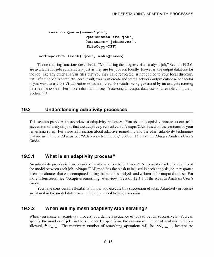
UNDERSTANDING ADAPTIVITY PROCESSES
session.Queue(name='job',queueName='aba_job',hostName='jobserver',fileCopy=OFF)
addImportCallback('job', makeQueues)
The monitoring functions described in “Monitoring the progress of an analysis job,” Section 19.2.6,
are available for jobs run remotely just as they are for jobs run locally. However, the output database for
the job, like any other analysis files that you may have requested, is not copied to your local directory
until after the job is complete. As a result, you must create and start a network output database connector
if you want to use the Visualization module to view the results being generated by an analysis running
on a remote system. For more information, see “Accessing an output database on a remote computer,”
Section 9.3.
19.3 Understanding adaptivity processes
This section provides an overview of adaptivity processes. You use an adaptivity process to control a
succession of analysis jobs that are adaptively remeshed by Abaqus/CAE based on the contents of your
remeshing rules. For more information about adaptive remeshing and the other adaptivity techniques
that are available in Abaqus, see “Adaptivity techniques,” Section 12.1.1 of the Abaqus Analysis User’s
Guide.
19.3.1 What is an adaptivity process?
An adaptivity process is a succession of analysis jobs where Abaqus/CAE remeshes selected regions of
the model between each job. Abaqus/CAE modifies the mesh to be used in each analysis job in response
to error estimates that were computed during the previous analysis and written to the output database. For
more information, see “Adaptive remeshing: overview,” Section 12.3.1 of the Abaqus Analysis User’s
Guide.
You have considerable flexibility in how you execute this succession of jobs. Adaptivity processes
are stored in the model database and are maintained between sessions.
19.3.2 When will my mesh adaptivity stop iterating?
When you create an adaptivity process, you define a sequence of jobs to be run successively. You can
specify the number of jobs in the sequence by specifying the maximum number of analysis iterations
allowed, . The maximum number of remeshing operations will be −1, because no
19–13
Abaqus ID:
Printed on:

UNDERSTANDING ADAPTIVITY PROCESSES
remeshing will be performed after the final analysis job is run. When you submit the remesh process,
Abaqus/CAE runs each job in the sequence until one of the following conditions is met:
• All active remeshing rules are satisfied. For more information, see “What are remeshing rules?,”
Section 17.13.1.
• All jobs are completed, indicating that Abaqus/CAE has reached the maximum number of analysis
iterations that you specified.
• A job fails to complete. This failure can be due to convergence difficulties or to machine resource
problems.
19.3.3 Manual mesh adaptivity
As an alternative to automatic mesh adaptivity, you can submit a job using the Job manager. When
you define a remeshing rule in the Mesh module, you request error indicator output variables that are
written to the output database when the job executes. After the job has completed, you can return to
the Mesh module and ask Abaqus/CAE to create a new mesh using a combination of your remesh rules
and the error indicators in the output database. You can perform this process indefinitely to adapt your
mesh successively until the goals of the remesh rules are met. For more information, see “What is the
difference between automatic adaptive remeshing and manual adaptive remeshing?,” Section 17.13.4.
19.3.4 Using a combination of automatic and manual mesh adaptivity
In many cases you will want to transition between automatic and manual use of adaptive remeshing.
Some examples include:
• You must keep the current Abaqus/CAE session active for automatic remeshing to occur between
analysis jobs. If you exit Abaqus/CAE and start a new session, you must use manual remeshing to
remesh the model.
• You start an automatic sequence of jobs, but a machine problem (such as a full disk) interrupts the
analysis prematurely. You can restart the analysis manually and then continue it in a fully automatic
manner. Variations of this case include an analysis ending because it failed to converge or an analysis
ending because you terminated the job during a particular iteration.
• You can experiment with sizing function parameters and remesh your model manually until you find
a set of remeshing rules that creates a mesh that appears to be responding actively to your variables
of interest. When you are comfortable with your remeshing rules, you can switch to automatic mesh
adaptivity and complete a specified number of analysis iterations.
• The mesh generated by the automatic mesh adaptivity procedure converges to an acceptable
configuration. You can now modify the loads applied to the model and perform an additional
manual iteration that makes a minor meshing adjustment to compensate for the new load.
19–14
Abaqus ID:
Printed on:
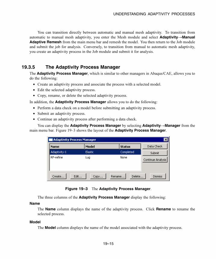
UNDERSTANDING ADAPTIVITY PROCESSES
You can transition directly between automatic and manual mesh adaptivity. To transition from
automatic to manual mesh adaptivity, you enter the Mesh module and select Adaptivity→ManualAdaptive Remesh from the main menu bar and remesh the model. You then return to the Job module
and submit the job for analysis. Conversely, to transition from manual to automatic mesh adaptivity,
you create an adaptivity process in the Job module and submit it for analysis.
19.3.5 The Adaptivity Process ManagerThe Adaptivity Process Manager, which is similar to other managers in Abaqus/CAE, allows you to
do the following:
• Create an adaptivity process and associate the process with a selected model.
• Edit the selected adaptivity process.
• Copy, rename, or delete the selected adaptivity process.
In addition, the Adaptivity Process Manager allows you to do the following:
• Perform a data check on a model before submitting an adaptivity process.
• Submit an adaptivity process.
• Continue an adaptivity process after performing a data check.
You can display the Adaptivity Process Manager by selecting Adaptivity→Manager from the
main menu bar. Figure 19–3 shows the layout of the Adaptivity Process Manager.
Figure 19–3 The Adaptivity Process Manager.
The three columns of the Adaptivity Process Manager display the following:
Name
The Name column displays the name of the adaptivity process. Click Rename to rename the
selected process.
Model
The Model column displays the name of the model associated with the adaptivity process.
19–15
Abaqus ID:
Printed on:

UNDERSTANDING ADAPTIVITY PROCESSES
Status
The Status column displays the current status of the adaptivity process and is updated continually
while the process is running. The status can be one of the following:
None
The process has not been submitted for analysis.
Check Submitted
The model is being submitted for a data check.
Check Running
The data check of the model is running.
Check Completed
The data check of the model completed successfully; you can now continue the adaptivity
process.
Submitted
The process is being submitted for execution.
Running
The process has been submitted for analysis and is running.
Completed
The process has run to completion.
Aborted
The process has been aborted due to problems such as fatal errors in the model or lack of disk
space.
Terminated
The process has been terminated by the user.
For detailed instructions on using the Adaptivity Process Manager to create, edit, and manipulate
adaptivity processes, see the following sections in the HTML version of this guide:
• “Creating a new adaptivity process,” Section 19.9.1
• “Performing a data check on an adaptivity process,” Section 19.9.2
• “Submitting an adaptivity process,” Section 19.9.3
• “Continuing an adaptivity process after a data check,” Section 19.9.4
• “Terminating an adaptivity process,” Section 19.9.5
19–16
Abaqus ID:
Printed on:

UNDERSTANDING CO-EXECUTIONS
19.4 Understanding co-executions
This section provides an overview of co-executions. The following topics are covered:
• “What is a co-execution?,” Section 19.4.1
• “The Co-execution Manager,” Section 19.4.2
• “The co-execution editor,” Section 19.4.3
19.4.1 What is a co-execution?
A co-execution is the co-simulation execution of two analysis jobs that are executed in Abaqus/CAE in
synchronization with one another using the same functionality as described in “Understanding analysis
jobs,” Section 19.2. For more information on this analysis technique, see “Structural-to-structural co-
simulation,” Section 17.3.1 of the Abaqus Analysis User’s Guide, and “Fluid-to-structural co-simulation
and conjugate heat transfer,” Section 17.3.2 of the Abaqus Analysis User’s Guide.
19.4.2 The Co-execution Manager
The Co-execution Manager, which is similar to other managers in Abaqus/CAE, allows you to do the
following:
• Create a co-execution and associate it with selected analyses.
• Edit the selected co-execution.
• Copy, rename, or delete the selected co-execution.
In addition, the Co-execution Manager allows you to do the following:
• Perform a data check on the models before submitting a co-execution.
• Submit a co-execution.
• View the results of a co-execution.
• Terminate a co-execution that is currently running.
You can display the Co-execution Manager by selecting Co-execution→Manager from the
main menu bar. Figure 19–4 shows the layout of the Co-execution Manager.The three columns of the Co-execution Manager display the following:
Name
The Name column displays the name of the co-execution. Click Rename to rename the selected
co-execution.
19–17
Abaqus ID:
Printed on:

UNDERSTANDING CO-EXECUTIONS
Figure 19–4 The Co-execution Manager.
Analyses
The Analyses column displays the type of analyses associated with the co-execution; for example,
Abaqus-Abaqus.
Status
The Status column displays the status of the jobs in the co-execution and is updated continually
while the co-execution is running. The status can be one of the following:
None
The co-execution has not been submitted for analysis.
Check Submitted
The analyses are being submitted for a data check.
Check Running
The data check of the analyses are running.
Check Completed
The data check of the analyses completed successfully; you can now continue the co-execution.
Submitted
The co-execution is being submitted.
Running
The co-execution has been submitted and is running.
Completed
The co-execution has run to completion.
19–18
Abaqus ID:
Printed on:

UNDERSTANDING CO-EXECUTIONS
Aborted
The co-execution has been aborted due to problems such as fatal errors in one of the models
or lack of disk space.
Terminated
The co-execution has been terminated by the user.
19.4.3 The co-execution editor
You use the co-execution editor to select the models, define the initial job parameter settings in the
individual job editors, and change the co-execution timeout value. After the co-execution is created, the
job parameters in the co-execution editor are unavailable for editing; you must edit the individual jobs.
You can display the co-execution editor by selecting Co-execution→Create or Co-execution→Edit→co-execution name from the main menu bar. (You can also click Create or Editin the co-execution manager.)
The co-execution editor contains the following tabbed pages for specifying the job parameters:
Submission
Use the Submission tabbed page to configure the submission attributes of your job, such as job
type, run mode, and submit time. You can also use the submission tabbed page to specify that the
job is to be submitted to remote queues that have been configured by your local Abaqus environment
file or by your system administrator.
General
Use the General tabbed page to configure job settings such as the analysis input file processor
printout and the name of the directory used for scratch files.
Memory
Use the Memory tabbed page to configure the amount of memory allocated to an Abaqus analysis.
Parallelization
Use the Parallelization tabbed page to configure the parallel execution of an Abaqus analysis job,
such as the number of processors to use and the parallelization method.
Precision
Use the Precision tabbed page to specify either single or double precision for Abaqus/Explicit
analyses. You can also choose the precision of nodal output that is written to the output database
during the analysis.
19–19
Abaqus ID:
Printed on:

UNDERSTANDING OPTIMIZATION PROCESSES
19.5 Understanding optimization processes
This section provides an overview of optimization processes. The following topics are covered:
• “What is an optimization process?,” Section 19.5.1
• “The Optimization Process Manager,” Section 19.5.2
• “The optimization process editor,” Section 19.5.3
19.5.1 What is an optimization process?Figure 19–5 illustrates how an optimization process iteratively updates the design variables,
modifies the finite element model, and runs Abaqus analyses while it searches for an
optimized solution.An optimization process reads an optimization task that you defined in the
Abaqus Topology Optimization Module and iteratively searches for an optimized solution based on the
objective functions and constraints that you defined in the optimization task. Each iteration is called a
design cycle. During each design cycle, a topology or shape optimization modifies the finite element
model, and an Abaqus analyses is performed on the modified model. The optimization process reads
the results of the analysis and decides whether to end the optimization because either the solution is
optimal or a specified stop condition has been reached or whether to continue the optimization and
iterate on another design cycle.
An optimization process appears in the Analysis section of theModel Tree and contains the Abaqus
jobs that were run during the optimization, as shown in Figure 19–6.
You can check the validity of your optimization process; however, the validation does not check
your Abaqus model. You should run a complete analysis of your model and make sure that it runs to
completion before you attempt to run an optimization process.
19.5.2 The Optimization Process ManagerThe Optimization Process Manager, which is similar to other managers in Abaqus/CAE, allows you
to do the following:
• Create and configure an optimization process.
• Edit the selected optimization process.
• Copy, rename, or delete the selected optimization process.
In addition, the Optimization Process Manager allows you to do the following:
• Validate the optimization before submitting an optimization process to ensure that the optimization
task has been configured correctly and the Abaqus model exists.
• Submit an optimization process.
19–20
Abaqus ID:
Printed on:

UNDERSTANDING OPTIMIZATION PROCESSES
Submit optimization process
Review results
No
Yes
Monitor job progress
Monitor optimizationprogress
Prepare design variables and update finite element model
Optimization complete?
Abaqus analysisDesigncycleiteration
Optimizationprocess
Figure 19–5 An optimization process iteratively searches
for an optimized solution.
Figure 19–6 An optimization process in the Model Tree.
• Restart an optimization process that has failed because of a problem external to the optimization or
the Abaqus analysis, such as a failure to obtain an Abaqus license.
19–21
Abaqus ID:
Printed on:
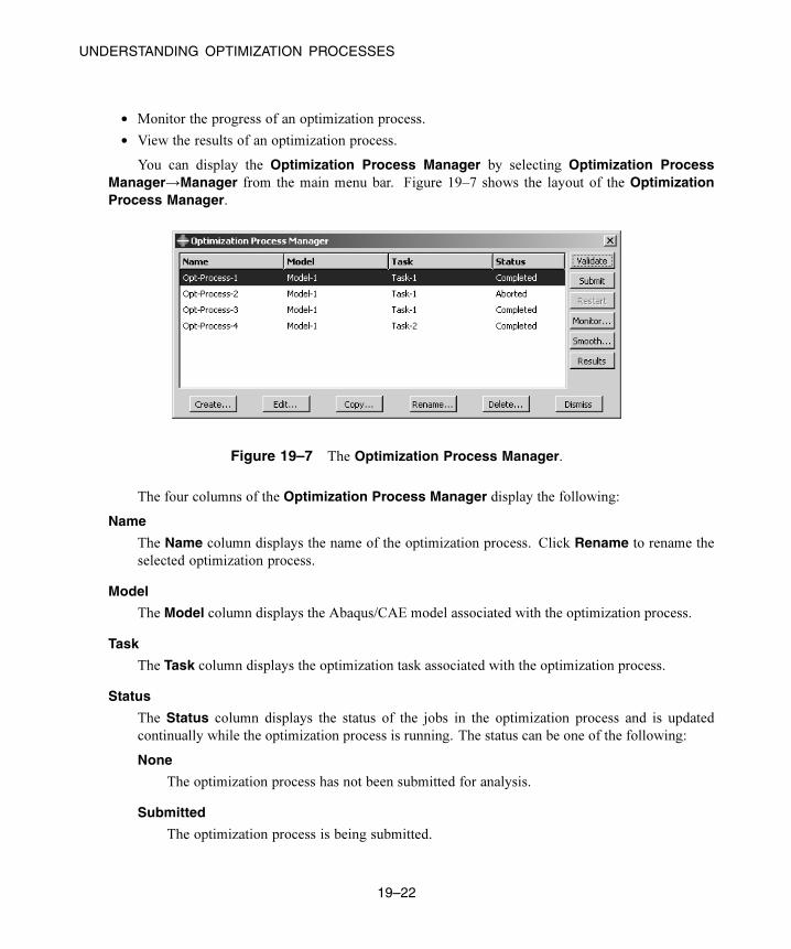
UNDERSTANDING OPTIMIZATION PROCESSES
• Monitor the progress of an optimization process.
• View the results of an optimization process.
You can display the Optimization Process Manager by selecting Optimization ProcessManager→Manager from the main menu bar. Figure 19–7 shows the layout of the OptimizationProcess Manager.
Figure 19–7 The Optimization Process Manager.
The four columns of the Optimization Process Manager display the following:
Name
The Name column displays the name of the optimization process. Click Rename to rename the
selected optimization process.
Model
The Model column displays the Abaqus/CAE model associated with the optimization process.
Task
The Task column displays the optimization task associated with the optimization process.
Status
The Status column displays the status of the jobs in the optimization process and is updated
continually while the optimization process is running. The status can be one of the following:
None
The optimization process has not been submitted for analysis.
Submitted
The optimization process is being submitted.
19–22
Abaqus ID:
Printed on:

UNDERSTANDING OPTIMIZATION PROCESSES
Running
The optimization process has been submitted and is running.
Completed
The optimization process has run to completion.
Aborted
The optimization process has been aborted due to problems such as fatal errors in one of the
models or lack of disk space.
Terminated
The optimization process has been terminated by the user.
19.5.3 The optimization process editor
You use the optimization process editor to select the Abaqus/CAE model and the optimization task that
will be included in the optimization process. You can also configure the optimization settings, such as
the maximum number of optimization iterations.
You can display the optimization process editor by selecting Optimization Process→Create or
Optimization Process→Edit→optimization process name from the main menu bar. (You can also
click Create or Edit in the optimization process manager.)
The optimization process editor allows you to configure the following:
Optimization
Use the Optimization tabbed page to specify the maximum number of optimization iterations that
should be run before the process terminates and the frequency at which data are saved. For more
information, see “Creating and editing optimization processes,” Section 19.12.1.
Submission
Use the Submission tabbed page to configure the submission attributes of your optimization
process, such as the submit time and whether the process is to be submitted to remote queues that
have been configured by your local Abaqus environment file or by your system administrator. For
more information, see “Configuring job submission attributes,” Section 19.8.2.
Memory
Use the Memory tabbed page to configure the amount of memory allocated to the Abaqus jobs
during the optimization process. For more information, see “Controlling job memory settings,”
Section 19.8.7.
19–23
Abaqus ID:
Printed on:

RESTARTING AN ANALYSIS
Parallelization
Use the Parallelization tabbed page to configure the parallel execution of the Abaqus analysis jobs
during the optimization process, such as the number of processors to use and the parallelization
method. For more information, see “Controlling job parallel execution,” Section 19.8.8.
Precision
Use the Precision tabbed page to choose the precision of nodal output that is written to the output
database during the Abaqus analysis. For more information, see “Controlling job precision,”
Section 19.8.9.
19.6 Restarting an analysis
If your model contains multiple steps, you do not have to analyze all of the steps in a single analysis job.
Indeed, it is often desirable to run a complex analysis in stages. This allows you to examine the results
and confirm that the analysis is performing as expected before continuing with the next stage. The restart
files generated by an Abaqus analysis allow you to continue the analysis from a specified step. For more
information, see “Restarting an analysis,” Section 9.1.1 of the Abaqus Analysis User’s Guide.
This section describes the restart capability in Abaqus/CAE. The following topics provide some
background information:
• “Controlling a restart analysis,” Section 19.6.1
• “Files required to restart an analysis,” Section 19.6.2
• “Rules governing a restart analysis,” Section 19.6.3
• “The relationship between the model and the restart analysis,” Section 19.6.4
The following topics describe examples of the most common uses for restart analysis:
• “Restarting after adding more analysis steps to the model,” Section 19.6.5
• “Restarting after modifying existing analysis steps,” Section 19.6.6
• “Restarting from the middle of a step,” Section 19.6.7
• “Visualizing results from restart analyses,” Section 19.6.8
• “Recovering an Abaqus/Standard analysis,” Section 19.6.9
• “Remote submission of restart jobs,” Section 19.6.10
19.6.1 Controlling a restart analysisBy default, no restart information is written for an Abaqus/Standard or an Abaqus/CFD analysis and
restart information is written only at the beginning and end of each step for an Abaqus/Explicit analysis.
19–24
Abaqus ID:
Printed on:

RESTARTING AN ANALYSIS
You can use the Step module to change the frequency at which restart information is written. For more
information, see “Restart output requests,” Section 14.5.2.
After an analysis has generated restart information, you can control the following aspects of the
subsequent restart analysis:
Model attributes
To configure a restart analysis, you must specify whether the model should reuse data from a
previous analysis of the same model. You can specify the step and the increment or time interval
of the previous analysis from which the new analysis should start. You can also choose one of the
following:
• Allow the selected step to continue to completion.
• Terminate the selected step at the specified increment and begin a new step.
For more information, see “Specifying model attributes,” Section 9.8.4, in the HTML version of
this guide.
Job type
You use the job editor to specify the job type. If you edit the model attributes to specify that the
model should reuse data from a previous analysis and you create a job that refers to this model,
Abaqus/CAE sets the job type to Restart. For more information, see “Selecting a job type,”
Section 19.2.5. You cannot create a restart job that refers to a job that was associated with an input
file.
19.6.2 Files required to restart an analysisTo restart an analysis, various files that were created by the previous analysis must be available in the
directory from which you started the Abaqus/CAE session.
Abaqus/Standard
• Output database (.odb)
• Restart file (.res)
• Model file (.mdl)
• Part file (.prt)
• State file (.stt)
Abaqus/Explicit
• Output database (.odb)
• Restart file (.res)
• Model file (.mdl)
• Package file (.pac)
• Part file (.prt)
19–25
Abaqus ID:
Printed on:

RESTARTING AN ANALYSIS
• State files (.abq and .stt)
• Selected results file (.sel)
Abaqus/CFD
• Output database (.odb)
• Restart and analysis database file (.sim)
The restart analysis generates an error if any of these files are not available in the current directory.
19.6.3 Rules governing a restart analysis
Defining the restart information for models and jobs is straightforward using Abaqus/CAE; however,
you should understand the following before you use the analysis restart capability:
• The model used in the restart analysis must be the same as the model used in the original analysis
up to the restart location. Specifically,
– For the new model do not modify or add any geometry, mesh, materials, sections, beam section
profiles, material orientations, beam section orientations, interaction properties, or constraints.
– Similarly, do not modify any steps or prescribed conditions (loads, boundary conditions, fields,
interactions, or output requests) at or before the restart location.
• If you used the keyword editor to edit the original model, Abaqus/CAE ignores those changes when
you restart the analysis.
WARNING: Abaqus/CAE does not perform any checks to ensure that the restart data stored for the
original job are consistent with the model used in the restart analysis. In some cases the analysis will
terminate with error messages. In other cases the analysis will run, but the results may not correspond
with your intent. A specific example of a case that will result in an error message is one where you define
a coupling constraint and its accompanying reference node in the original model and then suppress the
constraint prior to the original analysis submission. In this example Abaqus/CAEmaintains the reference
node definition but Abaqus/Standard or Abaqus/Explicit may remove it from the model definition if it is
not attached to other elements or constraints. Your subsequent Abaqus/CAE restart analysis in this
example will be seen as inconsistent with the original analysis. In many cases like this example you can
manually modify the restart analysis input file to correct the discrepancy.
19.6.4 The relationship between the model and the restart analysis
When you first submit a job based on a model for analysis, Abaqus/CAE generates an input file based on
the definition of your model; and that input file, in turn, is submitted for analysis. The input file contains
19–26
Abaqus ID:
Printed on:

RESTARTING AN ANALYSIS
the element and node definitions generated by the Mesh module along with the materials, steps, output
requests, loads, interactions, etc. that you specified using Abaqus/CAE.
To run a restart analysis of a job associated with a model, it is recommended that you copy the
model to a new model. The new model contains all the element and node definitions from the original
model along with all the materials, steps, output requests, loads, interactions, etc. To request a restart
analysis, you edit the new model’s attributes and specify that the analysis continue from a specified step
of the original analysis. When you create a new restart job that refers to the new model, Abaqus/CAE
sets the job type to Restart.When you submit the new job for analysis, Abaqus/CAE generates an input file based on the restart
information. No part, assembly, or property data are written to the restart input file. Only the following
data are written:
• Steps that appear after the analysis is restarted.
• Data from step-dependent objects that are associated with steps that appear after the restart step; for
example, loads, boundary conditions, fields, and output requests.
• New regions and amplitudes that are used by step-dependent objects that are associated with steps
that appear after the restart step.
Abaqus reads the part, assembly, and property data, along with data from steps that appear before
the restart step from the restart files that were generated by the original analysis. As a result, although
the model contains all this information, the information is not written to the input file that is submitted to
Abaqus/Standard or Abaqus/Explicit. This is an important consideration. Some changes that you make
to the model in a restart analysis, say a material property, will not appear in the input file that is analyzed.
19.6.5 Restarting after adding more analysis steps to the modelThe most common use of the restart capability is to analyze your model and then add one or more steps
to the model and continue the analysis. This section describes an example of this usage.
Assume that you have done the following:
• Created a model called Model-A that has two analysis steps, Step-1 and Step-2.
• Used the Edit Restart Requests dialog box in the Step module to output the restart information
at the end of each step.
• Created a job called Job-A that uses Model-A.
• Analyzed the model.
After studying the results of the analysis, you decide to add another step, Step-3, to the model.
The restart capability allows you to compute the results for Step-3 without having to repeat the
computations for Step-1 and Step-2. The following steps describe a recommended procedure to
follow:
1. Copy Model-A to a new model, say Model-A-restart, and make Model-A-restart the
current model.
19–27
Abaqus ID:
Printed on:

RESTARTING AN ANALYSIS
2. Add the new Step-3 to Model-A-restart.
3. Add new prescribed conditions (loads, boundary conditions, interactions, fields, or output requests)
in Step-3, or modify the prescribed conditions propagated from Step-2.
4. From the main menu bar, select Model→Edit Attributes→Model-A-restart. From the EditModel Attributes dialog box that appears, do the following:
• Enter Job-A as the job from which the restart data will be read.
• Set the restart location:
– Enter Step-2 to indicate the step from which the restart data will be read.
– Choose Restart from the end of the step. Step-3 will continue the analysis after the
end of Step-2.
5. Copy Job-A to a new job, say Job-A-restart, that uses Model-A-restart.
6. From the main menu bar, select Job→Edit→Job-A-restart. From the Edit Job dialog box that
appears, choose a job type of Restart.
7. Submit Job-A-restart for analysis.
19.6.6 Restarting after modifying existing analysis stepsYou can use the restart capability to analyze your model and then modify an existing step before
continuing the analysis. This section describes an example of this usage.
Assume that you have done the following:
• Created a model called Model-A that has two analysis steps, Step-1 and Step-2.
• Used the Edit Restart Requests dialog box in the Step module to output the restart information
at the end of each step.
• Created a job called Job-A that uses Model-A.
• Analyzed the model.
After examining the results of Job-A, you realize that you need to make changes to Step-2, to anoutput request in Step-2, or to a prescribed condition in Step-2, such as a load or boundary condition.You may also want to add some new steps with additional output requests and loads and with changes
to the boundary conditions. You know that you can still use the results from Step-1; however, yourealize that the results from Step-2 are no longer valid. The restart capability allows you to recompute
the results for Step-2 without having to repeat the computations for Step-1. The following steps
describe a recommended procedure to follow:
1. Copy Model-A to a new model, say Model-A-restart, and make Model-A-restart the
current model.
2. Do the following:
• Make the desired changes to Step-2.
• Add new steps after Step-2.
19–28
Abaqus ID:
Printed on:

RESTARTING AN ANALYSIS
• Create new prescribed conditions in Step-2 and subsequent steps.
3. From the main menu bar, select Model→Edit Attributes→Model-A-restart. From the EditModel Attributes dialog box that appears, do the following:
• Enter Job-A as the job from which the restart data will be read.
• Set the restart location:
– Enter Step-1 to indicate the step from which the restart data will be read.
– Choose Restart from the end of the step. Step-2 will continue the analysis after the
end of Step-1.
4. Copy Job-A to a new job, say Job-A-restart, that uses Model-A-restart. Abaqus/CAEsets the job type to Restart.
5. Submit Job-A-restart for analysis.
19.6.7 Restarting from the middle of a step
You can use the restart capability to continue the analysis from the middle of a completed step or from the
middle of a partially completed step. The restarted analysis uses a new step that continues the analysis
from a specified increment of the previous step. This section describes an example of this usage.
Assume that you have done the following:
• Created a model called Model-A that has two Abaqus/Standard analysis steps, Step-1 and
Step-2.
• Used the Edit Restart Requests dialog box in the Step module to output the restart information
every 10 increments.
• Created a job called Job-A that uses Model-A.
• Analyzed the model.
You suspected that the loading is too severe for the structure and might lead to instabilities or
collapse of the structure and, hence, to numerical convergence difficulties. As a result, you used the
Step module to save the restart information every 10 increments of each step. When you ran the
analysis, you found that the analysis terminated before the end of Step-2, at increment 25. You used
the Visualization module to look at the results of the analysis and realized that the negative eigenvalue
messages confirmed your suspicion that the structure might have become unstable. Now that you have
some idea of the collapse load level, you want to restart the analysis at increment 20 of Step-2with lower levels of loading and more frequent output of results data. The following steps describe a
recommended procedure to follow:
1. Copy Model-A to a new model, say Model-A-restart, and make Model-A-restart the
current model.
2. Add the new Step-3 to Model-A-restart.
19–29
Abaqus ID:
Printed on:

RESTARTING AN ANALYSIS
3. Modify the load levels and output requests in Step-3. For example, if the load at Step-2,increment 25 was 260 and the load at Step-2, increment 20 was 250, you might change the
load level for the end of Step-3 to 262. In addition, you can increase the frequency at which
data are written to the output database so that you can follow the progression of the collapse of
the structure. You can also reduce the size of the maximum increment to control the resolution
of the data that are generated by the analysis. For more information, see “Restarting an analysis,”
Section 9.1.1 of the Abaqus Analysis User’s Guide.
4. From the main menu bar, select Model→Edit Attributes→Model-A-restart. From the EditModel Attributes dialog box that appears, do the following:
• Toggle on Read data from job and enter Job-A to indicate the job from which the restart
data will be read.
• Set the restart location:
– Enter Step-2 to indicate the step from which the restart data will be read.
– Choose Restart from increment, interval, iteration, or cycle, and enter 20 to indicate
the increment from which the restart data will be read.
– Choose and terminate the step at this point to indicate that Step-2 should terminate
at increment 20. Step-3 will continue the analysis from this location.
5. Copy Job-A to a new job, say Job-A-restart, that uses Model-A-restart. Abaqus/CAEsets the job type to Restart.
6. Submit Job-A-restart for analysis.
19.6.8 Visualizing results from restart analyses
Each restart analysis creates a new output database. Consider the example described in “Restarting after
adding more analysis steps to the model,” Section 19.6.5, where you did the following:
• Ran an analysis of Job-A that referred to Model-A that contains Step-1 and Step-2. As a
result, the output database generated by the analysis, Job-A.odb, contains results from Step-1and Step-2.
• Ran a restart analysis of Job-A-restart that referred to Model-A-restart. Although
Model-A-restart contains Step-1, Step-2, and Step-3, the output database generated
by the restart analysis, Job-A-restart.odb, contains results from only Step-3.
You can use the Visualization module to create deformed, contour, and symbol plots of field data;
however, you can plot the results from only one output database at any time. You must change the output
database if you are looking at the results from Step-1 or Step-2 and want to look at the results from
Step-3.If you want to create an animation of results from all three steps, you must combine the two output
databases. Abaqus provides an execution procedure for this purpose. For more information, see “Joining
19–30
Abaqus ID:
Printed on:

RESTARTING AN ANALYSIS
output database (.odb) files from restarted analyses,” Section 3.2.19 of the Abaqus Analysis User’s
Guide.
Alternatively, you can create a history plot of a variable over all three steps using the following
technique:
• Create one X–Y data object for the variable from the original output database—Job-A.odb.
• Create a second X–Y data object from the output database generated by the restart analysis—Job-A-restart.odb.
• Create an X–Y plot of the two X–Y data objects. Alternatively, you can create a new X–Y data object
using the Operate on XY data option, append the first two X–Y data objects, and create an X–Y
plot of the result.
For more information, see Chapter 47, “X–Y plotting.”
You should take care that your X–Y data objects are not referring to the same step. For
example, consider the restart analysis described in “Restarting after modifying existing analysis steps,”
Section 19.6.6, where you modified an existing step and added a new step before continuing the analysis.
The first output database contains data from Step-1 and Step-2. The second output database
contains data from a modified Step-2 and the new Step-3. The first X–Y data object that you create
should use only the data from Step-1 and should exclude the data from the original Step-2. The
second X–Y data object should use the data from the modified Step-2 and the new Step-3.
19.6.9 Recovering an Abaqus/Standard analysisAbaqus/Explicit has a recovery mechanism for analysis jobs that terminate prematurely; for example,
because of disk space or power failures. For more information, see “Selecting a job type,” Section 19.2.5.
However, unlike Abaqus/Explicit, Abaqus/Standard does not have a recovery mechanism. The following
example describes how you can use the restart capabilities of Abaqus/Standard to continue an analysis
that terminated prematurely. Assume the following:
• You analyzed Model-A containing Step-1, Step-2, and Step-3.
• Because of a power outage, the analysis ended prematurely at Increment 17 of Step-2.
• You requested that restart information be saved every 10 increments. As a result, the last restart
information was saved at Increment 10 of Step-2.
The following procedure describes how you can recover the analysis using the last restart
information that was saved:
1. Copy Model-A to a new model, say Model-A-recover, and make Model-A-recover the
current model.
2. From the main menu bar, select Model→Edit Attributes→Model-A-recover. From the EditModel Attributes dialog box that appears, do the following:
• Toggle on Read data from job, and enter Job-A to indicate the job from which the restart
data will be read.
19–31
Abaqus ID:
Printed on:
RESTARTING AN ANALYSIS
• Set the restart location:
– Enter Step-2 to indicate the step from which the restart data will be read.
– Choose Restart from increment, interval, iteration, or cycle, and enter 10 to indicate
the increment from which the restart data will be read.
– Choose and complete the step. Step-2 will continue the analysis after increment 10and run to completion.
3. Copy Job-A to a new job, say Job-A-recover, that uses Model-A-recover. Abaqus/CAEsets the job type to Restart.
4. Submit Job-A-recover for analysis.
19.6.10 Remote submission of restart jobs
If you submit a job to a remote machine for analysis, by default Abaqus copies the files required for
a restart analysis back to your local directory when the job is complete. For more information, see
“Submitting a job remotely,” Section 19.2.7. If the remote job terminates prematurely, you may have to
copy the files back to your local directory manually.
Most of the files required for a restart analysis are platform-dependent binary files. As a result, you
will not be able to continue a restart analysis on aWindows machine after starting the analysis on a UNIX
machine, or vice versa. The part (.prt) file contains ASCII text and can be copied across platforms.
The lack of portability across platforms with different binary formats does not preclude you from
restarting an analysis on a machine that is different from the machine on which the original analysis was
run. However, the two machines must be binary compatible, and it is recommended that the original
analysis and the restart analysis both be executed on the same platform. Abaqus does not test cross-
platform compatibility of restart files.
19–32
Abaqus ID:
Printed on:

UNDERSTANDING THE ROLE OF THE SKETCH MODULE
20. The Sketch module
Sketches are two-dimensional profiles that are used to help form the geometry defining an Abaqus/CAE
native part. You use the Sketch module to create a sketch that defines a planar part, a beam, or a partition
or to create a sketch that might be extruded, swept, or revolved to form a three-dimensional part. This
chapter explains how you use the tools within the Sketch module to create, modify, and manage sketches.
The following topics are covered:
• “Understanding the role of the Sketch module,” Section 20.1
• “Entering and exiting the Sketch module,” Section 20.2
• “Overview of the Sketch module,” Section 20.3
• “Basic Sketcher concepts,” Section 20.4
• “Sketcher geometry,” Section 20.5
• “Specifying precise geometry,” Section 20.6
• “Controlling sketch geometry,” Section 20.7
• “Modifying, copying, and offsetting objects,” Section 20.8
In addition, the following sections are available in the HTML version of this guide:
• “Customizing the Sketcher,” Section 20.9
• “Sketching simple objects,” Section 20.10
• “Creating construction geometry,” Section 20.11
• “Constraining, dimensioning, and parameterizing a sketch,” Section 20.12
• “Editing dimensions,” Section 20.13
• “Adding reference geometry,” Section 20.14
• “Projecting edges onto a sketch,” Section 20.15
• “Moving or copying sketch geometry,” Section 20.16
• “Modifying objects,” Section 20.17
• “Repairing short edges, gaps, and overlaps,” Section 20.18
• “Creating patterns, offsetting, and deleting objects,” Section 20.19
• “Undoing and redoing sketching actions,” Section 20.20
• “Resetting the view,” Section 20.21
• “Managing stand-alone sketches,” Section 20.22
20.1 Understanding the role of the Sketch module
You use the Sketch module to create and manage two-dimensional profiles that are not associated with
a feature; these profiles are known as stand-alone sketches. Stand-alone sketches can be incorporated in
20–1
Abaqus ID:
Printed on:

OVERVIEW OF THE SKETCH MODULE
the current sketch, and they will overlay any existing geometry. For more information, see “Managing
stand-alone sketches,” Section 20.22, in the HTML version of this guide.
20.2 Entering and exiting the Sketch module
You can enter the Sketch module at any time during an Abaqus/CAE session by clicking Sketch in the
Module list located in the context bar. The Sketch module tools appear in the module toolbox, and the
Sketch menu appears on the main menu bar.
To exit the Sketch module, first exit the current drawing tool by clicking mouse button 2. Then
click the Done button that appears in the prompt area, and select any other module from the Modulelist. You need not take any specific action to save your sketches before exiting the module; they are
saved automatically when you save the entire model by selecting File→Save or File→Save As from
the main menu bar.
You should recognize the difference between the Sketch module and the Sketcher. When you create
or edit a stand-alone sketch, the Sketch module starts the Sketcher and displays the Sketcher tools in the
module toolbox. In addition, Abaqus/CAE starts the Sketcher whenever you do one of the following:
• Create or edit a feature while defining a part in the Part module.
• Sketch a partition on a face or cell while working in the Part module.
• Sketch a partition on a face or cell in the assembly while working in the Assembly module or the
Mesh module.
To exit the Sketcher and incorporate your sketch into the part or assembly, first exit the current
drawing tool by clicking mouse button 2. Then, click the Done button that appears in the prompt area.
Where applicable, follow any additional prompts to extrude, revolve, or sweep the feature. Abaqus/CAE
exits the Sketcher and returns to themodule that invoked it. In addition, Abaqus/CAE restores the original
view of the part or assembly.
20.3 Overview of the Sketch module
This section provides an overview of the Sketch module.
20.3.1 Stand-alone sketchesYou use the Sketch module to create and manage sketches that are not associated with a feature; these
sketches are called stand-alone sketches. A stand-alone sketch is stored in the model; like other objects
in the model, such as parts and loads, a stand-alone sketch can be edited, copied, renamed, and deleted.
To create a stand-alone sketch, click the sketch create tool in the Sketch module toolbox.
20–2
Abaqus ID:
Printed on:

OVERVIEW OF THE SKETCH MODULE
When you are using the Sketcher (for example, when you are sketching the profile of a solid
extrusion in the Part module), you can save your work as a stand-alone sketch by clicking the sketch
save tool in the Sketcher toolbox. Similarly, you can incorporate one stand-alone sketch in another
sketch by clicking the sketch retrieve tool in the Sketcher toolbox. When you retrieve a stand-alone
sketch, Abaqus/CAE does the following:
• Positions the retrieved sketch so that its origin is coincident with the origin of the current sketch.
• Resizes the viewport so that both the current sketch and the retrieved sketch are displayed.
• Asks if you want to translate, rotate, mirror, or scale the retrieved sketch from the default size and
position.
For detailed instructions on creating andmanaging stand-alone sketches, see “Managing stand-alone
sketches,” Section 20.22, in the HTML version of this guide.
20.3.2 Imported sketchesYou can import stand-alone sketches into the model by selecting File→Import→Sketch from the main
menu bar. You can import sketches from files stored in the following industry-standard formats:
• AutoCAD (file extension .dxf)
• IGES (file extension .igs)
• ACIS (file extension .sat)
• STEP (file extension .stp)
When you import a file as a stand-alone sketch, Abaqus/CAE translates the contents of the file into
a set of Sketcher entities, such as lines, arcs, and splines. Abaqus/CAE can import most planar entities
from an IGES-format file. For a complete list of the IGES entities that can be imported into a sketch,
see “IGES entities recognized by Abaqus/CAE when importing a part or a sketch,” Section 10.7.8, in
the HTML version of this guide. When you import an AutoCAD- or ACIS-format file, Abaqus/CAE
recognizes only the entities listed in Table 20–1 and Table 20–2. If Abaqus/CAE finds geometry that it
cannot translate, it ignores that geometry and continues importing the sketch.
Table 20–1 AutoCAD entities supported by the Sketcher.
AutoCAD entity Sketcher entity
Line Line
Circle Circle
Arc Arc
Vertex Point
Spline and polyline Points
20–3
Abaqus ID:
Printed on:

BASIC SKETCHER CONCEPTS
Table 20–2 ACIS entities supported by the Sketcher.
ACIS entity Sketcher entity
Line Line
Circle Circle
Arc Arc
Vertex Point
Ellipse Ellipse
Spline and polyline Spline
For Abaqus/CAE to convert the file to a sketch, the file must contain a two-dimensional planar profile
that can be mapped to the sketch plane. If the file contains three-dimensional geometry, Abaqus/CAE
cannot import the sketch.
In some cases, when you import a sketch to create the base feature of a part, Abaqus/CAE positions
the sketch relatively far from the Sketcher origin. As a result, the part will be far from its origin, and the
analysis of your model can be affected by a loss of precision. To improve precision, you may have to
move the part closer to its origin by moving the vertices of the sketch closer to the origin of the Sketcher
grid. For more information, see “The Sketcher sheet and grid,” Section 20.4.2.
20.4 Basic Sketcher concepts
You use the Sketcher to sketch the lines and curves that form the two-dimensional profile of a feature, to
add constraints to the sketch, and to modify the sketch. This section describes some of the basic concepts
used by the Sketcher and how these concepts influence the behavior of the Sketcher tools and appearance
of the sketch.
20.4.1 The Sketcher tools
You can access all the Sketcher tools through either the main menu bar or the toolbox. Figure 20–1 shows
the hidden icons for all the tools in the Sketcher toolbox. To see a tooltip containing a brief definition
of a Sketcher tool, hold the mouse over the tool for a moment. For information on using toolboxes and
selecting hidden icons, see “Using toolboxes and toolbars that contain hidden icons,” Section 3.3.2.
The Sketcher tools allow you to do the following:
• Create basic sketch entities, such as lines, circles, arcs, ellipses, fillets, and splines. For detailed
instructions, see “Sketching simple objects,” Section 20.10, in the HTML version of this guide.
20–4
Abaqus ID:
Printed on:

BASIC SKETCHER CONCEPTS
Sketch arc tangent to curve
Auto-Dimension
Edit dimension
Move or copy tools
Project edge orreference tools
Sketch point
Sketch circle
Sketch ellipse
Sketch arc center and end points
Drag
Sketch line
Sketch rectangle
Sketch fillet
Linear pattern or radial pattern
Add dimension
Parameter manager
Auto-Trim, Trim/Extend, and Split
Sketch spline
Offset curves
Sketch arc through three points
Constructiongeometry tools
Auto-Constrain Add constraint
Add sketch Save sketch
Sketcher options Reset view
Delete
Set as construction and unset construction
Undo Redo
Remove short edges, Repair gaps and overlaps, and Merge
Figure 20–1 The Sketcher toolbox.
• Add construction geometry to help you position and align sketch entities. For detailed instructions,
see “Creating construction geometry,” Section 20.11, in the HTML version of this guide.
• Add constraints, dimensions, and parameters to control your sketch geometry and add precision. For
detailed instructions, see “Constraining, dimensioning, and parameterizing a sketch,” Section 20.12,
in the HTML version of this guide.
• Translate, rotate, scale, or mirror sketch geometry. For detailed instructions, see “Moving or
copying sketch geometry,” Section 20.16, in the HTML version of this guide.
• Drag, trim, extend, split, or merge sketch entities. For detailed instructions, see “Modifying
objects,” Section 20.17, in the HTML version of this guide.
• Create similar objects by offsetting, creating linear patterns, or creating radial patterns. For detailed
instructions, see “Creating patterns, offsetting, and deleting objects,” Section 20.19, in the HTML
version of this guide.
20–5
Abaqus ID:
Printed on:

BASIC SKETCHER CONCEPTS
20.4.2 The Sketcher sheet and gridWhen you enter the Sketcher and either create a new sketch or edit an existing sketch, Abaqus/CAE
displays a sheet in the current viewport on which you sketch. In addition, the triad in the lower-left
corner of the viewport indicates the orientation of the part or the assembly relative to the Sketcher sheet.
The sheet is always square, and its height and width are determined by the sheet size. Abaqus/CAE
determines the sheet size and the location of the origin, depending on what you are sketching:
• If you are sketching the base feature of a new part, the sheet size is the same as the approximate
size of the part that you provided when you created the part. The origin of the sheet is located at
the origin of the part’s coordinate system. Similarly, if you are creating a stand-alone sketch, the
sheet size is the same as the approximate size of the sketch that you provided when you created the
sketch.
• If you are adding a feature to a part or to the assembly, the default sheet size depends on the size of
the face on which you are sketching. The origin of the sheet is located at the centroid of the selected
face. If you selected a datum plane as the sketching plane, the origin of the sheet is located at the
center of the part or assembly; the sheet size depends on the total size of the part or assembly.
You can use the Sketcher customization options to increase or decrease the sheet size if it does not
correspond with the size of the geometry you are trying to sketch. To access the Sketcher customization
options, select the customization tool from the Sketcher toolbox. For more information, see
“Customizing the sheet size and grid,” Section 20.9.4, in the HTML version of this guide. You may
need to use the magnify tool to view the entire Sketcher sheet within the viewport.
Abaqus/CAE overlays the sheet with a grid of invisible grid points to help you position the cursor
as you draw, move, resize, or reshape objects. By default, when you move the cursor near a grid point,
the cursor automatically moves, or snaps, to the point. This behavior allows you to easily position the
cursor precisely on a grid point while also providing you with full control when the cursor is not close
to any grid points. If it is more convenient, you can disable the snapping behavior so that you have full
control over the cursor. To help you visualize the grid points underlying the Sketcher grid, Abaqus/CAE
displays visible grid lines that pass through the grid points at a selected interval; for example, every other
grid point. For more information, see “Turning snapping on or off,” Section 20.9.2, and “Customizing
the sheet size and grid,” Section 20.9.4, in the HTML version of this guide.
For example, Figure 20–2 shows a magnified view of a sheet whose spacing is set to 2 units. In this
example the Sketcher displays both major grid lines (in a solid line style) and minor grid lines (in a thin,
dashed line style). Minor grid lines appear in the Sketcher only when the magnification level is high. In
addition, the thick dashed lines in the sheet indicate the X- and Y-axes of the sketch; the lines intersect
at the origin of the sketch.
You can customize the appearance and behavior of the grid by choosing the spacing of grid points,
the spacing of the visible grid lines that overlay the grid points, the number of minor intervals, and the
sheet size. You can also realign the grid relative to the sketch by moving the origin of the grid and by
20–6
Abaqus ID:
Printed on:

BASIC SKETCHER CONCEPTS
grid points axes
2
2
Major grid lines
Minor grid lines
Figure 20–2 Magnified view of the Sketcher grid.
rotating the grid. Your sketch can extend beyond the Sketcher grid; however, if you find that you need to
sketch outside the grid, it is recommended that you increase its size to include the entire sketch. If you
change the grid origin or rotation, the Sketcher displays cursor coordinates in two forms as you continue
to modify the sketch. Grid coordinates indicate the cursor position using the new grid origin or rotation;
sketch coordinates indicate the position based on the original grid location. For more information, see
“Customizing the Sketcher,” Section 20.9, in the HTML version of this guide.
The analysis of your model can be affected by a loss of precision if the coordinates of a part are
far from the origin of the part. For example, after you import a sketch to create the base feature of a
part, the sketch may be relatively far from the Sketcher origin; as a result, the part will be far from its
origin. To improve precision, you may have to move the part closer to its origin by moving the sketch
geometry closer to the origin of the Sketcher grid using the translate tool, . For more information,
see “Translating Sketcher objects along a vector,” Section 20.16.1, in the HTML version of this guide.
You should not move the origin of the sketch closer to the geometry. Moving the origin of the Sketcher
grid closer to the sketch is a graphical convenience only and has no effect on the underlying precision of
the coordinates.
20–7
Abaqus ID:
Printed on:

BASIC SKETCHER CONCEPTS
20.4.3 How Abaqus/CAE orients your sketchWhen the Sketcher starts, Abaqus/CAE orients the view of the part or assembly so that the face or datum
plane on which you are sketching is parallel to the screen; this plane is known as the sketch plane. The
orientation of the sketch plane depends on the modeling space of the part or assembly and the type of
feature you are creating:
Two-dimensional or axisymmetric modeling space
When you add a planar feature to a two-dimensional or axisymmetric part or assembly, Abaqus/CAE
starts the Sketcher and aligns the X- and Y-axes of the part with the axes of the Sketcher grid,
regardless of the type of feature you are creating. (Abaqus/CAE derives the X- and Y-axes of the
part from the axes of the sketch that defined the base feature.)
Three-dimensional modeling space
When you add a feature to a three-dimensional part or assembly, you must use the following
technique to control the orientation of the view relative to the Sketcher grid:
1. Select the plane on which to sketch by selecting appropriate geometry; for example, a face of
a part or a datum plane.
2. Select an edge. By default, the selected edge will appear vertical and on the right side of the
Sketcher grid. Alternatively, you can choose a different orientation for the edge in the Sketcher
grid before you select the edge; for example, horizontal and on the top of the Sketcher grid.
You can select any edge from the part or assembly that is not perpendicular to the selected
plane. You can select a datum axis, or you can select one of the axes of a datum coordinate
system; but you cannot select the edge of a datum plane. You can select a curved edge, but the
resulting orientation of the part or assembly is system dependent.
Abaqus/CAE highlights the selected edge, enters the Sketcher, and rotates the part until the selected
edge aligns with the grid in the desired orientation. The orientation of the view on the Sketcher grid
also depends on the type of feature you are creating:
• When you are sketching a cut feature in the Part module, Abaqus/CAE orients the view so that
the resulting feature will cut away from you and into the screen.
• When you are sketching a feature other than a cut (for example, an extruded solid),
Abaqus/CAE orients the view so that the resulting feature will protrude out of the screen
toward you.
• When you are adding a swept feature, you must sketch a sweep path and sweep profile. For
details of the resulting view orientation, see “Adding a swept solid feature,” Section 11.21.3;
“Adding a swept shell feature,” Section 11.22.3; and “Creating a swept cut,” Section 11.24.4,
in the HTML version of this guide.
When you are partitioning faces using the sketch method in the Partition toolset, Abaqus/CAE
orients the view based upon the modeling space of the part or assembly and the type of faces you selected
20–8
Abaqus ID:
Printed on:
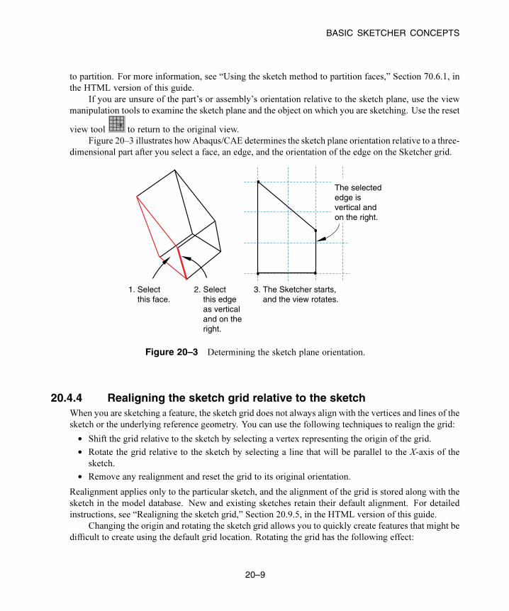
BASIC SKETCHER CONCEPTS
to partition. For more information, see “Using the sketch method to partition faces,” Section 70.6.1, in
the HTML version of this guide.
If you are unsure of the part’s or assembly’s orientation relative to the sketch plane, use the view
manipulation tools to examine the sketch plane and the object on which you are sketching. Use the reset
view tool to return to the original view.
Figure 20–3 illustrates how Abaqus/CAE determines the sketch plane orientation relative to a three-
dimensional part after you select a face, an edge, and the orientation of the edge on the Sketcher grid.
1. Select this face.
2. Select this edge as vertical and on the right.
The selectededge is vertical andon the right.
3. The Sketcher starts, and the view rotates.
Figure 20–3 Determining the sketch plane orientation.
20.4.4 Realigning the sketch grid relative to the sketchWhen you are sketching a feature, the sketch grid does not always align with the vertices and lines of the
sketch or the underlying reference geometry. You can use the following techniques to realign the grid:
• Shift the grid relative to the sketch by selecting a vertex representing the origin of the grid.
• Rotate the grid relative to the sketch by selecting a line that will be parallel to the X-axis of the
sketch.
• Remove any realignment and reset the grid to its original orientation.
Realignment applies only to the particular sketch, and the alignment of the grid is stored along with the
sketch in the model database. New and existing sketches retain their default alignment. For detailed
instructions, see “Realigning the sketch grid,” Section 20.9.5, in the HTML version of this guide.
Changing the origin and rotating the sketch grid allows you to quickly create features that might be
difficult to create using the default grid location. Rotating the grid has the following effect:
20–9
Abaqus ID:
Printed on:

BASIC SKETCHER CONCEPTS
• The grid coordinates of the current cursor position are displayed in the upper-left corner of the
viewport, and you can use these coordinates as a guide. The grid coordinates displayed are relative
to the current alignment of the sketch grid and change if you realign the grid.
• The sketch coordinates of the current cursor position are displayed in the upper-right corner of the
viewport. The sketch coordinates displayed are relative to the original alignment of the sketch grid
and do not change if you realign the grid.
• When you enter the coordinates of a vertex in the prompt area, those coordinates are relative to the
current alignment of the sketch grid.
• Old and new horizontal and vertical dimensions remain horizontal and vertical.
• Old horizontal and vertical construction lines remain horizontal and vertical.
• New horizontal and vertical construction lines and preselection points are aligned with the rotated
grid.
• The lines generated by the rectangle tool are aligned with the rotated grid.
20.4.5 The Sketcher cursors and preselectionThere are two cursors active within the Sketcher: the primary cursor and the secondary cursor. The two
cursors are shown in Figure 20–4.
primarycursor
secondarycursor
Figure 20–4 The Sketcher cursors.
The primary cursor is the one you use with most applications on your computer, including
Abaqus/CAE. The primary cursor usually appears as an arrow pointer or a pointing hand; you position
this cursor by moving the mouse. The secondary cursor is active only in the Sketcher; it appears near
the primary cursor when the Sketcher prompts you to select a point. The position of the secondary
cursor allows you to see exactly which point is selected before committing the selection. If you move
the primary cursor near a point that is eligible for selection, the secondary cursor jumps directly to the
point while the primary cursor remains fixed. This behavior is called preselection. If you click the
mouse button, Abaqus/CAE selects the point under the secondary cursor.
The appearance of the secondary cursor changes as you move around the sketch. Table 20–3 shows
the shape assumed by the secondary cursor when the primary cursor is close to the Sketcher entity listed.
20–10
Abaqus ID:
Printed on:

BASIC SKETCHER CONCEPTS
Table 20–3 Preselection cursors.
Preselection cursor Sketcher entity
A vertex
● The midpoint of a line or curve
× The intersection of lines and curves
×—— The projection of a line onto other lines and curves
○ Points along existing lines or curves
+ The intersection of grid lines with each other or with other
lines and curves
The secondary cursor works in conjunction with other preselection symbols in the sketch to indicate
special points that you can select. Table 20–4 shows the other preselection symbols used in the Sketcher
and the meaning of each symbol.
Table 20–4 Preselection symbols.
Preselection symbol Location and Meaning
At the starting point of a new line segment when the
line starts on existing sketch, reference, or construction
geometry. The new line segment is perpendicular to the
existing geometry.
|| Near the starting point when creating a new line starting on
an existing edge; the symbol is aligned with the existing
edge. The new line segment is tangent to the existing edge.
H Near the secondary cursor when creating a new line. The
new line segment is horizontal.
V Near the secondary cursor when creating a new line. The
new line segment is vertical.
The preselection cursors and symbols also indicate constraints that Abaqus/CAE will apply to the sketch
if you choose the preselected point. Constraints such as coincidence, perpendicularity, and tangency help
control sketch geometry and preserve your design intent.
Preselection applies to any entity that is a valid selection in the sketch. For example, as you move
the cursor around the sketch, preselection highlights the following to indicate a valid selection:
• Vertices, intersections, projections, and points of tangency highlight when you are sketching a line,
as shown in Table 20–3.
20–11
Abaqus ID:
Printed on:
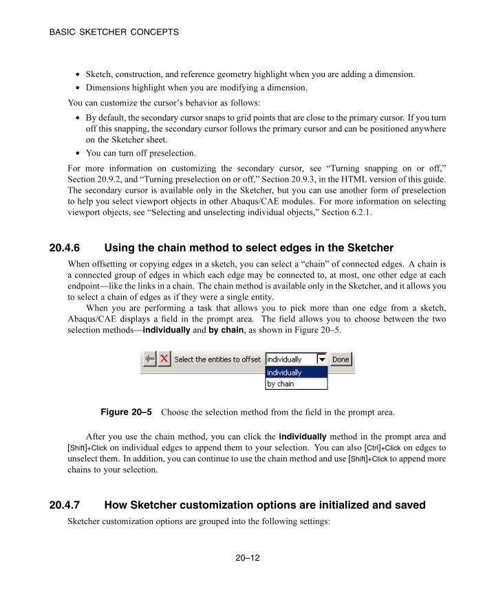
BASIC SKETCHER CONCEPTS
• Sketch, construction, and reference geometry highlight when you are adding a dimension.
• Dimensions highlight when you are modifying a dimension.
You can customize the cursor’s behavior as follows:
• By default, the secondary cursor snaps to grid points that are close to the primary cursor. If you turn
off this snapping, the secondary cursor follows the primary cursor and can be positioned anywhere
on the Sketcher sheet.
• You can turn off preselection.
For more information on customizing the secondary cursor, see “Turning snapping on or off,”
Section 20.9.2, and “Turning preselection on or off,” Section 20.9.3, in the HTML version of this guide.
The secondary cursor is available only in the Sketcher, but you can use another form of preselection
to help you select viewport objects in other Abaqus/CAE modules. For more information on selecting
viewport objects, see “Selecting and unselecting individual objects,” Section 6.2.1.
20.4.6 Using the chain method to select edges in the SketcherWhen offsetting or copying edges in a sketch, you can select a “chain” of connected edges. A chain is
a connected group of edges in which each edge may be connected to, at most, one other edge at each
endpoint—like the links in a chain. The chain method is available only in the Sketcher, and it allows you
to select a chain of edges as if they were a single entity.
When you are performing a task that allows you to pick more than one edge from a sketch,
Abaqus/CAE displays a field in the prompt area. The field allows you to choose between the two
selection methods—individually and by chain, as shown in Figure 20–5.
Figure 20–5 Choose the selection method from the field in the prompt area.
After you use the chain method, you can click the individually method in the prompt area and
[Shift]+Click on individual edges to append them to your selection. You can also [Ctrl]+Click on edges to
unselect them. In addition, you can continue to use the chain method and use [Shift]+Click to append more
chains to your selection.
20.4.7 How Sketcher customization options are initialized and savedSketcher customization options are grouped into the following settings:
20–12
Abaqus ID:
Printed on:

BASIC SKETCHER CONCEPTS
Sketcher options
• Snapping
• Preselection behavior
• Whether to display construction geometry, dimensions, parameter names, and constraints
• The types of constraints and dimensions that Abaqus/CAE can add automatically
Sketch options
• Sheet size, grid spacing, and grid display
• The origin of the grid and the alignment of the axes
• The text height and decimal places of dimensions and text height of parameter names
Sketcher options control the interactive behavior of the Sketcher, while Sketch options control the
appearance of individual sketches. Abaqus/CAE stores and uses your Sketcher customization settings
only for the duration of the session. In contrast, Abaqus/CAE stores your Sketch customization settings
along with each sketch in the model database. As a result, if you exit the Abaqus/CAE session and return
to the sketch at a later date, the Sketch customization options are retained.
When you create a new part or stand-alone sketch, Abaqus/CAE always uses the default Sketch
options. The sheet size and grid spacing are recalculated based on the approximate size of the part or the
selected sketch plane, the origin of the sketch is at 0,0 , the grid is displayed and aligns with the 1- and
2-axes, and the text height and decimal places are at their default settings.
For detailed instructions, see “Customizing the Sketcher,” Section 20.9, in the HTML version of
this guide.
20.4.8 Using the Query toolset in the Sketcher
Select Tools→Query from the main menu bar, or click the tool in the Query toolbar to start the
Query toolset.
You can use the Query toolset to request either general information or module-specific information.
For a discussion of the information displayed by general queries, see “Obtaining general information
about the model,” Section 71.2.2, in the HTML version of this guide.
The following queries are specific to the Sketcher:
Constraint
Abaqus/CAE displays the constraint type and the names of the constrained entities in the message
area and highlights the entities in the sketch.
Detail
Abaqus/CAE displays the number of geometries, vertices, constraints, dimensions, and
unconstrained degrees of freedom in the message area.
20–13
Abaqus ID:
Printed on:

SKETCHER GEOMETRY
20.5 Sketcher geometry
This section describes the different types of geometry available in the Sketcher.
20.5.1 Reference geometry
When you sketch the profile of a feature, Abaqus/CAE projects onto the sketch sheet all the edges and
vertices of the part or assembly that are in the same plane as the sketch plane. Abaqus/CAE also projects
all datum points and datum axes onto the sketch sheet, regardless of their location in the part or assembly.
These projected points and lines are called reference geometry, and you can use them for reference while
sketching.
You typically use reference geometry to position your sketch accurately by specifying a dimension
between a sketched entity, such as a line or a vertex, and the reference geometry. You can also use
reference geometry to realign the sketch grid. The sketch retains any reference geometry that is used to
position or dimension the sketch—the reference geometry reappears when you use the Sketcher to edit
the feature again. Abaqus/CAE discards any reference geometry that is not used in the sketch.
If your part is complex, projecting only the edges, vertices, and datum points in the sketch plane
onto the sketch sheet reduces the amount of clutter on the screen and makes the selection procedure more
straightforward. However, your selectionwill be limited to only edges, vertices, and datum points that are
in the sketch plane. If you want to use other edges, vertices, or datum points–including orphan element
edges and nodes—as references, you must project them onto the sketch plane as reference geometry by
using the Project References tool . Alternatively, if you want to create new sketch edges from
existing model edges or orphan element edges, you can use the Project Edges tool (for more
information, see “Projecting edges onto a sketch,” Section 20.15, in the HTML version of this guide).
When you sketch a new feature, you can constrain the position of the sketch to the underlying
reference geometry using one of the following methods:
• Select entities from the reference geometry while sketching the new feature; for example, select a
projected vertex to define the center of a circle or one end of a line.
• Create a constraint, dimension, or parameter between the sketch and any projected reference
geometry. For more information, see “Controlling sketch geometry,” Section 20.7.
Constraining the sketch defines how it is positioned relative to the reference geometry and how it will be
repositioned if you modify and regenerate the part or assembly.
When you exit the Sketcher, Abaqus/CAE determines whether you have constrained the sketch
to the reference geometry. If a constraint is found, Abaqus/CAE creates a parent-child relationship
between the new feature (the child) and the selected reference geometry (the parent). If no constraints are
found, Abaqus/CAE displays the following message in the message area: No sketch placement
20–14
Abaqus ID:
Printed on:

SKETCHER GEOMETRY
constraints specified on feature feature name. You do not have to constrain the
sketch; but if you do not, its position relative to the underlying geometry of the part or assembly may
change if you modify and regenerate the part or assembly.
If you save a stand-alone sketch, Abaqus/CAE saves only the sketch and does not save any
underlying reference geometry. As a result, if the sketch includes a dimension between a sketch line
and a reference line, the dimension is not saved with the stand-alone version of the sketch.
The order in which you create features influences the available reference geometry. Feature-based
modeling allows a child feature to be dependent on a parent feature but does not allow a parent to be
dependent on a child. As a result, if a feature was created after the feature you are editing, the edges and
vertices of the newer feature cannot be projected onto the sketch sheet. You can use the Query toolset to
determine the order in which features were created; for more information, see “Using the Model Tree to
obtain feature information,” Section 65.4.8, in the HTML version of this guide.
20.5.2 Construction geometryYou create construction geometry in the Sketcher to help you position and align the geometry in your
sketch; objects that you might need to position include holes, arcs, slots, or gear teeth. The Sketcher
allows you to add construction lines and circles to your sketch; in addition, points that you create using
the isolated point tool are considered construction geometry. Construction lines, circles, and points
do not appear in the feature you are creating or modifying.
While you are adding construction geometry and moving the cursor around the sketch, Abaqus/CAE
displays preselection symbols at the following locations:
• The intersection of the new construction geometry and sketched lines or curves.
• The intersection of the new construction geometry and existing construction geometry.
• The intersection of the new construction geometry and reference geometry. Abaqus/CAE displays
preselection symbols only when the reference geometry was created before the feature being edited.
(See “Reference geometry,” Section 20.5.1, for more information about the behavior of reference
geometry.)
The preselection symbols generated by construction geometry allow you to align objects precisely; for
example, along an oblique line or around a circle. For example, you could create an oblique construction
line and several vertical construction lines to help align a group of circles, as illustrated in Figure 20–6.
Construction lines also define the axis of rotation when sketching revolved solids and surfaces.
For more information about the relationship between construction lines and the axis of revolution, see
“Defining the axis of revolution for axisymmetric parts and for revolved features,” Section 11.13.5.
Construction geometry is shown using dashed lines to distinguish it from sketched geometry.
Construction geometry is visible only while you are working on a sketch; as soon as you exit the
Sketcher, the construction geometry disappears. Abaqus/CAE saves construction geometry with the
original sketch; if the Sketcher is invoked to modify a sketch that included construction geometry, the
construction geometry reappears along with the sketch.
20–15
Abaqus ID:
Printed on:
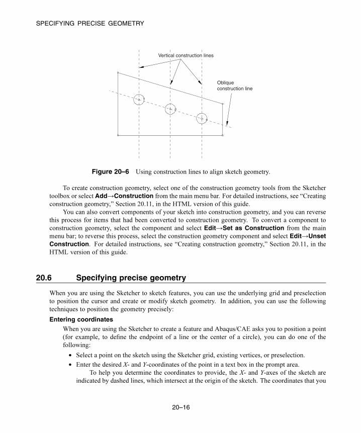
SPECIFYING PRECISE GEOMETRY
Vertical construction lines
Obliqueconstruction line
Figure 20–6 Using construction lines to align sketch geometry.
To create construction geometry, select one of the construction geometry tools from the Sketcher
toolbox or select Add→Construction from the main menu bar. For detailed instructions, see “Creating
construction geometry,” Section 20.11, in the HTML version of this guide.
You can also convert components of your sketch into construction geometry, and you can reverse
this process for items that had been converted to construction geometry. To convert a component to
construction geometry, select the component and select Edit→Set as Construction from the main
menu bar; to reverse this process, select the construction geometry component and select Edit→UnsetConstruction. For detailed instructions, see “Creating construction geometry,” Section 20.11, in the
HTML version of this guide.
20.6 Specifying precise geometry
When you are using the Sketcher to sketch features, you can use the underlying grid and preselection
to position the cursor and create or modify sketch geometry. In addition, you can use the following
techniques to position the geometry precisely:
Entering coordinates
When you are using the Sketcher to create a feature and Abaqus/CAE asks you to position a point
(for example, to define the endpoint of a line or the center of a circle), you can do one of the
following:
• Select a point on the sketch using the Sketcher grid, existing vertices, or preselection.
• Enter the desired X- and Y-coordinates of the point in a text box in the prompt area.
To help you determine the coordinates to provide, the X- and Y-axes of the sketch are
indicated by dashed lines, which intersect at the origin of the sketch. The coordinates that you
20–16
Abaqus ID:
Printed on:

CONTROLLING SKETCH GEOMETRY
specify are relative to this origin. In addition, when you select a Sketcher tool, the coordinates
of the current cursor position are displayed in the upper-left corner of the viewport, and you
can use these coordinates as a guide.
For detailed instructions, see “Sketching simple objects,” Section 20.10, in the HTML version of
this guide.
Creating and modifying dimensions
After you have created the geometry, the Sketcher allows you to add dimensions between lines and
vertices and other pieces of geometry in the sketch. You can then refine the sketch by replacing
these dimensions with precise dimensions, and the sketch changes to reflect the new dimensions.
In addition, dimensions allow you to annotate sketches for future reference.
You add dimensions by selecting the dimension tool in the Sketcher toolbox or by selecting
Add→Dimension from themainmenu bar—editing the dimension value is the final step in creating
a new dimension. To modify an existing dimension, select the modify dimension tool from the
Sketcher toolbox or select Edit→Dimension from the main menu bar. For detailed instructions,
see “Editing dimensions,” Section 20.13, in the HTML version of this guide.
20.7 Controlling sketch geometry
Controlling sketch geometry helps you prevent unintended changes by creating relationships between
sketch entities. If all the geometry in a sketch is controlled, the sketch is fully constrained—the entities
in the sketch cannot be modified without violating the controls, and you cannot add another control
without creating a conflict with one that already exists.
The following section describes how you can use constraints, dimensions, and parameters to control
sketch geometry. All three types of controls can be considered constraints since they all work to restrict
the degrees of freedom in a sketch, but each control creates a different type of relationship between the
selected entities.
For detailed instructions, see the following topics in the HTML version of this guide:
• “Automatically constraining a sketch,” Section 20.12.1
• “Automatically dimensioning a sketch,” Section 20.12.2
• “Adding individual constraints,” Section 20.12.3
• “Adding individual dimensions,” Section 20.12.4
• “Adding and editing parameters,” Section 20.12.5
• “Creating parametric equations,” Section 20.12.6
20–17
Abaqus ID:
Printed on:

CONTROLLING SKETCH GEOMETRY
20.7.1 Using constraints to control sketch geometry
Constraints create logical relationships that control the position or size of geometry. Constraints
are defined without using numerical values. The other types of geometry controls, dimensions and
parameters, are specialized constraints that use values or evaluated expressions to define numerical
relationships in a sketch. Constraints are not required in Abaqus/CAE sketches; however, they can help
you preserve the design intent. When you modify a constrained sketch, you must either work within the
existing controls, modify them, or delete them to complete your changes.
Table 20–5 lists each constraint type, its symbol, and a brief description of its use.
Table 20–5 Sketcher constraints.
Constraints Symbol Description
Coincident o Abaqus/CAE moves the selected entities so that they share
a common point. The point may be a point on both entities
or a projected point that would exist only if one of the
entities was extended. If two straight lines are selected, they
become colinear.
Concentric Abaqus/CAE moves the selected arcs or circles to share a
common center.
Equal length / Abaqus/CAE makes the selected lines all the same length.
Equal radius — Abaqus/CAE makes the selected arcs or circles the same
radius.
Fixed Abaqus/CAE fixes the radius of an arc or circle, the angle of
a line, or the position of a vertex.
Horizontal H Abaqus/CAE aligns the selected line with the X-axis of the
sketch. The horizontal constraint is not affected by grid
orientation.
Equal distance | | Abaqus/CAE moves the selected vertex so that it is the same
distance from the two vertices or lines used to define the
constraint.
Parallel // Abaqus/CAE makes the selected lines parallel.
Perpendicular Abaqus/CAE makes the selected lines perpendicular.
Symmetry | Abaqus/CAE makes the selected entities symmetrical about
your chosen line of symmetry.
20–18
Abaqus ID:
Printed on:

CONTROLLING SKETCH GEOMETRY
Constraints Symbol Description
Tangent || Abaqus/CAE makes the selected entities tangent at their
nearest point. At least one of the entities must be curved.
Vertical V Abaqus/CAE aligns the selected line with the Y-axis of the
sketch. The horizontal constraint is not affected by grid
orientation.
Note: The behaviors described in Table 20–5 assume that no other constraints are applied to the selected
entities. The presence of other constraints and the constraint solution method selected in the SketcherOptions may affect how Abaqus/CAE moves entities to comply with the constraints.
You can create multiple instances of the same type of constraint in a sketch. You can use the sketch
module queries to locate the geometries controlled by a constraint or to list the constraint details for the
entire sketch (for more information, see Chapter 71, “The Query toolset”).
You can use the following techniques to add constraints to a sketch:
Preselecting geometry
If preselection is active, Abaqus/CAE can add some constraints while you create geometry.
Coincident, horizontal, perpendicular, tangent, and vertical constraints can be added using
the preselection cursor. For more information, see “The Sketcher cursors and preselection,”
Section 20.4.5.
Selecting midpoints of lines or curves
If you select the midpoint of a line or curve as the vertex for additional sketch geometry,
Abaqus/CAE also creates an equal distance constraint between the midpoint and the endpoints of
the line or curve.
Adding constraints automatically
After you create a sketch, you can use the auto-constrain tool to add constraints to the entire
sketch or to a selected group of entities. Use the sketch options to control the constraint types that
Abaqus/CAE can add automatically and the allowable tolerances for adding a constraint. For more
information, see “Customizing the use of constraints in the Sketcher,” Section 20.9.10, in the HTML
version of this guide.
Adding individual constraints
After you create sketch geometry, you can select the constraint type and pick the entities to apply
the constraint. This method gives you the most control, but it is also the most time consuming. For
more information, see “Adding individual constraints,” Section 20.12.3, in the HTML version of
this guide.
20–19
Abaqus ID:
Printed on:

CONTROLLING SKETCH GEOMETRY
When you add constraints, you must not overconstrain the sketch geometry. Geometry is
overconstrained when multiple controls are applied to a single degree of freedom (for more information,
see “Fully constrained geometry,” Section 20.7.4). Abaqus/CAE colors conflicting constraints magenta
to indicate an overconstraint condition. You must resolve any overconstraints before you can use a
sketch to create a feature or save it with the model database.
20.7.2 Using dimensions to control sketch geometryDimensions are a type of constraints that use numerical values to define sizes, angles, or distances in a
sketch. Dimensions control sketch geometry by preventing changes to the dimensioned quantities. To
change a dimensioned quantity, you must modify the associated dimension.
The following dimension types are available in the Sketcher:
• horizontal
• vertical
• oblique
• angular
• radial
The first three dimension types correspond to linear distances between two points (including the
endpoints of a single line), two lines, or a point and a line. Angular dimensions always indicate the
angle, in degrees, between two lines. Radial dimensions indicate the radius of a circle, arc, or fillet or
the major and minor radii of an ellipse.
You can use the following techniques to add dimensions to a sketch:
Adding dimensions automatically
After you create a sketch, you can use the auto-dimension tool to add dimensions to the entire
sketch or to a selected group of entities. Use the sketch options to control the dimension types that
Abaqus/CAE can add automatically. For more information, see “Customizing the format and use
of dimensions in the Sketcher,” Section 20.9.9, in the HTML version of this guide.
Adding individual dimensions
After you create sketch geometry, you can add individual dimensions. This method gives you the
most control, but it is also the most time consuming. For more information, see “Adding individual
dimensions,” Section 20.12.4, in the HTML version of this guide.
You can modify any dimension in a sketch. When you edit an existing dimension, you can modify
it in several ways. You can
• edit the numerical value to modify the sketch,
• convert the dimension to a reference dimension, or
• link the dimension to a parameter.
20–20
Abaqus ID:
Printed on:

CONTROLLING SKETCH GEOMETRY
Reference dimensions annotate quantities that are already controlled elsewhere in the sketch or
quantities such as projected reference geometry that cannot be controlled within the current sketch.
Reference dimension values are enclosed in parentheses, and Abaqus/CAE updates them automatically
to match changes in the associated geometry. Dimensions that have been linked to parameters are
assigned a variable name for use in creating mathematical expressions (parametric equations) to
define other parameters in the sketch. For detailed instructions on editing dimensions, see “Editing
dimensions,” Section 20.13, in the HTML version of this guide.
When you add or modify dimensions, you must not overconstrain the sketch geometry. Geometry is
overconstrained when multiple controls are applied to a single degree of freedom (for more information,
see “Fully constrained geometry,” Section 20.7.4). Abaqus/CAE colors conflicting constraints magenta
to indicate an overconstraint condition. You must resolve any overconstraints before you can use a sketch
to create a feature or save it with the model database.
20.7.3 Using parameters to control sketch geometry
Parameters are dimensions or numerical constants that have been given a variable name and are used
to create parametric equations between pieces of geometry. While dimensions always have a numerical
value, parameters may have a numerical value or a value resulting from a mathematical expression.
For example, you can parameterize the radius dimension of a circle so it will always be half the size
of another dimension in the sketch, but you must first associate both dimensions with parameters to
create the expression. You can use the sketch options to control whether Abaqus/CAE displays the
names or values of parameters in a sketch (for more information, see “Customizing the format and use
of dimensions in the Sketcher,” Section 20.9.9).
Parameters must be defined within a single sketch—you cannot define parameters in one sketch
and use them to create expressions in another sketch. Defining a parameter adds it to the ParameterManager for the sketch. The order of parameters in the manager indicates the order in which they can
be used in expressions. Figure 20–7 shows two parameters; the length parameter is used to define the
width parameter. If you instead wanted to define the length in terms of the width, the width parameter
would need to appear first in the manager. You can use the buttons on the right side of the dialog box
to create parameters by selecting dimensions from the viewport or to insert, move, or delete parameters
from the manager. For detailed instructions, see “Adding and editing parameters,” Section 20.12.5, in
the HTML version of this guide.
20.7.4 Fully constrained geometry
Constraints, dimensions, and parameters are all used to create relationships that control, or constrain,
Sketcher geometry. Geometry is constrained by the removal of degrees of freedom from the sketch.
For example, if you apply a perpendicular constraint to two lines, you remove the angular degree of
freedom between those lines. If you drag one of the lines, the other line must also move to maintain the
perpendicular constraint.
20–21
Abaqus ID:
Printed on:

MODIFYING, COPYING, AND OFFSETTING OBJECTS
Figure 20–7 The Parameter Manager.
If geometry is controlled such that you cannot change it without redefining the
relationships—changing constraints, dimensions, or parameters—the geometry is fully constrained.
Abaqus/CAE colors fully constrained geometry green to indicate that it cannot be changed. If you
add too many constraints to a sketch, the geometry becomes overconstrained. Abaqus/CAE colors
conflicting constraints magenta to indicate the overconstraint condition. To resolve an overconstraint,
you can
• undo the last modification or constraint addition,
• delete constraints or dimensions, or
• convert unnecessary dimensions to reference dimensions.
If you intend to fully constrain an entire sketch, you can use the Detail query to list sketch
information—including the number of unconstrained degrees of freedom—in the message area. For
more information, see “Using the Query toolset in the Sketcher,” Section 20.4.8.
20.8 Modifying, copying, and offsetting objects
The following section describes the techniques you can use to modify your sketch and to copy or offset
Sketcher objects. For detailed instructions, see the following topics in the HTML version of this guide:
• “Dragging Sketcher objects,” Section 20.17.1
• “Editing dimensions,” Section 20.13
• “Modifying Sketcher objects by trimming or extending edges,” Section 20.17.2
• “Modifying Sketcher objects by automatically trimming edges,” Section 20.17.3
• “Modifying Sketcher objects by splitting edges,” Section 20.17.4
20–22
Abaqus ID:
Printed on:

MODIFYING, COPYING, AND OFFSETTING OBJECTS
• “Moving or copying sketch geometry,” Section 20.16
• “Undoing and redoing sketching actions,” Section 20.20
20.8.1 Modifying a sketch by dragging objectsYou can drag vertices, edges, construction geometry, and dimension text to new locations in a sketch.
You can drag only one object at a time, and the object you drag will snap to grid lines when the Snap togrid option in the Sketcher Options dialog box is toggled on. This option is toggled on by default.
When you drag a vertex or an edge, Abaqus/CAE repositions the selection and uses the Duringdrag constraint solutionmethod to modify any connected edges (for more information, see “Customizing
the use of constraints in the Sketcher,” Section 20.9.10, in the HTML version of this guide). Sketch
constraints may cause multiple objects to move along with the one you select. Constraints may also
restrict or prevent dragging some objects. For example, consider the sketch shown in Figure 20–8.
Figure 20–8 The original sketch.
The sketch includes the default horizontal, vertical, and perpendicular constraints created by
Abaqus/CAE during the sketching process and one added length dimension. With these constraints
in place, dragging the left edge of the sketch has the same effect as dragging the vertex at either end
of the left edge, as shown in Figure 20–9. With the constraints and dimension removed, dragging
the edge produces similar results to those shown in Figure 20–9, but dragging a vertex modifies the
sketch as shown in Figure 20–10. The result in Figure 20–10 is achieved using the default Minimummove constraint solution method. For this sketch, dragging the vertex using any of the other constraint
solution methods repositions the entire sketch.
Dragging edges and vertices is a quick, but imprecise, method of moving them since the motion is
based on the cursor position as opposed to an exact numerical change. To move objects more precisely,
20–23
Abaqus ID:
Printed on:
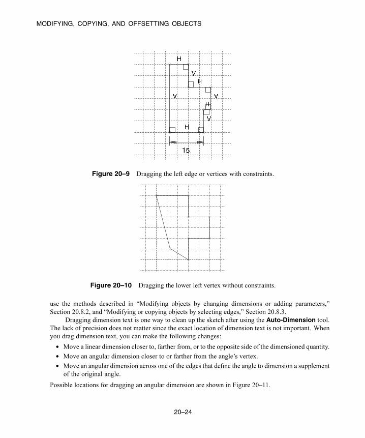
MODIFYING, COPYING, AND OFFSETTING OBJECTS
Figure 20–9 Dragging the left edge or vertices with constraints.
Figure 20–10 Dragging the lower left vertex without constraints.
use the methods described in “Modifying objects by changing dimensions or adding parameters,”
Section 20.8.2, and “Modifying or copying objects by selecting edges,” Section 20.8.3.
Dragging dimension text is one way to clean up the sketch after using the Auto-Dimension tool.
The lack of precision does not matter since the exact location of dimension text is not important. When
you drag dimension text, you can make the following changes:
• Move a linear dimension closer to, farther from, or to the opposite side of the dimensioned quantity.
• Move an angular dimension closer to or farther from the angle’s vertex.
• Move an angular dimension across one of the edges that define the angle to dimension a supplement
of the original angle.
Possible locations for dragging an angular dimension are shown in Figure 20–11.
20–24
Abaqus ID:
Printed on:
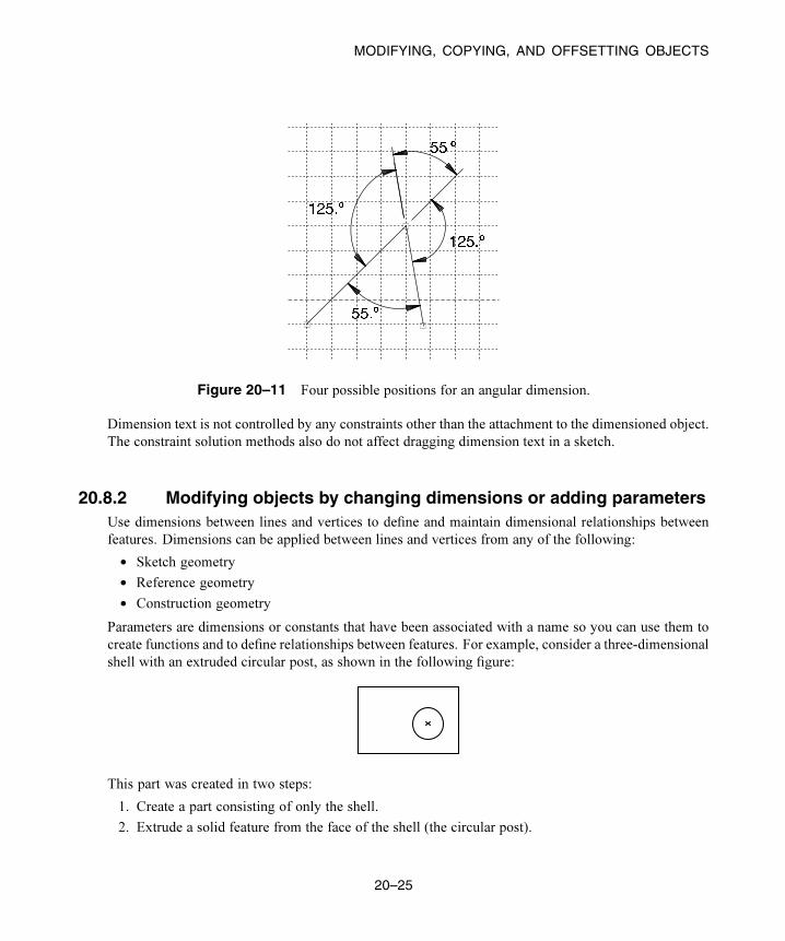
MODIFYING, COPYING, AND OFFSETTING OBJECTS
Figure 20–11 Four possible positions for an angular dimension.
Dimension text is not controlled by any constraints other than the attachment to the dimensioned object.
The constraint solution methods also do not affect dragging dimension text in a sketch.
20.8.2 Modifying objects by changing dimensions or adding parametersUse dimensions between lines and vertices to define and maintain dimensional relationships between
features. Dimensions can be applied between lines and vertices from any of the following:
• Sketch geometry
• Reference geometry
• Construction geometry
Parameters are dimensions or constants that have been associated with a name so you can use them to
create functions and to define relationships between features. For example, consider a three-dimensional
shell with an extruded circular post, as shown in the following figure:
This part was created in two steps:
1. Create a part consisting of only the shell.
2. Extrude a solid feature from the face of the shell (the circular post).
20–25
Abaqus ID:
Printed on:

MODIFYING, COPYING, AND OFFSETTING OBJECTS
If you want to keep the distance between the left edge of the shell and the center of the post constant,
you can edit the post and add a dimension between the center of the sketched circle and the left edge of
the reference geometry that represents the shell, as shown in the following figure:
5
If you move either the left or the right edge of the shell, the distance between the center of the circle
and the left edge remains constant, as shown in the following figure:
5
If you want to keep the post centered between the left and right edges of the shell, you must
add two dimensions and associate them with parameters. You can then define a parametric equation,
dim2=(dim1)/2, to set the distance from the left edge to the post at half the width of the shell, as shown
in the following figure:
dim2(dim1)
Note: The distance dimension associated with the parameter dim1 is defined in the sketch of the
shell feature and cannot be edited in the sketch of the post. When you dimension reference geometry,
Abaqus/CAE colors the dimension magenta to indicate an overconstraint. To clear the overconstraint,
you must make dim1 a reference dimension. Abaqus/CAE places parentheses around the value of
reference dimensions (or around the parameter name if the dimension is associated with a parameter)
and automatically updates their values if the dimensioned quantity changes. For more information, see
“Editing dimensions,” Section 20.13, in the HTML version of this guide.
20–26
Abaqus ID:
Printed on:

MODIFYING, COPYING, AND OFFSETTING OBJECTS
You can modify any dimension or parameter in a sketch. For detailed instructions, see “Editing
dimensions,” Section 20.13, and “Adding and editing parameters,” Section 20.12.5, respectively, in the
HTML version of this guide.
20.8.3 Modifying or copying objects by selecting edges
When you move edges, Abaqus/CAE repositions the selected edges and uses the During edit constraintsolution method to modify any connected edges (for more information, see “Customizing the use of
constraints in the Sketcher,” Section 20.9.10, in the HTML version of this guide). The sketch constraints
and constraint solution method may restrict the types of moves that you can make or cause Abaqus/CAE
to reposition edges that you did not select. When you copy edges, the copies are positioned according to
the copy method—the copied edges are not affected by any existing sketch constraints. You cannot copy
objects between sketches. Abaqus/CAE provides the following methods for moving or copying selected
edges:
Translate
You can translate selected edges by specifying the start and end coordinates of a translation vector.
The translation vector can start from any point; however, you may find it more meaningful to start
the vector from the vertex at one end of a selected edge and end it at the vertex’s new location.
Figure 20–12 shows the selected edges, the translation vector, and the result of the translation. To
achieve the results shown, Fixed constraints were added to prevent the two vertices of the upper
rectangle from moving.
Rotate
You can rotate selected edges by specifying the coordinates of the center of rotation and entering the
angle of rotation; a positive angle indicates a counterclockwise rotation. Figure 20–13 shows the
selected edges, the selected center of rotation, and the result of a 90° rotation. The selected edges
are not connected or otherwise constrained to other edges in the sketch, so the constraint solution
method has no effect on the rotation.
Mirror
You can mirror selected edges by selecting a straight line in the sketch as the mirror line.
Figure 20–14 shows the selected edges, the mirror line, and the resulting copy including a mirror
constraint for each of the four selected edges. The mirror line may be any straight object line or
construction line in the sketch.
Scale
You can scale selected edges by specifying a center point and a scale factor. A scale factor less
than 1.0 decreases the spacing between the edges, and a scale factor greater than 1.0 increases the
spacing between the edges. Figure 20–15 shows the selected edges, the selected center point, and
the result for a scale factor of 1.5.
20–27
Abaqus ID:
Printed on:

MODIFYING, COPYING, AND OFFSETTING OBJECTS
Selectededges
Translationvector
Figure 20–12 Translating selected edges.
Select the edgesto rotate
Select thecenter ofrotation
Figure 20–13 Rotating selected edges.
For detailed instructions on moving or copying objects, see “Moving or copying sketch geometry,”
Section 20.16, in the HTML version of this guide.
20–28
Abaqus ID:
Printed on:

MODIFYING, COPYING, AND OFFSETTING OBJECTS
Figure 20–14 Mirroring selected edges.
center point
original edges
scaled edges
Figure 20–15 Scaling selected edges.
20–29
Abaqus ID:
Printed on:

MODIFYING, COPYING, AND OFFSETTING OBJECTS
20.8.4 Modifying edges by trimming, extending, splitting, or mergingWhen you are modifying a sketch, you can implement your changes by modifying a dimension, by
moving selected vertices, or by trimming, extending, splitting, or merging edges. Abaqus/CAE provides
the following methods for trimming, extending, splitting, and merging edges:
Trim/Extend
You can trim or extend one end of a line or arc; you can also trim a spline curve, but spline curves
cannot be extended. To trim or extend an edge, first select the edge near the end that you want
to modify and then select a second edge to define an intersection point. The second edge may be
any object in the sketch, including construction geometry. The intersection point may lie beyond
the current endpoints of either selected edge. Abaqus/CAE trims or extends the first edge at the
intersection point. If you want to trim or extend the second edge to the same point, repeat the
process, reversing the selection order (see Figure 20–16).
Figure 20–16 Extending two edges to create a corner.
For detailed instructions on trimming and extending edges, see “Modifying Sketcher objects
by trimming or extending edges,” Section 20.17.2, in the HTML version of this guide.
Auto-trim
You can trim an intermediate or end segment from a line, arc, circle, or spline curve. Auto-trimis the fastest method you can use to remove unwanted edge segments from a sketch. Abaqus/CAE
uses preselection to highlight edges that you can remove. Preselection is based on cursor proximity
and the two nearest “trim points.” Trim points include intersection points, endpoints, vertices, and
the picked points that define the edges of circles. Unlike when you use Trim/Extend, Abaqus/CAEdoes not split the intersecting edges. Figure 20–17 shows several possible trim combinations based
on the circle and line shown in the upper left corner.
20–30
Abaqus ID:
Printed on:

MODIFYING, COPYING, AND OFFSETTING OBJECTS
Figure 20–17 Auto-trim selections.
For detailed instructions on automatically trimming edges, see “Modifying Sketcher objects
by automatically trimming edges,” Section 20.17.3, in the HTML version of this guide.
Split
You can split edges, creating separate pieces with a common vertex, where they intersect in the
sketch. Select the first edge to be broken, then select a second edge that intersects the first at the
desired split point. As you move the cursor near the second edge, a circle appears around the split
point that you would create. If there is more than one intersection point between the two edges,
Abaqus/CAE highlights the intersection closest to the cursor. Abaqus/CAE splits the first edge at
the indicated point. Figure 20–18 shows an intersecting line and spline on the left, indicates the
split point in the center image (the cursor is not shown), and shows the three resulting edges on the
right. In this case the spline was selected first, so the straight line remains unbroken.
Note: Spline curves retain their exact shape when you split or trim them, but the control points are
removed so you can no longer edit the shape of the curves.
For detailed instructions on splitting edges, see “Modifying Sketcher objects by splitting
edges,” Section 20.17.4, in the HTML version of this guide.
Merge
The Merge tool enables you to close small gaps in a sketch. These gaps commonly occur in the
following situations:
20–31
Abaqus ID:
Printed on:

MODIFYING, COPYING, AND OFFSETTING OBJECTS
Figure 20–18 Splitting a line and a spline.
• When you use the Project Edges tool on edges that are not in a plane parallel to the sketch
plane, the endpoints may be created in a slightly different location from other selected edges.
• When you import sketch geometry into an existing sketch, the edges may not line up exactly.
The Merge tool is intended only for closing small gaps. Merging edges to close larger gaps
may change the sketch geometry significantly. If you want to move elements in a sketch over a
large distance, use the drag tool from the Sketcher toolbox to move vertices in your sketch to a new
location. For more information, see “Dragging Sketcher objects,” Section 20.17.1, in the HTML
version of this guide.
For detailed instructions on merging edges, see “Modifying Sketcher objects by merging
edges,” Section 20.17.5, in the HTML version of this guide.
20.8.5 Copying sketch objects to create patterns
You can copy objects in your sketch and create a pattern of copied objects; for example, Figure 20–19
illustrates radial patterns of gear teeth and holes on a solid part. You can choose either of the following
methods to define the pattern:
Linear pattern
A linear pattern positions copies of selected objects along a direction; for example, the X-direction.
You can specify the number of copies and the spacing between the copies; and you can choose to
position the copies in a positive direction or a negative direction. In addition, you can change the
orientation of the linear pattern. Figure 20–20 shows how you can create different linear patterns
in a single direction.
20–32
Abaqus ID:
Printed on:

MODIFYING, COPYING, AND OFFSETTING OBJECTS
Figure 20–19 Radial patterns of gear teeth and holes.
Direction 1 Number = 5 Spacing = 25
Direction 2 Number = 1
Direction 1 Number = 1
Direction 2 Number = 3 Spacing =30
Select this entityto copy
Select this entityto copy
Figure 20–20 Linear patterns in a single direction.
You can create a matrix of copied objects by creating copies in a second direction; for example,
the Y-direction. The options are the same as for the first direction; you can control the number of
copies, the direction, and the angle. Figure 20–21 shows how you can create different linear patterns
in two directions.
20–33
Abaqus ID:
Printed on:

MODIFYING, COPYING, AND OFFSETTING OBJECTS
Direction 1 Number = 2 Spacing = 100
Direction 2 Number = 2 Spacing 60
Direction 1 Number = 6 Spacing = 20
Direction 2 Number = 2 Spacing 60
Select this entityto copy
Select this entityto copy
Figure 20–21 Linear patterns in two directions.
By default, the first direction is the X-axis and the second direction is the Y-axis. However,
you can change the orientation of the first direction or the second direction by selecting a line from
the sketch that represents the new orientation. Figure 20–22 shows a linear pattern oriented along
a selected line.
Select thisline to definedirection 1
Select thisentity to copy
Direction 1 Number = 5 Spacing = 20
Direction 2 Number = 1
Figure 20–22 A linear pattern oriented along a line.
By default, Abaqus/CAE creates the pattern in a positive direction; however, you can reverse the
direction. For example, Figure 20–23 shows the same linear pattern as in Figure 20–22 but with the
direction reversed. For detailed instructions on creating linear patterns, see “Creating linear patterns
of objects,” Section 20.19.1, in the HTML version of this guide.
20–34
Abaqus ID:
Printed on:

MODIFYING, COPYING, AND OFFSETTING OBJECTS
Figure 20–23 The effect of reversing the direction of a linear pattern.
Radial pattern
A radial pattern positions copies of selected objects in a circular pattern. You can specify the number
of copies, and you can specify the angle between the first and last copy, where a positive angle
corresponds to a counterclockwise direction. In addition, you can select a point from the sketch that
defines the center point of the circular pattern. Figure 20–24 shows how you can create different
radial patterns. For detailed instructions on creating radial patterns, see “Creating radial patterns of
objects,” Section 20.19.2, in the HTML version of this guide.
By default, Abaqus/CAE displays a preview of the linear and radial pattern as you enter the settings. In
most cases the preview will help you decide on the settings that will create the desired pattern. However,
if you are creating a large number of copies, the preview may slow down the generation of the sketch.
In this case you should toggle off the Preview button.
Several methods are also available for creating individual copies of sketch objects. These methods
are discussed in “Modifying or copying objects by selecting edges,” Section 20.8.3.
20.8.6 Offsetting objectsYou can offset objects in your sketch to create similar objects of a larger or smaller size. You select the
edges to offset and the offset distance; Abaqus/CAE displays a preview so that you can choose the offset
direction. You can offset any continuous open or closed loops that do not contain branches. Figure 20–25
shows the two possible offsets that can be created for several edge selections. (For clarity, vertices and
datum points are not shown in the figure.)
Abaqus/CAE offsets each object in the same way that you would offset edges on paper with a
drafting compass. Using a compass, you would draw the compass point along the original edge tracing
a new edge with the pencil at the required perpendicular (offset) distance. At any sharp corners, you
would rotate the compass to make it perpendicular to the second edge at the corner. At the end of this
process, you would trim any offset edges that intersected with other offset edges.
20–35
Abaqus ID:
Printed on:

MODIFYING, COPYING, AND OFFSETTING OBJECTS
Select this circle
Number = 8 Total Angle = 360
Number = 5 Total Angle = 180
Select this circle
Figure 20–24 Radial patterns.
As shown in Figure 20–25, Abaqus/CAE completes a similar process:
• Straight edges are copied.
• Offset edges that overlap, such as corners offset toward the “inside,” are trimmed to make new
corners.
• Where corners are offset toward the “outside,” you can choose to create sharp corners or fillets with
radii equal to the offset distance.
• Radii of existing curves are increased or decreased by the offset distance.
If the radius of a curve would be decreased to zero or less by the offset, Abaqus/CAE creates a new vertex
joining the surrounding edges that were previously connected by the curve. For detailed instructions, see
“Offsetting the edges of Sketcher objects,” Section 20.19.3, in the HTML version of this guide.
20–36
Abaqus ID:
Printed on:
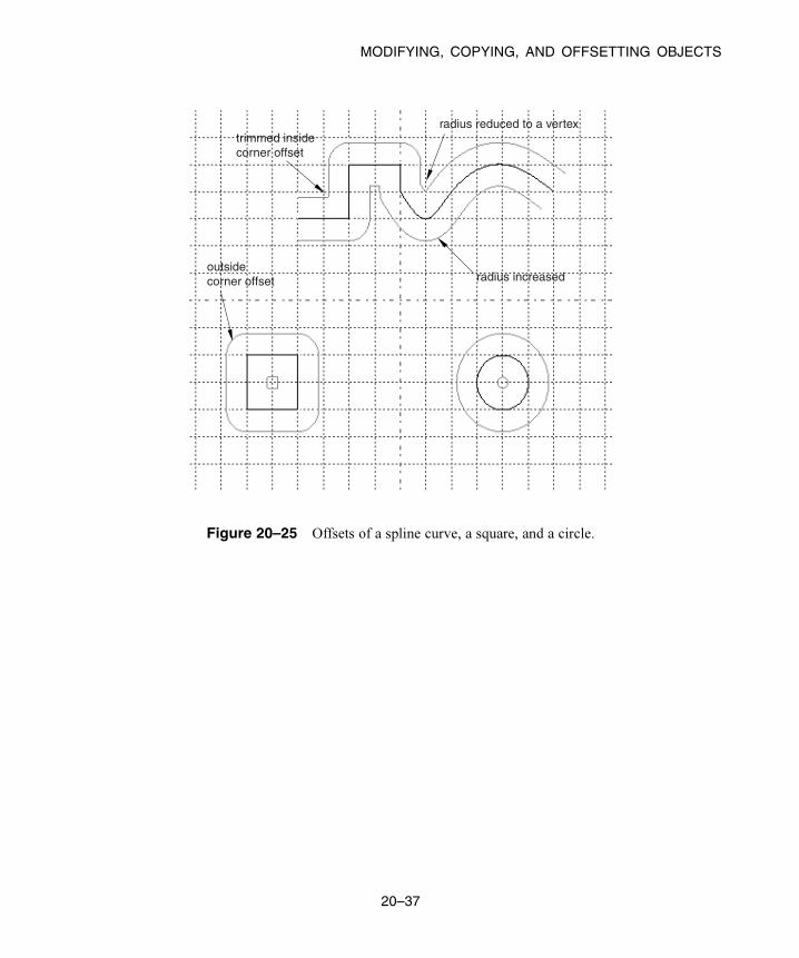
MODIFYING, COPYING, AND OFFSETTING OBJECTS
trimmed insidecorner offset
outsidecorner offset radius increased
radius reduced to a vertex
Figure 20–25 Offsets of a spline curve, a square, and a circle.
20–37
Abaqus ID:
Printed on:


Part IV: Modeling techniquesThis part discusses modeling techniques in Abaqus/CAE that span multiple Abaqus/CAE modules and that
define special engineering features in an Abaqus/CAE model. The following topics are covered:
• Chapter 21, “Adhesive joints and bonded interfaces”
• Chapter 22, “Bolt loads”
• Chapter 23, “Composite layups”
• Chapter 24, “Connectors”
• Chapter 25, “Continuum shells”
• Chapter 26, “Co-simulation”
• Chapter 27, “Display bodies”
• Chapter 28, “Eulerian analyses”
• Chapter 29, “Fasteners”
• Chapter 30, “Fluid dynamic analyses”
• Chapter 31, “Fracture mechanics”
• Chapter 32, “Gaskets”
• Chapter 33, “Inertia”
• Chapter 34, “Load cases”
• Chapter 35, “Midsurface modeling”
• Chapter 36, “Skin and stringer reinforcements”
• Chapter 37, “Springs and dashpots”
• Chapter 38, “Submodeling”
• Chapter 39, “Substructures”
Abaqus ID:
Printed on:


OVERVIEW OF ADHESIVE JOINT AND BONDED INTERFACE MODELING
21. Adhesive joints and bonded interfaces
This section provides information on how to model adhesive joints and bonded interfaces. The following
topics are covered:
• “Overview of adhesive joint and bonded interface modeling,” Section 21.1
• “Embedding cohesive elements in an existing three-dimensional mesh,” Section 21.2
• “Creating a model with cohesive elements using geometry and mesh tools,” Section 21.3
• “Defining tie constraints between the cohesive layer and the surrounding bulk material,”
Section 21.4
• “Assigning cohesive modeling data,” Section 21.5
21.1 Overview of adhesive joint and bonded interface modeling
You can create a model using cohesive elements to model the following:
• Adhesive joints – two components connected by a glue-like material that has a finite thickness.
• Fracture at bonded interfaces – crack propagation in glue material that is very thin and for all
practical purposes may be considered to be of zero thickness.
• Gaskets (limited capability) – seal between two components. No specialized gasket behavior
(typically defined in terms of pressure versus closure) is available. If you want to model special
gasket behavior, use special-purpose gasket elements as described in Chapter 32, “Gaskets.”
For more information, see “Cohesive elements: overview,” Section 32.5.1 of the Abaqus Analysis User’s
Guide.
The two main approaches that you can use to include cohesive elements in your model are
• embedding one or more layers of cohesive elements in the mesh of an existing model; or
• creating the analysis model using the geometry and mesh tools.
You can model the connection at the interface between the cohesive layer and the surrounding bulk
material by sharing nodes or by defining a tie constraint. The tie-constraint approach allows you to
model the cohesive layer using a finer discretization than that of the bulk material and may be more
desirable in certain modeling situations. For more information, see “Defining tie constraints between the
cohesive layer and the surrounding bulk material,” Section 21.4.
Like gasket elements, cohesive elements have an orientation associated with them. This orientation
defines the thickness direction of the elements, and it should be consistent throughout the cohesive layer.
Swept or offset meshing techniques should be used to generate the mesh in the cohesive layer because
these tools produce meshes that are oriented consistently. You can also use the bottom-up sweep meshing
method, but you must sweep in the direction of the element thickness to maintain the correct orientation.
You should create a single layer of solid elements to model the cohesive region. The use of more than one
21–1
Abaqus ID:
Printed on:

EMBEDDING COHESIVE ELEMENTS IN AN EXISTING THREE-DIMENSIONAL MESH
layer through the thickness could produce unreliable results and is not recommended. You can generate
the mesh in the surrounding bulk material using any of the mesh tools because these elements do not
need to be oriented.
The general procedure for modeling adhesive joints and bonded interfaces involves the following
steps:
1. Create a model, and assign a cohesive element type to the cohesive region in the Mesh module using
one of the following approaches:
• “Embedding cohesive elements in an existing three-dimensional mesh,” Section 21.2
• “Creating a model with cohesive elements using geometry and mesh tools,” Section 21.3
2. In the Property module, define amaterial and a cohesive section that refers to the material, and assign
the cohesive section to the cohesive region. See “Assigning cohesive modeling data,” Section 21.5,
for more information.
3. To model progressive damage and failure of cohesive layers as discussed in “Defining the
constitutive response of cohesive elements using a traction-separation description,” Section 32.5.6
of the Abaqus Analysis User’s Guide, include the desired damage initiation and damage evolution
information in the material definition (select Mechanical→Damage for Traction SeparationLaws→damage type). For more information, see “Defining damage,” Section 12.9.3, in the
HTML version of this guide.
21.2 Embedding cohesive elements in an existing three-dimensionalmesh
You can use the following procedure to embed a layer of cohesive elements:
1. In the Mesh module, use the solid offset mesh tool in the Edit Mesh toolset to embed elements in
an existing mesh (see “Editing the entire mesh,” Section 64.7). This approach generates a layer
of hexahedral or wedge elements that share nodes with the surrounding bulk material. The offset
mesh tool generates elements that are oriented consistently with a stack direction that is aligned with
the offset direction. When prompted to select the element faces from which the offset mesh will
be generated, select the interior element faces using the procedure described in “Selecting interior
surfaces,” Section 6.2.12.
Note: When generating an embedded layer of elements, the thickness should be much less than
that of the adjacent elements because the nodes are displaced when the offset layer is generated.
You can create an offset mesh from only three-dimensional element faces. As a result, you can
create only hexahedral- and wedge-shaped cohesive elements using an offset mesh. For example,
you cannot create quadrilateral cohesive elements by offsetting from element edges.
2. In the Mesh module, use the element type assignment tool to assign the cohesive element type to
the cohesive region. See “Element type assignment,” Section 17.5.3, for more information.
21–2
Abaqus ID:
Printed on:

CREATING A MODEL WITH COHESIVE ELEMENTS USING GEOMETRY AND MESH TOOLS
If your existing mesh is a native mesh, you should create a mesh part prior to adding cohesive elements.
For more information, see “Creating a mesh part,” Section 17.20, in the HTML version of this guide.
If you want to use a finer mesh in the cohesive layer, you should construct the cohesive layer as
a separate part. You should separate the mesh in the surrounding bulk material into two regions with
the appropriate spacing to accommodate the cohesive layer. You can mesh the cohesive layer using
the methods described in “Creating a model with cohesive elements using geometry and mesh tools,”
Section 21.3, and tie the cohesive layer to the surrounding bulk material. For more information, see
“Defining tie constraints between the cohesive layer and the surrounding bulk material,” Section 21.4.
21.3 Creating a model with cohesive elements using geometry andmesh tools
You can use the following procedure to create a model with cohesive elements using geometry and mesh
tools:
1. In the Part module, define the geometry of the model. You should define the geometric region
that represents the cohesive layer as a solid, even if the thickness of the layer is close to zero. To
avoid numerical problems, it is recommended that you model the geometry using a value of 10−4
or greater for the thickness. If the actual thickness of the layer is less than this value, you should
specify the actual thickness in the Initial thickness field of the cohesive section editor as described
in “Creating cohesive sections,” Section 12.13.16, in the HTML version of this guide
2. In the Mesh module, mesh the surrounding bulk material. You can use any of the mesh tools to
mesh the surrounding bulk material. See “Mesh generation,” Section 17.3.3, for more information.
3. In the Mesh module, mesh the cohesive region using one of the following methods:
Two- and three-dimensional models
Top-down swept or bottom-up meshing technique. You can assign the top-down swept
meshing technique or the bottom-up meshing technique to mesh the cohesive region. The
bottom-up meshing technique is available only for three-dimensional models (for more
information, see “Bottom-up meshing,” Section 17.11). Regardless of the meshing technique
that you choose, you must sweep, extrude, or revolve the mesh in the thickness direction
of the element to produce the correct element orientation. For a complex cohesive region,
you may need to partition the model to create a group of sweep regions that you can align
consistently. For more information, see “Selecting a meshing technique,” Section 17.18.3,
and “Specifying the sweep path,” Section 17.18.6, in the HTML version of this guide.
Three-dimensional models
Convert the cohesive region into a shell region, and use the offset meshing technique.
a. Convert the solid part to a shell using the From solid shell tool in the Part module.
21–3
Abaqus ID:
Printed on:

DEFINING TIE CONSTRAINTS BETWEEN THE COHESIVE LAYER AND THESURROUNDING BULK MATERIAL
b. Isolate a collection of faces that represents an idealized shell of the part using the Removefaces tool in the Geometry Edit toolset.
c. Mesh the simplified model with shell elements, and create a mesh part.
d. Use the mesh part to generate an offset mesh of solid hexahedral or wedge elements. The
elements will be oriented through the thickness of the part, and you can verify this with
the Query toolset.
For detailed instructions, see “Generating layers of solid elements offset from an existing
mesh,” Section 64.7.1, in the HTML version of this guide.
4. In the Mesh module, use the element type assignment tool to assign the cohesive element type to
the cohesive region. See “Element type assignment,” Section 17.5.3, for more information.
For example, Figure 21–1 illustrates the layered composite specimen that is used in the benchmark
problem “Delamination analysis of laminated composites,” Section 2.7.1 of the Abaqus Benchmarks
Guide. An Abaqus Scripting Interface script that reproduces the composite specimen model using
Abaqus/CAE is provided with this problem.
L = 200 mma = 40 mma = 20 mmwidth = 20 mm
1
2
cohesive elements (0.01325 mm thick)2 layers (0.265 mm)initial cracks12 layers (1.59 mm)
u
u
p
10 layers (1.325 mm)
L
a a a1 2 2
Figure 21–1 Model geometry for the Alfano delamination problem.
21.4 Defining tie constraints between the cohesive layer and thesurrounding bulk material
If you want to model the cohesive layer using a mesh that is finer than the adjacent bulk material mesh, the
cohesive layer should be generated as a separate mesh and tied to the bulk material using tie constraints
(see “Defining tie constraints,” Section 15.15.1, in the HTML version of this guide). You should create
a shell geometric model to represent the surface on one side of the cohesive layer and mesh that model
with the desired mesh density. You can use this mesh to create a mesh part from which you can generate
21–4
Abaqus ID:
Printed on:
ASSIGNING COHESIVE MODELING DATA
the offset mesh. For more information, see “Modeling with cohesive elements,” Section 32.5.3 of the
Abaqus Analysis User’s Guide.
You should use care when tying zero-thickness cohesive layers to the surrounding bulk material
mesh. Use the following procedure to avoid problems:
1. Use the solid offset mesh tool to create the layer of cohesive elements along with the top and bottom
surfaces. Abaqus/CAE appends TopSurf and BottomSurf to the surface name prefix when it
creates the two surfaces on either side of the layer of cohesive elements.
2. Use the stack orientation query tool to distinguish the top (brown) and bottom (purple) faces of the
cohesive elements.
3. Tie the surfaces of the surrounding bulk material mesh to the appropriate top and bottom cohesive
surfaces. When you are prompted to select a surface from the cohesive surface, clickSurfaces from
the right side of the prompt line and select the appropriate surface. For example, select surfacename-BottomSurf to tie the bottom (purple) face of the cohesive layer to the adjacent surface of
the bulk material mesh.
21.5 Assigning cohesive modeling data
In the Property module, you can complete the cohesive modeling data as follows:
1. Create a cohesive section to define the section properties of adhesive layers at the interface between
two bonded parts. You can model a negligibly thin layer of adhesive, a finite-thickness adhesive
layer, or a gasket by selecting the constitutive behavior of the cohesive section as TractionSeparation, Continuum, or Gasket, respectively. For more information, see “Creating cohesive
sections,” Section 12.13.16, in the HTML version of this guide.
2. Define a material for the cohesive region. If you select the Continuum or the Gasket responsein the cohesive section editor, you can use the material models available in the Property module
to define the continuum material properties. Abaqus/CAE does not support the material models
for the Traction Separation response. In this case you must add the material definition using the
Keywords Editor, as described in “Adding unsupported keywords to your Abaqus/CAE model,”
Section 9.10.1, in the HTML version of this guide.
3. Assign the cohesive section to the cohesive region. Formore information, see “Assigning a section,”
Section 12.15.1, in the HTML version of this guide.
21–5
Abaqus ID:
Printed on:


UNDERSTANDING BOLT LOADS
22. Bolt loads
This section explains how to model tightening forces or length adjustments in bolts or fasteners. The
following topic is covered:
• “Understanding bolt loads,” Section 22.1
In addition, “Creating and editing bolt loads,” Section 22.2, is available in the HTML version of
this guide.
22.1 Understanding bolt loads
Bolt loads model tightening forces or length adjustments in bolts or fasteners. For example, Figure 22–1
shows a container (A) that is sealed by tightening the bolts that hold the lid, which places the gasket
under pressure.
����������
bolt
gasket
boltcross-section
A
Figure 22–1 Modeling a pre-tensioned bolt.
You can model the tension in the tightened bolts by applying a bolt load to each one in the first step of
the analysis. You define the load in terms of either a concentrated force or a prescribed change in length,
and you apply the load across a bolt cross-section surface that you specify. In later steps you can modify
the load to prevent further length changes so that the bolt acts as a standard, deformable component
responding to other loadings on the assembly.
When you create a bolt load, you must specify the following:
A surface that defines the bolt cross-section
Abaqus/CAE applies the bolt load across the cross-section surface that you specify. The surface that
defines the bolt cross-section must cut through the bolt geometry. Abaqus/CAE creates an “internal”
surface at that location.
22–1
Abaqus ID:
Printed on:

UNDERSTANDING BOLT LOADS
If you are working with bolt part instances made from native or imported geometry, it is usually
necessary to partition the bolt at the location where you want the cross-section to be defined. For
example, a partition is selected as the bolt cross-section in Figure 22–2.
Figure 22–2 Using a partition to specify the bolt cross-section.
If you are working with orphan mesh elements, you must specify the cross-section surface by
selecting element faces. For example, element faces define a cross-section surface for the mesh
part shown in Figure 22–3.
Figure 22–3 Using element faces to specify the bolt cross-section.
The element faces need to be selected from elements on only one side of the pre-tension section. You
can use display groups to remove selected elements from the viewport to reveal the element faces
22–2
Abaqus ID:
Printed on:

UNDERSTANDING BOLT LOADS
of the cross-section surface. For more information on selecting surfaces, see Chapter 6, “Selecting
objects within the viewport.” For detailed information on selecting surfaces on wire part instances,
see “Specifying a particular side or end of a region,” Section 73.2.5.
Note: You can apply bolt loads only to three-dimensional solid, two-dimensional solid, and
three-dimensional wire part instances. Bolt loads on two-dimensional and axisymmetric wire part
instances are unsupported.
A bolt axis
If you are defining a bolt load on a solid region, you must select a datum axis or one of the axes
of a datum coordinate system that indicates the bolt axis direction (it need not be normal to the
cross-section). If you are defining a bolt load on a wire region, the bolt axis direction is always
assumed to be the direction of the tangent to the wire at the bolt cross-section.
Abaqus/CAE uses both the cross-section surface that you specify and the bolt axis to define
the pre-tension section data and the pre-tension reference node used by Abaqus/Standard. (See
“Prescribed assembly loads,” Section 34.5.1 of the Abaqus Analysis User’s Guide, for more
information.)
A method for applying the loading
When you create a bolt load, you must choose one of the following loading methods:
• Apply a force to the bolt. This method models tightening the bolt so that it carries a specified
load.
• Adjust the bolt length. This method models tightening the bolt until its free length has changed
by the specified value.
• Fix the bolt at its current length. This method is available only if you have already created the
load in the first analysis step and are now editing it in a subsequent analysis step. This method
allows the bolt length to remain unchanged so that the force in the bolt can change according
to the response of the model.
A magnitude for the chosen method
If you are applying a force to the bolt, you must enter the force magnitude. If you are adjusting the
bolt length, you must enter the length change.
You can create a bolt load only in the first analysis step, but you can modify the loading method or
the magnitude of the load in subsequent steps. For example, you can apply a specific tension in the first
step and then change the method in the second step to fix the bolt length.
For detailed information on creating a bolt load, see “Creating and editing bolt loads,” Section 22.2,
in the HTML version of this guide.
22–3
Abaqus ID:
Printed on:


AN OVERVIEW OF COMPOSITE LAYUPS
23. Composite layups
This section provides information on modeling composite layups with Abaqus/CAE. The following
topics are covered:
• “An overview of composite layups,” Section 23.1
• “Creating a composite layup,” Section 23.2
• “Understanding composite layups and orientations,” Section 23.3
• “Understanding composite layups and distributions,” Section 23.4
• “Requesting output from a composite layup,” Section 23.5
• “Viewing a composite layup,” Section 23.6
23.1 An overview of composite layups
Figure 23–1 illustrates a single composite layup that contains three plies. Each ply is composed of a
homogenous material of uniform thickness, with fibers oriented along a single orientation. However, a
ply can also be an isotropic material, such as a foam core.
Figure 23–1 A composite layup.
A ply represents a single piece of material that is placed in a mold during the composites manufacturing
process. A composite layup can contain a different number of plies in different regions. For example,
the composite layup in Figure 23–1 includes regions that contain a single ply, regions where two plies
overlap, and a region where three plies overlap.
Figure 23–2 shows the same model that is depicted in Figure 23–1 but defined using composite shell
sections. The number of plies cannot change within a composite shell section. Therefore, four composite
shell sections, each with a constant number of plies, are required to define this simple model. Section 1
contains a single ply, sections 2 and 3 each contain two plies, and section 4 contains three plies.
23–1
Abaqus ID:
Printed on:
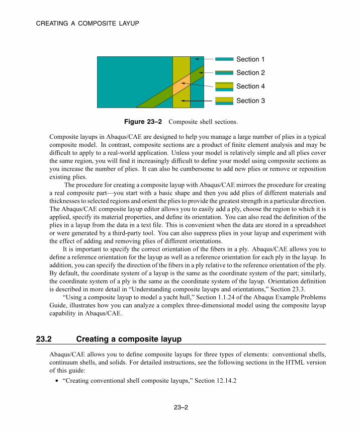
CREATING A COMPOSITE LAYUP
Section 1
Section 2
Section 4
Section 3
Figure 23–2 Composite shell sections.
Composite layups in Abaqus/CAE are designed to help you manage a large number of plies in a typical
composite model. In contrast, composite sections are a product of finite element analysis and may be
difficult to apply to a real-world application. Unless your model is relatively simple and all plies cover
the same region, you will find it increasingly difficult to define your model using composite sections as
you increase the number of plies. It can also be cumbersome to add new plies or remove or reposition
existing plies.
The procedure for creating a composite layup with Abaqus/CAE mirrors the procedure for creating
a real composite part—you start with a basic shape and then you add plies of different materials and
thicknesses to selected regions and orient the plies to provide the greatest strength in a particular direction.
The Abaqus/CAE composite layup editor allows you to easily add a ply, choose the region to which it is
applied, specify its material properties, and define its orientation. You can also read the definition of the
plies in a layup from the data in a text file. This is convenient when the data are stored in a spreadsheet
or were generated by a third-party tool. You can also suppress plies in your layup and experiment with
the effect of adding and removing plies of different orientations.
It is important to specify the correct orientation of the fibers in a ply. Abaqus/CAE allows you to
define a reference orientation for the layup as well as a reference orientation for each ply in the layup. In
addition, you can specify the direction of the fibers in a ply relative to the reference orientation of the ply.
By default, the coordinate system of a layup is the same as the coordinate system of the part; similarly,
the coordinate system of a ply is the same as the coordinate system of the layup. Orientation definition
is described in more detail in “Understanding composite layups and orientations,” Section 23.3.
“Using a composite layup to model a yacht hull,” Section 1.1.24 of the Abaqus Example Problems
Guide, illustrates how you can analyze a complex three-dimensional model using the composite layup
capability in Abaqus/CAE.
23.2 Creating a composite layup
Abaqus/CAE allows you to define composite layups for three types of elements: conventional shells,
continuum shells, and solids. For detailed instructions, see the following sections in the HTML version
of this guide:
• “Creating conventional shell composite layups,” Section 12.14.2
23–2
Abaqus ID:
Printed on:
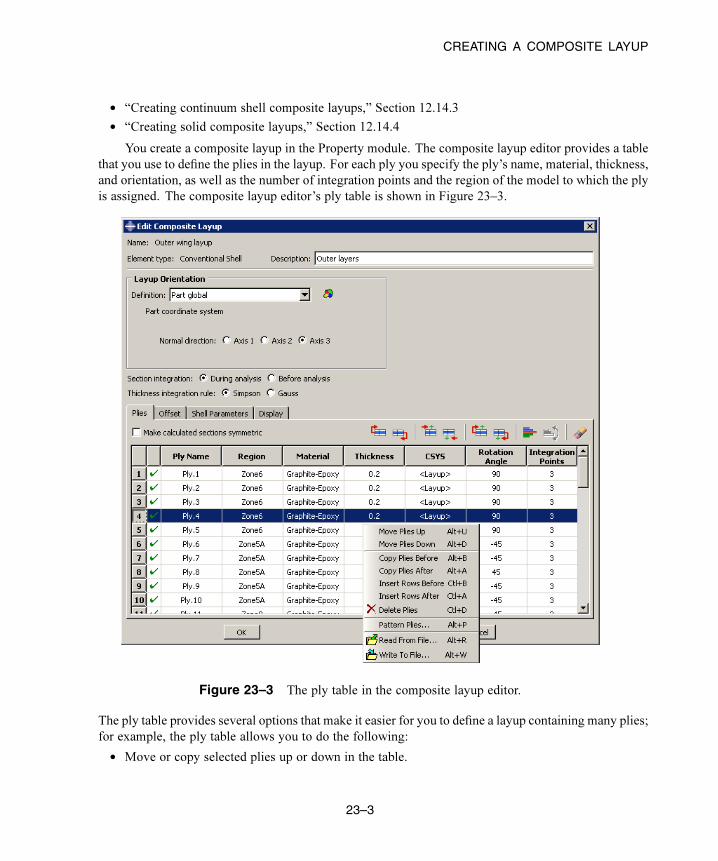
CREATING A COMPOSITE LAYUP
• “Creating continuum shell composite layups,” Section 12.14.3
• “Creating solid composite layups,” Section 12.14.4
You create a composite layup in the Property module. The composite layup editor provides a table
that you use to define the plies in the layup. For each ply you specify the ply’s name, material, thickness,
and orientation, as well as the number of integration points and the region of the model to which the ply
is assigned. The composite layup editor’s ply table is shown in Figure 23–3.
Figure 23–3 The ply table in the composite layup editor.
The ply table provides several options that make it easier for you to define a layup containing many plies;
for example, the ply table allows you to do the following:
• Move or copy selected plies up or down in the table.
23–3
Abaqus ID:
Printed on:

CREATING A COMPOSITE LAYUP
• Suppress or delete selected plies.
• Pattern a group of selected plies.
• Read ply data from or write ply data to an ASCII file. The data can define all the plies in the layup
or only a subset of the plies in the layup.
The ability to suppress plies allows you to easily experiment with different configurations of plies in the
composite layup and to see the effect on the results of an analysis of the model. For more information,
see “Using the ply table when defining a composite layup,” Section 12.14.1, in the HTML version of this
guide.
If you are defining a composite layup whose plies are symmetric about a central core, you only
need to enter the bottom half of the layup in the ply table. When you apply the symmetry option, Abaqus
automatically creates additional plies in the generated sections by repeating the entered plies (including
the central ply) in reverse order.
You will probably have to partition your model to create the regions to which you will assign plies.
You should create the partitions before you create the layup and start defining plies. You can select a
region directly from the part in the current viewport, or you can create a named set that refers to the
region and select the named set. Abaqus/CAE preserves any existing ply regions if you decide to add
partitions and plies after you have defined a composite layup; for example, you can add plies to a layup
that model a rib providing additional stiffness to a region. The region to which you assign a ply can be
either Abaqus/CAE geometry or a mesh. You can combine plies assigned to geometry and plies assigned
to a native mesh in a single composite layup.
Continuum shell and solid composite layups are expected to have a single element through the
entire thickness across a combination of all the regions specified in the composite layup. Each single
element through the thickness contains the multiple plies that you defined in the ply table. If the region
to which you assign your continuum shell or solid composite layup contains multiple elements through
the thickness, each element will contain all of the plies that you defined in the ply table and the analysis
results will not be as expected.
If your model contains multiple continuum shell or solid elements through the thickness of a region,
you can obtain correct results by defining a separate composite layup for each layer of elements. You
can define a composite layup for each layer by selecting the elements of a native Abaqus/CAE mesh or
the orphan elements when you specify the region of the layup. You must create a layup for each layer of
elements.
If you have plies that overlap in your composite layup, you must enter the plies in the ply table
in the order that they appear in the overlapping region. Figure 23–4 illustrates a simple example of an
overlapping region and the corresponding order of the plies in the ply table. The first ply in the ply table
represents the bottom ply in the layup.
Under certain circumstances, Abaqus cannot determine the orientations of the composite ply for
conventional shells. This can occur, for example, if your ply makes a sharp transition through an angle
of 90°, and/or your part is aligned with one or more planes of the global coordinate system. To help
you diagnose the problem region, Abaqus/CAE draws a collapsed coordinate system indicating regions
for which the user-selected coordinate system and the geometric normal cannot be resolved into a valid
23–4
Abaqus ID:
Printed on:

UNDERSTANDING COMPOSITE LAYUPS AND ORIENTATIONS
Ply-3
Ply-2
Ply-1
Ply-4
Ply-5
Figure 23–4 The order of the plies in the ply table.
orientation for display purposes. If this situation arises, you may be able to complete the analysis by
splitting the ply into multiple plies at the transitions and by assigning orientations to each new ply.
If you apply a composite layup and assign a section assignment to the same region, Abaqus/CAE
uses only the properties from the composite layup during the analysis. If you apply two or more
composite layups to regions that overlap, Abaqus/CAE uses the properties of the last layup, where
“last” refers to the alphabetical order of the names of the composite layups. The default color coding in
the Property module uses yellow coloring to indicate a region with overlapping composite layups and
section assignments or to indicate a region with multiple overlapping composite layups.
23.3 Understanding composite layups and orientations
The orientation of the fibers within each ply of a composite layup plays an important role in determining
the physical qualities of your model; however, defining this orientation in a model based on a real-world
application is not straightforward. Composite layups in Abaqus/CAEmake the process more manageable
by deriving the orientation of the fibers from three parameters that are relative to each other—the layup
orientation, the ply orientation, and an additional rotation—as shown in Figure 23–5.
Layup orientation
The layup orientation defines the base or reference orientation of all the plies in the layup. In
conventional and continuum shell layups, Abaqus projects the specified orientation onto the surface
of the shell, aligning the direction of the layup orientation that you choose with the shell normal. In
solid composite layups the orientation is not projected.
Abaqus/CAE provides several options for defining the layup orientation:
• Part global: By default, the layup orientation is the same as the orientation of the part.
• Coordinate system: You can create and select a datum coordinate system that defines the
orientation.
23–5
Abaqus ID:
Printed on:
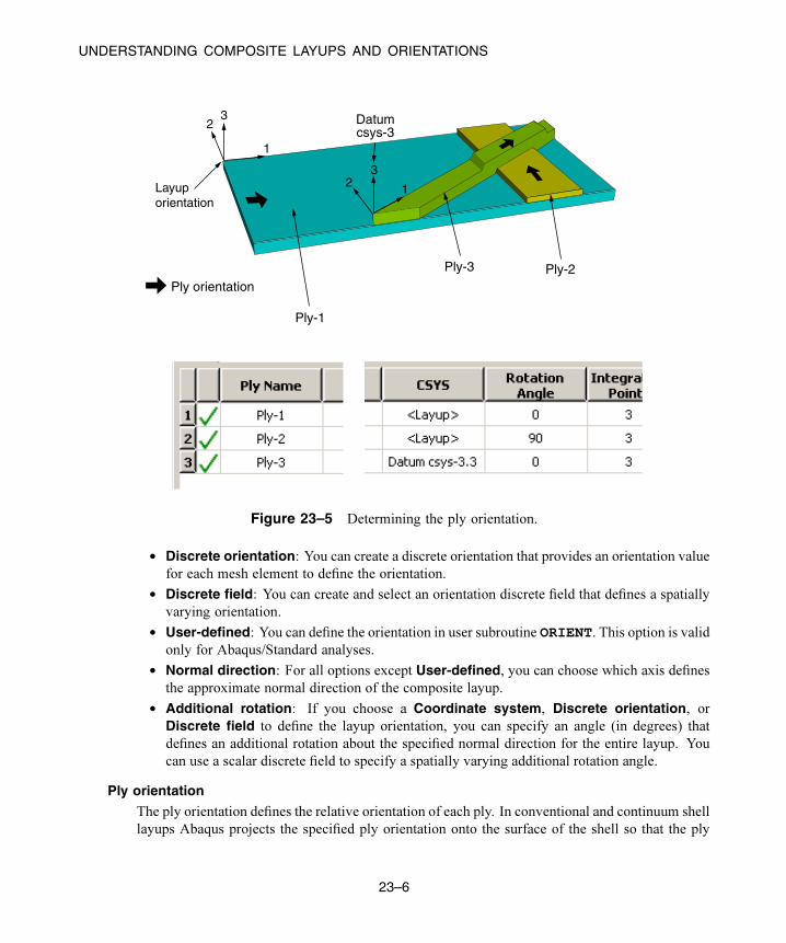
UNDERSTANDING COMPOSITE LAYUPS AND ORIENTATIONS
Ply-1
Ply-2Ply-3
1
23
123
Datumcsys-3
Ply orientation
Layuporientation
Figure 23–5 Determining the ply orientation.
• Discrete orientation: You can create a discrete orientation that provides an orientation valuefor each mesh element to define the orientation.
• Discrete field: You can create and select an orientation discrete field that defines a spatially
varying orientation.
• User-defined: You can define the orientation in user subroutine ORIENT. This option is validonly for Abaqus/Standard analyses.
• Normal direction: For all options except User-defined, you can choose which axis defines
the approximate normal direction of the composite layup.
• Additional rotation: If you choose a Coordinate system, Discrete orientation, or
Discrete field to define the layup orientation, you can specify an angle (in degrees) that
defines an additional rotation about the specified normal direction for the entire layup. You
can use a scalar discrete field to specify a spatially varying additional rotation angle.
Ply orientation
The ply orientation defines the relative orientation of each ply. In conventional and continuum shell
layups Abaqus projects the specified ply orientation onto the surface of the shell so that the ply
23–6
Abaqus ID:
Printed on:

UNDERSTANDING COMPOSITE LAYUPS AND ORIENTATIONS
normal direction is alignedwith the shell normal and the layup stacking direction. In solid composite
layups the plies are created with respect to the layup stacking direction, and the unprojected ply
orientation defines the material orientation within a ply (see Figure 23–6).
plies
plies
projected ply orientation
ply orientation
3
1
3 13 1
stac
king
di
rect
ion
stac
king
di
rect
ion
3 1
Continuum shell composite layup
Solid composite layupspecified ply orientation
specified ply orientation
Figure 23–6 Plies and ply orientations for shell and solid composite layups.
Abaqus/CAE calculates the ply orientation from a combination of two variables that you can
specify—the coordinate system (CSYS) and a rotation angle about the normal direction.
In cases where Abaqus/CAE attempts to draw coordinate systems for ply orientations in
composite layups at singularity points of the system (i.e., points for which the user-selected
coordinate system and the geometric normal from either geometry or elements cannot be resolved
into a valid orientation for display purposes in Abaqus/CAE), the coordinate system will be drawn
collapsed.
If the layup orientation is specified using a discrete field, the ply orientation is displayed relative
to the part’s base coordinate system. For continuum shell elements, Abaqus/CAE does not project
the displayed orientations onto the midplane surface. In both of these cases, you can perform a data
check and view the output database in the Visualization module to verify the orientations. For more
information, see “Performing a data check on a model,” Section 19.7.3, in the HTML version of
this guide.
Coordinate system
Abaqus/CAE provides the following options for defining the coordinate system of the ply:
• Layup: By default, the coordinate system of the ply is the same as the coordinate system
of the layup.
23–7
Abaqus ID:
Printed on:

UNDERSTANDING COMPOSITE LAYUPS AND DISTRIBUTIONS
• CSYS: You can create and select a datum coordinate system that defines the coordinate
system of the ply. If you choose to use a coordinate system for a ply, it overrides the layup
orientation for that ply.
You can also select the axis of the coordinate system that defines the normal direction
of the ply. The axis that you choose appears as the last digit in the CSYS column in the
layup table. For example, Datum csys1.3 indicates that you chose Datum csys-1to define the coordinate system of the ply, and you chose the 3-axis to define the normal.
Rotation angle
The rotation angle defines the orientation of the fibers within each ply relative to the ply’s
coordinate system. For example, in a typical composite the fibers might be oriented at −45° or
+90° relative to the coordinate system. You can also use a scalar discrete field to specify a fiber
orientation that varies spatially across the ply. If you specify a rotation angle, the ply is rotated
counterclockwise about the coordinate system normal, and the angle is measured relative to
the 1-axis.
Figure 23–7 shows the orientation of four plies in a composite layup and the corresponding
entries in the layup table. Abaqus/CAE determines the ply orientation as follows:
• You selected the layup orientation to define the coordinate system of VerticalTape-1 and
entered a rotation angle of 0°. The resulting ply orientation is along the 1-axis of the layup
orientation.
• You selected the layup orientation to define the coordinate system of VerticalTape-2and entered a rotation angle of 90°. The resulting ply orientation is a rotation of 90°
counterclockwise about the 3-axis (the normal direction) of the layup orientation. The rotation
angle is measured relative to the 1-axis.
• You selected Datum csys-1 to define the coordinate system of DiagonalTape-1 and entered
a rotation angle of 0°. The resulting ply orientation is along the 1-axis of Datum csys-1.
• You selected Datum csys-1 to define the coordinate system of DiagonalTape-2 and entered
a rotation angle of 90°. The resulting ply orientation is a rotation of 90° counterclockwise
about the 3-axis (the normal direction) of the datum coordinate system. The angle is measured
relative to the 1-axis.
23.4 Understanding composite layups and distributions
A discrete field is a spatially varying field where values are associated with a node or an element. The
Discrete Field toolset allows you to create and manage discrete fields in Abaqus/CAE. A discrete field
that is used by a composite layup is called a distribution. Because distributions are applied to specific
elements and nodes, you can use a distribution only after you have meshed the part. In most cases you
will use a third-party preprocessor that operates on meshed parts to create a distribution that can be
applied to a composite layup. For more information, see Chapter 63, “The Discrete Field toolset.”
23–8
Abaqus ID:
Printed on:

UNDERSTANDING COMPOSITE LAYUPS AND DISTRIBUTIONS
Plyorientation
Vertical Tape-1
Diagonal Tape-1
Vertical Tape-2
Diagonal Tape-2
Layuporientation
Plyorientation
Datumcsys-1
Datumcsys-1
Z
1
2
3
Layuporientation
1
2
3
Plyorientation
Plyorientation
12
3
12
3
Figure 23–7 Determining the orientation of each ply.
You can use a distribution for the following:
• To define a spatially varying local coordinate system that specifies the overall orientation of the
composite layup.
• To define an additional rotation for the layup orientation that is varying spatially across the layup.
• To define an additional rotation for a ply orientation that is varying spatially across the ply. You can
use a distribution to define the ply orientation only in an Abaqus/Standard analysis.
• To define an overall shell thickness that varies spatially across a conventional shell composite layup.
• To define a ply thickness that varies spatially across a ply in a conventional shell composite layup.
You can use a distribution to define the ply thickness only in an Abaqus/Standard analysis.
• To define a nodal thickness that varies spatially across a conventional shell composite layup.
• To define an offset that varies spatially across a conventional shell composite layup. You can use a
distribution to define the offset only in an Abaqus/Standard analysis.
23–9
Abaqus ID:
Printed on:
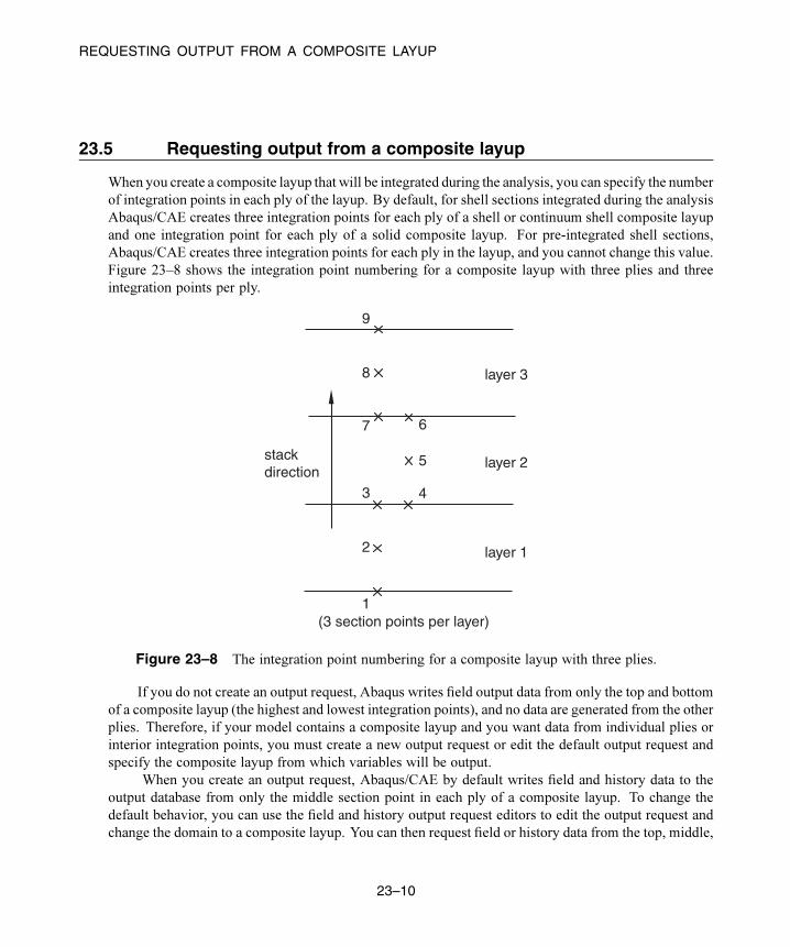
REQUESTING OUTPUT FROM A COMPOSITE LAYUP
23.5 Requesting output from a composite layup
When you create a composite layup that will be integrated during the analysis, you can specify the number
of integration points in each ply of the layup. By default, for shell sections integrated during the analysis
Abaqus/CAE creates three integration points for each ply of a shell or continuum shell composite layup
and one integration point for each ply of a solid composite layup. For pre-integrated shell sections,
Abaqus/CAE creates three integration points for each ply in the layup, and you cannot change this value.
Figure 23–8 shows the integration point numbering for a composite layup with three plies and three
integration points per ply.
layer 1
layer 2
layer 3
stack direction
1
7 6
5
9
4
(3 section points per layer)
8
3
2
Figure 23–8 The integration point numbering for a composite layup with three plies.
If you do not create an output request, Abaqus writes field output data from only the top and bottom
of a composite layup (the highest and lowest integration points), and no data are generated from the other
plies. Therefore, if your model contains a composite layup and you want data from individual plies or
interior integration points, you must create a new output request or edit the default output request and
specify the composite layup from which variables will be output.
When you create an output request, Abaqus/CAE by default writes field and history data to the
output database from only the middle section point in each ply of a composite layup. To change the
default behavior, you can use the field and history output request editors to edit the output request and
change the domain to a composite layup. You can then request field or history data from the top, middle,
23–10
Abaqus ID:
Printed on:
VIEWING A COMPOSITE LAYUP
and/or bottom section point of each ply, from all section points, or from specified section points. For
more information, see “Modifying field output requests,” Section 14.12.2, and “Modifying history output
requests,” Section 14.12.3, in the HTML version of this guide. You can request the following:
Selected
Abaqus/CAE writes field data to the output database from the selected section points of each ply
(top, middle, and/or bottom). If a ply has an even number of section points and you request output
from the middle section point, Abaqus/CAE generates data from the higher of the two section points
that span the middle of the ply. For example, if a ply has four section points and you request output
from the middle section point, Abaqus/CAE generates data from the third section point.
All
Abaqus/CAE writes field data to the output database from all of the section points of all of the plies.
Specify
Abaqus/CAE writes field data to the output database from specified section points. Section points
are numbered sequentially from the bottom of the bottom ply to the top of the top ply, where the
bottom ply is the first ply in the layup. For example, if you want output from the middle section
point of each ply shown in Figure 23–8, you would enter 2,5,8.
For more information, see “Understanding output requests,” Section 14.4.
23.6 Viewing a composite layup
You can view a composite layup while you are creating it or after it has been analyzed. Abaqus/CAE
provides the following tools for ply-based visualization of a composite layup:
Ply stack plot
A ply stack plot is a graphical representation of the plies from the selected region of a composite
layup or a composite section. Figure 23–9 illustrates a ply stack plot.The staircase appearance does
not indicate ply drop-offs in the layup; it is simply a graphical representation that allows you to see
the number of plies in the layup and, for example, the relative thickness of a ply, the material from
which it is constructed, and the orientation of its fibers. If your composite layup contains many
plies, the ply stack plot can become confusing and hard to interpret. To make the ply stack plot
more readable, Abaqus/CAE provides options that allow you to view only a manageable number of
plies.
The triad in a ply stack plot represents the element orientation system, and it shows the shell
normal or stacking direction (the 3-direction) and the 1- and 2-directions for the plies. The fibers
are always drawn in the 1–2 plane at an angle with respect to the 1-direction. In solid composite
layups the fibers in a ply do not always run parallel to the 1–2 plane (e.g., if the 3-direction of the ply
orientation and the element stacking direction are not aligned). In this situation the fibers in the ply
stack plot are not a true depiction of the fibers in the layup, but rather a graphical representation of
23–11
Abaqus ID:
Printed on:

VIEWING A COMPOSITE LAYUP
t = 0.1
t = 0.1
t = 0.15
t = 0.15
t = 0.1
t = 0.1
1
23
Layup: "RearCabinStiffener"Plot of plies 1 to 6, of 6.
A ply stack is acore samplefrom a region
Figure 23–9 A ply stack plot.
the rotation angles in the layup definition: the angle drawn in the ply stack plot is the rotation angle
specified in the ply table measured about the element stacking direction axis. For more information,
see “Understanding composite layups and orientations,” Section 23.3.
Ply stack plots do not draw fibers for ply orientations that are based on a user-defined coordinate
system or a rotation angle distribution. Abaqus/CAE displays an asterisk (for coordinate systems)
or a caret (for rotation angle distributions) on such plies to signify that it cannot draw lines in the
1–2 plane that accurately represent the fiber direction for the ply. Similarly, if you use a discrete
field distribution to define a ply’s thickness, Abaqus/CAE draws the ply in the ply stack plot based
on the average thickness of the other uniform plies in the layup and displays the discrete field name
next to the plot (if thickness labels are turned on).
You can display a ply stack plot in the Property module after you have created a composite
layup. You can also display a ply stack plot in the Visualization module after you have analyzed a
model with a composite layup. For more information, see Chapter 53, “Viewing a ply stack plot.”
Ply-based results
After you have analyzed a model with a composite layup, you can view a contour plot of results
from individual plies of the layup, or you can view an envelope contour plot that looks for maximum
or minimum values across all of the plies in the layup.
Results from individual plies
Ply-based results show the data from a selected ply in a composite layup. For a given ply, you
can view data from the bottom, middle, or top of the ply, or you can view data from both the
23–12
Abaqus ID:
Printed on:

VIEWING A COMPOSITE LAYUP
top and bottom plies. Figure 23–10 illustrates a contour plot of strain (E11) from selected plies
of a composite layup.
E11: Top and bottom
E11: Bulkhead E11: Cockpit
E11: Outer skin
Figure 23–10 Contour plots from selected plies.
If the same ply name is used in multiple composite layup definitions within a model, viewing
data for this ply displays results for all layups in which the ply name appears. To limit the
results to a single ply within a single layup, you must first use a display group to limit the
display to the individual composite layup (see “Selection methods for creating or editing a
display group,” Section 78.2.2), then plot the results for a section point within the desired ply
(see “Selecting section point data by ply” in “Selecting section point data,” Section 42.5.9).
Contour plots displaying output at both the top and bottom plies of a composite layup
vary in appearance depending on the type of layup. In a conventional shell composite layup
the two contours appear as a single double-sided shell with different contours on each side. In a
continuum shell composite layup or solid composite layup the two contours appear as distinct
single-sided contours at each section point location. Figure 23–11 illustrates the difference
between contour plots of conventional shell and continuum shell composite layups.
23–13
Abaqus ID:
Printed on:

VIEWING A COMPOSITE LAYUP
Conventional shellcomposite layup (three plies)
Continuum shellcomposite layup (three plies)
SPOSPly-3
SNEGPly-1 SPOS
Ply-3
SNEGPly-1
Figure 23–11 Contour plots of conventional shell and continuum shell composite layups.
Each layup contains three plies, and each plot is showing the output from the top of the top
ply and from the bottom of the bottom ply. Stress (S11) is plotted in both cases. For more
information, see “Selecting section point data by category” in “Selecting section point data,”
Section 42.5.9.
Envelope plots
An envelope plot allows you to view a contour plot of the highest or lowest value of a variable
in your model, regardless of the ply in which it is occurring. The plies in an envelope plot that
correspond with the extreme values are called the critical plies. You can choose the criterion
that Abaqus/CAE applies (absolute maximum, maximum, or minimum) and the position in the
ply at which Abaqus/CAE checks the value (integration point, centroid, element nodal).
For example, even though your composite layup can include a large number of plies, you
can view only the critical plies and determine the highest strain that is occurring in each element
of your model. You can decide if you want to reduce the strain in the critical plies by increasing
the number of plies in a particular region or by reorienting existing plies. Figure 23–12 shows
the value of the strain (E11) in the critical plies of the model.In addition, you can use the
contour plot options to display a quilt contour plot where the color of each element indicates
which ply is the critical ply, as shown in Figure 23–13.
23–14
Abaqus ID:
Printed on:

VIEWING A COMPOSITE LAYUP
(Avg: 75%)Envelope (max abs)E, E11
+2.984e−07+1.430e−04+2.858e−04+4.285e−04+5.713e−04+7.140e−04+8.568e−04+9.995e−04+1.142e−03+1.285e−03+1.428e−03+1.571e−03+1.713e−03
Figure 23–12 The value of the strain in the critical plies.
Envelope (max abs)E, E11 Ply
SKIN2SKIN
Figure 23–13 The critical plies.
Using a combination of the plots shown in Figure 23–12 and Figure 23–13, you can determine
both the value of the strain in the critical ply and the location of the critical ply in the layup. For
more information, see “Selecting the field output to display,” Section 42.5, and “Understanding
how contour values are computed,” Section 44.1.1.
If you do not create an output request, Abaqus/CAE writes field output data from only
the top and bottom of a composite layup, and no data are generated from the other plies. To
create an envelope plot that examines all of the plies in your model, you must create a new
23–15
Abaqus ID:
Printed on:

VIEWING A COMPOSITE LAYUP
output request or edit the default output request and specify the composite layup and the plies
and section points from which variables will be output.
In many cases, even though you change the position in the ply at which Abaqus/CAE
checks the value, the same ply experiences the extreme value, and the contour plot does not
change. However, the contour plot might change because the critical ply changed if:
• you have a small number of plies, and the results are changing rapidly through the
thickness of the ply; or
• the material is nonlinear, and its stiffness changes abruptly under some conditions.
Through thickness X–Y plots
After you have analyzed a composite layup and determined which regions contain the critical plies,
you can view the behavior of the plies across the layup with a through thickness X–Y plot. You
can create an X–Y data object by reading field output results from the section points in a selected
element of a shell region of your model. If you select an element in a composite layup, Abaqus/CAE
plots data for each section point in each ply across the entire thickness of the layup. Figure 23–14
illustrates a through thickness plot of the strain in the fiber direction through 13 plies of a composite
layup. The strain is discontinuous because the orientation of the fiber changes between plies.
Strain (E11)−0.01 0.00 0.01 0.02 0.03 0.04 0.05
Thi
ckne
ss (
Eac
h pl
y =
0.1
)
0.0
0.4
0.8
1.2
Figure 23–14 A through thickness X–Y plot.
23–16
Abaqus ID:
Printed on:
VIEWING A COMPOSITE LAYUP
For more information, see “Reading X–Y data through the thickness of a shell,” Section 47.2.3.
Color coding
You can use color coding in all of the Abaqus/CAEmodules to change the color of individual layups
and plies. If you choose to color code by plies, Abaqus/CAE displays only one ply in a region, which
by default is the last ply (in alphabetical order). To view a different ply, you can deactivate selected
plies. For more information, see “Coloring geometry and mesh elements,” Section 77.4, in the
HTML version of this guide.
Display groups
In the Visualization module you can use display groups to view the elements in only selected layups
or plies. For more information, see “Selection methods for creating or editing a display group,”
Section 78.2.2.
“Using a composite layup to model a yacht hull,” Section 1.1.24 of the Abaqus Example Problems
Guide, illustrates how you can create and analyze a complex three-dimensional composite model and
how you can use Abaqus/CAE to view the behavior of individual plies in the layup.
23–17
Abaqus ID:
Printed on:


OVERVIEW OF CONNECTOR MODELING
24. Connectors
This section provides information on how to model connectors. The following topics are covered:
• “Overview of connector modeling,” Section 24.1
• “What is a connector?,” Section 24.2
• “What is a connector section?,” Section 24.3
• “What is a CORM?,” Section 24.4
• “What are connector behaviors?,” Section 24.5
• “Creating the connector geometry, connector sections, and connector section assignments,”
Section 24.6
• “What is the relationship between reference points and connectors?,” Section 24.7
• “Defining connector orientations in connector section assignments,” Section 24.8
• “Requesting output from connectors,” Section 24.9
• “Applying connector loads and connector boundary conditions,” Section 24.10
• “Displaying connectors in the Visualization module,” Section 24.11
24.1 Overview of connector modeling
The procedure for modeling and using connectors in Abaqus/CAE involves the following general steps:
1. Create reference points and datum coordinate systems to use when modeling connectors.
2. Create assembly-level wire features.
3. Create connector sections to define the connection types, connector behavior, and section data.
4. Create a connector section assignment that associates the connector section with the wires that you
select and that specifies the orientations for the first and second points of the wires that you select.
5. In the Load module, prescribe connector loads and connector boundary conditions to simulate
connector actuations and constrain material flow.
6. In the Step module, create field and history output requests for connectors.
7. In the Visualization module, plot connector output results; control the display of connector section
assignments, wire endpoints, connection types, and current local orientations; and animate the time
history of wire endpoints and local orientations.
24–1
Abaqus ID:
Printed on:
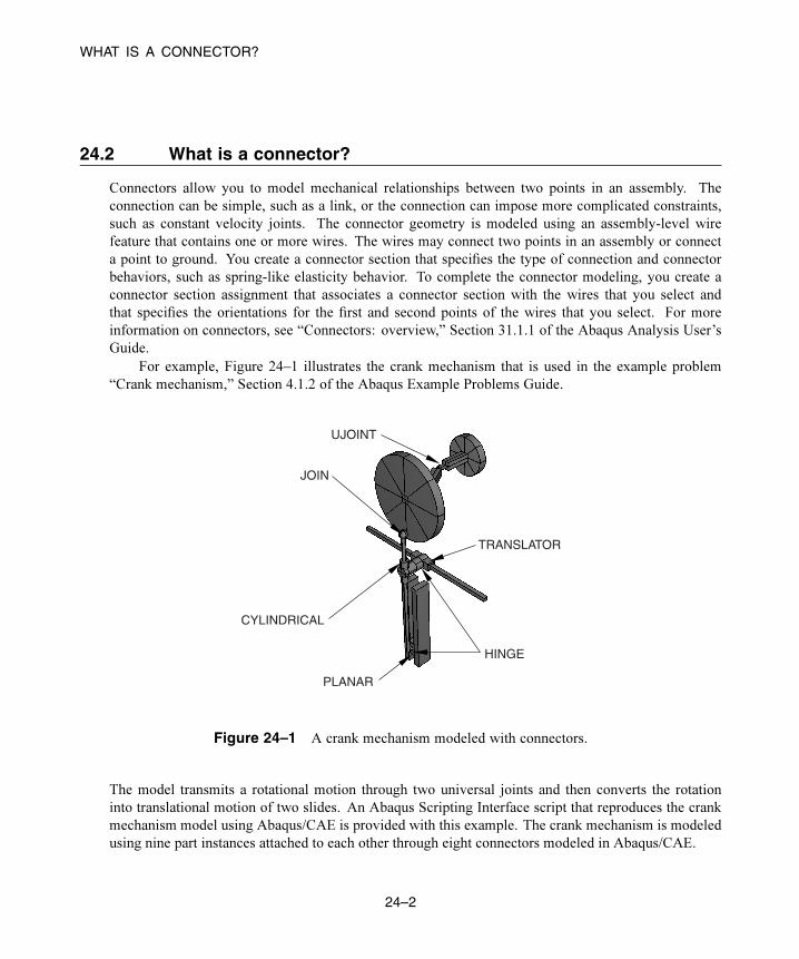
WHAT IS A CONNECTOR?
24.2 What is a connector?
Connectors allow you to model mechanical relationships between two points in an assembly. The
connection can be simple, such as a link, or the connection can impose more complicated constraints,
such as constant velocity joints. The connector geometry is modeled using an assembly-level wire
feature that contains one or more wires. The wires may connect two points in an assembly or connect
a point to ground. You create a connector section that specifies the type of connection and connector
behaviors, such as spring-like elasticity behavior. To complete the connector modeling, you create a
connector section assignment that associates a connector section with the wires that you select and
that specifies the orientations for the first and second points of the wires that you select. For more
information on connectors, see “Connectors: overview,” Section 31.1.1 of the Abaqus Analysis User’s
Guide.
For example, Figure 24–1 illustrates the crank mechanism that is used in the example problem
“Crank mechanism,” Section 4.1.2 of the Abaqus Example Problems Guide.
JOIN
CYLINDRICAL
TRANSLATOR
HINGE
PLANAR
UJOINT
Figure 24–1 A crank mechanism modeled with connectors.
The model transmits a rotational motion through two universal joints and then converts the rotation
into translational motion of two slides. An Abaqus Scripting Interface script that reproduces the crank
mechanism model using Abaqus/CAE is provided with this example. The crank mechanism is modeled
using nine part instances attached to each other through eight connectors modeled in Abaqus/CAE.
24–2
Abaqus ID:
Printed on:

WHAT IS A CONNECTOR SECTION?
24.3 What is a connector section?
A connector section defines the connection type and may include connector behavior and section data.
Abaqus provides several connection types—basic types, assembled types, complex types, and MPC
types.
Basic types
Basic connection types include translational types and rotational types. Translational types affect
translational degrees of freedom at both endpoints of the wires to which the connector section is
assigned and may affect rotational degrees of freedom at the first or both endpoints of the wires.
Rotational types affect only rotational degrees of freedom at both endpoints of the wires.
Assembled types
Assembled connection types are predefined combinations of basic connection types. For example,
a HINGE connection type combines a JOIN connection type (translational) and a REVOLUTE
connection type (rotational) to join the position of two points and provide a revolute constraint
between their rotational degrees of freedom.
Complex types
Complex connection types affect a combination of degrees of freedom in the connection and
cannot be combined with other connection types. They typically model highly coupled physical
connections.
MPC types
MPC connection types are used to define multi-point constraints between two points.
Note: Abaqus/CAE writes complete connector section data to the input file only when a connector
section has a connector section assignment in the model database. If you plan to import a model from
an input file and obtain connector sections, you must make sure that all of the connector sections have
assignments in the model database.
For an overview of the connection types that are available in Abaqus/CAE, see “Understanding
connector sections and functions,” Section 15.8. For a description of each connection type and the
equivalent basic connection types that define the kinematic constraints of assembled type connections,
see “Connection-type library,” Section 31.1.5 of the Abaqus Analysis User’s Guide, and “General multi-
point constraints,” Section 35.2.2 of the Abaqus Analysis User’s Guide.
24–3
Abaqus ID:
Printed on:

CREATING THE CONNECTOR GEOMETRY, CONNECTOR SECTIONS, ANDCONNECTOR SECTION ASSIGNMENTS
24.4 What is a CORM?
CORM is an abbreviation for component of relative motion: relative displacements and rotations local
to a connector. Available components of relative motion are relative displacements and rotations that
are not kinematically constrained. Depending upon the connection type, some of the components may
be available and some may be constrained. When you are creating or modifying a connector section,
Abaqus/CAE displays the available and constrained components of relative motion in the editor for
the specified connection type. In addition to applying behaviors to the components of relative motion,
you can prescribe connector loads and connector boundary conditions to the available components of
relative motion of a connector (see “Applying connector loads and connector boundary conditions,”
Section 24.10). For more information on creating connector sections, see “Connector section editors,”
Section 15.9.7.
24.5 What are connector behaviors?
After you specify a connection type for a connector section, you can define behaviors for the components
of relative motion. You can specify the following connector behaviors:
• Elasticity
• Damping
• Friction
• Plasticity
• Damage
• Stop
• Lock
• Failure
• Reference length
• Integration (Abaqus/Explicit analyses only)
For more information on behaviors, see “Connector behaviors,” Section 15.8.2, and “Connector
behavior,” Section 31.2.1 of the Abaqus Analysis User’s Guide.
24.6 Creating the connector geometry, connector sections, andconnector section assignments
You create the assembly-level wire features, connector sections, and connector section assignments in the
Interaction module to model a connector. Abaqus/CAE provides two methods for modeling connectors:
24–4
Abaqus ID:
Printed on:

CREATING THE CONNECTOR GEOMETRY, CONNECTOR SECTIONS, ANDCONNECTOR SECTION ASSIGNMENTS
you can use the Connector Builder to perform all the steps involved in creating a single connector,
including creation of the wire feature, connector section, connector section assignment, and any desired
reference points and datum coordinate systems; or you can create multiple connectors by creating the
wires, connector sections, and connector section assignments in separate dialog boxes in the Interaction
module. If you choose the latter technique, you should create the desired reference points and datum
coordinate systems before you begin modeling the connectors.
TheModel Tree, shown in Figure 24–2, is helpful for understanding the organization of the reference
points, datum coordinate systems, and wire features that you created in assembly-related modules, as
well as connector sections and connector section assignments that you created in the Interaction module.
You can use the Query toolset in the Interaction module to obtain connector assignment information for
selected wires.
Figure 24–2 Wire features, connector sections, and connector
section assignments in the Model Tree.
24–5
Abaqus ID:
Printed on:

WHAT IS THE RELATIONSHIP BETWEEN REFERENCE POINTS AND CONNECTORS?
For detailed instructions, see the following sections, in the HTML version of this guide:
• “Selecting a process for defining connector geometry,” Section 15.12.7
• “Creating a single connector,” Section 15.12.8
• “Creating or modifying wire features for multiple connectors,” Section 15.12.9
• “Creating connector sections,” Section 15.12.11
• “Creating and modifying connector section assignments,” Section 15.12.12
• “Using the Query toolset to obtain connector assignment information,” Section 15.18
24.7 What is the relationship between reference points andconnectors?
The points that you can use to define an assembly-level wire feature can be one of the following:
• Vertex or node of a part instance
• Reference point of a part instance or of an assembly
• Ground
Using a reference point is often more convenient than using a point or node on the assembly because the
same reference point can be used by a rigid body or coupling constraint. In the Part module you can use
the Reference Point toolset to create one reference point on each part; additional reference points can be
created in the Assembly module, Interaction module, and Load module.
You can use the Model Tree to rename reference points with more descriptive feature names.
Descriptive names allow you to more easily associate reference points and wires in a complex model,
as shown in Figure 24–3. If you want to use different feature names and labels for a reference point
on multiple instances of the same part, you must create the reference points in an assembly-related
module. You can create a node on a mesh using the Edit Mesh toolset and then select the node to define
an endpoint of an assembly-level wire; however, the node is not listed in the Model Tree and has no
label in the viewport. For more information on creating and renaming reference points, see Chapter 72,
“The Reference Point toolset.” For more information on creating a node on a mesh, see “Manipulating
nodes,” Section 64.1.1.
Each reference point or node that defines an endpoint of an assembly-level wire needs to be
associated with the model geometry, even if they are created in the Part module. In many cases you
will create a rigid body constraint or a coupling constraint (to distribute forces to an area instead of to a
single point) between the reference point or node and a part instance. As a result, the motion of the wire
endpoint will be constrained to the motion of the part instance. You create constraints in the Interaction
module. For more information, see “Understanding constraints,” Section 15.5.
24–6
Abaqus ID:
Printed on:

DEFINING CONNECTOR ORIENTATIONS IN CONNECTOR SECTION ASSIGNMENTS
Figure 24–3 The Model Tree for the crank mechanism.
24.8 Defining connector orientations in connector sectionassignments
When you model a connector, you may need to specify the orientation of the connector. Orientations
for a connector may be required, optional, or not applicable, depending upon the connection type. In
most cases the orientation will not be the same as the global coordinate system, and you must create a
datum coordinate system that defines the connector’s local orientation before you create a connector
24–7
Abaqus ID:
Printed on:
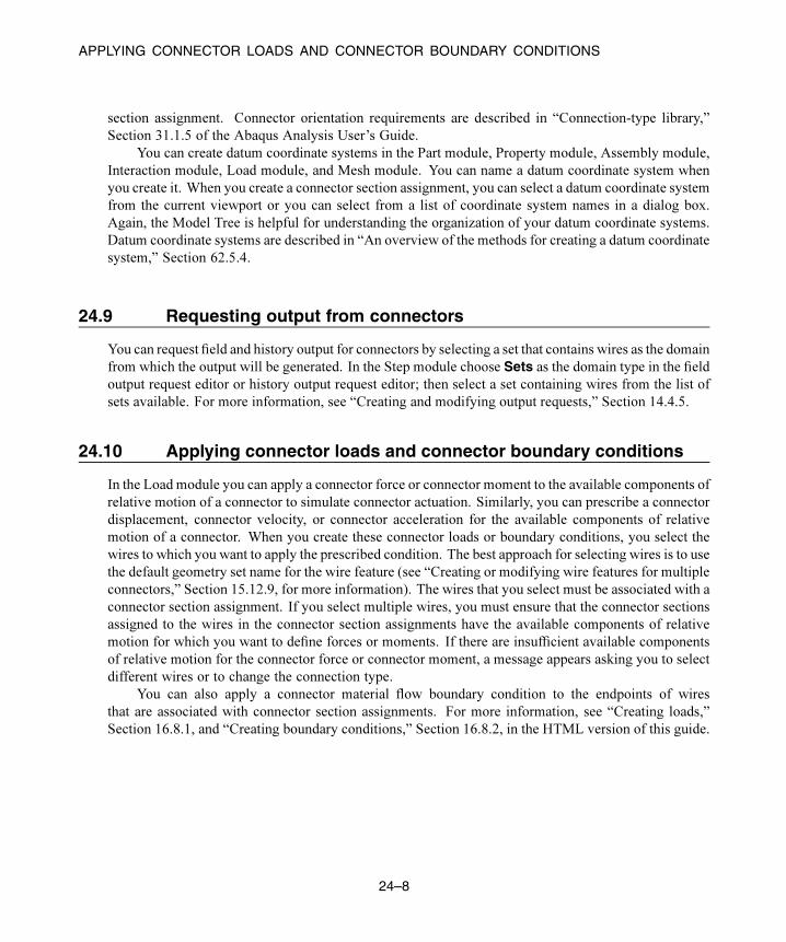
APPLYING CONNECTOR LOADS AND CONNECTOR BOUNDARY CONDITIONS
section assignment. Connector orientation requirements are described in “Connection-type library,”
Section 31.1.5 of the Abaqus Analysis User’s Guide.
You can create datum coordinate systems in the Part module, Property module, Assembly module,
Interaction module, Load module, and Mesh module. You can name a datum coordinate system when
you create it. When you create a connector section assignment, you can select a datum coordinate system
from the current viewport or you can select from a list of coordinate system names in a dialog box.
Again, the Model Tree is helpful for understanding the organization of your datum coordinate systems.
Datum coordinate systems are described in “An overview of the methods for creating a datum coordinate
system,” Section 62.5.4.
24.9 Requesting output from connectors
You can request field and history output for connectors by selecting a set that contains wires as the domain
from which the output will be generated. In the Step module choose Sets as the domain type in the field
output request editor or history output request editor; then select a set containing wires from the list of
sets available. For more information, see “Creating and modifying output requests,” Section 14.4.5.
24.10 Applying connector loads and connector boundary conditions
In the Load module you can apply a connector force or connector moment to the available components of
relative motion of a connector to simulate connector actuation. Similarly, you can prescribe a connector
displacement, connector velocity, or connector acceleration for the available components of relative
motion of a connector. When you create these connector loads or boundary conditions, you select the
wires to which you want to apply the prescribed condition. The best approach for selecting wires is to use
the default geometry set name for the wire feature (see “Creating or modifying wire features for multiple
connectors,” Section 15.12.9, for more information). The wires that you select must be associated with a
connector section assignment. If you select multiple wires, you must ensure that the connector sections
assigned to the wires in the connector section assignments have the available components of relative
motion for which you want to define forces or moments. If there are insufficient available components
of relative motion for the connector force or connector moment, a message appears asking you to select
different wires or to change the connection type.
You can also apply a connector material flow boundary condition to the endpoints of wires
that are associated with connector section assignments. For more information, see “Creating loads,”
Section 16.8.1, and “Creating boundary conditions,” Section 16.8.2, in the HTML version of this guide.
24–8
Abaqus ID:
Printed on:
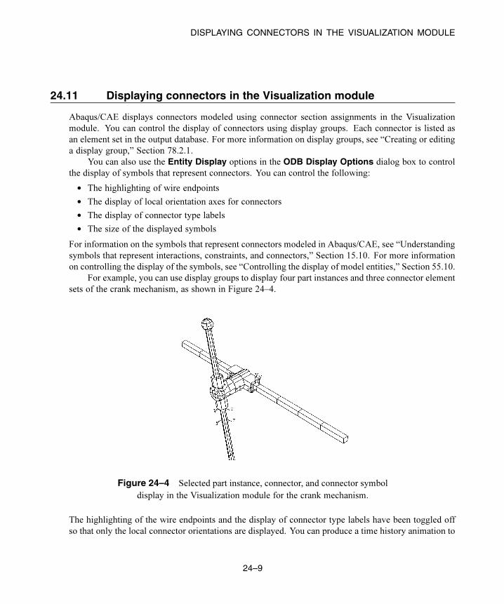
DISPLAYING CONNECTORS IN THE VISUALIZATION MODULE
24.11 Displaying connectors in the Visualization module
Abaqus/CAE displays connectors modeled using connector section assignments in the Visualization
module. You can control the display of connectors using display groups. Each connector is listed as
an element set in the output database. For more information on display groups, see “Creating or editing
a display group,” Section 78.2.1.
You can also use the Entity Display options in the ODB Display Options dialog box to control
the display of symbols that represent connectors. You can control the following:
• The highlighting of wire endpoints
• The display of local orientation axes for connectors
• The display of connector type labels
• The size of the displayed symbols
For information on the symbols that represent connectors modeled in Abaqus/CAE, see “Understanding
symbols that represent interactions, constraints, and connectors,” Section 15.10. For more information
on controlling the display of the symbols, see “Controlling the display of model entities,” Section 55.10.
For example, you can use display groups to display four part instances and three connector element
sets of the crank mechanism, as shown in Figure 24–4.
Figure 24–4 Selected part instance, connector, and connector symbol
display in the Visualization module for the crank mechanism.
The highlighting of the wire endpoints and the display of connector type labels have been toggled off
so that only the local connector orientations are displayed. You can produce a time history animation to
24–9
Abaqus ID:
Printed on:

DISPLAYING CONNECTORS IN THE VISUALIZATION MODULE
view the changes in the connector orientations during the mechanism operation. For more information,
see “Time history animation,” Section 49.1.1.
For information on plotting connector output results, see Chapter 47, “X–Y plotting.”
24–10
Abaqus ID:
Printed on:
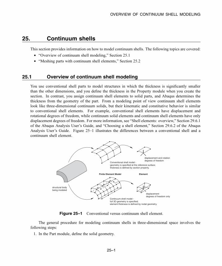
OVERVIEW OF CONTINUUM SHELL MODELING
25. Continuum shells
This section provides information on how to model continuum shells. The following topics are covered:
• “Overview of continuum shell modeling,” Section 25.1
• “Meshing parts with continuum shell elements,” Section 25.2
25.1 Overview of continuum shell modeling
You use conventional shell parts to model structures in which the thickness is significantly smaller
than the other dimensions, and you define the thickness in the Property module when you create the
section. In contrast, you assign continuum shell elements to solid parts, and Abaqus determines the
thickness from the geometry of the part. From a modeling point of view continuum shell elements
look like three-dimensional continuum solids, but their kinematic and constitutive behavior is similar
to conventional shell elements. For example, conventional shell elements have displacement and
rotational degrees of freedom, while continuum solid elements and continuum shell elements have only
displacement degrees of freedom. For more information, see “Shell elements: overview,” Section 29.6.1
of the Abaqus Analysis User’s Guide, and “Choosing a shell element,” Section 29.6.2 of the Abaqus
Analysis User’s Guide. Figure 25–1 illustrates the differences between a conventional shell and a
continuum shell element.
structural bodybeing modeled
Continuum shell model -full 3D geometry is specified; element thickness is defined by nodal geometry.
displacementdegrees of freedom only
displacement and rotationdegrees of freedom
Conventional shell model -geometry is specified at the reference surface;thickness is defined by section property.
Finite Element Model Element
Figure 25–1 Conventional versus continuum shell element.
The general procedure for modeling continuum shells in three-dimensional space involves the
following steps:
1. In the Part module, define the solid geometry.
25–1
Abaqus ID:
Printed on:
MESHING PARTS WITH CONTINUUM SHELL ELEMENTS
2. In the Property module, assign a shell section to any solid regions to which you will assign
continuum shell elements in the Mesh module. You must specify the thickness of a shell section;
however, Abaqus uses this thickness only to estimate certain section properties, such as hourglass
stiffness. Abaqus uses the actual thickness, based on the element nodal geometry, during the
analysis. If the thickness of the solid region varies along its length, you should provide an
approximate value of the thickness. For more information, see “Using a shell section integrated
during the analysis to define the section behavior,” Section 29.6.5 of the Abaqus Analysis User’s
Guide.
3. In the Mesh module, query the mesh stack orientation. If necessary, assign a stack orientation so
that the continuum elements are aligned consistently from the bottom to the top of the stack. See
“Applying a mesh stack orientation,” Section 17.18.8, in the HTML version of this guide, for more
information.
4. In the Mesh module, assign a continuum shell element type to the region, and mesh the region with
hexahedral or wedge elements. These are the only elements that can be stacked to form a continuum
shell mesh.
25.2 Meshing parts with continuum shell elements
You use continuum shell elements to model shell-like solids with greater accuracy than conventional
shell elements, as described in “Shell elements: overview,” Section 29.6.1 of the Abaqus Analysis User’s
Guide. In addition, although you model a continuum shell with hexahedral- or wedge-shaped elements,
the element formulations are still more computationally efficient than solid continuum elements.
When you are generating elements that will be assigned to continuum shell elements, the elements
in the mesh must be oriented consistently. For example, Figure 25–2 shows a swept mesh generated
in the direction of the sweep path. The generated elements are stacked in the direction of the sweep
path; however, if you plan to use continuum shell elements, the elements should be stacked through their
thickness. You can use the Query toolset to determine which faces are designated as the bottom face
and the top face and to look for inconsistent orientations between elements. For more information, see
“Obtaining general information about the model,” Section 71.2.2. In some cases, you can partition the
model and change the direction of the sweep path to obtain the correct orientation. Alternatively, you
can assign an orientation unrelated to the sweep path. For more information, see “Applying a mesh stack
orientation,” Section 17.18.8, in the HTML version of this guide.
25–2
Abaqus ID:
Printed on:

MESHING PARTS WITH CONTINUUM SHELL ELEMENTS
sweep pathand resulting stackdirection
desired continuumshell stackdirections
Figure 25–2 The resulting stack direction is not correct for continuum shell elements.
25–3
Abaqus ID:
Printed on:


WHAT IS A CO-SIMULATION?
26. Co-simulation
This section explains how to model and run a co-simulation in Abaqus/CAE. The following topics are
covered:
• “Overview of co-simulation,” Section 26.1
• “What is a co-simulation?,” Section 26.2
• “Linking and excluding part instances for a co-simulation,” Section 26.3
• “Ensuring matching nodes at the interface regions,” Section 26.4
• “Specifying the interface region and coupling schemes,” Section 26.5
• “Identifying the models involved and specifying job parameters,” Section 26.6
• “Viewing the results of the co-simulation,” Section 26.7
26.1 Overview of co-simulation
The procedure for modeling and running a co-simulation in Abaqus/CAE involves the following general
steps:
1. Create the models in a single model database.
2. Optionally, link part instances between models and exclude the linked instances from the analyses.
3. Optionally, ensure matching nodes at the interface regions.
4. In each model, create a co-simulation interaction to specify the interface region and coupling
schemes.
5. Create a co-execution to identify the two models involved and specify the job parameters for each
analysis.
6. Submit the co-execution to perform the co-simulation.
7. View the results of the co-simulation using overlay plots.
An example of Abaqus/CFD to Abaqus/Standard co-simulation is shown in “Conjugate heat transfer
analysis of a component-mounted electronic circuit board,” Section 6.1.1 of the Abaqus Example
Problems Guide.
26.2 What is a co-simulation?
The co-simulation technique is a multiphysics capability that provides run-time coupling of Abaqus
analysis programs. You can divide a model into multiple domains and use different analysis programs to
26–1
Abaqus ID:
Printed on:

ENSURING MATCHING NODES AT THE INTERFACE REGIONS
obtain solutions for each domain. For Abaqus/Standard to Abaqus/Explicit co-simulation, each Abaqus
analysis operates on a complementary section of the model domain where it is expected to provide
the more computationally efficient solution. For example, Abaqus/Standard provides a more efficient
solution for light and stiff components, while Abaqus/Explicit is more efficient for solving complex
contact interactions.
You define the interface region across which fields are exchanged and the coupling schemes. For
more information, see “Structural-to-structural co-simulation,” Section 17.3.1 of the Abaqus Analysis
User’s Guide, and “Fluid-to-structural co-simulation and conjugate heat transfer,” Section 17.3.2 of the
Abaqus Analysis User’s Guide.
26.3 Linking and excluding part instances for a co-simulation
For a co-simulation you may want to see the “whole” model involved in the co-simulation in a
single viewport. To achieve this, you can link part instances in one model to part instances in the
other model. For example, you can link part instances from the Abaqus/Standard model to part
instances in the Abaqus/Explicit model. In this case, the linked part instances in the Abaqus/Standard
model cannot be edited, their position is determined solely by the position of the part instance in the
Abaqus/Explicit model, and they are available only for display purposes. Any changes to the part
instances in the Abaqus/Explicit model are automatically updated in the linked part instances. You
must exclude the linked part instances from the appropriate analysis; for example, the part instances
in the Abaqus/Explicit model that are linked to the Abaqus/Standard model must be excluded from
the Abaqus/Explicit analysis. For more information, see “Linking part instances between models,”
Section 13.3.5, and “Excluding part instances from an analysis,” Section 13.3.6.
26.4 Ensuring matching nodes at the interface regions
You may have dissimilar meshes in regions shared in the model definitions. For Abaqus/Standard
to Abaqus/Explicit co-simulation, you can improve solution stability and accuracy in some cases by
ensuring that you have matching nodes at the interface (see “Dissimilar mesh-related limitations” in
“Structural-to-structural co-simulation,” Section 17.3.1 of the Abaqus Analysis User’s Guide). This
section describes the recommended modeling practices for ensuring matching nodes at the interface
regions.
In general, you will create a skin or a stringer (depending on whether the interface region is a face or
an edge) on the part that contains the interface region in the Abaqus/Explicit model, perform a variety of
modeling techniques, and obtain a part instance to use to define a tie constraint in the Abaqus/Standard
model.
Detailed instructions are provided in the following procedure.
26–2
Abaqus ID:
Printed on:

SPECIFYING THE INTERFACE REGION AND COUPLING SCHEMES
To ensure matching nodes at the interface regions:
1. In the Abaqus/Explicit model:
a. In the Property module display the part that contains the interface region. If the interface region
is a face, create a skin on the face. If the interface region is an edge, create a stringer on the
edge. For more information, see Chapter 36, “Skin and stringer reinforcements.”
b. If the part is geometry based, mesh the part.
c. Create a mesh part (even if you are working with a mesh part).
d. Delete all of the elements in the newly created mesh part other than those on the skin or stringer.
In addition, delete the associated unreferenced nodes using the Edit Mesh toolset.
2. In the Abaqus/Standard model:
a. Copy the mesh part containing the skin or stringer from the Abaqus/Explicit model, and create
an instance of the newly copied part.
b. To simplify region selection procedures, create a named set or surface that contains the mesh
part.
c. In the Interaction module, create a tie constraint specifying the copied mesh part (using the
named set or surface) as the master region and the interface region on the Abaqus/Standard
model as the slave region.
d. In the Interaction module, define a Standard-Explicit co-simulation interaction and specify the
mesh part (using the named set or surface) as the interface region. For more information, see
“Specifying the interface region and coupling schemes,” Section 26.5.
3. In the Abaqus/Explicit model:
a. Delete the mesh part that contains the skin or stringer.
b. Delete the skin or stringer from the part geometry.
c. If the part is geometry based, remesh the part.
d. In the Interaction module, define a Standard-Explicit co-simulation interaction and specify the
interface region in the original Abaqus/Explicit part as the interface region.
4. Continue with the co-simulation procedure as described in “Overview of co-simulation,”
Section 26.1.
26.5 Specifying the interface region and coupling schemes
In each model, you define a co-simulation interaction to specify the interface region (region for
exchanging data) and coupling schemes for the co-simulation. Only one co-simulation interaction
can be active in each model, and the settings in each co-simulation interaction must be the same in
each model. For more information, see “Defining a Standard-Explicit co-simulation interaction,”
26–3
Abaqus ID:
Printed on:
VIEWING THE RESULTS OF THE CO-SIMULATION
Section 15.13.14, and “Defining a fluid-structure co-simulation interaction,” Section 15.13.15, in the
HTML version of this guide.
26.6 Identifying the models involved and specifying job parameters
For co-simulation, the analyses are executed in synchronization with one another using the same
functionality as that used for executing a single analysis job. In the Job module, you create a co-execution
to identify the two analysis jobs involved in the co-simulation and to specify job parameters for each
analysis, and you submit the co-execution to submit both jobs for analysis. For more information, see
“Creating, editing, and manipulating co-executions,” Section 19.11, in the HTML version of this guide.
26.7 Viewing the results of the co-simulation
To display the results from the co-simulation, you can use the overlay plot functionality to display data
from both output databases in the same viewport. For more information, see Chapter 79, “Overlaying
multiple plots.”
26–4
Abaqus ID:
Printed on:
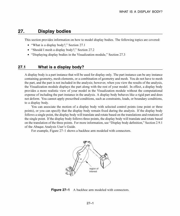
WHAT IS A DISPLAY BODY?
27. Display bodies
This section provides information on how to model display bodies. The following topics are covered:
• “What is a display body?,” Section 27.1
• “Should I mesh a display body?,” Section 27.2
• “Displaying display bodies in the Visualization module,” Section 27.3
27.1 What is a display body?
A display body is a part instance that will be used for display only. The part instance can be any instance
containing geometry, mesh elements, or a combination of geometry and mesh. You do not have to mesh
the part, and the part is not included in the analysis; however, when you view the results of the analysis,
the Visualization module displays the part along with the rest of your model. In effect, a display body
provides a more realistic view of your model in the Visualization module without the computational
expense of including the part instance in the analysis. A display body behaves like a rigid part and does
not deform. You cannot apply prescribed conditions, such as constraints, loads, or boundary conditions,
to a display body.
You can associate the motion of a display body with selected control points (one point or three
points), or you can specify that the display body remain fixed during the analysis. If the display body
follows a single point, the display body will translate and rotate based on the translations and rotations of
the single point. If the display body follows three points, the display body will translate and rotate based
on the translation of the three points. For more information, see “Display body definition,” Section 2.9.1
of the Abaqus Analysis User’s Guide.
For example, Figure 27–1 shows a backhoe arm modeled with connectors.
region ofinterest
Figure 27–1 A backhoe arm modeled with connectors.
27–1
Abaqus ID:
Printed on:
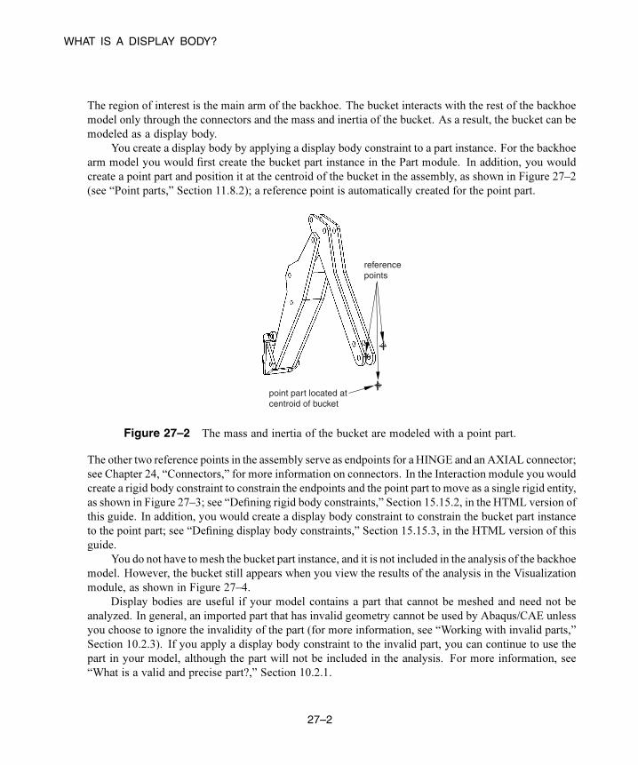
WHAT IS A DISPLAY BODY?
The region of interest is the main arm of the backhoe. The bucket interacts with the rest of the backhoe
model only through the connectors and the mass and inertia of the bucket. As a result, the bucket can be
modeled as a display body.
You create a display body by applying a display body constraint to a part instance. For the backhoe
arm model you would first create the bucket part instance in the Part module. In addition, you would
create a point part and position it at the centroid of the bucket in the assembly, as shown in Figure 27–2
(see “Point parts,” Section 11.8.2); a reference point is automatically created for the point part.
referencepoints
point part located atcentroid of bucket
Figure 27–2 The mass and inertia of the bucket are modeled with a point part.
The other two reference points in the assembly serve as endpoints for a HINGE and an AXIAL connector;
see Chapter 24, “Connectors,” for more information on connectors. In the Interaction module you would
create a rigid body constraint to constrain the endpoints and the point part to move as a single rigid entity,
as shown in Figure 27–3; see “Defining rigid body constraints,” Section 15.15.2, in the HTML version of
this guide. In addition, you would create a display body constraint to constrain the bucket part instance
to the point part; see “Defining display body constraints,” Section 15.15.3, in the HTML version of this
guide.
You do not have to mesh the bucket part instance, and it is not included in the analysis of the backhoe
model. However, the bucket still appears when you view the results of the analysis in the Visualization
module, as shown in Figure 27–4.
Display bodies are useful if your model contains a part that cannot be meshed and need not be
analyzed. In general, an imported part that has invalid geometry cannot be used by Abaqus/CAE unless
you choose to ignore the invalidity of the part (for more information, see “Working with invalid parts,”
Section 10.2.3). If you apply a display body constraint to the invalid part, you can continue to use the
part in your model, although the part will not be included in the analysis. For more information, see
“What is a valid and precise part?,” Section 10.2.1.
27–2
Abaqus ID:
Printed on:
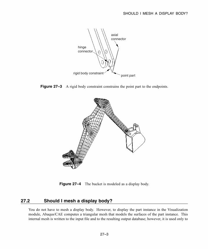
SHOULD I MESH A DISPLAY BODY?
axialconnector
point part
hingeconnector
rigid body constraint
Figure 27–3 A rigid body constraint constrains the point part to the endpoints.
Figure 27–4 The bucket is modeled as a display body.
27.2 Should I mesh a display body?
You do not have to mesh a display body. However, to display the part instance in the Visualization
module, Abaqus/CAE computes a triangular mesh that models the surfaces of the part instance. This
internal mesh is written to the input file and to the resulting output database; however, it is used only to
27–3
Abaqus ID:
Printed on:
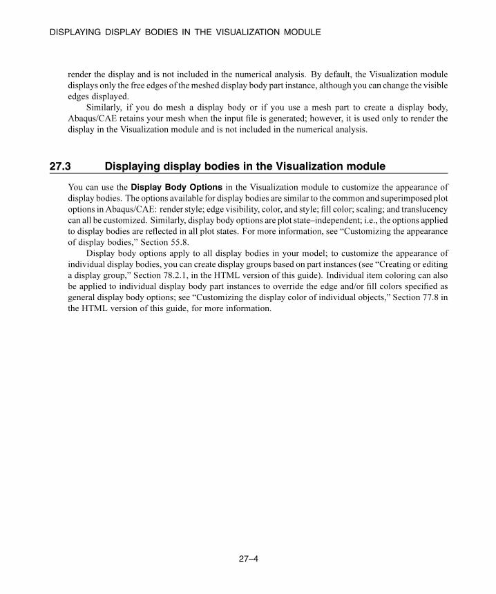
DISPLAYING DISPLAY BODIES IN THE VISUALIZATION MODULE
render the display and is not included in the numerical analysis. By default, the Visualization module
displays only the free edges of the meshed display body part instance, although you can change the visible
edges displayed.
Similarly, if you do mesh a display body or if you use a mesh part to create a display body,
Abaqus/CAE retains your mesh when the input file is generated; however, it is used only to render the
display in the Visualization module and is not included in the numerical analysis.
27.3 Displaying display bodies in the Visualization module
You can use the Display Body Options in the Visualization module to customize the appearance of
display bodies. The options available for display bodies are similar to the common and superimposed plot
options in Abaqus/CAE: render style; edge visibility, color, and style; fill color; scaling; and translucency
can all be customized. Similarly, display body options are plot state–independent; i.e., the options applied
to display bodies are reflected in all plot states. For more information, see “Customizing the appearance
of display bodies,” Section 55.8.
Display body options apply to all display bodies in your model; to customize the appearance of
individual display bodies, you can create display groups based on part instances (see “Creating or editing
a display group,” Section 78.2.1, in the HTML version of this guide). Individual item coloring can also
be applied to individual display body part instances to override the edge and/or fill colors specified as
general display body options; see “Customizing the display color of individual objects,” Section 77.8 in
the HTML version of this guide, for more information.
27–4
Abaqus ID:
Printed on:
OVERVIEW OF EULERIAN ANALYSES
28. Eulerian analyses
This section explains how to create Eulerian models in Abaqus/CAE. The following topics are covered:
• “Overview of Eulerian analyses,” Section 28.1
• “Assembling coupled Eulerian-Lagrangian models in Abaqus/CAE,” Section 28.2
• “Defining contact in Eulerian-Lagrangian models,” Section 28.3
• “Assigning materials to Eulerian part instances,” Section 28.4
• “The volume fraction tool,” Section 28.5
• “Eulerian mesh motion,” Section 28.6
• “Viewing output from Eulerian analyses,” Section 28.7
28.1 Overview of Eulerian analyses
Pure Eulerian analysis is a finite element technique in which materials are allowed to flow across
element boundaries in a rigid mesh. In the more traditional finite element formulation (also known as
the Lagrangian technique), materials are closely associated with an element, and the materials move
only with the deformation of the mesh. Because the element quality issues associated with a deformable
mesh are not present in Eulerian analyses, the Eulerian technique can be very effective at treating
problems involving very large deformations, material damage, or fluid materials. Eulerian analysis can
be performed only in Dynamic, Explicit steps. For a detailed discussion of Eulerian capabilities and
applications, refer to “Eulerian analysis,” Section 14.1.1 of the Abaqus Analysis User’s Guide.
The techniques for modeling pure Eulerian analyses in Abaqus/CAE are very different than those
used to model pure Lagrangian analyses. Most notably, instead of defining several parts and assembling
them into a complete model, Eulerian models typically consist of a single Eulerian part. This part, which
can be arbitrary in shape, represents the domain within which Eulerian materials can flow. The geometry
of bodies in the model is not necessarily defined by the Eulerian part; instead, materials are assigned to
different regions within the Eulerian part instance to define the body geometries.
Figure 28–1 compares the same model created using Lagrangian and Eulerian techniques. In the
Lagrangian model, two parts are modeled, and each part is assigned a unique section referencing a
material. In the Eulerian model, a single Eulerian part is modeled and assigned an Eulerian section. The
Eulerian section defines the materials that can be present within the part. Materials are then assigned to
different regions within the instanced part; any region without a material assignment is treated as a void
with no material properties.
The Eulerian analysis technique can be coupled with traditional Lagrangian techniques to extend
the simulation functionality in Abaqus:
• Arbitrary Lagrangian-Eulerian (ALE) adaptive meshing is a technique that combines features of
Lagrangian and Eulerian analysis within the same part mesh. ALE adaptive meshing is typically
used to control element distortion in Lagrangian parts undergoing large deformations, such as in
28–1
Abaqus ID:
Printed on:

OVERVIEW OF EULERIAN ANALYSES
EulerianLagrangian
Part 1:Eulerian section:Material instances: Lead Steel
Part 1:Homogeneous solid section:Lead
Part 2:Homogeneous solid section:Steel
Region 3:Void
Region 2:Steel
Region 1:Lead
Figure 28–1 Two bodies modeled using Lagrangian and Eulerian techniques.
a forming analysis. Most ALE adaptive meshing analyses can also be performed as pure Eulerian
analyses, but some of the features associated with a Lagrangianmesh will be lost; for a more detailed
comparison, see “ALE adaptive meshing: overview,” Section 12.2.1 of the Abaqus Analysis User’s
Guide.
• Coupled Eulerian-Lagrangian (CEL) analysis allows Eulerian and Lagrangian bodies within the
same model to interact. Coupled Eulerian-Lagrangian analysis is typically used to model the
interactions between a solid body and a yielding or fluidmaterial, such as a Lagrangian drill traveling
through Eulerian soil or an Eulerian gas inflating a Lagrangian airbag. Eulerian-Lagrangian
analysis is discussed in “Assembling coupled Eulerian-Lagrangian models in Abaqus/CAE,”
Section 28.2.
Viewing the results of Eulerian analyses requires some special techniques in the Visualization
module. These techniques are discussed in detail in “Viewing output from Eulerian analyses,”
Section 28.7.
The procedure for creating Eulerian models in Abaqus/CAE involves the following general steps:
1. In the Part module, create an Eulerian-type part that defines the geometric region within which
Eulerian materials can flow. For more information, see “Choosing the type of a new part,”
Section 11.19.3, in the HTML version of this guide.
2. In the Part module, you may want to create partitions that represent the initial boundaries between
different materials in the part. The partitions will affect the mesh of the part, and they are necessary
28–2
Abaqus ID:
Printed on:

OVERVIEW OF EULERIAN ANALYSES
only if you are assigning materials uniformly across a region. For more information about assigning
materials in an Eulerian part, see “Assigning materials to Eulerian part instances,” Section 28.4, and
“Defining a material assignment field,” Section 16.11.10, in the HTML version of this guide.
3. In the Property module, define the materials in the model.
4. In the Property module, define and assign an Eulerian section for the model. The Eulerian section
determines which materials can be present in the Eulerian part. The topology of the materials within
the part will be defined in the Load module, as discussed in Step 7. For more information, see
“Creating Eulerian sections,” Section 12.13.3, in the HTML version of this guide.
5. In the Assembly module, create an instance of the Eulerian part.
6. In the Step module, create a field output request for output variable EVF. This output is necessary
to view the deformation of materials in an Eulerian model. For more detailed information, see
“Viewing output from Eulerian analyses,” Section 28.7.
7. In the Load module, create a material assignment predefined field that defines the topology of
materials in the initial configuration of the Eulerian part instance. For more information, see
“Assigning materials to Eulerian part instances,” Section 28.4, and “Defining a material assignment
field,” Section 16.11.10, in the HTML version of this guide.
8. In the Load module, define any loads or boundary conditions acting on the model. Because the
mesh in an Eulerian part is rigid, traditional Lagrangian prescribed conditions do not move with the
material deformations; loads and boundary conditions are imposed on any material that occupies
(or moves into) the region to which the condition is prescribed. Zero-displacement boundary
conditions can be used along the sides of an Eulerian part instance to prevent Eulerian material
from entering or exiting the part. Boundary conditions and constraints based on nonzero nodal
displacements are ignored in an Eulerian part instance; typically, velocity boundary conditions or
predefined fields are used to prescribe initial motion in an Eulerian model. Specialized Eulerian
boundary conditions can also be defined to control the flow of material across the boundaries of
the Eulerian part (see “Defining an Eulerian boundary condition,” Section 16.10.21). For more
information about applying loads and boundary conditions to Eulerian models, see “Boundary
conditions” in “Eulerian analysis,” Section 14.1.1 of the Abaqus Analysis User’s Guide.
9. In the Mesh module, create a hexagonal mesh for the Eulerian part. EC3D8R elements are assigned
to themesh by default. After creating a regularmesh, you can trim any elements that are not expected
to experience material flow to reduce the model size and improve performance of the analysis.
An example of a basic Eulerian model created in Abaqus/CAE is provided in “Eulerian analysis of a
collapsing water column,” Section 1.7.1 of the Abaqus Benchmarks Guide. More complicated Eulerian
modeling procedures, including complex material assignments and coupled Eulerian-Lagrangian
interactions, are illustrated in “Impact of a water-filled bottle,” Section 2.3.2 of the Abaqus Example
Problems Guide.
28–3
Abaqus ID:
Printed on:
DEFINING CONTACT IN EULERIAN-LAGRANGIAN MODELS
28.2 Assembling coupled Eulerian-Lagrangian models in Abaqus/CAE
Abaqus allows you to create models that include both Eulerian part instances and Lagrangian part
instances. During a coupled Eulerian-Lagrangian analysis, the Lagrangian mesh interacts with the
materials in the Eulerian part. Coupled Eulerian-Lagrangian analyses typically offer better interpretation
of contact conditions than pure Eulerian analyses, particularly for interactions between fluid and solid
materials. During postprocessing, a solid Lagrangian body in a coupled Eulerian-Lagrangian analysis
appears to maintain its shape better than a similar body in a pure Eulerian analysis.
Figure 28–2 compares a pure Eulerian analysis (top) and a coupled Eulerian-Lagrangian analysis
(bottom) of a steel brick passing through a column of water. In the Eulerian analysis the water tends
to adhere to the sides of the brick, and the brick appears deformed in the final configuration. This
apparent deformation is a result of the material volume fraction calculations used for Eulerian materials,
as discussed in “Material interfaces” in “Eulerian analysis,” Section 14.1.1 of the Abaqus Analysis User’s
Guide. On the other hand, the Lagrangian brick maintains its shape as it passes through the Eulerian
water, and the water flows around the brick.
Coupled Eulerian-Lagrangian analyses also allow you to capitalize on the strengths of both analysis
techniques; for example, you can use the loads on a Lagrangian body moving through an Eulerian
material to drive a detailed submodel of the Lagrangian body.
To assemble a coupled Eulerian-Lagrangian model in Abaqus/CAE, simply instance both Eulerian
and Lagrangian parts in the same assembly. Coupled Eulerian-Lagrangian analyses can be performed
only in Dynamic, Explicit steps. You must create a general contact definition to enable contact between
Lagrangian and Eulerian parts. The general contact definition allows interactions between Lagrangian
surfaces and Eulerian material instances in the model (see “Defining contact in Eulerian-Lagrangian
models,” Section 28.3, for more information). Other interactions, loads, boundary conditions, and
predefined fields are applied to the Lagrangian and Eulerian parts in the usual manner.
In most cases the Lagrangian part is assembled inside of the Eulerian part instance. While
Lagrangian and Eulerian elements and nodes can overlap, three-dimensional Lagrangian elements
cannot occupy the same space as an Eulerian material instance. Therefore, Lagrangian parts must be
instanced in an area of void within the Eulerian part instance (i.e., a region with no material assignment).
To model a three-dimensional Lagrangian part instance that is completely surrounded by Eulerian
material, use the volume fraction tool to create an Eulerian material assignment field that includes a void
region corresponding to the Lagrangian part instance (see “The volume fraction tool,” Section 28.5, for
details).
28.3 Defining contact in Eulerian-Lagrangian models
Contact in a coupled Eulerian-Lagrangian analysis must be defined using general contact. The general
contact definition enables interactions between Lagrangian part surfaces and the surfaces of Eulerian
material instances; contact between different Lagrangian parts in the model is also enabled.
28–4
Abaqus ID:
Printed on:

DEFINING CONTACT IN EULERIAN-LAGRANGIAN MODELS
Figure 28–2 Comparison of a pure Eulerian analysis (top) and a coupled
Eulerian-Lagrangian analysis (bottom).
In Abaqus/CAE you can use the global All* with self contact domain to enforce contact between
all Lagrangian parts and all Eulerian material instances in the model. Alternatively, you can include
or exclude contact between a Lagrangian surface and a particular Eulerian material instance. Eulerian
material instances appear in the list of surfaces in the Include Pairs and Exclude Pairs dialog boxes,
as shown in Figure 28–3. You can also assign unique contact properties between particular Lagrangian
surfaces and particular Eulerian material instances in the Individual Contact Property Assignmentsdialog boxes.
True contact cannot be defined between different Eulerian material instances. A rudimentary
contact condition is enforced because material instances cannot penetrate each other. However, material
instances do not separate once they come into contact, which prevents the modeling of sliding or
rebounding behavior. Contact output is not available for Eulerian material instances. For a detailed
28–5
Abaqus ID:
Printed on:

ASSIGNING MATERIALS TO EULERIAN PART INSTANCES
Figure 28–3 Eulerian material instances in the Edit Excluded Pairs dialog box.
discussion of Eulerian analysis contact formulations, refer to “Interactions” in “Eulerian analysis,”
Section 14.1.1 of the Abaqus Analysis User’s Guide. If the contact conditions between two materials
are significant to your analysis, at least one of the materials should be modeled as a Lagrangian part.
28.4 Assigning materials to Eulerian part instances
In a pure Lagrangian analysis a section definition includes a reference to a single material. When you
assign a section to a region or element in the Lagrangian part, that region or element is completely filled
with the referenced material. The geometry of the region or element, therefore, defines the geometry of
the material.
In a pure Eulerian analysis the relationship between the section definition and material is
fundamentally different. An Eulerian section definition can reference a list of materials. When you
assign the Eulerian section to an Eulerian part, you are defining which materials may be present in the
part over the course of the analysis. The part, however, is initially empty of material. To introduce
material to the initial state of an Eulerian part, you must use a material assignment predefined field.
Material assignment predefined fields rely on the concept of material volume fractions. During
an Eulerian analysis, Abaqus tracks the material present in each element in terms of a volume fraction
assigned to each material instance; the volume fraction represents the percentage of the element’s volume
that is occupied by a given material instance. For elements that are partially filled or filled with multiple
materials, the exact geometric composition of the material within the element is not known; Abaqus
interpolates the material volume fractions from adjacent elements to estimate the material boundaries
within the element. These calculations are discussed in more detail in “Material interfaces” in “Eulerian
analysis,” Section 14.1.1 of the Abaqus Analysis User’s Guide.
In Abaqus/CAE the initial material volume fractions in an Eulerian part are specified by creating a
material assignment predefined field in the Load module. The predefined field associates each region in
an Eulerian part instance with a volume fraction for each material instance. The regions to which volume
28–6
Abaqus ID:
Printed on:

ASSIGNING MATERIALS TO EULERIAN PART INSTANCES
fractions are assigned can be cells (in geometry), mesh elements, or groups of elements. If you select a
cell or a group of elements, the volume fraction values are propagated to each of the underlying Eulerian
elements in the cell or group.
Volume fractions in a material assignment predefined field are expressed as a number between zero
and one; a volume fraction of one indicates that the region is completely filled with the specified material.
A volume fraction of less than one indicates that the region is only partially filled with the specified
material; for example, a volume fraction of 0.25 means that the specified material instance occupies 25%
of the region. As mentioned previously, Abaqus determines the material boundaries for partially filled
elements based on the volume fractions in adjacent elements; to achieve greater control over the material
boundaries within a region, you must refine the part mesh or redefine the region boundaries.
If material volume fractions are not defined for a region of an Eulerian part instance, that region is
assigned a void. Similarly, if the volume fractions for all materials in a region do not sum to one, the
remainder of the volume fraction in that region is assigned a void. Void regions do not have material
properties, but other materials can flow into and through a void region during an analysis.
The material assignment predefined field effectively defines the topology of materials in the initial
configuration of your model. The Eulerian part is typically arbitrary in shape; the material assignment
predefined field adds to the part the Eulerian materials that will interact during the analysis. For example,
consider the cross-section of the coupled Eulerian-Lagrangian model in Figure 28–4. The Eulerian part
is simply an empty cube. Four regions defined on the part determine the slope of the earth and the amount
of water in the tank, and material is assigned to these regions accordingly.
Eulerianpart instance
Lagrangiantank
Earth
Void
Water
Air
Figure 28–4 Material assignments in an Eulerian-Lagrangian model.
28–7
Abaqus ID:
Printed on:

ASSIGNING MATERIALS TO EULERIAN PART INSTANCES
Material assignment predefined fields can be created only in the initial step of an Eulerian analysis.
In subsequent steps the materials deform from their initial configuration and flow across the Eulerian
mesh according to the forces present in the model.
Abaqus/CAE offers two techniques for defining material assignment predefined fields:
Uniform definitions
Uniform material assignment field definitions are created by selecting regions from an Eulerian part
instance and directly specifying the volume fraction of each material instance within those regions.
Geometry must be partitioned into separate cells representing the material regions. In part instances
that include orphan elements you can select individual elements to act as regions.
Figure 28–5 illustrates a material assignment field created using uniform definitions. The
Eulerian part is partitioned into three regions, and material volume fractions are defined in each
region; each region is completely filled with a single material instance. Volume fractions are not
defined for the void region, since void is the default material assignment.
Sand
Water
Void
Figure 28–5 A uniform material assignment field.
The uniform material assignment definition should be used only for relatively simple regions
that are uniformly filled with material. The partitions needed to create complex regions can
28–8
Abaqus ID:
Printed on:

ASSIGNING MATERIALS TO EULERIAN PART INSTANCES
negatively impact the quality of the Eulerian mesh, and partially filled regions are difficult to define
and interpret, particularly when working with geometry.
For details on creating a uniform material assignment field in Abaqus/CAE, see “Defining a
material assignment field,” Section 16.11.10, in the HTML version of this guide. An example of a
uniform material assignment definition is illustrated in the Python script provided in “Deflection of
an elastic dam under water pressure,” Section 1.7.2 of the Abaqus Benchmarks Guide.
Discrete field definitions
Material assignments for meshed geometry and orphan meshes can be defined using a scalar discrete
field. For each material instance in the part you create a discrete field that associates individual
elements with a volume fraction for that material instance. For more information on creating discrete
fields, see Chapter 63, “The Discrete Field toolset.”
When you are assigning materials using a discrete field, you still must select the region of
the part instance to which the discrete field applies. If the discrete field includes data for elements
outside of the selected region, these data are ignored. The default value associated with the discrete
field is assigned to any elements within the selected region that are not explicitly listed in the discrete
field.
Figure 28–6 shows a very simple example of a material assignment defined using discrete
fields. The Eulerian part consists of four elements and two material instances. Two discrete fields,
as defined in Table 28–1, are used to specify the material composition within the elements. The
boundary between the water and the sand is an estimation based on interpolation of the material
volume fractions in adjacent elements.
Note: In any given element the sum of all material volume fractions should not be greater than one.
Abaqus/CAE assigns volume fractions incrementally by reading the discrete fields in the VolumeFractions table from right to left; once the volume fraction for an element reaches one, additional
volume fractions assigned to that element are ignored.
Since the discrete field can assign unique volume fractions to each individual element, it
allows more complicated material boundaries than the uniform definition method without the
need for excessive partitioning. The volume fraction tool in Abaqus/CAE creates discrete fields
specifically for use in material assignment predefined fields. Through this tool, you can define
complex Eulerian material regions using the part modeling techniques available in Abaqus/CAE.
For more information, see “The volume fraction tool,” Section 28.5.
For details on creating a discrete field material assignment in Abaqus/CAE, see “Defining a
material assignment field,” Section 16.11.10, in the HTML version of this guide. An example of
a discrete field material assignment definition (including the use of the volume fraction tool) is
illustrated in the Python script provided in “Rivet forming,” Section 2.3.1 of the Abaqus Example
Problems Guide.
28–9
Abaqus ID:
Printed on:

THE VOLUME FRACTION TOOL
Water
Sand
Element 1 Element 2
Element 3 Element 4
Figure 28–6 A discrete field material assignment.
Table 28–1 Volume fractions defined in discrete fields.
Discrete Field Element 3 Default
Water_Field 0.5 1
Sand_Field 0.5 0
28.5 The volume fraction tool
The volume fraction tool creates a scalar discrete field by performing a Boolean comparison between an
Eulerian part instance and a second part instance (the reference part instance) that intersects the Eulerian
instance. The comparison determines where the two part instances overlap, then assigns each element in
the Eulerian instance a volume fraction based on the percentage of the element that is also occupied by
the reference instance. The volume fraction is specified as a decimal between zero and one.
The discrete field that is created by the volume fraction tool can be used to assign material instances
to the Eulerian part instance (see “Assigning materials to Eulerian part instances,” Section 28.4). The
28–10
Abaqus ID:
Printed on:

THE VOLUME FRACTION TOOL
topology of the assigned Eulerian material instance corresponds to the shape of the reference part instance
within the Eulerian part instance.
Figure 28–7 and the following procedure summarize the process of using the volume fraction tool:
Referencepart Eulerian
part
(1) (2)
(3) (4)
Materialassignmentpredefined field
Discrete field
Referencepart
Figure 28–7 Procedure for using the volume fraction tool.
1. Using any of the modeling tools and techniques in Abaqus/CAE, create a reference part that
corresponds to the geometry of the desired Eulerian material region.
2. Instance the reference part within the Eulerian part instance. The reference part instance should
spatially correspond to the desired Eulerian material region.
3. Use the volume fraction tool to create a discrete field based on a comparison of the reference part
instance and the Eulerian part instance.
4. Define a material assignment predefined field for the Eulerian part instance using the discrete field
created by the volume fraction tool.
28–11
Abaqus ID:
Printed on:

THE VOLUME FRACTION TOOL
An option for the volume fraction tool controls whether the calculated discrete field represents the
space inside the reference instance (the volume fraction is nonzero in elements that overlap the reference
instance) or the space outside the reference instance (the volume fraction is nonzero in elements that do
not overlap or partially overlap the reference instance), as depicted in Figure 28–8.
Figure 28–8 Discrete fields representing volume fractions inside (left) and outside
(right) of the shaded reference region.
Typically, calculating the volume fraction outside of a reference instance is used to create an Eulerian
material assignment around a Lagrangian part instance in a coupled Eulerian-Lagrangian analysis.
Calculating the volume fraction inside of a reference instance is usually used to model complex
material assignment fields within a pure Eulerian part instance; in this situation, the reference instance
is suppressed after the Eulerian material is assigned. You can also calculate volume fractions inside of
a reference instance to create an Eulerian material assignment on the inside of an enclosed Lagrangian
shell in a coupled Eulerian-Lagrangian analysis.
To use the volume fraction tool, select Tools→Discrete Field→Volume Fraction Tool from the
main menu bar. For step-by-step instructions for using the tool, refer to “Creating discrete fields for
material volume fractions,” Section 63.4, in the HTML version of this guide.
28.5.1 Requirements for the volume fraction toolThe Eulerian part instance that is used by the volume fraction tool must be the same instance to which
materials are assigned. The Eulerian part must be meshed before using the volume fraction tool. You
should not edit the part mesh after creating the discrete field, as the element numbering in the discrete
field may not conform to the elements in the updated mesh.
The reference part instance used by the volume fraction tool can include unmeshed geometry, a
native mesh, or orphan elements; deformable, Eulerian, and discrete rigid parts are all allowed. The
28–12
Abaqus ID:
Printed on:

EULERIAN MESH MOTION
volume fraction tool always uses the mesh representation (if available) of the reference part instance
when calculating the discrete field; if the reference instance is partially meshed, only the meshed portion
of the instance is considered in the volume fraction calculation. The mesh on the reference instance
should be fine enough to capture all important geometric details in the subsequent material assignment.
The reference part instance must be either a three-dimensional solid or a fully enclosed three-
dimensional shell. The faces of a shell enclosure must define a single, continuous surface; features that
create T-intersections with the surface faces (such as ribs or interior dividing panels) are not allowed (see
Figure 28–9). An Eulerian element is considered to be inside a shell reference instance if it lies within
the volume enclosed by the shell surface.
Figure 28–9 Cross-sections of acceptable reference shell parts (top) and
unacceptable reference shell parts (bottom).
28.6 Eulerian mesh motion
Eulerian mesh motion is a technique that allows you to reduce the size of an Eulerian mesh for certain
models, thereby improving the performance of the analysis. In some cases the Eulerian domain at the
beginning of an analysis does not sufficiently capture the deformations in the model by the end of the
analysis. Some typical examples include:
• An airbag where the inflator gas is modeled as an Eulerian material: the gas initially occupies a
small region, but the region quickly expands as the airbag inflates.
• A projectile impact analysis where the projectile is modeled as an Eulerian material: the projectile
initially occupies a region that is far from its ultimate destination.
In such cases it is possible to adjust the size and location of the Eulerian domain during the analysis
so that it always captures a part or material of interest. By default, an Eulerian mesh is rigid and fixed in
28–13
Abaqus ID:
Printed on:

EULERIAN MESH MOTION
place; but enabling Eulerian mesh motion allows the Eulerian elements to scale and translate during the
analysis. Eulerian mesh motion can follow the deformation of an Eulerian material instance (as shown
in Figure 28–10) or a Lagrangian surface (as shown in Figure 28–11). The behavior of Eulerian mesh
motion is described in detail in “Eulerian mesh motion,” Section 14.1.3 of the Abaqus Analysis User’s
Guide.
Figure 28–10 Eulerian mesh motion tracking a material instance.
Figure 28–11 Eulerian mesh motion tracking a Lagrangian surface.
In Abaqus/CAE Eulerian mesh motion is defined as a boundary condition in the Load module.
Restrictions can be imposed on the scaling and translation of the Eulerian mesh as part of the boundary
condition definition. For more information about creating Eulerian mesh motion boundary conditions,
see “Defining an Eulerian mesh motion boundary condition,” Section 16.10.22, in the HTML version of
this guide.
28–14
Abaqus ID:
Printed on:

VIEWING OUTPUT FROM EULERIAN ANALYSES
28.7 Viewing output from Eulerian analyses
The results of an Eulerian analysis must be interpreted differently than those from a Lagrangian analysis.
In particular, any results based on nodal displacements are meaningless in an Eulerian model because
the Eulerian part is fixed and rigid. Details concerning how Eulerian results are written to the output
database are available in “Output” in “Eulerian analysis,” Section 14.1.1 of the Abaqus Analysis User’s
Guide.
Special steps must be taken in the Visualization module of Abaqus/CAE to view material instances
within an Eulerian part. By default, Abaqus/CAE displays the full Eulerian part mesh in both undeformed
and deformed plot states with no indication of the material instance boundaries within the mesh.
Visualization of material instances is based on output variable EVF, the Eulerian material volume
fraction. Output variable EVFmeasures the amount of a particular material instance within an element as
a relative fraction. An EVF value of one indicates that the element is completely filled with the specified
material instance; an EVF value of zero indicates that the element is completely devoid of the specified
material instance.
For elements that are partially filled or filled with multiple materials, Abaqus estimates a simple
boundary between materials by interpolating the EVF values in adjacent elements. These simple
boundaries may be slightly discontinuous across elements. To improve display of Eulerian materials,
you should instruct Abaqus/CAE either to use a results averaging threshold of 100% or to compute
scalars after averaging results; Abaqus/CAE remaps the material boundaries so they appear smooth
and continuous across elements. For more information about results averaging, see “Controlling result
averaging,” Section 42.6.6, in the HTML version of this guide; for a more detailed discussion of
how Abaqus calculates Eulerian material boundaries, see “Material interfaces” in “Eulerian analysis,”
Section 14.1.1 of the Abaqus Analysis User’s Guide.
Output variable EVF is written to the output database if you request the Preselected defaultsin the field output request editor (see “Modifying field output requests,” Section 14.12.2, in the HTML
version of this guide). When you request output for EVF, Abaqus creates a separate material volume
fraction output variable for each material instance in the model; for example, EVF_WATER is the volume
fraction for the material instance named Water. An output variable named EVF_VOID is created to
measure the volume fraction of empty regions in an Eulerian part.
The following techniques can be used in the Visualization module to view the initial and deformed
states of material in an Eulerian part:
Contour plots
A contour plot of output variable EVF for a particular material instance allows you to visualize
which areas of the model are occupied by the material during the analysis. Areas occupied by
the material (EVF equal to one) appear as a uniform color from the top of the contour spectrum,
while areas unoccupied by the material appear as a different color from the bottom of the contour
spectrum; depending on your contour plot settings, the boundary of the material instance appears
in a range of colors as EVF transitions from one to zero (see Figure 28–12).
28–15
Abaqus ID:
Printed on:

VIEWING OUTPUT FROM EULERIAN ANALYSES
Figure 28–12 Contour plot of an Eulerian material instance.
Contour plots are of limited usefulness when visualizing Eulerian materials because the
contours appear on the faces of the Eulerian parts. You cannot effectively visualize material
volume fraction contours on the interior of Eulerian parts.
For further details on using contour plots in the Visualization module, see Chapter 44,
“Contouring analysis results.”
View cuts
To visualize the behavior of a material on the interior of an Eulerian part, activate a view cut along an
isosurface of the EVF variable associated with that material instance. Abaqus/CAE automatically
creates these isosurface view cuts for each material instance in the model, but you must activate
them in the View Cut Manager. Using the view cut options, you can eliminate portions of the part
that do not include a selected material by rendering them unfilled, rendering them translucent, or
removing them from the display (see Figure 28–13).
If your Eulerian part includes regions without a material assignment, it may be helpful to
activate an isosurface view cut based on the EVF_VOID output variable. By cutting away all regions
in which EVF_VOID is greater than 0.5, you are able to see the shape of materials within the part.
After activating an isosurface view cut based on the EVF variable, you can change the primary
field output variable without affecting the view cut. This enables you to visualize results contours
along the boundaries of material instances instead of on Eulerian part faces (see Figure 28–14).
Isosurface view cuts based on output variable EVF do not affect Lagrangian part instances in
a coupled Eulerian-Lagrangian model. The Lagrangian parts remain visible when the cut is active.
Therefore, this technique is useful for visualizing the interaction between a Lagrangian part and an
Eulerian material instance.
For further details on using view cuts in the Visualization module, see Chapter 80, “Cutting
through a model.”
28–16
Abaqus ID:
Printed on:
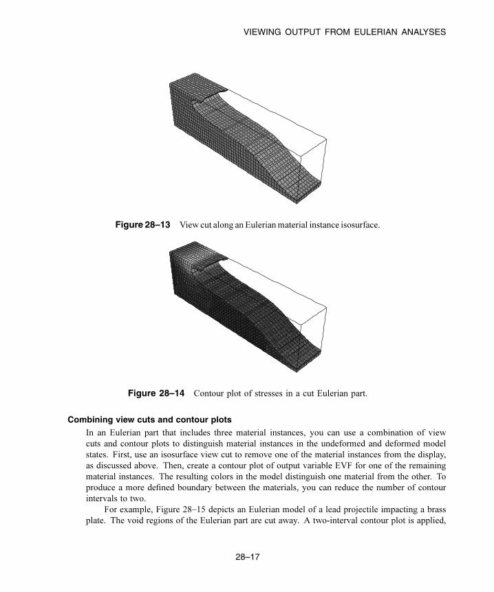
VIEWING OUTPUT FROM EULERIAN ANALYSES
Figure 28–13 View cut along an Eulerianmaterial instance isosurface.
Figure 28–14 Contour plot of stresses in a cut Eulerian part.
Combining view cuts and contour plots
In an Eulerian part that includes three material instances, you can use a combination of view
cuts and contour plots to distinguish material instances in the undeformed and deformed model
states. First, use an isosurface view cut to remove one of the material instances from the display,
as discussed above. Then, create a contour plot of output variable EVF for one of the remaining
material instances. The resulting colors in the model distinguish one material from the other. To
produce a more defined boundary between the materials, you can reduce the number of contour
intervals to two.
For example, Figure 28–15 depicts an Eulerian model of a lead projectile impacting a brass
plate. The void regions of the Eulerian part are cut away. A two-interval contour plot is applied,
28–17
Abaqus ID:
Printed on:
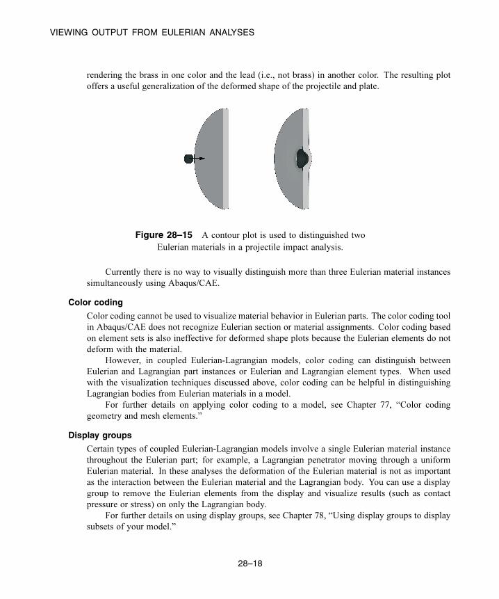
VIEWING OUTPUT FROM EULERIAN ANALYSES
rendering the brass in one color and the lead (i.e., not brass) in another color. The resulting plot
offers a useful generalization of the deformed shape of the projectile and plate.
Figure 28–15 A contour plot is used to distinguished two
Eulerian materials in a projectile impact analysis.
Currently there is no way to visually distinguish more than three Eulerian material instances
simultaneously using Abaqus/CAE.
Color coding
Color coding cannot be used to visualize material behavior in Eulerian parts. The color coding tool
in Abaqus/CAE does not recognize Eulerian section or material assignments. Color coding based
on element sets is also ineffective for deformed shape plots because the Eulerian elements do not
deform with the material.
However, in coupled Eulerian-Lagrangian models, color coding can distinguish between
Eulerian and Lagrangian part instances or Eulerian and Lagrangian element types. When used
with the visualization techniques discussed above, color coding can be helpful in distinguishing
Lagrangian bodies from Eulerian materials in a model.
For further details on applying color coding to a model, see Chapter 77, “Color coding
geometry and mesh elements.”
Display groups
Certain types of coupled Eulerian-Lagrangian models involve a single Eulerian material instance
throughout the Eulerian part; for example, a Lagrangian penetrator moving through a uniform
Eulerian material. In these analyses the deformation of the Eulerian material is not as important
as the interaction between the Eulerian material and the Lagrangian body. You can use a display
group to remove the Eulerian elements from the display and visualize results (such as contact
pressure or stress) on only the Lagrangian body.
For further details on using display groups, see Chapter 78, “Using display groups to display
subsets of your model.”
28–18
Abaqus ID:
Printed on:

ABOUT FASTENERS
29. Fasteners
This section describes how to model fasteners. The following topics are covered:
• “About fasteners,” Section 29.1
• “Managing fasteners,” Section 29.2
In addition, the following sections are available in the HTML version of this guide:
• “Creating point-based fasteners,” Section 29.3
• “Creating discrete fasteners,” Section 29.4
• “Creating assembled fasteners,” Section 29.5
29.1 About fasteners
You use fasteners to model a point-to-point connection between two or more faces, such as a spot weld,
a bolt, or a rivet. You can use the Attachment toolset to create attachments that help you define fasteners;
for more information, see “Understanding attachment points and lines,” Section 59.1. You can create
point-based fasteners, discrete fasteners, or assembled fasteners. The following topics provide overviews
of the different fastener types:
• “About point-based fasteners,” Section 29.1.1
• “About discrete fasteners,” Section 29.1.2
• “About assembled fasteners,” Section 29.1.3
Both point-based and discrete fasteners can be modeled using connectors or beam MPCs. If you
define connectors that use basic, assembled, or complex connection types, you can request output from
your point-based or discrete fasteners through connector output variables. However, if you use beam
MPCs, no output is available from your point-based or discrete fasteners.
29.1.1 About point-based fasteners
Point-based fasteners make use of positioning points to create mesh-independent fasteners in
Abaqus/Standard and Abaqus/Explicit, as described in “Mesh-independent fasteners,” Section 35.3.4
of the Abaqus Analysis User’s Guide. A positioning point can be an attachment point, a reference
point, or a node from an orphan mesh. Point-based fasteners modeling spot welds around the edge of a
bracket are shown in Figure 29–1. The user first created attachment points at equally spaced intervals
around the edge of the bracket. The attachment points were used to define the location of the fastener’s
positioning points.
29–1
Abaqus ID:
Printed on:

ABOUT FASTENERS
Figure 29–1 Point-based fasteners modeling spot welds.
A point-based fastener can connect selected faces with either connectors or rigid (beam) multi-point
constraints. If you want to model a rigid connection, you can use rigid connectors or rigid multi-point
constraints.
Connectors
If you use connectors to connect the faces, you can model either rigid, elastic, or inelastic
connections with failure by using the generality of connector behavior definitions. You can use a
rigid connector to model a rigid connection. However, if you are using rigid connectors and Abaqus
detects two adjacent point-based fasteners that are sharing nodes, you must avoid overconstraining
your model by defining some elasticity in the connector behavior to reduce the stiffness.
You can request output from connectors.
Rigid (beam) multi-point constraints
Rigid multi-point constraints are computationally cheaper than connectors and are less likely to
result in an overconstrained model when two adjacent fasteners are sharing nodes. When Abaqus
detects two adjacent fasteners that are sharing nodes and using rigid multi-point constraints, it uses
a penalty distributing coupling formulation that relaxes, to a small degree, the constraint between
the motion of the fastening point and its coupling nodes to avoid the overconstraint.
You cannot request output from multi-point constraints.
A point-based fastener uses distributing coupling constraints to connect the faces regardless of
how you mesh the faces. When you submit a job for analysis, Abaqus uses your fastener definition
29–2
Abaqus ID:
Printed on:
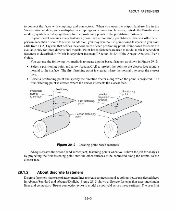
ABOUT FASTENERS
to connect the faces with couplings and connectors. When you open the output database file in the
Visualization module, you can display the couplings and connectors; however, outside the Visualization
module, symbols are displayed only for the positioning points of the point-based fasteners.
If your model contains many fasteners (more than a thousand), point-based fasteners offer better
performance than discrete fasteners. In addition, you may want to use point-based fasteners if you have
a file from a CAD system that defines the coordinates of each positioning point. Point-based fasteners are
available only for three-dimensional models. Point-based fasteners are used to model mesh-independent
fasteners as described in “Mesh-independent fasteners,” Section 35.3.4 of the Abaqus Analysis User’s
Guide.
You can use the following two methods to create a point-based fastener, as shown in Figure 29–2:
• Select a positioning point and allow Abaqus/CAE to project the point to the closest face along a
normal to the surface. The first fastening point is created where the normal intersects the closest
face.
• Select a positioning point and specify the direction vector along which the point is projected. The
first fastening point is created where the vector intersects the closest face.
Positioning pointProjection
normal to surface
Positioning pointSpecified
projectiondirectionFirst fastening
point
Second fastening point
Figure 29–2 Creating point-based fasteners.
Abaqus creates the second (and subsequent) fastening points when you submit the job for analysis
by projecting the first fastening point onto the other surfaces to be connected along the normal to the
closest face.
29.1.2 About discrete fastenersDiscrete fasteners make use of attachment lines to create connectors and couplings between selected faces
in Abaqus/Standard and Abaqus/Explicit. Figure 29–3 shows a discrete fastener that uses attachment
lines and connectors (Beam connection type) to model a spot weld across three surfaces. The user first
29–3
Abaqus ID:
Printed on:

ABOUT FASTENERS
created attachment lines at the locations of the spot welds. The attachment lines were used to define the
location of the discrete fastener.
Attachmentlines
Distributing coupling
Connectors
Figure 29–3 A spot weld across three surfaces modeled with a discrete fastener.
The process of creating an attachment line is similar to the process of creating point-based fasteners. You
select a starting point and specify which of the two methods Abaqus/CAE will use to project the point
onto the closest face. Figure 29–4 shows the two methods for creating an attachment line that is used to
define a discrete fastener.
StartingpointProjection
normal to surface
Specified projectiondirection
Attachment line
Attachment line
Startingpoint
First fastening point
Second fastening point
Figure 29–4 Creating an attachment line that is used to define a discrete fastener.
29–4
Abaqus ID:
Printed on:

ABOUT FASTENERS
Abaqus/CAE projects the attachment line along a normal to the closest face. You can use the
following two methods to determine the number of faces that are connected by the attachment line:
• Specify the number of projections or layers.
• Specify the maximum length of the projection.
For each attachment line, Abaqus/CAE determines the fastening points and applies a distributing
coupling between each fastening point and its corresponding surface. After you assign a connector
section to the attachment line, Abaqus/CAE creates a connector, and the discrete fastener is considered
to be fully defined. You can control the accuracy of the attachment line position on a faceted
representation of a part instance by specifying the level of curve refinement in the Part module and the
Property module. For more information, see “Controlling curve refinement,” Section 76.4.
If your model is complex, Abaqus/CAE can create a chain of attachment lines connecting multiple
surfaces that would be time consuming to create manually. In contrast with point-based fasteners, you can
view attachment lines and discrete fasteners and their connectors and couplings outside the Visualization
module.
If two surfaces are used by two attachment lines and share a common face, Abaqus/CAE merges the
two faces into a single face when you submit the model for analysis. This results in better performance
by Abaqus/Standard or Abaqus/Explicit, especially when the fasteners connect nodes across faces of a
refined orphan mesh.
When you submit a job that contains a model with discrete fasteners for analysis, Abaqus/CAE
writes special comment lines to the input file. These special comment lines, which are ignored by
the Abaqus solvers, allow Abaqus/CAE to recreate the fully defined discrete fasteners upon import
into Abaqus/CAE. For more information, see “Importing interactions, constraints, and fasteners” in
“Importing a model from an Abaqus input file,” Section 10.5.2.
An example of creating discrete fasteners is illustrated in the Python script included in “Buckling
of a column with spot welds,” Section 1.2.3 of the Abaqus Example Problems Guide.
29.1.3 About assembled fasteners
Assembled fasteners let you efficiently assign complex fastener behaviors in a large number of model
locations. Using the assembled fastener technique, you can read in connector and constraint behaviors
from a template model and assign these attributes in multiple locations in your main model. For a large
system such as an airframe or automobile, assembled fasteners allow you to define the fastener template
once and then assign it many times in the main model. With the appropriate use of coupling constraints
and adjust points constraints, slave nodes in the template model can be automatically resized in the main
model to accommodate the actual surface spacing.
The overall process for building assembled fasteners is as follows:
1. Build the template model containing your fastener-like construct: connector section assignments,
tie constraints, coupling constraints, and solid or beam section assignments. You must assign names
29–5
Abaqus ID:
Printed on:

ABOUT FASTENERS
to all surfaces involved in constraints. You must also define a single-point set as the control point,
which will be used to locate the template model copies in the main model.
2. Develop your main model, placing attachment points at the locations where you want the template
fastener to be replicated. The template model control point will be mapped onto the locations of the
attachment points in the main model (see Figure 29–5).
3. Working in your main model, use theCreate Fasteners andEdit Fasteners dialog boxes to define
how the template model will be read in, assigned, and oriented.
4. Optionally, use one or more property generation scripts to modify the properties copied into the main
model from the template model. Multiple property generation scripts can be used with the same
template model to achieve different results in separate assembled fastener objects. For example,
you could use two scripts to apply different materials to the same fastener template. You can use
the Abaqus Scripting Interface to write your property generation scripts; see “Creating and running
your own scripts,” Section 9.5.4, and the Abaqus Scripting User’s Guide.
Surface A
Control point
Main Model
Assignment surface B
(Generated model in input file)
Assignment surface AAttachment
points
etc.
Assembled fasteners
Template Model:-Connector sections-Tie constraints-Coupling constraints
Surface B
Figure 29–5 Replicating the template model in the main model.
The template model uses the global coordinate system, and the positive Z-axis direction of the
fastener construct will be aligned with the selected normal direction in the main model.
Assembled fasteners are different from point-based (mesh-independent) and discrete fasteners
in Abaqus/CAE. Assembled fasteners do not create individual fastener objects like point-based and
discrete fasteners, but instead they allow you replicate fastener-like behavior in many places. You
29–6
Abaqus ID:
Printed on:

ABOUT FASTENERS
cannot view or manipulate the individual fasteners (at each attachment point) in the main model while
working in the Abaqus/CAE GUI; they are produced only in the input file generated by Abaqus/CAE.
The template model sets are aggregated in the input file generated by Abaqus/CAE to help you manage
models containing large numbers of assembled fasteners.
Assembled fastener template models are intended only to model fastener-like constructs and do not
provide a generic subassembly capability. Only a few Abaqus/CAE features are supported in template
models, such as connectors and mass inertia. No other Abaqus/CAE features are allowed in template
models.
Table 29–1 lists the features that are supported and read from the template model into the main
model.
Table 29–1 Features supported in assembled fastener template models.
Beam and solid parts (beam, solid, and cohesive elements)
Beam and solid section assignments (but not distributions or composite layups)
Connector section assignments
Tie constraints and coupling constraints (except for tie constraints generated
due to incompatible meshes)
Adjust points constraints
Mass inertia
In particular, the Abaqus/CAE features and attributes listed in Table 29–2 are not supported by assembled
fasteners and are not read in from the template model.
Table 29–2 Features that are not supported in assembled fastener template models.
Point-based (mesh-independent) and discrete fasteners
Attachment points
Analytical rigid surfaces
Orphan mesh surfaces
Tie constraints generated internally due to incompatible meshes
Any constraint type other than tie, coupling, or adjust points
In addition, the following restrictions exist:
• Solid parts are allowed in the template model but material orientations are not.
• Beam parts are allowed in the template model, but beam orientations must be assigned using the
same region as the beam section assignment.
29–7
Abaqus ID:
Printed on:

ABOUT FASTENERS
• Solid and beam parts are allowed, but complex parts/assemblies may not work.
• Unmeshed constraint surfaces in the template model are allowed.
• Shell parts are not allowed in the template model, except as reference surfaces for constraints. These
constraint surfaces will effectively be replaced with main model surfaces when the input file is
generated by Abaqus/CAE. All constraint surfaces should be substituted with main model surfaces
for correct behavior of the assembled fastener.
• Template model surfaces are not copied into the main model when the input file is generated by
Abaqus/CAE. The only surfaces allowed in the template model are those that will have main model
surfaces substituted for them.
• Constraint surfaces cannot be orphan mesh surfaces.
• Reference points are allowed in template models, but attachment points are not allowed.
• The modeling space of the template models must match the modeling space of the main model (see
“Part modeling space,” Section 11.4.1).
• Coupling constraints in the template model must constrain all degrees of freedom and must not
specify a local coordinate system.
• Tie constraints in the template model must use a generic master surface and a slave node region,
not a slave surface.
• Point mass and rotary inertia features are allowed in template models. However, for rotary inertia
the local coordinate system will be ignored; thus, the only useful scenario is = = , and
= = = 0. Essentially, the rotary inertia feature must have rotational symmetry.
The control point must be a predefined set containing a single vertex or node in your template model.
You must create this set in the template model before creating the assembled fasteners in your main
model. When the template model is read in, the control point will be placed at the locations of your
attachment points in the main model.
The constraint surfaces in the template model must be mapped to corresponding surfaces in the main
model to enable the constraint behavior in the main model. When you define the assembled fasteners
in the main model, the Edit Fastener dialog box will automatically prepopulate the surface assignment
table with any template model surfaces involved in tie constraints, coupling constraints, or adjust points
constraints. The template surfaces are initially listed in ascending Z-axis order using the template model
global coordinate system. You can change the order to coincide with your template fastener design;
however, the ordering of the surfaces is not significant beyond the selection of the first surface, because
the corresponding assignment surface normal is used to orient the assembled fastener. In the main model
you must assign names to the surfaces that will be involved in the assembled fastener constraints.
At each attachment point in the main model, the template model is positioned and translated so that
the template model control point coincides with the attachment point. The template model is rotated
into the main model and oriented such that the positive Z-axis of the global coordinate system of the
template model aligns with the coordinate system you specify (on the Orientations tabbed page of the
Edit Fasteners dialog box). The default is to orient the template model copies according to the normal
vector of the first surface in the main model. This default orientation from the first surface normal creates
29–8
Abaqus ID:
Printed on:

ABOUT FASTENERS
a Z-axis alignment at every attachment point. The X-axis is then computed by projecting the globalX-axis
onto the surface.
For any sets that you create in the template model, the main model will aggregate all of the sets’
objects into a single set per assembled fastener. When the input file is generated by Abaqus/CAE,
template model sets will be aggregated across all attachment points of the assembled fastener. For
example, consider a template model that contains a connector section assignment for a wire set named
Wire-1-Set-1, and that set contains a single wire. If the assembled fastener is then placed at 10 attachment
points in the main model, the main model will have a set named TM-1_Wire-1-Set-1 that contains 10
wires. However, Abaqus/CAE generates these aggregated sets only when it creates the input file. The
aggregated sets are not directly visible in Abaqus/CAE.
Note: The Adjust control point to lie on surface option can be useful in coupling constraints you
create in assembled fastener template models; see “Defining coupling constraints,” Section 15.15.4, in
the HTML version of this guide. The more general-purpose adjust points constraint can also be useful
in assembled fastener template models; see “Defining adjust points constraints,” Section 15.15.5, in the
HTML version of this guide.
The adjust points capability should not be used in assembled fastener template models when the
main model attachment points are located at bolt hole center points. Any point along the bolt hole
centerline will be moved (incorrectly) to a random location along the perimeter of the hole instead of
being projected along the surface normal to the center of the hole.
Note: The size and shape of the template model surfaces do not matter, except with regard to the
display of those surfaces during template model rendering from the Edit Fasteners dialog box. The
recommended best practice is to make your template model surfaces square or rectangular in shape to
facilitate rendering speed and accuracy in the main model. Circular template model surfaces or surfaces
with any curvature will be rendered in a crudely approximate fashion in the main model.
Property generation scripts for assembled fasteners
Each assembled fastener can optionally reference a script that will modify the template model properties;
for example, to use different materials in the assembled fasteners. These property generation scripts
can be used to calibrate or adjust the fastener properties. In Abaqus/CAE property definitions include
material, profile, section, and connector section definitions.
You can use the Abaqus Scripting Interface to write your property generation scripts; see “Creating
and running your own scripts,” Section 9.5.4, and the Abaqus Scripting User’s Guide.
This feature lets you use the same template model multiple times with different property generation
scripts. The property definitions from the template model are copied into the main model and given
names based on the original names plus a prefix. The default prefix is TM-1 for the first assembled
fastener you create, and TM-2, TM-3, etc., for subsequent ones. For example, a connector section named
BoltSection in the template model will be named TM-1_BoltSection in the main model. You can change
the prefix on the Properties tabbed page of the Edit Fasteners dialog box. Property prefix strings must
be unique for all assembled fasteners you create.
29–9
Abaqus ID:
Printed on:

ABOUT FASTENERS
Figure 29–6 shows an example in which two template models are used with three different property
generation scripts.
Template Model A
Material-1ConnSect-1ConnSect-2
TM-1_Material-1TM-1_ConnSect-1TM-1_ConnSect-2
Property generation script
Property generation script
Property generation script
Assembledfastener 1
Assembledfastener 2
Assembledfastener 3
Material-1Material-2ConnSect-1
TM-3_Material-1TM-3_Material-2TM-3_ConnSect-1TM-2_Material-1
TM-2_ConnSect-1TM-2_ConnSect-2
Template Model B
Main Model
Figure 29–6 Using multiple property generation scripts.
Example property generation script
A complete example of a property generation script is provided in the blog post “Property generation
scripts for assembled fasteners in Abaqus/CAE” in the SIMULIA Learning Community. The script uses
a method named getSurfaceSections that is useful for assembled fastener property scripts. This
method accepts a surface name and returns a list of all section names found on the geometry underlying
the named surface region; see “getSurfaceSections,” Section 6.1.12 of the Abaqus Scripting Reference
Guide. The getSurfaceSections method can be used to obtain section information such as the
material name and thickness, as shown in the code fragment below.
def __init__(self, scriptName, modelName, fastenerName):self.scriptName = scriptNameself.modelName = modelNameself.fastenerName = fastenerNameprint 'Running script "%s" for "%s"' % (scriptName,
29–10
Abaqus ID:
Printed on:
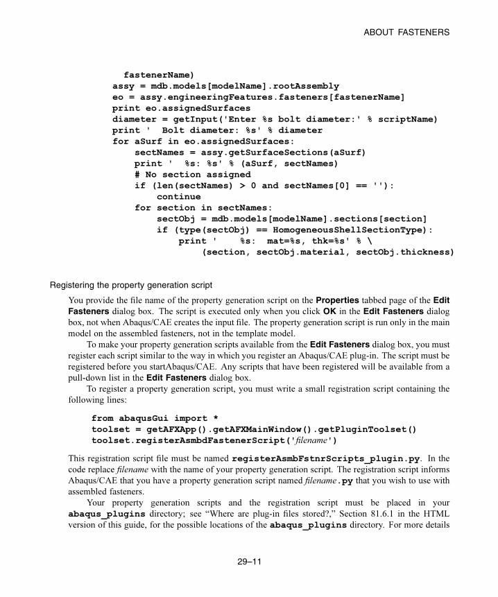
ABOUT FASTENERS
fastenerName)assy = mdb.models[modelName].rootAssemblyeo = assy.engineeringFeatures.fasteners[fastenerName]print eo.assignedSurfacesdiameter = getInput('Enter %s bolt diameter:' % scriptName)print ' Bolt diameter: %s' % diameterfor aSurf in eo.assignedSurfaces:
sectNames = assy.getSurfaceSections(aSurf)print ' %s: %s' % (aSurf, sectNames)# No section assignedif (len(sectNames) > 0 and sectNames[0] == ''):
continuefor section in sectNames:
sectObj = mdb.models[modelName].sections[section]if (type(sectObj) == HomogeneousShellSectionType):
print ' %s: mat=%s, thk=%s' % \(section, sectObj.material, sectObj.thickness)
Registering the property generation script
You provide the file name of the property generation script on the Properties tabbed page of the EditFasteners dialog box. The script is executed only when you click OK in the Edit Fasteners dialog
box, not when Abaqus/CAE creates the input file. The property generation script is run only in the main
model on the assembled fasteners, not in the template model.
To make your property generation scripts available from the Edit Fasteners dialog box, you must
register each script similar to the way in which you register an Abaqus/CAE plug-in. The script must be
registered before you startAbaqus/CAE. Any scripts that have been registered will be available from a
pull-down list in the Edit Fasteners dialog box.
To register a property generation script, you must write a small registration script containing the
following lines:
from abaqusGui import *toolset = getAFXApp().getAFXMainWindow().getPluginToolset()toolset.registerAsmbdFastenerScript('filename')
This registration script file must be named registerAsmbFstnrScripts_plugin.py. In the
code replace filename with the name of your property generation script. The registration script informs
Abaqus/CAE that you have a property generation script named filename.py that you wish to use with
assembled fasteners.
Your property generation scripts and the registration script must be placed in your
abaqus_plugins directory; see “Where are plug-in files stored?,” Section 81.6.1 in the HTML
version of this guide, for the possible locations of the abaqus_plugins directory. For more details
29–11
Abaqus ID:
Printed on:

ABOUT FASTENERS
about registration scripts, see “What are the kernel and GUI registration commands?,” Section 81.6.2 in
the HTML version of this guide.
Output requests for assembled fasteners
You can obtain both field output and history output from assembled fasteners in your main model. The
output must be requested on named sets that you have defined in the template model.
To request output for assembled fasteners:
1. In the Step module, working in your main model (not the template model), display the Edit HistoryOutput Request dialog box or the Edit Field Output Request dialog box; see the instructions
in “Creating and modifying output requests,” Section 14.4.5.
2. From the Domain list, choose Assembled fastener set.
3. From the Fastener list, choose the name of the assembled fastener for which you want output.
4. From the Set list, choose any set from the template model. The assembled fastener in your main
model references the sets defined in the template model.
5. Continue selecting output variables and other options, and click OK to save your request.
For information on related topics, refer to the following sections:
• “Creating assembled fasteners,” Section 29.5, in the HTML version of this guide
• “Understanding output requests,” Section 14.4
Assembled fasteners vs. point-based fasteners
Assembled fasteners and point-based (mesh-independent) fasteners produce slightly different analysis
results when used for the same fastener model. Assembled fasteners and point-based fasteners will
generate different coupling nodes and coupling weights, leading to different solutions. The differences
between point-based and assembled fasteners are described below and in Figure 29–7 and Figure 29–8.
Point-based fasteners
Abaqus looks at the first node of the connector and projects it onto the first surface (given the data
line). Abaqus then moves normal to the facet, where it finds the first projection point and finds the
subsequent projection points on the second surface.
Assembled fasteners
When the assembled fastener is instanced in the main model, Abaqus places the first node of the
connector where the first projection point of the point-based fastener model is located. Both fastener
types accomplish this placement with normal projections. However, for assembled fasteners an
adjust point constraint is performed on the second node of the connector; i.e., a normal projection
onto the second surface. This action is not the same as moving normal to the first projection point
facet unless the two normals align perfectly. Therefore, the second (subsequent) attachment points
29–12
Abaqus ID:
Printed on:

ABOUT FASTENERS
Adjusted to this location Instead of
this location
Figure 29–7 Adjustments for assembled fasteners vs. point-based fasteners.
First attachment point
Second attachment pointfor assembled fastener
Second attachment pointfor point-based fastener
Template model
Adjustment to second node of connector by adjust point constraint
Figure 29–8 Location of attachment point for assembled fasteners vs. point-based fasteners.
can be different for assembled fasteners versus point-based fasteners, which will lead to differences
in the analysis solution.
In an ideal case where the two surfaces are placed exactly the same distance apart as the
template model connector and are parallel to each other, Abaqus will get the same projection points
29–13
Abaqus ID:
Printed on:

MANAGING FASTENERS
for assembled fasteners and point-based fasteners. However, this situation will not be the case in
general.
29.2 Managing fasteners
The Fasteners Manager allows you to create and manage fasteners. The manager includes a list of
the names and types of fasteners that you have defined. The Create, Edit, Copy, Rename, and Deletebuttons in the manager allow you to create new fasteners or to edit, copy, rename, and delete existing
ones. The icons in the column along the left side of the manager allow you to suppress and resume
existing fasteners. You can also initiate these procedures using the Special→Fasteners menu from the
main menu bar in the Interaction module. After you select a management operation from the main menu
bar, the procedure is exactly the same as if you had clicked the corresponding button inside the manager
dialog box.
29–14
Abaqus ID:
Printed on:

OVERVIEW OF FLUID DYNAMIC ANALYSES
30. Fluid dynamic analyses
This section explains how to create fluid models in Abaqus/CAE. The following topics are covered:
• “Overview of fluid dynamic analyses,” Section 30.1
• “Modeling the fluid domain,” Section 30.2
• “Defining the fluid material properties,” Section 30.3
• “Specifying prescribed conditions for a fluid model,” Section 30.4
• “Meshing a fluid model,” Section 30.5
• “Running a fluid analysis,” Section 30.6
• “Using Abaqus/CFD for co-simulation,” Section 30.7
• “Viewing fluid analysis results,” Section 30.8
30.1 Overview of fluid dynamic analyses
Abaqus/CFD provides advanced computational fluid dynamics (CFD) capabilities for performing fluid
dynamic analyses and can be used to solve incompressible flow problems. Incompressible fluid dynamic
analyses can involve laminar or turbulent flow, thermal convective problems, and deforming-mesh
analyses. For more information, see “Incompressible fluid dynamic analysis,” Section 6.6.2 of the
Abaqus Analysis User’s Guide.
The procedure for creating fluid models in Abaqus/CAE involves the following general steps:
1. When you create a new model database, select a CFD model type to specify that you are modeling
an Abaqus/CFD analysis. Most of the functionality presented in the Abaqus/CAE interface is then
filtered to display only functionality that is valid for anAbaqus/CFD analysis. For more information,
see “Specifying model attributes,” Section 9.8.4, in the HTML version of this guide.
2. In the Part module, create a fluid part that defines the fluid domain (geometric region of the fluid).
For more information, see “Modeling the fluid domain,” Section 30.2.
3. In the Property module, define the fluid material properties in the model. For more information, see
“Defining the fluid material properties,” Section 30.3.
4. In the Property module, create and assign a fluid section for the model. The fluid section determines
which materials can be present in the fluid part. For more information, see “Creating homogeneous
fluid sections,” Section 12.13.13, and “Creating fluid sections for porous media,” Section 12.13.14,
in the HTML version of this guide.
5. In the Assembly module, create an instance of the fluid part.
6. In the Step module, define a fluid analysis step, solver controls, and turbulence model. For more
information, see “Configuring a flow procedure” in “Configuring general analysis procedures,”
Section 14.11.1, in the HTML version of this guide.
30–1
Abaqus ID:
Printed on:
DEFINING THE FLUID MATERIAL PROPERTIES
7. In the Step module, create field and history output requests. For more information, see
“Abaqus/CFD output variable identifiers,” Section 4.2.3 of the Abaqus Analysis User’s Guide.
8. In the Load module, define any loads, boundary conditions, or predefined fields acting on the fluid
model (see “Specifying prescribed conditions for a fluid model,” Section 30.4).
9. In the Mesh module, create a mesh for the fluid part. For more information, see “Meshing a fluid
model,” Section 30.5.
10. In the Job module, create a new job and submit the fluid analysis. For more information, see
“Running a fluid analysis,” Section 30.6.
30.2 Modeling the fluid domain
For a fluid part you can model only a three-dimensional part. You can use a three-dimensional sector to
represent an axisymmetric model and a three-dimensional part with one element through the thickness to
represent a two-dimensional model. All features for geometry creation are available for fluid analyses.
You can import an orphan CFD mesh to model the fluid domain.
30.3 Defining the fluid material properties
Fluid materials and their physical properties determine the fluid response. You create the fluid material
in the Property module. Depending on the analysis, you may need to specify the following properties:
Density
Fluid density must be defined for fluids in an Abaqus/CFD analysis; it is required for transient
Navier-Stokes computations. The fluid density is considered constant for incompressible flows.
Viscosity
You must specify the viscosity for viscous flows, and only a constant viscosity is supported.
Specific heat
For an incompressible fluid dynamic analysis that includes an energy equation, you must define the
specific heat and thermal conductivity. A specific heat using constant pressure is required; you can
define the specific heat using constant pressure, or you can define the specific heat using constant
volume and specify the ideal gas constant.
Thermal conductivity
Only a constant isotropic thermal conductivity is supported.
30–2
Abaqus ID:
Printed on:

SPECIFYING PRESCRIBED CONDITIONS FOR A FLUID MODEL
Thermal expansion coefficient
The coefficient of thermal expansion is used with the Boussinesq approximation for natural
convection flows.
Permeability
You can specify isotropic permeability (with dependence only on porosity) or permeability using a
Carman-Kozeny relation.
30.4 Specifying prescribed conditions for a fluid model
You specify the prescribed conditions for the fluid model in the Load module. You can specify fluid
predefined fields in the initial step of a fluid analysis, and you can specify loads and boundary conditions
for a fluid model in a fluid analysis step. Depending on the analysis, you may need to specify the
following prescribed conditions:
Predefined fields
The predefined field types available for fluid analyses include fluid density, fluid thermal energy,
fluid turbulence, and fluid velocity. For more information, see “Initial conditions in Abaqus/CFD,”
Section 34.2.2 of the Abaqus Analysis User’s Guide.
• A density value is required; however, if you do not specify the initial fluid density, the material
density definition is assumed.
• For an incompressible fluid dynamic analysis that includes an energy equation, you must define
the initial fluid temperature.
• For an incompressible fluid dynamic analysis that specifies a turbulencemodel, youmust define
the initial fluid turbulence values, such as the turbulent eddy viscosity.
• The initial velocity is assumed to be zero if no value is specified.
Loads
The load types available for fluid analyses include body force, gravity, body heat flux, and porous
drag body force. The fluid reference pressure can be used to specify the hydrostatic pressure level for
incompressible flows if there is no pressure boundary condition prescribed. For more information,
see the following sections:
• “Concentrated loads,” Section 34.4.2 of the Abaqus Analysis User’s Guide
• “Distributed loads,” Section 34.4.3 of the Abaqus Analysis User’s Guide
• “Thermal loads,” Section 34.4.4 of the Abaqus Analysis User’s Guide
30–3
Abaqus ID:
Printed on:

USING Abaqus/CFD FOR CO-SIMULATION
Boundary conditions
Boundary conditions types available for fluid analyses include displacement/rotation, fluid
inlet/outlet, and fluid wall condition. For more information, see “Boundary conditions in
Abaqus/CFD,” Section 34.3.2 of the Abaqus Analysis User’s Guide.
• You specify boundary conditions to define flow and thermal conditions on the fluid domain
boundaries.
• You can specify pressure or velocity boundary conditions.
• For an incompressible fluid dynamic analysis that includes an energy equation, you can define
the temperature or heat flux.
30.5 Meshing a fluid model
The fields active in a fluid analysis are not determined by the element type but by the analysis procedure
and its options. The sole purpose of the element type is to define the shape of the element used to
discretize the continuum. Three fluid type elements are available. Fluid elements are assigned to the
mesh by default. For more information, see “Fluid continuum elements,” Section 28.2 of the Abaqus
Analysis User’s Guide.
30.6 Running a fluid analysis
When you submit a job associated with a fluid model for analysis, Abaqus/CAE first generates an input
file representing your model and then Abaqus/CFD performs the analysis using the contents of this file.
As the analysis proceeds, Abaqus/CFD creates a data (.dat) file and a status (.sta) file. Abaqus/CFDuses domain-based parallelism implemented with explicit message passing for both shared memory and
distributed memory computers. For more information, see “Abaqus/Standard, Abaqus/Explicit, and
Abaqus/CFD execution,” Section 3.2.2 of the Abaqus Analysis User’s Guide, and “Parallel execution:
overview,” Section 3.5.1 of the Abaqus Analysis User’s Guide.
30.7 Using Abaqus/CFD for co-simulation
You can solve complex fluid-structure interactions and conjugate heat transfer problems using the co-
simulation technique to couple Abaqus/CFD with Abaqus/Standard and Abaqus/Explicit. For more
information, see “Co-simulation: overview,” Section 17.1.1 of the Abaqus Analysis User’s Guide.
30–4
Abaqus ID:
Printed on:

VIEWING FLUID ANALYSIS RESULTS
30.8 Viewing fluid analysis results
You can display the results of a fluid analysis in the Visualization module. Animations, line-type contour
plots, isosurface-type contour plots, and results displayed along a path are particularly useful for viewing
fluid analysis results. In addition, you can view the results from a co-simulation, such as a conjugate heat
transfer analysis using Abaqus/CFD and Abaqus/Standard, as shown in Figure 30–1.
Figure 30–1 Velocity vector plot representing air flow around a circuit board model.
30–5
Abaqus ID:
Printed on:


SEAM CRACKS
31. Fracture mechanics
You can do the following to model fracture mechanics with Abaqus/CAE:
• Create a seam crack that defines an edge or a face with overlapping nodes that can separate during
an analysis.
• Use contour integral estimates to study the onset of cracking in quasi-static problems; however, a
contour integral estimate does not predict how a crack will propagate. You can compute contour
integrals for two- or three-dimensional models.
• Use the extended finite element method (XFEM) to study the initiation and propagation of a crack
along an arbitrary, solution-dependent path without needing to remesh your model. XFEM is
available only for three-dimensional solid and planar models and orphan meshes.
• Use the virtual crack closure technique (VCCT) to study the initiation and propagation of a crack
along a known crack surface.
• Use the Crack Manager to create and manage your cracks.
This chapter covers the following topics:
• “Seam cracks,” Section 31.1
• “Using contour integrals to model fracture mechanics,” Section 31.2
• “Using the extended finite element method to model fracture mechanics,” Section 31.3
• “Using the virtual crack closure technique to model crack propagation,” Section 31.4
• “Managing cracks,” Section 31.5
31.1 Seam cracks
A seam defines an edge or a face with overlapping nodes that can separate during an analysis. You can
include a seam crack in your model. Alternatively, you can refer to the seam when creating a contour
integral; however, you cannot use a seam crack with the extended finite element method (XFEM). The
following topics are covered:
• “What is a seam?,” Section 31.1.1
In addition, the following sections are available in the HTML version of this guide:
• “Creating a seam,” Section 31.1.2
31.1.1 What is a seam?A seam defines an edge or a face in your model that is originally closed but can open during an analysis.
Abaqus/CAE places overlapping duplicate nodes along a seam when the mesh is generated. A seam
31–1
Abaqus ID:
Printed on:

SEAM CRACKS
cannot extend along the boundaries of a part and must be embedded within a face of a two-dimensional
part or within a cell of a solid part. After you create a seam, you can determine its crack properties using
a contour integral analysis. Because a seam modifies the mesh, you cannot create a seam on a dependent
part instance.
Figure 31–1 shows a seam on the face of a planar part and the effect of applying a tensile load to
the model. The duplicate nodes along the seam are independent of each other and are free to move.
sketchedpartition
seamcrack
Figure 31–1 A seam embedded in a face.
Figure 31–2 shows a similar analysis of a seam embedded in a solid part. The seam was created by
partitioning the solid with a sketch drawn on a datum plane.
sketchedpartition
seamcrack
Figure 31–2 A seam embedded in a cell.
For detailed instructions, see “Creating a seam,” Section 31.1.2, in the HTML version of this guide.
31–2
Abaqus ID:
Printed on:

USING CONTOUR INTEGRALS TO MODEL FRACTURE MECHANICS
31.2 Using contour integrals to model fracture mechanics
You can study the onset of cracking in a quasi-static model by selecting regions from your model that will
be used to compute contour integral estimates. During the analysis Abaqus/Standard writes the values
of the contour integrals to the output database as history output. For a detailed description of contour
integrals, see “Contour integral evaluation,” Section 11.4.2 of the Abaqus Analysis User’s Guide. This
section describes how you define a crack in Abaqus/CAE. The following topics are covered:
• “An overview of contour integral analysis,” Section 31.2.1
• “Defining the crack front,” Section 31.2.2
• “Defining the crack tip or crack line,” Section 31.2.3
• “Defining the crack extension direction,” Section 31.2.4
• “Controlling the singularity at the crack tip for a small-strain analysis,” Section 31.2.5
• “Contour integral output,” Section 31.2.6
• “Meshing the crack region and assigning elements,” Section 31.2.7
In addition, the following sections are available in the HTML version of this guide:
• “Controlling the singularity at the crack tip,” Section 31.2.8
• “Creating a contour integral crack,” Section 31.2.9
• “Modifying data for contour integrals,” Section 31.2.10
• “Requesting contour integral output,” Section 31.2.11
31.2.1 An overview of contour integral analysisYou can study the onset of cracking in quasi-static problems using contour integral estimates; however, a
contour integral estimate does not predict how a crack will propagate. You can compute contour integrals
for two- or three-dimensional models, and you can choose to perform one of the following types of
contour integral calculations:
• J-integral
• -integral (for creep)
• T-stress (for linear materials)
• Stress intensity factors for linear homogeneous materials and for interfacial cracks lying on the
interface between two linear homogeneous materials
For more information, see “Contour integral evaluation,” Section 11.4.2 of the Abaqus Analysis User’s
Guide.
You define cracks in the Interaction module. To perform a contour integral analysis, you must select
the crack front, the crack tip or crack line, and the crack extension direction, as described in the following
31–3
Abaqus ID:
Printed on:
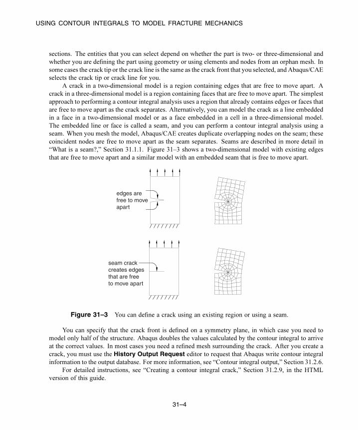
USING CONTOUR INTEGRALS TO MODEL FRACTURE MECHANICS
sections. The entities that you can select depend on whether the part is two- or three-dimensional and
whether you are defining the part using geometry or using elements and nodes from an orphan mesh. In
some cases the crack tip or the crack line is the same as the crack front that you selected, and Abaqus/CAE
selects the crack tip or crack line for you.
A crack in a two-dimensional model is a region containing edges that are free to move apart. A
crack in a three-dimensional model is a region containing faces that are free to move apart. The simplest
approach to performing a contour integral analysis uses a region that already contains edges or faces that
are free to move apart as the crack separates. Alternatively, you can model the crack as a line embedded
in a face in a two-dimensional model or as a face embedded in a cell in a three-dimensional model.
The embedded line or face is called a seam, and you can perform a contour integral analysis using a
seam. When you mesh the model, Abaqus/CAE creates duplicate overlapping nodes on the seam; these
coincident nodes are free to move apart as the seam separates. Seams are described in more detail in
“What is a seam?,” Section 31.1.1. Figure 31–3 shows a two-dimensional model with existing edges
that are free to move apart and a similar model with an embedded seam that is free to move apart.
seam crackcreates edgesthat are freeto move apart
edges arefree to moveapart
Figure 31–3 You can define a crack using an existing region or using a seam.
You can specify that the crack front is defined on a symmetry plane, in which case you need to
model only half of the structure. Abaqus doubles the values calculated by the contour integral to arrive
at the correct values. In most cases you need a refined mesh surrounding the crack. After you create a
crack, you must use the History Output Request editor to request that Abaqus write contour integral
information to the output database. For more information, see “Contour integral output,” Section 31.2.6.
For detailed instructions, see “Creating a contour integral crack,” Section 31.2.9, in the HTML
version of this guide.
31–4
Abaqus ID:
Printed on:

USING CONTOUR INTEGRALS TO MODEL FRACTURE MECHANICS
31.2.2 Defining the crack front
The first step in the procedure to configure a contour integral is to define the crack front by selecting
entities from the assembly. The crack front is the forward part of the crack. Abaqus uses the crack front
to compute the first contour integral using all of the elements inside the crack front and one layer of
elements outside the crack front. You can request output for more than one contour integral, in which
case Abaqus/CAE adds a single layer of elements to the group of elements that were used to calculate
the previous contour integral. Figure 31–4 illustrates how Abaqus/CAE computes successive contour
integrals for a two-dimensional model by adding layers of elements.
firstcontourintegral
thirdcontourintegral
secondcontourintegral
crackfront
cracktip
Figure 31–4 Successive contour integrals are calculated by adding a layer of elements.
31–5
Abaqus ID:
Printed on:

USING CONTOUR INTEGRALS TO MODEL FRACTURE MECHANICS
If your part is three-dimensional, Abaqus computes contour integrals at each node along the crack
line, as shown in Figure 31–5. For more information, see “Defining the crack front” in “Contour integral
evaluation,” Section 11.4.2 of the Abaqus Analysis User’s Guide.
crack line crack front(cell)
Figure 31–5 Abaqus computes the contour integral at each node along the crack line.
The entities from which you can select depend on whether the crack front is located in geometry or
an orphan mesh and on the modeling space of the part.
Geometry
When you are defining the crack front on geometry, the entities that you can select depend on the
modeling space of the part.
Two-dimensional geometry
If you are defining the crack front on two-dimensional geometry, you can select the following:
• A single vertex
• Connected edges
• Connected faces
Figure 31–6 shows the entities from which you can select when defining a crack front on two-
dimensional geometry.
Three-dimensional geometry
If you are defining the crack front on three-dimensional geometry, you can select the following:
• Connected edges
• Connected faces
31–6
Abaqus ID:
Printed on:

USING CONTOUR INTEGRALS TO MODEL FRACTURE MECHANICS
vertex faceedge
Figure 31–6 Selecting the crack front from two-dimensional geometry.
• Connected cells
Figure 31–7 shows the entities from which you can select when defining a crack front on three-
dimensional geometry.
edge cellface
Figure 31–7 Selecting the crack front from three-dimensional geometry.
Mesh
When you are defining the crack front on an orphan mesh, you can select the elements or element
edges or faces that define the crack front. Alternatively, you can select the nodes from the
corresponding region. When you are defining the crack front on an orphan mesh, the entities that
you can select depend on the modeling space of the part.
Two-dimensional orphan mesh
If you are defining the crack front on a two-dimensional orphan mesh, you can select the
following:
• A single node
• Connected element edges
31–7
Abaqus ID:
Printed on:

USING CONTOUR INTEGRALS TO MODEL FRACTURE MECHANICS
• Connected elements
Figure 31–8 shows the entities from which you can select when defining a crack front on a
two-dimensional orphan mesh.
node element edges elements
Figure 31–8 Selecting the crack front from a two-dimensional orphan mesh.
Three-dimensional orphan mesh
If you are defining the crack front on a three-dimensional orphan mesh, you can select the
following:
• Connected element edges
• Connected element faces
• Connected elements
Figure 31–9 shows the entities from which you can select when defining a crack front on a
three-dimensional orphan mesh.
element edges element faces elements
Figure 31–9 Selecting the crack front from a three-dimensional orphan mesh.
31–8
Abaqus ID:
Printed on:
USING CONTOUR INTEGRALS TO MODEL FRACTURE MECHANICS
31.2.3 Defining the crack tip or crack line
After you have defined the crack front, the next step in the procedure to configure the contour integral is
to define the crack tip or crack line by selecting entities from the assembly. The modeling space of your
assembly governs whether you need to define a crack tip or a crack line for a contour integral analysis.
Two-dimensional
If your assembly is two-dimensional, you must define the crack tip by selecting a vertex or a node.
The crack tip is the point on the crack front where you define the crack extension direction, . In
some cases the desired vertex or node will not exist, and you must create it by partitioning the crack
front.
If you selected a vertex or a node to define the crack front, the same vertex or node defines the
crack tip.
Three-dimensional
If your part is three-dimensional, you must define the crack line by selecting edges or element edges
that form a continuous line. The crack line is a series of connected edges along the crack front where
you define the crack extension direction, . In some cases the desired edges will not exist, and you
must create them by partitioning the crack front.
If you selected edges or element edges to define the crack front, the same edges define the
crack line.
Selected edges (from an Abaqus/CAE native part or from an orphan mesh) must be connected, must
connect one side of the crack front to the other, and must be included in the crack front.
31.2.4 Defining the crack extension direction
After you have defined the crack front along with the crack tip or crack line, Abaqus/CAE prompts
you to specify the crack extension direction at the crack tip or along the crack line. You can specify
the normal to the crack plane, ; or you can specify the crack extension direction, , directly. For a
detailed discussion of how Abaqus uses or to calculate the crack extension direction, see “Specifying
the virtual crack extension direction” in “Contour integral evaluation,” Section 11.4.2 of the Abaqus
Analysis User’s Guide.
Normal to crack plane
If you select Normal to crack plane, you can define the normal by selecting points from the model
that represent the start and the end of the normal to the crack plane. The crack plane contains the
vector that Abaqus needs to compute the contour integral. In many cases the crack plane represents
the plane of symmetry of the crack.
31–9
Abaqus ID:
Printed on:

USING CONTOUR INTEGRALS TO MODEL FRACTURE MECHANICS
You should define the normal to the crack plane only if the direction is the same at all points
along the crack line. If the direction of the normal to the crack plane varies along the crack line,
you cannot select a single normal that defines the crack extension direction at all points along the
crack line.
To define the normal to the crack plane, you can select points from geometry (such as vertices,
datum points, or midpoints), or you can select orphan mesh nodes. Alternatively, you can enter the
coordinates of the points in the prompt area. If you select points from geometry and subsequently
modify the part, Abaqus/CAE regenerates the points and updates the normal accordingly. If you
are working with orphan mesh nodes, you must select nodes that represent the start and the end of
the normal.
Abaqus calculates a crack extension direction, , that is orthogonal to the crack front tangent,
, and the normal, .
q vectors
If you select q vectors, you can define the crack extension direction, , directly by selecting points
from the model that represent the start and end of the vector. If you are working with orphan mesh
nodes, you must select nodes that represent the start and the end of the vector. Alternatively, you
can enter the coordinates of the points in the prompt area.
Figure 31–10 shows an example of a crack front formed by a circular arc along which the direction
of the vector is constantly varying. In contrast, the normal to the crack plane is constant. As a result,
for this case you should define the crack extension direction by specifying the normal to the crack plane.
Figure 31–11 shows a crack front formed by the edge of a truncated cone along which the directions of
both the vector and the normal to the crack plane are varying. For this case you should do the following:
1. Define the contour integral, and use a single vector to specify the crack extension direction.
2. Mesh the part, create a job, and write the model to an input file.
3. Import the input file, which will create an orphan mesh representation of the part.
4. Edit the crack that was imported with the model. Each node along the crack front will have the
crack extension direction defined by the vector that you specified in Step 1.
5. Use the Query toolset to determine the start and end coordinates of the vector at each node, and
edit the data defining the vectors at each node along the crack front.
This technique is shown in Figure 31–12. Figure 31–12 is taken from “Contour integrals for a conical
crack in a linear elastic infinite half space,” Section 1.4.2 of the Abaqus Example Problems Guide. An
Abaqus Scripting Interface script is provided with this example that illustrates how you can enter the
vector at each node along the crack front.
31–10
Abaqus ID:
Printed on:

USING CONTOUR INTEGRALS TO MODEL FRACTURE MECHANICS
select this edge torepresent the normalto the crack plane
n
qn
qn
q
n
q
Figure 31–10 The direction of the vector varies but the direction of the normal is constant.
31.2.5 Controlling the singularity at the crack tip for a small-strainanalysis
If the geometry of the crack region defines a sharp crack, the strain field becomes singular at the crack tip,
as described in “Constructing a fracture mechanics mesh for small-strain analysis with the conventional
finite element method” in “Contour integral evaluation,” Section 11.4.2 of the Abaqus Analysis User’s
Guide. Including the singularity in your model for a small-strain analysis improves the accuracy of the
contour integral and the stress and strain calculations.
To include the singularity in your contour integral estimates, click the Singularity tab in the Crackeditor and choose the desired position of the midside node and degenerate element control. For detailed
instructions, see “Controlling the singularity at the crack tip,” Section 31.2.8, in the HTML version of
this guide.
In addition, you must do the following in the Mesh module:
• If the assembly or part is two-dimensional, you must model the crack front with a ring of triangles
and assign quadrilateral elements to the remainder of the contour integral region.
• If the assembly or part is three-dimensional, you must model the crack front with a ring of wedges
and assign hexahedral elements to the remainder of the contour integral region.
31–11
Abaqus ID:
Printed on:

USING CONTOUR INTEGRALS TO MODEL FRACTURE MECHANICS
P
conical crack
crack front
n
q n q
Figure 31–11 The directions of both the vector and the normal vary along the crack front.
When you mesh the crack front, Abaqus does the following:
• Converts the elements in the crack front to collapsed quadrilateral or hexahedral elements.
• If you modeled the crack front with a ring of second-order triangles or wedges, Abaqus moves the
midside nodes to the specified position along the element edges that radiate out from the crack tip
or crack line. (If you modeled the crack front with a ring of first-order triangles or wedges, Abaqus
ignores the position that you specified for the midside nodes.)
A part instance that includes orphan mesh elements is always a dependent instance. As a result, you
cannot adjust the midside nodes of these instances in the assembly. For more information, see “What
is the difference between editing an orphan mesh, a meshed part, and a meshed part instance in the
assembly?,” Section 64.2. You must display the original orphan mesh and use the Edit Mesh toolset to
adjust the position of the midsize nodes. For more information, see “Adjusting the position of midside
nodes,” Section 64.5.7. In addition, you cannot create collapsed elements from triangular and wedge
elements of an orphan mesh.
31–12
Abaqus ID:
Printed on:

USING CONTOUR INTEGRALS TO MODEL FRACTURE MECHANICS
Figure 31–12 Entering the vector at each node along the crack front.
31.2.6 Contour integral outputAfter you have defined the crack, you must use the History Output Request editor in the Step module
to include the contour integral data in the output database generated by the analysis. The editor allows
you to configure the following:
• The output frequency.
• The type of contour integral calculation to perform (J-integral, -integral, stress intensity factors,
or T-stress).
• The number of contours to evaluate.
Abaqus writes a history output variable to the output database for each contour integral that it calculates.
Figure 31–13 shows the format of the name of an output variable representing a contour integral.
For detailed instructions, see “Requesting contour integral output,” Section 31.2.11, in the HTML
version of this guide. For more information, see “Modifying history output requests,” Section 14.12.3,
in the HTML version of this guide, and “Contour integral evaluation,” Section 11.4.2 of the Abaqus
Analysis User’s Guide.
31.2.7 Meshing the crack region and assigning elementsLarge stress concentrations occur at the crack tip. As a result, you should create a refined mesh around
the crack tip to get accurate results for stresses and strains. In contrast, because the J-integral is an
31–13
Abaqus ID:
Printed on:

USING CONTOUR INTEGRALS TO MODEL FRACTURE MECHANICS
outputtype
variable historyoutputname
contourintegralname
internal crack-tip node setgenerated fromuser-given crack-tip node set name
contour integralnumber
Figure 31–13 The format of a contour integral name in the output database.
energy measure, you can obtain accurate J-values with a relatively coarse mesh. However, if the material
becomes more nonlinear, you must create a finer mesh at the crack tip to maintain the accuracy of the J-
values. You can control the density of the mesh at the crack tip by partitioning the region and by assigning
mesh seeds to the resulting edges. For more information, see “Understanding seeding,” Section 17.4.
For a large-strain analysis during which Abaqus will allow for nonlinear geometry, you should
mesh the contour integral region with quadrilateral or hexahedral elements. For more information, see
“Constructing a fracture mechanics mesh for finite-strain analysis with the conventional finite element
method” in “Contour integral evaluation,” Section 11.4.2 of the Abaqus Analysis User’s Guide.
However, for a small-strain analysis that does not allow for nonlinear geometry, you must allow
for the singularity at the crack tip or crack line by meshing the region that defines the crack front with a
ring of triangles or wedges. For more information, see “Controlling the singularity at the crack tip for a
small-strain analysis,” Section 31.2.5.
You must use the swept meshing technique to create wedge elements; however, there are limitations
on the regions that Abaqus/CAE can mesh using the swept meshing technique, as described in “Swept
meshing of three-dimensional solids,” Section 17.9.3. As a result, if you cannot use the swept meshing
31–14
Abaqus ID:
Printed on:

USING THE EXTENDED FINITE ELEMENT METHOD TO MODEL FRACTURE MECHANICS
technique, you cannot create wedge elements, and you cannot allow for the singularity at the crack
line. In most cases you can ignore the singularity if your mesh is sufficiently refined to model the
deformation around the crack tip or crack line and the resulting high strain gradients. You can also
ignore the singularity if you are interested in only the contour integral output.
31.3 Using the extended finite element method to model fracturemechanics
You can use the extended finite element method (XFEM) to study the initiation and propagation of a crack
along an arbitrary, solution-dependent path without needing to remesh your model. XFEM is available
for three-dimensional solid and two-dimensional planar models; three-dimensional shell models are not
supported. The following topics are covered:
• “An overview of the extended finite element method (XFEM),” Section 31.3.1
• “Choosing the type of XFEM analysis,” Section 31.3.2
• “Viewing an XFEM crack,” Section 31.3.3
In addition, the following sections are available in the HTML version of this guide:
• “Creating an XFEM crack,” Section 31.3.4
• “Deactivating and activating an XFEM crack growth,” Section 31.3.5
• “Specifying a contact interaction property for XFEM,” Section 31.3.6
• “Requesting contour integral output for XFEM,” Section 31.3.7
31.3.1 An overview of the extended finite element method (XFEM)
You can study the onset and propagation of cracking in quasi-static problems using the extended finite
element method (XFEM). XFEMallows you to study crack growth along an arbitrary, solution-dependent
path without needing to remesh your model. XFEM is available only for three-dimensional solid and
two-dimensional planar models; three-dimensional shell models are not supported. You can use XFEM
to study a crack in parts containing geometry, orphan mesh elements, or a combination of the two. You
can choose to study a crack that grows arbitrarily through your model or a stationary crack. You define an
XFEM crack in the Interaction module. You can specify the initial location of the crack. Alternatively,
you can allow Abaqus to determine the location of the crack during the analysis based on the value of the
maximum principal stress or strain calculated in the crack domain. For more information, see “Modeling
discontinuities as an enriched feature using the extended finite element method,” Section 10.7.1 of the
Abaqus Analysis User’s Guide. Examples of XFEM models created in Abaqus/CAE are provided in
“Modeling discontinuities using XFEM,” Section 1.19 of the Abaqus Benchmarks Guide.
To perform an XFEM crack analysis, you must specify the following:
31–15
Abaqus ID:
Printed on:

USING THE EXTENDED FINITE ELEMENT METHOD TO MODEL FRACTURE MECHANICS
Crack domain
To define the crack domain, you can select one or more cells from three-dimensional parts or one or
more faces from two-dimensional planar parts. If you are defining the crack domain on an orphan
mesh or a part containing both orphan and native mesh elements, you can select elements. The
crack domain includes regions that contain any existing cracks and regions in which a crack might
be initiated and into which a crack might propagate.
Crack growth
You can allow the crack to propagate along an arbitrary, solution-dependent path, or you can specify
that the crack is stationary.
Initial crack location
To define the initial crack location, you can select faces from a three-dimensional solid or edges
from a two-dimensional planar model. The initial crack location must be contained within the crack
domain. A selected face can be a face of the solid, a face created by a partition, or a planar part
instance. Similarly, a selected edge can be an edge of the solid, an edge created by a partition, or a
wire part instance; you should not select a seam crack. You should not mesh the faces or edges that
you selected to define the initial crack location. Figure 31–14 shows examples of the crack domain
and the crack location for two- and three-dimensional geometry and orphan meshes.
Alternatively, you can choose not to define the initial crack location. Regardless of whether
you define the initial crack location, Abaqus initiates the creation of cracks during the simulation
by searching for regions that are experiencing principal stresses and/or strains greater than the
maximum damage values specified by the traction-separation laws.
Enrichment radius
The enrichment radius is a small radius from the crack tip within which the elements will be used for
calculating crack singularity for a stationary crack. Elements within the enrichment radius must be
included in the cells or faces that you chose to represent the crack domain. You can allow Abaqus
to calculate the radius (three times the typical element characteristic length in the enriched area), or
you can specify its value.
Contact interaction property
You can choose to associate a contact interaction property with the XFEM crack that defines the
contact of cracked element surfaces. For detailed information, see “Specifying a contact interaction
property for XFEM,” Section 31.3.6, in the HTML version of this guide.
Damage initiation
You must specify the conditions that will initiate a crack by specifying damage initiation criteria
in the material definition. You can specify a criterion based on either maximum principal stress or
maximum principal strain. For more information, see “Maximum principal stress or strain damage”
in “Defining damage,” Section 12.9.3.
31–16
Abaqus ID:
Printed on:

USING THE EXTENDED FINITE ELEMENT METHOD TO MODEL FRACTURE MECHANICS
Crack domain
Crack location
Crack domain
Crack location
Crack domain
Crack location
Crack domain
Crack location
Figure 31–14 Defining a crack for XFEM.
Analysis procedure
You can include an XFEM crack in a static analysis procedure. Alternatively, you can include an
XFEM crack in an implicit dynamic analysis procedure to simulate the fracture and failure in a
structure under high-speed impact loading. The XFEM-based crack propagation simulated in an
implicit dynamic procedure can also be preceded or followed by a static procedure to model the
damage and failure throughout the loading history.
For detailed instructions, see “Creating an XFEM crack,” Section 31.3.4, in the HTML version of
this guide.
31.3.2 Choosing the type of XFEM analysisAbaqus provides the following approaches for studying crack initiation and propagation using XFEM:
31–17
Abaqus ID:
Printed on:

USING THE EXTENDED FINITE ELEMENT METHOD TO MODEL FRACTURE MECHANICS
Traction-separation cohesive behaviorThe traction-separation cohesive behavior approach is described in detail in “Modeling moving
cracks with the cohesive segments method and phantom nodes” in “Modeling discontinuities as an
enriched feature using the extended finite element method,” Section 10.7.1 of the Abaqus Analysis
User’s Guide. You can specify the material properties that define the evolution of damage leading
to eventual failure. You apply the material to the section that is assigned to the crack domain.
You can choose to associate a normal behavior contact interaction property with the XFEM crack
that defines the contact of cracked element surfaces. For detailed information, see “Specifying a
contact interaction property for XFEM,” Section 31.3.6, in the HTML version of this guide. To
assist convergence as the material fails, you can introduce localized damping using the viscous
regularization technique. For more information, see “Damage stabilization” in “Defining damage,”
Section 12.9.3.
Linear elastic fracture mechanics (LEFM)
The linear elastic fracture mechanics (LEFM) approach uses the modified Virtual Crack Closure
Technique (VCCT) to calculate the strain energy release rate at the crack tip. The approach is
more appropriate for brittle fracture problems and is described in detail in “Modeling moving
cracks based on the principles of linear elastic fracture mechanics (LEFM) and phantom nodes”
in “Modeling discontinuities as an enriched feature using the extended finite element method,”
Section 10.7.1 of the Abaqus Analysis User’s Guide. To use this approach, you must create
a fracture criterion contact interaction property, as described in “Specifying fracture criterion
properties for crack propagation” in “Defining a contact interaction property,” Section 15.14.1.
If you specify localized damping in the contact interaction property, Abaqus will use the viscous
regularization technique to assist convergence as the material fails. For more information, see
“Specifying fracture criterion properties for crack propagation” in “Defining a contact interaction
property,” Section 15.14.1, in the HTML version of this guide.
31.3.3 Viewing an XFEM crackWhen you are creating your model, you must request field output for the signed distance function,
PHILSM. When you open an output database file containing the PHILSM output variable, Abaqus/CAE
creates a view cut along the XFEM crack (where the value of the signed distance function is zero).
Therefore, when you display a deformed or contour plot, the cracked elements in the enriched region
are visible, as shown in Figure 31–15. You can perform a time history animation of a contour plot and
view the onset of damage calculated by XFEM. The animation also allows you to view the propagation
of the damage through the enriched region as the analysis progresses. Turning on translucency allows
you to see the progression of the crack through interior elements. For more information, see “Changing
the translucency,” Section 77.3.
To view the initial crack front, you can create an isosurface cut shape with PSILSM selected as
the current primary field output variable. For more information, see “Creating or editing a view cut,”
Section 80.2.1, in the HTML version of this guide.
31–18
Abaqus ID:
Printed on:

USING THE VIRTUAL CRACK CLOSURE TECHNIQUE TO MODEL CRACK PROPAGATION
X
Y
Z X
Y
Z
Figure 31–15 Viewing an XFEM crack.
If you want to investigate the crack in more detail, you can create a contour plot of the signed
distance function (PHILSM) and determine in which elements the signed distance values are negative
or positive. The crack surface is situated in the elements where the value of PHILSM transitions from a
negative number to a positive number. In addition, you can use the option in theView Cut Managerto view only the surface where the value of the signed distance function is zero, which corresponds with
the surface of an XFEM crack. For more information, see “Understanding view cuts,” Section 80.1.
31.4 Using the virtual crack closure technique to model crackpropagation
You can use the virtual crack closure technique (VCCT) to study the initiation and propagation of
a crack along a known crack surface. Modeling crack propagation using VCCT is available only
for Abaqus/Standard models (three-dimensional solid and shell and two-dimensional planar and
axisymmetric models). The following topics are covered:
• “An overview of the virtual crack closure technique,” Section 31.4.1
In addition, the following section is available in the HTML version of this guide:
• “Creating a VCCT crack for Abaqus/Standard,” Section 31.4.2
31–19
Abaqus ID:
Printed on:

MANAGING CRACKS
31.4.1 An overview of the virtual crack closure technique
You can study the onset and propagation of cracking in quasi-static problems using the virtual crack
closure technique (VCCT). VCCT uses the principles of linear elastic fracture mechanics (LEFM) , so it
is appropriate for problems in which brittle crack propagation occurs along predefined surfaces. VCCT
is based on the assumption that the strain energy released when a crack is extended by a certain amount
is the same as the energy required to close the crack by the same amount.
You can include a VCCT crack in a static or quasi-static analysis procedure. Alternatively, you
can include a VCCT crack in an implicit dynamic analysis procedure to simulate the fracture and failure
in a structure under high-speed impact loading. VCCT is available only for Abaqus/Standard (three-
dimensional solid and shell and two-dimensional planar and axisymmetric models). You can use VCCT
to study a crack in parts containing geometry, orphan mesh elements, or a combination of the two. You
define a VCCT crack in the Interaction module. You can specify the location of the surfaces that are
initially bonded. For more information, see “Modeling discontinuities as an enriched feature using the
extended finite element method,” Section 10.7.1 of the Abaqus Analysis User’s Guide.
Creating VCCT or enhanced VCCT crack propagation models that converge to a successful solution
requires some understanding of the principles behind VCCT. See “Tips for using the VCCT or enhanced
VCCT criterion in Abaqus/Standard” in “Crack propagation analysis,” Section 11.4.3 of the Abaqus
Analysis User’s Guide, for information that will help you create models that can be analyzed successfully.
For detailed instructions, see “Creating a VCCT crack for Abaqus/Standard,” Section 31.4.2, in the
HTML version of this guide.
31.5 Managing cracks
The Crack Manager allows you to create and manage cracks. The manager includes a list of the names
and types of cracks that you have defined. The Create, Edit, Copy, Rename, and Delete buttons in the
manager allow you to create new cracks or to edit, copy, rename, and delete existing ones. The icons in
the column along the left side of the manager allow you to suppress and resume existing cracks. You can
also initiate these procedures using the Special→Crack menu from the main menu bar in the Interaction
module. After you select a management operation from the main menu bar, the procedure is exactly the
same as if you had clicked the corresponding button inside the manager dialog box.
31–20
Abaqus ID:
Printed on:

OVERVIEW OF GASKET MODELING
32. Gaskets
This section provides information on how to model gasket behavior. The following topics are covered:
• “Overview of gasket modeling,” Section 32.1
• “Defining materials for gaskets,” Section 32.2
• “Assigning gasket elements to a region,” Section 32.3
32.1 Overview of gasket modeling
Gaskets are thin sealing components that are positioned between structural components. (For detailed
information on gasket theory, see “Gasket elements,” Section 32.6 of the Abaqus Analysis User’s Guide.)
The general procedure for modeling gaskets in three-dimensional space involves the following steps:
1. In the Part module, define the solid geometry. Gasket parts are typically very thin, flat solids.
2. In the Property module, define a gasket material. The material can be a regular material or one
that includes special gasket behaviors. See “Defining materials for gaskets,” Section 32.2, for more
information.
3. In the Property module, define a gasket section that refers to the gasket material. Then assign the
gasket section to the gasket region.
4. In the Interaction module, establish appropriate tie constraints or contact interactions between the
gasket surfaces and the surfaces of adjacent regions.
5. In the Mesh module, assign the top-down swept meshing technique or the bottom-up meshing
technique to the gasket region. Regardless of the meshing technique that you choose, you must
sweep, extrude, or revolve the mesh in a direction normal to the gasket plane to produce gasket
elements with the correct orientation. See “Specifying the sweep path,” Section 17.18.6, in the
HTML version of this guide, or “Bottom-up meshing,” Section 17.11, for more information.
6. In the Mesh module, assign a gasket element type to the gasket region, and mesh the region.
When you model gaskets with solids, you can use one or a combination of the following techniques
to define the interaction between the gaskets and surrounding regions:
• You can create a separate gasket part and then use tie constraints or contact interactions to couple
the gasket part instance to the other part instances.
• You can create a thin region within a part and then assign a gasket section and element type to that
region. This approach is recommended if compatibility between the gasket mesh and the meshes of
adjacent regions is important.
Additional steps are necessary if the gasket model is composed of several layers and inserts. For
example, Figure 32–1 illustrates a gasket modeled as a solid layer with an embedded shell-like insert.
32–1
Abaqus ID:
Printed on:

OVERVIEW OF GASKET MODELING
AA
section A-A
idealizedcross-sectiongasket insert:
three-dimensionalshell-like "line"gasket elementson interior surfaceof solid regions
gasket solid:three-dimensionalsolid "area"gasket elements
Figure 32–1 Idealized gasket model.
The Abaqus/CAE representation of the idealized gasket model is shown in Figure 32–2. If you are
working with gaskets composed of several layers and inserts, you must perform the following additional
tasks:
1. Use the Partition toolset to partition the solid gasket region so that an internal surface is created at
the position of the insert.
2. In the Property module, define a skin reinforcement on the internal surface that represents the insert.
(See “Defining skin reinforcements,” Section 36.1, for more information.) The gasket sections that
you assign to the solid and to the insert are usually different, as are their materials.
3. No meshing is required (or allowed) for the insert skin, but you must assign a three-dimensional
“line” gasket element type to the skin in the Mesh module. See “Assigning element types to skin
or stringer reinforcements,” Section 36.5, for more information.
32–2
Abaqus ID:
Printed on:

DEFINING MATERIALS FOR GASKETS
shaded elements indicateinserted three-dimensionalshell-like "line" gasket elements
three-dimensional solid"area" gasket elements
Figure 32–2 A three-dimensional view of the gasket model and its elements.
32.2 Defining materials for gaskets
You can create two types of materials to include in gasket section definitions: materials with gasket-
specific behaviors and general-use materials. The type of material that you create depends on your
requirements for the gasket behavior.
• Create a material using the special gasket behaviors if you want the thickness-direction, transverse
shear, and membrane behaviors to be uncoupled. Gasket behavior materials are valid only for gasket
sections. For detailed information on this approach to defining gasket behavior, see “Defining the
gasket behavior directly using a gasket behavior model,” Section 32.6.6 of the Abaqus Analysis
User’s Guide.
• Create a general-use material if you want to consider only the thickness-direction behavior.
General-use materials are valid in gasket sections as well as in other types of sections. For detailed
information on this approach to defining gasket behavior, see “Defining the gasket behavior using
a material model,” Section 32.6.5 of the Abaqus Analysis User’s Guide.
32–3
Abaqus ID:
Printed on:

ASSIGNING GASKET ELEMENTS TO A REGION
You create a gasket-specific material by entering data for one or more of the behaviors found in the
Other→Gasket submenu. Data entered for any other behavior in the material editor are ignored, with
the following exceptions:
• You can include the Expansion behavior (located in the Mechanical menu) in a gasket behavior
material definition.
• You can include the Creep behavior (located in the Mechanical→Plasticity menu) in a gasket
behavior material definition.
• You can include the Depvar and User Output Variables behaviors (located in the General menu)
in a gasket behavior material definition.
You create a general-use material by entering data for any behaviors that are valid for gasket sections
except those found in the Other→Gasket submenu. (If you enter data for a behavior found in the
Other→Gasket submenu, you automatically create a gasket behavior material.) For information on
which material behaviors are valid for general-use materials included in gasket section definitions, see
“Gasket elements,” Section 32.6 of the Abaqus Analysis User’s Guide.
32.3 Assigning gasket elements to a region
If the region is a shell, you must assign the swept meshing technique; if the region is a solid, you can
assign any meshing technique. For solid regions you can define a stack orientation that is independent of
the mesh technique. (For more information, see “Applying a mesh stack orientation,” Section 17.18.8,
in the HTML version of this guide.) The swept meshing technique ensures that the elements are stacked
in a manner suitable for gasket modeling. When you sweep mesh shell regions or solid regions that have
not been assigned a stack orientation, the axis of each gasket element is coincident with the sweep path
direction; therefore, you can control gasket element alignment by specifying an appropriate sweep path.
For example, the part instance shown in Figure 32–3 has three possible sweep paths, and each path
has two possible sweep directions. If you mesh this part instance using gasket elements, you can choose
from six possible gasket axis orientations. For more information, see “Swept meshing,” Section 17.9,
and “Specifying the sweep path,” Section 17.18.6, in the HTML version of this guide.
Figure 32–3 For shell regions, you must choose a sweep path and direction that provides
an appropriate gasket axis orientation for your model.
32–4
Abaqus ID:
Printed on:

ASSIGNING GASKET ELEMENTS TO A REGION
In addition, you can assign gasket elements to orphan mesh elements. You can use the Query
toolset to verify that the gasket elements are aligned correctly for regions where the gasket axis has
more than one possible orientation. If necessary, you can use the Edit Mesh toolset to change the mesh
stack orientation. For more information, see “Orienting the stack direction,” Section 64.6.4, in the
HTML version of this guide. You can use these tools with hexahedral, wedge, and quadrilateral elements
because these are the only elements that can be stacked to form a continuum shell or gasket mesh. If
you have assigned second-order gasket elements to the region, you must first change the assignment to
conventional elements before you reorient the stack direction. You can then convert the region back to a
gasket mesh by reassigning second-order gasket elements.
32–5
Abaqus ID:
Printed on:

DEFINING INERTIA
33. Inertia
This section provides information on how to model different types of inertia for regions on a part or on
an assembly. You can define inertia in the Property module or in the Interaction module. The following
topics are covered:
• “Defining inertia,” Section 33.1
• “Managing inertia,” Section 33.2
In addition, the following sections are available in the HTML version of this guide:
• “Defining point mass and rotary inertia,” Section 33.3
• “Defining nonstructural mass,” Section 33.4
• “Defining heat capacitance,” Section 33.5
• “Editing the region to which inertia is applied,” Section 33.6
33.1 Defining inertia
Inertia can be defined for a part in the Property module or for an assembly in the Interaction module.
You can specify the following types:
• Point mass/inertia. You can define lumped mass and rotary inertia at a point on a part or on an
assembly. You can also define mass and inertia proportional damping. In an Abaqus/Standard
analysis, you can define composite damping. For more information, see “Point masses,”
Section 30.1.1 of the Abaqus Analysis User’s Guide, and “Rotary inertia,” Section 30.2.1 of the
Abaqus Analysis User’s Guide.
• Nonstructural mass. You can define nonstructural mass for a region on a part or on an assembly.
For more information, see “Nonstructural mass definition,” Section 2.7.1 of the Abaqus Analysis
User’s Guide.
• Heat capacitance. You can define concentrated heat capacitance at a point on a part or on an
assembly. For more information, see “Point capacitance,” Section 30.4.1 of the Abaqus Analysis
User’s Guide.
Select Special→Inertia→Create: type from the main menu bar in the Property module or the
Interaction module to define inertia. Select Edit from the same menu to make changes to an existing
definition.
Inertia definitions appear in the Model Tree in the Engineering Features container under the part
(if created in the Property module) or under the assembly (if created in the Interaction module).
When you define inertia, you can select objects from the viewport to identify the region on which
to apply the inertia. By default, a set or surface is created that contains the selected objects. You can
33–1
Abaqus ID:
Printed on:

MANAGING INERTIA
change this behavior by toggling off the option to create a set or surface in the prompt area. A default
name is provided in the prompt area, but you can enter a new name.
When you apply inertia to regions of the model, you can choose to display symbols in the viewport
that indicate where you have applied the inertia. If you apply inertia to geometry, symbols appear at the
vertices. If you apply inertia to an orphan mesh, symbols appear at the nodes. For information about
graphical symbol types, see “Symbols used to represent special engineering features,” Section C.3. For
information about controlling the visibility of these symbols, see “Controlling the display of attributes,”
Section 76.15.
For detailed instructions on creating this type of engineering feature, see the following sections in
the HTML version of this guide:
• “Defining point mass and rotary inertia,” Section 33.3
• “Defining nonstructural mass,” Section 33.4
• “Defining heat capacitance,” Section 33.5
33.2 Managing inertia
The Inertia Manager allows you to create and manage inertia definitions. The manager includes a list
of the names and types of inertia that you have defined. The Create, Edit, Copy, Rename, and Deletebuttons in the manager allow you to create new inertia definitions or to edit, copy, rename, and delete
existing ones. The icons in the column along the left side of the manager allow you to suppress and
resume existing inertia definitions. You can also initiate these procedures using the Special→Inertiamenu from the main menu bar in the Property module or the Interaction module. After you select a
management operation from the main menu bar, the procedure is exactly the same as if you had clicked
the corresponding button inside the manager dialog box.
33–2
Abaqus ID:
Printed on:
WHAT IS A LOAD CASE?
34. Load cases
This section provides information on how to use load cases. The following topics are covered:
• “What is a load case?,” Section 34.1
• “Managing load cases,” Section 34.2
• “Load case editors,” Section 34.3
• “Viewing load case output,” Section 34.4
In addition, more detailed information is available in “Defining a load case,” Section 34.5, in the
HTML version of this guide.
34.1 What is a load case?
A load case is a set of loads and boundary conditions used to define a particular loading condition.
You can use one or more load cases to study the linear responses of a structure subjected to different
loading conditions in the following types of analyses: static perturbation, direct steady-state dynamic,
SIM-based steady-state dynamic (mode-based and subspace-based), and substructure generation. A load
case analysis is generally much more efficient than the equivalent multiple step analysis since it takes
advantage of the principal of linear superposition.
You can define load cases directly in terms of loads and boundary conditions or in terms of
combinations of previously defined load cases. You use the Load module to define load cases directly
in terms of loads and boundary conditions. You use the Visualization module to define load case
combinations of previously defined load cases during postprocessing. Load case output is stored in
separate frames in the output database (.odb), and you can create results for load case combinations
by combining the results from multiple frames.
You use the Load Case menu in the Load module to create load cases that include previously
defined loads and boundary conditions. You can use a nonzero scale factor to scale the magnitude of
individual loads and boundary conditions within a load case. You may include a load or boundary
condition only once within each load case. If a step contains load cases, you must include each load
and boundary condition in the step in one or more load cases. By default, Abaqus/CAE includes all
boundary conditions propagated or modified from the base state in each load case you create but allows
you to modify this behavior for individual load cases. You can use the boundary condition manager to
deactivate unused propagated boundary conditions in a step containing load cases.
In steps containing load cases Abaqus supports only field output requests. The field output requests
created in the Step module apply to all load cases in the step. You can use the Visualization module to
view and manipulate load case results (see “Viewing load case output,” Section 34.4).
For more information on load cases, see “Multiple load case analysis,” Section 6.1.4 of the Abaqus
Analysis User’s Guide. For more information on creating loads and boundary conditions in the Load
module, see “Creating and modifying prescribed conditions,” Section 16.4.
34–1
Abaqus ID:
Printed on:
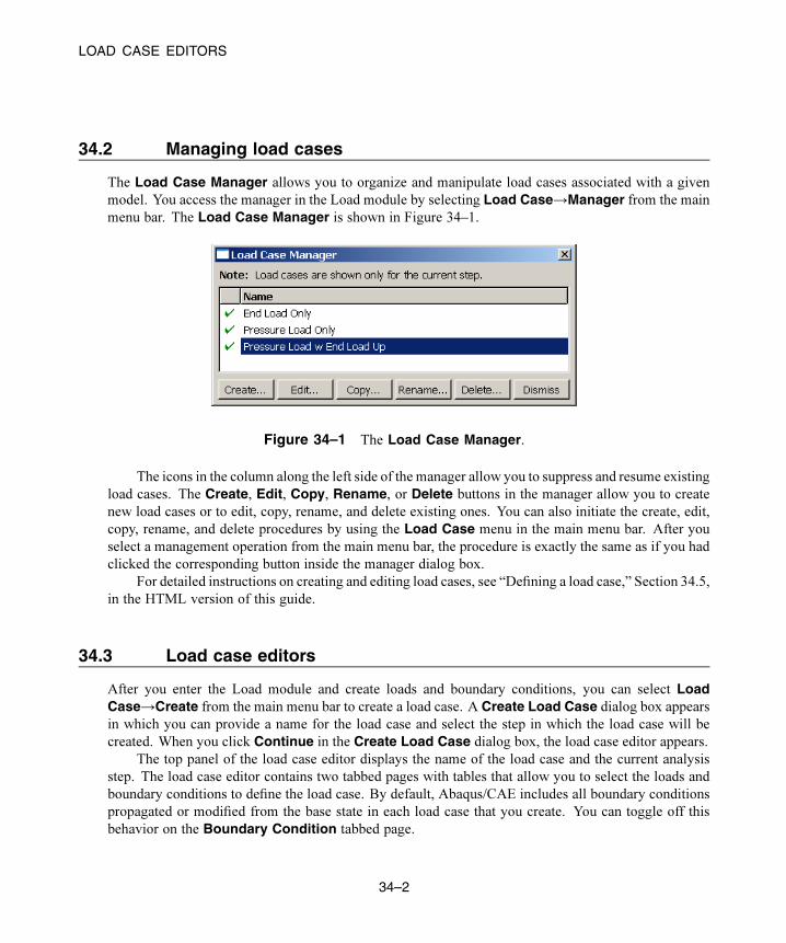
LOAD CASE EDITORS
34.2 Managing load cases
The Load Case Manager allows you to organize and manipulate load cases associated with a given
model. You access the manager in the Load module by selecting Load Case→Manager from the main
menu bar. The Load Case Manager is shown in Figure 34–1.
Figure 34–1 The Load Case Manager.
The icons in the column along the left side of the manager allow you to suppress and resume existing
load cases. The Create, Edit, Copy, Rename, or Delete buttons in the manager allow you to create
new load cases or to edit, copy, rename, and delete existing ones. You can also initiate the create, edit,
copy, rename, and delete procedures by using the Load Case menu in the main menu bar. After you
select a management operation from the main menu bar, the procedure is exactly the same as if you had
clicked the corresponding button inside the manager dialog box.
For detailed instructions on creating and editing load cases, see “Defining a load case,” Section 34.5,
in the HTML version of this guide.
34.3 Load case editors
After you enter the Load module and create loads and boundary conditions, you can select LoadCase→Create from the main menu bar to create a load case. A Create Load Case dialog box appears
in which you can provide a name for the load case and select the step in which the load case will be
created. When you click Continue in the Create Load Case dialog box, the load case editor appears.
The top panel of the load case editor displays the name of the load case and the current analysis
step. The load case editor contains two tabbed pages with tables that allow you to select the loads and
boundary conditions to define the load case. By default, Abaqus/CAE includes all boundary conditions
propagated or modified from the base state in each load case that you create. You can toggle off this
behavior on the Boundary Condition tabbed page.
34–2
Abaqus ID:
Printed on:
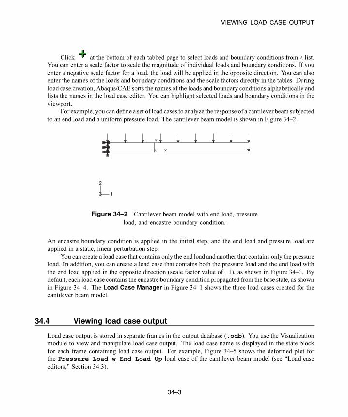
VIEWING LOAD CASE OUTPUT
Click at the bottom of each tabbed page to select loads and boundary conditions from a list.
You can enter a scale factor to scale the magnitude of individual loads and boundary conditions. If you
enter a negative scale factor for a load, the load will be applied in the opposite direction. You can also
enter the names of the loads and boundary conditions and the scale factors directly in the tables. During
load case creation, Abaqus/CAE sorts the names of the loads and boundary conditions alphabetically and
lists the names in the load case editor. You can highlight selected loads and boundary conditions in the
viewport.
For example, you can define a set of load cases to analyze the response of a cantilever beam subjected
to an end load and a uniform pressure load. The cantilever beam model is shown in Figure 34–2.
X
Y
Z
1
2
3
Figure 34–2 Cantilever beam model with end load, pressure
load, and encastre boundary condition.
An encastre boundary condition is applied in the initial step, and the end load and pressure load are
applied in a static, linear perturbation step.
You can create a load case that contains only the end load and another that contains only the pressure
load. In addition, you can create a load case that contains both the pressure load and the end load with
the end load applied in the opposite direction (scale factor value of −1), as shown in Figure 34–3. By
default, each load case contains the encastre boundary condition propagated from the base state, as shown
in Figure 34–4. The Load Case Manager in Figure 34–1 shows the three load cases created for the
cantilever beam model.
34.4 Viewing load case output
Load case output is stored in separate frames in the output database (.odb). You use the Visualization
module to view and manipulate load case output. The load case name is displayed in the state block
for each frame containing load case output. For example, Figure 34–5 shows the deformed plot for
the Pressure Load w End Load Up load case of the cantilever beam model (see “Load case
editors,” Section 34.3).
34–3
Abaqus ID:
Printed on:

VIEWING LOAD CASE OUTPUT
Figure 34–3 Load case definition that includes loads for the cantilever beam model.
Figure 34–4 Load case definition that includes boundary conditions propagated
from the base state for the cantilever beam model.
In the Visualization module you can linearly combine output from several load cases to represent
an actual loading environment. You can also obtain the minimum or maximum value of a selected field
variable over some or all load cases.
34–4
Abaqus ID:
Printed on:

VIEWING LOAD CASE OUTPUT
Step: "Cantilever loads", Multiple load case bendingLoad Case: PRESSURE LOAD W END LOAD UP
Deformed Var: U Deformation Scale Factor: +5.079e+00
1
2
3
Figure 34–5 Results from a load case analysis.
For example, you can combine the output from the End Load Only and Pressure LoadOnly load cases for the cantilever beam model to create new field output with a load case name of
Both loads, as shown in Figure 34–6.
Figure 34–6 Creating new field output by combining the output from two load cases (frames).
34–5
Abaqus ID:
Printed on:

VIEWING LOAD CASE OUTPUT
The new field output is contained in a frame of the session step and is available from the Field Outputdialog box. Figure 34–7 shows a plot of the combined deformation results.
Step: Session Step, Step for Viewer non-persistent fieldsFrame 1 (LC: Both loads): The sum of values over all selected frames
Deformed Var: U Deformation Scale Factor: +1.000e+00
1
2
3
Figure 34–7 Combined deformation results from both load cases.
For detailed information on manipulating load case output, see “Combining results from several
frames,” Section 42.7.3.
34–6
Abaqus ID:
Printed on:

UNDERSTANDING MIDSURFACE MODELING
35. Midsurface modeling
This section explains midsurface modeling and how you can use it to simplify thin solid models for
analysis. The following topics are covered:
• “Understanding midsurface modeling,” Section 35.1
• “Understanding the reference representation,” Section 35.2
• “Creating shell faces for the midsurface model,” Section 35.3
• “Examples of creating a midsurface model,” Section 35.4
In addition, “Creating and editing midsurface models,” Section 35.5, is available in the HTML
version of this guide.
35.1 Understanding midsurface modeling
Midsurface modeling is a technique for creating a simplified shell representation of a solid model.
Midsurface modeling can reduce the computational expense of analyzing a complete solid model when
a shell model with a defined thickness and fewer details is suitable for the required analysis.
The midsurface modeling process relies on an accurate solid model as the starting point.
Midsurface modeling is best suited to thin solids or thin-walled solids where wall thickness is constant
or where reasonable approximations of the wall thickness at each point can be made easily. You can
apply midsurface modeling to any solid cell within a model; you need not apply it to the entire model. If
you apply midsurface modeling to only a portion of a solid model, Abaqus/CAE automatically creates
shell-to-solid coupling constraints to couple the motion of the midsurface shell edges to that of the
remaining solid model faces. Shell-to-solid coupling constraints will not be created if the angle between
the shell surface and the solid face deviates significantly from 90°.
Besides reduced expense, you might use a midsurface model in place of a solid model to better
account for bending response in thin sections of the model. Shell elements are designed to manage
bending loads within the thickness of a single element, whereas a single solid element will have little or
no resistance to bending.
Creating a midsurface model in Abaqus/CAE is a manual process. The procedure presented below
provides an overview of the general steps involved. The tasks within each step may vary depending
on the complexity and completeness of the original solid model and the analysis requirements. Some
steps, such as Step 4 below, may not be required or may be completed in a different order from what is
presented here.
To create a midsurface model:
1. Assign midsurface regions on the solid part. Use the Assign Midsurface Region tool to select
one or more cells from the solid part to begin creating a midsurface model. For more information,
see “Assigning a midsurface region,” Section 35.5.1, in the HTML version of this guide.
35–1
Abaqus ID:
Printed on:

UNDERSTANDING THE REFERENCE REPRESENTATION
Abaqus/CAE removes the selected cells from the active representation and creates a reference
representation containing the selected cells.
2. Create new shell faces to replace the solid geometry that you moved to the reference representation.
You can use tools in the Geometry Edit toolset or the shell feature creation tools to add shell features
to the midsurface model. For more information, see Chapter 69, “The Geometry Edit toolset,” and
“Adding a shell feature,” Section 11.22, in the HTML version of this guide, respectively. The offset
faces tool in the Geometry Edit toolset is the most common face creation method for midsurface
models. The offset process creates new faces based on selected geometry and automatically assigns
a shell thickness based on the offset parameters.
3. Assign thicknesses to the new shell features.
The Assign Thickness and Offset tool allows you to assign shell thicknesses to the
new midsurface geometry (for more information, see “Assigning thicknesses and offsets,”
Section 35.5.2, in the HTML version of this guide). The tool allows you to assign thicknesses
to individual faces, and you can also use it to edit thicknesses that Abaqus/CAE assigned
automatically for faces created using the offset process. You must still assign a section to the new
faces in the Property module. During the section assignment process you can make a final decision
whether to use the thickness defined with the section properties or to use the definition from the
geometry. You can toggle the shell thickness display in all part and assembly-based modules
to see the thickness in the viewport (for more information, see “Visualizing shell thicknesses,”
Section 35.5.3, in the HTML version of this guide).
4. Revise any analysis attributes that were associated with the solid geometry that was used to create
the reference representation.
Analysis attributes such as loads, boundary conditions, or interactions cannot be applied to geometry
in the reference representation. Any attributes that were associated with the solid geometry before it
was moved to the reference representation will be associated with an empty region if the geometry is
no longer part of the active representation. For more information, see “Understanding the reference
representation,” Section 35.2.
35.2 Understanding the reference representation
A reference representation is an alternative representation of a part or a subset (one or more cells) of
a part that is not used in the analysis. The reference representation retains the original solid model
geometry, and, like reference geometry in the Sketcher, you can use entities from the reference
representation as tools to construct a simpler version of the part. The reference representation is most
commonly used to construct a midsurface model. When used with the offset face tool to create faces
for the midsurface model, the offset calculations between the reference representation and the new
faces also allow Abaqus/CAE to automatically compute shell thicknesses and element offsets in the
midsurface model.
35–2
Abaqus ID:
Printed on:

CREATING SHELL FACES FOR THE MIDSURFACE MODEL
Abaqus/CAE creates a reference representation when you assign a midsurface property to one or
more cells in a solid part. The selected cells are removed from the active representation of the part
and added to the reference representation. The reference representation appears by default in the Part
module and is colored translucent brown. You cannot change the color of the reference representation,
but you can toggle it on or off in all modules using the Show Reference Representation tool
located with the visible object tools in the main toolbar. You can also toggle translucency of the reference
representation on or off using the display options (for more information, see “Controlling edge visibility,”
Section 76.3, in the HTML version of this guide.
You can use the reference representation with the shape creation tools or with the tools in the
Geometry Edit toolset to help construct new geometric entities in the active representation. For example,
you can offset faces in the reference representation or you can select a planar face from the reference
representation as the sketch plane to create a new shell face using the extrude method. You can use
the geometry in the reference representation to define partitions—select an edge and a vertex from the
reference representation as the point and normal to partition a cell—or create datum entities. You can
also use reference representation geometry to position entities and define constraints in the Assembly
module.
You cannot edit the geometry within the reference representation, and you cannot assign analysis
attributes such as loads, boundary conditions, and interactions to it. When you create a reference
representation, any analysis attributes that were applied to the solid cells before you created the
reference representation will now be associated with an empty region. You can edit the empty regions
to associate the analysis attributes with geometry—solid geometry or shell geometry that you create
for the midsurface model—that is part of the active representation. Alternatively, you can suppress
or delete the analysis attributes. If you do not make any changes to the affected analysis attributes,
Abaqus/CAE will display a warning message when you submit the job in the Job module.
35.3 Creating shell faces for the midsurface model
Once you have a reference representation, you must manually build a shell model to replace the solid
cells that have been removed from the model. You can use the shell feature tools and the tools in the
Geometry Edit toolset to create and edit shell faces.
This section discusses some special conditions that may apply when you use these tools to create
faces for a midsurface model. The following topics are covered:
• “Using the offset face tool for midsurface modeling,” Section 35.3.1
• “Using the extend faces tool for midsurface modeling,” Section 35.3.2
35.3.1 Using the offset face tool for midsurface modelingYou can use the offset face tool from the Geometry Edit toolset to create midsurface faces. The offset
face tool creates new faces at an offset distance from an original set of faces. The offset faces are created
35–3
Abaqus ID:
Printed on:

CREATING SHELL FACES FOR THE MIDSURFACE MODEL
using a similar process to that used for offsetting objects in the Sketcher (for more information, see
“Offsetting objects,” Section 20.8.6). Use of the offset face tool is discussed in detail in “Offset faces,”
Section 69.7.7, in the HTML version of this guide.
In addition to the basic task of creating new shell faces, the offset face tool offers two functions that
are helpful for creating a midsurface model:
• The offset distance is used by Abaqus/CAE to assign a thickness to the new shell faces.
• The auto trim option automatically trims the new faces to the reference representation.
Once you have selected the faces to offset, you can enter a value for the offset distance or select a
set of target faces that represents the distance through the desired shell thickness and have Abaqus/CAE
calculate an offset. Abaqus/CAE calculates the distance between faces being offset and the target faces.
You can offset to half the average distance or a fraction of the distance to the closest or farthest point on
the target faces.
The difference in using each of the calculated offset distances is shown in Figure 35–1. The part has
three different thicknesses. The thinnest face is at the top, the thickest in the middle, and the vertical face
on the right has a thickness between the other two. The three outer faces of the reference representation
were selected to be offset, and the three inner faces are the target faces. The view on the left shows
the default Half the average distance method, and the offset is approximately the full thickness of
the top face. The middle view shows the Fraction distance to closest point on face method with
the fractional distance set to 0.5. The top target face is closest to the top offset face, so Abaqus/CAE
offsets the new faces by 0.5 times this distance. The view on the right shows the Fraction distanceto farthest point on face method with the fractional distance again set to 0.5. The middle (angled)
target face is farthest from the middle offset face, so Abaqus/CAE offsets the new faces by 0.5 times
this distance—notice that the top offset face is cut off where it would extend through the reference
representation of the original solid part because the Auto trim to reference representation option
was used.
Figure 35–1 Differences in the offset distance based on the three target face calculation methods.
Abaqus/CAE automatically associates the new offset shell faces with a thickness based on the offset
calculations. If you selected target faces to calculate the offset distance, Abaqus/CAE also automatically
35–4
Abaqus ID:
Printed on:

CREATING SHELL FACES FOR THE MIDSURFACE MODEL
recalculates the offset for any changes in the geometry of the top and bottom face sets. Use the
Assign Thickness and Offset tool and the Render shell thickness option to edit and view the
thicknesses assigned to the shell faces. For more information, see “Assigning thicknesses and offsets,”
Section 35.5.2, and “Visualizing shell thicknesses,” Section 35.5.3, in the HTML version of this guide.
If you use the auto trim option while offsetting faces, Abaqus/CAE offsets the faces and extends the
outer edges of the new faces by an amount equal to the offset distance. The new faces are then trimmed
where they intersect with the reference representation. Figure 35–2 shows a possible effect of using the
auto trim option. The reference representation contains two cells, and the highlighted face at the top of
the thinner cell was picked for the offset operation. Using the auto trim option, the new face extends into
the second cell of the reference representation.
Figure 35–2 The trim option trims only to the outer faces of the reference representation.
In this case the picked face could be offset without the trim option to create the offset without otherwise
altering the geometry. Alternatively, you could extend the offset face (extend faces tool) to fill the entire
reference representation, creating a single face for both cells.
35.3.2 Using the extend faces tool for midsurface modelingYou can use the extend faces tool from the Geometry Edit toolset to create midsurface faces. The
extend faces tool extends existing shell faces, so for midsurface modeling it must be used after you have
created one or more shell faces. Use of the extend faces tool is discussed in detail in “Extend faces,”
Section 69.7.8, in the HTML version of this guide.
You can extend faces by selecting individual edges to extend the faces in one or more directions,
or you can specify faces to extend the faces along all exterior edges. There are also several methods for
35–5
Abaqus ID:
Printed on:

EXAMPLES OF CREATING A MIDSURFACE MODEL
determining the extension distance; the Up to reference representation option is intended specifically
for midsurface modeling.
When you use the Specify edges of faces to extend option to extend faces along a set of edges,
the extend faces operation may fail. If this occurs, try reducing the number of selected edges and then
using a second operation to extend the faces along the remaining edges.
35.4 Examples of creating a midsurface model
This section provides examples of creating midsurface models from solid models. In the first example the
solid part has reasonably uniform thickness, and creation of the midsurface model is relatively easy. The
second example is more complex and requires multiple steps to create a midsurface model that accurately
represents the original solid model:
• “Midsurface modeling of a stamped bracket,” Section 35.4.1
• “Midsurface modeling of a complex part,” Section 35.4.2
35.4.1 Midsurface modeling of a stamped bracket
This example shows how you can use the midsurface modeling tools in Abaqus/CAE to convert a solid
model of a bracket to a shell representation of the same part.
The solid model
The model in this example is a 175.0 mm long bracket that is stamped from a 3.0 mm thick plate
of mild steel, as shown in Figure 35–3. A default mesh of the solid part results in one or two
elements through the thickness of the bracket that will not perform well in bending. Modeling a
shell representation of the bracket will provide a more accurate bending response.
Assign the midsurface region
Use the Assign Midsurface Region tool in the Part module to remove geometry from the active
representation of the model and to create a reference representation of the original solid geometry,
as shown in Figure 35–4. The reference representation is an abstract representation of the original
bracket. It retains the original geometry of the bracket, but it cannot be used in the analysis. The
reference representation appears by default in the Part module; you can toggle the view off and on
using the Show Reference Representation tool located with the visible object tools in the
main toolbar. Formore information, see “Understanding the reference representation,” Section 35.2,
and “Assigning a midsurface region,” Section 35.5.1, in the HTML version of this guide.
35–6
Abaqus ID:
Printed on:

EXAMPLES OF CREATING A MIDSURFACE MODEL
Figure 35–3 The solid model of the bracket.
Figure 35–4 The reference representation of the bracket.
Create the shell representation
You must create a shell representation of the bracket that can be analyzed by Abaqus. The most
commonly used tool for creating a midsurface shell model is the offset face tool, located with the
other face tools in the Geometry Edit toolset. The offset face tool allows you to select one or more
faces from the reference representation and to create new faces that are offset from the original faces.
You can enter a fixed distance, or you can select target faces that Abaqus/CAE uses to calculate the
distance. If you select target faces, the resulting shell thickness varies if the distance between the
face to offset and the target face is not constant. Abaqus/CAE calculates the nodal thickness and the
35–7
Abaqus ID:
Printed on:

EXAMPLES OF CREATING A MIDSURFACE MODEL
element offset for each node and element when you analyze the model. The Offset Faces dialog
box is shown in Figure 35–5.
Figure 35–5 The Offset Faces dialog box.
For more information, see “An overview of the methods for editing faces,” Section 69.2.2, and
“Adding a shell feature,” Section 11.22, in the HTML version of this guide.
Figure 35–6 shows the selected faces to offset and the selected target faces. The by angleselection method was used to select the inner group of face as the faces to offset and the outer group
of faces as the target faces.
In this example you select the default option of Half the average distance from the OffsetFaces dialog box, and Abaqus/CAE creates faces that are half the average distance between the
faces to offset and the target faces.
By default, Auto trim to reference representation is toggled off in the Offset Facesdialog box. However, the auto trim option was active for this step, so Abaqus/CAE trimmed the
offset faces to align with the reference representation. In some cases the trimming operation fails,
which results in a slight misalignment between the new faces and the reference representation and
a warning message from Abaqus/CAE. Even when trimming fails, the resulting shell face is often
still a reasonable approximation of the reference representation; so you may be able to ignore the
warning message. For more information, see “Using the offset face tool for midsurface modeling,”
Section 35.3.1.
Assign a shell section
You use the Property module to create a shell section and to assign it to the new face. When
you create the shell section, you can enter an arbitrary value for the shell thickness. When you
35–8
Abaqus ID:
Printed on:

EXAMPLES OF CREATING A MIDSURFACE MODEL
The faces to offsetThe target faces
Figure 35–6 The faces to offset and the target faces.
subsequently assign the section to the shell, you specify that the thickness and the shell offset
are calculated from the geometry in the Edit Section Assignment dialog box, as shown in
Figure 35–7. Abaqus/CAE ignores the thickness value that you entered for the shell section. For
more information, see “Assigning a section,” Section 12.15.1.
If desired, you can toggle on Render shell thickness from the Part Display Options to
view the thickness of the shell, as shown in Figure 35–8.
Mesh the part
Abaqus/CAE colors the shell part pink in the Mesh module to indicate it can be meshed using the
free meshing technique, as shown in Figure 35–9. You apply automatic virtual topology to the part
to remove small details from the original part and to remove details that were created during the
face trimming operation, as described in “Creating virtual topology automatically,” Section 75.6.1,
in the HTML version of this guide.
You apply default seeding and mesh controls, and the resulting mesh is shown in Figure 35–10.
35.4.2 Midsurface modeling of a complex partThis example uses several techniques and tools to create the midsurface model for a reinforced structural
component.
The solid model
The model in this example is the structural beam shown in Figure 35–11. The reinforcing ribs,
different thicknesses, and asymmetrical shape of the beam do not allow for a simple beam
section representation. The complexity of the part combined with its thin cross-sections make it a
35–9
Abaqus ID:
Printed on:
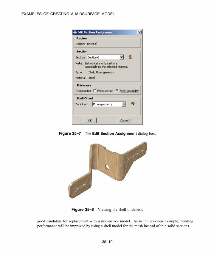
EXAMPLES OF CREATING A MIDSURFACE MODEL
Figure 35–7 The Edit Section Assignment dialog box.
Figure 35–8 Viewing the shell thickness.
good candidate for replacement with a midsurface model. As in the previous example, bending
performance will be improved by using a shell model for the mesh instead of thin solid sections.
35–10
Abaqus ID:
Printed on:
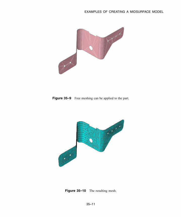
EXAMPLES OF CREATING A MIDSURFACE MODEL
Figure 35–9 Free meshing can be applied to the part.
Figure 35–10 The resulting mesh.
35–11
Abaqus ID:
Printed on:
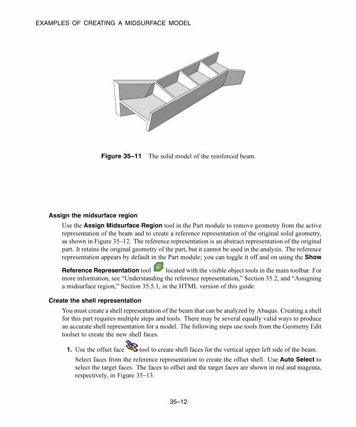
EXAMPLES OF CREATING A MIDSURFACE MODEL
Figure 35–11 The solid model of the reinforced beam.
Assign the midsurface region
Use the Assign Midsurface Region tool in the Part module to remove geometry from the active
representation of the beam and to create a reference representation of the original solid geometry,
as shown in Figure 35–12. The reference representation is an abstract representation of the original
part. It retains the original geometry of the part, but it cannot be used in the analysis. The reference
representation appears by default in the Part module; you can toggle it off and on using the Show
Reference Representation tool located with the visible object tools in the main toolbar. For
more information, see “Understanding the reference representation,” Section 35.2, and “Assigning
a midsurface region,” Section 35.5.1, in the HTML version of this guide.
Create the shell representation
You must create a shell representation of the beam that can be analyzed by Abaqus. Creating a shell
for this part requires multiple steps and tools. There may be several equally valid ways to produce
an accurate shell representation for a model. The following steps use tools from the Geometry Edit
toolset to create the new shell faces.
1. Use the offset face tool to create shell faces for the vertical upper left side of the beam.
Select faces from the reference representation to create the offset shell. Use Auto Select toselect the target faces. The faces to offset and the target faces are shown in red and magenta,
respectively, in Figure 35–13.
35–12
Abaqus ID:
Printed on:

EXAMPLES OF CREATING A MIDSURFACE MODEL
Figure 35–12 The reference representation of the beam.
Figure 35–13 Selected faces to create the offset for the upper left side.
The faces to offset are the two outer vertical faces toward the rear. The target faces are the
nine faces, mostly unconnected, that comprise the inner surface of the same beam wall. The
Fraction distance to closest point on face method is used with an entry of 0.5 to create
the offset with half the thickness of the thinner main portion along the top of the beam. Using
this option prevents the thicker sections at the left and along the bottom of the beam from
creating an offset larger than the thinner portion. TheAuto trim to reference representationoption is used for this step. This operation extends the faces during the offset process and
then trims them along the edges of the reference representation. Auto trim may fail when
multiple offset and target faces are selected; if auto trim fails, Abaqus/CAE displays a warning
indicating the failure. You can use the extend faces tool to extend the new faces to meet the
edges of the reference representation. The resulting offset faces are shown in Figure 35–14.
35–13
Abaqus ID:
Printed on:

EXAMPLES OF CREATING A MIDSURFACE MODEL
Figure 35–14 The resulting offset faces.
2. Repeat the process from Step 1 to create offset faces for the opposite side of the beam.
The resulting shell model now contains the two outer surfaces of the beam, as shown in
Figure 35–15.
Figure 35–15 The offset faces from the first and second steps.
3. Create offset faces for the four horizontal sections that connect the two side walls.
You can create the faces in a single offset operation by selecting the four top faces to offset
and using Auto Select to select the corresponding bottom faces. In this case Auto trim toreference representation is toggled off, so the new faces are not extended and trimmed. The
shell model of the horizontal faces is shown in Figure 35–16. (The faces created in Step 2 have
been suppressed for clarity.) Notice the gaps between the horizontal faces where they meet the
vertical reinforcement ribs in the original part. Similar gaps exist between the horizontal shell
faces and the side walls created in the previous two steps.
35–14
Abaqus ID:
Printed on:

EXAMPLES OF CREATING A MIDSURFACE MODEL
Figure 35–16 The horizontal offset faces.
4. Repeat the process from Step 3 to create offset faces for the vertical ribs that connect the sides
of the beam.
The midsurface shell model now contains faces representing nearly all of the solid geometry,
as shown in Figure 35–17. However, there are gaps between most of the faces due to the
thickness of the original solid structure.
Figure 35–17 The midsurface model with gaps between the faces.
5. Close the gaps between the vertical ribs and the beam sides.
Use the extend faces tool to extend the six vertical ribs to intersect with the sides. The
selected faces and target faces are shown in magenta and yellow, respectively, in Figure 35–18.
35–15
Abaqus ID:
Printed on:

EXAMPLES OF CREATING A MIDSURFACE MODEL
Figure 35–18 Specifying the faces to extend and the target faces.
When you click OK, Abaqus/CAE updates the highlighting to indicate the edges along which
the faces will be extended, as shown in Figure 35–19, and displays a warning dialog box with
options allowing you to accept the selection, to extend all edges of the selected faces, or to
cancel the extend faces procedure.
Figure 35–19 The edges where the vertical faces will be extended.
6. Use the extend faces tool to extend the horizontal faces to intersect with the sides of the
beam.
In this case, use the Specify edges of faces to extend method with Up to target faces to
pick the edges and faces, respectively, shown in Figure 35–20. When Abaqus/CAE highlights
the edges indicating the areas that will be extended, the four edges indicated by arrows in the
figure are removed from the selection because they do not completely match the target faces.
Click No to use the previous selection of edges.
35–16
Abaqus ID:
Printed on:

EXAMPLES OF CREATING A MIDSURFACE MODEL
Figure 35–20 The edges along which the horizontal faces will be the extended.
7. Close the remaining gaps between the horizontal and vertical connecting sections of the
beam. You can use either the blend faces tool or the extend faces tool to complete
the midsurface model by closing the remaining gaps between the horizontal and vertical
connecting sections of the beam.
a. Use the extend faces tool with the selections shown in Figure 35–21.
Toggle on Trim to extended underlying target surfaces so that Abaqus/CAE will
extend and trim the vertical faces to their implied intersections with the selected target
face.
Figure 35–21 Filling the gaps between the vertical reinforcing ribs.
b. Use the blend faces tool to fill the remaining gaps.
The tool must be used three times to fill the three remaining gaps in the model.
35–17
Abaqus ID:
Printed on:

EXAMPLES OF CREATING A MIDSURFACE MODEL
Assign thicknesses
All the original solid geometry has now been replaced with shell geometry. To complete the
model, you should verify that the shells have appropriate thickness information. Click the assign
thickness and offset tool . Abaqus/CAE highlights any shell faces that do not have thickness
data. In this case, since the shell faces were all created using the offset, extend, and blend tools,
all of the faces already have thickness data assigned. If there were faces without thickness data,
you would select each face and, using the Compute thickness from opposite faces method in
the Assign thickness and Offset dialog box, pick appropriate top and bottom faces from the
reference representation to create the missing thicknesses.
To view the model with shell thicknesses, you can toggle on Render shell thickness in
the Part Display Options dialog box (for more information, see “Visualizing shell thicknesses,”
Section 35.5.3, in the HTML version of this guide). As shown in Figure 35–22, the resulting view
includes the variations in thickness that were in the original solid model.
Figure 35–22 Shell faces with thickness displayed.
Assign a shell section
Use the Property module to create a shell section and assign it to the midsurface model. When
you create the shell section, you can enter an arbitrary value for the shell thickness. When you
subsequently assign the section to the shell, you specify that the thickness and the shell offset are
calculated from the geometry in the Edit Section Assignment dialog box. Abaqus/CAE ignores
the thickness value that you entered for the shell section and uses the thicknesses assigned to the
faces in the Part module. For more information, see “Assigning a section,” Section 12.15.1, in the
HTML version of this guide. Figure 35–23 shows the completed midsurface model with section
thicknesses after section assignment in the Property module. The geometry is identical to that in
Figure 35–22.
35–18
Abaqus ID:
Printed on:

EXAMPLES OF CREATING A MIDSURFACE MODEL
Figure 35–23 The completed midsurface geometry with shell thicknesses.
Mesh the part
Abaqus/CAE colors the shell part pink in the Mesh module to indicate it can be meshed using the
free meshing technique, as shown in Figure 35–24.
Figure 35–24 Free meshing can be applied to the part.
Before seeding and meshing the part, you can apply automatic virtual topology to remove
small details that are not needed in the mesh (for more information, see “Creating virtual topology
automatically,” Section 75.6.1, in the HTML version of this guide). The default automatic
virtual topology settings should remove the blended face edges and other small details that would
unnecessarily constrain the part mesh.
Note: Automatic virtual topology may fail if neighboring faces have inconsistent normals. If this
occurs, return to the Part module and use the tool in the Geometry Edit toolset to repair the
face normals.
35–19
Abaqus ID:
Printed on:

EXAMPLES OF CREATING A MIDSURFACE MODEL
Apply default seeding and mesh controls, and generate the mesh on the part. The resulting
mesh is shown in Figure 35–25, with the shell thickness displayed.
35–20
Abaqus ID:
Printed on:

EXAMPLES OF CREATING A MIDSURFACE MODEL
Figure 35–25 The resulting mesh with shell thickness rendering.
35–21
Abaqus ID:
Printed on:


DEFINING SKIN REINFORCEMENTS
36. Skin and stringer reinforcements
This section provides information on how to model skin and stringer reinforcements. The following
topics are covered:
• “Defining skin reinforcements,” Section 36.1
• “Defining stringer reinforcements,” Section 36.2
• “Managing skin and stringer reinforcements,” Section 36.3
• “Generating elements on a skin or stringer reinforcement,” Section 36.4
• “Assigning element types to skin or stringer reinforcements,” Section 36.5
• “Using offset meshes to create skin reinforcements,” Section 36.6
• “Assigning surface properties to skins and stringers,” Section 36.7
In addition, the following sections are available in the HTML version of this guide:
• “Creating and editing skin reinforcements,” Section 36.8
• “Creating and editing stringer reinforcements,” Section 36.9
36.1 Defining skin reinforcements
A skin reinforcement defines a skin that is bonded to the surface of an existing part and specifies its
engineering properties. The surface can be a face of a three-dimensional solid part, any edge of an
axisymmetric part, or any face of a two-dimensional part. The part can include geometry and orphan
mesh elements; however, skin reinforcements must be defined separately for the geometry and the orphan
mesh elements. You should think of a skin as a property of a part or region, in the same way a section is
a property of a part or region.
The composite beam shown in Figure 36–1 is an example of how youmight use a skin reinforcement
in your model.
aluminum skin
solid honeycomb core
Figure 36–1 A composite beam modeled by a solid honeycomb core and an aluminum skin.
36–1
Abaqus ID:
Printed on:

DEFINING SKIN REINFORCEMENTS
The beam has a solid honeycomb core and an aluminum skin on the upper and lower faces. You can
create a solid part representing the honeycomb and add a skin reinforcement representing the aluminum
layers. In the Mesh module you assign solid elements to the honeycomb and shell elements to the skin.
The solid and shell elements share the same nodes.
Select Special→Skin→Create from the main menu bar in the Property module to define one or
more skins. Select Edit from the same menu to make changes to an existing definition. All skins you
create also appear in the Model Tree in a Skins container under the part. Skins are not displayed in the
viewport by default, but you can make them visible by color coding them in the viewport. See “Coloring
geometry and mesh elements,” Section 77.4, for more information.
If you create a skin on a geometry region, Abaqus/CAE updates the skin if you make minor
modifications to the underlying geometry. If you edit orphan nodes or elements with a skin, Abaqus/CAE
updates the skin if you edit or delete nodes or elements; however, it does not update the skin if you
create new nodes or elements.
You may need to select the skin in subsequent modeling operations; for example, to:
• Assign a homogeneous shell section, a composite shell section, a membrane section, a surface
section, or a gasket section to a skin. Section assignments are performed in the Property module.
• Assign a material orientation or rebar reference orientation to a skin. Both of these orientation
assignments are performed in the Property module.
• Assign a normal direction to a skin in the Property module. Although you cannot assign a normal
direction to a skin directly, you can assign a normal direction to a face, which updates the normal
direction of all skins defined on that face.
• Prescribe a body force to the skin in the Load module.
• Prescribe a thermal flux on the skin in the Load module. In practice, you perform this modeling
operation by applying a thermal flux load to the underlying face or faces. Abaqus/CAE applies the
load to all skins on that face during the analysis.
• Assign an element type to the skin in the Mesh module.
• Request field data output or history data output for the skin in the Step module.
• Create a display group to view the stress values on the skin elements in the Visualization module.
While you cannot specifically select skins by name in the Create Display Group dialog box, you
can find them in this dialog box by searching for elements that share the same element type, section
assignment, or another property as the skin elements in your model. This process can help you
narrow down the list of elements to the skins you want to include.
When you are prompted to select a region for these modeling operations, select Skins from the list of
object types in theSelection toolbar, and select the skin region from the viewport. For more information,
see “Filtering your selection based on the type of object,” Section 6.3.2.
When performing contact calculations, Abaqus/CAE considers a geometric surface’s skin
reinforcements only in certain cases; for example, when you specify general contact for all exterior
surfaces, a default all-inclusive surface is defined automatically in Abaqus that will consider skin
reinforcements. Skin reinforcements can significantly influence contact calculations, due to skin
36–2
Abaqus ID:
Printed on:
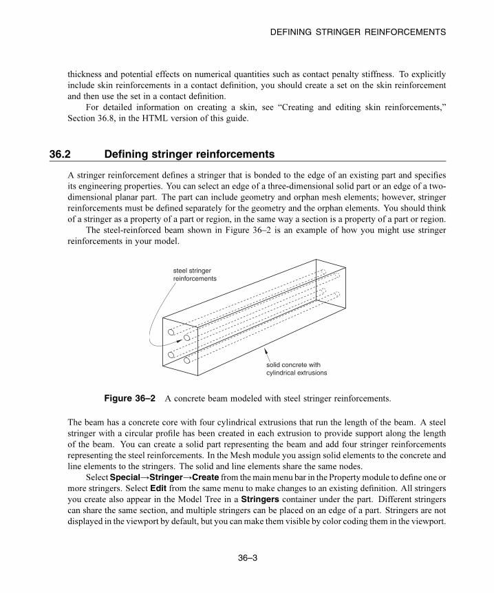
DEFINING STRINGER REINFORCEMENTS
thickness and potential effects on numerical quantities such as contact penalty stiffness. To explicitly
include skin reinforcements in a contact definition, you should create a set on the skin reinforcement
and then use the set in a contact definition.
For detailed information on creating a skin, see “Creating and editing skin reinforcements,”
Section 36.8, in the HTML version of this guide.
36.2 Defining stringer reinforcements
A stringer reinforcement defines a stringer that is bonded to the edge of an existing part and specifies
its engineering properties. You can select an edge of a three-dimensional solid part or an edge of a two-
dimensional planar part. The part can include geometry and orphan mesh elements; however, stringer
reinforcements must be defined separately for the geometry and the orphan elements. You should think
of a stringer as a property of a part or region, in the same way a section is a property of a part or region.
The steel-reinforced beam shown in Figure 36–2 is an example of how you might use stringer
reinforcements in your model.
solid concrete withcylindrical extrusions
steel stringerreinforcements
Figure 36–2 A concrete beam modeled with steel stringer reinforcements.
The beam has a concrete core with four cylindrical extrusions that run the length of the beam. A steel
stringer with a circular profile has been created in each extrusion to provide support along the length
of the beam. You can create a solid part representing the beam and add four stringer reinforcements
representing the steel reinforcements. In the Mesh module you assign solid elements to the concrete and
line elements to the stringers. The solid and line elements share the same nodes.
SelectSpecial→Stringer→Create from themainmenu bar in the Propertymodule to define one or
more stringers. Select Edit from the same menu to make changes to an existing definition. All stringers
you create also appear in the Model Tree in a Stringers container under the part. Different stringers
can share the same section, and multiple stringers can be placed on an edge of a part. Stringers are not
displayed in the viewport by default, but you can make them visible by color coding them in the viewport.
36–3
Abaqus ID:
Printed on:

MANAGING SKIN AND STRINGER REINFORCEMENTS
See “Coloring geometry and mesh elements,” Section 77.4, in the HTML version of this guide, for more
information.
If you create a stringer on a geometry region, Abaqus/CAE updates the stringer if you make
minor modifications to the underlying geometry. If you edit orphan nodes or elements with a stringer,
Abaqus/CAE updates the stringer if you edit or delete nodes or elements; however, it does not update
the stringer if you create new nodes or elements.
You may need to select the stringer in subsequent modeling operations; for example, to:
• Assign a section, beam section orientation, material orientation, or tangent direction to a stringer.
All of these activities are performed in the Property module.
• Prescribe a body force or line load to the stringer in the Load module.
• Prescribe a thermal flux on the stringer in the Load module. In practice, you perform this modeling
operation by applying a thermal flux load to the underlying edge or edges. Abaqus/CAE applies the
load to all stringers on that edge during the analysis.
• Assign an element type to the stringer in the Mesh module.
• Request field data output or history data output for the stringer in the Step module.
• Create a display group to view the stress values on the stringer elements in the Visualization module.
While you cannot specifically select stringers by name in the Create Display Group dialog box,
you can find them in this dialog box by searching for elements that share the same element type,
section assignment, or another property as the stringer elements in your model. This process can
help you narrow down the list of elements to the stringers you want to include.
When you are prompted to select a region for these modeling operations, select Stringers from the list
of object types in the Selection toolbar, and select the stringer from the viewport. For more information,
see “Filtering your selection based on the type of object,” Section 6.3.2.
When performing contact calculations, Abaqus/CAE considers a geometric surface’s stringer
reinforcements only in certain cases; for example, when you specify general contact for all exterior
surfaces, a default all-inclusive surface is defined automatically in Abaqus that will consider stringer
reinforcements. Stringer reinforcements can significantly influence contact calculations, due to
stringer thickness and potential effects on numerical quantities such as contact penalty stiffness. To
explicitly include stringer reinforcements in a contact definition, you should create a set on the stringer
reinforcement and then use the set in a contact definition.
For detailed information on creating a stringer, see “Creating and editing stringer reinforcements,”
Section 36.9, in the HTML version of this guide.
36.3 Managing skin and stringer reinforcements
The Skin Manager and Stringer Manager allow you to create and manage skin and stringer
reinforcements, respectively. These managers each include a list of the names of skins or stringers
that you have defined. The Create, Edit, Rename, and Delete buttons in the manager allow you to
create new skins and stringers or to edit, rename, and delete existing ones. You can also initiate these
36–4
Abaqus ID:
Printed on:

GENERATING ELEMENTS ON A SKIN OR STRINGER REINFORCEMENT
procedures using the Special→Skin menu and Special→Stringer menu from the main menu bar in
the Property module. After you select a management operation from the main menu bar, the procedure
is exactly the same as if you had clicked the corresponding button inside the manager dialog box.
Note: If you rename a skin or stringer after you have assigned sections, orientations, normals, or other
properties to it, the assignments become invalid.
36.4 Generating elements on a skin or stringer reinforcement
You can use the Mesh module to generate two-dimensional elements on a skin reinforcement on a face
of a three-dimensional part instance. Similarly, you can generate one-dimensional elements on a stringer
reinforcement on an edge of an axisymmetric part instance. Abaqus/CAE generates the skin or stringer
elements when the underlying geometry is meshed; you cannot mesh a skin or stringer reinforcement
independently.
Figure 36–3 shows a three-dimensional part instance with a skin reinforcement on the top surface.
skin elements
three-dimensionalelements
Figure 36–3 A three-dimensional part instance with a skin reinforcement.
When the part instance is meshed, the skin or stringer elements and the three-dimensional elements share
the same nodes and mesh topology. If you assign a different geometric order to the skin elements, you
should also change the order of the underlying elements. For more information, see “Assigning element
types to skin or stringer reinforcements,” Section 36.5.
If you create a skin or stringer on an orphan mesh, the skin or stringer elements and the underlying
orphan mesh elements share the same nodes and mesh topology. If you delete an orphan mesh element,
Abaqus/CAE automatically regenerates any skins or stringers associated with the deleted element. After
regeneration, these skins or stringers have new element ID numbers, so this regeneration renders invalid
any sets that include the skins or stringers. Therefore, if you delete elements from an orphan mesh,
you should update any set definitions that include skins or stringers formerly associated with the deleted
elements.
36–5
Abaqus ID:
Printed on:
ASSIGNING SURFACE PROPERTIES TO SKINS AND STRINGERS
36.5 Assigning element types to skin or stringer reinforcements
You use the Property module to create a skin or stringer reinforcement on a part in your model. You use
the Mesh module to assign an element type to a skin or stringer reinforcement. When you are prompted
to select the regions to be assigned element types, you must select either Skins or Stringers from the
list of object types in the Selection toolbar.
When you create a skin or a stringer for a geometric part, Abaqus/CAE adds an attribute to the
geometric entity. This attribute is used when you mesh the part to generate skin or stringer elements, and
these elements share nodes with the underlying elements of the part.
You can use stringer reinforcements in a buckling analysis, and you can use skin reinforcements
in a coupled structural-acoustic analysis. If the acoustic medium adjoins a structure, structural-acoustic
coupling occurs at the interface. It is recommended that you use surface-based tie constraints to enforce
the coupling; however, if you are conducting a structural-acoustic submodeling analysis where the
acoustic domain forms the submodel, you must line the interface portion of the submodel boundary with
acoustic-structural interface (ASI) elements to enforce the coupling. You can line the interface with
ASI elements by creating a skin at the interface and assigning ASI elements to the skin. For detailed
information about using skins to create ASI elements on geometry and orphan meshes, see the Dassault
Systèmes Knowledge Base at www.3ds.com/support/knowledge-base.
36.6 Using offset meshes to create skin reinforcements
As an alternative approach, you can use the mesh offset tool in the Edit Mesh toolset to create a skin
reinforcement by sharing the nodes of the offset shell with the underlying orphan mesh. However, the
equivalent offset shell does not appear in the Model Tree as a skin because using the offset shell to
represent a reinforcement skin is just one of many potential uses of the offset shell. If you are creating
more than one layer of reinforcement skins, you should specify a distance of zero between the layers so
that the layers can share nodes.
36.7 Assigning surface properties to skins and stringers
If you want to apply a surface property such as a pressure load to a skin or a stringer, you must apply
the property to its underlying surface or edge instead. Because skins and stringers share nodes with
the surfaces or edges to which they apply, Abaqus/CAE automatically propagates any applied surface
properties to skins and stringers as well. For more information about defining surface properties, see
“Assigning sections, orientations, normals, and tangents to a part,” Section 12.15, in the HTML version
of this guide.
36–6
Abaqus ID:
Printed on:

DEFINING SPRINGS AND DASHPOTS
37. Springs and dashpots
This section provides information on how to model springs and dashpots. The following topics are
covered:
• “Defining springs and dashpots,” Section 37.1
• “Managing springs and dashpots,” Section 37.2
In addition, the following sections are available in the HTML version of this guide:
• “Creating springs and dashpots connecting two points,” Section 37.3
• “Editing springs and dashpots connecting two points,” Section 37.4
• “Creating springs and dashpots connecting points to ground,” Section 37.5
• “Editing the region to which springs and dashpots connecting points to ground are applied,”
Section 37.6
37.1 Defining springs and dashpots
You can define springs and dashpots that exhibit the same linear behavior. You can also define both
spring and dashpot behaviors on the same set of points. If you define both spring and dashpot behaviors,
they act in parallel. You can model springs and dashpots using the following connectivity types:
• Connect two points and follow the line of action between the points
• Connect two points and act in a fixed direction (Abaqus/Standard analyses only)
• Connect points to ground (Abaqus/Standard analyses only)
For more information, see “Springs,” Section 32.1.1 of the Abaqus Analysis User’s Guide, and
“Dashpots,” Section 32.2.1 of the Abaqus Analysis User’s Guide.
Select Special→Springs/Dashpots→Create from the main menu bar in the Property module or
the Interaction module to define springs and dashpots. Select Edit from the same menu to make changes
to an existing definition. Springs and dashpots created on a part are instanced along with the part.
If you want to include the spring and dashpot results data in the output database generated by the
analysis, you must use the History Output Request editor in the Step module. Springs and dashpots
appear in the Model Tree in the Engineering Features container under the part (if created in the
Property module) or under the assembly (if created in the Interaction module).
For detailed information, see the following sections in the HTML version of this guide:
• “Modifying history output requests,” Section 14.12.3
• “Creating springs and dashpots connecting two points,” Section 37.3
• “Editing springs and dashpots connecting two points,” Section 37.4
• “Creating springs and dashpots connecting points to ground,” Section 37.5
37–1
Abaqus ID:
Printed on:

MANAGING SPRINGS AND DASHPOTS
• “Editing the region to which springs and dashpots connecting points to ground are applied,”
Section 37.6
37.2 Managing springs and dashpots
The Springs/Dashpots Manager allows you to create and manage springs and dashpots. The manager
includes a list of the names and types of springs and dashpots that you have defined. The Create, Edit,Copy, Rename, and Delete buttons in the manager allow you to create new springs and dashpots or to
edit, copy, rename, and delete existing ones. The icons in the column along the left side of the manager
allow you to suppress and resume existing springs and dashpots. You can also initiate these procedures
using the Special→Springs/Dashpots menu from the main menu bar in the Property module or the
Interaction module. After you select a management operation from the main menu bar, the procedure is
exactly the same as if you had clicked the corresponding button inside the manager dialog box.
37–2
Abaqus ID:
Printed on:

CREATING A SUBMODEL
38. Submodeling
You use submodeling to study in detail an area of interest in your model; for example, a region of high
stress. In most cases you will mesh the region of interest with a finer mesh, and the submodel can provide
an accurate, detailed solution. You can also change the modeling space from a shell global model to a
more representative solid submodel—shell-to-solid submodeling.
Creating a submodel is a two-step process. First you create and analyze the global model. You
then create the submodel and drive the boundaries of the submodel with time-dependent variables that
were saved during the analysis of the global model. You can drive submodel boundaries either with
boundary conditions or in some cases with stresses from the global model. Submodeling is described in
detail in “Submodeling: overview,” Section 10.2.1 of the Abaqus Analysis User’s Guide. “Shell-to-solid
submodeling and shell-to-solid coupling of a pipe joint,” Section 1.1.10 of the Abaqus Example Problems
Guide, includes an example of a submodel created using Abaqus/CAE.
The following topics are covered:
• “Analyzing the global model,” Section 38.1
• “Creating a submodel,” Section 38.2
• “Removing regions,” Section 38.3
• “Creating the submodel boundary condition,” Section 38.4
• “Creating the submodel load,” Section 38.5
• “Modifying the submodel,” Section 38.6
• “Analyzing the submodel,” Section 38.7
• “Checking the results from the submodel,” Section 38.8
38.1 Analyzing the global model
You first obtain results for the entire model using a relatively coarse mesh and perhaps simplified
geometry. This model is called the global model. Data from the output database that is generated by the
global model are used to drive the submodel. As a result, the output requests in the global model must
include the driven variables. You can also drive a submodel using the global model results stored in a
results file that was generated from the Abaqus execution procedure.
38.2 Creating a submodel
When you have successfully analyzed the global model and generated an output database or a results
file containing the global model results, you are ready to create the submodel. You start by copying
the global model to a new model that you will use to define the submodel. To copy a model, select
38–1
Abaqus ID:
Printed on:

CREATING THE SUBMODEL BOUNDARY CONDITION
Model→Copy→global model name from the main menu bar. Enter the name of the submodel in the
Copy Model dialog box that appears and click OK. The copied model becomes the current model.
You must select the output database or results file from the global analysis that will be used to drive
the submodel. From the main menu bar, select Model→Edit Attributes→submodel name. From the
Edit Model Attributes dialog box that appears, click the Submodel tab, and do the following:
• Toggle on Read data from job, and enter the name of the output database or results file containing
the global model that will drive the submodel. You must provide the file extension (.odb or .fil)if both an output database and a results file exist and they use the same name.
• In addition, if your shell global model is driving a solid submodel, toggle on Shell global modeldrives a solid submodel.
• Click OK to close the Edit Model Attributes dialog box.
38.3 Removing regions
Remove regions from the submodel that you are not interested in analyzing. Only the regions of interest
should remain. You can use several techniques to remove regions from a part.
• Use the cut tools in the Part module. For more information, see “Adding a cut feature,”
Section 11.24, in the HTML version of this guide.
• Use the Geometry Edit toolset to remove faces. For more information, see “An overview of editing
techniques,” Section 69.2.
• You can delete the part in the Part module and create a new part with the same name. You can then
create geometric features that represent the submodel; however, you must position the new features
in the same location as the original part. For a discussion of the tolerances between the submodel
and the global model, see “Submodeling: overview,” Section 10.2.1 of the Abaqus Analysis User’s
Guide. The new part and the original part must be created in three-dimensional modeling space.
Creating a new part is a useful technique for converting a shell global model to a solid
submodel. You can delete the shell part from the copied model and create a new solid part in the
same location. You must take care to ensure that the part defined in the solid submodel is contained
within the part defined in the shell global model.
38.4 Creating the submodel boundary condition
The most common submodeling technique is node-based submodeling, which uses a nodal results field
(including displacement, temperature, or pressure degrees of freedom) to interpolate global model results
onto the submodel nodes. Node-based submodeling is also a more general technique. To use node-based
submodeling, you create a submodel boundary condition.
If you apply a submodel boundary condition to nodes that are constrained by either a
displacement/rotation boundary condition or a connector displacement boundary condition on the
38–2
Abaqus ID:
Printed on:

CREATING THE SUBMODEL BOUNDARY CONDITION
global model in a previous step and the global model’s boundary condition is fixed using the Fixed atCurrent Position method, Abaqus/CAE disregards the submodel boundary condition for those nodes
and retains the specifications in the boundary condition on the global model instead. Abaqus/CAE
reports this replacement of boundary conditions in the data file for the analysis.
To create a submodel boundary condition:
1. Enter the Load module and select BC→Create from the main menu bar.
2. From the list of steps, select the step during which the submodel boundary condition will be applied.
3. From the Category field, select Other.
4. From the Types for Selected Step field, select Submodel and click Continue.
5. From the model, select the regions to which the boundary condition will be applied. In most cases
you apply the boundary condition to the edges and faces that were created when you cut away
regions from the global model. You can prescribe other boundary conditions to the same regions;
for example, a symmetry boundary condition. The prescribed boundary conditions take precedence
over the submodel boundary condition.
6. From the Edit Boundary Condition dialog box that appears, do the following:
a. In the Driving region field, do one of the following:
• Select Automatic to allow Abaqus/CAE to create the driving region by searching all
regions in the global model that lie in the vicinity of the submodel.
• Select Specify to specify a set name that will be used as the driving region.
You must give the complete name of the set. The syntax for the set name is
assembly_name.part_name-1.set_name, assuming that you are defining the
driving region on the first instance of the part.
b. If you are driving a solid submodel with a shell global model, you must enter the maximum
value of the shell thickness in the global model in the Shell thickness field.
c. In the Exterior tolerance field, do the following:
• Enter the absolute exterior tolerance. This is the absolute value by which a driven node
of the submodel may lie outside the elements of the global model. The default value is
the relative exterior tolerance.
• Enter the relative exterior tolerance. This is the fraction of the average element size in
the global model by which a driven node of the submodel may lie outside the elements of
the global model. The default value is .05.
For more information, see “Submodeling: overview,” Section 10.2.1 of the Abaqus Analysis
User’s Guide.
d. If you are driving a solid submodel with a solid global model or if you are driving a shell
submodel with a shell global model, you must enter a comma-separated list indicating the
38–3
Abaqus ID:
Printed on:

CREATING THE SUBMODEL LOAD
degrees of freedom that are being driven; for example, 1,2,3. You cannot leave this field
blank.
e. If you are driving a solid submodel with a shell global model, you can provide the thickness
of the center zone size around the shell midsurface. The default value is 10% of the maximum
shell thickness in the global model as defined in the Shell thickness field.
f. In the Global step number field, enter an integer representing the step number in the global
analysis from which the values of the driven variables will be read.
g. If you created the boundary condition in a static, linear perturbation step, you can specify the
increment in the global analysis step that will be the basis for calculating the values for the
driven variables. The default value of zero corresponds to the last increment of the previous
step.
h. If the time period of the submodel analysis is different from the time period of the global
analysis, you can choose to scale the time period of the global step to match the time period of
the submodel step. For example, Abaqus determines the displacements of the global model at a
time 20% into the global step and applies those displacements at a time 20% into the submodel
step.
If you do not choose to scale the time period of the global step to match the time period of the
submodel step, Abaqus applies the displacements of the global model at the same time during
the submodel step. For example, Abaqus determines the displacements of the global model
one second into the global step and applies those displacements one second into the submodel
step. This behavior is probably not desired if the two time periods are different. You choose
to scale the time period by toggling on Scale time period of global step to time period ofsubmodel step.
For information on related topics, refer to the following sections:
• “Defining a displacement/rotation boundary condition,” Section 16.10.2
• “Defining a connector displacement boundary condition,” Section 16.10.5
38.5 Creating the submodel load
The surface-based submodeling technique is an alternative submodeling technique that uses the stress
field to interpolate global model results onto the submodel integration points on the driven element-based
surface facets. To use surface-based submodeling, you create a submodel load.
To create a submodel load:
1. Enter the Load module and select Load→Create from the main menu bar.
2. From the list of steps, select the step during which the submodel load will be applied.
38–4
Abaqus ID:
Printed on:

MODIFYING THE SUBMODEL
3. From the Category field, select Other.
4. From the Types for Selected Step field, select Submodel and click Continue.
5. From the model, select the regions to which the load will be applied. In most cases you apply
the load to faces that were created when you cut away regions from the global model. If you are
applying the load to a face of a shell, Abaqus/CAE asks you to specify the side of the face to which
the load will be applied. For more information, see “Specifying a particular side or end of a region,”
Section 73.2.5.
6. From the Edit Load dialog box that appears, do the following:
a. In the Driving region field, do one of the following:
• Select Automatic to allow Abaqus/CAE to create the driving region by searching all
regions in the global model that lie in the vicinity of the submodel.
• Select Specify to specify a set name that will be used as the driving region.
You must give the complete name of the set. The syntax for the set name is
assembly_name.part_name-1.set_name, assuming that you are defining the
driving region on the first instance of the part.
b. In the Exterior tolerance field, do the following:
• Enter the absolute exterior tolerance. This is the absolute value by which a driven node
of the submodel may lie outside the elements of the global model. The default value is
the relative exterior tolerance.
• Enter the relative exterior tolerance. This is the fraction of the average element size in
the global model by which a driven node of the submodel may lie outside the elements of
the global model. The default value is .05.
For more information, see “Submodeling: overview,” Section 10.2.1 of the Abaqus Analysis
User’s Guide.
c. In the Global step number field, enter an integer representing the step number in the global
analysis from which the values of the driven variables will be read.
38.6 Modifying the submodel
You can make the following modifications to the submodel:
• You can use the Step module to change the analysis procedure. The submodel can use either a
general procedure or a linear perturbation procedure. For more information, see “Submodeling:
overview,” Section 10.2.1 of the Abaqus Analysis User’s Guide.
• In the Load module you must remove any loads, boundary conditions, or initial conditions that were
applied to regions of the global model that were removed.
• If a boundary condition is applied outside the region to which you applied the submodel boundary
condition, you must ensure that it corresponds to the loading of the global model.
38–5
Abaqus ID:
Printed on:

CHECKING THE RESULTS FROM THE SUBMODEL
• Similarly, if a load is applied to the submodel, you must ensure that it corresponds to the loading of
the global model.
• In most cases you will apply a more refined mesh to the submodel in the Mesh module. You can
change the element type assigned to the submodel; however, you cannot change the dimensionality.
Both the global model and the submodel must be either two-dimensional or three-dimensional.
38.7 Analyzing the submodel
To analyze your submodel in the Job module, do the following:
• Create a new job using the model containing the submodel.
• Submit the new job for analysis.
38.8 Checking the results from the submodel
After the analysis is complete, you can use the Visualization module to overlay contour plots from the
submodel and the global model. For a meaningful comparison, the layers of the overlay plots should
use the same legend scale and the same deformation scale factor. For more information, see Chapter 79,
“Overlaying multiple plots.”
You should check the following:
The submodel location
You should check that the position of the submodel is correct, relative to the global model. You
can check the relative positions using overlay plots from the global and submodel output databases.
Alternatively, you can check the relative positions in the Assembly module before you submit the
submodel for analysis by creating temporary instances of the parts in the global model. You can
view the position of the assembly in the global model relative to the position of the assembly in the
submodel. You can then delete or suppress the instances of the parts in the global model before you
mesh and analyze the submodel.
The submodel response does not influence the global response
You should check that the submodel response has insignificant impact on the global response. This
is the fundamental assumption of submodeling. You can check this by creating overlay contour
plots of variables like stress and strain. The contours should be reasonably continuous across the
submodel boundary.
38–6
Abaqus ID:
Printed on:

OVERVIEW OF SUBSTRUCTURES IN Abaqus/CAE
39. Substructures
This section explains how to integrate substructures into your analysis in Abaqus/CAE. The following
topics are covered:
• “Overview of substructures in Abaqus/CAE,” Section 39.1
• “Generating a substructure,” Section 39.2
• “Specifying the retained nodal degrees of freedom and load cases for a substructure,” Section 39.3
• “Importing a substructure into Abaqus/CAE,” Section 39.4
• “Using substructure part instances in an assembly,” Section 39.5
• “Activating load cases during substructure usage,” Section 39.6
• “Recovering field output for substructures,” Section 39.7
• “Visualizing substructure output,” Section 39.8
39.1 Overview of substructures in Abaqus/CAE
Substructures are collections of elements that have been grouped together, so the internal degrees of
freedom have been eliminated for the analysis. Using a substructure makes model definition easier and
analysis faster when you analyze a model that contains identical pieces that appear multiple times (such
as the teeth of a gear), because you can use a substructure repeatedly in a model. Substructures are
connected to the rest of the model by the retained degrees of freedom at the retained nodes. Factors
that determine how many and which nodes and degrees of freedom should be retained are discussed in
“Defining substructures,” Section 10.1.2 of the Abaqus Analysis User’s Guide. Substructure definition
in your model follows two sets of steps:
• “Creating substructures in your model database,” Section 39.1.1
• “Including substructures in your analysis,” Section 39.1.2
39.1.1 Creating substructures in your model databaseYou can create substructures in Abaqus/CAE by following these general steps:
1. Create or open the model database in which you want to specify substructures in Abaqus/CAE.
2. In the Step module, create a Substructure generation step. Abaqus/CAE converts the entire
model into a single substructure. For more information, see “Generating a substructure,”
Section 39.2.
3. In the Load module, create Retained nodal dofs boundary conditions to determine which degrees
of freedom will be retained as external degrees of freedom on the substructure. You can also define
39–1
Abaqus ID:
Printed on:
GENERATING A SUBSTRUCTURE
a load case in the substructure generation step if you want to apply a load to the substructure at
a location other than its retained degrees of freedom. For more information, see “Specifying the
retained nodal degrees of freedom and load cases for a substructure,” Section 39.3.
4. In the Job module, create a new job and submit the analysis.
When you perform an analysis of an assembly that includes substructure data, Abaqus/CAE
creates separate output databases for the results of each substructure part instance and does not
include the results from the substructure part instances in the output database for the assembly. The
Visualization module provides tools that enable you to integrate the results from the substructure
components back into the results from the assembly; for more information, see “Visualizing
substructure output,” Section 39.8.
39.1.2 Including substructures in your analysis
Substructure usage should be performed in a different model than substructure generation. You can
include substructures in your analysis in Abaqus/CAE by following these general steps:
1. Import each substructure that you want to use in your model database from the corresponding .simfile. For more information, see “Importing a substructure into Abaqus/CAE,” Section 39.4, in the
HTML version of this guide.
2. In the Assembly module, instance each substructure part that you want to add to the assembly, and
position the substructure part instances in the desired locations in the assembly. “Using substructure
part instances in an assembly,” Section 39.5, explains the capabilities and limitations of substructure
part instances.
3. In the Load module, activate substructure load cases by creating a Substructure load definition.
For more information, see “Activating load cases during substructure usage,” Section 39.6.
4. In the Step module, create a field output request with Substructure as the Domain, then select thesubstructure sets for which you want to recover field data. For more information, see “Recovering
field output for substructures,” Section 39.7.
5. In the Interaction module, apply constraints to attach the substructure part instance to the rest of the
assembly.
39.2 Generating a substructure
The first step in substructure definition is the addition of a Substructure generate step in your analysis.
The substructure generation step enables you to create a substructure in your model database and, if
desired, specify substructure-related options such as the writing of the recovery matrix, stiffness matrix,
mass matrix, and load case vectors to a file. These options are described later in this section.
39–2
Abaqus ID:
Printed on:

SPECIFYING THE RETAINED NODAL DEGREES OF FREEDOM AND LOADCASES FOR A SUBSTRUCTURE
A single analysis can include multiple substructure generate steps, and Abaqus/CAE creates
corresponding output database files for each step. Multiple preloading steps can precede every
substructure generation step in your analysis. If you want to specify retained eigenmodes for
substructure generation, you must also include a frequency extraction step in the analysis.
Substructure identifier
You must specify a unique identifier for each substructure you create. Substructure identifiers must
begin with the letter Z followed by a number that cannot exceed 9999.
Recovery options
You can recover the field output data for a substructure during the usage-level analysis, but you must
specify the recovery region during substructure generation. Substructure recovery can be performed
only on the sets included in the recovery region. You can specify that recovery be performed on
the whole model or for an individual node set or element set. While performing the substructure
recovery in the usage model, Abaqus/CAE must have access to the substructure’s .mdl, .prt,.stt, and .sup files. For more information about these file types, see “Defining substructures,”
Section 10.1.2 of the Abaqus Analysis User’s Guide.
Generation options
You can control several aspects of the substructure generation process, including calculation of
gravity load vectors, evaluation of frequency-dependent material properties, and generation of a
reduced mass matrix, reduced structural damping matrix, and viscous damping matrix.
Retained eigenmodes
You can specify retained eigenmodes for generation of a coupled acoustic-structural substructure.
When you choose to specify retained eigenmodes, Abaqus/CAE enables you to specify eigenmodes
by mode range or by frequency range.
Damping
You can specify several global damping controls and substructure damping controls. For global
damping you can choose to apply damping settings to acoustic or mechanical options; for
substructure damping you can specify separate controls for viscous and structural damping.
39.3 Specifying the retained nodal degrees of freedom and load casesfor a substructure
After you defined the substructure generation step or steps for your analysis, you must define a Retainednodal dofs boundary condition for a substructure. The retained degrees of freedom for a substructure
node are the degrees of freedom that are external and are available for use in the analysis; all other
degrees of freedom for the specified node are assumed to be internal to the substructure and do not factor
into the analysis. When you import a substructure from this analysis into a model for substructure usage,
39–3
Abaqus ID:
Printed on:

ACTIVATING LOAD CASES DURING SUBSTRUCTURE USAGE
Abaqus/CAE displays these nodes as light blue crosses, which enables you to pick them easily from a
part instance or assembly.
If you want to apply a load to the substructure at a location other than its retained degrees of freedom,
you can define a load case in the substructure generation step.
39.4 Importing a substructure into Abaqus/CAE
You can include substructure definitions in a model database and begin to use them for modeling by
importing the substructures as new part definitions. Substructure data are available in .sim files,
and the substructure identifier is included in the file name; for example, in an analysis in which the
substructure is named FAN and the substructure identifier is Z400, the substructure database file is
named FAN_Z400.sim.
The .sim file from which you import a substructure must reside in the same directory as the
supporting Abaqus files to which the .sim database refers; these supporting files may include data
in the formats .prt, .mdl, .stt, or .sup.
Substructure import also requires an output database (.odb) file for mesh display.
39.5 Using substructure part instances in an assembly
Once you import substructure parts into your model database, you can add them to your assembly by
instancing them in the same manner you would for any part. Substructure part instances are displayed
in a translucent color in the viewport.
You can move and apply constraints to substructure part instances; however, substructure part
instances have the following modeling limitations:
• You cannot assign sections to a substructure part instance.
• You cannot apply attributes to a substructure part instance.
• Substructure part instances are not eligible for definition of contact pairs.
• Gravity loads are the only load definition that can be applied to substructure part instances.
39.6 Activating load cases during substructure usage
The Substructure load definition enables you to activate the substructure load cases that are specified
during the substructure generation step. As you activate a load case, you can scale its load definitions or
apply an amplitude to them.
39–4
Abaqus ID:
Printed on:

VISUALIZING SUBSTRUCTURE OUTPUT
39.7 Recovering field output for substructures
You can specify that Abaqus/CAE write field output data for one or more substructure sets in your
analysis. From the field output editor, select Substructure from the Domain field, then click
to open the Select Substructure Sets dialog box. This dialog box lists only the substructure sets that
were defined while generating the substructure. You cannot recover data for sets that you define on
substructure part instances in Abaqus/CAE.
39.8 Visualizing substructure output
Abaqus/CAE creates separate output database (.odb) files for each substructure part instance used in
the analysis, so you must perform some additional steps if you want to display substructure results in
context with the rest of the assembly. The Visualization module provides the following tools that enable
you to incorporate substructure results into the rest of the model:
• You can use an overlay plot to display plots of substructure data in the same viewport as a plot of
the rest of the assembly.
• You can use the Combine ODBs plug-in to combine the data in one or more substructure output
database files with the data from the rest of the assembly.
39–5
Abaqus ID:
Printed on:


Part V: Viewing resultsThis part describes how to use the Visualization module (also licensed separately as Abaqus/Viewer) to view
your model and the results of your analysis. The following topics are covered:
• Chapter 40, “Visualization module basics”
• Chapter 41, “Viewing diagnostic output”
• Chapter 42, “Selecting model data and analysis results to plot”
• Chapter 43, “Plotting the undeformed and deformed shapes”
• Chapter 44, “Contouring analysis results”
• Chapter 45, “Plotting analysis results as symbols”
• Chapter 46, “Plotting material orientations”
• Chapter 47, “X–Y plotting”
• Chapter 48, “Viewing results along a path”
• Chapter 49, “Animating plots”
• Chapter 50, “Querying the model in the Visualization module”
• Chapter 51, “Probing the model”
• Chapter 52, “Calculating linearized stresses”
• Chapter 53, “Viewing a ply stack plot”
• Chapter 54, “Generating tabular data reports”
• Chapter 55, “Customizing plot display”
• Chapter 56, “Customizing viewport annotations”
Abaqus ID:
Printed on:


UNDERSTANDING THE ROLE OF THE VISUALIZATION MODULE
40. Visualization module basics
You can use the Visualization module to view your model and the results of your analysis. This chapter
covers the following topics:
• “Understanding the role of the Visualization module,” Section 40.1
• “Entering and exiting the Visualization module,” Section 40.2
• “Understanding plot states and plot customization,” Section 40.3
• “Understanding toolsets in the Visualization module,” Section 40.4
• “Understanding Visualization module performance,” Section 40.5
40.1 Understanding the role of the Visualization module
The Visualization module provides graphical display of finite element models and results. It obtains
model information from the current model database or model and result information from an output
database. You can control what information is placed in the output database by modifying output requests
in the Step module. (For more information, see “What is an output request?,” Section 14.4.1.) You can
view data from a model database using a contour plot or a symbol plot; you can view model and results
data from an output database by producing any of the plots described in this section.
Undeformed shape
An undeformed shape plot displays the initial shape or the base state of your model.
Deformed shape
A deformed shape plot displays the shape of your model according to the values of a nodal variable
such as displacement.
Contours
For an output database, a contour plot displays the values of an analysis variable such as stress or
strain at a specified step and frame of your analysis. For a model in the current model database, a
contour plot displays the value of a load, a predefined field, or an interaction at a selected step of
your model. The Visualization module represents the values as customized colored lines, colored
bands, or colored faces on your model.
Symbols
For an output database, a symbol plot displays the magnitude and direction of a particular vector
or tensor variable at a specified step and frame of your analysis. For a model in the current model
40–1
Abaqus ID:
Printed on:

UNDERSTANDING THE ROLE OF THE VISUALIZATION MODULE
database, a symbol plot displays the magnitude and direction of a load, a predefined field, or an
interaction at a specified step of your model. The Visualization module represents the values as
symbols (for example, arrows) at locations on your model.
Material orientations
A material orientation plot displays the material directions of elements in your model at a specified
step and frame of your analysis. The Visualization module represents the material directions as
material orientation triads at the element integration points.
X–Y data
An X–Y plot is a two-dimensional graph of one variable versus another.
Time history animation
Time history animation displays a series of plots in rapid succession, giving a movie-like effect.
The individual plots vary according to actual result values over time.
Scale factor animation
Scale factor animation displays a series of plots in rapid succession, giving a movie-like effect. The
individual plots vary in the scale factor applied to a particular deformation.
Harmonic animation
Harmonic animation displays a series of plots in rapid succession, giving a movie-like effect. The
individual plots vary according to the angle applied to the complex number results being displayed.
Additional capabilities include:
Visualizing diagnostic information
Diagnostic information helps you determine the causes of nonconvergence in a model. You can
view information for each stage of the analysis and use Abaqus/CAE to highlight problematic areas
on the model in the viewport.
Probing models, model plots, and X–Y plots
Probing displays model data and analysis results as you move the cursor around a model or a model
plot; probing an X–Y plot displays the coordinates of graph points. You can write this information
to a file.
Results plotting along a path
A path is a line you define by specifying a series of points through your model. You can view results
along the path in the form of an X–Y plot.
40–2
Abaqus ID:
Printed on:

ENTERING AND EXITING THE VISUALIZATION MODULE
Stress linearization
Stress linearization is the separation of stresses through a section into constant membrane and linear
bending stresses. You specify the section as a path through your model, and the Visualization
module displays the linearized stresses in the form of an X–Y plot.
Cutting through your model
View cuts allow you to slice through a model so that you can visualize the interior or selected
sections of the model. You can define planar, cylindrical, or spherical view cuts. In addition, you
can define a view cut along a constant contour variable value.
X–Y and field output reporting
An X–Y report is a tabular listing of X- and Y-data values; a field output report is a tabular listing of
field output values.
Visualizing the plies in a composite layup
A ply stack plot is a graphical representation of the plies in a composite layup. The image shows
the plies in the layup along with details of each ply, such as its fiber orientation, thickness, and the
reference plane. You can also create a ply stack plot in the Property module while you are creating
a composite layup.
Plot customization
The Visualization module provides numerous options that you can use to customize your plots.
40.2 Entering and exiting the Visualization module
You can enter the Visualization module at any time during an Abaqus/CAE session by clicking
Visualization in the Module list located in the context bar. The Result, Plot, Animate, Report,Options, and Tools menus appear on the main menu bar; and the title bar of the current viewport
displays the name of the current output database, if one exists.
You can also enter the Visualization module by opening an existing output database. To open an
output database, select File→Open from the main menu bar (for more information, see “Opening a
model database or an output database,” Section 9.7.2, in the HTMLversion of this guide) or clickResultsin the Job Manager when results are available for a selected job. When you use one of these methods
to enter the Visualization module, Abaqus/CAE displays a plot of the model from the output database in
the current viewport.
To exit the Visualization module, select any other module from the Module list, or end the session
by selecting File→Exit from the main menu bar. When you end the session, Abaqus/CAE closes all files
and windows. Abaqus saves your plot options only for the duration of the session.
40–3
Abaqus ID:
Printed on:
UNDERSTANDING PLOT STATES AND PLOT CUSTOMIZATION
40.3 Understanding plot states and plot customization
This section describes how to customize the appearance of a plot by selecting plot customization options.
40.3.1 What is a plot state?
The Visualization module offers several distinct types of plots for viewing your model and results. These
plot types are:
• Undeformed shape
• Deformed shape
• Contour
• Symbol
• Material orientation
• History or X–Y data
• Time history animation
• Scale factor animation
• Harmonic animation
Each of these plots corresponds to a plot state. Plot states are important because some of the
customization options provided by the Visualization module pertain only to a particular plot state.
40.3.2 Activating plot states
A plot state combines all of the active customization options to produce a plot in the viewport. Some
options are common to all plot types, some are applied only when you choose to superimpose the
deformed and undeformed model shapes, and some are specific to the current plot type. You enter a
particular plot state by producing a plot of the corresponding type. For example, if you produce an
undeformed plot, the current viewport will then be in the undeformed plot state. The plot state of a
viewport persists and Abaqus/CAE updates it with any changes you make to the customization options
until you produce a plot in some other state in that viewport. If you create multiple viewports, each
viewport can contain a different plot state. In addition, you can choose to allow multiple plot states
in a single viewport by plotting both the undeformed and deformed shape for a single plot type or by
displaying multiple plot types in the viewport.
40–4
Abaqus ID:
Printed on:
UNDERSTANDING PLOT STATES AND PLOT CUSTOMIZATION
40.3.3 Customizing your plots
The Visualization module provides numerous customization options, which are available through the
Viewport, Options, and View menus of the main menu bar. These options fall into three categories:
Plot state–dependent options
Plot type options affect only a particular plot state. These are separate options affecting contour,
symbol, and material orientation plots; X–Y curves; X–Y graphs; time history animations; scale
factor animations; and harmonic animations.
Plot state–independent options
Plot state–independent options are those that affect all plots collectively. These are common options
governing the viewpoint, graphics, individual item coloring, display body appearance, and such
general characteristics as plot legends, model labels, and the appearance of text blocks giving the
model’s title and state.
Superimpose options
Superimpose options are a special set of plot state–independent options that affect only the
undeformed plot state when you choose to superimpose it on a deformed, contour, symbol, or
material orientation plot. These options allow you to control many common customization options
to distinguish the undeformed plot from the deformed plot when both shapes are displayed.
Plot state–dependent options affect such plot attributes as the contour intervals, limits, and colors
(for example, color spectrums for contour plots or axis colors for material orientation plots). You
control these attributes separately for each plot state using the options associated with that state. To
choose the contour type, for example, you must use the Contour plot options. To do so, you can select
Options→Contour from the main menu bar. Alternatively, you can use the Contour Options tool
from the toolbox. The Options tools provide quick access to the plot state–dependent and plot
state–independent customization options.
Plot state–dependent options affect only plots in the associated state. If you select axis colors from
the material orientation plot options dialog box, those colors will affect only material orientation plots.
If there is a material orientation plot in the current viewport, you will see the effect of your changes
when you click Apply or OK in the material orientation plot options dialog box. However, if the current
viewport does not contain a material orientation plot, you will not see the effect of your changes until
you produce one.
Plot state–independent options affect plots across all plot states. For example, if you select
Viewport→Viewport Annotation Options from the main menu bar to suppress the appearance of
the view triad, the view triad will be suppressed for all plots. Settings in the Common Plot Optionsdialog box are also plot state–independent; when you change the render style in this dialog box, the new
render style is used for all plots.
40–5
Abaqus ID:
Printed on:
UNDERSTANDING TOOLSETS IN THE VISUALIZATION MODULE
Superimpose options affect the undeformed plot when you superimpose an undeformed plot on a
deformed plot in one of the plot states. For example, you can independently set the render style, edge
display, and fill color; and you can apply an offset between the undeformed and deformed shape symbol
plots when both are displayed.
Select File→Save Options from the main menu bar to save your plot state–dependent, plot
state–independent, and superimpose customization options. Saving your customization options allows
you to apply them to subsequent Abaqus/CAE sessions. For more information, see “Saving your display
options settings,” Section 76.16. For more information on the plot customization options available in
the Visualization module, see Chapter 55, “Customizing plot display.”
40.3.4 Customizing multiple viewports
When you create a new viewport, it initially inherits the customization options of the current viewport.
For example, if you establish the Filled render style for plots in the current viewport and then create a
new viewport, subsequent plots in the new viewport will appear in the filled render style. New viewports
inherit the plot state of the current viewport—until you change customization options, plot states, or
output databases, new viewports appear identical to the viewport that was active when you created them.
After a new viewport has been established, the plot state and any subsequent customizations are
independent of other viewports by default. Multiple viewports can each be in a separate plot state; if you
use multiple viewports, you must first designate a particular viewport as current to change its display.
Customization selections you apply affect only the current viewport. When you designate a viewport as
current, the options dialog boxes are refreshed to show the state of options associated with that viewport.
For more information on working with viewports, see “Working with viewports,” Section 4.3, in the
HTML version of this guide.
You can also link multiple viewports in your session to manipulate multiple objects simultaneously
and to display the same plot state and the same plot options in different viewports. For more information,
see “Linking viewports for view manipulation,” Section 4.5, in the HTML version of this guide.
40.4 Understanding toolsets in the Visualization module
Toolsets in the Visualization module provide additional control over data display. Unless otherwise
stated, the toolsets described in this section are for postprocessing of model and results data from output
databases only; only selected toolsets are for use with model data from the current model database. The
following toolsets are available in the Visualization module:
• The Color Code toolset allows you to customize the edge and fill color of individual elements. For
more information, see “Coloring nodes or elements in the Visualization module,” Section 77.6 in
the HTML version of this guide.
40–6
Abaqus ID:
Printed on:
UNDERSTANDING VISUALIZATION MODULE PERFORMANCE
• The Coordinate System toolset allows you to create local coordinate systems for use in
postprocessing. For more information, see “Creating coordinate systems during postprocessing,”
Section 42.8.
• The Create Field Output toolset allows you to perform operations on the field output available in an
output database. For more information, see “Creating new field output,” Section 42.7.
• The Display Group toolset allows you to selectively plot one or more items from a model or from
an output database. For more information, see Chapter 78, “Using display groups to display subsets
of your model.”
• The Free Body toolset allows you to create and delete free body cuts, display or hide them in the
viewport, and customize several aspects of their appearance. For more information, see Chapter 67,
“The Free Body toolset.”
• The Job Diagnostics toolset allows you to access the diagnostic information written to the output
database during an Abaqus/Standard analysis job. For more information, see Chapter 41, “Viewing
diagnostic output.”
• The Path toolset allows you to specify a path through your model along which you can obtain and
view X–Y data. For more information, see Chapter 48, “Viewing results along a path.”
• The Query toolset allows you to obtain information about your model, both for data from the
current model database or for data from an output database. For more information, see Chapter 50,
“Querying the model in the Visualization module.”
• The Stream toolset allows you to display streamlines to investigate velocity or vorticity in a fluid
flow analysis. For more information, see Chapter 74, “The Stream toolset.”
• The View Cut toolset allows you to create cuts through a model so that you can visualize the interior
or selected sections of the model. This functionality is available for model data from the current
model database or from an output database. For more information, see Chapter 80, “Cutting through
a model.”
• The XY Data toolset allows you to create and operate on X–Y data objects. For more information,
see Chapter 47, “X–Y plotting.”
40.5 Understanding Visualization module performance
In general, the speed of postprocessing and graphical results display in the Visualization module is more
than satisfactory for most models. However, it is often necessary to balance high performance levels
with detailed results plotting. Depending on your postprocessing requirements, you may wish to modify
the default display options at the expense of performance. Many options are available that can affect the
speed of graphics display.
To maximize performance in the Visualization module, we recommend the following:
• Cache results in memory during postprocessing to speed up the generation of images on the screen.
See “Understanding results caching,” Section 42.6.4.
40–7
Abaqus ID:
Printed on:

UNDERSTANDING VISUALIZATION MODULE PERFORMANCE
• Use the texture-mapped contour method whenever possible. Likewise, avoid using display
options that are not supported by the texture-mapped method: line-type contours, contour edges,
CAXA or SAXA elements, or shrinking elements about their centroid. If such display options are
used, Abaqus/CAE will override the user setting for texture-mapped contours and use the slower
tessellated method instead. See “Understanding how contours are rendered,” Section 44.1.2.
• Be selective about the model labels and symbols that you choose to display. The more model entities
that are drawn, the longer the screen refresh will take. This applies to element edges as well. See
“Controlling the display of model entities,” Section 55.10.
• Use a high results averaging threshold. The more contiguous the results are, the faster the contour
display will be. See “Understanding result value averaging,” Section 42.6.2.
• Use the status field output variable rather than creating display groups based on result values
to achieve high-performance time history animation. Abaqus/CAE recomputes result-based
display groups as each result frame is displayed, so using this type of display group degrades
animation performance. The status field output variable allows you to remove elements that meet a
result-based failure criteria from your model plots. See “Selecting the status field output variable,”
Section 42.5.6.
• Do not use a remote display. This configuration of Abaqus/CAE is not supported; its use is at the
sole discretion of the user. Performance optimization can never be achieved using remote display.
In some cases performance may not be optimal for element-based results plotting on very large models
because of physical memory limits on your machine. Increasing the physical memory or exiting other
applications that are consuming memory can help to restore optimal performance.
40–8
Abaqus ID:
Printed on:

OVERVIEW OF JOB DIAGNOSTICS
41. Viewing diagnostic output
Abaqus/CAE provides a visual diagnostics tool to help you understand the convergence behavior of your
job. You can use diagnostic output to assess the quality of analysis results or to locate the source of
convergence problems in a model.
This chapter explains how you locate and use diagnostic output within Abaqus/CAE. The following
topics are covered:
• “Overview of job diagnostics,” Section 41.1
• “Generating diagnostic information,” Section 41.2
• “Interpreting diagnostic information,” Section 41.3
In addition, the following section is available in the HTML version of this guide:
• “Accessing diagnostic information,” Section 41.4
41.1 Overview of job diagnostics
Abaqus writes diagnostic information to the output database, alongwith any other output that you request,
as it attempts to analyze your model. The diagnostic information in the output database is a subset of the
diagnostic information that is written to the message and status files. You can use the Job Diagnosticsdialog box to access the diagnostic information written to the output database during an Abaqus/Standard
or Abaqus/Explicit analysis job. Select Tools→Job Diagnostics in the Visualization module to view
diagnostic information.
For an Abaqus/Standard analysis, diagnostic information is available for the job and for each
step, increment, attempt, and iteration. Figure 41–1 shows contact diagnostics for an Abaqus/Standard
analysis iteration. You can choose the type of contact information that you want to view, and you can
select a column to sort the table data.
For an Abaqus/Explicit analysis, diagnostic information is available for the job and for each step.
Because of the large number of increments in a typical Abaqus/Explicit analysis, diagnostic information
is recorded for summary (heartbeat) increments and for any other increments in which diagnostic
information is generated. The interval between summary increments depends on the CPU time and the
amount of output specified in the analysis. The diagnostic data are written to the status file and to the
output database.
You can use the Job Diagnostics dialog box to determine when an analysis ended and whether
any warnings were issued. If warnings were issued during the job, you can view the warnings and assess
whether your results may have been affected. The Job Diagnostics dialog box also provides more
detailed information to explain the meanings of or possible causes for most warnings and errors and, if
the warnings are associated with nodes or elements, to help you locate them on the model in the viewport.
You can view diagnostic information during an analysis or after it ends. However, the JobDiagnostics dialog box does not update automatically. If you view diagnostic information while an
41–1
Abaqus ID:
Printed on:

GENERATING DIAGNOSTIC INFORMATION
Figure 41–1 The Job Diagnostics dialog box.
analysis is running, you must close and then reopen the output database as the analysis progresses to
display any new diagnostic information.
41.2 Generating diagnostic information
Abaqus generates diagnostic information during an analysis job; Abaqus/CAE reads the diagnostic
information that is stored in the output database. Thus, you can use the Job Diagnostics dialog box
to view convergence information only for procedures that generate information in the output database.
Job diagnostics are stored in the output database for the following Abaqus/Standard procedures:
• Coupled temp-displacement
• Geostatic
41–2
Abaqus ID:
Printed on:

INTERPRETING DIAGNOSTIC INFORMATION
• Soils
• Static, General
• Static, Linear perturbation
• Static, Riks
• Visco
Diagnostic information for other Abaqus/Standard analysis procedures is located in the message file and
cannot be viewed in Abaqus/CAE.
Diagnostic information is available in Abaqus/CAE for all Abaqus/Explicit analysis procedures.
An anneal procedure does not generate any diagnostic data, so no diagnostics are displayed for an anneal
step.
Detailed diagnostic information is saved to the output database by default for the supported analysis
procedures in both Abaqus/Standard and Abaqus/Explicit. If you do not want to include diagnostic
information, use the Keywords Editor to edit the input file to include the following line in the model
data:
*OUTPUT, DIAGNOSTICS=NO
You can also use the Keywords Editor to change the default diagnostic output parameters for
Abaqus/Explicit by including one or more lines for the keyword *DIAGNOSTICS and specifying the
desired parameter values.
For more information on using the Keywords Editor, see “Adding unsupported keywords to your
Abaqus/CAE model,” Section 9.10.1, in the HTML version of this guide.
41.3 Interpreting diagnostic information
In a typical Abaqus/Standard analysis a load is applied to the model in increments, and Abaqus attempts
to calculate the model’s response to each incremental load. Abaqus further reduces the response
calculations by performing iterations to approach the result for an increment. If the iterations are not
approaching a solution (converging), Abaqus stops and attempts to solve again, this time with a smaller
load increment. If Abaqus makes too many attempts without a solution, the analysis is ended. For more
information about load increments, see Chapter 7, “Analysis Solution and Control,” of the Abaqus
Analysis User’s Guide.
In an Abaqus/Explicit analysis, incrementation is based on a large number of small time increments.
The time incrementation is made according to an estimated stable time increment size based on the size
of the elements in the model. Abaqus/Explicit uses a central-difference time integration rule to integrate
the equations of motion, so there is no need for multiple attempts and iterations in each increment.
Viewing the diagnostic information can help you determine the causes of convergence problems
so that you can make the necessary corrections in the model. Diagnostic information also indicates
potential problems and areas for improvement even when a converged solution is reached. With proper
interpretation of the available diagnostic information, you can improve a model to achieve the results that
41–3
Abaqus ID:
Printed on:

INTERPRETING DIAGNOSTIC INFORMATION
match your analysis intent. The following sections describe the individual pages in the Job Diagnosticsdialog box (the available pages depend on the analysis type and results):
• “Diagnostics summary,” Section 41.3.1
• “Incrementation,” Section 41.3.2
• “Warnings and errors,” Section 41.3.3
• “Residuals,” Section 41.3.4
• “Contact,” Section 41.3.5
• “Elements,” Section 41.3.6
• “Other,” Section 41.3.7
41.3.1 Diagnostics summary
The Summary page in the Job Diagnostics dialog box is always available. The summary includes
attributes of the item that is currently highlighted in the Job History tree as well as an indication of the
diagnostic information available in the other pages of the dialog box. The information that appears for
each job, step, increment, attempt, and iteration for an Abaqus/Standard analysis or for each job, step,
and increment for an Abaqus/Explicit analysis varies as follows, becoming more specific as you move
from the job to an iteration.
Job
When you first open the Job Diagnostics dialog box, the job item is highlighted in the Job Historytree and the Summary page is visible. The job name and status and the analysis code and release
are displayed. For an Abaqus/Explicit job the Abaqus/Explicit precision (single or double) and the
number of domains for parallel job execution are displayed. If there are warnings or errors, the total
number of each is also displayed.
Step
The summary for each step displays the step name, step number, analysis procedure, and number
of warnings (if any) in the step. Depending on the procedure additional information may also be
displayed as part of the step summary. For example, the summary of a general nonlinear step will
also include the step time that has been completed, the number of increments that were completed,
the time incrementation method (automatic or fixed) that was used, whether nonlinear geometry
was accounted for during the step, and the extrapolation type used for a previous state at the start
of each increment. See Chapter 14, “The Step module,” for more information.
Increment
The summary for each increment displays the increment number and the number of warnings (if any)
in the increment. For an Abaqus/Standard analysis the number of attempts is also displayed. The
increment summary also indicates the convergence status; if the increment converged, the increment
size and the completed step time are displayed.
41–4
Abaqus ID:
Printed on:

INTERPRETING DIAGNOSTIC INFORMATION
Attempt
The summary for each attempt in an Abaqus/Standard analysis displays the attempt number, attempt
size, number of warnings (if any), and number of iterations. Severe discontinuity iterations and
equilibrium iterations are listed separately, along with the total number of iterations. If Abaqus is
unable to find a solution, it makes a cutback in the increment size and begins a new attempt; if
Abaqus makes a cutback, the attempt summary indicates the reason for the cutback. There are no
attempts in an Abaqus/Explicit analysis.
Iteration
The iteration summary in an Abaqus/Standard analysis displays the convergence status. If the
iteration did not converge, the summary indicates the other pages (Warnings, Residuals,Contact, and Elements) that provide detailed information about the convergence criteria that
were not satisfied. There are no iterations in an Abaqus/Explicit analysis.
41.3.2 Incrementation
The Incrementation page in the Job Diagnostics dialog box displays the incrementation control
settings and the resulting incrementation used by Abaqus during the analysis. The Incrementationpage is available only if you highlight a step in the Job History tree.
The Status table contents depend on whether you are viewing diagnostic information for an
Abaqus/Standard or Abaqus/Explicit analysis step. For an Abaqus/Standard step the table displays
each increment along with the number of attempts, the number of severe discontinuity and equilibrium
iterations, the total number of iterations, the step time, and the increment size. For an Abaqus/Explicit
step the table displays all summary increments and any additional increments for which diagnostic
information was recorded. The critical element, the stable time increment for that element, the elapsed
step time, the total time, and the kinetic energy are also listed for each increment. For more information
on incrementation diagnostics in Abaqus/Explicit, see “Explicit dynamic analysis,” Section 6.3.3 of the
Abaqus Analysis User’s Guide.
If you select a column of data and click Plot selected column, Abaqus/CAE creates an X–Y plot
using the increment number (first column) for the X-axis and the selected column for the Y-axis.
Note: You cannot plot the critical element numbers.
41.3.3 Warnings and errors
The Warnings and Errors pages in the Job Diagnostics dialog box both display detailed information
about undesirable conditions that were encountered during an analysis. Warnings include information
about conditions that may lead to questionable analysis results. Errors include information about
conditions that caused Abaqus to terminate the analysis prematurely.
41–5
Abaqus ID:
Printed on:

INTERPRETING DIAGNOSTIC INFORMATION
The contents of the Warnings page depend on the item that is highlighted in the Job History tree;
if the job is highlighted, the Warnings page displays all warnings saved to the output database for the
entire job. If you highlight a step, increment, attempt, or iteration in the Job History tree, Abaqus/CAE
displays information about only those warnings associated with the highlighted item. The Errors page
is available only when the job item is highlighted; it displays information about all errors saved to the
output database for the entire job.
Note: Only a subset of the warnings and errors written to the message and status files by
Abaqus/Standard and Abaqus/Explicit are saved to the output database for access through the JobDiagnostics dialog box.
Each Warnings or Errors page includes a Summary table that provides a concise description of
all the problems associated with the item that you highlighted in the Job History tree. If there is more
than one type of problem, you can filter the list of problems based on a common problem Category.The Details region of the Warnings and Errors pages displays more information corresponding
to the item that is highlighted in the Summary table. Depending on the type of warning or error that
you selected, Abaqus/CAE displays either a statement or a table providing detailed information about
the problem. If the Details region displays tabular information including nodes and elements, you can
toggle Highlight selections in viewport and select items to view them in the current viewport.
Figure 41–2 shows theWarnings page for a Abaqus/Standard analysis step; the first warning occurs
on the step, and the remaining warnings indicate the increment numbers where they occur. In this case
the Details section includes the coupling release variation for a numerical singularity.
41.3.4 ResidualsThe Residuals page in the Job Diagnostics dialog box displays information about the quantities that
Abaqus/Standard uses to determine whether an iteration has produced an equilibrium solution.
Residuals represent the difference between the internal and external forces acting on a model. If the
residuals are small, Abaqus accepts the iteration as converged. The tolerances used to determine whether
a solution is converged are very important. The tolerances must be small enough to provide an accurate
solution but large enough to achieve the solution within a reasonable number of iterations. Before
accepting an iteration as converged, Abaqus further requires that corrections to the primary solution
variables and constraint equation compatibility errors must also be small.
When the equilibrium iterations do not converge, the node where the maximum residual occurs
during the final iterations is usually the best place to begin searching for the problem. There are many
conditions that may prevent the equilibrium iterations from converging; diagnosing the source of the
problem requires a certain amount of experience.
Residual information, including the maximum residual value in each iteration, is summarized in
tabular form for each attempt that contains residual diagnostics. Your selections in the Equations and
Variables fields control the data in the table. You can plot columns from the table by selecting Plotselected column. When you have located a problematic iteration, select it in the Job History tree.
Then you can select items from the Residuals page for the iteration and click Highlight selections inviewport to view the regions in the current viewport.
41–6
Abaqus ID:
Printed on:

INTERPRETING DIAGNOSTIC INFORMATION
Figure 41–2 The Warnings page.
41.3.5 ContactThe Contact page in the Job Diagnostics dialog box displays information about regions of the model
where changes in the contact status prevent Abaqus from accepting the solution for an Abaqus/Standard
step. The Contact page can also indicate diagnostics such as initial contact overclosures and adjustments
for an Abaqus/Explicit step.
Abaqus/Standard contact information is available for any iterations that are followed by (SDI)(Severe Discontinuity Iteration) in the Job History tree. Contact information may also be available for
other iterations where contact impacts the analysis, such as when stick-slip friction behavior is present.
Use the contact information to locate regions in your model where Abaqus could not establish the correct
conditions. Youmay need to edit the contact controls to resolve a contact problem. For more information,
see “Customizing contact controls,” Section 15.12.3, in the HTML version of this guide.
Contact information, including the total number of problems in each iteration, is summarized in
tabular form for each attempt that contains contact diagnostics. Your selection in the Descriptionfield controls the data in the table, and you can plot columns from the table by selecting Plot selected
41–7
Abaqus ID:
Printed on:

INTERPRETING DIAGNOSTIC INFORMATION
column. When you have located a problematic iteration, select it in the Job History tree. Then you
can select items from the Contact page for the iteration and click Highlight selections in viewportto view the regions in the current viewport. Click the column headings to sort the information in the
Details field for an iteration.
For an Abaqus/Explicit step the contact summary may include diagnostics such as the number of
initial overclosures, unresolved initial overclosures, and initial contact adjustments. Your selection in
the Description field controls the data in the table. For example, if you select initial overclosures or
unresolved initial overclosures, the table lists the overclosed nodes and elements, the element face that
the nodes penetrated, and the overclosure amount. You can select items from the Details field and click
Highlight selections in viewport to view the contact nodes and elements in the current viewport.
41.3.6 Elements
The Elements page in the Job Diagnostics dialog box displays information about regions of the model
where problems with the element and material point calculations may be preventing Abaqus from finding
a converged solution for an Abaqus/Standard step. Abaqus/Explicit displays information for the critical
elements—the elements with the lowest stable time limits.
Note: Only a subset of the element and material point diagnostics written to the message and status files
by Abaqus/Standard and Abaqus/Explicit are accessible through the Job Diagnostics dialog box.
Select Highlight selections in viewport to locate elements in the current viewport. Your
selections in the Element Diagnostics and Details fields determine the elements that Abaqus/CAE
will highlight.
41.3.7 Other
The Other page in the Job Diagnostics dialog box appears only when you select a Step from the
Job History tree for an Abaqus/Standard analysis. It displays information about the matrix solver used
for the analysis and the characteristic element length in the mesh. Depending on the procedure type,
other pertinent information such as the mass of the model and the center of mass are also provided. This
reference information can help you determine the possible cause or extent of a problem. For example, if
the total mass or center of mass are not correct, there is a problem with the material definition, sections,
or section assignments in the Property module.
41–8
Abaqus ID:
Printed on:
OVERVIEW OF RESULTS SELECTION FROM AN OUTPUT DATABASE
42. Selecting model data and analysis results to plot
Abaqus/CAE obtains model data from the current model database and model data and analysis results
from the output database. Results need not be available to produce an undeformed plot; in this case
output database information from a datacheck run is sufficient.
This chapter explains how to select model data and analysis results for display. The following topics
are covered:
• “Overview of results selection from an output database,” Section 42.1
• “Overview of results selection from the current model database,” Section 42.2
• “Selecting the results step and frame,” Section 42.3
• “Customizing the display of steps and frames in the results,” Section 42.4
• “Selecting the field output to display,” Section 42.5
• “Selecting result options,” Section 42.6
• “Creating new field output,” Section 42.7
• “Creating coordinate systems during postprocessing,” Section 42.8
For detailed instructions on selecting results, see the corresponding section in the HTML version of this
guide.
42.1 Overview of results selection from an output database
Abaqus/CAE reads analysis results from the output database. Output database results consist of those
you have saved during the analysis as field and history output variables. If, for example, you have written
data to the field output portion of the output database after every 10 increments, you can now select results
at 10 increment intervals only. These increment intervals are called frames.
In addition to the analysis results you have saved, you can operate on output database field output
to create new results. You can display the values of both output database field output variables and field
output variables that you have created in the form of a deformed, contour, symbol, or X–Y plot; as X–Y
data obtained along a path through your model; by probing any model or X–Y plot; or in a tabular report.
Furthermore, you can display a subset of your model based on field output values, and you can color
code a portion of your model according to these values.
You can display output database history output values in the form of an X–Y plot.
Use the Result menu from the main menu bar to access the options affecting results; the following
menu items are available:
• Step/Frame: Control the step and frame at which Abaqus/CAE obtains results.
• Active Steps/Frames: Control the subset of steps and frames that Abaqus/CAE displays when
stepping through results frame by frame, in animations, and in X–Y plots.
42–1
Abaqus ID:
Printed on:

OVERVIEW OF RESULTS SELECTION FROM THE CURRENT MODEL DATABASE
• Section Points: Control which section points provide results for integration point variables.
• Field Output: The Field Output dialog box contains the following tabs:
– Primary Variable: Control the variable and, if applicable, the invariant or component for
which Abaqus/CAE displays results.
– Deformed Variable: Control the variable Abaqus/CAE uses to display the deformed model
shape.
– Symbol Variable: Control the vector or tensor variable and optionally the component
Abaqus/CAE uses for symbol plots.
– Status Variable: Control the removal of elements that meet the specified result-based failure
criteria from model plots.
• History Output: Select history output for X–Y plotting.
• Options: The Result Options dialog box contains the following tabs:
– Computation: Display field output or discontinuities, control the averaging of element-based
field output results, and control the computation of results at region boundaries.
– Transformation: Apply coordinate system transformations to field output results.
– Complex Form: Control the numeric form in which Abaqus/CAE displays complex number
results.
– Caching: Control whether analysis results are cached in memory during postprocessing and
how often the output database should be checked for updated results.
42.2 Overview of results selection from the current model database
Abaqus/CAE can read selected data from any of the models in the current model database. When you
select a model in the Visualization module, Abaqus/CAE makes a subset of the loads, predefined fields,
boundary conditions, and interactions specified in that model available for selection as field output
variables. Once selected, you can plot contours or symbols for the selected item in a particular step of
your analysis. Abaqus/CAE creates a single dummy frame for each step in the model database.
Only a subset of the loads, predefined fields, boundary conditions, and interactions you can define
in a model are available for visualization; and the attributes in this section can be displayed when their
propagation status is Created in this step, Propagated from a previous step, or Modified in thisstep. The following attributes can be displayed in contour plots or symbol plots in the Visualization
module:
Supported loads
Unless stated otherwise, the loads below are supported for display for all distributions except user-
defined distributions. Abaqus/CAE does not consider any amplitude data associated with the load
definition when you display it in the Visualization module. Abaqus/CAE displays (L) before the
name of each load that is available for display in the current step.
42–2
Abaqus ID:
Printed on:
OVERVIEW OF RESULTS SELECTION FROM THE CURRENT MODEL DATABASE
• Concentrated force
• Moment
• Concentrated charge
• Concentrated heat flux
• Surface charge
• Concentrated concentration flux
• Surface heat flux (for all distributions except total flux)
• Surface concentration flux
• Pressure load (for all distributions except total force)
If you defined a load using a user-specified coordinate system, the modified orientation is
reflected in the Visualization module as well. Abaqus/CAE also customizes the display of any load
that is defined using an expression field as its custom distribution; display of loads with mapped
fields is not supported.
Predefined fieldsAbaqus/CAE displays (P) before the name of each predefined field that is available for display in
the current step.
• Temperature (all distributions except From results or output database file and only the
Constant through section variation.)
• Velocity (translational velocity components only)
If you defined a predefined field using an expression field or a mapped field, the custom
distribution is reflected in the Visualization module as well.
Boundary conditions
Abaqus/CAE displays (B) before the name of each boundary condition that is available for
display in the current step. For boundary conditions that include degrees of freedom, such as
displacement/rotation, you can select the individual degree of freedom you want to display after
selecting the boundary condition. The individual components available for display are indicated
below in parentheses where applicable.
You can display data for any boundary condition with parameters that support distributions:
• Displacement/rotation (translational and rotational displacements)
• Velocity/angular velocity (translational and angular velocity)
• Acceleration/angular acceleration (translational and angular acceleration)
• Fluid inlet/outlet
• Fluid wall
• Temperature
• Pore pressure
• Electric potential
42–3
Abaqus ID:
Printed on:

SELECTING THE RESULTS STEP AND FRAME
• Mass concentration
• Acoustic pressure
• Connector material flow
Interactions
Abaqus/CAE displays (I) before the name of each interaction that is available for display in the
current step. Surface film condition (film coefficient and sink temperature) is the only supported
interaction.
42.3 Selecting the results step and frame
You can control the step and frame at which Abaqus/CAE obtains model data and results from an output
database. To choose the step and frame, select Result→Step/Frame from the main menu bar. You
can also step through results frames using the ODB Frame buttons or navigate directly to a frame by
launching the Frame Selector dialog box and entering a frame number or moving the slider. The ODBFrame buttons and Launch Frame Selector button are located on the right side of the context bar.
Firstimage
Nextimage
LaunchFrame
Selector
Play/Pause
Previousimage
Lastimage
For more information, see “Selecting a specific results step and frame,” Section 42.3.1, and “Stepping
through frames,” Section 42.3.2, in the HTML version of this guide.
Note: If you are displaying model data from the current model database in the Visualization module,
you can select a specific step using the dialog box, but the frame controls are disabled. Model database
data does not include individual frames.
To view field output variables that you have created, if any, you must select
Result→Step/Frame→Session Step. To view parametric shape variations defined in your analysis,
if any, you must select Result→Step/Frame→Step 0.It is possible to open an output database for an analysis that is still in progress. As the analysis
moves toward completion, the lists of completed steps and frames are updated every time you close and
then reopen the Step/Frame dialog box.
42–4
Abaqus ID:
Printed on:

SELECTING THE FIELD OUTPUT TO DISPLAY
42.4 Customizing the display of steps and frames in the results
You can customize your display of an output database’s steps and frames by activating only a subset of
these steps and frames or by changing the duration or arc length of one or more steps. Abaqus/CAE
displays only active steps and frames when you examine output data by stepping through data frame by
frame, when you animate the data, and when you generate X–Y history data from field data.
To activate steps and frames or change a step’s period value, select Result→Active Steps/Framesfrom the main menu bar. You can use the Selection Aids at the top of the Active Steps/Frames dialog
box to activate steps and frames according to their time or length, the frequency of the model during the
step or frame, or by frame number. You can also activate and deactivate steps and frames manually by
clicking rows in the bottom portion of the dialog box. To change a step’s period value, click the step’s
row under the Period column and edit the value. You cannot change periods that have a value of 0. For
more information, see “Activating and deactivating steps and frames,” Section 42.4.1, and “Changing
the period of a step,” Section 42.4.2, in the HTML version of this guide.
42.5 Selecting the field output to display
This section explains how to select field output variables to display. To learn how to select output database
history output to produce an X–Y plot, see “Reading X–Y data from output database history output,”
Section 47.2.1, in the HTML version of this guide. To learn how to select output database field output
to produce an X–Y plot, see “Reading X–Y data from output database field output,” Section 47.2.2, in the
HTML version of this guide.
42.5.1 Overview of field output variable selection
Contour plots, model probing, view cuts based on an isosurface, and X–Y plots of results along a model
path all show the values of a particular field output variable at a specified step and frame of your analysis.
Similarly, when you form a display group or specify color coding based on results, or when you display
a load or predefined field from data in the current model database, these results pertain to a particular
field output variable. The variable whose values are shown is called the primary field output variable.
Deformed plots show the shape of your model based on the values of a nodal variable (such as
displacement) at a specified step and frame of your analysis. The variable whose values are shown is
called the deformed field output variable.
Symbol plots show the magnitude and directions of a particular vector or tensor variable at a
specified step and frame of the analysis. A symbol plot can also the magnitude and direction of a
selected load or predefined field in a model from the current model database. The variable whose values
are shown is called the symbol field output variable.
42–5
Abaqus ID:
Printed on:
SELECTING THE FIELD OUTPUT TO DISPLAY
You can specify result-based criteria for element failure for a selected field output variable and
remove elements that meet the failure criteria from model plots. The variable for which you define the
failure criteria is called the status field output variable.
You can specify velocity or vorticity data for stream display. The variable for which you display
these data is called the stream field output variable.
To choose the primary, deformed, symbol, status, and stream field output variables, select
Result→Field Output from the main menu bar. You can also use the Field Output toolbar to select
most basic field output variables and options. (For more information, see “Using the field output
toolbar,” Section 42.5.2.)
You can choose to display contour and symbol plots on either the undeformed or deformed model
shape. When you use the deformed model shape, the contours or symbols represent the values of
the primary field output variable or symbol field output variable, respectively, while the shape of the
underlying model is determined by the values of the deformed field output variable.
You can use the Section Points dialog box (accessible from the Field Output dialog box) to
control the section points from which Abaqus obtains integration point results and material orientations.
Reinforcement layers in membrane, shell, and surface elements are treated as section points for output
purposes; each reinforcement layer has a unique name. For example, you can request results from the
section points at the top surfaces of certain shells in the model, from the middle section points of certain
beams in the model, or from a named reinforcement layer in certain membrane elements in the model.
For more information, see the following sections in the HTML version of this guide:
• “Selecting the primary field output variable,” Section 42.5.3
• “Selecting the deformed field output variable,” Section 42.5.4
• “Selecting the symbol field output variable,” Section 42.5.5
• “Selecting the status field output variable,” Section 42.5.6
• “Selecting the stream field output variable,” Section 42.5.7
• “Selecting complex results,” Section 42.5.8
• “Selecting section point data,” Section 42.5.9
• “Selecting contact output,” Section 42.5.10
42.5.2 Using the field output toolbar
You can use the Field Output toolbar to access the basic functionality of the Field Output dialog box.
From the toolbar, you can
• choose the type of field output variables to manipulate (Primary, Deformed, or Symbol);
• choose the variable name from a list of the available field output variables;
• choose the refinement level, such as invariants and components for the selected primary variable,
if available; and
• choose whether the viewport plot state should be synchronized with the toolbar selections.
42–6
Abaqus ID:
Printed on:

SELECTING RESULT OPTIONS
The Status and Stream variable types are the only field output that you cannot select from the toolbar.
The Status and Stream variable types are available in the Field Output dialog box; the status variableallows you to specify criteria that Abaqus/CAE uses to remove failed elements from the model display,
and the stream variable determines the field output displayed in streamlines for an analysis of fluid flow
data. To open the Field Output dialog box, click , located on the left side of the Field Outputtoolbar.
Figure 42–1 The Field Output toolbar.
As you make selections from the toolbar, Abaqus/CAE updates the current viewport to display the
output; the viewport plot state is also updated if a change in plot state is needed and if the plot state
synchronization toggle ( ) is enabled. For example, selecting Primary as the variable type changes
the plot state to display contours on the deformedmodel if the viewport does not already contain a contour
plot. If you disable synchronization, Abaqus/CAE still displays your newly selected field output variable
in the current viewport but does not change the plot state.
For more information, see the following sections in the HTML version of this guide:
• “Selecting the primary field output variable,” Section 42.5.3
• “Selecting the deformed field output variable,” Section 42.5.4
• “Selecting the symbol field output variable,” Section 42.5.5
• “Selecting the status field output variable,” Section 42.5.6
• “Selecting the stream field output variable,” Section 42.5.7
42.6 Selecting result options
Abaqus/CAE offers several methods for you to display field output results stored in the output database.
Some of these methods require that field output data originally saved to the output database at element
centroid or integration point locations be calculated at nodal locations. Such calculations apply to line-
and banded-type contour plots, probing at nodal locations, forming a display group or color coding based
on result values, and extracting element-based X–Y data along a path. You can control some of the options
related to these computations, such as how element-based results are averaged.
In addition, you can choose to apply coordinate system transformations to your field output results;
you can choose from several display forms for complex results: the magnitude, phase angle, real
component, imaginary component, or value at a specified angle; and you can choose whether or not to
cache results in memory to improve performance.
42–7
Abaqus ID:
Printed on:

SELECTING RESULT OPTIONS
Select Result→Options to locate the options that control the result calculations, result
transformations, display of complex results, and result caching. This section discusses the result
computations and the options that affect these computations.
42.6.1 Understanding how results are computed
The computations necessary to display results stored in the output database depend on whether the results
are for a node-based quantity, such as displacement or velocity, or for an element-based quantity, such
as stress or strain.
How node-based field output results are computed
Node-based field output variables are written to the output database at each node, along with any
nodal transformations applied during model creation. For the display of nodal field output variables,
Abaqus/CAE reads the required values from the output database for each node included in the plot.
By default, these values are displayed in the global coordinate system; you can choose to apply the
nodal transformations to the results or to apply a user-specified coordinate system transformation.
The final values are then used to produce contours, nodal probe values, display groups or color
coding based on results, or X–Y data along a path.
How element-based field output results are computed
Element-based field output variables are written to the output database at the integration points,
the element centroid, or the element nodes, depending on the variable. For the display of element-
based field output variables, Abaqus/CAE reads values from the output database for all elements
connected to all nodes included in the plot. Computations are then applied to these values to produce
contours, nodal probe results, display groups or color coding based on results, or X–Y data along a
path.
For results saved to the output database at the integration points or at the element centroid,
the first computation applied is extrapolation. (Results saved at the element nodes do not require
extrapolation.) For contour plots only, you can choose quilt-type extrapolation, in which case the
remaining computations discussed below do not apply. To learn more about quilt-type extrapolation,
see “Understanding how contour values are computed,” Section 44.1.1. For all other methods of
results display, Abaqus/CAE extrapolates results to the nodes using weighting appropriate for the
element type and shape.
Extrapolated values are generally not as accurate as the values calculated at the integration
points. Therefore, adequately detailed meshing is recommended around nodes where accurate
nodal values of such element results are needed. You should be particularly careful interpreting
output variables extrapolated to the nodes for second-order elements with midside nodes outside
the quarter-point region, such as when one edge is collapsed in two dimensions or one face is
collapsed in three dimensions.
Extrapolation of element tensor quantities is performed on the individual tensor components in
the local material coordinate system. Nodes common to two or more elements receive extrapolated
42–8
Abaqus ID:
Printed on:

SELECTING RESULT OPTIONS
values from all contributing elements. Depending on the characteristics of your model, these
contributions may originate from more than one result region. If all contributions at a node
originate from a single result region, the values are combined as necessary in further computations.
If contributions are received from more than one result region, you can choose to respect the
region boundary and keep the contributions separate in further computations or to ignore the region
boundary and combine the values. The default result regions in an output database duplicate the
regions that were used to assign section properties to the model prior to analysis. Alternatively,
you can select element sets or display groups to use as result regions. For more information, see
“Controlling computations at region boundaries,” Section 42.6.7, in the HTML version of this
guide.
If invariants or components are requested, you can specify whether Abaqus/CAE should use the
extrapolated data from each element or the combined data from all contributing elements to compute
the invariants. By default, invariants are computed before the extrapolated results are combined
(averaged). Contour plots of invariants or components may be affected by the order in whichAbaqus
performs the computations. For example, values for the von Mises stress may exceed the yield
stress of inelastic materials; in addition, the invariant results may not take into account situations
where the material orientations vary within a finite element in a non-isoparametric fashion. If
invariants are computed after averaging, Abaqus determines the orientations at a node by averaging
the contributing element orientations; component values will be affected if the orientations differ
between contributing elements.
If you select element sets to define the result regions and invariants will be computed after
averaging, the element sets that you select must contain compatible elements. Compatible elements
• share the same basic element type (continuum, shell, beam, etc.),
• use interpolation functions of the same order (first-order elements versus second-order
elements), and
• have the same integration scheme (reduced integration, full integration, etc.).
Finally, computations depend on whether you choose to display the field output values or
discontinuities; discontinuities are the differences in field output values between adjacent elements.
• Field Output: For the display of field output values, the calculated invariants or components
at nodes common to two or more elements are averaged conditionally, depending on the
compatibility of contributing result regions and on options you select. For more information,
see “Understanding result value averaging,” Section 42.6.2.
• Discontinuities: For the display of discontinuities, the calculated invariants or components
at nodes common to two or more elements are compared to determine the greatest difference,
depending on the compatibility of contributing result regions and on options you select. Nodes
associated with only one element and nodes receiving equivalent values from all contributing
elements will show a value of zero in a plot of discontinuities.
For more information, see “Displaying field output values or discontinuities,” Section 42.6.5, in the
HTML version of this guide.
42–9
Abaqus ID:
Printed on:

SELECTING RESULT OPTIONS
How result transformations are computed
Both node- and element-based results can be transformed into a user-specified coordinate system,
and angular transformations can be applied to coordinate- and distance-based nodal vector results;
see “Transforming results into a new coordinate system,” Section 42.6.8,in the HTML version of
this guide for information on applying a transformation to your results.
Element-based results for three-dimensional continuum elements and all node-based results are
transformed into the specified coordinate system based on the locations of the results. The 1-, 2-, and
3-directions for the transformed results correspond to the X-, Y-, and Z-directions of a rectangular
coordinate system; the R-, -, and Z-directions of a cylindrical coordinate system; and the R-, -,
and -directions of a spherical coordinate system.
Element-based results for two-dimensional continuum elements, shell elements, and
membrane elements are transformed by rotating the results about the element normal at the element
result location. The 2-direction for the transformed results is determined by the projection of
the rectangular Y-direction or the cylindrical or spherical -direction onto the element plane. If
the Y- or -direction of the user-defined coordinate system forms an angle less than 30° with the
element normal, the next axis that follows the Y- or -axis in a cyclic permutation of the axes
is projected on the element plane instead to form the local material 2-direction, and a warning
message is displayed. This method of results transformation is different from the method used
by Abaqus/Standard and Abaqus/Explicit to compute local orientations (see “Orientations,”
Section 2.2.5 of the Abaqus Analysis User’s Guide).
Element-based results for beam and truss elements cannot be transformed; they are always
displayed in the local element orientation system. In addition, element results for rebar and for
CAXA, SAX, or SAXA elements are not transformed.
When you transform results to a user-specified coordinate system, you can control the
following additional aspects of the coordinate system transformation:
• You can include or exclude the effects of the current deformation in the transformation
calculations. Deformation effects are not scaled; Abaqus/CAE performs these calculations
using a deformation scale factor of 1.0. Including deformation effects in a transformation can
change the orientation of node-based coordinate systems, the projection of coordinate systems
on shell and membrane elements, and the orientation of location-dependent cylindrical and
location-dependent spherical coordinate systems.
• You can adjust the results to account for the rigid body transformation of the coordinate system.
You can adjust the display of primary variable results or results from both the primary and
deformed variables.
Rigid body transformation helps you to understand relative displacements when large
rigid body displacements are present. Rigid body transformation applies a transformation to
the model to negate the displacement and rotation of a user-specified coordinate system that
follows nodes (see “Creating coordinate systems during postprocessing,” Section 42.8, for
more information) as these nodes deform from frame to frame. The rigid body transformation
42–10
Abaqus ID:
Printed on:

SELECTING RESULT OPTIONS
is determined as the translation and rotation necessary to transform the nodes of the specified
coordinate system from their current locations back to their original locations.
You can apply angular transformations for coordinate- and distance-based nodal vector results.
The angular transformation computes components in terms ofR, , and Z for cylindrical coordinate
systems and in terms of R, , and for spherical coordinate systems.
You can apply layup orientation transformations for results that include output from the field
output variable SORIENT and include composite sections. This transformation computes tensor
and vector fields using the orientation of elements on each individual ply rather than using a single
orientation for the entire composite layup.
42.6.2 Understanding result value averagingResult value averaging is applicable to the display of element-based field output variables using any of
the following methods:
• line- or banded-type contours,
• probing at nodal locations,
• forming a display group or color coding based on result values,
• extracting X–Y data from fields,
• extracting X–Y data along a path, or
• generating reports for field data.
The display of node-based field output variables, quilt contour plots, and plots of discontinuities does
not involve value averaging.
Extrapolated output database values at nodes common to two or more elements are averaged
conditionally. You can use the following options to control the extent to which Abaqus/CAE averages
the values at the nodes:
• Select result regions and choose whether averaging takes place across region boundaries.
• Choose whether shell and membrane feature edges are treated as region boundaries for averaging.
• Include or exclude contributions from elements that are not displayed.
• Choose whether invariants are computed and components are extracted before or after averaging.
• Select a threshold value to control averaging based on the difference between the contributing
element values (this option is available only if you choose to calculate invariants before averaging).
Abaqus/CAE averages values at nodes common to two or more elements when the contributing
elements lie in the same result region. The default result regions are the same regions defined when
you assign sections to your model; you can also define custom result regions using saved element sets
or display groups. You can choose whether or not Abaqus/CAE averages values at nodes common to
two or more result regions. You can suppress averaging across regions (use the region boundaries) to
emphasize any discontinuities at region boundaries, or you can request averaging across regions (ignore
42–11
Abaqus ID:
Printed on:

SELECTING RESULT OPTIONS
region boundaries) to produce a more continuous effect. For example, Figure 42–2 shows a contour plot
using region boundaries on the left and averaging across region boundaries on the right.
Figure 42–2 Contour plots using region boundaries and averaging across region boundaries.
If you choose to average across regions, the extent to which values are averaged is controlled by
the threshold that you specify as follows:
relative nodal variationmaximum at node minimum at node
maximum over active regions minimum over active regions
If the relative nodal variation for each node included in the plot is less than your averaging threshold,
values of contributing elements are averaged at that node. If the relative nodal variation exceeds your
setting, the values are not averaged. When you decide to average across regions, the averaging threshold
is considered in relation to the variation of values across the whole model unless you limit averaging to
the displayed elements. Setting a high averaging threshold would allow you to smooth out all but the
most extreme discontinuities relative to results across your model or all displayed results.
If you choose not to average across regions, the extent to which values are averaged at nodes within
each region is controlled by the averaging threshold that you specify as follows:
relative nodal variationmaximum at node minimum at node
maximum within region minimum within region
If the relative nodal variation for each node included in the plot is less than your averaging threshold,
values of contributing elements are averaged at that node. If the relative nodal variation exceeds your
setting, the values are not averaged. When you suppress averaging across regions, the averaging
threshold is considered in relation to the variation of values within each region rather than across the
whole model or all displayed results.
The lower the averaging threshold you apply, the more the displayed values depict the individual
element results. Conversely, a higher averaging threshold produces a smoother effect with fewer
noticeable discontinuities from element to element.
42–12
Abaqus ID:
Printed on:

SELECTING RESULT OPTIONS
When using threshold-based averaging in conjunction with the extraction of X–Y data from element-
based fields, you might want to adjust the threshold value. The element region used when extracting X–Y
data is reduced to include only the elements that are attached to the specified nodes.
If you choose to compute invariants and extract components after averaging,
• Abaqus/CAE does not apply the averaging threshold;
• tensors are transformed to an average orientation at each node prior to averaging; and
• result regions, if used, must contain compatible elements.
For more information, see “Understanding how results are computed,” Section 42.6.1.
Select Result→Options to locate the options that affect averaging. “Controlling result averaging,”
Section 42.6.6, and “Controlling computations at region boundaries,” Section 42.6.7,in the HTML
version of this guide, provide details on using the averaging options.
42.6.3 Understanding complex resultsIf the current step is a steady-state dynamic analysis, the value of an output variable such as stress (S) or
displacement (U) can be a complex number with both real and imaginary components. Complex number
results are saved during the analysis as pairs of real and imaginary data. When you use Abaqus/CAE to
display complex results, you can choose any of the following forms to view the analysis data:
• Magnitude displays the combined magnitude of both the real and imaginary portions of the result
value.
• Phase angle displays the angle between the positive horizontal axis and the plotted point (real,
imaginary). This selection is valid only for scalars or for vector and tensor components.
• Real displays only the real component. This option is the default setting.
• Imaginary displays only the coefficient of the imaginary component of the complex result.
• Value at angle displays the combined value of the real and imaginary portion of the result at an
angle that you specify. When the angle is 0°, the real part of the result is displayed; when the angle
is −90°, the imaginary part of the result is displayed.
The Magnitude is calculated after any invariants, such that the magnitude value is the square root
of the sum of the squares of the real and imaginary invariant components. Similarly, the other complex
forms are also calculated after invariants. Value at angle is the only exception; it is calculated prior to
invariants to preserve the proper physical meaning.
You can also choose to animate complex results using harmonic animation. This technique animates
complex field output by displaying the Value at angle through a sequence of angles. Abaqus/CAE
generates angles ranging from 0° to 180° or from −180° to 180°, according to your specification, and
displays the value of the complex results at each angle.
The magnitude and phase angle are related to the real and imaginary components with the usual
expressions. For example, the real and imaginary displacement components, and , are related to
the magnitude, , and phase angle, , as follows:
42–13
Abaqus ID:
Printed on:

SELECTING RESULT OPTIONS
and
The complex results represent a time-domain variation of the form:
where is the excitation frequency. This time variation is shown when you request a harmonic
animation. The value of the result at a selected angle, , is obtained by using so that
The magnitude, , for a given variable is displayed when Stepping from −180° to 180°
corresponds to one full animation cycle.
42.6.4 Understanding results cachingA cache is a portion of system memory. You can choose to store analysis results in a cache during
postprocessing to speed up the generation of images on the screen. When results are cached,
Abaqus/CAE can plot results without recomputing values for display or accessing the output database
file as often. This can greatly improve performance. However, caching results will increase memory
usage. If you find that Abaqus/CAE is consuming a lot of memory on your workstation and consequently
hindering the performance of your system, you can disable the results caching options to erase the
memory associated with results caches. Clearing this memory can increase overall performance;
however, the display of results will be slower. Switching to a new output variable or output database
will automatically clear the current results cache. For more information, see “Controlling results
caching,” Section 42.6.10, in the HTML version of this guide.
Abaqus/CAE can display data from an output database while an analysis job is still running and
while the database continues to be updated. After most Visualization module operations and during
animations, Abaqus/CAE monitors the output database for updated results and updates the current
viewport accordingly. If you are displaying data from a remote output database, the performance of
Abaqus/CAE may be degraded if the time taken to monitor the database over the network is significant.
To increase the performance, you can reduce the frequency with which Abaqus/CAE monitors the
output database for updates, or you can disable the monitoring. For more information, see “Accessing
an output database on a remote computer,” Section 9.3.
42–14
Abaqus ID:
Printed on:

CREATING NEW FIELD OUTPUT
42.7 Creating new field output
The field and history output initially available in the output database are limited to those variables you
have saved during the analysis. You can augment these analysis results by operating on field output to
create new results. The following two methods can be used to create new field output:
• Select Tools→Create Field Output→From Fields from the main menu bar or use the tool
in the toolbox to create new field output variables by operating on individual existing field output
variables.
• Select Tools→Create Field Output→From Frames from the main menu bar or use the tool
in the toolbox to create new field output by combining results from several output database frames.
You can display field output that you have created in the same ways as output database field
output variables: in the form of a deformed, contour, or symbol plot; as X–Y data obtained along a
path through your model; or in a tabular report. To view field output variables that you have created,
select Result→Step/Frame→Session Step from the main menu bar. Such field output variables are
retained until you end the session or close the output database from which the field output originates.
For more information, see “Creating field output by operating on fields,” Section 42.7.4, and
“Creating field output by operating on frames,” Section 42.7.5, in the HTML version of this guide.
42.7.1 Building valid field output expressionsTo define a new field output variable by operating on individual existing field output variables, you build
an arithmetic expression in the expression text field of the Create Field Output dialog box. To locate
this dialog box, select Tools→Create Field Output→From Fields from the main menu bar.
An expression is composed of one or more existing field output variable tags and, optionally,
one or more operators, transformations, and scalars. See “Overview of operations on field output,”
Section 42.7.2, for information on supported operators. Expressions are evaluated as Python input;
entries containing syntax errors will generate non-specific Python exceptions.
The Create Field Output dialog box lists field output by the variable name and by a unique “tag”
created by Abaqus/CAE. The tag for a given field output variable is composed of the step and frame
numbers prepended to the output variable name; for example, s1f1_RF is the reaction force at Step 1,
Frame 1. This tag enables you to combine output from different steps and frames in one expression.
Field output variables can consist of different types of data that may not be compatible. The
Create Field Output dialog box lists the type of each field output variable as one of three general
types: scalar, vector, and tensor. The tensor types are further subdivided into five subtypes that describe
the dimensionality of the tensor and the components available. The following rules apply:
• Only like data object types and subtypes can appear in an expression.
• Operations on complex data use only the real component.
42–15
Abaqus ID:
Printed on:

CREATING NEW FIELD OUTPUT
• The multiplication and division operations are not supported between two vector objects or between
two tensor objects.
• Operations on tensors are performed on the tensor component data that Abaqus/CAE reads from
the output database. Subsequently, the display of the resulting field output variable may give
unexpected values for extrapolated components or for computed invariants. For example, if the
components of a stress tensor are negative, applying the absolute value operation to the stress tensor
will produce positive values for the stress components, but the values of pressure—an invariant
computed after the absolute value operation has been applied—may be negative. Similarly,
applying the sine operation to a stress tensor will produce component values within the range
{−1, 1}, but the extrapolation used to compute contour values of such components may produce
values beyond this range.
• Operations on fields associated with different regions are not supported.
The following examples demonstrate valid field output expressions:
Example 1
To create a field output variable by finding the difference in the stress fields for two increments,
type:
s1f2_S - s1f1_S
in the expression text field of the Create Field Output dialog box.
s1f2_S and s1f1_S are field output variables representing stress at two different increments
of a particular step. The result of this equation is a field output variable representing the difference
in the stress fields for the two increments.
Example 2
To create a field output variable by expressing pressure in decibels as a function of acoustic pressure,
type:
20.0 * log10(s1f1_POR/Pref)
in the expression text field of the Create Field Output dialog box.
Pref is the reference pressure. The result of this equation is a field output variable representing
pressure in decibels as a function of the analysis variable POR.
Example 3
To create a field output variable by transforming a tensor result to a user-specified coordinate system:
1. Select Transformation from the Function list on the right side of the Create Field Outputdialog box.
2. Select a tensor result from the list of field output variables; for example, s1f10_S.
3. Select a coordinate system transformation to apply; for example, a fixed coordinate system
named CSYS-1.
42–16
Abaqus ID:
Printed on:

CREATING NEW FIELD OUTPUT
The expression
s1f10_S.getTransformedField(datumCsys=o_CSYS_1)
appears in the expression text field.
The result of this equation is a field output variable representing the transformation of the stress
tensor s1f10_S to the CSYS-1 coordinate system.
42.7.2 Overview of operations on field output
This section lists the operations that you can perform on individual field output variables using theCreateField Output dialog box and the arguments accepted by each operation. Arguments to trigonometric
functions are assumed to be in radians. The following keys are used to classify function arguments:
Text keys for operations on field output:
A The argument can be a field output variable, a floating point number, or an integer.
F The argument must be a floating point number.
FO The argument must be a field output variable.
Operations on field output:
+ Perform addition.
• Perform subtraction or unary negation.
* Perform multiplication.
/ Perform division.
abs(A) Take the absolute value.
acos(A) Take the arccosine.
asin(A) Take the arcsine.
atan(A) Take the arctangent.
cos(A) Take the cosine.
degreeToRadian(A) Convert degrees to radians.
exp(A) Take the natural exponential.
exp10(A) Take the base 10 exponential.
log(A) Take the natural logarithm.
log10(A) Take the base 10 logarithm.
power(FO,F) Raise a field output object to a power.
42–17
Abaqus ID:
Printed on:

CREATING COORDINATE SYSTEMS DURING POSTPROCESSING
radianToDegree(A) Convert radians to degrees.
sin(A) Take the sine.
sqrt(A) Take the square root.
tan(A) Take the tangent.
42.7.3 Combining results from several framesTo define new field output by combining results from several output database frames, you use the
Create Field Output From Frames dialog box. To locate this dialog box, select Tools→CreateField Output→From Frames from the main menu bar.
You can select from the following operations involving frames:
• Sum values over all frames
• Find the minimum value over all frames
• Find the maximum value over all frames
The Create Field Output From Frames dialog box initially contains no output. You select the
output database frames to consider; all the results available for these frames can then be combined, or
you can select individual field output variables to combine. If you choose to sum the values over the
selected frames, Abaqus/CAE will create new field output variables representing the linear combinations
of the selected results. Alternatively, you can choose to have Abaqus/CAE determine the minimum
or maximum values of the selected results in the range of selected frames. Abaqus does not perform
consistency checks on the physical validity of frame operations; for example, the linear superposition
of two frames containing the results from load cases with different boundary conditions is allowed even
though the combined results may not be physically meaningful.
Operations on tensors are performed in the local coordinate system, if it is available; otherwise,
the global system is used. Abaqus/CAE assumes that the local coordinate systems are consistent for
nonunary operations involving tensors.
Figure 42–3 shows an example of creating field output by combining the results from several load
cases (see Chapter 34, “Load cases,” for more information on load cases). A new “load case” is created
by summing the results from the selected load cases; you can assign a name to the new load case, as
shown in the figure.
42.8 Creating coordinate systems during postprocessing
You can create local (or “session”) coordinate systems in the Visualization module for postprocessing
purposes: field output results can be transformed to a specified user-defined coordinate system. These
user-defined coordinate systems can be fixed in space or move with specified nodes as the model deforms.
Session coordinate systems persist for the duration of your session only and are available only for a single
42–18
Abaqus ID:
Printed on:

CREATING COORDINATE SYSTEMS DURING POSTPROCESSING
Figure 42–3 Creating field output by combining the results from several load cases.
output database; however, you can save session coordinate systems to their associated output database
file for use in subsequent Abaqus sessions.
You can rename or delete session coordinate systems from the Coordinate System Manager orthe Session Coordinate Systems container in the Results Tree for the current output database. You
can also display, highlight, and hide individual coordinate systems by using their shortcuts from the
Results Tree or by adding them to display groups. See “Managing display groups,” Section 78.2, for
more information about adding both session-based and output database–based coordinate systems to
display groups.
“An overview of the methods for creating a coordinate system,” Section 42.8.1, provides a brief
discussion of user-defined coordinate systems. In addition, the following sections provide detailed
information on creating and managing coordinate systems and are available in the HTML version of
this guide:
• “Creating a fixed coordinate system,” Section 42.8.2
• “Creating a coordinate system following three nodes,” Section 42.8.3
• “Creating a coordinate system following three nodes on a circle,” Section 42.8.4
42–19
Abaqus ID:
Printed on:

CREATING COORDINATE SYSTEMS DURING POSTPROCESSING
• “Creating a coordinate system following a single node,” Section 42.8.5
• “Saving a coordinate system to an output database file,” Section 42.8.6
For information on controlling the display of all coordinate systems during postprocessing, see
“Controlling the display of model entities,” Section 55.10. For information on controlling the display
of individual coordinate systems during postprocessing, see “Managing display groups,” Section 78.2.
For information on results transformation, see “Transforming results into a new coordinate system,”
Section 42.6.8, and “Creating field output by operating on fields,” Section 42.7.4, in the HTML version
of this guide.
42.8.1 An overview of the methods for creating a coordinate system
Select Tools→Coordinate System→Create from the main menu bar in the Visualization module to
define a local coordinate system. You choose the type of coordinate system and follow the prompts in
the prompt area to define the coordinate system axes. The following types of coordinate systems are
available:
• Fixed system
• System following 3 nodes
• System following 3 nodes on a circle
• System following a single node
You can use the Session Coordinate Systems container in the Results Tree or the CoordinateSystem Manager to rename or delete user-defined coordinate systems and to save the coordinate
systems to an output database file for use in later Abaqus/CAE sessions.
42–20
Abaqus ID:
Printed on:

UNDERSTANDING UNDEFORMED SHAPE PLOTTING
43. Plotting the undeformed and deformed shapes
Immediately upon opening an output database, Abaqus/CAE displays the undeformed shape of your
model. For general analysis steps an undeformed plot displays the shape of your model without any
deformation. For linear perturbation steps an undeformed plot displays the base state of your model.
The deformed plot shows the shape of your model according to the values of a nodal variable such as
displacement. The undeformed and deformed shapes are also used to display each of the other plot
states available in Abaqus/CAE. You can view contours, symbols, or material orientations on either
the undeformed or the deformed shape or superimpose them to view the differences in the shapes. This
chapter explains undeformed and deformed shape plotting and superimposed plots. The following topics
are covered:
• “Understanding undeformed shape plotting,” Section 43.1
• “Understanding deformed shape plotting,” Section 43.2
• “Overview of common plot options,” Section 43.3
To produce an undeformed or deformed plot, select Plot→Undeformed Shape or Plot→Deformed
Shape from the main menu bar, or use the tool and the tool, respectively, in the toolbox. To
superimpose both shapes, use the tool in the toolbox.
For detailed instructions on undeformed and deformed shape plotting and superimposed plots, see
the following sections in the HTML version of this guide:
• “Producing an undeformed shape plot,” Section 43.4
• “Producing a deformed shape plot,” Section 43.5
• “Superimposing deformed and undeformed model plots,” Section 43.6
43.1 Understanding undeformed shape plotting
Abaqus/CAE obtains the information needed to produce an undeformed plot from the output database.
Immediately upon opening an output database, Abaqus/CAE displays the undeformed plot state
of your model. You can use the plot state-independent options to customize your plot. Select
Options→Common in the main menu bar to choose the plot state-independent customization options.
By default, Abaqus/CAE displays your undeformed model at the last frame of the last step available
in the output database. If your model varies between steps, perhaps because of the addition or removal
of contact surfaces or the application of loads or boundary conditions, you may want to view your
undeformed model at steps other than the default. You can choose the step at which to view your
undeformed model by selecting Result→Step/Frame from the main menu bar. For more information,
see “Selecting the results step and frame,” Section 42.3.
43–1
Abaqus ID:
Printed on:

UNDERSTANDING DEFORMED SHAPE PLOTTING
You can also use Abaqus/CAE to combine your undeformed and deformed model shapes into
a single plot. For more information, see “Superimposing deformed and undeformed model plots,”
Section 43.6, in the HTML version of this guide. Combining the shapes provides a context for
evaluating the deformations.
43.2 Understanding deformed shape plotting
A deformed plot shows the shape of your model according to the values of a nodal variable such as
displacement. You can choose the nodal variable (called the deformed field output variable) for which
Abaqus/CAE displays results, and you can choose the step and frame of these results.
If you do not choose a deformed field output variable, Abaqus/CAE attempts to select a default.
Most procedures in Abaqus/Standard and Abaqus/Explicit write displacement to the output database
by default; in these cases Abaqus/CAE selects displacement as the nodal vector quantity to use for the
default deformed variable. Some procedures—for example, heat transfer—do not write displacement
to the output database by default; therefore, Abaqus/CAE does not select a default deformed variable.
Abaqus/CAE cannot display a deformed plot if the output database does not contain any variables that
can be used to compute a deformed shape.
After obtaining the information needed to produce a deformed plot from the output database,
Abaqus/CAE computes the shape of your deformed model by adjusting the coordinates of each node
according to:
• The deformed field output variable (see “Selecting the deformed field output variable,”
Section 42.5.4, in the HTML version of this guide).
• The analysis step and frame (see “Selecting a specific results step and frame,” Section 42.3.1, in the
HTML version of this guide).
• Uniform or nonuniform deformation scale factors (see “Scaling deformations,” Section 55.4.1).
• Any user-defined rigid body transformation applied to the deformed field output variable (see
“Transforming results into a new coordinate system,” Section 42.6.8, in the HTML version of this
guide).
Like the undeformed plot shape, you can use the plot state–independent options to customize
your deformed shape plot. Select Options→Common in the main menu bar to choose the plot
state–independent customization options.
You can also use Abaqus/CAE to combine your undeformed and deformed model shapes into a
single plot. Combining the shapes provides a context for evaluating the deformations. If you choose to
superimpose your undeformed and deformed model shapes, you can use the Superimpose plot options
to control the display of the undeformed shape separately from the deformed shape. An example of
superimposed model shapes is shown in Figure 43–1.
Tip: Use the Allow Multiple Plot States tool to display both model shapes if you want
to display one or both shapes without contours, symbols, or material orientations. You can also
43–2
Abaqus ID:
Printed on:

OVERVIEW OF COMMON PLOT OPTIONS
Deformedshape
Undeformed shape
Figure 43–1 Deformed shape superimposed on the undeformed shape.
use this tool to select any combination of plot states from the tools in the Visualization module
toolbox (see “Displaying multiple plot states,” Section 55.6, for more information).
43.3 Overview of common plot options
You can use the common plot options to customize the appearance of undeformed and deformed plots.
The common options are also used in conjunction with the other plot state–independent options in the
View menu and the dependent and independent customization options for contour, symbol, and material
orientation plots. Select Options→Common from the main menu bar or use the tool in the toolbox
to access the Common Plot Options dialog box. Click the following tabs to customize the appearance
of plots in the current viewport:
• Basic: Choose render style, edge visibility, and deformation scale factor (deformed plot only).
• Color & Style: Control model edge color and style, model face color, edge style, and edge
thickness.
• Labels: Control element, face, and node labels and node symbols; and control probe annotation
labels.
• Normals: Control element and surface normals.
• Other: The Other page contains the following tabs:
– Scaling: Control model scaling and shrinking.
– Translucency: Control shaded and filled render style translucency.
If you choose to superimpose the undeformed and deformed model shapes, the common options
control the display of the deformed shape and the superimpose plot options control the display of the
43–3
Abaqus ID:
Printed on:
OVERVIEW OF COMMON PLOT OPTIONS
undeformed shape (for more information, see “Superimposing deformed and undeformed model plots,”
Section 43.6 in the HTML version of this guide). Plot state–dependent options may override some
common options; for example, the color options for contour plots will always override the common
color options.
To learn how to customize the render style and other display characteristics of your plots, see
Chapter 55, “Customizing plot display.”
43–4
Abaqus ID:
Printed on:

UNDERSTANDING CONTOUR PLOTTING
44. Contouring analysis results
A contour plot displays the values of an analysis variable at a specified step and frame. In addition, a
contour plot can be used to show the value of attributes such as loads or predefined fields at a specified
step of a model in the current model database. Abaqus/CAE represents the values as customized colored
lines, colored bands, colored faces, colored isosurfaces, or tick marks on your model. This chapter
explains contour plotting. The following topics are covered:
• “Understanding contour plotting,” Section 44.1
• “Overview of contour plot options,” Section 44.2
To produce a contour plot, select Plot→Contours from the main menu bar and, for data from an output
database, choose whether to plot the contours on the deformed model shape, the undeformed shape, or
both. Alternatively, use the deformed , undeformed , or superimposed contour tools in
the toolbox. For plots of data from the current model database, only the undeformed plot is available.
For detailed instructions on producing and customizing a contour plot, see the following sections in the
HTML version of this guide:
• “Producing a contour plot,” Section 44.3
• “Producing a contour plot of linear beam section stresses,” Section 44.4
• “Customizing a contour plot,” Section 44.5
44.1 Understanding contour plotting
A contour plot displays results that are stored in the output database or displays model attributes from
a model in the current model database. Each contour plot displays the following values: for an output
database, contour plots display the value of a particular field output variable in a specified step and frame
of the analysis; for a model in the current model database, contour plots display the value of a selected
attribute such as a load in a specified step in your analysis. These values are shown as colored lines,
colored bands, or quilt-type colored faces on the surface of your model, or they are shown as isosurfaces
that extend line contours into the model, depending on the customization options you select. A contour
plot cannot be produced if no elements are visible in the current viewport. Line, banded, quilt-type, and
isosurface contours are shown in Figure 44–1.
As with other elements, contour lines for line-shaped elements (beams, one-dimensional elements,
gasket link elements, and three-dimensional line gasket elements, as well as two-dimensional contact
surfaces) are plotted along the elements by default. Line-type contour plots are not recommended for
line-shaped elements. Tick mark contour plotting provides an alternative means of visualizing contours
on beams and other line-shaped elements. The contour is displayed as a curve plotted between two sets
44–1
Abaqus ID:
Printed on:

UNDERSTANDING CONTOUR PLOTTING
Figure 44–1 From left to right: contours shown as colored lines,
colored bands, colored faces, and colored isosurfaces.
of lines normal to the elements, as shown in Figure 44–2. The contour level is indicated by “tick marks”
on these normal lines.
Figure 44–2 Tick mark contour plot.
The key to interpreting a contour plot is the plot legend. The legend indicates the correspondence
between contour values and contour colors.
By default, Abaqus/CAE evenly divides the difference between the minimum and maximum
values in the legend into 12 intervals. You can change the number of intervals if necessary. A color
is associated with each interval. For a line-type or isosurface-type contour plot each colored line or
surface corresponds to a set of locations in the model for which the field output variable has the value
shown in the legend. For a banded contour plot each colored contour band corresponds to a range of
values within the bounds indicated by the legend. For a quilt contour plot each colored element face
44–2
Abaqus ID:
Printed on:

UNDERSTANDING CONTOUR PLOTTING
corresponds to a single value within the bounds indicated by the legend for that color. For a tick mark
contour plot each colored tick mark corresponds to a single value indicated by the legend.
Abaqus/CAE follows a different convention for contour plots of contact status (CSTATUS). This
variable describes whether individual nodes on the master and slave surfaces are in contact and, if so,
whether the surfaces are sticking or slipping at that point. Because three settings are available to describe
the contact status at each node—sticking, slipping, or open—Abaqus/CAE displays contact status data
using three contour intervals and renders the contour plot by coloring the region around a node according
to its contact status.
44.1.1 Understanding how contour values are computed
The computations necessary to produce a contour plot from results stored in the output database depend
on whether the contour plot displays values for a node-based quantity, such as displacement or velocity,
or for an element-based quantity, such as stress or strain. This section applies to contour plots of output
database data only.
How node-based field output variable contour values are computed
For contour plots of node-based field output variables, contour values are obtained directly from
the quantities on the output database. These values are then used without further computation to
produce colored lines or colored bands on the surface of your model.
How element-based field output variable contour values are computed
For contour plots of element-based field output variables, Abaqus/CAE applies computations to
the output database results to form the contour values. The computations vary according to the
following criteria:
• the quantity you choose to plot (field output or discontinuities),
• the averaging options you select,
• the result regions you select,
• the compatibility of elements included in the plot, and
• the type of contour plot you request (line, banded, or quilt).
Select Result→Field Output from the main menu bar to choose the field output variable. To
learn more about this topic, see “Selecting the field output to display,” Section 42.5.
Select Result→Options from the main menu bar to choose the quantity to plot, the averaging
options, the result regions, and to control the handling of incompatible elements during the
computation of element-based contour values. To learn more about these topics, see “Selecting
result options,” Section 42.6.
Select Options→Contour→Basic from the main menu bar to choose the type of contour
plot that you want. “Choosing line-, banded-, quilt-, or isosurface-type contours,” Section 44.5.1,
in the HTML version of this guide, contains detailed instructions on choosing the contour type.
44–3
Abaqus ID:
Printed on:

UNDERSTANDING CONTOUR PLOTTING
The type of contour plot that you request governs the extrapolation applied to the results
read from the output database. For line-, banded-, and isosurface-type contours of element-based
variable values, Abaqus/CAE extrapolates results to the nodes. By default, the results are
conditionally averaged after Abaqus/CAE performs any necessary transformations and computes
any requested scalar components or invariants; if desired, you can compute invariants after the
results are averaged. For quilt-type contours of element-based variable values, Abaqus/CAE
extrapolates results to the element faces on the surface of your model and then takes a weighted
sum to produce a single value per face. Since quilt contour values are computed for each element
face individually with no averaging across element boundaries, a quilt contour plot is an effective
means of displaying results on an element-by-element basis. You can choose quilt-type contours
only for element-based field output variables.
44.1.2 Understanding how contours are renderedContour values are drawn on element faces using one of two methods: texture mapping or tessellation.
Texture mapping is a high-performance rendering method that essentially lays an image of the contour
values (the texture) over an image of the model, similar to the process of wrapping a present. Tessellation
is a method of transforming arbitrary contour values into repeating patterns of distinct shapes, such as
triangles or simple polygons; the shape values are computed face by face and can take a long time for
large models. Texture mapping is the default and preferred method andwill maximize the performance of
Abaqus/CAE. Although certain graphics adapters do not support texture mapping properly, Abaqus/CAE
can emulate texture mapping in software. However, line-type and isosurface contours, the display of
contour edges, shrinking elements about their centroid, and contours on CAXA or SAXA elements are
supported only by the tessellation method.
The differences between contour plots generated with texture mapping or tessellation are minimal;
you may see slight differences in the appearance of contour bands on quadrilateral element faces. Texture
mapping can sometimes introduce precision issues; for example, if the contour value is exactly on a limit,
the color may appear as just above or below the value.
Note: If you display tessellated contours under intense lighting, the colors in the contours might not
match the colors displayed in the legend because the light can fade some colors on the surface facets.
For more information, see “Controlling model lighting,” Section 76.13.
For detailed information on choosing the contour method, see “Choosing the contour method,”
Section 44.5.6, in the HTML version of this guide.
44.1.3 Understanding contour limitsThe minimum and maximum values shown in a contour plot can be computed by Abaqus/CAE, or you
can specify them. You may want to specify one or both limits; for example, to eliminate extremes or to
examine variations within a fixed set of bounds.
44–4
Abaqus ID:
Printed on:

OVERVIEW OF CONTOUR PLOT OPTIONS
Contours are shown on visible surfaces of your model only; however, depending on the type of
contour plot and the result options that you select, contour values may be computed based on all elements
in the current display group or on all elements in the model. (For more information, see “Selecting result
options,” Section 42.6.) The reported minimum and maximum values may, therefore, occur at interior
elements. You can display contours on the interior of your model by using display groups to show only
the interior elements in the plot or by shrinking all elements about their centroids so that interior elements
are visible between the bodies of exterior elements.
Abaqus/CAE computes the minimum and maximum values differently, according to the type of
field output variable shown (nodal or element), the type of contour plot (quilt versus line or banded),
and options you select. For contour plots of nodal field output variables, the limits are the maximum
and minimum nodal values. For quilt-type contour plots, the limits are the maximum and minimum
element face values. For line-, banded-, or isosurface-type contours of element field output variables, the
minimum and maximum are determined by the extrapolated, averaged values as defined by the current
averaging criteria.
When Abaqus/CAE computes the minimum and maximum over values averaged at the nodes, the
limits are based on the values used to create the plot. In this case the legend bounds may vary as you vary
the averaging criteria. To learn how to control the averaging criteria, see “Controlling result averaging,”
Section 42.6.6, in the HTML version of this guide.
You can also control which contour limits are used for each frame of a contour plot animation: the
limits computed for the first and last frame, the limits computed for the current frame, the recomputed
limits for each individual frame, or the limits computed for all frames in the animation. Computing limits
based on all frames in the animation requires one full pass through the animation sequence to establish
the contour limits used for subsequent passes through the animation.
For detailed information on controlling contour limits, see “Setting contour limits,” Section 44.5.7,
in the HTML version of this guide. To learn how to display the minimum andmaximum values associated
with your contour plot, see “Customizing the legend,” Section 56.1.
44.2 Overview of contour plot options
You can use the contour plot options to customize the appearance of contour plots. Select
Options→Contour from the main menu bar or click in the toolbox to access the Contour PlotOptions dialog box. Click the following tabs to customize the appearance of contour plots in the
current viewport:
• Basic: Choose the contour type (including whether to show tick marks for line elements), contour
intervals, and contour method.
• Color & Style: The Color & Style page contains the following tabs:
– Model Edges: Control the color of model edges.
– Spectrum: Choose contour colors.
44–5
Abaqus ID:
Printed on:

OVERVIEW OF CONTOUR PLOT OPTIONS
– Line: For line-type contours control the style and thickness of each line.
– Banded / Isosurface: For banded- or isosurface-type contours control the color, style, andthickness of contour edges.
• Limits: Control the computation of contour limits and the display of annotations for the maximum
and minimum contour values.
• Other: Control tick mark plot display options, the display of nodal averaged vector or tensor
orientations, and the display of section point or envelope plots.
Other options such as the render style, edge visibility, deformation scale factor, and translucency are
located in theCommon Plot Options dialog box. If you choose to plot contours on both the undeformed
and the deformed shape, you can use theSuperimpose Plot Options to customize the appearance of the
undeformed shape. See “Superimposing deformed and undeformed model plots,” Section 43.6, for more
information about superimpose plots. To learn how to customize the render style and underlying model
of your contour plot, see Chapter 55, “Customizing plot display.” For information on the computation
of result values, see “Understanding how results are computed,” Section 42.6.1.
44–6
Abaqus ID:
Printed on:

UNDERSTANDING SYMBOL PLOTTING
45. Plotting analysis results as symbols
A symbol plot shows the magnitude and direction of a particular vector or tensor variable at a specified
step and frame of the analysis. In addition, a symbol plot can be used to show the magnitude and direction
of attributes such as loads or predefined fields at a specified step of a model in the current model database.
Abaqus/CAE represents the values as symbols (for example, arrows) at locations on your model. This
chapter explains symbol plotting. The following topics are covered:
• “Understanding symbol plotting,” Section 45.1
• “Overview of symbol plot options,” Section 45.2
To produce a symbol plot, select Plot→Symbols from the main menu bar and, for data from an output
database, choose whether to plot the symbols on the deformed model shape, the undeformed shape,
or both. Alternatively, use the deformed , undeformed , or superimposed symbol tools
in the toolbox. For detailed instructions on symbol plotting, see “Producing a results symbol plot,”
Section 45.3, “Producing a symbol plot of free body nodal forces,” Section 45.4, and “Customizing
symbol plot appearance,” Section 45.5, in the HTML version of this guide. For plots of data from the
current model database, only the undeformed plot is available.
45.1 Understanding symbol plotting
Symbol plots allow you to visualize the magnitude and direction of vector and tensor variable results.
In addition, a symbol plot can be used to show the magnitude and direction of attributes such as loads
or predefined fields at a specified step of a model in the current model database. Each vector and tensor
result value appears as an arrow drawn at the location in the model where the result was obtained or
the attribute is located; arrows representing nodal quantities appear at nodes, and arrows representing
integration point quantities appear at integration points. (You cannot create a symbol plot of element
quantities stored at nodes.)
For example, a symbol plot of the principal stress tensor is shown in Figure 45–1.Symbol plotting
behavior changes slightly when you cut through a model using view cuts. If you display a view cut to
investigate a symbol plot of a nodal output variable, Abaqus/CAE interpolates values from the nodes
closest to the view cut surface and draws these interpolated vector arrows on the view cut surface.
Abaqus/CAE performs this interpolation only for nodal output variables and does not perform any
interpolation on the cutting surface when you display the portions of the model below the cut or above
the cut. For more information on view cut functionality, see “Understanding view cuts,” Section 80.1.
The relative sizes of the arrows indicate the magnitude of the result values. The directions of the
arrows indicate the global directions of the results. In tensor plots arrows with arrowheads pointing
in toward the arrow shaft represent compressive values; arrows with arrowheads pointing out from the
arrow shaft represent tensile values.
45–1
Abaqus ID:
Printed on:

OVERVIEW OF SYMBOL PLOT OPTIONS
S, Max. Principal
S, Mid. Principal
S, Min. Principal
Figure 45–1 Symbol plot of principal stress.
The symbol plot legend shows you how each arrow color corresponds to a specific range of values.
To learn how to display the minimum and maximum values associated with your symbol plot, see
“Customizing the legend,” Section 56.1.
By default, Abaqus/CAE plots all of a variable’s result values in a symbol plot. The maximum value
appears as the largest arrow in the plot, and all other arrows are scaled in proportion to that arrow size.
However, you can use the Symbol Plot Options dialog box to limit the range of values that appear in
a plot.
• When you specify a particular maximum value, only arrows representing absolute values less than
or equal to that maximum value appear in the plot.
The largest arrow in the plot will represent the largest absolute result value that is less than or
equal to the limit you specify. All other arrows in the plot will be scaled in proportion to that arrow
size.
• When you specify a particular minimum value, only arrows representing absolute values greater
than that minimum value appear in the plot.
45.2 Overview of symbol plot options
You can use the symbol plot options to customize the appearance of symbol plots. For data from an
output database, use the Symbol Variable options in the Field Output dialog box to select the vector
or tensor quantity and optionally the component to plot.
Note: If you selected a model from the current model databases, symbol plots display the primary
variable, not the symbol variable. Changing the symbol variable has no effect unless you plot data from
an output database.
45–2
Abaqus ID:
Printed on:

OVERVIEW OF SYMBOL PLOT OPTIONS
Select Options→Symbol from the main menu bar or click in the toolbox to access the SymbolPlot Options dialog box. Click the following tabs to customize the appearance of symbol plots in the
current viewport:
• Color & Style: The Color & Style page contains the following tabs:
– Vector: Choose to customize the appearance of arrows that represent resultant values or
selected component values of a vector variable.
– Tensor: Choose to customize the appearance of arrows that represent all principal
components, all direct components, or selected components of a tensor variable.
• Limits: The Limits page contains the following tabs:
– Vector: Choose either to specify the minimum and maximum vector values or to have
Abaqus/CAE automatically compute these values.
– Tensor: Choose either to specify the minimum and maximum tensor values or to have
Abaqus/CAE automatically compute these values.
• Labels: The Labels page contains the following tabs:
– Vector: Choose to display numerical labels for the vector values and to customize the color,
font, type size, number format, and number of decimal places used for the vector values.
– Tensor: Choose to display numerical labels for the tensor values and to customize the color,
font, type size, number format, and number of decimal places used for the tensor values.
Other options such as the render style, edge visibility, deformation scale factor, and translucency are
located in the Common Plot Options dialog box. If you choose to plot symbols on both the undeformed
and the deformed shape, you can use theSuperimpose Plot Options to customize the appearance of the
undeformed shape. To learn how to customize the render style and other display characteristics of your
symbol plot, see Chapter 55, “Customizing plot display.” For more information on tensor and field output
variables, see “Overview of field output variable selection,” Section 42.5.1. For more information on
selecting the results step, see “Selecting a specific results step and frame,” Section 42.3.1, in the HTML
version of this guide.
45–3
Abaqus ID:
Printed on:


OVERVIEW OF MATERIAL ORIENTATION PLOT OPTIONS
46. Plotting material orientations
A material orientation plot shows the material directions of elements in the model at the element
integration points. The material orientations are plotted at a specified step and frame of the analysis and
at a specified section point for shell elements. Material orientation plots can also be created to show
the material directions of reinforcements (rebar orientation) in membrane, shell, and surface elements.
Abaqus/CAE represents the material orientations as triads. This chapter explains material orientation
plotting. The following topics are covered:
• “Understanding material orientation plotting,” Section 46.1
• “Overview of material orientation plot options,” Section 46.2
To produce a material orientation plot, select Plot→Material Orientations from the main menu bar
and choose whether to plot the orientations on the deformed model shape, the undeformed shape, or
both. Alternatively, use the deformed , undeformed , or superimposed material orientation
tools in the toolbox. For detailed instructions on plotting material orientations, see “Producing a material
orientation plot,” Section 46.3, and “Customizing material orientation plot appearance,” Section 46.4, in
the HTML version of this guide.
46.1 Understanding material orientation plotting
Material orientation plots allow you to visualize the material directions of the elements in your model.
Abaqus/CAE draws a triad at the element integration points to indicate the material orientation. For
example, a material orientation plot is shown in Figure 46–1.
Material orientations are available only for those elements for which field output is requested at the
selected section points. Valid elements include all shell elements, as well as solid elements for which you
have defined a local orientation. The material orientations are displayed at the current step and frame of
the analysis and at the current section point selection for shell elements. If display is enabled for both
the top and bottom section point locations, Abaqus/CAE displays material orientations for the bottom
location only. For small-strain shell elements the material orientations do not rotate with the deformation
of the model (see “Shell elements: overview,” Section 29.6.1 of the Abaqus Analysis User’s Guide, for
more information). Material orientation plots can also be created for reinforcement layers in membrane,
shell, and surface elements.
46.2 Overview of material orientation plot options
You can use the material orientation plot options to customize the appearance of material orientation
triads. Select Options→Material Orientation from the main menu bar or click in the toolbox to
46–1
Abaqus ID:
Printed on:

OVERVIEW OF MATERIAL ORIENTATION PLOT OPTIONS
2-axis(yellow)
3-axis(red)
1-axis(blue)
SNEG, (fraction = -1.0)
1-axis2-axis3-axis/shell normal
Figure 46–1 Material orientation plot.
access the Material Orientation Plot Options dialog box. Use the options in the dialog box to control
the visibility, color, length, thickness, and arrow appearance of the material orientation triad axes.
Other options such as the render style, edge visibility, deformation scale factor, and translucency are
located in the Common Plot Options dialog box. If you choose to plot material orientations on both
the undeformed and the deformed shape, you can use the Superimpose Plot Options to customize
the appearance of the undeformed shape. For more information on customizing a superimposed plot,
see “Superimposing deformed and undeformed model plots,” Section 43.6. To learn how to customize
the render style and other display characteristics of your material orientation plot, see Chapter 55,
“Customizing plot display.” For more information on selecting the results step, see “Selecting a specific
results step and frame,” Section 42.3.1, in the HTML version of this guide. For more information on
selecting section point locations, see “Selecting section point data by category” in “Selecting section
point data,” Section 42.5.9, in the HTML version of this guide.
46–2
Abaqus ID:
Printed on:

UNDERSTANDING X–Y PLOTTING
47. X–Y plotting
This chapter explains the concept of X–Y plotting and gives an overview of how to create X–Y data
objects, how to produce an X–Y plot, and the customization options that are available for X–Y plots. The
following topics are covered:
• “Understanding X–Y plotting,” Section 47.1
• “Specifying and saving X–Y data objects,” Section 47.2
• “Producing an X–Y plot,” Section 47.3
• “Operating on saved X–Y data objects,” Section 47.4
• “Customizing X–Y plot axes,” Section 47.5
• “Customizing X–Y curve appearance,” Section 47.6
• “Customizing X–Y plot appearance,” Section 47.7
• “Customizing the X–Y plot title,” Section 47.8
• “Customizing the appearance of the X–Y plot legend,” Section 47.9
• “Customizing border and fill colors for an X–Y plot,” Section 47.10
In addition, detailed instructions for working with X–Y data objects are presented in the corresponding
section in the HTML version of this guide.
47.1 Understanding X–Y plotting
An X–Y data object is a two-dimensional array of data that Abaqus/CAE stores in two columns. You can
display X–Y data as a graph in an X–Y plot or as a table in an X–Y report. In addition, you can probe an
X–Y plot to display the X- and Y-coordinates of graph points. This section discusses X–Y data objects and
the various methods you can use to create them. For more information on X–Y reports, see Chapter 54,
“Generating tabular data reports;” for information on probing X–Y plots, see Chapter 51, “Probing the
model.”
47.1.1 What is an X–Y data object, and what is an X–Y plot?AnX–Y data object is a collection of ordered pairs that Abaqus/CAE stores in two columns—anX-column
and a Y-column. The X–Y data can originate from an output database or an ASCII file, or you can enter the
data using the keyboard. In addition, you can derive X–Y data by combining existing X–Y data objects.
For example, you might combine an X–Y data object containing stress values versus time with a second
X–Y data object containing strain values versus time to produce an X–Y data object containing stress
versus strain at equivalent times. You can save X–Y data objects; and you can edit, copy, rename, and
delete them.
47–1
Abaqus ID:
Printed on:

UNDERSTANDING X–Y PLOTTING
By default, the X–Y data objects you save are retained for the duration of the session only. If you
want to make X–Y data objects available for subsequent sessions, you can save them to an XML file, to
the model database, or to an output database using the File→Save Session Objects option; or you can
copy them to an output database file using the Copy to ODB button in the XY Data Manager.Abaqus/CAE can display X–Y data in the form of an X–Y plot. An X–Y plot is a two-dimensional
graph of one variable versus another. Examples of X–Y plots include temperature versus time, load
versus displacement, and stress versus strain. You can display multiple X–Y data objects in one X–Y plot,
and you can use the customization options to control the appearance of each data object and the overall
appearance of the components of an X–Y plot. These components include the axes; the legend, which
is a key that associates each X–Y curve in the plot with the X–Y data object it represents; and the X–Y
curves. Figure 47–1 shows an X–Y plot displaying three X–Y data objects.
X−Data0.0 2.0 4.0 6.0 8.0 10.0
Y−
Dat
a
0.
5.
10.
15.XYData−1XYData−2XYData−3
XMIN 0.000E+00XMAX 1.000E+01YMIN 0.000E+00YMAX 1.600E+01
Figure 47–1 X–Y plot displaying three objects of data.
47.1.2 Understanding how to specify an X–Y data objectTo specify an X–Y data object, you first choose the source of the data and then provide any necessary
details. Possible sources are:
47–2
Abaqus ID:
Printed on:
UNDERSTANDING X–Y PLOTTING
ODB history output
Select this method to specify an X–Y data object by reading history output results from an output
database. You can specify which variables to read from the output database, from which steps of
the analysis to read, and the frequency at which to read the data; for example, you can read every
third data point. You can also specify a numeric form for any complex-valued output data. For
more information, see “Reading X–Y data from output database history output,” Section 47.2.1.
ODB field output
Select this method to specify an X–Y data object by reading field output results from an output
database. You can specify which variables to read from the output database and for which elements
or nodes to read the data. Abaqus/CAE extracts results from the currently active steps and frames;
see “Activating and deactivating steps and frames,” Section 42.4.1, in the HTML version of
this guide, for more information. You can also specify a numeric form for any complex-valued
output data. For more information, see “Reading X–Y data from output database field output,”
Section 47.2.2.
Thickness
Select this method to specify an X–Y data object by reading field output results from elements
through the thickness of a shell region of your model. Abaqus/CAE extracts results from the current
step and frame. You can specify which variables to read from the output database and for which
elements to read the data. For more information, see “Reading X–Y data through the thickness of a
shell,” Section 47.2.3.
Free body
Select this method to specify an X–Y data object by reading field output results from all active free
bodies in your session. Abaqus/CAE extracts results from the current step and frame and displays
results for the nodal force (NFORC) output variable. For more information, see “Reading X–Y data
from all active free body cuts,” Section 47.2.4.
Operate on X–Y data
Select this method to derive a new X–Y data object by manipulating previously saved X–Y data
objects. You specify the new X–Y data object by applying functions and mathematical operations
to existing data. An example of a function is Combine. If you Combine an X–Y data object
containing stress versus time with an X–Y data object containing strain versus time, you produce
an X–Y data object containing stress versus strain at equivalent times. For more information, see
“Operating on saved X–Y data objects,” Section 47.4.
ASCII file
Select this method to read X- and Y-values from an existing text file. The file can contain more than
two columns of data, separated by commas, spaces, or tabs; and you can specify which columns
correspond to the X- and Y-axis data. In addition, you can specify the frequency at which the data
47–3
Abaqus ID:
Printed on:

UNDERSTANDING X–Y PLOTTING
should be read from the file; for example, every third row. For more information, see “Reading X–Y
data from an ASCII file,” Section 47.2.5.
Keyboard
Select this method to manually type X- and Y-values into a simple table editor. Within this method,
Abaqus supports several special editing techniques, as well as an option to read data from a file. For
more information on this topic, see “Entering X–Y data from the keyboard,” Section 47.2.6.
Path
Select this method to specify an X–Y data object by reading field output results at locations along
a path through your model. Abaqus obtains results from an output database. You can specify the
points, elements, or edges that make up the path and the step, frame, and variable for which to obtain
results. For more information, see Chapter 48, “Viewing results along a path.”
In addition, you can create an X–Y data object while using the table editor to create a material in the
Property module. For more information, see “Entering tabular data,” Section 3.2.7.
Once you have specified your X–Y data object, you can save it or you can display it in the form of
an X–Y plot. Saving the X–Y data object allows you to subsequently plot, edit, rename, delete, or operate
on it; it also allows you to copy the X–Y data object to an output database file for use in later Abaqus
sessions. For X–Y data originating from sources other than output database history output, you must
save your data to later produce an X–Y plot containing multiple data objects. Saved X–Y data objects are
retained only for the duration of the session. For the X–Y data object to be persistent across sessions, you
must copy it to an output database file.
If you have copied an X–Y data object to your output database file during an earlier session, you can
access that object when you open the file in the current session. You can display the X–Y data object in
the form of an X–Y plot, just as you can any other specified objects. To edit, rename, delete, or operate
on a data object that was created in a previous session, you must load it to the current session.
47.1.3 Understanding “Temp” and other X–Y data object names
By default, when you save or plot an X–Y data object, Abaqus/CAE names it for you. This name is an
important means of identifying and referring to the X–Y data object. X–Y data object names appear in
the following instances:
• When you plot X–Y data, the X–Y plot legend identifies by name all X–Y data objects appearing in
the plot.
• When you select Tools→XY Data from the main menu bar, the Manager, Edit, Copy, Rename,Delete, and Plot tools list all X–Y data objects created during the session by name.
• When you customize the appearance of the curve representing an X–Y data object, you first select
the X–Y data object by name from those listed in the XY Curve Options dialog box.
47–4
Abaqus ID:
Printed on:
UNDERSTANDING X–Y PLOTTING
In most cases Abaqus/CAE is able to provide a meaningful default name for your X–Y data object. As
you save your X–Y data object, Abaqus/CAE shows you the default name and gives you an opportunity
to override this default with the name of your choice. Once saved, you can provide a new name for your
X–Y data object at any time by renaming it. For information on renaming, see “Managing objects using
manager dialog boxes,” Section 3.4.9, in the HTML version of this guide.
There are three basic forms of X–Y data object names, as follows:
Temp-n
If you produce an X–Y plot by clicking Plot from any of the following dialog boxes:
• XY Data from ASCII File
• XY Data from Keyboard
• XY Data from Path
• Plot Expression from the Operate on XY Data dialog box
Abaqus/CAE names your X–Y data according to the pattern Temp-1, Temp-2, etc. This name
indicates that the plot represents the data configured in the dialog box, which is considered
temporary data whether or not you have clicked Save As to save it.
Conversely, if Temp-n appears in your plot legend, you are plotting temporary data. You
cannot edit, copy, rename, delete, operate on, or produce a report of temporary data. To accomplish
any of these tasks, you must first save your data. You can select curve style preferences for
temporary data, but the curve styles will revert to the defaults if you replot the data without having
saved it. To learn how to save your data, see “Saving an X–Y data object,” Section 47.2.7.
XYData-n
If you create a new X–Y data object using the Save As button provided in the XY Data from ASCIIFile or XY Data from Keyboard dialog boxes, Abaqus/CAE suggests a default name for your X–Y
data according to the pattern XYData-1, XYData-2, etc. To establish a more meaningful name, you
can use the Save XY Data As dialog box to overwrite this default with the name of your choice.
To locate the XY Data from ASCII File or XY Data from Keyboard dialog boxes, select
Tools→XY Data→Create from the main menu bar; then click the choice of interest in the dialog
box that appears, and click Continue.
Meaningful names
You can establish a meaningful name (a name of your choice) for your X–Y data object either by
specifying a name as you save your data or by subsequently renaming it. As you save your data,
Abaqus/CAE displays the default name in the Save XY Data As dialog box; you can overwrite this
default. Abaqus/CAE generates meaningful default names for X–Y data created from the HistoryOutput or XY Data from ODB Field Output dialog boxes.
47–5
Abaqus ID:
Printed on:

SPECIFYING AND SAVING X–Y DATA OBJECTS
47.1.4 Understanding quantity typesA quantity type is a category that describes the data in one of the columns of an X–Y data object.
Abaqus/CAE includes over eighty predefined quantity types that describe the output of every variable
in Abaqus, including commonly used types like temperature, time, stress, and strain. The quantity types
associated with each column appear in X–Y reports and as the default axis labels in an X–Y plot of that
data object.
When you create an X–Y data object from field output data or history output data, Abaqus/CAE
automatically uses the quantity types specified in the output database. When you create an X–Y data
object by loading data from an ASCII file or by entering data directly from the keyboard, you can specify
quantity types for each column as you create the object. In either case, you can change the quantity types
associated with either column by editing the data object in the Edit XY Data dialog box.
47.2 Specifying and saving X–Y data objects
This section explains the various methods of specifying and saving X–Y data objects. X–Y data objects
can originate from analysis results, an external file, keyboard entry, or operations on previously saved
X–Y data objects.
For information on specifyingX–Y data objects by obtaining field output results along a path through
your model, see Chapter 48, “Viewing results along a path”; for information on specifying X–Y data
objects by operating on existing X–Y data, see “Operating on saved X–Y data objects,” Section 47.4.
47.2.1 Reading X–Y data from output database history outputYou can read X–Y data from history output in the output database. Available data consist of history output
that were saved during the analysis. From this output, you can select the following:
• a variable at a location—for example, U1 (displacement in the X-direction) at node 1;
• the step or steps of interest;
• a pattern of frames within those steps—for example, every 10th frame; and
• the time basis.
Abaqus/CAE then reads X–Y data pairs from the output database at the frames you specify. If you select
multiple variables, Abaqus/CAE reads the data pairs and creates a separate X–Y data object for each
variable by default. When you save history output variables, you can choose to operate on the data first;
Abaqus/CAE saves the results of the operation as a new X–Y data object.
For time-based analyses, X-values are taken as total time from the start of the analysis or, in the case
of a restarted analysis, as total time from the start of the last continuation of the analysis. Alternatively,
you can use the step time as the time basis. Y-values are taken as the value at that time of the variable at
the location you specify.
47–6
Abaqus ID:
Printed on:

SPECIFYING AND SAVING X–Y DATA OBJECTS
History output from an Abaqus/Standard analysis is available after 10 increments are written to
the output database; history output from an Abaqus/Explicit analysis is available after 100 increments
are written to the output database or after an Abaqus/Explicit heartbeat is triggered based on CPU time,
whichever occurs first.
To read X–Y data from history output in the output database, select Tools→XY Data→Create from
the main menu bar; then click ODB history output and Continue in the dialog box that appears. You
can also specify X–Y data from history output by selecting Result→History Output from the main
menu bar, by clicking Create in the XY Data Manager, or by using the tool in the toolbox.
47.2.2 Reading X–Y data from output database field output
You can read X–Y data from field output in the output database. Available data consist of field output
that were saved during the analysis. From this output, you can select the following:
• a variable at an output position—for example, S11 (stress in the 11-direction) at integration points;
and
• a single location or a set of locations (elements or nodes).
Abaqus/CAE then reads X–Y data pairs from the output database at the currently active steps and frames.
If you select multiple variables or multiple locations, Abaqus/CAE reads the data pairs and creates a
separate X–Y data object for each variable/location pair. For all time-based analyses, X-values are taken
as total time from the start of the analysis. Y-values are taken as the corresponding values of the variable
at the specified location.
Element-based field data extracted at nodes are controlled by the current settings for result
averaging. For more information, see “Understanding result value averaging,” Section 42.6.2.
To read X–Y data from field output in the output database, select Tools→XY Data→Create from
the main menu bar; then click ODB field output and Continue in the dialog box that appears. You
can also specify X–Y data by clicking Create in the XY Data Manager or by using the tool in the
toolbox.
47.2.3 Reading X–Y data through the thickness of a shell
You can read X–Y data from field output data that are stored in the elements through the thickness of
a shell or composite solid region of your model. Available data consist of field output that were saved
during the analysis. From this output, you can select the following:
• a variable at an output position—for example, S11 (stress in the 11-direction) at integration points;
and
• a single element or a set of elements.
Abaqus/CAE then reads X–Y data pairs from the output database at the current step and frame. If you
select multiple variables or multiple locations, Abaqus/CAE reads the data pairs and creates a separate
47–7
Abaqus ID:
Printed on:

SPECIFYING AND SAVING X–Y DATA OBJECTS
X–Y data object for each variable/location pair. Y-values are taken as the thickness through the model.
X-values are taken as the corresponding values of the variable at the specified location.
To read X–Y data from field output in the output database, select Tools→XY Data→Create from
the main menu bar; then click ODB field output and Continue in the dialog box that appears. You
can also specify X–Y data by clicking Create in the XY Data Manager or by using the tool in the
toolbox.
47.2.4 Reading X–Y data from all active free body cuts
You can read X–Y data from all the active free body cuts defined in your session. The data available for
selection include the following:
• data from forces, moments, or both entities; and
• for the entities you select, the resultant magnitude and the individual components in the 1-, 2-, and
3-directions.
Abaqus/CAE then computes X–Y data pairs by performing free body calculations at all pertinent time
frames and creates X–Y data objects showing force or moment data against time. A separate X–Y data
object is created for every entity and component combination you select; if you toggle on both entity
options and all four component options, Abaqus/CAE creates eight X–Y data objects for each active free
body cut in your session. You can activate and deactivate free body cuts in the Free Body Cut Manager;for more information, see “Displaying, hiding, and highlighting free body cuts,” Section 67.4, in the
HTML version of this guide.
Note: You can read X–Y data only from free body cuts that were defined in the Free Body toolset; that
is, the free bodies defined using nodes and elements, rather than the free bodies defined on view cuts.
To read X–Y data from the active free bodies in your session, select Tools→XY Data→Createfrom the main menu bar and click Free body and Continue in the dialog box that appears. You can
also specify X–Y data by clicking Create in the XY Data Manager or by using the tool in the
toolbox.
47.2.5 Reading X–Y data from an ASCII file
You can read X–Y data from an ASCII text file that contains columns of numerical data separated by
commas, tabs, or spaces. The file can contain more than two columns of data; you can specify which
columns (fields) correspond to the X- and Y-axis data. You can also specify which rows of data to read
from the file.
To read X–Y data from an ASCII file, select Tools→XY Data→Create from the main menu bar;
then click ASCII file and Continue in the dialog box that appears. You can also specify X–Y data by
clicking Create in the XY Data Manager or by using the tool in the toolbox.
47–8
Abaqus ID:
Printed on:
SPECIFYING AND SAVING X–Y DATA OBJECTS
47.2.6 Entering X–Y data from the keyboard
You can specify X–Y data directly from the keyboard. To do so, you type X- and Y-values into a simple
table editor.
To specify X–Y data directly from the keyboard, select Tools→XY Data→Create from the main
menu bar; then click Keyboard and Continue in the dialog box that appears. You can also specify X–Y
data by clicking Create in the XY Data Manager or by using the tool in the toolbox.
47.2.7 Saving an X–Y data object
Abaqus/CAE provides several dialog boxes to help you specify X–Y data. Each of these dialog boxes
contains a Save As button, which you can use to save the X–Y data object you create. You must save
your X–Y data to do any of the following:
• Produce an X–Y plot containing multiple X–Y data objects from any source other than history output.
• Edit, copy, rename, delete, or operate on your X–Y data. For history output, you can operate on the
data during the save procedure or after it has been saved.
• Establish persistent curve style preferences for your X–Y data.
• Produce a report of your X–Y data.
• Copy your X–Y data to an output database file.
Abaqus/CAE also saves the quantity types specified for each column in your X–Y data object, as long as
the quantity types you select are among the preset quantity types available in the XY Data from ASCIIFile, XY Data from Keyboard, and Edit XY Data dialog boxes. If you derive a different quantity type
by operating on X–Y data objects, Abaqus/CAE will not record the non-standard quantity type in the
saved X–Y data object.
Saved data persist only for the duration of the session. To save your X–Y data object beyond the
duration of the session, you must save the data to a file. You can either copy your X–Y data object to an
output database (binary) file or write it to a report (ASCII) file. For information on copying X–Y data to
an output database file, see “Copying a session X–Y data object to an output database file,” Section 47.2.8.
For information on writing X–Y data to a report file, see Chapter 54, “Generating tabular data reports.”
47.2.8 Copying a session X–Y data object to an output database file
You must save an X–Y data object to be able to manipulate the data within a session; however, saved data
persist only for the duration of the session in which they were created. You must copy saved data to a file
if you want it to be available in another session. You can either copy your data to an output database file or
write it to a report file. (For information on writing X–Y data to a report file, see Chapter 54, “Generating
tabular data reports.”) The output database file is binary, so it is efficient to save large amounts of data to
this file for future use. You can only append data to the output database; you cannot modify the contents
of the file in any other way. It is easy to read data into Abaqus/CAE from an output database file during
47–9
Abaqus ID:
Printed on:
PRODUCING AN X–Y PLOT
a later session. You can copy your data to any output database file for which you have write privileges,
including any currently open output database files.
Note: By default, Abaqus/CAE opens output database files as read-only. You must choose to open an
output database file with write privileges if you want to copy any X–Y data objects to it (see “Opening
a model database or an output database,” Section 9.7.2 in the HTML version of this guide, for more
information).
47.2.9 Loading an X–Y data object to the current session
When you create an X–Y data object, you must save it to be able to manipulate the data within a session.
You can then copy the X–Y data object to an output database file so that you can access it from a later
session. The XY Data Manager lists the X–Y data objects that are available from two sources: the
current session or the current output database file. If you have created an X–Y data object in a previous
session and copied it to an output database file, you must load the X–Y data object to the current session
to manipulate it.
47.2.10 Editing individual data points in an X–Y data object
You can edit individual records in any X–Y data object in your session, including temporary data objects.
Abaqus/CAE presents the data in tabular format in the Edit XY Data dialog box.
To edit individual items in an X–Y data object, select Tools→XY Data→Edit→XY Data Objectfrom the main menu bar, where XY Data Object is a saved X–Y data object in your session.
47.3 Producing an X–Y plot
To produce an X–Y plot, you first specify an X–Y data object. You can then choose to simply plot the
specified X–Y data object or to save the data object and plot it later.
History and field data objects can include complex numbers; you can control the displayed form
of complex numbers using the Result Options dialog box. An abbreviation of the complex form is
appended to the Y-axis title when you plot the variable and becomes part of the saved variable name. For
example, if S-Mises is the selected field output variable and Magnitude is the complex form, the
Y-axis title is S-Mises CPX: Mg. For more information on complex number forms in Abaqus/CAE,
see “Controlling the form of complex results,” Section 42.6.9, in the HTML version of this guide.
Use one of the following methods to produce an X–Y plot:
To produce an X–Y plot of history data from an output database:
Select Tools→XY Data→Create from the main menu bar to launch the Create XY Data dialog
box; then choose ODB history output. Click Continue. From the dialog box that appears, select
one or more variables to plot and the step or steps of interest; then click Plot.
47–10
Abaqus ID:
Printed on:
PRODUCING AN X–Y PLOT
Tip: To launch the Create XY Data dialog box from the Results Tree, click mouse
button 3 on the XYData container and select Create from the list that appears.
You can also specify history output by selectingResult→History Output from themainmenu
bar.
To produce an X–Y plot of field data from an output database:
Select Tools→XY Data→Create from the main menu bar; then choose ODB field output. ClickContinue. From the dialog box that appears, select one or more variables to plot, the location or
locations from which to read the data, and the step or steps of interest; then click Plot.
To produce an X–Y plot of output database results along a path through your model:
To specify a path through your model, select Tools→Path→Create from the main menu bar; then
configure the dialog boxes that appear. For more information, see “Creating a path through your
model,” Section 48.2, in the HTML version of this guide.
After you have created the path, select Tools→XY Data→Create from the main menu bar.
Choose Path as the source of the X–Y data object, then click Continue. Configure the dialog
box that appears, then click Plot. For more information, see “Obtaining X–Y data along a path,”
Section 48.3, in the HTML version of this guide.
To produce an X–Y plot of new data, not from an output database:
Select Tools→XY Data→Create from the main menu bar. Choose either Operate on XY data,ASCII file, or Keyboard as the source of the X–Y data object; then click Continue. In the dialog
box that appears, enter your X–Y data object; then click Plot (or Plot Expression in the Operateon XY Data dialog box).
To produce an X–Y plot of one or more saved X–Y data objects:
• To display a single X–Y data object, select Tools→XY Data→Plot from the main menu bar;
and select the X–Y data object from the pull-right menu.
• To display multiple X–Y data objects on a single X–Y plot, select Tools→XY Data→Manager from the main menu bar. Select the X–Y data objects from the dialog box that
appears; then click Plot.
You can also perform either of these actions from the Results Tree. To display a single X–Y data
object using the Results Tree, expand the XYData container, click mouse button 3 on the X–Y data
object you want to plot, and select Plot from the list that appears. To display multiple X–Y data
objects using the Results Tree, highlight multiple X–Y objects under the XYData container, click
mouse button 3 on one of the highlighted objects, and select Plot from the list that appears.
47–11
Abaqus ID:
Printed on:

OPERATING ON SAVED X–Y DATA OBJECTS
47.4 Operating on saved X–Y data objects
You can derive new X–Y data by operating on previously saved X–Y data objects. This section discusses
how to operate on X–Y data and presents each of the possible operations you can perform.
47.4.1 Understanding how to operate on saved X–Y data objects
You can derive new X–Y data by operating on previously saved X–Y data objects. You define your new
data by building a mathematical expression. The expression can include the names of previously saved
X–Y data objects, built-in functions, and mathematical operators. An example of an expression might
be: currentMax(“XYData-1”)+2.5. Abaqus/CAE evaluates the expression to derive the new
X–Y data.
To build your expression, you use the Operate on XY Data dialog box. This dialog box lists
the data object names and operators available for your expression. You can click to select listed data
objects and operators; type values in using the keyboard; and use standard mouse and keyboard editing
techniques such as backspace, copy, and paste to configure your expression. The expression can contain
any syntactically valid series of supported operations. The following syntax rules apply:
• Multiple arguments to a function must be separated by commas.
• Data object names must be surrounded by quotation marks.
• Parentheses must be used to group function arguments.
Parentheses can also be used to control mathematical evaluation or for visual clarity. Abaqus/CAE
notifies you if your expression contains invalid syntax or cannot be evaluated for mathematical reasons;
for example, if evaluation would require dividing by zero.
Tip: When you select multiple variables in the History Output dialog box and click SaveAs, you can choose to apply one of the more common operators to the X–Y data before saving
it.
By default, Abaqus/CAE performs checks to validate the mathematical expressions you create. If
your expression includes a large number of X–Y data points, this validation can be time consuming. You
can toggle on Skip checks to skip this set of checking procedures.
47.4.2 Understanding X–Y data interpolation and extrapolation
Abaqus/CAE performsX–Y data interpolation and extrapolation as necessary when you combinemultiple
X–Y data objects. You can combine multiple X–Y data objects by using X–Y data operations or by
requesting that multiple data objects appear in a single table within an X–Y report.
47–12
Abaqus ID:
Printed on:

OPERATING ON SAVED X–Y DATA OBJECTS
A complete list of X–Y data operations appears in “Overview of X–Y data operations,”
Section 47.4.4. Several of the X–Y data operations that accept two or more previously saved X–Y data
objects as input arguments require that the data objects have matching X-coordinate values. Examples
of such operations are the combine and sum functions.
Similarly, matching X–Y values are required for data objects appearing in the same X–Y report table.
For information on combining X–Y data objects into a single report table, see “Controlling report layout,
width, format, and coordinate system,” Section 54.5, in the HTML version of this guide.
If the X-coordinate values to be combined do not match, Abaqus/CAE computes additional data
points to allow the objects to be aligned. For each unmatched X-coordinate value, Abaqus/CAE
constructs a data pair by creating a matching X-coordinate value and computing a Y-coordinate value as
follows:
• If the missing X-coordinate lies within the minimum and maximum available X-coordinates for the
data object, a new Y-coordinate value is computed by linear interpolation.
• If the missing X-coordinate lies beyond the minimum or maximum available X-coordinates for the
data object, a new Y-coordinate value is computed by assuming the Y-coordinate value remains
constant beyond these extreme points.
These additional data points exist only to carry out the operation and are not saved as part of the input
argument data objects.
47.4.3 Operating on saved X–Y data objects
To define a new X–Y data object by operating on previously saved X–Y data objects, select Tools→XY Data→Create from the main menu bar; then choose Operate on XY data from the dialog box that
appears. For detailed instructions on using each of the built-in functions, see the online documentation.
47.4.4 Overview of X–Y data operations
This overview lists the operations you can perform on X–Y data.
The following keys are used to classify function arguments:
Text keys for X–Y operations:
A The argument can be an X–Y data object, a floating point number, or an integer.
X The argument must be an X–Y data object.
I The argument must be an integer.
F The argument must be a floating point number.
The following list indicates the section where you can find more information for each X–Y data
operation. These sections are available in the HTML version of this guide. (For instructions on using
the online documentation, see “Getting help,” Section 2.6.)
47–13
Abaqus ID:
Printed on:
OPERATING ON SAVED X–Y DATA OBJECTS
Mathematical operations:
+ “Using addition on X–Y data objects,” Section 47.4.5
• “Using negation or subtraction on X–Y data objects,”
Section 47.4.6
* “Using multiplication on X–Y data objects,” Section 47.4.7
/ “Using division on X–Y data objects,” Section 47.4.8
1/A “Using division on X–Y data objects,” Section 47.4.8
abs(A) “Taking the absolute value of an X–Y data object,” Section 47.4.9
avg(X,X,...) “Finding the average of two or more X–Y data objects,”
Section 47.4.10
currentAvg(X) “Finding the current average of an X–Y data object,”
Section 47.4.11
differentiate(X) “Differentiating an X–Y data object,” Section 47.4.12
fit(X) “Performing curve fitting on an X–Y data object,” Section 47.4.13
integrate(X) “Integrating an X–Y data object,” Section 47.4.14
interpolate(X) “Interpolating an X–Y data object,” Section 47.4.15
linearize(X,CONSTANT) “Linearizing an X–Y data object,” Section 47.4.16
linearize(X,LINEAR) “Linearizing an X–Y data object,” Section 47.4.16
normalize(X) “Normalizing an X–Y data object,” Section 47.4.17
sqrt(A) “Taking the square root of an X–Y data object,” Section 47.4.18
srss(X,X,...) “Taking the square root of the sum of the squares of two or more
X–Y data objects,” Section 47.4.19
sum(A,A,...) “Summing two or more X–Y data objects,” Section 47.4.20
vectorMagnitude(X,X,X) “Calculating vector magnitudes,” Section 47.4.21
Trigonometric operations:
For more information, see “Applying trigonometric functions to an X–Y data object,”
Section 47.4.22, in the HTML version of this guide.
cos(A) Take the cosine of an X–Y data object.
acos(A) Take the arccosine of an X–Y data object.
cosh(A) Take the hyperbolic cosine of an X–Y data object.
47–14
Abaqus ID:
Printed on:

OPERATING ON SAVED X–Y DATA OBJECTS
sin(A) Take the sine of an X–Y data object.
asin(A) Take the arcsine of an X–Y data object.
sinh(A) Take the hyperbolic sine of an X–Y data object.
tan(A) Take the tangent of an X–Y data object.
atan(A) Take the arctangent of an X–Y data object.
tanh(A) Take the hyperbolic tangent of an X–Y data object.
Logarithmic and exponential operations:
exp(A) “Taking the exponential of an X–Y data object,” Section 47.4.23
log(A) “Applying logarithmic functions to an X–Y data object,”
Section 47.4.24
log10(A) “Applying logarithmic functions to an X–Y data object,”
Section 47.4.24
power(A,A) “Raising an X–Y data object to a power,” Section 47.4.25
Filtering and smoothing operations:
butterworthFilter(X,F) “Applying Butterworth filtering to an X–Y data object,”
Section 47.4.26
chebyshev1Filter(X,F,F) “Applying Chebyshev Type I or Type II filtering to an X–Y data
object,” Section 47.4.27
chebyshev2Filter(X,F,F) “Applying Chebyshev Type I or Type II filtering to an X–Y data
object,” Section 47.4.27
decimateFilter(X,I) “Reducing the sample size of an X–Y data object,” Section 47.4.28
saeGeneralFilter(X,F) “Applying SAE filtering to an X–Y data object,” Section 47.4.29
sae60Filter(X,F) “Applying SAE filtering to an X–Y data object,” Section 47.4.29
sae100Filter(X,F) “Applying SAE filtering to an X–Y data object,” Section 47.4.29
sae180Filter(X,F) “Applying SAE filtering to an X–Y data object,” Section 47.4.29
sae600Filter(X,F) “Applying SAE filtering to an X–Y data object,” Section 47.4.29
sae1000Filter(X,F) “Applying SAE filtering to an X–Y data object,” Section 47.4.29
sineButterworthFilter(X,F) “Applying sine-Butterworth filtering to an X–Y data object,”
Section 47.4.30
47–15
Abaqus ID:
Printed on:

CUSTOMIZING X–Y PLOT AXES
smooth(X,I) “Smoothing an X–Y data object,” Section 47.4.31
smooth2(X,F) “Smoothing an X–Y data object,” Section 47.4.31
Range and magnitude related operations:
currentMax(X) “Finding the current maximum of an X–Y data object,” Section 47.4.32
currentMin(X) “Finding the current minimum of an X–Y data object,” Section 47.4.33
currentRng(X) “Finding the current range of an X–Y data object,” Section 47.4.34
maxEnvelope(A,A,...) “Finding the current maximum of two or more X–Y data objects,”
Section 47.4.35
minEnvelope(A,A,...) “Finding the current minimum of two or more X–Y data objects,”
Section 47.4.36
rng(A,A,...) “Finding the current range of two or more X–Y data objects,”
Section 47.4.37
Other operations:
append(X,X,...) “Appending two or more X–Y data objects,” Section 47.4.38
combine(X,X) “Combining two X–Y data objects,” Section 47.4.39
degreeToRadian(A) “Converting the angular units used for X–Y data objects,”
Section 47.4.40
radianToDegree(A) “Converting the angular units used for X–Y data objects,”
Section 47.4.40
swap(X) “Swapping the order of an X–Y data object,” Section 47.4.41
truncate(X,F) “Truncating data from the ends of an X–Y data object,”
Section 47.4.42
47.5 Customizing X–Y plot axes
“Overview of X–Y plot axis options,” Section 47.5.1, presents an overview of the options you can use
to customize the appearance of X–Y plot axes. In addition, the following topics give details on how to
customize X–Y plot axes and are available in the HTML version of this guide:
• “Overview of X–Y plot axis options,” Section 47.5.1
47–16
Abaqus ID:
Printed on:

CUSTOMIZING X–Y PLOT AXES
• “Plotting multiple X–Y data objects with different variables,” Section 47.5.2
• “Customizing the X–Y plot axis scale,” Section 47.5.3
• “Customizing the X–Y plot axis range,” Section 47.5.4
• “Customizing the X–Y plot axis tick mode,” Section 47.5.5
• “Customizing X–Y plot axis tick marks,” Section 47.5.6
• “Customizing the X–Y plot axis titles,” Section 47.5.7
• “Customizing the placement of X–Y plot axes,” Section 47.5.8
• “Customizing the X–Y plot axis labels,” Section 47.5.9
• “Customizing the X–Y plot axis color and style,” Section 47.5.10
47.5.1 Overview of X–Y plot axis options
You can use the axis options to customize the appearance of the axes in anX–Y plot. Figure 47–2 identifies
the X–Y plot characteristics that you can customize.
Abaqus/CAE provides access to these options from the Axis Options dialog box, which you can
open from the following locations in the Visualization module:
• From the main menu bar, select Options→XY Options→Axis.
• From the Visualization module toolbox, click .
• From the Results Tree, expand the X Axes or Y Axes container, highlight the axis or axes you want
to modify, click mouse button 3, and select Axis Options from the list that appears.
• With an X–Y plot displayed in the viewport, double-click one of the axes in the plot.
Items in an X–Y plot are selectable only when there is no active procedure in effect; you might
have to cancel the current procedure to activate the components in an X–Y plot.
You can click the following tabs to customize the appearance of the selected axes:
• Scale: Choose axes scales and limits and customize the occurrence of tick marks.
• Tick Marks: Control the appearance and placement of tick marks.
• Title: Specify the content and appearance of axes titles.
• Axes: Choose axes placement, color, style, and thickness, and control numeric axes labels.
47.5.2 Plotting multiple X–Y data objects with different variables
When you plot X–Y data objects with different variables on the same X–Y plot, Abaqus/CAE displays
an axis for each quantity type used in these data objects. In the X–Y plot shown in Figure 47–3, three
X–Y data objects are plotted: the ALLKE and ALLSE respectively show kinetic energy and strain energy
over time, while Displacement shows displacement of a selected node over time. The resultant plot
includes only a single axis, Time, in the X-direction because all three X–Y curves share this quantity type
47–17
Abaqus ID:
Printed on:

CUSTOMIZING X–Y PLOT AXES
Time0. 20. 40. 60. 80. 100.
Pos
ition
−0.10
0.00
0.10
0.20
0.30
0.40
0.50
0.60
Scale limits
Axis
Title
Grid lines
Labels
Figure 47–2 Characteristics of an X–Y plot.
along this axis. In the Y-direction, where these X–Y data objects use different quantity types, the X–Y
plot displays separate Energy and Displacement axes.When you plot multiple curves on the same X–Y plot, Abaqus/CAE sets the minimum andmaximum
values for the plot along both axes to the minimum and maximum values of the first X–Y data object you
included in your plot. This X–Y data object is listed first in the X–Y plot legend and in the Curves area
of the Curve Options dialog box.
When an X–Y plot displays multiple axes in the X- or Y-direction, you can align them on the same
side of the X–Y plot, on opposite sides, or place one or both in the middle of the X–Y plot. You can also
manipulate the scale or appearance of these X–Y plot axes independently to make their differences more
apparent in the viewport.
47–18
Abaqus ID:
Printed on:

CUSTOMIZING X–Y CURVE APPEARANCE
Time0.00 0.01 0.02 0.03 0.04 0.05
Dis
plac
emen
t
0.00
0.01
0.02
0.03
0.04
0.05E
nerg
y
0.
5.
10.
15.
[x1.E3]
ALLKE Whole ModelALLSE Whole ModelDisplacement
Figure 47–3 X–Y plot displaying two axes in the Y-direction.
47.6 Customizing X–Y curve appearance
To customize the appearance of X–Y curves, select Options→XY Curve from the main menu bar. You
can customize the line style, symbol style, and legend text of each curve. Only those curves that appear
in the most recent X–Y plot are available for customization. Figure 47–4 illustrates some of the ways in
which X–Y data curves can be customized.
The following topics give details on how to customize X–Y curves and are available in the HTML
version of this guide:
• “Overview of customizing X–Y curve appearance,” Section 47.6.1
• “Selecting one or more X–Y curves to customize,” Section 47.6.2
• “Customizing the X–Y plot legend,” Section 47.6.3
• “Customizing the appearance of an X–Y curve,” Section 47.6.4
• “Customizing the symbols used on an X–Y curve,” Section 47.6.5
• “Editing the list of auto-colors for X–Y plots,” Section 47.6.6
47–19
Abaqus ID:
Printed on:
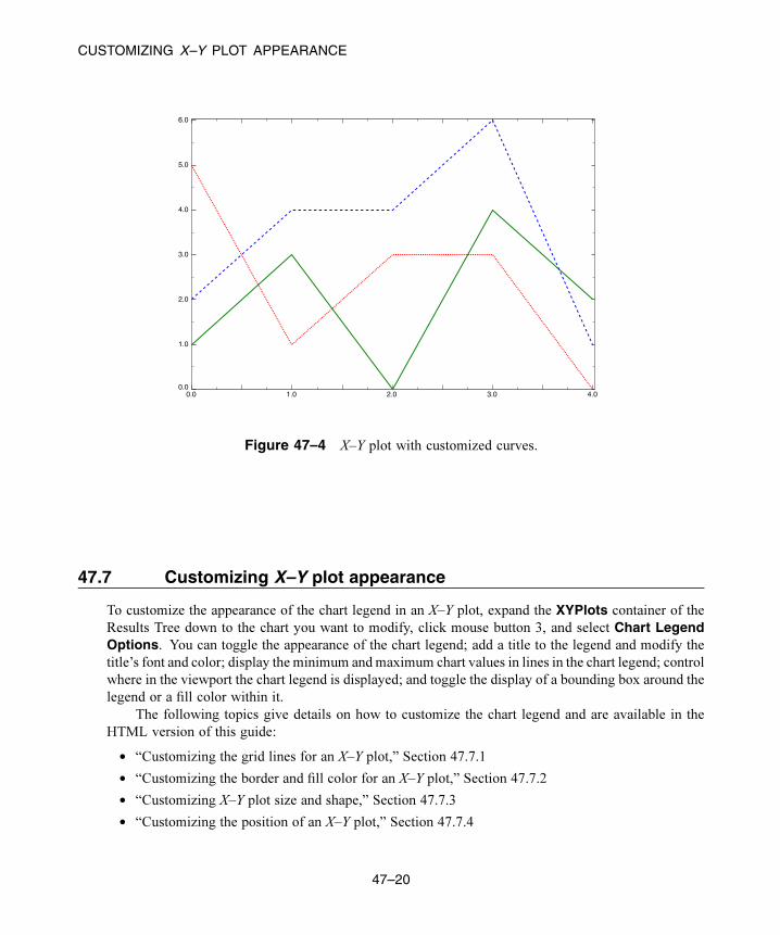
CUSTOMIZING X–Y PLOT APPEARANCE
0.0 1.0 2.0 3.0 4.00.0
1.0
2.0
3.0
4.0
5.0
6.0
Figure 47–4 X–Y plot with customized curves.
47.7 Customizing X–Y plot appearance
To customize the appearance of the chart legend in an X–Y plot, expand the XYPlots container of the
Results Tree down to the chart you want to modify, click mouse button 3, and select Chart LegendOptions. You can toggle the appearance of the chart legend; add a title to the legend and modify the
title’s font and color; display the minimum and maximum chart values in lines in the chart legend; control
where in the viewport the chart legend is displayed; and toggle the display of a bounding box around the
legend or a fill color within it.
The following topics give details on how to customize the chart legend and are available in the
HTML version of this guide:
• “Customizing the grid lines for an X–Y plot,” Section 47.7.1
• “Customizing the border and fill color for an X–Y plot,” Section 47.7.2
• “Customizing X–Y plot size and shape,” Section 47.7.3
• “Customizing the position of an X–Y plot,” Section 47.7.4
47–20
Abaqus ID:
Printed on:

CUSTOMIZING BORDER AND FILL COLORS FOR AN X–Y PLOT
47.8 Customizing the X–Y plot title
To customize the appearance of the chart legend in an X–Y plot, expand the XYPlots container of the
Results Tree down to the chart you want to modify, click mouse button 3, and select Chart LegendOptions. You can toggle the appearance of the chart legend; add a title to the legend and modify the
title’s font and color; display the minimum and maximum chart values in lines in the chart legend; control
where in the viewport the chart legend is displayed; and toggle the display of a bounding box around the
legend or a fill color within it.
The following topics give details on how to customize the chart legend and are available in the
HTML version of this guide:
• “Customizing the contents of the X–Y plot title,” Section 47.8.1
• “Customizing the location of the X–Y plot title,” Section 47.8.2
• “Adding a bounding box and fill color for the X–Y plot title,” Section 47.8.3
47.9 Customizing the appearance of the X–Y plot legend
To customize the appearance of the chart legend in an X–Y plot, expand the XYPlots container of the
Results Tree down to the chart you want to modify, click mouse button 3, and select Chart LegendOptions from the list that appears. You can toggle the appearance of the chart legend; add a title to the
legend and modify the title’s font and color; display the minimum and maximum chart values in lines in
the chart legend; control where in the viewport the chart legend is displayed; and toggle the display of a
bounding box around the legend or a fill color within it.
The following topics give details on how to customize the chart legend and are available in the
HTML version of this guide:
• “Displaying or hiding the X–Y plot legend,” Section 47.9.1
• “Customizing the title of the X–Y plot legend,” Section 47.9.2
• “Adding minimum and maximum values to the X–Y plot legend,” Section 47.9.3
• “Customizing the location of the legend,” Section 47.9.4
• “Customizing the border and fill for the X–Y plot legend,” Section 47.9.5
47.10 Customizing border and fill colors for an X–Y plot
Use the options in the Plot Options dialog box to create a custom border color and a custom background
fill color for one or more X–Y plots in your session. By default, X–Y plots have no border and they
are filled with a light grey background color. You might want to adjust the border color to distinguish
47–21
Abaqus ID:
Printed on:

CUSTOMIZING BORDER AND FILL COLORS FOR AN X–Y PLOT
between different X–Y plots used in an overlay plot; you might want to adjust the fill color if the X–Y
curves used in your plot do not stand out clearly against the default background.
To customize the border and fill colors for an X–Y plot:
1. Select Options→XY Options→Plot Options; or click , which is located with the X–Y
plotting tools in the Visualization module toolbox.
The Plot Options dialog box opens.
2. From the Plots frame, highlight one or more X–Y plots that you want to modify. This frame lists
plot names and the viewports in which they are displayed.
3. Toggle on Show border to display a border around the X–Y plot.
4. If desired, change the color of the X–Y plot border by performing the following steps:
a. Click the color sample immediately to the right of the Show border label .
Abaqus/CAE displays the Select Color dialog box.
b. Use one of the methods in the Select Color dialog box to select a new color. For more
information, see “Customizing colors,” Section 3.2.9.
c. Click OK to close the Select Color dialog box.
The color sample and the X–Y plot border change to the selected color.
5. Toggle on Fill to fill the X–Y plot with the color displayed to the right of the Fill label.
6. If desired, change the X–Y plot fill color by performing the following steps:
a. Click the color sample immediately to the right of the Fill label .
Abaqus/CAE displays the Select Color dialog box.
b. Use one of the methods in the Select Color dialog box to select a new color. For more
information, see “Customizing colors,” Section 3.2.9.
c. Click OK to close the Select Color dialog box.
The X–Y plot fill color changes to the selected color.
47–22
Abaqus ID:
Printed on:

UNDERSTANDING RESULTS ALONG A PATH
48. Viewing results along a path
A path is a series of connected lines that you define by specifying a series of points or edges through
your model. You can view results along the path in the form of an X–Y plot. This chapter explains how
to view results along a path. The following topic is covered:
• “Understanding results along a path,” Section 48.1
In addition, the following sections are available in the HTML version of this guide:
• “Creating a path through your model,” Section 48.2
• “Obtaining X–Y data along a path,” Section 48.3
48.1 Understanding results along a path
To view results along a path through your model, you first select Tools→Path to specify the path and
then select Tools→XY Data to obtain X–Y data along the path.
48.1.1 Path specificationA path is a line you define by specifying a series of points or line segments through your model. The
points can be nodes or coordinate locations; the line segments can be element edges or lines joining the
ends of element edges. Paths can cross more than one part instance. Abaqus/CAE offers four distinct
types of paths:
Node list
The points making up the path consist of nodal locations only. You specify the points using node
labels and node label ranges. A node label is a persistent means of referring to a given node; that is,
node labels do not change as your model deforms. Because of this, the node labels that comprise
a node list path are equally applicable to the undeformed or the deformed model shape. However,
node labels are part instance-specific. In other words, you can have the same node label for multiple
part instances; therefore, you must specify to which part instance you are referring when you use
node labels. For more information, see “Creating or editing a node list path,” Section 48.2.1, in the
HTML version of this guide.
Point list
The points making up the path consist of coordinate locations within your model. These locations
may or may not coincide with nodal locations. Point list coordinates remain fixed in space and
are independent of your model. For example, coordinates that coincide with a nodal location on
the undeformed shape may not coincide with any location on the deformed shape. By the same
48–1
Abaqus ID:
Printed on:

UNDERSTANDING RESULTS ALONG A PATH
logic, point list coordinates are independent of specific part instances. For more information, see
“Creating or editing a point list path,” Section 48.2.2, in the HTML version of this guide.
Edge list
The points making up the path consist of edges that connect nodes within your model. You specify
the edges by selecting individual element edges from the viewport or by selecting the starting edge
and direction and allowing Abaqus/CAE to automatically complete the path to the end of the feature
edge or to an endpoint that you select. Edges are defined by the elements in the model. Because
of this, the edges that comprise an edge list path are equally applicable to the undeformed or the
deformed model shape. However, element labels are part instance-specific. In other words, you can
have the same element label for multiple part instances; therefore, you must specify to which part
instance you are referring when you use edges. For more information, see “Creating or editing an
edge list path,” Section 48.2.3, in the HTML version of this guide.
Circular
The points making up the path consist of coordinate locations within your model. You can create
two types of circular paths in Abaqus/CAE: circumferential and radial. A circumferential path lies
along the edge of a circle or an arc; a radial path lies along a radius. You specify either type of
path by selecting coordinates that define a circle or circular arc and then defining the starting point,
ending point, and number of points along the path. Once you have defined the original circle or
arc, you can select a new radius length to create any path that shares the same center point as the
original. You can use circumferential paths to obtain cross-sectional results in a curved portion of
a model, as shown in Figure 48–1.
Figure 48–1 A circumferential path.
48–2
Abaqus ID:
Printed on:

UNDERSTANDING RESULTS ALONG A PATH
You can use radial paths to obtain results spanning from the inner to the outer face of a curve, as
shown in Figure 48–2; radial paths are ideal for use in stress linearization (for more information on
stress linearization, see Chapter 52, “Calculating linearized stresses”).
Figure 48–2 A radial path.
You can select coordinates by picking nodes from the viewport or by entering values in the prompt
area; in either case, the coordinates remain fixed in space and are independent of your model. For
example, coordinates that coincide with a nodal location on the undeformed shape may not coincide
with any location on the deformed shape. By the same logic, circular path coordinate definitions
are independent of specific part instances. For more information, see “Creating or editing a circular
path,” Section 48.2.4, in the HTML version of this guide.
Abaqus/CAE forms the path by connecting the nodes, points, or edges that you specify in the order you
have given.
After you create a path, you can select Tools→Path from the main menu bar to edit, copy, rename,
delete, or plot it. Plotting the path itself is a means to verify visually that you have specified the intended
line; to view results along the path, you must form X–Y data pairs and produce an X–Y plot. For more
information on managing paths, see “Managing objects using manager dialog boxes,” Section 3.4.9,
in the HTML version of this guide; for more information on producing an X–Y plot of path data, see
“Obtaining X–Y data along a path,” Section 48.3, in the HTML version of this guide.
48.1.2 How Abaqus/CAE obtains results along a pathAbaqus/CAE obtains results along a path in the form of X–Y data pairs. Abaqus determines the data pair
X-values based on the points that make up the path. These points define model locations at which to
48–3
Abaqus ID:
Printed on:

UNDERSTANDING RESULTS ALONG A PATH
obtain data. Abaqus determines the data pair Y-values based on analysis results at those model locations.
Abaqus/CAE considers only the entities in the current display group when calculating the data pairs.
Path data X-values
You can choose to form X-values based only on the points you have specified for the path or to
additionally include all locations at which the path intersects the model. (An intersection occurs
where the path crosses an element face, element edge, surface face, or surface edge. You can
omit individual intersections from the path definition if the intersection lies within a user-specified
distance of an actual data point. You can set this intersection tolerance value using Abaqus Scripting
Interface commands; for more information, see “Session object,” Section 55.18 of the Abaqus
Scripting Reference Guide.)
You can also choose whether Abaqus/CAE interprets the points that make up the path as
locations on the undeformed or the deformed model shape. When the deformed model shape
is chosen, Abaqus/CAE computes the deformed coordinates at a node as the sum of the base
coordinates and the deformation at that node multiplied by the viewport-specific deformation
scale factor. Node list labels and edge lists indicate model locations and are equally applicable to
the undeformed or the deformed model shape. Point list and circular path coordinates are fixed
locations independent of the model geometry. Abaqus does not form data pairs for points that do
not coincide with the model shape you have chosen.
The node labels or point coordinates that comprise a path are usually not in a form suitable for
direct use as X-values. Abaqus/CAE offers several options for you to convert this series of points to
useful X-values and subsequent X–Y plot axis labels. You can choose one of the following options
to convert path points to X-values:
• True distance: X-values correspond to each point’s actual distance along the path in model
space coordinates, starting with zero.
• Normalized distance: X-values correspond to each point’s distance along the path as a
fraction of the total length of the path.
• Sequence ID: X-values correspond to the order in which each point occurs in the path result
list.
• X, Y, or Z distance: X-values correspond to each point’s actual distance along the path in thesingle coordinate direction you specify, starting with zero. This option is particularly useful
for generating a plot of results versus radius in an axisymmetric model.
Path data Y-values
You can control data pair Y-values by choosing the results step, frame, and field output variable for
which Abaqus/CAE obtains results and by controlling how Abaqus/CAE computes certain types of
results, as follows:
• For node-based field output variables such as displacement to be obtained at nodal locations,
Abaqus/CAE reads results directly from the output database with no further computations.
48–4
Abaqus ID:
Printed on:

UNDERSTANDING RESULTS ALONG A PATH
• For element-based field output variables such as stress or strain to be obtained at nodal
locations, Abaqus/CAE reads results from the output database, extrapolates those values to
the nodes, then conditionally averages multiple contributions according to options you select.
• For both node-based and element-based variables to be obtained at path points that do not
coincide with nodal locations, Abaqus/CAE computes values by interpolating from the nodes
to the requested location using a geometric approximation of the element’s shape. You cannot
control this computation.
The averaging options for element-based variables and the complex form options for complex
number values are located in the Result Options dialog box. Averaging reduces multiple
contributions into a single value. When you select result options to partially or fully suppress
averaging, path points receiving multiple contributions produce multiple data pairs. Such data
pairs share the same X-value but have a separate Y-value for each contribution. Depending on your
path and on the characteristics of your model, the following techniques may be necessary to avoid
multiple data pairs sharing the same X-value:
• Set result options to fully enable averaging.
• Set result options to ignore region boundaries when computing values.
• Avoid paths that traverse region discontinuities.
• Avoid paths along a line separating discontinuous regions.
• Use display groups to isolate individual regions prior to obtaining results along a path.
For more information on value averaging, see “Understanding result value averaging,”
Section 42.6.2.
The Y-value of the data pairs is affected by the current complex form if your selected field
output variable contains complex number results. An abbreviation of the complex form is appended
to the Y-axis title when you plot the path. For example, if S-Mises is the selected field output
variable and Magnitude is the complex form, the Y-axis title is S-Mises CPX:Mg. Other
complex forms are similarly abbreviated. For more information on complex forms, see “Controlling
the form of complex results,” Section 42.6.9, in the HTML version of this guide.
Abaqus/CAE does not form data pairs for points that do not have results for the specified step,
frame, or field output variable.
48–5
Abaqus ID:
Printed on:

UNDERSTANDING ANIMATION
49. Animating plots
An animation is a sequence of images that Abaqus/CAE displays in rapid succession, resulting in a
movie-like effect. This chapter covers the following topics:
• “Understanding animation,” Section 49.1
• “Producing and customizing an object-based animation,” Section 49.2
• “Saving an animation file,” Section 49.3
• “Controlling animation playback,” Section 49.4
For detailed instructions on animating plots, see the corresponding chapter in the HTML version of this
guide.
49.1 Understanding animation
Abaqus/CAE offers two means of animation:
Object-based animation
Object-based animation is the display of a sequence of deformed shape plots, contour plots,
symbol plots, or material orientation plots. Abaqus/CAE can produce three different types of
sequences of these plots. These three sequence types are called “time history animation,” “scale
factor animation,” and “harmonic animation.”
Time history animation produces a sequence of deformed shape, contour, symbol, or material
orientation plots that vary over time according to actual analysis results. Scale factor animation
produces a sequence of images that vary only in the scaling of a single deformed shape, contour,
or symbol plot. Harmonic animation produces a sequence of images that represents complex result
values varying according to applied angles.
While an object-based animation is playing, you can dynamically change display
characteristics such as the view, any viewport annotations, and plot state-dependent customization
options.
Image-based animation
Image-based animation is the playback of an animation file. You create an animation file in
Abaqus/CAE by first playing object-based animations in one or more viewports and then selecting
Animate→Save As from the main menu bar. Once saved, your animation can be played
external to Abaqus/CAE using industry-standard animation software. You can choose to save your
image-based animation file in either QuickTime or Audio Video Interleave (AVI) format.
From within Abaqus/CAE you can also display an image-based animation by selecting the
animation file as a background movie. When active, the background movie is displayed in a
viewport in the Visualization module. For more information, see “Displaying and customizing a
background movie,” Section 4.6.3, in the HTML version of this guide.
49–1
Abaqus ID:
Printed on:

UNDERSTANDING ANIMATION
Note: Abaqus/CAE also enables you to save an animation in VRML format, which creates a three-
dimensional rendition of the animation. Because these files are three-dimensional, they are not
strictly image-based; however, you can play and distribute animation files in VRML format as you
would files in QuickTime or AVI formats.
In general, animation playback from a file provides better performance than object-based
animation, particularly for large models. While an image-based animation is playing, you cannot
change its display characteristics.
49.1.1 Time history animationIn a time history animation Abaqus/CAE creates the images in the sequence by redrawing the deformed
shape, contour, symbol, or material orientation plot for every specified frame found in the output database
for the active steps and frames. Each image in a time history animation displays actual analysis results.
The deformation scale factor remains constant for each image in a time history animation. Result frames
can be drawn sequentially or selected from the active frames based on time intervals.
If you are animating a contour plot, the display of the field output values depends on options you
select. The default behavior is for the values within the legend to be fixed based on the minimum and
maximum values for the first and last animation frame. To learn how to set contour limits, see “Setting
contour limits,” Section 44.5.7, in the HTML version of this guide.
49.1.2 Scale factor animationIn a scale factor animation Abaqus/CAE creates all of the deformed shape, contour, or symbol plot images
in the sequence from a single step and frame of the output database. Abaqus/CAE generates animation
scale factors ranging from 0 to 1 or from −1 to 1, according to your specification. Individual images
are formed by applying the range of animation scale factors to the field output values displayed in the
plot. This gives the appearance of the field output evolving over time, although all images are produced
from a single step and frame of your results. (To view the actual evolution of results over time, you must
produce a time history animation.)
If you are animating a contour plot, the display of the field output values depends on options you
select. The default behavior is for the values within the legend to be fixed based on the scaled minimum
and maximum values for the selected results step and frame. To learn how to set contour limits, see
“Setting contour limits,” Section 44.5.7, in the HTML version of this guide. To learn how to customize
the legend, see “Customizing the legend,” Section 56.1.
49.1.3 Harmonic animationHarmonic animation is valid only for field output containing complex numbers. In a harmonic animation
Abaqus/CAE creates all of the deformed shape, contour, or symbol plot images in the sequence from a
single step and frame of the output database. Abaqus/CAE generates angles ranging from 0 to 180° or
from −180° to 180°, according to your specification, and displays the value of the complex field output
49–2
Abaqus ID:
Printed on:

SAVING AN ANIMATION FILE
at each of these angles. This gives the appearance of the field output evolving over time, although all
images are produced from a single step and frame of your results. (To view the actual evolution of results
over time, you must produce a time history animation.) Harmonic animation is useful for simulating the
vibration modes computed by an eigenvalue analysis.
If you are animating a contour plot, the display of the field output values depends on options you
select. The default behavior is for the values within the legend to be fixed based on the range of the real
component. To learn how to set contour limits, see “Setting contour limits,” Section 44.5.7, in the HTML
version of this guide. To learn how to customize the legend, see “Customizing the legend,” Section 56.1.
To learn more about complex results, see “Understanding complex results,” Section 42.6.3.
49.2 Producing and customizing an object-based animation
To produce a time history animation, select Animate→Time History from the main menu bar or use
the tool in the toolbox. To produce a scale factor animation, select Animate→Scale Factor
from the main menu bar or use the tool in the toolbox. To produce a harmonic animation, select
Animate→Harmonic from the main menu bar or use the tool in the toolbox.
In a time history animation you can customize the analysis steps and frames that Abaqus/CAE
includes in your animation. In a scale factor or a harmonic animation you can customize the apparent
motion of your model. For all three types of animation you can customize the underlying deformed shape,
contour, symbol, or material orientation plot. To customize a time history or scale factor animation, select
Options→Animation from the main menu bar.
At any time before or during object-based animation playback you can customize the deformed
shape, contour, symbol, or material orientation plot that underlies your animation. For example, you can
toggle the legend, adjust the deformation scale factor, or choose a different field output variable. Use the
View, Result, and Options menus to customize the underlying plot of your animation.
For more information, see the following sections in the HTML version of this guide:
• “Producing a time history animation,” Section 49.2.1
• “Producing a scale factor animation,” Section 49.2.2
• “Producing a harmonic animation,” Section 49.2.3
• “Customizing a scale factor or harmonic animation,” Section 49.2.4
• “Customizing the underlying plot of an animation,” Section 49.2.5
49.3 Saving an animation file
You can save animations to a file by first playing animations in one or more viewports and then selecting
Animate→Save As from the main menu bar.
49–3
Abaqus ID:
Printed on:
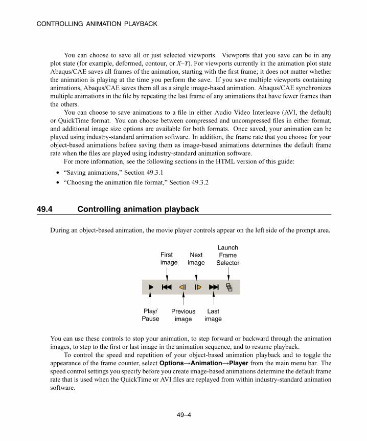
CONTROLLING ANIMATION PLAYBACK
You can choose to save all or just selected viewports. Viewports that you save can be in any
plot state (for example, deformed, contour, or X–Y). For viewports currently in the animation plot state
Abaqus/CAE saves all frames of the animation, starting with the first frame; it does not matter whether
the animation is playing at the time you perform the save. If you save multiple viewports containing
animations, Abaqus/CAE saves them all as a single image-based animation. Abaqus/CAE synchronizes
multiple animations in the file by repeating the last frame of any animations that have fewer frames than
the others.
You can choose to save animations to a file in either Audio Video Interleave (AVI, the default)
or QuickTime format. You can choose between compressed and uncompressed files in either format,
and additional image size options are available for both formats. Once saved, your animation can be
played using industry-standard animation software. In addition, the frame rate that you choose for your
object-based animations before saving them as image-based animations determines the default frame
rate when the files are played using industry-standard animation software.
For more information, see the following sections in the HTML version of this guide:
• “Saving animations,” Section 49.3.1
• “Choosing the animation file format,” Section 49.3.2
49.4 Controlling animation playback
During an object-based animation, the movie player controls appear on the left side of the prompt area.
Firstimage
Nextimage
LaunchFrame
Selector
Play/Pause
Previousimage
Lastimage
You can use these controls to stop your animation, to step forward or backward through the animation
images, to step to the first or last image in the animation sequence, and to resume playback.
To control the speed and repetition of your object-based animation playback and to toggle the
appearance of the frame counter, select Options→Animation→Player from the main menu bar. The
speed control settings you specify before you create image-based animations determine the default frame
rate that is used when the QuickTime or AVI files are replayed from within industry-standard animation
software.
49–4
Abaqus ID:
Printed on:

CONTROLLING ANIMATION PLAYBACK
For more information, see the following sections in the HTML version of this guide:
• “Stopping, restarting, and stepping through an animation,” Section 49.4.1
• “Navigating to a specific frame in the animation,” Section 49.4.2
• “Controlling animation speed and repetition,” Section 49.4.3
• “Showing the animation frame counter,” Section 49.4.4
• “Customizing animation of X–Y plots,” Section 49.4.5
• “Controlling animations in multiple viewports,” Section 49.4.6
• “Customizing the time history of synchronized viewports,” Section 49.4.7
49–5
Abaqus ID:
Printed on:


OVERVIEW OF QUERY TOOLSET IN THE VISUALIZATION MODULE
50. Querying the model in the Visualization module
This chapter explains how you can use the Query toolset to obtain general information about the mesh
and specific Visualization module information. The following topics are covered:
• “Overview of Query toolset in the Visualization module,” Section 50.1
For detailed instructions on querying your model, see “Using the Query toolset,” Section 50.2, in the
HTML version of this guide. For more information on the Query toolset in the Visualization module,
see the following:
• Chapter 51, “Probing the model”
• Chapter 52, “Calculating linearized stresses”
• Chapter 53, “Viewing a ply stack plot”
50.1 Overview of Query toolset in the Visualization module
The Query toolset allows you to obtain general information about your model. The Visualization module
displays the requested information in the message area, and the same information is written to the replay
file. Select Tools→Query from the main menu bar, or select the tool from the Query toolbar to
use the Query toolset.
Items under General Queries provide the following information:
Node
You can obtain information on a selected node’s label, deformed and undeformed coordinates, and
displacement.
Distance
You can obtain information on the deformed and undeformed distance between two selected nodes
and the relative displacement between the nodes.
Angle
You can obtain information on the deformed and undeformed angle formed between three selected
nodes. The second node that you select is the angle’s vertex.
Element
You can obtain information on a selected element’s mesh type, material, section, connectivity, and
current field output variables at the integration point locations. This query is available only when
an output database is selected.
50–1
Abaqus ID:
Printed on:

OVERVIEW OF QUERY TOOLSET IN THE VISUALIZATION MODULE
Mesh
You can obtain information on the name of the current output database, the number of nodes and
elements in your model, and the element types.
Mass properties
You can obtain basic mass properties for the whole model in the output database or for a portion of
the model. This query is available only when an output database is selected. Abaqus/CAE returns
the following information:
• Volume
• Volume centroid
• Mass
• Center of mass
• Moments of inertia about the center of mass or about a specified point
For more information on general model queries, see “Querying the model in the Visualization module,”
Section 50.2.1, in the HTML version of this guide.
Items under Visualization Module Queries provide the following information:
Probe values
Abaqus/CAE displays information in the Probe Values dialog box as you move the cursor around
the current viewport. Probing a model plot displays model data and analysis results; probing an
X–Y plot displays X–Y curve data. For more information on probing, see Chapter 51, “Probing the
model.”
Stress linearization
Stress linearization is the separation of stresses through a section into constant membrane and linear
bending stresses. Abaqus performs stress linearization calculations and displays the results in the
form of anX–Y plot. Stress linearization is available for output databases only. For more information
on stress linearization, see Chapter 52, “Calculating linearized stresses.”
Active elements and nodes
Abaqus/CAE displays the label numbers of all of the active nodes or active elements in the current
viewport. For more information, see “Querying active node or element labels,” Section 50.2.2, in
the HTML version of this guide.
Ply stack plot
Abaqus/CAE creates a new viewport and displays a representative image of a composite layup.
The image shows the plies in the layup along with details of each ply, such as its fiber orientation,
thickness, reference plane, and integration points. Ply stack plots are available for output databases
only. For more information, see Chapter 53, “Viewing a ply stack plot.”
50–2
Abaqus ID:
Printed on:
UNDERSTANDING PROBING
51. Probing the model
This chapter explains how you can use the Query toolset in the Visualization module to probe model and
X–Y plots for output data and to probe an Abaqus/CAE model for attribute values. The following topics
are covered:
• “Understanding probing,” Section 51.1
For detailed instructions on querying your model and probing models, model plots, and X–Y plots, see
“Using the Query toolset to probe the model,” Section 51.2, in the HTML version of this guide. For
information on writing selected probe values to a file, see Chapter 54, “Generating tabular data reports.”
51.1 Understanding probing
When you click the tool in the Visualization module toolbox, Abaqus/CAE enters probe mode and
displays information in the Probe Values dialog box as you move the cursor over the model in the
current viewport. You can also enter probe mode using the tool in the Query toolbar. Probing a
model plot displays model data and analysis results; probing an X–Y plot displays X–Y curve data; and
probing a model from the current model database displays the model data and the values of attributes
such as loads and predefined fields. You can write this information to a file.
The data table in the bottom portion of the Probe Values dialog box contains two dynamic display
rows (the row immediately above the row headings and the bold data row that appears first in the table)
and a series of additional storage rows. Abaqus/CAE updates the dynamic rows continuously to show
the probe values as you move the cursor over the model in the current viewport, and you can change the
value displayed in the top display row by clicking a column heading. Abaqus/CAE updates the table with
additional rows only when you select values of interest by clicking in the viewport, specifying a node or
element label, or selecting the nodes or elements in a particular display group. Values accumulate in the
bottom portion of the dialog box until you delete them, clear the table, or cancel probe mode. You can
also add selected values to a new display group, and you can annotate individual nodes or elements with
field output values at that location.
51.1.1 Probes of models or model plots
If the current viewport contains a model plot (an undeformed, deformed, contour, symbol, or material
orientation plot) or a model from the current model database,, Abaqus/CAE allows you to probe results
from the selected model or output database. The Probe Values dialog box identifies the step, frame,
and field output variable for which Abaqus/CAE will obtain values. To learn how to change the step,
51–1
Abaqus ID:
Printed on:

UNDERSTANDING PROBING
frame, or field output variable, see “Selecting the results step and frame,” Section 42.3, and “Selecting
the primary field output variable,” Section 42.5.3, in the HTML version of this guide.
When you probe a model plot of a three-dimensional shell or a composite solid, the results that
Abaqus/CAE returns depend on your choice of active location in the Section Points dialog box.
Abaqus/CAE returns results from the Top Location section point when Top is the active location and
returns results from the Bottom Location section point when the active location is set to Bottomor Top and bottom. For more information about section points, see “Selecting section point data,”
Section 42.5.9, in the HTML version of this guide.
For model plots you can choose to obtain node-based or element-based data and results, as follows:
Probing nodes
When you choose to probe nodes and position the cursor over a nodal location in the current
viewport, Abaqus/CAE highlights the node and displays the following information about the node
in the data table:
• the node’s label,
• the node’s original coordinates,
• the node’s deformed coordinates (using the current deformed field output variable),
• the elements sharing the node, and
• the current field output variable (including component values, if the current field output
variable is a tensor or vector quantity). If a model is selected in the current viewport, the
current field output variable reflects the value of a model attribute such as a load at the
selected node.
You can display field output at the node whether the current primary variable was originally
saved to the output database at nodal, centroidal, or integration point locations. Abaqus/CAE
calculates nodal values for centroidal and integration point data by extrapolating to the nodes
and averaging according to options you select. If the node refers to unaveraged element data,
all element data associated with the probed node will be displayed. For more information on
averaging, see “Understanding result value averaging,” Section 42.6.2.
You can also display or hide annotations that appear in the viewport for each node you select.
Probe annotations show the node’s label and the results at that node for the current field output
variable. You can customize the font and color of the probe annotation text.
Probing elements
When you choose to probe elements and position the cursor over an element in the current viewport,
Abaqus/CAE highlights the element and displays the following information about the element in
the data table:
• the element’s label,
• the element’s connectivity, and
• the current field output variable (including component values, if the current field output
variable is a tensor or vector quantity). If a model is selected in the current viewport, the
51–2
Abaqus ID:
Printed on:

UNDERSTANDING PROBING
current field output variable reflects the value of a model attribute such as a load at the selected
element.
You can display field output at the element only if the current primary variable is an element-
based variable, such as stress or strain. You can choose the output position at which field output
results are calculated: integration point, centroid, element node, or element face. For each of these
output positions, Abaqus/CAE calculates probe results on an element-by-element basis with no
averaging.
You can also display or hide annotations that appear in the viewport for each element you
select. Probe annotations show the element’s label and the results at that element for the current
field output variable. You can customize the font and color of the probe annotation text.
Regardless of the render style in which the model is displayed, only visible elements can be
probed. If necessary, you can create a display group or use a view cut to reveal otherwise unavailable
interior elements.
51.1.2 X–Y plot probes
If the current viewport contains an X–Y plot, Abaqus/CAE displays as probe values the X–Y curve legend
text, the sequence identification of each point within the curve, and the X- and Y-coordinates of curve
points. You can choose to display only the curve points that comprise an X–Y data object or to interpolate
to display arbitrary points along the curve.
51–3
Abaqus ID:
Printed on:

UNDERSTANDING STRESS LINEARIZATION
52. Calculating linearized stresses
The calculation of linearized stresses is a capability for advanced Abaqus users. It is most commonly
used for two-dimensional axisymmetric models. The following topics are covered:
• “Understanding stress linearization,” Section 52.1
• “Stress linearization example,” Section 52.2
For detailed instructions on stress linearization, see “Obtaining linearized stress results,” Section 52.3,
in the HTML version of this guide. For detailed information on linearized stress result quantities and the
methods of calculation used, see “Stress linearization,” Section 2.17.1 of the Abaqus Theory Guide.
52.1 Understanding stress linearization
Stress linearization is the separation of stresses through a section into constant membrane and linear
bending stresses. Stress linearization is available for output databases only. To linearize stresses in
Abaqus/CAE, the following procedure is used:
• You define a section through your model. You specify the endpoints of the section by selecting
nodes in the model, coordinates in space, or a saved path.
• Abaqus/CAE defines the stress line by interpolating between the two endpoints to obtain a user-
specified number of equal intervals along a straight line.
• You can save the stress line as a path; the saved path includes the endpoints and each interval point
along the stress line. If you save the stress line as a path, Abaqus/CAE always creates a point list
path, regardless of the method that you used to define the endpoints.
• The specified stress results are obtained at equally spaced intervals along the line in a local
coordinate system defined by the line.
• Abaqus/CAE performs stress linearization calculations and displays the results in the form of an
X–Y plot. You can choose to save the data and/or to write it to a file.
If you linearize stresses across multiple part instances, the results will be averaged for any points that
exist in more than one part instance.
To obtain linearized stresses along a line, select Tools→Query from the main menu bar, then select
Stress linearization from the Visualization Module Queries options.
52.1.1 Defining the stress lineYou can define the endpoints of the section for which you want to obtain linearized stresses by selecting
nodes in the model, points in space, or a saved path. You select nodes in the model by selecting the
nodes directly from the viewport or by typing the node labels, and you define points in space by typing
52–1
Abaqus ID:
Printed on:

UNDERSTANDING STRESS LINEARIZATION
the point coordinates. If you select a saved path, Abaqus/CAE uses the path endpoints as the endpoints of
the stress line—other points along the path are ignored. (For more information on paths, see Chapter 48,
“Viewing results along a path.”)
A node label is a persistent means of referring to a given node in a part instance; that is, node labels
do not change as your model deforms. Therefore, if you specify the endpoints of the section using node
labels or a saved node list path, these points will be equally applicable to the undeformed or the deformed
model shape. However, points in space remain fixed and are independent of your model. For example,
coordinates that coincide with a nodal location on the undeformed shape may not coincide with any
location on the deformed shape. If you specify the endpoints of the section using coordinates in space, a
point list path, or a radial path, be sure to specify the coordinates with respect to the correct shape. Edge
list paths cannot be used to define a stress line.
For the best results for an axisymmetric model, the endpoints chosen should be normal to the interior
and exterior surfaces of your model and to the midplane (see Figure 52–1).
axis ofsymmetry
midplane
recommendedstress paths
nonrecommendedstress path
ρ = ∞
ρ = 20
B
A
E
F
DC
2 1
Local coordinatesystem for CD
2
1
Local coordinatesystem for AB
Rc
Rc
Figure 52–1 Recommended stress paths.
52–2
Abaqus ID:
Printed on:

UNDERSTANDING STRESS LINEARIZATION
The section can extend from surface to surface, or it can be entirely in the interior of the model. The
section can also pass through more than one part instance. The following guidelines should also be
considered when selecting the endpoints for the section:
• Avoid paths that traverse spatial discontinuities.
• Avoid paths along a line separating discontinuities.
• Use display groups to isolate individual regions prior to specifying the section.
If the section extends across spatial discontinuities, such as a hole within a part instance or a space
between part instances, an error message will be given.
After you choose the endpoints of the section, you can specify the number of segments into which
the line should be divided or you can accept the default number. Abaqus/CAE defines the stress line by
interpolating between the two endpoints to obtain the specified number of equal intervals along a straight
line.
52.1.2 Extraction of the stress results
The stresses at each point along the stress line are obtained by interpolating the unique nodal stress
values using the averaging criteria defined in the Result Options dialog box (for more information
on specifying the averaging criteria, see “Controlling result averaging,” Section 42.6.6, in the HTML
version of this guide). Abaqus/CAE uses a local coordinate system that is defined by the stress line to
obtain the stress results. The local x-axis lies along the stress line; it originates at the first point on the
stress line and is defined by the vector connecting the first and second points on the stress line. The local
y- and z-axes are determined as follows:
For two-dimensional models:
The local y-axis is obtained by vector multiplication of the global z-axis with the local x-axis. The
local z-axis is the same as the global z-axis.
For three-dimensional models:
If the local x-axis is parallel to the global y-axis:
If the positive local x-axis lies along the positive global y-axis, the local y-axis will be the
negative of the global x-axis. If the positive local x-axis lies along the negative global y-axis,
the local y-axis will be the global x-axis. The local z-axis is obtained by vector multiplication
of the local x-axis and the local y-axis.
If the local x-axis is not parallel to the global y-axis:
The local z-axis is obtained by vector multiplication of the local x-axis and the global y-axis.
The local y-axis is obtained by vector multiplication of the local z-axis and the local x-axis.
52–3
Abaqus ID:
Printed on:

STRESS LINEARIZATION EXAMPLE
The stresses are then linearized. The stress linearization calculations differ for nonaxisymmetric
and axisymmetric models. For more information on these calculations, see “Stress linearization,”
Section 2.17.1 of the Abaqus Theory Guide.
Abaqus displays the resulting linearized stresses in the form of an X–Y plot. Three separate curves
are presented for each stress component representing the following:
1. The actual stress distribution across the stress line.
2. The linearized membrane stress.
3. The sum of the linearized membrane stress and the linearized bending stresses.
In addition, the linearized stress output for each stress component and the stress invariant calculations
for the linearized stresses are written to a report file.
52.2 Stress linearization example
Figure 52–2 shows an example of a stress line defined for an axisymmetric model of a pressure vessel.
(Avg: 75%)S, Mises
+1.206e+03+1.376e+03+1.545e+03+1.715e+03+1.884e+03+2.054e+03+2.223e+03+2.393e+03+2.562e+03+2.732e+03+2.901e+03+3.071e+03+3.240e+03
X
Y
Z
Stress lineSection_A_B
Figure 52–2 Stress line through an axisymmetric model of a pressure vessel.
The stress line Section_A_B is defined through the vessel wall. Figure 52–3 and Figure 52–4 show
the basic settings and computations, respectively, that you use to linearize the S22 stress component for
the undeformed model shape.
52–4
Abaqus ID:
Printed on:

STRESS LINEARIZATION EXAMPLE
Figure 52–3 Stress linearization basic specifications.
Figure 52–4 Stress linearization computations.
52–5
Abaqus ID:
Printed on:
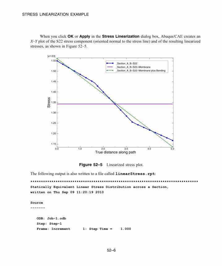
STRESS LINEARIZATION EXAMPLE
When you click OK or Apply in the Stress Linearization dialog box, Abaqus/CAE creates an
X–Y plot of the S22 stress component (oriented normal to the stress line) and of the resulting linearized
stresses, as shown in Figure 52–5.
True distance along path0.0 1.0 2.0 3.0 4.0 5.0
Str
ess
1.15
1.20
1.25
1.30
1.35
1.40
1.45
1.50
1.55
[x1.E3]
_Section_A_B−S22_Section_A_B−S22−Membrane_Section_A_B−S22−Membrane plus Bending
Figure 52–5 Linearized stress plot.
The following output is also written to a file called linearStress.rpt:
********************************************************************************
Statically Equivalent Linear Stress Distribution across a Section,
written on Thu Sep 09 11:20:19 2010
Source
-------
ODB: Job-1.odb
Step: Step-1
Frame: Increment 1: Step Time = 1.000
52–6
Abaqus ID:
Printed on:

STRESS LINEARIZATION EXAMPLE
Linearized Stresses for stress line 'Section_A_B'
Start point, Point 1 - (18.429651260376, 26.8930339813232, 0)
End point, Point 2 - (22.0184745788574, 30.3756923675537, 0)
Number of intervals - 40
------------------------------- COMPONENT RESULTS ------------------------------
S11 S22 S33 S12
0 -462.376 1550.19 1450.75 74.7673
0.125021 -453.722 1542.06 1445.35 74.6265
0.250043 -445.068 1533.93 1439.95 74.4865
0.375064 -436.413 1525.8 1434.55 74.3473
0.500086 -427.759 1517.67 1429.15 74.2089
0.625107 -419.114 1509.55 1423.76 74.0714
0.750128 -410.46 1501.42 1418.36 73.9345
0.87515 -401.806 1493.3 1412.96 73.7983
1.00017 -393.152 1485.17 1407.56 73.663
1.12519 -384.497 1477.04 1402.16 73.5284
1.25021 -375.842 1468.92 1396.76 73.3946
1.37524 -367.187 1460.79 1391.37 73.2615
1.50026 -358.531 1452.67 1385.97 73.1293
1.62528 -348.574 1443.22 1379.7 72.8307
1.7503 -333.79 1428.85 1370.22 71.77
1.87532 -319.007 1414.48 1360.74 70.7052
2.00034 -304.227 1400.1 1351.26 69.6367
2.12536 -289.448 1385.72 1341.78 68.5648
2.25039 -274.656 1371.33 1332.29 67.4908
2.37541 -259.847 1356.91 1322.81 66.4061
2.50043 -245.037 1342.49 1313.32 65.3195
2.62545 -230.228 1328.07 1303.83 64.2284
2.75047 -215.421 1313.64 1294.34 63.1328
2.87549 -200.613 1299.2 1284.84 62.0327
3.00051 -185.807 1284.76 1275.34 60.9282
3.12554 -171.002 1270.32 1265.84 59.8191
3.25056 -156.197 1255.88 1256.34 58.7056
3.37558 -149.216 1248.82 1251.71 57.583
3.5006 -143.031 1242.52 1247.58 56.4609
52–7
Abaqus ID:
Printed on:

STRESS LINEARIZATION EXAMPLE
3.62562 -136.844 1236.21 1243.45 55.34
3.75064 -130.658 1229.91 1239.32 54.2204
3.87566 -124.471 1223.61 1235.19 53.1021
4.00069 -118.283 1217.31 1231.06 51.985
4.12571 -112.095 1211.02 1226.93 50.8691
4.25073 -105.907 1204.72 1222.8 49.7545
4.37575 -99.7185 1198.42 1218.67 48.6412
4.50077 -93.5296 1192.13 1214.55 47.529
4.62579 -87.3403 1185.83 1210.42 46.4182
4.75081 -81.1506 1179.54 1206.3 45.3086
4.87584 -74.9605 1173.25 1202.17 44.2002
5.00086 -68.77 1166.96 1198.05 43.0931
Membrane
(Average) Stress -253.255 1342.83 1317.88 62.6971
Bending
Stress, Point 1 -209.122 218.613 140.324 0
Membrane plus
Bending, Point 1 -462.376 1561.45 1458.2 62.6971
Bending
Stress, Point 2 184.485 -206.054 -140.324 0
Membrane plus
Bending, Point 2 -68.77 1136.78 1177.55 62.6971
Peak Stress,
Point 1 0 -11.2522 -7.44933 12.0701
Peak Stress,
Point 2 0 30.1809 20.4932 -19.604
------------------------------- INVARIANT RESULTS -------------------------------
Bending components in equation for computing
membrane plus bending stress invariants are: S22
52–8
Abaqus ID:
Printed on:

STRESS LINEARIZATION EXAMPLE
Max. Mid. Min. Tresca Mises
Prin. Prin. Prin. Stress Stress
Membrane
(Average) Stress 1345.29 1317.88 -255.714 1601.01 1587.48
Membrane plus
Bending, Point 1 1563.61 1317.88 -255.418 1819.03 1709.46
Membrane plus
Bending, Point 2 1317.88 1139.6 -256.077 1573.95 1492.82
Peak Stress,
Point 1 132.875 -10.5186 -209.855 342.73 298.128
Peak Stress,
Point 2 186.936 27.7292 -119.831 306.767 265.732
The S22 corresponds to the S22 stress shown in Figure 52–5. The actual stress values plotted in the
curve Section_A_B_S22 do not appear in the report. The linearized membrane and membrane-
plus-bending stress curves are generated from the values shown for S22. The reported invariants are
calculated from the selected linearized components.
52–9
Abaqus ID:
Printed on:


OVERVIEW OF PLY STACK PLOTS
53. Viewing a ply stack plot
A ply stack plot shows the plies from the selected region of a composite model. You can create a ply
stack plot in either the Property module or the Visualization module. This chapter describes ply stack
plotting. The following topic is covered:
• “Overview of ply stack plots,” Section 53.1
In addition, the following section is available in the HTML version of this guide:
• “Customizing ply stack plots,” Section 53.2
53.1 Overview of ply stack plots
A ply stack plot is a graphical representation of the plies from a selected region of a composite model.
In effect, a ply stack plot is a core sample of the plies in the selected region. The region can be from a
composite layup or from a composite section.
You can customize the appearance of a ply stack plot. For example, the image can show the sequence
of plies, the orientation of the fibers in each ply, the material in each ply, the relative thickness of the ply,
and the location of the reference surface. Figure 53–1 illustrates a ply stack plot.
t = 0.1
t = 0.1
t = 0.15
t = 0.15
t = 0.1
t = 0.1
1
23
Layup: "RearCabinStiffener"Plot of plies 1 to 6, of 6.
A ply stack is acore samplefrom a region
Figure 53–1 A ply stack plot.
53–1
Abaqus ID:
Printed on:
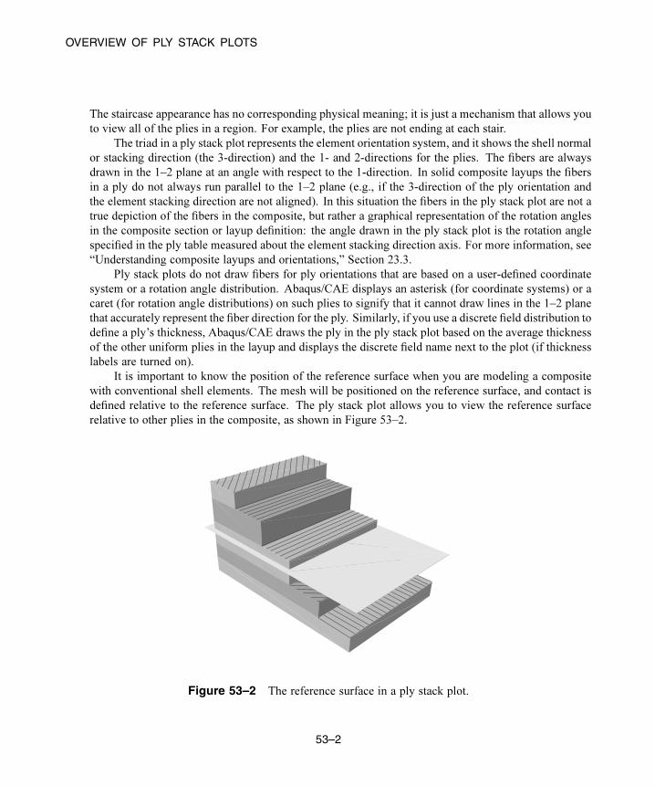
OVERVIEW OF PLY STACK PLOTS
The staircase appearance has no corresponding physical meaning; it is just a mechanism that allows you
to view all of the plies in a region. For example, the plies are not ending at each stair.
The triad in a ply stack plot represents the element orientation system, and it shows the shell normal
or stacking direction (the 3-direction) and the 1- and 2-directions for the plies. The fibers are always
drawn in the 1–2 plane at an angle with respect to the 1-direction. In solid composite layups the fibers
in a ply do not always run parallel to the 1–2 plane (e.g., if the 3-direction of the ply orientation and
the element stacking direction are not aligned). In this situation the fibers in the ply stack plot are not a
true depiction of the fibers in the composite, but rather a graphical representation of the rotation angles
in the composite section or layup definition: the angle drawn in the ply stack plot is the rotation angle
specified in the ply table measured about the element stacking direction axis. For more information, see
“Understanding composite layups and orientations,” Section 23.3.
Ply stack plots do not draw fibers for ply orientations that are based on a user-defined coordinate
system or a rotation angle distribution. Abaqus/CAE displays an asterisk (for coordinate systems) or a
caret (for rotation angle distributions) on such plies to signify that it cannot draw lines in the 1–2 plane
that accurately represent the fiber direction for the ply. Similarly, if you use a discrete field distribution to
define a ply’s thickness, Abaqus/CAE draws the ply in the ply stack plot based on the average thickness
of the other uniform plies in the layup and displays the discrete field name next to the plot (if thickness
labels are turned on).
It is important to know the position of the reference surface when you are modeling a composite
with conventional shell elements. The mesh will be positioned on the reference surface, and contact is
defined relative to the reference surface. The ply stack plot allows you to view the reference surface
relative to other plies in the composite, as shown in Figure 53–2.
Figure 53–2 The reference surface in a ply stack plot.
53–2
Abaqus ID:
Printed on:

OVERVIEW OF PLY STACK PLOTS
You can display a ply stack plot in the Property module after you have created a composite layup
or assigned a composite section to a region. You can also display a ply stack plot in the Visualization
module after you have analyzed a model with a composite layup or a composite section. For more
information, see “Defining composite layups,” Section 12.2.4, and “Creating composite shell sections,”
Section 12.13.7, in the HTML version of this guide.
To produce a ply stack plot, select Tools→Query from the main menu bar and select Ply stackplot from the dialog box that appears. After you have displayed a ply stack plot, you can customize its
appearance by clicking the Ply Stack Plot Options button from the prompt area or by clicking the
tool in the toolbox (in the Visualization module). For detailed instructions on customizing a ply stack
plot, see “Customizing ply stack plots,” Section 53.2, in the HTML version of this guide.
53–3
Abaqus ID:
Printed on:


OVERVIEW OF TABULAR REPORT OPTIONS
54. Generating tabular data reports
You can produce a tabular data report of X–Y data objects, field output results, probe values, or free body
cuts. Abaqus/CAE writes the report to the file name of your choice. Generate a tabular report to save
data values beyond the duration of the session or to print these values. In addition, you can use a tabular
report as ASCII input in subsequent Abaqus/CAE sessions.
This chapter explains how to produce a tabular report and gives an overview of the tabular report
customization options. The following topics are covered:
• “Producing a tabular report,” Section 54.1
• “Overview of tabular report options,” Section 54.2
In addition, the following sections provide details on customizing a tabular report and are available in
the HTML version of this guide:
• “Selecting report data,” Section 54.3
• “Specifying your report file name,” Section 54.4
• “Controlling report layout, width, format, and coordinate system,” Section 54.5
• “Sorting field output data,” Section 54.6
• “Formatting report values,” Section 54.7
• “Reporting data values, minimums, maximums, and totals,” Section 54.8
54.1 Producing a tabular report
To produce a tabular report ofX–Y data objects, field output results, or free body cuts, selectReport→XY,Report→Field Output, or Report→Free Body Cut from the main menu bar, respectively. Customize
the report content, format, and destination using the dialog box that appears. When you have finished,
click Apply to generate the report.
To produce a tabular report of probe values, select Tools→Query from the main menu bar to probe
a model or X–Y plot. Click mouse button 1 while probing to select probe values of interest, then click
Write to File to generate the report.
54.2 Overview of tabular report options
Select Report→XY, Report→Field Output, or Report→Free Body Cut to customize and generate
a tabular listing of X–Y data objects, field output variable values, or free body cuts, respectively. Select
Tools→Query to generate a tabular report of probe values. The following list identifies the tabular
report characteristics that you can customize and the sections where you can find information. You can
customize:
54–1
Abaqus ID:
Printed on:

OVERVIEW OF TABULAR REPORT OPTIONS
• The X–Y data objects or field output variables to include in the report. See “Selecting report data,”
Section 54.3, in the HTML version of this guide.
• The free body cuts to include in the report. Abaqus/CAE includes all active free body cuts in the
current output database in a free body cut report. You can activate and suppress free body cuts
from the Free Body Cut Manager. See “Displaying, hiding, and highlighting free body cuts,”
Section 67.4, in the HTML version of this guide.
• The probe values to include in the report. See Chapter 51, “Probing the model.”
• The file name to which the report is written. See “Specifying your report file name,” Section 54.4,
in the HTML version of this guide.
• The layout and width of the report. See “Controlling report layout, width, format, and coordinate
system,” Section 54.5, in the HTML version of this guide.
• How field output or probe values are sorted. For field output, see “Sorting field output data,”
Section 54.6, in the HTML version of this guide; for probe values, see “Entering tabular data,”
Section 3.2.7.
• The format and significant digits of report values. See “Formatting report values,” Section 54.7, in
the HTML version of this guide.
• Whether or not to include minimum and maximum value summaries or column totals. See
“Reporting data values, minimums, maximums, and totals,” Section 54.8, in the HTML version
of this guide.
• The form of complex results in the report. See “Controlling the form of complex results,”
Section 42.6.9, in the HTML version of this guide.
54–2
Abaqus ID:
Printed on:

OVERVIEW OF PLOT DISPLAY CUSTOMIZATION
55. Customizing plot display
This chapter explains how to customize the appearance of your plots by selecting various plot
state–dependent and plot state–independent options. The following topics are covered:
• “Overview of plot display customization,” Section 55.1
• “Customizing render style, translucency, and fill color,” Section 55.2
• “Customizing element and surface edges,” Section 55.3
• “Customizing model shape,” Section 55.4
• “Customizing model labels,” Section 55.5
• “Displaying multiple plot states,” Section 55.6
• “Displaying element and surface normals,” Section 55.7
• “Customizing the appearance of display bodies,” Section 55.8
• “Customizing camera movement,” Section 55.9
• “Controlling the display of model entities,” Section 55.10
• “Controlling the display of constraints in the Visualization module,” Section 55.11
• “Customizing general model display,” Section 55.12
For detailed instructions on customizing plot display, see the corresponding chapter in the HTML version
of this guide. Chapter 78, “Using display groups to display subsets of your model,” and Chapter 79,
“Overlaying multiple plots,” describe additional ways to customize the display of your model in the
viewport.
55.1 Overview of plot display customization
You can customize how your model appears in undeformed, deformed, contour, symbol, and material
orientation plots. For the undeformed and deformed plot states, all of the customization options applied
to the model shape are plot state–independent. That is, Abaqus/CAE applies the customizations to
all undeformed and deformed plots, including those that also display contours, symbols, or material
orientations. The plot state–independent options govern the render style and fill color; element and
surface edges; element colors; the appearance of model labels, node symbols, and display bodies; the
movement of the camera; the display of various model entities; the smoothness of curved edges; the
color of elements with no results; and model sweeping and extrusion. Use the Options menu in the
main menu bar to choose from these plot state–independent customization options.
Select Tools→Color Code from the main menu bar to color individual elements. Select
Options→Display Body from the main menu bar to customize the appearance of all display bodies
in your model. Select View→View Options from the main menu bar to customize the movement
of the camera. To choose from the remaining plot state–independent options, select View→ODB
55–1
Abaqus ID:
Printed on:

OVERVIEW OF PLOT DISPLAY CUSTOMIZATION
Display Options from the main menu bar. If you choose to superimpose the deformed model shape on
the undeformed shape for the same plot state, select Options→Superimpose from the main menu
bar to customize the undeformed shape independently from the deformed shape. Like the other plot
state–independent customizations, these plot options are applied to superimposed plots in all plot states.
Note: Displaying model labels and/or symbols in the viewport can increase the amount of time needed
to refresh the display for plots and animations.
In addition to the plot state–independent customization options, you can select plot state–dependent
options for the contour, symbol, and material orientation plot states. The plot state–dependent options
are unique to each plot type. For example, you can customize the contour color spectrum, the size and
style of symbols, and the display of material orientation triad axes. If a similar customization such as the
color of model edges in the common and contour plot options can be made using both independent and
dependent plot options, the plot state–dependent option overrides the independent option.
55.1.1 Saving customizations for use in subsequent sessions
By default, plot display customizations persist for the current session only, but you can save
customizations to a file if you want to apply them to subsequent sessions. Abaqus/CAE offers the
following methods to retain plot display customizations:
Saving customizations to the display options file
Select File→Save Display Options from the main menu bar to save all your plot state–dependent
and plot state–independent customization options as display options. Display options are stored in
a file called abaqus_v6.13.gpr, and Abaqus/CAE loads the settings in this file automatically
upon startup as the new default settings throughout your session. For plot state customization,
saving your display options to a file enables you to store settings such as the render style, the
visibility of prescribed conditions and the various types of datum geometry, and the display of
mesh, element, and node labels.
For more information, see “Saving your display options settings,” Section 76.16.
Saving customizations to an XML file, model database, or output database
Select File→Save Session Objects from the main menu bar to save selected plot state–dependent
and plot state–independent customization options to an XML file, the model database, or an output
database. When you use this method, you can save all the customization options or you can save
just the customization options related to one or more plot states. For example, you can save
customizations you make in the common plot options and in the contour plot options to a file.
If you save customizations to a model database or an output database, those settings are used
when you open the file. When you load customizations from an XML file, these customizations
become the new settings for your session. You can load settings from a file by selecting File→LoadSession Objects.
55–2
Abaqus ID:
Printed on:
OVERVIEW OF PLOT DISPLAY CUSTOMIZATION
For more information, see “Managing session objects and session options,” Section 9.9, in the
HTML version of this guide.
55.1.2 Available customization options
Abaqus/CAE provides the following customization options:
Render style
Render style is the style in which Abaqus/CAE displays your model. Render style is a plot
state–independent option; that is, you set it once for all undeformed, deformed, contour, symbol,
and material orientation plots. However, you can set a different value of render style for use
with the undeformed shape in a superimposed plot. Render style choices include wireframe,
filled, hidden, and lightsource-shaded. For more information, see “Customizing render style,
translucency, and fill color,” Section 55.2.
Element and surface edge style and visibility
Edge style is the line style and thickness of element and surface edges; edge visibility is the
extent to which Abaqus/CAE displays these edges. Edge style and visibility options are plot
state–independent, but you can set them differently for use with the undeformed shape in a
superimposed plot. For more information, see “Customizing element and surface edges,”
Section 55.3.
Element and surface edge color
You can control the overall color of element and surface edges using the plot state–independent
Color & Style options. In addition, you can customize the edge color of individual elements
and surfaces using the plot state–independent Color Code dialog box. By default, the color code
selections override the overall colors. For more information on overall edge coloring, see “Selecting
overall element and surface edge color,” Section 55.3.3. To learn more about individual item edge
coloring, see “Customizing the display color of individual objects,” Section 77.8, in the HTML
version of this guide. Individual item edge coloring applies only to wireframe and hidden render
style plots.
Element face and surface fill color
You can control the overall fill color of element faces and surfaces using the plot state–independent
Color & Style options. In addition, you can customize the face color of individual elements using
the plot state–independent Color Code dialog box. By default, the color code selections override
the overall colors. For more information on overall fill color, see “Selecting overall fill color,”
Section 55.2.3. To learn more about individual item color filling, see “Customizing the display
color of individual objects,” Section 77.8, in the HTML version of this guide. Individual item fill
coloring applies only to filled and shaded render style plots.
55–3
Abaqus ID:
Printed on:

OVERVIEW OF PLOT DISPLAY CUSTOMIZATION
Model labels and node symbols
You can change the visibility and customize the color and font of element, node, and face labels
and the color and style of node symbols. All these options are plot state–independent. For more
information, see “Customizing model labels,” Section 55.5.
Element and surface normals
You can choose to display arrows representing the element or surface normals in the model. The
arrows are visible in all plot states, and you can control the arrow size, color, and arrowhead style.
For more information, see “Displaying element and surface normals,” Section 55.7.
Display body appearance
You can customize the render style; edge visibility, color, and style; fill color; scaling; and
translucency for all display bodies in your model. These options are plot state–independent when
applied to display bodies. For more information, see “Customizing the appearance of display
bodies,” Section 55.8.
Camera movement
You can select a coordinate system and match the motion of that coordinate system with the camera.
You can also make the camera follow the rotation of the selected coordinate system. If you are
using the camera in movie mode, you can also position the camera in the model at the origin of the
coordinate system. For more information, see “Customizing camera movement,” Section 55.9.
Entity display
You can control the display of symbols representing various model entities, including boundary
conditions, connectors, coordinate systems, and point elements. Entity display options are
plot state–independent. For more information, see “Controlling the display of model entities,”
Section 55.10.
Constraints display
You can control the display of analysis constraints that were applied in the Interaction module; for
example, tie constraints or kinematic coupling constraints. For more information, see “Controlling
the display of constraints in the Visualization module,” Section 55.11.
General model display options
Abaqus/CAE offers several other plot state–independent general model display options. These
options include:
• Sweep/Extrude to control the three-dimensional display of two-dimensional models. For
more information, see “Sweeping and extruding your model,” Section 55.12.1.
• Mirror/Pattern to simulate the display of a complete model when only a representative portion
of the model was analyzed. For more information, see “Using mirrors and patterns to display
your results,” Section 55.12.2.
55–4
Abaqus ID:
Printed on:
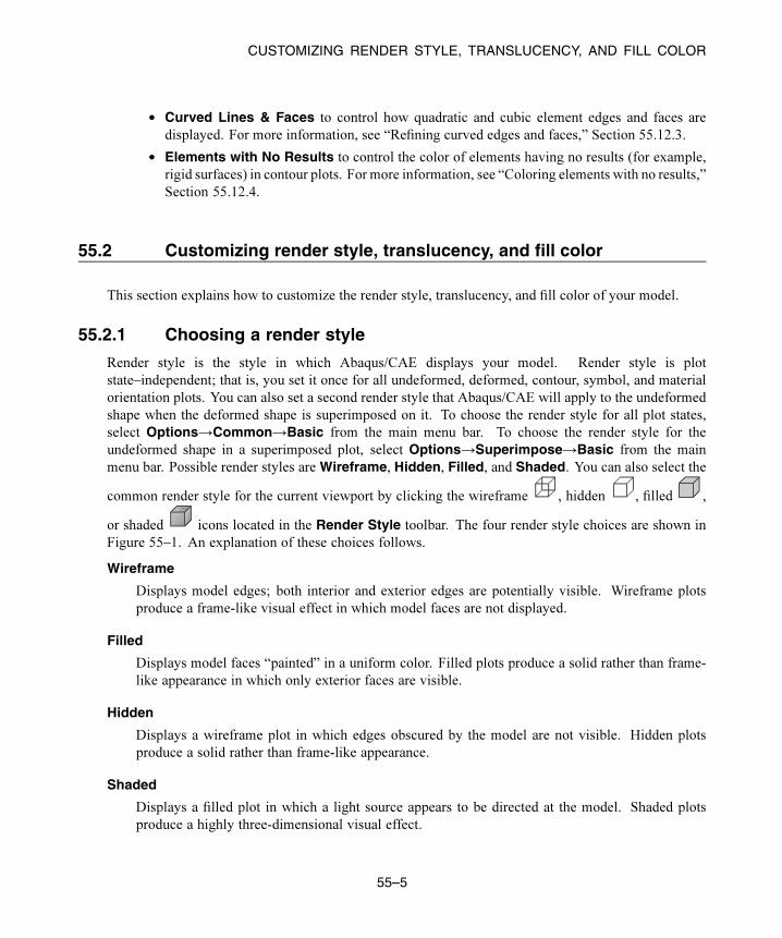
CUSTOMIZING RENDER STYLE, TRANSLUCENCY, AND FILL COLOR
• Curved Lines & Faces to control how quadratic and cubic element edges and faces are
displayed. For more information, see “Refining curved edges and faces,” Section 55.12.3.
• Elements with No Results to control the color of elements having no results (for example,
rigid surfaces) in contour plots. For more information, see “Coloring elements with no results,”
Section 55.12.4.
55.2 Customizing render style, translucency, and fill color
This section explains how to customize the render style, translucency, and fill color of your model.
55.2.1 Choosing a render style
Render style is the style in which Abaqus/CAE displays your model. Render style is plot
state–independent; that is, you set it once for all undeformed, deformed, contour, symbol, and material
orientation plots. You can also set a second render style that Abaqus/CAE will apply to the undeformed
shape when the deformed shape is superimposed on it. To choose the render style for all plot states,
select Options→Common→Basic from the main menu bar. To choose the render style for the
undeformed shape in a superimposed plot, select Options→Superimpose→Basic from the main
menu bar. Possible render styles are Wireframe, Hidden, Filled, and Shaded. You can also select the
common render style for the current viewport by clicking the wireframe , hidden , filled ,
or shaded icons located in the Render Style toolbar. The four render style choices are shown in
Figure 55–1. An explanation of these choices follows.
Wireframe
Displays model edges; both interior and exterior edges are potentially visible. Wireframe plots
produce a frame-like visual effect in which model faces are not displayed.
Filled
Displays model faces “painted” in a uniform color. Filled plots produce a solid rather than frame-
like appearance in which only exterior faces are visible.
Hidden
Displays a wireframe plot in which edges obscured by the model are not visible. Hidden plots
produce a solid rather than frame-like appearance.
Shaded
Displays a filled plot in which a light source appears to be directed at the model. Shaded plots
produce a highly three-dimensional visual effect.
55–5
Abaqus ID:
Printed on:

CUSTOMIZING RENDER STYLE, TRANSLUCENCY, AND FILL COLOR
Figure 55–1 Model showing render style options. From left to right: the wireframe,
filled, hidden, and lightsource-shaded render styles.
55.2.2 Customizing translucencyTranslucency options control the degree of transparency of your model, and they apply to plots in all
render styles except wireframe. Translucency is plot state–independent; that is, you set it once for all
undeformed, deformed, contour, symbol, andmaterial orientation plots. You can also set the translucency
that Abaqus/CAE will apply to the undeformed shape when the deformed shape is superimposed on it.
To control translucency for all plot states, select Options→Common→Other→Translucency from
the main menu bar. To choose the translucency for the undeformed shape in a superimposed plot, select
Options→Superimpose→Other→Translucency from the main menu bar.
For shaded symbol and material orientation plots, symbol plot arrows and material orientation triads
located in the interior of the model are easier to view if you turn on translucency.
55.2.3 Selecting overall fill colorFill color is the color in which Abaqus/CAE displays your model faces. This color is plot
state–independent; that is, you set it once for all undeformed, deformed, symbol, and material
orientation plots. You can also set the fill color that Abaqus/CAE will apply to the undeformed shape
when the deformed shape is superimposed on it. Fill color applies to filled and lightsource-shaded
render style plots only; it is not applicable to contour plots.
You can choose one display color for your entire model, or you can optionally override this display
color for selected items, such as particular elements. For example, you can display your model in
green, with a group of elements shown in red. For more information on individual item coloring, see
“Customizing the display color of individual objects,” Section 77.8 in the HTML version of this guide.
55–6
Abaqus ID:
Printed on:
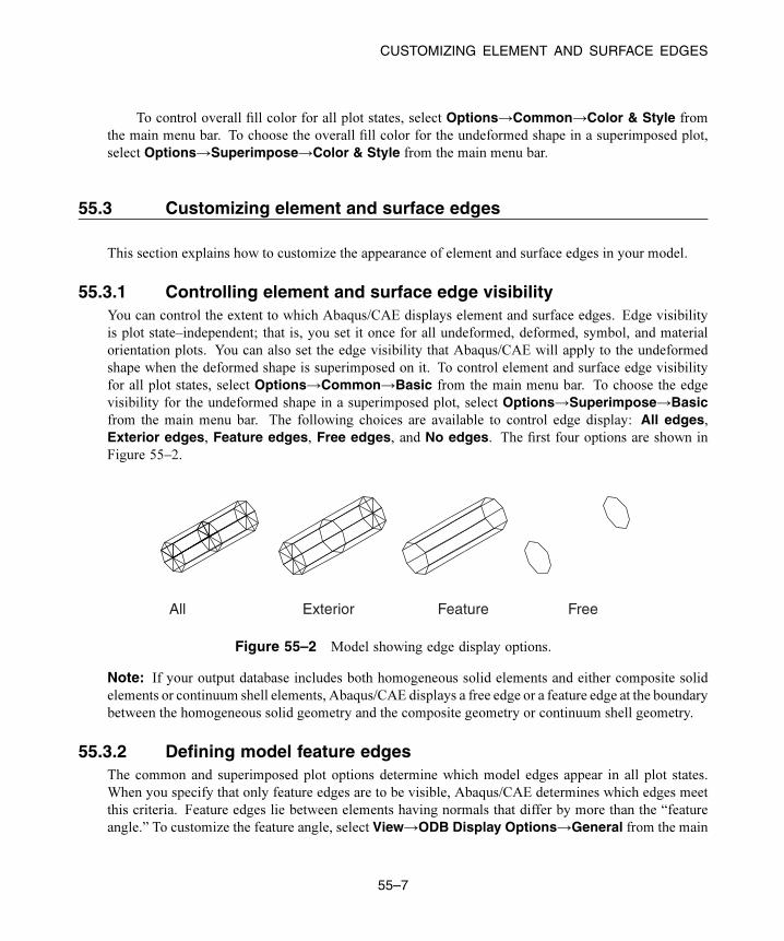
CUSTOMIZING ELEMENT AND SURFACE EDGES
To control overall fill color for all plot states, select Options→Common→Color & Style from
the main menu bar. To choose the overall fill color for the undeformed shape in a superimposed plot,
select Options→Superimpose→Color & Style from the main menu bar.
55.3 Customizing element and surface edges
This section explains how to customize the appearance of element and surface edges in your model.
55.3.1 Controlling element and surface edge visibilityYou can control the extent to which Abaqus/CAE displays element and surface edges. Edge visibility
is plot state–independent; that is, you set it once for all undeformed, deformed, symbol, and material
orientation plots. You can also set the edge visibility that Abaqus/CAE will apply to the undeformed
shape when the deformed shape is superimposed on it. To control element and surface edge visibility
for all plot states, select Options→Common→Basic from the main menu bar. To choose the edge
visibility for the undeformed shape in a superimposed plot, select Options→Superimpose→Basicfrom the main menu bar. The following choices are available to control edge display: All edges,Exterior edges, Feature edges, Free edges, and No edges. The first four options are shown in
Figure 55–2.
All Exterior Feature Free
Figure 55–2 Model showing edge display options.
Note: If your output database includes both homogeneous solid elements and either composite solid
elements or continuum shell elements, Abaqus/CAE displays a free edge or a feature edge at the boundary
between the homogeneous solid geometry and the composite geometry or continuum shell geometry.
55.3.2 Defining model feature edgesThe common and superimposed plot options determine which model edges appear in all plot states.
When you specify that only feature edges are to be visible, Abaqus/CAE determines which edges meet
this criteria. Feature edges lie between elements having normals that differ by more than the “feature
angle.” To customize the feature angle, select View→ODB Display Options→General from the main
55–7
Abaqus ID:
Printed on:

CUSTOMIZING ELEMENT AND SURFACE EDGES
menu bar. Larger angles will reduce the number of feature edges; conversely, smaller angles will cause
more edges to be visible. The default is 20°. The setting of the feature angle applies to all plot states.
However, all segment edges are drawn for analytical rigid surfaces regardless of the feature angle setting.
In Figure 55–3 the plot on the left shows feature edges when the feature angle is set to 0°, the plot
in the middle shows feature edges on the same model but with the feature angle set to 15°, and the plot
on the right shows the model with the feature angle set to 30°.
0° 15° 30°
Figure 55–3 Plots showing feature angles of 0°, 15°, and 30°.
55.3.3 Selecting overall element and surface edge colorYou can customize the color in which Abaqus/CAE displays element and surface edges. With the
exception of contour plots, edge color is plot state–independent; that is, you set it once for all
undeformed, deformed, symbol, and material orientation plots. You can choose a different edge color
for certain render styles, and you can set the edge color that Abaqus/CAE will apply to the undeformed
shape when the deformed shape is superimposed on it. For contour plots you can choose a different
edge color for certain contour types. To select the overall element and surface edge color:
• For all plots except superimposed and contour plots, select Options→Common→Color & Stylefrom the main menu bar.
• For contour plots, select Options→Contour→Color & Style→Model Edges from the main
menu bar.
• For the undeformed shape in a superimposed plot, select Options→Superimpose→Color &Style from the main menu bar.
55–8
Abaqus ID:
Printed on:

CUSTOMIZING MODEL SHAPE
You can choose one display color for your entire model, or you can optionally override this display
color for selected items, such as particular elements. For example, you can display your model in
green, with a group of elements shown in red. For more information on individual item coloring, see
“Customizing the display color of individual objects,” Section 77.8 in the HTML version of this guide.
55.3.4 Customizing element and surface edge styleYou can customize the style and thickness in which Abaqus/CAE displays element and surface
edges. For example, Figure 55–4 shows a plot with default element edges on the left and customized
edges on the right. Edge style options are plot state–independent; that is, you set them once for all
undeformed, deformed, symbol, and material orientation plots. You can also set the edge style options
that Abaqus/CAE will apply to the undeformed shape when the deformed shape is superimposed on
it. To customize the style and thickness in which Abaqus/CAE displays element and surface edges for
all plot states, select Options→Common→Color & Style from the main menu bar. To choose the
edge style for the undeformed shape in a superimposed plot, select Options→Superimpose→Color& Style from the main menu bar.
Figure 55–4 Models showing default and customized element edges.
55.4 Customizing model shape
This section explains how to customize the shape of your model.
55.4.1 Scaling deformationsDeformations are the values of a deformed field output variable; for example, displacement or velocity.
Abaqus/CAE computes the deformed shape by applying the deformations to the undeformed nodal
55–9
Abaqus ID:
Printed on:

CUSTOMIZING MODEL SHAPE
coordinates. You can scale the deformations to magnify, reduce, or otherwise distort the deformed
model shape. For example, Figure 55–5 displays a deformed shape contour plot on the left and the same
plot with the deformation magnified 15 times on the right.
Figure 55–5 Contour plots showing default and magnified deformation values.
Deformation scaling is plot state–independent; that is, you set it once for the deformed shape in
all deformed, contour, symbol, and material orientation plots. The default scaling is a uniform factor
of 1.00 for large-displacement analyses. For small-deformation analyses—for example, a perturbation
analysis—Abaqus/CAE scales the deformation such that the maximum deformation is 10% of the largest
model dimension. To control deformation scaling, select Options→Common→Basic from the main
menu bar.
55.4.2 Scaling coordinates and shrinking the model
You canmagnify, reduce, or otherwise distort the shape of your model by scaling, and you can shrink each
element about its centroid. Scaling modifies all nodal coordinates in each of the X-, Y-, and Z-directions.
Shrinking reduces each element in size uniformly about its centroid. For example, the elements shown
in Figure 55–6 have been shrunk by a factor of 0.40.
55–10
Abaqus ID:
Printed on:
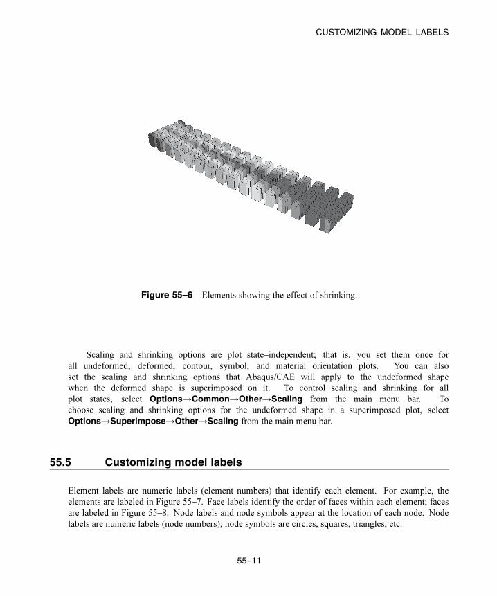
CUSTOMIZING MODEL LABELS
Figure 55–6 Elements showing the effect of shrinking.
Scaling and shrinking options are plot state–independent; that is, you set them once for
all undeformed, deformed, contour, symbol, and material orientation plots. You can also
set the scaling and shrinking options that Abaqus/CAE will apply to the undeformed shape
when the deformed shape is superimposed on it. To control scaling and shrinking for all
plot states, select Options→Common→Other→Scaling from the main menu bar. To
choose scaling and shrinking options for the undeformed shape in a superimposed plot, select
Options→Superimpose→Other→Scaling from the main menu bar.
55.5 Customizing model labels
Element labels are numeric labels (element numbers) that identify each element. For example, the
elements are labeled in Figure 55–7. Face labels identify the order of faces within each element; faces
are labeled in Figure 55–8. Node labels and node symbols appear at the location of each node. Node
labels are numeric labels (node numbers); node symbols are circles, squares, triangles, etc.
55–11
Abaqus ID:
Printed on:

CUSTOMIZING MODEL LABELS
Figure 55–7 Model showing element labels.
Figure 55–8 Model showing face labels.
Element labels, face labels, node labels, the label font, and node symbols are plot state–independent;
that is, you set them once for all undeformed, deformed, contour, symbol, and material orientation
plots. You can also set the labels, the label font, and the symbols that Abaqus/CAE will display on
55–12
Abaqus ID:
Printed on:

DISPLAYING ELEMENT AND SURFACE NORMALS
the undeformed shape when the deformed shape is superimposed on it. To display or suppress labels and
to choose their color and font, select Options→Common→Labels from the main menu bar; to choose
the options for the undeformed shape in a superimposed plot, selectOptions→Superimpose→Labels.
55.6 Displaying multiple plot states
In addition to superimposing the undeformed and deformed shape for a single plot state such as contour
plots, you can choose to display multiple plot states in a viewport. By toggling on Allow Multiple
Plot States in the toolbox, you can choose any combination of the undeformed and deformed
plot shapes with contours, symbols, and material orientations for the selected step and frame of the
current output database. Abaqus/CAE displays the deformed plots using the Common Plot Optionsand the undeformed plots using the Superimposed Plot Options in combination with the other plot
state–independent and dependent options for each plot state.
If you toggle offAllow Multiple Plot States, Abaqus/CAE uses the following order in combination
with the last plot states that were displayed to select the single plot state to display:
• Undeformed
• Deformed
• Contours
• Symbols
• Material Orientations
For example, if you display contours and material orientations, Abaqus/CAE retains the contour plot
when you toggle off Allow Multiple Plot States. This is the same order that the plot states are listed in
the Plot menu and displayed in the toolbox.
To display more complex plot combinations, you must use an Overlay Plot. Overlay plots allow
you to display animations or X–Y plots along with the stationary plot states listed above. You can also
use overlay plots to plot results from multiple steps, frames, or output databases. For more information,
see Chapter 79, “Overlaying multiple plots.”
55.7 Displaying element and surface normals
When you create an undeformed or deformed plot, you can choose to display arrows in the plot
that indicate the directions of the element or surface normals. You can display normal directions for
beams, pipes, frame elements, contact surfaces, membranes, rigid elements, rigid surfaces, shells,
three-dimensional solids, and trusses. (For information about normal directions for a particular type of
element or surface, see Part VI, “Elements,” of the Abaqus Analysis User’s Guide.) To display element
or surface normals in undeformed or undeformed plots, select Options→Common→Normals from
55–13
Abaqus ID:
Printed on:

CUSTOMIZING CAMERA MOVEMENT
the main menu bar. To display element or surface normals on the undeformed shape when the deformed
shape is superimposed, select Options→Superimpose→Normals from the main menu bar.
55.8 Customizing the appearance of display bodies
A display body is a part instance that does not take part in the analysis but is visible during postprocessing.
You can customize the appearance of such part instances in your model using the Display Body Optionsin the Visualization module. The options available for display bodies are similar to those available for
all of the plot states in Abaqus/CAE: render style; edge visibility, color, and style; fill color; scaling;
and translucency can all be customized. Similar to the common plot options, display body options are
plot state–independent; i.e., the options applied to display bodies are reflected in all plot states. Display
body options apply to all display bodies in your model; to customize the appearance of individual display
bodies, you can create display groups based on part instances (see “Creating or editing a display group,”
Section 78.2.1, in the HTML version of this guide). Individual item coloring can also be applied to
individual display body part instances to override the edge and/or fill colors specified as general display
body options; see Chapter 77, “Color coding geometry and mesh elements,” for more information.
To locate the display body options, select Options→Display Body from the main menu bar. Click
the following tabs to customize the appearance of all display bodies in the current viewport:
• Basic: Choose render style (“Choosing a render style,” Section 55.2.1) and edge visibility
(“Controlling element and surface edge visibility,” Section 55.3.1).
Note: The render style icons located in the Render Style toolbar do not apply to display bodies
in any plot state. In addition, by default, only free edges are shown for display bodies while all
exterior edges are shown for other model components.
• Color & Style: Control model edge color (“Selecting overall element and surface edge color,”
Section 55.3.3), model edge style (“Customizing element and surface edge style,” Section 55.3.4),
and model fill color (“Selecting overall fill color,” Section 55.2.3).
• Other: The Other page contains the following tabs:
– Scaling: Control model scaling and shrinking (“Scaling coordinates and shrinking the model,”
Section 55.4.2).
– Translucency: Control shaded render style translucency (“Customizing translucency,”
Section 55.2.2).
55.9 Customizing camera movement
You can customize two groups of camera options in your model by using the View Options in the
Visualization module, as shown in Figure 55–9.
55–14
Abaqus ID:
Printed on:

CUSTOMIZING CAMERA MOVEMENT
Figure 55–9 The View Options dialog box.
TheMode options are available in all Abaqus/CAEmodules except the Sketchmodule; theMode options
are discussed in Chapter 5, “Manipulating the view and controlling perspective,” and are saved only for
the current session. The Camera Movement options are available only in the Visualization module.
They control the position and movement of the camera with respect to a selected local coordinate system.
You can save the settings of the Camera Movement options by selecting File→Save Options from
the main menu bar.
To locate the view options, select View→View Options from the main menu bar. To use the
Camera Movement options, you must first toggle on Move camera with CSYS, then select a local
coordinate system using one of the following methods:
• Select a coordinate system from the list provided in the dialog box,
• Click Create to create a new local coordinate system,
• Click to pick a local coordinate system from the viewport, or
55–15
Abaqus ID:
Printed on:

CUSTOMIZING CAMERA MOVEMENT
• Click Move Camera With Node or use the button in the context bar to create a rectangular
coordinate system following a single node.
Note: To reset the camera to follow the global coordinate system, either toggle off Move camera with
CSYS or click the button in the context bar.
You can select from the following camera movement options:
Move camera with CSYS
Select this option to fix the origin of the selected coordinate system in the viewport. If you create
an animation or change the ODB frame, Abaqus/CAE moves all objects in the viewport relative to
the position of the selected local coordinate system. If the selected local coordinate system is not
a moving coordinate system, you will not observe any difference from the default settings that fix
the camera to the (stationary) global coordinate system.
If you select Move camera with CSYS, it is recommended that you pause any animation in
the current viewport before attempting to manipulate the view.
Follow CSYS rotation
Select this option to fix both the position and the rotation of the local coordinate system in the
viewport. All model rotations are transformed so that the model appears to rotate about the selected
coordinate system. This option is available only when Move camera with CSYS is toggled on.
Move camera to CSYS
This option is available only when Use movie mode and Move camera with CSYS are toggled
on. Use movie mode allows the camera to move into and through the model instead of viewing
the model from a distance (for more information, see “Camera modes and view terminology,”
Section 5.1.1). When you apply Move camera to CSYS, the camera moves to the origin of the
selected coordinate system. Abaqus/CAE toggles this option off immediately after you click Applyin the View Options dialog box to avoid conflicts with the view manipulation tools, some of which
also reposition the camera.
Note: When you apply Move camera to CSYS, Abaqus/CAE may display a blank view in the
viewport. The most common cause for this blank view is the Near plane distance setting; apply
a smaller Near plane distance to view portions of the model that are close to the camera.
WARNING: If you pan, rotate, or magnify the view in the Visualization module, it is recommended that
you first pause any animations in the viewport. Since animations and view manipulations both affect the
view, their instructions to Abaqus/CAE may conflict with each other and create undesirable results.
55–16
Abaqus ID:
Printed on:

CONTROLLING THE DISPLAY OF CONSTRAINTS IN THE VISUALIZATION MODULE
55.10 Controlling the display of model entities
The Entity Display options in the ODB Display Options dialog box allow you to control the display
of symbols representing the following entities in your model:
• boundary conditions applied during the analysis,
• connectors used in the model (the highlighting of endpoints, the display of local orientation
axes associated with each connector, and the display of connector type labels can be controlled
individually),
• coordinate systems written to the current output database or created in the Visualization module
during the current session, and
• point elements, including reference points, mass and inertia elements, springs and dashpots, spot
welds and distributing coupling (DCOUP*) elements, tracer particles, continuum particle elements,
and discrete particle elements.
Model entity display is plot state–independent. Abaqus/CAE displays model entity symbols for the
current step and frame of your output database. You can customize the appearance of the model entity
symbols in the Visualization module only by changing their size.
For information on the symbols representing boundary conditions, see “Understanding symbols that
represent prescribed conditions,” Section 16.5; for information on the symbols representing connectors,
see “Understanding symbols that represent interactions, constraints, and connectors,” Section 15.10. For
information on controlling the display of these entities in assembly-related modules, see “Controlling the
display of attributes,” Section 76.15.
Tip: You can also control the display of connectors using display groups; each connector is
listed as an element set. See “Creating or editing a display group,” Section 78.2.1, in the HTML
version of this guide for more information on display groups.
Only session coordinate systems and reference points are displayed by default. The display of model
entities can affect performance significantly. To maximize the performance of Abaqus/CAE, be selective
about the entities you choose to display.
55.11 Controlling the display of constraints in the Visualization module
In the Visualization module you can selectively control the display of analysis constraints using display
groups and the ODB Display Options dialog box. These controls are useful when debugging models
that contain large numbers of constraints. By turning the display of some constraints on and off, you can
more easily understand complex models.
There are two levels of controls for showing or hiding constraints:
55–17
Abaqus ID:
Printed on:
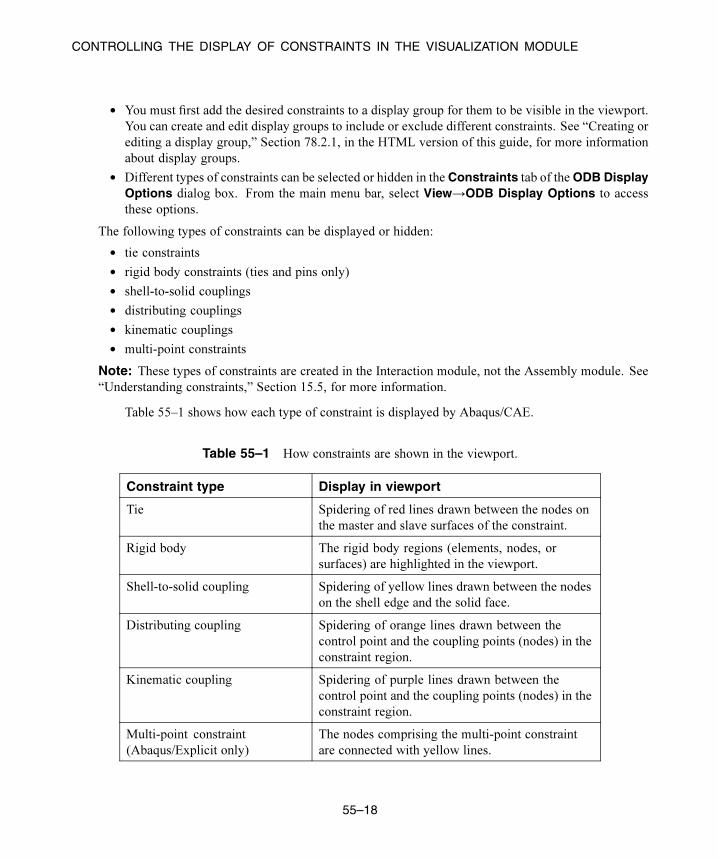
CONTROLLING THE DISPLAY OF CONSTRAINTS IN THE VISUALIZATION MODULE
• You must first add the desired constraints to a display group for them to be visible in the viewport.
You can create and edit display groups to include or exclude different constraints. See “Creating or
editing a display group,” Section 78.2.1, in the HTML version of this guide, for more information
about display groups.
• Different types of constraints can be selected or hidden in the Constraints tab of the ODB DisplayOptions dialog box. From the main menu bar, select View→ODB Display Options to access
these options.
The following types of constraints can be displayed or hidden:
• tie constraints
• rigid body constraints (ties and pins only)
• shell-to-solid couplings
• distributing couplings
• kinematic couplings
• multi-point constraints
Note: These types of constraints are created in the Interaction module, not the Assembly module. See
“Understanding constraints,” Section 15.5, for more information.
Table 55–1 shows how each type of constraint is displayed by Abaqus/CAE.
Table 55–1 How constraints are shown in the viewport.
Constraint type Display in viewport
Tie Spidering of red lines drawn between the nodes on
the master and slave surfaces of the constraint.
Rigid body The rigid body regions (elements, nodes, or
surfaces) are highlighted in the viewport.
Shell-to-solid coupling Spidering of yellow lines drawn between the nodes
on the shell edge and the solid face.
Distributing coupling Spidering of orange lines drawn between the
control point and the coupling points (nodes) in the
constraint region.
Kinematic coupling Spidering of purple lines drawn between the
control point and the coupling points (nodes) in the
constraint region.
Multi-point constraint
(Abaqus/Explicit only)
The nodes comprising the multi-point constraint
are connected with yellow lines.
55–18
Abaqus ID:
Printed on:

CUSTOMIZING GENERAL MODEL DISPLAY
You can change the default colors of the constraint spider lines in the Color Code dialog box. For
more information, see “Coloring constraints in the Visualization module,” Section 77.7, in the HTML
version of this guide.
55.12 Customizing general model display
This section explains several of the general model display options.
55.12.1 Sweeping and extruding your model
You can display axisymmetric models as planar, two-dimensional shapes or “sweep” the models through
a specified angle, producing a three-dimensional visual effect. Similarly, you can view just the modeled
sector of a cyclic symmetric structure or “sweep” the sector to see a specified portion of the entire
model. (For more information on cyclic symmetric structures, see “Analysis of models that exhibit
cyclic symmetry,” Section 10.4.3 of the Abaqus Analysis User’s Guide.) In addition, you can view
two-dimensional models (or three-dimensional cylindrical rigid surfaces) as planar or extrude them to a
specified depth, producing a three-dimensional visual effect. Sweeping and extruding are particularly
useful for displaying contour plots of two-dimensional elements and contact surfaces. To sweep or
extrude your model, select View→ODB Display Options→Sweep/Extrude from the main menu bar.
Axisymmetric analytical rigid surfaces can be rotated about an axis (swept), as can the following
elements: ACAXn, CAXn, CAXAn, CGAXn, DCAXn, DCCAXn, DSAXn, FAXn, MAXn, MGAXn,
RAXn, SAXn, and SAXAn. Models that contain three-dimensional axisymmetric analytical rigid
surfaces or CAXA elements are swept by default (the default start angle, end angle, and number of
sectors vary depending on the model type). If the model contains both analytical rigid surfaces and
CAXA elements, only the CAXA elements are swept by default. When you display boundary conditions
for swept axisymmetric elements, symbols appear on only the original nodes and not on the swept nodes.
Cyclic symmetric models are not swept by default. When you display contours on a swept cyclic
symmetric model, only nodal quantities can be contoured on the swept sectors; scalar, vector, and tensor
quantities at integration points can be contoured only on the original sector.
You can extrude analytical rigid surfaces and all of the planar, two-dimensional solid elements in the
Abaqus library along the Z-direction. For a list of these elements, see “Two-dimensional solid element
library,” Section 28.1.3 of the Abaqus Analysis User’s Guide.
Figure 55–10 shows an axisymmetric planar model in a planar view (left) and the same model with
an axisymmetric sweep angle of 90° and 10 sweep sectors (right). Figure 55–11 shows the original
modeled sector of a cyclic symmetric fan (left) and sectors 1–4 of the swept model (right). Figure 55–12
shows a two-dimensional planar model in a planar view (left) and the same model displayed with an
extrusion depth of 0.1 (right).
55–19
Abaqus ID:
Printed on:

CUSTOMIZING GENERAL MODEL DISPLAY
Figure 55–10 Axisymmetric model with planar and swept display.
Figure 55–11 Cyclic symmetric model: single sector and swept view of multiple sectors.
55.12.2 Using mirrors and patterns to display your resultsIn the Sketch module you can use mirrors and patterns to copy a common feature and complete the
sketch of a feature. Similarly, in the Visualization module you can copy analysis results representing a
repetitive portion of a model to visualize results for the entire model. To mirror results, you can select the
coordinate system and up to three mirrors corresponding to the principal planes of the selected system.
To pattern results, you can select the coordinate system and apply a rectangular or circular pattern. You
can apply mirrors, rectangular patterns, and circular patterns in conjunction; and you can select their
order of application to produce the desired view.
Note: There are no restrictions to prevent copied results from obscuring portions of the original data or
other copies in the viewport.
55–20
Abaqus ID:
Printed on:

CUSTOMIZING GENERAL MODEL DISPLAY
Figure 55–12 Two-dimensional model with planar and extruded display.
Mirrors and patterns are a visualization aid only. Any numerical representation of the results, such as the
contour legend, indicates only the portion of the model that was analyzed. Use great care in selecting
your model and the mirror and pattern settings so that the displayed results will accurately simulate the
complete model.
Figure 55–13 shows one quarter of a plastic fastener as it was modeled for analysis (left) and the
same model mirrored about two symmetry planes to display the complete fastener (right). (The rigid
hole is a swept profile and, thus, appears complete prior to mirroring the fastener.)
Figure 55–13 Quarter-symmetry model (left) and complete fastener display (right).
Figure 55–14 shows a rectangular pattern of completed fasteners.
To mirror or pattern your model, select View→ODB Display Options→Mirror/Pattern from the
main menu bar.
55–21
Abaqus ID:
Printed on:

CUSTOMIZING GENERAL MODEL DISPLAY
Figure 55–14 A rectangular pattern of fasteners.
55.12.3 Refining curved edges and facesIf your model contains quadratic elements, cubic elements, 2-node spring elements, or analytical rigid
surfaces having curved segments, you can control the refinement with which Abaqus/CAE displays these
curved model components. Similarly, if your model contains 2-node dashpot elements, you can control
the refinement of the symbol used to represent those elements. To control the refinement of curved edges
and faces in your model, select View→ODB Display Options→General from the main menu bar,
then choose a refinement level between extra coarse and extra fine. When you select Extra Coarserefinement, Abaqus/CAE displays curved elements using straight lines; midside nodes have no effect
on the shape displayed for these elements. Extra Coarse refinement will treat springs and dashpots as
straight lines. For example, in Figure 55–15 the Extra Coarse refinement level was used to create the
undeformed plot on the left, and the Extra Fine refinement level was used to produce an undeformed
plot of the same model on the right.
Note: As the refinement level increases, the display performance will decrease. The Medium setting
should produce acceptable results for most models.
55–22
Abaqus ID:
Printed on:

CUSTOMIZING GENERAL MODEL DISPLAY
Figure 55–15 Model plotted with different refinement levels (extra coarse and extra fine).
55.12.4 Coloring elements with no resultsTo produce a contour plot, Abaqus/CAE reads results for the variable and frame you specify from the
output database. Results for a particular variable and frame may not be available or may not be applicable
for one or more elements included in the plot. To specify the display color for elements that have no
results in contour plots (including display bodies), select View→ODB Display Options→Generalfrom the main menu bar. The default color is white.
For example, the contour plot in Figure 55–16 shows the von Mises stress generated when a blank
sheet is deformed using a die and punch (the punch is not shown in the figure). In this case the color
white was selected for elements with no results. The die elements appear white because the die is a rigid
surface for which no stress results exist.
55.12.5 Controlling beam profile displayYou can view a realistic display of the beam profile for results data by selecting View→ODB DisplayOptions in the Visualization module. Beam rendering is available in the Visualization module for
undeformed, deformed, and contour plots only. For deformed plots Abaqus/CAE scales the displacement
components of the deformation but does not scale the rotational components of the deformation when
you change the deformation scale factor.
In addition, because the rendering of beam profiles requires the presence of beam orientation data in
the output database, you can display beam profiles during postprocessing only if nodal output is requested
in the model. For more information, see “Using a beam section integrated during the analysis to define
the section behavior,” Section 29.3.6 of the Abaqus Analysis User’s Guide.
Abaqus/CAE does not render the tapering of beam profiles along their length. If your model includes
tapered beam sections, Abaqus/CAE renders these beams using the beam’s starting profile along its entire
55–23
Abaqus ID:
Printed on:

CUSTOMIZING GENERAL MODEL DISPLAY
Figure 55–16 Contour plot of blank and die.
length. For more information about tapered beams, see “Creating beam sections,” Section 12.13.11, in
the HTML version of this guide.
Displaying beam profiles is useful for checking that the correct profile has been assigned to a
particular region and that the assigned beam orientation results in the expected orientation of the profile.
For example, Figure 55–17 shows the box beam profiles displayed on the light-service crane described
in “Example: cargo crane,” Section 6.4 of Getting Started with Abaqus: Interactive Edition.
If you assign a general beam section to a wire, Abaqus/CAE displays the beam profile as an ellipse
with a cross-sectional area and moments of inertia ( and ) that match the values you specified.
If you assign a truss section to a wire, Abaqus/CAE displays the truss profile as a circle with a cross-
sectional area that matches the value you specified.
Abaqus/CAE renders beam profiles according to the current settings for color coding and
translucency. When these settings change, the color and translucency of the beam profiles change as
well. When beam profiles are displayed, Abaqus/CAE disables scaling and shrinking of the model.
55.12.6 Controlling shell thickness displayIf you use shell elements to model relatively thin components in your analysis, you can use the
View→ODB Display Options to view the actual thickness of these shell elements in your model
during postprocessing. Rendering of shell thickness is available in the Visualization module for all
plot states. For deformed and contour plots Abaqus/CAE scales the displacement components of the
55–24
Abaqus ID:
Printed on:
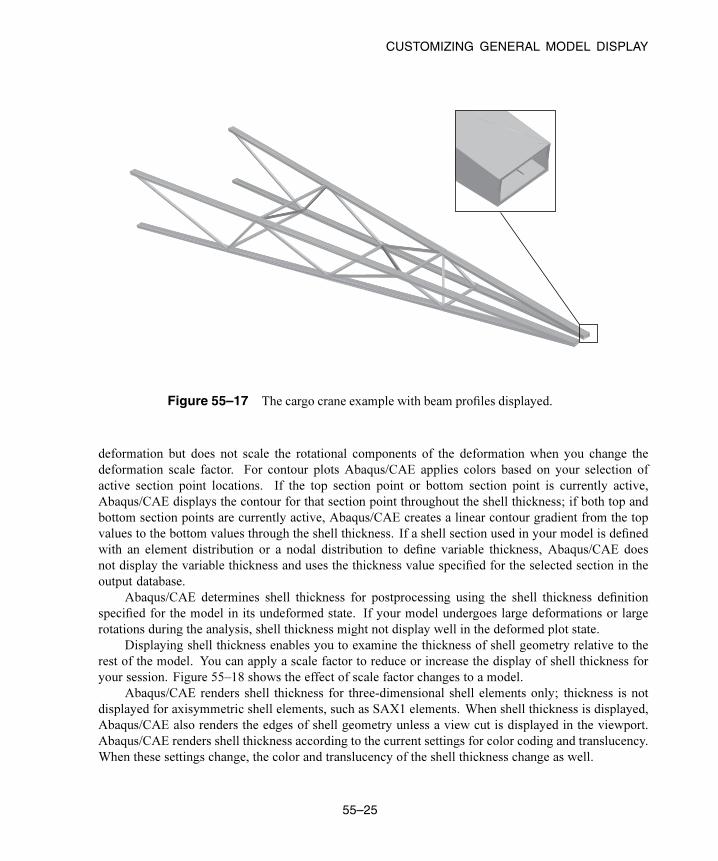
CUSTOMIZING GENERAL MODEL DISPLAY
Figure 55–17 The cargo crane example with beam profiles displayed.
deformation but does not scale the rotational components of the deformation when you change the
deformation scale factor. For contour plots Abaqus/CAE applies colors based on your selection of
active section point locations. If the top section point or bottom section point is currently active,
Abaqus/CAE displays the contour for that section point throughout the shell thickness; if both top and
bottom section points are currently active, Abaqus/CAE creates a linear contour gradient from the top
values to the bottom values through the shell thickness. If a shell section used in your model is defined
with an element distribution or a nodal distribution to define variable thickness, Abaqus/CAE does
not display the variable thickness and uses the thickness value specified for the selected section in the
output database.
Abaqus/CAE determines shell thickness for postprocessing using the shell thickness definition
specified for the model in its undeformed state. If your model undergoes large deformations or large
rotations during the analysis, shell thickness might not display well in the deformed plot state.
Displaying shell thickness enables you to examine the thickness of shell geometry relative to the
rest of the model. You can apply a scale factor to reduce or increase the display of shell thickness for
your session. Figure 55–18 shows the effect of scale factor changes to a model.
Abaqus/CAE renders shell thickness for three-dimensional shell elements only; thickness is not
displayed for axisymmetric shell elements, such as SAX1 elements. When shell thickness is displayed,
Abaqus/CAE also renders the edges of shell geometry unless a view cut is displayed in the viewport.
Abaqus/CAE renders shell thickness according to the current settings for color coding and translucency.
When these settings change, the color and translucency of the shell thickness change as well.
55–25
Abaqus ID:
Printed on:

CUSTOMIZING GENERAL MODEL DISPLAY
Figure 55–18 From left to right: shell thickness scale
factor settings of 0.5, 1 (default), and 2.
55.12.7 Viewing removed elements
You can create model change interactions that deactivate selected components of the model (geometry,
elements, skins, and stringers). Skins, geometry, and elements can be removed from the viewport for
model change interactions on model geometry. Skins, stringers, and elements can be removed from
the viewport for model change interactions on an orphan mesh. You can control the visibility of these
removed components from the ODB Display Options dialog box.
The behavior of the viewport depends on the status of the visibility toggle and on the plot state.
Elements deactivated in a model change interaction can be removed from the viewport for all plot states.
When the option to remove deactivated elements in the viewport is toggled off, the deactivated elements
are colored gray in the contour plot but remain unchanged for all other plot states. If the option to display
beam profiles is toggled off, Abaqus/CAE will not remove deactivated elements with beam profiles from
the viewport, regardless of the status of the removed element toggle.
55–26
Abaqus ID:
Printed on:
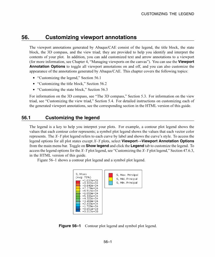
CUSTOMIZING THE LEGEND
56. Customizing viewport annotations
The viewport annotations generated by Abaqus/CAE consist of the legend, the title block, the state
block, the 3D compass, and the view triad; they are provided to help you identify and interpret the
contents of your plot. In addition, you can add customized text and arrow annotations to a viewport
(for more information, see Chapter 4, “Managing viewports on the canvas”). You can use the ViewportAnnotation Options to toggle all viewport annotations on and off, and you can also customize the
appearance of the annotations generated by Abaqus/CAE. This chapter covers the following topics:
• “Customizing the legend,” Section 56.1
• “Customizing the title block,” Section 56.2
• “Customizing the state block,” Section 56.3
For information on the 3D compass, see “The 3D compass,” Section 5.3. For information on the view
triad, see “Customizing the view triad,” Section 5.4. For detailed instructions on customizing each of
the generated viewport annotations, see the corresponding section in the HTML version of this guide.
56.1 Customizing the legend
The legend is a key to help you interpret your plots. For example, a contour plot legend shows the
values that each contour color represents; a symbol plot legend shows the values that each vector color
represents. The X–Y plot legend refers to each curve by label and shows the curve’s style. To access the
legend options for all plot states except X–Y plots, select Viewport→Viewport Annotation Optionsfrom the main menu bar. Toggle on Show legend and click the Legend tab to customize the legend. To
access the legend options for the X–Y plot legend, see “Customizing the X–Y plot legend,” Section 47.6.3,
in the HTML version of this guide.
Figure 56–1 shows a contour plot legend and a symbol plot legend.
Figure 56–1 Contour plot legend and symbol plot legend.
56–1
Abaqus ID:
Printed on:

CUSTOMIZING THE TITLE BLOCK
You can display or suppress legends for all plot states, and you can customize the following:
• the position of the legend,
• the font and color of the legend text,
• the appearance of a box outlining the legend,
• whether minimum and maximum plot values are shown,
• the appearance of the legend background (the rectangular area behind the legend),
• the formatting of the numbers displayed for the digit values, and
• the number of digits displayed for the legend values.
You cannot directly specify the size of the legend. However, by varying the size of the text font or the
number of digits in the legend values, you can increase or decrease the legend’s size.
The content of the legend depends on the plot type and on plot state–specific options such as the
number of contour intervals. For more information on contour plot legend content, see “Understanding
contour plotting,” Section 44.1.
This section describes how to customize the legend for all plot states except X–Y plots. To customize
the X–Y plot legend, see “Customizing the X–Y plot legend,” Section 47.6.3, in the HTML version of
this guide.
56.2 Customizing the title block
The title block contains text identifying the model and results shown in the current plot. This text
indicates:
• The name of the output database (from the name of the analysis job).
• The description of the model.
• The product name (usually Abaqus/Standard or Abaqus/Explicit) and release used to generate the
output database.
• The date the output database was last modified.
You can display or suppress the title block for all plot states, and you can display or suppress the
appearance of a box bounding the title block. In addition, you can control the position, text font, and text
color of the title block and the appearance of the title block background. You cannot directly specify the
size of the title block. However, by varying the size of the text font, you can increase or decrease the title
block’s size. The content of the title block is fixed and cannot be customized. To access the title block
options, select Viewport→Viewport Annotation Options from the main menu bar. Toggle on Showtitle block and click the Title Block tab to customize the appearance of the title block.
56–2
Abaqus ID:
Printed on:

CUSTOMIZING THE STATE BLOCK
56.3 Customizing the state block
The state block contains text identifying the analysis results associated with the current plot. This
information includes step, frame, results variables, deformation magnification factor, eigenmode, and
eigenvalue, as applicable.
You can display or suppress the state block for all plot states, and you can display or suppress the
appearance of a box bounding the state block. In addition, you can control the position, text font, and text
color of the state block and the appearance of the state block background. You cannot directly specify
the size of the state block. However, by varying the size of the text font, you can increase or decrease the
state block’s size. The content of the state block is fixed and cannot be customized. To access the state
block options, select Viewport→Viewport Annotation Options from the main menu bar. Toggle on
Show state block and click the State Block tab to customize the appearance of the state block.
56–3
Abaqus ID:
Printed on:


Part VI: Using toolsetsThis part describes how to use each of the toolsets in Abaqus/CAE (except those in the Visualization module,
which are discussed in Part V, “Viewing results”). The following topics are covered:
• Chapter 57, “The Amplitude toolset”
• Chapter 58, “The Analytical Field toolset”
• Chapter 59, “The Attachment toolset”
• Chapter 60, “The CAD Connection toolset”
• Chapter 61, “The Customize toolset”
• Chapter 62, “The Datum toolset”
• Chapter 63, “The Discrete Field toolset”
• Chapter 64, “The Edit Mesh toolset”
• Chapter 65, “The Feature Manipulation toolset”
• Chapter 66, “The Filter toolset”
• Chapter 67, “The Free Body toolset”
• Chapter 68, “The Options toolset”
• Chapter 69, “The Geometry Edit toolset”
• Chapter 70, “The Partition toolset”
• Chapter 71, “The Query toolset”
• Chapter 72, “The Reference Point toolset”
• Chapter 73, “The Set and Surface toolsets”
• Chapter 74, “The Stream toolset”
• Chapter 75, “The Virtual Topology toolset”
Abaqus ID:
Printed on:

UNDERSTANDING THE AMPLITUDE EDITORS
57. The Amplitude toolset
Amplitudes allow you to specify arbitrary time or frequency variations of load, displacement, and some
interaction attributes throughout a step using step time or throughout an analysis using total time. The
Amplitude toolset allows you to create and manage amplitudes. This chapter covers the following topics:
• “Understanding the role of the Amplitude toolset,” Section 57.1
• “Understanding the amplitude editors,” Section 57.2
In addition, more detailed information is available in “Selecting an amplitude type to define,”
Section 57.3, in the HTML version of this guide.
57.1 Understanding the role of the Amplitude toolset
The Amplitude toolset allows you to create any type of amplitude that is supported by Abaqus/Standard,
Abaqus/Explicit, or Abaqus/CFD. Amplitudes created in the Amplitude toolset always involve relative
data, while amplitudes defined directly in the input file can involve either relative or absolute data. (For
more information, see “Specifying relative or absolute data” in “Amplitude curves,” Section 34.1.2 of
the Abaqus Analysis User’s Guide.) You can also use the Amplitude toolset to define a spectrum to be
used in a response spectrum analysis.
Select Tools→Amplitude→Create from the main menu to create a new amplitude definition;
select Edit from the same menu to make changes to an existing definition. Either command opens the
amplitude editor, which allows you to select the options and provide the data needed to define your
amplitude.
You can also plot amplitude data in much the same way that you can plot X–Y data. For more
information about using the Amplitude Plotter plug-in, see “Plotting amplitude data,” Section 82.12,
in the HTML version of this guide.
57.2 Understanding the amplitude editors
You create amplitudes by entering data in the amplitude editor; you can type the data in using the
keyboard or you can read it in from a file. (For more information, see “Entering tabular data,”
Section 3.2.7.)
The top panel of the editor displays the name of the amplitude and the amplitude type. The format
of the rest of the editor depends on the type of amplitude you are creating. For example, the editor for
creating a periodic amplitude is shown in Figure 57–1.
57–1
Abaqus ID:
Printed on:

UNDERSTANDING THE AMPLITUDE EDITORS
Figure 57–1 The amplitude editor.
57–2
Abaqus ID:
Printed on:

USING ANALYTICAL EXPRESSION FIELDS
58. The Analytical Field toolset
Abaqus/CAE provides two types of analytical fields: expression fields and mapped fields. You can
use analytical fields to define spatially varying values for selected properties, loads, interactions, and
predefined fields, such as the variation of a pressure over a region in a pressure load. The Analytical Field
toolset allows you to create and manage analytical fields in the Property module, Interaction module, or
Load module. This chapter covers the following topics:
• “Using the Analytical Field toolset,” Section 58.1
• “Using analytical expression fields,” Section 58.2
• “Using analytical mapped fields,” Section 58.3
• “Displaying symbols for interactions and prescribed conditions that use analytical fields,”
Section 58.4
• “Displaying symbols to visualize mapping source data,” Section 58.5
In addition, more detailed information is available in the following topics, in the HTML version of this
guide:
• “Creating expression fields,” Section 58.6
• “Creating mapped fields,” Section 58.7
58.1 Using the Analytical Field toolset
The Analytical Field toolset allows you to create and manage analytical fields. Analytical fields defined
using mathematical expressions are called expression fields. Analytical fields defined using an external
data source, such as point cloud data, are called mapped fields. Analytical fields indicate points in space
using coordinates of the global coordinate system or of a local coordinate system.
Select Tools→Analytical Field→Create from the main menu bar in the Property module,
Interaction module, or Load module to create a new analytical field. Select Edit from the same menu to
change an existing analytical field.
58.2 Using analytical expression fields
Analytical expression fields define analytical functions—special types of mathematical functions.
You can use expression fields in many prescribed conditions to define spatially varying parameters.
For more information, see the following sections in the HTML version of this guide:
• “Using the interaction editors,” Section 15.13
58–1
Abaqus ID:
Printed on:

USING ANALYTICAL EXPRESSION FIELDS
• “Using the load editors,” Section 16.9
• “Using the boundary condition editors,” Section 16.10
• “Using the predefined field editors,” Section 16.11
58.2.1 Building valid expressions
Expression fields describe the variation of a parameter for selected interactions and prescribed
conditions (such as a pressure magnitude) at a point in space. You create an expression field by building
a mathematical expression in the expression field editor. To locate the expression field editor, select
Tools→Analytical Field→Create from the main menu bar.
Expression fields indicate points in space using coordinates of the global coordinate system or of a
local coordinate system. In the expression field editor, these coordinates are listed asParameter Names.By default, the expression is built using the coordinates of the global coordinate system (X, Y, and Zparameter names). The parameter names that are available depend on the type of coordinate system that
you select, as shown in Table 58–1. For cylindrical and spherical coordinate systems, the values for Thand P are evaluated in radians in the range from to .
Table 58–1 Relationship between coordinate system types and
parameter names in the expression field editor.
Coordinate system type Parameter Parameter names
Rectangular or Global (default) X-, Y-, and Z-axes X, Y, Z
Cylindrical R-, -, and Z-axes R, Th, Z
Spherical R-, -, and -axes R, Th, P
An expression is composed using one or more parameter names and one or more operators.
You can build the mathematical expression in the expression window of the editor by selecting the
parameter names and operators from lists or by typing the parameter names and operators directly into
the expression window. Parameter names and operators are case sensitive. Expressions use the syntax
required by Python; entries containing errors will generate standard Python errors. See “Overview of
operations and functions in expressions,” Section 58.2.2, for information on supported operators.
The following examples demonstrate valid expressions.
Example 1
To define a spatial variation with linear distance along a face, type:
4.5 * X + 2.75
in the expression window of the editor. X is the parameter name representing the distance along the
face.
58–2
Abaqus ID:
Printed on:

USING ANALYTICAL EXPRESSION FIELDS
Example 2
To define a more complex spatial variation in a cylindrical coordinate system, type:
R + sin(Th*pi/2)
in the expression window of the editor.
For detailed information, see “Creating expression fields,” Section 58.6, in the HTML version of this
guide.
58.2.2 Overview of operations and functions in expressions
This section lists the operations and functions available in the expression field editor. Arguments to
trigonometric functions are assumed to be in radians in the range from to . For more information,
see the documentation for the math module (http://www.python.org/doc/current/lib/module-math.html)
on the official Python home page.
Mathematical operations:
+ Add
• Subtract
* Multiply
/ Divide
% Return the remainder of integer division.
1/A Return the reciprocal of A.
ceil(A) Return the ceiling of A, the smallest integer value greater than or
equal to A.
fabs(A) Return the absolute value.
floor(A) Return the floor of A, the largest integer value less than or equal to A.
fmod(A,B) Return fmod(A, B), as defined by the platform C library. The intent
of the C standard is that fmod(A, B) be exactly (mathematically; to
infinite precision) equal to A − n * B for some integer n such that the
result has the same sign as A and magnitude less than abs(B).
58–3
Abaqus ID:
Printed on:

USING ANALYTICAL EXPRESSION FIELDS
frexp(A)[ ] Return the mantissa and exponent of A as the pair (m, e). m is a float
and e is an integer such that A = m * 2 ** e exactly. Use the brackets
to specify the index of the return value to use in the expression
evaluation.
modf(A)[ ] Return the fractional and integer parts of A. Use the brackets to specifythe index of the return value to use in the expression evaluation.
Trigonometric functions:
acos(A) Return the arccosine.
asin(A) Return the arcsine.
atan(A) Return the arctangent.
cos(A) Return the cosine.
cosh(A) Return the hyperbolic cosine.
hypot(A,B) Return the Euclidean norm, sqrt(A*A + B*B). This is the length of
the vector from the origin to point (A, B).
sin(A) Return the sine.
sinh(A) Return the hyperbolic sine.
tan(A) Return the tangent.
tanh(A) Return the hyperbolic tangent.
Power and logarithmic functions:
exp(A) Return the natural exponential to the power A, .
ldexp(A,B) Return A * ( ).
log(A) Return the natural logarithm.
log10(A) Return the base 10 logarithm.
pow(A,B) Raise a variable to a power.
sqrt(A) Return the square root.
Constants:
pi Mathematical constant π.
e Mathematical constant e.
58–4
Abaqus ID:
Printed on:
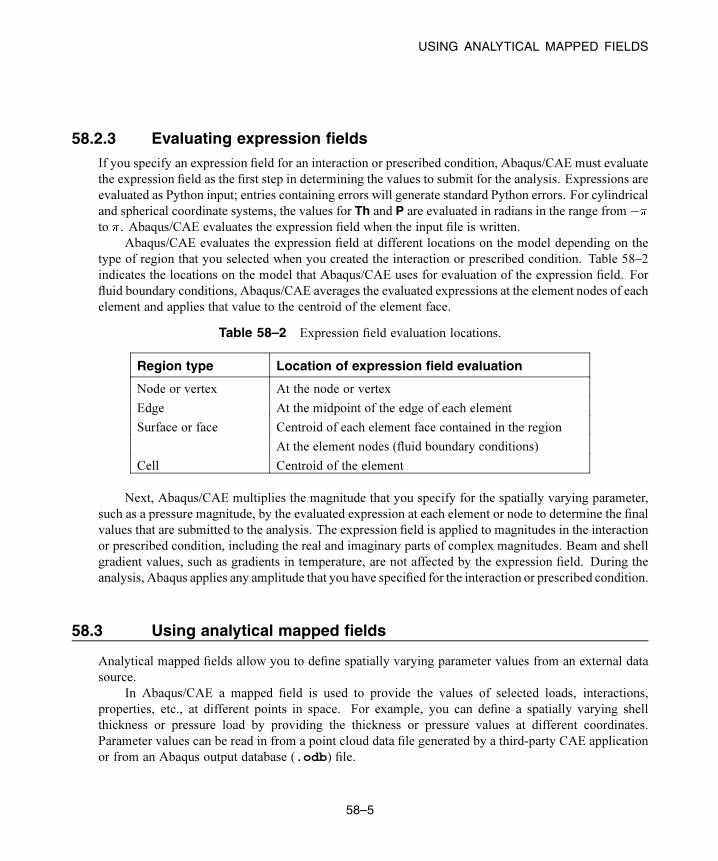
USING ANALYTICAL MAPPED FIELDS
58.2.3 Evaluating expression fieldsIf you specify an expression field for an interaction or prescribed condition, Abaqus/CAE must evaluate
the expression field as the first step in determining the values to submit for the analysis. Expressions are
evaluated as Python input; entries containing errors will generate standard Python errors. For cylindrical
and spherical coordinate systems, the values for Th and P are evaluated in radians in the range from
to . Abaqus/CAE evaluates the expression field when the input file is written.
Abaqus/CAE evaluates the expression field at different locations on the model depending on the
type of region that you selected when you created the interaction or prescribed condition. Table 58–2
indicates the locations on the model that Abaqus/CAE uses for evaluation of the expression field. For
fluid boundary conditions, Abaqus/CAE averages the evaluated expressions at the element nodes of each
element and applies that value to the centroid of the element face.
Table 58–2 Expression field evaluation locations.
Region type Location of expression field evaluation
Node or vertex At the node or vertex
Edge At the midpoint of the edge of each element
Centroid of each element face contained in the regionSurface or face
At the element nodes (fluid boundary conditions)
Cell Centroid of the element
Next, Abaqus/CAE multiplies the magnitude that you specify for the spatially varying parameter,
such as a pressure magnitude, by the evaluated expression at each element or node to determine the final
values that are submitted to the analysis. The expression field is applied to magnitudes in the interaction
or prescribed condition, including the real and imaginary parts of complex magnitudes. Beam and shell
gradient values, such as gradients in temperature, are not affected by the expression field. During the
analysis, Abaqus applies any amplitude that you have specified for the interaction or prescribed condition.
58.3 Using analytical mapped fields
Analytical mapped fields allow you to define spatially varying parameter values from an external data
source.
In Abaqus/CAE a mapped field is used to provide the values of selected loads, interactions,
properties, etc., at different points in space. For example, you can define a spatially varying shell
thickness or pressure load by providing the thickness or pressure values at different coordinates.
Parameter values can be read in from a point cloud data file generated by a third-party CAE application
or from an Abaqus output database (.odb) file.
58–5
Abaqus ID:
Printed on:

USING ANALYTICAL MAPPED FIELDS
Mapped fields allow you to import discrete and discontinuous parameter data and apply them to your
Abaqus/CAE model. Abaqus/CAE applies the values to the current model, mapping the input X-, Y-,
and Z-coordinates to locations in the model. Abaqus/CAE maps the source data onto the target model,
and Abaqus computes the distributed parameter values to be used during the analysis. The parameter
values are also called field values, or field data; for example, pressure values at different points on a
surface.
When you create a mapped field from point cloud data, you can assign a local coordinate system to
the source data region to simplify the three-dimensional definition of points in space. The local coordinate
system can be rectangular, cylindrical, or spherical. For example, with a rectangular coordinate system,
the X-, Y-, and Z-coordinates are interpreted in that local coordinate system.
Only scalar data values can be used in mapped fields. Each field data value is mapped from the
source to the target region as a scalar value. The Abaqus/CAE mapping algorithm is purely geometric,
with no physical considerations such as conservative mapping.
Mapped fields can be used to define the properties and attributes shown in Table 58–3.
Table 58–3 Attributes and properties that support mapped fields.
Category Attribute/Property
Body concentration flux
Body heat flux
Pressure
Surface concentration flux
Surface heat flux
Loads
Surface pore fluid flow
Acoustic pressure
Electrical potential
Mass concentration
Mass flow
Pore pressure
Boundary conditions
Temperature
Nodal temperature
Pore pressure
Saturation
Predefined fields
Void ratio
58–6
Abaqus ID:
Printed on:
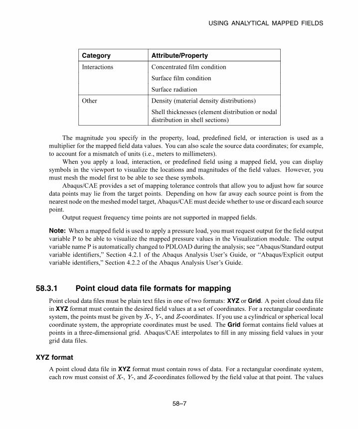
USING ANALYTICAL MAPPED FIELDS
Category Attribute/Property
Concentrated film condition
Surface film condition
Interactions
Surface radiation
Density (material density distributions)Other
Shell thicknesses (element distribution or nodal
distribution in shell sections)
The magnitude you specify in the property, load, predefined field, or interaction is used as a
multiplier for the mapped field data values. You can also scale the source data coordinates; for example,
to account for a mismatch of units (i.e., meters to millimeters).
When you apply a load, interaction, or predefined field using a mapped field, you can display
symbols in the viewport to visualize the locations and magnitudes of the field values. However, you
must mesh the model first to be able to see these symbols.
Abaqus/CAE provides a set of mapping tolerance controls that allow you to adjust how far source
data points may lie from the target points. Depending on how far away each source point is from the
nearest node on the meshed model target, Abaqus/CAEmust decide whether to use or discard each source
point.
Output request frequency time points are not supported in mapped fields.
Note: When a mapped field is used to apply a pressure load, you must request output for the field output
variable P to be able to visualize the mapped pressure values in the Visualization module. The output
variable name P is automatically changed to PDLOAD during the analysis; see “Abaqus/Standard output
variable identifiers,” Section 4.2.1 of the Abaqus Analysis User’s Guide, or “Abaqus/Explicit output
variable identifiers,” Section 4.2.2 of the Abaqus Analysis User’s Guide.
58.3.1 Point cloud data file formats for mapping
Point cloud data files must be plain text files in one of two formats: XYZ or Grid. A point cloud data file
in XYZ format must contain the desired field values at a set of coordinates. For a rectangular coordinate
system, the points must be given byX-, Y-, and Z-coordinates. If you use a cylindrical or spherical local
coordinate system, the appropriate coordinates must be used. The Grid format contains field values at
points in a three-dimensional grid. Abaqus/CAE interpolates to fill in any missing field values in your
grid data files.
XYZ format
A point cloud data file in XYZ format must contain rows of data. For a rectangular coordinate system,
each row must consist of X-, Y-, and Z-coordinates followed by the field value at that point. The values
58–7
Abaqus ID:
Printed on:

USING ANALYTICAL MAPPED FIELDS
in each row can be separated by any combination of spaces, tabs, or commas; each space, tab, or comma
is considered a single field delimiter. Comma-separated values (CSV), shown in the following example,
is a commonly used format:
X1,Y1,Z1,valueX2,Y2,Z2,valueX3,Y3,Z3,valueetc.
If you use a cylindrical or spherical local coordinate system, the appropriate coordinates must be given
in the data file; see “Coordinate system for point cloud mapped fields,” Section 58.3.2.
Figure 58–1 shows an example of point cloud data in XYZ format that have been imported into the
Edit Mapped Field dialog box.
58–8
Abaqus ID:
Printed on:

USING ANALYTICAL MAPPED FIELDS
Figure 58–1 Point cloud data in XYZ format.
Grid format
A point cloud data file in Grid format defines the field values at points in a three-dimensional grid. For
a rectangular coordinate system, this is a planar or cubic grid. Figure 58–2 shows a simple example of
point cloud data in Grid format that have been imported into the Edit Mapped Field dialog box.
Grid data consist of a set of files, each containing a single plane. For example, you could have one
file for the Z=3 plane. This file would contain a grid of X- and Y-coordinates and the field value at each
point; for example:
a, -2, -1, 0, 1, 2-2, 0.146, 0.141, 0.139, 0.137, 0.131
58–9
Abaqus ID:
Printed on:

USING ANALYTICAL MAPPED FIELDS
Figure 58–2 Point cloud data in Grid format.
-1, 0.141, 0.121, 0.116, 0.111, 0.1000, 0.139, 0.116, 0.105, 0.101, 0.0941, 0.133, 0.129, 0.122, 0.114, 0.1072, 0.128, 0.120, 0.111, 0.102, 0.090
The X-coordinates appear in the first (left) column in this file, and the Y-coordinates are in the first
(top) row, starting in the second position. The first position contains a dummy value that is ignored by
Abaqus/CAE when you import the file into the data table in the Create Mapped Field dialog box. In
the example file above, the dummy value is the character a; you can use any value in this position since
it will be ignored.
The values in each row of a grid data file can be separated by any combination of spaces, tabs, or
commas; each space, tab, or comma is considered a single field delimiter.
58–10
Abaqus ID:
Printed on:

USING ANALYTICAL MAPPED FIELDS
Your complete set of grid data files must include one file for each plane; for example, the X–Y
planes at Z=0, Z=1, Z=2, Z=3. The Y–Z, X–Z, Y–X, Z–Y, and Z–X planes can also be used. You
choose between the different grid planes in the Create Mapped Field dialog box.
If your grid data files have any missing field values, Abaqus/CAE interpolates to fill in the missing
points; you do not need to fill in these missing values in the Create Mapped Field dialog box.
If you use a cylindrical or spherical local coordinate system, the appropriate coordinates must be
given in the grid data files; see “Coordinate system for point cloud mapped fields,” Section 58.3.2.
58.3.2 Coordinate system for point cloud mapped fields
Mapped fields indicate points in space using coordinates of the global coordinate system or a local
coordinate system. For a point cloud data source, different coordinate systems can be involved when the
mapped data coordinates are interpreted and applied to the property, load, predefined field, or interaction.
Source data local coordinate system
The three-dimensional coordinates and field values are all defined in the local coordinate system.
You can specify the coordinate system to use in the Create Mapped Field dialog box. This is an
assembly-level (not part-level) coordinate system.
If you use a rectangular coordinate system (default), Abaqus/CAE uses X-, Y-, and
Z-coordinates to interpret the source data points. If you specify a cylindrical or spherical
coordinate system, Abaqus/CAE interprets the coordinates as shown in Table 58–4. The columns
shown in the data table of the Create Mapped Field dialog box depend on the type of local
coordinate system that you choose. For cylindrical and spherical coordinate systems, the values
for Th and P are entered in degrees and during the analysis are converted to radians in the range
from to .
Table 58–4 Coordinate system types and coordinate names for mapped fields.
Coordinate system type Coordinates Columns shown indata table
Rectangular or Global (default) X-, Y-, and Z-axes X, Y, Z
Cylindrical R-, -, and Z-axes R, Th, Z
Spherical R-, -, and -axes R, Th, P
Source data defined in part space
You can choose this option by toggling onSupplied data are defined in part space in theCreateMapped Field dialog box. The source data and its local coordinate system are both interpreted in
the part-level coordinate system of the target model region.
58–11
Abaqus ID:
Printed on:

USING ANALYTICAL MAPPED FIELDS
58.3.3 Mesh-to-mesh mapping from an output database fileWhen the data source is an Abaqus output database (.odb) file, the field output variable values must
be displayed in a viewport. This technique is called mesh-to-mesh mapping. The field output variable
values can be located at nodes, element centroids, or integration points. In this type of mapping the
geometric region of the source data is the mesh connectivity data such as element faces or element sets.
To select the exact source data you want to use, open the desired output database file and display the
undeformed contour plot in the Visualization module. You can also use the deformed plot, but the data
are still mapped from the undeformed mesh. Choose the field output variable and the step and frame of
the analysis for the value you want to map. When you create the newmapped field in your target model in
the model database (.cae) file, you specify the displayed viewport as the data source. The current stateof the viewport is taken as a snapshot of the set of values to be mapped onto the target model; namely,
the specific field output variable displayed at a specific step and frame of the analysis.
As an example, you might use mesh-to-mesh mapping in the following workflow:
1. Set up and run a thermal analysis in Abaqus to generate an output database containing nodal
temperatures (output variable NT).
2. Open the output database (.odb) file in the Visualization module, and display output variable NT
at Step-3, Frame 0 of the analysis.
3. Open the model database (.cae) file containing your main target model. Select Tools→AnalyticalField→Create from the main menu bar in the Load module to create a mapped field from the nodal
temperature values. In the Create Mapped Field dialog box, select the viewport containing the
output database as the source data.
4. Mesh (or remesh) your main model.
5. Create a temperature predefined field, and select the mapped analytical field to define the
temperature distribution. Abaqus/CAE maps the source data points and their associated
temperatures onto points in the target model.
6. Set up and run the subsequent analysis.
The source data on the output database mesh can be located at nodes, integration points, or whole
elements. Dissimilar meshes are supported.
The current settings in the selected viewport are used in the mapping. These settings are as follows:
• Primary field output variable
• Step/increment
• Averaging options selected in the Result Options dialog box
• Section points (top or bottom)
• Etc.
The following viewport settings are not supported for mesh-to-mesh mapping:
• Display groups
58–12
Abaqus ID:
Printed on:

USING ANALYTICAL MAPPED FIELDS
• Transformations
• Averaging by element sets or display groups in the Result Options dialog box
• Element face data
• User data in the current session (but data saved in the output database file is supported)
When you create a mapped field from output database data and close the Create Mapped fielddialog box, the source data are saved to the mapped field object, but the viewport itself is not saved. Any
changes made in the viewport after creating the mapped field are not reflected in the mapping data. After
you have created a mapped field using mesh-to-mesh mapping, you cannot edit the source data mesh
specifications; you can edit an existing mapped field only to change the default field value or mapper
control options.
Volumetric mesh-to-mesh mapping can be performed only with nodal temperatures and material
densities. When the mapping target is a mesh-based nodal region, you must specify whether the target
is a surface or a volumetric region. Abaqus/CAE uses different mapping algorithms for a surface versus
a volumetric region.
58.3.4 Supported elements for mappingMapped fields can be used only in models in which supported element types are used in the mesh. The
most commonly used elements are supported, including shells.
Supported element classes are listed below, according to the topology of the representative element
type: shape, number of nodes, and number of integration points. Any similar element with the same
topology is supported for mapping. The supported representative elements are as follows:
• S3, S4, S4R, S8R, STRI65
• C3D4, C3D6, C3D8, C3D8R, C3D10, C3D15, C3D20, C3D20R
• CPE3, CPE4, CPE6, CPE8
• CAX3, CAX4, CAX6, CAX8
The following classes of elements are not supported and cannot be used in a target model mesh or
output database source mesh:
• Surface elements
• Rigid elements
• Analytical rigid surface elements
• Cohesive elements
• Composite solid elements
• Continuum shell elements
• Cylindrical elements
• Eulerian elements
• Gasket elements
58–13
Abaqus ID:
Printed on:

DISPLAYING SYMBOLS FOR INTERACTIONS AND PRESCRIBED CONDITIONSTHAT USE ANALYTICAL FIELDS
• Internal elements
• Elements that use modified second-order interpolation
• Elements with twist
58.4 Displaying symbols for interactions and prescribed conditionsthat use analytical fields
When you apply an interaction or a prescribed condition to a region, you can display symbols in the
viewport that represent the interaction or prescribed condition.
By default, the symbols for interactions and prescribed conditions that use analytical field
distributions are scaled based on the calculated value. For symbols other than arrows, a plus sign (+) or
a minus sign (−) is displayed inside each symbol to indicate whether the magnitude of the interaction or
prescribed condition is positive or negative at that location. You can turn off the symbol scaling using
the Attribute display options in the Assembly Display Options dialog box. For more information,
see “Controlling the display of attributes,” Section 76.15.
Abaqus/CAE displays scaled-down symbols for interactions and prescribed conditions when an
analytical field evaluates to zero for a portion of its region. These scaled-down symbols are noticeably
smaller than the default symbol size. For more information, see “Understanding prescribed condition
symbol type, color, and size,” Section 16.5.1.
58.4.1 Expression field display symbol details
The points used for symbol display on meshes coincide with the locations where the expression field is
evaluated during the analysis. On geometry, when the symbols appear equally spaced along an edge or
over the face of a model, Abaqus/CAE selects a random set of points to use for symbol display. The
points selected for symbol display may or may not coincide with the locations where the expression field
is evaluated.
In some cases the expression field cannot be evaluated at a given point due to an error; for example,
division by zero. When this situation occurs, a message appears in the message area indicating that an
error occurred while evaluating the expression field. As a visual cue to indicate that there is an error,
the symbols displayed in the viewport are no longer scaled, even though the setting to scale symbols
based on the expression field value is turned on. You can attempt to eliminate the evaluation error by
changing the symbol density settings, which prompts Abaqus/CAE to select a different set of points to
use for symbol display. For more information on changing the symbol density settings, see “Controlling
the display of attributes,” Section 76.15.
58–14
Abaqus ID:
Printed on:

DISPLAYING SYMBOLS TO VISUALIZE MAPPING SOURCE DATA
58.4.2 Mapped field display symbol detailsTo be able to see the symbols representing amapped field, youmust first mesh yourmodel before applying
the load, interaction, or predefined field.The points used for symbol display onmapped fields are the native or orphanmesh nodes or elements
that will be used in the analysis. If a native mesh is not present, the symbols will be displayed unscaled.
In addition, if the mapping fails due to an error (for example, unsupported element types or incorrect
tolerances), the symbols will also be displayed unscaled.In these cases a message appears in the message area indicating an error in the evaluation. As a
visual cue to indicate that there is an error, the symbols displayed in the viewport are no longer scaled
and are displayed at the points they would be when scaling is turned off. You can try to fix the mapping by
remeshing or by changing the symbol density settings, which prompts Abaqus/CAE to select a different
set of points to use for symbol display. For more information on changing the symbol density settings,
see “Controlling the display of attributes,” Section 76.15.
58.5 Displaying symbols to visualize mapping source data
You can plot your mapping source data separately from the load, interaction, or predefined field where
it is applied. Plotting of source data is supported only for analytical mapped fields created from point
cloud data in XYZ format.
To display symbols representing the source data of a mapped field:
1. From the Model Tree, expand the Fields container and the Analytical Fields container to display
the mapped field object.
2. Click mouse button 3 on the mapped field object, and select Plot source data from the menu that
appears.
The displayed symbols represent the locations and relative magnitudes (field values) of the source data
points. The magnitudes are color coded using a rainbow color spectrum from red (for the maximum
value) to blue (for the minimum value), as shown in Figure 58–3.
Figure 58–3 Color coding used for visualizing mapping source data.58–15
Abaqus ID:
Printed on:


UNDERSTANDING ATTACHMENT POINTS AND LINES
59. The Attachment toolset
The Attachment toolset allows you to create attachment points and attachment lines that can be used to
define fasteners and other components in your model. The Attachment toolset is available in the Part,
Property, Assembly, and Interaction modules. This chapter describes the Attachment toolset and editing
features created using the toolset. The following topics are covered:
• “Understanding attachment points and lines,” Section 59.1
• “Understanding the projection methods,” Section 59.2
In addition, the following sections are available in the HTML version of this guide:
• “Creating attachment points by picking or reading from a file,” Section 59.3
• “Creating attachment points by choosing a direction and a spacing,” Section 59.4
• “Creating patterns of attachment points based on edges,” Section 59.5
• “Creating attachment lines by projecting points,” Section 59.6
• “Editing attachment points and lines,” Section 59.7
• “Removing attachment points and lines,” Section 59.8
59.1 Understanding attachment points and lines
You use the Attachment toolset to add attachment points and lines to your model. You use attachment
points to define point-based fasteners, inertia, springs, dashpots, loads or boundary conditions, or
connector points for a connector definition in your model; and you use attachment lines to define
discrete fasteners. Fasteners model point-to-point connections (such as spot welds, rivets, and bolts)
and are described in “About fasteners,” Section 29.1. You can create attachment points on the assembly
or on a part. You can create attachment lines on only the assembly.
You can use the Attachment toolset to create attachment points and lines by selecting
Tools→Attachment from the main menu bar and selecting one of the available menu options. In
the Interaction module you can use the tools in the module toolbox to create attachment points and
lines. The three attachment point tools are also available from the Property module and Part module
toolboxes. The Attachment toolset provides the following tools for creating attachment points:
Create attachment points by picking or reading from a file
This tool allows you to create attachment points by picking each point from the viewport or reading
the coordinates of the points from a file. For detailed instructions, see “Creating attachment points
by picking or reading from a file,” Section 59.3, in the HTML version of this guide.
59–1
Abaqus ID:
Printed on:

UNDERSTANDING ATTACHMENT POINTS AND LINES
Create attachment points by choosing a direction and a spacing
This tool allows you to create attachment points by defining a line and specifying the number of
points along the line or specifying the spacing of the points along the line. For detailed instructions,
see “Creating attachment points by choosing a direction and a spacing,” Section 59.4, in the HTML
version of this guide.
Create attachment points by choosing edges and offsets
This tool allows you to create simple patterns of attachment points on edges, on faces, or along
directions by selecting a single edge or connected edges and then defining pattern parameters. For
detailed instructions, see “Creating patterns of attachment points based on edges,” Section 59.5, in
the HTML version of this guide.
If desired, you can move the points to a specified face, as described in “Understanding the projection
methods,” Section 59.2.
The Attachment toolset provides the following tool for creating attachment lines:
Create attachment lines by projecting points
This tool allows you to create attachment lines by specifying points and then projecting them through
multiple faces. Attachment lines connect one or more faces. You can create attachment lines only on
the assembly; you cannot create attachment lines on a part. Creating attachment lines is a three-step
process:
1. Select the points to project.
2. Project the points onto a source face along the normal to the surface or along a specified
direction.
3. From the intersection of the projected points with the source face, project the attachment lines
to the target faces along the normal to the source face for a specified distance.
For detailed instructions, see “Creating attachment lines by projecting points,” Section 59.6, in the
HTML version of this guide.
Attachment points and lines are features, and they regenerate when you change the model; for
example, after you add a cut feature. The regeneration may affect the projection of attachment points
and lines and change the total number of fastening points and lines created by the attachment feature. In
addition, the sets that contain attachments may be affected by the regeneration. Therefore, you should
determine that your attachment points and lines are behaving as expected after you change the model.
You should also check that any prescribed conditions that you have applied to your attachment points
and lines, such as loads and boundary conditions, have not changed.
59–2
Abaqus ID:
Printed on:

UNDERSTANDING THE PROJECTION METHODS
59.2 Understanding the projection methods
The Attachment toolset provides three tools for creating attachment points. The tools provide convenient
methods for producing points, such as following an edge, reading the coordinates of each point from a file,
or spacing points along a line. However, in some cases it may be easier to define the attachment points
in one location and project the points onto a desired face. Therefore, Abaqus/CAE provides projection
options as a method of positioning attachment points on a face.
The Attachment toolset provides the following techniques to create attachment points by projecting
points onto the desired face:
• Project each point to its closest face.
• Choose the start point and end point of a projection vector. Abaqus/CAE projects each point along
the vector and creates an attachment point where it first intersects with a face.
Figure 59–1 illustrates the two techniques for projecting points onto a selected face.
Attachment points
Selectedpoints
Project tothe closestface
Project along a specified direction
Figure 59–1 Projecting points onto a selected face.
For more information about how fasteners use attachment points, see “About fasteners,”
Section 29.1.
For information on related topics, refer to the following sections:
• “Understanding attachment points and lines,” Section 59.1
• “About fasteners,” Section 29.1
59–3
Abaqus ID:
Printed on:


CREATING A CAD CONNECTION
60. The CAD Connection toolset
The CAD Connection toolset is used by the optional add-on associative interfaces for Abaqus/CAE
to create a connection from Abaqus/CAE to another CAD system. You can use the CAD system to
modify a model or to change its position, and you can use the established connection to update the model
quickly in Abaqus/CAE. You can also modify some geometric features in Abaqus/CAE and use the CAD
connection to update the original CAD system model. This chapter covers the following topics:
• “Creating a CAD connection,” Section 60.1
• “Updating geometry parameters in an imported model,” Section 60.2
60.1 Creating a CAD connection
You can use the CAD Connection toolset to create a connection from Abaqus/CAE to another CAD
system running an associative interface plug-in. You can use the connection to export the model from
the CAD system to the Assembly module in Abaqus/CAE. You can also use the connection to export
certain geometry modifications from an imported model in Abaqus/CAE back to the CAD system (see
“Updating geometry parameters in an imported model,” Section 60.2). Associative interface plug-ins
are available for the following CAD systems:
• CATIA V6
• CATIA V5
• SolidWorks
• Pro/ENGINEER
• NX (Unigraphics)
Figure 60–1 shows concurrent CATIA V5 and Abaqus/CAE sessions and illustrates the communication
between the applications. Using a CAD connection to transfer a model from a CAD system running
an associative interface plug-in to Abaqus/CAE is called associative import. For further information
about the individual associative interface plug-ins, see the Dassault Systèmes Knowledge Base at
www.3ds.com/support/knowledge-base. This information includes the following:
• The CAD packages that support associative import along with the supported version numbers.
• Download and installation instructions for the associative interface plug-ins.
• Complete documentation for each associative interface plug-in.
To create a CAD connection:
1. From the main menu bar in the Assembly module, select Tools→CAD Interfaces→CAD System.
CAD System is the name of the CAD system to which you are connecting; you can establish
connections with CATIA V6, CATIA V5, SolidWorks, and Pro/ENGINEER.
60–1
Abaqus ID:
Printed on:

CREATING A CAD CONNECTION
Abaqus/CAECATIA V5
Figure 60–1 Associative import using the CATIA V5 Associative Interface.
2. From the dialog box that appears, do one of the following:
Auto-assign port
Choose Auto-assign port, and click Enable to open a port from Abaqus/CAE.
Abaqus/CAE displays the port number that it assigned in the message area. When you
export a model from the CAD system, the data are transferred through this connection port
number.
Specify port
Choose Specify port, and enter a port number to specify a port. The number must be between
1025 and 65535. If you are reopening a connection, you can use the port number displayed by
Abaqus/CAE when it first assigned the port.
60–2
Abaqus ID:
Printed on:

CREATING A CAD CONNECTION
Disable port
If a connection has already been enabled, you can click Disable from the dialog box to disable
the connection.
3. After you have used the CAD Connection toolset to create a connection from Abaqus/CAE to
another CAD system running an associative interface plug-in, you can do the following to export
the assembly to the Abaqus/CAE session:
CATIA V6
CATIA V6R2013x or earlier
Select Tools→Associative Export→Export to Abaqus/CAE from the mainmenu bar.
CATIA V6R2014
Select Export to Abaqus/CAE from the Associative Export section of the action
bar.
More detailed instructions are available in the SIMULIA Associative Interface for
Abaqus/CAE User’s Guide; this guide is available after you install the SIMULIA Associative
Interface for Abaqus/CAE app.
CATIA V5
Select Abaqus→Export to Abaqus/CAE from the CATIA V5 main menu bar. In the
Export to Abaqus/CAE dialog box that appears, select Open Abaqus/CAE, and click
OK. More detailed instructions are available in the CATIA V5 Associative Interface User’s
Guide; you can download this guide from the Dassault Systèmes Knowledge Base at
www.3ds.com/support/knowledge-base.
SolidWorks
Select Abaqus→Export to Abaqus/CAE from the SolidWorks main menu bar. In the
Export to Abaqus/CAE dialog box that appears, toggle on Open in Abaqus/CAE, andclick the green check mark. More detailed instructions are available in the SolidWorks
Associative Interface User’s Guide; you can download this guide from the Dassault Systèmes
Knowledge Base at www.3ds.com/support/knowledge-base.
Pro/ENGINEER
Select Abaqus→Open in CAE from the Pro/ENGINEER main menu bar. More
detailed instructions are available in the Pro/ENGINEER Associative Interface User’s
Guide; you can download this guide from the Dassault Systèmes Knowledge Base at
www.3ds.com/support/knowledge-base.
60–3
Abaqus ID:
Printed on:

UPDATING GEOMETRY PARAMETERS IN AN IMPORTED MODEL
NX
Select Abaqus→Open in /CAE from the NX main menu bar. More detailed instructions are
available in the Abaqus/CAE Associative Interface for NX User’s Guide; you can download
this guide from the Elysium, Inc. web site.
For more information on associative import, see “What can I do with the associative interfaces?,”
Section 10.1.2.
60.2 Updating geometry parameters in an imported model
The parameter update capability allows a bidirectional associative import, in which you modify the
dimensions of geometric features in a model that has been imported into Abaqus/CAE, then propagate
the new dimensions back to the model files from the original CAD system. This bidirectional import
feature is currently available only with the CATIA V5 Associative Interface and the Pro/ENGINEER
Associative Interface.
To use the parameter update capability, you must first use the CAD system (CATIA V5 or
Pro/ENGINEER) to indicate which model dimensions can be modified within Abaqus/CAE. The
modifiable dimensions must be defined in terms of feature-level parameters, which are imported into
Abaqus/CAE along with the model. For example, a parameter may be associated with the radius of a
hole in the model; modifying the value of that parameter also modifies the radius of the hole. Each
parameter name must begin with the string ABQ_ to be imported into Abaqus/CAE.
The CATIA V5 Associative Interface and the Pro/ENGINEER Associative Interface use a special
parameters (.par_abq) file to pass parameters to Abaqus/CAE. For more information about defining
modifiable parameters in an imported CATIA V5 or Pro/ENGINEER model, refer to the CATIA V5
Associative Interface or the Pro/ENGINEER Associative Interface User’s Guides. These guides are
available from the Dassault Systèmes Knowledge Base at www.3ds.com/support/knowledge-base.
You can use the CAD Parameters dialog box in Abaqus/CAE to assign new values to the imported
parameters. When you change a parameter value, the associated geometry feature is regenerated both
in the Abaqus/CAE model and in the saved CAD model. This dialog box also enables you to keep the
CAD software running in the background after you make a change to CAD parameters. Having the CAD
software running in the background improves performance for bidirectional parameter update, but this
option occupies a license for your CAD software for the remainder of your session.
To update geometry parameters in an imported model:
1. Do either of the following:
• Import a model from CATIA V5 using the CATIA V5 Associative Interface. (You cannot
update geometry parameters from CATIA V6.)
• Import a model from Pro/ENGINEER using the Pro/ENGINEER Associative Interface.
60–4
Abaqus ID:
Printed on:

UPDATING GEOMETRY PARAMETERS IN AN IMPORTED MODEL
2. Open the CAD Parameters dialog box:
• In the Part module, select Tools→CAD Parameters.
• In the Assembly module, select Tools→CAD Interfaces→CAD Parameters.
The CAD Parameters dialog box displays all of the parameters that can be modified.
3. Click on a parameter name to highlight the portion of the model that is impacted by that parameter
in the viewport.
4. To modify a parameter value, click the appropriate cell in the Value column, and enter a new value.
5. If you are importing parameters from Pro/ENGINEER, you can toggle on Keep CAD softwarerunning in the background after parameter update. This option improves performance if you
perform bidirectional import or make additional updates.
6. When you have changed all of the necessary parameter values, do one of the following:
• Click Update to regenerate the model in Abaqus/CAE based on the new parameter values.
The geometry in the saved Pro/ENGINEER part (.prt) files is updated as well. The original
model must not be open in Pro/ENGINEER when you perform the update.
• Click mouse button 3, and select Write to File to create an updated parameters file without
updating the model geometry. This file can be used to manually update parameters using
the Abaqus Scripting Interface. For more information about the parameters file, refer to the
Pro/ENGINEER Associative Interface User’s Guide.
• Click Defaults to reset all of the parameters in the CAD Parameters table to the values in the
current Abaqus/CAE model.
For information on related topics, refer to the following sections:
• “What can I do with the associative interfaces?,” Section 10.1.2
• “Creating a CAD connection,” Section 60.1
60–5
Abaqus ID:
Printed on:


CONFIGURING THE VISIBILITY OF TOOLBARS
61. The Customize toolset
The Customize toolset allows you to change the behavior and appearance of some aspects of
Abaqus/CAE. This chapter covers the following topics:
• “Configuring the visibility of toolbars,” Section 61.1
• “Configuring keyboard shortcuts,” Section 61.2
• “Custom toolbars,” Section 61.3
• “Configuring icons in custom toolbars,” Section 61.4
For step-by-step instructions on using the Customize toolset, see “Using the Customize toolset,”
Section 61.5, in the HTML version of this guide.
61.1 Configuring the visibility of toolbars
Using the Customize toolset, you can remove individual toolbars from the Abaqus/CAE display. Hiding
toolbars that you use infrequently reduces clutter on the screen. You can always access the functionality
in a hidden toolbar using an alternate method (such as the main menu bar, module-specific toolboxes, or
keyboard shortcuts).
There are three ways to change the visibility of a toolbar:
Closing a floating toolbar
You can hide a floating toolbar by clicking the “X” in the toolbar’s title bar. For an explanation of
floating versus docked toolbars, see “Components of the toolbars,” Section 2.2.3.
To resume the display of a floating toolbar, you must use one of the techniques described below.
Using the main menu bar
To hide a visible toolbar, select View→Toolbars→Toolbar Name from the main menu bar. Use
the same procedure to resume the display of a hidden toolbar. Toolbars that are currently being
displayed have a check mark next to their names in the menu listing.
Using the Customize dialog box
Using the Customize dialog box, you can change the visibility of multiple toolbars at once. Open
the Customize dialog box by selecting Tools→Customize from the main menu bar. On the
Toolbars tabbed page, toggle off any toolbars you want to hide; toggle on any toolbars you want
to make visible.
61–1
Abaqus ID:
Printed on:

CUSTOM TOOLBARS
61.2 Configuring keyboard shortcuts
A keyboard shortcut is a single keystroke or combination of keys that you can use to launch a function in
Abaqus/CAE; for example, [Ctrl]+S saves the current model. Several keyboard shortcuts are defined by
default for common functions. You can use the Customize toolset to edit these default shortcuts, to add
new shortcuts for other functions in Abaqus/CAE, and to display a list of all currently defined shortcuts.
Select Tools→Customize from the main menu bar; display the Functions tabbed page of the dialog
box that appears to access the Keyboard editor.
Tip: Keyboard shortcuts are active only when their function is allowed in the current module
and only when the application’s focus is not in the Model Tree, Results Tree, message area,
or command line interface. If a shortcut does not appear to work, confirm that the function is
allowed in the current module or shift focus to the viewport by clicking the viewport title bar.
Abaqus/CAE allows the following keys and key combinations to be specified as keyboard shortcuts:
• Any function key except the [F1] key,
• [Alt]+[Shift]+any key, or
• [Ctrl]+any key. You can also add [Alt] or [Shift] to any keyboard shortcut that includes the [Ctrl] key.
However, not all keys are eligible for inclusion in a keyboard combination; you cannot specify a keyboard
combination that includes a function key or a key from the alphanumeric keypad.
61.3 Custom toolbars
The Customize toolset allows you to create custom toolbars containing shortcuts to most of the defined
functions in Abaqus/CAE. A custom toolbar can be used to collect commonly used tools in a single
location, create tools for functions that do not have an existing shortcut, or provide easily accessible
controls for a common procedure (for example, the create part, instance part, and mesh part functions
could all be part of the same toolbar). Custom toolbars are visible in all modules. If a tool acts as a
shortcut to a module-specific function, Abaqus/CAE automatically switches to the appropriate module
when that tool is invoked.
The contents and locations of custom toolbars are saved between sessions.
To create a custom toolbar, select Tools→Customize from the main menu bar. For detailed
instructions on the creation of custom toolbars, see “Creating and modifying custom toolbars,”
Section 61.5.4, in the HTML version of this guide.
61–2
Abaqus ID:
Printed on:
CONFIGURING ICONS IN CUSTOM TOOLBARS
61.4 Configuring icons in custom toolbars
You can change the default icon that is assigned to tools in custom toolbars. If you create a tool that
does not have a default icon assignment, you can assign a new icon to that tool. If a tool appears in
more than one custom toolbar, the icon assignment for that tool applies in all custom toolbars. The icons
in default Abaqus/CAE toolbars and toolboxes cannot be changed and are not affected by custom icon
assignments.
To change or add an icon assignment, select Tools→Customize from the main menu bar. On the
Functions tabbed page of the dialog box that appears, select a tool’s function and click Select to assigna new icon to that tool.
When assigning an icon, you can select from any of the icons currently used in Abaqus/CAE. You
can also import user icons. User icons must be in one of the following formats: bitmap (.bmp), GIF(.gif), PNG (.png), or XPM (.xpm). Icon images should be sized appropriately—the standard size
for toolbar icons in Abaqus/CAE is 24 × 24 pixels. You cannot scale the size with which user icons are
displayed in Abaqus/CAE; if you increase the icon size scale factor (as described in “Scaling the size of
icons,” Section 68.3), only the Abaqus/CAE icons will increase in size.
Abaqus/CAE creates a directory named abaqus_icons in your home directory to store imported
user icon images. If you delete an image file from this directory, Abaqus/CAE reverts to the default icon
assignment for any tools that use the deleted image file.
The same icon can be assigned to multiple tools. To distinguish the functions of tools using the
same icon, place the cursor over a tool for a moment; a small box, or “tooltip,” containing a description
of the tool’s function will appear.
61–3
Abaqus ID:
Printed on:


UNDERSTANDING THE ROLE OF DATUM GEOMETRY
62. The Datum toolset
A datum is a construction aid that helps you progress through the modeling process when the model itself
does not contain the desired geometry. You use the Datum toolset to create these construction aids. This
chapter explains how you use the Datum toolset to create and position datum points, axes, planes, and
coordinate systems. The following topics are covered:
• “Understanding the role of datum geometry,” Section 62.1
• “Using the Datum toolset,” Section 62.2
• “Why are datum coordinate systems so important?,” Section 62.3
• “Understanding a datum as a feature,” Section 62.4
• “An overview of datum creation techniques,” Section 62.5
In addition, the following sections are available in the HTML version of this guide:
• “Creating datum points,” Section 62.6
• “Creating datum axes,” Section 62.7
• “Creating datum planes,” Section 62.8
• “Creating datum coordinate systems,” Section 62.9
62.1 Understanding the role of datum geometry
As you proceed through the modeling process, you may find that you need a particular piece of geometry,
such as a vertex or an edge, that does not exist in your model. You can use the Datum toolset to create
the required piece of geometry, which is called a datum. You can create a datum point, a datum axis, a
datum plane, or a datum coordinate system.
• When prompted to select a point, you can select a point from a part, a datum point, or the origin of
a datum coordinate system.
• When prompted to select an edge, you can select an edge from a part, a datum axis, or one of the
axes of a datum coordinate system.
• When prompted to select a face, you can select a face from a part or a datum plane.
• When prompted to select a coordinate system, you must select a datum coordinate system.
An example of how you might use a datum plane as a sketching plane involves the part shown in
Figure 62–1. To extrude a blind cut into the curved surface, you need to sketch the profile on a plane
that is tangent to the curved surface. The desired plane does not exist, but you can create one with the
Datum toolset and sketch on the resulting plane. The datum plane and the resulting cut feature are shown
in Figure 62–2.
62–1
Abaqus ID:
Printed on:

USING THE DATUM TOOLSET
basefeature
Figure 62–1 Creating a sketch plane.
blind cut feature
datumplane
sketched profile
Figure 62–2 The resulting feature.
Abaqus/CAE does not generate meshes on datum geometry, and datum geometry has no effect on
the analysis of your model; it is simply a convenience to help you construct complex geometry. You
should use the Partition toolset if you want to add geometry to the model itself, such as a vertex along
an edge or a plane through a cell.
You create a datum by defining it with respect to existing geometry (such as vertices, planes, and
edges) or to other datum geometry. You can create a datum on a part in the Part or Property module or
on an assembly in other modules. For example, you can define a datum axis that passes through two
selected points of a part in the Part module, and you can use the axis to align instances of the part in the
Assembly module. A datum is a feature; and, like all features, it can be edited, deleted, suppressed, and
resumed. Similarly, a datum is regenerated when the assembly or part is regenerated. You can also use
display groups to show or hide datum geometry in a viewport.
62.2 Using the Datum toolset
You can access the Datum toolset in any module by selecting Tools→Datum from the main menu bar.
The Create Datum dialog box appears, and you choose the type of datum to create—point, axis, plane,
62–2
Abaqus ID:
Printed on:

WHY ARE DATUM COORDINATE SYSTEMS SO IMPORTANT?
or coordinate system (CSYS)—from the buttons in the Type region at the top of the dialog box. The
Method list changes to reflect the datum you create. Select the desired datum tool from the Methodlist, and follow the prompts in the prompt area to create the datum. “An overview of datum creation
techniques,” Section 62.5, provides an overview of the methods available for each type of datum. More
information on creating datum geometry on parts and assemblies is provided in “Using the Datum
toolset in the Part module,” Section 11.16.1, and “Using datum geometry in the Assembly module,”
Section 13.8.1. More information on displaying datum geometry is provided in “Controlling datum
display,” Section 76.9, in the HTML version of this guide.
You can also access the Datum toolset from the module toolbox; Figure 62–3 shows the hidden
icons for all the datum tools in the module toolboxes.
Datum point tools
Datum axis tools
Datum coordinate system tools
Datum plane tools
Figure 62–3 The datum tools.
To see a brief tooltip containing a definition of each datum tool, hold the mouse over the tool for a
moment. For information on using toolboxes and selecting hidden icons, see “Using toolboxes and
toolbars that contain hidden icons,” Section 3.3.2.In addition, the online HTML version of this guide
contains a more detailed description of each tool.
62.3 Why are datum coordinate systems so important?
Datum coordinate systems are used throughout Abaqus/CAE; for example,
• To define material orientations.
• To define connector orientations.
• To define the orientation of a coupling constraint.
• To define the orientation of an inertia relief load.
• To define the orientation of boundary conditions.
• To position and align part instances.
62–3
Abaqus ID:
Printed on:

UNDERSTANDING A DATUM AS A FEATURE
In addition, you can select the origin of a datum coordinate system when prompted to select a point, and
you can select an axis of a datum coordinate system when prompted to select an edge.
Abaqus/CAE provides three methods for creating a datum coordinate system:
• Three points
• Offset from coordinate system
• Two lines
For more information, see “An overview of the methods for creating a datum coordinate system,”
Section 62.5.4. In contrast with other types of datums, you can name a datum coordinate system while
you create it. As with all datums, you can use the Model Tree to rename a datum coordinate system.
62.4 Understanding a datum as a feature
A datum is a useful construction aid in the feature-based modeling process and is a feature itself.
As a result, you can use the Feature Manipulation toolset to delete, suppress, and resume a datum.
Abaqus/CAE regenerates a datum along with the part or assembly, taking into account any changes to
underlying geometry. You can edit any numerical parameters that define a datum; for example, the X-,
Y-, and Z-coordinates used to define a datum point. However, a datum is always defined by the same
underlying geometry you selected when you created it; if you need to define the datum using different
geometry, you must delete the datum and create a new one.
You can create a datum on a part in the Part or Property module or on an assembly in other modules.
If you create a datum on a part, the datum moves along with an instance of the part in the Assembly
module. If you create a datum on the assembly by selecting entities from a part instance, the datum
moves along with the instance in the Assembly module. However, if you create a datum on the assembly
by entering coordinates in the prompt area, the datum remains fixed when the instance moves.
When you modify a feature, you should be aware of any parent-child relationships between your
datum and the modified feature. For example, consider Figure 62–4, which shows a datum axis passing
through the midpoint of two arcs.The midpoints of the arcs that define the location of the datum axis are
parents of the datum axis.
Figure 62–4 The original datum axis between two midpoints.
62–4
Abaqus ID:
Printed on:

AN OVERVIEW OF DATUM CREATION TECHNIQUES
If you modify the part, Abaqus/CAE regenerates the datum axis so that it still passes through the two
midpoints, as shown in Figure 62–5.
Figure 62–5 The datum axis after the part is modified.
62.5 An overview of datum creation techniques
This section provides an overview of the methods for creating each type of datum. The online HTML
version of this guide contains detailed instructions for creating each type of datum. The online HTML
version of this guide also contains detailed instructions for showing and hiding datums; for more
information, see “Controlling datum display,” Section 76.9.
62.5.1 An overview of the methods for creating a datum point
When you choose Point from the Create Datum dialog box, the Method list displays the following
methods for creating a datum point:
Enter coordinates
Enter the X-, Y-, and Z-coordinates of the datum point, as shown in Figure 62–6. For detailed
instructions, see “Creating a datum point by entering its coordinates,” Section 62.6.1, in the HTML
version of this guide.
62–5
Abaqus ID:
Printed on:

AN OVERVIEW OF DATUM CREATION TECHNIQUES
datum point
(x, y, z)
Figure 62–6 Creating a datum point by entering coordinates.
Offset from point
Enter the location of the datum point in the form of the X-, Y-, and Z-coordinates of an offset from
a selected point, as shown in Figure 62–7. For detailed instructions, see “Creating a datum point at
an offset from a selected point,” Section 62.6.2, in the HTML version of this guide.
(x, y, z)
offset datum point
selected point
(0, -10, 0)
Figure 62–7 Creating a datum point by offsetting from a point.
Midway between 2 points
Select two points on the model; Abaqus/CAE creates the datum point midway between the two
selected points, as shown in Figure 62–8. For detailed instructions, see “Creating a datum point
midway between two points,” Section 62.6.3, in the HTML version of this guide.
datum point
selected points
Figure 62–8 Creating a datum point by selecting two end points.
62–6
Abaqus ID:
Printed on:

AN OVERVIEW OF DATUM CREATION TECHNIQUES
Offset from 2 edges
Select two edges on the model; and enter the distance from the datum point to each edge, as shown
in Figure 62–9. For detailed instructions, see “Creating a datum point at a specified distance from
two edges,” Section 62.6.4, in the HTML version of this guide.
datum point
selected edges
d1
d2
Figure 62–9 Positioning a datum point a specified distance from two edges.
Enter parameter
Select an edge on the model, and enter the location of the datum point in the form of a parameter
value that represents a percentage of the edge length. An arrow along the edge indicates the direction
of increasing parameter value from the start vertex (corresponding to an edge parameter value of
zero) to the end vertex (corresponding to a value of one), as shown in Figure 62–10. For detailed
instructions, see “Creating a datum point by entering an edge parameter,” Section 62.6.5, in the
HTML version of this guide.
datum point selected edge
Figure 62–10 Positioning a datum point a specified distance along an edge.
Project point on face/plane
Select a point and a face or plane on which to project the point. Abaqus/CAE creates the datum
point where the face or plane intersects a line that is normal to it and passing through the selected
point, as shown in Figure 62–11. The datum point also marks the shortest distance between the
selected point and the selected face or plane. For detailed instructions, see “Creating a datum point
by projecting a point on a face or plane,” Section 62.6.6, in the HTML version of this guide.
62–7
Abaqus ID:
Printed on:
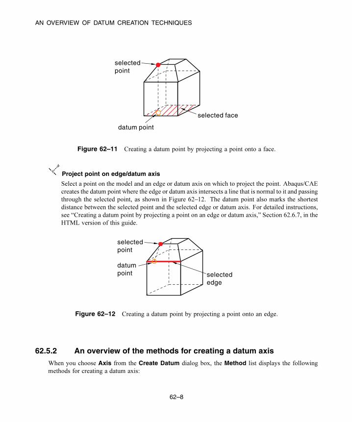
AN OVERVIEW OF DATUM CREATION TECHNIQUES
����������
datum point
selectedpoint
selected face
Figure 62–11 Creating a datum point by projecting a point onto a face.
Project point on edge/datum axis
Select a point on the model and an edge or datum axis on which to project the point. Abaqus/CAE
creates the datum point where the edge or datum axis intersects a line that is normal to it and passing
through the selected point, as shown in Figure 62–12. The datum point also marks the shortest
distance between the selected point and the selected edge or datum axis. For detailed instructions,
see “Creating a datum point by projecting a point on an edge or datum axis,” Section 62.6.7, in the
HTML version of this guide.
datumpoint
selectedpoint
selected edge
Figure 62–12 Creating a datum point by projecting a point onto an edge.
62.5.2 An overview of the methods for creating a datum axis
When you choose Axis from the Create Datum dialog box, the Method list displays the following
methods for creating a datum axis:
62–8
Abaqus ID:
Printed on:

AN OVERVIEW OF DATUM CREATION TECHNIQUES
Principal axis
Select one of the three principal axes with which the datum axis must be colinear, as shown
in Figure 62–13. For detailed instructions, see “Creating a datum axis along a principal axis,”
Section 62.7.1, in the HTML version of this guide.
datum axis
z
y
principal x-axis
x
Figure 62–13 Defining a datum axis as one of the three principal axes.
Intersection of 2 planes
Select two non-parallel planar surfaces. Abaqus/CAE creates the datum axis where the two planes
(or extensions of the two planes) intersect, as shown in Figure 62–14. For detailed instructions, see
“Creating a datum axis along the intersection of two planes,” Section 62.7.2, in the HTML version
of this guide.
�����������������������������������
datum axis
selected planes
Figure 62–14 Defining a datum axis as the intersection of two planes.
Straight edge
Select a straight edge on the model with which the datum axis must be colinear, as shown in
Figure 62–15. For detailed instructions, see “Creating a datum axis along a straight edge,”
Section 62.7.3, in the HTML version of this guide.
62–9
Abaqus ID:
Printed on:

AN OVERVIEW OF DATUM CREATION TECHNIQUES
datum axisselected edge
Figure 62–15 Defining a datum axis as a straight edge on the model.
2 points
Select any two points on the model through which the datum axis must pass, as shown in
Figure 62–16. For detailed instructions, see “Creating a datum axis through two points,”
Section 62.7.4, in the HTML version of this guide.
datum axis selected points
Figure 62–16 Defining a datum axis by selecting two points.
Axis of cylinder
Select a cylindrical face on the model. Abaqus/CAE creates a datum axis that lies along the axis
of the cylindrical face, as shown in Figure 62–17. For detailed instructions, see “Creating a datum
axis along the axis of a cylinder,” Section 62.7.5, in the HTML version of this guide.
cylinder
datum axis
Figure 62–17 Defining a datum axis as the axis of a cylinder.
62–10
Abaqus ID:
Printed on:

AN OVERVIEW OF DATUM CREATION TECHNIQUES
Normal to plane, thru point
Select a plane and a point that is not on the plane. Abaqus/CAE creates a datum axis that is normal
to the plane and passes through the point, as shown in Figure 62–18. For detailed instructions, see
“Creating a datum axis normal to a plane and passing through a point,” Section 62.7.6, in the HTML
version of this guide.
��������
datum axis
selected pointselected plane
Figure 62–18 Defining a datum axis by selecting a point and a plane.
Parallel to line, thru point
Select an edge of the model and a point outside the edge. Abaqus/CAE creates a datum
axis that is parallel to the edge and passes through the point, as shown in Figure 62–19. For
detailed instructions, see “Creating a datum axis parallel to a line and passing through a point,”
Section 62.7.7, in the HTML version of this guide.
datum axis
selected point
selected edge
Figure 62–19 Defining a datum axis by selecting a point and an edge.
3 points on circle
Select three points on the model that define a circle. Abaqus/CAE creates a datum axis along the
axis of the circle, as shown in Figure 62–20. For detailed instructions, see “Creating a datum axis
running along the axis of a circle defined by three points,” Section 62.7.8, in the HTML version of
this guide.
62–11
Abaqus ID:
Printed on:

AN OVERVIEW OF DATUM CREATION TECHNIQUES
datum axis
circle defined
selected points
Figure 62–20 Defining a datum axis as the axis of a circle.
Rotate from line
Select an edge and an axis of rotation, and specify the angle through which the edge will be rotated.
Abaqus/CAE creates a datum axis by rotating the edge about the axis through the specified angle, as
shown in Figure 62–21. For detailed instructions, see “Creating a datum axis by rotating an existing
edge through a specified angle,” Section 62.7.9, in the HTML version of this guide.
datum axis
selected axis of rotation(arrow indicates positivedirection of rotation basedon the right-hand rule)
selected edge
selected edge
selected point
α
α
three-dimensional two-dimensional or axisymmetric
Y
X
Z
Figure 62–21 Defining a datum axis by rotating an edge through a specified angle.
62–12
Abaqus ID:
Printed on:

AN OVERVIEW OF DATUM CREATION TECHNIQUES
62.5.3 An overview of the methods for creating a datum plane
When you choose Plane from the Create Datum dialog box, the Method list displays the following
methods for creating a datum plane:
Offset from principal plane
Select one of the three principal planes; and provide the location of the datum plane in the form of an
offset from the selected plane, as shown in Figure 62–22. A positive value indicates an offset in the
positive direction along the axis normal to the selected plane; for example, along the X-axis normal
to the Y–Z plane. For detailed instructions, see “Creating a datum plane offset from a principal
plane,” Section 62.8.1, in the HTML version of this guide.
z
y
x
datum plane
d
Figure 62–22 Creating a datum plane by offsetting from one of the three principal planes.
Offset from plane
Select any plane on the model; and provide the location of the datum plane by specifying the
direction of the normal and an offset from the selected plane along the normal, as shown in
Figure 62–23. You can specify the offset by entering a value or selecting a point. For detailed
instructions, see “Creating a datum plane at an offset from a selected plane,” Section 62.8.2, in the
HTML version of this guide.
3 points
Select three points through which the datum plane must pass, as shown in Figure 62–24. For
detailed instructions, see “Creating a datum plane passing through three points,” Section 62.8.3,
in the HTML version of this guide.
62–13
Abaqus ID:
Printed on:

AN OVERVIEW OF DATUM CREATION TECHNIQUES
datum plane
���������
doffsetdistance
selected plane
selected normal
Figure 62–23 Creating a datum plane by offsetting from any plane.
datum plane
selected points
Figure 62–24 Creating a datum plane by selecting three points.
Line and point
Select an edge and a point through which the datum plane must pass, as shown in Figure 62–25.
For detailed instructions, see “Creating a datum plane through a line and a point,” Section 62.8.4,
in the HTML version of this guide.
datum plane
selected edge
selectedpoint
Figure 62–25 Creating a datum plane by selecting a point and an edge.
62–14
Abaqus ID:
Printed on:

AN OVERVIEW OF DATUM CREATION TECHNIQUES
Point and normal
Select a point and an edge; the datum plane passes through the point and is normal to the selected
edge, as shown in Figure 62–26. For detailed instructions, see “Creating a datum plane passing
through a point and normal to an edge,” Section 62.8.5, in the HTML version of this guide.
datum plane selected point
selected edge
Figure 62–26 Creating a datum plane by selecting a point and a normal edge.
Midway between 2 points
Select two points. Abaqus/CAE creates a datum plane midway between the two selected points
and normal to the line connecting them, as shown in Figure 62–27. For detailed instructions, see
“Create a datum planemidway between two points and normal to the line connecting the two points,”
Section 62.8.6, in the HTML version of this guide.
datum plane
selected points
Figure 62–27 Positioning a datum plane midway between two points.
Rotate from plane
Select a face and an axis of rotation, and specify the angle through which the face will be rotated.
Abaqus/CAE creates a datum plane by rotating the face about the axis through the specified angle,
as shown in Figure 62–28. For detailed instructions, see “Creating a datum plane by rotating an
existing face through a specified angle,” Section 62.8.7, in the HTML version of this guide.
62–15
Abaqus ID:
Printed on:

AN OVERVIEW OF DATUM CREATION TECHNIQUES
datum plane
selectedface
���������������
����������������
selected axis of rotation(arrow indicates positivedirection of rotation basedon the right-hand rule)
α
Figure 62–28 Defining a datum plane by rotating a face through a specified angle.
62.5.4 An overview of the methods for creating a datum coordinatesystem
Datum coordinates systems are used throughout Abaqus/CAE; for example, to define material
orientations and to define connector orientations. To help you keep track of your datum coordinate
systems, you can name the systems when you create them, and the name appears alongside their entry
in the Model Tree. When you choose CSYS from the Create Datum dialog box, the Method list
displays the following methods for creating a datum coordinate system:
3 points
Define a rectangular, cylindrical, or spherical coordinate system by selecting the origin and,
optionally, two additional points. In the case of a rectangular system, the second point defines the
X-axis, and the X–Y plane passes through the second and third points, as shown in Figure 62–29.
This is the most versatile tool for creating a datum coordinate system, and you should use it when
possible. For detailed instructions, see “Creating a datum coordinate system defined by three
points,” Section 62.9.1, in the HTML version of this guide.
Offset from CSYS
Select a coordinate system; and provide the location of the rectangular, cylindrical, or spherical
datum coordinate system by specifying an offset, as shown by the example involving a rectangular
system in Figure 62–30. You can specify the offset by entering a value or by selecting a point. For
detailed instructions, see “Creating a datum coordinate system at an offset from another coordinate
system,” Section 62.9.2, in the HTML version of this guide.
62–16
Abaqus ID:
Printed on:

AN OVERVIEW OF DATUM CREATION TECHNIQUES
z'
y'
x'
three selected points
Figure 62–29 Positioning a rectangular datum coordinate
system by selecting the origin and two points.
z
y
x
z'
y'
x'
default coordinate system
datum coordinate system
Figure 62–30 Positioning a rectangular datum coordinate system
by offsetting from another coordinate system.
2 lines
Select two edges that define the rectangular, cylindrical, or spherical coordinate system. In the case
of a rectangular system, the first edge defines the X-axis and the X–Y plane passes through the second
edge, as shown in Figure 62–31. For detailed instructions, see “Creating a datum coordinate system
defined by two lines,” Section 62.9.3, in the HTML version of this guide.
z'
y'
x'two selected edges
Figure 62–31 Positioning a rectangular datum coordinate
system by selecting two edges.
62–17
Abaqus ID:
Printed on:


USING THE DISCRETE FIELD TOOLSET
63. The Discrete Field toolset
A discrete field is a spatially varying field where values are associated with a node or an element. The
Discrete Field toolset allows you to create and manage discrete fields. This chapter covers the following
topics:
• “Using the Discrete Field toolset,” Section 63.1
In addition, the following sections are available in the HTML version of this guide:
• “Creating discrete fields,” Section 63.2
• “Evaluating discrete fields,” Section 63.3
• “Creating discrete fields for material volume fractions,” Section 63.4
63.1 Using the Discrete Field toolset
The Discrete Field toolset allows you to define spatially varying parameters. The parameters in a discrete
field can be associated with specified elements or nodes. For example, you can define a spatially varying
thickness or orientation (Cartesian, cylindrical, or spherical). The Discrete Field toolset is available in
the Property module, Interaction module, and Load module.
Select Tools→Discrete Field→Create from the main menu bar to create a new discrete field;
select Edit from the same menu to change an existing discrete field. Either command opens the discrete
field editor, which allows you to associate data with elements or nodes.
63–1
Abaqus ID:
Printed on:


WHAT CAN I DO WITH THE EDIT MESH TOOLSET?
64. The Edit Mesh toolset
You can use the Edit Mesh toolset in the Mesh module to improve the mesh quality. You can modify an
orphan mesh, or you can modify an Abaqus native mesh. This chapter covers the following topics:
• “What can I do with the Edit Mesh toolset?,” Section 64.1
• “What is the difference between editing an orphan mesh, a meshed part, and a meshed part instance
in the assembly?,” Section 64.2
• “Meshing strategies and mesh editing techniques,” Section 64.3
In addition, the following sections are available in the HTML version of this guide:
• “An overview of the mesh editing tools,” Section 64.4
• “Editing nodes,” Section 64.5
• “Editing elements,” Section 64.6
• “Editing the entire mesh,” Section 64.7
• “Editing and refining an orphan mesh,” Section 64.8
• “Undoing or redoing a change in the Edit Mesh toolset,” Section 64.9
64.1 What can I do with the Edit Mesh toolset?
This section describes how you can use the Edit Mesh toolset to modify a mesh in the Mesh module.
All of the tools are available when you are modifying a mesh that contains orphan elements and nodes;
however, only a few of the tools are available for modifying mesh nodes or elements that are tied to
geometry, including meshed part instances in the assembly.
64.1.1 Manipulating nodesThe Edit Mesh toolset provides the following tools that allow you to manipulate the nodes in your mesh:
• Create a node. You can specify the coordinates of the new node either in the global coordinate
system or in a datum coordinate system that you specify.
• Edit nodes. You can specify the new coordinates of the nodes either in the global coordinate system
or in a datum coordinate system that you specify. Alternatively, you can specify an offset from the
current position. You can edit a single node, or you can edit multiple nodes simultaneously.
• Drag nodes. You can click and drag the nodes in a model. You can drag only one node at a time, and
you can use the Project to geometry option to project an exterior node to the geometry with which
it is associated. Element quality checks are automatically activated to show element errors and
64–1
Abaqus ID:
Printed on:
WHAT CAN I DO WITH THE EDIT MESH TOOLSET?
warnings while you drag a node. For more information on element quality checks, see “Verifying
element quality,” Section 17.19.1, in the HTML version of this guide.
• Project nodes. You can specify a vertex, edge, or face and Abaqus/CAE projects the nodes from
their current positions onto the selected entity. You can project a single node, or you can project
multiple nodes simultaneously. You can also project nodes to other nodes, element edges, element
faces, datum points, datum axes, or datum planes.
• Delete nodes. Any elements associated with the deleted nodes are also deleted. In addition, you
have the option of deleting any remaining nodes that would be left unassociated with any elements
once the nodes selected for deletion and their associated elements are deleted.
• Merge selected nodes. If you select only two nodes to merge, Abaqus/CAE creates a new node
at the midpoint of the selected nodes. If you select more than two nodes, you can specify the
Node merging tolerance, which is the maximum distance between nodes that will be merged.
Abaqus/CAE deletes nodes that are closer than the specified distance and replaces them with a
single new node. The location of the new node is the average position of the group of nodes that
were merged into the new node.
While Abaqus/CAE is removing duplicate nodes, you can choose to remove duplicate elements
that have the same connectivity. You can also merge instances of parts in the Assembly module and
you have the option to merge nodes within this process; for more information, see “Merging and
cutting part instances,” Section 13.7.1.
• Smooth selected nodes. You can select external nodes, and Abaqus/CAE smooths the node positions
with respect to the surrounding nodes. You can smooth any external nodes of the native mesh on
a part or on an assembly as long as they are not part of a region boundary; you can also smooth
external orphan mesh nodes that lie within a planar mesh face.
• Adjust the position of the midside node of second-order elements to allow for the singularity at the
crack tip in a fracture mechanics analysis. You can select nodes and enter a bias parameter between
0 and 1. Abaqus/CAE moves the midside nodes along connected element edges to a position based
on the parameter that you entered. For example, if you enter a parameter of 0.25, Abaqus/CAE
biases the position of the midside nodes one quarter of the length of the element edge away from
the selected nodes.
For more information, see “Controlling the singularity at the crack tip for a small-strain
analysis,” Section 31.2.5, and “Constructing a fracture mechanics mesh for small-strain analysis
with the conventional finite element method” in “Contour integral evaluation,” Section 11.4.2 of
the Abaqus Analysis User’s Guide.
• Renumber selected nodes within an orphan mesh. You can renumber the selected nodes by
specifying a starting label and an increment or by offsetting the existing label by a specified value.
Tip: The Mesh Edit Undo feature can roll back any change you make to the nodes in the
mesh. For more information, see “Undoing or redoing a change in the Edit Mesh toolset,”
Section 64.9, in the HTML version of this guide.
64–2
Abaqus ID:
Printed on:
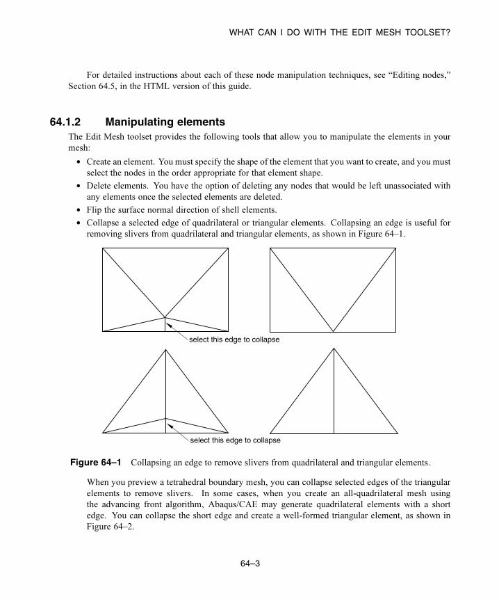
WHAT CAN I DO WITH THE EDIT MESH TOOLSET?
For detailed instructions about each of these node manipulation techniques, see “Editing nodes,”
Section 64.5, in the HTML version of this guide.
64.1.2 Manipulating elementsThe Edit Mesh toolset provides the following tools that allow you to manipulate the elements in your
mesh:
• Create an element. You must specify the shape of the element that you want to create, and you must
select the nodes in the order appropriate for that element shape.
• Delete elements. You have the option of deleting any nodes that would be left unassociated with
any elements once the selected elements are deleted.
• Flip the surface normal direction of shell elements.
• Collapse a selected edge of quadrilateral or triangular elements. Collapsing an edge is useful for
removing slivers from quadrilateral and triangular elements, as shown in Figure 64–1.
select this edge to collapse
select this edge to collapse
Figure 64–1 Collapsing an edge to remove slivers from quadrilateral and triangular elements.
When you preview a tetrahedral boundary mesh, you can collapse selected edges of the triangular
elements to remove slivers. In some cases, when you create an all-quadrilateral mesh using
the advancing front algorithm, Abaqus/CAE may generate quadrilateral elements with a short
edge. You can collapse the short edge and create a well-formed triangular element, as shown in
Figure 64–2.
64–3
Abaqus ID:
Printed on:

WHAT CAN I DO WITH THE EDIT MESH TOOLSET?
select this edge to collapse
Figure 64–2 Collapsing an edge of a quadrilateral element.
• Split a selected edge of a quadrilateral or triangular element into two parts. You can split the edge
at its midpoint, or you can click on the location of the split. You can use a combination of tools
to clean up your mesh. For example, Figure 64–3 illustrates how you can split an edge and then
collapse the resulting edge to remove a long narrow triangular element.
select this edge to split
the edge is splitwhere the user clicks
select this edge to collapse
Figure 64–3 Splitting and collapsing edges of a triangular element.
64–4
Abaqus ID:
Printed on:

WHAT CAN I DO WITH THE EDIT MESH TOOLSET?
If you are editing a native mesh in the Mesh module, Abaqus/CAE projects the new node on the
geometry. As a result, you can use this tool for improving a coarse mesh around curved edges, as
shown in Figure 64–4.
triangular elements
hole
split edges
Figure 64–4 Improving the mesh around a hole by splitting edges.
• Swap the diagonal of a pair of adjacent triangular elements, as shown in Figure 64–5. You can swap
the diagonal of either first- or second-order adjacent triangular elements if they are the same order.
In addition, the adjacent triangular elements must have consistent normals. If necessary, you can
flip the normals to make them consistent.
Figure 64–5 Swap the diagonal of a pair of adjacent triangular elements.
• Split a quadrilateral element into two triangular elements, as shown in Figure 64–6. You cannot
split a 5-node quadrilateral element, and you cannot split a gasket element.
Figure 64–6 Split a quadrilateral element into two triangular elements.
• Combine two adjacent triangular elements into one quadrilateral element, as shown in Figure 64–7.
You can combine either first- or second-order elements, but you cannot combine a combination of
both. In addition, you can combine elements only if the adjacent triangular elements have consistent
normals. If necessary, you can flip the normals to make them consistent.
64–5
Abaqus ID:
Printed on:

WHAT CAN I DO WITH THE EDIT MESH TOOLSET?
Figure 64–7 Combine two adjacent triangular elements into one quadrilateral element.
• Orient the stack direction of a continuum shell, cohesive, cylindrical, or gasket mesh. You can stack
only hexahedral, wedge, and quadrilateral elements to form a continuum shell, cohesive, cylindrical,
or gasket mesh. As a result, you can use this tool to orient the stack direction of only hexahedral,
wedge, and quadrilateral elements. If you have assigned cylindrical elements or second-order gasket
elements to the region, you must first change the assignment to conventional elements before you
reorient the stack direction. You can then convert the region back to a cylindrical or gasket mesh
by reassigning cylindrical elements or second-order gasket elements.
• Renumber selected elements within an orphan mesh. You can renumber the selected elements by
specifying a starting label and an increment or by offsetting the existing label by a specified value.
Tip: The Mesh Edit Undo feature can roll back any change you make to the element in the
mesh. For more information, see “Undoing or redoing a change in the Edit Mesh toolset,”
Section 64.9, in the HTML version of this guide.
For detailed instructions about manipulating elements, see “Editing elements,” Section 64.6, in the
HTML version of this guide.
64.1.3 Manipulating the meshThe Edit Mesh toolset provides the following tools that allow you to manipulate the mesh:
• Create layers of solid elements that are offset normal to selected element faces of an existing mesh,
as shown in Figure 64–8. This tool is useful for meshing shell-like parts with solid elements. You
can specify the total thickness of all the layers and the number of layers to create. The first layer
of elements can be merged with the existing elements, or it can be offset by a specified distance.
The selected element faces can be from either shell or solid elements, but not from both. If you
selected shell element faces, you can choose whether to delete the shell elements after Abaqus/CAE
generates the layers of solid elements. You should use this tool to generate continuum shell and
cohesive elements, because the solid elements that Abaqus/CAE generates are stacked normal to
the surface from which they were offset.
• Create layers of shell elements that are offset normal to selected element faces from an existing
mesh, as shown in Figure 64–9. This tool is similar to the previous tool; however, instead of
specifying the total thickness of the layers, you specify the distance between the layers. You should
use this tool to create an offset copy of an existing shell mesh and to create multi-layered composite
models or reinforcements.
64–6
Abaqus ID:
Printed on:

WHAT CAN I DO WITH THE EDIT MESH TOOLSET?
solid offset mesh
Figure 64–8 Creating layers of solid elements.
mesh shell offset mesh
Figure 64–9 Creating layers of shell elements.
• Wrap a mesh. You can wrap a planar orphan mesh about the global Z-axis at a specified radius. The
wrapping procedure will relocate a node at point ( , ) on the planar mesh to ( ), where is
the specified radius, = , and = .
• Collapse edges. You can specify the minimum element edge size desired in the mesh. Abaqus/CAE
merges the end nodes of element edges that are shorter than the specified length. By default,
Abaqus/CAE checks all element edges in a mesh part, but you can specify a different element
domain.
For structured meshes you can specify a thickness direction or reference edge to limit the
edge directions considered for collapse. If you select a thickness direction, Abaqus/CAE uses the
direction vector to measure the elements instead of measuring only the distance between nodes. If
elements are oriented such that the direction is topologically ambiguous, Abaqus/CAE highlights
the elements so you can either select a domain that excludes them or add a reference edge to further
define the desired edges. When you choose a reference edge, with or without a thickness direction,
Abaqus/CAE considers edges for collapse only if they are topologically parallel to the reference
edge. A reference edge can be applied only within a single section of structured mesh; multiple
separate sections must be handled in separate collapse operations if reference edges are required.
64–7
Abaqus ID:
Printed on:
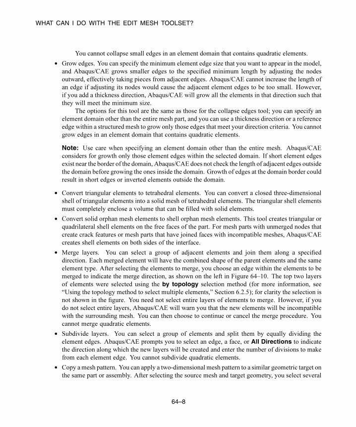
WHAT CAN I DO WITH THE EDIT MESH TOOLSET?
You cannot collapse small edges in an element domain that contains quadratic elements.
• Grow edges. You can specify the minimum element edge size that you want to appear in the model,
and Abaqus/CAE grows smaller edges to the specified minimum length by adjusting the nodes
outward, effectively taking pieces from adjacent edges. Abaqus/CAE cannot increase the length of
an edge if adjusting its nodes would cause the adjacent element edges to be too small. However,
if you add a thickness direction, Abaqus/CAE will grow all the elements in that direction such that
they will meet the minimum size.
The options for this tool are the same as those for the collapse edges tool; you can specify an
element domain other than the entire mesh part, and you can use a thickness direction or a reference
edge within a structured mesh to grow only those edges that meet your direction criteria. You cannot
grow edges in an element domain that contains quadratic elements.
Note: Use care when specifying an element domain other than the entire mesh. Abaqus/CAE
considers for growth only those element edges within the selected domain. If short element edges
exist near the border of the domain, Abaqus/CAE does not check the length of adjacent edges outside
the domain before growing the ones inside the domain. Growth of edges at the domain border could
result in short edges or inverted elements outside the domain.
• Convert triangular elements to tetrahedral elements. You can convert a closed three-dimensional
shell of triangular elements into a solid mesh of tetrahedral elements. The triangular shell elements
must completely enclose a volume that can be filled with solid elements.
• Convert solid orphan mesh elements to shell orphan mesh elements. This tool creates triangular or
quadrilateral shell elements on the free faces of the part. For mesh parts with unmerged nodes that
create crack features or mesh parts that have joined faces with incompatible meshes, Abaqus/CAE
creates shell elements on both sides of the interface.
• Merge layers. You can select a group of adjacent elements and join them along a specified
direction. Each merged element will have the combined shape of the parent elements and the same
element type. After selecting the elements to merge, you choose an edge within the elements to be
merged to indicate the merge direction, as shown on the left in Figure 64–10. The top two layers
of elements were selected using the by topology selection method (for more information, see
“Using the topology method to select multiple elements,” Section 6.2.5); for clarity the selection is
not shown in the figure. You need not select entire layers of elements to merge. However, if you
do not select entire layers, Abaqus/CAE will warn you that the new elements will be incompatible
with the surrounding mesh. You can then choose to continue or cancel the merge procedure. You
cannot merge quadratic elements.
• Subdivide layers. You can select a group of elements and split them by equally dividing the
element edges. Abaqus/CAE prompts you to select an edge, a face, or All Directions to indicate
the direction along which the new layers will be created and enter the number of divisions to make
from each element edge. You cannot subdivide quadratic elements.
• Copy a mesh pattern. You can apply a two-dimensional mesh pattern to a similar geometric target on
the same part or assembly. After selecting the source mesh and target geometry, you select several
64–8
Abaqus ID:
Printed on:
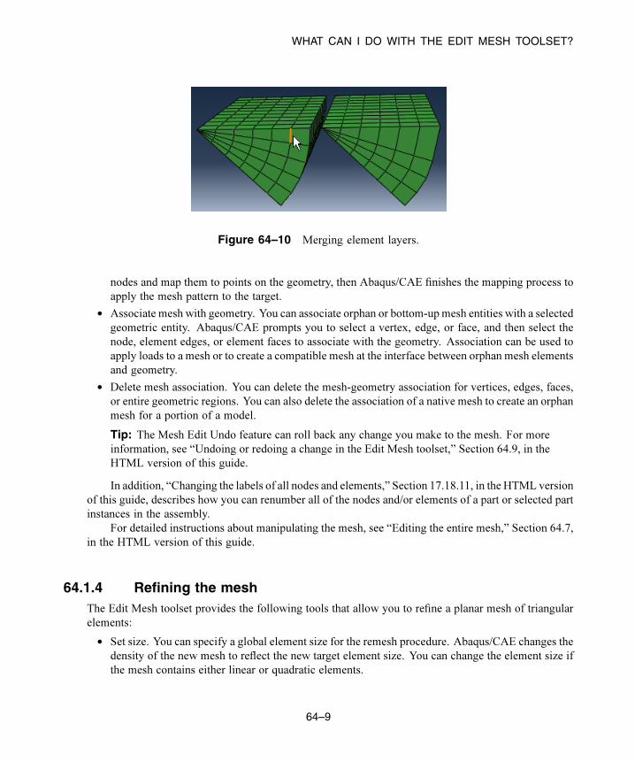
WHAT CAN I DO WITH THE EDIT MESH TOOLSET?
Figure 64–10 Merging element layers.
nodes and map them to points on the geometry, then Abaqus/CAE finishes the mapping process to
apply the mesh pattern to the target.
• Associate mesh with geometry. You can associate orphan or bottom-up mesh entities with a selected
geometric entity. Abaqus/CAE prompts you to select a vertex, edge, or face, and then select the
node, element edges, or element faces to associate with the geometry. Association can be used to
apply loads to a mesh or to create a compatible mesh at the interface between orphan mesh elements
and geometry.
• Delete mesh association. You can delete the mesh-geometry association for vertices, edges, faces,
or entire geometric regions. You can also delete the association of a native mesh to create an orphan
mesh for a portion of a model.
Tip: The Mesh Edit Undo feature can roll back any change you make to the mesh. For more
information, see “Undoing or redoing a change in the Edit Mesh toolset,” Section 64.9, in the
HTML version of this guide.
In addition, “Changing the labels of all nodes and elements,” Section 17.18.11, in the HTML version
of this guide, describes how you can renumber all of the nodes and/or elements of a part or selected part
instances in the assembly.
For detailed instructions about manipulating the mesh, see “Editing the entire mesh,” Section 64.7,
in the HTML version of this guide.
64.1.4 Refining the meshThe Edit Mesh toolset provides the following tools that allow you to refine a planar mesh of triangular
elements:
• Set size. You can specify a global element size for the remesh procedure. Abaqus/CAE changes the
density of the new mesh to reflect the new target element size. You can change the element size if
the mesh contains either linear or quadratic elements.
64–9
Abaqus ID:
Printed on:

WHAT IS THE DIFFERENCE BETWEEN EDITING AN ORPHAN MESH, A MESHEDPART, AND A MESHED PART INSTANCE IN THE ASSEMBLY?
• Remove size. You can maintain the global element size during the remesh procedure. Abaqus/CAE
maintains the edges of the elements along the boundary of the part while improving the mesh quality
in the interior. You can refine the mesh if the mesh contains either linear or quadratic elements.
• Remesh. You can remesh a planar mesh containing linear or quadratic triangular elements.
Tip: The Mesh Edit Undo feature can roll back any mesh refinement changes. For more
information, see “Undoing or redoing a change in the Edit Mesh toolset,” Section 64.9, in the
HTML version of this guide.
For detailed instructions about mesh refinement, see “Editing and refining an orphan mesh,”
Section 64.8, in the HTML version of this guide.
64.2 What is the difference between editing an orphan mesh, a meshedpart, and a meshed part instance in the assembly?
You can display either parts containing a combination of orphan and native mesh components or the
assembly in the Mesh module. You can use all of the tools in the Edit Mesh toolset to edit an orphan
mesh; however, you can use only the following tools to edit a meshed part instance in the assembly:
• Edit, drag, project, merge, and smooth nodes
• Delete elements
• Collapse element edges
• Split an edge of a quadrilateral or triangular element
• Swap the diagonal of a pair of adjacent triangular elements
• Split a quadrilateral element into two triangular elements
• Combine two triangular elements into one quadrilateral element
If you select a part instead of a part instance in the assembly, you can use the mesh editing tools listed
above plus the following additional tools:
• Create nodes and elements
• Offset mesh layers to create solid or shell layers
• Associate the mesh with geometry
• Delete mesh associativity
• Copy mesh pattern
In general, you cannot use the Edit Mesh toolset to modify the mesh of a dependent part instance.
However, you can edit, drag, and project the nodes of a dependent part instance; Abaqus/CAE modifies
the original meshed part, and your modifications appear on all dependent instances of the part.
You can create an orphan mesh in the Mesh module, or you can import an orphan mesh from an
output database or an Abaqus input file. You can add geometric features to an orphan mesh in the Part
module. An instance of an orphan mesh is always a dependent instance and; therefore, you cannot use
64–10
Abaqus ID:
Printed on:

MESHING STRATEGIES AND MESH EDITING TECHNIQUES
the Edit Mesh toolset to edit an instance of an orphan mesh in the assembly. However, you can display
the original orphan mesh that was used to create the instance and edit the part. For more information,
see “What is the difference between a dependent and an independent part instance?,” Section 13.3.2.
The Mesh Edit Undo feature can roll back any change you make to the mesh. For more information,
see “Undoing or redoing a change in the Edit Mesh toolset,” Section 64.9, in the HTML version of this
guide.
64.3 Meshing strategies and mesh editing techniques
This section describes strategies for improving your mesh using the Edit Mesh toolset and techniques
that you can use to create the desired mesh.
64.3.1 A strategy for improving the meshIf you have a complex assembly, you should selectMesh→Verify to verify the quality of the mesh before
you submit the job for analysis. The mesh verify tool can do the following:
• Highlight elements of a selected shape that do not meet specified criteria, such as aspect ratio.
• Print mesh statistics, such as the total number of elements of the chosen shape, the number of
highlighted elements, and the average and worst values of the selection criterion.
• Highlight elements that do not pass the mesh quality tests that are included with the input file
processor in Abaqus/Standard and Abaqus/Explicit.
If the mesh verify tool indicates that you should try to improve the quality of the mesh, you should
first try the following before turning to the Edit Mesh toolset:
• Change the seed distribution
• Add or modify partitions
• Change the mesh technique
In addition, you might try modifying the parts in the Part module, or you might try using the Virtual
Topology toolset and regenerating the mesh. You should treat the Edit Mesh toolset as the final step in
the meshing process and use it only to make minor adjustments to nodes and elements. Abaqus/CAE
tries to preserve attributes, such as loads and boundary conditions, if you make changes to the mesh. If
you modify a part, Abaqus/CAE deletes the mesh when you return to the Mesh module; as a result, you
will lose any edits that you made to the mesh.
64.3.2 Using offset meshes in Abaqus/CAEThe offset mesh tools in the Edit Mesh toolset have many uses in Abaqus/CAE, as follows:
64–11
Abaqus ID:
Printed on:

MESHING STRATEGIES AND MESH EDITING TECHNIQUES
Continuum shell meshes
You can use the solid offset mesh tool to mesh thin solids that are essentially thickened shells, such
as sheet metal, composites, or molded plastic components. The solid offset mesh tool is useful for
creating continuum shell elements because Abaqus/CAE orients the elements consistently in the
thickness direction. For more information, see “Meshing parts with continuum shell elements,”
Section 25.2.
Cohesive elements
You can assign cohesive elements to quadrilateral elements of a two-dimensional model. For three-
dimensional models you can use the solid offset mesh tool to generate a layer of cohesive elements
on a mesh. The offset mesh tool generates elements that are oriented consistently with a stack
direction that is normal to the thickness direction, and it is a convenient tool for quickly creating a
layer of cohesive elements. For more information, see “Embedding cohesive elements in an existing
three-dimensional mesh,” Section 21.2.
Skin reinforcements
If your skin can be defined as a single layer, creating the skin in the Property module is the
preferred approach. However, you can use the shell offset mesh tool to create a skin that uses
multiple reinforcement layers. For more information, see “Using offset meshes to create skin
reinforcements,” Section 36.6.
You can also use the solid offset mesh tool in conjunction with the mesh generation tools in the
Mesh module by doing the following:
1. Create a portion of the mesh in the Mesh module.
2. Use the solid offset mesh tool to complete the mesh.
You can create sets containing the elements from an offset mesh. You can create a single set that
contains the offset elements, or you can create separate sets for each layer of offset elements. In addition,
if you are creating a solid offset mesh, you can create surfaces from the top and the bottom of the offset
mesh, provided the first layer of elements is not embedded in the original mesh. You can use these sets
and surfaces in subsequent procedures to help you select elements from the offset mesh. For example,
you can select a set when assigning a section to a layer of offset elements. Similarly, you can select a
surface when you tie one side of a layer of cohesive elements to the surrounding bulk material.
64.3.3 Reducing element distortion and collapse during mesh offsetting
Abaqus/CAE creates an offset mesh by
• offsetting the nodes normal to the boundary of an existing mesh surface, and
• building elements that propagate out in the normal direction.
64–12
Abaqus ID:
Printed on:

MESHING STRATEGIES AND MESH EDITING TECHNIQUES
When you create a mesh that is offset from a concave mesh surface, the elements tend to converge, as
shown in Figure 64–11.
shell offset mesh
original mesh
normal
Figure 64–11 Elements converge when offset from a concave surface.
As a result, elements may collapse or become inverted, and the magnitude of the offset is limited by a
combination of the degree of curvature and the element size, as shown in Figure 64–12.
shell offset mesh
original mesh
Figure 64–12 When you offset small elements in a concave region, the elements
may collapse or become inverted.
You can try to avoid element collapse and element inversion by selecting Constant thickness aroundcorners from the Offset Mesh dialog box. When this option is selected, Abaqus/CAE tapers the offset
elements that propagate from sharp corners. The resulting elements have a constant nodal offset distance
64–13
Abaqus ID:
Printed on:

MESHING STRATEGIES AND MESH EDITING TECHNIQUES
as opposed to a constant distance between the layers of the element faces. Figure 64–13 illustrates the
effect on the offset mesh pattern of requesting a constant thickness around corners.
surface used togenerate the offset
offsetting without theconstant thickness aroundcorners option
offsetting with theconstant thickness around corners option
Figure 64–13 The effect on the offset mesh pattern of
requesting a constant thickness around corners.
The effect on the offset mesh pattern is similar for both solid and shell offset meshes. You can also reduce
element distortion by using a larger element size in the location of the concave region. However, you
can control the element size only if you can regenerate the mesh from which you are offsetting.
In contrast, when you create a mesh that is offset from a convex mesh surface, the elements tend to
fan out, as shown in Figure 64–14.
64.3.4 Allowing for branching in offset solid meshesIf a part has “branches,” as shown in Figure 64–15, creating an offset solid mesh is not straightforward
because the direction in which to offset is ambiguous in the region of the branch. To help you mesh this
configuration, Abaqus/CAE provides the option to copy the elements in the region of the branch to a set.
You can then do the following:
1. Use display groups to remove the set containing elements in the region of the branch from the orphan
mesh.
2. Create offset solid meshes from the non-branching regions that remain, as shown in Figure 64–16.
64–14
Abaqus ID:
Printed on:
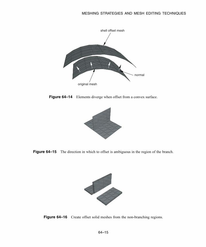
MESHING STRATEGIES AND MESH EDITING TECHNIQUES
shell offset mesh
original mesh
normal
Figure 64–14 Elements diverge when offset from a convex surface.
Figure 64–15 The direction in which to offset is ambiguous in the region of the branch.
Figure 64–16 Create offset solid meshes from the non-branching regions.
64–15
Abaqus ID:
Printed on:
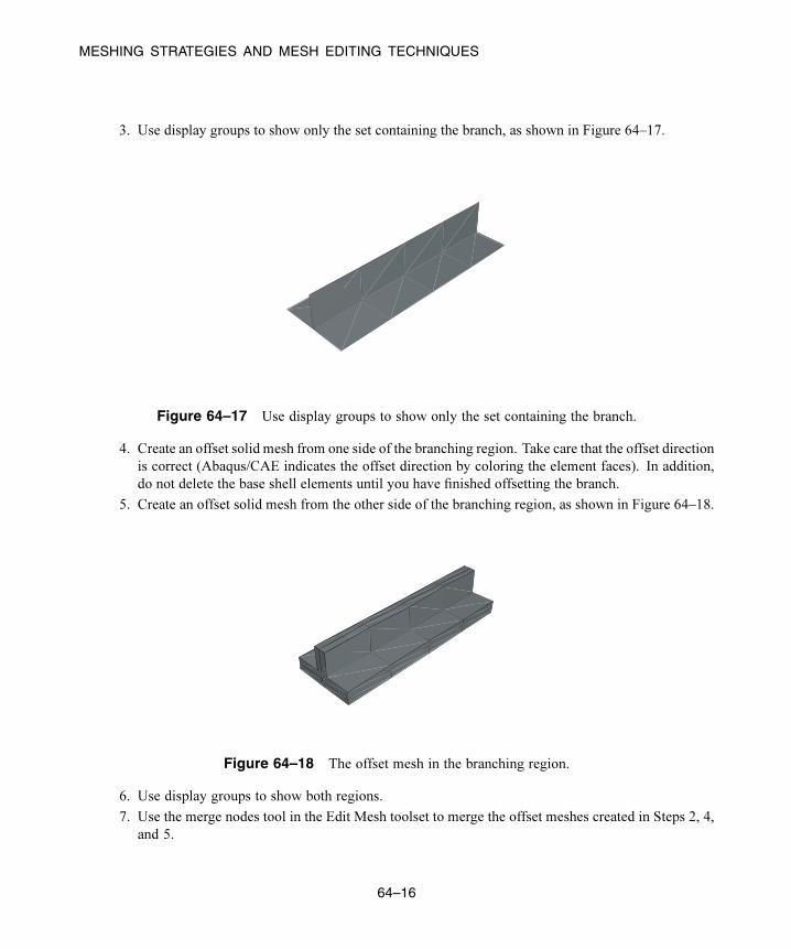
MESHING STRATEGIES AND MESH EDITING TECHNIQUES
3. Use display groups to show only the set containing the branch, as shown in Figure 64–17.
Figure 64–17 Use display groups to show only the set containing the branch.
4. Create an offset solid mesh from one side of the branching region. Take care that the offset direction
is correct (Abaqus/CAE indicates the offset direction by coloring the element faces). In addition,
do not delete the base shell elements until you have finished offsetting the branch.
5. Create an offset solid mesh from the other side of the branching region, as shown in Figure 64–18.
Figure 64–18 The offset mesh in the branching region.
6. Use display groups to show both regions.
7. Use the merge nodes tool in the Edit Mesh toolset to merge the offset meshes created in Steps 2, 4,
and 5.
64–16
Abaqus ID:
Printed on:

MESHING STRATEGIES AND MESH EDITING TECHNIQUES
64.3.5 Creating a mid-plane shell mesh from a thin solid model
You can use the following procedure to create a mid-plane shell mesh from a thin solid model using the
offset meshing tool:
1. Convert the solid part to a shell using the From solid shell tool in the Part module.
2. Isolate a collection of faces on the upper or lower surface of the part using the Remove faces tool
in the Geometry Edit toolset.
3. Mesh the simplified model with shell elements, and create a mesh part.
4. Create an offset shell mesh, and specify an Initial Offset corresponding to half the model thickness.
64.3.6 Using a combination of tools to mesh an imported solid part withtetrahedral elements
In some cases you may not be able to mesh an imported solid part with tetrahedral elements because of
very thin triangular elements in the surface mesh or because some sliver faces cannot be meshed with
triangles. The following procedure explains how you can use a combination of tools in the Mesh module
to mesh the part successfully:
To mesh an imported solid part with tetrahedral elements:
1. Do one of the following:
• Start with a tetrahedral boundary mesh. Go to the Mesh module, and create a tetrahedral
boundary mesh on the solid.
• Start with a mesh of linear triangles.
a. Convert the solid part into a shell part by selecting Shape→Shell→From Solid from
the main menu bar.
b. Go to the Mesh module, and mesh the shell part with linear triangular elements.
2. Select Mesh→Create Mesh Part from the main menu bar to create a new part that is an orphan
mesh. For more information, see “Creating a mesh part,” Section 17.20, in the HTML version of
this guide.
3. Change the displayed object to the orphan mesh.
4. Select Tools→Edit Mesh from the main menu bar, and do the following to clean the mesh:
a. From the Category field, choose Mesh.
b. From the Method list, select Collapse edges.
64–17
Abaqus ID:
Printed on:

MESHING STRATEGIES AND MESH EDITING TECHNIQUES
Cleaning the mesh will automatically merge nodes on short element edges and remove the
collapsed elements. For more information, see “Collapsing short edges of a linear orphan mesh,”
Section 64.7.4, in the HTML version of this guide.
5. Use the Edit Mesh toolset to repair any remaining bad elements or gaps manually. For more
information, see “Editing elements,” Section 64.6, in the HTML version of this guide.
6. Select Tools→Edit Mesh from themainmenu bar, and selectConversion to replace the shell mesh
of linear triangles with a solid mesh of linear tetrahedrons. For more information, see “Converting
a triangular shell mesh to a solid tetrahedral mesh,” Section 64.7.6, in the HTML version of this
guide.
7. Go to the Assembly module, and select Instance→Replace to replace the original shell part
instance with an instance of the orphan mesh.
8. If you want the orphan mesh to use second-order tetrahedral elements, you can assign a quadratic
element type to the orphan mesh in the Mesh module.
64–18
Abaqus ID:
Printed on:
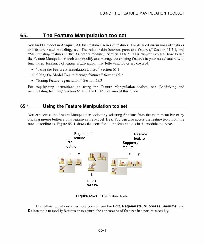
USING THE FEATURE MANIPULATION TOOLSET
65. The Feature Manipulation toolset
You build a model in Abaqus/CAE by creating a series of features. For detailed discussions of features
and feature-based modeling, see “The relationship between parts and features,” Section 11.3.1, and
“Manipulating features in the Assembly module,” Section 13.8.2. This chapter explains how to use
the Feature Manipulation toolset to modify and manage the existing features in your model and how to
tune the performance of feature regeneration. The following topics are covered:
• “Using the Feature Manipulation toolset,” Section 65.1
• “Using the Model Tree to manage features,” Section 65.2
• “Tuning feature regeneration,” Section 65.3
For step-by-step instructions on using the Feature Manipulation toolset, see “Modifying and
manipulating features,” Section 65.4, in the HTML version of this guide.
65.1 Using the Feature Manipulation toolset
You can access the Feature Manipulation toolset by selecting Feature from the main menu bar or by
clicking mouse button 3 on a feature in the Model Tree. You can also access the feature tools from the
module toolboxes. Figure 65–1 shows the icons for all the feature tools in the module toolboxes.
Figure 65–1 The feature tools.
The following list describes how you can use the Edit, Regenerate, Suppress, Resume, andDelete tools to modify features or to control the appearance of features in a part or assembly.
65–1
Abaqus ID:
Printed on:

USING THE FEATURE MANIPULATION TOOLSET
Edit a feature
You can edit the features of a part only in the Part module. Any changes that you make to a part are
applied automatically to each instance of that part in the assembly. Likewise, you can edit features
of the assembly only in the Assembly and Mesh modules. For information on restrictions that apply
to editing partitions and datum geometry, see “Understanding a datum as a feature,” Section 62.4,
and “Understanding partitions,” Section 70.3.
Regenerate a feature
Regeneration is the process of recalculating model geometry after a feature of the model has
been modified. By default, Abaqus/CAE automatically regenerates a part or assembly after you
have edited one of its features. However, you can control whether or not features are regenerated
automatically by toggling the Regenerate on OK option off or on in the Feature Editor. For
more information, see “Editing a feature,” Section 65.4.1, in the HTML version of this guide.
Suppress a feature
When you aremanipulatingmany features in a complexmodel (for example, when you are exploring
design alternatives), Abaqus/CAE allows you to temporarily disable certain features to simplify the
display or to speed regeneration. A suppressed feature is not visible and cannot be partitioned
or meshed. In addition, Abaqus/CAE ignores all suppressed features when regenerating a part or
assembly. You can edit a suppressed feature, although your changes will have no effect on the part
or assembly until you resume the feature. Suppressing a feature also suppresses any children of
that feature. (For information on parent and child features, see “The relationship between parts and
features,” Section 11.3.1.)
Abaqus/CAE does not include a suppressed feature in the input file that it generates when you
submit a job for analysis. However, Abaqus/CAE does include in the input file prescribed conditions
that refer to the suppressed feature or regions of the suppressed feature. To ensure that the analysis
completes successfully, you should do one of the following:
• Resume the suppressed feature.
• Edit the prescribed condition, and apply the prescribed condition to a different region.
• Delete the prescribed condition.
If you want to temporarily make a part instance invisible in the assembly, you can hide the part
instance by selecting options in theAssembly Display Options dialog box. For more information,
see “Controlling instance visibility,” Section 76.14.
Resume a feature
When you resume a suppressed feature, it reappears in the display of the part or assembly and
becomes reestablished in the model. If you edited the feature when it was suppressed, resuming
the feature causes Abaqus/CAE to regenerate the model automatically to take into account your
65–2
Abaqus ID:
Printed on:

USING THE MODEL TREE TO MANAGE FEATURES
changes. When you resume a feature, you have the option of resuming all of its children as well.
(You cannot resume a child feature without also resuming its parent.)
Tuning regeneration performance
Tuning feature regeneration performance is a balance between the convenience of saved states
and the effect on performance of memory consumption. In most cases the default settings will
result in acceptable regeneration performance; however, you can tune the speed of regeneration by
selecting Feature→Options from the main menu bar. For more information, see “Tuning feature
regeneration,” Section 65.3.
Delete a feature
Deleting a feature removes the feature from the model permanently. If you delete a parent feature,
all of its children will also be deleted and cannot be recovered.
In addition, you can reduce all the feature and parameter information to a simple definition of the
part when you copy a part to a new part. If you reduce the feature list while copying a part, Abaqus/CAE
will regenerate the new part faster if you subsequently modify it; however, you will no longer be able to
modify any parameters of the new part. To copy a part, select Part→Copy from the main menu bar in
the Part module.
65.2 Using the Model Tree to manage features
The Model Tree, shown in Figure 65–2, includes a list of all available features in the model. You can
click mouse button 3 on a feature in the Model Tree and use the menu that appears to manage the features.
You must use the Model Tree to manipulate assembly constraints, suppressed features, or failed
features since they are not visible in the viewport. You can also select multiple features to delete,
suppress, or resume at the same time. As you select features in the Model Tree, they are highlighted
in the viewport (if they are visible). In addition, parents or children of any feature can be highlighted in
the viewport.
The Model Tree displays the status of each feature in the model. The icon before each feature name
indicates the status:
• A yellow check mark indicates that the feature is modified but has not been regenerated. If a part
is locked by a database upgrade, all active features show this status until they are regenerated when
the part is unlocked. Abaqus/CAE also displays a yellow check mark next to a feature that you
edited but did not subsequently regenerate.
• A padlock indicates that a part or the assembly has been locked by the user or by a database upgrade.
• A red “X” indicates that the feature is suppressed.
• A red “!” indicates that the feature has failed to regenerate. A red “!” next to the part name indicates
that the part is invalid.
65–3
Abaqus ID:
Printed on:

USING THE MODEL TREE TO MANAGE FEATURES
Figure 65–2 The Model Tree.
To get more information about a feature, click mouse button 3 on the feature in the Model Tree and select
Query from the menu that appears. The information is displayed in the message area.
65–4
Abaqus ID:
Printed on:

TUNING FEATURE REGENERATION
65.3 Tuning feature regeneration
This section describes how you can tune feature regeneration using settings in the Feature Optionsdialog box. You open the Feature Options dialog box by selecting Feature→Options from the main
menu bar. In most cases the default settings will result in acceptable regeneration performance. You
should modify the feature options only if Abaqus/CAE takes a long time to regenerate a part or the
assembly or if memory consumption is excessive.
The settings in the Feature Options dialog box apply only to the current model and are saved in
the model database. If you change to a different model, Abaqus/CAE reverts to the default settings or to
any modified settings associated with the new model.
65.3.1 What is regeneration?Whenever you modify a feature of a part, Abaqus/CAE has to regenerate the part. Similarly, to
incorporate the modified feature into any instances of the part, Abaqus/CAE also regenerates features
in the assembly when you enter an assembly-related module. However, to save time, Abaqus/CAE
determines the minimum number of features that need to be regenerated and regenerates only the
features that were affected by the modification. If your parts and your assembly are relatively simple,
you will not notice Abaqus/CAE performing this regeneration. However, in a more complex model the
regeneration can result in a decrease in performance. Modifications to features that trigger regeneration
include using the Feature Manipulation toolset to edit, suppress, resume, and delete a feature.
The Model Tree indicates that a feature needs to be regenerated using a yellow check mark,
as described in “Using the Model Tree to manage features,” Section 65.2. You can always force
Abaqus/CAE to regenerate a part of the assembly by selecting Feature→Regenerate from the main
menu bar or by clicking mouse button 3 on the Features container in the Model Tree.
65.3.2 What is a geometric state?A geometric state refers to the internal geometric representation of a part or of the assembly; for example,
the equations of the curves and surfaces that define the topology and the connectivity of those curves
and surfaces. A geometric state is a snapshot of this internal representation. Abaqus/CAE stores this
snapshot and creates a geometric state in memory at regular intervals while you work on your model and
then regenerate features.
If Abaqus/CAE did not save geometric states, regeneration would start from the first feature that you
created and continue through all the features that need to be regenerated, making regeneration very costly.
By saving states, Abaqus/CAE can determine which state is closest to the feature that was modified.
Regeneration starts from that point and continues through all the features that need to be regenerated. As
a result, the speed of regeneration can be increased significantly.
65–5
Abaqus ID:
Printed on:

TUNING FEATURE REGENERATION
Ideally, to gain the maximum regeneration performance, you would save the geometric state after
every feature modification. However, storing every state would consume large amounts of memory and
hinder overall performance. Deciding how many states to save is a tradeoff between regeneration speed
and memory consumption.
By default, Abaqus/CAE automatically saves up to five geometric states for each part and for the
assembly. If Abaqus/CAE has already stored the specified number of states, it deletes one of the older
states before saving the most recent state. You can use the Geometry Caching for Fast Regenerationoptions in the Options dialog box to change the number of states automatically saved by Abaqus/CAE.
Abaqus/CAE uses an internal logic to decide when to create a geometric state; you cannot control when
a state is created.
65.3.3 What is a cache?A cache is a portion of memory. Abaqus/CAE uses the following feature-related caches to store
geometric states:
• The Current part cache contains snapshots of the geometric state of the current part. Abaqus
creates one part cache for each part in the model.
• The All part caches contains snapshots of the geometric state of all the parts in the current model.
• The Assembly cache contains snapshots of the geometric state of the assembly. Abaqus creates
one assembly cache for the model.
If you find that Abaqus/CAE is consuming an excessive amount of memory on your workstation
and affecting the performance of your system, you can use the Clear buttons in the Options dialog
box to erase the memory associated with the part and assembly caches. Clearing this memory will
increase performance; however, the snapshots of the geometric state will be erased and regeneration will
be slower. If you toggle off the option to cache geometric states, Abaqus/CAE does not clear the states
that have already been stored. In addition, Abaqus/CAE stores a separate cache for each model. As
a result, you can make more memory available by deleting the caches of any models that you are not
currently working on.
If you spent a lot of time making a series of changes to a part and are satisfied that your design
is correct, you can manually save the current state in memory by clicking Cache current statein the Options dialog box. As a result, Abaqus/CAE can return to this state and regenerate any
subsequent additions or modifications. However, if you continue to automatically cache geometric
states, Abaqus/CAE may erase the state that you saved manually after it has saved the maximum number
of geometric states. Alternatively, you can toggle off the option to automatically cache geometric states
and continue to manually save states at significant intervals.
The Geometry Caching for Fast Regeneration options in the Options dialog box indicate how
many geometric states are stored in the three feature-related caches. A cache can contain a combination
of geometric states that you saved manually and states that Abaqus/CAE saved automatically. You can
query the Current part cache and the Assembly cache to determine the positioning of geometric
states relative to the sequence of features.
65–6
Abaqus ID:
Printed on:
TUNING FEATURE REGENERATION
65.3.4 What are self-intersection checks?
Self-intersection checks are tests used to help ensure that complex geometry you create in Abaqus/CAE
is valid for analysis. If faces of a feature intersect other faces of the same feature, Abaqus/CAE displays
a warning that there are invalid intersections and does not create the feature. A feature that intersects
itself may not be meshable and may cause problems with the analysis. Abaqus/CAE allows you to check
for self-intersection during feature creation; however, the checking process will slow down creation of
the feature. In addition, checking for self-intersection will slow down regeneration of the feature. The
time required to complete the tests varies with the complexity of the feature you are attempting to create
or regenerate.
The Feature Options dialog box allows you to toggle self-intersection checks on and off. Performself-intersection checks is toggled off by default. In general, self-intersection is possible only when
you are creating features with complex geometry, such as loft features (for more information, see “What is
lofting?,” Section 11.14, and “Self-intersection checks,” Section 11.14.4). If you know that your features
do not self-intersect or if you plan to remove the self-intersection during a subsequent operation, you can
leave Perform self-intersection checks toggled off to speed up feature regeneration.
65.3.5 How are position constraints regenerated?
By default, when Abaqus/CAE regenerates the assembly, it regenerates all of the position constraints
before regenerating other features that might depend on the position, such as partitions and datums.
However, if the position constraint uses an entity that was created by selecting from a part instance
in the Assembly module, such as a face created by a partition or a datum axis running through two
vertices, Abaqus/CAE changes its behavior and regenerates features in the order that you created them.
As a result, partitions and datums that you created before the position constraint may not move along
with the movable instance.
If you are working in the assembly-related modules, the Feature Options dialog box includes
a Constraints field that allows you to control this regeneration behavior. For more information, see
“Tuning regeneration performance,” Section 65.4.7, in the HTML version of this guide.
65–7
Abaqus ID:
Printed on:

FILTERING FIELD AND HISTORY DATA
66. The Filter toolset
Filters allow you to remove extraneous field output data or history output data—noise—during the
analysis of a model without a loss of resolution in the desired data range. You can also use filters to
filter field output or history output before the data are saved to the output database (.odb) file; as aresult, filters can also reduce the size of the output database. The Filter toolset allows you to create and
manage filters in the Step module. This chapter covers the following topics:
• “Filtering field and history data,” Section 66.1
• “Applying bounding values to field and history data,” Section 66.2
In addition, more detailed information is available in “Creating a filter,” Section 66.3, in the HTML
version of this guide.
66.1 Filtering field and history data
You can create filters in Abaqus/CAE and apply them to field output requests or history output requests for
Abaqus/Explicit analyses. Abaqus filters data while the analysis is running; filtering during the analysis
(“real time” filtering) can reduce the size of the output database by excluding high-frequency data before
it is saved. Real time filtering also avoids potential aliasing problems in the resulting data. Aliasing is a
loss of valid results data; aliasing will occur if the sampling frequency (the frequency at which the data
are saved) is less than twice the highest frequency expected in the results. For example, if a sine wave
was sampled at only two points, the aliased result would appear to be a straight line, whereas sampling
at least four points would reproduce the shape of the curve.
The Filter toolset allows you to create the following filters for use with Abaqus/Explicit field output
requests and history output requests:
• Butterworth
• Type I Chebyshev
• Type II Chebyshev
For more specific information about these filters, see “Filtering output and operating on output in
Abaqus/Explicit” in “Output to the output database,” Section 4.1.3 of the Abaqus Analysis User’s
Guide. The different filter types are distinguished by their capabilities to transition from the acceptance
of low-frequency data to the rejection of data above the filter’s Cutoff frequency. An ideal filter wouldstop all data above the cutoff frequency and have a flat response (no affect on accepted data); “real”
filters include a transition band around the cutoff where some data are accepted and they usually have
some effect on the accepted data. The Butterworth filter provides a maximally flat response magnitude
with a wider transition band (slower transition) than the Chebyshev filters. The Chebyshev filters
introduce an oscillation—a ripple—in the response magnitude, but they have a narrower transition band
than the Butterworth filter. The two types of Chebyshev filters differ in where in their response ripples
66–1
Abaqus ID:
Printed on:

APPLYING BOUNDING VALUES TO FIELD AND HISTORY DATA
occur; the Ripple factor indicates how much oscillation you will allow in exchange for an improved
filter response. You can also specify the Order of the filter, which determines the size of the filter’s
transition band: the higher the order, the narrower the transition band, although the computational cost
increases as the order increases. The filter order must be a positive, even integer no greater than 20.
In addition to the filters that you can define using the Filter toolset, Abaqus also includes a default
Antialiasing filter. Abaqus automatically sets the cutoff frequency of the Antialiasing filter based on
the time interval at which the field output or history output is saved during the analysis. When you define
a filter, you must specify the cutoff frequency based on your knowledge of the frequencies expected in
the solution. Whether you set the cutoff or Abaqus calculates it, no checks are performed to ensure that
the cutoff frequency is appropriate. If the cutoff is set too low, valid data will be filtered from the results;
if it is set too high (above half the sampling frequency), no filtering will be performed.
Select Tools→Filter→Create from the main menu to create a new filter definition; select Editfrom the same menu to make changes to an existing definition. Either command opens the filter editor,
which allows you to select the options and provide the data needed to define your filter.
To apply a filter to an analysis, include it in a field output request or history output request for an
Abaqus/Explicit analysis procedure (for more information, see “Defining output requests,” Section 14.12,
in the HTML version of this guide).
66.2 Applying bounding values to field and history data
Bounding values in a filter definition enable you to investigate the maximum or minimum values for a
particular output request and to establish an upper or lower bound on the variable values that are returned
for an output request. You can establish bounding values for both filtered and unfiltered data; to specify
these values in a filter definition without performing Butterworth filtering or either type of Chebyshev
filtering on your data, define an Operator filter, which enables you to implement bounding values on an
output request without changing the output data in any other way.
Abaqus/CAE provides three types of bounding values:
• Maximum bounding values return the highest value within each output interval for the variables in
an output request.
• Minimum bounding values return the lowest value within each output interval for the variables in
an output request.
• Absolute maximum bounding values return the highest absolute value for the variables in an
output request within each output interval.
In addition, you can set a limit on the bounding value, which determines the highest or lowest value
that Abaqus/CAE records for variables that use this filter. If desired, you can stop the analysis when any
variables in an output request reach this limiting value.
By default, each component of a tensor or vector quantity is filtered individually and the maximum,
minimum, or absolute maximum value and the limiting values are reported separately for each
component. You can, however, apply a filter directly to an invariant.
66–2
Abaqus ID:
Printed on:

RESULTANT FORCES AND MOMENTS ON FREE BODY CUTS IN Abaqus/CAE
67. The Free Body toolset
Free body cuts display the resultant forces and moments transmitted across a selected surface of your
model. The Free Body toolset is available only in the Visualization module, and you can create a free
body cut only when the current step and frame of the output database includes element force nodal output
(NFORC).
This chapter explains how to use the Free Body toolset to create and delete free body cuts, display
or hide them in the viewport, and customize several aspects of their appearance. The following topics
are covered:
• “Resultant forces and moments on free body cuts in Abaqus/CAE,” Section 67.1
In addition, the following sections are available in the HTML version of this guide:
• “Creating or editing a free body cut,” Section 67.2
• “Selection methods for free body cross-sections,” Section 67.3
• “Displaying, hiding, and highlighting free body cuts,” Section 67.4
• “Customizing free body cut display,” Section 67.5
Abaqus/CAE also enables you to generate reports or create X–Y data objects that describe the forces and
moments in all active free body cuts in your session. See “Producing a tabular report,” Section 54.1, and
“Reading X–Y data from all active free body cuts,” Section 47.2.4, in the HTML version of this guide,
respectively.
Abaqus/CAE provides two other methods for displaying free body data:
• You can display resultant forces and moments along an arbitrary plane through your model by
toggling on free body display for a planar view cut. For more information, see “Understanding
view cuts,” Section 80.1.
• You can display the free body nodal forces in a symbol plot to determine which nodes have an
imbalance of forces or moments due to applied loads or to visualize the nodal force distribution on
internal sections. For more information, see “Producing a symbol plot of free body nodal forces,”
Section 45.4.
67.1 Resultant forces and moments on free body cuts in Abaqus/CAE
A free body cross-section in Abaqus/CAE is an area of your model across which you want to display
resultant forces and moments. Once you define a cross-section, Abaqus/CAE displays vectors that show
the magnitude and direction of the resultant forces and moments across the area you select. Force vectors
are displayed with a single arrowhead and moment vectors with a double arrowhead, as shown in the
example in Figure 67–1.
You can define the nodes and elements that comprise the cross-section using processes that closely
resemble the definition of display groups. Abaqus/CAE enables you to specify the components of the
67–1
Abaqus ID:
Printed on:

RESULTANT FORCES AND MOMENTS ON FREE BODY CUTS IN Abaqus/CAE
Figure 67–1 Resultant force and moment displayed
on a model of a fuselage.
cross-section by including surfaces, display groups, and elements or nodes by number; and you can
pick items from the viewport, either by feature angle or individually. See “Creating or editing a free
body cut,” Section 67.2, for detailed instructions. After you define the physical components of your free
body cross-section, you can set the location of the summation point (about which resultant moments are
taken), and you can indicate the coordinate system transformation that applies when vectors are displayed
in component form.
Cross-sections can be created along mesh boundaries only; you cannot specify a cross-section along
an arbitrary plane. You can create and display free body cuts only in the Visualization module.
67–2
Abaqus ID:
Printed on:

CUSTOMIZING MEMORY LIMITS AND REGENERATION OPTIONS
68. The Options toolset
This chapter covers the following topics:
• “Customizing memory limits and regeneration options,” Section 68.1
• “Using view manipulation shortcuts,” Section 68.2
• “Scaling the size of icons,” Section 68.3
68.1 Customizing memory limits and regeneration options
A geometric state is a snapshot of the internal representation of a part or an independent part instance.
Saving geometric states in a memory cache speeds up regeneration performance; however, the saved
states can consume large amounts of memory and decrease overall performance.
The options on the Memory tabbed page of the Options dialog box allow you to control the amount
of memory allocated to the Abaqus kernel, specify the percentage of memory use that will prompt
Abaqus/CAE to run in reduced memory mode, and tune the balance between the convenience of saving
states and the performance degradation from increasing memory consumption. Select Tools→Optionsfrom the main menu bar to display the Options dialog box, then click the Memory tab.
In most cases the default settings will result in acceptable regeneration performance. You should
modify the feature options only if Abaqus/CAE takes a long time to regenerate a part or the assembly.
For more information, see “Tuning feature regeneration,” Section 65.3.
To customize the memory limits and memory cache settings for your session:
1. From the main menu bar in any module, select Tools→Options.
The Options dialog box appears.
2. Display the Memory tabbed page.
3. If desired, specify a new Kernel memory limit in megabytes. If this setting is zero, no limit is
imposed on kernel memory.
4. Toggle on Run in reduced memory mode when memory reaches, and specify a percentage ofthe kernel memory limit above which Abaqus/CAE runs in reduced memory mode. Abaqus/CAE
reduces memory by either paging geometric data to disk or by deleting data in inactive parts that
can be automatically regenerated when needed.
5. If desired, change the number of geometric states that Abaqus/CAE automatically caches in
memory. Ideally, to gain the maximum regeneration performance, you would save the geometric
state after every feature modification. However, storing a large number of geometric states
consumes large amounts of memory and hinders overall performance. Deciding how many states
68–1
Abaqus ID:
Printed on:

USING VIEW MANIPULATION SHORTCUTS
to save is a tradeoff between regeneration speed and memory consumption. For more information,
see “What is a geometric state?,” Section 65.3.2.
6. If you find that Abaqus/CAE is consuming a lot of memory on your workstation and affecting the
performance of your system, you can use the Clear buttons in the Options dialog box to erase
the memory associated with the part and assembly caches. Clearing this memory will increase
performance; however, the snapshots of the geometric state will be erased and regeneration will be
slower. For more information, see “What is a cache?,” Section 65.3.3.
7. If you want to save a current state in memory, click Cache current state in the Options dialog
box. Abaqus/CAE can return to this state and regenerate any subsequent additions or modifications.
The Options dialog box indicates how many geometric states are stored in the caches. Click Queryto determine the positioning of geometric states relative to the sequence of features in the current
part cache or the assembly cache. When Abaqus/CAE is running in reduced memory mode, the
geometric states may be deleted if the memory consumption is higher than the specified threshold.
8. Click OK to change the memory limits and regeneration performance options for the current model.
The options apply only to the current session and are not saved in the model database.
68.2 Using view manipulation shortcuts
You can access the pan, rotate, and magnify view manipulation tools using combinations of keyboard and
mouse actions. These shortcuts can make it easier and less interruptive to manipulate the view of a model
while performing other tasks (for example, selecting elements to define a set). Abaqus/CAE activates the
specified view manipulation tool as long as the associated combination of keyboard and mouse buttons
is depressed; to exit the view manipulation tool, release the associated keyboard and mouse buttons.
In addition to the default Abaqus/CAE shortcuts, you can configure the view manipulation
shortcuts to mimic five other common CAD applications, as outlined in Table 68–1. Change the
shortcuts configuration by selecting Tools→Options from the main menu bar and changing the ViewManipulation options. Your configuration is saved for future Abaqus/CAE sessions.
Table 68–1 View manipulation shortcuts for available configurations
(“MB” stands for “mouse button”).
Application Pan Rotate Zoom
Abaqus/CAE (default) [Ctrl]+[Alt]+[MB2] [Ctrl]+[Alt]+[MB1] [Ctrl]+[Alt]+[MB3]
CATIA V5 [MB2] [MB2]+[MB3]; or
[MB2]+[MB1]
[MB2]+[MB3], then release
[MB3]; or [MB2]+[MB1],
then release [MB1]
SolidWorks [Ctrl]+[MB2] [MB2] [Shift]+[MB2]
68–2
Abaqus ID:
Printed on:

SCALING THE SIZE OF ICONS
Application Pan Rotate Zoom
HyperView [Ctrl]+[MB3] [Ctrl]+[MB1] [Ctrl]+[MB2]
Pro/ENGINEERWildfire
[Shift]+[MB2] [MB2] [Ctrl]+[MB2]
UGS NX [MB2]+[MB3] [MB2] [MB2]+[MB1]
Note: The HyperView key combination for rotation ([Ctrl]+[MB1]) conflicts with the Abaqus/CAE use
of this combination to unselect objects in the viewport. To make complex viewport selections where
unselecting individual objects may be useful, it is recommended that you choose one of the other shortcut
configurations.
Nondefault configurations of the view manipulation shortcuts change the behavior of the magnify
tool. In the default Abaqus/CAE configuration, the magnify tool operates by dragging the cursor
horizontally; in all other configurations, the magnify tool operates by dragging the cursor vertically.
In the default Abaqus/CAE shortcuts configuration, you can access the alternate modes of the pan,
rotate, andmagnify tools by holding the [Shift] key in addition to the other shortcut keys (see “An overviewof the view manipulation tools,” Section 5.2.1, for details). This convention conflicts with some of the
shortcut combinations in nondefault configurations; therefore, you cannot access alternate modes of the
view manipulation tools while using nondefault shortcuts. The alternate modes are always available,
regardless of your shortcuts configuration, if you access a view manipulation tool using the standard
methods (selecting a tool from the View menu in the main menu bar or clicking a tool in the ViewManipulation toolbar).
68.3 Scaling the size of icons
The default size for icons in toolbars and toolboxes is 24 × 24 pixels. The default size for icons in the
Model Tree and the Results Tree is 16 × 16 pixels. You can specify a scale factor to increase or decrease
the size of these icons so that they appear at a size that is appropriate for your display resolution. For
example, increasing the icon size scale factor to 1.5 prompts Abaqus/CAE to display toolbar and toolbox
icons at 36 × 36 pixels and Model Tree and Results Tree icons at 24 × 24 pixels.
Select Tools→Options, then click the Icons tab to display the icon scaling options. You can click
the arrows to the right of the Scale factor field to increase or decrease the size of icons in Abaqus/CAE.The maximum scale factor is 3; the minimum scale factor is 0.5.
Changes to icon size are implemented when you restart Abaqus/CAE. Your selected scale factor is
saved for future Abaqus/CAE sessions.
68–3
Abaqus ID:
Printed on:


AN OVERVIEW OF EDITING TECHNIQUES
69. The Geometry Edit toolset
The Geometry Edit toolset provides a set of tools in the Part module that allow you to create or edit the
geometry of a part. You can use the tools to edit the regions of a part that make it invalid or imprecise.
The following topics are covered:
• “Using the Geometry Edit toolset,” Section 69.1
• “An overview of editing techniques,” Section 69.2
• “What is stitching?,” Section 69.3
• “A strategy for repairing geometry,” Section 69.4
• “Creating a part from orphan elements,” Section 69.5
In addition, the following sections are available in the HTML version of this guide:
• “Editing and repairing edges,” Section 69.6
• “Editing and repairing faces,” Section 69.7
• “Editing parts,” Section 69.8
69.1 Using the Geometry Edit toolset
You can use the Geometry Edit toolset in the Part module to edit or repair the geometry of a part. The
Geometry Edit toolset enables you to edit an imported part to improve its precision and validity; however,
Abaqus/CAE does not require parts to be completely precise. In addition, you can use the Geometry
Edit toolset to remove small features from a part. You can use the Geometry Edit toolset to edit edges,
faces, or the entire part. “An overview of editing techniques,” Section 69.2, provides an overview of the
methods available for each type of partition. Abaqus/CAE stores most of the edit operations as features.
As a result, you can undo an edit by deleting or suppressing the corresponding feature using the Feature
Manipulation toolset.
You can access the edit tools by selecting Tools→Geometry Edit from the main menu and
choosing the desired tool from the Geometry Edit dialog box that appears. You can also access the
Geometry Edit tools through the Part module toolbox. Figure 69–1 shows the hidden icons for all the
Geometry Edit tools in the Part module toolbox. To see a tooltip containing a short description of each
Geometry Edit tool, hold the mouse over the tool for a moment. For more information, see “Using
toolboxes and toolbars that contain hidden icons,” Section 3.3.2.
69.2 An overview of editing techniques
This section provides an overview of the different editing techniques. The following topics are covered:
• “An overview of the methods for editing edges,” Section 69.2.1
• “An overview of the methods for editing faces,” Section 69.2.2
69–1
Abaqus ID:
Printed on:

AN OVERVIEW OF EDITING TECHNIQUES
stitch
repairface
normals
convert toanalytical
convert toprecise
repairsmalledges
mergeedges
removeredundant
entities
repairsmallfaces
replacefaces
repairsliver
removefaces
remove wire
edges
repair invalidedgesgeometry
edit
offset faces
blend faces
extend faces
cover edges
face from element faces
Figure 69–1 The Geometry Edit toolset toolbox.
• “An overview of the methods for editing entire parts,” Section 69.2.3
69.2.1 An overview of the methods for editing edgesSelect Tools→Geometry Edit from the main menu to display the Geometry Edit dialog box. When
you choose Edge from the dialog box, the Tool list displays the following methods for editing edges:
69–2
Abaqus ID:
Printed on:
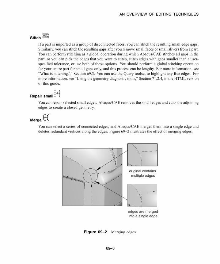
AN OVERVIEW OF EDITING TECHNIQUES
Stitch
If a part is imported as a group of disconnected faces, you can stitch the resulting small edge gaps.
Similarly, you can stitch the resulting gaps after you remove small faces or small slivers from a part.
You can perform stitching as a global operation during which Abaqus/CAE stitches all gaps in the
part, or you can pick the edges that you want to stitch, stitch edges with gaps smaller than a user-
specified tolerance, or use both of these options. You should perform a global stitching operation
for your entire part for small gaps only, and this process can be lengthy. For more information, see
“What is stitching?,” Section 69.3. You can use the Query toolset to highlight any free edges. For
more information, see “Using the geometry diagnostic tools,” Section 71.2.4, in the HTML version
of this guide.
Repair small
You can repair selected small edges. Abaqus/CAE removes the small edges and edits the adjoining
edges to create a closed geometry.
Merge
You can select a series of connected edges, and Abaqus/CAE merges them into a single edge and
deletes redundant vertices along the edges. Figure 69–2 illustrates the effect of merging edges.
original contains multiple edges
edges are mergedinto a single edge
Figure 69–2 Merging edges.
69–3
Abaqus ID:
Printed on:

AN OVERVIEW OF EDITING TECHNIQUES
Remove redundant entities
An imported part can contain redundant vertices that are positioned along a continuous edge.
Similarly, an imported part can include redundant edges that are internal edges. Redundant
vertices and edges do not change the shape or the area of a part and are not required for a complete
definition, as shown in Figure 69–3.
Redundantvertices
Redundantedges
Redundantvertex
Figure 69–3 Redundant edges and vertices.
Repair invalid
In rare cases after you import a part, Abaqus will report that some of its edges are invalid. The
Repair invalid tool will try to repair the invalid edges by recomputing the data that define them.
You should also use this tool if the Query toolset indicates that the part contains only invalid edges.
Remove wire
You can remove selected wire edges. Abaqus/CAE removes the wire edges.
69.2.2 An overview of the methods for editing facesWhen you choose Face from theGeometry Edit dialog box, the Tool list displays the followingmethods
for repairing faces:
Remove
You can remove selected faces (including chamfers, fillets, and holes) from a three-dimensional
solid or shell or from a two-dimensional planar part. After you have selected the faces to remove,
Abaqus/CAE looks for adjacent faces that define a feature. You can remove the entire feature, or you
can remove only the selected faces. When you remove one or more faces from a three-dimensional
solid part, Abaqus/CAE converts the part to a shell.
69–4
Abaqus ID:
Printed on:

AN OVERVIEW OF EDITING TECHNIQUES
Cover edges
You can create a face on a three-dimensional part by selecting one or more edges of the new face.
Abaqus/CAE loops through the adjacent edges and calculates the location of the new face. If you
selected multiple edges that are not connected by a common loop, Abaqus/CAE creates multiple
faces, one for each loop of edges. Abaqus/CAE creates the new faces as shells. If the new shells
form a closed part, you can use the solid-from-shell tool to convert the part to a solid.
Replace
In some cases Abaqus/CAE may not be able to accurately recreate some of the faces when you
import a part. For example, a planar face may appear wavy or distorted, or Abaqus/CAE might
create small faces that have a large impact on the mesh density. You can select connected faces,
and Abaqus/CAE replaces them with a single face. The new face has minimal faceting and will be
smoother than the original faces. Figure 69–4 illustrates the effect of replacing selected faces.
selectedfaces toreplace
Figure 69–4 The effect of replacing selected faces.
Alternatively, you can replace the selected faces with a single face that is formed by extending
neighboring faces. You can use this tool to remove bosses and small details from imported parts,
as shown in Figure 69–5.
Repair small
You can repair selected small faces. Abaqus/CAE removes the small faces and edits the adjoining
faces to create a closed geometry. Figure 69–6 illustrates the effect of repairing small faces.
69–5
Abaqus ID:
Printed on:

AN OVERVIEW OF EDITING TECHNIQUES
selectedfaces toreplace
Figure 69–5 The effect of replacing selected faces and extending neighboring faces.
original small faces
small faces removed
Figure 69–6 Repairing small faces.
Repair sliver
A sliver can be thought of as a small, sharp piece of extra material. You can remove an unwanted
sliver from a face of a three-dimensional solid or shell or from a two-dimensional planar part. You
must select the face containing the sliver to remove and two points from the face. Abaqus/CAE
draws a line between the two points that divides the selected face into two regions. The first region is
the face that will remain; the second region is the sliver that will be removed. Figure 69–7 illustrates
the effect of removing a sliver.
69–6
Abaqus ID:
Printed on:

AN OVERVIEW OF EDITING TECHNIQUES
original sliver face
sliver face removed
Figure 69–7 Removing a sliver.
Repair normals
You can repair the face normals of shell and solid imported parts, and you can perform these repairs
on either manifold parts (parts in which every edge is shared by only one or two faces) and non-
manifold parts. The tool has different uses for solid and shell parts.
Solid
In rare cases the Query toolset reports that the volume of an imported solid part is negative
because the face normals indicate it was inside out in the CAD system from which it originated.
The Repair face normals tool will flip the normals and turn the solid right side out.
ShellAn imported shell part can contain faces that have normals pointing in opposite directions. The
Repair face normals tool will align all the normals on a shell part. If the face normals are
already aligned, this tool will flip all the normals so that they remain aligned but point in the
opposite direction.
Note: The element normal orientation, which is specified using the Element Normalassignment in the Property module, specifies the relative element normal with respect to the
geometry normal. These element normals will be updated using the new geometry normals
after the Repair face normals operation.
When you perform repairs of non-manifold shell parts, you cannot align the normals for
all of the faces in the part in a single operation; you must select faces individually to flip the
direction of their normals. You can perform a query using the Shell element normals option
from the Query dialog box to assess the orientation of the face normals before you repair your
shell part.
69–7
Abaqus ID:
Printed on:
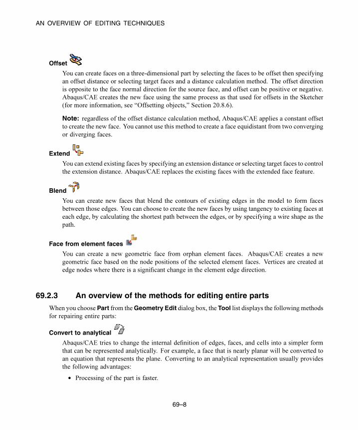
AN OVERVIEW OF EDITING TECHNIQUES
Offset
You can create faces on a three-dimensional part by selecting the faces to be offset then specifying
an offset distance or selecting target faces and a distance calculation method. The offset direction
is opposite to the face normal direction for the source face, and offset can be positive or negative.
Abaqus/CAE creates the new face using the same process as that used for offsets in the Sketcher
(for more information, see “Offsetting objects,” Section 20.8.6).
Note: regardless of the offset distance calculation method, Abaqus/CAE applies a constant offset
to create the new face. You cannot use this method to create a face equidistant from two converging
or diverging faces.
Extend
You can extend existing faces by specifying an extension distance or selecting target faces to control
the extension distance. Abaqus/CAE replaces the existing faces with the extended face feature.
Blend
You can create new faces that blend the contours of existing edges in the model to form faces
between those edges. You can choose to create the new faces by using tangency to existing faces at
each edge, by calculating the shortest path between the edges, or by specifying a wire shape as the
path.
Face from element faces
You can create a new geometric face from orphan element faces. Abaqus/CAE creates a new
geometric face based on the node positions of the selected element faces. Vertices are created at
edge nodes where there is a significant change in the element edge direction.
69.2.3 An overview of the methods for editing entire parts
When you choose Part from the Geometry Edit dialog box, the Tool list displays the following methods
for repairing entire parts:
Convert to analytical
Abaqus/CAE tries to change the internal definition of edges, faces, and cells into a simpler form
that can be represented analytically. For example, a face that is nearly planar will be converted to
an equation that represents the plane. Converting to an analytical representation usually provides
the following advantages:
• Processing of the part is faster.
69–8
Abaqus ID:
Printed on:

WHAT IS STITCHING?
• The converted entity is available during feature operations. For example, the extrude operation
requires a planar face and a linear edge.
• The geometry is improved.
• If you subsequently need to stitch the part, the stitching operation is more likely to be
successful.
Convert to precise
Abaqus/CAE offers two methods to convert entities to precise geometry:
• If you choose Tighten Gaps, Abaqus/CAE attempts to improve the precision of the
faces, edges, and vertices in your model. This method is faster but does not perform a full
computation of the geometry.
• If you choose Recompute Geometry, Abaqus/CAE tries to change neighboring entities
so that their geometry matches exactly. Recomputing geometry usually results in precise
geometry; however, this operation can be lengthy and increases the complexity of the imported
part, which means that processing of the part is slower. Moreover, if the part contains many
complex surfaces, converting to a precise representation is likely to fail. If possible, you
should return to the CAD application that generated the original file and increase the precision.
69.3 What is stitching?
When you select this option, Abaqus/CAE tries to join adjoining faces along their free edges. The
intent of stitching is usually to create a solid part. Stitching edges usually results in valid geometry.
Abaqus/CAE stitches gaps between trimmed surfaces by adjusting the underlying surfaces until the edges
intersect. Figure 69–8 illustrates the stitching process.
To stitch gaps between intersecting edges, Abaqus/CAE adjusts the underlying surfaces until the two adjacent faces share the same edge.
Figure 69–8 Stitching edges until they intersect.
Abaqus/CAE tries to recognize the edges of a solid from a set of trimmed surfaces. If the edges of
each trimmed surface are close to an edge of an adjacent surface (within a user-specified tolerance),
69–9
Abaqus ID:
Printed on:

A STRATEGY FOR REPAIRING GEOMETRY
Abaqus/CAE stitches the trimmed surfaces. The end result of stitching is a B-rep solid in which the edge
definition is shared between the two intersecting surfaces. For more information on B-rep solids, see
“How do solid modelers represent a solid?,” Section 10.1.7. Stitching fails in the presence of wires or
internal faces.
When you import an IGES- or VDA-FS-format part, Abaqus/CAE stitches the part by default.
However, because of the internal tolerances of IGES- and VDA-FS-format parts, the resulting
representation of small features may not match the geometry that was intended in the original file.
In some cases stitching an IGES- or VDA-FS-format part results in Abaqus/CAE importing a single
part that should have been imported as separate parts. If you copy the imported part to a new part, you
can choose to separate disconnected regions into separate parts. For more information, see “Copying a
part,” Section 11.18.3, in the HTML version of this guide.
69.4 A strategy for repairing geometry
The tools in the Geometry Edit toolset are often used to repair geometry that was imported into
Abaqus/CAE. The goals of the repair operations are to create a part with no invalid entities and to
create a part that has the smallest number of edges and faces to avoid impacting the mesh generation. If
you are unable to create a valid part, you can ignore the invalidity. For more information, see “Working
with invalid parts,” Section 10.2.3. Ideally, the part will have no small edges or faces. You do not have
to create a precise part, and you should continue to work with an imprecise part if possible. Parts with
imprecise geometry can be meshed. However, in rare cases other operations may fail on parts with
imprecise geometry; for example, other meshing functions, adding geometry features, and partitioning.
If you cannot work with the imprecise part and you cannot make the part precise, you should return to
the CAD application that generated the original file and increase the precision. For more information,
see “What is a valid and precise part?,” Section 10.2.1.
Abaqus/CAE provides many different editing tools, and it is often difficult to decide which of the
tools to use and in which order to use them. In general, repairing the geometry of an imported part is an
art that requires experimentation and experience to master. The best approach depends on the complexity
of the part and how much detail you want to remain in the part when you mesh the part and analyze it.
The following guidelines will help you develop an efficient approach to repairing your parts:
Use the geometry diagnostic tools
Use the geometry diagnostic tools to query the part for invalid and imprecise entities, free edges,
short edges, small faces, and sharp corner angles.
Use selection groups
You can use mouse button 3 to create temporary selection groups to make the combination of
geometry diagnostic tools and repair tools easier to use. You can use the geometry diagnostic tools
to highlight a region of invalid and imprecise geometry, and you can copy the region into a selection
group. You can then paste the selection group into the Geometry Edit toolset when specifying the
region to repair.
69–10
Abaqus ID:
Printed on:

A STRATEGY FOR REPAIRING GEOMETRY
Use display groups
Use display groups to selectively remove faces and cells to help you see inside complex parts and
to determine which entities are highlighted by the geometry diagnostic tools.
Take an incremental approach
Use the repair tools on small groups of selected faces and edges and check that the outcome of the
repair process is correct before proceeding.
Keep solids intact
Try not to convert a solid into a shell by removing faces from the solid. To avoid removing faces,
use the Replace tool for faces, and the Repair small tools for edges and faces.
Avoid creating wires
If your part is a solid or a shell, try not to perform operations that result in wires. It is difficult for
Abaqus/CAE to reconstruct faces from wires.
Remove fillets and chamfers
Use the Replace tool and the Extend neighboring faces option to remove fillets and chamfers
from your part and extend the neighboring faces to close the resulting gap.
Remove faces that meet tangentially
Use the Replace tool or the Repair small tool to repair faces that are approximately tangential.
You should use the Repair small tool to remove faces that are relatively small. The Repairsmall tool simply extends the remaining faces until they meet. The small face is deleted in the
process, although the result may be imprecise. Use the Replace tool for relatively large faces that
meet tangentially. The Replace tool uses underlying points to replace the original faces with an
approximate surface.
Check the validity of the part
If your part is invalid, you can check if the repair operations have made the part valid by clicking
mouse button 3 on the part in the Model Tree and selecting Update validity from the menu that
appears. Checking the validity can be a lengthy operation, and you should wait until you have
finished editing the part before you check its validity. If a part is already valid, none of the repair
operations will make it invalid.
Create partitions after you repair
If your part contains partitions, the Geometry Edit toolset may delete them during a repair operation.
To avoid this problem, you should wait to partition the part until after you have finished editing it.
69–11
Abaqus ID:
Printed on:

CREATING A PART FROM ORPHAN ELEMENTS
69.5 Creating a part from orphan elements
You can use tools from the Geometry Edit toolset to create geometry from the faces of orphan mesh
elements. This technique is useful when you have a meshed part that requires modifications, but you
do not have some or all of its geometry available. The decision to add geometric features to an orphan
mesh, recreate the part geometry from scratch, or reverse engineer geometry from the orphan elements
depends on a number of factors, including:
• complexity of the existing part
• complexity of the features to be added
• degree of difficulty required to modify the existing orphan mesh
• desire to create a new mesh for the entire part
Other factors such as the time constraints for the project and the ability to export model geometry may
also be involved in your decision.
The goal of creating a part from an orphan mesh is to create geometry that matches the original
design intent while providing a platform for current and future modifications. The geometry must also
be suitable for creation of a native mesh by either full association with the current mesh or creation of a
new mesh.
The following guidelines will help you create geometry for an orphan mesh:
Create new geometric faces
Use the Face from element faces tool to create the outer surface geometry for the model.
Each use of the tool creates a single shell face from selected exterior orphan element faces. The
tool includes several unique methods for selection of multiple orphan element boundary faces, and
it automatically stitches the newly created face to any adjacent geometry. For more information, see
“Create face from element faces,” Section 69.7.10, in the HTML version of this guide. When you
are finished creating faces, all exterior orphan element faces should be covered by geometric faces.
Remove extra edges and faces
Use other tools from the Geometry Edit toolset to remove extra edges, small faces, and any other
features that would restrict generation of a good quality mesh. If necessary, convert the part to
precise geometry. For more information, see “A strategy for repairing geometry,” Section 69.4.
Convert to solid
If you are working with a solid part, use the Create solid from shell tool to fill the space
inside the created shell faces.
Partition and mesh the part
Suppress or delete the orphan mesh, and create a new mesh for the part.
69–12
Abaqus ID:
Printed on:

CREATING A PART FROM ORPHAN ELEMENTS
Create partitions after you repair
If your part contains partitions, the Geometry Edit toolset may delete them during a repair operation.
To avoid this problem, you should wait to partition the part until after you have finished editing it.
69–13
Abaqus ID:
Printed on:


USING THE PARTITION TOOLSET
70. The Partition toolset
You use the Partition toolset to divide a part or assembly into regions. Regions are used throughout the
modeling process; for example, to indicate the location of a load, a change in material properties, or a
mesh boundary.
This chapter explains how you use the Partition toolset to create and position partitions on an edge,
a face, or a cell. The following topics are covered:
• “Understanding the role of partitions,” Section 70.1
• “Using the Partition toolset,” Section 70.2
• “Understanding partitions,” Section 70.3
• “An overview of partitioning techniques,” Section 70.4
In addition, the following sections are available in the HTML version of this guide:
• “Partitioning edges,” Section 70.5
• “Partitioning faces,” Section 70.6
• “Partitioning cells,” Section 70.7
70.1 Understanding the role of partitions
As you proceed through the modeling process, you may find that you need to select a particular region
that does not exist in your model. Such regions might be used to define material boundaries, indicate the
location of loads and constraints, and help refine your mesh. You use the Partition toolset to partition
your model into regions.
Partitions can be created on edges, faces, and cells. A partition along an edge creates a new vertex,
while partitions through faces and cells create new edges and faces, respectively. In all cases, partitioning
serves to subdivide the geometry being partitioned. Figure 70–1 illustrates partitioning an edge, a face,
and a cell.
You partition edges, faces, and cells by defining partitions that refer to existing geometry. You can
partition a part in either the Part module or the Property module, or you can partition an assembly in
the modules that operate on the assembly. For example, you can partition a face of the assembly in the
Mesh module, and you can seed the resulting internal edge to refine your mesh. A partition is a feature;
and, like all features, it can be edited, deleted, suppressed, resumed, and queried. Similarly, a partition
is regenerated when the assembly or a part is regenerated.
70.2 Using the Partition toolset
You can access the Partition toolset by selecting Tools→Partition from the menu bar. The CreatePartition dialog box appears, and you choose the type of geometry to partition—edge, face, or
70–1
Abaqus ID:
Printed on:

USING THE PARTITION TOOLSET
����
partitionededge
partitionedface partitioned
cell
Figure 70–1 Partitioning an edge, a face, and a cell.
cell—from the buttons in the Type region at the top of the dialog box. The Method list changes
to reflect the partitions you can create. Select the desired partition tool from the Method list, and
follow the prompts in the prompt area to create the partition. Most of the tools allow you to partition
multiple edges, faces, or cells in one operation. You can use a combination of drag select, [Shift]+Click,
[Ctrl]+Click, and the angle method to select the edges, faces, or cells to partition. For more information,
see “Selecting objects within the current viewport,” Section 6.2.
“An overview of partitioning techniques,” Section 70.4, provides an overview of the methods
available for each type of partition. More information on creating partitions on parts and assemblies
is provided in “Using the Partition toolset in the Part module,” Section 11.16.3, and “Partitioning the
assembly,” Section 13.8.3.
You can also access the Partition toolset from the module toolbox; Figure 70–2 shows the hidden
icons for all the partition tools in the module toolboxes.
Partition edge tools
Partition cell tools
Partition face tools
Auto-partition tool(available only in Mesh module)
Figure 70–2 The partition tools.
To see a tooltip containing a short description of each partition tool, hold the mouse over the tool
for a moment. For more information, see “Using toolboxes and toolbars that contain hidden icons,”
Section 3.3.2. In addition, the HTML version of this guide contains a more detailed description of each
tool.
70–2
Abaqus ID:
Printed on:

UNDERSTANDING PARTITIONS
70.3 Understanding partitions
This section describes basic concepts you should understand before using the Partition toolset.
70.3.1 Why partition?
Deciding when to use the Partition toolset depends on how you will use the resulting regions, as described
in the following list:
Partitioning parts
Use the Partition toolset in the Part or Property module to divide a part into regions. You might
use the resulting regions in the Property module to apply section definitions, which include cross-
sectional geometry information as well as material property information. Partitions created in the
Part module and Property module are associated with the part and are available in every instance of
the part in the assembly; however, you cannot modify or delete the partitions in a part instance.
Partitioning the assembly
Use the Partition toolset in the assembly-related modules to divide the part instances in the assembly
into regions. You might use the resulting regions to do the following:
• Apply loads, boundary conditions, and predefined fields to regions.
• Associate an output request with regions.
• Gain finer control over the meshing process by adding internal edges that can be seeded.
• Subdivide complex three-dimensional regions into simpler regions that the automatic mesh
generator can mesh.
Partitions created in an assembly are associated only with the assembly, not with the original parts,
and are available in all the modules that operate on the assembly. They will not appear in other
instances of the same part, and they are not available in the Part or Property module.
70.3.2 Partitions as features
The geometry of each part is constructed from a set of features; a partition is simply an additional
geometric feature that you add to the part. Because partitions are features, they can be edited, deleted,
suppressed, and resumed with the Feature Manipulation toolset.
If you create a partition and then modify the geometry of the underlying part or assembly,
Abaqus/CAE regenerates the partition along with all the other features. Furthermore, the geometry of
the regenerated partition is dependent on the method you used to create the partition. The following
70–3
Abaqus ID:
Printed on:
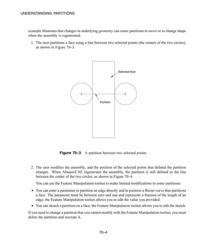
UNDERSTANDING PARTITIONS
example illustrates that changes in underlying geometry can cause partitions to move or to change shape
when the assembly is regenerated.
1. The user partitions a face using a line between two selected points (the centers of the two circles),
as shown in Figure 70–3.
Selected face
Partition
Figure 70–3 A partition between two selected points.
2. The user modifies the assembly, and the position of the selected points that defined the partition
changes. When Abaqus/CAE regenerates the assembly, the partition is still defined as the line
between the center of the two circles, as shown in Figure 70–4.
You can use the Feature Manipulation toolset to make limited modifications to some partitions:
• You can enter a parameter to partition an edge directly and to position a Bézier curve that partitions
a face. The parameter must be between zero and one and represents a fraction of the length of an
edge; the Feature Manipulation toolset allows you to edit the value you provided.
• You can sketch a partition on a face; the Feature Manipulation toolset allows you to edit the sketch.
If you need to change a partition that you cannot modify with the Feature Manipulation toolset, you must
delete the partition and recreate it.
70–4
Abaqus ID:
Printed on:

AN OVERVIEW OF PARTITIONING TECHNIQUES
Partition
Figure 70–4 The partition after regeneration.
70.4 An overview of partitioning techniques
This section provides an overview of the different partitioning techniques.
70.4.1 An overview of the methods for partitioning edgesSelect Tools→Partition from the main menu bar to display the Create Partition dialog box. When you
choose Edge from the Create Partition dialog box, the Method list displays the following methods for
partitioning edges:
Specify parameter by location
Pick a point anywhere along the edge. For detailed instructions, see “Using the specify parameter
by location method to partition edges,” Section 70.5.1, in the HTML version of this guide.
Enter parameter
Enter a parameter in the prompt area, as shown in Figure 70–5. An arrow along the edge indicates the
direction of increasing parameter value from the start vertex (corresponding to an edge parameter
70–5
Abaqus ID:
Printed on:

AN OVERVIEW OF PARTITIONING TECHNIQUES
value of zero) to the end vertex (corresponding to a value of one). For detailed instructions, see
“Using the enter parameter method to partition edges,” Section 70.5.2, in the HTML version of this
guide.
partition select edge to partition
direction of increasing parameter
Figure 70–5 Entering a parameter to partition an edge.
Select midpoint/datum point
Select the midpoint of the edge or a datum point along the edge, as shown in Figure 70–6. For
detailed instructions, see “Using the pick midpoint/datum point method to partition an edge,”
Section 70.5.3, in the HTML version of this guide.
partitionselect edge to partition
Figure 70–6 Selecting the midpoint or a datum to partition an edge.
Use datum plane
Select a datum plane. Abaqus/CAE creates the partition where the datum plane intersects the edges,
as shown in Figure 70–7. Partitioning a group of selected edges with a datum plane is a useful
technique for aligning a group of partitions. For detailed instructions, see “Using the datum plane
method to partition edges,” Section 70.5.4, in the HTML version of this guide.
70–6
Abaqus ID:
Printed on:

AN OVERVIEW OF PARTITIONING TECHNIQUES
partitionsselected edges to partition
Figure 70–7 Selecting a datum plane to partition edges.
70.4.2 An overview of the methods for partitioning facesWhen you choose Face from the Create Partition dialog box, the Method list displays the following
methods for partitioning faces:
Sketch planar partition
Partition a selected face by sketching a partition with the Sketcher, as shown in Figure 70–8. For
detailed instructions, see “Using the sketch method to partition faces,” Section 70.6.1, in the HTML
version of this guide.
You can sketch directly on the face to be partitioned, or you can sketch on a second face or
datum plane and then project the sketch onto the face that you want to partition. For an example
of projecting a sketch from a datum plane, see “Using the Datum toolset in the Part module,”
Section 11.16.1.
partitionselect face to partition
sketch
Figure 70–8 Partitioning a face using the Sketcher.
70–7
Abaqus ID:
Printed on:
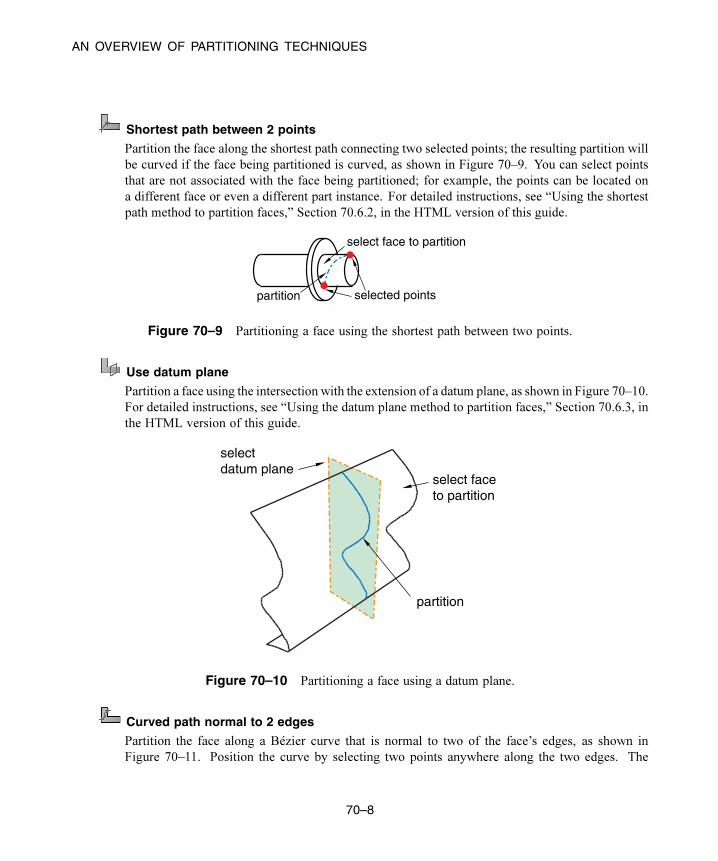
AN OVERVIEW OF PARTITIONING TECHNIQUES
Shortest path between 2 points
Partition the face along the shortest path connecting two selected points; the resulting partition will
be curved if the face being partitioned is curved, as shown in Figure 70–9. You can select points
that are not associated with the face being partitioned; for example, the points can be located on
a different face or even a different part instance. For detailed instructions, see “Using the shortest
path method to partition faces,” Section 70.6.2, in the HTML version of this guide.
partition
select face to partition
selected points
Figure 70–9 Partitioning a face using the shortest path between two points.
Use datum plane
Partition a face using the intersection with the extension of a datum plane, as shown in Figure 70–10.
For detailed instructions, see “Using the datum plane method to partition faces,” Section 70.6.3, in
the HTML version of this guide.
select datum plane
select faceto partition
partition
Figure 70–10 Partitioning a face using a datum plane.
Curved path normal to 2 edges
Partition the face along a Bézier curve that is normal to two of the face’s edges, as shown in
Figure 70–11. Position the curve by selecting two points anywhere along the two edges. The
70–8
Abaqus ID:
Printed on:

AN OVERVIEW OF PARTITIONING TECHNIQUES
arc subtended by the two edges must be less than 180°. For detailed instructions, see “Using the
curved path method to partition a face,” Section 70.6.4, in the HTML version of this guide.
partition
select face to partition
selected points
Figure 70–11 Partitioning a face using a Bézier curve.
Extend another face
Partition the face using the intersectionwith the extension of another face, as shown in Figure 70–12.
The face being extended can be either planar, cylindrical, conical, or spherical; and it need not
belong to the part containing the face to be partitioned. For detailed instructions, see “Using the
extended face method to partition faces,” Section 70.6.5, in the HTML version of this guide.
partition
select face to partition
select face to extend
Figure 70–12 Partitioning a face using the extension of another face.
Intersect by other faces
Partition the face using the intersection of the target face with one or more other faces, as shown in
Figure 70–13. The faces can be intersecting or tangential. For detailed instructions, see “Using the
intersection method to partition faces,” Section 70.6.6, in the HTML version of this guide.
70–9
Abaqus ID:
Printed on:

AN OVERVIEW OF PARTITIONING TECHNIQUES
part 2
part 1
select faceto partition
select faceto intersect
resultingpartition
Figure 70–13 Partitioning a face using an intersection of faces.
Project edges
Partition the face by projecting edges in the model, as shown in Figure 70–14. The partition is
created using a perpendicular projection from the face being partitioned to the partitioning edge.
You can choose to use only the projection or, if necessary, to extend the ends of the projected edge
to complete the face partition. For detailed instructions, see “Using the project edges method to
partition faces,” Section 70.6.7, in the HTML version of this guide.
select face to partition select edge to project
resulting partition
optional extended partition
optional extended partition
Figure 70–14 Partitioning a face by projecting an edge.
70–10
Abaqus ID:
Printed on:

AN OVERVIEW OF PARTITIONING TECHNIQUES
Auto-partition
When you mesh a face with quadrilateral elements using the free meshing technique, the Mesh
module internally partitions the face into regions with three to five logical sides before meshing
the face. For more information, see “Free meshing with quadrilateral and quadrilateral-dominated
elements,” Section 17.10.2. However, if you want to view and perhaps modify the automatically
generated regions before generating the mesh, you can use the auto-partitioning tool to partition the
face without meshing it. This tool is available only in the Mesh module. For detailed instructions,
see “Using the automatic generationmethod to partition faces,” Section 70.6.8, in the HTMLversion
of this guide.
70.4.3 An overview of the methods for partitioning cells
When you choose Cell from the Create Partition dialog box, the Method list displays the following
methods for partitioning cells:
Define cutting plane
Partition a cell by cutting it with a plane; the plane will pass completely through the cell. Use one
of the following three methods to define the cutting plane:
• Select a point on the cutting plane; then pick an edge or datum axis that defines the normal to
this plane, as shown in Figure 70–15.
partition
select cell to partition
select point
select normal
Figure 70–15 Defining the cutting plane with a point and a normal.
• Select three distinct and noncolinear points, as shown in Figure 70–16.
70–11
Abaqus ID:
Printed on:

AN OVERVIEW OF PARTITIONING TECHNIQUES
������������partitionselect cell to partition
select points
Figure 70–16 Defining the cutting plane with three points.
• Select an edge and a point along the edge; the cutting plane will be normal to the edge at the
selected point, as shown in Figure 70–17.
����
select cell to partitionselect edge
partition
select point
Figure 70–17 Defining the cutting plane with an edge and a point.
For detailed instructions, see “Using the cutting plane method to partition cells,” Section 70.7.1, in
the HTML version of this guide.
Use datum plane
Partition a cell using the intersection with the extension of a datum plane, as shown in Figure 70–18.
For detailed instructions, see “Using the datum plane method to partition cells,” Section 70.7.2, in
the HTML version of this guide.
���������
select cell to partition datum plane
partition
Figure 70–18 Partitioning a cell using a datum plane.
70–12
Abaqus ID:
Printed on:

AN OVERVIEW OF PARTITIONING TECHNIQUES
Extend face
Partition a cell by cutting it with a shell, where the shell is the extended geometry of a face, as
shown in Figure 70–19. The face being extended can be planar, cylindrical, conical, or spherical.
For detailed instructions, see “Using the extended face method to partition cells,” Section 70.7.3,
in the HTML version of this guide.
�����������
partition
select cell to partition
select face
Figure 70–19 Partitioning a cell using an extension of a face.
Extrude/Sweep edges
Partition a cell by sweeping selected edges (that form the sweep profile) along a selected path
(known as the sweep path). You can select any number of edges to be swept, although all the
edges must be connected, must lie on the same plane, and must belong to the same part instance.
Use either of the following two methods to define the sweep path:
• Create a straight partition through the cell by extending the sweep profile infinitely in a
direction parallel to a selected straight edge or datum axis that acts as a sweep path; the
partition is created where the swept edge(s) pass through the selected cell, as shown in
Figure 70–20. The sweep path must be straight and perpendicular to the set of edges being
swept.
������
�����������
partition
select cell to partition
select 4 edges to sweep
select sweep path
Figure 70–20 Sweeping a profile along a direction.
• Create a straight or curved partition through the cell by extending the sweep profile along
or parallel to a selected edge. The partition extends only as far as the selected edge; and
the partition is created where the swept edge(s) pass through the selected cell, as shown in
70–13
Abaqus ID:
Printed on:

AN OVERVIEW OF PARTITIONING TECHNIQUES
Figure 70–21. The sweep path must begin in the plane containing the edges to be swept, and
its tangent must be perpendicular to the same plane.
������������������������������������������������������
select sweep path
select cell to partition
select edge to sweep
partition
Figure 70–21 Sweeping a profile along an edge.
For detailed instructions, see “Using the extrude/sweep method to partition cells,” Section 70.7.4,
in the HTML version of this guide.
Use n-sided patch
Partition a cell by dividing it with a surface patch formed from a loop of connected edges. The
edges can be curved or straight, must be connected, and must belong to the same part as the cell
to be partitioned. In addition, the patch must pass completely through the cell. Choose from the
following methods to define the patch:
Select Edges
You can choose from the following methods to select the edges that form the N-sided patch:
Loop
Select a single edge, and allow Abaqus/CAE to search for a continuous loop of connected
edges that will partition the cell, as shown in Figure 70–22. The resulting patch can have
any number of edges.
Edges
Manually select the edges that will partition the cell. You can select any number of edges,
and the selected edges must form a closed loop.
Select Corner Points
Select three, four, or five points that define the corners of the patch. If two of the points are
connected by an existing edge, the resulting partition will follow the curve of the edge, as
shown in Figure 70–23. The points must be on the boundary edges of the cell being partitioned.
70–14
Abaqus ID:
Printed on:
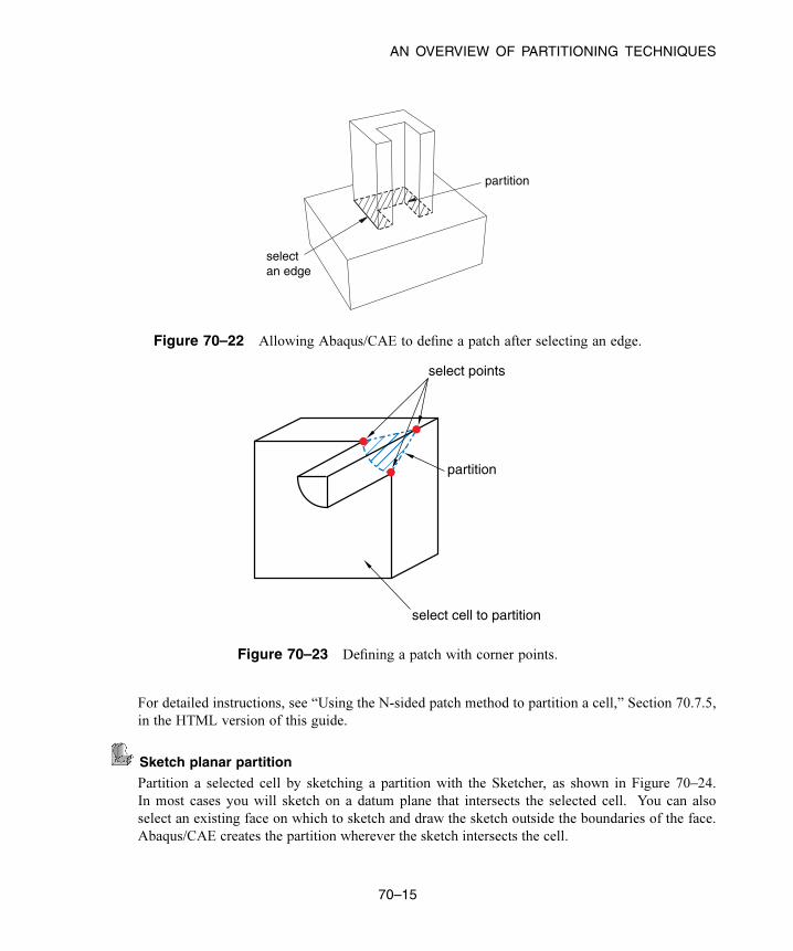
AN OVERVIEW OF PARTITIONING TECHNIQUES
selectan edge
partition
Figure 70–22 Allowing Abaqus/CAE to define a patch after selecting an edge.
partition
select cell to partition
select points
������
Figure 70–23 Defining a patch with corner points.
For detailed instructions, see “Using the N-sided patch method to partition a cell,” Section 70.7.5,
in the HTML version of this guide.
Sketch planar partition
Partition a selected cell by sketching a partition with the Sketcher, as shown in Figure 70–24.
In most cases you will sketch on a datum plane that intersects the selected cell. You can also
select an existing face on which to sketch and draw the sketch outside the boundaries of the face.
Abaqus/CAE creates the partition wherever the sketch intersects the cell.
70–15
Abaqus ID:
Printed on:

AN OVERVIEW OF PARTITIONING TECHNIQUES
select theface on whichto sketch
sketchpartition
select thecell to partition
Figure 70–24 Partitioning a cell using the Sketcher.
For detailed instructions, see “Using the sketch planar partition method to partition a cell,”
Section 70.7.6, in the HTML version of this guide.
70–16
Abaqus ID:
Printed on:

UNDERSTANDING THE ROLE OF THE QUERY TOOLSET
71. The Query toolset
The Query toolset allows you to obtain information about your model. This chapter covers the following
topic:
• “Understanding the role of the Query toolset,” Section 71.1
In addition, more detailed information is available in “Querying the model,” Section 71.2, in the HTML
version of this guide.
71.1 Understanding the role of the Query toolset
The Query toolset allows you to obtain information about your model. In most cases Abaqus/CAE
displays the requested information in the message area, and the same information is written to the replay
file. Select Tools→Query from the main menu bar to use the Query toolset, or select the tool in
the Query toolbar.
The Query dialog box is split into two sections. The top section of the dialog box contains general
queries that are available in each module except the Job module, where the Query toolset is not available
at all. The bottom portion of the dialog box contains module-specific queries; as you switch between
modules, Abaqus/CAE displays queries that are appropriate for the contents of the current module.
71.1.1 General queries
You can always use the Query toolset to obtain general information about the model, regardless of which
module you are using, although the Query toolset is not available in the Job module. The GeneralQueries in the Visualization module are similar to those in the other modules, but they are discussed
separately in Chapter 50, “Querying the model in the Visualization module,” due to differences in some
selection methods and the inclusion of undeformed and deformed model data in the results.
For all other modules, the items under General Queries in the Query toolset provide the following
general information:
Point/Node
Coordinates of a selected point or node
Distance
Distance between two selected points or nodes, or; in the Part module, the Property module, or the
Mesh module; the distance between two points, nodes, edges, faces, or any combination of these
objects
71–1
Abaqus ID:
Printed on:

UNDERSTANDING THE ROLE OF THE QUERY TOOLSET
Angle
The angle between two edges or faces or between an edge and a face
Feature
For a selected feature:
• Feature name
• Description
• Status (if the feature is suppressed or if it failed to regenerate)
• Parent feature names
• Child feature names
• Parameters
Shell element normals
Display shell/membrane normal directions
Beam element tangents
Display beam/truss tangent directions
In addition, if the current viewport contains a mesh, the Query toolset provides the following information:
Mesh stack orientation
For hexahedral, wedge, and quadrilateral elements that you can use in a continuum shell, cohesive,
cylindrical, or gasket mesh, Abaqus/CAE indicates the mesh stack orientation. For hexahedral
and wedge elements, Abaqus/CAE colors the top face brown and the bottom face purple. For
quadrilateral elements, arrows indicate the orientation of the elements. In addition, Abaqus/CAE
highlights any element faces and edges that have inconsistent orientation.
Note: The query results do not account for changes made in the mesh stack orientation while
defining a solid composite layup or a composite shell layup in the Property module.
Mesh
For an assembly, part or part instance, geometric region, or element:
• The total number of nodes and elements in the selected area
• The number of elements for each element shape
By default, Abaqus/CAE displays mesh information in the message area, but you can display this
information in tabular format in the Mesh statistics dialog box by toggling on Display detailedreport in the prompt area. The Mesh statistics dialog box also enables you to display mesh
information by part instance or by element type.
71–2
Abaqus ID:
Printed on:

UNDERSTANDING THE ROLE OF THE QUERY TOOLSET
Element
For a selected element:
• Element label
• Element topology; for example, linear hexahedron
• Abaqus element name; for example, C3D8I
• Nodal connectivity
Mesh gaps/intersectionsFor a selected part or part instance:
• Display element edges of boundary faces with incompatible interfaces
• Display element edges of boundary faces with cracks or gaps
• Display element edges of boundary faces that intersect other faces
Mass propertiesFor an assembly, selected part or part instance, geometric region, solid element, shell, solid face,
beam, or truss, Abaqus/CAE returns some or all of the following information:
• Surface area (displayed only for shell elements and for solid faces)
• Area centroid
• Volume
• Volume centroid
• Mass
• Center of mass
• Moments of inertia about the center of mass or about a specified point
For more information about this query, see “Querying mass properties,” Section 71.2.3.
Geometry diagnostics
• Invalid, imprecise, or small geometry
• Topology
For more information, see “Obtaining general information about the model,” Section 71.2.2, in the
HTML version of this guide.
71.1.2 Module-specific queriesIn addition to general queries, you can query the model for information specific to the module you are
using. Abaqus/CAE displays these module-specific queries at the bottom of the Query toolset under,
“Modulename Module Queries.” The Query toolset can provide the following module-specific
information:
71–3
Abaqus ID:
Printed on:

UNDERSTANDING THE ROLE OF THE QUERY TOOLSET
Part module
The items under Part Module Queries provide the following module-specific information about
the current part:
Part attributes
• Name
• Modeling space
• Type (deformable or rigid body)
Regeneration warnings
If any sets or surfaces in the selected part cannot be regenerated because their underlying
geometry has been modified or deleted, Abaqus/CAE displays the set or surface name, the
original number of faces, and the number of faces found during the query.
Substructure statistics
Abaqus/CAE displays the following information about the selected substructure part: the
number of retained nodes, eigenmodes, and substructure loads in the part; the availability of
the recovery matrix, gravity load vectors, reduced mass matrix, reduced structural damping
matrix, and reduced viscous damping matrix in the substructure; and mass properties of the
substructure.
For more information, see “Using the Query toolset in the Part module,” Section 11.16.4.
Property module
The items under Property Module Queries provide the following module-specific information
about the current part:
Section assignments
Sections assigned to a selected region
Regions missing sections
Regions that require a section assignment
Beam orientations
Beam orientations assigned to a selected wire region (Abaqus/CAE displays the ( , , )
axis system on the selected wire region)
Material orientations
Material orientations assigned to a selected region
Rebar orientations
Rebar reference orientations assigned to a selected region
71–4
Abaqus ID:
Printed on:

UNDERSTANDING THE ROLE OF THE QUERY TOOLSET
Ply stack plot
Abaqus/CAE creates a new viewport and displays a graphical representation of a core sample
through a region of a composite layup or composite section. The image shows the plies in the
layup along with details of each ply, such as its fiber orientation, thickness, reference plane,
and integration points.
Disjoint ply regions
Abaqus/CAE displays in the message area the names of the composite layups and the plies
within them that contain disjoint regions.
For more information, see “Using the Query toolset to obtain assignment information,”
Section 12.19, in the HTML version of this guide and Chapter 53, “Viewing a ply stack plot.”
Assembly module
The items under Assembly Module Queries provide the following module-specific information
about a selected part instance:
Instance attributes
Name, type, and modeling space
Instance position
• Position of the origin relative to the global coordinate system
• Sum of the translations and rotations applied to the instance
• Number of translational and rotational constraints applied
For more information, see “Using the Query toolset to query the assembly,” Section 13.12, in the
HTML version of this guide.
Step module
The Query toolset provides only general information in the Step module.
Interaction module
The item under Interaction Module Queries provides the following module-specific information
about a selected wire:
• Connector assignment information
For more information, see “Using the Query toolset to obtain connector assignment information,”
Section 15.18, in the HTML version of this guide.
Load module
The Query toolset provides only general information in the Load module.
71–5
Abaqus ID:
Printed on:

UNDERSTANDING THE ROLE OF THE QUERY TOOLSET
Mesh module
The items under Mesh Module Queries provide the following module-specific information about
a part or part instance:
• Free/Non-manifold edges
• Unmeshed regions
• Unassociated geometry
For more information, see “Obtaining mesh information,” Section 17.19.2, in the HTML version of
this guide.
Job module
None of the Abaqus/CAE toolsets are available in the Job module.
Visualization module
The items under Visualization Module Queries provide the following module-specific
information:
• Probe values. Abaqus/CAE displays information in the Probe Values dialog box as you move
the cursor around the current viewport. Probing a model plot displays model data and analysis
results; probing an X–Y plot displays X–Y curve data. For more information, see Chapter 51,
“Probing the model.”
• Stress linearization. Stress linearization is the separation of stresses through a section into
constant membrane and linear bending stresses. Abaqus/CAE performs stress linearization
calculations and displays the results in the form of an X–Y plot. For more information, see
Chapter 52, “Calculating linearized stresses.”
• Active elements or nodes. Abaqus/CAE displays the label numbers of all of the active nodes
or active elements in the current viewport. For more information, see “Querying active node
or element labels,” Section 50.2.2, in the HTML version of this guide.
• Ply stack plot. Abaqus/CAE creates a new viewport and displays a graphical representation of
a core sample through a region of a composite layup or composite section. The image shows
the plies in the layup along with details of each ply, such as its fiber orientation, thickness,
reference plane, and integration points. For more information, see Chapter 53, “Viewing a ply
stack plot.”
Sketch module
The items under Sketch Module Queries provide the following information about a selected
constraint or sketch:
Constraint
• Constraint type
• Constrained entity names
In addition, the constrained entities are highlighted in the sketch.
71–6
Abaqus ID:
Printed on:

UNDERSTANDING THE ROLE OF THE QUERY TOOLSET
Detail
• Number of geometries
• Number of vertices
• Number of constraints
• Number of dimensions
• Number of unconstrained degrees of freedom
71–7
Abaqus ID:
Printed on:


WHAT IS A REFERENCE POINT USED FOR?
72. The Reference Point toolset
This chapter describes the Reference Point toolset. The following topics are covered:
• “What is a reference point?,” Section 72.1
• “What is a reference point used for?,” Section 72.2
In addition, more detailed information is available in “Creating a reference point,” Section 72.3, in the
HTML version of this guide.
72.1 What is a reference point?
A reference point is a point that you create on a part. You can also create reference points on the assembly.
You can position a reference point anywhere in space, and a reference point is useful for creating a point
in your model where a vertex is not available; for example, at the center of a hole. In contrast to a vertex
a reference point is ignored by the Mesh module when the mesh is generated.
You can use the Reference Point toolset in the Part module to create a reference point that is
associated with a part by selecting Tools→Reference Point from the main menu bar. When you
create the assembly, the reference point appears on each instance of the part in the assembly. A part can
include only one reference point, and Abaqus/CAE labels the reference point RP. Abaqus/CAE asks
you if you want to delete the original point if you try to assign a second point.
Alternatively, you can use the Reference Point toolset in the Assembly, Interaction, or Load modules
to create a reference point on the assembly by selecting Tools→Reference Point from the main menu
bar. In the Interaction module you can use the tool in the module toolbox to create a reference
point. The assembly can include more than one reference point, and Abaqus/CAE labels them RP-1,RP-2, RP-3, etc. For more information, see “Creating a reference point,” Section 72.3, in the HTML
version of this guide. If desired, you can turn off the display of the reference point symbol and the
reference point label; for more information, see “Controlling reference point display,” Section 76.11.
72.2 What is a reference point used for?
You can use a reference point for the following:
• If the part is a deformable planar part that is modeled with generalized plane strain elements,
you must create a reference point to indicate the required reference node. For more information,
see “Creating generalized plane strain sections,” Section 12.13.2, in the HTML version of this
guide. For more information on generalized plane strain elements, see “Choosing the element’s
dimensionality,” Section 27.1.2 of the Abaqus Analysis User’s Guide.
72–1
Abaqus ID:
Printed on:

WHAT IS A REFERENCE POINT USED FOR?
• If the part is a discrete or analytical rigid part, you use the reference point to indicate the rigid body
reference point. Constraints or motion that you apply to the reference point are applied to the entire
rigid part.
The location of the rigid body reference point affects how you prescribe moments or motion; in
addition, the location of the rigid body reference point affects the interpretation of moment reactions.
If your model includes a dynamic analysis involving rotations, the rotary inertia specification of a
rigid body must be made consistent with the location of its rigid body reference point.
• You must refer to a reference point on the assembly when you create a rigid body constraint in the
Interaction module. A rigid body constraint constrains the motion of regions of the assembly to the
motion of a reference point. You can create and name a set containing the reference point and refer
to the set, or you can select the reference point directly from the current viewport. You can also
apply loads and boundary conditions to a reference point in the Load module.
• In some cases you will want to position the reference point at the center of mass, which you can find
using the Query toolset. You can use the Property module to assign mass and rotary inertia section
properties to the reference point. The section can also include optional damping data.
• You can apply constraints to a reference point; for example, equation, coupling, and display body
constraints.
• You can use a reference point when you create an assembly-level wire feature in the Assembly
module or the Interaction module. A reference point is useful if you want to attach the connector
to a point in space. You can create a reference point at the desired location and use a rigid body
constraint to attach a part instance to the reference point. When you attach a connector to such a
reference point, the connector is effectively attached to the part instance.
72–2
Abaqus ID:
Printed on:

UNDERSTANDING THE ROLE OF THE SET AND SURFACE TOOLSETS
73. The Set and Surface toolsets
When you need to specify a region of your model (for example, to apply a load or to define contact), you
can select the region from the viewport or you can define a set or a surface that contains the region. You
use the Set and Surface toolsets to create and manage sets and surfaces.
The Set and Surface toolsets are available from the Tools menu in the main menu bar in all modules
except the Visualization module.
The following topics are covered:
• “Understanding the role of the Set and Surface toolsets,” Section 73.1
• “Understanding sets and surfaces,” Section 73.2
In addition, more detailed information is available in “Using the Set and Surface toolsets,” Section 73.3,
in the HTML version of this guide.
73.1 Understanding the role of the Set and Surface toolsets
The Set and Surface toolsets are collections of tools that allow you to create andmanage sets and surfaces.
You can use these tools to perform the following tasks:
Create
Create a set or surface by selecting a group of entities, such as faces and edges.
Edit
Modify a set or surface by selecting entities to add to it or to delete from it.
Rename
Replace the current name of an existing set or surface with a new name.
Delete
Delete a set or surface from the model.
In addition, you can use the Model Tree to merge a group of selected sets and surfaces into a new
set or surface. For detailed instructions on creating and manipulating sets and surfaces, see the following
sections in the HTML version of this guide:
• “Creating, editing, renaming, and deleting sets and surfaces,” Section 73.3.1
• “Creating sets,” Section 73.3.2
• “Creating surfaces,” Section 73.3.3
• “Performing Boolean operations on sets or surfaces,” Section 73.3.4
• “Editing sets and surfaces,” Section 73.3.5
• “Associating objects (such as loads and sections) with sets and surfaces,” Section 73.3.6
73–1
Abaqus ID:
Printed on:

UNDERSTANDING SETS AND SURFACES
73.2 Understanding sets and surfaces
This section describes basic concepts concerning sets and surfaces.
73.2.1 What is a set?A set is a named region or collection of entities on which you can perform various operations. For
example, once you create a set, you can use it to perform the following tasks:
• Assign section properties in the Property module.
• Create contact pairs with contact node sets and surfaces in the Interaction module.
• Define loads and boundary conditions in the Load module.
• Request output from specific regions of the model in the Step module.
You can create the following types of sets:
Geometry sets
A geometry set contains geometric objects (cells, faces, edges, and vertices) that you have selected
from one of the following types of parts or from instances of these parts:
• Native parts (those created using the tools in the Part module)
• Parts that you imported from a file.
You select the entities to include in the set from the current viewport. Depending on the shape
and modeling space of the part, you can include any combination of cells, faces, edges, and vertices
in a set. However, some procedures can be performed only with certain types of objects. As a
result, the set that you select must include only object types that are valid for the procedure. For
example, concentrated forces can be applied only to vertices; therefore, the sets to which you apply
concentrated forces can include only vertices.
Node and element sets
Node and element sets contain nodes and elements that you have selected. You can create node and
element sets from native Abaqus nodes and elements on a part that you have meshed in the Mesh
module, from orphan mesh nodes and elements, or from nodes and elements on any instances of
parts. A set can include nodes or elements from a single part or from multiple part instances. Sets
that you create using the Set toolset can include either nodes or elements but not both. However,
you can create sets containing a mixture of nodes and elements by merging sets or by importing
an output database or an input file containing multiple sets with the same name. Native nodes and
elements within sets allow you to request output or add loads to specific areas without deleting the
mesh and partitioning the geometry. However, any changes to the mesh—including regenerating it
from replay or journal files—may invalidate or change the native portion of mesh sets.
73–2
Abaqus ID:
Printed on:

UNDERSTANDING SETS AND SURFACES
For more information about mesh parts and orphan mesh nodes and elements, see “What kinds
of files can be imported and exported fromAbaqus/CAE?,” Section 10.1.1; “Importing amodel from
an Abaqus input file,” Section 10.5.2; “Importing a model from an output database,” Section 10.5.3;
and, in the HTML version of this guide, “Creating a mesh part,” Section 17.20.
If you rename or delete a set, any objects associated with the set, such as sections or loads, become
invalid. However, if you change the name of a renamed set back to its original name or if you recreate a
deleted set using its original name, objects associated with that set are restored.
73.2.2 How do part sets and assembly sets differ?
Sets that you create from a part or sets that you create from a part instance in the assembly are used
differently:
Part sets
Part sets are sets that you created in the part-related modules—Part or Property. The Mesh module
also acts as a part-related module when you select the Part object from the context bar. When you
import an orphan mesh from an output database, you also automatically import any sets as part sets.
Part sets appear in the Model Tree in a Set container under the part with which they are associated.Only part sets are visible in the Set Manager in the Part and Property modules. You do not use part
sets directly in the Part module; however, in the Property module you can assign sections to regions
specified by part sets. If you assign a section to a region defined by a part set, Abaqus applies the
section assignment to all instances of that part in the assembly.
When you instance a part in the Assembly module, you can refer to any part sets that you
previously created; however, the assembly-related modules provide only read-only access to these
sets, and you cannot access part sets from the Set Manager in assembly-related modules. Sets
from an instanced part appear in the Model Tree under the assembly. You can select an eligible part
set during a procedure (while applying a load or boundary condition, for example) by clicking the
Set button on the far right side of the prompt area and selecting the set from the Region Selectiondialog box that appears. Abaqus names the sets part_instance_name.set_name. You cannot access
part sets from the Set Manager in an assembly-related module.
Assembly sets
Assembly sets are sets that you created in the assembly-related modules—Assembly, Step,
Interaction, or Load. The Mesh module also acts as an assembly-related module when you select
the Assembly object from the context bar. Assembly sets appear in the Model Tree in a Setcontainer under the assembly along with any sets from an instanced part. Only assembly sets
are visible in the Set Manager in the assembly-related modules. You can use assembly sets to
indicate, for example, regions of the assembly where you would like to apply a load or boundary
condition or to obtain output. Assembly sets can include regions from multiple part instances.
73–3
Abaqus ID:
Printed on:
UNDERSTANDING SETS AND SURFACES
An assembly set refers to the assembly itself and not to the individual part instances. As a
result, Abaqus/CAE does not delete an assembly set if you delete a part instance contained in the
set. You must manually delete the assembly set.
A single part cannot contain a geometry set, a node set, or an element set with the same name as an
existing set; however, different parts can contain sets with the same name. All assembly set names must
be unique.
73.2.3 What is a surface?Surfaces are collections of faces and edges or collections of element faces and edges. You can select
a surface when a procedure is expecting a face; for example, when you are applying distributed loads,
such as pressure loads, and defining contact interactions. You can select an interior surface; for example,
when you are using the solid offset mesh tool.
When you create a surface on a shell model, you must select which side of the surface is the desired
face; you can also select both faces. Similarly, if you create a surface on a wire model, you must select
which end of the wire is the desired face; you can also select the circumference of the wire. For more
information, see “Specifying a particular side or end of a region,” Section 73.2.5.
You can define a surface that includes edges of a shell or element edges. You can use edge-based
surfaces in Abaqus/Explicit general contact interactions. You can also use edge-based surfaces to tie two
shells along two edges or to tie two shells that intersect to form a “T.”
You can create two different types of surfaces:
Geometry surfaces
Create a geometry surface by selecting geometric objects (faces and edges) from native or imported
geometry. When the analysis input file is created, the surface definition in the input file specifies
the element edges (in the case of axisymmetric part instances) or faces that are associated with the
surface geometry.
Mesh surfaces
Create a mesh surface by selecting element faces (for three-dimensional regions) or edges (for two-
dimensional regions) from meshes. Adding surfaces to the mesh allows you to request output or add
loads to specific areas without deleting the mesh and partitioning the geometry. However, native
element faces or edges within mesh surfaces may be invalidated or the content may change if you
make any changes to the mesh—including regenerating the mesh from replay or journal files.
If you rename or delete a surface, any objects associated with the surface, such as loads or interactions,
become invalid. However, if you change the name of a renamed surface back to its original name or if
you recreate a deleted surface using its original name, objects associated with that surface are restored.
If you use the Virtual Topology toolset to create virtual faces and edges, you can select those virtual
faces and edges when you create sets and surfaces. In addition, if an existing set or surface contains an
edge or vertex that you ignored using the Virtual Topology toolset, the edge or vertex is removed from
73–4
Abaqus ID:
Printed on:

UNDERSTANDING SETS AND SURFACES
the set or surface. Similarly, if an existing set or surface contains faces or edges that you combined,
Abaqus/CAE replaces the original faces and edges with the new combined faces and edges. This is true
only if all of the faces and edges that you combined are members of the same set. For more information,
see “What can I do with a part or a part instance containing virtual topology?,” Section 75.3.
73.2.4 Regeneration of geometry sets and surfaces
Geometry sets and surfaces are regenerated automatically when you change the underlying geometry
of the model. However, if you change the geometry of the model significantly, objects that you had
previously included in sets or surfaces may be unidentifiable.
For example, if you delete or suppress a feature of a part, sets and surfaces associated with that
feature are altered:
• If components of the feature were the only objects in a set or surface, the set or surface still appears
in the Set Manager but is empty. You can edit the set so that it includes new geometry.
• If components of the feature were included with other objects in a set or surface, the set or surface
no longer contains the components of the feature but continues to contain all of the other objects.
• If you suppress and then resume a feature, the sets and surfaces associated with that feature are also
restored, as well as any objects assigned to those sets and surfaces, such as loads or interactions.
73.2.5 Specifying a particular side or end of a region
When you create a surface definition from a shell, a wire, or an internal face of a three-dimensional
part, you must specify which side of the part you want to include in the surface definition. When you
are selecting sides from a shell or face, Abaqus/CAE uses different colored faces to indicate the two
sides and prompts you to select the color corresponding to the side that you want to select. During this
procedure, the model display becomes translucent to make obstructed or interior sides visible. When you
are selecting sides of a wire, Abaqus/CAE uses different colored arrowheads to indicate the two sides of
the part.
Selecting sides from a shell
To distinguish the sides of a shell, Abaqus/CAE colors one side of the shell brown and the other
side purple. You select a specific side by clicking either the Brown or Purple button in the prompt
area (see Figure 73–1).
Figure 73–1 Select the side of the surface.
73–5
Abaqus ID:
Printed on:

UNDERSTANDING SETS AND SURFACES
You also have the option of selectingBoth sides, which defines a double-sided surface that includesboth the brown and the purple sides of the shell. Double-sided surfaces can be used only in the
following situations:
• Contact interactions using three-dimensional shells, membranes, and rigid bodies in an
Abaqus/Explicit analysis
• Contact interactions using the small-sliding, surface-to-surface contact formulation in an
Abaqus/Standard analysis
Consider the conical shell in Figure 73–2.
Purple
Brown
Figure 73–2 Colors indicate the side of a shell.
Abaqus/CAE displays the exterior side of the cone in purple and the interior side of the cone in
brown. Therefore, to select the exterior of the cone, you would click Purple in the prompt area; to
select the interior, you would click Brown.If you select more than one shell face as part of a surface definition, you can control the color
coding for each face individually. Abaqus/CAE includes a Flip a surface option that allows you to
reverse the orientation of any individual face before creating the surface definition (see Figure 73–3).
Figure 73–3 The Flip a surface option becomes available for multi-faced shell surfaces.
Use this option to make all of the desired sides the same color, then select that color from the prompt
area. If you select Both Sides, Abaqus/CAE selects both sides of all selected faces regardless of
any surfaces that you previously flipped.
In the model in Figure 73–4 both rounded ends are selected as part of the surface.
73–6
Abaqus ID:
Printed on:

UNDERSTANDING SETS AND SURFACES
Brown
Purple
Figure 73–4 Two faces are included in the surface selection.
Initially, Abaqus/CAE colors the convex sides of both faces brown. However, the desired surface
actually consists of one convex face and one concave face. To achieve this surface, click Flip asurface, and select the face on the right side of the model. Abaqus/CAE reverses the color-coding
for only this face, as shown in Figure 73–5.
Brown
Brown Purple
Purple
Figure 73–5 Flipping a surface.
Click Brown in the prompt area; Abaqus/CAE defines the surface on all of the brown face sides in
the model.
Selecting sides on interior surfaces
When you select an internal face to create a surface, the surface side is ambiguous. For example,
the highlighted face in Figure 73–6 could be either the right side of cell A or the left side of cell B.
73–7
Abaqus ID:
Printed on:

UNDERSTANDING SETS AND SURFACES
Purple Brown
Figure 73–6 Defining a surface on an internal face.
Abaqus/CAE uses the same brown/purple color-coding interface discussed above to determine
which side of the surface you intended to select. Click Purple to define a surface on the right side
of cell A; click Brown to define a surface on the left side of cell B.
Selecting sides from a wire
If you are selecting a surface of a three-dimensional wire part instance, Abaqus/CAE displays the
wire in red along with the arrowheads shown in Figure 73–7.
magenta red yellow
Figure 73–7 Arrows indicate the ends of a three-dimensional wire.
You can select the end with the magenta arrowhead, the end with the yellow arrowhead, or the
circumferential surface of the part, which is indicated by the red wire (see Figure 73–8).
Figure 73–8 Select the end or the circumference of the surface.
If the wire part is two-dimensional, Abaqus/CAE distinguishes the two sides of the surface
using the arrowheads shown in Figure 73–9.
73–8
Abaqus ID:
Printed on:
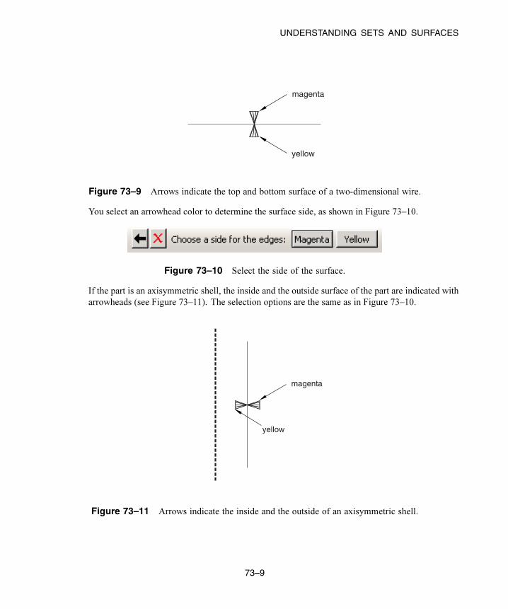
UNDERSTANDING SETS AND SURFACES
yellow
magenta
Figure 73–9 Arrows indicate the top and bottom surface of a two-dimensional wire.
You select an arrowhead color to determine the surface side, as shown in Figure 73–10.
Figure 73–10 Select the side of the surface.
If the part is an axisymmetric shell, the inside and the outside surface of the part are indicated with
arrowheads (see Figure 73–11). The selection options are the same as in Figure 73–10.
yellow
magenta
Figure 73–11 Arrows indicate the inside and the outside of an axisymmetric shell.
73–9
Abaqus ID:
Printed on:

UNDERSTANDING STREAM DISPLAY
74. The Stream toolset
A streamline is a curve that is instantaneously tangent to the velocity vector of the flow, and a stream is a
set of streamlines that enable you to visualize the velocity or vorticity data in a fluid flow analysis. The
Stream toolset is available only in the Visualization module.
This chapter explains how to use the Stream toolset to create, modify, and delete streams; display
or hide them in the viewport; and customize several aspects of their appearance. The following topics
are covered:
• “Understanding stream display,” Section 74.1
In addition, the following sections are available in the HTML version of this guide:
• “Creating a stream,” Section 74.2
• “Displaying and hiding streams,” Section 74.3
• “Customizing stream display,” Section 74.4
74.1 Understanding stream display
A streamline traces the path tangent to a nodal vector field, and a stream is a set of streamlines that enable
you to visualize data emanating from a particular location in a vector field. Figure 74–1 shows a sample
stream of 12 streamlines displaying velocity data in a fluid flow analysis. You can create streams by first
defining a rake, which is a line segment with a series of points specified along its length that control the
locations where Abaqus/CAE displays streamlines for a fluid flow analysis. Rakes are placed into an
area of interest in the fluid flow; when you create and display the stream in the viewport, Abaqus/CAE
displays a number of streamlines that corresponds to the number of points on the rake. Streamlines
are evenly spaced along the rake, except for rakes defined using nontrivial path definitions; for more
information about stream rake definition, see “Creating a stream,” Section 74.2, in the HTML version of
this guide.
The streamline shape is driven by the currently selected stream variable, which is usually velocity
or vorticity. To change the current stream variable, see “Selecting the stream field output variable,”
Section 42.5.7. The streamline color is driven by the currently selected primary variable. For more
information on customizing streamline color options, see “Customizing stream colors,” Section 74.4.1,
in the HTML version of this guide.
Youmust define separate stream rakes for each part instance for which youwant to display flow data.
Abaqus/CAE computes stream data for individual part instances only and does not display streamlines
across separate part instances.
74–1
Abaqus ID:
Printed on:
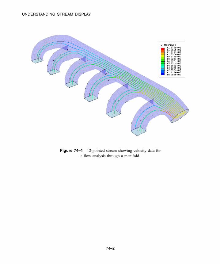
UNDERSTANDING STREAM DISPLAY
Figure 74–1 12-pointed stream showing velocity data for
a flow analysis through a manifold.
74–2
Abaqus ID:
Printed on:

WHAT IS VIRTUAL TOPOLOGY?
75. The Virtual Topology toolset
The Virtual Topology toolset allows you to ignore details, such as very small faces and edges, when you
mesh a part or a part instance. The following topics are covered:
• “What is virtual topology?,” Section 75.1
• “What can I do with the Virtual Topology toolset?,” Section 75.2
• “What can I do with a part or a part instance containing virtual topology?,” Section 75.3
• “Why repair a part if I can use virtual topology?,” Section 75.4
• “Creating virtual topology based on geometric parameters,” Section 75.5
In addition, more information is available in “Using the Virtual Topology toolset,” Section 75.6, in the
HTML version of this guide.
75.1 What is virtual topology?
In some cases parts or part instances contain details such as very small faces and edges. These features
can be important for the detailed machining and packaging design of the component; however, they may
be redundant in the numerical analysis if they have little impact on the mechanics of the problem being
studied. Indeed, these small details may unduly constrain the generation of the mesh, resulting in a poor
mesh or a finer mesh density. In some circumstances small faces and edges can be significant if they
occur in a region of interest where you need a fine mesh. However, in most cases the details add nothing
to the analysis, and you want Abaqus/CAE to ignore them during the mesh generation process and during
the analysis.
The topology of the model is its composition from faces, edges, and vertices. The Virtual Topology
toolset allows you to manipulate this topology and create a simplified form for the purpose of meshing.
This simplified form is different from the real model and is called “virtual topology.” The faces and edges
that result from the manipulation are said to be “virtual.” Similarly, parts and part instances that contain
virtual faces and edges are said to be “virtual.”
The Virtual Topology toolset allows you to remove small details by combining a small face with an
adjacent face or by combining a small edge with an adjacent edge. The faces or edges to be combined
can be specified directly, or you can choose the edges and vertices to ignore.
For example, Figure 75–1 shows a piston that has some small details where the blended surfaces
intersect. These details result in a dense mesh that includes some sliver-shaped elements. You can use
virtual topology to ignore the small details, resulting in the more uniform mesh of better quality that is
illustrated in Figure 75–2.
75–1
Abaqus ID:
Printed on:

WHAT CAN I DO WITH THE VIRTUAL TOPOLOGY TOOLSET?
geometry mesh
Figure 75–1 Small details result in a dense mesh of sliver-like elements.
Abaqus/CAE treats virtual topology in the same way that it treats standard geometry. For example,
you can do the following:
• Partition virtual topology.
• Use the Geometry Edit toolset on virtual topology.
• Use Part module tools on virtual topology, such as extrude, sweep, and blend.
For example, Figure 75–3 shows the piston containing virtual topology from Figure 75–2 after it has
been cut using the extruded cut tool in the Part module.
Note: When you export a part containing virtual topology to an ACIS file, Abaqus/CAE removes the
virtual topology from the part that is exported.
75.2 What can I do with the Virtual Topology toolset?
The Virtual Topology toolset is available only in the Mesh module. You can apply virtual topology to
parts, or you can apply it to independent instances in the assembly. The Virtual Topology toolset allows
you to do the following:
75–2
Abaqus ID:
Printed on:

WHAT CAN I DO WITH THE VIRTUAL TOPOLOGY TOOLSET?
geometry mesh
Figure 75–2 Using virtual topology to ignore small details
results in a more uniform mesh of better quality.
Figure 75–3 A part containing virtual topology is cut.
75–3
Abaqus ID:
Printed on:

WHAT CAN I DO WITH THE VIRTUAL TOPOLOGY TOOLSET?
Combine faces or edges
You can select two or more faces or edges that Abaqus/CAE will combine into a single virtual face
or virtual edge. If you combine two faces, any edges between the faces are ignored when Abaqus
generates the mesh. Similarly, if you combine two edges, any vertices between the edges are ignored
when the mesh is generated.
Ignore an edge or a vertex
You can select edges or vertices that Abaqus/CAE will ignore. Ignoring an edge between two faces
is the equivalent of combining the faces. Similarly, ignoring a vertex between two edges is the
equivalent of combining the edges; however, you will find the combine tools useful when you have
a large number of faces and edges to combine. Using ignore to create virtual topology has the same
effect as using combine to create virtual topology—ignored edges or vertices are not considered
when Abaqus generates the mesh.
Automatically combine or ignore entities
You can specify a set of geometric parameters that Abaqus/CAE will use to create virtual topology.
You can also select the area—faces, parts, part instances, or an entire assembly—to which
Abaqus/CAE will apply the selected parameters. The virtual topology parameters are located in the
Create Virtual Topology dialog box, which also includes tools that you can use to measure and
highlight entities and preview the virtual topology. When you are finished, Abaqus/CAE creates
a single virtual topology feature that contains all of the changes.
Restore entities
Rather than deleting or suppressing virtual topology features that may contain entities that you want
to ignore along with some that you need to use, you can use the Restore Entities tool to highlight
all entities that have been ignored and select the ones that you want to reactivate.
To preserve mesh quality, edges and faces to be combined should have shallow included angles that
are close to 180°. The recommended angle is between 120° and 240°. You can use the angle method to
choose only adjacent faces with shallow included angles. For more information, see “Using the angle
and feature edge method to select multiple objects,” Section 6.2.3. If the included angle at some edges or
vertices lies outside this range, Abaqus/CAE displays a warning and allows you to remove those edges
or vertices from your selection. If you choose to retain the sharp edges, the resulting mesh may not lie
on a smooth surface. Figure 75–4 illustrates a mesh on a virtual surface that is not smooth.
You can ignore an edge only if that edge is shared by two adjacent faces or if it is embedded in a
face. For example, you cannot ignore the free edge of a shell or an edge shared by three faces, as shown
in Figure 75–5. Similarly, you can ignore a vertex only if that vertex is shared by two adjacent edges or
embedded in a face. For example, you cannot ignore the vertex at the free end of a wire or where a wire
intersects with a face, as shown in Figure 75–6.
75–4
Abaqus ID:
Printed on:

WHAT CAN I DO WITH THE VIRTUAL TOPOLOGY TOOLSET?
Figure 75–4 When you apply virtual topology to sharp edges and vertices, the resulting
mesh can deviate substantially from the original surface.
A
B
B
Edges A can be ignored
Edges B cannotbe ignored
Figure 75–5 Some edges cannot be ignored.
B
A
Vertices A canbe ignored
Vertices B cannotbe ignored
Figure 75–6 Some vertices cannot be ignored.
75–5
Abaqus ID:
Printed on:

WHAT CAN I DO WITH A PART OR A PART INSTANCE CONTAINING VIRTUAL TOPOLOGY?
Abaqus/CAE does not support all of the meshing techniques on regions that contain virtual topology
(combined faces or combined edges). Specifically, Abaqus/CAE does not support the following:
• Two-dimensional free meshing with quadrilateral or quadrilateral-dominated elements using the
medial axis algorithm.
• Three-dimensional swept meshing using the medial axis algorithm.
• Two-dimensional structured meshing if the region to be meshed is not bounded by four corners.
• Three-dimensional structured meshing if the region to be meshed is not bounded by six sides.
If you need to apply virtual topology to a dependent instance, you can create a copy of the original
part and then create an independent instance of the copy. You can then replace the dependent instance
with the new independent instance and apply virtual topology to the replacement. For more information,
see “What is the difference between a dependent and an independent part instance?,” Section 13.3.2.
You may be able to make a part swept meshable by combining multiple faces on the target side into
a single face; for more information, see “Swept meshing of three-dimensional solids,” Section 17.9.3.
However, if you combine many faces into a single face, the meshing procedure may be slower and the
resulting mesh may not be acceptable. If you try to combine a large number of faces into a single face,
Abaqus/CAE displays a warning and allows you to change your selection. Abaqus/CAE calculates the
number of faces being combined from the cumulative number of faces in your selection. For example, if
you try to combine two faces each of which already contains five combined faces, the cumulative number
of faces will be ten.
75.3 What can I do with a part or a part instance containing virtualtopology?
Abaqus/CAE stores virtual topology as features of the corresponding part or assembly. As a result, you
can use the Model Tree to rename, suppress, resume, and delete virtual topology features. You cannot
edit a virtual topology features. You can restore entities that have been ignored or combined using virtual
topology. Restoring entities creates more new virtual topology features in the Model Tree—the original
virtual topology features are unchanged.
You can create sets and surfaces that contain virtual faces and edges. In addition, if an existing set
or surface contains an edge or vertex that you ignored, the edge or vertex is removed from the set or
surface. Similarly, if an existing set or surface contains faces or edges that you combined, Abaqus/CAE
replaces the original faces and edges with the new combined faces and edges. This is true only if all of
the faces and edges that you combined are members of the same set.
Virtual topology is not exported; for example, if you export an assembly containing virtual topology
to an ACIS file, Abaqus/CAE removes the virtual topology from the exported model. When you are
creating the assembly in the Assembly module, you cannot merge or cut part instances that contain virtual
topology.
75–6
Abaqus ID:
Printed on:

CREATING VIRTUAL TOPOLOGY BASED ON GEOMETRIC PARAMETERS
75.4 Why repair a part if I can use virtual topology?
Introducing virtual topology is a convenient method for creating a clean, well-formed mesh. The
emphasis is to ignore small geometric details that result in distorted elements in areas where the analysis
results are not of significant interest. Virtual topology relaxes the need for the mesh to conform to every
edge or vertex and allows you to obtain a simpler model with less detail. However, virtual topology
does not change the underlying geometry of the part instance.
When you combine two faces to form a virtual face, Abaqus/CAE updates the display to reflect the
ignored edge. However, to form a basis for the new virtual face, Abaqus/CAE maintains the underlying
geometry of the faces that were combined. The nodes in the mesh will be placed on the underlying
geometry. Therefore, a coarse mesh will interpolate across the virtual face, and a fine mesh will tend to
converge to the geometry of the underlying combined faces. Virtual topology allows the mesh definition
to be controlled by meshing parameters, such as seed size, and it helps to free meshing from constraints
imposed by geometry, such as small faces.
In contrast, you use the Geometry Edit toolset to correct minor flaws that are typically introduced
when a part is imported from a third-party application. You use the Geometry Edit toolset to correct the
underlying geometry; for example, to stitch small gaps and to delete self-intersecting faces and recreate
a valid replacement face. You also use the Geometry Edit toolset to remove redundant topology, such as
superfluous vertices and edges. The Geometry Edit toolset modifies the actual geometry, and geometric
restrictions limit how you can apply the repair tools; for example, you can remove redundant vertices
only if the vertex lies on a curve that is common to both edges.
When you export a virtual part instance, the virtual topology is lost because the virtual face, edge,
or vertex is not true geometry. For example, a virtual face is an abstracted reference to the underlying
collection of combined faces. Therefore, you should use the Geometry Edit toolset if you need to remove
small details from a part and want to export the part with the changes retained.
75.5 Creating virtual topology based on geometric parameters
You can use the controls in the Create Virtual Topology dialog box to automatically ignore unnecessary
model details based on a set of geometric parameters. You can control the following parameters to
determine which features Abaqus/CAE considers merging with surrounding geometry:
• Edge length
• Face size
• Face aspect ratio
• Face corner angle
• Thickness of faces representing small stair features
• Corner angle for combining adjacent edges or faces
75–7
Abaqus ID:
Printed on:
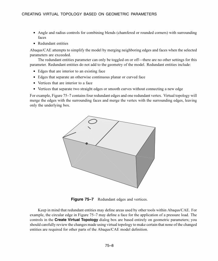
CREATING VIRTUAL TOPOLOGY BASED ON GEOMETRIC PARAMETERS
• Angle and radius controls for combining blends (chamfered or rounded corners) with surrounding
faces
• Redundant entities
Abaqus/CAE attempts to simplify the model by merging neighboring edges and faces when the selected
parameters are exceeded.
The redundant entities parameter can only be toggled on or off—there are no other settings for this
parameter. Redundant entities do not add to the geometry of the model. Redundant entities include:
• Edges that are interior to an existing face
• Edges that separate an otherwise continuous planar or curved face
• Vertices that are interior to a face
• Vertices that separate two straight edges or smooth curves without connecting a new edge
For example, Figure 75–7 contains four redundant edges and one redundant vertex. Virtual topology will
merge the edges with the surrounding faces and merge the vertex with the surrounding edges, leaving
only the underlying box.
Figure 75–7 Redundant edges and vertices.
Keep in mind that redundant entities may define areas used by other tools within Abaqus/CAE. For
example, the circular edge in Figure 75–7 may define a face for the application of a pressure load. The
controls in the Create Virtual Topology dialog box are based entirely on geometric parameters; you
should carefully review the changes made using virtual topology to make certain that none of the changed
entities are required for other parts of the Abaqus/CAE model definition.
75–8
Abaqus ID:
Printed on:

CREATING VIRTUAL TOPOLOGY BASED ON GEOMETRIC PARAMETERS
By default, all the virtual topology parameters in the dialog box are active, as shown in Figure 75–8.
The default values for the edge length, face size, stair feature, and blend radius are calculated based on
the size of the selected part or part instance; the other criteria are dimensionless and suitable default
values are provided. You can toggle off the controls for entities that you want to be ignored by virtual
topology. For example, if you have small faces that are a critical component of the model, toggle off
Faces smaller than.
Figure 75–8 The Create Virtual Topology dialog box.
To help you review potential changes, each parameter in the dialog box contains tools that you can
use to measure and highlight entities in the viewport that satisfy the corresponding geometric criteria.
Items that are highlighted may not be changed if they conflict with other criteria or model requirements.
To use the tools, click on the icons located to the right of each parameter in the Create Virtual Topology
dialog box. The measure entities tools allow you to measure entities in the viewport. Abaqus/CAE
75–9
Abaqus ID:
Printed on:
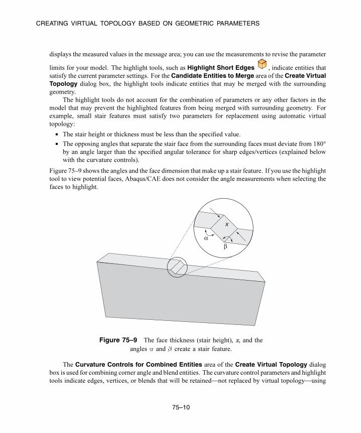
CREATING VIRTUAL TOPOLOGY BASED ON GEOMETRIC PARAMETERS
displays the measured values in the message area; you can use the measurements to revise the parameter
limits for your model. The highlight tools, such as Highlight Short Edges , indicate entities that
satisfy the current parameter settings. For the Candidate Entities to Merge area of the Create VirtualTopology dialog box, the highlight tools indicate entities that may be merged with the surrounding
geometry.
The highlight tools do not account for the combination of parameters or any other factors in the
model that may prevent the highlighted features from being merged with surrounding geometry. For
example, small stair features must satisfy two parameters for replacement using automatic virtual
topology:
• The stair height or thickness must be less than the specified value.
• The opposing angles that separate the stair face from the surrounding faces must deviate from 180°
by an angle larger than the specified angular tolerance for sharp edges/vertices (explained below
with the curvature controls).
Figure 75–9 shows the angles and the face dimension that make up a stair feature. If you use the highlight
tool to view potential faces, Abaqus/CAE does not consider the angle measurements when selecting the
faces to highlight.
βα
x
Figure 75–9 The face thickness (stair height), x, and the
angles and create a stair feature.
The Curvature Controls for Combined Entities area of the Create Virtual Topology dialog
box is used for combining corner angle and blend entities. The curvature control parameters and highlight
tools indicate edges, vertices, or blends that will be retained—not replaced by virtual topology—using
75–10
Abaqus ID:
Printed on:
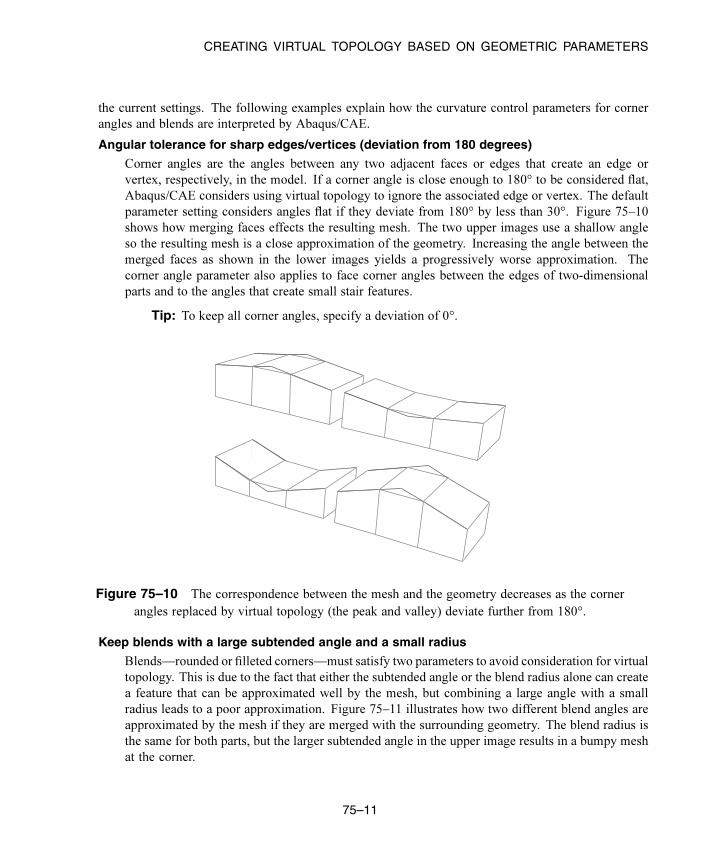
CREATING VIRTUAL TOPOLOGY BASED ON GEOMETRIC PARAMETERS
the current settings. The following examples explain how the curvature control parameters for corner
angles and blends are interpreted by Abaqus/CAE.
Angular tolerance for sharp edges/vertices (deviation from 180 degrees)
Corner angles are the angles between any two adjacent faces or edges that create an edge or
vertex, respectively, in the model. If a corner angle is close enough to 180° to be considered flat,
Abaqus/CAE considers using virtual topology to ignore the associated edge or vertex. The default
parameter setting considers angles flat if they deviate from 180° by less than 30°. Figure 75–10
shows how merging faces effects the resulting mesh. The two upper images use a shallow angle
so the resulting mesh is a close approximation of the geometry. Increasing the angle between the
merged faces as shown in the lower images yields a progressively worse approximation. The
corner angle parameter also applies to face corner angles between the edges of two-dimensional
parts and to the angles that create small stair features.
Tip: To keep all corner angles, specify a deviation of 0°.
Figure 75–10 The correspondence between the mesh and the geometry decreases as the corner
angles replaced by virtual topology (the peak and valley) deviate further from 180°.
Keep blends with a large subtended angle and a small radius
Blends—rounded or filleted corners—must satisfy two parameters to avoid consideration for virtual
topology. This is due to the fact that either the subtended angle or the blend radius alone can create
a feature that can be approximated well by the mesh, but combining a large angle with a small
radius leads to a poor approximation. Figure 75–11 illustrates how two different blend angles are
approximated by the mesh if they are merged with the surrounding geometry. The blend radius is
the same for both parts, but the larger subtended angle in the upper image results in a bumpy mesh
at the corner.
75–11
Abaqus ID:
Printed on:

CREATING VIRTUAL TOPOLOGY BASED ON GEOMETRIC PARAMETERS
Figure 75–11 A large blend angle (upper image) may yield a
bumpy mesh when it is replaced by virtual topology.
In Figure 75–12 the subtended angle is the same for both parts, but the small blend radius in the
upper image results in a poor quality mesh.
Figure 75–12 A small blend radius (upper image) may yield a
poor quality mesh when it is replaced by virtual topology.
For detailed instructions on how to use the Create Virtual Topology dialog box, see “Creating
virtual topology automatically,” Section 75.6.1, in the HTML version of this guide.
75–12
Abaqus ID:
Printed on:

Part VII: Customizing model displayThis part explains how you can customize your model display. The following topics are covered:
• Chapter 76, “Customizing geometry and mesh display”
• Chapter 77, “Color coding geometry and mesh elements”
• Chapter 78, “Using display groups to display subsets of your model”
• Chapter 79, “Overlaying multiple plots”
• Chapter 80, “Cutting through a model”
Abaqus ID:
Printed on:

OVERVIEW OF GEOMETRY AND MESH DISPLAY OPTIONS
76. Customizing geometry and mesh display
This chapter explains how you can customize your geometry and mesh display. The Visualization
module has its own set of options to customize model appearance; for more information, see Chapter 55,
“Customizing plot display,” and Chapter 56, “Customizing viewport annotations.”
The following topics are covered:
• “Overview of geometry and mesh display options,” Section 76.1
• “Choosing a render style,” Section 76.2
• “Controlling edge visibility,” Section 76.3
• “Controlling curve refinement,” Section 76.4
• “Defining mesh feature edges,” Section 76.5
• “Controlling translucency for substructure parts,” Section 76.6
• “Controlling beam profile display,” Section 76.7
• “Controlling shell thickness display,” Section 76.8
• “Controlling datum display,” Section 76.9
• “Controlling the display of individual coordinate systems,” Section 76.10
• “Controlling reference point display,” Section 76.11
• “Customizing mesh display,” Section 76.12
• “Controlling model lighting,” Section 76.13
• “Controlling instance visibility,” Section 76.14
• “Controlling the display of attributes,” Section 76.15
• “Saving your display options settings,” Section 76.16
For detailed instructions on each of these topics, see the corresponding sections in the HTML version of
this guide.
76.1 Overview of geometry and mesh display options
Depending on the module you are using, Abaqus/CAE presents you with one of the following menu
selections to customize geometry and mesh display:
View→Part Display Options
In geometry-related modules you can use this menu item to control your geometry render style,
edge visibility, curve refinement, element and node labels, and the visibility of the various types of
datum geometry.
76–1
Abaqus ID:
Printed on:
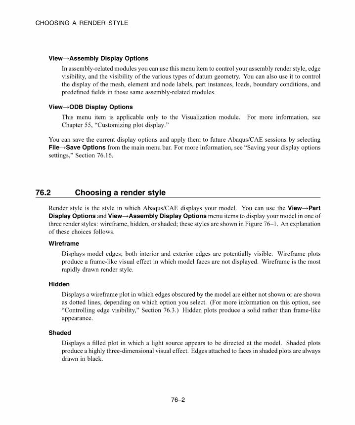
CHOOSING A RENDER STYLE
View→Assembly Display Options
In assembly-related modules you can use this menu item to control your assembly render style, edge
visibility, and the visibility of the various types of datum geometry. You can also use it to control
the display of the mesh, element and node labels, part instances, loads, boundary conditions, and
predefined fields in those same assembly-related modules.
View→ODB Display Options
This menu item is applicable only to the Visualization module. For more information, see
Chapter 55, “Customizing plot display.”
You can save the current display options and apply them to future Abaqus/CAE sessions by selecting
File→Save Options from the main menu bar. For more information, see “Saving your display options
settings,” Section 76.16.
76.2 Choosing a render style
Render style is the style in which Abaqus/CAE displays your model. You can use the View→PartDisplay Options and View→Assembly Display Options menu items to display your model in one of
three render styles: wireframe, hidden, or shaded; these styles are shown in Figure 76–1. An explanation
of these choices follows.
Wireframe
Displays model edges; both interior and exterior edges are potentially visible. Wireframe plots
produce a frame-like visual effect in which model faces are not displayed. Wireframe is the most
rapidly drawn render style.
Hidden
Displays a wireframe plot in which edges obscured by the model are either not shown or are shown
as dotted lines, depending on which option you select. (For more information on this option, see
“Controlling edge visibility,” Section 76.3.) Hidden plots produce a solid rather than frame-like
appearance.
Shaded
Displays a filled plot in which a light source appears to be directed at the model. Shaded plots
produce a highly three-dimensional visual effect. Edges attached to faces in shaded plots are always
drawn in black.
76–2
Abaqus ID:
Printed on:

CONTROLLING EDGE VISIBILITY
Figure 76–1 Model showing render style options. From left to right: the wireframe,
hidden, and lightsource-shaded render styles.
76.3 Controlling edge visibility
Using the View→Part Display Options or View→Assembly Display Options menu items, you can
control the visibility of the following:
Geometry edgesIf a part or part instance is displayed with the hidden render style, Abaqus/CAE suppresses obscured
geometry edges by default. Alternatively, if you toggle on the Show dotted lines in hiddenrender style option, Abaqus/CAE displays the obscured edges using a dotted line style.
If a part or part instance is displayed with the shaded render style, Abaqus/CAE displays the
edges by default. Non-wire edges (edges attached to faces) are displayed in black. Alternatively,
if you toggle off the Show edges in shaded render style option, Abaqus/CAE suppresses edge
display.
If a three-dimensional part or part instance contains faces with curved edges, by default
Abaqus/CAE displays gray “silhouette” edges originating from the faces, as shown in the
hidden-line plot in Figure 76–2. Unlike true edges, silhouette edges serve only as a visual aid; for
example, you cannot select or partition a silhouette edge. Alternatively, if you toggle off the Showsilhouette edges option, Abaqus/CAE displays only true edges.
Abaqus/CAE displays a curved part using a faceted representation of the part, and you use the
Curve refinement option to specify the degree of faceting. For more information, see “Controlling
curve refinement,” Section 76.4.
Reference representation
If you are creating a midsurface model and have assigned midsurface regions to cells in the solid
model, the geometry of the selected cells is contained in the reference representation. By default,
76–3
Abaqus ID:
Printed on:

CONTROLLING EDGE VISIBILITY
silhouette edgestoggled off
silhouette edgestoggled on
Figure 76–2 Hidden-line plot showing silhouette edges.
Abaqus/CAE displays the reference representation in the Part module. However, you can use the
Show reference representation option to toggle display of the reference representation in all
modules where the part or assembly is displayed. Toggle off Apply translucency to display
the reference representation as opaque instead of the default translucent appearance. For more
information on the reference representation, see “Understanding the reference representation,”
Section 35.2.
Highlighted faces
You can control the style with which Abaqus/CAE displays the highlighted geometry faces of parts
and assemblies. Figure 76–3 shows three views of a sample part with its front face selected: the
left figure uses stippling as the selection method, the middle figure shows an example of isolines,
and the right figure displays facet selection.
Figure 76–3 Highlighting faces with Stippling, Isolines, and Facets.
The stippling method offers a performance advantage, particularly for large, complex parts and
assemblies. Using isolines can allow you to see a part or assembly more easily in wireframe mode
than the stippling method. Finally, displaying all of a part or assembly’s facets can help you debug a
mesh more effectively, because meshing depends on the orientation of facets in a part or assembly.
76–4
Abaqus ID:
Printed on:
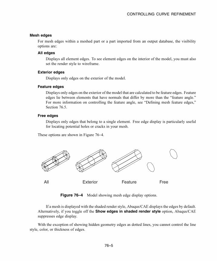
CONTROLLING CURVE REFINEMENT
Mesh edges
For mesh edges within a meshed part or a part imported from an output database, the visibility
options are:
All edges
Displays all element edges. To see element edges on the interior of the model, you must also
set the render style to wireframe.
Exterior edges
Displays only edges on the exterior of the model.
Feature edges
Displays only edges on the exterior of the model that are calculated to be feature edges. Feature
edges lie between elements that have normals that differ by more than the “feature angle.”
For more information on controlling the feature angle, see “Defining mesh feature edges,”
Section 76.5.
Free edges
Displays only edges that belong to a single element. Free edge display is particularly useful
for locating potential holes or cracks in your mesh.
These options are shown in Figure 76–4.
All Exterior Feature Free
Figure 76–4 Model showing mesh edge display options.
If a mesh is displayed with the shaded render style, Abaqus/CAE displays the edges by default.
Alternatively, if you toggle off the Show edges in shaded render style option, Abaqus/CAE
suppresses edge display.
With the exception of showing hidden geometry edges as dotted lines, you cannot control the line
style, color, or thickness of edges.
76–5
Abaqus ID:
Printed on:
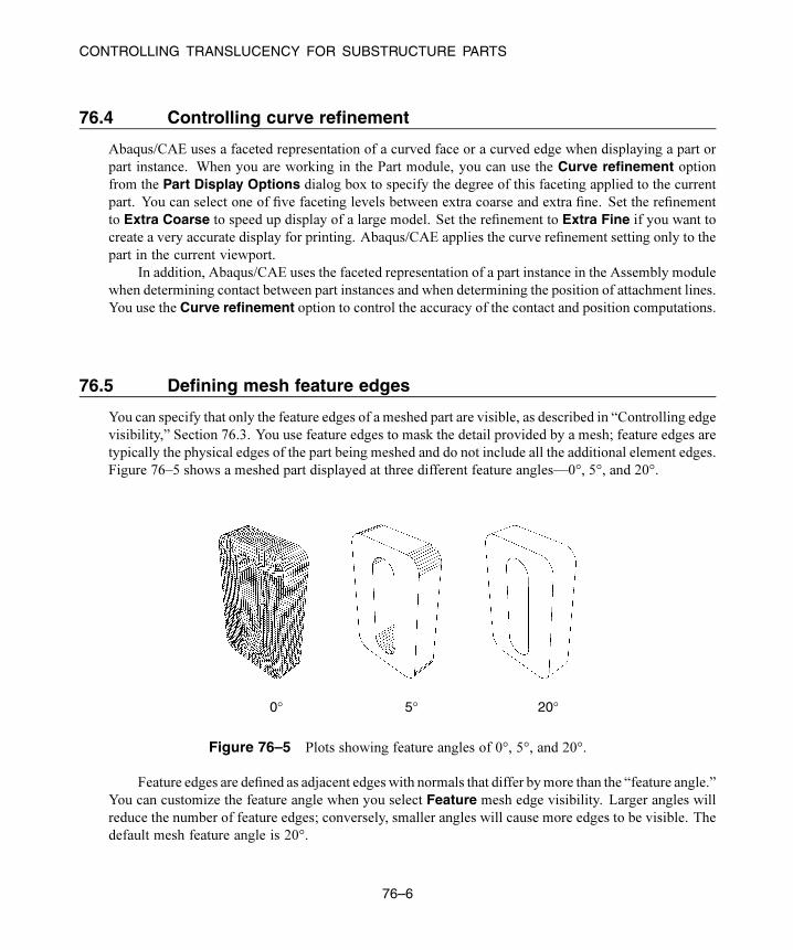
CONTROLLING TRANSLUCENCY FOR SUBSTRUCTURE PARTS
76.4 Controlling curve refinement
Abaqus/CAE uses a faceted representation of a curved face or a curved edge when displaying a part or
part instance. When you are working in the Part module, you can use the Curve refinement optionfrom the Part Display Options dialog box to specify the degree of this faceting applied to the current
part. You can select one of five faceting levels between extra coarse and extra fine. Set the refinement
to Extra Coarse to speed up display of a large model. Set the refinement to Extra Fine if you want to
create a very accurate display for printing. Abaqus/CAE applies the curve refinement setting only to the
part in the current viewport.
In addition, Abaqus/CAE uses the faceted representation of a part instance in the Assembly module
when determining contact between part instances and when determining the position of attachment lines.
You use the Curve refinement option to control the accuracy of the contact and position computations.
76.5 Defining mesh feature edges
You can specify that only the feature edges of a meshed part are visible, as described in “Controlling edge
visibility,” Section 76.3. You use feature edges to mask the detail provided by a mesh; feature edges are
typically the physical edges of the part being meshed and do not include all the additional element edges.
Figure 76–5 shows a meshed part displayed at three different feature angles—0°, 5°, and 20°.
0° 5° 20°
Figure 76–5 Plots showing feature angles of 0°, 5°, and 20°.
Feature edges are defined as adjacent edges with normals that differ bymore than the “feature angle.”
You can customize the feature angle when you select Feature mesh edge visibility. Larger angles will
reduce the number of feature edges; conversely, smaller angles will cause more edges to be visible. The
default mesh feature angle is 20°.
76–6
Abaqus ID:
Printed on:

CONTROLLING BEAM PROFILE DISPLAY
76.6 Controlling translucency for substructure parts
You can specify that the substructure parts and part instances in your model be displayed with or
without translucency. If you want to control the level of translucency for part and assembly display, see
“Changing the translucency,” Section 77.3.
76.7 Controlling beam profile display
If you use wire parts to model beams, you must create a beam section that refers to a beam profile, and
you must assign the beam section to the wire part. In addition, you must assign a beam orientation to
the wire part. You can then use the View→Part Display Options and the View→Assembly DisplayOptions menu items to view a realistic display of the beam profile in parts and the assembly in the
current viewport.
When beam profiles are displayed, Abaqus/CAE disables both view cuts and scaling and shrinking
of the model. Displaying beam profiles is useful for checking that the correct profile has been assigned to
a particular region and that the assigned beam orientation results in the expected orientation of the profile.
For example, Figure 76–6 shows the box beam profiles displayed on the light-service crane described in
“Example: cargo crane,” Section 6.4 of Getting Started with Abaqus: Interactive Edition.
Figure 76–6 The cargo crane example with beam profiles displayed.
76–7
Abaqus ID:
Printed on:

CONTROLLING DATUM DISPLAY
If you assign a general beam section to a wire, Abaqus/CAE displays the beam profile as an ellipse
with a cross-sectional area and moments of inertia ( and ) that match the values you specified.
If you assign a truss section to a wire, Abaqus/CAE displays the truss profile as a circle with a cross-
sectional area that matches the value you specified.
Abaqus/CAE does not render the tapering of beam profiles along their length. If your model includes
tapered beam sections, Abaqus/CAE renders these beams using the beam’s starting profile along its entire
length. For more information about tapered beams, see “Creating beam sections,” Section 12.13.11.
Abaqus/CAE renders beam profiles according to the current settings for color coding and
translucency. When these settings change, the color and translucency of the beam profiles change as
well.
76.8 Controlling shell thickness display
If you use shell elements to model relatively thin components in your analysis, you can use the
View→Part Display Options and the View→Assembly Display Options menu options to view
the actual thickness of these shell elements in your model. Displaying shell thickness enables you to
examine the thickness of shell geometry relative to the rest of the model. You can apply a scale factor
to reduce or increase the display of shell thickness for your session. Figure 76–7 shows the effect of
scale factor changes displayed on the stiffened plate model described in “Example: blast loading on a
stiffened plate,” Section 10.5 of Getting Started with Abaqus: Interactive Edition.
Abaqus/CAE renders shell thickness for three-dimensional shell elements only; thickness is not
displayed for axisymmetric shell elements, such as SAX1 elements. When shell thickness is displayed,
Abaqus/CAE also renders the edges of shell geometry unless a view cut is displayed in the viewport.
Abaqus/CAE renders shell thickness according to the current settings for color coding and translucency.
When these settings change, the color and translucency of the shell thickness change as well.
76.9 Controlling datum display
You can use the View→Part Display Options and the View→Assembly Display Options menu
items to control the display of datum geometry in parts and the assembly in the current viewport. You
can control the display of each of the datum types—points, axes, planes, and coordinate systems—and
you can toggle their display individually or all at once. Datum geometry that you choose not to display,
although invisible, is still a feature of the part or assembly. For more information on datum geometry,
see Chapter 62, “The Datum toolset.” You can also control the display of reference points; for more
information, see “The reference point,” Section 11.8.1.
76–8
Abaqus ID:
Printed on:
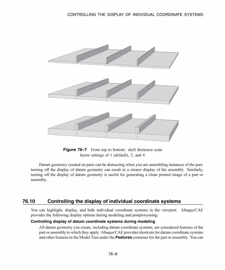
CONTROLLING THE DISPLAY OF INDIVIDUAL COORDINATE SYSTEMS
Figure 76–7 From top to bottom: shell thickness scale
factor settings of 1 (default), 2, and 4.
Datum geometry created on parts can be distracting when you are assembling instances of the part;
turning off the display of datum geometry can result in a clearer display of the assembly. Similarly,
turning off the display of datum geometry is useful for generating a clean printed image of a part or
assembly.
76.10 Controlling the display of individual coordinate systems
You can highlight, display, and hide individual coordinate systems in the viewport. Abaqus/CAE
provides the following display options during modeling and postprocessing:
Controlling display of datum coordinate systems during modeling
All datum geometry you create, including datum coordinate systems, are considered features of the
part or assembly to which they apply. Abaqus/CAE provides shortcuts for datum coordinate systems
and other features in the Model Tree under the Features container for the part or assembly. You can
76–9
Abaqus ID:
Printed on:
CUSTOMIZING MESH DISPLAY
highlight an individual datum coordinate system by clicking its shortcut in the Model Tree; when
highlighted, a coordinate system is rendered in red in the viewport and its title is displayed. To hide
or display the coordinate system in the viewport, click mouse button 3 on the shortcut and select
Suppress or Resume.You can also control the display of individual datum coordinate systems by adding them to
display groups. See “Managing display groups,” Section 78.2, for more information.
Controlling display of any coordinate system during postprocessing
In the Visualization module the available coordinate systems are divided into two groups: ODB
coordinate systems, which are part of the output database file; and session coordinate systems,
which are created during postprocessing. Session coordinate systems apply to one output database
only and persist only for your Abaqus/CAE session, unless you move the session coordinate system
to the output database. See “Saving a coordinate system to an output database file,” Section 42.8.6.
You can highlight, display, or hide individual coordinate systems using either of the following
techniques:
• All available coordinate systems have shortcuts in the Results Tree under theODB CoordinateSystems and Session Coordinate Systems containers. You can click any shortcut to
highlight that coordinate system in the viewport; when highlighted, a coordinate system is
rendered in red in the viewport and its title is displayed. You can also display or hide any
coordinate system by clicking mouse button 3 on the shortcut and selecting a Boolean operator
from the list that appears.
• You can control the display of ODB coordinate systems and session coordinate systems by
adding them to display groups, which can be displayed or hidden using the Boolean display
options. See “Managing display groups,” Section 78.2, for more information.
The Coordinate System Manager also provides information about the ODB coordinate systems
and session coordinate systems for the selected output database. You cannot change the display of
coordinate systems from this manager, but you can rename or delete them. See “Creating coordinate
systems during postprocessing,” Section 42.8.
76.11 Controlling reference point display
You can use the View→Part Display Options and the View→Assembly Display Options menu
items to control the display of reference points in the current viewport on a part or on the assembly.
Turning off the display of reference points is useful for generating a clean printed image of a part or the
assembly. Even though you choose not to display reference points, they are still a feature of the part or
assembly. For more information on reference points, see “The reference point,” Section 11.8.1.
76–10
Abaqus ID:
Printed on:

CONTROLLING MODEL LIGHTING
76.12 Customizing mesh display
You can use the View→Part Display Options and the View→Assembly Display Options menu
items to specify whether or not node and element labels are displayed on a meshed part or assembly. You
can choose to display or suppress your native mesh and, if displayed, to do so only in the Mesh module
or in all part-related or all assembly-related modules. If you display the native mesh, you can choose
to also display the geometry of bottom-up meshed sections, non-bottom-up sections, or both along with
the mesh. Displaying the geometry provides a visual indication of how well the mesh conforms to the
geometry.
76.13 Controlling model lighting
You can use the View→Light Options menu item to control the lighting of your model. Lights affect
the appearance of your model in the current viewport when the Shaded render style is used. You can
control the intensity of the Ambient light and the Shininess of the model surface. You can also control
the locations and intensities of up to eight additional positional lights. The combined effects of the light
settings can be used to simulate different surface finishes and light conditions on your model. The default
settings provide good contrast for viewing all features in most models.
The default settings provide good contrast for viewing all features in most models. Using the default
settings is particularly important for tessellated, banded contour plots, for which intense light can fade
the colors in the facets of the contour plot and display misleading results that do not match the colors in
the plot legend. These changes to contour colors can also appear in printouts of banded contour plots if
you print to file in EPS, PostScript, or SVG formats, because these three formats use tessellated contours
by default. To print a banded contour plot to any of these formats without creating misleading contour
colors, turn off shading before printing.
Global settings
Ambient light is applied evenly to the entire scene and brightens a model from all directions. Low
intensity ambient light allows the positional lighting to create shading that distinguish small features
and surface contours from the rest of the model. High intensity ambient light removes shading and
may make some model features difficult to see.
If your computer’s graphics card supports OpenGL shading language (GLSL), Abaqus/CAE
also reveals the global Shading options, from which you can enable Phong shading for your
session. Phong shading renders more realistic shading on three-dimensional surfaces than the
default option, Gouraud shading, but it can cause a noticeable performance impact on some
systems. This performance impact occurs only when the mesh is hidden; if the mesh is displayed
(either during modeling or postprocessing), Abaqus/CAE renders Phong lighting with no noticeable
performance impact.
Shininess is the reflectivity of the model surface and is used to control the size of specular
highlights from the positional lights. A very shiny surface reflects light like a mirror—the light
76–11
Abaqus ID:
Printed on:
CONTROLLING INSTANCE VISIBILITY
reflects in one direction based on the incident angle of the light source. Therefore, a surface must
be positioned correctly with respect to the light source to reflect light to your viewpoint. Surfaces
that are less shiny reflect light more randomly, so a wider range of surface angles can reflect light
to your viewpoint. Like high intensity ambient lighting, low shininess can obscure small features
and contours of your model from view.
The Viewpoint option controls how specular lighting effects are calculated. An Infiniteviewpoint assumes a constant vector for the direction from the camera to each point when
calculating reflections and specular highlights at a point. A Local viewpoint calculates a separatedirection vector for each point based on its position in the viewport. A Local viewpoint createsmore realistic lighting effects but can decrease overall performance.
Positional light settings
Positional lights provide a light bulb effect. A positional light is projected onto the model from the
specified location, and its effects change as you rotate your model view. Positional lights work in
conjunction with shininess to determine how your model reflects light.
The distance of the light from the model is equal to the distance from the camera to the model.
You can position the lights by specifying their Latitude and Longitude on a hemisphere around
the model. You can also specify the Type of light source being used. A Directional light is a planarlight source; the angle of incident light on the model will be equivalent for all parallel surfaces. A
Point light is a point light source; the angle of incident light depends on the location of the surface
or point relative to the light. A Point light creates more realistic lighting effects but can decrease
overall performance.
You can control two different qualities for positional lights: Diffuse intensity and Specularintensity. The Diffuse setting controls the intensity of a positional light. Unlike ambient light,
surfaces that face toward the light position will brighten more readily than other surfaces in the
model when increasing the diffuse intensity of a positional light. The Specular setting controls thebrightness of those surfaces that are reflecting from the light toward the viewpoint. You should first
set the position and diffuse intensity of the positional light to achieve the shading you desire. Then
you can adjust the brightness of reflected light with the Specular slider.
76.14 Controlling instance visibility
By default, Abaqus/CAE displays all part instances included in the assembly. You can turn the display
of all instances on or off, or you can toggle the display of individual instances. Part instances that you
have suppressed or that do not belong to the current display group cannot be made visible using this
dialog box; you must use the Feature Manipulation toolset or the Display Group toolset instead. For
more information, see Chapter 13, “The Assembly module,” or Chapter 78, “Using display groups to
display subsets of your model.”
This section describes how to control instance visibility from the Assembly Display Optionsdialog box. You can also change instance visibility from the Model Tree or the viewport: from the
76–12
Abaqus ID:
Printed on:

SAVING YOUR DISPLAY OPTIONS SETTINGS
Model Tree, highlight the part instances that you want to display or hide, click mouse button 3, and
select Hide or Show; from the viewport, highlight the instances you want to hide, click mouse button 3,
and select Hide Instance from the menu that appears.
76.15 Controlling the display of attributes
The Attribute display options in the Assembly Display Options dialog box allow you to control the
display of symbols representing
• interactions, constraints, and connectors that you create in the Interaction module,
• loads, boundary conditions, and predefined fields that you create in the Load module,
• engineering features that you create in the Property module and Interaction module, and
• optimization attributes that you create in the Optimization module.
You can control when and how these attributes are displayed, and you can click Set all on or Set all offto display or hide all attributes, respectively. For information on the symbols representing each attribute,
see Appendix C, “Special graphical symbols.”
For information on controlling the display of boundary conditions, coupling constraints,
connectors, and point elements in the Visualization module, see “Controlling the display of model
entities,” Section 55.10.
76.16 Saving your display options settings
If you change your display options settings (for example, if you change the render style or turn off
the display of datum planes), you can store the new settings for future sessions. Abaqus/CAE saves
your settings in a file called abaqus_v6.13.gpr. For more information, see “Working with
abaqus_v6.13.gpr files,” Section 2.1.3.
From the mainmenu bar, select File→Save Display Options to save all the current display options
settings. TheSave Display Options dialog box appears and allows you to save the options in the current
directory or in your home directory.
You can edit the abaqus_v6.13.gpr file using API commands in the Abaqus Scripting
Interface; for more information, see “Editing display preferences and GUI settings,” Section 8.4 of
the Abaqus Scripting User’s Guide. You can also delete the file to restore the default GUI and display
options settings, and you can copy the file to other directories on your computer or transfer the file to a
different computer. When you save your settings from abaqus_v6.13.gpr, Abaqus/CAE always
saves all of the current settings and always overwrites all the settings that were previously saved.
You cannot save only selected settings. You can use the noSavedOptions command line option to
start Abaqus/CAE without loading the settings in abaqus_v6.13.gpr. For more information, see
“Starting Abaqus/CAE (or Abaqus/Viewer),” Section 2.1.1.
Abaqus/CAE saves the following display options settings in abaqus_v6.13.gpr:
76–13
Abaqus ID:
Printed on:

SAVING YOUR DISPLAY OPTIONS SETTINGS
• Part and assembly display options; for example, render style, the visibility of prescribed conditions
and the various types of datum geometry, and the display of mesh, element, and node labels.
• Graphics options and viewport annotation options. Abaqus/CAE also saves the perspective setting.
• Print options.
• Display options in the Visualization module; for example, the contour type for contour plots and
the render style and fill color in the common plot options.
• Animation options in the Visualization module.
• Other options in the Visualization module, such as probe, field report, X–Y plot, and X–Y report
options.
76–14
Abaqus ID:
Printed on:

UNDERSTANDING COLOR CODING
77. Color coding geometry and mesh elements
This section explains how you can apply color coding to viewable geometry and mesh elements. The
following topic is covered:
• “Understanding color coding,” Section 77.1
In addition, the following sections are available in the HTML version of this guide:
• “Changing the initial color,” Section 77.2
• “Changing the translucency,” Section 77.3
• “Coloring geometry and mesh elements,” Section 77.4
• “Coloring all geometry in the Visualization module,” Section 77.5
• “Coloring nodes or elements in the Visualization module,” Section 77.6
• “Coloring constraints in the Visualization module,” Section 77.7
• “Customizing the display color of individual objects,” Section 77.8
• “Displaying multiple color mappings,” Section 77.9
• “Editing the colors in the Auto-Color List,” Section 77.10
• “Saving and restoring custom color mappings,” Section 77.11
77.1 Understanding color coding
This section includes the following topics:
• “Color coding concepts,” Section 77.1.1
• “Color coding in the Visualization module,” Section 77.1.2
77.1.1 Color coding conceptsYou can distinguish between components in your model or output database by color coding the viewable
geometry and mesh elements in the current viewport. Abaqus/CAE applies color coding according to
Color Mappings that specify the colors assigned to each item for a particular type of object, such as
parts, section assignments, boundary conditions, or display groups. In the example shown in Figure 77–1
the color mapping is by parts, and each row describes the color assigned to one of the three part definitions
in this model. The Color Code dialog box thus provides a legend that describes all of the color coding
currently displayed in the current viewport.
Color coding is applied in two layers. All geometry and mesh elements are first colored with
the Initial color, a customizable setting that is grey by default. (See “Changing the initial color,”
Section 77.2, for more information.) Abaqus/CAE then applies color coding on top of the initial color
according to the colors and objects in the color mapping that you select. Areas will remain visible in
77–1
Abaqus ID:
Printed on:

UNDERSTANDING COLOR CODING
Figure 77–1 The Color Code dialog box.
the initial color if you apply a color mapping such as Boundary conditions, Loads, or Sets, for which
Abaqus/CAE usually color codes only distinct points or surfaces in the model.
Abaqus/CAE automatically creates color mappings for all items in your model by associating the
name of each item with a color in the Auto-Color List. The colors are selected by matching the Auto-Color List with an alphabetical listing of item names; thus, in the Parts example in Figure 77–1, Blockis color coded with the first color in the Auto-Color List, Floor is color coded with the second color, andso on. Color assignments depend on the item name only; therefore, resorting these items in the ColorCode dialog box does not change the color assignments.
Note: If a region is shared by two or more items in the model, such as when a skin section is assigned to
the surface and a solid section is assigned to the entire block, the common region will be colored with the
color definition for the item whose name appears later in the alphabetical list. Abaqus/CAE overwrites
the first color mapping color definition as each color assignment is displayed in the viewport.
Because each color mapping is a set of links between item names and color definitions, color
mappings persist between modules in Abaqus/CAE and between a model database and its output
77–2
Abaqus ID:
Printed on:

UNDERSTANDING COLOR CODING
databases. However, because Abaqus/CAE relies on object names for color coding, you cannot retain
the color coding associated with an object when you rename that object. By contrast, Abaqus/CAE
usually deletes an object’s color definition when you delete the object definition from your model; the
two exceptions are material and section definitions, whose color coding persists in the viewport even
after you delete the definition. To refresh the color coding in the current viewport after you delete a
material or section definition, you must either apply a color mapping or switch to a different module.
Abaqus/CAE also provides a default color mapping for each module. For example, when you
display the Mesh defaults color mapping in the Mesh module, Abaqus/CAE color codes items in
the viewport according to their meshability. Each module’s default color mapping is available only in
that module; you cannot color code objects in the Property module using the assignments in the Meshdefaults color mapping. Module default mappings cannot be edited, and the module default mappings
correspond to the default colors that Abaqus/CAE uses if no color coding is applied.
Color mappings are viewport-specific and, in some cases, they persist betweenmodules. Persistence
of color coding between modules depends on whether you have the default color mapping displayed for
your current module:
• If the default color mapping for your module is selected, Abaqus/CAE automatically changes the
color mapping as you switch modules. For example, if you select the Assembly defaults color
mapping in the Assembly module and then switch to the Mesh module, Abaqus/CAE automatically
applies the Mesh defaults color mapping.
• If a non-default color mapping is selected, Abaqus/CAE retains the color mapping as you switch
modules. For example, if you select the Part instances color mapping in the Assembly module
and then switch to the Mesh module, Abaqus/CAE continues to color code by part instance name
rather than by meshability.
When you change the color mapping, Abaqus/CAE refreshes color coding only in the current viewport
while retaining any color coding in other inactive, visible viewports. When you add a new viewport to
your session, the new viewport inherits the color mappings of the previously current viewport.
Once color mappings are created, you can customize any color mapping (except the module
defaults) by changing the colors assigned to any of its individual objects. You can also toggle the active
status of individual objects in the color mapping, which controls whether an individual object is color
coded in the current viewport. Objects whose color coding is inactive are rendered with the initial color.
The Color Code dialog box also provides sorting and filtering tools that you can use to display a subset
of the objects in a color mapping. These tools can help you focus your display when a color mapping
has many objects.
77.1.2 Color coding in the Visualization moduleThe color coding process is slightly different in the Visualization module than in other Abaqus/CAE
modules. You control the overall edge and fill colors of your model using the Color & Style options
in the Common Plot Options or Superimpose Plot Options dialog box. Using these options, you
select a single color for all element and surface edges and a separate color for all element faces and
surfaces. The colors you select apply uniformly to the entire model.
77–3
Abaqus ID:
Printed on:

UNDERSTANDING COLOR CODING
You can also control the colors of individual elements and part instances using the Color Codeoptions. The Color Code dialog box allows you to select separate colors for individual items. You must
use the Color Code options to execute any complex, nonuniform color scheme.
By default, individual item colors override the overall common or superimposed edge color and fill
color. You can change this behavior by using the Color & Style options in the Common Plot Optionsor Superimpose Plot Options dialog box to specify whether individual or overall item colors should
take precedence. (Individual item colors do not apply to contour plots.)
The Visualization module offers a smaller subset of color mappings than are available in the other
modules. When an output database is displayed in the current viewport, the available color mappings
for color coding are part instances, elements, nodes, constraints, materials, sections, display groups,
averaging regions, internal sets, layups, and plies; when a model in the current model database is
displayed, the only available color mapping is by part instance. However, you can control both the edge
and fill colors when you customize colors for the individual objects in the current viewport, and you can
choose to apply color coding to the entire model or to its nodes or elements only. In addition, settings in
the Visualization module depend upon other options; when you specify an individual item color in the
Color Code dialog box, Abaqus/CAE applies the color based on two characteristics of the current plot:
Color precedence setting
Abaqus/CAE applies the color if, on the Color & Style page of the Common Plot Options or
Superimpose Plot Options dialog box, Allow color code selections to override options inthis dialog is toggled on.
Render style
In the wireframe and hidden render styles, Abaqus/CAE displays only element edges. If the current
plot uses the wireframe or hidden render style, Abaqus/CAE applies the individual item color to
those edges.
In the filled and shaded render styles, Abaqus/CAE displays element faces as well as element
edges. If the current plot uses the filled or shaded render style, Abaqus/CAE applies the individual
item fill color to the element faces and the individual item edge color to the element edges.
In the filled and shaded render styles, line-type elements (such as beams) are treated as if their
lines are faces. In the filled and shaded render styles, Abaqus/CAE applies the individual item fill
color to the lines representing such an element.
77–4
Abaqus ID:
Printed on:

UNDERSTANDING DISPLAY GROUPS
78. Using display groups to display subsets of your model
By default, Abaqus/CAE displays your entire model; however, you can choose to display subsets of your
model by creating display groups. These subsets can contain combinations of part instances, geometry
(cells, faces, or edges), datum geometry (points, axes, planes, or coordinate systems), elements, nodes,
and surfaces from the current model or output database. This chapter explains the concept of display
groups and provides a brief overview of how you can manage them. The following topics are covered:
• “Understanding display groups,” Section 78.1
• “Managing display groups,” Section 78.2
78.1 Understanding display groups
A display group is a collection of selected model components and can contain the entire model or
combinations of part instances, geometry (cells, faces, or edges), datum geometry (points, axes, planes,
or coordinate systems), elements, nodes, surfaces, constraints, and output database coordinate systems.
Display groups allow you to reduce clutter on your screen and focus on areas of interest within your
model, to access “hidden” components in complex models, and to decrease the amount of time needed
to refresh the display in the current viewport. For example, you can use display groups to show contact
surfaces but suppress elements or to produce a contour plot showing elements in the interior of your
model that would otherwise be obscured. You can plot, save, edit, copy, rename, and delete display
groups. In the Visualization module you can plot more than one display group in the same viewport,
and you can customize the plot options for each display group independently.
78.1.1 Understanding how to create display groups
A display group can contain combinations of model components: part instances, geometry (cells, faces,
or edges), datum geometry (points, axes, planes, or coordinate systems), elements, nodes, surfaces,
constraints, output database coordinate systems, or the entire model. In addition, you can create a display
group by operating on previously saved display groups. However, while creating a display group, you can
perform operations on only one type of model component at a time. Creating a display group containing
selected components of more than one type is an incremental process. The model components that can be
used to create a display group depend on the module in which you are working, as shown in Table 78–1
and Table 78–2.
To create a display group, you first select the particular items of interest. You can then perform
a Boolean operation on your selection and the contents of the current viewport. This sequence can be
repeated as necessary to create the desired group. In addition, you can create a new display group by
78–1
Abaqus ID:
Printed on:

UNDERSTANDING DISPLAY GROUPS
Table 78–1 Model components that can be used to create
display groups in the Part- and Assembly-related modules
and in the Visualization module.
Modules Available Model Components
Geometry (cells, faces, or edges)
Datum geometry (points, axes, planes, or coordinate systems)
Elements
Nodes
Reference points
Sets (geometry, element, or node)
Part-related (Part,
Property)
Display groups
Part instances
Geometry (cells, faces, or edges)
Datum geometry (points, axes, planes, or coordinate systems)
Assembly wires (connector wires)
Elements
Nodes
Reference points
Sets (geometry, element, or node)
Surfaces
Assembly-related
(Assembly, Step,
Interaction, Load,
Mesh)
Display groups
Part instances
Elements
Nodes
Surfaces
Visualization
module
Display groups
editing (for example, performing additional Boolean operations on) the contents of a previously saved
display group.
You can save either the selection in the dialog box or the contents of the current viewport as a display
group. By default, a display group persists only for the duration of the session. If you want to retain
78–2
Abaqus ID:
Printed on:

UNDERSTANDING DISPLAY GROUPS
Table 78–2 Model components that can be used to create display
groups for output databases in the Visualization module.
Module Available Model Components
Part instances
Elements
Nodes
Surfaces
Display groups
Coordinate systems
Tie constraints
Shell-to-solid coupling constraints
Distributing coupling constraints
Kinematic coupling constraints
Visualization
Rigid body constraints
a display group for use in subsequent sessions, save it to an XML file, to the model database, or to an
output database; for more information, see “Managing session objects and session options,” Section 9.9,
in the HTML version of this guide. You can access a display group only in modules of the same type as
the one in which it was created (see Table 78–1 and Table 78–2). For example, if you create and save
a display group in the Part module, you will be able to access this display group only in the Part and
Property modules.
A display group named All that contains all objects in the current part, assembly, or output database
is created automatically by Abaqus/CAE. This display group appears in the display group manager for
the current module and cannot be edited, copied, renamed, or deleted. It is not associated with a particular
part, assembly, or output database. You can use this display group to quickly return to a plot of the entire
part or model after performing Boolean operations.
78.1.2 Understanding display group Boolean operationsTo create or edit a display group, you can perform Boolean operations on selected model components
and the contents of the current viewport. Abaqus/CAE offers the following Boolean operations in the
Display Group toolset: Replace, Add, Remove, Intersect, and Either.As an example of a simple Boolean operation, assume the current viewport shows the entire model.
If you select a single element set and then apply the Remove operation, that element set is eliminated
from the display in the current viewport.
78–3
Abaqus ID:
Printed on:

UNDERSTANDING DISPLAY GROUPS
For each Boolean operation you perform to create or edit a display group, you can select only one
type of model component: part instances, geometry (cells, faces, or edges), datum geometry (points,
axes, planes, or coordinate systems), elements, nodes, surfaces, previously saved display groups, or the
entire model. For a given display group, Abaqus/CAE initially assumes that you want to include all
nodes connected to all elements in the group. However, if you select particular nodes, all subsequent
operations on that display group include only the nodes you have selected.
An explanation of each of the Boolean operations follows. In the icons below, the circle on the
left represents the items in the current viewport; the circle on the right represents your selection. The
shaded portion represents the resulting display group. All of these Boolean operations except the last
one, Replace All, are available in the Create Display Group dialog box; the Display Group toolbar
provides access to theReplace, Remove, Either, andReplace AllBoolean operations, as well asUndoand Redo operations.
Replace
Use the Replace operator to replace the current viewport contents with your selection.
Add
Use the Add operator to add your selection to the current viewport contents.
Remove
Use the Remove operator to remove your selection from the current viewport contents. If your
selection includes one or more elements or surfaces, the nodes connected to those items are also
removed, provided that you have not specifically operated to include those nodes in the display
group.
Intersect
Use the Intersect operator to display only those items common to your selection and the display
in the current viewport.
Either
Use the Either operator to display only model components that are either in your selection or in the
current viewport but not in both.
Note: The button in the Display Group toolbar hides all the model components that are
displayed in the current display group and displays all the model components that were hidden. This
operation is equivalent to selecting all the objects in the Create Display Group or Edit DisplayGroup dialog box and clicking the Either button.
78–4
Abaqus ID:
Printed on:
MANAGING DISPLAY GROUPS
Replace All
Use the Replace All operator to replace your display group and display all entities in the current
viewport. This operator is available in the toolbar only.
When you select the (Replace Selected) or (Remove Selected) operators from the
toolbar, Abaqus/CAE displays a list of model components in the prompt area. Select the type of model
component that you want to replace or remove from the selected display group, then click one or more
model components in the viewport to change the contents of the display group.
Note: The Replace Selected and Remove Selected operators perform the same actions as the
Replace and Remove operators in the display group dialog boxes. The toolbar operators have
different names to indicate that you must select model components from the viewport before using these
operators to change the current display.
78.2 Managing display groups
The display group managers allow you to create a display group and to plot, edit, copy, rename, or
delete a previously saved display group. The display group manager for the current module lists only
the display groups that you have saved in modules of the same type during the current session. The PartDisplay Group Manager in the part-related modules lists the model and part to which each display
group belongs; theAssembly Display Group Manager in the assembly-related modules lists the model
to which each display group belongs.
In the Visualization module you can plot multiple display groups in the same viewport. The ODBDisplay Group Manager in the Visualization module allows you to lock and unlock plotted display
groups to selectively customize plot options. In addition, you can synchronize all plotted display groups
to use the same plot options.
To access the display group manager for the current module, select Tools→Display
Group→Manager from the main menu bar, or use the tool on the toolbar. For detailed
instructions on creating and managing display groups, see the corresponding section in the HTML
version of this guide. (For instructions on using the online documentation, see “Getting help,”
Section 2.6.)
78–5
Abaqus ID:
Printed on:

UNDERSTANDING HOW TO OVERLAY PLOTS
79. Overlaying multiple plots
By default, Abaqus/CAE displays only one plot at a time in the current viewport. A plot may display
multiple plot states, such as the contours and material orientations of the same model. However, a single
plot cannot display data from more than one output database nor can it display both the model and an
X–Y plot in the same viewport. If you want to display data in this fashion, you must overlay individual
plots in the same viewport. This chapter explains the concept of overlaying plots and provides a brief
overview of how you can create and manage such plots. The following topicis covered:
• “Understanding how to overlay plots,” Section 79.1
To overlay multiple plots, select View→Overlay Plot from the main menu bar. For detailed instructions
on overlaying plots, see “Producing and modifying overlay plots,” Section 79.2, in the HTML version
of this guide.
79.1 Understanding how to overlay plots
You can create a display that contains multiple plots in one viewport. For example, you may want to do
any of the following:
• combine a contour plot and an X–Y plot
• compare the deformed plot shapes from two different output database files in the same viewport
• combine a time history animation with an animated X–Y plot displaying the change in several
variables in the model over time
Overlay plots are useful, for example, for displaying data from both output databases in a co-simulation
in the same viewport.
Overlay plots are composed of layers; each layer contains one plot, and the layers are stacked on
top of each other to create the combined plot. Figure 79–1 shows a plot containing the deformed shape
plots at four different increments of an analysis as well as an X–Y plot of the strain energy in the model
versus time.
By default, the viewport does not contain any layers; only one plot at a time is displayed. To overlay
multiple plots, you create a layer for each individual plot as you interact with Abaqus/CAE. You then
choose the layers to display in the current viewport. You can create as many layers as you would like;
any number of layers can be displayed in the same viewport. In addition, you can open multiple output
databases and automatically display the combined contents in an overlay plot in a single viewport.
Use the Overlay Plot Layer Manager to create, display, position, and delete layers. To access
the manager, select View→Overlay Plot from the main menu bar or click the Overlay Plot Layer
Manager tool in the toolbox.
When you create a layer, it contains everything that is visible in the current viewport. You can
change the contents of a layer, manipulate its view, reorder the layer with respect to the other layers in
79–1
Abaqus ID:
Printed on:

UNDERSTANDING HOW TO OVERLAY PLOTS
Figure 79–1 Overlay plot.
the overlay plot, and change the various display options that are applied to the contents. By default, layers
are plotted directly on top of one another. Sometimes lines that appear directly on top of one another
can create undesirable visual effects. You can offset the layers with respect to each other to avoid such
display anomalies.
The settings in the Overlay Plot Layer Manager are applied to the contents of the current viewportonly when you click Plot Overlay. Abaqus/CAE then enters the overlay plot state; when you click PlotSingle in the Overlay Plot Layer Manager, the overlay plot disappears from the viewport and the
display reverts back to the previous plot state. You can also click the tool in the toolbox to switch
between the single plot and overlay plot state at any time.
When you are in the overlay plot state, Abaqus/CAE displays your plots relative to an overlay plot
coordinate system. As you create a layer, Abaqus/CAE assigns the view in which the layer was created
to the overlay plot front (1–2) view. You can modify what is displayed in the overlay plot front view by
manipulating the view for each individual layer, as described in “Manipulating the view for an overlay
plot,” Section 79.2.3, in the HTML version of this guide. User-specified views defined in the overlay
plot state are relative to the overlay plot coordinate system.
Columns in the Overlay Plot Layer Manager display the following information about each layer:
Visible
A check mark in this column indicates that the layer is visible in the viewport when you are in the
overlay plot state.
79–2
Abaqus ID:
Printed on:

UNDERSTANDING HOW TO OVERLAY PLOTS
Current
A check mark in this column indicates that the layer is current. Only one layer can be current at a
time, although each layer can contain multiple plot states (for more information, see “Displaying
multiple plot states,” Section 55.6). Plot options are applied to only the current layer when you
are in the overlay plot state; you can choose whether view manipulation options are applied to all
existing layers or to only the current layer. The current layer is not necessarily the foremost layer
in the viewport.
Name
The name of the layer.
Object
The name of the object contained in the layer; for example, an output database or an X–Y plot.
79–3
Abaqus ID:
Printed on:

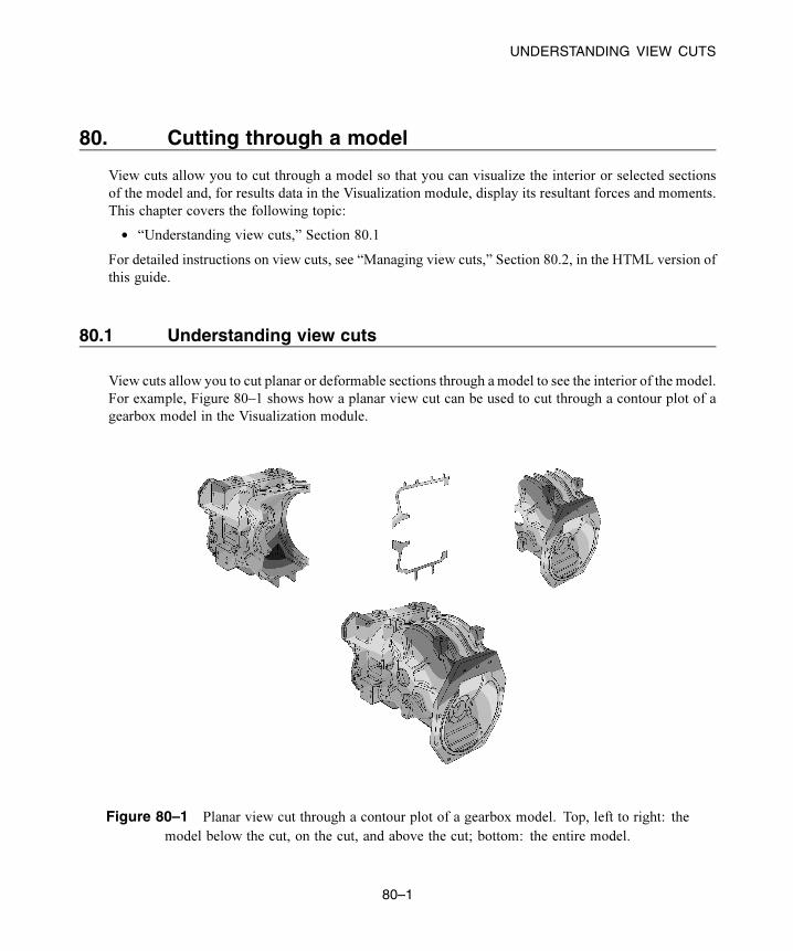
UNDERSTANDING VIEW CUTS
80. Cutting through a model
View cuts allow you to cut through a model so that you can visualize the interior or selected sections
of the model and, for results data in the Visualization module, display its resultant forces and moments.
This chapter covers the following topic:
• “Understanding view cuts,” Section 80.1
For detailed instructions on view cuts, see “Managing view cuts,” Section 80.2, in the HTML version of
this guide.
80.1 Understanding view cuts
View cuts allow you to cut planar or deformable sections through a model to see the interior of the model.
For example, Figure 80–1 shows how a planar view cut can be used to cut through a contour plot of a
gearbox model in the Visualization module.
Figure 80–1 Planar view cut through a contour plot of a gearbox model. Top, left to right: the
model below the cut, on the cut, and above the cut; bottom: the entire model.
80–1
Abaqus ID:
Printed on:
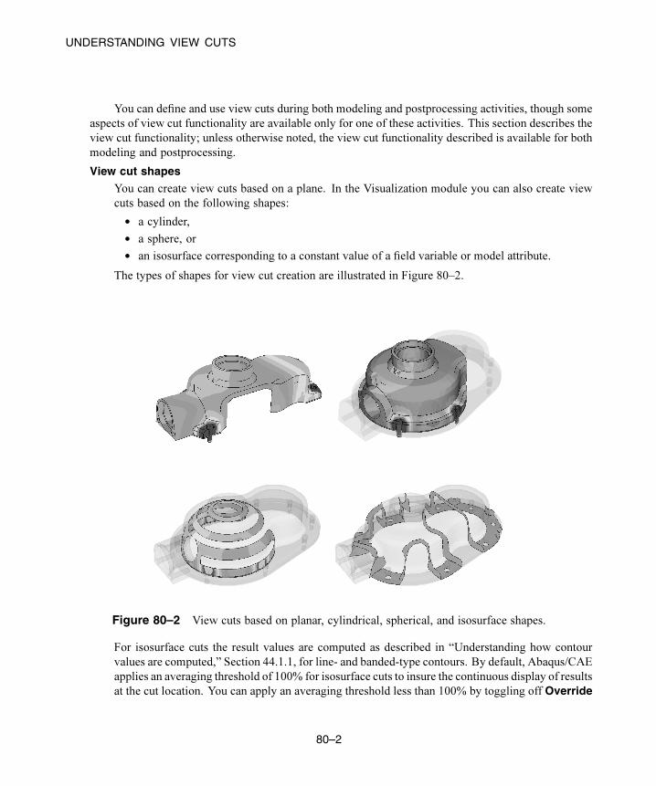
UNDERSTANDING VIEW CUTS
You can define and use view cuts during both modeling and postprocessing activities, though some
aspects of view cut functionality are available only for one of these activities. This section describes the
view cut functionality; unless otherwise noted, the view cut functionality described is available for both
modeling and postprocessing.
View cut shapes
You can create view cuts based on a plane. In the Visualization module you can also create view
cuts based on the following shapes:
• a cylinder,
• a sphere, or
• an isosurface corresponding to a constant value of a field variable or model attribute.
The types of shapes for view cut creation are illustrated in Figure 80–2.
Figure 80–2 View cuts based on planar, cylindrical, spherical, and isosurface shapes.
For isosurface cuts the result values are computed as described in “Understanding how contour
values are computed,” Section 44.1.1, for line- and banded-type contours. By default, Abaqus/CAE
applies an averaging threshold of 100% for isosurface cuts to insure the continuous display of results
at the cut location. You can apply an averaging threshold less than 100% by toggling off Override
80–2
Abaqus ID:
Printed on:

UNDERSTANDING VIEW CUTS
primary variable averaging when you create the isosurface cut. Abaqus/CAE then applies the
averaging threshold specified in the Averaging options in the Result Options dialog box; for
more information, see “Controlling result averaging,” Section 42.6.6. Cuts along the X-, Y-, and
Z-planes are created by default.
Note: Isosurface view cuts offer slightly different functionality and behavior than isosurface-type
contour plots. An isosurface view cut always reflects the results of the primary variable that was
active when the view cut was created; you cannot change the variable for which an isosurface
view cut displays results. By contrast, isosurface-type contour plots always display data from the
currently selected primary variable for your session. Because each isosurface view cut is tied to a
single variable, you can investigate the locations where two isosurface view cuts intersect if you
display multiple isosurface view cuts that are based on different output variables.
Displaying the cut section
To display the cut section of your model, you activate a cut and choose whether to display the model
on the cut, above the cut, and/or below the cut, as illustrated in Figure 80–1. The cut itself is never
visible. For planar cuts the portion of the model below the cut is defined as that part located on the
negative side of the plane (relative to the orientation of the normal to the plane). For cylindrical and
spherical cuts the portion of the model below the cut is defined as that part located at radii less than
the radius of the cut shape. For an isosurface cut the portion of the model below the cut is defined
as that part located at isovalues less than the specified isovalue. By default, Abaqus/CAE displays
the model on and below the cut. In the Visualization module, you can display the model above the
cut and the model below the cut at the same time; in all other modules, only one of these display
options is available at a time.
Plot options
You can select different plot options for the portions of themodel below the cut, on the cut, and above
the cut; for example, in Figure 80–2 some portions of the model are displayed with translucency
activated, while others are displayed with no translucency.
Displaying multiple view cuts (Visualization module only)
Only one cut can be active (used to display the model in the current viewport) at a time in modules
other than the Visualization module; in the Visualization module, however, you can display
multiple view cuts at once. In addition, in the Visualization module you can activate view cuts
on undeformed, deformed, contour (texture-mapped only), symbol, or material orientation plots.
For symbol and material orientation plots, Abaqus/CAE displays symbols and material orientation
triads at all integration points for each element included in the view, even if the element is partially
cut.
80–3
Abaqus ID:
Printed on:
UNDERSTANDING VIEW CUTS
Animation of view cuts (results data only)
Plots with an active view cut can be animated for output database data in the Visualization module;
the view cut will be updated for each animation frame. View cuts cannot be activated on tessellated
contour plots; swept, shrunk, or extruded plots; or highly refined plots (medium, fine, or extra fine).
Results caching
By default, Abaqus/CAE caches the result values used to generate images of a cut model in memory
to improve performance. However, you can disable results caching for cut fields to decreasememory
usage if necessary; see “Controlling results caching,” Section 42.6.10, in the HTML version of this
guide, for more information.
Following the deformation
For plots of the deformed model, you can choose to have the cut follow the deformation; i.e., the
cut surface will be calculated relative to a reference frame, and the cut deformation will match the
deformation of the model.
Repositioning view cuts
You can reposition cuts on your model: planar cuts can be rotated or translated, while the other cut
shapes can only be translated.
View Cut Manager
You can select a cut (either active or inactive) in the View Cut Manager to position, edit, copy,
rename, or delete it. Selecting a cut in the manager is not the same as activating the cut. A cut can
be both selected and active, unselected and active, or selected and inactive; and you can display
or hide a free body cut for the currently displayed view cut if it is active. Figure 80–3 shows an
example of the information displayed in the view cut manager in the Visualization module; in other
modules, the free body display options are not included in this dialog box.
Resultant forces and moments on view cuts (results data only)
For view cuts of output database data in the Visualization module you can also display the resultant
forces and moments, and you can compute these values based on the entire model or based on the
current display group. The example shown in Figure 80–4 includes the resultant force and moment
displayed for a view cut of a landing gear assembly. You can display the resultant force and moment
on a view cut only for solid geometry, shell sections, or beam sections; for shell sections and beam
sections the output database must include section force (SF) and section moment (SM) output for
resultant forces and moments to be displayed. Abaqus/CAE does not support display of resultant
forces and moments on view cuts for axisymmetric models. You can display the resultant force and
moment on a view cut for any of the displayed view cuts in your session. Abaqus/CAE updates the
resultant force and moment vectors and summation point as you reposition the view cut or animate
the model.
80–4
Abaqus ID:
Printed on:

UNDERSTANDING VIEW CUTS
active cut
selected cut
belowcut
oncut
abovecut
free body
Figure 80–3 The View Cut Manager dialog box in the Visualization module.
By default, Abaqus/CAE displays vectors on the view cut only, showing the resultant force and
moment across the view cut. However, you can also display a series of vectors that show resultant
force and moment data at regular intervals in your model. This series of resultant force and moment
vectors can run through the entirety of your model or within a user-specified region.
XFEM-based view cut components (results data only)
Abaqus/CAE automatically creates and displays a view cut when you open an output database
containing a crack calculated by the extended finite element method (XFEM). The view cut
displays the model at the isosurface where the value of the signed distance function is zero, which
corresponds with the surface of the XFEM crack. Boundary conditions are not displayed while an
XFEM crack view cut is active.
The tools in the View Cut Manager operate as follows for XFEM cracks:
• The below cut check box displays the entire model, except for the XFEM crack.
80–5
Abaqus ID:
Printed on:

UNDERSTANDING VIEW CUTS
Figure 80–4 Planar view cut of a landing gear assembly
with resultant force and moment displayed.
• The on cut check box displays the isosurface where the value of the signed distance
function is zero, which corresponds with the surface of an XFEM crack.
80–6
Abaqus ID:
Printed on:
UNDERSTANDING VIEW CUTS
• The above cut check box is not used by an XFEM crack.
Optimization-based view cut components (results data only)
Abaqus/CAE automatically creates and displays a view cut when you open an output database
created by an optimization process, for both topology and shape optimizations. By default, the
view cut displays the model at the isosurface where the value of the material property is zero, which
corresponds with elements that have a density and stiffness close to zero and consequently play
an insignificant role in the strength of the model. Boundary conditions are not displayed while an
optimization view cut is active.
The tools in the View Cut Manager operate as follows for optimizations:
• The below cut check box displays the material that has a property less than the value of
the slider. By default, this is the material that is not contributing to the strength of the model.
• The on cut check box displays the isosurface where the material has a property equal to
the value of the slider.
• The above cut check box displays the material that has a property greater than the value
of the slider. By default, this is the material that continues to contribute to the strength of the
model.
80–7
Abaqus ID:
Printed on:


Part VIII: Using plug-insThis part of the guide describes how you can use plug-ins and the Plug-in toolset to extend the capabilities of
Abaqus/CAE. The following topic is covered:
• Chapter 81, “The Plug-in toolset”
In addition, detailed information on the plug-ins that are provided with Abaqus/CAE is available in
Chapter 82, “Abaqus plug-ins,” in the HTML version of this guide.
Abaqus ID:
Printed on:


WHAT IS A PLUG-IN?
81. The Plug-in toolset
The Plug-in toolset loads plug-in files into Abaqus/CAE. The following topics are covered:
• “What is a plug-in?,” Section 81.1
• “Where can I get plug-ins?,” Section 81.2
• “How can I get information about a plug-in?,” Section 81.3
In addition, the following sections are available in the HTML version of this guide:
• “An example of a Python module and a function,” Section 81.4
• “What can I do with a GUI plug-in?,” Section 81.5
• “How do I make a plug-in available from Abaqus/CAE?,” Section 81.6
• “How are kernel plug-ins executed?,” Section 81.7
• “Overwriting plug-ins,” Section 81.8
• “How are GUI plug-ins executed?,” Section 81.9
• “Hiding a plug-in’s source code,” Section 81.10
• “Displaying exceptions for imported plug-ins at startup,” Section 81.11
• “Abaqus/CAE modules and plug-ins,” Section 81.12
• “How can I provide information about a plug-in?,” Section 81.13
81.1 What is a plug-in?
A plug-in is a piece of software that installs itself into another application to extend the capabilities
of that application. Abaqus plug-ins execute Abaqus Scripting Interface and Abaqus GUI Toolkit
commands, and they provide a way to customize Abaqus/CAE for your particular needs or preferences.
For example, a simple plug-in could automatically print the contents of the current viewport according
to some predefined options. A more complex plug-in could provide a graphical user interface to a
specialized postprocessing routine that you have written.
There are two types of plug-ins: kernel and GUI. A kernel plug-in consists of functions written
using the Abaqus Scripting Interface. In contrast to a kernel plug-in, a GUI plug-in is written using the
Abaqus GUI Toolkit and contains commands that create graphical user interfaces, which in turn send
commands to the kernel. Both kernel and GUI plug-ins are available from the Plug-ins menu on the
main menu bar or from a plug-ins toolbox.
By default, several kernel and GUI example plug-ins are available from the Plug-ins menu on the
main menu bar. You can use these examples to see how plug-ins are created and to learn how plug-ins
interact with Abaqus/CAE. In addition, you can access two example plug-ins from a plug-ins toolbox.
When you select Plug-ins→Toolboxes→Examples from the main menu bar, Abaqus/CAE displays
81–1
Abaqus ID:
Printed on:

HOW CAN I GET INFORMATION ABOUT A PLUG-IN?
the Examples toolbox. You can click an icon in the toolbox to start a plug-in. Figure 81–1 shows the
Toolboxes menu and the Examples toolbox.
Figure 81–1 The Toolboxes menu and the
Examples plug-in toolbox.
81.2 Where can I get plug-ins?
Several plug-ins are provided on the Abaqus installation disk. You can view these plug-ins by selecting
Plug-ins→Abaqus or Tools from the main menu bar.
For information on how to view a document that describes the plug-in and its usage, see “How can
I get information about a plug-in?,” Section 81.3.
Additional plug-ins are available in the SIMULIA Learning Community, which provides example
plug-ins as well as access to a community of users that fosters the advance of the Abaqus Scripting
Interface and the Abaqus GUI Toolkit. Click Blog and filter by Process Automation to browse plug-in
examples in this community. You can also write your own plug-ins, as described in the online HTML
version of this chapter.
81.3 How can I get information about a plug-in?
The Plug-ins menu that appears in the Abaqus/CAE main menu bar contains an About Plug-ins item
that displays the About Plug-ins dialog box. This dialog box lists all the plug-ins that are currently
installed. As you click on each plug-in in the tree list, Abaqus/CAE displays information about that
plug-in, such as the author and the version. In addition, you can click View in the About Plug-insdialog box to view a document that describes the plug-in. For more information, see “How can I provide
information about a plug-in?,” Section 81.13, in the HTML version of this guide.
81–2
Abaqus ID:
Printed on:

HOW CAN I GET INFORMATION ABOUT A PLUG-IN?
This information is specified as optional arguments to the plug-in registration command. As a result,
if the author of the plug-in chose not to supply some of these optional arguments, the corresponding
information will not be available in the About Plug-ins dialog box.
81–3
Abaqus ID:
Printed on:


APPENDIX A: KEYWORD SUPPORT
Appendix A: Keyword support
This appendix contains a table you can use to determine whether a particular Abaqus keyword’s functionality
is supported by Abaqus/CAE and, if so, which Abaqus/CAE module embodies that functionality. The table
is contained in the following section, which is available only in the HTML version of this guide:
• “Abaqus keyword browser table,” Section A.1
(For information on displaying the online documentation, see “Getting help,” Section 2.6.) You can also view
this section by selecting Help→Keyword Browser from the main menu bar.
This appendix also describes the support from the Abaqus/CAE input file reader for Abaqus keywords.
The description is contained in the following section in the HTML version of this guide:
• “Keyword support from the input file reader,” Section A.2
The input file reader is described in “Importing a model from an Abaqus input file,” Section 10.5.2.
A–1
Abaqus ID:
Printed on:


APPENDIX B: SPECIAL ELEMENT TYPES
Appendix B: Special element types
Abaqus uses special element types to designate model features such as analytical rigid surfaces that are not part
of the mesh. These element types appear in the output database. Youmay see them in the Visualizationmodule
while querying the model or creating display groups based on element type. Table B–1 lists the element types
generated by Abaqus.
Table B–1 Special element types in the output database.
ARSC Analytic rigid surface (cylindrical)
ARSR Analytic rigid surface (rotational)
ARSSE Analytic rigid surface (extruded)
ARSSS Analytic rigid surface (segmented)
LSURF1 2-node line on two-dimensional surface
LSURF2 2-node line on axisymmetric surface
LSURF3 3-node line on three-dimensional surface
LSURF4 3-node line on two-dimensional surface
LSURF5 3-node line on axisymmetric surface
LSURF6 Quadratic triangular surface
PSURF1 Node (point) on two-dimensional surface
PSURF2 Node on axisymmetric surface
PSURF3 Node on three-dimensional surface
QSURF1 4-node facet on three-dimensional surface
QSURF2 8-node facet on three-dimensional surface
QSURF3 9-node facet on three-dimensional surface
RNODE2D Reference node (two-dimensional)
RNODE3D Reference node (three-dimensional)
TSURF1 3-node facet on three-dimensional surface
TSURF1 6-node facet on three-dimensional surface
B–1
Abaqus ID:
Printed on:


APPENDIX C: SPECIAL GRAPHICAL SYMBOLS
Appendix C: Special graphical symbols
Abaqus/CAE uses special graphical symbols to represent prescribed conditions; interactions; constraints;
connectors; special engineering features; and spring and dashpot elements, reference nodes, and tracer
particles in the Visualization module.
C.1 Symbols used to represent prescribed conditions
Table C–1, Table C–2, and Table C–3 present the special graphical symbols used by Abaqus/CAE to
represent loads, boundary conditions, and predefined fields, respectively. For information about symbol
size and location, see “Understanding symbols that represent prescribed conditions,” Section 16.5. For
information on controlling the display of these symbols, see “Controlling the display of attributes,”
Section 76.15.
C–1
Abaqus ID:
Printed on:

APPENDIX C: SPECIAL GRAPHICAL SYMBOLS
Table C–1 Load symbol types and color.
Load category Load type Symbol Color
Concentrated force Arrow Yellow
Moment Arrow Violet
Pressure Arrow Pink
Shell edge traction Arrow Pink
Shell edge moment Arrow Violet
Surface traction Arrow Pink
Pipe pressure Arrow Pink
Body force Arrow Yellow
Line Arrow Yellow
Gravity Arrow Yellow
Bolt load Arrow Yellow
Generalized plane strain Arrow Yellow
Rotational body force Arrow Green
Connector force Arrow Yellow
Connector moment Arrow Violet
Mechanical
Inertia relief Sphere with arrow Green
Surface heat flux Arrow Green
Body heat flux Square Yellow
Thermal
Concentrated heat flux Square Yellow
Acoustic Inward volume acceleration Square Yellow
Concentrated pore fluid
flow
Square Yellow
Surface pore fluid flow Arrows Blue
Fluid reference pressure Sphere Pink
Fluid
Porous drag body force Square Green
C–2
Abaqus ID:
Printed on:

APPENDIX C: SPECIAL GRAPHICAL SYMBOLS
Load category Load type Symbol Color
Concentrated current Square Yellow
Surface current Square Green
Body current Circle Green
Surface current density Arrow Yellow
Body current density Arrow Green
Concentrated charge Square Yellow
Surface charge Square Green
Electrical/Magnetic
Body charge Circle Green
Concentrated concentration
flux
Square White
Surface concentration flux Arrow Yellow
Mass diffusion
Body concentration flux Circle Yellow
C–3
Abaqus ID:
Printed on:

APPENDIX C: SPECIAL GRAPHICAL SYMBOLS
Table C–2 Boundary condition symbol types and color.
Boundaryconditioncategory
Boundary conditiontype
Symbol Color
Orange for components applied to
degrees of freedom 1–3.
Symmetry/Antisymmetry/
Encastre
Arrow
Blue for components applied to
degrees of freedom 4–6.
Displacement/Rotation Arrow Orange for components applied to
degrees of freedom 1–3.
Blue for components applied to
degrees of freedom 4–6.
Sandy brown for components
applied to degrees of freedom 1–3.
Velocity/Angular velocity Arrow
Magenta for components applied to
degrees of freedom 4–6.
Yellow for components applied to
degrees of freedom 1–3.
Acceleration/Angular
acceleration
Arrow
Blue for components applied to
degrees of freedom 4–6.
Orange for components applied to
degrees of freedom 1–3.
Connector displacement Arrow
Blue for components applied to
degrees of freedom 4–6.
Sandy brown for components
applied to degrees of freedom 1–3.
Connector velocity Arrow
Magenta for components applied to
degrees of freedom 4–6.
Retained nodal DOFs
(while being defined
in Substructuregeneration step)
Arrow Blue
Mechanical
Retained nodal DOFs
(during substructure
usage)
Cross Blue
C–4
Abaqus ID:
Printed on:

APPENDIX C: SPECIAL GRAPHICAL SYMBOLS
Boundaryconditioncategory
Boundary conditiontype
Symbol Color
SquareFluid inlet/outlet
Arrow, if
prescribed
for velocity
Green
Circle
Fluid
Fluid wall condition
Arrow, if
prescribed
for velocity
Yellow
Electrical potential Square YellowElectrical/Magnetic
Magnetic vector potential Arrow Green
Temperature Square Yellow
Pore pressure Square Yellow
Fluid cavity pressure Circle Yellow
Mass concentration Square Yellow
Acoustic pressure Square Yellow
Connector material flow Square Yellow
Eulerian boundary Arrow Green
Eulerian mesh motion Square Yellow
Submodel boundary
condition
Square Yellow
Other
Submodel load Circle Yellow
C–5
Abaqus ID:
Printed on:
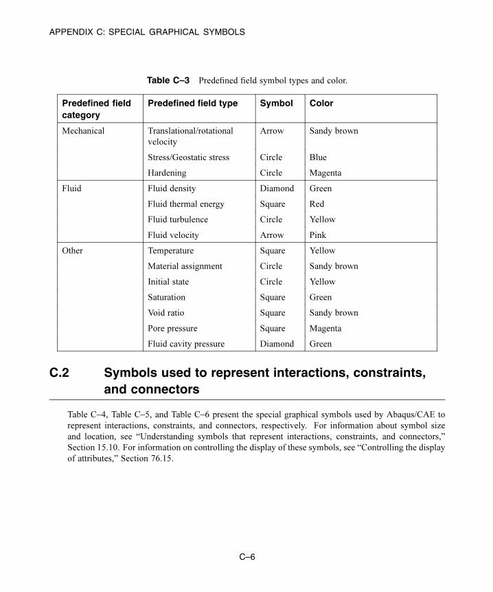
APPENDIX C: SPECIAL GRAPHICAL SYMBOLS
Table C–3 Predefined field symbol types and color.
Predefined fieldcategory
Predefined field type Symbol Color
Translational/rotational
velocity
Arrow Sandy brown
Stress/Geostatic stress Circle Blue
Mechanical
Hardening Circle Magenta
Fluid density Diamond Green
Fluid thermal energy Square Red
Fluid turbulence Circle Yellow
Fluid
Fluid velocity Arrow Pink
Temperature Square Yellow
Material assignment Circle Sandy brown
Initial state Circle Yellow
Saturation Square Green
Void ratio Square Sandy brown
Pore pressure Square Magenta
Other
Fluid cavity pressure Diamond Green
C.2 Symbols used to represent interactions, constraints,and connectors
Table C–4, Table C–5, and Table C–6 present the special graphical symbols used by Abaqus/CAE to
represent interactions, constraints, and connectors, respectively. For information about symbol size
and location, see “Understanding symbols that represent interactions, constraints, and connectors,”
Section 15.10. For information on controlling the display of these symbols, see “Controlling the display
of attributes,” Section 76.15.
C–6
Abaqus ID:
Printed on:

APPENDIX C: SPECIAL GRAPHICAL SYMBOLS
Table C–4 Interaction symbol types and color.
Interactions Symbol Color
Surface-to-surface contact Square Yellow
Self-contact Square Yellow
Filled circle
(cavity point)
GreenFluid cavity
Square
(cavity surface)
Green
Fluid exchange Circle (large) Yellow
Model change Square Yellow
Cyclic symmetry Square Yellow
Elastic foundation Square Yellow
Cavity radiation Square Yellow
Actuation/sensor Square Yellow
Standard-Explicit co-simulation Filled circle Magenta
Fluid-structure co-simulation Filled circle Green
Square Yellow
Sphere
(source point)
Yellow
Incident wave
Filled circle
(standoff point)
Yellow
Acoustic impedance Square Yellow
Surface film condition Square Yellow
Concentrated film condition Square Yellow
Surface radiation Square Yellow
Concentrated radiation to ambient Square Yellow
Arrow GreenPressure penetration (2D)
Square
(penetration
region)
Green
C–7
Abaqus ID:
Printed on:

APPENDIX C: SPECIAL GRAPHICAL SYMBOLS
Interactions Symbol Color
Filled triangle GreenPressure penetration (3D)
Square
(penetration
region)
Green
Table C–5 Constraint symbol types and color.
Constraints Symbol Color
Tie Circle Yellow
Rigid body Circle Yellow
Circle PinkCoupling
Lines Gray
Circle GreenMPC constraint
Lines Green
Shell-to-solid coupling Circle Yellow
Embedded region Circle Yellow
Equation Circle Yellow
Table C–6 Connector symbols and color.
Connector symbols Color
Square (first points of wires) Orange
Triangle (second points of wires) Yellow
Orientation triad, if not the global
coordinate system
Orange
Connection type label Orange
Connector section assignment tag Orange
C–8
Abaqus ID:
Printed on:
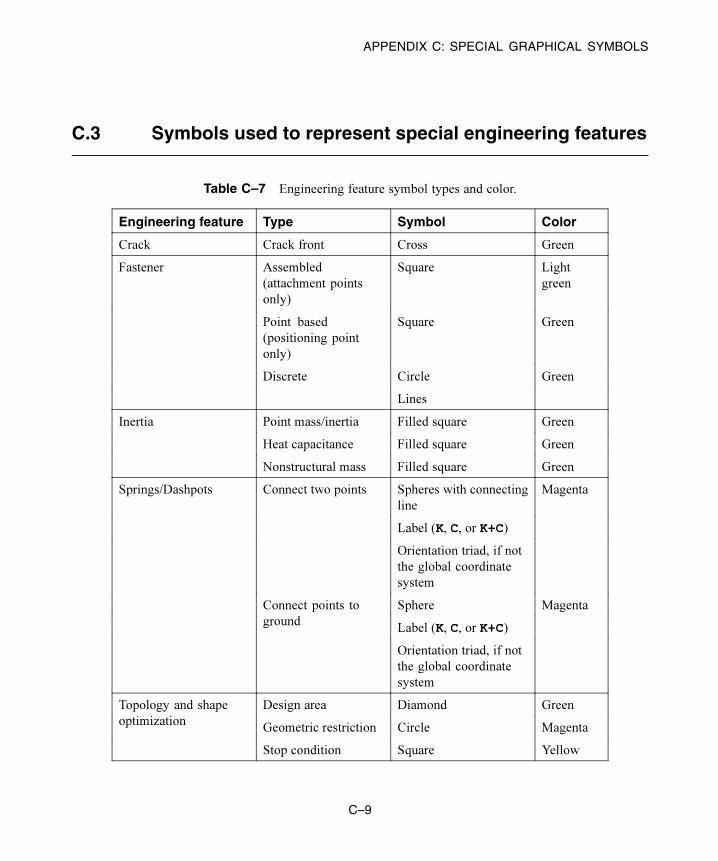
APPENDIX C: SPECIAL GRAPHICAL SYMBOLS
C.3 Symbols used to represent special engineering features
Table C–7 Engineering feature symbol types and color.
Engineering feature Type Symbol Color
Crack Crack front Cross Green
Assembled
(attachment points
only)
Square Light
green
Point based
(positioning point
only)
Square Green
Circle
Fastener
Discrete
Lines
Green
Point mass/inertia Filled square Green
Heat capacitance Filled square Green
Inertia
Nonstructural mass Filled square Green
Spheres with connecting
line
Label (K, C, or K+C)
Connect two points
Orientation triad, if not
the global coordinate
system
Magenta
Sphere
Label (K, C, or K+C)
Springs/Dashpots
Connect points to
ground
Orientation triad, if not
the global coordinate
system
Magenta
Design area Diamond Green
Geometric restriction Circle Magenta
Topology and shape
optimization
Stop condition Square Yellow
C–9
Abaqus ID:
Printed on:

APPENDIX C: SPECIAL GRAPHICAL SYMBOLS
C.4 Symbols used in the Visualization module
Table C–8 presents the special graphical symbols used by the Visualization module. These special
symbols appear when you produce an undeformed, deformed, contour, or symbol plot of a model
containing any of these components. For information on customizing the color and size of these
symbols, see “Coloring all geometry in the Visualization module,” Section 77.5 in the HTML version
of this guide, and “Controlling the display of model entities,” Section 55.10, respectively.
Table C–8 Special graphical symbols used by the Visualization module.
Two-node dashpot elements
The Visualization module displays two-node dashpot elements using the symbol
shown. You can choose to display a straight line in place of this symbol by
selecting Extra coarse refinement for all curved edges and faces in your model.
For more information, see “Refining curved edges and faces,” Section 55.12.3.
Two-node spring elements
The Visualization module displays two-node spring elements using the symbol
shown. You can customize the appearance of the curves in this symbol using the
options for refining curved edges and faces. The Visualization module displays
a two-node spring element as a straight line when you select Extra coarserefinement for all curved edges and faces in your model. For more information, see
“Refining curved edges and faces,” Section 55.12.3.
Reference nodes
The Visualization module displays the reference node for a rigid surface as a cross.
You cannot customize the shape of this symbol.
Tracer particles
The Visualization module displays a tracer particle as a cross within a square. You
cannot customize the shape of this symbol.
In addition to the special symbols the Visualization module uses to display the model components
listed above, you can choose to display symbols representing results, model entities (boundary
conditions, connectors, coordinate systems, and point elements), and nodal locations. For more
information, see the following sections:
• Chapter 45, “Plotting analysis results as symbols”
• “Controlling the display of model entities,” Section 55.10
• “Controlling the display of constraints in the Visualization module,” Section 55.11
• “Customizing node symbols,” Section 55.5.5, in the HTML version of this guide
C–10
Abaqus ID:
Printed on:
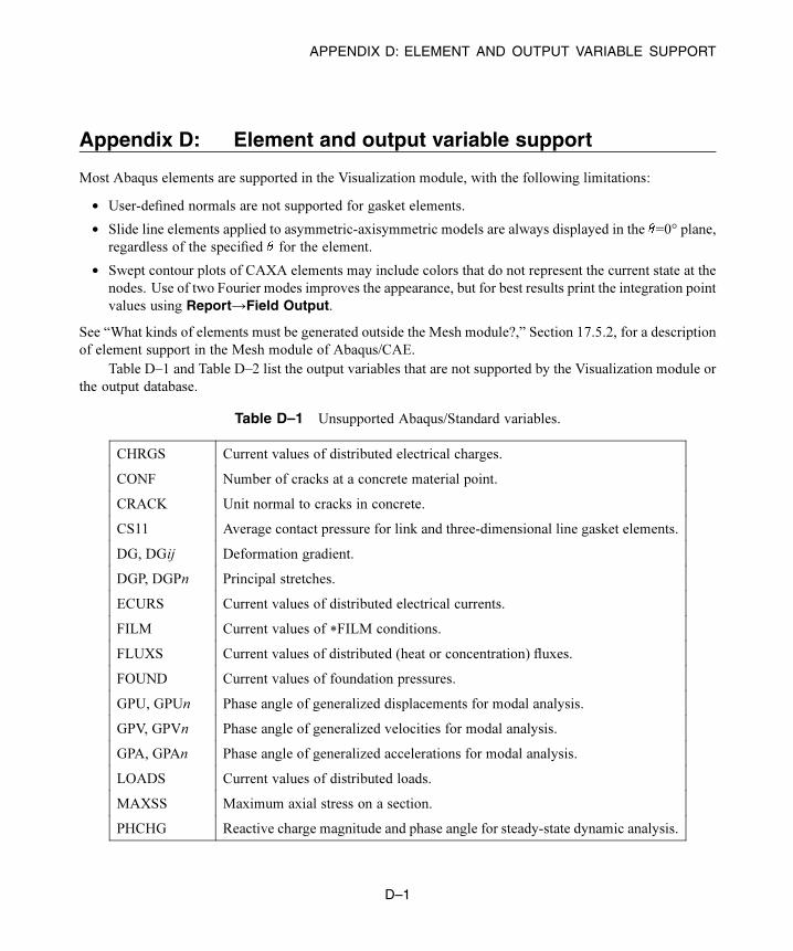
APPENDIX D: ELEMENT AND OUTPUT VARIABLE SUPPORT
Appendix D: Element and output variable support
Most Abaqus elements are supported in the Visualization module, with the following limitations:
• User-defined normals are not supported for gasket elements.
• Slide line elements applied to asymmetric-axisymmetric models are always displayed in the =0° plane,
regardless of the specified for the element.
• Swept contour plots of CAXA elements may include colors that do not represent the current state at the
nodes. Use of two Fourier modes improves the appearance, but for best results print the integration point
values using Report→Field Output.
See “What kinds of elements must be generated outside the Mesh module?,” Section 17.5.2, for a description
of element support in the Mesh module of Abaqus/CAE.
Table D–1 and Table D–2 list the output variables that are not supported by the Visualization module or
the output database.
Table D–1 Unsupported Abaqus/Standard variables.
CHRGS Current values of distributed electrical charges.
CONF Number of cracks at a concrete material point.
CRACK Unit normal to cracks in concrete.
CS11 Average contact pressure for link and three-dimensional line gasket elements.
DG, DGij Deformation gradient.
DGP, DGPn Principal stretches.
ECURS Current values of distributed electrical currents.
FILM Current values of *FILM conditions.
FLUXS Current values of distributed (heat or concentration) fluxes.
FOUND Current values of foundation pressures.
GPU, GPUn Phase angle of generalized displacements for modal analysis.
GPV, GPVn Phase angle of generalized velocities for modal analysis.
GPA, GPAn Phase angle of generalized accelerations for modal analysis.
LOADS Current values of distributed loads.
MAXSS Maximum axial stress on a section.
PHCHG Reactive charge magnitude and phase angle for steady-state dynamic analysis.
D–1
Abaqus ID:
Printed on:
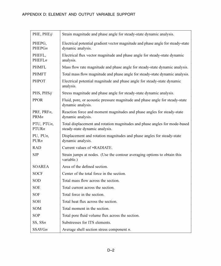
APPENDIX D: ELEMENT AND OUTPUT VARIABLE SUPPORT
PHE, PHEij Strain magnitude and phase angle for steady-state dynamic analysis.
PHEPG,
PHEPGn
Electrical potential gradient vector magnitude and phase angle for steady-state
dynamic analysis.
PHEFL,
PHEFLn
Electrical flux vector magnitude and phase angle for steady-state dynamic
analysis.
PHMFL Mass flow rate magnitude and phase angle for steady-state dynamic analysis.
PHMFT Total mass flow magnitude and phase angle for steady-state dynamic analysis.
PHPOT Electrical potential magnitude and phase angle for steady-state dynamic
analysis.
PHS, PHSij Stress magnitude and phase angle for steady-state dynamic analysis.
PPOR Fluid, pore, or acoustic pressure magnitude and phase angle for steady-state
dynamic analysis.
PRF, PRFn,
PRMn
Reaction force and moment magnitudes and phase angles for steady-state
dynamic analysis.
PTU, PTUn,
PTURn
Total displacement and rotation magnitudes and phase angles for mode-based
steady-state dynamic analysis.
PU, PUn,
PURn
Displacement and rotation magnitudes and phase angles for steady-state
dynamic analysis.
RAD Current values of *RADIATE.
SJP Strain jumps at nodes. (Use the contour averaging options to obtain this
variable.)
SOAREA Area of the defined section.
SOCF Center of the total force in the section.
SOD Total mass flow across the section.
SOE Total current across the section.
SOF Total force in the section.
SOH Total heat flux across the section.
SOM Total moment in the section.
SOP Total pore fluid volume flux across the section.
SS, SSn Substresses for ITS elements.
SSAVGn Average shell section stress component n.
D–2
Abaqus ID:
Printed on:

APPENDIX D: ELEMENT AND OUTPUT VARIABLE SUPPORT
TPFL Total pore fluid volume flux leaving the slave surface.
TPTL Time integrated TPFL.
Connector output for steady-state dynamic analysis.
Element output for user elements.
Table D–2 Unsupported Abaqus/Explicit variables.
BONDSTAT Spot weld bond status for nodes.
BONDLOAD Spot weld bond load for nodes.
CKE, CKEij Cracking strain in global directions.
CKEMAG Cracking strain magnitude.
CKLE, CKLEij Cracking strain in local crack directions.
CKLS, CKLSij Cracking stress in local crack directions.
CKSTAT Crack status of each crack.
CRACK Crack orientations.
EIHEDEN Internal heat energy density.
ESEDEN Total elastic strain energy density.
SSAVGn Average membrane or transverse shear stress component n.
D–3
Abaqus ID:
Printed on:

About SIMULIASIMULIA is the Dassault Systèmes brand that delivers a scalable portfolio of Realistic Simulation applications including Abaqus for unified Finite Element Analysis and multiphysics simulation; Isight for design exploration and optimization; and SLM for managing simulation data, processes, and intellectual property. SIMULIA’s realistic simulation applications are used as part of key business practices by world-leading manufacturing and research organizations to explore physical behavior, discover innovative solutions, and improve product performance.
About Dassault SystèmesDassault Systèmes, the 3DEXPERIENCE Company, provides business and people with virtual universes to imagine sustainable innovations. Its world-leading solutions transform the way products are designed, produced, and supported. Dassault Systèmes’ collaborative solutions foster social innovation, expanding possibilities for the virtual world to improve the real world. The group brings value to over 150,000 customers of all sizes, in all industries, in more than 80 countries. www.3ds.com
Abaqus, the 3DS logo, SIMULIA, CATIA, SolidWorks, DELMIA, ENOVIA, 3DVIA, Isight, and Unified FEA are trademarks or registered trademarks of Dassault Systèmes or its subsidiaries in the US and/or other countries. Other company, product, and service names may be trademarks or service marks of their respective owners.
© Dassault Systèmes, 2013