MKS 537E – Intro to CAE

MKS 537E – Intro to CAELECTURE #8

ASSEMBLY MODELING

DefinitionAssembly modeling is a technology and method used by computer-aided design and product visualization computer software systems to handle multiple files that represent components within a product.Assembly modeling allows the integration of design and manufacturing to production planning and control.

Assembly modeling

In an assembly model, components are brought together to define a larger, more complex product representation. Assembly modeling is a tool that allows and facilitates the collaboration among designers, analysis people, manufacturing people, and others, to insure their assembly works together.

Assembly modelers

Assembly modelers can be thought of as more advanced geometric modelers where the data structure is extended to allow representation and manipulation of hierarchical relationships and mating conditions that exist between components in an assembly.

Geometric and Assembly Modelers

The geometric modeler acts as a front end to the assembly modeler. Individual parts may be modeled using the geometric modeler. These models may be analyzed individually at this stage. After each part has been analyzed and optimized, the designer would use the assembly modeler to synthesize an assembly model and analyze the entire system.

Geometric modeler

Geometric model of

part 1

Geometric model of

part 2

Geometric model of

part n

Assembly modeler

Assembly model

To partanalysis

To assemblyanalysis

…

Assembly modeling

Assembly modeling used for

Ø Creation of orthographic assembly drawings.

Ø Creation of exploded assemblies.

Ø Facilitate packaging

Ø Perform interference and clearance checks

Definitions

Assembly : is a collection of pointers to piece parts and/or subassemblies. An assembly is a part file that contains component objects. Subassembly : is an assembly that is used as a component object within a higher level assembly. A subassembly contains component objects of its own. Component object : is the entity that contains and links the pointer from the assembly back to the master component part. A component object can also be a subassembly made up of its own component parts and/or component objects.

Types of Assembly Design Approach

Assemblies modelling in parametric CAD systems often use Bottom-up Design and Top-down Design strategies. There is also the method which is the combination of these two methods.

Bottom-up Assembly : is the most preferred approach for creating assembly models.

Top-down Assembly: Adopting the top-down design approach gives the user the distinctive advantage of using the geometry of one component to define the geometry of the other.

Bottom-up Assembly Approach

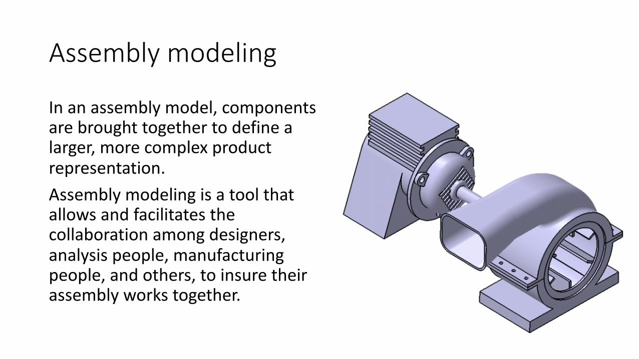
The individual parts a created independently, inserted into the assembly, and located and oriented (using the mating conditions) as required by the design. The bottom-up-approach is the preferred technique if the parts have already been created (off the shelf).

Top-down Assembly Approach

In this approach, the assembly file is created first with an assembly layout sketch. The parts are made in the assembly file or the concept drawing of the parts are inserted and finalized in the assembly file. The final geometry of the parts have not been defined before bringing them into the assembly file.This design approach is highly preferred, while working on a conceptual design or a tool design where the reference of previously created parts is required to develop a new part.

Mixed Assembly Approach

The vast majority of the designed assemblies consist two modelling strategies, bottom-up technique and top-down technique. Generally, most of the assemblies are defined of already existing components.New part is designed in the case when design assumptions are changed or when the project needs to have some design changes.

Assembly tree

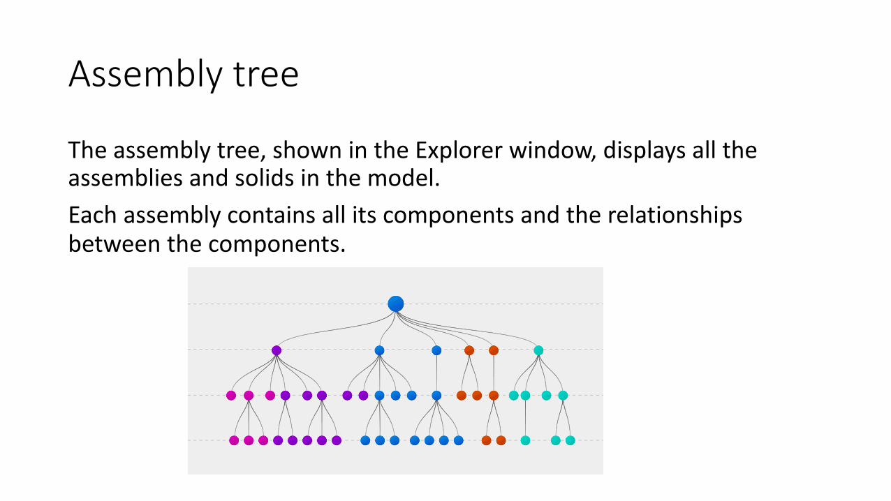
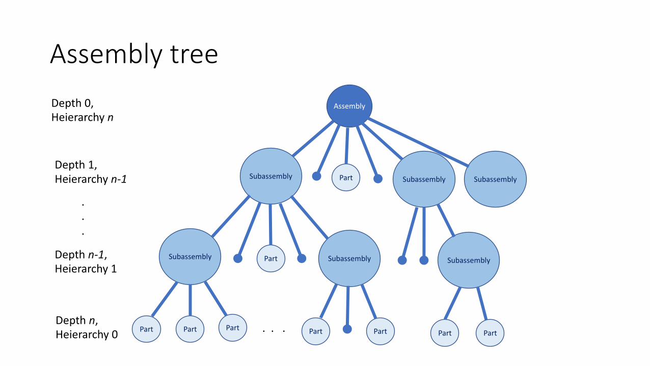
The assembly tree, shown in the Explorer window, displays all the assemblies and solids in the model.Each assembly contains all its components and the relationships between the components.

Assembly tree

Assembly

Subassembly Subassembly Subassembly

SubassemblySubassemblySubassembly

Part Part Part

Part

Part

Part Part Part Part

Depth 0, Heierarchy n

Depth 1, Heierarchy n-1

Depth n-1, Heierarchy 1

Depth n, Heierarchy 0

.

.

.

. . .

Assembly tree

Assembly tree explodes the overall assembly into subassemblies and parts, as well as illustrates where within the tree structure the various parts and subassemblies are connected or attached.Depth 0: we have the overall assembly.Depth 1: shows how the major subassemblies and parts fit into the overall assembly.

Assembly tree : bicycle

Assembly tree : pulley block

Structural layer

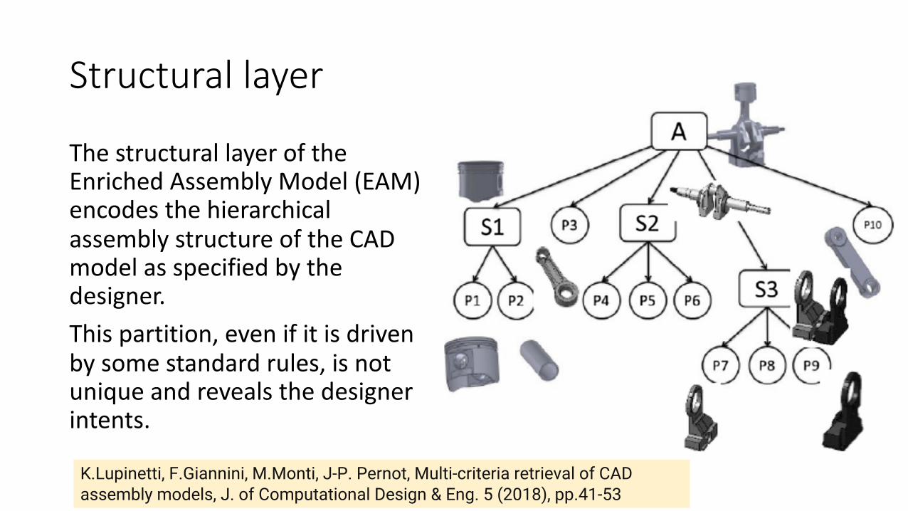
The structural layer of the Enriched Assembly Model (EAM) encodes the hierarchical assembly structure of the CAD model as specified by the designer. This partition, even if it is driven by some standard rules, is not unique and reveals the designer intents.

K.Lupinetti, F.Giannini, M.Monti, J-P. Pernot, Multi-criteria retrieval of CAD assembly models, J. of Computational Design & Eng. 5 (2018), pp.41-53

Possible relationships between parts

The possible relationships between two parts can be grouped into contact, interference, and clearance.Contact : Two parts are in contact, if they touch along low-level geometric entities such as surfaces, curves or points without any shared volume.

Interference : Two parts define an interference, if a common volume exists between them. Most of the time, this configuration does not exist between two real objects

Clearance : occurs when the distance between two surfaces of two parts is meaningful for the considered assembly, i.e. it is a small non-null distance between two parts in the assembly.

DOF values according to the surface type

where 𝑅 indicates a rotation, 𝑇 a translation, the subscripts 𝑢, 𝑣 and 𝑛the vector along which the rotations/translations are allowed.

Example

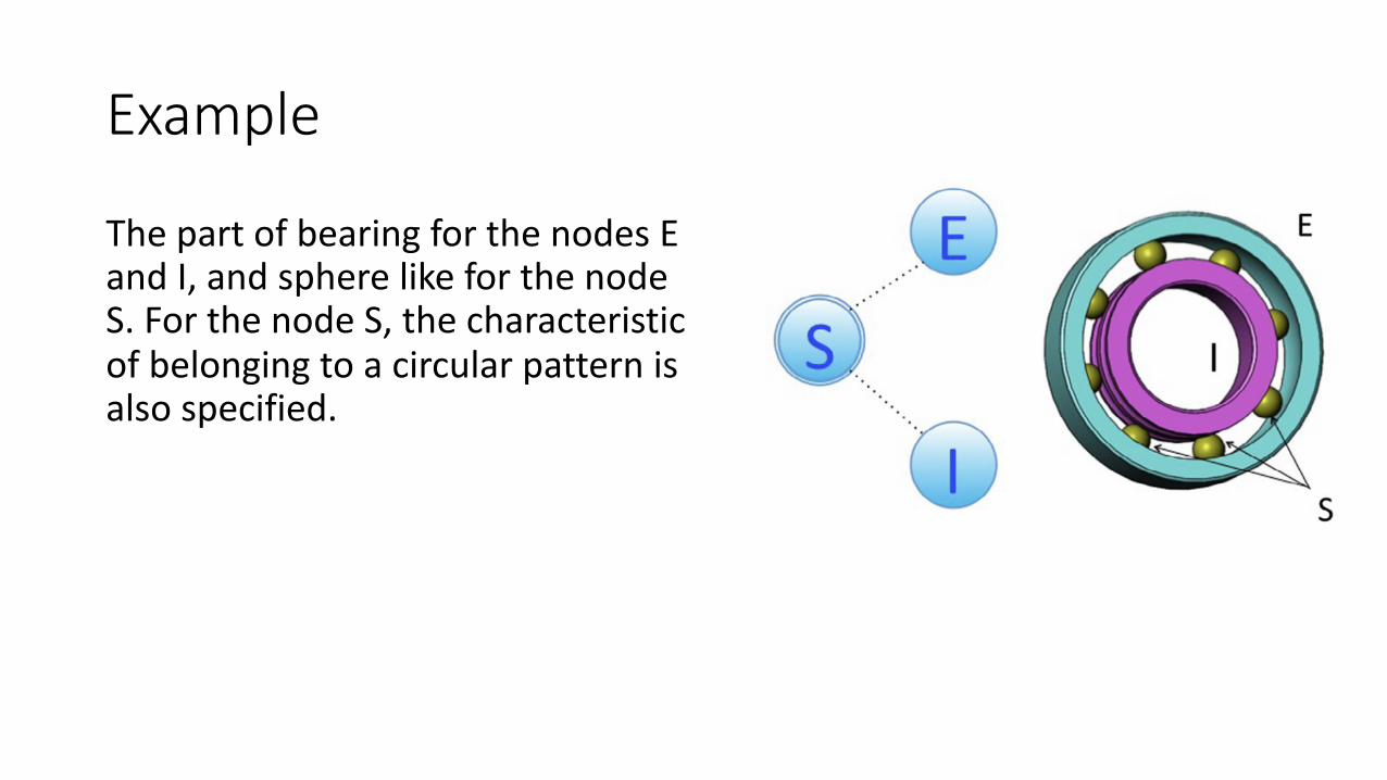
The simply-circled nodes are associated with parts, while the double-circled nodes (S and N) are associated with a set of parts belonging to circular rotational patterns. The straight arc connects two components, which are in face contact. The wavy arcs indicate a line contact and according to the description of the interface layer.

Example

The part of bearing for the nodes E and I, and sphere like for the node S. For the node S, the characteristic of belonging to a circular pattern is also specified.

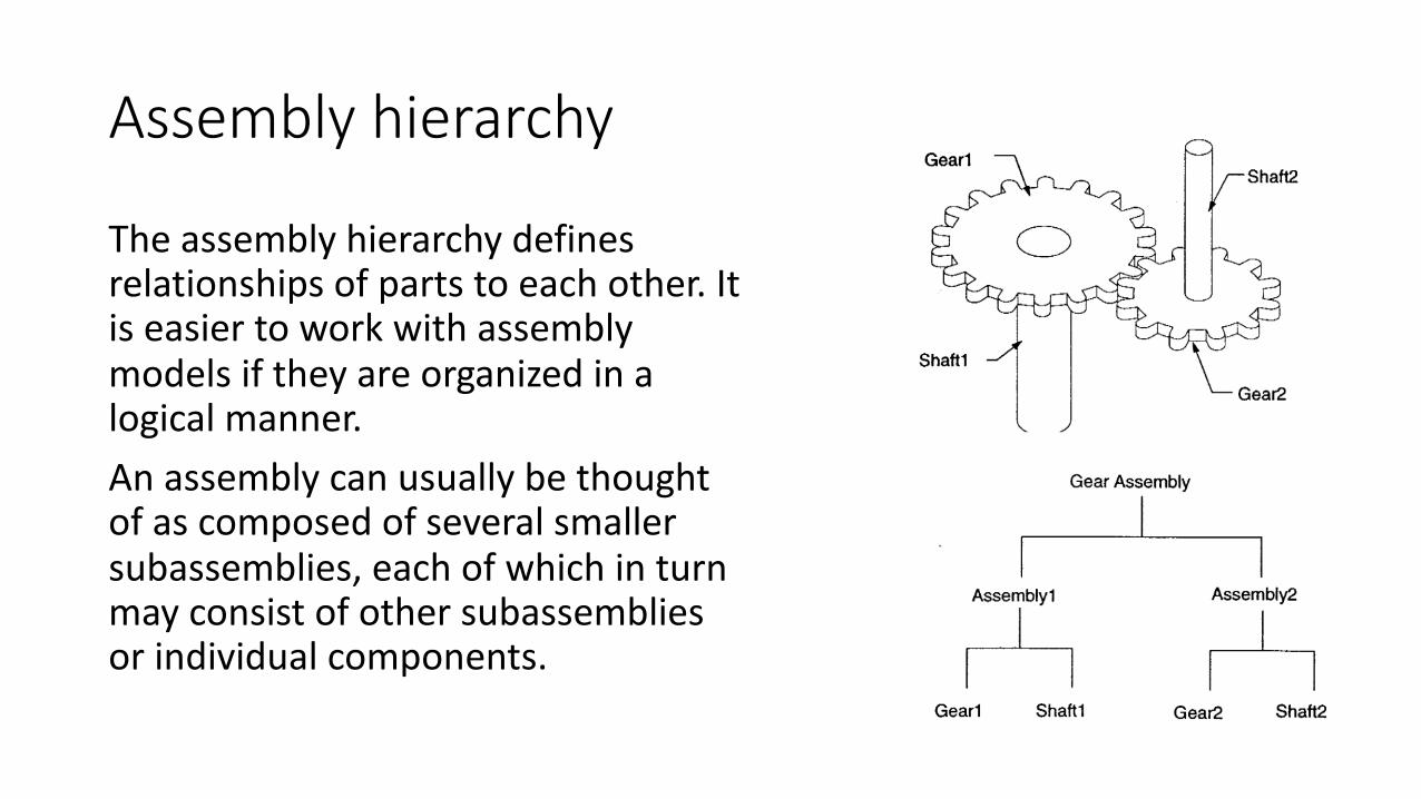
Assembly hierarchyAn assembly is a modeling entity that combines parts into a hierarchical product structure.An assembly hierarchy is a way to organize the collection of parts. A part contains geometry definition and other attributes such as color and mass properties.

Assembly hierarchy

The assembly hierarchy defines relationships of parts to each other. It is easier to work with assembly models if they are organized in a logical manner. An assembly can usually be thought of as composed of several smaller subassemblies, each of which in turn may consist of other subassemblies or individual components.

Example : electric clutch (Part hierarchy )

Frame Pinion

Electric motor

Rotor shaft Gear Load

shaft Rotor Field

Armature

Friction material Bolt

Part hierarchy

Depth 1

Depth 0

Depth 2

Depth 3

Hub Coil

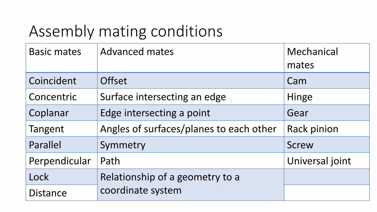
Assembly mating conditionsBasic mates Advanced mates Mechanical

matesCoincident Offset CamConcentric Surface intersecting an edge HingeCoplanar Edge intersecting a point GearTangent Angles of surfaces/planes to each other Rack pinionParallel Symmetry ScrewPerpendicular Path Universal jointLock Relationship of a geometry to a

coordinate systemDistance

Constraints of components

The constraints are the basic element of assemblies designing. They make geometrical correlations between components in the assembly. Each unrelated component in the assembly has six degrees of freedom.

The elements associated in the constraint can be: planar, cylindrical and conical faces, planes, axes, origins, edges of components, elements of sketches, vertices or sketch points.

Translation – movement along X, Y, and Z axis.Rotation – rotate about X, Y, and Z axis

Assembly constraints

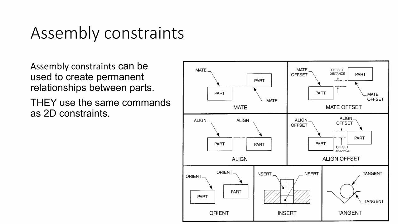
Assembly constraints can be used to create permanent relationships between parts.THEY use the same commands as 2D constraints.

Assembly constraints – mate & mate Offset

The Mate constraint type is used to place two surfaces coplanar. Any datum plane, part plane, or planar surface can be used. Selected surface faces are placed along a common plane but do not actually have to touch.


The Mate constraint type is used to place two surfaces coplanar. Any datum plane, part plane, or planar surface can be used. Selected surface faces are placed along a common plane but do not actually have to touch.

When a datum plane is selected, since a datum plane has no defined thickness, CAD software provides the option of selecting either the positive side or negative side of the datum plane.


The Mate Offset constraint type is similar to the Mate constraint type. Unlike the Mate type, the Mate Offset constraint places a user-specified offset distance between selected features.

Assembly constraints – align & align offset

The align constraint type is used to place two surfaces coplanar and facing in the same direction. Like the mate constraint, the surfaces do not have to touch. In addition, the align constraint type is used to align axes, edges, curves and points.

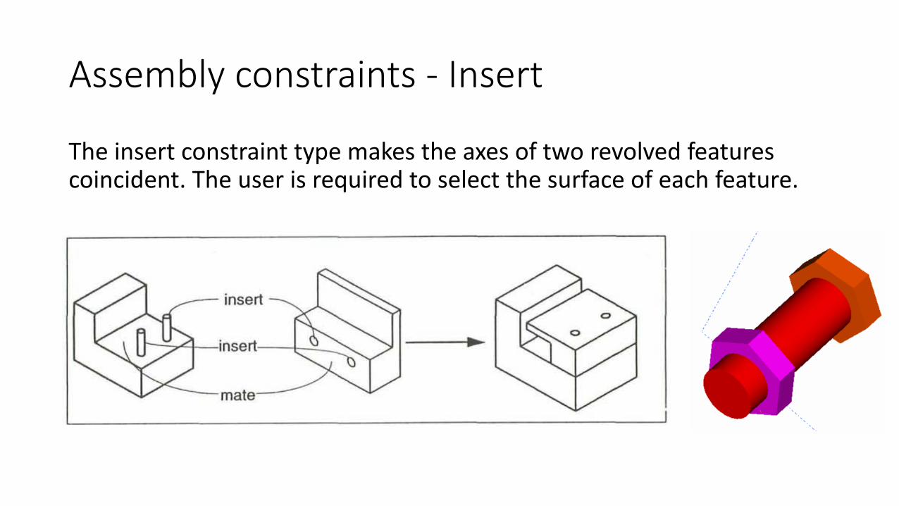
Assembly constraints - Insert

The insert constraint type makes the axes of two revolved features coincident. The user is required to select the surface of each feature.

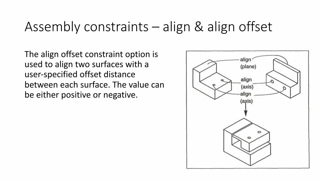
Assembly constraints – align & align offset

The align offset constraint option is used to align two surfaces with a user-specified offset distance between each surface. The value can be either positive or negative.

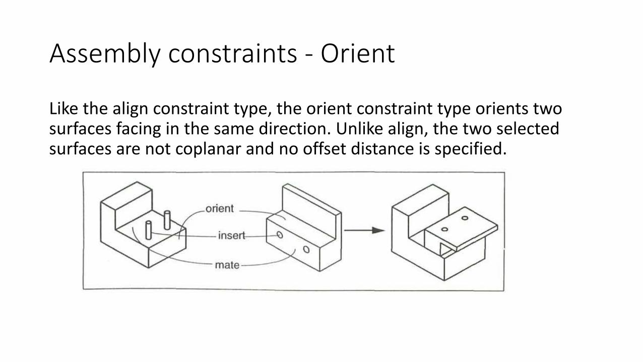
Assembly constraints - Orient

Like the align constraint type, the orient constraint type orients two surfaces facing in the same direction. Unlike align, the two selected surfaces are not coplanar and no offset distance is specified.

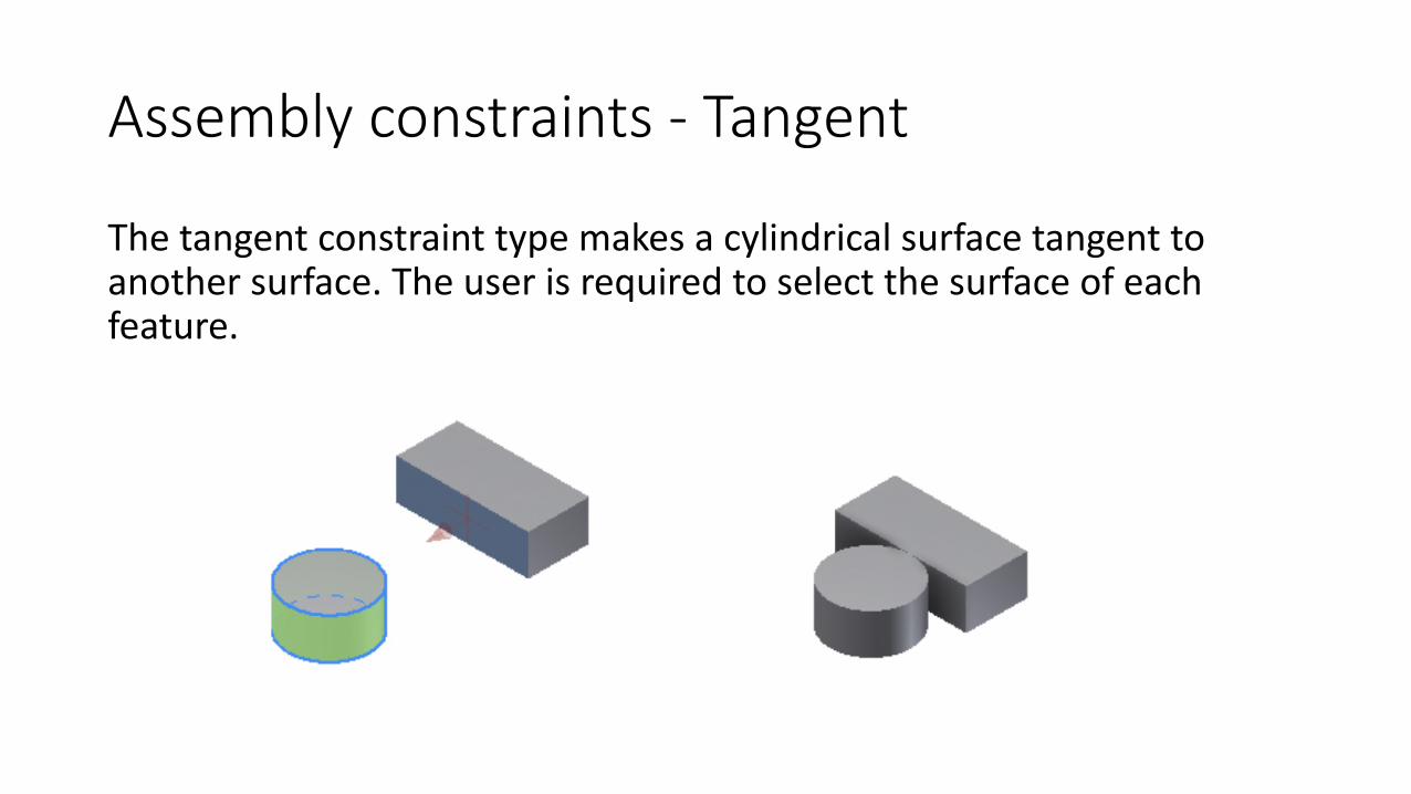
Assembly constraints - Tangent

The tangent constraint type makes a cylindrical surface tangent to another surface. The user is required to select the surface of each feature.

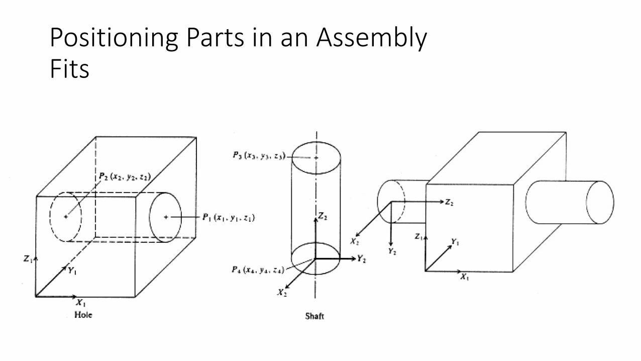
Positioning Parts in an Assembly

Parts can be positioned by translating and rotating them into the right locations. This requires careful measurement of relative locations, knowledge of coordinate systems, and entry of numerical values. If position or dimensions of one part change, this has to be redone.Mating feature types: Ø Against : two normal vectors are in against directions Ø Fits : between two cylinders: center lines are concentricØ Contact : requires two points correspondØ Coplanar : two normal vectors are parallel

Positioning Parts in an AssemblyAgainst between two planar faces

Positioning Parts in an AssemblyAgainst between a planar face and a cylindrical face

Positioning Parts in an AssemblyFits

Positioning Parts in an AssemblyContact

Positioning Parts in an AssemblyCoplanar

Basic Properties of Transforms

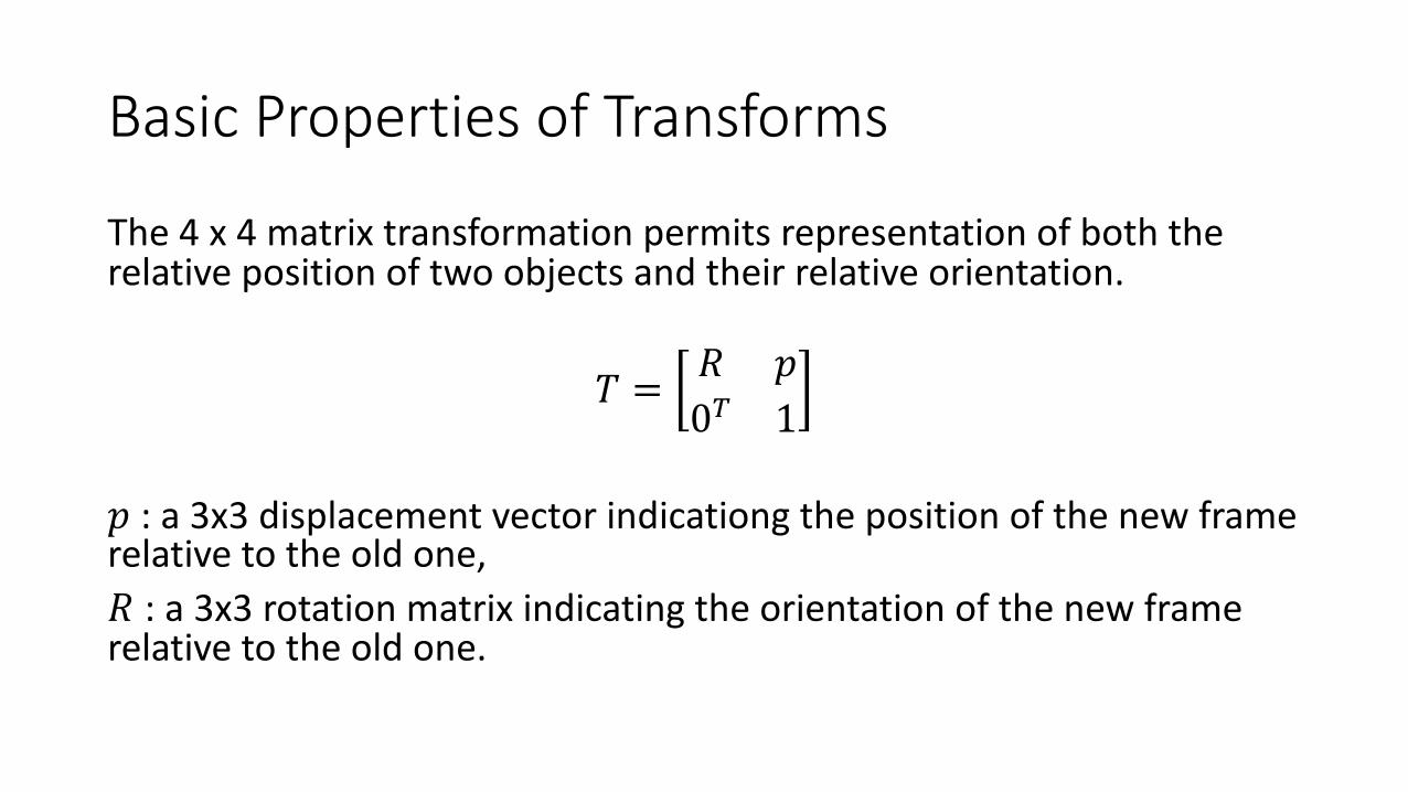
The 4 x 4 matrix transformation permits representation of both the relative position of two objects and their relative orientation.

𝑇 = 𝑅 𝑝0* 1

𝑝 : a 3x3 displacement vector indicationg the position of the new frame relative to the old one,𝑅 : a 3x3 rotation matrix indicating the orientation of the new frame relative to the old one.

Schematic Representation of a Transform

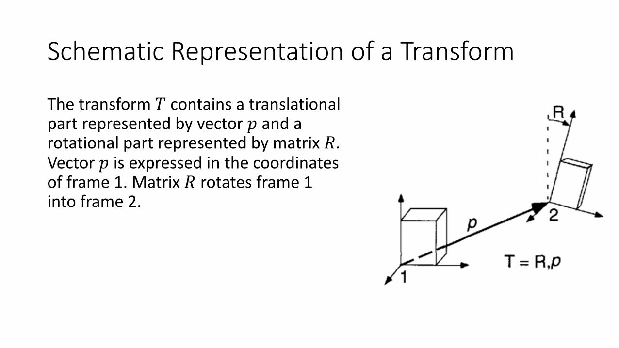
The transform 𝑇 contains a translational part represented by vector 𝑝 and a rotational part represented by matrix 𝑅. Vector 𝑝 is expressed in the coordinates of frame 1. Matrix 𝑅 rotates frame 1 into frame 2.


On a component-by-component basis, transform 𝑇 is

𝑇 =

𝑟-- 𝑟-. 𝑟-/ 𝑝-𝑟.- 𝑟.. 𝑟./ 𝑝.𝑟/- 𝑟/. 𝑟// 𝑝/0 0 0 1

𝑝 :is expressed in the coordinates of the original frame and 𝑟0,1 are the direction cosines of axis 𝑖 in frame 1 to axis 𝑗 in frame 2.


Transform 𝑇 can be used to calculate the coordinates of a point in the second coordinate frame in terms of the first coordinate frame. Then, in general, if 𝑞 is a vector in the second frame, its coordinates in the first frame are given by 𝑞′ :

𝑞6 = 𝑅 𝑝0* 1

𝑞1 = 𝑅𝑞 + 𝑝

This says that 𝑞′ is obtained by rotating 𝑞 by 𝑅 and then adding 𝑝. The coordinates of a point are given by

𝑝 =𝑥𝑦1


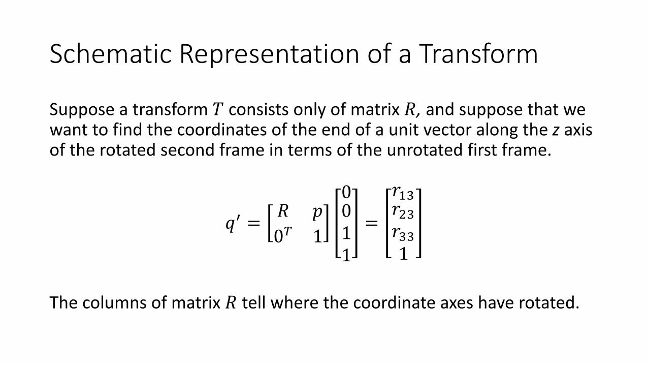
Suppose a transform 𝑇 consists only of matrix 𝑅, and suppose that we want to find the coordinates of the end of a unit vector along the z axis of the rotated second frame in terms of the unrotated first frame.

𝑞6 = 𝑅 𝑝0* 1

0011

=

𝑟-/𝑟./𝑟//1

The columns of matrix 𝑅 tell where the coordinate axes have rotated.

Matrix 𝑅

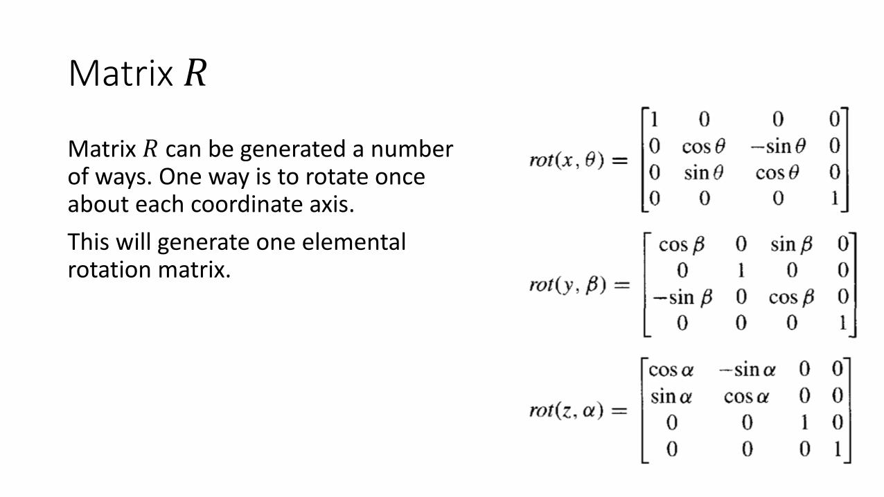
Matrix 𝑅 can be generated a number of ways. One way is to rotate once about each coordinate axis. This will generate one elemental rotation matrix.


A transform that simply repositions a frame without reorienting it is

𝑇:;<=> =

0 0 0 𝑝?0 0 0 𝑝@0 0 0 𝑝A0 0 0 1

= 𝑡𝑟𝑎𝑛𝑠(𝑝?, 𝑝@, 𝑝A)


A transform 𝑇 that comprises a translation 𝑝? along 𝑥 followed by a rotation of 90° about the new (translated) 𝑧 could then be written

𝑇 = 𝑡𝑟𝑎𝑛𝑠 𝑝?, 0,0 𝑟𝑜𝑡(𝑧, 90)

Sample : Transform that Repositions a Feature With- out Rotating ItIt shows how to position a feature whose axes align with part center coordinate axes. This feature is a locating pin. Accordingly, the Z axis of the pin's coordinate frame coincides with the pin's centerline.

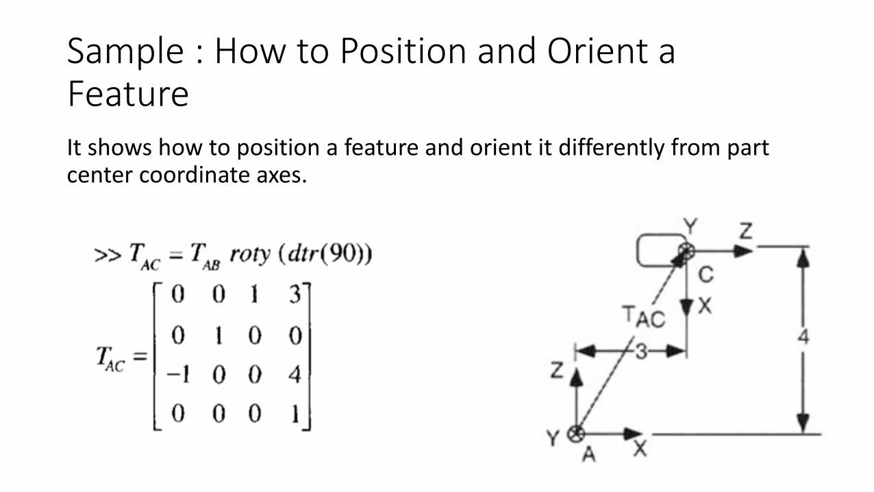
Sample : How to Position and Orient a Feature It shows how to position a feature and orient it differently from part center coordinate axes.

Sample : How to Build a Part and Place a Feature on It. The transform equation may be read to say: "To go from part A's coordinate center at A to the tip of the peg feature at frame D, go 3 units along frame A’s X-axis, 2 units along Y, and 4 units along Z, and then rotate 90° about frame A's relocated Y-axis."

Sample : Construction of a Second Part

This part has a hole feature on it as well as a point F that is one end of a KC. The transform equation may be read to say: "To go from the bottom of the hole to point F, go 6 units along frame E's X axis and 1 unit along its Z axis."

Sample : Assembling Two Parts

These two parts are "assembled" by placing frame D of the pin on the first part onto frame E of the hole on the second part.

Sample : Assembling Two Parts

An interface transform 𝑇JK is needed because the axes of these frames are not aligned in the same way. The equation for assembly transform 𝑇LM may be read to say: "To go from frame A to KC point F, follow transform 𝑇LJ TAD, then align frame D and frame E by rotating 180°about frame D's Z axis, then follow transform 𝑇KN.

Assembly representations

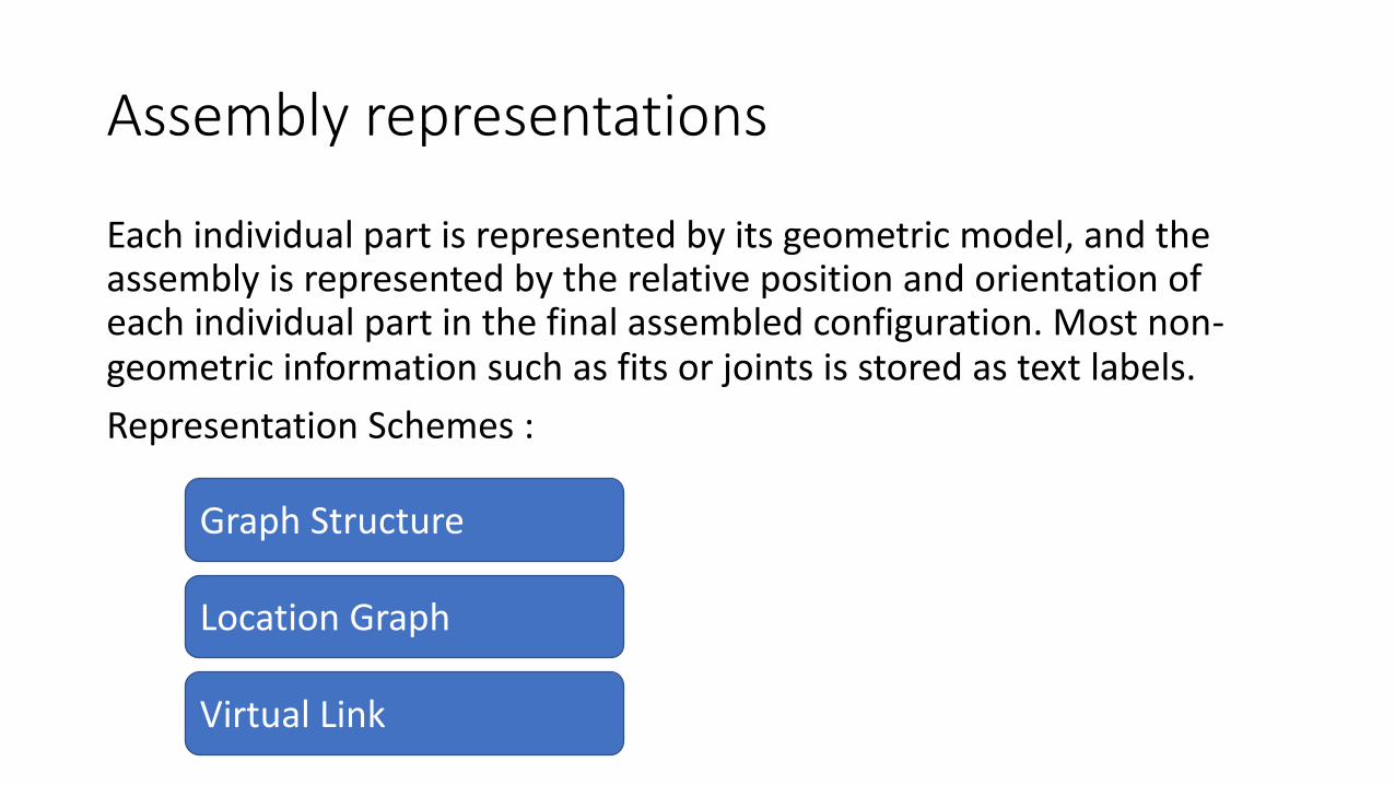
Each individual part is represented by its geometric model, and the assembly is represented by the relative position and orientation of each individual part in the final assembled configuration. Most non-geometric information such as fits or joints is stored as text labels. Representation Schemes :

Graph Structure

Virtual Link

Location Graph

Assembly representations

Assembly data base stores: ØThe geometric models of individual parts. ØThe spatial positions and orientations of the parts in the assembly. ØAttachment relationships between parts. ØThe inherent problem.

Graph Structure

An assembly graph is used to represent the final assembly of a genome (or metagenomes). In simple terms, the assembler builds this assembly graph based on reads and their overlap information.An assembly model is represented by a graph structure.

Graph Structure

Each node represents an individual parts / subassembly.Arc (branch) represents relationship among parts.Four kinds of relationship exist:P : ‘part-of’ relationship

Logical containment of one object in another.

A : ‘attachment’ relationshipC : ‘constraint’ relationship

physical constraints

SA : ‘sub-assembly’ relationship

Example : electric clutchShaft

Head

Head

Pinion

Gear

FrameRotor shaft

RotorElectric motor

Load shaft

Hub

Armature

Fied

Coil

Friction material

Cluth

A

A

A

AAA

A

A

SA

CA A

A

PP

Location Graph

Coordinate system is the means used to specify location of one part relative to other. A chain of locations can be defined such that each location is defined in terms of [T] another part’s coordinate system. A set of these chains results in a location graph. Part to part is related by the transformation matrix [T].

Example : electric clutchFrame

Armature

Hub

Rotor

Field

Shaft Friction material

Gear

Coil

Pinion

Electric motor

Load shaft

𝑇/

𝑇.

Bolt𝑇-

𝑇P

𝑇Q

𝑇R

𝑇S

𝑇T𝑇U

𝑇-V

𝑇--

𝑇-.

Virtual Link

Graph structure and location graph requires the user to input transformation matrix. Virtual link requires more basic information (mating conditions) used to calculate the transformation matrices.Virtual link is defined as the complete set of information required to describe the type of attachment and the mating conditions between the mating pair. Data structure of this scheme is based on the concept of virtual link.

Virtual Link

Virtual link defined as the complete set of information required to describe the type of attachment and the mating conditions between the mating pair.

Assembly graph structure based on virtual link

Sub-assembly

Sub-assembly

Sub-assembly

Assembly

Virtual link

Virtual link

Virtual link

Virtual link

Virtual link

Virtual link

Virtual link

Virtual link

Virtual link

Part Part Part Part Part

PartPartPartPartPartPart

Example : electric clutch (graph structure based virtual link)

Clutch

VL1 VL2 VL3 VL4 VL5 VL6 VL7 VL8 VL9 VL10 VL11 VL12 VL13

Hub Hub CoilLoad shaft Field Field

Friction material GearFrame Frame Frame FrameBolt Gear

Load shaftRotor Rotor Rotor

Rotorshaft

Rotorshaft

Pinion Electric motor

Electric motor

Pinion Rotor shaftArmature

Armaturedata

Hubdata

Load shaftdata

Coildata

Fielddata

Rotordata

Frictional material

data

Framedata

Geardata

Rotorshaftdata

Piniondata

Electricmotordata

Boltdata

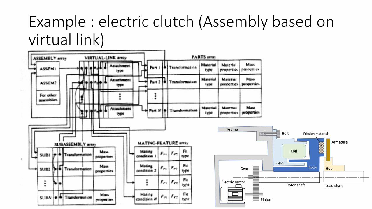
Example : electric clutch (Assembly based on virtual link)

Assembling sequence

It is always useful when studying the assembly of a part. In most assembly, there are multiple assembly sequence:Not unique In most assembly, there are more than one assembly sequence to generate assemblies from their respective parts. Production engineer must decide on most optimum sequence.

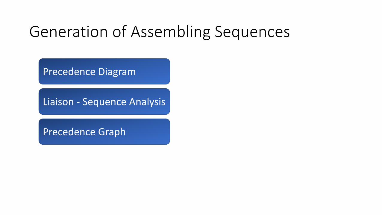
Generation of Assembling Sequences

Precedence Diagram

Liaison - Sequence Analysis

Precedence Graph

Precedence Diagram

Designed to show all the possible assembly sequences of a product. Each individual assembly operation is assigned a number.It show all the possible assembly sequences of a product. To develop the precedence diagram for a product, each individual assembly operation is assigned a number & is represented by circle with number inscribed. Circles are connected by arrows showing the precedence relations.

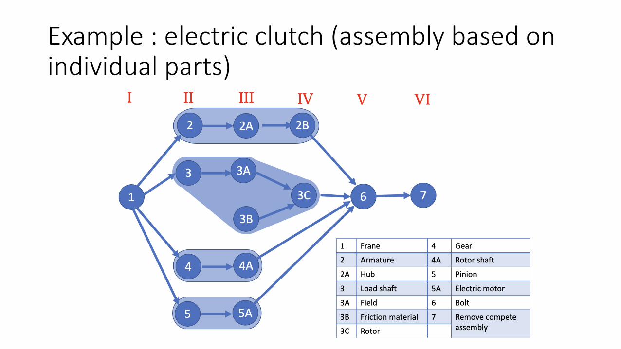
Example : electric clutch (assembly based on individual parts)

Example : electric clutch (assembly based on subassemblies)

Liaison - Sequence Analysis

Liaison - sequence analysis use precedence relations; In precedence diagram: engineer generates possible sequence directly.In liaison method: asks a series of questions to engineers about mating condition and precedence relationships.Generate sequences: manually or algorithmically.

Liaison diagram

A liaison diagram is a simple graph that uses nodes to represent parts and lines between nodes to represent liaisons or connections between parts. A simple graph that denotes parts as nodes and connections as arcs.Can be augmented with information about the connection.

Node: represent parts Line: represent any mating conditions between parts.

Each part has no more than one liaison(line) with any other part.

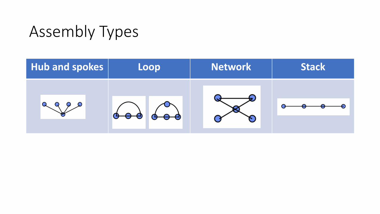
Assembly Types

Hub and spokes Loop Network Stack

Key characteristics

Key characteristics are the product, subassembly, part, and process features whose variation from nominal significantly impacts the final cost, performance [including the customer's perception of quality], or safety of a product. Special control should be applied to those KCs if the cost of variation justifies the cost of control.

Thornton, A. C., "A Mathematical Framework for the Key Characteristic Process," Research in Engineering Design, vol. 11, pp. 145-157, 1999.

Key Characteristics FlowdownThe example here is drawn from the auto industry and shows how KCs describing the customer's perception of a door can be flowed down through subassemblies, to features on parts, and finally to manufacturing processes.

Thornton, A. C., "A Mathematical Framework for the Key Characteristic Process," Research in Engineering Design, vol. 11, pp. 145-157, 1999.

Liaison diagram : bolt connection

A

B

C

C

B

A

Face/face

Threaded hole

Face/face&Peg/hole

Liaison diagram

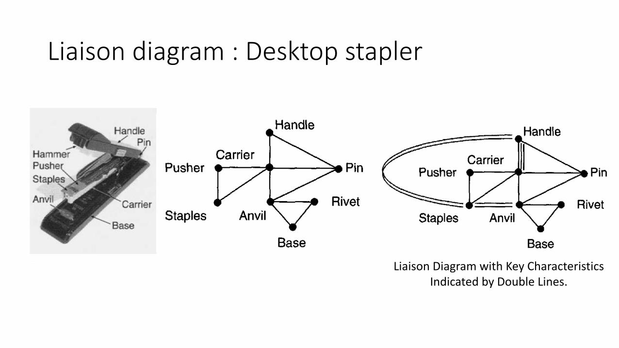
Liaison diagram : Desktop stapler

Liaison Diagram with Key Characteristics Indicated by Double Lines.

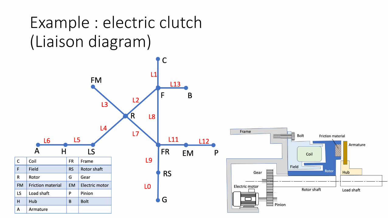
Example : electric clutch (Liaison diagram)

Precedence Graph

The representation mostly used in assembly planning is the precedence diagram or precedence graph, which contains all the valid sequences of an assembly. Even for the precedence diagrams, different representations have been proposed in the literature that include process times, levels of assembly, etc. . Assembly sequence is generated with the aid of interference checking.

1. Input mating conditions. 2. Generate mating graph.

Precedence Graph

The diagram of a precedence graph, theoretically, presents all the possible assembly sequences of tasks for assembling a product. Identify the part that is connected to the largest, of parts by virtual links, the base part.

Example : electric clutch (mating graph)

Example : electric clutch (Precedence Graph)

Intelligent Assembly Modeling & Simulation

The designer creates an assembly design using a commercial CAD package.The goal of IAMS is to avoid this expensive and time-consuming process by facilitating assemblabilitychecking in a virtual, simulated environment.

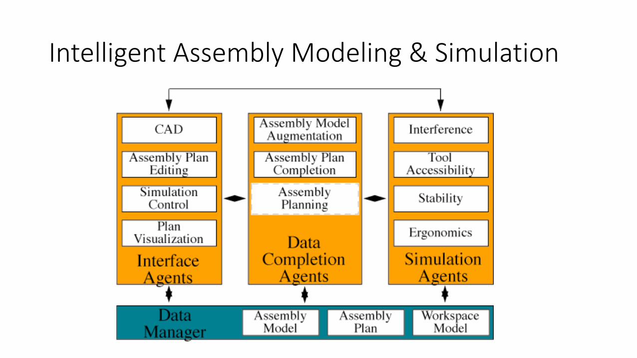
Intelligent Assembly Modeling & Simulation

Assembly planning

Assembly planning

Assembly can be done in two ways: Ølinear assembly; in which parts are assembled one after the other. Øparallel assembly; in which sub-assemblies (a set of parts grouped

together) are identified and joined simultaneously to obtain the final assembled product.

As the assembly process uses 50% of total production time and around 20–30% of manufacturing cost, efficient AP is required to reduce the time and cost of the manufacturing process.

Assembly related issues in different product development stages

Assembly planning and their classification

Assembly Sequence Planning

Assembly Sequence Planning (ASP) is one of important component in assembly planning. ASP refers to a task for which planners, on the basis of their particular heuristics in assembling all the components of a product, arrange a specific assembly sequence according to the product design description.

Assembly Sequence Planning

Assembly optimisation in the production planning stage deals with determination of optimum assembly sequence and determination of optimum location of each resource. Solving the Assembly Sequence Planning (ASP) problem is crucial because it will determine many assembly aspects including tool changes, fixture design and assembly freedom.

Assembly representation- directed graph

In assembly representation, directed graph is specifically known as precedence diagram since the graph represents the precedence relation of assembly.

Assembly representation- directed graph

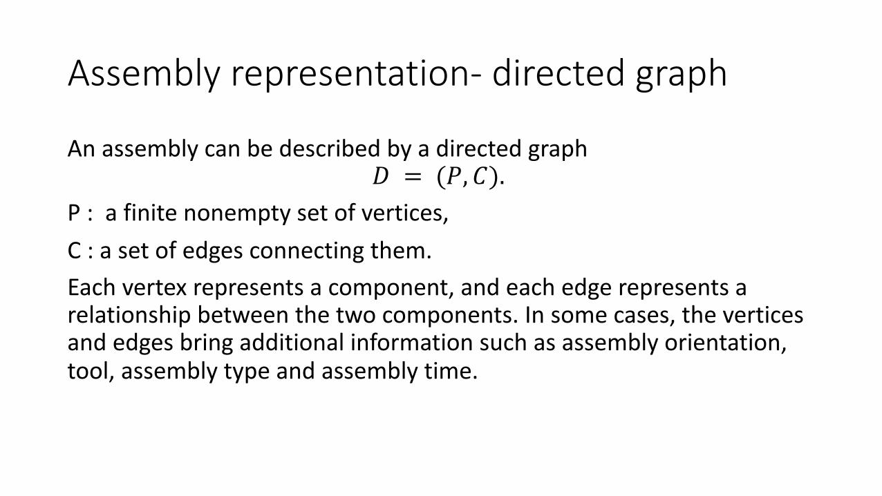
An assembly can be described by a directed graph 𝐷 = (𝑃, 𝐶).

P : a finite nonempty set of vertices, C : a set of edges connecting them. Each vertex represents a component, and each edge represents a relationship between the two components. In some cases, the vertices and edges bring additional information such as assembly orientation, tool, assembly type and assembly time.

Assembly precedence diagram with additional information

T1, T2, T3 and T4 : represent the assembly tools(+x, −x, +y, −y, +z, −z) : represents the assembly direction for a particular component

ASP Constraints

There are two types of constraints in assembly.• Absolute constraints : refer to constraints that, if violated, lead to

infeasible assembly sequence. • Optimisation constraints : are the constraints that lead to lower

quality of assembly sequences when violated.

Absolute constraints

Liaison data: This gives the information about contact details of the parts in the product. Stability data: This gives the information about the stability of the parts in the product during assembly.Geometric feasibility data: This gives the information in which direction one part assemble with the other without collision.Mechanical feasibility data: This gives the information whether any two parts can be assembled in the presence of the other part.

Absolute constraints

The absolute constraints that are usually considered include• Precedence constraints : shows the relation of predecessor and

successor components for assembly process. • Geometrical constraints : is about assembling the components

without any collision.

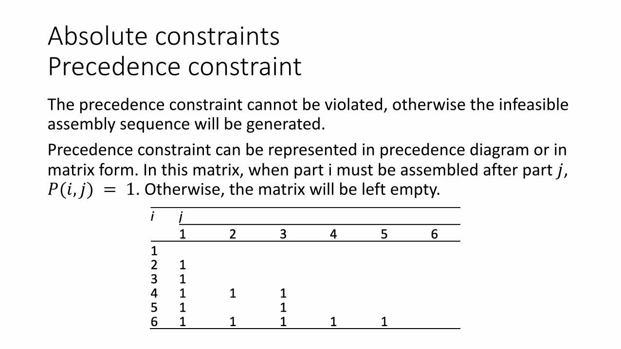
Absolute constraintsPrecedence constraintThe precedence constraint cannot be violated, otherwise the infeasible assembly sequence will be generated.Precedence constraint can be represented in precedence diagram or in matrix form. In this matrix, when part i must be assembled after part 𝑗, 𝑃(𝑖, 𝑗) = 1. Otherwise, the matrix will be left empty.

Absolute constraintsGeometrical constraintsAll valid assembly sequences must meet geometric constraints for a given structure.For each pair of components (𝑃𝑖, 𝑃𝑗), the matrix records directions in which 𝑃𝑖 can be assembled without colliding with 𝑃𝑗. Then, a set of valid assembly directions, for each (𝑃𝑖, 𝑃𝑗) is defined, as the moving wedge of 𝑃𝑖 with respect to 𝑃𝑗 , denoted by 𝑀𝑊 𝑃𝑖, 𝑃𝑗 .They compute moving wedges for all pairs of components and store all moving wedges in the MW matrix.

Assembly Line Balancing

Assembly Line Balancing is the decision problem of optimally partitioning the assembly work among the stations with respect to some objective.ALB was first mathematically formulated by Salveson in 1955.ALB problem into two categories:ØSimple Assembly Line Balancing Problem (SALBP) ØGeneralised Assembly Line Balancing Problem (GALBP)

Assembly Line Balancing

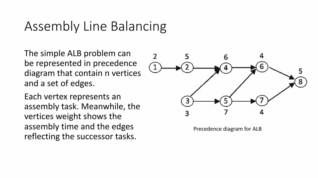
The simple ALB problem can be represented in precedence diagram that contain n vertices and a set of edges. Each vertex represents an assembly task. Meanwhile, the vertices weight shows the assembly time and the edges reflecting the successor tasks.

Precedence diagram for ALB

Abrrivations

IAMS Intelligent Assembly Modeling & SimulationASP Assembly Sequence PlanningALB Assembly Line BalancingEAM Enriched Assembly ModelPLM Product Lifecycle Management HAG Hierarchical assembly graphKC key characteristics

MKS 537E – Intro to CAE

Documents

Transcript of MKS 537E – Intro to CAE