MANAGERIAL ECONOMICS

EC 652 Your instructor:

Dmitri Nizovtsev (D-MEET-tree Knee-SOFT-safe)

Office: 310N in Henderson

Phone: 670-1599

E-mail: dmitri.nizovtsev@washburn.edu

Office Hours:

See the syllabus

Web support: Desire2Learn EC652

Econ 652 1

• Textbook: Baye, Managerial Economics and Business Strategy, 7th ed.

• Grading: HW assignments: 25% of the overall score. Group project: 15% of the overall score. Two “midterm” exams: 17.5% each, for a total of 35%. Final exam: 25% of the overall score.

Econ 652 2

Cornerstones of (managerial) economics

1. Opportunity cost The Opportunity cost (of a product, action etc.) is the value of the second best alternative that has to be forgone in order to obtain it.

The total economic cost consists of explicit (out of pocket, monetary) and implicit (measured in lost opportunities) costs. A good manager has to recognize both.

Econ 652 3 2. Cost/benefit comparison.

Unhappy Very happy

Cons (–) Pros (+)

Econ 652 4

“Net benefit” is the difference between benefits and costs. Example: PROFIT

(1+2): The concept of economic profit

Econ 652 5

Example: Gomez runs a small pottery firm. Total annual revenue from his pottery sales is $72,000. Gomez hires one helper at $12,000 per year, pays annual rent of $5000 for his shop, and spends $20,000 per year on materials. He also has $40,000 of his own funds invested in equipment (pottery wheels, kilns, and so forth). That $40,000 could earn him $4000 per year if alternatively invested. Gomez has been offered $15,000 per year to work as a potter for a competitor. How large are Gomez’ accounting profit and economic profit? Econ 652 6 3. Marginal analysis Instead of looking at the overall costs and benefits, one can look at how costs and benefits change as a result of the action that is being evaluated. Benefits increase more than costs … Econ 652 7

Demand, Supply, and Market Equilibrium We often hear that “prices are governed by forces of supply and demand”. That is to a large extent true. (And not only prices, but quantities, too!) It is important for a manager to understand how those forces work, be able to predict their direction, and in some cases maybe even affect them. Ideally, it should work the following way: • Step 1: Look at the “Big Picture” (S-D analysis) • Step 2: What does that mean for your company? • Step 3: Worry about details (create an action plan) First, let us see if we agree on what supply and demand are. Econ 652 8 Demand is … What is the shape of a demand relationship? “Law of Demand”: Why so? Econ 652 9 Supply is The shape? Why? Econ 652 10

An illustration : A farmer is deciding how to divide his land between wheat and corn. Suppose every piece of his land is identical with respect to growing wheat (produces 50W), but when it comes to growing corn, some pieces are better than the other (the yields range from 20C to 50C). He is currently growing only wheat but want to start producing some corn. Which piece of land should he plant corn on?

(Recall cost-benefit analysis)

Since by taking each piece of land out of wheat production he has to give up 50 bushels of wheat (same opp.cost), he wants to maximize his benefit (make sure that in exchange he gets as much corn as possible). Econ 652 11 Solution: First, use…..

He loses He gains ____ bushels of wheat ____ bushels of corn Each bushel of corn you acquire costs him …….. Econ 652 12 What if he wants more than 50 bushels of corn? How should he allocate his land in this case? The opp. cost of each bushel of corn is now …and so on. This reflects a general “Principle of increasing (opportunity) cost”: As we produce more of some good, the (opportunity) cost of the next unit of that good increases. Econ 652 13

Market equilibrium When supply and demand curves are put on the same graph, they usually intersect. P

PE Q QE The point where the two curves intersect is called the market equilibrium. It is characterized by a price and a quantity. Econ 652 14 In “perfect” markets,

1. there are many buyers and sellers; 2. goods offered by different sellers are identical; 3. sellers can freely enter and exit the market; 4. everyone has perfect information about all the transactions (prices,

quantity, etc.) Prices charged by different sellers in such markets are usually closely clustered around the equilibrium price. It can be shown by using common sense that it is in no one’s interest to try to ask or offer a price different from the equilibrium price. All the changes in market prices come only from changes in demand or supply. Econ 652 15

Equilibrium price (a.k.a. “market-clearing price”)

Supply and Demand Shifts

and Changes in Market Equilibrium Consider the U.S. market for chicken meat. Econ 652 16 Econ 652 17

PCH

PCH PCH

PCH

QCH QCH

QCH QCH

A new feeding pattern helps birds gain weight 50% than before, at no extra cost

The price of pork decreases

It is getting harder to find workers willing to work in the chicken meat industry

Chicken meat is scientifically proven to have substantial health benefits

Factors that can shift demand (also called “determinants”, or “shifters”):

• P of a “substitute good” increases – Demand for our good

• P of a “complementary good” increases – Demand for our good

Econ 652 18

• Consumer income increases – Demand for our good….

if it is a “normal good”. if it is an “inferior good”.

• Price of a good is expected to go up in the near future – Demand for the good today …

There are many other, more trivial factors (# of consumers, information about the good, prior experience with the good, consumer demographics, time of the year, etc.) Econ 652 19

Factors that can shift supply:

• Increase in costs (higher input prices, tax on producers, etc.)

Supply ___________________

• Decrease in costs (cheaper inputs, subsidy to producers, technol. progress, etc.)

Supply ___________________

• Increase in the number of firms in the market Econ 652 20

• Prices of other goods (Y) that can be produced instead of the good of interest (X), “substitutes in production”

Logic: Price of Y goes up Resources shift … … Or: Price of Y goes up The opp.cost of X….

Econ 652 21

Important things to keep in mind in S-and-D analysis: When both curves (supply AND demand) shift, and we are asked about the direction of change in price and quantity, we will be able to predict only one of the two. The other one will be indeterminate. A common mistake is shifting too many curves too many times (in most cases, one event causes only one shift). A shift in a curve should occur only if we are dealing with one of the “shifters” listed above. A change in the price of the good in question doesn’t cause a shift! Buyers and sellers do react to the price of the good but that reaction is illustrated by movement along a curve. Econ 652 22

Why care about supply-and-demand analysis? Example (Ch.2 opener): •Scenario: You manage a small firm that manufactures PCs. •Event: The WSJ reports that three major chip manufacturers accounting for 30% of the total market share suspend their operations for one week. • Step 1: Look at the “Big Picture” (S-D analysis)

• Step 2: What does that mean for your company?

• Step 3: Worry about details (create an action plan)

Econ 652 23 The Big Picture is: PC prices are likely to fall, and more computers will b e sold. Econ 652 24 Use this to create an action plan

• contracts/suppliers? (a future contract – is this an iss ue?) • inventories? (try to sell n ow) • human resources? ( may need more staff to increase Q) • marketing? (not in SD model, differentiate?) • etc. (new or rep lacement users?)

Econ 652 25

Often, quantitative analysis of market environment allows to present supply and demand relationships in the form of equations, such as

QD,X = F(Px , Py , M, HD, …), where

QD,X = quantity demanded of good X; Px = price of good X; Py = price of a related good Y(can be substitute or complement); M = consumers’ income; HD = any other variables affecting demand. (Where those equations may come from will be discussed next week.) Econ 652 26 Example (from p.42 in the text): An economic consultant for X Corp. recently provided the firm’s marketing manager with this estimate of the demand function for the firm’s product (AX represents spending on advertising good X):

QD,X = 12,000 – 3 PX + 4 PY – M + 2 AX,

Are goods X and Y substitutes or complements? (look at the sign on PY – what would an increase in PY do to QD,X?) Is good X a normal or an inferior good? (look at the sign on income, M) – what would an increase in M do to QD,X?) Econ 652 27 Often, price is the most flexible “control variable” firms have. There it can be useful to first account for all the “external” variables before taking a closer look at price. Example, continued: Currently, good Y sells for $15 per unit, the company spends $2000 on advertising, and the average consumer income is $10,000. Simplify the demand equation. Next question is, how much of good X will consumers purchase if the price is set at $900? At $1,500? Econ 652 28

Normally, supply and demand equations are given in the form similar to the one above, where quantity is on the left-hand side and is expressed as a function of price. On some occasions, we will need a different form of a demand equation, known as “inverse demand”. There, price is on the left hand side of the equation. Let’s make sure we know how to make this transformation. For example, the above demand equation, QD = 6,060 – 3 P, can be rewritten as Econ 652 29

Week 2

Last week we talked, among other things, about supply and demand equations and said that having those available may improve the accuracy of our predictions. How can we obtain those equations? What information do we need for that? What techniques do we use to translate raw data into an equation? How much faith can we have in the equations we obtain? This is our next topic. Econ 652 30

Regression analysis The simplest case is the relationship between two variables, which may help answer such business-type questions as

• How does the quantity demanded of paper towels depend on the population of a town?

• How does the volume of ice cream sales depend on the outside

temperature?

• How does the number of TVs sold at an outlet depend on the TV price? Econ 652 31

Univariate regression Step 1. Collect data.

Observation # Quantity Price 1 18 475 2 59 400 3 43 450 4 25 550 5 27 575 6 72 375 7 66 375 8 49 450 9 70 400

10 21 500 Econ 652 32

Explaining variations in one variable with ONE other variable

Step 2. Assume a functional form of the relationship between the variables of interest. Can be very complex, QD = A/P – B⋅P + CP – D, Or quite simple, QD = A – B⋅P The more complex the formula is, the more accurately it would fit the data, but the estimation procedure would be more labor intensive. The fit produced by simpler formulas is quite crude but they are much easier to estimate. Practitioners usually use the simplest form that is consistent with theory and/or common sense - the linear one. Econ 652 33 Step 3. Find the best values for coefficients. How? Each observation is a point in the price-quantity space. Each pair of numbers, A and B, when plugged into the equation above, uniquely defines a line in the price-quantity space. It is unlikely that all the points (observations) will be on the same line. The best line will therefore be the one that minimizes the sum of squared deviations between the line and the actual data points. Econ 652 34 Econ 652 35

This procedure can be performed using a MS Excel “add-on”. Data tab Data Analysis Regression, then enter the range of cells that contain data for each variable.

- Y is the “dependent variable” (in our case, QD).

- X is the “independent variable”, also called the explanatory variable (in our case, P).

- Check the “Labels” box if you include column headers.

- Click on the cell where you want the output printout to start, then click ‘OK’. (If ‘Data Analysis’ is not showing, you need to add it in: File OptionsAdd-Ins”Manage Excel Add-Ins” at the bottom check ‘Analysis ToolPak’ click ‘OK’) Econ 652 36 Once you run the regression, you should see something like this: SUMMARY OUTPUT

Regression Statistics Multiple R 0.8682997 R Square 0.7539444 Adjusted R Square 0.7231875 Standard Error 11.147108 Observations 10

ANOVA

df SS MS F Significance F Regression 1 3045.9357 3045.935 24.512989 0.00111939 Residual 8 994.06424 124.2580 Total 9 4040

Coefficients Standard Error t Stat P-value Lower 95% Upper 95% Intercept 163.70670 24.23376 6.755314 0.000144 107.82350 219.58990 Price -0.260894 0.052695 -4.951059 0.001119 -0.382408 -0.139380

Econ 652 37

Interpreting the output: 1. First, how well did the regression perform overall? 1.1. R2 shows the portion of the variation in the dependent variable, QD, that is explained by the independent one, P. (In the case when the independent variable you used is the only one that matters, it would be 1.) R2 depends on the quality of the data. Therefore low R2 is rarely the reason for scrapping the entire regression. 1.2. The F-statistic is a more formal measure of the overall “goodness of fit”. The greater F is, the lower is the probability that the estimated regression model fits the data purely by accident. That probability is given under “Significance F”. (Make sure it is reasonably low – if it isn’t, then there’s a reason to worry.) Econ 652 38 The ‘Coefficients’ column contains the values of A and B that provide the best fit between the straight demand line and the data points. 2. Before we state the preferred demand equation, our next set of questions needs to address the statistical significance of coefficient estimates (or, in other words, we need to check whether the coefficient estimates are reliable).

There are several ways to do this:

2.1. The t-statistics: The larger the absolute value of the t-statistic, the higher are the chances that the coefficient is different from zero. Caveat: interpreting t-stats requires access to statistical tables.

Econ 652 39

2.2. The P-values answer the question directly: what are the chances that the coefficient really has the sign shown in the “Coefficients” column?

In our case, the P-value indicates there is only a 0.11% probability that the coefficient on price is non-distinguishable from zero, or in other words that price is irrelevant for consumer decisions. In other words, we are 100 – 0.11 = 99.89% confident that price negatively affects Q demanded (higher P lower Qd) This, however, is very different from saying “There is a 99.89% probability that the coefficient on price is exactly –0.26”, which is a FALSE statement. Econ 652 40

(Statistical significance, continued…) 2.3. The “Lower 95%” and “Upper 95%” columns in the printout give the upper and lower bounds within which the true value of each coefficient falls with a certain probability (95%, in this case).

This range is also known as the “95% confidence interval”. In our case, it is … Econ 652 41 Visualizing the relationship between the confidence interval and the P-values: 0 100 200 300 400 500 600 700 –100 0 100 200 300 400 Econ 652 42

Finally, once (if!) we are pleased with the statistical significance, we can proceed to stating that, based on the data provided, the best estimate of the demand for TVs is Having obtained such an equation enables us to comment on the “economic significance” of the coefficients: For every ….. increase in price, the number of units sold …………………. by …………..

• Try to avoid making any causality inferences!

• Note the distinction between the economic significance and the statistical significance!

First, evaluate the statistical significance (do we have a reason to believe the variable matters?); THEN comment on the economic significance (how much does it matter?)

Econ 652 43 In summary, we want: The sign of coefficients to make economic sense;

R2 to be

The F-statistic to be

The t-statistic to be

‘Significance F’ and P-values to be

The confidence interval to be

Econ 652 44

Univariate regression is rarely used by real-world practitioners. To see why, consider the following data on soft drink sales: P

Q While a univariate regression would produce ONE estimated demand curve going through the middle of this cloud of points… Econ 652 45 … the true story may in fact be different: P

Q Obviously, some factors other than price, that were omitted from the univariate regression, also matter. Econ 652 46

Apr

Jan

July

Oct

Apr

Apr

Jan

July

Oct

Apr Demand estimate from the univariate regression

More accurate demand estimates

In order to account for those “other factors”, we need to add more explanatory variables to the regression. Usually, that increases its explanatory power.

Multivariate regression The idea is similar to a univariate regression, except there are more than one explanatory (independent) variable. When compared to a univariate regression, a multivariate regression helps avoid the aforementioned “omitted variable problem”, improves the overall goodness of fit, and improves the understanding of factors relevant for the variable of interest. Econ 652 47 Other variables that may matter in the soft drink example: Other variables that may matter in the cell phone example: Econ 652 48 As we add new variables, the good practice is to check whether they are statistically significant, before we attempt to put the results to practical use. Things to look for: R2 will always improve with the addition of new variables. Therefore, it is NOT a good basis for judgment. Instead, you need to pay attention to what is happening to R2adj (pronounced “adjusted R-square”). Essentially, R2adj punishes the researcher for adding variables that don’t contribute enough to the explanatory power of the regression. Econ 652 49

Using MULTIPLE explanatory variables

Therefore the recommended procedure for adding explanatory variables is as follows:

- Add a variable (preferably one at a time!);

- Re-run the regression;

- Check the P-value for the new variable – is it small enough to your liking?

- Check that the adjusted R2 has increased;

- Either keep the new variable or revert to the previous specification. Econ 652 50 The procedure for performing a multivariate regression in MS Excel is similar to a univariate one except the fact that, when choosing the cell range for independent variables, you need to include all the independent variables at once. The output will contain more rows, according to the number of variables included in the regression. (A demonstration session follows.) What is your opinion of the regression output? Does it require any tweaking? Econ 652 51 SUMMARY OUTPUT

Regression Statistics Multiple regression (OwnP, P of tablet, Adv) Multiple R 0.94691 R Square 0.896638 Adjusted R Square 0.844957 Standard Error 8.34248 Observations 10 ANOVA

df SS MS F Significance

F Regression 3 3622.418 1207.472 17.349503 0.002319 Residual 6 417.5818 69.59696 Total 9 4040

Coefficients Std Error t Stat P-value Lower 95% Upper 95% Intercept 134.4809 40.3801 3.330369 0.0157994 35.67417 233.287 Price -0.28606 0.04206 -6.800871 0.0004951 -0.388981 -0.1831 Advertising 0.011769 0.0045 2.586609 0.0414001 0.000635 0.02290 P tablet 0.008373 0.01138 0.735681 0.4896732 -0.01947 0.03622

Econ 652 52

Yes, we may encounter a situation when some of the variables disappoint us. This may happen, for example, when we start with a large set of explanatory variables we expect to matter, and then trim it as needed. The recommended procedure for dropping variables:

- Find the variable with the worst (largest) P-value;

- Drop it and re-run the regression;

- Confirm that the adjusted R2 has in fact increased;

- Feel good about yourself ;

- Repeat as needed. Variables should be dropped ONE AT A TIME! Econ 652 53 This bears repeating: While adding and dropping variables, the ultimate indicator is the adjusted R-square (not the R-square, not the P-values)! Only statistically significant variables should be included in the final regression run and the resulting equation. More advanced statistical packages perform ‘stepwise regressions’ when the program itself decides which variables are worth keeping and which deserve to be dropped. Econ 652 54 Once our regression contains only significant explanatory variables, we can translate the regression output into an equation: Equations derived from multivariate regressions helps us to evaluate not only the relationship between price and quantity, but also answer such questions as…

- Are goods X and Y substitutes or complements?

- How does the consumption of our good depend on income?

- Does advertising matter and how much?

and so on.

Recall that multivariate regression results are also more accurate. Econ 652 55

Log-linear regression

Sometimes, the low overall quality of the fit may be due to the fact that the points on the “scatter plot” do not align well along a straight line.

Econ 652 56 In such a case, a curve may provide a better fit than a line. One way to make your regression line curved is by performing a log-linear regression. To do this, you first need to compute “auxiliary” variables,

' logD DQ Q= and ' logP P= Here, log stands for the logarithm. After that, proceed as usual. Econ 652 57 The resulting equation will be of the form

'' 0 PQ PD ββ += or PQ PD lnln 0 ββ += which is equivalent to

PPeQDββ0=

Such a functional form allows for curvilinear relationships, but has its own set of limitations as well. More about the log-linear specification next week. Econ 652 58

Categorical variables, also known as

“Dummy” variables

Sometimes, we are interested in the role of a factor that doesn’t have a numerical value attached to it, such as gender, race, day of the week, etc. Such factors can be included in the regression by assigning a binary value to each realization of the variable except one. Dummy variables are usually assigned values of either 0 or 1 – this makes the results easier to interpret. Econ 652 59 Examples: 1. Does gender play a factor in the number of credit hours students take?

• Create a variable, “Gender” • Assign “0” if male, “1” if female

(one dummy is enough)

2. Does the day of the week play a factor in soccer game attendances? • We need six (7-1=6) additional variables.

o X1: “1” if Monday, “0” otherwise. o X2: “1” if Tuesday, “0” otherwise… etc. o No variable for Sunday. o We will know Sunday is important if a regression with the six

dummies included produces a noticeably better R2ADJ than without them.

Econ 652 60

The “economic” interpretation of the effect of dummy variables is similar to that for regular variables.

Let’s say a multiple regression that examines the demand for college credit hours produces a coefficient of -0.6 for the “Gender” dummy variable coded as “0” for male, “1” for female. This would imply that, after accounting for all the other factors included in the regression, an average female takes 0.6 fewer credit hours per semester than an average male. Econ 652 61

Elasticity

Suppose a firm is facing a downward sloping demand. If that firm raises its price, it will earn more on each unit it produces and sells (good!) but the number of units it sells would decrease (bad). The overall effect of price variation on firm’s sales or profit will depend on how strongly the quantity demanded depends on price (how big of a change in QD does a certain change in price cause?). That relationship can be better understood with the help of the elasticity concept, more specifically, Price elasticity of demand (measures the sensitivity of the quantity demanded of the good to a change in the price of the good). Econ 652 62 Elasticity compares the relative changes in two correlated variables. This is more sensible than nominal changes. Nominal units – dollars for price, gallons, cans, etc. for quantity. Relative changes are most commonly expressed as percentages, in relation to some reference value. Dealing with relative changes is better because

- A statement, “the sales volume increased by 10 percent” is much more meaningful than “…by 200 units”;

- This is the only way we can actually compare a change in price to a change in quantity;

- This allows us to make statements that characterize the product itself and do not depend on the size of the market.

Econ 652 63 What is used as the reference value:

- Either the current value

- Or, in cases when we are discussing elasticity over some interval of values, the average value

Which approach should be used is usually clear from the context. Notation:

%100% ⋅∆

=∆PPP

Here, P∆% stands for “percentage change in P”. Econ 652 64

The most widely used application of the elasticity concept to economics is

the own price elasticity of demand, XX PQE , – the percentage change in the

quantity demanded, Q, divided by the corresponding percentage change in the price, P:

X

XPQ P

QEXX ∆

∆=

%%

,

(the variable causing the change is in the denominator, the affected (“dependent”) variable – in the numerator.) Econ 652 65

Since QD and P always change in the opposite directions, X

XPQ P

QEXX ∆

∆=

%%

, is

always negative.

The convention: When saying “more elastic” about own price elasticity of demand, we will refer to a greater absolute value of a negative number. Econ 652 66 Demand is called

• “elastic with respect to price” or simply “elastic” if quantity demanded changes more than price:

XX PQ ∆>∆ %% .

This implies 1, −<<∞−XX PQE .

• “inelastic” if relatively large changes in price correspond to relatively small

changes in quantity demanded:

XX PQ ∆<∆ %% and 01 , <<−XX PQE .

• “unitary elastic” if XX PQ ∆=∆ %% and 1, −=XX PQE .

Econ 652 67

What factors (product or market characteristics) does own price elasticity of demand depend on?

Econ 652 69

Ceteris paribus, would you rather be producing a good with high or low elasticity of demand? Why?

Some facts from empirical studies published in recent years. A study of the demand for coffee estimated the price elasticity to be – 0.2 in the short run and – 0.33 in the long run. A study of the demand for kitchen and household appliances stated that the elasticity was – 0.63. Meals (excluding alcoholic beverages) purchased at restaurants have a demand elasticity of – 2.27. A study of air-travel demand over the North Atlantic found price elasticity to be – 1.2. Furthermore, the elasticity for first-class and economy travel was – 0.4 and – 1.8, respectively. The elasticity of air travel inside the U.S. is – 1.98. The U.S. Department of Agriculture estimated the price elasticity of a number of farm products. Among them were potatoes at – 0.27, butter at – 0.62, and peaches at – 1.49. The price elasticity of beer has been estimated at – 0.84 and of wine at – 0.55. The price elasticity of white pan bread in Chicago appeared to be – 0.69, while for premium white pan bread elasticity was measured at – 1.01. The price elasticity of attendance at English rugby league games was – 0.57. In the short run, demand elasticity for cigarettes in the United States appeared to be – 0.4, while in the long run it was – 0.6. An interesting observation made by Alfred Marshall (the grandfather of modern economics) about a century ago that may be of interest to managers on either side of business-to-business sales: Elasticity of “derived demand” (for components demanded because there is demand for the final product requiring them): The derived demand will be more inelastic:

- the ___________ essential is the component in question;

- the ___________ elastic is the demand curve for the final product;

- the ___________ is the fraction of the total cost going to this component.

Why should we care about own price elasticity? Elasticity and revenue. (Total) Revenue, TR = Revenue is not the best measure of the overall firm performance (profit is a much better one) but is important nevertheless. In Problem 1a, as Price $12 $10, what happens to revenue? Why? Elasticity determines the relationship between price and revenue. Econ 652 70

Econ 652 71

When demand is elastic, then

Price up, P x Q = TR

Price down, P x Q = TR

When demand is inelastic, then

Price up, P x Q = TR

Price down, P x Q = TR

Elasticity along a linear demand curve Q = 6 – 2 P

A convenient version of the elasticity formula for practical use P 0 1 2 3 4 5 6 Q Econ 652 72 We can trace what happens to the revenue and to elasticity as we move along the demand curve.

Q P TR E

0 3

1 2.50

2 2

3 1.50

4 1

5 0.50

6 0

Econ 652 73

$3

2.50

$2

1.50

$1

0.50

TR is maximized where ED =

QPPQ

PQE PxQx ⋅∆

⋅∆=

∆∆

=%%

,

Other applications of elasticity: • Income elasticity of demand

MQE X

PQ XX ∆∆

=%%

, , where M stands for consumer income.

What can be said about the income elasticity of demand for normal goods?

As consumer income goes up (positive change), Qd _______________. We expect

What about inferior goods? Econ 652 74 • Cross-price elasticity of demand

Y

XPQ P

QEXX ∆

∆=

%%

,

measures the effect of a change in the price of good Y on the quantity of good X demanded.

Substitute goods: As PY goes up, QDX goes ….

We expect YX PQE , to be …

Complementary goods: As PY goes up, QDX goes ….

We expect YX PQE , to be

Econ 652 75

the coefficients in a log-linear equation are actually the elasticities!

Inferring elasticities from regression coefficients

• Linear demand specification: If the demand equation is QD = 6 – 2 P, then for each $1 incremental increase in P,

QD will ___________________________ ,

or =∆∆

PQD

In the more general case, QD = A + b P (b here is negative), =∆∆

PQD

so overall , 0X X

DQ P

D D

Q P PE bP Q Q

∆= ⋅ = ⋅ <

∆

where P, QD are the current price and quantity demanded. The same holds for more complex equations such as

QD = A + b P + c Pother + d M + e T Econ 652 76

• Elasticity under the log-linear specification

Log-linear specification establishes a relationship not between the actual values of the variables but between rates of their change.

Therefore For example, an equation such as logQD,X = 6.4 – 1.3 logPX + 0.4 logPY – logM says, “If own price increases by 10%, and everything else stays the same, the unit sales of our product would ______________ by _____________.” Shortcoming: Such an equation format does not allow making sensible revenue projections. Econ 652 77

You need to be able to

- Derive information about elasticities from demand equations, linear and log-linear

- Use the knowledge of elasticity formulas to predict changes in relevant variables;

- List and elaborate on the factors that affect own-price elasticity of demand for a product;

- Explain how own-price elasticity affects the relationship between price and revenue;

- Find the revenue-maximizing price-quantity pair when given a linear demand equation.

Econ 652 78 A sample problem on revenue maximization:

(Problem 15 on p.113 in the text)

You are a division manager at Toyota. If your marketing department estimates that the semiannual demand for the Highlander is

QD = 100,000 – 1.25P, what price should you charge in order to maximize revenues from sales of the Highlander? We can solve it either by using the fact we just learned about elasticity, or by using derivatives. Econ 652 79

The most important takeaway points:

DERIVATIVES

The derivative of a function y=f(x) is equal to the rate of instantaneous change in variable y with respect to variable x. Can be denoted in a number of different ways:

y I f I(x) dxdy

dx

xdf )(

Graphically, it is equal to the slope of the function at a particular point. Positive derivative – positive relationship – positive slope Negative derivative – negative relationship –negative slope Econ 652 80 How derivatives help us find the maximum of a function: f(x) x Econ 652 81 Four basic rules of differentiation. (“Differentiation” is the procedure of finding the derivative of a function.) Rule 1. The derivative of a constant is zero. (Easy to see if you plot it) Econ 652 82

derivative positive, f(x) still growing

slope negative, f(x) is decreasing

The MAXIMUM: the derivative (the slope) = 0

Rule 2. The derivative of a “power function” (a function of the form y = xn, where n is any number).

If y = x2, then xdxdy 2=

If y = x3, then 23xdxdy

= , etc.

1)( −⋅= nn

xndxxd

, in other words…

The power in the original function becomes the coefficient; The new power is 1 less than the old one. What is the derivative of y = x? Econ 652 83 Rule 3. A constant times a function.

If y = k f(x), then dx

xdfkdxdy )(

= .

The derivative of a constant times a function is equal to the constant times the derivative of the function. Example: Y = 3 x3

=dxdY

Econ 652 84

Finally, Rule 4.

The derivative of the sum of two functions is the sum of their derivatives.

The derivative of the difference of two functions is the difference of their derivatives. Example: Y = x3 – 2x + 3

=dxdY

Econ 652 85

Production. Costs. Profit

Problem 6 on p.193 Output FC VC TC AFC AVC ATC MC

0 10,000 ---

100 200

200 125

300 133.3

400 150

500 200

600 250

Econ 652 86 MC is probably the only part that may be somewhat tricky. Marginal cost = the cost of making one extra unit. ∆TC MC = --------

∆Q If cost is given as a function of Q, then d(TC) MC = -------- , for example:

dQ If TC = 10,000 + 200 Q + 150 Q2, then MC = Econ 652 87

Profit is believed to be the ultimate goal of any firm. If the production unit described in the problem above can sell as many units as it wants for P=$360, What is the best quantity to produce (and sell)? Two approaches are possible. The aggregate approach involves calculating the profit directly:

Output TC

0

100

200

300

400

500

600 Econ 652 88 An alternative, “marginal” approach looks at the rates of change in relevant variables: Output MC

0

100

200

300

400

500

600

Econ 652 89

Principle: (Marginal approach to profit maximization) • If data is provided in the discrete (tabular) form, then profit is maximized by

producing all the units for which …

and stopping right before the unit for which …

• If costs are continuous functions of QOUTPUT, then profit is maximized where

… Econ 652 90

What if FC is $100,000 instead of $10,000? How does the profit maximization point change?

Output FC VC TC

0

100

200

300

400

500

600

Econ 652 91 Principle: Consistently low profits may induce the firm to close down eventually (in the long run) but not any sooner than your fixed inputs become variable ( your building lease expires, your equipment wears out and new equipment needs to be purchased, you are facing the decision of whether or not to take out a new loan, etc.) Econ 652 92

Fixed cost does not affect the firm’s optimal short-term output decision and can be ignored while deciding how much to produce today.

Sometimes, it is more convenient to formulate a problem not through costs as a function of output but through output (product) as a function of inputs used. Problem 2 on pp.191-192. “Diminishing marginal returns” – what are they? Econ 652 93 How can we identify the range of DMR? Econ 652 94 Note the relationship between MP and MC:

Worker #10 costs $8/hr, makes 10 units. MCunit =

Worker #11 costs $8/hr, makes 8 units (indication of DMR). MCunit =

In the range of diminishing returns, Marginal Product of input is falling and MC of output is increasing. Econ 652 95

Total output, or Total Product, TP

Amount of input used

Marginal product, MP

MC

Marginal product, MP

Amount of input used

Amount of input used

Amount of output

In problem 2, when we are asked about the profit maximizing amount of input, once again either aggregate or marginal approach can be used. Aggregate:

K L Q VC FC TC TR Profit

0 20 0

1 20 50

2 20 150

3 20 300

4 20 400

5 20 450

6 20 475

Econ 652 96 The marginal approach compares the marginal benefit from a change to the marginal cost of than change. More specifically, we compare VMPK, the value of marginal product of capital, to the price we pay for capital (so, in other words, our COST of capital).

K L Q

0 20 0

1 20 50

2 20 150

3 20 300

4 20 400

5 20 450

6 20 475 Econ 652 97

How should we feel about DMR? Should we ever be in that range? The profit maximizing point is always somewhere in the diminishing marginal returns range! The starting point of DMR is NOT the profit-maximizing point!

Econ 652 98

The profit maximization approach discussed above consists in finding the best quantity to produce. But as we do that, we need to ensure that we produce that quantity in the most economical way possible. Therefore, a digression (but an important one):

Cost minimization

The most important part of minimizing costs is picking the right combination of inputs. Suppose, contrary to the statement of the last problem, we ARE ABLE to change not just the amount of capital but the amount of labor as well. Given that extra degree of freedom, can we do better? (In other words, is there a better way to allocate our budget to achieve our production goals?) In order not to get lost in the multiple (K, L, Q) combinations we can attain, it is useful to have some of them fixed and focus on the question of interest. In our case, we can either:

• Fix the total budget spent on inputs and see if we can increase the total output;

or, • Fix the target output and see if we can reduce the cost by

spending our money differently. Econ 652 99 Think of the following analogy: Sam needs his 240 mg of caffeine a day or he will fall asleep while driving, and something bad will happen. He can get his caffeine fix from several options listed below: Option Caffeine, mg

Bottled Frappucino,9.5oz 80

Coca-Cola, 12oz 40

Mountain Dew, 12oz 60

Econ 652 100 Next, consider the case when the “yield” from “an “input” varies (Diminishing returns: more input used – smaller yield from each unit of it). Principle: In order to minimize your cost (in other words, to produce your target output in the most economical way), you need to: Hire more labor and/or get rid of some capital if Invest more in capital and/or reduce the amount of labor used if No need to change input composition (you are spending your budget optimally) if Econ 652 101

Effects of market structure on profit maximization

In the problems on profit maximization considered above, the price of each unit of output did not depend on how much we produced. While this may feel strange, there is an explanation for that. Traditionally, economics textbooks distinguish four types of market, or market structures. They differ in the degree of market power an individual firm has:

• Perfect competition the least market power • Monopolistic competition • Oligopoly • Monopoly the most market power

“Market power” or “pricing power” is defined in the managerial literature as the ability of an individual firm to vary its price while still remaining profitable or as the firm’s ability to charge the price above its marginal cost.

Econ 652 102

Perfect competition The features of a perfectly competitive market are:

- Large number of firms competing; - Firms are small relative to the entire market;

- Products made by different firms are identical; - Information on prices is readily available;

- It is easy for new firms to enter the market.

Econ 652 103 As a result of these features, the price is set by the interaction of supply and demand forces, and an individual firm can do nothing about the price. P P The market The firm This is the story of any small-size firm that cannot differentiate itself from the others. Econ 652 104

The profit maximization story told graphically:

In aggregate terms: Econ 652 105 In marginal terms: Econ 652 106

Previously, we did profit maximization for a perfectly competitive firm using tables. Let us now do that by using algebra (and a little bit of calculus). TC = 100 + 40 Q + 5 Q2 and the market price is $160.

(Recall that price is “set” by the market.) What is the profit maximizing quantity? Just like if the case with tabular data, there are two approaches. Econ 652 107 1. Aggregate approach:

i. Write the expression for Profit = TR – TC, expressing everything in terms of Q.

ii. Find the profit maximum point by taking the derivative of profit with respect to Q and setting it to zero. iii. Solve for Q. Econ 652 108 2. Marginal approach: i. From TC, derive the expression for Marginal Cost.

ii. Determine the Marginal Revenue from each extra unit.

iii. Set MR=MC.

iv. Solve for Q.

Econ 652 109

What happens if the market is NOT perfectly competitive?

(This happens if some or all of the attributes of perfect competition are not present. For example: The firm in question is large (takes up a large portion of the market); The firm produces a good that consumers perceive as different from the others; Searching for the best deal is costly for consumers; Etc.) Econ 652 110 For now, we will consider

Monopolistic competition and Monopoly How they differ: What they have in common: Econ 652 111 A demand curve facing an individual firm:

P Q Econ 652 112

Recall an earlier exercise on slide 72, where we traced the behavior of TR and elasticity as we moved along a linear demand curve.

Q P TR

0 3

1 2.50

2 2

3 1.50

4 1

5 0.50

6 0 Now, we can pay attention to Marginal Revenue as well. Marginal Revenue, MR, tells us what happens to the total revenue as the quantity produced increases by one unit. Econ 652 113 P 0 1 2 3 4 5 6 Q Econ 652 114 MR>0 tells us that increasing Q of output would increase TR. If MR<0, then increasing Q would decrease TR. MR represents the slope of the TR curve plotted against output, Q. Therefore when MR changes its sign from ( + ) to ( – ),

or, when the MR graph crosses zero, is when Total Revenue is maximized. Econ 652 115

$3

2.50

$2

1.50

$1

0.50

The profit maximization story told graphically:

In aggregate terms: Econ 652 116 In marginal terms: Econ 652 117 Comparing revenue maximization to profit maximization for an imperfectly competitive firm: To maximize revenue, stop once MR falls below 0. To maximize profit, stop once MR falls below MC…. which is >0. Therefore, a principle: For an imperfectly competitive firm, profit is always maximized at a smaller output quantity – therefore at a higher price – than revenue. Econ 652 118

MC

Demand, P as a function of Q

MR

Analytical solution:

TC = 100 + 40 Q + 5 Q2 , And the demand facing the firm is given by QD = 25 – 0.1 P

What is the profit maximizing quantity AND price?

1. Aggregate approach:

i. Write the expression for Profit = TR – TC, expressing everything in terms of Q.

QD = 25 – 0.1 P needs to be rewritten as P = …

ii. Find the profit maximum point by taking the derivative of profit with respect to Q and setting it to zero.

iii. Solve for Q.

iv. Go back to the demand equation and find P for that Q.

2. Marginal approach:

i. From TC, derive the expression for MC = d(TC)/dQ.

ii. Determine the Marginal Revenue from each extra unit as a function of Q. MR=d(TR)/dQ

(Note the similarity with the inverse demand equation!)

iii. Set MR=MC.

iv. Solve for Q.

v. Go back to the demand equation and find P for that Q.

Bad news: Using the above approach (in either version) is possible only if you have full information about your MC and demand schedules. Good news: Even in the absence of complete information, you can use a simple rule to get a ball park estimate for your optimal price. It can be shown mathematically that

+

=

+=

EEP

EPMR 111 ,

where E is the own price elasticity of demand (preserving the negative sign). Econ 652 121 Combined with the profit maximizing condition, MR=MC, it yields

+

==E

EPMRMC 1, or …

If you have an idea about your marginal costs (which you usually do) and your own price elasticity (which is not that hard to obtain), then you may get an idea whether you are maximizing profits and if you are not, what changes need to be made. Econ 652 122 Example, borrowed from the textbook: MC = $1.25 E = – 4 Which approach is better?

If you “know” the demand equation, then use the full-scale analytical approach.

If you don’t have a reliable demand equation, then use the second-best, inferior, approximate approach laid out on this page. Econ 652 123

Another demonstration: Pick an industry. The empirically observed markup factor* by a representative firm: The theoretically optimal markup factor:

=

+

=E

EMCP

1

---------------------------- * Markup = P – MC, Markup factor = P/MC Econ 652 124

Non-trivial pricing strategies for firms with market power

So far, we’ve been discussing cases when every unit of output was priced the same. Now, it’s time to look at more interesting cases. First, some background.

Econ 652 125

Welfare measures Every consumer has some subjective valuation for each unit of the good, called marginal value, or marginal “utility”. Think of it as the highest price she would pay, or what the good is “worth” to her. Consumer surplus (CS) – equals the value (“utility”) a consumer gets from a good but doesn’t have to pay for. CS from an individual purchase: (price actually paid)

CS = MV – P (marginal value/utility) Total market CS is represented by the area under the demand curve and above the price. Econ 652 126 By analogy, producer surplus (PS) is the difference between the actual price and the minimum price at which the producer would agree to sell the good (the latter usually equals the marginal cost, MC).

PS = P – MC

Note the concept of PS is somewhat similar to but not the same as profit! Total PS is represented by the area below the market price level and above the supply curve. Econ 652 127

In perfect competition: $ S D Q Total market surplus = PS + CS Econ 652 128 For a monopoly: P 60 35 MC (set constant for simplicity) 10 Q 10 20 Econ 652 129 Note that under this straightforward pricing the firm fails to capture the entire market surplus. Part of it goes to the consumer while the other part is simply not created, due to the way the firm sets its price. All pricing strategies to be discussed below are designed to increase the chunk of the market surplus that goes to the producer, thus further increasing its profit. Econ 652 130

1. Price discrimination (3rd degree) Price discrimination is a general name for the practice of charging different consumers or groups of consumers different prices for the same product. Consider a town with 2000 college students and 1000 retirees. Students want to see a movie as long as the price doesn’t exceed $8. Elderly people are interested only if the price is $5 or below. Econ 652 131 If you set the ticket price at $8, the revenue is If you lower the price to $5, the revenue is If you frame it as a discount for seniors, your revenue is Econ 652 132 Such practice – splitting the market into two or more groups and charging each the same price – is called third-degree price discrimination. Conditions necessary for its success:

• Certain degree of pricing power to the firm;

• Presence of at least two groups with known demand differences;

• The ability of the firm to distinguish among groups;

• The possibility of resale has to be eliminated.

Econ 652 133

Other examples of 3rd degree price discrimination:

• Museum admissions • Airfare contingent on Saturday night stay

• Store coupons Econ 652 134 Once it is established that the markets are separable (“the possibility of resale is eliminated… or highly unlikely”), the optimal price for each market can be determined using either the “full” analytical approach or the ball-park optimal markup formula. The choice of a tool will depend on the amount of information you are given (see slide 123). Econ 652 135 A sample problem: Solar Electrique, a company based in France, manufactures long-life light bulbs at the marginal cost of 50 cents per unit and considers selling them domestically as well as in Russia and South Africa. The cost of shipping is 5 cents per unit to Russia and 10 cents per unit to South Africa. The estimated price elasticity of demand for Solar’s bulbs is –1.25 in France, –2 in Russia, and –1.5 in South Africa. What prices should Solar set in each market? Show your work. Econ 652 136

2. Perfect (first-degree) price discrimination The hypothetical case when each consumer is charged the maximum price she is willing to pay (her subjective value, that is). It is rarely observed in real-world situations due to the difficulty of determining each consumer’s Marginal Value. Still, we can think of examples when a seller tries to achieve this. The chances for success of such practice are higher when the seller has only a few customers. Also, consider person-to-person sales. Econ 652 137 We can compare the distribution of welfare under “regular”, or “uniform” pricing… $ MC MR D Q Econ 652 138 … and under first-degree price discrimination. $ MC MR D Q Econ 652 139

3. Volume discounts (a.k.a. 2nd degree PD) Also a form of price discrimination, since the buyers self-select themselves into high-volume and low-volume buyers, and each group pays a different per-unit price. Suppose you are a seller who has certain stock of shirts you need to sell. For simplicity, your goal is to maximize revenue. Every day, a hundred customers visit your store. Let’s start with the unrealistic case when

- All customers are identical; - You know everyone’s valuation for successive shirts:

Shirt # Marginal Value, $

1 15 2 10 3 6 4 2

Econ 652 140 You need to decide what price tag to put on the shirt rack. If you charge a flat rate for each shirt: A better idea, based on the recognition of the “diminishing marginal utility/value” principle: Econ 652 141 Problems with using this approach in the real world: 1. People have different tastes, therefore different utility schedules. 2. You never know what those schedules are.

Therefore, stores use the trial and error approach. Still, the above example explains how some stores in some cases may benefit from running sales of the “Buy one, get second at 50% off” type. Other examples of volume discounts:

- declining rates in parking garages, - pricing by (some) electric companies, - frequent flyer programs.

Econ 652 142

4. Price variation across time

In September 2007, Apple suddenly cut the price for their then top-of-the line product, iPhone, which alienated many early buyers. Steve Jobs ended up issuing a public apology and a compensation to unhappy customers. In the same letter, he argued that the company had good reasons to lower the price, such as… Econ 652 143 In general, why do we often see product prices fall over time? What are some of the possible reasons?

- compe tition - obsolescenc - better technology – lower cos t - and other (signaling by high prices, etc.)

Econ 652 144 Some economists have argued that such a price pattern may be due in part to the so-called “intertemporal” (across-time) price discrimination. Econ 652 145

5. Bundling, or tie-in sales The table below shows how Bill and Jack value two rides at an amusement park.

Ride Person Mamba Timberwolf

Bill $5 $1

Jack $3 $2

Suppose you (the manager of the amusement park) first decide to charge a separate price for each ride. Econ 652 146 What is the best ticket price for the Mamba? For the Timberwolf? What is your total revenue from Bill and Jack? Econ 652 147 Can you do better? This strategy works best when the valuations of different consumers for different goods or services are “negatively correlated”. Other examples of bundling: Newspapers, Cable TV. Econ 652 148

6. Block pricing P 0 1 2 3 4 5 6 7 8 Q Econ 652 149 Reminder: We are done discussing price discrimination. We are back to the setting where the seller cannot tell different customer types apart. If each item is sold individually: Econ 652 150 If we sell them in 6-packs: Consumer value for a 6-pack: Examples of block pricing: Why do we often see products offered in several different “block” sizes at the Econ 652 151

Shown is the demand of an individual “average” consumer

$2

1.50

$1

0.50

How to determine the optimal size of a package, or a ‘block’: Compare your (seller’s) cost of adding one more item to the package and the increase of the package value in the eyes of a consumer. (For that, you need to have beliefs about consumer preferences.)

Adding an item is worthwhile only if the increase in “value”, or consumer willingness to pay, exceeds your MC. In other words, the optimal size of the package is where the MV schedule (known to us as ‘demand’) meets the MC curve. The rest is trivial – use any of the two methods (the “stairs” or the “triangle” ) from the previous slide. Econ 652 152 7. Two-part pricing P 60 35 MC 10 Q 10 20 Econ 652 153

The profit-maximizing point is P = $35, Q = 10, Π = $250. But the consumer takes away some surplus from the market. CS = .5 · 25 · 10 = $125 If the seller charges her a one-time fee that is slightly less than her CS, the consumer would still be interested in buying the same quantity, but her CS will decrease while the seller’s profit will increase by the amount of the fee. Go on. Is there a way for the firm to turn the “deadweight loss” into profit as well?

Yes, there is! Econ 652 154

We start with the traditional monopoly pricing, as a point of reference

The best scheme for the seller:

1) Announce you will charge P = MC for each unit;

2) Consumer will feel they will consume the Q corresponding to the point where demand and MC meet;

3) Charge a one-time fee equal to the value of such a ‘package’ to a consumer.

This way, the firm captures the entire economic surplus. Examples of two-part pricing: Econ 652 155 P 60 35 MC 10 Q 10 20 Econ 652 156

Called “two-part” because the seller receives money from the buyers in two forms: - the one-time “membership” fee - the per-unit charge

Oligopoly. Game Theory.

Oligopoly is the name for a market dominated by a few sellers, at least some of which are large enough relative to the entire market to be able to affect the market price. An important feature of such a market is that each firm’s optimal actions depend on what other firms do. (Recall this isn’t the case in monopoly or perfect competition.) Interdependence of actions of parties involved is not unique for markets. Consider wars, card games, tic-tac-toe, chess, etc.

Econ 652 157

Game theory is a field of math that combines various tools useful for analyzing strategic behavior (“strategic” refers to the case when each “player” has to take the others’ actions into account). Before applying the tools to economics, we need to familiarize ourselves with the terminology. • Game – a situation in which in order to achieve desired result one has to

take the others’ actions into account.

• Player – a participant in a game.

• Strategy – a plan of actions to be undertaken. Econ 652 158 • Pure strategy – “Play X” • Mixed strategy – Randomize between two or more strategies,

“Play X with a 40% probability and Y with a 60% probability” • Outcome – a terminal situation resulting from the players’ actions. • Payoff – the “score” each player gets at the end of the game. • Equilibrium – a situation (outcome) in which none of the players wants to

change their actions. Let’s look at some examples. Econ 652 159

Suppose two airlines, American and United, are competing on the same route. Further suppose they have to simultaneously pick their pricing for the Memorial Day travel. For simplicity, let’s limit their choices to only two: “high” price (say, $250) or “low” price ($230).

Both airlines know that… - If both of them pick LOW prices, then they split the market more or less

evenly, and earn moderate profits. - If both of them pick HIGH prices, then they would again split the market

more or less evenly, and their profits would be higher than in the previous case.

- If one of them charges a HIGH price while the other charges a LOW price, then the airline with a low price would get many more customers and therefore earn substantially higher profits than the airline that charges the high price.

Since the final outcome and the payoffs depend on the combination of both airlines’ choices, it is a game. Econ 652 160 We can present it in a form of a table.

United Low price High price American

Low price ($230)

5, 4

8, 1

High price ($250)

2, 7

7, 6

The numerals in the cells are PROFITS, Firm 1’s entry first. Players know the structure of the game and the payoffs, but not the actions chosen by the opponent. Econ 652 161 Strictly speaking, airlines cannot communicate to negotiate their pricing with each other. (That would be considered collusion and is punishable under the U.S. law.) In other words, “players” know the structure of the game and the payoffs, but not the actions chosen by the opponent. The best they can do is infer each other’s actions by assuming rationality. What is the best strategy for American? … This question may be easier to deal with if we split it into two. Econ 652 162

• If United chooses LOW, what should American do?

• If United chooses HIGH, what should American do? Conclusion: If there is a strategy that gives a player the best payoff among all other strategies regardless of what the other player does, such strategy is called the DOMINANT strategy. Econ 652 163 Similarly, we can find the best strategy for United. If American chooses LOW, United should choose …. If American chooses HIGH, United should choose …. United also has the dominant strategy, ‘LOW”. Therefore it has every reason to play “LOW”. Thus, we naturally arrive at an equilibrium, (LOW, LOW). (Any outcome is best defined through strategies chosen by players, not through payoffs!) Econ 652 164 An equilibrium is the name for an outcome in which players’ choices are best responses to each other. As a result, none of the players wants to change their actions. The opposite (right bottom) corner would make both companies better off, but it is risky and unstable (each of them has an incentive to “cheat”), hence it’s not an equilibrium. A convenient way to keep track of the logic in the process of ‘solving’ a game is to circle the largest (therefore more preferred) payoff in each pair a player is facing. This is commonly called “the best-response technique”. Econ 652 165

The full algorithm, for future reference:

1. Make decision for player 1 (on the left, chooses rows): - assume a certain action on player 2’s part; - determine Player 1’s best response to that action; - circle Player 1’s payoff in that case.

2. Reverse roles and do the same for player 2 (player 2 is the one on top,

chooses columns): - assume a certain action on player 1’s part; - determine Player 2’s best response to that action; - circle Player 2’s payoff in that case.

3. The cell with both entries circled is the most likely outcome, or “the

equilibrium”.

Econ 652 166

The game matrix one more time for your reference:

United Low price High price American

Low price ($230)

5, 4

8, 1

High price ($250)

2, 7

7, 6

Econ 652 167

Summary of the pricing game: 1. If each firm is concerned with its own profit in a “myopic” way, then the game arrives at an equilibrium outcome, where each firm sets its price low. 2. If firms are able to coordinate, then they can arrive at an outcome that is better for both firms (both set price high). This “coordination” may be explicit or implicit.

Explicit collusion (a “cartel”) is illegal, however. “Cartel” is a group of independent companies that get together and collude on output and price in order to maximize their joint profits (effectively acting as a monopoly would).

The firms need to be creative in finding the means to achieve the desired coordination. Econ 652 168

An example of implicit, or tacit coordination:

“Price leadership”:

• Starting with the equilibrium where both firms charge low prices, one firm raises its price.

• This causes it to lose many customers to the other firm.

• The other firm may do nothing and enjoy the increase in profits – in that case the “price leader” reverts back to old low price.

• Or, the second firm may follow suit and also raise the price, which would result in higher profits for BOTH firms… at least temporarily.

3. The catch: even if firms form a cartel, each of them would have an incentive to “defect” or “cheat” (lower the price unilaterally and grab a large market share). Econ 652 169 The characteristics of the game we just considered are similar to the so-called “Prisoners’ Dilemma” game. (As it turns out, suspects in a case often face precisely the same situation, and the understanding of the game enables law enforcement to make suspects confess.) The most important feature of the “prisoners’ dilemma” type of games is that both (all) parties are led to take an action that is against their mutual interest. This happens because taking an individual action that is not coordinated with other players is too risky. The prisoners’ dilemma model, as well as other models that are beyond the scope of this class, demonstrate that collusion (cooperative oligopoly) is always better for the firms than non-cooperative oligopoly.

Econ 652 170

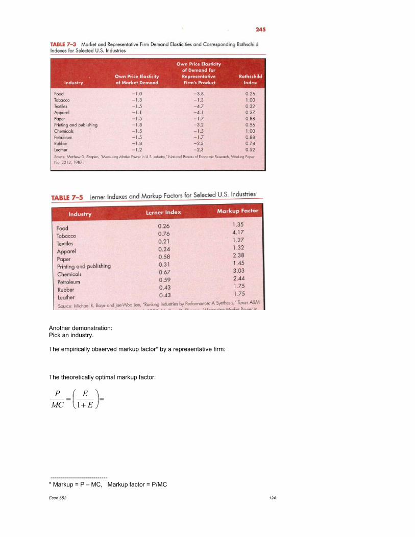
A note on the number of equilibria: A game may have more than one equilibrium in pure strategies. Consider the following game:

Firm 2’s price High Medium Low

Firm 1’s

price High 6, 7 3, 8 1, 6

Medium 7, 4 5, 6 2, 5

Low 8, 0 4, 2 3, 3

Let’s practice finding the Nash equilibria using the algorithm on slide 166. Econ 652 171

Infinitely repeated games The concept of present value (see pp.14-18 in the book): Profit today is more valuable than profit one year from today. The present value of the future profit is Profit PV = ---------- , (1+i) where i is the “discounting factor”, often set equal to the interest rate (but it is better to think about it more broadly, as a subjective “patience factor”: if getting money today is the matter of life and death, then I discount the future at a very high rate, i is large). Econ 652 172 A firm that is believed to exist and earn profits infinitely into the future has the present value of

⋅⋅⋅++

++

++

+= 33

221

0 )1()1()1( iiiPV

ππππ

(Such an expression is called an infinite series.) Econ 652 173 A couple of useful facts about infinite series: If the profits, π, start now and are the same in each future period, then

ii

iiiPV πππππ )1(

)1()1()1( 32

+=⋅⋅⋅+

++

++

++=

If the profits are the same in each period, but start one period from now, then

iiiiPV ππππ

=⋅⋅⋅++

++

++

= 32 )1()1()1(

Econ 652 174

The pricing game revisited:

Firm 2 Low price High price Firm 1

Low price

5, 4

8, 1

High price

2, 7

7, 6

When this game is played repeatedly, the collusive outcome becomes more sustainable. Econ 652 175 To achieve that, firms use so-called “trigger strategies” – strategies contingent on the past play of a game (a certain action “triggers” a certain response, ). We will consider an extreme example of a trigger strategy (called “grim trigger strategy”): “I will continue to play “HIGH” as long as you are playing “HIGH”. Once you cheat by playing “LOW”, I will play “LOW” in every period thereafter.” Let’s look at the present values of stream of payments if the firms adopt such a strategy. Econ 652 176 If firm 1 cooperates, its present value is PV = If firm 1 cheats, its present value is PV = Firm 1 will prefer to cooperate if Econ 652 177

Another example (p.369 in the book): A firm gets to choose the quality of its product. Consumers choose whether to buy or not.

Firm Low quality High quality Consumer

Don’t buy

0; 0

0; - 10

Buy

- 10; 10

1; 1

Econ 652 178 Consumers can deploy the grim trigger strategy: Econ 652 179

Use of game theory in decision making Suggested rules:

- If there is a dominant strategy, play it. - If you don’t have a dominant strategy, but the game has a unique Nash

equilibrium, play the equilibrium strategy.

- If you don’t have a dominant strategy, and there is more than one (or none) equilibria, then you may want to play a secure strategy.

“Secure strategy” – a strategy that guarantees the highest payoff among all strategies in the worst possible scenario.

With these recommendations in mind, what is the best strategy to play in each of the following games? (In all cases, you are Firm 1.) Econ 652 180

Firm 2 L R

Firm 1

U 3, 2 8, 1

D 1, 6 6, 2

Econ 652 181

Firm 2 L R

Firm 1

U 3, 3 4, 1

D 1, 4 6, 3

Firm 2 L R

Firm 1

U 3, 5 8, 8

D 4, 4 5, 0

Econ 652 182

Sequential games So far, we have dealt with games in which players were making simultaneous choices.

But what if in the game on slide 171 Firm 1 gets to pick the price first, and then commits to its decision? In that case, it is more convenient to represent the game as a tree (it is also called the “extensive form”):

• Each node of the tree corresponds to the point when one of the players chooses an action.

• Each branch of the tree is an action.

• The pairs of numbers at the nine terminal nodes represent the payoffs of players 1 and 2, respectively (carefully copied from slide 171).

Econ 652 183

6,7 3,8 1,6 7,4 5,6 2,5 8,0 4,2 3,3 Econ 652 184 If by the time firm 2 has to make its decision firm 1’s decision is known, we can predict with certainty what firm 2 will do. Having this information, firm 1 can decide what to do. This method is called “backward induction”, or “solving the game backwards”. This version of the game has only one Nash equilibrium, (Medium, Medium). Firm 1’s and firm 2’s payoffs are 5 and 6, respectively. Note an equilibrium has to be characterized by the set of strategies, not by the payoffs! So (M, M), not (5,6). Econ 652 185

1

2 2

2

M H L M M L L H H

H M L

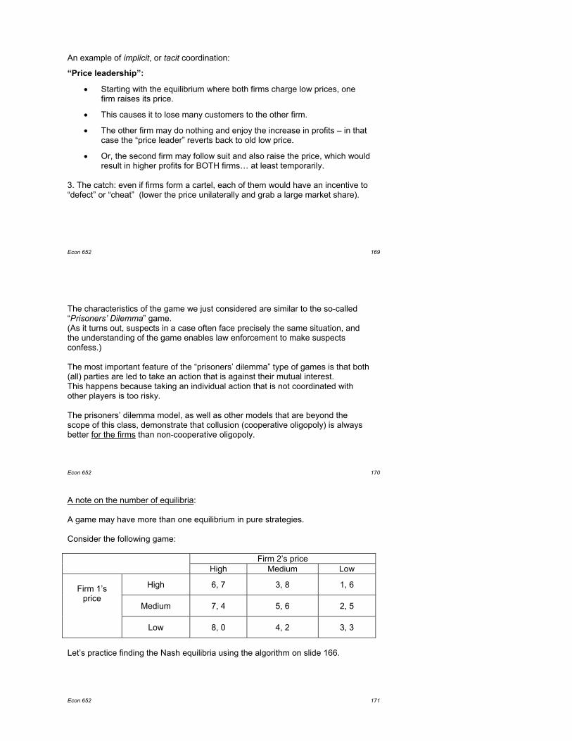
Market entry decisions. Preventing market entry

Two firms consider entering the market. Market can accommodate only one firm. Simultaneous decisions:

Firm 2 Not Enter Enter Firm 1 Not Enter 0, 0 0, 1

Enter 1, 0 -1, -1

Econ 652 186 Sequential decisions: The outcome: Conclusion: The sequence of moves is important! Econ 652 187

1

2 2

Not Enter

Enter

Enter Enter Not Enter

Not Enter

A somewhat less dramatic example: The market can accommodate two firms.

Firm 2 Do Not Enter Enter Firm 1 Do Not Enter 0, 0 0, 5

Enter 5, 0 1, 1

In this case, each firm has a dominant strategy, so the sequence of moves does not matter. The unique Nash equilibrium is… Econ 652 188 If Firm 1 could buy the exclusive rights to serve this market, up to what amount would it be willing to pay for those rights? Econ 652 189

Entry decisions and government policy Airbus and Boeing are both considering investing into making a new model of a gigantic cargo aircraft. If Boeing is the only firm entering the market, it would earn $250 million in profit. If Airbus is the only firm entering the market, it would earn $200 million in profit. The market is too small to support two firms. Thus, if both firms enter, their profits are substantially smaller: Boeing would earn $10 million while Airbus, due to higher labor costs in Europe, will lose $40 million. The firm that stays out of the market earns nothing. Both firms have to make their decisions simultaneously. Econ 652 190 Present it in the form of the game and solve it.

Airbus Enter Not enter

Boeing

Enter

10; - 40

250; 0

Not enter

0; 200

0; 0

What is the most likely outcome of the game? Econ 652 191 Now consider the same story, but the EU government promises to give Airbus a $50m subsidy if Airbus builds such a plane. Rewrite the game matrix and find the most likely outcome under such a scenario.

Airbus

Enter Not enter

Boeing

Enter

10; - 40

250; 0

Not enter

0; 200

0; 0

Conclusion? Econ 652 192

Another trick that may help prevent entry: Raising the costs of all firms in the industry (pp.488-491 in the book) You are a monopolist, earning $10 (million) in profit. If another firm enters, then each of you would earn $3. You can convince the government to insist on pollution-control devices that would raise everyone’s costs by $4. Let’s represent this as a sequential game: Econ 652 193 (GM, catalytic converters, 1973)

example in the text at the beginning of the chapter .

Overall market demand

Limit Pricing (pp.475-480) You are the incumbent (a monopolist):

$ Econ 652 194

The same market as viewed by a potential entrant (which we will assume has the same cost):

$

Econ 652 195 Where do you want the demand for the entrant’s product to be?

$ How can you achieve that? Econ 652 196

Q produced by the incumbent (the entrant treats it as given)

“Residual demand” left for the entrant

A follow-up question: Instead of deviating from the profit-maximizing quantity of output, can’t you simply make a threat to potential entrants that, in case they enter, you increase your output, lower your price and thus make the entrant lose money? Let’s take a look. (I had tw o versions of a sequential game set up – see the not es) Econ 652 197 Can the possibility of another firm’s entry affect the incumbent’s decision on some long-term strategic issues, such as expansion, for example? See the following two pages. Econ 652 198

Scenario 1. You are a monopolist, making a product with no substitutes. The market demand for the product you are making is represented by the following table: Price 1 3 5 7 9 Q demanded 1000 800 600 400 200 Currently, your costs are given by the ATC curve #1 on the graph below. $ 6 1 2 4 2 0 100 200 300 400 500 600 700 800 Q You are considering expansion by building another production unit. If you do that, then your average total cost relationship would be represented by curve 2 on the graph. Keep in mind that ATC = AFC + AVC, therefore any fixed costs, including those required for the expansion, are already captured by the ATC curve. Is expansion a good idea under the current circumstances? Explain.

Scenario 2. You are a monopolist, but there is a possibility that another firm will enter and make a product very similar if not identical to yours. If it does so, then its ATC curve will be the same as your original one (#1). The appearance of another firm in the market would not change the overall market demand. Therefore, the table on the previous page is no longer the demand your firm is facing – instead, the price will be determined by the sum of the output quantities the two firms produce. Given the current demand parameters and cost relationships, is it likely that the other firm will enter? Once again, you are considering building another production unit. Under the new circumstances, is doing so a good idea? At the first glance, it may look like there is too much information to keep track of. However, game theory provides us with tools to answer this question. I suggest you to present and solve this problem as a sequential game, consisting of your investment decision, your opponent’s entry decision, and (this last part is optional) your decision whether to make 200, 400, or 600 units. Present this game in the extensive form, identify who makes a decision at each tree node and what strategies are available, calculate the payoffs (profits) in each possible outcome and write them down as pairs of numbers, your payoff first. Identify the equilibria of this game. Finally, answer the question: Given the possibility of entry by another firm, is expansion a good idea?

How can a firm deter entry? – A summary

- pay for exclusive rights; - make new entry unprofitable:

- strategic lobbying for new laws; - limit pricing; - predatory pricing (sometimes below MC); - reduce the degree of substitutability between the two products:

• advertising; • reputation;

- fill all niches (i.e., make both high- and low-end products); - “burn bridges” (make an irreversible credible commitment):

• build a large plant; • invest in a technology.

Threats that are not credible do not work!!!

Econ 652 199

Economics of incomplete information

Traditional microeconomic analysis deals with economic agents making decisions under complete information. Examples of such assumptions:

- Consumers know the utility they get from a good; - Firms know demand schedules; - Firms know each others’ prices; and so on.

Real life is more complicated and less certain. Econ 652 200

Comparing projects with uncertain outcomes Every project has two characteristics, the expected value and the degree of risk. A certain outcome = no risk. The expected value, or the mean: Computed as the weighted sum of all possible payoffs (“weighted” = multiplied by the probabilities of each respective outcome):

E[x] = q1x1 + q2x2 + … + qnxn,

where xi is payoff i, qi is the probability that payoff i occurs,

and q1 + q2 + … + qn= 1. Econ 652 201 Variance (a measure of risk): The sum of the probabilities that different outcomes will occur multiplied by the squared deviations from the mean of the random variable: Var = q1(x1 – E[x])2 + q2(x2 – E[x])2 + … + qn(xn – E[x])2 The standard deviation, σ, is the square root of the variance. The larger the variance (or the standard deviation), the riskier the project. (For events occurring with certainty, Var = 0) Econ 652 202

How much would you be willing to pay for a lottery ticket that pays $100 with a 50% probability and nothing with a 50% probability? What is the expected value of this lottery ticket? E[x] = Why do the two answers differ? Econ 652 203 The attitude to risk may vary. Individuals who prefer less risk to more risk, all other things being equal, are called “risk averse”. It is believed that most people belong to this group. Those who don’t care about the degree of risk and care only about the expected value are called “risk neutral”. Individuals who prefer more risk to less risk, all other things being equal, are called “risk preferring”, or “risk loving”. (Sort of an anomaly.) In the example above, the person in question is . . . Econ 652 204 Risk premium – the minimum reward that would induce a risk averse person to accept risk while preserving the same expected value. Alternatively, risk premium is the maximum amount of money an individual will be willing to pay to replace an uncertain situation with a certainty situation that has the same expected value. Risk premium depends on the characteristics of the lottery as well as on individual preferences. In the example above, the risk premium is… Econ 652 205

Suppose we have two projects: A: expected value = $1000, Var = 5000 B: expected value = $1000, Var = 1500 What will each group choose? Risk averse – Risk neutral – Risk loving – Econ 652 206 If the expected values differ as well: A: expected value = $1200, Var = 5000 B: expected value = $1000, Var = 1500 Everyone prefers higher expected value to lower expected value, all other things being equal. Preferences in regard to risk are as above. Type of individual

Preferences Exp. value Risk Overall

Risk averse

Risk neutral

Risk loving

Econ 652 207

What can a risk averse individual do to reduce risk?

1. Be informed. 2. Diversify.

Here is an example of diversification, or “spreading the risk”. You are considering investing $100 into one or both of the two assets (stocks, for concreteness). Each share is worth $50 now, and you believe that within the next three months its value can with equal probability either increase to $80 or drop to $40. For now, let us assume that what happens to one stock is not correlated to what happens to the other one. Econ 652 208 Let’s first look at the expected value of your investment in either case. If you invest in the shares of one of the companies: E[x] = 2(.5·8 0 + .5·40) = $120 If you buy one share of each of the companies: E[x] = (. 5·80 + .5·40) + (.5 ·80 + .5·40) = $120 Econ 652 209 The variance (a measure of risk): If you invest in one company: Var = 0.5 (160 – 120)2 + 0.5 (80 – 120)2

= 800 + 800 = 1600 If you invest in both… Possible outcomes: W/prob ¼ both stocks go up, x = $160 W/prob ¼ stock A goes up, stock B falls, x = $120 W/prob ¼ stock B goes up, stock A falls, x = $120 W/prob ¼ both stocks fall, x = $80 Var =

Econ 652 210

If the payoffs from two assets are negatively correlated, then diversification becomes even more attractive. Example: Two companies compete for a large government contract. After the winner is announced, the winner’s stocks go up and the loser’s stocks stay at the same level as before. An investment company is very well off if it “hedges” against either of the outcomes. When firms undertake many projects simultaneously, it is best for them to be risk neutral. Moreover, shareholders WANT managers to act in a risk-neutral manner (to care only about expected values). Econ 652 211 Summary of this topic so far:

• Everyone prefers a higher expected value to a lower expected value. • Most individuals are risk averse. This means they prefer less risk to

more risk, provided the expected value stays the same. If one project offers a higher expected value and a higher risk at the same time, then we need more information to tell which of the two will a risk averse person choose.

• Firms can be assumed to be risk neutral. They evaluate projects based

solely on their expected values. Econ 652 212

Pricing and output decisions under uncertainty All the rules we have learned before (MR=MC, etc.) stay the same but “expected” appear in them as needed. Consider a modification of problem 4 on p.469. You are the manager of a firm that sells soybeans in a perfectly competitive market. Your cost function is C(Q) = 2Q +2Q2. Due to production lags, you must make your output decision prior to knowing what the market price will be. You believe that there is a 25% chance the market price will be $120 and a 75% chance it will be $160.

a. Calculate the expected market price. Econ 652 213 b. What Q of output should you produce to maximize expected profits? Econ 652 214 c. Let’s check: What are your profits under each outcome and the expected profits? Econ 652 215

The same approach can be extended to the imperfectly competitive market case. A firm with market power produces at a constant marginal (and average) cost of $1. (So TC = 1∙Q, or simply Q.) There is a 50% chance of a recession and a 50% chance of an economic boom. During a boom, the inverse demand for firm’s product will be P = 10 – 0.5 Q If there is a recession, the inverse demand will be P = 6 – 0.5 Q The firm is risk neutral and must set output before demand is known. How much output should it produce to maximize expected profit? Econ 652 216

Consumer search for the best price and implications for the firm’s behavior

General idea: A consumer samples several stores and obtains a price quote from each. The cost of obtaining each quote is the same. The total number of stores is large, so “drawing” one of them doesn’t affect the odds. After several quotes, you can always return to the store with the best price. It makes sense to continue searching as long as the (expected) benefit exceeds the cost of search. Econ 652 217 Expected benefit: Joe wants to buy a DVD player. He thinks one-third of the stores charge $130 for a DVD player, one-third charge $100, and one-third charge $85. The lowest price he’s found so far is $100. What is the expected benefit from sampling another store? Econ 652 218 How will the answer change if the best price found so far is $130? Econ 652 219

In general, if you sample a store and the price is high, the expected benefit from

further search is ______________ (it makes _________ sense to search).

This principle holds even if the distribution of prices is not known. Econ 652 220 Benefits and costs combined: Cost/benefit of continuing to search Price observed Econ 652 221 What happens if the cost of search increases? See the graph above. What has happened with the appearance of the Internet? Which industries/markets are more affected? Less affected?

Econ 652 222

Socially optimal risk sharing

If individuals are risk averse while firms are risk neutral, what is the optimal risk sharing between consumers and firms? Getting out of risk has value for consumers but not for firms. Therefore there is room for mutually beneficial exchange: Consumers may reward the firm for reducing risk for them. Example: insurance industry. Econ 652 223 Insurance companies are able to make money selling insurance because they may - have better information about the odds than their clients; - differ from clients in their attitude to risk; - diversify. The larger the group of the insured, the __________________ the variance,

therefore the ___________________ the risk.

Econ 652 224

Incomplete asymmetric information “Asymmetric” in this case points out the fact that one party is less informed than the other. An example of asymmetric information: Sellers know quality, buyers do not. The only way for buyers to find out the true value is to try the product out. (such goods are sometimes called “experience goods”). Econ 652 225 Under certainty, the rule would be: Buy if Value > P, where “value” (a.k.a. “utility”) stands for the subjective value the buyer gets from the product. Under uncertainty, it becomes (for a risk-neutral consumer) Buy if Expected Value > P Say if the product works as expected it has a value of $100 for a consumer. The consumer believes that there is a 90% chance the product will deliver services. There is also a 10% chance it will break down immediately, in which case its value is 0. Econ 652 226 Up to what price will a risk neutral consumer pay for the product? What happens if the consumer is risk averse? If buyers’ subjective valuations of the good are below the producer’s cost of making it, the market breaks down – nothing will be sold. Both buyers and sellers are hurt by that. Econ 652 227

In order to see this is indeed the case, consider the following example:

The market for “lemons” Akerlof (1973) considers the market for “lemons”, or cars with hidden defects. Asymmetric information is reflected in the fact that the quality of cars in the market is known to sellers but not to buyers. There are two types of used cars offered for sale in the market, good cars and “lemons”. 2,000 cars are offered for sale, 1,000 of each type. Econ 652 228 The number of potential buyers exceeds the number of cars available. All buyers are identical – each of them will pay up to $1,000 for a lemon and $2,000 for a good car. (Those numbers are also called “reservation prices”.) The sellers’ “reservation price” (the lowest price they would agree to sell for) is $800 for a lemon and $1600 for a good car. Econ 652 229 Case 1. Symmetric complete information – the true quality of each car is known to both parties. We have two separate markets: P P Q

Good cars Lemons Econ 652 230

Q

Case 2. Symmetric incomplete information – the true quality of a particular car is not known to anybody. Each car is either a good one (with a 50% probability) or a lemon (with a 50% probability). Neither buyers nor sellers have a way to tell one from another. For simplicity, we are going to assume both sides are risk neutral. Therefore they base their reservation prices strictly on their expected values (no “risk premium” involved!) For sellers, EV = For buyers, EV = Econ 652 231 P Q Equilibrium price = Equilibrium quantity = Econ 652 232 Case 3. Asymmetric incomplete information – sellers know the quality, buyers don’t. For buyers, the situation is the same as in the previous case – they will pay $1500 for any car. Sellers, however, can tell good cars from lemons, and their reservation price is different for each category. (how will the S-curve look?) P Econ 652 233

As a result, only lemons are sold. This is an example of adverse selection, or a situation when poor quality products drive high quality products out of the market. Adverse selection prevents markets from operating efficiently and is detrimental for both buyers and sellers. After buyers realize that no good cars are being traded, what happens to the expected value of a car for them? What happens to the market price? Econ 652 234 A similar example: Adverse selection in the health insurance market An individual knows his/her probability of accident, illness, etc. better than the insurance company.

Insurance companies know only the composition of the population. If they offer a uniform insurance contract and price it based on the average degree of risk, then such a policy is attractive only for high-risk individuals.

Low-risk individuals don’t buy insurance, and the average probability of accident/illness exceeds the initial insurance company projections… The company adjusts the premiums….

…more people become uninterested…

…etc. Econ 652 235 Note that, while asymmetric information is a common occurrence, it does not always result in adverse selection. That would depend of reservation values, attitudes to risk, etc. For example, if in the above exercise sellers’ reservation price for a good car is $1200, then efficiency is restored. See below. P Econ 652 236

Ways to overcome the undesirable consequences of information asymmetry involve making the uninformed party better informed or reducing the amount at stake for them: - laws protecting consumers; - consumer reports; - return policies; - “screening”; - “signaling”. The last two deserve some discussion. Econ 652 237 1. Screening – the uninformed party does something that makes it better informed. In the context of the lemons example, the (informed) seller may want to let (uninformed) buyers try the product out. We may spend extra time reading reviews of a product on the Internet. Insurance companies use a combination of tools to screen consumers and to better identify groups with different degree of risk:

- Questionnaires (age, marital status, smoking habits, etc.), - A variety of contracts that differ in premiums, deductibles, and co-pay

shares (a self-selection device). Other examples: credit scores, asking for a second opinion when buying a car Econ 652 238 2. Signaling – an informed party sends an observable indicator of his or her hidden characteristics to an uninformed party. In order to be effective, the signal must not be easily mimicked by other types.

Examples: warranties as signals of quality, education as a signal of ability, etc.

Why a warranty may work as a quality signal:

Econ 652 239

Other forms of signaling: Low introductory price offer (used mainly for goods purchased repeatedly). Then, as consumers become more confident about the quality of the product, the seller can return to the profit-maximizing price level. An extreme case of such a practice: free samples. (Note that in this case low prices don’t imply low quality! In fact, it’s the exact opposite – the firm wants as many consumers as possible to try their product out.) For goods purchased only a few times over a consumer’s lifetime (“durable goods”), a seller can offer a free trial period – a practice that is getting more and more popular. Econ 652 240 For durable goods, quality can also be signaled by high prices: Pricing above the profit maximizing price results in revenue loss. This loss is more substantial for a low quality firm. Set the price at the level that would never be chosen by the low quality firm. This would convince consumers, who initially were uncertain about your product quality, that you sell a product of high quality. They will revise their willingness to pay for your good. A practice known as “money burning advertising” may seem wasteful but serves a similar purpose – signaling high product quality. Econ 652 241 Yet another, separate problem resulting from the presence of asymmetric information is “moral hazard” – a hidden action by one party that allows it to get benefits at the expense of another party. Examples of moral hazard:

- individual behavior depending on whether they are insured or not (buy insurance, then start engaging in risky behaviors);

- abuse of warranted products;

- tenure at academic institutions;

- the “principal-agent problem” – you assign a task to a worker, but only the worker himself knows how much effort he puts into performing a task.

Econ 652 242

Back to the earlier example: There is a 90% probability the product will deliver services, hence have a value of $100. There is also a 10% probability it will break down immediately, in which case its value is 0. Now, the firm offers a warranty of some form. For concreteness, let’s say it’s an unconditional money-back guarantee: an unsatisfied customer can get a refund, no questions asked. Up to what price will a risk neutral consumer pay for the product? What happens if the consumer is risk averse? Econ 652 243

Auctions

A form of competition for scarce objects. The attractiveness of this form of competition from the economics perspective is that in most cases the object goes to the person with the highest valuation – a sign of efficiency. If a player with reservation value v makes bid, b, and wins the auction, his payoff

is x = v – b.

A player who doesn’t win gets x = 0.

Econ 652 244 Auctions differ in

- The order in which bids are made; - What information bidders have about each other; - Correlation of individual valuations for the object:

“Private value” (value of the object is different for every bidder) vs. “common value” (the value is the same no matter who wins it);

- What the winner is asked to pay.

We’ll consider several different types of auctions starting with private value auctions (individual bidders’ valuations for the object are independent of each other). Econ 652 245

The most well-known form of an auction: The English (ascending-price) auction: The initial price is set low, bidders outbid each other by announcing the prices they are prepared to pay until only one bidder is left. The last bidder left pays the amount of his own last bid and gets the object. The term for this is “first-price auction”. The optimal strategy in an English auction is to pay the amount that is incrementally larger than a competing bid but never more than the own valuation. Econ 652 245 English auction – an example: Your valuation is $207, the minimum allowed bidding increment is $20, Last bid was $100 - bi d $120 Last bid was $140 - bid $160 Last bid was $200 - do n ot bid Econ 652 247

First-price, sealed-bid auction. Each bidder submits only one bid without knowing the bids of others (so in a sense, simultaneously). Bids are revealed and the highest bidder pays his bid and gets the object. Bidding principles:

- Never bid more than your true value; - If you believe you are the highest bidder, bid below your true value and

as close to the second-highest valuation as the bidding interval allows. Econ 652 248

In general, in the presence of uncertainty about others’ valuations, reducing or “shaving” the bid makes sense no matter where you are on the valuation ladder. For example, it can be shown that… In a FPSB auction with n bidders whose independent private values are drawn from a uniform distribution between the lowest possible value L and the highest possible value H, the optimal bid for a player whose valuation is v is

nvnL

nLvvb )1( −+=

−−=

For an indirect proof this is the case, let’s consider the case of two bidders. If valuations are distributed uniformly and players consistently use the same rule to determine their optimal bid, then the distribution of bids is also uniform. Econ 652 249 Let’s say valuations are distributed uniformly over the [5,15] interval and my valuation is $11. There is no point in b > 11. If b = $11, I win w/prob and earn I lose w/prob and earn E(x) = If b = $10, I win w/prob and earn I lose w/prob and earn E(x) = If b = $9, I win w/prob and earn I lose w/prob and earn E(x) = Econ 652 250 If b = $8, I win w/prob and earn I lose w/prob and earn E(x) = If b = $7, I win w/prob and earn I lose w/prob and earn E(x) = Econ 652 251

We can do the same for the general case of parameters. Given the interval of possible bids, [L, H] and my bid b, I win w/prob (b – L)/(H – L) and get x = 11 – b (and zero otherwise) My expected payoff is therefore

LH

LbbLvbvLH

bvLbxE−

+−−=

−−−

=2

)())(()(

Econ 652 252 There is only one variable of choice in this expression, b. To find the value of b that maximizes E(x), we will use differentiation. Interestingly, the upper limit of the uniform distribution affects the chances of winning but does not affect the optimal strategy! Econ 652 253 Caveat: This formula is attractively simple due to the simplicity of the uniform distribution. However, in real life uniform distributions are not too common, and for a different distribution of valuations, the formula will be different as well. Deriving optimal bidding strategies for normal (bell-shaped), gamma, exponential, and other distributions requires more analytical work (and mathematicians have written volumes about those cases!) However, the above formula does capture the important principles: The higher one’s valuation, the ________ the optimal bid. The more bidders there are, the ________ the optimal bid and

the ____________ the spread between v and b.

The closer is one’s valuation to L, the __________ the spread between v and b. Econ 652 254

This was done for risk neutral bidders. What if bidders are risk averse? Let’s go back to the previous example and calculate risks associated with each bidding strategy.

If b = $11, E(x) = 0, Var(x) = 0

If b = $10, I win w/prob 0.5 and earn 1 I lose w/prob 0.5 and earn 0 E(x) =

Var(x) =

If b = $9, I win w/prob 0.4 and earn 2 I lose w/prob 0.6 and earn 0 E(x) =

Var(x) = Conclusion: the more risk averse the bidders are,

the ____________ they will shave off their bids in a FPSB auction. ( the bids will Econ 652 255 Note that if the player with the highest valuation in a FPSB auction doesn’t know the second bid and guesses incorrectly, he may “shave” his bid too much and therefore lose, in which case the object will go NOT to the player with the highest valuation. This leads to market inefficiency. This shortcoming can be mitigated by using Second-price, sealed-bid (SPSB) auction: (a.k.a. the Vickrey auction) Whoever places the highest bid, wins, but is asked to pay only the amount of the second highest bid. Econ 652 256 Optimal bidding strategy in a SPSB auction: This scheme is often used when the auctioneer is concerned with efficiency and is confident in getting a large number of bidders. It has also produced the largest number of disappointments regarding auction outcomes (mainly low revenues). Sellers may establish the “reserve price” which is de facto the minimum bid accepted. Example of SPSB: proxy bidding on eBay. ------------------------- Econ 652 257

Dutch (descending-price) auction. A seller begins by asking a very high price for the item. The price is gradually lowered until one buyer indicates a willingness to buy the item at that price. The winning bidder pays that price and gets the item. What is the optimal bidding strategy? Since bidders don’t know each others’ valuations, and since the winning bidder has to pay his own bid, this is equivalent to…. Therefore so is the optimal strategy –

Econ 652 258

Common-value auctions In this type of auctions, the true value of the item is not known. It will end up being the same no matter who wins it. (Example: the commercial value of gas/oil deposits) The situation looks something like this:

Probabilistic distribution of “signals” bidders receive

0 100 200 300 400 500 600 700 “True” expected value of the item, $350 Econ 652 259 If everyone bids according to the value of their signals, then the winner would be the bidder with the most optimistic estimate of the object value. Consequently, it will likely be above the true value, which is to say that the auction winner is likely to end up losing money. This phenomenon is known as the “winner’s curse”. In common value auctions, the optimal strategy is to bid less than the perceived value, in order to avoid the winner’s curse. Just like private-value auctions, common-value auctions can be conducted in various forms. Among those, the winner’s curse is partially mitigated in an English auction, where bidders can gain additional information about the distribution of “signals” by observing others’ bids (how active/enthusiastic other bidders are). Econ 652 260

Revenue from an auction: Which scheme would raise the most revenue? In private value auctions, RevENGL = RevSPSB = RevFPSB = RevDUTCH on average The above is for risk-neutral bidders. As we discussed above, risk averse bidders shave their bid less than risk neutral ones (this applies only to …… As a result, in the case of risk-averse bidders the above identity no longer holds: RevENGL = RevSPSB = RevFPSB = RevDUTCH

Econ 652 261

In common value auctions, everything is determined by how much bidders who are afraid of the winner’s curse shave their bids. The winner’s curse is the strongest in … making bidders shave their bids more. Therefore RevENGL = RevSPSB = RevFPSB = RevDUTCH

for risk neutral bidders When bidders in a common value auction are risk averse, the two factors counteract each other, and the relative ranking depends on the degree of risk aversion. RevENGL = RevSPSB = RevFPSB = RevDUTCH

Econ 652 262

Asymmetric information in the labor market In theory, a firm should hire a worker only if the value of his marginal product exceeds the pay he receives. (Marginal benefit vs. marginal cost) Ideally, the marginal product of each worker is known. For example, if you believe that hiring Mr. Doe as a manager will increase your profit by $50,000 a year, then $50,000 is the maximum amount you should be paying him. In most real-world cases, however, the future MP of a worker is unknown. Econ 652 263 Workers’ marginal product depends on their inherent characteristics (talent, skills, intellect, physical strength, etc.) and the effort they decide to put into the assigned task. All those variables are known to the worker but not to the firm – an example of asymmetric information. (Moral hazard!) Keeping a worker who is not fit for the job is costly even when it is done for a limited time. If the firm wants to increase its chances of hiring the right person, it can use remedies common to any market with asymmetric information. Econ 652 264 1. Screening – the uninformed party (the firm) does something that gives it a better idea about the future productivity of a worker. This effort is usually costly. Screening applicants is more justified when

• The degree of correlation between the measured variable and the abilities is ____________

• The cost of screening is ______________

• A ____________ portion of applicants will be refused employment as a

result

• The spread in applicants’ abilities is _______________ Econ 652 265

(Keep in mind that future productivity cannot be determined with certainty. We can only measure some characteristic that we believe is correlated with abilities.) Examples: Form of screening What is measured Rationale Physicals Questionnaires Personality test Econ 652 266 2. Signaling – the informed party does something to signal their “type” to the uninformed party. In the labor market, high-ability workers signal their ability to the firm, thus distinguishing themselves from low-ability individuals. Examples:

• Credentials (extra lines on the resume) • Education

Examples: CPA, Ph.D., bar exam, MBA,…) Econ 652 267 As always, a signal has to be credible. Therefore, it has to be hard for the other type(s) to mimic it. The signal is more credible when producing a signal (obtaining the credential) is

______________ for high-ability workers and _________________ for low-ability workers. Also note that, if the reward to low-ability workers for mimicking the signal of high ability increases, then they will try harder to do that, and in larger numbers. Therefore, as the difference in pay to individuals identified as high- and low-ability workers gets larger, the credibility of the credential signaling high ability ________________. Econ 652 268

Education as a signal

Model developed by Spence (a 2001 Nobel laureate). What do we learn in college? How relevant is the knowledge gained for our future career? If it is relevant, then why do many firms, upon hiring college graduates, send them to some sort of job-specific training? What if a college degree (or our GPA) is nothing more than a signal of our abilities or our commitment to hard work? Econ 652 269 Let us take this hypothesis to an extreme and assume (for the purpose of this model) that college (or any other form of education) does not add anything to our innate abilities. Instead, it is sort of a tryout. Let’s say there are two different types of individuals in the economy, those of high ability and those of low ability. Once being hired, they are capable of producing different marginal product, the high-ability types being more productive. Assume each worker is paid the value of his marginal product. Each worker knows his own type, but the firms don’t (hence we deal with asymmetric information). Econ 652 270 IF firms HAD perfect information, they would pay each type what that type deserves, wH and wL, respectively.

wH > wL

Since firms cannot distinguish between high and low type workers, they pay everyone the same wage, equal to the expected value of the marginal product. For the purpose of our example, we assume that the shares of the two types in the population are equal, αH = αL= 0.5 (naturally, they don’t have to be). Then the average wage, equal to the expected value of the marginal product, is

wAV = αH · wH + αL · wL = (wH + wL)/2. Because of incomplete information, high type workers are underpaid while low type are overpaid. Econ 652 271

Now, suppose anyone can signal their ability by getting a college degree, or some other education credential. Education is obtained at a cost. (This cost is not necessarily monetary – it can be expressed in the time spent and the amount of misery a person has to go through to get a degree.) This cost is different for the two types, cH < cL. Econ 652 272 The following table is constructed assuming all individuals of the same type do the same thing (this does not have to be true, but let us not go there). Low type

Get education No High type

Get educ.

HLH cww−

+2

, LLH cww−

+2

HH cw − , Lw

No

Lw , LH cw −

2LH ww +

, 2

LH ww +

The selection of an equilibrium depends on model parameters. Econ 652 273 Example 1. wH = 400 wL = 200 (wH > wL) cH = 60 cL = 120 (cH < cL) Low type

Get education No

High type

Get educ.

No

Econ 652 274

Example 2. wH = 400 wL = 200 (wH > wL) cH = 40 cL = 60 (cH < cL) Low type

Get education No

High type

Get educ.

No

Econ 652 275 Formal definitions of the two types of equilibria: Separating equilibrium – a situation when it is possible to differentiate between the two types of people (or products, as in the lemons model). A separating equilibrium is preferred because it leads to higher efficiency (think of an analogy with the lemons model). However: If the spread between H and L wages is too small relative to the cost of obtaining the credential – then the credential is not worth getting, so no one does. The firms can’t tell workers apart. (Pooling equilibrium) If the spread between H and L wages gets too high relative to the cost of obtaining the credential (as in example 2) – then everyone gets it. That’s another pooling equilibrium. The firms still can’t tell workers apart… in spite of spending nation’s resources on administering a meaningless credential. Econ 652 276 In summary, education best serves its signaling purpose when attaining it is neither too hard nor too easy (with “too easy” being the worse of the two choices). If we add the obvious fact that we do acquire some useful skills as we get educated back in, then the “too easy” option looks even less attractive. A degree from a program that demands students to work and learn has more value for the employers and therefore a degree holder.

Econ 652 277