Graphical pangenomics

Erik Peter Garrison

Wellcome Sanger InstituteUniversity of Cambridge

This dissertation is submitted for the degree ofDoctor of Philosophy

Fitzwilliam College September 2018

for E2 & E3

Declaration

I hereby declare that except where specific reference is made to the work of others, thecontents of this dissertation are original and have not been submitted in whole or in partfor consideration for any other degree or qualification in this, or any other university.This dissertation is my own work and contains nothing which is the outcome of workdone in collaboration with others, except as specified in the text and Acknowledgements.This dissertation contains fewer than 65,000 words including appendices, bibliography,footnotes, tables and equations and has fewer than 150 figures.

Erik Peter GarrisonSeptember 2018

Graphical pangenomics

Erik Peter Garrison

Completely sequencing genomes is expensive, and to save costs we often analyze newgenomic data in the context of a reference genome. This approach distorts our image ofthe inferred genome, an effect which we describe as reference bias. To mitigate referencebias, I repurpose graphical models previously used in genome assembly and alignment toserve as a reference system in resequencing. To do so I formalize the concept of a variationgraph to link genomes to a graphical model of their mutual alignment that is capable ofrepresenting any kind of genomic variation, both small and large. As this model combinesboth sequence and variation information in one structure it serves as a natural basis forresequencing. By indexing the topology, sequence space, and haplotype space of thesegraphs and developing generalizations of sequence alignment suitable to them, I am ableto use them as reference systems in the analysis of a wide array of genomic systems, fromlarge vertebrate genomes to microbial pangenomes. To demonstrate the utility of thisapproach, I use my implementation to solve resequencing and alignment problems inthe context of Homo sapiens and Saccharomyces cerevisiae. I use graph visualizationtechniques to explore variation graphs built from a variety of sources, including divergedhuman haplotypes, a gut microbiome, and a freshwater viral metagenome. I find thatvariation aware read alignment can eliminate reference bias at known variants, and this isof particular importance in the analysis of ancient DNA, where existing approaches resultin significant bias towards the reference genome and concomitant distortion of populationgenetics results. I validate that the variation graph model can be applied to align RNAsequencing data to a splicing graph. Finally, I show that a classical pangenomic inferenceproblem in microbiology can be solved using a resequencing approach based on variationgraphs.

Acknowledgements

This work responds to ideas that arose in conversation with Deniz Kural. Our friendshipis the first reason that I became a biologist, and his exploration of graphical modelsfor genomes inspired my own. It is thanks to Alexander Wait Zaranek that we had theopportunity to work in George Church’s lab, which pulled us both into biology from ourprevious fields. There I met Madeline Price Ball, who guided me during an immersiveand engaging introduction to biology and genomics.

Deniz introduced me to Gabor Marth, with whom I apprenticed in the art of bioin-formatics. Gabor encouraged me to contribute extensively to the 1000 Genomes Project,whose objective captured my imagination and whose participants, in particular themembers of the analysis group, taught me many lessons in the way of science. I can thankHyun Min Kang, Goncalo Abecasis, Adam Auton, Laura Clarke, Gerton Lunter, MarkDePristo, Lisa Brooks, Ryan Poplin, Zamin Iqbal, and Heng Li, for always motivatingme, and for helping me to understand and correct the many mistakes I made. Meanwhile,Mengyao Zhao and Wan-Ping Lee gave me my first look inside the alignment algorithmsthat are such an important part of this thesis.

During those years I had the pleasure of living with Benjamin “Mako” Hill and MikaMatsuzaki, who showed me what it means to work as a scientist for the commons. Notonly did I learn from them, but from the many thinkers, dreamers, and travelers whothey brought into our life in Somerville. These include Hanna Wallach, who helped meto understand the theory and practice of the learning problems I first encountered ingenomics, and Nicolás Della Penna, who continues to shape my understanding of manyaspects of the scientific artifice, in particular the fuzzy boundary between the social andthe technical. I thank my friends Nathan Trachimowicz and Barbara Eghan, with whomI passed so much time in those years, for not letting me lose touch with the beautifulnatural and human world in which this work lives and from which it derives its purpose.

This thesis would cover a considerably narrower set of topics if not for the efforts ofthe many people with whom I have worked to build the variation graph toolkit, vg. Theseinclude, but are not limited to: Jouni Sirén, from whom I learned about the world ofsuccinct data structures as I watched him build the graph sequence indexes that brought

vi

vg to a level of quality I never could have achieved on my own; Benedict Paten, whoapplied his unique expertise on genome graphs to help guide the effort of the ever-growinggroup of project collaborators without a pause in his own stream of contributions; EricDawson, whose ready conversation, energy and persistence buoyed me in the early daysof vg, and who laid the foundation for future work on structural variant calling on graphs;Shilpa Garg, who brought new ideas about assembly and diploid genome inference toour project while helping to establish the long read alignment algorithms in vg; AdamNovak, who arrived first and transformed the heart of vg from a weak toy model into afoundation suitable for the work of this wide-ranging team, and who continues to carryit forward; Charles Markello, whose precise work on building resequencing pipelines withvg has ensured it is and will be widely usable; Emily Kobayashi, who further honedvg’s topology index and is pushing improvement in the dynamic graph indexes we use;Wolfgang Beyer, Toshiyuki Yokoyama, Orion Buske, and Ryan Wick, whose work onsequence graph visualization gave me eyes to understand my work; William Jones, whoseclear-minded experiments on alignment identity and score comparison provide the basisfor so many figures in this work; Hajime Suzuki, whose work on alignment accelerationlies at the core of the next phase of graph based mappers; Jordan Eizenga, with whom Iexplored the deep complexity of string to graph alignment algorithms; Xian Chang, whois driving the next high-performance paradigm for sequence to graph alignment; MikeLin, whose experience and tact guided me both in the vg project and in extracurricularwork for DNAnexus; Yohei Rosen, who showed us that old models of haplotype matchingcould thrive inside our new pangenomic, graphical world; Glenn Hickey, who, in additionto caring for the project, took vg full circle and built variant calling into the graphmodel; Jerven Bolleman, who found a way to link vg into the enormous world of semanticbiological data; and Toshiaki Katayama, who has explored our work and done so muchto bring developers of graphical pangenomic techniques together. These members ofthe “vgteam” have each shared so much more than I can describe here, and I am deeplygrateful to have had the opportunity to work with them. The work that I present here isfundamentally based on the productive collaboration that we have shared, and I couldnot have completed it without their watchful critique and steadfast exploration of theirown research questions.

During my time as a student, I benefited from many long conversations with myfellow Sanger PhD cohort over lunch and coffee at the Genome Campus. In particularI learned from the other students with whom I lived: Ignacio Vázquez García, MartinFabry, Daniel Bruder, Manuela Carrasquilla, and Girish Nivarti.

vii

Pedro Fernandes gave Tobias Marschall and me the chance to teach a course onpangenomics using vg, which motivated many of the applications of variation graphsthat I present here. Eppie Jones, Rui Martiniano, and Daniel Wegmann have guided andsupported my work on ancient DNA. Remo Sanges and Mariella Ferrante gave me a labto be part of and a fascinating project to explore in my time in Napoli. My corrections forthis thesis drew on Alex Bowe’s excellent series of blog posts on succinct data structures,and I thank him for allowing me to exposit some of his examples here.

The final version of this thesis reflects a long and memorable conversation led by myexaminers Aylwyn Scally and Gerton Lunter. I thank them for their clear suggestions forits improvement, and will forever be grateful for the time they devoted to this sprawlingwork. They focused my time on its roughest and most incomplete aspects. I am proudof the result that their critique has encouraged me to achieve.

Working with Richard Durbin has been a singular pleasure. Richard has an expansivevision for genomics, but he is always ready to dig into the details of a problem. He isa true master of his craft, able to support and guide every aspect of our work. Thegroup he leads is motivated by his wide-ranging interests in biology. I owe its former andcurrent members thanks for their encouragement and imagination.

Without my family, it is unlikely I would have ever begun the meandering trip thathas led me to this thesis. My parents, Mark Garrison and Diane Garrison, helped meto be independent, and opened my mind to the world of ideas, which set me out on awonderful trip. Along the way, my brother Nels and sister Astrid have kept me honestand careful of myself.

Much of this trip has been alongside my partner Enza Colonna. Non so come direquanto mi ha aiutato, o quanti passi ho fatto in questo viaggo secondo le idee che abbiamocondiviso. I also am grateful to her parents, Donato Colonna e Concetta Tummolo, underwhose almond and olive trees I wrote many pages of this work. Mi hanno sollevato daiproblemi di vita quotidiana, e con il loro aiuto ho potuto scrivere la prima bozza diquesta tesi in un solo mese.

Our daughter, Exa, who always convinces me to play, made sure that I was never tootired to keep going. I look forward to sharing this with her.

Table of contents

List of figures xii

List of tables xiv

1 Introduction 11.1 Genome inference . . . . . . . . . . . . . . . . . . . . . . . . . . . . . . . 4

1.1.1 Reading DNA . . . . . . . . . . . . . . . . . . . . . . . . . . . . . 41.1.1.1 The old school . . . . . . . . . . . . . . . . . . . . . . . 51.1.1.2 “Next generation” sequencing . . . . . . . . . . . . . . . 61.1.1.3 Single molecules . . . . . . . . . . . . . . . . . . . . . . 7

1.1.2 Genome assembly . . . . . . . . . . . . . . . . . . . . . . . . . . . 91.2 Reference genomes . . . . . . . . . . . . . . . . . . . . . . . . . . . . . . 11

1.2.1 Resequencing . . . . . . . . . . . . . . . . . . . . . . . . . . . . . 121.2.2 Sequence alignment . . . . . . . . . . . . . . . . . . . . . . . . . . 13

1.2.2.1 Compressed full text indexes . . . . . . . . . . . . . . . 151.2.3 Variant calling . . . . . . . . . . . . . . . . . . . . . . . . . . . . 161.2.4 The reference bias problem . . . . . . . . . . . . . . . . . . . . . . 17

1.3 Pangenomes . . . . . . . . . . . . . . . . . . . . . . . . . . . . . . . . . . 181.3.1 On pangenomic models . . . . . . . . . . . . . . . . . . . . . . . . 201.3.2 The variation graph . . . . . . . . . . . . . . . . . . . . . . . . . . 23

1.4 Graphical techniques in sequence analysis . . . . . . . . . . . . . . . . . . 241.4.1 (Multiple) sequence alignment . . . . . . . . . . . . . . . . . . . . 241.4.2 Assembly graphs . . . . . . . . . . . . . . . . . . . . . . . . . . . 27

1.4.2.1 Overlap graphs . . . . . . . . . . . . . . . . . . . . . . . 281.4.2.2 De Bruijn graphs . . . . . . . . . . . . . . . . . . . . . . 291.4.2.3 String graphs . . . . . . . . . . . . . . . . . . . . . . . . 301.4.2.4 RNA sequencing graphs . . . . . . . . . . . . . . . . . . 321.4.2.5 Genome alignment graphs . . . . . . . . . . . . . . . . . 32

Table of contents ix

1.4.3 Pangenomic alignment . . . . . . . . . . . . . . . . . . . . . . . . 341.4.3.1 Alignment to unfolded pangenomic references . . . . . . 341.4.3.2 Alignment to tiled pangenomic references . . . . . . . . 351.4.3.3 Alignment to graphical assembly models . . . . . . . . . 361.4.3.4 Genotyping using a sequence DAG . . . . . . . . . . . . 371.4.3.5 Population reference graphs . . . . . . . . . . . . . . . . 381.4.3.6 Succinct pangenomic sequence indexes . . . . . . . . . . 391.4.3.7 Mapping to k-mer based pangenome indexes . . . . . . . 42

1.5 Overview and objectives . . . . . . . . . . . . . . . . . . . . . . . . . . . 43

2 Variation graphs 452.1 A generic graph embedding for genomics . . . . . . . . . . . . . . . . . . 47

2.1.1 The bidirectional sequence graph . . . . . . . . . . . . . . . . . . 472.1.2 Paths with edits . . . . . . . . . . . . . . . . . . . . . . . . . . . . 482.1.3 Alignments . . . . . . . . . . . . . . . . . . . . . . . . . . . . . . 482.1.4 Translations . . . . . . . . . . . . . . . . . . . . . . . . . . . . . . 492.1.5 Genotypes . . . . . . . . . . . . . . . . . . . . . . . . . . . . . . . 502.1.6 Extending the graph . . . . . . . . . . . . . . . . . . . . . . . . . 50

2.2 Variation graph construction . . . . . . . . . . . . . . . . . . . . . . . . . 512.2.1 Progressive alignment . . . . . . . . . . . . . . . . . . . . . . . . . 512.2.2 Using variants in VCF format . . . . . . . . . . . . . . . . . . . . 512.2.3 From gene models . . . . . . . . . . . . . . . . . . . . . . . . . . . 522.2.4 From multiple sequence alignments . . . . . . . . . . . . . . . . . 532.2.5 From overlap assembly and de Bruijn graphs . . . . . . . . . . . . 532.2.6 From pairwise alignments . . . . . . . . . . . . . . . . . . . . . . 54

2.3 Data interchange . . . . . . . . . . . . . . . . . . . . . . . . . . . . . . . 562.4 Index structures . . . . . . . . . . . . . . . . . . . . . . . . . . . . . . . . 57

2.4.1 Dynamic in-memory graph model . . . . . . . . . . . . . . . . . . 582.4.2 Graph topology index . . . . . . . . . . . . . . . . . . . . . . . . 582.4.3 Graph sequence indexes . . . . . . . . . . . . . . . . . . . . . . . 61

2.4.3.1 Graph k-mer indexes . . . . . . . . . . . . . . . . . . . . 622.4.3.2 The FM-index and Compressed Suffix Array (CSA) . . . 622.4.3.3 BWT-based tree and graph sequence indexes . . . . . . 662.4.3.4 The Generalized Compressed Suffix Array . . . . . . . . 682.4.3.5 GCSA2 . . . . . . . . . . . . . . . . . . . . . . . . . . . 70

2.4.4 Haplotype indexes . . . . . . . . . . . . . . . . . . . . . . . . . . 742.4.5 Generic disk backed indexes . . . . . . . . . . . . . . . . . . . . . 78

Table of contents x

2.4.6 Coverage index . . . . . . . . . . . . . . . . . . . . . . . . . . . . 782.5 Sequence alignment to the graph . . . . . . . . . . . . . . . . . . . . . . 79

2.5.1 MEM finding and alignment seeding . . . . . . . . . . . . . . . . 812.5.2 Distance estimation . . . . . . . . . . . . . . . . . . . . . . . . . . 822.5.3 Collinear chaining . . . . . . . . . . . . . . . . . . . . . . . . . . . 832.5.4 Unfolding . . . . . . . . . . . . . . . . . . . . . . . . . . . . . . . 862.5.5 DAGification . . . . . . . . . . . . . . . . . . . . . . . . . . . . . 872.5.6 POA and GSSW . . . . . . . . . . . . . . . . . . . . . . . . . . . 872.5.7 Banded global alignment and multipath mapping . . . . . . . . . 902.5.8 X-drop DP . . . . . . . . . . . . . . . . . . . . . . . . . . . . . . 912.5.9 Chunked alignment . . . . . . . . . . . . . . . . . . . . . . . . . . 932.5.10 Alignment surjection . . . . . . . . . . . . . . . . . . . . . . . . . 962.5.11 Base quality adjusted alignment . . . . . . . . . . . . . . . . . . . 972.5.12 Mapping qualities . . . . . . . . . . . . . . . . . . . . . . . . . . . 98

2.6 Visualization . . . . . . . . . . . . . . . . . . . . . . . . . . . . . . . . . 992.6.1 Hierarchical layout . . . . . . . . . . . . . . . . . . . . . . . . . . 1002.6.2 Force directed models . . . . . . . . . . . . . . . . . . . . . . . . . 1012.6.3 Linear time visualization . . . . . . . . . . . . . . . . . . . . . . . 101

2.7 Graph mutating algorithms . . . . . . . . . . . . . . . . . . . . . . . . . 1052.7.1 Edit . . . . . . . . . . . . . . . . . . . . . . . . . . . . . . . . . . 1052.7.2 Pruning . . . . . . . . . . . . . . . . . . . . . . . . . . . . . . . . 106

2.7.2.1 k-mer m-edge crossing complexity reduction . . . . . . . 1062.7.2.2 Filling gaps with haplotypes . . . . . . . . . . . . . . . . 1072.7.2.3 High degree filter . . . . . . . . . . . . . . . . . . . . . . 107

2.7.3 Graph sorting . . . . . . . . . . . . . . . . . . . . . . . . . . . . . 1082.7.4 Graph simplification . . . . . . . . . . . . . . . . . . . . . . . . . 108

2.8 Graphs as basis spaces for sequence data . . . . . . . . . . . . . . . . . . 1102.8.1 Coverage maps . . . . . . . . . . . . . . . . . . . . . . . . . . . . 1102.8.2 Bubbles . . . . . . . . . . . . . . . . . . . . . . . . . . . . . . . . 1102.8.3 Variant calling and genotyping . . . . . . . . . . . . . . . . . . . . 112

3 Applications 1143.1 Yeast . . . . . . . . . . . . . . . . . . . . . . . . . . . . . . . . . . . . . . 115

3.1.1 A SNP-based SGRP2 graph . . . . . . . . . . . . . . . . . . . . . 1153.1.2 Cactus yeast variation graph . . . . . . . . . . . . . . . . . . . . . 1173.1.3 Constructing diverse cerevisiae variation graphs . . . . . . . . . . 1213.1.4 Using long read mapping to evaluate cerevisiae graphs . . . . . . 124

Table of contents xi

3.2 Human . . . . . . . . . . . . . . . . . . . . . . . . . . . . . . . . . . . . . 1263.2.1 1000GP graph construction and indexing . . . . . . . . . . . . . . 1263.2.2 Simulations based on phased HG002 . . . . . . . . . . . . . . . . 1273.2.3 Aligning and analyzing a real genome . . . . . . . . . . . . . . . . 1273.2.4 Whole genome variant calling experiments . . . . . . . . . . . . . 1293.2.5 A graph of structural variation in humans . . . . . . . . . . . . . 1313.2.6 Progressive alignment of human chromosomes . . . . . . . . . . . 1313.2.7 Building graphs from the MHC . . . . . . . . . . . . . . . . . . . 1333.2.8 CHiP-Seq . . . . . . . . . . . . . . . . . . . . . . . . . . . . . . . 138

3.3 Ancient DNA . . . . . . . . . . . . . . . . . . . . . . . . . . . . . . . . . 1393.3.1 Evaluating reference bias in aDNA using simulation . . . . . . . . 1403.3.2 Aligning ancient samples to the 1000GP pangenome . . . . . . . . 140

3.4 Neoclassical bacterial pangenomics . . . . . . . . . . . . . . . . . . . . . 1453.4.1 An E. coli pangenome assembly . . . . . . . . . . . . . . . . . . . 1463.4.2 Evaluating the core and accessory pangenome . . . . . . . . . . . 146

3.5 Metagenomics . . . . . . . . . . . . . . . . . . . . . . . . . . . . . . . . . 1493.5.1 Arctic viral metagenome . . . . . . . . . . . . . . . . . . . . . . . 1503.5.2 Human gut microbiome . . . . . . . . . . . . . . . . . . . . . . . 153

3.6 RNA-seq . . . . . . . . . . . . . . . . . . . . . . . . . . . . . . . . . . . . 1563.6.1 Yeast transcriptome graph . . . . . . . . . . . . . . . . . . . . . . 156

4 Conclusions 158

References 161

Appendix Related publications 185

List of figures

1.1 The tree of life, reference genomes, and variation graphs. . . . . . . . . . 21.2 A variation graph . . . . . . . . . . . . . . . . . . . . . . . . . . . . . . . 31.3 Computational pangenomics . . . . . . . . . . . . . . . . . . . . . . . . . 211.4 Pangenomic models . . . . . . . . . . . . . . . . . . . . . . . . . . . . . . 22

2.1 The basic elements of a variation graph . . . . . . . . . . . . . . . . . . . 462.2 A sketch of the XG index . . . . . . . . . . . . . . . . . . . . . . . . . . . 602.3 An example of a suffix tree . . . . . . . . . . . . . . . . . . . . . . . . . . 632.4 Building the BWT and suffix array . . . . . . . . . . . . . . . . . . . . . 642.5 Backward search in the BWT and suffix array . . . . . . . . . . . . . . . 652.6 The XBW transform . . . . . . . . . . . . . . . . . . . . . . . . . . . . . 672.7 Succinct de Bruijn graph construction . . . . . . . . . . . . . . . . . . . . 692.8 A sequence graph and its de Bruijn transformation . . . . . . . . . . . . 712.9 Searching in the GCSA2 . . . . . . . . . . . . . . . . . . . . . . . . . . . . 732.10 The Graph Burrows Wheeler Transform . . . . . . . . . . . . . . . . . . 762.11 Alignment of a PacBio read to a yeast pangenome . . . . . . . . . . . . . 802.12 Finding maximal exact matches (MEMs) . . . . . . . . . . . . . . . . . . 812.13 The MEM Chain Model . . . . . . . . . . . . . . . . . . . . . . . . . . . 842.14 DAGification . . . . . . . . . . . . . . . . . . . . . . . . . . . . . . . . . 882.15 The dozeu X-drop alignment algorithm . . . . . . . . . . . . . . . . . . . 922.16 The Alignment Chain Model . . . . . . . . . . . . . . . . . . . . . . . . . 942.17 Hierarchical visualization with Graphviz’s dot . . . . . . . . . . . . . . . 1022.18 Force-directed layout with Graphviz’s neato . . . . . . . . . . . . . . . . 1032.19 Force-directed layout with Bandage . . . . . . . . . . . . . . . . . . . . . 1032.20 Linearized variation graph visualization . . . . . . . . . . . . . . . . . . . 1042.21 Pileup variant calling with vg call . . . . . . . . . . . . . . . . . . . . 1122.22 Graph augmentation-based variant calling in vg genotype . . . . . . . . 113

List of figures xiii

3.1 Comparing alignment to the linear reference and SGRP2 . . . . . . . . . 1183.2 Cactus yeast variation graph . . . . . . . . . . . . . . . . . . . . . . . . . 1193.3 Cactus yeast simulation . . . . . . . . . . . . . . . . . . . . . . . . . . . 1203.4 Whole genome alignment graphs for S. cerevisiae . . . . . . . . . . . . . 1233.5 Long read alignment against various S. cerevisiae pangenome graphs . . 1253.6 Simulated reads from HG002 versus various human pangenome graphs. . 1283.7 Indel allele balance in HG002 . . . . . . . . . . . . . . . . . . . . . . . . 1293.8 Alignment against the HGSVC graph . . . . . . . . . . . . . . . . . . . . 1323.9 Seqwish assembly of the MHC in GRCh38. . . . . . . . . . . . . . . . . . 1353.10 vg msga progressive alignment of the MHC in GRCh38. . . . . . . . . . . 1363.11 Path-coincidence dotplots from variation graphs of the MHC in GRCh38. 1373.12 Resolving reference bias in 36bp CHiP-seq . . . . . . . . . . . . . . . . . 1383.13 Comparing bwa aln and vg map using simulated ancient DNA . . . . . . 1413.14 Downsampling a high-coverage aDNA sample . . . . . . . . . . . . . . . 1433.15 Allele balance in the Yamnaya sample . . . . . . . . . . . . . . . . . . . . 1433.16 D-statistic based ABBA-BABA test of reference bias in aDNA . . . . . . 1443.17 An E. coli pangenome . . . . . . . . . . . . . . . . . . . . . . . . . . . . 1473.18 Evaluating alignment to the E. coli pangenome. . . . . . . . . . . . . . . 1483.19 An arctic freshwater viral metagenome . . . . . . . . . . . . . . . . . . . 1513.20 Comparing vg and bwa alignment to the viral metagenome . . . . . . . . 1523.21 A human gut microbiome . . . . . . . . . . . . . . . . . . . . . . . . . . 1543.22 Human gut microbiome alignment comparison . . . . . . . . . . . . . . . 1553.23 Aligning reads against the yeast transcriptome . . . . . . . . . . . . . . . 157

List of tables

3.1 S. cerevisiae variation graphs . . . . . . . . . . . . . . . . . . . . . . . . 1213.2 1000GP variation graphs . . . . . . . . . . . . . . . . . . . . . . . . . . . 1263.3 Selected results from the PrecisionFDA Truth Challenge . . . . . . . . . 130

Chapter 1

Introduction

All life on our planet is connected through a shared history recorded in its DNA. Overtime, the genomes of organisms are copied, sometimes with error or recombination. Thesemutations give rise to genetic, and ultimately phenotypic diversity. Through isolationand drift, genetic diversity enables and defines the generation of new species.

Although easily surmised, this basic process is often forgotten at the level of the mostcommon analyses in genomics. When considering the genomes of many individuals, wefrequently pluck a single related genome from the tree of life to use as a reference. Usingalignment, we express our sequencing data from the collection of samples in terms ofpositions and edits to the reference sequence. We then use variant calling and phasingalgorithms to filter and structure these edits into a reconstruction of the underlyinghaplotypes. We can then proceed to use the inferred genotypes and haplotypes to answerbiological questions of interest.

In this way, we have not fully sequenced the new genomes, but resequenced themagainst the reference genome. Pieces of the new genomes which could not be mapped tothe reference will be left out of our analysis, which can distort our results.

Resequencing has arisen in response to the technical properties of the most commonly-used DNA sequencing technologies. These “second generation” sequencing-by-synthesistechnologies produce abundant and inexpensive short reads of up to 250 base pairs, andin the past decade have become the largest source of data in the DNA sequencing market.

Higher sequencing costs previously motivated the application of expensive computa-tional approaches to analyze all the sequences of interest simultaneously. The decadesprior to the development of cheap sequencing saw the use of multiple sequence alignmentalgorithms with high computational complexity. Analyzing hundreds or thousands ofsequences with such techniques is expensive but justifiable given the costs of acquiringthem.

2

gene

ratio

ns

variation

genomesvariation graph

reference genome

Fig. 1.1 The tree of life, reference genomes, and variation graphs..

However, such approaches became too expensive as new sequencing technologiesallowed the generation of tens and then hundreds of gigabytes of data in a single run.The new, low-cost techniques allowed joint analyses of thousands of genomes from asingle species. Resequencing provided a practical means to complete these analyses.By relating data to a common linear reference system, the alignment phase could becompleted independently and in parallel, with each sample compared to the commonreference genome. Only in a final phase of analysis might all the genome data be collectedtogether for the inference of alleles at a given genetic locus.

In resequencing, the reference sequence shapes the observable space, resulting in aneffect known as reference bias. DNA sequencing reads that contain sequence which isdivergent from or not present in the reference sequence are likely to be unmapped ormismapped. This results in lower coverage for non-reference alleles, in effect forcing newsamples to appear more similar to the reference than they actually are. Divergence itselffrustrates the genome inference process, as alignment may produce different descriptionsof diverged sequences depending on the relative position of the read. Alignment worksbest when the sequences we are aligning are similar to the reference. Increasing divergencerequires greater computational expenditure to overcome reference bias.

3

We can avoid reference bias by working on pure assemblies generated only from thesequencing data in our experiment and unguided by any prior information. Doing so canbe rigorous, but comes at a significant cost. Obtaining whole genome de novo assembliesrequires greater sequencing and computational costs than resequencing, putting thisapproach out of reach for many study designs.

Genome assemblers frequently use a graphical transformation of their inputs thatsupports algorithm steps used to infer contigs implied by the reads. These data structuresare typically bidirectional graphs in which nodes are labeled by sequences and edgesrepresent observed linkages between sequences. If constructed from a set of reads thatfully cover the genome, it can be shown that such a graph contains the genome whichhas been sequenced. In effect, the assembler works to filter the edges from the graph andun-collapse repeats in order to establish a sequence assembly.

In this work I repurpose the assembly graph data model to build a pangenomicreference system. Assembly graphs are designed to represent the full set of genomicinformation to which they are applied, so it is natural to use them to develop coherentreference systems for unbiased sequence analysis. By building a conceptual frameworkand data structures that enable resequencing against this structure, we can mirror thepatterns and workflows that have already been developed for resequencing. This allowsus to retain the benefits of parallel analysis even while we resolve the issue of referencebias. By recording genomic sequences as paths through this graph, I provide anchorsfor existing annotations and positional systems within the pangenome. I call thesebidirectional sequence graphs with paths variation graphs.

T

A

T

T

CA CTAAATTATAAAATGA

A

G

A

GGG TCAT

C

G

C

TTGCAACATG TCTCTCC

A

C T

A

CTACTGTCTTT

A

GG

C

ATTTGCTCACTGATTCAGCA G

A

Fig. 1.2 A fragment of a variation graph built from fully-assembled Saccharomycescerevisiae genomes. Colored paths represent genomes which traverse sequences (nodes).Edges are implied by the path structure of the graph. The construction and propertiesof the graph are described in section 3.1.2. This visualization was rendered using theSequenceTubeMap https://github.com/vgteam/sequenceTubeMap.

.

1.1 Genome inference 4

This chapter provides historical justification for the need for an integrative model forsequence analysis like the variation graph. I contextualize my work within the historyof DNA sequencing (1.1), assembly algorithms (1.1.2), resequencing methods (1.2), andpangenomic models (1.3). This deep introduction is meant to justify the need for anintegrative model like the variation graph to serve as a coordinating system in a researchsetting characterized by increasing data scale and complexity. Readers who need nofurther introduction to these issues should continue to section 1.4, which reviews recentwork on algorithms based on data models similar to variation graphs.

The remainder of the thesis builds on this foundation. In chapter 2, I describe datastructures and algorithms that allow the use of variation graphs as a reference systemfor unbiased genome inference. Finally, in chapter 3, I demonstrate the benefits of thisapproach with a series of experimental case studies.

1.1 Genome inferenceNot two centuries have passed since the first experiments that demonstrated the existenceof genetic material [183]. In the first part of the twentieth century, these ideas aboutheredity grew into the core of a modern synthesis linking biological micro- and macro-evolutionary theory to the quantitative basis of genetics [116]. It was understood thatDNA encoded the information that gave rise to biological structures [11]. The discoveryof the structure of DNA in the 1950s [285] made clear the nature of that informationand the mechanism for its faithful transmission from generation to generation. Thisknowledge, coupled with the sequencing and synthesis of proteins, which demonstratedthat they had distinct polymeric chemical identities [236] led to Crick’s postulation ofthe “central dogma” of biology [50, 51]. Simply stated, the “dogma” argues that inliving systems information is transcribed from DNA to RNA and ultimately translatedinto proteins, which guide and structure the cell and thus living organisms. The centraldogma clarifies the significance of the sequence of the genome, and over the followingdecades a series of projects scaled up the throughput and fidelity of DNA sequencinguntil genome inference became a practical and everyday reality in biology.

1.1.1 Reading DNA

The quest to sequence genomes began with arduous and sometimes dangerously radioac-tive experimental techniques, in which years of researcher time could be spent in obtainingsequences of tens of bases from partly-characterized sources. It has then progressed

1.1 Genome inference 5

through three distinct phases. In the first, these early laboratory techniques gave wayto automated sequencing using chain terminator chemistry, and related techniques wereultimately used to generate genome sequences for human and a number of organisms,albeit at high costs. In the second phase, multiplex sequencing reactions were used tominiaturize the chain terminator reaction and observe its progression using fluorescentimaging or electrical sensing, evoking a drop in cost per sequenced base of many orders ofmagnitude, and simplifying library preparation steps dramatically by sequencing clonesof individual molecules. The third wave of development has been characterized by twotechniques which allow realtime observation of single DNA molecules. These produceenormously long read lengths that are limited by the molecular weight of input DNA,but produce readouts with high per-base error rates. Supporting the second and thirdwave are methods that allow for haplotype-specific sequencing and the observation oflong range structures in the genome.

1.1.1.1 The old school

In the 1970s a group led by Walter Fiers published the first complete gene [125], andthen genome sequence [84] from the MS2 bacteriophage using laborious digestion and2-dimensional gel electrophoresis techniques to sequence RNA based on work by FredrickSanger and colleagues [234, 3]. To avoid the limitations of digestion based assays, RayWu and colleagues developed a sequencing technique based on the partial blockage ofDNA polymerization with radiolabeled nucleotides [290, 208]. Subsequently, Sangerdeveloped a reliable DNA sequencing method based on the same DNA polymerizationchain-termination concept by dividing the sequencing reaction into four, one for eachbase, and sorting the resulting DNA fragments in parallel on an acrylamide gel [238].Optimized and implemented using fluorescent chemistry [264], this approach, now knownas Sanger sequencing, became the foundation of the first commercial sequencing machinesin the late 1980s.

Sanger sequencing was the workhorse standard of biology for nearly 30 years, fromthe late 1970s until the mid 2000s. Its read length is limited by the reaction efficiencyrequired to obtain a fraction of terminations at every base in the sequence. In practice,reads of 500 to 1000 base pairs can be obtained. With clonal DNA as input the per baseaccuracy of the method is extremely high, as each base readout reflects the terminationof large numbers of molecules [33], a feature which has ensured it remains importantfor validation of sequencing results [251]. However, heterogeneity in the input DNAlibrary can produce muddled signals that rapidly become uninterpretable. Insertionsand deletions (indels) will cause a loss of phase in the sequencing trace [271], a problem

1.1 Genome inference 6

which is still encouraging algorithm development [111]. In order to sequence wholegenomes, which are often heterozygous, laboratory techniques were developed to allowthe segregation of clonal DNA as a substrate for sequencing. These include bacterialartificial chromosomes (BACs) and their equivalent in yeast (YACs) [189]. The effectiveread length could be increased by using “mate pair” techniques, in which the ends of alonger molecule would be sequenced [242]. To yield fully assembled genomes, these datarequired the development of suitable computational techniques [198].

1.1.1.2 “Next generation” sequencing

In the late 1990s and early 2000s, several groups began exploring alternative sequencingstrategies. In the ultimately dominant one, DNA that has been clonally arrayed on asurface is directly sequenced using fluorescent imaging. Sequencing progresses throughthe synthesis of the second strand of each of the molecules, and so these techniquesare typically called “sequencing-by-synthesis.” This modality allowed for a massiveparallelization of the sequencing reaction, and has resulted in a dramatic reduction ofcost.

In 2003 George Church and colleagues demonstrated that individual sequences couldbe read from polymerase colonies or “polonies” suspended in an acrylamide gel usingfluorescence microscopy [188]. This fluorescent imaging model became the basis for “nextgeneration” sequencing [246]. Contemporaneously, a sequencing-by-synthesis methodwhich is now known as Illumina dye sequencing, was implemented using laser fluorescentimaging and reversible terminator technology developed by Shankar Balasubramanian andDavid Klenerman at Solexa (later acquired by Illumina) [12, 16]. Rather than polymerasecolonies embedded in an emulsion or gel, Solexa’s technology relied on “bridging PCR”,in which the polymerized clones of a particular fragment were locally hybridized to anadapter-bearing surface of a flowcell. Controlled synthesis of the second strand, based onreversible terminator chemistry [30] and fluorescently labeled dNTPs, is then used toobserve the sequence of the DNA molecule in each colony.

A diverse set of similar approaches were explored during this period, although fewsaw more than limited success in the sequencing market. Church’s group focused on ahybridization based sequencing protocol proceeded by an emulsion based polony PCRstep [247], and later attempted to commercialize an open source sequencing device (thePolonator)1. In ion semiconductor sequencing direct observation of pH changes were used

1My interest in open source projects, developed while an undergraduate studying the social sciences,led me to work on this device. The project introduced me to biology, bioinformatics, and DNA sequencing,which have attracted my interest and effort ever since.

1.1 Genome inference 7

to determine DNA sequences [233]. 454 Life Sciences’ “pyrosequencing” implementationused a luciferase reporter assay to track the progression of DNA synthesis [177], and itwas used to generate the first whole genome human sequence using “next generation”techniques [288]. Helicos commercialized the first single-molecule sequencing system,using a similar chemistry to Illumina’s but observing single molecules rather than pools,which proved technically challenging and only saw use in its own development [108].

Illumina’s sequencing protocol provides greater throughput and a superior error profilerelative to these methods. Its low per base error rates and handful of context specificerror types simplify analysis [6]. It is unsurprising that the vast majority of sequencingdata produced in the 2010s comes from Illumina sequencers. Illumina’s sequencingtechnology is characterized by short reads (<250bp) with per-base accuracy (≈ 99.5%)comparable to that of Sanger sequencing. Although the read length has been increasedby optimization of the technology, the difficulty of achieving perfect per-base reactionefficiency apparently prevents greater extension of the read length.

A number of methods extend the genome inference capacity of Illumina sequencing,allowing it to be used to infer long haplotypes and genome organization. Moleculo, andlater 10X Genomics commercialized barcode-guided haplotype sequencing and assembly[296]. The later has focused on providing raw tag information that could be useddownstream by an array of haplotype-resolution and assembly tools [191]. The singletemplate aspect of Illumina paired end sequencing allows longer contiguous DNA reads tobe obtained by merging partly-overlapping read pairs computationally [173]. Single-cellDNA template strand sequencing (strand-seq) can be used to obtain reads from onlyone half of the chromatids in a single cell [74] via bromodeoxyuridine (BrdU) treatmentand cleavage of the nascent strand, which can aid in haplotype reconstruction [219].The Hi-C method [164] uses bisulfite treatment to generate read pairs that are likely tophysically co-locate in vivo, thus enabling the mapping of long range DNA and chromatininteractions. It may be combined with other sequencing information to obtain estimatesof the syntenic ordering of contigs produced by assembly [93], which has already beenused to obtain de novo reference quality genomes in several difficult sequencing projectsincluding amaranth [165], Aedes aegypti [64], and the domestic goat [18].

1.1.1.3 Single molecules

All previously described sequencing techniques are dependent on the observation of poolsof molecules. These methods benefit from amplification of DNA, which increases signal,but also adds and a potential source of error to DNA sequencing. They also suffer fromde-phasing resulting from imperfect stepwise reaction efficiency, which fundamentally

1.1 Genome inference 8

limit the maximum length of an accurate read. A method to sequence single moleculesaccurately would theoretically allow longer read lengths, but this requires the difficult,direct observation of DNA. Efforts to develop such a method have been continuouslyunderway throughout 2000s and 2010s. Two successful commercial sequencing platformsbased on this principle are rapidly defining a new technical phase of genome inference.

By utilizing zero-mode waveguides (ZMWs) to observe DNA polymerase in real time,Pacific Biosciences (PacBio) generated the first successful commercial single-moleculesequencing system [72]. In this platform, DNA polymerase is immobilized in sub-diffraction size, picoliter detection volumes at the bottom of wells formed in aluminumon a glass slide [142]. Single stranded DNA and fluorescently-labeled dNTPs are addedto the buffer above the ZMWs. As synthesis progresses, the fluorophore attached tothe DNA base that is being incorporated will tend to remain inside the ZMW longerthan would be expected due to random diffusion of the dNTPs, allowing a readout ofthe sequence of incorporated bases as a series of fluorescent pulses. The base-level errorrate of sequencing is high, up to 15%. It is difficult to perfectly observe the series offluorophores pulled into the well, and random occupancy is often indistinguishable frompolymerization-mediated occupancy, which results in insertion errors. Although subtlecontext dependent biases do exist [206], due to their genesis in Brownian motion, theerrors themselves may be considered as almost perfectly random in analysis [232, 195]. Inrecent years PacBio’s system has become a foundational technology in genome sequencing,with many recent genome assemblies completed using it [229].

The idea that electrophoresis of DNA through nanometer scale pores might allowthe direct sequencing of DNA was first postulated in the late 1980s by David Deamerand others [58]. While the sequencing model itself is among the simplest ever proposed,it would take twenty-five years of work [128, 221] before the technique was brought tomarket by Oxford Nanopore (ONT) [185] and used to fully sequence genomes [171, 122].In this approach, a DNA strand is pulled through a nanometer pore by electrophoresis.The specific DNA bases in the pore effect characteristic changes in the electric currentdensity, and the DNA molecule can be read by measuring the changes in current overtime. Due to context and history-dependent effects that distort the signal, the measuredpatterns in the current flux must be interpreted by sophisticated models that have beentrained to convert the traces to DNA sequences [54]. As with PacBio, its per-base errorrate approaches 15%. In practice nanopore sequencing has the highest error rate of anycommercially available method, which reflects the difficulty of mapping between theobserved signal and the underlying DNA sequence. Nanopore sequencing can also obtain

1.1 Genome inference 9

the longest reads of any sequencing technology, with megabase-scale reads reported bysome users.

1.1.2 Genome assembly

Due to technical limits that are unlikely to ever be fully eliminated, individual DNAsequence reads are rarely able to cover the entire genome of an organism. This meansthat in many cases, the best sequencing data possible is a set of random reads sampledfrom fragments of the genome. In whole genome “shotgun” sequencing the genome isfragmented, perhaps by sonication or enzymatic digestion, and the resulting fragmentsare sequenced and then reassembled using computer programs [90, 235]. This processnecessitates a reconstructive step in which the information obtained from the sequencedfragments is reassembled into the whole genome from which they arose. This processis known as assembly, and computer algorithms implementing it have been used wheninferring genome sequences since the generation of the first whole genome sequence forbacteriophage φX174 in 1977 [237, 262].

The earliest assembly algorithms have come to be known as “overlap-layout-consensus”(OLC) algorithms, due to their three-phase strategy. They first establish a set of headto tail overlaps between reads (overlap), an ≈ O(N2) order problem when all pairwiserelationships are considered between N sequence reads. However, given an efficientmethod to find read pairs that are very likely to match together, the overlap step remainstractable as the overall complexity of matching can be reduced to be approximatelyquadratic in read depth and linear in genome size [114]. These overlaps are then usedto establish an estimate of the ordering of the reads (layout). The layout is then usedto generate a consensus sequence through heuristics or dynamic programming over thelayout [130]. This final phase is equivalent to the multiple sequence alignment (MSA)problem, although instead of generating an MSA as output methods would typically takethe consensus sequence, as the objective is often to reconstruct a linear representationof the input genome. Early assemblers committed frequent assembly errors, whichnecessitated time-consuming manual “finishing” [96]. The OLC assembly approach wasutilized by genome projects for the following twenty-five years, including in the publicHuman Genome Project (HGP), where BAC clones of 150kb fragments of the genomewere sequenced, initially assembled by algorithm and finally manually finished into the“golden path” that would become the reference genome [48].

In principle, the assembly process could be fully automated, but as late as the early1990s this frequently was not seen as feasible due to the lack of reliable algorithms [175].The improvement of OLC algorithms eventually met the challenge, yielding methods such

1.1 Genome inference 10

as PHRAP [102] (a quality aware assembler that saw extensive use downstream of Sangersequencers), TIGR [267] (which was used in the generation of the first assembly of a freeliving organism, the 1.8Mbp genome of Haemophilus influenzae [86]), GigAssembler [133](which was used by the HGP), and the Celera assembler [198, 186] (which saw extensiveuse in the generation of early large whole genome assemblies in the late 1990s and early2000s, including the privately funded genome project [281]2.) The process implementedin the Celera assembler (including repeat masking) has remained essential to the genomeassembly problem until the present.

In 2005, Myers formalized an idealized version of the assembly problem in the stringgraph data structure [194], which is a sequence graph induced from the overlaps in a set ofshotgun sequencing reads. This model demonstrates that repeats greater than the lengthof a sequence read will collapse into single copies in the graph, while unique sequenceswill form loops between different repeat classes that flank them. The string graph can beshown to represent the full information available in the input sequence data, and successfulassembly algorithms are built around an induction of the string graph via the constructionof the FM-index [79] from Illumina read sets [253, 254, 155]. If not using compressed datastructures and low-error reads, the repeats are often irresolvable and may be masked fromthe assembly process to improve performance on the tractable non-repetitive regions ofthe genome, which is a strategy still promoted and employed by Myers [195]. Canu andFALCON, which to some extent stand as contemporary implementations of the Celeraassembly process, are among the best-performing assemblers for noisy single-moleculesequencing data that is the mainstay of current genome assembly projects [41, 141].These and similar methods have shown that long reads can be used to fully assemblegenomes without human finishing [171, 122].

The repeat problem has been tackled in various ways, but one of the most enduringsolutions resolves the issue through the reduction of the assembly overlap graph to ade Bruijn graph (DBG) [217]. In this approach, the read set is fragmented into allsubsequences of reads of a given length k, and a graph is constructed where k-merslabel nodes and overlaps of k − 1 between successive k-mers induce edges representinglinkages between them. The de Bruijn graph simplifies the representation of the read set,providing a clean basis for assembly algorithms. It enabled the first [294, 255, 120], andmost memory-efficient assembly methods for short read sequencing data, with techniqueslike bloom filters [39], succinct DBGs [23, 150], and minimizer partitioning [40] applied togenerate a compressed representation of the graph. DBG based assemblies suffer from the

2This project apparently still relied on data produced by the HGP [284], but the significance of thisreliance was disputed by researchers involved in the private project [199], who argued that the mannerin which they used the public sequences avoided contamination by manual finishing done by the HGP.

1.2 Reference genomes 11

loss of information induced through the k-merization of their input, causing a reductionin assembly contiguity [67], although in practice this can be mitigated by reconsiderationof the input reads and read pairs [29]. They also are applicable only where the sequenceerror rate is low enough for overlapping reads to be expected to have exact matchingk-mers of the appropriate size (typically, k ∈ [20 . . . 50] base pairs), and as such cannotbe applied to third generation single molecule sequencing due to its inherently high errorrate.

Many of the sequencing methods I have described above are still in use today. Eachpopular method, as it fades from use, remains relevant in a niche area where its particularproperties provide it a comparative advantage. As a result, we are not presented todaywith a single ideal sequencing method, but a menagerie of approaches, each with its ownlimitations and benefits, and current assembly pipelines require thoughtful design toincorporate these myriad sources of information. It would appear that in order to usethese many technologies to generate the best-possible assemblies we must bring themtogether in a single model [34]. A current development in assembly focuses on the designof a common interchange format for which to organize such assembly processes, whichhas been implemented as the GFA v1 and v2 formats.3 This file format and the datamodel it implies is an essential link between the work that I present later in this thesisand the problem of genome inference.

1.2 Reference genomesObtaining a single genome sequence de novo is an arduous task, and remains a complexproblem. The result is a valuable object which can be used to lower the cost of subsequentanalyses and enable direct whole genome comparisons which provide a full perspectiveon the genetic relationship between multiple individuals or species. The need for ref-erence genomes is clear, and they are collected in open public databases to allow theirdissemination and use by researchers. NCBI’s RefSeq release 89 of July 13, 2018 containssome 81,345 organisms4, although it should be noted that only a small fraction of thesegenomes are eukaryotic. Recent developments in long read, single molecule sequencinghave enabled great decreases in the cost and complexity of generating high-quality genomeassemblies, supporting a recent project to generate reference quality genomes of tenthousand vertebrates [205, 140].

3https://github.com/GFA-spec/GFA-spec4https://www.ncbi.nlm.nih.gov/refseq/

1.2 Reference genomes 12

The reference genome serves as an anchor for annotations that describe sequencesand regions of interest within the genome, such as genes, exons, chromatin structures,DNA interacting proteins, and genetic variation [248, 222, 47]. An established referencegenome can serve as a conceptual foundation for the communication and interpretationof scientific results [134], and is seen as essential for collaboration and the developmentof a genome research community in a particular organism [260, 38].

Reference genomes tend to represent only a single version of each genomic locus. Thisconceptual simplicity is a core feature of their public use. Although the issue of geneticdiversity has always been appreciated by those who work with genomes, expediency hasencouraged the use of linear models for reference genomes. Within the HGP, members ofthe consortium could observe diversity within the BAC clones that they had sequencedfrom different human donors, and initiated a debate about the inclusion of heterozygosityin the reference itself. Ultimately, a graphical model was seen as too complicated, andpracticality necessitated the publication of a linear reference based around what cameto be called the “golden path” through the assembly5. Since early releases, the humanreference genome has included alternative versions of some regions, with current releasesincluding alternates for around 200 loci [244, 42], but these are represented as linearsequences without a unifying alignment between them, which complicates their use inresequencing and annotation [121].

1.2.1 Resequencing

Due to the high cost of obtaining error-free, full length genomes, standard practice willuse the best genome assembly for a given organism as a reference genome when analyzingthe sequences of other organisms from the same species. To do so, the genomes of theother individuals do not need to be fully assembled, and instead shotgun sequencinglibraries from these new individuals may be aligned back to the reference to find smalldifferences between the genomes. To distinguish it from whole genome sequencing andassembly, this process is known as resequencing.

Resequencing has two phases. In the first phase, reads from the sample or samplesunder study are aligned against an appropriate, genetically similar, reference genome. Inthe second phase, the aligned reads (alignments) are processed together locus by locus todetermine allelic variation within the samples relative to the reference genome.

5Personal communication with David Haussler.

1.2 Reference genomes 13

1.2.2 Sequence alignment

An alignment expresses one sequence in terms of a set of positions, edits, and matchesto another. Algorithms to determine the most plausible alignment between a pair ofsequences have as long a history as sequencing itself. The first significant attemptsto algorithmically assess sequence homology and divergence between protein sequencesarose in the 1960s with Fitch’s method for homology detection [85]. To account forinsertions and deletions, this method required the comparison of many subsequences of twosequences to be compared, resulting in poor computational bounds. In 1970, Needlemanand Wunsch responded with an O(NM) time algorithm for the global alignment ofsequences [200]. Given strings to compare of length N and M , the algorithm builds anM ×N matrix in which any possible full length alignment between both sequences canbe expressed as a path through a series of cells. The matrix is designed such that amatch corresponds to the shortest (diagonal) path through the matrix, and insertions anddeletions correspond to horizontal or vertical movements. To determine the most-likelypath, Needleman and Wunsch apply a recurrence relation dependent on the charactersat each pair of positions in the strings and the values of the cells above and/or to theleft. This implements a dynamic programming (DP) method [15]. For each cell, thescore is given as the maximum of: the score of cell to the diagonal plus a bonus if thecorresponding sequence characters are the same and minus a penalty if they are different;and the scores of the cells above and below minus a penalty corresponding to the weightgiven to an insertion or deletion. Finally, we determine the optimal path beginning fromthe opposite extreme cell of the matrix from where the scoring began, in which we walkback through the successive maximum scores until reaching the opposite extreme cornerof the matrix. This “traceback” encodes the alignment, which is most-simply representedas a vector of pairs of matched bases in each sequence. It can be shown that providedfull evaluation of the dynamic programming problem, the optimal alignment is obtainedgiven a set of scores parameterizing the recurrence relation.

This alignment algorithm is known as a “global” alignment algorithm, in that thealignment covers all bases of both sequences. In practice, this type of comparison is notalways needed, and it can be advantageous to obtain only the optimal sub alignmentsbetween sequences. Smith and Waterman provided a clean modification of the algorithmof Needleman and Wunsch, altering it to prevent negative scores, which allowed it toproduce optimal “local” alignments [261], while ignoring regions unlikely to containsignificant homology. The algorithm, further refined by Gotoh [97] to enable affine

1.2 Reference genomes 14

gaps6 and computation in O(MN) time, is today one of the most important in genomeanalysis. The amount of work on this topic is considerable, and the subsequent decadeyielded numerous modifications of the basic alignment concept, for instance reducingthe memory bounds to O(N) through a divide and conquer approach [196], and furtherexplorations of affine gap scoring schemes [8, 98]. Subsequent works have offered improvedimplementations, using vectorized instructions to improve the runtime of the algorithm[76] and heuristics to selectively evaluate only part of the DP matrix [268]. However,such changes were not sufficient to enable alignment against large sequence databases.

O(MN) algorithms for sequence alignment are impractical when either M or N

becomes large. Naturally, as sequence databases grew and the size of sequenced genomesincreased, heuristic strategies to efficiently reduce the alignment problem size wereintroduced. When aligning a short sequence against a large database we expect to obtaina sensitive alignment, but provided sufficient homology between the sequence and thedatabase it is unlikely that we need to evaluate the full problem using an algorithm likeSmith-Waterman-Gotoh (SWG). By indexing either the query or target set of sequencesto efficiently obtain patterns of exact matches, candidate sub-regions of both can beisolated and submitted for more sensitive alignment.

This strategy was implemented in the mid- to late-1980s in the FASTA [215] andBLAST [9] alignment algorithms. FASTA first uses a seeding step that finds exactmatches between the query and target, using chains of short k-mer seeds to establish thelongest matching subsequences. A few of the best scoring candidates are enumeratedand evaluated using a banded SWG algorithm. In contrast, BLAST implements a fullyheuristic alignment process based solely on the k-mer seeds and ungapped alignment.This is much faster than FASTA but can perform slightly worse with highly divergentsequences. BLAST’s heuristic alignment is many orders of magnitude faster than fullDP based algorithms at a minor cost to accuracy. The popularity of BLAST in biology7

is clear evidence of the importance of the alignment problem to all kinds of genomicanalysis. It is also evidence that minor losses in accuracy are acceptable given the costof sequence analysis in large data sets. Jim Kent’s Blast-like alignment tool (BLAT)indexes the target set with non-overlapping k-mers and queries all k-mers in the reads,yielding a method that is less sensitive but several orders of magnitude faster again thanBLAST [132].

6In affine gap schemes the cost of a gap per base decreases as its length increases. Such a schemeapproximates the ζ-distributed excursions of a particle under Brownian motion, which structure thelength of insertions and deletion mutations observed in nature.

7The BLAST1 paper has been cited more than 70,000 times as of August 2018.

1.2 Reference genomes 15

As reliable commercial second-generation sequencing systems became available therate of sequence data acquisition growth rapidly outstripped the rate of improvementin computing performance [149, 139]. This necessitated further improvements in thecomputational cost of sequence alignment. The most-widely used of these methodsfocused on the increasingly prevalent problem of aligning short reads to reference genometype sequence databases. Due to the high quality of the reference sequence, low error rateof the short (≤100bp) reads, and low nucleotide diversity of humans (where θ ≈ 10−3),algorithms that focused on exact string matching had great success. Much like BLASTand BLAT, the first wave of aligners capable of indexing the human reference genome andaligning short reads to it utilized exact k-mer matching via hash tables followed by localalignment [162, 148, 160]. Substantial improvements would be yielded by the developmentof aligners based on contemporary developments in compressed data structures.

1.2.2.1 Compressed full text indexes

The suffix tree [287] encodes all suffixes of a sequence S in the structure of a tree suchthat the suffixes may be enumerated by a depth first search (DFS) of the tree. Thisstructure can be used to determine if a given sequence q = c1c2 . . . c|q| is present in S inO(|q|) time. Search begins at the root, progressing across the topology (edge or node)of the tree which is labeled with the next character until no further matches may befound. By labeling the tree with the sequence positions corresponding to each node, thesearch may also yield the positions of the exact matches detected within S. Suffix treesmay be built in linear time and space relative to their input [278], and support diversealgorithms for string comparison [10], such as whole genome alignment [61], but theyrequire relatively large amounts of memory per input base. They were superseded byequivalent data structures with better memory bounds such as the suffix array, whichrepresents the lexicographically ordered suffixes as a vector of numbers [176], and itscompressible sibling the Burrows-Wheeler Transform (BWT) [28]. Compressed suffixarrays (CSA) (equivalently, the “fast, minute” FM-index) are data structures whichcombine a compressed representation of the BWT with auxiliary data structures thatsupport rank and select operations on it [77, 81, 103]. To support suffix array operationsin this compressed context, including pattern matching and positional queries, standardimplementations include additional auxiliary information, in particular a sampled subsetof the entries in the suffix array. See section 2.4.3.2 for a detailed review of the importantfeatures of these data structures as they relate to string matching.

The FM-index is used in modern short-read aligners such as BWA [158] and BOWTIE[145], which apply a backtracking search algorithm to directly align sequences to the

1.2 Reference genomes 16

suffix array encoded in the FM-index. This approach is fast, but has problems detectingindels (as these require exponentially more backtracks to infer) and performs less wellwith increasing read length. In response, the authors merged initial exact matchingwith a final DP step to yield “long read” capable aligners like BWA-SW [159] andBOWTIE2 [144]. Further refinements of this concept yielded BWA MEM [153], whichuses a heuristic algorithm to determine “supermaximal exact matches” (SMEMs) andreseed “sub matches” within them using a bidirectional FM-index (the FMD index).Due to its relative robustness to error and variation, the MEM concept has ultimatelyprevailed and as of the time of this writing BWA MEM can be seen as the industrystandard method for aligning short reads to the genome.

Much of the second generation sequencing data has been generated for humans inmedically-motivated genome wide association studies [49] or population survey projectslike the 1000 Genomes Project (1000GP) [1, 45]. The development of these methods wasaccelerated by an open, competitive spirit fostered during the 1000GP, whose primarysequencing data remains the largest completely publicly available data set, with morethan 100TB of sequence data available for download from public URLs without anyauthentication. There, project participants formalized the resequencing process bygenerating a series of data formats linking the various stages of analysis, including thesequence alignment/map format (SAM) and its binary equivalent (BAM) [161] that isthe standard output format for contemporary aligners.

1.2.3 Variant calling

DNA sequencing reads of all types contain errors, and genomes contain diversity. Toresolve these errors and infer the genome’s state, we aggregate information from manyreads mapping to each locus. In the context of resequencing, this process is known asvariant calling. The simplest methods resemble the consensus step in OLC assembly, andare implemented as heuristic filters on the mutually gapped alignment matrix of a set ofhomologous sequence reads [138]. A Bayesian model can incorporate prior expectationsabout the genomic state with the available data to generate a posterior estimate of theprobability of polymorphism that can propagate uncertainty to downstream analyses.It can use first principles to integrate various sources of information in addition to thesequence of the reads themselves, including the base quality (BQ), or machine-estimatedprobability of an erroneous base call, and mapping quality (MQ), which represents thealigner’s estimate that the given alignment is a mismapping or ambiguous [151]. ABayesian approach also supports the joint analysis of many individuals from the samepopulation. For instance, in a panmictic population under neutral selection the pattern

1.2 Reference genomes 17

of observed genotypes should be consistent with Hardy-Weinberg Equilibrium (HWE),and to have confidence in a given genotyping call, the evidence for variation should bestronger than the prior odds of there being no genetic variation at the site.

The earliest implementations of Bayesian variant calling and genotyping were appliedto expressed sequence transcripts (ESTs) [178]. Competition fostered by the 1000GPencouraged the development of variant calling algorithms based on a variety of principles.The simplest methods would detect variation given pointwise SNP and indel descriptionsdirectly from the alignments [161, 62]. However, this technique was shown to be suscep-tible to inconsistencies in the alignment process, and several groups developed methodsthat would reevaluate the alignments in a reference-independent manner in order to ho-mogenize the representation of small variation. These techniques became known as “localassembly” variant detection algorithms, and include the windowed haplotype detectionimplemented in freebayes [91] as well as full local de novo assembly based on de Bruijngraphs as implemented in Dindel [4], Platypus [230] and the GATK’s HaplotypeCaller.In parallel, several whole genome de novo assembly methods, including SGA and Cortex,were applied to the full data set, yielding variant calls that minimized bias towardsthe reference genome. The final project results were merged into a population genomeassembly using statistical phasing algorithms [27, 112, 60] guided by genotyping resultsfrom sequencing and genotyping arrays [45]. Members of the 1000GP also developed a fileformat for describing collections of resequenced genomes, including their genotypes andinferred haplotypes, the variant call format (VCF) [53], which has become the standardinterchange format for sequencing-based variant and genotyping information.

Due to the absence of a reliable truth set, early variant calling method implementedconceptually-derived inference methods rather than machine learning techniques. Subse-quently, projects at Illumina (Platinum genomes) and NIST (Genome in a Bottle) havegenerated “truth sets” for variant calls matched to cell lines for which large amountsof sequencing data is publicly-available [69, 299]. These truth sets have then enabledthe development of “universal” variant callers using machine learning techniques [218]8.It may be expected that this trend will continue as the number of highly accurateindependently sequenced genomes increases.

1.2.4 The reference bias problem

Short reads are insufficient to generate de novo assemblies of reference quality, andthis issue is exacerbated when they are used in resequencing, as the prior information

8Along with Nicolás Della Penna, I developed a similar but much simpler method based on a linearlearner: https://github.com/ekg/hhga

1.3 Pangenomes 18

provided by the reference is relatively strong and can distort our results [266]. Mostaligners operate on the principle of matching each sequence read to the linear reference,and differences between the read and the reference induced by both error and variationwill tend to reduce the success of mapping. As I will demonstrate later in this work,reference bias is most severe for larger variants. However, the bias towards the referenceis relevant even for SNPs, a fact which adds great complexity to experimental contextsthat are sensitive to slight changes in allele observation count, such as allele specificexpression (ASE) quantification from RNA sequencing [263], or in the context of shortand high error reads as are common in the sequencing of ancient DNA [297].

Advances in sequencing technology can reduce reference bias in some contexts wherelong reads can be obtained. Long reads can overlap structural variants that would containshorter reads, allowing their direct discovery by alignment. However, costs of secondgeneration sequencing continue to drop, so it seems likely that there will continue tobe a cost advantage to resequencing with short reads for the near future. Nonetheless,reference bias remains relevant even in a future in which all sequencing is completed withlong, low-error reads. As long as the reference is used as a basis space for analysis, itwill be impossible to develop unbiased representations of all sequences in a given cohort.We cannot consistently describe variation in sequences which are not in the referenceunless we bring these sequences into communication with each other. It is non-trivial toestablish if structural variants independently described against the reference representthe same allele [34]. We can use improvements in assembly methods, such as the linkedDBG [277], to build space-efficient joint assemblies of populations of genomes. But theseapproaches are unlikely to improve in efficiency by the many orders of magnitude requiredto consider applying them directly to sequencing from hundreds of thousands or millionsof genomes.

1.3 PangenomesFollowing the completion of the 1000GP, researchers have sought to use the populationreference established by that project as an input to genome inference processes. Ratherthan establishing a single linear reference genome, these methods base their analysison a representation that contains some or all of the known variation in the species ofinterest. In these approaches, the reference system becomes a pangenome9, or dataspace representing all the genomes and their interrelationships. The term was firstused to describe the sequence information obtained from DNA and RNA for a cancer

9“pan-” from Greek παν−, meaning “all” or “every”

1.3 Pangenomes 19

sample [250], but later became an important concept in microbiology as results frombacterial genome sequencing indicated extensive diversity between bacterial genomes[272, 182]. Due to horizontal gene transfer (driven in large part by the permissive sexlives of bacteria), mobile DNA in the form of viruses and transposable elements, and theirenormous population sizes, the genome diversity of many prokaryotes is much greaterthan that seen in larger, complex organisms. In microbial pangenomic theory, the mainobject of interest is the open reading frame (ORF) and its distribution across species ina clade [282], with particular interest to classification of ORFs or genes into a gradientbetween those that are essential and found in every species (the “core” pangenome) tothose that are found infrequently (the “dispensable” pangenome). The term “pangenome”is by no means microbiology-specific, and has also seen use in species contexts wheresmall, homozygous genomes support practical direct whole genome comparison, suchas Arabidopsis thaliana [31]. With reducing sequencing costs, the levels of diversity ineukaryotic genomes can be more easily appreciated, and in the 2010s evidence has rapidlyaccumulated that significant levels of large-scale variation occur in the genomes of manyspecies, humans [163, 265, 266, 34], arabidopsis [7], brewer’s yeast [292], and the fruit fly[35].

Evidence that non-reference genomic variation matters even in a human or medicalcontext motivated extensive discussion within a sub-project of the Global Alliance forGenomics and Health (GA4GH)10. At the beginning of my studies I participated in theGA4GH’s reference variation task team (RefVar), which was led by Benedict Paten,David Haussler, and Richard Durbin. The group had regular meetings where its membersentertained proposals for new variation-aware genomic data models and discussed resultsobtained with software implementations of them. By chance, a meeting of the GA4GHin June 2015 in Leiden overlapped a conference held at the Lorentz Centre on “FuturePerspectives in Computational Pan-Genomics”11, whose participants were discussingways to apply the concept of pangenomics to many problems in genomics. Can Alkan,who had been invited to both meetings, brought members of the GA4GH’s RefVar groupto the concurrent workshop, where both groups presented on their work and ultimatelyjoined efforts. This exchange motivated members of the RefVar group to considermany alternative resequencing and genome modeling problems. For the consortium,our software vg became a template for the pangenomic resequencing concept that itwould present in the paper resulting from the meeting [46] (figure 1.3). And in turn,the consortium imagined the missing pieces that would be required to fully enable a

10The GA4GH is an international consortium of researchers and genomics professionals chartered withthe development of new genomics data formats and interchange systems https://www.ga4gh.org/.

11https://www.lorentzcenter.nl/lc/web/2015/698/info.php3?wsid=698&venue=Oort

1.3 Pangenomes 20

pangenomic reference system and support common genome inference patterns using it.Much of the work I will present in chapters 2 and 3 of this thesis follows the designpresented by this group.

1.3.1 On pangenomic models

My own work builds on a particular model for encoding a pangenome. Here, I will brieflydescribe alternative models and justify the use of the graphical one that I present, whilethe remainder of the chapter will provide background on more-closely related graphicalapproaches more closely related to my work.

Traditional techniques from microbial pangenomics have focused on cataloging thedistribution of ORFs across bacterial species [209]. In this sense the pangenome is not somuch a sequence-based object, but a matrix encoding the presence or absence of genesacross the species of a given clade.

If we want to use pangenomic principles to resolve issues with resequencing, thenwe must take the concept of pangenome more literally, and build a representation thatlosslessly encodes genomes together with a focus on their sequence content. In thisperspective, the classical bacterial pangenome becomes a derivative product that we canproduce using analyses based on a sequence-oriented pangenomic reference. I will mostlyfocus on sequence-based pangenomic models. The main classes are described visually infigure 1.4.

The simplest possible sequence-aware pangenome is just a set of whole genome se-quences of many species or individuals, in which all sequence homologies and evolutionaryrelationships are implicit (figure 1.4A). The unfolded pangenome resolves reference bias,and can be extended with new data by simply including new genome sequences. Thismodel does not benefit from compression related to shared sequences in the pangenome, asadding a new genome always adds all the sequence in that genome to our system. Withoutadditional information about homologies, an unfolded pangenome cannot represent newsequences in terms of recombinants between known sequences.

An MSA (figure 1.4B) provides a matrix describing the relationships between thesequences as well as the sequences themselves. We must introduce a concept of a gapcharacter to pad the matrix. The MSA is a linear object, and cannot represent structuralvariation compactly. An MSA has an equivalent representation as a sequence DAG, as infigure 1.4D.

Assembly graphs, in particular DBGs (figure 1.4C), provide a simple decompositionof collections of genomes. However, a strict DBG without any labeling loses the mappingback to the original genomes. Sequence graphs, as in figure 1.4E, when annotated with

1.3 Pangenomes 21

monotonic sequences of coordinates where possible and coord-inates should be concise and interpretable.

Biological features and computational layersAnnotation of biological features should be coherently providedacross all individual genomes (see Figure 2, ‘Annotate’ oper-ation). Computationally, these features represent additionallayers on top of pan-genomes. This includes information about(1) genes, introns, transcription factor binding sites; (2)

epigenetic properties; (3) linkages, including haplotypes; (4)gene regulation; (5) transcriptional units; (6) genomic 3D struc-ture; and (7) taxonomy among individuals.

Data retrievalA pan-genome data structure should provide positional access toindividual genome sequences, access to all variants and to thecorresponding allele frequencies (see Figure 2, ‘Retrieve’

Figure 2. Illustration of operations to be supported by a pan-genome data structure.

124 | Marschall et al.

Downloaded from https://academic.oup.com/bib/article-abstract/19/1/118/2566735by gueston 03 August 2018

Fig. 1.3 An overview of techniques required to support pangenome-based resequencing.In vg, we have implemented virtually all the presented components and algorithms.Reprinted from [46].

.

1.3 Pangenomes 22

Fig. 1.4 Various pangenomic models of a small collection of sequences. (A) shows anunfolded pangenome, (B) provides an MSA encoding the same sequences, (C) shows theDBG with k = 3, (D) is an acyclic version of the pangenome, akin to the alignment in(B), and (E) represents a compressed alignment graph allowing cycles to represent copynumber variants. Reprinted from [46].

.

1.3 Pangenomes 23

the full set of input paths, provide a lossless representation of the input genomes. Ifthey are also bidirectional like DBGs (not shown in figure 1.4E) then they can directlyrepresent copy number variations and inversions.

1.3.2 The variation graph

In this thesis I employ a reference system that encodes genomes and the base-levelrelationships between them. This model can be understood as a kind of all-versus-allalignment between the sequences in the pangenome. If the data model is to allowrecombination between known sequences (a key contributor to genomic diversity) andtandem repeat copy number variation (which occurs readily in genomes), then it can berepresented as a regular language encoded in a graphical model like a nondeterministicfinite automaton (NFA).

We can adjust the regular language model slightly so that it has properties similar tothose of DNA. NFAs are represented graphically with states (in our case, pangenomiccoordinates) as nodes connected by edges labeled by characters (e.g. DNA bases) inthe alphabet of strings that the language recognizes. In DNA the atomic element is theDNA base, which is represented as a character. Graphical models with nodes (or edges)labeled by sequences and edges (or nodes) representing allowed transitions between themare a straightforward generalization of the linear string. Compression can be achieved byallowing the labels on the nodes to have more than a single character on them. BecauseDNA is double-stranded, any such a language implies a reverse complement languagewhich recognizes the reverse complement of any sequence in the first. Formalizing thisby allowing edges to transition between different strands of the graph allows the modelto directly represent sequence inversions.

If we combine these adjustments, we arrive at a kind of regular language modelthat resembles DNA and allows the representation of collections of related sequences byallowing us to represent homologous sequences and all kinds of natural polymorphismbetween them. This structure is often referred to as a bidirectional DNA sequence graph,indicating that the graph is sequence-centric, directed, stranded, and allows transitionsbetween strands. Sequence graph, then implies a simpler concept in which the graph ismeant to model sequences but only one strand is considered. Assembly and multiplesequence alignment methods have employed sequence graphs of both types since theearliest computational analyses of biosequences, and it is sensible that we might employthem to represent collections of genomes.

The conceptual basis of the work I present here is the extension of the bidirectionalDNA sequence graph with paths that may be used to describe sequences as walks through

1.4 Graphical techniques in sequence analysis 24

the graph. In this way, the panel of reference genomes or sequences used to constructthe graph may be related to the graph itself, and the relationships between them madeevident in the structure of the graph. Existing knowledge expressed with respect toknown sequences may thus be projected into the graphical pangenome model. Similarly,entities within the graph may be projected out into the space of a given path (as describedin section 2.5.10). These properties ensure that the pangenome fully encompasses existingreference technologies. In addition, maintaining the sequences in the space of the graphmakes the graph lossless, in that it fully represents the input sequences without additionalinformation. Perhaps most importantly, this feature resolves the exponential decay inmutual information which limits the applicability of Markovian models like the sequencegraph to modeling natural sequences [166]. I term this combination of a bidirectionalsequence graph and paths a variation graph, as it represents sequences and the variationbetween them. In chapter 2 I will formalize the variation graph model and importantauxiliary data structures that enable its modification and use in resequencing.

1.4 Graphical techniques in sequence analysisMany genome analysis algorithms employ sequence graphs. I introduced the alignmentalgorithms described in 1.2.2 in terms of a matrix, but they may also be described asalgorithms on graphs, although the nodes in these graphs correspond to matrix cells andthus alignment states rather than characters or sequences. Similarly, hidden Markovmodels (HMMs) have a long history of use in bioinformatics [66], and these modelsbear similarities to the bidirectional sequence graph model. Here, I will focus on thosemethods that are most closely related to variation graphs, and upon which my workdraws most heavily. These include techniques for generating and encoding multiplesequence alignments, genome assembly graphs, RNA splicing graphs, and the relatedgene model graphs used in RNA sequence analysis, and the sequence DAG implied bythe VCF format.

1.4.1 (Multiple) sequence alignment

Optimal multiple sequence alignment generalizes the problem of pairwise sequencealignment from a 2D matrix to an N -dimensional lattice, where the optimal mutualalignment of N sequences of average length L can be determined in O(LN) time [32].In the early days of sequencing, when only a handful of sequences might be consideredin one analysis, such costs were almost acceptable, even if they limited the number

1.4 Graphical techniques in sequence analysis 25

of sequences in the MSA to only 3. By pruning regions of the lattice in which nooptimal alignments could occur, the authors of the tool “MSA” increased the number ofsequences which could be optimally aligned into an MSA to 6 [168]. In contrast to theoptimal alignment approach, progressive multiple sequence aligners such as CLUSTALbuild a guide tree based on alignment of all sequences to all others in O(NL2) time,and then generate the MSA progressively using the guide tree in O(L2 log N) time,resulting in polynomial time algorithms capable of generating MSAs for hundreds ofsequences using contemporary computers [110]. In this form of progressive alignment,the MSA is built recursively from the leaves to the root of the guide tree, with eachstep combining pair of MSAs representing different branches of the tree using the bestpairwise alignment between the sequences they contain. The progressive approach isfundamentally greedy, and susceptible to errors that propagate along the guide tree,although such errors can be mitigated by structuring the alignment using biological priors[273]. Further improvements to the quality of the MSA can be gained by guiding theprogressive alignment with a limited kind of global information about the relationships ofall the sequences, as in T-COFFEE [201], but this popular method exhibits a worst-casecomputational complexity of O(N3L2).

The progressive alignment in MSA algorithms like CLUSTAL may be representedgraphically. In the late 1980s Eugene Myers and Webb Miller developed algorithms tooptimally align sequences to sequence graphs, and sequence graphs (in the form of regularexpressions) to each other in O(MN) time (where M and N are the sequence length ofthe graphs) [197, 291]. Unfortunately, to my knowledge these were never implemented inpublicly available software for sequence analysis12. A recent implementation of sequenceto graph alignment [227] transforms a sequence graph into an alignable graph which isacyclic and partially ordered, on which a bit-parallel alignment algorithm is applied toachieve high performance when aligning long noisy reads to arbitrary sequence graphs.This work is related to that of Wu, Manber and Myers [291], wherein the authors providean algorithm for the alignment of pairs of regular expressions using a transformation ofthe regexes to NFAs and bit-parallel resolution of the final alignment. Later in chapter 2I will present and evaluate a similar approach to align reads to arbitrary bidirectionalsequence graphs through transformation of the graph into an ordered graph against whichaccelerated sequence to graph alignment may be run.

Christopher Lee later provided the first implementation of an MSA algorithm based onsequence to graph alignment [147]. Apparently unaware of the work of Myers and Miller,he instead built on the concept of “consistent equivalence relations” that DIALIGN used

12Myers was unable to provide related source code on request.

1.4 Graphical techniques in sequence analysis 26

to represent the MSA [190]. Where DIALIGN’s authors appear to consider the MSAin the space of the N -dimensional lattice, Lee encoded the equivalence relations in apartial order graph, which is often referred to as a directed acyclic graph (DAG). Inthis DAG, characters label nodes and edges label observed linkages between them insequences embedded in the MSA. Lee demonstrated that a straightforward generalizationof the recurrence relations used in Smith-Waterman-Gotoh would allow the alignment ofsequences of length N to the DAG of sequence length M in approximately O(MN) time.To determine the score at a given position, partial order alignment (POA) considersmatches and deletions relative to all the characters that immediately preceded the currentone in the partial order. Later, POA was extended to allow the direct alignment of pairs ofMSAs using partial order to partial order alignment (PO-POA) [100]. Like CLUSTAL-Wand other progressive methods, POA would build its MSA using pairwise alignments acrossa guide tree. But, rather than aligning the last pair of sequences, PO-POA alignmentwould be used to align the MSAs from each branch together. This resolved problems withorder dependence, yielding MSAs with nearly the same accuracy13 as T-COFFEE acrossa range of problems. As PO-POA proceeds over a neighbor joining guide tree, it requiresN log N alignment steps. Given low sequence divergence, the cost of each step willapproximate L2. The algorithm thus has a lower bound of approximately O(L2N log N),which the authors confirmed with experiments demonstrating subquadratic scaling inthe number of input sequences.

Despite its use of an algorithm that scales cubically with the number of input sequences,T-COFFEE’s higher accuracy has resulted in it receiving ten times the citations of POA.The low rate of use meant that the POA concept was “rediscovered” by participants inthe 1000GP who needed a computationally inexpensive method to align sequences toVCF-based pangenomes.14

Lee’s POA model provides a simple pattern for thinking about pangenomes. However,POA MSAs are linear objects which cannot capture many natural kinds of geneticvariation such as repeats or rearrangements without duplication of the rearrangedsequences. Several methods have extended the MSA concept to unordered graphs,including the Threaded Blockset Aligner (TBA) [21], which models the MSA graph asa set of partially ordered MSAs linked by unordered larger scale connections, and theA-Bruijn Aligner (ABA), which models the MSA using a de Bruijn graph and represents

13Here goodness is quantified using a sum of pairs score (SPS) metric representing the goodness of thealignment.

14Sequence to graph DAG alignment was one of Deniz Kural’s main PhD projects. I worked with himin Gabor Marth’s laboratory, and we applied his implementation of POA to generate accurate genotypelikelihoods for indels and complex variation in the final phase of the 1000GP. We learned of the priorwork later, when a reviewer pointed out that the algorithm was roughly equivalent to POA.

1.4 Graphical techniques in sequence analysis 27

a solution to problems in MSA using techniques that later become important to shortread assembly [225]. Variation graphs generalize these models without the limitations oforder (as in POA and TBA) or k-mer based graph structures (as in ABA).

The POA model also inspired the development of a graphical model that supports thecomparison of various editions or versions of the same text in the field of textual criticism,the variant graph [241, 106]. The variant graph can be understood as a POA DAG builtfrom a collection of texts, whose nodes are labeled by the input texts that traverse them.Variant graphs are very similar to the variation graphs that I present in this thesis, butwhile variant graphs are specialized for linear written texts, variation graphs aim tomodel DNA and genomic variation. Although they have similar structure, these twomodels are in fact an unusual instance of interdisciplinary convergent naming.15 Variantgraphs are used mostly to reduce the effort required to collate and manually reviewdifferent versions of texts. Recent work has focused on their visualization, resulting intechniques that are very similar to those developed for variation graphs which I presentlater in this thesis [124].

1.4.2 Assembly graphs

The problem of assembling large genomes is not dissimilar from that of multiple sequencealignment. MSA algorithms tend to be applied to the alignment of a single coherentgenomic locus. Their input sequences might be expected to have approximately thesame length, and maintain synteny between them. In contrast, whole genome shotgunassembly methods cannot rely on such assumptions, as reads of a large genome rarelyoverlap, and both strands of DNA will be sampled, yielding ambiguity about relativeorientation. Thus, the graphical models used in assembly must maintain bidirectionalstructure, which distinguishes them from those used in multiple sequence alignment.Earlier in section 1.1.2 I gave a historical outline of the development of these methods inresponse to changes in available sequencing technology. Here, I provide deeper technicaldetail to describe these methods and illustrate their relationship to the variation graphmodel.

15I developed the term “variation graph” without knowledge of this prior work. I first become awareof it in the week before the initial submission of this thesis, when Daniel Bruder brought textual variantgraphs to my attention. In practice, some researchers use both terms to refer to the model I present inthis thesis.

1.4 Graphical techniques in sequence analysis 28

1.4.2.1 Overlap graphs

One interesting feature of overlap-based assembly graphs is that their efficient constructiontends to yield a representation in which sequences attached to nodes partially overlapwith the nodes in their neighborhood in the graph16. This follows from the fact thatthe graph induction algorithms use a kind of pairwise alignment, retaining relationshipsbetween sequences in a pairwise rather than compacted N-wise form. In the case of DBGsand the FM-index based string graph assemblers, an iterative overlap-wise sequencecomparison where unitigs (unbranching sequences in the graph) are inferred from thecompressed sequence graph yields overlap graph. Given a node-labeled sequence graph,it is common to think of the edges as representing the overlaps between the nodes theyconnect. This represents an incomplete compression of the relational information in thegraph, but this is typically not important to the use of these methods. They are judgedby the quality of the set of contiguous sequences (contigs) they output rather than theirraw assembly graph. These methods will traverse linear portions of the graph to generatecontigs, after pruning or ignoring edges, which the uncompressed overlap representationdoes not inhibit.

Due to its duplicated representation of sequences within overlaps, the overlap graphmodel is more complex to use as a reference system (in which positions should be unique)than a “bluntified” representation in which the overlaps are non-ambiguously reducedinto the nodes in the graph and its linkage topology. In their most general form, overlapsare themselves alignments, and have a natural encoding in graph form (section 1.4.1).However, assembly data models often encode alignments using several dissimilar datastructures, a fact which is reflected in the complexity and redundancy of the GFA version2 specification17. In general this overlap representation makes it difficult to work directlywith such graphs using the algorithms we will introduce, and they must be reduced intoa “blunt-ended” bidirectional graph.

It is also possible to directly induce a bidirectional string graph from a set of pairwisealignments, sidestepping the overlap issue. In section 2.2.6 I will present my designand implementation of an external memory algorithm that transforms sets of pairwisealignments into a variation graph using a transitive closure of the equivalencies impliedby the alignments.

16In many formulations, sequences in the overlap graph are attached to edges rather than nodes. Thismodel is equivalent to one in which sequences are attached to nodes, which I will use here for consistency.The same convention is used in vg’s data model and in the GFA interchange format that it reads andwrites.

17https://github.com/GFA-spec/GFA-spec/blob/master/GFA2.md

1.4 Graphical techniques in sequence analysis 29

1.4.2.2 De Bruijn graphs

De Bruijn graphs [56] are graphs in which a set of k-mers are taken as the nodes ofthe graph, and edges are added for each pair of k-mers k1 → k2 in which the last k − 1bases of k1 are the same as the first k − 1 bases of k2. As discussed previously in section1.1.2, this model simplifies the overlap graph structure, allowing efficient calculation andrepresentation of the graph. For instance, k-mer lengths may be chosen so that theyfit inside a machine word, allowing bitwise operations and integer math rather thanstring comparison to be used to infer the graph structure directly implied by the k-mersthemselves.

In second generation sequencing, where per-base error rates are low and read lengthsare short, little information is lost by breaking the read set into k-mers of 1/3 or 1/5th thelength of the original reads, and so the de Bruijn graph model has been readily appliedto cheap short read sequence data since its introduction to genomics in the mid 1990sand early 2000s [117, 217]. Velvet [294], which used a straightforward but memory-costlyhash table strategy to encode the DBG. Zamin Iqbal then extended the DBG modelto support various kinds of pangenomic analysis by labeling each k-mer with “colors”representing read counts from different samples [120]. The colored DBG (cDBG) modelhas seen application in RNA-seq transcript quantification, where the model is used as areference basis for the relation of known transcripts to pseudoalignments of reads to thecDBG [25]. Later versions of the Cortex assembler have extended this to fully encodelong reads or contigs relative to the DBG [277]. Similarly, improvements in performancehave been yielded by linking read pairs in the DBG model [13].

The simplicity of the DBG has made it possible to develop very memory-efficientdata models to support its use in assembly. The DBG can be effectively encoded in theFM-index of a read set [23], and this succinct DBG model underpins the most-scalableassembly methods currently available [150]. Other techniques, such as bloom filterencodings and minimizer partitioning schemes are also used to provide time and spaceefficiency to DBG methods [39, 40].

In the compacted DBG generalization non-furcating regions of the graph are mergedinto a single node with label length > k. The compacted DBG is now often a typicaloutput for DBG assemblers [40, 187]. The compressed nodes and their overlaps withtheir neighbors comprise a set of unitigs that, together with their neighbor relations, areoften taken as the most-raw kind of assembly output. DBG assemblers like SPAdes andMinia3 infer longer contigs by filtering and further contracting the unitig graph [13].

As with any overlap graph, DBGs must be made into blunt-ended sequence graphsbefore they can be utilized by variation graph based algorithms. The basic method for

1.4 Graphical techniques in sequence analysis 30

doing so is simpler than for generic overlap graphs, as overlaps in DBGs are exact stringmatches. In my work I have found this an important feature, as in addition to beinggenerated by efficient methods, it ensures that DBGs are universally convertible intovariation graphs.

1.4.2.3 String graphs

The string graph is a formalism that describes the full information represented bya shotgun sequencing experiment and an all-against-all alignment between its reads[193, 194]. Myers argued that the then-current paradigm of assembly, which attempted togenerate the shortest common superstring (SCS) incorporating all the N input sequencereads, failed to reconstruct the genome correctly in the context of repeats in the genomethat are longer than the average read length L. He then posited the “chunk graph” (later,string graph) as a graphical model of the overlap set, showing that the correct consensussequence would by definition exist as a walk through the graph, and that constrainingthe collapse using coverage information would improve reconstruction of the genome readin the shotgun sequencing experiment. In this graph nodes (or edges) represent sequencereads and directed edges (or nodes) represented observed ϵ-approximate overlaps betweenthem. Repeat units in the genome that are longer than L will collapse in this graph,provided errors in the reads can be corrected so such repeats become fully identical.

This idea was introduced at the same time as de Bruijn graphs, with Myers’ workon string graphs and the first description of a genome assembly algorithm using deBruijn graphs both presented at the same workshop in 1995 [193, 117]. Myers’ 2005formalization of the string graph [194] responds particularly to de Bruijn models, and hepoints out that generating k-mers from the reads as the basis for the graph means thatthe resulting graph is not “read coherent”, or in other words does not accurately representthe information in the read set. Subsequent work has shown that the boundaries betweenthe two models are not so well-defined. As a specialization of the overlap string graph,the de Bruijn model may be applied to certain complex subsets of a string graph, creatinga kind of hybrid assembler where the k-mer model is used to resolve the most-difficultcomponents, while the generic overlap model is used elsewhere [115]. Similarly, the highcost of error and graphical complexity suffered by the string graph encourage the use ofk-mer based read correction methods, which could be seen as filtering the reads using aDBG model.

String graphs are often described as “lossless” representations of the input read setand the alignments between them [152]. Neither in practice, in Myers’ formalizations, norits implementations like the Celera assembler (CABOG) [186] is this strictly true. In the

1.4 Graphical techniques in sequence analysis 31

model, overlaps are assumed to be ϵ−correctable at approximately the raw sequencingerror rate. In practice, this filtering can result in a loss of input sequence from the stringgraph. String graphs can consume very large amounts of memory when fully constructedwithout filtering from a read set [156, 141]. Input filtering, mostly to reduce repeatcontent, is used to mitigate this issue. If not aggressively corrected, repeats tend togenerate ultra-dense graph regions that are known as “hairballs” which can increase thecomplexity of assembly by orders of magnitude.

To deal with repetitive sequences in the genome, one solution is to mask out repetitivek-mer, minimizer, or alignment seeds used in generating the overlap set, as in CABOG,FALCON, and miniasm [186, 41, 156]. Recently, the authors of Canu showed that alter-native probabilistic seed filtering based on the tf-idf (term frequency, inverse documentfrequency) metric can retain information about repeats and support their separationrather than excision from the assembly string graph [141].

String graph methods related to the Celera assembler, such as FALCON and Canu,implement error correction steps before overlap inference, as this reduces memory require-ments during assembly. Similarly, methods that generate assemblies via a string graphinduction step from Illumina sequencing data (SGA, fermi, and fermikit) also apply anerror correction processes before the generation of the string graph [254, 252, 155], whichhelps to reduce the graph complexity and improve contiguity of the resulting assembly.

Allelic diversity in either a string graph or de Bruijn graph will, if sufficiently separatedfrom repeats and other allelic variants, result in a bubble, or graph component connectedto the rest of the graph via single sources and sinks. Like de Bruijn graphs, stringgraphs have been used to support variant calling, for instance finding heterozygotesrepresented as bubbles in the assembly graph [152]. All methods that I am aware ofwill establish variants relative to a reference sequence threaded through the graph. Also,thus far no method has specifically merged the two concepts of variant calling and graphbased assembly finishing together, although assembly projects may use a variant callerto establish variants in their contigs [122, 240].

With minimap and miniasm Heng Li took the approach of efficient all versus allalignment and overlap graph generation without prior read correction [156]. With nomultiple alignment step, this generates an assembly in which the error rate in the contigsapproaches that of the input reads. Tools like racon [280] have been developed tosubsequently generate a consensus, but these work on the level of individual contigsrather than an assembly graph. Li [156] also proposed to mix and match differentassembly components (for instance using DALIGNER [195] rather than minimap for theoverlap step, or swapping quiver for nanopolish for consensus generation) by establishing

1.4 Graphical techniques in sequence analysis 32

a set of standard data types including the pairwise alignment format (PAF) and thegraphical fragment assembly (GFA). These encode the results of the overlap step and agraphical model for the assembly at any state of its progression. GFA is used in a widenumber of methods, but as of August 2018 it appears that very few tools both read andwrite GFA18, and much of the assembly improvement steps are implemented on contigs(encoded in FASTQ or FASTA format) rather than the string graph itself.

1.4.2.4 RNA sequencing graphs

While many approaches to transcript analysis consider each particular gene transcriptseparately, a more compact representation would be as a splicing graph in which allalternative splicing junctions are represented by edges connecting bases of the underlyingreference sequence [109, 147]. Transcript assembly has attracted many of the sameapproaches as those used in genome inference, but their application must be adjustedto account for variation in read coverage of several orders of magnitude caused bylarge differences in expression of different genes [179], and in some cases they maynot be suitable as the ideal of a transcript assembly is not a linear sequence assembly,but a splicing graph that models the combinatorial relationships in the transcriptome[99]. Standard assemblers, parameterized or modified to better support RNA transcriptassembly have been applied to the problem since their development for genome assembly[20, 231, 245]. But methods which are specifically design to meet the needs of the problemhave arguably been more popular [99, 37].

Direct use of the splicing graph concept is limited, with the most-popular workflowinvolving “splice-aware” alignment to a reference transcript model followed by quantifi-cation of expression versus the alignment and transcript model [274]. More recently,probabilistic approaches have come into favor, and to support these assembly modelshave been applied to transcript quantification via pseudoalignment to a colored DBGannotated with reference transcripts [25]. In contrast, Daewan Kim’s HISAT2 alignsRNA-seq reads to a whole genome splicing graph [136, 137], including SNP and indelvariation directly in the whole genome index.

1.4.2.5 Genome alignment graphs

The graphs used in genome alignment algorithms are the nearest in content and structureto variation graphs, and it can be shown than a number them of nearly identicalrepresentational capacities [131]. The alignment graph, first introduced in the context of

18https://github.com/GFA-spec/GFA-spec#gfa-1

1.4 Graphical techniques in sequence analysis 33

multiple sequence alignment [129, 226], represents a collection of alignments in graphicalform, supporting the induction of a sequence graph (or MSA when such a graph ispartially ordered). Vertices in the alignment graph Ga = (V, E) represent characters inthe input sequences S, and edges represent cases where characters in the input sequenceshave been aligned, with an additional relation ≺ on V such that v ≺ w holds if and onlyif v precedes w in S. As it contains both the sequences and their alignments, this graphmay then be contracted to produce a compressed graph that represents both. We canthen contract Ga into the base graph Gs, adding a node for each connected componentin Ga and labeling it with the corresponding character, while adding an edge for eachpair of nodes X and Y which represent a pair of input characters in Ga that satisfy ≺.Each column of an MSA matrix or each base in a variation graph would correspondto a particular connected component in Ga. It is worth noting that the equivalence isnot exact unless we generalize the alignment graph to represent alignments in both theforward or reverse complement orientations, which has been explored in the A-Bruijnmodel [225].

The Enredo graph model Ge = (V, E), used by Benedict Paten’s Enredo/Pecanmultiple genome aligner [210], generalizes the alignment graph model to be bidirectionalby representing each genome segment in the graph with two nodes, a head and tail.The graph maintains two kinds of edges, Es which represent genome segments and areequivalent to nodes in Gs, and Ea which represent breakpoints of adjacencies betweensegments. To obtain a graph like Gs from the Enredo graph, the MSA resolver Pecan isapplied to sets of homologous Es connecting the same head and tail nodes.

Paten further refined multiple genome alignment by the development of the Cactusgraph Gc = (V, E) [211]. To construct the Cactus graph, we build a precursor graphG′

c by adding a node for each adjacency-connected component in the Enredo graph Ge

and adding edges between nodes for each segment Es whose head and tail lie in bothadjacency components. To obtain the Cactus graph, we collapse three-edge connectedcomponents in G′

c into single nodes, yielding an Eulerian graph with a tree like structure.The nodes in the Cactus graph can be shown to correspond to a tree of ultrabubbles(graph components connected to the rest of the graph by one or two head and tail nodes)in the sequence graph from which it was constructed [213]. This forms the basis for thedevelopment of genotype models on top of arbitrary graphs.

Without additional labeling, these graph models are insufficient to fully reproducetheir input, and although it may be implemented in corresponding software, existingmodels to do not clarify how this labeling is accomplished [131]. Variation graphs respond

1.4 Graphical techniques in sequence analysis 34

to this issue by making the path embedding of the sequences in the graph explicit in themodel.

1.4.3 Pangenomic alignment

As the review presented in this chapter shows, the idea of using pangenomic modelsas a reference basis is not new, and interest in the topic extends back to the earliestexplorations of the multiple sequence alignment problem. But it was only in the lastdecade, as surveys of populations of genomes routinely produced sets of phased variantcalls [169, 286, 31, 1, 45] that the idea of scaling up alignment to enable the alignmentof short reads to populations of genomes gained traction. Numerous methods use someform of pangenome aware alignment. These have helped me to understand the problemand guided my work to a significant degree. Each has important limitations relative tomore generic problems. For instance, some operate on sequence DAGs, and cannot easilybe generalized to work on arbitrary bidirectional sequence graphs. Others implement alimited form of alignment that prevents their use for every kind of sequencing technology.Virtually all use the pangenome only as an additional source of information duringalignment, and do not use the pangenome as the reference system itself.

1.4.3.1 Alignment to unfolded pangenomic references

As discussed in section 1.3.1, the simplest pangenomic model stores each genome sequenceindividually, without recording the implied homologies or relationships between thesequences. Such a model grows linearly with the number of genomes included, and in thisway it does not benefit from compression provided by sequence relationships and sharedevolutionary histories. Annotations can be provided for each genome and interlinked ata higher level of semantic relationships, as is done in major genome annotation catalogslike Ensembl genomes [135]. This expedient approach provides almost all the benefits ofthe kind of pangenomic models I present in this thesis, excepting that it cannot representbase-level sequence relationships within the semantic model without significant effort.Whenever a researcher uses BLAST or BLAT to search a large database of sequence theyare interrogating this “unfolded” pangenome. This pattern could be thought of as thedefault in bioinformatics, and it is the starting place for many DNA-based analyses.

In terms of methods specifically designed to align large sequence read sets against anunfolded pangenome, few are currently under development. Of note, the CHIC alignerprovides an initial implementation of such an idea [279] This method is based on anindexing strategy which uses Lempel-Ziv (LZ77) [298] parsing of the pangenome to

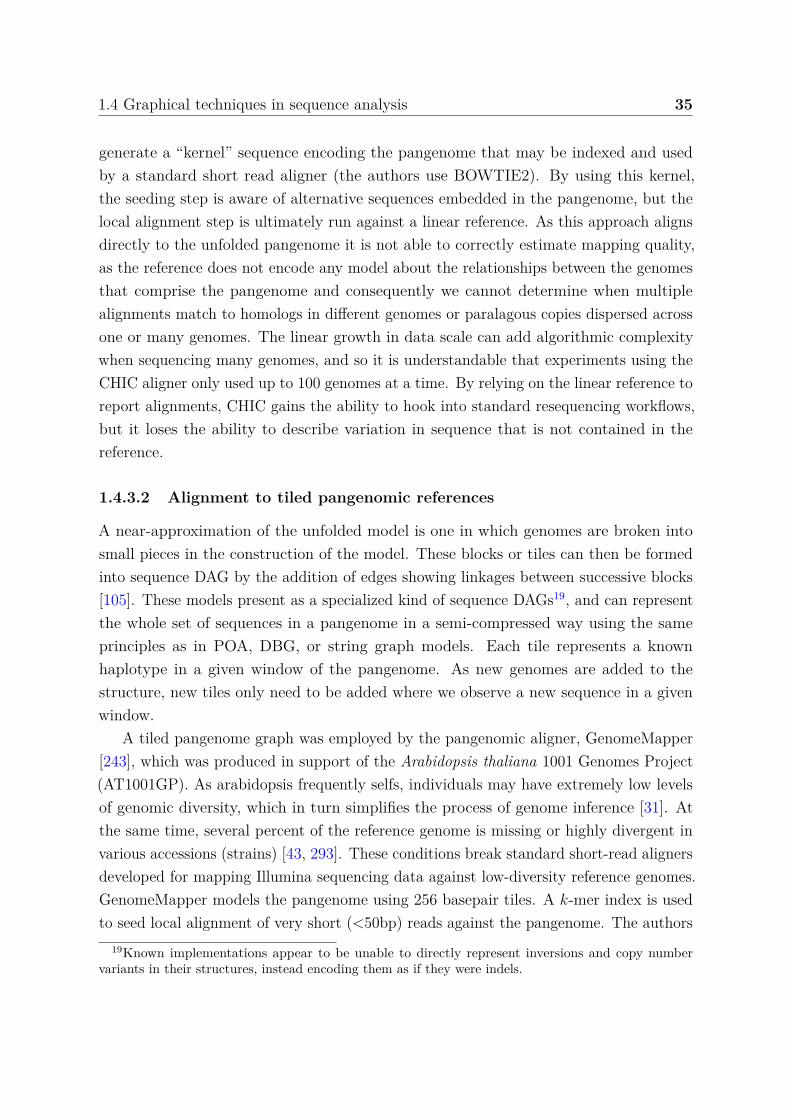
1.4 Graphical techniques in sequence analysis 35

generate a “kernel” sequence encoding the pangenome that may be indexed and usedby a standard short read aligner (the authors use BOWTIE2). By using this kernel,the seeding step is aware of alternative sequences embedded in the pangenome, but thelocal alignment step is ultimately run against a linear reference. As this approach alignsdirectly to the unfolded pangenome it is not able to correctly estimate mapping quality,as the reference does not encode any model about the relationships between the genomesthat comprise the pangenome and consequently we cannot determine when multiplealignments match to homologs in different genomes or paralagous copies dispersed acrossone or many genomes. The linear growth in data scale can add algorithmic complexitywhen sequencing many genomes, and so it is understandable that experiments using theCHIC aligner only used up to 100 genomes at a time. By relying on the linear reference toreport alignments, CHIC gains the ability to hook into standard resequencing workflows,but it loses the ability to describe variation in sequence that is not contained in thereference.

1.4.3.2 Alignment to tiled pangenomic references

A near-approximation of the unfolded model is one in which genomes are broken intosmall pieces in the construction of the model. These blocks or tiles can then be formedinto sequence DAG by the addition of edges showing linkages between successive blocks[105]. These models present as a specialized kind of sequence DAGs19, and can representthe whole set of sequences in a pangenome in a semi-compressed way using the sameprinciples as in POA, DBG, or string graph models. Each tile represents a knownhaplotype in a given window of the pangenome. As new genomes are added to thestructure, new tiles only need to be added where we observe a new sequence in a givenwindow.

A tiled pangenome graph was employed by the pangenomic aligner, GenomeMapper[243], which was produced in support of the Arabidopsis thaliana 1001 Genomes Project(AT1001GP). As arabidopsis frequently selfs, individuals may have extremely low levelsof genomic diversity, which in turn simplifies the process of genome inference [31]. Atthe same time, several percent of the reference genome is missing or highly divergent invarious accessions (strains) [43, 293]. These conditions break standard short-read alignersdeveloped for mapping Illumina sequencing data against low-diversity reference genomes.GenomeMapper models the pangenome using 256 basepair tiles. A k-mer index is usedto seed local alignment of very short (<50bp) reads against the pangenome. The authors

19Known implementations appear to be unable to directly represent inversions and copy numbervariants in their structures, instead encoding them as if they were indels.

1.4 Graphical techniques in sequence analysis 36

report an extension of the Needleman-Wunsch alignment algorithm that allows alignmentagainst the graph wherein the graph traversal is converted into a tree of alignmentsby duplicating the alignment process at each furcation. This alignment algorithm isexponential in the average number of forks per sequence base, which may contribute tothe observation that it runs hundreds of times slower than standard alignment methodson 100bp reads [170]. GenomeMapper does not have a graph-specific alignment format,and instead reports alignments against the genome to which each is most similar, whichthe authors call “reference free”. So that the alignments may be used downstream instandard approaches, they may be projected against another chosen reference genome.

1.4.3.3 Alignment to graphical assembly models

In order to report their results relative to the reference, assembly methods require theability to align the reference genome into the sequence graph they have generated denovo [120, 254], although this can be achieved through the alignment of the assemblygraph’s unitigs to the reference genome [155], which results in greater sensitivity to smallvariation but may also increase bias towards the reference genome. Aligning externalsequence to an assembly graph is equivalent to extending the assembly to include thesequence and recording the path through the assembly graph that represents it.

The de Bruijn Graph Aligner (deBGA) inverts this approach by enabling the alignmentof short reads to a reference DBG (RdBG) [170]. An RdBG is a compacted DBG in whichone or more reference genomes have been embedded, and the authors of deBGA enablealignment against it through a k-mer index that is used to drive a kind of MEM-basedseed and extend alignment. The alignment process itself attempts to link patternsof k-mer hits in unitigs in the graph into larger alignments, finally producing a localalignment by applying Smith-Waterman-Gotoh to the read and the particular referencegenome region to which it aligns. While deBGA uses a DBG to structure alignment,it can output a BAM file against the linear reference genome for use in variant callingor other analyses. The authors claim that deBGA is fast and, thanks to its use of aDBG-based index, robust to alignment problems introduced by repeats. However, it isnot clear how the method develops mapping qualities, and due to its inability to representevolutionary homology or equivalence between regions of genomes, this would appear tobe is a significant limitation of the reference data structure they have chosen.

deBGA is the first published method specifically designed to align short reads againstarbitrarily-structured graph genomes. While deBGA was designed to work on collectionsof linear references, the authors note that it would also be possible to apply the indexingstrategy to any sequence graph, as k-mer enumeration may be used to convert any

1.4 Graphical techniques in sequence analysis 37

sequence graph into a DBG20 The authors do not evaluate its operation on genericDBGs, and instead compare it to linear reference based aligners on the same collectionsof genomes.

1.4.3.4 Genotyping using a sequence DAG

Variant calls in the VCF format, when combined with the reference genome to whichthey refer, form a sequence DAG that encodes all the genomes from which the calls werederived as well as novel recombinations between them. As this feature of variant callswas appreciated, it led to the development of several methods which first map readsglobally to a linear reference and then realign them locally to a variation-aware reference.This can be shown to reduce reference bias, but it can only do so in a localized sense asthis form of graph resequencing cannot change the global placement of reads.

By the final phase of the 1000GP [45] it was apparent that indels and complexvariation were more difficult to genotype than SNPs. Their significance was appreciatedby 1000GP subprojects that examined the putative functional effects of such variants[36], which motivated efforts to develop a high-quality variant set including them for thefinal release. The best-performing methods for generating the SNP genotype likelihoods(GLs) were only able to model biallelic SNPs [283], and additional methods would beapplied to derive GLs for non-SNP, non-biallelic variant types.

While participating in the project, Deniz Kural and I extended (as glia21) a POAalgorithm he had developed to realign poorly-mapped reads (such as those with softclips,many mismatches, gaps, or unaligned fragments anchored by their pair mates) to asequence DAG created from the reference and candidate alleles in the region. Byprojecting the alignment back into the reference space, we were able to generate a BAMoutput from glia. I implemented improvements to freebayes that allowed it to genotypealleles represented by observations in these alignments, as well as contamination estimatesthat were essential to high-quality GLs in low-coverage data. This pipeline outperformedalternatives, and was ultimately used to generate GLs for all non-SNP variation in theproject.

The indels were integrated into the phased scaffolds provided by the SNPs through twocycles of genotyping. In the first, GLs generated by the method were given to MVNcall[184], a multalleleic, site-independent phasing algorithm that can phase genotypes ata given site onto a fixed background haplotype scaffold. The posterior genotype and

20Jouni Sirén and I had implemented an aligner based on a DBG transform of an arbitrary sequencegraph at the time of deBGA’s publication. The authors of deBGA were apparently as unaware of ourwork as we were of theirs.

21https://github.com/ekg/glia

1.4 Graphical techniques in sequence analysis 38

phasing quality estimates produced by MVNcall, along with a number of other metricsrelated to indel sequencing error such as sequence entropy and homopolymer context,were then used to establish a support vector machine (SVM) classification model whichwas trained using data from high-quality genomes and applied to the full set of alleles toremove likely errors. The final set of alleles were fed back through the glia, freebayes, andMVNcall process to ultimately produce the set of indels in the 1000GP phase 3 release.

Hannes Eggertson’s GraphTyper [71] implements a similar workflow to the genotypelikelihood generation method applied to the 1000GP indels. In the GraphTyper pipeline,Illumina reads are aligned against the reference genome using a standard short readaligner. Those alignments with soft clips and apparent differences from the reference arematched to a sequence DAG built from the reference and VCF in a window around theread’s candidate mapping location. GraphTyper matches short k-mers between the readand the sequence DAG using a k-mer index of the reference structure and 1bp-overlappingk-mers from the read. This does not produce an alignment per se, but rather a listof variant traversals supported by each read. This transformation provides sufficientinformation to genotype the variants in the graph. The pipeline may update its referencesystem so that it includes both known variation from other studies and new variationdiscovered during analysis. GraphTyper uses the graph reference system internally toimprove algorithm performance, but results are projected into the linear reference and thegraph has no other representation than VCF. This prevents the representation of “nested”variation or non-SNP or indel SVs. GraphTyper’s efficient and accurate performance onexceptionally large resequencing problems supports the authors’ design decisions andfirmly asserts the utility of the graph realignment approach.

Sibbesen and colleagues generalize the genotyping problem to arbitrary variationgraphs with BayesTyper [249]. They adopt a kind of pseudoalignment model in whichexact k-mer matches between a read set and the reference are used to establish support forpaths across bubbles in the variation graph. These can then be used to build probabilisticmodels of genotypes for any kind of variation represented in the graph, both small (SNPsand indels), including nested variation.

1.4.3.5 Population reference graphs

Pangenomic references need not be used as a coordinate system in the same manner asthe linear reference genome. Instead, they can be used as a prior to infer most-likelyunderlying haplotypes of a given individual. Further refinement can be achieved byaligning the read set back to the inferred haplotypes. This approach makes sense if

1.4 Graphical techniques in sequence analysis 39

alignment against the pangenome is extremely costly, but efficient haplotype inferencepatterns can be applied to the genome.

Population reference graphs (PRGs) [63] are POA-like graphs in which sequencesaligned by MSA are collapsed in the case of identity above a given k-mer size, whichembeds some information about local phasing into the graph. First assembled fromlong sequences, the PRG is then augmented with local variation information, with SNPsand indels added to all paths at appropriate positions. Dilthey and colleagues developa genome inference model based on the comparison of the PRG to a DBG built fromreads from a given individual. By comparison between these two structures, weightedby k-mer frequency in the genome and PRG, they provide sufficient annotations to thePRG to run an HMM on the graph to infer the most-likely underlying pair of haplotypes.Short read alignment can be used to map the full reads back to these haplotypes in anad hoc manner in order to find new small variation against them and fully resolve theirsequences. The authors demonstrate that this method can be applied to the humanMHC, where high sequence diversity frustrates methods optimized for typical regions ofthe human genome.

1.4.3.6 Succinct pangenomic sequence indexes

Generalizations of the FM-index to support indexing of sequence DAGs, or equivalentlyregular languages, yielded a number of short read to sequence graph aligners. Suchmethods enable pattern matching against pangenome graphs in much the same way asdone by FM-index based short read aligners.

The Generalized Compressed Suffix Array (GCSA) [257, 258] enables pattern matchingagainst arbitrary finite regular languages. It indexes a reverse-deterministic automaton22

that encodes the sequence DAG implied by a VCF and reference genome. To enablepath queries, it builds the BWT based on the sorted prefixes of the language encoded inthe automaton, adding support structures that allow pattern search as in an FM-index.Additional support bitvectors akin to those used to encode and index labeled trees [82]allow the traversal of the sequence DAG during query matching. Sirén constructs theindex using the prefix-doubling method used to construct sorted suffixes, wherein prefixesand their starts and ends may be extended from length L to 2L through a sort and joinoperation. Because it indexes a memoryless automaton and the construction requires theenumeration of all the prefixes of the automaton, GCSA suffers from exponential costs inindex generation in the order of the number of possible recombinations represented in the

22Reverse determinization ensures that each prefix of this automaton can only have a single startingposition.

1.4 Graphical techniques in sequence analysis 40

sequence DAG. Careful curation of the pangenome allows the construction of the GCSAfor the entire human genome in the memory of an available computer (1TB), providedthe construction is broken into chromosomes and local complexity in the input sequenceDAG is reduced. Experiments with the GCSA used backtracking search as in BWA [158]to directly align reads with differences from the indexed graph, but the method was notdeveloped into a full-featured short read alignment method.

Alternative schemes make no fundamental change to the CSA/FM-index model, butrather embed information about particular kinds of pangenome graphs into the sequencethat is indexed. BWBBLE [113] encodes SNPs by extending the reference alphabet toinclude ambiguity codes which match more than one DNA base. To encode indels, itextends the reference by adding a sequence for each indel which includes the non-referenceallele and the surrounding 2l bases of the reference. The resulting index can supportqueries of up to length l. A mapping between the positions in the extended reference andthe original reference sequence space is used to project alignments from the extendedreference to the base reference. This approach is simple and allows for a linear-timeindexing of the pangenome, but the added complexity of the extended reference andlarger alphabet required to represent SNPs yield a query time that is 100-fold slowerthan the backtracking BWA method [113].

In gramtools [172], a particular kind of sequence DAG is indexed in a large-alphabetCSA based on wavelet trees [104].23 Maciuca and colleagues develop an encoding for asequence DAG in which bubbles may not have any deeper internal structure, and anytraversal across a bubble is required to contain sequence. Effectively, bubbles contain anumber of alternate alleles that may be represented as linear sequences, and conveniently,this kind of graph is exactly that which is used in VCF. To build its vBWT index ofthe graph, gramtools linearizes the alt-bubble sequence DAG into an integer vector (the“linear PRG”) in which DNA bases are represented normally while the structure of eachbubble is encoded as a series of alternate alleles delimited by i, flanked by delimiters i−1.Each bubble gets a unique even integer i, requiring the use of alphabets with millions ofsymbols. A CSA-based FM-index is then built from the linear PRG. The use of a uniquepair of integers for each bubble ensures that the alleles in the bubble will be sortedtogether in the CSA of the linear PRG. To support direct matching to the sequence DAG,the standard backwards search algorithm is augmented to consider the alternate alleles

23Wavelet trees reduce the representation of a large alphabet of size Σ into a tree of O(log Σ) bitvectorsthat recursively partition the sequence space into each character. These bitvectors may be compressedefficiently while maintaining accessibility, and by augmenting them with rank and select supports theentire structure can be used to determine the number of each class of character before a given position,or select the ith of a given character. This allows for the implementation of LF mapping on a CSArepresented in a large alphabet.

1.4 Graphical techniques in sequence analysis 41

when it encounters an odd integer greater than 4 (the alphabet space allocated to DNAsequence encoding). On encountering a bubble, the search algorithm adds new suffixarray intervals for each alternate allele to a heap of intervals that are extended togetherat each step. As this scheme results in an exponential increase in the number of suffixarray intervals as a query traverses multiple variants, the input set of alleles must bestructured in a way to reduce the density of bubbles. In their experiments the authors setan allele frequency threshold and merge alleles within a certain window size into largerhaplotype alleles24. It is perhaps due to this exponential factor that gramtools’ queryperformance is many times slower than BWBBLE and around 1000 times slower thanbwa mem on a linear version of the same reference [172]. In effect, the method tradesexponentially expensive construction for exponentially expensive queries. Gramtools doesnot implement any local alignment model, and to demonstrate the method’s conceptualutility, the authors apply it to infer the most-likely linear genome for a given query set,to which the read set is ultimately mapped using a standard aligner.

HISAT2 implements variation-aware alignment against human genome scale graphs,including alignment to RNA splicing junctions [137]. Its hierarchical GFM-index structureallows seeding alignments against sequence DAGs. To find seeds globally, it uses animplementation of the generalized compressed suffix array (GCSA) [257]. It buildsthe global index including common short SNPs and indels. Then a set of local GCSAindexes are used to allow fast search of the splice graph and determination of candidatesplicing junctions even when supported by minimal evidence in the read. HISAT2 is animportant point of reference as a scalable and mature implementation of sequence tograph alignment, and is presently the only widely-used aligner based on the GCSA index.Like other methods, HISAT2 writes BAM alignments resulting from the expression ofalignments to the sequence graph against the linear reference genome. Unlike the otherpangenomic aligners, HISAT2 can achieve very high throughput, and is competitive withstandard short read aligners even when considering splicing and small variants.

Sirén’s more recent work on this topic has produced GCSA2 [256]. This modelremoves the automaton reverse-determinization step, allowing the index to be built ontop of any kind of graph. GCSA2 indexes a DBG generated from a bidirectional sequencegraph in which nodes retain both k-mer identity and their starting and ending positionalcontext in the graph. This positional information is used to drive the prefix doubling steprequired to build the BWT of the DBG. The space requirements of GCSA are avoidedby terminating the prefix doubling at a length appropriate to accommodate queries

24The algorithm used to convert the input VCF into the haplotype bubble form appears to be similarto vcfgeno2haplo in vcflib: https://github.com/vcflib/vcflib/blob/master/src/vcfgeno2haplo.cpp.

1.4 Graphical techniques in sequence analysis 42

of interest, which in practice is limited to 256bp. By computing the longest commonprefix array (LCP) of its sorted suffixes, GCSA2 encodes the implied suffix tree, whichsupports MEM-based seed generation algorithms for efficient and sensitive alignmentagainst variation graphs.

1.4.3.7 Mapping to k-mer based pangenome indexes

A k-mer index is trivial to build from a graph: one just needs to be able to enumerateor sample k-long walks through the graph and link the graph position to the k-mer inan efficient hash table or other kind of index. The size of the index can be reducedby sampling k-mers in some pattern. This indexing strategy was used in an earlyversion of vg, which supported experiments by the GA4GH-DWG [203] oriented atunderstanding the utility of various graphs constructed for a set of loci where GRCh38encoded alternative sequences. This same indexing technique is used by a proprietarymethod developed by members of the GA4GH-DWG from Seven Bridges Genomics Inc.(SBG) [223]. The SBG graph aligner’s (SBGA) input is constructed from higher-frequencyvariants found in various public variation resources. It masks out regions of high alleliccomplexity and builds a reference-rooted edge-labeled sequence DAG to serve as analignment target. To enable graph mapping it builds an index of spaced k-mers bywalking short segments of the graph. The k-mers and their locations are used as seeds toestablish mapping candidate loci. A local alignment is obtained for each candidate, andthe output is transformed into the reference space as BAM.

Curiously, to align the reads to the graph locally SBG’s aligner does not use a methodlike POA, and instead uses a kind of local backtracking exact matching against the treeof paths through the local graph which has exponential complexity with respect to thedensity of variation. If the variant density and read error rates are kept low, this schemeallows SBGA to achieve extremely high read throughput, equivalent to that of bwa memwithout any apparent loss in accuracy on the linear reference. In this context the authorsdemonstrate their method can significantly (although slightly) improve sensitivity toknown indels. However, the method is not adaptable to other graph types or sequencingcontexts, with reports from users indicating high increases in runtime with increased readerror and variant density. Due to the fact that SBGA is closed source and proprietary itis not possible to appreciate exactly why.

1.5 Overview and objectives 43

1.5 Overview and objectivesResolving the genome of a sample de novo requires sequencing and assembly. Standardapproaches to assembly are built on graphical models that allow for ambiguity, and outof this system they attempt to derive a set of contigs which represent the true haplotypesof the genome. When we have already assembled a genome related to the one we wish toinfer, we can describe our new sample in terms of a reference genome, with ambiguityand variation represented only in the alignments of the new sequences where they canbe mapped to the reference genome. This reduces the cost of sequencing, as we caninfer much of the genome using lower sequencing coverage and shorter reads, but it alsoexposes resequencing based genome inference to reference bias, which is a distortion ofinferred genomes towards the sequence of the reference genome.

I posit that by extending the reference genome to be a pangenome with a graphicalrepresentation, we can enable population aware resequencing that avoids reference biasto any particular linear reference. The model I develop, the variation graph, extendsthe bidirectional sequence graph models used in assembly to support the labeling ofpaths through the graph, and allowing the representation and relation of linear referencesystems within itself.

Variation graphs are related to a wide array of graphical models used in bioinformatics.They have similarity with string graphs, multiple sequence alignments, and whole genomealignment graphs. This indicates that they could serve as a unifying basis for manydomains of sequence analysis which have traditionally been separated by methodologicaldifferences, such as assembly and variant calling.

Recently, several methods have been published which provide variation-aware align-ment or genotyping based on sequence DAGs built from population resequencing. Thesemethods demonstrate the difficulty of the problem of generalizing resequencing to graph-ical reference systems at the multi-gigabase scale of vertebrate genomes. In virtuallyall cases, they use a graph reference model internally, but express their results in termsof a linear reference genome, producing BAM alignments or genotyping results in VCFformat. None implement a generic strategy to work with a graphical model equivalentto the variation graph. The method I develop, vg, is not the first pangenomic aligner,but it is the first that models its results in terms of the pangenome itself, enabling fullresequencing analyses to be completed within the graphical model.

In the following chapters I will precisely define the variation graph and associateddata models that allow representing all kinds of resequencing data types in the context ofa variation graph. Then I will describe the algorithms implemented in vg that enable theuse of variation graphs as a basis for genome analysis, including their construction from

1.5 Overview and objectives 44

many data sources, serialization and visualization. I will present indexing methods thatsupport the queries needed to enable resequencing, and I will provide algorithms thatimplement efficient read alignment to large scale graphs. Finally, I will cover applicationsof the method I developed. I will show that vg is applicable to a wide range of genomicinference problems, with a particular focus on the quality of alignment of both short andlong sequence reads against variation graphs constructed from all kinds of sources.

Throughout this work I use the first person singular “I” to refer to work that Icompleted alone, while the plural “we” where presenting work completed in collaborationwith others. Wherever possible, I clarify the nature of the collaboration and identify mycollaborators.

Chapter 2

Variation graphs

Variation graphs (VGs)1, previously introduced in section 1.3.2, combine a bidirectionalsequence graphs with paths that model sequences as walks through the positional spaceof the graph. They link graphical models and linear sequence models. This allows themto be used to model the relationships between collection of sequences, including allvariation contained therein. The encapsulation of these two divergent ways of modelingabout bioinformatic data systems allows them to bridge traditionally isolated analysismodalities.

In this chapter, I will articulate the variation graph model and lay out the algorithmsand data structures that enable its use as a reference system in pangenomic resequencing.First I will provide formulations for the graph, its paths, edits, alignments, and genotypesdefine within it. Then I will present algorithms that induce the variation graph fromdifferent data models introduced in the previous chapter. I describe the serializationtechniques used to exchange variation data via computer files or network connections. Idevelop index structures to enable queries of the graph’s topology, sequence, and pathspaces, and algorithms to derive optimal alignments to the graph. Understanding variationgraphs requires techniques to visualize them, and I will present various approaches, eachwith particular advantages and drawbacks. Working with variation graph referencesnecessitates a number of graph-modifying operations, including augmentation, sorting,pruning, and bubble simplification. Finally, I will discuss how variation graphs can providenormalized basis spaces for the analysis of pangenomes, such as through various projectionsof alignment sets and the graph including coverage maps, ultrabubble decomposition,and haplotype matching.

1I will refer to variation graph as VG, and to the software implementation of the VG model vg

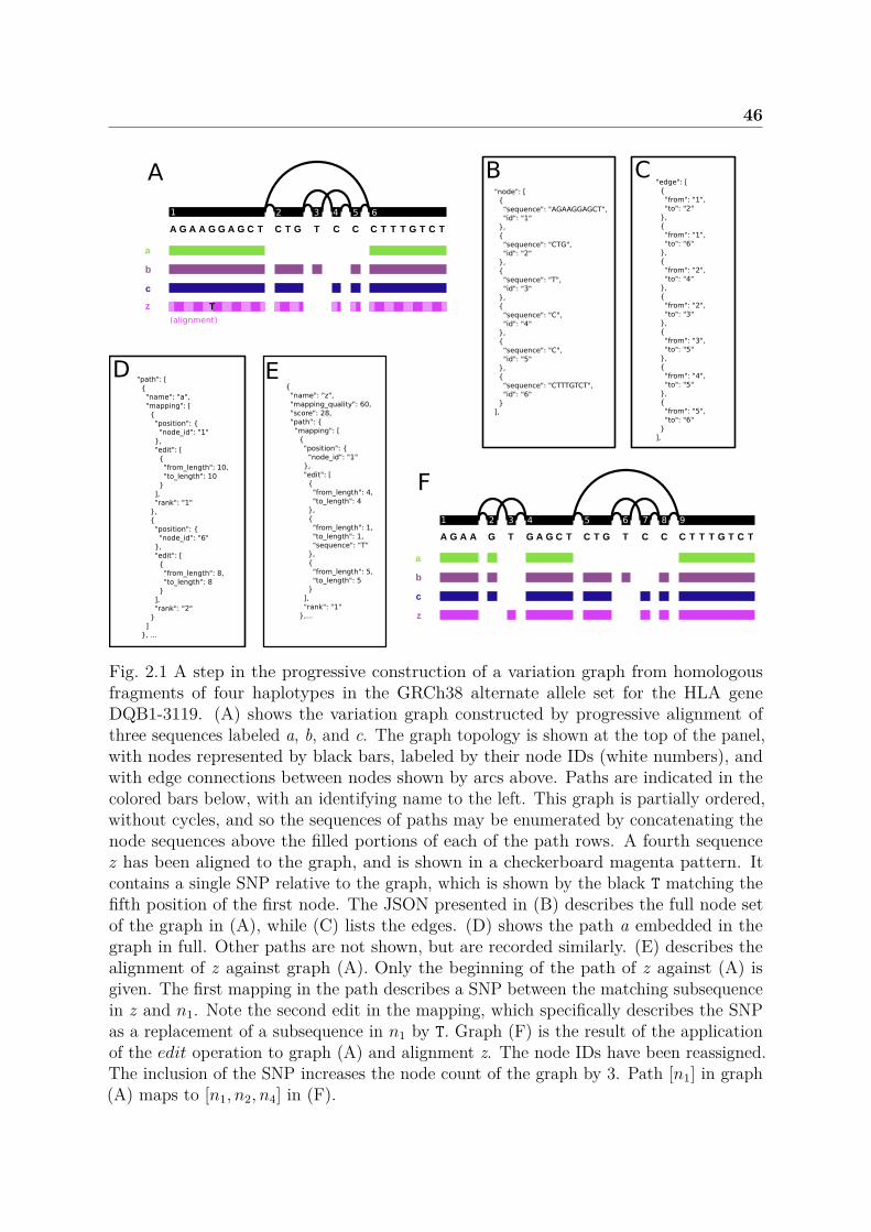
46

1 2 3 4 5 6

(alignment)

A "node": [ "sequence": "AGAAGGAGCT", "id": "1" , "sequence": "CTG", "id": "2" , "sequence": "T", "id": "3" , "sequence": "C", "id": "4" , "sequence": "C", "id": "5" , "sequence": "CTTTGTCT", "id": "6" ],

B "edge": [ "from": "1", "to": "2" , "from": "1", "to": "6" , "from": "2", "to": "4" , "from": "2", "to": "3" , "from": "3", "to": "5" , "from": "4", "to": "5" , "from": "5", "to": "6" ],

C

"path": [ "name": "a", "mapping": [ "position": "node_id": "1" , "edit": [ "from_length": 10, "to_length": 10 ], "rank": "1" , "position": "node_id": "6" , "edit": [ "from_length": 8, "to_length": 8 ], "rank": "2" ] , ...

D "name": "z", "mapping_quality": 60, "score": 28, "path": "mapping": [ "position": "node_id": "1" , "edit": [ "from_length": 4, "to_length": 4 , "from_length": 1, "to_length": 1, "sequence": "T" , "from_length": 5, "to_length": 5 ], "rank": "1" ,...

E

1 2 3 4 5 6 97 8

F

Fig. 2.1 A step in the progressive construction of a variation graph from homologousfragments of four haplotypes in the GRCh38 alternate allele set for the HLA geneDQB1-3119. (A) shows the variation graph constructed by progressive alignment ofthree sequences labeled a, b, and c. The graph topology is shown at the top of the panel,with nodes represented by black bars, labeled by their node IDs (white numbers), andwith edge connections between nodes shown by arcs above. Paths are indicated in thecolored bars below, with an identifying name to the left. This graph is partially ordered,without cycles, and so the sequences of paths may be enumerated by concatenating thenode sequences above the filled portions of each of the path rows. A fourth sequencez has been aligned to the graph, and is shown in a checkerboard magenta pattern. Itcontains a single SNP relative to the graph, which is shown by the black T matching thefifth position of the first node. The JSON presented in (B) describes the full node setof the graph in (A), while (C) lists the edges. (D) shows the path a embedded in thegraph in full. Other paths are not shown, but are recorded similarly. (E) describes thealignment of z against graph (A). Only the beginning of the path of z against (A) isgiven. The first mapping in the path describes a SNP between the matching subsequencein z and n1. Note the second edit in the mapping, which specifically describes the SNPas a replacement of a subsequence in n1 by T. Graph (F) is the result of the applicationof the edit operation to graph (A) and alignment z. The node IDs have been reassigned.The inclusion of the SNP increases the node count of the graph by 3. Path [n1] in graph(A) maps to [n1, n2, n4] in (F).

2.1 A generic graph embedding for genomics 47

2.1 A generic graph embedding for genomicsWe define a variation graph to be a graph with embedded paths G = (N, E, P ) comprisinga set of nodes N = n1 . . . nM , a set of edges E = e1 . . . eL, and a set of paths P = p1 . . . pQ,each of which describes the embedding of a sequence into the graph. By generalizing thesepaths to support edits against the graph, we provide a mechanism to describe relationsbetween the graph and other sequences. Augmenting the path with additional informationimportant to sequence analysis allows us to construct an alignment. Collections of pairsof paths covering the space of two graphs describe a graph to graph alignment, ortranslation which can be generated when the graph is edited, to allow for the projectionof coordinates and sequences in one graph into the space of the other. A limited formof this translation is a genotype, which maps the implied bubble formed across multiplecopies of a homologous locus into the space of the graph. Collections of genotypes arethe primary output of resequencing. Phasing algorithms extend genotypes into longerphased haplotypes, which we record as paths through the graph. These data models thusprovide a sufficient informational basis for resequencing against variation graphs.

2.1.1 The bidirectional sequence graph

Each node ni represents a sequence seq(ni) that is built from an alphabet Σ = A, C, G, T, N.Nodes may be traversed in either the forward or reverse direction, with the sequence beingreverse-complemented in the reverse direction. We write ni for the reverse-complementof node ni, so that seq(ni) = revcomp(seq(ni)). Note that ni = n. For convenience, werefer to both ni and ni as “nodes”.

Edges represent adjacencies between the sequences of the nodes they connect. Thus,the graph implicitly encodes longer sequences as the concatenation of node sequencesalong walks through the graph. Edges can be identified with the ordered pairs of orientednodes that they link, so we can write eij = (ni, nj). Edges also can be traversed in eitherthe forward or the reverse direction, with the reverse traversal defined as eij = (nj, ni).VGs can contain ordinary cycles (in which ni is reachable from ni), reversing cycles (inwhich ni is reachable from ni), and non-cyclic instances of reversal (in which both ni andni are reachable from nj).

The bidirectional sequence graph underlying the variation graph model is illustratedin panels A, B, and C of figure 2.1.

2.1 A generic graph embedding for genomics 48

2.1.2 Paths with edits

We implement paths as an edit string with respect to the concatenation of node sub-sequences along a directed walk through the graph. We do not require the alignmentdescribed by the edit string to start at the beginning of the sequence of the initial node,nor to terminate at the end of the sequence of the terminal node. To allow the pathmodel to support differences from the graph, each path is composed of a series of nodemappings pi = m1 . . . m|pi| which are semantically identical to the alignment formatused by standard aligners. Each mapping mi = (bi, ∆i) has a starting position encodedas a node and offset in the graph bi = (nj, oi) and a series of edits ∆i = δ1 . . . δ|mi|.Edits δi = (fi, ti, ri) represent a length fi in the graph node nj (a “from length” in thereference), a length ti in the sequence the path encodes (a “to length” in the query), andan additional sequence ri that would replace the sequence at the given position in thereference in order to transform it into the query. In the case of exact matches, we allowthe replacement sequence ri to be empty.

Alignments are often described in terms of matches, mismatches, and indels. Weencode matches when fi = ti ∧ ri = ∅, single mismatches when fi = ti = 1 ∧ ri = ∅,deletions when fi > 0 ∧ ti = 0 ∧ ri = ∅, and insertions when fi = 0 ∧ ti > 0 ∧ ri = ∅. Aspaths are described by a series of mappings with independent positions, they can representall kinds of structural variation relative to the graph. When mapping positions are alwaysat the start of a node, the edit set for the path contains only matches, and the edgestraversed by the path are all present in the graph2, we say that the path is embedded. Thepaths from which we construct the variation graph are fully embedded, and in practicepaths that contain differences occur only in the alignment of new sequences into thegraph.

The example variation graph in figure 2.1 panel A contains several paths, while panelD explicitly describes a portion of one of the paths using an equivalent model to the onedescribed here.

2.1.3 Alignments

Auxiliary read information is important when analyzing collections of DNA sequencingdata sets. Each read has a name, and an identity related to a particular sequencingexperiment. It may be related to a particular genomic sample or individual. DNAsequence reads themselves result from a previous set of analyses run on raw observations

2Note that paths may contain disjoint mappings that are not connected by edges in the graph, whichallows them to represent structural variations.

2.1 A generic graph embedding for genomics 49

derived from DNA, perhaps fluorescence or current traces or images. The process ofcollapsing this raw information into the sequence read yields a confidence in addition toa base call. These are recorded in a quality string in FASTQ. The need to collect thisinformation has resulted in the development of the SAM/BAM sequence alignment format,which provides a standard for linking the called bases (sequence), quality information,read name, features of the alignment against a reference genome and additional optionaltyped annotations.

I follow this same model in developing an alignment format for read alignmentsto the graph. An aligned set of sequences Q, A = a1 . . . a|Q|, represents a sequencingexperiment. Each aligned read connects a sequence, an (optional) quality string, apath through the graph including possible edits, and an optional set of Di annotations:ai = (si, qi, pi, k1 . . . kDi

). In principle the read sequence can be reconstructed from thepath, but retaining the sequence information makes the alignment object lossless withrespect to the input FASTQ and provides redundancy which can help in data processing.

Panels A and E of figure 2.1 demonstrate how an alignment to a variation graph canencode putative variation, in this particular case encoding a SNP.

2.1.4 Translations

A generalization of the alignment is the translation set Φ = ϕ1 . . . ϕ|Φ|, which relates pathsin different graphs to describe the mapping between them. A translation ϕ = (pf , pt)defines the projection between two paths which may arise in the context of two graphsGf and Gt. In this use each pf corresponds to a path relative to Gf (conventionally thebase or reference graph), and each pt to some path in Gt.

If each node and edge and path in both graphs is represented in some graph translationin Φ then it provides an isomorphic relationship between the graphs. Provided eachΦ encodes an isomorphism, then we can layer a series of Φi together to provide acoherent coordinate space across any number of updates to a given graph. Consider afunction pattern translate, which allows the projection of paths relative to Gf throughtranslations Φ to yield paths in Gt: translate(pi, Φ)→ pj ∈ Gt, and similarly allows thetransformation of a base graph into a target graph: translate(Gf , Φ)→ Gt. If we have aseries of (Gi, Φ1) . . . (Gρ, Φρ), where translate(Gi, Φi)→ Gi+1 and thus each Φi describesan isomorphism between Gi and Gi+1, then we can generate a graph translation Φ∆

providing translate(G1, Φ∆)→ Gρ. We build this graph translation with the functionlayer(Φα, Φβ)→ Φαβ by rewriting each path translation ϕi ∈ Φα so that its pt refers toGβ. We do so by projecting the pt through Φβ, and finally adding any ϕj ∈ Φβ for whichpf = ∅, as these represent insertions of new sequence in Gβ relative to Gα.

2.1 A generic graph embedding for genomics 50

2.1.5 Genotypes

As path to path relationships can provide descriptions of allelic diversity, they formthe basis for a graph-relative genotype encoding. To represent the exact genotype ofa particular sample with ploidy ν at a given locus ι we can simply collect the multisetof alleles πι = (p1 . . . pν). We could alternatively build a probabilistic model ϖ ofan unphased genotype by using a set of µ alleles p1 . . . pµ. To do so, we associatelikelihoods γξ for each possible genotype πιξ

that could be sampled from the alleles suchthat ϖ = γ1 . . . γ µ!

ν!(µ−ν)!. In practice, we develop our γξ out of quality information from

the reads and a sampling model related to ν [91, 151]. Existing genotyping models canbe applied to drive genotyping using read sets aligned to the graph, and the output ofthe genotyper is defined fully in the space of the graph.

2.1.6 Extending the graph

Given an alignment ai, we can edit the graph G so that it includes the alignment andthe sequence it represents as an embedded path, augment(G, ai)→ (G′, Φ), such thattranslate(pi, Φ) ∈ G′. To update the path space of the graph we project all paths,including that of ai, through the translation implied by the augmentation of the graphwith pi. Any other alignment aj whose path pj overlaps pi would no longer be valid,although it could be projected through the graph translation Φ as well to express it inthe space of the new graph G′. Updating the graph one alignment at a time is inefficientas we need to build and layer a new translation for each alignment. It is simpler to editthe graph in a single step, taking a collection of alignments and including them in thegraph, edit(G, A)→ (G′, Φ).

One way to accomplish this is to first take the set of unique mappings representedin the paths of A, Ω = m1 . . . m|Ω|, and for each mi cut ni at the breakpoints whereany new variation would need to be added in, adding new nodes to represent the cutportions. Then, walking through each alignment we add in unique novel sequences andtheir linkages to the preexisting nodes or new breakpoints to the graph. This processwill disrupt the identifier space of the nodes and edges of the graph, but it naturallyyields a translation that can be used as described in section 2.1.4. Both alignments andgenotypes are based on paths, so this mechanism can be used to extend the graph basedon any sequence level differences observed through alignment or variant calling.

Figure 2.1 provides an example to provide a concrete intuition about the edit function.Editing the graph in panel A with the alignment of sequence z yields the graph in panelF. The corresponding translation is described in the figure legend.

2.2 Variation graph construction 51

2.2 Variation graph constructionWe will use variation graphs as the core model for a number of essential processes ingenome inference. This model can represent many graphical sequence models used ingenomics. Each one necessitates conversion into the variation graph model. Here I describethe transformation of a number of graphical models into variation graphs, includingMSAs, assembly graphs, and alignment graphs induced from pairwise alignments. Insome cases the conversion is direct, but in others it requires the addition of new labels toour model. Variation graphs may also be built from first principles, provided a functionthat aligns a sequence into the graph and the editing operations described in 2.1.6.

2.2.1 Progressive alignment

If we have a series of k queries q1 . . . qk, then we can build a progressive alignment by aseries of edit and alignment operations applied to the variation graph. First, take theempty graph G∅, to which any alignment will yield a path p1 that has no mappings andwhich encodes the query sequence q1 as a replacement sequence in the path. We thenedit the graph to add the sequence using edit(G∅, p1)→ G1. For each subsequent qj weobtain the next graph by finding the alignment align(qj, Gj)→ pj and editing the graphwith it to yield the next graph edit(Gj, pj)→ Gj+1 until j = k and we obtain our finalgraph. This simple approach is attractive as it allows the variation graphs to be builtfrom whole sequences using only techniques that are native to the variation graph modelitself. However, it is obviously order dependent, with potentially different results if theset of input sequences are presented in different orders. I later presents results based onthis multiple sequence to graph alignment process, vg msga.

2.2.2 Using variants in VCF format

As discussed in section 1.4.3.4, the VCF format that is popular in resequencing impliesa sequence DAG. We can consider how to build a trivial variation graph using thecore operation edit. First, we build a variation graph from the reference genome Qref

: Gref. This graph contains one path pref : seq(pref) = Qref. As described in section2.1.5 each locus reported in VCF can be encoded as a set of paths Pvcf = p1 . . . pV ,each representing a different allele. We now edit the graph to embed these allele paths,edit(Gref, Pvcf) → Gvcf. It is possible to regenerate the VCF file input by walking thepositions of pref and enumerating the overlapping paths as alleles in VCF format.

2.2 Variation graph construction 52

For efficiency, we have not implemented VCF to variation graph conversion withspecifically this algorithm, but instead build up Gvcf by walking along the referencegenome Qref and processing each locus sequentially. This exploits the partially orderedproperty of the VCF to limit memory requirements. For regions before, after, andbetween variant records at reference offsets i and j we add a node ncurr : seq(ncurr) =substr(Qref, i, j), linking these by edges to those nodes ending at position i of thereference and adding corresponding mappings for the reference path to pref. At simplevariant sites we add each of the alleles as a new node nvari

, including an edge for eachecurr≺vari

. Here we also handle the reference allele differently in that we append amapping mref = ((nref, 0), ∅) to pref.

As long as the VCF records are ordered, this process allows for streaming conversionof the VCF format into a variation graph. However, VCFs used to represent structuralvariation often do not describe a fully-ordered series of loci. For instance, a large deletionmay be described in one record, and followed by a number of records describing variationon the reference within the scope of the deletion. In the graph, this results in the nestingof bubbles, and requires a deviation from a simple streaming algorithm in order to behandled. Deletions must be recorded and linked into the downstream portion of thegraph as it is later generated.

VCFs may also encode phased haplotypes, which, like the reference, have a naturalrepresentation in the graph as paths. Parsing these may require multiple passes overthe VCF due to the memory requirements for storing large numbers of haplotypesuncompressed and cross-indexed to allow traversal in RAM. To prevent O(H|Gvcf|)growth of the required memory to store these, we implement compression strategies onthe haplotype set that exploit their repetitiveness. The VCF format does not imposea semantic requirement that the encoded haplotypes are valid, which introduces somecomplexity in the implementation of this method. We must break haplotypes where theyare found to be invalid in order to record them in VG format. For instance, a phased VCFmay report more than ν (expected ploidy) alleles for a given individual, such as whendeletion and SNP variants overlap. We expect these haplotype paths to be embeddedin the graph. Although haplotype sets are equivalent to large collections of paths, weterm their components threads to indicate that they have a simpler representation thanarbitrary paths.

2.2.3 From gene models

A reference-based RNA splicing graph is usually expressed as a set of named intervalsin BED or the General Feature Format (GFF). As with the generic VCF generation

2.2 Variation graph construction 53

algorithm, we can convert the transcripts to alignments A relative to the graph. Then wecan then embed the transcript paths in the graph edit(Gref, A)→ Gsplice. Any transcriptin our set is thus encoded by the graph, and can be matched to it directly with alignment.The resulting structure will also support novel isoforms built with splices from the knownset.

2.2.4 From multiple sequence alignments

A multiple sequence alignment in matrix form has a simple translation into a sequenceDAG and thus a VG [147]. Given a set of sequences Q = q1 . . . qκ their υ-long mutual align-ment may be described in a κυ matrix X designed to maximize ∑υ

i=1∑κ

j=1∑κ

k=1 δXijXik,

where δ is the Kronecker delta, or some generalization of this. The alphabet used toencode the matrix is the same as the input sequences with the addition of a special gapcharacter which does not match itself, and gaps thus do not contribute positivelyto the matrix score. To build a variation graph Gmsa from the MSA we proceed fromi = 1→ υ through X. For each unique character B in the query alphabet Σ \ foundin each row i, we create a node nB in Gmsa and append a mapping to each path pi forwhich nB ∈ qi. We construct the edges of Gmsa by taking the distinct pairs of consecutivenode traversals found in the path set Pmsa produced after the generation of the nodesin MSA traversal. Adding add an edge eij for each pair of nodes (ni, nj) consecutivelytraversed in Pmsa ensures that our sequences are present as walks through the graph.We can optionally compact series of nodes (which represent single characters) where nofurcations occur to obtain a simpler graph.

Instead of a matrix, we can formulate the multiple alignment as an alignment graph(described in section 1.4.2.5). By making this graph bidirectional, and thus equivalent ininformation content with the Enredo graph, it becomes equivalent to a variation graph.Aligners that produce data formats of this type, such as Cactus [212], can thus be usedto produce VGs, so long as the relationship between the input sequences and the graph isrecorded and can be converted into a path description. In section 3.1.2 I discuss the useof this method to build a pangenomic reference system for a diverse set of yeast strains.

2.2.5 From overlap assembly and de Bruijn graphs

Overlap-based sequence graphs used in assembly, described in sections 1.4.2.1, 1.4.2.2,and 1.4.2.3, are nearly identical to variation graphs. The critical difference between thesemodels and the variation graph is that they attach a label to each edge (or node) describingthe alignment between the pair of nodes (or edges) which they connect. Variation graphs

2.2 Variation graph construction 54

do not support such a feature in their basic definition, as it is unimportant for any usebesides temporarily representing overlap graphs. We call the process of transferringsequence information from the edges to the nodes bluntification.

We start by assigning the sequence of each node to be the sequence of the correspondingread. If we shorten the sequence of a node to reduce an overlap between a pair ofnodes, it will render other overlaps on the same nodes incorrect. Thus, it is essentialthat the bluntification algorithm work by the reduction of sets of overlaps on edgeswhich are transitively closed by connection to the same ends of each node, net(eij)→∀ei∗ ∈ G ∪ ∀e∗j ∈ G, considering both strands of the graph when doing so. For each netwe apply a function pinch(net(eij))→ Gpinchij

, which reduces the overlaps between thenodes in the net into a blunt-edged variation graph. We then link Gpinchij

back into therest of the graph by connecting with the inbound links to each node involved in the net.

In a de Bruijn graph or string graph as generated by SGA or Fermi2, overlaps are exactmatches and so are defined given only a length. This simplifies the implementation ofpinch, as no further computation is required to correctly determine the mutual alignmentof overlapping sequences. In contrast, overlaps in a generic string or overlap graph arecorrectly defined as alignments. Resolving a single pairwise alignment into structures inthe graph is trivial, but it becomes considerably more complex when many sequencesmap into a transitively closed set of overlaps. These nets can then be resolved into analignment graph by an algorithm similar to that given in section 2.2.6, but in practice,vg implements bluntification using a pinch graph library developed for whole genomealignment [212].

2.2.6 From pairwise alignments

A set of pairwise alignments imply a variation graph, however I know of no containedmethod that will generate the variation graph or lossless string graph from these align-ments. To explore this, I developed an algorithm to do so that operates in externalmemory, which I here present in detail. It operates by conversion of the alignment setinto an alignment graph and the subsequent use of this graph in the elaboration of thevariation graph including paths representing the input sequences. The resulting graph isa lossless representation of the input and the alignments between them. To distinguishthe approach from string graphs, which imply error correction, I call this variation graphinduction model the squish graph.

2.2 Variation graph construction 55

seqwish3 implements a lossless conversion from pairwise alignments between sequencesto a variation graph encoding the sequences and their alignments. As input, we typicallytake all-versus-all alignments, but the exact structure of the alignment set may be definedin an application specific way. seqwish uses a series of disk-backed sorts and passesover the alignment and sequence inputs to allow the graph to be constructed in lowmemory relative to the size of the input sequence set. Memory usage during constructionand traversal is limited by the use of sorted disk-backed arrays and succinct rank/selectdictionaries to record a queryable version of the graph.

As input, we have Q, which is a concatenation of the sequences from which we willbuild the graph. We build a compressed suffix array (CSA) mapping sequence names tooffsets in Q, and also the inverse using a rank/select dictionary on a bitvector markingthe starts of sequences in Q. This allows us to map between positions in the sequences ofQ, which is the format in which alignment algorithms typically express alignments, andpositions in Q itself, which is the coordinate space we will use as a basis for the generationof our graph. We encode the set of input pairwise alignments between sequences in Q

as object A. Although these alignments tend to be represented using oriented intervalpairs in Q, for simplicity and robustness to graph complexity, we describe A as a set ofpairs of bidirectional positions (sequence offsets and strands) [1 . . . |Q1 . . . Q|Q||] , suchthat A = (bq, br), . . .. We sort A by the first member (bq) of each pair, ensuring thatthe entries in A are ordered according to their order in Q.

To query the induced graph we build a rank/select dictionary allowing efficienttraversal of A, based on a bit vector Abv of the same length as A such that we record a 1at those positions which correspond to the first instance of a given bq and record a 0 inAbv otherwise. We record which bq we have processed in the bitvector Qseen which is ofthe same length as Q. This allows us to avoid a quadratic penalty in the order of thesize of the transitive closures in Q generated by pairs in A.

Now we inductively derive the graph implied by the alignments. For each base bq

in Q not already marked in Qseen, we find its transitive closure cq := bq, br1 , . . . bytraversing aligned base pairs recorded in A. We write the character of the base bq toan entry si in a vector S, then for each bc in cq we record a pair (si, bc) into N and itsreverse, (bc, si) into P . We mark Qseen for each base in each emitted cluster, so that wewill not consider these bases in subsequent transitive closures. By sorting N and P bytheir first entries, we can build rank/select dictionaries on them akin to that we built onA that allow random access by graph base (as given in S) or input base (as given in Q).

3https://github.com/ekg/seqwish

2.3 Data interchange 56

To fully induce the variation graph we need to establish the links between bases in S

that would be required for us to find any sequence in the input as a walk through thegraph. We do so by rewriting Q (in both the forward and reverse orientation) in termsof pairs of bases in S, then sorting the resulting pairs by their first element, which yieldsL = [(ba, bb), . . .]. These pairs record the links and their frequencies, which we can emitor filter (such as by frequency) as needed in particular applications. In typical use wetake the graph to be given by the unique elements of L.

Our data model encodes the graph using single-base nodes, but often downstream userequires identifying nodes and thus we benefit from compressing the unitigs of the graphinto single nodes, which reduces memory used by identifiers in analysis. We can compressthe node space of the graph by traversing S, and for each base querying the inboundlinks. Maintaining a bitvector Sid of length equal to S we mark each base at which wesee any link other than one from or to the previous base on the forward or reverse strand,or at bases where we have no incoming links. By building a rank/select dictionary on Sid

we can assign a smaller set of node ids to the sequence space of the graph.Given the id space encoded by Sid we can materialize the graph in a variety of

interchange formats, or provide id-based interfaces to the indexed squish graph. Togenerate graphs in vg or GFA format, we want to decompose the graph into its nodes(S), edges (L) and paths (P ). The nodes are given by S and Sid, and similarly we projectL and P through Sid to obtain a compressed variation graph.

2.3 Data interchangeIn vg, a schema language, Google Protocol Buffers (Protobuf), is used to define acompact description of data structures sufficient for the representation of all the requiredcomponents. One cause of this pattern was my involvement in the GA4GH-DWG atthe beginning of my thesis, which was then seeking a coherent way of describing graphgenomes4 to support pangenomic resequencing and related information exchange acrossthe internet. I implemented the schema for vg in the popular Protobuf schema language.This provided a core API on which to build vg. It also implied a set of streaming dataformats, which I implemented as a template library capable of serializing any stream ofProtobuf objects. Due to the reliance on Protobuf, the only code needed to implementreading and writing of these formats is vg schema and the stream library5. This greatly

4https://github.com/ga4gh/ga4gh-schemas5At the time of writing the schema, https://github.com/vgteam/vg/blob/master/src/vg.proto and

stream parsing library https://github.com/vgteam/vg/blob/master/src/stream.hpp total around 1000 linesof code, and are sufficient to link any C++ program into the vg ecosystem.

2.4 Index structures 57

simplified the process of developing libraries for working with the variation graph datamodels. Although in practice the Protobuf data structures are slower to parse thanhandmade C-struct serializations like BAM, the amount of effort required to begin writingefficient and structured binary data formats was considerably less with the schema basedapproach. Most importantly, the schema based definition of the core data types in vghelped new developers and researchers using the system quickly appreciate the basicconcepts.

Several data formats are important to vg. In .vg format, the graph itself is serializedin non-overlapping chunks, where each edge eij is stored once in the chunk Gchunk : ni ∈Gchunk. Path mappings must have a rank that identifies their position in the path inorder to be subdivided in this way. This allows them to be read in and rebuilt even ifthey have been serialized out of order. A series of alignment objects is a sensible outputof the mapping algorithm vg map. The file format produced by writing out a series ofProtobuf alignment object serializations using the stream.hpp library is called GAM,for Graphical Alignment/Map, in analogy to SAM (Sequence Alignment/Map format).

These data models have various other equivalent serializations. The GFA format canbe used to directly encode VGs. However, GFA lacks a representation of an alignmentwith the semantics required by vg. VGs that are partially ordered can be deconstructedinto VCF files. As paths in variation graphs can be used to represent any kind of existingannotations, data providers who represent annotations across many genomes (such asENSEMBL Genomes) can build their annotation sets which were previously spread acrossmany genomes into a single one embedded in a VG. To enable this several collaborators6

have developed a Resource Description Framework (RDF) compatible version of the coreVG model.

2.4 Index structuresAs described in section 1.2.2, the large collections of read data produced by currentsequencing methods require efficient read alignment to support downstream analysis.Typically, these methods develop indexes of their reference genome, using k-mer hashtables or FM-index/CSA based data structures that support efficient arbitrary-lengthexact matching. These indexes remain static during the resequencing analysis, and canthus be designed to be very compact and to support efficient queries.

When the genome is just a linear string, distances between locations may be computedtrivially, and subsets of the sequence are simply substring operations on the vector

6Jerven Bolleman and Toshiaki Katayama among others.

2.4 Index structures 58

representing the genome, so no additional structure beyond a full text index is requiredto seed the alignment of reads to the genome. However, this situation changes in graphs,where the computation of distances is more complex and particular topologies of thegraph must be recorded and reproduced. Graph distances may be estimated using anapproximate sort and the paths embedded in the graph. However, to do so requiresefficient indexes of the path structure in the graph. Furthermore, loading the entiregraph into memory in a naïve manner can be very expensive, and effort is required tominimize the runtime costs to enable resequencing even on lower-memory commoditycompute servers.

2.4.1 Dynamic in-memory graph model

Serialized in .vg or compressed GFA format, the graph of the 1000GP is not much largerthan the uncompressed human reference genome. However, the performance-orientedimplementation of the dynamic variation graph which I developed at the beginning ofmy studies can use a hundred times this much memory when the entire graph is loadedinto RAM. In this scheme implemented in vg, indexes on the node identifier space ofthe graph allow for fast traversal and query of nodes by identity and neighborhood, aswell as insertion or deletion of nodes and edges and associated editing of paths. Variousinefficiencies are accepted, such as on the hash table occupancies used to build theseindexes, in the pursuit of higher performance during dynamic modification of the graph.I now believe that it should be easy to provide a dynamic VG in low memory by using asuccinct encoding, but I have not yet completed any work on this issue. Operating ongraphs of hundreds of millions of nodes with annotations like paths remains a difficultproblem. In most cases the graph can be subdivided (as with map/reduce processingpatterns [59] which underpin most industrial operation on large graphs [44]). This isparticularly easy to implement for sequence DAG VGs, allowing for us to work on graphsof arbitrary sizes if they are approximately linear.

2.4.2 Graph topology index

The graph is unlikely to be changed during many kinds of analysis, and so we have theopportunity to compress it into static data structures that provide efficient access toimportant aspects of the graph with low memory overhead. Specifically, we care aboutthe node and edge structure of the graph and queries that allow us to extract and seekto positions in embedded paths. We would like to be able to query a part of the graphcorresponding to a particular region of a chromosome in a reference path embedded in

2.4 Index structures 59

the graph. Similarly, if we find an exact match on the graph using GCSA2, we wouldlike to load that region of the graph into memory for efficient local alignment.

We implement a succinct representation of variation graphs in the XG7 library, usingdata structures from the C++ toolkit SDSL-lite [95]. Node labels and node ids are storedin a collection of succinct vectors, augmented by rank/select dictionaries that allow thelookup of node sequences and node ids. An internal node rank is given for each node, andwe map from and to this internal coordinate system using a compressed integer vector ofthe same order as the node id range of the graph we have indexed. To allow efficientexploration of the graph, we store each node’s edge context in a structured manner in aninteger vector, into which we can jump via a rank/select dictionary keyed by node rankin the graph. Efficient traversal of the graph’s topology via this structure is enabled bystoring edges as relative offsets to the nodes to which they connect, which obviates theneed for secondary lookups and reduces the cost of traversal. Paths provided to XG areused to induce alternative coordinate systems over the graph. We store them using acollection of integer vectors and rank/select dictionaries that allow for efficient queries ofthe paths at or near a given graph position, as well as queries that give us the graphcontext near a given path position.

An XG index of G = (N, E, P ) is composed primarily of the backing graph vectorGiv = g1 . . . g|N |, with each gi recording the edge context for node ni in the graph:gi = (ηi, Ξi), a sequence vector Siv recording the sequences labels of the nodes in abitcompressed form, and a path membership mapping Npath. Each pi ∈ P is encodedwith a set of structures that allow random access to the graph by path position, which isimportant for the use of paths as reference coordinate systems in the graph. A visualsketch of this model is provided in figure 2.2.

To enable better compression, the node sequence space is recorded as a concatenationof node labels Siv = seq(ni) . . . seq(n|N |), in which each node has an offset in thissequence space defined by seqoffset(ni). In bitvector Sbv : |Sbv| = |Siv| we set 1 at eachfirst character in a node label, and 0 otherwise: Sbv[i] = 1 ⇐⇒ ∃j : seqoffset(nj) = i∨ 0.Random access by node rank i is provided by function Sselect1

bv , allowing us to find thesequence given a node rank in Giv.

Each ηi records node contextual information, including an external id, its offset inthe sequence vector, and the degree of ni in terms of inbound and outbound nodes:ηi = [id(i), seqoffset(ni), |seq(ni)|, in(ni), out(ni)]. The use of an external identifier allowsthe index to work on subsets of larger graphs, and the information about node degreeallows us to parse the edge records and efficiently traverse Giv.

7“X” implies compression and “G” refers to the graph that is compressed.

2.4 Index structures 60

CAAAAGTCTTGAGTAAG

10001111100111000

SivSbv

Giv

Srank1bv 11112345666789999

Sselect1bv

1:CAAA

2:A

3:G

4:T

5:C

6:TTG

7:A

8:G9:TAAG

🔷 path 1🔷 3 🔷 5

🔷 6

🔷 8🔷 9

1 56789 12 13 14

η5 =(5,8,1,2,1)

Ξ5 =(1,2,1)... (ηi,Ξi ) ...

p1offset

p1pos

p1ids

Npath 101011011

p1offsetrank1

p1offsetselect1

1 3 5 6 8 9

1 5 6 7 10 1110001110011000

11112344456666

1 567 10 11

Fig. 2.2 A visual presentation of the key elements of the XG index for the given graph.

The edge context Ξi enumerates the set of edges that connect to this node in astructured way that allows for oriented traversals across the two strands of the graph.To enable fast traversal we rewrite the edges in terms of relative positions in the encodedGiv vector, which is stored as a bitcompressed integer vector using SDSL-lite’s templateprimitives. Each node record is stored contiguously. We delimit the records by a secondarybitvector Gbv, for which we build supports for functions Grank1

bv and Gselect1bv , which allow

random access of Giv by node id. Previous designs decomposed the graph structure intoa set of parallel vectors, but this required multiple select queries during traversal andprovided poor cache locality and performance.

Node to path membership is recorded in an integer vector Npath, which contains acontiguous record of path ids that cross each node. Random access to Npath is provided bya rank/select dictionary built on a bitvector delimiting the various node path membershiplists. Nodes with no path membership are marked in Npath with a 0.

Each path is represented in a set of succinct data structures that let us walk the pathby starting at a particular node, query the path position of a given node, or find thenode at a particular path position. We store the path pi = m1 . . . m|pi| by decomposingits mappings into the nodes (id and orientation) it traverses piids = id(nj)∀nj ∈ pi and

2.4 Index structures 61

pidir such that pidir [j] = 0 ⇐⇒ mj = (nj, . . .) ∨ 1 ⇐⇒ mj = (nj, . . .). To allowrank and select queries on the node ids, we can store piids in a wavelet tree, although inpractice performance is greatly improved by also recording a minimum node id, whichdecreases the alphabet size and thus memory and runtime costs of the wavelet tree. Sothat we may transform nodes to path positions, we use an integer vector to store apath position for each node traversal in the path, pipos . To go from path offset to node,we build a bitvector that marks the beginning of each node traversal in the path in amanner similar to that used to mark the sequence beginning of each node in Siv, suchthat pioffset is a bitvector of length ∑|pi|

j=1 |seq(pi[j])| where we have marked 1 for eachnode start in the path, pioffset [j] =

(1 ⇐⇒ ∃nk ∈ p : j = ∑k

m=1 |seq(pi[m])|)∨ 0. By

implementing prank1ioffset

we can find the node at a given path position Q by prank1ioffset

(Q) →j :(∑j

k=1 |seq(pi[k])| ≤ Q ∧∑j+1k=1 |seq(pi[k])| > Q

). We can also find the position of the

jth node in a path as pselect1ioffset

(j). A compressed suffix array (CSA) and rank dictionaryPcsa and P rank1

name map from path name to internal rank of the path in P .A number of compression techniques can be applied to the data models in XG to

reduce the size of the overall index without any loss in functionality. However, many ofthese compression methods producing compressed bitvectors, integer vectors, and wavelettrees, will result in slower access. In the context of read alignment, such losses may beundesirable as long as there is sufficient memory to load the entire index into systemmemory, and so I have tuned the index by choosing compression strategies appropriatefor its use on current datasets.

2.4.3 Graph sequence indexes

As I presented in section 1.2.2, sequence alignment is driven by sequence indexes thatallow efficient queries of subsequences in a given corpus (for instance a reference genome,or a set of reads). Two main varieties have proved useful. In k-mer indexes, shortsubsequences of length k are recorded in a hash table or equivalent data structure thatallows efficient lookup. The keys in this table are the k-mers, while the values are typicallya list of strand-oriented positions in the target set of sequences. BWT-based indexesemulate the suffix tree of their input text in small space, and allow O(l) time queries forsequences of length l, irrespective of the size of the target corpus. Implementations ofthe popular FM-index [78, 80] and the functionally equivalent compressed suffix array(CSA) [103] compress the BWT using encodings that allow fast decompression or directoperation on the compressed data (compressed for example with run-length compression,or that of Raman, Raman, and Rao [224]), and augment the BWT with positionalinformation that allows the index to be used for substring matching.

2.4 Index structures 62

Indexing the sequence space of variation graphs requires a generalization of theprinciples behind these indexing techniques. Junctions allow for the representation ofalternative sequences, with an exponential size relative to the number of furcations inthe graph. This introduces problems of representation and scale which have requiredsubstantial work to resolve. In vg, I was ultimately to encourage the development ofand use a practical implementation of a succinct data structure akin to the CSA, theGCSA2. This model was developed within the context of vg, and is the first sequenceindex specifically designed to work on variation graphs. It generalizes concepts andalgorithms from the CSA to any kind of bidirectional sequence graph. Here, I will providea description of related data structures from which this model draws inspiration, as wellas a careful summary of the GCSA2 and the features which make it ideal as the coresequence index to drive a short read to variation graph mapper. Due to space, I will notfully elaborate this model, as it is not among my contributions. Readers are encouragedto examine the cited works if they seek a complete description of this and related datastructures.

2.4.3.1 Graph k-mer indexes

It is straightforward to construct a k-mer index of a variation graph. We simply enumeratethe k-length walks through the sequence space of the graph. Problematically, the k-merspace of a graph can grow exponentially where variant bubbles cluster within the givenlength k. To mitigate this issue, we can short-circuit the k-mers enumeration when agiven number of edges are crossed within k characters. Another way to mitigate thelimitations posed by the exponential number of k-mers in the graph is to build theindex on disk, rather than using main memory. In the early stages of the vg project, Iimplemented a k-mer based index using a disk-backed system (see section 2.4.5). Bysorting the k-mers, the index could be efficiently compressed, but still the graph for thehuman 1000 Genomes Project required over 200GB of memory, and was too slow to useunless cached in main memory. This index formed the basis for the first prototypes ofthe vg mapper, but is impractical due to its time and memory requirements.

2.4.3.2 The FM-index and Compressed Suffix Array (CSA)

As introduced in section 1.2.2.1, compressed full text self indexes like the CSA andequivalent FM-index provide functionality similar to that of the suffix tree (as in Figure2.3) but in compressed space. The functionality of these indexes is the basis for theindexing techniques applied in vg to the alignment of reads to variation graphs. Here, Iwill first illustrate the construction of a full text index based on the Burrows Wheeler

2.4 Index structures 63

transform (BWT) and suffix array (SA), and show how it can be used to locate occurrencesof a pattern in the source text. This discussion will form the basis for an elaboration ofthe generalizations that lead to a similar kind of index built over a variation graph.

11

10

7

4

1

0

98

6

3

5

2

$i

$

$ipp

ssi

$ipp

ssippi$mississippi$

p

i$ pi$

s

i

$ipp

ssippi$

si

ppi$

ssippi$

Fig. 2.3 A suffix tree built from the suffixes of the string mississippi. Suffixes begin atthe root, shown at the top. Leaves are labeled by their suffix, which is written in termsof the 0-based starting position of the suffix in the source text. A red arrow shows asearch for the string “iss” on the tree. The leaves of the tree below the ultimate pointreached by this search give the positions of the matched pattern in the source text, inthis case 1 and 4. Rendered with https://github.com/mpetri/draw-suffix-tree.

To construct the BWT from a given string T , we first append a marker characterthat is outside the alphabet (e.g. $) to the text. We take all rotations of this string,and lexicographically order them to form a matrix, which is sometimes referred to asthe Burrows Wheeler matrix (BWM). The first column of this matrix is F , and lists thecharacters in the source text in lexicographic order. We can compactly represent it asa vector of counts C of characters that are lexicographically smaller than a given one,indexed by the characters as encoded in a compact set of integers. The last column ofthe BWM is the Burrows Wheeler transform (BWT) of the source text. The order inwhich the rotations (or equivalently, suffixes) appear in the sort is the suffix array (SA)

2.4 Index structures 64

of the text. Assume a function rankBW T (c, i) which returns the number of charactersequal to c in the prefix of BWT [0 . . . i]. The function LF (i) = C[c] + rankBW T (c, i)− 1reconstructs the mapping between the same character in the BWT and F , thus providesa way to unwind the permutation generated by the sort and reconstruct the source text.These construction steps are illustrated in Figure 2.4.

01234567891011

BWM

$mississippii$mississippippi$missississippi$missississippi$mmississippi$pi$mississipppi$mississisippi$missississippi$misssippi$missississippi$mi

SA

11107410986352

C

$→0i→1m→5p→6s→8

F

$iiiimppssss

BWT

ipssm$pissii

LF(i)

16895072101134

Fig. 2.4 A BWT and suffix array built from the string mississippi. The BurrowsWheeler Matrix (BWM) shows all rotations of the string (appended with terminal marker$) in lexicographical order. SA provides the suffix array, which lists the suffixes relativeto the original string in their sorted order in the BWM. The first column of the BWMcorresponds to vector F , which contains a series of runs of single characters in theirlexicographic order, and is compactly represented in C. We find the BWT in the lastcolumn of the BWM. The function LF (i) is shown for each position in the BWT , andlines drawn between F and BWT show the characters in the system that have the sameidentity in the source text. Produced using https://github.com/ekg/drawbwt.

We can iteratively apply LF mapping to execute search on the BWT. Algorithm 1defines the function find(Q), which returns the suffix array interval (or lexicographicrange) in which suffixes are prefixed by Q, should it exist, and an empty interval if Q isnot a substring of T . We begin our search by looking at the SA interval prefixed by thelast character in our pattern, which is trivially obtained from array C. The body of theloop constitutes one step of backward searching. Searching works by maintaining theinvariant that the prefix of the suffixes in the SA interval defined by [sp, ep] is that givenby the set of characters that we have considered in reverse order from the query string Q.

The addition of the longest common prefix (LCP) array on the sorted suffixes allowsthe CSA to emulate all algorithms on suffix trees [2]. This augmented data structureprovides a compact encoding of the full suffix tree topology. In vg, an equivalent

2.4 Index structures 65

01234567891011

→

→

F$iiiimppssss

BWTipssm$pissii

SA11107410986352

$i$ippi$issippi$ississippi$mississippi$pi$ppi$sippi$sissippi$ssippi$ssissippi$

ssss

pattern = issstep = ↑sp = 8

ep = 11

01234567891011

→→

F$iiiimppssss

BWTipssm$pissii

SA11107410986352

$i$ippi$issippi$ississippi$mississippi$pi$ppi$sippi$sissippi$ssippi$ssissippi$ssss

pattern = issstep = ↑sp = 10

ep = 11

01234567891011

→→

F$iiiimppssss

BWTipssm$pissii

SA11107410986352

$i$ippi$issippi$ississippi$mississippi$pi$ppi$sippi$sissippi$ssippi$ssissippi$

ississ

pattern = issstep = ↑sp = 3

ep = 4

(1)

(2)

(3)

Fig. 2.5 Using backward search to find all occurrences of iss in mississippi, using theBWT and suffix array constructed in Figure 2.4. The index structure is shown in each ofthe three required steps (1→3), which progress from top to bottom. At each step, weconsider a character, beginning from the end of the string we are searching. We applyLF mapping to find the new SA interval corresponding to the backwards extension ofour query pattern. The subsequence matched up to the current step is shown in red inthe sorted suffixes (in gray) represented by F , BWT , and SA. We do not store thesesorted suffixes, as they are given by the BWT and SA. Nor do we store F , as the Carray is sufficient to reconstruct it. Rendered with https://github.com/ekg/drawbwt.

2.4 Index structures 66

Algorithm 1 Backward searching on the BWTfunction find(Q)

c← Q[|Q| − 1] ▷ Current character in our searchsp← C[c] ▷ Beginning of our SA intervalep← C[c + 1]− 1 ▷ End of our SA intervalfor i ∈ [|Q| − 2 . . . 0] do ▷ Step backwards through the string

c← Q[i] ▷ Update our charactersp← C[c] + rankBW T (c, sp− 1) ▷ Update sp dependent on cep← C[c] + rankBW T (c, ep)− 1 ▷ Do the same for epif sp > ep then return ∅ ▷ We do not find Q in our textend if

end forreturn [sp, ep] ▷ Return the SA interval prefixed by Qend function

generalization is used to enable the determination of maximum exact matches betweenquery P and the sequences of a graph.

2.4.3.3 BWT-based tree and graph sequence indexes

In contrast to k-mer based indexes, generalizations of the CSA to graphs have requiredsubstantial conceptual development to produce. But, they have yielded compact, efficientdata structures that require similar space to their linear counterparts while supporting awide array of query patterns.

Most generalizations of succinct self indexes from strings to graphs draw on the XBWtransform [82], which provides a compressed self index of trees based on a generalizationof the FM-index [83]. In the XBW transform (figure 2.6), rather than considering allsuffixes of a linear sequence in the construction of the BWT, we sort all concatenatedpaths from the root to leaves of each node in the tree and use this as the basis forthe BWT in a manner analogous to the use of sorted suffixes for a linear sequence.To record the topology of the tree and support its navigation relative to the resultingBWT, auxiliary bitvectors record which edges connect to leaf nodes e (or equivalently,an expanded alphabet as originally presented in [82]), and which are the last edge amongtheir siblings: F . Rank and select queries on these bitvectors allow the generalizationof the LF-mapping (last-first) permutation and its inverse Ψ to work on the tree. Thelexicographic ranks of the standard versions of these functions are mapped into theappropriate BWT ranges using rank and select queries on F .

2.4 Index structures 67

$$TACGA

$TA$TACGAC$TACGAC

$TAC$TACG$TACG

$T$TACGT

0001100001

0110110111

TCCGTGATAC

e F paths WT

A

C

G

A T

C C

G T

Fig. 2.6 The XBW transform and the LF function computed for the given graph.Nodes are stored in W , while bitvector e marks the leaf nodes (whose LF-mappingis ∅), and bitvector F marks the last nodes in each set of siblings. By construction,siblings are sorted together in the set of sorted paths. Paths are not stored, but areshown here for clarity. Example adapted from a public talk by Alex Bowe, posted athttps://pdfs.semanticscholar.org/e42a/daab2806d5c0d715cb812c3a10aa26a2c75a.pdf.

Succinct de Bruijn graphs (SDBG) extend the XBW model to support DBGs byrecording both in and out degree for each node [23, 192].8 In vg, we do not use theSDBG model directly, but it is important to describe here as the GCSA2 model drawsheavily on its design.

To construct the SDBG (illustrated in figure 2.7), we build two sorted lists of tuplesrepresenting the edge and k-mer space of the DBG G = (N, E). First, we pad the graphwith additional nodes labeled by a character lexicographically lower than the alphabetof the graph, so that each k-mer in G is now reachable from a path at least k − 1 long.This ensures that we can reconstruct the graph without loss. In F , we record the listof G’s edges sorted co-lexicographically by the reverse sequence of their ending nodeand their label. In L, we record the list of G’s edges sorted co-lexicographically by thereverse sequence of their starting node and their label. The edge-BWT (EBWT) is thesequence of edge labels as given in L.

Navigation of the graph is provided by the mapping between F and L that is basedon the relative stability of sorting of edges with the same label in the two lists. If an

8See https://alexbowe.com/succinct-debruijn-graphs/ for a high-level overview of Bowe’s initial modelfor succinct DBGs, which explains in detail how the various graph traversal and query operations areimplemented.

2.4 Index structures 68

edge e is in position p in L, and l(e) is a function that gives the character label of edge e,then its position in F is given by |d : d ∈ E ∧ l(d) ≺ l(e)|+ rankEBW T (l(e), p)− 1. Notethat this function corresponds to LF mapping on the BWT. A similar extension of thisidea affords backward search of patterns in node labels in the SDBG. For full navigation,we must edge topology bitvectors BF , which marks the last edge for each node in F , andBL, which does the same for L. We can traverse the graph using these structures. Givena character c and the co-lexicographic rank of a node, we can use BL to find the intervalin L containing its node’s outgoing edges, then find the edge e labeled c in the EBWT ,and finally use BF to find the co-lexicographic rank of e’s ending node, should it exist.

2.4.3.4 The Generalized Compressed Suffix Array

In section 1.4.3.6, I discuss a variety of indexing models that support indexing referencegenomes and variants. Many schemes are possible, but the first to provide a conceptuallycomplete solution to the problem of establishing a sequence index for a structure similarto a variation graph is Sirén’s Generalized Compressed Suffix Array (GCSA) [258]. Thisstructure allows for queries of arbitrary length within a directed, acyclic variation graph(equivalently, a finite language model or MSA) in much the same way as the FM-indexor CSA do for linear sequences.

To build the GCSA, we first construct a sequence labeled DAG (which Sirén describesas a MSA) from the reference and a set of genetic variants. As in the succinct DBG,we attach marker nodes to the graph for its head and tail. The MSA is converted intoa reverse deterministic automaton via a standard procedure for determinizing finitestate automata. This results in a structure where there is no more than one of eachcharacter in the alphabet among the predecessors of each node. Recall (section 2.4.3.2)that backward searching using the BWT requires that positions in the text containing agiven character c are sorted in the same order as text positions preceded by character c.Thus, to provide equivalent functionality for an automaton, we must ensure that eachnode in the automaton will be stably sorted when we enumerate and sort its suffixes.This implies a transformation of the automaton that ensures that each prefix of a paththrough the graph is the only way to generate a suffix with the particular prefix. Sirénimplements this prefix-sorting transform in an algorithm that k-prefix-sorts the graph fora given k. The process is iterated for k′ = 2k until k′ is greater than the length of thelongest path in the automaton. At this point, it is possible to enumerate and sort thesuffixes of the given automaton, build the corresponding BWT, and augment the datastructure with bitvector F , which allows a single node to have multiple predecessors, andbitvector M, which records the number of successors or outgoing edges from each node

2.4 Index structures 69

$$$ $$$ T 1CGA A 0 CGA C 1CGA A 0 $TA C 1CGA A 1 GAC G 0$TA A 1 GAC T 1GAC C 1 TAC G 1TAC C 1 CGC G 1CGC C 1 GTC G 1GTC C 1 ACG A 0ACG G 0 ACG C 0ACG G 1 ACG T 1GCG G 1 GCG A 1TCG G 1 TCG A 1ACT T 1 $$T A 1CGT T 1 ACT $ 1$$T T 1 CGT C 1

F L EBWT

FB LB

$$$

$$T

T

$TA

A

TAC

C

ACG

G

CGC

C

CGT

T

CGA

A

GCG

G

GTC

C

TCG

G

A

A

GAC

C

G

ACT

T

∅

$

Fig. 2.7 On the left, a de Bruijn graph with k = 3, with edges labeled by the charactertransition that they imply. Right, the construction of the succinct de Bruijn graph forthe given graph. F indicates the co-lexicographically sorted set of edges keyed by thenode that they enter. L indicates the co-lexicographically sorted set of edges keyed bythe node that they leave. BF marks if the edge in F is co-lexicographically the last forits corresponding node, and BL marks the last edge for a given node in L. The “edgeBWT” or EBWT is given as the set of edges ordered as in L. The SDBG is given byBF , BL, and EBWT . Example adapted from [192].

2.4 Index structures 70

in the automaton. Backward searching in this structure (LF ) uses a similar principle tothe XBW and succinct DBG models. We first use bitvector F to convert lexicographicranks to a BWT range, and then we use M to convert the edge range to lexicographicranks.

2.4.3.5 GCSA2

Sirén’s update to GCSA, GCSA2, is specifically designed for application to arbitraryvariation graphs [256]. It is the first index to provide an emulation of the full rangeof suffix tree operations in the context of a sequence graph. The crucial observationthat drove the development of GCSA2 is that it is not necessary to enable full lengthqueries of the graph for a graph path index to be useful. Shorter graph path queriesare fully sufficient as the basis for sequence mapping to the graph, which is the primaryapplication of a graph sequence index.

GCSA2 brings together ideas from succinct DBGs and the GCSA model. At a highlevel, we can consider it to be a compact de Bruijn graph k-mer index of a variationgraph. However, in implementation several transformations are required to maintainacceptable bounds on the space required by this model. The de Bruijn graph is prunedby using strings smaller than k characters as nodes so long as the shorter strings stilluniquely identify the corresponding paths in the graph. GCSA2 transforms the prunedDBG into a BWT, using additional bitvectors IN and OUT analogous to F and L inSDBG to record the graph topology in a generalization of the FM-index. The full datastructure includes extensions to allow suffix tree operations that are important for findingmaximal exact matches during sequence search.

The GCSA2 model is more flexible with respect to the complexity of input graphsthan GCSA. GCSA2 uses disk backed construction methods to allow the indexing processto scale to very large graphs. The k-mer length limitation of the index allows it tobe applied to any variation graph, including those that have cycles or other regions oftopological complexity, with the caveat that we cannot search for sequences of lengthgreater than k without the risk of finding false positives. Denser graphs may be indexedby limiting the maximum query length. The DBG transformation provides flexibility bydecoupling the graph we are indexing from the index structure itself. For instance, edgepruning can be applied to the input graph to remove regions of local complexity, yet it isstill possible to generate an index from such fragmented subgraphs because we can alwaysgenerate a DBG by enumerating k-paths through a variation graph. Unlike competinggraph indexing methods, such as BWBBLE and the vBWT (section 1.4.3.6), GCSA2

2.4 Index structures 71

avoids exponential costs during backwards search. However, it does incur exponentialcosts in construction of the index, as it must enumerate all k-paths in the graph.

0:# 1:G 2:C

3:A

4:T

5:T

6:C 7:A

8:G

9:T 10:A 11:$

Figure2: Left: Input graph G = (V,E ), with each ndeBruijn graph G0= (V0,E 0) of graph G, with each nEdges (t,s) arenot shown. Thehighlighted path in tdisjoint paths in the input graph.

Lemma 3 4 (No short fal se posit ives)

###0 : 2

##G0 : 1

#GC0

GCA1

GCT1

CAT2, 6

CTT2

ATC3

ATG3

TTC4

TTG4

TCA5

TGT5

ATA7

GTA8

TA$9

A$$10

$$$11

Fig. 2.8 A sequence graph (top) and its de Bruijn transformation (bottom) for k = 3.The highlighted path in the DBG is a false positive, as it consists of two disjoint pathsin the input graph, and is shown to demonstrate the fact that the DBG is not a losslessrepresentation of the input for any length greater than k. Reprinted from [256].

To construct the GCSA2 index from variation graph G, we transform it into a deBruijn graph whose nodes are the full set of k-length walks through the G (as in figure2.8) on both strands. Before doing so, to ensure that all elements of the graph areincluded in k-length paths, we add head and tail nodes labeled # and $ to the variationgraph prior to this transformation. To maintain the lexicographic ordering invariancerequired for searching in the GCSA2, we add a special edge connecting these nodes priorto generating our k-mer set.9 To allow larger query lengths without direct in-memoryenumeration of the full length paths in the source variation graph, GCSA2 uses a seriesof disk backed steps to double the DBG k until it reaches the desired length. In practice,it uses four rounds of doubling, beginning with k = 16, and progressing through 2k,4k, 8k, and 16k = 256. At each step, the DBG is pruned to remove redundancy andreduce memory usage (compare the graph in figure 2.9 to the DBG in 2.8). The finalFM-index-like model is encoded using succinct data structures from SDSL-lite [95], withsuccinct bitvectors used for rare characters like N, $, and #.

9This can be seen in the LF mapping drawn between BWT and OUT in figure 2.9, where a lineconnects $ with #.

2.4 Index structures 72

The final GCSA2 data structure model (illustrated in figure 2.9) consists of: theBWT , which (as in SDBG) represents the edge space of the pruned DBG; IN , whichmarks which edge is the last among the inbound edges to a given node; OUT , whichmarks which edge is the last among the outgoing edges from a given node; and positionalsamples connecting the DBG nodes with positions in the input graph G. As in the SDBGand GCSA, the nodes of the pruned DBG are not stored, but given implicitly in thenumber of 1-marked bits in IN and OUT . This can be seen in the relationship betweenthe “key” vectors in figure 2.9 and the BWT vector. A vector (not shown in figure 2.9)C records the lexicographic ranges of the starting characters in the node labels, servingthe same purpose as the equivalent vector in the FM-index. For the index to be usefulfor graph path queries, we should be able to link lexicographic ranges within the BWT topositions in the original graph. To do so, we store a set of positional samples as: a vectorBS, which indicates those nodes for which we have positional samples; a unary encodingof the number of values stored for each node BV ; and the vector of positional samplesthemselves VS. Positional samples are stored at the case of branches in the pruned DBG,or at some configurable frequency otherwise. In linear regions of the pruned DBG, it ispossible to use graph DBG graph traversal operations to compute un-sampled positions,thus trading off time and space as is typically done in FM-index implementations onlinear strings.

The GCSA2 encoding is highly efficient on real data sets. When including the suffixtree extensions, GCSA2 uses around 1 bit per k-mer in indexes of the 1000GP pangenomegraph for k = 128, which is favorable with comparison to SDBG indexes [256]. Toappreciate the costs of indexing a human genome sized graph10, the order-256 GCSA2index of the 1000GP variation graph may be constructed using less than 500GB of scratchspace, to and from which are written approximately 3TB during construction, all whilerequiring less than 50GB of RAM. This puts GCSA2’s indexing resource requirementswell within the specifications of standard commodity compute servers. The resultingindex occupies between five and ten times the input graph’s serialized size, no more than50GB for a human genome. Although it could appear to be a critical limitation, thelimit on query length is not a problem in practice. Few contemporary reads are likelyto generate 256bp-long sequences with no mismatch from the reference11, this approacheffectively allows us to find all the exact matches for a typical sequencing read.

10Precise sizes are given later in the discussion of results.11Illumina’s reads rarely reach 256bp, and when they do they tend to have higher error rates in the

later cycles. The 10-15% error rate of PacBio and ONT sequencing mean that a 256bp exact match isextremely unlikely, although PacBio circular consensus reads (CCR) may approach this level of accuracy.

2.4 Index structures 73

###0 : 2

##G0 : 1

#G0

CA2, 6

CT2

ATC3

ATG3

TT4

TC5

TG5

ATA7

GT8

TA9

A$10

$$$11

GC1

Figure3: Left: An order-3 pruned deBruijn graph G00 3-eGCSA for graph G00. Leftward arrows illustratebackward sRightward arrowsmark thesamples belonging to each nod

label c. This simplif es backward searching to

spout = C[X [i]]+BX [i ].rank(spi+1,1);

epout = C[X [i]]+BX [i ].rank(epi+1 +1,1)−1;

[spi ,epi ]= [OUT.rank(spout,1),OUT.rank(epout,1)].

5uinaing

key OUT BWT IN key BS BV VS

$$$A$ATAATCATGCACTGCGTTATCTGTT#G##G###

1

0

1111

11110101011111

$$$A$ATAATCATGCACTGCGTTATCTGTT#G##G###

11111001101

111

1

01111

ATCCCG

T#

A

A

A

G

T

GT

TC##$

0011110011111001

111

111111

0

7332

89554

0 : 2

1 6

Fig. 2.9 Top: An order-3 pruned de Bruijn graph 3-equivalent to the de Bruijn graph infigure 2.8. Bottom: the GCSA2 for the given graph, including both stored elements (IN ,OUT , BWT , BS, BV , and VS) and the implicit node sequences shown as the vectorslabeled “key”. Not shown, a vector C encodes the number of nodes lexicographicallysmaller than a given character, supporting backward search and LF-mapping as in thenormal FM-index. Leftward red arrows illustrate backward searching, showing the stepstaken from T to AT. As in algorithm 1, the range of nodes beginning with T is found fromtwo queries on C: [sp, ep] = [C[T ], C[T +1]−1] = [9, 12]. The lexicographic range in BWTcorresponding to this interval is found by [selectIN (1, sp−1)+1, selectIN (1, ep)] = [10, 16].We then apply LF-mapping (as in algorithm 1) to find the range in OUT correspondingto the pattern AT. Finally, rank queries on OUT allow us to convert to a lexicographicrange of nodes prefixed by the pattern AT, although in this case the mapping is trivial:[sp, ep] = [rankOUT (1, 2), rankOUT (1, 4)] = [2, 4]. Rightward blue arrows mark thesamples belonging to each node, with the blue ones showing them for node CAT, whichdoes not correspond to the given backward searching steps, but which would be foundby another round of backward searching on C. Reprinted from [256].

2.4 Index structures 74

2.4.4 Haplotype indexes

Recording the path set of a graph in XG (described in section 2.4.2) requires O(NP +L|P |)space where L is the average haplotype length in terms of nodes it crosses, N is thenumber of nodes in the graph, |P | is the number of paths in the graph, and P the averagenumber of paths crossing each node. Although, such a representation can be compressed,the size of this representation will grow linearly with the addition of new paths, makingit impractical as a means to record very large numbers of genomes.

Recording collections of paths is an important requirement for the use of VG inresequencing, as the Markovian property of the bare sequence graph G = (N, E, P = ∅)means it can encode exponentially many paths relative to the true input path set usedto build the graph. This introduces significant issues during read mapping and genomeinference. With increasing variant density the number of possible sequence paths of agiven length grows exponentially, and this can lead to spurious mismapping (section3.2.2). The exponential growth of the path space of the graph has relevance for sequenceindexing with GCSA2, and as described in 2.4.3, simplification of the graph in complexregions prior to GCSA2 indexing is required to build indexes in practice. A haplotypeindex allows the pruning operation to preserve known haplotypes, rather than defaultingto the reference genome in such cases. Efficient path indexes could be used for manyoperations in variant calling and phasing, and may have utility in assembly problems, forinstance to losslessly record a read set embedded in a variation graph representing theirmutual alignment (section 2.2.6).

Haplotype sequences from the genomes of the same species often share extensiveregions of homology, which suggests that they may be very efficiently compressed. Thisproperty was used to store large haplotype sets in the positional BWT (PBWT) [65]. Asinput, the PBWT assumes a set of haplotype strings S1 . . . Sm of the same length whichdescribe a set of haplotypes relative to a set of variable loci. Sj[i] records the allele inhaplotype j found at locus i. We set Sj[i] = 0 when haplotype j has the reference alleleat locus i, and Sj [i] > 0 if it encodes one of possibly several alternate alleles. The PBWTcan be understood as an FM-index of texts T1 . . . Tm : Tj [i] = (i, Sj [i]) [87]. To search fora haplotype of h in the range [i, j] we look for pattern h′ = (i, h[1]) . . . (j, h[|h|]). Thealphabet size of this FM-index is large, but the matrix like structure of the haplotypeset means that we can implicitly encode the array indexes by building a separate subindex for each position. Applying run length encoding to the BWT allows extremelygood compression of real haplotype sets.

With the graph positional Burrows–Wheeler transform (gPBWT) [202], we extendedthis model to work on variation graphs. The basic model is the same as the generic

2.4 Index structures 75

PBWT except that instead of variant matrix positions we consider haplotype traversalsof oriented nodes12 ni or ni, and rather than a local alphabet of variant alleles we encodea local alphabet Σni

= j ∈ N |eij ∈ E which describes the set of nodes nj∈N |eij∈E

to which haplotypes continue immediately after the current node ni. As in the genericPBWT we build an FM-index of T1 . . . Tm, encoded in what we call the Bs arrays,which provide the local description of prefix sorted haplotypes (equivalently, threads)traversing each node ns. To deal with the bidirectionality of paths in variation graphs,each haplotype must be encoded in its forward and reverse orientation. In [202] wedemonstrated the expected sublinear scaling of the gPBWT by building an index forchr22 with increasing numbers of samples. Constructing the gPBWT for haplotype setsrepresenting more than a few hundred samples proved difficult when using our particularimplementation. Progressive construction of the gPBWT in generic graphs was enabledby encoding the gPBWT into dynamic succinct data structures and adding a singlehaplotype thread and its inverse one at a time. While functional, we found this to beuntenable for large graphs and haplotype sets. Overheads associated with the dynamicdata structures it uses were significant, but the most-difficult issue was the serial natureof the progressive construction algorithm, which gives the algorithm O(m) runtime.Consequently, all our large-scale experiments were carried out using a partially orderedconstruction algorithm that worked using a VCF file as input.

The graph Burrows-Wheeler transform (GBWT) [259] simplifies the data model usedby gPBWT so that it is independent of vg. Conceptually, the GBWT can be understoodas the FM-index of a transformation of the graph’s paths p1 . . . pm ∪ p1 . . . pm into thetext T = $(p1 = ni . . . nj) . . . $(pm = nj . . . ni) wherein the paths are rewritten as aseries of characters representing node traversals in a large alphabet and delimited by amarker $. This approach is challenging due to the large size of T for moderately-sizedhaplotype sets embedded in variation graphs, e.g. |T | ≈ 1012 for the 1000GP [259].Literally implementing this model would require a large alphabet CSA with suboptimalperformance bounds. Serializing the path set during construction is not feasible, whichsuggests a dynamic version of the model is required during large scale construction.Natural variation graphs have a number of properties, such as a manifold partial order,which ca be exploited to improve the memory usage of the GBWT.

In the GBWT we break the full FM-index into per-node records, each of whichencodes a header defining an alphabet Σni

of all the nodes that follow ni in any path,and a body BWTni

which is the subset of the full BWT specifying which node follows ni

in each path that passes through ni, with the paths sorted in reverse sequence order up12These are described as “sides” in [202].

2.4 Index structures 76

13 6

57

2

4

Node $|Σ$ | = 10 : (1, 0)

000

Node 1|Σ1 | = 20 : (2, 0)1 : (3, 0)

001

Node 2|Σ2 | = 20 : (4, 0)1 : (5, 0)

01

Node 3|Σ3 | = 10 : (4, 1)

0

Node 4|Σ4 | = 20 : (5, 1)1 : (6, 0)

10

Node 5|Σ5 | = 10 : (7, 0)

00

Node 6|Σ6 | = 10 : (7, 2)

0

Node 7|Σ7 | = 10 : ($, 0)

000

Fig. 2.10 Top: A graph with three paths, each represented as a colored line walkingabove a series of nodes, where N = n1 . . . n7. Bottom: GBWT of the paths. To buildthe GBWT we first append a marker node, n$, to the head of the graph. Each nodein the GBWT is represented by a record, shown as a white box. At the top of eachrecord we find the node identifier, which is implicitly stored in the actual GBWT. Eachrecord consists of a local alphabet described in a header and a body consisting of thesubset of the full GBWT applying to the given node. The alphabet Σi maps nodeswhich paths crossing this node reach in their next step into a more compact alphabet.It is encoded as a mapping between next node identifier i, the local character used torepresent that node ∈ [0 . . . |Σi|), and the number of instances of i in the BWTs of allnodes which are lexicographically smaller than the current one. For instance, at n6 wefind Σ6 = 0 : (7, 2), because n7 is referred to by the orange and green path crossingthe edge n5 → n7. This arrangement encodes the full BWT in per-node local records.We see each path represented as it passes through the BWT record for each node. Ateach node, the sort order of the paths implicitly represented in the BWT reflects thelexicographic sort of their prefixes. For instance, at n4, we see nBW T = [1, 0], becausethe prefix of the purple path before n4 is encoded as [0, 0, 0], which is lexicographicallylower than the prefix of the orange path, [0, 1, 0]. Reprinted from [259].

2.4 Index structures 77

until ni. Since paths that are similar before ni tend to be similar after it, this sequenceof next node values run length compresses well.

The GBWT supports essential FM-index operations including: find(X)→ [sp, ep]yielding the lexicographic range of suffixes starting with pattern X; locate(sp, ep) →paths occurring in SA[sp, ep]; and extract(j) → pj which returns the jth path in thegraph. By encoding all paths in both orientations, the GBWT can be treated as a kindof FMD-index for haplotypes, allowing bidirectional search. This means that the GBWTin turn supports MEM-based haplotype matching, which has potential uses in genotypeimputation, phasing, association mapping, and other population genetic and evolutionaryassays. Although supported, this particular modality has not yet been explored.

The GBWT representation reflects a number of assumptions that tend to hold formost DNA sequence graphs. Nodes tend to have low degree, which means the localalphabet size |Σni

| is small, and we can afford to decompress a small local alphabetencoding efficiently. Most nodes are not traversed more than once by each path, sothe BWTni

remains small and can be accessed and modified in bounded time. Due torelatedness among individuals in many species, it is sensible to assume that haplotypeswill be highly repetitive, which allows for efficient RLE encoding of BWTni

. The graphis sorted, and its identifier space has been compacted, which allows us to store the sameinformation for the entire range of node identifiers in bounded memory with respect to|N |. The graph tends to be locally ordered in most places, which decreases the complexityof construction.

A dynamic GBWT implementation presents the node records through an index overthe range of [min(i : ni ∈ N), max(i : ni ∈ N)], for each linking to its header, body,incoming edges, and haplotype identifiers. Construction employs this model in a mannersimilar to RopeBWT2 [154], where batches of paths are insert into the index in a singlestep following the BCR construction algorithm [14]. This process includes the new pathsin the dynamic GBWT by rebuilding each node record affected by the extension. Bybreaking the construction process apart for each chromosome and finally merging thecompressed GBWTs, it is possible to build the GBWT for the entire 1000GP haplotypeset in around 30 hours. When constructed, the GBWT may be encoded in a compactedbut immutable form that uses less memory by representing the per-node model of thedynamic GBWT in a columnar model, for instance concatenating the node BWT vectorsand header information for each node each into a single compressed integer vector. Theresulting GBWT requires ≈ 15 GB, with around half allocated to the GBWT structureitself and half to haplotype identifiers. The index consumes less than 0.1 bit per node in

2.4 Index structures 78

the stored paths, and we should expect this to improve when we build the GBWT forlarger haplotype panels.

2.4.5 Generic disk backed indexes

I began the development of vg alone, starting with schemas for the data models, thenbuilding an index of the graph using the disk-backed key/value store RocksDB13. Itranscribed the data model into namespaces and sorted arrays written into the key/valuestore. As compressors of various types could be applied to the sorted arrays backingRocksDB, the memory required for this approach was ultimately similar to that for thefinal indexing models that I present here. However, performance was far worse, and theinitial version of the aligner based on these systems could not achieve correct resultsusing reasonable amounts of time for large graphs. Ultimately, this flexible databasemodel has remained important for some pipelines, in particular as a technique to organizealignments against the graph. Other workloads such as sequence queries were untenablefor large genomes, with reliable performance only possible if the entire index of spaced27-mers was cached in RAM, requiring nearly 200G in the case of the 1000GP variationgraph. The sorted disk-backed array does have the useful property of allowing prefixqueries of the k-mer set, but this can easily be attained with GCSA2. On the networkedstorage available in my institutional setting, the construction costs for disk-backed indexmodels were usually much worse than those of the XG and GCSA2 models.

2.4.6 Coverage index

A coverage map, of the alignments to a VG is similar to the labeling required to implement“colors” on a DBG [118]. The coverage map loses information about the edge traversalsand the paths taken through the graph, which could reduce the visibility of some kinds ofvariation within it. But in benefit, this simple model is efficient to use. The complexity ofcomputing the coverage map is linear in the number of input alignments, and it requiresO(∑∀ni∈N |ni|) space to store once built.

I developed an compact coverage index by mapping the sequence space of the graphinto a vector and recording coverage across it for a GAM read set. During construction,a succinct format is employed to store each base’s coverage in a single byte as long asit is below 255, and in a secondary hash table if it reaches or exceeds 255. Finally, acompressed integer vector is generated, which can be queried by graph position computedfrom the XG index of the graph. I extended this concept with a succinct “pileup” format

13https://github.com/vgteam/vg/blob/master/src/index.hpp

2.5 Sequence alignment to the graph 79

[161] generated from the edits against the graph. In this model edits in mappings whichdon’t match the reference were serialized into a byte alphabet using Protobuf, such thateach non-reference edit ej at position bi was recorded as a string $biej , with the idea thatby building a CSA/FM-index from these I could obtain the set of edits at each graphposition through pattern matching. However, I found it impossible to construct this for alarge high-coverage sequencing sample, and have not continued this line of investigation.

2.5 Sequence alignment to the graphTo align sequences to a VG, we use the graph and sequences indexes described in theprevious section (2.4) to derive MEMs between a query and the graph. A weighted DAGcollinear chaining model is built from the MEMs which respects their relative positionsin the graph and the read, favoring collinear mappings of MEMs, and a max-sum DPalgorithm is applied to this alignment DAG to extract likely mappings based on theMEMs. We then align the sequence locally to the graph at each of the high scoringchains using various sensitive alignment algorithms that use various kinds of dynamicprogramming.

To detect structural variation and align long reads without incurring quadratically-scaling computational penalties, we apply a kind of banding and a second layer of chaining.In chunked alignment, large sequences are broken up into overlapping segments, each ofwhich is aligned individually in any order or orientation. This subdivision provides akind of banding to the alignment algorithm, preventing the evaluation of the full DPmatrix, but more importantly it also allows alignments that are generated to representany kind of variation. Each chunk is aligned independently. The same collinear chainingmodel, with different parameters, is used to establish the optimal global chain throughthe alignment chunks, thus yielding a full alignment for an input sequence of any size.Where our reads are shorter than the standard chunk size (256bp), the alignment behavesexactly as in bwa mem. Figure 2.11 illustrates the alignment of a long read against acomplex graph.

Unfolding and DAGification transform a cyclic bidirectional sequence graph withinversions to an acyclic simple sequence graph one in which all k-paths in the first graphare represented. Any alignment algorithm that may be implemented on a sequence DAGcan thus be used. Optionally, other alternative DP alignment algorithms implementing abanded global alignment can be applied, and I describe one of these that I implementedto surject alignments into a particular reference path.

2.5 Sequence alignment to the graph 80

A

B

C

Fig. 2.11 Aligning a 32,737bp PacBio read from the SK1 strain to a yeast pangenomegraph (section 3.1.2). Red nodes contain initial MEM hits, while other nodes are coloredif they were matched during local alignment. (A) The nodes found in the best alignmentare labeled in blue. (B) A much smaller secondary alignment is shown in green. (C)MEM hits for this read cluster in chromosome ends, which are seen as tips in the graphvisualization.

2.5 Sequence alignment to the graph 81

Reference sequence

Query sequence

MEMs

Fig. 2.12 Maximal exact matches (MEMs) found by the application of algorithm 2 tothe given query sequence and a GCSA2 index built from the shown reference sequence.MEMs are listed below the query sequence with colors that match their matching locationin the reference sequence. Note that one MEM is found on the reverse strand of thereference (ACC matches GTT).

2.5.1 MEM finding and alignment seeding

A set of super-maximal exact matches (SMEMs) of a query sequence are generated bybackward search in the GCSA2 index. When backward search breaks, we step back tothe last matching interval and use the suffix tree extension of the index to obtain theparent node of this interval. The GCSA2’s LCPArray extension allows interrogation ofthe suffix tree structure, which in turn this allows us to remove the invariant sequencefrom the end of our previous matched range and continue search for the next maximalmatch. Algorithm 2 provides a sketch of this process as it relates to the GCSA2 FM-indexencoding and LCPArray.

Not shown in this algorithm sketch are a series of “reseeding” passes whereby longMEMs are used as the basis for further exact match finding, but with a maximum limitto the detected match size. When backward search yields an exact match of this size,we use the same suffix tree operation to reset our match range with the next possiblematch. This reseeding operation is required to obtain high sensitivity via MEM basedalignment seed lookup. At sufficient frequency to frustrate our mapping sensitivity inreal genomes, a long MEM can mask out shorter sub-matches that might be containedwithin it, and which correspond to the correct mapping location. The resulting MEMsare not super-maximal, thus we tend to call these heuristically derived exact matches“MEMs” for simplicity.

We use MEMs to seed alignments in vg. As indicated in algorithm 2, the GCSA2index supports lookup of matches by position in the original graph. In conjunction with

2.5 Sequence alignment to the graph 82

a distance estimator, these positions are used to build a collinear chaining model thatallows us to estimate likely subgraphs matching our query (described subsequently insection 2.5.3). Chains of MEMs that are consistent with a mapping between the querysequence and the graph are found using a weighted graphical model in which the optimalalignment is likely to form a max-sum path. For each candidate chain, we then locallyalign the read against the graph. Scoring results from the local alignment are used to rankthe candidate alignments. We then return the best alignment, or multiple candidates ifmultiple mappings are required, with calculation of mapping quality used to provide anestimate in our confidence in the best alignment (section 2.5.12).

Algorithm 2 Finding maximal exact matches using the GCSA2 suffix tree extensionfunction FindMEMs(Q) ▷ Find the MEMs for the given query sequence Q

mems← ∅ ▷ The list of MEMs that we’ll returnc← Q[|Q| − 1] ▷ Current character in our searchsp← C[c] ▷ Beginning of our SA intervalep← C[c + 1]− 1 ▷ End of our SA intervalmem.begin← |Q| − 2 ▷ Build up a MEM structure to store our current matchmem.end← |Q| − 1 ▷ Record the current matching intervalfor i ∈ [|Q| − 2 . . . 0] do ▷ Step backwards through the string

last = [sp, ep] ▷ Store the last range, in case search breaksc← Q[i] ▷ Update our charactersp← C[c] + rankBW T (c, sp− 1) ▷ Update sp dependent on cep← C[c] + rankBW T (c, ep)− 1 ▷ Do the same for epif sp > ep then ▷ The current extension has failed

mem.begin← i + 1 ▷ Remove the last (unmatched) charactermem.range← last ▷ Set the range to the last matching rangemem.positions← GCSA2.locate(mem.range) ▷ Get MEM positionsmems.append(mem) ▷ Store the last MEM for returnp← LCP.parent(last) ▷ Get the suffix tree node parent of the last rangemem.end← mem.begin + p.lcp() ▷ Remove the common prefix[sp, ep]← p.range() ▷ Use the SA range of the suffix tree parent node

end ifend formems.append(mem) ▷ Add the last MEM to the MEMs to return

return mems ▷ Return the MEMs we’ve foundend function

2.5.2 Distance estimation

To cluster our MEMs we require a distance function that returns the minimum distancebetween any two positions dist(bi, bj). Distance measurement between nodes in a vari-

2.5 Sequence alignment to the graph 83

ation graph is non-trivial, with exact solutions to the problem theoretically requiringO(E log log L) where L = max∀ni∈N |ni| is the maximum node length [127]. Precompu-tation of the full set of distances would thus require O(N2E log log L) time and O(N2)space, which is infeasible for any large graph. Many variation graphs are mostly linear,which we can exploit to build an approximate distance metric. Provided we have applieda partial sort to the graph, in the partially ordered regions we can use the offset of eachnode in the XG sequence vector Siv as an approximate 1D coordinate, which we queryusing the corresponding rank/select dictionary Sbv. We expect that in much of the graphSselect1

bv (id(bj)) + offset(bj) − Sselect1bv (id(bi)) + offset(bi) ∝ dist(bi, bj), where id(b) is the

function that returns the rank of position b’s node in the XG index, and offset(b) returnsthe position’s offset inside the sequence label of the node.

Nonlinearities in the graph will frustrate this metric, and to manage these we rely onthe positional index provided by the positional paths given in the XG index. In these,we can query the relative positions of nodes in the path in O(1) time. Where bothpositions are not on the same path, we use a bounded local exploration of the graphnear our positions bi and bj to attempt to find anchoring nodes on the same path. In ourclustering step (section 2.5.3) we consider the multiple coordinate systems to develop aglobal pseudoalignment.

2.5.3 Collinear chaining

In most cases, single MEMs do not cover the full read length, so we need to combineinformation from multiple MEMs to determine a candidate mapping location. It isimpractical to attempt a full DP based alignment at each MEM location, and instead,we apply a heuristic approach wherein a model is built with the available MEM seedinformation, their graph positions, their positions in the query sequence, and the scoringparameters used for local alignment. The MEM Chain Model is a DAG, GMemChain =(N, E), in which each node ni ∈ N derives from a MEM, and each edge eij ∈ E torepresent a possible transition between MEMs that we may find in an alignment.

Each ni has a starting position in the query mem_pos(ni) and a length mem_length(ni).To estimate the alignment score that we would achieve by using this MEM in an align-ment, we add a weight Wni

to each node that scales this length by the match score usedin local alignment ωmatch:

Wni= mem_length(ni)ωmatch (2.1)

2.5 Sequence alignment to the graph 84

id:1 seq:TTGATTGAGGA score:11 pos:[:217140:-,z:211330:-,]

id:4 seq:TAATTATGACAAAGACCTTGCCTTCAAGAAGCTTGAAGAC score:100 pos:[:217078:-,z:211270:-,]

-0

id:3 seq:GAGACAGATATTATAAGAGATTCAGAAAATAATTATGACA score:71 pos:[:217107:-,z:211299:-,]

-0 id:2 seq:GATTGAGGAAATGGTGTGTGAAAGGCACTGAGACAGATAT score:42 pos:[:217138:-,z:211328:-,]

-9

-11

-0

-11

query TTGATTGAGGAAATGGTGTGTGAAAGGCACTGAGACAGATATTATAAGAGATTCAGAAAATAATTATGACAAAGACCTTGCCTTCAAGAAGCTTGAAGACmems TTGATTGAGGA GATTGAGGAAATGGTGTGTGAAAGGCACTGAGACAGATAT GAGACAGATATTATAAGAGATTCAGAAAATAATTATGACA TAATTATGACAAAGACCTTGCCTTCAAGAAGCTTGAAGAC

Fig. 2.13 Establishing collinear chains of MEMs to drive sequence read mapping. Above:a set of MEMs derived from a perfect read simulated from a 1Mbp test region from the1000GP graph of chr20, using a maximum MEM length of 40bp to generate multipleMEMs for exposition. Below: the first evaluation of the MEM Chain Model for this setof MEMs. The model is shown in full, with the scores established as described in thetext. Each node refers to a single MEM, its positions in the graph, and the score derivedfrom the first pass of the max-sum algorithm. A weight is applied to each node equalto the length of its sequence times the match score used in local alignment. A score oneach edge is computed as the gap open and extension score implied by the difference indistance between the MEMs in the read and in the graph positions, minus the overlaplength of the MEMs in the read. The maximum scoring chain is shown in red.

2.5 Sequence alignment to the graph 85

Each ni also has an associated set of graph positions graph_pos(ni) = b1 . . . bm.Edges eij in GMemChain represent possible transitions between MEMs, and are weighted(Weij

) by the minimum estimated distance between the given graph positions for eachMEM, times the gap open and extension costs, less the overlap between the MEMs inthe read times the match score:

disteij= min

dist(b,d)∀b ∈ graph_pos(ni),∀d ∈ graph_pos(nj) (2.2)

costeij= ωextenddisteij

+ ωopen[disteij= 0] (2.3)

overlapeij= (mem_pos(ni) + mem_length(ni))−mem_pos(nj) (2.4)

Weij= costeij

− overlapeijωmatch (2.5)

If we are establishing GMemChain based on MEMs derived from a read pair, and ni

and nj are in different fragments in the read pair, then we derive Weijbased on a weight

related to the probability of disteijunder an observed fragment length distribution:

Wpairedeij

= P (disteij|obs_frag_len) (2.6)

These node and edge weights relate to the alignment score that we would obtain bypassing through a series of MEMs. We expect a positive score due to an exact match, sowe apply a positive weight to each node as it represents a MEM. Transitions betweenMEMs may encode gaps or mismatches. We cannot estimate mismatch counts for theread from the set of MEMs obtained for our query, but we can use our position index andthe function dist(b, d) to estimate gap lengths. We take the score of a pseudoalignmentP = ni . . . nj in the model to be:

SP =|P|−2∑i=0WP[i] +WeP[i]P[i+1] (2.7)

Given this definition, we expect the maximum sum walk Pmax = ni . . . nj throughthe graph to be likely to yield the series of MEMs and graph positions involved inthe maximum scoring alignment. This pseudoalignment is approximate due to theincompleteness of our score estimate and the fact that our MEM set is not guaranteed tocapture the optimal alignment. To obtain a precise score we must then locally align thequery against the graph.

2.5 Sequence alignment to the graph 86

To use GMemChain to drive alignment, we need to be able to use it to derive a seriesof candidate alignment locations. We do so by applying a standard max-sum dynamicprogramming approach to GMemChain. In this process, we derive a score for each node,Sni

, as the sum of own weight, the maximum score of any previous node, and the weightof the edge connecting the maximum scoring inbound node and the current node.

Sni=Wni

+ max∀eji∈E

(Weji

+ Snj

)(2.8)

To allow traceback of the maximum scoring path, we record the maximum inboundnode for each node.

Tni= argmax

nj

(Weji

+ Snj

)(2.9)

At the end of the scoring phase, we find the highest scoring node.

nmax = max∀ni∈N

Sni(2.10)

Walking back through the series of recorded traceback pointers yields the maximumscoring path under the model. We define the series of nodes in the max-sum path bynmax−i−1 = Tnmax−i

. The resulting path is expressed in reverse order relative to ourtraceback.

Pmax = nmax−|Pmax| . . . nmax−1, nmax (2.11)

To obtain a series of candidate alignments, after each pass of max-sum, we mask outthe set of nodes and edges traversed by our last optimal path, run the scoring phasewithout these MEMs, and finally derive the next-best traceback.

Although the exact algorithm is different, in spirit our implementation is similar tothat developed in [143], which extends collinear chaining to DAGs by running a similarmodel over a minimal set of paths covering the graph.

2.5.4 Unfolding

Every node has an implicit default orientation so that it is possible to determine edges thatcause an inversion, i.e. those which connect between a forward and a reverse complementnode orientation. When unfolding the graph, we use a breadth first search starting atevery inverting edge in the graph to explore the reverse complemented portions of thegraph that we can reach within length k from the inverting edge. We then copy this

2.5 Sequence alignment to the graph 87

subgraph, take its reverse complement, and replace the inverting edges connecting it tothe forward strand of the graph with non-inverting ones. If k is as long as the longestwalk in the graph, then unfolding will render the forward and reverse complement of theoriginal graph on the forward strand of the unfolded graph.

2.5.5 DAGification

Variation graphs may have cycles. These are useful as compact representations of copynumber variable regions, and arise naturally in the process of genome assembly. However,partial order alignment algorithms do not handle these structures, and so we convertcyclic graphs into k-path equivalent acyclic form in order to apply DAG-based alignmentalgorithms to them. To do so, we unroll cyclic structures by copying their internalnodes an appropriate number of times to allow a given query length to align through theunrolled version of the component. If our query is shorter than this limit, k ≥ |Q|, thenwe are guaranteed to find the optimal alignment in the original graph by aligning againstthe DAGified one.

We first detect all strongly connected components by using a recursion-free imple-mentation of Tarjan’s strongly connected components algorithm [270]. Then, we copyeach strongly connected component and its internal edges into a new graph. We greedilybreak edges in this graph that introduce cycles. Next we k-DAGify the componentprogressively copying the base component and, for each edge between nodes in thecomponent, connecting from the source node in the previous copy to the target node inthe current copy.

We use dynamic programming to track the minimum distance back through the graphto a root node outside the component at each step. When this reaches our target k, westop unrolling, and add the expanded component back into the graph by reconnecting itwith its original neighborhood. For each copy of a node in the DAGified component wecopy all its inbound and outbound edges where the other end of the edge lies outside thestrongly connected component. The resulting graph is acyclic and supports queries up tolength k on the original graph using a translation that we maintain between the newgraph and the source one.

2.5.6 POA and GSSW

Graph striped Smith-Waterman (GSSW)14 generalizes an implementation [295] of Farrar’sSIMD-accelerated striped Smith Waterman (SSW) algorithm [76] to enable string to

14https://github.com/vgteam/gssw

2.5 Sequence alignment to the graph 88

1:A

2:T

5:A

3:G 4:C

(a) k = 0

1:A

5:A6:T

2:T

7:G

3:G8:C

4:C

(b) k = 1

1:A

5:A

6:T

9:T12:T

2:T7:G

3:G

8:C

4:C10:G

11:C13:G14:C

(c) k = 4

1:A

5:A

6:T

9:T 12:T 15:T18:T

21:T

24:T

27:T

30:T2:T

7:G

3:G

8:C4:C

10:G

11:C

13:G

14:C

16:G

17:C

19:G

20:C

22:G

23:C25:G

26:C28:G

29:C

31:G32:C

(d) k = 10

1:A

5:A

6:T

9:T

12:T15:T

18:T21:T

24:T27:T

30:T33:T

36:T39:T

42:T

45:T

48:T

51:T

2:T 7:G3:G

8:C4:C 10:G

11:C 13:G

14:C 16:G

17:C19:G

20:C22:G

23:C25:G

26:C28:G

29:C31:G

32:C34:G

35:C37:G

38:C40:G

41:C43:G

44:C46:G

47:C49:G

50:C52:G53:C

(e) k = 17

1:A

5:A

6:T

9:T

12:T

15:T

18:T

21:T

24:T

27:T

30:T

33:T

36:T

39:T

42:T

45:T

48:T

51:T

54:T

57:T

60:T

63:T

66:T

69:T

72:T

75:T

2:T

7:G

3:G

8:C4:C

10:G

11:C

13:G

14:C16:G

17:C

19:G

20:C

22:G

23:C

25:G

26:C

28:G

29:C

31:G

32:C

34:G

35:C

37:G

38:C

40:G

41:C

43:G

44:C

46:G

47:C

49:G

50:C

52:G

53:C

55:G

56:C

58:G

59:C

61:G

62:C64:G

65:C

67:G

68:C

70:G

71:C

73:G

74:C

76:G

77:C

(f) k = 25

Fig. 2.14 DAGification of a small graph, as seen in 2.14a, with the k unrolling parametergiven below each graph. In 2.14a we see a strongly connected component (SCC) ofnodes 2, 3, and 4, which is copied in subsequent steps. Node ids in subsequent steps arenot directly mapped to these original node ids. The DAGification algorithm proceedsby greedily breaking the cycles in this component, then copying the component andadding edges from the subsequent copy to the previous for each directed edge withinthe component until the minimum distance through the unrolled series of SCC copiesis at least k. This minimum distance is tracked using a min-sum DP algorithm that isupdated at each copy step by assigning a new minimum length for each node equal tothe minimum of the previous minimum length among nodes in the previous SCC copythat it is connected to, plus their sequence label length. In panels 2.14d, 2.14e, and 2.14f,we see the unrolled SCC forming a braid in the middle of the rendered graphs, whoselength increases with the increase in k. This algorithm is not optimal, as can be seen bythe duplication of paths connecting in and out of the component. However, it is linear,and requires only O(kc) time and space, with c representing a constant factor related tothe size of the SCCs in the original graph.

2.5 Sequence alignment to the graph 89

graph alignment. Single-Input Multiple-Data (SIMD) instructions allow vectorizedmathematical operations in a single machine instruction, and can be used to greatlyspeed up algorithms which can be implemented in terms of operations on vectors.

GSSW generalizes all aspects of SSW to operate over sequence directed acyclic graphs,including affine gap penalties, and retains its matrices for traceback15. This is simpleto accomplish if the reference is a graph, as the striping of SIMD calculations in SSWacross the reference is done by a single character at a time, and thus boundaries betweennodes do not split the SIMD embedded variables. We can generalize SSW to GSSW byextending the recurrence relation that defines the scores in the DP matrices to considerall previous positions on all nodes that connect to the current one.

Given a query Q and a sequence graph G = (N, E) with sequence length L =∑|N |i |seq(ni)|. We record the maximum scores of partial alignments between Q and G in

the set of matrices H = H1 . . .H|N | : each Hi is a |seq(ni)| × |Q| matrix. H thus contains|Q| × L cells. When we have completed the scoring phase of alignment each Hi[x, y] willrecord the maximum score of an alignment between Q and G ending at (ni[x], Q[y])16.To develop our scores, we use a scoring function score(a, b), which in the case of DNAreturns the value of a match (typically a positive integer) when a = b ∨ a = N ∨ b = N

and the value of mismatch when a = b (typically a negative integer). We score a gapbeginning with ωopen and a gap extension as ωextend. We record the score of a gap alongG in matrices E = E1 . . . E|N | and a gap along Q in matrices F = F1 . . .F|N |.

Gaps in E extend across the graph, and so we need to consider all the inbound edgeswhen we are at the beginning of a node:

Ei[x, y] = max

Ei[x, y − 1]− ωextend

Hi[x, y − 1]− ωopen

max∀j:∃eji∈E Ej[|nj|, y − 1]− ωextend if x = 1max∀j:∃eji∈EHj[|nj|, y − 1]− ωopen if x = 1

(2.12)

However, this is not the case for F , whose data dependencies flow vertically over thequery Q:

Fi[x, y] = max

Fi[x− 1, y]− ωextend

Hi[x− 1, y]− ωopen(2.13)

15SSW discards these matrices for performance reasons, instead establishing the traceback later withlocal banded DP.

16Here I will use brackets [. . .] to identify the cells in 2-dimensional arrays.

2.5 Sequence alignment to the graph 90

The score in H combines the affine gap calculations in E and F . As with E , we herewe also must consider the inbound nodes:

Hi[x, y] = max

0Ei[x, y]Fi[x, y]Hi[x− 1, y − 1]− score(Q[x], ni[y])max∀j:eji∈EHj[|nj|, y − 1]− score(Q[x], nj[y]) if x = 1

(2.14)

The values of Hi, Ei, and Fi are 0 when x = 0 or y = 0 and node ni has no inboundedges. Note that this is the initial condition provided by Gotoh to improve the algorithmof Smith and Waterman.

We fill the matrices using Farrar’s SSW algorithm [76], based on Zhao’s implementation[295]. By storing the full score matrices we can then trace back from the maximum scorein H to obtain the optimal alignments under our scoring parameters. The traceback canbe represented as moves in the matrix, or equivalently as the alignment object modeldescribed in section 2.1.3.

2.5.7 Banded global alignment and multipath mapping

By modifying equation 2.14 so that it is no longer lower-bounded at 0 and changing thetraceback so that it goes from beginning to end of query Q and graph G, we obtain a“global” alignment algorithm with the same properties as Needleman-Wunsch. To reducecomputational costs, we can band the algorithm to limit the region of the DP tables whichneeds to be explored. This approach, as implemented in vg by Jordan Eizenga, formsthe basis for multipath mapping, in which alignments are represented probabilisticallyas DAGs rather than linear series of node traversals and edits. In multipath mapping,regions between MEMs in a particular cluster are aligned using global alignment. The useof global alignment ensures that the alignment fully covers the gap between the MEMs.Multiple traceback allows for alternatives to be included, and each of these may be scoredon the basis of both alignment score and haplotype matching score. His implementationis key to the development of haplotype aware mapping, which is the subject of a papercurrently in preparation by myself and collaborators on the vg project. In the case oflow-error reads, this limited exploration of the DP problem allows for fast derivationof the optimal alignments, and so the multipath mapper in vg mpmap achieves runtime

2.5 Sequence alignment to the graph 91

comparable to or exceeding vg map. Multipath mapping concepts also form the basisfor alignment surjection, in which an alignment to the graph is projected into the linearreference.

2.5.8 X-drop DP

As our query length |Q| increases, so does the practical complexity of deriving thealignment using POA/GSSW. We align longer queries against larger graphs, and so weeffectively face a quadratic penalty with increasing alignment length, |Q| ∝ |L| =⇒GSSW is O(|Q|2). The most direct solution to this is to use a banded alignment methodlike banded global alignment, as described in section 2.5.7. However, this method cannotexploit data parallel operations that allow dramatic speedups on modern processors.

In the course of our work on vg, Eizenga and I explored the application of HajimeSuzuki’s adaptive banded global alignment (libgaba)17 [268], which has been used inminimap2 to greatly improve alignment speed with long single-molecule reads [157]. Inthis approach, an antidiagonal band of cells is computed at each step, of a predeterminedwidth designed to fit into the word sizes of SIMD instructions. The band can moveeither “right” or “down” at each step, depending on where the highest score is found. Atermination criterion is given, so that alignment stops when the maximum score falls agiven amount. This is similar to the X-drop parameter used in BLAST to stop alignmentextension. Although it improves performance, it can hurt sensitivity to indels.

Suzki had already implemented a version of alignment over graphs by transformingthe graph into a tree through a dynamic unrolling process akin to that described in 2.5.5and aligning to the tree using libgaba18. His implementation supports graph to graphalignment as described in section 2.1.4, but the exponential expansion of the alignmentproblem on trees is fundamentally limiting. Eizenga, Suzuki and I discussed methodsto merge the bands together after traversal of unifications in the graph, but we couldnot establish a safe generic method to merge them. Furcated bands may only be mergeddirectly if they map to the same query coordinate. This is unlikely to happen if thedifferent paths in the graph that they have traversed have different lengths or if thereare indels in the alignment.

During a biohackathon meeting in Kyoto, Suzuki presented an alternative bandingmodel based on the “X-drop DP” algorithm from BLAST. In this model, the alignmentis matrix broken into vertical non-striped windows that tile across the DP matrices overfixed subsequences in the query. To efficiently resolve the data dependencies between

17https://github.com/ocxtal/libgaba18https://github.com/ocxtal/comb

2.5 Sequence alignment to the graph 92

successive steps, a SIMD shuffle operation is applied to the cell values stored in eachwindow. Forward progression of each window stops when the highest score in the forefrontcells drops X below the previously-observed maximum. This approach thus allows theband to spread as wide as needed to accommodate larger insertions, while being boundedby the X-drop parameter. The result is an approach that is more sensitive than theantidiagonal banded alignment in libgaba, but runs a factor of 2 slower for equivalentband sizes.

CAGTCAA

A

C

G

CATAT

C A G T C A A G C A G A T T C T G

query

targ

et

gra

ph

Fig. 2.15 Evaluation of the dozeu X-drop alignment algorithm for an example graph. Graycells represent the part of the score matrix for which our X-drop parameter would allowevaluation if we were calculating the matrix one cell at a time. 8-cell wide black rectanglesthat contain the full set of gray cells represent the region of the score matrix for which wecalculate scores when using a SIMD-based accelerated version of the algorithm. Tracebackand per-cell scores are not shown. This figure is meant to illustrate the adaptive bandingproperty of the X-drop algorithm and how that can be used in a SIMD-based accelerationof the algorithm. Adapted with permission from https://github.com/ocxtal/dozeu.

2.5 Sequence alignment to the graph 93

I have since worked with Suzuki to integrate his implementation of this algorithmdozeu19 into vg. Due to difficulties in handling paired end rescue, the approach is notyet performing as well as GSSW for vg map. This remains a work in progress, but is apromising approach to enable the direct alignment of long sequences against the graph.It is orthogonal to the “chunked” alignment approach, and in principle, they can beapplied together to build a SV-aware, chunked and banded alignment process. Futurework in this direction may yield a new VG alignment algorithm, but this lies outside thescope of this thesis.

2.5.9 Chunked alignment

For long reads, where in the worst case the local dynamic programming can becomeprohibitively expensive, we break the reads into “bands” of a fixed width w (default256 base pairs) with overlap between successive bands of w/8. Chunking the alignmentprocess allows us to directly detect complex structural variation within our alignment, andprovides a kind of split read alignment model for vg. We align these bands independently,trim the overlaps from the alignments, and build an alignment DAG model GAlignChain =(N, E) similar to that built for MEM chaining (as in 2.5.3). The only significant differencebetween these two models is that in GAlignChain, we consider sub alignments as nodes inthe model rather than MEMs.

In this model we put weights on transitions between alignments that relate to theestimated distance between the alignments in the graph versus their distance in theread, with the objective of making long co-linear chains be the highest-scoring walksthrough the chaining model. We take the max-sum path through the model to be the bestalignment. Then, to obtain multiple alignments, we mask out this path, re-score, andtake the next max-sum path to get the 2nd-, 3rd-, and ultimately Nth-best alignment.

After they have been extracted from the model, alignments are “patched” using localalignment of unaligned regions anchored in the graph near the end of previous mappedregions, so that sub-alignments which may have been misaligned due to repeats may belocally aligned correctly. This model allows vg to map noisy reads of arbitrary length,and is used as a core component in the long read progressive assembler vg msga.

Although the development of GAlignChain is very similar to GMemChain, a numberof important differences distinguish the two models. I will fully describe the chunkedalignment chaining model here so that it may stand apart from the MEM chaining model.

19https://github.com/ocxtal/dozeu

2.5 Sequence alignment to the graph 94

CAGTGCCTGCTCCAGACTTAAACTCCACGTCGTCGGGid:1 band:0 weight:60 score:60positions: :575000+ z:558998+ start: 56737+:12 end: 56743+:2

GCTCCCTTTCTGGAACTTCACACAGid:4 band:1 weight:60 score:120positions: :575039+ z:559035+start: 56743+:2 end: 56746+:14

-0GCTCCCTTTCTGGAACTTCACACAG

id:5 band:1 weight:55 score:110positions: :608339+ z:592054+start: 58481+:2 end: 58481+:27

-33057

GCTCCCTTTCTGGAACTTCACACAGid:6 band:1 weight:50 score:100positions: :921860+ z:896024- start: 91188-:1 end: 91188-:26

-346861

TAGTAGGTGCCGGCATCTGCTGGGGTGATGTTACTGATid:7 band:2 weight:60 score:180positions: :575065+ z:559060+

start: 56746+:14 end: 56749+:23 -0

-0

TAGTAGGTGCCGGCATCTGCTGGGGTGATGTTACTGATid:8 band:2 weight:60 score:170positions: :608364+ z:592079+start: 58481+:27 end: 58488+:3

-33045

TAGTAGGTGCCGGCATCTGCTGGGGTGATGTTACTGATid:9 band:2 weight:55 score:155positions: :921835+ z:895986- start: 91188-:26 end: 91179-:8

-346797

-0

-313497

-313497

-0

CAGTGCCTGCTCCAGACTTAAACTCCACGTCGTCGGGid:2 band:0 weight:55 score:55positions: :608299+ z:592017+ start: 58472+:13 end: 58481+:2

-32983

-0

-313562

-32933

CAGTGCCTGCTCCAGACTTAAACTCCACGTCGTCGGGid:3 band:0 weight:50 score:50positions: :921900+ z:896049- start: 91199-:14 end: 91188-:1

-346862

-313562

-0

-346811

Fig. 2.16 The first evaluation of the alignment chain model for a set of alignment bandsderived from a simulated query mapped against a test 1Mbp 1000GP graph includedin the vg repository, using vg map parameters -w 50 -O 25 -J 2 to simplify the modelfor exposition. Each node refers to a single mapping of an alignment band, its sequence,weight, its band index among bands taken from the original query, a node id in the graph,and the score derived from the first pass of the max-sum algorithm. Edges are labeledwith their derived weight Weij

, which can be seen to be 0 for edges connecting bandswhose end and start positions directly connect. The maximum scoring chain is shown inred, and corresponds to the correct mapping location of the simulated query.

As each subalignment is part of the full alignment that we’ll derive by finding themax-sum path through the model, we apply use the alignment score to set the initialweight for the node:

Wni= alignment_score(ni) (2.15)

Each alignment node ni has a set of graph start and end positions graph_start_pos(ni) =b1 . . . bm, graph_end_pos(ni) = b1 . . . bm. We use these to provide weights for theedges in the alignment chain model. Edges eij in GAlignChain represent possible transitionsbetween sub-alignments, and are weighted (Weij

) by the minimum estimated distance be-tween the given graph positions for each alignment end, times the gap open and extensioncosts. The alignment bands overlap during the alignment of each sub-alignment, but atthe point when we establish the model, we have trimmed the overlaps between successivesub-alignments and re-calculated the alignment score, so we do not need to considerthem here. Unlike the MEM chaining model, which is driven entirely by approximatedistances, when we obtain an estimated distance less than the length of the alignmentchunk, we walk the graph using a depth first search in order to obtain a precise minimumvalue for the distance.

2.5 Sequence alignment to the graph 95

disteij= min

dist(b,d)∀b ∈ graph_end_pos(ni),∀d ∈ graph_start_pos(nj) (2.16)

The chunked alignment model allows us to align through inversions, which we scoreusing a basic heuristic that they are twice as costly as a gap of the same length as theinverted sequence. The inversion distance estimate walks forward from the positions innj and seeks ni. In the case of a non-inversion, the resulting estimate will be ∞, as ni

will never be reached by walking forward from nj.

dist_inveij= disteji

(2.17)

Weij= max

ωextenddisteij+ ωopen[disteij

= 0]2×

(ωextenddist_inveij

+ ωopen[dist_inveij= 0]

) (2.18)

These node and edge weights relate to the final alignment score that we wouldexpect should we concatenate a particular series of sub-alignments. We cannot preciselyestimate the final score of the read without the final patching step, but we can use ourposition index and the function dist(b, d) to estimate gap lengths. We take the score of aconcatenated alignment P = ni . . . nj in the model to be:

SP =|P|−2∑i=0WP[i] +WeP[i]P[i+1] (2.19)

Given this definition, we expect the maximum sum walk Pmax = ni . . . nj through thegraph to be likely to yield the series of sub-alignments and graph positions involved inthe maximum scoring alignment we would obtain should we have aligned the entire queryin one step. This concatenated alignment is approximate due to the incompleteness ofour score estimate and the fact that our alignment set is not guaranteed to capture theoptimal alignment due to the arbitrariness of the banding pattern that we have applied.Incompleteness due to our partitioning of the alignment problem means that to obtain aprecise score we must locally realign unaligned portions of the concatenated alignment.This alignment patching process resolves problems that can occur due to induced softclips, fully unaligned bands, or structural variations such as inversions or small CNVsthat frustrate the complete alignment of a particular band.

2.5 Sequence alignment to the graph 96

As with the MEM chaining model, we derive partial alignments from GAlignmentChain

by applying a standard max-sum dynamic programming algorithm to derive the maximumpossible final alignment score at each node, and then, by working from the maximumscoring node, derive the maximum scoring path through the graph. The score for eachnode Sni

, combines the sum of own weight, the maximum score of any previous node itis connected to, and the weight of the edge connecting the maximum scoring inboundnode and the current node:

Sni=Wni

+ max∀eji∈E

(Weji

+ Snj

)(2.20)

To allow traceback of the maximum scoring path, we record the maximum inboundnode for each node.

Tni= argmax

nj

(Weji

+ Snj

)(2.21)

At the end of the scoring phase, we find the highest scoring node.

nmax = max∀ni∈N

Sni(2.22)

Walking back through the series of recorded traceback pointers yields the maximumscoring concatenated alignment under the alignment scoring and transition weight modelwe’ve applied. We define the series of nodes in the max-sum path by nmax−i−1 = Tnmax−i

.The resulting path is expressed in reverse order relative to our traceback.

Pmax = nmax−|Pmax| . . . nmax−1, nmax (2.23)

2.5.10 Alignment surjection

Alignments to graphs that include linear reference sequences as paths can be transformedinto alignments against those paths. Alignment surjection projects alignments to the fullgraph onto the subgraph defined by a given set of paths in the graph. This transformationis used to project graph based alignments onto the linear reference, and is of great utility inthe application of vg in resequencing based analyses, where it supports a lossy translationbetween vg’s native GAM format and BAM.

In surjection, portions of the alignment that already map to the path specific graphsubset are left unchanged. However, regions of the original alignment to parts of thegraph that are not in the selected path subset are mapped onto the nearest suitablenode, with additional edits to specify the differences between the alignment and the

2.5 Sequence alignment to the graph 97

graph subset defined by the target paths. To produce a meaningful alignment, surjectionrequires that the alignment path matches the reference path for some portion of itslength. Otherwise, the resulting alignment would be empty, or unaligned.

The name “surjection” is meant to be illustrative, and is not mathematically precisein the sense that it only applies to the alignments in terms of the node space of theirpaths. When we consider only the set of nodes that are traversed by a given alignmentand its surjection, it is given that the function is surjective, as the domain of the functionis the full graph, while the codomain is the subset defined by a given set of paths, witheach node corresponding to one or more nodes in the original graph. (For instance, amapping to a non-reference allele would be projected onto the nearest neighboring nodein a reference path.) This surjective property would be violated in the case of a graphthat only consisted of nodes in the paths that we are projecting our alignments into, asin this case the projection would bijective or the identity.

However, it is not clear that projecting the alignments into a graph subset definedby a given set of paths is surjective when we consider the full alignment data model.Information about the original alignment sequence is fully retained in the node mappingsof the surjected alignment path, and this can be seen as violating the surjective propertyof the transformation.

The simplest surjection technique extracts the reference path region matching analignment and realigns the read against it. Doing so without global alignment will oftenresult in soft clipping, such as where non-reference alleles in the graph have allowed fulllength alignment. This can be resolved to some extent by applying global alignmentof the alignment query sequence against the reference. But a more rigorous approachrebuilds the alignment in parts. For each piece that is not aligned to the reference, weextract the intervening reference sequence and align only the subset of the query that isno longer matching to this region. A kind of anchored semi-global alignment may beused on the ends of the reads, where the opposite reference-matching end is not defined.The resulting alignment may easily be expressed in the BAM format and thus be usedby standard downstream variant calling and analysis methods.

2.5.11 Base quality adjusted alignment

Base qualities are typically reported on the Phred scale so that the probability of errorfor a given quality Q is ϵ = 10−Q/10. Assuming no bias in which bases are mistaken foreach other, this defines a posterior distribution over bases b for a base call x.

2.5 Sequence alignment to the graph 98

P (b|x, ϵ) =

1− ϵ b = x

13ϵ b = x

(2.24)

We use this distribution to derive an adjusted score function. Normally, the matchscore for two bases is defined as the logarithm of the likelihood ratio between seeing twobases x and y aligned and seeing them occur at random according to their backgroundfrequencies.

sx,y = log(

px,y

qyqx

)(2.25)

Next we marginalize over bases from the posterior distribution to obtain a qualityadjusted match score.

sx,y(ϵ) = log (1− ϵ)px,y + ϵ

3∑

b =x pb,y

qy

((1− ϵ)qx + ϵ

3∑

b=x qb

) (2.26)

vg works backwards from integer scoring functions to the probabilistic alignmentparameters in this equation. After doing so, the match scores are given by

sx,y(ϵ) = 1λ

log(1− ϵ)qxqyeλsx,y + ϵ

3∑

b =x qbqyeλsb,y

qy

((1− ϵ)qx + ϵ

3∑

b =x qb

) . (2.27)

Here, λ is a scale factor that can be computed from the scoring parameters, and thebackground frequencies qx are estimated by their frequency in the reference graph. Sincebase quality scores are already discretized, the adjusted scores can be precomputed andcached for all reasonable values of ϵ.

2.5.12 Mapping qualities

The algorithm for mapping qualities in vg is also motivated by a probabilistic inter-pretation of alignment scores. The score of an alignment A of two sequences X andY is the sum of scores given in equation 2.25. This makes it a logarithm of a jointlikelihood ratio across bases, where the bases are assumed independent (a more complete

2.6 Visualization 99

justification including gap penalties involves a hidden Markov model, but it can beshown to approximate this formula). We denote this score S(A|X, Y ). Thus, assuminga uniform prior over alignments, we can use Bayes’ Rule to motivate a formula for thePhred scaled quality of the optimal alignment, A.

Q(A|X, Y ) = −10 log10(1− P (A|X, Y ))

= −10 log10

(1− P (X, Y |A)∑

A P (X, Y |A)

)

= −10 log10

1− eλS(A|X,Y )∑A eλS(A|X,Y )

(2.28)

Using the close approximation of the LogSumExp function by element-wise maximum,there is a fast approximation to this formula that does not involve transcendentalfunctions.

Q(A|X, Y ) ≈ 10λ

log 10

(S(A|X, Y )−max

A =AS(A|X, Y )

)(2.29)

In practice, we do not compare the optimal alignment to all possible alignments, butto the optimal alignments from other seeds. Thus, the mapping quality indicates theconfidence that we have aligned the read to approximately the correct part of the graphrather than that the fine-grained alignment in that part of the graph is correct. Sincethis formula is based on alignment scores, it can incorporate base quality informationthrough the base quality adjusted alignment scores.

2.6 VisualizationVisualization helps enormously to understand variation graphs and algorithms on them.While text-mode renderings are sufficient for evaluating results in resequencing againstthe linear reference, they are simply impractical when the reference is a graph. A set ofdotplots can allow us to understand the relationship between many paths embedded in agraph. But this scales quadratically with the number of embedded paths and quicklybecomes impossible to interpret. The alternative is to render graphs visually using acoherent set of visual motifs.

2.6 Visualization 100

Here I describe several such techniques designed specifically for variation graphs.The simplest leverage standard utilities for graph drawing, and the most performant ofthese are hierarchical models that benefit from linear ordering which is often availablein reference-ordered variation graphs. Force-directed layouts techniques developed forassembly graph interpretation allow us to interrogate larger-scale graphs. While it maybe topologically complex, any graph is composed of sets which can be ordered linearly.By exploiting a linear sort of the graph I provide a linear-time layout algorithm that willscale to arbitrary data scales, allowing the visualization of both paths and read coverageagainst any graph.

2.6.1 Hierarchical layout

To develop a visualization method quickly, I relied most heavily on the four-phasehierarchical graph layout algorithm dot [89] that is part of the Graphviz package [88, 73].This approach tries to generate a layout in which hierarchical structures in the graphare exposed, visual anomalies such as edge crossings and sharp edge bends are avoided,edges are short, and the layout is overall balanced or symmetric. It first uses a partialsort on the graph to derive a rank for each node. This aspect of the algorithm means itis best suited for DAGs. Then the unordered regions of the partially sorted graph areordered to reduce edge crossings. Finally, the actual layout is derived and splines aredrawn to show edges. The output of dot as well as other tools in Graphviz is a vectorgraphic, so the resulting renderings may be viewed in a number of ways.

To generate a visualization that captures the structure of the variation graph, Itransform the graph into a visualization oriented structure in which the graph paths arerendered as nodes and edges. The layout is then driven entirely by the chosen algorithmin Graphviz, which is typically dot. This approach allows us to view rather large chunksof graphs, up to tens of kilobases, provided the graph is partially orderable.

The set of nodes may be rendered as boxes labeled by id(ni) and seq(ni). Edges havefour types, and to indicate these we use the top and bottom of the node boxes. The topleft corner of each node ni receives incoming edges eji∀j : eji ∈ E. While the bottomright corner of each node box represents edges arriving at ni and thus eji∀j : eji ∈ E.Similarly, the top right corner of each node box represents edges leaving ni, and we addan edge for each eij∀j : eij ∈ E. Finally, the bottom left corner represents the “end” ofthe reverse complement of the node ni, and, so we add edges for eij∀j : eij ∈ E. As eachedge implies its own reverse complement, we tend to replace edges eij with eji, and thisis done both in normalization as in Graphviz based rendering.

2.6 Visualization 101

Paths are not naturally supported in the Graphviz data model, and must be addedas subgraphs with a different rendering style to identify them. In order to achieve avisually meaningful layout, these subgraphs must be also anchored appropriately into thegraph. For each path, I hash the path name name(pi) into a set of colors and Unicodeemoji, yielding 8 × 766 = 6128 possible color/symbol combinations. This generates asymbol for each path that is unlikely to collide with another given the typical applicationrendering a graph with tens of embedded paths. The hashing process also ensures thesame rendering is returned as long as the same path names are given. For each mappingmi . . . m|pj | ∈ pj I add invisible edges to the graph that link the mapping to the particularnode it maps to as well as a visible edge in the path color from mi−1 → mi when i > 1and from mi → mi+1 when i < |pj|. A hint is given to dot to force the rank of eachmapping to be the same as the node it maps to. Otherwise, the invisible edges encouragedot to render the path mappings close to the node they refer to. The resulting layouttends to look like a kind of multiple alignment matrix, as can be seen in figure 2.17.

2.6.2 Force directed models

Not all graphs yield easily to hierarchical layout algorithms. Graphviz also includesa force-directed layout algorithm neato that simulates the layout which would occurif connected nodes “pull” each other together and non-connected nodes “repel” eachother apart. While the same input to dot may be used with neato, in practice thenode labels become impossible to read and the edge types are confusing to infer, so asimplified rendering is produced without specific sequence labels on the nodes. This canstill capture the overall structure of the graph as seen in figure 2.18.

While this rendering captures the path space of the graph even in arbitrary graphs, itcannot scale to graphs of significant size due to its approximately O(|N |3) scaling. Thelargest graphs I have visualized using this method contain tens of kilobases of sequence.Bandage [289] is an alternative method which is oriented towards visualizing assemblygraphs. It reads GFA as input and provides an interactive rendering of the graph topology.This approach can render graphs of up to tens of megabases. Figure 2.19 shows theproperties of this technique using the same region of H-3136.

2.6.3 Linear time visualization

Graph layout algorithms are computationally complex due to their need to iterativelyrelate all components of the graph to all others. In these layouts, we can observe largescale features about the topology and organization of the graph. These views are helpful

2.6 Visualization 102

1:TCATGGCGCCCCGAACCCTCCTCCTGCTGCTC 2:TCAGGGGC3:CCTGG

6:CCTGACCCAGACCTGGGC

4:CCCTGA

5:C

🏁 gi|157734152:29655387-29658695 1 🏁 2

🏁 3 🏁 5 🏁 6

🖔 gi|528476637:29857650-29860980 1 🖔 2

🖔 3 🖔 5 🖔 6

👔 gi|568815454:1147498-1150806 1 👔 2

👔 3 👔 5 👔 6

💧 gi|568815529:1369172-1372480 1 💧 2

💧 3 💧 5 💧 6

💄 gi|568815551:1144967-1148275 1 💄 2

💄 3 💄 5 💄 6

🖰 gi|568815561:1144211-1147513 1 🖰 2 🖰 6

🐨 gi|568815564:1144604-1147912 1 🐨 2

🐨 3 🐨 5 🐨 6

🖋 gi|568815567:1144633-1147940 1 🖋 2

🖋 3 🖋 5 🖋 6

📹 gi|568815569:1187595-1190897 1 📹 2 📹 6

🌞 gi|568815592:29887759-29891079 1 🌞 2 🌞 3 🌞 4 🌞 5 🌞 6

Fig. 2.17 The beginning of a variation graph built by progressive assembly of the GRCh38haplotypes in HLA gene H-3136 visualized using dot. The graph topology of nodes andedges is represented above, with node ids and sequences labeled the rectangular nodes,and edges connecting the upper corners of nodes representing the edge topology relativeto the forward strand of the graph. Below, paths in the graph are represented in amatrix-like format, with each mapping in the path represented by a node id and a coloredemoji, and subsequent steps connected by a colored line. The emoji/color combinationis determined by a hash function applied to the path name. A hidden edge connectingeach path mapping step and the corresponding node in the graph topology is used toforce the rendering to place them at the same horizontal position, increasingly legibility.

2.6 Visualization 103

1

2

3

6

4

5

7

89

1011

12

13

14

15

1617

18

19

20

21

22

23

24

25

26

27

28

29

30

31

32

33

34

35

36

37

38

39

40

41

42

43

44

45

4647

48

49

50

51

52

🏁 gi|157734152:29655387-29658695 1

🏁 2

🏁 3 🏁 5

🏁 6

🏁 7

🏁 8

🏁 10 🏁 11

🏁 12

🏁 13

🏁 15

🏁 16

🏁 18

🏁 19

🏁 20

🏁 22

🏁 23

🏁 24

🏁 25

🏁 26

🏁 28 🏁 29

🏁 31

🏁 32 🏁 34

🏁 35

🏁 37 🏁 38

🏁 40

🏁 41

🏁 42

🏁 43

🏁 44 🏁 46

🏁 47

🏁 49

🏁 50

🏁 52

🖔 gi|528476637:29857650-29860980 1

🖔 2

🖔 3

🖔 5

🖔 6

🖔 7

🖔 8 🖔 9

🖔 11

🖔 12

🖔 13

🖔 15

🖔 16

🖔 18

🖔 19

🖔 20

🖔 22

🖔 23

🖔 24

🖔 25

🖔 26

🖔 28

🖔 29

🖔 30

🖔 32

🖔 33

🖔 35

🖔 36 🖔 38

🖔 39

🖔 40

🖔 42

🖔 43

🖔 44 🖔 46

🖔 47

🖔 48

🖔 50

🖔 51

👔 gi|568815454:1147498-1150806 1

👔 2

👔 3 👔 5

👔 6

👔 7

👔 8

👔 10

👔 11

👔 12

👔 13

👔 15

👔 16

👔 18

👔 19

👔 20

👔 22

👔 23

👔 24 👔 25

👔 26

👔 28

👔 29

👔 30 👔 32

👔 33 👔 35

👔 36 👔 38

👔 39

👔 40

👔 42

👔 43

👔 44

👔 46 👔 47

👔 48

👔 50

👔 51

💧 gi|568815529:1369172-1372480 1

💧 2

💧 3

💧 5

💧 6

💧 7

💧 8

💧 10 💧 11 💧 12 💧 13

💧 15

💧 16

💧 18

💧 19

💧 20

💧 22

💧 23

💧 24

💧 25

💧 26

💧 28

💧 29

💧 30 💧 32

💧 33 💧 35

💧 36

💧 38

💧 39

💧 40

💧 42

💧 43

💧 44 💧 46 💧 47

💧 48 💧 50

💧 51

💄 gi|568815551:1144967-1148275 1

💄 2

💄 3 💄 5

💄 6

💄 7

💄 8

💄 10

💄 11 💄 12

💄 13

💄 15

💄 16

💄 18

💄 19

💄 20

💄 22

💄 23

💄 24

💄 25 💄 26

💄 28

💄 29 💄 31

💄 32 💄 34

💄 35

💄 37

💄 38 💄 40 💄 41

💄 42

💄 43

💄 44

💄 46

💄 47

💄 49

💄 50

💄 52

🖰 gi|568815561:1144211-1147513 1

🖰 2 🖰 6

🖰 7 🖰 8

🖰 10

🖰 11

🖰 12

🖰 13

🖰 15

🖰 16

🖰 18

🖰 19

🖰 20

🖰 22

🖰 23

🖰 24

🖰 25

🖰 27

🖰 28

🖰 29

🖰 30 🖰 32

🖰 33 🖰 35

🖰 36 🖰 38

🖰 39

🖰 40

🖰 42

🖰 43

🖰 44 🖰 46 🖰 47

🖰 48

🖰 50

🖰 51

🐨 gi|568815564:1144604-1147912 1

🐨 2

🐨 3

🐨 5

🐨 6

🐨 7

🐨 8

🐨 10 🐨 11 🐨 12

🐨 13

🐨 15

🐨 16

🐨 18

🐨 19

🐨 20

🐨 22

🐨 23

🐨 24

🐨 25

🐨 26 🐨 28

🐨 29

🐨 31

🐨 32

🐨 34

🐨 35

🐨 37

🐨 38 🐨 40

🐨 41

🐨 42

🐨 43

🐨 44 🐨 46 🐨 47

🐨 49

🐨 50

🐨 52

🖋 gi|568815567:1144633-1147940 1

🖋 2

🖋 3 🖋 5

🖋 6

🖋 7

🖋 8

🖋 10 🖋 11

🖋 12

🖋 13 🖋 15

🖋 16

🖋 18

🖋 19

🖋 20

🖋 22

🖋 23

🖋 24

🖋 25 🖋 26 🖋 28 🖋 29

🖋 31

🖋 32

🖋 34

🖋 35

🖋 37

🖋 38 🖋 40

🖋 41

🖋 42

🖋 43

🖋 44 🖋 46 🖋 47

🖋 49

🖋 50

🖋 52

📹 gi|568815569:1187595-1190897 1

📹 2 📹 6

📹 7

📹 8 📹 10

📹 11 📹 12

📹 13

📹 15

📹 16

📹 18

📹 19

📹 20

📹 22

📹 23

📹 24

📹 25

📹 26

📹 28

📹 29

📹 30 📹 32

📹 33

📹 35 📹 36 📹 38

📹 39

📹 40 📹 42

📹 43

📹 44

📹 46

📹 47

📹 48

📹 50

📹 51

🌞 gi|568815592:29887759-29891079 1

🌞 2

🌞 3

🌞 4

🌞 5

🌞 6

🌞 7

🌞 8

🌞 10 🌞 11

🌞 12

🌞 14

🌞 15

🌞 17

🌞 18

🌞 19

🌞 21

🌞 22

🌞 23

🌞 24

🌞 25

🌞 26

🌞 28

🌞 29

🌞 30 🌞 32

🌞 33

🌞 35 🌞 36 🌞 38

🌞 39

🌞 40 🌞 42

🌞 43

🌞 45

🌞 46

🌞 47

🌞 49 🌞 50

🌞 52

Fig. 2.18 A larger region of the same variation graph in figure 2.17 rendered using neato.Here, each path in the variation graph is represented by a colored path, with the nodesteps As in 2.17, paths in the graph are represented as colored paths connecting node idsand emoji. The same hash function is used to determine the color and emoji combinationused to label each path. Each mapping in each path corresponds to one such node id /emoji label, and it is connected to the previous and subsequent steps by a line of thesame color. A hidden edge connects each of these path steps to the node it correspondsto. This link causes the force directed layout algorithm to draw each path mapping nodeclose to the node it refers to. Note that the graphviz data input here rendered by neatois the same as that given to dot in 2.17.

Fig. 2.19 The graph from figure 2.18 rendered using Bandage. This rendering algorithmdoes not include the graph’s paths. Here, node colors have been randomly assigned, andserve to indicate where nodes start and end.

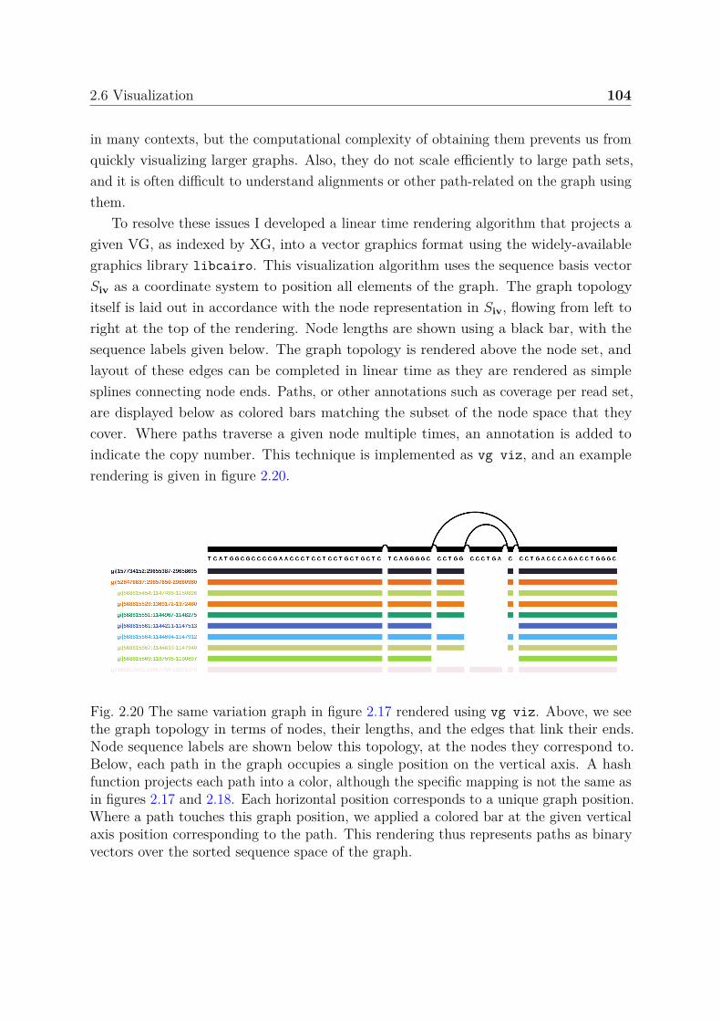
2.6 Visualization 104

in many contexts, but the computational complexity of obtaining them prevents us fromquickly visualizing larger graphs. Also, they do not scale efficiently to large path sets,and it is often difficult to understand alignments or other path-related on the graph usingthem.

To resolve these issues I developed a linear time rendering algorithm that projects agiven VG, as indexed by XG, into a vector graphics format using the widely-availablegraphics library libcairo. This visualization algorithm uses the sequence basis vectorSiv as a coordinate system to position all elements of the graph. The graph topologyitself is laid out in accordance with the node representation in Siv, flowing from left toright at the top of the rendering. Node lengths are shown using a black bar, with thesequence labels given below. The graph topology is rendered above the node set, andlayout of these edges can be completed in linear time as they are rendered as simplesplines connecting node ends. Paths, or other annotations such as coverage per read set,are displayed below as colored bars matching the subset of the node space that theycover. Where paths traverse a given node multiple times, an annotation is added toindicate the copy number. This technique is implemented as vg viz, and an examplerendering is given in figure 2.20.

Fig. 2.20 The same variation graph in figure 2.17 rendered using vg viz. Above, we seethe graph topology in terms of nodes, their lengths, and the edges that link their ends.Node sequence labels are shown below this topology, at the nodes they correspond to.Below, each path in the graph occupies a single position on the vertical axis. A hashfunction projects each path into a color, although the specific mapping is not the same asin figures 2.17 and 2.18. Each horizontal position corresponds to a unique graph position.Where a path touches this graph position, we applied a colored bar at the given verticalaxis position corresponding to the path. This rendering thus represents paths as binaryvectors over the sorted sequence space of the graph.

2.7 Graph mutating algorithms 105

It is important to recognize that this approach is lossy. Path ordering is not clearlyrepresented, as the paths are treated like masks over the sequence space of the graph.Furthermore, it can be difficult to interpret complex graphs as the topology of the graphis obscured in the simplistic rendering. vg viz’s linear layout treats the graph sequencesas a basis space in which other paths or alignments may be interpreted. This simplisticview is central to many potential applications of vg, which I further discuss in section2.8. The linear scaling of the algorithm should allow it to be applied to whole genomes,provided suitable front-end visualization software can be built, such as in a web interface.

2.7 Graph mutating algorithmsTo use variation graphs as reference systems, we need to be able to modify them.Algorithms in graph theory are frequently based on graph transformations, and I havediscussed some of them in the context of assembly and whole genome alignment. vgimplements many algorithms that alter the graph, but a number are of importance to itsdevelopment as a system for resequencing, and I detail them here.

2.7.1 Edit

As discussed in section 2.1.6, the extension of a variation graph to include new sequencesand paths can be thought of as a transformation yielding a bijection between the newand old graphs edit(G, A) → (G′, Φ). The main issue which adds complexity to thisprocess is that nodes represent more than a single character.

If nodes did represent a single character, then they would remain atomic throughgraph extension. It is simple to edit a “basepair” graph of this type: G = (N, E, P ),where ∀n∈N |seq(n)| = 1. We walk through the alignments to it A = a1 . . . a|A|, addingnovel bases represented in them (seq(A) /∈ G = NA) as new nodes. Then for eachalignment ai, we add edges connecting nodes in the order they would be traversed bythe path of the alignment embedded in the graph pai

∈ G′, yielding EA. Finally, weadd paths representing the embedded alignments PA. The resulting graph unifies theseadditions G′ = (N ∪NA, E ∪ EA, P ∪ PA).

To achieve lower representation costs in graphs with sparse variation, we usuallycompress the graph so that nodes cover multiple bases and thus we must considerthe editing process in multiple phases. We first modify graph G so that every novelsequence will be added at the start or end of a node. We do this by breaking nodes intomultiple derivative nodes when they overlap mappings that do not match the graph using

2.7 Graph mutating algorithms 106

break(G, A)→ (G′, Φ). For instance, if seq(ni) = GATTACA and we have a SNP T→ C atoffset 4, we would obtain ni → n′

i, n′′i , n′′′

i : seq(n′i) = GAT, seq(n′′

i ) = T, seq(n′′i ) = ACA.

We can then apply translate(A, Φ)→ A′, and add edges to G′ implied by the alignmentsas we would when editing a graph with single character nodes.

2.7.2 Pruning

The number of paths in a sequence graph grows exponentially with the number ofvariable sites. As I have discussed, this causes problems for alignment algorithms andgraph sequence indexing. While we can use efficient disk-backed index constructionalgorithms like GCSA2 to mitigate the effects of this exponential scaling, only a handfulof dense clusters of variation in the graph can increase the memory requirements of pathenumeration beyond any reasonable level. To control this we restructure the graph tolimit recombinations in the global sequence index.

We have explored two main techniques for the reduction of graph complexity. In thefirst, we prune regions of the graph which have high path complexity using a depth-firstsearch (DFS). We can optionally add back known haplotypes, in order to mitigate theloss of information from the index. For VCF-based VGs, where we have haplotype panels,the performance of local alignment is unaffected by the topological complexity, so weonly need to apply this pruning to the graph input to GCSA2 indexing. In assemblygraphs, we find that nodes which represent repeats can sometimes have extremely highdegree, which causes problems both for indexing and local alignment to the graph. There,we must remove these nodes in order to use the graph even for local alignment.

2.7.2.1 k-mer m-edge crossing complexity reduction

In k-mer complexity reduction, we enumerate the k-mers of the graph, removing edgeswhen a given k-mer crossing them would cross > m edges. We implement this filter,prune(G, k, m)→ Gsimple, using the k-mer enumeration algorithm that generates a DBGfrom the variation graph, only that our walks through the graph are bounded at m edgecrossings. For each offset in each node ni and ni, we run a DFS forward until we haveread k characters of the graph. During the pruning operation, instead of emitting thek-mers with their contexts, we stop the DFS when we have crossed m edges. We recordthe edge in Ecomplex. We thus derive the subgraph from the current graph by removingthe complexity-inducing edges: (N, E \ Ecomplex, P ) → Gsimple. It can be helpful toremove any small isolated components that result from this pruning, which can be donewith a linear subgraph enumeration algorithm and the measurement of the sequence

2.7 Graph mutating algorithms 107

length of each. A disjoint component Gsub ∈ Gsimple : ∀eij∈Nsubni ∈ Nsub ∧ nj ∈ Nsub

must have length ∑∀n∈Nsub |seq(n)| ≥ J . By default, we use k = 24, m = 3, and J = 33.

2.7.2.2 Filling gaps with haplotypes

Although removing complex regions will reduce the number of recombinant haplotypesrepresented by the graph, it is likely to also remove sections of known haplotypes. Wecan retain the complexity reduction without losing sequences in known haplotypes byreplacing the pruned regions in Gsimple with unfolded copies of each haplotype sequence.When we have a single reference path in Gref, we can accomplish this by overlaying Gsimple

and Gref. However, this will not achieve the desired result with even two overlappingpaths, as where these differ they would reintroduce the re-combinatorial explosion thatwe hope to resolve with pruning. An alternative is to copy the haplotypes in the GBWTindex that stretch from one border to the other of each removed region into the removedsubgraphs in Gsimple. Doing so, we must preserve a mapping between the new nodes andthe previous underlying ones in G. This allows matches to the haplotypes to be convertedinto matches in the base graph. The exact method by which this filling implemented isdescribed in [259].

2.7.2.3 High degree filter

Because they separate dense variation into heterozygous bubbles, assembly graphs mayfeature greater “smoothness” than VCF-based graphs locally. But, in the context ofrepeats, they can contain nodes with exceptionally high degree. If these cluster togetherthen they generate highly-connected regions that introduce degeneracy in the path space ofthe graph, and cause problems for k-mer enumeration and GCSA2 indexing. Furthermore,the local alignment methods in VG do not support efficient alignment through such denseregions. Preventing this is relatively simple, in that we remove nodes with more than Dedges linking them to the graph, yielding Gprune : ∀ni∈NpruneD ≥ |e∗i ∪ ei∗ ∪ ei∗ ∪ e∗i|.

It is not necessary that our local alignment suffers from high-degree nodes. Theproblem is that GSSW is provided an alignable graph that is an extracted subset ofthe full graph. If this subgraph is extracted using context expansion in the graph, thenhigh-degree nodes will generate extremely large subgraphs. One solution would be touse the bit-parallel string to graph alignment approach in [227], as this achieves optimalbounds in the size of transformed graph to which we align. Alternatively, the graphexploration should be more directly linked to the alignment process. The X-drop alignerdozeu could be adapted to this approach, as the X-drop parameter would provide anatural limit to the graph exploration. Such approaches may allow us to tolerate a

2.7 Graph mutating algorithms 108

larger D, but it seems unlikely that they will allow alignment to be driven through themost-tangled areas of the graph without a large performance penalty relative to graphswith lower maximum degree.

2.7.3 Graph sorting

To achieve as much partial ordering as possible, we order and orient the nodes in thegraph using a topological sort. The sort is guaranteed to be machine-independent giventhe initial graph’s node and edge ordering. The algorithm is well-defined on non-DAGgraphs, but in these cases the order is necessarily not a topological order. Our approachis a bidirected adaptation of Kahn’s topological sort [126], which is extended to handlegraph components with no heads or tails. This algorithm can be understood as a kind ofseeded depth first search through the graph. Where the graph has nodes which are pureheads, it begins there. Otherwise, a set of seed nodes which are stably selected given aparticular graph are used to begin the sort. The details of this procedure are provided inalgorithm 3.

Sorting can provide a simple optimization during read alignment. If the referencegraph has been sorted, then we can use the given order to generate node identifiers,embedding the rank of each node in its id. We can detect if a given subgraph is possiblynon-acyclic if ∃eij ∈ E : i > j, and if so submit the graph to sorting, unfolding, andDAGification before applying local alignment.

Similarly, the sort allows us to project data in the context of the graph into asingle dimension. Provided the graph is regionally partially ordered, this projectionpreserves local structures, which is a desirable property. This makes the sort applicableto visualization techniques as in figure 2.20.

2.7.4 Graph simplification

Assembly algorithms often employ a bubble popping phase, in which small bubbles, whichare graph components connected to the rest of the graph through a single source andsink node, are replaced by linear components representing the most-likely path throughthe bubble given the read data. In vg we can carry out a similar operation based onthe bubble decomposition of the graph. Unlike assembly graph bubble popping, wemust retain information about the embedded paths and annotations in the variationgraph. Simplification has a number of potential applications, for instance in reducing thecomplexity of visualizations of large variation graphs.

2.7 Graph mutating algorithms 109

Algorithm 3 Pseudo-topological sortG = (N, E, P ) ▷ A copy of our input graph which we will destructively modifyL← [. . .] ▷ Stores the pseudo-topological orderS ← ∅ ▷ Set of nodes which have been oriented but not yet traversedV ← ni ∈ N : ∃eji∀nj ∈ N ▷ We start from the head nodes of the graphif V = ∅ then ▷ If there are no head nodes, we use “seed” nodes

V ← Stably-selected seed nodes ∈ Nend ifwhile V = ∅ do

n← n ∈ V ▷ Select a seed nodeV ← V \ n ▷ Remove it from the input node set VS ← S ∪ n ▷ Store it in our working set Swhile S = ∅ do

ni ← ni ∈ S ▷ Remove an oriented node from SS ← S \ niL← [L[1] . . . L[|L|], ni] ▷ Append it to our output order Lfor ∀nj : eij ∈ E do

E ← E \ eij ▷ Remove the edge from our edge setif ∃ekj∀k ∈ N then ▷ nj has no other edges to that side

if eij thennj ← nj ▷ Orient nj so the side the edge comes to is first

end ifN ← N \ nj ▷ Remove nj from NS ← S ∪ nj ▷ Insert nj into S

else ▷ This helps start at natural entry points to cyclesV ← V ∪ nj ▷ Record nj as a place to start when S is empty

end ifend for

end whileend whilereturn L ▷ Return our pseudo-topologically sorted order and orientation

2.8 Graphs as basis spaces for sequence data 110

2.8 Graphs as basis spaces for sequence dataIf we can construct a graph which embeds all the sequences of all genomes which weare interested in, we resolve the separation between reference sequence and variationthat is present in standard resequencing. This suggests that the intermediate steps inresequencing may be made redundant. If variation is already available during alignmentthen there is no need for a variant detection phase. However, if the graph does not includevariation in our samples, then variant calling is required. In vg we have implementedseveral methods to do so. Similarly, we have implemented coverage summaries of readsets that may be used directly in downstream analyses.

2.8.1 Coverage maps

Numerous population genetic analyses are based on matrix representations of a collectionof genomes. Such models can be used to infer population structure and phylogeny, as wellas to associate phenotypes to genomic variants. If the variation graph used as a referencecontains all sequences relevant to our analysis, then a matrix of per-base coverage of thegraph by sample will provide highly representative information to downstream analyses.Exceptions include structural variation that does not result in coverage changes, such asbalanced events like inversions. Also, some local patterns of variation between successivesmall variation will not be distinguishable. If we were to annotate edges with theircoverage, this method would produce a result equivalent in information content to aMarkov model. It is thus clear that any coverage based index will be lossy relative tothe full read set. However, the lossiness reduces the information cost of storing andprocessing these coverage maps. As I described in section 2.4.6, in vg I developed anefficient method to accumulate coverage information of this kind across the graph.

2.8.2 Bubbles

In a sequence graph, a bubble is a pair of paths which start and end at the same nodes (s,t) but are otherwise disjoint in the graph [294]. Bubbles encompass our intuition aboutgenetic variation in graphs. A homologous sequence corresponding to the common startand end nodes in the bubble flanks two or more alternative alleles in the middle. Thesestructures were first considered in the context of finding small variation, and it was onlyin recent years that methods were developed to efficiently enumerate all bubbles of anysize in DAGs [19].

2.8 Graphs as basis spaces for sequence data 111

Bubbles can nest and contain more complicated internal structures between the pathsthrough them. The bubble may be generalized to the idea of a superbubble, which is adirected, acyclic component of a graph with a single head and tail node [207]. As forbubbles, efficient enumeration of superbubbles is possible in a DAG [24]. The optimalmethod relies on a recursive topological sort of the graph to structure the nested bubbles.Candidate node starts (s) and ends (t) are found following the definition of a superbubble.The set of candidates is then validated by range min queries (RMQ) to produce theset of superbubbles. As sort is linear O(|N |+ |E|), and the candidate enumeration andRMQ may be implemented on the sorted graph in O(1) each, this yields a linear timealgorithm for the enumeration of superbubbles.

The DAG requirement of this method is a significant limitation. In order to applythe superbubble enumeration to an arbitrary graph we must first DAGify it. In response,I worked with Benedict Paten and others to generalize the idea of a genetic site tosupport arbitrary bidirectional sequence graphs [213]. To formulate a generalizationof superbubbles, we introduce the concept of a snarl, which is any graph componentconnected to the rest of the graph by two or fewer bordering nodes20. Snarls whoseinternal separated component is acyclic and does not contain any tips are ultrabubbles.

Paten observed that trees embedded in the Cactus graph transformation of a variationgraph corresponded to the standard concept of superbubbles. Specifically, the cactusgraph is transformed into a cactus tree in which each simple cycle in the cactus graphbecomes a special kind of node. Various rootings of this tree may then be used to definea hierarchy of bubbles. The bidirectional nature of the variation graph mean that snarlscan embed each other in a manner akin to how the twist used to generate an Möbiusstrip results in it having a single surface and border. In these cases the resulting cactustree will support multiple alternative ultrabubble tree rootings, and so unlike the bubbleand superbubble decompositions for DAGs the ultrabubble decomposition is not unique.We can enumerate a subset of these by identifying bridge edges (typically representingtips) in the “bridge forest”, which is the result of a contraction of the cycles in the cactusgraph into a set of top-level cycle representing nodes, and then use them to producevarious rootings of the cactus tree.

Ultrabubbles and superbubbles provide a natural framework in which to reason aboutthe hierarchy of variable genetic sites embedded in a graph. As such they provide thebasis for generic models of genotype inference based on variation graphs which are capable

20In the paper the formulation is based on a bi-edged graph akin to the Enredo graph, but we notethat a node-based formulation is equivalent and matches the other models in this section.

2.8 Graphs as basis spaces for sequence data 112

of genotyping any kind of genetic variation, including structural variation as well asnested variation, in the same model as SNPs and indels.

2.8.3 Variant calling and genotyping

Given a definition of variable genetic loci in the graph, we can build a genotyping systemcapable of generating genotype calls in the context of the graph. In vg we have exploredtwo such methods. The first, originally implemented in vg call, generalizes the conceptsfirst implemented in samtools mpileup to work on the graph. A set of alignments arefirst reduced to pointwise edits against the graph and per base coverage of the graph.This graph “pileup” is then processed by a genotyping algorithm that considers geneticsites using the ultrabubble model. A schematic overview of the method is shown in figure2.21.

aaacacc a

Read alignment Graph pileup Variant calls Augmented graph

Sample graph

Fig. 2.21 Pileup variant calling with vg call

The second model, implemented in vg genotype, embeds the alignments in thevariation graph using edit(A, Gbase)→ (Gaug, Φaug→base), and then genotypes across theultrabubbles of Gaug which are supported by reference paths in Gbase or reads. As theresulting genotypes are represented as unordered sets of paths in Gaug, they are projectedback into the coordinate space of Gbase using the translation Φaug→base. An overview ofthe process is shown in figure 2.22.

While principled, the full augmentation model in vg genotype is very expensiveto compute. The pileup model has proven to be more efficient. Over time vg callhas been adjusted to implement some features of the full graph augmentation modelin vg genotype where the graph is augmented only with sequences supported by somenumber of alignments at a given quality threshold. Both methods employ a diploidspecification of the genotyping model in freebayes [91] to develop their posterior estimatesof variant quality. The generalization of SNP and indel calling to haplotype callingimplemented in freebayes corresponds to the same allele model used in both vg variantcalling methods. Alleles correspond to DNA sequences of arbitrary length, anchored at

2.8 Graphs as basis spaces for sequence data 113

Reference Graph

AugmentedGraph

AlleleSupports

Ultrabubbles

GenotypeLikelihoods Genotypes

AlignedReads

TranslationUpdated

Reference Graph

Fig. 2.22 Graph augmentation-based variant calling in vg genotype.

the ends to the reference genome (in the case of freebayes) or to the rest of the graph (asin the ultrabubbles used in vg).

The complexity of running and evaluating genotyping in the graph has sloweddevelopment of these methods. Currently they are still outperformed by standardvariant calling methods based on the linear reference, as indicated by our results in thePrecisionFDA variant calling challenge that I will describe in the next chapter.

Chapter 3

Applications

In the first two chapters I have provided an overview of the theoretical basis of my workand placed it within the history of related approaches. Here, I will demonstrate how themethods I develop can aid biological insight in a number of species domains. To do so, Iwill use methods described in chapter 2 as implemented in vg.

The small genome of Saccharomyces cerevisiae and ready availability of sources forpangenomic data models made it very useful to my development of vg. I begin byillustrating this for a variety of pangenome constructions and also a variety of readlengths.

However, much interest in bioinformatics is with larger genomes, specifically human.I use evaluations based on the human genome to validate the ability of vg to scale tolarge genomes. Through simulation and the analysis of real genomes, I show that thealigner I implement, vg map, yields the same quality of alignment as bwa mem againstlinear genomes. Although vg map’s runtime is between five to ten-fold slower than bwamem, it provides improved, less biased alignment against variation graphs. I develop avariation graph for the reference-guided genome assemblies from the HGSVC project anddemonstrate the strong effect of reference bias in ChIP-seq data.

One context where reference bias has very significant effects is in the analysis ofancient DNA (aDNA). Here short reads and high intrinsic error rates encourage a highrate of reference bias. I show that alignment against a pangenome graph ameliorates thisissue.

vg can be applied to any kind of variation graph. To demonstrate the utility of this,I use de Bruijn assemblers to generate reference variation graphs from collections of rawsequencing reads in the absence of a prior reference. I recreate a classical pangenomicanalysis of core and accessory pangenome by analyzing the coverage of alignments mappedto an assembly graph built from 10 Escheria coli strains. To illustrate the application of

3.1 Yeast 115

vg to metagenomic data containing unknown source genomes, I show that vg enablesthe full length alignment of reads to a complex assembly graph built from an arcticviral metagenome, and similarly improves alignment to an assembly graph built from ahuman gut microbiome. Finally, I demonstrate that the data models and indexes in vgare capable of encoding splicing graphs, and that aligning to these splicing graphs allowsthe direct observation of the transcriptome.

3.1 YeastSaccharomyces cerevisiae, commonly known as baker’s or brewer’s yeast due to itsgastronomic applications, has long been among the most important model organisms inbiology, and its small genome attracted some of the first population scale whole genomesurveys of variation to be undertaken using low-cost sequencing. The genome of S.cerevisiae was the first eukaryotic genome sequenced, in 1996 [94]. Resequencing studiesfollowed that used cerevisiae as a model system to understand genome evolution. TheSaccharomyces Genome Resequencing Project (SGRP) [169], which used low-coveragecapillary Sanger sequencing to generate a population survey for cerevisiae can be seenas a precursor to the 1000GP, in its use of low-coverage sequencing and imputationto establish the panel1. A followup project, the SGRP2, used resequencing and wholegenome assembly of high coverage, low cost Illumina sequencing to establish that thegreater phenotypic diversity in S. cerevisiae relative to its wild relative S. paradoxus islikely due to structural variation (as measured by presence/absence and copy number)rather than SNP diversity [17]. Recently, whole genome de novo assembly with longsingle-molecule reads has further refined this conclusion by demonstrating that thestructural diversity is non-uniformly distributed throughout the genomes of S. cerevisiae,concentrating in subtelomeric regions [292]. In this section, I use data from independentsequencing of the UK’s National Center for Yeast Collections (NCYC) as well as longreads from [292] to demonstrate the capabilities of vg and compare the utility of variousvariation graph models built from these population surveys.

3.1.1 A SNP-based SGRP2 graph

The earliest rigorous testing of vg’s alignment method was against a variation graphconstructed from the SGRP2’s released VCF for S. cerevisiae2. This early populationresequencing project produced a VCF including only SNPs, yet using it already presented

1https://www.sanger.ac.uk/research/projects/genomeinformatics/assets/sgrp_manual.pdf2http://www.moseslab.csb.utoronto.ca/sgrp/data/SGRP2-cerevisiae-freebayes-snps-Q30-GQ30.vcf.gz

3.1 Yeast 116

problems typical even when working with larger scale genomes. The transposable elementsin the genome generate rich patterns of repeats which make alignment difficult and requirethe development of mapping quality. Dense variation is also present in the results andthis necessitates the application of pruning strategies to the graph to mask out high-complexity regions for indexing. Mistakes in the mapper could be readily observed andtesting could easily be done on a laptop, whereas larger genomes require longer runtimesfor indexing and larger servers in order to support the indexes during alignment.

The SGRP2 graph can be built and indexed in around 10 minutes on a commoditycompute server, including the construction of the GBWT index and the generationof an order-256 GCSA2 index using a pruned and refilled version of the graph. Itcontains exactly the number of bases in the SGD_2010 reference plus the number ofSNP alternate alleles in the SGRP2 VCF: 12163423 + 243629 = 12407052. The graphitself uses 23MB on disk, in contrast to that of the SGD_2010 reference, which takesonly 7.6MB. Much of this difference is due to the larger number of entities required byto represent the variation-containing graph. The SGD_2010 graph is linear, with a gapfor each chromosome, and contains 380,115 nodes and 380,097 edges after splitting intonodes of typical size 32bp, while the SGRP2 graph contains SNPs and is representedwith 714,533 nodes and 969,690 edges. Note that by default, GCSA2 indexing workson nodes with a maximum length less than 1024, and vg map performs better if themaximum node size is limited further, with 32bp usually the standard maximum lengthin experiments I will present here. The resulting indexes also differ in size, with theSGRP2 graph’s xg index requiring 71MB, while the SGD_2010 graph’s only 38MB. Thefull GCSA index for the SGRP2 graph is substantially larger, at 220MB, in contrastto only 50MB for the linear reference, which reflects the greater complexity requiredto include all the recombination in the pruned and haplotype re-filled graph used forindexing.

To validate that the SGRP2 reference is a closer match to real read sets, I thenmapped subsets of reads from cerevisiae samples that were in the NCYC collection butwere not part of SGRP2. I aligned 100K read pairs from each of 12 samples (N = 2.4Mtotal reads) to both the SGD_2010 reference graph and the SGRP2 pangenome graph.For each read, we can compare the alignment score and identity between the two graphsto evaluate the gain provided by using the pangenome as a reference. When we mapthe real reads from new strains not used to build the graph, 24.5% of the reads mapbetter to the pangenome than to the linear reference (figure 3.1). A small fraction ofreads (0.46%) map better to the linear than to the pangenome graph, which could result

3.1 Yeast 117

from changes in paired alignment rescue, the effects of the pruning process, the slightlydifferent minimum MEM size calculated for the two graphs, or errors in the SGRP2.

3.1.2 Cactus yeast variation graph

Variation graphs are generic objects capable of representing any kind of alignment betweengenomes or assembly of read data from them. To test the ability of vg to use graphs ofcomplex topology, we constructed a variation graph from the whole genome alignment ofde novo assemblies produced from PacBio sequencing of seven strains of S. cerevisiae. Tobuild this graph, each chromosome of each assembly in [292] was aligned using LASTZ[107] according to a phylogenetic guide tree. The resulting alignment set was reduced to avariation graph using the Cactus reference-free whole genome multiple alignment method[212], which internally maintains a sequence graph equivalent to a VG. Its output wasthen converted to vg format using the hal2vg utility3. As illustrated in figure 3.2, thisgraph encodes a complex global topology that captures the structural variation betweenthe species also reported in [292] as well as a local DAG-like topology which we expectwhen homologous sequences are represented compactly in a graph. This illustrates theability of vg to represent paths corresponding to both collinear (inset) and structurallyrearranged (main figure) regions of genomic variation.

A simulation study based on the SK1 strain provides some insight into the capabilitiesof vg and tradeoffs inherent in different graph designs. I compared four variation graphs:a linear reference graph from the standard S288c strain, a linear reference from the SK1strain, a pangenome graph of all seven strains, and a “drop SK1” variation graph in whichall sequence private to the strain SK1 was removed from the pangenome graph. Themultiple genome graphs were based on that first constructed with Cactus, as describedabove, and then filtered down to the various subgraphs using path subsetting facilities invg mod.

We simulated 100,000 150bp paired-end reads from the SK1 reference, modelingsequencing errors, and mapped them to the four references (ROC curves, Figure 3.3).Not surprisingly, the best performance was obtained by mapping to a linear reference ofthe SK1 strain from which the data were simulated, with substantially higher sensitivityand specificity compared to mapping to the standard linear reference from the strainS288c with either vg or bwa mem. Mapping to the variation graphs gave intermediateperformance, with >1% more sensitivity and lower false-positive rates than mappingto the standard reference. There was surprisingly little difference between mapping to

3https://github.com/ComparativeGenomicsToolkit/hal2vg

3.1 Yeast 118

(a) Alignment score (b) Alignment identity

1e+11

1e+26

1e+41

1e+56

−100 −50 0 50 100

score.SGRP2 − score.SGD

stac

ked

log

coun

ts

name

NCYC1006

NCYC1026

NCYC1187

NCYC1228

NCYC1245

NCYC1681

NCYC78

NCYC84

NCYC88

NCYC92

NCYC93

NCYC97

(c) Difference in alignment score

1e+11

1e+26

1e+41

1e+56

−1.0 −0.5 0.0 0.5 1.0

id.SGRP2 − id.SGD

stac

ked

log

coun

ts

name

NCYC1006

NCYC1026

NCYC1187

NCYC1228

NCYC1245

NCYC1681

NCYC78

NCYC84

NCYC88

NCYC92

NCYC93

NCYC97

(d) Difference in alignment identity

Fig. 3.1 Alignment of 100k read pairs from 12 NCYC S. cerevisiae strains against thereference genome (SGD) or the pangenome (SGRP2). In (3.1a) alignment scores areplotted for each read. The shift in density to the right relative to y = x indicatesimproved alignments to the pangenome. In (3.1b) we observe the same pattern whenusing alignment identity rather than score. Subfigures 3.1c and 3.1d provide a stackedlog-scaled histogram of the difference in score and identity between the two graphs.

3.1 Yeast 119

568371

568372

568373568374

568347

568375

568376568377

568378

568338

568335568337

568334

568336568339

568341

568342

568340

568348568349

568343 568344

568345

568346

568350

568351568352

568353

568354

568355

568356568357568358568359

568360

568361

568362

568363

568364

568365

568314

568313568312

568315568316 568320

568321568317

568326

568327

568318568319

568322

487

568324568323

568325

568328

568331568329

568330

568333

568332

DBVPG6044.chrII 568378

568376

568375

568374

568372

568347

568345

568344

568342

568341

568338

568337

568334

568333

568332

568331

568327

568326

568325 568323

568322

568321

568320

568314

568313 568312

DBVPG6044.chrIX 568365

568363

568362

568360 568359

568357

568356 568353

568352 568351

568349

568348

568339

568338

568337

568334

568329

568328 568327

568318 568317

568315

568314

568313

DBVPG6044.chrVII 568378

568376

568375

568374

568372

568347

568345

568344

568342

568341

568338

568337

568334

568333

568332

568331

568327

568326

568325 568324

568322

568321

568320

568314

568313

568312

DBVPG6765.chrIX 568364

568363

568361

568360

568358 568357 568355

568353 568352 568350

568349

568340

568339 568338

568335

568334

568329

568328

568327

568318

568317

568315

568314

568313

S288c.chrIX 568364

568363 568361

568360 568358

568357

568355

568353

568352

568350

568349

568340 568339 568338

568335

568334

568329

568328

568327

568318

568317

568315

568314

568313

SK1.chrII 568378

568376

568375

568374

568372

568347

568345

568344

568342

568341

568338

568337

568334

568333 568332

568331

568327

568326

568325 568323

568322

568321

568320 568314

568313 568312

SK1.chrIX 568365 568363

568362 568360

568359

568357

568356

568353 568352 568351

568349 568348

568339

568338

568337

568334

568329

568328

568327

568318

568317

568315

568314

568313

SK1.chrVII 568378

568376

568375

568374

568372

568347

568345

568344

568342

568341

568338

568337

568334

568333 568332

568331

568327

568326

568325

568322

568321

568320

568314

568313

568312

UWOPS034614.chrIX 568364

568363

568361

568360

568358 568357

568355

568354 568352

568350 568349

568340

568339 568338

568335

568334

568329

568328 568327

568318

568317

568315

568314

568313

UWOPS034614.chrVIII 568312 568313

568314

568316

568317

568319

568327

568328

568330

568333

568336 568337

568338

568341

568342

568343

568345

568346

568347

568372

568373

568375

568376

568378

UWOPS034614.chrXI 568312 568313

568314

568316

568317

568319

568327

568328

568330

568333

568336 568337

568338

568341

568342

568343

568345

568346

568347

568372

568373

568375

568376

568378 UWOPS034614.chrXIV 568378

568376

568375

568373

568372

568347

568346

568345

568343

568342

568341

568338

568337 568336

568333

568330

568328

568327

568319

568317

568316

568314

568313 568312

Y12.chrIX 568364

568363 568361

568360

568358

568357

568355 568353

568352

568350 568349 568340 568339 568338

568335

568334

568329

568328

568327

568318

568317

568315

568314

568313

Y12.chrVII 568378

568377

568375

568373

568372

568371

568347

568345

568344

568342

568341

568338

568337 568336

568333

568330

568328

568327

568326

568317

568316

568314

568312

YPS128.chrIX 568364

568363 568361

568360 568358

568357

568355 568353

568352

568350

568349

568340 568339

568338

568335

568334

568329

568328 568327

568318

568317

568315

568314

568313

C

ACTC

A

G

CCAAAGGCGTGCCTTTGTTGA

G

T

C

ATCCATT

G

TGCTACGTTAGAAAGGCCCACAGTATTCTTC

Fig. 3.2 A region of a yeast genome variation graph. This displays the start of thesubtelomeric region on the left arm of chromosome 9 in a multiple alignment of thestrains sequenced in [292] as assembled by Cactus [212]. The inset shows a subregion ofthe alignment at single-base level. The colored paths correspond to separate contiguouschromosomal segments of these strains. Reprinted from [92].

3.1 Yeast 120

60

60

60

60

6060

60

60

60

60

50

50

50

50

5050

50

50 50

50

40

40

40

40

4040

4040

40

40

30

30

30

30

30

30

30

30

30

30 2020

20

20

2020

20

20

20

20

10

10

1010

1010

10

10

10

10

0

0

0

0

0

0

0 0

0

0

0.92

0.94

0.96

0.98

0.001 0.010FPR

TPR

25000

50000

75000

aligneraaaaaaaaaa

bwa-mem-pe

bwa-mem-se

cactus-pe

cactus-se

cactus_S288c-pe

cactus_S288c-se

cactus_SK1-pe

cactus_SK1-se

cactus_drop_SK1-pe

cactus_drop_SK1-se

number

Fig. 3.3 Mapping short reads with vg to yeast genome references. ROC curves obtainedby mapping 100,000 simulated SK1 yeast strain 150bp paired-end reads against a varietyof references described in the text. Reprinted from [92].

3.1 Yeast 121

graphs with and without the SK1 private variation, probably because much of whatis novel in SK1 compared to the reference is also seen in other strains. Mapping toeither graph had lower sensitivity compared to mapping just to the SK1 sequence, likelybecause of suppression of GCSA2 index k-mers in complex or duplicated regions, whichour indexing strategy was not designed to address.

3.1.3 Constructing diverse cerevisiae variation graphs

With vg, our goal is to build a toolkit that allows the use of any genome graph as areference. To validate this capability, I used data sources for S. cerevisiae to build sevenvariation graphs, whose dimensions are listed in table 3.1. In the next section (3.1.4) Ipresent an evaluation of these graphs using long reads from the SK1 strain.

name size (MB) length nodes edges subgraphsSGD_2010 7.3 12163423 380115 380097 18S288c 7.3 12249246 382797 382781 18SGRP2 21 12407052 714533 969690 18minia unitigs 15 14419206 1232804 1332994 46131minia contigs 6.4 12233279 421125 425683 2961Cactus 31 13243056 1059173 1304205 580vg msga 42 13793955 1156295 1387903 2

Table 3.1 A summary of seven different variation graphs constructed to represent variationin S. cerevisiae. As described in section 3.1.1, the SGD_2010 graph is built from thereference, while SGRP2 adds SNPs in the SGRP2 population survey. The Illumina datafrom [292] was used to build the minia unitigs and minia contigs graphs, while the wholegenome, chromosome-resolved PacBio assemblies from the same work were used to buildthe Cactus and vg msga variation graphs. S288c is the de novo assembly of the referencestrain produced in [292].

Three of the graphs are effectively linear or DAG-like, except for their mitochondriaand plasmid chromosomes, which are included as circular components. SGD_2010 andS288c represent two assemblies of the reference genome, the former from the SGD genomesequencing project, and the latter is a de novo assembly from [292]. The difference inquality between the two approaches will be made apparent in the subsequent section. Asdescribed in section 3.1.1, the SGRP2 graph adds SNP variation from the populationsurvey in [17] to build a pangenome reference. The SGD_2010 reference contains themitochondria and 6kbp plasmid sequence, while the S288c assembly excludes them dueto the sequencing protocol, where size selection in the library preparation stage removed

3.1 Yeast 122

these short sequences, so to enable direct comparison in later tests these were added tothe S288c graph.

The remaining four graphs are different forms of assembly graph. Using the Illuminadata published in [292], I build two assemblies with minia3, using a k-mer size of 51and a high abundance threshold (50) to limit the resulting graph complexity. In thefirst, I take the unitig graph that represents all non-branching paths in the compactedDBG as nodes. The second is the result of the minia contigification process that popsbubbles and cleans the graph to attempt to arrive at longer contigs. Both results areexpressed as overlap graphs in GFA, and I can import them as variation graphs usingbluntification and graph pseudotopological sorting. As shown in table 3.1, the unitiggraph is considerably more complex in terms of node density than the contig graph. Italso contains more sequence, presumably because some regions that are separated in theunitig graph are collapsed in the contig graph. The number of disjoint components inthese graphs is very high (2961 for the contig graph and 46131 for the unitig graph),suggesting that pruning of the assembly graph has yielded a greatly fragmented result.The resulting graphs are difficult to align long reads to. I conclude that further tuning ofthe parameters used during de novo assembly from short reads will be required to useassemblies like this as reference graphs.

Finally, I used the whole genome de novo assemblies of long read data from [292] tobuild whole genome alignment graphs using Cactus (as described in section 3.1.2) andvg msga. The multiple sequence to graph alignment (MSGA) process implemented invg msga is akin to the progressive POA method, but generalized to arbitrary graphs ofany size. Rather than using a local alignment algorithm to expand the graph, the longread alignment algorithm described in section 2.5.9 allows the direct alignment of wholechromosomes to the graph. Where the Cactus variation graph uses a phylogenetic guidetree to structure its construction, vg msga simply aligns the chromosomes in order fromlongest to shortest to the growing graph. The long read alignment in vg is structured toenforce long range synteny, and the resulting graph is substantially different in structurethan that of Cactus. I find that vg msga is less likely to collapse repeats than Cactus, atleast in the configuration used for this assembly. We can see this in figure 3.4, where theCactus variation graph (3.4a) shows two dense repeat structures in its core connected byloops of unique sequence, while the vg msga graph appears to have much longer loops,with collapsed repeats embedded in these loops. This observation is supported by thelength statistics in table 3.1, with vg msga producing a graph that is 550,899bp longerthan that of Cactus. At the same time, the node count of the vg msga graph is higher,which perhaps reflects a different local alignment result.

3.1 Yeast 123

(a) Cactus variation graph

(b) vg msga variation graph

Fig. 3.4 Whole genome alignment graphs for S. cerevisiae visualized using Bandage.

3.1 Yeast 124

3.1.4 Using long read mapping to evaluate cerevisiae graphs

In this section I evaluate the graphs I constructed in section 3.1.3 and simultaneouslydemonstrate the ability of vg to align long reads to graphs of any type. For each of theseven graphs I aligned a set of 43,337 Pacific Biosciences SK1 reads (mean length 4.7kbp)from [292] to the graph. We can then compare the alignment identity for each readacross the various graphs. I do so using the same dot plot technique used to demonstratealignment quality improvement using the Illumina data from the NCYC strains. In figure3.5 I present a number of pairwise comparisons based on this read set.

I find that the SGD_2010 reference provides a better match for the SK1 PacBio readsthan the S288c assembly (top left), which can be seen in a subset of reads that mapnearly perfectly to the SGD_2010 graph but not to the S288c one. This may be due tothe higher quality and curation of the SGD reference, which was initially based on BACsand capillary sequencing, but I have not determined the exact cause of this discrepancy.This same effect is clear in the comparison of S288c and the SGRP2 (top middle, figure3.5), although there the SNPs in the SGRP2 graph tend to improve the overall matchbetween the SK1 reads and the graph, which can be seen in a shift in density upwardsfrom the diagonal. For other comparisons I focused on using the S288c reference, as itforms a part of the progressive alignments and the source data for the minia assembliescomes from the same paper.

The minia graphs appear to provide very low quality as a reference for the alignment oflong reads (bottom left and middle, figure 3.5). The minia unitig graph is too fragmentedfor any practical use. In almost no case does it provide a better match for the long reads.However, while the minia contig graph is also outperformed by the S288c graph, for anotable subset of the reads it provides a perfect match, while the S288c graph fails tomatch them at all. This suggests that some contigs in the Illumina assembly match theSK1 strain, which is to be expected and demonstrates that in principle this kind of graphcan represent multiple genomes.

Finally, the whole genome alignment graphs are notable in their similarity. Despitethe fact that they were constructed using different algorithms, both provide a similarbasis for alignment of the SK1 reads. It is notable that alignment time against the vgmsga graph was the highest of the tested graphs, and significantly higher than that forthe Cactus graph. This may relate to the un-collapsed state of the repeats in the graph.The alignment algorithm will attempt more alignments for each band where there isambiguity, and the “patching” at the end of the alignment process will be more intensive.

3.1 Yeast 125

Fig. 3.5 Density plots of alignment identity when mapping 43,337 Pacific Bioscienceslong reads from the SK1 strain to different variation graphs. Linear assemblies: (Topleft) the SGD_2010 reference vs. the S288c assembly from [292]. (Top middle) theS288c assembly vs. the SGRP2 SNP pangenome. Assembly graphs from Illumina data:(Bottom left) the minia contig graph vs. the S288c assembly. (Bottom middle) the miniaunitig graph vs. the S288c assembly. Whole genome alignment graphs: (Top right) theCactus variation graph vs. the S288c assembly. (Bottom right) the vg msga variationgraph vs. the S288c assembly.

3.2 Human 126

3.2 HumanFor a species such as human, with only 0.1% nucleotide divergence on average betweenindividual genome sequences, over 90% of 100bp reads will derive from sequence exactlymatching the reference. Therefore, new mappers should perform at least as well for linearreference mapping as the current standard, which we take to be bwa mem with defaultparameters. We show that vg does this, and then that vg maps more informativelyaround divergent sites.

3.2.1 1000GP graph construction and indexing

The final phase of the 1000 Genomes Project (1000GP) produced a data set of ∼80million variants in 2,504 humans [45]. We made a series of vg graphs containing allvariants or those above minor allele frequency thresholds of 0.1%, 1%, or 10%, as well asa graph corresponding to the standard GRCh37 linear reference sequence without anyvariation. The full vg graph uses 3.92 GB when serialized to disk, and contains 3.181Gbpof sequence, which is exactly equivalent to the length of the input reference plus thelength of the novel alleles in the VCF file. Complete file sizes including indices rangefrom 25 GB to 63 GB, with details including build and mapping times given in table 3.2.

Reference set N vars vg index search time(M) time size time size PE SE

GRCh37 0 1:09:54 1.76 23:30:41 25.11 33:34 28:331000GP AF0 84.8 3:42:01 3.92 51:05:07 63.28 45:10 39:461000GP AF0.001 30.2 2:00:08 2.58 31:45:12 38.10 39:33 32:531000GP AF0.01 14.3 1:35:02 2.17 27:18:53 30.94 33:13 27:091000GP AF0.1 6.8 1:23:04 1.97 26:06:38 27.79 32:35 28:43

Table 3.2 Numbers of variants, file sizes in gigabytes (GB) and build and search times inhours:minutes:seconds for various human vg graphs and associated indexes. Referencesets are the linear reference GRCh37, the full 1000 Genomes Project set 1000GP AF0,and subsets of 1000GP AF0 including only variants with allele frequency above thresholds0.001 (0.1%), 0.01 (1%) and 0.1 (10%) respectively. The number of variants in millionsfor each of these data sets is shown. Search times are for 10 million 2x150bp read pairssimulated from NA24385. Reprinted from [92].

3.2 Human 127

3.2.2 Simulations based on phased HG002

We next aligned ten million 150bp paired-end reads simulated with errors4 from theparentally phased haplotypes of an Ashkenazim male NA24385, sequenced by the Genomein a Bottle (GIAB) Consortium [300] and not included in the 1000GP sample set, toeach of these graphs as well as to the linear reference using bwa mem. Figure 3.6 showsthe accuracy of these alignments compared with bwa mem for the full range of frequencythresholded graphs, in terms of receiver operating characteristic (ROC) curves.

Reads that come from parts of the sequence without differences from the reference(middle panels of Figure 3.6) mapped slightly better to the reference sequence (green)than to the 1000GP graph (red), which we attribute to a combination of the increase inoptions for alternative places to map reads provided by the variation graph, and the factthat we needed to prune some search index k-mers in the most complex regions of thegraph. The best balance of performance appears at the threshold of 0.01. As expected,this difference increased as the allele frequency threshold was lowered and more variantswere included in the graph.

For reads that were simulated from segments containing non-reference alleles (∼10%of reads), which are the reads relevant to variant calling, vg mapping to the 1000GPgraph (red) gave better performance than either vg (green) or bwa mem (blue) mappingto the linear reference (right panels of Figure 3.6), because many variants present inNA24385 are already represented in the 1000GP graph. This is particularly clear forsingle-end mapping, since many paired-end reads are rescued by the mate read mapping.Overall, vg performed at least as well as bwa mem, even on reference-derived reads, andsubstantially better on reads containing non-reference variants.

3.2.3 Aligning and analyzing a real genome

We also mapped a real human genome read set with ∼50× coverage of Illumina 150bppaired-end reads from the NA24385 sample to the 1000GP graph. vg produced mappingsfor 98.7% of the reads, 88.7% with reported mapping quality score 30 on the Phred scale,and 76.8% with perfect, full-length sequence identity to the reported path on the graph.For comparison, we also used vg to map these reads to the linear reference. Similarproportions of reads mapped (98.7%) and with reported quality score 30 (88.8%), butconsiderably fewer with perfect identity (67.6%). Markedly different mappings werefound for 1.0% of reads (0.9% mapping to widely separated positions on the two graphs,and 0.1% mapping to one graph but not the other). The reads mapping to widely

4SNP errors are introduced at a rate of 0.01 per base and indels at a rate of 0.002 per base.

3.2 Human 128all

vari

ants

AF

> 0

.01

AF

> 0

.00

1A

F >

0.1

all reads reference-matching alternate-matching

Fig. 3.6 ROC curves parameterized by mapping quality for 10M read pairs simulated fromNA24385 as mapped by bwa mem, vg to various 1000GP pangenome references, and vgwith a linear reference, using single end (se) or paired end (pe) mapping. Allele frequencythresholds are given to the left of each row. Within each panel, the left subpanel is basedon all reads, middle on reads simulated from segments with no genetic variants fromthe linear reference, and the right on reads simulated from segments containing variants.Reprinted from [92].

3.2 Human 129

separated positions were strongly enriched for repetitive DNA. For example, the linearreference mappings for 27.5% of these read pairs overlapped various types of satelliteDNA identified by RepeatMasker, compared to 3.0% of all read pairs.

To illustrate the consequences of mapping to a reference graph rather than a linearreference, we stratified the sites independently called as heterozygous in NA24385 bydeletion or insertion length (0 for single-nucleotide variants) and by whether the site waspresent in 1000GP, and measured the fraction of reads mapped to the alternate allele foreach category. The results show that mapping with vg to the population graph whenthe variant was present in 1000GP (95.4% of sites) gave nearly balanced coverage ofalternate and reference alleles independent of variant size, whereas mapping to the linearreference either with vg or bwa mem led to a progressively increasing bias with increasingdeletion and (especially) insertion length (Figure 3.7), so that for insertions around 30bp,a majority of insertions containing reads were missing (there were over twice as manyreference reads as alternate reads).

0.2

0.3

0.4

0.5

0.6

<=

−40

−39

−38

−37

−36

−35

−34

−33

−32

−31

−30

−29

−28

−27

−26

−25

−24

−23

−22

−21

−20

−19

−18

−17

−16

−15

−14

−13

−12

−11

−10 −

9−

8−

7−

6−

5−

4−

3−

2−

1 0 1 2 3 4 5 6 7 8 9 10 11 12 13 14 15 16 17 18 19 20 21 22 23 24 25 26 27 28 29 30 31 32 33 34 35 36 37 38 39>

=40

Size of deletion (negative) or insertion (positive)

Fra

ctio

n of

alte

rnat

e al

lele

method

bwa.fb

vg.in1000GP

vg.not1000GP

Fig. 3.7 The mean alternate allele fraction at heterozygous variants previously called inHG002/NA24385 as a function of deletion or insertion size (SNPs at 0). Error bars are ±1 s.e.m. Reprinted from [92].

3.2.4 Whole genome variant calling experiments

During the development phase of vg, we explored its application to whole genomealignment and variant calling in the PrecisionFDA Truth Challenge, in which the teamwhich developed the Genome in a Bottle truth set developed and held out a new sample.Methods were first tested against publicly available truth sets on NA12878 in the“consistency” challenge, in which the vg development team received a star for “heroiceffort” in completing the first whole-genome graph based alignment and variant callinganalysis. The results for this first iteration were very poor, with F-scores for indels and

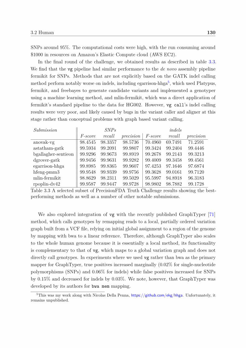
3.2 Human 130

SNPs around 95%. The computational costs were high, with the run consuming around$1000 in resources on Amazon’s Elastic Compute cloud (AWS EC2).

In the final round of the challenge, we obtained results as described in table 3.3.We find that the vg pipeline had similar performance to the de novo assembly pipelinefermikit for SNPs. Methods that are not explicitly based on the GATK indel callingmethod perform notably worse on indels, including egarrison-hhga5, which used Platypus,fermikit, and freebayes to generate candidate variants and implemented a genotyperusing a machine learning method, and mlin-fermikit, which was a direct application offermikit’s standard pipeline to the data for HG002. However, vg call’s indel callingresults were very poor, and likely caused by bugs in the variant caller and aligner at thisstage rather than conceptual problems with graph based variant calling.

Submission SNPs indelsF-score recall precision F-score recall precision

anovak-vg 98.4545 98.3357 98.5736 70.4960 69.7491 71.2591astatham-gatk 99.5934 99.2091 99.9807 99.3424 99.2404 99.4446bgallagher-sentieon 99.9296 99.9673 99.8919 99.2678 99.2143 99.3213dgrover-gatk 99.9456 99.9631 99.9282 99.4009 99.3458 99.4561egarrison-hhga 99.8985 99.8365 99.9607 97.4253 97.1646 97.6874hfeng-pmm3 99.9548 99.9339 99.9756 99.3628 99.0161 99.7120mlin-fermikit 98.8629 98.2311 99.5029 95.5997 94.8918 96.3183rpoplin-dv42 99.9587 99.9447 99.9728 98.9802 98.7882 99.1728

Table 3.3 A selected subset of PrecisionFDA Truth Challenge results showing the best-performing methods as well as a number of other notable submissions.

We also explored integration of vg with the recently published GraphTyper [71]method, which calls genotypes by remapping reads to a local, partially ordered variationgraph built from a VCF file, relying on initial global assignment to a region of the genomeby mapping with bwa to a linear reference. Therefore, although GraphTyper also scalesto the whole human genome because it is essentially a local method, its functionalityis complementary to that of vg, which maps to a global variation graph and does notdirectly call genotypes. In experiments where we used vg rather than bwa as the primarymapper for GraphTyper, true positives increased marginally (0.02% for single-nucleotidepolymorphisms (SNPs) and 0.06% for indels) while false positives increased for SNPsby 0.15% and decreased for indels by 0.03%. We note, however, that GraphTyper wasdeveloped by its authors for bwa mem mapping.

5This was my work along with Nicolas Della Penna, https://github.com/ekg/hhga. Unfortunately, itremains unpublished.

3.2 Human 131

3.2.5 A graph of structural variation in humans

The Human Genome Structural Variation Consortium (HGSVC)6 has continued thedifficult process of cataloging structural variation in humans. Recently, the group hasdeveloped a set of haplotype-resolved structural variation callsets for the children in threeparent-child trios from diverse populations: NA19240 (Yoruban Nigerian), HG00733(Puerto Rican), and HG00514 (Han Chinese) [34]. These variant calls are derived frommany sources, and are unified into a common framework in phased VCF files. I built agraph from these variants and the GRCh38 reference against which they are represented,then used vg map to align short reads from a sample in the HGSVC set (NA19240) aswell as a sample that was not included (HG002/NA24385).

Although I mapped only 1M read pairs, alignments to the HGSVC graph weresignificantly better (when measured via the identity metric) than alignments to theGRCh38 linear reference (figure 3.8). This was much more significant in the case ofNA19240 (two sample T-test p-value = 0.008529) than for NA24385 (p-value = 0.06813).Presumably the lower number of shared alleles with NA24385 means a larger set of readswould need to be mapped to obtain a clear result. The HGSVC graph did not significantlyimprove alignment scores for 1M random reads (only 2.4% align, with p-value = 0.9889),or for reads sampled without error (p-value = 0.4665) or with 0.5% SNP error and 0.1%indel error from GRCh38 (p-value = 0.9106).

These results are statistically significant and our negative controls validate thatthe representation in the reference of recurrent SV polymorphisms contributes to theimprovement in alignment performance. However, it would be most interesting to seethat the variant calling process implemented in vg call could genotype the structuralvariants in these samples. Investigations into this are ongoing, and although the resultsare promising they are not yet complete. As the HGSVC graph is produced from SV callsin a VCF, we retain the original problems of representing structural variation in VCF.We cannot represent nested variation, and so alleles that are only marginally differentare represented as completely separate paths in the resulting graph. This adds ambiguityto the mapping and apparently causes problems when attempting to use the graph forvariant calling.

3.2.6 Progressive alignment of human chromosomes

There are only a few truly de novo human genome assemblies which achieve near-completechromosomes, and so a reference-guided variant detection approach has prevailed for

6http://www.internationalgenome.org/human-genome-structural-variation-consortium/

3.2 Human 132

(a) NA19240 HGSVC vs. GRCh38 (b) NA24385 HGSVC vs. GRCh38

(c) NA19240 HGSVC - GRCh38 (d) NA24385 HGSVC - GRCh38

Fig. 3.8 1M 2x150bp Illumina read pairs from NA19240 (which is in the HGSVC graph)and NA24385/HG002, which is not, aligned against both the HGSVC graph and theGRCh38 reference, then compared. In panels 3.8a and 3.8b the difference in performanceis seen by the alignments which have positive identity against the HGSVC graph but 0identity against the GRCh38 reference. Panels 3.8c and 3.8d are log-scaled histograms ofthe difference in alignment score. In these we can observe a small subset of reads whichmap to the HGSVC graph but not GRCh38 as increased density at 1.0.

3.2 Human 133

the discovery of novel structural variation [75]. Using vg msga, I explored if it would bepossible to use the HGSVC reference-guided assemblies directly in progressive alignment.It was possible to produce the progressive alignment of the six haplotypes for chr20on system I used at the Sanger for most experiments, which has 256 GB of RAM and32 vCPUs. However, doing so took more than week of wall clock time, suggestingthat this approach is untenable in its current form. I was not able to complete theprogressive alignment of the six haplotypes of chromosome 2. Optimization may improvethe performance of vg msga, but the linear nature of the approach suggests that aligningmore than a handful of sequences will never be feasible.

The progressive assembly can be seen to compress the input. The resulting graphcontains 76,875,262bp of sequence, while the input FASTA file of the six haplotypescontains 386,748,228bp, around a 5-fold compression. This result serves to demonstratethat the hierarchical alignment process can scale to many tens of megabases. The lowperformance of the method prevented its application to the whole genome.

3.2.7 Building graphs from the MHC

In [203] we explored methods to build graphs from the GRCh38’s ALT sequences andreference genome. One of the most challenging regions is the Major HistocompatibilityComplex (MHC) on chromosome 6. In this ∼5Mb region, balancing selection hasgenerated a high level of genetic diversity, and today we observe up to 40 million yearsof divergence between alternative copies of the locus, dating far back into the primatelineage. Previous efforts to build reference graphs from this region have often requiredhand curation to achieve reliable results [63].

Automatically building a sensible MHC graph with tools in vg requires that the toolswork correctly, and over the course of my work I have used this region as an importanttest case. It took nearly a year for vg msga to mature enough to build the MHC graphwithout crashing, and another two years before my long read alignment implementationbecame capable of developing a sensible result.

My further interest in the problem of building graphs from sequences yielded seqwish(section 2.2.6). seqwish losslessly induces the variation graph implied by a set of sequencealignments. It implements a disk-backed bidirectional alignment graph akin to thatdescribed in [131], and with a similar objective as tools developed in [123]. The goal isto build a pangenome graph in which pairwise alignments between the sequences definethe graph. Unlike vg msga, it is fully dependent on an input alignment set, and is notprogressive.

3.2 Human 134

As an exposition of the differing solutions to this problem offered by these two methods,I built the MHC graph from the 9 haplotypes overlapping the MHC in GRCh387. Tobuild the seqwish graph, I used [157] to generate an all versus all alignment8, and inducethe graph from this9. With vg msga I supplied suitable parameters to encourage greatercolliniearity in the alignment, but otherwise used defaults10. seqwish used very littlememory, never more than around a gigabyte, but wrote 12 GB of intermediate filesto disk during graph induction. vg msga used several times this much RAM at peak,indicating that it will be difficult to scale its application beyond small genomic regions.Both processes took around 2 hours to complete on the 256GB/32vCPU server I usedfor most of the experiments in this thesis.

The seqwish MHC graph contains 9,764,108bp of sequence, in 224,873 nodes and321,990 edges, while the vg msga assembly is larger, with 10,900,412bp of sequence in480,734 nodes and 536,592 edges. Unlike the vg msga graph, whose nodes are cut tobe shorter than 32bp to enable GCSA2 indexing during progressive construction, theseqwish graph is fully compressed by default, and this results in its much lower nodecount. We can compare the aggregate results for seqwish (figure 3.9a) to those for vgmsga (figure 3.10). It becomes clear from these visualizations that the seqwish graphcompresses its repeats much more than vg msga (figure 3.9b). However, the alignment ingeneral is sensible in that unique alignments between the input sequences generate linearcomponents, as seen in panel 3.9c. This compression tends to confuse operations on thegraph, as it reduces the distance between all positions in the graph and causes overlapsof many genomic regions in the pangenome graph. A different parameterization of thealigner might need to be used to reconstruct the approximately nature of this genomiclocus.

To appreciate the effect of repeat collapse on the resulting graph, I applied vgdotplot, which generates path-coincidence dotplots from indexed variation graphs, tocompare the in-graph alignments of the same pair of sequences in both the seqwish andvg msga graphs. These results are presented in figure 3.11.

vg dotplot does not make a dotplot in the same manner as is done to representpairwise alignments. Rather, it produces plots that represents the relationship betweenpairs of sequences as they are embedded in the variation graph. For a given pair ofpaths embedded in the graph, vg dotplot renders a dot for each instance where both

7These were collected for use in the GA4GH-DWG by the human genome variation map (HGVM)project [22].

8minimap2 MHC.fa MHC.fa -c -X -x asm20 -t 32 >MHC.paf9seqwish -s MHC.fa -a MHC.paf -b MHC.seqwish >MHC.gfa

10vg msga -f MHC.fa -w 512 -J 16384 -b ref -D >MHC.vg

3.2 Human 135

(a) The full seqwish MHC graph

353767

353768

353765

353766

389229

353762353763

389230

389231

353760353761

353764

353780

389232492333

353759

354027

389233

389234

492331492332

353755353758

354028

389235

492330

353754

354029

389236

389237

492329

353752353753

354030

389238

492328

353750

353751

354031

389239

389240

492327

353749

492326

📱 GI568335879 353749

📱 353751

📱 353753

📱 353754

📱 353755

📱 353759

📱 353761

📱 353762

📱 353765

📱 353767

📱 353768

📱 389229 📱 389231

📱 389232 📱 389234

📱 389235 📱 389237

📱 389238

📱 389240

🐸 GI568335954 353749

🐸 353750

🐸 353752

🐸 353754

🐸 353755

🐸 353759

🐸 353760

🐸 353762

🐸 353763 🐸 353764

🐸 354027 🐸 354028 🐸 354029

🐸 354030 🐸 354031

🐸 492326

🐸 492327

🐸 492328

🐸 492329

🐸 492330

🐸 492331

🐸 492333

🐸 389229

🐸 389230 🐸 389232

🐸 389233 🐸 389235

🐸 389236 🐸 389238

🐸 389239

🐸 353749

🐸 353751

🐸 353752

🐸 353754

🐸 353758

🐸 353759

🐸 353761

🐸 353762

🐸 353765

🐸 353766

🐸 353768

🐸 389229 🐸 389231

🐸 389232 🐸 389234

🐸 389235 🐸 389237

🐸 389238

🐸 389240

🎆 GI568335976 353749

🎆 353750

🎆 353752

🎆 353754

🎆 353755

🎆 353759

🎆 353760

🎆 353762

🎆 353763 🎆 353764 🎆 354027 🎆 354028

🎆 354029 🎆 354030

🎆 354031

🎆 492326

🎆 492327

🎆 492328

🎆 492329

🎆 492330

🎆 492332

🎆 492333

🎆 389229

🎆 389230 🎆 389232

🎆 389233 🎆 389235

🎆 389236 🎆 389238

🎆 389239

🎆 353749

🎆 353751

🎆 353752

🎆 353754

🎆 353755

🎆 353759

🎆 353761

🎆 353762

🎆 353765

🎆 353766

🎆 353768

🎆 389229

🎆 389231

🎆 389232

🎆 389234

🎆 389235 🎆 389237

🎆 389238 🎆 389240

💦 GI568335986 353749

💦 353750

💦 353752

💦 353754

💦 353755

💦 353759

💦 353760

💦 353762 💦 353763

💦 353780 💦 354027

💦 354028 💦 354029

💦 354030 💦 354031

💦 492326

💦 492327

💦 492328

💦 492329

💦 492330

💦 492332

💦 492333

💦 389229

💦 389230

💦 389232

💦 389233 💦 389235

💦 389236 💦 389238

💦 389239

💦 353749

💦 353751

💦 353752

💦 353754

💦 353755

💦 353759

💦 353761

💦 353762

💦 353765

💦 353766

💦 353768

💦 389229 💦 389231

💦 389232 💦 389234

💦 389235 💦 389237

💦 389238 💦 389240

👯 GI568335989 353749

👯 353750

👯 353752

👯 353754

👯 353755

👯 353759

👯 353760

👯 353762 👯 353763

👯 353764

👯 354027

👯 354028 👯 354029

👯 354030 👯 354031

👯 492326

👯 492327

👯 492328

👯 492329

👯 492330

👯 492332

👯 492333

👯 389229

👯 389230

👯 389232

👯 389233 👯 389235

👯 389236 👯 389238

👯 389239

👯 353749

👯 353751

👯 353752

👯 353754

👯 353755

👯 353759

👯 353761

👯 353762

👯 353765

👯 353766

👯 353768

👯 389229 👯 389231

👯 389232

👯 389234

👯 389235

👯 389237

👯 389238

👯 389240

🎇 GI568335992 353749

🎇 353750

🎇 353752

🎇 353754

🎇 353755

🎇 353759

🎇 353760

🎇 353762

🎇 353763 🎇 353764

🎇 354027

🎇 354028 🎇 354029

🎇 354030

🎇 354031

🎇 492326

🎇 492327

🎇 492328

🎇 492329

🎇 492330

🎇 492331

🎇 492333

🎇 389229

🎇 389230

🎇 389232

🎇 389233 🎇 389235

🎇 389236 🎇 389238

🎇 389239

🎇 353749

🎇 353751

🎇 353752

🎇 353754

🎇 353755

🎇 353759

🎇 353761

🎇 353762

🎇 353765

🎇 353766

🎇 353768

🎇 389229 🎇 389231

🎇 389232 🎇 389234

🎇 389235 🎇 389237

🎇 389238

🎇 389240

🌼 GI568335994 353749

🌼 353750

🌼 353752

🌼 353754

🌼 353755

🌼 353759

🌼 353760

🌼 353762

🌼 353763 🌼 353764

🌼 354027

🌼 354028 🌼 354029

🌼 354030 🌼 354031

🌼 492326

🌼 492327

🌼 492328

🌼 492329

🌼 492330

🌼 492332

🌼 492333

🌼 389229

🌼 389230 🌼 389232

🌼 389233 🌼 389235

🌼 389236 🌼 389238

🌼 389239

🌼 353749

🌼 353751

🌼 353752

🌼 353754

🌼 353755

🌼 353759

🌼 353761

🌼 353762

🌼 353765

🌼 353766

🌼 353768

🌼 389229 🌼 389231

🌼 389232 🌼 389234

🌼 389235 🌼 389237

🌼 389238 🌼 389240

🗟 ref 353749

🗟 353750

🗟 353752

🗟 353754

🗟 353755

🗟 353759

🗟 353760

🗟 353762 🗟 353763 🗟 353764

🗟 354027

🗟 354028

🗟 354029

🗟 354030 🗟 354031

🗟 492326

🗟 492327

🗟 492328

🗟 492329

🗟 492330

🗟 492331

🗟 492333

🗟 389229

🗟 389230 🗟 389232

🗟 389233 🗟 389235

🗟 389236 🗟 389238

🗟 389239

🗟 353749

🗟 353751

🗟 353752

🗟 353754

🗟 353755

🗟 353759

🗟 353761

🗟 353762

🗟 353765

🗟 353766

🗟 353768

🗟 389229 🗟 389231

🗟 389232 🗟 389234

🗟 389235

🗟 389237

🗟 389238

🗟 389240

(b) A repeat in the seqwish MHC graph

(c) A linear component in the seqwish MHC graph

Fig. 3.9 Seqwish assembly of the MHC in GRCh38. In panel 3.9a Bandage was usedto gain a view of the full graph. The fine structure of the graph is similar as for theearlier yeast assemblies. The core of the graph forms a hairball of repeats, as in panel3.9b flanked by low-copy loops which are locally directed and acyclic as in panel 3.9c,which adjoins the subgraph plotted in panel 3.9b.

3.2 Human 136

Fig. 3.10 Variation graph of the MHC in GRCh38 constructed by progressive alignmentwith vg msga and visualized by Bandage.

paths traverse the same graph position. The dot is shown at a position (x, y) where x

corresponds to the position in one path, and y in the other. In the case of a graph builtfrom the pairwise alignment of two sequences, the resulting path-coincidence dotplotwould be equivalent to a traditional dotplot made from the alignments. However, forprogressive alignments, we cannot be guaranteed the same structure for any given pair,due to the order dependence of the inclusion of each sequence.

It is clear (in 3.11a) that the minimap2 based alignment process encorages the collapseof repeats, which results in the large off-diagonal blocks of graph positional matchesbetween the sequences. minimap2 allows for the multiple mapping of parts of its querysequences, but no filtering was completed on the input alignments to reduce the impactof multimapping on the resulting graph. In contrast, figure 3.11b shows that a differentalignment model allow the sequences to align through the graph in an approximatelylinear fashion, with little repeat collapse. This linearity is enforced by setting a highalignment chain model “bandwidth” parameter (-J 16384) (described in section 2.5.9),which limits the size of an insertion or deletion that can be tolerated in collinear chaining.With a primary alignment chunk size of 512 and overlap of 64, this yields an alignmentchain model bandwidth of approximately 6Mb, which roughly covers the entire MHC forany input sequence. Setting a shorter bandwidth allows repeat collapse to occur in amanner similar to what occurs when inducing the graph from the minimap2 alignments.

3.2 Human 137

(a) seqwish (b) vg msga

Fig. 3.11 Comparing seqwish and vg msga variation graphs built for the MHC inGRCh38. In both panels we see a path-coincidence dotplot between GI568335954 (x-axis)and GI568335994 (y-axis) as they are embedded in each graph, with 3.11a showing theplot for seqwish and 3.11b that for vg msga. In these plots, we render a dot for each pairof path positions that coincide in the graph. The repeated positions in the seqwish plot,which appear as dark verticals banded regions in the plot, represent repeats that havetriggered the collapse of multiple positions in each path onto the same graph position.In contrast, the vg msga plot shows a relatively linear relationship between the twosequences in the graph, with large indels and a few gaps, but no off-diagonal relationshipsthat might suggest repeat collapse or structural variation.

3.2 Human 138

3.2.8 CHiP-Seq

The removal of mapping bias is important when working with functional genomics datasuch as ChIP-seq data, where allele-specific expression analysis can reveal genetic variationthat affects function but is confounded by reference mapping bias [181], especially giventhat read lengths are typically shorter for these experiments. We compared mappingwith bwa mem and vg for data set ENCFF000ATK from the ENCODE project [47], whichcontains 14.9 million 51bp ChIP-seq reads for the H3K4me1 histone methylation markfrom the NA12878 cell line. When mapping with bwa the ratio of reference to alternateallele matches at heterozygous sites was 1.20, whereas with vg to the 1000GP graph theratio was 1.01, effectively eliminating reference bias.

(a) Reference observations (b) Alternate observations

Fig. 3.12 Resolving reference bias in 36bp CHiP-seq data from ENCODE sampleENCDO115AAA, using CHiP-seq targeting H3K4me1 (experiment ENCFF000ATK).We compare the counts of reference-supporting (panel 3.12a) or alternate-supporting(panel 3.12b) alignments between vg map and bwa mem at sites called as heterozygousin the sample which were also polymorphic in the 1000GP. To shown density we havejittered the points in the unit square centered on the integral values taken by the counts.

The effect is dramatically stronger when using 36bp reads. To illustrate, I aligned theultra-short reads from ENCODE experiment ENCSR290YLQ11 to the full 1000GP graphusing vg map and to the GRCh37 reference genome using bwa mem. To simplify analysis,the vg mappings were surjected to the GRCh37 reference. This sample came from an

11https://www.encodeproject.org/experiments/ENCSR290YLQ/

3.3 Ancient DNA 139

adult donor, and so we have no “truth” set as with NA12878, but we can use a subset ofsites called as variable using freebayes which also are known to be polymorphic in the1000GP to examine the effect of reference bias. By plotting the reference and alternatecounts obtained from each aligner relative to each other, we can observe the effect ofreference bias on a per-site basis. I find that bwa mem and vg map obtain insignificantlydifferent counts of reference observations at the heterozygous sites (panel 3.12a), but ascan be seen in panel 3.12b, aligning to the graph uncovers dramatically more alternateobservations at these loci, as is shown by the strong increase in density below the diagonal.The strength of this effect indicates that small variation will disrupt alignment of veryshort reads of relatively high quality and low error rates. The issue becomes even moredramatic when we consider data sources with higher error.

3.3 Ancient DNAIn suitable conditions, DNA can survive for tens or even hundreds of thousands of yearsex vivo, providing a unique window into the past history of life [52]. However, thesequencing analysis of Ancient DNA poses several significant challenges. The amountof DNA available is often limited, and sequencing costs are increased in the presence ofhigh rates of contamination by organisms that inhabit the sample after its death. Readlengths are limited by the degradation of DNA due to necrotic processes and subsequentenvironmental exposure. Post-mortem damage (PMD) of the DNA occurs at a highrate, introducing mutations in the tails of the short DNA molecules, which occur ina single-stranded and relatively unprotected state [167]. This manifests mostly as theconversion of cytosines to uracil, but also can lead to apurination [52]. Ancient DNAdata is thus often of short length, low coverage, and high intrinsic error rate.

In combination these issues cause a strong bias against non-reference variation, whichcan have a significant effect on population genetic inference and implications for manyaDNA studies. Ancient DNA may be treated with uracil-DNA-glycosylase (UDG) andendonuclease VIII to remove uracil residues and abasic sites, leaving undamaged portionsof the DNA fragments intact [26]. However, this process results in a reduction of readlength and library depth, which is disadvantageous, and it is not guaranteed to proceedwithout introducing new bias. There have also been many attempts to mitigate the effectsof reference bias and low coverage, such as by implementing a model of reference bias ingentoyping [220], or by working with genotype likelihoods throughout all downstreampopulation genetic analyses [167]. To avoid genotyping or even the generation of genotype

3.3 Ancient DNA 140

likelihoods, standard practice often involves modeling each genome as a collection ofhaploid chromosomes modeled by reads.

Here I report on the results of an ongoing collaboration with Rui Martiniano andEppie Jones to explore the use of vg to mitigate reference bias in ancient DNA samples.They have completed most of the analyses, while I have supported their work anddeveloped the alignment (and surjection) algorithms that are essential to them.

3.3.1 Evaluating reference bias in aDNA using simulation

Using simulation, Eppie Jones and I completed an exploratory analysis which demon-strates that the high degree of reference bias inherent in ancient DNA analysis maybe mitigated at known sites by aligning against a pangenome graph. We simulated allpossible 50 bp reads which spanned variant sites on chromosome 11 of the Human OriginsSNP panel [214, 146], which is a set of SNPs designed to be highly informative aboutancient genomes and human ancestors. In half of the simulated reads the SNP positionwas mutated to the alternate allele. We then mapped these reads back to the 1000GPgraph or GRCh37 linear genome using vg map and bwa aln respectively, with vg’s sur-jection process used to produce a BAM file from the alignment for direct comparison.Different levels of ancient DNA damage estimated using 100 ancient genomes from [5]were simulated in these data using gargammel [228]. We filtered the resulting alignmentsfor those above mapping quality 30, which has approximately the same significance inboth vg and bwa. Our results are shown in figure 3.13.

At high levels of error, alignment against the linear reference prevents the observationof non-reference alleles in a large fraction of cases. This effect is notable at deaminationrates as low as 10%, and with 30% PMD error the rate of alignment to non-referencealleles is reduced by nearly 15% relative to the total. While bwa aln suffers a significantreference bias with increasing simulated PMD rates (dashed dark blue versus orange fitlines representing alternate and reference alleles), we observe no such effect for vg map(light blue and yellow) (figure 3.13). Most of the alleles in the Human Origins panel arealso in the 1000GP, which suggests that modern sources are useful when constructing apangenomic reference for ancient samples.

3.3.2 Aligning ancient samples to the 1000GP pangenome

To evaluate whether pangenomic read mapping techniques could mitigate referencebias in real samples, we collected data from a number of recently published ancientDNA studies. This includes Iron Age, Roman, and Anglo-Saxon individuals sequenced

3.3 Ancient DNA 141

reference allelealternate allele

bwa

vg

0.0 0.1 0.2 0.3 0.4

8085

9095

100

deamination rate at 5' terminal base

% re

ads

alig

ning

Fig. 3.13 Comparing bwa aln and vg map performance when aligning reads simulatedfrom chromosome 11 of the Human Origins panel. Lines represent OLS regression resultsfor the allele/aligner conditions corresponding to their colors.

3.3 Ancient DNA 142

at low coverage in [239] and [180], and high-coverage Yamnaya and Botai individualsfrom [55]. We used vg map to align the samples to the 1000GP pangenome of variantsabove 0.1% frequency, and bwa aln to align them to the GRCh37 reference plus decoys,using standard parameters for the analysis of ancient DNA (-l1024 -q15 -n0.02). Forboth alignment results we filtered the resulting BAMs using samtools view -q30 toremove reads with mapping quality less than 30, and removed duplicates using sambambamarkdup [269].

We first considered the high-coverage Yamnaya sample from [55], which providesapproximately 20-fold coverage of the genome. This is very high for ancient samples andthus allows us to complete some experiments which would be otherwise very difficult. Wecalled variants on chromosome 21 using bcftools [161] for both vg and bwa alignments. Toevaluate the effect of reference bias with decreasing coverage, we then used these callsetsas ground truth and measured our ability to recover the heterozygous variants in the fullcoverage set at coverage levels of 0.1, 0.2, 0.3, 0.4, 0.5 of the original. As seen in figure3.14, at lower coverages common in ancient DNA sequencing, bwa aln recovers notablyfewer heterozygous SNPs than vg map alignment to the 1000GP graph. At the samplingrate of 0.2, which corresponds to coverage ≈4, vg map recovers 8% more heterozygotesas a fraction of the total. vg map recovers more heterozygous SNPs than bwa aln at allthe coverage levels, although at higher levels the difference is less pronounced. We expectthis would have a significant effect on population genetic analyses depending on thesealignments.

In an illustrative, if less well-controlled experiment, we simply examined the distribu-tion of the ratio between reference and alternate allele observations in the set of variantscalled by freebayes from the surjected vg map Yamnaya alignments. We first subsetthe called alleles into heterozygous transversions, and further divided the resulting set ofputative transversions into those alleles in the 1000GP graph, and those which are not.As shown in figure 3.15, we observe that if the variant is in the graph (N ≈ 1M) we haveeffectively removed bias towards the reference allele. This is not the case for those calledalleles (N ≈ 300K) which are not in the graph.

We expect reference bias of the degree demonstrated in these experiments to affectpopulation genetic inference. To evaluate this, we apply the ABBA BABA test ofphylogenetic tree topology based on Patterson’s D-statistic of population relationship[101]. To do so, we used the Human Origins dataset distributed with [146]. For eachsample we ran samtools pileup yielding ∼1.2 million SNPs. We converted the pileupresults to plink format, selecting one allele at random from the confidently mapped readsspanning each site, as is standard in the field. This was done 5 times, generating 5

3.3 Ancient DNA 143

0.4

0.6

0.8

0.1 0.2 0.3 0.4 0.5

Sampling rate

hete

rozy

gous

cal

ls r

ecov

ered

afte

r do

wns

ampl

ing

method

vg

bwa

Fig. 3.14 The comparative effect of downsampling of an ancient DNA sample on bwaaln and vg map alignment.

0

5000

10000

15000

20000

0.00 0.25 0.50 0.75 1.00

non−reference allele support

coun

t in 1000GP

FALSE

TRUE

heterozygous transversions in high−cov Yamna

Fig. 3.15 Allele balance in the vg alignment of the Yamnaya sample to the 1000GP graphversus its presence in the 1000GP graph.

3.3 Ancient DNA 144

12880A12881A12883A12884A12885A

148915558A15569A15570A15577A15579A15594A3DT163DT266DT186DT216DT226DT236DT3Botai

NO3423Yamnaya

−0.0

6

−0.0

4

−0.0

2

0.00

0.02

0.04

0.06

D(vg,bwa;GRCh37,Chimp)

||

|||

||

||||

|||

||

||

||

||

12880A12881A12883A12884A12885A

148915558A15569A15570A15577A15579A15594A3DT163DT266DT186DT216DT226DT236DT3Botai

NO3423Yamnaya

−6 −4 −2 0 2 4 6

Z−Score

||

||

||

||

||

||

||

||

||

||

||

vg bwa h37 chimp vg bwa h37 chimp vg bwa h37 chimp vg bwa h37 chimp

(a) D-statistic absolute values

12880A12881A12883A12884A12885A

148915558A15569A15570A15577A15579A15594A3DT163DT266DT186DT216DT226DT236DT3Botai

NO3423Yamnaya

−0.0

6

−0.0

4

−0.0

2

0.00

0.02

0.04

0.06

D(vg,bwa;GRCh37,Chimp)

||

|||

||

||||

|||

||

||

||

||

12880A12881A12883A12884A12885A

148915558A15569A15570A15577A15579A15594A3DT163DT266DT186DT216DT226DT236DT3Botai

NO3423Yamnaya

−6 −4 −2 0 2 4 6Z−Score

||

||

||

||

||

||

||

||

||

||

||

vg bwa h37 chimp vg bwa h37 chimp vg bwa h37 chimp vg bwa h37 chimp

(b) D-statistic z-scores

Fig. 3.16 D-statistic based ABBA-BABA test of reference bias in aDNA. Panel 3.16aprovides the absolute values for the given D-statistic, calculated as described in the text,while panel 3.16b shows estimated significance level for the various samples. On bothpanels, points to the left of the dashed line at 0 indicate excess allele sharing between bwaalignments of the samples and GRCh37 (the ABBA pattern), while those to the rightindicate an excess of sharing between vg alignments and GRCh37 (the BABA pattern).The two patterns are illustrated by the trees above the panels, where A alleles are givenas blue lines on the tree and B alleles that arose between the split with the outgroup(Chimpanzee) are shown in red.

3.4 Neoclassical bacterial pangenomics 145

replicates of randomly selected alleles for each sample. We then filtered by genotypingrate, excluding poorly genotyped SNPs12, resulting in 1,142,867 SNPs. Finally, wemerged individual plink files with those for GRCh37 and Chimpanzee, converted plinkto eigenstrat format using convertf and calculated D-statistics using qpDstat [214] ofthe form D(vg, bwa; GRCh37, Chimp) to test for excess of shared alleles between vg andbwa-aligned samples with the reference.

Our results, summarized in figure 3.16, indicate an excess of allele sharing betweenthe bwa-aligned samples and GRCh37 relative to the vg-aligned ones and GRCh37. Allbut a handful of replicates have negative D-statistics, which implies that alignmentagainst GRCh37 makes the samples appear more like the reference (subfigure 3.16a).We conclude that reference bias is strong enough to affect common population geneticanalysis completed with ancient DNA, and this can be mitigated at least for knownalleles by aligning against a pangenomic reference.

3.4 Neoclassical bacterial pangenomicsAs I discussed in the introduction (section 1.3), during much of the past decade pange-nomic concepts have been employed in microbiology to characterize the relationshipbetween strains that frequently share DNA through horizontal gene transfer and exhibitwide variability in gene content. It is often helpful to consider the “core” and “accessory”pangenome of a given clade, with core genes being those present in all strains andaccessory ones those present in only a subset. Techniques to evaluate these features of apangenome are often based on gene counting approaches that can be driven by simplek-mer matching.

In this section I demonstrate that vg can be applied to derive the same kind of resultby directly working on a pangenome graph reference built from diverse strains of Escheriacoli13. The basic idea is to build a pangenome using a standard DBG assembler, thenalign all the strain level data we have available against the resulting assembly graph. Theadvance that vg offers is precision. Rather than considering gene-level counts, alignmentwith vg provides per-base, per-sample coverage information. The results can be usedas in resequencing to find new variants, and to genotype existing ones in the graph.This approach is similar to colored de Bruijn graphs [119], but it allows for out-of-core

12We used the plink filter –geno 0.05.13I developed this technique during the Computational Pangenomics (CPANG18) course at the Instituto

Gulbenkian de Ciéncia in Oieras, Portugal. See https://gtpb.github.io/CPANG18/. This particularpractical was explored on the third day of the course https://gtpb.github.io/CPANG18/pages/bacteria.html.

3.4 Neoclassical bacterial pangenomics 146

computation, retains full alignment information, and is consequently (in principle) losslesswith respect to the input reads.

3.4.1 An E. coli pangenome assembly

In line with early work on bacterial pangenomics [182], I used a handful of genomes todemonstrate the utility of pangenomic approaches in E. coli. I collected Illumina datafrom 10 strains published in [68]14. These data total 2.3 GB of compressed FASTQ in2x151bp paired end format. I built a compressed DBG using minia with k = 51 and anabundance minimum of 10, which was selected due to the very high genomic coverageoffered by this data, although I did not observe large changes in assembly structure whenvarying it. I then processed the resulting graph with vg to decompress long nodes intonodes with a maximum length of 32bp, then sort it pseudotopologically and compact itsnode identifier space. These steps are required for efficient mapping given the absence ofany annotated reference paths to provide distance estimates. As seen in figure 3.17, theassembly graph features a giant component representing most of the input sequencingdata. Other fragments could represent plasmids or other contaminating elements. Thenormalized graph contains 10,456,557bp of sequence, in 429,377 nodes and 455,892 edges.The facts that the average node length is over 24bp and that there are only 1.06 edgesper node suggest that despite its tangled appearance, it is mostly composed of linearcomponents. It took less than an hour to assemble and index the graph, yielding a 6.3MBvg graph, a 37MB xg index, and a 47MB GCSA2 index.

3.4.2 Evaluating the core and accessory pangenome

The generation of the compressed DBG loses the read-level relationships to the graph,but these may be obtained trivially with vg by aligning the read set back to the assemblygraph. Doing so required around 5 minutes per sample, yielding 3.3 GB of GAM files inaround an hour. To obtain coverage counts per sample across the graph I then appliedthe vg pack utility to project the alignment GAMs into coverage maps for each sample,which I collated for processing in R.

Figure 3.18a shows the coverage across a typical region of the pangenome. We seeregions shared by all strains, as well as others which are particular to a single or smallnumber of strains. This is exactly in line with our expectations based on observationsfrom “classical” bacterial pangenomics. To quantify this over the whole pangenome, I

14SRA accessions SRR3050857, SRR3050919, SRR3050929, SRR3050978, SRR3050990, SRR3050992,SRR3050994, SRR3051002, SRR3051049, and SRR3051079.

3.4 Neoclassical bacterial pangenomics 147

(a) The full E. coli assembly graph.298051298050298049

298052298048

298053

298047

298054

298046

298055

298045

298056

298044

298057

298043

298058

298042

298059 298060

298041

298061

298066

298040298062

298067

298035

298039

298038

298063

298068

298034

298037

298064

298069

298033

298036

298065

298070

298032

298031

298071

298030

298072

298029

298073

298028

298074

298027

298075

298026

298076

298025

298077

298024

298078

298023

298079

298022

298080

298021

298081

298020

298082

298019

298083

298018

298084

298017

298085

298016

298086

298015

298087

298014

298088

298013

298089

298012298011

298090

298010

298091

298008

298009

298092

298007

298093

298005

298006

298094

298004

298095

298098

297994

298003

298096

298097

298099

298101

297993

298002

298100

297992

298104

298102

297991

298001

298103

297990

298000 298105

298106

297989

297999 298107

297988

297998

298108

298113

297997

298109

298114

297984

297985

297987

297996

298110

298115

297983

297986

297995

298111

298116

297982

298112

298117

297981297980

298118

297979

298119

298127

297978

298120

298128

297977

298121

298129

297976

298122

298130

297975

298123

298125

298131

297974

298124

298126

298132

297973

298133

297972

298134

298135

297971297970

298136

297969

298137

297968

298138

297967

298139

298153

297966

298140

298154

297965

298141

298142

298155

297964

298143

298145

298156

297963

298144

298146

298157

297962

298147

298158

297961

298148

298159

297960

298149

297959

298150

298160

297954

297958

298151

298161

297953

297957

298152

298164

298162

297952

297956

298163

298165

297951

297955

298166

297950

298167

298169

297949

298168

298170

297948

298171

297947

298172

297946

298173

298174

297944

297945

298175

297943

298176

297938

297942

298177

297936

297937

297941

298178

297934

297935

297940

298179

298188

297933

297939

298180

297932

298181

298189

297931

297930

298182

298190

298183

298191

297927

297929

298184

298192

297926

297925

297928

298185

298193

298194

297923

297924

297912

298186

298195

297911

297922

298187

298196

298206

297910

297921

298198

298197

297909

297920

298199

298201

298207

297919

298200

298202

298208

297907

297908

297918

298209

(b) A linear region of the assembly graph, with variation.

213909

213908

213910

213907

213911

213900

213906

213913

213912

213899

213905

213914

213917

213898

213904

213915

213918

213897

213903

213916

213924

213919

213896

213902

213920

213925

213895

213901

213921

213926

213894

213891

213922

213927213890

213892

213893

213923

213928

213929

213930

213889

213931

213888213932

213936

213887

213933

213886

213934

213937

213885213935

213938

213939

213884

213940

213883

213941

213882

213942

213943

213881

213944

213880 213879

213945

213878213877

213946213947

213948

213875

213876

213950

213949

213951

213874

213952

213870

213872

213873

213953

213869

213871

213954

213868

213955

213958

213867

213959

213866

213956

213960

213865

213957

213961

213864

213962

213863

213963

213862

213964

213965

213861

213966

213860

213967

213858

213859

213857

213968

214025

213852

213856

213969

214049

213851

213855

213970

214026

213850

213854

213971

213983

214027

214050

213849

213853

213972213973

214028

214051

213848

213974

213984

214029

214052

213847

213975

213977

213985

214030

213988

214053

213976

213989

213978

213986

213987

214031

214054

213846

213981

213979

213980

213990

214032

214055

213845

213982

213991

214033

214035

214056

213844

213992

214034

214036

214057

213843

213993

214058

213842

213994

214037214038

214059

213841

213995

214039

214040

214060

213840

213996

214041

214061

213839

213997

214042

214062

213838

213998

214043

214063

213837

213999

214044

214064

213836

214000

214045

214065

213835

214001

214046

214066

213834

214002

214047

214067

213833

214003

214048

214068

213832

214004

214077

214069

213831

214005

214070

214076

213830

214006

214071

214075

214078

213829

214007

214072

214074

214079

213828

214008

214073

214080

213827

214009

214081

213826

214010

214082

213825

214011

214083

214084

214091

213824

214012

214085

214092

213823

214013

214093

213822

214014

214086214103

214094

213821

214015

214087

214095

214104

213820

214016

214088

214096

214105

213819

214017

214024

214089

214097

214090

213818

214018

214023

214098

214106

213817

214019

214022

214099

214107

214108

213816

214020

214021

214100

214109

214110

214112

213815

214101

214190

214111

214113

213814

214102

214114

214118

214191

213813

214132

214115

214119

214192

213812

214116

214120

214133

214135

214193

213811

214117

214126

214121

214131

214134

214194

213810

214122

214130

214127

214172

214136

214179

214382

213809

214123

214125

214124

214128214129

214137

214173

214180

214383

352175

213808

213807

214138

214174

214175

214181

214384

372351

213806

214139

214588

214176

214182

214266

214385

214388

352174

213805

214140

214177

214183

214267

214386

214387

214589

352173

372350

213804

214141

214178

233303

214184

214268

214391214390

214389

214587

214586

214590

352172

372349

214142

214185

214269

214392

214585

214591

233304

352171

372348

213724

213803

214143

214186

214270

214393

214584

214592

233305

352170

372347

423010

213723

213802

214144

214187

214271

214394

214582

214583

214593

233306

352169372346

423009

213620 213619

213632

213631

213722

213801

213800

214145

214188

214272

214395

214594

233307

233453

352168372345

423008

213618

213630

213721

213799

214146

214189

370900

214273

214396

214595

233308

233454

352167 372344

423007

213617

213621

213629

213720

213798

214147

214274

214397

214596

233309

233455

242779

242780

352166

370899370901

372343

213616

213622

213628

213719

213797

214148

214275

214398

214597

233310

233456

242752

242781

352165

370898370902

372342

213615

213623

213627

213718

213796

214149

214276

214399

214598

233311

233457

242751242750

242764

242782

352164

370897370903

372341

213614

213624

213626

213717

213795

214150

214277

214400

214599

233458

242749

242765

242783

242784

352163

370896370904

370917

372340

152463

213613

213625

213716

213794

214151

214278

214401

214600

233312

233459

242748

242766

242794

242785

352162

370895370905

370916

372339

152462

213612

213715

213793

214152

214279

214402

214601

233313

233460

242747

242767

242786

352161

370894370906

370915

372338

152461

213611

213714

213792

214153

214280

214403

214602

233314

233461

242768

242787

242795

242796

352160

370893370907

370914

372337

425941

152460

213610

213713

213791

214154

214281

214404

214603

233315

233462

242746

242753

242769

242788

242797

290373

352159

370892370908

370913

425942

152459

213712

214155

214282

233316

233433

242745

290372

352158

370912

(c) A semi-tangled region of the assembly graph.

Fig. 3.17 An assembly graph built from 10 E. coli strains using minia. In the full graphwe observe a single giant component (panel 3.17a). The graph is largely linear (3.17b).However, in some regions it is densely tangled (3.17c).

3.4 Neoclassical bacterial pangenomics 148

(a) Per-strain coverage across 100kbp of the E. coli pangenome

0e+00

1e+06

2e+06

0 1 2 3 4 5 6 7 8 9 10

number of strains mapping to position

num

ber

of g

raph

pos

ition

s

(b) Genomes per base of the pangenome

0.995

0.996

0.997

0.998

0.999

2e+06 3e+06 4e+06

number of reads

alig

nmen

t rat

e

strain

SRR3050857

SRR3050919

SRR3050929

SRR3050978

SRR3050990

SRR3050992

SRR3050994

SRR3051002

SRR3051049

SRR3051079

(c) Realignment rate versus input read count

Fig. 3.18 Evaluating alignment to the E. coli pangenome. Panel 3.18a shows per-straincoverage across a selected region of the ≈10MB pangenome, including several regionsspecific to a subset of the strains. Panel 3.18b provides a histogram of the number ofgenomes covering each base of the pangenome demonstrates that much of the genome isin all strains or in single strains. Although the alignment rate of the input reads to thepangenome graph is in all cases is above 99.5%, we see a significant correlation betweenthis rate and the number of input reads from each strain used to construct the graph(panel 3.18c).

3.5 Metagenomics 149

computed the histogram of graph positions by the number of strains mapping to eachposition, as summarized in figure 3.18b. I find that 26.9% of the pangenome is coveredby all ten strains, while 25.6% is covered by only one strain. The remaining 47.5% of thepangenome has intermediate numbers of strains mapping to it. As such we can concludethat around 1

4 of the pangenome is the conserved “core,” and 14 is purely “accessory,”

occuring in only a single strain.Virtually all the graph is covered by some strain, with only 80bp receiving no mappings,

which indicates that the pangenome object is complete. However, the read sets are notequivalently contained in the pangenome, and a significant (p = 0.00534) correlationexists between the realignment rate of the reads to the pangenome and the number ofraw reads from each strain, as seen in figure 3.18c. This statistic suggests that a fewstrain-specific regions are not assembled. Naturally, the rate at which this failure occursis dependent on read depth. It is possible that this effect is driven by the high abundancecount (10) used in constructing the compressed DBG, and possibly it could be mitigatedby tuning this parameter and the k-mer length.

3.5 MetagenomicsMetagenomics is conceptually close to pangenomics. But, where pangenomics considersa single clade, metagenomics considers the total DNA in an environmental context. Thisadds significant complexity to the analysis of metagenomic data. To obtain high coverageacross all the extant genomes in a sample may be impossible, as many exist at extremelylow copy. Furthermore, doing so could be extremely expensive. In response, reductiveapproaches focused on sequencing 16S ribosomal DNA or other conserved gene sequenceshave been popular [275]. These methods are only applicable where such homologoussequences are available, and so cannot be applied to viral contexts [70]. As sequencingcosts have decreased, assembly techniques have become more important to metagenomics[204]. A typical workflow involves assembling contigs out of a DBG, mapping thesecontigs into annotated databases using sensitive alignment with BLAT or BLAST, andcomputing abundance by aligning the read set back to the contig set. Contigs, in beingunary, suppress variation that could be useful in analysis. Furthermore, in graphs thatare dense, contigs will be very short, and linear read alignment will fail to completelycapture the set of contigs that a given read maps to. This will result in distortion incoverage estimates, and at very least loss of information due to the breakage of sequencesthat cross contigs boundaries. The information loss suggests that a technique basedon alignment to the assembly graph itself could benefit downstream analysis. In this

3.5 Metagenomics 150

section I use analyses of viral and bacterial metagenomes to demonstrate that vg enablescontiguous alignments against topologically complex metagenomic assembly graphs.

3.5.1 Arctic viral metagenome

To explore this issue, I built an assembly graph from a single sequencing data set from astudy of freshwater viruses in Svalbard [57]15 and compared the performance of alignmentagainst the graph with alignment against the contig set. As with other assembly graphbased variation graphs, I used minia to construct the graph, with k = 51 and a minimumabundance of 3. To enable efficient alignment against the graph, I chopped its long nodesinto nodes of a maximum of 32bp. The resulting graph has 39,503,775bp of sequence in1,387,287 nodes and 1,326,573 edges. The low ratio of edges to nodes suggests a locallylinear structure, which enables direct use of the graph by vg. In fact there are feweredges than nodes, which also means the graph contains many isolated components. Tosuccessfully index the graph I found I had to remove complex regions using vg prune,cutting edges that induced 3 bifurcations in any 16-mer. Indexing yielded a 119MB xgindex and 158MB GCSA2 index.

As expected given the small genome size of most viruses, the graph contains manysmall components (figure 3.19). The graph also contains a few large components, andmany of the medium-sized components are circular, which is expected given the natureof many DNA viruses. Some components are topologically complex, which can be seenin figure 3.19 as “hairball” like structures. When using k = 31, indexing and alignmentagainst the graph were impossible without a high-degree filter which removed nodes insuch regions, however in the case of k = 51 it is possible to index with only standardpruning of the DBG.

I held out 100,000 reads from the input to the assembly graph. To evaluate the utilityof using this graph as a reference for alignment, I aligned these 100,000 reads using vgmap and bwa mem to the assembly graph and linear contig set respectively. Although bothmethods mapped ∼96% of the reads, vg had an average identity score of 95% comparedto 87% for bwa, reflecting that the bwa alignments in many cases are not full length whilethose of vg are. Furthermore, many reads mapped with higher scores (longer matches)to the graph than to the contig set (figure 3.20).

15Data from https://www.ebi.ac.uk/ena/data/view/ERS396648

3.5 Metagenomics 151

Fig. 3.19 An arctic freshwater viral metagenome graph, built with minia as describedin the text. As in other Bandage visualizations, colored splines in this figure representcontigs or nodes in the assembly graph, with edges represented by junctions connectingthe ends of these splines. The width of the nodes corresponds to the coverage measuredby minia during the assembly process. Bandage renders graphs with many small contigswith a vertical order related to the size of each weakly connected component, so thenodes at the bottom are smaller than those at the top. The presence of many small,often circular contigs in this figure demonstrates the viral origin of the DNA sample usedto build the graph. We should expect these to represent fully assembled viral genomes[57]. The fact that no giant component emerges in this graph indicates that there issufficient sequence divergence between the viral species to prevent collapse in the k = 51order de Bruijn graph. The widely varying width of the nodes in the graph indicatethat some viral species are vastly more abundant than others. We can see that thereare few very short contigs (at the bottom of the rendering) with high coverage, whichmay indicate that these represent partial assemblies, rare species, or contaminants fromnon-viral sources.

3.5 Metagenomics 152

Fig. 3.20 Comparison of alignment score between vg map and bwa mem when aligningagainst the pangenome graph or assembled contig set of the graph. The region of higherdensity seen below the diagonal in the upper right of the plot indicates an increase inalignment score when mapping against the full assembly graph (with vg map) relative tomapping to the linearized contig set (with bwa mem).

3.5 Metagenomics 153

3.5.2 Human gut microbiome

As a counterpoint to the viral metagenomic sample used in the previous section, here Ipresent a similar analysis based on a predominantly bacterial human gut microbiomeobtained from a stool sample16 as part of the Human Microbiome Project (HMP)[276, 216].

As with other assembly graph based analyses, I applied minia with k = 51 and aminimum abundance filter of 3 to the 29 GB of compressed FASTQs from this sample.The resulting assembly graph is shown in figure 3.21. It contains 144,829,925bp ofsequence in 4,788,652 nodes and 4,665,919 edges, and as with other DBG assemblies Ihave discussed is locally linear. Building and indexing the graph took around an houron the 32vCPU/256GB server used in other experiments, and yielded a 74MB vg graphwith a 403MB xg index and 606MB GCSA2 index, which was built with pruning with a 3edge crossing limit in k = 16.

Human gut flora are primarily comprised of two main phyla, the Firmicutes and theBacteroidetes [174]. We can observe their presence in this sample in the structure ofthis assembly graph. By aligning the node sequences in the graph against a subset ofRefSeq Genomes which are commonly found in the human git microbiome, I verify thatthe two ends of dumbbell-like main component of the graph (figure 3.21) represent thesephyla. The connection between them may be generated by horizontal transfer of genesor spurious correlation due to recurrent k-mers in the assembly graph, and it is notablethat many of the nodes in the bridge between the two components show a high depth inthe assembly graph, as shown by the node width in the figure. E. coli can be found on asmall component connected to this bridge, shown at the top middle of the rendering.

To evaluate the utility of this graph for read alignment, I aligned 100k of the held-outreads with vg map and bwa mem to the graph and the contig set respectively. This contigset would appear to be more suited to use as a linear reference and bwa mem alignmentthan the viral metagenome in described in the previous section. Alignment to the graphmarginally improves the number of aligned reads, with bwa mem aligning 95.7% of themand vg map aligning 96.3%. Overall, we can observe a similar level of change in thealignment score, with vg’s mean score at 92.5 and bwa’s at 92.0, which is a small butsignificant difference (two-tailed T -test p = 3.62× 10−7). The longer length of contigs inthis graph and the lack of small circular contigs apparently contribute to the reductionin relative improvement offered by alignment to the graph in this bacterial context. Ascatterplot of alignment scores between the two methods reveals a slight shift in density

16Sample described at https://portal.hmpdacc.org/cases/3674d95cd0d27e1de94ddf4d2e0398c4, withdata from http://downloads.hmpdacc.org/data/Illumina/PHASEII/stool/SRS105153.tar.bz2.

3.5 Metagenomics 154

Fig. 3.21 The largest components in a human gut microbiome assembly graph. Nodewidth shows coverage in the assembly. Nodes that match to RefSeq genomes for ninegiven phyla are colored in the graph as described here with abundances: Bacteroides(red) 34827, Clostridium (green) 9521, Faecalibacterium (blue) 5921, Bifidobacterium(magenta) 373, Enterococcus (cyan) 73, Enterobacter (orange) 25, Klebsiella (purple) 21,Escherichia (yellow) 17, and Enterobacteriaceae (brown) 2.

3.5 Metagenomics 155

Fig. 3.22 Comparing alignment performance between vg map and bwa mem to the humangut microbiome assembly graph or its contigs.

3.6 RNA-seq 156

below the diagonal in vg’s favor (figure 3.22). It is possible that an assembly designedto capture more variation in the strains might benefit more greatly from the use of vg.A number of issues appear when inspecting these results, for instance that vg does notalign some reads that bwa does. This could represent a bug in the aligner or the effect ofpruning on the gut metagenome graph’s GCSA2 index. We can conclude that while thismethod shows promise in a variety of metagenomic applications, improvements may berequired for it to yield benefits in some contexts.

3.6 RNA-seqAs described in section 1.4.2.4, graphs have been used as a description of transcriptomes.A transcript graph can encode alternatively spliced transcripts in a DAG. By recordingthe transcripts as paths in this graph we can build a coherent annotation describingall the known transcripts and their sequences, and by indexing the graph with vg wecan align RNA-seq reads directly to it. To build a splicing graph in vg requires a linearreference and a gene model encoded in GFF, and uses the edit function to augment thegraph with alignments representing each gene annotation, thus incorporating edges foreach spliced intron (section 2.2.3).

3.6.1 Yeast transcriptome graph

An obvious application of vg is to the direct alignment of reads to a splicing graph. Ihave only begun to explore this at the end of my studentship. Once again, I startedwith yeast, which has only a small number (∼280) of spliced genes. I built a gene modelgraph (SGD+CDS) using the yeast reference genome from the Saccharomyces GenomeDatabase (SGD) and its gene annotations17. At 8.8MB, the serialized SGD+CDS vggraph itself is only slightly larger than the SGD linear reference graph, which is 7.3MB.However, its xg index is much larger, 642MB, in contrast to the linear index at 38MB.This index suffers a large penalty for the ∼5000 embedded transcript annotations, aseach becomes a full reference path, usable in alignment for positional inference. To verifythat the splicing graph would allow reads to align full length across splice junctions, Ialigned 100k reads from a yeast mRNA sequencing data set18.

The low rate of alternative splicing in yeast means that only a handful of reads mapacross splice junctions encoded in the graph, but those that do now align full length,

17I used the 20150113 release from https://downloads.yeastgenome.org/sequence/S288C_reference/genome_releases/S288C_reference_genome_R64-2-1_20150113.tgz.

18SRR2069949 in SRA, https://www.ncbi.nlm.nih.gov/sra/?term=SRR2069949

3.6 RNA-seq 157

as seen in figure 3.23. The difference in aggregate alignment identity is small (0.91 vs0.912) but marginally significant (two-tailed T -test p = 0.03927). This provides a basicproof of principle that the splicing graph can be represented as a variation graph andthat vg can align reads to it without any particular RNA-specific considerations. Dueto time constraints I was unable to further explore this topic. One major concern wasthe runtime and memory costs to construct the xg index. These suggest that it may notbe possible to build a splicing graph for a large genome with the transcripts encoded aspositional paths, which further implies that improvements in the approximate positionalmetric in the graph will be required to scale RNA-seq alignment with vg. Further, theresults shown in figure 3.23 indicate that there may be a positional offset bug in theconversion of the GFF files representing the transcriptome into the graph. In summary,future work will be required to explore the use of vg for RNA-seq data.

Fig. 3.23 Comparing alignment identity between vg map on the linear SGD reference(y-axis) and the SGD reference augmented by the transcripts in the annotated CDS(x-axis).

Chapter 4

Conclusions

Genomics is driven by comparison. It is rare that we have reason to consider a singlegenome in isolation. We apply alignment algorithms to infer the sequence-level relation-ship between genomes, or between additional sequence data and genomes. As data scaleshave increased, we have required incomplete methods to determine these relationshipsamong many individuals. Contemporary resequencing techniques focus on the placementof new sequencing information into a reference system which is typically linear andrepresentative of only a single copy of each genomic locus. A pangenomic referencesystem allows us to represent multiple versions of each locus, but until recently suchtechniques have been difficult to apply at scales commonly reached in current analyses.

I propose the use of variation graphs as reference systems in resequencing. Thesepath-labeled, bidirectional DNA sequence graphs allow us to represent collections ofgenomes in a single, coherent structure which fully capture the sequences and variationbetween them. They support the direct representation of all kinds of genomic variation.By building a software system supporting the construction, manipulation, indexing, andalignment of new read sets and genomes to variation graphs, I am able to show that thismodel reduces bias towards the reference in alignment in a wide array of genomic contexts.These methods achieve a level of performance that will make them usable for large-scaleresequencing analyses. As I have shown, their modular implementation, based around ahandful of core data models, enables the rapid construction of novel graph-based analysisprocesses that provide conceptual unity to alignment, assembly, and variant calling.Although other methods for aligning sequences against pangenome data structures exist,vg is the first set of tools that does so in a completely coherent manner against arbitrarybidirectional sequence graphs. This is also the first framework to provide graph basedanalogs of many of the data types standardly used in resequencing.

159

In addition to developing methods to support alignment to variation graphs, we haveexplored a variety of related analyses. We developed new techniques for visualizingvariation graphs that will help to build the genome browsers necessary to navigate dataplaced in the context of the graph. To record and interface with annotations embeddedin a variation graphs, we have linked the variation graph data model to RDF. To simplifytheir construction, I provide a method to losslessly induce variation graphs from a setof aligned sequences. We built systems that allow for the efficient summarization ofalignment data sets against variation graph. And we worked on methods to supportgenotyping known and novel variation in graphs. Throughout my work I have supportedand worked with a growing group of researchers focused on these techniques, collaboratingin the development of graph sequence and haplotype indexing techniques, the evaluationof diverse variation graph models, and the study of ancient DNA using variation graphs.

Graphical models are often regarded with apprehension by members of the bioin-formatics community who are accustomed to working with linear reference genomes. Ishow that arbitrary variation graphs may be consistently linearized for visualization andanalysis. Variation graphs built from related sequences tend to have a regional linearproperty despite the frequent presence of large scale variation. I show that this holdsfor graphs constructed from a variety of sources using alignment or assembly techniques.They retain relatively linear structures locally, and as such can be used for efficientalignment. The linearization of the graph suggests a projection of sequencing informationin the graph into a basis vector space defined by the graph itself. Such an approach maygreatly simplify genomic analyses by removing the complicated variant calling step. Ifthe variation we want to consider is already embedded in the graph, we do not need togenotype novel variation or engage in filtering our results. As variation is now embeddedin the graph, we can perhaps avoid variant calling altogether where downstream it ispossible to work with a normalized coverage model across this graph basis vector. Doingso practically will require the development of techniques that can scale genetic analysesto the large matrix representations implied by such maps.

It is not clear how to build the best graph for a given analysis context. The resultsI present show that the addition of variation to a graph does not necessarily improvealignment performance in all contexts. Additional variation increases graph complexity,and this can make results more ambiguous. One important step is likely to be the use ofhaplotype information at the level of alignment. Ongoing work suggests that doing somay mitigate scaling issues that will occur as we build graphs from tens and hundredsof thousands of genomes, but there is still much work to be done. We can expect that,with time, practices will arise that capture the ideal patterns for constructing variation

160

graphs. I found a number of potential input sources unreliable in their current form,and I hope to explore them as variation graph analysis techniques mature. Progressiveand multiple whole genome alignment algorithms look to be the most promising way tomerge haplotype resolved genome assemblies that new genome inference technologies areenabling. However, as they have difficulty scaling to more than single human chromosomes,I am interested in exploring ways of building variation graphs from networks of pairwisealignments. Given improvement of the input alignment process, this technique could alsoserve as a scalable way to construct variation graphs in any context where collections ofsequenced genomes exist.

I believe that reference genomes should be replaced with pangenomic structures.This is the clearest way to resolve representational issues that arise as we collect largecollections of genomes in the species we examine. The variation graph is a naturalmodel with which to do this. Its adoption is now a social as well as a technical question.Can the community generate a unified set of data structures that encapsulate the ideasI have presented here? Large distributed projects like the 1000GP gave rise to thecurrent generation of genomic data formats. It seems natural that the next, graphical,pangenomic phase will require the same. At present, it is not clear what project mightsupport this. Top-down approaches like that presented by the GA4GH have not provenas capable of promoting standards as analysis-oriented projects like the 1000GP, althoughthey have served a coordinating role for the community of researchers interested in thesetopics. One obvious target for the widespread introduction of variation graph data modelswould be in the generation of a new reference genome system based on a collection offully-resolved genomes. Motivation for such an advance increases as evidence mountsthat a substantial and important fraction of genetic variation is neither small nor simple.I am hopeful that my work may support such an effort, and that the ideas which arisetherein may follow at least in part from the generic graphical pangenomic models I haveproposed and demonstrated here.

References

[1] The 1000 Genomes Project Participants. An integrated map of genetic variationfrom 1,092 human genomes. Nature, 491(7422):56–65, 2012.

[2] Mohamed Ibrahim Abouelhoda, Stefan Kurtz, and Enno Ohlebusch. Replacingsuffix trees with enhanced suffix arrays. Journal of Discrete Algorithms, 2(1):53–86,2004.

[3] JM Adams, PGN Jeppesen, F Sanger, and BG Barrell. Nucleotide sequence fromthe coat protein cistron of r17 bacteriophage RNA. Nature, 223(5210):1009–1014,1969.

[4] Cornelis A Albers, Gerton Lunter, Daniel G MacArthur, Gilean McVean, Willem HOuwehand, and Richard Durbin. Dindel: accurate indel calls from short-read data.Genome Research, 21(6):961–973, 2011.

[5] Morten E Allentoft, Martin Sikora, Karl-Göran Sjögren, Simon Rasmussen, MortenRasmussen, Jesper Stenderup, Peter B Damgaard, Hannes Schroeder, TorbjörnAhlström, Lasse Vinner, et al. Population genomics of bronze age Eurasia. Nature,522(7555):167–172, 2015.

[6] Manuel Allhoff, Alexander Schönhuth, Marcel Martin, Ivan G Costa, Sven Rahmann,and Tobias Marschall. Discovering motifs that induce sequencing errors. BMCBioinformatics, 14(5):S1, 2013.

[7] Carlos Alonso-Blanco, Jorge Andrade, Claude Becker, Felix Bemm, Joy Bergelson,Karsten M Borgwardt, Jun Cao, Eunyoung Chae, Todd M Dezwaan, Wei Ding,et al. 1,135 genomes reveal the global pattern of polymorphism in Arabidopsisthaliana. Cell, 166(2):481–491, 2016.

[8] Stephen F Altschul and Bruce W Erickson. Optimal sequence alignment usingaffine gap costs. Bulletin of Mathematical Biology, 48(5-6):603–616, 1986.

[9] Stephen F Altschul, Warren Gish, Webb Miller, Eugene W Myers, and David JLipman. Basic local alignment search tool. Journal of Molecular Biology, 215(3):403–410, 1990.

[10] Alberto Apostolico. The myriad virtues of subword trees. In Combinatorialalgorithms on words, pages 85–96. Springer, 1985.

References 162

[11] Oswald T Avery, Colin M MacLeod, and Maclyn McCarty. Studies on the chemicalnature of the substance inducing transformation of pneumococcal types: inductionof transformation by a desoxyribonucleic acid fraction isolated from pneumococcustype iii. Journal of Experimental Medicine, 79(2):137–158, 1944.

[12] Shankar Balasubramanian, David Klenerman, and David Bentley. Arrayedbiomolecules and their use in sequencing, 2004. US Patent 6,787,308.

[13] Anton Bankevich, Sergey Nurk, Dmitry Antipov, Alexey A Gurevich, MikhailDvorkin, Alexander S Kulikov, Valery M Lesin, Sergey I Nikolenko, Son Pham,Andrey D Prjibelski, et al. SPAdes: a new genome assembly algorithm and itsapplications to single-cell sequencing. Journal of Computational Biology, 19(5):455–477, 2012.

[14] Markus J Bauer, Anthony J Cox, and Giovanna Rosone. Lightweight algorithmsfor constructing and inverting the BWT of string collections. Theoretical ComputerScience, 483:134–148, 2013.

[15] Richard Bellman. On the theory of dynamic programming. Proceedings of theNational Academy of Sciences, 38(8):716–719, 1952.

[16] David R Bentley, Shankar Balasubramanian, Harold P Swerdlow, Geoffrey P Smith,John Milton, Clive G Brown, Kevin P Hall, Dirk J Evers, Colin L Barnes, Helen RBignell, et al. Accurate whole human genome sequencing using reversible terminatorchemistry. Nature, 456(7218):53–59, 2008.

[17] Anders Bergström, Jared T Simpson, Francisco Salinas, Benjamin Barré, LeopoldParts, Amin Zia, Alex N Nguyen Ba, Alan M Moses, Edward J Louis, VilleMustonen, et al. A high-definition view of functional genetic variation from naturalyeast genomes. Molecular Biology and Evolution, 31(4):872–888, 2014.

[18] Derek M Bickhart, Benjamin D Rosen, Sergey Koren, Brian L Sayre, Alex RHastie, Saki Chan, Joyce Lee, Ernest T Lam, Ivan Liachko, Shawn T Sullivan, et al.Single-molecule sequencing and chromatin conformation capture enable de novoreference assembly of the domestic goat genome. Nature Genetics, 49(4):643–650,2017.

[19] Etienne Birmelé, Pierluigi Crescenzi, Rui Ferreira, Roberto Grossi, Vincent Lacroix,Andrea Marino, Nadia Pisanti, Gustavo Sacomoto, and Marie-France Sagot. Effi-cient bubble enumeration in directed graphs. In International Symposium on StringProcessing and Information Retrieval, pages 118–129. Springer, 2012.

[20] Inanç Birol, Shaun D Jackman, Cydney B Nielsen, Jenny Q Qian, Richard Varhol,Greg Stazyk, Ryan D Morin, Yongjun Zhao, Martin Hirst, Jacqueline E Schein, et al.De novo transcriptome assembly with ABySS. Bioinformatics, 25(21):2872–2877,2009.

[21] Mathieu Blanchette, W James Kent, Cathy Riemer, Laura Elnitski, Arian FA Smit,Krishna M Roskin, Robert Baertsch, Kate Rosenbloom, Hiram Clawson, Eric DGreen, et al. Aligning multiple genomic sequences with the threaded blocksetaligner. Genome Research, 14(4):708–715, 2004.

References 163

[22] Nathan Blow. Decoding the unsequenceable, 2015. URL https://www.future-science.com/doi/pdf/10.2144/000114252.

[23] Alexander Bowe, Taku Onodera, Kunihiko Sadakane, and Tetsuo Shibuya. Succinctde Bruijn graphs. In International Workshop on Algorithms in Bioinformatics,pages 225–235. Springer, 2012.

[24] Ljiljana Brankovic, Costas S Iliopoulos, Ritu Kundu, Manal Mohamed, Solon PPissis, and Fatima Vayani. Linear-time superbubble identification algorithm forgenome assembly. Theoretical Computer Science, 609:374–383, 2016.

[25] Nicolas L Bray, Harold Pimentel, Páll Melsted, and Lior Pachter. Near-optimalprobabilistic RNA-seq quantification. Nature Biotechnology, 34(5):525–527, 2016.

[26] Adrian W Briggs, Udo Stenzel, Matthias Meyer, Johannes Krause, Martin Kircher,and Svante Pääbo. Removal of deaminated cytosines and detection of in vivomethylation in ancient DNA. Nucleic Acids Research, 38(6):e87–e87, 2009.

[27] S. R. Browning and B. L. Browning. Rapid and accurate haplotype phasing andmissing-data inference for whole-genome association studies by use of localizedhaplotype clustering. Am. J. Hum. Genetics, 81(5):1084–1097, 2007.

[28] Michael Burrows and David J Wheeler. A block-sorting lossless data compressionalgorithm. Digital Equipment Corporation technical reports, 124, 1994.

[29] Jonathan Butler, Iain MacCallum, Michael Kleber, Ilya A Shlyakhter, Matthew KBelmonte, Eric S Lander, Chad Nusbaum, and David B Jaffe. ALLPATHS: de novoassembly of whole-genome shotgun microreads. Genome Research, 18(5):810–820,2008.

[30] Bruno Canard and Robert S Sarfati. DNA polymerase fluorescent substrates withreversible 3’-tags. Gene, 148(1):1–6, 1994.

[31] Jun Cao, Korbinian Schneeberger, Stephan Ossowski, Torsten Günther, SebastianBender, Joffrey Fitz, Daniel Koenig, Christa Lanz, Oliver Stegle, Christoph Lippert,et al. Whole-genome sequencing of multiple Arabidopsis thaliana populations.Nature Genetics, 43(10):956–963, 2011.

[32] Humberto Carrillo and David Lipman. The multiple sequence alignment problemin biology. SIAM Journal on Applied Mathematics, 48(5):1073–1082, 1988.

[33] John Castiblanco. A primer on current and common sequencing technologies.El Rosario University Press, 2013. URL https://www.ncbi.nlm.nih.gov/books/NBK459463/.

[34] Mark JP Chaisson, Ashley D Sanders, Xuefang Zhao, Ankit Malhotra, DavidPorubsky, Tobias Rausch, Eugene J Gardner, Oscar Rodriguez, Li Guo, Ryan LCollins, et al. Multi-platform discovery of haplotype-resolved structural variationin human genomes. bioRxiv:193144, 2018.

References 164

[35] Mahul Chakraborty, Nicholas W VanKuren, Roy Zhao, Xinwen Zhang, ShannonKalsow, and JJ Emerson. Hidden genetic variation shapes the structure of functionalelements in drosophila. Nature Genetics, 50(1):20–25, 2018.

[36] Danny Challis, Lilian Antunes, Erik Garrison, Eric Banks, Uday S Evani, DonnaMuzny, Ryan Poplin, Richard A Gibbs, Gabor Marth, and Fuli Yu. The distributionand mutagenesis of short coding indels from 1,128 whole exomes. BMC Genomics,16(1):143, 2015.

[37] Zheng Chang, Guojun Li, Juntao Liu, Yu Zhang, Cody Ashby, Deli Liu, Carole LCramer, and Xiuzhen Huang. Bridger: a new framework for de novo transcriptomeassembly using RNA-seq data. Genome Biology, 16(1):30, 2015.

[38] J Michael Cherry, Caroline Adler, Catherine Ball, Stephen A Chervitz, Selina SDwight, Erich T Hester, Yankai Jia, Gail Juvik, TaiYun Roe, Mark Schroeder,et al. SGD: Saccharomyces genome database. Nucleic Acids Research, 26(1):73–79,1998.

[39] Rayan Chikhi and Guillaume Rizk. Space-efficient and exact de Bruijn graphrepresentation based on a bloom filter. Algorithms for Molecular Biology, 8(1):22,2013.

[40] Rayan Chikhi, Antoine Limasset, and Paul Medvedev. Compacting de Bruijngraphs from sequencing data quickly and in low memory. Bioinformatics, 32(12):i201–i208, 2016.

[41] Chen-Shan Chin, Paul Peluso, Fritz J Sedlazeck, Maria Nattestad, Gregory TConcepcion, Alicia Clum, Christopher Dunn, Ronan O’Malley, Rosa Figueroa-Balderas, Abraham Morales-Cruz, et al. Phased diploid genome assembly withsingle-molecule real-time sequencing. Nature Methods, 13(12):1050–1054, 2016.

[42] Deanna M Church. Genomes for all. Nature Biotechnology, 36(9):815–816, 2018.

[43] Richard M Clark, Gabriele Schweikert, Christopher Toomajian, Stephan Ossowski,Georg Zeller, Paul Shinn, Norman Warthmann, Tina T Hu, Glenn Fu, David AHinds, et al. Common sequence polymorphisms shaping genetic diversity inArabidopsis thaliana. Science, 317(5836):338–342, 2007.

[44] Jonathan Cohen. Graph twiddling in a mapreduce world. Computing in Science &Engineering, 11(4):29–41, 2009.

[45] 1000 Genomes Project Consortium et al. A global reference for human geneticvariation. Nature, 526(7571):68–74, 2015.

[46] Computational Pan-Genomics Consortium. Computational pan-genomics: status,promises and challenges. Briefings in Bioinformatics, 19(1):118–135, 2018.

[47] ENCODE Project Consortium et al. An integrated encyclopedia of DNA elementsin the human genome. Nature, 489(7414):57–74, 2012.

[48] International Human Genome Sequencing Consortium et al. Initial sequencing andanalysis of the human genome. Nature, 409(6822):860–921, 2001.

References 165

[49] UK10K Consortium et al. The UK10K project identifies rare variants in healthand disease. Nature, 526(7571):82–90, 2015.

[50] Francis HC Crick. On protein synthesis. Symposia of the Society for ExperimentalBiology, 12:138–163, 1958.

[51] Francis HC Crick. Central dogma of molecular biology. Nature, 227(5258):561–563,1970.

[52] Jesse Dabney, Matthias Meyer, and Svante Pääbo. Ancient DNA damage. ColdSpring Harbor Perspectives in Biology, page a012567, 2013.

[53] Petr Danecek, Adam Auton, Goncalo Abecasis, Cornelis A Albers, Eric Banks,Mark A DePristo, Robert E Handsaker, Gerton Lunter, Gabor T Marth, Stephen TSherry, et al. The variant call format and VCFtools. Bioinformatics, 27(15):2156–2158, 2011.

[54] Matei David, Lewis Jonathan Dursi, Delia Yao, Paul C Boutros, and Jared TSimpson. Nanocall: an open source basecaller for oxford nanopore sequencing data.Bioinformatics, 33(1):49–55, 2016.

[55] Peter de Barros Damgaard, Rui Martiniano, Jack Kamm, J Víctor Moreno-Mayar,Guus Kroonen, Michaël Peyrot, Gojko Barjamovic, Simon Rasmussen, Claus Zacho,Nurbol Baimukhanov, et al. The first horse herders and the impact of early BronzeAge steppe expansions into Asia. Science, 360(6396):1422–1442, 2018.

[56] Nicolaas Govert De Bruijn. A combinatorial problem. Koninklijke NederlandseAkademie v. Wetenschappen, 49(49):758–764, 1946.

[57] Daniel Aguirre de Cárcer, Alberto López-Bueno, David A Pearce, and AntonioAlcamí. Biodiversity and distribution of polar freshwater DNA viruses. ScienceAdvances, 1(5):e1400127, 2015.

[58] David Deamer, Mark Akeson, and Daniel Branton. Three decades of nanoporesequencing. Nature Biotechnology, 34(5):518–524, 2016.

[59] Jeffrey Dean and Sanjay Ghemawat. MapReduce: simplified data processing onlarge clusters. Communications of the ACM, 51(1):107–113, 2008.

[60] O. Delaneau, J. Marchini, and J. F. Zagury. A linear complexity phasing methodfor thousands of genomes. Nature Methods, 9(2):179–181, 2012.

[61] Arthur L Delcher, Simon Kasif, Robert D Fleischmann, Jeremy Peterson, OwenWhite, and Steven L Salzberg. Alignment of whole genomes. Nucleic Acids Research,27(11):2369–2376, 1999.

[62] Mark A DePristo, Eric Banks, Ryan Poplin, Kiran V Garimella, Jared R Maguire,Christopher Hartl, Anthony A Philippakis, Guillermo Del Angel, Manuel A Rivas,Matt Hanna, et al. A framework for variation discovery and genotyping usingnext-generation DNA sequencing data. Nature Genetics, 43(5):491–498, 2011.

References 166

[63] Alexander Dilthey, Charles Cox, Zamin Iqbal, Matthew R Nelson, and Gil McVean.Improved genome inference in the MHC using a population reference graph. NatureGenetics, 47(6):682–688, 2015.

[64] Olga Dudchenko, Sanjit S Batra, Arina D Omer, Sarah K Nyquist, Marie Hoeger,Neva C Durand, Muhammad S Shamim, Ido Machol, Eric S Lander, Aviva PresserAiden, et al. De novo assembly of the Aedes aegypti genome using Hi-C yieldschromosome-length scaffolds. Science, 356(6333):92–95, 2017.

[65] Richard Durbin. Efficient haplotype matching and storage using the positionalBurrows–Wheeler transform (PBWT). Bioinformatics, 30(9):1266–1272, 2014.

[66] Richard Durbin, Sean R Eddy, Anders Krogh, and Graeme Mitchison. Biologicalsequence analysis: probabilistic models of proteins and nucleic acids. CambridgeUniversity Press, 1998.

[67] Dent A Earl, Keith Bradnam, John St John, Aaron Darling, Dawei Lin, JosephFaas, Hung On Ken Yu, Buffalo Vince, Daniel R Zerbino, Mark Diekhans, et al.Assemblathon 1: a competitive assessment of de novo short read assembly methods.Genome Research, 21(12):2224–2241, 2011.

[68] Sarah G Earle, Chieh-Hsi Wu, Jane Charlesworth, Nicole Stoesser, N Claire Gordon,Timothy M Walker, Chris CA Spencer, Zamin Iqbal, David A Clifton, Katie LHopkins, et al. Identifying lineage effects when controlling for population structureimproves power in bacterial association studies. Nature Microbiology, 1(5):16041,2016.

[69] MA Eberle, M Kallberg, HY Chuang, P Tedder, S Humphray, D Bentley, andE Margulies. Platinum genomes: A systematic assessment of variant accuracyusing a large family pedigree. In 60th Annual Meeting of The American Society ofHuman Genetics, pages 22–26, 2013.

[70] Robert A Edwards and Forest Rohwer. Viral metagenomics. Nature ReviewsMicrobiology, 3(6):504–510, 2005.

[71] Hannes P Eggertsson, Hakon Jonsson, Snaedis Kristmundsdottir, Eirikur Hjar-tarson, Birte Kehr, Gisli Masson, Florian Zink, Kristjan E Hjorleifsson, AslaugJonasdottir, Adalbjorg Jonasdottir, et al. Graphtyper enables population-scalegenotyping using pangenome graphs. Nature Genetics, 49(11):1654–1660, 2017.

[72] John Eid, Adrian Fehr, Jeremy Gray, Khai Luong, John Lyle, Geoff Otto, PaulPeluso, David Rank, Primo Baybayan, Brad Bettman, et al. Real-time DNAsequencing from single polymerase molecules. Science, 323(5910):133–138, 2009.

[73] John Ellson, Emden Gansner, Lefteris Koutsofios, Stephen C North, and GordonWoodhull. Graphviz—open source graph drawing tools. In International Symposiumon Graph Drawing, pages 483–484. Springer, 2001.

[74] Ester Falconer, Mark Hills, Ulrike Naumann, Steven SS Poon, Elizabeth A Chavez,Ashley D Sanders, Yongjun Zhao, Martin Hirst, and Peter M Lansdorp. DNAtemplate strand sequencing of single-cells maps genomic rearrangements at highresolution. Nature Methods, 9(11):1107–1112, 2012.

References 167

[75] Xian Fan, Mark Chaisson, Luay Nakhleh, and Ken Chen. HySA: A HybridStructural variant Assembly approach using next generation and single-moleculesequencing technologies. Genome Research, 27(5):793–800, 2017.

[76] Michael Farrar. Striped Smith–Waterman speeds database searches six times overother SIMD implementations. Bioinformatics, 23(2):156–161, 2007.

[77] Paolo Ferragina and Giovanni Manzini. Opportunistic data structures with ap-plications. In Proceedings of the 41st Annual Symposium on the Foundations ofComputer Science, pages 390–398. IEEE, 2000.

[78] Paolo Ferragina and Giovanni Manzini. Opportunistic data structures with ap-plications. In Proceedings 41st Annual Symposium on Foundations of ComputerScience, pages 390–398. IEEE, 2000.

[79] Paolo Ferragina and Giovanni Manzini. An experimental study of an opportunisticindex. In Proceedings of the twelfth annual ACM-SIAM symposium on DiscreteAlgorithms, pages 269–278. Society for Industrial and Applied Mathematics, 2001.

[80] Paolo Ferragina and Giovanni Manzini. Indexing compressed text. Journal of theACM (JACM), 52(4):552–581, 2005.

[81] Paolo Ferragina, Giovanni Manzini, Veli Mäkinen, and Gonzalo Navarro. Analphabet-friendly FM-index. In String Processing and Information Retrieval, pages150–160. Springer, 2004.

[82] Paolo Ferragina, Fabrizio Luccio, Giovanni Manzini, and S Muthukrishnan. Struc-turing labeled trees for optimal succinctness, and beyond. In 46th Annual IEEESymposium on Foundations of Computer Science (FOCS’05), pages 184–193. IEEE,2005.

[83] Paolo Ferragina, Fabrizio Luccio, Giovanni Manzini, and Shan Muthukrishnan.Compressing and indexing labeled trees, with applications. Journal of the ACM(JACM), 57(1):4, 2009.

[84] Walter Fiers, Roland Contreras, Fred Duerinck, Guy Haegeman, Dirk Iserentant,Jozef Merregaert, W Min Jou, Francis Molemans, Alex Raeymaekers, A Van denBerghe, et al. Complete nucleotide sequence of bacteriophage ms2 RNA: primaryand secondary structure of the replicase gene. Nature, 260(5551):500–507, 1976.

[85] Walter M Fitch. An improved method of testing for evolutionary homology. Journalof Molecular Biology, 16(1):9–16, 1966.

[86] Robert D Fleischmann, Mark D Adams, Owen White, Rebecca A Clayton, Ewen FKirkness, Anthony R Kerlavage, Carol J Bult, Jean-Francois Tomb, Brian ADougherty, Joseph M Merrick, et al. Whole-genome random sequencing andassembly of haemophilus influenzae Rd. Science, 269(5223):496–512, 1995.

[87] Travis Gagie, Giovanni Manzini, and Jouni Sirén. Wheeler graphs: A frameworkfor BWT-based data structures. Theoretical Computer Science, 698:67–78, 2017.

References 168

[88] Emden R Gansner and Stephen C North. An open graph visualization system andits applications to software engineering. Software: practice and experience, 30(11):1203–1233, 2000.

[89] Emden R Gansner, Eleftherios Koutsofios, Stephen C North, and K-P Vo. Atechnique for drawing directed graphs. IEEE Transactions on Software Engineering,19(3):214–230, 1993.

[90] Richard C Gardner, Alan J Howarth, Peter Hahn, Marianne Brown-Luedi, Robert JShepherd, and Joachim Messing. The complete nucleotide sequence of an infectiousclone of cauliflower mosaic virus by M13mp7 shotgun sequencing. Nucleic AcidsResearch, 9(12):2871–2888, 1981.

[91] Erik Garrison and Gabor Marth. Haplotype-based variant detection from short-readsequencing. arXiv:1207.3907, 2012.

[92] Erik Garrison, Jouni Sirén, Adam M Novak, Glenn Hickey, Jordan M Eizenga,Eric T Dawson, William Jones, Shilpa Garg, Charles Markello, Michael F Lin, et al.Variation graph toolkit improves read mapping by representing genetic variation inthe reference. Nature Biotechnology, 36(9):875–879, 2018.

[93] Jay Ghurye, Arang Rhie, Brian P Walenz, Anthony Schmitt, Siddarth Selvaraj,Mihai Pop, Adam M Phillippy, and Sergey Koren. Integrating Hi-C links withassembly graphs for chromosome-scale assembly. bioRxiv:261149, 2018.

[94] André Goffeau, Bart G Barrell, Howard Bussey, RW Davis, Bernard Dujon, HeinzFeldmann, Francis Galibert, JD Hoheisel, Cr Jacq, Michael Johnston, et al. Lifewith 6000 genes. Science, 274(5287):546–567, 1996.

[95] Simon Gog, Timo Beller, Alistair Moffat, and Matthias Petri. From theory topractice: Plug and play with succinct data structures. In 13th InternationalSymposium on Experimental Algorithms, (SEA 2014), pages 326–337, 2014.

[96] David Gordon, Chris Abajian, and Phil Green. Consed: a graphical tool forsequence finishing. Genome Research, 8(3):195–202, 1998.

[97] Osamu Gotoh. An improved algorithm for matching biological sequences. Journalof Molecular Biology, 162(3):705–708, 1982.

[98] Osamu Gotoh. Optimal sequence alignment allowing for long gaps. Bulletin ofMathematical Biology, 52(3):359–373, 1990.

[99] Manfred G Grabherr, Brian J Haas, Moran Yassour, Joshua Z Levin, Dawn AThompson, Ido Amit, Xian Adiconis, Lin Fan, Raktima Raychowdhury, QiandongZeng, et al. Full-length transcriptome assembly from RNA-seq data without areference genome. Nature Biotechnology, 29(7):644–652, 2011.

[100] Catherine Grasso and Christopher Lee. Combining partial order alignment andprogressive multiple sequence alignment increases alignment speed and scalabilityto very large alignment problems. Bioinformatics, 20(10):1546–1556, 2004.

References 169

[101] Richard E Green, Johannes Krause, Adrian W Briggs, Tomislav Maricic, UdoStenzel, Martin Kircher, Nick Patterson, Heng Li, Weiwei Zhai, Markus Hsi-YangFritz, et al. A draft sequence of the Neandertal genome. Science, 328(5979):710–722,2010.

[102] Stuart J. Green, Reigh P. Monreal, Alan T. White, Thomas G. Bayer, Stuart J.Green, Reigh P. Monreal, Alan T. White, Thomas G. Bayer, Yasmin D. Arquiza,Alan T. White, Stuart J. Green, R. Buenaflor, and Jr. Nd Y. D. Arquiza. Phrapdocumentation, 1999.

[103] Roberto Grossi and Jeffrey Scott Vitter. Compressed suffix arrays and suffixtrees with applications to text indexing and string matching. SIAM Journal onComputing, 35(2):378–407, 2005.

[104] Roberto Grossi, Ankur Gupta, and Jeffrey Scott Vitter. High-order entropy-compressed text indexes. In Proceedings of the fourteenth annual ACM-SIAMsymposium on Discrete algorithms, pages 841–850. Society for Industrial andApplied Mathematics, 2003.

[105] Sarah Guthrie, Abram Connelly, Peter Amstutz, Adam F Berrey, Nicolas Cesar,Jiahua Chen, Radhika Chippada, Tom Clegg, Bryan Cosca, Jiayong Li, et al. Tilingthe genome into consistently named subsequences enables precision medicine andmachine learning with millions of complex individual data-sets. Technical report,PeerJ PrePrints, 2015. URL https://peerj.com/preprints/1426/.

[106] Ronald Haentjens Dekker, Dirk Van Hulle, Gregor Middell, Vincent Neyt, andJoris Van Zundert. Computer-supported collation of modern manuscripts: Collatexand the beckett digital manuscript project. Digital Scholarship in the Humanities,30(3):452–470, 2014.

[107] Robert S Harris. Improved Pairwise Alignment of Genomic DNA. PhD thesis, ThePennsylvania State University, 2007.

[108] Timothy D Harris, Phillip R Buzby, Hazen Babcock, Eric Beer, Jayson Bowers, IdoBraslavsky, Marie Causey, Jennifer Colonell, James DiMeo, J William Efcavitch,et al. Single-molecule DNA sequencing of a viral genome. Science, 320(5872):106–109, 2008.

[109] Steffen Heber, Max Alekseyev, Sing-Hoi Sze, Haixu Tang, and Pavel A Pevzner.Splicing graphs and EST assembly problem. Bioinformatics, 18(suppl_1):S181–S188, 2002.

[110] Desmond G Higgins and Paul M Sharp. Clustal: a package for performing multiplesequence alignment on a microcomputer. Gene, 73(1):237–244, 1988.

[111] Jonathon T Hill, Bradley L Demarest, Brent W Bisgrove, Yi-Chu Su, Megan Smith,and H Joseph Yost. Poly peak parser: Method and software for identification ofunknown indels using sanger sequencing of polymerase chain reaction products.Developmental Dynamics, 243(12):1632–1636, 2014.

[112] B. Howie, J. Marchini, and M. Stephens. Genotype imputation with thousands ofgenomes. G3 (Bethesda), 1(6):457–470, 2011.

References 170

[113] Lin Huang, Victoria Popic, and Serafim Batzoglou. Short read alignment withpopulations of genomes. Bioinformatics, 29(13):i361–i370, 2013.

[114] Xiaoqiu Huang. A contig assembly program based on sensitive detection of fragmentoverlaps. Genomics, 14(1):18–25, 1992.

[115] Yao-Ting Huang and Chen-Fu Liao. Integration of string and de Bruijn graphs forgenome assembly. Bioinformatics, 32(9):1301–1307, 2016.

[116] Julian Huxley. Evolution: the modern synthesis. George Allen and Unwin, 1942.

[117] Ramana M Idury and Michael S Waterman. A new algorithm for DNA sequenceassembly. Journal of Computational Biology, 2(2):291–306, 1995.

[118] Z. Iqbal, M. Caccamo, I. Turner, P. Flicek, and G. McVean. De novo assemblyand genotyping of variants using colored de Bruijn graphs. Nature Genetics, 44(2):226–232, 2012.

[119] Z. Iqbal, I. Turner, and G. McVean. High-throughput microbial population genomicsusing the Cortex variation assembler. Bioinformatics, 29(2):275–276, 2013.

[120] Zamin Iqbal, Mario Caccamo, Isaac Turner, Paul Flicek, and Gil McVean. Denovo assembly and genotyping of variants using colored de Bruijn graphs. NatureGenetics, 44(2):226–232, 2012.

[121] Marten Jäger, Max Schubach, Tomasz Zemojtel, Knut Reinert, Deanna M Church,and Peter N Robinson. Alternate-locus aware variant calling in whole genomesequencing. Genome Medicine, 8(1):130, 2016.

[122] Miten Jain, Sergey Koren, Karen H Miga, Josh Quick, Arthur C Rand, Thomas ASasani, John R Tyson, Andrew D Beggs, Alexander T Dilthey, Ian T Fiddes, et al.Nanopore sequencing and assembly of a human genome with ultra-long reads.Nature Biotechnology, 36(4):338–345, 2018.

[123] Christine Jandrasits, Piotr W Dabrowski, Stephan Fuchs, and Bernhard Y Renard.seq-seq-pan: Building a computational pan-genome data structure on whole genomealignment. BMC Genomics, 19(1):47, 2018.

[124] Stefan Jänicke, Annette Geßner, Greta Franzini, Melissa Terras, Simon Mahony,and Gerik Scheuermann. Traviz: A visualization for variant graphs. DigitalScholarship in the Humanities, 30(suppl_1):i83–i99, 2015.

[125] W Min Jou, G Haegeman, M Ysebaert, and W Fiers. Nucleotide sequence of thegene coding for the bacteriophage MS2 coat protein. Nature, 237(5350):82–88,1972.

[126] Arthur B Kahn. Topological sorting of large networks. Communications of theACM, 5(11):558–562, 1962.

[127] Rolf G Karlsson and Patricio V Poblete. An O(m log log D) algorithm for shortestpaths. Discrete Applied Mathematics, 6(1):91–93, 1983.

References 171

[128] John J Kasianowicz, Eric Brandin, Daniel Branton, and David W Deamer. Char-acterization of individual polynucleotide molecules using a membrane channel.Proceedings of the National Academy of Sciences, 93(24):13770–13773, 1996.

[129] John Kececioglu. The maximum weight trace problem in multiple sequence align-ment. In Annual Symposium on Combinatorial Pattern Matching, pages 106–119.Springer, 1993.

[130] John D Kececioglu and Eugene W Myers. Combinatorial algorithms for DNAsequence assembly. Algorithmica, 13(1-2):7–51, 1995.

[131] Birte Kehr, Kathrin Trappe, Manuel Holtgrewe, and Knut Reinert. Genomealignment with graph data structures: a comparison. BMC Bioinformatics, 15(1):99, 2014.

[132] W James Kent. BLAT—the BLAST-like alignment tool. Genome Research, 12(4):656–664, 2002.

[133] W James Kent and David Haussler. Assembly of the working draft of the humangenome with GigAssembler. Genome Research, 11(9):1541–1548, 2001.

[134] W James Kent, Charles W Sugnet, Terrence S Furey, Krishna M Roskin, Tom HPringle, Alan M Zahler, and David Haussler. The human genome browser at UCSC.Genome Research, 12(6):996–1006, 2002.

[135] Paul Julian Kersey, James E Allen, Irina Armean, Sanjay Boddu, Bruce J Bolt,Denise Carvalho-Silva, Mikkel Christensen, Paul Davis, Lee J Falin, ChristophGrabmueller, et al. Ensembl genomes 2016: more genomes, more complexity.Nucleic Acids Research, 44(D1):D574–D580, 2015.

[136] Daehwan Kim, Ben Langmead, and Steven L Salzberg. HISAT: a fast splicedaligner with low memory requirements. Nature Methods, 12(4):357–360, 2015.

[137] Daehwan Kim, B Langmead, and S Salzberg. HISAT2: graph-based alignment ofnext-generation sequencing reads to a population of genomes. https://github.com/infphilo/hisat2, 2017.

[138] Daniel C Koboldt, Ken Chen, Todd Wylie, David E Larson, Michael D McLellan,Elaine R Mardis, George M Weinstock, Richard K Wilson, and Li Ding. VarScan:variant detection in massively parallel sequencing of individual and pooled samples.Bioinformatics, 25(17):2283–2285, 2009.

[139] Yuichi Kodama, Martin Shumway, and Rasko Leinonen. The sequence read archive:explosive growth of sequencing data. Nucleic Acids Research, 40(D1):D54–D56,2011.

[140] Klaus-Peter Koepfli, Benedict Paten, Genome 10K Community of Scientists, andStephen J O’Brien. The Genome 10K Project: a way forward. Annual Review ofAnimal Biosciences, 3(1):57–111, 2015.

References 172

[141] Sergey Koren, Brian P Walenz, Konstantin Berlin, Jason R Miller, Nicholas HBergman, and Adam M Phillippy. Canu: scalable and accurate long-read assemblyvia adaptive k-mer weighting and repeat separation. Genome Research, 27(5):722–736, 2017.

[142] Jonas Korlach, Patrick J Marks, Ronald L Cicero, Jeremy J Gray, Devon L Murphy,Daniel B Roitman, Thang T Pham, Geoff A Otto, Mathieu Foquet, and Stephen WTurner. Selective aluminum passivation for targeted immobilization of single DNApolymerase molecules in zero-mode waveguide nanostructures. Proceedings of theNational Academy of Sciences, 105(4):1176–1181, 2008.

[143] Anna Kuosmanen, Topi Paavilainen, Travis Gagie, Rayan Chikhi, AlexandruTomescu, and Veli Mäkinen. Using minimum path cover to boost dynamic pro-gramming on DAGs: co-linear chaining extended. In International Conference onResearch in Computational Molecular Biology, pages 105–121. Springer, 2018.

[144] Ben Langmead and Steven L Salzberg. Fast gapped-read alignment with Bowtie 2.Nature Methods, 9(4):357–359, 2012.

[145] Ben Langmead, Cole Trapnell, Mihai Pop, and Steven L Salzberg. Ultrafast andmemory-efficient alignment of short DNA sequences to the human genome. GenomeBiology, 10(3):R25, 2009.

[146] Iosif Lazaridis, Nick Patterson, Alissa Mittnik, Gabriel Renaud, Swapan Mallick,Karola Kirsanow, Peter H Sudmant, Joshua G Schraiber, Sergi Castellano, MarkLipson, et al. Ancient human genomes suggest three ancestral populations forpresent-day Europeans. Nature, 513(7518):409–413, 2014.

[147] Christopher Lee, Catherine Grasso, and Mark F Sharlow. Multiple sequencealignment using partial order graphs. Bioinformatics, 18(3):452–464, 2002.

[148] Wan-Ping Lee, Michael P Stromberg, Alistair Ward, Chip Stewart, Erik P Garrison,and Gabor T Marth. Mosaik: A hash-based algorithm for accurate next-generationsequencing short-read mapping. PLoS ONE, 9(3):e90581, 2014.

[149] Rasko Leinonen, Hideaki Sugawara, Martin Shumway, and International NucleotideSequence Database Collaboration. The sequence read archive. Nucleic AcidsResearch, 39(suppl_1):D19–D21, 2010.

[150] Dinghua Li, Chi-Man Liu, Ruibang Luo, Kunihiko Sadakane, and Tak-Wah Lam.MEGAHIT: an ultra-fast single-node solution for large and complex metagenomicsassembly via succinct de Bruijn graph. Bioinformatics, 31(10):1674–1676, 2015.

[151] Heng Li. A statistical framework for SNP calling, mutation discovery, associationmapping and population genetical parameter estimation from sequencing data.Bioinformatics, 27(21):2987–2993, 2011.

[152] Heng Li. Exploring single-sample SNP and INDEL calling with whole-genome denovo assembly. Bioinformatics, 28(14):1838–1844, 2012.

[153] Heng Li. Aligning sequence reads, clone sequences and assembly contigs withBWA-MEM. arXiv:1303.3997, 2013.

References 173

[154] Heng Li. Fast construction of FM-index for long sequence reads. Bioinformatics,30(22):3274–3275, 2014.

[155] Heng Li. Fermikit: assembly-based variant calling for Illumina resequencing data.Bioinformatics, 31(22):3694–3696, 2015.

[156] Heng Li. Minimap and miniasm: fast mapping and de novo assembly for noisylong sequences. Bioinformatics, 32(14):2103–2110, 2016.

[157] Heng Li. Minimap2: pairwise alignment for nucleotide sequences. Bioinformatics,34(18):3094–3100, 2018.

[158] Heng Li and Richard Durbin. Fast and accurate short read alignment with Burrows–Wheeler transform. Bioinformatics, 25(14):1754–1760, 2009.

[159] Heng Li and Richard Durbin. Fast and accurate long-read alignment with Burrows–Wheeler transform. Bioinformatics, 26(5):589–595, 2010.

[160] Heng Li, Jue Ruan, and Richard Durbin. Mapping short DNA sequencing reads andcalling variants using mapping quality scores. Genome Research, 18(11):1851–1858,2008.

[161] Heng Li, Bob Handsaker, Alec Wysoker, Tim Fennell, Jue Ruan, Nils Homer, GaborMarth, Goncalo Abecasis, and Richard Durbin. The sequence alignment/mapformat and SAMtools. Bioinformatics, 25(16):2078–2079, 2009.

[162] Ruiqiang Li, Yingrui Li, Karsten Kristiansen, and Jun Wang. SOAP: shortoligonucleotide alignment program. Bioinformatics, 24(5):713–714, 2008.

[163] Ruiqiang Li, Yingrui Li, Hancheng Zheng, Ruibang Luo, Hongmei Zhu, Qibin Li,Wubin Qian, Yuanyuan Ren, Geng Tian, Jinxiang Li, et al. Building the sequencemap of the human pan-genome. Nature Biotechnology, 28(1):57–63, 2010.

[164] Erez Lieberman-Aiden, Nynke L Van Berkum, Louise Williams, Maxim Imakaev,Tobias Ragoczy, Agnes Telling, Ido Amit, Bryan R Lajoie, Peter J Sabo, Michael ODorschner, et al. Comprehensive mapping of long-range interactions reveals foldingprinciples of the human genome. Science, 326(5950):289–293, 2009.

[165] DJ Lightfoot, David Erwin Jarvis, T Ramaraj, R Lee, EN Jellen, and PJ Maughan.Single-molecule sequencing and Hi-C-based proximity-guided assembly of amaranth(Amaranthus hypochondriacus) chromosomes provide insights into genome evolution.BMC Biology, 15(1):74, 2017.

[166] Henry W Lin and Max Tegmark. Critical behavior in physics and probabilisticformal languages. Entropy, 19(7):299, 2017.

[167] Vivian Link, Athanasios Kousathanas, Krishna Veeramah, Christian Sell, AmelieScheu, and Daniel Wegmann. ATLAS: analysis tools for low-depth and ancientsamples. bioRxiv:105346, 2017.

[168] David J Lipman, Stephen F Altschul, and John D Kececioglu. A tool for multiplesequence alignment. Proceedings of the National Academy of Sciences, 86(12):4412–4415, 1989.

References 174

[169] Gianni Liti, David M Carter, Alan M Moses, Jonas Warringer, Leopold Parts,Stephen A James, Robert P Davey, Ian N Roberts, Austin Burt, VassilikiKoufopanou, et al. Population genomics of domestic and wild yeasts. Nature, 458(7236):337–341, 2009.

[170] Bo Liu, Hongzhe Guo, Michael Brudno, and Yadong Wang. deBGA: read alignmentwith de Bruijn graph-based seed and extension. Bioinformatics, 32(21):3224–3232,2016.

[171] Nicholas J Loman, Joshua Quick, and Jared T Simpson. A complete bacterialgenome assembled de novo using only nanopore sequencing data. Nature Methods,12(8):733–735, 2015.

[172] Sorina Maciuca, Carlos del Ojo Elias, Gil McVean, and Zamin Iqbal. A naturalencoding of genetic variation in a Burrows-Wheeler Transform to enable mappingand genome inference. In International Workshop on Algorithms in Bioinformatics,pages 222–233. Springer, 2016.

[173] Tanja Magoč and Steven L Salzberg. FLASH: fast length adjustment of short readsto improve genome assemblies. Bioinformatics, 27(21):2957–2963, 2011.

[174] Michael A Mahowald, Federico E Rey, Henning Seedorf, Peter J Turnbaugh,Robert S Fulton, Aye Wollam, Neha Shah, Chunyan Wang, Vincent Magrini,Richard K Wilson, et al. Characterizing a model human gut microbiota composedof members of its two dominant bacterial phyla. Proceedings of the NationalAcademy of Sciences, 106(14):5859–5864, 2009.

[175] BWJ Mahy, JJ Esposito, and JC Venter. Sequencing the smallpox virus genome:prelude to destruction of a virus species. ASM News, 57:577–580, 1991.

[176] Udi Manber and Gene Myers. Suffix arrays: a new method for on-line stringsearches. SIAM Journal on Computing, 22(5):935–948, 1993.

[177] Marcel Margulies, Michael Egholm, William E Altman, Said Attiya, Joel S Bader,Lisa A Bemben, Jan Berka, Michael S Braverman, Yi-Ju Chen, Zhoutao Chen,et al. Genome sequencing in microfabricated high-density picolitre reactors. Nature,437(7057):376–380, 2005.

[178] Gabor T Marth, Ian Korf, Mark D Yandell, Raymond T Yeh, Zhijie Gu, HamidehZakeri, Nathan O Stitziel, LaDeana Hillier, Pui-Yan Kwok, and Warren R Gish. Ageneral approach to single-nucleotide polymorphism discovery. Nature Genetics, 23(4):452–456, 1999.

[179] Jeffrey A Martin and Zhong Wang. Next-generation transcriptome assembly. NatureReviews Genetics, 12(10):671–682, 2011.

[180] Rui Martiniano, Anwen Caffell, Malin Holst, Kurt Hunter-Mann, Janet Mont-gomery, Gundula Müldner, Russell L McLaughlin, Matthew D Teasdale, WouterVan Rheenen, Jan H Veldink, et al. Genomic signals of migration and continuityin Britain before the Anglo-Saxons. Nature Communications, 7:10326, 2016.

References 175

[181] Ryan McDaniell, Bum-Kyu Lee, Lingyun Song, Zheng Liu, Alan P Boyle, Michael RErdos, Laura J Scott, Mario A Morken, Katerina S Kucera, Anna Battenhouse, et al.Heritable individual-specific and allele-specific chromatin signatures in humans.Science, 328(5975):235–239, 2010.

[182] Duccio Medini, Claudio Donati, Herve Tettelin, Vega Masignani, and Rino Rappuoli.The microbial pan-genome. Current Opinion in Genetics & Development, 15(6):589–594, 2005.

[183] Gregor Mendel. Versuche über Pflanzenhybriden. Verhandlungen des naturforschen-den Vereines in Brunn, 44:1–47, 1866.

[184] Androniki Menelaou and Jonathan Marchini. Genotype calling and phasing usingnext-generation sequencing reads and a haplotype scaffold. Bioinformatics, 29(1):84–91, 2012.

[185] Alexander S Mikheyev and Mandy MY Tin. A first look at the oxford nanoporeminion sequencer. Molecular Ecology Resources, 14(6):1097–1102, 2014.

[186] Jason R Miller, Arthur L Delcher, Sergey Koren, Eli Venter, Brian P Walenz,Anushka Brownley, Justin Johnson, Kelvin Li, Clark Mobarry, and Granger Sutton.Aggressive assembly of pyrosequencing reads with mates. Bioinformatics, 24(24):2818–2824, 2008.

[187] Ilia Minkin, Son Pham, and Paul Medvedev. TwoPaCo: An efficient algorithm tobuild the compacted de Bruijn graph from many complete genomes. Bioinformatics,33(24):4024–4032, 2016.

[188] Robi D Mitra, Jay Shendure, Jerzy Olejnik, George M Church, et al. Fluorescentin situ sequencing on polymerase colonies. Analytical Biochemistry, 320(1):55–65,2003.

[189] Anthony P Monaco and Zoia Larin. YACs, BACs, PACs and MACs: artificialchromosomes as research tools. Trends in Biotechnology, 12(7):280–286, 1994.

[190] Burkhard Morgenstern, Andreas Dress, and Thomas Werner. Multiple DNA andprotein sequence alignment based on segment-to-segment comparison. Proceedingsof the National Academy of Sciences, 93(22):12098–12103, 1996.

[191] Yulia Mostovoy, Michal Levy-Sakin, Jessica Lam, Ernest T Lam, Alex R Hastie,Patrick Marks, Joyce Lee, Catherine Chu, Chin Lin, Željko Džakula, et al. Ahybrid approach for de novo human genome sequence assembly and phasing. NatureMethods, 13(7):587–590, 2016.

[192] Martin D Muggli, Alexander Bowe, Noelle R Noyes, Paul S Morley, Keith E Belk,Robert Raymond, Travis Gagie, Simon J Puglisi, and Christina Boucher. Succinctcolored de Bruijn graphs. Bioinformatics, 33(20):3181–3187, 2017.

[193] Eugene W Myers. Toward simplifying and accurately formulating fragment assembly.Journal of Computational Biology, 2(2):275–290, 1995.

References 176

[194] Eugene W Myers. The fragment assembly string graph. Bioinformatics, 21(suppl_2):ii79–ii85, 2005.

[195] Eugene W Myers. Efficient local alignment discovery amongst noisy long reads. InInternational Workshop on Algorithms in Bioinformatics, pages 52–67. Springer,2014.

[196] Eugene W Myers and Webb Miller. Optimal alignments in linear space. Bioinfor-matics, 4(1):11–17, 1988.

[197] Eugene W Myers and Webb Miller. Approximate matching of regular expressions.Bulletin of Mathematical Biology, 51(1):5–37, 1989.

[198] Eugene W Myers, Granger G Sutton, Art L Delcher, Ian M Dew, Dan P Fasulo,Michael J Flanigan, Saul A Kravitz, Clark M Mobarry, Knut HJ Reinert, Karin ARemington, et al. A whole-genome assembly of drosophila. Science, 287(5461):2196–2204, 2000.

[199] Eugene W Myers, Granger G Sutton, Hamilton O Smith, Mark D Adams, andJ Craig Venter. On the sequencing and assembly of the human genome. Proceedingsof the National Academy of Sciences, 99(7):4145–4146, 2002.

[200] Saul B Needleman and Christian D Wunsch. A general method applicable tothe search for similarities in the amino acid sequence of two proteins. Journal ofMolecular Biology, 48(3):443–453, 1970.

[201] Cédric Notredame, Desmond G Higgins, and Jaap Heringa. T-coffee: a novelmethod for fast and accurate multiple sequence alignment1. Journal of MolecularBiology, 302(1):205–217, 2000.

[202] Adam M Novak, Erik Garrison, and Benedict Paten. A graph extension of the po-sitional Burrows–Wheeler transform and its applications. Algorithms for MolecularBiology, 12:18, 2017.

[203] Adam M Novak, Glenn Hickey, Erik Garrison, Sean Blum, Abram Connelly,Alexander Dilthey, Jordan Eizenga, MA Saleh Elmohamed, Sally Guthrie, AndréKahles, et al. Genome graphs. bioRxiv:101378, 2017.

[204] Sergey Nurk, Dmitry Meleshko, Anton Korobeynikov, and Pavel A Pevzner. metaS-PAdes: a new versatile metagenomic assembler. Genome Research, 27(5):824–834,2017.

[205] Genome 10K Community of Scientists. Genome 10K: a proposal to obtain whole-genome sequence for 10 000 vertebrate species. Journal of Heredity, 100(6):659–674,2009.

[206] Yukiteru Ono, Kiyoshi Asai, and Michiaki Hamada. PBSIM: PacBio reads simula-tor—toward accurate genome assembly. Bioinformatics, 29(1):119–121, 2012.

[207] Taku Onodera, Kunihiko Sadakane, and Tetsuo Shibuya. Detecting superbubblesin assembly graphs. In International Workshop on Algorithms in Bioinformatics,pages 338–348. Springer, 2013.

References 177

[208] R Padmanabhan, Ernest Jay, and Ray Wu. Chemical synthesis of a primer and itsuse in the sequence analysis of the lysozyme gene of bacteriophage t4. Proceedingsof the National Academy of Sciences, 71(6):2510–2514, 1974.

[209] Andrew J Page, Carla A Cummins, Martin Hunt, Vanessa K Wong, Sandra Reuter,Matthew TG Holden, Maria Fookes, Daniel Falush, Jacqueline A Keane, and JulianParkhill. Roary: rapid large-scale prokaryote pan genome analysis. Bioinformatics,31(22):3691–3693, 2015.

[210] Benedict Paten, Javier Herrero, Kathryn Beal, Stephen Fitzgerald, and EwanBirney. Enredo and Pecan: genome-wide mammalian consistency-based multiplealignment with paralogs. Genome Research, 18(11):1814–1828, 2008.

[211] Benedict Paten, Mark Diekhans, Dent Earl, John St John, Jian Ma, BernardSuh, and David Haussler. Cactus graphs for genome comparisons. Journal ofComputational Biology, 18(3):469–481, 2011.

[212] Benedict Paten, Dent Earl, Ngan Nguyen, Mark Diekhans, Daniel Zerbino, andDavid Haussler. Cactus: Algorithms for genome multiple sequence alignment.Genome Research, 21(9):1512–1528, 2011.

[213] Benedict Paten, Jordan M Eizenga, Yohei M Rosen, Adam M Novak, Erik Garrison,and Glenn Hickey. Superbubbles, ultrabubbles, and cacti. Journal of ComputationalBiology, 25(7):649–663, 2018.

[214] N. Patterson, P. Moorjani, Y. Luo, S. Mallick, N. Rohland, Y. Zhan, T. Genschoreck,T. Webster, and D. Reich. Ancient admixture in human history. Genetics, 192(3):1065–1093, 2012.

[215] William R Pearson and David J Lipman. Improved tools for biological sequencecomparison. Proceedings of the National Academy of Sciences, 85(8):2444–2448,1988.

[216] Jane Peterson, Susan Garges, Maria Giovanni, Pamela McInnes, Lu Wang, Jeffery ASchloss, Vivien Bonazzi, Jean E McEwen, Kris A Wetterstrand, Carolyn Deal, et al.The NIH human microbiome project. Genome Research, 19(12):2317–2323, 2009.

[217] Pavel A Pevzner, Haixu Tang, and Michael S Waterman. An eulerian path approachto DNA fragment assembly. Proceedings of the National Academy of Sciences, 98(17):9748–9753, 2001.

[218] Ryan Poplin, Dan Newburger, Jojo Dijamco, Nam Nguyen, Dion Loy, Sam S Gross,Cory Y McLean, and Mark A DePristo. Creating a universal snp and small indelvariant caller with deep neural networks. bioRxiv:092890, 2017.

[219] David Porubsky, Ashley D Sanders, Niek Van Wietmarschen, Ester Falconer,Mark Hills, Diana CJ Spierings, Marianna R Bevova, Victor Guryev, and Peter MLansdorp. Direct chromosome-length haplotyping by single-cell sequencing. GenomeResearch, 26(11):1565–1574, 2016.

[220] Kay Prüfer. snpAD: an ancient DNA genotype caller. Bioinformatics, 2018. doi:10.1093/bioinformatics/bty507.

References 178

[221] Robert F Purnell, Kunal K Mehta, and Jacob J Schmidt. Nucleotide identificationand orientation discrimination of DNA homopolymers immobilized in a proteinnanopore. Nano Letters, 8(9):3029–3034, 2008.

[222] Aaron R Quinlan and Ira M Hall. BEDTools: a flexible suite of utilities forcomparing genomic features. Bioinformatics, 26(6):841–842, 2010.

[223] Goran Rakocevic, Vladimir Semenyuk, James Spencer, John Browning, IvanJohnson, Vladan Arsenijevic, Jelena Nadj, Kaushik Ghose, Maria C Suciu, Sun-GouJi, et al. Fast and accurate genomic analyses using genome graphs. bioRxiv:194530,2018.

[224] Rajeev Raman, Venkatesh Raman, and S Srinivasa Rao. Succinct indexabledictionaries with applications to encoding k-ary trees and multisets. In Proceedingsof the thirteenth annual ACM-SIAM symposium on Discrete algorithms, pages233–242. Society for Industrial and Applied Mathematics, 2002.

[225] Benjamin Raphael, Degui Zhi, Haixu Tang, and Pavel Pevzner. A novel methodfor multiple alignment of sequences with repeated and shuffled elements. GenomeResearch, 14(11):2336–2346, 2004.

[226] Tobias Rausch, Anne-Katrin Emde, David Weese, Andreas Döring, CedricNotredame, and Knut Reinert. Segment-based multiple sequence alignment. Bioin-formatics, 24(16):i187–i192, 2008.

[227] Mikko Rautiainen, Veli Mäkinen, and Tobias Marschall. Bit-parallel sequence-to-graph alignment. bioRxiv:323063, 2018.

[228] Gabriel Renaud, Kristian Hanghøj, Eske Willerslev, and Ludovic Orlando. gargam-mel: a sequence simulator for ancient DNA. Bioinformatics, 33(4):577–579, 2016.

[229] Anthony Rhoads and Kin Fai Au. PacBio sequencing and its applications. Genomics,Proteomics & Bioinformatics, 13(5):278–289, 2015.

[230] Andy Rimmer, Hang Phan, Iain Mathieson, Zamin Iqbal, Stephen RF Twigg,Andrew OM Wilkie, Gil McVean, Gerton Lunter, WGS500 Consortium, et al.Integrating mapping-, assembly-and haplotype-based approaches for calling variantsin clinical sequencing applications. Nature Genetics, 46(8):912–918, 2014.

[231] Gordon Robertson, Jacqueline Schein, Readman Chiu, Richard Corbett, MatthewField, Shaun D Jackman, Karen Mungall, Sam Lee, Hisanaga Mark Okada, Jenny QQian, et al. De novo assembly and analysis of RNA-seq data. Nature Methods, 7(11):909–912, 2010.

[232] Michael G Ross, Carsten Russ, Maura Costello, Andrew Hollinger, Niall J Lennon,Ryan Hegarty, Chad Nusbaum, and David B Jaffe. Characterizing and measuringbias in sequence data. Genome Biology, 14(5):R51, 2013.

[233] Nicole Rusk. Torrents of sequence. Nature Methods, 8(1):44–44, 2010.

[234] F Sanger, GG Brownlee, and BG Barrell. A two-dimensional fractionation procedurefor radioactive nucleotides. Journal of Molecular Biology, 13(2):373–398, 1965.

References 179

[235] F Sanger, Ar R Coulson, GF Hong, DF Hill, and GB d Petersen. Nucleotidesequence of bacteriophage λ DNA. Journal of Molecular Biology, 162(4):729–773,1982.

[236] Frederick Sanger and Hans Tuppy. The amino-acid sequence in the phenylalanylchain of insulin. 1. the identification of lower peptides from partial hydrolysates.Biochemical Journal, 49(4):463–481, 1951.

[237] Frederick Sanger, Gilian M Air, Bart G Barrell, Nigel L Brown, Alan R Coulson,John C Fiddes, Clyde A Hutchison III, Patrick M Slocombe, and Mo Smith.Nucleotide sequence of bacteriophage φx174 DNA. Nature, 265(5596):687–695,1977.

[238] Frederick Sanger, Steven Nicklen, and Alan R Coulson. DNA sequencing withchain-terminating inhibitors. Proceedings of the National Academy of Sciences, 74(12):5463–5467, 1977.

[239] Stephan Schiffels, Wolfgang Haak, Pirita Paajanen, Bastien Llamas, ElizabethPopescu, Louise Loe, Rachel Clarke, Alice Lyons, Richard Mortimer, DuncanSayer, et al. Iron age and Anglo-Saxon genomes from East England reveal Britishmigration history. Nature Communications, 7:10408, 2016.

[240] Michael Schmid, Daniel Frei, Andrea Patrignani, Ralph Schlapbach, Juerg E Frey,Mitja NP Remus-Emsermann, and Christian H Ahrens. Pushing the limits of denovo genome assembly for complex prokaryotic genomes harboring very long, nearidentical repeats. bioRxiv:300186, 2018.

[241] Desmond Schmidt and Robert Colomb. A data structure for representing multi-version texts online. International Journal of Human-Computer Studies, 67(6):497–514, 2009.

[242] Holger Schmitt, Ung-Jin Kim, Tatiana Slepak, Nikolaus Blin, Melvin I Simon, andHiroaki Shizuya. Framework for a physical map of the human 22q13 region usingbacterial artificial chromosomes (BACs). Genomics, 33(1):9–20, 1996.

[243] Korbinian Schneeberger, Jörg Hagmann, Stephan Ossowski, Norman Warthmann,Sandra Gesing, Oliver Kohlbacher, and Detlef Weigel. Simultaneous alignment ofshort reads against multiple genomes. Genome Biology, 10(9):R98, 2009.

[244] Valerie A Schneider, Tina Graves-Lindsay, Kerstin Howe, Nathan Bouk, Hsiu-ChuanChen, Paul A Kitts, Terence D Murphy, Kim D Pruitt, Françoise Thibaud-Nissen,Derek Albracht, et al. Evaluation of GRCh38 and de novo haploid genome assembliesdemonstrates the enduring quality of the reference assembly. Genome Research, 27(5):849–864, 2017.

[245] Marcel H Schulz, Daniel R Zerbino, Martin Vingron, and Ewan Birney. Oases:robust de novo RNA-seq assembly across the dynamic range of expression levels.Bioinformatics, 28(8):1086–1092, 2012.

[246] Jay Shendure and Hanlee Ji. Next-generation DNA sequencing. Nature Biotech-nology, 26(10):1135–1145, 2008.

References 180

[247] Jay Shendure, Gregory J Porreca, Nikos B Reppas, Xiaoxia Lin, John P Mc-Cutcheon, Abraham M Rosenbaum, Michael D Wang, Kun Zhang, Robi D Mitra,and George M Church. Accurate multiplex polony sequencing of an evolved bacterialgenome. Science, 309(5741):1728–1732, 2005.

[248] Stephen T Sherry, M-H Ward, M Kholodov, J Baker, Lon Phan, Elizabeth MSmigielski, and Karl Sirotkin. dbSNP: the NCBI database of genetic variation.Nucleic Acids Research, 29(1):308–311, 2001.

[249] Jonas Andreas Sibbesen, Lasse Maretty, The Danish Pan-Genome Consortium,and Anders Krogh. Accurate genotyping across variant classes and lengths usingvariant graphs. Nature Genetics, 50:1054–1059, 2018.

[250] F Sigaux. Cancer genome or the development of molecular portraits of tumors.Bulletin de L’Academie Nationale de Medecine, 184(7):1441–7, 2000.

[251] Birgit Sikkema-Raddatz, Lennart F Johansson, Eddy N de Boer, Rowida Almomani,Ludolf G Boven, Maarten P van den Berg, Karin Y van Spaendonck-Zwarts, J Petervan Tintelen, Rolf H Sijmons, Jan DH Jongbloed, et al. Targeted next-generationsequencing can replace Sanger sequencing in clinical diagnostics. Human Mutation,34(7):1035–1042, 2013.

[252] Jared T Simpson. Exploring genome characteristics and sequence quality withouta reference. Bioinformatics, 30(9):1228–1235, 2014.

[253] Jared T Simpson and Richard Durbin. Efficient construction of an assembly stringgraph using the FM-index. Bioinformatics, 26(12):i367–373, 2010.

[254] Jared T Simpson and Richard Durbin. Efficient de novo assembly of large genomesusing compressed data structures. Genome Research, 22(3):549–556, 2012.

[255] Jared T Simpson, Kim Wong, Shaun D Jackman, Jacqueline E Schein, Steven JMJones, and Inanç Birol. ABySS: a parallel assembler for short read sequence data.Genome Research, 19(6):1117–1123, 2009.

[256] Jouni Sirén. Indexing variation graphs. In 2017 Proceedings of the ninteenthworkshop on algorithm engineering and experiments (ALENEX), pages 13–27.SIAM, 2017.

[257] Jouni Sirén, Niko Välimäki, and Veli Mäkinen. Indexing finite language repre-sentation of population genotypes. In International Workshop on Algorithms inBioinformatics, pages 270–281. Springer, 2011.

[258] Jouni Sirén, Niko Välimäki, and Veli Mäkinen. Indexing graphs for path querieswith applications in genome research. IEEE/ACM Transactions on ComputationalBiology and Bioinformatics (TCBB), 11(2):375–388, 2014.

[259] Jouni Sirén, Erik Garrison, Adam M Novak, Benedict Paten, and Richard Durbin.Haplotype-aware graph indexes. arXiv:1805.03834, 2018.

[260] Temple F Smith. Functional genomics—bioinformatics is ready for the challenge.Trends in Genetics, 14(7):291–293, 1998.

References 181

[261] Temple F Smith and Michael S Waterman. Comparison of biosequences. Advancesin Applied Mathematics, 2(4):482–489, 1981.

[262] Rodger Staden. A strategy of DNA sequencing employing computer programs.Nucleic Acids Research, 6(7):2601–2610, 1979.

[263] Kraig R Stevenson, Joseph D Coolon, and Patricia J Wittkopp. Sources of biasin measures of allele-specific expression derived from RNA-seq data aligned to asingle reference genome. BMC Genomics, 14(1):536, 2013.

[264] Erich C Strauss, Joan A Kobori, Gerald Siu, and Leroy E Hood. Specific-primer-directed DNA sequencing. Analytical Biochemistry, 154(1):353–360, 1986.

[265] P. H. Sudmant, J. O. Kitzman, F. Antonacci, C. Alkan, M. Malig, A. Tsalenko,N. Sampas, L. Bruhn, J. Shendure, 1000 Genomes Project, and E. E. Eichler.Diversity of human copy number variation and multicopy genes. Science, 330(6004):641–646, 2010.

[266] Peter H Sudmant, Tobias Rausch, Eugene J Gardner, Robert E Handsaker, AlexejAbyzov, John Huddleston, Yan Zhang, Kai Ye, Goo Jun, Markus Hsi-Yang Fritz,et al. An integrated map of structural variation in 2,504 human genomes. Nature,526(7571):75–81, 2015.

[267] Granger G Sutton, Owen White, Mark D Adams, and Anthony R Kerlavage. TIGRAssembler: A new tool for assembling large shotgun sequencing projects. GenomeScience and Technology, 1(1):9–19, 1995.

[268] Hajime Suzuki and Masahiro Kasahara. Acceleration of nucleotide semi-globalalignment with adaptive banded dynamic programming. bioRxiv:130633, 2017.

[269] Artem Tarasov, Albert J Vilella, Edwin Cuppen, Isaac J Nijman, and Pjotr Prins.Sambamba: fast processing of NGS alignment formats. Bioinformatics, 31(12):2032–2034, 2015.

[270] Robert Tarjan. Depth-first search and linear graph algorithms. SIAM Journal onComputing, 1(2):146–160, 1972.

[271] Aaron E Tenney, Jia Qian Wu, Laura Langton, Paul Klueh, Ralph Quatrano,and Michael R Brent. A tale of two templates: Automatically resolving doubletraces has many applications, including efficient pcr-based elucidation of alternativesplices. Genome Research, 17(2):212–218, 2007.

[272] Hervé Tettelin, Vega Masignani, Michael J Cieslewicz, Claudio Donati, DuccioMedini, Naomi L Ward, Samuel V Angiuoli, Jonathan Crabtree, Amanda L Jones,A Scott Durkin, et al. Genome analysis of multiple pathogenic isolates of strepto-coccus agalactiae: implications for the microbial “pan-genome”. Proceedings of theNational Academy of Sciences, 102(39):13950–13955, 2005.

[273] Julie D Thompson, Desmond G Higgins, and Toby J Gibson. CLUSTAL W: im-proving the sensitivity of progressive multiple sequence alignment through sequenceweighting, position-specific gap penalties and weight matrix choice. Nucleic AcidsResearch, 22(22):4673–4680, 1994.

References 182

[274] Cole Trapnell, Adam Roberts, Loyal Goff, Geo Pertea, Daehwan Kim, David RKelley, Harold Pimentel, Steven L Salzberg, John L Rinn, and Lior Pachter.Differential gene and transcript expression analysis of RNA-seq experiments withtophat and cufflinks. Nature Protocols, 7(3):562–578, 2012.

[275] Susannah Green Tringe, Christian Von Mering, Arthur Kobayashi, Asaf A Salamov,Kevin Chen, Hwai W Chang, Mircea Podar, Jay M Short, Eric J Mathur, John CDetter, et al. Comparative metagenomics of microbial communities. Science, 308(5721):554–557, 2005.

[276] Peter J Turnbaugh, Ruth E Ley, Micah Hamady, Claire M Fraser-Liggett, RobKnight, and Jeffrey I Gordon. The human microbiome project. Nature, 449(7164):804–810, 2007.

[277] Isaac Turner, Kiran V Garimella, Zamin Iqbal, and Gil McVean. Integratinglong-range connectivity information into de Bruijn graphs. Bioinformatics, 34(15):2556–2565, 2018.

[278] Esko Ukkonen. On-line construction of suffix trees. Algorithmica, 14(3):249–260,1995.

[279] Daniel Valenzuela and Veli Mäkinen. CHIC: a short read aligner for pan-genomicreferences. bioRxiv:178129, 2017.

[280] Robert Vaser, Ivan Sović, Niranjan Nagarajan, and Mile Šikić. Fast and accuratede novo genome assembly from long uncorrected reads. Genome Research, 27(5):737–746, 2017.

[281] J Craig Venter, Mark D Adams, Eugene W Myers, Peter W Li, Richard J Mural,Granger G Sutton, Hamilton O Smith, Mark Yandell, Cheryl A Evans, Robert AHolt, et al. The sequence of the human genome. Science, 291(5507):1304–1351,2001.

[282] George Vernikos, Duccio Medini, David R Riley, and Herve Tettelin. Ten years ofpan-genome analyses. Current Opinion in Microbiology, 23:148–154, 2015.

[283] Y. Wang, J. Lu, J. Yu, R. A. Gibbs, and F. Yu. An integrative variant analy-sis pipeline for accurate genotype/haplotype inference in population NGS data.Genome Research, 23(5):833–842, 2013.

[284] Robert H Waterston, Eric S Lander, and John E Sulston. On the sequencing of thehuman genome. Proceedings of the National Academy of Sciences, 99(6):3712–3716,2002.

[285] James D Watson, Francis HC Crick, et al. Molecular structure of nucleic acids.Nature, 171(4356):737–738, 1953.

[286] Detlef Weigel and Richard Mott. The 1001 genomes project for Arabidopsis thaliana.Genome Biology, 10(5):107, 2009.

References 183

[287] Peter Weiner. Linear pattern matching algorithms. In Switching and AutomataTheory, 1973. SWAT’08. IEEE Conference Record of 14th Annual Symposium on,pages 1–11. IEEE, 1973.

[288] David A Wheeler, Maithreyan Srinivasan, Michael Egholm, Yufeng Shen, Lei Chen,Amy McGuire, Wen He, Yi-Ju Chen, Vinod Makhijani, G Thomas Roth, et al. Thecomplete genome of an individual by massively parallel DNA sequencing. Nature,452(7189):872–876, 2008.

[289] Ryan R Wick, Mark B Schultz, Justin Zobel, and Kathryn E Holt. Bandage:interactive visualization of de novo genome assemblies. Bioinformatics, 31(20):3350–3352, 2015.

[290] Ray Wu. Nucleotide sequence analysis of DNA. Nature New Biology, 236(68):198–200, 1972.

[291] Sun Wu, Udi Manber, and Eugene Myers. A subquadratic algorithm for approximateregular expression matching. Journal of Algorithms, 19(3):346–360, 1995.

[292] Jia-Xing Yue, Jing Li, Louise Aigrain, Johan Hallin, Karl Persson, Karen Oliver,Anders Bergström, Paul Coupland, Jonas Warringer, Marco Cosentino Lagomarsino,et al. Contrasting evolutionary genome dynamics between domesticated and wildyeasts. Nature Genetics, 49(6):913–924, 2017.

[293] Georg Zeller, Richard M Clark, Korbinian Schneeberger, Anja Bohlen, DetlefWeigel, and Gunnar Rätsch. Detecting polymorphic regions in Arabidopsis thalianawith resequencing microarrays. Genome Research, 18(6):918–929, 2008.

[294] Daniel Zerbino and Ewan Birney. Velvet: algorithms for de novo short read assemblyusing de Bruijn graphs. Genome Research, 18(5):821–829, 2008.

[295] Mengyao Zhao, Wan-Ping Lee, Erik P Garrison, and Gabor T Marth. SSW library:An SIMD Smith-Waterman C/C++ library for use in genomic applications. PLoSONE, 8(12):e82138, 2013.

[296] Grace XY Zheng, Billy T Lau, Michael Schnall-Levin, Mirna Jarosz, John MBell, Christopher M Hindson, Sofia Kyriazopoulou-Panagiotopoulou, Donald AMasquelier, Landon Merrill, Jessica M Terry, et al. Haplotyping germline and cancergenomes with high-throughput linked-read sequencing. Nature Biotechnology, 34(3):303–311, 2016.

[297] Boyan Zhou, Shaoqing Wen, Lingxiang Wang, Li Jin, Hui Li, and Hong Zhang.Antcaller: an accurate variant caller incorporating ancient DNA damage. MolecularGenetics and Genomics, 292(6):1419–1430, 2017.

[298] Jacob Ziv and Abraham Lempel. A universal algorithm for sequential data com-pression. IEEE Transactions on Information Theory, 23(3):337–343, 1977.

[299] Justin M Zook, Brad Chapman, Jason Wang, David Mittelman, Oliver Hofmann,Winston Hide, and Marc Salit. Integrating human sequence data sets provides aresource of benchmark SNP and indel genotype calls. Nature Biotechnology, 32(3):246–251, 2014.

References 184

[300] Justin M Zook, David Catoe, Jennifer McDaniel, Lindsay Vang, Noah Spies, ArendSidow, Ziming Weng, Yuling Liu, Christopher E Mason, Noah Alexander, et al.Extensive sequencing of seven human genomes to characterize benchmark referencematerials. Scientific Data, 3:160025, 2016.

Related publications

During my graduate studies I have been an author on a number of publications whichare related to this work. These include the following:

• Garrison, Erik, Jouni Sirén, Adam M. Novak, Glenn Hickey, Jordan M. Eizenga,Eric T. Dawson, William Jones et al. “Variation graph toolkit improves readmapping by representing genetic variation in the reference.” Nature Biotechnology,36(9):875–879, (2018).

• Paten, Benedict, Jordan M. Eizenga, Yohei M. Rosen, Adam M. Novak, ErikGarrison, and Glenn Hickey. “Superbubbles, ultrabubbles, and cacti.” Journal ofComputational Biology, 25(7):649–663, (2018).

• Garg, Shilpa, Mikko Rautiainen, Adam M. Novak, Erik Garrison, Richard Durbin,and Tobias Marschall. “A graph-based approach to diploid genome assembly.”Bioinformatics, 34(13):i105–i114, (2018).

• Sirén, Jouni, Erik Garrison, Adam M. Novak, Benedict Paten, and Richard Durbin.“Haplotype-aware graph indexes.” arXiv:1805.03834 (2018).

• Paten, Benedict, Adam M. Novak, Jordan M. Eizenga, and Erik Garrison. “Genomegraphs and the evolution of genome inference.” Genome Research, 27(5):665–676,(2017).

• Novak, Adam M., Glenn Hickey, Erik Garrison, Sean Blum, Abram Connelly,Alexander Dilthey, Jordan Eizenga et al. “Genome graphs.” bioRxiv:101378 (2017).

• Computational pan-genomics consortium. “Computational pan-genomics: status,promises and challenges.” Briefings in Bioinformatics, 19(1):118–135, (2016).

• Novak, Adam M., Erik Garrison, and Benedict Paten. “A graph extension ofthe positional Burrows–Wheeler transform and its applications.” Algorithms forMolecular Biology, 12:18, (2017).