Automotive Supply Chain Management - Zenodo

Automotive Supply Chain Management

RAHUL GUHATHAKURTA

A2Z

CONTENTS

Scoring with SCOR-Typical Automotive Supply Chain Network-SCOR Framework-Supply Chain Planning-Supply Chain Manager’s Balancing Act-Supply Chain – Strategic Partnering-Supplier to the Chevrolet Volt 2011-Build-to-Forecast Model-Build-to-Delivery Model-Inbound Supply Chain Network Visibility-Outbound Supply Chain Network Visibility-Outbound Supply Chain Network Layers- Aftermarket/Spare Parts – Supply Chain Network- Aftermarket/ Spare Parts – Business Stages-Aftermarket/Spare Parts – Value Chain System- Aftermarket/Spare Parts – Counterfeit/GrayMarket Elements in SCM

Inventory & Warehouse Management- Cost of Inventory Model – Inbound & Outbound- Total Cost and Economic Order of Quantity- Case Study: Deducing Auto Dealer Order Size- Predictability of Demand- Lead Time Demand

- Stock-Out Point- Relationship between ROP and Uncertain Demand- Safety Stock- EOQ based Quantity Discount Model for Aftermarket vendors

Mixed Integer Linear Programing Model (MILP) – SCOR Based- MILP – Notations- MILP – Equations- LINGO- Limitations of MILP- Outcome of MILP

Collaboration in SCM- Three Types of Collaboration in SCM- KANBAN - CATIA V5- ENOVIA V6- SAP ECC 6.0-SAP NetWeaver

ConclusionBibliography

SCORING WITH SCOR

SCOR Model

• The integrated processes of Plan, Source, Make, Deliver and Return• Spanning your suppliers, supplier to your customers and customers• Aligned with Operational Strategy, Material, Work & Information Flows.

PROCESS LEVELS OF SCOR Model

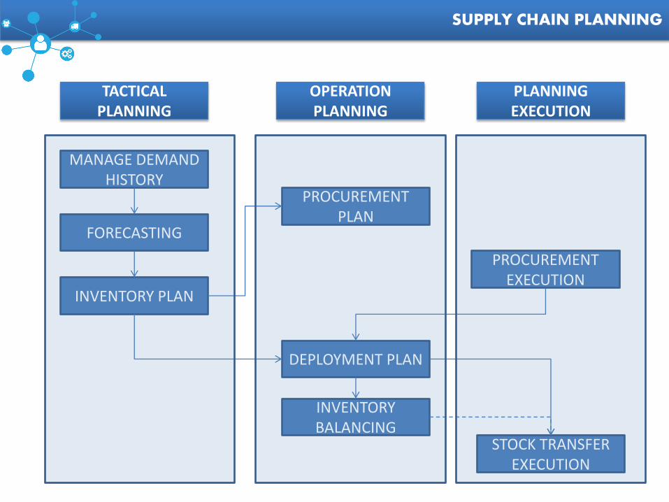
SUPPLY CHAIN PLANNING

MANAGE DEMAND HISTORY

FORECASTING

INVENTORY PLAN

PROCUREMENT PLAN

DEPLOYMENT PLAN

INVENTORY BALANCING

PROCUREMENT EXECUTION

STOCK TRANSFER EXECUTION

TACTICAL PLANNING

OPERATION PLANNING

PLANNING EXECUTION

At this level, you and your partners make joint decisions on strategic issues such as the following examples:

– Production capacities– Product design– Production facility and fulfilment network expansion– Portfolio joint marketing– Pricing plans

SUPPLY CHAIN PLANNING – STRATEGIC

This level involves sharing information with your partners on topics such as the following:

– Forecasts– Production and transportation plans and capacities– Bills of material (BOMs)– Orders– Product descriptions– Prices and promotions– Inventory– Allocations– Product and material availability– Service levels– Contract terms, such as supply capacity, inventory, and services

SUPPLY CHAIN PLANNING –TACTICAL

SUPPLY CHAIN PLANNING – EXECUTION

At this level, you and your partners engage in anintegrated exchange of key transactional data such asthe following information:

– Purchase orders– Production/work orders– Sales orders– POS information– Invoices– Credit notes– Debit notes– Payments

SUPPLY CHAIN MANAGER’S BALANCING ACT

Source: 2006 (c) McGraw Hill/Irwin

SUPPLY CHAIN – STRATEGIC PARTNERING

Criteria Types

DecisionMaker

InventoryOwnership

New SkillsEmployed by vendors

QuickResponse

AutomotiveManufacturer

AutomotiveManufacturer

Forecasting Skills

ContinuousReplenishment

Contractually Agreed to Levels

EitherParty

Forecasting & Inventory Control

AdvancedContinuous

Replenishment

Contractually agreed to & ContinuouslyImproved Levels

EitherParty

Forecasting & Inventory Control

VMI Vendor/Supplier EitherParty

DistributionManagement

Source: Simchi-Levi, Kaminsky & Simchi-Levi, Irwin McGraw Hill, 2000

BUILD TO FORECAST MODEL

TIER 2SUPPLIERS

TIER 1SUPPLIERS

INBOUND SUPPLY CHAIN

BODY/PAINT/ASSEMBLY

OUTBOUNDSUPPLY CHAIN

SEQUENCING

SCHEDULING

ORDERPLAN

SCHEDULING

PLAN

SCHEDULING

PURCHASING PROGRAMING MARKETING

NATIONAL SALES OFFICE

DEALER CUSTOMER

MATERIAL FLOW

INFO

RM

ATI

ON

FLO

W

INVENTORY

BUILD TO FORECAST MODEL

•Sales Forecasting aggregates all dealers and national sales companies’ forecasts and usesthem as an input for production programming. The method is the bottom-up approach.

•Production programming is the process of consolidating forecast market demand to availableproduction capacity to get the framework that defines how many vehicles will be built in eachfactory.

•Order entry is the stage in which orders are checked and entered into an order bank to awaitproduction scheduling.

•Production scheduling and sequencing fit orders from the order banks into productionschedules. These orders are used to develop the sequence of cars to be built on thescheduled date. Supplier scheduling is the process whereby suppliers receive forecasts atvarious times, actual schedules, and daily call-offs.

•Inbound logistics are the process of moving components and parts from supplier to assemblyplant.

•Vehicle production is the process of welding, painting, and assembling the vehicle.

•Vehicle distribution is the stage at which the finished vehicle is shipped to dealers.

BUILD TO DELIVERY MODEL

ORDER ENTRY BY DEALER 1

ORDER ALLOCATION CHECK BY

NATIONAL/REGIONAL SALES OFFICE

BUILD FEASIBILITY

CHECK

BILL-OF –MATERIALS (BOM)

EXPLOSION

ORDER BANK

ORDER ENTRY BY DEALER 2

AUTOMOBILE MANUFACTURER

TIER 2SUPPLIERS

TIER 1SUPPLIERS

INBOUND SUPPLY CHAIN

BODY/PAINT/ASSEMBLY

OUTBOUNDSUPPLY CHAIN

SEQUENCING

SCHEDULING

PLAN

SCHEDULING

PLAN

SCHEDULING

DEALER 1

CUSTOMER

DEALER 2

MATERIAL FLOW

INFORMATION FLOW

BUILD TO DELIVERY MODEL

•Order entry begins when a salesperson enters a customer order into the system. Then, theorder is passed on from the dealer to the national sales/regional sales office andsubsequently to the manufacturer’s headquarters.

•An allocation check is done at the national sales company to see if the desired vehicle isavailable or not for the dealer.

•Then, a build-feasibility check, which is the process of checking whether the special optionsand specifications are feasible for the production, follows to determine whether specialoptions and specifications are available for that vehicle in the market. If not, the systemrejects the order and the dealer must make the necessary order correction. Bill-Material-Conversion is the process of converting the orders received from the dealer to a bill ofmaterials.

•Bill-of-Material-Conversion is the process of converting the orders received from the dealerto a bill of materials. This tells the manufacturers what kind of components they need tobuild the vehicle.

•The final stage in order entry is to transfer the order as a bill of material to the order bank.The order will stay in the order bank until the system transfers it into the•plant’s production schedule.

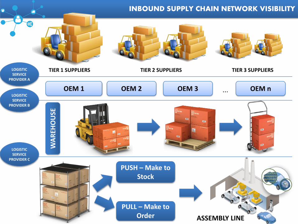
INBOUND SUPPLY CHAIN NETWORK VISIBILITY

TIER 1 SUPPLIERS TIER 2 SUPPLIERS TIER 3 SUPPLIERS

OEM 1 OEM 2 OEM 3 OEM n

LOGISTIC SERVICE

PROVIDER A

LOGISTIC SERVICE

PROVIDER B

LOGISTIC SERVICE

PROVIDER C

...

WA

REH

OU

SE

PUSH – Make to Stock

PULL – Make to Order ASSEMBLY LINE

INBOUND SUPPLY CHAIN COST OPTIMIZATION BY CROSS DOCKING

CROSS DOCK

OVERSEAS OEMs

MILK RUN

OEM 2

OEM 1

TIER 1 SUPPLIER

TIER 2 SUPPLIER

TIER 2 SUPPLIER

VEHICLEASSEMBLYCONSOLIDATED

DELIVERY

This strategy enables firms to use trucks moreefficiently. It also allows more frequent deliveries.This yields decreased logistics costs and allowsassembly plants to maintain supply stocks.

OUTBOUND SUPPLY CHAIN NETWORK VISIBILITY

LOGISTIC SERVICE

PROVIDER D

LOGISTIC SERVICE

PROVIDER E

WAREHOUSE 1 WAREHOUSE 2 WAREHOUSE 3 (EXPORT)

CENTRALIZED FINISHED GOODS – CAR LOT

AUTO DEALER 1 AUTO DEALER 2 AUTO DEALER 3

VEHICLE ASSEMBLY LINE

OUTBOUND SUPPLY CHAIN NETWORK LAYERS – AVAILABLE OPTIONS

REGIONAL DC 1 REGIONAL DC 2

CENTRAL WAREHOUSE(FINISHED GOODS – CAR LOT)


OPTION B: 2 LAYERS

OPTION A: 1 LAYER


.......................

Concept: Single Central Warehouse + Multiple RDCs

Product: Finished Brand New Automobile

Concept: Single Central Warehouse + Multiple Auto Dealers




OPTION C : 2 LAYERS

.........

CENTRAL WAREHOUSE 1(FINISHED GOODS – CAR LOT)

CENTRAL WAREHOUSE 2(FINISHED GOODS – CAR LOT)

REGIONAL DC 1 REGIONAL DC 2 REGIONAL DC 3

AUTO DEALER 1 AUTO DEALER 2 AUTO DEALER 3 AUTO DEALER 4

Concept: Multiple CentralWarehouses + Multiple RDCs



OPTION D: 3 LAYER OEM AFTERMARKET PARTS/

SPARE PARTS DISTRIBUTION CHANNEL

OEM 1 OEM 2 OEM n......

Concept: Multiple OEM Warehouses +Single Central Warehouse + Multiple RDCs + OEM Distribution Hub + Super Stockist

Product: Genuine Auto Spare Parts


REGIONAL DC 1 REGIONAL DC 2


OEM s OWNED DUSTRIBUTION HUB

AUTO MECHANIC 1 & 2 AFTERMARKET RETAILER

....... ...........

STOCKIST/ SUPER STOCKIST

Sou

rce:

(c)

Rah

ul G

uh

ath

aku

rta,

20

14

OEMsIndependent

parts makers

Repair parts

makers

Automobile makers Wholesalers Special agents

Dealers

Sub-dealers

Cooperative

sales companies

2nd-level

wholesalers

Retailers

Large usersPetrol

stations

Automobiles

repair shops

End users

Source: McKinsey Industry Studies

AFTERMARKET/SPARE PARTS – SUPPLY CHAIN NETWORK

Source: McKinsey Industries Study

AFTERMARKET/SPARE PARTS BUSINESS STAGES

Source: Deolite Automotive Aftermarket Survey

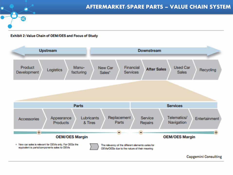
AFTERMARKET/SPARE PARTS – VALUE CHAIN SYSTEM

Legitimatew/ Counterfeitand Gray Market

UnauthorizedInternationalSupplier

UnauthorizedManufacturer

Internet/ web site/mail order

Will-FitSupplier

Broker

converted to counterfeit

DomesticSupplier

DomesticManufacturer

InternationalSupplier

Distribution Center

O.E. VehicleManufacturer

WarehouseDistributor

Auto Parts Store

Mechanic/ Repair Facility

End User /Vehicle Owner

SIAM Member CompanyIndian Manufacturer

Raw MaterialOrComponent

Color Key:= Raw Materials and/or Components

= SIAM Member Companies / Indian Mfgs= Original Equipment Channel= Independent Aftermarket Channel= Steps in the legitimate Supply Chain Model= Illegitimate Steps in Supply Chain

O.E. Dealer

Independent Aftermarket Channel

Original Equipment Channel

Master Dist/ Importer of Record

AFTERMARKET – COUNTERFIET/GRAY MARKET ELEMENTS IN SCM

Origin: Rajkot, Belgaum, Pune, Delhi NCR

INVENTORY AND WAREHOUSE MANAGEMENT

COST OF INVENTORY

Inventory is the raw materials, component parts, work-in-process, or finished products that are held at a location in the supply chain.

Physical holding costs:

-Out of pocket expenses for storing inventory (insurance, security, warehouse rental, cooling)- All costs that may be entailed before you sell it (obsolescence, spoilage, rework...)

Opportunity cost of inventory: foregone return on the funds invested.

Operational costs:

-Delay in detection of quality problems.

-Delay the introduction of new products.

-Increase throughput times.

COST OF INVENTORY - INBOUND

ORDER

TIER BASED SUPPLIERS/ OEMs

INVENTORY WAREHOUSE


COSTS

ORDERING COST

HOLDING COST

Key questions:•How often to review?•When to place an order?•How much to order?•How much stock to keep?

ORDER

COST OF INVENTORY - OUTBOUND

BU

ILD TO

FOR

ECA

ST OR

DER

NATIONAL/REGIONAL SALES OFFICE B

UILD

TO D

ELIVER

Y O

RD

ER

CENTRALIZED FINISHED GOODS – CAR LOT

AUTO DEALER


Let’s say we decide to order in batches of Q…

Number of periods will be

D

Q

Time

Total Time

Period over which demand for Q has occurred

Q

Inventory position

The average inventory for each period is…

Q

2

NOTATIONS

• Demand is known and deterministic: D units/year

• We have a known ordering cost, S, and immediate replenishment

• Annual holding cost of average inventory is H per unit

• Purchasing cost C per unit

UNDERSTANDING INVENTORY POSITION WITH RESPECT TO TIME

COMPUTATION OF TOTAL COST

Total Cost = Purchasing Cost + Ordering Cost + Inventory Cost

Purchasing Cost = (total units) x (cost per unit) = D x C

Ordering Cost = (number of orders) x (cost per order) =

Inventory Cost = (average inventory) x (holding cost) =

TOTAL COST = D x C + +

D

Qx S

Q

2x H

D

Qx S

Q

2x H

NOTE: In order now to find the optimal quantity we need to optimize the totalcost with respect to the decision variable (the variable we control)

COMPUTATION OF EOQ- ECONOMIC ORDER OF QUANTITY

Order Quantity (Q*)

Co

st

Total cost

Holding costs

Ordering costs

Q* = 2SD

H

EOQ = Q*

EOQ Insight on EOQ: There is a tradeoffbetween holding costs and orderingcosts

EOQ applies only when demand for a product is constant over the year and each new order is delivered in full when inventory reaches zero.

There is a fixed cost for each order placed, regardless of the number of units ordered. There is also a cost for each unit held in storage, commonly known as holding cost, sometimes expressed as a percentage of the purchase cost of the item.

CASE STUDY: DEDUCING AUTO DEALER ORDER SIZE

CASE STUDY:

Assume a car dealer that faces demand for 5,000 cars per year, and that it costs INR3,00,000 to have the cars shipped to the dealership. Holding cost is estimated at INR10,000 per car per year. How many times should the dealer order, and what should bethe order size?

54810000

)000,5)(300000(2* Q

Therefore, optimum Economic Order Of Quantity is 548 Cars

CASE STUDY

Receive

order

Time

Inve

nto

ry

Place

order

Lead Time

Order

Quantity

Q

If delivery is not instantaneous, but there is a lead time L:

When to order? How much to order?

ROP = LxD

Receive

order

Time

Inve

nto

ry

Order

Quantity

Q

Place

order

Lead Time

Reorder

Point

(ROP)

D: demand per periodL: Lead time in periods

Q: When shall we order?A: When inventory = ROP

Q: How much shall we order?A: Q = EOQ

If demand is known exactly, place an order when inventory equals demand during lead time.

What if the lead time to receive cars is 10 days? (when should you place your order?)

Since D is given in years, first convert: 10 days = 10/365yrs

10

365D = R =

10

3655000 = 137

So, when the number of cars on the lot reaches 137, order 548 more cars.

Time

Inventory

Level

Order

Quantity

Demand???

Receive

order

Place

order Lead Time

ROP = ???

PREDICTABILITY OF DEMAND

X

Inventory at time of receipt

Receive

order

Time

Inventory

Level

Order

Quantity

Place

order

Lead Time

ROP

Lead Time Demand

LEAD TIME DEMAND

Actual Demand < Expected Demand

Stockout

Point

Unfilled demand

Receive Receive

orderorder

TimeInven

tory

OrderOrder

QuantityQuantity

PlacePlace

orderorder

Lead TimeLead Time

If Actual Demand > Expected, we Stock-Out

STOCK-OUT POINT

ROP = Expected Demand

Average

Time

Inventory

Level

Order

Quantity

Uncertain Demand

RELATION BETWEEN ROP AND UNCERTAIN DEMAND

If ROP = expected demand, service level is 50%. Inventory left 50% of the

time, stock outs 50% of the time.

To reduce stock-outs we add safety stock

Receive Receive

orderorder

TimeTime

PlacePlace

orderorder

Lead TimeLead Time

InventoryLevel

ROP =

Safety

Stock +

Expected

LTDemand

Order QuantityQ = EOQ

ExpectedLT Demand

Safety Stock

SAFETY STOCK

Service level

Safety

Stock

Probabilityof stock-out

Decide what Service Level you want to provide (Service level = probability of NOT stocking out)

DECISION FOR SERVICE LEVEL

Variance over multiple periods = the sum of the variances of each period (assuming independence) and Standard deviation over multiple periods is the square root of

the sum of the variances, not the sum of the standard deviations!!!

Average Inventory = (Order Qty)/2 + Safety Stock

Receive Receive

orderorder

TimeTime

PlacePlace

orderorder

Lead TimeLead Time

InventoryLevel

Order

Quantity

Safety Stock (SS)

EOQ/2Average

Inventory

How to find ROP & Q

Order quantity Q =

To find ROP, determine the service level (i.e., the probability of NOT stocking out.) Find the safety factor from a z-table or from the graph. Find std deviation in LT demand: square root law.

Safety stock is given by: SS = (safety factor)(std dev in LT demand) Reorder point is: ROP = Expected LT demand + SS

Average Inventory is: SS + EOQ/2

2SDEOQ

H

( )

LT D

std dev in LT demand std dev in daily demand days in LT

LT

CALCULATING ROP BASED ON EOQ

Back to the car lot… recall that the lead time is 10 days and the expectedyearly demand is 5000. You estimate the standard deviation of daily demandto be d = 6. When should you re-order if you want to be 95% sure youdon’t run out of cars?

168)36(1065.1137 ROP

Since the expected yearly demand is 5000, the expected demand over thelead time is 5000(10/365) = 137. The z-value corresponding to a service levelof 0.95 is 1.65. So

Order 548 cars when the inventory level drops to 168.

COMPLETING THE CASE STUDY BY FINDING ROP – REORDER POINT

EOQ BASED QUANTITY DISCOUNT – AFTERMARKET VENDORS

PDHQ

SQ

DTCQD

2

Same as the EOQ, except: Unit price depends upon the quantity ordered

Calculate the EOQ at the lowest price

Determine whether the EOQ is feasible at that price

•Will the vendor sell that quantity at that price?•If yes, stop – if no, continue

Check the feasibility of EOQ at the next higher price

Continue until you identify a feasible EOQ

Calculate the total costs (including total item cost) for the feasible EOQ model

Calculate the total costs of buying at the minimum quantity required for each of the cheaper unit prices

Compare the total cost of each option & choose the lowest cost alternative

Any other issues to consider?


Annual Demand of Bearing Model TEX123 = 5000 units

Ordering cost = INR 49

Annual carrying charge = 20%

Quantity Unit Price

0 to 999 INR 5

1000 to 1999 INR 4.8

2000 and over INR 4.75

Unit price schedule:

feasiblenotQ INRP 71875.42.0

49000,5275.4

feasiblenotQ INRP 71480.42.0

49000,5280.4

feasibleQ INRP 70000.52.0

49000,5200.5

QUANTITY DISCOUNT : STEP 1


Annual Demand of Bearing Model TEX123 = 5000 units

Ordering cost = INR 49

Annual carrying charge = 20%

Quantity Unit Price

0 to 999 INR 5

1000 to 1999 INR 4.8

2000 and over INR 4.75

Unit price schedule:

QUANTITY DISCOUNT : STEP 2

700,25500000.500.52.02

70049

700

000,5700 INRTCQ

725,24500080.480.42.02

100049

1000

000,51000 INRTCQ

50.822,24500075.475.42.02

200049

2000

000,52000 INRTCQ

FEASIBLE

SCOR based MILP – Mixed Integer Linear Programing Model

The supply chain structure of the automobile industry under study consists of fourechelons viz. Suppliers, Manufacturing plants, Distribution Centres (DCs) and Customers .

The strategic level modelling is the long term planning which decides the basicconfiguration of the supply chain and determine the optimum number of the suppliersout of the approved list, plants and distribution centres to keep under operation and theassignment of customers to distribution centres with an objective of minimizing the totalcost of supply chain.

TIER BASED SUPPLIERS

OEMsAUTO

MANUFACTURERSDISTRIBUTION

CENTERSRETAILERS CUSTOMERS

ROLE OF CORPORATE HQ/OFFICE IN MILP MODEL

The MILP strategic level modeling is the long term planning which decides the basicconfiguration of the supply chain and determine the optimum number of the suppliersout of the approved list, plants and distribution centres to keep under operation and theassignment of customers to distribution centres with an objective of minimizing the totalcost of supply chain.

All the supply chain activities are controlled by the corporate office using a network ofinformation flow between the corporate office and various echelons. The industry underinvestigation receives the customer orders at its corporate office. The customer ordersprimarily include the three key information i.e. the quantity required, delivery dates andpenalty clause for late delivery.

All customers’ demands are aggregated and the annual production distribution planningis done by the corporate office. At the strategic level decision, the corporate office decidesthe suppliers and the allocation of the quantities of the raw materials to the selectedsuppliers, optimum production quantity allocation to various manufacturing plants, theassignment of the distribution centres to the manufacturing plants and also theassignment of the customers to the distribution centres.

ASSUMPTIONS MADE IN THE MILP MODEL

• It has been assumed that production of one unit of a product requires one unit of plant capacity,regardless of type of product. The similar assumption is adopted for distribution centres also.

• The components/raw materials procurement and finished product inventory at stores follow acontinuous-review inventory control policy.

• The demand for the finished products is deterministic and the demand rate is constant over timehorizon under study. The model considers the demands generated at each distribution centreindependently from each other.

• The processing time, which is the time to perform the operation, is a linear function of the quantityof the products produced.

• Transportation times of components/raw materials, subassemblies and finished products betweenthe stages of the production cycle have been assumed to be same in the present model.

• A type of product can be produced in more than one plant, and each plant can produce at least onetype of product.

• The transportation time, waiting time, setup time and production processing times have beenassumed to be fixed.

• The plants usually hold raw material stock to maintain production.

NOTATIONS DESCRIPTION OF NOTATIONS

T Index on product, where t = 1…….T, T is number of types of products produced

Z Index on manufacturing plant, where z = 1…….Z, Z is the number of manufacturing plants

D Index on distribution centre, where d = 1…….D, D is the number of distribution centres

C Index on customer, where c = 1…….C, C is the number of customers

S Index on supplier, where s = 1…….S, S is the number of suppliers

B (d) Binary variable for distribution centre

B (dc) Binary variable for distribution centre ‘d’ serving customer ‘c’

B (z) Binary variable for plant ‘z’

CP (z) Production capacity of plant ‘z’ (number of products/year)

D (tc) Demand of customer ‘c’ for product ‘t’ (number of products/year)

MILP – Mixed Integer Linear Programing Model (NOTATIONS)



F (d) Fixed cost of distribution centre ‘d’ (Rupees/year)

F (z) Fixed cost of plant ‘z’ (Rupees/year)

Max. PV (tz) Maximum production capacity for product ‘t’ at plant ‘z’ (number of products/year)

Max. TP (d) Maximum throughput capacity of distribution centre ‘d’ (number of products per year)

Min. PV (tz) Minimum production volume required for product ‘t’ at plant ‘z’ to keep the plant operational (number of products/year)

Min. TP (d) Minimum throughput required at distribution centre ‘d’ to keep the distribution centre operational (number of products/year)

PC (ms) Unit cost of component/raw material ‘m’ of supplier ‘s’ (Rupees per component or Rupees per Kg)

Q (tz) Quantity of product ‘t’ produced at plant ‘z’ (number of products per year)

Q (tzd) Quantity of product ‘t’ shipped from plant ‘z’ to distribution centre ‘d’ (number of products/year)



Q (msz) Quantity of component/raw material ‘m’ shipped from supplier ‘s’ to plant ‘z’ (number of products/year)

UCT (td) Unit throughput cost (handling and inventory)of product ‘t’ at distribution centre ’d’ (Rupees/product)

UPC (tz) Unit production cost for product ‘t’ at plant ‘z’ (Rupees/product)

UTC (tdc) Unit transportation cost of product ‘t’ from distribution centre ‘d’ to customer ‘c’ (Rupees per product)

UTC (tzd) Unit transportation cost of product ‘t’ from plant ‘z’ to distribution centre ‘d’ (Rupees per product)

UTC (msz) Unit transportation cost of component/raw material ‘m’ from supplier ‘s’ to plant ‘z’(Rupees per unit of component/raw material)

w(1), w(2)... Weight factors for plant and distribution centre volume flexibility

X Total cost of entire supply chain (Rupees/year)

The objective function of the strategic model is to minimize the total cost of entire supplychain. The total cost of the supply chain includes the cost of raw materials, varioustransportation costs of components/raw materials and finished products between variousechelons and various fixed and variable costs associated with the plants and distributioncentres. The objective function which is the sum of various costs is represented inmathematical form as:

Min X = Cost 1+ Cost 2 + Cost 3 + Cost 4 + Cost 5 + Cost 6 + Cost 7 + Cost 8

MILP – Mixed Integer Linear Programing Model (EQUATIONS)

COST 1 Total cost of components/raw materials supplied by suppliers

∑Unit cost of component/raw material ‘m’ of supplier ‘s’(Rupees per component or Rupees per Kg) X Quantity ofcomponent/raw material ‘m’ shipped from supplier ‘s’ toplant ‘z’ (number of products/year)

∑ PC(ms) x Q (msz)( )msz


COST 2

∑COST 3

∑

∑Transportation cost of components/raw materials from suppliers to the manufacturing plants.

Transportation cost of components/raw materials fromsuppliers to the manufacturing plants X Quantity ofcomponent/raw material ‘m’ shipped from supplier ‘s’ toplant ‘z’ (number of products/year)

msz

( )UTC (msz) x Q (msz)

Fixed cost associated with plant operations

∑ Fixed cost of plant ‘z’ (Rupees/year) X Binary variable for plant ‘z’

( )F(z) x B(z)

z


COST 4

∑COST 5

∑

Variable costs associated with plant operations

∑ Unit production cost for product ‘t’ at plant ‘z’ (Rupees/product) X Quantity of product ‘t’ produced at plant ‘z’ (number of products per year)

tz

( )UPC (tz) x Q (tz)

Fixed cost associated with distribution centre operations

∑ Fixed cost of distribution centre ‘d’ (Rupees/year) X Binary variable for distribution centre

( )F (d) x B (d)

d

∑COST 7

∑


COST 6 Variable cost associated with distribution centre operations

∑Unit throughput cost (handling and inventory)of product ‘t’ at distribution centre ’d’ (Rupees/product) X Demand of customer ‘c’ for product ‘t’ (number of products/year) X Binary variable for distribution centre ‘d’ serving customer ‘c’

( )UCT(td) x D(tc) x B(dc)

Transportation cost of products from plants to the distribution centres

tdc

Unit transportation cost of product ‘t’ from plant ‘z’ todistribution centre ‘d’ (Rupees per product) X Quantityof product ‘t’ shipped from plant ‘z’ to distribution centre‘d’ (number of products/year)

∑( )UTC (tzd) x Q (tzd)

tzd


∑

COST 8

∑

Transportation cost of products from distribution centres to customers

Unit transportation cost of product ‘t’ from distributioncentre ‘d’ to customer ‘c’ (Rupees per product) XDemand of customer ‘c’ for product ‘t’ (number ofproducts/year) X Binary variable for distribution centre‘d’ serving customer ‘c’

UTC (tdc) x D (tc) x B(dc)( )tdc

Min. X

MILP SOLUTION BY LINGO 14.0

The use of conventional tools for solving theMILP problem is limited due to the complexityof the problem and the large number ofvariables and constraints, particularly forrealistically sized problems.

LINGO an Operations Research software tool isused to solve the strategic MILP model forsupply chain of the said automobile industry.LINGO solves the problems by using branchand bound methodology.

The main purpose of LINGO is to allow a userto quickly input a model formulation, solve it,assess the correctness or appropriateness ofthe formulation based on the solution, quicklymake minor modifications to the formulation,and repeat the process.

LINGO features a wide range of commands,any of which may be invoked at any time.LINGO optimization model has two attributes:objective function of problem and constraintsof problem.

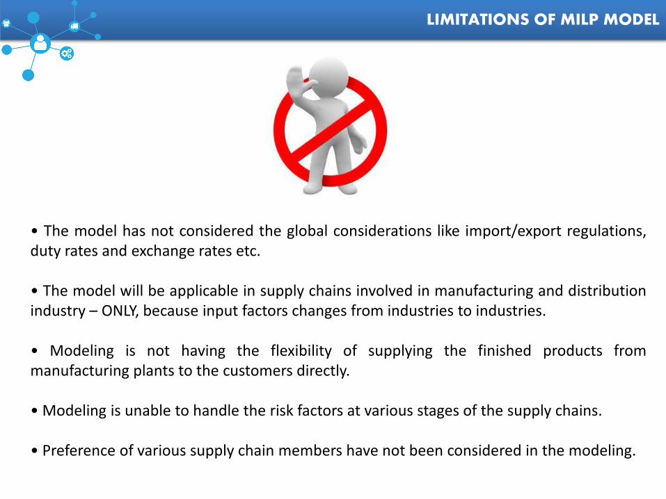
LIMITATIONS OF MILP MODEL

• The model has not considered the global considerations like import/export regulations,duty rates and exchange rates etc.

• The model will be applicable in supply chains involved in manufacturing and distributionindustry – ONLY, because input factors changes from industries to industries.

• Modeling is not having the flexibility of supplying the finished products frommanufacturing plants to the customers directly.

• Modeling is unable to handle the risk factors at various stages of the supply chains.

• Preference of various supply chain members have not been considered in the modeling.

After giving the above as input, the strategic model, given by above equation is able to give the following outputs:

• Quantities of products produced at the plants.

• Quantities of raw materials shipped from the suppliers to the plants.

• Quantities of products shipped from plants to the distribution centers.

• Quantities of products shipped from the distribution centers to the customers.

• Total volume flexibility.

• Total cost of the entire supply chain.

FINAL OUTPUT OF MILP MODEL

COLLABORATION IN SCM

COLLABORATION IN SUPPLY CHAIN MANAGEMENT

Inter-organizational Systems forSupply Chain Collaboration can beclassified into sub-systems thatsupport varying degrees of supplychain co-ordination andcollaboration into three majortypes:

1. message-based systems thattransmit information to partnerapplications using technologiessuch as fax, e-mail EDI oreXtensible Markup Language(XML) messages.

2. Electronic procurement hubs,portals or market places thatfacilitates purchasing of goodsand services from electroniccatalogues, tenders andauctions.

3. Shared collaborative SCM systems that includecollaborative planning, forecasting andreplenishment capabilities in addition toelectronic procurement functionality.

WORK FLOW – KANBAN BOARD IN SAP

看板 – Kanban literallymeans “visual card,”“signboard,” or “billboard.”

Toyota originally usedKanban cards to limit theamount of inventory tied upin “work in progress” on amanufacturing floor.

Not only is excess inventorywaste, time spent producingit is time that could beexpended elsewhere.

Kanban cards act as a formof “currency” representinghow WIP is allowed in asystem.

GOALS STORY QUE WORK IN PROGRESS DONE!

ACCEPTANCE DEVELOPMENT TEST DEPLOYMENT

EXPEDITE

WORK FLOW – A TYPICAL KANBAN BOARD

14 Days Wait Time

18 Days Wait Time

GOALS

GOALS

GOALS

Waiting Work Queue

CATIA V5 – INTEGRATED DESIGN PLATFORM

ENOVIA 3D Live: Virtual Product LifeCycle Management

ENOVIA is for collaborativemanagement and global lifecycle (PLM) with thehistorical VPM (VirtualProduct Management) andits successor VPLM as well asDMU which came from theSmartTeam and MatrixOneacquisitions.

ENOVIA provides aframework for collaborationfor Auto Company's PLMsoftware. It is an onlineenvironment that involvescreators, collaborators andconsumers in the productlifecycle.

CATIA V5ENOVIA

V6SAP

CIDEON V6X PDM SAP INTERFACE

ENGINEERING = (DESIGN+PLM) MANUFACTURING

Customer Relationship

Management

Supplier Relationship Management

CRM

SRM

FI / CO MM PP QM SD

Finance /

Control

Materials

Management

Production

Planning

Quality

Management

Ext. Services

Management

IPMS

ESM

Sales &

Distribution

PM

Plant

Maint.

PLM

Product Life-Cycle Management

TYPICAL SAP MODULES IN AUTOMOTIVE ASSEMBLY PLANT

Integrated Production Management

SAP ver ECC 6.0

Sales &

DistributionProduction

Planning

Finance / Control

Human Resource

Quality

Management

Business

Warehouse

Supply Rel

Management

Product Lifecycle

Management

Material

Managment

SAP ECOSYSTEM

SAP NETWEAEVER PLATFORM

The SAP NetWeaver® platformempowers the collaborativefunctionalities of SAP SCM. It allowsyou to flexibly and rapidly deploy,execute, monitor, and refine thesoftware that enables your businessprocesses and strategies. With SAPNetWeaver, you can deployinnovative business processes acrossthe organization while making use ofyour existing software and systems.

SAP NetWeaver provides end-to-endprocess integration by enablingapplication-to-application processesand business to- business processes,performing business processmanagement and business taskmanagement and enabling platforminteroperability.

CONCLUSION

A supply chain is defined as a set of relationships among suppliers, manufacturers,distributors, and retailers that facilitates the transformation of raw materials into finalproducts. Although the supply chain is comprised of a number of business components,the chain itself is viewed as a single entity.

In construction and identification of this integrated logistics model, we identified theprimary processes as logistics processes concerning all the participants of the integratedvalue chain. It is reasonable to consider transfers and transaction of products andinformation as primary processes, when logistics functions are in focus

It shares operating and financial risks by having these suppliers build with their capital andoperate their employees, facilities that are usually part of the OEM’s span of control. Theyshare the profits with Automotive Manufacturers when demand is strong because thesesuppliers receive a payment per unit that covers variable material and labor costs andcontributes to overhead and profit. When demand is high, this relationship is profitable forall. When the economy is slumping, they share the loss with Automotive Manufacturersbecause Automotive Manufacturers buys only what it needs to meet consumer demand.Automotive Manufacturers has less invested capital and therefore lower fixed costs.

CONCLUSION

Even though Automotive Manufacturers is at the end of the assembly process, itcoordinates the supply chain by providing demand information to not only first tier butsecond, third, and fourth tier suppliers. This process of spreading information aboutproduct demand often, quickly, and simultaneous provides the supply chain members withup-to-date information that greatly reduces/eliminates fluctuation in demand usually seenby suppliers, commonly known as the bullwhip effect .

Sequence Part Delivery and Pay As Built systems are commonly used by OEMs and theirsupply chains to simplify transactions, reduce transportation cost, slash inventory, andimprove efficiency. These systems work very well when the components being shipped arebulky and take much inventory space, can be easily damaged, and are expensive to ship

Just In Time (JIT) concept can also be incorporated to improve further the integratedlogistics model which can be considered as a future work.

ABOUT AUTHOR

Email: [email protected] / [email protected]

Cell Number/WhatsApp/Viber : +91-9978066443, Skype: rahul.gt

Webpage: http://about.me/rahul.guhathakurta, SlideShare: http://www.slideshare.com/rahulogy

Copyright Guidelines

DO1. Make a copy of backups on your hard-drive or network2. Use this presentation for personal, educational or professional purpose3. Print as hand-outs for your audience or shared groups4. Embed this power-point and integrate with your website5. Use it to make your own presentation but do give due credit

DON’T1. Resell or distribute my work as your own’2. Make it available for download on a portal3. Edit of modify this presentation and claim/pass off as your own work

mailto:[email protected]

mailto:[email protected]

http://about.me/rahul.guhathakurta

http://www.slideshare.com/rahulogy

BIBLIOGRAPHY

• Supply Chain Collaboration: The Key to Success in aGlobal Economy by SAP

• Supply Chain Collaboration Alternatives:Understanding the expected costs and benefits – TimMcLaren, Milena Head, Yufei Yuan

• A Strategic Level Model for Supply Chain of anAutomotive Industry: Formulation and SolutionApproach by Dr. Amit Kumar Gupta, Dr. O.P. Singh, Dr.R.K. Garg

• A Structured Approach to Optimize Outbound SupplyChain Cost in an Automotive Industry by C. P. ArunaKumari , Y. Vijaya Kumar

• Damien Power, titled, “Adoption of Supply ChainManagement Enabling Technologies: Comparing Small,Medium and Larger Organizations”, Journal ofOperations and Supply Chain Management (1), Volume1, Number 1, May 2008, pp 31-42.

• Aguilar-Savén, R.S., 2004. Business Process Modelling:Review and Framework. Int. J. Production Economics,90, 129-149.

• Kejia Chen, Ping Ji “A mixed integer programmingmodel for advanced planning and scheduling”European Journal of Operations Research, 181(2007),515-522

• Aslam T., Ng A.H.C., 2010. Multi-objective Optimizationfor Supply Chain Management: a Literature Reviewand New Development. SCMIS 8thInternationalConference on Supply Chain Management andInformation Systems, 6-9 October 2010, 1-8

• Supply Chain Operations Reference (SCOR®) model 10.0 by SCC• Managing Supply Networks in the Automotive Industry:

Integration of OEM, Suppliers and Logistic Service Providersby Bernd Hellingrath

• The Aftermarket in the Automotive Industry-CapgemniConsulting

• Supply Chain Design and Analysis: Models and Methods byBenita M. Beamon, University of Washington

• Bhatnagar, Rohit, Chandra Pankaj, and Suresh K. Goyal, 1993.Models for Multi-Plant Coordination, European Journal ofOperational Research, 67: 141-160.

• Chen, Fangruo, 1997. Decentralized Supply Chains Subject toInformation Delays (formerly The Stationary Beer Game),Graduate School of Business, Columbia University, New York, NY.

• Clark, A.J. and H. Scarf, 1962. Approximate Solutions to a SimpleMulti- Echelon Inventory Problem, in K.J. Arros, S. Karlin, and H.Scarf (eds.), Studies in Applied Probability and ManagementScience, pp. 88-110, Stanford, CA: Stanford University Press.

• Cohen, Morris A. and Sanqwon Moon, 1990. Impact ofProduction Scale Economies, Manufacturing Complexity, andTransportation Costs on Supply Chain Facility Networks, Journalof Manufacturing and Operations Management, 3: 269- 292.

• North American automotive supplier supply chain performancestudy BY PwC

• An Analysis of Automobile Demand by Øyvind ThomassenExeter College University of Oxford MPhil thesis in EconomicsTrinity term

• Caplin, A., and B. Nalebuff (1991): “Aggregation and ImperfectCompetition: On the Existence of Equilibrium,” Econometrica,59(1), 25–59.

Automotive Supply Chain Management - Zenodo

Documents

Transcript of Automotive Supply Chain Management - Zenodo