MONITORING DIACHRONIC CHANGES OF THE CITY OF SAO PAULO WITH

MULTI-TEMPORAL SPECTRAL MIXTURE ANALYSIS.

Reinaldo Paul Pérez MachadoDepartamento de Geografia, Universidade de São Paulo,

Av. Prof. Lineu Prestes, 338CEP 0558-000. São Paulo – SP. Brasil

rpmgis@usp.br

Christopher Small304b Oceanography

Lamont Doherty Earth Observatory of Columbia University,Palisades NY 10964. USAsmall@ldeo.columbia.edu

ABSTRACT

Spatio-temporal change mapping with remotely sensed imagery has thepotential to inform a wide variety of urban research and managementquestions. Despite its great potential, moderate resolution (10-30 m)remotely sensed imagery is underutilized for urban applications.Traditionally, urban applications of remote sensing use high spatialresolution imagery, while moderate spatial resolution is widely useon non-urban applications. But Landsat’s 30 m resolution has provedsufficient for measurement of some environmental urban parametersthat would be both very difficult and expensive to measure directly.The spatiotemporal distribution of the increase of urban built-upareas coincident with the apparent diminishing of the vegetation isan important relationship of the urban fabric that can be quantifiedusing multispectral imagery. However, conventional classificationmethods used at scales compatible with the sensor spatial resolutionhave proven to be of limited utility in urban areas, due to thespectral heterogeneity of this complex environment, which commonlycombines several different materials. Spectral mixture models, on theother hand, may provide a physically based solution to the urbanspectral heterogeneity issue, especially because it is possible toreduce the dimensionality of the multispectral reflectance byconverting it to areal fractions of land cover components, thusfacilitating the interpretation. The purpose of this study is toanalyze the most conspicuous changes occurred on the city of São

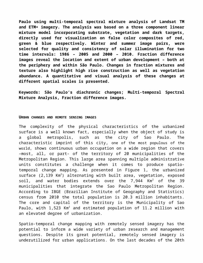
Paulo using multi-temporal spectral mixture analysis of Landsat TMand ETM+ imagery. The analysis was based on a three component linearmixture model incorporating substrate, vegetation and dark targets,directly used for visualization on false color composites of red,green & blue respectively. Winter and summer image pairs, wereselected for quality and consistency of solar illumination for twotime intervals: 1986 – 2005 and 2000 – 2010. Fraction differenceimages reveal the location and extent of urban development – both atthe periphery and within São Paulo. Changes in fraction mixtures andtexture also highlight high rise construction as well as vegetationabundance. A quantitative and visual analysis of these changes atdifferent spatial scales is presented.

Keywords: São Paulo’s diachronic changes; Multi-temporal SpectralMixture Analysis, Fraction difference images.

URBAN CHANGES AND REMOTE SENSING IMAGES

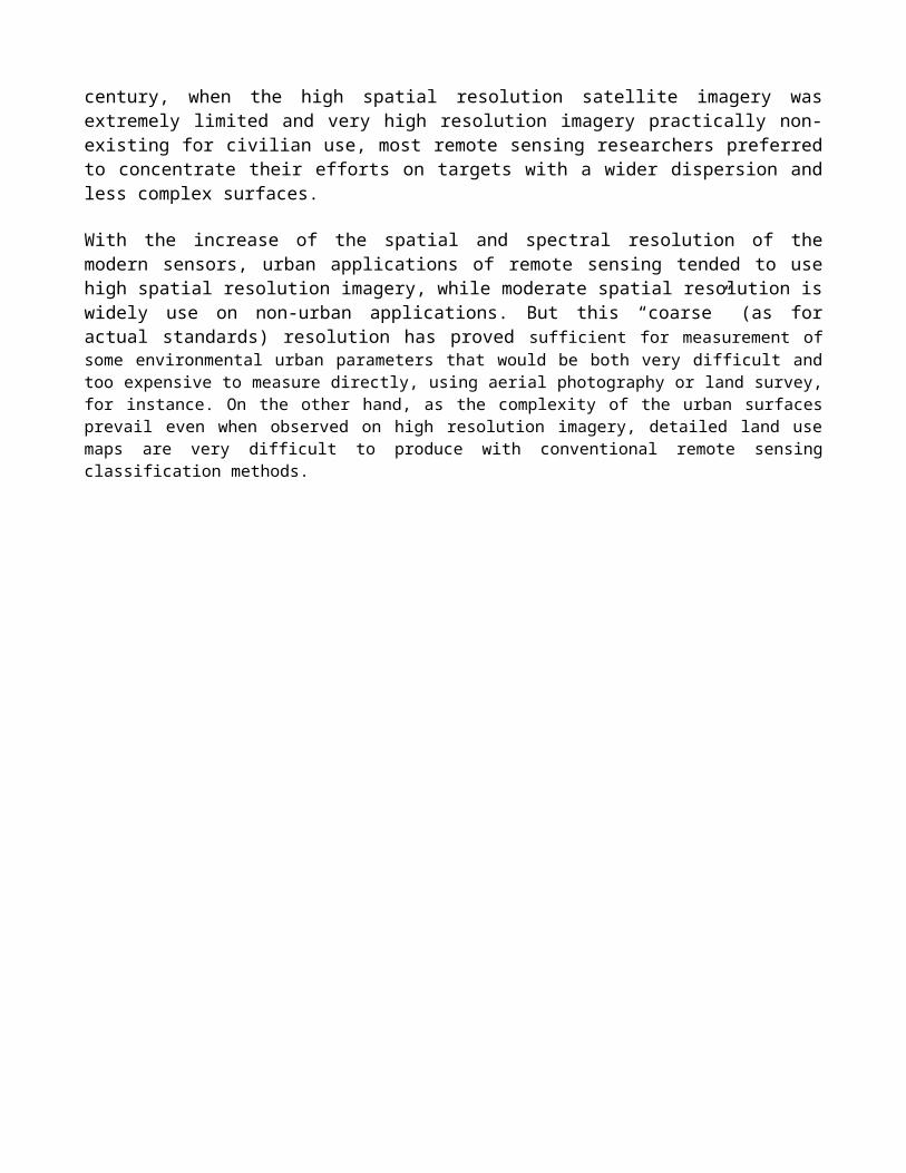
The complexity of the physical characteristics of the urbanizedsurface is a well known fact, especially when the object of study isa global metropolis, such as the city of Sao Paulo. Thecharacteristic imprint of this city, one of the most populous of theworld, shows continuous urban occupation on a wide region that covers–most, all, or part- of the territory of 20 municipalities of theMetropolitan Region. This large area spanning multiple administrativeunits constitutes a challenge when it comes to produce spatio-temporal change mapping. As presented in Figure 1, the urbanizedsurface (2,139 Km2) alternating with built area, vegetation, exposedsoil, and water bodies extends over the 7,944 Km2 of the 39municipalities that integrate the Sao Paulo Metropolitan Region.According to IBGE (Brazilian Institute of Geography and Statistics)census from 2010 the total population is 20.3 million inhabitants.The core and capital of the territory is the Municipality of SaoPaulo, with 1,523 Km2 and estimated population of 11.2 million withan elevated degree of urbanization.

Spatio-temporal change mapping with remotely sensed imagery has thepotential to inform a wide variety of urban research and managementquestions. Despite its great potential, remotely sensed imagery isunderutilized for urban applications. On the last decades of the 20th

century, when the high spatial resolution satellite imagery wasextremely limited and very high resolution imagery practically non-existing for civilian use, most remote sensing researchers preferredto concentrate their efforts on targets with a wider dispersion andless complex surfaces.

With the increase of the spatial and spectral resolution of themodern sensors, urban applications of remote sensing tended to usehigh spatial resolution imagery, while moderate spatial resolution iswidely use on non-urban applications. But this “coarse” (as foractual standards) resolution has proved sufficient for measurement ofsome environmental urban parameters that would be both very difficult andtoo expensive to measure directly, using aerial photography or land survey,for instance. On the other hand, as the complexity of the urban surfacesprevail even when observed on high resolution imagery, detailed land usemaps are very difficult to produce with conventional remote sensingclassification methods.

Figure 1. Visible/infrared false color composition Landsat 5 image (TMbands 7, 4 and 2 - RGB) of the study area. The municipality limits of SaoPaulo’s Metropolitan Region are shown in yellow. Note that the urbancontinuum (in rose-pink) of the city extends over the municipality of SaoPaulo, at the center. Water bodies are depicted as black. The image wascollected 12:55 PM April 4th 2010.

The characteristic spatial scale and the spectral variability ofurban landcover pose serious problems for traditional imageclassification algorithms. In urban areas where the reflectancespectra of the landcover vary appreciably at scales comparable to, or

smaller than, the Ground Instantaneous Field Of View (GIFOV) of mostsatellite sensors, the spectral reflectance of a individual pixelwill generally not resemble the reflectance of a single landcoverclass but rather a mixture of the reflectances of two or more targetspresent within the GIFOV. Because they are combinations of spectrallydistinct landcover types, mixed pixels in urban areas are frequentlymisclassified as other landcover classes. Conversely, the definitionof an urban spectral class will often misclassify pixels of othernon-urban landcover.

Perhaps, the logical solution to avoid this situation would be toincrease the spatial resolution of the input remote sensing imageryby selecting a sensor with a very small GIFOV. These images have beennamed as high resolution (1 to 5 meters pixel size) and very highresolution (less than 1 meter). The problem is that urban tissue isstill very complex as we “zoom in” increasing the spatial resolution,so the costs of the images and consequent processing would rise aswell.

The spatiotemporal distribution of the increase of urban built-upareas coincident with the apparent diminishing of the vegetation isan important relationship of the urbanized surfaces that can bequantified using multispectral imagery. However, conventionalclassifications methods used at scales compatible with the sensorspatial resolution have proven to be of limited utility in urbanareas, due to the spectral heterogeneity of this dynamic and complexenvironment, which commonly combines several different materials ofnatural and artificial origin. Spectral Mixture Models - SMM, on theother hand, may provide a physically based solution to the urbanspectral heterogeneity issue, especially because it is possible toreduce the dimensionality of the multispectral reflectance byconverting it to areal fractions of land cover components, thusfacilitating the interpretation. The good news is that as the SMMassumes the spectral heterogeneity as a basis of its analysis (asSpectral Mixture Analysis –SMA); consequently it would be possible touse coarse resolution imagery to study urban territories.

For instance, if an urban area contains significant amounts ofvegetation then the reflectance spectra measured by the sensor willbe influenced by the reflectance characteristics of the vegetation.Macroscopic combinations of homogeneous "endmember" materials within

the GIFOV often produce a composite reflectance spectrum that can bedescribed as a linear combination of the spectra of the endmembers(SINGER & MCCORD, 1979). If mixing between the endmember spectra ispredominantly linear and the endmembers are previously known, it maybe possible to "unmix" individual pixels by estimating the fractionof each endmember in the composite reflectance of a mixed pixel(BOARDMAN, 1989); (ADAMS, SABOL, et al., 1995). A variety of methodshave been developed to estimate the areal abundance of endmembermaterials within mixed pixels - particularly for use with imagingspectrometers in geologic remote sensing e.g. (CLARK & ROUSH, 1984);(GOETZ, VANE, et al., 1985); (KRUSE, 1988); (BOARDMAN & KRUSE, 1994)and vegetation mapping (PECH, DAVIES, et al., 1986); (SMITH, USTIN, etal., 1990); (ELVIDGE, CHEN & GROENEVELD, 1993); (ROBERTS, SMITH &ADAMS, 1993), (KAWAKUBO, MORATO, et al., 2009). Some authors (HOLBENand SHIMABUKURO, 1993; SMALL, 2005; SMALL & LU, 2006; CARNEIRO,2009); have used the endmember fractions provided by the SpectralMixture Models to analyze urban surfaces.

Apparently, the advantage of using the analysis by means of spectralmixture (SMA) would be the possibility to enhance and facilitateimage interpretation. To interpret an image in terms of proportionsor approximate fractions of the different materials that forms eachpixel is much easier to be done than considering separate values ofradiance, reflectance and emitance of the present materials (ADAMS &GILLESPIE, 2006). Thus, on the concept of Spectral Mixture Model, animage representing soil fraction, for instance, would be analyzedover its proportion within the pixel, that might vary from zero (0) –area totally covered by vegetation- to 100% -area of exposed soilwhere vegetation would be totally missing. The strength of theSpectral Mixture Analysis approach lies in the fact that itexplicitly takes into account the physical processes responsible forthe observed radiances and therefore accommodates the existence ofmixed pixels.

Spectral mixture occurs in two ways: linear and non linear. Linearmixture is more frequently used and it considers the mixture as alinear combination of the different components of the pixel weightedby their respective proportions. The non linear mixture is moreintricate to be represented than the linear one because on that kindof mixture, the radiance interact with more than one material, thusresulting on multiple and complex interactions.

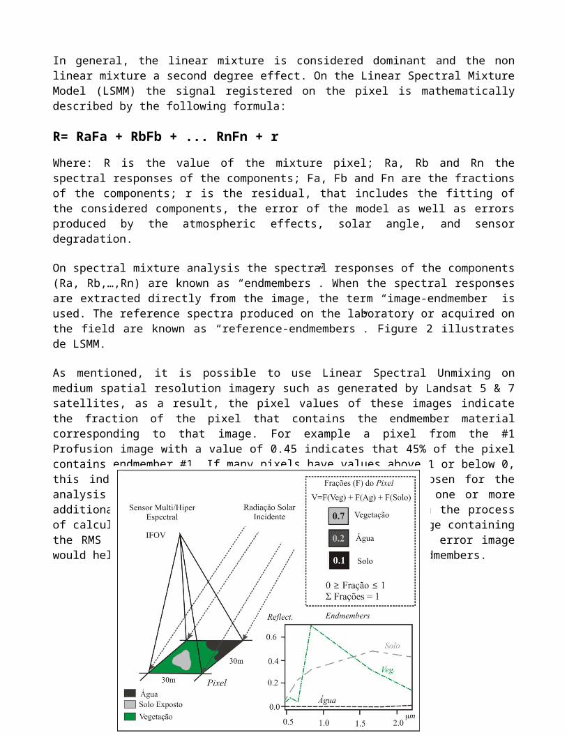
In general, the linear mixture is considered dominant and the nonlinear mixture a second degree effect. On the Linear Spectral MixtureModel (LSMM) the signal registered on the pixel is mathematicallydescribed by the following formula:

R= RaFa + RbFb + ... RnFn + rWhere: R is the value of the mixture pixel; Ra, Rb and Rn thespectral responses of the components; Fa, Fb and Fn are the fractionsof the components; r is the residual, that includes the fitting ofthe considered components, the error of the model as well as errorsproduced by the atmospheric effects, solar angle, and sensordegradation.

On spectral mixture analysis the spectral responses of the components(Ra, Rb,…,Rn) are known as “endmembers”. When the spectral responsesare extracted directly from the image, the term “image-endmember” isused. The reference spectra produced on the laboratory or acquired onthe field are known as “reference-endmembers”. Figure 2 illustratesde LSMM.

As mentioned, it is possible to use Linear Spectral Unmixing onmedium spatial resolution imagery such as generated by Landsat 5 & 7satellites, as a result, the pixel values of these images indicatethe fraction of the pixel that contains the endmember materialcorresponding to that image. For example a pixel from the #1Profusion image with a value of 0.45 indicates that 45% of the pixelcontains endmember #1. If many pixels have values above 1 or below 0,this indicates that one or more of the endmembers chosen for theanalysis are probably not well-characterized, or that one or moreadditional endmembers are missing from the analysis. On the processof calculating three endmembers of an image, a forth image containingthe RMS error is generated. A good analysis of the RMS error imagewould help to determine areas of missing or incorrect endmembers.

Figure 2. Perfect decomposition with a Linear Spectral Mixture Model (LSMM)on a 30m pixel formed by a mixture of 3 components: vegetation, water andsoil. On this case the residual is zero. Source (KAWAKUBO, 2010, p. 27).

Analysis of Landsat TM and ETM+ imagery suggests that the spectralreflectance of the Sao Paulo metropolitan area can be described aslinear mixing of three distinct spectral endmembers: Substrate,Vegetation and Dark. This paper provides only a brief summary ofurban Spectral Mixture Analysis (SMA) technique. A more detaileddiscussion of the use of Linear Spectral Mixture Analysis (LSMA) aswell as the theory, analysis and validation is given by Adams andGillespie (2006) for urban areas is given by Kressler andSteinnocher, (1996), Small, (2001; 2003; 2005) and Small and Lu,(2006).

In this case, the Substrate represents bare soil, rocks and built upareas, including impervious and non impervious surfaces. Vegetationcorresponds to dense forest, grass or agricultural areas. Forest andopen canopy vegetation contain an internal shade component and arerepresented along the mixing line between the Vegetation and Darkendmembers. The Dark endmember corresponds to clear water or deepshadow. Water containing suspended sediment and biologicalproductivity is more reflective so it occurs along the mixing linebetween the Substrate and Dark endmembers. But in some cases appearsdistinct Vegetation endmember on the water bodies due to the presenceof algae and aquatic macrophytes which emergence and grow was boosted

by different degrees of eutrophication. Clouds were not present onthe study area in any of the four scenes selected for this paper.

CHANGE ANALYSIS ON THE CITY OF SAO PAULO

The purpose of this study is to analyze the most conspicuous changesoccurred on the city of Sao Paulo using multi-temporal spectralmixture analysis of Landsat TM and ETM+ imagery. The analysis wasbased on a three component linear mixture model incorporatingSubstrate, Vegetation and Dark targets (also known as Endmembers),directly used for visualization on false color composites of red,green & blue respectively. Summer (April) and winter (August) imagepairs, were selected for quality and consistency of solarillumination for 1986 – 2005 and 2000 – 2010. Selected images weremosaicked to cover the study area (164 x 127 km), and cutaccordingly. The two pairs were matched by date, as presented on thelist in Table 1.

Table 1. The eight scenes of Landsat TM and ETM+ that were processedmosaicked and cut, as depicted on Figure 1. Note the date, time and solarelevation alignment on the two pairs (1986 – 2005) and (2000 – 2010).

IMAGE SATELLITE SENSOR

ACQUISITION

DATE TIMESOLAR

ELEVATION

219076 &

219077

Landsat

5TM

08/06/198

6

12:26 PM 33.22

219076 &

219077

Landsat

7ETM+

08/02/200

5

12:53 PM 36.97

219076 &

219077

Landsat

7ETM+

04/30/200

0

12:57 PM 40.90

219076 &

219077

Landsat

5TM

04/18/201

0

12:55 PM 43.39

Fraction images with the three previously mentioned Endmembers foreach of the four selected scenes were produced. An example, showingthe most recent image (from 04/18/2010) is depicted on Figure 3.

In order to apply the LSMA technique of image processing, the sixspectral bands (30 m spatial resolution) that are common on bothsensors were used. It was a very fortunate circumstance that the 2010image became available, because good quality Landsat 5 TM imagery areitems of rare occurrence, as this satellite (launched on 1984) shouldhave cease to work a long time ago; the sensor is still active, wellbeyond it’s designed lifespan.

Figure 3. False color composite fraction image generated with 2010 Landsat5 TM multispectral bands. Red represents Substrate and high reflectionsurfaces, Green shows vegetation and Blue indicates dark and clear waterbody endmembers respectively. A linear stretch between 0 and 0.34 has beenapplied to each fraction band.

Additionally, after October 2003 the images from Landsat 7 ETM+became negatively affected by gaps produced by a failure on the ScanLine Corrector – SLC, but only one of the images used on the research(08/02/2005) had this problem. As attenuating effect on this, shouldbe considered that a stripe 21 km wide at the center of the scene(slightly slant due the satellite orbit) is not affected by the SLCfailure, and the gaps are not so wide as to ruin the entire surfaceof the image. They go from 2 pixels wide (60 m near the central non-gapped stripe) to 14 pixels wide (420 m at the periphery of bothsides of the image). The average separation of this gaps withcontinuous imagery (on all the spectral bands of Landsat 7 with SLCoff) goes around 1,000 meters.

The next step was generating the fraction difference images, newerless old (as in 2005 – 1986 and 2010 – 2000), in order to emphasizeand calculate the rate of changes. The more important changes to besought would be those of Vegetation fraction that turned intoSubstrate, as in principle, they would characterize urbanization indetriment of reducing a natural, or at least a well vegetated portionor land coverage.

Fraction difference images reveal the location and extent of urbandevelopment – both at the periphery and within Sao Paulo. Changes infraction mixtures and texture also highlight high rise constructionas well as vegetation abundance. Red on the difference images meansdeep changes: Vegetation that turned into Substrate, as depicted onFigures 4 & 5.

Many changes became evident on the two difference fraction imagesthat were produced. The amount of total change that was calculatedgoes around 3 % of the total surface of both images, as presented onTable 2. A conspicuous change of great proportions considering theshorter time period (2010 – 2000), was the appearance of the southernportion of the road ring of the city, as shown on Figure 5. Theconstruction of this part of the ring was concluded at the beginningof 2010 and the road was officially inaugurated on April 1st 2010,just few days before the capture of the Landsat 5 image at April 18th

2010.

Table 2. The figures indicate the amount of changed surface that alteredits fraction predominance from Vegetation into Substrate. Note that thepercentage of changed pixels is almost equivalent.

To produce the data presented on Table 2, first was generated asingle binary band image for each of the change difference imagesused. The logic behind this operation was: “find all the pixels that meet thecondition of vegetation decrease (more than some threshold amount) AND substrate increase

DIFFERENCE

IMAGE

TOTAL

SURFACE (KM2)

CHANGED

SURFACE (KM2)

CHANGED

SURFACE (%)2005-1986 21,037.5 688.5 3.272010-2000 21,037.5 708.4 3.37

(more than another threshold amount)”. If the condition is true, theresulting image will have a value of 1, otherwise will be 0.

Performing a careful and detailed research on the most relevant andevident change spots that showed decrease in vegetation with anincrease in substrate fraction (reddish stains on the image), theproper threshold values were found and the following formula wasapplied:

(b1 GT -0.465) AND (b2 GT 0.1)Where: b1 means the Vegetation fraction difference image for one ofthe time periods studied, and b2 means the Substrate fractiondifference image for the same time period. Then a simple summarystatistics (histogram calculation) produced the data and info asneeded.

Figure 4. Detail (24 x 20.7 Km) from the south part of the city of SaoPaulo. False color composite fraction difference image generated with 2005- 1986 Landsat 7 ETM+ / Landsat 5 TM multispectral bands. Relevant changesconcentration occurs at the south center area of the city, on the regionamong the two water reservoirs.

Detailed analysis of the difference maps revealed several points ofinterest, such as big and contiguous built up spots that should haveremain untouched because they belong to the Environmental Protected

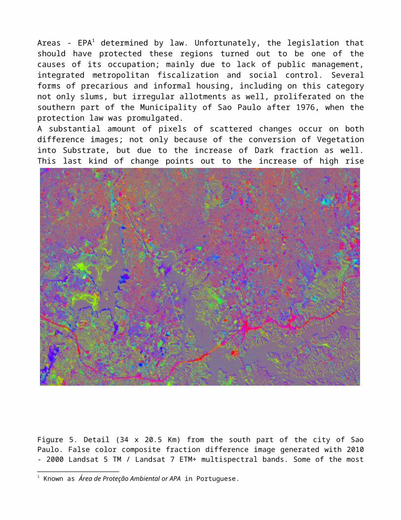
Areas - EPA1 determined by law. Unfortunately, the legislation thatshould have protected these regions turned out to be one of thecauses of its occupation; mainly due to lack of public management,integrated metropolitan fiscalization and social control. Severalforms of precarious and informal housing, including on this categorynot only slums, but irregular allotments as well, proliferated on thesouthern part of the Municipality of Sao Paulo after 1976, when theprotection law was promulgated.A substantial amount of pixels of scattered changes occur on bothdifference images; not only because of the conversion of Vegetationinto Substrate, but due to the increase of Dark fraction as well.This last kind of change points out to the increase of high risebuildings on different parts of Sao Paulo’s Metropolitan area.

Figure 5. Detail (34 x 20.5 Km) from the south part of the city of SaoPaulo. False color composite fraction difference image generated with 2010- 2000 Landsat 5 TM / Landsat 7 ETM+ multispectral bands. Some of the most

1 Known as Área de Proteção Ambiental or APA in Portuguese.

evident changes occur at the south and eastern area of the city, where thesinuosities of the road ring stands out as a major change of metropolitandimensions. The highway crosses over the two reservoirs.

CONCLUSIONS

A quantitative and visual analysis of the changes at differentspatial scales has been carried out during the execution of thisresearch. Results so far indicate that the methodology here presentedopens venue to the development of a change cartographic base map forthe whole Sao Paulo’s Metropolitan Region that would have thepotential to inform a wide variety of urban research and crucialmanagement questions, such as the appearance and growth of slumspockets and irregular allotments, monitoring of protected areasincluding the prevention of deforestation and other relevantlandcover changes.

On this study, the whole analysis has been carried out using moderatespatial resolution with imagery with satisfactory results. In ouropinion, the main objective of the research can be accomplished whenthe most conspicuous changes are detected by means of using multi-temporal spectral mixture analysis of Landsat TM and ETM+ imagery.The analysis is based on a three component linear mixture modelincorporating substrate, vegetation and dark targets, directly usedfor visualization on false color composites of red, green & bluecolors respectively. Further study will focus on quantitativeanalysis of the results and application to the areas given above.Winter and summer image pairs, were used for quality and consistencyof solar illumination for 1986 – 2005 and 2000 – 2010.

Fraction difference images revealed the location and extent of urbandevelopment – both at the periphery and within the city of Sao Paulo.Changes in fraction mixtures and texture also point out high riseconstruction as well as vegetation abundance. In some cases, shadowsof individual high rises can be seen. Many pixels of scatteredchanges occur on both difference images; not only because of theconversion of Vegetation into Substrate, but due to the increase ofDark fraction as well. This last kind of change points out to theincrease of high rise buildings on different parts of Sao PauloMetropolitan area, when occurred on conjunction with the augment ofSubstrate.

Further analysis of the quantity, quality, location and rate ofchange occurring within the city of Sao Paulo will build on thisresearch. Even though the amount of changes measured on both periodsof time are very similar, it should be considered that a small numberof large changes can outweigh the majority - even on small intervals.However, it is important to know where those changes are, and howthey relate with the evolution of the metropolitan region during theconsidered time span.

REFERENCES

ADAMS, J. B. et al. (1995). Classification of multispectral images based onfractions of endmembers:application to landcover change in the BrazilianAmazon. Remote Sensing of Environment, 52, 137-154.

ADAMS, J. B.; GILLESPIE, A. R. (2006). Remote Sensing of Landscape withSpectral Images: a physical modeling approach. Nova York: CambridgeUniversity Press, 378 p. ISBN 9780521662215.

BOARDMAN, J. W. (1989). Inversion of imaging spectrometry data usingsingular value decomposition. Proceedings of IGARSS’89, 12th CanadianSymposium on Remote Sensing. Calgary, Canada, p. 2069-2072.

BOARDMAN, J. W.; KRUSE, F. A. (1994). Automated spectral analysis: ageologic example using AVIRIS data, north Grapevine mountains, Nevada.Proceedings of the Tenth Thematic Conference on Geologic Remote Sensing.Ann Arbor, MI. USA, p. I407-I418.

CARNEIRO, A. M. C. (2009). Uso do Modelo de Mistura MESMA e Imagens ASTERpara Construção de um Mapa de Conforto Urbano para Belo Horizonte – MG.Instituto de Geociências da UFMG. Belo Horizonte, p. 98.

CLARK, R. N.; ROUSH, T. L. (1984). Reflectance spectroscopy: quantitativeanalysis techniques for remote sensing applications. Journal of GeophysicalResearch, 89, 6329-6340.

ELVIDGE, C. D.; CHEN, Z.; GROENEVELD, D. P. (1993). Detection of tracequantities of green vegetation in 1990 AVIRIS data. Remote Sensing ofEnvironment, 44, 271-279.

GOETZ, A. F. H. et al. Imaging spectrometry for earth remote sensing.Science, 1985. 1147-1153.

HOLBEN, B. N.; SHIMABUKURO, Y. E. (1993). Linear mixing model applied tocoarse spatial resolution data from multispectral satellite sensors.International Journal of Remote Sensing, 14 n. 11, 2231-2240.

KAWAKUBO, F. S. (2010). Metodologia de Classificação de ImagensMultiespectrais aplicada ao Mapeamento do Uso da Terra e Cobertura Vegetalna Amazônia: Exemplo do Caso na Região de São Félix do Xingu, Sul do Pará.Faculdade de Filosofia Letras e Ciências Humanas. Universidade de SãoPaulo. São Paulo, p. 113. PhD dissertation.

KAWAKUBO, F. S. et al. (2009). Land use and vegetation-cover mapping of aindigenous land are in the state of Mato Grosso (Brazil) based on spectrallinear mixing model, segmentation and region classification. GeocartoInternational, 25 n. 2, 165-175.

KRESSLER, F.; STEINNOCHER, K. (1996). Change detection in urban areas usingsatellite data and spectral mixture analysis. International Archives ofPhotogrammetry and Remote Sensing, XXXI(B7), 379-383.

KRUSE, F. A. (1988). Use of airborne imaging spectrometer data to mapminerals associated with hydrotermally altered rocks in the northernGrapevine Mountains Nevada and California. Remote Sensing of Environment,24, 31-51.

PECH, R. P. et al. (1986). Calibaration of Landsat data for sparselyvegetated semi-arid rangelands. International Journal of Remote Sensing, 7,1729-1750.

ROBERTS, D. A.; SMITH, M. O.; ADAMS, J. B. (1993). Green vegetation,nonphotosynthetic vegetation and soils in AVIRIS data. Remote Sensing ofEnvironment, 44, 255-269.

SINGER, R. B.; MCCORD, T. B. (1979). Mars: large scale mixing of bright anddark surface materials and implications for analysis of spectralrefectance. Proceedings of 10th Lunar and Planetary Science Conference.Washington D.C.: American Geophysical Union. p. 1835-1848.

SMALL, C. (2001). Multiresolution analysis of urban reflectance.Proceedings of The IEEE Joint Workshop on Remote Sensing and Data Fusionover Urban Areas. Rome.

SMALL, C. (2003). High spatial resolution spectral mixture analysis ofurban reflectance. Remote Sensing of Environment, 88. 170-186.

SMALL, C. (2005). A Global analysis of urban reflectance. InternationalJournal of Remote Sensing, 26, n. 4, p. 661-681.

SMALL, C.; LU, J. W. T. (2006). Estimation and vicarious validation ofurban vegetation abundance by spectral mixture analysis. Remote Sensing ofEnvironment, 4, 441-456.

SMITH, M. O. et al. (1990). Vegetation in deserts: I. A regional measure ofabundance from multispectral images. Remote Sensing of Environment, 31, 1-26.