An Exploratory Analysis of Diachronic Settlement Patterns in Central Ohio

12

Introduction

The Ohio Archaeological Inventory (OAI) is the

official state database of archaeological sites in Ohio.

With over 40,000 records currently, this is the largest

and most comprehensive collection of archaeological

data in the state. Despite this, the OAI is not often

utilized as a research tool. The compilation and

maintenance of the database represents a substantial

public investment in archaeology required by the Na-

tional Historic Preservation Act (NHPA) 1966. The

OAI holds most of the academically investigated sites

in the state, though some records are missing and oth-

ers woefully incomplete. The OAI is also a repository

for information provided by the public about archaeo-

logical locales. More importantly, the database holds

the record of all sites recorded in the gray cultural

resource management (CRM) literature. Most of these

sites are small, non-diagnostic lithic scatters. Few of

these CRM-documented sites are incorporated into

research or promulgated to the broader research

community. There are notable exceptions (e.g., Purtill

2012). If the database is to serve the purpose and jus-

tify the expenditure of vast quantities of public funds

to preserve the archaeological record from destruction

in the wake of development, the OAI must be able to

serve directly as a research tool.

Use of the OAI is becoming ever easier (see

Wakeman 2003:26). The system is maintained in a

queriable Microsoft Access database linked to a geo-

graphic information system (GIS) operated in ESRI

software. Records are now available and searchable

online through a GeoCortex portal

(http://www.ohiohistory.org/ohio-historic-

preservation-office/online-mapping-system). This

system of organization of the records, and the availa-

bility online is one of the best in the region (though

Indiana is also making great strides in this direction:

https://gis.in.gov/apps/dnr/SHAARDGIS/). However,

the system is still seeing little use by the research

community (see Church [1987] and Wakeman [2003]

for exceptions). The online and in-house versions

serve primarily to facilitate background research for

CRM surveys, which then feed into the gray literature

and are amassed in the OAI records. While this func-

tion is important, we have yet to realize the full

potential of the OAI database, and the massive ex-

penditure of public funds has yet to bear the promised

fruit of advancing our understanding of the past. Few

academics have the time or willingness to sort

through the massive volume of gray literature, and

few CRM practitioners have time to pursue publica-

AN EXPLORATORY ANALYSIS OF DIACHRONIC SETTLEMENT

PATTERNS IN CENTRAL OHIO

Kevin C. Nolan

Abstract

The Ohio Archaeological Inventory (OAI) is the state database of officially recorded archaeological sites. There

are tens of thousands of records. The database is far from complete, but this still represents the largest compila-

tion of site-based records. The potential for region-level analysis is vast. I undertake a first-pass, exploratory

analysis of all recorded prehistoric sites in eight central Ohio counties. There are definite temporal patterns in

the data that complement the fine-scale narratives derived from the more detailed, larger-scale data of intensive

survey and excavation. The clearest patterns are associated with the transition from a mobile hunting and gather-

ing lifeway to a more sedentary horticultural pattern from the Archaic into the Woodland. The OAI is a valuable

research tool that holds much potential to elucidate patterns in the prehistory of the state.

Kevin C. Nolan, Applied Anthropology Laboratories, Department of Anthropology, Ball State University

[email protected]

Journal of Ohio Archaeology 3:12-37, 2014

An electronic publication of the Ohio Archaeological Council

http://www.ohioarchaeology.org/joomla/index.php?option=com_content

&task=section&id=10&Itemid=54

http://www.ohioarchaeology.org/joomla/index.php?option=com_content&task=section&id=10&Itemid=54

http://www.ohioarchaeology.org/joomla/index.php?option=com_content&task=section&id=10&Itemid=54

Journal of Ohio Archaeology Vol. 3, 2014 Kevin C. Nolan

13

tion of their results. Very often, researchers choose

not to consult the massive quantity of records gener-

ated by CRM. Further, the majority of the CRM

surveys result in findings that are considered not

worth promulgating. However, the mass of infor-

mation accumulated in the OAI (not the full detail of

all the reports that buttress the data) presents a unique

opportunity for regional analyses that are well beyond

the capabilities of any one researcher or research team

to compile on their own. I propose that demonstrating

the usefulness of the OAI GIS and database is the first

step in bringing the immense quantity of data gener-

ated by CRM archaeology more regularly into the

attention span of regional researchers. Such a demon-

stration is a prerequisite to realizing the promised

return on the public investment in recovery and

preservation of archaeological information.

There are many deficiencies in the database.

Some sites are unreported. There are differing meth-

ods of recording and classification that obscure de-

tails. These problems should not be ignored.

However, these problems are most significant at large

scales (small areas), and become minor variation at

small scales (large areas or regions). All state data-

bases have their deficiencies, but many have proven

useful in regional research (e.g., Thompson and Turck

2009; Wakeman 2003; Wells 2011). The large num-

bers available in state databases allow the researcher

to treat these deficiencies and minor, non-systematic

biases as noise. It is only with such large samples that

the signal can be detected. Most analysis in archaeol-

ogy focuses on the few handfuls of sites from each

time period that have received academic excavation

attention. This is a small and potentially very biased

sample of the prehistoric record. Further, this is only a

sample of a portion of the archaeological record.

There is an overwhelming focus on long-term habita-

tion sites to the exclusion of the rest of the archaeo-

Figure 1. Location of research region within Ohio.


14

logical record. The state databases provide an oppor-

tunity to overcome this bias of focus. Incorporating

lithic scatters, isolated finds, other and unknown site

types allows analysis of the full distribution of activi-

ty, not just the location of sleeping quarters.

It has been suggested that a focus on only

Phase II and Phase III compliance investigations

would eliminate some of the bias in the state data-

base. However, this would only perpetuate the biased

focus on long-term habitation sites, and substantially

limit the sample size and eliminate the possibility of

performing a distributional analysis such as that per-

formed here. Sites that are selected for Phase II are

overwhelmingly long-term habitation sites, and there

are unknown and unknowable biases in how different

investigators make their judgments of significance.

This would also eliminate amateur excavations, aca-

demic investigations, etc. If we are interested in the

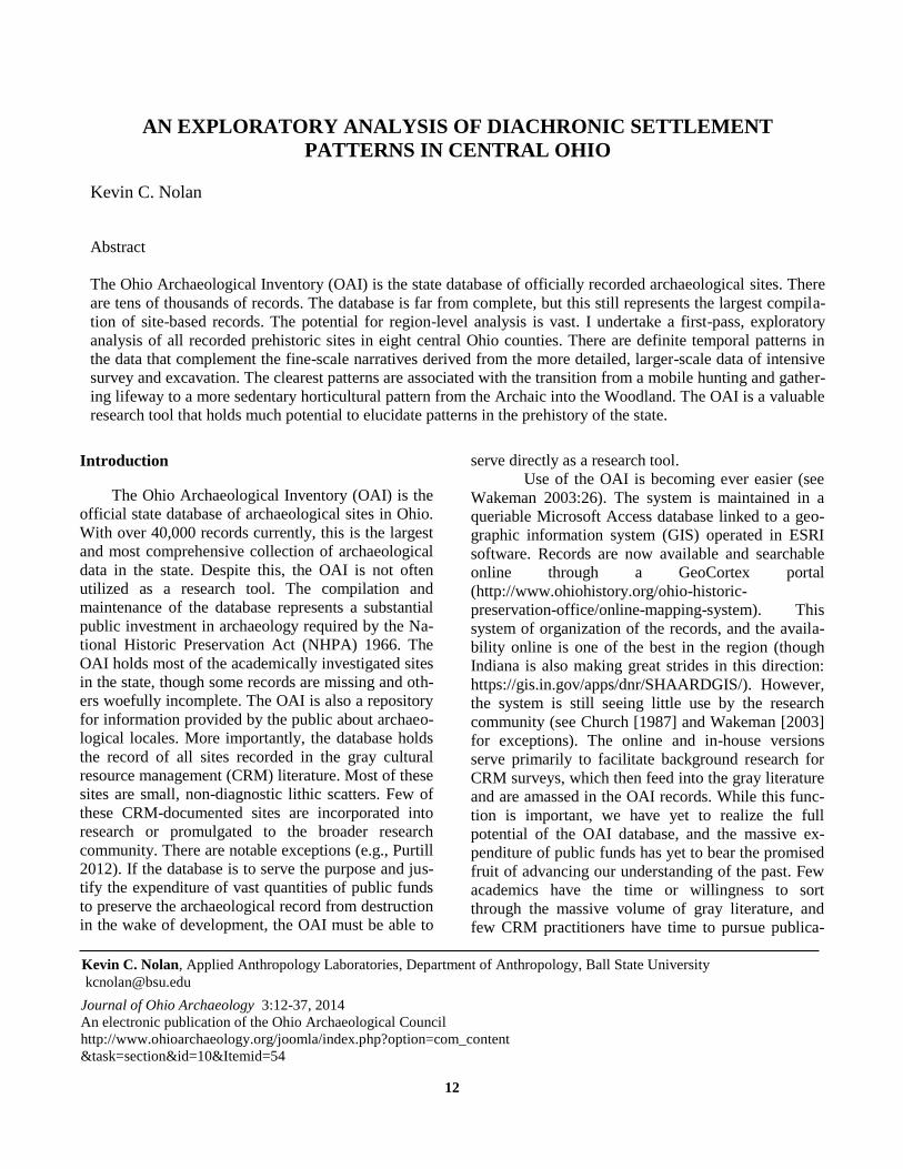
Figure 2. Location and temporal affiliation of sites used in the analysis. Red line represents the southern margin of the Wis-

consin glacial advance and the yellow and black line represents the maximum advance of the Illinoian glaciation. UN =

Unknown; PI = Paleoindian; EA = Early Archaic; MA = Middle Archaic; LA = Late Archaic; EW = Early Woodland; MW =

Middle Woodland; LW = Late Woodland; LP = Late Prehistoric; PH = Protohistoric.


15

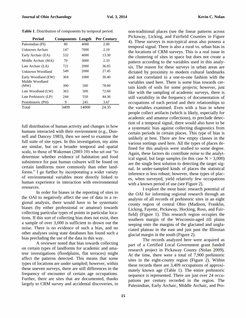
Table 1. Distribution of components by temporal period.

Period Components Length Per Century

Paleoindian (PI) 80 4000 2.00

Unknown Archaic 147 7000 2.10

Early Archaic (EA) 532 4000 13.30

Middle Archaic (MA) 70 3000 2.33

Late Archaic (LA) 721 2000 36.05

Unknown Woodland 549 2000 27.45

Early Woodland (EW) 304 1000 30.40

Middle Woodland

(MW) 390 500 78.00

Late Woodland (LW) 363 500 72.60

Late Prehistoric (LP) 244 550 44.36

Protohistoric (PH) 9 245 3.67

Total 3409 14000 24.35

full distribution of human activity and changes in how

humans interacted with their environment (e.g., Dun-

nell and Dancey 1983), then we need to examine the

full suite of site types. In this investigation, my aims

are similar, but on a broader temporal and spatial

scale, to those of Wakeman (2003:10) who set out “to

determine whether evidence of habitation and food

subsistence for past human cultures will be found on

certain landforms more commonly than other land-

forms.” I go further by incorporating a wider variety

of environmental variables more directly linked to

human experience in interaction with environmental

resources.

In order for biases in the reporting of sites to

the OAI to negatively affect the use of data in a re-

gional analysis, there would have to be systematic

biases (by either professional or amateur) towards

collecting particular types of points in particular loca-

tions. If this sort of collecting bias does not exist, then

a sample of over 3,000 is sufficient to drown out the

noise. There is no evidence of such a bias, and no

other analyses using state databases has found such a

bias precluding the use of the data in this way.

A reviewer noted that bias towards collecting

on certain types of landforms for academic and ama-

teur investigations (floodplains, flat terraces) might

affect the patterns detected. This means that some

types of locations are under sampled; however, within

these uneven surveys, there are still differences in the

frequency of encounter of certain age occupations.

Further, there are sites that are documented, thanks

largely to CRM survey and accidental discoveries, in

non-traditional places (see the linear patterns across

Pickaway, Licking, and Fairfield Counties in Figure

4). These surveys in non-typical areas also possess a

temporal signal. There is also a rural vs. urban bias in

the locations of CRM surveys. This is a real issue in

the clustering of sites in space but does not create a

pattern according to the variables used in this analy-

sis. The reason for these surveys in urban areas are

dictated by proximity to modern cultural landmarks

and not correlated in a one-to-one fashion with the

variables used here. There is some bias towards cer-

tain kinds of soils for some projects; however, just

like with the sampling of academic surveys, there is

still variability in the frequency of documentation of

occupations of each period and their relationships to

the variables examined. Even with a bias in where

people collect artifacts (which is likely, especially for

academic and amateur collections), to preclude detec-

tion of a temporal signal, there would also have to be

a systematic bias against collecting diagnostics from

certain periods in certain places. This type of bias is

unlikely at best. There are few empty classes in the

various sortings used here. All the types of places de-

fined for this analysis were studied to some degree.

Again, these factors do contribute noise to the analyt-

ical signal, but large samples (in this case N > 3,000)

are the single best solution to detecting the target sig-

nal. In under-sampled kinds of places the statistical

inference is less robust; however, these types of plac-

es, when surveyed, yield relatively few occupations

with a known period of use (see Figure 2).

I explore the most basic research potential of

the OAI for informing regional research through an

analysis of all records of prehistoric sites in an eight

county region of central Ohio (Madison, Franklin,

Licking, Fayette, Pickaway, Hocking, Ross, and Fair-

field) (Figure 1). This research region occupies the

southern margin of the Wisconsin-aged till plains

seeping onto the margins of the glaciated and ungla-

ciated plateau in the east and just past the Illinoian

glacial margin in the south (Figure 2).

The records analyzed here were acquired as

part of a Certified Local Government grant funded

research project in Pickaway County (Nolan 2009).

At the time, there were a total of 7,900 prehistoric

sites in the eight-county region (Figure 2). Within

these records there are 3,409 occupations of approxi-

mately known age (Table 1). The entire prehistoric

sequence is represented. There are just over 24 occu-

pations per century recorded in the region. The

Paleoindian, Early Archaic, Middle Archaic, and Pro-

kcnolan

Cross-Out

kcnolan

Inserted Text

-


16

tohistoric periods present below-average occupation

rates. The Middle Woodland and Late Woodland pe-

riods are substantially above the average occupation

rate. Whether these rates are representative of the ac-

tual occupation population is unknown, and I suspect

that the Middle Woodland is systematically over-

sampled. Further, occupation densities cannot be

translated directly into population densities given the

different size of typical habitation sites within each

period.

Regional Prehistory

The general trend of prehistory in central Ohio is

characterized relatively well by the general narrative

for the Midwest. The prehistory of the Midwest is

characterized by a series of subsistence and associated

settlement shifts. In general, settlement patterns

should be correlated with subsistence patterns; how-

ever, there is significant variability around this

generalization. The first occupants of the region were

Pleistocene hunter-gatherers characterized by a mo-

bile settlement system with a generally light imprint

on the landscape. With the start of the Holocene the

environment and available resources began to change.

Subsistence focus changed as well, but the mobile

pattern generally prevailed. As the climate and envi-

ronment approached the modern, subsistence became

more intensive and gardening and farming based on

local domesticated crops developed. There are signif-

icant settlement changes associated with this

transition. As agriculture intensified, settlement sys-

tems continued to change, eventually resulting in

large villages with hundreds of residents living in the

same place (Lepper 2011).

The first major subsistence change in eastern

North America was the increasing frequency of

starchy and oily seeds in the Middle Archaic leading

to eventual domestication of a several taxa by the

Late Archaic period (Smith 2009). The general pic-

ture for the Middle and Late Archaic is one of

seasonally mobile peopled gradually settling into a

more modern and stable environment. Settlements

became larger and more stable over time, and human

impacts on ecological communities began to affect

subsistence (e.g., Braun 1987; Smith 1987, 1989,

1995, 2009). Smith (2009:5) describes the typical

Late Archaic pattern as:

…a small-scale society consisting of perhaps a half-

dozen related extended family units. Situated along

and tethered to first- through third-order tributary riv-

er valley corridors …[and following] an annual cycle

that linked semi-permanent to permanent river valley

settlements in river valley locations like Riverton,

with a range of other short-term multiple-family and

single-family floodplain and upland occupations.

Central Ohio seems to have followed a similar

pattern as that discussed by Smith (see Lepper 2011).

The subsequent domination of Early and Middle

Woodland assemblages by largely the same suite of

starchy and oily seeds is as well documented in Ohio

as it is in Illinois (e.g., Leone 2007; Wymer 1996,

1997). The pattern of human mobility and the effect

this has on surrounding ecology plays a central role in

models which account for both the change in subsist-

ence and the eventual increase in residential stability.

Central Ohio falls within Gremillion’s (2002: Figure

22.3) zone of developed pre-maize agriculture (see

also Smith 1989:Figure 1).

The next major transition in settlement and sub-

sistence draws on much Ohio data for its formulation.

Early and Middle Woodland period domesticates and

non-domesticated cultigens constitute a large portion

of archaeobotanical assemblages. This is interpreted

as an increasing emphasis on food production (sensu

Smith 2001) and is thought by some to be associated

with a high degree of residential stability (Abrams

2009; Dancey and Pacheco 1997; Pacheco 1997;

Weaver et al. 2011; Wymer 1996, 1997). While most

researchers agree that domesticated plants contributed

to the diet of Early/Middle Woodland peoples, there

is disagreement over the degree of dependence on

cultigens. One extreme is represented by Wymer’s

(1997) characterization of the Ohio Hopewell people

as “farmers.” The other extreme is represented by

Yerkes (e.g., 2002, 2009) who characterizes the

Hopewell as hunter-gatherer populations. Both ex-

tremes are represented by distinct settlement models.

Abrams (2009:178) presents a balanced assessment of

extant arguments and evidence when he depicts “the

Hopewell economy as one based on hunting (espe-

cially of white-tailed deer) and gathering (nuts as well

as local seeds), supplemented to some degree with

horticulture involving the intentional tending or plant-

ing of local seed-bearing plants.” As Abrams points

out (2009:179), what remains to be determined is the

variability with which communities pursued disparate

strategies. Whether it is the mobile-hunting-gathering

extreme, the sedentary-farmer extreme, or something

in-between, we need the distributional data on various

settlement and activity patterns for each period. One

peculiarity of activity distribution has been docu-

kcnolan

Highlight

Should this be aligned under and in smaller font? Otherwise it is not clear this is a quote.

kcnolan

Highlight

Why is this multi-line quote treated differently than that above? Should be the same.


17

mented in the eastern portion of the current study re-

gion. Spurlock et al. (2006) note that there is a

conspicuous absence of Middle Woodland activity in

the rockshelters of east-central Ohio. This is distinct

from both preceding and subsequent time periods and

may indicate different hunting strategies (Abrams

2009:178-179), different overall settlement system,

and/or different subsistence strategies.

In the early Late Woodland people began exploit-

ing new physiographic regions (Dancey 1992, 1996;

McElrath et al. 2004:24; Seeman and Dancey

2000:594; Wakeman 2003:31). During the time be-

tween the “collapse” of Hopewell (ca. AD 400) and

the emergence of Fort Ancient (ca. AD 950-1000) the

economic and behavioral regimes diversified. After

the end of the Middle Woodland period (ca. AD 400)

large nucleated settlements begin to appear (Dancey

1992; Seeman and Dancey 2000). These nucleated,

and occasionally fortified, settlements are generally

characterized by an ethnobotanical assemblage simi-

lar to their predecessors, though Wymer argues that,

in contrast to the Middle Woodland hamlets, early

Late Woodland (ca. AD 400 – 800) nucleated settle-

ments were places “where every available resource

seems to have been intensively utilized, including less

desirable plant foods” (Wymer 1996:42; emphasis

added). However, the number of settlements inten-

sively studied is small. Around the time that maize

begins to show up with any ubiquity in botanical as-

semblages at the advent of the later Late Woodland

(ca. AD 700 – 1000), dispersed hamlets seem to in-

crease in frequency (Church 1987; Church and Nass

2002; Dancey 1992; Seeman and Dancey 2000).

Seeman and Dancey (2000) note, however, that there

is variability in settlement size, organization, and dis-

tribution throughout the Late Woodland period.

The final major subsistence shift is the advent of

maize agriculture ca. AD 800 – 1000. Maize is known

in the eastern Woodlands and Ohio as early as 200

BC, but does not become a major part of the diet for

any populations until after AD 800 (Greenlee 2002;

Hart 1999). Like the previous subsistence shifts, this

transition is accompanied by changes in settlement

patterns. As maize consumption steadily increases,

the dispersed population of the later Late Woodland

begin to aggregate. This aggregation generally results

in more structured communities than the nucleated

settlements of the earlier Late Woodland typified by

circularly organized sites like SunWatch (Cook

2008). This shift is also often associated with a

change in the location of settlements (Church

1987:169; Prufer and Shane 1970; Wakeman

2003:36). The contrast between Late Woodland and

Late Prehistoric settlement led Prufer and Shane

(1970) to propose a population intrusion; however,

Church (1987) and Essenpreis (1982) directly chal-

lenged Prufer and Shane’s invasion model.

Specifically, Church (1987:168) found “no indication

of a major population shift … with the transition from

Late Woodland to Late Prehistoric.” In some models,

the increasing productivity of maize, especially rela-

tive to native cultigens, is related causally to these

changes in settlement pattern and structure (Pollack

and Henderson 1992).

This concomitant change in subsistence, settle-

ment, and community patterns is often recognized as

the origin of Fort Ancient (Griffin 1966; Pollack and

Henderson 1992; Prufer and Shane 1970). The degree

of commitment to maize has been shown to be widely

variable at the community (Cook and Schurr 2009)

and the regional levels (Greenlee 2002). If maize ag-

riculture entails consequences for settlement location

and community aggregation, then variable commit-

ment to maize (coupled with retention of native

domesticates [see Martin 2009; Nolan 2009: Appen-

dix B]) should entail variable settlement and activity

distributions and variable community organizations.

This brief review of regional prehistory serves to

show that each of the major changes in subsistence

strategy is generally associated with specific settle-

ment patterning. A first step towards investigating the

local nuance to these larger scale patterns, and to-

wards more fully reconstructing the narrative of

central Ohio’s prehistory, is the examination of the

massive compilation of distributional and coarse tem-

poral data contained in the OAI.

Methods

In what follows I explore the distribution of tem-

porally identified occupations in central Ohio from

the OAI database (N = 3,409) in relation to a number

of environmental attributes. This is the most modest

use of the > 200 fields of information contained with-

in the OAI database. Occupations will be examined

for their relationship to water, soil texture, flooding

frequency, ponding frequency, soil drainage class,

slope, and ecoregions (Omernik 1987; Woods et al.

1998; Figure 3). It is expected that as populations in-

crease and/or change the way in which they interact

with their surroundings, there will be clear patterns in

relationships between locations of occupation and

kcnolan

Highlight

if there is no emphasis, then this needs to be removed.


18

these environmental attrib-

utes.

Variables

The empirical unit of

analysis in this investigation

is the occupation. The use of

the term “occupation” does

not connote a habitation site. I

use the term as defined and

used by Dunnell (1971, 2008;

Lipo and Dunnell 2008) and

Rafferty (2008, 2012; Raffer-

ty et al. 2011), among others.

Dunnell (1971:150-151,

2008:50) defines occupations

as the empirical (observable

and observed) discrete entity

(i.e., it has definite limits and

component parts associated in

reality) that occurs at the

scale of the site or assem-

blage. Definition of

occupation and delineation

(empirical observation) of

occupations are problem and

analysis specific. Rafferty (2008:102) notes that the

occupation is the empirical unit that allows meaning-

ful treatment of change and difference and constitutes

“the basic artifact scale used in settlement pattern

analysis.” “Occupations are composed of non-

portable discrete artifacts that are associated in a pri-

mary depositional context that is spatially discrete and

that represents continuous deposition through time”

(Rafferty 2012:2). Both Dunnell and Rafferty note

that occupations can be delineated at multiple scales

and for multiple purposes. Recognizing the full poten-

tial of classes at this scale is beyond the use of the

OAI data; however, we can recognize the presence of

at least an occupation in this sense at each one of the

locations in the OAI database. If there is a diagnostic

artifact or other date from the site, we can place at

least one of the occupations from the site in a relative

temporal scale.

Any particular “site” will have one or more occu-

pations. In this analysis, only occupations that can be

assigned to a particular time period are used. All oc-

cupations without temporal information are excluded.

This results in the exclusion of many sites, and leav-

ing one or more occupations from some sites

excluded. That is, there may be a site that contains

multiple discrete (temporally) occupations where only

one yielded an artifact assemblage that could be

placed in a relative and coarse temporal scale. All

occupations in this site are delineated by the identifi-

cation in the OAI of known period of occupation at

the site. This field is supplied directly from the OAI

database. An occupation does not mean any particular

site type, it simply means that there exists at that spot

at least one assemblage of relatively known age. This

includes isolated finds, lithic scatter, habitation sites,

camps, mounds, and unknown site types. What is be-

ing analyzed is not the location of any one site type

over space and time, but the changes in the distribu-

tion of activity of any kind. Certainly there are

activities that are not represented or underrepresented;

however, this is unavoidable with the current state

archaeology and archaeological data.

The majority of the environmental variables ex-

amined are derived from the county soil surveys, and

the SSURGO (Soil Survey Geographic Database)

spatial data. For each county, the characteristics of the

soil map units (phases) were compiled from the print-

ed county surveys. The various counties in some

cases had different abbreviations for the same series,

so this task had to be done at the county level. The

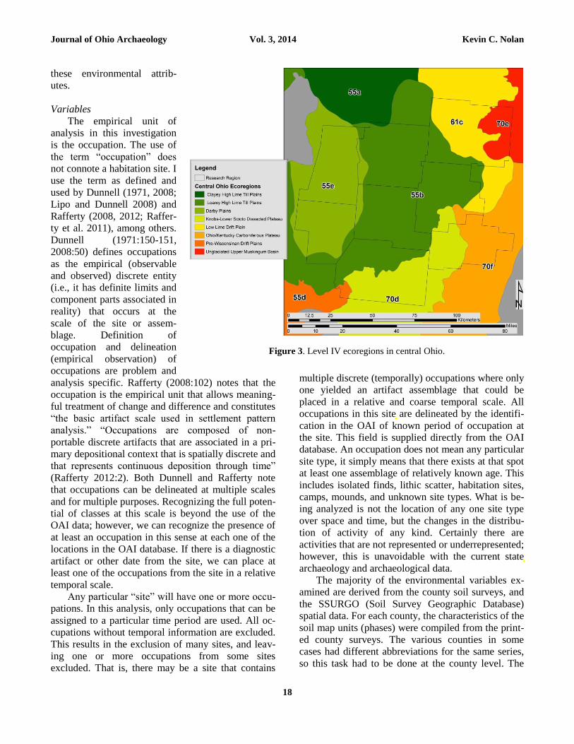
Figure 3. Level IV ecoregions in central Ohio.

kcnolan

Cross-Out

kcnolan

Inserted Text

study

kcnolan

Inserted Text

of


19

Web Soil Survey (websoilsurvey.nrcs.usda.gov/app/)

would now make this task obsolete. Variables ex-

tracted from the SSURGO and county soil survey

data were slope class (A, B, C, D, etc.), soil texture

class (e.g., clay loam, silt loam, sandy loam), drainage

class (excessive, well, moderately well, somewhat

poor, poor, very poor), flooding frequency class

(none, rare, occasional, frequent), and ponding fre-

quency class.

It is important to realize that county-level soil

surveys, while being the most detailed surveys pro-

duced as a standard USDA product, are still

generalizations (see Butler 1980). Any given spot

within a soil map unit (SMU) may have properties not

characteristic of the mapped soil series and phase. It

is not possible to use SSURGO data to conduct an

analysis of soil characteristics that occur at the loca-

tion of a particular artifact or site. Most sites, and

certainly all artifacts occur at scales larger than the

SMU; however, the SMU that contains the artifact or

site is a fairly good characterization of the context

within which the site sits. If an agriculturalist is seek-

ing a particular set of soil characteristics for their

gardens and fields, they will settle in areas surrounded

by those characteristics (if they want to be success-

ful). In fact, the location of the habitation might even

avoid those characteristics as to not remove produc-

tive land from use.

The only thing that can be analyzed using

SSURGO is the predominant characteristics of the

vicinity around the place where the artifacts were re-

covered. This is relevant and appropriate to this

analysis as I am attempting to explore the variability

in landscape use over time with changes in subsist-

ence and resource procurement activities. Artifacts

diagnostic of a particular period will gravitate around

the factors (moisture, texture, slope, etc.) that were

important for the people in getting their subsistence

from their surroundings. The soil characteristics

tracked by the USDA are characteristics that are rele-

vant for understanding what kinds of plant and animal

resources would be expected in a given area. As sub-

sistence patterns change through time, different kinds

of resources are exploited with variable frequency,

and therefore different kinds of soils should exhibit

patterned relationships with the temporally identifia-

ble occupations.

Distance to water features was determined in the

GIS using a base shapefile from the Ohio Department

of Natural Resources (ODNR 2005). These are digit-

ized from modern 1:24,000 scale USGS topographic

maps, and, therefore, cannot be thought to represent

natural water bodies, and certainly cannot reflect the

prehistoric landscape. However, this is a standard and

readily available dataset. The bias and error intro-

duced here is suspected to be minimal. From all of the

water bodies present in this layer, I selected all rivers,

streams, ponds, lakes, and wetlands. This does not

Table 2. Ecoregion descriptions (after Woods et al. 1998).

Level

III Name

Level

IV Name Description

55 Eastern Corn Belt

Plains

a

Clayey High Lime

Till Plains Original beech and scattered Elm-Ash swamp forests

b

Loamy High Lime

Till Plains

Better drained, more fertile; beech, oak-maple, and elm-ash

swamp forests

d

Pre-Wisconsinan Drift

Plains

Leached, acidic soils; greater stream biodiversity than ‘b’,

though less fertile soils; beech & elm-ash swamp forests

e Darby Plains Mixed oak and prairies, major stream high diversity

61 Erie/Ontario Drift

and Lake Plain

c Low Lime Drift Plain

Less fertile than 55, rolling landscape, relatively short growing

season

70 Western Alleghany

Plateau

d

Knobs-Lower Scioto

Dissected Plateau

Rugged over shale and sandstone; mixed oak, mixed meso-

phytic, and bottomland hardwoods

e

Unglaciated Upper

Muskingum Basin Dissected plateau; mixed oak and mixed mesophytic

f

Ohio/Kentucky Car-

boniferous Plateau Mixed oak hill slopes and mixed mesophytic valleys


20

exclude artificial ponds, as this distinction is not

maintained by the ODNR; however, it does eliminate

many artificial features such as drainage ditches.

Finally, the relationship between EPA Level IV

Ecoregions (Omernik 1987; Woods et al. 1998) and

site locations were explored. A shapefile for these

was downloaded from the EPA website

(http://www.epa.gov/wed/pages/ecoregions/level_iii_i

v.htm). The ecoregions vary in their typical geology,

hydrography, climate, and ecology (Table 2). These

units therefore represent coarse environmental varia-

tion. Ecoregions were included in this analysis to

attempt to see if people favored areas with greater

ecological diversity, over those with relatively uni-

form ecology.

To analyze distance from a particular feature, I

created a series of 1 km buffers (0-1 km, 1-2 km, 2-3

km, etc.) up to 20 km from each ecoregion and up to

10 km for bodies of water. The sites were assigned a

value for each ecoregion based on which buffer they

fell into (e.g., 0-1 km assigned a value of 1). For

quantitative analyses, the middle value for each class

was assigned as the value for that site. Additionally,

an ecotone score was computed for each site. The

ecotone score was designed to rank highly those sites

that are situated near the intersection of two or more

ecoregions. A score was calculated by taking the

buffer value for each ecoregion and subtracting it

from 21. For example, a site in the 0-1 km buffer is

given a value of 1 and a score of 20 for that ecore-

gion. The composite ecotone score is the sum of all

scores for each site. A higher ecotone score means the

site is positioned in proximity to one or more ecore-

gion boundaries. Most of the region is within 20 km

of at least one boundary, and, therefore, most sites

have a score greater than 0.

There will be little relevance to the earliest time

periods for many of these variables, as they can

change over time, especially with changes in climatic

patterns. However, these will serve as a useful start-

ing point. The requisite models of paleoecology and

paleoenvironment are not available at present. These

are the best available proxy data with sufficient spa-

tial resolution, and suffice for this initial analysis.

Statistical Tests

The data used in this analysis are categorical, or

continuous with unequal variances. All tests were

conducted in SPSS 20. Comparisons among time pe-

riods for the continuous variables were conducted

with a Welch test, followed by a Games-Howell post-

hoc test. The Welch test (Welch 1951) is a method of

comparing central tendency among groups where the

assumption of equal variances required for a one-way

ANOVA is not met. Likewise, if the samples exhibit

unequal variances or unequal sample sizes, the

Games-Howell post-hoc test is an appropriate tool for

exploring which categories contribute to the multi-

sample statistical differences (Tamhane 1979). For

categorical attributes, a X2 test was used to test for

association between particular periods and categories

of environmental variables. With large sample sizes,

the probability of achieving a significant association

with the X2 test increases; to account for the sample-

size effect, Cramer’s V was calculated for each com-

parison to assess the strength of the documented

association (Drennan 1996:193-194; see also Norušis

2010:436-437). A significant, but weak association is

not likely to be meaningful. A value of 0.15, though

not strong is suggested by Drennan to represent a

meaningful difference; however, there is no standard

for assessing how strong an association is meaningful.

Additionally, adjusted residuals were calculated for

all X2 tests. Residuals ≥ 2 are considered significant at

the 0.05 level (IBM 2012).

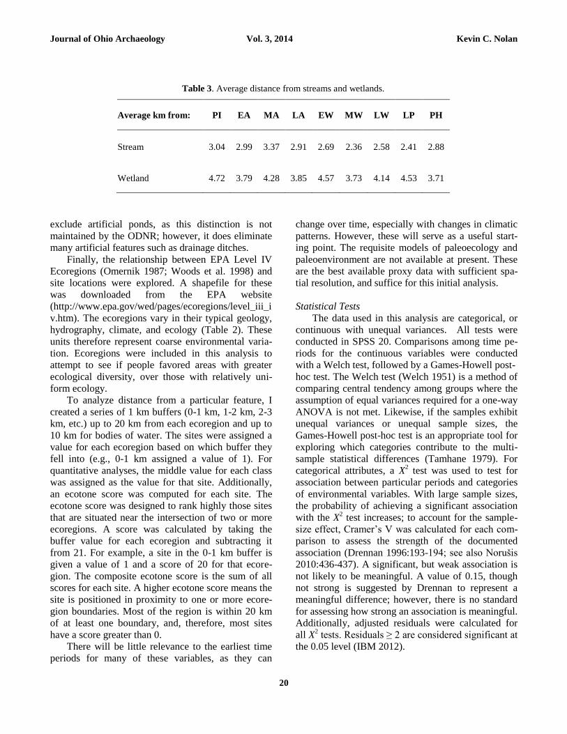
Table 3. Average distance from streams and wetlands.

Average km from: PI EA MA LA EW MW LW LP PH

Stream 3.04 2.99 3.37 2.91 2.69 2.36 2.58 2.41 2.88

Wetland 4.72 3.79 4.28 3.85 4.57 3.73 4.14 4.53 3.71


21

Results

Continuous Variables

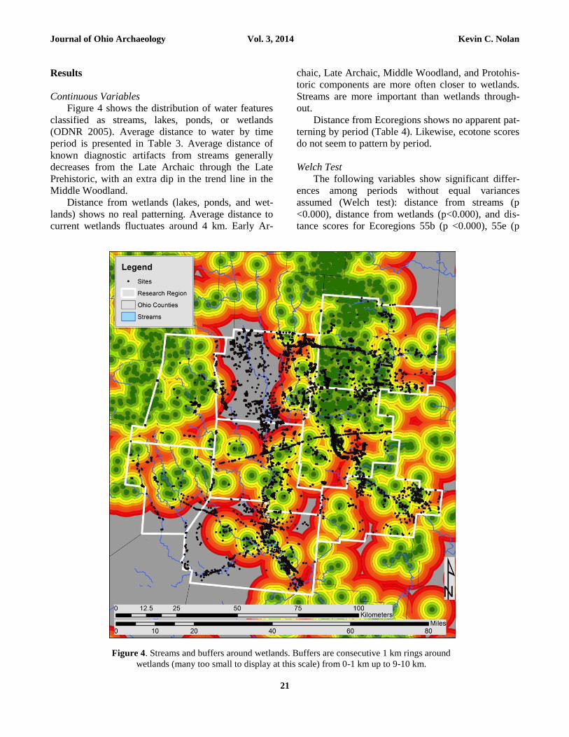
Figure 4 shows the distribution of water features

classified as streams, lakes, ponds, or wetlands

(ODNR 2005). Average distance to water by time

period is presented in Table 3. Average distance of

known diagnostic artifacts from streams generally

decreases from the Late Archaic through the Late

Prehistoric, with an extra dip in the trend line in the

Middle Woodland.

Distance from wetlands (lakes, ponds, and wet-

lands) shows no real patterning. Average distance to

current wetlands fluctuates around 4 km. Early Ar-

chaic, Late Archaic, Middle Woodland, and Protohis-

toric components are more often closer to wetlands.

Streams are more important than wetlands through-

out.

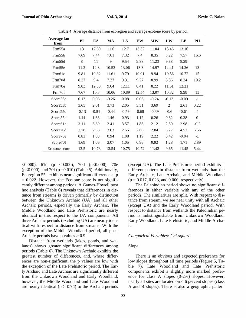
Distance from Ecoregions shows no apparent pat-

terning by period (Table 4). Likewise, ecotone scores

do not seem to pattern by period.

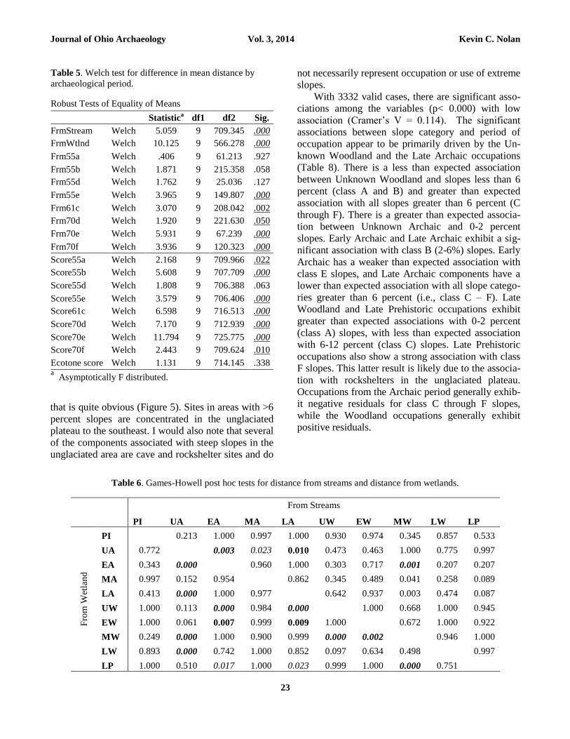
Welch Test

The following variables show significant differ-

ences among periods without equal variances

assumed (Welch test): distance from streams (p

<0.000), distance from wetlands (p<0.000), and dis-

tance scores for Ecoregions 55b (p <0.000), 55e (p

Figure 4. Streams and buffers around wetlands. Buffers are consecutive 1 km rings around

wetlands (many too small to display at this scale) from 0-1 km up to 9-10 km.


22

<0.000), 61c (p <0.000), 70d (p<0.000), 70e

(p<0.000), and 70f (p =0.010) (Table 5). Additionally,

Ecoregion 55a exhibits near significant difference at p

= 0.022. However, the Ecotone score is not signifi-

cantly different among periods. A Games-Howell post

hoc analysis (Table 6) reveals that differences in dis-

tance from streams is driven primarily by distinction

between the Unknown Archaic (UA) and all other

Archaic periods, especially the Early Archaic. The

Middle Woodland and Late Prehistoric are nearly

identical in this respect to the UA components. All

three Archaic periods (excluding UA) are nearly iden-

tical with respect to distance from streams. With the

exception of the Middle Woodland period, all post-

Archaic periods have p values > 0.9.

Distance from wetlands (lakes, ponds, and wet-

lands) shows greater significant differences among

periods (Table 6). The Unknown Archaic exhibits the

greatest number of differences, and, where differ-

ences are non-significant, the p values are low with

the exception of the Late Prehistoric period. The Ear-

ly Archaic and Late Archaic are significantly different

from the Unknown Woodland and Early Woodland;

however, the Middle Woodland and Late Woodland

are nearly identical (p > 0.74) to the Archaic periods

(except UA). The Late Prehistoric period exhibits a

different pattern in distance from wetlands than the

Early Archaic, Late Archaic, and Middle Woodland

(p = 0.017, 0.023, and 0.000, respectively).

The Paleoindian period shows no significant dif-

ferences in either variable with any of the other

periods. The similarities are split. With respect to dis-

tance from stream, we see near unity with all Archaic

(except UA) and the Early Woodland period. With

respect to distance from wetlands the Paleoindian pe-

riod is indistinguishable from Unknown Woodland,

Early Woodland, Late Prehistoric, and Middle Archa-

ic.

Categorical Variables: Chi-square

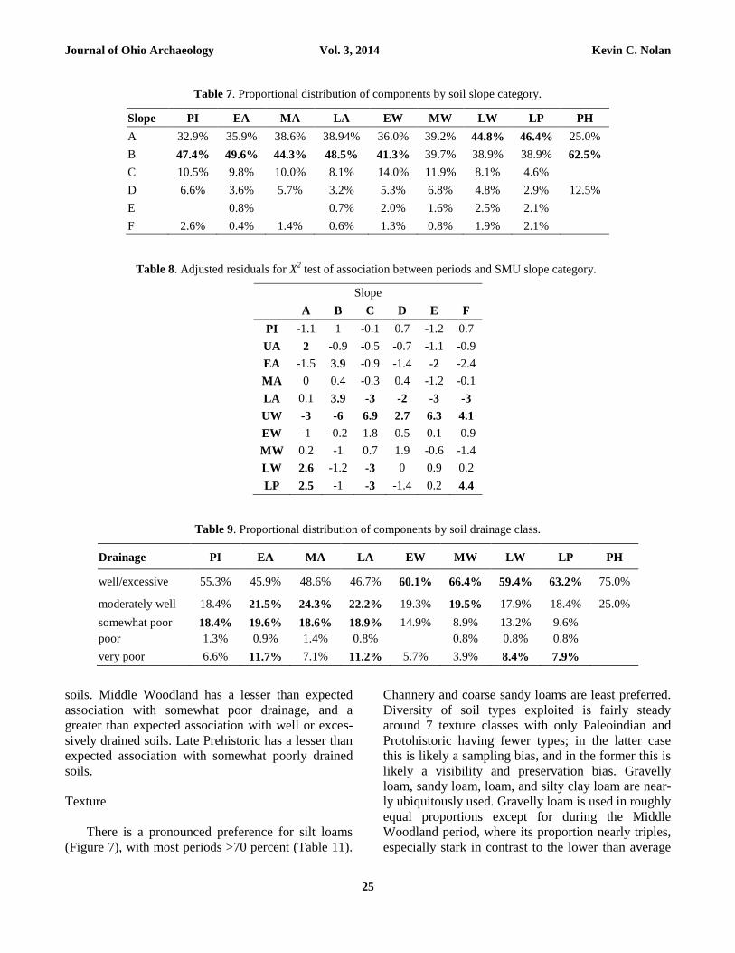
Slope

There is an obvious and expected preference for

low slopes throughout all time periods (Figure 5, Ta-

ble 7). Late Woodland and Late Prehistoric

components exhibit a slightly more marked prefer-

ence for class A slopes (0-2%) slopes. However,

nearly all sites are located on < 6 percent slopes (class

A and B slopes). There is also a geographic pattern

Table 4. Average distance from ecoregion and average ecotone score by period.

Average km

from: PI EA MA LA EW MW LW LP PH

Frm55a 13 12.69 11.6 12.7 13.32 11.04 13.46 13.16

Frm55b 7.69 7.44 7.61 7.32 7.4 8.35 8.22 7.57 16.5

Frm55d 8 11 9 9.54 9.88 11.23 9.83 8.29

Frm55e 11.2 12.3 10.53 13.06 13.3 14.97 14.41 14.36 13

Frm61c 9.81 10.32 11.61 9.79 10.91 9.94 10.56 10.72 15

Frm70d 8.27 9.4 7.27 9.31 9.27 8.99 8.86 8.24 10.2

Frm70e 9.83 12.53 9.64 12.11 8.41 8.22 11.51 12.21

Frm70f 7.67 10.8 10.06 10.89 12.54 13.07 10.82 9.98 15

Score55a 0.13 0.08 -0.26 0.08 0.06 -0.24 -0.13 -0.09 -1

Score55b 3.65 2.01 3.73 2.05 3.51 3.69 2 2.61 0.22

Score55d -0.13 -0.81 -0.44 -0.59 -0.68 -0.39 -0.6 -0.61 -1

Score55e 1.44 1.33 1.46 0.93 1.12 0.26 0.82 0.38 0

Score61c 3.11 3.39 2.41 3.57 1.88 2.12 2.59 2.98 -0.2

Score70d 2.78 2.58 3.63 2.55 2.68 2.84 3.27 4.52 5.56

Score70e 0.83 1.08 0.94 1.08 1.19 2.22 0.42 -0.04 -1

Score70f 1.69 1.06 2.07 1.05 0.96 0.92 1.28 1.71 2.89

Ecotone score 13.5 10.73 13.54 10.75 10.72 11.42 9.65 11.45 5.44


23

that is quite obvious (Figure 5). Sites in areas with >6

percent slopes are concentrated in the unglaciated

plateau to the southeast. I would also note that several

of the components associated with steep slopes in the

unglaciated area are cave and rockshelter sites and do

not necessarily represent occupation or use of extreme

slopes.

With 3332 valid cases, there are significant asso-

ciations among the variables (p< 0.000) with low

association (Cramer’s V = 0.114). The significant

associations between slope category and period of

occupation appear to be primarily driven by the Un-

known Woodland and the Late Archaic occupations

(Table 8). There is a less than expected association

between Unknown Woodland and slopes less than 6

percent (class A and B) and greater than expected

association with all slopes greater than 6 percent (C

through F). There is a greater than expected associa-

tion between Unknown Archaic and 0-2 percent

slopes. Early Archaic and Late Archaic exhibit a sig-

nificant association with class B (2-6%) slopes. Early

Archaic has a weaker than expected association with

class E slopes, and Late Archaic components have a

lower than expected association with all slope catego-

ries greater than 6 percent (i.e., class C – F). Late

Woodland and Late Prehistoric occupations exhibit

greater than expected associations with 0-2 percent

(class A) slopes, with less than expected association

with 6-12 percent (class C) slopes. Late Prehistoric

occupations also show a strong association with class

F slopes. This latter result is likely due to the associa-

tion with rockshelters in the unglaciated plateau.

Occupations from the Archaic period generally exhib-

it negative residuals for class C through F slopes,

while the Woodland occupations generally exhibit

positive residuals.

Table 5. Welch test for difference in mean distance by

archaeological period.

Robust Tests of Equality of Means

Statistica df1 df2 Sig.

FrmStream Welch 5.059 9 709.345 .000

FrmWtlnd Welch 10.125 9 566.278 .000

Frm55a Welch .406 9 61.213 .927

Frm55b Welch 1.871 9 215.358 .058

Frm55d Welch 1.762 9 25.036 .127

Frm55e Welch 3.965 9 149.807 .000

Frm61c Welch 3.070 9 208.042 .002

Frm70d Welch 1.920 9 221.630 .050

Frm70e Welch 5.931 9 67.239 .000

Frm70f Welch 3.936 9 120.323 .000

Score55a Welch 2.168 9 709.966 .022

Score55b Welch 5.608 9 707.709 .000

Score55d Welch 1.808 9 706.388 .063

Score55e Welch 3.579 9 706.406 .000

Score61c Welch 6.598 9 716.513 .000

Score70d Welch 7.170 9 712.939 .000

Score70e Welch 11.794 9 725.775 .000

Score70f Welch 2.443 9 709.624 .010

Ecotone score Welch 1.131 9 714.145 .338 a Asymptotically F distributed.

Table 6. Games-Howell post hoc tests for distance from streams and distance from wetlands.

From Streams

PI UA EA MA LA UW EW MW LW LP

Fro

m W

etla

nd

PI 0.213 1.000 0.997 1.000 0.930 0.974 0.345 0.857 0.533

UA 0.772 0.003 0.023 0.010 0.473 0.463 1.000 0.775 0.997

EA 0.343 0.000 0.960 1.000 0.303 0.717 0.001 0.207 0.207

MA 0.997 0.152 0.954 0.862 0.345 0.489 0.041 0.258 0.089

LA 0.413 0.000 1.000 0.977 0.642 0.937 0.003 0.474 0.087

UW 1.000 0.113 0.000 0.984 0.000 1.000 0.668 1.000 0.945

EW 1.000 0.061 0.007 0.999 0.009 1.000 0.672 1.000 0.922

MW 0.249 0.000 1.000 0.900 0.999 0.000 0.002 0.946 1.000

LW 0.893 0.000 0.742 1.000 0.852 0.097 0.634 0.498 0.997

LP 1.000 0.510 0.017 1.000 0.023 0.999 1.000 0.000 0.751


24

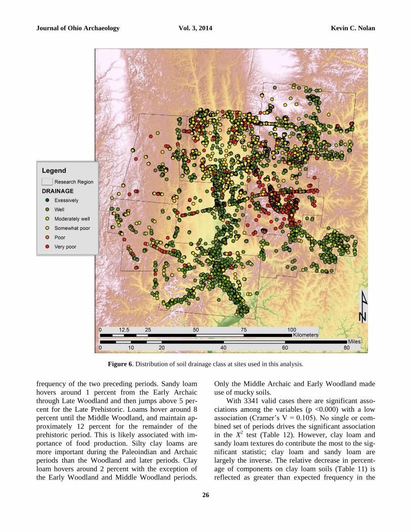
Drainage

As expected, there is a strong preference for bet-

ter drained soils; there is a strong geographic pattern

(Figure 6). A plurality of components for all time pe-

riods is found on well drained soils. While less than

50 percent of Archaic components are located on well

drained soils, a greater proportion (> 59%) of Wood-

land and Late Prehistoric occupations are located on

well drained soils (Table 9). Archaic periods have a

greater proportion of more poorly drained soils.

With 3337 valid cases there are significant asso-

ciations among the variables (p <0.000) with low

association (Cramer’s V = 0.118). The significant X2

results are driven primarily by the very strong con-

trast between the Late Archaic and Unknown Wood-

land components (Table 10). Late Archaic

components are significantly more frequent than ex-

pected on somewhat poor and very poorly drained

soils, and to a lesser degree on moderately well

drained soils. Whereas, Unknown Woodland are sub-

stantially underrepresented on those same drainage

classes and in addition to poorly drained. The rela-

tionship switches with the well-drained class. Late

Archaic components are underrepresented on well-

drained soils and Unknown Woodland components

are even more over-represented. Early Archaic has a

greater than expected association with very poorly

and somewhat poorly drained soils, and a lesser than

expected association with well or excessively drained

Figure 5. Distribution of soil slope categories by sites used in analysis.


25

soils. Middle Woodland has a lesser than expected

association with somewhat poor drainage, and a

greater than expected association with well or exces-

sively drained soils. Late Prehistoric has a lesser than

expected association with somewhat poorly drained

soils.

Texture

There is a pronounced preference for silt loams

(Figure 7), with most periods >70 percent (Table 11).

Channery and coarse sandy loams are least preferred.

Diversity of soil types exploited is fairly steady

around 7 texture classes with only Paleoindian and

Protohistoric having fewer types; in the latter case

this is likely a sampling bias, and in the former this is

likely a visibility and preservation bias. Gravelly

loam, sandy loam, loam, and silty clay loam are near-

ly ubiquitously used. Gravelly loam is used in roughly

equal proportions except for during the Middle

Woodland period, where its proportion nearly triples,

especially stark in contrast to the lower than average

Table 7. Proportional distribution of components by soil slope category.

Slope PI EA MA LA EW MW LW LP PH

A 32.9% 35.9% 38.6% 38.94% 36.0% 39.2% 44.8% 46.4% 25.0%

B 47.4% 49.6% 44.3% 48.5% 41.3% 39.7% 38.9% 38.9% 62.5%

C 10.5% 9.8% 10.0% 8.1% 14.0% 11.9% 8.1% 4.6%

D 6.6% 3.6% 5.7% 3.2% 5.3% 6.8% 4.8% 2.9% 12.5%

E

0.8%

0.7% 2.0% 1.6% 2.5% 2.1%

F 2.6% 0.4% 1.4% 0.6% 1.3% 0.8% 1.9% 2.1%

Table 8. Adjusted residuals for X2 test of association between periods and SMU slope category.

Slope

A B C D E F

PI -1.1 1 -0.1 0.7 -1.2 0.7

UA 2 -0.9 -0.5 -0.7 -1.1 -0.9

EA -1.5 3.9 -0.9 -1.4 -2 -2.4

MA 0 0.4 -0.3 0.4 -1.2 -0.1

LA 0.1 3.9 -3 -2 -3 -3

UW -3 -6 6.9 2.7 6.3 4.1

EW -1 -0.2 1.8 0.5 0.1 -0.9

MW 0.2 -1 0.7 1.9 -0.6 -1.4

LW 2.6 -1.2 -3 0 0.9 0.2

LP 2.5 -1 -3 -1.4 0.2 4.4

Table 9. Proportional distribution of components by soil drainage class.

Drainage PI EA MA LA EW MW LW LP PH

well/excessive 55.3% 45.9% 48.6% 46.7% 60.1% 66.4% 59.4% 63.2% 75.0%

moderately well 18.4% 21.5% 24.3% 22.2% 19.3% 19.5% 17.9% 18.4% 25.0%

somewhat poor 18.4% 19.6% 18.6% 18.9% 14.9% 8.9% 13.2% 9.6%

poor 1.3% 0.9% 1.4% 0.8%

0.8% 0.8% 0.8%

very poor 6.6% 11.7% 7.1% 11.2% 5.7% 3.9% 8.4% 7.9%


26

frequency of the two preceding periods. Sandy loam

hovers around 1 percent from the Early Archaic

through Late Woodland and then jumps above 5 per-

cent for the Late Prehistoric. Loams hover around 8

percent until the Middle Woodland, and maintain ap-

proximately 12 percent for the remainder of the

prehistoric period. This is likely associated with im-

portance of food production. Silty clay loams are

more important during the Paleoindian and Archaic

periods than the Woodland and later periods. Clay

loam hovers around 2 percent with the exception of

the Early Woodland and Middle Woodland periods.

Only the Middle Archaic and Early Woodland made

use of mucky soils.


ciations among the variables (p <0.000) with a low

association (Cramer’s V = 0.105). No single or com-

bined set of periods drives the significant association

in the X2 test (Table 12). However, clay loam and

sandy loam textures do contribute the most to the sig-

nificant statistic; clay loam and sandy loam are

largely the inverse. The relative decrease in percent-

age of components on clay loam soils (Table 11) is

reflected as greater than expected frequency in the

Figure 6. Distribution of soil drainage class at sites used in this analysis.


27

Archaic period and, to a lesser extent, lower than ex-

pected frequencies after that. Sandy loam frequencies

are lower than expected in the Early and Late Archaic

with substantially greater than expected frequency

during the Late Prehistoric and Unknown Woodland

periods. Middle Archaic exhibits a greater than ex-

pected association with Silt Loam. Middle Woodland

exhibits a greater than expected association with

Channery or Gravelly Loams and a less than expected

association with Clay Loam. Overall there is a slight

shift from avoidance of coarse texture to avoidance of

fine texture (or at least less emphasis on fine texture)

over time. However, this pattern is not pronounced.

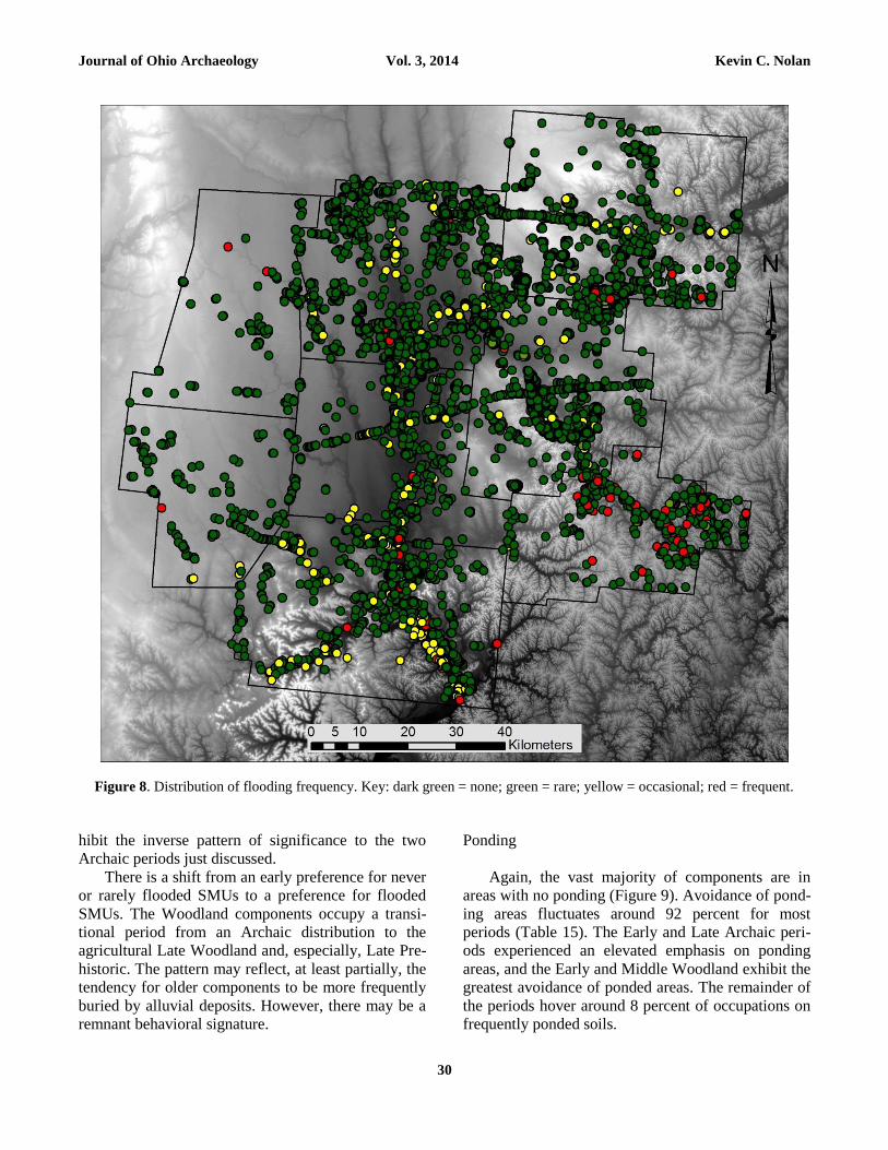
Flooding

The vast majority of components are located in

areas with no flooding (Figure 8). Emphasis on flood-

ed areas increases over time, with a concomitant

decrease in the emphasis on flood-free areas (Table

13).


ciations between frequency of flooding and periods of

occupation (p<0.000); however, the strength of asso-

ciation is low (Cramer’s V = 0.099). The significant

X2 result is driven almost entirely by the contrast be-

tween two Archaic (Early and Late) periods and the

final two prehistoric periods (Late Woodland and

Late Prehistoric) (Table 14). Early and Late Archaic

periods have greater than expected frequencies of

never flooded locations, and a less than expected fre-

quency of occasionally flooded locations. Only the

Early Archaic reaches a level of significance among

the pair. The Late Woodland and Late Prehistoric ex-

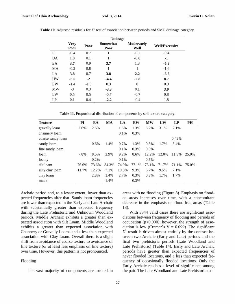
Table 10. Adjusted residuals for X2 test of association between periods and SMU drainage category.

Drainage

Very

Poor Poor

Somewhat

Poor

Moderately

Well Well/Excessive

PI -0.4 0.7 1 -0.2 -0.4

UA 1.8 0.1 1 -0.8 -1

EA 3.7 0.9 3.7 1.3 -5.8

MA -0.2 0.8 1 1 -1.6

LA 3.8 0.7 3.8 2.2 -6.6

UW -5.5 -2 -4.4 -2.8 8.7

EW -1.4 -1.5 0.3 0 0.9

MW -3 0.3 -3.3 0.1 3.9

LW 0.5 0.5 -0.7 -0.7 0.8

LP 0.1 0.4 -2.2 -0.4 1.8

Table 11. Proportional distribution of components by soil texture category.

Texture PI EA MA LA EW MW LW LP PH

gravelly loam 2.6% 2.5%

1.6% 1.3% 6.2% 3.1% 2.1%

channery loam

0.1% 0.3%

coarse sandy loam

0.42%

sandy loam

0.6% 1.4% 0.7% 1.3% 0.5% 1.7% 5.4%

fine sandy loam

0.1% 0.3% 0.3%

loam 7.8% 8.5% 2.9% 9.2% 8.6% 12.2% 12.0% 11.3% 25.0%

loamy

0.2%

0.1%

0.5%

silt loam 76.6% 73.6% 84.3% 74.9% 77.1% 73.1% 71.7% 71.1% 75.0%

silty clay loam 11.7% 12.2% 7.1% 10.5% 9.3% 6.7% 9.5% 7.1%

clay loam

2.3% 1.4% 2.7% 0.3% 0.3% 1.7% 1.7%

muck

1.4%

0.3%


28

Figure 7. Distribution of soil texture at sites used in this analysis.

Table 12. Adjusted residuals for X2 test of association between periods and soil texture.

Texture

Channery/

Gravelly

Loam

Sandy

Loam Loam

Silt

Loam

Clay

Loam

PI -0.4 -1.2 -0.7 0.7 0.4

UA -1.8 -0.3 -0.2 -0.9 2.8

EA -1.1 -2.3 -1.4 -0.3 3.4

MA -0.9 -0.2 -2 2.2 -0.4

LA -2.7 -2.1 -1 0.5 2.8

UW 3.4 4 1.7 0.2 -5.8

EW -0.4 -0.6 -1 1.3 -0.4

MW 3.5 -1.5 1.6 -0.5 -2.3

LW -0.1 -0.5 1.1 -1 0.6

LP -0.5 5.1 0.5 -1.1 -0.8


29

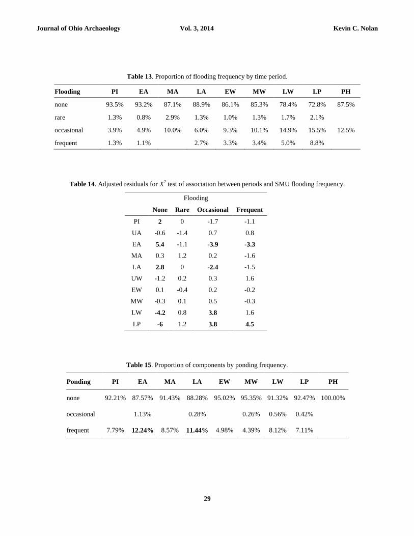
Table 13. Proportion of flooding frequency by time period.

Flooding PI EA MA LA EW MW LW LP PH

none 93.5% 93.2% 87.1% 88.9% 86.1% 85.3% 78.4% 72.8% 87.5%

rare 1.3% 0.8% 2.9% 1.3% 1.0% 1.3% 1.7% 2.1%

occasional 3.9% 4.9% 10.0% 6.0% 9.3% 10.1% 14.9% 15.5% 12.5%

frequent 1.3% 1.1%

2.7% 3.3% 3.4% 5.0% 8.8%

Table 14. Adjusted residuals for X2 test of association between periods and SMU flooding frequency.

Flooding

None Rare Occasional Frequent

PI 2 0 -1.7 -1.1

UA -0.6 -1.4 0.7 0.8

EA 5.4 -1.1 -3.9 -3.3

MA 0.3 1.2 0.2 -1.6

LA 2.8 0 -2.4 -1.5

UW -1.2 0.2 0.3 1.6

EW 0.1 -0.4 0.2 -0.2

MW -0.3 0.1 0.5 -0.3

LW -4.2 0.8 3.8 1.6

LP -6 1.2 3.8 4.5

Table 15. Proportion of components by ponding frequency.

Ponding PI EA MA LA EW MW LW LP PH

none 92.21% 87.57% 91.43% 88.28% 95.02% 95.35% 91.32% 92.47% 100.00%

occasional

1.13%

0.28%

0.26% 0.56% 0.42%

frequent 7.79% 12.24% 8.57% 11.44% 4.98% 4.39% 8.12% 7.11%


30

hibit the inverse pattern of significance to the two

Archaic periods just discussed.

There is a shift from an early preference for never

or rarely flooded SMUs to a preference for flooded

SMUs. The Woodland components occupy a transi-

tional period from an Archaic distribution to the

agricultural Late Woodland and, especially, Late Pre-

historic. The pattern may reflect, at least partially, the

tendency for older components to be more frequently

buried by alluvial deposits. However, there may be a

remnant behavioral signature.

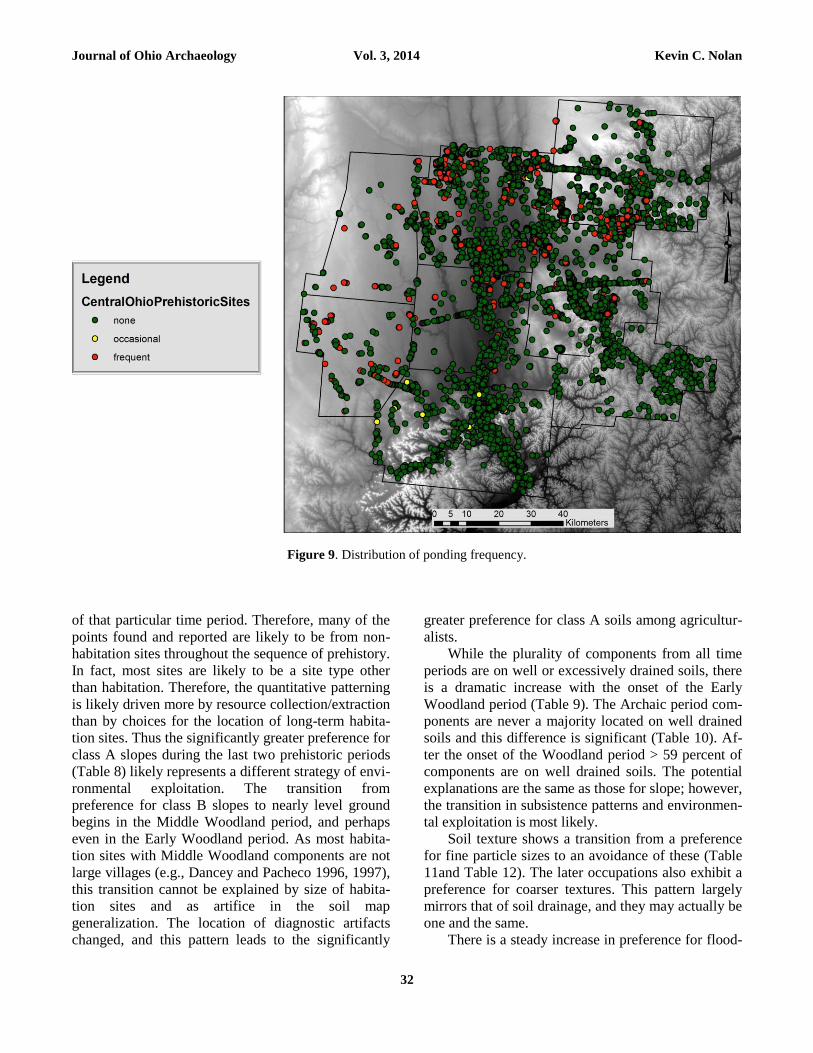
Ponding

Again, the vast majority of components are in

areas with no ponding (Figure 9). Avoidance of pond-

ing areas fluctuates around 92 percent for most

periods (Table 15). The Early and Late Archaic peri-

ods experienced an elevated emphasis on ponding

areas, and the Early and Middle Woodland exhibit the

greatest avoidance of ponded areas. The remainder of

the periods hover around 8 percent of occupations on

frequently ponded soils.

Figure 8. Distribution of flooding frequency. Key: dark green = none; green = rare; yellow = occasional; red = frequent.


31

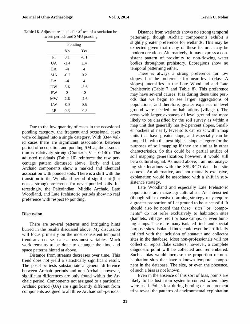
Table 16. Adjusted residuals for X2 test of association be-

tween periods and SMU ponding.

Ponding

No Yes

PI 0.1 -0.1

UA -1.4 1.4

EA -4 4

MA -0.2 0.2

LA -4 4

UW 5.6 -5.6

EW 2 -2

MW 2.6 -2.6

LW -0.5 0.5

LP 0.3 -0.3

Due to the low quantity of cases in the occasional

ponding category, the frequent and occasional cases

were collapsed into a single category. With 3344 val-

id cases there are significant associations between

period of occupation and ponding SMUs; the associa-

tion is relatively strong (Cramer’s V = 0.140). The

adjusted residuals (Table 16) reinforce the raw per-

centage pattern discussed above. Early and Late

Archaic components show a marked and identical

association with ponded soils. There is a shift with the

transition to the Woodland period of significant (but

not as strong) preference for never ponded soils. In-

terestingly, the Paleoindian, Middle Archaic, Late

Woodland, and Late Prehistoric periods show no real

preference with respect to ponding.

Discussion

There are several patterns and intriguing hints

buried in the results discussed above. My discussion

will focus primarily on the most consistent temporal

trend at a coarse scale across most variables. Much

work remains to be done to detangle the time and

space patterns hinted at above.

Distance from streams decreases over time. This

trend does not yield a statistically significant result.

The post-hoc tests substantiate a general difference

between Archaic periods and non-Archaic; however,

significant differences are only found within the Ar-

chaic period. Components not assigned to a particular

Archaic period (UA) are significantly different from

components assigned to all three Archaic sub-periods.

Distance from wetlands shows no strong temporal

patterning, though Archaic components exhibit a

slightly greater preference for wetlands. This may be

expected given that many of these features may be

modern creations. Alternatively, it may express a con-

sistent pattern of proximity to non-flowing water

bodies throughout prehistory. Ecoregions show no

temporal patterning either.

There is always a strong preference for low

slopes, but the preference for near level (class A

slopes) intensifies in the Late Woodland and Late

Prehistoric (Table 7 and Table 8). This preference

may have several causes. It is during these time peri-

ods that we begin to see larger aggregations of

populations, and therefore, greater expanses of level

ground were needed for habitations (villages). The

areas with larger expanses of level ground are more

likely to be classified by the soil survey as within a

map unit that generally has 0-2 percent slopes. Small-

er pockets of nearly level soils can exist within map

units that have greater slope, and especially can be

lumped in with the next highest slope category for the

purposes of soil mapping if they are similar in other

characteristics. So this could be a partial artifice of

soil mapping generalization; however, it would still

be a cultural signal. As noted above, I am not analyz-

ing site locations with the SSURGO data, but site

context. An alternative, and not mutually exclusive,

explanation would be associated with a shift in sub-

sistence strategy.

Late Woodland and especially Late Prehistoric

populations are maize agriculturalists. An intensified

(though still extensive) farming strategy may require

a greater proportion of flat ground to be successful. It

should also be noted that these “sites” or “compo-

nents” do not refer exclusively to habitation sites

(hamlets, villages, etc.) or base camps, or even hunt-

ing camps. There are many isolated finds and special

purpose sites. Isolated finds could even be artificially

inflated with the inclusion of amateur and collector

sites in the database. Most non-professionals will not

collect or report flake scatters; however, a complete

diagnostic point will be collected and remembered.

Such a bias would increase the proportion of non-

habitation sites that have a known temporal compo-

nent in the database. The size, or even the presence,

of such a bias is not known.

Even in the absence of this sort of bias, points are

likely to be lost from systemic context where they

were used. Points lost during hunting or procurement

trips reveal the patterns of environmental exploitation


32

of that particular time period. Therefore, many of the

points found and reported are likely to be from non-

habitation sites throughout the sequence of prehistory.

In fact, most sites are likely to be a site type other

than habitation. Therefore, the quantitative patterning

is likely driven more by resource collection/extraction

than by choices for the location of long-term habita-

tion sites. Thus the significantly greater preference for

class A slopes during the last two prehistoric periods

(Table 8) likely represents a different strategy of envi-

ronmental exploitation. The transition from

preference for class B slopes to nearly level ground

begins in the Middle Woodland period, and perhaps

even in the Early Woodland period. As most habita-

tion sites with Middle Woodland components are not

large villages (e.g., Dancey and Pacheco 1996, 1997),

this transition cannot be explained by size of habita-

tion sites and as artifice in the soil map

generalization. The location of diagnostic artifacts

changed, and this pattern leads to the significantly

greater preference for class A soils among agricultur-

alists.

While the plurality of components from all time

periods are on well or excessively drained soils, there

is a dramatic increase with the onset of the Early

Woodland period (Table 9). The Archaic period com-

ponents are never a majority located on well drained

soils and this difference is significant (Table 10). Af-

ter the onset of the Woodland period > 59 percent of

components are on well drained soils. The potential

explanations are the same as those for slope; however,

the transition in subsistence patterns and environmen-

tal exploitation is most likely.

Soil texture shows a transition from a preference

for fine particle sizes to an avoidance of these (Table

11and Table 12). The later occupations also exhibit a

preference for coarser textures. This pattern largely

mirrors that of soil drainage, and they may actually be

one and the same.

There is a steady increase in preference for flood-

Figure 9. Distribution of ponding frequency.


33

ed soils (Table 13) and decrease in preference for

ponded soils (Table 15) through time. Both of these

patterns are significant (Table 14 and Table 16) and

significance once again seems to follow the transition

in subsistence patterns and the shift from the Archaic

to the Woodland period.

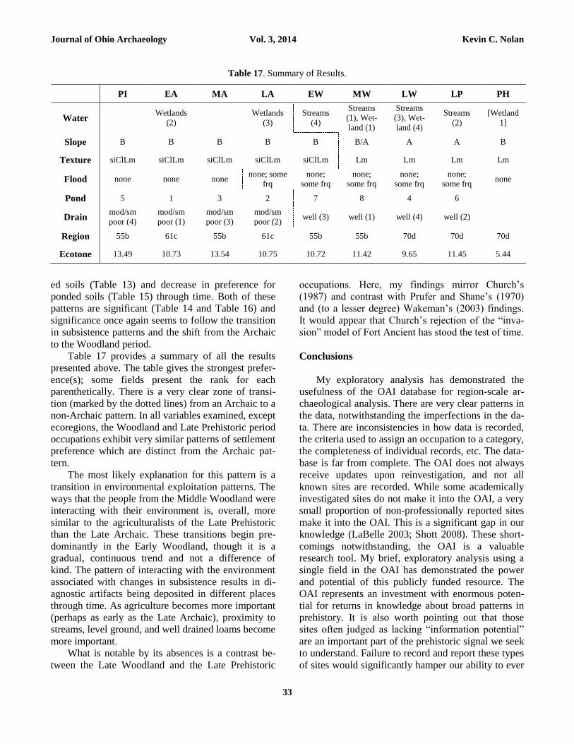
Table 17 provides a summary of all the results

presented above. The table gives the strongest prefer-

ence(s); some fields present the rank for each

parenthetically. There is a very clear zone of transi-

tion (marked by the dotted lines) from an Archaic to a

non-Archaic pattern. In all variables examined, except

ecoregions, the Woodland and Late Prehistoric period

occupations exhibit very similar patterns of settlement

preference which are distinct from the Archaic pat-

tern.

The most likely explanation for this pattern is a

transition in environmental exploitation patterns. The

ways that the people from the Middle Woodland were

interacting with their environment is, overall, more

similar to the agriculturalists of the Late Prehistoric

than the Late Archaic. These transitions begin pre-

dominantly in the Early Woodland, though it is a

gradual, continuous trend and not a difference of

kind. The pattern of interacting with the environment

associated with changes in subsistence results in di-

agnostic artifacts being deposited in different places

through time. As agriculture becomes more important

(perhaps as early as the Late Archaic), proximity to

streams, level ground, and well drained loams become

more important.

What is notable by its absences is a contrast be-

tween the Late Woodland and the Late Prehistoric

occupations. Here, my findings mirror Church’s

(1987) and contrast with Prufer and Shane’s (1970)

and (to a lesser degree) Wakeman’s (2003) findings.

It would appear that Church’s rejection of the “inva-

sion” model of Fort Ancient has stood the test of time.

Conclusions

My exploratory analysis has demonstrated the

usefulness of the OAI database for region-scale ar-

chaeological analysis. There are very clear patterns in

the data, notwithstanding the imperfections in the da-

ta. There are inconsistencies in how data is recorded,

the criteria used to assign an occupation to a category,

the completeness of individual records, etc. The data-

base is far from complete. The OAI does not always

receive updates upon reinvestigation, and not all

known sites are recorded. While some academically

investigated sites do not make it into the OAI, a very

small proportion of non-professionally reported sites

make it into the OAI. This is a significant gap in our

knowledge (LaBelle 2003; Shott 2008). These short-

comings notwithstanding, the OAI is a valuable

research tool. My brief, exploratory analysis using a

single field in the OAI has demonstrated the power

and potential of this publicly funded resource. The

OAI represents an investment with enormous poten-

tial for returns in knowledge about broad patterns in

prehistory. It is also worth pointing out that those

sites often judged as lacking “information potential”

are an important part of the prehistoric signal we seek

to understand. Failure to record and report these types

of sites would significantly hamper our ability to ever

Table 17. Summary of Results.

PI EA MA LA EW MW LW LP PH

Water

Wetlands

(2)

Wetlands

(3)

Streams

(4)

Streams

(1), Wet-

land (1)

Streams

(3), Wet-

land (4)

Streams

(2)

[Wetland

1]

Slope B B B B B B/A A A B

Texture siClLm siClLm siClLm siClLm siClLm Lm Lm Lm Lm

Flood none none none none; some

frq

none;

some frq

none;

some frq

none;

some frq

none;

some frq none

Pond 5 1 3 2 7 8 4 6

Drain mod/sm

poor (4)

mod/sm

poor (1)

mod/sm

poor (3)

mod/sm

poor (2) well (3) well (1) well (4) well (2)

Region 55b 61c 55b 61c 55b 55b 70d 70d 70d

Ecotone 13.49 10.73 13.54 10.75 10.72 11.42 9.65 11.45 5.44


34

fully understand the cultural systems we study (c.f.

Baker 1998:54-55; ODOT 2012:7). The results of this

analysis would have been drastically different if

large-scale surveys and CRM investigations did not

record all site types.

More work must be done to exploit the latent re-

search potential of the OAI, and more work must be

done to ensure the integrity and comparability of the

data collected and entered.

Acknowledgements

First, I must thank Brent Eberhardt from OHPO

for his assistance with the OAI, introducing me to the

in-house version, and always taking the time to an-

swer my questions. The data used in this analysis was

purchased with funds from Certified Local Govern-

ment grant #39-08-21740. I am also grateful to the

managing editor, members of the editorial board, and

two anonymous reviewers for their constructive

comments that helped clarify and strengthen the cur-

rent manuscript. Finally, I must express my gratitude

to James A. Jones (Director Research and Academic

Effectiveness, Ball State University) for advice and

guidance on the statistical analysis. Any and all

shortcoming and errors contained in the final manu-

script are mine alone.

References Cited

Abrams, Elliot

2009 Hopewell Archaeology: A View from the North-

ern Woodlands. Journal of Archaeological Research

17:169-204.

Baker, Stanley W.

1998 Phase I and II Cultural Resources Survey for the

ADA-SR136-21.51 Bridge Replacement Project Locat-

ed in Winchester Township, Adams County, Ohio (PID

12905). Cultural Resources Unit, Bureau of Environ-

mental Services, Ohio Department of Transportation.

Braun, David P.

1987 Coevolution of Sedentism, Pottery Technology,

and Horticulture in the Central Midwest, 200 B.C. –

A.D. 600. In Emergent Horticultural Economies of the

Eastern Woodlands, edited by W. F. Keegan, pp. 153-

181. Center for Archaeological Investigations, Southern

Illinois University Carbondale, Carbondale, Illinois.

Butler, Brian E.

1980 Soil Classification for soil survey. Oxford Univer-

sity Press, Oxford.

Church, Flora

1987 An Inquiry into the Transition from Late Wood-

land to Late Prehistoric Cultures in the central Scioto

Valley, Ohio, circa A.D. 500 to A.D. 1250. Un-

published Ph.D. dissertation, Department of

Anthropology, The Ohio State University, Columbus,

Ohio.

Church, Flora and John P. Nass

2002 Central Ohio Valley During the Late Prehistoric:

Subsistence-Settlement Systems Respond to Risk. In

Northeast Subsistence-Settlement Change, A.D. 700-

A.D.1300, edited by J. P. Hart and C. Reith, pp. 11-42.

New York State Museum Bulletin 496. The University

of the State of New York, Albany.

Cook, Robert A.

2008 SunWatch: Fort Ancient Development in the Mis-

sissippian World. Tuscaloosa: University of Alabama

Press.

Cook, Robert A. and Mark R. Schurr

2009 Eating between the Lines: Mississippian Migra-

tion and Stable Carbon Isotope Variation in Fort

Ancient Populations. American Anthropologist

111:344-359.

Dancey, William S.

1992 Village Origins in Central Ohio: The Results and

Implications of Recent Middle and Late Woodland Re-

search. In Cultural Variability in Context, Woodland

settlements of the Mid-Ohio Valley, edited by M. F.

Seeman, pp. 24-29. MCJA Special Paper No. 7. Kent

State University Press, Kent, Ohio.

1996 Putting an End to Hopewell. In A View from the

Core: A Synthesis of Ohio Hopewell Archaeology, ed-

ited by P. J. Pacheco, pp. 394-405. The Ohio

Archaeological Council, Inc., Columbus, Ohio.

Dancey, William S., and Paul J. Pacheco (Editors)

1997 Ohio Hopewell Community Organization. Kent

State University Press, Kent, Ohio.

Drennan, Robert D.

1996 Statistics for Archaeologists: A commonsense ap-

proach. Plenum, New York.

Dunnell, Robert C.

1971 Systematics in Prehistory. The Free Press, Lon-

don.

2008 Archaeological Things: Languages of Observa-

tion. In Times River: Archaeological Syntheses from


35

the lower Mississippi River Valley, edited by J Rafferty

and E Peacock, pp. 45- 68. University of Alabama

Press, Tuscaloosa.

Dunnell, Robert C., and William S. Dancey

1983 The Siteless Survey: A Regional Scale Data Col-

lection Strategy," in Michael B. Schiffer, ed., Advances

in Archaeological Method and Theory 6: 267-287.

Essenpreis, Patricia S.

1982 The Anderson Village Site: Redefining the Ander-

son Phase of the Fort Ancient Tradition of the Middle

Ohio Valley. Ph.D. Dissertation, Anthropology, Har-

vard University.

Greenlee, Diana M.

2002 Accounting for Subsistence Variation among

Maize Farmers in Ohio Valley Prehistory. Doctoral dis-

sertation, Department of Anthropology, University of

Washington, Seattle, Washington.

Gremillion, Kristen J.

2002 The Development and Dispersal of Agricultural

Systems in the Woodland Period Southeast. In The

Woodland Southeast, edited by D. G. Anderson and R.

C. J. Mainfort, pp. 483-501. University of Alabama

Press, Tuscaloosa.

Griffin, James B.

1966 The Fort Ancient Aspect: Its Cultural and Chrono-

logical Position in Mississippi Valley Archaeology.

Universtity of Michigan, Museum of Anthropology,

Ann Arbor, MI.

Hart, John P.

1999 Maize agriculture evolution in the Eastern Wood-

lands of North America: A Darwinian perspective.

Journal of Archaeological Method and Theory 6:137-

180.

IBM

2012 Technote 34140: Interpreting adjusted residuals in

Crosstabs cell statistics. http://www-01.ibm.com/su

pport/docview.wss?uid=swg21479605, accessed 8/26/

2012.

LaBelle, Jason M.

2003 Coffee Cans and Folsom Points: Why we cannot

continue to ignore the artifact collector. In Ethical Is-

sues in Archaeology, edited by L. Zimmerman, K.

Vitelli and J. Hollowell-Zimmerman, pp. 115-127. Al-

tamira Press, Walnut Creek, CA.

Leone, Karen L.

2007 Sedentism in the Middle Woodland: Archaeobo-

tanical Evidence from the Strait Site. Unpublished MA

thesis, Department of Anthropology, The Ohio State

University, Columbus, Ohio.

Lepper, Bradley T.

2011 Ohio – “The Heart of it All” for over 15,000

Years. Journal of Ohio Archaeology 1(1):1-21.

Lipo, Carl P., and Robert C. Dunnell

2008 Prehistoric Settlement in the Central and Lower

Mississippi Valley: A Critical Review. In Time’s Riv-

er: Archaeological Syntheses from the Central and

Lower Mississippi River Valley, edited by J. Rafferty

and E. Peacock. University of Alabama Press

Martin, Kristie R.

2009 Eastern Agricultural Complex Traditions in Small

Fort Ancient Communities - The Wildcat Example. Un-

published MA thesis, Department of Anthropology, The

Ohio State University, Columbus, Ohio.

McElrath, Dale L., Thomas E. Emerson, and Andrew C.

Fortier

2004 Social Evolution or Social Response? A Fresh

Look at the "Good Gray Cultures" After Four Decades

of Midwest Research. In Late Woodland Societies: Tra-

dition and Transformation across the Midcontinent,

edited by TE Emersion, DL McElrath, and AC Fortier.

University of Nebraska Press, Lincoln.

Nolan, Kevin C.

2009 Archaeological Survey of the Reinhardt Tract

Property through a Certified Local Government (CLG)

Grant on behalf of the City of Columbus in Harrison

Township, Pickaway County, Ohio, Volume I: Survey

Results. Report submitted to the Ohio Historic Preser-

vation Office, Columbus, Ohio.

Norušis, Marija J.

2010 PASW Statistics 18 Guide to Data Analysis. Pren-

tice Hall, Upper Saddle River, New Jersey.

Ohio Department of Natural Resources

2005 Detailed Hydrography Polygons. Ohio Depart-

ment of Natural Resources, Columbus, Ohio.

Ohio Department of Transportation

2012 Chapter 7: Identification of Historic Properties:

Phase I Archaeology Survey. In Cultural Resources

Manual. Ohio Department of Transportation, Colum-

bus, Ohio.

Omernik, James M.

1987 Ecoregions of the coterminous United States. Map

(scale 1:7,500,000). Annals of the Association of Amer-

ican Geographers 77(1):118-125.


36

Pacheco, Paul J.

1997 Ohio Middle Woodland Intracommunity Settle-

ment Variability: A Case Study from the Licking

Valley. In Ohio Hopewell Community Organization,

edited by W. S. Dancey and P. J. Pacheco, pp. 41-84.

The Kent State University Press, Kent, Ohio.

Pacheco, Paul J., editor

1996 A View From the Core: A Synthesis of Ohio

Hopewell Archaeology. Ohio Archaeological Council,

Columbus, Ohio.

Pollack, David and A. Gwynn Henderson

1992 Towards a Model of Fort Ancient Society. In Fort

Ancient Cultural Dynamics in the Middle Ohio River

Valley, edited by A. G. Henderson, pp. 281-294. Mon-

ographs in World Archaeology No. 8, Prehistory Press,

Madison, Wisconsin.

Prufer, Olaf H. and Orin C. Shane

1970 Blain Village and the Fort Ancient Tradition in

Ohio. Kent State University Press, Kent, Ohio.

Purtill, Matthew

2012 A Persistent Place: A Landscape Approach to the

prehistoric archaeology of the Greenlee Tract in South-

ern Ohio. Gray & Pape, Cincinnati, Ohio.

Rafferty, Janet

2008 Settlement Patterns, Occupations, and Field

Methods. In Times River: Archaeological Syntheses

from the lower Mississippi River Valley, edited by J

Rafferty and E Peacock, pp. 99-124. University of Ala-

bama Press, Tuscaloosa.

2012 Classification at the Scale of Occupation: A Case

Study. Paper prepared for SAARAS Workshop, Missis-

sippi State University, Starkville, Mississippi, April 16-

17, 2012.

Rafferty, Janet, Jeffrey Alvey, Keith Baca, Jason Edmonds,

Michael Fazio, and Marcus Hayes

2011 Systematic Cultural Resources Survey of a Pro-

posed Mine Area in Kemper and Lauderdale Counties,

Mississippi. Report prepared for North American Coal

Corporation. Cobb Institute of Archaeology, Mississippi

State University, Starkville.

Seeman, M. F. and W. S. Dancey

2000 The late woodland period in southern Ohio: basic

issues and prospects. In Late Woodland Societies: Tra-

dition and Transformation across the Midcontinent,

edited by T. E. Emerson, E. L. McElrath and A. C.

Fortier, pp. 583-612. University of Nebraska Press, Lin-

coln, Nebraska.

Shott, Michael J.

2008 equal o nll roofht w ded I e vsbr cted: A Proposal

for Conservation of Private Collections in American

Archaeology. Archaeological Record 8:30-34.

Smith, B. D.

1987 The Independent Domestication of Indigenous

Seed-Bearing Plants in Eastern North America. In

Emergent Horticultural Economies of the Eastern

Woodlands, edited by W. F. Keegan, pp. 3-48. Occa-

sional ed. Center for Archaeological Investigation,

Southern Illinois University at Carbondale, Carbondale,

Illinois.

1989 Origins of Agriculture in Eastern North America.

Science 246(4937):1566-1571.

1995 Seed Plant Domestication in Eastern North Amer-

ica. In Last Hunters First Farmers, edited by T. D. Price

and A. B. Gebauer. School of American Research Ad-

vanced Seminar Series. School of American Research

Press, Sante Fe.

2001 Low-Level Food Production. Journal of Archaeo-

logical Research 9:1-43.

2009 Initial formation of an indigenous crop complex in

eastern North America at 3800 B.P. PNAS

106(16):6561-6566.

Spurlock, Linda B., Olaf H. Prufer, and Thomas R. Pigott

2006 Caves and Culture: 10,000 Years of Ohio History.

Kent State University, Kent, Ohio.

Tamhane, Ajit C.

1979 A Comparison of Procedures for Multiple Com-

parisons of Means with Unequal Variances. Journal of

the American Statistical Association 74(366):471-480.

Thompson, Victor and John A. Turck

2009 Adaptive Cycles of Coastal Hunter-Gatherers.

American Antiquity 74:255-278.

Wakeman, Joseph E.

2003 Archaeological Settlments of the Late Woodland

and Late Prehistoric Tribal Communities in the Hocking

River Watershed, Ohio. MS Thesis, Program of Envi-

ronmental Studies, Ohio University, Athens.

Weaver, Sarah A., Elliot A. Abrams, AnnCorinne Freter,

and Dorothy Sack

2011 Middle Woodland Domestic Architecture and the

Issue of Sedentism: Evidence from the Patton Site

(33AT990). Journal of Ohio Archaeology 1(1):22-40.

Welch, B.L.

1951 On the Comparison of Several Mean Values: An

Alternative Approach. Biometrika 38(3-4):330-336.


37

Wells, Joshua J.

2011 Digital Dimensions of Mississippian Settlement:

Strengths and Weaknesses of Scalar Efforts with Curat-

ed Data for GIS Analysis and Modeling. Poster

presentation at the Annual Meeting of the Midwest Ar-

chaeological Conference, LaCrosse, Wisconsin

Woods, Alan J., James M. Omernik, C. Scott Brockman,

Timothy D. Gerber, William D. Hosteter, and Sandra H.

Azevedo

1998 Ecoregions of Indiana and Ohio (Map). United

States Geological Survey, Denver, Colorado.

Wymer, Dee Ann

1996 The Ohio Hopewell Econiche: Human-Land In-

teraction in the Core Area. In A View From the Core: A

Synthesis of Ohio Hopewell Archaeology, edited by P.

J. Pacheco, pp. 36-52. The Ohio Archaeological Coun-

cil, Columbus, Ohio.

1997 Paleoethobotany in the Licking River Valley,

Ohio: Implications for Understanding Ohio Hopewell.

In Ohio Hopewell Community Organization, edited by

W. S. Dancey and P. J. Pacheco, pp. 153-171. Kent

State University, Kent, Ohio.

Yerkes, Richard W.

2002 Hopewell Tribes: A Study of Middle Woodland

Social Organization in the Ohio Valley. In The Archae-

ology of Tribal Societies, edited by W. A. Parkinson,

pp. 227-245. International Monographs in Prehistory,

Ann Arbor, Michigan.

2009 Microwear Analysis of a Sample of 100 Chipped

Stone Artifacts from the 1971-1977 Excavations at the

Seip Earthworks. Midcontinental Journal of Archaeolo-

gy 34:109-122.

An Exploratory Analysis of Diachronic Settlement Patterns in Central Ohio

Documents

Transcript of An Exploratory Analysis of Diachronic Settlement Patterns in Central Ohio