...,~1_)_):!"'-"'~

-""'15:... ...r4-- .:.:, ) ._r\..:..:<).5: _j?... &'-->"

i i

SOLUTIONS MANUAL

MODERN CONTROL ENGINEERING THIRD EDITION

KATSUHIKO OGATA Univn-~ity of Minn~sota

Estelh-ro~·: Benuordo Snero do Sitn Fdba

Titulo: A­Class~lo ISBN: "''"de: ordcm Data:

:j ~ ' j' u PRENTICE H:\LL Upper Saddle Ri"cr. NJ 074~8

,_i...,,'-"'~ www.shmirzamohamm~ _i.blogfa.com

~-----------------------

. .

~

N

e ~

~ ~

• 0

0 ~

e ~

w

• 0

~

> ~

~

• N

~

w

• ~

~

e e

N

N

"' ... 1: ~

c: 0 u

~

N

~

~

• w

~

• ~

~ "

" i "

" " l

• •

tt •

! •

" lt

lt lt

~ ~

~

il il

il iJ

il il

• 6

6

_.;;"

'?------------:-

-------------···-

··--·-

-····

J ~

/

·~ ' < 0

! " ' ' 0 -----------

t ~ ' ·~

~

...;~I_)_J:!"'-""'~

~15:... ...r4-- .:.:, ) .,rl...:..:<_)lS -~ &'-->"

Preface

The third edition of Modern oont~ol Engineering contains 418 problems. 206 of them are provided with complete solutions (A Problems) and 212 of them are given without solutions (B Problems). This solutions manual presents solu­tions to illl 212 unsolved B Problems •. Ex~pt for the. case of -Simple and straightforward problems, all solutions given here are detailed and compre­hensive.

Tile text may be used in a few different ways depending on the course objective and time alloc:atecl to the course. sample course coverages are shoWn below.

www.shmirzamohammadi.blogfa.com

For one quarter course For one semester For tlltl quarters ( 4 hours/wee){, 40 lecture course (4 hours/week, course ( 3 hours/ hours) or one semester 52 lecture hours) week, 60 or mor, course ( 3 hours/week:, 42 lecture hourS) lecture hours)

#1 #2 #3

Chapter 1 Chapter 1 Chapter 1 Chapter 2* Ch01pter 2* Chapter 2 Chapter 3 Chapter 3 Chapter 3 Chapter 4 Chapter 4 Chapter 4 Chapter 5 Chapter 5 Chapter 5 Chapter 6 Chapter 6 Chapter 6 Chapter 7 Ch01pter 7 Chapter 7 Chclpter 8 Chapter 8 Chapter 8 Chclpter 9 Chapter 9 Chapter 9 Chapter 10** Chapter 10 Chapter 10

Chapter 11 Chapter 11 Chapter 12 Chapter 12

Chapter 13

* JM.Y be omitted if students have adequate background on Laplace transform

•• ma.y be emitted if short in time

For the one semester course (#2) the instructor will have flexibility in omitting certain subjects depending on the course objective.

Katsuhiko Ogata

' ._..i...> _ _,...;.~

' "''" ' ~-.---

".,.

:-' '.,;•;."_,, •. '

·i:-:;., ·--- -.

...;~I_)_J:!"'-""'~

-""'15:... ...r4-- .:.:, ) ..r4_)1..5: -~ &'-->"

I

I

CHAPTER I

\ B-1-1. CloSed-loop control systems found in hOllies:

( l) Room temperature control system. Room temperature is kept constant regardless of the nl.lll'1ber or people in the roan or the outside t.arp!r, ture.

(2) Refrigerator. regardless of

Keeps the temperature in the refrigerator constant · the amount of food in 1 t and the outside temperature.

( 3) Cooking oven temperature control. The oven temperature is controlh at the set point regardless of the allllunt of food in the oven and thE> outside roam temperature.

Open-loop control systems found in homes:

(1) Washer and dryer for cloths.

{2) Dish washer.

(3} A person takes a pill (for example, cholesterol control pill) every day to keep cholesterol level within a desired limit. He or she doe-

~-

not check the cholesterol level every day. 'The process c::<;~ntinues without check for a few months. It operates as an open-loop control system. The open-loop control system needs calibration fran time to time. He or she goes to a doctor to check the cholesterol level and the doctor controls the amount of pill. {This is a calibration pro­cess.)

{1) Watering a garden. The output wanted is a certain level of satura- · tion. The input is water and the controller is the human watching the soil to determine whether the soil is adequately saturated. once the required saturation is met, the controller {human) either moves the sprinkler or turns off water, until the soil again requires water­ing.

{2) Driving a car. The output is a certain speed, for example, 65 mph. The'input is the driver's foot on the accelerator, and the controller is the human(driver) who tris to maintain the speed by monitoring the speedometer and either accelerates or lift foot off the accelerator to slow d01m. Perhaps ve can simulate a disturbance in this example. The sudden sighting ot a police officer which causes the controller to react by touching the brakes.

( 3) selection of 'IV channel controlled by a human.

or TV volume by means of a remote controller. The reference channel is ~he desired channel

1 www.shmirzamohammadi.blogfa.com ~-.,'-""'~

' -""'15:... ...r4-- .:.:, ) .,rl...:..:<_)\!l_~ &'-->"

and the output charmel is the channel currently showing. If the current channel is numerically lower than the desired channel, the human can push the '+' channel button until the desired channel is reached. The volume is similarly controlled. If the volume is lou­der than the desired volume, the '-' volume button is pushed until the desired VOlUII'e is reached.

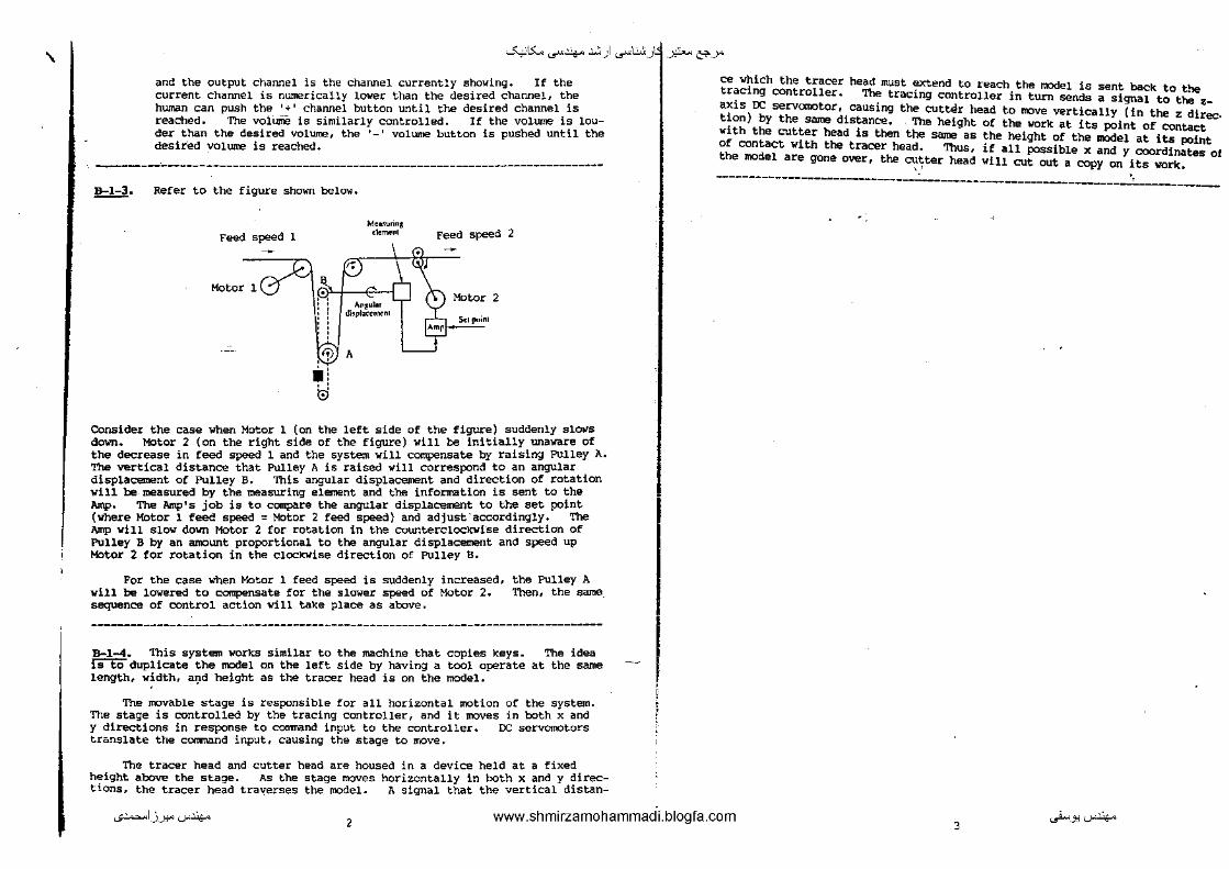
-------·------------------------------------------------------------------------B-1-3. Refer to the figure shown below.

Feed speed 1 M<0.<unn1

'"'""'"' Feed speed 2

Motor 1

5<1 p.oinl

Consider the case When Motor 1 (on the left side of the figure) suddenly slows down. Motor 2 (on the right side of the figure) will be initially unaware of the decrease in feed speed 1 and the system will compensate by raising Pulley A. The vertical distance that Pulley A is raised will correspond to an angular displacement of Pulley B. This angular displacement and direction of rotation will be measured by the measuring element and the information is sent to the Amp. The Amp's job is to a:npare the angular displacement to the set point (where Motor 1 feed speed= Motor 2 feed speed} and adjust·accordingly. The Amp will slow down Motor 2 for rotation in the countercloclcwise direction of Pulley B by an amount proportional to the angular displacement and speed up Motor 2 for rotation in the clockWise direction of Pulley B.

For the case when Motor 1 feed speed is suddenly increased, will be lowered to compensate for the slower speed of Motor 2. sequence of control action will take place as aboVe.

the Pulley A Then, the same_

B-l.-4. This system works similar to the machine that copies keys. The idea is to duplicate the model on the left side by having a tool operate at the same length, w~dth, a~d height as the tracer head is on the model.

The movable stage is responsible for all horizontal motion of the system. The stage is controlled by the tracing controller, and it moves in both x and y directions in response to command input to the controller. DC servomotors translate the command input, causing the stage to move.

The tracer head and cutter head are housed in a device held at a fixed height above the stage. As the stage moves horizontally in both x and y direc­tions, the tracer head traverses the model. A signal that the vertical distan-

' !

ce which the tracer head must extend to reach the model is sent back to the tracing controller. The tracing controller in turn sends a signal to the z­axis r:c serv0010tor, causing the cutter head to rove vertically (in the z direc. tion) by the same distance. The height of the work at its point of contact with the cutter head is then the same as the height of the model at its point of contact with the tracer head. Thus, if all possible x and y coordinates of the model are gone over, the cutter head will cut out a copy on its work.

'' ---------------------------------------------------------------~-------------

...;~I_)_J:!"'-"'~ 1 www.shmirzamohammadi.blogfa.com 3

._..i..._J:l'-"'~

' CHAPTER 2

-""'15:... ...r4-- .:.:, ) .,rl...:..:<_.ts: -~ &'-->"

~-

B-2-1. .S+",¥-

(a) F,(s) == (s+,.oa. +tza. S+tf. p.

Sz.+II•IS +IJt.p./4

<b> f,(+J-.....:. (4~+ 7) =u.s..;_ "t +- •·n•""" 1-r

F,(s) =

B-2-2.

o.sxft + • Sol.+~

#,3tf.S.S 2+4·.P4'Ps sa+9-~ = s:~-_,..111

<•> f,{t) = ~ ......_ ( S't+ ?.>") = 2. 121 ...;. .st + 2. 121 en st

F,(s) = '%, IZ/ X 5"" + ,s-1-+Gz

2./Z/ s sz.+ s&.

/t~,lfo'?+ 2./ZI s

.s'"'+zs-

{b} fz.(t) = IJ.P3- tJ.()~ c.n. zt"

~-

!!±i·

F, (s) = ~ $

"·"3 s s'r 9-

= :•:·~'::-':_S::_'_:+,.::P~·:_IZ:_:-..;.•~·:'.:"'~":.._' s (s'-t f-)

--:--7'-;·i' /2';:-;;-;­= :s(s'+l')

.Z[t']=-:fr z

F(s) = l. [ -t•e-•"J = (.>+«)'

f{t) = en Zwt · c.._ 3w't =-f: ( "-'< >vt + c.< -.Jt)

I ( s S ) F(s)=z s2+2S4JI + sz+wz..

(:s'+/3AJ')s = (:i''·+ZS<v'')(s 1 +w")

.I ' ! t

f(t)=(t-4.) !U-"-)

Ff<) = e-c.s

s• --------------------------------~------------------------------~-----------

~-f(t)= t 1(t)-- (t- T) i(i-T)

F(s) = _I_ e- T.r ,sz.--­s' --

1-e-T.s­r•

-------------------------------------------------------------------B-2-7.

~/t)~ 2~ t-- .!!':i(t-.9..)- Zfi U-«)i(<-~' ,,. a" A.z. z a.J '/

2f' ( I a e -i-r e -<s) Ffs) = a.r Si - ~ - -:;;:-

l-4se-f,._e-"s J.t... F{s) = 2~ 1.;.,_ ll?o s, •~o 4"

.t { -. 44 1-A.se ~'""-e-•s)

/ .. c~') - .!!:._ #.... - &~ "'...,."

:=- 2.¢ ~ -se-f,. +" -fe-i-s + s e-u ~~ t~~-+# .7~ &

-=.LJh.... .S~ c-t"

II t.;.. = 7 4-tO

-- L .[,;,...

.;f(-se_.,.,+q .;.e-r~+.se-·~

~(•') s• e- ... ,s + s• e-~-.$ as•e-.f:..s ~.._-2 T r -.- - ... e ....

.-/;:( .re-+'"- -¥-e- Ts- sa.e-.u) - sJ. "-~"~

:. (:z-J

?-(- J.-: +s) =.s

-------------------------------------------------------------------------------

...;~I_)_J:!"'-""'~ 4

www.shmirzamohammadi.blogfa.com 5

~-.,'-""'~

" ~-

-""'15:... ...r4--.:.:,) .,rl...:..:<_)i..51.~ &'-->"

.!!:±!.?.·

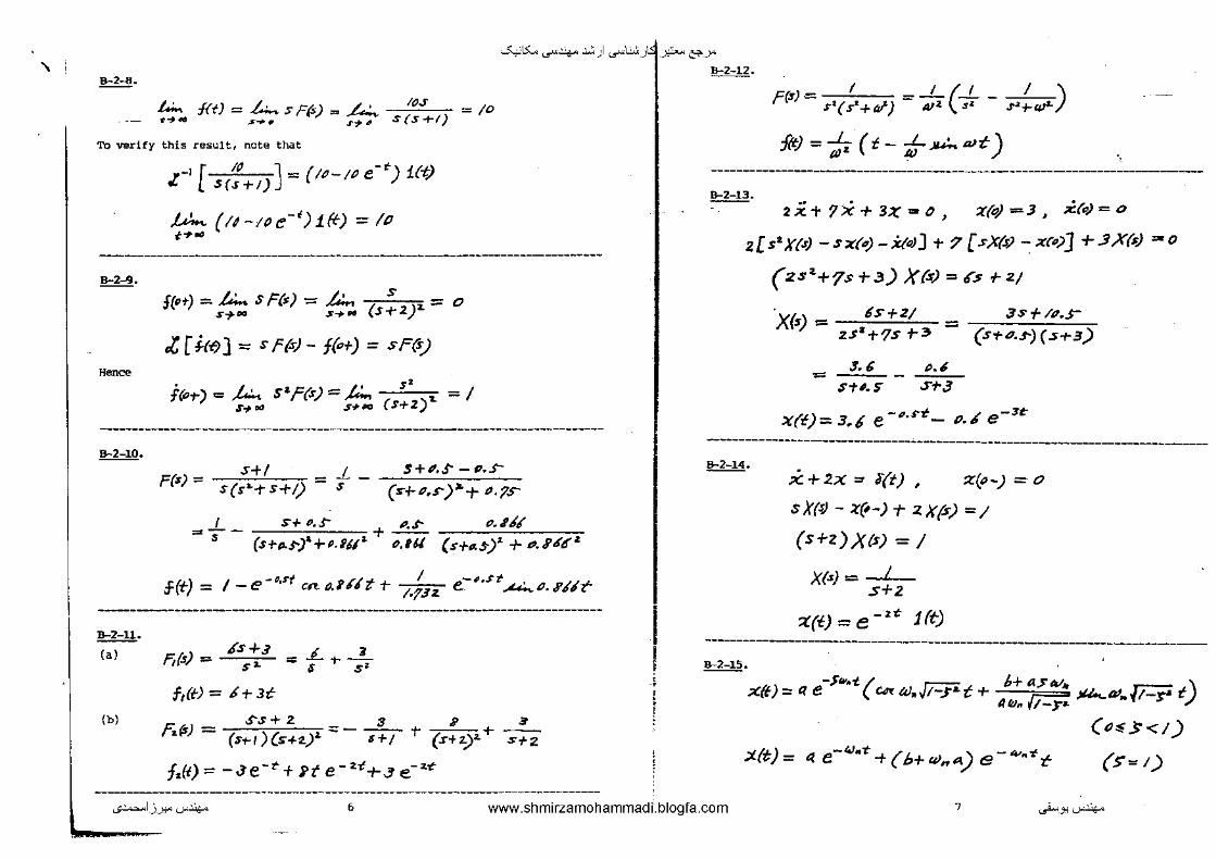
t.w., f(t) = .14.. s F(s) = ~ s :~:t) = ;o .,~..., .s~. .T'1'"

TO verity this result, note that

.-1 [ /Q J ~ ( (P-(P e-t) i(-1) "" S(s+t)

.U... {ti-1Pe-')1ft) =to ·~~

~-f(•t) = /.:- S F(s) = .t;.., s = 0

S-j-110 S-i>M (S-t-2JZ.

.l [ftf) J = s f'(s) - f(or) = sF(>) Hen~

f(or) = ~ S'f'(s) = j.;., s' 1 ~ 1 ~~"" S#'PO (S+Z)

B-2-10.

F(s) = s+! 1 S+#,J'"- tJ • .J-

s(s'-ts+l) = s- (s-r-•.s-)~+ P.?s-

I s~o.,r ~ . .t- o • .t66 = -S - (ST(l..$-t'+P.itl"" + -•. -,11- ~(;-s-r_A_S:C:)'-0,'-"+~,-.~-;::<f.-;{f=•

;f(t) = 1-e-D,S"f cntJ.I.fltt- ;~;:,, e-~ . .rt~P.J'.I6t-

B-2-u. l{s + 3 _ ..L. -r --, • (a) F,(.s) = -:a. - 6 s

f,(t) = • + 3t

{b) Ss+ z a a 3 Ta.~J = (s+-t)(s·HY_::::- s+t t- (.r+.z.)z.+ ~

f,(t) = -Je-• +Pte- ''+3 e-•-<

I ' ~

F(s!= I =-1 (..1..- I ) s~(s1+fll) 412. s~o ~+-~

f{t) ~ -/;; ( t - -fJ J<k wt)

!!:±Q. 2 Xi' 7 i: + 3-t: - () ' 'X(o/ = 3 I X,(,) = 0

z[s')((s) -s:<"M-.ir"'J + 7 [sX(.<I -:"'r•)] +.3)((s) ~o

(:zs'+7s+3)XfsJ=os r2/

6S+2/ 3S+/11,,S-

X(s) = 2s'+'!S r3 = (sra.s)(s+3)

= 3. 6

S-ti.S

.. ~ S+3

x(t)= 3.6 e-•. s-t_ "·' e_, ..

-------------------------------------------------------------------------------~-

x+2x~4(t}, z(o-)=O

s X(s.! - :r@-) + 2 )((s) =I

(sr-z)XCsJ =I

X(s) = _L s+2

X(t) = e- '" Ht) --------------------------------------------------------------------------!!±li·

-s~ •• ( ,.,.-::;- 6+ a.,:w. r.-= t) x(f) = Q e ""u;.,t-.J'•t + (i::p )U...t>~.,t-P

IUu,. 1-:T'-

(P'i:S<I)

:l.{t)~ Q e-"'•"-t(b+u>n")e-~""'t- (S=I)

...;~I_)_J:!"'-""'~ 6 www.shmirzamohammadi.blogfa.com ' ~-.,'-""'~

' ~15:... ...r4-- .:.:, ) .,rl..:..:<_J.S -~ &'-->"

-f • r-~+5) b J -{~~ ... _,)"'·"' z(t:·' - -- - e " - · 2 .J~~-t 2(1J .. Jr-; -----

• . +{ ~(-fiei -rs '\ + b l e-l~-.fF=i)a~.r-z. ../s-'-1 7 Ja~.jfe'j J

" F~~ (~,./) ~ ·-~----------------~------------------------------------------------------i--~:' B-2-16.

"'""'"~-f~J-~\'.~ ~ -"~ " ......

Laplace transforming both sides of the differential equation, ve get

sX(sJ-Xf•)+a.X(s)= A_!<!. sa+"'& .or •.

-"-:0- :;~-< - -

A., (s+•)X(s) = , T- b

$ + QJJ.

-.. -~-Solving for X(s), ve obtain

XM= Aw + b (S+.~t)(.r'+W:~.) S+L

-- A~<~ ( I - 4z-rw"" ~-

S-"- ) b &"+"":a. + S+tA.

=(b+ A«< ) I r!< w A~+Wa. S"I-A + a."'+ul'" s&-r-IV"

AAI ttr.+cu 11

s S:a.+W&

-

;;

-:;

j

I

!!::!:.!·

CHAPTER 3

f?(s) ..-.... eM

.£f!2_ = Jt(;s)

£11 Tcf~

1-t-(Y,+'i.)('i,- ... ) -------------------------------B-3-2.

!Us) CCI)

#) q:~. eM /-1-61,

C{s) = 1/i>)

I+ tiz. ( H,-ff.)

(l+(j, }t:;il f~a,z(f-1,-Hz)

--------------------------------------------------------------------------------Inverse Laplace transform of X(s) gives

X(i) = .C' [X(s)J

=(>+ Aw ) e-•" \' 4.1.1"41& +

...;~I_)_J:!"'-""'~ 8

A< (1. & -;:;;;;: ,.U:,.(lJ t - A A'

.~+~ Ut41t" I B-3-3.

C&) -[

( -t~") [ '

www.shmirzamohammadi.blogfa.com ' ~-.,'-""'~

' -""'15:... ...r4-- .:.:, ) ._rl..:..:<_J5l.J?... &'-->"

R(.r) C(:r)

~ Cj,f,((j~+H1) C(.t·)

(lto7,1'1 .. +(t:1:~ +II,) Ci1 11J

£il.. = q,q, t;., + q, q;, li,

R(s) l+'i,.!lz. +tf,~ll1 t-fi.sJ-4fl., +fi,(jz '{, + ti/93flt

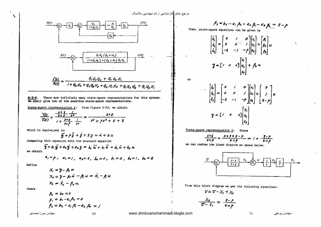
B-3-4. There are infinitely many state-space representations for this system. we shall give two of the possible state-space representations.

State-space representation l• From Figure 3-53, we obtain s1' r I

...lt!l._ s-. e .s" _ s+-$

U'p-) :: I+ L!:.L _/_ - sJ t- fS 2 + S + ! S+f s~

Which is equivalent to

,-... ,~ ..-ft-iv =«+"' ~ing this equation with the standard equation

f+ Q, J + 4a 1j T 'fa; ;s b, ;;_· + P1 ii + A U T b., "' we obtain

Define

where

4,=,, t~tz=/, ~3=l1 k=o, b1 =oJ Pz=l, kr=i!

x, ='il-l·" x.=~-1-"- -fl;"=:i,-~u x8 - ;:(~ - fa "

'~=b,=o p1 = J,,-111/o =()

I• = 1>,- "' /1 -a:, ,e. =I

. . !~

I F

Then, j1,=J,,-q,~z-q.,,-.,,,.~ i!-1'

state-space equations can be given by

n r. , . 0 1~'1 r~ 1

~~ = ~ : ·. _' Xz + ~l u

:t, l/f·~·

,.[!. •][:]~,.~ O<

r;J=r; ; ~JrJ+r ; J~ x, -1 -1 _, .(, ,_,

y=[' • •][~] State-space r-epresentation 2 = since

!.:t_L.., s+t+E.-f' =!+_1=..£.. S+f S+f S+f

we can redraw the bloclc diagram as sho\m below.

~t .!.:LI x, ~--

From this block disgram we get the following equations:

v= u-x, ;- x, x, -~

v- x, -~-I'

"+/'

x,

...;~I_)_J:!"'-""'~ w www.shmirzamohammadl.blogfa.com 11 ~-.,.:r~

. .

' x, I -u-x~+x3 •

lSi_- _j__ x~ - 6

fr0111 lihich we obtain

x, _,. /'"• =(l-t)•-(i!-f)X1 X,~,""' -X1+X.s +l(

:i, = :tz Rewriting, we have

0'

. .:tj = X a.

.i,~, = - Xt 1" x. +- "f:

:i, =- (•-r)x, -;r, +(•-!')«

1 = x,

[:i:,1 [ P I ']t"'] [ o J .fl. = -1 0 I X'a. + I LL

.:i, t-• d _, "' l-f'

~=[I d •l[~]

-""'15:... ...r4-- .:.:, ) .,rl..:..:<_.J.S -~ &'-->" Th•n

"'

i ~-"

i, + 3:(:s + ZXz. = ~ . X,a. =X, . ;rl = ;K,_

[x,] [ • 1 o]["'] ['] " ~,.=(!() l:t..z+4ll

X. I -2. -3 :t, I

1=[1 d •1[~]

d=[-: -I]• B=[']· C!=[l -1 .... I '"'

The transfer function G(s) of the system is given by

I [S+i' ({(s)=~(·!-dre,=[l o] -3

=[I •] I [S+I (n·'J.)(S+t)+.3 3

= I [I

\

o)

1] -1 ['] S+/ I

s::][;] -------------------------------------------------------------------------- I

I sz+S"s+7 •J[.:7]

~-1"+3ff+2j=«

.. - S~+S's+7

Define

x, ='I !!±!:·

• Xz=' .. .... =;

(a} The system equation is

n~;(,. = -J,,(i# -i,.) - 6.z x • 13

...;~I_)_J:!"'-""'~ 12 www.shmirzamohammadi.blogfa.com ~-.,'-""'~

' O<

mX., + b,i, + b~~. i~ ~ b, X~-

-""'15:... ...r4-- .:.:, ) ._rl...:..:<_)1-~ &'-->"

!!±:!· (•) 111;; -rKx =~

!~once

[ms'+(b,+b,)s] x.rsJ = ;,sx..rs; The transfer function Xo(s)/Xi(s) is

,, -;<-

X,(s) -X;(r} -

b,s IllS a.+ ( b1 +ba.)S

= __ ::.bL' -­'ltfs+(b,+i.z.)

:1:· .•. (b) Define the displacesnent of the lower end of spring k1 as Y• -~--e>-uystem equations are ~'f:.-;->-" • .if.t:,~ - A,:r-. - Hi. - ~) = o

':;-·: ~ ~<, r:x, -~) = b(')-x.) . ' --~£cor '--'0.-~:

""' .!~- It, Zo + b i:, = b :j ~-~

k, :ti + b i ... = k, ~ + b ~ !~once

( "• + >s) X,fsJ = :., Y(s)

~~ X;(s) + bsX,{s) = (k, +h) 'f(r)

Then the

Elimdnating Y{s) from these equations, we obtain the transfer function as !ollo~s=

(c)

o<

Hen~

x.(s) _ k,b. bs

Xds) - /r, ;t.z + (J1-rlcz.)bS - "· + ( 1,. z; ) ~s The system equation is

ftiltJ(o = h(i',. -X.,.)+~,cx .. -x,)

.t. X., -t J,:i;, + k I X"' = !. _:f,- + ~~ ;t 1

( *• +bs r k,) X, P,) = (bs + 1<,) X;(r)

The transfer function Xc,(s)/Xi(s) becomes

&1£ = X;~J

bs+'lt1 fr, lc,+Jt;,. +bS = lf,+frz.

14

It- i;s b s

I+ lr,+-lr2.

XtiJ =-' (T(s) "!•'+~

(b) Define the displacement of a point between springs k1 and k2 as y. 'lben the equations of motion for this system beccme

.,;;_ +~. (x-:;.) = u J, ~ = ~. (x-?)

Frorn the second equation, we have

or

Then

or

!!±2·

Define

Then

..

~.~+~•t =*·"' ~. X

~}= k,-+*•

"'"' + ~l~z. :( = lA..

~~1-~a.

I ..K& = ft.ir "UP') ?11Sz+ ff

1 +If&

"'' j, ·H, (-j,-V,) +It, ;t, = "-t

m,;; +>, (j,- ~1 )+~•:tz =tt,

x, ... #;

:r .. =;, , '!', = 1z . :r,= Y:a.

m,:(& +b1 (~.z.-Xt-)T~,X1 ==-tt1

7flz. i.,. + b1 (~"- Zz)+ I,_ X 3 = v.r.

1 =, ~-J:l~~

" -""'15:... ...r4-- .:.:, ) .,rl..:4_~ -~ &'-->"

Hen~

or

.!!±!!!·

where

:i, = X'a

;:(~ :=- "k[ /!If~,- r,.) +~, x,] -t- ,!;;I(, ~ =~;.

"'•=- i"[b,(x, -X,)+k, x, J +-;!;; "z

i, 0 I~ tJ;<, 00

;/ •. ., "' .L J --"'- -- o - • D ~ a. 11t1 1'111 m1 ""2. nt, 1

:t, tJ p o I x, o tJ [~. • - + • "' ~& J, ..J_ X 0 - -- -- :t. 0 ,. lila. llfa. :m2 ,. m,

·x,

[~']= [' 0 0 •] "· 'Vz. 0 () I g XJ

"• .,. ... ~ T

T = -2k84'-m;L~e

J ~ m.L' For Bmall S,

mi•e' =- 2k4'8 _,,,, or

i + ( 2~·· + _1:_) b = 0 m,tt. .)

B-3-U. Note that

"f = "'+ .t,..:.. 1!9 ' J'q =! <="

For x direction=

Hi+m;~ =t.t.

•• JZ. • NX+"'·Jt• (x-r/.--1!9) =~< ..

Si~

.,";;A4e =- (...:..t>)P '+ (CR/!9) 8'

-ha~

•• • z -(M+>t) x - 111./(....:...e) II -t-11f..l ( cn.II)P = u.

For small 6 and small 62, we have

(M+.,)X +,.,;,; ="'-

For rotational motion•

-re

Thus,

;r;· = ,,, .... , _,;; .t t:.n.{?

3"= I+ mL 1 ~ ,,

I= m-;r

( I+mi' );· = 711fl..,;. d - .,'; ../""' P For small e, we have

( r-r, i') ; = "'I .t e - ., .t x Fran Equ<~.tion (2),

.. X = j6 _ I+711.f' .. lll.t &

Substituting this last equation into Equation ( 1), we obtain

( )( r-.. .. 1• '') .. M-rnt ~~- •' I +mit!=« or

(M+"') •P- (M+1»)Irt<-(M./' "_ • "'.t t9 - ""

Th~.

.. ?fl.! ( "fi-m)f "'-' e= e- u (Mr,)Irl-ftn.l' (Nr.,)I +-M111i'

Also, fcom Equation (1) we have

...;~I_)_J:!"'-""'~ " www.shmirzamohammadi.blogfa.com ~-.,'-""'~

(:

(2)

(3)

" -""'15:... ...r4-- .:.:, ) .,rl..:..:<_)~ &'-->"

111f/ ~ - m./;C: I+m,['

(,<t-r .. )x .,.,_t =«.

0'

[MI+ 1ff(I+,<tl'}]% -r m'i'J~ = «{ I-t-"'L')

fran which we get

11fz.(zl -I+~t~l._ · · er ~

MI + 111 {I+III') MI r "'{ I+t11l')

.. ::< =-

Equations (3) and (4) describe the system dynamics in ter:ms of differential equations.

"'

Hence

By taking the Laplace transform of Equation (3), we obtain

[s'- ?od ( 1'1 .. •);. J 8{s) = - m.l VI>

(H+M)I+,H>d• (MM)I+Mm.t'· )

f [MI.,., {z.,.MiiJ] s•- m./( M+m),1} @(.,! = -m./7ll<)

(9{$) -- "'' V(s) - [MI+"'(I+Mi')] s'-m.l(M.,..,)J

By taking the Laplace transform of Equation ( 4), we get

(4)

(5)

s'X(>) =- ""''-'•.!_,' 1'---o-o- I+Jn./z. - 6)6) 7" 7J{'s) /of,_,.., (I+H.l') MI-t-m( I+,<f.l•)

Heoce

0'

£Ml TT(sJ

:£1!2_ VrsJ

=-, • ./', 1!1~

MI+"' (z.tMl') Z>Tr)

+ I+m.l' MI +"'(I+M-1')

..r.l ';- ---'"'"''"-~~c:---,-.,-= [-'II +"'(I+,./')]51 [MTT"' (z.,..,b)] ,..__.,I(H+*')J

+ IT-wt.l 2

[MI _,..,(r+M.L')] s' · {6}

Equations (5) and (6} define the inverted pendulum control system in terms of transfer functions •

...;~I_)_J:!"'--'"~ "

Next, we shall obtain a state-space representation of the system. state variables by

Defin

and output variables by

;(,;" . X. =8

x, = ;(: . .:(~ =x

Vr =I =x, 12 =% =X3

\

Then, fran the definition of state variables and Equations (3) and {4), the state equation and output equation can be written as

>il I 0

:r, I .. 1(,11+ .. )1=

= I'II +" (I+/ofl') • ~. 0 . ,'Z.JZ.l. x, - MI+r~~(I+M.t')

. -[~] =[;

0 0 of 0 I () x:

"• ~- Impedance Z1 is

Impedance Z2 is

I z, =R,+c~~

I

0

I)

/)

_I_ Zz. = Kz.. + C":a.s

Hence

I) p

{) p

0 I

ll (J

19

"' 0 .. ( "• -

T m .,..,(IrHL') 1 u.

:r, 0 ., I+m.l' -'II+'»t(It-1119

---·~

I '· f';·~· ~~-~i~ .. f-, •. •. I -. ._.

1.~· T­'

~-J:lt.r~

' ~15:... ...r4-- .:.:, ) ._rt::.;:_J: -~ &'-->" Since

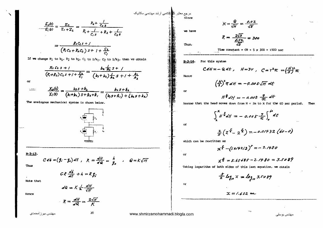
£~(1) Zz I .,,+ --

-------e,·(r) = z, -t-Z.z. = ells

11, +_I_+ K:z. + _L_ C,s c~s

~:zG.s +I

= (H,czr~t:z)s+ I+~~ I

I! we change R1 to 1>]_, R2 to Q2, C1 to 1/kl, Cz to l/k2• then we obtain

R1CzS+/ ;,-f.s+ 1 (ll,+Rz)Cz.S T!+~ (b,H,)i;_s +!+-¥ • ~.

= X9(s) =- bzs +frz. , _ b.~. s 1-~z. )(t(s) (b,+b,) s+ fr,+ft, - (b,s+ft,) + (hs+k,)

'nle analogous mechanical system is Shown below.

·.~ ... -._,_. ·~

·~· ' ' ' '·

~

------------------------------------------------------------------------!!:1::Y·

Th~

Note that

"""""

41/ " (!<(r,-(; .. -;.).tt' "'= <iQ = ;.

c~"' +/,=11.•. «f ,.

de = K -f <If! V7i

<If/ -!( = d'l --

z,fiT /(

' fii=KIH

/<=: = tJ,() 2

.ff ~haw

!(= 2ff ,,,z.. .. = 3"D Thus, 7r

Time constant "' CR = 5 x 300 :: 1500 sec

-----------· ------~· For this system

C!tiH=- Q,{i" .I H-3Y ,I C= r 2 '1C" =(1.Y1C He~

(.f)' 1(' .t H = -(UP s,flT .tf:

= Iff .!If = - ~. ~~s ck- .cr

Assll!OO that the head n'IOVeS down from H "" 2m to x for the 60 sec period. Then

S" • I'' H'.llf=-o.~••.:L lit . "' . o<

; (zi'_ 2 f) =-•·Ni'-32 (6~-o)

'olhich can be rewritten as

.£ )r ;<• -(f.</f-2/3 =- 2./f-30

O<

;;(f = 5: l$"08$"- z. /fl' ~~ = ;1 • .!"8 8?

Taking logarithm of both sides of this last equation, we obtain

0<

~ 1~ X -:z -,,, ~ .u. iJ..f-"' 11"'/ ~"

:X: = /.b sz .,._ --------------------------------------------------------------------------------

"" ...;~I_)_J:!"'-""'~ 20 www.shmirzamohammadi.blogfa.com ~-.,'-""'~

' B-3-15. From Figure 3-62 we obtain the following equations: ~15:... ...r4-- .:.:, ) .,rl...:..:<_)ts: &'-->"

liJ(sJ -!laCs) :::::.' Q1

(T)

II',

llz(S) ,.. Q, (.r) K,

Q.-(i) -Q,{s) = ~($) c,,..

~,(.r) - O:afs) + Qo~tsJ .

C =Hz4> .s For eadh of the above equations, a bloc~ diagram can be drawn, as shown next.

~ J --"-f-{,(•)

~ f c,s

Qp)

~- - f/1 o,prl ------u;_r-

Q.t(•)

~(~. H,($) -f)~(s)

Combining these elements of block diagrams, we obtain a block diagram for the system as shown below.

Simplifying this block diagram successively, block diagram as follows:

22

QJ<')

Q,(s) r-

we obtain a reasonably simplified

' --~ I ~ i i i

I

Q.t(r)

Q,•(J') Q,{>)

~

QJ(•)

0,-{s) A>. I ' I h I --'- I Q,(s)

R0 C1><tl

~

1,<",1 ~

1 lf,(,s+l I Q,l(.-)

Qi(s} ~--~}{,(:,, • ,,

( R,c, s rt)( R,c, s~ f)

-Jt, (, s

Q"(l) ......__.

~ fH'-R, •'·· r:J;(J) • • (R,c,• t!)(tr,c,st-f)t-/,"or,~

From this last block diagram we obtain H2(s) as a function of Of{lS) and:.: t as follows:

~. [ -H,(s) = Q;~)+(lt,0s+;;;,·c (~1 C1 s +t)(K~C'~S+-1 )+Ra C'1 s '.

-----------------------------------------------------------------------------I 1 1-3-16. Define I .

'- ....,~1_)_):!" '-""'~ 4 2Z- ---------·

23 ~-.,·'-""'~

I www.shmirzamohammiidi.blogfa.com --

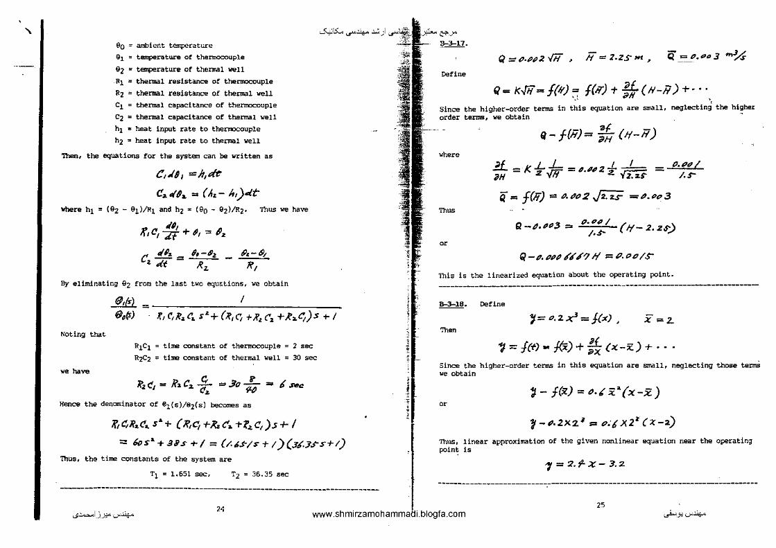
' eo : ambient temperature

St = temperature of thermocouple

9z = temperature of thermal well Rt = thermal resistance of theOJPCOUple

Rz = thermal resistance of thermal well C1 = thermal capacitance of thermocouple

Cz = thermal c::apacitance of thermal well

h1 ., heat input rate to thermocouple

hz = heat input rate to thermal well

Then, the equations for the system can be vritten as

e,.tp, =It,<#

1!, o'P, = (A,- lt)«t-Wbere ht = (9z - 6tl1Rt and hz = (eo - 9z)/Rz. Thus we have

'"' ' ~~ C1 -z.r + It -:::= Vz

C. til.,. = 1, -.92 .z. dt l?z.

tl'.r- .9;

71,

By eliminating 9z from the last two equ~tions, we obtain

1!1,{<) = I

-""'15:... ...r4-- .:.:,)

8oM 'Kt C',R.a.l' .. sz.+ (l?,c; +ifz C"z +A"2.li)s +I

Noting that

w ha~

R1C1 = time constant of thermocouple = 2 sec

RzCz = time constant of thermal well = 30 sec

c;, .. A'2 t!1 = Ra C.z. C!z. = 3o -;ii" = 6....,

Hence the denominator of e1(s)/8z(s) becomes as

,f1 ~R ... <" .. s~~.+ (.t'/+Xze'a. +l.z.C,)s+-1

= 6os'+ 39s + 1 = (/.•sis + 1 )(3'6-:u-s+l) Thus, the time constants of the system are

T1 = 1.651 sec, T2 = 36.35 sec

------------------------------------------------------------------------------

...;~l_)_..l:!"'-"'~ 24

'

&'-->" S-3-17.

Define

Q ::::p.pp2 .fiT ~ i1 = z.zsm ~ Q ~___!'· t;ll) 3 '"~

11= k.fiT= f{lf) = f(lf) + &(H-ii) +·--•.\ PH •

Since the higher-order terms in this equation are small, neglecting' the higher order terms, we obtain

where

Th~

O<

Q- f(i1)= ;~ (lf-Ti)

lL-KL.L iJH- 2 VH

I _L_ -= #.112 z Yz.z.s-

Q = f(lf) = P.<!P2 J>.z,r =<1-•o3

O.Pa/ /.$"

Q -4.#tJ3 = (J.PP/

/-$- (lf-2-zs-)

Q-(!l.t?Pti~#JI'J# =P.OP/$"

This is the linearized equation about the operating point.

------------------------------------------------------------------------------B-3-18. Define

'J=•.:zx'=j(<), X ;:::. 2.. Then

"J = /(+)- f(x) + ~ (x->:) +--

Since the higher-order terms in this equation are small, neglecting those termS we obtain

'J- f(x) =•-•x.'(x-x) "

f-o-2xz' = '"' x2' (:<->) Thus, linear approximation of the given nonlinear equation near the operating point is

"/ = 2.f'-x- 3.:z

25 ~-.,'--""'~

"\ ~15:... ...r4-- .:.:, ) ._rl...:..:<_)~~ &'-->"

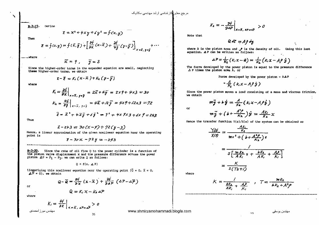
B-3-19. Define ~

Then

--where

Y =><'+~x~+lt!' =f<'><,tJ)

l!=f!z.y)=f<"'5)+[:; (><-'<)+ ~ {1-,P] __ +··· " :;!( •:;!(, t~;

X= 'I, :t=3 Since the higher-order terms in the expanded equation are small, neglecting these higher-order terms, we obtain

z- f = K, (x-X. )+ Kd tJ- iJ where

K,=££1 = 2x+1-f = 2Xf+ f'XJ =.30 ;x :K=f, 1"'"1

k, = ~~ _ _ = f'i< +llj = f-x1+12x3 =7z a1 x'"'~- :t=?

~=X'+ r,<.Zj +ifjz. ._ 'j"- +¥-X !X3 +.&'X f=2fl.J Thu•

Z-Z5<.3 = 3o(X-?)+ 12(?-3) Hence, a linear approximation of the given nonlinear equation near the operating point is

i!-3c~ -721 =-2{'3

-------------------------------------------------------------------------------B-3-20. Since the rate of oi-l flow 0 to the power cylinder is a f~mction of the piston valve displacement x and the pressure difference across the power piston dP = P1 - P2• we can write Q as follows:

0 "' f(x, A P)

Linearizing this nonlinear equation near the operating point (Q = 0, X = 0, A.P = 0), we obtain

-- Bf · o< Q- Q =- (x-x) +-"'-.,x #AP ( Ll P-4f)

" Q = K, :<.-- k, .<>7' whm

K,=

~

-~ i I I

~;I > 0 Kt = - ~ X=J, "'~··P

Note that

Q.lr ~AJ~ .. where A is the piston area and ~ is the density of oil. equation, A P can be written as follows!

Using this last

AP= i(K,>:-Q) = -k; (K,%-- Aj ~) The force developed by the power piston is equal to the pressure difference .6 P times the piston area A, or

Force developed by the power piston = A~P

·1, (K,x-llj;)

Since the power piston moves a load consisting of a mass and viscous friction, we obtain

.,:; +~>i = :. c k,x-A.Jn

•• ( A'.P) • At, 71f !J + J, + ----;;:;:- !f. = --,r;- X

or

Hence the transfer function Y(s)/X(s) of the system can be obtained as

_A.&.

.:l1!L = "' XIS) ows'+( b+.tl!L)•

k,

I --S [ ...1!!..&. • + bK, + _dL.1

AK1 IlK, l<t

K = S(Ts+l)

where

1<.= I ,I:, 6KI ;- AL ) T= hkz+A:,O Ak1 j<1

::. 1 :<:=-£/ 4.,=.,;; > () www.shmirzamohammadi.blogfa.com ...;~I_)_J:!"'-""'~ ._..i...> _ _,...;.~

" 26

'\ -""'15:... ...r4-- .:.:, ) ...rl¥1S -~ &'-->"

CHAPTER 4

!!::±:!.· Time constant = 0.25 min. The steady-state error is 2.5 degrees.

!!....!...!• Define the current in the armature circuit to-be ia,. Then, we have

~· II L ;1 _,. u, + t<, -"jf- = e, ~

(Ls..li.)T.,is} "!' K,s@.(s)= £.-{S)

Also, we have

J .. JJ: TT= T..=l(i.._ 0

T- Tli. =~7<. ~

<{if =T,_ Equation (2) can be rewritten as

l ~ ' (~+nh)~=·~. or

(J~ +n ':J;.) s' lfPM= "K I. {;c)

By substituting Equation (3} into Equation (1). we obtain

or

Henee

(Ls+JI) (;T.+n'J•)s• fiP(s) -t-/C,s ~(<) =liilr) nl<

[(Ls +I? )(J.'t»' J"L)s'+l<kb s ]61(<) = i1 K t:,.rr)

~- ?tk -·· E;(s) s [( L.r+J/)(J;. -r >1 'J,) s +- K K,J

(1)

(2)

(3)

-------------------------------------------------------------------------------B--4-3. For the system shown in Figure 4-54(b), we have

(!(s} /o

l{{s) = sa+ ( 17/~/(4 )s +10

' 'I& . J • ·] ' • ' ' ' '1 1 • ~ • :1 ~ ~ i

i

Noting that 2 'Silln ,. l + lOKh• 4Jn2 "' 10, !; = 0.5, we obtain

I+/!? K, - 2 x•.s- X ,f/4 = -lib H~~

v .Jii-/ / "" :."·: f() = t!.21o

The unit-step response curves of both systema are shown belOio'.

--.. '·'

I --· ·- --~ r-·- -••• --, ... -" -- -

' I 1\

7 v -• I u

" -+-- -- -- - ---- -· -· -· ul u -- ·-·

•• ' ' • • • • ' • • ' ~·

Note that for the original system

E',($) k(s)-C1{s) .s1.rs -= =

K(S) l(.(s) .rl+s +!()

For the tactlometer-feedbaclt" system

..bl1_ = ~(.\) -C',(_, = s'+3./#s J(.{S) !((s) ~" +-~.;•s +IO

For the unit-ramp input, ve have

( Sz+S

E, (r) = ,r1.+ S+ld .L).L = s s SI:+S f

&I+S'+/4S T

£ ~ (_ s'+~./6s !J 1 s'-rl./ls ..L s'S) =\s'+3.//S-t/O"'ijS= s3+:J-1{&af'/~S .r

The error versus time curves [el(t) versus t and e2(t) versus tJ are shown on next page.

" ...;~I_)_J:!"'-""'~ 28 www.shmirzamohammadi.blogfa.com ._..i...>_J:l'-""'~

' -""'15:... ...r4-- .:.:, ) .,ri...:..:<_J? -~ &'-->"

T---,---,---'''"""'"'"~,-, ... ,,., .... ,,.'--,c---,--, •• .. i"'

.. 05 v 0 ••••• , •• ,.

:f!:• ·----------------------·---------------------------------------------------------!!±f·

!::!:2·

c(t) =I- _j,_ e-t +-'-- e-~· 3 '

(t-;.o)

--------------------------------------------------------Rise time = 2.42 sec

Peak time = 3.63 sec

Maxirmw overshoot = 0.163

settling time = 8 sec (2 % criterion)

!!:::!::§.• 'I11e maximum overshoot of 5% corresponc:!s to ~ = 0.69. Hence

ti..Z·

41n = ~ = ~ - 2. fp .f.<w"'ftec s 11'.6'f

<!{>-) _ k(Ts+l) 111<)- Jr-t-KTs+l<

Since T = 3, KIJ = 2/9, we have

C(s) - f (JS+I)

R($}- s'+{-f-)3S +; Hence, 2 S41n = 6/9 and Wn2 = 2/9. Thus

'S = "'· 7"' 1

-------------------------------------------------------------------------------·

. -;.:

J. ·2.'

>\

8-4-8. When the mass m is set into motion by a unit-impulse force, the system equation becomes -

?II!< +Ax= 4rt-J Define another impulse force to stop the 1110tion as A b (t - T), where A is the undetermined magnitude o! the impulse force and t = T is the undetermined ins­tant that this illq)Ulse is to be given to the system. Then, the equation foe the system when the two impulse foices are given is \

?~tx+~x=t(tJ+At(t-_-T), :x(•-)=o,xl!'-)=c i ~- The Laplace transfoClll of this last equation gives

%i

j ~

~

• .1 i i l

I

("'s'+J) ,IQ's) = 1 + 11 .,-•T Solving for X(s),

I + X(.$) = m.s'+'A.

A e-sT

nu'+l

I ={h

Jf; s• " +-

""

__;!__ + -./t, ..

.[{- e-.sr

S:LT-.[, The inverse Laplace transform of X(s) is

:x(t)- J;;, .<4.{f; -t+ ~:,., [,..;...f,f (t-7/).i(t-T)

If the motion of the mass m is to be stopped at t : T, then x(t) must be iden­tically zero fort ~T.

Notice that x(t) can be made identically zero foe t ~ T if we choose

A= I 1

1r ,,..

T= VI ' 'IE ' .f';r -, ... {-fc

Thus, the motion of the mass m can be stopped by another illq:lulse force, such as

J"{+- [f) ' 3>r ) t{i- "$ '

!!::::1::2.· For a unit-impulse input

c(t) ~- 'fe-t + .Z e -<-

For a unit-step input

Sir) .. ;(t-7/i ,.

(t ;;.o)

C(t)- 1+- te-+- e -• (r ;;>o)

...;~I_)_J:!"'-""'~ 30 www.shmirzamohammatli.blogfa.com 31 ._..i...> _ _,~~

'\ -""'15:... ...r4-- .:.:, ) .,rt..:..:i _ _l, -~ &'-->"

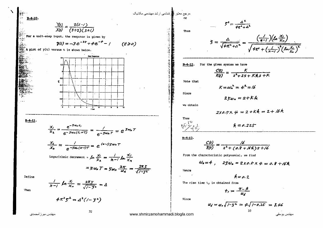
YM - 2(S-1)

XI<) - (sn)(s+l) the response is given by

t(t) = -3e-•~ +~e-•- I versus t is shown below.

--(tii1'c)

:(\ I I +++-l of-- -+--1 ' ;

• uf--,JFL_J__} -t I ,,.m·l1 ill• ~+-·-· : "! ' i ' '

•~ ; ~:!I . ~-+,++-'" --~---:- :---+-r-i--! ~~ 1

• ' , I •

····l•<5f11110

•. .,

·------------------------------------------------------------------------~-

Define

Then

;:( e-.1'"""'"1 z: = -e--"=sc~~.-(c,c,c~~T~:) = I e-$W.. r

= e>.-..,r

~= x.

I e -;T~Vt. (j~-I)T = e (•-/)>~V~t T

Logarithmic decrement = }#t ..::!!. x.

= ___ / ' "' ?t-1 .£f'.­x,

I -,_X, JJ-1 }A'I­x.

'""' ;:: 54J11 T- >,Pn l#.t.

.2.T£ - /t-7• =.d

4-n::'s' = A'(t- s•)

32

2t5-- -./1-p

-'·

-~

·f ' -· ' ·~ -, l -1

O<

Sl.= Az. Hr+~z.

Th~

A , (- -~~ )(Ln ::) -s - ' = -.J~7C·+L1~ = I (-'--)'(t....&)~

1-'IC' +- n -1 x.

------------------------------------------------------ ------u.J1. For the given system we have

C!(;) - K ~il) - s'-r2s -t- K~s -t-1<

i• Note that

-~

.1 ~ :!

K =W,.,_ :=. 4-&.=16 Si~

z:; .... = 2-t-K.-t. we obtain

2XP.'lX ~ = 2 +KI._ = 2+ /.51<

"'"" lo 1}7 "( ,cl f< = •· 2 z.s-________ ;c ________________________________________________________________ _

~-C($) __ 1.5 1!,(s) - s•-t- (t?.li' +lhl.)s +16

From the characteristic polynomial, we find

4JII=+ I 2!;01. = 2Xd.5:'-X 4- = <>.i-t-16/l

Hen~

IE=P. 2. The rise time tr is obtained from

Since

tr = 7r-~ lliJ

"'' = lli./1-S' = 4-/t-•.zs = 33

/.#

...;~I_)_J:!"'-""'~ www.shmirzamohammadi.blogfa.com ._..i...>.J:l'-""'~

' -""'15:... ...r4-- .:.:, ) ._ri...:..:<_)S:P, &'-->"

-ha~

~=~-~~ =~-lt7.8'/. tv.

t,= '!1:- ·he ~-~·

= IJ, 6tJJ- S~c

The peak time tp is obtained as

= 'II" 3

.. = ...2L = 3./fL

' f.IJ~ J. "' The marlmurn overshoot Mp is

= P. '!P 7 .Sec

•• Hr=e-~ = e tl,.#" XI•IP. -f,l/,:. .;,_,,zs- =-e =1?.//.3

The settling time t 5 is

t. 4- f<. =' ~ = -~=-~:'-::)(-;;,_:- -= 2. .u.c..

-------------------------------------------------------------------------------.!!:±:!1.· MA.TLIUl programs to obtain unit-step response, unit-ranp response, and unit-il!lp\llse response of the given system are shown below, together with the resp::mse curves.

% •• ••• Unit-step response ••• ••

num = [0 0 10]; den = (1 2 101; t = 0:0.02:10; step{num,den.t) grid title('Unit-Step Response') xlabell't Sec'/ ylabell'clt)'J

% • •• •• Unit-ramp response • ••••

numr = {0 0 0 10); denr = (1 2 10 OJ; c = step(numr,denr,t/; p/otlt,c, •.· ,t,t, '--'1 grid title(' Unit-Ramp Response') xlabel('t Sec') ylabeH'c(t/'1

% •• • •• Unit-impulse response • • •••

impulse(num,den, I) grid tit!e('Unit-Jmpulse Response') xlabel!'t Sec') ylabel('c(tl')

~'"

i " ·f

' j . ~ i • ;_t

' '

I ...;~1_)_):!-"'--"'~

34 www.shmirzamohammadi.tblogfa.com

•

. -.--r-._c-~ .. ;~~~---~~~-, "r I I "'1--itlc+---1-T--!-----r-.....,.... -~-- ~~-·---

'

.. , ·· 1. : 1' ·

1

• 1 -~ ·-1 r

1 D3 I : : i I ! I - I I I

"••tl41111110 ·---" "" • 0' • / ' / • • ,/

I /; • •

'A"i ' i ' i i

' ' I J i ' I ' 1/ I 'A I I I .. ' ' • • • • ' • • " ·---"

' ' ' '

I '

•

! I • I I i

' ' I ' ' I ' I ! I ..• ' ' ' 0 I ' ; ' • I '

i ' i I - ' ' -,---' v ' l I ' ' ·•, ' • ' • • • ' • • "

••

·~

35 ._..i... _ _,.:r~

" -""'15:... ...r4-- .:.:, ) ,_rd.l.:<_f: -~ &'-->"

w "'~

tJ= ~-I~ =A -I P,~J'I rv.

t,= 1<-·hc 1.~.

= IJ. ~(J,J- S«~

The peak time tp is obtained as

=1

t, ?r- 3./ft. = -;;;:; = J, f'l = IJ~ t;IJ 7 .sec

; The wax!= overshoot Mp is

•• Mr = e-7r-f' e ,,$" Xl•/1' -/.l/f:. .;,_,,zs- =- e =ll./#.3

The settling time t 5 is

t, ..L= = J'tP, ~

= 2. ....,c.. ,.sxP.

--------------------------------------------------------------------------------!!:::±:!!· MATIJI.B programs to obtain unit-step response, unit-ramp response, and unit-impulse response of the given system are shown J::elov, together with the response curves.

._;~I_)_J:!"'--"'~

% • • • • • Unit-step nlSJlOnse • • • • •

num = [0 0 TO]; den= (1 2 10/; t = 0:0.02:10; steplnum,den.t) grid title['Unit-Step Response') xlabeU't Sec') ylebelf'cltl'l

% • • • • • Unit-ramp response • • • • •

numr .. [0 0 0 10]; denr "" {1 2 10 OJ; c = step[numr,denr,t); plotlt,c, '.',t,t, '··'/ grid title!' Unit-Ramp Response') xlabel{'t Sec') ylabe)('c(t)'J

% •• •• • Unit·impulse response • • •••

impulse(num,den,t) grid title('Unit-lmpulse Response') xlabel('t Sec') ylabelf'clti'J

34

-"' -----.--..

•

A\ I I i I I . . . ., --- ---L .. ...:. ___ ]_

' I \I ' i I : ~-~~ ' I ; '

•• _ _;____!_:,J.__l_j_ j_ . I : I ! I i ,

" --t ' ! --r·---+- -----, ! I . . . R=FR= " -· -.--1-,--I .

" lc--· ' I I : : :

·,

•• • • • • • • • • • • ·-- -.,.. __

" """ •

• /I / •

""' • • •• /

I ,/ • .--· . / i ! i • ' I

• ,/ I I /

'0 I I .. ' • • • • • • • • " ·-u --

.1 I i i . !

u •

I I , I • I I I I ••

f"'l : I ' ' . I HI 'II I ·: v ! II I i '

o•J~ ••,•••o ·-35

._..i.,._J:l'--"'~

' -""'15:... ...r4-- .:.:, ) .,rl..:..:<_)~~ &'-->"

8 4 JS. is goiven

A MATIAB program to obtain a unit-step response of belov, together with the unit-step response curve.

= -0 ~

,

!o " " • 0

.Q.O&i

% • • •• • Unit-Step Response • • • • •

A = [-1 -0.5;1 OJ: B • [0.5;0); c .. ,, 0[; D =[OJ; [y,x,t] - step(A,B,C,DI; plotlt,y) grld tltle['Unit-Step Response') :K111beU't Sec') ylabeU'Output'l

--ri I I 1\ I ;

' \ l I I

' \• i I : +-\ ' \ '

I I

'-.: !

I ' ' • • • ·-

I ' ' I I ' '

!

•

I i i

' '

" " • "

the given system

A MATLAB program to obtain a unit-ramp response of the given system is presented below, together with the unit-ramp response curve.

"' • • • • • Unit-ramp response • • • ••

A • 1·1 -0.5;1 01; B • [0.5;0); C .. [1 OJ; D • [0);

'II. • • • • • Enter matrices AA. 88, CC, and DO oltha new enlarged state % equation and output equation • • • • •

AA "' lA leros(2, TJ;C 0); BB • (B;OJ; cc "'(0 0 11; DO"' IOJ;

% •' • •' £mer step-response command l•,x.t) "' stepiAA,BB,CC.DDJ • ••• •

lz.x,t) "' st<!piAA,BB,CC,ODJ; x3 ~ 10 0 TJ'x'; plo!l!.xl.t.t,'--'1 llfid titlei'Uni!-Ramp Response') xlaball't Sec')

\

-· -~ ' ~-\!!_

t•

" ' ' ~ '" •. ,_ " ! ~

~

'I

--~--•

!:c----. -j-=+--~ 17 ' I lc" I

"-~-, " '

·1----c I -0/ 1- -0 . . .. • • •

l

f I

!

•.

·~

Finally, a MATLAB program to obtain a unit-impulse response of the system is given next, together with the unit-impulse response curve.

% • • • • • Unit-Impulse response • • • ••

A= [-1 -0.5;1 0}; B "" [0.5;01: c .. 11 0); 0 = 101; lmpulse(A,B,C,D)

-r---,---,---,--="";:"'"===·r'""""==:;=-.,---.---.---,

i +___;,,

I I

I -·1 ' - T

• • • ' • • '" ·~

-------------------------------------------------------------------------------.!!:±!&· The The resulting

required, modified version of MA'I'I..AB Program 4-14 is given below • impulse-response curves are also given.

ylabeii'Output and Unit-Ramp tnpu!'l

1.

text\11,3, 'Output') ..s~I_)J:!" ·· irzamohammad .blogfa.com " ~-J:l''-""'~

2111 It J\

~r---,---,-:,--,----,-,o

I ..

' "L

I -1 .. -..

: I

---•--'-----:--

5 :!l*'ttM'tz11U

H'P'I'! 19'fM

1M

f'f'NM

S' 'P"bi'M

't'tr'

• • E ;: 0

" m

~ ,

•· • 1 ' ~ i. -'li .•

~d

:: : . . " .. ""

,Q

g::. •• "' !.

.

" Q

• Q " ! " ~ 0 ~ '. ~i "o

!] ' •

Q

-.;:;--

I I

I 0

~'21:~

{l~{l.g

' ... ......... .., u

u "

"

' 1 ' ]

'

' "-::'. -~-­·!4~

-""'15:... ...r4-- .:.:,)

CHAPTER 5

~- consider the system shown below.

'"' ) C(•)

:.x~ <fM 1 ,

Fran the diagram we obtain

C'{s) - q{>) P(s) - t+-q(s)f$c;{J)

For a ramp clisturbance d(t) = at, we have D(s} "'a/s2. Hence,

c{ ,o)

c(o) = fk s C(s) = £-•~•

sgM 4

/+- &}(J)t!fds) :s~ " = R.;... s (i,(s) ••• "' becomes zero if Gc(s) contains double integrators.

-------------------------------------------------------------------------------B-5-2. In the following diagrams, (a) denotes the unit-step response and {b) corresponds to the unit-ramp response.

··~~ "'' . I '" "' 1/ ( ... ) • • ,., ~

• • • ' • ' • • • ' *f:.t;~fL .J&l K; ::z.

£(S>=s•-:s

""" •/ w{f)

'r~J 'f /',., 'f 1. ,(•)

'•> •

• • ' • ' • ' • ' • ' 1./(t)"' t:,.{ ~r-..L) ='{Il-L) t:(>} r.• .n ~ = K1 ( n- T.is) = t(/t,.n)

E(•)

11.5: _ _y?... &'-->"

'1i ~~

;:;:

.:i --{

• ~ ~l

i c~ -~ 5 ~I! t: ~ ' '

-·

"" "

'" ~ lll,._r,t

: .. tl' ( l.f .,is 'f'T.s) • ft.( 1+ i7 H.Zs)

_________________________________ ;,... ________ _

J>-5-3. The elosed-loop transfer function is

= K J's1 -t-Bs +K

For a Unit-ramp input, R(s) = l/s2. n.~.

=

£~)

I<~)

R(s)-C{1-) JSt+8s

= !?~) = Js'..- 8s + K

£{r) =- Js ... +Bs JS ... -t-8.$ Tf::.

(

?" The steady-state error is

e.,= e{«) =h...s£(s) =-f-H•

. .

We see that we can reduce the steady-state error e55 by increasing the gain K or decreasing the viscous-friction coefficient B. Increasing the gain or

• 1 decreasing the viscous-friction coefficient, however, causes the damping ratio to decrease, with the result that the transient response of the system will beCCIIIE! more oscillatory. Doubling K decreases ess to half of its original value, while~ is decreased to 0.707 of its original value since~ is inversely proportional to the square root of K. on the other hand,decreasing B to half of its original value decreases both e55 and t to the halves of their original values, respectively. Therefore, it is advisable to increase the value of K rather than to decrease the value of B. After the transient response has died out and a steady state is reaehed, the outpUt velocity becomes the same as the input velocity. However, there iS a steady-state positional error between the unit-ramp response of the system for

rated to the right. <I" (/ ~- .. three different values of K ace illust- '"'! ~·-"

'"' y ,...L-..... ~

/)_ . ' ...;~I_)_J:!"'-""'~ 40

www.shmirzamohammadi.blogta:.corrr-----------------------------------------------~JEF~-----------·

' '

-""'15:... ...r4-- .:.:, ) .,ru.& _)

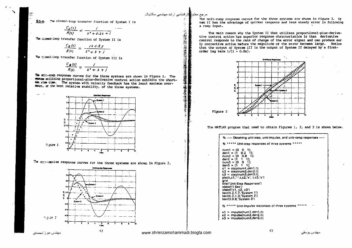
......... ~ closed-loop transfer function of System I is

Cz{J) I = R(.s} :.•+o.zs+f .,_ ~lcop transfer function of System II is

CJrM -= /tP,f.r

Kf.sJ s~+S+/

,0._..; ~"-loop transfer function of System III is

C._(s) :=

R(s)

I S 1 +St-/

~ m:i:.-ste;~ response curves for the three systems are shown in Figure 1. The ...,.._ Ei1iting proportional-plus-derivative control action exhibits the short­.-. r..a ti.JE. The system with velocity feedback has the least maximum over­aa;,:., rc ~best relative stability, of the three systems.

!:~ 1

--1.1 • I I r --·--~·-P=

....... ' 1 --:T ' ' -

'-' ._l_ •u~ l_.______;__-!'----o 1.21

~

' ·-

---

~ --------

• •

~.e :r.:::-:.lr;:dse response curves for the three systems are shown in Figure 2. --~·h-A-· ---------,-~------'-

-----····-·-

:; ol !~~~~u• .. •.oo

.0.2: .. , ~-.;-""? ' '

"'"o !~<fo>o••• ·-

~-

j. -;£: ~

" ~ i il

I .. .~ ·.!! 41 '! ~ • ,

4

f~ &'-->" The unit-ramp response curves for the three systems are shown in Figure 3. Sy· tern II has the advantage of quicker response and less steady error in following a ramp input.

The main reason why the System II that utilizes proportional-plus-deriva­tive control action has superior response chracteristics is that derivative control responds to the rate of change of the error signal and can produce ear· ly corrective action before the magnitude o! the error becares large. Notice that the output of System Ill is the output of system II delayed by' a first­order lag term 1/(1 + o.as).

--" ' • :&' ' • . . :.,& •• ' .. ' ~ .... • ' -~00 ' •

' < • ·-11 o"' !

10 o ,j --i------1--------r- 1 i ! < • •

' Figure 3 ..

' ' ' . o • I -+------+ iff"'" i i i

1/,'~ 0~ ~-"' Ll:J v&,·' I ' '•' •

• • • ·- ' : -

"

ThE! MA.TIAB program that used to obtain Figures 1, 2, and 3 is shown below.

%-----Obtaining unit-step, unit-impulse, and unit-ramp responses·····

% • • • •• Unit-step reSJIOnses of three systems • • • • •

numl - ro 0 1]: dent = 11 0.2 1]; num2 = ro 0.8 1 J: den2 = 11 1 11: num3 = [0 0 TJ; den3 ,. [1 1 1]; c1 = stepjnum1,den1,tl: c2 "" steplnum2,den2,t); c3 = steplnum3,den3,tl; pfotlt,cl, '.' ,t,c2, 'x', t,c3, 'o'J grid titlei'Unit-Step Responses') xlabeH't Sec') ytabelf'cl, c2, c3'1 textj4.2,1. 7, 'System 1 'I text(4.2,1.3,'System 2'1 textj3,0.9, 'System 3'1

% • • • • • Unit-impulse responses of three systems • • • • •

xl = impulsejnuml,denl,t) x2 '"' impulse(num2,den2.t] x3 = impulse[num3,den3,1)

...;~1_)_):!"'--"'~ 42

www.shmirzamohammadi.blogfa.com 43

._..i..._J:l'-"'~

'\ -""'15:... ...r4-- .:.:,) ~

plot(t,x1.'-',t,x2.'x', t,~J,'o') grid title('Unit·lmpulse Responses') JCiaDel!'t Sec') ylabel('xt, K2, xJ'J text(3,0.5,'System 1'1 te)(t(O.S,-0.1, 'System 2'1 textl4. 1,0. 1, 'System 3'1

% • • • • • Unit-ramp respor>ses of three systems • • • • •

numtr = (0 0 0 1]; denlr ~ [1 0.2 1 01; num2r = 10 o o.a 1]; den2r ~ [1 t 1 OJ; num3r = [0 0 0 1]; den3r = [1 1 1 0]; yt .. step(numtr,dentr,t) y2 = steplnum2r,den2r,t) y3,. steplnum3r,den3r,t) plotft,t.'··' ,t,yl, '-' ,t,y2, 'x', t,y3,'o'l grid title('Unit-Ramp Responses') xlabel!'t Sec') ylabel('yl, y2, y3') text(2.5,5.5,'System 1'1 text(6.2,4.5,'System 2') taxt(4.8,2.5,'System 3')

------------------------------------------------------------------~- The closed-loop transfer function of the system is

_&jJ_ - "" Rr.tJ - o.fs-1 + s l. 1- l'.r+- ~

MATLAB program to obtain the unit-step response curve is given below, together with the unit-step response curve.

% • • • • • Unit·step response • • • • •

num .. {0 0 0 401; den ~ [0.1 1 10 401; I- 0:0.01:2; x1 .. step!num,den,t); plot(t,xl,'-'1 grid title!'Unlt·Step Response'] xlebel('t Sec') vlabel/'x1'1

---c~----~"r='"'~~c_~-c--;-, ~

.. ;;ool

,.

'1: ··----

--+---·-----·

-- -----

0.20<MU11.2UU10

·~

:~ :.,.,.

:C

'if ·f·

k 1i !;

~ ·~ • f. ';;:

-~ -·'· f ' 1

;;, )1.5: -~ &-..Y'

1\ MA.TLA.B program to obtain the unit-ramp response curve is given below. The resulting unit-ramp response curve is also shown.

~-

ut-+~,~-+~-f-___;-

···~ ' .

-------~

% • • • • • Unit-ramp response • • • • •

"'~ --numr = [0 0 0 0 40];

denr - [0.1 1 10 40 OJ; t = 0:0.01 :2; vt = step(numr,denr,t); plotlt,t, • .. • ,t,y1, '· 'J grid title('Unit-Ramp Response'] xlabef('t Sec')

'1.2 : i 6 ' - -----r--··· ---,~~-1 -t--_j . . /! ~ j . I . V ·£' i u -+---;----'-- ~y -;-~-

:~;: '"~' ylabei('Ramp Input and Output xl'J ' I ..J..- I , ..

I ' I ; : --------

~o•o.•o•

Noting that xz = ft. x1, we have

Xz.(r} _ f.QS

K(f) - o.t sJ -+ S 1 or /0 S' +- f&O

The response xz(t) for the unit-step input and that for can be obtained by using the following MA.TLAB program. curves x 2(t) versus t curves are shown below.

•.i .... ... ... 2 ·-

the unit-ramp input The resulting response

% ••••• MATLAB program to obtain responses x2 to inputs rft) % r(tJ .. t.1(tJ •••••

tit) end

num2 - [0 0 40 OJ; den2 ... i0.1 1 10 401: I = 0:0.02:3; :o;2 .. step!num2,den2,tl; plot(t,x2J grid title!'Response :o;2 to Jnout r(tJ = Ill)') xlabel{'t Sec') ylabel('x2'J

num2r "'" (0 0 0 40 OJ; den2r = 10.1 1 10 40 OJ; v2 .. step(num2r,den2r,tJ; plot(!, I,' .. ' ,t,y2, 'o'); grid ' title(' Response :o;2 to input rJtJ = 1.1 (t)'J xtabel!'t Sec'] ylabei('Jnput Unit-Ramp and Response :o;2'J

...;~1.).):!-" '-"'.lo/<- www.shmirzamohamniadi.blogfa.com "

._..i...>_., .:_...lo/<-44

' ~-- -""'15:... ...r4-- .:.:, ) .,ri...:Wi _ _.l -~ &'-->" Hence, the following MATLAB program can be used to obtain resporlses XJ(t) to inputs r(t) = l(t) and r(t) "'t•l(t). ,The response curves are shown below. -.-...:.:­

~-·

;;. ~..,.._>2.,~'11J•I~I

.,,__ "1-\---·

+-\---- - .. ---,., j-

'il UH---f.· -- -----, --

·:t=t-_ = : =- ~ .. ~Err ___ j ·'o

' I , ' l"" ' ! ' l

00 " ·~ '

_>2 ........ oll).~"" u

------·---

·~----------- ... - ·-- -------

'o ~ " ·~ >0

Next, we shall obtain x3(t) versus t curves for the unit-step input and unit-ramp input. Noting that

Xz(S) ;::: /0

);3 (s) o.rs +I

ond .. s X1 (s) =-

R(s) ~./ S 1 ;- SZ. T /QS + 9-o

we have

JiJjQ_ _ .XJfJJ. Xz(s)

/((!) - Xa.{s) R{$)

'1-s: -r (t.Ps ~

0.1.~ +- I

10

f<JS

0./S:J-t sl + (tJ$ T ~

j

f

..

.£ "' ~ ' i z • 1 1i • ,, ~ l ·• " • -

...;~1_)_):!"'--"'~

S;-t-/QS~ -t-IP(}S+ WO

46 www.shmirzamohammadi.blogfa.com

'lb ·-- • • M" 1 l.AD program 10 obtain re$ponse ~3 to inputs % r(t) .. 1 (I) end rttl '"' t.1 (t) • • • • •

num3 = 10 4 40 0]; den3 "' 11 10 ·100 400]; l .. 0;0.01 :3; x3 -.. step{nurn3,den3,t'; plot!t,x3'; grid . title1'ResPonse x3 to InpUt r(ll "' 1!tl'l xlabeH't Sec' I ylabel('x3'J

num3r "' 10 0 4 40 OJ; den3r • (1 10 100 400 OJ; y3 .. step{num3r,den3r,t); plotlt,t, '··' ,t,y3, 'o'l grid title I' Response x3 to Input r(t) "" 1.1 !II') xlabel{'t Sec') ylabel{'lnput Unit Ramp and x3')

"'r------,--~-'":"'":e:-:•oe•; ... ,,.,.,."'"~-----------, .. OJi -----------~

"' ' ...

..,,.._. _____ , __ ,~-

" ' <1.20 u l$o< u '

--......... '(1)•<1~1

u

i +---~___:____ --- ----------'-----/-- , ___ , __

J, .• l i If·--

oo:

•' 0

-··-

~ .. Ok

41

"

~-.,,__,.~

' Ji'c;. -""'15:... ...r4-- .:.:, ) .:r~t-~ &'-->"

~--

~- '-~

.#...;_--

"" -"~

~

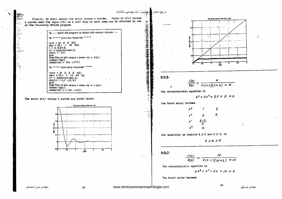
Finally, we shall obtain the t curves when the input r(t) is a of the following MATLAB program.

error versus unit step or

t curves. Plots of e(t} versus unit ramp can be obtained by use

% ----- MATLAB program to obtain e[t) versus t curves·····

% • • • • • Unit-step response • • • • •

num ..- [0 0 0 40); den,. [0.1 1 10 40]; t = 0: 0.01 :3; xt =-step{rrum,den,t); plot It, 1 - xl); grid titleCPlot of eltl versus 1 when rltJ = 11ti'J xtabel('t Sec') ylabel!'eltl = Htl • x1ftl'l

% • • • • • Unit-ramp response • • • • •

numr "" [0 0 0 0 40]; denr = 10.1 1 10 40 OJ; yl "" step(numr,denr,tJ; plot[t,t,'--',t,t'- y1.'o'J grid titlei'Piot of e(t) versus 1 when rhl ,.. t.lltl'l :dabel('t Sec') ylabel('eltl .. !.1[11· xl!U'J

'!be error e(t) versus t curves are shown below.

...;~I_)_J:!"'-""'~

,...,""1......,,-.ml•'l'l

M; ~~~~--------·

"·"i ! ... i ~

'

42o~'1U215l ·-

48

""' '

'~~

!

i 15~--~-r

i_ -1

..... o!!!--•-!111•<1(11

·:! ~u'

___ _j ____ ....!.. --- ·-- - ,_.

• t~ 1/ , 1-r , 1 .?:1 i , ! : I

0 u ' u 2 u 1 ·-

\

------·------------- -----~ J>-S-<;.

C{r) - K

• f{J) - S(S1-1)('+ ~) 1- K

The characteristic equation is

sJ+J'Sa-t-ZS+ /( =0

The Routh array becomes

s' I 2

,. J K

I' ,_,

J ,. K

For stability we require 6 > K and K > o, or

~>K:>O

---------------------------~------------------------------------------------

!t2::1· /0 Ctr) ;:::

R(I) S(S-I)(U+J) +IO

The characteristic equation is

2 5 3 -r s~-3s t- ;o = o

The Routh array becomes

49 ._..i...>_J:l'-""'~

\ ... ~, -""'15:... ...r4-- .:.:, ) ._r!.Sfj•_y?... &'-->" Noting that pc}l " lex, we obtain

•' 2 -3 ---- ,. I (0

J -23

J' /0

The-system is unstable.

-----------------------------------------------------------------------------~- s -I 0

/sr- ~/ ~ ,, s -I 0 b, St- b,

_ . ._,_

;>}i -~~ ."' -~:,

"if ~' -_-£-~;;;£

:.1!1

I I

0'

Hence

..f'.~ A

ft:::: .tr I<

~·- -;::qX

R

;' k . ..X(s} = k[P.N- ~ XI•J]

XIs}:_ _ __:_l __ llM - CR< s <

~+A

A T

= CRs-t-/

-----------------------------------------------------------------------------D:;§;;:!Q.

Pct>)

--- ~ • = s.J-t-b1 sz.+(b~.+~~)s+btb.J

1he Routh array is ,., I b,. to J, .J

s• b, b, b,J

>' b, 0

s' ., b..J

Thus, the first column of the Routh array of the characteristic equation con­sists or 1, b1, b2, and b1b3-

~-

Heo~

-------------------------------------------------------------------------For this system we have

PA = k.r.,

(F "'f•) A = k(<. -r x_)

c "I'· ~ t .1-t-

J= "' - I:.

" c "'& ,It- =

t.· -I' ..

"

I .,. c ·-~

i

l -' -t

' '7

'

ro:-

r.,r,-) ~ r£(r)

b

•H

K,kz I+ K, I(~ _4__ A

c:i+!> A

~ k,

The control action of this controller is proportional. Thus, the controller is a proportional controller.

-------------------------------------------------------------------------------B-5-11. Define the pressure of air in the bellows as Pc + Po• Then

(' "''· ~ 3 ,(t ' Hence

(' i&. __ If - P. -tr -- R

"' RC ;9 ,_ /', = f~

!= i( -~ .. ii'

Define the area of .bellows as A and the displacement of the bellows Then, noting that pcJ!."' ky, Equation {1) becomes as

k:f:­RcA ,tf +l:t~l',

5I

(1)

as Y + Y·

50 ...;~1_)_):!"'--"'~ www.shmirzamohammadi.blogfa.com ~>'-"-"'~

'\ -""'15:... ...r4-- .:.:, ) ._rl..:..:<_,Jts:l?-- &'-->"

.,

"'"'

-'• A KC'-+- + • ~ -v ~ u It' r'<...

A YM = T l'CM l?c $" t- I

A block diagram for this system is shown below.

"'' .1.--:l ~

f;;{f) b E(s) = tt+b

K,/(

A/t q t+K,K A+],

Res+ J

Assurre that KtK~ 1. Then

?.if!= _b_ <t-b RCs+-/ = ( M_\(!?c st--l) EM a-t-b '1. + 4A)

Thus, the control action is proportional-plus-derivative. The controller is a proportional-plus-derivative controller.

---------------------------------------------------------------------B-5-12·

~{>-)

E(s)

If KtK»l, then

• =----,.. x,~

I+ .A\IK<1 (.A-L c>.+b ,f k --Y

' .,.;;, _7.;_

·:-:--.;); _,,, .ck· _.,.

~it ·t:t:s

I I ~ ~;~. ~ ~ '!f ·F:i·

l 1 ' '

J>~M - ___!_ £TY) - a+b

K,t: -(bk)( I K, kif. A I?Cs - ~~~ I+- '/i'(;) -;.j::"b I( ~ C s -r I

The controller is a proportional-Plus-integral controller.

B-5-13. ~ XfsJ ~GEJ -G?l ·I'· 1--1

fc(.t)

k,K Jil!.2.. == ~·~ "' ..d. Jf, c l.$ cc-:'-'-:-:-: e(r) «+-I- I +-Jr;., k a-tb 1e K,_cJs-H ~c,s +!

If KtK ~1, then

T;{s) __ b _ /

E & ; - a + b ~·C::~A~~"~.;Jc';:. :;:, :::-:::;::::2;= a+b k N,c.,,·+J R1c1 s<t-l

= (.l.!L)U•r.a; -\l,c,, +- 1) t~~A \ {(,('~. s /

:: ( /+ R:r./Cls)( J?,c,s+t)

_H_ a A

{I-t R,c, + .ftc~

_!_ il ('l s + R,c,.s)

Thus, the control action is proportional-plus-integral-plus-derivative. The controller is a PID controller.

~· Define

Output pressure : P0 + Po

...;~1_)_):!"'--"'~ 52 www.shmirzamohammadi!blogfa.com 53 ~-.,:,;.~

'\

f~

-""'15:... ...r4-- .:.:,)

Displacement of point A ; nozzle-flapper distance ~ X + x

Displacement of point B = Y + y

Displacement of bellows = Z + z

Displacement of point C = W + w where P0 , X, 'Y, Z, and W are steady-state values. The positive directions ilre indicated in the figure shown below.

TN·

lu

Frcm this figure we obtain the following equations;

k. F 4+-e f,- ,x. .. f-:Klfl)) T=-.{-Note that

Change in magnetic force due to change in current = Ki

Change in spring force = k(y - w)

The torque balailce equation is

*!;-•oc =Ki (a+h) The displacement x and w are related by

w c -.:r :::: T

So the torque balance equation becomes

Ki(Hb) = k{~+-.!j;-x) c

By substituting

p, ;;(o::;-)

K, !!= "•-"kl' d+e - 4-H!! :

into Equation ( 1) , we get

Ki(A+b) ~ k ( d:e k, + b~,) f, C-

....,~1.).):!"......-~ "

(1)

•

'

oc

. ~c(" c) c.= ··- .. ;;:;; Kz. T .&AI PQ

Thus, Po (change current).

in the output pressure} is proportional to i {change in the

\

-------------------------------------------------------------------------------B-5-15. Referring to the figure shown below, we Can obtain the following eqUations:

),

,,

~ ·--·

Jl A· q.!; ci'l3::/ II r 4t-A' nn. '· -· I . I o~ "~'~" ""

p ..... ,. l 001 ond<f ·-·

For the diaphragm and spring assembly,

oc

For the jet pipe.

oc

,A.i:< ~ f<

2tr-J :=

X(s)

p ~ K,'

~ ~

"" ~ ~ _1_= A;JI

A;f, du ~y dt

~f llj .f•

...J!!!L - _..!5!_ Z(s} - A;f~.S

For the pilot valve,

A; j, ""1 = J, .tt ,

!'L - .-lt__ d:t - A!Jl-.

K, u

AI f, <;:;

j,=kz«.

._..i...> _ _, ...... ~

' -""'15:... ...r4-- .:.:, ) ...r'~----~ &'-->"

0'

H~~

vhere-

YM x~ lfts) = Arft.s

Y(.r) - 'Y(J") lT/rJ Z(.s) ;= _L ~ A,. Xts) - lJ(f) Z{IJ .Xfl} Atfzs ~-,,s ,E

K= K2k1 At~

AtJa.Aj.!'.lt.

/(

s•

'l1le controller is a double integrator. A simplified block diagram is shmm. l:elow.

X~J •{f] ZM•~~~ ZTfs)_•j k~ I YfSJ• k A~J:' s A1 /,.s

-----------------------------------------------B->16. Define displacements e, x, and y as shown in the figure below.

e f

Od•od"

"''""'

Uu' !~ /h(

J.l~ jiii

]I ![ -, II// '

From this figure we can construct a block: diagram as shown below.

8{1) , QJL Efs!l ~ J ·-· Yt~'

L ---j • 1- I •+;.

From the block diagram we obtain the transfer function Y(s)/@(s) as follows:

___ ,,

,;.:: -~?

:"'--~' _A._ ~

t -~ ~­;f. "' ·~ 1 ~ !! ·i -~

:T

!

Y!s) : @(s)

J, K '~s

k -· /+" s 4-t;b

;:: /b Q+-b

•+b ~

= _( _!,_ .._

\ We see that the piston displacement y is proportional to the deflection ;mgle 9 of the control lever. Also, fra:n the system diagram we see that for eac:h value of y, there is a corresponding value of angl!;! 111 .•. Therefore,_. for eact; angle a of the control lever, there is a corresponding steady-state el~tor angle !If.

----·----B-5-17. For the system

!.·ll = ux -e! where A is the area of the bellows and z is the displacement of the lower end of the spring. Also,

iJ=KJx.tt-, 'j= _,

Thu•

Yfr) = _!£_ )((>!, s

YM=-Zfr!

"'~ llP..(sJ = k [XM-Zis)] f[xfs) + YM] = ;,(tt-: ))(!'s)

Therefore,

YfsJ _ .5_ XM _ kll t:·~J - • P,·M - s< (~> -1f-)

= kll UuK)

B-5-18.

Th•n

"'

Z1 =- R,

Zz =Rz

I +c;-

E".-1•) = ( R, + c~) J(s)

Ep{s) ==- R2 Ifs-J

z, r·-·· ,c~

<>-t-1 . '-·- J

'•

,, -·-, ! .... '

<,

~ Ee&J,_ t, =- RzCS

j e;lfJ .?1 +~ l?,cs+/ www .sh mi rza mo ham mad i. bloQfa.COifi ___________________ .c ________ ~:--------------~-;.:;..~------------

...;~1_)_):!"'--"'~

"'

' ~15:... ...r4-- .:.:, ) ......... ~.~_)1..5: -~ &'-->"

B-5-19. The voltage at point A is for the unit-ramp input r{t) = t,

eA = f{e,- -r e.,) 0'

E.4(s) ~; [ E,-(.r) + E,{rJ}

The voltage at point B is

E1 (s) = l?z.C.s €i(s) K,cst-1

,, ~ ·-~

#, 2 ,!;:!

"'-'

Tho•

e.,

S" -r ars_.!!_-l + · . · +a, --a s 1 Elf)=

s"+4,s"-'-t-··· +a .. -ts t-.:t,.

I s•

= ,£;-..sE(.$) = 1J..-, S(s"-rti,S 11_,T- ... 1-a..,-i!.\S')

$ Tif,S' + ... -f-II,_,.S+4,).F:z. s..,, s7P ( .. ,_,

=0

Since [Ea(s) - EA(s) )K = E0 (s) and K» 1, we must have EA(s) = Ea(s). Th~. ~ -------------------- ------------------------------------------------

lienee

~

f [ Ei(J') + E,{s)].:::::: "~2.,("~ 1 Elfs)

(;_- f(,Cs ) Rlcs+! E;M =-f-£"{5)

E-p(s} RzCs- I

6j'(s) = /(lCs +I

-----------------------------------------------------------------------------!!::2:::12.

CM ~{sJ Ks+-b l?(s-) =: lt-t;{s)::: s'"+a.F+b

Hence

(<•+ M+-~) <¥/'JJ = ( ks+ >) [t+ <if-'J] 0'

C;(s) = Kst-b s(st-~- k)

The steady-state error in the unit-ramp response is

~-

e _ _j_ _ 17. _1 __ _ 1, S(S+-~-k) u- _JMy. -...w.....

Kv .s-u S~(s) s.;.." s(Ks+b)

£f!l. = 11,-t 5 +a,. J?(s) S"+ t:11 S 11

- 1 + ··· t-tt.,.1srlf,

•-k =-b--

.s"t-q,s"-1+··· +tl,-z.sl :

:0

I ~

" i '{"' "" • >€ ;'!•

-£

t=(s) -Rts-J -

...;~I_)_J:!"'-"'~

RM-C{s)

II{>! s" -rq1 s"-1 + 58

+n,_,;s; +4,

www.shmirzamohamm~di.blogfa.com <O ~-.,'-""'~

' -""'15:... ...r4-- .:.:, ) -r¥-r: -~ &'-->"

CHAPTER 6

!!:::§:::!.· The open-loop transfer function

K 'i~)HfS)= s(s+t)(s 1 -t-f'.1+S)

has the poles at s = 0, s = -1, s = -2 ~ jl and no zeros. The asymptotes have angles ± 45~ and t 135~, 'lbe asymptotes meet on the negative real axis at

O'a. = -1.25. Two branches of the root loci cross the imaginary axis at s = ± jl. The angle of departure fran the complex pole in the upper half s plane is -198·.

A MATLAB program to plot the root loci and asymptotes is given belov,to­gether with the resulting root-locus plot.

~ I

' ,

'

0

,,

% • • • • • Roo Hocus plot • • • • •

num"' [o"-0 o o 11; den = [1 5 9 5 01; numa"' 10 0 0 0 11; dena~ [1 5 9.375 7.8125 2.4414]; r .. rlocuslnum,den); plotlr,'-'J hold Current plot held plotlr,'o'/ rtocus(numa,dena/ v = [-4 2 -3 3]; axis(v); i'l.llisl'square'J; grid tittet"Piot of Root loci and Asymptotes']

-afA<:>clli.J:x:>-~

_, • --2 ·1 0 --. ,

_,-;_

:,~

' .i{

" j ,it ~ ~

~

" \1! 10 .. ·~ :f, i e ~· ~

:_~

B-6-2. The open-loop transfer function

I((Stf) C:rPJit(S}= s(rz +~s t-!1)

has the poles at s = O, s = -2 ±. j .[7 and the zero at s = -9. The asyq>totes have angles+ go• and meet the reat.axis at ct"a = 2.5. The complex branches cross the iJMginary axis at s =;!; j' 4.45. The angle of departure fl:"OOI the complex pole in the upper half s plane is -16.s•.

The dominant closed-loop P.Oles-l)aving the damping ntio !;: = 0.5 can be located illS the intersection of the root loei and lines from the origin having angles ± 60•. The desired dominant closed-loop poles ;~re found to be at

S = -/.S" X.j 2-S'Pi

The third pole is at s "' -1. The gain value corresponding to these daninant closed-loop poles is K = 1. A MATIAB program to plot the root-loci is shoWn below, together with the resulting root-locus plot.

% • • • • • Root-locus plot • • • • •

num = [0 0 1 9]; den=ll 411 OJ; rlocvs{num,den] hold Current plot held x"' [0,-3]; y .. [0,5.19GJ; llne(x,y); v- [-15 5 -10 tOJ; existvJ; alli~('squere'J grid tit!e('Root-locus Plot uf GlsJHisJ .., K(s + 9/[sls • 2 +4s + 11)'1

~PlotatG(•)H(•)•I<(~~tf)

'" •

.. L r"iu~ r-"'"''·' '~ I

L I~ ~ o I 1 •. ,

:'-~~t--4---.=~ ___ I • T ----

·f-----+---+-·-= -. --t~i". --:.:/o,.-~.--iJ·--·=-=·-=-0 ' --

------------·------------------------------------------------------------ I . -------------------------------------------------------------...;~I_)_J:!" '-'"'.lo/<- 50 www.shmirzamohammaai.blogfa.com 61 ._..i... _ _, '-'"'.lo/<-

' -""'15:... ...r4-- .:.:, ) .....:i~", Note that the locations of the dominant cl~sed-loop poles and the corres­

ponding value of K can be determined as follows: Since~ is specified as 0.5, define .

-,J s ~ cr:rjfix

Substitute s "' x + j .{3x into the characteristic equation

SJ+ 9-St+//J" t Kst- 9K =0

Then, we obtain

(:uj.fix_)' + f- ( X+)fi X)' +II ( x +)fix.)+ K ( ><':J'fi<)+/1:'<1

S~lifying this equation, we obtain

-8:r~- B' .:C" +-//X+ k .r t- 'fl< + jfi ( ?::t 2 +1/X f- /<X) =0

By equating the real part and the imaginary part to zero, respect! vely, we get

- f ::c~- rx .. -;-1; x +t< x + fk =o

""" 'IX .. +//xT-I<.x=cJ

Fran Equation (2), noting that x # o, we have

3X-t-//t- k = 0 or

I<= -J'X -II

Substituting this value of K into Equation (1),

-8z 1 -i'.:r a. +II X T- {-l-1/) X + r {-3-X -/;) = 0

~

rx 1 -rdx,+7Z x +?? =o

Solving this cubic equation for x, we obtain x = -1.5. (Disregard other values of x.) Thus, the doodnant closed-loop poles are located at

s-= :rxj{Jx = -;.s:L.j zN"s Then, the value of K is determined as

K = -N-I·.r-)-11 = /.

(1)

(2)

-------------------------------------------------------------------------------

~ ,.;;,; ~ --~ ·-~

''i'¥ 1 .. ~ ;.;. -;~

'i "' ·~

I ~ it

I • • ~

-~&'-->" B-6-3. A MATLAB pr-ogram to plot the r-oot loci and asymptotes for the follow-ing system:

- /( {j($) l{(s) =

S(S+ e'.S)(S~+ 0./.S+IO)

is given below and the resulting r?'t-locus plot is shown below.

Note that the equation for the asymptotes is

k (j._(s)H~(s) = ($f"'/1.t?s-f

•,

~~--~----~K~--------~ sJJ. .,. t.t J" J #- "' fl.rJ ?.s- s:o. -r o.e'l' 11 .17'-1 s t- "·'' 1'71/'1

% • • • • • RooHucus plot • • • • •

num = 10 0 0 0 1]; den .. 11 1.1 10.3 5 OJ; nl.fTlll .. ]0 0 0 0 1]; dena • If 1.1 0.45375 0.0831874 0.00571911: r - rtucus{num,dunt; ptottr."-'1 hold Current plot held plotlr,'o'J rtocuslnuma,donal

v .. [-5 5 -5 5); axisfv); axis('square'); grid tftle!'Plot of Root Loci and Asymptotes (Problem B-6-3)')

I J

-· ...... "' . .,

~ ··- - ...... -... .. ·-----·- ...

'"'" // ' "'-" // ' "'- "'"-! / / ,_ / ' "'-' '\

/"' ·' / "'-: / ..................... " /_/ ""-"'-:'/"'. ~

. " -- ' -----------------------------------------------------------------------------

62 ._;~I_)_):!" "-"'.lo/<o

I www.shmirzamohammadi.blogfa.com

63 ~>'- ...... .lo/<o

' -""'15:... ...r4-- .:.:, ) .,rl..:..:<_. -~ &'-->"

........ A MATIAB program to plot the root loci and asymptotes for the system ~ !!::::§::§ •

---~.7 (1) If (r) = K (s'+Zs--t- z)(S" 1 -tZs+~)

is shown below. The resulting root-locus plot is also shown below. The root loci cross the imaginary axis at tJ"' ± 1.87. This point is obtained by solving the following equation•

[r;w)'~ 2jwr>][6"'!'+2jw~s-] r I<

= (w'~>-"ft.I)L +ltJ+ 1<:) +j{-'1-~+IP.w) =0

By equating the imaginary part equal to zero, we obtain tJ= ± 1.8708. By equating the real part equal to zero, we get the gain value at the crossing point to be 9.25.

% • • • • • RooHocus plot • • • • •

num"' [0 0 0 0 1); den"' [1 4 11 14 10]; numa = 10 0 0 0 11; dena"' [1 4 6 4 1]; r ,. rlocus(num,den); plotlr,'-') hold Current plot held plotlr,'o'J rlocuslnuma,denal v "' [-6 4 -5 51: ax1slvJ; axis('square'); grid title("Piot of Root Loci and Asymptotes (Problem B-6-4)')

~ I

' • ' ' ' 0

'

PICII of ROC!Ii.o<i - Aoym;ll<>lllo (Prell...., 11-6-<1;

• ' 0 ' • --

·-''

-~

"# '

"'"" ''"'' ~ -~ ~

I .. j I ! I -~

-~-

I+ Q(T) HPJ::

The characteristic equation

,(t+K)s' r(z-rttc)s T/l)t-/~K.

s""+2s+lo

(t+l<)'z.+ (2+-6~)-S +Ill+ ltJk=O

has two roots at

S=-/i-:JK

It" I<. ±j

If we write s =X + jY, that is

X=-

then

!.!:E.. 1-t" '

(k"-t-I?-K+9 1-tK

/K'+-1'1-K+? Y= I+K

\

xa. + Y' = ( J+:JK.)• I+ I< -t K"'-t-11-K. +f'

(!+I<)' /P { /CN )~ ::; /0

= (1+1<).

This indicates that the root loci are on a circle about the origin of radius .(10"'

---------------------------------------- ----· !!±§_. The open-loop transfer function

<j(>)#(s) = /((s+P.>) s'( St"3.6)

has the zero at s = -0.2 and the double POles at s = 0 and a single pole at s "' -3.6. The asyroptotes haw angles of :!: go•. The asy~~~ptotes meet on the real axis at ct"8 = -1. 7. The breakaway or break-in points are located at s = 0, s "" -0.43155, and s = -1.6665. A MATUJl program to obtain the root locus plot is shoWn below. The resulting root-locus plot is shown on next page •

% • •• • • Root-locus plot • • • • •

num = [0 0 1 0.2/: den .. [1 3.6 0 OJ; rlocus[num,den[ v .. 1-6 2 -4 4]; axislvl: axis['square'l grid tiUe('Root-Locus Plot [Problem B-6-6[')

---:~=~:)=:;~:;.------------------------------------------------------------M www.shmirzamohammadli.blogfa.com " ~-J:l~~

' RooH.=• Mot {Prolllom a-e.e)

• ' '

·--

·1---- --­J l' · I

-·1---- -

•f----

·r---+-1 I I H--i-1-1 "\ -6 -II ..) RMJ-2NJI, ,•1 - 0 1 2

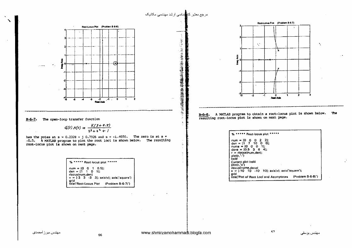
-------------------------------------------------------------------!!±!• The open-loop transfer function

~(.r)fi(r);::: K(J+~.s-) sJ+.s .. +/

has the poles at s = 0.2328 + j 0.7926 and s = -1.4656. The zero is at s = -0.5. A MA'l'lAB program to plot the root loci is shown below. The resulting root-locus plot is shown on next page.

% • ••• • Root-locus plot •••••

num = 10 0 1 0.5]: den~ 11 1 0 11; rlocu5lnum,den) v = !·3 3 -3 3]; axis[v); axisl'square') grid title!'Root-locus Plot \Problem B-6-7)')

'f ·'

:;'!,_

~ ~-·-~ ~-'±

I ~ ~ ;;l!i-

~ 1! 1 '

,1.5: -~ &'-->"

I

I

i l

'

'

'

'

·•

' • " . •

" ~-~-- ...

''

'

lL

-' --

~·) ----- -I

---j----

• • ' ' ·--------------------------------------

~· A MATLAB program to obtain a root-locus plot is shoWn below. resulting root-locus plot is shoWn on next page.

% • • • • • Root-locus plot • • • • •

num.-[0 0 0 2 2]; den= [1 7 10 0 OJ; numa = 10 0 0 1]; dene = ]0.5 3 6 4); r .. rlocuslnum,den); plottr,'-'1 hold Current plot held plot(r,'o') rlocuslnuma,den<~J v ""1-10 10 -10 10]; axislvl; !lllisl'squere'); grid titJe('Piot of Root Loci 0111d Asymptotes \Problem B-6-81'1

-

...;~I_)_J:!"'-""'~ 66

www.shmirzamohammadi.blogfa.com " ~-.,'-""'~

.... ~· =· i ~

-""'15:... ...r4-- .:.:, ) ...r\i'.t: -~ &'-->"

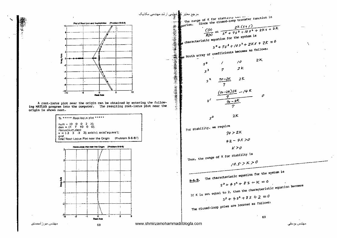
-* .&tt.erion• Since the closed-lODP transfer runction is

! I

-'~'"""""'L""...,...,.._ ,...,.,._,,......,......, '" -f! I •r- ·--- - ····-··- --- __ J'~--·-

' I! •r--' I I • '

\

' • '\..

'\ ' '\ '" . " • ·• ' -- "

A root-locus plot near the origin ing MATIAB program into the computer. origin is shovn next.

can be obtained by entering the follow­The resulting root-locus plot near the

I % • • .. • RooHocus plot • • .. • I num = 10 0 0 2 'l.]; den = [1 7 10 0 0); rlocus(num,den) v = (-3 3 -3 3]; axis(v); axis(' square'); grid title(' Root-Locus Plot near the Origin {PIOblem B-6-8)')

Flllci-I.DCtlll't:ll.--- ongn .,..__, ' I I 17 '

.![

~-

·i: -i -1 _·:)i;

l ., 'j'

·~ .&:: i

Jj;

_fit· ,}. ~-~·

.:t;

:~

't'he range of K for staDU.l.~J ........ -­

C(sJ z/< (S+ f) ~;:::;.-~{$) s" -t- 7SJ -t-IOS'" + 2/<5 + 2j:;..

characteristic equation for the system is

s•+?sJ rf()$ 2 +z'KS' t- zt. ::o

Routh array of caefficients ~s as fottows:

s'

s'

s'

•'

s'

I

7

?tJ-P::. ~

7

;o

2k

21'

{!•-")/!; -14' K 7 ?o- zl::.

7

~K

For stabilitY• we require 7tJ 7 Zl<

f-2.- 9-tt >0

K~o

Thus, the range of K for stabilitY is

21<.

0

\

-r I

i·l ! I l I I .

-------------------------------------------------------------------------;o.> ;;- K. ;> o

ll-{>::9· The ctJaracteristic equation for the system is

t ( _ _I_._ I~ ... i 1\

0 ·• 0 ......

s'o~- f-S' ... +" B"S +- K :::::o

If K is set equal to z, then the characteristic equation ~s .s 1 -r 9-Sz.+FS +2 =0

The closed-lOOP pates are 1ooated as fottows:

69

...;~I_)_J:!"'-""'~ 68 www.shmirzamohammadiiblogfa.com ~-.,'-""'~

--

' -""'15:... ...r4-- .:.:,F s = -1.8557 + j1.8669

s " -1.8557 jl-8669

s = -0.2887

See the following MATLAB program for finding the Closed-loop poles.

P"' 11 4 a 21: rootslp)

ans ""

-1.8557 + 1.8669i -1.8557-1.8669i -0.2887

A MATIAB program to plot the root loci is shown below. lccus plot is also shown below.

% • •• • • Root-locus plot • • • ••

num"' (0 0 0 1): den "" !1 4 8 OJ; rlocuslnum,den) a>;isl'squaro'J grid

The resulting root-

title('Root-Locus Plot of Gis) = l(/(sls'2+4s+81/'l

Rccl.locus F'lolof G£s) ~ K.ts(r'2~J

:[UJ/17 I I I I -. I ! ·-t--, 1 I

I

, -r-i I I

I' I I I _, . -r-- ~---t-+------1 I

-2~---L._ ------'--~i---L-1 I j ' I

~ :---,--~-- . ~ !

•}--,--j,c--:_,f--.!-~+--~-~ _, 0 ' ' -- •

--------------------------------------------------------------------------------

-..:,)'

,----

:~:

'":l' ~~-·} = ~l -~7.: ~

1 "' ·""" ·f . ~ E: ; ':iii. '('I • _,,

·;,_)1.5: -~ &'-->"

~-

C(:r) k. /?{rj = -,-,-, -:-+-"K-:-K::-,-:-,-:-t-:-K~

Noting that

s'"+I'K11 s+k =(s+t+-j'..ff)(s+I-Jfi) = s"-tzs '+f we obtain KKh z 2 and K = 4. Hence, Kh = o.s.

To plot a root-locus diagram for the system vith Kh = 0.5, we need to rewrite the open-loop transfer function such that it contains a multiplying factor K. Since the characteristic equation for Kh: 0.5 is

51

-t-P.S"K s + k = 0

we rewrite this equation as

I+ _~_,_(_'·:-c'"::-S-'-+'--'1 )'-- = O ••

and consider K(O.Ss + l)/s2 as the open-loop transfer function, or

Gt(r) = k(P.!"r4/) s'

'Thus, the system will have an open-loop zero. (This zero is not a closed-loop zero. ) A MATLAB program to obtain the root-locus plot is shown below. The resulting root-locus plot is also shown below.

% • • • • • Root-locus plot •' • • •

num"' [0 0.5 11; den .. 11 0 OJ; rlocuslnum.den) v = [-5 1 -3 3[; axis[v); exis!'square') grid titlei'Root-Locus Plot !Protl!em B-6-10)')

~ Plr:ll (Pn;>bl.m a.&. I D) 3 I - '

I I i ' I ' i I -r-----tc

--l ! __ J__ ___ L\~-i I I I !

f I lr 0 I I • ; I I

___j --~-- -----;- -; _,

' ' ' ·2•--

_____ j _____ .i~

: I '>',_ __ J·,_--,_,!---,±---J,,---,,!--~, --

...;~I_)_J:!"'-""'~ -- www.shmirzamohammadi.blogfa.com 71 ~-.,'---"'~

o\

''I II\

II[ II

II

II'

I.

I 1:

111

" II

I 1: I I !

' -""'15:... ...r4-- .:.:, ) .,ri...:.Ui)-l-~ &'-->"

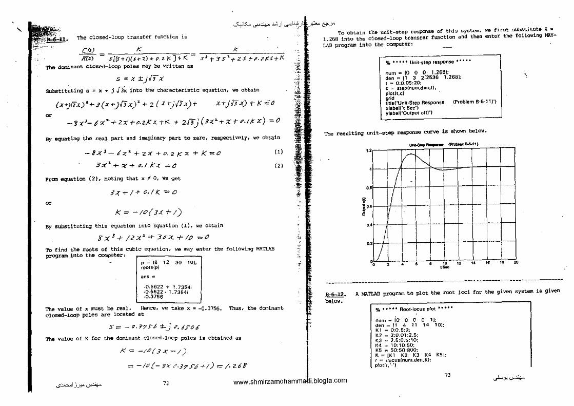
To obtain the unit-step response of this system. we first substitute K = 1.268 into the closed-loop transfer function and then enter the following MAY­

LAB program into the computer: The closed-loop transfer function is

K k C($) R(s) s[(s-tt)(s+Z)+O.ZK]+K = s.t r Js~-r2S TP-2K~+I<

The dominant. Closed-loop poles may be written <IS

s =-X :tjffX

SUbstituting s = x + j ~ into the characteristic equation, we obtain

(X+)ff.r.) 1 + 3(X r )fix)"+ 2 (X t-jo/J .x) +- x+jlT.x)+-K=o or

-'j;(~-0-;ta.+2Xf-o.zK.t.-tk + 2ffj(.J.:tl-+Xt-P-IKX) =0

By equating the real part and imaginary part to zero, respectively, we obtain

-axJ- tfA:.'" + zx +o.2 KX + K=o

~::e'"+x+ o.tk.:r =o Fran equation (2), noting that x f. 0, we get

l.:r+!+ 0./K. =0

or

k = -10(3X +-1)

By substituting this equation into Equation (1}, we obtain

Sx 3 +!2Xz.+3vx+tP =0

To find the roots of this cubic equation, we may enter the following MATLI\B program into the computer,

1•,. ra 12 Jo tor; roots[p)

ans ,.

-0.5622 + 1.7354i -0.5622. 1.7354i -0.3756

(1)

(2)

The value of x l!lllst be real. Hence, ;;e take x = -0.3756. Thus, the dominant closed-looP poles are located at

S=- ~-?7.>6 -±-._/ .7,/.)1/,{

..... ·.j; .>

' . -~r di

"' I .. I 1 . J ! ·I'

-~

-~'

•

<

The value of K for the dominant closed-loop poles is obtained as I I

= -10{- 3'X .:".Jp.>tf+l) = /• 263"

% • • • • • Unit-step response • • • • •

num ,. 10 0 0· 1.268!; den "'11 3 2.'2536 1.268); I ~ 0:0.05:20; c = step(num,den,t); plot(t,cl grid title('Unlt·Step Response (Problem 8·6-11)') xlabel('t Sec'! ylabel('Qutput c(tJ'I

The resulting unit-step response curve is shown below.

'

'

• .,

" i' ' , •

'j "

0

0

~~ ~8-6-11)

r !'---I

I I I

'

I [

' . . • • '

' I

8 10 12 ·-

+ '

u<fi182D ..

..

-------------------------------------------------------------------------------~· A MATLMI program to plot the root lOCi for the given system is given

belOW. % • • • • • Root-locus plot • • •• •

num = 10 0 0 0 1); <.len= !1 4 11 14 10); K1 .. o-.o.s:2; 1<2 = 2:0.01:2.5; K3 = 2.5:0.5:10; 1<4 = 10:10:50; K5 = 50:50:800; K"' [K1 K2 K3 1<4 1<5]; r = rlo~:us(nunl.<.len.KI; plotrr,'-'1

73

I<= -/0(3cr-l) t ...;~IJ----'*"' '--"'.lo/<- 72 www.shmirzamohamma i.blogfa.com

._..i..->.J;l '--"'.lo/<-

" -""'15:... ...r4-- .:.:, ) ._.,J.<i.f_)ts: -~ &'-->" Hence, we enter the following numerators and denominatc~s in the program. the system, v = !·5 3 -4 4!; axis(v); axisl'square'J

grill tltlo('floul-locus Plot ul G(s) = K/J(s'2+2s+211s"2+2s·15)]') xi;IIJeii'Real Axis') --ylabell'lmag Axis')

The root-locus plot is shown below.

i I

Root-loc:ul Plot of G(o) • KI((J"2~2o+2)( .. 2+Zo+5))

''-..

'

'

'

' ' • ' • ' ~ ., /

•

"

/ /

•

/

/

-'-.

" "-..

-2 -1 0 ' RaBIA>cla ' -------------------------------------------------------------------------------!!:::§=ll. The open-loop transfer function is given by

C,(s)/tfs) = K(s-o./d'J'?) .S" + j. ]fl.tJS.J -t- 7. P,72S I~

The equation for the asymptotes may be obtained as

ClaMH.,(.s) =

~

K

S 1 + ( j,J'f~+P./61"7) S'L+ •• •

K

(st- 3-J'H';o-1!67)3

K (>+/.3Jst)3

K

~;;' ' ,:;;; ;~-

·i,ti' -~­#--

140.

.

I 'g.

I .~ ._:-£

"

< :?. • ~ ~~

'· 2: 'i:r

" -4

" ' ..

'

•

it !

num :: (0 0 0 1 -0.6667}

den= (l 3.340 7.0325 0 0)

For the asymptotes, '

numa = [0 0 ·o I )

dena= [l 4.0068 5.3515 2.3825]

/1. M/I.TL/I.B program to plot the root loci_and asymptotes is given OOlow. resulting root-locus plot is also given below.

i l

• ' ' ' ' ·•

• ' • ' ~

% • • • • • Root-locus plot • • • • •

num = [0 0 0 1 -0.66671: den .. [1 3.34 7.0325 0 OJ: nume"' [0 0 0 11: dena"' [1 4.0068 5.3!>15 2.38251; Kl - 0:1:50; K2 "' 50:5:200; K .. [Kl K2]; r "' rlocus(num,den,K); e = rlocuslnuma,tlena,K); plotlr,'o') v = (-6 2 -4 4]; axlslvl; axist'square'l hohJ Current plot held plotfa.'-'J llfid tltle!'Root-locus Plot (Problem B-6-13!'1 xlabell'Real Axis') ylabell'lmng Axis']

-~ l'li>l • r.-..8-f-131

..

• • •

I

. ., ""'""

VI / I

\ ~ ~

-1 0 1 2

., The

Fo'

s.J+ 'f,NJ llS._-t t;o,Jf'IS'S T2.39lS"

74 -------------------------------------------------------------------------------

75 ...;~I_)_J:!"'-""'~ www.shmirzamohammadi.blogfa.com ._..i..._J:l'--"'~

' -""'15:... ...r4-- .:.:, ) ~uJ_)ts: -~ &'-->"

!!±:!..1· By substituting s = a- + jW into

'--" /~/ and rewriting, we obtain

Thus,

·~

The constant below.

1<~ J!~•j'-')(~+)"'+t)J ~ Jco--r)"')'+~•Ju!l = jo-2.+ o--w'_tj~(l+ZD"-)1

. ( )~ . K = (J"&+a--w:z.. -r w._(J+a6")

= [a-(0'-ti) -w•]' -t- cf(1+ ~ 6' + 9-a-')

= [fJ'(rr-+t);-w']' ;-w~

gain loci forK = 1, 2, 5, 10, and 20 on the s plane are shown

_, -·

,a ••

I•

,,

' •

- /4.

-------------------------------------------------------------------------------

• ~ ~

-)l! ~. ,. ~ ,:,:.s_ ·.~

-:1 ~

l I 1<' lt ""'

8-6-15. The term (s + 1) in the feedforvard transfer function arul the term "'("S+"l"j in the feedback transfer function cancel each other. The reduced characteristic equation is

/:;(.HI)

J+tj($}fl(s)= /+ S(S"t-~ST{) I

5+/ - I + ---"'-K-----, - 5(S,._T-2s+t)

=0

\ The open-loop poles of G(s)H(s} is at s = 0 aml s = -1 .:!:: j .[5. MATLAB program produces the root lOCUS plot sholm below •

The follow~ng

~ l

' ' '

% • • • • • Roo !-locus plot • • • • •

num = [0 0 0 1[; den= [1 2 6 OJ; rlocuslnum,denl

Warning: Divide by zero v .. 1-5 3 -4 41; axislv); axis(' square'] grid litle('Root-locus Plot (Problem 8-6-151'1

Roai-UJc:ul Plot (l'l'tlt>ltm B-6-15)

L i I ~

I tt-- I

• I ., I

-~ , --._

~ ! • ' r • . . . . ' ' • • • -2 -1 0 --

To find the closed-loop poles when the gain K is set equal to 2, we may enter the folloWing MATLAB program into the CQI!IPUter.

p = 11 2 6 2); roots(p)

ans "'

-0.6147 + 2.1754i -0.8147. 2.1754i ·0.3706

._;~I_)_J:!"'--"'~ '" i

www.shmirzamohammadi.blogfa.com " ._..i..._J:l'--"'~

... -""'15:... ...r4-- .:.:, )l._rt..:..:<_)S: -~ &'-->"

''r--,--~...._~~--~~(~Po~--~, .. ~,.~·-r,--;

1.5~--- ---1--

Thus, the closed-loop poles are located at

s : -0.8147 ~ j 2.1754, s " -0.3706

------------------------------------------------------------------------------B-6-16. The characteristic equation is

(J+Ct') z +I =O s~( S+-2'

In thia case the variable ~ is not a multiplying factor. Hence, we need to rewrite the charactristic equation such that K becomes a multiplying factor. Slnoe the characteristic equation is

s"'+2s~-r2:>t-20( =O

we rewrite it as follows:

;>(I( = 0 s't-2.r'+2S

!+

Define K "' D( • '!ben, the characteristic equation becomes

2K /+- ;:;0 s{J .. -t-2s+2)

A root-locus plot of this system may be obtained by entering the following Hli.TLAB prcx;rram into the o::xoputer, The resulting root-locus plot is shoWn on next page.

% • * • • • Root-locus plot • • • • •

num,JO 0 0 2); t.len ~ !1 2 2 OJ; Kl ~ 0:0.1:10; 1<2 = 10:0.5:200; K "' !Kl K21; r "' rlocuslnum,den,KJ; ploW,'·') hold Current plot held x = [0 -2); y = 10 3.464); linelx,y) v "" l-3 1 ·2 2); axislv); axis!'square'J yriU tillei'Rool·locus Plot IPro!Jiem B-6-16)'1 x!aiJel('llea! Axis'); ylaiJel!'lmag Axis')

From the' coot-locus plot, the dominant closed-loop poles that correspond to the damping ratio> of 0.5 are found to be

S= -e<.S'i:jc.tM

The value of K corresponding to the dominant closed-loop poles is obtained as

-· <-k=l S{S'~+ZS+z)l 2 s=-t>·f"+j<>-UI

? " .,

t ,~· :;,

"' " -.{' ·I

,~--- + --i--- 1-~~- 1- -i

. ... 1 .. c.s~---

l '.: -- --- -- .. ~~-c +--- -+-+-

--lS:. __ -1.5~------l-~

-~ -2.5 -2 -1.5 ·1 -0.5 ' ,, ......

-----------------------------------------------------------------------------· !::§=!1_. The closed-loop transfer function is

f.st-(:1'-) /0 (s+;o) \...s+s s(s+/)(s+/c) +-/e<.f.s C&-) -----=

/(fr)

( S+J.~) /O(S+/0)

J t- .S+S S(S+!}(5t-IC)+!tJA S

Thus, the characteristic equation is

J+ (_S+/·f-) /C{s-t-/0) =-O \: S+S" S(5+i}(S+-/O)+!#S

Since the variable k is not a multiplying factor, we rewrite the characteristic equation as

(.}'1-r-).s (s-+l)(r-trP)+ prr)ICI(.s + (s+-Jt)tof.Jf/P) =" Which may be rewritten as

!t'(S+.s-)i!..s /+

(5-t-/t> )( s_,+D.s 2 + ;s-s t-1¥-) =0

,, f(J (SI-r-) 1( r

I+ (:J+Z)(:s-r;o)(S+2·tjJ.73~)(Y+z Jf.7.Jz.) =0

Notice that the open-loop poles are at s = -2, s = -10, and s = -2 ~ jl.731.

...;~I_)_J:!"'-"'~ www.shmirzamohammadi.blogfa.com ._.,i..._J:l'-"'~

' -~15:... ...r4-- .:.:, ,, .. ~ ~ 1.5: '" obtained by entering the follOwing "~-I--_) -~~= 9.08, G(s)H(s) can be given as

A root locus plot for the system m8y be MA.TI.J\B program into the computer. 'I'tle below.

resulting root-locus plot is shown

% • • • • • RooHocus plot • • •• •

num "' tO 0 10 50 OJ; den"' II 16 75 164 140); numa ~ [0 0 10]; dena"'[t 11 20]; rlgcuslnum,denJ hold Current plot hold a = rlocuslnuma,dena). plot(a.'-'1 v = 1-15 5 -10 10]; axis(v); axis("square'l x .,. 10 -5.51: v = [0 9.52631; line(x,yl grid titlei'Root-Locus Plot (Problem B-6-17)') text!- t 2,3. 'Asymptote')

Roal.-l"""" Plol (Prcbt.m B+11) 10

J ---1-==k-+= • ,

~ 0

I I _, '

• I • i • 1··-. __ ,_, ______ --~

I

·'" ... ., • 0 -- •

The dominant closed-loop poles having the damping ratio equal to 0.5 can be determined as the intersections of the root-locus branches and the straight lines from the origin having an angle of 60~ or -60° with the negative real axis. The intersections are located at s = -5.14 ±. j6.90. The gain value k is obtained from

~ ~1 (s+z)f~-rN)(s+2+J;.?u.)(s+2-. .JA?32)1 /0 (s+S).S s~-s,t~+j¥.fD

= ·;u? 80

·'

;;

-~ -~.

' <

" ' -' :.~

/O(S+/0) f5r(s} H(s) == f. H/. f~

\ s+.r J S(S-+ I)(S+/0) + 9d. i"S

The static velocity error constant Kv is

Kv = ,£.:..,. .S" Cj(;}lt(·9 ·~·

,i;_ /_.5+f.9 _'j /t/(.S+IP)

~ s·u .S"Cs+..r J s[(s+l)(.s+tc)+fP,s>]

~ tJ,Z'J?3

',

--------------------------B-6-18. A root-locus plot of the system is shown below. unstable for K > 19.6398.

J• 111•11.4YJM·

lii•D·~

w. f.% j D.2.

'-'"D·I

The system tecanes

-1-4 -f."l. • '·' #.f- o--

-jo.1.

~;e.t

---------------------------------------------------------------------B-6-19. A root-contour plot of the system is sh01o/Jl on next page. Notice that the system becomeS unstable if a '- 0, regardless of the gain value of R.

81

....,~1.).):!-"l...i"~ www.shmirzamohammadi.blogfa.com ._..i...>.J:ll...i"~

_< ... :,AS:-.. ...r~ .:..::, )

-~:;: ,,..,,

};ti­.~-

'" l it ,;;;

W; -~-'

------------------------------------------------------------------------------- -+

~· A root-locus plot of the system with Kh = 0.5 is shoWn below.

B2

'·i..i.:<)< ,.",.A.t;:OQt-<o'Ontour plot of the system with 0 ~ K< <><1 , 0 ~ Kh <()() is shown ' - ~.~~-Afhe closed-loop poles on the root contour when K : 10 and Kh = 0.5

are shown on thd root-contour plot.

jW

K,=~ f'' )4

·jJ

-jt

-jl

-· i\' c, \ _,~I 'I ' ' a-

-jl

-Jl

-p

-J··

------------------------------------------------------------·

83

...;~1_)_):!"'-"'~ www.shmirzamohammadi.blogfa.com ...,i->_J:l'-"'~

' :.- -""'15:... ...r4--.:.:,) ..ri.J:<_Jts: -~sCi's"' a lag network.

CHAPTER 7

8-7-1. The diffe~ential equation for this mechanical system is

hz ( i,· -i.,) + k (.f,· -.x.,) == p, i., Taking the_ Laplace _transforms of both sides of this equation, initial conditions and then rewriting, we obtain

If we define

X~(r) _ h'5 + ,t f,,

- ys t-/

Xi(S) - (b,-rh)st-/t.. b, + ;.., --1<--- < +I

•• If= T~ b, + j,z =f.>/ b,

then the transfer function Xo(sl/Xtfs) becomes

X.M _ T>+l _ _f_ ( s+f) Xt(s') - fTS+/ - f1 s+jr

ass.uming zero

This is a lag network, because the pale (s : -1/ T) is located closer to the origin than the zero (s = -1/T).

!!::l::l· The canplex impedances z1 and Z2 are

Z, = 'R., , I Z,. = f?z+ Cs

The transfer function between the output voltage E0(s) and the input voltage Et(s) is given by

E,{.r) 2z KzCS-t-/

£ds) = Z1+Zt =(R,+f.:)C's+/ Define

l, C = T_. R,+_l,. =;9;-/ ,, Then, the tranSfer function becomes

Eo{$) _

El(s)

Ts+ I

jYTs + I ~_L(s++) f S+ __ I __

n_ 84

"

_, -~ """''

. ~ _, f

-------------------------------------------------------------------------------B-7-3. The following MATLAB program gives a root-locus plot for the -system.

The plot obtained is shown below •

i I

.---,-,. ------; % • • • • • Aoot·locus plot • • • • •

num"" !0 0 0 1]; den = !1 4 5 OJ; rlocuslnum,denl hold Current plot held x - !0 -2]; y .. (0 3.464]; line!x,y] exis('square'J grid title!'Root-locus Plot (Problem B-7-3!'1

~ ..... ~ .. 1~)

• l-·-

I ---··~ f--

f-11. A 1/ ,_

X ' -- r -- c- ---- f--I

0

' ·1 --- --- --\ ---~- ---

-~ , --

-3 --- -· -.-- ·'\ i ~ ~ ~ -· • • • • ..... •

Since the doolinant closed-loop poles have the damping ratio t of 0.5, we may write them as

s =:t:±j.fix.

The characteristic equation for the system is

s 1 -r y.s ... + s-5 + 1< =O

By substituting s "x + j.j"3x into this equation, we obtain

(;< ~lfx)' t- ~ ( >"j.[f x )' + s-( "- +jVJX) T /< =a

"' -rx 3 -fixl.+.>::r. +K+ 2-fij(l"-xz..+z.!.-x):::o

85

...;~I_)_J:!"'-""'~ www.shmirzamohammadi.blogfa.com ._..i...>_J:l'-""'~

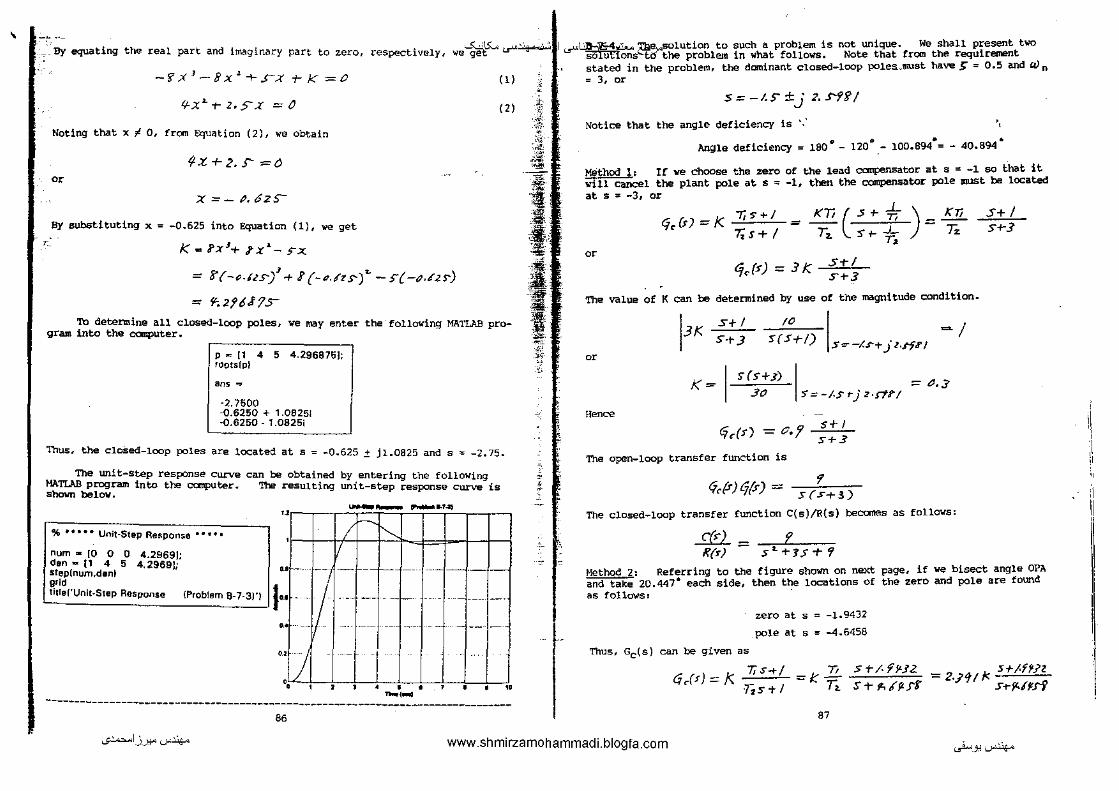
' _By equating the real part and imaginary part to zero, respectively, we~IS:... c.r'~

-::.

-'?X 1 -8x~-t-F.X t-k=O

4'-X._ +- 2. s- .X = ()

Noting that x # 0, from Equation (2), we obtain

f..:t.+2.s- =0 or

x =- "· 6zs-

ay substituting x = -0.625 into Equation {1), we get

k., i'X 1-t- .f X>.- 5":X.

= 8'( -p.us/ + f r-~Jz s-) ... - s·"(-()J.ZS')

= f'-.2t6J?s-

(1)

(2)

To determine all closed-loop poles, we may enter the following MATLAB pro­gram into the canputer.

p "' [1 4 5 4.2968751; roots(pl

ens ,..

-2.7500 -0.6250 + 1.0825! -0.6250- 1.0825i

Thus, the cloSed-loop poles are located at s = -0.625! jl.0825 and s = -2,75.

The unit-step response curve can be obtained MATU.B program into the canputer. '!he resulting Shawn be lOll',

by entering the following unit-step response curve is

% • • • • • Unit-Step Re~ponse • • • • • "I 1 1 ru TT 1 1 1 num • [0 0 0 4.2969]; den • 11 4 5 4.2969[; step(num,denl grid title('Unit-Step Response (Problam 8-7-3)")

u~-·-

'" u~--I

" 1L . '

-++I~H-1-

i

+~'

• • -·-'

• .. -------------------------------------------------------------------------------

86

~

t: ·i;·. ;l -~ s~' ·~.!!!'

-~

""' ,,.... ')I ·"-' --1 I J i ·g. ~0

t·' .'4-<' ,,

• ;

~

I ._rl.31--·;!i-4,.&.., 2:ile,.solution to such a problem is not unique. we shall present two SB!i:i"rions tO the problem in what follows. Note that from the requiremmt stated in the problem, the dominant closed-lOOp poles__must have!: = 0.5 and uJ n = 3, or

I

S;-I.S"±j 2.$-'f'i/

Notice that the angle deficiency is ·: ., .. " .. .

Angle deficiency = 180 - 120 - 100.894 = - 40.894

Method l1 If we choose the zero of the lead canpensator at s = -1 so that it will cancel the plant pole at s = -1, then the compen10ator pole lllllSt be located at s "' -3, or

(j, (r) =I<

or

7i~+l

7; s+ I = KTics+--t

T:r. s +- --L T,

'f,l<) =.? K S-t-1 S+.?

) ~ K1i

--Tz

The value of K can be tleternined by use o! the magnitude condition.

13K or

S+/

S-t-J

(0 -; S(S-t-1) S=---l.s-+ J 1-ff.J'/

I S(S+J) I ~ (J,:J

K= JO '5=-1-St)z-rtr/

Hence

{j<fr) = o,y s+ I s+.?

The open-loop transfer function is

r (j,{f}lj(.r) =

s{..s-+3)

The closed-loop transfer function C(s)/R(s) becomes as follows:

...£(d.-K(:r) -

f sz.+r.s+'f

S+ I s+-5

Method 2: Referring to the figure shown on next page, if we bisect angle OPA and take 20.447 6 each side, then the locations of the zero and pole are found as follows:

zero at s -1.9432

pole at s = -4.6458

Thus, Gc(s) can be given as

(i .. (f) = J<. 7i S+( ·Tis T I

'r, -k~ ~ ,,

87

St-/-'/1'-JZ.

S+ P.dP:J'f '= 2-.J"i/ J< S+/-f1-.i'Z

S+fl.-ll!l'f

...;~I_)_J:!"'-""'~ www.shmirzamohammadi.blogfa.com ._..i..-> _ _, '-""'.lo/<-

ii ' ' ,I il

'

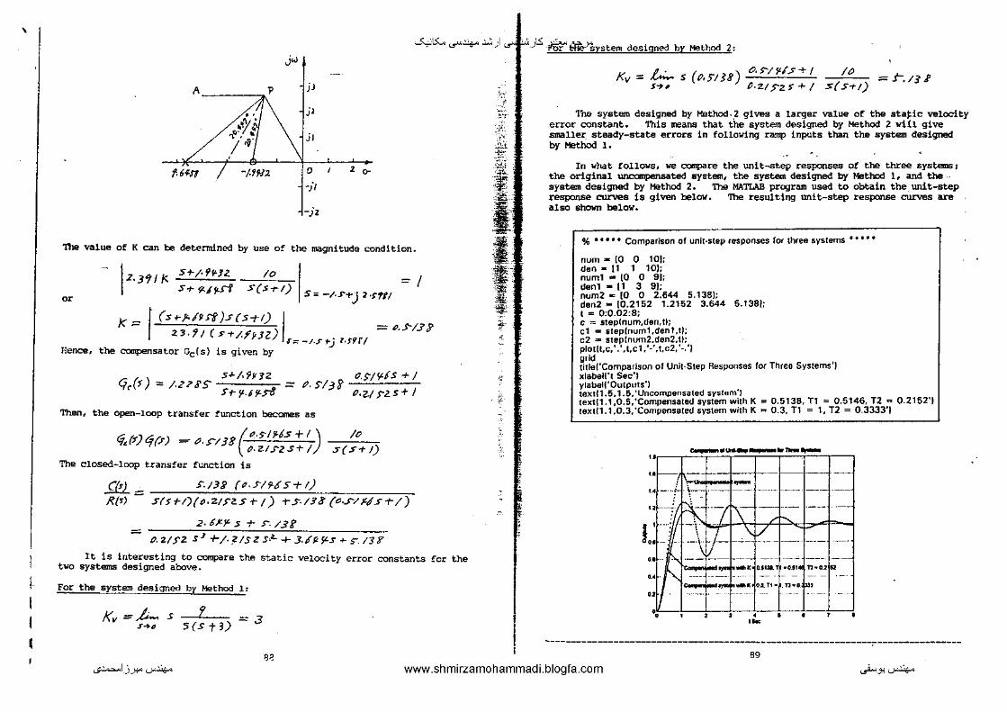
I I I I

-""'15:... ...r4-- .:.:,) '· •' 1.5: " ''.) ·riir' ~ystem designed by Method 2: jw

p j jJ

·, • I\ jl

A __ _,.

~<;.~ '\.0) .. , \ /~- ,,,

f. 6f.fT ,; jo ' '

-/.1,.12 ' ' o-~Jt

-iz

'Ihe value of K can be determined by use of the magnitude condition.

or

Hence,

/0 IZ.Jf/J< St-/•9'fJZ. s +- ?.J 'f$"1 S(s-r-t) =I

S: -/-S'+) ~ ·~'f/1

I (:S+-J<./Hf )J (:5-N} I = P . .!"/3? k:::::: 2.3-?J C :>+/.Fi'JZ) T=-/-ft-j l-!i~rt

the compensator Gc(s) is given by

S.J-f,'fi'1Z

Cir(~) == ;.Z?J'S St-'f.Jft.-o. ::::P.SI;JS 0-S"JY.i.S+/

0 ·2-I>Z.s+l

'11len, the open-loop transfer function becomes as

(_P-5"/ftiS+I_\ /0 ~~($"}(j(.r) =-t'-.>"/.JS\t~-ZI.f"Z.S+i) S(f+!)

The closed-loop transfer function is

m_ _ s-.na (t:~J/9-Ss+r)

~{r)- f(:ft-I)(P·ZI.)Z.S+/) -r.S-!33(o ... N~ST/)

.z. t)'JL s -r s: 13E

- 0. 'Z/ .f'Z. sJ T /· ,2 IS Z .s.l... + 3Jf< $LS + s-. /1 :f'

It is interesting to compare the static velocity error constants for the two systems designed above.

For the system designed by Method 1'

/(, =ft.. S S(Stl) V S~i:J ~3

"

Kv = h.. s (P-5"118) "' ;:;'

"

().~/'1/.S+!

P-zty-zs+/ /0

s(.s+t) =r./31'

"' ar The system designed by Msthod-2 gives a larger value of the staj.:ic velocity error constant. This means that the system designed by Method 2 will give ,.. J smaller. steady-state errors in following ramp inputs than the system designed

..'.ic by Method 1. ·~·

Oil'

I &­lfl: I I '~

"" .,a;. ~-

• ' ;(.

~·

·~

In what follows, we CCK!JPilt"e the unit-st.ep responses ot the three systaDs 1

the original unccmpensated system, the system designed by Method 1, and the· system designed by Method 2. The MATIAB program used to obtain the unit-step response curves is given below. The resulting unit-step response curves ue also shown below.

% • • • • • Comparison of unit·step responses lor three systems • • • • •

num • [0 0 101; den • [1 1 10}; num1 .. [0 0 91; denl • [1 3 91; num2., (0 0 2.644 5.1381; den2 .. [0.2152 1.2152 3.644 5.1381; t = 0:0.02:8; c "' step!num,den,U; ct .. 5tep[num1,denl,t); c2 .. step(num2.den2,t]; plot(t,c,'.' ,t,c1 .'-' ,t,c2, '-. 'J grid titie('Comparison of Unit-Step Responses for Three Systems'! xiabell't Sec') yiabei!'Outputs'J text{1.5,1.5, 'Uncompensated system') text!1.1,0.5.'Compensatell system with K = 0.5138, T1 = 0.5146, T1 .. 0.2152'1 texti1.1,0.3,'Compensatell system with K .. 0.3, T1 = 1, T2 = 0.3333'1

·----,--''"""'i'-...,.,.,.,.,-...,,·;4==,·r:-=:.;==--T--. "r \:.._ ...;: - ~--' -- - -·-- --

... r---,

::rf:{:f::t::t;~t~. utL_ .. .. •• ,-2 -·-~- .--· •

;:;~~~-

·~

89

...;~I_)_J:!"'-""'~ www.shmirzamohammadi.blogfa.com ~-J:l'--"'~

' ~· The closed-loop transfer function for the system is

C(s) k L 2

Rfr!;::;- 2S 2 +S+kK~o5+K From this equation, we obtsin

S~+ lt-kK~ s-t£ z ,

"'· ~ "' vz . .2>cv"= I+KK., 2

Since the darnping ratio); is specified as 0.5, .we get

%= 1-rl:k~

Therefore, we have

!+KK, 2

The settling time is specified as

«

, -=If

ts= -~~~ 5w~ ::::: (! + KI<A)/1- ;::

/£ t+KK.it .:S 2

Since the feedforward tran5fer function G(s) is _}£_ 2,;- I I

(j(.~)::::: kK., J I+ ZJ'-f(

K .)_ 2ST-f + jt:Ks. S

the static velocity error constant Kv is

K,.. = .t.;..._, s qt.s) = L s k ...1.. ..._ 1:

~15:... ...r4-- .:.:, )J._rt..:..:<_)~-~ &'-->"

J:

' :~ .,._

•\.-!1

. .;_::.!:

' -"""'

3:z < K

From Equation (3) we obtain

k So ~ 1+/<C~~ =.JZK

o•

j( ~ $"1?PP

If we choose K = 5000, then we get

,. I+ I< K, = JiK, = (PO

99 ~ =~ = O.eJI?i

Thus, we determined a set o! values o! K and Kh as follows:

K = ,SP.(1P .. ~ = P.i' IFS'

With these values of K and ~· all specificatLons ace satisfied.

\

!!::::1:§· The angle deficiency at the closed-loop pole s = -2 + j2 .[3 is

1ao•- 120•- go• = - 30"

S~P s~t> 2:S T I +KK~o S ThiEl value I!IUSt be equal to or greater than 50. Hence,

!+KK~o The lead compensa_tor l!lllSt contribute 30•.

k I+~<K,. ~so

Thus, the conditions to be satisfied can be Sllll!lliirizecl as follows:

/+-!<~

2 =If II

/+kK,~2

" It Kk11 ~ Sc

0 < KJ, < I

From Equations (1) and (2), we get

go;; !+KK~, ::::: JZK 90

...;~I_)_J:!"'-""'~

(1)

(2}

(3)

(<)

Let us choose the zero of the lead compensator at s = -2. Then, the pole of the compensator must be located at s "' -4. Thus,

The gain K

,.

Hence,

"' (•' = K S~2 '1~ / S+ 9-

is determined from the magnitude condition.

IK s+ 2 s- I = I

S-tS' .s(D . .ss+l) s~-zrjzfi

K= IS(S+•)I ~ ;,6 10 .S:-tfo}l/3

G;,(J) = ;,£ S+Z ST'f

Next, we shall obtain unit-step responses of the original system and the compensated system. The original system has the following closed-loop trans­fer function:

Cfs') "/o 1?{1) = s 1 +2.s +IO

9!

www.shmirzamohammadi.blogfa.com ._..i...>.J:l'-""'~

'

I I I I

-""'15:... ...r4--.:.:,) ..rJ-.:<_)1..5: -~ Wsystem designed by Method 2=

jw

p v ·,'I \ jl

A __ -;;<~

l'l.~ o· .. , >~· \ jjt

f,6f.J7 t!t jo ' '

-f,l"~ ' ' <>-~JI

_,,

The value of K can be determined by use of the magnitude condition.

or

Henc:e,

/0

1

2, 3"1 II< S+ /• 9¥JZ. s.,. f<IJLrf S(S-t-1) =I

S:: -/·S'"+) 2·t'111

f (srf<,/Jrf)J(S-tl) I = t'.~/JJ>

k:::: 23.f/($+J.f'HZ) •=--t.f+-jl-rPf/

the compensator Gc(s) is given by

S.f.J,'fttJZ (j""(r) = J.Z?!'S .f'+y..lft.-"'

=P-S/3S 17-~1¥-IS+/ 0 •z.ts-zs+/

Then, the open-loop transfer !unction becomes as

(:"-SI<J.ts +I) /o fi~[f)tj(.F) =-<P.r/38 o.u.,rzs+J s(s-+t)

The closed-loop transfer function is

.ff!l._ .S:/::JJ' (P.J"/'MS+I} ____ _

/?{'s) - 5'($+-l)(o.Z/J"Z..$ t-1) +S-/$3" ("·.r/J~/s+/)

2· !~r- .s T s-. /38'

- tJ.Z/.f'Z s-'+-j._21SZ5·L+3J~Y.S+5>.1'3?

It is interesting to compare the static Velocity error constants for the two systems designed above.

For the system designed by Method 1'

v, =ft... S 5(S 'f-l) 1\ ~ S~4 ~3

"

-'·-· <

:-.,. -~:-..• ~c +.•

0\> ;·~"'-

·il!l ~

1-, .

' . .

I a '!It •it ~ ~

'

e:•

I<

Kv::: £.,;,.... s (P.YJJ8) o.S"/fi..f..>-+ I s~, p,z.tyz s + 1

/0 s(.S+I) =.t-.n.f

The system designed by Method._2 gives a larger value of the staJ:.ic velocity error constant. This means that the system designed by Method 2 w111 give smaller steady-state errors in following ramp inputs than the system designed by Method l.

In what follCJWs, we ccmpare the unit-step responses of the three systeftls 1 the original WlC'OIIIpensated system, the system designed by Method l, and the · system designed by Method 2. The MATLAB program used to obtain the unit-step response curves is given below. Tile resulting unit-step response curves are also shown below.

% • • • • • Comparison ol unit-step responses for three systems • • • • •

num • \0 0 101; den- 11 1 10); numt - 10 0 9]; denl - 11 3 9); num2 .. [0 0 2.644 5.1361; den2 .. 10.2152 1.2152 3.644 5.138]; I = 0:0.02:8; c "" step{num,den,tl; cl '"'stepfnum1,dan1,t); c2 .. step(num2,den2,tJ; plot(t,c,'.' ,t,cl, '·' ,t,c2, '·.'I gr!d title!'Comparison of Unit-Step Responses for Three Systems') xtabel('t Sec') ytabeH'Outputs'J text(1.5,1.5, 'Uncompensated syslem'J text{1.1,0.5,'Compensated system with K = 0.5138, T1 = 0.5146, T2 .. 0.2152'1 t&xtll.l,0.3,'Compensated system with K = 0.3, T1 = 1, T2 = 0.3333'1

" r--,'-"i'.,.,~,, .. ,,._,;,=;-,-=,.,·r· =·=·,--1 ,_. ! •.• -· t

--/--1---t -t-1-· ... ~~ ------ ---- --" ' --·

t: ··--· o•; 1. ---- :;.. ,_.-;-,; -~--;,~

u~-N -· 0~-; .. : .. _~~·t --;:-;;j;--

" •' • • •

·~

-------------------------------------------------------------------------------B9

...;~I_)_J:!"'-""'~ www.shmirzamohammadi.blogfa.com ._..i... _ _, '-"'.lo/<o

'\

~· The closed-loop transfer function for the system is

CN K 1 R(rJ :::::: 2 s ~ +S + KKn -; -+ K = ---;sC'~+~]'_I ~r~<~K,;::-5~,_~Kii: . . z 2 From this equation, we obtstn

"'· ~ rk 1/T ' .2~w ... = I+KK.,

2

Since the damping ratio y; is specified as 0.5, _we get

""~ Therefore, we have

I+I::K., .2

!+ ICI<t 2

The settling time is specified as

"'

=if t3= -~-~

!;w, (I+ J:K.4)/'r -/6

ltkK.~, ~ 2 Since the feedforward transfer function G( s) is

___.K__ 2$-t I

C,(r) ~ I kK. +~,

l_ J

the static velocity error constant Kv is

K, = ~ s rfifs) = ~ s

K _1_ ZSt- ( 1- Kl<1< s

k _j_ "

-""'15:... ...r4-- .:.:, )l.rt..:..:<_)!Or:~ &'-->"

..\:

' :f ~-

'" .. _:1:

b-,,

'

32. < K

From Equation (3) we obtain

k sv~ I+/Cif- =J2K

oc

/( ~ S~Pt)

If we choose K = 5000, then we get

oc !+I<K, =JiK =/PO

99 K, =~-= 0.0/f'i

Thus, we determined a set of values of K and Kh as follows:

K = .SPt'P .. Aj = "·" ITJ' With these values of K ancl Kh, all specifications are satisfied.

\

B-7-6. The angle deficiency at the closed-loop pole s = -2 + j2 fi is

• • • • 160 - 120 - 90 = - 30

S-#., ¥~.:>

This value must be equal to or greater than Zs T 1-t-KKs. 5

50. Hence, !+KK"

The lead compensa~or must contribute 30°.

k I+KK14 ~SO

1bus, the conditions to be satisfied can be sUIII!Iarized as follows:

It- fC Ki. 2

~[f

/( /+KK~, ~2

I: tT I<K~-o ~ Sc

o < Kh < I

From Equations (l) and (2), we get

F~ 1-+KK, ::::- VZK

'" ...;~I_)_J:!"'-""'~

(1)

( 2)

(3)

(4)

Let us choose the zero of the lead COIIlpellSator at s = -2. Then, the pole of the ClJllilE!llSator IIIUSt be located at s = -4. Thus,

~ (•) = K S+-2. '1r: s-rsz..

The gain K is determined from the magnitude condition.

IK S+Z s- I = I

S-+ SL S("S s+l) S=-Z·•·j2{i

oc

Hence, I

S(S+ft..)l := j.6 K::::: /0 S=-2+}2fi

·Next, we shall compensated system. fer f~ion:

C,,(s) = /.6 S+Z S+'f

obtain unit-step responses of the original system and the The original system has the following closed-loop trans-

Ct>) _ /o

RM - s 1 +2s +10

91

www.shmirzamohammadi.blogfa.com ~-.,'-""'~

' ~~;-_;~nsated system has the following closed-loop transfer function:...""'IS:... ...r~ '7) tt..:..:<J-t:~~I Thus,

at s = -0.5. Then, the pola .of the ccrnpensator lllllSt be at s , -3.

C(sj - ;.t R(n- sz+.fLS+/£

1.:: program to plot the unit-step response curves of the original and

ted system is shown below. The resulting unit-step response C'llrves also 6hcMl belo1o1.

% • • • •' Unit-step responses of original system and compensateU system '• • ••

nurn "" [0 0 101; den= [1 2 10[; numc .. [0 0 16); dane- [1 4 16[: t .. 0:0.01 :5; cl "" step(num,den,tJ; c2 "' step(numc,denc,t); plot[t,cl,' .' ,t,c2, '.'I ,,. tiUeC'Unit-step responses of original system amJ compensate\! system') xlabei('Sec') ylabeii'Outputs') textl1.5, 1.3. 'Oriyinal sVStem') text(1.8, 1.1,'Compensated system')

.. r--,:~~:·~"';'-~-~~-~·~·:; .. ~·~~~;'!"~~~-~,~~·"*o;~~~~;'·~·~-~~-~

I~·---

f ••• ,,

I li

''

' '

;, ' ;~- ~

'' ... ' " '"" ' ''

-- I . ·--

i I

• ••• ' -------------------------------------------------------------------------------!!:±:1· The angle deficiency is

1Bo"- t3s" -135.:- go•

A lead compensator can contribute 90°. _Let us choose the zero of the lead

92

;'!!"

~c

~--

.~

_3 ·''-,.~

<j,(r} = K 5+ 4,S'

H> The gain K can be determined fr0111 the liBgnitude condition.

IK sns _1 I ·.' ~ I

S-t-3 sz. , S: -1-f·.JI

or

k -I (s+.j) si I = ¢ - S+t1,,r Yz:. -t~JI

Hence the lead compensator becanes as follows:

(j.(r) ~ 1- S+d..s­S+3

The teedforward transfer function is '/.S+Z

9.:f.r) fiJ(J) = sl+.Jsz.

A root-locus plot of the system is shown below.

-.t.o<:us Pkll at (411+ 2)1(1"3<-3$"2)

~ I

'

'

'

' .,

·• . ~

,., /.1., .... ,.

. •

1-t-·

~ '\\ :~

/

. • ~· " """""

~ate that the closed-loop transfer function is

C(s) _ f<.s +- Z. l?(s) - J' -t- 3S'._+ 'fs t-.Z.

'

The closed-loop poles are located at s : -1 z jl and s : -1.

In what follows we shall gi~ the unit-step and unit-ramp responses of the uncompensated system and the compensated system. A MATLAB program to obtain

93

...;~1_)_):!"'--"'~ www.shmirzamohammadi.blogfa.com ._..i...>.J:l'-""'~

II !.'

ii II ]i

I Iii ,, ill 'I

II ! I

I I II II ,, ,.

' ~~..........,_

The resulting curves are also shcnm ~~:steP response curves is given below. -""'15:... ..r~ ,£' )!Jri...:.C<_)\S -~ &'-->" __ ,,,~,-,,--,~-;e·~-,-::,-:-:::.:-:.:-:r-=-=c·,·:-=·-7 .. , % • • • • • Unit-step responses <.>I uncompensated and compensated systems •' • • •

num .. 10 0 11; .den .. 11 0 11:

numc = 10 0 4 21; denc ~ [1 3 4 21: 1 • 0:0.02: 10; cl o: step(num,den,t); c2 = step{llumc,tlenc,U; ... plol(t,cl ,'. ',t,c2, '·'I grid title("Unit-step responses ul uncompens~ted anll compensated systems'! xlabei('Sec'l ylabeii'Outputs'J text(3,0.9, 'Compensated system') Utxt(J, 1. 5, 'Uncompensated system'!

• ....__ .. ___ _

'-' _L_\ 11 1-,.

u J I "ri-f='j '\ - --1~ -1-J' -~--1(/-l~~oJ-. i . '--,--i 1:=' •• - l-- \ /' -,--.. ~~ 11 1 fi-- 1---::~--f:!=t+~--

0 ~ 3 o 5 6 7 I 5--10 -A MATLAB program to obtain unit-ramp response curves is given next. suiting response curves are shown on next page.

The re-

% ••••• UrtiHamp responses of uncompensated and compensated systems • • • ••

num"" [0 0 0 t!; den= [1 0 1 01; numc "" (0 0 0 4 2!; denc = [1 3 4 2 01: t .. 0:0.02:15; c1 = step(uum.den,t); c2 = stepfnumc,denc.l); plmlt.t.'. · ,t.c 1, '·. · ,t,c2, '·'I grid titlei'Unit-mrnp responses of uncompensmed and compensated systems ') xlabeH't Sec' I yh1bell'lnput and Outputs') textl4, 1.5, 'Compensated system') text18.6, 'Uncompensated system')

94

-· . ...:,

•.:'

~~ .)""

•

! l i

"'

•' •

·.

·------------------------------------------------------------------------~------

B-7-8. The original ~nsated system ha5 the following closed-loop trans­fer" "function:

C(') _ /6 /?(l) - sa +1-s-t-16

'lbe two closed-loop poles are located at s ,. -2 ± .j 2,f3. Choose a lag c:oospen­sator of the following form:

ffr('~) =kc s + .:. '~-'­IT

' (p>!)

Then, the static velocity error constant Kv can be given by

K" ~ _t.:... '"ic~)tj{s) = H•

h-. s~•

Let us choose Kc = 1. Then

(3= s

sK< s+f >+-'­PT

/6 .s(S+!-) =9-/K,=2C

The pole and zero of the lag compensator mu5t be located clo~>e to the origin. Let us t:hoose T = 20. Then, the Hr.g c:anpen~>ator bet:omes

Notice that

<jJs) = .L-5 + '2.0

-'-5+- (PO =

s+o.P.s­

sro,o I

s+o.os-1 ::::: o. ?'ls-o s+-o.t/ I :s-=- -.l·tp-r:r

S+P,t;$"1 / S+P.O/ J=-z+jz.IJ

= /-..< 95""+)2/3 - /-t.ff+jz.[i

= -(o.Cz!-1"+-/tJ./Zfiz" =-o.~P?7'"

95

...;~!_).):!-" '-""'.lo/<- www.shmirzamohammadi.blogfa.com ._..i... _ _, '-""'.lo/<-

'\

-""'15:... ...r4-- .:.:, )_';...rt··_J~Llll'ft~tep -The angle cc:~ntribution of this lag network is very small (-0.4999 ) and th" ' magnitude of Gc(s) is approximately unity at the desired closed-loop pole.

respons? curves obtained are shown below.

Hence! the designed lag compensator is satisfactory. Thus

fi,(<) = S"+t:?.t:?S"

sro,o 1 Let~

COII{IE!llSated S)'l>tem is

compare the unit-step response curves of the systems. The closed-loop transfer function

uncompansa ted and of the uncompensated

CO! /! -= K{.!) r -r 1-.r +- 16

For the COIIIpE!nsated system the closed-loop transfe:.; function is

Crr-J f?(s)

/6 ( .St-P.Vs-)

(5-t-P.V/) 5(f+P...) +-16 (.S+tJ,&_r-)

/ts+-o.8 SJ+P..P!S~+I5.o9-S +- o,,?

The closed-loop poles into the con;:ruter. can be found by entering the following MATLAB program

p = [1 4.01 16.04 0.8); roots{pl

ans '"'

-1.9797 + 3.4526i -1.9797.3.45261 -0.0505

The daninant closed-loop poles are located at s "' -1.9797 ± j3.4526, locations are very close to the original closed-loop poles. The~

The following MATLM! program produces a plot of unit-step response curves.

% • •' • • Comparison of Unit-Step Responses for Two Systems • • • • •

num = !0 0 16); den., 11 4 16!; numc"' !0 0 16 0.81; denc "' !1 4.01 16.04 0.6]; 1 .. 0:0.02:5; c1 "' stepfnum,den,t); c2 = steplnumc,denc,l); ploHt,c1, '.', t,c2, '· ') grid titlef'Unit·Step Responses of Uncomperosawd and Comrensated Systems') xlaUeH'Sec'J ylaUel I 'OutJmts 'J textl1.5, 1.1 ,'Compensated system') text/1.5;0. 9, 'Uncompensated system')

96

.:r:.

:~-

. ·"f~

u.~ ..... ,...,..., .. ,.,, • ......_.,., .. ~.,c .. ,.... ....... ,... .....

" 1/it O.t•·--·•··-1-·-·•·-· '<

i"t- --- -1-

Jtl11jj--U~:U3U~H

o.o•-•-·

0.2f.-/ .. +--1··--j:---J

o' .. 0 O.J -

Clearly, the sans.

the unit-step response curves fOr the two systems are approximately

For the unit-ramp response, the response curves for the two systems differ, because the original uncompensated system gives the steady-state error of 0.25, while the compensated system exhibits the steady-state error of 0.05. The following MATIAS program gives the unit-ramp response curves in the time range 95 sec .::;; t .:f: 100 sec. The resulting unit-ramp response curves are shown on next page.

% • •• •• Comparison of Unlt-Aam11 Responses for Two Systems ••• • ·-

numo.]Q 0 0 16); don"" 11 4 16 OJ; numc = 10 0 0 16 0.8); denc .. 11 4.01 16.04 0.8 OJ; t = O·O 1•100· c1 = ·stePinun'.,uen,t); c2 = step!numc,denc,t); plotft,t, ' •. ' ,t,c1, ·-. ',t,c7, '. ') v = 195 100 95 100]; axis(v) grill title!' Unit-Ramp Responses of Uncompensated ~nd Compensated Systems') xlabel('Sec') ylabel('lnput and Ourputs') text(95.5,97. 7, 'Compensated system'! textl97 .5,96. 7, 'UncompansateU system')

91

...;~I.J...l:!"'-""'~ www.shmirzamohammadi.blogfa.com ._..i....J:l'-""'~

'\

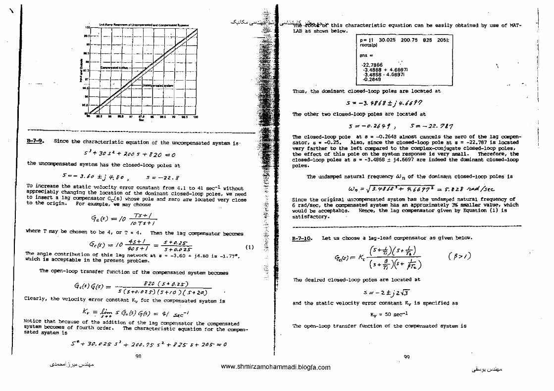
~:~,~=-=~0==·-~ ~IS... ._r-~:~l...r·~~-~ this characteristic eqwtion can be easily obtained by use of MAT­

lAB as shown below.

·r-----"- "l- !- --~;;:~~ oul- -- -- - ------ -v·· -~r---

! " "-- - - - - -~ - --r:'=~e· Jc?-~r--d=~

"• - /. -ou --[-- . -- --

·r-- /. "- -H ··~~ -- ,_ -~-r--~r---'10 •s w r>.f

k ·- • • •• • ou ,..,

-----------------------------------------------------~------~- Since the characteristic equation of the uncompensated

s.J+ J()s.t-r iJ.(JO s + !20 =o

the WlCODpensated system has the closed-lOOp poles at

s-- 3.6t:~ ±) t~;6c, :s=-zz.e

system is-

To increase the static velocity error constant tram 4.1 to 41 sec-1 without appreciably changing the location of the dominant closed-loop poles, we need to insert a lag canpensator Gc(s) whose pole and zero are located very close to the origin. For example, we may choose

C;,ds) = /O Ts+ 1 loT$+ I

lo'here T may be chosen to be 4, or T = 4. Then the lag compensator becomes

"lr)=IO 4-s+l = s+t~,.z.s-~ 'f<;s+/ S+-IP.t'ZS

The angle contribution Of this lag natwork at s ~ -3.60 • j4.80 is -1.77°, which is acceptable in the present problem.

The open-loop transfer function of the cqnpensated system becomes

£,r(:s)t:j(5) = 3'2C ( s+~.zs) s ( SH,t:!Z s-) ( :s+ro) ( S+ .za.)

Clearly, the velocity error constant Kv for the compensated system is

kv =:=f;-; s{jc.(5}(j(j) = ~/ S-(c- 1

(!)

Notice that because of the addition of the tag compensator the compensated system becomes of fourth order. The characteristic equation for the compen­sated system is

S<F-+ ?IP. P.ZS" SJ + 2t1t1. 7S _,:z. +-I' ..?S s +-;;as-= 0

98

~;

" -'-[ 1!;.

' -::.~

k "'

~~

p= 11 30.025 200.75 825 205]; roots(p]

ens =

-22.7866 ·3.4868 + 4.6697! ·3.4868- 4.6697i -o.2649

Thus, the dominant closed-loop poles are located. at

.5.,. -3. 9-1'181;} ~JDf?

The other two closed-loop poles are located at

s~-o-269-1) S= -22. 787

. '

The closed-loop pole at s = -0.2646 almost cancels the :z.ero of the lag c:arq:en­sator, 5., -0.25. Also, since the closed-loop pole at s = -22.787 is located very farther to the left CCIIil<U"ecl to the ca:nplex-conjugate closed-loop pole5, the effect of this pole on the system response is very small. Therefore, the closed-loop poles at s = -3.4868 ± j4.6697 are indeed the d001inant closed-loop poles.

The undamped natural frequency CUn of the dominant closed-loop poles is

W 11 := J .J, ¥4'.t.t 1 + $/-.£6 772. = S". IZI -'liiVJf /sec_

Since the or{ginal uncompensated system has the undamped natural frequency of 6 rad/sec, the compensated system has an approximately 3% smaller value, which would be acceptable. Hence, the lag compensator given by Equation {1) is satisfactory.

------~--------~-~-~--~-~-~~--~~--~-------------------~~-------~-

!!±!2· Let us choose a lag-lead compensator as given below.

Crc(•!}= k~ (aif){nf;) (,. :, )(wjr.)

The desired closed-loop poles are located at

:s=-2±jz5

(f>t)

anO the static velocity error constant Kv is specified as

Kv = 50 sec-1

The open-loop transfer function of the cornpensated system is

qg

....,~1_).):!"'--""'~ www.shmirzamohammadi.blogfa.com ._..i....J:l'-""'~

I 'I

' '

" ,I 'I i

'

I I

-""'15:... ...r4-- .:.:,-;1 ci<L:M_)ts: _ _p..., &'-->"

(5+f,)( s.-fz) ;o C,.I>)C,{S) ~ t:, ( -'-)( _/_ \ s (S+<)(s+s)

s.;..T, s+jlTzl

~lienee

Kv = ./i-. .s o/cf!:) o/fSJ =A ke. .--.!!!.. S~t1 $~.,. 2XS

J::e = stJ

Th~

kr:_ =SO

The time constant T1 and the value of 1 are determined from the requirements that

S+ ..L T, S1::J )t /()

S+L 7i

S(s+z)(:St--5') = I S=-2.,...j.2-Ji

_L S+ Tj

5+1_ 7i

= 7f./t'E6'

s"' -2 + J zll

The angle 79.1066 • CCXtVaS from the fact that the tead portion must compensate the angle deficiency Which is

Angle deficiency = 160° - 120°- 90°- 49.1066° = - 79.1066 °

See the diagram shCMI below.

-s -z

By using trigonometry we find the locations portion of the compensator as follows:

jW jUJ

..... 1201

o·

of the zero and pole of the lead

• ~ • ~ ~ q ~ : ~~-. .

.

- :, .

• -,~ . .

? (~ ' ~

~ 1

Hence.

.L S'+ Tj

s+L r,

?; = o. ~o7 ~

.S+Z.2!.f7

srz?.!tll

(3 = !?· 2.! fP.

_ For the lag portion, we may choose T2 = 10. Then, the lag portion may be

given by

Notice that

_L S'+- Tl.

>+-'-fTi

s+.L ~

:r+t'-1

5+ "·""$/R/1-

H..L pr, S= -2 T-jl . .fi

I :>+P./ I 5+P-fJPfl,.fl.

5:- -zrjzS

_L 5+ 1i

5+.1.. pr, "5"" -z.r.jzP

'· 998/i

= -1-IS"Fi'o

The changes caused by the lag portion are small ana acceptable. lag-lead canpensator can be given by

(j,(s) ~ )t! :s-r,;.Z/1?

s+t7.1///

s+ o.; S-t-P. PP f/ f9

The COJ!!Pensated system will have the open-loop transfer fUnction

/0

Hoocethe

lj,{s)q(<} ~ t"O(s-tz.ztn)(:NP.I) (:s t z?-/f/1 J( .st-11.# riFf£-) s(s+z){s+s)

S"tJ() .sz.r //sj'. 3J'..s t-//t?,?Ss-

.5 f" -1- .JJL. 1/'/3 :S " + 2PP.P >7t' s' -t- Z? .?. ?9'/Z .s'"" ~ 2. Z/ F!' S

The .closed-loop transfer function J::>ecOmes as follows:

C(s) ~P s~ + 1/S"f. ;1rs --+ //p. f$s-

R("f) = s~" -t- 19-; f!fjS,. + ]M. t7.J"7PS' + 772. 7!/2. S~+l///. Sill! +//'-fit"

!OJ wo www.shmirzamohammadi.blogfa.com

._..i...>.J:l'--"'~

~IJ..>!"''-""'~

r.

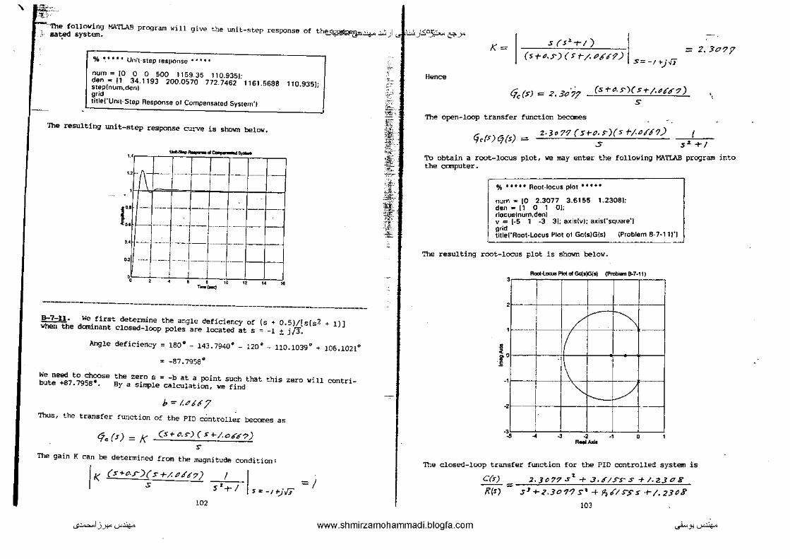
"\ L:;V:;: ~-;--

'The following MA'I'!.AB program will give the unit-step response of thEL~tft:<~ .:...:;) .l- aat;ec~ system.

% o. o o o o Unit-step resjlonse •''''

num = 10 0 0 500 1159.35 110.935); den"' /1 34.1193 200.0570 772.7462 1161.5688 110.935]; step(num.denJ grid title!"Unit·Step Response or Compensated System')

The resulting unit-step response curve is shown below.

.......... """"""-d-=--s.-

''f L 1--~-Lj-/--j--, (\I I I I 'I r,.= r l

rtl-r---i-+-+3--- -~­,. --1- i - !--~-- - +--1 i i

o.H-- -- ~--- ~-~----

~ -l-1 i --~--- - f-f--0 ' ' I

"•••••o''"'" ,_,_,

---------------------------------------------------------------------s-7-n. lihen the

We first determine the angle deficiency of (s + 0.5)/[s(s2 dC(Ilfnant closed-loop poles are loc:ated at s "' -1 ;t j./Y. + 1)]

Angle deficiency :: 160°- 143.7940°- 120°- 110.1039° + 106.1021°

-87. 7958'"

We need to choose the zero s = -b at a point such that this zero will contri­bute +67.7956°. By a simple calculation, we find

b=l.<1t~7

Thus, the transfer function of the PID cOntroller becomes as

<:fo{')=k (S+-tH') ( S+/.0615"?)

s The gain K can be determined from the magnitude condition:

IK (s+c . .r ){ s +/. t'.f 4"7) s

102

I I . . s=-J~>;ifi

=/

~--

·~c:'

~·--

~--or:~

fj .r.:o-­~---­':--<c

it-· r ~

~·-1: " ~

•:1..:..:<_)1.5:05?--- &'-->"

K=

Hence

S (S 1 -t-l)

('s -t-tJS) ( s t"/. P.{tr?) S!: -J +j.fi

Cic(>) = 2. 3o7? (s +- "· s-)( s + /.tJ,f" tr "7) s

The open-loop transfer function becomes

2· 3" 7? ( 5+P· s- )(s f-j.tJ/PJ)

2. 3o7y

..

I (jt;($)(Jj(s) = sz.-t-1 -

To obtain a root-locus plot, we may enter the following MATLAB progra111 into the canputer.

% • • • • • Roo Hocus plot • o • o o

num.., [0 2.3077 3.6155 1.2308]; den ..- 11 0 1 0]; rlocuslnum,denJ v = 1·5 1 -3 31; axislvl; axisl'square'J grid title('Root-Locus Plot ol GclsJGisl (Problem B-7·11 J'J

The resulting root-locus plot is shown below.

"'"

~ I

Root-lor::us Plol a1 Gc(•)G(s) (Probl<rn 8-7-1 t)

' I

'

·---+-' '

I -1f-- '

I -2 ---------r

I

·' " ~

/~~ 1/ I I I :\ i

,

" /

• -- '

--

closed-loop transfer function for the PID controlled system is

C(s) 2.J077St + .3.6/.SS"S' +I.Z.JO/l

/?($):::: s,+-~.Jo"l-? st + ~,rts-.>'s ·t-/.23C3

103

...;~1_)_):!" '-"'.lo/<o www.shmirzamohammadi.blogfa.com ._..i..>_., '-"'.lo/<o

' ;~-~-. -~-

~~'- Tb obtain the unit-step response curve, ·-:- grlllll into the canputer. The resulting

-~15:... ·4-- .:.:, ,[" .,. )1.5: '" we may enter t~ following M.\~pro- --r - ·-Thfs~?ggests that the controller should have tvo zeros near point s = response curve lS shmm below. ;E'- . Therefore, we choose the controller Gc(s) to have the following term:

% • • • • • Unit-step reSJ!Onse '• •' •

num .. ro 2.3077 3.6155 1.23081; den= 11 2.3077 4.6155 1.2308[; slep(num,denl grid title('Unit-Step Response of Comp~tnsated System (Problem 8- 7-111'1

'7.:(s) ~

(It is a PID controller.)

K(.J-r-z-/

• Let us plot a root-locus plot for this system. Note that

cl<(r)6j(') = K(S-t-2)&

• /0

s~+2

/OK(S"+9-S+.;.:.)

= s'+z.s:

-2.

---"-:r==-:;==·=-::;==::.;-==-=·i·=-==~::.;·':"c.-, "c The folloYing MATI.AB program Yill produce the root-locus plot as shOJI'Il below.

(\

~::rct=t=tt1~ o•fl --[-~ .. -~ ---1--0--+----·--o----

···--1---1---f---f--1- -1----<

• • • • r..,.(OE! .. " ..

-------------------------------------------------------------------------------B-7-12. The system needs at least one integrator to eliminate offset in the step response. Therefore, the controller should include an open-loop pole at the origin. Suppose that ~ want to have the dominant closed-loop poles around s = -2 ± j2{:i. Then, the angle deficiency becomes as follows:

Angle deficiency= 180•- 134.29424•- 112.29253"- 120~

-186.58677 °

See the diagram shown belo\i, jw ,,

_, ' ~

-j~

10<

'

-~ " ' f' f = ~ "'"' :r: -· • ~ '•" '

...;~I_)_J:!"'-"'~ www.shmirzamohammadi.blogfa.com

% • • • • • Root-locus plot • • • • •

num=IO 14 41; den- [1 0 2 OJ; rlocus(num,denl v -= [-8 2 ·5 51; axis(vJ; axis(' square') grid tltle('Root-Locus Plot of Gc(sJG(s) = 1 OK Is· 2 +4s+4lllsls "2 + 2)1'J

Root-l..call Plot al Gc(•)G(•J. 10K(a"2-)11(t"2+2)J

i I

:·r=-l-::~=e-,=t;"':::J ' J,L .../•luJ' k.r

' I , r I \ Jo I

_, - f- -~l--------,-----7' ' r---__J_~. y = :---+ I I .

! .

• • ... • • < ' ' --

105

._..i...>_J:l'-"'~

'\

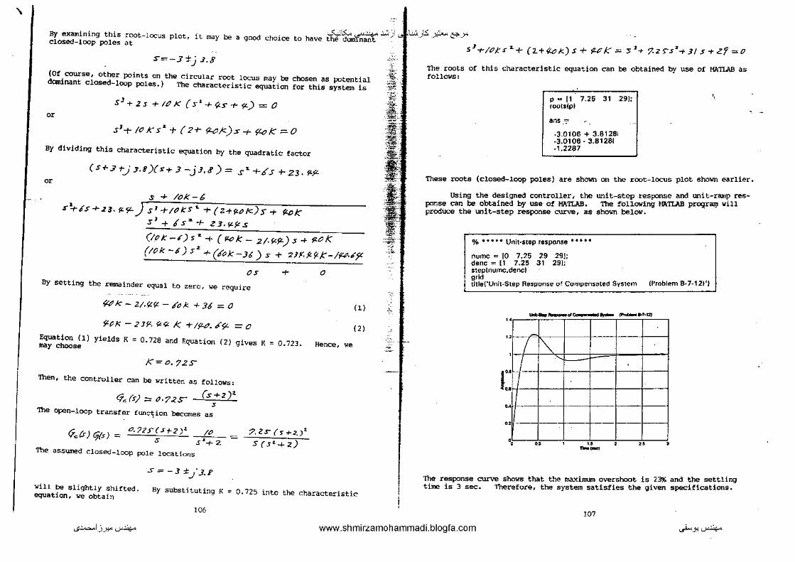
-~15:... ...r4--.:.:, ·I By examining this root-locus plot, it may be a good choice to have the dominant " closed-loop poles at

S=-3±j .1.8

(Of course, other points on the circular root locus may be chosen as potential dominant closed-loop poles.) The characteristic equation for this system is

s' + z s + 1~ K { sz + Y-s + 9-) = 0 or

S1+ /OK sa.+ (2+- tfLO.K)s+ fl.oK =0

By dividing this characteristic equation by the quadratic factor

or ( S+J t-j .7,8 )(s"t" 3 -j J, &') = s"" +6 .r + 23. f4P.

s + /ok-6

r~Fs + .Z3. f49- }s1 + 101: s .. + ( Z.-t-f/.() !<) s -r fr.oK s 1 + tfsz + Z3.SL9.s

(IPK-~) sa+ { F<:!k- 2/·f/.fL) s + fl.OK

(!Ok -~) sz +(tfok-:u) s + '2J~.fc?-k-l~·.fjZ

Os By setting the remainder equal to zero, we require

~ k- 2./.t,t.r;t. - /() .k. + 36 = 0

ilt?K-21~.~-;;:J< -t-1{47.69- =o

+

Equation (1) yields K = 0.728 and Equation (2) gives K ~ 0.723. may choose

K=o.72.s-

Then, the controller can be written as follows:

(s+z)t £f"'(s);:::; P·7.<s- :s

'Ihe open-loop transfer func~ion becomes as

.-= _ o.?2F(5+-2)z _____!!!_ Vet>) q{$)- s s•+ z

'Ihe assumed closed-loop pole locations

.S= -3 :tJ3.1"

P.Zr(~+-2.Jt

S(s~+Z)

0

(1)

(2)

Hence, we

~ill be slightly shifted. By substituting K: 0.725 into the characteristic equation, we obtain

106

-:c•-

l -"'!_~

i":.,; -~-

-~-~--

1' "i!.i",

1f'

F' :-# .:r.

.;.

•:1...:..:<_)1..5: _ _y?... &-..Y'

s-'-r-;o;:s"-+ (l.+~l<)s+ .p;cf::;::;:. ~ 2 + 7.z>s 2 -+JI.s+Z'i=o

The roots of this characteristic equation can be obtained by use of MATU.B as follows:

p .. [1 7.25 31 291; roots(pJ

ans =

·3.0106 + 3.8128i -3.0106-3.81281 -1.2287

'•

'

These roots (closed-loop poles) are shown on the root-locus plot sho\lll earlier.

Using the designed controller, the unit-step response and unit-ramp res­ponse can be obtained by use of Mli.TLAB. The following Nli..TIJ\B prCJL:lraJ!I vill produce the unit-step response curve, as shown below.

% • • • • • Unit-step response • • • • •

numc = [0 7.25 29 29]; denc"" (1 7.25 31 291; step(numc,dencJ grid tltle('Unlt-Step Response of Compensated System (Problem B-7-121'1

~-"'~.,_ -·1-12) .. ., r-y '

......

l " - ---- -

" " ---- ---" -- --- ·-- ·--!--

"• "' ' ..• ' ..• • --The response curve shows that. the maximum overshoot is 23'!1> and the settling time is 3 sec. Therefore, the system satisfies the given specifications.

107

...;~I.J...l:!"'-"'~ www.shmirzamohammadi.blogfa.com ._..i...>.J:l'-"'~

'\ ~ MATLAB program shown next produces a unit-ramp -""'15:... ...r4-- .:.:, ) ._r\1:<_)1..5: -~~ response curve. _._. I following diagram for the computation of the angle deficiency.

% • • • • • Unit·ramp respons11 •• • •'

numt - [0 0 7.25 29 29]; dun1 "' [1 7.25 31 29 OJ; I "" 0;0.02:3; c ... step[numl,denl.tJ; plot(t,c, '·',t,t,'--'1 grid title('Unit-Ramp Response of Compensated System !Problem 8-7-121'1 ;o:labell't Sec')

_ylabeU'Inpur Ramp and Output'] •

1118 resulting unit-r<UI!p resp:>nae curve is shown beiow.

~.;,I;~ ·!'--

~;-~i _ .. , , __ _

'~···

--.,~- -H-02)

! I l 1

'

" '

•

'

'/

'/ 1/

!/ I/ f-!/

-

•• o.5 ' u z 2-5 l

this system is

= {.:.... s H<

?.zs (s-.J.z)l S{s-a+z.)

·-= /:!; s-

error in the unit-ramp response is

es .. =+== I "II /St'.S =: "-"61'Pi

~---•-- controller is acceptable. .. · roUU. can be designed for this systE!II.

ot mny pJUible controllers, )

(Note TI>e

that infinitely many other cent­present controller is just one

-------------------------------------------------------------------------------~- Let us choose the dominant closed-loop poles at s "' -2 ± j2/3. Then, the angle deficienc-z at a closed-loop poles"' -2 + j2/Jbecomes as follows;

Angle deficiency 1eo•- 120G- so"'- 106.1021 .. + n3.4132~

:: -22.6889G

lOB

:z: -"'­' :.: '

•:l

--,

J•

j2.fi /(1/.ltiZ/ 0

f/J,,/)2' \

-ltl-ltf'l

~l-lrl1" '/:J.~·

•Ill -r _, -· _, etl (t--

From this diagram we find the zero of the ccmpensator to be at s = -10.2857. The compensator thus can be written as

o/drJ = K { S+/P, zN7) The feedforward transfer function be!;:Oltll!s

<j.!r) 'iff)= K(S-rf",ZIS7) (2s+l)

S(S+t)(S+2)

The gain K can he determined trom the magnitude condition:

O<

Kr $+/8. ur? Jr z$ r-1 J s(.s+J)(n-z) .s:"'-Z-1-j2.{3

~I

k --I .S($-tJ)(~t-z) - (St-/.,1,:zi'".f'7)(2S"TI)j s .. -.J.+jN~·

The evaluation of this K can be made easily by use of Ml\'I'Lli.B. MATLAB program produces the value of K,

% ••.••• Determination of gain constant K •• •• •

a"' 11 3 2 OJ; b "' 12 21.5714 f0.2857J; s = -2+J"2"sqrt(3!; lormatlong K .. abslpotyvalla,s))/abslpolyval\b,s)J

K =

0.73684318666243

Hence, the compensator becooles as fol1011s:

GJJs} ::::- (), ?.J6 FfL { S + /0. Zl 5""1) The closed-loop transfer function becomes as

109

The folloving

,_;~l_)___l:!"'-"'~ www.shmirzamohammadi.blogfa.com ._..i..->_J:l'-"'~

' ·-~~' ('(r)

/l{r)

~IS:...._r4-­/. Y:'?U f s ~-<- /J.~. 31' ~.f? 5 + tJ. .>?J'f /.r

s~ + Y., (l.'J,36? s 'l: T /'/, S 9i<?S +- ?.' f'?lf/s-

The following MATLAB program will produce the unit-step response curve.

% • • • • • Unit-step response • • • • •

numc"' 10 1.47368 15.89467 7.578915]; done·.., (1 4.47368 17.8947 7.578915/; t ... 0;0.01 :5; c "' s1ep[numc,denc,tl; plot[I,C/ grid title['Unit-Step Response of Compensated System (Problem 8-7-13)") J<labeH't Sec') ylabeH'Output'/

The resulting unit-step response curve is shmm t:elow.

........,,.,._ .. coo.-_ .-~·1>1 '

!r +- -

. .. , " g·· • • • --

,

• • .. ' .. , u • .. • .. • Ok

The response curve shows the maximum overshoot of 13% and the settling time of approximately 3 sec. Thus, the designed system satisfies the requirements of the problem.

~-' The first step in the design of the compensator is to choose the desired closed-loop pole locations. Considering the open-loop poles of the plant and the given specifications, we may choose the dominant closed-loop poles to be

S=-?-±jf

(Of course, other choices can be made.) With the present choice of the domi­nant closed-loop pales, ve may choose the compensator to have a zero at s = -4

110

~-"-

_,_

,-

-Ju..:<).SO~~_?E! plant pale at s "' -4 can be canceled. We may also include a zero -L - - • Thus, we may choOse the transfer function of the canpensator to be

C,Jr) = K (s-+-td(.s+l) s+h

where the compensator pale at s "' -b need be detetlllined based on the angle defi­ciency. The angle deficiency is , ,

Angle deficiency = 180• - 135°- 135° + 126.8699• "' 36.8699°

The compensator pole must provide an angle of -36.8699• • given below we find b to be -9.3333.

From the diagram

-9- .. j!l-

-1#-Uif'

~6. rl ft' I

-10 t _,

-'i.HJJ

Then, the compensator Gc(s) can be given by

GJs) = K (S+~)(:>+!) St' f. 3J.?J

'" - -~j~

,,

,~s·

-1 (/

-,jl.

The open-loop transfer function becomes as follows:

~

{j<(r)(i{s) = K(:S+'I-){S1"1) K(S+!)

(S+f,J3.33)S 2 (S+<;4) ::= -s•(:s+f,H3.J)

The value of gain K can be determined frOlll the magnitude condition:

or

K(s+l) I =I st(s+f.HJ3) .s=-~t")'f

I< =I s1+7.H33S?. I

S+ I :s ... -y.+j9

The value of gain K can be determined easily by use of MATLAB. lowing MATLAB program:

lU

see the fol-

...;~I_)_J:!"'-"'~ www.shmirzamohammadi.blogfa.com ._..i...>_J:l'-"'~

'\ -""'15:... ...r4-- .:.:, ;I ._rJ'..:<_Jts: -~ &'-->" The closed-loop poles are located at s = -4 ± j4 and s ~ -1.3333 as seen from

% •• •• • Determmation of gain K • • •• •

II = (1 9.3333 0 0[; b - [1 1[; $ "'-4+j'4; K = abslpolyvalla.sll/abslpolyvallb.s!J

K -

42.6665

Hence, the compensator becomes as follows:

(j& (s) =:; ~ 2 .1'/6 s- (s+~)(s+t)

Srf. ~333

The closecl-loop trai1ster function of the designed system bec:cmes as

C'(!) _ f<-Z.U/S"S + t.Z./#5S'

Rrn - s 5 +-9. IJ:I.J $ .. + '1--Z-/I/ss + ~~.1'//.r

The following Mi\'I'I.AB program produces shown below.

the unit-step response curve, which is

% • • • • • Unit-step response • • • • •

numc =- 10 0 42.66fi5 42.6665]; denc = (1 9.3333 42.6665 42.6665]; step(numc,dencl grid titlei'Unit-Step Response of Compensated System !Problem B-7-14)')

---- ~ .. - .. I

<;-

t-~ ' I +- '

i " r..l--I

-" - ·-~~ ~I . -r-.: . ---cj 1-]- ...

' ... •• ' •• --

"~ ';':";-~

,g, !it

Ill.

~~ )11&.

~-~·

.

---!-~-

'<· c.:J;-_ _,..__ "'

the following MATLAB output.

roots!denc)

ans ':'• '•

-4.0000 + 4.0000i -4.0000- 4.00001 -1.3333

The unit-step response curve shows that the ma.xil!lll!ll overshoot is approximately 25% and the settling timE! is approximately 3 sec. Hence, the given specifi­cations are met and the designed system is acceptable.

---------------------------------------------------------

113

...;~1_)___.1:!-"'---"'~ ,,., www.shmirzamohammadi.blogfa.com ._..i..->_J:l'-""'~

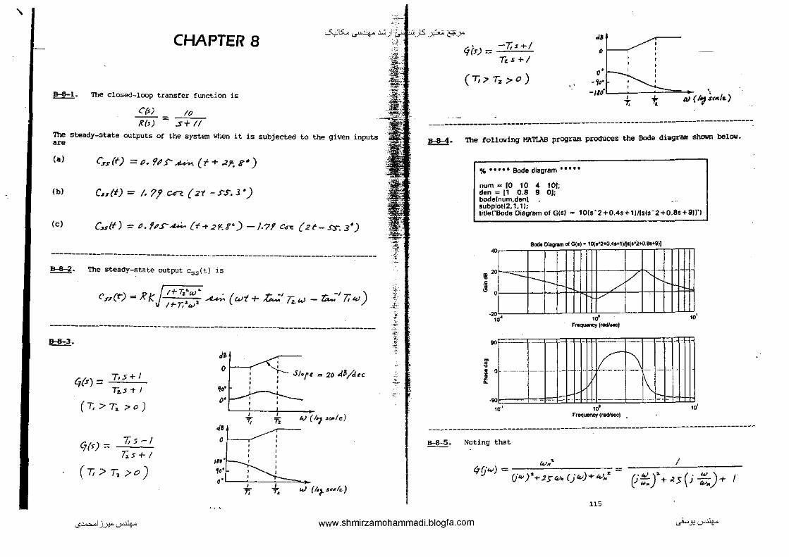
' CHAPTER 8 ~IS:... ...r4-- .:.:, ) ·~_Jts: -~ ~-->" - r; s +I

- .. - l/(s) :::= ~r.-',"-~=-+'-1-'-.. '

!t::!!=!· The closed-loop transfer function is

C'(s) /()

K(J) ::; ..S+ II The steady-state outputs of the system when it is subjected to the given inputs ON

(ol Css{f) = p. 9-.c- AM< (t + .21'. li'•)

(b) Cult)=/. 7? ""'- {2t -ss-. J•)

(c) C.ss(f) ~ o.IP.r-~ (t-+2r.-.r) -/.?! ~ {2t-ss.3•)

------------------------------------------------------------------------------!t:!!::l· The steady-state output c55 (t) is

c ST(t) - !? K t+- T: .. w .. ~ {wt + ;/;...:.' 71.. w 1+-T,:t.ll.)l.

- ta--l Tt 4))

-------------------------------------------------------------------------------~-

t;(s) = T,s+l

T2.S 1" I

(T.>T,.;:-o)

Cj(<) = T, s -I !;.s+l

(Ti>J;>o)

J> 0

,,. •• .. 0

,n·l ,,. ,.

., -

' T,

.L r.

, Ti

t,

Sloft .. 20 48/J~c

4J (~~~~~/e)

I.e) {l.}.s~,/~..)

·'iS_

;: i. ·•--;

•?·

~ "-'

(T,7T,,.o) ,.

··~ -uo· ' t. T,

\ 4) ( '1 Stff.fft. )

-------------------------------------------------------------------------------........ 'Ihe following M!\TLAB program produces the Bode diagram shown below •

% • • • • • Bode diagram • • • • •

num .. 10 10 4 101; den = 11 0.8 9 OJ; bodelnum,denl subplot(2,1,1); title("Bode Diagram of G(S} ,. 10ts• 2 +0.4s + 1}/lsls· 2 +0.8s +9)]')

·1)1[t( .. 2+0.Bo+9)J I() .,.....,u.,,..,.,~....,•l ,.,.~·-.,- ...

• ~

'f-=:::j:::::II-----T+-1-H+I V ' /

' ' ,.. ,. .. -Fr.quency (fld/MC:)

10~ l-::::::t t==t ++H l ! ! ! ++4 -Hi

Ill\ [ I 1111Jm [NdJlli -90 --·~-~ 1~ ,~ ~

.. r Frequency (radlsee)

-------------------------------------------------------------------------------B-8-5. Noting that

w.. - ----'-'--,--:-:--:---¢'[jw) = (jw)&-+-.2$'41"()"-')+-W"z- ~'':..J'+.?J(i ;:;,)+

U5

...;~1_)_):!"'--"'~ www.shmirzamohammadi.blogfa.com ~-.,'-""~

' '-""- ' ' "'~:.+·· " ' -.. ...r'"'-+"......,.::5: ')"" "-'-"-"'"-"' - -~--...._ .. )"' The MA'TIAB program sho-.m next vill produce a Bode diagram where the phase curv€-

we have

l'lDw.JI = 1-/ +;>j +/ i= -'­•s

-------------------------------------------------------------------------------B-8-6. A Bode diagram for this transfer function obtained by use of MATLAB versioo 3.5 and that obtained by use of MATIAB version 4.0 differs slightly. 'Ihe pha:se curve· obtained by use of MATLAB version 3.5 starts at 0 • and ends lBO•, while the phase curve obtained by use of MATlAB version 4.0 starts fr· _ -360• and ends at -tao•. However, if we add a very small nonzero coefficient'~· to the s term, that is, change the characteristic equation to -~

S' 1 +SJt.T E.S+ I =0

where t. is a very small nU!IIber, positive or negative, then the Bode diagram obtained by use of MATLAB version 4.0 changes. 'Ihe phase curve starts frcm o• and ends _at 1ao• (the same as that obtained by use of MA'J'.[AB version 3.5).

The follOwing MATLAB program produces a Bode diagram where the phase starts fran -36o• , as shown in the Bode diagram shown below.

% • • • • • Bode die gram • • • • •

num ~ (0 0 1 0.5): den~ [1 1 0 1]; bodelnum,den) subp1otl2, 1.11 titlei'Bode Diagram of Gls) "' Is +0.51/ls • 3 +s· 2 + 1)')

• s

ro

•

~

" '

··t_ ~"~b ~

• "

8odl Di11Jwn d G(•J" (a.O.Sy(~•1)

IIIII -.._

' 10~ 10' ,. Frequency (nod/sec)

~----·--·-

'"1-!O'' ,, ,.

F-(r:acr.e)

.-'i­'i!!" t;t;<· ~· ._.<li; .,. jE. ~

-~-:s:

;i '·

starts from o•. See the resulting Bode diagram shown below.

% • • • • • Bode diagram • • • • •

num "" 10 0 t 0.5): den = 11 1 o.oooooooboooooooooooo1 11: bodelnum,denl subp!otl2,1,1l tltlei'Bode Olagrem of Glsl ~ Is +0.5JI!s "3 +s • 2 +Os + 11"1

~ --..- .. -- ---· "

• ! 0 ' ~ iII II

·" ,. tO'' ,,

F..quenq(1'11C14o0C)

teo: •f-· I--

• l • -- ----- .. - -

0 • .~ ,. ,. ,, F.--(nod!Me)

'<

"

'"'

-------------------------------------------------------------------------------B 8 7.

lm (b) T>];.)o, T'71j>O

~ --- 0 ~·

(4) T.>T>O, iDT>o

------------------------------------------------------------------------------

117

...;~I_)_J:!"'--"'~ www.shmirzamohammadi.blogfa.com ._..i.,>_J:l'--"'~

~

-.!!::::§::! •

lm ~{J) Pf~t-

Im F:z{~) Pllnfl.

,, Re

I•J I b)

' '' ·1--""'IS:...._r~......,_,

,,..

+:. _,_

j£ ·Jo-~

<tr ~­}ff,I'

------------------------------------------------------------------------------- I. left

. .... _..

Im

..--+-... / w< '

-1 0 Re

">o

The stability requirement of the unity feedback control system with

«n~! = /<(1-Jw) ) ,;W+/

is that -K be greater than -1, or

t:. < I Since we assume that K > 0, the condition for stability is

1>!<>0

~- A closed-loop system with the following open-loop transfer function

K Cj{s)H{s) = sz(T;s+/) (T,>o)

118

. . ,-. .

·>i> ji_

·~ ·if "7' -<-'-

·:<;>-

-"-

~;

·::_).5J~~9J.e, while a closed-loop system with the following open-loop transfer function is stable.

K(U,H!) tj(J)f/{$) = s~(7;s+t) -(Tz>J; ;>0)

Nyquist plots of these two systems are shown below.

4(s)Hf~)"' ( U .. :s~.-.bl~) s•rr.s+O Im

~·, K(Tr. S'f-f) ( )

{J(r)H{t)• ) Sf"b/t> s'(7is+l

(T1 ;>T.> o)

Ke

-------------------------------------------------------------------------------IHI-11.

~ .. ,::' .. t I

?/lid ftH ?14M ..

K= IO .St.,J.lc

tAJ,.(}-~(11-oo>

\ ~ -II \'oVI /lie t.J,.o+ -~ ,_ ~~~ .. - .. ,, w~o-

K=t St .. ble

.____j_/ ~ ,., __

The system is stable for 0 < K < 16.8.

-------------------------------------------------------------------------------B-8--12.

{j(j«>) HyN) = ke- 2J..;

j'<'

friUw)H{i•) = / c.n. 2"' -j_..;. 2"' - ,90 '

.... -:?11)- ?o"

119

...;~1_)_):!"'--"'~ www.shmirzamohammadi.blogfa.com ._..i...>.J:l'-""'~

' The phase angle becanes equal to -180° at 2 w = t-he magnitude jG(jw}H(jW)Jat w= ?r/4 must be noting that

_•;: .. ;)S:... ._r4-- .:.:, •I _;;G:IIts: ~ :9 ~ rad/sec. F~r stability," -- I -The "fOllowing MATIAB program produces the Nyquist plot sho1m below.

/"v-'J H!i., !/ =

we require that K < ?l/4 for stability.

k

"'

"/2 less than unity. Hence,

----------------------------------------------------------------------B-8-13. The following MATLAB program will produce the Nyquist plot shown

% • • • • • Nyqui$1 plot • • • • •

num = [0 0 0 lJ; den = [1 0.8 1 OJ: nvquist[num,den) v "' [-4 4 -4 4]; allislvJ; axisl'square'J grid tltlei'Nyquist Plot of G(s) ~ 1/[sls"2+0.8s+1J]')

• ~Plot CJI G(a) • tJ[-tr'2'<1.a.-t)l

I I 't'lr --+rr I I ' ' I I ----;---

!' I '=R '[-' --t- -1- --- --• ' I I_ I 1" --i i ~ 1--- . I ~ I ' ~----+--" -- --- '----1 j I _, ' I I I I I-~-

,,_ ,. -t-- -+--4 I I I -4.J-2-10t23 • .......

-------------------------------------------------------------------------------in the right-hals s plane, as B-8--14. Note that G(s) has two bpen-loop poles

seen from the following MATLMI output.

.-=--------,----. p=[1 0,2 1 1]; rootslp]

ans "'

0.2623 + 1.1451i 0.2623. 1.1451i

·0.7246

120

-.

'"·

'!I> • • • • • Nyquist plot • • • • •

num- [0 0 0 1); den- 11 0.2 1 1]; nyquistlnum,denJ v- [·1.5 1.5 ·1.5. 1.5]; axis(v); axisl'square') grid • "tlai'Nyqulst Plot of GM - 1 /Is· J + 0.2s · 2 +s + 111'1

,_,

' ,, ,,

~ l •

_,

'

•

'

-~ ~

'

_,

JW.oirll Pk:t ol G(t). 1J(N+O~+a+1)J - - - -

/

~~ I L1

"--

I I ..f.l.5 0 0.5 '·' --

From the plot notice that the critical !Xlint (-l+jO) is not encircled. Because there are two open-loop poles in the right-half s plane and no encirclement of the critical point, the closed-loop system is unstable.

~· The following MATI.AB program produces the Nyquist plot shown in next page.

% • • • • • Nyquist plot • • • • •

num = [0 1 2 1); den"' (1 0.2 1 11; nyqulst[num,den) grid titlel'Nyquist Plot of Glsl = (s • 2 + 2s + 11/ls • 3 +0.2s • 2 + s + 11'1

Since G(s) has two open-loop poles in the right-half s plane (see the solution to Problem B-8-14) and the Nyquist plot encircles the critical point {-l+jO]

"' ...;~1.).):!" '-"'.lo/<- www.shmirzamohammadi.blogfa.com ~.J:l '-"'.lo/<-

~

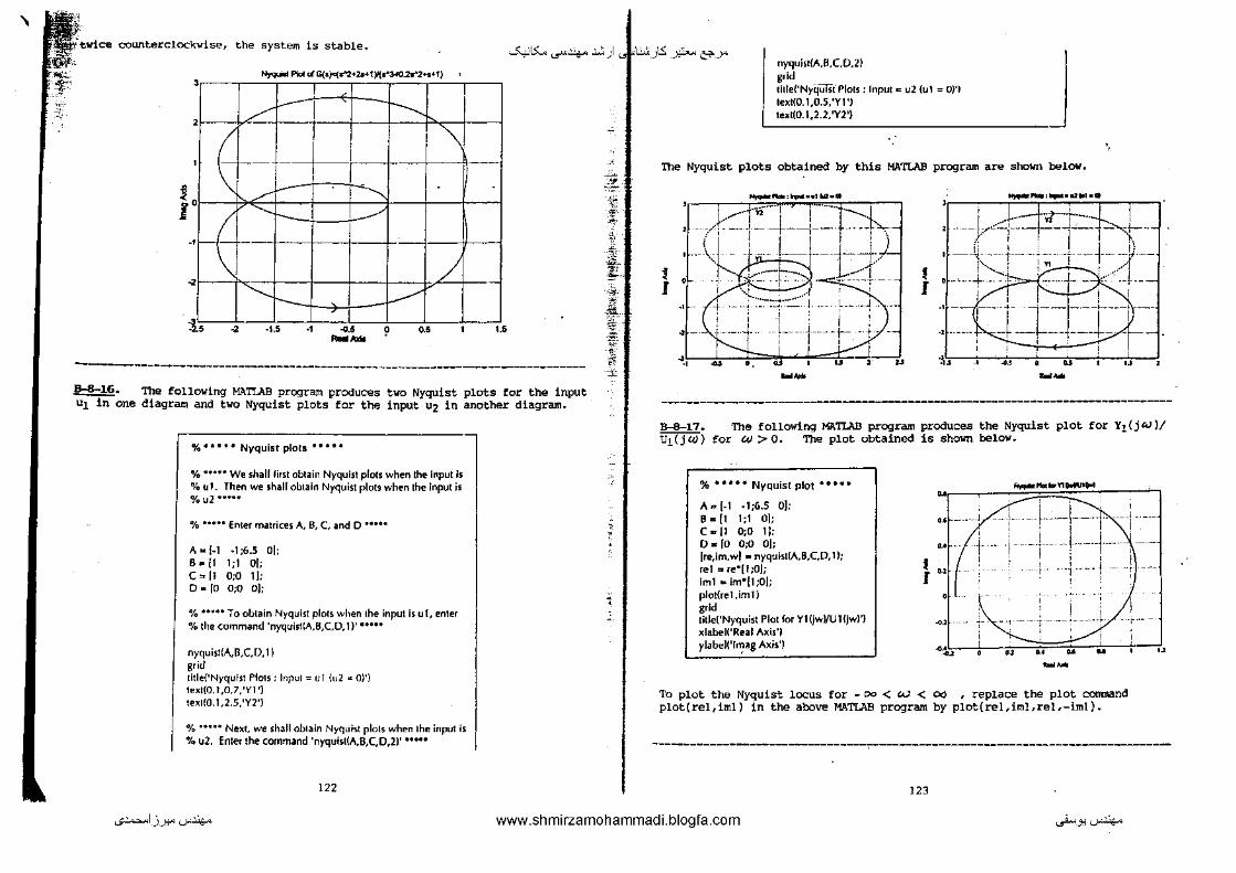
counterclockwise, the system is stable. -""'15:... ...r4-- .:.:, ) ..J<t..:..:<_)ts: -~ &'-->" ny<Juisi(A,B.C.0.2) J

~ P1c1 d G(s)'o(~•WI)I(r"J.<028"2+sH)

~ I

,

' / ./' _I

1 -+-~-' :~---

' " _/

, r . I~

_, ( '---'/

I

\ • '------ I :j', . • .. ·1,5 .

Ra!~ 9

...._____

I ""\.

-

/

---"" •• .

-

-

... --------------------------------------------------------------

B-8-~6. 'The following MATI.AB program produces two Nyquist plots for the input Ut in one diagram and two Nyquist plots for the input u2 in another diagram.

% • • • • • Nyquist plots • • • • •

% ••••• We shalt first obtain Nyquist plots when the Input Is % ul. Then we shall obtain Nyquist plots when the Input is % u2 •••••

% ••••• fnter matrices A, B, C, and 0 •••••

A"!·l ·1;6.5 Ol; B•fl 1;1 Ol; c .. [1 0;0 1]; o. ro o;o oJ;

% ••••• To obtain Nyquist plots when the input is ul, enter %the command 'nyquistrA,B,C,D, 1)' •••••

nyquis!(A,B,C,O, 1) grid title('Nyqulst Plo1S; lnpul = ul (u2 "0)') l~xi(O, I ,0.7, 'YI ') lexi(O.l ,2.5,'Y2')

% ••••• NeKI. we shall oblain Nyquisl plols wh~n lh~ inpul is % u2. fnler !he command 'nyqulst(,A,,8,C,0,2)' •••••

122

,::t ,., ;€' . ..,.

~ ,,_, ·ill'.. ~­-~

!. {f :;>!:

it Fe .,.

' "

'

goid lille('Ny(jUisi Plots: lnpul c u2 (ul = 0/'1 leKI{0.1,0.5, 'Yl ') tu1{0.1,2.2.'Y2')

•,

the Nyquist plots obtained by this MA'I'LAB program are shoWn below.

-- -··•W•,. 11 I .J--~-~1 ' 1' '"·--~

l I ,, ·---··· ~ .. ~· •• ~ .. -1' ·t ·~ .. ~ ... L -- .• ~

' ~~--'\.i---"i-"

·­_, ~ o ' o.J I

~-

' < ,---- I

' I

u

I l

..,..._,_ ......... -· -1.-~+::j:-!:.-:rl>hL

(. I , ·\

--l-.:..-· +·-- .. ~~-· •(-~+- -.:r·--..j.. .•. ·:-:i. 1

... ... L _ ' .. :···<J ... i 1 I · ' ' I !

-·~- ----_ ... _ r·-- -·--·----t .. ___ LJ_ -- ---L-J ... ' ••

' u

~-

,,

B-8-17. Ul(jW)

The following MATIAB program produces the Nyquist plot for Yl(jt.J)/ for (A)> o. The plot obtained is shown below.

% • • • • • Nyquist plot • • •• • u,

.._ ......... '"'"" .... A-[-1 -1;6.5 0);

•• ~· -I -1--l'"- !---B •II 1;1 0]; c .. ,, 0;0 I];

I : I 0"' [0 0;0 0]; U··· j· ~---• [re,im,wl•nyqulsi(A,B,C,D,ll; I • I ; I rei :ore"[l;O]; } .... : ·l .... j lmJ,.im"[l;O]; plo!(rel.iml) ,, grid titlei'Nyquist Plot for Yl(jwl/UHjw)') 1

~· •· '- .. , ·- - ; ..... - ·--- .... / ., ....

xlabei('Real Axis') yl~btd('ln:aag Axis') I ..,, • ~ •• u u ' u

~-

To plot the Nyquist locus for -DO < W < OQ , replace the! plot cotm~ano:l plot(rel,iml) in the! above MATLAB program by plot(rel,iml,rel,-iml).

123

...;~I_)_J:!"'-""'~ www.shmirzamohammadi.blogfa.com ~-.,'-""~

' * !::!!::!!·

l«!i~J I~ j,.,.,.+ I

"'. '

-""'15:... ...r4-- .:.:,)

/c10·t.>) = ta..._-'aw -/SO~

~ 'I1Ie phase margin of 45" at c.; = 4J 1 requires that ,,

c

'lbus, ve have

)a2W,'+t

w• '

=I

tw.-'Aw1 -ltfoe;:;:; ft.s•-;so"

t:t ~cv/ +I = UJ1 ,. j aw, =I Solving for a, we obtain

a-fl_\t -lli" _/ = P, N-1

----------------------------------------------.!!±:!2· A Bode diagram of the system is shown below •

From this Bode respectively.

• ,b

• , I

~ •

-· •

" "

-. -. '

' + _,J, ' ' ' ' '

~ i ' '

' •

,_, .. , ;.1 I

~

~4.t~:m

oil AAooih-

I I ~·

m• II-' i

I -l/11"

" j~ ,,

diagram, we find the phase and gain margins to be 21• and 13 dB,

------------------------------------------------------------------------------

124

{.

.t :_,-

1,~ ~ -·.

-;~ -~-

;i;-:<~-

;~ -=:co -31. --~

·;:_)S:~y

•

• a ' • ' f.fU<IJ

' '

" : '

•• • \ ' ' ..

' ' ' ' ... -· • +Jill ,,,

-.,,.

·;·t' ••• 1.

-- ...... """ ' ' ' • • • •• .. -2f;" .. ,. f.l ., ·- l.l .W/-.t•

The phase margin is 103.657• and the gain margin is 9.929 dB.

-------------------------------------------------------------- --------B-8-21.

~{s) = 1< =' o.-zs-K '1 S(.s.t+S+ft.) S(p.2SS ... +&>.ZSS-t-/)

The quadratic tenn in the denominator has the undamped natural frequency of 2 rad/sec and the damping ratio of 0.25. Define the frequency c:orresponding to the angle of -130 to be c.J 1•

/4Gw1) = -~- /t-CI.2Sa;tt.+-j0.2S411

= -lfo•- ta..:' (!.zsrv, = -/30" /- "· 2 s tV/"

Solving this last equation tor t..i1• we find Cc/1 =< 1.491. Thus, the phase angle becomes equal to -13o• at w = 1.491 rad/sec. At this frequency, the magnitude must be unity, or jG(j 4J 1l I = 1. The required gain K can be deter­mined from

(?(·)~(/; = = ~.zBfoj( I I I --2$'/( I '.} ) (j/.~I1)(-~>·ST.S+j~·J72f'"TI)

125

...;~1_)_):!"'--"'~ www.shmirzamohammadi.blogfa.com ~-.,'-""'~

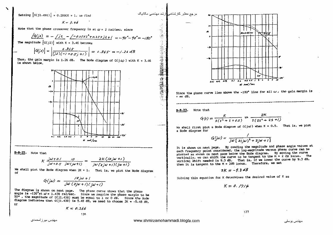
' setting ja(jl-491)! 0.2890K " 1. ·~ find ~15:... ...r4-- .:.:, )l.rt..:..:<_)S: -~ &'-->" 'I'-

j(..: ;. '1-6

Note that the ~hase crossover frequency is at 41"' 2 racl/sec, since

/~rpJ =-f..!!:_ -;-~.trxzLrtJ.z.r-xj2rl =-'1~~-r~"=-;so· The magnitude /G(j2Jj with K = 3.46 becomes

1"'··>1 ~ I · '.-'6$" I = !) (JZJ(-1-I'O . .f'j +t) .:- . .P~s- = -/.2148

Thus, the gain margin is 1.26 dB. is sholm below,

The Bode diagram or G( j ~ ) vi th K "

.. --... },.,jJ •

" .

"

. 1\ . ••

K ~

! ,,~· 1-·

•.. u . ..... ' . • • " -~,,.

20 • H I,.

J.1 -'/s ...

3.46

-------------------------------------------------------------------------------B--8-22. Note that

k JWTO.I JW+b•S"

____!£_ JW(jw+l)

=

We shall plot the Bode diagram When 2K = 1. of

2k(/oJw +1)

)~~,.J {zjCf./ +-I )(jw T/)

That is, we plot the Bode diagram

U('w)= Njwt-1 'IJ j(,()(2jW+I)(jW-t!)

The diagraJil is Shm/n on next page. '!'he phase curve shows that the phase angle is -130"at (A)= 1.438 rad/sec. Since we require the phase margin to be SO• , the magnitude of G{jl.438) must be equal to 1 or o dB. Since the Bode diagram indicates that G(j1.438) is 5.46 dB, we need to choose 2K : -5.48 dB, oc

K =: tJ, 216

'"

., ·--~1

·' i iii""~ -~·-

.sa

t-·::-.-

h-. f: . . -· ,,,.. ' ... •

' ' . 1'--' .. . . . ' • . ' ' -1 . ••

[;> m·

'"' ... l -·· ' .. .. •-• o.tl I

IU '·' • • • ,.

#() ,W/.ue

Since the + <X1 dB.

phase curve lies atove the -tBo• tine for all w , the gain l!lilrgin is

-------------------------------------------------------------------------------B-8-23. Note that

K cf(s)== 5(st+s-t-e>.s)

= Zl< S(ZSz....._ ZS -t--1)

We shall first plot a Bode diagram of G(j~) when K = 0.5. a Bode diagram for

I Ci{jt..J) = jW [ 2(jW)'- + 2)111-+ I}

That is, we plot

It is shown on next page. By reading the magnitude and phase angle values at each frequency point considered, the tog-magnitude versus phase curve can be plotted as !'<hmm on next paqe below the Bode diagram. By moving the curve vertically, we can shift the curve to be tangent to theM"' 2 d.B lOCl.IS· The vertical shift needed is 9.3 dB. 'Tha.t is, if we lower the curve by 9.3 dB, then it is tangent to the M "' 2dB locus. Therefore, we set

•I< =-f. 3 dB

Solving this equation for K determines the desired value of K as

/< = P. /7/f'

127

...;~1_).):!"'--"'~ www.shmirzamohammadi.blogfa.com ._..i...>.J:l'--"'~

' ~,

• ..

• ' !

'

••

•

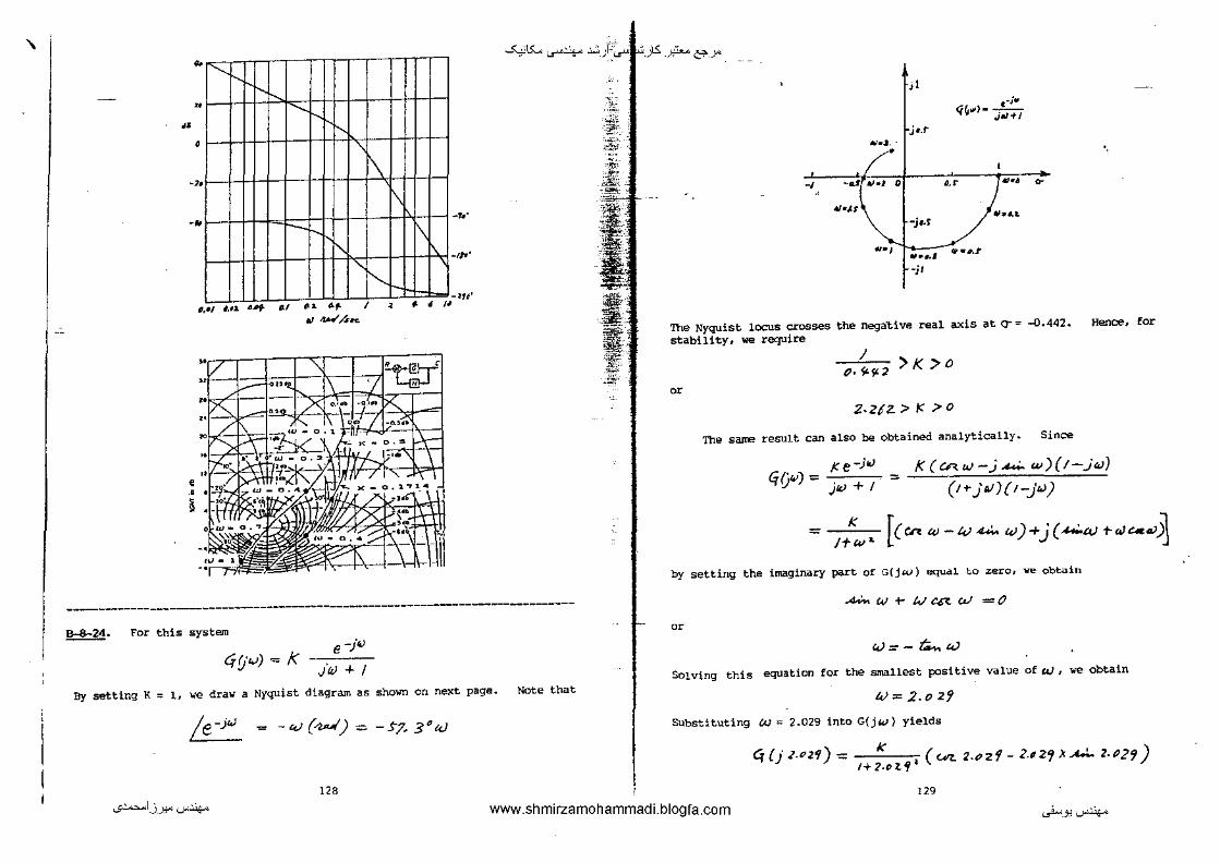
tl,., '·"· •If tl.l

'-

.. .. ol• ' w ~.4 ....

~IS:...._r4--

1\ _,_ .

,,,..

I"-l11'

' I . .. " '"

...

-------------------------------------------------------------------------------~- For this system

e -j4J {j!J"') - k itV + I

By setting K ~ 1, we draw a Nyquist diagram as shown on next page. Note that

je-J" - -41(wl) = --'7. 3'w

118

-~ &'-->"

jl ..; ..

q~ .. )- J;i;T

·jr.t •. , j ' _, -..sri.l~:o '-' 1 &0•• ~

111•/.t '\ ' , ........ -jr.f

~fJI•d -jl

The Nyquist l!X:US crosses the nega'tive real axis at o-"' -0.442. stability, we require

/ o-~so:2>K>o

~

2-ZIZ. > K > o

The same result can also be obtained analytically. Since

Hence, for

G(jw) = I' e -)ltJ )kJ+I:::.

K(CAw-;~ w)(!-jtU)

(t• J"){t-J'-')

= K !+w-... [ (en "' -"' ~ w) + j ( 4.4) t-"'"""' ~

by setting the imaginary part of' G(jW) ~d.l to zero, we obtuin

~w+-W~W=O

or

W=-Z:O.,W

Solving this equation for the smallest positive value of W, we obtain

tV=2.oz~

Substituting W" 2.029 into G(jw) yields

4 {j Z-•21) ~ K I+ l.cl. f 1 ( UZ. 2.1' 2f- 2.t12'f )f .A,..!.. z. P21)

129

...;~I_)_J:!"'-""'~ www.shmirzamohammadi.blogfa.com ._..i...>.J:l'-""'~

•

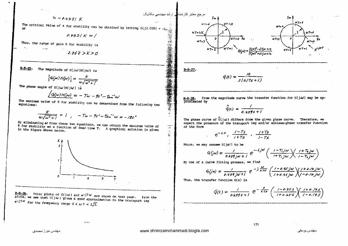
=- tr·'i£?-2/ K -""'15:... ...r4-- .:.:, ) ..f<i...:..:<_)\S -~ &--->"

r~ lm

The critical value of K for stability can be obtained by letting G(j2.029) = -1, or

().9-f'2/ K =I

Thus, the range of gain K for stability is

:?.ziZ>K>O

-------------------------------------------------------------------------------B-8-25. The magnitude of G(jW)H(j"-'l is

k 1 4fj")H~") I= 4!Jf<1 .. +/

The phase angle of G(j41 )H(j((.l )" iS

jq,•t.~)Hf,'(()) = - Tw- fo·-~-14J The maximum value of K for stability can be determined from the following two equations 1

K tvlw'+t = I ~ - Tw- 9()·- ra_-, w = -180 •

By eliminating t.;J from these two equations, we can obtain the maximum value of K for stability as a function of dead timeT. A graphical solution is given in the figure shcn;n below,

K

'

0 1 .z 3 T

-------------------------------------------------------------------------------B-B-26. Polar plots of G(j~) and e-jTI<I are sho'Wll on next page. From the ~we see that G(jlc.l) gives a good approximation to the transport 1ag e-jTW for the frequency range 0 < w T < 2,/3.

' ~r.

,..,_

~

I<IT"'b UT•4

WTcVi 1 t' 61T'•J

0 fJT=O fie ... r .. J ' •• "''"J bli'i,l

"'T• -zr- 4) T• I" qt;·.,),. (TJ•lf -tTjoJ .. ,~ !/ (T,p..) TITjulHZ.

"T•:t

8-6-27.

10 tf{s) = s{M7s+/)

---------------· --------------8-8-28. From the magnitude curve the transfer function for G{jAI) may be ap-proximated by

A

A --,':';:-:~ <iM = ~. ~J.Sf~ t- I

The phase curve of G(jGI.I) differs trom the given phase curve. Therefore, we expect the presence of the transport lag and/or minimum-phase transfer function of the form

-<s e '

1-T.s !TT..1

Hence, we may assume G(jlo.)) to be

1-tT.s 1- T.s

~~w/= e Gl. ,1 1 -l}W ( J-T;_.jw)( ;+T;JW~ M•Sfjw+l 1+-7jjW 1-T..jw

By use of a curve fitting process, we find

G,{'w) = .,--,-"'::7= .!1 I• tSf jW +I

Thus, the transfer function G(s) is

{j(s) =_I

e -) ~-~> (-'- t~-¥-.r.Jw )fJ+P.Ift. ~·I()) /1-IJ.'JJ'jW \,1 tl•lft.jW

s e- 7:?r

l3l

( 1-o.,ss_y t+o.f>s) I+C.flS'S )\_ 1-~./~.J'

...;~I.J...l:!"'-"'~ www.shmirzamohammadi.blogfa.com ._..i...>.J:l'-"'~

' , ~

·~ .

\ ' '

. '

•

' ' -

~

0 + ~

~

" • J>

1\

±I

• •

~ ' • • ' • • •

\ "

" ~ ) >

' • • : • ' •

·., lr. • ~·0

1/

1\ "

~ - ~ ~ ~ 0 ~ ;,

• "

- ~

;;; •

w

~ ;;

0 M

+

1! w

•

0 ;;;

~

• -"

··~ "

M

-0

• M

~ •

~

• w

•

~

:;; . •

i E

0

~ w

0

M

•• E

~

...,..:..:: "'

• -0

"

~ ~

<'I

c;.: :i' <"!-~--i5 0

.-

I •

!:'.oE

NIII

. -:.-"<

>

• " ~ .s. o&

• ~

• e.,{:~'i

I -•

:::JQ

IO:>

O::

~ <:"C&.IO-~

I ~

~

' 0

I ~

I -~ ±~ ' I

'-;':--':-L-L

LJ "I 0

0~~~

.,~

I 0

0

~

. • . I I I I I ! I ' I I r ' ' I ' ' I I

' ! I I I ' i

I I • 0P U

!89

-

I •

•

I ~I

---I • I i ''··i

'

i I ' ' ' I I ' ' i • ' ' I

J .

\ <

I ' I

-

i ' i '

I i .

' ' \

' j ' -

' I I "

0

~

-· 1--

---f------· l j • • ' • ; • ~ • •

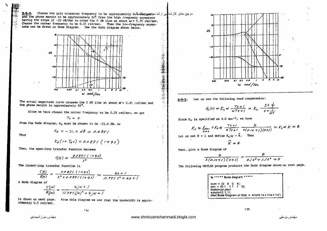
' 'l!i!! .~ '·". • I ·o:-~~ B-9-4. Choose the gain crossover frequency to be approximately 0~/~.:..;,) '\:c~: ifidthe phase margin to be approximately 60~ Draw the high frequency asymptote

having the slope of -20 dB/dec to cross the 0 dB line at about tJ: 0.35 rad/sec. Choose the corner frequency to be 0.25 rad/sec. Then the lrn.r-frequency asymp-tote can be .dra'<lr! on Bode diagram. See the Bode diagram shown below.

', ... ·· ~

~I

"" ~ T .l

• '

" .

" ' . . ,.t <' .

• •

' ' ~ . ,. ,.

• •• -~ "' .. , ••• ' . ' .. •• ' ' . • • .. ·lh'

41 .luUC/u.:.

The actual magnitude curve crosses the 0 dB line at about~: 0.41 rod/sec and the phase margin is approximately sa•.

Sinc::e we haVE chosen the corner frequency to be 0.25 rad/sec, we get

T~ = fl-

From the Bode diagram, Kd must be chosen to be -21.4 dB, or

k.t ::::::- 21, .;.. dB = o, o ~s-1

"'"' Kd 1<- 7;, <) ~ -· o ;-s ( ( 1 + ~s)

Then, the open-loop transfer function becomes

Cj(s} = tNJ?S"I ( !+(Ls)

5'

The closed-loop transfer function is

C(r} l?(r)

A Bode diagram of

cGwJ Rfjw)

is shown on next page. ximately 0.5 rad/sec.

"·" !lS"/. ( l+~s) _ fl..s +I S".f- ~.d 1'$"/ (I+ <f..S) - /;,?s-Js"+?--s+J

Y..jw + I =

1/. ') s-/ {/IV}~ + ~.JW + I

From this diagram we see that the bandwidth is appro-

'"

-~-'·"" --":'

-~ Ji!' .. '"""' -~

:i, ·~ "-!'il'

'~ ~-' -~

·;,_)1.5: _ _y?... &'-->" " / •

" • .. '•' .. -· . ·,

. • I"

' •• • 1\ -....

.. ' 1.1 P.Z fl,ll/ ~t•¥ W A.A.<{ /.Tee

, • • _,. . ,,

-------------------------------------------------··-------------------------~· Let us use the following lead compensator:

(jJr) =- ke o( _I!_~ o<T'S'+/

_ K srf - c. S"+......L_

'" Since Kv is specified as 4.0 sec-1, we have

K, '=!.;... sKoO( ,., Ts +I

o< Ts--r f ' Let us set K : l and define KcO< : K.

A

K='/-Next, plot a Bode diagram of

~

k = Kco< k = 4-s(p,fs +!)(s+-/)

Then

i' S{t>./STf) (STI) c.;sJ-r/./S" +s

'The following MATUIB program produces the Bode diagram shown on next page.

% • • • • • Bode diagram • • • • •

num = [0 0 0 4); den= 10.1 1.1 1 0); bodelnum,den) subp!ot[2,1, 1 ); title('Bode Diagram ol G{s) ., 4/[st0.1s + 11\s+ 1 ll'l

135

...;~1_)_):!" '-""'.lo/<o www.shmirzamohammadi.blogfa.com ._..i.,. _ _, '-""'.lo/<o

• ~-

<JtG(' ["((l1o•1Xo•l)J

-""'IS... ...r4--.:.:, ),:riJ'J.S: -~~-yo 4-J::= 2.61 rad/sec. we select this frequency to be the new gain cross-over frequency t..Jc• Then we obtain

• -~

• ' ~ •

_,., .,.

' ,.., J.•oo

'"' , •.

,...___

1ff 10' ,,

F-ftadlsec)

'" --· Fran this plot, the phase and gain margins are 17" and 8.7 dB, respectively.

Since the specifications call for a phase margin of 45~ let us choose

rf,.. = fL!i" ·-17• +I z: = ftc •

(This rooans that 12 • has been added to compensate for the shift in the gain crossover frequency.) The maximum phase lead is 40 •. Since

~f~ (-oi =--- o~ = 90·) !+"'

Q( is determined as 0.2174. O<

Let us choose, instead of 0.2174, ~to be 0.21,

o!:::::IJ,2/

Next step is to determine the COiner frequencies aJ = 1/T and W"' 1/(Q.' T) of the lead compensator. Note that the maximum phase-lead angle ¢m occurs at the geanetric mean of the two corner frequencies, orW= l/(5T). The amount of the modification in the magnitude curve at w = 1/( .{r/(T) due to the inclusion of the term (Ts + 1)/(c.'Ts + 1) is

Note that

t+jWT l+jt.J/)(7

I .f<F~

1 .. =~ L

v~. 7./

_j_ .,foi.

= 2Jtf'Z2 -:::::: 6. 77?3' PIS

We need to find the frequency point where, when the lead c~nsator is added, the total magnitude becomes 0 dB. The magnitude G(jW) is -6.7778 dB corres-

136

~~-

<•'

-· .

H~=

~d

Th~

+ = [r( 4Jc ·-;, .[i:l/ X Z. 8 I == f. 2 S ?7

_j__::::: o<T

.!!±.

"' 2-11

= \Jo.z, = 6.13/9

(je{~) =- Kc. s+J.2J??

S+6.HI'1

C?,M =

f( ~ Kc = 7 = l'.2./

• p_.'Z/

sf-/. 2.6'?7

s t"l·/3/9

_ ¥- o.nlls +-I p.//,JtJJ'S +-/

-,

The open-loop transfer !wtction becoi!IE!S as

ti~(O(j(s) ~?-,.??.US+/ I ~-ln~s-s+J S(C./st-!){$"~1)

J',Jt76¥ s +- fL = "· P/.13/~ ~ + tJ.2'Jff-SJ. _../. 26 ~/ .r' +S

The closed-loop transfer function is

('{$) 3./i#~ s + -;. /?.(s) :: £1.~ It J/ sf' +-P·219P. sJ + /• 21 ~/ S '"-+- ~,/PD.fLS + 9-

The following Ml'o.TLAB program produces the unit-step response curve as shcnm on

next page.

% • • •• • Unit-step response • o • o •

numc = [0 0 0 3.1064 4!; denc"' !0.01631 0.2794 1.2631 4.1064 4J; steplnumc,denc! grid tltlel'Upit-Step Response of Compen5ated System [Problem B-9·51'1

137

...;~I.J...l:!"''-"'~ www.shmirzamohammadi.blogfa.com ~-.,'-""~

' ........... -.,~·- ~IJ-.&)

-""'IS:... ._r~ .:...:;) ~_)1..5: -~-->"To satisfy the requirements, try _a lead compensator Gc{s) of the form ..• -- ' ,,_ -r ~ -----

' I j 00--

·:~f -~ ---

u ul

./ .. -u ·-u --

---f---

- ·-

-·- ·-·--·.

u

Similarly, the following MATLAB program produces as shown belov. -

the unit-ramp response curve

% • • • • • Unit-ramp response • • • • •

numc .. 10 0 0 0 3.1064 4); denc .. 10.01631 0.2794 1.2631 4.1064 4 0); t .. 0:0.01:5; c .. step(numc, denc,t); plot(t,c,t,t) grid titlel'Unit-Ramp Response of Compensated System (Problem B-9-51'1 xlabeU'.t Sec'] ylabeH'Unit-Ramp Input and System Output') __ .. ___ .....,

- -- - -- -- --• ,, •

r .. } I '

• '

I i

~ 7

7 17: -

~

-/

~ v; h

! i . • :2~r=f= -=I:-- f-

!

0 00 ' u ' u > ... ~ u • ·--------------------------------------------------------------------------------1)8

.;.

.-

Ts+t ' Cj.,(s') =k.:tX. l)(n+l = Kc

Define K C{,(5) = K 'ils):= s{S-i-1)

s+-"­T ,,_..L

wT

\

where K = KcO(. sec-1, we have

Since the static velocity error constant Kv is given as 50

Kv ~ .{..:.. S ff.{s)(jfs) =j.;,_, S_,.tll S,_,t>

We shall nov plot a Bode diagram of

<i,{s) ~ 57> .S(S-t/)

Ts-t'/ s ri-T.s-t/

r< s{s+l) =: K-SP

The following MATLAB program produces the Bode diagram shoWn below.

•oo

% • •• • • Bode diagram • • • • •

num .. [0 0 50]; den "' [1 1 0]; w .. logspa~;:e(-1,2,1001; bodelnum,den,w); subplot(2, 1,11; L title!' Bode Diagram of Gl!sl .. 50/[s(s+l)]'l

Bodoo;,v...<#G1(•)• 50'(ll(a+1Jl

' •" ~ 0

_., ,. ' ---

trf 10' " F._.:y (radiHC)

~1 I I lllfHt=1+Hi1111 I I I Hilli

I:::~t=jit! '"~ •I ul=l4±~ltltl11

w·' to• 10' to' F~l,_)

139

...;~I_)_J:!"'-""'~ www.shmirzamohammadi.blogfa.com ~-.,'-""'~

' Free this plot, the phase margin is found to be 7.8•. The gain ma~lfR.. iie-<~) dB. Since the specifications call for a phase margin of so•. the additional phase lead angle necessary to satisfy the phase margin requirement is 42.2~. We may assume the maximun phase lead required to be 49•, This means that s.a• has been added to compensate for the shift in the gain crossover frequency. since

~ ,/, - !-o< r.- ---1+~

~ = 48., corresponds to~= 0.14735, 47.657",) Whether we choose ¢m"' 48" renee in the final solution. Hence,

{Note that ot = 0.15 corresponds to ¢m = or f6m = 47.657 • does not m<~ke much diffe­\o'e choose c( = 0.15.

The next step is to detennine the corner frequencies W= 1/T and w: 1/(0CT) of the lead canpensator. Note that the maximum phase-lead angle !11m occurs at the geanetric mean of the two eorner frequencies, or t:u = 1/{&T). The amount of the II\Odification in the magnitude curve at t.J == 1/{ftiTl due to the inclusion of the term (Ts + 1)/(0C' Ts + 1) is

Note that

I I+J"'T I !+)WotT ..;-...L -,.T I 1+-JF./ _ _L_

- I+ 'C>( _l_ - ,[0{ J ""'

I ~::::.

I Jc./r = 2.5'120 = ?. 2]'/ 4B

We need to find the frequency point where, when the lead compensator is added, the total magnitude becomes 0 dB. The frequency at which the magnitude of Gl(JlV) is equal to -8.239 dB occurs between~= 10 and 100 rad/sec. From the Bode diagram~ find the frequency point where jG1 (jtv) I e -8.239 dB occurs at o.J= 11.4 rad/sec. Noting that this frequency corresponds to 1/(.[o{T), or

we obtain

4Jc = ___L_ {O(T

-9:-""" 4'cr.;( = 1/. $'- .Jc,/s- = ff f'/$'2

I H

<.Jo =~ :::: II·~ == 2'f. ~J 9-7

,; ... /.$'

The lead compensator thus determined is

9-:fs) = Ke s+-f s +of:r =Ke.

where Kc is determined as

K,

Thus,

GJJJ=

K 0(

/000

3

= s-o /J./S =

S+-$'-.fl/$'2....

$ +-zt.ftJS!-7

140

s.,. If «;sz S f"Zf. 'f.-1ft.?

/Pt:'O

3

=SO (), 2Z / J'S T I

~.~JJ'I7 s +I

·--·

·;. 1.5: pre following MI\TLI\B program produces the Bode diagram of the lead canpens<~tor ·.) ·>:J'Mfte!igned, as shown below.

% • o • o • Bode diagram 0 o • o •

numl "'"111.325 50]; den1 = ]0.03397 1]; w ~ logspace(-1,3, 100); bodelnum1 ,den1 ,w]; subplot(2, 1, 11; tltlel'Bode Diagram of Gels) = 50(0.2265s+ 1)/(0.03397s+ 11'1

The open-loop transfer function of the designed system is

c-,,{s) <q(s) ~ !.EE£. • ( jS"+~~!SZ.) I S-1-2f.$<.l¥7 J(.S+I)

\

'I1le following MATI.AB program produces the Bode diagram of Gc(s)G(s), which is shown Qll next page.

% • • • • • Bode diagram • • • • •

num .. JO 0 1000 4415.21; dan .. 13 91.3041 88.3041 OJ; w .. logspacel·1,3,100); bode{num,den,w]; subplotf2, 1, 1); title('Bode Diagram of Gc(s)Gis) =- lOOOfs +4.4 1 52)/[3(s + 29.4347]s(s + H/'1

141

~- ,.S)~ . ..l:!"''-""'~ www.shmirzamohammadi.blogfa.com ._..i...>.J:l'-""'~

·-

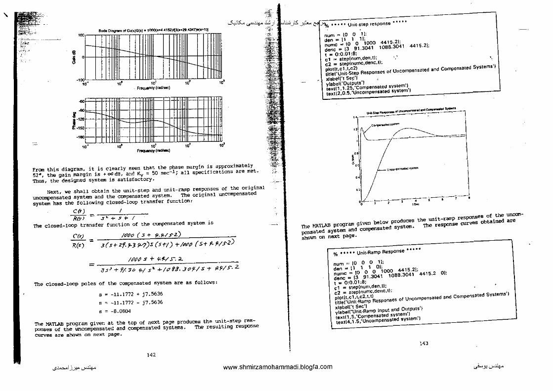
' ;:;:--""'IS... ._r~ if,) .1...:..:<_)1..5: -~ ci->% , • , ,, Unit-step response ••' ''

Bodo Oia1 G<:(•)GI - . --··-·· -· -~------ 000(•~ ~152_ _.,..,--~·--· ,., ... , 000

-~o=.----

num ,. (0 0 1): den""\1 111: numc"' 10 0 1000 4415.21: ;:·0<:'

-"''-' • ~ '

·100'

" _,

oo' oo' Fre<j~~~IIC)' (radiltiC)

F~(rm'Mc)

r---0 ,,.

"

From this diagram, it is clearly seen that the phase margin is approximately 52•, the gain margin is +oOdB, and Kv: 50 sec-1; all specifications are met. ;-~~ Thus, the designed system is satisfactory.

Next, we shall obtain the unit-step and unit-ramp responses of the original uncompensated system and the compensated system. The original Wlcompensated system has the following closed-loop transfer function:

C&) -.~~~~~--R(s)=-·s .. +$+-1

The closeO-lOOP transfer function of the compensated system is

C(1) -:

l{(S")

/&Jt'O ( .S + ~.fL/$"Z)

.3 ( s t- zf. '!-J ft-? )s ( s t-1) + /NJ() ( s -t P. fl./ .J'2)

jtit'tJ s + '1-~1' J""'. 2.

asJ+f(.3c 9-(s'""+!tJf3,Jofi./S-t flf'-l$".2.

The closed-loop poles of the compensated system are as follows:

s"' -11.1772 + j7.5636

s"' -11.1772- j7.5636

s = -8.0804

The MATLAB program given at the top of next page produces the unit-step res­ponses of the unco:npensated and compensated systems. The resulting response curves are shovn on next page.

!42

denc =- 13 91.3041 1088.3041 4415.2\: t ... 0:0.01 :8; .. .. ct "' step]num,den.tl: c2 = steplnumc,denc,ll: plotlt,c1,t,c21 titlel'Unit·Step Responses of Uncompensated and Compensated Systems')

xlabe!rt sec' I ylabei!'OutPuts'l telltll ,1.25, 'Compensated system') text\2,0.5,'Uncompensated system')

....... .s ... ~·-"..,._.,.,..., ...... ~ _. ··-----r----'-· -~-~--c .. .,. ..... , .. ~...,

" (~~

'" i

':::1 ~ .. ~ "'I -· ·--·-· , . I ~~'

Un<en1>'"' .... '''-

oL---;---~3 Uoo 0

The MATLAB program given belOW produces pensated system and compensated system. shown on next page .

the uni t-r<IIIIP responses of the uncan­The response curves obtained are

% • • • • • Unit-Ramp Response • • • ••

num = [0 0 0 1}; den""l1 11 01; numc "" 10 0 0 1000 4415.2]; denc = 13 91.3041 1088.3041 4415.2 0]; t = 0:0.01:8; cl = step\num,den,tl: c2 = steptnumc,denc.tl: plot\t,c1 ,t,c2,t,t) titlei'Unlt-Ramp Responses of Uncompensated and Compensated Systems')

xlabeU't Sec'\ ylabei\'Unit-Ramp Input and Olltputs'l text\1,5,'Compensated svstern') text\4, 1 .S,'Uncompensated system')

143

...;~1_).):!-" '-"".lo/<- www.shmirzamohammadi.blogfa.com ._..i... _ _, '-"".lo/<-

::!~-

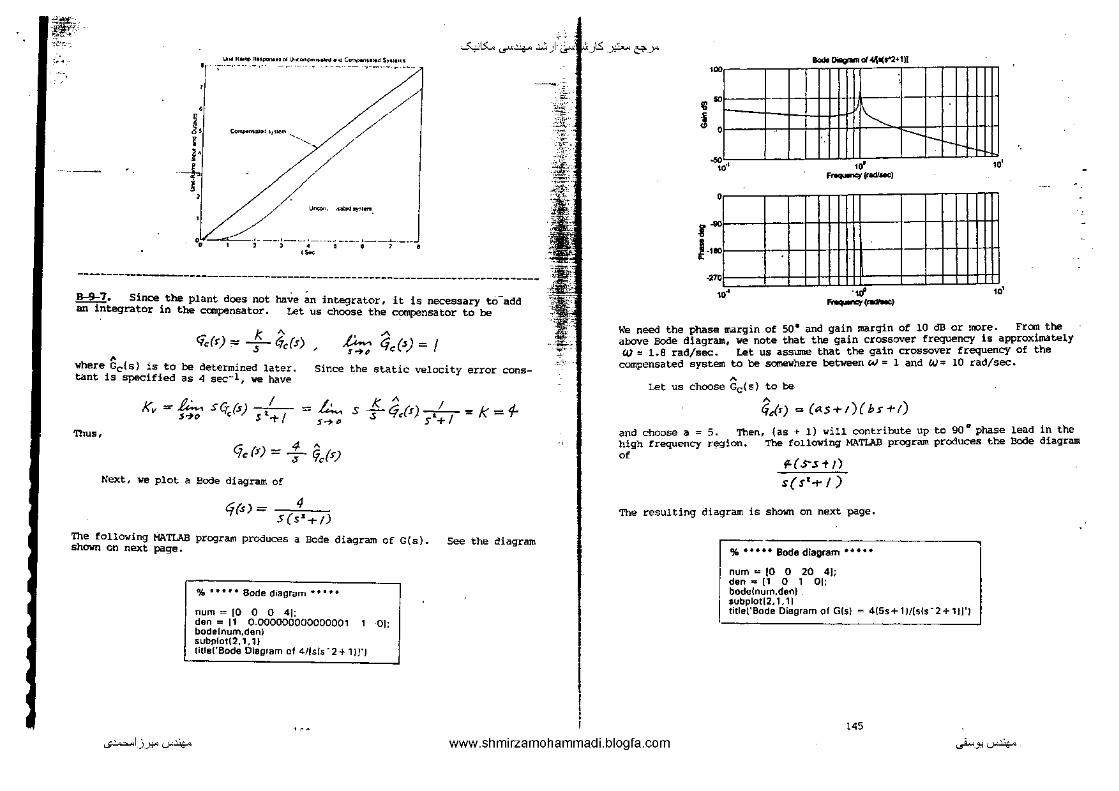
~· -~·c-- -""'IS:... ...r-4-- .:.:, J ..,-.......J:<)-.5: _ _y?... &--->" ,_. "'~ "~"" "-~ ...... ~ ... .-~ .... "~ c .... ,.., .. ,., s,. ...... 'I -.-- -~- ·-- -- -·--·

• i ,, I i•

+ l '

•• •

~-··""'" '• / / ;/ /,/-'/ ~-······-

/ ' j· ~-;--:i.e --·;---- .-~-;-- -·-·

-------- -------------------------------------------------------------B-9-7. Since the plant does not have an integrator, it is necessary to-add an integrator in the canpensator. Let us choose the compensator to be

k ' 'io!•) = -,-- Crds) £<-.. q,(') = I ·~· where 6c{s} is to be determined later.

tant is specified as 4 sec-1, we have Since the static velocity error cons-

Kv = ~ Sfr;;(s) S1.~ 1 = /,;_, H•

K A I s T <iJ•) -.----1 = k = 4-

s+ Thus,

Clc {f) ::= : ~cfsJ Next, we plot a Bode diagram of

<j(,s) = S(s4z+/)

The following MATLI\B program produces a Bode diagram of G(s}. shown on next page •

% • • • • • Bode diagram • •' • •

num "' [0 0 0 4]: den = [1 0.000000000000001 1 OJ: bodelnum,den) subplotl2, 1, 1) title('Bode Diagram of 4/[sls • 2 + 1 )]")

See the diagram

-0: ~ • !

»

•

' ~ ,.

' • t -90i

J.· • .,,

' ,.

'

'

8oOI Oillgnrn d <CIIo(.-:1+1)1 .

'-....

,. f...,....qt (raclfaec)

.~ ---

"

,.

We need the phase margin of so• and gain margin of 10 dB or nore. Fran the aboVe Bode diagram, we note that the gain crossover frequency is approximately W = 1.8 rad/sec. Let us assume that the gain crossover frequency of the

compensated system tote sot!IE!Where between W = 1 and W= 10 rad/sec.

' Let us choose Gc(s} to be

and choose a = high frequency of

' fieM = (AS+t){bs+!)

5. Then, {as + 1) will contribute up to 90" phase lead in the r'!f!9ion. The following MATI.JUI program produces the Bode diagram

fL( S.s T /)

s(S1 -+I)

The resulting diagram is shown on next page.

F•• Bode diagram •• • • •

I num=IO o 20 41; den "" [1 0 1 01: bodelnum,dent

I subplot[2,1,1) titlel'Bode Diagram of Gls) = 415s+ 1 1/[sls • 2 + 1!]')

145

...;~1_)_):!"' '--"'.lo/<- www.shmirzamohammadi.blogfa.com ~-J:l '--"'.lo/<-

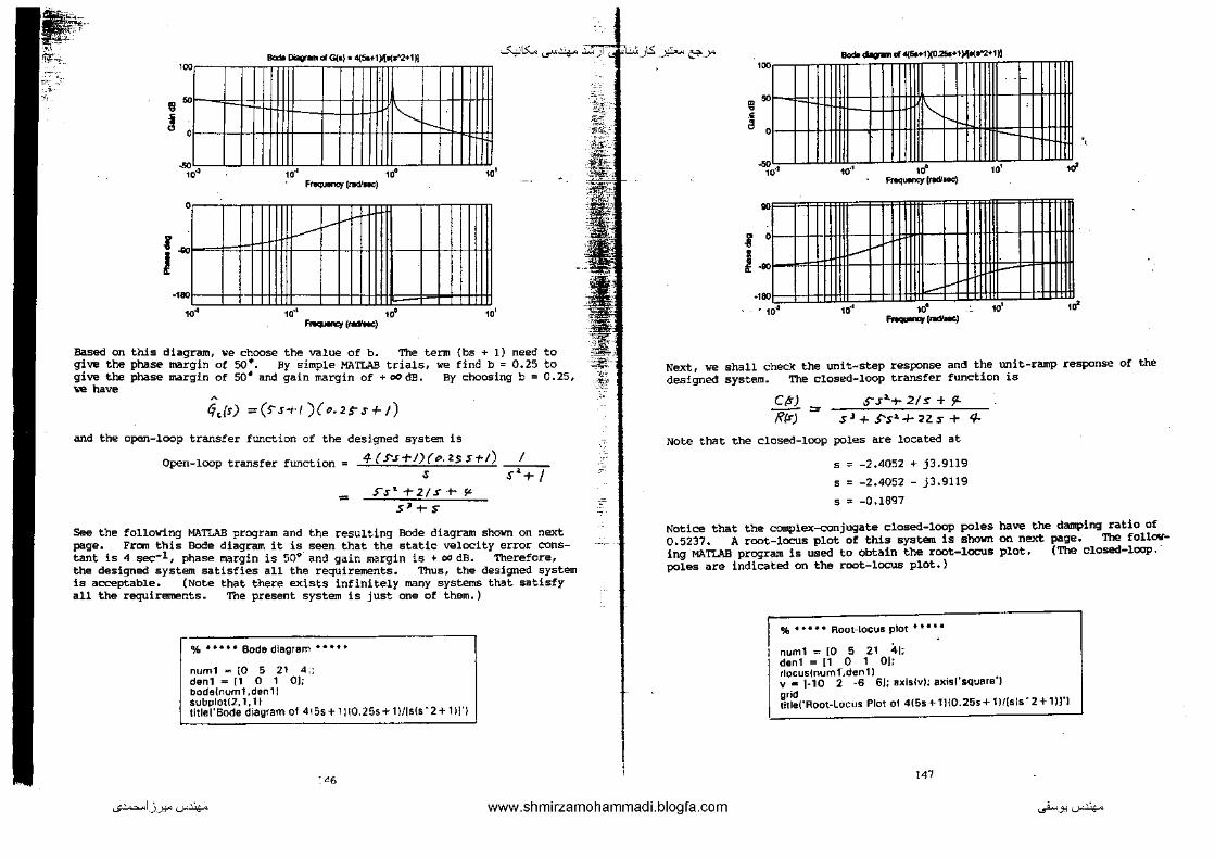
Balo ~ d Glo)'" 4(5o+1)1[Jjr-2+1)! -""'15:... ...r4-- ~_)1..5: -~ &'-->" •oo

• . .. !

l I

0

.., ... ' 0

..,

-·~ ...

M'l

" ,,

" FI'Oq\lllnCl' (..alne)

---,_...

10'1 ,, ... _,_ Based on this diagram, we choose the value of b. The term (bs + 1) need to give the phase margin of so•. By simple MATLAB trials, we find b = 0.25 to give the phase margin of so• and. gain margin of+ COdE. By choosing b = 0.25, ~ha~

~~(s) =(s-s-rl)(t~.2~s+-J) ;md the open-loop transfer function of the designed system is

Open-loop transfer function = 4(S".s-t-J)(t:>.2SS1"1) -;i/-:-T s .r~+ I

~ rs~T2ts·t-~

s' + s

See the folloving MATLAB program and the resulting Bode diagram shown on next page. Ft'CIII this Bode diagram it is seen that the static velocity error cons­tant is 4 sec-1, phase margin is 50" and gain margin is + 00 dB. Therefore, the designed system satisfies all the requirements. Thus, the designed system is acceptable. (Note that there exists infinitely many systems that satisfy all the requirements. The present system is just one of them.)

% • • • • • Bode diagram • • • • •

numl - [0 5 21 4,; denl "'[1 0 1 OJ; bode[num1,den11 subplotll, 1,11 title[' Bode diagram ot 415s + 1110.25s + 11/lsls · 2 + 1 II'!

.,,

=0 ,·

~:}-,-

... ~ ~

• !

•,

....... ,.._,

Next, we shall check the unit-step response anc!l the unit-ramp response of the designed system. The closed-loop transfer function is

Cfr) s-s"'+ 21~ + 9-Rtr) == s J + J's .. ..,_ n :!' + 4-

Note that the closed-loop poles are located at

s := -2.4052 + j3.9119

s : -2.4052 - j3.9119

s "' -0.1697

Notice that the complex-conjugate closed-loop poles have the damping ratio of 0.5237. A root-locus plot of this system is shotm on next page. The follow­ing MA.TIAB program is used to obtain the root-locus plot, (The closed-loop.· poles are indicated on the root-locus plot.)

% • • • • • Root-locus plot • • • • •

numl = [0 5 21 41; dent = [1 0 1 OJ; rlocus(num1',den1 I v • 1-10 2 -6 6[; Rxislv); axisl'square'J grid tltlei'Root-Locus Plot ot 4(5s + 1H0.25s + 11/[sls • 2 + 1 )J'l

147

...;~I_)_J:!"'-"'~ www.shmirzamohammadi.blogfa.com ._..i...>_J:l'-"'~

The n~ pensat.ed

Rool..l.oaa Plot ol "(5.+1)102So+ 1 ytll(r'2o1)] -""'IS... ..r~ .:.:,) ._rU..::Jts: _ _y?....nili-'following MATIAB program produces the unit-ramp response curve of

pensated system. The resulting response curve is shown below. the-

' I i •

~ I

'~~¥, o I I

[

' 1\J •

• _, • •

-

"\ Cl•"" . 'l,.+t

'\

v • 4 0 ' .......

HATLAB system

program will produce the lrllich is sh0>1n below.

unit-step response curve of the com-

% • • • • • Unit·step reS)lOnse • • • • •

numc = {0 5 21 4]; denc = {1 5 22 4]; l!ep(numc,denc) grid title!' Unit-Step Response of Compensated System !Problem B-9-7)')

(M,I·Siop R"''""' d "-">otod "'"'"' II''<"""" 0.0-'J rr I i "1/\ i

!" t.

,,

! I i 1

. ' J' I ' . ' I ' ' ' I I

__ j__j~--'--'-~-, , • • • • • 10

"

•• T.,.!_l

'"

·"-

_il __ ~ ..

IJf.

-

-~~) ;I; -~,--

~­-~ -"' -~-_ ,-

% •••• • Unit·ramp response • • • ••

numc = ]0 0 5 21 4]; denc ~It 5 22 4 OJ; I ~ 0:0.05;20; c "' steplnumc,denc,t); plot(t,c,' -' ,t,t,' ··'] titlei'Unit-Ramp Response of Compensated System (Problem B-9-7]') Klabel('t Sec') ylabeWOutput and-Input Ramp'! teKt(10,7,'Compensated System'!

....__,_s,_ (Pr-.a+'l

•,---.-----" " " !,

l,. I J• ,..._.., ... ,. _

ok::::_.__ ' ' • 10 " " ,. '" 2o 0 ' ' So•

The Nyquist plot is given next. the Nyquist plot shown on next page.

The following MA'!'LAB program produces_

'lfo o • • o • Nyquist plot • o • • o

numl .. [0 5 21 4); dent ., ]1 0 1 01; nyqulst(num1 ,dent J v"' [-120 40 -80 80]; aKislvJ; eKisl'squere'J title!'Nyquist Plot of 4!5s + 1 )(0.25s + 1 Jlls!s • 2 + 1 )]')

'" ....,~1_)_):!"''-"'~ www.shmirzamohammadi.blogfa.com ._..i...>_J:l'-"'~

~·:'"-

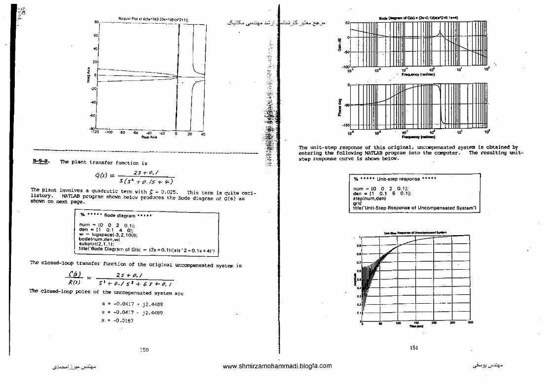
-~-"7 ~ Nyqurst Plol ol ~15t• I )10 25o•l Jl!<[s•2• 11)

-~15:... ...r4-- .:.:, ) J..-<~...:..:<_)1..5: _ _y?... &'-->" '" -~--~~-----,-- -r-

j

f

" " " 0-

'" '" ~· ., •o

• "

-------- '----

oo ..eo -&J -40 -20 RniA>ro

0 " " ----------------------------------------------------------------------------!!±!· The plant transfer function is

'J(s):::::: 2S-t--0,/

S{s"--ro.IS+f<.)

The plant involves a quadratic term with ~ = 0.025. This term is quite osci­llatory. MJl.'I!.AB program shown below produces the Bode diagram of G{s) as shown on next page.

% • • • • • Bode diagram • • • • •

num"' [0 0 2 0.1]; den,[1 0.1 4 OJ; w = logspace[-3,2, 100); bodelnum,den,wJ subplotl2. 1,1 J: .titlei"Bode Diagram of GlsJ = (2s +0.1)/[sls "2 +0.1s +4)")

The closed-loop transfer function of the original uncanpensated system is

--1Y!l... - 2 s + (),/ R(J) S't-o.;st+6.r-I-P,/

The closed-loop poles of the uncompensated system are

s" -0.0417 + j2.4489

s " -0.04!7 j2.4~89

s" -O.Ol67

~50

""ll~' -•4!

,1}_: ~.

:1:· '~~'-~ ~~

·;t·.: ., ' ,:':.__:·- ~

:!{-~ --ci;:_ -,--,_';'

• ~ ..,H+H

r _,~ I If! J

,,

The unit-step response of this original, unccmpensa.ted system is obtained by entering the following HATIAB program into the canputer, The resulting unit­step response curve is shown belOW,

% • • • • • Unit-step response • • •• •

num,..[O 0 2 0.11: den= [1 0.1 6 0.1[; steplnum,den) grid titlei"Unit-Step Response of Uncompensated System')

-0.0

/

II .. .. .. o.• .,_ ..

•, • , . •• ~ ~ --151

...;~1_)_):!-" '-""'.lo/<o www.shmirzamohammadi.blogfa.com ._..i...> _ _, '-""'.lo/<o

' -""'15:... ...r4-- .:.:, ) ._r~...:..:<,tts: -~ &'-->"

To design a compensator for such a system, it is desirable to cancel the zero of the plant, since it is located very close to the origin. It is some­times useful to include double zero and double pole in the compensator. So, we may choose the curnpensat.or to be----

$ - 1:. (s+Z)l > +~ {jc{. ) - C- {Sf-10}1 .2S +P, /

where ~ have chosen the double zero at s = -2 and double pole at s = -10. The value of a is determined later. since the static velocity error constant is specified as 4 sec-1, we have

k, = ~ 'qc(>) q{$) =.!.;.. <k, (.T+zt (s +tl)'-

St4 zst-P-/ ~_,, S?l 2SM/ S(S 1-tt7,/,H~)

ko ·~.

__L = i'­I'P

ko: "- = ft..t't?

By several MATLAB trials ve find a ~ 4 will give a satisfactory result. There­fore, ve choose a = 4 and Kc = 100. Then, the transfer ftmction of the ccm­pensator becomes

~,(s) =!t>O (srz.Jt (Sh")~

5+P. ZST-&1, I

The open-loop transfer function becomes as follows:

The ing

Cj,{r) Cj(r) = /00 ( 5+-Z.)l.(S+fL)

(S+!G}l 5 ( S1 t-O·/S-t-~)

_ /CI) .s J + J't:J" s'- + 20(Jt:JS +-/6oer

- sr+ ZP.(s~+ /~:?6' s.s t- ?o.s~+ ~ s

following mTLAB program produces a Bode diagram of Gc(s)G(s). Bode diagram is shown on next page.

% • • • • • Bode diagtam • .. • •

num = [0 0 100 BOO 2000 16001; den= [1 20.1 106 90 400 OJ; bodelnum,den). subplofl2.1, 11 titlei'BMe Doagram of 100[s + 21 · 2(s +4)/[(s + 10) · 2sls • 2 + 0.1 s +41J'J

The result-

From this Bode diagram, it is seen that mately so• and gain margin is + D<l dB.

Kv ~ 4 sec-1, phase margin is approxi­so, all the requirements are met.

~-·

;f: -:;~­

"5\'-

~ .""'. :!, -1!-._ft ~j .~;:_

""""""

• ' -~:·-"rmr·- .. -..

~ ' -----''

, to·• ,, ,. ••

F~(' . , v

• ·~ J 1'-_, •

to·' to" to" ' -·-The closed-loop transfer function of the compensated system bee-alEs as foll.ovs:

CM IO"~J + ~Op S"2. + Zt:P, s -r ft()O

~ = sst- 2()./ S' + :zo~ s J t- 8 'ltJ s'- + 2'HJCS t-/6dO

The closed-loop poles of the compensated system can be found as follows.

denc .. 11 20.1 206 890 2400 1600[; IOOIS(denc)

ans =

-7.3481 + 7.2145i -7.3481. 7.2145i -2.2424 + 3.37511 -2.2424.3.37511 -0.9189

'!he following MATLAB system.

program produces the unit-step response o! the designed

% • • • • • Unit-step response • • • • •

numc = [0 0 100 800 2000 16001; denc = [1 20.1 206 890 2400 16001; steplnumc.dencl grid titlel'Unit-Step Response of Compensated System (Problem B-9-81'1

..s~u . ..l:!" '-"'.lo/<o '"' www.shmirzamohamm.di.blogfa.com 153 ._.,i... _ _,. '-"'.lo/<o

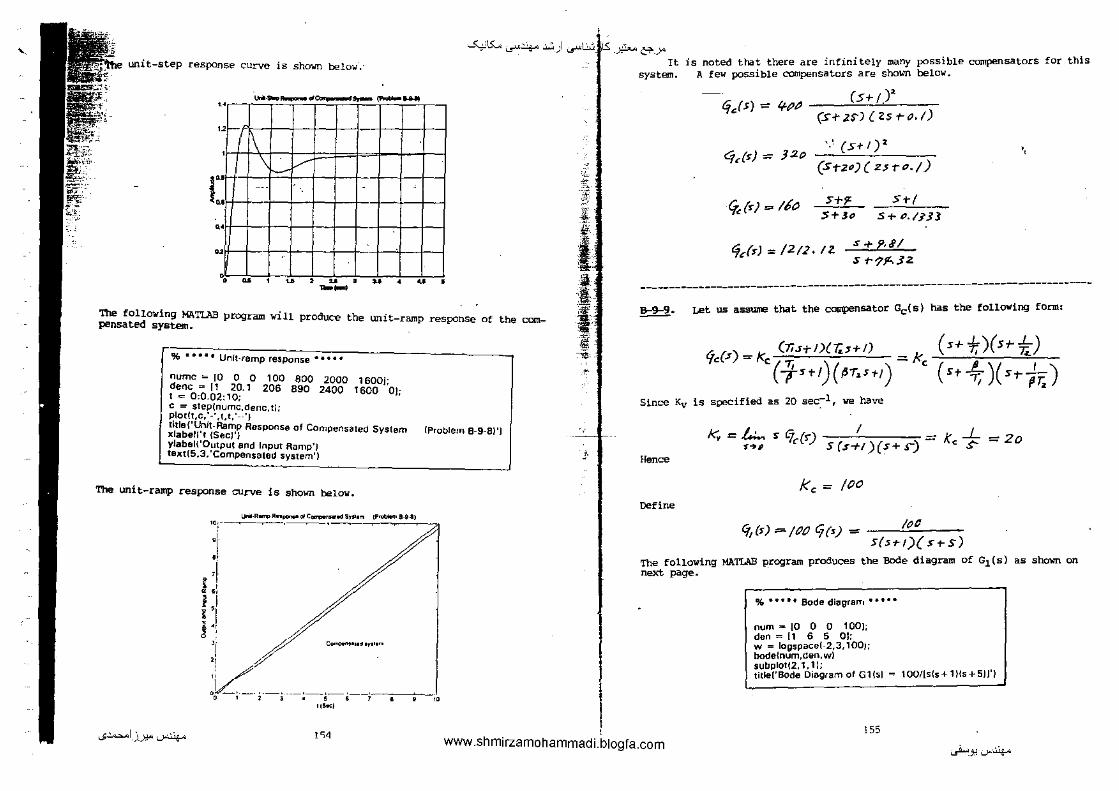
' unit-step response curve is shmm below.·

" ___ .. ....,..__ ~_.,

" ' l\

/

" --· . - -

" r " ' " ~ ,

•• " ' u ' u ' u • " -- •

~15:... ...r4-- .:.:, ) ._rt..:..:<_its: -~ &'-->"

'~ jt

':ffi $.. ii ;;!<.

.i .. -~ li j!o

It is noted that there are infinitely many possible compensatocs foe this system. l\ few possible compensatocs ace shown below.

(j,,(s} = q.pp (5+ 1Y (s.rzsJ(Zsro.t)

·.! (st-1 )'1. Cfcfs} = J2o

(srz1)( zsro.;)

!{;,{<) -110 S+F HI S+J1 S+ 0./.133

fj&(s) = /2(2,/Z S+f.NI S t-?JL.3Z

.,

------------------------------------------------------------------------------

The following MATLAB program will pensated system. produce the unit-ramp response of the corn- ll :"!f!!_·-J

~· Let us asSUITE! that the CQI£Pensator Gc(s) has the following form:

% • • • • • Unlt-remp response • • • • •

numc ,_ ro o o 100 BOO 2000 16001; denc = 11 20.1 206 890 2400 1600 OJ; t ., 0:0.02:10; c = step(numc,denc,tl; plot(t,c,·-·,t,t,'--'1

'i -~

:-:--

(jc(.s) = k. (7is+IXT..:s+/)

'(3)->+t)(~T.'>t) ~J<, (s+i)(sr-f.) ( "* )(s;- ;,J

Since Kv is specified as 20 sec:-1, ve have

title{'Unit-Ramp Response of Compensated System xlabell't (Sec)') !Problem B-9-BJ'J 1<., = ./...;...,. s fi, (s-) I - K _j_ =2o ylabeU'Output end Input Ramp') IBI!t(5,3,'Compensated system')

The unit-ramp response curve is shown below.

...;~I_)_J:!"'-""'~

Lni-1!-Rn-OIC....-... odSfll"" iP-8-U) '": ~~----r--------·~ ·i ·' ·I ! ' . "

l ,I I I ! ., 0

'[ / ,, .?

c....,...,,,..,,,.,m

·~ . ---·--·-.--;· • • ,r. "o ~•- ' l • ,,i.,l

'"

!· Hence 'f~l c s (s+t )(s+ .r)- c S

kc = /00

Define

ft,(s) =-/00 Cj(:s) = Nd S(s.+-1)($+S)

The following MATI.AB program produces next page.

the Bode diagram of G1(s) as shown on

I ' www.shmirzamohammadi.blogfa.com

% •• • • • Bode diagran-. • • • • •

num ~ 10 0 0 100); den "' [1 6 5 01; w = logspace(-2,3, 100); bode(num,dan,w) subplot(2, 1,1 J; title(' Bode Diagram of G11sl

!55

100/[s(s + 1 Us+ 5JJ'J

~-J:l \.,)-'.lo/<o

' ~15:... ...r4-- .:.:,) ...r•· .. 'l.ts: ~ -a.' -~-- C:'?'-->"

- o;.gr.marG1(o) ~ 1001s(s+1)(o..S)J

1001 1 1 I II 1111 I I II IIIII I I I I IIIII I I I I I

• ~ ,ooi-1-j~IIIIII--HH

Fraa this diagram we find the phase crossover frequency to be 4) = 2.25 radj sec. Let us choose the gain crossover frequency of the designed system to be 2.25 rad/sec so that the phase lead angle required at 41= 2.25 rad/sec is oo•.

Once we choose the gain crossover frequency to be 2.25 rad/sec, we can determine the corner frequencies of the phase lag portion of the lag-lead cat~pensa.tor. Let us chtx:~se the corner frequency l/T2 to be cne decaae below the new gain crossover frequency, or l/T2 " 0.225. For the lead portion of ~he compensator, we first determine the value of p that provides~" 65',(5' added to 60 •. ) Since

__..:.. f-1- .L

--"­/+ t

5 -I ' ~ -1-/

we €ind ~ = 20 eorresponds to 64.7912', Since wa need 65D phase margin, we may Choose p = 20. Thus

t~ 20

Then, the corner frequency 1/( pT2l of the phase lag portion becomes as follows:

J__ 17i -

I -'--:ZO)< loll~•

= t>. 22S'

2o = (),()//.?~

Hence, the phase lag portion of the compensator becomes as

St-0-lZ.S' ~ 20

( f.fl:i<S<.Jc-'5 +/) .s +0.0112) - 81, 't!8'ts +I

...;~1_)_):!"'--"'~ ~'Sfi

,-_, .

J

, .. 'i

For the phase lead portl?"• we first note that

4/)~·2S) = 1~.3S dB

If the lag-lead compensator contributes -10.35 dB at~= 2.25 rad/sec, then the new gain crossover frequency will be as desired. The intersections of the line with slope +20 dB/dec [passing through the point {2.25, -10.35 dB)] and the 0 dB line and -26.0206 dB line determine the corner frequencies. Such intersections are found as w = 0. 3'704 and 4)"' 7.4077 rad/sec, respect;ively. Thus, the phase lead portion becomes '

S-+C.37ofL ( ( 2.6??8 51-/) S"r?.~o'l? = 2c 0./J.r"sr;

Hence the compensator can be written as

q, (s) = ;oo( ¥."-(<'~sts+ 1~\ ( z.&?P8 s+l _\ ' 'if,Ft"f'fSi-/)rp,f]~OS+//

= 100 ( sro.zzs )( .S+-tJ, 370$1-) St-P.O//:Zt;' .S + 7·fit'77

Then the open-loop transfer function Gc(s)G(s} becomes as follows:

( p:.~rd•-1'-S+I )( z.tfff3s+l) -:-:---'1~;-:---:;-

q.:(f) Cj(s) = ftJ(J r;.l/f'/S-t-1 "·/Jros+l S(.s+-t){H.t:-)

The following fer function.

II'?'/. 90 S l + 71~. {t-2 s T /00 = --=---~.:..C.:.--'--;-'--"­

J:lSr + /6/. P2 3 f s" T S''/.S: l"lft- sJ -t- "f.~t.J!fS s l-+ N

MATIAB program produces the Bode diagram of the open-lOCip trans-

<M. • • • • • Rods diagram • • '•'

num"" [0 0 0 1199.90 714.42 100[; den"' (12 161.0239 595.1434 451.1195 5 01; w = logspacet-3,3,1 001; bodelnum,den,wl subplot\2, 1, 1); title('Bode Oiegrsm of Compensated Systam'J

The resulting Bode diagram is shown on next page.

!57 ._..i.,. _ _,.:r~

. :J:TT111l1C--h.;;Bodoo OoQwn ~ ~ S)'>'lom >OOFH+mlll::i Ill

• ~-•ooHf

,. . F~'*"''' (1'8d/Hc)

r I <··~H-++

To read the phase margin and gain margin precisely, we need to expand the dia­gram between w = 1 and 4J = 10 rad/sec:. This can be done easily by modifying the preceding MATIAB program. [Simply change the comnand w = logspace (-3,3, 100) tow = togspaoe(Q,l,lOO).] The resulting Bode diagram is shown below.

~·.----------''""~~ ... ~·~-~~~~·"'"~~·v-~---~~·~"""T'C,c-.--r-r-,

;~t ______ J ___ t±4ttllJ 4 ~ ~

Frequen<:J~ (radlsec)

o,--------,----,---,--,--r,-TII

r=~----- I F#M . . .... __ I --1-·1 j·-1·1-ti, -2TOc ..... - t 10 ,.

F~(~l

;.:.~

'£:: ~

"t

~-' ;,"./o' -· ;,t.• ..,_, ~ ,, ';),:·

i:. J• ,o

~-~ From this diagram we find that the phase margin is approximately 60• and gain margin is 14.35 dB. The static velocity error constant is 20 sec~l.

The closed-loop transfer function of the designed system is

..fE2_ _ !I'! 'I· ffJ :5" + 714-- fl-Z .s + /00

7?.(~) - /lJ$+/If s""t', srs-./ s' T j,{..)/ s«+ 'lf'f.~S +/00

The following MATI.AB program produces the unit-step response. The resulting unit-step response curve is shown belo~.

% • • • • • Unit-step feSIJOOse • • • • •

numc = [0 0 0 11!}9.90 714.42 1001; done= 112 161 595.1 1651 719.4 1001; step(numc,dencl gfid tltle('Unit-Step Response of Compensated System'] ___ .. __ _

ul I I ( \ \ \ \ \ I I

.. ·i -1-'--1-+-+-1----i---1 I j I -f+-- . - 1--+--1----~--

.1 \ bH±J r~r=n 0~···"'·~··"··2(1

-·~

i" oo~I--1--J·~\----+-

..

The closed-loop poles can be obtained by entering the following MATL!'.B progn-·

into the computer.

roots(dencJ

ans ""

-9.7022 -1.6110 + 3.0494i -1.6110-3.04941 -0.2463 + 0.10761 -0.2463 • 0.1 076i

159 ...;~I_)_J:!"'-""'~ ]';8 www.shmirzamohammadi.blogfa.com ._..i...> _ _, '-"'.lo/<-

' '

_.,._,-t::.;:.

--·'

-""'15:... ...r4-- .:.:, ) ._rG:{).S: -~ &'-->"

Notice that there are two zeros (s = -0.225 and s = -0.4939) near the closed­loop poles at s = -0.2463 ± j0.1076. Such a pole-zero combination generates a long tail with small amplitude in the unit-step response.

The follOwing MATLAB program will produce the unit-ramp response as shown ~1~-

% • • • • • Unit-ramp re5ponse • • • • •

numc"" 10 0 0 0 1199.90 714.42 100]; denc .. 112 161 595.1 1651 719.4 100 01: I .. 0:0.05:20; c "' step[numc,dem:.t); plotlt,c,'-',t,t,'.'J grld tltle('Unit-Remp Response of Compensated System' I xlabel('t Sec'J ylebei!'Output and Ramp Input' I textl11, 7, 'Output']; text(l, 7, 'Ramp Input')

! ! l

J

__ .. ___ • .. -·-. 171L •• - -l-- ----+- -- --;•f-r-· - f-- .. JlL . , -+·+- -,--IZILI--- 1--'' ·i - - ·1:;;; --I-- - ·-·r.;(~p D ~-.- -- ---• -"i-- )- -~- -{~ W-f-- -- -- i -2- --· -

"o•~•••o<l•••••• ·-

·''""" -":-

~f­~

.;:.. --4··---·-·· "·'· '~-~~;;--,

-If ~

'b f; ~ :W:, -=

B-10-1.

CHAPTER 10

Referring to EqUation {5-'3.0), we have

k, _ Rt(~,C,i-Rt.CJ ' '- -~~, 1?1 cit

= 3f~Z

7i.::::: if,c 1 +- K1.C'z = 3. o77

~,C,Ic.CL ::::: (),'7/fZ

RICI + Rc.la. T,=

First, notice that

(K,.c,)+(R.c.) = J,P77

(!r,c1)(Rz.Cz,.) = o.?lf.?x.J.P-:17 = :?.111'1

Hence we obtain

l(,C1 = /.Y.Ji'S.; l'z..C'z =/.S',JKS

since we have six unlmmm variables and three equatiops, we can ehoose three variables arbitrarily. So we choose c1 = c2 = lOJ'F and one remaining varia­ble later. Then we get

1(1 = k,::::: /S3. f'.> k.f2.

From the equation for Kp• we have

_& N1 C,+i?~:.C~ =J?.!o'-Z RJ R1 C.,

"' _&

"' Jf.Jr.2 X+= ff.7/

we now choose arbitrarily R3 = 10 k.O.. Then, R4 , 197.1 Jt.(t,

roller obtained is shown be lew.

The PIO cont-

_j ·!J-'-f, •o '" ' <---- 1~3.S5 •n '.. •

"•' '1'~'-· r=,, ....

------------------------------------------------------------------------------...;~I_)_J:!"'-""'~ www.shmirzamohammadi.blogfa.com 1<1 ._..i..-> _ _,~~

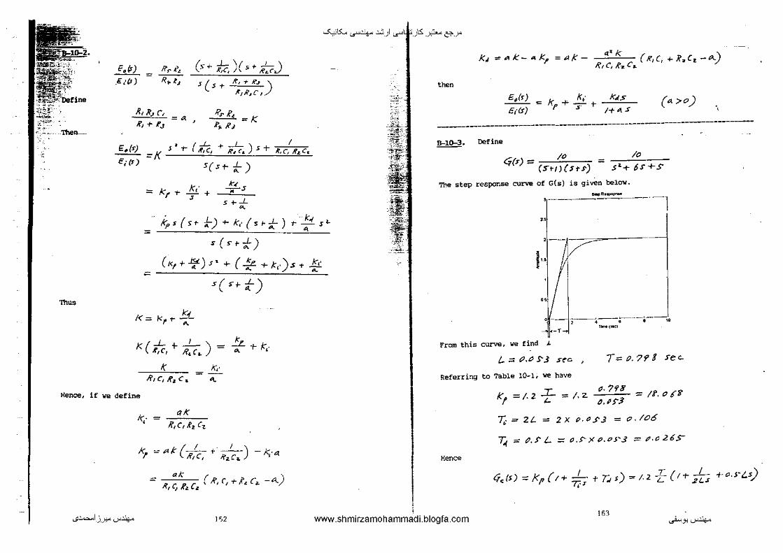
E~VJ -~ _E,'(J)

ffr R~

R.,.t_,

(n- h)(" ;b) 5 ( s + ((, ... R'J )

~,R~c,

R,Jt_, l, = .::t. ~ K, + I'.J

R.rR( =K Rl< /i'~

I • (-"- +-L)s+ r=..(:>) = K s r ~r,c, I?~ c. R.c, trz.C, E; #) S(srf:::)

k' == kr.,... T + k< .z:.

s.-'­~

~15:... ...r4-- .:.:, ) ._rif'_)ts: -~ &'-->"

theo

a• k ) f<J =o<'lk-4K, =t:l/(- {K1 C,+l?.,Cz-""-R1C,/f.,Ca.

k, £.(r) = kr + S + 5t"&)

ku

I+ <1. s (•>o)

\

------------------------------------------------------------------------B-lo-3. Define

/0 ~($) := (S"t-I)(S·t.t')

.;:: /O .Sz.-t- 6S+S

The step response curve of G(s) is given below.

-"·- -----I ' k

kps ( s+- .J:-) +- k,· { s r-..1:-) r-/- s'-

Thuo

=

I<=

s(S'r-f)

( "' +- ~) s ... + ( 5.e. -+- k,·) s + k,• 4 ~

k; 1<,. t- -;:-

s( n- f)

_L I ) _!L_ K ( K,c, + R:c... = t::~.. i- k~-

/( )(,.

I?,C,/i'z.C• = ~

Hence, if we define

Qk k,: = J?,c, kz Cz

k. = Ak (--1- + ~1

-) - k,·a 'I' H,c, l?tCa.

_ ak ( - I(,Cj R::. c~~. R, r, + t~ c,. -4..)

2•---

1 .. I

.. ,, I ··---j~" ' . .----~----· .r-r ..... ( .. ,· .---;,

From this curve, we find ./.

t.. = t?.~ S 3 src. T=P.7P8 fee..

Referring to Table 10-1, we have

..L f/-7'18 K1

=/.2 =/.Z. :::::;i'.o{"8" t- ~.~)3

7,: = 2L = 2X p.tJ..f"3 = CJ.I06

7.(;:::: ~.J'L::: o.S"-XP.o.J.'.3::: p.tJ26S

Hence

t/c (>) == /<p {I+ ~$ + T.J s) = /. 2 [ ( 1-t- 2~.r 7-tJ.J·Ls)

...;~I_)_J:!"'-""'~ ]&,2 www.shmirzamohammadi.blogfa.com 153

._..i...>.J:l'-""'~

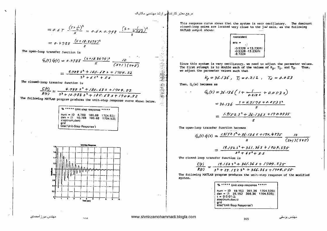
' ~15:... ...r4-- .:.:, ) .rjt..:..:<_)ts: -~ &'-->"

=o.6 T -'-)'

(sri. -c-.tfx.o.7f8'" s

::::: ()-~?8? (st-a, ?67f)_l

s

The open-loop transfer function is

(sr ~)l s

/0 ~c(r) Gfr) = ~-f'-'lBF (s+/tf-U?9Y s

(.S+!) (s-r.s-)

f,?l/'1" Sz. + /.ft), /of' .s + /?()j:L, S2

s) +-tr.s~ -r >-s

The closed-loop transfer function is

C(J')- ~-'71/i'Sl.+/J'tJ.&SSt-/?t>f'.s-2 K(r)- sJt-/tJ.?J'Ssl+tJ'S""..frsrl?of£.S2

The fOllOWing MA'I'IAB pro;ram produces the unit-step response curve shown below,

'' ,. '·' ,, '

•• ~ .. u

'•

% • • • • • Unit-step resr1onse • • • • •

num = (0 4.788 180.68 1704.52]; den= (1 10.788 185.68 1704.521; s~ep(num,den) grid t•tlei'Unit-Step Response')

- ~- -:J __ --~--

I ~--

-

' ' • ' T-[ooc) • • • "

.,.,

'~-

This response curve shows that the system is very oscillatory. The dOII'Iinant closed-loop poles are located very close to the j~ axis, as the following MATLAB output shows:

roots(denl

ens=

-0.5328 +13.2301i -0.5328 -13.2301i ·9.7224

Since this system is very oscillatory, we need to adjust the parameter values. The first attempt is to double each of the values of Kp• Ti• and Td- Thus, we adjust the parameter values such that

/y:::: :JI./36 J J; :=-P,ZIZ. , 7j = "-PS3

Then, Gc(s) becoroes as

Ci,(s) = 36.1:16 (I+ I P· """i"{Z; +- 0, p S' 3 S)

= 3i.l)b S+- f.?l?t' +'·~'S"JS" s

/.f/.rz.st+.Jt•/36S +I?O·F'S.i.>

$

The open-loop transfer function becomes

10 o/~fs)t;(s) = /.P/f"Z.r .... +:U·/31~-t-17,./f.>JJ­s (5t-/ )( H <:-)

tf.;sz.s~-t-36/. J6s T!?ot-.s-Js­.sJ T- ts•-r s.s

The closed-loop transfer function is

C(:s) If, /J'.Z s l + Jt/. J6 .s t- /?(;19, S3s-

Rt;r> = .sJ..,..zs.ts-zs:a.+3,6.J6s+I'7P9!-,.r.u-The following MATIAB program produces the unit-step response of the modified system.

% • • • • • Unit·step response • • • • •

num = [0 19.152 361.36 1704.535); den .. [1 25.152 366.36 1704.535); t = 0:0.01 :2; step(num,den,tl grid tille!'Unit-Step Response')

...;~I_)_J:!"'-""'~ '"II www.shmirzamohammadi.blogfa.com l65 ._..i...>.J:l'-"'~

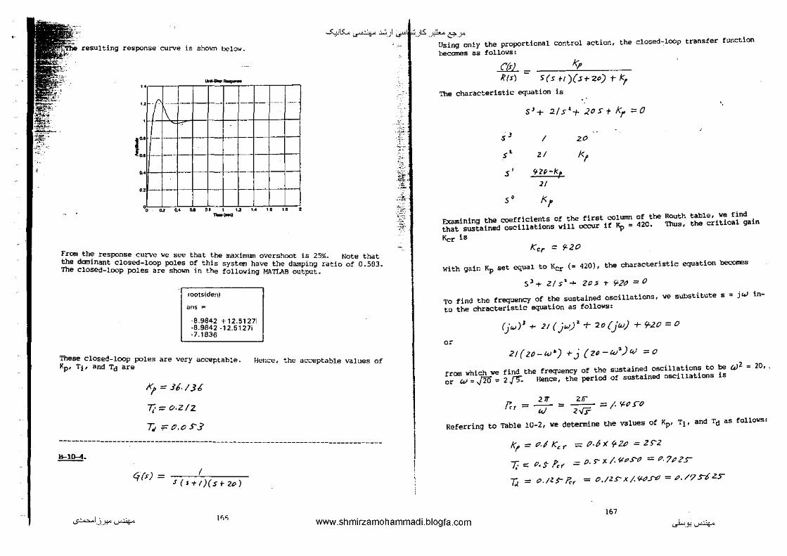
• ~15:... ...r4-- .:.:, ) ..r!fM.)ts: -~ &'-->" Using only the proportional control action, the closed~loop transfer function becomes as follows:

resulting response curve is sho~~ below.

. -,--r-,-~~;~~-~,_~-,-"r •.• 1--;:: -+-

i::R=-t:tttt o>•---~--

0o cuo.•UM t U1.4U1.1 t --FrOfll the response curve we see that the maximum overshoot is 25%. Note that the dominant closed-loop poles of this system have the damping ratio of 0.563. The closed-loop poles are shown in the following MATlAB output.

roots(den)

ans "'

·8.9842 +12.5127i -8.9842 -12.5127i -7.1836

These closed-loop poles are very acceptable. Kp• Tt• and Td are

l<t ~ 36./36

T;=O-Z/2

T.t :;::o.os-3

Hence, the acceptable values of

------------------------------------------------------------------------------.!=!!!::1-

'{($) I .I($+/)(ST2o)

-""-'

t ..

-.:

-~--~,

.~

-·:l'"<

The

('(r) - l<p Rts) - S(s +I ){.st-2c) t- k!

characteristic equation is

SJ+ 2/S'-t- .<OSt /(f ==0

•' I zo

s' Zl l<f

s' 'IU-kp

2/

,. l<f

Examining the coefficients of the first column of the Routh table, we find that sustained oscillations will occur if Kp = 420. Thus, the critical gain

Kcr is Ker = 'i£20

with gain Kp set equal to Kcr (= 420), the characteristic equation becOmeS

S'+ Z/s~+ Z05 -r if'20 =0

TO find the frequency of the sustained oscillations, we substitute s = j4) in­to the chracteristic equation as follows:

(jw)J +- 21 ( jw)~ + 20 (jw} + 9-20 = 0

O' 2/(zo-w .. ) +j {u-C4J,.){() =o

cram which we find the frequency of the sustained oscillations to be cJZ = 20, . or w = J20 = 2 0 Hence, the period of sustained oscillations is

Frr= 2. w

- 21! - <..J"r ~ j. f!,-().f'"'O

Referring to Table 10-2, we determine the volues of Kp, Ti• and To as follows:

kt = e?./ Kc:r- = tJ.6X ~ZtJ = 2f'Z

J;=: P.Sf'n• =o.s-x./.~t>.NJ =P·7t'2S'

Tj_ = c>./l.$-f:.r = 0,/ZS"X/.¥-t'..N:J =t'./?S"£2.,r

167 ...;~I_)_J:!"'-""'~ \0< www.shmirzamohammadi.blogfa.com ~-.,'-""'~

-""'15:... ...r4-- .:.:, ) ...rG!JS: -~ &'-->"

function of the PJD controller is thus

C;J') ~ kf ( I+ __}__ T;· J -t ~s)

I : 2S2 ( t+ tJ.7tJZ!>'S r P-1? J'tf zr-.s)

(/{l.,?.r?J"'s2,.+zr2.s T75"J'.7Z

s

ft.S<.ZY7S (Jf2.J>~?o)l. s.

The open-loop transfer function becomes as

I Cic(s) tj(s) = .Y.P..zs-u- s ~+ 2 s-z s -t- Jr-r.pz. s S"(ST/)(5tz0)

{I.I'.Z~?.rs-._+ 2s-zs +-3s-J".?z.

S"+ 2/s 3 + ..<os"­The closed-loop transfer function is

C{s) l?(S) :::

The folloving MATLAB next page.

{<1£. z s-7.s J .. + z s-z s + .1 ~~. '72.

sfl + 21 s.l + 61"; Zf>?S S2.+ 2SZ. s +- ),S-,f. 'lZ. program produces the tmi t-step response curve as Sholffi on

% • • • • • Unit-step resr1onse • • • • •

num = [0 0 44.2575 252 358.72]; den= 11 21 64.2575 252 358.721; step(num,den) grid titler'Unit·Step Response'/

Fr0111 the Wlit-step response curve we see that the system has the maximum over­shoot of 66%. 'Ibis is because the daninant closed-loop poles are located very near the j W axis, as the MATIAB output below shows.

roots(den)

ans =

-18.1666 ·0.5134 + 3.2659i -0.5134. 3.2659i -1.8066

'

,)_~.

.:.;.

-,--r-,c-~~~=r--~-o_y--,-,--, .. , --1--·---·--u~

:=:rA~ " --·-+-1.ll

t:l "' JilHD! /--r·

.. ~H-

·­• ' ' .• -, 6 •

-·~ • • "

Since the system involves two poles at the origin, it is desirable to cancel one of the c:ompensa.tor zeros with the plant pole at s = -1. SUppose we choose two zeros of Gc{S) to be at s '" -1 and choose Gc(s) as

k.(S+I)' -(j., (J') .::;: '

By several MATLAB trials, we find K ~ 100 will yield a desirable unit-step response. Thus, we may choose K = 100. Then the open-loop transfer !unc:tion of the system becomes

I <i.l'! 0 (') = j(>P{ra+2S+I)

• 5(Stl )(S"-t-.2o)

~

tOO Sl+ ZOOS+ /1>0

sl<+zts~ +-zos'

The closed-loop transfer function becomes

C(T) {()()S'- +- 20t:J.S -t-/00

RfJ) =- s'+- z/sJ +!2o.s• + 2.0I>S +tPP

The following MATIJ\B program produces the unit-step response as shown on next ,.,.. % •• ••• Unit·Step res)lonse •••••

num .. !0 0 100 200 100!; den"' /1 21 120 200 100); t - 0:0.01 :5; steplnum,den.tl grid titlel'Unit-Step Response')

•

...;~I.J.J:!"'-""'~ 16e www.shmirzamohammadi.blogfa.com 169 ~.J:l"'-""'~

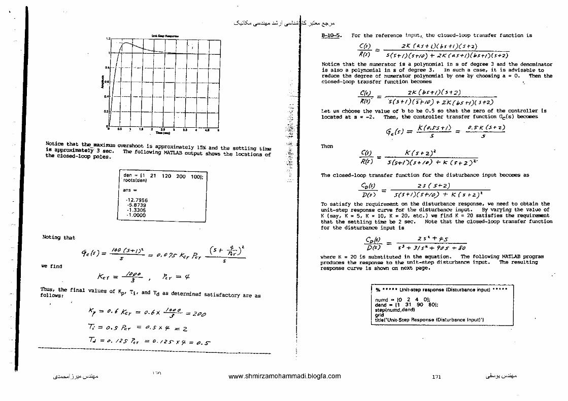
T7t+JJli;lll -""'15:... ...r4-- .:.:, ) ...r~...:..:<tts: -~ &'-->"

~· For the reference input,_ the closed-loop transfer function is

··r;-f- --- ______ , __ , __ , ___ ,_ 1::- F __ ~ttt~t ~IT- -U-+-~W

2 -u s

-·~ . " u u • u •

Notice that the lllaXimum overshoot is approxil!lilltely 15% and the settling time 11!1 approximatelY' 3 sec. The following MATLAB output shows the locations of the closed-loop poles.

Noting that

we find

den= 11 21 120 200 100]; IOOtslden)

ans '"'

-12.7956 ·5.8739 ·1.3305 ·1.0000

tfcfr) = 1" 0 (S+!Y'· s = P, "?r K.:r Rr

kcr = /Ppo

3 ?.:,.. = ¢

(s t- -;£:-;/ s

Thus, the follows, final values of Kp, Ti• and Td as determined satisfactory are as

K '" It>"'"' f = "·# Kcr = o.6x ---y-- =2P?P

T.·=o.sR...- = o.sx~ =2.

T.!=o./2S~, =0./ZS"X]>'=o.s

-----------------------------------------------------------------------------

. __ ,

-~

;;"i_

.it. ---,_ . . , ..

C{T) _ 2K (As+ 0( bs-tr)(St-2)

if{f) - .S(H/)(H/0) + ..lK(AS+/){i>st-t)(H2)

Notice that the numerator is a polynomial in s of degree 3 and is also a polynomial in s of degree 3. In such a case, it is reduce the deg-ree of nll!~Erator polynomial by one by choosing a closed-loop transfer function becomes

C(t) _ /(($). -

Zlt:(bs-t·J){H2)

"s(.H·I){srtP) +Zk(bsrt)( J+2)

the denominator advisable to

o. Then the

Let us chOose the value of b to be 0.5 so that the zero of the controller is located at s = -2. Then, the c:ontroller transfer function Gc(s) becomes

(j (r) = /((P,J"5-t/) = P.>K (s+-z) ' s s

Th~

C(f) _ k(st-2/· R(s") - S(5+/)($+/~) +- k (S"+2)t.·

The closed-loop transfer function for the disturbance input becomes as

2S ( S+2) CoM P(s) :::: $(S+-/)(Sf-/P) -t- k ($ +-Z) 1

To satisfy the requirement on the disturbance response, we need to obtain the unit-step response curve for the disturbance input. By varying the value of K (say, K = 5, K = 10, K = 20, etc.) we find K = 20 satisfies the requirement that the settling time be 2 sec. Note that the closed-loop transfer function for the disturbance input is

C0

{s) _ z~~+f-s

{){s) - s'+ :nsa.+ 'lt1f +-5o

where K = 20 is substituted in the equation. The following MATLAB program produces thl! response to th2 unit-step disturbance input. The resulting­response curve is shown on next page.

r

.% • • • • • Unit-step fBSI>Onse !Disturbance input) • • • • •

numd .. [0 2 4 01; dend .. 11 31 90 SOJ; ateplnumd,dendl grid title!"Unit-Step Response !Disturbance Input!')

...;~1_)_):!" '-"'.lo/<- '"' www.shmirzamohammadi.blogfa.com m ._..i...> _ _, '-"'.lo/<-

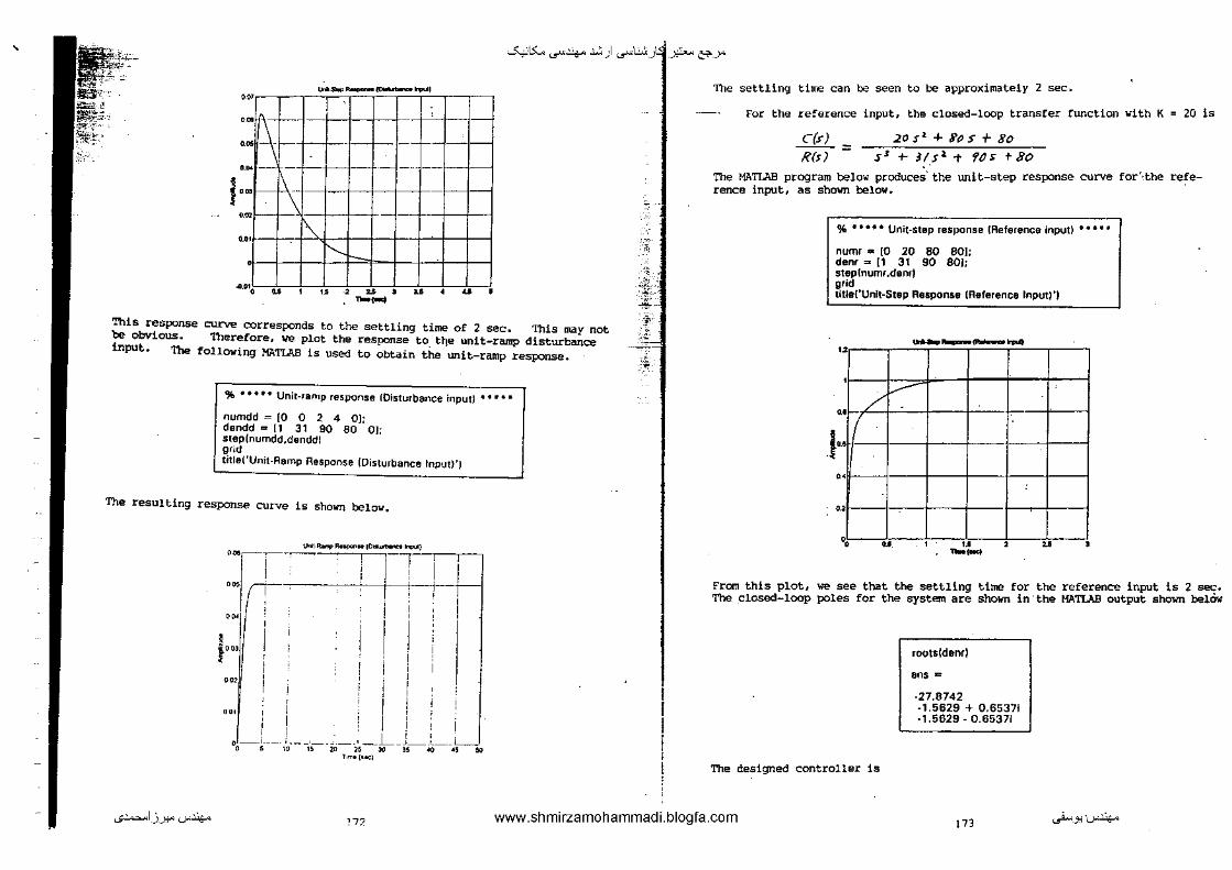
' -""'15:... ...r4--.:.:,) .,rl..:..:<_)i..51.~ &'-->" ____ ..,.., ' " 0 -1-

' l\ 1--~-1-

·- -

jo ·I- \ • -- -,,

" " "' 1'----0 .. "• u ' u ' u • .. • .. • --

This response cw:-ve corresponds to the settling time of 2 sec. This may not be obvious. Therefore, we plot the response to ttte unit-ramp disturbance input. The following MATIAB is used to obtain the unit-ramp response.

% • • • • • Unit-ramp response !Disturbance input) • • • • •

numdd "' [0 0 2 4 OJ; dendd = [1 31 90 80 OJ; step(numdd,denddl grid titlei'Unit-Ramp Response (Disturbance Input)')

The resulting response curve is shown below.

...... .._ •• _. .. ,o"'-..,..1

··~r~~-~ i l-1 I ooo I .

, , I O(W l , ! I I

Jo· i i I ! I ' ' I ' I ' ' ' ' ' o02 ' ' 1 •

' . !

oool i o'---~---- : ___ ,_ , _, _L _ _i ___ :_ __ _ ""'""2"~"'"."" '"'"''""'

•

., 1:·-: ~--

:;.. ;,£-

--~

The settling time can be seen to be approximately 2 sec.

for the reference input, the closed-loop transfer function with K

C{;-)

R(~) == 20s 1 + JI()S +- 8o

s 1 +-Us~1' 'fl)s; tBo

20 is

The MATIJ\B program below pwduces' the unit-step response curve for"·the refe­rence input, as sho\IJl below.

% • • •• • Unit-step response (Reference Input) • • • • •

nurm .. [0 20 80 801; denr = [1 31 90 80J; steplnumr,denr] grid titlei"Unlt-Step Response (Reference Input)")

----·~-- ..... u

'

-----.. /

" j '·'

u' u

•• .. ' u ' " -- •

From this plot, we see that the settling time for the reference input is 2 sec. The closed-loop poles for the system are sho\IJl in the MATLAB output shown belciw

roots[denrl

ens=

-27.8742 -1.5629 + 0.65371 ·1.5629. 0.65371

The designed controller is

...;~I_)_J:!"'-""'~ 177 www.shmirzamohammadi.blogfa.com !73 ~-.,·'-"'"'~

-""'15:... ...r4-- .:.:,)

4c:(f) = ZO(Q.Y.f+l) !O(.S+l) ' s >

The Closed-loop transfer function of the system shown in Figure 10-(o)!o

C(rJ Kp (I+ rfs + 7;p) ti,(.r) X(<) = . ( ..L )

JrKr lt-~0 +T.ts tj1 {s) (l)

The closed-loop transfer function of the system shown in Figure 10-39 (b) can be obtained a~; follow~;: Define the input to the block Gp(s) as U{s). Then,

~ V{s) = kr ( 1+ T.a) R(s) +- T.·~ [ R(sl- CM] - K, (If- 7;, s)Cfr)

Also, we have

H~=

C(r) = 91 19'/T(r)

.£!!]_ = k. ( !+- -1 +- 1.1r) R(s}- k1 (If- f;+-TJ$) Cfr) G1(.r) 1 7/s t

from which ~ obtain

C(r) X, { 1+ i; + 1;$) 'l,fs)

RM = l+t<,{t+is+-~s)~(s)

Thi5 last equation is the same as Equation (1). Thus, the two systems are equivalent.

------------------------------------------------------------------------------!!::::!2:1• We shall first obtain the closed-loop transfer function C(s)/R(s) of the I-PD controlled system. In the absence of the disturbance D( s), the minor loop has the following transfer function:

C{s') 3'/. ~2

U'(s) = .S($-ri){STS)+J?.S'Z(I+P.71f2S)

where U(~;) is the input to the minor loop. The open-loop transfer function G(s) of the system is

C](s) = -c--"1:::-~ [ 3'/. <r2. 1 ].6?'JS S(H/)(Hs) + 3f·!tl. (l+tJ.?/'/lS)

~:.-

l

·;,_)1.5: _ _y?... &'-->"

= IZ.Ifl/2

S"+ l.s'+ ~s-. !21'/ s~+37.¥Z..S The closed-loop transfer function is

C($) 12. 11112

K{s) = s'-r GS 1 ..f.-.JS'.J~/9Sz-t-.Jf,1-Z.S -tJ,l.ii/Z.

The following MATLAB program produces the unit-step response. response curve i5 ~;hown below.

% • • • • • Unit·step restlonse • • • • •

num = 10 0 0 0 12.8112]; den ... 11 6 35.3219 39.42 12.8112); t ... 0;0.05;30; step(num,den,tl

''" title!'Unlt·Step Response of t-PD controlled System')

------,--~ ..... ~~~""'""'"''"";"'~"""""'"""~'"""'""--r-----, ~

_, v

iT7L--I---t-:=--r--H ~.[ _j_~-~f------1----j ~H~--+-~~1--1---f----i------1

•' • w " .. _,_, • •

The resulting

Notice that the response is slow but shows no overshoot. pole5 are shown in the following MATLAB output.

The closed-loop

rootstdenl

ans ""

·2.3514 + 4.8215i ·2.3514- 4.8215i -0.6486 + 0.1568i ·0.6480 · O.T568i

Since the d0111inant closed-loop poles are located very close to the jW axis, the re~;ponse speed b very 5101<1' compared with that of the closed-loop system shown in Figure 10-40 (a).

...;~1_)_):!" '-""'.lo/<o 174 www.shmirzamohammadi.blogfa.com 175 ._..i.,. _ _, '-""'.lo/<o

' -""'15:... ...r4-- .:.:, ) ..rlt_)ts: -~ &'-->"

~---f,;r· the PID controlled system shown in Figure 10-40 (a), the closed­>lrransfer fu~ction between the output and the disturbance input is

C(:s) s D{s)..::: s~(s+J)(s+~) +.if. ~z.(st-~.Jz.ro-ro.?~fzs•)

s 5~ + 6' sJ + JS. 1 z 11 s t. + 11. ft2 s + IZ • .ttl 2

For the I-PD controlled system shown in Figure 10-40 (b), the closed-loop transfer function between the output and the disturbance input can be obtained as follows:

C{•) P(J)

=

s :Sz.(St-1) ( .H· >') + 3f. S<Z ( 5 +t;J.JZ,>P t-o· 71f'/2 ~ ~)

s Sfl+6sJ+.JS::JZI7sl.+ 1f.y.2s+-/z.3/IZ

Since the two closed-loop tranSfer functions are identical, we get the same unit-step response t':Ut'Ves for the two systems. The folloving MATLAB program produces the response to the unit-step disturbance input. The resulting response curve is shown below.

_,._

--~~

-'··'

~- For the reference input, the closed-loop transfer function is

_@_ _ Cf,M 9z(s)

!(s) - I+ 9tCs)'],(s)H(s)

For the disturbance input,

S/!L- i?,,(>) 1>($) - 1 + C'/ls)q,.(s)H(s)

For the noise input,

C(') A/(.J) = -

(/,(s) Y~.(s)li4).

It (j1(s)(jz{s) Hf$) Notice that the characteristic equations for the three closed-loop transfer functions are the same;

/+ rfi,{>} q,(s)f{{s) = 0

That is, the characteristic equation for this system is ~he same regardless of which input signal is chosen ~s input.

------------------------------------------------------------------------------B--l.D-10. The open-loop transfer function ()f the system is

% ••••• Un!t-step response ••••• j I Cj(s)

num = 10 0 0 1 OJ: den= It 6 35.3219 39.42 12.81121: steplnum,den) grid title!' Response to Unit-Step Disturban~:e Input')

- .. -...... ---• " ( _:t l:- 1--

" - ~~· , .. - . -· --- --

"--II --

• - --

I~ ~

• IS=: --

• --1--- ---

. , .. .. ... .. i ., o.oot]

·~· ·-·~

•• , • ' • .. " " -·~

._;~]_)_):!" '-""'.lo/<-'"

I -qF(s)

Hence, the closed-loop transfer function is

((•) <?(s)

R(i) = /- 'f1

(I) + (j{f) If Gf(s) is chosen nearly 1 but less than 11 then the closed-loop transfer function C(s)/R(s) becomes nearly 1. (We must maKe sure that all closed-loop poles are in the left-half plane for stability.)

------------------------------------------------------------------------------B-lD-11. i•

The closed-loop transfer function C(s)/R(s) for the reference input

c;,C¥, Q.J

r:;, fi.z 9 ,j' C:(.r) /+- ~" 191 H~ /({1) = I+ (j,tj,_C$,1{,

lt-r:j~(jJ/{:1.

~

I+ 9l411-1z+-4,'1~~JH,

The closed-loop transfer function C(s)/O(s) for the disturbance input is ob­tained as follOIJS: Noting that the feedforward transfer function is G3{s) and the feedback transfer function is (-Gt{s)Hl(s)- H2(s)JG2(s), and that the closed-loop system is a positive-feedbacK system, ve have

www.shmirzamohammadi.blogfa.com 177 ~-J:l ~.lo/<-

f

-""'15:... ...r4-- .:.:, ) ..ri..J:<_)ts: -~ &'-->"

((r) 0J

P{s) = I- qJ [- o/Jil; -H,.] c;,

<;, = 1-+- 0,c,,qJH1 -tChtiJh'-z..

For the system shown in Figure 10-44 (b), the closed-loop transfer for the disturbance input is

C{.r) - k Cj(r)fl{s)

D(.i) = J+ kC1(s)fl(.r)

TO minimi~ the effect of disturbances, the adjustable gain K should be chosen as small as possible. Thus, the answer to the question is "no".

---------·-----------------------------------------------------------------The transfer function between the output C(s) and the disturbance

given by

Gr) I- Ci~(s) (j1 {s)

/)(s) = IT Ci/s)[.;.Js)

If G2(s)G3(s)~ 1 in the neighborhood of s = 0, then steady-state error to the disturbance can be eliminated. Thus,

I G ;is) = ch($) for small values of / s J

Limitation: This approach cannot be used if G2(s} has a zero or zeros in the right half s plane because of the stability consideration.

B-10-14. The block diagram of Figure 10-46 (a)

J(,+K,-~o /Gil

,, K,-tl<,-t<:,~-t-T

simplified as follows:

Jld•J

.fle(s)

-

. __ ,

~

ft .. ~,-, ""'

'~ '"'-

-._;

,;.c-

D(•J ~ •f*l Jl.(s)~ - JS I

. (-·_K ___ ) (k,-tK~-1-K•s)S+):.-,,. " ' ,, ',

From this last block diagram, we obtain

----'--...!2,($) - J"S I>(r)- !+-..L-(__5___) (k.,+K,rkt~s)st-k.:

..:r.s Ls t R. s

s(Ls+R.) = JL .sJ + { JKt-Kk~ )s .. t- K {K., -r K1)s +-Kf:,

The bior:k diagram of Figure 10-46 (b) can-be ltDdified as follows:

.PM J- KKo~ ,J'(ts+l()-+ l(k.,

JK J(l.s .. K)-ti(/(J

I n.t•J I •

K,-t K,. T ~.-

From this diagram the transfer function .I2.c(s)/D(s) becomes

.il.Jr) J( Ls-t~) --v(i) = J(Lr-t~)tKI<I. ;+ _L JS

_j__ ] Js

J;::: or. r /(r 1" la(s) J(U-ti?)+I<KJ

= ---~~~---~s~(=L=s~+=R~)~------~-------­JL~J+ (:T.(t-I<Kt~)s•+ /((K.~tK;)s+-I<K,·

(1)

which is the same aS Equation (1). Hence, the block diagrams of Figures 10-46 (a) and (b) are equivalent •

-----------------------------------------------------------------------------

...;~I_)_J:!"'-""'~ www.shmirzamohammadi.blogfa.com ~ 7q ._..i...>_J:l'-""'~

-""'15:... ...r4-- .:.:, ) ._rl...:..:<_)~ _ _y?... &'-->"

B-10-15.

(•)

Hence

Yl>) 9.:, q, -= R(s) I t-qc, c?ca 9/

YM <'lt -= j)(s) It- tj,, fie~ 9p

Y(J) - tJc1 '7n. <ip -= 1/isJ It- c;,, 9a. 91'

"'' = ifCJ q,, c;,"' - c;,

Cit q,. =

If ~ is given, then Gyn is fixed but Gyr is not fixed because Gel is indepen­dent of Gvd· 'Thus, two closed-loop transfer functions among three closed-loop transfer functions Gyr• Gyd, and Gyn are independent. Hence, the system is a two-degrees-of-freedom system.

(b)

Yt1J tJJo ~,, l?e -= !<(s) lt-(jcz. GJ,

YM q, p(s) 11- (jcz 9/'

Yl'l - C?c~ ~~ --= N(S) 1+-Cj,z~/'

Hence

~.,'( =: .q(', 0;: C:;'f.;

/"_ Cl,.~-c:,, l..J'l} ::::::

"' If Gyd is given, then Gyn is fixed but Gyr is not fixed because Gc1Gc2 is in-dependent of Gj'd' Thus, two closed-loop transfer functions among three closed-

,', . '>I;r' '5!·'· :-,s . ' -~~:' ·'---

-~~

loop t<ansfer functions Gyr• Gyd• and Gyn are independent.- Hence, the system is a two-degrees-of-freedom system.

(c)

Y&l _ Get Yt --;((f) I"'" Yc~.c?1 . '

~- G, [)(>)- !+<f""t

Yl') --;

- c;a r;, M'i If' tjca 9,.

Hence

c;.,, = lj" c-;,, q,. = C1,,- q,

"' If Gyd is given, then ?Yo is fixed. Gyr is not fixed because Gel is indepen­dent of Gyd· Thus, the system is a two-degrees-of-freedom system.

B-10-16. Define the input signal to box Gc3 as A(s). Then we have

A(s-) = 'lcz RrsJ + 0c1 [R{r)- YfsJ]- ~~9nAfs")

Y(r) = 0c3 '-1 1 92 Afs)

Eliminating A(s) from the aboVe two equations, we get

Y(s"} ; c?cJ rf1

Ga. ('7n -t C7C'~) l<.(s)- c;c, Yf~}

"' It tfc3 q

1

(1 + o/" <;1 r 9" ~" q, ij,) YM =: Cfo 'f, f$, ( !$" tf$,,)11('1 Hence,

Y(s) (9cr T lJ~z) o/o (/, Cfz. --; (1)

R(J) 1-r ~CI Cft + 6rct '7c3 (j, t:?z.

To find Y(s)/D(s), we may proceed as follows. Since

...;~1_)_):!-"'---"'~ 1r>O www.shmirzamohammadi.blogfa.com ]8; ._..i..->-.!:l'-""'~

j

I

I

I

I ~I

I I

I

I I

-""'15:... ...r4-- .:.:, ) uf<t..:..:<_)ts: -~ &'-->"

ve have

A(s) = 'io [- rr>i] - c;, [ DM r CJCJ A(s)}

Yes! = c;, 9, [ D{s! t <fo A{sJ1

Yro = c-;, ~-z [ J>M + (-;c~ - q,, YM- Ci, t:M1 ·I+ C:,o c;;, J

Simplifying, we have

OS ( /f ~c~ l]1 + qC', Gc..1 Cj,9z) Yff}.:: 9J9;J J>{s)

_lli- 0, ql Pfs)- I+ 9t'J G;1 -t- <:!lc, Cln. Cf,£7z

Next, we shall find Y(s)/N(s). Since

ve have

OS

Hen~.

A{s) =- c;" [Yio +N(<!]- c;,,c;, A{s)

Y(>) = "" c;, c;, A(s)

Yls) == r:fcJ q, Clz -t?o Y6J- 0o N(J) 11-if('Jq,

(It" r!in rj, T Cj t't 9t:J c;, t:;z) Yfs) ~- (jC', ($", Gj, !fz NP)

'((.T} - Cict t.7r.J Cj, $z N(J) ; /+ 9e.J €;1 + C1c1 9o q, 0r.

From Equations (1), (2), and (J), we get

9r., ::::- Ci<!', 9('J tiy.f

Cf1r =-Cit"+ 9o. ClrJ 9r.t

(2)

(3)

If Gyd is given, Gyn is independent of Gyd because Gel + Gc2 is independent of Gyd. Gyr is independent of Gyd and Gyn because Gc2Gc3 is independent of Gyn and Gyd• Hence, all three closed-loop transfer functions Gyr• Gyd• and Gyn are independent. Hence, the system is a three-degrees-of-freedom system. ------------------------------------------------------------------------------

':t -{:

'l'" ·;_'-

~'~-~c'"'t"

lt ~.i:;~c

-ji,;:~

--~·,

CHAPTER 11

!!::!!=.!· (a) Controllable canonical form: \

~:] = [ :, -~J[ ::] . [} ~=[' '][:,]

(b) Observable canoniCal form:

[;.]=[: ~:][:}[~]~ 1=[• 1)[;:]

------------------------------------------------------------------------------B-11-2. The transfer function representation of this system is

y~ 6 c U(s) = JJ-r 6S"""-t/IS-+I = (s:+/)(s-t-z)(:s+.;>)

The partial-fraction eXpansion of Y(s)/U(s) is

Yfs) V(s) = 3 -· --+

s+ 1 s+z. + 3

st-3

Then, a diagonal canonical form of the system is

[ ·1 [ J[ J r 1 .x, -1 () tJ Xt I

~~ = o -z o :t~ -t 1 u ;tJ o tJ -3 :iJ _1

....,~1_)_):!" '-""'.lo/<o 182 www.shmirzamohammadi.blogfa.com !83 ~:J:l '-""'.lo/<o

,,

'i II II

11

[I

11

l'i :1

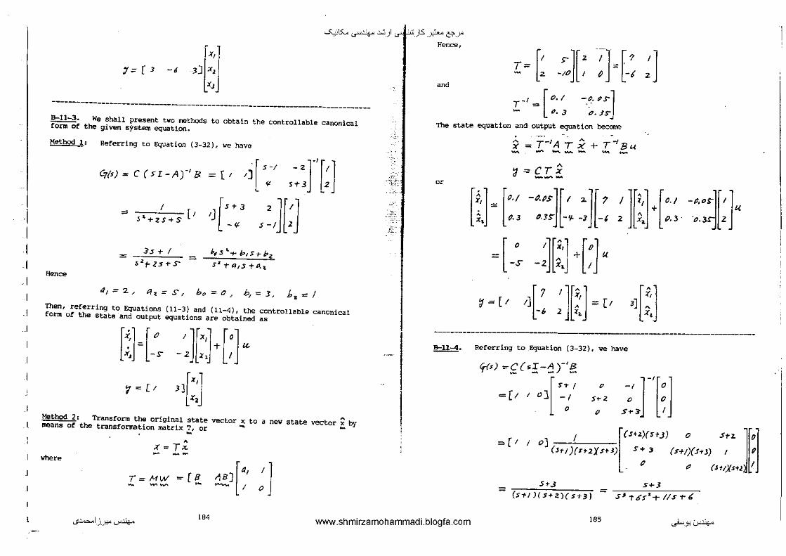
I I I I I

..1

.I

-

~15:... ...r4-- .:.:,)

1~[3 -· 3][~] ------------------------------------------------------------------------------~· We shall present tvo methods to obtain the controllable canonical form of the given system equation.

Method l; Referring to Equation (3-32), we have

C7(•) = C (SI-A)-' B = [' '] [ ·.-/ ,~:n~J I ["' ,:J[:] ~

:;'+ZS-+S [I '] -· Js + I b1 s'-..,. b,s-rb:z.

~ = :;<l~<?s+-S Szt-4/StAl. Hence

a,::::: 2, t!~.::::s, bo = 0, h,-= 3, ba =I Then, referring to Equations (11-3) and (11-4), the controllable canonical form of the state and output equations are obtained dS

where

[1H:, -~}[:JT[;Ju 1=[, 3)[::]

• Transform the original state vector x to a nev state vector x by the transformation matrix T, or ~ -

~

' X= T x.

[a,

1\B] - ' :] T=MW =[8 - -....... -

};.__

·;,_)1..5: _ _y?... &"-->"

Hence,

•nd

T= - r~ -~l ;J=r.: ~ J r.~' = [0./

•• 3 -o. ''"] >,

t7 • .IS

The state equation and output equation become

X= :;:_,AT x- + T_,Bu ----- - ...... ~.:;cr; ---or

[~]=['·I -MsJ[' ~][ 7 I][~] •['-1 -P,•>l[l]" x, ~.3 (),JS" ~9- -3 -1 2 Xz. "'·3· 0.3~ Z

=[ _: -~][::] +[~]" 1=[1 !][_: ~][::]=[1 3][:.]

------------------------------------------------------------------------------~· Referring to Equation (3-32}, we have

fM =f( •:r -:! r·~

[

HI

=[1 1 o] -: •

SrZ

0 s:J[;]

= [I I I [(S'<)(stJ) 0 SH J[•J o] '- •. " ·• S+.) (S+t){.J+J) I ~ _ P e: {lttXs+J. 1

su SH ...- (S-ti)(S+2)(S+3) = sJ1"£s-"-t-l/s-t-6

...;~I_)_J:!"'-""'~ 184 www.shmirzamohammadi.blogfa.com 185 ._..i... _ _,.:_r~

I

I

I

I

J

I

~·Although this is a third-order 'the numerator and denominator.

-""'IS:... ..r4-- .:.:, ) ~.)1..5: -~ &"..Y'

·-· ____ .. __ .. system, there is a cancellation of (s + 3) in Hence, the reduced transfer function becames

The transfer function expression can be easily obtained from the state­expression if MA.'lt.AB conrnand

[num,den] = ss2tf(A,B,C,O)

see the following MA'lt.AB output.

A-., 1-1-0 1;1 -2-0;0 0 ·.1]; 8 .. 10;0;1]; C = [1 1 OJ; D- [OJ; Jnvm,den/ .. ss2tf(A,U,C,OJ

num ..

0 0 1.0000 3.0000

den -

6 11 6

This output corresponds to the transfer function

5+3

S 3 + 6 S"L T-IIS -t-6

Notice that the MATLABoutput does not show the reduced transfer function when cancellation occurs.

-------------------------------------------------------------------------------~- The eigenvalues are

A,=J, Az.=-1"' "'\J "'".i, /\j<.: -j

The following transformation matrix P will give p-1AP"' diaq()..l,)..2,), 3•.-\4)' - --I

" 'J l / / /

l' =i '· Aa. ).J ;.., - I _, j -j

>-t .. }.. ... ... -;.., J .)._, I I -I -I

A' • • • I /\~ ;.., ;.,_ I -I -; J

This can be seen as follows. Since the inverse of matrix P is

166

-:o;.::.

~haw

B-11-6.

Method 1:

Method 2:

...;~I.J...l:!'"''-"'~ www.shmirzamohammadi.blogfa.com

I

-I p-1 = I

?'"

I

I

I I

-I I

I

-;

) -I

I I I I

I -1 I -1

p-'A P = ~ I I -j -I J - --1 J -I -)

[

/PPO] =- () -! ~ 0

0 tJ J 0

o t? o-j

-I

j

-;

tJ I o o

0 tJ I 0

Ot? 0 I

IC/110

I I I I

I -1 J -J

I I -/ -1

I -I -j j

ei'= ~.-· [Cs£-~n =..:-·![: ,~J'}

Referring to Equation (11-46), we have

187

._..i...>.J:l'-"'~

~

' J

J

J

I

I

[ •''' A-t P"t ·t

e-=f.e.-!.. =! ~ a ] r' e).&t ....

~15:... ...r4-- .:.:, ) ..ru..f_)ts: _ _y?... &'-->"

B-11-7. are-

Since

Since the eigenvalues are )., 1 "' -1 and )I 2 = -2, we obtain

Method 3: ~

or

[I 1]['-t '][' 1] e :1r = -I -.2 0 e-lt -I -I

[

2e-T- e-lt

== -.:ze-1" -r 2 e-z:t

e-•-e->< ] -e-tr2e-te

Referring to Equation (11-47), we have

I A, e >.,t

I A, eJ.,.t I =0

I A e~t

I -I e-'

I -2 e -u-j =0 -I A

H e-which can be rewritten as

., (A ) -t -e ... -r + 2 r e -- - e-~t- I= Ae-t.t:. - -Thu•

1'!-t -t' -lt -z.t-e- =(A+2I)e -e I-e A - .... ..... ....,

=[' 1 ]e-"~-[' o]e-"-[ 0

-z -1 d 1 -z

[

ze-•-e-n:

= -2e--t-t2e-u

l]e-'' -J

e-•-e-'' ] -e-T -r 2 e-z.t-

-----------------------~-----------------------------------------------------

we have

or

.!!::!!::!·

...;~I_)_J:!""-"'~ 188 www.shmirzamohammadi.blogfa.com

The given ~trix is in the Jordan canonical form. 11le eigenvalues

A,==.Z, ).L .::: 2' )IJ = 2

[

e" A< e- = o

- - t>.

-tez.t

e" 0

X(t-) = e:i' X{P) - -:f Itt) e ,, -t €' ~t

X.(t) l= 0 e"

;i,tt) 0 0

A=[~ :,]

~ <'e "] -t eu·

e"

trEez.-t·-11 Xt(~)

t et.-c

e''

X-r..fP)

:fJ(P)

IH-Ai =Is - - 3

-I~ =sl+2S+3 =(s+lt-jfZ)(s-+r-J~) , .. <' r-'[( -•} e- =.., >I-A) - - = .:-'{[: s:', rJ

-ll I [ SH I] t = J: S(S-t-2.) t.3 -3 .s J

[

st-1+1

= ;c-' (Stf) .. +.fi• -3

(s+t)z.+li'

189

(sn/,. .fi'] s+f-L_

(st!)z +.fil

._..i...> _ _,~~

! I I I I I

J

-""'15:... ...r4-- .:.:,)

He~

[

H/ I ,r,: _ _ 1 (stt)'-+li' +,vz l.s+J)'-t.JI;. -l J .jj"

-(2 ($"tl)l+Ji"'

__ ""!o._[e~~Ur..fit ~--ke-T~JZt" _..Le-T .u:- 5-t fi

I $ J Vz (.HI)"'"+.fZ~

St-1 I 5 rs+0'2-+ rz·- .rz. (HJ)'-t-li"

-' e-".«- ~~ ] fi vz. "

e- te&l: .J"i:-t - * e-r..u,:... ,[i--t

At A~[l] X(~)= e- X(P' = e-.... - / -J

[e-t ec..-1<-t . . J

::; -e-'tW'l.-fi"t- -rze--r~./2-t

----------------------------------------------------!!:!!=:2· Define

[_, ,d = -II

-t ~ :l ~ = [ ~] • G = [ 10 o]

Define also the transfo~tion matrix as P such that x = Pz. - - -[ '" f,- !',,][''] ! = J:! = p, l'n !>J l,

l'u /~.. J'JJ i 3

Then with this transformation the state equation and output equation:

:(=A X-t- 8t.< - -- .....

~= £:£ can be written as

i .... r-'APi+ p-'eu - - ........ - - .... 'J =CP• --

,~'-­__ .,__.

·~·

•:1...:..:<_)..5: _ _y?... &'-->" In this problem it is specified that

Thu•

Hence

Since

[0 0 -6] [I] r-'A r = , o -11 , p-'a = P

..... -- - ..... C I -t o

[I] ['" !=J:.4=Pz, 0 fJ,

r=H /',,

'" !',

r ..

'" ,,.

"J p,, fn

~:J[;J =r;~J= r~1 /JJ 0 hi ~ 2

[

0 0 -6] A P = p 1 o -11 -- -

0 I -~

\

we have

[-6 I 0][2 !',. f,,J [2 fn f.][O 0 -6] -11 t' I ~ lzr. ~~~ = I fu ;~ 1 0 -II

-I P 0 2 In ftJ z. lh fu 0 1 -6

O'

[ -/>T 6 -lp,. t ;, ... -If,, •!uJ [H' t,, -12-llth _,,_ J

-22.T2 -/If~~.+- /)z. -1/{IJ+,AJ :::;: pll !,. -JI-IIf,. -1/u -IZ

- '''" -lfo PH t, -IZ -11/'J .. -!In

from which we obtain

~d

fo = -6 ' .Pu =- 20, ?Jz =-/Z

-6j7,z -r ,Pn =/i:. -6/'IJ + f.u = -/2-// f/ll- -d' l't~

-lift. +f'~z ==th

"' ...;~1_)_):!"'--"'~ '()0 www.shmirzamohammadi.blogfa.com ._..i..._J:l"-"'~

Ill Iii '

I" I;

II I'

I

J

~15:... ...r4-- .:.:, ) ..rl.::f}S: -~ &'-->"

-I/ /ll -r f'1:~ =::- 3! -II /n- .f /b

- 'f'n. =?n

-6 fJ.J = -12 - II j11 - / /'J.J the last six equations for PI3• P23• and P33 we find

/1) = /tf 1 f'z., = >--F ~ /'J.J = Jb

!=U -6

::] -Zp

-/z 36

We thus determdned the necessary transformation matrix P. becooes -

The output equation

"iJ=Cf'Y=[Z -_, 16][:;]

Alternative approach: An alternative approach to the solution of this pro­blem is given below. Since the characteristic equation for the system is

we find

Define

"'""

Jsr-~1= "' II

-I

s 0

0

-I s,+ tf ... +-/ls t-£ 6 $

= s'+ t(, s~+4a.5+P.J

a1 = 6J 4~=11~ q~ = ~

~'!] =[; -6 16 J M = [ ~ ~· ->P ry - -12 36

~-' =Hr -3 "'l -s- I.S

-;..r .. ..-

' ;;-

-_-;~---

~)i;

--~:;;:-

:.i' .-

__ It can be shown that

~>r'A M ~ -- [

• 0 -•,j [ 0 = I () -A~ = I

() I - .::r, ()

0 -6] 0 -;;

I -6 M-'B =[:] ~- c

Also

o][: -6 "] eM= [t 0 -20 N = [2 _, ;.r] -- 36 -I<

Hence, by use of the following transformation:

X =11• =P -6

:: 1[:; l -u -- 36 FJ z -12

the given system_

;:( = /IX+BL<. - - -1 = ex -

can be transformed ~nto

i = ;•r'A M ? -r ;tr1 B"' .... - ... -- ...... 1 = CN..; --O<

[i,] [ 0 0 -6][1'] ['] :: =: ~ ~ :': :: + : K

~ =[ 2 -6 16{::] ----------------------------------------·---------------------------------------B-11-10. A MATLAB program to obtain a state-space representation is given '-'" uext page,

...;~I_)_J:!"'-""'~ 192 www.shmirzamohammadi.blogfa.com 193 ._..i...>_J:l.'-""'~

Aj !II ... ... •

nurn"' )0 10.4 47 1601; den ~ 11 14 56 1601; JA.B,C,DJ ~ tr2ss!nu,.,,denJ

A •

·14 -56 -160 , 0 0 0 , 0

B • , 0 0

c •

10.4000 47.0000 160.0000

0•

0

The state-space representation is

[~'] r·N -s6 -;6o][''] ['] "z = I 0 0 ;>(l + 0 t<

i:1 0 I 0;(1 0

~=[to.< <7 16o][:;] + 0 u

-""'IS:... ...r-4-- .:.:, ) ..r¥.)1..5: -~ &"..Y'

. .~, . ,.,

""

The transfer function representation of the system is

B-11 12.

Yr:s-> U~)

I s'+s'-+S

A = 12 1 0;0 2 0;0 1 3); B .. 10 1;1 0;0 11; c .. 11 o OJ: 0- IO OJ; !NUM,den] - n2tf!A,B,C.O,l)

NUM =

0 0 ·3

den = -7 16 -12

[NUM,denJ .. ss2tf!A,B,C,0,21

NUM =

0 ·5 6

den = -7 16 -12

The transfer function representation of the system consists of two equations:

~ _ S-3

Vd:s)- s 1 -7..rt..,...us-tz.

Y(s") st_ ss + 6

------------------------------------------------------------------------------ I U":.(s) =: sJ -?.s'-+(tf S -IZ

B-11-ll.

...;~I.J...l:!"'-"'~

A= 10 1 0;-1 -1 0;1 0 OJ; B = 10;1;0!; c = 10 0 1]; D = 101; [nurn,den) = ss2tHA.)3.C,Di

num ~

0 0 0.0000 1.0000

den =

1.0000 1.0000 1.0000

194

0

j B-11-13. The controllabilitY and observability of the system can be deter­mined by examining the rank conditions of

[8 A$ A'8] ~ -- --'"'

[£' A"'-c• (!1')' c'] -- - -respectively.

www.shmirzamohammadi.blogfa.com 195

._..i...>.J:l'-"'~

j

t

'

t

t

~15:... ..r-'4-- .:.:, ) ...j.<t..:..:<_)ts: _ _y?... &'-->" B-ll-15.

A~ !·1 -2 -2;0 -1 1;1 0 -1J; a- J2:0:1J: C- [1 I OJ; D ~[OJ; rank([B A'B A "2'6])

ans =

3

rankl[C' A"C' A'"2'C'IJ

ans =

3

Since the ranJr; of (B AB A2B] is 3 and the rank of [C' A'C' ,\'2c•) is also 3, the system rs cOiiiPte'teiy state controllable and-observi'ble.- -

------------------------------------------------------------------------------B--ll-14.

A • [2 0 0;0 2 0;0 3 11; 8 .. [0 1;1 0;0 1); C = !1 0 0;0 1 OJ; D = 10 0;0 OJ;" rankUB A'B A"2'BJJ

ens""

3

ranki[C' A"C' A'"2'C'IJ

ans =

2

rank(!C•B C'A•e C:'A"2'BJJ

ans =

2

From the rank conditions obtained above, the system is completely state cont­rollable and completely observable. It is also completely output controllable. Note that the condition of the output controllability is that the rank of

[~t C A~ -- .£:~',!) be m (the dimension of the output vector, which is 2 in the present system).

------------------------------------------------------------------------------

,.,

_o;;," _ __, __

--~--

A"' [0 1 0;0 0 1;-6 -11 -61; B .. (0;0;1[;---· c- 120 9 1[; 0 .. [0); ranld[B A'B A"2'BJI

ans •

3

rank(IC' A''C' A"2'C'JJ

ans •

3

Since the rank of (B AB A2a] is 3 and that of [c• A'C' A•2c•) is also 3, the system is cc:Uipletily 'Sti'te controllable and 'Comp1ete'1y obsei:Vable.

-----------------·-- - ------B-11-16.

A ~ [: ~ ~] ' .!! ~[:] ' C'=[c1 c~. c,j -6 -11 -6 I

The observability matrix is

[£' [

c, ~:<~s:J= c,

c,

A"'C_.. --

--$Cl

c, -II c.t

C,- ~CJ

-,;(c,-0 C1) ]

-/I Ct. T 6P C"_,

c,- 6 c~ + zs-(;l

There ~re infinitely many sets of c1, c2, and c3 that will make the system un­observable. Examples of such a set of cl, c2, and c3 are

With than

C = [ I I o}

c = [1 I ;J c ~ [6 s !] -c = L ~ I tl --e.tc.

any of ti1ese matrices £. the rank of the 3 and the system beccmes unobservable.

observability matrix beCQmeS less

-------------------------------------------------------------------------------

._;~I_)_J:!"'-"'~ 196 www.shmirzamohammadi.blogfa.com

197

._..i..->_J:l'-"'~

~ ,

-""'15:... ...r4-- .:.:, ) ._r~_)ts: -~ &'-->"

~ ~[; 0

2

J ~]~ I I] C ~ [I -

t··s-]=U ' I;] [~· A•c'" .... -- I is two, because

I 2 ~

= 0, I: ;J = 3 I j- 13

I I I Hence, the system is not c:cmple~ly observable.

(b) I! the output vector is given by

[~J = [; I ~J[:J = £~ '

then the rank of

[£' A~c· -- !''£·]=[: I

2

3

2 z s 13 I 3

~

13 I ~}

is three, because the detenninant of a 3 x 3 matrix consisting of the first, fourth, and sixth column is

since the rank of A MATLAB solution

I

I

I

2

{3

]

¥ ;t-1 = -¥2.

3

' A ' [C* A*C* A•2c•] is J, the system is completely observable. to thiS Problem Ts given on next page.

~-~ ·-'-~

~'-'-

_i{ -:-~ _,,

A"' 12 0 0;0 2 0;0 3 11:-1 c = [1 ' 1 ]; rank([C' A .. C' A''2'C'I)

ans =

2

A- [2 0 O;O 2 0;0 3 1];

' 1 ;1 2 3]; c- [1 rankUC' A'"C' A' ·z·c·n ans =

3

- ---------------------B-U-18. consider the system

i =A,.. i + C" 71' - -- - " Z'(~) = 9.

In Problem A-11-16 it was proved that this system is ccrnpletely state control­lable if there is no cancellation in

('1-A•)c'; ~ ~ ~

Henc:e, the dual system

x=AX ~ --~=ex --

I

IS!_-6_'1

Us)

p.(<)

;. (<)

is completely observable if there is no cancellation in

., c. I I (sr-~/- = 1sr-~·1

or if there is no cancellation in

fd.J)

f~(')

!,($)

C{H-A) = 1 [ f,l<l f,{>) · ·- P.!•!] - - - fSf:-~1

199 ...;~I_)_J:!"'-""'~ J9P, www.shmirzamohammadi.blogfa.com ~-.,'-""'~

I -1 I I

I

I

!

-""'15:... ...r4-- .:.:, ) ..rlt:<_)ts: -~ &'-->"

a direct approach to the solution to this problem can be obtained by the steps shown in Problem A-11-16. CHAPTER 12

~· Referring to Equation (3-32), we have

!j(f); C(si-11)"'!> =[I I - ... - - ]-1[ l 0 -' 0

STZ 0 p

t? s+3 I [

HI

o] -:

[

(f+2)(ST J) 0 s+ 2 ][•] o) 5-t-J (stt)(stJ) I g

0 () (s-tt){H·i) I

I [ - I I -(HI )(s+2)(StJ)

s+3 s+.J = (s-tl)(s+2)(s-t~) = s 1-t-,£$L+(/s-t6

Comparing this transfer function with

6,5J-t- b1S 1 + br.S+J,J

.sl +t~rs ... +tf&S"+&/:~

we obtain

Cit= {'

/Jo:::;-o,

A;z =//I II~ : 6

b, = 0 b .. =I I It-,~= 3

(1)

{a) controllable canonical form: Referring to Equations (11-3) and (11-4), ~ h<w

n l. I OJ ~, fo

I

X.~:::() 0 I ~. tlu (2)

XJ -i -II -( x,

!1 = [ J I o][::] '"

...;~I_)_J:!"'-""'~ 200 www.shmirzamohammadi.blogfa.com 201 ~-.,~~

c j

• l

I.

L

'

because of the cancellation of the tenns (s the system defined by Equations (2) and (3)

not observable.-

-""'15:... ...r4-- .:.:, ) rt..:..:<_)ts: -~ &'-->": we obta1n

+ 3) in the transfer is state controllable, q,== I I a,.=./t, "'J = 6

Observable canonical form: Referring to Equations (11-5) and {11-6), we

[~'] [0 0 -•][''] ['] ~~ = I o -11 Xt + I {..(

XJ 0 I - t x, 0

/4)

~ ~ [ 0 0 ~t:l (5)

Because of the cancellation of the terms (s + 3) in the transfer function given by Equation (1), the system defined by Equations {4) and (5) is observable, but not state controllable.

It is important to note that When cancellation of the numerator and deno­minator of the transfer function occurs [see Equation (1) ], the system becomes controllable but not observable or observable but not controllable depending on how one writes the state and output equations.

~ ..

[ ]

-1 [ l ST I 0 -/ 0

tJ -1 S--t-2. {) I

o o s.+.3 I

q{s) = C (5L-A)-'B ~ [I ... - - ...... I

' S+2 ]['] ('>+! )(n J) I I

o Ut~Xn-2). I

~ I [I I (St-t)( s-tl ){H~) [

(,., )(" •! I) 5 + 3

' _ ZS ... +-8s-t- 8

- (s-r/)(S+z){st-:1)

2s .. +rs-t i"

:::: s3 +{$~+!/s-t-6

Comparing this transfer function with

b(ISJ+b!SL-t-J.,zS +-6..1

S 3 +q,S~+4zs+q~

b(l == 0 ~ b, ==2' b.:=. 1J ~ b.l = z Referring to Equations (U-S) and (11-6), 1iE' have the state-space equations in the following observable canonical form:

r··] r, 0 -6]r·,] [8] l;, =l ;- ; ~~~ l:: + :

~=[• 0 1][::] ------------------------------------------------------------------------------B-12-3. Referring to Equation (12-lB), the state-feedback: gain matrix! can be given by

K=[ooi][B ~ - A8 -- NB] _, <f(~) -- --

where f( A) = A .J + &< r A a. + ol 'L A + of.! I - - - - ,_.

The values of ()( 1, C( 2, and 0{ 3 are determined fram the desired characteristic equation:

Thus,

Theo

Is!-- ( 6.- ~~/ = (.s..- u )"-)( 5T 2 -j'l-)( NICJ)

::= S 1 T /9-S 1 T .ft>S -t- 200

= s'-rD{,ss.-t- o< ... s+ ot.z

'iJ(I:;::.f'fJ 0(2. = tt? ) 0(> =.:?tJO

[0 I "J' l o I f(~) = o 0 I + 19- v o -1-S-i. -1-S

OJ' (' I OJ ['' 0] t + /o ~ o I + 2~P p I o -6 -t-.r-6 o()/

,03

...;~I_)_J:!"'-""'~ :'02 www.shmirzamohammadi.blogfa.com ~-.,'-""'~

~

=r~~ sr If'~

-·] /£]

-""~ '""'"'""" "") """"r ?- o>r

---1-· -7

[1J. [

0 I I] :f~J :::: _ I I -1/

I -11 60

A8 -~ have the desired state-feedback gain matrix ~ as follows:

.-.;~

1] [ ;

I Tf?9 sr

J7] k; [o ' I -11 . --.~ !Sf - -If 6C -7 -¥3

[ ''"" o. u·s-~ '·'"'"] = [o 0 I J t>. I' J't"lf "·"12() -t>, 11/ZO

D./r,<Sf.b -"·" /2() l?.tP/2t'J

[m sr

/:J X -0 f;-9

-7 _ _,

[ l$1·"" 17P· 'ZUf Zf ?IJI]

= [ 0 0 1] /7(1-7.16') F,Lf, '1-J" 1'1 ..1".~;,. I ZP-?KJ/ .5' • .,r;s I z. St-,.11

:;; [ z/". 78 J I S'-S"/31

% •·••• Pole plucemant --···

% • • • • • Determination of state feedback gai" matriK K by % use of Ackermann's formula • • • • •

% • • • • • Enter matrices A and B • • • • •

A= 10 1 0;0 0 1;·1 -5 -61; a "' to:t;tJ: % • • • • • Deline the controllability matrix M • • • • •

M"" 18 A'B A'2'BJ;

% • • • • • Check the rank of matrix M • • • • •

ranltiMJ

ans =

3

% • • • • • Since the nmk of M is 3, the system is completely % state controllable. Hence, arbitrary pole placement is % possible • •• • •

% • • • • • Obtain the desired characteristic polynomial by % defining the following matrix J and entering statement % poly!Jl .....

J"" [-2+4"1 0 0

puly(_JJ

~:~ns -

0 0 -2·4·i 0

0 . -10];

14 60 200

% • • • • • Compute tha characteristic polynomial %Phi ... polyvalm(po\y(JJ,AJ •• ***

Phi = polyvalm(poly(JJ,A);

% • • • • • State feedbnck gain matrix K can be given by • • • • •

K = {0 0 1]"hnviM)]*Phi

K• 28.7831 5.5181 2.4819

·,

z. ""' 17] ------------------------------------------------------------------------------

B-12-4. A MATLAB p<ogram to obtain the state-feedback gain matrix K by use of Ackermann's formula is given on next page. -

B-12-5. Substituting

kt:J U=-k;(=-[fr, --into the state equation, we obtain

..s~u . ..l:!"''--"'~ 204

www.shmirzamohammadi.blogfa.com 205 ._..i...>.J:l'--"'~

'

,.

j

I

I I I

.I

[~}[:1 ~][x}[;]~ -""'15:... ._r4-- .:.:, ) 11...:..:<_)1..5: -~ -&'Y

I .

=[ ~~ ~][:]-[;]r•, ·t:J = [-/:~, ~~-·]~:]

The characteristic equation becomes

J.s.f-:1/ =I s+;+lr, -/+K,~.I = (S+/+ ~I)( S-2) = 0

5-2

Because of the presence of one eigenvalue {s = 2) in the right-half plane, the systEm is unstable whatever values k1 and k2 may assume.

------------------------------------------------------------------------------.@:::!l:§_. Since

YM tO v;) =- (S-ti)(S"+l.)(Hi)

10

s 3 +d's~ -t-1/S + 6 - ha~

f + 6 i + II~ + 6 ~ = IO"

Using the state variables as defined in the problem statement, the state equ­ation beccmes

[x,] [ o / o] [x'j ["j i .. ~ c 0 I x, + D t(

:i, -6 -11 -6 XJ /0

"'"'

~=l-~ ~ ~]' ~=[:] _, -11 -6 10

Referring to Equation (12-18), the state-feedback gain matrix K can be given by . -

_,

~·-1

'-" I

K~[• o 1][8 - -_,

A•B] <f(A) ......... ,,.. __ AB -where

4'{A) ... AJ + "< 1 A .t+ ()(1 A+ ot3 ..I ..... - - - .....

The values of J)( 1• o( 2• and CX 3 are determined from the desired characteristic equation:

l si~(A-BK)i = (s+zrJ· zfi)(s+z-Jz.,f3)(sn•) - - -:;: S ,T/1! S:..T s-1 S" + /60

= sJ + oo:, s& -r «~ s -t Q-'3

Th~

ot, == If'- I c1~ = H, ~J =/£0

Hence,

[ J' [ ]z [ 1 2] fl!O 0/(J ()

¢~) = o o 1 + Fl- o p 1 T s-6 o " -~ -11 -/. -1. -11 -6 -6 -II

+f·-u - ~] I

-[IN .... -~] ;:;;: -'II .. II -It- ••

Since

A'8) =[: - I"] ra AB 1- -to - - -- 10 -·· z<t;

we have

[' 0 ~-rT~· ..... -:] K = [o 0 I) b /0 -tP -Y.B !6 - 10 -ltJ ~ro t8 -I> 39

...;~I_)_J:!"'-""'~ 206 www.shmirzamohammadi.blogfa.com 207 ._..i...>_J:l'-""'~

' I· I' I' I. ' ]i

I r I

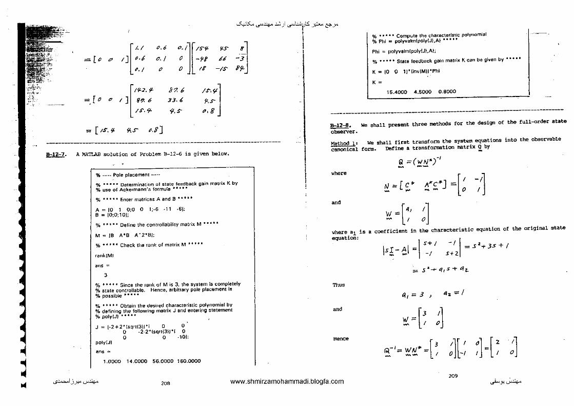
loll

-""'15:... ...r4-- .:.:, ) ..r~...:..:<vts: -~ &--->"

[I./ o.o

= [o " ;J ,_, 0./

0./ 0

[m.~ ~ [ 0 " I ] fi'?. 6

IS'·9-

; ( ;S,. 1\S' o.S]

o./] [IS'~ •s- "-] 0 -9-f ,{,{ -3

0 IC -IS J'fL

87. b :13. t

9.s I"·"] •. s-o,8

------------------------------------------------------------------------------Jt:!£:1. A MATLAB solution of Problem B-12-6 is given below.

% .•••• Pole placement .....

% • • • • • Determinat1Un of state feedback gain matlix K by %use of Ackermann':; formula •• •• •

% • • • • • Enter matrices A and B • • • • •

A= [0 1 0;0 0 1;-6 -11 -6); e = to;o;IOJ;

% • •' • • Deline the conttollabilitv matrix M • •' • •

M = JB A'B A"2'!ll;

% •• '• • Check tile rank of matrix M •• • • •

ranktMI

ens =

3

% • • • • • Since the rank of M is 3, the system is completely % state controllable. Hence, arbitrary pole placement is %possible ••• ••

% • • • • • Obtain the desireU characteristic polynomial by % defining the following matrix J anU enteriflg statement % poly!JJ • • • • •

J"' [·2+2'1sqrtl31!'1 0 0 0 -2-2"1sqrt!JU'l 0 0 0 -10[;

polyiJJ

ens "'

1.0000 14.0000 56.0000 160.0000

l l

% •' • • • Compute thPJ characteristic polynomial %Pili = polyvalm(poly\JI,AI •• • • •

Phi = polyvalm{poly!Jt.At;

o/o • • • • • State leedbltck gain rnauix K can be given by • • •' •

K = )0 0 1]'\inviMII'Phl

K =

15.4000 4.5000 0.8000

------------------------------------------------------------------------------~· We shall present three ~~~ethod.s for the design of the full-order state

obserVer.

We shall first transform the system equations into the observable form. Define a transformation matrix 2. by

where

~·

where a1 is equation:

Thu•

""'

Hence

Q ~(wN'i' - --N = [ c• - - !'£'] =[~ -:] w =['' '] - I 0

a coefficient in the characteristic equation of the original state

isJ.-!1 =\S+/ -I

-/\=S 2+JS+/ S+l

:= s~-+-q 1 s+4z...

Cf,:::: 3} 4-:. -;:::/

~ = [ ~ ;]

_ 1 • [ 3 /1[ I 0] [ l I] Q = WN = = ..... -- I 0 -1 I I 0

209 ._;~I_)_J:!"'-""'~ 208 www.shmirzamohammadi.blogfa.com ._..i..._J:l __;.~

~ • •

l

' '

•

-""'15:... ...r4-- .:.:, ) ._r\..:..:<).5: -~ &'-->"

~ =U -~l LDetine a new state vector f by ~----- ...

X={; J - --the state and output equations become

i = >1-'A (;! J .............. .....,

~ = CQ f ---Q-'A Q = = [ 2 '][-/ 'J[• '] [ 0 -I] ..., ... - I 0 I -z I -2. 1 -3

c~ = [t -- o][o l]=[o I -2

t]

The new state and output equations are in the observable canonical form. Re­f"erring to Equation (12-50), the state observer gain matrix ~e can be given by

[ .. - •·] Ke = Q "' - o(,-ar

where t:J{ 1 and 0( 2 are determined from the desired characteristic equation:

(s-)i,){S-)'1z) = (S+S){s+s) = S 1+N5 -t2S"

=J"+o<IS+ o<z =0

•• r:.t, = ;o J CX1. = 2S

Hence,

ce [0 '][2S-/J [7]

:::: I -z IP -3 = 10

~ethod 2: Define

- [~"] K,-- 'h Then, the characteristic equation of the observer is

Homce

oe

Thus,

[sf_-d+.!:•£1 = s+l+_.i._o;:,_

-I +.tf'~

-I

$+2

::= s~.+ (I+ k~, + 2)s +-I r zf,., + .t~,z.

= S 1 + I_OI +ZS

j+/t:~, + 2:::10 7 /1- 2/r~, 1- ..ftoz = 2~

~e.=?" /t,-2 =lo

~=~] Method 3: Next, we shall obtain the observer gain matrix:~ by use of Acker-mann's formula given by Equation (12-55): '""

K, = h1l[:~1T1 where ¢(s) is the desired characteristic polynomial, or

rf{$) ,.. (S-f'!)( S -p~) = {;s-t r){ Sf- S) = S' 1

"1- /0 5 t-2~

Hence

'/'(<!,) =d'+!od+2>!_

[-1 ']' [-/ = -t-10 I -2 I

'] + ,-[/ -2 0

OJ =[/7 7] I 7 I()

Thos

[17 7][ I o]-' [•] [17 7J[ I •][•] r 7] re = 7 . /0 -·1 I I = 7 10 I I I =lo The equation for the full-order state observer is given by Equation (12-51):

;?_=I A-!c.c) X:+ 8• ...... .... .......... - t- Ke fj -

where B = 0 in this problem. Hence - -...;~1_)_):!"'--'"'~ "" www.shmirzamohammadi.blogfa.com 211 ._..i...>_J:l'--'"'~

-""'15:... ...r4-- .:.:, ) ._ri...:..:<_)).S _ _y?... &'-->" i

[!:]= /[ ~~ -~]- r,][t oJ1[;} [:.]if [tl =[ ~: _:J[;H: l~

This is the equation for the full-order state observer.

-------------------------------------------------------------------------------B-12-9.

-~Ht+~::j · [

-I ~ := I c = [1 - o]

The characteristic equation for the minimum-order observer is

lsi-Au.+keAo~~.~o! = S+2-r-':e:::: s+s-

"'"" S-t-2+'ko: = S+s-

O<

It~ = 3

The equation for the minimum-order observer is

! = ( A~o~o- ~eA .. ~.) f+ [( fl~·- ~e A ... io) ~e + Ah- .f~ A...,.]~

+(B,-{,8.)~<

where u = 0 for this system. Thus

f = (-z --Jxl) f + [1-z -Jxt)X3 + 1-3 x {-t)] ~

~

given below.

% •··•· Design of luff-order stele observer .....

% • • • • • This program determines observer gain matrix Ke % based on Ackermann's formula • • • • •

% • • • • • Enter matrices A and C • • • • •

A"' {0 1 0;0 0 1;-5 -6 0]; c = ]1 0 0];

\

% • • • • • Enter tha observabj~ity ml!_trix N and check its rank • • • • •

N "' \C' A'"C' A'" 2'C']

rankiN!

ans "'

3

% • • • • • Since the rank of the observabi\ity matrix Is 3, design % of observer is possible • • • • •

% • •••• Enter the desired characteristic polynomial by defining % the following matrix J and entering stetement poly(JJ • • • • •

J = l-10 0 0;0 -10 0;0 0 -15);

JJ "' poly(JI

JJ "'

35 400 1500

% • • • • • Enter charet:teristic polynomial Phi • • • • •

Phi "' polyvalmlpoly{J),A);

% • • ••• The observer gain metrix Ke is obtained from •••••

Ke"' Phl"(invlN'll'[0;0;11

Ke"'

35 394

1285

-5'~-11]

O< •

'f +St =-"!I 'if

Referring to Equation {12-51) the full-order state observer is given by

i '=~- (A - Kfl C ) ~ -t- B u + k"e 'J - ............ - - ....

This equation defines the dynamics of the minimum-order observer.

------------------------------------------------------------------------------B-12-10. A full-order state observer for the given system is designed by use of MATI..M>. The MATI.AB program used for the design of the state observer is

...;~I_)_J:!""-"'~ www.shmirzamohammadi.blogfa.com

lii,l [-J!> I ~. = -Jtj'- 0

;.J -tzt~ -6 ~][i.]-~-l~1u +[:~J ~ 0 t~ I I tf~

213 ~-.,"-""'~

• f

~•

I

-""'15:... ...r4-- .:.:, ) ._r\..:..:<).5: -~ &'-->" We shall pr-esent two methods for obtaining the f!-lll-order state ob- ' The values of r>f 1 , !;>( 2• and D( 3 are determined from the desired characteristic matrix ~e· A ~~TLAB solution is also given, equation.

Method 1: Referring to Equation 02-50), can t:e given by the state observer gain matrix ~e

["' - ''] _ftt = £ Of._- 'h. at, - tt I

Matrix 0 is given by -s-c~~T'

.mere

[

I 0 01 N.::-[C~ A""C.- A .. .zc~]:::: 0 I() =T - ... -- ...... ........ ...... 0 o I

[ ..

'!! = ~I q, '] I 0

0 p

The values of a1 and az are determined from the characteristic equation of the original system.

·~~

-I " I -I :r+ ;J. /f'.-,r

/<;!:-,11=/ : -;.z~p

s

-P·:JJ'$",{

:::: Sl + J. I~S .s ~- (), :J'f.fif s -/. 2$L;E

-:=- s 3 + q,sz-t- (jz. s +43

4 1 .::3./f<-r; a~=-.::>.J?.s-.5', a 3 = -/.2!<-9

Th"'

[

-d•Jfs-6

w = .3-/Jl.S'"

- I

"'"'"'o'e [ _,, 5J'.J"6

Q. = (WN"~ F' = 3·/J-' r - -- 1

3-/F.r

~] I

0

J-t9-s-

~FU I

'

'"

o. I

-.J.!JlS I J -3./Y.f'

10. Ull'

"'"' Hence

( ,_ ;i;J ( 5 -,1.1. )(>-,I.!,)

= ( H:>-jN'i)(S +5'+)f'fi ){sT!o)

= (sz+ ;o s- +too){ s t-lo)

= S3 + .:z.or'"-+ :2t>os +;poCJ

= S-' +- o!tS"-t- IX:o.. s t-c;o(3 = 0

CV1 =2o, 0(4!. =- 2&'P 1 .:Y.1 '=/Ptft:J

[.-,-a,] [' lfe=~cva-.::1._::::: 0

II(, - l:ft I

[I'·''"] .::: 19-?· 317

~~. 38"/

0

I -J./'fs-

I J [1-.o T- /. < ~fL J -3.11<..r- zo, +o.uro ;o, z.rtfrf 2~ - .J. 1 ,.S

Method 2: -Define the state observer gain matrix as

['"] !f.e = "t'r. . ., The desired characteristic equation t:eoomes

I•I-A+K.c) = - - ....... [,,,Jr· I OSP- 0 ()

0 eJ S .f·U-f' O•:Jts-6

rt-Jrr, -1 ~r& s

-/.2"-fJ T-~t:) -O•JfFtf

J [ ,

() lr1 1 + '*t,,(t o o]

-3-111-S' A:tl

" -{

:H· j'. l'fS'-

.> 1 + { 1tr1 + J, IP:S) s .._ + (J,; 1-s-4~1 +A-t-& -p,JJ'Sb).s

t- (-/.:1~Y. +-lrr, t- :J,/fl.sA:i!:Jl. -o.~ff-.f' ~~1 )

...;~1_)_):!" '-"".lo/<o www.shmirzamohammadi.blogfa.com 215

~-J:l '-"".lo/<o I

~ j

,_

L

I

'

'-

1-

1-

I

-""'15:... ...r4-- .:.:, ) .,rl...:..:<_)ts: -~ &'-->"

== s 3 + 2" s& + 2otJ .5 + lt!tJil = o

Hence

-/e, + 3./~S:::: zo

'J./'f-S !:.e, rk,.,._ -~- 3?.5'6 = 200

-I. 2 S<jZ r Kr-, +- J../St.s -fc-. - "· 3f.s-~ Kc, = /OdO

from which we obtain

If~, =/If'. ?>S -fe.,_ =./fL7.3t7 ~ -f'~:~ = S"fi-~.34'/ or

[~>· •ss-1 ~e = IP-7· 3K".,.I

$'9-p:.:U/

Referring to Equation (12-51), the full-order state observer becomes

or

. ~

;(::::: (A-kec).x: +:Bu -+Ke:J. - .... ___ .........

[~]- [-"· ., ~a -=- -JY.7.317

iJ -SS'-J·I 3 7

I

0

t'.Jf.$'6 '[-] [ ] [ J

o X, o J.t,IS~ ( :i', i" 0 u + /Jt?. Jl7 ~

-J.tv;-j :r, ;.,.~ s.- 111

MATIAB solution: A MATU\B program to obtain the state observer gain matri:x ~e is shown below.

% ----- Design of full-order state ol.lserver -----

% • • • • • This program determir1es observer gain matrix Ke %based on Ackermann's formula • ••• •

% • • • • • Enter matrices A and C • • • • •

A= 10 1 0;0 0 1:1.244 0.3956 -3.145); C'= [1 0 OJ;

% • • • • • Enter the ol>servability matrix Nand check its rank • •• • •

N = IC' A"C' A''l'C'I rankiN)

ens ""

3

% • • •' • Since the rank of tho <Jbserval>ility matrix is 3, design % of observer is possible • • • •, •

% • • • • • Enter the desired characteristic polynomial l>y defining % the following matriK J and entering statement poly(JJ • • • • •

J = [-5+5'(sqf![3t)'l 0 0;0 -5-5'\sqrUJ/I'i 0;0 0 -10); JJ = poly(JJ

JJ"

1.~7003_ ~

0.0010 0.0200 0.2000 1.0000

% • • • • • Enter chara1:teristic potynomi<~l Phi • • • • •

Phi = polyvalrn(poly(JJ.A);

% • • • • • The observer gain matrix Ke Is obtained from • • •' •

Ke = Phi'(inv(N')I'[0;0;1) .. -16.8550

147.3866 544.3809

B-12 12. Referring to Equation (12-71), we have

Define

[~J=[;:~-j-L~~---~~-:J[~J+UJ ~=[1 0 •)[~]

['··] !~ ;:;: }~I

The characteristic polynomial for the minimum-order observer is

...;~I_)_J:!"'-""'~ .'IF.

www.shmirzamohammadi.blogfa.com :<17 ._..i...>_J:l\...i"~

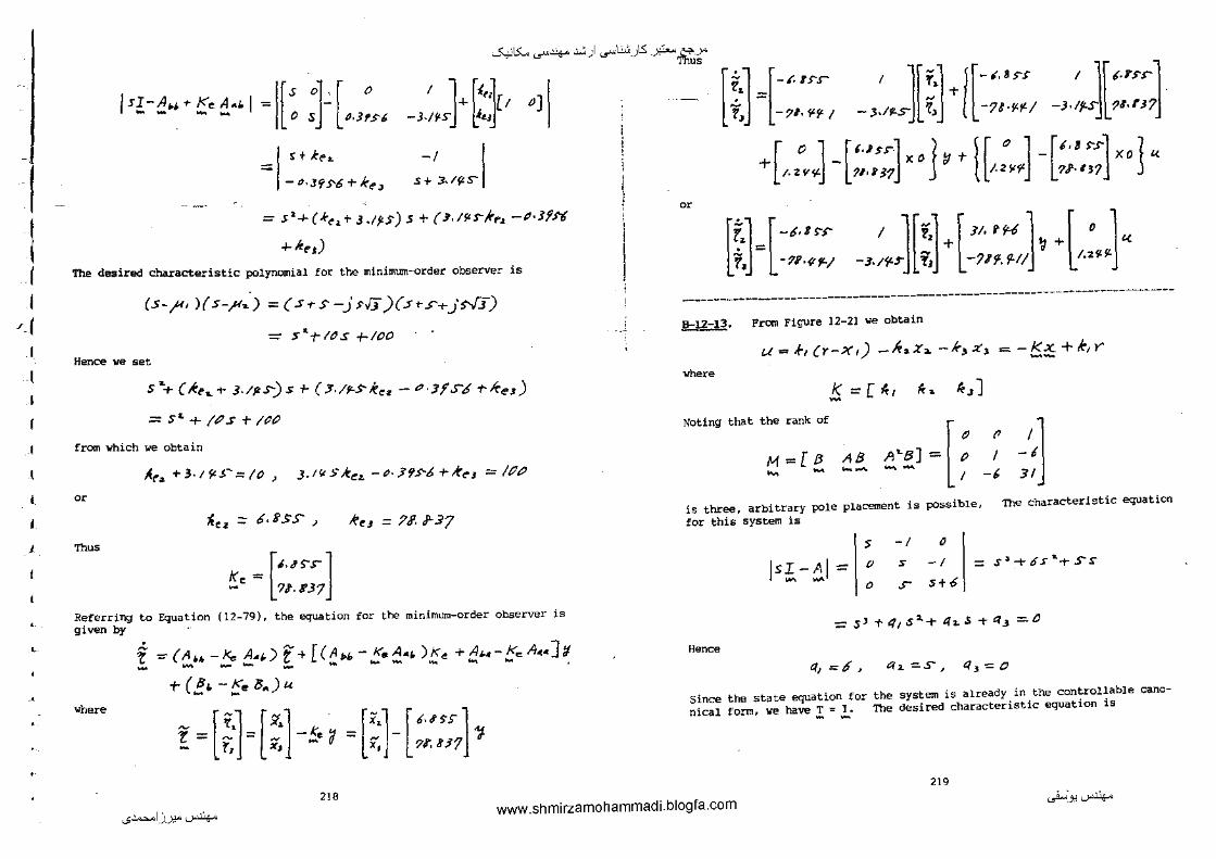
I l I I

, I

I

I

I

-""'15:... ._r~ .:.:, ) ._r\..:..:<_)1.5: -~ BY

"'"' ' Jf'·] /[-•·•N 1 lf•·n..-1 / s!-d" • ~e ::!·• I [

s ol. [ o = l 0 s J- 4.]f$'b

I l Hr -3-/I<SJ-1-l,f,_JJ I

o]

I S" t ke~:..

= -tJ.Jt(N+keJ

-I

.s + 3./ft.S"

= S 2-f- (A-t":~.+ J ./f.S) S + ( ~. /lf.s-/r,.z -~·Jf#

+-Itt-l)

The desired Characteristic polynomial for the minimum-order observer is

(s-,u. )(s-,u.) ~ ( S•S -j ,5 )(.rrr+J<'fi)

=: So.f-ltJ.s +-100

Hence we set

S '""+ ( ,tt>.._ + J./pS") s +- ( Y·/P:.S ke~ - d ·Jf S,tf 1-/(oe.r)

;;;:: S" + /t'S + /t'tJ

from which we obtain

A~~~. +J.,~r::::to) J.ll<.>'.k~.z. -P·.J95-6 +A'C"J ~ /(lt)

0<

""t<~ :::;; 6.8SS) ke.r = ?JI. JL-37

- ·"

[ ?] [-<.NT i :;:; -71. ¥f< I -J./(I...S l f, + l-78·¥1'/ -J·If'.~l?I·TJ7j.

[ 0 l ['·IU'·] ] I[ 0

] [''' s-.r-1 1 + /.ZVi'j- ?lol$7 XO ~ T t /.Z!'f" - 7.1·137 XO j U.

O<

rr.] [-t.ts-r l~' = -'li·V,_./

I l[f'·] r "· •r-t] r , 1 -3./S'S'"J t, +l-?ljt.Jl./1 ta +lt.-:sr:lf.J"'

------------------------------------------------------------------------------B-12-13. From Figure 12-21 we obtain

u = k, (r-x,) _If, :tao -K, x, =- Kx.. + k1 Y' --where

K=[~, ~. k,] -Noting that the rank of

[

0 -A'B] = P I --

1 -·

_I,} 31

1'1=[13 - AB ~-~

is three, arbitrary pole placement is possible, The characteristic equation for this system is

['·'"S"] ' J Thus -I 0

-I

st6

'

'

~c = ?1.1'37

Referring to Equation (12-79), the equation for the minimum-order observer is given by

f -=(Au -ke A .. ") f + [(AI>h- KaA•" )ke +A~_.-I<eA"'~.],;t .... -- - - -- ... .... ... . -r ( 8 0 -Ke IJ.)u - -

where

- [•·1 [Sf·] ["·] ["·"'} ! = ~ ;::: X, -:._e 'Q :;;; X', - 71'. 8J7 ";.

Hence

Jsr-6.1~ " 0

s s~+o.rt.-rss

.s-

-::: s' Tti1 .S2.-t" th.S -t43 =0

t:f, =tf ~ t:12.=s~ t?:s-=0

Since the state equation for the system is already in the controllable cano­nical form, we have!: I. The desired characteristic equation is

219 218 ~:.,'-""~

...;~l_)..l:!"'-""~ www.shmirzamohammadi.blogfa.com

• ~

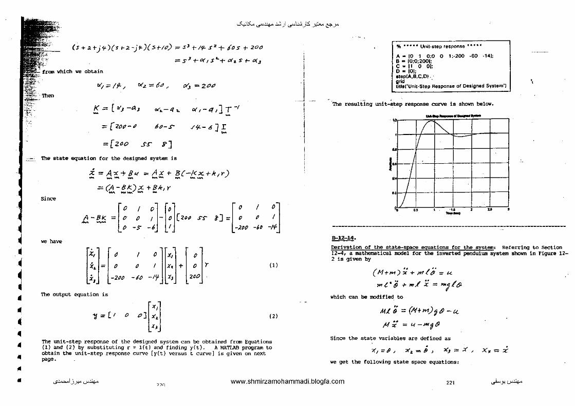
~ • • c ~

• • ~

•

·',·

-""'15:... ...r4-- .:.:, ) .,rl...:..:<_)ts: -~ &'-->"

(1 + 2 + j<r)(s t-2. -jfl.)( :S+-It7) = s:t Tl¥- s 2 -t- los + 200

= s :~ +- C(, s "-+ or.,. s +- o<~

1)(';==/P.,. otz = 6d .- Cl'): = 2011

K; [ "'' _,., - ot .. -4'1.. ] -( o<,-t:{, "I =[ZOP-P hJ-,S'" .t~- 6] I -=[200 .ST ?]

The state equation for the designed system is

:i =A:t:-t81l =AX+- B{-!<x+k 1 r) - -- - -- - --=(A-BK.)x. +BI,,y

...... --- -Since

e -~ J ~ ; ~J-[~][z.o I o -s -6 ' '

~] -[: -1()0

S"S"

w haw

l. 1 [ ][ ] [ ] z, ~ tox, o x .. = o o t x. + o r iJ -200 -£0 -1¥ :tJ 2()0

The output equation is

~=[r o o][::]

I p _,, _:]

(1)

(2)

The unit-step response of the designed system can be obtained from Equations (1) and (2) by substituting r ~ l{t) and finding y(t). A MATLAB program to obtain the unit-step response curve [y(t) versus t curve] is given on next page.

i

J

% • • • • • Unit-step reS!lOnse • • • • •

A .. ro 1 o:o o t:-2oo -eo -141; B "" [0;0;2001; c .. 11 0 0[; 0 .. 101; step[A,B,C,DI- ·, grid tillei'Unit-Step Response of Designed System')

·'lhe resulting unit-~tep response curve is shown below.

---·--,, 7 ~

'

ul •

I· " I " I "/ .. ' .. •• ul

'i --B-12 1.4.

2 is given by

(M+,._,);;+Irlt!i::-u.

)Ht•i; +-,/X= "'i-1& which can be modified to

ML (i = (N+ M) ~ t9 - u.

N;/ = u-mg&

Since the state variables are defined as

' u

.

'

·--·---

Referring to Section shown in Figure 12-

;(1 o::::J9 1 Xz.=,9) X:.J;::::::X~ X,.=:i

we get the following state space equations:

...;~I_)_J:!"'-""'~ nc www.shmirzamohammadi.blogfa.com 221 ~.J:lt.r~

• .I

[

'

' L

'

•

;., 0 I 0 '.-t.t+l>f

;, M.l '

0 0 =

;(, 0 0 0

. ~

x, - M? 0 0

[~J =[ ~ 0 0 "'(: 0 I 0 .,

x,

0 <, 0

I 0 x, -NT

+ I x, 0

_/_ 0 x, M

,

I«

-""'15:... ...r4-- .:.:, ) .,r\..:..:<_)1..5: _ _y?... &'-->"

(1)

(2) I

S=-1'-rj¥, s=-~t-j9-, s=-.zo, s=-z.o

the following MATIAB program can be written for the detennination of the state­feedback: gain matrix !:

% ----- State-feedback gain ~lfi)( -----

% •• • • • This progrem determines the state-feedback gain % m;mix K ., (k1 k2 k3 k41 by use of Ackermann's %formula •••o• % • o o •• Enter matrices A,B,C. ;md D • • • • 0

\

A= 10 1 0 0;12.2625 0 0 0;0 0 0 1;-2.4525 0 0 0]; B '"' 10;-0.5;0;0.5): c .. 11 0 0 0;0 0 1 0]; D -IO:OJ;

% • • • • • Define the controllability matri)( M and check its rank • • • ••

Substituting the given numerical values into Equations (1) and (2), we obtain the following state-space equations for the system:

- I ) I J M = IB A"B A'2"B A'3"BJ;

rank(MI

. "' 0 I 0 0 <,I ;, IZ. UzS 0 0 0 •• = +

'· 0 0 0 I ., . x, ., - z. Jt..f'2.S" " 0 0 •

,

[~J = [ ~ 0 "' or " I 0 x:

'• Determination of the state-feedback: gain matrix K: this system are

0 I 0 0

0

I 0

-o . .s-1 u 0

o.s

Since matrices A and B for ~

/ ~:s A~

1/2. 2.6 zs v 0 ' B =

0 ' - I ~

l o~s -z.rt..s:zs 0 0 0

and the desired closed-loop poles are at

...;~1_)_):!" '--"'.lo/<o :?2? www.shmirzamohammadi.blogfa.com

ens ""'

4

% 0 0 0 • 0 Since the rank of M Is 4, the system is completely % state controllable. Hence, arbitrary pole placement is %possible. •••••

% •• 0 0 • Enter the desired characteristic polynomial which % can be obtained by defining the following matrix J and %entering statement poly(JJ •o•oo

J"' l·4+4"i 0 0 0;0 -4-4°i 0 0;0 0 -20 0;0 0 0 -20]; JJ .. poly(JJ

JJ = .. 752 4480 12800

% • • 0 0 0 Enter characteristic polynomial Phi • 0 •

0 •

Phi ,. polyvalm(poly(JJ,AJ;

% • • o o • State feed buck gain matri)( K can be determined %from • •• ••

K = 10 0 0 1]"linv(M))"Phi

K•

1.0e+003 •

-4.1381 -1.0094 -2.60~36 -0.9134

223 ~-J:l '--"'.lo/<o

' ~ (

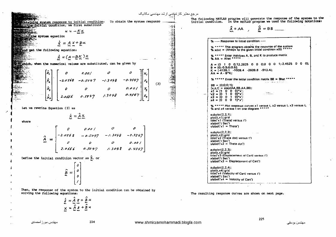
t

'· I

'

~15:... ...r4-- .:.:, ) ._ri.f:<_)S: -~ &'-->"

To obtain the system response

~ --::( = fl X+ gu. -- -

following equation1

x~(A-!3K)X - - -- -when the n!JIIIi!t'ical values are substituted, can be given by

. x, 0 "·""/ x ~.

-z..c >lt -#· s-c~ 7

"'· 0 0

• Z.R/#6 (J ' .f'"P '! 7 "• Let us rewrite Equation {3) as

• A x;;,tZ, where

0 tJ.t:'R I

A = ~-Z,PS"! 8 - /I.S"t:>fl-7 A

0 0

z.o/tft O.J'(J Y.J

A Define the initial condition vector as B, or -

~ = [;]

"' 0

-/.JDH -(). ~S¥7

0 (7,/IOI

I· 3 o ~2 d.~#7

0 0

-/. J()fi -O,f<S67

" tJ, ""I /• Jt'~f p, r,tSdJ

x,

'• I '\

'•

Then, the response of the system to the initial condition can be obtained by solving the following equations:

0 A A

"'=A?+B« ... -- -A A X'=Az+B<.t --

(3)

--~~ The following MI\.TLM program will generate the response of the systao to the ------ initial condition. In the W.TLM program we used the following notational

,,,j

~~· ··-~: ·""" :I,:-.. ,_.

J~~ ~

;~,. '1;;. '"

-~ -~~

·"$~· ·._ .... -- _:::

... I •• _."<-

' ' '

A

A :AA ~ '

A .B =- BB -

% ----· Response to fnltiBI condition -----

% • • • • • This program obtai'nk the response of the system % xdot ,., (Ahat)x to the given initial condition xiOJ • • • • •

% •• • • • Enter matrices A, 8, and K to produce matrix %AA ... Ahat•••••

A"' [0 1 0 0;12.2625 0 0 0;0 0 0 1;-2.4525 0 0 OJ; 8 .. [0;-0.510;0.6]; K m [-4138.1 -1009.4 ·2609.6 -913.4); AA- A·B"K;

% • • ... Enter the Initial condition matrix BB • Bhat .. •• •

BB "' (0;0;0;11; [x,r,tl .. stepfAA,BB,AA,BB/; x1 .. [1 0 0 OJ•x';

·x2 - [0 1 0 OJ•x'; x3 .. (0 0 1 O]•x'; x4 = [0 0 0 1)•x';

% ••••• Plot response curves x1 versus I, x2 versus I; x3 versus I, % and x4 versus t on one diagram • • • • •

subplot[2,2, 11; plol{t,xlJ;grid titlef'x1 (Theta) versus t'l xlabel!'t Sec'J ylabeH'x1 = Theta')

subplot(2,2,21; plotft,x2);grld tltlef'x2 !Theta dot) versus t'J xlabel('t Sec'J ylabeH'x2 - Theta dot')

subplot(2,2,3J; plotrt,x31;grid title!'x3 IDisr>lecAmAnt ~~Cart) versus t'J xlabelf't Sec') ylabeH'x3 .. Displacement of Cart')

subplot(2,2,4J; plot(l,x4);grid titlel'x4 (Velocity of Carl) versus t'J xlabeU't Sec'J ylabeU'x4 .. Velocity of Cilrt'l

---

The resulting response curves are shown on next page,

225 ...;~I_)_J:!"'-""'~ "' www.shmirzamohammadi.blogfa.com ._..i...> _ _,.:;.~

'

-~

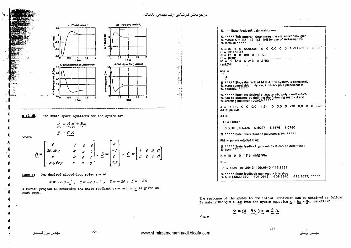
• • • • I

• • j

I

• • • • • • • •

-""'15:... ...r4-- .:.:, ) .,rl...:..:<_)ts: -~ &'-->"

0 ' 0

L ' ' ' .. '

:1 {Thotll) "' , .. __ ,.., I ~

'

.0.00 --•• ' . -u ' .,

~~I

J: •

""' l<l(D~IIC.O......,I

... -o 0.6 1 1.5

""' '

~

i " •

~ • f • '

x2{1Mia<lol)_...t_

'o o.s 1 t.s

""' )(( (VIIOCily 0( Cart} ------•O

' 0

1./ ·-'o o.s t 1.5 .... --

'

'

-------------------------------------------------------B-12-15. The state-space equations for the system are

.i =A ;e +.8'< - ...................

where <1 ~ex -

[ 0

I ' 0 0

u. PtJ I ~ 0 0 -I ' C ~ [I 00 "] A~ , B = 0 0 I " -e>~'i-f'S'

p 0 I ~ ~ d

0 0 0 o.s

Case 1: The desired closed-loop poles are at

S= -I.J-+-j, ~=-/.3-J, S=-2P, S=-20

A MATLAB program to determine the state-feedback gain matrix K is given on next page. · -

,_ j

i 1

.I ~J : l : l

·:::::; ' --t

% ---- State feedback gain matrix ·····

% • • • • • Thls program determines the state-laedback gain % mauilc K • [kl- k2 k3 k41 by use of Ackerm;mn's %formula •••••

A~ !0 1 0 0;20.601 0 0 0;0 0 0 1;-0.4905 0 0 01:'· a"' ID:-t;0;0.5J: c "' [1 0 0 0;0 0 1 0]; 0"' [0;0]; __ M • [8 A"B A'2"8 A"3"8J; rankiMJ

ans "'

4 % • .. •• SillCB tha nmk of M is 4, the system is completely % state conuollable. Hence, arbitrary pole placement Is %possible. •••••

% • • • •• Ent11r thlt desired characteristic polynomial which % can blt.obtained by defining the following matrix J und % entering 1tatement poly(JI • • • • •

J .. 1·1.3+1 0 0 0;0 -1.3-i 0 0;0 0 -20 0;0 0 0 ·20]; JJ = poly{JI

JJ = 1.0e+003 •

0.0010 0.0426 0.5067 1.1476 1.0760

% • • • • • Enter characteristic polynomial Phi • • • • •

Phi -=- polyvalm(poly(Jt,A);

% • • • • • State feedb<~ck gain matrix K can be determined %from •••••

K = [0 0 0 1]"lirwiM))"Phi

K =

-582.1330 -101.0913 -109.6840 ·116.9827

% • • • • • State laedbilck gain matrix K is thus % K = [·582.1330 ·101.0913 -109.6840 ·116.9827) •••••

The response of the system to the initial condition can be obtained as follo~ By substituting u = -~into the system equation i = ~ + ~u, we obtain

X =!/4-BK):c. ;::;,4x. - - -- .... --where

m ...;~I_)_J:!"'-""'~ '" www.shmirzamohammadi.blogfa.com ._..i...>_J:l'-""'~

(

' •

.·-

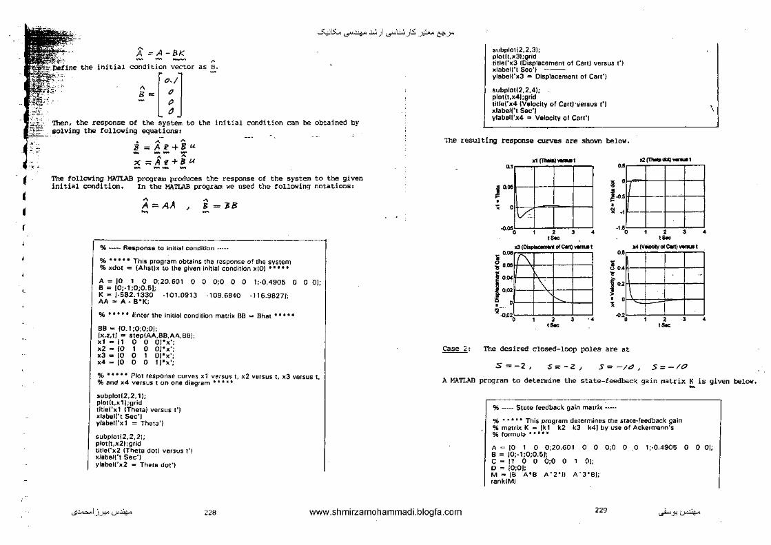
-""'15:... ...r4-- .:.:, ) .,rl...:..:<_)ts: -~ &'-->"

A==A-BI< - ' the initial condition vector as B.

A [0,/1 B= g - p

~

Then, the response of the system to the initial condition can be obtained by solving the following equationst

The following MATLAB initial condition.

• A ' E = AP+8U - -- -' A X;:::;fl'i+S« -- -program produces the response In the MA'llAB program we used

A A= AA - '

A

8 = JB

% ..... Response to init•al condition ••.••

of the system to the given the following notations:

% • • • • • This program obtains the response of the system % xdot -= !Ahat)x to the given initial condition xiOJ •••• •

A= JO 1 0 0;20.601 0 0 0;0 0 0 1;-0.4905 0 0 OJ; B = !0;·1;0;0.5]; K- J-582.1330 -101.0913 -109.6840 -116.9827/; AA .. A· B"K;

% • • • •• Enter the initial condition matlix BB = Bhat •• •••

BB "' [0.1 ;0;0;0]; [x.z,t/ = step(AA.BB,AA,BB); x1 = 11 0 0 OJ"x'; x2 .. 10 1 0 OJ•x·; x3 = [0 0 1 O]'x'; x4 .. [0 0 0 t]'x';

% • • • • • Plot response curves x1 versus C x2 versus I, x3 versus t. % and x4 versus 1 r.m one diagram • • • • •

subplotl2,2, 1); plot(t,x1 );grid title('xt !Theta) versus t') xlabeU't Sec') y/abel!'xl =Theta')

subplotl2. 2, 2); plot(t,x2);grid title('x2 (Theta dotJ versus t'l xlabel('t Sec") ylabeU'x2 - Theta dot')

subplo\(2,2,31; plotlt,x3t;grid title('x3 !Displacement of Cart) versus t'J xlabell't Sec'/ ----ylabei!'JC3 = Displacement of Cart')

subplotl2,2.4); plotlt.x4J;grid tltlel'x4 !Velocity of Cart) ·Versus t'J JCiabeWt Sec'] ylabell'x4 = Velocity or Can')

\

The resulting response curves are shown below.

Case 2:

:d {11Wiol-l

• '

~· • •

I " 0

Vc

"'" ;0 ' ' , • '"' x3(~olc.tl)-t

~ 0.08

'8 0.05

10~ 0.00

0 • -~-:;,.0. ·o

'\

'

\

' , .... •

.. ;,--=·;-~:o:""r--==r''--, I o

~·· • . _,

_,.;!----!----!---c!-----! 0 1 2 3 •

., ~ 0. •

' ' ' f'-'

> • ' '

'"' )04 (VIIocllyol c.t} __ ,

.

' .0 .• 0123

'"' •

The desired closed-loop poles are at

S=-2, s= -z J S=-/~, 5=-/0

A MATLAB program to determine the state-feedback gain matrix K is given below. -% ..... State feedbacl1 gain matrix .....

% • • • • • This program determines the state-leedback gain %matrix K .. [kt k2 k3 k4] by use of Ackermann's % formula • • •• •

A = JO 1 0 0;20.601 0 0 0;0 0 0 1;·0.4905 0 0 0[; B = )0;-1;0;0.51; C = 11 0 0 0;0 0 1 OJ; D = [0;0); M = [B A'B A"2'0 A"3'8); rankiMJ

...;~I_)_J:!"'-""'~ 228 www.shmirzamohammadi.blogfa.com 229 ._..i..._J:l'-.!"~

(

I I

/I

~,

·._'

l

'

'

ans --""'IS:... ..r-4-- .:.:, ) ._r\..:..:<_)1.5: _ _y?... &-..Y'

subplot12.2.11; plotlt,lll); grid

4

% • • • • • S111~e tim rani< ul M is 4, tt1e system is completely %state contwllal>le. Hen~"· albHrary pole pli!cement is % pr;>ssil>le. • • • • •

% • • • • • Enter the <lesired ch~racteristic polynomial which %can be obtained by <lefiningthe following matrll<. J and % entering statement poly(J) •' • • •

J .. 1-.2 0 0 0;0 ·2 0 0;0 0 -10 0;0 0 0 -101; JJ = polyiJ!

JJ •

24 184 480 400

% • • • • • Enter charactltristic polynomial Phi • • • • •

Phi ,.· polyvalm(polyfJJ.AJ;

% • • • • • State feedba1:k gain mall ill K can be determined %from •••••

K .. [0 0 0 _ 1J'linv(M)J"Phi

K•

-224.9884 -48.4648 -40.7747 -48.9297

% • • • • • State feedba1:k gain rna trill K is thus % K = 1·224.9884 -48.4648 -40.7747 -48.92971 '"''

The response to the given initial condition can be obtained by entering the following MATLAB program into the canputer.

% ----- Response to initial condition ·-·--

% • • • • • This program obtains the response of the system % xdot • IAhatlx to the given initial condition ~40) • • • • •

A- 10 1 0 0;20.601 0 0 0:0 0 0 1;·0.4905 0 0 0); B .. {0;-1;0;0.5); K .. [-224.9884 -48.4648 -40.7747 -48.9297); AA"" A· B'K;

% • • • • • Enter the initial condition matrix BB = Bhat • • • • •

BB = [0.1 ;0;0;0); t .. 0:0.01:4; )li,Z,I],., step(AA,BB,AA,BB, 1,1); >~1 =,11 o a Ol'x'; x2'"' [0 1 0 0)'>~'; x3"" JO 0 1 Ol"x'; x4 = {0 0 0 1)'x';

% ••••• Plot response curves lll versus 1, ~2 versus t, x3 versus 1. % end x4 versus t on one diagram • • • • •

230

titlel'lll (Theta! versus l'l Jllabel!'t Sec') ylabell'>~1 "'Theta'!

subploti2,2,2J; plotlt,ll2); grid title!'ll2 (Theta dot) varsuS-t'J Jllabel('t Sec') ytabell'x2 .. Theta don

subploti2,2,3J; plotlt,K3);'giid tltle('x3 !Di~placement of Cart) versus t'J xlabell't Sec'! ylabel('x3 .. Displacement of Cart')

subplotl2.2.41; plotlt,ll4); grid tltlel'x41Velocity of Cart) versus t'J xlabel('t Sec'/ ytabell'x4 .. Velocity of Cart')

The resulting response curves are shown below.

~~~-)--\

• "·'

r " I , I •

' .0.050

VI . , ' ·- •

• ~ r •• • • •

, • , ·-• 'o

><2 {lhollo dol)- I

!

' , ' ·-x3 (Olsplacemlnt of Car\) vtrwa I "" (Veio<ity t;l c.rt) _, ,, ~ '

1·:: ... . ""'

'(\

'-- ~

\. • '

; I

' • , ' -\·

8. • f•

•

• ' ' ' 1'--, ·- ' • ..o.:!0\23<1

"" Comparing response curves Xi versus t (i = 1,2,3,4) for Case 1 and Case 2, re­spectively, they are substantially the same. This means that the response· characteristics are about the same provided the dominant closed-loop poles are located in the same general region and the non-dominant closed-loop poles are located far away from the origin.

231

,._ ._;~I_)_J:!"'-'"'~ www_:s~~!_rz_a}!1_9h<!!!l.madi.blogfa.com ._..i..>_J:l'-'"'~ -- -----~---

(

,(

4

• • • 4

• • • • • • • • •

-""'15:... ...r4-- .:.:, ) ._ri.S:<_)ts: -~ &'-->"

to Section 12-8, the inverted pendulum control system can following equations:

X;,::;;AX-t-[lu : ,,._ - -- -< "1-_ 7=£::::

u :-Kx+ lz f --I= Y~·V,; Y-C <: --llhere the state vector ! is defined by . - -;(, •

>. 9

"' =I = ,, X . x, :<

and matrices A, B, and C are given by -- -0 I 0 0

A= I ZC.6'/ 0 0 f l ' B= -I C=[o o ;o] -- p 0 0 0 --I.Pf'P.r 0 0 o.s-

The state error equation can be given by Equation (12-114), or

. ' ' e :::;'Ae+B~e .... -- ... where .

0 I 0 0 0

, [A OJ 2a. t" I 0 0 0 0

i= [:] A- - -- 0 0 0 I - - 0 ' - -c o - (), fl-ft!.> 0 0 - 0 0 I 0 -1 0 0

" and Ue is given by

' Ur: =- Ke

'ilhere

0

-I

0

OS"

0

K = [ K .' -h] = [ ~, L ', '• i -<z 1 - -The desired closed-loop poles for this system are located at

s=-l, .s--z._ s.=-to, s = -/tJ ~ s = -10 •.

A MATLAB program to produce the state-feedback gain matrix K and the integral gi'lin constant 11:1 is given below. -

% ----- Design of 11n Inverted pendulum control system -----

% • • • • • This program determines the state feedback gain matlix % K ,. lk1 k2 k3 k4J and Integral gain constant kl by use of % Ackermann's formula • • • • •

% • • • • • Enter matrices A, 8, C, and 0 • • • • •

A"' 10 1 0 0;20.601 0 0 0;0 0 0 1;·0.4905 0 0 OJ; B = [0;-1;0;0.5]; C=[OOIOJ; 0 = [0];

% ••••• Enter matrices A1 and 61

AI =[A zeros(4, t);·C 0); 81 = [8;0];

.....

% • • • • • Define the controll!lbilit';' matrix M • • • • •

M = [61 A1"B1 A1"2•St A1"J•St A1"4"B1]

% • • • • • Check the rank of matrix M • • • • •

rank(MJ

ans ..

5

% • • • • • Since the rank of M is 5, the system is completely %state controllable. Hence, !lrbitrary pole placement Is %possible .

% •• ••• Enter the desired characteristic polynomial, which % can be obtained by defining the following matrho; J and % entering statement polyiJI • • • • •

J = [·2 0 0 0 0

0 0 ·2 0 0 ·10 0 0 0 0

JJ = poly(JJ

0 0 0 0 0 0

-10 0 0 -10];

...;~I_)_J:!"'-""'~ www.shmirzamohammadi.blogfa.com 213 ._..i... _ _,.:_r~ .,.,.,

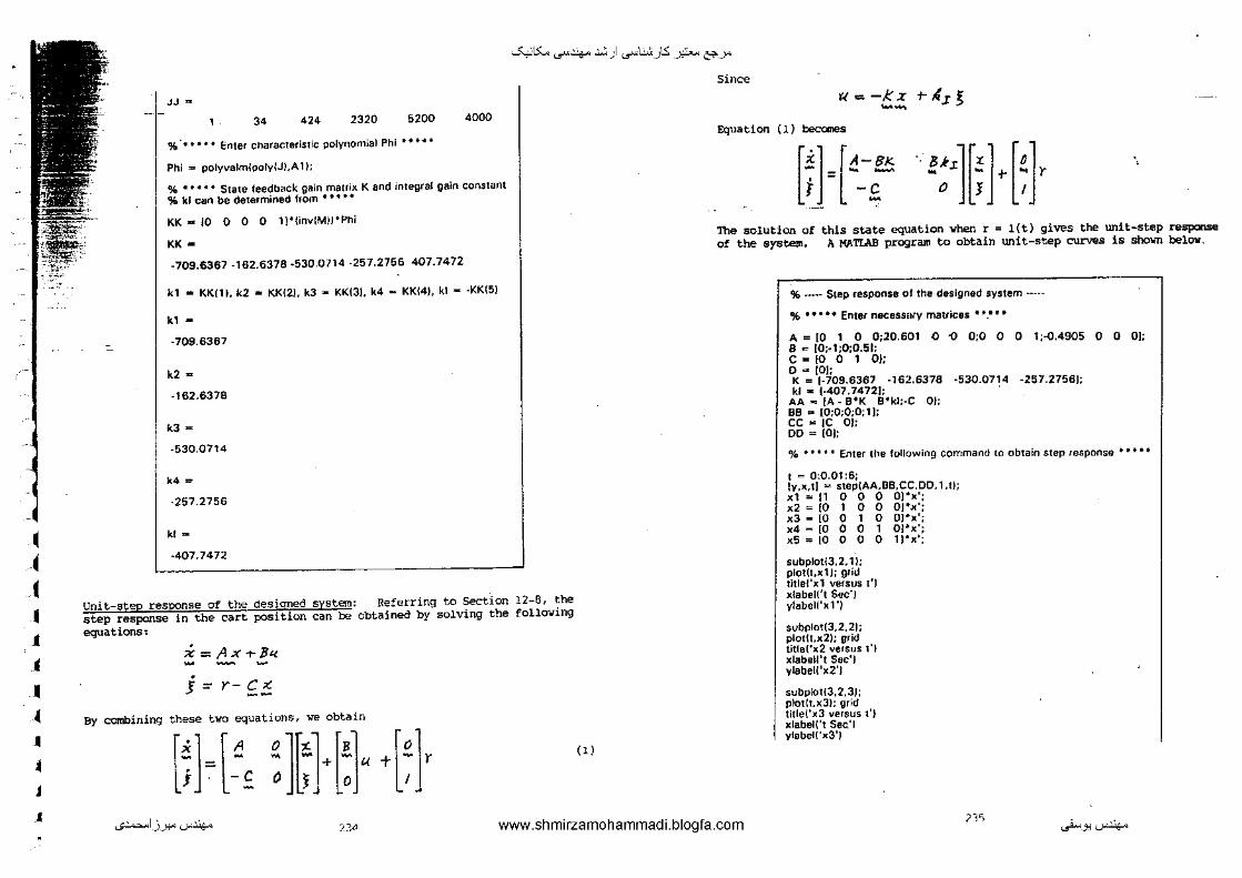
• • c • J j

• ~

• ~

j

•

-""'15:... ...r4-- .:.:, ) .,rl...:..:<_)ts: -~ &'-->"

equations•

,_

" 424 2320 5200 4000

% · • • • • • Enter charac:teristic polynomial Phi • • •• •

Phi"" polyvalm!pofyW,A1!;

% • • • • • State leedbi!Ck gain matrix K and integral gain constant % kl can be determined from • • • • •

KK .. 10 0 0 0 ll"(invlMJJ'Phi

KK • -709.6367-162.6378-530.0714-257.2756 407.7472

k1 .. KK!H. k2 • KKl2), kJ - KKlJ), k4 - KKl4), kl - -KKl5)

k1 -

-709.6367

k2-

-162.6378

k3 -

-530.0714

k4-

·257.2756

kl­

-407.7472

i=Ax-t-ll'<

j = Y- C >: --

Referring to Section 12-6, the obtained by solving the folloving

By combining these two equations, we obtain

[;]=[:£ ~]~}[:]" +[~)r '"

Since

't(=-Kx t--'.d ~-

Equation (1) becomes

[1}[:~ ~:"][;H~Jr ..

The solution or of the system.

this state equation when r = l(t) gives the Wlit-step response A MATLAB program to obtain unit-step curves is shcnm below.

% -·-- Step response of the designed system •••·•

% • • • •• Enter ni!CeSSiiiY matrices • •.• • •

A = [0 1 0 0;20.601 .() {) 0;0 0 0 1;-<l.4905 0 0 0]; 8 "' [0;-1;0;0.51: c-tootoJ: D .. [0]; K = [-709.6367 -162.6378 ·530.0714 -257.2756); kl'"' 1-407.7472];

AA .., lA- B"K B"ki;-C OJ; BB'" (0;0;0;0;1); CC,. IC OJ; DO= [0];

% • • • • • Enter the following command to obtain step 1esponse • • • • •

t = 0:0.01:6; [y,X,t] .. step(AA,BB,CC,DD, l,t); xl = 11 0 0 0 O]"x'; x2 = [0 1 0 0 0[ 0 JoC'; x3 - [0 0 1 0 OJ"x'; x4 = [0 0 0 1 0[ 0 >:'; xS = [0 o 0 0 li"JO:';

subplotl3,2, 1 J; plot[t,xlJ; griU tltlel'xl versus t'J xlebel('t Sec') ylabell'xl']

subplot(3,2,21; plotH,x2); grid title('>e2 versus t'l xlabell't See') ylebel!'x2'J

subplot!3,2,3J: plotlt.K3); grid titlel'x3 versus t') Klabel('t Sec'! ylabel!'K3')

...;~I_)_J:!"'-""'~ ;;:;<] www.shmirzamohammadi.blogfa.com m ~-.,'-""'~

'

j .. .~

A .. • • J

I

' J

J

J

-""'15:... ...r4-- .:.:, ) .,rl...:..:<_)ts: -~ &'-->"

subplo!l3,2,4); plo!lt,x41: grid , !i!le!'x4 versus 1') xlabeWt Se~:'l ylab~l!'x4'l

subplotl3,2,51; plotlt,x5J; grid title!'ll5 versus t') xlabel('t Sec') ylabeU'x5'1

Tile step response curves obtained by use of the above MATLMI program are sh01m belov.

·-· -·:rg; I I ' ~ . ~ ' • ' ' "~

~-·

.·:1-zf ij .(1_

5o2•6

"~ ~-·

.:~v1 I I 0 2 .t 6 ·-

~-·

·~I I I ~~ 4 ! I 0 2 • 6 ·-Mv.,. .. t

··*~>b I I ..o_so 2 4 6 ·-

CHAPTER 13

!!:!H.· The given quadratic form can be written as

[ I / -I]["'] Q = (x, ;tl XJ] I -9 -J ){l

-1 -3 I xJ

Applying Sylvester's criterion, we find that the quadratic form Q since

~. = I> o

f11 /"n .. ) /1 I =

f'r• /'zal I/ ~ 3 /0

;, /'" /'a I I -I ,., fh fv = I • -31=-9-<0 Pu p,. '"

-I -3 I

-------c--------------------------------------------------------------B·H-2. The given quadratic form Q can be written as

[-I I -!]["] Q = [ :t, x,

XJ] ~ -] - 2. :ill _, -1! XJ

Applying Sylvester's criterion, we find

I~~ I -; I -I

_, < 0 ~ >O, I -3 -< I <O -3

-I _, -II

The given quadratic fom is negative definite.

------------------------------------------------------------------------------~- Consider a tentative Liapunov function~

V(X) = f/ + :t/' = positive definite •

...;~I_)_J:!"'-""'~

"' www.shmirzamohammadi.blogfa.com 237 ._..i...>.J:l.J-~

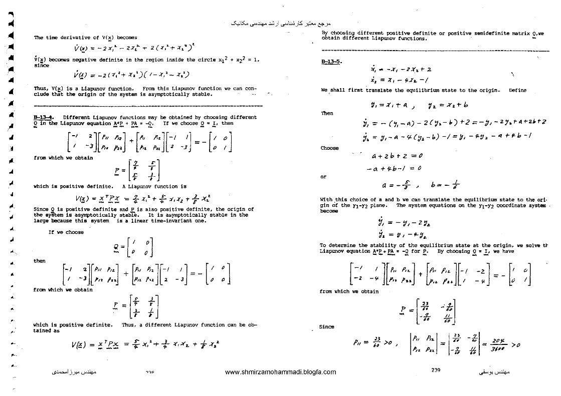
"' .c .. .. • .. .. .. •• • .. .. ,J

.. ~

~

• .... .. ... .. ,., __

• • • • • ' ,. ,_

• •

-""'15:... ...r4-- .:.:, ) .,rl...:..:<_)ts: -~ &'-->"

The time derivative of V(~) becomes

. . ' ( . ') . V(~;>:::: -2 ;:(! - 2Xt. ..... 2 :r, -t- ;(~

VC~) becomes negative definite in the region inside the circle x12 + x22 ~ 1, ,,~

Ve-; = -2t-r.'+ :(,')( t-:r/- :r:J

Thus, V(~) is a Liapunov function. From this Liapunov function we can con­clude that the origin of the system is asymptotically stable •

B-13-4. Different Liapunov functions may be obtained by choosing different 0 in the Liapunov equation A*P + PA "' -Q. If we choose 0 = r, then ... -- .. - - - -

[~ ']['" -3 PtJJ "'] + ["' /?~ ;,i "·][-/ '] ~-[' Pz, 2 -3 0 ~]

il !rom which ve obtain

p = l- f - _c

T

which is positive definite. A Liapunov function is

l/(3") =: ~T?1_ = f X,z.+: :¥,.:(2 't: Xz.'

Since 0 is positive definite and P is also pos1tive definite, the origin of the syStem is asymptotically stabi'e. It is asymptotically stable in the large because this system is a linear time-invariant one.

I! we choose

Q = [I - ' :] then

+ ['" "·][-/ 1]=- [' '] p,. I'·~ 2 -J " 0 [-1 •][p"

I -J !H p,.] ,,. -from which we oPtain

r = [t i] which is positive definite. Thus, a different Liapunov function can be ob­tained as

VI ) 'p - S'" a _L 1 z. 1;: = =: _-:!:- Tx, -r 'i" :t',Xz. -r 7 .:r.

By choosing different positive definite or positive semidefinite matrix Q,we obtain different Liapunov functions. ..

~-":!,- -.:r, -2:(_l. t- 2

X,= :r,- 9-Iz.. -I \

We shall first translate the equilibrium state to the origin • Define

Then

Choose

or

,,=X,t-.lt .J '12. =X:t-b

~~ =--(.,,-a)- 2 {'J-,.- ir) +-2 =-;;,- z.7a. ra +-z.J.rz

;1,. =- :J,-a -Sl{:J~-1.) -/=~1 -9-:J:.-"' +-P.b -I

t.i+Zhtz =D

-a +'f.b-1 = o

a= _ _£_ . ' b=-f

With this choice of a and b we can translate the equilibrium state to the ori· gin Of the n-n plane. The system equations on the n-n coordinate system bee~

'J, = - 't f- z 'J(Il

t~=v,-fl-~(1!. To determine the stability of the equilibrium state at the origin, we solve tt Liapunov equation A*P + PA " -0 for P. By choosing 0 = I, ve have ... _- - - - -

[~ 1 _' ]['" p,,] t [ll· f,. ][-/ -z] = _ [' ~J

Z $1- }',. }1-... J1o. fu 1 - S< () I

from which we obtain

[" "~] p =: 7i - -L .!!.-

" " Since

" I,, P,,H :: _zj Plf=j;>O, il> - ,2(1 y.

P,, Pu -f, .11. - 31'" >o .. ...;~I_)_J:!"'--'"'~ 0,0 www.shmirzamohammadi.blogfa.com 239 ~-.,'--'"'~

~ ~ ~

~ .. .A

4 .. .. .. ..

-

-""'15:... ...r4-- .:.:, ) .,rl...:..:<_)ts: -~ &'-->"

matrix p is positive definite. stab,le rn the large.

Hence, the equilibrium state is asymptotically

------------------------------------------------------------------------------!!::::!1::§.. The system equation can be written as

whm

X ==A X

A

-·--

[

I 3 0] -3 -2 -3

I 0 0

The characteristic equation for the systE:Ill is

I • -I -3 0

l•!--~1= s H2 .11::; s 1 ...,...st.-r7srr -I 0 s

= ( H· /. z 3- S )(s- .::>·II 7 s-- + j 2-D'! '?) (s.- f?./17.!'-j 2-CP7) =0

Since t~ roots (eigenvalues) are located in the right-half plane, the equili-

"'

[: -3 l][p,,p., fu l ['" p,.r,, ][I .1 OJ [0 ° 0] -2. a f, .. A1 fu + P,z Pu lu - .J -2: -.J = o 0 o -J tJ f,, f•J Pu _ 1'11 l'z~ f'.n 1 0 P 0 0 -I

ore obtain the following six lin'early independent equations: ·,

,P,,- 3~a +fo = o

/',1- Jf'..J r,Pi..~-3/ta. =O

j/11 -2fn T {'1z - JjJu "t-/aJ =0

3fn. -2/z' +- Jf•z -2fu. =0

3fl1 - 2./u - 3 /{~ = ()

- 3f'•J- 3fz.J :::::-I

Solving these six equations for the Pij, we obtain

11 --~- brium state (the origin) is unstable. -L -.!::. ,. 4 .. •

• •

This problem can, of course, be solved by use of the Liapunov approach • The Liapunov appriach will take more time to solve but is given below as a ref­erence. Chooose a positive semidefinite real symmetric matrix~ to be

[" 0 0] Q = 0 t:' 0

a " I To verify this choice, note that V(x) : -x•Qx. - ... __ Since

V(,:r) = -z.-.Q .:c. = -x:Jl . - ---V(~) being identically zero implies that x3 is identically identically zero, then x1 is also identically zero, since

X'J =-XI "" 0 =.X,

zero.

If xl is identically zero, then x2 must be identically zero, since

;(, :;(,-rXz... .,.,._ xz:~o

If x3 is

Thus, V(x) is identically zero only at the sen Q matrix for the stability analysis of equa'E'ion:

origin. Hence we may use the cho­this system. Solving the Liapunov

ATF+f'A;:::-Q ~- -

p:;;: 1-j- _.J... + ~

-..C. I .£...

" ... 36

Since the first principal minor is negative, P is not positive definite. Hence, the origin of the system is unstable. -

------------------------------------------------------------------------------!t!H·

[::] = [ _: -~tJ The Liapunov equation is

AT~+ PA =-Q ... - -- -Choosing Q : I, we obtain - -

[~ -•]['" - J' p,. l'n] ['" ~•] [ 0 I J [I "] ?en .. + p,._ p,_._ -£ -S ; -- 0 I

simplifying, we get the following three linearly independent equations:

...;~I_)_J:!"'-"'~ www.shmirzamohammadi.blogfa.com 241 ._..i...> _ _,.j.~

"0

I' .,, r;;::,:

~i~~

· .. ~ •.. ~~-~·

.. ... .1.

~

... ~

~

~

~

J .. " ---'

' r

' .

~15:... ...r4-- .:.:, ) .,rl...:..:<_)ts: -~ &'-->"

-/Z.f',z = -1

-(fH t-jJ11-Sj12 :::0

2( fn- s-f-.)~ -I

Solving these three equations for Pij, we obtain

[" '] 'P="'j';" /z - .-!- .!L I& It>

This matrix P is positive definite. Hence, the origin is asymptotically sta­ble in the 1:irge.

-------------------------------------------------------------------------------.!!:.Q::!. If matrix!, is positive definite, au the eigenvalues of P are posi­tive. Hence, the roots Sf of the charateristic equation

fs.r- fl ~ U-s,)(,-s,). · · (>->.) ~o are all positive. Note that

(s-.s,)(s-.s..,) ( s-s.)

-.. :."'- (s,+.S;z.+ ) "-! " + s., S -r ··· T(-) S1 .Sa ···S ..

= 5"- b, s .,_, + ..;-(-t)"b.,

Since the si are positive, the bi are also positive. are positive, then

J,,.,. 51 +S;a.+ ·· +S,.. >O

Conversely, if the bi

b2 =~,:>aT" .$"a :!iJ t- -t-.s...s, >o

J,,. = s, '· ' .. s., > 0

•nich means that the Sf are all positive. case where n = 3:

j,1 = .J1 -t-S" ;- S1 >O

To show this clearly, consider the

b" ~ S",5;:, + SaSJ t- s,s, >O

b 1 -= S, Sz. S"J >0

Since b3 > 0, if there are any negative s's, then the number of Such negativL s's must be even. Suppose that s 1 < 0, s2 < O, and S) > 0. Since b1 > O,lol" hm

ls-,1-s,~.j<sl

Hence

/:5,/ '(' SJ ' /Sz./ < S;r

Then we have

b-.=s,sa.-t-Sa.S1 t-s,s,= s,s .. ·t-{s,rJL)s.~~ <o

which is a contradiction. Hence, all s's must be positive. This same argu­ment can be extended to the case where n = 4, 5, 6, ...• Hence, a necessary and sufficient condition that a Hennitian matrix P be positive definite is th...-all bt be positive. -

~· Choose the following V as a possible Liapunov function:

V,.. :x""P~ - --Then

V = i""Px + ::c•r:i ... ... _ --- = x~ { A"P+ PA):t:. 1- t1""9~!"X -- -- - .... - -... t- x~PBu ... ----:r..""LX +-2~.$.?8 u.. --- ---

If u = -B*Px is substituted into this last equation, we obtain

V :::::-x>trx -zx*PBB""fx. - -- - --- --Since~ is always positive definite or positive,semidefinite, V is always negative definite. Since V is positive definite, V is negative definite, and V ~""' as J xM ~ O<J , the ongin of the system is asymptotically stable in the· large. ...

B-13-10. To determine the parameter a in matrix A, we first determine matrix P from -

AT.f'"-r PA =-I -- --0'

[: 0 -If' p,.p,,] l" p,. p,, ][0 I 0] [/HI () - Z /'11 f'l~ PaJ + ,P, .. fu f3~ 0 0 I=-~ /Of 1 - et I'Jr fu fn p,) P•s p11 -1 -2 -A. 0 IJ l.l

...;~1_).):!"'-"'~ "' www.shmirzamohammadi.blogfa.com 243

._..i...>.J:l'-"'~

·~. ~·

~

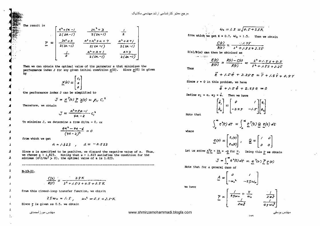
• • .~ A

• • ~

• A

J

)

1

J

J.

J

J

J

•

-""'15:... ...r4-- .:.:, ) .,rl...:..:<_)ts: -~ &'-->"

Then we can obtain the optimal value of the parameter a that minimizes the performance index J for any given initial conCition x(O). Since x{O) is given by - -

~I•! = [ ;•]

the performance index J can be simplified to

J = ;( T(t.?) 7" X.(#,) = f?o C, ;z - --Therefore, we obtain

• J = "' +.t"IJ -/ s:::a. -2

c' '

TO minimize J, we determine a from dJ/da = 0, or

from which we get

?'1. a._ fL4 _,

(<fA- <)l. :o

~ = 1·3Z3 ' a= -".rz1 Since a is specified to be positive, we discard the negative value of a. Thus, we choose a = 1.823. Noting that a = 1.823 satisfies the condition for the minimum (d2J/da2 > 0), the optimal value of a is 1.823.

B-13-11.

C(J) ·- "ZSI< le(T) - S' +-/..$""$ + a.S+Z.>K

From this closed~loop transfer function, we obtain

2!:41 .. = /. s-) Since) is given as 0.5, we obtain

w .. t =0.S+2.s-k

41,. =/.S =JP.S-+2.S/<.

from whi~ 'we get K 2 0.7, wJn: 1.5. Then we obtain

Cfr) ·'/.?S

kfs) ::: J 1 .;./S.sT;.zs-E(s)/R(s) can then be obtained as

'!hus

E{s) !U>) :

R(1)- C(s)

,!?(') ;

Jl: +-/. s .s + o.s s&.+ ;.s-.s +.?-zs-

f:: + ;..s-t!- r ;-.zs-~ = 'Y +/.si-r ().S'Y

Since r "' 0 in this problem, w have .. . e -r;.s-e +z.zse =O

Define el " e, e2 = e. Then we have

Note that

where

[::] =[_:..s -;.~][:J s: e{t)dt = r £_T{<)~ ~{t)4t ~(r) = ['dt)l

t',Jt) J ) 101=[' 0

] - 0 0

Let us solve ATp + PA = -Q for P. -- - - .... Using this ! we obtain

J = J .. "' e "'ft) dt =. :z. 7ca) J: ~ (") Note that for a general case of

.d =[_:_. -z:w.] 'ole have

[

I .,. • 7' ;:::: 9-]"~V.. ~ ~ -L

:?4>.,z -LJ z~ . .-.. __ s

...;~I.J...l:!"'-""'~ www.shmirzamohammadi.blogfa.com ._..i...>.J:l"'-""'~

'"

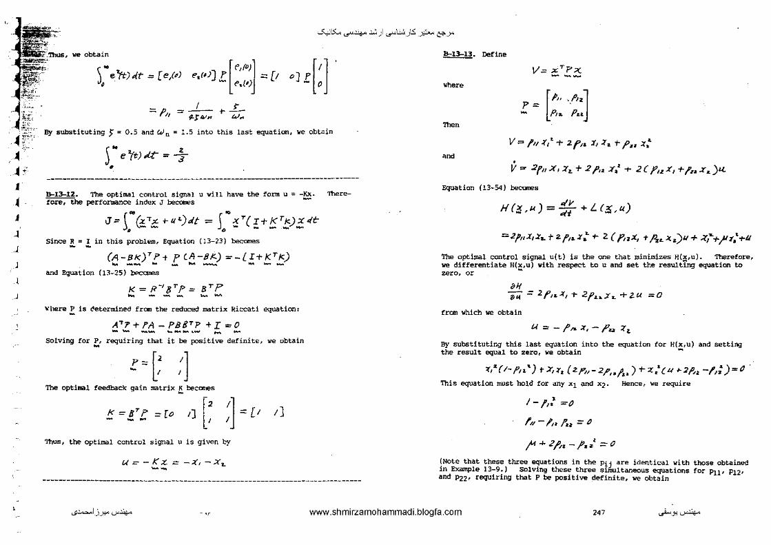
I

1 J

~

J

J

.J

-""'15:... ...r4-- .:.:, ) .,rl...:..:<_)ts: -~ &'-->"

we obtain

J"e'ft-Jdr = [e,M e.I•J) P =o [1 [e,f•!J

...... e .. l') o][[~]·

'

= fll = _j___ ?-ftVn

.. L-w.

By substituting ) = 0.5 and W 0 = 1.5 into this last equation, ..,e obtain

r e'{t)d:C = 3-• a

B-13-12. The optimal control signal u will have the fonn u : -Kx. 'lbere-fore, the performance index J beeanes -

1~ •

J: ('!_Tz t-U')at = 5 ';!T(:!_+!5.T!9!..{tc . ' Since R =I in this problem, Equation (13-23} becomes - -

(A-Bk)'P; p CA-B!') =-/I+KTI<) ....... _____ -- .... and Equation (lJ-25) becomes

K=f?-'8T?::::: BTP ... - -- ........... Where!:_ is t'etermin!!<l frcm the reducec:! matrix Riccati equation:

A"T1' +!'A- PB8TP +I= 0 -- -- ... --·- - -Solving for ~· requiring that it be positive definite, we obtain

!:= 0 :] The optimal feedback gain matrix ~ becomes

I<= 8T p = [o - -- :] = [t !] 2

1]

Thus, the optimal control signal u is given by

U=-KX:=-;(,-XL --

B-13-13. Define

V.= .xTP:x.. ---Where

['" ·""] P= . ... P1a. Pu

Then

V =- /11.:(/ + 2f'"· :l1 :1-._ +-f'u ::t~., ~d

V.,.. 2fu x, :tz. + 2 p,z .Xa1 + 2c f'u.:t'1 +fu. x.._)u.

Equation (13-54) becomes

H(i:!,u)= ::: rL!i:i.,u)

=zp,x,z ... t z. ,,,. x .,z. +- 2 { "'Jx:, .,. Az. x.z)u + .::rt+l'~•1.+"

The optimal control signal u(t) is the one that minimizes H(x,u). Therefore, we differentiate H(x,u) with respect to u and set the resulting equation to

• zero, or

>H 8'f.j = 2{'1&-:il r 2fu.Xa. +z.u =O

from '<lhich we obtain

U :::-j'.-..X,-/'u :<'z.

By substituting this last equation into the equation for H(x,u) and setting the result equal to zero, we obtain

l:/1( 1- f'o.') T X,.r, ( Zf'n- 2,P0 jJ,..) '+- 'Z / (i.t ~>- 2~~ -/,:) = ()

This equation must hold for any x1 and x2. Hence, we require

' 1- ,,, =tJ

Itt -lo ?,, = "

' )" ...,_ 2f't,- )J,.z. ;:::: ()

(Note that these three equations in the Pij are identical with those obtained in Example 13-9.) Solving these three simultaneous equations for PU• P12• and P22• requiring that P be positive definite, we obtain

...;~I_)_J:!"'-"'"~ -.- www.shmirzamohammadi.blogfa.com 247 ._..i...>_J:l'-"'"~

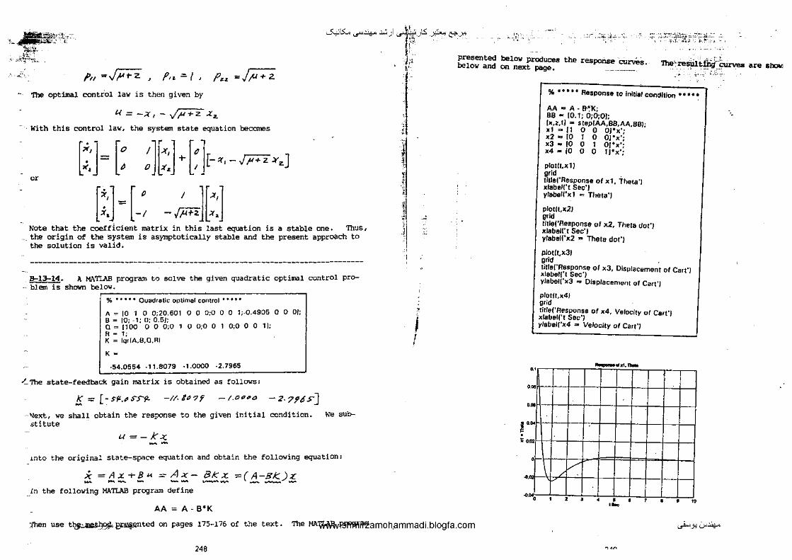
-"-"~ '-"'"'-" '-') u•!\')\S .~ C?Y !''

· -j~~ presented

.i'•. p, =-J,A-4.,..2. ~ f"=t, P":z. =)p+z. The optimal contiol law is then given by

U = -:X 1 - -/~+-Z -'z. - With this control law, the system state equation becomes

or

[~:]= [: ~][:}[~]r-~.-n;+z¥,J

[::]=[_: _;.,][::] Note that the coefficient matrix in this last equation is a stable one. Thus, the origin of the system is asymptotically stable and the present approach to the solution is valid.

B-13-14. A MATlAB program to solve the given quadratic optimal control pro-blem is shown below.

~~~~----~~------, % • • • • • Ouadretio; optimer control • • • • •

A "' 10 1 o o;2o.6o1 o o o:o o o 1;-0.4905 o o or: B"' 10; .1; O; 0.51; 0 = 1100 0 0 0;0 1 0 0;0 0 1 0;0 0 0 1]; fl "' T; K "' lqdA.B,O.RI

K •

·54.0554 · T 1.8079 ·1.0000 -2.7965

~The state-feedback gain matrix is obtained as follows:

5_ == (- Sft • ., s-s-p. -//.I"? f -/.011>10 -2·7?6>]

-·-~ext, we shall obtain the response to the given initial condition. stitute

U=-k.:r:. --we sub-

1nto the original state-space equation and obtain the following equation:

X =Ax+8J-t =Ax- Bkx. -==(A-Bk.)z - -- - -- -- ~--ln the following MATLAB program define

AA = A- e•K

f.! below and

l }, ~'

' ·~

'I I

. i I

-

·_fhen use t~ e_J;•nted on pages 175-176 of the text. The MA~~amoh.ammadi.blogfa.com

248

,. ~-'

.:~:;"'-· ~: ·:::-."-':.l;;o-:~,.,_2::~ -. • · - i ,j n":i' • ~ ~-

below produces on next page. the response curves. 'lbe~resU!tlii:J--brves are &bowl

' ,,_ ~- ,-_.,c_-·

••

•• ••

! •• . ' =

•

·~.

% • • • • • Response to Initial condition • • • • •

AA "' A • 8-~l<; BB ., [0. T; 0;0;01: [Jo:,:z,ll .. sJep[AA,88,AA,BB!; xT .. IT 0 0 OJ"Jo:'; Jo:2 .. 10 1 0 OJ'x'; x3 - [0 0 1 0/"x'; x4 • /0 0 0 TJ"x';

ploHt.x1) grid . tltle('Response of x1, Theta') xfabel!'t Sec') ylabelf"xl .. Theta')

plot[t,x2J grid tltfe('Aellponse of x2. Theta dot') xlabell'.t Sec' I ylabell'x2 .. Theta dof"J

plot[t,x3J grid . ti!fe['Response of x3, Displ;:~cement ol Cert'l xlabel{'t Sec') yJ;:~b-e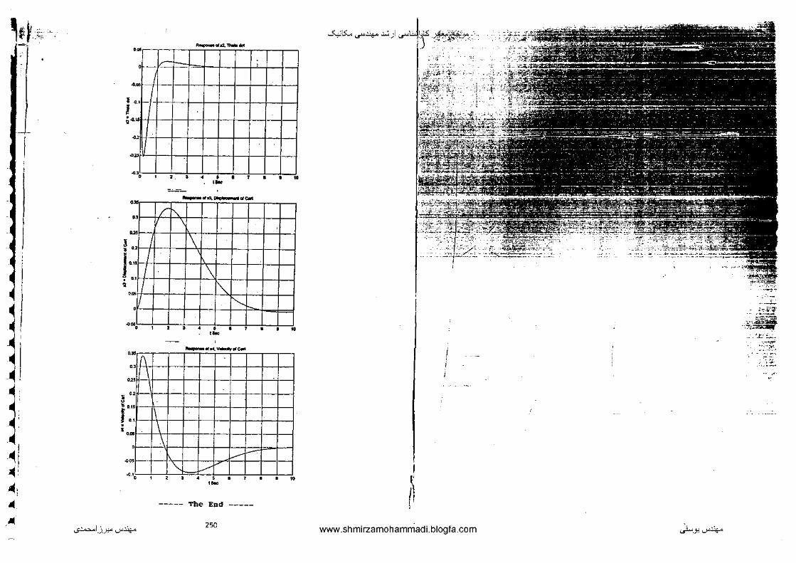!["x3 ""' Oisplao;emenr of C<:~rt'/

plotlt,x41 grid title(' Response of x4. Velocity of Cart') xf<:~belf't Sec'/ ylabef('x4 =- Velocity of Carl")

--.-..-

v

' • • • • . ·~ ' • • •

._..i..>_.,.:;.~

· ..

., 'cl r ~ ,l ./ I

' • • ...

-• I

•

' • .

J •

I •

' I "

'

,I :I ! • I • • i i\

I -

' I

! 0

' ;

, ' .o

' '

' .

... -.. ...

:it

1/ I/

v v

I

' -

~ a

"' "

! ...,,. __ "'

0

' . • -• • • " " -0

' ' !

I I ! • f ' • i

vi

I I

I ' . .

" • -a

.. ..

9 0

lr.IIO

-• ..

~-~--·----!

''"-' v '

. -~-------·

\ v i ' ' -

E

0 0

~

0>

0 :0

"0

~

.E

E

~

~

0 E

ro ~

E

~

~

• • • • . . -• . I • . " -0

..,-a

•• u

ww

w

w w

w

w

w

....... w"""'f"........-~-....--w ..-

... ..,...-.,...-.....-.,..

11