Physics of Radiation Therapy - Third Edition by Faiz M. Khan

Physics of RadiationTherapyThird Editionby Faiz M. Khan

Pertinent to the entire radiation oncology team,Physics of Radiation Therapy is clinicallyoriented and presents practical aspects as well asunderlying theory to clarify basic concepts. Theformat begins with underlying physics, thenprogresses to treatment planning, and ends withradiation.

This edition contains an expanded focus withseven new chapters on special procedures. Remaining chapters have been revised todetail any new developments in the field over the past eight years. Illustrations areoverhauled to reflect current practice and to detail the new procedures added.Provides a solid foundation for residents and a strong review for practitioners.

Features of Physics of Radiation Therapy:

Focus on team approach to practice of physics in the radiation oncology clinicProvides solid foundation for residents and a good review for practitionersClinically oriented with a uniform approach by a single author renowned in thefieldBalanced coverage of theory and practiceIncludes dosimetry protocolsIncludes commissioning and quality assurance proceduresHeavily referenced and illustrated (over 5,000 references and 300 illustrations)

Contents

Basic Physics

Structure of Matter1.Nuclear Transformations2.Productions of X-Rays3.Clinical Radiation Generators4.Interactions of Ionizing Radiation5.Measurement of Ionizing Radiation6.Quality of X-Ray Beams7.

8.

Physics of RadiationTherapyThird Editionby Faiz M. Khan

Pertinent to the entire radiation oncology team,Physics of Radiation Therapy is clinicallyoriented and presents practical aspects as well asunderlying theory to clarify basic concepts. Theformat begins with underlying physics, thenprogresses to treatment planning, and ends withradiation.

This edition contains an expanded focus withseven new chapters on special procedures. Remaining chapters have been revised todetail any new developments in the field over the past eight years. Illustrations areoverhauled to reflect current practice and to detail the new procedures added.Provides a solid foundation for residents and a strong review for practitioners.

Features of Physics of Radiation Therapy:

Focus on team approach to practice of physics in the radiation oncology clinicProvides solid foundation for residents and a good review for practitionersClinically oriented with a uniform approach by a single author renowned in thefieldBalanced coverage of theory and practiceIncludes dosimetry protocolsIncludes commissioning and quality assurance proceduresHeavily referenced and illustrated (over 5,000 references and 300 illustrations)

Contents

Basic Physics

Structure of Matter1.Nuclear Transformations2.Productions of X-Rays3.Clinical Radiation Generators4.Interactions of Ionizing Radiation5.Measurement of Ionizing Radiation6.Quality of X-Ray Beams7.

8.

5.6.7.

Measurement of Absorbed Dose8.

Classic Radiotherapy

Dose Distribution and Scatter Analysis9.A System of Dosimetric Calculations10.Treatment Planning I: Isodose Distributions11.Treatment Planning II: Patient Data, Corrections, and Setup12.Treatment Planning III: Field Shaping, Skin Dose, and Field Separation13.Electron Beam Therapies14.Brachytherapy15.Radiation Protections16.Quality Assurances17.Total Body Irradiation18.

Modern Radiotherapy

Three-dimensional Conformal Radiotherapy19.Intensity-modulated Radiotherapy20.Stereo tactics Radio surgery21.High Dose Rate Brachytherapy22.Prostate Implants23.Intravascular Brachytherapy24.

Appendices

Editors: Khan, Faiz M.

Title: Physics of Radiation Therapy, The, 3rd Edition

Copyright ©2003 Lippincott Williams & Wilkins

> Front of Book > Editors

Editors

Faiz M. Khan Ph.D.

Professor Emeritus

Department of Therapeutic Radiology, University of Minnesota

Medical School, Minneapolis, Minnesota

Secondary Editors

Jonathan Pine

Acquisitions Editor

Michael Standen

Developmental Editor

Lisa R. Kairis

Developmental Editor

Thomas Boyce

Production Editor

Benjamin Rivera

Manufacturing Manager

Cover Designer: QT Design

Compositor: TechBooks

Printer: Maple Press




> Front of Book > Dedication

Dedication

To very special people in my life: my wife, Kathy, and my

daughters, Sarah, Yasmine, and Rachel




> Front of Book > PREFACE TO THE FIRST EDITION

PREFACE TO THE FIRSTEDITION

Most textbooks on radiological physics present a broad field

which includes physics of radiation therapy, diagnosis, and

nuclear medicine. The emphasis is on the basic physical

principles which form a common foundation for these areas.

Consequently, the topics of practical interest are discussed only

sparingly or completely left out. The need is felt for a book

solely dedicated to radiation therapy physics with emphasis on

the practical details.

This book is written primarily with the needs of residents and

clinical physicists in mind. Therefore, greater emphasis is given

to the practice of physics in the clinic. For the residents, the

book provides both basic radiation physics and physical aspects

of treatment planning, using photon beams, electron beams,

and brachytherapy sources. For the clinical physicist,

additionally, current information is provided on dosimetry.

Except for some sections in the book dealing with the theory of

absorbed dose measurements, the book should also appeal to

the radiotherapy technologists. Of particular interest to them

are the sections on treatment techniques, patient setups, and

dosimetric calculations.

Since the book is designed for a mixed audience, a careful

balance had to be maintained between theory and practical

details. A conscious effort was made to make the subject

palatable to those not formally trained in physics (e.g.,

residents and technicians) without diminishing the value of the

book to the physicist. This object was hopefully achieved by a

careful selection of the topics, simplification of the

mathematical formalisms, and ample references to the relevant

literature.

In developing this text, I have been greatly helped by my

physics colleagues, Drs. Jeff Williamson, Chris Deibel, Barry

Werner, Ed Cytacki, Bruce Gerbi, and Subhash Sharma. I wish

to thank them for reviewing the text in its various stages of

development. My great appreciation goes to Sandi Kuitunen

who typed the manuscript and provided the needed

organization for this lengthy project. I am also thankful to

Kathy Mitchell and Lynne Olson who prepared most of the

illustrations for the book.

Finally, I greatly value my association with Dr. Seymour Levitt,

the chairman of this department, from whom I got much of the

clinical philosophy I needed as a physicist.

Faiz M. Khan




> Front of Book > PREFACE TO THE SECOND EDITION

PREFACE TO THE SECONDEDITION

The second edition is written with the same objective as the

first, namely to present radiation oncology physics as it is

practiced in the clinic. Basic physics is discussed to provide

physical rationale for the clinical procedures.

As the practice of physics in the clinic involves teamwork

among physicists, radiation oncologists, dosimetrists, and

technologists, the book is intended for this mixed audience. A

delicate balance is created between the theoretical and the

practical to retain the interest of all these groups.

All the chapters in the previous edition were reviewed in the

light of modern developments and revised as needed. In the

basic physics part of the book, greater details are provided on

radiation generators, detectors, and particle beams. Chapter 8

on radiation dosimetry has been completely revised and

includes derivation of the AAPM TG-2 1 protocol from basic

principles. I am thankful to David Rogers for taking the time to

review the chapter.

Topics of dose calculation, imaging, and treatment planning

have been augmented with current information on interface

dosimetry, inhomogeneity corrections, field junctions,

asymmetric collimators, multileaf collimators, and portal-

imaging systems. The subject of three-dimensional treatment

planning is discussed only briefly, but it will be presented more

comprehensively in a future book on treatment planning.

The electron chapter was updated in the light of the AAPM TG-

25 report. The brachytherapy chapter was revised to include

the work by the Interstitial Collaborative Working Group, a

description of remote afterloaders, and a commentary on

brachytherapy dose specification.

Chapter 16 on radiation protection was revised to include more

recent NCRP guidelines and the concept of effective dose

equivalent. An important addition to the chapter is the

summary outline of the NRC regulations, which I hope will

provide a quick review of the subject while using the federal

register as a reference for greater details.

Chapter 17 on quality assurance is a new addition to the book.

Traditionally, this subject is interspersed with other topics.

However, with the current emphasis on quality assurance by

the hospital accrediting bodies and the regulatory agencies,

this topic has assumed greater importance and an identity of

its own. Physical aspects of quality assurance are presented,

including structure and process, with the objective of improving

outcome.

I acknowledge the sacrifice that my family had to make in

letting me work on this book without spending quality time

with them. I am thankful for their love and understanding.

I am also appreciative of the support that I have received over

the years from the chairman of my department, Dr. Seymour

Levitt, in all my professional pursuits.

Last but not least I am thankful to my assistant, Sally

Humphreys, for her superb typing and skillful management of

this lengthy project.

Faiz M. Khan




> Front of Book > PREFACE

PREFACE

New technologies have greatly changed radiation therapy in the

last decade or so. As a result, clinical practice in the new

millennium is a mixture of standard radiation therapy and

special procedures based on current developments in imaging

technology, treatment planning, and treatment delivery. The

third edition represents a revision of the second edition with a

significant expansion of the material to include current topics

such as 3-D conformal radiation therapy, IMRT, stereotactic

radiation therapy, high dose rate brachytherapy, seed implants,

and intravascular brachytherapy. A chapter on TBI is also added

to augment the list of these special procedures.

It is realized that not all institutions have the resources to

practice state-of-the-art radiation therapy. So, both the

conventional and the modern radiation therapy procedures are

given due attention instead of keeping only the new and

discarding the old. Based on content, the book is organized into

three parts: Basic Physics, Classical Radiation Therapy, and

Modern Radiation Therapy.

A new AAPM protocol, TG-51, for the calibration of megavoltage

photon and electron beams was published in September, 1999,

followed by the IAEA protocol, TRS-398, in 2000. Chapter 8 has

been extensively revised to update the dosimetry formalism in

the light of these developments.

I have enjoyed writing the Third Edition, partly because of my

retirement as of January 2001. I simply had more time to

research, think, and meditate.

I greatly value my association with Dr. Seymour Levitt who was

Chairman of my department from 1970 to 2000. I owe a lot to

him for my professional career as a medical physicist.

I greatly appreciate the departmental support I have received

from the faculty and the current Chairwoman, Dr. Kathryn

Dusenbery. My continued involvement with teaching of

residents and graduate students has helped me keep abreast of

current developments in the field. I enjoyed my interactions

with the physics staff: Dr. Bruce Gerbi, Dr. Pat Higgins, Dr.

Parham Alaei, Randi Weaver, Jane Johnson, and Sue Nordberg.

I acknowledge their assistance in the preparations of book

material such as illustrations and examples of clinical data.

My special thanks go to Gretchen Tuchel who typed the

manuscript and managed this project with great professional

expertise.

Faiz M. Khan

â†‘â†‘

Table of Contents

[-]

Part I - Abasic Physics

[+]

1 - Structure of Matter

[+]

2 - Nuclear Transformations

[+]

3 - Production of X-Rays

[+]

4 - Clinical Radiation Generators

[+]

5 - Interactions of Ionizing Radiation

[+]

6 - Measurement of Ionizing Radiation

[+]

7 - Quality of X-Ray Beams

[+]

8 - Measurement of Absorbed Dose

[-]

Part II - Classical Radiation Therapy

[+]

9 - Dose Distribution and Scatter Analysis

[+]

10 - A System of Dosimetric Calculations

[+]

11 - Treatment Planning I: Isodose Distributions

[+]

12 - Treatment Planning II: Patient Data, Corrections, and Set-Up

[+]

13 - Treatment Planning III: Field Shaping, Skin Dose, and Field Separation

[+]

14 - Electron Beam Therapy

[+]

15 - Brachytherapy

[+]

16 - Radiation Protection

[+]

17 - Quality Assurance

[+]

18 - Total Body Irradiation

[-]

Part III - Modern Radiation Therapy

[+]

19 - Three-Dimensional Conformal Radiation Therapy

[+]

20 - Intensity-Modulated Radiation Therapy

[+]

21 - Stereotactic Radiosurgery

[+]

22 - High Dose Rate Brachytherapy

[+]

23 - Prostate Implants

[+]

24 - Intravascular Brachytherapy

â†‘â†‘

Back of Book

[-]

Resources

[+]

Appendix




> Table of Contents > Part I - Abasic Physics > 1 - Structure

of Matter

1

Structure of Matter

1.1. THE ATOM

All matter is composed of individual entities called elements.

Each element is distinguishable from the others by the physical

and chemical properties of its basic componentâ€”the atom.

Originally thought to be the â€œsmallestâ€ and

â€œindivisibleâ€ particle of matter, the atom is now known to

have a substructure and can be â€œdividedâ€ into smaller

components. Each atom consists of a small central core, the

nucleus, where most of the atomic mass is located and a

surrounding â€œcloudâ€ of electrons moving in orbits around

the nucleus. Whereas the radius of the atom (radius of the

electronic orbits) is approximately 10-10 m, the nucleus has a

much smaller radius, namely, about 10-14 m. Thus, for a

particle of size comparable to nuclear dimensions, it will be

quite possible to penetrate several atoms of matter before a

collision happens. As will be pointed out in the chapters ahead,

it is important to keep track of those particles that have not

interacted with the atoms (the primary beam) and those that

have suffered collisions (the scattered beam).

1.2. THE NUCLEUS

The properties of atoms are derived from the constitution of

their nuclei and the number and the organization of the orbital

electrons.

The nucleus contains two kinds of fundamental particles:

protons and neutrons. Whereas protons are positively charged,

neutrons have no charge. Because the electron has a negative

unit charge (1.60 — 10-19 coulombs) and the proton has a

positive unit charge, the number of protons in the nucleus is

equal to the number of electrons outside the nucleus, thus

making the atom electrically neutral.

An atom is completely specified by the formula AZX, where X is

the chemical symbol for the element; A is the mass number,

defined as the number of nucleons (neutrons and protons in the

nucleus); and Z is the atomic number, denoting the number of

protons in the nucleus (or the number of electrons outside the

nucleus). An atom represented in such a manner is also called

a nuclide. For example, 11H and 42He represent atoms or nuclei

or nuclides of hydrogen and helium, respectively.

On the basis of different proportions of neutrons and protons in

the nuclei, atoms have been classified into the following

categories: isotopes, atoms having nuclei with the same

number of protons but different number of neutrons; isotones,

having the same number of neutrons but different number of

protons; isobars, with the same number of nucleons but

different number of protons; and isomers, containing the same

number of protons as well as neutrons. The last category,

namely isomers, represents identical atoms except that they

differ in their nuclear energy states. For example, 131m54Xe (m

stands for metastable state) is an isomer of 13154Xe.

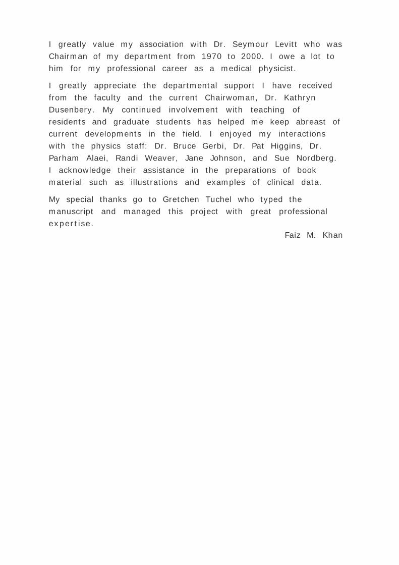
Certain combinations of neutrons and protons result in stable

(nonradioactive) nuclides than others. For instance, stable

elements in the low atomic number range have an almost equal

number of neutrons, N, and protons, Z. However, as Z increases

beyond about 20, the neutron-to-proton ratio for stable nuclei

becomes greater than 1 and increases with Z. This is evident in

Fig. 1.1, which shows a plot of the ratios of neutrons to protons

in stable nuclei.

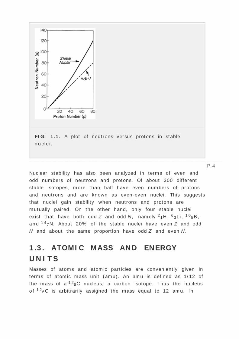
FIG. 1.1. A plot of neutrons versus protons in stable

nuclei.

P.4

Nuclear stability has also been analyzed in terms of even and

odd numbers of neutrons and protons. Of about 300 different

stable isotopes, more than half have even numbers of protons

and neutrons and are known as even-even nuclei. This suggests

that nuclei gain stability when neutrons and protons are

mutually paired. On the other hand, only four stable nuclei

exist that have both odd Z and odd N, namely 21H, 63Li, 105B,

and 147N. About 20% of the stable nuclei have even Z and odd

N and about the same proportion have odd Z and even N.

1.3. ATOMIC MASS AND ENERGY

UNITS

Masses of atoms and atomic particles are conveniently given in

terms of atomic mass unit (amu). An amu is defined as 1/12 of

the mass of a 126C nucleus, a carbon isotope. Thus the nucleus

of 126C is arbitrarily assigned the mass equal to 12 amu. In

basic units of mass,

1 amu = 1.66 — 10-27 kg

The mass of an atom expressed in terms of amu is known as

atomic mass or atomic weight. Another useful term is gram

atomic weight, which is defined as the mass in grams

numerically equal to the atomic weight. According to

Avogadro's law, every gram atomic weight of a substance

contains the same number of atoms. The number, referred to as

Avogadro's number (NA) has been measured by many

investigators, and its currently accepted value is 6.0228 —

1023 atoms per gram atomic weight.

From the previous definitions, one can calculate other

quantities of interest such as the number of atoms per gram,

grams per atom, and electrons per gram. Considering helium as

an example, its atomic weight (AW) is equal to 4.0026.

Therefore,

P.5

The masses of atomic particles, according to the atomic mass

unit, are electron = 0.000548 amu, proton = 1.00727 amu, and

neutron = 1.00866 amu.

Because the mass of an electron is much smaller than that of a

proton or neutron and protons and neutrons have nearly the

same mass, equal to approximately 1 amu, all the atomic

masses in units of amu are very nearly equal to the mass

number. However, it is important to point out that the mass of

an atom is not exactly equal to the sum of the masses of

constituent particles. The reason for this is that, when the

nucleus is formed, a certain mass is destroyed and converted

into energy that acts as a â€œglueâ€ to keep the nucleons

together. This mass difference is called the mass defect.

Looking at it from a different perspective, an amount of energy

equal to the mass defect must be supplied to separate the

nucleus into individual nucleons. Therefore, this energy is also

called the binding energy of the nucleus.

The basic unit of energy is the joule (J) and is equal to the

work done when a force of 1 newton acts through a distance of

1 m. The newton, in turn, is a unit of force given by the

product of mass (1 kg) and acceleration (1 m/sec2). However, a

more convenient energy unit in atomic and nuclear physics is

the electron volt (eV), defined as the kinetic energy acquired

by an electron in passing through a potential difference of 1 V.

It can be shown that the work done in this case is given by the

product of potential difference and the charge on the electron.

Therefore, we have:

1 eV = 1 V — 1.602 — 10-19 C = 1.602 — 10-19 J

Multiples of this unit are:

1 keV = 1,000 eV

1 million eV(MeV) = 106 eV

According to the Einstein's principle of equivalence of mass and

energy, a mass m is equivalent to energy E and the relationship

is given by:

where c is the velocity of light (3 — 108 m/sec). For example,

a mass of 1 kg, if converted to energy, is equivalent to:

E = 1 kg — (3 — 108 m/sec2)

= 9 — 1016 J = 5.62 — 1029 MeV

The mass of an electron at rest is sometimes expressed in

terms of its energy equivalent (E0). Because its mass is 9.1

— 10-31 kg, we have from Equation 1.1:

E0 = 0.511 MeV

Another useful conversion is that of amu to energy. It can be

shown that:

1 amu = 931 MeV

1.4. DISTRIBUTION OF ORBITAL

ELECTRONS

According to the model proposed by Niels Bohr in 1913, the

electrons revolve around the nucleus in specific orbits and are

prevented from leaving the atom by the centripetal force of

attraction between the positively charged nucleus and the

negatively charged electron.

On the basis of classical physics, an accelerating or revolving

electron must radiate energy. This would result in a continuous

decrease of the radius of the orbit with the electron eventually

spiraling into the nucleus. However, the data on the emission

or absorption of radiation by elements reveal that the change

of energy is not continuous but discrete. To explain the

observed line spectrum of hydrogen, Bohr theorized that the

sharp lines of the spectrum represented electron jumps from

one orbit down to another with the emission of light of a

particular frequency or a quantum of energy. He proposed two

P.6

fundamental postulates: (a) electrons can exist only in those

orbits for which the angular momentum of the electron is an

integral multiple of h/2 €, where h is the Planck's constant

(6.62 — 10-34 J-sec); and (b) no energy is gained or lost

while the electron remains in any one of the permissible orbits.

FIG. 1.2. Electron orbits for hydrogen, helium, and oxygen.

The arrangement of electrons outside the nucleus is governed

by the rules of quantum mechanics and the Pauli exclusion

principle (not discussed here). Although the actual

configuration of electrons is rather complex and dynamic, one

may simplify the concept by assigning electrons to specific

orbits. The innermost orbit or shell is called the K shell. The

next shells are L, M, N, and O. The maximum number of

electrons in an orbit is given by 2n2, where n is the orbit

number. For example, a maximum of 2 electrons can exist in

the first orbit, 8 in the second, and 18 in the third. Figure 1.2

shows the electron orbits of hydrogen, helium, and oxygen

atoms.

Electron orbits can also be considered as energy levels. The

energy in this case is the potential energy of the electrons.

With the opposite sign it may also be called the binding energy

of the electron.

1.5. ATOMIC ENERGY LEVELS

It is customary to represent the energy levels of the orbital

electrons by what is known as the energy level diagram (Fig.

1.3). The binding energies of the electrons in various shells

depend on the magnitude of Coulomb force of attraction

between the nucleus and the orbital electrons. Thus the binding

energies for the higher Z atoms are greater because of the

greater nuclear charge. In the case of tungsten (Z = 74), the

electrons in the K, L, and M shells have binding energies of

about 69,500, 11,000, and 2,500 eV, respectively. The so-

called valence electrons, which are responsible for chemical

reactions and bonds between atoms as well as the emission of

optical radiation spectra, normally occupy the outer shells. If

energy is imparted to one of these valence electrons to raise it

to a higher energy (higher potential energy but lower binding

energy) orbit, this will create a state of atomic instability. The

electron will fall back to its normal position with the emission

of energy in the form of optical radiation. The energy of the

emitted radiation will be equal to the energy difference of the

orbits between which the transition took place.

If the transition involved inner orbits, such as K, L, and M

shells where the electrons are more tightly bound (because of

larger Coulomb forces), the absorption or emission of energy

will involve higher energy radiation. Also, if sufficient energy is

imparted to an

P.7

inner orbit electron so that it is completely ejected from the

atom, the vacancy or the hole created in that shell will be

almost instantaneously filled by an electron from a higher level

orbit, resulting in the emission of radiation. This is the

mechanism for the production of characteristic x-rays.

FIG. 1.3. A simplified energy level diagram of the tungsten

atom (not to scale). Only few possible transitions are

shown for illustration. Zero of the energy scale is arbitrarily

set at the position of the valence electrons when the atom

is in the unexcited state.

1.6. NUCLEAR FORCES

As discussed earlier, the nucleus contains neutrons that have

no charge and protons with positive charge. But how are these

particles held together, in spite of the fact that electrostatic

repulsive forces exist between particles of similar charge?

Earlier, in section 1.3, the terms mass defect and binding

energy of the nucleus were mentioned. It was then suggested

that the energy required to keep the nucleons together is

provided by the mass defect. However, the nature of the forces

involved in keeping the integrity of the nucleus is quite

complex and will be discussed here only briefly.

There are four different forces in nature. These are, in the

order of their strengths: (a) strong nuclear force, (b)

electromagnetic force, (c) weak nuclear force, and (d)

gravitational force. Of these, the gravitational force involved in

the nucleus is very weak and can be ignored. The

electromagnetic force between charged nucleons is quite

strong, but it is repulsive and tends to disrupt the nucleus. A

force much larger than the electromagnetic force is the strong

nuclear force that is responsible for holding the nucleons

together in the nucleus. The weak nuclear force is much weaker

and appears in certain types of radioactive decay (e.g., ²

decay).

The strong nuclear force is a short-range force that comes into

play when the distance between the nucleons becomes smaller

than the nuclear diameter (~10-14 m). If we assume that a

nucleon has zero potential energy when it is an infinite

distance apart from the nucleus, then as it approaches close

enough to the nucleus to be within the range of nuclear forces,

it will experience strong attraction and will â€œfallâ€ into the

potential well (Fig. 1.4A). This potential well is formed as a

result of the mass defect and provides the nuclear binding

energy. It acts as a potential barrier against any nucleon

escaping the nucleus.

In the case of a positively charged particle approaching the

nucleus, there will be a potential barrier due to the Coulomb

forces of repulsion, preventing the particle from approaching

the nucleus. If, however, the particle is able to get close

enough to the nucleus so as to be within the range of the

strong nuclear forces, the repulsive forces will be overcome

P.8

and the particle will be able to enter the nucleus. Figure 1.4B

illustrates the potential barrier against a charged particle such

as an ± particle (traveling 42He nucleus) approaching a238

92U nucleus. Conversely, the barrier serves to prevent an

± particle escaping from the nucleus. Although it appears,

according to the classical ideas, that an ± particle would

require a minimum energy equal to the height of the potential

barrier (30 MeV) in order to penetrate the 23892U nucleus or

escape from it, the data show that the barrier can be crossed

with much lower energies. This has been explained by a

complex mathematical theory known as wave mechanics, in

which particles are considered associated with de Broglie

waves.

FIG. 1.4. Energy level diagram of a particle in a nucleus:

a, particle with no charge; b, particle with positive charge;

U(r) is the potential energy as a function of distance r from

the center of the nucleus. B is the barrier height; R is the

nuclear radius.

1.7. NUCLEAR ENERGY LEVELS

The shell model of the nucleus assumes that the nucleons are

arranged in shells, representing discrete energy states of the

nucleus similar to the atomic energy levels. If energy is

imparted to the nucleus, it may be raised to an excited state,

and when it returns to a lower energy state, it will give off

energy equal to the energy difference of the two states.

Sometimes the energy is radiated in steps, corresponding to

the intermediate energy states, before the nucleus settles down

to the stable or ground state.

Figure 1.5 shows an energy level diagram with a decay scheme

for a cobalt-60 (6027Co) nucleus which has been made

radioactive in a reactor by bombarding stable 5927Co atoms

with neutrons. The excited 6027Co nucleus first emits a

particle, known as ²- particle and

P.9

then, in two successive jumps, emits packets of energy, known

as photons. The emission of a ²- particle is the result of a

nuclear transformation in which one of the neutrons in the

nucleus disintegrates into a proton, an electron, and a

neutrino. The electron and neutrino are emitted

instantaneously and share the released energy with the

recoiling nucleus. The process of ² decay will be discussed in

the next chapter.

FIG. 1.5. Energy level diagram for the decay of 6027Co

nucleus.

1.8. PARTICLE RADIATION

The term radiation applies to the emission and propagation of

energy through space or a material medium. By particle

radiation, we mean energy propagated by traveling corpuscles

that have a definite rest mass and within limits have a definite

momentum and defined position at any instant. However, the

distinction between particle radiation and electromagnetic

waves, both of which represent modes of energy travel, became

less sharp when, in 1925, de Broglie introduced a hypothesis

concerning the dual nature of matter. He theorized that not

only do photons (electromagnetic waves) sometimes appear to

behave like particles (exhibit momentum) but material particles

such as electrons, protons, and atoms have some type of wave

motion associated with them (show refraction and other wave-

like properties).

Besides protons, neutrons, and electrons discussed earlier,

many other atomic and subatomic particles have been

discovered. These particles can travel with high speeds,

depending on their kinetic energy, but never attain exactly the

speed of light in a vacuum. Also, they interact with matter and

produce varying degrees of energy transfer to the medium.

The so-called elementary particles have either zero or unit

charge (equal to that of an electron). All other particles have

charges that are whole multiples of the electronic charge. Some

elementary particles of interest in radiological physics are

listed in Table 1.1. Their properties and clinical applications

will be discussed later in this book.

1.9. ELECTROMAGNETIC RADIATION

A. Wave Model

Electromagnetic radiation constitutes the mode of energy

propagation for such phenomena as light waves, heat waves,

radio waves, microwaves, ultraviolet rays, x-rays, and ³ rays.

These radiations are called â€œelectromagneticâ€ because

they were first described, by Maxwell, in terms of oscillating

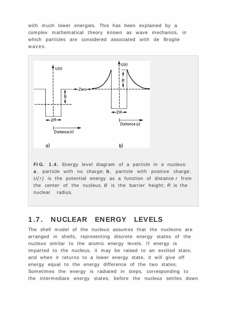
electric and magnetic fields. As illustrated in Fig. 1.6, an

electromagnetic wave can be represented by the spatial

variations in the intensities of an electric field (E) and a

magnetic field (H), the fields being at right angles to each

other at any given instant. Energy is propagated with the speed

of light (3 — 108 m/sec in vacuum)

P.10

in the Z direction. The relationship between wavelength ( »),

frequency ( ½), and velocity of propagation (c) is given by:

TABLE 1.1. ELEMENTARY PARTICLESa

Particle Symbol Charge Mass

Electron e-, ²- - 1 0.000548 amu

Positron e+, ²+ +1 0.000548 amu

Proton p, 11H+ +1 1.00727 amu

Neutron n, 10n 0 1.00866 amu

Neutrino ½ 0 <1/2,000 m0b

Mesons II+, II- +1, -1 273 m0

II ° 0 264 m0

µ+, µ- +1, -1 207 m0

K+, K- 1, -1 967 m0

K ° 0 973 m0

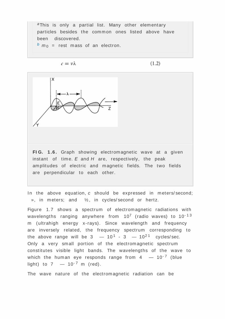
aThis is only a partial list. Many other elementary

particles besides the common ones listed above have

been discovered.b m0 = rest mass of an electron.

FIG. 1.6. Graph showing electromagnetic wave at a given

instant of time. E and H are, respectively, the peak

amplitudes of electric and magnetic fields. The two fields

are perpendicular to each other.

In the above equation, c should be expressed in meters/second;

», in meters; and ½, in cycles/second or hertz.

Figure 1.7 shows a spectrum of electromagnetic radiations with

wavelengths ranging anywhere from 107 (radio waves) to 10-13

m (ultrahigh energy x-rays). Since wavelength and frequency

are inversely related, the frequency spectrum corresponding to

the above range will be 3 — 101 - 3 — 1021 cycles/sec.

Only a very small portion of the electromagnetic spectrum

constitutes visible light bands. The wavelengths of the wave to

which the human eye responds range from 4 — 10-7 (blue

light) to 7 — 10-7 m (red).

The wave nature of the electromagnetic radiation can be

demonstrated by experiments involving phenomena such as

interference and diffraction of light. Similar effects have been

observed with x-rays using crystals which possess interatomic

spacing comparable to the x-ray wavelengths. However, as the

wavelength becomes very small or the frequency becomes very

large, the dominant behavior of electromagnetic radiations can

only be explained by considering their particle or quantum

nature.

B. Quantum Model

To explain the results of certain experiments involving

interaction of radiation with matter, such as the photoelectric

effect and the Compton scattering, one has to consider

P.11

electromagnetic radiations as particles rather than waves. The

amount of energy carried by such a packet of energy, or

photon, is given by:

FIG. 1.7. The electromagnetic spectrum. Ranges are

approximate.

where E is the energy (joules) carried by the photon, h is the

Planck's constant (6.62 — 10-34 J-sec), and ½ is the

frequency (cycles/second). By combining equations 1.2 and

1.3, we have:

If E is to be expressed in electron volts (eV) and » in meters

(m), then, since 1 eV = 1.602 — 10-19 J,

The above equations indicate that as the wavelength becomes

shorter or the frequency becomes larger, the energy of the

photon becomes greater. This is also seen in Fig. 1.7.




> Table of Contents > Part I - Abasic Physics > 2 - Nuclear

Transformations

2

Nuclear Transformations

2.1. RADIOACTIVITY

P.12

Radioactivity, first discovered by Henri Becquerel in 1896, is a

phenomenon in which radiation is given off by the nuclei of the

elements. This radiation can be in the form of particles,

electromagnetic radiation, or both.

Figure 2.1 illustrates a method in which radiation emitted by

radium can be separated by a magnetic field. Since ± particles

(helium nuclei) are positively charged and ²- particles

(electrons) are negatively charged, they are deflected in

opposite directions. The difference in the radii of curvature

indicates that the ± particles are much heavier than ²

particles. On the other hand, ³ rays, which are similar to x-

rays except for their nuclear origin, have no charge and,

therefore, are unaffected by the magnetic field.

It was mentioned in the first chapter (section 1.6 ) that there is

a potential barrier preventing particles from entering or escaping

the nucleus. Although the particles inside the nucleus possess

kinetic energy, this energy, in a stable nucleus, is not sufficient

for any of the particles to penetrate the nuclear barrier.

However, a radioactive nucleus has excess energy that is

constantly redistributed among the nucleons by mutual

collisions. As a matter of probability, one of the particles may

gain enough energy to escape from the nucleus, thus enabling

the nucleus to achieve a state of lower energy. Also, the

emission of a particle may still leave the nucleus in an excited

state. In that case, the nucleus will continue stepping down to

the lower energy states by emitting particles or ³ rays until

the stable or the ground state has been achieved.

2.2. DECAY CONSTANT

The process of radioactive decay or disintegration is a statistical

phenomenon. Whereas it is not possible to know when a

particular atom will disintegrate, one can accurately predict, in a

large collection of atoms, the proportion that will disintegrate in

a given time. The mathematics of radioactive decay is based on

the simple fact that the number of atoms disintegrating per unit

time, ( ”N / ”t ) is proportional to the number of radioactive

atoms, (N ) present. Symbolically,

where » is a constant of proportionality called the decay

constant . The minus sign indicates that the number of the

radioactive atoms decreases with time.

If ”N and ”t are so small that they can be replaced by their

corresponding differentials, dN and dt , then Equation 2.1

becomes a differential equation. The solution of this equation

yields the following equation:

where N 0 is the initial number of radioactive atoms and e is the

number denoting the base of the natural logarithm (e = 2.718).

Equation 2.2 is the well-known exponential equation for

radioactive decay.

FIG. 2.1. Diagrammatic representation of the separation of

three types of radiation emitted by radium under the influence

of magnetic field (applied perpendicular to the plane of the

paper).

P.13

2.3. ACTIVITY

The rate of decay is referred to as the activity of a radioactive

material. If ”N / ”t in Equation 2.1 is replaced by A , the

symbol for activity, then:

Similarly, Equation 2.2 can be expressed in terms of activity:

where A is the activity remaining at time t , and A 0 is the

original activity equal to »N 0 .

The unit of activity is the curie (Ci), defined as:

1 Ci = 3.7 — 1010 disintegrations/sec (dps)1

Fractions of this unit are:

1 mCi = 10-3 Ci = 3.7 — 107 dps

1 µCi = 10-6 Ci = 3.7 — 104 dps

1 nCi = 10-9 Ci = 3.7 — 101 dps

1 pCi = 10-12 Ci = 3.7 — 10-2 dps

The SI unit for activity is becquerel (Bq). The becquerel is a

smaller but more basic unit than the curie and is defined as:

1 Bq = 1 dps = 2.70 — 10-11 Ci

2.4. THE HALF-LIFE AND THE MEAN

LIFE

The term half-life (T 1/2 ) of a radioactive substance is defined

as the time required for either the activity or the number of

radioactive atoms to decay to half the initial value. By

substituting N/N 0 = ½ in Equation 2.2 or A/A 0 = ½ in

Equation 2.4 , at t = T 1/2 , we have:

P.14

where ln 2 is the natural logarithm of 2 having a value of 0.693.

Therefore,

FIG. 2.2. General decay curve. Activity as a percentage of initial

activity plotted against time in units of half-life. A , plot on

linear graph; B , plot on semilogarithmic graph.

Figure 2.2A illustrates the exponential decay of a radioactive

sample as a function of time, expressed in units of half-life. It

can be seen that after one half-life, the activity is ½ the initial

value, after two half-lives, it is ¼, and so on. Thus, after n

half-lives, the activity will be reduced to ½n of the initial

value.

Although an exponential function can be plotted on a linear

graph (Fig. 2.2A ), it is better plotted on a semilog paper

because it yields a straight line, as demonstrated in Fig. 2.2B .

This general curve applies to any radioactive material and can

be used to determine the fractional activity remaining if the

elapsed time is expressed as a fraction of half-life.

The mean or average life is the average lifetime for the decay of

radioactive atoms. Although, in theory, it will take an infinite

amount of time for all the atoms to decay, the concept of

average life (T a ) can be understood in terms of an imaginary

source that decays at a constant rate equal to the initial activity

and produces the same total number of disintegrations as the

given source decaying exponentially from time t = 0 to t = âˆ .

Because the initial activity = »N 0 (from Equation 2.3 ) and

the total number of disintegrations must be equal to N 0 , we

have:

Comparing Equations 2.5 and 2.6 , we obtain the following

relationship between half-life and average life:

Example 1

P.15

Calculate the number of atoms in 1 g of 226 Ra.

What is the activity of 1 g of 226 Ra (half-life = 1,622

years)?

In section 1.3 , we showed that:

where N A = Avogadro's number = 6.02 — 1023 atoms

per gram atomic weight and A W is the atomic weight.

Also, we stated in the same section that A W is very

nearly equal to the mass number. Therefore, for 226 Ra

Activity = »N (Equation 2.3 , ignoring the minus sign).

Since N = 2.66 — 1021 atoms/g (example above) and:

Therefore,

The activity per unit mass of a radionuclide is termed the

specific activity . As shown in the previous example, the specific

activity of radium is slightly less than 1 Ci/g, although the curie

was originally defined as the decay rate of 1 g of radium. The

reason for this discrepancy, as mentioned previously, is the

current revision of the actual decay rate of radium without

modification of the original definition of the curie.

High specific activity of certain radionuclides can be

advantageous for a number of applications. For example, the use

of elements as tracers in studying biochemical processes

requires that the mass of the incorporated element should be so

small that it does not interfere with the normal metabolism and

yet it should exhibit measurable activity. Another example is the

use of radioisotopes as teletherapy sources. One reason why

cobalt-60 is preferable to cesium-137, in spite of its lower half-

life (5.26 years for 60 Co versus 30.0 years for 137 Cs) is its

much higher specific activity. The interested reader may verify

this fact by actual calculations. (It should be assumed in these

calculations that the specific activities are for pure forms of the

nuclides.)

Example 2

Calculate the decay constant for cobalt-60 (T 1/2 = 5.26

years) in units of month-1 .

What will be the activity of a 5,000-Ci 60 Co source after 4

years?

From Equation 2.5 , we have:

P.16

since T 1/2 = 5.26 years = 63.12 months. Therefore,

t = 4 years = 48 months. From Equations 2.4 , we have:

Alternatively:

Therefore,

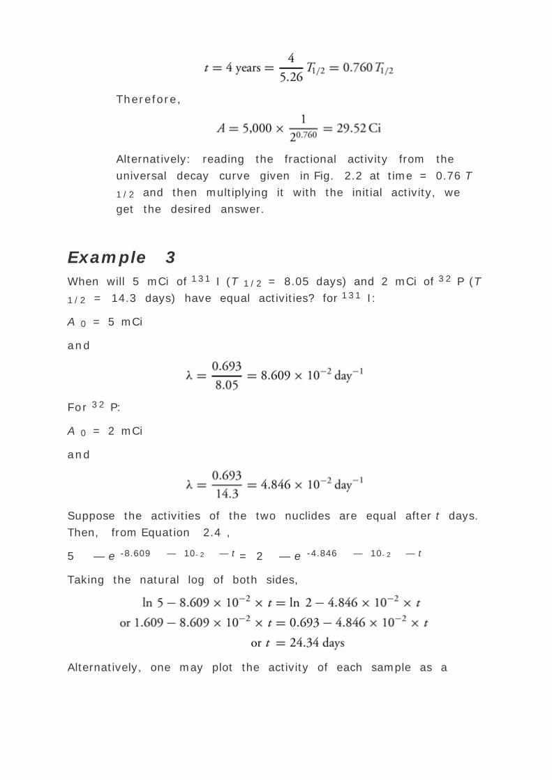
Alternatively: reading the fractional activity from the

universal decay curve given in Fig. 2.2 at time = 0.76 T

1/2 and then multiplying it with the initial activity, we

get the desired answer.

Example 3

When will 5 mCi of 131 I (T 1/2 = 8.05 days) and 2 mCi of 32 P (T

1/2 = 14.3 days) have equal activities? for 131 I:

A 0 = 5 mCi

and

For 32 P:

A 0 = 2 mCi

and

Suppose the activities of the two nuclides are equal after t days.

Then, from Equation 2.4 ,

5 — e -8.609 — 10- 2 — t = 2 — e -4.846 — 10- 2 — t

Taking the natural log of both sides,

Alternatively, one may plot the activity of each sample as a

function of time. The activities of the two samples will be equal

at the time when the two curves intersect each other.

2.5. RADIOACTIVE SERIES

There are a total of 103 elements known today. Of these, the

first 92 (from Z = 1 to Z = 92) occur naturally. The others have

been produced artificially. In general, the elements with lower Z

tend to be stable whereas the ones with higher Z are

radioactive. It

P.17

appears that as the number of particles inside the nucleus

increases, the forces that keep the particles together become

less effective and, therefore, the chances of particle emission

are increased. This is suggested by the observation that all

elements with Z greater than 82 (lead) are radioactive.

FIG. 2.3. The uranium series. (Data from U.S. Department of

Health, Education, and Welfare. Radiological health handbook ,

rev. ed. Washington, DC: U.S. Government Printing Office,

1970.)

All naturally occurring radioactive elements have been grouped

into three series: the uranium series, the actinium series, and

the thorium series. The uranium series originates with 238 U

having a half-life of 4.51 — 109 years and goes through a

series of transformations involving the emission of ± and ²

particles. ³ rays are also produced as a result of some of these

transformations. The actinium series starts from 235 U with a

half-life of 7.13 — 108 years and the thorium series begins

with 232 Th with half-life of 1.39 — 1010 years. All the series

terminate at the stable isotopes of lead with mass numbers 206,

207, and 208, respectively. As an example and because it

includes radium as one of its decay products, the uranium series

is represented in Fig. 2.3 .

2.6. RADIOACTIVE EQUILIBRIUM

Many radioactive nuclides undergo successive transformations in

which the original nuclide, called the parent , gives rise to a

radioactive product nuclide, called the daughter . The naturally

occurring radioactive series provides examples of such

transitions. If the half-life of the parent is longer than that of

the daughter, then after a certain time, a condition of

equilibrium will be achieved, that is, the ratio of daughter

activity to parent activity

P.18

will become constant. In addition, the apparent decay rate of the

daughter nuclide is then governed by the half-life or

disintegration rate of the parent.

FIG. 2.4. Illustration of transient equilibrium by the decay of 99

Mo to 99m Tc. It has been assumed that only 88% of the 99 Mo

atoms decay to 99m Tc.

Two kinds of radioactive equilibria have been defined, depending

on the half-lives of the parent and the daughter nuclides. If the

half-life of the parent is not much longer than that of the

daughter, then the type of equilibrium established is called the

transient equilibrium . On the other hand, if the half-life of the

parent is much longer than that of the daughter, then it can give

rise to what is known as the secular equilibrium.

Figure 2.4 illustrates the transient equilibrium between the

parent 99 Mo (T 1/2 = 67 h) and the daughter 99m Tc (T 1/2 = 6

h). The secular equilibrium is illustrated in Fig. 2.5 showing the

case of 222 Rn (T 1/2 = 3.8 days) achieving equilibrium with its

parent, 226 Ra (T 1/2 = 1,622 years).

A general equation can be derived relating the activities of the

parent and daughter:

where A 1 and A 2 are the activities of the parent and the

daughter, respectively. »1 and »2 are the corresponding

decay constants. In terms of the half-lives, T 1 and T 2 , of the

parent and daughter, respectively, the above equation can be

rewritten as:

Equation 2.9 , when plotted, will initially exhibit a growth curve

for the daughter before approaching the decay curve of the

parent (Figs. 2.4 and 2.5 ). In the case of a transient

equilibrium, the time t to reach the equilibrium value is very

large compared with the half-life of the daughter. This makes

the exponential term in Equation 2.9 negligibly small.

P.19

Thus, after the transient equilibrium has been achieved, the

relative activities of the two nuclides is given by:

FIG. 2.5. Illustration of secular equilibrium by the decay of 226

Ra to 222 Rn.

or in terms of half-lives:

A practical example of the transient equilibrium is the 99 Mo

generator producing 99m Tc for diagnostic procedures. Such a

generator is sometimes called â€œcowâ€ because the daughter

product, in this case 99m Tc, is removed or â€œmilkedâ€ at

regular intervals. Each time the generator is completely milked,

the growth of the daughter and the decay of the parent are

governed by Equation 2.9 . It may be mentioned that not all the

99 Mo atoms decay to 99m Tc. Approximately 12% promptly

decay to 99 Tc without passing through the metastable state of99m Tc (1 ). Thus the activity of 99 Mo should be effectively

reduced by 12% for the purpose of calculating 99m Tc activity,

using any of Equations 2.8 , 2.9 , 2.10 , 2.11 .

Since in the case of a secular equilibrium, the half-life of the

parent substance is very long compared with the half-life of the

daughter, »2 is much greater than »1 . Therefore, »1 can

be ignored in Equation 2.8 :

Equation 2.12 gives the initial buildup of the daughter nuclide,

approaching the activity of the parent asymptotically (Fig. 2.5 ).

At the secular equilibrium, after a long time, the product »2 t

becomes large and the exponential term in Equation 2.12

approaches zero.

P.20

Thus at secular equilibrium and thereafter:

or

Radium source in a sealed tube or needle (to keep in the radon

gas) is an excellent example of secular equilibrium. After an

initial time (approximately 1 month), all the daughter products

are in equilibrium with the parent and we have the relationship:

2.7. MODES OF RADIOACTIVE DECAY

A. ± Particle Decay

Radioactive nuclides with very high atomic numbers (greater

than 82) decay most frequently with the emission of an ±

particle. It appears that as the number of protons in the nucleus

increases beyond 82, the Coulomb forces of repulsion between

the protons become large enough to overcome the nuclear forces

that bind the nucleons together. Thus the unstable nucleus

emits a particle composed of two protons and two neutrons. This

particle, which is in fact a helium nucleus, is called the ±

particle.

As a result of ± decay, the atomic number of the nucleus is

reduced by two and the mass number is reduced by four. Thus a

general reaction for ± decay can be written as:

A Z X â†’ A - 4 Z - 2 Y + 4 2 He + Q

where Q represents the total energy released in the process and

is called the disintegration energy . This energy, which is

equivalent to the difference in mass between the parent nucleus

and product nuclei, appears as kinetic energy of the ± particle

and the kinetic energy of the product nucleus. The equation also

shows that the charge is conserved, because the charge on the

parent nucleus is Z e (where e is the electronic charge); on the

product nucleus it is (Z - 2)e and on the ± particle it is 2e.

A typical example of ± decay is the transformation of radium

to radon:

Since the momentum of the ± particle must be equal to the

recoil momentum of the radon nucleus and since the radon

nucleus is much heavier than the ± particle, it can be shown

that the kinetic energy possessed by the radon nucleus is

negligibly small (0.09 MeV) and that the disintegration energy

appears almost entirely as the kinetic energy of the ± particle

(4.78 MeV).

It has been found that the ± particles emitted by radioactive

substances have kinetic energies of about 5 to 10 MeV. From a

specific nuclide, they are emitted with discrete energies.

B. ² Particle Decay

The process of radioactive decay, which is accompanied by the

ejection of a positive or a negative electron from the nucleus, is

called the ² decay. The negative electron, or negatron, is

denoted by ²- , and the positive electron, or positron, is

represented by ²+ . Neither of these particles exists as such

inside the nucleus but is created at the instant of the decay

process. The basic transformations may be written as:

where 1 0 n, 1 1 p,

and v stand for neutron, proton, antineutrino, and neutrino,

respectively. The last two particles, namely antineutrino and

neutrino, are identical particles but with opposite spins. They

carry no charge and practically no mass.

FIG. 2.6. ² ray energy spectrum from 32 P.

P.21

B.1. Negatron Emission

The radionuclides with an excessive number of neutrons or a

high neutron-to-proton (n/p) ratio lie above the region of

stability (Fig. 1.1 ). These nuclei tend to reduce the n/p ratio to

achieve stability. This is accomplished by emitting a negative

electron. The direct emission of a neutron to reduce the n/p

ratio is rather uncommon and occurs with some nuclei produced

as a result of fission reactions.

The general equation for the negatron or ²- decay is written

as:

where Q is the disintegration energy for the process. This energy

is provided by the difference in mass between the initial nucleusA Z X and the sum of the masses of the product nucleus A Z + 1 Y

and the particles emitted.

The energy Q is shared between the emitted particles (including

³ rays if emitted by the daughter nucleus) and the recoil

nucleus. The kinetic energy possessed by the recoil nucleus is

negligible because of its much greater mass compared with the

emitted particles. Thus practically the entire disintegration

energy is carried by the emitted particles. If there were only one

kind of particle involved, all the particles emitted in such a

disintegration would have the same energy equal to Q , thus

yielding a sharp line spectrum. However, the observed spectrum

in the ² decay is continuous, which suggests that there is more

than one particle emitted in this process. For these reasons,

Wolfgang Pauli (1931) introduced the hypothesis that a second

particle, later known as the neutrino,2 accompanied each ²

particle emitted and shared the available energy.

The experimental data show that the ² particles are emitted

with all energies ranging from zero to the maximum energy

characteristic of the ² transition. Figure 2.6 shows the

distribution of energy among the ² particles of 32 P. The

overall transition is:

As seen in Fig. 2.6 , the endpoint energy of the ²-ray spectrum

is equal to the disintegration energy and is designated by E max

, the maximum electron energy. Although the shape of the

energy spectrum and the values for E max are characteristic of

the particular nuclide, the average energy of the ² particles

from a ² emitter is approximately E max /3.

The neutrino has no charge and practically no mass. For that

reason the probability of its interaction with matter is very small

and its detection is extremely difficult. However, Fermi

successfully presented the theoretical evidence of the existence

of the neutrino and

P.22

predicted the shape of the ²-ray spectra. Recently, the

existence of neutrinos has been verified by direct experiments.

B.2. Positron Emission

Positron-emitting nuclides have a deficit of neutrons, and their

n/p ratios are lower than those of the stable nuclei of the same

atomic number or neutron number (Fig. 1.1 ). For these nuclides

to achieve stability, the decay mode must result in an increase

of the n/p ratio. One possible mode is the ² decay involving

the emission of a positive electron or positron. The overall decay

reaction is as follows:

A Z X â†’ A Z -1 Y + 0 +1 ² + v + Q

As in the case of the negatron emission, discussed previously,

the disintegration energy Q is shared by the positron, the

neutrino, and any ³ rays emitted by the daughter nucleus.

Also, like the negatrons, the positrons are emitted with a

spectrum of energies.

A specific example of positron emission is the decay of 22 11 Na:

The released energy, 1.82 MeV, is the sum of the maximum

kinetic energy of the positron, 0.545 MeV, and the energy of the

³ ray, 1.275 MeV.

An energy level diagram for the positron decay of 22 11 Na is

shown in Fig. 2.7 . The arrow representing ²+ decay starts

from a point 2m 0 c 2 (= 1.02 MeV) below the energy state of

the parent nucleus. This excess energy, which is the equivalent

of two electron masses, must be available as part of the

transition energy for the positron emission to take place. In

other words, the energy levels of the parent and the daughter

nucleus must be separated by more than 1.20 MeV for the ²+

decay to occur. Also, it can be shown that the energy released is

given by the atomic mass difference between the parent and the

daughter nuclides minus the 2m 0 c 2 . The positron is unstable

and eventually combines with another electron, producing

annihilation of the particles. This event results in two ³ ray

photons, each of 0.51 MeV, thus converting two electron masses

into energy.

C. Electron Capture

The electron capture is a phenomenon in which one of the

orbital electrons is captured by the nucleus, thus transforming a

proton into a neutron:

1 1 p + 0 -1 e â†’ 1 0 n + v

FIG. 2.7. Energy level diagram for the positron decay of 22 11

Na to 22 10 Ne.

P.23

The general equation of the nuclear decay is:

A Z X + 0 -1 e â†’ A Z -1 Y + v + Q

The electron capture is an alternative process to the positron

decay. The unstable nuclei with neutron deficiency may increase

their n/p ratio to gain stability by electron capture. As

illustrated in Fig. 2.7 , 22 11 Na decays 10% of the time by K

electron capture. The resulting nucleus is still in the excited

state and releases its excess energy by the emission of a ³ ray

photon. In general, the ³ decay follows the particle emission

almost instantaneously (less than 10-9 sec).

The electron capture process involves mostly the K shell electron

because of its closeness to the nucleus. The process is then

referred to as K capture . However, other L or M capture

processes are also possible in some cases.

The decay by electron capture creates an empty hole in the

involved shell that is then filled with another outer orbit

electron, thus giving rise to the characteristic x-rays. There is

also the emission of Auger electrons , which are monoenergetic

electrons produced by the absorption of characteristic x-rays by

the atom and reemission of the energy in the form of orbital

electrons ejected from the atom. The process can be crudely

described as internal photoelectric effect (to be discussed in

later chapters) produced by the interaction of the electron

capture characteristic x-rays with the same atom.

D. Internal Conversion

The emission of ³ rays from the nucleus is one mode by which

a nucleus left in an excited state after a nuclear transformation

gets rid of excess energy. There is another competing

mechanism, called internal conversion, by which the nucleus can

lose energy. In this process, the excess nuclear energy is passed

on to one of the orbital electrons, which is then ejected from the

atom. The process can be crudely likened to an internal

photoelectric effect in which the ³ ray escaping from the

nucleus interacts with an orbital electron of the same atom. The

kinetic energy of the internal conversion electron is equal to

energy released by the nucleus minus the binding energy of the

orbital electron involved.

As discussed in the case of the electron capture, the ejection of

an orbital electron by internal conversion will create a vacancy

in the involved shell, resulting in the production of characteristic

photons or Auger electrons.

D.1. Isomeric Transition

In most radioactive transformations, the daughter nucleus loses

the excess energy immediately in the form of ³ rays or by

internal conversion. However, in the case of some nuclides, the

excited state of the nucleus persists for an appreciable time. In

that case, the excited nucleus is said to exist in the metastable

state. The metastable nucleus is an isomer of the final product

nucleus which has the same atomic and mass number but

different energy state. An example of such a nuclide commonly

used in nuclear medicine is 99m Tc, which is an isomer of 99 Tc.

As discussed earlier (section 2.6 ), 99m Tc is produced by the

decay of 99 Mo (T 1/2 = 67 hours) and itself decays to 99 Tc with

a half-life of 6 hours.

2.8. NUCLEAR REACTIONS

A. The ±,p Reaction

The first nuclear reaction was observed by Rutherford in 1919 in

an experiment in which he bombarded nitrogen gas with ±

particles from a radioactive source. Rutherford's original

transmutation reaction can be written as:

14 7 N + 4 2 He â†’ 17 8 O + 1 1 H + Q

where Q generally represents the energy released or absorbed

during a nuclear reaction. If Q is positive, energy has been

released and the reaction is called exoergic , and if Q is

P.24

negative, energy has been absorbed and the reaction is

endoergic. Q is also called nuclear reaction energy or

disintegration energy (as defined earlier in decay reactions) and

is equal to the difference in the masses of the initial and final

particles. As an example, Q may be calculated for the previous

reaction as follows:

14 7 N = 14.00307417 8 O = 16.999133

Mass of Initial Particles

(amu)

Mass of Final Particles

(amu)

The total mass of final particles is greater than that of the initial

particles.

Difference in masses, ” m = 0.001281 amu

Since 1 amu = 931 MeV, we get:

Q = -0.001281 — 931 = -1.19 MeV

Thus the above reaction is endoergic, that is, at least 1.19 MeV

of energy must be supplied for the reaction to take place. This

minimum required energy is called the threshold energy for the

reaction and must be available from the kinetic energy of the

bombarding particle.

A reaction in which an ± particle interacts with a nucleus to

form a compound nucleus which, in turn, disintegrates

immediately into a new nucleus by the ejection of a proton is

called an ±,p reaction. The first letter, ±, stands for the

bombarding particle and the second letter, p, stands for the

ejected particle, in this case a proton. The general reaction of

this type is written as:

A Z X + 4 2 He â†’ A + 3 Z + 1 Y + 1 1 H + Q

A simpler notation to represent the previous reaction is A X

( ±,p)A + 3 Y . (It is not necessary to write the atomic number

Z with the chemical symbol, since one can be determined by the

other.)

B. The ±,n Reaction

The bombardment of a nucleus by ± particles with the

subsequent emission of neutrons is designated as an ±,n

reaction. An example of this type of reaction is 9 Be( ±,n)12 C.

This was the first reaction used for producing small neutron

sources. A material containing a mixture of radium and

beryllium has been commonly used as a neutron source in

research laboratories. In this case, the ± particles emitted by

radium bombard the beryllium nuclei and eject neutrons.

C. Proton Bombardment

The most common reaction consists of a proton being captured

by the nucleus with the emission of a ³ ray. The reaction is

known as p, ³. Examples are:

7 Li(p, ³)8 Be and 12 C(p, ³)13 N

Other possible reactions produced by proton bombardment are of

the type p,n; p,d; and p, ±. The symbol d stands for the

deuteron (2 1 H).

D. Deuteron Bombardment

The deuteron particle is a combination of a proton and a

neutron. This combination appears to break down in most

deuteron bombardments with the result that the compound

P.25

nucleus emits either a neutron or a proton. The two types of

reactions can be written as

A Z X (d,n)A + 1 Z + 1 Y and A

Z X (d,p)A + 1 Z X .

An important reaction that has been used as a source of high

energy neutrons is produced by the bombardment of beryllium

by deuterons. The equation for the reaction is:

2 1 H + 9 4 Be â†’ 10 5 B + 1 0 n

The process is known as stripping . In this process the deuteron

is not captured by the nucleus but passes close to it. The proton

is stripped off from the deuteron and the neutron continues to

travel with high speed.

E. Neutron Bombardment

Neutrons, because they possess no electric charge, are very

effective in penetrating the nuclei and producing nuclear

reactions. For the same reason, the neutrons do not have to

possess high kinetic energies in order to penetrate the nucleus.

As a matter of fact, slow neutrons or thermal neutrons (neutrons

with average energy equal to the energy of thermal agitation in

a material, which is about 0.025 eV at room temperature) have

been found to be extremely effective in producing nuclear

transformations. An example of a slow neutron capture is the

n, ± reaction with boron:

10 5 B + 1 0 n â†’ 7 3 Li + 4 2 He

The previous reaction forms the basis of neutron detection. In

practice, an ionization chamber (to be discussed later) is filled

with boron gas such as BF3 . The ± particle released by the

n, ± reaction with boron produces the ionization detected by

the chamber.

The most common process of neutron capture is the n, ³

reaction. In this case the compound nucleus is raised to one of

its excited states and then immediately returns to its normal

state with the emission of a ³ ray photon. These ³ rays,

called capture ³ rays , can be observed coming from a

hydrogenous material such as paraffin used to slow down (by

multiple collisions with the nuclei) the neutrons and ultimately

capture some of the slow neutrons. The reaction can be written

as follows:

1 1 H + 1 0 n â†’ 2 1 H + ³

Because the thermal neutron has negligible kinetic energy, the

energy of the capture ³ ray can be calculated by the mass

difference between the initial particles and the product particles,

assuming negligible recoil energy of 2 1 H.

Products of the n, ³ reaction, in most cases, have been found to

be radioactive, emitting ² particles. Typical examples are:

59 27 Co + 1 0 n â†’ 60 27 Co + ³

followed by:

followed by:

Another type of reaction produced by neutrons, namely the n,p

reaction, also yields ² emitters in most cases. This process

with slow neutrons has been observed in the case of nitrogen:

14 7 N + 1 0 n â†’ 14 6 C + 1 1 H

P.26

followed by:

The example of a fast neutron n,p reaction is the production of32 P:

32 16 S + 1 0 n â†’ 32 15 P + 1 1 H

followed by:

It should be pointed out that whether a reaction will occur with

fast or slow neutrons depends on the magnitude of the mass

difference between the expected product nucleus and the

bombarded nucleus. For example, in the case of an n,p reaction,

if this mass difference exceeds 0.000840 amu (mass difference

between a neutron and a proton), then only fast neutrons will be

effective in producing the reaction.

F. Photo Disintegration

An interaction of a high energy photon with an atomic nucleus

can lead to a nuclear reaction and to the emission of one or

more nucleons. In most cases, this process of photo

disintegration results in the emission of neutrons by the nuclei.

An example of such a reaction is provided by the nucleus of 63

Cu bombarded with a photon beam:

63 29 Cu + ³ â†’ 62 29 Cu + 1 0 n

The above reaction has a definite threshold, 10.86 MeV. This can

be calculated by the definition of threshold energy , namely, the

difference between the rest energy of the target nucleus and

that of the residual nucleus plus the emitted nucleon(s).

Because the rest energies of many nuclei are known to a very

high accuracy, the photodisintegration process can be used as a

basis for energy calibration of machines producing high energy

photons.

In addition to the ³,n reaction, other types of

photodisintegration processes have been observed. Among these

are ³,p, ³,d, ³,t, and ³, ±, where d stands for deuteron

(2 1 H) and t stands for triton (3 1 H).

G. Fission

This type of reaction is produced by bombarding certain high

atomic number nuclei by neutrons. The nucleus, after absorbing

the neutron, splits into nuclei of lower atomic number as well as

additional neutrons. A typical example is the fission of 235 U

with slow neutrons:

235 92 U + 1 0 n â†’ 236 92 U â†’ 141 56 Ba + 92 36 Kr + 31 0 n +

Q

The energy released Q can be calculated, as usual, by the mass

difference between the original and the final particles and, in

the above reaction, averages more than 200 MeV. This energy

appears as the kinetic energy of the product particles as well as

³ rays. The additional neutrons released in the process may

also interact with other 235 U nuclei, thereby creating the

possibility of a chain reaction . However, a sufficient mass or,

more technically, the critical mass of the fissionable material is

required to produce the chain reaction.

As seen in the above instance, the energy released per fission is

enormous. The process, therefore, has become a major energy

source as in the case of nuclear reactors.

H. Fusion

Nuclear fusion may be considered the reverse of nuclear fission;

that is, low mass nuclei are combined to produce one nucleus. A

typical reaction is:

2 1 H + 3 1 H â†’ 4 2 He + 1 0 n + Q

P.27

Because the total mass of the product particles is less than the

total mass of the reactants, energy Q is released in the process.

In the above example, the loss in mass is about 0.0189 amu,

which gives Q = 17.6 MeV.

For the fusion reaction to occur, the nuclei must be brought

sufficiently close together so that the repulsive coulomb forces

are overcome and the short-range nuclear forces can initiate the

fusion reaction. This is accomplished by heating low Z nuclei to

very high temperatures (greater than 107 K) which are

comparable with the inner core temperature of the sun. In

practice, fission reactions have been used as starters for the

fusion reactions.

2.9. ACTIVATION OF NUCLIDES

Elements can be made radioactive by various nuclear reactions,

some of which have been described in the preceding section. The

yield of a nuclear reaction depends on parameters such as the

number of bombarding particles, the number of target nuclei,

and the probability of the occurrence of the nuclear reaction.

This probability is called the cross-section and is usually given in

units of barns , where a barn is 10-24 cm2 . The cross-section of

nuclear reaction depends on the nature of the target material as

well as the type of the bombarding particles and their energy.

Another important aspect of activation is the growth of activity .

It can be shown that in the activation of isotopes the activity of

the transformed sample grows exponentially. If both the

activation and decay of the material are considered, the actual

growth of activity follows a net growth curve that reaches a

maximum value, called saturation activity , after several half-

lives. When that happens, the rate of activation equals the rate

of decay.

As mentioned earlier, the slow (thermal) neutrons are very

effective in activating nuclides. High fluxes of slow neutrons

(1010 to 1014 neutrons/cm2 /sec) are available in a nuclear

reactor where neutrons are produced by fission reactions.

2.10. NUCLEAR REACTORS

In nuclear reactors, the fission process is made self-sustaining

by chain reaction in which some of the fission neutrons are used

to induce still more fissions. The nuclear â€œfuelâ€ is usually235 U, although thorium and plutonium are other possible fuels.

The fuel, in the form of cylindrical rods, is arranged in a lattice

within the reactor core. Because the neutrons released during

fission are fast neutrons, they have to be slowed down to

thermal energy (about 0.025 eV) by collisions with nuclei of low

Z material. Such materials are called moderators . Typical

moderators include graphite, beryllium, water, and heavy water

(water with heavy hydrogen 2 1 H as part of the molecular

structure). The fuel rods are immersed in the moderators. The

reaction is â€œcontrolledâ€ by inserting rods of material that

efficiently absorbs neutrons, such as cadmium or boron. The

position of these control rods in the reactor core determines the

number of neutrons available to induce fission and thus control

the fission rate or power output.

One of the major uses of nuclear reactors is to produce power.

In this case, the heat generated by the absorption of ³ rays

and neutrons is used for the generation of electrical power. In

addition, because reactors can provide a large and continuous

supply of neutrons, they are extremely valuable for producing

radioisotopes used in nuclear medicine, industry, and research.

REFERENCES

1. U.S. Department of Health, Education, and Welfare.

Radiological health handbook rev. ed. Washington, DC: U.S.

Government Printing Office, 1970

1 This definition is based on the rate of decay of 1 g of radium

which was originally measured to be 3.7 — 1010 dps. Although

the recent measurements have established the decay rate as

3.61 — 1010 dps/g of radium, the original definition of curie

remains unchanged.

2 Neutrino is the generic name for the two specific particles,

neutrino and antineurino.




> Table of Contents > Part I - Abasic Physics > 3 - Production

of X-Rays

3

Production of X-Rays

X-rays were discovered by Roentgen in 1895 while studying

cathode rays (stream of electrons) in a gas discharge tube. He

observed that another type of radiation was produced

(presumably by the interaction of electrons with the glass walls

of the tube) that could be detected outside the tube. This

radiation could penetrate opaque substances, produce

fluorescence, blacken a photographic plate, and ionize a gas.

He named the new radiation x-rays.

Following this historic discovery, the nature of x-rays was

extensively studied and many other properties were unraveled.

Our understanding of their nature was greatly enhanced when

they were classified as one form of electromagnetic radiation

(section 1.9 ).

3.1. THE X-RAY TUBE

Figure 3.1 is a schematic representation of a conventional x-ray

tube. The tube consists of a glass envelope which has been

evacuated to high vacuum. At one end is a cathode (negative

electrode) and at the other an anode (positive electrode), both

hermetically sealed in the tube. The cathode is a tungsten

filament which when heated emits electrons, a phenomenon

known as thermionic emission . The anode consists of a thick

copper rod at the end of which is placed a small piece of

tungsten target. When a high voltage is applied between the

anode and the cathode, the electrons emitted from the filament

are accelerated toward the anode and achieve high velocities

before striking the target. The x-rays are produced by the

sudden deflection or acceleration of the electron caused by the

attractive force of the tungsten nucleus. The physics of x-ray

production will be discussed later, in section 3.4 . The x-ray

beam emerges through a thin glass window in the tube

envelope. In some tubes, thin beryllium windows are used to

reduce inherent filtration of the x-ray beam.

A. The Anode

The choice of tungsten as the target material in conventional x-

ray tubes is based on the criteria that the target must have

high atomic number and high melting point. As will be

discussed in section 3.4 , the efficiency of x-ray production

depends on the atomic number, and for that reason, tungsten

with Z = 74 is a good target material. In addition, tungsten,

which has a melting point of 3,370 °C, is the element of

choice for withstanding intense heat produced in the target by

the electronic bombardment.

Efficient removal of heat from the target is an important

requirement for the anode design. This has been achieved in

some tubes by conduction of heat through a thick copper anode

to the outside of the tube where it is cooled by oil, water, or

air. Rotating anodes have also been used in diagnostic x-rays

to reduce the temperature of the target at any one spot. The

heat generated in the rotating anode is radiated to the oil

reservoir surrounding the tube. It should be mentioned that the

function of the oil bath surrounding an x-ray tube is to insulate

the tube housing from high voltage applied to the tube as well

as absorb heat from the anode.

Some stationary anodes are hooded by a copper and tungsten

shield to prevent stray electrons from striking the walls or

other nontarget components of the tube. These are secondary

electrons produced from the target when it is being bombarded

by the primary

P.29

electron beam. Whereas copper in the hood absorbs the

secondary electrons, the tungsten shield surrounding the

copper shield absorbs the unwanted x-rays produced in the

copper.

FIG. 3.1. Schematic diagram of a therapy x-ray tube with

hooded anode.

An important requirement of the anode design is the optimum

size of the target area from which the x-rays are emitted. This

area, which is called the focal spot , should be as small as

possible for producing sharp radiographic images. However,

smaller focal spots generate more heat per unit area of target

and, therefore, limit currents and exposure. In therapy tubes,

relatively larger focal spots are acceptable since the

radiographic image quality is not the overriding concern.

The apparent size of the focal spot can be reduced by the

principle of line focus , illustrated in Fig. 3.2 . The target is

mounted on a steeply inclined surface of the anode. The

apparent side a is equal to A sin ¸, where A is the side of the

actual focal spot at an angle ¸ with respect to the electron

beam. Since the other side of the actual focal spot is

perpendicular to the electron, its apparent length remains the

same as the original. The dimensions of the actual focal spot

are chosen so that the apparent focal spot results in an

approximate square. Therefore, by making the target angle ¸

small, side a can be reduced to a desired size. In diagnostic

radiology, the target angles are quite small (6â€“17 degrees)

to produce apparent focal spot sizes ranging from 0.1 — 0.1

to 2 — 2 mm. In most therapy

P.30

tubes, however, the target angle is larger (about 30 degrees)

and the apparent focal spot ranges between 5 — 5 to 7 — 7

mm.

FIG. 3.2. Diagram illustrating the principle of line focus. The

side A of the actual focal spot is reduced to side a of the

apparent focal spot. The other dimension (perpendicular to the

plane of the paper) of the focal spot remains unchanged.

Since the x-rays are produced at various depths in the target,

they suffer varying amounts of attenuation in the target. There

is greater attenuation for x-rays coming from greater depths

than those from near the surface of the target. Consequently,

the intensity of the x-ray beam decreases from the cathode to

the anode direction of the beam. This variation across the x-ray

beam is called the heel effect . The effect is particularly

pronounced in diagnostic tubes because of the low x-ray energy

and steep target angles. The problem can be minimized by

using a compensating filter to provide differential attenuation

across the beam in order to compensate for the heel effect and

improve the uniformity of the beam.

B. The Cathode

The cathode assembly in a modern x-ray tube (Coolidge tube)

consists of a wire filament, a circuit to provide filament

current, and a negatively charged focusing cup. The function of

the cathode cup is to direct the electrons toward the anode so

that they strike the target in a well-defined area, the focal

spot. Since size of focal spot depends on filament size, the

diagnostic tubes usually have two separate filaments to provide

â€œdual-focus,â€ namely one small and one large focal spot.

The material of the filament is tungsten, which is chosen

because of its high melting point.

3.2. BASIC X-RAY CIRCUIT

The actual circuit of a modern x-ray machine is very complex.

In this section, however, we will consider only the basic

aspects of the x-ray circuit. For more detailed information the

reader is referred to the literature.

A simplified diagram of a self-rectified therapy unit is shown in

Fig. 3.3 . The circuit can be divided into two parts: the high-

voltage circuit to provide the accelerating potential for the

electrons and the low-voltage circuit to supply heating current

to the filament. Since the voltage applied between the cathode

and the anode is high enough to accelerate all the electrons

across to the target, the filament temperature or filament

current controls the tube current (the current in the circuit due

to the flow of electrons across the tube) and hence the x-ray

intensity.

FIG. 3.3. Simplified circuit diagram of a self-rectified x-ray

unit.

P.31

The filament supply for electron emission usually consists of 10

V at about 6 A. As shown in Fig. 3.3 , this can be accomplished

by using a step-down transformer in the AC line voltage. The

filament current can be adjusted by varying the voltage applied

to the filament. Since a small change in this voltage or filament

current produces a large change in electron emission or the

current (Fig. 3.10 ), a special kind of transformer is used which

eliminates normal variations in line voltage.

The high voltage to the x-ray tube is supplied by the step-up

transformer (Fig. 3.3 ). The primary of this transformer is

connected to an autotransformer and a rheostat . The function

of the autotransformer is to provide a stepwise adjustment in

voltage. The device consists of a coil of wire wound on an iron

core and operates on the principle of inductance. When an

alternating line voltage is applied to the coil, potential is

divided between the turns of the coil. By using a selector

switch, a contact can be made to any turn, thus varying the

output voltage which is measured between the first turn of the

coil and the selector contact.

The rheostat is a variable resister, i.e., a coil of wire wound on

some cylindrical object with a sliding contact to introduce as

much resistance in the circuit as desired and thus vary the

voltage in a continuous manner. It may be mentioned that,

whereas there is appreciable power loss in the rheostat because

of the resistance of the wires, the power loss is small in the

case of the inductance coil since the wires have low resistance.

The voltage input to the high-tension transformer or the x-ray

transformer can be read on a voltmeter in the primary part of

its circuit. The voltmeter, however, is calibrated so that its

reading corresponds to the kilovoltage which will be generated

by the x-ray transformer secondary coil in the output part of

the circuit and applied to the x-ray tube. The tube voltage can

be measured by the sphere gap method in which the voltage is

applied to two metallic spheres separated by an air gap. The

spheres are slowly brought together until a spark appears.

There is a mathematical relationship between the voltage, the

diameter of the spheres, and the distance between them at the

instant that the spark first appears.

The tube current can be read on a milliammeter in the high-

voltage part of the tube circuit. The meter is actually placed at

the midpoint of the x-ray transformer secondary coil, which is

grounded. The meter, therefore, can be safely placed at the

operator's console.

The alternating voltage applied to the x-ray tube is

characterized by the peak voltage and the frequency. For

example, if the line voltage is 220 V at 60 cycles/sec, the peak

voltage will be 220âˆ 2 = 311 V, since the line voltage is

normally expressed as the root mean square value. Thus, if this

voltage is stepped up by an x-ray transformer of turn ratio

500:1, the resultant peak voltage applied to the x-ray tube will

be 220âˆ 2 — 500 = 155,564 V = 155.6 kV.

Since the anode is positive with respect to the cathode only

through half the voltage cycle, the tube current flows through

that half of the cycle. During the next half-cycle, the voltage is

reversed and the current cannot flow in the reverse direction.

Thus the tube current as well as the x-rays will be generated

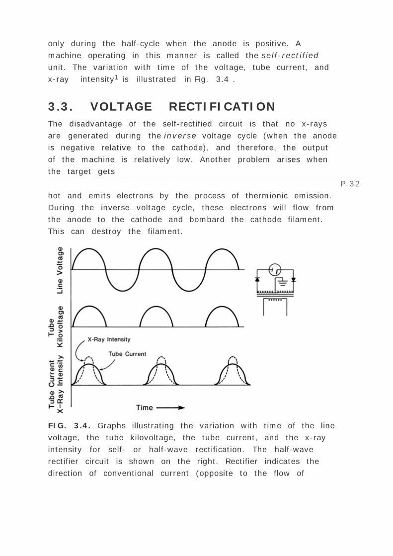
only during the half-cycle when the anode is positive. A

machine operating in this manner is called the self-rectified

unit. The variation with time of the voltage, tube current, and

x-ray intensity1 is illustrated in Fig. 3.4 .

3.3. VOLTAGE RECTIFICATION

The disadvantage of the self-rectified circuit is that no x-rays

are generated during the inverse voltage cycle (when the anode

is negative relative to the cathode), and therefore, the output

of the machine is relatively low. Another problem arises when

the target gets

P.32

hot and emits electrons by the process of thermionic emission.

During the inverse voltage cycle, these electrons will flow from

the anode to the cathode and bombard the cathode filament.

This can destroy the filament.

FIG. 3.4. Graphs illustrating the variation with time of the line

voltage, the tube kilovoltage, the tube current, and the x-ray

intensity for self- or half-wave rectification. The half-wave

rectifier circuit is shown on the right. Rectifier indicates the

direction of conventional current (opposite to the flow of

electrons).

The problem of tube conduction during inverse voltage can be

solved by using voltage rectifiers. Rectifiers placed in series in

the high-voltage part of the circuit prevent the tube from

conducting during the inverse voltage cycle. The current will

flow as usual during the cycle when the anode is positive

relative to the cathode. This type of rectification is called half-

wave rectification and is illustrated in Fig. 3.4 .

The high-voltage rectifiers are either valve or solid state type.

The valve rectifier is similar in principle to the x-ray tube. The

cathode is a tungsten filament and the anode is a metallic plate

or cylinder surrounding the filament. The current2 flows only

from anode to the cathode but the valve will not conduct during

the inverse cycle even if the x-ray target gets hot and emits

electrons.

A valve rectifier can be replaced by solid state rectifiers. These

rectifiers consist of conductors which have been coated with

certain semiconducting elements such as selenium, silicon, and

germanium. These semiconductors conduct electrons in one

direction only and can withstand reverse voltage up to a certain

magnitude. Because of their very small size, thousands of these

rectifiers can be stacked in series in order to withstand the

given inverse voltage.

Rectifiers can also be used to provide full-wave rectification.

For example, four rectifiers can be arranged in the high-voltage

part of the circuit so that the x-ray tube cathode is negative

and the anode is positive during both half-cycles of voltage.

This is schematically shown in Fig. 3.5 . The electronic current

flows through the tube via ABCDEFGH when the transformer

end A is negative and via HGCDEFBA when A is positive. Thus

the electrons flow from the filament to the target during both

half-cycles of the transformer voltage. As a result of full-wave

rectification, the effective tube current is higher since the

current flows during both half-cycles.

FIG. 3.5. Graphs illustrating the variation with time of the line

voltage, the tube kilovoltage, the tube current, and the x-ray

intensity for full-wave rectification. The rectifier circuit is

shown on the right. The arrow symbol on the rectifier diagram

indicates the direction of conventional current flow (opposite to

the flow of electronic current).

P.33

In addition to rectification, the voltage across the tube may be

kept nearly constant by a smoothing condenser (high

capacitance) placed across the x-ray tube. Such constant

potential circuits are commonly used in x-ray machines for

therapy.

3.4. PHYSICS OF X-RAY PRODUCTION

There are two different mechanisms by which x-rays are

produced. One gives rise to bremsstrahlung x-rays and the

other characteristic x-rays . These processes were briefly

mentioned earlier (sections 1.5 and 3.1 ) but now will be

presented in greater detail.

A. Bremsstrahlung

The process of bremsstrahlung (braking radiation) is the result

of radiative â€œcollisionâ€ (interaction) between a high-

speed electron and a nucleus. The electron while passing near a

nucleus may be deflected from its path by the action of

Coulomb forces of attraction and lose energy as

bremsstrahlung, a phenomenon predicted by Maxwell's general

theory of electromagnetic radiation. According to this theory,

energy is propagated through space by electromagnetic fields.

As the electron, with its associated electromagnetic field,

passes in the vicinity of a nucleus, it suffers a sudden

deflection and acceleration. As a result, a part or all of its

energy is dissociated from it and propagates in space as

electromagnetic radiation. The mechanism of bremsstrahlung

production is illustrated in Fig. 3.6 .

Since an electron may have one or more bremsstrahlung

interactions in the material and an interaction may result in

partial or complete loss of electron energy, the resulting

bremsstrahlung photon may have any energy up to the initial

energy of the electron. Also, the direction of emission of

bremsstrahlung photons depends on the energy of the incident

electrons (Fig. 3.7 ). At electron energies below about 100 keV,

x-rays are emitted more or less equally in all directions. As the

kinetic energy of the electrons increases, the direction of x-ray

emission becomes increasingly forward. Therefore,

transmission-type targets are used in megavoltage x-ray tubes

(accelerators) in which the electrons bombard the target from

one side and the x-ray beam is obtained on the other side. In

the low voltage x-ray tubes,

P.34

it is technically advantageous to obtain the x-ray beam on the

same side of the target, i.e., at 90 degrees with respect to the

electron beam direction.

FIG. 3.6. Illustration of bremsstrahlung process.

The energy loss per atom by electrons depends on the square

of the atomic number (Z 2 ). Thus the probability of

bremsstrahlung production varies with Z 2 of the target

material. However the efficiency of x-ray production depends

on the first power of atomic number and the voltage applied to

the tube. The term efficiency is defined as the ratio of output

energy emitted as x-rays to the input energy deposited by

electrons. It can be shown (1 ,2 ) that:

Efficiency = 9 — 10-10 ZV

where V is tube voltage in volts. From the above equation it

can be shown that the efficiency of x-ray production with

tungsten target (Z = 74) for electrons accelerated through 100

kV is less than 1%. The rest of the input energy (~99%)

appears as heat. The accuracy of above equation is limited to a

few MV.

B. Characteristic X-rays

Electrons incident on the target also produce characteristic x-

rays. The mechanism of their production is illustrated in Fig.

3.8 . An electron, with kinetic energy E 0 , may interact with

the atoms of the target by ejecting an orbital electron, such as

a K, L, or M electron, leaving the atom ionized . The original

electron will recede from the collision with energy

P.35

E 0 - ”E , where ”E is the energy given to the orbital

electron. A part of ”E is spent in overcoming the binding

energy of the electron and the rest is carried by the ejected

electron. When a vacancy is created in an orbit, an outer

orbital electron will fall down to fill that vacancy. In so doing,

the energy is radiated in the form of electromagnetic radiation.

This is called characteristic radiation, i.e., characteristic of the

atoms in the target and of the shells between which the

transitions took place. With higher atomic number targets and

the transitions involving inner shells such as K, L, M, and N,

the characteristic radiations emitted are of high enough

energies to be considered in the x-ray part of the

electromagnetic spectrum. Table 3.1 gives the major

characteristic radiation produced in a tungsten target.

FIG. 3.7. Schematic illustration of spatial distribution of x-rays

around a thin target.

FIG. 3.8. Diagram to explain the production of characteristic

radiation.

It should be noted that, unlike bremsstrahlung, characteristic

radiation or x-rays are emitted at discrete energies. If the

transition involved an electron descending from the L shell to

the K shell, then the photon emitted will have energy hv = EK -

EL , where EK and EL are the electron-binding energies of the K

shell and the L shell, respectively.

The threshold energy that an incident electron must possess in

order to first strip an electron from the atom is called critical

absorption energy . These energies for some elements are

given in Table 3.2 .

3.5. X-RAY ENERGY SPECTRA

X-ray photons produced by an x-ray machine are heterogenous

in energy. The energy spectrum shows a continuous distribution

of energies for the bremsstrahlung photons superimposed by

characteristic radiation of discrete energies. A typical spectral

distribution is shown in Fig. 3.9 .

If no filtration, inherent or added, of the beam is assumed, the

calculated energy spectrum will be a straight line (shown as

dotted lines in Fig. 3.9 ) and mathematically given by Kramer's

equation (3) :

where IE is the intensity of photons with energy, E, Z is the

atomic number of the target, Em is the maximum photon

energy, and K is a constant. As pointed out earlier, the

maximum possible energy that a bremsstrahlung photon can

have is equal to the energy of the incident electron. The

maximum energy in kiloelectron volts is numerically equal to

the applied kilovolts peak (kVp). However, the intensity of such

photons is zero as predicted by the previous equation, that is,

IE = 0 when E = Em .

The unfiltered energy spectrum discussed previously is

considerably modified as the photons experience inherent

filtration (absorption in the target, glass walls of the tube, or

thin beryllium window). The inherent filtration in conventional

x-ray tubes is usually equivalent to about 0.5- to 1.0-mm

aluminum. Added filtration, placed externally to the

P.36

tube, further modifies the spectrum. It should be noted that the

filtration affects primarily the initial low-energy part of the

spectrum and does not affect significantly the high-energy

photon distribution.

FIG. 3.9. Spectral distribution of x-rays calculated for a thick

tungsten target using Equation 3.1 . Dotted curves are for no

filtration and the solid curves are for a filtration of 1-mm

aluminum. (Redrawn from Johns HE, Cunningham JR. The

physics of radiology , 3rd ed. Springfield, IL: Charles C

Thomas, 1969, with permission.)

K Series

K ²2

NI I I â€“ K

69.09

K ²1

MI I I â€“ K

67.23

K ±1

LI I I â€“ K

59.31

K ±2

LI I â€“ K

57.97

L Series

L ³1

NI V â€“ LI I

11.28

L ²2

NV â€“ LI I I

9.96

L ²1

MI V â€“ LI I

9.67

L ±I

MV â€“ LI I I

8.40

L ±2

MI V â€“ LI I I

8.33

Data from U.S. Department of Health, Education, and Welfare.

Radiological health handbook. Rev. ed. Washington, DC: U.S.

Government Printing Office, 1970.

Series Lines Transition Energy (keV)

TABLE 3.1. PRINCIPAL CHARACTERISTIC X-RAY

ENERGIES FOR TUNGSTEN

The purpose of the added filtration is to enrich the beam with

higher-energy photons by absorbing the lower-energy

components of the spectrum. As the filtration is increased, the

transmitted beam hardens , i.e., it achieves higher average

energy and therefore greater penetrating power. Thus the

addition of filtration is one way of improving the penetrating

power of the beam. The other method, of course, is by

increasing the voltage across the tube. Since the total intensity

of the beam (area under the curves in Fig. 3.9 ) decreases with

increasing filtration and increases with voltage, a proper

combination of voltage and filtration is required to achieve

desired hardening of the beam as well as acceptable intensity.

The shape of the x-ray energy spectrum is the result of the

alternating voltage applied to the tube, multiple

bremsstrahlung interactions within the target and filtration in

the beam. However, even if the x-ray tube were to be

energized with a constant potential, the x-ray beam would still

be heterogeneous in energy because of the multiple

bremsstrahlung processes that result in different energy

photons.

Because of the x-ray beam having a spectral distribution of

energies, which depends on voltage as well as filtration, it is

difficult to characterize the beam quality in terms of energy,

penetrating power, or degree of beam hardening. A rule of

thumb is often used which states that the average x-ray energy

is approximately one-third of the maximum energy or kVp. Of

course, the one-third rule is a rough approximation since

filtration significantly alters the average energy. Another

quantity, known as half-value layer , has been defined to

describe the quality of an x-ray beam. This topic is discussed in

detail in Chapter 7 .

Z

1

6

8

13

20

29

50

53

56

74

82

92

K

0.0136

0.283

0.531

1.559

4.038

8.980

29.190

33.164

37.41

69.508

88.001

115.59

L

0.087

0.399

1.100

4.464

5.190

5.995

12.090

15.870

21.753

Data from U.S. Department of Health, Education, and Welfare.

Radiological health handbook. Rev. ed. Washington, DC: U.S.


Level

Element

H C O Al Ca Cu Sn I Ba W Pb U

TABLE 3.2. CRITICAL ABSORPTION ENERGIES

(keV)

FIG. 3.10. Illustration of typical operating characteristics.

Plots of relative exposure rate versus a , filament current at a

given kVp; b , tube current at a given kVp; and c , tube voltage

at a given tube current.

3.6. OPERATING CHARACTERISTICS

P.37

In this section, the relationships between x-ray output,

filament current, tube current, and tube voltage are briefly

discussed.

The filament current affects the emission of electrons from the

filament and, therefore, the tube current. Figure 3.10A shows

the typical relationship between the relative exposure rate and

the filament current measured in amperes (A). The figure

shows that under typical operating conditions (filament current

of 5 to 6 A), a small change in filament current produces a

large change in relative exposure rate. This means that the

constancy of filament current is critical to the constancy of the

x-ray output.

The output of an x-ray machine can also be expressed in terms

of the ionization it produces in air. This quantity, which is a

measure of ionization per unit mass of air, is called exposure .

In Figure 3.10B , the exposure rate is plotted as a function of

the tube current. There is a linear relationship between

exposure rate and tube current. As the current or

milliamperage is doubled, the output is also doubled.

The increase in the x-ray output with increase in voltage,

however, is much greater than that given by a linear

relationship. Although the actual shape of the curve (Fig. 3.10C

) depends on the filtration, the output of an x-ray machine

varies approximately as a square of kilovoltage.

REFERENCES

1. Botden P. Modern trends in diagnostic radiologic

instrumentation. In: Moseley R, Rust J, eds. The reduction

of patient dose by diagnostic instrumentation . Springfield,

IL: Charles C Thomas, 1964:15.

2. Hendee WR. Medical radiation physics , 2nd ed. Chicago:

Year Book Medical Publishers, 1979.

3. Kramers HA. On the theory of x-ray absorption and the

continuous x-ray spectrum. Phil Mag 1923;46:836.

1 Intensity is defined as the time variation of energy fluence or

total energy carried by particles (in this case, photons) per unit

area per unit time. The term is also called energy flux density.

2 Here the current means conventional current. The electronic

current will flow from the cathode to the anode.




> Table of Contents > Part I - Abasic Physics > 4 - Clinical

Radiation Generators

4P.38

Clinical Radiation Generators

4.1. KILOVOLTAGE UNITS

Up to about 1950, most of the external beam radiotherapy was

carried out with x-rays generated at voltages up to 300 kVp.

Subsequent development of higher-energy machines and the

increasing popularity of the cobalt-60 units in the 1950s and the

1960s resulted in a gradual demise of the conventional

kilovoltage machines. However, these machines have not

completely disappeared. Even in the present era of the

megavoltage beams, there is still some use for the lower-energy

beams, especially in the treatment of superficial skin lesions.

In Chapter 3 , we discussed in general the principle and

operation of an x-ray generator. In this chapter, we will consider

in particular the salient features of the therapy machines.

On the basis of beam quality and their use, the x-ray therapy in

the kilovoltage range has been divided into subcategories (1 ,2

). The following ranges are more in accordance with the National

Council on Radiation Protection (2 ).

A. Grenz-ray Therapy

The term grenz-ray therapy is used to describe treatment with

beams of very soft (low-energy) x-rays produced at potentials

below 20 kV. Because of the very low depth of penetration (Fig.

4.1 , line a), such radiations are no longer used in radiation

therapy.

B. Contact Therapy

A contact therapy or endocavitary machine operates at

potentials of 40 to 50 kV and facilitates irradiation of accessible

lesions at very short source (focal spot) to surface distances

(SSD). The machine operates typically at a tube current of 2

mA. Applicators available with such machines can provide an

SSD of 2.0 cm or less. A filter of 0.5- to 1.0-mm thick aluminum

is usually interposed in the beam to absorb the very soft

component of the energy spectrum.

Because of very short SSD and low voltage, the contact therapy

beam produces a very rapidly decreasing depth dose1 in tissue.

For that reason, if the beam is incident on a patient, the skin

surface is maximally irradiated but the underlying tissues are

spared to an increasing degree with depth. The dose versus

depth curve or simply the depth-dose curve of a typical contact

therapy beam is shown in Fig. 4.1 , line b. It is readily seen that

this quality of radiation is useful for tumors not deeper than 1 to

2 mm. The beam is almost completely absorbed with 2 cm of

soft tissue.

C. Superficial Therapy

The term superficial therapy applies to treatment with x-rays

produced at potentials ranging from 50 to 150 kV. Varying

thicknesses of filtration (usually 1- to 6-mm aluminum) are

added to harden the beam to a desired degree. As mentioned in

section 3.5 , the degree of hardening or beam quality can be

expressed as the half-value layer (HVL). The HVL is

P.39

defined as the thickness of a specified material that, when

introduced into the path of the beam, reduces the exposure rate

by one-half. Typical HVLs used in the superficial range are 1.0-

to 8.0-mm Al.

FIG. 4.1. Depth dose curves in water or soft tissues for various

quality beams. Line a: Grenz rays, HVL = 0.04 mm Al, field

diameter [asymptotically equal to] 33 cm, SSD = 10 cm. Line b:

Contact therapy, HVL = 1.5 mm Al, field diameter = 2.0 cm,

SSD = 2 cm. Line c: Superficial therapy, HVL = 3.0 mm Al, field

diameter = 3.6 cm, SSD = 20 cm. Line d: Orthovoltage, HVL =

2.0 mm Cu, field size = 10 — 10 cm, SSD = 50 cm. Line e:

Cobalt-60 ³ rays, field size = 10 — 10 cm, SSD = 80 cm.

(Plotted from data in Cohen M, Jones DEA, Green D, eds. Central

axis depth dose data for use in radiotherapy. Br J Radiol

1978[suppl 11]. The British Institute of Radiology, London, with

permission.)

The superficial treatments are usually given with the help of

applicators or cones attachable to the diaphragm of the

machine. The SSD typically ranges between 15 and 20 cm. The

machine is usually operated at a tube current of 5 to 8 mA.

As seen in Fig. 4.1 , line c, a superficial beam of the quality

shown is useful for irradiating tumors confined to about 5-mm

depth (~90% depth dose). Beyond this depth, the dose dropoff

is too severe to deliver adequate depth dose without

considerable overdosing of the skin surface.

D. Orthovoltage Therapy or Deep

Therapy

The term orthovoltage therapy , or deep therapy , is used to

describe treatment with x-rays produced at potentials ranging

from 150 to 500 kV. Most orthovoltage equipment is operated at

200 to 300 kV and 10 to 20 mA. Various filters have been

designed to achieve half-value layers between 1 and 4 mm Cu.

An orthovoltage machine is shown in Fig. 4.2 .

Although cones can be used to collimate the beam into a desired

size, a movable diaphragm, consisting of lead plates, permits a

continuously adjustable field size. The SSD is usually set at 50

cm.

FIG. 4.2. Photograph of Sieman's Stabilapan.

P.40

Figure 4.1 , line d shows a depth dose curve for a moderately

filtered orthovoltage beam. Although the actual depth dose

distribution would depend on many conditions such as

kilovoltage, HVL, SSD, and field size, some generalizations can

be made from this curve about the orthovoltage beam

characteristics. The maximum dose occurs close to the skin

surface, with 90% of that value occurring at a depth of about 2

cm. Thus, in a single field treatment, adequate dose cannot be

delivered to a tumor beyond this depth. However, by increasing

beam filtration or HVL and combining two or more beams

directed at the tumor from different directions, a higher dose to

deeper tumors is delivered. As will be discussed in further detail

in Chapter 11 , there are severe limitations to the use of

orthovoltage beam in treating lesions deeper than 2 to 3 cm.

The greatest limitation is the skin dose, which becomes

prohibitively large when adequate doses are to be delivered to

deep-seated tumors. In the early days of radiation therapy,

when orthovoltage was the highest energy available, treatments

were given until radiation tolerance of the skin was reached.

Although methods were developed to use multiple beams and

other techniques to keep the skin dose under tolerance limits,

the problem of high skin dose remained an overriding concern in

the orthovoltage era. With the availability of cobalt teletherapy,

the skin-sparing properties of higher energy radiation (Fig. 4.1 ,

line e) became the major reason for the modern trend to

megavoltage beams.

Although skin dose and depth dose distribution have been

presented here as two examples of the limitations posed by low-

energy beams, there are other properties such as increased

absorbed dose in bone and increased scattering that make

orthovoltage beams unsuitable for the treatment of tumors

behind bone.

E. Supervoltage Therapy

X-ray therapy in the range of 500 to 1,000 kV has been

designated as high-voltage therapy or supervoltage therapy . In

a quest for higher-energy x-ray beams, considerable progress

was made during the postwar years toward developing higher-

voltage machines. The major problem at that time was

insulating the high-voltage transformer. It soon became

apparent that conventional transformer systems were not

suitable for producing potential much

P.41

above 300 kVp. However, with the rapidly advancing technology

of the times, new approaches to the design of high-energy

machines were found. One of these machines is the resonant

transformer, in which the voltage is stepped up in a very

efficient manner.

FIG. 4.3. Diagram of a resonant transformer unit.

E.1. Resonant Transformer Units

Resonant transformer units have been used to generate x-rays

from 300 to 2,000 kV. The schematic diagram of the apparatus

is shown in Fig. 4.3 . In this apparatus, the secondary of the

high-voltage transformer (without the iron core) is connected in

parallel with capacitors distributed lengthwise inside the x-ray

tube. The combination of the transformer secondary and the

capacitance in parallel exhibits the phenomenon of resonance.

At the resonant frequency, the oscillating potential attains very

high amplitude. Thus the peak voltage across the x-ray tube

becomes very large when the transformer is tuned to resonate at

the input frequency. Since the electrons attain high energies

before striking the target, a transmission-type target (section

3.4 ) may be used to obtain the x-ray beam on the other side of

the target. The electrical insulation is provided by pressurized

Freon gas.

F. Megavoltage Therapy

X-ray beams of energy 1 MV or greater can be classified as

megavoltage beams. Although the term strictly applies to the x-

ray beams, the ³ ray beams produced by radionuclides are also

commonly included in this category if their energy is 1 MeV or

greater. Examples of clinical megavoltage machines are

accelerators such as Van de Graaff generator, linear accelerator,

betatron and microtron, and teletherapy ³ ray units such as

cobalt-60.

4.2. VAN DE GRAAFF GENERATOR

The Van de Graaff machine is an electrostatic accelerator

designed to accelerate charged particles. In radiotherapy, the

unit accelerates electrons to produce high-energy x-rays,

typically at 2 MV.

Figure 4.4 shows a schematic diagram illustrating the basic

principle of a Van de Graaff generator. In this machine, a charge

voltage of 20 to 40 kV is applied across a moving belt of

insulating material. A corona discharge takes place and

electrons are sprayed onto the belt. These electrons are carried

to the top where they are removed by a collector connected to a

spherical dome. As the negative charges collect on the sphere, a

high potential is developed between the sphere and the ground.

This potential is applied across the x-ray tube consisting of a

filament, a series of metal rings, and a target. The rings are

connected to resistors to provide a uniform drop of potential

from the bottom to the top. X-rays are produced when the

electrons strike the target.

Van de Graaff machines are capable of reaching energies up to

10 MV, limited only by size and required high-voltage insulation.

Normally the insulation is provided by a mixture

P.42

of nitrogen and CO2 . The generator is enclosed in a steel tank

and is filled with the gas mixture at a pressure of about 20 atm.

FIG. 4.4. A Van de Graaff generator.

Van de Graaff and resonant transformer (section 4.1.E ) units

for clinical use are no longer produced commercially. The reason

for their demise is the emergence of technically better machines

such as cobalt-60 units and linear accelerators.

4.3. LINEAR ACCELERATOR

The linear accelerator (linac) is a device that uses high-

frequency electromagnetic waves to accelerate charged particles

such as electrons to high energies through a linear tube. The

high-energy electron beam itself can be used for treating

superficial tumors, or it can be made to strike a target to

produce x-rays for treating deep-seated tumors.

There are several types of linear accelerator designs, but the

ones used in radiation therapy accelerate electrons either by

traveling or stationary electromagnetic waves of frequency in

the microwave region (~3,000 megacycles/sec). The difference

between traveling wave and stationary wave accelerators is the

design of the accelerator structure. Functionally, the traveling

wave structures require a terminating, or â€œdummy,â€ load

to absorb the residual power at the end of the structure, thus

preventing a backward reflected wave. On the other hand, the

standing wave structures provide maximum reflection of the

waves at both ends of the structure so that the combination of

forward and reverse traveling waves will give rise to stationary

waves. In the standing wave design, the microwave power is

coupled into the structure via side coupling cavities rather than

through the beam aperture. Such a design tends to be more

efficient than the traveling wave designs since axial, beam

transport cavities, and the side cavities can be independently

optimized (3 ). However, it is more expensive and requires

installation of a circulator (or isolator) between the power

source and the structure to prevent reflections from reaching the

power source. For further details on this subject and linear

accelerator operation the reader is referred to Karzmark, Nunan,

and Tanabe (3 ).

Figure 4.5 is a block diagram of a medical linear accelerator

showing major components and auxiliary systems. A power

supply provides direct current (DC) power to the modulator ,

which includes the pulse-forming network and a switch tube

known as hydrogen

P.43

thyratron . High-voltage pulses from the modulator section are

flat-topped DC pulses of a few microseconds in duration. These

pulses are delivered to the magnetron or klystron 2 and

simultaneously to the electron gun. Pulsed microwaves produced

in the magnetron or klystron are injected into the accelerator

tube or structure via a waveguide system. At the proper instant

electrons, produced by an electron gun , are also pulse injected

into the accelerator structure .

FIG. 4.5. A block diagram of typical medical linear accelerator.

The accelerator structure (or accelerator waveguide) consists of

a copper tube with its interior divided by copper discs or

diaphragms of varying aperture and spacing. This section is

evacuated to a high vacuum. As the electrons are injected into

the accelerator structure with an initial energy of about 50 keV,

the electrons interact with the electromagnetic field of the

microwaves. The electrons gain energy from the sinusoidal

electric field by an acceleration process analogous to that of a

surf rider.

As the high-energy electrons emerge from the exit window of

the accelerator structure, they are in the form of a pencil beam

of about 3 mm in diameter. In the low-energy linacs (up to 6

MV) with relatively short accelerator tube, the electrons are

allowed to proceed straight on and strike a target for x-ray

production. In the higher-energy linacs, however, the

accelerator structure is too long and, therefore, is placed

horizontally or at an angle with respect to the horizontal. The

electrons are then bent through a suitable angle (usually about

90 or 270 degrees) between the accelerator structure and the

target. The precision bending of the electron beam is

accomplished by the beam transport system consisting of

bending magnets, focusing coils, and other components.

A. The Magnetron

The magnetron is a device that produces microwaves. It

functions as a high-power oscillator, generating microwave

pulses of several microsecondsâ€™ duration and with a

repetition rate of several hundred pulses per second. The

frequency of the microwaves within each pulse is about 3,000

MHz.

The magnetron has a cylindrical construction, having a central

cathode and an outer anode with resonant cavities machined out

of a solid piece of copper (Fig. 4.6 ). The space between the

cathode and the anode is evacuated. The cathode is heated by

an inner filament and the electrons are generated by thermionic

emission. A static magnetic field is applied perpendicular to the

plane of the cross-section of the cavities and a pulsed DC

electric field is applied between the cathode and the anode. The

electrons emitted from the cathode are accelerated toward the

anode by the action of the pulsed DC electric field. Under the

simultaneous influence of the magnetic field, the electrons move

in complex spirals

P.44

toward the resonant cavities, radiating energy in the form of

microwaves. The generated microwave pulses are led to the

accelerator structure via the waveguide.

FIG. 4.6. A, B: Cutaway magnetron pictures. C: Cross-sectional

diagram showing principle of magnetron operation. (From

Karzmark CJ, Morton RJ. A primer on theory and operation of

linear accelerators in radiation therapy. Rockville, MD: U.S.

Department of Health and Human Services, Bureau of

Radiological Health, 1981, with permission.)

Typically, magnetrons operate at 2 MW peak power output to

power low-energy linacs (6 MV or less). Although most higher-

energy linacs use klystrons, accelerators of energy as high as 25

MeV have been designed to use magnetrons of about 5 MW

power.

B. The Klystron

The klystron is not a generator of microwaves but rather a

microwave amplifier. It needs to be driven by a low-power

microwave oscillator.

FIG. 4.7. Cross-sectional drawing of a two-cavity klystron.

(From Karzmark CJ, Morton RJ. A primer on theory and operation

of linear accelerators in radiation therapy. Rockville, MD: U.S.

Department of Health and Human Services, Bureau of

Radiological Health, 1981, with permission.)

P.45

Figure 4.7 shows a cross-sectional drawing of an elementary

two-cavity klystron. The electrons produced by the cathode are

accelerated by a negative pulse of voltage into the first cavity,

called the buncher cavity, which is energized by low-power

microwaves. The microwaves set up an alternating electric field

across the cavity. The velocity of the electrons is altered by the

action of this electric field to a varying degree by a process

known as velocity modulation. Some electrons are speeded up

while others are slowed down and some are unaffected. This

results in bunching of electrons as the velocity-modulated beam

passes through a field-free space in the drift tube.

As the electron bunches arrive at the catcher cavity (Fig. 4.7 ),

they induce charges on the ends of the cavity and thereby

generate a retarding electric field. The electrons suffer

deceleration, and by the principle of conservation of energy, the

kinetic energy of electrons is converted into high-power

microwaves.

C. The Linac X-ray Beam

Bremsstrahlung x-rays are produced when the electrons are

incident on a target of a high-Z material such as tungsten. The

target is water cooled and is thick enough to absorb most of the

incident electrons. As a result of bremsstrahlung-type

interactions (section 3.4.A ), the electron energy is converted

into a spectrum of x-ray energies with maximum energy equal to

the incident electron energy. The average photon energy of the

beam is approximately one third of the maximum energy.

It is customary for some of the manufacturers to designate their

linear accelerators that have both electron and x-ray treatment

capabilities by the maximum energy of the electron beam

available. For example, the Varian Clinac 18 unit produces

electron beams of energy 6, 9, 12, 15, and 18 MeV and x-rays of

energy 10 MV. The electron beam is designated by million

electron volts because it is almost monoenergetic before

incidence on the patient surface. The x-ray beam, on the other

hand, is heterogeneous in energy and is designated by

megavolts, as if the beam were produced by applying that

voltage across an x-ray tube.

D. The Electron Beam

As mentioned previously, the electron beam, as it exits the

window of the accelerator tube is a narrow pencil about 3 mm in

diameter. In the electron mode of linac operation, this beam,

instead of striking the target, is made to strike an electron

scattering foil to spread the beam as well as get a uniform

electron fluence across the treatment field. The scattering foil

consists of a thin metallic foil, usually of lead. The thickness of

the foil is such that most of the electrons are scattered instead

of suffering bremsstrahlung. However, a small fraction of the

total energy is still converted into bremsstrahlung and appears

as x-ray contamination of the electron beam.

FIG. 4.8. Components of treatment head. A: X-ray therapy

mode. B: Electron therapy mode. (From Karzmark CJ, Morton RJ.

A primer on theory and operation of linear accelerators in

radiation therapy. Rockville, MD: U.S. Department of Health and

Human Services, Bureau of Radiological Health, 1981, with

permission.)

P.46

In some linacs, the broadening of the electron beam is

accomplished by electromagnetic scanning of the electron pencil

beam over a large area. Although this minimizes the x-ray

contamination, some x-rays are still produced by electrons

striking the collimator walls or other high atomic number

materials in the electron collimation system.

E. Treatment Head

The treatment head (Fig. 4.8 ) consists of a thick shell of high-

density shielding material such as lead, tungsten, or lead-

tungsten alloy. It contains an x-ray target, scattering foil,

flattening filter, ion chamber, fixed and movable collimator, and

light localizer system. The head provides sufficient shielding

against leakage radiation in accordance with radiation protection

guidelines (see Chapter 16 ).

F. Target and Flattening Filter

In section 3.4.A , we discussed the angular distribution of x-rays

produced by electrons of various energies incident on a target.

Since linear accelerators produce electrons in the megavoltage

range, the x-ray intensity is peaked in the forward direction. To

make the beam intensity uniform across the field, a flattening

filter is inserted in the beam (Fig. 4.8A ). This filter is usually

made of lead, although tungsten, uranium, steel, aluminum, or a

combination has also been used or suggested. The choice of

target and flattening filter materials has been discussed by

Podgorsak et al. (4 ).

G. Beam Collimation and Monitoring

The treatment beam is first collimated by a fixed primary

collimator located immediately beyond the x-ray target. In the

case of x-rays, the collimated beam then passes through the

flattening filter. In the electron mode, the filter is moved out of

the way (Fig. 4.8B ).

The flattened x-ray beam or the electron beam is incident on the

dose monitoring chambers . The monitoring system consists of

several ion chambers or a single chamber with multiple plates.

Although the chambers are usually transmission type, i.e., flat

parallel plate chambers to cover the entire beam, cylindrical

thimble chambers have also been used in some linacs.

The function of the ion chamber is to monitor dose rate,

integrated dose, and field symmetry. Since the chambers are in

a high-intensity radiation field and the beam is pulsed, it is

important to make sure that the ion collection efficiency of the

chambers

P.47

remains unchanged with changes in the dose rate. Bias voltages

in the range of 300 to 1,000 V are applied across the chamber

electrodes, depending on the chamber design. Contrary to the

beam calibration chambers, the monitor chambers in the

treatment head are usually sealed so that their response is not

influenced by temperature and pressure of the outside air.

However, these chambers have to be periodically checked for

leaks.

After passing through the ion chambers, the beam is further

collimated by a continuously movable x-ray collimator . This

collimator consists of two pairs of lead or tungsten blocks (jaws)

which provide a rectangular opening from 0 — 0 to the

maximum field size (40 — 40 cm or a little less) projected at a

standard distance such as 100 cm from the x-ray source (focal

spot on the target). The collimator blocks are constrained to

move so that the block edge is always along a radial line

passing through the target.

The field size definition is provided by a light localizing system

in the treatment head. A combination of mirror and a light

source located in the space between the chambers and the jaws

projects a light beam as if emitting from the x-ray focal spot.

Thus the light field is congruent with the radiation field.

Frequent checks are required to ensure this important

requirement of field alignment.

Whereas the x-ray collimation systems of most medical linacs

are similar, the electron collimation systems vary widely. Since

electrons scatter readily in air, the beam collimation must be

achieved close to the skin surface of the patient. There is a

considerable scattering of electrons from the collimator surfaces

including the movable jaws. Dose rate can change by a factor of

two or three as the collimator jaws are opened to maximum field

size limits. If the electrons are collimated by the same jaws, as

for x-rays, there will be an extremely stringent requirement on

the accuracy of the jaw opening, since output so critically

depends on the surface area of the collimator. This problem has

been solved by keeping the x-ray collimator wide open and

attaching an auxiliary collimator for electrons in the form of

trimmers extended down to the skin surface. In other systems,

the auxiliary electron collimator consists of a set of attachable

cones of various sizes.

The dose distribution in an electron field is significantly

influenced by the collimation system provided with the machine

because of electron scattering.

H. Gantry

Most of the linear accelerators currently produced are

constructed so that the source of radiation can rotate about a

horizontal axis (Fig. 4.9 ). As the gantry rotates, the collimator

axis (supposedly coincident with the central axis of the beam)

moves in a vertical plane. The point of intersection of the

collimator axis and the axis of rotation of the gantry is known as

the isocenter .

The isocentric mounting of the radiation machines has

advantages over the units that move only up and down. The

latter units are not suitable for isocentric treatment techniques

in which beams are directed from different directions but

intersect at the same point, the isocenter, placed inside the

patient. However, the nonisocentric units are usually swivel

mounted, that is, the treatment head can be swiveled or rotated

in any direction while the gantry can move only upward or

downward. Although these units are not as flexible, they are

mechanically simpler, more reliable, and less expensive than the

isocentric models.

4.4. BETATRON

The operation of the betatron is based on the principle that an

electron in a changing magnetic field experiences acceleration in

a circular orbit. Figure 4.10 shows a schematic drawing of the

machine. The accelerating tube is shaped like a hollow doughnut

and is placed between the poles of an alternating current

magnet. A pulse of electrons is introduced into this evacuated

doughnut by an injector at the instant that the alternating

current cycle begins. As the magnetic field rises, the electrons

experience acceleration continuously and spin with increasing

velocity around the tube. By the end of the first quarter cycle of

P.48

the alternating magnetic field, the electrons have made several

thousand revolutions and achieved maximum energy. At this

instant or earlier, depending on the energy desired, the

electrons are made to spiral out of the orbit by an additional

attractive force. The high-energy electrons then strike a target

to produce x-rays or a scattering foil to produce a broad beam of

electrons.

FIG. 4.9. Photograph of a linear accelerator, isocentrically

mounted. (Courtesy of Varian Associates, Palo Alto, California.)

Betatrons were first used for radiotherapy in the early 1950s.

They preceded the introduction of linear accelerators by a few

years. Although the betatrons can provide x-ray and electron

therapy beams over a wide range of energies, from less than 6

to more than 40 MeV, they are inherently low-electron-beam

current devices. The x-ray dose rates and field size capabilities

of medical betatrons are low compared with medical linacs and

even modern cobalt units. However, in the electron therapy

mode, the beam current is adequate to provide a high dose rate.

The reason for this difference between x-ray and electron dose

P.49

rates is that the x-ray production via bremsstrahlung as well as

beam flattening requires a much larger primary electron beam

current (about 1,000 times) than that required for the electron

therapy beam.

FIG. 4.10. Diagram illustrating the operation of a betatron.

The availability of medium energy linacs with high x-ray does

rates, large field sizes, and electron therapy energies up to 20

MeV has given the linacs a considerable edge in popularity over

the betatrons. Moreover, many radiation therapists regard the

small field size and dose rate capabilities of the betatron as

serious disadvantages to the general use of the device. Thus a

significant increase in betatron installations in this country,

paralleling medical linacs, seems unlikely.

4.5. MICROTRON

The microtron is an electron accelerator that combines the

principles of both the linear accelerator and the cyclotron

(section 4.6 ). In the microtron, the electrons are accelerated by

the oscillating electric field of one or more microwave cavities

(Fig. 4.11A,B ). A magnetic field forces the electrons to move in

a circular orbit and return to the cavity. As the electrons receive

higher and higher energy by repeated passes through the cavity,

they describe orbits of increasing radius in the magnetic field.

The cavity voltage, frequency, and magnetic field are so

adjusted that the electrons arrive each time in the correct phase

at the cavity. Because the electrons travel with an

approximately constant velocity (almost the speed of light), the

above condition can be maintained if the path length of the

orbits increases with one

P.50

microwave wavelength per revolution. The microwave power

source is either a klystron or a magnetron.

FIG. 4.11. A: Schematic diagram of a circular microtron unit.

(Reprinted with permission from AB Scanditronix, Uppsala,

Sweden.) B: Electron orbits and accelerating cavities in a

racetrack microtron. (From Karzmark CJ, Nunan CS, Tanabe E.

Medical electron accelerators. New York: McGraw-Hill, 1993, with

permission.)

The extraction of the electrons from an orbit is accomplished by

a narrow deflection tube of steel that screens the effect of the

magnetic field. When the beam energy is selected, the deflection

tube is automatically moved to the appropriate orbit to extract

the beam.

The principal advantages of the microtron over a linear

accelerator of comparable energy are its simplicity, easy energy

selection, and small beam energy spread as well as the smaller

size of the machine. Because of the low energy spread of the

accelerated electrons and small beam emittance (product of

beam diameter and divergence), the beam transport system is

greatly simplified. These characteristics have encouraged the

use of a single microtron to supply a beam to several treatment

rooms.

Although the method of accelerating electrons used in the

microtron was proposed as early as in 1944 by Veksler (5 ), the

first microtron for radiotherapy (a 10-MeV unit) was described

by Reistad and Brahme (6 ) in 1972. Later, a 22-MeV microtron

(7 ) was developed by AB Scanditronix and installed at the

University of Ume ¥, Sweden. This particular model (MM 22)

produced two x-rays beams of energy 6 or 10 and 21 MV and 10

electron beams of 2, 5, 7, 9, 11, 13, 16, 18, 20, and 22 MeV.

The circular microtron, as described above and shown

schematically in Fig. 4.11A , is a bulky structure because it

requires a large magnetic gap to accommodate accelerating

cavity and large diameter magnetic field to accommodate the

large number of spaced orbits with limited energy gain per orbit.

These constraints are removed by a racetrack microtron, which

uses a standing wave linac structure (instead of a single cavity)

to accelerate the electrons (Fig. 4.11B ). The parameters of a

50-MeV racetrack microtron developed at the Royal Institute of

Technology, Stockholm, are given by Rosander et al. (8 ). A

review is also provided by Karzmark et al. (3 ).

4.6. CYCLOTRON

The cyclotron is a charged particle accelerator, mainly used for

nuclear physics research. In radiation therapy, these machines

have been used as a source of high-energy protons for proton

beam therapy. More recently, the cyclotrons have been adopted

for generating neutron beams. In the latter case, the deuterons

(2 1 H+ ) are accelerated to high energies and then made to

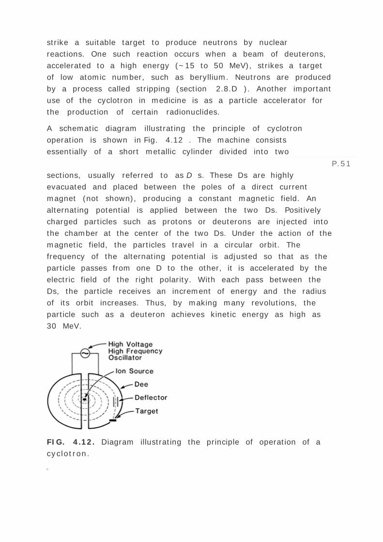
strike a suitable target to produce neutrons by nuclear

reactions. One such reaction occurs when a beam of deuterons,

accelerated to a high energy (~15 to 50 MeV), strikes a target

of low atomic number, such as beryllium. Neutrons are produced

by a process called stripping (section 2.8.D ). Another important

use of the cyclotron in medicine is as a particle accelerator for

the production of certain radionuclides.

A schematic diagram illustrating the principle of cyclotron

operation is shown in Fig. 4.12 . The machine consists

essentially of a short metallic cylinder divided into two

P.51

sections, usually referred to as D s. These Ds are highly

evacuated and placed between the poles of a direct current

magnet (not shown), producing a constant magnetic field. An

alternating potential is applied between the two Ds. Positively

charged particles such as protons or deuterons are injected into

the chamber at the center of the two Ds. Under the action of the

magnetic field, the particles travel in a circular orbit. The

frequency of the alternating potential is adjusted so that as the

particle passes from one D to the other, it is accelerated by the

electric field of the right polarity. With each pass between the

Ds, the particle receives an increment of energy and the radius

of its orbit increases. Thus, by making many revolutions, the

particle such as a deuteron achieves kinetic energy as high as

30 MeV.

FIG. 4.12. Diagram illustrating the principle of operation of a

cyclotron.

There is a limit to the energy that a particle can attain by the

above process. According to the theory of relativity, as the

particle reaches high velocity (in the relativistic range), further

acceleration causes the particle to gain in mass. This tends to

slow down the particle, which can then get out of step with the

frequency of the alternating potential applied to the Ds. This

problem has been solved in the synchrotrons where the

frequency of the potential is adjusted to compensate for the

decrease in particle velocity.

4.7. MACHINES USING

RADIONUCLIDES

Radionuclides such as radium-226, cesium-137, and cobalt-60

have been used as sources of ³ rays for teletherapy.3 These

³ rays are emitted from the radionuclides as they undergo

radioactive disintegration.

Of all the radionuclides, 60 Co has proved to be the most

suitable for external beam radiotherapy. The reasons for its

choice over radium and cesium are higher possible specific

activity (curies per gram), greater radiation output per curie and

higher average photon energy. These characteristics for the

three radionuclides are compared in Table 4.1 . In addition,

radium is much more expensive and has greater self-absorption

of its radiation than either cesium or cobalt.

A. Cobalt-60 Unit

A.1. Source

The 60 Co source is produced by irradiating ordinary stable 59 Co

with neutrons in a reactor. The nuclear reaction can be

represented by 59 Co(n , ³) 60 Co.

The 60 Co source, usually in the form of a solid cylinder, discs,

or pallets, is contained inside a stainless-steel capsule and

sealed by welding. This capsule is placed into another steel

capsule which is again sealed by welding. The double-welded

seal is necessary to prevent any leakage of the radioactive

material.

The 60 Co source decays to 60 Ni with the emission of ²

particles (E max = 0.32 MeV) and two photons per disintegration

of energies 1.17 and 1.33 MeV (decay scheme given in Fig. 1.5

). These ³ rays constitute the useful treatment beam. The ²

particles are absorbed in the cobalt metal and the stainless-steel

capsules resulting in the emission of bremsstrahlung x-rays and

a small amount of characteristic x-rays. However, these x-rays

of average energy around 0.1 MeV do not contribute appreciably

to the dose in the patient because they are strongly attenuated

in the material of the source and the capsule. The other

â€œcontaminantsâ€ to the treatment beam are the lower-

energy ³ rays produced by the interaction of the primary ³

radiation with the source itself, the surrounding capsule, the

source housing, and the collimator system. The scattered

components of the beam contribute significantly (~10%) to the

total intensity of the beam (9 ). All these secondary interactions

thus, to

P.52

some extent, result in heterogeneity of the beam. In addition,

electrons are also produced by these interactions and constitute

what is usually referred to as the electron contamination of the

photon beam.

Radium-226 (filtered by 0.5 mm Pt)

1,622

0.83 (avg.)

0.825

~0.98

Cesium-137

30.0

0.66

0.326

~50

Cobalt-60

5.26

1.17, 1.33

1.30

~200a Exposure rate constant ( “) is discussed in Chapter 8 . The

higher the “ value, the greater will be the exposure rate or

output per curie of the teletherapy source.

Radionuclide

Half-

Life

(yr)

³-Ray

Energy

MeV

“ Valuea

Specific

Activity

Achieved

in

Practice

(Ci/g)

TABLE 4.1. TELETHERAPY SOURCE CHARACTERISTICS

A typical teletherapy 60 Co source is a cylinder of diameter

ranging from 1.0 to 2.0 cm and is positioned in the cobalt unit

with its circular end facing the patient. The fact that the

radiation source is not a point source complicates the beam

geometry and gives rise to what is known as the geometric

penumbra.

A.2. Source Housing

The housing for the source is called the sourcehead (Fig. 4.13 ).

It consists of a steel shell filled with lead for shielding purposes

and a device for bringing the source in front of an opening in the

head from which the useful beam emerges.

Also, a heavy metal alloy sleeve is provided to form an

additional primary shield when the source is in the off position.

A number of methods have been developed for moving the

source from the off position to the on position. These methods

have been discussed in detail by Johns and Cunningham (10 ). It

will suffice here to mention briefly four different mechanisms:

(a) the source mounted on a rotating wheel inside the

sourcehead to carry the source from the off position to the on

position; (b) the source mounted on a heavy metal drawer plus

its ability to slide horizontally through a hole running through

the sourceheadâ€”in the on position the source faces the

aperture for the treatment beam and in the off position the

source moves to its shielded location and a light source mounted

on the same drawer occupies the on position of the source; (c)

mercury is allowed to flow into the space immediately below the

source to shut off the beam; and (d) the source is fixed in front

of the aperture and the beam can be turned on and off by a

shutter consisting of heavy metal jaws. All of the above

mechanisms incorporate a safety feature in which the source is

returned automatically to the off position in case of a power

failure.

A.3. Beam Collimation and Penumbra

A collimator system is designed to vary the size and shape of

the beam to meet the individual treatment requirements. The

simplest form of a continuously adjustable diaphragm consists of

two pairs of heavy metal blocks. Each pair can be moved

independently to obtain a square or a rectangle-shaped field.

Some collimators are multivane type, i.e., multiple blocks to

control the size of the beam. In either case, if the inner surface

of the blocks is made parallel to the central axis of the beam,

the radiation will pass through the edges of the collimating

blocks resulting in what is known as the transmission penumbra

. The extent of this penumbra will be more pronounced for larger

collimator openings because of greater obliquity of the rays at

the edges of the blocks. This effect has been minimized in some

designs by shaping the collimator blocks so that the inner

surface of the blocks remains always parallel to the edge of the

beam. In these collimators, the blocks are hinged to the top of

the collimator housing so that the slope of the blocks is

P.53

coincident with the included angle of the beam. Although the

transmission penumbra can be minimized with such an

arrangement, it cannot be completely removed for all field sizes.

FIG. 4.13. Photograph of cobalt unit, Theratron 780. (Courtesy

of Atomic Energy of Canada, Ltd., Ottawa, Canada.)

The term penumbra , in a general sense, means the region, at

the edge of a radiation beam, over which the dose rate changes

rapidly as a function of distance from the beam axis (10 ). The

transmission penumbra, mentioned above, is the region

irradiated by photons which are transmitted through the edge of

the collimator block.

Another type of penumbra, known as the geometric penumbra ,

is illustrated in Fig. 4.14 . The geometric width of the penumbra

(Pd ) at any depth (d ) from the surface of a patient can be

determined by considering similar triangles ABC and DEC . From

geometry, we have:

If AB = s , the source diameter, OM = SDD, the source to

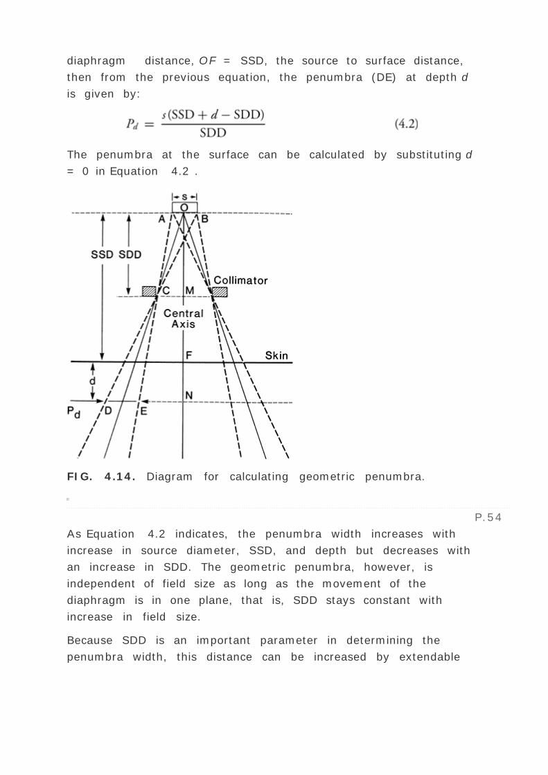
diaphragm distance, OF = SSD, the source to surface distance,

then from the previous equation, the penumbra (DE) at depth d

is given by:

The penumbra at the surface can be calculated by substituting d

= 0 in Equation 4.2 .

FIG. 4.14. Diagram for calculating geometric penumbra.

P.54

As Equation 4.2 indicates, the penumbra width increases with

increase in source diameter, SSD, and depth but decreases with

an increase in SDD. The geometric penumbra, however, is

independent of field size as long as the movement of the

diaphragm is in one plane, that is, SDD stays constant with

increase in field size.

Because SDD is an important parameter in determining the

penumbra width, this distance can be increased by extendable

penumbra trimmers . These trimmers consist of heavy metal

bars to attenuate the beam in the penumbra region, thus

â€œsharpeningâ€ the field edges. The penumbra, however, is

not eliminated completely but reduced since SDD with the

trimmers extended is increased. The new SDD is equal to the

source to trimmer distance. An alternative way of reducing the

penumbra is to use secondary blocks, placed close to the

patient, for redefining or shaping the field. As will be discussed

in Chapter 13 , the blocks should not be placed closer than 15 to

20 cm from the patient because of excessive electron

contaminants produced by the block carrying tray.

The combined effect of the transmission and geometric

penumbras is to create a region of dose variation at the field

edges. A dose profile of the beam measured across the beam in

air at a given distance from the source would show

dosimetrically the extent of the penumbra. However, at a depth

in the patient the dose variation at the field border is a function

of not only geometric and transmission penumbras but also the

scattered radiation produced in the patient. Thus, dosimetrically,

the term physical penumbra width has been defined as the

lateral distance between two specified isodose curves4 at a

specified depth (11 ).

4.8. HEAVY PARTICLE BEAMS

Whereas x-rays and electrons are the main radiations used in

radiotherapy, heavy particle beams offer special advantages

with regard to dose localization and therapeutic gain (greater

effect on tumor than on normal tissue). These particles include

neutrons, protons, deuterons, ± particles, negative pions, and

heavy ions accelerated to high energies. Their

P.55

use in radiation therapy is still experimental, and because of the

enormous cost involved, only a few institutions have been able

to acquire these modalities for clinical trials. From the

literature, which is full of encouraging as well as discouraging

reports about their efficacy, it appears that the role of heavy

particles in radiation therapy is not yet established. However,

the radiobiological interest in the field remains as strong as

ever.

A. Neutrons

High-energy neutron beams for radiotherapy are produced by

deuterium tritium (D-T) generators, cyclotrons, or linear

accelerators. The bombarding particles are either deuterons or

protons and the target material is usually beryllium, except in

the D-T generator in which tritium is used as the target.

A.1. D-T Generator

A low-energy deuteron beam (100â€“300 keV) incident on a

tritium target yields neutrons by the following reaction:

The disintegration energy of 17.6 MeV is shared between the

helium nucleus ( ± particle) and the neutron, with about 14

MeV given to the neutron. The neutrons thus produced are

essentially monoenergetic and isotropic (same yield in all

directions). The major problem is the lack of sufficient dose rate

at the treatment distance. The highest dose rate that has been

achieved so far is about 15 cGy/min at 1 m. The advantage of

D-T generators over other sources is that its size is small

enough to allow isocentric mounting on a gantry.

A.2. Cyclotron

Deuterons accelerated to high energies (~15â€“50 MeV) by a

cyclotron bombard a low atomic number target such as beryllium

to produce neutrons according to a stripping reaction (see

section 2.8.D ):

2 1 H + 9 4 Be â†’ 10 5 B + 1 0 n

Neutrons are produced mostly in the forward direction with a

spectrum of energies, as shown in Fig. 4.15 . The average

neutron energy is about 40% to 50% of the deuteron energy.

FIG. 4.15. Neutron spectra produced by deuterons on beryllium

target. (From Raju MR. Heavy particle radiotherapy. New York:

Academic Press, 1980. Data from Hall EJ, Roizin-Towle L, Attix

FH. Radiobiological studies with cyclotron-produced neutrons

currently used for radiotherapy. Int J Radiol-Oncol Biol Phys

1975;1:33, and Graves RG, Smathers JB, Almond PR, et al.

Neutron energy spectra of d(49)-Be and P(41)-Be neutron

radiotherapy sources. Med Phys 1979;6:123; with permission.)

FIG. 4.16. Depth dose distribution characteristic of heavy

charged particles, showing Bragg peak.

P.56

The bombarding particles can also be protons accelerated to

high energies by a cyclotron or a linear accelerator. The neutron

spectrum produced by 41 MeV protons is shown in Fig. 4.15 . A

hydrogenous material filter (e.g., polyethylene) is used to

reduce the number of low-energy neutrons in the spectrum.

B. Protons and Heavy Ions

Proton beams for therapeutic application range in energy from

150 to 250 MeV. These beams can be produced by a cyclotron or

a linear accelerator. The major advantage of high-energy

protons and other heavy charged particles is their characteristic

distribution of dose with depth (Fig. 4.16 ). As the beam

traverses the tissues, the dose deposited is approximately

constant with depth until near the end of the range where the

dose peaks out to a high value followed by a rapid falloff to

zero. The region of high dose at the end of the particle range is

called the Bragg peak.

Figure 14.17 shows the range energy relationship for protons.

The approximate range for other particles with the same initial

velocity can be calculated by the following relationship:

where R 1 and R 2 are particle ranges, M 1 and M 2 are the

masses, and Z 1 and Z 2 are the charges of the two particles

being compared. Thus from the range energy data for protons

one can calculate the range of other particles.

The energy of heavy charged particles or stripped nuclei is often

expressed in terms of kinetic energy per nucleon (specific

kinetic energy) or MeV/u where u is the mass number of the

nucleus. Particles with the same MeV/u have approximately the

same velocity and range. For example, 150 MeV protons, 300

MeV deuterons, and 600 MeV helium ions all have approximately

the same range of about 16 cm in water. However, for ions

heavier than helium, the range for the same MeV/u is somewhat

less than that for protons. As predicted by Equation 4.4 , the

range is dependent on A /Z 2 , where A is the atomic number

and Z is the nuclear charge. Since A /Z 2 decreases as the ions

get heavier, the range of heavier ions is less than the range of

lighter ions for the same MeV/u .

C. Negative Pions

The existence of pi mesons was theoretically predicted by

Yukawa in 1935 when he postulated that protons and neutrons

in the nucleus are held together by a mutual exchange of pi

mesons. A pi meson (or pion) has a mass 273 times that of

electron and may have a positive charge, a negative charge, or

may be neutral. The charged pions decay into mu

P.57

mesons and neutrinos with a mean life of 2.54 — 10-8 seconds

and the neutral pions decay into pairs of photons with a mean

life of about 10-16 seconds.

FIG. 4.17. Range energy relationship for protons. (From Raju

MR. Heavy particle radiotherapy. New York: Academic Press,

1980, with permission.)

Only negative pions have been used for radiation therapy.

Beams of negative pions can be produced in a nuclear reaction.

Protons of energy in the range of 400 to 800 MeV, produced in a

cyclotron or a linear accelerator are usually used for pion beam

production for radiotherapy. Beryllium is a suitable target

material. Pions of positive, negative, and zero charge with a

spectrum of energies are produced and negative pions of

suitable energy are extracted from the target using bending and

focusing magnets. Pions of energy close to 100 MeV are of

interest in radiation therapy, providing a range in water of about

24 cm.

The Bragg peak exhibited by pions is more pronounced than

other heavy particles because of the additional effect of nuclear

disintegration by €- capture. This phenomenon,

P.58

commonly known as star formation , occurs when a pion is

captured by a nucleus in the medium near the end of its range.

A pion capture results in the release of several other particles

such as protons, neutrons, and ± particles.

Although pion beams have attractive radiobiologic properties,

they suffer from the problems of low dose rates, beam

contamination, and high cost.

REFERENCES

1. Paterson R. The treatment of malignant disease by radium

and x-rays . Baltimore: Williams & Wilkins, 1963.

2. National Council on Radiation Protection. Medical x-ray

and gamma ray protection for energies up to 10 MeV . NCRP

report 34 Washington, DC: National Council on Radiation

Protection and Measurements, 1970.

3. Karzmark CJ, Nunan CS, Tanabe E. Medical electron

accelerators . New York: McGraw-Hill, 1993.

4. Podgorsak EB, Rawlinson JA, Johns HE. X-ray depth doses

from linear accelerators in the energy range from 10 to 32

MeV. AJR 1975;123:182.

5. Veksler VJ. A new method for acceleration of relativistic

particles. Dokl Akad Nauk SSSR 1944;43:329.

6. Reistad D, Brahme A. The microtron, a new accelerator for

radiation therapy. The Third ICMP Executive Committee , ed.

Digest of the 3rd international conference on medical

physics. G ¶tenborg, Sweden: Chalmers University of

Technology, 1972:23.5.

7. Svensson H, Johnsson L, Larsson LG, et al. A 22 MeV

microtron for radiation therapy. Acta Radiol Ther Phys Biol

1977;16:145.

8. Rosander S, Sedlacek M, Werholm O. The 50 MeV

racetrack microtron at the Royal Institute of Technology,

Stockholm. Nucl Inst Meth 1982;204:1â€“20.

9. Cormack DV, Johns HE. Spectral distribution of scattered

radiation from a kilocurie cobalt 60 unit. Br J Radiol

1958;31:497.

10. Johns HE, Cunningham JR. The physics of radiology , 3rd

ed. Springfield, IL: Charles C Thomas, 1969:120.

11. International Commission on Radiation Units.

Determination of absorbed dose in a patient irradiated by

beams of x- or gamma rays in radiotherapy procedures. ICRU

report 24. Washington, DC: International Commission on

Radiation Units and Measurements, 1976:54.

1 The term dose , or absorbed dose , is defined as the energy

absorbed per unit mass of the irradiated material.

2 Magnetron and klystron are both devices for producing

microwaves. Whereas magnetrons are generally less expensive

than klystrons, the latter have a long life span. In addition,

klystrons are capable of delivering higher-power levels required

for high-energy accelerators and are preferred as the beam

energy approaches 20 MeV or higher.

3 Teletherapy is a general term applied to external beam

treatments in which the source of radiation is at a large distance

from the patient.

4 An isodose curve is a line passing through points of equal

dose.




> Table of Contents > Part I - Abasic Physics > 5 -

Interactions of Ionizing Radiation

5

Interactions of IonizingRadiation

When an x- or ³ ray beam passes through a medium,

interaction between photons and matter can take place with the

result that energy is transferred to the medium. The initial step

in the energy transfer involves the ejection of electrons from the

atoms of the absorbing medium. These high-speed electrons

transfer their energy by producing ionization and excitation of

the atoms along their paths. If the absorbing medium consists of

body tissues, sufficient energy may be deposited within the

cells, destroying their reproductive capacity. However, most of

the absorbed energy is converted into heat, producing no

biologic effect.

5.1. IONIZATION

The process by which a neutral atom acquires a positive or a

negative charge is known as ionization . Removal of an orbital

electron leaves the atom positively charged, resulting in an ion

pair. The stripped electron, in this case, is the negative ion and

the residual atom is the positive ion. In some cases, an electron

may be acquired by a neutral atom and the negatively charged

atom then becomes the negative ion.

Charged particles such as electrons, protons, and ± particles

are known as directly ionizing radiation provided they have

sufficient kinetic energy to produce ionization by collision1 as

they penetrate matter. The energy of the incident particle is lost

in a large number of small increments along the ionization track

in the medium, with an occasional interaction in which the

ejected electron receives sufficient energy to produce a

secondary track of its own, known as a ´ ray . If, on the other

hand, the energy lost by the incident particle is not sufficient to

eject an electron from the atom but is used to raise the

electrons to higher energy levels, the process is termed

excitation .

The uncharged particles such as neutrons and photons are

indirectly ionizing radiation because they liberate directly

ionizing particles from matter when they interact with matter.

Ionizing photons interact with the atoms of a material or

absorber to produce high-speed electrons by three major

processes: photoelectric effect, Compton effect, and pair

production. Before considering each process in detail, we shall

discuss the mathematical aspects of radiation absorption.

5.2. PHOTON BEAM DESCRIPTION

An x-ray beam emitted from a target or a ³ ray beam emitted

from a radioactive source consists of a large number of photons,

usually with a variety of energies. A beam of photons can be

described by many terms, some of which are defined as follows:

P.60

The fluence ( ¦) of photons is the quotient dN by da , where

dN is the number of photons that enter an imaginary sphere

of cross-sectional area da .

Fluence rate or flux density ( †) is the fluence per unit

time.

where dt is the time interval.

Energy fluence ( ¨) is the quotient of dEf l by da , where dEf l

is the sum of the energies of all the photons that enter a

sphere of cross-sectional area da .

For a monoenergetic beam, dEf l is just the number of

photons dN times energy h ½ carried by each photon:

Energy fluence rate, energy flux density, or intensity ( ˆ) is

the energy fluence per unit time:

5.3. PHOTON BEAM ATTENUATION

An experimental arrangement designed to measure the

attenuation characteristics of a photon beam is shown in Fig. 5.1

. A narrow beam of monoenergetic photons is incident on an

absorber of variable thickness. A detector is placed at a fixed

distance from the source and sufficiently farther away from the

absorber so that only the primary photons (those photons that

passed through the absorber without interacting) are measured

by the detector. Any photon scattered by the absorber is not

supposed to be measured in this arrangement. Thus, if a photon

interacts with an atom, it is either completely absorbed or

scattered away from the detector.

Under these conditions, the reduction in the number of photons

(dN ) is proportional to the number of incident photons (N ) and

to the thickness of the absorber (dx ). Mathematically,

dN âˆ Ndx

or

P.61

where µ is the constant of proportionality, called the

attenuation coefficient . The minus sign indicates that the

number of photons decreases as the absorber thickness

increases. The above equation can also be written in terms of

intensity (I ):

dI = - µIdx

or

If thickness x is expressed as a length, then µ is called the

linear attenuation coefficient . For example, if the thickness is

measured in centimeters, the units of µ are 1/cm, or cm-1 .

FIG. 5.1. Diagram to illustrate an experimental arrangement for

studying narrow beam attenuation through an absorber.

Measurements are under â€œgood geometry,â€ i.e., scattered

photons are not measured.

Equation 5.7 is identical to Equation 2.1 , which describes

radioactive decay, and µ is analogous to decay constant ».

As before, the differential equation for attenuation can be solved

to yield the following equation:

where I (x ) is the intensity transmitted by a thickness x and I 0

is the intensity incident on the absorber. If I (x ) is plotted as a

function of x for a narrow monoenergetic beam, a straight line

will be obtained on semilogarithmic paper (Fig. 5.2A ), showing

that the attenuation of a monoenergetic beam is described by an

exponential function.

The term analogous to half-life (section 2.4 ) is the half-value

layer (HVL) defined as the thickness of an absorber required to

attenuate the intensity of the beam to half its original value.

That means that when x = HVL, I /I 0 = 1/2, by definition. Thus

from Equation 5.8 it can be shown that:

FIG. 5.2. A: Graph showing percent transmission of a narrow

monoenergetic photon beam as a function of absorber thickness.

For this quality beam and absorber material, HVL = 2 cm and µ

= 0.347 cm-1 . B: Universal attenuation curve showing percent

transmission of a narrow monoenergetic beam as a function of

absorber thickness in units of half-value layer (HVL).

P.62

As mentioned previously, exponential attenuation strictly applies

to a monoenergetic beam. Figure 5.2B is a general attenuation

curve for a monoenergetic beam or a beam whose half-value

layer does not change with absorber thickness. Such a curve

may be used to calculate the number of HVLs required to reduce

the transmitted intensity to a given percentage of the incident

intensity.

A practical beam produced by an x-ray generator, however,

consists of a spectrum of photon energies. Attenuation of such a

beam is no longer quite exponential. This effect is seen in Fig.

5.3 , in which the plot of transmitted intensity on

semilogarithmic paper is not a straight line. The slope of the

attenuation curve decreases with increasing absorber thickness

because the absorber or filter preferentially removes the lower-

energy photons. As shown in Fig. 5.3 , the first HVL is defined as

that thickness of material which reduces the

P.63

incident beam intensity by 50%. The second HVL reduces the

beam to 50% of its intensity after it has been transmitted

through the first HVL. Similarly, the third HVL represents the

quality of the beam after it has been transmitted through the

absorber of thickness equal to two HVLs. In general, for a

heterogeneous beam, the first HVL is less than the subsequent

HVLs. As the filter thickness increases, the average energy of

the transmitted beam increases or the beam becomes

increasingly harder . Thus, by increasing the filtration in such an

x-ray beam, one increases the penetrating power or the half-

value layer of the beam.

FIG. 5.3. Schematic graph showing transmission of an x-ray

beam with a spectrum of photon energies through an aluminum

absorber. First HVL = 0.99 mm Al, second HVL = 1.9 mm Al,

third HVL = 2.0 mm Al.

5.4. COEFFICIENTS

A. Attenuation Coefficient

In the previous section, we discussed the linear attenuation

coefficient µ, which has units of cm-1 . In general, this

coefficient depends on the energy of the photons and the nature

of the material. Since the attenuation produced by a thickness x

depends on the number of electrons presented in that thickness,

µ depends on the density of the material. Thus, by dividing µ

by density , the resulting coefficient ( µ/ ) will be

independent of density; µ/ is known as the mass

attenuation coefficient . This is a more fundamental coefficient

than the linear coefficient, since the density has been factored

out and its dependence on the nature of the material does not

involve density but rather the atomic composition.

The mass attenuation coefficient has units of cm2 /g because

µ/ = cm-1 /(g/cm3 ). When using µ/ in the

attenuation Equation 5.8 , the thickness should be expressed as

x , which has units of g/cm2 , because µx =

( µ/ )( x ) and x = (g/cm3 )(cm).

In addition to the cm and g/cm2 units, the absorber thickness

can also be expressed in units of electrons/cm2 and atoms/cm2 .

The corresponding coefficients for the last two units are

electronic attenuation coefficient (e µ) and atomic attenuation

coefficient (a µ), respectively.

where Z is the atomic number and N 0 is the number of electrons

per gram and N 0 is given by:

where NA is Avogadro's number and AW is the atomic weight

(see section 1.3 ).

The attenuation process or the attenuation coefficient represents

the fraction of photons removed per unit thickness. The

transmitted intensity I (x ) in Equation 5.8 is caused by photons

that did not interact with the material. Those photons which

produced interactions will transfer part of their energy to the

material and result in part or all of that energy being absorbed.

B. Energy Transfer Coefficient

When a photon interacts with the electrons in the material, a

part or all of its energy is converted into kinetic energy of

electrons. If only a part of the photon energy is given to the

electron, the photon itself is scattered with reduced energy. The

scattered photon may interact again with a partial or complete

transfer of energy to the electrons. Thus a photon may

experience one or multiple interactions in which the energy lost

by the photon is converted into kinetic energy of electrons.

If we consider a photon beam traversing a material, the fraction

of photon energy transferred into kinetic energy of charged

particles per unit thickness of absorber is given

P.64

by the energy transfer coefficient ( µt r ). This coefficient is

related to µ as follows:

where ’t r is the average energy transferred into kinetic energy

of charged particles per interaction. The mass energy transfer

coefficient is given by µt r / .

C. Energy Absorption Coefficient

Most of the electrons set in motion by the photons will lose their

energy by inelastic collisions (ionization and excitation) with

atomic electrons of the material. A few, depending on the atomic

number of the material, will lose energy by bremsstrahlung

interactions with the nuclei. The bremsstrahlung energy is

radiated out of the local volume as x-rays and is not included in

the calculation of locally absorbed energy.

The energy absorption coefficient ( µen ) is defined as the

product of energy transfer coefficient and (1 - g ) where g is the

fraction of the energy of secondary charged particles that is lost

to bremsstrahlung in the material.

As before, the mass energy absorption coefficient is given by

µen / .

For most interactions involving soft tissues or other low Z

material in which electrons lose energy almost entirely by

ionization collisions, the bremsstrahlung component is

negligible. Thus µen = µt r under those conditions. These

coefficients can differ appreciably when the kinetic energies of

the secondary particles are high and material traversed has a

high atomic number.

The energy absorption coefficient is an important quantity in

radiotherapy since it allows the evaluation of energy absorbed in

the tissues, a quantity of interest in predicting the biologic

effects of radiation.

5.5. INTERACTIONS OF PHOTONS

WITH MATTER

Attenuation of a photon beam by an absorbing material is

caused by five major types of interactions. One of these, photo

disintegration, was considered in section 2.8F . This reaction

between photon and nucleus is only important at very high

photon energies (>10 MeV). The other four processes are

coherent scattering, the photoelectric effect, the Compton effect,

and the pair production. Each of these processes can be

represented by its own attenuation coefficient, which varies in

its particular way with the energy of the photon and with the

atomic number of the absorbing material. The total attenuation

coefficient is the sum of individual coefficients for these

processes:

where ƒcoh , „, ƒc , and € are attenuation coefficients for

coherent scattering, photoelectric effect, Compton effect, and

pair production, respectively.

5.6. COHERENT SCATTERING

The coherent scattering, also known as classical scattering or

Rayleigh scattering, is illustrated in Fig. 5.4 . The process can

be visualized by considering the wave nature of electromagnetic

radiation. This interaction consists of an electromagnetic wave

passing near the electron and setting it into oscillation. The

oscillating electron reradiates the energy at the same frequency

as the incident electromagnetic wave. These scattered x-rays

P.65

have the same wavelength as the incident beam. Thus no energy

is changed into electronic motion and no energy is absorbed in

the medium. The only effect is the scattering of the photon at

small angles. The coherent scattering is probable in high atomic

number materials and with photons of low energy. The process is

only of academic interest in radiation therapy.

FIG. 5.4. Diagram illustrating the process of coherent

scattering. The scattered photon has the same wavelength as

the incident photon. No energy is transferred.

5.7. PHOTOELECTRIC EFFECT

The photoelectric effect is a phenomenon in which a photon

interacts with an atom and ejects one of the orbital electrons

from the atom (Fig. 5.5 ). In this process, the entire energy h

½ of the photon is first absorbed by the atom and then

transferred to the atomic electron. The kinetic energy of the

ejected electron (called the photoelectron) is equal to h ½ - EB

, where EB is the binding energy of the electron. Interactions of

this type can take place with electrons in the K, L, M, or N

shells.

After the electron has been ejected from the atom, a vacancy is

created in the shell, thus leaving the atom in an excited state.

The vacancy can be filled by an outer orbital electron with the

emission of characteristic x-rays (section 3.4B ). There is also

the possibility of emission of Auger electrons (section 2.7C ),

which are monoenergetic electrons produced by the absorption

of characteristic x-rays internally by the atom. Because the K

shell binding energy of soft tissues is only about 0.5 keV, the

energy of the characteristic photons produced in biologic

absorbers is very low and can be considered to be locally

absorbed. For higher-energy photons and higher atomic number

materials, the characteristic photons are of higher energy and

may deposit energy at large distances compared with the range

P.66

of the photoelectron. In such cases, the local energy absorption

is reduced by the energy emitted as characteristic radiation

(also called fluorescent radiation) which is considered to be

remotely absorbed.

FIG. 5.5. Illustration of the photoelectric effect.

FIG. 5.6. Mass photoelectric attenuation coefficient ( „/ )

plotted against photon energy. Curves for water (Z eff = 7.42)

and lead (Z = 82). (Data from Grodstein GW. X-ray attenuation

coefficients from 10 keV to 100 MeV. Pub. No. 583. Washington,

DC: U.S. Bureau of Standards, 1957.)

The probability of photoelectric absorption depends on the

photon energy as illustrated in Fig. 5.6 , where the mass

photoelectric attenuation coefficient ( „/ ) is plotted as a

function of photon energy. Data are shown for water,

representing a low atomic number material similar to tissue, and

for lead, representing a high atomic number material. On

logarithmic paper, the graph is almost a straight line with a

slope of approximately -3; therefore, we get the following

relationship between „/ and photon energy:

The graph for lead has discontinuities at about 15 and 88 keV.

These are called absorption edges and correspond to the binding

energies of L and K shells. A photon with energy less than 15

keV does not have enough energy to eject an L electron. Thus,

below 15 keV, the interaction is limited to the M or higher-shell

electrons. When the photon has an energy that just equals the

binding energy of the L shell, resonance occurs and the

probability of photoelectric absorption involving the L shell

becomes very high. Beyond this point, if the photon energy is

increased, the probability of photoelectric attenuation decreases

approximately as 1/E 3 until the next discontinuity, the K

absorption edge. At this point on the graph, the photon has 88

keV energy, which is just enough to eject the K electron. As

seen in Fig. 5.6 , the absorption probability in lead at this

critical energy increases dramatically, by a factor of about 10.

The discontinuities or absorption edges for water are not shown

in the graph because the K absorption edge for water occurs at

very low photon energies (~0.5 keV).

P.67

The data for various materials indicate that photoelectric

attenuation depends strongly on the atomic number of the

absorbing material. The following approximate relationship

holds:

This relationship forms the basis of many applications in

diagnostic radiology. The difference in Z of various tissues such

as bone, muscle, and fat amplifies differences in x-ray

absorption, provided the primary mode of interaction is

photoelectric. This Z 3 dependence is also exploited when using

contrast materials such as BaSO4 mix and Hypaque. In

therapeutic radiology, the low-energy beams produced by

superficial and orthovoltage machines cause unnecessary high

absorption of x-ray energy in bone as a result of this Z 3

dependence; this problem will be discussed later in section 5.10

. By combining Equations 5.16 and 5.17 , we have:

The angular distribution of electrons emitted in a photoelectric

process depends on the photon energy. For a low-energy photon,

the photoelectron is emitted most likely at 90 degrees relative

to the direction of the incident photon. As the photon energy

increases, the photoelectrons are emitted in a more forward

direction.

5.8. COMPTON EFFECT

In the Compton process, the photon interacts with an atomic

electron as though it were a â€œfreeâ€ electron. The term free

here means that the binding energy of the electron is much less

than the energy of the bombarding photon. In this interaction,

the electron receives some energy from the photon and is

emitted at an angle ¸ (Fig. 5.7 ). The photon, with reduced

energy, is scattered at an angle †.

The Compton process can be analyzed in terms of a collision

between two particles, a photon and an electron. By applying the

laws of conservation of energy and momentum, one can derive

the following relationships:

where h ½0 , h ½â€², and E are the energies of the incident

photon, scattered photon, and electron, respectively and, ± =

h ½0 /m 0 c 2 , where m 0 c 2 is the rest energy of the electron

(0.511 MeV). If h ½0 is expressed in MeV, then ± = h ½0

/0.511.

FIG. 5.7. Diagram illustrating the Compton effect.

P.68

A. Special Cases of Compton Effect

A.1. Direct Hit

If a photon makes a direct hit with the electron, the electron will

travel forward ( ¸ = 0 degrees) and the scattered photon will

travel backward ( † = 180 degrees) after the collision. In such

a collision, the electron will receive maximum energy E max and

the scattered photon will be left with minimum energy h

½â€²min . One can calculate E max and h ½â€²min by

substituting cos † = cos 180 degrees = -1 in Equations 5.19

and 5.20 .

A.2. Grazing Hit

If a photon makes a grazing hit with the electron, the electron

will be emitted at right angles ( ¸ = 90 degrees) and the

scattered photon will go in the forward direction ( † = 0

degrees). By substituting cos † = cos 0 degrees = 1 in

Equations 5.19 and 5.20 , one can show that for this collision E

= 0 and h ½â€² = h ½0 .

A.3. 90-Degree Photon Scatter

If a photon is scattered at right angles to its original direction

( † = 90 degrees), one can calculate E and h ½â€² from

Equations 5.19 and 5.20 by substituting cos † = cos 90

degrees = 0. The angle of the electron emission in this case will

depend on ±, according to Equation 5.21 .

Examples

Some useful examples will now be given to illustrate application

of the Compton effect to practical problems.

Interaction of a low-energy photon . If the incident photon

energy is much less than the rest energy of the electron,

only a small part of its energy is imparted to the electron,

resulting in a scattered photon of almost the same energy as

the incident photon. For example, suppose h ½0 = 51.1

keV; then ± = h ½0 /m 0 c 2 = 0.0511 MeV/0.511 MeV =

0.1. From Equations 5.22 and 5.23 ,

Thus, for a low-energy photon beam, the Compton scattered

photons have approximately the same energy as the original

photons. Indeed, as the incident photon energy approaches

zero, the Compton effect becomes the classical scattering

process described in section 5.6 .

Interaction of a high energy photon . If the incident photon

has a very high energy (much greater than the rest energy

of the electron), the photon loses most of its energy to the

Compton electron and the scattered photon has much less

energy. Suppose h ½0 = 5.11 MeV; then ± = 10.0. From

Equations 5.22 and 5.23 ,

P.69

In contrast to example (a) above, the scattered photons

produced by high-energy photons carry away only a small

fraction of the initial energy. Thus, at high photon energy,

the Compton effect causes a large amount of energy

absorption compared with the Compton interactions involving

low-energy photons.

Compton scatter at † = 90 degrees and 180 degrees . In

designing radiation protection barriers (walls) to attenuate

scattered radiation, one needs to know the energy of the

photons scattered at different angles. The energy of the

photons scattered by a patient under treatment at 90

degrees with respect to the incident beam is of particular

interest in calculating barrier or wall thicknesses against

scattered radiation.

By substituting † = 90 degrees in Equation 5.20 , we

obtain:

For high-energy photons with ± â‰« 1, the previous

equation reduces to:

or

h ½â€² = m 0 c 2 = 0.511 MeV

Similar calculations for scatter at † = 180 degrees will indicate

h ½â€² = 0.255 MeV. Thus, if the energy of the incident

photon is high ( ± â‰« 1), we have the following important

generalizations: (a) the radiation scattered at right angles is

independent of incident energy and has a maximum value of

0.511 MeV; (b) the radiation scattered backwards is independent

of incident energy and has a maximum value of 0.255 MeV.

The maximum energy of radiation scattered at angles between

90 and 180 degrees will lie between the above energy limits.

However, the energy of the photons scattered at angles less

than 90 degrees will be greater than 0.511 MeV and will

approach the incident photon energy for the condition of forward

scatter. Because the energy of the scattered photon plus that of

the electron must equal the incident energy, the electron may

acquire any energy between zero and E max (given by Equation

5.22 ).

B. Dependence of Compton Effect on

Energy and Atomic Number

It was mentioned previously that the Compton effect is an

interaction between a photon and a free electron. Practically,

this means that the energy of the incident photon must be large

compared with the electron binding energy. This is in contrast to

the photoelectric effect which becomes most probable when the

energy of the incident photon is equal to or slightly greater than

the binding energy of the electron. Thus, as the photon energy

increases beyond the binding energy of the K electron, the

photoelectric effect decreases rapidly with energy (Equation 5.16

) (Fig. 5.6 ) and the Compton effect becomes more and more

important. However, as shown in Fig. 5.8 , the Compton effect

also decreases with increasing photon energy .

Because the Compton interaction involves essentially free

electrons in the absorbing material, it is independent of atomic

number Z . It follows that the Compton mass attenuation

coefficient ( ƒ/ ) is independent of Z and depends only on

the number of electrons per gram. Although the number of

electrons per gram of elements decreases slowly but

systemically with atomic number, most materials except

hydrogen can be considered as having approximately the same

number of electrons per gram (Table 5.1 ). Thus, ƒ/ i s

nearly the same for all materials .

From the previous discussion, it follows that if the energy of the

beam is in the region where the Compton effect is the only

possible mode of interaction, approximately the same

P.70

attenuation of the beam will occur in any material of equal

density thickness,2 expressed as g/cm2 . For example, in the

case of a 60 Co ³ ray beam that interacts by Compton effect,

the attenuation per g/cm2 for bone is nearly the same as that

for soft tissue. However, 1 cm of bone will attenuate more than

1 cm of soft tissue, because bone has a higher electron density,3

e (number of electrons per cubic centimeter), which is given

by density times the number of electrons per gram. If the

density of bone is assumed to be 1.85 g/cm3 and that of soft

tissue 1 g/cm3 , then the attenuation produced by 1 cm of bone

will be equivalent to that produced by 1.65 cm of soft tissue:

FIG. 5.8. A plot of Compton electronic coefficient e ƒ against

photon energy. The mass coefficient ( ƒ/ ) is obtained by

multiplying the electronic coefficient with the number of

electrons per gram for a given material. (Data from Hubbell JH.

Proton cross sections attenuation coefficients and energy

absorption coefficients from 10 keV to 100 GeV. Pub. No. 29.

Washington, DC: U.S. National Bureau of Standards, 1969.)

5.9. PAIR PRODUCTION

If the energy of the photon is greater than 1.02 MeV, the photon

may interact with matter through the mechanism of pair

production. In this process (Fig. 5.9 ), the photon interacts

strongly with the electromagnetic field of an atomic nucleus and

gives up all its energy in the process of creating a pair

consisting of a negative electron (e- ) and a positive electron

(e+ ). Because the rest mass energy of the electron is

equivalent to 0.51 MeV, a minimum energy of 1.02 MeV is

required to create the pair of electrons. Thus the threshold

energy for the pair production process is 1.02 MeV. The photon

energy in excess of this threshold is shared between the

particles as kinetic energy. The total kinetic energy available for

the

P.71

electron-positron pair is given by (h ½ - 1.02) MeV. The

particles tend to be emitted in the forward direction relative to

the incident photon.

Hydrogen

0.0000899

1

6.00 — 1023

Carbon

2.25

6

3.01 — 1023

Oxygen

0.001429

8

3.01 — 1023

Aluminum

2.7

13

2.90 — 1023

Copper

8.9

29

2.75 — 1023

Lead

11.3

82

2.38 — 1023

Effective Atomic Number

Fat

0.916

5.92

3.48 — 1023

Muscle

1.00

7.42

3.36 — 1023

Water

1.00

7.42

3.34 — 1023

Air

0.001293

7.64

3.01 — 1023

Bone

1.85

13.8

3.00 — 1023

Data from Johns HE, Cunningham JR. The physics of radiology.

3rd ed. Springfield, IL: Charles C Thomas, 1969.

Material Density

(g/cm3 )

Atomic

Number

Number of

Electrons per Gram

TABLE 5.1. NUMBER OF ELECTRONS PER GRAM OF

VARIOUS MATERIALS

The most probable distribution of energy is for each particle to

acquire half the available kinetic energy, although any energy

distribution is possible. For example, in an extreme case, it is

possible that one particle may receive all the energy while the

other receives no energy.

The pair production process is an example of an event in which

energy is converted into mass, as predicted by Einstein's

equation E = mc 2 . The reverse process, namely the conversion

of mass into energy, takes place when a positron combines with

an electron to produce two photons, called the annihilation

radiation.

A. Annihilation Radiation

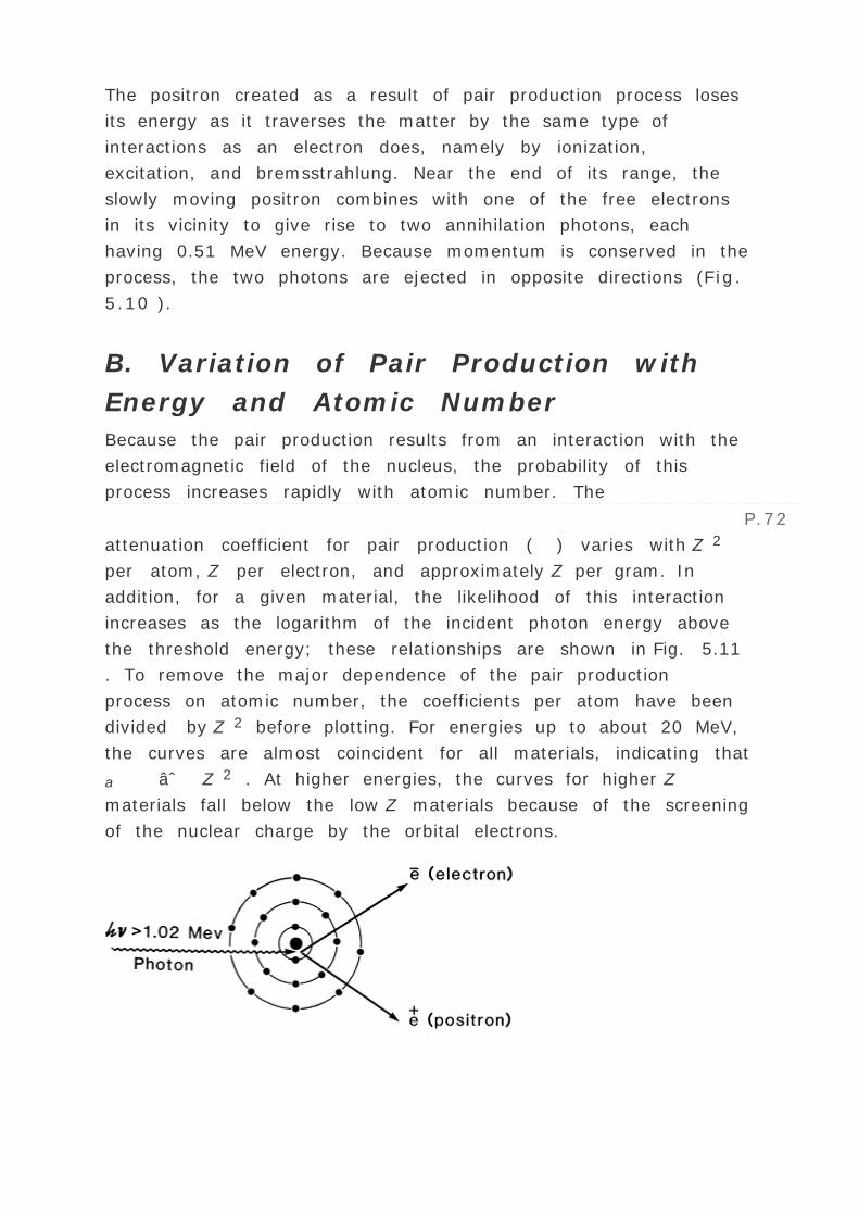
The positron created as a result of pair production process loses

its energy as it traverses the matter by the same type of

interactions as an electron does, namely by ionization,

excitation, and bremsstrahlung. Near the end of its range, the

slowly moving positron combines with one of the free electrons

in its vicinity to give rise to two annihilation photons, each

having 0.51 MeV energy. Because momentum is conserved in the

process, the two photons are ejected in opposite directions (Fig.

5.10 ).

B. Variation of Pair Production with

Energy and Atomic Number

Because the pair production results from an interaction with the

electromagnetic field of the nucleus, the probability of this

process increases rapidly with atomic number. The

P.72

attenuation coefficient for pair production ( ) varies with Z 2

per atom, Z per electron, and approximately Z per gram. In

addition, for a given material, the likelihood of this interaction

increases as the logarithm of the incident photon energy above

the threshold energy; these relationships are shown in Fig. 5.11

. To remove the major dependence of the pair production

process on atomic number, the coefficients per atom have been

divided by Z 2 before plotting. For energies up to about 20 MeV,

the curves are almost coincident for all materials, indicating that

a âˆ Z 2 . At higher energies, the curves for higher Z

materials fall below the low Z materials because of the screening

of the nuclear charge by the orbital electrons.

FIG. 5.9. Diagram illustrating the pair production process.

FIG. 5.10. Diagram illustrating the production of annihilation

radiation.

FIG. 5.11. Plot of pair atomic attenuation coefficient divided by

the square of the atomic number as a function of photon energy

for carbon (Z = 6) and lead (Z = 82). The mass attenuation

coefficient can be obtained by multiplying a € /Z 2 obtained

from the graph, first by Z 2 and then by the number of atoms

per gram of the absorber. (Data from Hubbell JH. Proton cross

sections attenuation coefficients and energy absorption

coefficients from 10 keV to 100 GeV. Pub. No. 29. Washington,

DC: U.S. National Bureau of Standards, 1969.)

P.73

5.10. RELATIVE IMPORTANCE OF

VARIOUS TYPES OF INTERACTIONS

The total mass attenuation coefficient ( µ/ ) is the sum of

the four individual coefficients:

As noted previously, coherent scattering is only important for

very low photon energies (<10 keV) and high Z materials. At

therapeutic energies, it is often omitted from the sum.

Figure 5.12 is the plot of total coefficient ( µ/ )total vs.

energy for two different materials, water and lead,

representative of low and high atomic number materials. The

mass attenuation coefficient is large for low energies and high

atomic number media because of the predominance of

photoelectric interactions under these conditions.

The attenuation coefficient decreases rapidly with energy until

the photon energy far exceeds the electron binding energies and

the Compton effect becomes the predominant mode of

interaction. In the Compton range of energies, the µ/ of

lead and water do not differ greatly, since this type of

interaction is independent of atomic number. The coefficient,

however, decreases with energy until pair production begins to

become important. The dominance of pair production occurs at

energies much greater than the threshold energy of 1.02 MeV.

The relative importance of various types of interactions is

presented in Table 5.2 . These data for water will also be true

for soft tissue. The photon energies listed in column 1 of Table

5.2 represent monoenergetic beams. As discussed in Chapter 3 ,

an x-ray tube operating at a given peak voltage produces

radiation of all energies less than the peak energy. As a rough

approximation and for the purposes of Table 5.2 , one may

consider the average energy of an x-ray beam to be equivalent

to one-third of the peak energy. Thus a 30-keV monoenergetic

beam in column 1 should be considered as equivalent to an x-

ray beam produced by an x-ray tube operated at about 90 kVp.

Of course, the

P.74

accuracy of this approximation is limited by the effects of

filtration on the energy spectrum of the beam.

FIG. 5.12. Plot of total mass attenuation coefficient ( µ/ )

as a function of photon energy for lead and water. (Reprinted

with permission from Johns HE, Cunningham JR. The physics of

radiology , 3rd ed. Springfield, IL: Charles C Thomas, 1969.)

0.01

95

5

0

0.026

50

50

0

0.060

7

93

0

0.150

0

100

0

4.00

0

94

6

10.00

0

77

23

24.00

0

50

50

100.00

0

16

84

Data from Johns HE, Cunningham JR. The physics of radiology.

3rd ed. Springfield, IL: Charles C Thomas, 1969.

Photon Energy

(MeV)

Relative Number of Interactions

(%)

„ ƒ

TABLE 5.2. RELATIVE IMPORTANCE OF PHOTOELECTRIC

( „), COMPTON ( ƒ), AND PAIR PRODUCTION ( )

PROCESSES IN WATER

5.11. INTERACTIONS OF CHARGED

PARTICLES

Whereas photons interact with matter by photoelectric,

Compton, or pair production process, charged particles

(electrons, protons, ± particles, and nuclei) interact principally

by ionization and excitation. Radiative collisions in which the

charged particle interacts by the bremsstrahlung process are

possible but are much more likely for electrons than for heavier

charged particles.

The charged particle interactions or collisions are mediated by

Coulomb force between the electric field of the traveling particle

and electric fields of orbital electrons and nuclei of atoms of the

material. Collisions between the particle and the atomic

electrons result in ionization and excitation of the atoms.

Collisions between the particle and the nucleus result in

radiative loss of energy or bremsstrahlung. Particles also suffer

scattering without significant loss of energy. Because of much

smaller mass, electrons suffer greater multiple scattering than

do heavier particles.

In addition to the Coulomb force interactions, heavy charged

particles give rise to nuclear reactions, thereby producing

radioactive nuclides. For example, a proton beam passing

through tissue produces short-lived radioisotopes 11 C, 13 N, and15 O, which are positron emitters.

The rate of kinetic energy loss per unit path length of the

particle (dE /dx ) is known as the stopping power (S ). The

quantity S / is called the mass stopping power, where is

the density of the medium and is usually expressed in MeV cm2

/g.

A. Heavy Charged Particles

The rate of energy loss or stopping power caused by ionization

interactions for charged particles is proportional to the square of

the particle charge and inversely proportional to the square of

its velocity. Thus, as the particle slows down, its rate of energy

loss increases and so does the ionization or absorbed dose to the

medium. As was seen in Fig. 4.16 , the dose deposited in water

increases at first very slowly with depth and then very sharply

near the end of the range, before dropping to an almost zero

value. This peaking of dose near the end of the particle range is

called the Bragg peak .

Because of the Bragg peak effect and minimal scattering,

protons and heavier charged particle beams provide a much

sought-after advantage in radiotherapyâ€”the ability to

concentrate dose inside the target volume and minimize dose to

surrounding normal tissues.

P.75

B. Electrons

Interactions of electrons when passing through matter are quite

similar to those of heavy particles. However, because of their

relatively small mass, the electrons suffer greater multiple

scattering and changes in direction of motion. As a consequence,

the Bragg peak is not observed for electrons. Multiple changes in

direction during the slowing down process smears out the Bragg

peak.

In water or soft tissue, electrons, like other charged particles,

lose energy predominantly by ionization and excitation. This

results in deposition of energy or absorbed dose in the medium.

As stated earlier, the ionization process consists of stripping

electrons from the atoms. If the energy transferred to the orbital

electron is not sufficient to overcome the binding energy, it is

displaced from its stable position and then returns to it; this

effect is called excitation . Furthermore, in the process of

ionization, occasionally the stripped electron receives sufficient

energy to produce an ionization track of its own. This ejected

electron is called a secondary electron, or a ´ ray.

Again, because of its small mass, an electron may interact with

the electromagnetic field of a nucleus and be decelerated so

rapidly that a part of its energy is lost as bremsstrahlung. The

rate of energy loss as a result of bremsstrahlung increases with

the increase in the energy of the electron and the atomic

number of the medium. The topic of electron interactions will be

discussed further in Chapter 14 .

5.12. INTERACTIONS OF NEUTRONS

Like x-rays and ³ rays, neutrons are indirectly ionizing.

However, their mode of interaction with matter is different.

Neutrons interact basically by two processes: (a) recoiling

protons from hydrogen and recoiling heavy nuclei from other

elements, and (b) nuclear disintegrations. The first process may

be likened to a billiard-ball collision in which the energy is

redistributed after the collision between the colliding particles.

The energy transfer is very efficient if the colliding particles

have the same mass, e.g., a neutron colliding with a hydrogen

nucleus. On the other hand, the neutron loses very little energy

when colliding with a heavier nucleus. Thus the most efficient

absorbers of a neutron beam are the hydrogenous materials such

as paraffin wax or polyethylene. Lead, which is a very good

absorber for x-rays, is a poor shielding material against

neutrons.

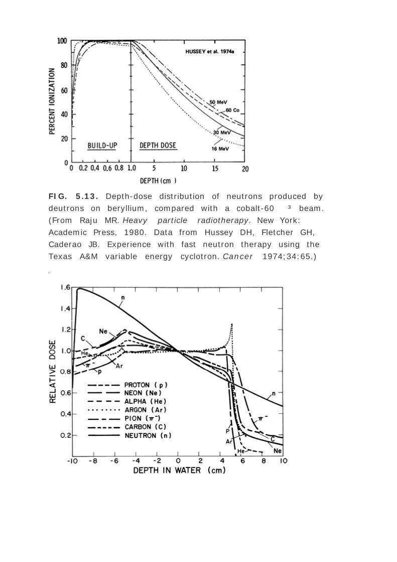
FIG. 5.13. Depth-dose distribution of neutrons produced by

deutrons on beryllium, compared with a cobalt-60 ³ beam.

(From Raju MR. Heavy particle radiotherapy. New York:

Academic Press, 1980. Data from Hussey DH, Fletcher GH,

Caderao JB. Experience with fast neutron therapy using the

Texas A&M variable energy cyclotron. Cancer 1974;34:65.)

FIG. 5.14. Depth-dose distribution for various heavy particle

beams with modulated Bragg peak at a depth of 10 cm and

normalized at the peak center. (From Raju MR. Heavy particle

radiotherapy. New York: Academic Press, 1980.)

P.76

Dose deposited in tissue from a high-energy neutron beam is

predominantly contributed by recoil protons. Because of the

higher hydrogen content, the dose absorbed in fat exposed to a

neutron beam is about 20% higher than in muscle. Nuclear

disintegrations produced by neutrons result in the emission of

heavy charged particles, neutrons, and ³ rays and give rise to

about 30% of the tissue dose. Because of such diverse

secondary radiation produced by neutron interactions, the

neutron dosimetry is relatively more complicated than the other

types of clinical beams.

5.13. COMPARATIVE BEAM

CHARACTERISTICS

No one kind of radiation beam is ideal for radiation therapy.

Whereas x-rays and electrons are the most useful beams,

particle beams have some unique physical and radiobiologic

P.77

characteristics that have attracted the attention of many

investigators. For details the reader is referred to reference 1.

FIG. 5.15. Comparison of depth-dose distribution for protons

and electrons. (From Koehler AM, Preston WM. Protons in

radiation therapy. Radiology 1972;104:191, with permission.)

Physical advantages of a radiation therapy beam are derived

from the depth-dose distributions and scatter characteristics.

Figures 5.13 , 5.14 , and 5.15 compare the depth-dose

characteristics of various beams. It is seen that the depth dose

distribution of neutron beams is qualitatively similar to the 60

Co ³ rays. The heavy charged particle beams, the Bragg peaks

of which were modulated using filters (as is typically done in

clinical situations), show a flat dose distribution at the peak

region and a sharp dose dropoff beyond the range. Electron

beams also show a constant dose region up to about half the

particle range and a sharp dose dropoff beyond that point.

However, for higher electron energies, the characteristic falloff

in dose becomes more gradual. Protons, on the other hand,

maintain a sharp cutoff in dose beyond the range, irrespective of

energy.

REFERENCES

1. Raju MR. Heavy particle radiotherapy . New York:

Academic Press, 1980.

1 The process of collision is an interaction between the

electromagnetic fields associated with the colliding particle and

orbital electron. Actual physical contact between the particles is

not required.

2 Density thickness is equal to the linear thickness multiplied by

density, i.e., cm — g/cm3 = g/cm2 .

3 In the literature, the term electron density has been defined

both as the number of electrons per gram and as the number of

electrons per cubic centimeter. The reader should be aware of

this possible source of confusion.





Measurement of Ionizing Radiation

6P.78

Measurement of IonizingRadiation

6.1. INTRODUCTION

In the early days of x-ray usage for diagnosis and therapy,

attempts were made to measure ionizing radiation on the basis

of chemical and biologic effects. For instance, radiation effects

on photographic emulsions, changes in the color of some

chemical compounds, and reddening of the human skin could be

related to the amount of radiation absorbed. However, these

effects were poorly understood at the time and could only

provide crude estimation of radiation dose. For example, in

radiotherapy, a unit called skin erythema dose (SED) was

defined as that amount of x or ³ radiation that just produced

reddening of the human skin. However, the unit has many

drawbacks. Skin erythema depends on many conditions, such

as the type of skin, the quality of radiation, the extent of skin

exposed, dose fractionation (dose per fraction and interval

between fractions), and differences between early and delayed

skin reactions.

Although the SED was later discarded in favor of a more

precisely measurable unit such as the roentgen, the skin

erythema was used by physicians as an approximate index of

response to the radiation treatments. This happened in the

orthovoltage era when the skin was the limiting organ to the

delivery of tumoricidal doses. The reliance on skin reaction for

the assessment of radiation response had to be abandoned

when megavoltage beams with the skin-sparing properties

became the main tools of radiation therapy.

In 1928, the International Commission on Radiation Units and

Measurements (ICRU) adopted the roentgen as the unit of

measuring x and ³ radiation exposure. The unit is denoted by

R.

6.2. THE ROENTGEN

The roentgen is a unit of exposure. The quantity exposure is a

measure of ionization produced in air by photons. The ICRU (1)

defines exposure (X) as the quotient of dQ by dm where dQ is

the absolute value of the total charge of the ions of one sign

produced in air when all the electrons (negatrons and

positrons) liberated by photons in air of mass dm are

completely stopped in air.

The Systems Internationale dâ€™Unites (SI) unit for exposure

is coulomb per kilogram (C/kg) but the special unit is roentgen

(R).1

1R = 2.58 — 10-4 C/kg air

FIG. 6.1. Diagram illustrating electronic equilibrium in a

free-air chamber.

P.79

The definition of roentgen is illustrated in Fig. 6.1. An x-ray

beam in passing through air sets in motion electrons by

photoelectric effect, Compton effect, or pair production. These

high-speed electrons produce ionization along their tracks.

Because of the electric field produced by the voltage applied

across the ion-collection plates, the positive charges move

toward the negative plate and the negative charges move

toward the positive plate. This constitutes a current. The

collected charge of either sign can be measured by an

electrometer.

According to the definition of roentgen, the electrons produced

by photons in a specified volume (shaded in Fig. 6.1) must

spend all their energies by ionization in air enclosed by the

plates (region of ion collection) and the total ionic charge of

either sign should be measured. However, some electrons

produced in the specified volume deposit their energy outside

the region of ion collection and thus are not measured. On the

other hand, electrons produced outside the specified volume

may enter the ion-collecting region and produce ionization

there. If the ionization loss is compensated by the ionization

gained, a condition of electronic equilibrium exists. Under this

condition, the definition of roentgen is effectively satisfied.

This is the principle of free-air ionization chamber, described

below.

6.3. FREE-AIR IONIZATION CHAMBER

The free-air, or standard, ionization chamber is an instrument

used in the measurement of the roentgen according to its

definition. Generally, such a primary standard is used only for

the calibration of secondary instruments designed for field use.

The free-air chamber installations are thus confined principally

to some of the national standards laboratories.

A free-air chamber is represented schematically in Fig. 6.2. An

x-ray beam, originating from a focal spot S, is defined by the

diaphragm D, and passes centrally between a pair of parallel

plates. A high-voltage (field strength of the order of 100 V/cm)

is applied between the plates to collect ions produced in the air

between the plates. The ionization is measured for a length L

defined by the limiting lines of force to the edges of the

collection plate C. The lines of force are made straight and

perpendicular to the collector by a guard ring G.

As discussed previously, electrons produced by the photon

beam in the specified volume (shaded in Fig. 6.2) must spend

all their energy by ionization of air between the

P.80

plates. Such a condition can exist only if the range of the

electrons liberated by the incident photons is less than the

distance between each plate and the specified volume. In

addition, for electronic equilibrium to exist, the beam intensity

(photon fluence per unit time) must remain constant across the

length of the specified volume, and the separation between the

diaphragm and the ion-collecting region must exceed the

electron range in air.

FIG. 6.2. A schematic diagram of a free-air chamber.

If ”Q is the charge collected in Coulombs and is the

density (kg/m3) of air, then the exposure Xp at the center of

the specified volume (point P) is:

where Ap is the cross-sectional area (in meters squared) of the

beam at point P and L (in meters) is the length of the collecting

volume. In practice, it is more convenient to state the exposure

(X) at the position of the diaphragm. Suppose f1 and f2 are the

distances of the x-ray source to the diaphragm and point P,

respectively. Because the intensity at point P and at the

diaphragm are related by an inverse square law factor (f1/f2)2,

which also relates the area of the beams at the diaphragm and

at point P, exposure XD at the diaphragm is given by:

where AD is the diaphragm aperture area.

Accurate measurements with a free-air ionization chamber

require considerable care. A few corrections that are usually

applied include (a) correction for air attenuation; (b) correction

for recombination of ions; (c) correction for the effects of

temperature, pressure, and humidity on the density of air; and

(d) correction for ionization produced by scattered photons. For

details of various corrections the reader is referred to National

Bureau of Standards handbook (2).

There are limitations on the design of a free-air chamber for

the measurement of roentgens for high-energy x-ray beams. As

the photon energy increases, the range of the electrons

liberated in air increases rapidly. This necessitates an increase

in the separation of the plates to maintain electronic

equilibrium. Too large a separation, however, creates problems

of nonuniform electric field and greater ion recombination.

Although the plate separation can be reduced by using air at

high pressures, the problems still remain in regard

P.81

to air attenuation, photon scatter, and reduction in the

efficiency of ion collection. Because of these problems, there is

an upper limit on the photon energy above which the roentgen

cannot be accurately measured. This limit occurs at about 3

MeV.

6.4. THIMBLE CHAMBERS

Free-air ionization chambers are too delicate and bulky for

routine use. Their main function is in the standardizing

laboratories where they can be used to calibrate field

instruments such as a thimble chamber.

The principle of the thimble chamber is illustrated in Fig. 6.3.

In Fig. 6.3A, a spherical volume of air is shown with an air

cavity at the center. Suppose this sphere of air is irradiated

uniformly with a photon beam. Also, suppose that the distance

between the outer sphere and the inner cavity is equal to the

maximum range of electrons generated in air. If the number of

electrons entering the cavity is the same as that leaving the

cavity, electronic equilibrium exists. Suppose also that we are

able to measure the ionization charge produced in the cavity by

the electrons liberated in the air surrounding the cavity. Then

by knowing the volume or mass of air inside the cavity, we can

calculate the charge per unit mass or the beam exposure at the

center of the cavity. Now if the air wall in Fig. 6.3A is

compressed into a solid shell as in Fig. 6.3B, we get a thimble

chamber. Although the thimble wall is solid, it is air equivalent,

i.e., its effective atomic number is the same as that of air. In

addition, the thickness of the thimble wall is such that the

electronic equilibrium occurs inside the cavity, just as it did in

Fig. 6.3A. As before, it follows that the wall thickness must be

equal to or greater than the maximum range of the electrons

liberated in the thimble wall.

Since the density of the solid air-equivalent wall is much

greater than that of free air, the thicknesses required for

electronic equilibrium in the thimble chamber are considerably

reduced. For example, in the 100 to 250 kVp x-ray range, the

wall thickness of the thimble (assuming unit density) is about 1

mm, and in the case of 60Co ³ rays (average h ½ â‰ˆ 1.25

MeV), it is approximately 5 mm. In practice, however, a

thimble chamber is constructed with wall thicknesses of 1 mm

or less and this is supplemented with close-fitting caps of

Plexiglas or other plastic to bring the total wall thickness up to

that needed for electronic equilibrium for the radiation in

question.

A. Chamber Wall

Figure 6.3C shows a typical thimble ionization chamber. The

wall is shaped like a sewing thimbleâ€”hence the name. The

inner surface of the thimble wall is coated by a special

P.82

material to make it electrically conducting. This forms one

electrode. The other electrode is a rod of low atomic number

material such as graphite or aluminum held in the center of the

thimble but electrically insulated from it. A suitable voltage is

applied between the two electrodes to collect the ions produced

in the air cavity.

FIG. 6.3. Schematic diagram illustrating the nature of the

thimble ionization chamber. A: Air shell with air cavity. B:

Solid air shell with air cavity. C: The thimble chamber.

As mentioned previously, most of the ionization produced in the

cavity air arises from electrons liberated in the surrounding

wall (for at least up to 2 MeV photons). For the thimble

chamber to be equivalent to a free-air chamber, the thimble

wall should be air equivalent. This condition would ensure that

the energy spectrum of electrons liberated in the thimble wall

is similar to that in air.

For the thimble chamber to be air equivalent, the effective

atomic number of the wall material and the central electrode

must be such that the system as a whole behaves like a free-

air chamber. Most commonly used wall materials are made

either of graphite (carbon), Bakelite, or a plastic coated on the

inside by a conducting layer of graphite or of a conducting

mixture of Bakelite and graphite. The effective atomic number

of the wall is generally a little less than that of air. It is closer

to that of carbon (Z = 6). As a consequence, such a wall should

give rise to less ionization in the air cavity than a free-air wall.

However, the usually greater atomic number of the central

electrode, its dimensions, and the placement geometry within

the thimble can provide compensation for the lower atomic

number of the wall.

B. Effective Atomic Number

It is instructive to discuss the term effective atomic number (

) in a greater detail.

is the atomic number of an element with which photons interact

the same way as with the given composite material. Since

photoelectric effect is highly Z dependent (section 5.7),

is considered for photoelectric interactions. Mayneord (3) has

defined the effective atomic number of a compound as follows:

where a1, a2, a3,â€¦an are the fractional contributions of each

element to the total number of electrons in the mixture.

Example 1. Calculation of Symbol. for

Air

Composition by weight: nitrogen 75.5%, oxygen 23.2%, and

argon 1.3%

Number of electrons/g of air:

Total number of electrons/g of air = 3.01 — 1023 (Table 5.1)

P.83

C. Chamber Calibration

A thimble chamber could be used directly to measure exposure

if (a) it were air equivalent, (b) its cavity volume were

accurately known, and (c) its wall thickness was sufficient to

provide electronic equilibrium. Under the above conditions, the

exposure X is given by:

where Q is the ionization charge liberated in the cavity air of

density and volume ½; A is the fraction of the energy

fluence transmitted through the air-equivalent wall of

equilibrium thickness. The factor A is slightly less than 1.00

and is used here to calculate the exposure for the energy

fluence that would exist at the point of measurement in the

absence of the chamber.

There are practical difficulties in designing a chamber that

would rigorously satisfy the conditions of Equation 6.5. It is

almost impossible to construct a thimble chamber that is

exactly air equivalent, although with a proper combination of

wall material and the central electrode one can achieve

acceptable air equivalence in a limited photon energy range. In

addition, it is difficult to determine accurately the chamber

volume directly. Therefore, in actual practice, the thimble

chambers are always calibrated against a free-air chamber for

x-rays up to a few hundred kilovolts (2). At higher energies (up

to 60Co ³ rays), the thimble chambers are calibrated against

a standard cavity chamber with nearly air-equivalent walls

(e.g., graphite) and accurately known volume (4). In any case,

the exposure calibration of a thimble chamber removes the

need for knowing its cavity volume (see Chapter 8).

Although adequate wall thickness is necessary to achieve

electronic equilibrium, the wall produces some attenuation of

the photon flux. Figure 6.4 shows the effect of wall thickness

on the chamber response. When the wall thickness is much less

than that required for equilibrium or maximum ionization, too

few electrons are generated in the wall, and thus the chamber

response is low. Beyond the equilibrium thickness, the chamber

response is again reduced because of increased attenuation of

the beam in the wall. The true exposure (without attenuation)

can be obtained by extrapolating linearly the attenuation curve

beyond the maximum back to zero thickness, as shown in Fig.

6.4. If the chamber response is normalized to the maximum

reading, then the extrapolated value for zero wall thickness

gives the correction factor 1/A used in Equation 6.5. The

correction for zero wall thickness, however, is usually allowed

for in the exposure calibration of the chamber and is inherent

in the calibration factor. Thus, when the calibration factor is

applied to the chamber reading (corrected for changes in

temperature and pressure of cavity air), it converts the value

into true exposure in free air (without chamber). The exposure

value thus obtained is free from the wall attenuation or the

perturbing influence of the chamber.

FIG. 6.4. The effect of wall thickness on chamber response

(schematic).

P.84

D. Desirable Chamber Characteristics

A practical ion chamber for exposure measurement should have

the following characteristics.

There should be minimal variation in sensitivity or exposure

calibration factor over a wide range of photon energies.

There should be suitable volume to allow measurements for

the expected range of exposures. The sensitivity (charge

measured per roentgen) is directly proportional to the

chamber sensitive volume. For example, the reading

obtained for a given exposure with a 30-cm3 chamber will

be approximately 50 times higher than that obtained with a

0.6-cm3 chamber. However, the ratio may not be exactly

50, because a chamber response also depends on the

chamber design, as discussed previously.

There should be minimal variation in sensitivity with the

direction of incident radiation. Although this kind of

variation can be minimized in the design of the chamber,

care is taken to use the chamber in the same configuration

with respect to the beam as specified under chamber

calibration conditions.

There should be minimal stem â€œleakage.â€ A chamber

is known to have stem leakage if it records ionization

produced anywhere other than its sensitive volume. The

problem of stem leakage is discussed later in this chapter.

The chamber should have been calibrated for exposure

against a standard instrument for all radiation qualities of

interest.

There should be minimal ion recombination losses. If the

chamber voltage is not high enough or regions of low

electric field strength occur inside the chamber, such as in

the vicinity of sharply concave surfaces or corners, ions

may recombine before contributing to the measured charge.

The problem becomes severe with high-intensity or pulsed

beams.

6.5. PRACTICAL THIMBLE CHAMBERS

A. Condenser Chambers

A condenser chamber is a thimble ionization chamber

connected to a condenser. Figure 6.5 shows a Victoreen

condenser chamber, manufactured by Victoreen Instrument

Company. The thimble at the right-hand end consists of an

approximately air equivalent wall (Bakelite, nylon, or other

composition) with a layer of carbon coated on the inside to

make it electrically conducting. The conducting layer makes

contact with the metal stem. The central electrode (aluminum

rod) is connected to a conducting layer of carbon coated on the

inside of a hollow polystyrene insulator. This arrangement of an

outer metal shield and an inner conducting layer with an

insulator in between constitutes an electrical condenser capable

of storing charge. The central wire and the thimble's inner

conducting surface together also act as a condenser. Thus the

chamber has a total capacitance (C) between the central

electrode and the outer metal sheath which is given by:

P.85

where Cc and Ct are the capacitance of the condenser and

thimble, respectively. Usually Cc is much greater than C t.

FIG. 6.5. Schematic diagram of a typical condenser

chamber.

The device for charging the condenser chamber and measuring

its charge is an electrometer (described later in this section).

When fully charged, the potential difference between the

carbon layer of the thimble wall and the central electrode is of

the order of 400 V. When the chamber is exposed to radiation,

electrons are generated in the thimble wall and produce

ionization of the air in the thimble cavity. The negative ions

are attracted to the positive central electrode and the positive

ions are attracted to the negative inner wall. As ions are

collected, the charge on the electrodes is reduced. The

reduction in charge is proportional to the exposure.

In general, all the ionization measured is produced in the air

volume within the thimble. Although the ionization is also

produced in the air within the hollow portion of the stem, these

ions recombine since they are in a field-free region.

Figure 6.6 shows several Victoreen condenser chambers

designed with different sensitivities. The chambers are

designated by the maximum exposure that can be measured.

For example, a 100-R chamber is capable of measuring

exposures up to 100 R. This chamber has a sensitive volume of

about 0.45 cm3. A 25-R chamber has a volume of about 1.8

cm3, which is four times that of 100-R chamber and, therefore,

about four times as sensitive, since chamber sensitivity is

directly proportional to sensitive volume (see Equation 6.11).

A.1. Chamber Sensitivity

Suppose a chamber with volume ½ is given an exposure X.

The charge Q collected is given by:

where air is the density of air and air · ½ is the mass

of the air volume. The Equation 6.7 is in accordance with the

definition of exposure, given by Equation 6.1 as well as

Equation 6.5

P.86

if A is assumed equal to 1. Using appropriate units,

FIG. 6.6. A set of Victoreen condenser chambers with a

string electrometer. (Courtesy of Victoreen, Inc.,

Melbourne, Florida.)

Q(coulombs) = X(R) ·(2.58 — 10-

4C/kgair) · air(kg/m3) · ½(m3)

If air is assumed to be at standard temperature and pressure

(0 °C and 760 mm Hg), air = 1.29 kg/m3. Then,

If C is the total capacitance of the chamber (Equation 6.6) in

farads, then the voltage drop V across the chamber is:

The voltage drop per roentgen is:

The voltage drop per roentgen is known as the sensitivity of the

chamber. Thus the chamber sensitivity is directly proportional

to the chamber volume and inversely to the chamber

capacitance.

If the chamber is connected to an electrometer of capacitance

Ce used to measure the charge, then the sensitivity of the

chamber is modified:

A.2. Stem Effect

Figure 6.7 shows an arrangement used for measuring exposure

with a condenser chamber. A chamber is oriented with the axis

of the chamber at a right angle to the direction of the beam.

Different lengths of the chamber stem are included in the field,

depending on the field size. However, the calibration of the

thimble chamber against a standard chamber is performed with

a fixed field that may cover the entire stem or only a small

portion of the stem. If the irradiation of the stem gives rise to

ionization that can be measured by the chamber, the chamber

reading depends on the amount of the stem in the beam. Thus

a correction will be necessary whenever the length of the stem

irradiated differs from that irradiated at the time of the

chamber calibration.

Stem effect can be caused by two problems: (a) measurable

ionization in the body of the stem and (b) ionization of the air

between the end of the chamber and the metal cap. As

discussed earlier, the ionization produced in air in the central

hollow portion of the stem is normally not measured since this

is a field-free region and the ions produced there

P.87

recombine. However, electrons ejected from the metal stem

and the insulator could reach the central electrode and reduce

its charge. This kind of stem leakage is usually small and

occurs only with high-energy radiation (~2 MeV or higher). The

stem leakage caused by ionization of the air surrounding the

stem end is eliminated or minimized by a metal cap which fits

over the end of the chamber and covers up the central

electrode. In addition, the end cap attenuates the radiation and

reduces the stem ionization. This cap must be in place during

irradiation (Fig. 6.6). If the cap does not fit properly over the

chamber end, some charge can be collected in the air adjacent

to the end of the electrode, thus causing stem leakage.

Correction for the stem effect may be as large as 10%. For

further details concerning condenser chamber stem leakage,

see Adams (5).

FIG. 6.7. Geometry of exposure measurements with a

condenser chamber.

FIG. 6.8. Geometry of stem correction determination.

The stem correction may be determined as illustrated in Fig.

6.8. Measurements are made with the chamber oriented in each

of the two positions shown. A number of points in the field are

selected for such measurements and correction factors are

obtained as a function of the stem length exposed relative to

the amount of the stem exposed during calibration. Figure 6.9

presents data for a particular chamber which had been

calibrated for 60Co exposure with the center of the chamber

sensitive volume at the center of a 10 — 10-cm field. It

appears that in this case the major stem effect is occurring at

the stem end where the protective cap seals the chamber.

B. Farmer Chamber

Condenser chambers are suitable for measuring exposure rate

in air for relatively lower-energy beams (â‰¤2 MeV). Although

there are no basic limitations to their use for

P.88

higher-energy radiation, the design of the stem and excessive

stem leakage create dosimetric problems, especially when

making measurements in phantoms. In 1955, Farmer (6)

designed a chamber which provided a stable and reliable

secondary standard for x-rays and ³ rays for all energies in

the therapeutic range. This chamber connected to a specific

electrometer (to measure ionization charge) is known as the

Baldwin-Farmer substandard dosimeter.

FIG. 6.9. Plot of stem correction factor (multiplicative) as

a function of stem length, measured from center of

sensitive volume.

FIG. 6.10. Farmer graphite/aluminum chamber. Nominal

air volume, 0.6 ml. PTCFE, polytrichlorofluorethylene.

(Redrawn from Aird EGA, Farmer FT. The design of a

thimble chamber for the Farmer dosimeter. Phys Med Biol

1972;17:169.)

The original design of the Farmer chamber was later modified

by Aird and Farmer (7) to provide better (flatter) energy

response characteristics and more constancy of design from one

chamber to another. This chamber is shown schematically in

Fig. 6.10. Actual dimensions of the thimble and the central

electrode are indicated on the diagram. The thimble wall is

made of pure graphite and the central electrode is of pure

aluminum. The insulator consists of polytrichlorofluorethylene.

The collecting volume of the chamber is nominally 0.6 cm3.

There are three electrodes in a well-guarded ion chamber: the

central electrode or the collector, the thimble wall and the

guard electrode. The collector delivers the current to a charge

measuring device, an electrometer. The electrometer is

provided with a dual polarity HV source to hold the collector at

a high bias voltage (e.g., 300 V). The thimble is at ground

potential and the guard is kept at the same potential as the

collector. Most often the collector is operated with a positive

voltage to collect negative charge although either polarity

should collect the same magnitude of ionization charge, if the

chamber is designed with minimal polarity effects (to be

discussed later).

The guard electrode serves two different purposes. One is to

prevent leakage current from the high voltage electrode (the

collector) and the other is to define the ion collecting volume.

In a plane-parallel ion chamber (to be discussed later) the

plane-collecting electrode is surrounded by a wide margin of

guard ring to prevent undue curvature of the electric field over

the collector. In such a chamber, when graphite coatings are

used as collecting surfaces on an insulator, the collector can be

separated from the guard ring by a scratch through the

graphite coating.

The energy response of the chamber designed by Aird and

Farmer is shown in the form of a plot of calibration factor as a

function of beam half-value layer (Fig. 6.11). The response is

almost constant from 0.3 mm Cu HVL upward and within 4%

from 0.05 mm

P.89

Cu upward. Aird and Farmer found the total stem leakage of

this chamber to be about 0.4% when irradiated with 4-MV x-

rays with the whole stem in the beam.

FIG. 6.11. Energy response of the chamber shown in Fig.

6.10. (Redrawn from Aird EGA, Farmer FT. The design of a

thimble chamber for the Farmer dosimeter. Phys Med Biol

1972;17:169.)

Farmer chambers, like the one described above and other

Farmer-type chambers are commercially available. The latter

chambers are constructed similar to the original Farmer

chamber but vary with respect to the composition of the wall

material or the central electrode. The user of any such chamber

is cautioned against using a chamber the characteristics of

which have not been evaluated and found acceptable. For

further details of chamber design and characteristics the reader

is referred to Boag (8).

6.6. ELECTROMETERS

A. String Electrometer

The electrometer is basically a charge measuring device. The

string electrometer is a type of electrometer that operates on

the principle of a gold-leaf electroscope. Such electrometers

are commonly used for the measurement of charge on a

condenser chamber. Figure 6.12 shows the mechanism of a

string electrometer used in a Victoreen R meter. The device

consists of a string (platinum wire) stretching along a support

rod and maintained under tension by a quartz loop attached at

one end of the rod. A deflection electrode is mounted near the

middle of the string. When the support rod and the platinum

wire are positively charged, a negative charge is induced on the

deflection electrode. The deflection electrode attracts the wire

that moves a distance that depends on the amount of charge on

the wire. The deflection of the wire is viewed through a small

microscope that shows a shadow of the wire projected on an

illuminated scale.

To operate the instrument, the condenser chamber is inserted

into the electrometer. This connects the central electrode of the

chamber with the support rod and the wire. The chamber and

the electrometer are then charged until the shadow of the wire

coincides with the zero end of the scale (fully charged

position). The voltage across the chamber electrodes at this

instant is about 400 V. The chamber is then removed from the

electrometer and exposed to radiation. The ionization produced

in the thimble air of the chamber reduces

P.90

the charge on the central electrode. As the chamber is

reconnected to the electrometer, the reduction in charge is

shared by the chamber and the electrometer. The attraction

between the wire and the deflection electrode is decreased and

the string shadow moves upscale. The reading on the scale

reflects the amount of radiation received by the chamber. The

exposure in roentgens can be calculated by multiplying the

reading with several correction factors such as temperature and

pressure correction, chamber calibration factor for the given

quality of radiation, and stem correction.

FIG. 6.12. Schematic diagram of Victoreen electrometer.

(Adapted from a diagram by Victoreen, Inc.)

B. Other Electrometers

The condenser chambers described earlier are detached from

the electrometer during exposure and then reattached to

measure the charge. Other exposure-measuring devices are

available in which the chamber remains connected to the

electrometer during exposure. The cable is long enough so that

the electrometer is placed outside the room at the control

console of the radiation generator. This arrangement is more

convenient than that of the detachable condenser chamber in

which the operator must carry the chamber to the room, return

to the control console, operate the machine, and then go back

in the room to retrieve the chamber for charge measurement.

In calibrating a radiation unit, this amounts to a large number

of trips, going in and out of the room.

B.1. Operational Amplifiers

Since the ionization current or charge to be measured is very

small, special electrometer circuits have been designed to

measure it accurately. The most commonly used electrometers

use negative-feedback operational amplifiers. Figure 6.13

schematically shows three simplified circuits that are used to

measure ionization in the integrate mode, rate mode, and

direct-reading dosimeter mode. The operational amplifier is

designated as a triangle with two input points. The negative

terminal is called the inverting terminal and the positive

P.91

one as the noninverting position. This terminology implies that

a negative voltage applied to the inverting terminal will give a

positive amplified voltage and a positive voltage applied to the

noninverting terminal will give a positive amplified voltage. A

negative-feedback connection is provided, which contains either

a capacitor or a resistor.

FIG. 6.13. Schematic diagrams of ion chambers connected

to negative-feedback operational amplifiers. A: Integrate

mode. B: Rate mode. C: Direct-exposure reading mode.

The operational amplifier has a high open-loop gain (> 104)

and a high input impedence (> 1012 ohm). Because of this, the

output voltage is dictated by the feedback element,

independent of the open-loop gain, and the potential between

the positive and negative inputs of the amplifier (called the

error voltage) is maintained very low (< 100 mV). For example,

if the ionization current is 10-8 A and the resistor in the

feedback circuit of Fig. 6.13B is 109 ohm, the output voltage

will be current times the resistance or 10 V. Assuming open-

loop gain of 104, the error voltage between the input terminals

of the amplifier will be 10-3 V or 1 mV. This leads to a very

stable operation, and the voltage across the feedback element

can be accurately measured with the closed-loop gain of almost

unity.

In the integrate mode (Fig. 6.13A), the charge Q collected by

the ion chamber is deposited on the feedback capacitor C. The

voltage V across C is read by a voltmeter and is given by Q/C,

where C is the capacity. Measurement of this voltage is

essentially the measurement of ionization charge.

In the rate mode (Fig. 6.13B), the capacitor is replaced by a

resistance R. Irradiation of the chamber causes an ionization

current I to flow through the resistor, generating a voltage V =

IR across the resistance. The measurement of this voltage

reflects the magnitude of the ionization current.

For total capacitative or resistive feedback circuits, the closed-

loop gain of the operational amplifier is unity, i.e., the output

voltage is given by the voltage across the feedback element. If

a variable fraction of the output voltage is fed back to the input

as by a voltage divider (Fig. 6.13C), the electrometer can be

converted into a direct exposure-reading (R or R/min)

instrument for a given chamber and a given quality of

radiation.

Special electrometer circuits have been designed to measure

accurately ionization currents, even as low as 10-15 A. The

reader is referred to Johns (9) for further details.

Several combinations of chambers and electrometers using

operational amplifiers are commercially available. Figure 6.14

shows one of such systems. A Farmer 0.6-cm3 ion chamber is

connected through a long shielded cable to a Keithley 616

electrometer. The system can be used to measure integrated

charge or ionization current. Both the chamber and the

electrometer are calibrated so that the reading can be

converted into exposure.

6.7. SPECIAL CHAMBERS

A cylindrical thimble chamber is most often used for exposure

calibration of radiation beams when the dose gradient across

the chamber volume is minimal. It is not suitable for surface

dose measurements. As will be discussed in Chapter 13, high-

energy photon beams exhibit a dose buildup effect, that is, a

rapid increase of dose with depth in the first few millimeters.

To measure the dose at a point in this buildup region or at the

surface, the detector must be very thin so that there is no dose

gradient across its sensitive volume. In addition, the chamber

must not significantly perturb the radiation field. Special

chambers have been designed to achieve the above

requirements.

A. Extrapolation Chamber

Failla (10) designed an ionization chamber for measuring

surface dose in an irradiated phantom in 1937. He called this

chamber an extrapolation chamber (Fig. 6.15). The beam

enters through a thin foil which is carbon coated to form the

upper electrode. The lower or the collecting electrode is a small

coin-shaped region surrounded by a guard ring and is

connected to an electrometer. The electrode spacing can be

varied accurately by micrometer screws. By measuring the

ionization per unit volume as a function of electrode spacing,

one can estimate the superficial dose by extrapolating the

ionization curves to zero electrode spacing.

FIG. 6.14. A photograph of a Farmer 0.6-cm3 ion chamber

with a Keithley 616 electrometer. (Courtesy of Keithley

Instruments, Inc., Cleveland, Ohio.)

FIG. 6.15. Extrapolation ion chamber by Failla. (Redrawn

from Boag JW. Ionization chambers. In: Attix FH, Roesch

WC, eds. Radiation dosimetry, Vol 2. New York: Academic

Press, 1969:1.)

P.92

P.93

The extrapolation chambers of the type described above have

been used for special dosimetry, e.g., the measurement of dose

in the superficial layers of a medium and the dosimetry of

electrons and ² particles.

B. Parallel-plate Chambers

Parallel-plate chambers are similar to the extrapolation

chambers except for the variable electrode spacing. The

electrode spacing of the parallel-plate chambers is small (~2

mm) but fixed. A thin wall or window (e.g., foils of 0.01- to

0.03-mm-thick Mylar, polystyrene, or mica) allows

measurements practically at the surface of a phantom without

significant wall attenuation. By adding layers of phantom

material on top of the chamber window, one can study the

variation in dose as a function of depth, at shallow depths

where cylindrical chambers are unsuitable because of their

larger volume.

The small electrode spacing in a parallel-plate chamber

minimizes cavity perturbations in the radiation field. This

feature is especially important in the dosimetry of electron

beams where cylindrical chambers may produce significant

perturbations in the electron field.

6.8. ION COLLECTION

A. Saturation

As the voltage difference between the electrodes of an ion

chamber exposed to radiation is increased, the ionization

current increases at first almost linearly and later more slowly.

The curve finally approaches a saturation value for the given

exposure rate (Fig. 6.16). The initial increase of ionization

current with voltage is caused by incomplete ion collection at

low voltages. The negative and the positive ions tend to

recombine unless they are quickly separated by the electric

field. This recombination can be minimized by increasing the

field strength (V/cm).

If the voltage is increased much beyond saturation, the ions,

accelerated by the electric field, can gain enough energy to

produce ionization by collision with gas molecules. This results

in a rapid multiplication of ions, and the current, once again,

becomes strongly dependent on the applied voltage. The

chamber should be used in the saturation region so that small

changes in the voltage do not result in changes in the ionic

current.

B. Collection Efficiency

As previously discussed, the maximum field that can be applied

to the chamber is limited by the onset of ionization by collision.

Depending on the chamber design and the ionization

P.94

intensity, a certain amount of ionization loss by recombination

can be expected. Especially at very high ionization intensity,

such as is possible in the case of pulsed beams, significant loss

of charge by recombination may occur even at maximum

possible chamber voltages. Under these conditions, the

recombination losses may have to be accepted and the

correction applied for these losses.

FIG. 6.16. Saturation curve for an ion chamber.

The collection efficiency, defined as the ratio of the number of

ions collected to the number produced, may be determined

either by calculation (8,11) or by measurements (11).

Experimentally, the measured current is plotted against the

inverse of the polarizing voltage in the region of losses below

5%. The â€œidealâ€ saturation current is then determined by

linear interpolation of the curve to infinite polarizing voltage.

Another, simpler, method, called the two-voltage testing

technique, has been described by Boag and Currant (12) for

determining the efficiency of ion collection. In this method,

measurements are made at two different voltages, one given

working voltage and the other much lower voltage. By

combining the two readings in accordance with the theoretical

formula by Boag and Currant (12), one can obtain the collection

efficiency at the given voltage.

A more practical method of determining ion recombination

correction (Pion) is to measure ionization at two bias voltages,

V1 and V2, so that V1 = 2V2. The ratio of the two readings is

related to Pion. Figure 6.17 is based on the work by Boag (13)

and Almond (14) and may be used to determine Pion for a

chamber for continuous radiation (e.g., 60Co), pulsed radiation,

or pulsed scanning beams produced by accelerators.

Whenever possible, the voltage on the chamber should be

arranged to give less than 1% loss of charge by recombination,

that is, collection efficiency of better than 99%. In a 0.6-cm3

Farmer-type chamber, this is generally achieved if the

collection voltage is about 300 V or higher and a dose per pulse

in the chamber cavity is 0.1 cGy or less.

FIG. 6.17. Ion recombination correction factors (Pion) for

continuous radiation (Co60, Van de Graaff), pulsed radiation

(accelerator-produced x-rays and electron beams), and

pulsed scanning beams. These data are applicable when V1

= 2V2. (From AAPM. A protocol for the determination of

absorbed dose from high-energy photon and electron

beams. Med Phys 1983;10:741, with permission.)

P.95

6.9. CHAMBER POLARITY EFFECTS

It is sometimes found that for a given exposure the ionic

charge collected by an ion chamber changes in magnitude as

the polarity of the collecting voltage is reversed. There are

many possible causes of such polarity effects, some of which

have been reviewed by Boag (8). With the chamber operating

under saturation conditions, major causes of the polarity

effects include the following:

High energy electrons such as Compton electrons ejected by

high-energy photons constitute a current (also called the

Compton current) independent of gas ionization. This may

add to or reduce the collector current, depending on the

polarity of the collecting electrode. In addition, some of

these electrons may stop in the collector but may not be

entirely balanced by ejection of recoil electrons from the

collector. The previous effects are minimized by making the

central electrode very thin. Errors due to these causes are

likely to be appreciable for parallel-plate chambers with

small electrode spacing. However, the true ionization

current in this case can be determined by taking the mean

of two currents obtained by reversing the chamber polarity.

Extracameral current, for example, current collected outside

the sensitive volume of the chamber, may cause the

polarity effect. Such current may be collected at

inadequately screened collector circuit points. Also,

irradiation of the cable connecting the chamber with the

electrometer can cause extracameral current as well as the

Compton current discussed above. The errors caused by

these effects can be minimized but not eliminated by

reversing the chamber polarity and taking the mean value

of the collector current.

In general, the chamber polarity effects are relatively more

severe for measurements in electron beams than photon

beams, and in addition, the effect increases with decreasing

electron energy. Therefore, it is important to determine polarity

effects of a chamber at various depths in a phantom. The

polarity effect is very much dependent on chamber design and

irradiation conditions. Several commercially available chambers

have been studied for this effect (15,16) and the reader is

referred to these reports for further details.

Many of the polarity effects and stem leakage can be minimized

in the design of the chamber and the associated circuitry. Also,

the adequacy of chamber voltage is an important factor in

minimizing some of the other polarity effects (not mentioned

here but discussed by Boag [8]). Finally, it is recommended

that the difference between the ionization currents measured at

positive and negative polarizing potential should be less than

0.5% for any radiation beam quality.

6.10. ENVIRONMENTAL CONDITIONS

If the ion chamber is not sealed, its response is affected by air

temperature and pressure. In fact, most chambers are unsealed

and communicate to the outside atmosphere. Because the

density of air depends on the temperature and pressure, in

accordance with the gas laws, the density of air in the chamber

volume will likewise depend on these atmospheric conditions.

The density or the mass of air in the chamber volume will

increase as the temperature decreases or pressure increases.

Since exposure is given by the ionization charge collected per

unit mass of air (section 6.2), the chamber reading for a given

exposure will increase as the temperature decreases or as the

pressure increases.

Standard laboratories calibrate chambers under the conditions

present at the time of calibration. This factor is then converted

to specific atmospheric conditions, namely, 760 mm Hg

pressure and 22 °C temperature. The correction CT,P for

conditions other than the above reference conditions can be

calculated.

where P is the pressure in millimeters of mercury and t is

temperature in degrees Celsius.

P.96

The second bracketed term gives the ratio of temperature t to

the reference temperature (22 °C), both converted to the

absolute scale of temperature (in degrees Kelvin) by adding

273.2 to the Celsius temperatures.

6.11. MEASUREMENT OF EXPOSURE

Exposure in units of roentgen can be measured with a thimble

chamber having an exposure calibration factor NC traceable to

the National Institute of Standards and Technology (NIST) for a

given quality of radiation. The chamber is held at the desired

point of measurement in the same configuration as used in the

chamber calibration (Fig. 6.7). Precautions are taken to avoid

media, other than air, in the vicinity of the chamber which

might scatter radiation. Suppose a reading M is obtained for a

given exposure. This can be converted to roentgens as follows:

where CT,P is the correction for temperature and pressure

(Equation 6.12), Cs is the correction for loss of ionization as a

result of recombination (section 6.8), and Cs t is the stem

leakage correction (section 6.5). The quantity X given by

Equation 6.13 is the exposure that would be expected in free

air at the point of measurement in the absence of the chamber.

In other words, the correction for any perturbation produced in

the beam by the chamber is inherent in the chamber calibration

factor NC.

For lower-energy radiation such as in the superficial and

orthovoltage range, the thimble chambers are usually

calibrated and used without a buildup cap. For higher energies

such as cobalt-60, a Lucite buildup cap is used unless the

chamber wall is already thick enough to provide electronic

equilibrium (e.g., Victoreen high-energy chambers). In either

case, the correction to zero wall thickness (section 6.4) is

inherent in the chamber calibration factor NC.

REFERENCES

1. International Commission on Radiation Units and

Measurements. Radiation quantities and units. Report No.

33. Washington, DC: ICRU, 1980.

2. Wyckoff HO, Attix FH. Design of free-air ionization

chambers. National Bureau of Standards Handbook No. 64.

Washington, DC: U.S. Government Printing Office, 1957.

3. Mayneord WV. The significance of the r ¶ntgen. Acta Int

Union Against Cancer 1937;2:271.

4. Loftus TP, Weaver JT. Standardization of 60Co and 137Cs

gamma-ray beams in terms of exposure. J Res Natl Bur

Stand (US) 1974;78A(Phys Chem):465.

5. Adams GD. On the use of thimble chambers in phantoms.

Radiology 1962;78:77.

6. Farmer FT. A substandard x-ray dose-meter. Br J Radiol

1955;28:304.

7. Aird EGA, Farmer FT. The design of a thimble chamber for

the Farmer dosimeter. Phys Med Biol 1972;17:169.

8. Boag JW. Ionization chambers In: Attix FH, Roesch WC,

eds. Radiation dosimetry Vol 2. New York: Academic Press,

1969:1.

9. Johns HE, Cunningham JR. The physics of radiology, 4th

ed. Springfield, IL: Charles C Thomas, 1983.

10. Failla G. The measurement of tissue dose in terms of

the same unit for all ionizing radiations. Radiology

1937;29:202.


Measurements. Physical aspects of irradiation. Report No.

10b. Handbook 85. Washington, DC: NBS, 1964.

12. Boag JW, Currant J. Current collection and ionic

recombination in small cylindrical ionization chambers

exposed to pulsed radiation. Br J Radiol 1980;53:471.

13. Boag JW. The recombination correction for an ionization

chamber exposed to pulsed radiation in a â€ swept

beamâ€™ technique. Phys Med Biol 1982;27:201.

14. Almond PR. Use of a Victoreen 500 electrometer to

determine ionization chamber collection efficiencies. Med

Phys 1981;8:901.

15. Mattsson LO, Johansson KA, Svensson H. Calibration and

use of plane-parallel ionization chambers for the

determination of absorbed dose in electron beams. Acta

Radiol Oncol 1981;20:385.

16. Gerbi BJ, Khan FM. The polarity effect for commercially

available plane-parallel ionization chambers. Med Phys

1987;14:210.

1Roentgen was originally defined as 1R = 1 electrostatic unit

(esu)/cm3 air at standard temperature and pressure (STP)

(0 °C, 760 mm Hg). The current definition of 1R = 2.58 —

10-4 C/kg air is equivalent to the original if the charge is

expressed in coulombs (1 esu = 3.333 — 10-10 C) and the

volume of air is changed to mass (1 cm3 of air at STP weighs

1.293 — 10-6 kg).




> Table of Contents > Part I - Abasic Physics > 7 - Quality of

X-Ray Beams

7

Quality of X-Ray Beams

In Chapter 5, we described x-ray beam in terms of photon

fluence and energy fluence. Such a description requires the

knowledge of the number and energy of the photons in the

beam. In this chapter, we will characterize an x-ray beam in

terms of its ability to penetrate materials of known

composition. The penetrating ability of the radiation is often

described as the quality of the radiation.

An ideal way to describe the quality of an x-ray beam is to

specify its spectral distribution, that is, energy fluence in each

energy interval as shown in Fig. 3.9. However, spectral

distributions are difficult to measure and, furthermore, such a

complete specification of the beam quality is not necessary in

most clinical situations. Since the biologic effects of x-rays are

not very sensitive to the quality of the beam, in radiotherapy

one is interested primarily in the penetration of the beam into

the patient rather than its detailed energy spectrum. Thus a

crude but simpler specification of the beam quality is often

used, namely the half-value layer.

7.1. HALF-VALUE LAYER

As defined earlier (Chapter 5), the term half-value layer (HVL)

is the thickness of an absorber of specified composition

required to attenuate the intensity of the beam to half its

original value. Although all beams can be described in terms of

their HVL, the quality of a ³ ray beam is usually stated in

terms of the energy of the ³ rays or its nuclide of origin

which has a known emission spectrum. For example, the quality

of a ³ ray beam emitted from a 60Co source can be stated in

terms of 1.17 and 1.33 MeV (average 1.25 MeV) or simply

cobalt-60 beam. Because all x-ray beams produced by radiation

generators are heterogeneous in energy, that is, possess

continuous energy spectra that depend on the peak voltage,

target material, and beam filtration, they are usually described

by the HVL, a single parameter specifying the overall

penetrating ability of the beam.

In the case of low-energy x-ray beams (below megavoltage

range), it is customary to describe quality in terms of HVL

together with kVp, although HVL alone is adequate for most

clinical applications. On the other hand, in the megavoltage x-

ray range, the quality is specified by the peak energy and

rarely by the HVL. The reason for this convention is that in the

megavoltage range the beam is so heavily filtered through the

transmission type target and the flattening filter that any

additional filtration does not significantly alter the beam

quality or its HVL. Thus for a â€œhardâ€ beam with a fixed

filtration, the x-ray energy spectrum is a function primarily of

the peak energy and so is the beam quality. The average

energy of such a beam is approximately one third of the peak

energy.

7.2. FILTERS

In section 3.5, we briefly discussed the energy spectrum of an

x-ray beam. The x-rays produced by an x-ray generator show a

continuous distribution of energies of bremsstrahlung photons

on which is superimposed discrete lines of characteristic

radiation (Fig. 7.1). Curve A in Fig. 7.1 schematically

represents the energy spectrum of a 200-kVp x-ray beam

filtered by a 1-mm-thick aluminum filter. This distribution

includes the effects of attenuation in

P.98

the glass envelope of the x-ray tube, the surrounding oil, and

the exit window of the tube housing as well. This so-called

inherent filtration is equivalent to approximately 1-mm Al in

most x-ray tubes.

FIG. 7.1. Schematic graph showing changes in spectral

distribution of 200 kVp x-ray beam with various filters.

Curve A is for Al, curve B is for Sn + Al, and curve C is for

Sn + Cu + Al.

The K characteristic x-rays produced in the tungsten target

possess discrete energies between 58 and 69 keV (Table 3.1).

Other emission lines of tungsten, however, have much lower

energies and are not shown in Fig. 7.1 because they are

effectively removed by the inherent filtration as well as the

added filtration.

The energy fluence of the K lines of tungsten can be

preferentially reduced using a tin filter. Because the K

absorption edge of tin is at about 29.2 keV (Table 3.2), it

strongly absorbs photons above 29.2 keV by the photoelectric

process. However, lower-energy photons cannot eject the K

electrons. As seen in curve B of Fig. 7.1, the energy fluence in

the region from 30 to 70 keV is considerably reduced relative to

either the higher-energy part of the spectrum or the spectrum

below 29 keV. Because the L absorption edge of tin is only 4.5

keV, there is little reduction in the spectrum below 29 keV. In

addition to the above effects, tin produces its own

characteristic radiation by the photoelectric process involving

the K shell, and these lines are superimposed on the spectrum

below the tin absorption edge.

To absorb preferentially the energy fluence below the K edge of

tin, including the characteristic x-rays of tin, a copper filter is

quite efficient. The K edge of copper is at 9 keV, and therefore,

the photons below 29 keV are strongly absorbed by the copper

filter as seen in curve C of Fig. 7.1 The very low energy

characteristic x-rays produced by copper can be effectively

absorbed by adding an aluminum filter next to the copper filter.

Combination filters containing plates of tin, copper, and

aluminum have been designed to increase the resulting half-

value layer of the orthovoltage beams without reducing the

beam intensity to unacceptably low values. Such filters are

called Thoraeus filters (1) and are described in Table 7.1. It is

important that the combination filters

P.99

be arranged in the proper order, with the highest atomic

number material nearest the x-ray target. Thus a Thoraeus

filter is inserted with tin facing the x-ray tube and the

aluminum facing the patient, with the copper sandwiched

between the tin and the aluminum plates.

TABLE 7.1. THORAEUS FILTERS USED WITH

ORTHOVOLTAGE X-RAYS

Filter Composition

Thoraeus I 0.2 mm Sn + 0.25 mm Cu + 1 mm Al

Thoraeus II 0.4 mm Sn + 0.25 mm Cu + 1 mm Al

Thoraeus III 0.6 mm Sn + 0.25 mm Cu + 1 mm Al

In the diagnostic and superficial x-ray energy range (section

4.1), primarily aluminum filters are used to harden the beam.

The half-value layers of these beams are also expressed in

terms of millimeters of aluminum. In the orthovoltage range,

however, combination filters are often used to obtain half-value

layers in the range of about 1 to 4 mm Cu. For cesium and

cobalt teletherapy machines, on the other hand, filters are not

needed because the beams are almost monoenergetic.

Although a megavoltage x-ray beam has a spectrum of

energies, the beam is hardened by the inherent filtration of the

transmission target as well as by transmission through the

flattening filter. Thus no additional filtration is required to

improve the beam quality. It may be mentioned that the

primary purpose of the flattening filter is to make the beam

intensity uniform in cross-section rather than to improve the

beam quality.

7.3. MEASUREMENT OF BEAM

QUALITY PARAMETERS

A. Half-Value Layer

As discussed in section 5.3, the half-value layer of a beam is

related to the linear attenuation coefficient ( µ) by the

following equation:

Like the attenuation coefficient, the half-value layer must be

measured under narrow-beam or â€œgoodâ€ geometry

conditions. Such a geometry can be achieved by using a narrow

beam and a large distance between the absorber and the

detector such as an ion chamber (Fig. 5.1). Under these

conditions, the exposure reading is mainly a result of the

photons that are transmitted through the absorber without

interaction and practically no scattered photons are detected by

the chamber. The attenuation data are obtained by measuring

transmitted exposure through absorbers of varying thickness

but constant composition. These data are then plotted on a

semilogarithmic graph paper to determine HVL. If the beam has

a low filtration or contains an appreciable amount of low-

energy component in the spectrum, the slope of the attenuation

curve decreases with increasing absorber thickness (Fig. 5.3).

Thus different half-value layer beams can be obtained from

such a beam by using different filters. In general, the HVL

increases with increasing filter thickness as the beam becomes

increasingly â€œharder,â€ that is, contains a greater

proportion of higher-energy photons. Beyond a certain

thickness, however, additional filtration may result in

â€œsofteningâ€ of the beam by Compton scattering.

Because an increase in filtration is accompanied by a reduction

in the available exposure rate, the filtration is carefully chosen

to obtain a suitable HVL as well as acceptable beam output. In

addition, as discussed in the previous section, certain filters

are more efficient than others in selectively removing low-

energy photons from the beam, including characteristic x-rays

which are undesirable for therapy because of their low energy.

B. Peak Voltage

Neither the HVL nor the tube potential nor both provide

sufficient information regarding the spectral distribution of the

radiation. However, for most clinical purposes, these two

parameters give an appropriate specification of radiation

quality. It has been recommended (2) that the quality of the

clinical beams in the superficial and orthovoltage range be

specified by the HVL and the kVp in preference to the HVL

alone.

P.100

The determination of x-ray tube potential is difficult because

the high-tension circuits of most x-ray equipment are sealed

and hence are not easily accessible for direct voltage

measurement. Indirect methods, therefore, are often used to

measure the kVp without approach to the high-tension circuits.

However, if access to the high-voltage terminals can be

achieved, direct measurements can be made by precision

voltage dividers or a sphere-gap apparatus.

B.1. Direct Measurement

Voltage Divider. If the high-tension leads of the x-ray tube are

accessible, then the effective voltage across the tube can be

measured directly by a voltage divider. The voltage divider is a

circuit in which several high resistances are connected in series

to form a resistance tower which is placed across the high-

tension leads. The total potential is thus divided among the

separate resisters. The effective voltage between any two

points is given by the effective current through the tower times

the resistance between the two points. The ratio of total

resistance to the output resistance between two selected points

gives the calibration factor, which when multiplied by the

observed output voltage across those points gives the total

voltage across the voltage divider. For further details of the

method, the reader is referred to Gilbertson and Fingerhut (3)

and Giarratano et al. (4).

Sphere-Gap Method. The sphere-gap method is one of the

oldest methods of determining the kVp. Each high-voltage lead

of the x-ray tube is connected to a polished metallic sphere by

a cable adapter. The distance between the two spheres is

reduced until an electric spark passes between them. By

knowing the critical distance, corrected for air density and

humidity, one can calculate the peak voltage across the x-ray

tube.

B.2. Indirect Measurement

Fluorescence Method. The fluorescence method is based on two

principles (5). First, the peak photon energy is given by the

peak potential, i.e., hvmax in keV is numerically equal to the

kVp. Second, K edge absorption is a threshold phenomenon in

which K orbit fluorescence (characteristic x-ray production)

occurs when the photon energy is just equal to or greater than

the binding energy of the K shell electron. Hence, by using

materials of several different K absorption edges, one can

calibrate the kVp dial on the machine.

Figure 7.2 illustrates an experimental arrangement for the

procedure. A secondary radiator (attenuator), the K absorption

edge of which is accurately known, is placed at an angle of 45

degrees to the central axis of the beam. While one ionization

chamber, placed behind the radiator, measures the transmitted

x-rays, a second chamber, placed at an angle of 90 degrees to

the beam axis, measures scattered and fluorescent radiation.

This chamber is shielded to prevent the reception of radiation

other than that from the radiator. Furthermore, a differential

filter (low Z absorber) is used in front of this chamber to

minimize the effect of low-energy scattered x-rays.

When the tube voltage is below the K edge, both the

transmitted and the scattered radiation increase at a faster

rate. Because of a sudden increase in absorption at and beyond

the K edge, the transmitted radiation decreases and the

secondary radiation increases as a result of the production of

characteristic fluorescent radiation. Thus, if the ratio of the

transmitted to the secondary radiation is plotted against the

tube potential, a break in the curve is observed at the K edge

threshold (Fig. 7.3). The applied kVp at that point is

numerically equal to the K edge absorption energy expressed in

keV.

Attenuation Method. The attenuation method, described by

Morgan (6) and Newell and Henny (7), is based on the

observation that the slope of the transmission curve of an x-ray

beam at high filtration depends on the peak kilovoltage. The

apparatus consists of a detector such as an ion chamber with

two caps of copper or aluminum of different thicknesses. The

instrument is first calibrated by determining the ratio of the

detector response with the two caps in place as a function of

kVp of x-ray beams produced by a

P.101

generator of accurately known peak potentials. Accordingly, an

unknown kVp of an x-ray beam can be estimated from the

calibration curve by determining the ratio of the detector

response for the same two caps. This method, however, has a

limited accuracy and depends strongly on the wave form of the

x-ray tube potential.

FIG. 7.2. Experimental arrangement for measuring tube

voltage by K fluorescence method. Chamber 1 measures

radiation transmitted through the attenuator and chamber 2

measures characteristic as well as scattered x-rays. The

filter in front of chamber 2 absorbs most of the scattered

radiation from the attenuator.

Penetrameter. The operation of the penetrameter consists of

comparing transmission through two materials with x-ray

absorptions that change differently with photon energy. The

original penetrameter was designed by Benoist (8) in 1901. The

design was optimized in 1966 by Stanton et al. (9). Their

device consists of a rectangular central reference block of

polyethylene, on both sides of which are identical metal step

wedges. Aluminum wedges

P.102

are recommended for the low kilovolt range and brass wedges

for the higher kilovolt. The central polyethylene block is

surrounded on its sides by lead scatter shields.

FIG. 7.3. Plot of the transmitted (chamber 1 reading) to

scattered radiation (chamber 2 reading) as a function of

tube kilovoltage. The discontinuity occurs in the curve at

the tube voltage numerically equal to the K edge threshold

of the attenuator.

For kilovoltage measurement, the penetrameter is radiographed

in the beam with heavy filtration and scatter shielding. The

optical density ratios of adjacent wedge and reference areas

are used to obtain the â€œmatching step position.â€ If the

instrument has been calibrated against known potentials, the

desired peak voltage can be read from the calibration curve.

Another penetrameter is known as the Ardran-Crooks cassette

(10). This device consists of a film which is covered partly with

a slow intensifying screen and partly with a fast screen. A

copper step system is superimposed on the fast screen, while

the slow screen is kept uncovered to serve as a reference. A

sheet of lead allows only small (0.5-cm diameter) beam to pass

through each copper step and the uncovered slow screen. When

a radiograph is taken, the match of a step density with the

reference depends on the kilovoltage. By using an appropriate

calibration curve, one can determine the desired kilovolts. A

commercial version of the Ardran-Crooks penetrameter is

known as the Wisconsin Test Cassette.1

C. Effective Energy

Because x-ray beams used in radiology are always

heterogeneous in energy, it is convenient sometimes to express

the quality of an x-ray beam in terms of the effective energy.

The effective (or equivalent) energy of an x-ray beam is the

energy of photons in a monoenergetic beam which is

attenuated at the same rate as the radiation in question. Since

the attenuation curve for a given material is characterized by

the slope or the linear attenuation coefficient ( µ), the

effective energy is determined by finding the energy of

monoenergetic photons which have the same µ as the given

beam. In general, however, the µ or the effective energy of a

heterogeneous beam varies with the absorber thickness (Fig.

5.3).

Because µ and HVL are interrelated (Equation 7.1), the

effective energy may also be defined as the energy of a

monoenergetic photon beam having the same HVL as the given

beam. Figure 7.4 shows the relationship between effective

energy and half-value layer for x-ray beams in the superficial

and orthovoltage range. These data were calculated by using

Equation 7.1

P.103

to obtain µ and finding the energy of a monoenergetic photon

beam with the same µ given in the Appendix.

FIG. 7.4. Plot of effective energy as a function of half-

value layer. Data calculated from attenuation coefficients of

monoenergetic photon beams.

Although lead is commonly used to express half-value layers

for the megavoltage beams, it is not necessarily the best choice

for characterizing the beam quality in this energy range. It has

been shown that the low atomic number materials such as

water are more sensitive to changes in spectral quality of

megavoltage x-rays than the high atomic number materials

such as lead (11). This can be seen in Fig. 7.5 in which HVL is

plotted as a function of peak photon energy. The HVL in terms

of lead begins to decrease with increase in energy beyond

about 20 MV. This is because the mass attenuation coefficient

of lead first decreases and then increases with increase in

energy, whereas for water it monotonically decreases (see

section 5.10).

D. Mean Energy

The spectral distribution of a radiation field (particles or

photons) is characterized by the distribution of fluence or

energy fluence with respect to energy. Suppose ¦(E) denotes

fluence ¦ of photons with energy between 0 and E. The

differential distribution ( ¦E) of the fluence with respect to

energy is given by:

The product ¦EdE is the fluence of photons with energies lying

between E and E + dE. The total fluence ( ¦) is given by:

The mean energy ’ of a photon beam can be calculated as:

P.104

The mean energy can also be calculated from the energy

fluence ( ¨E) distribution.

The above two expressions, however, lead to different values of

’ because ¦E â‰ ¨E. Thus it is important to specify the

type of distribution used in calculating the mean energy.

FIG. 7.5. Half-value layer as a function of peak photon

energy for water and lead. Note: Since these data were

calculated from thin-target Schiff (12) spectra, HVL values

plotted here are slightly lower than those measured in

practical radiotherapy machines. (Data from Nath R, Schulz

RJ. On the choice of material for half-value-layer

measurements for megavoltage x-rays. Med Phys

1977;4:132, with permission.)

7.4. MEASUREMENT OF MEGAVOLTAGE

BEAM ENERGY

The complete energy spectrum of a megavoltage x-ray beam

can be obtained by calculation using thin target bremsstrahlung

spectra (12), scintillation spectrometry (13,14), and

photoactivation (15). However, for the characterization of a

megavoltage x-ray beam by a single energy parameter,

namely, by its maximum energy, one needs to determine the

energy of the electron beam before incidence on the target.

Several methods for determining this energy are discussed in

Chapter 14.

The most practical method of determining the megavoltage

beam energy is by measuring percent depth dose distribution,

tissue-air ratios, or tissue-maximum ratios (Chapter 10) and

comparing them with the published data such as those from the

Hospital Physicist's Association (16). Although clinically

relevant, the method is only approximate since depth dose

distributions are relatively insensitive to small changes in the

peak energy.

A sensitive method of monitoring x-ray beam spectral quality

has been proposed by Nath and Schulz (17) and is referred to

as the photoactivation ratio (PAR) method. The basic procedure

involves irradiating a pair of foils that can be activated by the

photodisintegration process (section 2.8F). The choice of foils

must be such that one of them is sensitive to higher energies

than the other in the energy spectrum of the x-ray beam. After

irradiation, the induced radioactivity in the foils is measured

using a scintillation counter. The ratio of induced activities

gives the PAR which can be related to the peak photon energy.

The PAR method provides a more sensitive method of

measuring x-ray spectral quality than the conventional method

of measuring HVL in water.

7.5. MEASUREMENT OF ENERGY

SPECTRUM

Although the HVL is a practical parameter characterizing

therapeutic beams, it is only approximate and cannot be used

in systems that are sensitive to spectral distribution of

photons. For example, some radiation detectors show a large

variation in response with different photon energies (e.g., film,

diodes), and even ion chambers are more or less energy

dependent, depending on their design. In such instances,

spectral distribution is the relevant parameter of beam quality.

In this and other investigative work, it is important to

determine experimentally spectral distributions of photon

beams. There are many references dealing with spectrometry

(12, 13, 14, 15), and the interested reader is referred to those

papers. Only one method, namely scintillation spectrometry,

will be briefly described here.

The scintillation spectrometer consists of a crystal or phosphor,

usually sodium iodide, attached to a photomultiplier tube (Fig.

7.6). When a photon beam is incident on the crystal, electrons

are ejected which travel in the crystal and produce ionization

and excitation of the crystal atoms. As a result, photons of

energy in the optical or ultraviolet region are produced along

the electron tracks. These light photons, on striking the

photosensitive surface (photocathode) of a photomultiplier

tube, eject low-energy photoelectrons which are collected and

multiplied about a million times by the photomultiplier

dynodes. This results in an output pulse which is proportional

to the energy of the original x-ray photon entering the crystal.

A multichannel pulse height analyzer is used to sort out

electronically different-size pulses. Each channel corresponds

to a particular input photon energy and accumulates counts or

number of photons with a particular energy. The spectrum is

then displayed in terms of photons per unit energy interval as a

function of photon energy (Fig. 7.6).

FIG. 7.6. Energy spectrum of an x-ray beam determined by

scintillation spectrometer (shown in the inset).

P.105

REFERENCES

1. Thoraeus R. A study of the ionization method for

measuring the intensity and absorption of x-rays and of

different filters used in therapy. Acta Radiol 1932;15[suppl].


Measurements. Physical aspects of irradiation. Report 10b.

Washington, DC: U.S. National Bureau of Standards, 1964.

3. Gilbertson JD, Fingerhut AG. Standardization of

diagnostic x-ray generators. Radiology 1969;93:1033.

4. Giarratano JC, Waggener RG, Hevezi JM, et al.

Comparison of voltage-divider, modified Ardran-Crooks

cassette and Ge (Li) spectrometer methods to determine the

peak kilovoltage (kVp) of diagnostic x-ray units. Med Phys

1976;3:142.

5. Greening J. The measurement of ionization methods of

the peak kilovoltage across x-ray tubes. Br J Appl Phys

1955;6:73.

6. Morgan R. A simple method of measuring peak voltage in

diagnostic roentgen equipment. AJR 1944;52:308.

7. Newell RR, Henny GC. Inferential kilovoltmeter:

measuring x-ray kilovoltage by absorption in two filters.


8. Glasser O, Quimby EH, Taylor LS, et al. Physical

foundations of radiology, 3rd ed. New York: Paul B. Hoeber,

1961:241.

9. Stanton L, Lightfoot DA, Mann S. A penetrameter method

for field kV calibration of diagnostic x-ray machines.


10. Ardran GM, Crooks HE. Checking diagnostic x-ray beam

quality. Br J Radiol 1968;41:193.

11. Nath R, Schulz RJ. On the choice of material for half-

value-layer measurements for megavoltage x-rays. Med

Phys 1977;4:132.

12. Schiff LI. Energy-angle distribution of thin target

bremsstrahlung. Phys Rev 1951;83:252.

13. Skarsgard LD, Johns HE. Spectral flux density of

scattered and primary radiation generated at 250 kV. Radiat

Res 1961;14:231.

14. Epp ER, Weiss H. Experimental study of the photon

energy spectrum of primary diagnostic x-rays. Phys Med Biol

1966;11:225.

15. Nath R, Schulz RJ. Determination of high energy x-ray

spectra by photoactivation. Med Phys 1976;3:133.

16. Hospital Physicist's Association. Central axis depth dose

data for use in radiotherapy. Br J Radiol 1983;17[suppl].

17. Nath R, Schulz RJ. Photoactivation ratios for

specification of high-energy x-ray quality: part I and II. Med

Phys 1977;4:36.

1Available Radiation Measurements, Inc., Middleton, Wisconsin.





Measurement of Absorbed Dose

8

Measurement of Absorbed Dose

8.1. RADIATION ABSORBED DOSE

In Chapter 6 , the quantity exposure and its unit, the roentgen (C/kg), were discussed. It was then pointed out that

exposure applies only to x and ³ radiations, is a measure of ionization in air only, and cannot be used for photon

energies above about 3 MeV. The quantity absorbed dose has been defined to describe the quantity of radiation for all

types of ionizing radiation, including charged and uncharged particles; all materials; and all energies. Absorbed dose is

a measure of the biologically significant effects produced by ionizing radiation.

The current definition of absorbed dose , or simply dose , is the quotient d [ µ with bar above]/dm , where d [ µ with

bar above] is the mean energy imparted by ionizing radiation to material of mass dm (1 ). The old unit of dose is rad

(an acronym for radiation absorbed dose) and represents the absorption of 100 ergs of energy per gram of absorbing

material.

The SI unit for absorbed dose is the gray (Gy) and is defined as:

Thus the relationship between gray and rad is:

or

Because gray is a larger unit than rad, there is a practical difficulty in switching from rad to grays. For instance, if a

patient receives treatments of 175 rad/day, the dose will have to be recorded as 1.75 grays. Because most people prefer

numbers without decimals as well as a common resistance to change to the SI units in this country, the adoption of the

SI system has been delayed. However, for some, the change is inevitable and the rad is routinely converted into grays.

A subunit, centigray (cGy), has often been used as being equivalent to rad.

8.2. RELATIONSHIP BETWEEN KERMA, EXPOSURE, AND ABSORBED DOSE

A. Kerma

The quantity kerma (K) (k inetic e nergy r eleased in the m edium) is defined as â€œthe quotient of dE t r by dm , where

dE t r is the sum of the initial kinetic energies of all the charged ionizing particles (electrons and positrons) liberated by

uncharged particles (photons) in a material of mass dm â€ (1 ).

P.107

The unit for kerma is the same as for dose, that is, J/kg. The name of its SI unit is gray (Gy) and its special unit is rad.

For a photon beam traversing a medium, kerma at a point is directly proportional to the photon energy fluence ¨ and

is given by:

where

t r / is the mass energy transfer coefficient for the medium averaged over the energy fluence spectrum of photons. As

discussed in section 5.4 ,

where

en / is the averaged mass energy absorption coefficient and

is the average fraction of an electron energy lost to radiative processes. Therefore,

A major part of the initial kinetic energy of electrons in low atomic number materials (e.g., air, water, soft tissue) is

expended by inelastic collisions (ionization and excitation) with atomic electrons. Only a small part is expended in the

radiative collisions with atomic nuclei (bremsstrahlung). Kerma can thus be divided into two parts:

where Kcol and Krad are the collision and the radiation parts of kerma, respectively. From Equations 8.8 and 8.9 ,

and

B. Exposure and Kerma

In Chapter 6 , the quantity exposure was defined as dQ /dm where dQ is the total charge of the ions of one sign

produced in air when all the electrons (negatrons and positrons) liberated by photons in (dry) air of mass dm are

completely stopped in air.

Exposure is the ionization equivalent of the collision kerma in air. It can be calculated from Kcol by knowing the

ionization charge produced per unit of energy deposited by photons. The mean energy required to produce an ion pair in

dry air is almost constant for all electron energies and has a value of

= 33.97 eV/ion pair (2 ). If e is the electronic charge (= 1.602 — 10-19 C), then

is the average energy required per unit charge of ionization produced. Since 1 eV = 1.602 — 10-19 J,

= 33.97 J/C. Exposure (X ) is given by:

From Equations 8.10 and 8.12 ,

The SI unit for exposure is C/kg and the special unit is roentgen (1 R = 2.58 — 10-4 C/kg).

FIG. 8.1. Relationship between absorbed dose (D ) and collision kerma (Kcol ) for a megavoltage photon beam. ² is

the ratio of absorbed dose to collision kerma. The point designated as c.e.p. is the center of electron production (see

text). (From Loevinger R. A formalism for calculation of absorbed dose to a medium from photon and electron beams.

Med Phys 1981;8:1, with permission.)

P.108

C. Absorbed Dose and Kerma

Relationship between absorbed dose (D ) and the collision part of kerma Kcol is illustrated in Fig. 8.1 when a broad

beam of photons enters a medium. Whereas kerma is maximum at the surface and decreases with depth, the dose

initially builds up to a maximum value and then decreases at the same rate as kerma. Before the two curves meet, the

electron buildup is less than complete, and:

where ² is the quotient of absorbed dose at a given point and the collision part of kerma at the same point.

Because of the increasing range of the electrons, complete electronic equilibrium does not exist within megavoltage

photon beams. However, conceptually electronic equilibrium would exist if it were assumed that photon attenuation is

negligible throughout the region of interest. Then:

At depths greater than the maximum range of electrons, there is a region of quasiequilibrium called the transient

electron equilibrium in which:

In the transient equilibrium region, ² is greater than unity because of the combined effect of attenuation of the photon

beam and the predominantly forward motion of the electrons. Because the dose is being deposited by electrons

originating upstream, one can think of a point somewhere upstream at a distance less than the maximum electron range

from where the energy is effectively transported by secondary electrons. This point has been called the â€œcenter of

electron productionâ€ (3 ). Since the effective center of electron production is located upstream relative to the point

of interest, the dose is greater than kerma in the region of transient electronic equilibrium.

The relationship between absorbed dose and photon energy fluence ¨ at a point where a transient electron equilibrium

exists is given by:

Suppose D 1 is the dose at a point in some material in a photon beam and another material is substituted of a thickness

of at least one maximum electron range in all directions from

P.109

the point, then D 2 , the dose in the second material, is related to D 1 by:

The factor ² has been calculated for 60 Co and other photon energies for air, water, polystyrene, carbon, and

aluminum (4 ,5 ). The results show that the value of ² varies with energy, not medium. A fixed value of ² = 1.005

has been used for 60 Co in conjunction with ion chamber dosimetry (6 ).

For further details of the relationship between absorbed dose and kerma and its significance in dosimetry, the reader is

referred to a paper by Loevinger (4 ).

8.3. CALCULATION OF ABSORBED DOSE FROM EXPOSURE

A. Absorbed Dose to Air

Determination of absorbed dose from exposure is readily accomplished under conditions of electron equilibrium.

However, for energies in the megavoltage range, the electron fluence producing absorbed dose at a point is

characteristic of photon energy fluence some distance upstream. Consequently, there may be appreciable photon

attenuation in this distance. The calculation of absorbed dose from exposure when rigorous electronic equilibrium does

not exist is much more difficult, requiring energy-dependent corrections. Therefore, the determination of exposure and

its conversion to absorbed dose is practically limited to photon energies up to 60 Co.

In the presence of charged particle equilibrium (CPE), dose at a point in any medium is equal to the collision part of

kerma, that is, ² = 1. Dose to air (D air ) under these conditions is given by (see Equation 8.12 ):

Inserting units

Since 1 rad = 10-2 J/kg,

From Equation 8.20 it is seen that the roentgen-to-rad conversion factor for air, under the conditions of electronic

equilibrium, is 0.876.

B. Absorbed Dose to Any Medium

In the presence of full charged particle equilibrium, the absorbed dose (D ) to a medium can be calculated from the

energy fluence ¨ and the weighted mean mass energy absorption coefficient,

en / (i.e., ² = 1 in Equation 8.17 ).

Suppose ¨air is the energy fluence at a point in air and ¨med is the energy fluence at the same point when a material

other than air (medium) is interposed in the beam. Then, under conditions of electronic equilibrium in either case, the

dose to air is related to the dose to the medium by the following relationship:

where A is a transmission factor which equals the ratio ¨med / ¨air at the point of interest.

P.110

From Equations 8.19 and 8.22 , we obtain the relationship between exposure to air and absorbed dose to a medium.

Again, if we express X in roentgens and D med in rad, we have:

The quantity in brackets has frequently been represented by the symbol f med so that:

where

The quantity f med or simply the f factor is sometimes called the roentgen-to-rad conversion factor. As the above

equation suggests, this factor depends on the mass energy absorption coefficient of the medium relative to the air. Thus

the f factor is a function of the medium composition as well as the photon energy.

A list of f factors for water, bone, and muscle as a function of photon energy is given in Table 8.1 . Since for materials

with an atomic number close to that of air, for example, water and soft tissue, the ratio (

en / )med /(

en / )air varies slowly with photon energy (~10% variation from 10 keV and 10 MeV), the f factor for these materials

does not vary much over practically the whole therapeutic range of energies. However, bone with a high effective atomic

number not only has a much larger f factor between 10 and 100 keV but the f factor drops sharply from its maximum

value of 4.24 at 30 keV to about 1.0 at 175 keV. This high peak value and rapid drop of the f factor are the result of the

photoelectric process for which the mass energy absorption coefficient varies approximately as Z 3 and 1/E 3 (see

Chapter 5 ). At higher photon energies where the Compton

P.111

process is the only mode of interaction possible, the f factors are approximately the same for all materials.

10

35.3

0.911

134

3.46

35.7

0.921

15

34.9

0.900

149

3.85

35.7

0.921

20

34.6

0.892

158

4.07

35.6

0.919

30

34.3

0.884

164

4.24

35.6

0.918

40

34.4

0.887

156

4.03

35.7

0.922

50

34.9

0.900

136

3.52

36.0

0.929

60

35.5

0.916

112

2.90

36.3

0.937

80

36.5

0.942

75.1

1.94

36.8

0.949

100

37.1

0.956

56.2

1.45

37.1

0.956

150

37.5

0.967

41.2

1.06

37.2

0.960

200

37.6

0.969

37.9

0.978

37.2

0.961

300

37.6

0.970

36.5

0.941

37.3

0.962

400

37.6

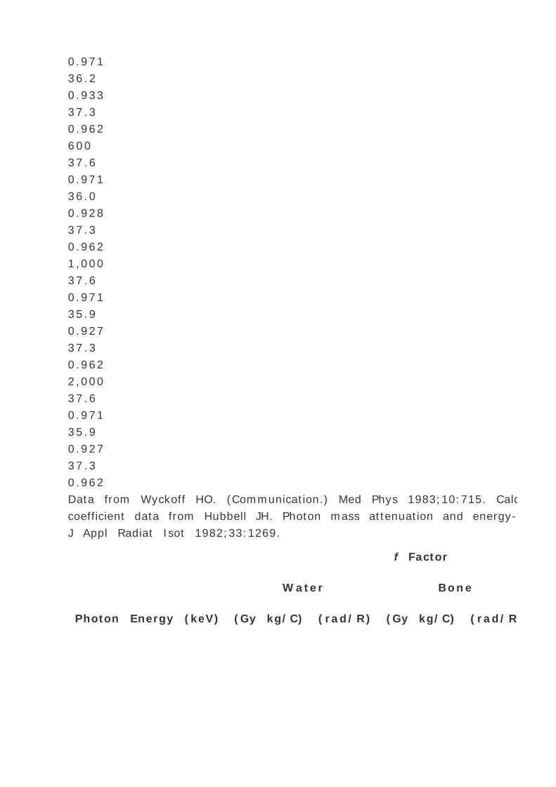
0.971

36.2

0.933

37.3

0.962

600

37.6

0.971

36.0

0.928

37.3

0.962

1,000

37.6

0.971

35.9

0.927

37.3

0.962

2,000

37.6

0.971

35.9

0.927

37.3

0.962

Data from Wyckoff HO. (Communication.) Med Phys 1983;10:715. Calculations are based on energy absorption

coefficient data from Hubbell JH. Photon mass attenuation and energy-absorption coefficients from 1 keV to 20 MeV. Int

J Appl Radiat Isot 1982;33:1269.

Photon Energy (keV)

f Factor

Water Bone Muscle

(Gy kg/C) (rad/R) (Gy kg/C) (rad/R) (Gy kg/C) (rad/R)

TABLE 8.1. f FACTORS FOR WATER, BONE, AND MUSCLE UNDER CONDITIONS OF CHARGED PARTICLE

EQUILIBRIUM

Strictly speaking, in the Compton range of energies, the f factor varies as a function of the number of electrons per

gram. Since the number of electrons per gram for bone is slightly less than for air, water, or fat, the f factor for bone is

also slightly lower than for the latter materials in the Compton region of the megavoltage energies. Of course, the f

factor is not defined beyond 3 MeV since the roentgen is not defined beyond this energy.

C. Dose Calibration with Ion Chamber in Air

As discussed in Chapter 6 , a cavity ion chamber is exposure calibrated against a free-air ion chamber or a standard

cavity chamber, under conditions of electronic equilibrium. For lower-energy radiations such as x-ray beams in the

superficial or orthovoltage range, the chamber walls are usually thick enough to provide the desired equilibrium, and

therefore, the chamber calibration is provided without a build-up cap. However, in the case of higher-energy radiations

such as from cobalt-60, a build-up cap is used over the sensitive volume of the chamber so that the combined thickness

of the chamber wall and the build-up cap is sufficient to provide the required equilibrium. This build-up cap is usually

made up of acrylic (same as Plexiglas, Lucite, or Perspex) and must be in place when measuring exposure.

Suppose the chamber is exposed to the beam (Fig. 8.2A ) and the reading M is obtained (corrected for air temperature

and pressure, stem leakage, collection efficiency, etc.). The exposure X is then given by:

where N x is the exposure calibration factor for the given chamber and the given beam quality. The exposure thus

obtained is the exposure at point P (center of the chamber sensitive volume) in free air in the absence of the chamber

(Fig. 8.2B ). In other words, the perturbing influence of the chamber is removed once the chamber calibration factor is

applied.

Consider a small amount of soft tissue at point P that is just large enough to provide electronic equilibrium at its center

(Fig. 8.2C ). The dose at the center of this equilibrium mass of tissue is referred to as the dose in free space . The term

dose in free space was introduced by Johns and Cunningham (7 ) who related this quantity to the dose in an extended

tissue medium by means of tissue air ratios (to be discussed in Chapter 9 ).

Equation 8.25 can be used to convert exposure into dose in free space, D f.s. .

P.112

where A eq is the transmission factor representing the ratio of the energy fluence at the center of the equilibrium mass

of tissue to that in free air at the same point. Thus, A eq represents the ratio of the energy fluence at point P in Fig.

8.2C to that at the same point in Fig. 8.2B . For cobalt-60 beam, A eq is close to 0.99 (7 ) and its value approaches

1.000 as the beam energy decreases to the orthovoltage range.

FIG. 8.2. A: Chamber with build-up cap is placed in a radiation beam at point P in air and reading M is obtained. B:

Exposure in free air at P is calculated using Equation 8.27 . C: Dose in free space at P is calculated using Equation 8.28

.

D. Dose Measurement from Exposure with Ion Chamber in a Medium

Equations 8.27 and 8.28 provide the basis for absorbed dose calculation in any medium from exposure measurement in

air. Similar procedure is valid when the exposure measurement is made with the chamber imbedded in a medium. Figure

8.3A shows an arrangement in which the chamber with its build-up cap is surrounded by the medium and exposed to a

photon energy fluence ¨b at the center of the chamber (point P ). If the energy of the beam incident on the chamber is

such that a state of electronic equilibrium exists within the air cavity, then the exposure at point P , with the chamber

and the build-up cap removed, is given by:

X = M ·N x

The exposure thus measured is defined in free air at point P due to energy fluence ¨c that would exist at P in the air-

filled cavity of the size equal to the external dimensions of the buildup cap (Fig. 8.3B ). To convert this exposure to

absorbed dose at P in the medium, the air in the cavity must be replaced by the medium (Fig. 8.3C ) and the following

equation is applied:

D med = X ·f med ·A m

or

where A m is the transmission factor for the photon energy fluence at point P when the cavity in Fig. 8.3B is replaced by

the medium. If ¨m is the energy fluence at P in the medium, the factor A m is given by ¨m / ¨c and has been called

a displacement factor.

The above equation is similar to Equation 8.28 except that A m is used instead of A eq . However, the difference between

A m and A eq is small for a tissue equivalent medium since

P.113

the equilibrium mass of tissue to which A eq applies is only slightly smaller than the mass of the medium displaced by a

typical small ion chamber with its build-up cap.

FIG. 8.3. A: Chamber with build-up cap with its center at point P in a medium, exposed to a photon beam whose energy

fluence is ¨b at P . Reading M is obtained. B: Exposure at P in air cavity of size equal to the external dimensions of the

build-up cap is calculated. Energy fluence at P is ¨c . C: Absorbed dose at point P in the medium is calculated by

Equation 8.29 . ¨m is the energy fluence at P .

An interesting question arises in regard to the necessity of the build-up cap being left on the chamber when making

measurements in a medium. If the chamber has been calibrated for exposure in air with its build-up cap on (to achieve

electronic equilibrium) and if a significant part of the cavity ionization is the result of electrons produced in the build-up

cap, then replacing the build-up cap with the medium could, in general, alter the chamber reading. This substitution of

a layer of medium for the build-up cap could change the electronic and photon fluence incident on the chamber wall by

virtue of differences in the composition of the medium and the material of the build-up cap. However, in practical

calibration measurements, no significant differences have been observed when exposing the chamber in water with and

without the Lucite build-up cap. Day et al. (8 ) added Perspex sheaths up to 5 mm in thickness to a Baldwin-Farmer

ionization chamber irradiated at a depth of 5 cm in a water phantom using radiations from 137 Cs to 6 MV. The readings

differed by less than 0.5%.

8.4. THE BRAGG-GRAY CAVITY THEORY

As discussed earlier, calculation of absorbed dose from exposure is subject to some major limitations. For instance, it

may not be used for photons above 3 MeV and may not be used in cases where electronic equilibrium does not exist. In

addition, the term exposure applies only to x and ³ radiations and for that reason methods of section 8.3 are not valid

for particle dosimetry. The Bragg-Gray cavity theory, on the other hand, may be used without such restrictions to

calculate dose directly from ion chamber measurements in a medium.

According to the Bragg-Gray theory (9 ,10 ), the ionization produced in a gas-filled cavity placed in a medium is related

to the energy absorbed in the surrounding medium. When the cavity is sufficiently small so that its introduction into the

medium does not alter the number or distribution of the electrons that would exist in the medium without the cavity,

then the following Bragg-Gray relationship is satisfied:

where D med is the absorbed dose in the medium (in the absence of the cavity), J g is the ionization charge of one sign

produced per unit mass of the cavity gas, and (

/ )g med is a weighted mean ratio of the mass stopping power of the medium to that of the gas for the electrons

crossing the cavity. The product of J g (

) is the energy absorbed per unit mass of the cavity gas.

The basic Bragg-Gray relationship has been carefully examined by many investigators and several modifications of the

theory have been proposed (11 ,12 ,13 ,14 ). These refinements resulted in more detailed considerations of what is

appropriate to use for the mass stopping power ratio in Equation 8.30 .

A. Stopping Power

The term stopping power refers to the energy loss by electrons per unit path length of a material (for greater details,

see section 14.1 ). An extensive set of calculated values of mass stopping powers has been published (15 ,16 ). As

mentioned earlier, to use stopping power ratios in the Bragg-Gray formula, it is necessary to determine a weighted

mean of the stopping power ratios for the electron spectrum set in motion by the photon spectrum in the materials

concerned. Methods for calculating average stopping powers (S ) for photon beams have been published (17 ).

Several authors have worked out the theory of the stopping power ratio for an air-filled cavity in a medium such as

water under electron irradiation. A good approximation

P.114

is provided by the Spencer-Attix formulation (11 ,18 ):

where ¦(E ) is the distribution of electron fluence in energy and L / is the restricted mass collision stopping power

with ” as the cutoff energy.

The â€œprimary electronsâ€ (original electrons or electrons generated by photons) give rise to ionization as well as

â€œsecondary electronsâ€ or ´ rays. The effects of the latter are accounted for in the Spencer-Attix formulation by

using an arbitrary energy limit, ”, below which energy transfers are considered dissipative, that is, the secondary

electron of energy less than ” is assumed to dissipate its energy near the site of its release. Thus, when the

integration is performed (Equation 8.31 ) to obtain the energy deposited in the cavity by the electron fluence, the lower

energy limit should be ”, greater than zero. For ion chambers it must have a value of the order of the energy of an

electron that will just cross the cavity. The value of ” for most cavity applications in ion chambers will lie between 10

and 20 keV.

The Spencer-Attix formulation of the Bragg-Gray cavity theory uses the following relationship:

where [L with bar above] / is the average restricted mass collisional stopping power of electrons. Tables A.1 to A.5 in

the Appendix give [L with bar above] / for various media and various photon and electron energies.

B. Chamber Volume

The quantity J g in Equation 8.32 can be determined for a chamber of known volume or known mass of air in the cavity

if the chamber is connected to a charge-measuring device. However, the chamber volume is usually not known to an

acceptable accuracy. An indirect method of measuring J air is to make use of the exposure calibration of the chamber for60 Co ³ ray beam. This in effect determines the chamber volume.

Consider an ion chamber that has been calibrated with a build-up cap for 60 Co exposure. Suppose the chamber with this

build-up cap is exposed in free air to a 60 Co beam and that a transient electronic equilibrium exists at the center of the

chamber. Also assume initially that the chamber wall and the build-up cap are composed of the same material (wall).

Now, if the chamber (plus the build-up cap) is replaced by a homogeneous mass of wall material with outer dimensions

equal to that of the cap, the dose D wall at the center of this mass can be calculated as follows:

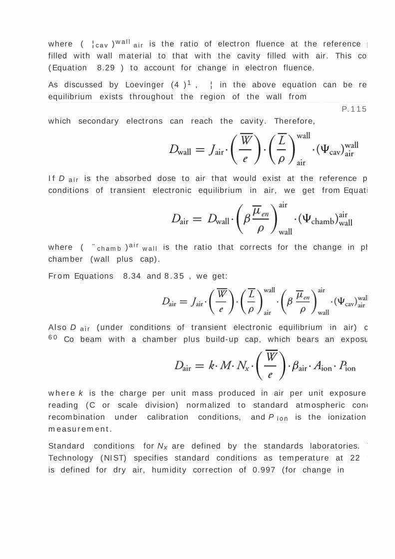
where ( ¦cav )wall air is the ratio of electron fluence at the reference point P (center of the cavity) with chamber cavity

filled with wall material to that with the cavity filled with air. This correction is applied to the Bragg-Gray relation

(Equation 8.29 ) to account for change in electron fluence.

As discussed by Loevinger (4 )1 , ¦ in the above equation can be replaced by ¨, provided a transient electron

equilibrium exists throughout the region of the wall from

P.115

which secondary electrons can reach the cavity. Therefore,

If D air is the absorbed dose to air that would exist at the reference point with the chamber removed and under

conditions of transient electronic equilibrium in air, we get from Equation 8.18 :

where ( ¨chamb )air wall is the ratio that corrects for the change in photon energy fluence when air replaces the

chamber (wall plus cap).

From Equations 8.34 and 8.35 , we get:

Also D air (under conditions of transient electronic equilibrium in air) can be calculated from exposure measurement in a60 Co beam with a chamber plus build-up cap, which bears an exposure calibration factor Nx for 60 Co ³ rays.

where k is the charge per unit mass produced in air per unit exposure (2.58 — 10-4 C kg-1 R-1 ); M is the chamber

reading (C or scale division) normalized to standard atmospheric conditions, A ion is the correction for ionization

recombination under calibration conditions, and P ion is the ionization recombination correction for the present

measurement.

Standard conditions for Nx are defined by the standards laboratories. The National Institute of Standards and

Technology (NIST) specifies standard conditions as temperature at 22 °C and pressure at 760 mm Hg. Since exposure

is defined for dry air, humidity correction of 0.997 (for change in

with humidity) is used by NIST, which can be assumed constant in the relative humidity range of 10% to 90% for the

measurement conditions with minimal error (19 ). Thus the user does not need to apply additional humidity correction

as long as

is used for dry air.


The product ( ¨cav )air wall ·( ¨chamb )wall air equals ( ¨wall )wall air which represents a correction for the change in J

air due to attenuation and scattering of photons in the chamber wall and build-up cap. This factor has been designated

as A wall in the AAPM protocol (6). Thus, Equation 8.38 becomes:

Now consider a more realistic situation in which the chamber wall and build-up cap are of different materials. According

to the two-component model of Almond and Svensson (20 ), let ± be the fraction of cavity air ionization owing to

electrons generated in the wall and the remaining (1 - ±) from the build-up cap. Equation 8.39 can now be written as:

or

J air = k ·M ·Nx ·A wall · ²wall ·A ion ·A ± ·P ion

where A ±

P.116

is the quantity in the brackets of Equation 8.40 .

FIG. 8.4. The fraction, ±, of cavity ionization due to electrons generated in the chamber wall, plotted as a function of

wall thickness. (From Lempert GD, Nath R, Schulz RJ. Fraction of ionization from electrons arising in the wall of an

ionization chamber. Med Phys 1983;10:1, with permission.)

The fraction a has been determined experimentally by dose build-up measurements for various wall thicknesses (Fig.

8.4 ). In addition, it has been shown (21 ) that ± is independent of wall composition or build-up cap, as long as it is

composed of low atomic number material.

Since J air is the charge produced per unit mass of the cavity air, we have:

where Vc is the chamber volume and air is the density of air normalized to standard conditions. Comparing Equations

8.40 and 8.41 , we have:

C. Effective Point of Measurement

C.1. Plane Parallel Chambers

Since the front plane (toward the source) of the air cavity is flat and is exposed to a uniform fluence of electrons, the

point of measurement is at the front surface of the cavity. This would be strictly true if the electrons were

monodirectional and forward directed, perpendicular to the cavity face. If a significant part of the cavity ionization is

caused by back-scattered electrons, the point of measurement will shift toward the center. If the plane-parallel chamber

has a small plate separation and the electron fluence is mostly forward

P.117

directed, it is reasonable to assume that the point of measurement is the front surface of the cavity.

C.2. Cylindrical Chambers

Electrons (from an electron beam or generated by photons) transversing a cylindrical chamber of internal radius r will

enter the sensitive volume of the chamber (air cavity) at different distances from the center of the chamber. Dutreix

and Dutreix (22 ) showed that theoretically the point of measurement for a cylindrical chamber in a unidirectional beam

is displaced by 0.85r from the center and toward the source. Derivation of this value is instructive in understanding the

concept and is, therefore, presented here.

Figure 8.5 shows a cross-section of a cylindrical chamber exposed to a parallel, uniform, and forwardly directed fluence

¦ of electrons. For an electron entering the chamber at point A , the point of measurement is at a distance X above the

center. Considering electrons entering the chamber at point A , the effective point of measurement is influenced by the

number of electrons entering through a surface area ds at A of the chamber and the track length of these electrons in

the cavity. Thus the effective point of measurement, X eff , can be determined by weighting the displacement X by the

number of electrons ( ¦ ·ds cos ¸) entering the chamber and the track length (2X ).

P.118

substituting X = r cos ¸ and ds = rd ¸,

The above theoretical result is modified under actual irradiation conditions as some of the electrons enter the chamber

at oblique angles.

FIG. 8.5. Diagram to illustrate the determination of effective point of measurement for a cylindrical chamber exposed

to a unidirectional electron beam.

The shift in the point of measurement takes place because of the cylindricality of the chamber cavity. If there is a

gradient of electron fluence across the cavity (as in the exponential falloff of the depth dose curve), a shift in the point

of measurement will result in a â€œgradient correctionâ€ to the dose measured at a point corresponding to the center

of the chamber (to be discussed).

8.5. CALIBRATION OF MEGAVOLTAGE BEAMS: TG-21 PROTOCOL

A. Cavity-Gas Calibration Factor (N gas )

The AAPM TG-21 protocol (6) for absorbed dose calibration introduced a factor (N gas ) to represent calibration of the

cavity gas in terms of absorbed dose to the gas in the chamber per unit charge or electrometer reading. For an

ionization chamber containing air in the cavity and exposed to a 60 Co ³ ray beam,2


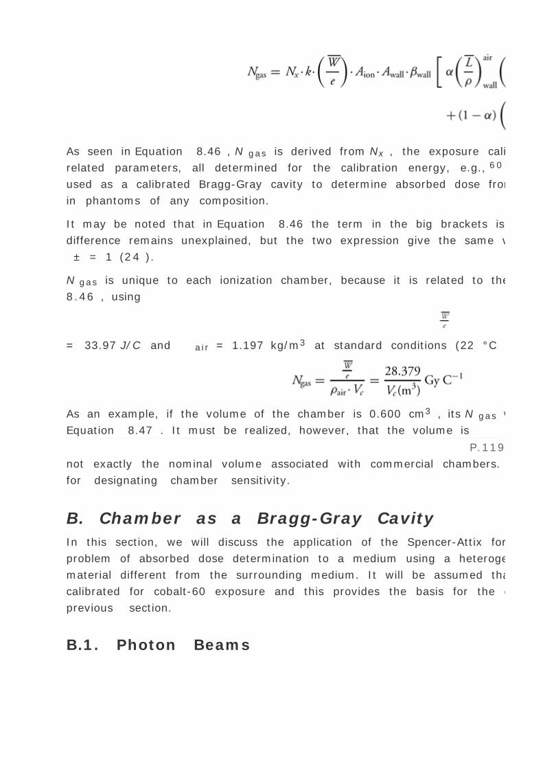
As seen in Equation 8.46 , N gas is derived from Nx , the exposure calibration for the chamber, and other chamber-

related parameters, all determined for the calibration energy, e.g., 60 Co. Once N gas is determined, the chamber can be

used as a calibrated Bragg-Gray cavity to determine absorbed dose from photon and electron beams of any energy and

in phantoms of any composition.

It may be noted that in Equation 8.46 the term in the big brackets is presented differently from the AAPM protocol. This

difference remains unexplained, but the two expression give the same value to within 0.05% in the limit of ± = 0 and

± = 1 (24 ).

N gas is unique to each ionization chamber, because it is related to the volume of the chamber. From Equations 8.42 and

8.46 , using

= 33.97 J/C and air = 1.197 kg/m3 at standard conditions (22 °C and 1 atm),

As an example, if the volume of the chamber is 0.600 cm3 , its N gas will be 4.73 — 107 Gy/C, as calculated from

Equation 8.47 . It must be realized, however, that the volume is

P.119

not exactly the nominal volume associated with commercial chambers. The latter is usually an approximate value used

for designating chamber sensitivity.

B. Chamber as a Bragg-Gray Cavity

In this section, we will discuss the application of the Spencer-Attix formulation of the Bragg-Gray cavity theory to the

problem of absorbed dose determination to a medium using a heterogeneous chamber, that is, a chamber with wall

material different from the surrounding medium. It will be assumed that the chamber with its build-up cap has been

calibrated for cobalt-60 exposure and this provides the basis for the determination of N gas , as discussed in the

previous section.

B.1. Photon Beams

Suppose the chamber, with its build-up cap removed (it is recommended not to use build-up cap for in-phantom

dosimetry), is placed in a medium and irradiated by a photon beam of given energy. If M is the charge measured, the

absorbed dose (D air ) to cavity air, at a point at the center of the cavity (P ), is given by:

where P ion is a correction factor for ion recombination losses.

Dose to medium (D med ) is given by the Bragg-Gray relationship using the Spencer-Attix formulation. Using AAPM

protocol (6) notation and substituting â€œairâ€ for â€œgasâ€ in the chamber,

where P repl is a replacement factor that corrects for perturbation in the electron and photon fluences at point P as a

result of insertion of the cavity in the medium and P wall is a factor which accounts for perturbation caused by the wall

being different from the medium.

In general, Equation 8.49 is valid for any energy and any depth in the medium (irrespective of the state of electronic

equilibrium) provided P repl and P wall are known for the measurement conditions. Although these correction factors are

quite small (usually less than 1%) for typical photon dosimetry conditions, their determination is complex, especially

under conditions of nonequilibrium. The AAPM values for P repl and P wall have been derived with the chamber irradiated

under the conditions of transient electronic equilibrium (on the descending exponential part of the depth dose curve).

The following derivation of these factors will initially assume these conditions but later will consider their applicability

to nonequilibrium situations.

Suppose the chamber is positioned at depth in the medium at which transient electronic equilibrium exists. If the

chamber wall is thick enough so that the electrons crossing the cavity arise entirely from photons interacting with the

wall material, we have:

where D wall is the dose at point P when cavity air is replaced by the wall material and ( ¨cav )wall air is the ratio that

corrects for the difference in the photon energy fluence at point P when air cavity is replaced by the wall material. The

rationale for using ( ¨cav )wall air as the perturbation correction factor in this case has been discussed by Loevinger (4

).

Dose to point P if the chamber is replaced by the medium is given by:

or

P.120

where ( ¨chamb )med wall is the ratio that corrects for the change in photon energy fluence when medium replaces the

wall material in a volume that corresponds to the entire chamber (wall plus cavity).

Now if all the electrons crossing the cavity arise from the medium, we effectively have a case of a chamber with

medium equivalent wall. Then, under conditions of transient electronic equilibrium,

For a given chamber, suppose a fraction ± of the cavity ionization is contributed by electrons from the chamber wall

and the remainder (1 - ±) by electrons from the medium, then, dose to air in the chamber is given by:

where D air (wall) and D air (med) are derived from Equations 8.52 and 8.53 . Thus,

By rearranging Equation 8.55 ,

The product term ( ¨cav )med wall ·( ¨chamb )wall med may be equated to ( ¨wall )wall med , a factor that accounts for

change in photon energy fluence when wall is replaced by medium.

Then from Equations 8.48 , 8.49 , and 8.56 ,

where

and

P.121

Since ² does not change significantly with change in material composition (4 ), the ratio ²wall med can be equated to

1. Equation 8.59 becomes:

Equation 8.60 as an expression for P wall differs from the one in the AAPM protocol, since the components ± and (1 -

±) are applied to D air before calculating D med (see Equation 8.52 ). Rogers (24 ) has pointed out that the AAPM

expression for P wall , which assigns the two components to D med directly, is not theoretically justified. However, this

does not give rise to any significant differences in the results. Also, the previous expression includes ( ¨wall )wall med ,

which appears from the theoretical considerations presented here. This factor may approximately be equated to

where x is the wall thickness.

An alternative approach to deriving P repl is to define D air = M ·N gas as the dose to air of an infinitesimally small air

cavity located in the medium at a point P â€², corresponding to the chamber's effective point of measurement (see

section 8.4C ). Because P repl for this small cavity can be assumed as 1, we have:

Dose to medium at point P corresponding to the center of the chamber will then be:

Therefore, P repl for the chamber under consideration is:

This derivation assumes that P repl arises as a result of the displacement of the effective point of measurement of the

chamber, and its value depends on the depth dose gradient. This point has been discussed by Khan (25 ). For a

cylindrical chamber, P repl can be calculated from the following equation:

where D (d ) is the dose at depth d , ·r is the displacement correction, and r is the radius of the cavity. · for photon

beams is taken to be equal to 0.6. Equation 8.64 shows that P repl depends not only on energy but also on the depth of

measurement.

The AAPM TG-21 protocol recommends P repl factors based on the semiempirical values of Cunningham and Sontag (26 ).

These values are applicable only if a measurement is made at a point on the descending exponential part of the depth

dose curve. Moreover, as pointed out by Rogers (24 ), Cunningham and Sontag's values pertain to the outer diameter of

the chamber instead of the inner diameter presented in the protocol data.

The use of chamber displacement correction to determine P repl (Equation 8.64 ) is useful not only in calibration but

also in correcting the entire depth-dose distribution. In the latter case, instead of calculating P repl at individual points,

the depth-dose (or depth ionization) curve as a whole is shifted toward the surface by a distance ·r .

B.2. Electron Beams

When a chamber, with its build-up cap removed, is placed in a medium and irradiated by an electron beam, it is usually

assumed that the chamber wall does not introduce any perturbation of the electron fluence. This assumption is

considered valid for thin-walled

P.122

(â‰¤0.5 mm) chambers composed of low atomic number materials (e.g., graphite, acrylic) (15 ,27 ). Thus the Bragg-

Gray relationship can be applied without the wall perturbation correction, i.e., P wall = 1.

For an electron beam of mean energy ’z at depth Z of measurement,

or in the notation of the AAPM protocol (6),

where P repl is a replacement correction factor to account for three effects: (a) the in-scatter effect , which increases

the fluence in the cavity since electron scattering out of the cavity is less than that expected in the intact medium; (b)

the obliquity effect , which decreases the fluence in the cavity because electrons travel relatively straight in the cavity

instead of taking oblique paths as they would owing to larger-angle scattering in the medium; and (c) displacement in

the effective point of measurement , which gives rise to a correction if the point of measurement is on the sloping part

of the depth dose curve. The first two effects may be grouped into a fluence correction while the third is called the

gradient correction .

The AAPM TG-21 protocol (6) recommends that the electron beam calibration be made at the point of depth dose

maximum. Because there is no dose gradient at that depth, the gradient correction is ignored. P repl , then, constitutes

only a fluence correction. Table 8.2 gives P repl for cylindrical chambers as a function of mean electron energy at the

depth of measurement and the inner diameter of ion chamber. These values were measured by Johansson et al. (27 ).

As discussed in an AAPM report (28 ), a depth ionization curve can be converted into a depth dose curve using Equation

8.66 . The parameters ([L with bar above] / )med air and P repl are both energy or depth dependent. The gradient

correction, however, is best handled by shifting the point of measurement toward the surface through a distance of 0.5r

(28 ,29 ). For well-designed plane-parallel chambers with adequate guard rings, both fluence and gradient corrections

are ignored, i.e., P repl = 1; the point of measurement is at the front surface of the cavity.

C. Dose Calibration Parameters

Absorbed dose calibration of a clinical radiation beam requires that a nationally or internationally approved protocol be

followed. This is important not only to ensure acceptable

P.123

dosimetric accuracy in patient treatments but also to provide consistency of dosimetric data among institutions that

provide radiotherapy. In the previous section, derivation of a dose calibration formalism recommended by the AAPM TG-

21 protocol was presented. In the process, a few discrepancies or inconsistencies in the protocol were noted. However,

their overall impact on the accuracy of the protocol is not serious enough to recommend variance from the protocol. An

AAPM task group was formed which was charged with the task of carefully reviewing the protocol and making necessary

revisions or updates. In the meantime the user was advised to follow the protocol as it stood. A new protocol, TG-51,

was introduced by the AAPM in 1999 (to be discussed later).

2

0.977

0.962

0.956

0.949

3

0.978

0.966

0.959

0.952

5

0.982

0.971

0.965

0.960

7

0.986

0.977

0.972

0.967

10

0.990

0.985

0.981

0.978

15

0.995

0.992

0.991

0.990

20

0.997

0.996

0.995

0.995

From Johansson K, Mattsson L, Lindberg L, Svensson H. Absorbed-dose determination with ionization chambers in

electron and photon beams having energies between 1 and 50 MeV. IAEA-SM-222/35. Vienna, 1977;243:270, with

permission.

Ez

(MeV)

Inner Diameter (mm)

3 5 6 7

TABLE 8.2. ELECTRON FLUENCE PERTURBATION FACTORS FOR ION CHAMBERS

As a summary to the previous section, pertinent calibration parameters of the TG-21 protocol are outlined below with a

brief description of their function and evaluation.

C.1. Chamber Calibration Factor, Nx

Ion chamber exposure calibration factor (R/C or R/scale division) for 60 Co ³ rays is provided by the NIST or an

Accredited Dosimetry Calibration Laboratory (ADCL). This factorâ€”which is characteristic of the chamber, its volume,

and its build-up capâ€”is determined by exposing it to a 60 Co beam of known exposure rate and/or comparing its

response with a chamber of known exposure calibration factor for 60 Co.

At the NIST, specially constructed spherical, graphite ionization chambers of known volume are used to calibrate the

cobalt beam in terms of exposure rate. Details of the procedure are given by Loftus and Weaver (3 ).

NX provided by the U.S. calibration laboratories is normalized to 22 °C and 760 mm Hg. Calibration of the electrometer

(device to measure ionization charge), if detached, is provided separately.

Exposure measured in a cobalt-60 beam is given by:

where X is the exposure at a point corresponding to the center of the chamber when the chamber is not there; M is the

reading corrected for temperature and pressure and N e l is the electrometer calibration factor, if separate from the

chamber. The above equation functionally defines Nx .

C.2. Cavity-Gas Calibration Factor, N gas

Cavity-gas calibration factor (Gy/C or Gy/scale division) is calculated from Nx and other parameters as discussed earlier.

It is defined as dose to the gas in the chamber per unit charge or electrometer reading. D gas is simply given by J gas

·(

) where J gas is the charge per unit mass of cavity gas and

is the average energy expended per unit charge of ionization produced in the gas. Since mass of air in the cavity or

chamber volume is not accurately known, one has to determine this volume indirectly from Nx (Equation 8.46 ).

However, it may be pointed out that N gas is independent of all properties of the chamber except its cavity volume

(Equation 8.47 ).

If N gas is not provided by the calibration laboratory, the user is required to calculate it. Table 8.3 gives ratios of N gas

/Nx for a number of commercially available chambers. It is seen that N gas /Nx does not vary greatly between commonly

used chambers. However, the user must follow the protocol to calculate N gas for the given chamber and use Table 8.3

for comparison. Normally, chambers are recalibrated every 2 years and N gas is calculated at each new calibration of the

chamber.

C.3. Symbol

For dry air,

is independent of electron energy above a few kiloelectron volts and its currently accepted value is 33.97 ± 0.06 J /C .

The TG-21 protocol (6) uses 33.7 J /C

P.124

in all its equations because at the time the protocol was written the accepted value of

for dry air was 33.85 J/C and was corrected for 50% relative humidity to give 33.7 J/C. Whereas users of the TG-21

protocol may stick to the original protocol for consistency reasons, the current understanding is that, since exposure is

defined for dry air and Nx is already corrected for humidity effect by the standards laboratory,

value in the equations discussed earlier should pertain to dry air, i.e., 33.97 J/C.

Capintec: PR-06C, PR-06G (C552â€“polystyrene)

0.991

0.46

1.000

1.032

8.51 — 10-3

Capintec: PR-05 (C552â€“polystyrene)

0.989

0.89

1.000

1.032

8.61 — 10-3

Capintec: PR-05P (C552â€“polystyrene) Exradin: A1, Spokas (C552â€“C552)

0.988

0.89

1.000

1.032

8.60 — 10-3

2-mm build-up cap

0.985

0.86

1.000

1.00

8.61 — 10-3

4-mm build-up cap

0.976

0.86

1.000

1.00

8.53 — 10-3

Exradin: T2, Spokas (A150â€“A150)

0.985

0.73

1.037

1.037

8.30 — 10-3

Exradin: T1, min Shonka (A150â€“A150)

0.992

0.74

1.037

1.037

8.36 — 10-3

Exradin: A3, Shonkaâ€“Wycoff (C552)

0.984

1.00

1.000

â€”

8.60 — 10-3

NEL Farmer: 2505, â€²54â€“â€²59 (Tufnolâ€“acrylic)

0.992

0.59

1.021

1.020

8.49 — 10-3

NEL Farmer: 2505, â€²59â€“â€²67 (Tufnolâ€“acrylic)

0.990

0.59

1.021

1.020

8.48 — 10-3

NEL Farmer: 2505/A, â€²67â€“â€²74 (nylonâ€“acrylic)

0.990

0.53

1.038

1.020

8.40 — 10-3

NEL Farmer: 2505/3,3A, â€²71â€“â€²79 (graphiteâ€“acrylic)

0.990

0.54

1.009

1.020

8.53 — 10-3

NEL Farmer: 2505/3,3B, â€²74â€“(nylonâ€“acrylic)

0.990

0.40

1.038

1.020

8.42 — 10-3

NEL Farmer: 2571, â€²79â€“(graphiteâ€“Delrin)

0.990

0.54

1.009

1.019

8.54 — 10-3

NEL Farmer: 2581, â€²80â€“(A150â€“Lucentine)

0.990

0.39

1.037

1.032

8.37 — 10-3

NEL NPL Secondary Standard: 2561 (graphiteâ€“Delrin)

0.984

0.65

1.009

1.019

8.49 — 10-3

PTW: N23333, NA 30-351 (acrylic-acrylic) 3-mm build-up cap

0.993

0.51

1.020

1.020

8.50 — 10-3

PTW: N23333, NA 30-351 NA 30-352, VIC 500-104 (acrylic-acrylic) 4.6-mm build-up cap

0.990

0.48

1.020

1.020

8.48 — 10-3

PTW: N233331, NA 30-361 (acrylicâ€“acrylic)

0.990

0.79

1.020

1.020

8.48 — 10-3

PTW: M23332-Normal, NA 30-348 (acrylicâ€“acrylic)

0.993

0.51

1.020

1.020

8.50 — 10-3

PTW: M23331-Transit, NA 30-349 (acrylicâ€“acrylic)

0.992

0.51

1.020

1.020

8.50 — 10-3

PTW: N2333641, NA 30-316 (acrylicâ€“acrylic)

0.992

0.65

1.020

1.020

8.50 — 10-3

Victoreen: 555-100HA (Derlin)

0.990

1.00

1.019

â€”

8.49 — 10-3

Victoreen: 550-6, 6A (polystyreneâ€“acrylic)

0.991

0.74

1.032

1.020

8.42 — 10-3

Far West: IC-17 (A150)

0.983

1.00

1.037

â€”

8.28 — 10-3

Far West: IC-17A (A150â€“A150)

0.984

0.79

1.037

1.037

8.29 — 10-3

Far West: IC-18 (A150â€“A150)

0.991

0.86

1.037

1.037

8.35 — 10-3

From Gastorf R, Humphries L, Rozenfeld M. Cylindrical chamber dimensions and the corresponding values of A wall and N

gas /NX A ion ). Med Phys 1986;13:751, with permission.

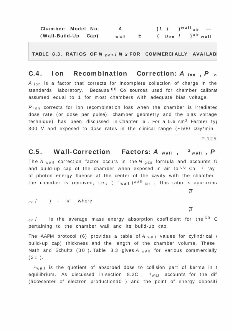
Chamber: Model No.

(Wall-Build-Up Cap)

A

wall ±

(L / )wall air —

( µen / )air wall

(L / )cap air —

( µen / )air cap

N gas /(NX A ion

) (Gy/R)

TABLE 8.3. RATIOS OF N gas /N X FOR COMMERCIALLY AVAILABLE CHAMBERS

C.4. Ion Recombination Correction: A ion , P ion

A ion is a factor that corrects for incomplete collection of charge in the chamber at the time of its calibration at the

standards laboratory. Because 60 Co sources used for chamber calibration usually have low dose rates, A ion can be

assumed equal to 1 for most chambers with adequate bias voltage.

P ion corrects for ion recombination loss when the chamber is irradiated in the user's beam. This factor depends on the

dose rate (or dose per pulse), chamber geometry and the bias voltage. A method for determining P ion (two-voltage

technique) has been discussed in Chapter 6 . For a 0.6 cm3 Farmer type chamber operating at a bias voltage of about

300 V and exposed to dose rates in the clinical range (~500 cGy/min or less), P ion is usually less than 1.005.

P.125

C.5. Wall-Correction Factors: A wall , ²wall , P wall

The A wall correction factor occurs in the N gas formula and accounts for attenuation and scatter of photons in the wall

and build-up cap of the chamber when exposed in air to 60 Co ³ ray beam. In Equation 8.36 , A wall appears as a ratio

of photon energy fluence at the center of the cavity with the chamber and its build-up cap in place in air to that when

the chamber is removed, i.e., ( ¨wall )wall air . This ratio is approximately given by e - (

en / ) · x , where

en / is the average mass energy absorption coefficient for the 60 Co beam and x is the density thickness, both

pertaining to the chamber wall and its build-up cap.

The AAPM protocol (6) provides a table of A wall values for cylindrical chambers as a function of chamber wall (plus

build-up cap) thickness and the length of the chamber volume. These values are based on Monte-Carlo calculation by

Nath and Schultz (30 ). Table 8.3 gives A wall for various commercially available chambers, derived from the same data

(31 ).

²wall is the quotient of absorbed dose to collision part of kerma in the wall under the conditions of transient electronic

equilibrium. As discussed in section 8.2C , ²wall accounts for the difference between the point of interaction

(â€œcenter of electron productionâ€ ) and the point of energy deposition. Its value is taken to be 1.005 for 60 Co.

Although the TG-21 protocol uses ²wall in addition to the A wall , it is now understood (23 ,24 ,32 ) that the Monte-

Carlo calculated values of A wall include ²wall . Thus the use of ²wall in the AAPM protocol is an error. However, as

pointed out earlier, some of the errors in the TG-21 protocol cancel each other and, therefore, no change was

recommended in the protocol until a revised protocol was introduced.

P wall is a correction factor that accounts for the difference between the composition of the chamber wall and the

phantom as it pertains to photon beam interactions in the user's beam. This factor depends on beam energy, wall

thickness, wall composition, and the fraction ± of the cavity ionization contributed by electrons originating in the

chamber wall. Calculations indicate that P wall [asymptotically equal to] 1 when ± <0.25. As can be deduced from

Table 8.3 , P wall is close to unity for Farmer type chambers (wall thickness <0.1 g/cm2 ) and photon energies â‰¥6

MV.

The expression for the calculation of P wall , given by Equation 8.60 , is different from the one in the TG-21 protocol.

The reasons for the discrepancy have been discussed earlier. Again, because the differences are quite small, no variance

is recommended if TG-21 protocol is followed.

C.6. Replacement Correction Factor, P repl

From the previous discussion of this factor, it is evident that P repl corrects for change in J air (ionization charge per unit

mass of cavity air) caused by the finite size of the cavity. According to Equation 8.58 , if the measurement is made

under the conditions of transient electronic equilibrium, P repl is the ratio of photon energy fluence at the center of the

cavity when the cavity is filled with medium to that when the cavity is filled with air.

This ratio is also the ratio of electron fluences with and without the cavity. One may call this a fluence correction factor

or Pf l . However, when the electron fluence is measured with a cylindrical ion chamber, there is a shift in the point of

measurement depending on the radius of the cavity (see section 8.4 , C.2 ). Because of this shift upstream, the

ionization measured is greater than if there was no shift or cavity radius was zero. The component of P repl caused by

the shift in the point of measurement is called the gradient correction or P gr . The magnitude of P gr is dependent on

the gradient of the dose and the inner diameter of the ion chamber. Thus P repl may be the thought of having two

components, the gradient and fluence correction factor or P repl = Pf l Pgr .

In the case of photon beams, fluence corrections are not needed if the measurements are made at d max or beyond in a

broad beam because transient electronic equilibrium exists there (33 ). Under these conditions, P f l = 1 because electron

spectrum is not changed by

P.126

the presence of air cavity. P repl for photon beams can therefore be equated to P gr only if the chamber is positioned on

the descending portion of the depth dose curve.

Replacement correction for electron beam calibration is more complex. Presence of the cavity alters the primary electron

fluence because air scatters electrons less than the medium. Generally, the fluence correction factor is less 1 and its

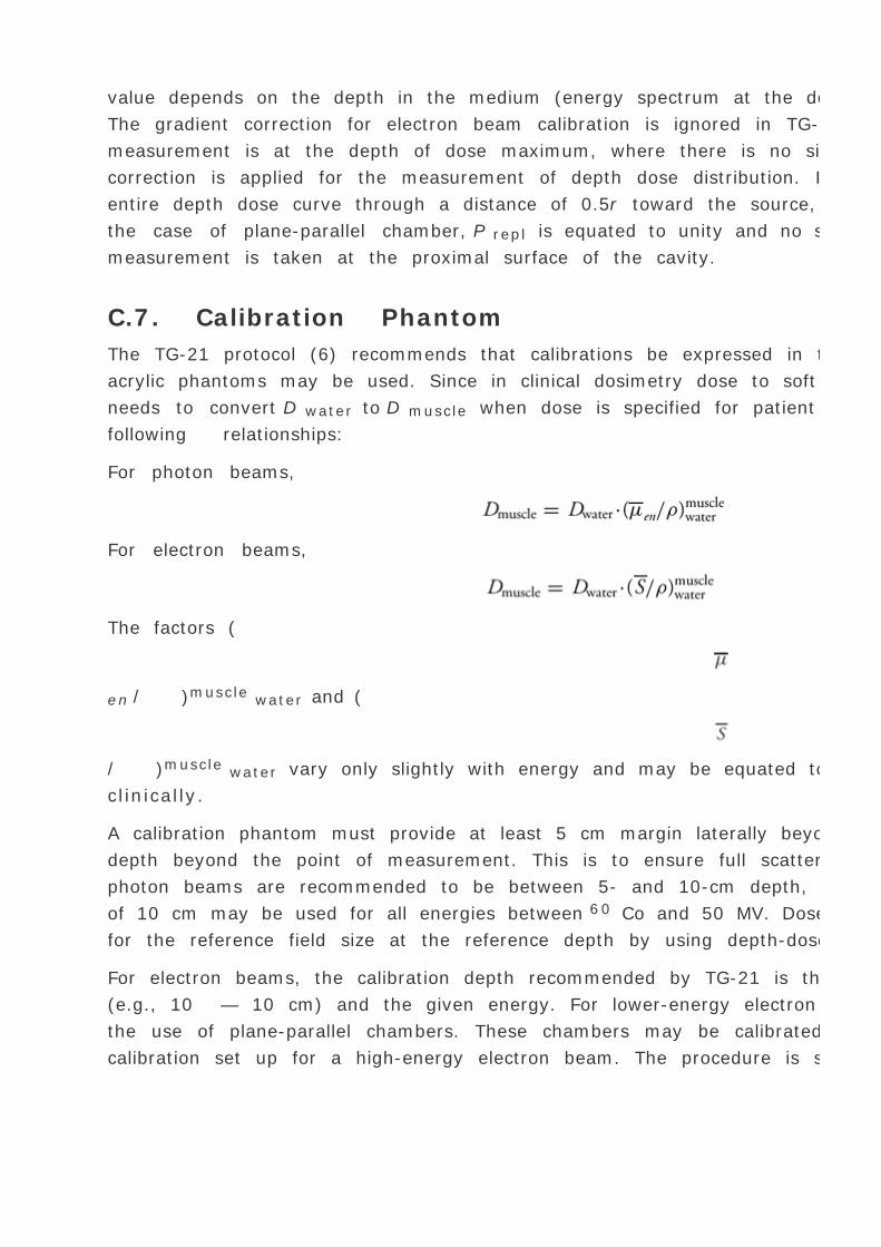
value depends on the depth in the medium (energy spectrum at the depth of measurement) and the size of the cavity.

The gradient correction for electron beam calibration is ignored in TG-21 because the recommended point of

measurement is at the depth of dose maximum, where there is no significant dose gradient. However, gradient

correction is applied for the measurement of depth dose distribution. In practice, this is accomplished by shifting the

entire depth dose curve through a distance of 0.5r toward the source, where r is the radius of the cylindrical cavity. In

the case of plane-parallel chamber, P repl is equated to unity and no shift correction is used as long as the point of

measurement is taken at the proximal surface of the cavity.

C.7. Calibration Phantom

The TG-21 protocol (6) recommends that calibrations be expressed in terms of dose to water. Water, polystyrene, or

acrylic phantoms may be used. Since in clinical dosimetry dose to soft tissue or muscle is the quantity of interest, one

needs to convert D water to D muscle when dose is specified for patient treatments. This conversion is done by the

following relationships:

For photon beams,

For electron beams,

The factors (

en / )muscle water and (

/ )muscle water vary only slightly with energy and may be equated to 0.99 for all photon and electron beams used

clinically.

A calibration phantom must provide at least 5 cm margin laterally beyond field borders and at least 10 cm margin in

depth beyond the point of measurement. This is to ensure full scatter conditions. Calibration depths for a megavoltage

photon beams are recommended to be between 5- and 10-cm depth, depending on energy. Alternatively, a single depth

of 10 cm may be used for all energies between 60 Co and 50 MV. Dose rate or dose per monitor unit is then calculated

for the reference field size at the reference depth by using depth-dose distribution data.

For electron beams, the calibration depth recommended by TG-21 is the depth of dose maximum for the reference cone

(e.g., 10 — 10 cm) and the given energy. For lower-energy electron beams (<10 MeV), the AAPM protocol recommends

the use of plane-parallel chambers. These chambers may be calibrated in comparison with cylindrical chambers, using a

calibration set up for a high-energy electron beam. The procedure is somewhat complicated by the fact that plane-

parallel chambers are used in plastic phantoms, thereby creating additional uncertainties in the interconversion of dose

to water and plastic media.

C.8. Simplified Equations

The TG-21 protocol (6) has worksheets for calculating N gas and dose to water for photon and electron beam calibration.

It is important that the user of this protocol complete these worksheets for any new chamber and a new beam to be

calibrated. Once all the relevant calibration parameters have been established for the given chamber and the given

beam, routine calibration checks can be performed using simplified equations and precalculated tables.

60 Co

5

80.4

1.134

0.992

1.114

6

5

87.0

1.127

0.993

1.108

10

5

91.1

1.117

0.994

1.099

18

10

79.9

1.100

0.994

1.082

24

10

84.5

1.094

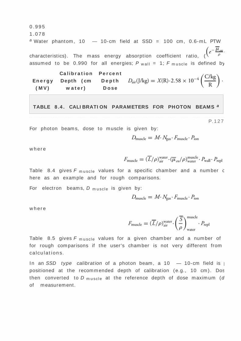
0.995

1.078a Water phantom, 10 — 10-cm field at SSD = 100 cm, 0.6-mL PTW Farmer chamber N23333 (see Table 8.3 for

characteristics). The mass energy absorption coefficient ratio, ( en / )muscle water , is

assumed to be 0.990 for all energies; P wall = 1; F muscle is defined by Eq. 8.71 .

Energy

(MV)

Calibration

Depth (cm

water)

Percent

Depth

Dose

P

repl

F

muscle

TABLE 8.4. CALIBRATION PARAMETERS FOR PHOTON BEAMS a

P.127

For photon beams, dose to muscle is given by:

where

Table 8.4 gives F muscle values for a specific chamber and a number of photon beam energies. This table is reproduced

here as an example and for rough comparisons.

For electron beams, D muscle is given by:

where

Table 8.5 gives F muscle values for a given chamber and a number of electron energies. Again these data may be used

for rough comparisons if the user's chamber is not very different from Farmer type ion chamber used in these

calculations.

In an SSD type calibration of a photon beam, a 10 — 10-cm field is placed at an SSD of 100 cm and the chamber is

positioned at the recommended depth of calibration (e.g., 10 cm). Dose to muscle3 per monitor unit is calculated and

then converted to D muscle at the reference depth of dose maximum (dm ) by using percent depth dose (P ) at the depth

of measurement.

An isocentric calibration involves setting up of a 10 — 10-cm field at the recommended depth of calibration (e.g., 10

cm) and a source-to-chamber distance (SCD) of 100 cm. If TMR is the tissue-maximum ratio (discussed in Chapter 10 )

at the depth of measurement,

8.6. AAPM TG-51 PROTOCOL

The TG-51 protocol (34 ) represents a major upgrade of the TG-21 protocol in several respects: (a) it is based on

absorbed-dose-to-water calibration factor, N 60C o D, W , instead of exposure or air kerma calibration of the ion chamber;

(b) the user does not need to

P.128

calculate any theoretical dosimetry factors; and (c) large tables of stopping-power ratios and mass-energy absorption

coefficients are not needed. Although the adoption of TG-51 results in only modest improvement in dosimetric accuracy

over the TG-21 protocol (1%â€“2%), the gain in simplicity is a significant factor from the user's point of view.

Energy (MeV)

6

5.66

1.3

3.2

1.077

0.960

1.020

9

8.62

1.9

5.0

1.052

0.965

1.005

12

11.53

2.1

7.5

1.025

0.974

0.985

15

14.63

2.1

10.5

1.002

0.982

0.971

18

17.59

1.5

14.7

0.979

0.991

0.958

22

20.85

1.5

18.0

0.967

0.993

0.948a Water phantom, field size, 10 — 10 cm cone, SSD = 100 cm, energy derived from broad-beam depth dose

distribution (25 — 25 cm field), 0.6-ml PTW Farmer chamber N23333 (see Table 8.3 for characteristics). ([s with bar

above]/ )muscle water is assumed to be 0.987 for all energies, F muscle is defined by Eq. 8.73 , E 0 is the mean

electron energy at the surface.

Depth

dm

(cm

water)

Mean

Energy

(MeV)

at dm

P

repl

F

muscle Nominal

E

0

TABLE 8.5. CALIBRATION PARAMETERS FOR ELECTRON BEAMS a

The theoretical aspects of TG-51 go back to the TG-21 formalism, especially in the calculation of correction factors such

as [L with bar above]/ ratios, P wall , P repl , P ion , P polarity , P gradient , P fluence , etc. If these factors are

normalized to reference conditions of absorbed-dose-to-water in a 60 Co beam, the formalism simplifies to the

application of a quality conversion factor, which converts the calibration factor for a 60 Co beam to that for the user's

beam.

The basic TG-51 equation for absorbed calibration is as follows:

where DQ w is the absorbed dose to water at the reference point of measurement in a beam of quality Q ; M is the

electrometer reading that has been fully corrected for ion recombination, environmental temperature and pressure,

electrometer calibration and chamber polarity effects; kQ is the quality conversion factor that converts the absorbed-

dose-to-water calibration factor for a 60 Co beam into the calibration factor for an arbitrary beam of quality Q ; and

N60C o D, w is the absorbed-dose-to-water calibration factor for the chamber in a 60 Co beam under reference conditions.

The reference point of measurement in Equation (8.76) is specified at the reference depth corresponding to the center of

cavity for a cylindrical chamber and the front surface of the cavity for a plane parallel chamber. Although the effective

point of measurement occurs upstream for a cylindrical chamber, the resulting gradient correction has already been

taken into account in the kQ factor.

A. Beam Quality, Q

1. Photon Beams

The TG-21 protocol specifies photon beam energy in terms of nominal accelerating potential which is shown to be

related to â€œionization ratioâ€ (6 ). The ionization ratio is defined as the ratio of ionization charge or dose measured

at 20-cm depth to that measured at 10-cm depth for a constant source to detector distance and a 10 — 10 cm2 field at

the plane of the chamber (isocentric geometry). This ionization ratio is the same as what is also known as TPR20 10 or

TPR20,10 used by Andreo and Brahme (35 ) and the International Atomic Energy Agency (IAEA) protocol (36 ). The AAPM

TG-51 (34 ) protocol has instead recommended %dd(10)x as the beam quality-specifier. The quantity %dd(10)x is the

photon component of the photon beam percentage depth dose at 10-cm depth in a 10 — 10 cm2 field on the surface of

a water phantom at an SSD of 100 cm. The pros and cons of using TPR20 10 versus %dd(10)x have been discussed in the

literature (37 ,38 ).

FIG. 8.6. A plot of water to air stopping power ratios as a function of %dd(10)x . (From Kosunen A, Rogers DWO. Beam

quality specification for photon beam dosimetry. Med Phys 1993;20:1013â€“1018, with permission.)

P.129

The rationale for %dd(10)x as a photon beam quality specifier is provided by Kosunen and Rogers (39 ) who showed that

for any x-ray beam above 4 MV, there is a linear relationship between stopping powers ratios and %dd(10)x for the

photon component of the beam (Fig. 8.6 ). Mathematically,

Determination of %dd(10)x requires that the photon beam be free of electron contamination. Because it is impossible to

remove electron contamination completely from clinical photon beams, the TG-51 protocol recommends that %dd(10)x

be measured by interposing a 1-mm-thick lead (Pb) foil in the beam at a distance of about 50 cm from the phantom

surface. This arrangement minimizes the electron contamination incident at the phantom surface as the lead foil acts as

an electron filter (40 ).

For photon beams of energy less than 10 MV, the contribution of dose at d max from incident electron contamination is

minimal for a 10 — 10 cm2 . So the %dd(10) measured in an open beam without lead may be equated to the

%dd(10)x . The use of lead foil, however, is recommended for %dd(10)x measurement for energies of 10 MV or higher.

Calculation of %dd(10)x for various beam energies involves the following equations, as recommended by TG -51:

It should be noted that the Pb foil is used only when determining the beam quality specifier, %dd(10)x , and must be

removed at the conclusion of that determination. In addition, if the measurement of depth doses involves a cylindrical

chamber, the depth dose curve must be corrected for gradient effects, that is, shift of the curve upstream by 0.6rcav ,

where rcav is the radius of the chamber cavity.

In case the lead foil is not available, an approximate relationship for the determination of %dd(10)x on an interim basis

is recommended by TG-51:

The previous equation is based on a global fit to data (33 ) and in extreme cases may lead to an error in kQ or absorbed

dose of 0.4%.

FIG. 8.7. A typical electron beam depth dose curve showing depth of maximum dose (d max ), depth of 50% dose (R 50

) and depth for clinic reference dosimetry (d ref ). (From AAPM. AAPM's TG-51 protocol for clinical reference dosimetry of

high-energy photon and electron beams. Med Phys 1999;26:1847â€“1870, with permission.)

P.130

2. Electron Beams

The beam quality for electron beam dosimetry is specified by R50 , the depth in water (in centimeters) at which the

percent depth dose is 50% for a â€œbroad beamâ€ (field size at the phantom surface â‰¥ 10 — 10 cm2 for

energies up to 20 MeV or 20 — 20 cm2 for all energies in the clinical range) at an SSD of 100 cm. Figure 8.7 shows a

typical electron beam depth dose curve with d max , d ref (reference depth of calibration) and R 50 indicated.

R 50 for a broad beam (e.g., 20 — 20 cm2 field size) may be determined by measurement of dose at two points on

central axis: one at d max and the other at depth where the dose falls to 50% of the maximum dose. If a cylindrical ion

chamber is used for this measurement, the point of d max should correspond to where the chamber reads maximum

ionization on central axis. A point is then located downstream on central axis where the ionization measured is 50% of

the maximum value. The depth of 50% ionization (I 50 ) is determined by subtracting 0.5rcav from the depth indicated

by the center of chamber cavity. The beam quality specifier, R 50 , is then calculated from I 50 (41 ):

or

Alternatively, R 50 may be determined from the depth ionization curve (measured with a cylindrical chamber), which has

been corrected for gradient effects by shifting the entire curve upstream by 0.5rcav (Fig. 8.8 ) and converting I 50 to R

50 by using the above Equations. If a water phantom scanner with ion chamber is used, most systems are equipped with

software to convert depth ionization curves into depth-dose curves using appropriate factors (e.g., ([L with bar

above]/ )w a ir and P repl or P f l ·Pgr , as a function of depth). This allows a quick determination of important

dosimetry parameters such as d max , d ref , R 50 , and Rp .

FIG. 8.8. Shifting of depth ionization curves upstream by 0.6rcav for photons and 0.5rcav for electrons in order to

correct for shift in the point of measurement when using a cylindrical ion chamber of cavity radius, rcav . (From AAPM.

AAPM's TG-51 protocol for clinical reference dosimetry of high-energy photon and electron beams. Med Phys 1999;

26:1847â€“1870, with permission.)

If a diode or film is used to determine depth-dose distribution in a water or water equivalent phantom, the detector

response as a function of depth gives depth dose curve directly without further corrections (section 14.3B ). However, it

is important to establish

P.131

first by suitable benchmark tests, that these dosimetry systems agree with corrected ion chamber dosimetry.

B. Quality Conversion Factor, kQ

By definition, kQ is given by:

From TG-21 Equation [8.57] :

As discussed earlier (section 8.5 , C.6 ), P repl has two components, the gradient and fluence correction factors:

Equation 8.84 may be further revised by multiplying the right hand side of the equation by the central electrode

correction factor, P cel . This factor was ignored by the TG-21 protocol but it is included in the kQ values of the TG-51

protocol. The central electrode effect is quite small for electron beams (<0.2%), but for photon beams it has been

shown to be significant. For example, P cel for Farmer-like chambers with an aluminum electrode of 1 mm diameter

varies between 0.993 for 60 Co to 0.996 for 24 MV x-rays (42 ).

From Equations 8.83 , 8.84 , and 8.85 along with the use of P cel we get the expression for kQ :

1. kQ for Photon Beams

Using the above relationship, Rogers (33 ) calculated kQ values for a variety of commercially available cylindrical ion

chambers as a function of photon beam energy from 60 Co to 24 MV. These data comprise Table I of the TG-51 protocol

and are reproduced here in Table 8.6 . Data for plane-parallel chambers are not included because of insufficient

information about P wall in photon beams, other than 60 Co for which kQ = 1 by definition for all chambers.

2. kQ for Electron Beams

Although Equation 8.76 is general and can be applied for both photon and electron beams (see IAEA Protocol , section

8.7 ), authors of the TG-51 Protocol felt that for electron beams

P.132

the PQ gr factor in Equation (8.86) at the reference point of measurement may vary from one accelerator to another and

therefore must be measured in the user's beam. Thus kQ has been redefined for electron beams by the following

equations (43 ):

where

and PQ gr is the gradient correction at the reference depth of measurement. The reference depth, called d ref , for

electron beams is based on recommendation by Burns et al. (44 ) and is given by:

The gradient correction at the reference depth is given by:

where I (d) is the ionization reading of the cylindrical chamber with the cylindrical axis at depth d .

Capintec PR-05/PR-05P

0.999

0.997

0.995

0.990

0.972

0.948

Capintec PR-06C/G 0.6cc Farmer

1.000

0.998

0.994

0.987

0.968

0.944

Exradin A1 Shonkaa

0.999

0.998

0.996

0.990

0.972

0.948

Exradin A12 Farmer

1.000

0.999

0.996

0.990

0.972

0.948

NE2505/3,3A 0.6cc Farmer

1.000

0.998

0.995

0.988

0.972

0.951

NE2561 0.3cc NPL Sec. Stdb

1.000

0.998

0.995

0.989

0.974

0.953

NE2571 0.6cc Farmer

1.000

0.998

0.995

0.988

0.972

0.951

NE2577 0.2cc

1.000

0.998

0.995

0.988

0.972

0.951

NE2581 0.6cc robust Farmer

1.000

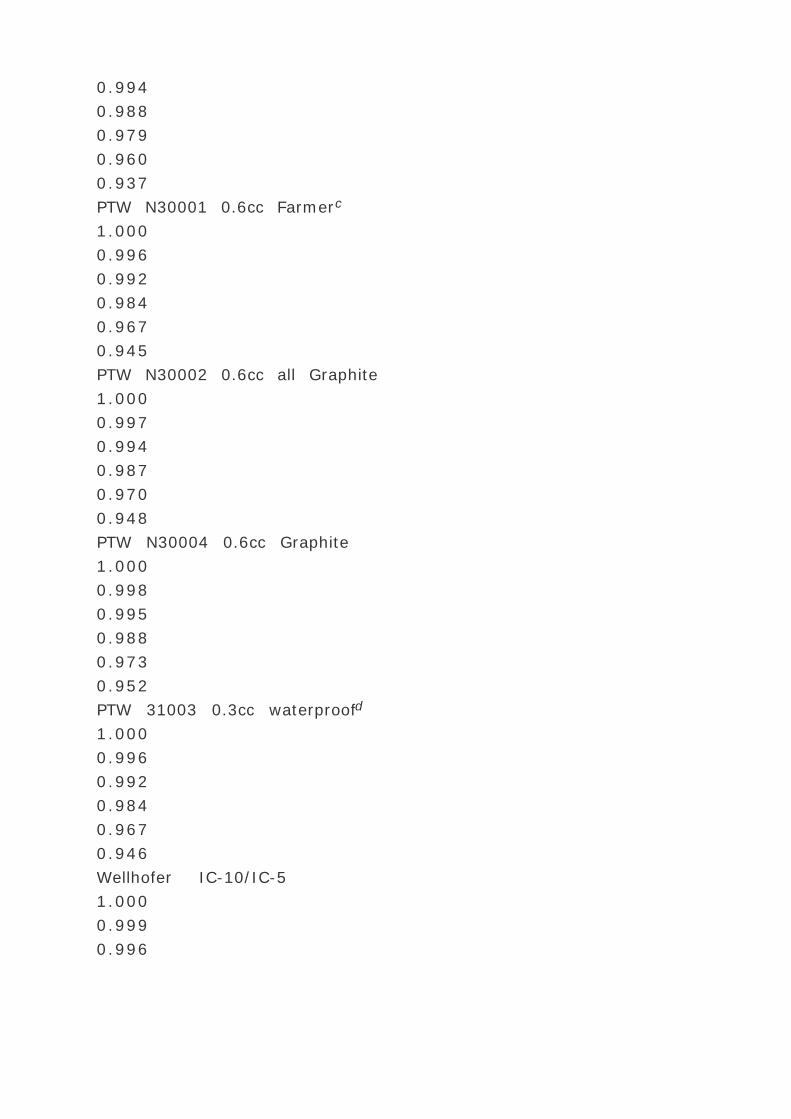
0.994

0.988

0.979

0.960

0.937

PTW N30001 0.6cc Farmerc

1.000

0.996

0.992

0.984

0.967

0.945

PTW N30002 0.6cc all Graphite

1.000

0.997

0.994

0.987

0.970

0.948

PTW N30004 0.6cc Graphite

1.000

0.998

0.995

0.988

0.973

0.952

PTW 31003 0.3cc waterproofd

1.000

0.996

0.992

0.984

0.967

0.946

Wellhofer IC-10/IC-5

1.000

0.999

0.996

0.989

0.971

0.946

For 60 Co beams, kQ = 1.000 by definition.a The cavity radius of the A1 here is 2 mm although in the past Exradin has designated chambers with another radius as

A1.b The NE2611 has replaced the equivalent NE2561.c PTW N30001 is equivalent to the PTW N23333 it replaced.d PTW N31003 is equivalent to the PTW N233641 it replaced.

From AAPM. AAPM's TG-51 protocol for clinical reference dosimetry of high-energy photon and electron beams. Med Phys

1999; 26:1847â€“1870, with permission.

Ion Chamber

kq

%dd(10)x

58.0 63.0 66.0 71.0 81.0 93.0

TABLE 8.6. kQ VALUES FOR ACCELERATOR PHOTON-BEAMS AS A FUNCTION OF %DD(10)x FOR CYLINDRICAL

ION CHAMBERS

Further, the authors of TG-51 thought that the values of k R 5 0 for different ion chambers vary considerably (43 ) and

that there was no provision in this formalism for a future possibility of having chamber calibration factors measured

directly for electron beams. These drawbacks could be avoided by arriving at k R 5 0 in two steps instead of the one

derived directly by quality comparison with 60 Co. Thus, k R 5 0 is redefined as:

P.133

where k ecal is the quality conversion factor for a reference electron beam of high energy with an arbitrary beam quality

Qe of R 50 = 7.5cm, relative to 60 Co.

or, from Equation 8.88 :

and k â€²R 5 0 is the quality conversion factor for the given electron beam of quality Q relative to the reference electron

beam of quality Qe , that is,

Values of k ecal for the plane-parallel and cylindrical ion chambers have been calculated using Equation 8.94 (43 ) and

are presented in Tables II and III of the TG-51 protocol (34 ). These are reproduced in Tables 8.7 and 8.8 of this

chapter. The values of k â€²R 5 0 for Farmer-like cylindrical chambers and plane-parallel chambers are calculated by

Rogers (43 ) using the following equations respectively:

and

C. Calibration Phantom

TG-51 requires that the calibration of photon and electron beams be performed in a water phantom. The recommended

dimensions of the phantom are at least 30 — 30 — 30 cm3 . If the beam enters the phantom from the side through a

plastic wall, all depths must be scaled to water equivalent depths using a scaling factor of 1 cm acrylic = 1.12 cm H2 O.

D. Chamber Waterproofing

A cylindrical ion chamber may be waterproofed using a thin (â‰¤ 1-mm thick) acrylic sleeve. The chamber should slip

into the sleeve with little resistance and with minimal air gaps

P.134

around the thimble (â‰¤ 0.2 mm). Another option is to use a latex condom but without any talcum powder because the

talcum powder could leak into the chamber cavity. Waterproof chambers or chambers with waterproofing kits are also

commercially available.

Attix

0.883

Capintec

0.921

PTB/Roos

0.901

Extradin

0.888

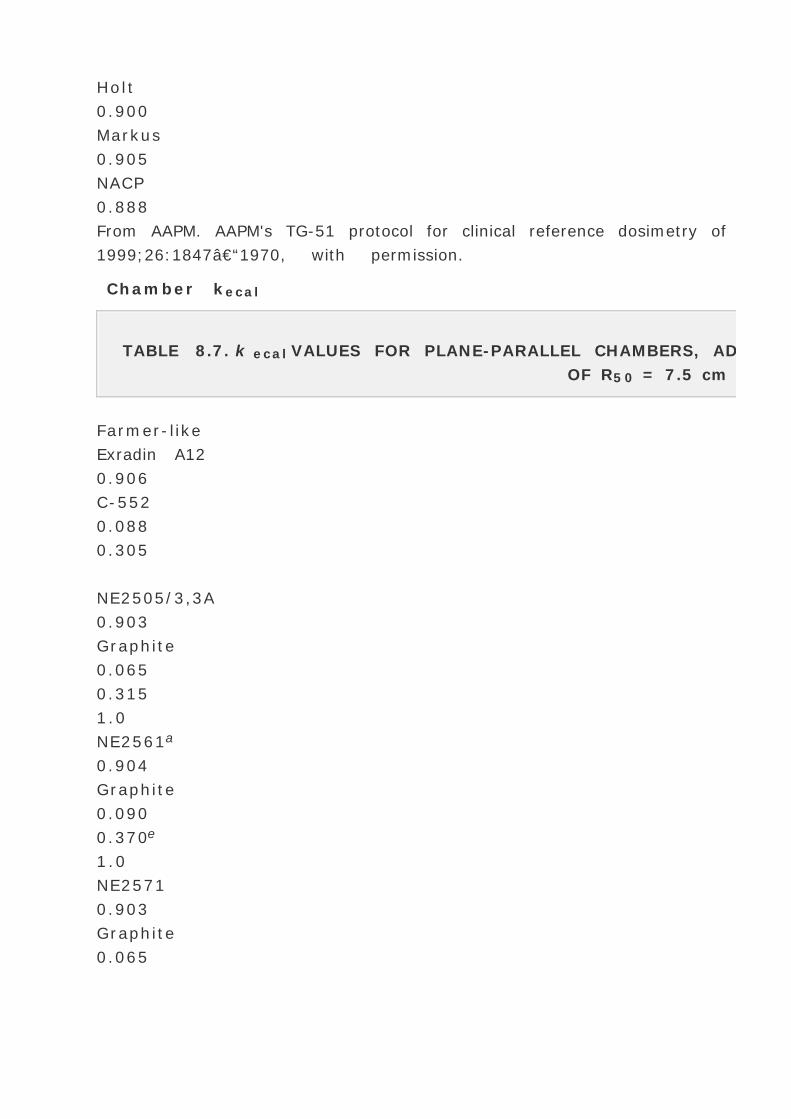
Holt

0.900

Markus

0.905

NACP

0.888


1999;26:1847â€“1970, with permission.

Chamber kecal

TABLE 8.7. k ecal VALUES FOR PLANE-PARALLEL CHAMBERS, ADOPTING A REFERENCE BEAM QUALITY Qecal

OF R50 = 7.5 cm

Farmer-like

Exradin A12

0.906

C-552

0.088

0.305

NE2505/3,3A

0.903

Graphite

0.065

0.315

1.0

NE2561a

0.904

Graphite

0.090

0.370e

1.0

NE2571

0.903

Graphite

0.065

0.315

1.0

NE2577

0.903

Graphite

0.065

0.315

1.0

NE2581

0.885

A-150

0.041

0.315

Capintec PR-06C/G

0.900

C-552

0.050

0.320

PTW N23331

0.896

Graphite

0.012

0.395e

1.0

PMMA

0.048

PTW N30001b

0.897

Graphite

0.012

0.305

1.0

PMMA

0.033

PTW N30002

0.900

Graphite

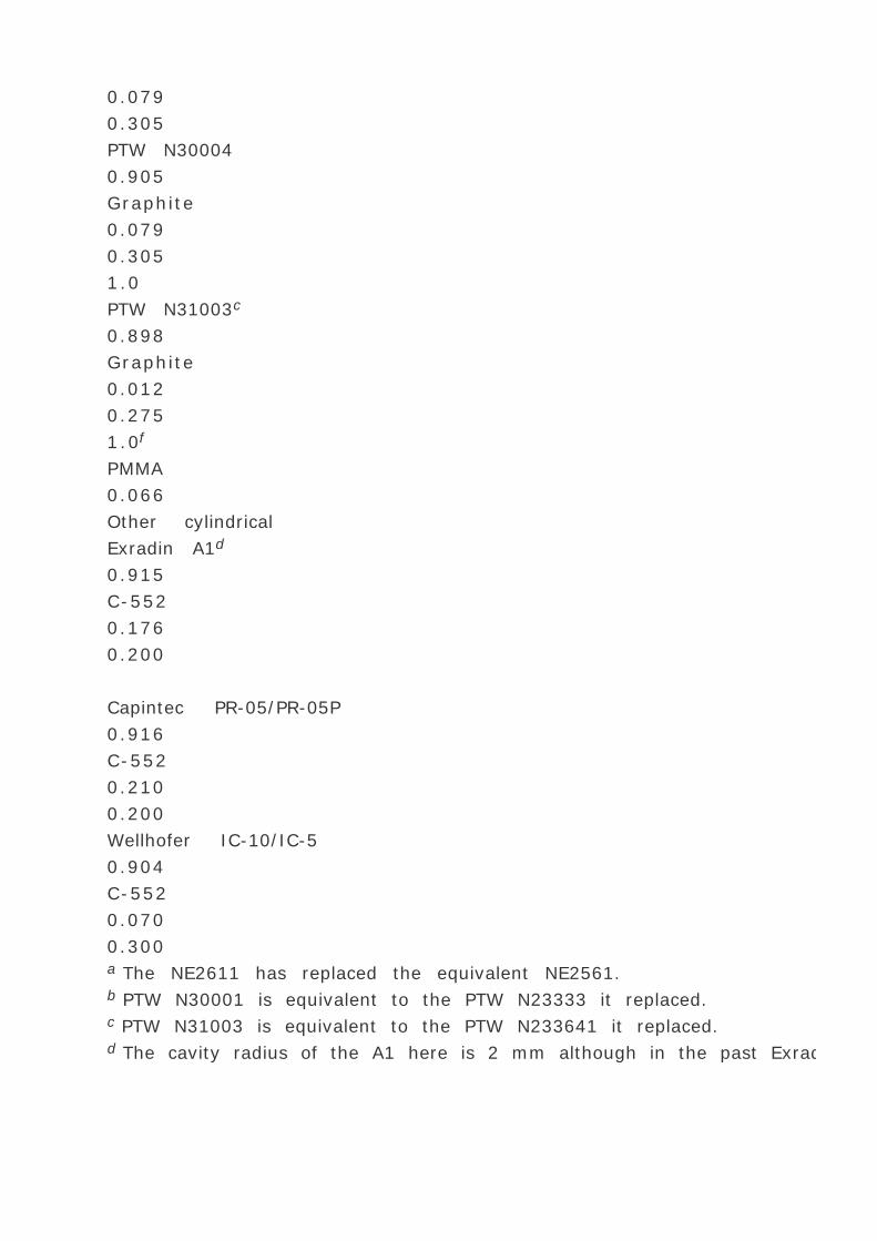
0.079

0.305

PTW N30004

0.905

Graphite

0.079

0.305

1.0

PTW N31003c

0.898

Graphite

0.012

0.275

1.0f

PMMA

0.066

Other cylindrical

Exradin A1d

0.915

C-552

0.176

0.200

Capintec PR-05/PR-05P

0.916

C-552

0.210

0.200

Wellhofer IC-10/IC-5

0.904

C-552

0.070

0.300a The NE2611 has replaced the equivalent NE2561.b PTW N30001 is equivalent to the PTW N23333 it replaced.c PTW N31003 is equivalent to the PTW N233641 it replaced.d The cavity radius of the A1 here is 2 mm although in the past Exradin has designated chambers with another radius as

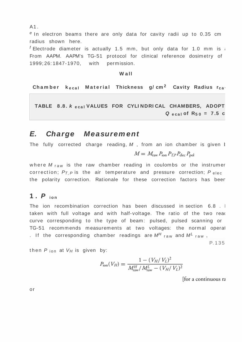
A1.e In electron beams there are only data for cavity radii up to 0.35 cm and so 0.35 cm is used rather than the real cavity

radius shown here.f Electrode diameter is actually 1.5 mm, but only data for 1.0 mm is available


1999;26:1847-1970, with permission.

Chamber kecal

Wall

Cavity Radius rcav (cm) Al Electrode Diameter (mm)Material Thickness g/cm2

TABLE 8.8. k ecal VALUES FOR CYLINDRICAL CHAMBERS, ADOPTING A REFERENCE ELECTRON BEAM QUALITY

Q ecal of R50 = 7.5 cm

E. Charge Measurement

The fully corrected charge reading, M , from an ion chamber is given by:

where M raw is the raw chamber reading in coulombs or the instrument's reading; P ion is the ion recombination

correction; PT,P is the air temperature and pressure correction; P elec is the electrometer calibration factor; and P pol is

the polarity correction. Rationale for these correction factors has been discussed.

1. P ion

The ion recombination correction has been discussed in section 6.8 . In one of the methods, the chamber readings are

taken with full voltage and with half-voltage. The ratio of the two readings is related to P ion which is read off from a

curve corresponding to the type of beam: pulsed, pulsed scanning or continuous radiation (Fig. 6.17 ). Alternatively,

TG-51 recommends measurements at two voltages: the normal operating voltage, VH and approximately half-voltage VL

. If the corresponding chamber readings are MH raw and ML raw ,

P.135

then P ion at VH is given by:

or

2. P T,P

In the United States, the calibration laboratories [National Institute of Standards and Technology (NIST) and Accredited

Dose Calibration Laboratories (ADCLs)] provide chamber calibration factors for standard environmental conditions of

temperature T o = 22 °C and pressure P o = 760 mm Hg or 101.33 kPa (1 atmosphere). The temperature and pressure

correction, PT,P , is given by:

or

The rationale for the use of temperature and pressure correction for ion chamber readings has been discussed in section

6.10 .

3. P elec

The electrometer correction factor, P elec , depends on whether the electrometer is detached or forms an integral unit

with the ion chamber. If separate, the electrometer must bear a calibration factor for charge measurement. P elec

corrects the electrometer reading to true coulombs. Its unit of measurement is C/C or C/rdg. If the electrometer and ion

chamber form a single unit, P elec = 1.00.

4. P pol

Chamber polarity effects depend on the chamber design, cable position, and beam quality (see section 6.9 ). P pol is the

polarity correction factor, which corrects chamber's response for possible polarity effects.

Measurement of P pol involves taking chamber readings with both polarities and determining P pol from:

where M + raw is the reading when positive charge is collected and M - raw is the reading when negative charge is

collected, and M raw is the reading corresponding to the polarity used for beam calibration (which is recommended to be

the same as used for the chamber calibration). It should be noted that the sign of the charge for M + raw and M - raw

(which would normally be opposite) is to be carried in Equation 8.103 . Also sufficient time should be given between

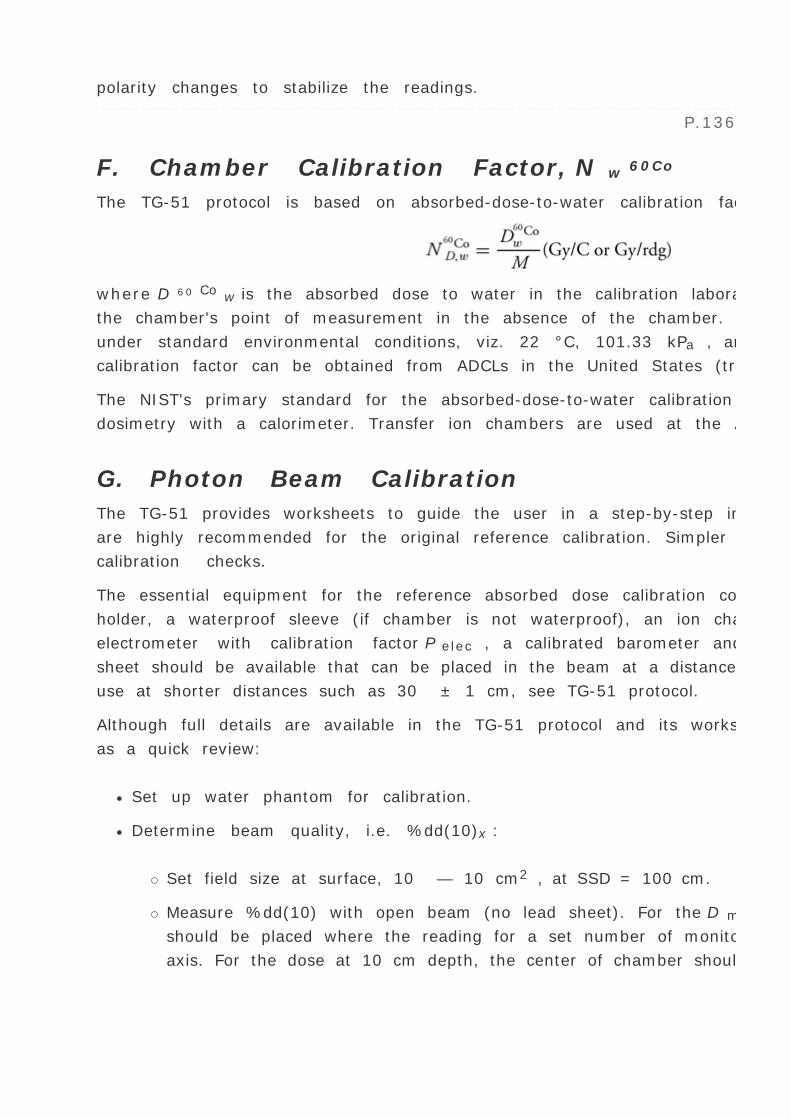
polarity changes to stabilize the readings.

P.136

F. Chamber Calibration Factor, N w 60Co

The TG-51 protocol is based on absorbed-dose-to-water calibration factor,

where D 6 0 Co w is the absorbed dose to water in the calibration laboratory's 60 Co beam under reference conditions, at

the chamber's point of measurement in the absence of the chamber. As discussed earlier, the calibration factor applies

under standard environmental conditions, viz. 22 °C, 101.33 kPa , and relative humidity between 20% and 80%. The

calibration factor can be obtained from ADCLs in the United States (traceable to NIST).

The NIST's primary standard for the absorbed-dose-to-water calibration of the chamber is currently based on absolute

dosimetry with a calorimeter. Transfer ion chambers are used at the ADCLs to provide NIST traceable calibrations.

G. Photon Beam Calibration

The TG-51 provides worksheets to guide the user in a step-by-step implementation of the protocol. These worksheets

are highly recommended for the original reference calibration. Simpler forms or worksheets may be designed for routine

calibration checks.

The essential equipment for the reference absorbed dose calibration consists of a suitable water phantom, a chamber

holder, a waterproof sleeve (if chamber is not waterproof), an ion chamber with calibration factor N 6 0 Co D,w ,

electrometer with calibration factor P elec , a calibrated barometer and a calibrated thermometer. One-mm thick lead

sheet should be available that can be placed in the beam at a distance of 50 ± 5 cm from the phantom surface. For

use at shorter distances such as 30 ± 1 cm, see TG-51 protocol.

Although full details are available in the TG-51 protocol and its worksheets, the calibration steps are summarized below

as a quick review:

Set up water phantom for calibration.

Determine beam quality, i.e. %dd(10)x :

Set field size at surface, 10 — 10 cm2 , at SSD = 100 cm.

Measure %dd(10) with open beam (no lead sheet). For the D max or peak dose measurement, the chambers

should be placed where the reading for a set number of monitor units (e.g., 200 MU) is maximum on the central

axis. For the dose at 10 cm depth, the center of chamber should be placed at (10 + 0.6rcav )cm.

The ratio of ionization at 10 cm depth to that at d max times 100 gives %dd (10). If the beam energy is <10 MV,

then %dd(10)x = %dd(10).

If the beam energy is â‰¥10 MV, use 1-mm lead sheet in the beam at a distance of 50 ± 5 cm from the

surface. Measure %dd(10)Pb as in (b) above.

Use Equation 8.79 to determine %dd(10)x if %dd(10)Pb is â‰¥73 %; or Equation 8.80 if the lead is not used

and %dd(10) is greater than 75% but not exceeding 89%.

Remove the lead sheet.

Depending on the chamber model, determine kQ corresponding to %dd(10)x (Table 8.6 ).

Measure temperature and pressure to get PT,P (Eq. 8.101 or 8.102 ).

Measure M + raw and M - raw to determine P pol (Eq. 8.103 ).

Measure Mh raw and ML raw to determine P ion at VH (Eq. 8.100 ).

Set 10 — 10 cm2 field size at the surface with SSD = 100 cm (SSD-type calibration) or at isocenter with SSD = 90

cm (SAD-type calibration).

Position the chamber with its center of cavity at 10 cm depth.

Irradiate for a set number of monitor units (e.g., 200 MU). Take an average of at least three consistent ion chamber

readings. The fully corrected reading M is given by

P.137

Equation 8.98 :

M = M raw PT,P P ion P elec P pol

Dose to water at 10 cm depth:

DQ w = MkQ N 6 0 Co D,w

Dose per monitor unit at reference d max 4

For SSD-type calibration,

For SAD-type calibration,

Note that the gradient correction for shift in the chamber point of measurement is included as part of kQ . So the

measurement depth of 10 cm for calibration is set at the center of chamber cavity. Also, the values of %dd(10,10 —

10) and TMR (10,10 — 10) used in step 11 above must be derived from data that have been corrected for shift in the

chamber's point of measurement if a cylindrical chamber had been used in the acquisition of the data.

H. Electron Beam Calibration

Because of the severe depth dose gradients and increased perturbations caused by chamber cavity in a low energy

electron beam, the TG-51 protocol recommends the use of plane-parallel chamber for electrons with R50 â‰¤ 2.6 cm

(incident energies of 6 MeV or less). It offers two methods of obtaining k ecal N 6 0 Co D,w for plane-parallel chambers:

one by cross-calibration against a calibrated cylindrical chamber (preferred method) and the other by using 60 Co

absorbed-dose calibration factor for the plane-parallel chamber. The reader is referred to TG-51 protocol for details on

the use of plane-parallel chamber for calibration.

Although the use of plane-parallel chamber for calibration offers some advantages, for example, absence of gradient

correction and minimal fluence perturbation correction, the disadvantages include the lack of absorbed-dose-to-water

calibration factor by the ADCLs, the difficulty of waterproofing the chamber, and eliminating water pressure on the thin

window of the plane-parallel chamber. Because of these drawbacks, some users ignore the protocol recommendation and

use Farmer-type chambers for the whole range of clinically useful energies, for example, from 6 MeV to 20 MeV and

higher.

In this section, the calibration steps with cylindrical chambers will be summarized for a quick review.

Determine beam quality or R 50 . This parameter can be determined by point measurements or obtained from the

pre-measured depth dose curve, corrected for stopping power ratios and all the perturbation effects as discussed in

section 14.3B . A broad beam (e.g., 20 — 20 cm2 ) is used for these measurements.

For the given chamber, determine k ecal (Table 8.8 ).

For the given beam energy, determine k â€²R 5 0 (Eq. 8.96 ).

Set up reference conditions for calibration:

P.138

Measure PT,P , P pol , and P ion .

Irradiate for a set number of monitor units (e.g., 200 MU) and take an average of at least three consistent readings.

The fully corrected reading M at d ref is given by:

M = M raw P ion PT,P P elec P pol

Determine gradient correction at d ref :

Dose to water at d ref :

Dw Q = MPgr Q k ecal k R 5 0 â€²ND,w 6 0 Co

Dose per monitor unit at

Dose per monitor unit at d max

Note that the calibration measurement is made with the center of chamber cavity at d ref . The gradient correction at d

ref due to shift in the point of measurement is determined separately and applied explicitly (unlike photons). The %dd(d

ref ) is obtained from depth dose data which have been corrected for changes in ([L with bar above]/ )w a ir and

perturbation effects if the data were acquired by an ion chamber.

8.7. IAEA TRS 398 PROTOCOL

The IAEA published its most recent calibration protocol, Technical Report Series (TRS) No. 398, in 2000 (36 ). This

protocol supersedes the previous IAEA TRS-277 protocol (45 ). The development of TRS-398 has paralleled that of the

AAPM TG-51 protocol. Consequently, the two protocols are very similar in their formalisms and both are based on

absorbed-dose-to-water calibration of the ion chamber in a cobalt-60 beam. Having presented TG-21 and TG-51 in the

previous sections, the TRS-398 will be discussed only briefly, primarily to highlight its differences from TG-51. The user

of the TRS-398 protocol is advised to follow the protocol document in all its details.

A. Formalism

The basic equation for the determination of absorbed dose to water for a beam of quality Q is the same as the TG-51

equation (Eq. 8.76 ). Using IAEA's notation,

where Dw,Q is the absorbed dose to water in the user's beam of quality Q , N D, w, Q 0 is the chamber calibration factor in

terms of absorbed dose to water in the reference beam of quality Q 0 (e.g., 60 Co), k Q, Q 0 is the factor that corrects for

the effects of the difference between the reference beam quality Q 0 and the user quality Q and MQ is the fully corrected

chamber reading. MQ is given by:

where M 1 is the dosimeter reading at the normal voltage V 1 , hp l is the phantom dependent fluence scaling factor to

correct for the difference in electron fluence in plastic (if calibration is performed in a plastic phantom) with that in

water at an equivalent depth, kTP is the temperature and pressure correction factor:

P.139

(noting that many international Primary Standards Laboratories specify reference air temperature of 20 °C [instead of

22 °C in the United States]), k elec is the electrometer calibration factor, k pol is the chamber polarity correction factor

(the same as Eq. 8.103 ), and k s is the ion recombination correction.

In the TRS-398, k s is determined by taking chamber readings M 1 and M 2 at voltages of V 1 (normal operating voltage)

and V 2 (half of V 1 or less) and calculating k s by:

where ±0 , ±1 , and ±2 are constants that depend on type of beam (pulsed or pulse-scanned). In continuous

radiation (e.g., 60 Co), the two voltage method may also be used using the relationship:

For pulsed and pulse-scanned beams, values of ±0 , ±1 , and ±2 are provided by Table 9 of the protocol.

B. Beam Quality, Q

1. Photon Beams

A major difference between TG-51 and TRS-398 consists of beam quality specification. Whereas, TG-51 recommends

%dd(10)x (see section 8.6A ), TRS-398 specifies beam quality by TPR20,10 . Although the choice of one or the other has

been debated in the literature (37 ,38 ), this difference has little effect on the end result, namely, the calculation of k Q

or absorbed dose to water. In my opinion, the TPR20,10 method is simpler to implement as it avoids the use of a lead

filter or dose measurement at d max which is somewhat messy (e.g., width of dose peak relative to chamber cavity

diameter and the question of residual electron contamination at d max in spite of the lead filter). In addition, the

determination of TPR20,10 does not require displacement correction nor is it sensitive to small systematic errors in

positioning of the chamber at each depth. However, the user of either protocol is advised to follow the respective

method recommended by the protocol.

The experimental setup for the determination of TPR20,10 is the same as that for the ionization ratio recommended by

the TG-21 protocol (see section 8.6A ). The source-to-chamber distance is kept constant at 100 cm and the

measurements are made with 10 cm and 20 cm of water over the chamber. The field size at the chamber position is 10

— 10cm2 . As previously mentioned, there is no need to use displacement correction. The ratio of ionization at 20cm

depth to that at 10cm depth gives the TPR20,10 .

It has been shown (37 ) that the restricted stopping power ratio, ([L with bar above]/ )w a ir , for all clinical beams

decreases with increase in TPR20,10 in a sigmoid relationship which has been represented by a cubic polynomial, fitting

the data to better than 0.15%. The quality conversion factors, k Q, Q 0 (or kQ in the notation of TG-51) can then be

calculated using stopping power ratios and perturbation factors (Eq. 8.86 ).

2. Electron Beams

The specification of beam quality in the TRS-398 protocol is the same as in the TG-51 protocol, namely, by R 50 (see

section 8.6A.2 ). A broad beam (e.g., 20 — 20 cm2 ) is recommended for the measurement of R 50 .

C. Quality Conversion Factor, k Q, Q 0

1. Photon Beams

Using TPR20,10 as the index of beam quality, Andreo (46 ) has calculated k Q, Q 0 values for a variety of commercially

available ion chambers and photon beams of TPR20,10 , ranging from 0.5 to 0.84. These values are presented in Table

14 of the TRS-398 protocol.

P.140

2. Electron Beams

TRS-398 deviates from the TG-51 methodology in that it directly calculates k Q, Q 0 for electrons using relevant stopping

power ratios and perturbation factors (see Eq. 8.86 ) instead of redefining k Q, Q 0 in terms of k ecal , k â€²R 5 0 and PQ gr

. In other words, the k Q, Q 0 formalism used for electrons is the same as for photons. A table of k Q, Q 0 values for

electrons is provided by the protocol for various types of ion chambers and beam quality R 50 . This simplifies the

calibration process somewhat since k ecal and PQ gr do not need to be determined. The gradient correction at d ref (the

same as in TG-51) is implicit in the k Q,Q 0 factor for electrons as it is for photons.

TRS-398 does provide the option of chamber calibration at a series of electron beam qualities. The calibration

laboratories could, in the future, provide N D, w, Q 0 for a reference electron beam of quality Q 0 and k Q, Q 0 factors

corresponding to a number of other beams of quality Q so that the user could determine k Q, Q 0 by interpolation.

Currently, this option is not available by the Primary Standard Dosimetry Laboratories (PSDLs).

D. Calibration

Reference conditions for the calibration of photon and electron beams in the TRS-398 are the same as in TG-51. TRS-

398 also provides worksheets, which guide the user in a step-by-step implementation of the protocol.

Comments: The TG-51 and TRS-398 protocols are similar, except for minor differences in beam quality specification and

notation. There is no reason why one protocol could not be followed worldwide. In this day and age, it does not make

sense to promote these more or less identical protocols packaged with different names and notations. Although it's too

late for these protocols to be merged into one, I hope that the next revision of either of these protocols will be

combined and carried out by an internationally constituted panel or a task group.

8.8. EXPOSURE FROM RADIOACTIVE SOURCES

Exposure rate from a radioactive source can be determined from the knowledge of its photon emission spectrum and the

relevant mass energy absorption coefficients for air. A relationship between exposure (X ) and energy fluence ( ¨) may

be derived by comparing Equations 8.19 and 8.21 . Under the conditions of changed particle equilibrium,

Therefore,

Suppose a radioisotope emits N photons of different energy and with different probability per disintegration. Imagine a

sphere of radius 1 m around this point source of activity 1 Ci. Because 1 Ci undergoes 3.7 — 1010 dps, and since area

of a sphere of radius 1 m is 4 € m2 and since 1 h = 3,600 sec, we have:

where f i is the number of photons emitted/decay of energy Ei . From Equation 8.110 ,

P.141

where

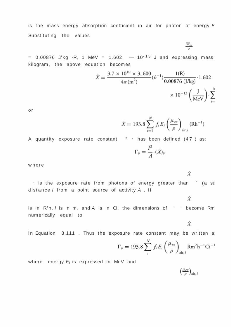
is the mass energy absorption coefficient in air for photon of energy E i .

Substituting the values

= 0.00876 J/kg ·R, 1 MeV = 1.602 — 10-13 J and expressing mass energy absorption coefficient in square meters per

kilogram, the above equation becomes

or

A quantity exposure rate constant “ ´ has been defined (47 ) as:

where

´ is the exposure rate from photons of energy greater than ´ (a suitable cutoff for the energy spectrum) at a

distance l from a point source of activity A . If

is in R/h, l is in m, and A is in Ci, the dimensions of “ ´ become Rm2 h-1 Ci-1 . It is also apparent that “ ´ is

numerically equal to

in Equation 8.111 . Thus the exposure rate constant may be written as:

where energy Ei is expressed in MeV and

is in m2 /kg.

Example

Calculate the exposure rate constant for 60 Co. Determine the exposure rate in R/min from a 5,000-Ci source of 60 Co at

a distance of 80 cm.

60 Co emits 2 ³-rays of energy 1.17 and 1.33 MeV per disintegration

1.00

1.17

0.00270

1.00

1.33

0.00261

fi Ei (MeV) (m2 /kg)

P.142

The previous calculation applies only very approximately to an actual cobalt teletherapy unit since exposure rate would

depend not only on the source activity but also on the collimator scatter, source size, and self-absorption in the source.

8.9. OTHER METHODS OF MEASURING ABSORBED DOSE

A. Calorimetry

Calorimetry is a basic method of determining absorbed dose in a medium. It is based on the principle that the energy

absorbed in a medium from radiation appears ultimately as heat energy while a small amount may appear in the form of

a chemical change. This results in a small increase in temperature of the absorbing medium which, if measured

accurately, can be related to the energy absorbed per unit mass or the absorbed dose.

If a small volume of the medium is thermally isolated from the remainder, the absorbed dose D in this volume is given

by:

where dE h is the energy appearing as heat in the absorber of mass dm and dEs is the energy absorbed or produced as a

result of chemical change, called the heat defect (which may be positive or negative). Neglecting the latter for the

moment, one can calculate the rise in temperature of water by the absorption of 1 Gy of dose:

where 4.18 is the mechanical equivalent of heat (4.18 J of energy = 1 cal of heat). Because the specific heat of water is

1 cal/g/ °C or 103 cal/kg/ °C, the increase in temperature ( ”T ) produced by 1 Gy is:

To measure such a small temperature rise, thermistors are most commonly used. Thermistors are semiconductors which

show a large change in electrical resistance with a small change in temperature (about 5% per 1 °C). Thus, by

measuring the change in resistance by an apparatus such as a Wheatstone bridge, one can calculate the absorbed dose.

Extensive literature exists on radiation calorimetry to which the reader is referred (48 ,49 ). Most of these apparatuses

are difficult to construct and, for various reasons, are considered impractical for clinical dosimetry. However, Domen (50

) has described a simpler water calorimeter for absolute measurement of absorbed dose. Essential features of this

calorimeter are briefly described.

Figure 8.9 is a schematic drawing of Domen's calorimeter. An ultrasmall (0.25-mm diameter) bead thermistor is

sandwiched between two 30- µm polyethylene films stretched on polystyrene rings. The thermistors are cemented to

one of the films to increase thermal coupling. The films provide the necessary high and stable resistance (>1011 ©)

between the thermistor leads and water.

The films held horizontally in a plastic frame are then immersed in an insulated tank of distilled water. Because of the

low thermal diffusivity of water and imperviousness of polyethylene film to water, nearly negligible conductive heat

transfer occurs at a point in the water medium. Therefore, a thermally isolated volume element of water is not

necessary. This apparatus measures dose rates in water of about 4 Gy/min with a precision (for the reproducibility of

measurements) of 0.5%.

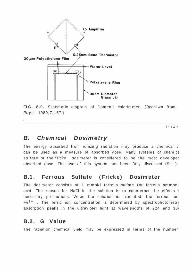
FIG. 8.9. Schematic diagram of Domen's calorimeter. (Redrawn from Domen SR. Absorbed dose water calorimeter. Med

Phys 1980;7:157.)

P.143

B. Chemical Dosimetry

The energy absorbed from ionizing radiation may produce a chemical change, and if this change can be determined, it

can be used as a measure of absorbed dose. Many systems of chemical dosimetry have been proposed but the ferrous

sulfate or the Fricke dosimeter is considered to be the most developed system for the precision measurement of

absorbed dose. The use of this system has been fully discussed (51 ). A brief description will be provided.

B.1. Ferrous Sulfate (Fricke) Dosimeter

The dosimeter consists of 1 mmol/l ferrous sulfate (or ferrous ammonium sulfate), 1 mmol/l NaCl, and 0.4 mol/l sulfuric

acid. The reason for NaCl in the solution is to counteract the effects of organic impurities present despite all the

necessary precautions. When the solution is irradiated, the ferrous ions, Fe2+ , are oxidized by radiation to ferric ions,

Fe3+ . The ferric ion concentration is determined by spectrophotometry of the dosimeter solution, which shows

absorption peaks in the ultraviolet light at wavelengths of 224 and 304 nm.

B.2. G Value

The radiation chemical yield may be expressed in terms of the number of molecules produced per 100 eV of energy

absorbed. This number is known as the G value. Thus, if the yield of ferric ions can be determined, the energy absorbed

can be calculated when the G value is known.

Suppose a ”M (moles/l) concentration of ferric ions is produced by an absorbed dose of D grays:

Molecules of ferric ions produced = ”M — 6.02 — 1023 molecules/liter

where is the density of the solution in kilograms per liter.

P.144

Number of molecules produced per eV of energy absorbed:

or

Thus,

The G values for the Fricke dosimeter have been determined by many investigators. Table 8.9 gives the values

recommended by Nahum (17 ) for photons from 137 Cs to 30 MV. A constant G value of 15.7 ± 0.6/100 eV is

recommended for electrons in the energy range of 1 to 30 MeV for 0.4 mol/liter H2 SO4 dosimeter solution (29 ).

137 Cs

15.3 ± 0.3

2 MV

15.4 ± 0.360 Co

15.5 ± 0.2

4 MV

15.5 ± 0.3

5â€“10 MV

15.6 ± 0.4

11â€“30 MV

15.7 ± 0.6

Data from ICRU. Radiation dosimetry: x rays and gamma rays with maximum photon energies between 0.6 and 50 MeV.

Report 14. Bethesda, MD: International Commission on Radiation Units and Measurements, 1969, with permission.

Radiation G Value (No./100 eV)

TABLE 8.9. RECOMMENDED G VALUES FOR THE FERROUS SULFATE DOSIMETER (0.4 mol/l H2 SO4 FOR

PHOTON BEAMS

C. Solid State Methods

There are several solid state systems available for the dosimetry of ionizing radiation. However, none of the systems is

absoluteâ€”each needs calibration in a known radiation field before it can be used for the determination of absorbed

dose.

There are two types of solid state dosimeters: (a) integrating type dosimeters (thermoluminescent crystals,

radiophotoluminescent glasses, optical density type dosimeters such as glass and film), and (b) electrical conductivity

dosimeters (semiconductor junction detectors, induced conductivity in insulating materials). Of these, the most widely

used systems for the measurement of absorbed dose are the thermoluminescent dosimeter (TLD), diodes, and film,

which are described.

C.1. Thermoluminescence Dosimetry

Many crystalline materials exhibit the phenomenon of thermoluminescence. When such a crystal is irradiated, a very

minute fraction of the absorbed energy is stored in the crystal lattice. Some of this energy can be recovered later as

visible light if the material is

P.145

heated. This phenomenon of the release of visible photons by thermal means is known as thermoluminescence (TL).

FIG. 8.10. Schematic diagram showing apparatus for measuring thermoluminescence.

The arrangement for measuring the TL output is shown schematically in Fig. 8.10 . The irradiated material is placed in a

heater cup or planchet, where it is heated for a reproducible heating cycle. The emitted light is measured by a

photomultiplier tube (PMT) which converts light into an electrical current. The current is then amplified and measured

by a recorder or a counter.

There are several TL phosphors available but the most noteworthy are lithium fluoride (LiF), lithium borate (Li2 B4 O7 ),

and calcium fluoride (CaF2 ). Their dosimetric properties are listed in Table 8.10 (52 ). Of these phosphors, LiF is most

extensively studied and most frequently used for clinical dosimetry. LiF in its purest form exhibits relatively little

thermoluminescence. But the presence of a trace amount of impurities (e.g., magnesium)

P.146

provides the radiation-induced TL. These impurities give rise to imperfections in the lattice structure of LiF and appear

to be necessary for the appearance of the TL phenomenon.

Density (g/cc)

2.64

2.3

3.18

3.18

2.61

Effective atomic no.

8.2

7.4

16.3

16.3

15.3

TL emission spectra (A)

Range

3,500â€“6,000

5,300â€“6,300

4,400â€“6,000

3,500â€“5,000

4,500â€“6,000

Maximum

4,000

6,050

5,000

3,800

5,000

Temperature of main TL glow peak

195 °C

200 °C

260 °C

260 °C

110 °C

Efficiency at cobalt-60 (relative to LiF)

1.0

0.3

3

23

70

Energy response without added filter (30 keV/cobalt-60)

1.25

0.9

13

13

10

Useful range

Small, <5%/12 wk

mRâ€“106 R

mRâ€“3 — 105 R

mRâ€“104 R

Râ€“104 R

Fading

mRâ€“105 R

10% in first mo

10% in first mo

No detectable fading

50â€“60% in the first 24 hr

Light sensitivity

Essentially none

Essentially none

Essentially none

Yes

Yes

Physical form

Powder, extruded, Teflon-embedded, silicon-embedded, glass capillaries

Powder, Teflon-embedded

Powder, Teflon-embedded, hotpressed chips, glass capillaries

Special dosimeters

Powder, Teflon-embedded

From Cameron JR, Suntharalingam N, Kenney GN. Thermoluminescent dosimetry. Madison: University of Wisconsin

Press, 1968, with permission.

Characteristic LiF Li2 B407

:Mn

CaF2

:Mn

CaF2 :nat CaSo4

:Mn

TABLE 8.10. CHARACTERISTICS OF VARIOUS PHOSPHORS

FIG. 8.11. A simplified energy-level diagram to illustrate thermoluminescence process.

C.2. Simplified Theory of Thermoluminescent Dosimetry

The chemical and physical theory of TLD is not exactly known, but simple models have been proposed to explain the

phenomenon qualitatively. Figure 8.11 shows an energy-level diagram of an inorganic crystal exhibiting TL by ionizing

radiation.

In an individual atom, electrons occupy discrete energy levels. In a crystal lattice, on the other hand, electronic energy

levels are perturbed by mutual interactions between atoms and give rise to energy bands: the â€œallowedâ€ energy

bands and the forbidden energy bands. In addition, the presence of impurities in the crystal creates energy traps in the

forbidden region, providing metastable states for the electrons. When the material is irradiated, some of the electrons in

the valence band (ground state) receive sufficient energy to be raised to the conduction band. The vacancy thus created

in the valence band is called a positive hole. The electron and the hole move independently through their respective

bands until they recombine (electron returning to the ground state) or until they fall into a trap (metastable state). If

there is instantaneous emission of light owing to these transitions, the phenomenon is called fluorescence . If an

electron in the trap requires energy to get out of the trap and fall to the valence band, the emission of light in this case

is called phosphorescence (delayed fluorescence). If phosphorescence at room temperature is very slow, but can be

speeded up significantly with a moderate amount of heating (~300 °C), the phenomenon is called thermoluminescence

.

A plot of thermoluminescence against temperature is called a glow curve (Fig. 8.12 ). As the temperature of the TL

material exposed to radiation is increased, the probability of releasing trapped electrons increases. The light emitted

(TL) first increases, reaches a maximum value, and falls again to zero. Because most phosphors contain a number of

traps at various energy levels in the forbidden band, the glow curve may consist of a number of glow peaks as shown in

Fig. 8.12 . The different peaks correspond to different â€œtrappedâ€ energy levels.

C.3. Lithium Fluoride

The TL characteristics of LiF have been studied extensively. For details, the reader is referred to Cameron et al. (52 ).

Lithium fluoride has an effective atomic number of 8.2 compared with 7.4 for soft tissue. This makes this material very

suitable for clinical dosimetry. Mass energy absorption coefficients for this material have been given by Greening et al.

(53 ). The dose absorbed in LiF can be converted to dose in muscle by considerations similar to those discussed earlier.

For example, under electronic equilibrium conditions, the ratio of absorbed doses in the two media will be the same as

the ratio of their mass energy absorption coefficients. If the dimensions of the dosimeter are smaller than the ranges of

the electrons crossing the dosimeter, then the Bragg-Gray relationship can also be used. The ratio of absorbed doses in

P.147

the two media then will be the same as the ratio of mass stopping powers. The applicability of the Bragg-Gray cavity

theory to TLD has been discussed by several authors (54 ,55 ).

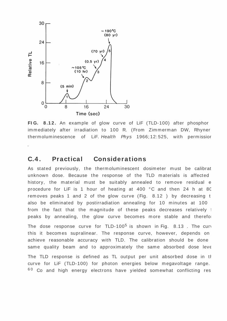
FIG. 8.12. An example of glow curve of LiF (TLD-100) after phosphor has been annealed at 400 °C for 1 h and read

immediately after irradiation to 100 R. (From Zimmerman DW, Rhyner CR, Cameron JR. Thermal annealing effects on

thermoluminescence of LiF. Health Phys 1966;12:525, with permission.)

C.4. Practical Considerations

As stated previously, the thermoluminescent dosimeter must be calibrated before it can be used for measuring an

unknown dose. Because the response of the TLD materials is affected by their previous radiation history and thermal

history, the material must be suitably annealed to remove residual effects. The standard preirradiation annealing

procedure for LiF is 1 hour of heating at 400 °C and then 24 h at 80 °C. The slow heating, namely 24 hours at 80 °C,

removes peaks 1 and 2 of the glow curve (Fig. 8.12 ) by decreasing the â€œtrapping efficiency.â€ Peaks 1 and 2 can

also be eliminated by postirradiation annealing for 10 minutes at 100 °C. The need for eliminating peaks 1 and 2 arises

from the fact that the magnitude of these peaks decreases relatively fast with time after irradiation. By removing these

peaks by annealing, the glow curve becomes more stable and therefore predictable.

The dose response curve for TLD-1005 is shown in Fig. 8.13 . The curve is generally linear up to 103 cGy but beyond

this it becomes supralinear. The response curve, however, depends on many conditions that have to be standardized to

achieve reasonable accuracy with TLD. The calibration should be done with the same TLD reader, in approximately the

same quality beam and to approximately the same absorbed dose level.

The TLD response is defined as TL output per unit absorbed dose in the phosphor. Figure 8.14 gives the energy response

curve for LiF (TLD-100) for photon energies below megavoltage range. The studies of energy response for photons above60 Co and high energy electrons have yielded somewhat conflicting results. Whereas the data of Pinkerton et al. (56 )

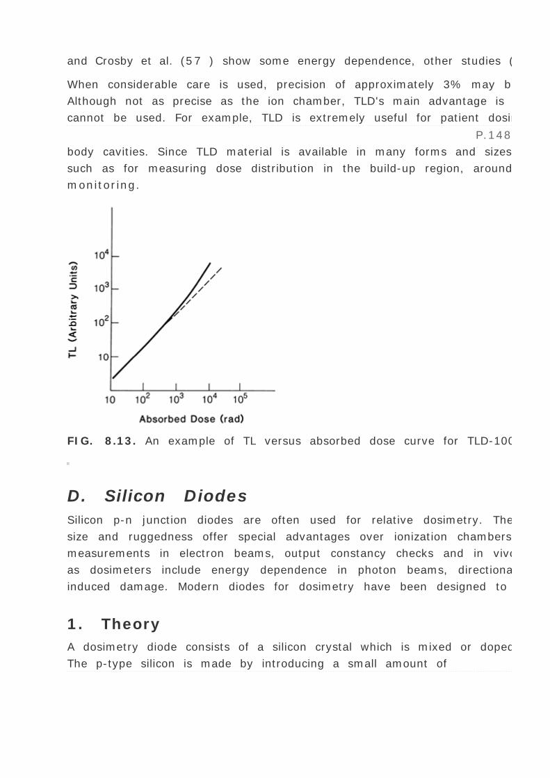
and Crosby et al. (57 ) show some energy dependence, other studies (58 ) do not show this energy dependence.

When considerable care is used, precision of approximately 3% may be obtained using TLD powder or extruded material.

Although not as precise as the ion chamber, TLD's main advantage is in measuring doses in regions where ion chamber

cannot be used. For example, TLD is extremely useful for patient dosimetry by direct insertion into tissues or

P.148

body cavities. Since TLD material is available in many forms and sizes, it can be used for special dosimetry situations

such as for measuring dose distribution in the build-up region, around brachytherapy sources, and for personnel dose

monitoring.

FIG. 8.13. An example of TL versus absorbed dose curve for TLD-100 powder (schematic).

D. Silicon Diodes

Silicon p-n junction diodes are often used for relative dosimetry. Their higher sensitivity, instantaneous response, small

size and ruggedness offer special advantages over ionization chambers. They are particularly well suited for relative

measurements in electron beams, output constancy checks and in vivo patient dose monitoring. Their major limitations

as dosimeters include energy dependence in photon beams, directional dependence, thermal effects, and radiation-

induced damage. Modern diodes for dosimetry have been designed to minimize these effects.

1. Theory

A dosimetry diode consists of a silicon crystal which is mixed or doped with impurities to make p- and n-type silicon.

The p-type silicon is made by introducing a small amount of

P.149

an element from group III of the periodic table (e.g., boron), making it into an electron receptor. When silicon is mixed

with a material from group V (e.g., phosphorus) it receives atoms that are carriers of negative charge, thus making it

into an electron donor or n-type silicon. A p-n junction diode is designed with one part of a p-silicon disc doped with an

n-type material (Fig. 8.15 ). The p-region of the diode is deficient in electrons (or contains â€œholesâ€ ) while the n-

region has an excess of electrons.

FIG. 8.14. Energy response curve for LiF (TLD-100), CaF2 :Mn and a photographic film. (From Cameron JR,

Suntharalingam H, Kenney GN. Thermoluminescent dosimetry. Madison: University of Wisconsin Press, 1968, with

permission.)

FIG. 8.15. A schematic diagram showing basic design of a silicon p-n junction diode. (From Attix FH. Introduction to

radiological physics and radiation dosimetry. New York: John Wiley & Sons, 1986, with permission.)

At the interface between p- and n-type materials, a small region called the depletion zone is created because of initial

diffusion of electrons from the n-region and holes from the p-region across the junction, until equilibrium is established.

The depletion zone develops an electric field which opposes further diffusion of majority carriers once equilibrium has

been achieved.

When a diode is irradiated electron-hole pairs are produced within the depletion zone. They are immediately separated

and swept out by the existing electric field in the depletion zone. This gives rise to a radiation-induced current. The

current is further augmented by the diffusion of electrons and holes produced outside the depletion zone within a

diffusion length. The direction of electronic current flow is from the n- to the p-region (which is opposite to the direction

of conventional current).

2. Operation

Figure 8.16A shows schematically a radiation diode detector, which essentially consists of a silicon p-n junction diode

connected to a coaxial cable and encased in epoxy potting material. This design is intended for the radiation beam to be

incident perpendicularly at the long axis of the detector. Although the collecting or sensitive volume (depletion zone) is

not known precisely, it is on the order of 0.2 to 0.3 mm3 . It is located within a depth of 0.5 mm from the front surface

of the detector, unless electronic buildup is provided by encasing the diode in a buildup material.

Figure 8.16B shows the diode connected to an operational amplifier with a feedback loop to measure radiation induced

current. There is no bias voltage applied. The circuit acts as a current-to-voltage transducer, whereby the voltage

readout at point B is directly proportional to the radiation induced current.

Diodes are far more sensitive than ion chambers. Since the energy required to produce an electron-hole pair in Si is 3.5

eV compared to 34eV required to produce an ion-pair in

P.150

air and because the density of Si is 1,800 times that of air, the current produced per unit volume is about 18,000 times

larger in a diode than in an ion chamber. Thus, a diode, even with a small collecting volume, can provide an adequate

signal.

FIG. 8.16. Schematic diagrams showing (a) silicon p-n junction diode, and (b) basic electronic circuit using operational

amplifier with a feedback loop. (From Gager LD, Wright AE, Almond PR. Silicon diode detectors used in radiobiological

physics measurements. Part I: Development of an energy compensating shield. Med Phys 1977;4:494â€“498, with

permission.)

3. Energy Dependence

Because of the relatively high atomic number of silicon (Z = 14) compared to that of water or air, diodes exhibit severe

energy dependence in photon beams of non-uniform quality. Although some diodes are designed to provide energy

compensation through filtration (59 ), the issue of energy dependence never goes away and therefore, their use in x-ray

beams is limited to relative dosimetry in situations where spectral quality of the beam is not changed significantly, for

example, profile measurements in small fields, dose constancy checks. In electron beams, however, the diodes do not

show energy dependence as the stopping power ratio of silicon to water does not vary significantly with electron energy

or depth. Thus diodes are qualitatively similar to films so far as their energy dependence is concerned.

Some diodes exhibit greater stability and less energy dependence than others. It is therefore incumbent upon the user

to establish dosimetric accuracy of a diode by comparative measurements with an ion chamber.

4. Angular Dependence

Diodes exhibit angular dependence, which must be taken into account if the angle of beam incidence is changed

significantly. Again these effects should be ascertained in comparative measurements with a detector which does not

show angular dependence.

P.151

5. Temperature Dependence

Diodes show a small temperature dependence that may be ignored unless the change in temperature during

measurements or since the last calibration is drastic. The temperature dependence of diodes is smaller than that of an

ion chamber. Moreover, their response is independent of pressure and humidity.

6. Radiation Damage

A diode can suffer permanent damage when irradiated by ultrahigh doses of ionizing radiation. The damage is most

probably caused by displacement of silicon atoms from their lattice positions. The extent of damage will depend upon

the type of radiation, energy and total dose. Because of the possibility of radiation damage, especially after prolonged

use, diode sensitivity should be checked routinely to assure stability and accuracy of calibration.

7. Clinical Applications

As previously mentioned, diodes are useful in electron beam dosimetry and in limited situations in photon beam

measurements. Most often their use is dictated by the requirements on the detector size. For example, dose profiles or

output factors in a small field may pose difficulties in the use of an ion chamber. So a film or a diode response is

checked against an ion chamber under suitable benchmark conditions.

Diodes are becoming increasingly popular with regard to their use in patient dose monitoring. Since diodes do not

require high voltage bias, they can be taped directly onto the patient at suitable points to measure dose. The diodes are

carefully calibrated to provide a check of patient dose at a reference point (e.g., dose at d max ). Different amounts of

buildup material can be incorporated to make the diode sample the dose close to the peak dose for a given energy

beam. Calibration factors are applied to convert the diode reading into expected dose at the reference point, taking into

account source-to-detector distance, field size, and other parameters used in the calculation of monitor units.

For further details on diodes and their clinical applications, the readier is referred to some key articles in the literature

(59 ,60 ,61 ,62 ).

E. Radiographic Film

A radiographic film consists of a transparent film base (cellulose acetate or polyester resin) coated with an emulsion

containing very small crystals of silver bromide. When the film is exposed to ionizing radiation or visible light, a

chemical change takes place within the exposed crystals to form what is referred to as a latent image . When the film is

developed, the affected crystals are reduced to small grains of metallic silver. The film is then fixed . The unaffected

granules are removed by the fixing solution, leaving a clear film in their place. The metallic silver, which is not affected

by the fixer, causes darkening of the film. Thus the degree of blackening of an area of the film depends on the amount

of free silver deposited and, consequently, on the radiation energy absorbed.

The degree of blackening of the film is measured by determining optical density with a densitometer. This instrument

consists of a light source, a tiny aperture through which the light is directed and a light detector (photocell) to measure

the light intensity transmitted through the film.

The optical density, OD, is defined as:

where I 0 is the amount of light collected without film and It is the amount of light transmitted through the film. A

densitometer gives a direct reading of optical density if it has been calibrated by a standard strip of film having regions

of known optical density.

P.152

In dosimetry, the quantity of interest is usually net optical density which is obtained by subtracting the reading for the

base fog (OD of unexposed processed film) from the measured optical density.

A plot of net optical density as a function of radiation exposure or dose is termed the sensitometric curve, or H-D

curve.6 Figure 8.17 shows examples of characteristic curves for two commonly used dosimetry films. Film speed and

linearity of the sensitometric curve are the two main characteristics which are considered in selecting a film for

dosimetry. If a film is exposed in the nonlinear region, corrections are necessary to convert optical density into dose.

FIG. 8.17. Sensitometric curve of Kodak XV-2 film and Kodak RPM-2 (Type M) film.

Although film is well-established as a method of measuring electron beam distributions (Chapter 14 ), its usefulness in

photon dosimetry is relatively limited. Because the photoelectric effect depends on the cube of the atomic number, the

silver (Z = 45) in the film emulsion absorbs radiation below 150 keV very strongly by the photoelectric process. Since

most clinical beams contain a scatter component of low-energy photons, the correlation between optical density and

dose becomes tenuous. In addition, film suffers from several potential errors such as changes in processing conditions,

interfilm emulsion differences, and artifacts caused by air pockets adjacent to the film. For these reasons, absolute

dosimetry with film is impractical. However, it is very useful for checking radiation fields, light-field coincidence, field

flatness, and symmetry, and obtaining quick qualitative patterns of a radiation distribution.

In the megavoltage range of photon energies, however, film has been used to measure isodose curves with acceptable

accuracy ( ±3%) (63 ,64 ,65 ). One of the techniques (65 ) consists of exposing the film packed tightly in a

polystyrene phantom, parallel to the central axis of the beam. The film edge is carefully aligned with the phantom

surface and air pockets between the film surface and the surrounding jacket are removed by punching holes near the

corners. Optical densities are correlated with dose by using a depth-dependent sensitometric curve derived from known

central axis depth dose data for a reference field such as 10 — 10 cm. The method is made practical by a computer-

controlled densitometer and a computer program that performs the required isodensity-to-isodose curve conversion.

P.153

F. Radiochromic Film

The use of radiochromic films for radiation dosimetry has been evolving since the 1960s (66 ,67 ). With the recent

improvement in technology associated with the production of these films, their use has become increasingly popular

especially in brachytherapy dosimetry. Major advantages of radiochromic film dosimeters include tissue equivalence,

high spatial resolution, large dynamic range (10-2 -106 Gy), relatively low spectral sensitivity variation (or energy

dependence), insensitivity to visible light and no need for chemical processing.

Radiochromic film consists of an ultra thin (7- to 23- µm thick), colorless, radiosensitive leuco dye bonded onto a 100-

µm thick Mylar base (68 ). Other varieties include thin layers of radiosensitive dye sandwiched between two pieces of

polyester base (69 ). The unexposed film is colorless and changes to shades of blue as a result of a polymerization

process induced by ionizing radiation.

No physical, chemical, or thermal processing is required to bring out or stabilize this color. The degree of coloring is

usually measured with a spectrophotometer using a narrow spectral wavelength (nominal 610â€“670 nm). Commercially

available laser scanners and CCD microdensitometer cameras can also be used to scan the films. These measurements

are expressed in terms of optical density as defined by Equation 8.115 .

Radiochromic films are almost tissue equivalent with effective Z of 6.0 to 6.5. Post irradiation color stability occurs after

about 24 hours. Energy dependence is much lower than the silver halide (radiographic) films. Although radiochromic

films are insensitive to visible light, they exhibit some sensitivity to ultraviolet light and temperature. They need to be

stored in a dry and dark environment at the temperature and humidity not too different from those at which they will be

used for dosimetry. Because radiochromic films are sensitive to ultraviolet light, they should not be exposed to

fluorescent light or to sunlight. They may be read and handled in normal incandescent light.

Radiochromic films must be calibrated before they can be used for dosimetry. The sensitometric curve shows a linear

relationship up to a certain dose level beyond which its response levels off with increase in dose (Fig. 8.18 ).

The most commonly used radiochromic films for dosimetry that are commercially available are GafChromic HD-810 film

(International Specialty Product (ISP), Wayne, NJ) and Double-layer GafChromic MD-55â€“2 film (ISP or other

vendor(s): Nuclear Associates,

P.154

Carle Place, NY). Whereas HD-810 films are mainly used in the dose range of 50 to 2,500 Gy, MD-55-2 are useful in the

range of 3 to 100 Gy.

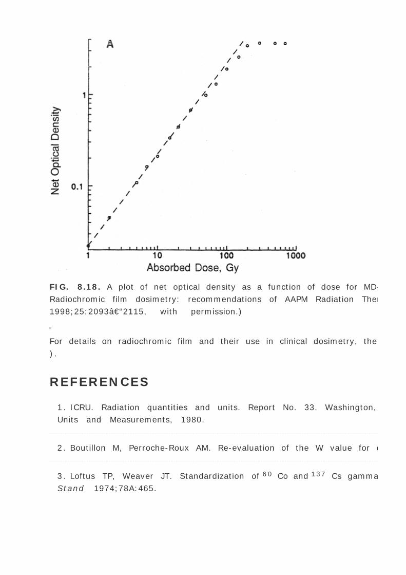
FIG. 8.18. A plot of net optical density as a function of dose for MD-55â€“2 radiochromic film. (From AAPM.

Radiochromic film dosimetry: recommendations of AAPM Radiation Therapy Committee Task Group 55. Med Phys

1998;25:2093â€“2115, with permission.)

For details on radiochromic film and their use in clinical dosimetry, the reader is referred to the AAPM TG-55 report (70

).

REFERENCES

1. ICRU. Radiation quantities and units. Report No. 33. Washington, DC: International Commission on Radiation

Units and Measurements, 1980.

2. Boutillon M, Perroche-Roux AM. Re-evaluation of the W value for electrons in dry air. Phys Med Biol 1987;32:213.

3. Loftus TP, Weaver JT. Standardization of 60 Co and 137 Cs gamma-ray beams in terms of exposure. J Res Natl Bur

Stand 1974;78A:465.

4. Loevinger R. A formalism for calculation of absorbed dose to a medium from photon and electron beams. Med Phys

1981;8:1.

5. Mackie TR, Bielajew AF, Rogers DWO, et al. Generation of photon energy deposition kernels using the EGS Monte

Carlo code. Phys Med Biol 1988;33:1.

6. American Association of Physicists in Medicine. RTC Task Group 21. A protocol for the determination of absorbed

dose from high energy photon and electron beams. Med Phys 1983;10:741.

7. Johns HE, Cunningham JR. The physics of radiology , 3rd ed. Springfield, IL: Charles C Thomas, 1969.

8. Day MJ, Greene D, Massey JB. Use of a Perspex sheath for ionization chamber measurements in a water phantom.

Phys Med Biol 1965;10:111.

9. Bragg WH. Studies in radioactivity . New York: Macmillan, 1912.

10. Gray LH. An ionization method for the absolute measurement of gamma-ray energy. Proc R Soc 1936;A156:578.

11. Spencer LV, Attix FH. A theory of cavity ionization. Radiat Res 1955;3:239.

12. Greening JR. An experimental examination of theories of cavity ionization. Br J Radiol 1957;30:254.

13. Burlin TE. An experimental examination of theories relating the absorption of gamma-ray energy in medium to

the ionization produced in a cavity. Phys Med Biol 1961;6:33.

14. Burlin TE. Further examination of theories relating the absorption of gamma-ray energy in a medium to the

ionization produced in a cavity. Phys Med Biol 1966;11:255.

15. Nahum AE. Dosimetry in radiotherapy. IAEA-SM-298/81. Proc Symp Int Atomic Energy Agency 1988;1:87.

16. ICRU. Stopping powers for electrons and positrons. Report 37 . Bethesda, MD: International Commission on

Radiation Units and Measurements, 1984.

17. Nahum AE. Water/air mass stopping power ratios for megavoltage photon and electron beams. Phys Med Biol

1978;23:24.

18. Burlin TE. Cavity chamber theory. In: Attix FH, Roesch WC, eds. Radiation dosimetry, Vol I , 2nd ed. New

York: Academic Press, 1969.

19. ICRU. Average energy required to produce an ion pair . Report 31. Washington, DC: ICRU, 1979.

20. Almond PR, Svensson H. Ionization chamber dosimetry for photon and electron beams. Acta Radiol 1977;16:177.

21. Lempert GD, Nath R, Schulz RJ. Fraction of ionization from electrons arising in the wall of an ionization chamber.

Med Phys 1983;10:1.

22. Dutreix J, Dutreix A. Etude compar © dâ€™une s ©rie de chambres dâ€™ionization dans des faisceaux

dâ€™ ©lectrons de 20 et 10 MeV. Biophysik 1966;3:249â€“258.

23. Schulz RJ, Almond PR, Kutcher G, et al. Clarification of the AAPM Task Group 21 protocol. Med Phys

1986;13:755.

24. Rogers DWO. Fundamentals of high energy x-ray and electron dosimetry protocols . AAPM Summer School, 1990.

25. Khan FM. Replacement correction (P repl ) for ion chamber dosimetry. Med Phys 1991;18:1244.

26. Cunningham JR, Sontag MC. Displacement correction used in absorbed dose determination. Med Phys

1980;7:672â€“676.

27. Johansson K, Mattsson L, Lindberg L, et al. Absorbed-dose determination with ionization chambers in electron and

photon beams having energies between 1 and 50 MeV. IAEA-SM-222/35 . Vienna: International Atomic Energy

Agency, 1977:243â€“270.

28. AAPM. Clinical electron beam dosimetry. TG-25 Report. Med Phys 1991;18:73â€“109.

29. ICRU. Radiation dosimetry: electron beams with energies between 1 and 50 MeV . Report 35. Washington, DC:

ICRU, 1984.

30. Nath R, Schulz RJ. Calculated response and wall correction factors for ionization chambers exposed to 60 Co

gamma-rays. Med Phys 1981;8:85.

P.155

31. Gastorf R, Humphries L, Rozenfeld M. Cylindrical chamber dimensions and the corresponding values of A wall and

N gas /(Nx A ion ). Med Phys 1986;13:751.

32. Bielajew AF. Ionization cavity theory: a formal derivation of perturbation factors for thick walled ion chambers in

photon beams. Phys Med Biol 1986;31:161.

33. Rogers DWA. Fundamentals of dosimetry based on absorbed dose standards. In: Mackie TR, Palta JR, eds.

Teletherapy: present and future . Madison, WI: Advanced Medical Publishing, 1996:319â€“356.

34. AAPM. Protocol for clinical reference dosimetry of high-energy photon and electron beams. Med Phys

1999;26:1847â€“1870.

35. Andreo P, Brahme A. Stopping-power data for high-energy photon beams. Phys Med Biol 1986;31:839â€“858.

36. IAEA. Absorbed dose determination in external beam radiotherapy. Technical Reports Series No. 398 . Vienna:

International Atomic Energy Agency, 2000.

37. Andreo P. On the beam quality specification of high-energy photons for radiotherapy dosimetry. Med Phys

2000;27:434â€“440.

38. Rogers DWO. Comment on â€œOn the beam quality specification of high-energy photons for radiotherapy

dosimetryâ€ . Med Phys 2000;27:441â€“444.

39. Kosunen A, Rogers DWO. Beam quality specification for photon beam dosimetry. Med Phys

1993;20:1181â€“1188.

40. Li XA, Rogers DWO. Reducing electron contamination for photon-beam quality specification. Med Phys

1994;21:791â€“798.

41. Ding GX, Rogers DWO, Mackie TR. Calculation of stopping-power ratios using realistic clinical electron beams.

Med Phys 1995;22:489â€“501.

42. Ma CM, Nahum AE. Effect of size and composition of central electrode on the response of cylindrical ionization

chambers in high-energy photon and electron beams. Phys Med Biol 1993;38:267â€“290.

43. Rogers DWO. A new approach to electron-beam reference dosimetry. Med Phys 1997;25:310â€“320.

44. Burns DT, Ding GX, Rogers DWO. R50 as a beam quality specifier for selecting stopping-power ratios and

reference depths for electron dosimetry. Med Phys 1996;23:383â€“388.

45. IAEA. Absorbed dose determination in photon and electron beams: an international code of practice. Technical

Report Series No. 277 . Vienna: International Atomic Energy Agency, 1987.

46. Andreo P. Absorbed dose beam quality factors for the dosimetry of high-energy photon beams. Phys Med Biol

1992;37:2189â€“2211.

47. ICRU. Radiation quantities and units. Report No. 19 . Washington, DC: International Commission on Radiation


48. Laughlin JS, Genna S. Calorimetry. In: Attix FH, Roesch WC, eds. Radiation dosimetry, Vol II . New York:

Academic Press, 1967:389.

49. Gunn SR. Radiometric calorimetry: a review. Nucl Inst Methods 1964;29:1; 1970;85:285; 1976;135:251.

50. Domen SR. Absorbed dose water calorimeter. Med Phys 1980;7:157.

51. ICRU. Radiation dosimetry: x-rays generated at potentials of 5 to 150 kV . Report No. 17. Washington, DC:

International Commission on Radiation Units and Measurements, 1970.

52. Cameron JR, Suntharalingam N, Kenney GN. Thermoluminescent dosimetry . Madison: University of Wisconsin

Press, 1968.

53. Greening JR, Law J, Redpath AT. Mass attenuation and mass energy absorption coefficients for LiF and Li2 B4 O7

for photons from 1 to 150 keV. Phys Med Biol 1972;17:585.

54. Paliwal BR, Almond PR. Application of cavity theories for electrons to LiF dosimeters. Phys Med Biol 1975;20:547.

55. Holt JG, Edelstein GR, Clark TE. Energy dependence of the response of lithium fluoride TLD rods in high energy

electron fields. Phys Med Biol 1975;20:559.

56. Pinkerton A, Holt JG, Laughlin JS. Energy dependence of LiF dosimeters at high energies. Phys Med Biol

1966;11:129.

57. Crosby EH, Almond PR, Shalek RJ. Energy dependence of LiF dosimeters at high energies. Phys Med Biol

1966;11:131.

58. Suntharalingam N, Cameron JR. Thermoluminescent response of lithium fluoride to high-energy electrons [high-

energy radiation therapy dosimetry issue]. Ann NY Acad Sci 1969;161:77.

59. Gager LD, Wright AE, Almond PR. Silicon diode detectors used in radiobiological physics measurements. Part I:

Development of an energy compensating shield. Med Phys 1977;4:494â€“498.

60. Wright AE, Gager LD. Silicon diode detectors used in radiobiological physics measurements. Part II: Measurement

of dosimetry data for high-energy photons. Med Phys 1977;4:499â€“502.

61. Dixon RL, Ekstrand KE. Silicon diode dosimetry. Int J Appl Radiat Isot 1982;33:1171â€“1176.

62. Rikner G. Characteristics of a selectively shielded p-Si detector in 60 Co and 8 and 16 MV Roentgen radiation.

Acta Radiol Oncol 1985;24:205â€“208.

63. Jacobson A. 4 MeV x-ray film dosimetry. Radiology 1972;103:703.

64. Patten L, Purdy J, Oliver G. Automated film dosimetry [Abstract]. Med Phys 1974;1:110.

65. Williamson JF, Khan FM, Sharma SC. Film dosimetry of megavoltage photon beams: a practical method of

isodensity-to-isodose curve conversion. Med Phys 1981;8:94.

P.156

66. McLaughlin WL, Chalkley L. Low atomic numbered dye systems for ionizing radiation measurements. Photogr Sci

Eng 1965;9:159â€“165.

67. McLaughlin WL. Microscopic visualization of dose distribution. Int J Appl Radiat Isot 1966;17:85â€“96.

68. Zhu Y, Kirov AS, Mishra V, et al. Quantitative evaluation of radiochromic film response for two-dimensional

dosimetry. Med Phys 1997;25:223â€“231.

69. Soares CG, McLaughlin WL. Measurement of radial dose distributions around small beta-particle emitters using

high-resolution radiochromic foil dosimetry. Radiat Protect Dosim 1993;47:367â€“372.

70. AAPM. Radiochromic film dosimetry: recommendations of AAPM Radiation Therapy Committee Task Group 55. Med

Phys 1998;25:2093â€“2115.

1 Electron fluence at P with the cavity filled with wall material is proportional to ¨wall at P . With the air cavity in

place, the electron fluence at P is proportional to the mean photon energy fluence at the surface of the cavity, which

can be taken as equal to ¨air at the center of the cavity.

2 The TG-21 protocol uses

value of 33.7 J /C which assumes a dry air value of 33.85 J /C and corrects it for 50% relative humidity (23 ). In our

derivation we will assume a dry air value of 33.97 J /C and no humidity correction, as discussed earlier in relation to

Equation 8.37 .

3 Although the AAPM protocol recommends calibration in terms of dose to water, many consider it more convenient to

convert D water to D muscle at the time of calibration and set the accelerator in terms of dose to muscle per monitor unit.

4 Reference d max is the fixed d max used for normalizing percent depth dose and TMR data for all field sizes (see

Chapter 10 ).

5 TLD-100 (Harshaw Chemical Co.) contains 7.5% 6 Li and 92.5% 7 Li.

6 The expression H-D is derived from the names of Hurter and Driffield, who in 1890 used such curves to characterize

the response of photographic film to light.




> Table of Contents > Part II - Classical Radiation Therapy >

9 - Dose Distribution and Scatter Analysis

9

Dose Distribution and ScatterAnalysis

It is seldom possible to measure dose distribution directly in patients

treated with radiation. Data on dose distribution are almost entirely derived

from measurements in phantomsâ€”tissue equivalent materials, usually

large enough in volume to provide full-scatter conditions for the given

beam. These basic data are used in a dose calculation system devised to

predict dose distribution in an actual patient. This chapter deals with

various quantities and concepts that are useful for this purpose.

9.1. PHANTOMS

Basic dose distribution data are usually measured in a water phantom,

which closely approximates the radiation absorption and scattering

properties of muscle and other soft tissues. Another reason for the choice

of water as a phantom material is that it is universally available with

reproducible radiation properties. A water phantom, however, poses some

practical problems when used in conjunction with ion chambers and other

detectors that are affected by water, unless they are designed to be

waterproof. In most cases, however, the detector is encased in a thin

plastic (water equivalent) sleeve before immersion into the water phantom.

Since it is not always possible to put radiation detectors in water, solid dry

phantoms have been developed as substitutes for water. Ideally, for a

given material to be tissue or water equivalent, it must have the same

effective atomic number, number of electrons per gram, and mass density.

However, since the Compton effect is the most predominant mode of

interaction for megavoltage photon beams in the clinical range, the

necessary condition for water equivalence for such beams is the same

electron density (number of electrons per cubic centimeter) as that of

water.

The electron density ( e ) of a material may be calculated from its mass

density ( m ) and its atomic composition according to the formula:

where

NA is Avogadro's number and ai is the fraction by weight of the i th element

of atomic number Zi and atomic weight A i . Electron densities of various

human tissues and body fluids have been calculated according to Equation

9.1 by Shrimpton (1 ). Values for some tissues of dosimetric interest are

listed in Table 5.1 .

Table 9.1 gives the properties of various phantoms that have been

frequently used for radiation dosimetry. Of the commercially available

phantom materials, Lucite and polystyrene are most frequently used as

dosimetry phantoms. Although the mass density of these materials may

vary depending on a given sample, the atomic composition and the number

of electrons per gram of these materials are sufficiently constant to warrant

their use for high-energy photon and electron dosimetry.

Water

H2 O

1

3.34

7.42

Polystyrene

(C8 H8 )n

103â€“1.05

3.24

5.69

Plexiglas (Perspex, Lucite)

(C5 O2 H8 )n

1.16â€“1.20

3.24

6.48

Polyethylene

(CH2 )n

0.92

3.44

6.16

Paraffin

Cn H2n +2

0.87â€“0.91

3.44

5.42

Mix D

Paraffin: 60.8

Polyethylene: 30.4

MgO: 6.4

TiO2 : 2.4

0.99

3.41

7.05

M 3

Paraffin: 100

MgO: 29.06

CaCO3 : 0.94

1.06

3.34

7.35

Solid waterb

Expoxy resin-based mixture

1.00

3.34a Z eff for photoelectric effect is given by Eq. 6.4 .b Available from Radiation Measurements, Inc. (Middleton, Wisconsin).

Data are from Tubiana M, Dutreix J, Duterix A, Jocky P. Bases physiques de

la radiotherapie et de la radiobiologie. Paris: Masson ET Cie, ‰diteurs,

1963:458; and Schulz RJ, Nath R. On the constancy in composition in

polystyrene and polymethylmethacrylate plastics. Med Phys 1979;6:153.

Material

Chemical

Composition

Mass

Density

(g/cm3 )

Number of

Electrons/g

( —1023 )

Z eff a

(Photoelectric)

TABLE 9.1. PHYSICAL PROPERTIES OF VARIOUS PHANTOM

MATERIALS

P.160

In addition to the homogeneous phantoms, anthropomorphic phantoms are

frequently used for clinical dosimetry. One such commercially available

system, known as Alderson Rando Phantom,1 incorporates materials to

simulate various body tissuesâ€”muscle, bone, lung, and air cavities. The

phantom is shaped into a human torso (Fig. 9.1 ) and is sectioned

transversely into slices for dosimetric applications.

White et al. (2 ) have developed extensive recipes for tissue substitutes.

The method is based on adding particulate fillers to epoxy resins to form a

mixture with radiation properties closely approximating that of a particular

tissue. The most important radiation properties in this regard are the mass

attenuation coefficient, the mass energy absorption coefficient, electron

mass stopping, and angular scattering power ratios. A detailed tabulation of

tissue substitutes and their properties for all the body tissues is included in

a report by the International Commission on Radiation Units and

Measurements (3 ).

Based on the previous method, Constantinou et al. (4 ) designed an epoxy

resin-based solid substitute for water, called solid water . This material

could be used as a dosimetric calibration phantom for photon and electron

beams in the radiation therapy energy range. Solid water phantoms are

now commercially available from Radiation Measurements, Inc. (Middleton,

WI).

9.2. DEPTH DOSE DISTRIBUTION

As the beam is incident on a patient (or a phantom), the absorbed dose in

the patient varies with depth. This variation depends on many conditions:

beam energy, depth, field size, distance from source, and beam collimation

system. Thus the calculation of dose in the patient involves considerations

in regard to these parameters and others as they affect depth dose

distribution.

An essential step in the dose calculation system is to establish depth dose

variation along the central axis of the beam. A number of quantities have

been defined for this

P.161

purpose, major among these being percentage depth dose (5 ), tissue-air

ratios (6 , 7 , 8 , 9 ), tissue-phantom ratios (10 , 11 , 12 ), and tissue-

maximum ratios (12 ,13 ). These quantities are usually derived from

measurements made in water phantoms using small ionization chambers.

Although other dosimetry systems such as TLD, diodes, and film are

occasionally used, ion chambers are preferred because of their better

precision and smaller energy dependence.

FIG. 9.1. An anthropomorphic phantom (Alderson Rando Phantom)

sectioned transversely for dosimetric studies.

9.3. PERCENTAGE DEPTH DOSE

One way of characterizing the central axis dose distribution is to normalize

dose at depth with respect to dose at a reference depth. The quantity

percentage (or simply percent ) depth dose may be defined as the quotient,

expressed as a percentage, of the absorbed dose at any depth d to the

absorbed dose at a fixed reference depth d 0 , along the central axis of the

beam (Fig. 9.2 ). Percentage depth dose (P ) is thus:

For orthovoltage (up to about 400 kVp) and lower-energy x-rays, the

reference depth is usually the surface (d 0 = 0). For higher energies, the

reference depth is taken at the position of the peak absorbed dose (d 0 =

dm ) .

FIG. 9.2. Percentage depth dose is (Dd /Dd 0 ) — 100, where d is any

depth and d 0 is reference depth of maximum dose.

P.162

In clinical practice, the peak absorbed dose on the central axis is

sometimes called the maximum dose , the dose maximum , the given dose ,

or simply the D max . Thus,

A number of parameters affect the central axis depth dose distribution.

These include beam quality or energy, depth, field size and shape, source

to surface distance, and beam collimation. A discussion of these parameters

will now be presented.

A. Dependence on Beam Quality and Depth

The percentage depth dose (beyond the depth of maximum dose) increases

with beam energy. Higher-energy beams have greater penetrating power

and thus deliver a higher percentage depth dose (Fig. 9.3 ). If the effects

of inverse square law and scattering are not considered, the percentage

depth-dose variation with depth is governed approximately by exponential

attenuation. Thus the beam quality affects the percentage depth dose by

virtue of the average attenuation coefficient

.2 As the

decreases, the more penetrating the beam becomes, resulting in a higher

percentage depth dose at any given depth beyond the build-up region.

A.1. Initial Dose Build-Up

As seen in Fig. 9.3 , the percentage depth dose decreases with depth

beyond the depth of maximum dose. However, there is an initial buildup of

dose which becomes more and more pronounced as the energy is increased.

In the case of the orthovoltage or lower-energy x-rays, the dose builds up

to a maximum on or very close to the surface. But for higher-energy

beams, the point of maximum dose lies deeper into the tissue or phantom.

The region between the surface and the point of maximum dose is called

the dose build-up region .

The dose build-up effect of the higher-energy beams gives rise to what is

clinically known as the skin-sparing effect . For megavoltage beams such as

cobalt-60 and higher energies the surface dose is much smaller than the D

max . This offers a distinct advantage over the lower-energy beams for

which the D max occurs at the skin surface. Thus, in the case

P.163

of the higher energy photon beams, higher doses can be delivered to deep-

seated tumors without exceeding the tolerance of the skin. This, of course,

is possible because of both the higher percent depth dose at the tumor and

the lower surface dose at the skin. This topic is discussed in greater detail

in Chapter 13 .

FIG. 9.3. Central axis depth dose distribution for different quality photon

beams. Field size, 10 — 10 cm; SSD = 100 cm for all beams except for

3.0 mm Cu HVL, SSD = 50 cm. (Data from Hospital Physicistsâ€™

Association. Central axis depth dose data for use in radiotherapy. Br J

Radiol 1978;[suppl 11]; and the Appendix.)

The physics of dose buildup may be explained as follows: (a) As the high-

energy photon beam enters the patient or the phantom, high-speed

electrons are ejected from the surface and the subsequent layers; (b)

These electrons deposit their energy a significant distance away from their

site of origin; (c) Because of (a) and (b), the electron fluence and hence

the absorbed dose increase with depth until they reach a maximum.

However, the photon energy fluence continuously decreases with depth

and, as a result, the production of electrons also decreases with depth. The

net effect is that beyond a certain depth the dose eventually begins to

decrease with depth.

It may be instructive to explain the buildup phenomenon in terms of

absorbed dose and a quantity known as kerma (from k inetic e nergy r

eleased in the m edium). As discussed in Chapter 8 , the kerma (K ) may

be defined as â€œthe quotient of dEt r by dm , where dEt r is the sum of the

initial kinetic energies of all the charged ionizing particles (electrons)

liberated by uncharged ionizing particles (photons) in a material of mass

dm â€ (14 ).

Because kerma represents the energy transferred from photons to directly

ionizing electrons, the kerma is maximum at the surface and decreases

with depth because of the decrease in the photon energy fluence (Fig. 9.4

). The absorbed dose, on the other hand, first increases with depth as the

high-speed electrons ejected at various depths travel downstream. As a

result, there is an electronic build-up with depth. However, as the dose

depends on the electron fluence, it reaches a maximum at a depth

approximately equal to the range of electrons in the medium. Beyond this

depth, the dose decreases as kerma continues to decrease, resulting in a

decrease in secondary electron production and hence a net decrease in

electron fluence. As seen in Fig. 9.4 , the kerma curve is initially higher

than the dose curve but falls below the dose curve beyond the build-up

region. This effect is explained by the fact that the areas under the two

curves taken to infinity must be the same.

FIG. 9.4. Schematic plot of absorbed dose and kerma as functions of

depth.

P.164

B. Effect of Field Size and Shape

Field size may be specified either geometrically or dosimetrically. The

geometrical field size is defined as â€œthe projection, on a plane

perpendicular to the beam axis, of the distal end of the collimator as seen

from the front center of the sourceâ€ (15 ). This definition usually

corresponds to the field defined by the light localizer, arranged as if a point

source of light were located at the center of the front surface of the

radiation source. The dosimetric , or the physical , field size is the distance

intercepted by a given isodose curve (usually 50% isodose) on a plane

perpendicular to the beam axis at a stated distance from the source.

Unless stated otherwise, the term field size in this book will denote

geometric field size. In addition, the field size will be defined at a

predetermined distance such as the source-surface distance (SSD) or the

source-axis distance (SAD). The latter term is the distance from the source

to axis of gantry rotation known as the isocenter .

For a sufficiently small field one may assume that the depth dose at a point

is effectively the result of the primary radiation, that is, the photons which

have traversed the overlying medium without interacting. The contribution

of the scattered photons to the depth dose in this case is negligibly small

or 0. But as the field size is increased, the contribution of the scattered

radiation to the absorbed dose increases. Because this increase in scattered

dose is greater at larger depths than at the depth of D max , the percent

depth dose increases with increasing field size.

The increase in percent depth dose caused by increase in field size depends

on beam quality. Since the scattering probability or cross-section decreases

with energy increase and the higher-energy photons are scattered more

predominantly in the forward direction, the field size dependence of percent

depth dose is less pronounced for the higher-energy than for the lower-

energy beams.

Percent depth dose data for radiation therapy beams are usually tabulated

for square fields. Since the majority of the treatments encountered in

clinical practice require rectangular and irregularly shaped (blocked) fields,

a system of equating square fields to different field shapes is required.

Semiempirical methods have been developed to relate central axis depth

dose data for square, rectangular, circular, and irregularly shaped fields.

Although general methods (based on Clarkson's principleâ€”to be discussed

later in this chapter) are available, simpler methods have been developed

specifically for interrelating square, rectangular, and circular field data.

Day (16 ) and others (17 ,18 ) have shown that, for central axis depth-dose

distribution, a rectangular field may be approximated by an equivalent

square or by an equivalent circle.

P.165

Data for equivalent squares, taken from Hospital Physicistsâ€™ Association

(5) are given in Table 9.2 . As an example, consider a 10 — 20-cm field.

From Table 9.2 , the equivalent square is 13.0 — 13.0 cm. Thus the

percent depth dose data for a 13 — 13-cm field (obtained from standard

tables) may be applied as an approximation to the given 10 — 20-cm

field.

2

2.0

4

2.7

4.0

6

3.1

4.8

6.0

8

3.4

5.4

6.9

8.0

10

3.6

5.8

7.5

8.9

10.0

12

3.7

6.1

8.0

9.6

10.9

12.0

14

3.8

6.3

8.4

10.1

11.6

12.9

14.0

16

3.9

6.5

8.6

10.5

12.2

13.7

14.9

16.0

18

4.0

6.6

8.9

10.8

12.7

14.3

15.7

16.9

18.0

20

4.0

6.7

9.0

11.1

13.0

14.7

16.3

17.7

18.9

20.0

22

4.0

6.8

9.1

11.3

13.3

15.1

16.8

18.3

19.7

20.9

22.0

24

4.1

6.8

9.2

11.5

13.5

15.4

17.2

18.8

20.3

21.7

22.9

24.0

26

4.1

6.9

9.3

11.6

13.7

15.7

17.5

19.2

20.9

22.4

23.7

24.9

26.0

28

4.1

6.9

9.4

11.7

13.8

15.9

17.8

19.6

21.3

22.9

24.4

25.7

27.0

28.0

30

4.1

6.9

9.4

11.7

13.9

16.0

18.0

19.9

21.7

23.3

24.9

26.4

27.7

29.0

30.0

From Hospital Physicists' Association. Central axis depth dose data for use

in radiotherapy. Br J Radiol 1978;(suppl 11), with permission.

Long

Axis

(cm)

2 4 6 8 10 12 14 16 18 20 22 24 26 28 30

TABLE 9.2. EQUIVALENT SQUARES OF RECTANGULAR FIELDS

A simple rule of thumb method has been developed by Sterling et al. (19 )

for equating rectangular and square fields. According to this rule, a

rectangular field is equivalent to a square field if they have the same

area/perimeter (A /P ). For example, the 10 — 20-cm field has an A/P of

3.33. The square field which has the same A/P is 13.3 — 13.3 cm, a value

very close to that given in Table 9.2 .

The following formulas are useful for quick calculation of the equivalent

field parameters: For rectangular fields,

where a is field width and b is field length. For square fields, since a = b ,

where a is the side of the square. From Equations 9.5 and 9.6 , it is evident

that the side of an equivalent square of a rectangular field is 4 — A/P .

For example, a 10 — 15-cm field has an A/P of 3.0. Its equivalent square

is 12 — 12 cm. This agrees closely with the value of 11.9 given in Table

9.2 .

Although the concept of A/P is not based on sound physical principles, it is

widely used in clinical practice and has been extended as a field parameter

to apply to other quantities such as backscatter factors, tissue-air ratios,

and even beam output in air or in phantom. The reader may, however, be

cautioned against an indiscriminate use of A/P . For example, the A/P

parameter, as such, does not apply to circular or irregularly shaped fields,

although radii of equivalent circles may be obtained by the relationship:

Equation 9.7 can be derived by assuming that the equivalent circle is the

one that has the same area as the equivalent square. Validity of this

approximation has been verified from the table of equivalent circles given

in Hospital Physicistsâ€™ Association (5).

P.166

C. Dependence on Source-Surface Distance

Photon fluence emitted by a point source of radiation varies inversely as a

square of the distance from the source. Although the clinical source

(isotopic source or focal spot) for external beam therapy has a finite size,

the source-surface distance is usually chosen to be large (â‰¥80 cm) so

that the source dimensions become unimportant in relation to the variation

of photon fluence with distance. In other words, the source can be

considered as a point at large source-surface distances. Thus the exposure

rate or â€œdose rate in free spaceâ€ (Chapter 8 ) from such a source

varies inversely as the square of the distance. Of course, the inverse

square law dependence of dose rate assumes that we are dealing with a

primary beam, without scatter. In a given clinical situation, however,

collimation or other scattering material in the beam may cause deviation

from the inverse square law.

Percent depth dose increases with SSD because of the effects of the inverse

square law. Although the actual dose rate at a point decreases with

increase in distance from the source, the percent depth dose, which is a

relative dose with respect to a reference point, increases with SSD. This is

illustrated in Fig. 9.5 in which relative dose rate from a point source of

radiation is plotted as a function of distance from the source, following the

inverse square law. The plot shows that the drop in dose rate between two

points is much greater at smaller distances from the source than at large

distances. This means that the percent depth dose, which represents depth

dose relative to a reference point, decreases more rapidly near the source

than far away from the source.

In clinical radiation therapy, SSD is a very important parameter. Because

percent depth dose determines how much dose can be delivered at depth

relative to the surface dose or D max , the SSD needs to be as large as

possible. However, because dose rate decreases with distance, the SSD, in

practice, is set at a distance which provides a compromise between dose

rate and percent depth dose. For the treatment of deep-seated lesions with

megavoltage beams, the minimum recommended SSD is 80 cm.

Tables of percent depth dose for clinical use are usually measured at a

standard SSD (80 or 100 cm for megavoltage units). In a given clinical

situation, however, the SSD set on a patient may be different from the

standard SSD. For example, larger SSDs are required for treatment

techniques that involve field sizes larger than the ones available at

P.167

the standard SSDs. Thus the percent depth doses for a standard SSD must

be converted to those applicable to the actual treatment SSD. Although

more accurate methods are available (to be discussed later in this chapter),

we discuss an approximate method in this section: the Mayneord F Factor

(20 ). This method is based on a strict application of the inverse square

law, without considering changes in scattering, as the SSD is changed.

FIG. 9.5. Plot of relative dose rate as inverse square law function of

distance from a point source. Reference distance = 80 cm.

FIG. 9.6. Change of percent depth dose with SSD. Irradiation condition (a)

has SSD = f 1 and condition (b) has SSD = f 2 . For both conditions, field

size on the phantom surface, r — r , and depth d are the same.

Figure 9.6 shows two irradiation conditions, which differ only in regard to

SSD. Let P (d,r,f ) be the percent depth dose at depth d for SSD = f and a

field size r (e.g., a square field of dimensions r — r ). Since the variation

in dose with depth is governed by three effectsâ€”inverse square law,

exponential attenuation, and scatteringâ€”

where µ is the linear attenuation coefficient for the primary and Ks is a

function which accounts for the change in scattered dose. Ignoring the

change in the value of Ks from one SSD to another,

Dividing Equation 9.9 by 9.8 , we have:

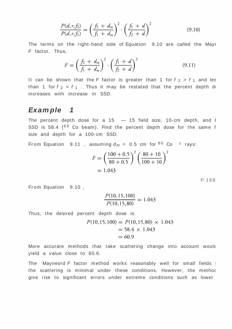
The terms on the right-hand side of Equation 9.10 are called the Mayneord

F factor. Thus,

It can be shown that the F factor is greater than 1 for f 2 > f 1 and less

than 1 for f 2 < f 1 . Thus it may be restated that the percent depth dose

increases with increase in SSD.

Example 1

The percent depth dose for a 15 — 15 field size, 10-cm depth, and 80-cm

SSD is 58.4 (60 Co beam). Find the percent depth dose for the same field

size and depth for a 100-cm SSD.

From Equation 9.11 , assuming dm = 0.5 cm for 60 Co ³ rays:

P.168

From Equation 9.10 ,

Thus, the desired percent depth dose is:

More accurate methods that take scattering change into account would

yield a value close to 60.6.

The Mayneord F factor method works reasonably well for small fields since

the scattering is minimal under these conditions. However, the method can

give rise to significant errors under extreme conditions such as lower

energy, large field, large depth, and large SSD change. For example, the

error in dose at a 20-cm depth for a 30 — 30-cm field and 160-cm SSD

(60 Co beam) will be about 3% if the percent depth dose is calculated from

the 80-cm SSD tables.

In general, the Mayneord F factor overestimates the increase in percent

depth dose with increase in SSD. For example, for large fields and lower

energy radiation where the proportion of scattered radiation is relatively

greater, the factor (1 + F )/2 applies more accurately. Factors intermediate

between F and (1 + F )/2 have also been used for certain conditions (20 ).

9.4. TISSUE-AIR RATIO

Tissue-air ratio (TAR) was first introduced by Johns et al. (6 ) in 1953 and

was originally called the â€œtumor-air ratio.â€ At that time, this quantity

was intended specifically for rotation therapy calculations. In rotation

therapy, the radiation source moves in a circle around the axis of rotation

which is usually placed in the tumor. Although the SSD may vary depending

on the shape of the surface contour, the source-axis distance remains

constant.

Since the percent depth dose depends on the SSD (section 9.3C ), the SSD

correction to the percent depth dose will have to be applied to correct for

the varying SSDâ€”a procedure that becomes cumbersome to apply

routinely in clinical practice. A simpler quantityâ€”namely, TARâ€”has been

defined to remove the SSD dependence. Since the time of its introduction,

the concept of TAR has been refined to facilitate calculations not only for

rotation therapy but also for stationary isocentric techniques as well as

irregular fields.

Tissue-air ratio may be defined as the ratio of the dose (Dd ) at a given

point in the phantom to the dose in free space (Df s ) at the same point.

This is illustrated in Fig. 9.7 .

P.169

For a given quality beam, TAR depends on depth d and field size rd at that

depth:

FIG. 9.7. Illustration of the definition of tissue-air ratio. TAR (d , rd ) = Dd

/Df s .

A. Effect of Distance

One of the most important properties attributed to TAR is that it is

independent of the distance from the source. This, however, is an

approximation which is usually valid to an accuracy of better than 2% over

the range of distances used clinically. This useful result can be deduced as

follows.

Because TAR is the ratio of the two doses (Dd and Df s ) at the same point,

the distance dependence of the photon fluence is removed. Thus the TAR

represents modification of the dose at a point owing only to attenuation

and scattering of the beam in the phantom compared with the dose at the

same point in the miniphantom (or equilibrium phantom) placed in free air.

Since the primary beam is attenuated exponentially with depth, the TAR for

the primary beam is only a function of depth, not of SSD. The case of the

scatter component, however, is not obvious. Nevertheless, Johns et al. (21

) have shown that the fractional scatter contribution to the depth dose is

almost independent of the divergence of the beam and depends only on the

depth and the field size at that depth. Hence the tissue-air ratio, which

involves both the primary and scatter component of the depth dose, is

independent of the source distance.

B. Variation with Energy, Depth, and Field

Size

Tissue-air ratio varies with energy, depth, and field size very much like the

percent depth dose. For the megavoltage beams, the tissue-air ratio builds

up to a maximum at the depth of maximum dose (dm ) and then decreases

with depth more or less exponentially. For a narrow beam or a 0 — 0 field

size3 in which scatter contribution to the dose is neglected, the TAR beyond

dm varies approximately exponentially with depth

where

is the average attenuation coefficient of the beam for the given phantom.

As the field size is increased, the scattered component of the dose

increases and the variation of TAR with depth becomes more complex.

However, for high-energy megavoltage beams, for which the scatter is

minimal and is directed more or less in the forward direction, the TAR

variation with depth can still be approximated by an exponential function,

provided an effective attenuation coefficient ( µeff ) for the given field size

is used.

B.1. Backscatter Factor

The term backscatter factor (BSF) is simply the tissue-air ratio at the depth

of maximum dose on central axis of the beam. It may be defined as the

ratio of the dose on central axis at the depth of maximum dose to the dose

at the same point in free space. Mathematically,

or

where rdm is the field size at the depth dm of maximum dose.

FIG. 9.8. Variation of backscatter factors with beam quality (half-value

layer). Data are for circular fields. (Data from Hospital Physicistsâ€™

Association. Central axis depth dose data for use in radiotherapy. Br J

Radiol 1978;[suppl 11]; and Johns HE, Hunt JW, Fedoruk SO. Surface back-

scatter in the 100 kV to 400 kV range. Br J Radiol 1954;27:443.)

P.170

The backscatter factor, like the tissue-air ratio, is independent of distance

from the source and depends only on the beam quality and field size.

Figure 9.8 shows backscatter factors for various quality beams and field

areas. Whereas BSF increases with field size, its maximum value occurs for

beams having a half-value layer between 0.6 and 0.8 mm Cu, depending on

field size. Thus, for the orthovoltage beams with usual filtration, the

backscatter factor can be as high as 1.5 for large field sizes. This amounts

to a 50% increase in dose near the surface compared with the dose in free

space or, in terms of exposure, 50% increase in exposure on the skin

compared with the exposure in air.

For megavoltage beams (60 Co and higher energies), the backscatter factor

is much smaller. For example, BSF for a 10 — 10-cm field for 60 Co is

1.036. This means that the D max will be 3.6% higher than the dose in free

space. This increase in dose is the result of radiation scatter reaching the

point of D max from the overlying and underlying tissues. As the beam

energy is increased, the scatter is further reduced and so is the backscatter

factor. Above about 8 MV, the scatter at the depth of D max becomes

negligibly small and the backscatter factor approaches its minimum value

of unity.

C. Relationship between TAR and Percent

Depth Dose

Tissue-air ratio and percent depth dose are interrelated. The relationship

can be derived as follows: Considering Fig. 9.9A , let TAR(d,rd ) be the

tissue-air ratio at point Q for a field size rd at depth d . Let r be the field

size at the surface, f be the SSD, and dm be the reference depth of

maximum dose at point P . Let Df s (P ) and Df s (Q ) be the doses in free

space at points P and Q , respectively (Fig. 9.9B,C ). D f s (P ) and Df s (Q )

are related by inverse square law.

P.171

The field sizes r and rd are related by:

By definition of TAR,

or

Since

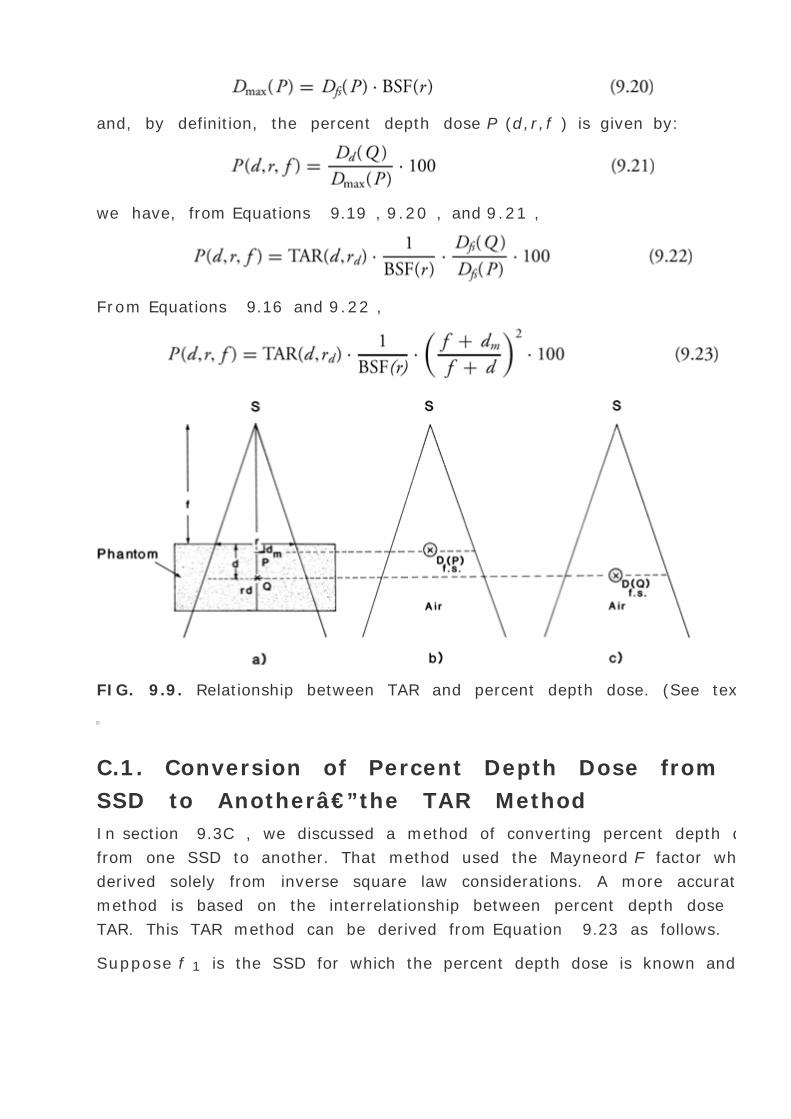
and, by definition, the percent depth dose P (d,r,f ) is given by:

we have, from Equations 9.19 , 9.20 , and 9.21 ,


FIG. 9.9. Relationship between TAR and percent depth dose. (See text.)

C.1. Conversion of Percent Depth Dose from One

SSD to Anotherâ€”the TAR Method

In section 9.3C , we discussed a method of converting percent depth dose

from one SSD to another. That method used the Mayneord F factor which is

derived solely from inverse square law considerations. A more accurate

method is based on the interrelationship between percent depth dose and

TAR. This TAR method can be derived from Equation 9.23 as follows.

Suppose f 1 is the SSD for which the percent depth dose is known and f 2 is

the SSD for which the percent depth dose is to be determined. Let r be the

field size at the surface and

P.172

d be the depth, for both cases. Referring to Fig. 9.6 , let r d,f 1 and r d,f 2 be

the field sizes projected at depth d in Fig. 9.6A,B , respectively.


and

From Equations 9.26 and 9.27 , the conversion factor is given by:

The last term in the brackets is the Mayneord factor. Thus the TAR method

corrects the Mayneord F factor by the ratio of TARs for the fields projected

at depth for the two SSDs.

Burns (22 ) has developed the following equation to convert percent depth

dose from one SSD to another:

where F is the Mayneord F factor given by

Equation 9.29 is based on the concept that TARs are independent of the

source distance. Burns's equation may be used in a situation where TARs

are not available but instead a percent depth dose table is available at a

standard SSD along with the backscatter factors for various field sizes.

As mentioned earlier, for high-energy x-rays, that is, above 8 MV, the

variation of percent depth dose with field size is small and the backscatter

is negligible. Equations 9.28 and 9.29 then simplify to a use of Mayneord F

factor.

Practical Examples

In this section, I will present examples of typical treatment calculations

using the concepts of percent depth dose, backscatter factor, and tissue-air

ratio. Although a more general system of dosimetric calculations will be

presented in the next chapter, these examples are presented here to

illustrate the concepts presented thus far.

Example 2

A patient is to be treated with an orthovoltage beam having a half-value

layer of 3 mm Cu. Supposing that the machine is calibrated in terms of

exposure rate in air, find the time required to deliver 200 cGy (rad) at 5

cm depth, given the following data: exposure rate = 100 R/min at 50 cm,

field size = 8 — 8 cm, SSD = 50 cm, percent depth dose = 64.8,

backscatter factor = 1.20, and rad/R = 0.95 (check these data in reference

5).

P.173

Example 3

A patient is to be treated with 60 Co radiation. Supposing that the machine

is calibrated in air in terms of dose rate free space, find the treatment time

to deliver 200 cGy (rad) at a depth of 8 cm, given the following data: dose

rate free space = 150 cGy/min at 80.5 cm for a field size of 10 — 10 cm,

SSD = 80 cm, percent depth dose = 64.1, and backscatter factor = 1.036.

Example 4

Determine the time required to deliver 200 cGy (rad) with a 60 Co ³ ray

beam at the isocenter (a point of intersection of the collimator axis and the

gantry axis of rotation) which is placed at a 10 cm depth in a patient, given

the following data: SAD = 80 cm, field size = 6 — 12 cm (at the

isocenter), dose rate free space at the SAD for this field = 120 cGy/min

and TAR = 0.681.

Since TAR = Dd /Df s

FIG. 9.10. Contour of patient with radii drawn from the isocenter of

rotation at 20-degree intervals. Length of each radius represents a depth

for which TAR is determined for the field size at the isocenter. (See Table

9.3 .)

P.174

D. Calculation of Dose in Rotation Therapy

The concept of tissue-air ratios is most useful for calculations involving

isocentric techniques of irradiation. Rotation or arc therapy is a type of

isocentric irradiation in which the source moves continuously around the

axis of rotation.

The calculation of depth dose in rotation therapy involves the

determination of average TAR at the isocenter. The contour of the patient is

drawn in a plane containing the axis of rotation. The isocenter is then

placed within the contour (usually in the middle of the tumor or a few

centimeters beyond it) and radii are drawn from this point at selected

angular intervals (e.g., 20 degrees) (Fig. 9.10 ). Each radius represents a

depth for which TAR can be obtained from the TAR table, for the given

beam energy and field size defined at the isocenter. The TARs are then

summed and averaged to determine

, as illustrated in Table 9.3 .

Example 5

For the data given in Table 9.3 , determine the treatment time to deliver

200 cGy (rad) at the center of rotation, given the data: dose rate free

space for 6 — 6-cm field at the SAD is 86.5 cGy/min.

0

16.6

0.444

180

16.2

0.450

20

16.0

0.456

200

16.2

0.450

40

14.6

0.499

220

14.6

0.499

60

11.0

0.614

240

12.4

0.563

80

9.0

0.691

260

11.2

0.606

100

9.4

0.681

280

11.0

0.614

120

11.4

0.597

300

12.0

0.580

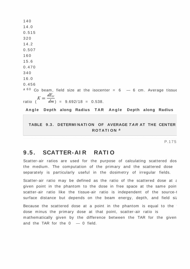
140

14.0

0.515

320

14.2

0.507

160

15.6

0.470

340

16.0

0.456a 60 Co beam, field size at the isocenter = 6 — 6 cm. Average tissue-air

ratio ( ) = 9.692/18 = 0.538.

Angle Depth along Radius TAR Angle Depth along Radius TAR

TABLE 9.3. DETERMINATION OF AVERAGE TAR AT THE CENTER OF

ROTATION a

P.175

9.5. SCATTER-AIR RATIO

Scatter-air ratios are used for the purpose of calculating scattered dose in

the medium. The computation of the primary and the scattered dose

separately is particularly useful in the dosimetry of irregular fields.

Scatter-air ratio may be defined as the ratio of the scattered dose at a

given point in the phantom to the dose in free space at the same point. The

scatter-air ratio like the tissue-air ratio is independent of the source-to-

surface distance but depends on the beam energy, depth, and field size.

Because the scattered dose at a point in the phantom is equal to the total

dose minus the primary dose at that point, scatter-air ratio is

mathematically given by the difference between the TAR for the given field

and the TAR for the 0 — 0 field.

Here TAR(d ,0) represents the primary component of the beam.

Because SARs are primarily used in calculating scatter in a field of any

shape, SARs are tabulated as functions of depth and radius of a circular

field at that depth. Also, because SAR data are derived from TAR data for

rectangular or square fields, radii of equivalent circles may be obtained

from the table in reference 5 or by Equation 9.7 .

A. Dose Calculation in Irregular

Fieldsâ€”Clarkson's Method

Any field other than the rectangular, square, or circular field may be

termed irregular. Irregularly shaped fields are encountered in radiation

therapy when radiation sensitive structures are shielded from the primary

beam or when the field extends beyond the irregularly shaped patient body

contour. Examples of such fields are the mantle and inverted Y fields used

for the treatment of Hodgkin's disease. Since the basic data (percent depth

dose, tissue-air ratios, or tissue-maximum ratiosâ€”to be discussed later)

are available usually for rectangular fields, methods are required to use

these data for general cases of irregularly shaped fields. One such method,

originally proposed by Clarkson (23 ) and later developed by Cunningham

(24 ,25 ), has proved to be the most general in its application.

Clarkson's method is based on the principle that the scattered component

of the depth dose, which depends on the field size and shape, can be

calculated separately from the primary component which is independent of

the field size and shape. A special quantity, SAR, is used to calculate the

scattered dose. This method has been discussed in detail in the literature

(26 ,27 ) and only a brief discussion will be presented here.

Let us consider an irregularly shaped field as shown in Fig. 9.11 . Assume

this field cross-section to be at depth d and perpendicular to the beam axis.

Let Q be the point of calculation in the plane of the field cross-section.

Radii are drawn from Q to divide the field into elementary sectors. Each

sector is characterized by its radius and can be considered as part of a

circular field of that radius. If we suppose the sector angle is 10 degrees,

then the scatter contribution from this sector will be 10 °/360 ° = 1/36

of that contributed by a

P.176

circular field of that radius and centered at Q . Thus the scatter

contribution from all the sectors can be calculated and summed by

considering each sector to be a part of its own circle the scatter-air ratio of

which is already known and tabulated.

FIG. 9.11. Outline of mantle field in a plane perpendicular to the beam

axis and at a specified depth. Radii are drawn from point Q , the point of

calculation. Sector angle = 10 degrees. (Redrawn from American

Association of Physicists in Medicine. Dosimetry workshop: Hodgkin's

disease. Chicago, IL, M.D. Anderson Hospital, Houston, TX, Radiological

Physics Center, 1970.)

Using an SAR table for circular fields, the SAR values for the sectors are

calculated and then summed to give the average scatter-air ratio (

) for the irregular field at point Q . For sectors passing through a blocked

area, the net SAR is determined by subtracting the scatter contribution by

the blocked part of sector. For example, net (SAR)QC = (SAR)QC - (SAR)QB +

(SAR)QA .

The computed

is converted to average tissue-air ratio (

) by the equation:

where TAR(0) is the tissue-air ratio for 0 — 0 field, that is,

where

is the average linear attenuation coefficient for the beam and d is the

depth of point Q .

The percent depth dose (%DD ) at Q may be calculated relative to D max on

the central axis using Equation 9.23 .

where BSF is the backscatter factor for the irregular field and can be

calculated by Clarkson's method. This involves determining TAR at the

depth dm on the central axis, using the field contour or radii projected at

the depth dm .

P.177

In clinical practice, additional corrections are usually necessary such as for

the variation of SSD within the field and the primary beam profile. The

details of these corrections will be discussed in the next chapter.

REFERENCES

1. Shrimpton PC. Electron density values of various human tissues: in

vitro Compton scatter measurements and calculated ranges. Phys Med

Biol 1981;26:907.

2. White DR, Martin RJ, Darlison R. Epoxy resin based tissue

substitutes. Br J Radiol 1977;50:814.

3. International Commission on Radiation Units and Measurements.

Tissue substitutes in radiation dosimetry and measurement. Report No.

44 . Bethesda, MD: International Commission on Radiation Units and

Measurements, 1989.

4. Constantinou C, Attix FH, Paliwal BR. A solid phantom material for

radiation therapy x-ray and ³-ray beam calibrations. Med Phys

1982;9:436.

5. Hospital Physicistsâ€™ Association. Central axis depth dose data for

use in radiotherapy. Br J Radiol 1978; [suppl 11].

6. Johns HE, Whitmore GF, Watson TA, et al. A system of dosimetry for

rotation therapy with typical rotation distributions. J Can Assoc Radiol

1953;4:1.

7. Johns HE. Physical aspects of rotation therapy. AJR 1958;79:373.

8. Cunningham JR, Johns HE, Gupta SK. An examination of the

definition and the magnitude of back-scatter factor for cobalt 60 gamma

rays. Br J Radiol 1965;38:637.

9. Gupta SK, Cunningham JR. Measurement of tissue-air ratios and

scatter functions for large field sizes for cobalt 60 gamma radiation. Br J

Radiol 1966;39:7.

10. Karzmark CJ, Dewbert A, Loevinger R. Tissue-phantom ratiosâ€”an

aid to treatment planning. Br J Radiol 1965;38:158.

11. Saunders JE, Price RH, Horsley RJ. Central axis depth doses for a

constant source-tumor distance. Br J Radiol 1968;41:464.

12. Holt JG, Laughlin JS, Moroney JP. Extension of concept of tissue-air

ratios (TAR) to high energy x-ray beams. Radiology 1970;96:437.

13. Khan FM, Sewchand W, Lee J, et al. Revision of tissue-maximum

ratio and scatter-maximum ratio concepts for cobalt 60 and higher

energy x-ray beams. Med Phys 1980;7:230.


Radiation quantities and units. Report No. 33 . Washington, DC: U.S.

National Bureau of Standards, 1980.


Determination of absorbed dose in a patient irradiated by beams of x or

gamma rays in radiotherapy procedures. Report No. 24 . Washington,

DC: U.S. National Bureau of Standards, 1976.

16. Day MJ. A note on the calculation of dose in x-ray fields. Br J Radiol

1950;23:368.

17. Jones DEA. A note on back-scatter and depth doses for elongated

rectangular x-ray fields. Br J Radiol 1949;22:342.

18. Batho HF, Theimer O, Theimer R. A consideration of equivalent

circle method of calculating depth doses for rectangular x-ray fields. J

Can Assoc Radiol 1956;7:51.

19. Sterling TD, Perry H, Katz I. Derivation of a mathematical

expression for the percent depth dose surface of cobalt 60 beams and

visualization of multiple field dose distributions. Br J Radiol

1964;37:544.

20. Mayneord WV, Lamerton LF. A survey of depth dose data. Br J Radiol

1944;14:255.

21. Johns HE, Bruce WR, Reid WB. The dependence of depth dose on

focal skin distance. Br J Radiol 1958;31:254.

22. Burns JE. Conversion of depth doses from one FSD to another. Br J

Radiol 1958;31:643.

23. Clarkson JR. A note on depth doses in fields of irregular shape. Br J

Radiol 1941;14:265.

24. Johns HE, Cunnningham JR. The physics of radiology , 3rd ed.

Springfield, IL: Charles C Thomas, 1969.

25. Cunningham JR. Scatter-air ratios. Phys Med Biol 1972;17:42.

26. American Association of Physicists in Medicine. Dosimetry workshop:

Hodgkin's disease. Chicago, IL: MD Anderson Hospital, Houston, TX,

Radiological Physics Center, 1970.

27. Khan FM, Levitt SH, Moore VC, et al. Computer and approximation

methods of calculating depth dose in irregularly shaped fields. Radiology

1973;106:433.

1 Alderson Research Laboratories, Inc., Stamford, Connecticut.

2

is the average attenuation coefficient for the heterogeneous beam.

3 A 0 — 0 field is a hypothetical field in which the depth dose is entirely

due to primary photons.





10 - A System of Dosimetric Calculations

10

A System of Dosimetric Calculations

Several methods are available for calculating absorbed dose in a patient.

Two of these methods using percent depth doses and tissue-air ratios

(TARs) were discussed in Chapter 9 . However, there are some limitations

to these methods. For example, the dependence of percent depth dose on

source-to-surface distance (SSD) makes this quantity unsuitable for

isocentric techniques. Although tissue-air ratios (TAR) and scatter-air

ratios (SAR) eliminate that problem, their application to beams of energy

higher than those of 60 Co has been seriously questioned (1 ,2 ,3 ) as

they require measurement of dose in free space. As the beam energy

increases, the size of the chamber build-up cap for in-air measurements

has to be increased and it becomes increasingly difficult to calculate the

dose in free space from such measurements. In addition, the material of

the build-up cap is usually different from that of the phantom and this

introduces a bias or uncertainty in the TAR measurements.

In order to overcome the limitations of the TAR, Karzmark et al. (1 )

introduced the concept of tissue-phantom ratio (TPR). This quantity

retains the properties of the TAR but limits the measurements to the

phantom rather than in air. A few years later, Holt et al. (4 ) introduced

yet another quantity, tissue-maximum ratio (TMR), which also limits the

measurements to the phantom.

In this chapter, I develop a dosimetric system based on the TMR concept,

although a similar system can also be derived from the TPR concept (5 ).

10.1. DOSE CALCULATION PARAMETERS

The dose to a point in a medium may be analyzed into primary and

scattered components. The primary dose is contributed by the initial or

original photons emitted from the source and the scattered dose is the

result of the scattered photons. The scattered dose can be further

analyzed into collimator and phantom components, because the two can

be varied independently by blocking. For example, blocking a portion of

the field does not significantly change the output or exposure in the open

portion of the beam (6 ,7 ) but may substantially reduce the phantom

scatter.

The above analysis presents one practical difficulty, namely, the

determination of primary dose in a phantom which excludes both the

collimator and phantom scatter. However, for megavoltage photon beams,

it is reasonably accurate to consider collimator scatter as part of the

primary beam so that the phantom scatter could be calculated separately.

We, therefore, define an effective primary dose as the dose due to the

primary photons as well as those scattered from the collimating system.

The effective primary in a phantom may be thought of as the dose at

depth minus the phantom scatter. Alternatively, the effective primary

dose may be defined as the depth dose expected in the field when

scattering volume is reduced to zero while keeping the collimator opening

constant.

Representation of primary dose by the dose in a 0 — 0 field poses

conceptual problems because of the lack of lateral electronic equilibrium

in narrow fields in megavoltage photon beams. This issue has been

debated in the literature (8 ,9 ,10 ), but practical solutions are still not

agreed on. Systems that use electron transport in the calculation of

primary and scattered components of dose would be appropriate but are

not as yet fully developed and

P.179

implemented. Until then, the concept of 0 — 0 field to represent

primary beams with the implicit assumption that lateral electronic

equilibrium exists at all points will continue to be used for routine

dosimetry.

FIG. 10.1. Arrangement for measuring Sc and Sc,p . A: Chamber with

build-up cap in air to measure output relative to a reference field, for

determining Sc versus field size. B: Measurements in a phantom at a

fixed depth for determining S c,p versus field size. (From Khan FM,

Sewchand W, Lee J, et al. Revision of tissue-maximum ratio and scatter-

maximum ratio concepts for cobalt 60 and higher energy x-ray beams.


A. Collimator Scatter Factor

The beam output (exposure rate, dose rate in free space, or energy

fluence rate) measured in air depends on the field size. As the field size

is increased, the output increases because of the increased collimator

scatter,1 which is added to the primary beam.

The collimator scatter factor (Sc ) is commonly called the output factor

and may be defined as the ratio of the output in air for a given field to

that for a reference field (e.g., 10 — 10 cm). Sc may be measured with

an ion chamber with a build-up cap of a size large enough to provide

maximum dose build-up for the given energy beam. The measurement

setup is shown in Fig. 10.1A . Readings are plotted against field size (side

of equivalent square or area/perimeter [A/P ]) and the values are

normalized to the reference field (10 — 10 cm).

In the measurement of Sc , the field must fully cover the build-up cap for

all field sizes if measurements are to reflect relative photon fluences. For

small fields, one may take the measurements at large distances from the

source so that the smallest field covers build-up cap. Normally, the

collimator scatter factors are measured at the source-to-axis distance

(SAD). However, larger distances can be used provided the field sizes are

all defined at the SAD.

B. Phantom Scatter Factor

The phantom scatter factor (Sp ) takes into account the change in scatter

radiation originating in the phantom at a reference depth as the field size

is changed. Sp may be defined as the ratio of the dose rate for a given

field at a reference depth (e.g., depth of maximum dose) to the dose rate

at the same depth for the reference field size (e.g., 10 — 10 cm), with

the same collimator opening. In this definition, it should be noted that Sp

is related to the changes in the volume of the phantom irradiated for a

fixed collimator opening. Thus one

P.180

could determine Sp , at least in concept, by using a large field incident on

phantoms of various cross-sectional sizes.

For photon beams for which backscatter factors can be accurately

measured (e.g., 60 Co and 4 MV), Sp factor at the depth of maximum dose

may be defined simply as the ratio of backscatter factor (BSF) for the

given field to that for the reference field (see Appendix, section A ).

Mathematically,

where r 0 is the side of the reference field size (10 — 10 cm).

A more practical method of measuring Sp , which can be used for all beam

energies, consists of indirect determination from the following equation

(for derivation, see Appendix, section A ):

where Sc,p (r ) is the total scatter factor defined as the dose rate at a

reference depth for a given field size r divided by the dose rate at the

same point and depth for the reference field size (10 — 10 cm) (Fig.

10.1B ). Thus Sc,p (r ) contains both the collimator and phantom scatter

and when divided by Sc (r ) yields Sp (r ).

Since Sp and Sc,p are defined at the reference depth of D max , actual

measurement of these factors at this depth may create problems because

of the possible influence of contaminant electrons incident on the

phantom. This can be avoided by making measurements at a greater

depth (e.g., 10 cm) and converting the readings to the reference depth of

D max by using percent depth dose data, presumably measured with a

small-diameter chamber. The rationale for this procedure is the same as

for the recommended depths of calibration (11 ).

C. Tissue-Phantom and Tissue-Maximum

Ratios

The TPR is defined as the ratio of the dose at a given point in phantom to

the dose at the same point at a fixed reference depth, usually 5 cm. This

is illustrated in Fig. 10.2 . The corresponding quantity for the scattered

dose calculation is called the scatter-phantom ratio (SPR), which is

analogous in use to the scatter-air ratio discussed in the previous

chapter. Details of the TPR and SPR concepts have been discussed in the

literature (1 ,3 ,5 ).

TPR is a general function which may be normalized to any reference

depth. But there is no general agreement concerning the depth to be used

for this quantity, although a 5-cm depth is the usual choice for most

beam energies. On the other hand, the point of central axis D max has a

simplicity that is very desirable in dose computations. If adopted as a

fixed

P.181

reference depth, the quantity TPR gives rise to the TMR. Thus TMR is a

special case of TPR and may be defined as the ratio of the dose at a given

point in phantom to the dose at the same point at the reference depth of

maximum dose (Fig. 10.2 ).

FIG. 10.2. Diagram illustrating the definitions of tissue-phantom ratio

(TPR) and tissue-maximum ratio (TMR). TPR(d, rd ) = Dd /Dt0 , where t 0

is a reference depth. If t 0 is the reference depth of maximum dose, then

TMR(d, rd ) = TPR(d, rd ) .

For megavoltage beams in the range of 20 to 45 MV, the depth of

maximum dose (dm ) has been found to depend significantly on field size

(12 ,13 ) as well as on SSD (14 ,15 ). For the calculative functions to be

independent of machine parameters, they should not involve

measurements in the build-up region. Therefore, the reference depth

must be equal to or greater than the largest (dm ). Since (dm ) tends to

decrease with field size (12 ) and increase with SSD (14 ), one should

choose (dm ) for the smallest field and the largest SSD. In practice, one

may plot [(DD) — (SSD + d )2 ] as a function of depth d to find (dm )

(15 ). This eliminates dependence on SSD. The maximum (dm ) can then

be obtained by plotting (dm ) as a function of field size and extrapolating

to 0 — 0 field size.

The reference depth of maximum dose (t 0 ), as determined above, should

be used for percent depth dose, TMR, and Sp factors, irrespective of field

size and SSD.

C.1. Properties of TMR

The concept of tissue-maximum ratio is based on the assumption that the

fractional scatter contribution to the depth dose at a point is independent

of the divergence of the beam and depends only on the field size at the

point and the depth of the overlying tissue. This has been shown to be

essentially true by Johns et al. (16 ). This principle, which also underlies

TAR and TPR, makes all these functions practically independent of source-

surface distance. Thus a single table of TMRs can be used for all SSDs for

each radiation quality.

Figure 10.3 shows TMR data for for 10-MV x-ray beams as an example.

The curve for 0 — 0 field size shows the steepest drop with depth and is

caused entirely by the primary beam. For megavoltage beams, the

primary beam attenuation can be approximately represented by:

where µ is the effective linear attenuation coefficient and t 0 is the

reference depth of maximum dose. µ can be determined from TMR data

by plotting µ as a function of field size (side of equivalent square) and

extrapolating it back to 0 — 0 field.

TMR and percent depth dose P are interrelated by the following equation

(see Appendix, section B , for derivation).

where

Here the percent depth dose is referenced against the dose at depth t 0 so

that P (t 0 , r, f ) = 100 for all field sizes and SSDs.

Although TMRs can be measured directly, they can also be calculated from

percent depth doses, as shown by Equation 10.4 . For 60 Co, Equations

10.2 and 10.4 can be used to calculate TMRs. In addition, TMRs can be

derived from TAR data in those cases, such as 60 Co, where TARs are

accurately known:

FIG. 10.3. Plot of TMR for 10-MV x-rays as a function of depth for a

selection of field sizes.

P.182

D. Scatter-Maximum Ratio

The scatter-maximum ratio (SMR), like the SAR, is a quantity designed

specifically for the calculation of scattered dose in a medium. It may be

defined as the ratio of the scattered dose at a given point in phantom to

the effective primary dose at the same point at the reference depth of

maximum dose (5 ). Mathematically,

For derivation of the above equation, see Appendix, section C .

From Equations 10.1 , 10.5 , and 10.6 , it can be shown that for 60 Co ³

rays, SMRs are approximately the same as SARs. However, for higher

energies, SMRs should be calculated from TMRs by using Equations 9.7

and 10.6 .

Another interesting relationship can be obtained at the reference depth of

maximum dose (t 0 ). Since TMR at depth t 0 is unity by definition,

Equation 10.6 becomes:

This equation will be used in section 10.2C .

P.183

10.2. PRACTICAL APPLICATIONS

Radiotherapy institutions vary in their treatment techniques and

calibration practices. For example, some rely exclusively on the SSD or

the SAD (isocentric) type techniques, while others use both. Accordingly,

units are calibrated in air or in phantom at a suitable reference depth. In

addition, clinical fields, although basically rectangular or square, are

often shaped irregularly to protect critical or normal regions of the body.

Thus a calculation system must be generally applicable to the above

practices, with acceptable accuracy and simplicity for routine use.

A. Accelerator Calculations

A.1. SSD Technique

Percent depth dose is a suitable quantity for calculations involving SSD

techniques. Machines are usually calibrated to deliver 1 rad (10-2 Gy) per

monitor unit (MU) at the reference depth t 0 , for a reference field size 10

— 10 cm and a source-to-calibration point distance of SCD. Assuming

that the Sc factors relate to collimator field sizes defined at the SAD, the

monitor units necessary to deliver a certain tumor dose (TD) at depth d

for a field size r at the surface at any SSD are given by:

where K is 1 rad per MU, rc is the collimator field size, given by:

and:

It must be remembered that, whereas the field size for the Sc is defined

at the SAD, Sp relates to the field irradiating the patient.

Example 1

A 4-MV linear accelerator is calibrated to give 1 rad (10-2 Gy) per MU in

phantom at a reference depth of maximum dose of 1 cm, 100-cm SSD,

and 10 — 10 cm field size. Determine the MU values to deliver 200 rads

to a patient at 100-cm SSD, 10-cm depth, and 15 — 15 cm field size,

given Sc (15 — 15) = 1.020, Sp (15 — 15) = 1.010, %DD = 65.1.


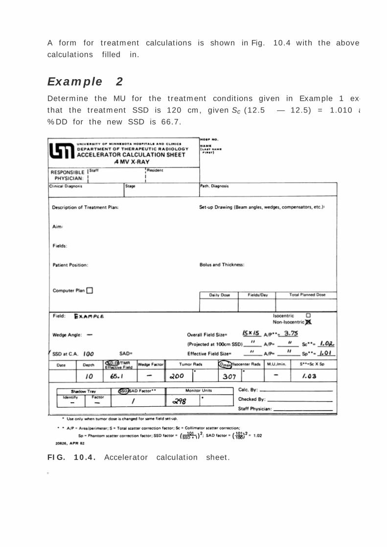
A form for treatment calculations is shown in Fig. 10.4 with the above

calculations filled in.

Example 2

Determine the MU for the treatment conditions given in Example 1 except

that the treatment SSD is 120 cm, given Sc (12.5 — 12.5) = 1.010 and

%DD for the new SSD is 66.7.

FIG. 10.4. Accelerator calculation sheet.

P.184


A.2. Isocentric Technique

TMR is the quantity of choice for dosimetric calculations involving

isocentric techniques. Since the unit is calibrated to give 1 rad (10-2

Gy)/MU at the reference depth t 0 , calibration distance SCD, and for the

reference field (10 — 10 cm), then the monitor units necessary to

deliver isocenter dose (ID) at depth d are given by:

where

Example 3

A tumor dose of 200 rads is to be delivered at the isocenter which is

located at a depth of 8 cm, given 4-MV x-ray beam, field size at the

isocenter = 6 — 6 cm, Sc (6 — 6) = 0.970,

P.185

Sp (6 — 6) = 0.990, machine calibrated at SCD = 100 cm, TMR(8, 6 —

6) = 0.787. Since the calibration point is at the SAD, SAD factor = 1.

Thus, using Equation 10.9 ,

Example 4

Calculate MU values for the case in Example 3, if the unit is calibrated

nonisocentrically, i.e., source to calibration point distance = 101 cm.

Thus,

B. Cobalt-60 Calculations

The above calculation system is sufficiently general that is can be applied

to any radiation generator, including 60 Co. In the latter case, the

machine can be calibrated either in air or in phantom provided the

following information is available: (a ) dose rate D 0 (t 0 , r 0 , f 0 ) in

phantom at depth t 0 of maximum dose for a reference field size r 0 and

standard SSD f 0 ; (b ) Sc ; (c ) Sp ; (d ) percent depth doses; and (e )

TMR values. If universal depth dose data for 60 Co (16 ) are used, then

the Sp and TMRs can be obtained by using Equations 10.1 and 10.5 . In

addition, the SSD used in these calculations should be confined to a

range for which the output in air obeys an inverse square law for a

constant collimator opening.

A form for cobalt calculations is presented in Fig. 10.5 .

FIG. 10.5. Calculation sheetâ€”cobalt-60.

P.186

Example 5

A tumor dose of 200 rads is to be delivered at a 8-cm depth, using 15

— 15-cm field size, 100-cm SSD, and penumbra trimmers up. The unit

is calibrated to give 130 rads/min in phantom at a 0.5-cm depth for a 10

— 10-cm field with trimmers up and SSD = 80 cm. Determine the time

of irradiation, given Sc (12 — 12) = 1.012, Sp (15 — 15) = 1.014,

and %DD (8, 15 — 15, 100) = 68.7.

C. Irregular Fields

Dosimetry of irregular fields using TMRs and SMRs is analogous to the

method using TARs and SARs (section 9.5 ). Since the mathematical

rationale of the method has been discussed in detail in the literature (5 ),

only a brief outline will be presented here to illustrate the procedure.

An irregular field at depth d may be divided into n elementary sectors

with radii emanating from point Q of calculation (Fig. 9.10 ). A Clarkson

type integration (Chapter 9 ) may be performed to give averaged scatter-

maximum ratio (

(d,rd )) for the irregular field rd :

where r i is the radius of the i th sector at depth d and n is the total

number of sectors (n = 2 €/ ” ¸, where ” ¸ is the sector angle).

The computed

(d,rd ) is then converted to

(d,rd ) by using Equation 10.6 .

P.187

where

p ,(rd ) is the averaged Sp for the irregular field and Sp (0) is the Sp for

the 0 — 0 area field. The above equation is strictly valid only for points

along the central axis of a beam that is normally incident on an infinite

phantom with flat surface. For off-axis points in a beam with nonuniform

primary dose profile, one should write

where Kp is the off-axis ratio representing primary dose at point Q

relative to that at the central axis.

(d,rd ) may be converted into percent depth dose P (d, r, f ) by using

Equation 10.4 .

From Equations 10.7 and 10.13 we get the final expression:

Thus the calculation of percent depth dose for an irregular field requires a

Clarkson integration over the function SMR both at the point of

calculation Q as well as at the reference depth (t 0 ) at central axis.

C.1. SSD Variation Within the Field

The percent depth dose at Q is normalized with respect to the D max on

the central axis at depth t 0 . Let f 0 be the nominal SSD along the

central axis, g be the vertical gap distance, i.e., â€œgapâ€ between

skin surface over Q and the nominal SSD plane, and d be the depth of Q

from skin surface. The percent depth dose is then given by:

The sign of g should be set positive or negative, depending on if the SSD

over Q is larger or smaller than the nominal SSD.

C.2. Computer Program

A computer algorithm embodying the Clarkson's principle and scatter-air

ratios was developed by Cunningham et al. (17 ) at the Princess Margaret

Hospital, Toronto, and was published in 1970. Another program, based on

the same principle, was developed by Khan (18 ) at the University of

Minnesota. It was originally written for the CDC-3300 computer using

SARs and later rewritten for the Artronix PC-12 and PDP 11/34 computers.

The latter versions use SMRs instead of SARs.

The following data are permanently stored in this computer program: (a)

a table of SMRs as functions of radii of circular fields and (b) the off-axis

ratios Kp , derived from dose profiles at selected depths. These data are

then stored in the form of a table of Kp as a function of l /L where l is the

lateral distance of a point from the central axis and L is the distance

along the same line to the geometric edge of the beam. Usually large

fields are used for these measurements.

The following data are provided for a particular patient:

Contour points: the outline of the irregular field can be drawn from

the port (field) film with actual blocks or markers in place to define

the field. The field contour is then digitized and the coordinates

stored in the computer.

The coordinates (x, y) of the points of calculation are also entered,

including the reference point, usually on the central axis, against

which the percent depth doses are calculated.

Patient measurements: patient thickness at various points of interest,

SSDs, and source-to-film distance are measured and recorded as

shown in Fig. 10.6 for a mantle field as an example.

Figure 10.7 shows a daily table calculated by the computer for a typical

mantle field. Such a table is useful in programming treatments so that

the dose to various regions of the

P.188

field can be adjusted. The areas that receive the prescribed dose after a

certain number of treatments are shielded for the remaining sessions.

FIG. 10.6. Form for recording patient and dosimetric data for mantle

field. Note that the measurement points are standardized by anatomic

landmarks.

D. Asymmetric Fields

Many of the modern linear accelerators are equipped with x-ray

collimators (or jaws) that can be moved independently to allow

asymmetric fields with field centers positioned away from the true central

axis of the beam. For example, an independent jaw can be moved to block

off half of the field along central axis to eliminate beam divergence. This

feature is useful for matching adjacent fields. Although this function can

also be performed by beam splitters or secondary blocking on a shadow

tray, an independent jaw feature reduces the setup time and spares the

therapist from handling heavy blocks.

The effect of asymmetric beam collimation on dose distribution has been

discussed in the literature (19 ,20 ). When a field is collimated

asymmetrically, one needs to take into account changes in the collimator

scatter, phantom scatter, and off-axis beam quality. The

P.189

latter effect arises as a consequence of using beam-flattening filters

(thicker in the middle and thinner in the periphery), which results in

greater beam hardening close to the central axis compared with the

periphery of the beam (21 ,22 ).

FIG. 10.7. Computer output sheet showing cumulative midthickness

doses for a mantle field. Total dose to various points is programmed by a

line drawn through the table. As soon as a given area reaches its

prescribed dose, it is shielded during subsequent treatments. It is not

necessary to recalculate the table with this change in blocking since only

a few treatments are affected.

A dose calculation formalism for asymmetric fields has been developed

which is described below.

For a point at the center of an asymmetric field and a lateral distance x

away from the beam central axis, the collimator scatter factor may be

approximated to a symmetric field of the same collimator opening as that

of the given asymmetric field. In other words, the Sc will depend on the

actual collimator opening, ignoring small changes in the scattered photon

fluence that may result owing to the change in the angle of the

asymmetric jaws relative to the beam. This approximation is reasonable

as long as the point of dose calculation is centrally located, that is, away

from field edges.

The phantom scatter can also be assumed to be the same for an

asymmetric field as for a symmetric field of the same dimension and

shape, provided the point of calculation is located away from the field

edges to avoid penumbral effects.

The primary dose distribution has been shown to vary with lateral

distance from central axis because of the change in beam quality, as

mentioned earlier. Therefore, the percent depth dose or TMR distribution

along the central ray of an asymmetric field is not the same as along the

central axis of a symmetric field of the same size and shape. In addition,

the incident primary beam fluence at off-axis points varies as a function

of distance from the central axis, depending on the flattening filter

design. These effects are not emphasized in the dosimetry of symmetric

fields, because target doses are usually specified at the beam central axis

and the off-axis dose distributions are viewed from the isodose curves. In

asymmetric fields, however, the target or the point of interest does not

lie on the beam central axis; therefore, an off-axis dose correction may

be required in the calculation of target dose. This correction will depend

on the depth and the distance from the central axis of the point of

interest.

Since beam flatness within the central 80% of the maximum field size is

specified within ±3% at a 10-cm depth, ignoring off-axis dose

correction in asymmetric fields will introduce errors of that magnitude

under these conditions. Thus the off-axis dose

P.190

correction will follow changes in the primary beam flatness as a function

of depth and distance from central axis.

In view of the above discussion, the following equations are proposed for

the calculation of monitor units for asymmetric fields.

For SSD type of treatments, Equation 10.8 is modified to:

where OARd (x ) is the primary off-axis ratio at depth d , that is, ratio of

primary dose at the off-axis point of interest to the primary dose at the

central axis at the same depth for a symmetrically wide open field.

Primary off-axis ratios may be extracted from depth dose profiles of the

largest field available by subtracting scatter. A direct method consists of

measuring transmitted dose profiles through different thicknesses of an

absorber under â€œgood geometryâ€ conditions (a narrow beam and a

large detector-to-absorber distance) (23 ). Another direct but

approximate method is to measure profiles as a function of depth for a

narrow elongated field (e.g., 5 — 40 cm). Since the primary dose profile

is created by the flattening filter, which has a radial symmetry, primary

OAR data can be tabulated as a function of depth and radial distance from

central axis.

For isocentric type of treatments, Equation 10.9 is modified to:

The above formalism is general and can be used for an off-axis point dose

calculation in symmetric or asymmetric fields generated by blocks or

collimators, including multileaf collimators. For irregularly shaped fields

the parameter rd is the equivalent field size determined by Clarkson's

technique or geometric approximation (section 10.3 ). The parameter rc i s

the collimator opening size projected at the standard SSD.

10.3. OTHER PRACTICAL METHODS OF

CALCULATING DEPTH DOSE DISTRIBUTION

A. Irregular Fields

Clarkson's technique is a general method of calculating depth dose

distribution in an irregularly shaped field, but it is not practical for

routine manual calculations. Even when computerized, it is time-

consuming since a considerable amount of input data is required by the

computer program. However, with the exception of mantle, inverted Y ,

and a few other complex fields, reasonably accurate calculations can be

made for most blocked fields using an approximate method (18 ), to be

discussed.

Figure 10.8 shows a number of blocked fields encountered in

radiotherapy. Approximate rectangles may be drawn containing the point

of calculation to include most of the irradiated area surrounding the point

and exclude only those areas that are remote to the point. In so doing, a

blocked area may be included in the rectangle, provided this area is small

and is remotely located relative to that point. The rectangle thus formed

may be called the effective field , while the unblocked field, defined by

the collimator, may be called the collimator field .

Once the effective field has been determined, one may proceed with the

usual calculations as discussed in section 10.2 . However, it is important

to remember that, whereas the Sc is related to the collimator field, the

percent depth dose, TMR, or Sp corresponds to the effective field.

B. Point Off-Axis

It is possible to calculate depth dose distributions at any point within the

field or outside the field using Clarkson's technique. However, as stated

earlier, it is not practical for manual calculations. Day (24 ) has proposed

a particularly simple calculation method for

P.191

rectangular fields. In this method, percent depth dose can be calculated

at any point within the medium using the central axis data.

FIG. 10.8. Examples of irregularly shaped fields. Equivalent rectangles

for dose at points of interest are shown by dashed lines. Points versus

equivalent rectangles are (A) 1, GHKL; 2, ABEJ; (B) 1, AGHD; 2, LIJK;

(C) 1, EFGH; (D) 1, KLGH . From Levitt SH, Khan FM, Potish RA, eds.

Technological basis of radiation therapy: practical and clinical applications

, 2nd ed. Philadelphia: Lea & Febiger, 1992:73, with permission.

To calculate dose at any point Q , the field is imagined to be divided into

four sections (Fig. 10.9 ) and their contribution is computed separately.

Thus the dose at depth d along the axis through Q is given by ¼(sum of

central axis dose at depth d for fields 2a — 2b , 2a — 2c , 2d — 2b ,

and 2d — 2c ).

Suppose the dose in free space on the central axis through P at SSD +

(dm ) is 100 cGy (rad) and its value at a corresponding point over Q is K Q

— 100, where KQ is the off-axis ratio determined in air from the

primary beam profile. If the BSF and central axis %DD for rectangular

fields are available, the dose at depth d along the axis through Q will be

given by:

FIG. 10.9. Day's method of calculating dose at any point Q in a

rectangular field. (See text.)

P.192

Since the D max at P is 100 — BSF[(a + d ) — (b + c )], the percent

depth dose at depth d along the axis through Q , relative to D max at P ,

will be given by:

Example 6

Suppose in Fig. 10.9 that the overall field size is 15 — 15 cm. Find the

percent depth dose at point Q at 10 cm depth, given a = 10, b = 5, c =

10, and d = 5. Assume 60 Co beam with KQ = 0.98 and SSD = 80 cm.

Using the above procedure and consulting Table A.9.1 in the Appendix to

the book, the required percent depth dose is given by:

or

In the above example, if the primary beam profile were flat, that is, KQ =

1, the percent depth dose at Q would be 56.9, which is still less than

58.4, the percent depth dose at P . This off-axis decrease in dose is due

to the reduced scatter at point Q compared with point P . Similarly, it can

be shown that the magnitude of the reduction in scatter depends on the

distance of Q from P as well as depth. Thus the depth dose profile across

the field is a function not only of the beam flatness in air but also the

depth in the phantom.

For higher-energy beams (â‰¥8 MV), the above procedure may be

further simplified by assuming BSF = 1 for all field sizes. Also, Day's

procedure can be adopted using Sp values instead of BSF, since the two

quantities are related by Equation 10.1 .

FIG. 10.10. Calculation of depth dose outside a rectangular field. (See

text.)

C. Point Outside the Field

Day's method can be extended also to the case of determining dose

distribution at points outside the field limits. In Fig. 10.10 , a rectangular

field of dimensions a — b is shown with the central axis passing through

P . Suppose Q is a point outside the field at a distance c from the field

border. Imagine a rectangle adjacent to the field such that it contains

point Q and has dimensions 2c — b . Place another rectangle of

dimensions a — b on the other side of Q such that the field on the right

of Q is a mirror image of the field on the left, as shown in the figure. The

dose at point Q at depth d is then given by subtracting the depth dose at

Q for field 2c — b from that for field (2a + 2c ) — b and dividing by 2.

The procedure is illustrated by the following example.

P.193

Example 7

Suppose it is required to determine percent depth dose at Q (relative to D

max at P ) outside a 15 — 10-cm field at a distance of 5 cm from the

field border. In Fig. 10.10 , then, a = 15, b = 10, and c = 5. Suppose Q is

at the center of the middle rectangle of dimensions 2c — b . Then the

dose DQ at 10-cm depth is given by:

½ [DQ (40 — 10) - DQ (10 — 10)]

If DQ is normalized to D max at P , one gets the percent depth dose at Q

or %DQ .

Thus for a 60 Co beam at SSD = 80 cm,

Again for higher-energy beams, the above procedure is simplified by

assuming BSF = 1. Also, if Sp values are known instead of BSF, the above

calculation can be performed by substituting Sp for BSF.

D. Point Under the Block

As discussed earlier, the dose distribution in a blocked field is best

determined by Clarkson's method of irregular field dosimetry. However, if

the blocked portion of the field is approximated to a rectangle, a simpler

method known as negative field method may be used. The concept of

negative field has been described in the literature (25 ,26 ). In this

method, the dose at any point is equal to the dose from the overall

(unblocked) field minus the dose expected if the entire field were

blocked, leaving the shielded volume open. In other words, the blocked

portion of the field is considered a negative field and its contribution is

subtracted from the overall field dose distribution.

A computerized negative field method not only is a fast method of

calculating isodose distribution in blocked fields but is very convenient

for manual point dose calculation. Its practical usefulness is illustrated by

Example 8.

Example 8

A patient is treated with a split field of overall size 15 — 15 cm,

blocked in the middle to shield a region of size 4 — 15 cm on the

surface (Fig. 10.11 ). Calculate (a) the treatment time to deliver 200 cGy

(rad) at a 10-cm depth at point P in the open portion of the field

P.194

and (b) what percentage of that dose is received at point Q in the middle

of the blocked area, given 60 Co beam, SSD = 80 cm, dose rate free

space for a 15 — 15-cm field at 80.5 cm = 120 rads/min, lead block

thickness = 5 cm with primary beam transmission of 5%, and shadow tray

(or block tray) transmission = 0.97.

FIG. 10.11. Example of calculating depth dose under a block.

Approximate equivalent field at point P [asymptotically equal to]

5.5 — 15, assuming negligible scatter contribution to P from the

other open portion of the field across the blocked area.

DQ = DQ (15 — 15) - DQ (4 — 15) — (1 - T )

where T is the transmission factor for the lead block.

Thus,

Since Dp = 200 cGy (given)

Alternative

Let us project all fields at depth = 10 cm.

Projected fields.

(15 — 15) cm — 1.125 = 17 — 17 cm

(4 — 15) cm — 1.125 = 4.5 — 17 cm = 7 — 7 cm equivalent

square

(5.5 — 15) cm — 1.125 = 6.2 — 17 cm = 9 — 9 cm equivalent

square

P.195

Alternative

Since

Substituting values from Table A.9.2 in the Appendix to the book

Although the primary transmission through the lead block is only 5%, the

dose at a 10-cm depth under the block in the middle is about 20% of the

dose in the open portion. This increase in dose is a result of the internal

scatter contributed by the open areas of the field to point Q . Of course,

the dose under the block depends on the extent of the blocked area,

overall field size, block thickness, depth, and location of point Q .

Appendices

APPENDIX TO CHAPTER

A. Derivation of Sp

Sp (r ), as defined in section 10.1B , is the ratio of dose rate for the given

field (r ) at a reference depth to the dose rate at the same point for the

reference field size (r 0 ), with the same collimator opening. This is

illustrated in Fig. 10.12 . The given field in Fig. 10.12A is blocked down

to the size of the reference field in Fig. 10.12B without changing the

collimator opening. Thus both arrangements have the same collimator

scatter factor, Sc (r ),

P.196

but different phantom scatter. Let Df s and D max be the free space dose

rate and D max dose rate, respectively. Then, at the reference depth of

maximum dose,

which is the same as Equation 10.1 .

Equation A1 can also be written as:

where Sc,p (r ) is the total scatter correction factor defined as the ratio of

D max dose rate for a given field to the D max dose rate for the reference

field (Fig. 10.1B ).

FIG. 10.12. Diagrams to illustrate definition of Sp . A: Dose in phantom

at reference depth for a given field. B: Dose at the same point for a

reference field with the same collimator opening. (From Khan FM,

Sewchand W, Lee J, et al. Revision of tissue-maximum ratio and scatter-

maximum ratio concepts for cobalt 60 and higher energy x-ray beams.


B. Derivation of TMR

In Fig. 10.2 , let D 1 and D 2 be the doses at depths d and t 0 (reference

depth of maximum dose), respectively. Let r, r t 0 , and rd be the field

sizes at distances f, f + t 0 , and f + d from the source, respectively.

Then, by definition:

and

where D (t 0 , rt0 , f ) is the dose at depth t 0 , field size rt0 and SSD = f .

Combining Equations A4 , A5 , and A6 ,

C. Derivation of SMR

Referring to Fig. 10.2 , let D 1 (d, rd ) be the dose at point 1 and D 2 (t 0

, rd ) be the dose at point 2 for field size rd . Let D 1 (d , 0) and D 2 (t 0 ,

0) be the corresponding doses for 0 — 0 field with the same collimator

opening. Then:

P.197

or

where r 0 is the reference field (10 — 10 cm) for normalizing Sp .

Since:

and

Equation A9 becomes:

REFERENCES

1. Karzmark CJ, Deubert A, Loevinger R. Tissue-phantom ratiosâ€”an

aid to treatment planning. Br J Radiol 1965;38:158.

2. Holt JG. Letter to the editor. Am Assoc Phys Med Q Bull

1972;6:127.

3. Saunders JE, Price RH, Horsley RJ. Central axis depth doses for a

constant source-tumor distance. Br J Radiol 1968;41:464.

4. Holt JG, Laughlin JS, Moroney JP. The extension of the concept of

tissue-air ratios (TAR) to high energy x-ray beams. Radiology

1970;96:437.

5. Khan FM, Sewchand W, Lee J, et al. Revision of tissue-maximum

ratio and scatter-maximum ratio concepts for cobalt 60 and higher

energy x-ray beams. Med Phys 1980;7:230.

6. Khan FM. Dose distribution problems in cobalt teletherapy [Thesis] .

University of Minnesota, 1969:106.

7. Cundiff JH, Cunningham JR, Golden R, et al. RPC/AAPM, compiler.

Dosimetry workshop on Hodgkin's disease . Houston, TX: MD Anderson

Hospital, 1970.

8. Mohan R, Chui C. Validity of the concept of separating primary and

scatter dose. Med Phys 1985;12:726.

9. Bjarngard BE, Cunningham JR. Comments on â€œValidity of the

concept of separating primary and scatter doseâ€ . Med Phys

1986;13:760.

10. Mohan R, Chui C. Reply to comments by Bjarngard and

Cunningham. Med Phys 1986;13:761.

11. American Association of Physicists in Medicine. A protocol for the

determination of absorbed dose from high energy photon and electron

beams. Med Phys 1983;10:741.

12. Almond P, Roosenbeek EV, Browne R, et al. Variation in the

position of the central axis maximum build-up point with field size for

high-energy photon beams [Letter to the Editor]. Br J Radiol

1970;43:911.

13. Dawson DJ. Percentage depth doses for high energy x-rays. Phys

Med Biol 1976;21:226.

14. Bagne F. Physical aspects of supervoltage x-ray therapy. Med Phys

1974;1:266.

15. Suntharalingam N, Steben DJ. Physical characterization of 45-MV

photon beams for use in treatment planning. Med Phys 1977;4:134.

16. Johns HE, Bruce WR, Reid WB. The dependence of depth dose on

focal skin distance. Br J Radiol 1958;31:254.

17. Cunningham JR, Shrivastava PN, Wilkinson JM. Computer

calculation of dose within an irregularly shaped beam. RPC/AAPM,

compiler. Dosimetry workshop on Hodgkin's disease . Houston, TX: MD

Anderson Hospital, 1970.

18. Khan FM, Levitt SH, Moore VC, et al. Computer and approximation

methods of calculating depth dose in irregularly shaped fields.

Radiology 1973;106:433.

19. Khan FM, Gerbi BJ, Deibel FC. Dosimetry of asymmetric x-ray

collimators. Med Phys 1986;13:936.

20. Loshek DD. Analysis of tissue-maximum ratio/scatter-maximum

ratio model relative to the prediction of tissue-maximum ratio in

asymmetrically collimated fields. Med Phys 1988;15:672.

P.198

21. Hanson WF, Berkley LW. Off-axis beam quality change in linear

accelerator x-ray beams. Med Phys 1980;7:145.

22. Kepka AG, Johnson PM, David J. The effect of off-axis quality

changes on zero area TAR for megavoltage beams. Phys Med Biol

1985;30:589.

23. Gibbons JP, Khan FM. Calculation of dose in asymmetric x-ray

collimators. Med Phys 1995;22:1451â€“1457.

24. Day MJ. A note on the calculation of dose in x-ray fields. Br J

Radiol 1950;23:368.

25. Sundbom L. Method of dose planning on application of shielding

filters in cobalt 60 teletherapy. Acta Radiol Ther Phys Biol 1965;3:210.

26. Khan FM. Computer dosimetry of partially blocked fields in cobalt

teletherapy. Radiology 1970;97:405.

1 Collimator scatter includes photons scattered by all components of the

machine head in the path of the beam.





11 - Treatment Planning I: Isodose Distributions

11

Treatment Planning I: IsodoseDistributions

The central axis depth dose distribution by itself is not sufficient

to characterize a radiation beam that produces a dose

distribution in a three-dimensional volume. In order to represent

volumetric or planar variation in absorbed dose, distributions are

depicted by means of isodose curves , which are lines passing

through points of equal dose. The curves are usually drawn at

regular intervals of absorbed dose and expressed as a

percentage of the dose at a reference point. Thus the isodose

curves represent levels of absorbed dose in the same manner

that isotherms are used for heat and isobars, for pressure.

11.1. ISODOSE CHART

An isodose chart for a given beam consists of a family of isodose

curves usually drawn at equal increments of percent depth dose,

representing the variation in dose as a function of depth and

transverse distance from the central axis. The depth-dose values

of the curves are normalized either at the point of maximum

dose on the central axis or at a fixed distance along the central

axis in the irradiated medium. The charts in the first category

are applicable when the patient is treated at a constant source-

to-surface distance (SSD) irrespective of beam direction. In the

second category, the isodose curves are normalized at a certain

depth beyond the depth of maximum dose, corresponding to the

axis of rotation of an isocentric therapy unit. This type of

representation is especially useful in rotation therapy but can

also be used for stationary isocentric treatments. Figure 11.1

shows both types of isodose charts for a 60 Co ³ ray beam.

Examination of isodose charts reveals some general properties of

x- and ³-ray dose distributions.

The dose at any depth is greatest on the central axis of the

beam and gradually decreases toward the edges of the

beam, with the exception of some Linac x-ray beams, which

exhibit areas of high dose or â€œhornsâ€ near the surface

in the periphery of the field. These horns are created by the

flattening filter, which is usually designed to

overcompensate near the surface in order to obtain flat

isodose curves at greater depths.

Near the edges of the beam (the penumbra region), the dose

rate decreases rapidly as a function of lateral distance from

the beam axis. As discussed in Chapter 4 , the width of

geometric penumbra, which exists both inside and outside

the geometrical boundaries of the beam, depends on source

size, distance from the source, and source-to-diaphragm

distance.

Near the beam edge, falloff of the beam is caused not only

by the geometric penumbra but also by the reduced side

scatter. Therefore, the geometric penumbra is not the best

measure of beam sharpness near the edges. Instead the

term physical penumbra may be used. The physical

penumbra width is defined as the lateral distance between

two specified isodose curves at a specified depth (e.g.,

lateral distance between 90% and 20% isodose lines at the

depth of D max ).

P.200

Outside the geometric limits of the beam and the penumbra,

the dose variation is the result of side scatter from the field

and both leakage and scatter from the collimator system.

Beyond this collimator zone, the dose distribution is

governed by the lateral scatter from the medium and

leakage from the head of the machine (often called

therapeutic housing or source housing ).

FIG. 11.1. Example of an isodose chart. A: SSD type, 60 Co

beam, SSD = 80 cm, field size = 10 — 10 cm at surface. B:

SAD type, 60 Co beam, SAD = 100 cm, depth of isocenter = 10

cm, field size at isocenter = 10 — 10 cm. (Data from

University of Minnesota Hospitals, Eldorado 8 Cobalt Unit, source

size = 2 cm.)

Figure 11.2 shows the dose variation across the field at a

specified depth. Such a representation of the beam is known as

the beam profile. It may be noted that the field

P.201

size is defined as the lateral distance between the 50% isodose

lines at a reference depth. This definition is practically achieved

by a procedure called the beam alignment in which the field-

defining light is made to coincide with the 50% isodose lines of

the radiation beam projected on a plane perpendicular to the

beam axis and at the standard SSD or source-to-axis distance

(SAD).

FIG. 11.2. Depth dose profile showing variation of dose across

the field. 60 Co beam, SSD = 80 cm, depth = 10 cm, field size at

surface = 10 — 10 cm. Dotted line indicates geometric field

boundary at a 10-cm depth.

FIG. 11.3. Cross-sectional isodose distribution in a plane

perpendicular to the central axis of the beam. Isodose values

are normalized to 100% at the center of the field.

Another way of depicting the dose variation across the field is to

plot isodose curves in a plane perpendicular to the central axis

of the beam (Fig. 11.3 ). Such a representation is useful for

treatment planning in which the field sizes are determined on

the basis of an isodose curve (e.g., 90%) that adequately covers

the target volume.

11.2. MEASUREMENT OF ISODOSE

CURVES

Isodose charts can be measured by means of ion chambers, solid

state detectors, or radiographic films (Chapter 8 ). Of these, the

ion chamber is the most reliable method, mainly because of its

relatively flat energy response and precision. Although any of

the phantoms described in Chapter 9 may be used for isodose

measurements, water is the medium of choice for ionometric

measurements. The chamber can be made waterproof by a thin

plastic sleeve that covers the chamber as well as the portion of

the cable immersed in the water.

As measurement of isodose charts has been discussed in some

detail in the International Commission on Radiation Units and

Measurements (ICRU) (1 ), only a few important points will be

discussed here. The ionization chamber used for isodose

measurements should be small so that measurements can be

made in regions of high dose gradient, such as near the edges of

the beam. It is recommended that the sensitive volume of the

chamber be less than 15 mm long and have an inside diameter

of 5 mm or less. Energy independence of the chamber is another

important requirement. Because the x-ray beam spectrum

changes with position in the phantom owing to scatter, the

energy response of the chamber should be as flat as possible.

This can be checked by obtaining the exposure calibration of the

chamber for orthovoltage (1 to 4 mm Cu) and 60 Co beams. A

variation of approximately 5% in response throughout this

energy range is acceptable.

FIG. 11.4. Schematic diagram of an automatic isodose plotter

system, Therados RFA-3. (Reprinted with permission from

Instrument AB Therados, Uppsala, Sweden.)

P.202

Automatic devices for measuring isodose curves have been

developed for rapid mapping of the isodose curves. These

systems are designed to be either stand alone or computer

driven. Basically, the apparatus (Fig. 11.4 ) consists of two

ionization chambers, referred to as the detector A (or probe) and

the monitor B. Whereas the probe is arranged to move in the

tank of water to sample the dose rate at various points, the

monitor is fixed at some point in the field to monitor the beam

intensity with time. The ratio of the detector to the monitor

response (A/B) is recorded as the probe is moved in the

phantom. Thus the final response A/B is independent of

fluctuations in output. In the stand-alone system, the probe

searches for points at which A/B is equal to a preset percentage

value of A/B measured at a reference depth or the depth of

maximum dose. The motion of the probe is transmitted to the

plotter which records its path, the isodose curve.

In the computer-driven models, the chamber movement of the

probe is controlled by a computer program. The probe-to-

monitor ratio is sampled as the probe moves across the field at

preset increments. These beam profiles are measured at a

number of depths, determined by computer program. The data

thus measured are stored in the computer in the form of a

matrix that can then be transformed into isodose curves or other

formats allowed by the computer program.

A. Sources of Isodose Charts

Acquisition of isodose charts has been discussed (1 ). Atlases of

premeasured isodose charts for a wide range of radiation

therapy equipment are available from the sources listed in the

literature (2 ,3 ,4 ). In addition, isodose distributions may also

be obtained from manufacturers of radiation generators or from

other institutions having the same unit. However, the user is

cautioned against accepting isodose charts from any source and

using them as basis for patient treatment without adequate

verification. The first and most important check to be performed

is to verify that the central axis depth-dose data correspond

with percent depth-dose data measured independently in a water

phantom. A deviation of 2% or less in local dose is acceptable

up to depths of 20 cm. The edges of the distribution should be

checked by measuring beam profiles for selected field sizes and

depths. An agreement within 2 mm in the penumbra region is

acceptable.

Besides direct measurements, isodose charts can also be

generated by calculations using various algorithms for treatment

planning (5 ,6 ,7 ,8 ,9 ). More current algorithms are discussed

in

P.203

Part III of this book. Some of these programs are commercially

available with treatment planning computers. Again, the

applicability of the computer-generated isodose curves to the

user's machine must be carefully checked.

11.3. PARAMETERS OF ISODOSE

CURVES

Among the parameters that affect the single-beam isodose

distribution are beam quality, source size, beam collimation,

field size, SSD, and the source-to-diaphragm distance (SDD). A

discussion of these parameters will be presented in the context

of treatment planning.

A. Beam Quality

As discussed previously, the central axis depth dose distribution

depends on the beam energy. As a result, the depth of a given

isodose curve increases with beam quality. Beam energy also

influences isodose curve shape near the field borders. Greater

lateral scatter associated with lower-energy beams causes the

isodose curves outside the field to bulge out. In other words, the

absorbed dose in the medium outside the primary beam is

greater for low-energy beams than for those of higher energy.

Physical penumbra depends on beam quality as illustrated in Fig.

11.5 . As expected, the isodose curves outside the primary beam

(e.g., 10% and 5%) are greatly distended in the case of

orthovoltage radiation. Thus one disadvantage of the

orthovoltage beams is the increased scattered dose to tissue

outside the treatment region. For megavoltage beams, on the

other hand, the scatter outside the field is minimized as a result

of predominantly forward scattering and becomes more a

function of collimation than energy.

B. Source Size, Source-to-Surface

Distance, and Source-to-Diaphragm

Distanceâ€”The Penumbra Effect

Source size, SSD, and SDD affect the shape of isodose curves by

virtue of the geometric penumbra, discussed in Chapter 4 . In

addition, the SSD affects the percent depth dose and therefore

the depth of the isodose curves.

As discussed previously, the dose variation across the field

border is a complex function of geometric penumbra, lateral

scatter, and collimation. Therefore, the field sharpness at depth

is not simply determined by the source or focal spot size. For

example, by using penumbra trimmers or secondary blocking,

the isodose sharpness at depth for 60 Co beams with a source

size less than 2 cm in diameter can be made comparable with

higher-energy Linac beams, although the focal spot size of these

beams is usually less than 2 mm. Comparison of isodose curves

for 60 Co, 4 and 10 MV in Fig. 11.5 illustrates the point that the

physical penumbra width for these beams is more or less

similar.

FIG. 11.5. Isodose distributions for different quality radiations.

A: 200 kVp, SSD = 50 cm, HVL = 1 mm Cu, field size = 10 —

10 cm. B: 60 Co, SSD = 80 cm, field size = 10 — 10 cm. C: 4-

MV x-rays, SSD = 100 cm, field size = 10 — 10 cm. D: 10-MV

x-rays, SSD = 100 cm, field size = 10 — 10 cm.

C. Collimation and Flattening Filter

The term collimation is used here to designate not only the

collimator blocks that give shape and size to the beam but also

the flattening filter and other absorbers or scatterers in the

beam between the target and the patient. Of these, the

flattening filter, which is used for megavoltage x-ray beams, has

the greatest influence in determining the shape of the isodose

curves. Without this filter, the isodose curves will be conical in

shape, showing markedly increased x-ray intensity along the

central axis and a rapid reduction transversely. The function of

the flattening filter is to make the beam intensity distribution

relatively uniform across the field (i.e., â€œflatâ€ ). Therefore,

the filter is thickest in the middle and tapers off toward the

edges.

The cross-sectional variation of the filter thickness also causes

variation in the photon spectrum or beam quality across the field

owing to selective hardening of the beam by the filter. In

general, the average energy of the beam is somewhat lower for

the peripheral areas

P.204

compared with the central part of the beam. This change in

quality across the beam causes the flatness to change with

depth. However, the change in flatness with depth is caused by

not only the selective hardening of the beam across the field but

also the changes in the distribution of radiation scatter as the

depth increases.

Beam flatness is usually specified at a 10-cm depth with the

maximum limits set at the depth of maximum dose. By careful

design of the filter and accurate placement in the beam, it is

possible to achieve flatness to within ±3% of the central axis

dose value at a 10-cm depth. This degree of flatness should

extend over the central area bounded by at least 80% of the

field dimensions at the specified depth or 1 cm from the edge of

the field. The above specification is satisfactory for the precision

required in radiation therapy.

To obtain acceptable flatness at 10-cm depth, an area of high

dose near the surface may have to be accepted. Although the

extent of the high dose regions, or horns, varies with the design

of the filter, lower-energy beams exhibit a larger variation than

higher-energy beams. In practice, it is acceptable to have these

â€œsuperflatâ€ isodose curves near the surface

P.205

provided no point in any plane parallel to the surface receives a

dose greater than 107% of the central axis value (10 ).

D. Field Size

Field size is one of the most important parameters in treatment

planing. Adequate dosimetric coverage of the tumor requires a

determination of appropriate field size. This determination must

always be made dosimetrically rather than geometrically. In

other words, a certain isodose curve (e.g., 90%) enclosing the

treatment volume should be the guide in choosing a field size

rather than the geometric dimensions of the field.

Great caution should also be exercised in using field sizes

smaller than 6 cm in which a relatively large part of the field is

in the penumbra region. Depending on the source size,

collimation, and design of the flattening filter, the isodose

curves for small field sizes, in general, tend to be bell-shaped.

Thus treatment planning with isodose curves should be

mandatory for small field sizes.

The isodose curvature for 60 Co increases as the field size

becomes overly large unless the beam is flattened by a

flattening filter. The reason for this effect is the progressive

reduction of scattered radiation with increasing distance from

the central axis as well as the obliquity of the primary rays. The

effect becomes particularly severe with elongated fields such as

cranial spinal fields used in the treatment of medulloblastoma.

In these cases, one needs to calculate doses at several off-axis

points or use a beam-flattening compensator.

11.4. WEDGE FILTERS

Frequently, special filters or absorbing blocks are placed in the

path of a beam to modify its isodose distribution. The most

commonly used beam-modifying device is the wedge filter. This

is a wedge-shaped absorber that causes a progressive decrease

in the intensity across the beam, resulting in a tilt of the

isodose curves from their normal positions. As shown in Fig.

11.6 , the isodose curves are tilted toward the thin end, the

degree of tilt depends

P.206

on the slope of the wedge filter. In actual wedge filter design,

the sloping surface is made either straight or sigmoid in shape;

the latter design is used to produce straighter isodose curves.

FIG. 11.6. Isodose curves for a wedge filter. A: normalized to D

max . B: normalized to D max without the wedge. 60 Co, wedge

angle = 45 degrees, field size = 8 — 10 cm, SSD = 80 cm.

The wedge is usually made of a dense material, such as lead or

steel, and is mounted on a transparent plastic tray which can be

inserted in the beam at a specified distance from the source

(Fig. 11.7 ). This distance is arranged such that the wedge tray

is always at a distance of at least 15 cm from the skin surface,

so as to avoid destroying the skin-sparing effect of the

megavoltage beam.

FIG. 11.7. Photograph of a 45 degree wedge filter for a 4-MV x-

ray Linac (ATC 400).

Another class of wedges (not discussed here) are the dynamic

wedges. These wedges are generated electronically by creating

wedged beam profiles through dynamic motion of an

independent jaw within the treatment beam. Dynamic wedges do

not offer significant clinical advantages over the traditional

metal wedges. Moreover, all wedges and compensators are now

superseded by the new technology using dynamic multileaf

collimators in conjunction with the intensity-modulated radiation

therapy (IMRT).

A. Wedge Isodose Angle

The term wedge isodose angle (or simply wedge angle ) refers to

â€œthe angle through which an isodose curve is titled at the

central ray of a beam at a specified depthâ€ (11 ). In this

definition, one should note that the wedge angle is the angle

between the isodose curve and the normal to the central axis, as

shown in Fig. 11.6 . In addition, the specification of depth is

important since, in general, the presence of scattered radiation

causes the angle of isodose tilt to decrease with increasing

depth in the phantom. However, there is no general agreement

as to the choice of reference depth. Some choose depth as a

function of field size (e.g., 1/2 or 2/3 of the beam width) while

others define wedge angle as the angle between the 50%

isodose curve and the normal to the central axis. The latter

choice, however, becomes impractical when higher-energy

beams are used. For example, the central axis depth of the 50%

isodose curve for a 10-MV beam lies at about 18 cm for a 10 —

10-cm field and 100-cm SSD. This depth is too large in the

context of most wedge filter applications. As will be discussed in

section 11.7 , the wedge filters are mostly used for treating

superficial tumors, for example, not more than 10 cm deep.

Therefore, the current recommendation is to use a single

reference depth of 10 cm for wedge angle specification (11 ).

P.207

B. Wedge Transmission Factor

The presence of a wedge filter decreases the output of the

machine, which must be taken into account in treatment

calculations. This effect is characterized by the wedge

transmission factor (or simply wedge factor ), defined as the

ratio of doses with and without the wedge, at a point in phantom

along the central axis of the beam. This factor should be

measured in phantom at a suitable depth beyond the depth of

maximum dose (e.g., 10 cm).

In cobalt-60 teletherapy, the wedge factor is sometimes

incorporated into the isodose curves, as shown in Fig. 11.6B . In

this case, the depth dose distribution is normalized relative to

the D max without the wedge. For example, the isodose curve at

depth of D max is 72%, indicating that the wedge factor is

already taken into account in the isodose distribution. If such a

chart is used for isodose planning, no further correction should

be applied to the output. In other words, the machine output

corresponding to the open beam should be used.

A more common approach is to normalize the isodose curves

relative to the central axis D max with the wedge in the beam. As

see in Fig. 11.6A , the 100% dose is indicated at the depth of D

max . With this approach, the output of the beam must be

corrected using the wedge factor.

C. Wedge Systems

Wedge filters are of two main types. The first may be called the

individualized wedge system , which requires a separate wedge

for each beam width, optimally designed to minimize the loss of

beam output. A mechanism is provided to align the thin end of

the wedge with the border of the light field (Fig. 11.8A ). The

second system uses a universal wedge , that is, a single wedge

serves for all beam widths. Such a filter is fixed centrally in the

beam while the field can be opened to any size. As illustrated in

Fig. 11.8B , only a small part of this wedge, i.e., ABC , is

effective in producing the given wedge angle. The rest (ACDE) ,

being unwedged, does not contribute to the isodose tilt but

unnecessarily reduces the beam intensity. Since the

individualized system economizes on the beam output, it is

preferred for use in cobalt teletherapy. The universal wedge, on

the other hand, is useful for linear accelerator beams where the

output is plentiful. From the set-up and treatment planning

points of view, the universal wedge is simpler to use than the

individualized filter.

D. Effect on Beam Quality

In general, the wedge filter alters the beam quality by

preferentially attenuating the lower-energy photons (beam

hardening) and, to a lesser extent, by Compton scattering,

which results in energy degradation (beam softening). For the 60

Co beam, because the primary beam is essentially

monoenergetic, the presence of the wedge filter does not

significantly alter the central axis percent depth dose

distribution. For x-rays, on the other hand, there can be some

beam hardening (12 ), and consequently, the depth dose

distribution can be somewhat altered, especially at large depths.

Although the wedge filters produce some change in beam

quality, as noted above, the effect is not large enough to alter

other calculation parameters such as the backscatter factor or

the equivalent square, which may be assumed to be the same as

for the corresponding open beams. Even central axis percent

depth doses, tissue-air ratios or tissue maximal ratios may be

assumed unchanged for small depths (e.g., less than 10 cm).

The error caused by this assumption is minimized if the wedge

transmission factor has been measured at a reference depth

close to the point of interest.

E. Design of Wedge Filters

The design of wedge filters for megavoltage beams has been

described by many authors (13 ,14 ,15 ,16 ). Here I will briefly

present the design of a universal wedge filter following the

P.208

technique of Aron and Scapicchio (16 ). The principle of this

method is to determine the ratio of percent depth doses at

various points for wedged and nonwedged fields. The thickness

of the wedge filter material at these points is then determined

from these ratios and the knowledge of the half-value layer or

the attenuation coefficient of the given beam for the filter

material.

FIG. 11.8. Schematic representation of (A) an individualized

wedge for a specific field width in which the thin end of the

wedge is always aligned with the field border and (B) a

universal wedge in which the center of the wedge filter is fixed

at the beam axis and the field can be opened to any width.

Figure 11.9 illustrates the design of a wedge filter. A line is

drawn at a selected depth across the nonwedged field at right

angles to the central axis. This depth should correspond to the

reference depth used for the wedge angle definition. Fan lines,

representing rays from the source, are drawn at fixed intervals

(e.g., 1 cm) on both sides of the central axis. A series of parallel

lines is drawn making an angle with the central axis equal to the

complement of the given wedge angle and intersecting the

central axis at the same points of intersection as the nonwedged

isodose lines. A table is constructed that includes the percentage

depth doses at the points of intersection of the fan lines and the

reference depth line for the nonwedged isodose curves and the

wedged isodose lines (sloping lines). The ratio of the wedged to

nonwedged values is calculated as shown in Table 11.1 . These

ratios are normalized to the highest value within the field

(excluding the penumbra region) to give the relative

transmission ratio along the designated fan lines. A wedge filter

of a given material can then be designed to provide these

transmission ratios.

FIG. 11.9. New 45 degree lines constructed parallel to one

another, intersecting the central axis at same points of

intersection as nonwedge isodose lines. (Redrawn from Aron BS,

Scapicchio M. Design of universal wedge filter system for a

cobalt 60 unit. Am J Roentgenol 1966;96:70.)

P.209

11.5. COMBINATION OF RADIATION

FIELDS

Treatment by a single photon beam is seldom used except in

some cases in which the tumor is superficial. The following

criteria of acceptability may be used for a single field treatment:

(a) the dose distribution within the tumor volume is reasonably

uniform (e.g., within ±5%); (b) the maximum dose to the

tissues in the beam is not excessive (e.g., not more than 110%

of the prescribed dose); and (c) normal critical structures in the

beam do not receive doses near or beyond tolerance. Whereas

single fields of superficial x-rays are routinely used for treating

skin cancers which are confined to a depth of a few millimeters,

single megavoltage beams are used only in rare cases for which

a combination of beams is either technically difficult or results

in unnecessary or excessive irradiation of the normal tissues.

Examples of a few treatments that use single megavoltage

beams include the supraclavicular region, internal mammary

nodes (anterior field), and the spinal

P.210

cord (posterior field). Although the dose distribution is not ideal,

the single-field technique in these cases results in simplicity of

set-up without violating the above criteria of acceptability.

Nonwedge isodose

40

55

62

65

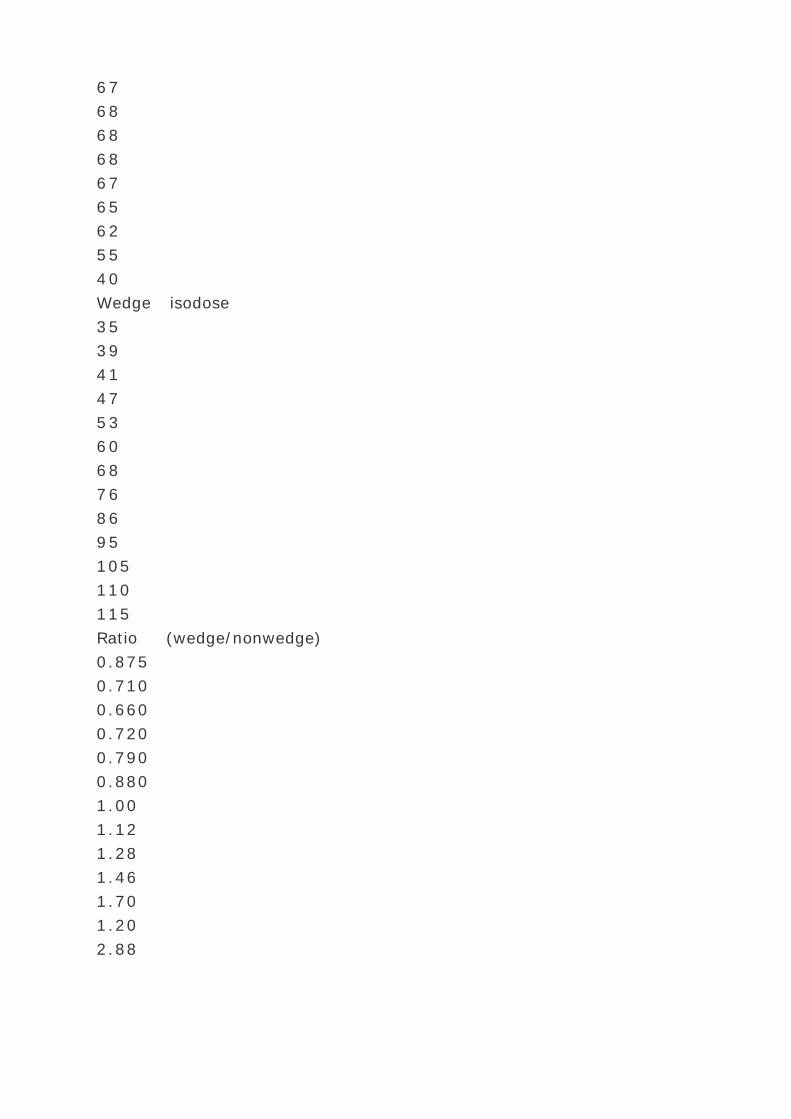
67

68

68

68

67

65

62

55

40

Wedge isodose

35

39

41

47

53

60

68

76

86

95

105

110

115

Ratio (wedge/nonwedge)

0.875

0.710

0.660

0.720

0.790

0.880

1.00

1.12

1.28

1.46

1.70

1.20

2.88

Transmission ratio

â€”

â€”

0.387

0.425

0.462

0.515

0.59

0.66

0.75

0.86

1.0

â€”

â€”

mm Pb

â€”

â€”

15.2

13.6

12.2

10.5

8.3

6.5

4.5

2.3

0

â€”

â€”

From Aron BS, Scapicchio M. Design of universal wedge filter

system for a cobalt 60 unit. AJR 1966;96:70, with permission.

A B C E G I K M O Q S T U

TABLE 11.1. TRANSMISSION RATIOS FOR THE

CONSTRUCTION OF WEDGE FILTER

For treatment of most tumors, however, a combination of two or

more beams is required for an acceptable distribution of dose

within the tumor and the surrounding normal tissues. Although

radiation fields may be combined in many ways, the discussion

here will be confined to the basic principles that are useful in

treating tumors involving different sites.

A. Parallel Opposed Fields

The simplest combination of two fields is a pair of fields directed

along the same axis from opposite sides of the treatment

volume. The advantages of the parallel opposed fields are the

simplicity and reproducibility of set-up, homogeneous dose to

the tumor, and less chances of geometrical miss (compared with

angled beams), given that the field size is large enough to

provide adequate lateral coverage of the tumor volume. A

disadvantage is the excessive dose to normal tissues and critical

organs above and below the tumor.

A composite isodose distribution for a pair of parallel opposed

fields may be obtained by adding the depth dose contribution of

each field (Fig. 11.10 ). The manual procedure consists of

joining the points of intersection of isodose curves for the

individual fields which sum to the same total dose value. The

resultant distribution shows the combined isodose

P.211

distribution normalized to the individual beam weights. The

beams are usually weighted in dose units of 100 at the depth of

D max in the case of SSD techniques or at the isocenter for the

isocentric techniques. For the example shown in Fig. 11.10A ,

the minimum percent isodose surrounding the tumor is 110. This

means that the minimum dose to the tumor (with a generous

margin) is 110 rads if 100 rads are delivered at the depth of D

max by each field. Thus, if the tumor dose were to be specified

at this isodose level, one could calculate the D max dose and the

treatment time for each field. For the isocentric plan shown in

Fig. 11.10B , the beam weights refer to doses delivered to the

isocenter. Thus the 190% isodose curve represents the specified

minimum dosage level if each beam delivered 100 rads to its

isocenter. Once the isocenter dose is calculated, one can

determine the treatment time or monitor units as described in

section 10.2 .

FIG. 11.10. Composite isodose distribution for a pair of parallel

opposed fields. A: Each beam is given a weight of 100 at the

depth of D max . B: Isocentric plan with each beam weighted 100

at the isocenter.

A.1. Patient Thickness Versus Dose

Uniformity

One advantage of equally weighted parallel opposed beams is

that the dose distribution within the irradiated volume can be

made uniform. However, the uniformity of distribution depends

on the patient thickness, beam energy, and beam flatness. In

general, as the patient thickness increases or the beam energy

decreases, the central axis maximum dose near the surface

increases relative to the midpoint dose. This effect, called tissue

lateral effect , is shown in Fig. 11.11 in which two opposing

beams are placed 25 cm apart with the midpoint dose

normalized to 100. The curves for cobalt-60 and 4 MV show that

for a patient of this thickness parallel opposed beams would give

rise to an excessively higher dose to the subcutaneous tissues

compared with the tumor dose at the midpoint. As the energy is

increased to 10 MV, the distribution becomes almost uniform and

at 25 MV it shows significant sparing of the superficial tissues

relative to the midline structures.

The ratio of maximum peripheral dose to midpoint dose is

plotted in Fig. 11.12 as a function of patient thickness for a

number of beam energies. Such data are useful in choosing the

appropriate beam energy for a given patient thickness when

using parallel opposed fields. For example, acceptable uniformity

of dose, that is, within ±5%, is achievable with cobalt-60 or 4-

to 6-MV beams for thicknesses of about 15 cm or less (e.g.,

head, neck, and extremities). However, for thicknesses of 20 cm

or greater (e.g., thorax, abdomen, and pelvis), 10-MV or higher

energies must be used to spare the normal subcutaneous

tissues.

FIG. 11.11. Depth dose curves for parallel opposed field

normalized to midpoint value. Patient thickness = 25 cm, field

size = 10 — 10 cm, SSD = 100 cm.

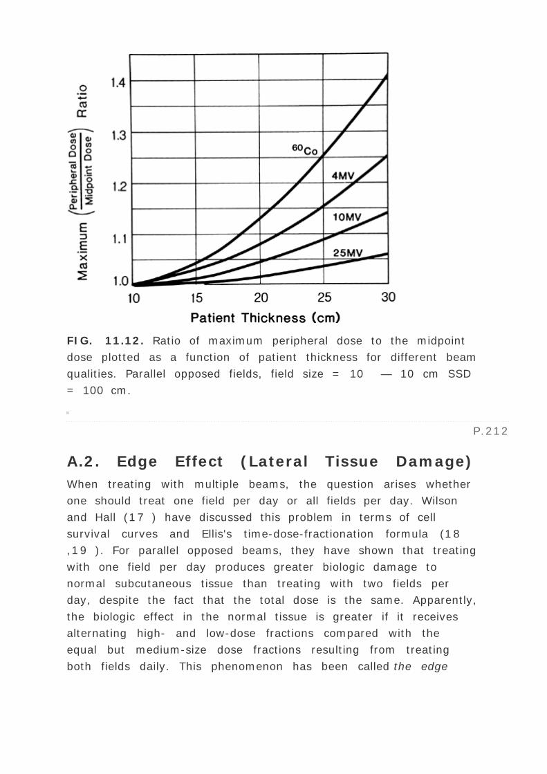
FIG. 11.12. Ratio of maximum peripheral dose to the midpoint

dose plotted as a function of patient thickness for different beam

qualities. Parallel opposed fields, field size = 10 — 10 cm SSD

= 100 cm.

P.212

A.2. Edge Effect (Lateral Tissue Damage)

When treating with multiple beams, the question arises whether

one should treat one field per day or all fields per day. Wilson

and Hall (17 ) have discussed this problem in terms of cell

survival curves and Ellis's time-dose-fractionation formula (18

,19 ). For parallel opposed beams, they have shown that treating

with one field per day produces greater biologic damage to

normal subcutaneous tissue than treating with two fields per

day, despite the fact that the total dose is the same. Apparently,

the biologic effect in the normal tissue is greater if it receives

alternating high- and low-dose fractions compared with the

equal but medium-size dose fractions resulting from treating

both fields daily. This phenomenon has been called the edge

effect , or the tissue lateral damage (20 ). The problem becomes

more severe when larger thicknesses (e.g., â‰¥20 cm) are

treated with one field per day using a lower-energy beam (e.g.,

â‰¤6 MV). In such cases, the dose per fraction to the

subcutaneous tissues, although delivered on alternate days,

becomes prohibitively high.

A.3. Integral Dose

One way of comparing dose distributions for different quality

beams is to calculate the integral dose for a given tumor dose.

Integral dose is a measure of the total energy absorbed in the

treated volume. If a mass of tissue receives a uniform dose,

then the integral dose is simply the product of mass and dose.

However, in practice, the absorbed dose in the tissue is

nonuniform so rather complex mathematical formulas are

required to calculate it.

For a single beam of x- or ³ radiation, Mayneord (21 )

formulated the following expression:

where âˆ‘ is the integral dose, D 0 is the peak dose along the

central axis, A is the geometric area of the field, d is the total

thickness of patient in the path of the beam, d 1/2 is the half-

value depth or the depth of 50% depth dose and SSD is the

source-surface distance. The term

is a correction for geometric divergence of the beam.

FIG. 11.13. Integral dose as a function of photon beam energy,

when 1,000 rad are delivered at a midpoint of a 25-cmâ€“thick

patient. Field size, 10-cm diameter at an SSD of 100 cm.

(Redrawn from Podgorsak EB, Rawlinson JA, Johns HE. X-ray

depth doses for linear accelerators in the energy range from 10

to 32 MeV. Am J Roentgenol 1975;123:182.)

P.213

Because integral dose is basically the product of mass and dose,

its unit is the gram-rad or kilogram-gray or simply joule (since 1

Gy = 1 J/kg). Figure 11.13 shows the integral dose as a function

of the energy of radiation for a tumor dose of 1,000 rad (1 rad =

10-2 Gy) at a depth of 12.5 cm in the patient of 25-cm thickness

treated with parallel opposed beams (22 ). The curve shows a

useful result, namely, the higher the photon energy the lower

the integral dose.

Although it is generally believed that the probability of damage

to normal tissue increases with the increase in the integral dose,

this quantity is seldom used clinically to plan dosages or predict

treatment outcome. However, it does provide qualitative

guidelines for treatment planning for selecting beam energy,

field sizes, and multiplicity of fields. As a general rule, one

should keep the integral dose to a minimum, provided the

adequacy of tumor irradiation and the sparing of critical organs

are not compromised.

B. Multiple Fields

One of the most important objectives of treatment planing is to

deliver maximum dose to the tumor and minimum dose to the

surrounding tissues. In addition, dose uniformity within the

tumor volume and sparing of critical organs are important

considerations in judging a plan. Some of the strategies useful

in achieving these goals are (a) using fields of appropriate size;

(b) increasing the number of fields or portals; (c) selecting

appropriate beam directions; (d) adjusting beam weights (dose

contribution from individual fields); (e) using appropriate beam

energy; and (f) using beam modifiers such as wedge filters and

compensators. Although obtaining a combination of these

parameters that yields an optimal plan is time-consuming if

done manually, treatment-planning computers are now available

that can do the job quickly and accurately. Some of these

systems are highly interactive so that the user can almost

instantly modify, calculate, and examine various plans to select

one that is clinically superior.

In section 11.5A , I discussed the case of two parallel opposed

fields. Although the technique results in uniform irradiation of

the tumor, there is little sparing of the surrounding normal

tissue. In fact, the dose to the peripheral tissues can be

significantly higher than the midline dose. Reduction of dose to

subcutaneous tissue and normal tissue surrounding the tumor

can be achieved by using a combination of three or more fields.

Figure 11.14 illustrates various multiple-field arrangements in

which the beam

P.214

enters the patient from various directions, always directed at

the tumor. Thus, by using multiple fields, the ratio of the tumor

dose to the normal tissue dose is increased. Figure 11.15A,B

shows typical examples of multiple fields, one used for

treatment of the esophagus and the other, for the prostate

gland. Figure 11.15C illustrates a fixed SSD-type technique in

which the beam weights are delivered to D max points. In actual

practice, one may use a combination of parallel opposed fields

and multiple fields to achieve the desired dose distribution.

FIG. 11.14. Schematic diagram showing examples of multiple

fields. A: Two opposing pairs at right angles. B: Two opposing

pairs at 120 degrees. C: Three fields: one anterior and two

posterior oblique, at 45 degrees with the vertical.

Although multiple fields can provide good distribution, there are

some clinical and technical limitations to these methods. For

example, certain beam angles are prohibited because of the

presence of critical organs in those directions. Also, the set-up

accuracy of a treatment may be better with parallel opposed

than with the multiple angled beam arrangement. It is,

therefore, important to realize that the acceptability of a

treatment plan depends not only on the dose distribution on

paper but also on the practical feasibility, set-up accuracy, and

reproducibility of the treatment technique.

11.6. ISOCENTRIC TECHNIQUES

Most modern machines are constructed so that the source of

radiation can rotate about a horizontal axis. The gantry of the

machine is capable of rotating through 360 degrees with the

collimator axis moving in a vertical plane. The isocenter is the

point of intersection of the collimator axis and the gantry axis of

rotation.

A. Stationary Beams

The isocentric technique of irradiation consists of placing the

isocenter of the machine at a depth within the patient and

directing the beams from different directions. The distance

P.215

of the source from the isocenter, or the SAD, remains constant

irrespective of the beam direction. However, the SSD in this

case may change, depending on the beam direction and the

shape of the patient contour. For any beam direction, the

following relationship holds:

where d is the depth of the isocenter. Knowing the depth and

position of isocenter from one direction such as the anterior

posterior, the SSD can be calculated according to Equation 11.2

P.216

and set up from that direction. Then the positioning of

subsequent fields simply requires moving the gantry and not the

patient.

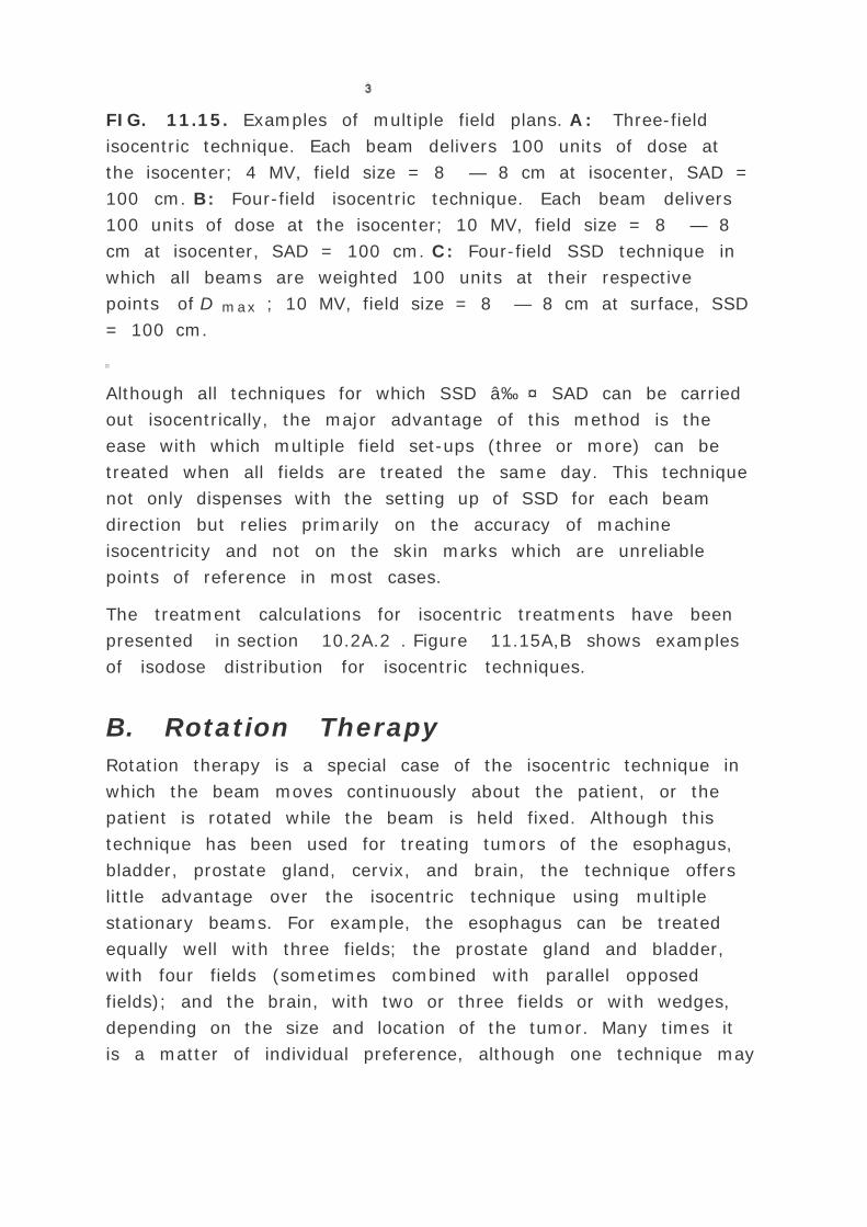
FIG. 11.15. Examples of multiple field plans. A: Three-field

isocentric technique. Each beam delivers 100 units of dose at

the isocenter; 4 MV, field size = 8 — 8 cm at isocenter, SAD =

100 cm. B: Four-field isocentric technique. Each beam delivers

100 units of dose at the isocenter; 10 MV, field size = 8 — 8

cm at isocenter, SAD = 100 cm. C: Four-field SSD technique in

which all beams are weighted 100 units at their respective

points of D max ; 10 MV, field size = 8 — 8 cm at surface, SSD

= 100 cm.

Although all techniques for which SSD â‰¤ SAD can be carried

out isocentrically, the major advantage of this method is the

ease with which multiple field set-ups (three or more) can be

treated when all fields are treated the same day. This technique

not only dispenses with the setting up of SSD for each beam

direction but relies primarily on the accuracy of machine

isocentricity and not on the skin marks which are unreliable

points of reference in most cases.

The treatment calculations for isocentric treatments have been

presented in section 10.2A.2 . Figure 11.15A,B shows examples

of isodose distribution for isocentric techniques.

B. Rotation Therapy

Rotation therapy is a special case of the isocentric technique in

which the beam moves continuously about the patient, or the

patient is rotated while the beam is held fixed. Although this

technique has been used for treating tumors of the esophagus,

bladder, prostate gland, cervix, and brain, the technique offers

little advantage over the isocentric technique using multiple

stationary beams. For example, the esophagus can be treated

equally well with three fields; the prostate gland and bladder,

with four fields (sometimes combined with parallel opposed

fields); and the brain, with two or three fields or with wedges,

depending on the size and location of the tumor. Many times it

is a matter of individual preference, although one technique may

offer particular advantages over the other in regard to patient

positioning, blocking, and the size of volume to be irradiated.

Especially when intricate blocking is required, rotation therapy

should not be attempted.

Rotation therapy is best suited for small, deep-seated tumors. If

the tumor is confined within a region extending not more than

halfway from the center of the contour cross-section, rotation

therapy may be a proper choice. However, rotation therapy is

not indicated if (a) volume to be irradiated is too large, (b) the

external surface differs markedly from a cylinder, and (c) the

tumor is too far off center.

Calculation for rotation therapy can be made in the same way as

for the stationary isocentric beams, except that a reasonably

large number of beams should be positioned around the patient

contour at fixed angular intervals. The dose rate at the isocenter

is given by:

where [D with dot above]ref is the reference dose rate related to

the quantity

which may be average tissue-to-air ratio (TAR) or tissue

maximal ratio (TMR) (averaged over all depths at the selected

angles). In the case of TARs, [D with dot above]ref is the dose

rate in free space for the given field at the isocenter. A method

of manual calculations based on this system was discussed in

section 9.4D . If the TMRs are used, [D with dot above]ref is the

D max dose rate for the given field at the SAD. Using the TMR

system discussed in Chapter 10 ,

where [D with dot above]0 is the D max dose rate for a 10 —

10-cm field at the SAD, and Sc and Sp are the collimator and

phantom scatter correction factors for the given field size at the

isocenter. In the case of a linear accelerator, [D with dot

above]0 is the monitor unit (MU) rate (assuming 1 MU = 1 rad

(cGy) at the isocenter for a depth of D max for a 10 — 10-cm

field).

Example

A patient is to receive 250 rad at the isocenter by rotation

therapy, using 4-MV x-rays, 6 — 10-cm field at the isocenter,

and a SAD of 100 cm. If

calculated according to the procedure in section 9.4D is 0.746,

calculate the number of monitor units to be set on

P.217

the machine if the machine output is set at 200 MU/min and

given Sc (6 — 10) = 0.98 and Sp (6 — 10) = 0.99. From

Equation 11.4 ,

or

Gantry rotation speed is set so that 345 MU are delivered at the

conclusion of the rotation. Some machines perform only one

rotation, whereas others can perform a specified number of arcs

or rotations in a pendulum manner. Most modern machines allow

for automatic adjustment of rotation speed to deliver a preset

number of monitor units by the end of a single rotation.

The determination of complete isodose curves for rotation

therapy by manual means is very time-consuming. It is

essentially the same procedure as used in multiple fixed beams,

but with a large number of beams. The isocentric isodose chart

(Fig. 11.1B ) in which isodoses are normalized to a point at

depth on the central axis is used with the isocenter placed at the

point of normalization. By summing the isodose values at

selected points while the chart is placed at different angles, the

dose distribution can be determined relative to the isocenter.

Because of the tedium involved in the procedure, this task is

ideally suited for computer application. Such programs are

available with commercial treatment planning computers.

Figure 11.16 shows three examples of isodose distribution for

rotation therapy: (a) 100 degree arc rotation; (b) 180 degree

arc rotation; and (c) full 360 degree rotation. It should be noted

that whereas the maximum dose for the 360-degree rotation

occurs at the isocenter, for the partial arcs it is displaced toward

the irradiated sector. This illustrates an important principle that

in arc therapy or when oblique fields are directed through one

side of a patient, they should be aimed a suitable distance

beyond the tumor area. This is sometimes referred to as past

pointing . The extent of past pointing required to bring the

maximum dose to the tumor site depends on the arc angle and

should be determined for an individual case by actual isodose

planning.

11.7. WEDGE FIELD TECHNIQUES

Relatively superficial tumors, extending from the surface to a

depth of several centimeters, can be irradiated by two

â€œwedgedâ€ beams directed from the same side of the

patient. Figure 11.17A shows isodose distribution of two angled

beams with no wedge in the beams. It is seen that in the region

of overlap of the beams, the dose distribution is quite

nonuniform. The dose is highest in the superficial or proximal

region of overlap and falls off to lower values toward the deeper

areas. By inserting appropriate wedge filters in the beam and

positioning them with the thick ends adjacent to each other, the

angled field distribution can be made fairly uniform (Fig. 11.17B

). Each wedged beam in this case has a reduced dose in the

superficial region relative to the deeper region so that the dose

gradient in the overlap region is minimized. The dose falls off

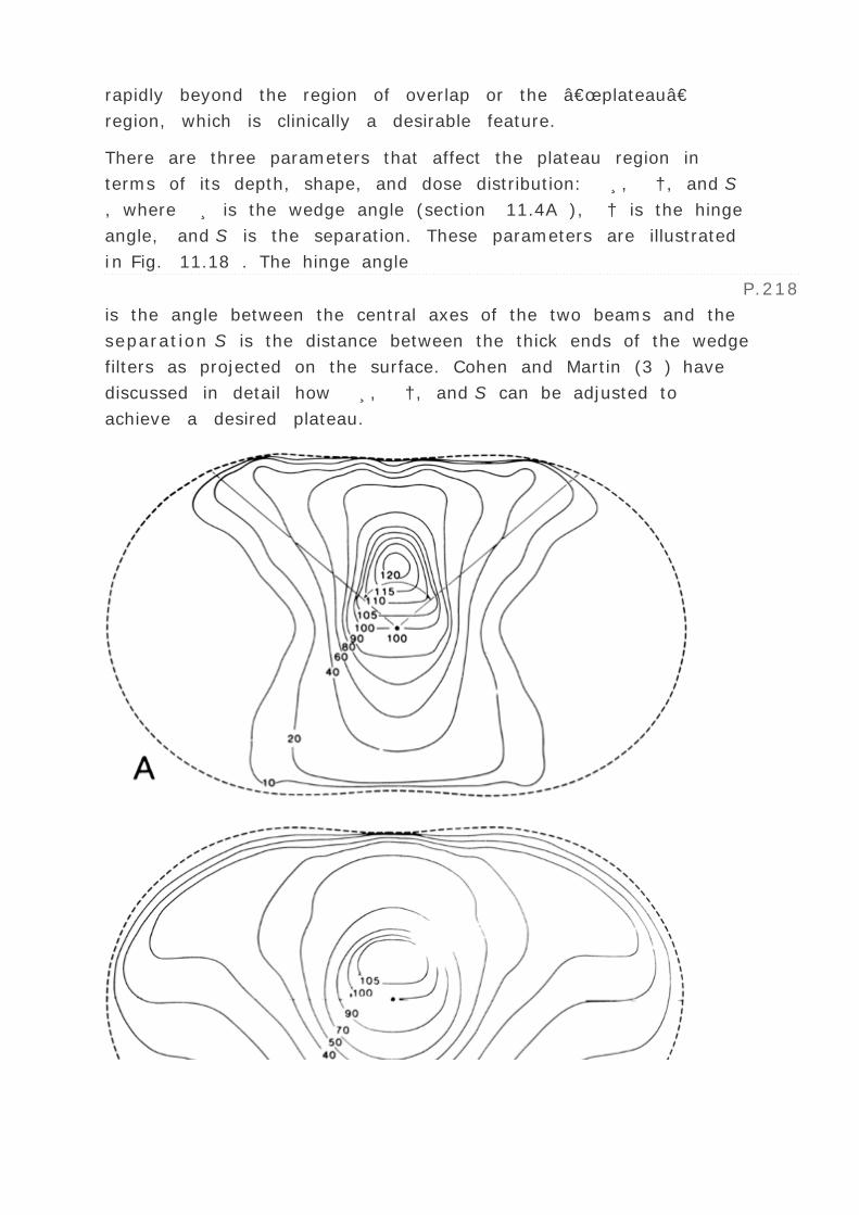
rapidly beyond the region of overlap or the â€œplateauâ€

region, which is clinically a desirable feature.

There are three parameters that affect the plateau region in

terms of its depth, shape, and dose distribution: ¸, †, and S

, where ¸ is the wedge angle (section 11.4A ), † is the hinge

angle, and S is the separation. These parameters are illustrated

in Fig. 11.18 . The hinge angle

P.218

is the angle between the central axes of the two beams and the

separation S is the distance between the thick ends of the wedge

filters as projected on the surface. Cohen and Martin (3 ) have

discussed in detail how ¸, †, and S can be adjusted to

achieve a desired plateau.

FIG. 11.16. Examples of isodose distribution for rotation

therapy. A: Arc angle = 100 degrees. B: Arc angle = 180

degrees. C: Full 360 degree rotation; 4 MV, field size = 7 — 12

cm at isocenter, SAD = 100 cm.

There is an optimum relationship between the wedge angle ¸

and the hinge angle † which provides the most uniform

distribution of radiation dose in the plateau:

This equation is based on the principle that for a given hinge

angle the wedge angle should be such that the isodose curves

from each field are parallel to the bisector of the hinge angle

(Fig. 11.18 ). Under these conditions, when the isodoses are

combined, the resultant distribution is uniform.

The Equation 11.5 , although helpful in treatment planning, may

not yield an optimum plan for a given patient contour. The

relationship assumes that the wedge isodose curves are not

modified by the surface contour. In practice, however, contours

are usually curved

P.219

or irregular in shape and thus modify the isodose distribution for

the wedged beams. As a result, the isodose curves for the

individual fields are no longer parallel to the bisector of the

hinge angle, thus giving rise to a nonuniform distribution in the

overlap region. This problem can be solved by using

compensators (discussed in Chapter 12 ), which make the skin

surface effectively flat and perpendicular to each beam. An

alternative approach is to modify the wedge angle (using a

different wedge angle filter from that given by Equation 11.5 )

so that a part of the wedge angle acts as a compensator and the

rest as a true wedge filter. The main objective is to make the

isodose curves parallel to the hinge angle bisector. Although the

latter approach obviates the need for a compensator, the

determination of an

P.220

optimum wedge angle may not be easy if planning is done

manually. The former method, on the other hand, is well-suited

for manual calculations since all you need is a compensator and

an atlas of precalculated isodose distributions for a variety of

¸, †, and S values. This method, however, becomes

technically difficult to implement if complicated secondary

blocking is required in addition to the compensator and the

wedge filter.

FIG. 11.17. Isodose distribution for two angle beams. A:

Without wedges. B: With wedges; 4 MV, field size = 10 — 10

cm, SSD = 100 cm, wedge angle = 45 degrees.

FIG. 11.18. Parameters of the wedge beams, ¸ is wedge

angle, † is hinge angle, and S is separation. Isodose curves for

each wedge field are parallel to the bisector.

Equation 11.5 suggests that for each hinge angle one should use

a different wedge angle. However, in practice, selected wedge

angles, i.e., 15 degrees, 30 degrees, 45 degrees, and 60

degrees, are adequate over a wide range of hinge angles.

In modern radiation therapy, complex treatment techniques are

frequently used, which may involve wedge filters, compensators,

field blocking, and field reductions, all for the same patient.

Manual treatment planning is difficult for such cases. For this

reason, in many institutions, all complex treatments, including

wedged fields, are planned by computer as a matter of standard

practice.

A. Uniformity of Dose Distribution

Because wedge pair techniques are normally used for treating

small, superficial tumor volumes, a high-dose region (hot spot)

of up to +10% within the treatment volume is usually

acceptable. These hot spots occur under the thin ends of the

wedges and their magnitude increases with field size and wedge

angle. This effect is related to the differential attenuation of the

beam under the thick end relative to the thin end.

Generally, the wedge filter technique is suitable when the tumor

is approximately from 0 to 7 cm deep and when it is necessary

to irradiate from one side of the skin surface. The most desirable

feature of this technique is the rapid dose falloff beyond the

region of overlap. This falloff can be exploited to protect a

critical organ such as the spinal cord. Although wedge filters are

invaluable in radiotherapy, some of these techniques are being

replaced by electron beam techniques (Chapter 14 ).

B. Open and Wedged Field

Combinations

Although wedge filters were originally designed for use in

conjunction with the wedge-pair arrangement, it is possible to

combine open and wedged beams to obtain a particular dose

distribution. One such arrangement which uses an open field

anteriorly and wedged field laterally in the treatment of some

tumors is shown in Fig. 11.19A . The anterior field is weighted

to deliver 100 units to the lateral 15 units to the isocenter

(these beams could be weighted in terms of D max in the SSD

technique). The weights and wedge angle are usually adjusted

for an individual case to obtain an acceptable distribution. The

principle of this technique is that as the dose contribution from

the anterior field decreases with depth, the lateral beam

provides a boost to offset this decrease. As seen in Fig. 11.19A ,

a wedged beam with the thick end positioned superiorly provides

the desired compensation for the dose dropoff. Thus such a

combination of open and wedged beams gives rise to a

distribution which remains constant with depth within certain

limits.

Figure 11.19B shows another technique in which the anterior

open beam is combined with the two lateral wedged beams.

Again, the beam weights and wedge angles are chosen to make

the open beam distribution remain constant throughout the

tumor volume.

11.8. TUMOR DOSE SPECIFICATION

FOR EXTERNAL PHOTON BEAMS

The results of treatments can be meaningfully interpreted only if

sufficient information is provided regarding the irradiation

technique and the distribution of dose in space and time. In the

absence of this information, recording of only the so-called

tumor dose serves little purpose. Unfortunately, this important

problem is often ignored. More often than not, treatment

summaries and records are ambiguous and even

incomprehensible

P.221

P.222

to other people. Therefore, one cannot overemphasize the need

for a dose recording system which is sufficiently explicit and

detailed to enable other centers to reproduce the treatment.

FIG. 11.19. Treatment plans using open and wedged field

combinations. A: Isocentric plan with anterior open field

weighted 100 and lateral wedged field weighted 15 at the

isocenter. B: A combination of anterior open beam and two

lateral wedged beams; 4 MV x-ray beam from ATC-400 Linac.

FIG. 11.20. Schematic illustration of ICRU volumes. (From

ICRU. Prescribing, recording, and reporting photon beam

therapy. ICRU Report 50. Bethesda, Maryland. International

Commission of Radiation Units and Measurements, 1993.)

In 1978, the ICRU (23 ) recognized the need for a general dose-

specification system which could be adopted universally.

Although the system proposed by the ICRU has not been

universally implemented, there is a substantial advantage in

adopting a common method of dose specification. In this section,

I present the highlights of the ICRU proposal. For details, the

reader is referred to current documents: Report No. 50 and 62

(24 ,25 ).

Figure 11.20 is a schematic representation of various volumes

that the ICRU Report no. 50 (24 ) recommends to be identified

in a treatment plan. Delineation of these volumes is greatly

facilitated by 3-D imaging but the concept is independent of the

methodology used for their determination.

A.1. Gross Tumor Volume

The gross tumor volume (GTV) is the gross demonstrable extent

and location of the tumor. It may consist of primary tumor,

metastatic lymphadenopathy, or other metastases. Delineation

of GTV is possible if the tumor is visible, palpable or

demonstrable through imaging. GTV cannot be defined if the

tumor has been surgically removed, although an outline of the

tumor bed may be substituted by examining preoperative and

postoperative images.

A.2. Clinical Target Volume

The CTV consists of the demonstrated tumor(s) if present and

any other tissue with presumed tumor. It represents, therefore,

the true extent and location of the tumor. Delineation of CTV

assumes that there are no tumor cells outside this volume. The

CTV must receive adequate dose to achieve the therapeutic aim.

A.3. Internal Target Volume

ICRU Report no. 62 (25 ) recommends that an internal margin

(IM) be added to CTV to compensate for internal physiological

movements and variation in size, shape, and position of the CTV

during therapy in relation to an internal reference point and its

corresponding

P.223

coordinate system. The volume that includes CTV with these

margins is called the internal target volume (ITV).

A.4. Planning Target Volume

The volume that includes CTV with an IM as well as a set-up

margin (SM) for patient movement and set-up uncertainties is

called the planning target volume (PTV). To delineate the PTV,

the IM and SM are not added linearly but are combined rather

subjectively. The margin around CTV in any direction must be

large enough to compensate for internal movements as well as

patient-motion and set-up uncertainties.

A.5. Planning Organ at Risk Volume

The organ(s) at risk (OR) needs adequate protection just as CTV

needs adequate treatment. Once the OR is identified, margins

need to be added to compensate for its movements, internal as

well as set-up. Thus, in analogy to the PTV, one needs to outline

planning organ at risk volume (PRV) to protect OR effectively.

Figure 11.21 schematically illustrates the process of outlining

PTV and PRV. This process is intended to make the radiation

oncologist think methodically and analytically when outlining

targets and organs at risk instead of taking a wild guess.

Although absolute accuracy in either case cannot be assured, the

objective of this approach is to minimize errors by paying

attention to details.

It is also important to point out that there is a common

tendency among practitioners to draw target volumes based on

GTV with little margins to account for subclinical

P.224

disease, organ motion, or set-up uncertainties. The so-called

conformal radiation therapy is a double-edged swordâ€”a high

degree of plan conformity can create a high probability of

geographical miss. Thus great caution must be exercised in

designing PTV and PRV. It is just as important to know the

limitations of the system as it is to know its capabilities.

FIG. 11.21. Schematic representation of ICRU volumes and

margins. (From ICRU. Prescribing, recording and reporting

photon beam therapy [supplement to ICRU Report 50]. ICRU

Report 62. Bethesda, Maryland. International Commission on

Radiation Units and Measurements, 1999.)

A.6. Treated Volume

Additional margins must be provided around the target volume

to allow for limitations of the treatment technique. Thus the

minimum target dose should be represented by an isodose

surface which adequately covers the PTV to provide that margin.

The volume enclosed by this isodose surface is called the treated

volume . The treated volume is, in general, larger than the

planning target volume and depends on a particular treatment

technique.

A.7. Irradiated Volume

The volume of tissue receiving a significant dose (e.g.,

â‰¥50% of the specified target dose) is called the irradiated

volume . The irradiated volume is larger than the treated volume

and depends on the treatment technique used.

A.8. Maximum Target Dose

The highest dose in the target area is called the maximum target

dose , provided this dose covers a minimum area of 2 cm2 .

Higher dose areas of less than 2 cm2 may be ignored in

designating the value of maximum target dose.

A.9. Minimum Target Dose

The minimum target dose is the lowest absorbed dose in the

target area.

A.10. Mean Target Dose

If the dose is calculated at a large number of discrete points

uniformly distributed in the target area, the mean target dose is

the mean of the absorbed dose values at these points.

Mathematically:

where N is the number of points in the matrix and Di , j is the

dose at lattice point i,j located inside the target area (AT ) .

A.11. Median Target Dose

The median target dose is simply the value between the

maximum and the minimum absorbed dose values within the

target.

A.12. Modal Target Dose

The modal target dose is the absorbed dose that occurs most

frequently within the target area. If the dose distribution over a

grid of points covering the target area is plotted as a frequency

histograph, the dose value showing the highest frequency is

called the modal dose. In Fig. 11.22 the modal dose corresponds

to the peak of the frequency curve.

FIG. 11.22. Target volume-dose frequency curve. (Reprinted

with permission from Ellis F, Oliver R. The specification of tumor

dose. Br J Radiol 1961;34:258.)

P.225

A.13. Hot Spots

A hot spot is an area outside the target that receives a higher

dose than the specified target dose. Like the maximum target

dose, a hot spot is considered clinically meaningful only if it

covers an area of at least 2 cm2 .

B. Specification of Target Dose

The absorbed dose distribution in the target volume is usually

not uniform. Although a complete dosimetric specification is not

possible without the entire dose distribution, there is value in

having one figure as the main statement of target dose. The use

of the term tumor dose is not recommended (23 ).

The quantity maximum target dose alone cannot be used for

reporting, since it can conceal serious underdosages in some

parts of the target volume. Although local tumor control depends

on the minimum target dose, this quantity alone is not

recommended by the ICRU (23 ), because it is difficult to

determine the extent of the tumor, and therefore, the selection

of the minimum target dose becomes difficult if not arbitrary.

Moreover, if most of the target volume receives a dose that is

appreciably different from the minimum, this may also reduce its

clinical significance. A statement of both the maximum and

minimum values is useful, but it is not always representative of

the dose distribution. Furthermore, this would do away with the

simplicity of having one quantity for reporting target dose.

The mean, median, and modal doses are not generally

recommended, because they usually require elaborate

calculations for their accurate determination and may not be

feasible by institutions having limited computation facilities.

B.1. The ICRU Reference Point

The target dose should be specified and recorded at what is

called the ICRU reference point. This point should satisfy the

following general criteria (25 ):

The point should be selected so that the dose at this point is

clinically relevant and representative of the dose throughout

the PTV;

The point should be easy to define in a clear and

unambiguous way;

The point should be selected where the dose can be

accurately calculated;

The point should not lie in the penumbra region or where

there is a steep dose gradient.

P.226

In most cases the ICRU reference point should lie well within the

PTV, provided it generally meets the above mentioned criteria.

Recommendations for simple beam arrangements are discussed

below as examples.

B.1.1. Stationary Photon Beams

For a single beam, the target absorbed dose should be

specified on the central axis of the beam placed within the

PTV.

For parallel opposed, equally weighted beams, the point of

target dose specification should be on the central axis

midway between the beam entrances.

For parallel opposed, unequally weighted beams, the target

dose should be specified on the central axis placed within

the PTV.

For any other arrangement of two or more intersecting

beams, the point of target dose specification should be at

the intersection of the central axes of the beams placed

within the PTV.

B.1.2. Rotation Therapy

For full rotation or arcs of at least 270 degrees, the target dose

should be specified at the center of rotation in the principal

plane. For smaller arcs, the target dose should be stated in the

principal plane, first, at the center of rotation and, second, at

the center of the target volume. This dual-point specification is

required because in a small arc therapy, past-pointing

techniques are used that give maximum absorbed dose close to

the center of the target area. The dose at the isocenter in these

cases, although important to specify, is somewhat less.

B.2. Additional Information

The specification of target dose is meaningful only if sufficient

information is provided regarding the irradiation technique. The

description of technique should include radiation quality, SSD or

SAD, field sizes, beam-modification devices (wedges and

shielding blocks, etc.), beam weighting, correction for tissue

heterogeneities, dose fractionation, and patient positioning.

Many of the above treatment parameters are listed with the

treatment plan (isodose pattern) and can be attached to the

patient chart. In vivo absorbed dose measurements can also

provide useful information and should be recorded in the chart.

Finally, the main objectives of a dose specification and reporting

system are to achieve uniformity of dose reporting among

institutions, to provide meaningful data for assessing the results

of treatments, and to enable the treatment to be repeated

elsewhere without having recourse to the original institution for

further information.

REFERENCES


Measurements. Measurement of absorbed dose in a phantom

irradiated by a single beam of x or gamma rays. Report No.

23. Washington, DC: National Bureau of Standards, 1973.

2. Webster EW, Tsien KC, eds. Atlas of radiation dose

distributions . Vol. I of Single-field isodose charts. Vienna:


3. Cohen M, Martin SM, eds. Atlas of radiation dose

distributions . Vol. II of Multiple-field isodose charts. Vienna:


4. Tsien KC, Cunningham JR, Wright DJ, et al. Atlas of

radiation dose distributions . Vol. III of Moving field isodose

charts. Vienna: International Atomic Energy Agency, 1967.

5. Sterling TD, Perry H, Katz I. Automation of radiation

treatment planning. IV. Derivation of a mathematical

expression for the percent depth dose surface of cobalt 60

beams and visualization of multiple field dose distributions.

Br J Radiol 1964;37:544.

6. Khan FM. Computer dosimetry of partially blocked fields in

cobalt teletherapy. Radiology 1970;97:405.

7. Van de Geijn J. A computer program for 3-D planning in

external beam radiation therapy, EXTD † T S. Comput Prog

Biomed 1970:1â€“47.

P.227

8. Cunningham JR, Shrivastava PN, Wilkinson JM. Program

IRREGâ€”calculation of dose from irregularly shaped radiation

beams. Comput Prog Biomed 1972;2:192.

9. Weinkam JJ, Kolde RA, Sterling TD. Extending the general

field equation to fit the dose distributions of a variety of

therapy units. Br J Radiol 1973;46:983.

10. Nordic Association of Clinical Physics. Procedures in

external beam radiation therapy dosimetry with electron and

photon beams with maximum energies between 1 and 50

MeV. Acta Radiol Oncol 1980;19:58.


Measurements. Determination of absorbed dose in a patient

irradiated by beams of x or gamma rays in radiotherapy

procedures. Report No. 24. Washington, DC: National Bureau

of Standards, 1976.

12. Sewchand W, Khan FM, Williamson J. Variation in depth

dose data between open and wedge fields for 4 MV X-rays.

Radiology 1978;127:789.

13. Cohen M, Burns JE, Sears R. Physical aspects of cobalt 60

teletherapy using wedge filters. I. Physical investigation.

Acta Radiol 1960;53:401. II. Dosimetric considerations. Acta

Radiol 1960;53:486.

14. Tranter FW. Design of wedge filters for use with 4 MeV

linear accelerator. Br J Radiol 1957;30:329.

15. Van de Geijn J. A simple wedge filter technique for cobalt

60 teletherapy. Br J Radiol 1962;35:710.

16. Aron BS, Scapicchio M. Design of universal wedge filter

system for a cobalt 60 unit. Am J Roentgenol 1966;96:70.

17. Wilson CS, Hall EJ. On the advisability of treating all

fields at each radiotherapy session. Radiology 1971;98:419.

18. Ellis F. Nominal standard dose and the ret. Br J Radiol

1971;44:101.

19. Orton CG, Ellis F. A simplification in the use of the NSD

concept in practical radiotherapy. Br J Radiol 1973;46:529.

20. Tapley N. Parallel opposing portals technique. In:

Fletcher GH, ed. Text book of radiotherapy , 3rd ed.

Philadelphia: Lea & Febiger, 1980:60.

21. Mayneord WV. The measurement of radiation for medical

purposes. Proc Phys Soc 1942;54:405.

22. Podgorsak EB, Rawlinson JA, Johns HE. X-ray depth doses

for linear accelerators in the energy range from 10 to 32

MeV. Am J Roentgenol 1975;123:182.


Measurements. Dose specification for reporting external

beam therapy with photons and electrons. Report No. 29.

Washington, DC: National Bureau of Standards, 1978.

24. ICRU. Prescribing, recording, and reporting photon beam

therapy. ICRU Report 50. Bethesda, Maryland: International

Commission on Radiation Units and Measurements, 1993.


therapy (supplement to ICRU Report 50). ICRU Report 62.

Bethesda, Maryland: International Commission of Radiation






12 - Treatment Planning II: Patient Data, Corrections, and

Set-Up

12

Treatment Planning II: PatientData, Corrections, and Set-Up

Basic depth-dose data and isodose curves are usually measured in a

cubic water phantom having dimensions much larger than the field

sizes used clinically. Phantom irradiations for this purpose are

carried out under standard conditions, for example, beams incident

normally on the flat surface at specified distances. The patient's

body, however, is neither homogeneous nor flat in surface contour.

Thus the dose distribution in a patient may differ significantly from

the standard distribution. This chapter discusses several aspects of

treatment planning, including acquisition of patient data, correction

for contour curvature, and tissue inhomogeneities and patient

positioning.

12.1. ACQUISITION OF PATIENT DATA

Accurate patient dosimetry is only possible when sufficiently

accurate patient data are available. Such data include body contour,

outline, and density of relevant internal structures, location, and

extent of the target volume. Acquisition of these data is necessary

whether the dosimetric calculations are performed manually or with

a computer. However, this important aspect of treatment planning is

often executed poorly. For example, in a busy department there may

be an inordinate amount of pressure to begin the patient's treatment

without adequate dosimetric planning. In other cases, lack of

sufficient physics support and/or equipment is the cause of this

problem. In such a case, it must be realized that the final accuracy

of the treatment plan is strongly dependent on the availability of the

patient data and that great effort is needed to improve its quality.

A. Body Contours

Acquisition of body contours and internal structures is best

accomplished by imaging (computed tomography [CT] and magnetic

resonance imaging, etc.). The scans are performed specifically for

treatment planning purposes, with the patient positioned the same

way as for actual treatment. In 3-D treatment planning (Chapter 19

) these data are all image-based and are acquired as part of the

treatment planning process. However, for cases in which 3-D

treatment planning is not considered necessary or if body contours

are obtained manually for verification of the image-based contours,

mechanical or electromechanical methods are used for contouring.

A number of devices have been made to obtain patient contours.

Some of these are commercially available while others can be

fabricated in the department machine shop. The most common and

the simplest of the devices is a solder wire or a lead wire embedded

in plastic. Because the wire may not faithfully retain the contour

dimensions when transferring it from the patient to the paper, one

must independently measure anteroposterior and/or lateral

diameters of the contour with a caliper.

FIG. 12.1. Photograph of a contour plotter. (Courtesy of Radiation

Products Design, Buffalo, MN.)

Another kind of simple device (1 ) consists of an array of rods, the

tips of which are made to touch the patient's skin and then placed

on a sheet of paper for contour drawing. Perhaps the most accurate

of the mechanical devices is a pantograph type apparatus (Fig. 12.1

) in which a rod can be moved laterally as well as up and down.

When the rod is moved over the patient contour, its motion is

followed by a pen that records the outline on paper.

P.229

Clarke (2 ) has described an electromechanical device in which

motion of the rod over the patient contour is read by a sensing

device and transferred to an X-Y recorder. Such a device can be

used for digitizing the patient contour for direct input to the

treatment planning computer. Optical (3 ) and ultrasonic (4 )

methods have also been devised to obtain the contour information.

Although any of the above methods can be used with sufficient

accuracy if carefully used, some important points must be

considered in regard to manual contour making.

The patient contour must be obtained with the patient in the

same position as used in the actual treatment. For this reason,

probably the best place for obtaining the contour information is

with the patient properly positioned on the treatment simulator

couch.

A line representing the tabletop must be indicated in the contour

so that this horizontal line can be used as a reference for beam

angles.

Important bony landmarks as well as beam entry points, if

available, must be indicated on the contour.

Checks of body contour are recommended during the treatment

course if the contour is expected to change due to a reduction of

tumor volume or a change in patient weight.

If body thickness varies significantly within the treatment field,

contours should be determined in more than one plane.

P.230

B. Internal Structures

Localization of internal structures for treatment planning should

provide quantitative information in regard to the size and location of

critical organs or inhomogeneities. Although qualitative information

can be obtained from diagnostic radiographs or atlases of cross-

sectional anatomy, they cannot be used directly for precise

localization of organs relative to the external contour. In order for

the contour and the internal structure data to be realistic for a given

patient, the localization must be obtained under conditions similar

to those of the actual treatment position and on a couch similar to

the treatment couch.

The following devices are used for the localization of internal

structures and the target volume. A brief discussion regarding their

operation and function will be presented.

B.1. Transverse Tomography

Conventional tomography pre-dates the introduction of CT. A

transverse tomography unit (Fig. 12.2 ) consists of a diagnostic x-

ray tube and a film cassette that rotates simultaneously with the x-

ray tube. The tube is set in such a position that the central axis of

the beam makes an angle of about 20 degrees with the film surface.

The patient is positioned on the table so that the x-ray beam can

pass through a desired body cross-section. As the gantry rotates,

structures in only one transverse plane are â€œin focus.â€ The

structures in regions other than that plane are blurred because of

the motion of the x-ray tube and the film cassette.

The difference between conventional tomography and transverse

tomography is the orientation of the plane in focus. Whereas a

conventional tomographic image is parallel to the long axis of the

patient, the transverse tomogram provides a cross-sectional image

perpendicular to the body axis.

Transverse tomograms have been used in radiation therapy to

provide cross-sectional information of internal structures in relation

to the external contour (5 ,6 ). Although the

P.231

method can be used for localizing bone, lung, air cavities, and

organs with contrast media, the tomograms have poor contrast and

spatial resolution. In addition, the images are marred by artifacts

and require interpretation.

FIG. 12.2. Photograph of a conventional transverse tomography unit

(right ) in combination with a treatment simulator. (Courtesy of

Toshiba Medical Systems, Chicago, IL.)

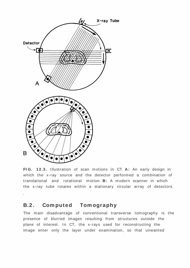
FIG. 12.3. Illustration of scan motions in CT. A: An early design in

which the x-ray source and the detector performed a combination of

translational and rotational motion. B: A modern scanner in which

the x-ray tube rotates within a stationary circular array of detectors.

B.2. Computed Tomography

The main disadvantage of conventional transverse tomography is the

presence of blurred images resulting from structures outside the

plane of interest. In CT, the x-rays used for reconstructing the

image enter only the layer under examination, so that unwanted

planes are completely omitted. Basically, a narrow beam of x-rays

scans across a patient in synchrony with a radiation detector on the

opposite side of the patient. If a sufficient number of transmission

measurements are taken at different orientations of the x-ray source

and detector (Fig. 12.3A ), the distribution of attenuation

coefficients within the layer may be determined. By assigning

different levels to different attenuation coefficients, an image can

be reconstructed that represents various structures with different

attenuation properties. Such a representation of attenuation

coefficients constitutes a CT image.

Since CT scanning was introduced about 30 years ago, there has

been a rapid development in both the software and hardware. Most

of the improvements in hardware had to do with the scanner motion

and the multiplicity of detectors to decrease the scan time. Figure

12.3B shows a modern scanner in which the x-ray tube rotates

within a circular

P.232

array of 1,000 or more detectors. With such scanners, scan times as

fast as 1 sec or less are achievable. Figure 12.4 shows a typical CT

image.

FIG. 12.4. Typical CT image.

Spiral or helical CT scanners were introduced in the early 1990s in

which the x-ray tube rotates continuously as the patient is slowly

translated through the CT aperture. Helical CTs are faster and

provide better visualization of anatomy and target volumes.

The reconstruction of an image by CT is a mathematical process of

considerable complexity, generally performed by a computer. For a

review of various mathematical approaches for image reconstruction,

the reader is referred to a paper by Brooks and Di Chiro (7 ). The

reconstruction algorithm generates what is known as CT numbers ,

which are related to attenuation coefficients. The CT numbers range

from -1,000 for air to +1,000 for bone, with that for water set at 0.

The CT numbers normalized in this manner are called Hounsfield

numbers (H ).

where µ is the linear attenuation coefficient. Thus a Hounsfield

unit represents a change of 0.1% in the attenuation coefficient of

water.

Because the CT numbers bear a linear relationship with the

attenuation coefficients, it is possible to infer electron density

(electrons cm-3 ) as shown in Fig. 12.5 . Although CT numbers can

be correlated with electron density, the relationship is not linear in

the entire range of tissue densities. The nonlinearity is caused by

the change in atomic number of tissues, which affects the proportion

of beam attenuation by Compton versus photoelectric interactions.

Figure 12.5 shows a relationship that is linear between lung and soft

tissue but nonlinear between soft tissue and bone.

Atomic number information can also be obtained if attenuation

coefficients are measured at two different x-ray energies (8 ). It is

possible to transform the attenuation coefficients measured by CT at

diagnostic energies to therapeutic energies (9 ). However, for low

atomic number materials such as fat, air, lung, and muscle, this

transformation is not necessary for the purpose of calculating dose

distributions and inhomogeneity corrections (9 ).

Application of CT in radiation therapy treatment planning has been

the subject of many papers (9 ,10 ,11 ,12 ,13 ,14 ,15 ,16 ,17 ,18 ,19

,20 ,21 ). The CT information is useful in two aspects of treatment

planning: (a) delineation of target volume and the surrounding

structures in relation to the external contour; and (b) providing

quantitative data (in the form of CT numbers) for tissue

P.233

heterogeneity corrections. From a practical point of view, the first

aspect is more important than the second. Accurate delineation of

surface contour, internal structures, and target volume is not only

crucial for optimizing a treatment technique but also necessary for

accurate calculation of dose distribution. Even the tissue

heterogeneity corrections for megavoltage photon beams can be

made with acceptable accuracy by using the CT cross-sectional

image to determine the extent of the inhomogeneity and employing

published values of electron density. To quote Sontag et al. (12 ),

â€œThe most severe errors in computing the dose distribution are

caused by inaccurate delineation of the geometric outlines of tissue

inhomogeneities. Less severe errors in the dose calculation are

caused by using an inaccurate relative electron density for the

inhomogeneity, provided the outline is accurate.â€ Similar

observations were also made by Geise and McCullough (11 ).

FIG. 12.5. CT numbers plotted as a function of electron density

relative to water. (From Battista JJ, Rider WD, Van Dyk J. Computed

tomography for radiotherapy planning. Int J Radiat Oncol Biol Phys


From these investigations, it seems that more sophisticated

inhomogeneity correction algorithms such as those using â€œpixel-

by-pixelâ€ CT data produce only small improvements in dose

accuracy compared with the traditional methods using equivalent

depth, provided the extent of the inhomogeneity is accurately

known. However, greater precision in the inhomogeneity outline and

electron density may be required in regions where severe dose

gradients exist in the direction of the beam. For example, the

electron density information may be critical for some cases of

electron beam therapy and, for high energy photons, in regions

where electronic equilibrium is not established. In such instances,

methods using pixel-by-pixel correction methods may be required

(16 ,22 ,23 ).

P.234

There are several commercially available computer treatment

planning systems that allow display and use of CT images for

treatment planning. Once the CT image has been produced, the data

can be transferred to the treatment-planning computer either

directly or the outlines of the contour and internal structures can be

traced by hand and then entered into the computer. In direct

systems, the CT scan is displayed in gray-scale mode on the

computer monitor of the treatment planning system and relevant

structures can be outlined on the basis of CT number distribution.

After the treatment plan is finalized, it can be superimposed on the

CT image for visual display.

The use of CT scans in treatment planning is now an established

procedure. Comparative studies of treatment planning with and

without CT have demonstrated significantly improved accuracy of

target delineation, field shaping and normal tissue exclusion from

the field when treatments are designed with the aid of CT scans. A

review of CT applications in radiotherapy is presented in a book

edited by Ling et al. (24 ). More current applications are discussed

in part III of this book.

Although external contour and internal structures are well-

delineated by CT, their use in treatment planning requires that they

be localized accurately with respect to the treatment geometry.

Diagnostic CT scans obtained typically on a curved tabletop with

patient position different from that to be used in treatment have

limited usefulness in designing technique and dose distribution.

Special treatment planning CT scans are required with full attention

to patient positioning and other details affecting treatment

parameters.

Some of the common considerations in obtaining treatment planning

CT scans are the following: (a) a flat tabletop should be used,

usually a flat wooden board can be designed to provide a removable

insert for the diagnostic CT couch; (b) a large diameter CT aperture

(e.g., â‰¥70 cm) can be used to accommodate unusual arm

positions and other body configurations encountered in radiation

therapy; (c) care should be taken to use patient-positioning or

immobilization devices that do not cause image artifacts; (d)

patient-positioning, leveling, and immobilization should be done in

accordance with the expected treatment technique or simulation if

done before CT; (e) external contour landmarks can be delineated,

using radiopaque markers such as plastic catheters; (f) sufficiently

magnified images for digitization can be obtained if radiographs on

film are to be used for drawing target and other structures; and (g)

image scale should be accurate both in the X and Y directions.

Three-dimensional Treatment Planning

Additional considerations go into CT scanning for 3-D treatment

planning. Because the 3-D anatomy is derived from individual

transverse scans (which are imaged in 2-D), the interslice distance

must be sufficiently small to reconstruct the image in three

dimensions. Depending on the tumor site or the extent of

contemplated treatment volume, contiguous scans are taken with

slice thickness ranging from 2 to 10 mm. The total number of slices

may range from 30 to 80 mm. This requires fast scan capability to

avoid patient movement or discomfort.

Delineation of target and critical organs on each of the scans is

necessary for the 3-D reconstruction of these structures. This is an

extremely time-consuming procedure, which has been a deterrent to

the adoption of 3-D treatment planning on a routine basis. Efforts

have been directed toward making this process less cumbersome

such as automatic contouring, pattern recognition, and other

computer manipulations. However, the basic problem remains that

target delineation is inherently a manual process. Although

radiographically visible tumor boundaries can be recognized by

appropriate computer software, the extent of target volume depends

on grade, stage, and patterns of tumor spread to the surrounding

structures. Clinical judgment is required in defining the target

volume. Obviously, a computer cannot replace the radiation

oncologist! At least, not yet.

Besides the time-consuming process of target localization, 3-D

computation of dose distribution and display requires much more

powerful computers in terms of speed and

P.235

storage capacity than the conventional treatment-planning systems.

However, with the phenomenal growth of computer technology this

is not perceived to be a significant barrier to the adoption of routine

3-D planning. The biggest deterrent, however, is going to be the

cost of treatment, including equipment and personnel.

Whereas 3-D planning for every patient may not be presently

realistic, it has already been found to be quite useful and practical

for certain tumors or tumor sites (head and neck, lung, prostrate).

Treatment of well-localized small lesions (e.g., less than 4 cm in

diameter) in the brain by stereotactic radiosurgery has greatly

benefited by 3-D planning. In this procedure, the target volume is

usually based on the extent of radiographically visible tumor (with

contrast), thus obviating the need for manual target delineation on

each CT slice. The 3-D display of dose distribution to assess

coverage of the target volume confined to a relatively small number

of slices is both useful and practical. Similarly, brachytherapy is

amenable to 3-D planning because of the limited number of slices

involving the target.

The next best thing to full-fledged 3-D planning (e.g., 3-D

computation and display) is to do 2-D planning, using a limited

number of CT scans, selected to obtain a reasonably adequate

perspective of the dose distribution in three dimensions. For

example, targets and other critical structures may be drawn on 5 to

10 CT cuts, spanning the volume of interest. This can be done either

by drawing targets and structures on the CT films or directly on the

computer screen by using a cursor or a light pen. Treatment-

planning software is available whereby margins around the target

volume can be specified to set the field boundaries. After optimizing

field margins, beam angles, and other plan parameters relative to

the central CT cut, the dose distributions can be viewed in other

slices either individually or simultaneously by serial display on the

screen. Beam's eye view (BEV) display in which the plan is viewed

from the vantage point of the radiation source (in a plane

perpendicular to the central axis) is useful in providing the same

perspective as a simulator or port film. In addition, a BEV outline of

the field can be obtained to aid in the drawing of custom blocks on

the simulator film. More discussion on CT-based treatment planning

is provided in Chapter 19 .

B.3. Magnetic Resonance Imaging

Magnetic resonance imaging (MRI) has developed, in parallel to CT,

into a powerful imaging modality. Like CT, it provides anatomic

images in multiple planes. Whereas CT provides basically transverse

axial images (which can be further processed to reconstruct images

in other planes or in three dimensions) MRI can be used to scan

directly in axial, sagittal, coronal, or oblique planes. This makes it

possible to obtain optimal views to enhance diagnostic interpretation

or target delineation for radiotherapy. Other advantages over CT

include not involving the use of ionizing radiation, higher contrast,

and better imaging of soft tissue tumors. Some disadvantages

compared with CT include lower spatial resolution; inability to image

bone or calcifications; longer scan acquisition time, thereby

increasing the possibility of motion artifacts; technical difficulties

due to small hole of the magnet and magnetic interference with

metallic objects; and current unavailability of many approved MRI

contrast agents.

The previous cursory comparison between CT and MRI shows that

the two types of imaging are complementary.

Basic physics of MRI involves a phenomenon known as nuclear

magnetic resonance (NMR). It is a resonance transition between

nuclear spin states of certain atomic nuclei when subjected to a

radiofrequency (RF) signal of a specific frequency in the presence of

an external magnetic field. The nuclei that participate in this

phenomenon are the ones that intrinsically possess spinning motion,

i.e., have angular momentum. These rotating charges act as tiny

magnets with associated magnetic dipole moment, a property that

gives a measure of how quickly the magnet will align itself along an

external magnetic field. Because of the spinning motion or the

magnetic dipole moment, nuclei align their spin axes along the

external magnetic field (H) as well as orbit or precess around it (Fig.

12.6 ).

P.236

The frequency of precession is called the Larmor frequency. A

second alternating field is generated by applying an alternating

voltage (at the Larmor frequency) to an RF coil. This field is applied

perpendicular to H and rotates around H at the Larmor frequency.

This causes the nuclei to precess around the new field in the

transverse direction. When the RF signal is turned off, the nuclei

return to their original alignment around H. This transition is called

relaxation. It induces a signal in the receiving RF coil (tuned to the

Larmor frequency) which constitutes the NMR signal.

FIG. 12.6. Alignment and precession of protons in a strong

magnetic field. (From Halverson RA, Griffiths HJ, Lee BCP, et al.

Magnetic resonance imaging and computed tomography in the

determination of tumor and treatment volume. In: Levitt SH, Khan

FM, Potish RA, eds. Technological basis of radiation therapy , 2nd

ed. Philadelphia: Lea & Febiger, 1992:38, with permission.)

The turning off of the transverse RF field causes nuclei to relax in

the transverse direction (T2 relaxation) as well as to return to the

original longitudinal direction of the magnetic field (T1 relaxation).

This is schematically illustrated in Fig. 12.7 . The relaxation times,

T1 and T2 , are actually time constants (like the decay constant in

radioactive decay) for the exponential function that governs the two

transitions.

The signal source in MRI can be any nucleus with nonzero spin or

angular momentum. However, certain nuclei give larger signal than

the others. Hydrogen nuclei (protons), because of their high intrinsic

sensitivity and high concentration in tissues, produce signals of

sufficient strength for imaging. Work with other possible candidates,31 P, 23 Na, 19 F,

P.23713 C, and 2 H is continuing. Currently, routine MRI is based

exclusively on proton density and proton relaxation characteristics

of different tissues.

FIG. 12.7. Effects of radiofrequency applied at right angles to the

magnetic field. (From Halverson RA, Griffiths HJ, Lee BCP, et al.

Magnetic resonance imaging and computed tomography in the

determination of tumor and treatment volume. In: Levitt SH, Khan

FM, Potish RA, eds. Technological basis of radiation therapy , 2nd

ed. Philadelphia: Lea & Febiger, 1992:38, with permission.)

Localization of protons in a 3-D space is achieved by applying

magnetic field gradients produced by gradient RF coils in three

orthogonal planes. This changes the precession frequency of protons

spatially, because the MR frequency is linearly proportional to field

strength. Thus by the appropriate interplay of the external magnetic

field and the RF field gradients, proton distribution can be localized.

A body slice is imaged by applying field gradient along the axis of

the slice and selecting a frequency range for a readout. The strength

of the field gradient determines the thickness of the slice (the

greater the gradient, thinner the slice). Localization within the slice

is accomplished by phase encoding (using back-to-front Y-gradient)

and frequency encoding (using transverse X-gradient). In the

process, the computer stores phase (angle of precession of the

proton at a particular time) and frequency information and

reconstructs the image by mathematical manipulation of the data.

Most MR imaging uses a spin echo technique in which a 180-degree

RF pulse is applied after the initial 90-degree pulse, and the

resulting signal is received at a time that is equal to twice the

interval between the two pulses. This time is called the echo time

(TE). The time between each 90-degree pulse in an imaging

sequence is called the repetition time (TR). By adjusting TR and TE,

image contrast can be affected. For example, a long TR and short TE

produces a proton (spin) density-weighted image, a short TR and a

short TE produces a T1 -weighted image, and a long TR and a long

TE produces a T2 -weighted

P.238

image. Thus differences in proton density, T1 , and T2 between

different tissues can be enhanced by a manipulation of TE and TR in

the spin echo technique.

FIG. 12.8. Examples of MR images of the head. A: Transverse

plane. B: Sagittal plane. C: Coronal plane.

Figure 12.8 shows examples of MR images obtained in the axial,

sagittal, and coronal planes. By convention, a strong MR signal is

displayed as white and a weak signal is displayed as dark on the

cathode ray tube or film.

B.4. Ultrasound

Ultrasonic imaging for delineating patient contours and internal

structure is becoming widely recognized as an important tool in

radiation therapy. Tomographic views provide cross-sectional

information that is always helpful for treatment planning. Although

in most cases the image quality or clinical reliability is not as good

as that of the CT, ultrasonic procedure does not involve ionizing

radiation, is less expensive, and in some cases, yields data of

comparable usefulness.

P.239

Ultrasound can provide useful information in localizing many

malignancy-prone structures in the lower pelvis, retroperitoneum,

upper abdomen, breast, and chest wall (25 ). A detailed review of

these techniques in the context of radiation therapy planning has

been presented by Carson et al. (25 ,26 ).

An ultrasound (or ultrasonic) wave is a sound wave having a

frequency greater than 20,000 cycles per sec or hertz (Hz). At this

frequency, the sound is inaudible to the human ear. Ultrasound

waves of frequencies 1 to 20 MHz are used in diagnostic radiology.

Ultrasound may be used to produce images either by means of

transmission or reflection. However, in most clinical applications,

use is made of ultrasonic waves reflected from different tissue

interfaces. These reflections or echoes are caused by variations in

acoustic impedance of materials on opposite sides of the interfaces.

The acoustic impedance (Z ) of a medium is defined as the product

of the density of the medium and the velocity of ultrasound in the

medium. The larger the difference in Z between the two media, the

greater is the fraction of ultrasound energy reflected at the

interface. For example, strong reflections of ultrasound occur at the

air-tissue, tissue-bone, and chest wall-lung interfaces due to high

impedance mismatch. However, because lung contains millions of

air-tissue interfaces, strong reflections at the numerous interfaces

prevents its use in lung imaging.

Attenuation of the ultrasound by the medium also plays an

important role in ultrasound imaging. This attenuation takes place

as the energy is removed from the beam by absorption, scattering,

and reflection. The energy remaining in the beam decreases

approximately exponentially with the depth of penetration into the

medium, allowing attenuation in different media to be characterized

by attenuation coefficients. As the attenuation coefficient of

ultrasound is very high for bone compared with soft tissue, together

with the large reflection coefficient of a tissue-bone interface, it is

difficult to visualize structures lying beyond bone. On the other

hand, water, blood, fat, and muscle are very good transmitters of

ultrasound energy.

Ultrasonic waves are generated as well as detected by an ultrasonic

probe or transducer. A transducer is a device that converts one form

of energy into another. An ultrasonic transducer converts electrical

energy into ultrasound energy, and vice versa. This is accomplished

by a process known as the piezoelectric effect. This effect is

exhibited by certain crystals in which a variation of an electric field

across the crystal causes it to oscillate mechanically, thus

generating acoustic waves. Conversely, pressure variations across a

piezoelectric material (in response to an incident ultrasound wave)

result in a varying electrical potential across opposite surfaces of

the crystal.

Although the piezoelectric effect is exhibited by a number of

naturally occurring crystals, most common crystals used clinically

are made artificially such as barium titanate, lead zirconium

titanate, and lead metaniobate. The piezoelectric effect produced by

these materials is mediated by their electric dipole moment, the

magnitude of which can be varied by addition of suitable impurities.

As the ultrasound wave reflected from tissue interfaces is received

by the transducer, voltage pulses are produced that are processed

and displayed on the cathode ray tube (CRT), usually in one of three

display modes: A (amplitude) mode, B (brightness) mode, and M

(motion) mode. A mode consists of displaying the signal amplitude

on the ordinate and time on the abscissa. The time, in this case, is

related to distance or tissue depth, given the speed of sound in the

medium. In the B mode, a signal from a point in the medium is

displayed by an echo dot on the CRT. The (x, y ) position of the dot

on the CRT indicates the location of the reflecting point at the

interface and its proportional brightness reveals the amplitude of

the echo. By scanning across the patient, the B-mode viewer sees an

apparent cross-section through the patient. Such cross-sectional

images are called ultrasonic tomograms.

In the M mode of presentation, the ultrasound images display the

motion of internal structures of the patient's anatomy. The most

frequent application of M mode scanning is echocardiography. In

radiotherapy, the cross-sectional information used for treatment

planning is exclusively derived from the B scan images (Fig. 12.9 ).

The use of ultrasound in brachytherapy (e.g., ultrasound-guided

prostate implants) is discussed in Chapter 23 .

FIG. 12.9. Ultrasonic tomogram showing chest wall thickness (right

) compared with the CT image (left).

P.240

12.2. TREATMENT SIMULATION

A treatment simulator (Fig. 12.10 ) is an apparatus that uses a

diagnostic x-ray tube but duplicates a radiation treatment unit in

terms of its geometrical, mechanical, and optical properties. The

main function of a simulator is to display the treatment fields so

that the target volume may be accurately encompassed without

delivering excessive irradiation to surrounding normal tissues. By

radiographic visualization of internal organs, correct positioning of

fields and shielding blocks can be obtained in relation to external

landmarks. Most commercially available simulators have fluoroscopic

capability by dynamic visualization before a hard copy is obtained in

terms of the simulator radiography.

Specifications of a treatment simulator must closely match those of

the treatment unit. Several authors (27 ,28 ,29 ,30 ,31 ) have

discussed these aspects. For a comprehensive discussion, the reader

is referred to the paper by McCullough and Earl (31 ).

FIG. 12.10. Varian (TEM) Ximatron 5 treatment simulator.

(Courtesy of Varian Associates, Palo Alto, CA.)

P.241

The need for simulators arises from four facts: (a) geometrical

relationship between the radiation beam and the external and

internal anatomy of the patient cannot be duplicated by an ordinary

diagnostic x-ray unit; (b) although field localization can be achieved

directly with a therapy machine by taking a port film, the

radiographic quality is poor because of very high beam energy, and

for cobalt-60, a large source size as well; (c) field localization is a

time-consuming process which, if carried out in the treatment room,

could engage a therapy machine for a prohibitive length of time; (d)

unforeseen problems with a patient set-up or treatment technique

can be solved during simulation, thus conserving time within the

treatment room.

Although the practical use of simulators varies widely from

institution to institution, the simulator room is increasingly

assuming the role of a treatment-planning room. Besides localizing

treatment volume and setting up fields, other necessary data can

also be obtained at the time of simulation. Because the simulator

table is supposed to be similar to the treatment table, various

patient measurements such as contours and thicknesses, including

those related to compensator or bolus design, can be obtained under

appropriate set-up conditions. Fabrication and testing of

individualized shielding blocks can also be accomplished with a

simulator. To facilitate such measurements, modern simulators are

equipped with accessories such as laser lights, contour maker, and

shadow tray.

Some simulators have a tomography attachment in which the image

from the image intensifier is analyzed and reconstructed using

either analogue1 or digital2 processing. Because of the poor image

quality, this technology cannot compete with CT-based virtual

simulation.

An exciting development in the area of simulation is that of

converting a CT scanner into a simulator. A commercial device3

known as CT-SIM uses a CT scanner to localize the treatment fields

on the basis of the patient's CT scans. A computer program,

specifically written for simulation, automatically positions the

patient couch and the laser cross hairs to define the scans and the

treatment fields. The software provides automatic outlining of

external contours and critical structures, interactive portal displays

and placement, display of isodose distribution, and review of

multiple treatment plans. Such an integrated approach to treatment

planning has the potential of becoming the simulator cum

treatment-planning system of the future.

12.3. TREATMENT VERIFICATION

A. Port Films

The primary purpose of port filming is to verify the treatment

volume under actual conditions of treatment. Although the image

quality with the megavoltage x-ray beam is poorer than with the

diagnostic or the simulator film, a port film is considered mandatory

not only as a good clinical practice but as a legal record.

As a treatment record, a port film must be of sufficiently good

quality so that the field boundaries can be described anatomically.

However, this may not always be possible due to either very high

beam energy (10 MV or higher), large source size (cobalt-60), large

patient thickness (>20 cm), or poor radiographic technique. In such

a case, the availability of a simulator film and/or a treatment

diagram with adequate anatomic description of the field is helpful.

Anatomic interpretation of a port film is helped by obtaining a full-

field exposure on top of the treatment port exposure.

FIG. 12.11. Schematic diagram of video-based electronic portal

imaging device.

P.242

Radiographic technique significantly influences image quality of a

port film. The choice of film and screen as well as the exposure

technique is important in this regard. Droege and Bj ¤rngard (32 )

have analyzed the film screen combinations commonly used for port

filming at megavoltage x-ray energies. Their investigation shows

that the use of a single emulsion film with the emulsion adjacent to

a single lead screen4 between the film and the patient is preferable

to a double emulsion film or a film with more than one screen. Thus,

for optimum resolution, one needs a single emulsion film with a

front lead screen and no rear screen. Conventional nonmetallic

screens are not recommended at megavoltage energies. Although

thicker metallic screens produce a better response, an increase in

thickness beyond the maximum electron range produces no further

changes in resolution (32 ).

Certain slow-speed films, ready packed but without a screen, can be

exposed during the entire treatment duration. A therapy verification

film such as Kodak XV-2 is sufficiently slow to allow an exposure of

up to 200 cGy without reaching saturation. In addition, such films

can be used to construct compensators for both the contours and

tissue heterogeneity (33 ).

B. Electronic Portal Imaging

Major limitations of port films are (a) viewing is delayed because of

the time required for processing; (b) it is impractical to do port

films before each treatment; and (c) film image is of poor quality

especially for photon energies greater than 6 MV. Electronic portal

imaging overcomes the first two problems by making it possible to

view the portal images instantaneously, i.e., images can be

displayed on computer screen before initiating a treatment or in

real-time during the treatment. Portal images can also be stored on

computer discs for later viewing or archiving.

On-line electronic portal imaging devices (EPIDs) are currently being

clinically used in several institutions, and some of them are

commercially available. Many of the systems are video based; the

beam transmitted through the patient excites a metal fluorescent

screen, which is viewed by a video camera using a 45 degree mirror

(34 ,35 ,36 ,37 ) (Fig. 12.11 ).

P.243

The camera is interfaced to a microcomputer through a frame-

grabber board for digitizing the video image. The images are

acquired and digitized at the video rate of 30 frames per second. An

appropriate number of frames is averaged to produce a final image.

Depending on the computer software, the image data can be further

manipulated to improve the image quality or perform a special

study.

One problem with mirror-based EPIDs is the large size of the mirror,

which can pose practical problems. Wong et al. (38 ) have developed

a system that replaces the mirror with a fiberoptics system to direct

the fluorescent light to the video camera. The fiberoptics channels

consist of thin clear polystyrene columns encased by a thin acrylic

cladding. Because of the difference in the refractive indices of the

two plastics, it is possible to conduct light without significant loss of

intensity. This â€œlight pipingâ€ is accomplished by the process

of total internal reflection at the cladding interface.

Another class of EPIDs consists of a matrix of liquid ion chambers

used as detectors (39 ,40 ). These devices are much more compact

than the video-based systems and are comparable in size to a film

cassette, albeit a little heavier. Figure 12.12 shows a system

developed at The Nederlands Kanker Institute. The system consists

of a matrix of 256 — 256 ion chambers containing an organic fluid

and a microcomputer for image processing. Figure 12.13 shows an

image obtained with such a device. Besides imaging, another

potential use of this device is on-line patient dose monitoring.

Further work is needed to develop this application.

Yet another type of EPID uses solid-state detectors. One approach

employs a scanning linear array of silicon diodes. Another uses a

linear array of zinc tungstate (Zn WO4 ) scintillating crystals

attached to photodiodes. An excellent review of these developments

is provided by Boyer et al. (41 ).

FIG. 12.12. Varian Portalvision system containing a matrix of liquid

ionization chambers, mounted on the accelerator gantry. The

mounting arm swings into position for imaging and out of the way

when not needed. (Courtesy of Varian Associates, Palo Alto, CA.)

FIG. 12.13. Example of a portal image. (Courtesy of Varian

Associates, Palo Alto, CA.)

P.244

A variety of technologies are being explored to develop new EPIDS

or refine the existing ones. For example, Varian Medical Systems

has recently introduced PortalVision aS500 featuring an array of

image detectors based on Amorphous Silicon (a-Si) technology.

Within this unit a scintillator converts the radiation beam into

visible photons. The light is detected by an array of photodiodes

implanted on an amorphous silicon panel. The photodiodes integrate

the light into charge captures. The sensitive area of the EPID is 40

— 30 cm2 with 512 — 384 pixels, spatial resolution is 0.78 mm

and the read-out image has about 200,000 pixels. This system offers

better image quality than the previous system using liquid ion

chambers.

12.4. CORRECTIONS FOR CONTOUR

IRREGULARITIES

As mentioned at the beginning of this chapter, basic dose

distribution data are obtained under standard conditions, which

include homogeneous unit density phantom, perpendicular beam

incidence, and flat surface. During treatment, however, the beam

may be obliquely incident with respect to the surface and, in

addition, the surface may be curved

P.245

or irregular in shape. Under such conditions, the standard dose

distributions cannot be applied without proper modifications or

corrections.

Contour corrections may be avoided by using a bolus or a

compensator (to be discussed in section 12.4 ) but under some

circumstances, it is permissible or even desirable, to determine the

actual dose distribution by calculation. The following three methods

are recommended for angles of incidence of up to 45 degree for

megavoltage beams and of up to 30 degree from the surface normal

for orthovoltage x-rays (42 ). Although all computer treatment-

planning algorithms are capable of correcting for contour

irregularities, these methods are discussed below to illustrate the

basic principles.

A. Effective Source-to-Surface Distance

Method

Consider Fig. 12.14 in which source-to-surface is an irregularly

shaped patient contour. It is desired to calculate the percent depth

dose at point A (i.e., dose at A as a percentage of D max dose at

point Q ). The diagram shows that the tissue deficit above point A is

h cm and the depth of D max is d m . If we note that the percent

depth dose does not change rapidly with SSD (provided that the SSD

is large), the relative depth dose distribution along the line joining

the source with point A is unchanged when the isodose chart is

moved down by the distance h and positioned with its surface line at

S â€²â€“S â€². Suppose DA is the dose at point A. Assuming beam

to be incident on a flat surface located at: S â€²â€“S â€²,

where P â€² is percent depth dose at A relative to D â€²max at point

Q â€². Suppose P corr is the correct percent depth dose at A relative

to D max at point Q. Then,

P.246

From Equation 12.2 and 12.3 ,

Because, when the distribution is moved, the SSD is increased by a

distance h , we have:

Therefore,

FIG. 12.14. Diagram illustrating methods of correcting dose

distribution under an irregular surface such as S â€“S. The solid

isodose curves are from an isodose chart which assumes a flat

surface located at S â€²â€“S â€². The dashed isodose curves assume

a flat surface at S â€³â€“S â€³ without any air gap.

Thus the effective SSD method consists of sliding the isodose chart

down so that its surface line is at S â€²â€“S â€², reading off the

percent dose value at A and multiplying it by the inverse square law

factor to give the corrected percent depth dose value.

The above method applies the same way when there is excess tissue

above A instead of tissue deficit. In such a case, the isodose chart is

moved up so that its surface line passes through the point of

intersection of the contour line and the ray line through A. The

value of h is assigned a negative value in this case.

B. Tissue-air (or Tissue-maximum) Ratio

Method

This method depends on the principle that the tissue-air, or tissue-

maximum, ratio does not depend on the SSD and is a function only

of the depth and the field size at that depth. Suppose, in Fig. 12.14

, the surface is located at S â€³â€“S â€³ and the air space between

S â€“S and S â€³â€“S â€³ is filled with tissue-like material. Now, if

a standard isodose chart for the given beam and SSD is placed with

its surface at S â€³â€“S â€³, the percent depth dose value at A will

correspond to the depth d + h. But the actual value at A is greater

than this as there is a tissue deficit. The correction factor can be

obtained by the ratio of tissue-air or tissue-maximum ratios for

depths d and d + h.

where T stands for tissue-air ratio or tissue-maximum ratio and rA i s

the field size projected at point A (i.e., at a distance of SSD + d + h

from the source).

Thus if the uncorrected value of percent depth dose at A with the

surface line of the isodose chart at S â€³â€“S â€³ is P â€³, then the

corrected value P corr is given:

P corr = P â€³ ·CF

C. Isodose Shift Method

The preceding methods are useful for making individual point dose

calculations. However, for manual treatment planning, it is

convenient to correct the entire isodose chart for contour

irregularities. This can be done by an empirical method, known as

the isodose shift method. The procedure is illustrated in Fig. 12.15 .

Suppose S â€“S is the patient contour drawn on a transparent paper

and S â€²â€“S â€² is a flat surface line passing through the point of

intersection of the central axis with the contour. From the line S

â€²â€“S â€², draw vertical grid lines, parallel to the central axis and

spaced about 1 cm apart, to cover the full field width. Place the

standard isodose chart underneath this paper and align the central

line of the chart with that of the grid. Mark the percent depth dose

values on the central axis. For each grid line, slide the isodose chart

up or down, depending on whether there is tissue

P.247

excess or deficit along that line, by an amount k — h where k is a

factor less than 1 (given in Table 12.1 ). Then mark the isodose

values at points of intersection of the given grid line and the shifted

isodose curves. After all the isodose positions along all the grid lines

have been marked, new isodose curves are drawn by joining the

marked points having the same isodose values.

FIG. 12.15. Diagram illustrating isodose shift method of correcting

isodose curves for surface contour irregularity.

The factor k depends on the radiation quality, field size, depth of

interest, and SSD. Table 12.1 gives approximate values

recommended for clinical use when manual corrections are needed.

Of the three methods discussed above, the tissue-air or tissue-

maximum ratio method gives the most accurate results. The first

two methods are especially useful in computer treatment planning.

Up to 1

0.860 Co-5

0.7

5â€“15

0.6

15â€“30

0.5

Above 30

0.4

Data from Giessen PH. A method of calculating the isodose shift in

correcting for oblique incidence in radiotherapy. Br J Radiol

1973;46:978.

Photon Energy (MV) Approximate Factor k

TABLE 12.1. ISODOSE SHIFT FACTORS FOR DIFFERENT BEAM

ENERGIES

P.248

Example 1

For point A in Fig. 12.14 , h = 3 cm and d = 5 cm. Calculate the

percent depth dose at point A using (a) the effective SSD method

and (b) the tissue-air ratio method.

Given 60 Co beam, TAR(5, 11 — 11) = 0.910 and TAR(8, 11 —

11) = 0.795 and SSD = 80 cm:

using solid isodose curve lines in Fig. 12.14 ,

Field dimension projected at

cm. Thus field size at A = 11 — 11 cm:

Using dashed isodose lines in Fig. 12.14 , uncorrected percent

depth dose = 65.2.

Comparing the results for (a) and (b), the agreement between

the two methods is within 3%.

12.5. CORRECTIONS FOR TISSUE

INHOMOGENEITIES

Applications of standard isodose charts and depth dose tables

assume homogeneous unit density medium. In a patient however,

the beam may transverse layers of fat, bone, muscle, lung, and air.

The presence of these inhomogeneities will produce changes in the

dose distribution, depending on the amount and type of material

present and on the quality of radiation.

The effects of tissue inhomogeneities may be classified into two

general categories: (a) changes in the absorption of the primary

beam and the associated pattern of scattered photons and (b)

changes in the secondary electron fluence. The relative importance

of these effects depends on the region of interest where alterations

in absorbed dose are considered. For points that lie beyond the

inhomogeneity, the predominant effect is the attenuation of the

primary beam. Changes in the associated photon scatter distribution

alters the dose distribution more strongly near the inhomogeneity

than farther beyond it. The changes in the secondary electron

fluence, on the other hand, affects the tissues within the

inhomogeneity and at the boundaries.

For x-ray beams in the megavoltage range, where Compton effect is

a predominant mode of interaction, the attenuation of the beam in

any medium is governed by electron density (number of electrons

per cm3 ). Thus an effective depth can be used for calculating

transmission through nonwater-equivalent materials. However, close

to the boundary or interface, the distribution is more complex. For

example, for megavoltage beams, there may be loss of electronic

equilibrium close to the boundaries of low-density materials or air

cavities. For orthovoltage and superficial x-rays, the major problem

is the bone. Absorbed dose within the bone or in the immediate

vicinity of it may be several times higher than the dose in the soft

tissue in the absence of bone. This increased energy absorption is

caused

P.249

by the increase in the electron fluence arising from the photoelectric

absorption in the mineral contents of the bone.

FIG. 12.16. Schematic diagram showing a water equivalent

phantom containing an inhomogeneity of electron density e

relative to that of water. P is the point of dose calculation.

A. Corrections for Beam Attenuation and

Scattering

Figure 12.16 is a schematic diagram showing an inhomogeneity of

electron density e relative to that of water. The material

preceding and following the inhomogeneity is water equivalent

(relative e = 1). Lateral dimensions of this composite phantom

are assumed infinite or much larger than the field size. Calculation

is to be made at point P , which is located at a distance d 3 from the

lower boundary, distance (d 2 + d 3 ) from the front boundary of the

inhomogeneity, and distance d = d 1 + d 2 + d 3 from the surface.

Three methods of correcting for inhomogeneities are illustrated with

reference to Fig. 12.16 .

A.1. Tissue-air Ratio Method

The following CF applies to the dose at P if the entire phantom was

water equivalent:

where d â€² is the equivalent water depth, i.e., d â€² = d 1 + e

d 2 + d 3 , and d is the actual depth of P from the surface; rd is the

field size projected at point P .

The above correction method does not take into account the position

of the inhomogeneity relative to point P. In other words, the

correction factor will not change with d 3 as long as d and d â€²

remain constant.

A.2. Power Law Tissue-air Ratio Method

Batho (43 ) and Young and Gaylord (44 ) have proposed a method in

which the ratio of the tissue-air ratios is raised to a power.

Referring again to Fig. 12.16 , the correction factor at

P.250

point P is:

Here e is the electron density (number of electrons/cm3 ) of the

heterogeneity relative to that of water.

As seen in Equation 12.9 , the correction factor does depend on the

location of the inhomogeneity relative to point P but not relative to

the surface. This formulation is based on theoretical considerations

assuming Compton interactions only. It does not apply to points

inside the inhomogeneity or in the build-up region. Experimental

verification of the model has been provided for 60 Co ³ beams (43

,44 ).

A more general form of the power law method is provided by Sontag

and Cunningham (45 ) that allows for correction of the dose to

points within an inhomogeneity as well as below it. This is given by:

where 3 is the density of the material in which point P lies and d

3 is its depth within this material. 2 is the density of the

overlying material, and (d 2 + d 3 ) is the depth below the upper

surface of it. It may be pointed out that Equation 12.10 reduces to

Equation 12.9 if P lies in a unit density medium as shown in Fig.

12.16 .

A.3. Equivalent Tissue-air Ratio Method

The use of water equivalent depth in Equation 12.8 appropriately

corrects for the primary component of dose. However, the change in

scattered dose is not correctly predicted because the effect of

scattering structures depends on their geometric arrangement with

respect to point P. Sontag and Cunningham (21 ) accounted for

these geometric factors through the scaling of the field size

parameter. Their method using â€œequivalentâ€ tissue-air ratios

(ETARs) is given by:

where d â€² is the water equivalent depth, d is the actual depth, r is

the beam dimension at depth d, r â€² = r ·~ = scaled field size

dimension, and ~ is the weighted density of the irradiated

volume.

The weighted density ~ can be determined by the averaging

procedure:

where i jk are the relative electron densities of scatter elements

(e.g., pixels in a series of CT images of the irradiated volume) and

W i jk are the weighting factors assigned to these elements in terms

of their relative contribution to the scattered dose at the point of

calculation.

The weighting factors are calculated using Compton scatter cross-

sections and integrating scatter over the entire irradiated volume for

each point of dose calculation. A more practical approach is to

â€œcoalesceâ€ all of the density information from individual slices

into a single â€œequivalentâ€ slice, thus reducing the volume

integration to an integration over a plane. Details of this procedure

are discussed by Sontag and Cunningham (21 ).

An alternative approach to the ETAR method is to calculate scattered

dose separately from the primary dose by summation of the scatter

contribution from individual scatter elements in the irradiated

heterogeneous volume. This method is known as the differential

scatter-air ratio (DSAR) method (46 ,47 ). More advanced computer-

based methods such

P.251

as delta volume (DV) (47 ,48 ), dose spread array (DSA) (49 ) and

differential pencil beam (DPB) (50 ) methods have been proposed to

take into account multiple scattering of photons and electron

transport to predict dose more accurately as well as in the regions

where electronic equilibrium does not exist. A discussion of model-

based algorithms using dose kernels (e.g., convolution/superposition

algorithms) and Monte Carlo techniques is presented in Chapter 19 .

Air cavity

-0.6

Lung

-0.4

Hard bone

0.5

Spongy bone

0.25a Approximate factors, determined empirically for 60 Co and 4-MV x-

rays.

From Greene D, Stewart JR. Isodose curves in non-uniform

phantoms. Br J Radiol 1965;38:378; Sundblom L. Dose planning for

irradiation of thorax with cobalt in fixed beam therapy. Acta Radiol

1965;3:342; with permission.

Inhomogeneity Shift Factor n a

TABLE 12.2. ISODOSE SHIFT FACTORS a FOR

INHOMOGENEITIES

A.4. Isodose Shift Method

This method, proposed by Greene and Stewart (51 ) and Sundblom

(52 ), is convenient for manually correcting isodose charts for the

presence of inhomogeneities. The isodose curves beyond the

inhomogeneity are moved by an amount equal to n times the

thickness of the inhomogeneity as measured along a line parallel to

the central axis and passing through the point of interest. The shift

is toward the skin for bone and away from the skin for lung or air

cavities. Table 12.2 gives experimentally determined values of n

which apply to 60 Co radiation and 4-MV x-rays. The factors are

believed to be independent of field size.

A.5. Typical Correction Factors

None of the methods discussed above can claim an accuracy of

±5% for all irradiation conditions encountered in radiotherapy.

The new generation of algorithms that take account of the 3-D

shape of the irradiated volume and the electron transport are

expected to achieve that goal but are still under development. Most

commercial systems use one-dimensional methods in which bulk

density-based inhomogeneity corrections are applied along ray lines,

disregarding the extent of inhomogeneities in the other dimensions.

Tang et al. (53 ) have compared a few commonly used methods,

namely, the TAR, the ETAR, and the generalized Batho against

measured data using a heterogeneous phantom containing layers of

polystyrene and cork. Their results show that for the geometries

considered (a) the TAR method overestimates the dose for all

energies, (b) the ETAR is best suited for the lower-energy beams

(â‰¤6 MV), and (c) the generalized Batho method is the best in the

high-energy range (â‰¥10 MV). Thus the accuracy of different

methods depend on the irradiation conditions, e.g., energy, field

size, location and extent of inhomogeneity, and location of point of

calculation.

Table 12.3 gives some examples of increase in dose beyond healthy

lung for various beam energies. These correction factors have been

calculated by using Equation 12.10 , assuming d 1 = 6 cm, d 2 = 8

cm, and d 3 = 3 cm, relative e for lung = 0.25, and field size =

10 — 10 cm. The values were rounded off to represent

approximate factors for typical lung corrections. More detailed tables

of the beyond-lung and in-lung correction factors have been

calculated by McDonald et al. (54 ) for several representative beam

energies and field sizes.

Orthovoltage

+10%/cm of lung60 Co ³ rays

+4%/cm of lung

4-MV x-rays

+3%/cm of lung

10-MV x-rays

+2%/cm of lung

20-MV x-rays

+1%/cm of lunga Approximate values calculated with Equation 12.10 for typical

clinical situations.

Beam Quality Correction Factor

TABLE 12.3. INCREASE IN DOSE TO TISSUES BEYOND

HEALTHY LUNG a

P.252

Table 12.4 gives the decrease in dose beyond bone that might be

expected with beams of different energies. These are approximate

values because the shielding effect of bone depends on the size of

the bone, field size, and other parameters that affect scattering. The

shielding effect of bone diminishes quite rapidly as the beam energy

increases. The shielding effect of bone for x-rays generated between

500 kV and 4 MV is entirely due to its greater electron density

(electrons per cm3 ), as all the attenuation is due to the Compton

process. In the megavoltage range, the corrections for bone

attenuation in most clinical situations are small and are usually

neglected. However, as the x-ray energy increases beyond 10 MV,

the shielding effect begins to increase because pair production

becomes significant. Recall that the absorption of radiation as a

result of pair production depends on the atomic number.

B. Absorbed Dose within an

Inhomogeneity

As mentioned earlier, the absorbed dose within an inhomogeneity or

in the soft tissues adjacent to it is strongly influenced by alterations

in the secondary electron fluence. For example, for x-rays generated

at potentials less than 250 kVp, there is a substantial increase in

absorbed dose inside bone because of increased electron fluence

arising from photoelectric absorption. Spiers (55 ,56 ) has made a

comprehensive study of absorbed dose within mineral bone as well

as within soft tissue components of bone. The interested reader is

referred to the original work or to Johns and Cunningham (57 ) for

details. Some practical aspects of the problem will be discussed in

this section.

B.1. Bone Mineral

Under the conditions of electronic equilibrium, the ratio of absorbed

doses in different media, for a given photon energy fluence, is given

by the ratio of their energy absorption coefficients (see Chapter 8 ).

Because the rad/R or the f factor is proportional to the energy

P.253

absorption coefficient relative to air, the ratio of f factors also

reflects the relative absorbed dose. Thus, for a given quality

radiation and the energy fluence, the absorbed dose in bone mineral

relative to absorbed dose in muscle is the ratio:

under electronic equilibrium conditions.

1 mm Cu HVL

-15b

3 mm Cu HVL

- 760 Co

-3.5

4 MV

- 3

10 MV

- 2a Approximate values calculated with Equation 12.8 for typical

clinical situations. Assumed electron density of bone relative to

water = 1.65.b Estimated from measured data by Haas LL, Sandberg GH.

Modification of the depth dose curves of various radiations by

interposed bone. Br J Radiol 1957;30:19.

Beam Quality Correction Factor (%)

TABLE 12.4. REDUCTION IN DOSE BEYOND 1 CM OF HARD

BONE a

Figure 12.17A shows a plot of absorbed dose as a function of depth

for an orthovoltage beam incident on a composite phantom

containing 2-cm thick bone. Because for this quality radiation f bone

/f muscle = 1.9/0.94 = 2.0, the dose in the first layer of bone will be

about twice as much as in soft tissue. In the subsequent layers, the

dose will drop from this value due to increased attenuation by bone

(Table 12.4 ). Figure 12.17B compares the

P.254

situation with 60 Co beam. Since f bone /f muscle = 0.955/0.957 =

0.96 for this energy, the dose to bone mineral for a 60 Co beam is

slightly less than that expected in the soft tissue. Beyond the bone,

the dose is reduced due to the shielding effect of bone because the

electron density of bone is higher than that of the muscle tissue.

FIG. 12.17. Percentage depth dose as a function of depth in a

phantom containing 2 cm of bone. A: HVL = 1 mm Cu; SSD = 50

cm; field size = 10 — 10 cm. B: 60 Co ³ ray beam; SSD = 80

cm; field size = 10 — 10 cm.

1 mm Al

20 keV

4.6

5.0

3 mm Al

30 keV

4.8

5.3

1 mm Cu

80 keV

2.1

3.8

2 mm Cu

110 keV

1.4

2.4

3 mm Cu

135 keV

1.2

1.6

10.4 mm Pb (60 Co ³ rays)

1.25 MeV

0.96

1.03

11.8 mm Pb (4-MV x-rays)

1.5 MeV

0.96

1.03


4 MeV

0.98

1.05


8 MeV

1.02

1.09


10 MeV

1.04

1.11

HVL, half-value layer.a HVL and approximate effective energies calculated using

attenuation coefficients (chapter 7 ).b Derived from data given in Johns HE, Cunningham JP. The physics

of radiology. 4th ed. Springfield, IL: Charles C Thomas, 1983.

Radiation Quality

Bone

MineralbSoft Tissue in

BoneHVLa

Approximate Effective

Energy

TABLE 12.5. ABSORBED DOSE TO BONE RELATIVE TO SOFT

TISSUE FOR DIFFERENT ENERGY BEAMS

Table 12.5 , column 3, gives the change in dose expected in the

bone mineral for different energy beams. These calculations are

made on the basis of the f factor ratios of bone to muscle or the

ratio of energy absorption coefficients. For orthovoltage beams,

these values represent the maximal enhancement in dose occurring

just inside bone on the entrance side of the beam.

B.2. Bone-tissue Interface

Soft Tissue in Bone

The bone discussed in section B.1 is the inorganic bone (bone

mineral). Of greater importance biologically, however, is the dose to

soft tissue embedded in bone or adjacent to bone. The soft tissue

elements in bone may include blood vessels (the Haversian canals),

living cells called osteocytes and bone marrow. These structures

may have very small thicknesses, ranging from a few microns to a

millimeter. When the thickness of a soft tissue structure in bone is

small compared with the range of the electrons traversing it, it may

be considered as a Bragg-Gray cavity (see Chapter 8 ), containing

soft tissue embedded in the bone medium. Under these conditions

photon interactions in the cavity can be ignored and the ionization

in the cavity is considered entirely due to electrons (photo-,

Compton-, or pair-production electrons) originating from the

surrounding material. The dose D STB to a very small volume of soft

tissue embedded in bone, assuming no perturbation of the photon or

electron fluences, is given by:

where D B is the dose to the surrounding bone matrix and (

/ )ST B is the ratio of average mass collision stopping power of

soft tissue to bone for the electrons.

As discussed earlier in section B.1 , the dose at a point in the bone

mineral is related to the dose (D ST ) at the same point if the bone

is replaced by a homogeneous medium of soft tissue:

P.255

From equations 12.13 and 12.14 , we get:

The ratio ³ of dose to a soft tissue element embedded in bone to

the dose in a homogeneous medium of soft tissue, for the same

photon energy fluence, is given by:

Calculated values of ³ for different energy beams are given in

column 4 of Table 12.5 . These data show that for the same photon

energy fluence, soft tissue structures inside the bone will receive

higher dose than the dose to the bone mineral or the dose to soft

tissue in the absence of bone. There are two reasons for this

increase in dose: (a)

en / is greater for bone than soft tissue in the very low energy

range because of the photoelectric process and in the very high

energy range because of the pair production. However, in the

Compton range of energies,

en / for bone is slightly less than that for soft tissue; (b)

/ is greater for soft tissue at all energies because it contains

greater number of electrons per unit mass than the bone (Table 5.1

). The combined effect of (a) and (b) gives rise to a higher dose to

the soft tissue embedded in bone than the surrounding bone mineral

or the homogeneous soft tissue in the absence of bone.

In a clinical situation, the dose to a small tissue cavity inside a bone

may be calculated by the following equation:

where t ST and t B are thicknesses of soft tissue and bone,

respectively, traversed by the beam before reaching the point of

interest; B is the relative electron density of bone; and TMR is

the tissue-maximum ratio (or similar attenuation function) for the

given field size.

Soft Tissue Surrounding Bone

On the entrance side of the photon beam, there is a dose

enhancement in the soft tissue adjacent to the bone. In the

megavoltage range of energies, this increase in dose is primarily

due to the electron backscattering. Das and Khan (58 ) have shown

that the magnitude of the backscatter is nearly the same for all

photon energies from 60 Co to 24 MV. For bone, the dose

enhancement due to backscatter is approximately 8% in the above

energy range. Because of the very short range of the backscattered

electrons, the enhancement effect is limited only to a few

millimeters (Fig. 12.18 ). For instance the dose enhancement drops

from 8% to less than 2% within 2 mm upstream from the interface.

On the transmission side of the beam, the forward scatter of

electrons from bone and the buildup of electrons in soft tissue give

rise to a dose perturbation effect which depends on photon energy

(59 ). Figure 12.19 shows this energy dependence. For energies up

to 10 MV, the dose at the interface is initially less than the dose in

a homogeneous soft tissue medium but then builds up to a dose that

is slightly greater than that in the homogeneous case. For higher

energies, there is an enhancement of dose at the interface because

of the increased electron fluence in bone due to pair production. The

effect decreases with distance and lasts up to the range of the

electrons.

Most patients are treated with parallel-opposed beams. Also dose

distributions are normally not corrected for the presence of bone

when using megavoltage photon beams. The following discussion

analyzes the bone dosage problem in a practical clinical situation.

Figure 12.20 shows examples of depth dose distributions expected in

a patient treated with parallel-opposed beams. Doses are normalized

to the midpoint dose expected in a homogeneous soft tissue

medium. The distribution corrected for increased bone attenuation

(shielding effect) alone shows dose reduction throughout. The

magnitude of this reduction depends on bone thickness relative to

the soft tissue thickness, bone density and beam energy. The actual

distribution in the presence of bone includes both bone attenuation

and bone-tissue interface effects discussed earlier. These effects in

the megavoltage range of

P.256

P.257

energies cause an increase in dose to soft tissue adjacent to bone,

but the net increase is not significant at lower energies (â‰¤10

MV). However, as the pair production process becomes significant at

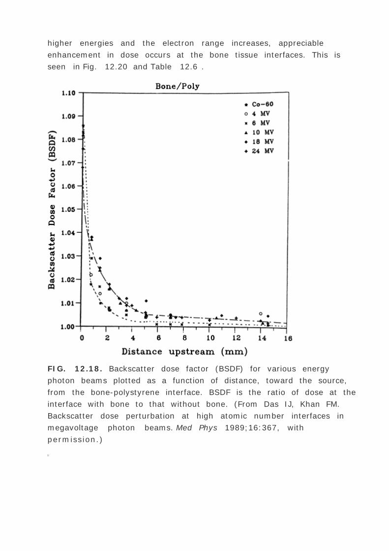
higher energies and the electron range increases, appreciable

enhancement in dose occurs at the bone tissue interfaces. This is

seen in Fig. 12.20 and Table 12.6 .

FIG. 12.18. Backscatter dose factor (BSDF) for various energy

photon beams plotted as a function of distance, toward the source,

from the bone-polystyrene interface. BSDF is the ratio of dose at the

interface with bone to that without bone. (From Das IJ, Khan FM.

Backscatter dose perturbation at high atomic number interfaces in

megavoltage photon beams. Med Phys 1989;16:367, with

permission.)

FIG. 12.19. Forward dose perturbation factor (FDPF) for various

energy photon beams plotted as a function of distance, away from

the source, from bone-polystyrene interface. FDPF is the ratio of

dose at the interface with bone to that without bone for the same

photon energy fluence. (From Das IJ. Study of dose perturbation at

bone-tissue interfaces in megavoltage photon beam therapy.

[Dissertation.] University of Minnesota, 1988:119, with permission.)

FIG. 12.20. Percent depth dose distribution in a 20-cmâ€“thick

polystyrene phantom containing a bone substitute material. Doses

are normalized to midpoint dose in the homogeneous polystyrene

phantom of the same thickness. Parallel-opposed beams, field size =

10 — 10 cm, SSD = 100 cm. The symbol * signifies dose to a

small tissue cavity in bone. A: 6 MV photon beam. B: 24 MV photon

beam. (From Das IJ, Khan FM, Kase KR. Dose perturbation at high

atomic number interfaces in parallel opposed megavoltage photon

beam irradiation [abst.]. Phys Med Biol 1988;33[suppl 1]:121, with

permission.)

B.3. Lung Tissue

Dose within the lung tissue is primarily governed by its density. As

discussed in section 12.5A , lower lung density gives rise to higher

dose within and beyond the lung. Figure 12.21

P.258

gives the increase in lung dose as a function of depth in the lung for

selected energies using a 10 — 10 cm field. But in the first layers

of soft tissue beyond a large thickness of lung, there is some loss of

secondary electrons (60 ). This gives rise to a slight decrease in

dose relative to that calculated on the basis of lung transmission.

0.5

1.01

1.02

1.03

1.04

1.0

1.01

1.02

1.03

1.05

2.0

1.00

1.01

1.03

1.05

3.0

0.99

1.00

1.03

1.05a Dose to soft tissue adjacent to bone relative to midpoint dose in a

homogeneous soft tissue; total thickness = 20 cm; field size = 10

— 10 cm; SSD = 100 cm.

From Das IJ, Khan FM, Kase KR. Dose perturbation at high atomic

number interfaces in parallel opposed megavoltage photon beam

irradiation [abstract]. Phys Med Biol 1988;33[Suppl 1]:121, with

permission.

Thickness of Bone (cm) 6 MV 10 MV 18 MV 24 MV

TABLE 12.6. DOSE ENHANCEMENT AT BONE-TISSUE

INTERFACE FOR PARALLEL-OPPOSED BEAMS a

Kornelson and Young (61 ) have discussed the problem of loss of

lateral electronic equilibrium when a high-energy photon beam

traverses the lung. Because of the lower density of lung, an

increasing number of electrons travel outside the geometrical limits

of the beam. This causes the dose profile to become less sharp. For

the same reason there is a greater loss of laterally scattered

electrons, causing a reduction in dose on the beam axis. The effect

is significant for small field sizes (<6 — 6 cm) and higher energies

(>6 MV). Clinically, when treating a tumor in the lung there is a

possibility of underdosage in the periphery of the tumor if small

fields and high-energy beams are used. However, considering the

fact that most protocols in this country require no lung correction in

dose prescription, consideration of this effect in dosimetry becomes

rather academic.

B.4. Air Cavity

The most important effect of air cavities in megavoltage beam

dosimetry is the partial loss of electronic equilibrium at the cavity

surface. The actual dose to tissue beyond and in front of the cavity

may be appreciably lower than expected. This phenomenon of dose

buildup at the air cavities has been extensively studied by Epp et al.

(62 ,63 ). The most significant decrease in dose occurs at the

surface beyond the cavity, for large cavities (4 cm deep) and the

smallest field (4 — 4 cm). Epp et al. (62 ) have estimated that in

the case of 60 Co the reduction in dose in practical cases, such as

the lesions located in the upper

P.259

respiratory air passages, will not be greater than 10% unless field

sizes smaller than 4 — 4 cm are used. The underdosage is

expected to be greater for higher-energy radiation (63 ).

FIG. 12.21. Percentage increase in lung dose as a function of depth

in the lung for selected energies. Field size = 10 — 10 cm. (From

McDonald SC, Keller BE, Rubin P. Method for calculating dose when

lung tissue lies in the treatment field. Med Phys 1976;3:210, with

permission.)

12.6. TISSUE COMPENSATION

A radiation beam incident on an irregular or sloping surface

produces skewing of the isodose curves. Corrections for this effect

were discussed in section 12.2 . In certain treatment situations,

however, the surface irregularity gives rise to unacceptable

nonuniformity of dose within the target volume or causes excessive

irradiation of sensitive structures such as the spinal cord. Many

techniques have been devised to overcome this problem, including

the use of wedged fields or multiple fields and the addition of bolus

material or compensators. Areas having a smaller thickness of tissue

can also be blocked for the last few treatments to reduce the dose in

these areas.

Bolus is a tissue-equivalent material placed directly on the skin

surface to even out the irregular contours of a patient to present a

flat surface normal to the beam. This use of bolus should be

distinguished from that of a bolus layer, which is thick enough to

provide adequate dose buildup over the skin surface. The latter

should be termed the build-up bolus.

Placing bolus directly on the skin surface is satisfactory for

orthovoltage radiation, but for higher-energy beams results in the

loss of the skin sparing advantage. For such radiations, a

compensating filter should be used, which approximates the effect of

the bolus as well as preserves the skin-sparing effect. To preserve

the skin-sparing properties of the megavoltage photon beams, the

compensator is placed a suitable distance (â‰¥20 cm) away from

the patient's skin. Yet the compensator is so designed that its

introduction in the beam gives rise to isodose curves within the

patient that duplicate, as closely as possible, those for the bolus.

A. Design of Compensators

Figure 12.22 illustrates schematically the use of a compensator to

provide the required beam attenuation that would otherwise occur in

the â€œmissingâ€ tissue when the body surface is

P.260

irregular or curved. Because the compensator is designed to be

positioned at a distance from the surface, the dimensions and shape

of the compensator must be adjusted because of (a) the beam

divergence, (b) the relative linear attenuation coefficients of the

filter material and soft tissues, and (c) the reduction in scatter at

various depths when the compensator is placed at a distance from

the skin rather than in contact with it. To compensate for this

scatter, the compensator is designed such that the attenuation of

the filter is less than that required for primary radiation only. These

considerations and others have been discussed in the literature (64

,65 ,66 ,67 ,68 ,69 ,70 ).

FIG. 12.22. Schematic representation of a compensator designed

for an irregular surface. (From Khan FM, Moore VC, Burns DJ. The

construction of compensators for cobalt teletherapy. Radiology


Minification of the compensating material for geometric divergence

of the beam has been achieved in many ways. One method (64 ,66

,67 ,68 ) constructs the compensator out of aluminum or brass

blocks, using a matrix of square columns corresponding to the

irregular surface. The dimension of each column is minified

according to the geometric divergence correction, which is

calculated from the SSD and the filter-surface distance. Khan et al.

(71 ) described an apparatus that uses thin rods duplicating the

diverging rays of the therapy beam (Fig. 12.23 ). The rods move

freely in rigid shafts along the diverging paths and can be locked or

released by a locking device. The apparatus is positioned over the

patient so that the lower ends of the rods touch the skin surface.

When the rods are locked, the upper ends of the rods generate a

surface that is similar to the skin surface but corrected for

divergence. A plastic compensator can then be built over this

surface (69 ). Beck et al. (72 ) and Boge et al. (73 ) have described

Styrofoam cutters (Fig. 12.24 ) that work on a pantographic

principle and use a heating element or a routing tool mechanism for

the hollowing of the Styrofoam. The cavity thus produced is a

minified version of the patient surface, which can be filled with the

compensator material.

FIG. 12.23. An apparatus for the construction of 3-D compensator

in one piece. (From Khan FM, Moore VC, Burns DJ. An apparatus for

the construction of irregular surface compensators for use in

radiotherapy. Radiology 1968;90:593, with permission.)

FIG. 12.24. Schematic diagram of a Styrofoam cutter fitted with a

routing tool for constructing compensators. (Redrawn from Boge RJ,

Edland RW, Mathes DC. Tissue compensators for megavoltage

radiotherapy fabricated from hollowed Styrofoam filled with wax.

Radiology 1974;111:193, with permission.)

P.261

A tissue equivalent compensator designed with the same thickness

as that of the missing tissue will overcompensate, i.e., the dose to

the underlying tissues will be less than that indicated by the

standard isodose chart. This decrease in depth dose, which is due to

the reduction in scatter reaching a point at depth, depends on the

distance of the compensator from the patient, field size, depth, and

beam quality. To compensate for this decrease in scatter, one may

reduce the thickness of the compensator to increase the primary

beam transmission. The compensator thickness should be such that

the dose at a given depth is the same whether the missing tissue is

replaced with the bolus in contact or with the compensator at the

given distance from the skin surface. The required thickness of a

tissue-equivalent compensator along a ray divided by the missing

tissue thickness along the same ray may be called the density ratio

or thickness ratio (69 ) (h â€²/h in Fig. 12.22 ). Figure 12.25

P.262

gives a plot of thickness ratio, „, as a function of compensator-

surface distance, d. „ is unity at the surface and decreases as d

increases.

FIG. 12.25. A plot of density ratio or thickness ratio as a function

of compensator distance for a uniformly thick compensator. 60 Co

³ rays, field size = 10 — 10 cm, SSD = 80 cm, compensation

depth = 7 cm, and tissue deficit = 5.0 cm. (From Khan FM, Moore

VC, Burns DJ. The construction of compensators for cobalt

teletherapy. Radiology 1970;96:187, with permission.)

Thickness ratio depends, in a complex way, on compensator-surface

distance, thickness of missing tissue, field size, depth, and beam

quality. However, a detailed study of this parameter has shown that

„ is primarily a function of d (for d â‰¤ 20 cm) and that its

dependence on other parameters is relatively less critical (69 ,74 ).

Thus a fixed value of „, based on a given d (usually 20 cm), 10

— 10 cm field, 7-cm depth, and a tissue deficit of 5 cm can be

used for most compensator work.

The concept of thickness ratios also reveals that a compensator

cannot be designed to provide absorbed dose compensation exactly

at all depths. If, for given irradiation conditions, „ is chosen for a

certain compensation depth, the compensator overcompensates at

shallower depths and undercompensates at greater depths.

Considering the limitations of the theory and too many variables

affecting „, we have found that an average value of 0.7 for „

may be used for all irradiation conditions provided d â‰¥ 20 cm.

The same value has been tested to yield satisfactory results (errors

in depth dose within ±5%) for 60 Co, 4-MV and 10-MV x-rays (74

).

In the actual design of the compensator, the thickness ratio is used

to calculate compensator thickness (tc ) at a given point in the field:

where TD is the tissue deficit at the point considered and c is the

density of the compensator material.

A direct determination of thickness ( „/ c ) for a compensator

system may be made by measuring dose at an appropriate depth

and field size in a tissue equivalent phantom (e.g., polystyrene)

with a slab of compensator material placed in the beam at the

position of the compensator tray. Pieces of phantom material are

removed from the surface until the dose equals that measured in the

intact phantom, without the compensator. The ratio of compensator

thickness to the tissue deficit gives the thickness ratio.

It may be mentioned that a term compensator ratio (CR) has also

been used in the literature to relate tissue deficit to the required

compensator thickness (75 ). It is defined as the ratio of the missing

tissue thickness to the compensator thickness necessary to give the

dose for a particular field size and depth. The concepts of

compensator ratio and the thickness ratio are the same, except that

the two quantities are inverse of each other, i.e., CR = TD/tc = c

/ „.

B. Two-dimensional Compensators

Designing a 3-D compensator is a time-consuming procedure. In a

well-equipped mold or machine shop, a trained technician can

probably construct such compensators routinely with a reasonable

expenditure of time. In the absence of such facilities and personnel,

however, most situations requiring compensation can be handled

satisfactorily with simple 2-D compensators. In many treatment

situations, the contour varies significantly in only one direction:

along the field width or length. In such cases, a compensator can be

constructed in which the thickness varies only along this dimension.

For example, if anterior and posterior fields are incident on a

sloping mediastinum, compensation is usually not changed in the

lateral direction but only in the craniocaudal direction.

One simple way of constructing a two-dimensional compensator is to

use thin sheets of lead (with known thickness ratio or effective

attenuation coefficient) and gluing them together in a stepwise

fashion to form a laminated filter. The total thickness of the filter at

any point is calculated to compensate for the air gap at the point

below it. Another method, used routinely at the University of

Minnesota, is to construct the compensator in one piece from a block

of Lucite. The patient contour is taken showing body thickness at at

least three reference points: central axis, inferior margin, and

superior margin of the field. Tissue deficits, ”t , are calculated by

subtracting thicknesses at the reference points from the maximum

thickness. A thickness minification factor is calculated by dividing

the

P.263

thickness ratio „ by the electron density (e- per cm3 ) of Lucite

relative to that of tissue. The geometric minification factor is

calculated by (f - d )/f where f is the SSD at the point of maximum

thickness and d is the filter-surface distance. The compensator

dimensions can now be drawn by multiplying the ”t values with the

thickness minification factor and the spacing between the reference

points with the geometric minification factor. A Lucite block is then

machined and glued on a thin Lucite plate for placement in the

beam. The same method may be used to construct a compensator by

stacking Lucite plates in a stepwise fashion and attaching them

together firmly with pieces of Scotch tape.

C. Three-dimensional Compensators

Early 3-D compensator systems were mechanical devices to measure

tissue deficits within the field in both the transverse and the

longitudinal body cross-sections. Examples of these systems include

Ellis type filters (64 ,66 ), rod boxes (68 ,69 ) and pantographic

devices (72 ,73 ). More recent devices include Moir © camera, 3-D

magnetic digitizers, CT-based compensator programs and electronic

compensation using Multileaf collimators (Chapter 20 ).

C.1. Moir © Camera

A specially designed camera system allows topographic mapping of

the patient body surface and provides tissue deficit data necessary

for the design of a 3-D compensator. The principle of operation of

the camera has been discussed by Boyer and Goitein (76 ). The

camera can be mounted on a simulator without interfering with the

simulator's normal use. Moir © fringes observed on the patient's

surface represent iso-SSD lines from which the tissue deficit data

can be deduced. The data can be used to drive a pantographic

cutting unit. A commercial version of this system is manufactured by

DCD, S&S PAR Scientific (Brooklyn, NY).

C.2. Magnetic Digitizer

A handheld stylus containing a magnetic field sensor is used to

digitize the position of the sensor as it is scanned over the patient's

surface in the presence of a low-strength, low-frequency magnetic

field. Tissue deficit data are calculated by the computer from the

sensor coordinates and used to drive a Styrofoam cutter. Cavities

corresponding to the tissue deficit are then filled with an

appropriate compensator material to design a compensator. A

commercially available system, known as Compuformer is

manufactured by Huestis Corporation (Bristol, RI).

C.3. Computed Tomographyâ€“based

Compensator Systems

Three-dimensional radiotherapy treatment planning systems that

use multilevel CT scans have sufficient data available to provide

compensation not only for the irregular surface contours but also for

the tissue inhomogeneities. There are two commercial systems that

provide software for the design of compensating filters: the Target

(G.E. Medical Systems, Milwaukee, WI) and the Theracomp/HEK

(Theratronics Ltd., Ontario, Canada). These systems extract the

tissue deficit data from the CT scans, which are then used to cut the

Styrofoam mold using a drill bit or a heated wire loop. Although any

compensator material of known compensator ratio may be cast into

the filter molds, it is desirable to use medium-density materials

rather than heavier materials such as Cerrobend. The main reason

for this is to minimize error in dose distribution when small errors

are made in cutting the mold.

There are several other compensator systems that have not been

discussed here. For a detailed review of this topic the reader is

referred to Reinstein (77 ).

P.264

D. Compensating Wedges

For oblique beam incidence or curved surfaces for which the contour

can be approximated with a straight line, standard compensating

wedges are very convenient (69 ,70 ). Compensating wedges (C-

wedges) are fabricated from a metal such as copper, brass, or lead.

They are designed to compensate for a â€œmissingâ€ wedge of

tissue, using the same design principles as discussed in section

12.4B .

Distinction needs to be made between a wedge filter and a

compensating wedge. Although a wedge filter can be used

effectively as a compensator, it is primarily designed to tilt the

standard isodose curves through a certain wedge angle in

conjunction with the wedge-pair technique (Chapter 11 ). The wedge

filter isodose curves must be available and used to obtain the

composite isodose curves before the filter is used in a treatment

set-up. The C-wedge, on the other hand, is used just as a

compensator, so that the standard isodose charts can be used

without modification. In addition, no wedge transmission factors are

required for the C-wedges.

An important advantage of C-wedges over wedge filters used as

compensators is that the C-wedges can be used for partial field

compensation, that is, the C-wedge is used to compensate only a

part of the contour, which is irregular in shape. A wedge filter, in

this case, could not be used as a compensator because it is designed

to be placed in the field in a fixed position.

E. Other Applications

Compensating filters can be designed to compensate for tissue

heterogeneity. Most of this work was done by Ellis and his coworkers

(33 ) in which compensators were designed from the knowledge of

cross-sectional anatomy using transaxial tomography or a

photographic film. More recently, Khan et al. (78 ) have described

compensators for total body irradiation including compensation for

lungs.

Compensators have also been used to improve dose uniformity in

the fields where nonuniformity of the dose distribution arises from

sources other than contour irregularity: reduced scatter near the

field edges and unacceptable high dose regions or â€œhornsâ€ in

the beam profile. Leung et al. (79 ) have discussed the design of

filters for the mantle technique in which the compensator is

designed on the basis of calculated dose distribution in the absence

of a compensator. Boge et al. (80 ) have described a special

compensator filter to reduce the horns present in large fields of a 4-

MV linear accelerator.

F. Compensator Set-up

As mentioned earlier, the compensator should be placed at a

distance of 20 cm or more away from the skin surface to preserve

the skin-sparing properties of the megavoltage beams. Because the

dimensions of the compensator are reduced (compared to the bolus)

in the plane perpendicular to the beam axis to allow for beam

divergence, the filter must be placed at the filter-surface distance

for which it is designed. In addition, the nominal SSD should be

measured from the plane perpendicular to the beam axis, containing

the most elevated point on the contour included in the field (Fig.

12.22 ). For isocentric treatments, it is most convenient to use field

dimensions projected at the isocenter in compensator design.

Accordingly, the depth of the isocenter is measured from the level of

the most elevated point on the contour to be compensated.

12.7. PATIENT POSITIONING

Availability of isocentric treatment machines, simulators, CT

scanners, and computers has made it possible to achieve a high

degree of precision in radiation therapy. However, one of the

weakest links in the treatment-planning process is the problem of

patient positioning

P.265

and immobilization. It is frequently observed that some of the

treatment techniques in current practice are outdated or do not take

advantage of the accuracy available with the modern equipment. For

example, the patients are treated in less than a stable position, are

moved between different fields, and set up primarily by marks inked

or tattooed on the skin surface. But, as any experienced observer

knows, such practices are prone to serious errors. Skin marks are

vulnerable to variation in skin sag and body position on the

treatment table.

FIG. 12.26. Bite block system for head and neck immobilization.

(Courtesy of Radiation Products Design, Buffalo, MN.)

The problem of precise patient positioning and immobilization has

been addressed by a number of investigators (81 ,82 ,83 ,84 ,85 ,86

), including a recent review by Reinstein (87 ). But this problem still

remains the area of greatest variance in actual treatment. The

following ideas are presented to focus attention on this important

area and offer some guidelines for precise patient positioning.

A. General Guidelines

Treatments should be set up isocentrically. The principal

advantage of isocentric technique over SSD technique is that the

patient is not moved between fields. Once the isocenter is

positioned accurately within the patient, the remaining fields are

arranged simply by gantry rotation or couch movement, not by

displacing the patient relative to the couch.

Isocenter position within the patient can be established using

the treatment simulator. This is usually accomplished by

anterior and lateral radiographs, using the radiographically

visible structures to define the target volume.

To accurately define the patient's position, thick pads or

mattresses should not be used on the simulator table or the

treatment table. This is essential for accurate measurement of

set-up parameters as well as reproducibility.

For head and neck treatments, flexible head rests, such as

pillows or sponges, should be avoided. The head should rest on a

rigid surface such as a block of hard Styrofoam or a plastic

â€œhead-neckâ€ support (Fig. 12.26 ).

Many methods of head immobilization are available such as

partial body casts (85 ), bite block system (88 ),5 nose bridges,5

head clamps,5 or simple masking tape. Choice of any of the

above will depend on the location of the treatment fields.

As far as possible, the patient should be treated in the supine

position. An overhead

P.266

sagittal laser line is useful in aligning the sagittal axis of the

patient with the axis of gantry rotation.

For head and neck treatments, the chin extension should be

defined anatomically, for example, distance between the sternal

notch and the chin bone. This measurement should be accurately

made after the head position has been established on the basis

of stability and field localization.

During simulation as well as treatment, the depth of isocenter

should be defined by either the set-up SSD (usually measured

anteriorly or posteriorly) or by setting the distance between the

tabletop distance and lateral beam axis. Side laser lights may

also be used for this purpose. In the latter case, the laser lights

should be checked frequently for alignment accuracy, because

these lights are known to drift presumably by expansion and

contraction of the walls on which they are mounted.

Skin marks should not be relied on for daily localization of the

treatment field. The field boundaries should be defined relative

to the bony landmarks established during simulation. Do not

force the field to fit the skin marks!

For lateral portals, the Mylar section of the couch or tennis

racket should be removed and the patient placed on a solid

surface to avoid sag. These should be used only for

anteroposterior (AP) treatments for which skin sparing is to be

achieved. For example, if the four-field pelvis technique is used,

one can use two fields a day in which case AP treatments are

given isocentrically on a Mylar window using anterior or

posterior set-up SSD, and lateral fields are treated on a flat

tabletop section using the tabletop distance to lateral beam axis.

Or if four fields are treated the same day, the posterior field can

be treated through the rigid Plexiglas section of the couch

instead of the Mylar window. Or AP treatments can be given on

the Mylar window and then the window can be replaced by the

Plexiglas section for the lateral treatments. The last alternative

involves two separate set-ups, one for the AP and the other for

the lateral fields. It should be used only when skin dose from

the posterior fields is to be reduced to a minimum.

For isocentric techniques, field sizes must be defined at the

isocenter which will, in most cases, be at the center of the

treatment volume and not on the skin surface. Physicians who

are accustomed to using standard field sizes (e.g., pelvic fields)

defined at the skin surface should make adjustments in field

sizes so that the fields encompass the same irradiated volume.

Some institutions have developed elaborate casting techniques to

immobilize patients during treatments. This requires a well-

equipped mold room as well as personnel trained in mold

technology. Some of these techniques have been shown to be quite

effective in minimizing patient motion (85 ,87 ). However, patients

are known to move within a cast especially if the fit is not good or if

there is a change in the surfaces contour due to regression of the

tumor or weight loss.

Detection of patient motion is possible by using small dots of

reflective tape on the patient with a pencil light ray and photocell

device. Laser localization lights can also be used for this purpose.

The signal received from the photocell can be further processed to

activate an interlock to interrupt treatment or sound an alarm if

pertinent motion exceeds a preset limit. Thus a good motion

detection system can complement patient positioning and

immobilization techniques by monitoring the stability of patient

position as well as the effectiveness of immobilization.

B. The XYZ Method of Isocenter Set-up

In the isocentric technique, the isocenter is placed inside the

patient, usually at the center of the target volume. Once this point

has been localized by simulation, a good treatment set-up should

reproduce it quickly and accurately. The following steps outline a

procedure, hereby called the XYZ method, for the localization of this

important point.

P.267

B.1. Simulation Procedure

The patient is positioned on the simulator couch following the

general guidelines discussed in section 12.7A .

The patient is leveled using the side lasers (or a bubble level)

and the sagittal laser beam to define the sagittal axis of the

patient. The patient is then constrained from movement by a

suitable immobilization device. For head and neck positioning,

chin extension (distance between chin bone and the sternal

notch) should be accurately measured.

The treatment fields are simulated using anterior and lateral

radiographs and the isocenter is established according to the

treatment plan.

A reference anatomic point is chosen on the sagittal axis,

somewhere in the neighborhood of the treatment area, to

represent a stable anatomic landmark. For example, nasion for

head and neck, sternal notch for neck and thorax, tip of xiphoid

for thorax and abdomen, and bottom of pubic ramus or tip of

coccyx for pelvis, can be chosen as reasonably stable reference

points.

The coordinates of the treatment isocenter are represented by

(X, Y, Z) where X is the lateral distance and Y is the longitudinal

distance (along patient axis) of the isocenter from the reference

point and Z is the tabletop to isocenter distance (Fig. 12.27 ).

Beam angle ¸ is recorded.

B.2. Treatment Set-up

Position and level the patient on the treatment couch as in

simulation.

With the gantry vertical, place the central axis at the reference

anatomic point and mark it with ink.

Move the couch: up or down to obtain Z using the side laser;

laterally through X and

P.268

longitudinally through distance Y. Rotate the gantry through

angle ¸. This gives the required central axis of the field and

the isocenter location.

FIG. 12.27. A diagram to illustrate X, Y, Z coordinates to a

patient set-up.

Make secondary checks according to the field diagram such as

SSD, location of field borders, etc.

For isocentric set-up, other fields are positioned by simply

rotating the gantry and positioning it at predetermined angles.

One potential advantage of this method is that the set-up

parameters X, Y, Z, and ¸ could be computer controlled, thereby

decreasing the set-up time and minimizing human errors. The

therapist, in this case, will position the patient as usual and place

the central axis vertically at the reference point. Then, with a switch

on the hand pendant, the computer control could be initiated to

move the couch and the gantry to the X, Y, Z, and ¸ coordinates.

Such a method could be adopted by some of the existing treatment

monitoring systems that are capable of moving the couch and the

gantry.

Even manually, the XYZ method can greatly economize set-up time

as well as enhance set-up precision. Most modern couches are motor

driven and equipped with motion-sensing devices. Videographic

display of the couch motions could be conveniently used to position

the couch. A reset switch for the X, Y, and Z coordinates would

make it easier to move the couch through the X, Y, and Z distances.

REFERENCES

1. Kuisk H. â€œContour makerâ€ eliminating body casting in

radiotherapy planning. Radiology 1971;101:203.

2. Clarke HC. A contouring device for use in radiation treatment

planning. Br J Radiol 1969;42:858.

3. Clayton C, Thompson D. An optical apparatus for reproducing

surface outlines of body cross-sections. Br J Radiol 1970;43:489.

4. Carson PL, Wenzel WW, Avery P, et al. Ultrasound imaging as

an aid to cancer therapyâ€”part I. Int J Radiat Oncol Biol Phys

1975;1:119. Part II. Int J Radiat Oncol Biol Phys 1976;2:335.

5. Takahashi S, Matsuda T. Axial transverse laminography

applied to rotation therapy. Radiology 1960;74:61.

6. Pierquin B. La tomographie transversale: technique de routine

en radiotherapie. J Radiol Electrol 1961;42:131.

7. Brooks RA, Di Chiro G. Principles of computer assisted

tomography (CAT) in radiographic and radioisotopic imaging.

Phys Med Biol 1976;21:689.

8. Rutherford RA, Pullan BR, Isherwood I. Measurement of

effective atomic number and electron density using an EMI

scanner. Neuroradiology 1976;11:15.

9. Kijewski PK, Bj ¤rngard BE. The use of computed tomography

data for radiotherapy dose calculations. Int J Radiat Oncol Biol

Phys 1978;4:429.

10. Munzenrider JE, Pilepich M, Ferrero JBR, et al. Use of body

scanners in radiotherapy treatment planning. Cancer

1977;40:170.

11. Geise RA, McCullough EC. The use of CT scanners in

megavoltage photon-beam therapy planning. Radiology

1977;124:133.

12. Sontag MR, Battista JJ, Bronskill MJ, et al. Implications of

computed tomography for inhomogeneity corrections in photon

beam dose calculations. Radiology 1977;124:143.

13. Chernak ES, Antunez RA, Jelden GL, et al. The use of

computed tomography for radiation therapy treatment planning.

Radiology 1975;117:613.

14. Sternick ES, Lane FW, Curran B. Comparison of computed

tomography and conventional transverse axial tomography in

radiotherapy treatment planning. Radiology 1977;124:835.

15. Fullerton GD, Sewchand W, Payne JT, et al. CT determination

of parameters for inhomogeneity corrections in radiation therapy

of the esophagus. Radiology 1978;124:167.

16. Parker RP, Hobday PA, Cassell KJ. The direct use of CT

numbers in radiotherapy dosage calculations for inhomogeneous

media. Phys Med Biol 1979;24:802.

17. Hobday P, Hodson NJ, Husband J, et al. Computed

tomography applied to radiotherapy treatment planning:

techniques and results. Radiology 1979;133:477.

18. Ragan DP, Perez CA. Efficacy of CT-assisted two-dimensional

treatment planning: analysis of 45 patients. Am J Roentgenol

1978;131:75.

19. Goitein M. The utility of computed tomography in radiation

therapy: an estimate of outcome. Int J Radiat Oncol Biol Phys

1979;5:1799.

P.269

20. Goitein M. Computed tomography in planning radiation

therapy. Int J Radiat Oncol Biol Phys 1979;5:445.

21. Sontag MR, Cunningham JR. The equivalent tissue-air ratio

method for making absorbed dose calculations in a

heterogeneous medium. Radiology 1978;129:787.

22. Hogstrom KR, Mills MD, Almond PR. Electron beam dose

calculations. Phys Med Biol 1981;26:445.

23. Cassell KJ, Hobday PA, Parker RP. The implementation of a

generalized Batho inhomogeneity correction for radiotherapy

planning with direct use of CT numbers. Phys Med Biol

1981;26:825.

24. Ling CC, Rogers CC, Morton RJ, eds. Computed tomography in

radiation therapy . New York: Raven Press, 1983.

25. Carson PL, Wenzel WW, Hendee WR. Ultrasound imaging as

an aid to cancer therapyâ€”I. Int J Radiat Oncol Biol Phys

1975;1:119.

26. Carson PL, Wenzel WW, Avery P, et al. Ultrasound imaging as

an aid to cancer therapyâ€”II. Int J Radiat Oncol Biol Phys

1976;1:335.

27. Green D, Nelson KA, Gibb R. The use of a linear accelerator

â€œsimulatorâ€ in radiotherapy. Br J Radiol 1964;37:394.

28. Ovadia J, Karzmark CJ, Hendrickson FR. Radiation therapy

simulation and transverse tomography: apparatus bibliography

and tumor localization . Houston: American Association of

Physicists in Medicine Radiological Physics Center, 1971.

29. Karzmark CJ, Rust DC. Radiotherapy simulators and

automation. Radiology 1972;105:157.

30. Bomford CK, Craig LM, Hanna FA, et al. Treatment

simulators. Report no. 10. London: British Institute of Radiology,

1976.

31. McCullough EC, Earl JD. The selection, acceptance testing,

and quality control of radiotherapy treatment simulators.

Radiology 1979;131:221.

32. Droege RT, Bj ¤rngard BE. Metal screen-film detector MTF at

megavoltage x-ray energies. Med Phys 1979;6:515.

33. Ellis F, Lescrenier C. Combined compensation for contours

and heterogeneity. Radiology 1973;106:191.

34. Baily NA, Horn RA, Kampp TD. Fluoroscopic visualization of

megavoltage therapeutic x-ray beams. Int J Radiat Oncol Biol

Phys 1980;6:935.

35. Leong J. Use of digital fluoroscopy as an on-line verification

device in radiation therapy. Phys Med Biol 1986;31:985.

36. Shalev S, Lee T, Leszczynski K, et al. Video techniques for

on-line portal imaging. Comput Med Imaging Graph

1989;13:217.

37. Visser AG, Huizenga H, Althof VGM, et al. Performance of a

prototype fluoroscopic imaging system. Int J Radiat Oncol Biol

Phys 1990;18:43.

38. Wong JW, Binns WR, Cheng AY, et al. On-line radiotherapy

imaging with an array of fiber-optic image reducers. Int J Radiat

Oncol Biol Phys 1990;18:1477.

39. Van Herk M, Meertens H. A matrix ionization chamber

imaging device for on-line patient set up verification during

radiotherapy. Radiother Oncol 1988;11:369.

40. Meertens H, Van Herk M, Bijhold J, et al. First clinical

experience with a newly developed electronic portal imaging

device. Int J Radiat Oncol Biol Phys 1990;18:1173.

41. Boyer AL, Antnuk L, Fenster A, et al. A review of electronic

portal imaging devices (EPIDs). Med Phys 1992;19:1.


Measurements (ICRU). Determination of absorbed dose in a

patient irradiated by beams of x or gamma rays in radiotherapy

procedures. Report No. 24. Washington, DC: United States


43. Batho HF. Lung corrections in cobalt 60 beam therapy. J Can

Assn Radiol 1964;15:79.

44. Young MEJ, Gaylord JD. Experimental tests of corrections for

tissue inhomogeneities in radiotherapy. Br J Radiol 1970;43:349.

45. Sontag MR, Cunningham JR. Corrections to absorbed dose

calculations for tissue inhomogeneities. Med Phys 1977;4:431.

46. Cunningham JR. Scatter-air ratios. Phys Med Biol

1972;17:42.

47. Wong JW, Henkelman RM. A new approach to CT pixel-based

photon dose calculation in heterogeneous media. Med Phys

1983;10:199.

48. Krippner K, Wong JW, Harms WB, et al. The use of an array

processor for the delta volume dose computation algorithm. In:

Proceedings of the 9th international conference on the use of

computers in radiation therapy, Scheveningen, The Netherlands.

North Holland: The Netherlands, 1987:533.

49. Mackie TR, Scrimger JW, Battista JJ. A convolution method of

calculating dose for 15-MV x-rays. Med Phys 1985;12:188.

50. Mohan R, Chui C, Lidofsky L. Differential pencil beam dose

computation model for photons. Med Phys 1986;13:64.

51. Greene D, Stewart JR. Isodose curves in non-uniform

phantoms. Br J Radiol 1965;38:378.

52. Sundblom I. Dose planning for irradiation of thorax with

cobalt in fixed beam therapy. Acta Radiol 1965;3:342.

P.270

53. Tang WL, Khan FM, Gerbi BJ. Validity of lung correction

algorithms. Med Phys 1986;13:683.

54. McDonald SC, Keller BE, Rubin P. Method for calculating dose

when lung tissue lies in the treatment field. Med Phys

1976;3:210.

55. Spires SW. Dosage in irradiated soft tissue and bone. Br J

Radiol 1951;24:365.


Measurements (ICRU). Clinical dosimetry. Report No. 10d.

Washington, DC: United States Bureau of Standards, 1963.

57. Johns HE, Cunningham JR. The physics of radiology , 2nd ed.

Springfield, IL: Charles C Thomas, 1969:455.

58. Das IJ, Khan FM. Backscatter dose perturbation at high

atomic number interfaces in megavoltage photon beams. Med

Phys 1989;16:367.

59. Werner BL, Das IJ, Khan FM, et al. Dose perturbation at

interfaces in photon beams. Med Phys 1987;14:585.

60. Leung PMK, Seaman B, Robinson P. Low-density

inhomogeneity corrections for 22-MeV x-ray therapy. Radiology

1970;94:449.

61. Kornelson RO, Young MEJ. Changes in the dose-profile of a

10 MV x-ray beam within and beyond low density material. Med

Phys 1982;9:114.

62. Epp ER, Lougheed MN, McKay JW. Ionization buildup in upper

respiratory air passages during teletherapy units with cobalt 60

radiation. Br J Radiol 1958;31:361.

63. Epp ER, Boyer AL, Doppke KP. Underdosing of lesions

resulting from lack of electronic equilibrium in upper respiratory

air cavities irradiated by 10 MV x-ray beam. Int J Radiat Oncol

Biol Phys 1977;2:613.

64. Ellis F, Hall EJ, Oliver R. A compensator for variations in

tissue thickness for high energy beam. Br J Radiol 1959;32:421.

65. Cohen M, Burns JE, Sear R. Physical aspects of cobalt 60

teletherapy using wedge filters. II. Dosimetric considerations.

Acta Radiol 1960;53:486.

66. Hall EJ, Oliver R. The use of standard isodose distributions

with high energy radiation beamsâ€”the accuracy of a

compensator technique in correcting for body contours. Br J

Radiol 1961;34:43.

67. Sundblom I. Individually designed filters in cobalt-60

teletherapy. Acta Radiol Ther Phys Biol 1964;2:189.

68. Van De Geijn J. The construction of individualized intensity

modifying filters in cobalt 60 teletherapy. Br J Radiol

1965;38:865.

69. Khan FM, Moore VC, Burns DJ. The construction of

compensators for cobalt teletherapy. Radiology 1970;96:187.

70. Sewchand W, Bautro N, Scott RM. Basic data of tissue-

equivalent compensators for 4 MV x-rays. Int J Radiat Oncol Biol

Phys 1980;6:327.

71. Khan FM, Moore VC, Burns DJ. An apparatus for the

construction of irregular surface compensators for use in

radiotherapy. Radiology 1968;90:593.

72. Beck GG, McGonnagle WJ, Sullivan CA. Use of Styrofoam

block cutter to make tissue-equivalent compensators. Radiology

1971;100:694.

73. Boge RJ, Edland RW, Matthes DC. Tissue compensators for

megavoltage radiotherapy fabricated from hollowed Styrofoam

filled with wax. Radiology 1974;111:193.

74. Khan FM, Sewchand W, Williamson JF. Unpublished data.

75. Henderson SD, Purdy JA, Gerber RL, et al. Dosimetry

considerations for a Lipowitz metal tissue compensator system.

Int J Radiat Oncol Biol Phys 1987;13:1107.

76. Boyer AL, Goitein M. Simulator mounted Moir © topography

camera for constructing compensator filters. Med Phys

1980;7:19.

77. Reinstein LE. New approaches to tissue compensation in

radiation oncology. In: Purdy JA, ed. Advances in radiation

oncology physics . Medical Physics Monograph No. 19. Woodbury,

NY: American Institute of Physics, Inc., 1992:535.

78. Khan FM, Williamson JF, Sewchand W, et al. Basic data for

dosage calculation and compensation. Int J Radiat Oncol Biol

Phys 1980;6:745.

79. Leung PMK, Van Dyke J, Robins J. A method for large

irregular field compensation. Br J Radiol 1974;47:805.

80. Boge RJ, Tolbert DD, Edland RW. Accessory beam flattening

filter for the Varian Clinac-4 linear accelerator. Radiology

1975;115:475.

81. Chung-Bin A, Kartha P, Wachtor T, et al. Development and

experience in computer monitoring and the verification of daily

patient treatment parameters. In: Sternick ES, ed. Proceedings

of the 5th international conference on use of computers in

radiation therapy. Hanover, NH: University Press of New England,

1976:551.

82. Haus A, Marks J. Detection and evaluation of localization

errors in patient radiation therapy. Invest Radiol 1973;8:384.

83. Kartha PKI, Chung-Bin A, Wachtor T, et al. Accuracy in

patient set-up and its consequence in dosimetry. Med Phys

1975;2:331.

84. Williamson TJ. Improving the reproducibility of lateral

therapy portal placement. Int J Radiat Oncol Biol Phys

1979;5:407.

P.271

85. Verhey LJ, Goitein M, McNulty P, et al. Precise positioning of

patients for radiation therapy. Int J Radiat Oncol Biol Phys

1982;8:289.

86. Hendrickson FR. Precision in radiation oncology. Int J Radiat


87. Reinstein LE. Patient positioning and immobilization. In:

Khan FM, Potish RA, eds. Treatment planning in radiation

oncology . Baltimore: Williams & Wilkins, 1998:55â€“88.

88. Huaskins LA, Thomson RW. Patient positioning device for

external-beam radiation therapy of the head and neck. Radiology

1973;106:706.

1 Oldelft Corporation of America, Fairfax, Virginia.

2 Varian Associates, Palo Alto, California.

3 Theratronics International Ltd., Kanata, Ontario, Canada. Also,

Picker International, Inc., St. Davids, Pennsylvania.

4 Such a sheet of lead acts as an intensifying screen by means of

electrons ejected from the screen by photon interactions. These

electrons provide an image on the film which reflects the variation

of beam intensity transmitted through the patient.

5 Such devices are commercially available, for example, from

Radiation Products Design, Inc., Buffalo, Minnesota and Med-Tec,

Orange City, Iowa.





13 - Treatment Planning III: Field Shaping, Skin Dose, and

Field Separation

13

Treatment Planning III: FieldShaping, Skin Dose, and FieldSeparation

Shielding of vital organs within a radiation field is one of the major

concerns of radiation therapy. Considerable time and effort are

spent in shaping fields not only to protect critical organs but also to

avoid unnecessary irradiation of the surrounding normal tissue.

Attendant to this problem is its effect on skin dose and the buildup

of dose in the subcutaneous tissue. Skin sparing is an important

property of megavoltage photon beams, and every effort should be

directed to maintaining this effect when irradiating normal skin.

Another problem frequently encountered in radiation therapy is the

matching of adjacent fields. This situation arises when radiation

fields available with the equipment are not large enough to

encompass the entire target volume. In some cases, the target

volume is divided into two parts so treatment to the second part

does not commence until the treatment course to the first part has

been completed. Such a scheme is designed to avoid toxicity due to

irradiating an excessive volume of tissue. Multiple adjacent fields

are also used when tumor distribution or patient anatomy does not

allow coplanar fields (fields with central axes in the same plane).

The main problem with these techniques is the possibility of

extreme dose inhomogeneity in the junctional region. Because

radiation beams are divergent, adjacent fields can overlap at depth

and give rise to regions of excessive dose or hot spots. Overlaps can

be avoided by separating the fields, but this in turn can give rise to

areas of reduced dose or â€œcold spots.â€

This chapter on treatment planning focuses on the above problems

and discusses their possible solutions.

13.1. FIELD BLOCKS

The shaping of treatment fields is primarily dictated by tumor

distributionâ€”local extensions as well as regional metastases. Not

only should the dose to vital organs not exceed their tolerance but

the dose to normal tissue, in general, should be minimized. As long

as the target volume includes, with adequate margins, the

demonstrated tumor as well as its presumed occult spread,

significant irradiation of the normal tissue outside this volume must

be avoided as much as possible. These restrictions can give rise to

complex field shapes, which require intricate blocking.

The frequency and complexity of field shaping vary from institution

to institution. However, if complex techniques involving elaborate

blocking are used often, it is necessary to establish a rational

system of field shaping.

A. Block Thickness

Shielding blocks are most commonly made of lead. The thickness of

lead required to provide adequate protection of the shielded areas

depends on the beam quality and the allowed transmission through

the

P.273

block. A primary beam transmission of 5% through the block is

considered acceptable for most clinical situations. If n is the number

of half-value layers to achieve this transmission,

or

or

or

Thus a thickness of lead between 4.5 and 5.0 half-value layers

would give less than 5% primary beam transmission and is,

therefore, recommended for most clinical shielding.

Shielding against primary radiation for superficial and orthovoltage

beams is readily accomplished by thin sheets of lead that can be

placed or molded on to the skin surface. However, as the beam

energy increases to the megavoltage range, the thickness of lead

required for shielding increases substantially. The lead blocks are

then placed above the patient supported in the beam on a

transparent plastic tray, called the shadow tray. Table 13.1 gives

the recommended lead shield thicknesses for various quality beams.

Although the primary beam transmission can be reduced further by

using extra thick blocks, the reduction in dose in the shielded region

may not be that significant due to the predominance of scattered

radiation from the adjoining open areas of the field.

B. Block Divergence

Ideally, the blocks should be shaped or tapered so that their sides

follow the geometric divergence of the beam. This minimizes the

block transmission penumbra (partial transmission of the beam at

the edges of the block). However, divergent blocks offer little

advantage for beams with large geometric penumbra. For example,

in the case of 60 Co, the sharpness of the beam cutoff at the block

edge is not significantly improved by using divergent blocks. Also,

for some clinical situations this sharpness is not critical or worth the

time required for making divergent blocks, which have to be

invariably custom designed for a given treatment set-up. Therefore,

most institutions keep a stock of straight-cut blocks of various

shapes and dimensions.

1.0 mm Al HVL

0.2 mm

2.0 mm Al HVL

0.3 mm

3.0 mm Al HVL

0.4 mm

1.0 mm Cu HVL

1.0 mm

3.0 mm Cu HVL

2.0 mm

4.0 mm Cu HVL

2.5 mm137 Cs

3.0 cm60 Co

5.0 cm

4 MV

6.0 cm

6 MV

6.5 cm

10 MV

7.0 cm

25 MV

7.0 cma Approximate values to give â‰¤5% primary transmission.

HVL, half-value layer.

Beam Quality Required Lead Thickness

TABLE 13.1. RECOMMENDED MINIMUM THICKNESS OF LEAD

FOR SHIELDING a

P.274

Divergent blocks are most suited for beams having small focal spots.

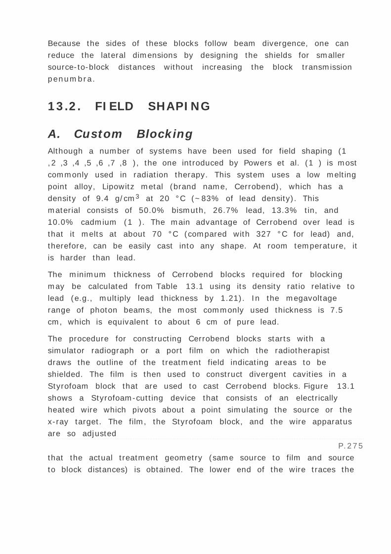
Because the sides of these blocks follow beam divergence, one can

reduce the lateral dimensions by designing the shields for smaller

source-to-block distances without increasing the block transmission

penumbra.

13.2. FIELD SHAPING

A. Custom Blocking

Although a number of systems have been used for field shaping (1

,2 ,3 ,4 ,5 ,6 ,7 ,8 ), the one introduced by Powers et al. (1 ) is most

commonly used in radiation therapy. This system uses a low melting

point alloy, Lipowitz metal (brand name, Cerrobend), which has a

density of 9.4 g/cm3 at 20 °C (~83% of lead density). This

material consists of 50.0% bismuth, 26.7% lead, 13.3% tin, and

10.0% cadmium (1 ). The main advantage of Cerrobend over lead is

that it melts at about 70 °C (compared with 327 °C for lead) and,

therefore, can be easily cast into any shape. At room temperature, it

is harder than lead.

The minimum thickness of Cerrobend blocks required for blocking

may be calculated from Table 13.1 using its density ratio relative to

lead (e.g., multiply lead thickness by 1.21). In the megavoltage

range of photon beams, the most commonly used thickness is 7.5

cm, which is equivalent to about 6 cm of pure lead.

The procedure for constructing Cerrobend blocks starts with a

simulator radiograph or a port film on which the radiotherapist

draws the outline of the treatment field indicating areas to be

shielded. The film is then used to construct divergent cavities in a

Styrofoam block that are used to cast Cerrobend blocks. Figure 13.1

shows a Styrofoam-cutting device that consists of an electrically

heated wire which pivots about a point simulating the source or the

x-ray target. The film, the Styrofoam block, and the wire apparatus

are so adjusted

P.275

that the actual treatment geometry (same source to film and source

to block distances) is obtained. The lower end of the wire traces the

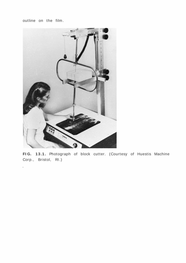
outline on the film.

FIG. 13.1. Photograph of block cutter. (Courtesy of Huestis Machine

Corp., Bristol, RI.)

FIG. 13.2. A: Cerrobend blocks for lung shielding. B: Custom blocks

for head and neck.

If â€œpositiveâ€ blocks such as lung blocks are to be made,

cavities are cut in the Styrofoam with the heated segment of the

wire and subsequently filled with melted Cerrobend. If a

â€œnegativeâ€ block with central area open and peripheral areas

blocked is desired, an inner cut is first made to outline the field

opening. An outer rectangular cut is then made to define the

collimator field with 1- to 2-cm margin. The three Styrofoam pieces

thus made are placed on a Lucite plate and carefully aligned relative

to the central axis. The intermediate piece, corresponding to the

areas to be shielded, is then removed and Cerrobend is poured into

the cavity.

It is important that the Cerrobend is poured slowly to prevent

formation of air bubbles. Also, the Styrofoam block should be

pressed tightly against a rubber pad at the bottom to avoid leakage

of the liquid metal. The inside walls of the cavity may be sprayed

with silicone for easy release of the Styrofoam pieces from the

block.

The blocks can be mounted on a Lucite plate or blocking tray, which

is premarked with the central axis cross hairs. Blocks can also be

placed on a template made on a clear film by tracing the outline of

the field at the shadow tray position while the port film outline is

placed at the distance at which the radiograph was taken.

Figure 13.2 shows examples of Cerrobend blocks, one constructed

for shielding lungs and the other for a head and neck field.

B. Independent Jaws

Asymmetric fields are sometimes used to block off a part of the field

without changing the position of the isocenter. Although blocking is

often used to generate irregular field shapes, rectangular blocking

can be easily done by independently movable collimators, or

P.276

jaws. This feature is very convenient when matching fields or beam

splitting. In the latter case, the beam is blocked off at the central

axis to remove divergence. Whereas half-beam blocks have been

used as beam splitters in the past, this can now be done simply by

moving in the independent jaws.

Most modern machines are equipped with independently movable

jaws. Some machines have one independent jaw, others have two

independent pairs, and some have all four jaws as independent.

Operationally, the independent jaw option is interlocked to avoid

errors in the setting of symmetric fields, in which case the opposite

jaws open or close symmetrically.

One of the effects of asymmetric collimation is the change in the

physical penumbra (defined in section 11.1 ) and the tilt of the

isodose curves toward the blocked edge (Fig. 13.3 ). This effect is

simply the result of blocking, which eliminates photon and electron

scatter from the blocked portion of the field, thereby reducing the

dose near the edge. The same effect would occur on the isodose

curves if the blocking were done with a lead or Cerrobend block on a

tray.

FIG. 13.3. Comparison of isodose distribution with half the beam

blocked by an independent jaw versus a block on a tray. Notice close

agreement as well as the tilt of the isodose curves toward the

blocked edge.

FIG. 13.4. Varian multileaf collimator: (top ) attached to

accelerator and (bottom ) with an end-on view. (Courtesy of Varian

Associates, Palo Alto, CA.)

P.277

When asymmetric fields are used, special considerations must be

given to the beam flatness and the dosimetric parameters used to

calculate monitor units. Khan et al. (9 ) have proposed a system of

dose calculation for fields generated by asymmetric collimators,

which was discussed in Chapter 10 .

C. Multileaf Collimators

A multileaf collimator (MLC) for photon beams consists of a large

number of collimating blocks or leaves that can be driven

automatically, independent of each other, to generate a field of any

shape (Fig. 13.4 ). Typical MLC systems consist of 80 leaves (40

pairs) or

P.278

more. The individual leaf has a width of 1cm or less as projected at

the isocenter. The leaves are made of tungsten alloy ( = 17.0 to

18.5 g/cm3 ) and have thickness along the beam direction ranging

from 6 cm to 7.5 cm, depending on the type of accelerator. The leaf

thickness is sufficient to provide primary x-ray transmission through

the leaves of less than 2% (compared with about 1% for jaws and

3.5% for Cerrobend blocks). The interleaf (between sides)

transmission is usually less than 3%. The primary beam

transmission may be further minimized by combining jaws with the

MLC in shielding areas outside the MLC field opening.

Some MLC systems have double-focused leaves, that is, the leaves

form a cone of irregular cross-section diverging from the source

position and move on a spherical shell centered at the source. The

rationale behind a double-focused MLC is to provide a sharp beam

cutoff at the edge. However, for high-energy beams this objective is

achieved only to a limited extent, because the dose falloff at the

edge is largely determined by scattered photons and electrons.

Because double-focused MLCs are difficult to manufacture, some

systems have been designed with rounded leaf edges and directions

of travel perpendicular to the central ray. The purpose of rounded

edges is to provide constant beam transmission through a leaf edge,

regardless of its position in the field.

An important consideration in the use of MLCs for stationary fields is

the conformity between the planned field boundary, which is

continuous, and the jagged stepwise boundary created by the MLC.

The degree of conformity between the two depends not only on the

projected leaf width but also on the shape of the target volume and

the angle of rotation of the collimator. Optimization of MLC rotation

and setting has been discussed by Brahme (10 ). His analysis shows

that the best orientation of the collimator is when the direction of

motion of the leaves is parallel with the direction in which the target

volume has the smallest cross-section.

The physical penumbra (section 11.1 ) with MLC is larger than that

produced by the collimator jaws or the Cerrobend blocks (Fig. 13.5

). This is usually not a serious drawback except for the treatment of

small fields or when blocking is required close to critical structures.

Also, jaggedness of the field edges makes it difficult to match

adjacent fields.

The use of MLC in blocking and field shaping is ideally suited for

treatments requiring large numbers of multiple fields because of

automation of the procedure thus resulting in a significant reduction

of set-up time. MLC can practically eliminate the use of Cerrobend

blocking except for shaping small fields or â€œislandâ€ blocking in

which an area within the open portion of the fields needs to be

blocked.

The importance of MLC is not just the replacement of Cerrobend

blocking. The greater impact of this technology is in the automation

of field shaping and modulation of beam intensity. Modern

radiotherapy techniques such as 3-D conformal radiation therapy

(Chapter 19 ) and intensity-modulated radiation therapy (Chapter 20

) are dependent on the dynamically controlled MLC. Other

applications include dynamic wedges and electronic compensation.

For further details on MLC designs and applications, the reader is

referred to a review by Boyer (11 ).

13.3. SKIN DOSE

When a patient is treated with a megavoltage beam, the surface

dose or skin dose can be substantially lower than the maximum dose

that occurs in the subcutaneous tissues. In contrast to lower energy

beams (e.g., superficial and orthovoltage x-rays), which give rise to

maximum ionization at or close to the skin surface, the megavoltage

beams produce an initial electronic buildup with depth, resulting in

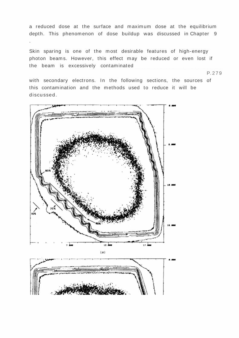
a reduced dose at the surface and maximum dose at the equilibrium

depth. This phenomenon of dose buildup was discussed in Chapter 9

.

Skin sparing is one of the most desirable features of high-energy

photon beams. However, this effect may be reduced or even lost if

the beam is excessively contaminated

P.279

with secondary electrons. In the following sections, the sources of

this contamination and the methods used to reduce it will be

discussed.

FIG. 13.5. Comparison of physical penumbra associated with MLC

(A) and cerrobend blocks (B). Field size 15 —15, depth 10 cm, and

energy 6MV. Dose distribution normalized to 100% at central axis.

(From Galvin JM, et al. Evaluation of multileaf collimator design for

a photon beam. Int J Radiat Oncol Biol Phys 1992;23:789â€“801,

with permission.)

A. Electron Contamination of Photon

Beams

Surface dose is the result of electron contamination of the incident

beam as well as the backscattered radiation (both electrons and

photons) from the medium. It is well-known that all x-ray and ³

ray beams used in radiation therapy are contaminated with

secondary electrons. These electrons arise from photon interactions

in the air, in the collimator,

P.280

and in any other scattering material in the path of the beam. If a

shadow tray is used to support beam-shaping blocks, secondary

electrons produced by photon interactions in the tray and the air

column between the tray and the skin surface significantly increase

skin dose. The shadow tray is usually thick enough to absorb most

of the electrons incident on the tray.

There has been a controversy as to the relative contribution of

secondary electrons vs. low energy scattered photons to the dose in

the build-up region. It is well known that as the field size increases,

the depth dose in the build-up region increases resulting in a shift

in the depth of maximum dose, d max , to increasingly shallower

depths (12 ,13 ,14 ). Specifically, the cause of the d max shift with

field size has been studied by several investigators (15 ,16 ,17 ).

Current evidence favors the hypothesis that the effect is

predominantly caused by the secondary electrons.

B. Measurement of Dose Distribution in

the Build-up Region

Because of the steep dose gradient in the build-up region, the size

of the dosimeter along the beam direction should be as small as

possible. Extrapolation chambers (see Chapter 6 ) are the

instruments of choice for these measurements. However, few

institutions have these instruments available. Instead, fixed-

separation plane-parallel ionization chambers are most commonly

used for this purpose. Although these chambers are very suitable for

measurements in regions of severe dose gradients, their response is

dependent, in a complex manner, on their design. Several papers

have discussed the inaccuracies in the measurement of dose in the

build-up region when using fixed-separation plane-parallel

chambers. These inaccuracies arise primarily as a result of electron

scattering from the side walls of the chamber (18 ,19 ,20 ). These

may be minimized by using a smaller plate separation and wider

guard ring in the design of the chamber. Furthermore, the chambers

may exhibit a significant polarity effect in the build-up region, which

may be corrected by averaging the readings obtained with the

positive and negative polarities. Gerbi and Khan (21 ) have studied

several commercially available plane-parallel chambers and found

that they overrespond in the build-up region. The errors were more

severe at the surface and for the lower beam energies (e.g., 60 Co).

The magnitude of overresponse at the surface for a 60 Co beam

ranged from 9% to 20% for the chambers studied.

Thin layers (<0.5 mm) of thermoluminescent dosimeter (TLD)

material can also be used for measuring dose distribution in the

build-up region. The TLD phosphor (e.g., LiF) can be in the form of

chips, crystals embedded in plastic, or powder layers (18 ,22 ,23 ).

The surface dose may be obtained by extrapolating the depth dose

distribution curve to zero depth. In vivo measurements of surface

dose can also be made by placing thin TLD chips directly on the skin

surface. Such measurements are useful in checking dosimetry if an

unacceptable degree of skin reaction develops.

C. Skin Sparing as a Function of Photon

Energy

Studies have shown that the dose distribution in the build-up region

depends on many variables such as beam energy, SSD, field size,

and configuration of secondary blocking tray (18 ,22 ,23 ,24 ,25 ,26

). Table 13.2 gives values for different energies. These data are

presented here as an example and should not be considered

universal for all machines, especially for depths less than 2 mm.

Reasonable agreement between different machines has been shown

to exist for greater depths.

Examination of Table 13.2 would also indicate that for all energies

the dose increases rapidly within the first few millimeters and then

gradually achieves its maximum value at the depth of peak dose.

For example, in the case of 4 MV, the percent depth dose increases

from 14% to 74% in the first 2 mm, reaches 94% at a 5-mm depth

and achieves its maximum value at a 10-mm depth. A practical

application of this phenomenon is the case in which build-up bolus

(Chapter 12 ) is used intentionally to maximize the dose on the

P.281

skin (e.g., covering a scar with a strip of bolus). A tissue equivalent

bolus of 5- to 6-mm of thickness is usually adequate for 4 MV. Thus

the thickness of bolus required to achieve 90% to 95% build-up of

dose is substantially less than the depth of maximum dose.

0

18.0

14.0

12.0

17.0

1

70.5

57.0

30.0

28.0

2

90.0

74.0

46.0

39.5

3

98.0

84.0

55.0

47.0

4

100.0

90.0

63.0

54.5

5

100.0

94.0

72.0

60.5

6

â€”

96.5

76.0

66.0

8

â€”

99.5

84.0

73.0

10

â€”

100.0

91.0

79.0

15

â€”

â€”

97.0

88.5

20

â€”

â€”

98.0

95.0

25

â€”

â€”

100.0

99.0

30

â€”

â€”

â€”

100.0a Data from Velkley DE, Manson DS, Purdy JA, Oliver GD. Buildup

region of megavoltage photon radiation sources. Med Phys

1975;2:14.b Data from Khan FM, Moore VC, Levitt SH. Effect of various atomic

number absorbers on skin dose for 10-MeV x-rays. Radiology

1973;109:209.

Depth

(mm)

60 Co 80

cma

4 MV 80

cma

10 MV 100

cmb

25 MV 100

cma

TABLE 13.2. BUILD-UP DOSE DISTRIBUTION IN

POLYSTYRENE FOR A 10 — 10 cm FIELD

Although the skin sparing depends on many conditions, as

mentioned earlier, the effect, in general, becomes more and more

pronounced as photon energy increases. For higher-energy beams,

significant sparing can be achieved not only for the skin surface but

also for the subcutaneous tissues.

D. Effect of Absorber-skin Distance

The electron contamination with no absorber placed in the beam is

mainly caused by the secondary electron emission from the

collimator (including source, flattening filter, and air). When an

absorber of thickness greater than the range of secondary electrons

(equilibrium thickness) is introduced in the beam, the collimator

electrons are almost completely absorbed but the absorber itself

becomes the principal source of electron contamination of the beam.

By increasing the distance between the tray and the surface, the

electron fluence incident on the skin is reduced because of

divergence as well as absorption and scattering of electrons in the

air. Thus skin sparing is enhanced by placing the shadow tray

farther away from the skin. In the case of a 60 Co ³ ray beam, it

has been shown (27 ,28 ) that for small fields an air gap of 15 to 20

cm between the scatterer and the skin is adequate to keep the skin

dose to an acceptable level (<50% of the D max ). This has been

found to be true for higher-energy beams as well (17 ).

Figure 13.6 shows the effect on dose distribution in the build-up

region as a Lucite shadow tray is placed in the beam at various

distances from the phantom surface. Not only does the relative

surface dose increase with decreasing tray-to-surface distance but

the point of maximum dose buildup moves closer to the surface.

Figure 13.6 also illustrates the principle of what is known as the

â€œbeam spoiler.â€ A low atomic number absorber, such as a

Lucite shadow tray, placed at an appropriate distance from the

surface, can be used to modify the build-up curve. Doppke et al. (29

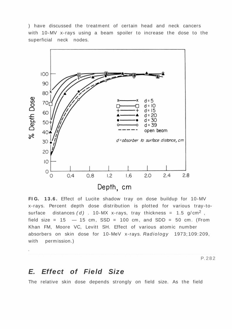
) have discussed the treatment of certain head and neck cancers

with 10-MV x-rays using a beam spoiler to increase the dose to the

superficial neck nodes.

FIG. 13.6. Effect of Lucite shadow tray on dose buildup for 10-MV

x-rays. Percent depth dose distribution is plotted for various tray-to-

surface distances (d) . 10-MX x-rays, tray thickness = 1.5 g/cm2 ,

field size = 15 — 15 cm, SSD = 100 cm, and SDD = 50 cm. (From

Khan FM, Moore VC, Levitt SH. Effect of various atomic number

absorbers on skin dose for 10-MeV x-rays. Radiology 1973;109:209,

with permission.)

P.282

E. Effect of Field Size

The relative skin dose depends strongly on field size. As the field

dimensions are increased, the dose in the build-up region increases.

This increase in dose is due to increased electron emission from the

collimator and air. Figure 13.7 is a plot of relative surface dose as a

function of field size for 60 Co, 4-MV, and 10-MV beams. These data

show that skin sparing is significantly reduced for the larger field

sizes.

Saylor and Quillin (24 ) have discussed the relative importance of

field size and tray-to-skin distance for 60 Co ³ rays. They have

shown that the optimum skin sparing occurs for an h /r value of

about 4, where h is the tray-to-surface distance and r is the radius

of an

P.283

equivalent circular field. This ratio can be easily achieved for the 5

— 5 cm field, because it requires a distance of 12 cm; however,

for the 30 — 30 cm field, the corresponding absorber-surface

distance is 67 cm, which is hardly possible for isocentric treatments.

FIG. 13.7. Percent surface dose as a function of field size. 60 Co,

Theratron 80, SSD = 80 cm, SDD = 59 cm. 4 MV, Clinac 4, SSD =

80 cm. 10 MV, LMR 13, SSD = 100 cm, SDD = 50 cm. 60 Co and 4-

MV. (Data are from Velkley DE, Manson DJ, Purdy JA, et al. Buildup

region of megavoltage photon radiation sources. Med Phys

1975;2:14. 10-MV data are from Khan FM, Moore VC, Levitt SH.

Effect of various atomic number absorbers on skin dose for 10-MeV

x-rays. Radiology 1973;109:209.)

FIG. 13.8. Variation of percent surface dose with atomic number of

absorber. Each absorber had a thickness of 1.5 g/cm2 and was

mounted underneath a Lucite shadow tray. 10-MV x-rays, field size

= 15 — 15 cm and absorber-to-surface distance = 15 cm. (From

Khan FM, Moore VC, Levitt SH. Effect of various atomic number

absorbers on skin dose for 10-MeV x-rays. Radiology 1973;109:209,

with permission.)

When using large fields with a tray-to-skin distance of 15 to 20 cm,

it becomes necessary to use electron filters to maintain the skin-

sparing effect. These are discussed in the next section.

F. Electron Filters

The skin dose can be reduced by using ³ ray absorbers of medium

atomic number (Z in the range of 30â€“80). Such absorbers are

commonly known as electron filters, because their introduction in

the photon beam reduces the secondary electron scatter in the

forward direction. Hine (30 ,31 ) studied the scattering of electrons

produced by ³ rays in materials of various atomic numbers. He

showed that the medium atomic number absorbers give less electron

scatter in the forward direction than either the low or the very high

Z materials. Khan (22 ) and Saylor and Quillin (24 ) applied the

results of Hine's study to the design of electron filters for the

purpose of improving skin dose for 60 Co teletherapy. Later it was

shown that such filters not only reduce the surface dose but also

improve the build-up characteristics of large fields (32 ).

Figure 13.8 is a plot of relative surface dose as a function of log (Z

+ 1). These data are plotted in this manner to show agreement with

the theoretical relationship discussed by Hine (30 ,31 ). As Z

increases, the surface dose falls to a shallow minimum due to

increased electron scattering in the absorbers. Further increases in

Z result in increased surface dose due to increased production of

photoelectrons and electron pairs in addition to the Compton

electrons. The minimum occurs at about Z = 50, which is the atomic

number of tin. These results qualitatively agree with those obtained

for 60 Co ³ rays (24 ,30 ,31 ).

Effectiveness of tin in reducing skin dose is demonstrated in Fig.

13.9 . Greater reduction is possible by increasing filter-skin distance

as discussed previously.

To preserve the light field, Saylor and Quillin (24 ) have suggested

the use of leaded glass as an electron filter. However, breakability

of leaded glass may pose a serious problem. We have used a tin

sheet mounted on a pressed wood sheet that could be slipped under

the Plexiglas tray at the end of the treatment set-up. In this

arrangement, the tin filter must face the patient surface.

FIG. 13.9. Percent surface dose plotted as a function of field size

for open beam, Lucite tray and tin filter mounted underneath the

tray. 10-MV x-rays, tray-to-surface distance = 15 cm. (From Khan

FM, Moore VC, Levitt SH. Effect of various atomic number absorbers

on skin dose for 10-MeV x-rays. Radiology 1973;109:209, with

permission.)

P.284

The thickness of an electron filter, in theory, should be at least

equal to the maximum range of secondary electrons. For 60 Co, this

thickness is about 0.5 g/cm2 or 0.9 mm of tin (assuming t in =

5.75 g/cm3 ). For higher energies, thicknesses less than the

maximum range of electrons may be used for practical reasons.

G. Skin Sparing at Oblique Incidence

Skin dose has been shown to increase with increasing angle of

incidence (33 ,34 ,35 ,36 ,37 ,38 ,39 ). Clinically, brisk reactions

have been observed in patients when the beam is incident at near

glancing angles. Jackson (35 ) has explained the increase in skin

dose with increasing angle of incidence through the concept of

electron range surface (ERS). The ERS is a 3-D representation of

secondary electron range and distribution produced by a pencil beam

of photons interacting with the medium (Fig. 13.10 ). Electrons

generated inside the ERS volume will reach P and contribute to the

dose there, whereas those generated outside, because of their

inadequate range, make no contribution. The ERS for 60 Co ³ rays

is in the shape of an ellipsoid with axial dimensions of 5 — 2.4

mm (35 ). As illustrated in Fig. 13.10 , the increase in the angle of

incidence of the photon beam results in additional surface dose at P

because of electron contribution from the portion of the ERS, which

appears below the phantom surface (hatched curve). For tangential

beam incidence, since half of the ERS is below the phantom surface,

an upper estimate of the dose to the skin may be obtained by the

following relationship (35 ,39 ):

P.285

where the entrance dose represents the surface dose for normal

incidence expressed as a percentage of D max . The skin dose for

other angles of incidence will lie between the values for the normal

and the tangential incidence.

FIG. 13.10. The use of ERS to determine surface dose buildup at

point P. A: Perpendicular beam incidence. B: Oblique beam

incidence. C: Tangential beam incidence.

Gerbi et al. (40 ) did a systematic study of dose buildup for

obliquely incident beams as a function of energy (6â€“24 MV),

angle, depth, field size, and SSD. A quantity obliquity factor (OF)

was defined as the dose at a point in phantom on central axis of a

beam incident at angle ¸ °, with respect to the perpendicular to

the surface, divided by the dose at the same point and depth along

central axis with the beam incident at angle 0 °. The obliquity

factor, therefore, represents dose enhancement due to beam

obliquity for the same depth. Figure 13.11 shows that the obliquity

factor at the surface increases with the increase in the angle of

incidence, first gradually and then dramatically beyond 45 degrees.

Thus the surface dose at large oblique angles can be significantly

higher than at normal incidence. At tangential or grazing incidence,

the surface dose approaches the value given by Equation 13.1 .

Another important effect associated with oblique angles is that as

the surface dose increases with the angle of incidence, the depth of

maximum buildup decreases. The dose reaches its maximum value

faster at glancing angles than at normal incidence. As a result, the

dose build-up region is compressed into a more superficial region.

Under these conditions, a high skin reaction becomes much more

likely. Jackson (35 ) has discussed the possibility that if the

sensitivity of the skin extends to the first or second millimeter

below the surface, at glancing angles skin sparing is practically lost

for the cobalt unit and greatly reduced for higher-energy beams.

13.4. SEPARATION OF ADJACENT FIELDS

Adjacent treatment fields are commonly employed in external beam

radiation therapy, such as the â€œmantleâ€ and â€œinverted-

Yâ€ fields for the treatment of Hodgkin's disease. In some cases,

the adjacent fields are orthogonal, such as the craniospinal fields

used in the

P.286

treatment of medulloblastoma. Another example is the irradiation of

head and neck tumors when the lateral neck fields are placed

adjacent to the anterior supraclavicular field. In each of these

situations, there is a possibility of introducing very large dosage

errors across the junction. Consequently, this region is at risk for

tumor recurrence if it is underdosed or severe complications if it is

overdosed.

FIG. 13.11. Obliquity factor at the surface plotted as a function of

beam angle for various energy beams. Jackson formula for

tangential beam incidence is based on Equation 13.1 . (From Gerbi

BJ, Meigooni AS, Khan FM. Dose buildup for obliquely incident

photon beams. Med Phys 1987;14:393, with permission.)

The problem of adjacent fields has been extensively studied (41 ,42

,43 ,44 ,45 ,46 ,47 ,48 ,49 ,50 ,51 ,52 ,53 ). A number of techniques

have been devised to achieve dose uniformity in the field junction

region. Some of the more commonly used techniques are illustrated

in Fig. 13.12 . Figure 13.12A has been described by Lance and

Morgan (41 ); here fields are angled away from a common line of

abutment to avoid overlap of the fields due to their geometric

divergence. Figure 13.12B illustrates the methods in which the

fields are separated at the skin surface to provide dose uniformity at

a desired depth. The separation or gap between the fields is

calculated on the basis of geometric divergence (53 ) or isodose

curve matching (42 ,43 ). A technique using split beams (49 ,53 ) is

illustrated in Fig. 13.12C . In this method, the beam is split along

the plane containing the central axis by using a half-beam block or a

beam-splitter, thus removing the geometric divergence of the beams

at the split line. Figure 13.12D uses penumbra generators or

spoilers (46 ,47 ). These lead wedges are custom designed to

provide satisfactory dose distribution across the field junction.

In clinical practice, the fields are usually abutted at the surface if

the tumor is superficial at the junction point. Care is however taken

that the hot spot created due to the overlap of the beams at depth

is clinically acceptable, considering the magnitude of the overdosage

and the volume of the hot spot. In addition, the dosage received by

a sensitive structure such as the spinal cord must not exceed its

tolerance dose.

For the treatment of deep-seated lesions such as in the thorax,

abdomen, and pelvis, the fields can be separated on the surface. It

is assumed in this case that the cold spots created by the field

separation are located superficially where there is no tumor.

FIG. 13.12. Schematic representation of various techniques used

for field matching. A: Angling the beams away from each other so

that the two beams abut and are aligned vertically. B: Fields

separated at the skin surface. The junction point is at depth where

dose is uniform across the junction. C: Isocentric split beam

technique for head and neck tumors. (Redrawn from Williamson TJ.

A technique for matching orthogonal megavoltage fields. Int J Radiat

Oncol Biol Phys 1979;5:111.) D: Craniospinal irradiation using

penumbra generators. (Redrawn from Griffin TW, Schumacher D,

Berry HC. A technique for cranial-spinal irradiation. Br J Radiol

1976;49:887.)

P.287

A. Methods of Field Separation

As stated earlier, the field separation can be accomplished

geometrically or dosimetrically.

A.1. Geometric

If the geometric boundary of the field is defined by the 50%

decrement line (line joining the points at depth where the dose is

50% of the central axis value at the same depth), the dose at the

point of junction between the beams will add up to be 100%. The

dose distribution laterally across the junction is more or less

uniform, depending on the interfield scatter contribution and the

penumbra characteristics of the beam.

If the two fields are incident from one side only and made to

junction at a given depth (Fig. 13.13 ), the dose above the junction

will be lower and below the junction higher than the junction dose.

In the case of four fields when two fields are incident from one side

and two from the parallel opposed direction (Fig. 13.14 ), the fields

are usually made to junction at the midline depth (e.g., mantle and

inverted Y fields). Such an arrangement

P.288

P.289

can be used to obtain almost a uniform distribution at the midline,

but cold spots are created above and below the junction point.

FIG. 13.13. Geometry of two adjacent beams, separated by a

distance S 1 + S 2 on the surface and junctioning at depth d.

FIG. 13.14. Two pairs of parallel opposed fields. Adjacent fields are

separated on the surface so that they all join at a point on the

midline. A: Ideal geometry in which there is no three-field overlap.

B: Arrangement in which there are two regions (shaded) of three-

field overlap.

Figure 13.13 shows the geometry of two adjacent beams that are

allowed to join at a given depth d. Let L 1 and L 2 be the field

lengths and SSD1 and SSD2 be the source-surface distances. Since

triangles ABC and CDE are similar:

or

giving

Similarly,

Thus the total separation S on the surface is given by:

Figure 13.14A shows an ideal geometry in which there is no overlap

between a field and its adjacent opposing neighbor. The

arrangement shown in Fig. 13.14B , on the other hand, creates

regions of â€œthree-field overlapâ€ (shaded areas) where the

bigger fields diverge into the opposing smaller fields. Consequently,

the total dose there may exceed the central axis dose at the same

depth. This will be of concern if a significant portion of the spinal

cord is in the three-field overlap region.

The maximum length of three-field overlap ( ”S ) occurs on the

surface and is given by:

”S can be made equal to zero if:

Thus if the field lengths are different, the SSDs can be adjusted to

eliminate the three-field overlap. Also, if the geometrically

calculated gap (S 1 + S 2 ) is increased by ”S , the three-field

overlap is eliminated at the expense of a cold spot at the midline.

As a compromise, one could increase the gap (S 1 + S 2 ) by an

amount ”S â€² just enough to eliminate the three-field overlap in

a specific region such as the spinal cord. ”S â€² can be calculated

geometrically:

where d â€² is the depth of the cord from the anterior surface and d

is the midline depth.

The three-field overlap in Fig. 13.14B can also be avoided by using

the same length and SSD for all the four fields and blocking the

second pair (e.g., paraortic or inverted Y fields) caudally as needed.

This technique is more convenient when the accelerator is equipped

with asymmetric collimators that can be moved independently of

each other.

P.290

Example 1

A patient is treated with parallel-opposed mantle and paraortic

fields of lengths 30 and 15 cm, respectively. Calculate (a) the gap

required on the surface for the beams to intersect at a midline depth

of 10 cm and (b) the gap required to just eliminate the three-field

overlap on the cord assumed to be at a depth of 15 cm from the

anterior surface, given SSD = 100 cm for all the fields:

Although the previous geometric considerations provide useful

criteria for field separation, one must be aware of their limitations.

For example, the actual dose distribution may present a different

picture than the predictions based on pure geometry of beam

divergence. Patient positioning, beam alignment, field penumbra,

and radiation scatter are all relevant factors that make this problem

one of the most complex in radiation therapy.

Figure 13.15 shows the dose distribution for the cases discussed in

Example 1. The expected three-field hot spot is seen in Fig. 13.15A

when the beams intersect at the midline. This hot spot is eliminated

when the gap is increased from 2.3 to 3.0 cm (= S 1 + S 2 + ”S )

(Fig. 13.15B ). However, the dose in the junction region has dropped

considerably. Such a procedure will be justified only if the junction

region is tumor free. Figure 13.15C shows the distribution when the

gap is just enough to eliminate the three-field overlap at the cord,

i.e., gap = 2.7 cm. This reduces the dose to the cord but also cools

down the midjunction area by about 10%.

In practice, the choice between the options shown in Fig. 13.15

should be based on physical, clinical, and technical considerations.

As usual, the guiding principles are that the tumor must receive

adequate dosage and sensitive structures must not be treated

beyond tolerance. If these conditions are not satisfied, other

methods of field matching, discussed earlier in this chapter, may be

considered.

A.2. Dosimetric

The separation of fields can be determined by optimizing the

placement of fields on the contour so that the composite isodose

distribution is uniform at the desired depth and the hot and cold

spots are acceptable. The accuracy of this procedure depends on the

accuracy of the individual field isodose curves especially in the

penumbra region.

B. Orthogonal Field Junctions

Orthogonal fields denote an arrangement in which the central axes

of the adjacent fields are orthogonal (i.e., perpendicular to each

other). For example, orthogonal fields are used for the treatment of

medulloblastoma in which the craniospinal irradiation is

accomplished by lateral parallel-opposed brain fields coupled with a

posterior spine field. Another common

P.291

example is treatment of the neck by bilateral fields while an

orthogonally adjacent anterior field is used to treat the

supraclavicular areas.

FIG. 13.15. Geometric separation of fields with all the four beams

intersecting at midpoint. Adjacent field sizes: 30 — 30 cm and 15

— 15 cm; SSD = 100 cm; AP thickness = 20 cm; 4-MV x-ray

beams. A: Field separation at surface = 2.3 cm. A three-field

overlap exists in this case because the fields have different sizes

but the same SSD. B: The adjacent field separation increased to 3

cm to eliminate three-field overlap on the surface. C: Field

separation adjusted 2.7 cm to eliminate three-field overlap at the

cord at 15 cm depth from anterior.

The problem of matching orthogonal fields has been discussed by

several investigators (48 ,49 ,50 ,51 ,52 ). For superficial tumors

such as in the head and neck areas, it may be inadvisable to

separate the adjacent fields unless the junction area is over a

tumor-free region. If separation is not possible, one may use beam

splitters and abut the fields along or close to their central axes (50

). The matching line should be drawn each time before treatment to

avoid overlap of the fields. If a sensitive structure such as the

spinal cord exists in the junction region, one may additionally block

an appropriate segment of the cord anteriorly or laterally, provided

there is no tumor in the shielded region.

FIG. 13.16. A: A general diagram showing the separation of

orthogonal fields. B: An example of orthogonal fields used for

craniospinal irradiation. C: A lateral view of B , illustrating the

geometry of orthogonal field separation.

P.292

As stated previously, field separation is possible for deep-seated

tumors if there is no tumor in the superficial junction region. A

geometrical method of orthogonal field separation has been

described by Werner et al. (52 ). According to this method, one pair

of opposing fields, defined by the collimating light, is allowed to

diverge on the skin and the point of intersection of the field borders

is marked. From this point, a distance S is calculated to separate

the orthogonal fields. The separation S is given by:

where d is the depth at which the orthogonal fields are allowed to

join. A general diagram for orthogonal field separation is illustrated

in Fig. 13.16A .

B.1. Craniospinal Fields

Craniospinal irradiation involves a complex technique in which

orthogonal junctions are created between the lateral brain fields and

a posterior spine field. The spinal field, because of its large length,

may be split into two spinal fields with a junction gap calculated

according to Equation 13.5 . The junction between the cranial and

the spinal fields can be accomplished in several ways (48 ,49 ,50 ,52

,54 ,55 ).

P.293

Technique A

Figure 13.16B presents an example showing bilateral cranial fields

adjacent to a spinal field. The cranial light fields are allowed to

diverge on the skin and their inferior borders meet at a point

midway on the posterior neck surface. From this point, the spinal

field is separated by a distance S , which is calculated from Equation

13.9 by substituting depth d of spine (from the posterior surface),

length L , and SSD for the spinal field. In this diagram, the solid

line represents the light field on the surface. The dashed line shows

the field projected at the depth of the spinal cord. Figure 13.16C is

the lateral view of Fig. 13.16B .

Technique B

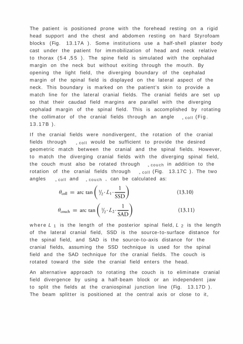
The patient is positioned prone with the forehead resting on a rigid

head support and the chest and abdomen resting on hard Styrofoam

blocks (Fig. 13.17A ). Some institutions use a half-shell plaster body

cast under the patient for immobilization of head and neck relative

to thorax (54 ,55 ). The spine field is simulated with the cephalad

margin on the neck but without exiting through the mouth. By

opening the light field, the diverging boundary of the cephalad

margin of the spinal field is displayed on the lateral aspect of the

neck. This boundary is marked on the patient's skin to provide a

match line for the lateral cranial fields. The cranial fields are set up

so that their caudad field margins are parallel with the diverging

cephalad margin of the spinal field. This is accomplished by rotating

the collimator of the cranial fields through an angle ¸coll (Fig.

13.17B ).

If the cranial fields were nondivergent, the rotation of the cranial

fields through ¸coll would be sufficient to provide the desired

geometric match between the cranial and the spinal fields. However,

to match the diverging cranial fields with the diverging spinal field,

the couch must also be rotated through ¸couch in addition to the

rotation of the cranial fields through ¸coll (Fig. 13.17C ). The two

angles ¸coll and ¸couch , can be calculated as:

where L 1 is the length of the posterior spinal field, L 2 is the length

of the lateral cranial field, SSD is the source-to-surface distance for

the spinal field, and SAD is the source-to-axis distance for the

cranial fields, assuming the SSD technique is used for the spinal

field and the SAD technique for the cranial fields. The couch is

rotated toward the side the cranial field enters the head.

An alternative approach to rotating the couch is to eliminate cranial

field divergence by using a half-beam block or an independent jaw

to split the fields at the craniospinal junction line (Fig. 13.17D ).

The beam splitter is positioned at the central axis or close to it,

thereby eliminating divergence of the rays at the junction line. The

collimator of the cranial fields is still tilted through ¸coll as

discussed earlier.

The technique of using independent jaw and ¸coll to match the

craniospinal fields, has two advantages: (a) orthogonal field

matching is achieved with no overlaps between the cranial and

spinal fields at any depth, and (b) the independent jaw can be

conveniently used to move the craniospinal junction line caudally by

about a centimeter each week during the treatment course to smear

out the junctional dose distribution. As long as the independent jaw

splits the cranial fields within a few centimeters of the central axis,

the divergence of the cranial fields into the spinal field at the

matching line will be minimal.

C. Guidelines for Field Matching

The site of field matching should be chosen, insofar as possible,

over an area that does not contain tumor or a critically sensitive

organ.

FIG. 13.17. Craniospinal irradiation technique. A: Patient set-

up showing Styrofoam blocks and Alpha Cradle mold to provide

stable position for abdomen, chest, and head. B: Lateral view of

fields showing cranial field rotated to align with the diverging

border of the spinal field. C: Couch rotated to provide match

between the spinal field and the diverging border of the cranial

field. D: Elimination of cranial field divergence by using an

independent jaw as a beam splitter. This provides an alternative

to couch rotation in C.

P.294

If the tumor is superficial at the junction site, the fields should

not be separated because a cold spot on the tumor will risk

recurrence. However, if the diverging fields abut on the skin

surface, they will overlap at depth. In some cases, this may be

clinically acceptable, provided the excessive dosage delivered to

the underlying tissues does not exceed their tolerance. In

particular, the tolerances of critical structures such as the spinal

cord must not be exceeded. In the case of a superficial tumor

with a critical organ located at depth, one may abut the fields at

the surface but eliminate beam divergence using a beam splitter

or by tilting the beams.

For deep-seated tumors, the fields may be separated on the skin

surface so that the junction point lies at the midline. Again, care

must be taken in regard to a critical structure near the junction

region.

P.295

The line of field matching must be drawn at each treatment

session on the basis of the first field treated. It is not necessary

anatomically to reproduce this line every day because variation

in its location will only smear the junction point, which is

desirable. For the same reason some advocate moving the

junction site two or three times during a treatment course.

A field-matching technique must be verified by actual isodose

distributions before it is adopted for general clinical use. In

addition, beam alignment with the light field and the accuracy of

isodose curves in the penumbra region are essential

prerequisites.

REFERENCES

1. Powers WE, Kinzie JJ, Demidecki AJ, et al. A new system of

field shaping for external-beam radiation therapy. Radiology

1973;108:407.

2. Earl JD, Bagshaw MA. A rapid method for preparation of

complex field shapes. Radiology 1967;88:1162.

3. Maruyama Y, Moore VC, Burns D, et al. Individualized lung

shields constructed from lead shots embedded in plastic.


4. Edland RW, Hansen H. Irregular field-shaping for 60 Co

teletherapy. Radiology 1969;92:1567.

5. Jones D. A method for the accurate manufacture of lead

shields. Br J Radiol 1971;44:398.

6. Parfitt H. Manufacture of lead shields. Br J Radiol

1971;44:895.

7. Karzmark CJ, Huisman PA. Melting, casting and shaping of

lead shielding blocks: method and toxicity aspects. AJR

1972;114:636.

8. Kuisk H. New method to facilitate radiotherapy planning and

treatment, including a method for fast production of solid lead

blocks with diverging walls for cobalt 60 beam. AJR

1973;117:161.

9. Khan FM, Gerbi BJ, Deibel FC. Dosimetry of asymmetric x-ray

collimators. Med Phys 1986;13:936.

10. Brahme A. Optimal setting of multileaf collimators in

stationary beam radiation therapy. Strahlenther Onkol

1988;164:343.

11. Boyer AL. Basic applications of a multileaf collimator. In:

Mackie TR, Palta JR, ed. Teletherapy: present and future .

College Park, MD: American Association of Physicists in Medicine,

1996.

12. Almond PR, Roosenbeek EV, Browne R, et al. Variation in the

position of the central axis maximum buildup point with field size

for high energy photons beams [Correspondence]. Br J Radiol

1970;43:911.

13. Marinello G, Dutreix A. Etude dosim ©trique dâ€™un

faisceau de rayons X de 25 MV (Dosimetric study of a 25 MV x-

ray beam). J Radiol Electrol 1973;54:951.

14. Johns HE, Rawlinson JA. Desirable characteristics of high-

energy photons and electrons. In: Kramer S, Suntharalingam N,

Zinniger GF, eds. High energy photons and electrons . New York:

John Wiley & Sons, 1976:11.

15. Marbach JR, Almond PR. Scattered photons as the cause of

the observed d max shift with field size in high-energy photon

beams. Med Phys 1977;4:310.

16. Padikal TN, Deye JA. Electron contamination of a high energy

x-ray beam. Phys Med Biol 1978;23:1086.

17. Biggs PJ, Ling CC. Electrons as the cause of the observed d

max shift with field size in high energy photons beams. Med Phys

1979;6:291.

18. Velkley DE, Manson DJ, Purdy JA, et al. Buildup region of

megavoltage photon radiation sources. Med Phys 1975;2:14.

19. Nilson B, Montelius A. Fluence perturbation in photon beams

under non-equilibrium conditions. Med Phys 1986;13:192.

20. Rubach A, Conrad F, Bischel H. Dose build-up curves for

cobalt 60 irradiations: a systematic error with pancake chamber

measurements. Phys Med Biol 1986;31:441.

21. Gerbi BJ, Khan FM. Measurement of dose in the buildup

region using fixed-separation plane-parallel ionization chambers.

Med Phys 1990;17:17.

22. Khan FM. Use of electron filter to reduce skin dose in cobalt

teletherapy. AJR 1971;111:180.

23. Khan FM, Moore VC, Levitt SH. Effect of various atomic

number absorbers on skin dose for 10-MeV x-rays. Radiology

1973;109:209.

24. Saylor WL, Quillin RM. Methods for the enhancement of skin

sparing in cobalt-60 teletherapy. AJR 1971;111:174.

25. Gray L. Relative surface doses from supervoltage radiation.

Radiology 1973;109:437.

26. Rao PX, Pillai K, Gregg EC. Effect of shadow trays on surface

dose and buildup for megavoltage radiation. AJR 1973;117:168.

27. Johns HE, Epp ER, Cormack DV, et al. Depth dose data and

diaphragm design for the Saskatchewan 1,000 curie cobalt unit.

Br J Radiol 1952;25:302.

P.296

28. Richardson JE, Kerman HD, Brucer M. Skin dose from cobalt

60 teletherapy unit. Radiology 1954;63:25.

29. Doppke K, Novack D, Wang CC. Physical considerations in the

treatment of advanced carcinomas of the larynx and pyriform

sinuses using 10 MV x-rays. Int J Radiat Oncol Biol Phys

1980;6:1251.

30. Hine GJ. Scattering of secondary electrons produced by

gamma rays in materials of various atomic numbers. Phys Rev

1951;82:755.

31. Hine GJ. Secondary electron emission and effective atomic

numbers. Nucleonics 1952;10:9.

32. Leung PMK, Johns HE. Use of electron filters to improve the

buildup characteristics of large fields from cobalt-60 beams. Med

Phys 1977;4:441.

33. Burkell CC, Watson TA, Johns HE, et al. Skin effects of cobalt

60 telecurie therapy. Br J Radiol 1954;27:171.

34. Hughes HA. Measurements of superficial absorbed dose with

2 MV x-rays used at glancing angles. Br J Radiol 1959;32:255.

35. Jackson W. Surface effects of high-energy x-rays at oblique

incidence. Br J Radiol 1971;44:109.

36. Orton CG, Seibert JB. Depth dose in skin for obliquely

incident 60 Co radiation. Br J Radiol 1972;45:271.

37. Hanson WF, Grant W. Use of auxillary collimating devices in

the treatment for breast cancer with 60 Co teletherapy units. II.

Dose to the skin. AJR 1976;127:653.

38. Gagnon WF, Peterson MD. Comparison of skin doses to large

fields using tangential beams from cobalt-60 gamma rays and 4

MV x-rays. Radiology 1978;127:785.

39. Gagnon WF, Horton JL. Physical factors affecting absorbed

dose to the skin from cobalt-60 gamma rays and 25-MV x-rays.

Med Phys 1979;6:285.

40. Gerbi BJ, Meigooni AS, Khan FM. Dose buildup for obliquely

incident photon beams. Med Phys 1987;14:393.

41. Lance JS, Morgan JE. Dose distribution between adjoining

therapy fields. Radiology 1962;79:24.

42. Glenn DW, Faw FL, Kagan RA, et al. Field separation in

multiple portal radiation therapy. AJR 1968;102:199.

43. Faw FL, Glenn DW. Further investigations of physical aspects

of multiple field radiation therapy. AJR 1970;108:184.

44. Page V, Gardner A, Karzmark CJ. Physical and dosimetric

aspects of the radiotherapy of malignant lymphomas. II. The

inverted Y technique. Radiology 1970;96:619.

45. Agarwal SK, Marks RD, Constable WC. Adjacent field

separation for homogeneous dosage at a given depth for the 8

MV (Mevatron 8) linear accelerator. AJR 1972;114:623.

46. Armstrong DI, Tait JJ. The matching of adjacent fields in

radiotherapy. Radiology 1973;108:419.

47. Hale J, Davis LW, Bloch P. Portal separation for pairs of

parallel opposed portals at 2 MV and 6 MV. AJR 1972;114:172.

48. Griffin TW, Schumacher D, Berry HC. A technique for cranial-

spinal irradiation. Br J Radiol 1976;49:887.

49. Williamson TJ. A technique for matching orthogonal

megavoltage fields. Int J Radiat Oncol Biol Phys 1979;5:111.

50. Bukovitz A, Deutsch M, Slayton R. Orthogonal fields:

variations in dose vs. gap size for treatment of the central

nervous system. Radiology 1978;126:795.

51. Gillin MT, Kline RW. Field separation between lateral and

anterior fields on a 6 MV linear accelerator. Int J Radiat Oncol

Biol Phys 1980;6:233.

52. Werner BL, Khan FM, Sharma SC, et al. Border separation for

adjacent orthogonal fields. Med Dos 1991;16:79.

53. Hopfan S, Reid A, Simpson L, et al. Clinical complications

arising from overlapping of adjacent radiation fieldsâ€”physical

and technical considerations. Int J Radiat Oncol Biol Phys

1977;2:801.

54. Van Dyk J, Jenkin RDT, Leung PMK, et al. Medulloblastoma:

treatment technique and radiation dosimetry. Int J Rad Oncol Biol

Phys 1977;2:993.

55. Bentel GC, Nelson CE, Noell KT. Treatment planning and dose

calculation in radiation oncology , 4th ed. New York: Pergamon

Press, 1989:282.





14 - Electron Beam Therapy

14

Electron Beam Therapy

High-energy electrons have been used in radiation therapy since the

early 1950s. Originally, the beams were extracted mostly from

betatrons although a few linear accelerators and Van de Graaff

generators with relatively low electron energies were also available.

In the 1970s, high-energy linear accelerators, having photon and

multienergy electron beam capabilities, became increasingly

available for clinical use. The surge in the commercial development

of these machines was prompted largely by the clinical experience

gained at a few major centers, which showed that in some

commonly encountered situations â€œthere is no alternative

treatment to electron beam therapyâ€ (1 ).

The most clinically useful energy range for electrons is 6 to 20 MeV.

At these energies, the electron beams can be used for treating

superficial tumors (less than 5 cm deep) with a characteristically

sharp drop-off in dose beyond the tumor. The principal applications

are (a) the treatment of skin and lip cancers, (b) chest wall

irradiation for breast cancer, (c) administering boost dose to nodes,

and (d) the treatment of head and neck cancers. Although many of

these sites can be treated with superficial x-rays, brachytherapy, or

tangential photon beams, the electron beam irradiation offers

distinct advantages in terms of dose uniformity in the target volume

and in minimizing dose to deeper tissues.

This chapter is intended to provide basic information on electron

beam characteristics, dosimetry, and treatment planning. Most of

the discussion will pertain to 6- to 20-MeV electrons, although the

data at these energies can be qualitatively extrapolated to the

lower or the higher energy range.

14.1. ELECTRON INTERACTIONS

As electrons travel through a medium, they interact with atoms by a

variety of processes owing to Coulomb force interactions. The

processes are (a) inelastic collisions with atomic electrons

(ionization and excitation), (b) inelastic collisions with nuclei

(bremsstrahlung), (c) elastic collisions with atomic electrons, and

(d) elastic collisions with nuclei.

In inelastic collisions, some of the kinetic energy is lost as it is

used in producing ionization or converted to other forms of energy

such as photon energy and excitation energy. In elastic collisions,

kinetic energy is not lost although it may be redistributed among

the particles emerging from the collision. In low atomic number

media such as water or tissues, electrons lose energy predominantly

through ionizing events with atomic electrons. In higher atomic

number materials, such as lead, bremsstrahlung production is more

important. In the collision process with the atomic electrons, if the

kinetic energy acquired by the stripped electron is large enough for

it to cause further ionization, the electron is known as a secondary

electron or a ´-ray. As a beam of electrons travels through a

medium, the energy is continually degraded until the electrons

reach thermal energies and are captured by the surrounding atoms.

A. Rate of Energy Loss

An electron traveling in a medium loses energy as a result of

collisional and radiative processes. The magnitudes of the two

effects for water and lead are shown in Fig. 14.1 .

P.298

The theoretical treatment of this subject is given elsewhere (2 ,3 ,4

,5 ). It will suffice here to provide some important generalizations.

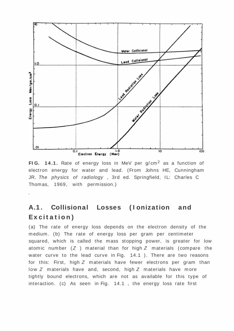
FIG. 14.1. Rate of energy loss in MeV per g/cm2 as a function of

electron energy for water and lead. (From Johns HE, Cunningham

JR. The physics of radiology , 3rd ed. Springfield, IL: Charles C

Thomas, 1969, with permission.)

A.1. Collisional Losses (Ionization and

Excitation)

(a) The rate of energy loss depends on the electron density of the

medium. (b) The rate of energy loss per gram per centimeter

squared, which is called the mass stopping power, is greater for low

atomic number (Z ) material than for high Z materials (compare the

water curve to the lead curve in Fig. 14.1 ). There are two reasons

for this: First, high Z materials have fewer electrons per gram than

low Z materials have and, second, high Z materials have more

tightly bound electrons, which are not as available for this type of

interaction. (c) As seen in Fig. 14.1 , the energy loss rate first

decreases and then increases with increase in electron energy with

a minimum occurring at about 1 MeV. Above 1 MeV, the variation

with energy is very gradual. (d) The energy loss rate of electrons of

energy 1 MeV and above in water is roughly 2 MeV/cm.

A.2. Radiation Losses (Bremsstrahlung)

The rate of energy loss per centimeter is approximately proportional

to the electron energy and to the square of the atomic number (Z 2

). Moreover, the probability of radiation loss relative to the

collisional loss increases with the electron kinetic energy and with

Z. That means that x-ray production is more efficient for higher

energy electrons and higher atomic number absorbers.

P.299

A.3. Polarization

A high-energy electron loses more energy per gram per square

centimeter in a gas than in traversing a more dense medium,

because of appreciable polarization of the condensed medium (5 ,6

,7 ). Atoms close to the electron track screen those remote from the

track. This phenomenon is particularly important in dosimetry with

ionization chambers when energy deposition in a medium and a gas

cavity are compared. The ratio of mass stopping power of water to

air varies with electron energy, and consequently, the dose

conversion factor for an air ionization chamber in water (or another

condensed medium) varies with depth.

A.4. Stopping Power

The total mass stopping power (S / )tot of a material for charged

particles is defined by the International Commission on Radiation

Units and Measurements (ICRU) (8 ) as the quotient of dE by dl

, where dE is the total energy lost by the particle in traversing a

path length dl in the material of density .

where (S / )col and (S / )rad apply to collisional losses and

radiation losses, respectively, discussed in previous sections A.1

and A.2 .

A.5. Absorbed Dose

In calculating the energy absorbed per unit mass (absorbed dose),

one needs to know the electron fluence and the â€œrestrictedâ€

collision stopping power. Restricted collision stopping power refers

to the linear energy transfer (LET) concept, that is, the rate of

energy loss per unit path length in collisions in which energy is

â€œlocallyâ€ absorbed, rather than carried away by energetic

secondary electrons. Thus the restricted collision mass stopping

power, (L / )col , of a material for charged particles is defined (8

) as the quotient of dE by dl , where dE is the energy lost by a

charged particle in traversing a distance dl as a result of those

collisions with atomic electrons in which the energy loss is less than

”.

If ¦E is the differentiated distribution of fluence with respect to

energy

, the absorbed dose, D , is closely approximated by:

The use of stopping powers in photon and electron dosimetry has

been discussed in Chapter 8 . Quantitative data on stopping powers

as a function of electron energy for various elements and materials

have been calculated by Berger and Seltzer (9 ,10 ,11 ) and

tabulated in Table A.8 of the appendix. More extensive tables of

stopping powers are given by the ICRU (12 ).

B. Electron Scattering

When a beam of electrons passes through a medium, the electrons

suffer multiple scattering due to Coulomb force interactions

between the incident electrons and, predominantly, the nuclei of

the medium. As a result, the electrons acquire velocity components

and displacements transverse to their original direction of motion.

For most practical applications, the angular and spatial spread of a

narrow, collimated beam of electrons can be approximated by a

Gaussian distribution (13 ).

P.300

By analogy with mass stopping power, the ICRU (8 ) defines the

mass angular scattering power of the material as the quotient

2 / l , where

2 is the mean square scattering angle. Following the calculations of

Rossi (13 ), mass scattering powers for various materials and

electron energies have been tabulated (14 ).

The scattering power varies approximately as the square of the

atomic number and inversely as the square of the kinetic energy.

For this reason, high Z materials are used in the construction of

scattering foils. Scattering foils spread out the electron beam that

emerges from the accelerator tube and are made thin to minimize

x-ray contamination of the electron beam.

14.2. ENERGY SPECIFICATION AND

MEASUREMENT

Although an electron beam is almost monoenergetic before striking

the accelerator window, the random energy degradation that the

electrons suffer as they pass through the exit window, scattering

foil, monitor chambers, air, and other materials results in the beam

taking on a spectrum of energies at the phantom surface. Further

degradation and spread of beam energy take place with depth in the

phantom (Fig. 14.2 ).

In clinical practice, an electron beam is usually characterized by the

energy at the body surface. There are several methods that can be

used to determine this energy: measurement of threshold energy

for nuclear reactions; range measurements; and the measurement

of Cerenkov radiation threshold (14 ). Of these, the range method is

the most practical and convenient for clinical use.

FIG. 14.2. Distribution of electron fluence in energy, ¦E , as the

beam passes through the collimation system of the accelerator and

the phantom. (From ICRU. Radiation dosimetry: electrons with

initial energies between 1 and 50 MeV. Report No. 21. Washington,

DC: International Commission on Radiation Units and

Measurements, 1972, with permission.)

FIG. 14.3. Depth-dose curve illustrating the definition of Rp and R

50 .

P.301

A. Most Probable Energy

The Nordic Association of Clinical Physics (15 ) recommends the

specification of most probable energy, (Ep )0 (defined by the

position of the spectral peak in Fig. 14.2 ) at the phantom surface

and the use of the following relationship:

where Rp is the practical range in centimeters as defined in Fig.

14.3 . For water, C 1 = 0.22 MeV, C 2 = 1.98 MeV cm-1 , and C 3 =

0.0025 MeV cm-2 (16 ,17 ,18 ). They further recommend that the

field size for range measurements be no less than 12 — 12 cm for

energies up to 10 MeV and no less than 20 — 20 cm for higher

energies.

For the determination of range, ion chambers, diodes, or film may

be used. Although the range measurements are usually made using

the depth ionization curve the result is only slightly different from

what would be obtained using depth dose curves (19 ). The practical

range, Rp , is the depth of the point where the tangent to the

descending linear portion of the curve (at the point of inflection)

intersects the extrapolated background, as shown in Fig. 14.3 .

To be in strict accordance with Equation 14.4 , each point on the

depth ionization curve should be corrected for beam divergence

before the range is determined. The correction factor is

, where f is the effective source-to-surface distance (see section

14.4E for details) and z is the depth. However, this correction in Rp

is clinically not significant in terms of its impact on the ionization

to dose conversion factor (20 ).

B. Mean Energy

It has been shown (21 ) that the mean energy of the electron beam,

’0 , at the phantom surface is related to R 50 (the depth at which

the dose is 50% of the maximum dose) by the following

relationship:

where C 4 = 2.33 MeV cm-1 for water. Again the divergence

correction is applied to each point on the depth dose curve before

determining R 50 .

The AAPM TG-21 protocol recommended the value of C 4 as 2.33

MeV cm-1 . However, more recent Monte-Carlo calculations of

Rogers and Bielajew (22 ) have shown that the value of C 4 in the

energy range of clinical interest is closer to 2.4 MeV cm-1 .

P.302

Again, this small change in the value of C 4 as well as the

divergence correction mentioned above has little impact on clinical

dosimetry (20 ).

C. Energy at Depth

Harder (23 ) has shown that the most probable energy and,

approximately, the mean energy of the spectrum decreases linearly

with depth. This can be expressed by the relationships:

and approximately:

where z is the depth.

Equation 14.7 is important in dosimetry because for absorbed dose

measurements it is necessary to know the mean electron energy at

the location of the chamber.

14.3. DETERMINATION OF ABSORBED

DOSE

Calorimetry is the most basic method for the determination of

absorbed dose, but because of technical difficulties, the use of

calorimeters is not practical in a clinical setting. Ionization

chambers and Fricke dosimeters are more commonly used. Film,

thermoluminescent dosimeters (TLD), and solid state diodes are

used to find the ratio of the dose at one point in a phantom to the

dose at another point but not usually to measure the absolute

absorbed dose at a point.

Ionization chambers should be calibrated by an Accredited Dose

Calibration Laboratory (ADCL) or the National Institute of Standards

and Technology (NIST). However, an ADCL can usually provide

calibrations only for high-energy photon beams (60 Co or 2-MV x-

rays) but not for high-energy electron beams. The use of ionization

chambers calibrated for photon beams for the measurement of

absorbed dose in electron beams has been the subject of many

national and international protocols (14 ,15 ,24 ,25 ,26 ). The most

current recommendations are included in the protocols by Task

Group 51 of the American Association of Physicists in Medicine

(AAPM) (24 ) and the International Atomic Energy Agency (IAEA)

TRS398 (25 ). Elements of these protocols and other related

concepts were presented in Chapter 8 .

A. Output Calibration

The variation of output (absorbed dose at a reference point in

phantom) with field size differs considerably from one type of

accelerator to another. Therefore, for every available electron

energy, the output of each treatment applicator or representative

field size should be measured. The output for one applicator or field

size (often the 10 — 10 cm field), is selected as the standard to

which the other output measurements are referred. Since the beam

is calibrated to give 1 cGy/MU for the standard applicator at the

depth of maximum dose on central axis (nominal SSD = 100 cm),

the output factor for any applicator represents cGy/MU at d max .

This topic will be further discussed in section 14.4D .

B. Depth-dose Distribution

The depth-dose and isodose distributions can be determined by ion

chambers, diodes, or films. Automatic isodose and isodensity

plotters are useful in this regard and are available commercially.

P.303

B.1. Ionization Chambers

Depth ionization curves obtained with air ionization chambers can

be converted into depth-dose curves by making corrections for

change in stopping power ratio of water to air with depth. In

addition, perturbation and displacement corrections are required for

cylindrical chambers.

A general equation for obtaining percent depth dose in water (%DW

) from ion chamber measurements made in any medium or phantom

is given by the following equation (20 ):

where the quantities in the numerator are determined at the

effective depth of measurement and the denominator equals the

value of the numerator at the depth of maximum dose.

B.2. Silicon Diodes

Silicon p-n junction diodes offer some advantages in terms of small

size and high sensitivity (Chapter 8 ). However, diodes suffer from

energy and temperature dependence and can be damaged by

radiation. For these reasons absolute dosimetry with diodes is not

recommended. Dose distributions obtained with diodes should be

checked by ion chamber measurements.

Because the variation of silicon to water stopping power ratio with

electron energy is quite minimal (~5% between 1 and 20 MeV),

measurements made with a diode may be used directly to give

depth-dose distributions. Figure 14.4 shows a comparison of depth

P.304

dose distributions obtained with an ion chamber (corrected for

stopping power ratios and other effects) and a diode. The data show

close agreement.

FIG. 14.4. Comparison of depth-dose curves measured with a diode

and an ion chamber. Whereas the diode response was uncorrected,

the chamber readings were corrected for change in ([L with bar

above])water air as a function of depth, and the displacement of the

effective point of measurement. (From Khan FM. Clinical electron

beam dosimetry. In: Monograph No. 15. Keriakes JG, Elson HR, Born

CG, eds. Radiation oncology physicsâ€”1986. AAPM Monograph No.

15. New York: American Institute of Physics, 1986:211, with

permission.)

B.3. Film

Film dosimetry offers a convenient and rapid method of obtaining a

complete set of isodose curves in the plane of the film. Its use for

determining electron beam dose distributions is well established (27

,28 ,29 ). It has been shown that the depth dose distributions

measured by using film agree well with those by ion chambers when

the latter measurements are corrected as outlined in section A (Fig.

14.5 ). Good agreement has also been demonstrated between film

and FeSO4 dosimeters used for the measurement of depth dose

curves (29 ). The energy independence of film may be explained by

the fact that the ratio of collision stopping power in emulsion and in

water varies slowly with electron energy (9 ). Thus the optical

density of the film can be taken as proportional to the dose with

essentially no corrections.

Film is useful for a variety of dosimetry problems such as

determining practical range, isodose curves, and beam flatness.

However, film cannot be used reliably for absolute dosimetry

because the optical density of a film exposed to electrons depends

on many variables such as emulsion, processing conditions,

magnitude of absorbed dose, and some measurement conditions,

which can give rise to serious artifacts. The use of film is,

therefore, restricted to relative dosimetry. Care is required to avoid

air gaps adjacent to the film. In addition, the sensitometric curve

(optical density as a function of absorbed dose) must be known to

interpret the optical density in terms of absorbed dose. Wherever

possible, a film with a linear response over the range of measured

dose should be used. Errors caused by changes in the processing

conditions can be minimized by developing the films at

P.305

approximately the same time. Accuracy can also be improved by

using films from the same batch.

FIG. 14.5. Comparison of central axis depth dose curve measured

with an ion chamber, film, and FeSO4 dosimeter. (From Almond PR.

In: Handbook of medical physics, Vol 1. Boca Raton, FL: CRC Press,

1982:173, with permission.)

FIG. 14.6. Film artifacts created by misalignment of the film in the

phantom. The effects of (A) air gaps between the film and the

phantom, (B) film edge extending beyond the phantom, and (C)

film edge recessed within the phantom. (From Dutreix J, Dutreix A.

Film dosimetry of high energy electrons. Ann NY Acad Sci


Film can be positioned either perpendicular or parallel to the beam

axis. In the latter case, precautions must be taken to align the top

edge of the film with the surface of the phantom or serious artifacts

and errors in the depth-dose distribution may result (28 ) (Fig. 14.6

).

To obtain isodose curves, the film is usually placed in a plastic

phantom such as polystyrene and oriented parallel to the beam

axis. The film can be kept in its original paper jacket and pressed

tightly between the phantom slabs. Small holes can be punched in

the corners of the jacket for trapped air to escape. The film

wrapping that extends beyond the phantom should be folded to one

side and taped down. After processing, the film may be analyzed

using a densitometer having a light aperture of about 1 mm

diameter. Figure 14.7 shows an example of a film exposed to

electrons and a set of isodose curves obtained by isodensity

scanning. Because the effective density of transparent polystyrene

is close to that of water, the resulting isodose curves can be used

clinically without further correction.

Because many electron energies are often available with

accelerators, an automatic film dosimetry system is a desirable

thing to have in a clinical department. Automatic density plotters

are commercially available, and some of them are interfaced with

treatment-planning computers. Although hand processing of films

gives the best results, automatic rapid processors can be used in

many instances. A strict quality assurance, however, is necessary to

maintain consistency in film dosimetry.

FIG. 14.7. Film used for obtaining isodose curves. A: A film

exposed to 12-MeV electron beam, 14 — 8 cm cone, in a

polystyrene phantom. B: Isodensity curves.

P.306

B.4. Phantoms

Water is the standard phantom for the dosimetry of electron beams.

However, it is not always possible or practical to perform dosimetry

in a water phantom. For example, plastic phantoms are more

suitable when using film or plane-parallel chambers. It also is

difficult to make measurements near the surface of water, because

of its surface tension and the uncertainty in positioning the detector

near the surface.

For a phantom to be water equivalent for electron dosimetry it must

have the same linear stopping power and the same linear angular

scattering power. This is approximately achieved if the phantom has

the same electron density (number of electrons per cubic

centimeter) and the same effective atomic number as water. Of the

commonly used materials for electron dosimetry, polystyrene and

electron solid water (Radiation Measurements, Inc., Middleton, WI)

come closest to being water equivalent.

A depth-dose distribution measured in a nonwater phantom may be

converted to that expected in a water phantom by the following

relationship (20 ):

provided the energy spectra of electrons at each position are

identical. However, because of differences in stopping power and

scattering power among different phantoms, it is not possible to

find corresponding depths at which the energy spectra are identical.

Consequently, there is no single scaling factor that can accurately

transform an entire depth dose curve in a nonwater phantom to that

in water. An effective density may be assigned to a medium to give

water equivalent depth dose distribution near the therapeutic range

and

P.307

along the descending portion of the depth dose curve. The AAPM (20

) has recommended that the water equivalent depth or the effective

density ( eff ) may be estimated from the following relationship:

where R 50 is the depth of 50% dose or detector response.

Recommended values of eff for various phantoms are given in

Table 14.1 .

Water

1

1

Polystyrene (clear)

1.045

0.975

Polystyrene (high impact, white)

1.055

0.99

Acrylic

1.18

1.15

Electron solid water

1.04

1.00a Recommended in AAPM. Clinical electron-beam dosimetry. AAPM

Task Group No. 25. Med Phys 1991;18:73.

Material Mass Density

(g/cm3 )

Effective Density Relative to

Water

TABLE 14.1. EFFECTIVE DENSITY FOR SCALING DEPTH IN

NONWATER PHANTOMS TO WATER FOR ELECTRON BEAMS a

14.4. CHARACTERISTICS OF CLINICAL

ELECTRON BEAMS

A. Central Axis Depth-dose Curves

The major attraction of the electron beam irradiation is the shape of

the depth dose curve, especially in the energy range of 6 to 15

MeV. A region of more or less uniform dose followed by a rapid

dropoff of dose offers a distinct clinical advantage over the

conventional x-ray modalities. This advantage, however, tends to

disappear with increasing energy.

It was stated earlier that high-energy electrons lose energy at the

rate of about 2 MeV/cm of water or soft tissue. Beyond the

maximum range of electrons, the dose is contributed only by the x-

ray contamination of the beam, indicated by the tail of the depth

dose curve (Fig. 14.8 ).

For a broad beam, the depth in centimeters at which electrons

deliver a dose to the 80% to 90% isodose level, is equal to

approximately one-third to one-fourth of the electron energy in

MeV. Thus a 13-MeV electron beam is useful to a depth of about 3

to 4 cm, depending on the isodose level specified. As seen in Fig.

14.8 , the depth dose curve falls off sharply beyond the useful

depth and, therefore, the underlying tissues are spared.

The most useful treatment depth, or therapeutic range, of electrons

is given by the depth of the 90% depth dose. For modern

accelerators with trimmer type applicators this depth is

approximately given by E /3.2 cm, where E is the most probable

energy in MeV of the electron beam at the surface. The depth of the

80% depth dose occurs approximately at E /2.8 cm. The depth of D

max does not follow a linear relationship with energy but it covers a

broad region and its value may be approximated by 0.46 E0.67 (30

). Figure 14.9 shows a comparison of depth of 90% dose (R 90 ) as

a function of beam energy for two different linear accelerators.

These differences can be clinically significant and, therefore,

underscore the requirement of using beam data that have been

measured specifically for the given machine.

The choice of beam energy is much more critical for electrons than

for photons. Because the dose decreases abruptly beyond the 90%

dose level, the treatment depth and the required electron energy

must be chosen very carefully. The guiding principle is that, when

in doubt, use a higher electron energy to make sure that the target

volume is well within the specified isodose curve.

FIG. 14.8. Central axis depth dose distribution measured in water.

Incident energy, (Ep )0 = 13 MeV; 8 — 10 cm cone; effective

source to surface distance = 68 cm.

P.308

The skin-sparing effect with the clinical electron beams is only

modest or nonexistent. Unlike the photon beams, the percent

surface dose for electrons increases with energy. This effect can be

explained by the nature of the electron scatter. At the lower

energies, the electrons are scattered more easily and through larger

angles. This causes the dose to build up more rapidly and over a

shorter distance. The ratio of surface dose to maximum dose is,

therefore, less for the lower-energy electrons than for the higher-

energy electrons. A simple illustration of this effect is seen in Fig.

14.10 . For the same incident electron fluence (e - /cm2 ), the

lower-energy electrons build up to a larger fluence at the depth of

maximum dose than the higher-energy electrons. The increase in

fluence is given by 1/cos ¸, where ¸ is the angle of scatter.

Because of differences in beam generation, beam bending, and

collimation, the depth dose distribution and the surface dose can be

quite different for different machines. Figure 14.11 illustrates this

point by comparing central axis depth dose curves for the Sagittaire

linear accelerator and the Siemen's betatron for different beam

energies. In clinical practice, therefore, it is not sufficient to specify

just beam energy. Isodose distributions for an individual machine,

cone, and/or field size are required.

B. Isodose Curves

The scattering of electrons plays an important role in determining

the shape of the isodose curvesâ€”the central axis distribution,

flatness, and curvature near the field borders. Significant

differences exist among the shapes of the isodose curves for

different machines. These differences arise as a result of different

collimation systems that the accelerators employ. The collimation

system (e.g., scattering foil, monitor chambers, jaws, and cones)

and the air column above the patient cause an angular dispersion of

the beam as well as energy spread. Thus beams of the same

energy, E 0 , but passing through different collimation systems give

rise to different dose distributions.

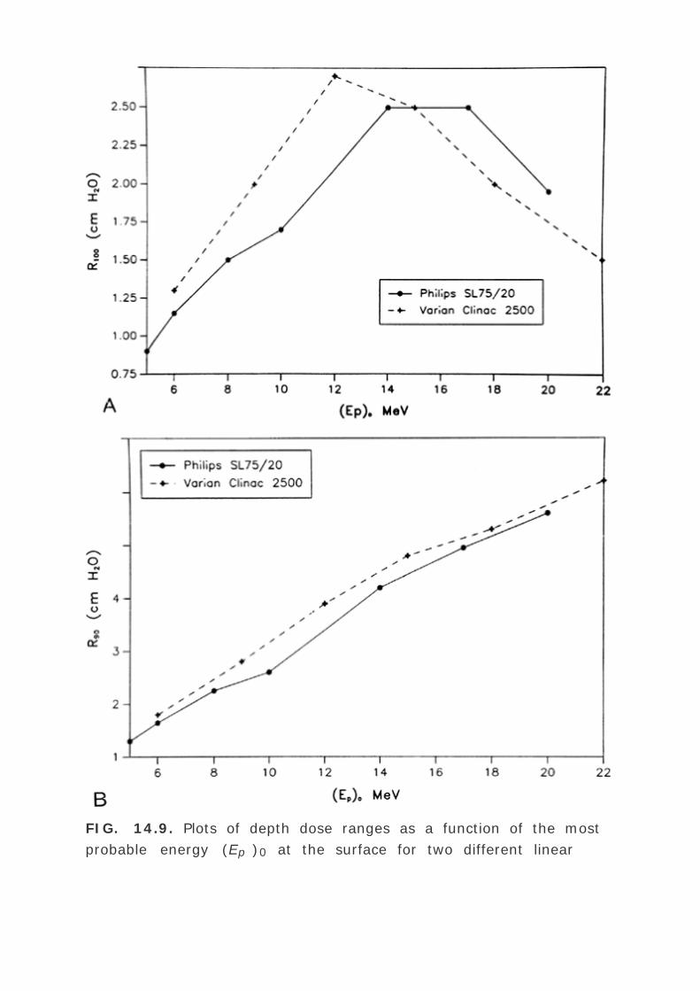
FIG. 14.9. Plots of depth dose ranges as a function of the most

probable energy (Ep )0 at the surface for two different linear

accelerators. A: R 100 , the depth of maximum dose versus (Ep )0 .

B: R 90 , the depth of 90% depth dose versus (Ep )0 . (From Khan

FM. Clinical electron beam dosimetry. In: Keriakes JG, Elson HR,

Born CG, eds. Radiation oncology physicsâ€”1986. AAPM Monograph

No. 15. New York, American Institute of Physics, 1986:211, with

permission.)

P.309

As the beam penetrates a medium, the beam expands rapidly below

the surface due to scattering. However, individual spread of the

isodose curves varies, depending on the isodose level, energy, field

size, and collimation. Figure 14.12 shows isodose patterns for two

different energy beams. Whereas for the low-energy beams all the

isodose curves show some expansion, for the higher energies only

the low isodose levels bulge out. The higher isodose levels tend to

show lateral constriction, which becomes worse with decreasing

field size.

C. Field Flatness and Symmetry

Uniformity of the electron beam is usually specified in a plane

perpendicular to the beam axis and at a fixed depth. The ICRU (31 )

specifies beam flatness in terms of a uniformity index.

P.310

This is defined in a reference plane and at a reference depth as the

ratio of the area where the dose exceeds 90% of its value at the

central axis to the geometric beam cross-sectional area at the

phantom surface. The uniformity index should exceed a given

fraction (e.g., 0.80 for a 10 — 10 cm field size and at depth of

maximum dose). In addition, the dose at any arbitrary point in the

reference plane should not exceed 103% of the central axis value.

FIG. 14.10. Schematic illustration showing the increase in percent

surface dose with an increase in electron energy. (From Khan FM.

Clinical electron beam dosimetry. In: Keriakes JG, Elson HR, Born

CG, eds. Radiation oncology physicsâ€”1986. AAPM Monograph No.

15. New York, American Institute of Physics, 1986:211, with

permission.)

Figure 14.13 shows isodose curves obtained from a film exposed

perpendicular to an electron beam at the depth of maximum dose.

The dashed line is the boundary of the geometric beam at the

surface. In this example, the homogeneity index is 0.8.

Because of the presence of lower-energy electrons in the beam, the

flatness changes significantly with depth. Therefore, it has been

recommended (32 ) that the uniformity

P.311

index be defined at the depth of half the therapeutic range (e.g.,

one-half the depth of 85% depth dose). Furthermore, it is defined

as the ratio of the areas inside the 90% and 50% isodose lines at

this depth. A uniformity index of 0.70 or higher is acceptable with

field sizes larger than 100 cm2 . The peak value in this plane should

be less than 103%.

FIG. 14.11. Comparison of central axis depth-dose distributions of

the Sagittaire linear accelerator (continuous curves) and the

Siemen's betatron (dashed curves). (From Tapley N, ed. Clinical

applications of the electron beam. New York: John Wiley & Sons,

1976, with permission.)

FIG. 14.12. Comparison of isodose curves for different energy

electron beams. (From Tapley N, ed. Clinical applications of the

electron beam. New York: John Wiley & Sons, 1976:86, with

permission.)

The AAPM (20 ) recommends that the flatness of an electron beam

be specified in a reference plane perpendicular to the central axis,

at the depth of the 95% isodose beyond the depth of dose

maximum. The variation in dose relative to the dose at central axis

should

P.312

not exceed ±5% (optimally to be within ±3%) over an area

confined within lines 2 cm inside the geometric edge of fields equal

to or larger than 10 — 10 cm.

FIG. 14.13. Isodose curves in a plane perpendicular to central axis,

obtained with a film placed in a phantom at the depth of maximum

dose. (From Almond PR. Radiation physics of electron beams. In:

Tapley N, ed. Clinical applications of the electron beam. New York:

John Wiley & Sons, 1976:50, with permission.)

Beam symmetry compares a dose profile on one side of the central

axis to that on the other. The AAPM recommends that the cross-

beam profile in the reference plane should not differ more than 2%

at any pair of points located symmetrically on opposite sides of the

central axis.

C.1. Beam Collimation

Acceptable field flatness and symmetry are obtained with a proper

design of beam scatterers and beam defining collimators.

Accelerators with magnetically scanned beam do not require

scattering foils. Others use one or more scattering foils, usually

made up of lead, to widen the beam as well as give a uniform dose

distribution across the treatment field.

The beam collimation has been significantly improved by the

introduction of the dual-foil system (33 ). Figure 14.14 shows a

typical arrangement for such a system. Whereas, the first foil

widens the beam by multiple scattering, the second foil is designed

to make the beam uniform in cross-section. The thickness of the

second foil is differentially varied across the beam to produce a

desired degree of beam widening and flattening. Analysis by Werner

et al. (34 ) shows that the dual-foil systems compare well with the

scanning beam systems in minimizing angular spread and, hence,

the effect on dose distribution characteristics.

The beam-defining collimators are designed to provide a variety of

field sizes and to maintain or improve the flatness of the beam.

Basically, all collimators provide a primary

P.313

collimation close to the source that defines the maximum field size

and a secondary collimation close to the patient to define the

treatment field. The latter can be in the form of trimmer bars or a

series of cones. In the electron therapy mode, the x-ray collimator

jaws are usually opened to a size larger than the cone or the

applicator opening. Because the x-ray jaws give rise to extensive

electron scatter, they are interlocked with the individual cones to

open automatically to a fixed predetermined size.

FIG. 14.14. Principle of dual-foil system for obtaining uniform

electron beam field. (From Almond PR. Handbook of medical

physics, Vol I. Boca Raton, FL: CRC Press, 1982:149, with

permission.)

D. Field Size Dependence

The output and the central axis depth-dose distribution are field

size dependent. The dose increases with field size because of the

increased scatter from the collimator and the phantom. As stated

previously, some electron collimators provide a fixed jaw opening,

and the treatment field size is varied by various size cones, inserts,

or movable trimmer bars. Such an arrangement minimizes the

variation of collimator scatter, and therefore, the output variation

with field size is kept reasonably small. If the collimator aperture

(x-ray jaw setting) were allowed to change with the treatment field,

the output would vary too widely with field size, especially for

lower-energy beams. This effect is shown in Fig. 14.15 , where the

cone size is held fixed while the x-ray jaws are varied (35 ). Note

that the dose rate varies by a factor of greater than 2 between

small and large jaw openings at 4 MeV.

The effects of field size on output and the central axis depth dose

curve due to phantom scatter alone is significant as long as the

distance between the point of measurement and the edge of the

field is shorter than the range of the laterally scattered electrons.

When this distance is reached, there is no further increase in depth

dose caused by phantom scatter. When the field is reduced below

that required for lateral scatter equilibrium, the dose rate decreases

rapidly. This is shown in Fig. 14.16 . In these measurements, the

field size at the phantom was varied without changing the photon

collimator opening. For small fields, the output factor as well as

depth dose can be significantly reduced compared with the broad

beam distribution.

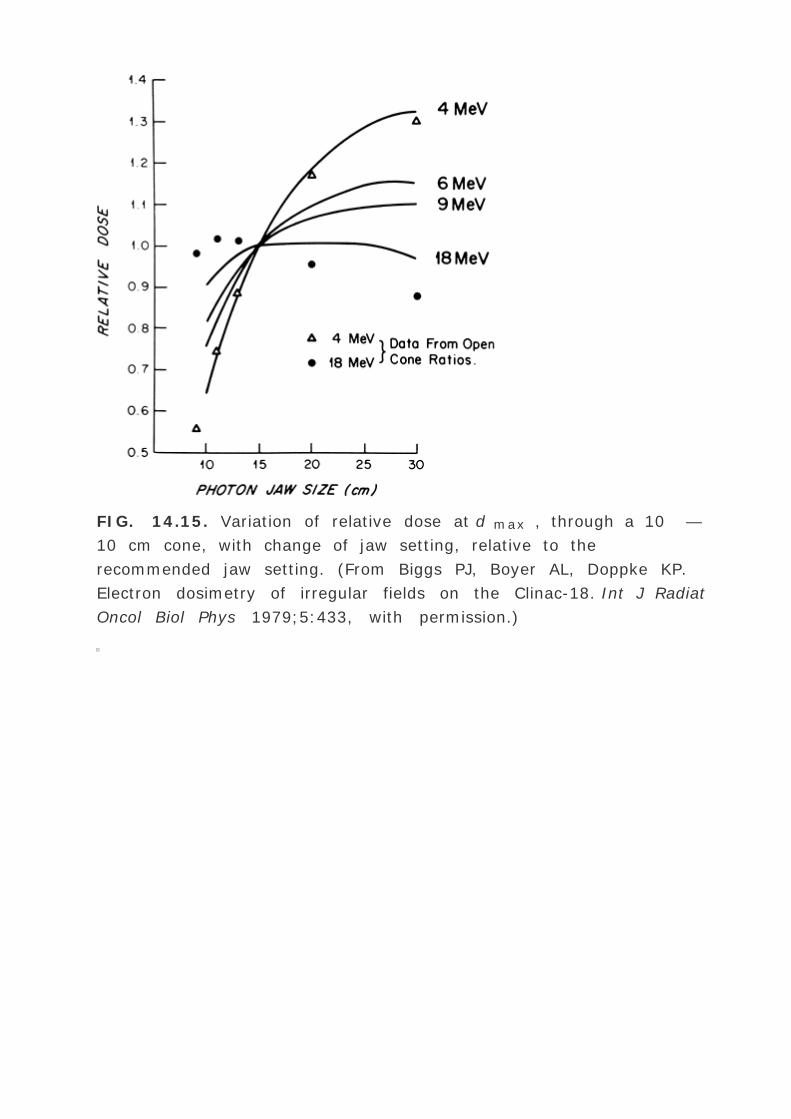
FIG. 14.15. Variation of relative dose at d max , through a 10 —

10 cm cone, with change of jaw setting, relative to the

recommended jaw setting. (From Biggs PJ, Boyer AL, Doppke KP.

Electron dosimetry of irregular fields on the Clinac-18. Int J Radiat

Oncol Biol Phys 1979;5:433, with permission.)

FIG. 14.16. Output factors as a function of side of square field.

Primary collimator fixed, secondary collimators (trimmers) close to

the phantom varied to change the field size. Data are from Therac

20 linear accelerator. (From Mills MD, Hogstrom KR, Almond PR.

Prediction of electron beam output factors. Med Phys 1982;9:60,

with permission.)

P.314

Figure 14.17 shows the change in central axis depth-dose

distribution with field size. As the field size is increased, the

percent depth dose initially increases but becomes constant beyond

a certain field size when the lateral scatter equilibrium is reached.

Furthermore the depth d max shifts toward the surface for the

smaller fields. Thus in clinical practice, depth-dose distribution for

small fields should be measured individually in addition to the

output calibration.

It has been shown (36 ) that the minimum field radius for the

establishment of lateral scatter equilibrium at all depths on central

axis is given by the following approximate

P.315

relationship:

where R eq is the field radius in cm and Ep,o is the most probable

energy in MeV. For example, the equilibrium fields for 8 MeV and 32

MeV electrons have diameters of 5cm and 10cm, respectively, which

agree with the data shown in Fig. 14.17 . In clinical practice, the

above relationship may be used to classify fields with radius < R eq

as small or narrow fields and radius â‰¥ R eq as broad fields. As

stated earlier, the depth-dose distribution for small fields is field

size dependent while for broad fields it is independent of field size.

FIG. 14.17. Variation of depth-dose distribution with field size.

(From ICRU. Radiation dosimetry: electron beams with energies

between 1 and 50 MeV. Report No. 35. Bethesda, MD: International

Commission on Radiation Units and Measurements, 1984, with

permission.)

E. Field Equivalence

Exact field equivalence for electron beams cannot be established.

However, it has been shown (36) that approximate equivalent

circular or square fields can be determined for fields of any size,

shape, and energy. The term field equivalence means that for the

same incident fluence and cross-sectional beam profile, the

equivalent fields have the same depth-dose distribution along the

central ray. Thus field equivalence here is defined in terms of

percent depth doses and not the output factors, which depend on

particular jaw setting for the given applicator or other collimation

conditions. According to this definition, all broad fields are

equivalent because their depth-dose distribution is the same

irrespective of field size. For example, 10 — 10, 10 — 15, 10

— 20, 20 — 20, etc. are all broad fields for energies up to 30

MeV (see Eq. 14.11 ) and hence are equivalent. Field equivalence is

therefore relevant only for small fields in which the lateral scatter

equilibrium does not exist and consequently, the depth-dose

distribution is field size dependent.

Harder et al. (37 ) have shown that for a square field of cross-

section (2a — 2a) the equivalent circular field has a radius R equiv

, given by:

However, for a small rectangular or irregularly shaped fields, field

equivalence is not as straightforward. Khan and Higgins (36 ) have

applied Gaussian pencil beam theory to this problem and derived

relationships that can be used to find approximate equivalent

circular or square fields for fields of any shape. The reader is

referred to their paper for further details on this subject.

F. Square Root Method

Hogstrom et al. (38 ) have shown that, if the change in collimator

scatter with field size is not considered, the depth dose for

rectangular field sizes can be extracted from square field data by

the following relationships:

where D is the central axis depth dose and X and Y are the field

dimensions. Thus the dose for a rectangular field size can be

determined from the square root of the two square field depth doses

when the sides of the two square fields are equal to the two sides of

the rectangular field. Referred to as the square root method, this

concept has also been applied to the determination of output factors

when the primary collimation is fixed and the secondary collimation

close to the phantom is varied (39 ). It may be restated that the

collimator scatter is neglected in this model. Thus the applicability

of the square root method is not automatically valid for those

machines in which collimator scatter varies substantially with field

size.

G. Electron Source

Unlike an x-ray beam, an electron beam does not emanate from a

physical source in the accelerator head. A pencil electron beam-

after passing through the vacuum window

P.316

of the accelerator, bending magnetic field, scattering foils, monitor

chambers, and the intervening air column-is spread into a broad

beam that appears to diverge from a point. This point is called the

virtual source (40 ), which may be defined as an intersection point

of the backprojections along the most probable directions of

electron motion at the patient surface (41 ). This is illustrated in

Fig. 14.18 .

FIG. 14.18. Definition of virtual point source of an electron beam:

the intersection point of the backprojections along the most

probable directions of motion of electrons at the patient surface.

(From Schroeder-Babo P. Determination of the virtual electron

source of a betatron. Acta Radiol 1983;364[suppl]:7, with

permission.)

A number of methods have been suggested for the determination of

virtual source position. Pohlit's (40 ) method consists of taking

electron radiographs of a grid of copper wires at different distances

from the collimator and backprojecting the images to a point, the

virtual source. A multipinhole technique (41 ) uses double conical

holes in a metal plate. Pinhole images are obtained on a film.

Backprojection of the pinhole images gives the virtual source

position. Meyer et al. (42 ) have described the method of

determining field size magnification on film with distance. The

virtual source point is found by the backprojection of the 50% width

of the beam profiles obtained at different distances. A broad beam

(â‰¥20 — 20 cm) is used for these measurements.

The use of virtual source-to-surface distance (SSD) does not give

accurate inverse square law correction for output at extended SSDs

under all clinical conditions. Measurements have shown that the

virtual SSD gives correct inverse square law factor only for large

field sizes (43 ). For small field sizes, the inverse square law

correction underestimates the change in output with virtual SSD.

This deviation from the inverse square law is caused by an

additional decrease in output because of a loss of side-scatter

equilibrium in air and in phantom that is significant for small field

sizes and low electron energies. Thus the use of the virtual SSD to

predict dose variation with distance requires correction factors, in

addition to the inverse square law factor, as a function of field size

and energy (42 ).

FIG. 14.19. Determination of effective SSD. (From Khan FM,

Sewchand W, Levitt SH. Effect of air space on depth dose in

electron beam therapy. Radiology 1978;126:249, with permission.)

P.317

An alternative method of correcting dose output for the air gap

between the electron collimator and the patient is to determine

effective SSD , which gives the correct inverse square law

relationship for the change in output with distance. Khan et al. (44

) have recommended a method that simulates as closely as possible

the clinical situation. In this method, doses are measured in a

phantom at the depth of maximum dose (dm ), with the phantom

first in contact with the cone or at the standard SSD (zero gap) and

then at various distances, up to about 20 cm from the cone end.

Suppose f = effective SSD; I 0 = dose with zero gap; Ig = dose with

gap g between the standard SSD point and the phantom surface.

Then, if electrons obey inverse square law,

or

By plotting

as a function of gap g (Fig. 14.19 ), a straight line is obtained, the

slope of which is:

. Thus,

Although the effective SSD is obtained by making measurements at

the depth dm , its value does not change significantly with the

depth of measurement (44 ). However, the effective SSD does

change with energy and field size, especially for small field sizes

and low energies. A table of effective SSDs as a function of energy

and field size is necessary to meet clinical situations.

F. X-ray Contamination

The x-ray contamination dose at the end of the electron range can

be determined from the tail of the depth-dose curve by reading off

the dose value at the point where the tail becomes straight (Fig.

14.3 ). This dose in a patient is contributed by bremsstrahlung

interactions of electrons with the collimation system (scattering

foils, chambers, collimator jaws, etc.) and the body tissues.

5

0.1

10

0.5

15

0.9

20

1.4

30

2.8

40

4.2

50

6.0

Data are for theoretical beam with no initial x-ray contamination

and are extracted from Monte Carlo data of Berger MJ, Seltzer SM.

Tables of energy-deposition distributions in water phantoms

irradiated by point-monodirectional electron beams with energies

from 1 to 60 MeV, and applications to broad beams. NBSIR

82â€“2451. Washington, DC: National Bureau of Standards, 1982.

Energy (MeV) Dx (%)

TABLE 14.2. X-RAY CONTAMINATION DOSE (Dx ) TO WATER,

AT THE END OF THE ELECTRON RANGE AS A PERCENTAGE OF

D max

P.318

Table 14.2 gives the x-ray dose for the theoretical beam, with no

initial x-ray contamination. These values were extracted from the

depth-dose distributions in water calculated by Berger and Seltzer

(45 ), using a Monte Carlo program. The x-ray contamination dose

from a medical accelerator depends very much on its collimation

system and is usually an order of two greater than the values given

in Table 14.2 . In general, the x-ray contamination is least in the

scanning beam type of accelerator, because the scattering foils are

not used. In a modern linear accelerator, typical x-ray

contamination dose to a patient ranges from approximately 0.5% to

1% in the energy range of 6 to 12 MeV; 1% to 2%, from 12 to 15

MeV; and 2% to 5%, from 15 to 20 MeV.

For regular treatment field sizes, the dose contributed by the x-ray

contamination is not of much concern. However, even small

amounts of x-ray contamination become critical for total body

electron irradiation such as in the treatment of mycosis fungoides

(section 14.8 ).

14.5. TREATMENT PLANNING

Most electron beam treatments are planned for a single field

technique. For a relatively flat and homogeneous block of tissue,

the dose distribution can be found by using the appropriate isodose

chart. However, this simplicity of treatment planning is the

exception rather than the rule. Surface areas are seldom flat, and in

many cases, inhomogeneities, such as bone, lung, and air cavities,

present dosimetric complexities.

A. Choice of Energy and Field Size

The energy of beam is dictated, in general, by the depth of the

target volume, minimum target dose required, and clinically

acceptable dose to a critical organ, if present in the path of the

beam. In most cases, when there is no danger of overdosing a

critical structure beyond the target volume, the beam energy may

be set so that the target volume lies entirely within the 90%

isodose curve. However, in the treatment of the breast, the energy

is often chosen so that the depth dose at the chest wall-lung

interface is 80% (46 ). The rationale for this lowering of the energy

is to spare the lung, with the belief that the target volume for the

chest wall irradiation is quite superficial and that a minimum of

80% (and some even advocate 70%) isodose curve is sufficient for

the chest wall. Beyond the 80% depth dose, the dose falloff is

characteristically rapid at these beam energies.

The choice of field size in electron beam therapy should be strictly

based on the isodose coverage of the target volume. Examination of

the electron isodose curves (Fig. 14.20 )

P.319

reveals that there is a significant tapering of the 80% isodose curve

at energies above 7 MeV (46 ). The constriction of the useful

treatment volume also depends on the field size and is worse for

the smaller fields. Thus, with electrons, a larger field at the surface

than one is usually accustomed to (in the case of photon beams)

may be necessary to cover a target area adequately.

FIG. 14.20. Lateral constriction of the 80% isodose curve with

depth. (From Almond PR. Radiation Physics of electron beams. In:

Tapley N, ed. Clinical applications of the electron beam. New York:


B. Corrections for Air Gaps and Beam

Obliquity

In electron beam therapy, there is a frequent problem of treatment

cone end1 not being parallel to the skin surface. These uneven air

gaps can sometimes be large as a result of the extreme curvature of

the sloping surface. In these cases, it is a common practice to

calculate dose distribution simply by applying inverse square law

correction to the dose distribution along fan lines emanating from a

virtual or effective electron source (47 ,48 ,49 ). As a result of this

correction, the relative depth dose distribution for a sloping contour

remains almost unchanged but the absolute value of the dose is

decreased at all depths because of beam divergence. This method,

however, does not take into account changes in side scatter owing

to beam obliquity. This has been pointed out by Ekstrand and Dixon

(50 ), who showed that the beam obliquity tends to (a) increase

side scatter at the depth of maximum dose (d max ), (b) shift d max

toward the surface, and (c) decrease the depth of penetration (as

measured by the depth of the 80% dose). These effects are evident

in Fig. 14.21 .

A broad electron beam can be represented by a summation of a

large number of pencil or slit beams placed adjacent to each other.

When the beam is incident obliquely on the patient surface, the

point at the shallow depth receives greater side scatter from the

adjacent pencil beams, which have traversed a greater amount of

material, whereas the point at the greater depth receives less

scatter. This is schematically illustrated in Fig. 14.22A . As a result

of these changes in the relative orientation of the pencils, one

would expect an increase in dose at shallow depths and a decrease

in dose at greater depths. However, because the

P.320

beam is divergent, the dose will also decrease at all depths as a

result of the inverse square law effect, as the air gap between the

cone end and the surface increases with the increase in the angle of

obliquity. Thus the depth dose at a point in an obliquely incident

beam is affected both by the â€œpencil scatter effectâ€ and the

beam divergence.

FIG. 14.21. Change in depth dose with the angle of obliquity for a

9-MeV electron beam. (From Ekstrand KE, Dixon RL. The problem of

obliquely incident beams in electron beam treatment planning. Med

Phys 1982;9:276, with permission.)

Figure 14.22B schematically represents an arrangement used

frequently for the treatment of chest wall. The beam is incident

vertically on a sloping surface, thus increasing the angle of

obliquity as well as the air gap between the end of the cone and the

surface. Let D 0 (f ,d ) be the dose at a point at depth d for a beam

incident normally on a flat-surfaced phantom with an effective SSD

= f . When the cone is placed on the chest wall, the depth dose D (f

+ g,d ) will be given by:

where g is the air gap and OF ( ¸,d ) is the obliquity factor for the

pencil beam scatter effect discussed previously. OF ( ¸,d )

accounts for the change in depth dose at a point if the beam angle

¸ changes relative to the surface without change in the distance

from the point to the effective source position.

The obliquity factor becomes significant for angles of incidence

approaching 45 degrees or higher. For example, a 60-degree angle

of obliquity for a 9-MeV beam gives rise to OF = 1.18 at the d max ,

a shift of the d max to about 0.5 cm, and a shift of the 80% depth to

about 1.5 cm (52 ). Of course, in a given clinical situation, these

effects are compounded by the inverse square law effect when

significantly large air gaps are caused by the sloping surface.

Khan et al. (51 ) have determined obliquity factors as a function of

energy and depth for obliquity angles of 30 degrees, 45 degrees,

and 60 degrees. These data are presented in Table 14.3 . Depths

are normalized to the practical range, which is approximately given

by E (MeV)/2 in centimeters of water. The Z /Rp values in column 1

can be converted to

P.321

P.322

depths by multiplying with the Rp for the given energies. These

obliquity factors can be used in Equation 14.15 for the calculation of

dose at a point for an obliquely incident beam.

FIG. 14.22. A: A schematic illustration of how the relative

orientation of pencil beams changes with the angle of obliquity. For

a parallel beam, this effect would increase dose at the shallower

points and decrease dose at the deeper points as the angle of

obliquity is increased. (Redrawn from Ekstrand KE, Dixon RL.

Obliquely incident electron beams. Med Phys 1982;9:276.) B: A

diagrammatic representation of irradiation of a chest wall with

sloping surface. The gap g and depth d for a point are measured

along the fan line (the line joining the point to the effective source

location). ¸ is the angle between the fan line and normal to the

tangent to the sloping surface. The figure on the right represents

the reference set-up, with beam incident normal, with no air gaps

between the cone end and the phantom. C: Comparison of measured

(solid lines) and calculated (dashed lines) isodose distribution for a

beam incident on a polystyrene cylindrical phantom. The measured

distribution represents isodensity distribution obtained with a film

sandwiched in the phantom according to the procedure outlined in

section 14.3B . The calculated distribution was obtained with a

computer using a divergent pencil beam algorithm. Both

distributions are normalized to the D max in a reference set-up in

which the beam is incident normally on a flat phantom with no air

gaps between the cone end and the phantom. 12-MeV electrons;

field size 18 — 12 cm; effective SSD = 70 cm.

(a) ¸ = 30 °

0.0

1.00

0.98

0.98

1.00

0.94

1.01

0.1

1.00

1.00

1.00

1.00

1.00

1.08

0.2

1.00

1.00

1.01

1.02

1.05

1.11

0.3

1.01

1.00

1.02

1.03

1.05

1.06

0.4

1.01

1.01

1.02

1.00

1.00

0.96

0.5

1.00

1.00

0.98

0.96

0.92

0.86

0.6

0.95

0.94

0.92

0.90

0.86

0.79

0.7

0.92

0.90

0.87

0.86

0.86

0.83

0.8

0.93

0.85

0.82

0.90

1.00

0.96

0.9

1.09

1.00

1.20

1.11

1.44

1.00

1.0

1.42

1.54

1.50

1.50

1.30

1.00

(b) ¸ = 45 °

0.0

1.03

1.02

1.03

1.05

0.98

1.14

0.1

1.03

1.04

1.04

1.06

1.10

1.14

0.2

1.05

1.06

1.07

1.11

1.12

1.12

0.3

1.06

1.07

1.09

1.09

1.05

1.07

0.4

1.04

1.04

1.04

1.01

0.93

0.92

0.5

1.00

0.99

0.92

0.92

0.80

0.77

0.6

0.93

0.90

0.86

0.82

0.70

0.69

0.7

0.84

0.84

0.82

0.77

0.70

0.76

0.8

0.87

0.83

0.85

0.86

0.83

1.10

0.9

1.30

1.00

1.43

1.20

1.40

1.46

1.0

2.17

2.31

2.19

2.50

2.00

2.14

(c) ¸ = 60 °

0.0

1.06

1.06

1.10

1.14

1.14

1.30

0.1

1.10

1.12

1.17

1.20

1.23

1.21

0.2

1.12

1.14

1.15

1.16

1.17

1.08

0.3

1.07

1.07

1.07

1.02

0.98

0.90

0.4

1.00

0.96

0.93

0.86

0.79

0.70

0.5

0.87

0.84

0.79

0.74

0.67

0.56

0.6

0.75

0.74

0.69

0.63

0.58

0.51

0.7

0.70

0.68

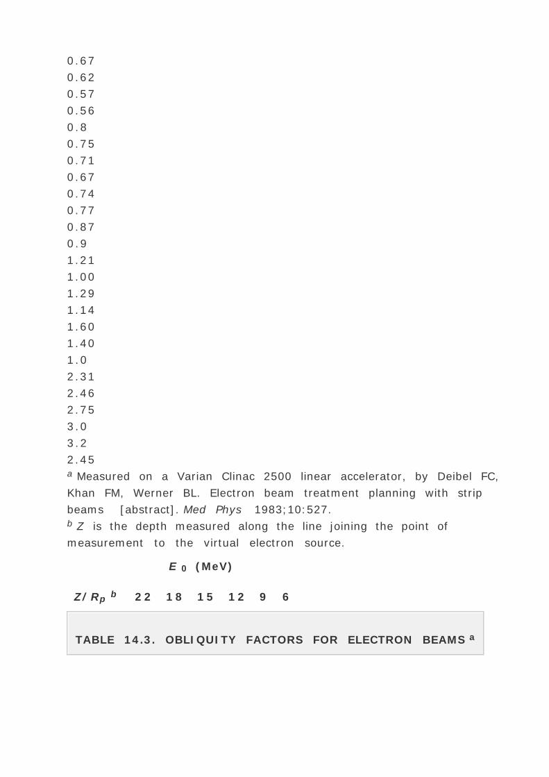
0.67

0.62

0.57

0.56

0.8

0.75

0.71

0.67

0.74

0.77

0.87

0.9

1.21

1.00

1.29

1.14

1.60

1.40

1.0

2.31

2.46

2.75

3.0

3.2

2.45a Measured on a Varian Clinac 2500 linear accelerator, by Deibel FC,

Khan FM, Werner BL. Electron beam treatment planning with strip

beams [abstract]. Med Phys 1983;10:527.b Z is the depth measured along the line joining the point of

measurement to the virtual electron source.

Z/Rp b

E 0 (MeV)

22 18 15 12 9 6

TABLE 14.3. OBLIQUITY FACTORS FOR ELECTRON BEAMS a

Computer algorithms have been developed (38 ,52 ,53 ,54 ) by

which broad beam distribution is calculated by placing a set of

narrow or pencil beams along the contour. The divergence

correction can be taken into account by aligning central axes of the

pencil beams along the fan lines and normalizing the resulting dose

distribution to the dose at d max for the beam incident normally on

a flat-surfaced phantom. Figure 14.22C compares the calculated

distribution using a pencil beam algorithm with the measured

distribution obtained in a cylindrical polystyrene phantom.

Sharp surface irregularities produce localized hot and cold spots in

the underlying medium due to scattering. Electrons are

predominantly scattered outward by steep projections and inward by

steep depressions. This can be seen in Fig. 14.23 (55 ). In practice,

such sharp edges may be smoothed with an appropriately shaped

bolus. Also, if a bolus is used to reduce beam penetration in a

selected part of the field, its edges should be tapered to minimize

the effect shown in Fig. 14.23 .

FIG. 14.23. Effect of sharp surface irregularities on electron beam

isodose distributions. (From Dutreix J. Dosimetry. In: Gil y Gil, Gil

Gayarre, eds. Symposium on high-energy electrons. Madrid: General

Directorate of Health, 1970:113, with permission.)

P.323

C. Tissue Inhomogeneities

Electron beam dose distribution can be significantly altered in the

presence of tissue inhomogeneities such as bone, lung, and air

cavities. It is difficult to determine dose distribution within or

around small inhomogeneities because of enhanced scattering

effects. However, for large and uniform slabs, dose distribution

beyond the inhomogeneity can be corrected by using the coefficient

of equivalent thickness (CET) method (49 ,56 ,57 ,58 ,59 ). It is

assumed that the attenuation by a given thickness z of the

inhomogeneity is equivalent to the attenuation (z — CET) of

water. The CET for a given material is approximately given by its

electron density (electron/ml) relative to that of water. The dose at

a point beyond the inhomogeneity is determined by calculating the

effective depth, d eff , along the ray joining the point and the

virtual source of the electrons.

where d is the actual depth of point P from the surface. The depth

dose is read from dose distribution data for water at the effective

depth. An additional correction may be applied due to the inverse

square law, that is,

, where f is the effective SSD.

P.324

C.1. Bone

The CET method is in good agreement with in vivo measurements in

patients for the dose behind the mandible (60 ). The electron

density (or CET) of a compact bone (e.g., mandible) relative to that

of water is taken as 1.65. For spongy bone, such as sternum, which

has a density of 1.1 g/cm3 , the electron densities are not much

different from water, and therefore, CET can be assumed to be

unity.

C.2. Lung

The problem of lung inhomogeneity has been studied by many

investigators (56 ,57 ,58 ,59 ). Results of in vivo measurements in

the lungs of dogs have shown that there is a considerable variation

of CET with depth in the lung (61 ). This is illustrated by Fig. 14.24

for a water-cork system (simulating chest wall and lung interface).

The dose near the interface is decreased due to reduced scatter

from the low-density cork. Beyond a certain depth, the dose to the

cork begins to increase relative to the reference curve (measured in

water) as the increased penetration overtakes the reduced scatter.

Thus, in general, the CET values for lung depend on depth within

the lung. Empirical equations for the CET values derived from in

vivo measurements have been proposed to take this variation into

account (60 ). An average lung CET value of 0.5 has also been

suggested (56 ). More recent measurements (62 ) in

anthropomorphic phantoms have shown that a CET value based on

electron density gives an accuracy of approximately 10% in depth

dose for typical chest wall irradiations.

The relative electron density of lung may be equated to its mass

density. The studies with computed tomography (CT) have shown

that the electron density of lung varies between 0.20 and 0.25

relative to that of water. Therefore, if CET is assumed equal to

electron density, Equation 14.16 may be used to calculate lung

correction by substituting lung density in place of CET. Figure 14.25

shows examples of uncorrected and corrected isodose distributions

obtained by using pencil beams. In the case of the corrected

distribution, the effective depth was calculated assuming CET equal

to the lung density.

In routine treatment planning, any of the previous methods may be

used as approximations. Obviously, the effective depth calculation

based on electron density or some empirically derived CET is only a

rough approximation, for which scattering effects are not fully taken

into account.

FIG. 14.24. Depth-dose distribution in water and water-cork

phantoms. CET values may be calculated from these data. CET = X 1

/X 2 . (Modified from Almond PR, Wright AE, Boone ML. High-energy

electron dose perturbations in regions of tissue heterogeneity.

Radiology 1967;88:1146.)

FIG. 14.25. An example of chest wall irradiation with electrons.

The surface contour was irregular in shape, so bolus was used to

even out chest wall thickness as well as maximize surface dose. A:

Calculated isodose curves uncorrected for lung density. B:

Calculated isodose curves corrected for lung density ( = 0.25

g/cm3 ). 10-MeV electron beam; effective SSD = 68 cm; field size =

13 — 15 cm.

P.325

C.3. Small Inhomogeneities

Small inhomogeneities present a more complex situation because of

electron scattering behind edges. Figure 14.26 schematically

illustrates the effect at a single edge. For simplicity, it is assumed

that the path of the electrons in medium M is along straight lines. If

a material M â€² of a higher mass scattering power is introduced,

electrons are scattered at larger angles. This causes a decrease in

the electron fluence behind the slab, thus reducing the dose there.

The scattered electrons, on the other hand, increase the dose in the

medium M. Thus a small inhomogeneity causes cold spots and hot

spots behind its edges.

Pohlit and Manegold (63 ) have made a systematic analysis of dose

distributions behind edges of different materials. Their method can

be used to get a rough estimate of the maximum values for increase

and decrease of dose behind such inhomogeneities. Figure 14.27

defines angles ± and ² of dose perturbation. The mean angle

± gives the position of the maxima of reduction and of increase of

dose, and ² represents the mean angle at which the effect of the

inhomogeneity is practically negligible. These angles, which are

related to the scattering of electrons in the medium, depend mainly

on the mean electron energy ’ at the edge. Figure 14.28 gives

these angles as a function of ’.

The dose distribution under the inhomogeneity but outside angle ²

may be calculated according to the regular CET method discussed

previously. The maxima and minima of

P.326

dose along the boundaries of angle ± may be estimated by

defining a maximum change, P max , in dose.

where Dm is the dose at the highest increase or depression and D 0

is the dose in the homogeneous water phantom at that point. Figure

14.29 may be used to estimate P max

P.327

for different energies and materials. It is important to note that the

influence of an edge increases with increasing electron energy.

FIG. 14.26. Schematic illustration of electron scatter behind edges

between materials M and M â€². The scattering power of M â€² is

greater than that of M.

FIG. 14.27. Isodose distribution behind an edge of a thin lead slab

in water. Angle ± denotes the maxima of dose change and angle

² of negligible change. (From Pohlit W, Manegold KH. Electron-

beam dose distribution in inhomogeneous media. In: Kramer S,

Suntharalingam N, Zinninger GF, eds. High energy photons and

electrons. New York: John Wiley & Sons, 1976:243, with

permission.)

FIG. 14.28. Plot of angles ± and ² as a function of mean energy

at the edge for inhomogeneities in water (or tissue). (From Pohlit

W, Manegold KH. Electron-beam dose distribution in inhomogeneous

media. In: Kramer S, Suntharalingam N, Zinninger GF, eds. High

energy photons and electrons. New York: John Wiley & Sons,


FIG. 14.29. Plot of maximum change in dose P max as a function of

mean electron energy at the edge of various inhomogeneities in

water. (From Pohlit W, Manegold KH. Electron-beam dose

distribution in inhomogeneous media. In: Kramer S, Suntharalingam

N, Zinninger GF, eds. High energy photons and electrons. New York:


Scattering effects can be enhanced by adjoining scattering edges,

and therefore, small inhomogeneities produce complex effects,

resulting in large changes in dose caused by the overlapping of

these regions.

The previous method is useful for quick-and-rough calculations.

More accurate calculations require more sophisticated methods

based on multiple scattering theory. Some work along these lines

has been reported in the literature (34 ,38 ,54 ,64 ,65 ).

D. Use of Bolus and Absorbers

Bolus is often used in electron beam therapy to (a) flatten out an

irregular surface, (b) reduce the penetration of the electrons in

parts of the field, and (c) increase the surface dose. Ideally, the

bolus material should be equivalent to tissue in stopping power and

scattering power. A given bolus material should be checked by

comparing depth dose distribution in the bolus with that in the

water. If a scaling factor is required, it should be documented and

used in treatment planning whenever the bolus is used.

A number of commercially available materials can be used as bolus,

e.g., paraffin wax, polystyrene, Lucite, Superstuff, and Superflab.

Usefulness of some of these materials for electron bolusing have

been discussed in the literature (66 ,67 ). In my experience,

Superflab2 is excellent for bolusing. This material is transparent,

flexible, and almost water equivalent.

A plate of low atomic number material such as Lucite and

polystyrene is sometimes used to reduce the energy of an electron

beam. Such plates are known as decelerators. The decelerator

should be placed in close contact with the patient surface as with a

bolus. Large air gaps between the absorber and the surface would

result in scattering of electrons outside the field and reduction in

dose, which may not be easily predictable unless specifically

measured for those conditions. For these reasons, a flexible bolus

that conforms to the surface is more desirable.

FIG. 14.30. Isodose distributions for adjacent electron fields with

different gap widths. (From Almond PR. Radiation physics of

electron beams. In: Tapley N, ed. Clinical applications of the

electron beam. New York: John Wiley & Sons, 1976, with

permission.)

P.328

E. Problems of Adjacent Fields

When two adjacent electron fields are overlapping or abutting, there

is a danger of delivering excessively high doses in the junction

region. On the other hand, separating the fields may seriously

underdose parts of the tumor. Examples of combined isodose

distributions for different field separations are shown in Fig. 14.30 .

In a clinical situation, the decision as to whether the fields should

be abutted or separated should be based on the uniformity of the

combined dose distribution across the target volume. Because the

tumors treated with electrons are mostly superficial, the electron

fields are usually abutted on the surface. The hot spots can be

accepted, depending on their magnitude, extent, and location.

Similar considerations apply to electron fields adjacent to x-ray

fields.

When an electron field is abutted at the surface with a photon field,

a hot spot develops on the side of the photon field and a cold spot

develops on the side of the electron field (68 ). This is caused by

outscattering of electrons from the electron field. Figure 14.31

shows this effect when a 9-MeV electron field is abutted with a 6-

MV photon field, an

P.329

example typifying a clinical situation involving treatment of tumors

in the neck. Whereas the photon field is used to treat the anterior

neck, the electron field is used to treat the posterior neck nodes

overlying the cord. Because of the limited range of the electrons,

the cord can be spared, while sufficient dose can be delivered to the

nodes.

FIG. 14.31. Isodose curves in a plane perpendicular to the junction

line between abutting photon and electron fields. 9-MeV Electron

beam; field size = 10 — 10 cm; 6-MV photon beam; SSD = 100

cm. A: Electron beam at standard SSD of 100 cm. B: Electron beam

at extended SSD of 120 cm. (From Johnson JM, Khan FM. Dosimetric

effects of abutting extended SSD electron fields with photons in the

treatment of head and neck cancers. Int J Radiat Oncol Biol Phys


An examination of the isodose distribution in Fig. 14.31 also reveals

that the extent of hot and cold spots depends on the electron beam

SSD. In Fig. 14.31A , the electron beam is incident at the standard

SSD of 100 cm, with the distance between the applicator end and

the surface being 5 cm. In Fig. 14.31B , the electron beam is

incident at an extended SSD of 120 cm, exemplifying a practical

situation when clearance is required between the applicator and the

patient shoulder. The increased air gap between the applicator and

the surface causes the electron beam profile to become less flat as

a result of increased scattering of electrons by air. Consequently,

the hot and cold spots spread out to cover larger areas, without

significantly changing their magnitudes.

P.330

14.6. FIELD SHAPING

Extensive field shaping is sometimes required in electron beam

therapy. Lead cutouts are often used to give shape to the treatment

area and to protect the surrounding normal tissue or a critical

organ. These cutouts are placed either directly on the skin or at the

end of the treatment cone.

For lower-energy electrons (<10 MeV), less than 5 mm thickness of

lead is required for adequate shielding (e.g., â‰¤5%

transmission). Lead sheets of this thickness can be molded to

conform more or less to the surface contour and, therefore, can be

placed directly on the skin surface. For higher-energy electrons,

however, thicker lead is required and cannot be so easily contoured.

Moreover, a heavy lead mask may cause discomfort to the patient.

The alternative method is to support a lead cutout at the end of the

treatment cone or the field trimmers. Shields to be used in such a

configuration can be designed from pure lead sheets or a low

melting alloy such as Lipowitz metal (trade names: Cerrobend,

Ostalloy, and Lometoy).

A. External Shielding

Several publications have reported the thickness of lead or low

melting point lead alloy required for shielding in electron beam

therapy (69 ,70 ,71 ,72 ,73 ). Figure 14.32 shows a set of

transmission measurements through lead. The thickness for

shielding can be chosen on the basis of allowable transmission

(e.g., 5%). The shield thickness should be neither overly large nor

so critical in measurement that a small change in thickness would

cause a large change in the transmitted dose.

FIG. 14.32. Transmission curves through lead for 7-, 9-, 11-, 15-,

and 18-MeV electrons. Measurements made with a plane-parallel

chamber in a polystyrene phantom, at a depth of 0.5 cm. Solid lines

are for 10.5 — 10.5 cm effective field size and dashed lines are

for 6.3 — 6.3 cm effective field size. (Redrawn from Giarratano

JC, Duerkes RJ, Almond PR. Lead shielding thickness for dose

reduction of 7- to 28-MeV electrons. Med Phys 1975;2:336.)

P.331

An important consideration in electron beam shielding is to make

certain that the thickness is appropriate to reduce the dose to an

acceptable value. As seen in Fig. 14.32 , if the lead is too thin, the

transmitted dose may even be enhanced directly behind the shield.

Normally, if weight or thickness is no problem, one can use a shield

of thickness greater than the required minimum. But there are

practical limits on the amount of lead that can be used. For

example, in the case of eyeshields (74 ) and internal shields, it is

important to use the minimum thickness of lead to obtain the

desired reduction in dose.

B. Measurement of Transmission Curves

Transmission curves for a shielding material may be obtained with

an ion chamber embedded in a phantom. A suitable arrangement for

such measurements consists of a parallel-plate ion chamber in a

polystyrene phantom. Because the maximum transmitted dose

through lead occurs at a point close to the patient's surface, the

measurement depth in the phantom should not exceed 5 mm (75 ).

The transmission curve is a plot of ionization current as a function

of shield thickness. Generally, the shielding measurements made

with broad beams gives an upper limit to the shielding requirements

for all field sizes (69 ,73 ). However, if minimum thickness shields

are needed, as for internal shielding, a transmission curve may be

measured especially for the given field size and the depth of the

structure to be shielded.

Although it is desirable to make measurements with the shields in

the same configuration relative to the applicator and the phantom

as used clinically, this is not a critical consideration. Purdy et al.

(73 ) made measurements with the shield placed at the end of the

treatment cone and at the phantom surface. They did not find

significant differences in the percent transmission for the two

arrangements.

Figure 14.33 shows a plot of minimum lead thickness required to

stop electrons as a function of the most probable electron energy

incident on lead. The transmitted dose in this case is only the result

of bremsstrahlung. From these data a rule of thumb may be

formulated: the minimum thickness of lead required for blocking in

millimeters is given

P.332

by the electron energy in MeV incident on lead divided by 2.

Another millimeter of lead may be added as a safety margin. The

required thickness of Cerrobend is approximately 20% greater than

that of pure lead.

FIG. 14.33. A plot of published data for minimum lead thickness

required to stop primary electrons as a function of electron energy

incident on lead. (From Khan FM, et al. Clinical electron-beam

dosimetry. Report of AAPM Radiation Therapy Committee Task

Group No. 25. Med Phys 1991;18:73, with permission.)

FIG. 14.34. Ratio of ionization for the open cone to the ionization

for the shaped field (output ratio) as a function of beam energy.

Output factor is inverse of output ratio. The field sizes for the

reduced fields were defined by a lead cutout placed at the phantom

surface. (From Choi MC, Purdy JA, Gerbi BJ, et al. Variation in

output factor caused by secondary blocking for 7â€“16 MeV electron

beams. Med Phys 1979;6:137, with permission.)

C. Effect of Blocking on Dose Rate

Blocking a portion of the electron beam field, in general, produces

changes in the dose rate and dose distribution. The magnitude of

the change depends on the extent of blocking, the thickness of

lead, and the electron energy. Figure 14.34 shows increase in

output ratio (or decrease in output factor) at d max when a field is

blocked down to a smaller size (72 ). If a field produced by a lead

cutout is smaller than the minimum size required for maximum

lateral dose buildup, the dose in the open portion is reduced (70 )

(Fig. 14.35 ).

P.333

The reduction in dose also depends on the depth of measurement.

Thus field shaping affects output factor as well as depth-dose

distribution in a complex manner.

FIG. 14.35. Change of dose at D max as the field size is changed

using a lead cutout at the phantom surface (72 ).

FIG. 14.36. Minimum field diameter, d , versus most probable

energy at the surface, Ep,0 , for which the depth dose distribution

can be considered independent of field size. The curve labeled 2z 1

shows maximum lateral excursion diameter of electrons. Rp is the

extrapolated range. ”z is the maximum shift in the depth dose

distribution for field diameter relative to broad beam. The curve 2R

1 gives the field diameter at which the maximum dose is 1% less

than its value for a broad beam. These data do not include the

effects of collimator or air scatter. (From Lax I, Brahme A. On the

collimation of high energy electron beams. Acta Radiol Oncol


As the most conservative measure, a special dosimetry (e.g., output

factor, depth-dose, and isodose distribution) should be measured

for any irregularly shaped electron field used in the clinic. However,

this is impractical because most radiation therapy fields are

irregular. The ICRU (14 ) suggested Rp as the lower limit for field

diameter, above which the field size dependence of the depth dose

is negligible. That means that for a given point of interest in an

irregularly shaped field, the field edges should be farther than Rp / 2

for the lateral scatter equilibrium to be approximately achieved. For

example, a 10 — 10 cm size field of a 12-MeV electron beam (Rp

[asymptotically equal to] 6 cm) may be blocked down to 6 — 6 cm

field without significantly affecting the depth-dose distribution.

Lax and Brahme (76 ) have measured field diameters above which

the maximum shift of the depth-dose curve in water is less than 2

mm and the dose maximum is within 1% of its value for a broad

beam. From these data (Fig. 14.36 ) a rough rule of thumb may be

formulated: the minimum field diameter for approximate lateral

scatter equilibrium (LSE) is given by E (MeV)/2.5 in centimeters of

water. This rule is slightly less stringent than that of the ICRU (14 )

discussed above. An alternative method is to determine equilibrium

radius, Req, from Equation 14.11 . For an irregularly shaped field,

radius in any direction must be â‰¥ Req for the establishment of

LSE.

D. Internal Shielding

In some situations, such as the treatment of lip, buccal mucosa,

and eyelid lesions, internal shielding is useful to protect the normal

structures beyond the target volume. Lead shielding

P.334

may be used to reduce the transmitted dose to an acceptable value.

However, the electron backscatter from lead enhances the dose to

the tissue near the shield. This effect has been discussed by several

investigators (70 ,77 ,78 ,79 ,80 ,81 ,82 ).

FIG. 14.37. Electron backscatter from lead as a function of mean

electron energy at the interface. The solid line represents the best

fit to the experimental data of Klevenhagen et al. (84 ), from which

this graph is reprinted by permission.

The enhancement in dose at the tissue-lead interface can be quite

substantial, e.g., 30% to 70% in the range of 1 to 20 MeV, having a

higher value for the lower-energy beams. Figure 14.37 shows the

increase in dose (relative to homogeneous phantom) as a function

of the mean energy incident at the tissue-lead interface. The

scatter in the experimental data is probably due to differences in

the measurement techniques and the state of angular spread of the

electron beam before incidence at the interface. The curve by

Klevenhagen et al. (82 ) represents the best fit to the experimental

data for the polystyrene-lead interface and has been characterized

by the following equation:

where EBF is the electron backscatter factor, defined as the

quotient of the dose at the interface with the lead present to that

with a homogeneous polystyrene phantom at the same point. ’Z i s

the average electron energy incident at the interface.

Variation of electron backscatter with atomic number Z of the

scattering material has also been studied (81 ,82 ). Figure 14.38

gives the data by Klevenhagen et al. (82 ).

An important aspect of the electron backscatter problem is the

range of the backscattered electrons. Measurements of dose in the

phantom layers preceding the lead have shown (70 ,81 ,82 ) that for

electrons in the range of 1 to 25 MeV the range of the backscattered

electrons is about 1 to 2 g/cm2 of polystyrene, depending on the

energy of the incident electrons. The dose enhancement drops off

exponentially with the distance from the interface on the entrance

side of the beam. Figure 14.39 illustrates this effect for 10-MeV

beam incident on a phantom with a sheet of lead placed at various

depths.

FIG. 14.38. Variation of electron backscatter with atomic number Z

of scattering material for different electron energies at the

interface. (From Klevenhagen SC, Lambert GD, Arbabi A.

Backscattering in electron beam therapy for energies between 3 and

35 MeV. Phys Med Biol 1982;27:363, with permission.)

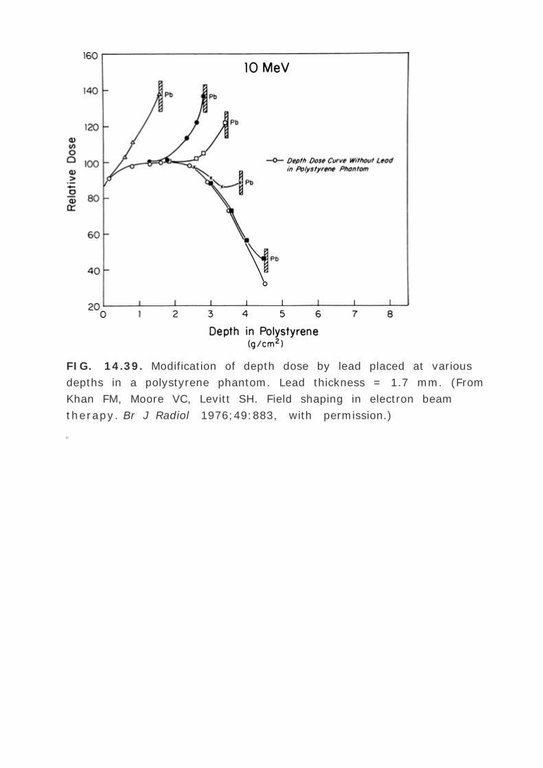
FIG. 14.39. Modification of depth dose by lead placed at various

depths in a polystyrene phantom. Lead thickness = 1.7 mm. (From

Khan FM, Moore VC, Levitt SH. Field shaping in electron beam

therapy. Br J Radiol 1976;49:883, with permission.)

FIG. 14.40. Intensity of backscattered electrons from lead

transmitted through polystyrene in the upstream direction of the

primary beam. (From Lambert GD, Klevenhagen SC. Penetration of

backscattered electrons in polystyrene for energies between 1â€“25

MeV. Phys Med Biol 1982;27:721, with permission.)

P.335

P.336

To dissipate the effect of electron backscatter, a suitable thickness

of low atomic number absorber such as bolus may be placed

between the lead shield and the preceding tissue surface. Saunders

and Peters (8 ) recommend the use of an aluminum sheath around

any lead used for internal shielding. Oral shielding has also been

accomplished by special oral stents made of dental acrylic that

encompasses the lead (46 ). Such a shield provides lead protection

for the tongue and other structures as well as reduces the electron

backscatter from lead reaching the buccal mucosa.

The thickness of low atomic number absorber required to absorb the

backscattered electrons may be calculated using the data in Fig.

14.40 . For a given energy of electrons incident on lead, the

thickness of polystyrene, determined from Fig. 14.40 , is converted

to the absorber thickness by dividing it by its relative electron

density.

Example

A buccal mucosa lesion is treated with a 9-MeV electron beam

incident externally on the cheek. Assuming cheek thickness,

including the lesion, to be 2 cm, calculate (a) thickness of lead

required to shield oral structures beyond the cheek, (b) magnitude

of electron backscatter, and (c) thickness of bolus or aluminum to

absorb backscattered electrons.

For these calculations, the most probable energy and the mean

energy of electrons may be assumed to be the same.

Incident energy = 9 MeV; Rp â‰ˆ 4.5 cm. Energy at the lead-

mucosa interface (at 2 cm depth) = 9

â‰ˆ 5 MeV, (see Eq. 14.7 ) and lead thickness for shielding

â‰ˆ

= 2.5 mm (Fig. 14.33 ).

From Equation 14.18 or Fig. 14.38 , electron backscatter for 5-

MeV electrons incident on lead [asymptotically equal to] 56%.

From Fig. 14.40 , depth upstream in polystyrene for

backscattered electrons is approximately equal to 10 mm for a

10% transmission of backscatter intensity. Assuming density of

polystyrene or bolus to be approximately unity and that of

aluminum equal to 2.7 g/cm3 , thickness of bolus

[asymptotically equal to] 1 cm and thickness of aluminum

[asymptotically equal to] 4 mm.

Thus, either 1 cm of bolus or 4 mm of aluminum may be used to

absorb 90% of the backscattered electrons. Considering the

available space for oral shielding, one may adjust the calculated

thickness of materials or the incident electron energy to provide

acceptable target dose and the allowed transmitted dose through

lead.

P.337

Eyeshields are designed using the same principles to protect the

lens. Minimum thickness of lead is used to provide acceptable

transmission value. Because a significant thickness of low Z

material is required to absorb the electron backscatter, eyeshields

cannot be coated with an adequate thickness of such materials

without exceeding the size requirements. In such cases, it is

desirable to coat the lead shield with a thin film of dental acrylic (to

absorb the very low energy electrons) and calibrate the set-up for

the actual enhanced dose received by the lid. Alternatively, if space

allows, a 2-mm-thick aluminum sheath may be interposed between

the lead shield and the eyelid to absorb the backscattered

electrons.

14.7. ELECTRON ARC THERAPY

Electron beam arc technique gives excellent dose distribution for

treating superficial tumors along curved surfaces. The technique

was first described by Becker and Weitzel (83 ) in 1956. Several

papers (84 ,85 ,86 ,87 ,88 ,89 ,90 ,91 ) have since appeared in the

literature describing the various technical and physical aspects of

electron arc therapy. For details, the reader is referred to Paliwal

(92 ).

On the basis of isodose distribution, electron arc therapy is most

suited for treating superficial volumes that follow curved surfaces

such as chest wall, ribs, and entire limbs. Although all chest wall

irradiations can be done with electron arcing, this technique is

mostly useful in cases for which the tumor involves a large chest

wall span and extends posteriorly beyond the midaxillary line. The

conventional technique of using tangential photon beams in this

case will irradiate too much of the underlying lung. The alternative

approach of using multiple abutting electron fields is fraught with

field junction problems, especially when angled beams are used. In

short, it appears that for a certain class of cases, electron arc

therapy has no reasonable alternative.

Not all electron accelerators are equipped with electron arc mode.

However, with increasing interest in this technique, more and more

linear accelerators are being made with this capability. Besides the

arcing capability, certain modifications in electron collimation are

necessary to make this technique feasible. For example, one needs

a beam-defining aperture with adequate clearance from the patient

and additional collimation close to the patient surface to sharpen

the dose falloff at the arc limits (86 ).

Machines that cannot rotate in the electron mode may still be used

to perform what is called a â€œpseudoarcâ€ technique (93 ). In

this technique, the field is defined by the x-ray jaws and the

electron collimation is provided on the patient's skin surface. The

beam is directed isocentrically through equally spaced large number

of angles. The fields are overlapped by aligning the center of a

given fixed field with the edge of its next neighboring field. Thus

the pseudoarc technique is designed to achieve the results of a

continuous arc by using a sufficiently large number of overlapping

fields directed isocentrically.

A. Calibration of Arc Therapy Beam

Calibration of an electron arc therapy procedure requires special

considerations in addition to those required for stationary beam

treatments. Dose per arc can be determined in two ways: (a)

integration of the stationary beam profiles and (b) direct

measurement. The first method requires an isodose distribution as

well as the dose rate calibration of the field (under stationary beam

conditions) used for arcing. The integration procedure is illustrated

in Fig. 14.41 . Radii are drawn from the isocenter at a fixed angular

interval ” ¸ (e.g., 10 degrees). The isodose chart is placed along

each radius while the dose at point P as a fraction of the maximum

dose on the central axis is recorded. Let Di (P) be this dose as the

isodose chart is placed at the radius. The dose per arc at P is given

by the following equation (94 ):

P.338

where [D with dot above]0 is the dose rate per minute in the

stationary field at the depth of d max , n is the speed of rotation

(number of revolutions per minute), and Inv(i ) is the inverse

square law correction for an air gap between the dotted circle and

the beam entry point. The term ” ¸ ·âˆ‘N i =1 Di (P ) also can be

evaluated graphically as shown in Fig. 14.41 .

FIG. 14.41. Integration of dose per arc at a point P. Solid line

represents an irregularly shaped patient contour and the dotted line

is a circle approximating the contour. Isodose curves for the

scanning field are placed along each radius to integrate the dose at

point P. (From Khan FM. Calibration and treatment planning of

electron beam arc therapy. In: Paliwal B, ed. Proceedings of the

symposium on electron dosimetry and arc therapy. New York:

AAPM/American Institute of Physics, 1982, with permission.)

The direct measurement of dose per arc requires a cylindrical

phantom of a suitable material such as polystyrene or Lucite. A hole

is drilled in the phantom to accommodate the chamber at a depth

corresponding to the d max . The radius of the phantom need only

be approximately equal to the radius of curvature of the patient,

because only a small part of the arc contributes dose to the

chamber reading (94 ). However, the depth of isocenter must be the

same as used for the treatment. The integrated reading per arc can

be converted to dose per arc by using correction factors normally

applicable to a stationary beam.

B. Treatment Planning

The treatment planning for electron arc therapy includes (a) choice

of beam energy, (b) choice of field size, (c) choice of isocenter, (d)

field shaping, and (e) isodose distribution. These are briefly

considered below.

B.1. Beam Energy

The central axis dose distribution is altered due to field motion. For

a small scanning field width, the depth dose curve shifts slightly

and the beam appears to penetrate somewhat farther than for a

stationary beam (Fig. 14.42 ). The surface dose is reduced and the

bremsstrahlung dose at the isocenter is increased. This phenomenon

is known as the â€œvelocity effectâ€ : a deeper point is exposed

to the beam longer than a shallower point, resulting in apparent

enhancement of beam penetration.

FIG. 14.42. Effect of isocenter depth on depth-dose distribution

compared with a stationary beam. Cylindrical polystyrene phantoms

of radii 10 and 15 cm were used. SAD = 100 cm; SSD = 64 cm;

diaphragm opening = 3 — 6 cm; arc angle = 120 degrees. (From

Khan FM, Fullerton GD, Lee JM, Moore VC, Levitt SH. Physical

aspects of electron-beam arc therapy. Radiology 1977;124:497,

with permission.)

P.339

B.2. Scanning Field Width

Although any field width may be used to produce acceptable isodose

distribution, smaller scanning fields (e.g., width of 5 cm or less)

give lower dose rate and greater x-ray contamination (86 ,88 ).

However, small field widths allow almost normal incidence of the

beam on the surface, thus simplifying dosimetry. Another advantage

of the smaller field width is that the dose per arc is less dependent

on the total arc angle. For these reasons, a geometric field width of

4 to 8 cm at the isocenter is recommended for most clinical

situations.

B.3. Location of Isocenter

The isocenter should be placed at a point approximately equidistant

from the surface contour for all beam angles. In addition, the depth

of isocenter must be greater than the maximum range of electrons

so that there is no accumulation of electron dose at the isocenter.

B.4. Field Shaping

Without electron collimation at the patient surface, the dose falloff

at the treatment field borders is rather gradual. To sharpen the

distribution, lead strips or cutouts should be used to define the arc

limits as well as the field limits in the length direction (Fig. 14.43 ).

Cast shielding has been found to be useful for routine electron arc

therapy (91 ). For a greater detail of the treatment-planning

process and the accessory preparation steps, the reader is referred

to Leavitt et al. (95 ).

B.5. Isodose Distribution

This crucial information for arc therapy is not as easily available for

electrons as it is for photons. Until computer programs of adequate

sophistication are routinely available for electron arc therapy, this

modality of treatment will probably remain inaccessible to most

institutions. Of course, this problem is part of the general problem

of electron beam treatment planning. However, the current surge of

activity in this area as well as the CT

P.340

development provide an optimistic future for the development of

sophisticated electron beam therapy techniques, including the arc.

FIG. 14.43. Isodose distribution in arc rotation with and without

lead strips at the ends of the arc, using a section of an Alderson

Rando phantom closely simulating an actual patient cross section.

Arc angle = 236 degrees; average radius of curvature = 10 cm;

beam energy = 10 MeV; lead strip thickness = 6 mm; field size at

the surface = 4.2 — 8.5 cm. (From Khan FM, Fullerton GD, Lee

JM, Moore VC, Levitt SH. Physical aspects of electron-beam arc

therapy. Radiology 1977;124:497, with permission.)

14.8. TOTAL SKIN IRRADIATION

Electrons in the energy range of 2 to 9 MeV have been found useful

for treating superficial lesions covering large areas of the body,

such as mycosis fungoides and other cutaneous lymphomas. At

these energies, electron beams are characterized by a rapid falloff

in dose beyond a shallow depth and a minimal x-ray background

(1% or less). Thus superficial skin lesions extending to about 1 cm

depth can be effectively treated without exceeding bone marrow

tolerance.

The treatment of mycosis fungoides with total skin irradiation was

suggested at least 50 years ago (96 ). Since that time, various

techniques have been developed and applied with success to the

treatment of this disease (97 ,98 ,99 ,100 ). Basically, the methods

fall into two general categories: (a) translational technique in which

a horizontal patient is translated relative to a beam of electrons of

sufficient width to cover the transverse dimensions of the patient

and (b) large field technique in which a standing patient is treated

with a

P.341

combination of broad beams produced by electron scattering and

large SSDs (2 to 6 m). Salient features of these techniques are

discussed below.

A. Translational Technique

The translational technique has been described by a number of

investigators (98 ,103 ,104 ). The patient lies on a motor-driven

couch and is moved relative to a downward-directed beam at a

suitable velocity. Alternatively, the patient may be stationary and

the radiation source translated horizontally. In the latter technique,

which has been described by Haybittle (103 ), a 24-Ci 90 Sr ²

source, in the form of a 60-cm linear array, is used. The source is

contained in a shielded source housing and positioned above the

couch. The maximum energy of the ² particles emitted by 90 Sr is

2.25 MeV. However, due to the spectral distribution of ²-ray

energies, the effective depth of treatment in this case is only a

fraction of a millimeter.

The translational technique using a 3-MeV Van de Graaff generator

has been described by Wright et al. (102 ). A well-collimated

monoenergetic electron beam is scattered just after leaving the

vacuum window to improve uniformity. The beam is then collimated

by an aluminum cone with a 5 mm — 45 cm defining slit. The

patient is translated under this beam at a suitable speed. Williams

et al. (103 ) have described a similar technique with a linear

accelerator. No applicator is used in this technique and the x-ray

collimators are fully retracted. The patient is treated anteriorly and

posteriorly. The dose uniformity along the length of the patient is

achieved by moving the patient through a distance sufficient that

the areas treated start outside the electron beam, pass through,

and finish outside the electron beam. The dose uniformity in the

transverse direction is enhanced by suitably combining transversely

overlapping fields.

B. Large Field Technique

Large electron fields required for total body skin irradiation can be

produced by scattering electrons through wide angles and using

large treatment distances. The field is made uniform over the

height of the patient by vertically combining multiple fields or

vertical arcing. The patient is treated in a standing position with

four or six fields directed from equally spaced angles for

circumferential coverage of the body surface.

B.1. Field Flatness

Low-energy electron beams are considerably widened by scattering

in air. For example, a 6-MeV narrow electron beam, after passing

through 4 m of air, achieves a Gaussian intensity distribution with a

50% to 50% width of approximately 1 m (104 ). This usually gives

adequate uniformity over a patient's width. If two such fields are

joined together vertically at their 50% lines, the resultant field will

be uniform over a height of approximately 1 m. A proper

combination of more such fields or a continuous arc can lead to a

larger uniform field, sufficient to cover a patient from head to foot

(Fig. 14.44 ).

The size and shape of an electron beam developed at a distance by

air scatter can be estimated by multiple scattering theory. Holt and

Perry (104 ) have used this approach to obtain a uniform field by

combining multiple field profiles in proper proportions and angular

separation (Fig. 14.44A ).

In addition to air, the electron beam is scattered by a scattering foil

inside or outside the collimator. However, the x-ray contamination

would be increased, because unnecessarily wide beams waste

electron flux to the sides.

B.2. X-ray Contamination

X-ray contamination is present in every therapy electron beam and

becomes a limiting factor in total skin irradiation. Ordinarily, these

x-rays are contributed by bremsstrahlung

P.342

interactions produced in the exit window of the accelerator,

scattering foil, ion chambers, beam-defining collimators, air, and

the patient. The bremsstrahlung level can be minimized if the

electron beam is scattered by air alone before incidence on the

patient. This would necessitate some modifications in the

accelerator, such as removing the scattering foil and other

scatterers in the collimation system. Various safety interlocks would

be required to make this separation feasible for routine clinical use.

Such a system was developed at Memorial Hospital, New York, on a

Varian Clinac-6 (105 ).

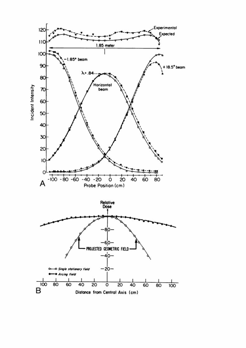
FIG. 14.44. A: Combination of three beam intensity profiles along

the vertical axis to obtain a resultant beam profile. The central

beam is directed horizontally, whereas the others are directed at

18.5 degrees from the horizontal. » is a weighting factor used in

an equation developed by Holt and Perry. (From Holt JG, Perry DJ.

Some physical considerations in whole skin electron beam therapy.

Med Phys 1982;9:769, with permission.) B: Vertical beam profile at

the treatment plane for a stationary single field and an arcing field.

(From Sewchand W, Khan FM, Williamson J. Total-body superficial

electron-beam therapy using a multiple-field pendulum-arc

technique. Radiology 1979;130:493, with permission.)

In the Stanford technique, described by Karzmark et al. (97 ,106

,107 ), the electron beam, after emerging from the accelerator

window, is scattered by a mirror (0.028-inch Al), an aluminum

scatterer located externally at the front of the collimator (0.037-

inch

P.343

Al), and about 3 m of air before incidence on the patient. The x-ray

contamination incident on the patient is reduced by angling the

beam 10 degrees to 15 degrees above and below the horizontal.

Because the x-rays produced in the scatterers at the collimators are

preferentially directed along the central axes, they largely miss the

patient. In addition, this set-up provides a large electron field with

sufficient dose uniformity in the vertical dimensions of the patient.

B.3. Field Arrangement

In the Stanford technique, the patient is treated with six fields

(anterior, posterior, and four obliques) positioned 60 degrees apart

around the circumference of the patient. Each field is made up of

two component beams, pointing at a suitable angle with respect to

the horizontal. The patient treatment positions and the full six-field

treatment cycle are illustrated in Fig. 14.45 .

FIG. 14.45. Patient positions for the six-field Stanford technique.

Patient is treated by two beams at each position, one beam directed

15 degrees below horizontal and the other 15 degrees above

horizontal. (From Page V, Gardner A, Karzmark CJ. Patient

dosimetry in the treatment of large superficial lesions. Radiology


P.344

The Memorial technique (105 ) also uses dual fields to obtain field

flatness in the vertical direction. The patient is treated from four

directions, the anterior, the posterior, and each of the laterals. Holt

and Perry (104 ) reexamined this technique and found that at least

six fields are required to achieve adequate uniformity. They

recommend eight fields, treating with four fields 1 day, and rotated

four the next.

A multiple field arc technique used at the University of Minnesota

has been described by Sewchand et al. (108 ). In this technique,

the beam describes an up-and-down arc as the gantry of the linear

accelerator rotates in an oscillatory manner analogous to a

pendulum. Six fields are used for each cycle of treatment, as in the

Stanford technique. The advantage of this technique is that the

dose distribution in the vertical plane can be made reproducibly

uniform over the height of any patient standing at a distance of

about 4 m. However, if the electron beam is scattered by a

scattering foil at the position of the collimators, this technique

contributes higher x-ray contamination to the patient than does the

stationary dual field technique. This problem may be minimized by

removing scattering foils and allowing the electron beam to be

scattered by air alone, as in the Memorial technique.

B.4. Dose Distribution

The depth-dose distribution in a single large field incident on a

patient will depend on the angle of incidence of the beam relative

to the surface contour. For an oblique beam, the depth-dose curve

and its d max shift toward the surface. When multiple large fields

are directed at the patient from different angles, the composite

distribution shows a net shift with apparent decrease in beam

penetration. This shift of the relative depth doses closer to the

surface has been explained by Bjarngard et al. (109 ) as being due

to greater path lengths taken by the obliquely incident electrons in

reaching a point.

Although a dose uniformity of ±10% can be achieved over most of

the body surface using the six-field technique, areas adjacent to

surface irregularities vary substantially due to local scattering.

Areas such as inner thighs and axillae, which are obstructed by

adjacent body structures, require supplementary irradiation.

The total bremsstrahlung dose in the midline of the patient for the

multiple field technique is approximately twice the level of a single

field. This factor of two has been experimentally observed by a

number of investigators (104 ,108 ,110 ).

C. Modified Stanford Technique

The Stanford technique of six dual fields described earlier requires

modifications of the accelerator such as removing the scattering foil

and installing a scatterer at the front end of the collimator. These

changes would require safety interlocks to prevent operation of the

accelerator in this configuration for conventional electron beam

treatments. Most institutions, including the University of Minnesota,

have adopted the Stanford technique in principle without making

alterations in the accelerator hardware. Because the regular

scattering foils and various interlocks are left in place, no special

precautions are required in preparing the machine for total skin

irradiation.

In some accelerators (e.g., Varian Clinac C series) a high dose rate

mode is installed to allow an output of more than 2,000 monitor

units per minute. This significantly speeds up the treatments.

Because conventional electron cones are not used, the electron field

is collimated by a special wide-aperture insert attached at the end

of the collimator. It is preset via interlock to a wider jaw setting

and a specific electron energy, selected for high dose rate mode of

operation. Some institutions use an acrylic scatter plate

([asymptotically equal to] 1 cm in thickness) in front of the patient

to provide additional scatter to the electron beam (Fig. 14.45 ).

To shorten the treatment time, the patient is treated with three

dual fields per day, for example, day 1: one dual field from the

anterior, two dual oblique fields from the posterior; day 2: one dual

field posterior and two dual fields anterior oblique. A complete cycle

of six

P.345

dual fields is thus completed in 2 days (Fig. 14.45 ). A source-to-

patient distance of about 4 m is sufficient for this technique.

C.1. Dual Field Angle

A low-energy electron beam is considerably widened in size by

scattering in air. For example, a 9-MeV electron beam, after

transversing 4 m of air and an acrylic scatter plate, attains a

Gaussian dose profile measuring a 90% to 90% isodose width of

about 60 cm, which is usually sufficient to cover a patient's width.

Along the height of the patient, two fields, one directed toward the

head and the other toward the feet, are angled such that in the

composite dose distribution a ±10% dose uniformity can be

obtained over a length of about 200 cm.

A method of determining dual field angle by film dosimetry has

been described by Khan (111 ). A series of dosimetry films in their

jackets are mounted on a vertical board, larger than the height of a

typical patient, and are positioned at the treatment distance. The

scatter plate is placed in front of the films as in actual treatment.

The films are exposed to a single electron field directed at 10

degree to 15 degree angle with respect to the horizontal axis. The

films are scanned for the optical density profile in the vertical

direction. The profile is then placed side by side with its mirror

image and separated by a distance such that the combined profile

shows not more than ±10% variation within about 200 cm (Fig.

14.46A ). The separation between the two profiles gives the desired

angle between the dual fields. A confirmatory composite profile is

then measured by exposing the films to the dual fields with the

interfield angle determined above (Fig. 14.46B ). Figure 14.47

shows a transverse beam profile for the dual field arrangement.

FIG. 14.46. Combining individual beam profiles to obtain a

composite profile with ±10% dose variation in the vertical

direction. A: Data for 9 MeV; SSD = 410 cm; scatter plate to

phantom distance = 20 cm; individual profile beam angle = 12

degrees relative to horizontal axis. A dual field angle ¸ = ±11

degrees is obtained by combining the profiles as shown. B:

Confirmatory beam profile for the dual field using ¸ = ±11

degrees. (From Khan FM. Total skin electron therapy: technique and

dosimetry. In: Purdy JA, ed. Advances in radiation oncology physics.

AAPM Monograph No. 19. New York, American Institute of Physics,


FIG. 14.47. Transverse dose profile showing width of the profile

within ±90% dose relative to central axis. (From Khan FM. Total

skin electron therapy: technique and dosimetry. In: Purdy JA, ed.

Advances in radiation oncology physics. AAPM Monograph No. 19.

New York, American Institute of Physics, 1990:466, with

permission.)

P.346

C.2. Calibration

A thin window (â‰¤0.05 g/cm2 ) plane-parallel chamber is a

suitable instrument for measuring depth dose distribution for the

low-energy beams used for this technique. Because plane-parallel

chambers are presently not calibrated by the calibration

laboratories, they may be calibrated by intercomparison with a

calibrated Farmer-type chamber, using a high-energy (â‰¥10 MeV)

electron beam (20 ).

The AAPM (112 ) recommends that the total skin irradiation dose be

measured at the calibration point located at the surface of the

phantom and the horizontal axis. This dose for a single dual field is

called the calibration point dose, DP .

A plane-parallel chamber, embedded in a polystyrene phantom, is

positioned to first measure the depth dose distribution along the

horizontal axis for the single dual field (the depth dose distribution

can also be measured by a film sandwiched in a polystyrene

phantom and placed parallel to the horizontal axis). The surface

dose measurement is made at a depth of 0.2 mm (20 ). Suppose M

is the ionization charge measured, the calibration point dose to

polystyrene, (DP )Poly , is given by:

The symbols are defined in Chapter 8 . The calibration point dose to

water, (DP )W , can then be determined as:

The electron fluence factor ¦W Poly is approximately unity, because

the calibration measurement is made close to the surface. P repl can

also be equated to unity for the plane-parallel chambers. The

parameters [L with bar above]/ and

/ are determined for the mean energy of electrons at the depth

of measurement, which is given by Equation 14.7 .

The treatment skin dose , (

S )Poly is defined by the AAPM (112 ) as the mean of the surface

dose along the circumference of a cylindrical polystyrene phantom

30 cm in diameter and 30 cm high that has been irradiated under

the total skin irradiation conditions with all six dual fields. If (DP

)Poly is the calibration point dose for the single dual field, then

where B is a factor relating the treatment skin dose with the

calibration point dose, both measured at the surface of a cylindrical

polystyrene phantom. Typically, B ranges between 2.5 and 3 for the

Stanford type technique.

FIG. 14.48. Composite depth-dose distribution for six dual fields

obtained with a dosimetry film sandwiched in a cylindrical

polystyrene phantom exposed under treatment conditions.

Irradiation conditions are given in Fig. 14.46 . (From Khan FM. Total

skin electron therapy: technique and dosimetry. In: Purdy JA, ed.

Advances in radiation oncology physics. AAPM Monograph No. 19.

New York: American Institute of Physics, 1990:466.)

P.347

The treatment skin dose for a water phantom,

S )W , can be calculated from Equations 14.21 and 14.22 :

The factor B can also be determined by taping a film strip in its

light-tight paper to the surface of the cylindrical polystyrene

phantom, specified above, and exposing it to a single dual field.

Another filmstrip taped around the phantom is exposed to six dual

fields. By relating optical densities to doses in the two cases, factor

B can be determined from Equation 14.22 .

The composite depth-dose distribution for the six dual fields may be

determined by sandwiching a dosimetry film (in its paper jacket) in

the cylindrical polystyrene phantom and cutting the excess film so

that the edges conform to the circular surface of the phantom. A

black tape is wrapped around the phantom over the film edges to

make the film light-tight. The phantom, with the film parallel to the

horizontal axis, is exposed to the six dual fields, duplicating actual

treatment conditions. After appropriate processing, the film is

scanned for optical density distribution, which is related to dose

distribution by a reference sensitometric curve. Figure 14.48 gives

the results of such a measurement.

C.3. In Vivo Dosimetry

Although an overall surface dose uniformity of ±10% can be

achieved at the treatment distance, in a plane perpendicular to the

horizontal axis and within an area equivalent to a patient's

dimensions, there are localized regions of extreme nonuniformity of

dose on the patient's skin. Excessive dose (e.g., 120%â€“130%)

can occur in areas with sharp body projections, curved surfaces, or

regions of multiple field overlaps. Low-dose regions occur when the

skin is shielded by other parts of the body or overlying body folds.

From in vivo measurements, areas receiving a significantly less

dose can be identified for local boost. If

P.348

eyelids need to be treated, internal eyeshields can be used, but the

dose to the inside of the lids should be assessed, taking into

account the electron backscatter from lead.

Thermoluminescent dosimeters (TLD) are most often used for in

vivo dosimetry. For these measurements, the TLD must be thin

(<0.5 mm) to minimize the effect of dose gradient across the

dosimeters. TLD chips are commercially available that meet these

specifications. These chips can be sealed in thin polyethylene

sheets to avoid contamination. The reference chips may be

calibrated in a polystyrene phantom using an electron beam of

approximately the same mean energy incident on the TLDs as in the

in vivo measurement conditions. The desired mean energy may be

obtained by selecting an appropriate incident beam energy and

depth (Eq. 14.7 ).

14.9. TREATMENT-PLANNING

ALGORITHMS

Early methods of electron beam dose computation were based on

empirical functions that used ray line geometrics, assuming broad

beam dose distribution. Inhomogeneity corrections were

incorporated using transmission data measured with large slabs of

heterogeneities. These methods have been reviewed by Sternick

(113 ).

Major limitations of the empirical methods based on broad beams

and slab geometries are their inability to predict effects on dose

distribution of small fields, sudden changes in surface contour,

small inhomogeneities, and oblique beam incidence. An

improvement over the empirical methods came about with the

development of algorithms based on the age-diffusion equation by

Kawachi (114 ) and others in the 1970s. These methods have been

reviewed by Andreo (115 ). Although these algorithms are able to

use semiempirically derived pencil beams that can be placed along

the surface contour to predict effects of small fields and surface

irregularity, their accuracy to calculate inhomogeneity correction is

limited. They use effective path lengths between the virtual source

and the point of calculation but the effects of anatomy and small

tissue heterogeneities in three dimensions are not fully accounted

for.

Major advancement in electron beam treatment planning occurred in

the early 1980s (38 ,54 ,65 ,116 ). Methods were developed that

were based on Gaussian pencil beam distributions calculated with

the application of Fermi-Eyges multiple scattering theory (117 ).

For a detailed review of these algorithms the reader is referred to

Brahme (118 ) and Hogstrom, Starkschall, and Shiu (119 ).

Pencil beam algorithms based on multiple scattering theory are the

algorithms of choice for electron beam treatment planning. A brief

discussion is presented to familiarize the users of these algorithms

with the basic theory involved.

A. Pencil Beam Based on Multiple

Scattering Theory

Assuming small-angle multiple scattering approximation, an

elementary pencil beam penetrating a scattering medium is very

nearly Gaussian in its lateral spread at all depths. Large-angle

scattering events could cause deviations from a pure Gaussian

distribution, but their overall effect on dose distributions is

considered to be small. The spatial dose distribution for a Gaussian

pencil beam can be represented thus:

where dp (r, z ) is the dose contributed by the pencil beam at a

point at a radial distance r from its central axis and depth z, dp (o,

z ) is the axial dose and ƒ2 r (z ) is the mean square radial

displacement of electrons as a result of multiple Coulomb

scattering. It can be shown that ƒ2 r = 2 ƒ2 x = 2 ƒ2 y where

ƒ2 x and ƒ2 y are the mean square lateral displacements

projected on the X, Y, and Y, Z planes. The exponential function in

Equation (14.25) represents the off-axis ratio for the pencil beam,

normalized to unity at r = 0.

P.349

Another useful form of Equation (14.25) is:

where D â ˆ (o, z ) is the dose at depth z in an infinitely broad field

with the same incident fluence at the surface as the pencil beam.

The Gaussian distribution function in Equation 14.26 is normalized

so that the area integral of this function over a transverse plane at

depth z is unity.

FIG. 14.49. A pencil beam coordinate system. (From Khan FM.

Dose distribution algorithms for electron beams. In: Khan FM,

Potish RA, eds. Treatment planning in radiation oncology. Baltimore:

Williams & Wilkins, 1998:113â€“122, with permission.)

In Cartesian coordinates Equation (14.26) can be written as:

where dp (x, y, z ) is the dose contributed to point (x, y, z ) by a

pencil beam whose central axis passes through (x â€², y â€², z )

(Fig 14.49 ).

The total dose distribution in a field of any size and shape can be

calculated by summing all the pencil beams:

The integration of a Gaussian function within finite limits cannot be

performed analytically. To evaluate this function necessitates the

use of error function (erf). Thus convolution calculus shows that for

an electron beam of a rectangular cross section (2a — 2b), the

spatial dose distribution is given by:

where the error function is defined thus:

The error function is normalized so that erf(âˆ ) = 1 (it is known

that the integral âˆ«â ˆ 0 e - t2 dt = âˆ €/2). Error function

values for 0 < x âˆ can be obtained from tables published in

mathematics handbooks (120 ). The quantity D â ˆ (o, o, z ) is

usually determined

P.350

from the measured central axis depth-dose data of a broad electron

field (e.g., 20 — 20 cm).

FIG. 14.50. A plot of normal distribution function given by

Equation 14.29 for ƒ = 1. The function is normalized to unity for

limits âˆ — âˆ . (From Khan FM. Dose distribution algorithms

for electron beams. In: Khan FM, Potish RA, eds. Treatment

planning in radiation oncology. Baltimore: Williams & Wilkins,


A.1. Lateral Spread Parameter, ƒ

Gaussian function is characterized by its lateral spread parameter,

ƒ, which is similar to the standard deviation parameter of the

familiar normal frequency distribution function:

The previous function is plotted in Fig. 14.50 for ƒ = 1. The

function is normalized so that its integral between the limits -âˆ

< x < + âˆ is unity.

The dose distribution in a pencil electron beam incident on a

uniform phantom looks like a teardrop or onion (Fig. 14.51 ). The

lateral spread (or ƒ) increases with depth until

P.351

a maximum spread is achieved. Beyond this depth there is a

precipitous loss of electrons as their larger lateral excursion causes

them to run out of energy.

FIG. 14.51. Pencil beam dose distribution measured with a narrow

beam of 22 MeV energy incident on a water phantom. (From ICRU

Report 35. Radiation dosimetry: electron beams with energies

between 1 and 50 MeV. Bethesda, MD: International Commission on

Radiation Units and Measurements 1984:36, with permission.)

FIG. 14.52. Schematic representation of the Hogstrom algorithm

for electron beam treatment planning. (From Hogstrom KR, Mills

MD, Almond PR. Electron beam dose calculation. Phys Med Biol


Eyges (117 ) predicted ƒ theoretically by extending the small-

angle multiple scattering theory of Fermi to slab geometry of any

composition. Considering ƒx (z ) in the x-z plane,

where ¸2 / l is the mass angular scattering power and is

the density of the slab phantom.

There are limitations to the previous Eyges equation. As pointed out

by Werner et al. (54 ), ƒ, given by Equation 14.32 , increases

with depth indefinitely which is contrary to what is observed

experimentally in a narrow beam dose distribution. Also, Equation

14.32 is based on small-angle multiple Coulomb scattering, hence

ignores the probability of large-angle scatter. This results in an

underestimate of ƒ. Correction factors have been proposed to

overcome these problems (54 ,121 ,122 ).

Practical implementation of the above algorithm was carried out by

Hogstrom et al. in 1981 (38 ) and was subsequently adopted by

several commercial treatment-planning systems. Figure 14.52

shows a schematic representation of the Hogstrom algorithm. The

pencil beam ƒ is calculated using the Fermi-Eyges equation (Eq.

14.32 ). By correlating electron linear collision stopping power and

linear angular scattering power relative to that of water with CT

numbers, effective depth and ƒ are calculated for inhomogeneous

media. Thus the method allows pixel-by-pixel calculation of

heterogeneity correction.

P.352

Figure 14.53 shows a comparison of calculated and measured

isodose curves as an example. Starkschall et al. (123 ) have

extended the Hogstrom algorithm to three dimensions. An

irregularly shaped field is divided into strip beams and each strip is

divided into segments so that ƒ of the pencil beams and effective

depths are calculated in three dimensions. Integration of the pencils

is carried out over all strips and segments.

FIG. 14.53. Comparison of calculated and measured isodose

distribution. (From Hogstrom KR, Mills MD, Almond PR. Electron

beam dose calculation. Phys Med Biol 1981;26:445, with

permission.)

REFERENCES

1. Fletcher GH. Introduction. In: Tapley N, ed. Clinical

applications of the electron beam . New York: John Wiley & Sons,

1976:1.

2. Evans RD. The atomic nucleus . New York: McGraw-Hill, 1955.

3. Johns HE, Laughlin JS. Interaction of radiation with matter.

In: Hine G, Brownell G, eds. Radiation dosimetry . New York:

Academic Press, 1956:49.

4. National Council on Radiation Protection and Measurements

(NCRP). Stopping powers for use with cavity ionization

chambers. Report No. 27. Handbook 79. Washington, DC:


5. Sternheimer RM. The density effect for the ionization loss in

various materials. Phys Rev 1952;88:851.

6. Fermi E. The ionization loss of energy in gases and condensed

materials. Phys Rev 1940;57:485.

7. Laughlin JS, Beattie JW. Ranges of high energy electrons in

water. Phys Rev 1951;83:692.

8. ICRU. Radiation quantities and units. Report No. 33.

Washington, DC: International Commission on Radiation Units

and Measurements, 1980.

9. Berger MJ, Seltzer SM. Tables of energy losses and ranges of

electrons and positrons. NASA SP-3012. Washington, DC:

National Aeronautics and Space Administration, 1964.

10. Berger MJ, Seltzer SM. Additional stopping power and range

tables for protons, mesons, and electrons. NASA SP-3036.

Washington, DC: National Aeronautics and Space Administration,

1966.

11. Berger MJ, Seltzer SM. Stopping powers and ranges of

electrons and positrons , 2nd ed. Washington, DC: U.S.

Department of Commerce, National Bureau of Standards, 1983.

12. ICRU. Stopping powers for electrons and positrons. Report

No. 37. Bethesda, MD: International Commission on Radiation


13. Rossi BB. High energy particles . Englewood Cliffs, NJ:

Prentice-Hall, 1956.

14. ICRU. Radiation dosimetry: electrons with initial energies

between 1 and 50 MeV. Report No. 21. Washington, DC:

International Commission on Radiation Units and Measurements,

1972.

15. Nordic Association of Clinical Physics (NACP). Procedures in

external radiation therapy dosimetry with electron and photon

beams with maximum energies between 1 and 50 MeV. Acta

Radiol 1980;19:55.

16. Markus B. Beitrage zur Entwicklung der Dosimetrie schneller.

Elektronen Strahlentherapie 1964;123:350, 508 and

1964;124:33.

17. Nusse M. Factors affecting the energy-range relation of fast

electrons in aluminum. Phys Med Biol 1969;14:315.

18. Harder D, Schulz HJ. Some new physical data for electron

beam dosimetry. In: Proceedings of the European Congress of

Radiology. Amsterdam: Excerpta Medica, 1971.

P.353

19. Svensson H, Hettinger G. Dosimetric measurements at the

nordic medical accelerators. I. Characteristics of the radiation

beam. Acta Radiol 1971;10:369.

20. Khan FM, Doppke K, Hogstrom KR, et al. Clinical electron-

beam dosimetry. Report of AAPM Radiation Therapy Committee

Task Group No. 25. Med Phys 1991;18:73.

21. Brahme A, Svensson H. Specification of electron beam

quality from the central-axis depth absorbed-dose distribution.

Med Phys 1976;3:95.

22. Rogers DWO, Bielajew AF. Differences in electron depth-dose

curves calculated with EGS and ETRAN and improved energy-

range relationships. Med Phys 1986;13:687.

23. Harder D. Energiespectren Schneller Elecktronen in

Verschiedenen Tiefen. In: Montreux Zuppinger A, Poretti G, eds.

Symposium on high-energy electrons . Berlin: Springer-Verlag,

1965:260.

24. AAPM. Task Group 51. Protocol for clinical reference

dosimetry of high-energy photon and electron beams. Med Phys

1999;26:1847â€“1870.

25. IAEA. Technical Reports Series No. 398. Absorbed dose

determination in external beam radiotherapy. Vienna:


26. American Association of Physicists in Medicine (AAPM). A

protocol for the determination of absorbed dose from high

energy photons and electrons. RTC Task Group No. 21. Med Phys

1983;10:741.

27. Loevinger R, Karzmark CJ, Weissbluth M. Radiation

dosimetry with high energy electrons. Radiology 1961;77:906.

28. Dutreix J, Dutreix A. Film dosimetry of high energy

electrons. Ann NY Acad Sci 1969;161:33.

29. Hettinger G, Svensson H. Photographic film for

determination of isodose from betatron electron radiation. Acta

Radiol 1967;5:74.

30. Khan FM, Higgins PD. Calculation of depth dose and dose per

monitor unit for irregularly shaped electron fields: an addendum.

Phys Med Biol 1999;44:N77â€“N80.

31. ICRU. Radiation dosimetry: electron beams with energies

between 1 and 50 MeV. Report No. 35. Bethesda, MD:


1984.

32. Almond PR. Characteristics of current medical electron

accelerator beams. In: Chu F, ed. Proceedings of the symposium

on electron beam therapy . New York: Memorial Sloan-Kettering

Cancer Center, 1979:43.

33. Mandour MA, Harder D. Systematic optimization of the

double-scatterer system for electron beam field flattening.

Strahlentherapie 1978;154:328.

34. Werner BL, Khan FM, Deibel FC. Model for calculating depth

dose distributions for broad electron beam. Med Phys

1983;10:582.

35. Biggs PJ, Boyer AL, Doppke KP. Electron dosimetry of

irregular fields on the Clinac-18. Int J Radiat Oncol Biol Phys

1979;5:433.

36. Khan FM, Higgins PD. Field equivalence for clinical electron

beams. Phys Med Biol 2001;46:N9â€“N14.

37. Harder D, Schr ¶der-Babo P, Abou Mandour M. Private

communication, 1982.

38. Hogstrom KR, Mills MD, Almond PR. Electron beam dose

calculations. Phys Med Biol 1981;26:445.

39. Mills MD, Hogstrom KR, Almond PR. Prediction of electron

beam output factors. Med Phys 1982;9:60.

40. Pohlit W. Dosimetrie Zur Betatrontherapie. Stuttgart: Verlag,

1965.

41. Shroder-Babo P. Determination of the virtual electron source

of a betatron. Acta Radiol 1983;364[suppl]:7.

42. Meyer JA, Palta JR, Hogstrom KR. Determination of relatively

new electron dosimetry measurement techniques on Mevatron

80. Med Phys 1984;11:670.

43. Jamshidi A, Kuchnir FT, Reft SC. Determination of the source

position for the electron beam from a high-energy linear

accelerator. Med Phys 1986;13:942.

44. Khan FM, Sewchand W, Levitt SH. Effect of air space on

depth dose in electron beam therapy. Radiology 1978;126:249.

45. Berger MJ, Seltzer SM. Tables of energy-deposition

distributions in water phantoms irradiated by point-

monodirectional electron beams with energies from 1 to 60 MeV,

and applications to broad beams. NBSIR 82â€“2451. Washington,

DC: National Bureau of Standards, 1982.

46. Tapley N, ed. Clinical applications of the electron beam . New

York: John Wiley & Sons, 1976.

47. Okumura Y. Correction of dose distribution for air space in

high energy electron therapy. Radiology 1972;103:183.

48. Khan FM, Lee JMF. Computer algorithm for electron beam

treatment planning. Med Phys 1979;6:142.

49. Holt JG, Mohan R, Caley R, et al. Memorial electron beam

AET treatment planning system. In: Orton CG, Bagne F, eds.

Practical aspects of electron beam treatment planning . New

York: American Institute of Physics, 1978.

50. Ekstrand KE, Dixon RL. Obliquely incident electron beams.

Med Phys 1982;9:276.

51. Khan FM, Deibel FC, Soleimani-Meigooni A. Obliquity

correction for electron beams. Med Phys 1985;12:749.

52. McKenzie AL. Air-gap correction in electron treatment

planning. Phys Med Biol 1979;24:628.

P.354

53. Deibel FC, Khan FM, Werner BL. Electron beam treatment

planning with strip beams [abst.]. Med Phys 1983;10:527.

54. Werner BL, Khan FM, Deibel FC. Model for calculating

electron beam scattering in treatment planning. Med Phys

1982;9:180.

55. Dutreix J. Dosimetry. In: Gil y Gil, Gil Gayarre, eds.

Symposium on high-energy electrons . Madrid: General

Directorate of Health, 1970:113.

56. Laughlin JS. High energy electron treatment planning for

inhomogeneities. Br J Radiol 1965;38:143.

57. Laughlin JS, Lundy A, Phillips R, et al. Electron-beam

treatment planning in inhomogeneous tissue. Radiology

1965;85:524.

58. Almond PR, Wright AE, Boone ML. High-energy electron dose

perturbations in regions of tissue heterogeneity. Radiology

1967;88:1146.

59. Dahler A, Baker AS, Laughlin JS. Comprehensive electron-

beam treatment planning. Ann NY Acad Sci 1969;161:189.

60. Almond PR. Radiation physics of electron beams. In: Tapley

N, ed. Clinical applications of the electron beam . New York:


61. Boone MLM, Almond PR, Wright AE. High energy electron

dose perturbation in regions of tissue heterogeneity. Ann NY

Acad Sci 1969;161:214.

62. Prasad SC, Bedwinek JM, Gerber RL. Lung dose in electron

beam therapy of chest wall. Acta Radiol 1983;22:91.

63. Pohlit W, Manegold KH. Electron-beam dose distribution in

inhomogeneous media. In: Kramer S, Suntharalingam N,

Zinninger GF, eds. High energy photons and electrons . New

York: John Wiley & Sons, 1976:243.

64. Goitein M. A technique for calculating the influence of thin

inhomogeneities on charged particle beams. Med Phys

1978;5:258.

65. Perry DJ, Holt JG. A model for calculating the effects of

small inhomogeneities on electron beam dose distributions. Med

Phys 1980;7:207.

66. Bagne F, Tulloh ME. Low energy electrons. In: Orton CG,

Bagne F, eds. Practical aspects of electron beam treatment

planning. AAPM Publication . New York: American Institute of

Physics, 1978:80.

67. Sharma SC, Deibel FC, Khan FM. Tissue equivalence of bolus

materials for electron beams. Radiology 1983;146:854.

68. Johnson JM, Khan FM. Dosimetric effects of abutting

extended SSD electron fields with photons in the treatment of

head and neck cancers. Int J Radiat Oncol Biol Phys

1994;28:741â€“747.

69. Giarratano JC, Duerkes RJ, Almond PR. Lead shielding

thickness for dose reduction of 7- to 28-MeV electrons. Med Phys

1975;2:336.

70. Khan FM, Moore VC, Levitt SH. Field shaping in electron

beam therapy. Br J Radiol 1976;49:883.

71. Goede MR, Gooden DS, Ellis RG, et al. A versatile electron

collimation system to be used with electron cones supplied with

Varian's Clinac 18. Int J Radiat Oncol Biol Phys 1977;2:791.

72. Choi MC, Purdy JA, Gerbi BJ, et al. Variation in output factor

caused by secondary blocking for 7â€“16 MeV electron beams.

Med Phys 1979;6:137.

73. Purdy JA, Choi MC, Feldman A. Lipowitz metal shielding

thickness for dose reduction of 6â€“20 MeV electrons. Med Phys

1980;7:251.

74. Asbell SO, Sill J, Lightfoot DA, et al. Individualized eye

shields for use in electron beam therapy as well as low-energy

photon irradiation. Int J Radiat Oncol Biol Phys 1980;6:519.

75. Khan FM, Werner BL, Deibel FC. Lead shielding for electrons.

Med Phys 1981;8:712.

76. Lax I, Brahme A. On the collimation of high energy electron

beams. Acta Radiol Oncol 1980;19:199.

77. Okumura Y, Mori T, Kitagawa T. Modification of dose

distribution in high energy electron beam treatment. Radiology

1971;99:683.

78. Weatherburn H, McMillan KTP, Stedford B, et al. Physical

measurements and clinical observations on the backscatter of 10

MeV electrons from lead shielding (correspondence). Br J Radiol

1975;48:229.

79. Saunders JE, Peters VG. Backscattering from metals in

superficial therapy with high energy electrons. Br J Radiol

1974;47:467.

80. Nusslin F. Electron back-scattering from lead in a Perspex

phantom (correspondence). Br J Radiol 1974;48:467.

81. Gagnon WF, Cundiff JH. Dose enhancement from

backscattered radiation at tissue-metal interfaces irradiated with

high energy electrons. Br J Radiol 1980;53:466.

82. Klevenhagen SC, Lambert GD, Arbabi A. Backscattering in

electron beam therapy for energies between 3 and 35 MeV. Phys

Med Biol 1982;27:363.

83. Becker J, Weitzel G. Neue Formen der Bewegungstrahlung

beim 15 MeV-Betatron der Siemens-Reinger-Werke.

Strahlentherapie 1956;101:180.

84. Benedetti GR, Dobry H, Traumann L. Computer programme

for determination of isodose curves for electron energies from

5â€“42 MeV. Electromedica (Siemens) 1971;39:57.

P.355

85. Rassow J. On the telecentric small-angle pendulum therapy

with high electron energies. Electromedica (Siemens) 1972;40:1.

86. Khan FM, Fullerton GD, Lee JM, et al. Physical aspects of

electron-beam arc therapy. Radiology 1977;124:497.

87. Ruegsegger DR, Lerude SD, Lyle D. Electron beam arc

therapy using a high energy betatron. Radiology 1979;133:483.

88. Kase KR, Bjarngard BE. Bremsstrahlung dose to patients in

rotational electron therapy. Radiology 1979;133:531.

89. Leavitt DD. A technique for optimization of dose distributions

in electron rotational therapy [abst.]. Med Phys 1978;5:347.

90. Blackburn BE. A practical system for electron arc therapy.

In: Paliwal B, ed. Proceedings of the symposium on electron

dosimetry and arc therapy . New York: AAPM/American Institute

of Physics, 1982:295.

91. Thomadsen B. Tertiary collimation of moving electron beams.

In: Paliwal B, ed. Proceedings of the symposium on electron

dosimetry and arc therapy . New York: AAPM/American Institute


92. Paliwal B, ed. Proceedings of the symposium on electron

dosimetry and arc therapy. New York: AAPM/American Institute

of Physics, 1982.

93. Boyer AL, Fullerton GD, Mira MD, et al. An electron beam

pseudoarc technique. In: Paliwal B, ed. Proceedings of the

symposium on electron dosimetry and arc therapy . New York:

AAPM/American Institute of Physics, 1982:267.

94. Khan FM. Calibration and treatment planning of electron

beam arc therapy. In: Paliwal B, ed. Proceedings of the

symposium on electron dosimetry and arc therapy . New York:

AAPM/American Institute of Physics, 1982:249.

95. Leavitt DD, Peacock LM, Gibbs FA, et al. Electron arc

therapy: physical measurements and treatment planning

techniques. Int J Radiat Oncol Biol Phys 1985;11:987.

96. Trump JG, Wright KA, Evans WW, et al. High energy

electrons for the treatment of extensive superficial malignant

lesions. AJR 1953;69:623.

97. Karzmark CJ, Loevinger R, Steel RE. A technique for large-

field, superficial electron therapy. Radiology 1960;74:633.

98. Szur L, Silvester JA, Bewley DK. Treatment of the whole

body surface with electrons. Lancet 1962;1:1373.

99. Fuks Z, Bagshaw MA. Total-skin electron treatment of

mycosis fungoides. Radiology 1971;100:145.

100. Heller EH. The management of cutaneous manifestations of

lymphoma by means of electron beam. Australas J Dermatol

1972;13:11.

101. Haybittle JL. A 24 curie strontium 90 unit for whole-body

superficial irradiation with beta rays. Br J Radiol 1964;37:297.

102. Wright KA, Granke RC, Trump JG. Physical aspects of

megavoltage electron therapy. Radiology 1956;67:533.

103. Williams PC, Hunter RD, Jackson SM. Whole body electron

therapy in mycosis fungoidesâ€”successful translational

technique achieved by modification of an established linear

accelerator. Br J Radiol 1979;52:302.

104. Holt JG, Perry DJ. Some physical considerations in whole

skin electron beam therapy. Med Phys 1982;9:769.

105. Edelstein GR, Clark T, Holt JG. Dosimetry for total-body

electron-beam therapy in the treatment of mycosis fungoides.

Radiology 1973;108:691.

106. Karzmark CJ. Large-field superficial electron therapy with

linear accelerators. Br J Radiol 1964;37:302.

107. Karzmark CJ. Physical aspects of whole-body superficial

therapy with electrons. Frontiers Radiat Ther Oncol 1968;2:36.

108. Sewchand W, Khan FM, Williamson J. Total-body superficial

electron-beam therapy using a multiple-field pendulum-arc

technique. Radiology 1979;130:493.

109. Bjarngard BE, Chen GTY, Piontek RN, et al. Analysis of dose

distributions in whole body superficial electron therapy. Int J

Radiat Oncol Biol Phys 1977;2:319.

110. Tetenes PJ, Goodwin PN. Comparative study of superficial

whole-body radiotherapeutic techniques using a 4-MeV

nonangulated electron beam. Radiology 1977;122:219.

111. Khan FM. Total skin electron therapy: technique and

dosimetry. In: Purdy JA, ed. Advances in radiation oncology

physics. AAPM Monograph No . 19. New York: American Institute


112. AAPM. Total skin electron therapy technique and dosimetry.

Report No. 23. New York: American Institute of Physics, 1988.

113. Sternick E. Algorithms for computerized treatment

planning. In: Orton CG, Bagne F, eds. Practical aspects of

electron beam treatment planning . New York: American

Institute of Physics, 1978:52.

P.356

114. Kawachi K. Calculation of electron dose distribution for

radiotherapy treatment planning. Phys Med Biol 1975;20:571.

115. Andreo P. Broad beam approaches to dose computation and

their limitations. In: Nahum AE, ed. The computation of dose

distributions in electron beam radiotherapy . Kungalv, Sweden:

mimiab/goatab, 1985:128.

116. Jette D. The application of multiple scattering theory to

therapeutic electron dosimetry. Med Phys 1983;10:141.

117. Egyes L. Multiple scattering with energy loss. Phys Rev

1948;74:1534.

118. Brahme A. Brief review of current algorithms for electron

beam dose planning. In: Nahum AE, ed. The computation of dose

distributions in electron beam radiotherapy . Kungalv, Sweden:

miniab/gotab, 1985:271.

119. Hogstrom KR, Starkschall G, Shiu AS. Dose calculation

algorithms for electron beams. In: Purdy JA, ed. Advances in

radiation oncology physics . American Institute of Phyiscs

Monograph 19. New York: American Institute of Physics,

1992:900.

120. Beyer WH. Standard mathematical tables , 25th ed. Boca

Raton: CRC Press, 1978:524.

121. Lax I, Brahme A. Collimation of high energy electron

beams. Acta Radiol Oncol 1980;19:199.

122. Lax I, Brahme A, Andreo P. Electron beam dose planning

using Gaussian beams. In: Brahme A, ed. Computed electron

beam dose planning . Acta Radiol 1983;364[suppl]:49.

123. Starkschall G, Shie AS, Buynowski SW, et al. Effect of

dimensionality of heterogeneity corrections on the

implementation of a three-dimensional electron pencil-beam

algorithm. Phys Med Biol 1991;36:207.

1 In a general sense, the cone end means a plane perpendicular to

the beam axis at the nominal SSD.

2 Developed by G. R. Feaster, University of Kansas at Kansas City,

and supplied by Mick Radio-Nuclear Instruments, Inc., The Bronx,

New York.





15 - Brachytherapy

15

Brachytherapy

Brachytherapy is a method of treatment in which sealed radioactive

sources are used to deliver radiation at a short distance by

interstitial, intracavitary, or surface application. With this mode of

therapy, a high radiation dose can be delivered locally to the tumor

with rapid dose fall-off in the surrounding normal tissue. In the past,

brachytherapy was carried out mostly with radium or radon sources.

Currently, use of artificially produced radionuclides such as 137 Cs,192 Ir, 198 Au, 125 I, and 103 Pd is rapidly increasing.

New technical developments have stimulated increased interest in

brachytherapy: the introduction of artificial isotopes, afterloading

devices to reduce personnel exposure, and automatic devices with

remote control to deliver controlled radiation exposure from high-

activity sources. Although electrons are often used as an alternative

to interstitial implants, brachytherapy continues to remain an

important mode of therapy, either alone or combined with external

beam.

15.1. RADIOACTIVE SOURCES

From the time of its discovery in 1898, radium has been the most

commonly used isotope in brachytherapy. However, artificial

radioisotopes offer special advantages in some situations because of

their ³ ray energy, source flexibility, source size, and half-life. Table

15.1 lists the most commonly used sources for brachytherapy with

their relevant physical properties.

A. Radium

A.1. Decay

Radium is the sixth member of the uranium series, which starts with238 92 U and ends with stable 206 82 Pb (Fig. 2.3 ). Radium

disintegrates with a half-life of about 1,600 years to form radon.

The product nucleus radon is a heavy inert gas that in turn

disintegrates into its daughter products as shown in Fig. 2.3 . As a

result of the decay process from radium to stable lead, at least 49 ³

rays are produced with energies ranging from 0.184 to 2.45 MeV. The

average energy of the ³ rays from radium in equilibrium with its

daughter products and filtered by 0.5 mm of platinum is 0.83 MeV (1

). A filtration of at least 0.5 mm platinum provided by the source case

is sufficient to absorb all the ± particles and most of the ²

particles emitted by radium and its daughter products. Only ³ rays

are used for therapy.

Because the half-life for radioactive decay is much greater for 226 Ra

than for any of its daughter products, radium, when placed in a sealed

container, achieves a secular equilibrium with its daughters (Fig. 2.5

). The time required to establish equilibrium is approximately 1 month

from the time of encapsulation.

226 Ra

1,600 yr

0.047â€“2.45 (0.83 avg)

12.0

8.25a ,b (Rcm2 /mg-h)222 Rn

3.83 days

0.047â€“2.45 (0.83 avg)

12.0

10.15a ,c

60 Co

5.26 yr

1.17, 1.33

11.0

13.07c

137 Cs

30.0 yr

0.662

5.5

3.26c

192 Ir

73.8 days

0.136â€“1.06 (0.38 avg)

2.5

4.69c

198 Au

2.7 days

0.412

2.5

2.38c

125 I

59.4 days

0.028 avg

0.025

1.46c

103 Pd

17.0 days

0.021 avg

0.008

1.48c

a In equilibrium with daughter products.b Filtered by 0.5 mm Pt.c Unfiltered.

Radionuclide

Half-

Life

Photon

Energy

(MeV)

Half-

Value

Layer

(mm lead)

Exposure Rate

Constant (Rcm2

/mCi-h)

TABLE 15.1. PHYSICAL CHARACTERISTICS OF

RADIONUCLIDES USED IN BRACHYTHERAPY

P.358

A.2. Source Construction

The radium is supplied mostly in the form of radium sulfate or radium

chloride which is mixed with an inert filler and loaded into cells about

1 cm long and 1 mm in diameter. These cells are made of 0.1- to 0.2-

mm-thick gold foil and are sealed to prevent leakage of radon gas.

The sealed cells are then loaded into the platinum sheath, which in

turn is sealed. Radium sources are manufactured as needles or tubes

in a variety of lengths and activities (Fig. 15.1 ).

A.3. Source Specification

Radium sources are specified by: (a) active length, the distance

between the ends of the radioactive material; (b) physical length, the

distance between the actual ends of the source; (c) activity or

strength of source, milligrams of radium content; and (d) filtration,

transverse thickness of the capsule wall, usually expressed in terms of

millimeters of platinum.

Linear activity of a source can be determined by dividing the activity

by the active length. Figure 15.1 illustrates three types of radium

needles used for implants: needles of uniform linear activity, needles

with higher activity at one end (Indian club), and needles with high

activity at both ends (dumbbell). Uniform linear activity needles may

be â€œfull intensityâ€ (0.66 mg/cm) or â€œhalf intensityâ€ (0.33

mg/cm). Needles also are constructed with linear activities of 0.5 and

0.25 mg/cm. Tubes for intracavitary and mold therapy are usually

furnished in multiples of 5 mg of radium filtered by 1 mm platinum.

FIG. 15.1. Types of radium sources used in interstitial and

intracavitary therapy.

FIG. 15.2. An autoradiograph of a cesium-137 tube. Isodose curves

are shown for the same source in the diagram on the right.

P.359

To test the uniformity of activity distribution, an autoradiograph is

obtained by placing the source on an unexposed x-ray film for a time

long enough to obtain reasonable darkening of the film. The source

may be radiographed at the same time to show physical dimensions of

the source superimposed on the autoradiograph. Figure 15.2 shows an

autoradiograph obtained in this manner. The exposed film may be

scanned with a densitometer to obtain optical density distribution.

Uniformity of activity distribution can thus be assessed from such a

distribution.

A.4. Exposure Rate Constant1

The activity of a radioactive nuclide emitting photons is related to the

exposure rate by the exposure rate constant, “ ´ (see section 8.8

for derivation). In brachytherapy, this constant is usually expressed

as numerically equal to the exposure rate in R/h at a point 1 cm from

a 1 mCi point source. In the case of radium, the source strength is

specified in terms of milligrams of radium instead of mCi.

The International Commission on Radiation Units and Measurements

(ICRU) (4 ) has recommended that “ ´ for radium filtered by 0.5

mm platinum be taken as

P.360

8.25 Rcm2 h-1 mg-1 . Table 15.2 gives “ ´ factors for radium with

other filtrations. These values are based on relative transmission

measurements versus platinum thickness (5 ) and normalized to “ ´

= 8.25 for 0.5 mm platinum.

0

9.09

0.5

8.25

0.6

8.14

0.7

8.01

0.8

7.90

0.9

7.81

1.0

7.71

1.5

7.25

2.0

6.84

From Shalek RJ, Stovall M. Dosimetry in implant therapy. In: Attix FH,

Roesch WC, eds. Radiation dosimetry. Vol. 3. New York: Academic

Press, 1969:chap 31, with permission.

Filtration (mm Pt) “ ´ (Rcm2 h- 1 mg- 1 )

TABLE 15.2. EXPOSURE RATE CONSTANT FOR RADIUM POINT

SOURCE FILTERED BY VARIOUS THICKNESSES OF PLATINUM

A.5. Radon Hazard

Leakage of radon gas from a radium source represents a significant

hazard if the source is broken. The sources are, however, doubly

encapsulated to prevent such an occurrence. Spontaneous rupture of a

sealed radium source due to pressure build-up of helium gas (from

± particle disintegrations) is considered unlikely. Van Roosenbeek et

al. (6 ) have calculated that sources encapsulated in platinum may

remain safely sealed for more than 400 years.

B. Cesium-137

Cesium-137 is a ³ ray-emitting radioisotope that is used as a radium

substitute in both interstitial and intracavitary brachytherapy. It is

supplied in the form of insoluble powders or ceramic microspheres,

labeled with 137 Cs, and doubly encapsulated in stainless-steel

needles and tubes. The advantages of 137 Cs over radium are that it

requires less shielding (compare half-value layers in Table 15.1 ) and

is less hazardous in the microsphere form. With a long half-life of

about 30 years, these sources can be used clinically for about 7 years

without replacement, although the treatment times have to be

adjusted to allow for radioactive decay (2% per year).

137 Cs emits ³ rays of energy 0.662 MeV. The decay scheme shows

that 137 Cs transforms to 137 Ba by the process of ²- decay but

93.5% of the disintegrations are followed by ³ rays from the 137 Ba

metastable state. The ² particles and low-energy characteristic x-

rays are absorbed by the stainless-steel material, so that the clinical

source is a pure ³ emitter.

It should be emphasized that “ ´ is defined in terms of an ideal

point source. Any practical source will have a finite size and would

necessitate corrections for photon attenuation and scattering.

The ³ rays from cesium have nearly the same penetrating power as

radium ³ rays in tissue. Meisberger et al. (7 ) have compared the

measured and calculated depth-dose values along the transverse axes

of the sources and showed that the exposure in water to exposure in

air ratio is the same for radium and cesium for depths up to 10 cm.

Significant differences, however, exist between radium and cesium

doses at points along oblique angles (near the longitudinal axis) due

to the filtration effect (8 ,9 ). Not only is the attenuation of ³ rays

in steel and platinum quite different but also cesium emits

monoenergetic ³ rays while radium emits ³ rays of wide energy

range.

P.361

The exposure rate constant “ ´ for unfiltered 137 Cs is 3.26 Rcm2

mCi-1 h-1 (10 ). Comparing this with the “ ´ of 8.25 Rcm2 mg-1 h-1

for radium filtered by 0.5 mm Pt, the conversion factor is 8.25/3.26 =

2.53 mCi of 137 Cs/mg of 226 Ra. However, along the transverse axes

of clinical sources (cesium with 0.5 mm steel and radium with 0.5 mm

Pt filtration), the mean conversion factor has been calculated to be

2.55 for cesium needles and 2.59 for cesium tubes (9 ).

C. Cobalt-6060 Co has been used for brachytherapy but is rarely used now. The

main advantages of 60 Co is its high specific activity, which allows

fabrication of small sources required for some special applicators.

However, it is more expensive than 137 Cs and has a short half-life

(5.26 years), necessitating more frequent replacement and a complex

inventory system.

Cobalt brachytherapy sources are usually fabricated in the form of a

wire that is encapsulated in a sheath of platinum iridium or stainless

steel. The sources can be used to replace 226 Ra in intracavitary

applications. Curie-sized cobalt sources have also been used in a unit

called the Cathetron (11 ,12 ,13 ). This is a remote-loading device and

provides high dose rates for intracavitary therapy, e.g., 250â€“300

cGy/min at point â€œAâ€ (see section 15.7B for definition of point

A).

D. Iridium-192

Iridium-192 (alloy of 30% Ir and 70% Pt) sources are fabricated in

the form of thin flexible wires which can be cut to desired lengths.

Nylon ribbons containing iridium seeds 3 mm long and 0.5 mm in

diameter, spaced with their centers 1 cm apart, are also commonly

used. Both the wires and the seed ribbons are quite suitable for the

afterloading technique (14 ,15 ) (see section 15.6B ).

192 Ir has a complicated ³ ray spectrum with an average energy of

0.38 MeV. Because of the lower energy, these sources require less

shielding for personnel protection (compare half-value layers in Table

15.1 ). 192 Ir has the disadvantage of a short half-life (73.8 days).

However, the half-life is long compared to the average treatment time

so that the sources can be used in nonpermanent implants similar to

radium and cesium. The activity varies by only a few percent during

an average implant duration.

Many values have been cited in the literature for “ ´ for 192 Ir. The

differences in the calculated values arise because different

spectroscopic data were used by each investigator. This problem has

been discussed in detail by Glasgow and Dillman (16 ). Basing their

calculations on the most recent nuclear spectroscopy data for 192 Ir,

they recommend a value of 4.69 Rcm2 h-1 mCi-1 .

E. Gold-198

Seeds or â€œgrainsâ€ consisting of a radioactive isotope of gold,

198 Au, are used for interstitial implants. They are used in the same

way as radon seeds have been used for permanent implants. 198 Au

has a half-life of 2.7 days and emits a monoenergetic ³ ray of

energy 0.412 MeV. ² rays of maximum energy 0.96 MeV are also

emitted but are absorbed by the 0.1-mm-thick platinum wall

surrounding the seed. A gold seed is typically 2.5 mm long with an

outer diameter of 0.8 mm.

Because of its lower ³ ray energy, personnel protection problems

with gold are easier to manage than those of radon. Moreover, radon

seeds continue to exhibit low-level ³ activity for many years due to

bremsstrahlung, arising from high-energy ² particles emitted by its

long-lived daughter products. It is suspected that this chronic

irradiation may be carcinogenic (17 ). For these reasons, gold seeds

replaced radon seeds for many years, until 125 I seeds gained more

widespread acceptance.

FIG. 15.3. Schematic diagram of 125 I seeds. A: Model 6702. B:

Model 6711. (From Medical Products Division, 3M Co., New Brighton,

MN, with permission.)

P.362

F. Iodine-125125 I has gained a wide use for permanent implants in radiation

therapy (18 ,19 ). The advantages of this isotope over radon and 198

Au are its long half-life (59.4 days), which is convenient for storage,

and its low photon energy, which requires less shielding. However, the

dosimetry of 125 I is much more complex than the conventional

interstitial sources.

Three 125 I seed models, designated 6701, 6702 and 6711, have been

manufactured,2 which are identical in size and encapsulation but

differ in the active source design. The earlier model 6701 is now

obsolete. Figure 15.3 shows the design of the currently used seeds.

The encapsulation consists of a 0.05-mm-thick titanium tube welded

at both ends to form a cylindrical capsule of dimensions 4.5 — 0.8

mm. The model 6702 seed contains ion-exchange resin beads, which

are impregnated with 125 I in the form of the iodide ion. The model

6711 seed contains a silver wire with the active material, silver iodide

(AgI), adsorbed on its surface.

In the new seed design, namely model 6711, the silver wire is readily

visible on radiographs and shows seed position as well as orientation.

The model 6702 seed is radiographically less visible although the

titanium end welds can be seen when surrounded by reduced

thickness of tissue.

125 I decays exclusively by electron capture to an excited state of 125

Te, which spontaneously decays to the ground state with the emission

of a 35.5-keV ³ photon. Characteristic x-rays in the range of 27 to

35 keV also are produced due to the electron capture and internal

conversion processes. Titanium encapsulation serves to absorb

liberated electrons and x-rays with energies less than 5 keV. The

model 6711 seed emits two additional photons at 22.1 keV and 25.2

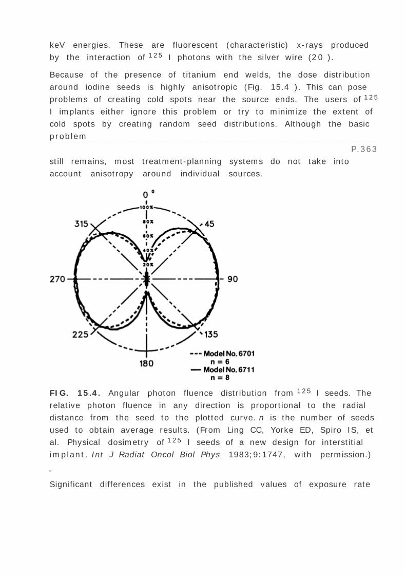
keV energies. These are fluorescent (characteristic) x-rays produced

by the interaction of 125 I photons with the silver wire (20 ).

Because of the presence of titanium end welds, the dose distribution

around iodine seeds is highly anisotropic (Fig. 15.4 ). This can pose

problems of creating cold spots near the source ends. The users of 125

I implants either ignore this problem or try to minimize the extent of

cold spots by creating random seed distributions. Although the basic

problem

P.363

still remains, most treatment-planning systems do not take into

account anisotropy around individual sources.

FIG. 15.4. Angular photon fluence distribution from 125 I seeds. The

relative photon fluence in any direction is proportional to the radial

distance from the seed to the plotted curve. n is the number of seeds

used to obtain average results. (From Ling CC, Yorke ED, Spiro IS, et

al. Physical dosimetry of 125 I seeds of a new design for interstitial

implant. Int J Radiat Oncol Biol Phys 1983;9:1747, with permission.)

Significant differences exist in the published values of exposure rate

constant for 125 I. Schulz et al. (21 ) have reported a calculated value

of 1.464 Rcm2 mCi-1 h-1 for an unfiltered point source. As will be

discussed, the use of the exposure rate constant for unfiltered point

sources to calculate dose distribution around actual sources of

complex design such as 125 I has serious accuracy limitations.

G. Palladium-103103 Pd seeds have recently become available for use in brachytherapy.

Their clinical applications are similar to those of 125 I. Having a

shorter half-life (17 days) than that of 125 I (59.4 days), 103 Pd may

provide a biologic advantage in permanent implants because the dose

is delivered at a much faster rate (22 ).

The palladium-103 seed model 2003 consists of a laser-welded

titanium tube containing two graphite pallets plated with 103 Pd (Fig.

15.5 ). A lead marker between the pallets provides radiographic

identification.

103 Pd decays by electron capture with the emission of characteristic

x-rays in the range of 20 to 23 keV (average energy 20.9 keV) and

Auger electrons. The photon fluence distribution around the source is

anisotropic due to the self-absorption by the source

P.364

pallets, the welds, and the lead x-ray marker (Fig. 15.6 ). The

dosimetry data for 103 Pd is sparse. The reader is referred to Meigooni

et al. (23 ) and Chiu-Tsao and Anderson (24 ) for dose-distribution

data.

FIG. 15.5. Schematic diagram of 103 Pd seed (model 200). (From

Theragenics Corp., Norcross, GA, with permission.)

15.2. CALIBRATION OF BRACHYTHERAPY

SOURCES

A. Specification of Source Strength

The strength of a brachytherapy source may be specified in several

ways.

A.1. Activity

The source strength for any radionuclide may be specified in terms of

millicuries (mCi). The exposure rate at any particular point is

proportional to the product of activity and its exposure rate constant.

Errors, however, may be introduced in this method from the fact that

corrections must be applied for the source and wall filtration and that

the exposure rate constant may not be known accurately. It should be

recalled that the accuracy of the

P.365

exposure rate constant depends critically on the accurate knowledge

of the spectroscopic data and the relevant absorption coefficients.

FIG. 15.6. Photon fluence distribution in air for 103 Pd seed. (From

Meli JA, Anderson LL, Weaver KA. Dose distribution. In: Interstitial

Collaborative Working Group, ed. Interstitial brachytherapy. New

York: Raven, 1990:21, with permission.)

A.2. Exposure Rate at a Specified Distance

The National Council on Radiation Protection and Measurements

(NCRP) (25 ) recommends that the strength of any ³ emitter should

be specified directly in terms of exposure rate in air at a specified

distance such as 1 m. This specification can be carried out simply by

measuring exposure rate in free air at a distance sufficiently large

that the given source can be treated as a point. A long distance

measurement geometry minimizes the dependence of the calibration

upon the construction of the source and the detector because both can

be treated as points. In addition, the effect of oblique transmission of

photons through the source capsule becomes negligible.

Loevinger (26 ) has recommended calibration of brachytherapy

sources in terms of absorbed dose in water, close to the source.

However, such calibrations are not routinely available. So, until these

are available, the exposure rate calibration, far from the source,

remains the most appropriate method.

A.3. Equivalent Mass of Radium

There are historical reasons that make it convenient to specify

brachytherapy sources in terms of the equivalent mass of radium.

Because some users, especially the physicians who are accustomed to

radium sources, continue to use mg-Ra eq, it has been suggested (25

) that the exposure rate could be expressed in terms of

â€œeffectiveâ€ equivalent mass of radium. This conversion is simply

made by dividing the exposure rate at 1 m by the exposure rate

constant of radium (point source filtered by 0.5 mm Pt) at 1 m. It

should, however, be emphasized that the best way to calibrate and

specify brachytherapy sources is still in terms of exposure rate or air

kerma rate at a distance of 1 m. The effective mg-Ra eq should be

used only to provide output comparison with radium sources.

Example

An iridium-192 source has been calibrated and its strength is specified

as 0.495 mR/h at 1 m. What is the strength of this source in terms of

effective mg-Ra eq?

Exposure rate constant of radium filtered by 0.5 mm Pt = 8.25

R ·cm2 /h ·mg = 0.825 mR ·m2 /h ·mg

Note that such a conversion of units must explicitly specify the radium

source in terms of a point source and its filtration.

A.4. Apparent Activity

If the source is calibrated in terms of exposure rate at 1 m, its

strength may be specified as apparent activity. It is defined as the

activity of a bare point source of the same nuclide that produces the

same exposure rate at 1 m as the source to be specified. The apparent

activity of a brachytherapy source is determined by dividing the

measured exposure rate at 1 m with the exposure rate constant of the

unfiltered source at 1 m.

It is a common practice with the vendors of brachytherapy sources to

specify source strength as apparent activity, although the original

calibration is done in terms of exposure rate. In order for the user to

calculate exposure rate from the apparent activity, the exposure rate

constant to be used must be the same as the one used by the vendor.

Thus the exposure rate constant is used as a dummy constant in this

conversion, that is, a purely

P.366

arbitrary value would do, provided its product with the apparent

activity yields the same exposure rate as determined by the original

calibration.

A.5. Air Kerma Strength

Although exposure rate at a specified distance is the method of choice

in designating source strength, the quantity exposure is in the process

of being phased out. Most of the standards laboratories have already

replaced exposure by the quantity air kerma. In keeping with these

trends the AAPM recommended the quantity air kerma strength for the

specification of brachytherapy sources.

The air kerma strength is defined (27 ) as the product of air kerma

rate in â€œfree spaceâ€ and the square of the distance of the

calibration point from the source center along the perpendicular

bisector, that is,

where SK is the air kerma strength and [k with dot above]l is the air

kerma rate at a specified distance l (usually 1 m). Recommended

units for air kerma strength are µGym2 h-1 .

Because no single system is being currently followed universally, it is

instructive to derive relationships between the different quantities

being used for source strength specification.

From Equations 8.6 and 8.13 (see Chapter 8 ) kerma is related to

exposure by:

where K is kerma, X is exposure,

/e is the average energy absorbed per unit charge of ionization in air,

t r / and

en / are, respectively, the average values of the mass transfer

coefficient and the mass energy absorption coefficient of air for the

photons. Also,

where g is the fraction of the energy lost to bremsstrahlung. However,

in the energy range of brachytherapy photons and for the air medium

en / [asymptotically equal to]

t r / . Therefore,


Thus the exposure calibration of a brachytherapy source can be

readily converted to air kerma strength by the use of Equation 15.5 .

If exposure rate is measured in R/h at l = 1 m,

where 0.876 cGy/R is the value of

/e for dry air (see section 8.3 ) or:

Milligram Radium Equivalent

By definition, 1 mg-Ra eq gives 8.25 — 10-4 R/h at 1 m; therefore,

in terms of air kerma strength (from Eq. 15.6 ),

P.367

or

Apparent Activity

By definition, 1 unit of apparent activity, App, gives exposure rate at

1 m equal to the exposure rate constant of the specified source at 1

m. Using the exposure rate constants given in Table 15.1 and

Equation 15.6 , 1 µGy m2 h-1 = 0.348 mCi for 137 Cs; 0.243 mCi for192 Ir; 0.486 mCi for 198 Au; 0.787 for 125 I; and 0.773 for 103 Pd.

These apparent activities per unit air kerma strength may be used to

convert source strengths calibrated in air kerma strengths to apparent

activities in millicuries.

Example

An 192 Ir seed calibrated by an accredited dose calibration laboratory

(ADCL) has air kerma strength of 5.00 µGy m2 h-1 . What is the

strength of the source (a ) in units of mg-Ra eq and (b ) in units of

mCi (apparent activity)?

Using the conversion factors derived above,

B. Exposure Rate Calibration

The National Institute of Standards and Technology (NIST) has

established exposure rate calibration standards for some of the

brachytherapy sources, e.g., 226 Ra, 60 Co, 137 Cs, and 192 Ir. The

NIST method consists of calibrating a working standard of each type

using open-air geometry and a series of spherical graphite cavity

chambers (28 ,29 ). A given source is then calibrated by

intercomparison with the working standard using a 2.5-liter spherical

aluminum ionization chamber, positioned at a distance of about 1 m.

A similar procedure is used for calibrating a radium source except that

the working standards of radium have been calibrated in terms of

actual mass of radium.

Because of their lower exposure rate and shorter half-life, 192 Ir is

calibrated in a slightly different manner (29 ). A composite source

containing about 50 seeds is calibrated in terms of exposure rate at 1

m in open-air scatter-free geometry, as in the case of 137 Cs sources,

using spherical graphite chambers. Each seed is then measured

individually in a well-type ionization chamber to calibrate the

chamber. This well-type ionization chamber now serves as the working

standard for calibrating 192 Ir seeds.

125 I seeds are calibrated at the NIST in terms of exposure rate in

free space at 1 m using a free-air ionization chamber (30 ). For

routine calibrations a well-type ionization chamber is used whose

calibration is maintained by a free-air chamber as the primary

standard.

Calibration of clinical sources should be directly traceable to NIST or

one of the AAPM-ADCLs. This means that the sources should be

calibrated by direct comparison with a NIST- or ADCL-calibrated

source of the same kind, i.e., the same radionuclide with the same

encapsulation, size, and shape. If a well-type ionization chamber is

used, it should bear a calibration factor determined with a NIST- or

ADCL-calibrated source of the same kind.

B.1. Open-air Measurements

Figure 15.7 is a schematic representation of an open-air measurement

geometry for the calibration of brachytherapy sources. The

arrangement consists of a large source to ion

P.368

chamber distance relative to source and detector dimensions. The

apparatus is set up as far away as possible from potential scattering

surfaces. Because the output from brachytherapy sources is low at

large distances, the chamber volume should be large, for example,

100 ml or larger. A signal-to-noise ratio greater than 100:1 should be

achievable.

FIG. 15.7. Schematic drawing of open air geometry for exposure rate

calibration of brachytherapy sources.

Because of the difficulty in obtaining â€œgood geometryâ€

conditions, the open-air method is a time-consuming measurement. It

is not suitable for routine calibration checks required in a busy

department. A well-type ionization chamber is more suited to routine

measurements.

B.2. Well-type Ion Chambers

Routine calibration of brachytherapy sources is usually carried out

with a â€œre-entrantâ€ -type ion chamber in which the walls of the

chamber surround the source, approximating a 4 € measurement

geometry. Examples of such chambers are those designed by the

British National Physics Laboratory (31 ), a re-entrant chamber

designed by Radiological Physics Center (32 ), a spherical aluminum

chamber designed by NIST (33 ), and commercially available dose

calibrators (34 ,35 ,36 ).

Figure 15.8 is a schematic drawing of a dose calibrator, Capintec

Model CRC-10. This unit consists of an aluminum wall ion chamber

filled with argon gas under high pressure. The collection potential

applied to the chamber is about 150 V. A source holder is devised to

reproduce the source geometry in relation to the surrounding chamber

walls.

The dose calibrator is traditionally used for assay of

radiopharmaceuticals in which the instrument response is interpreted

as activity in units of millicuries. These activity calibrations of various

isotopes are based on relative chamber response measured by

intercomparison with the respective standards calibrated by NIST

directly in terms of activity (37 ). However, these standards are

usually in the form of an aqueous suspension of the isotope sealed in

a glass ampule. These vendor calibrations of the instrument are,

therefore, not valid for brachytherapy sources because of differences

in construction between brachytherapy and standard sources. Even

the practice of using a radium standard for calibrating different

sources is prone to significant errors due to energy dependence of the

instrument (35 ,36 ,38 ). In addition, the response of well chambers is

known to depend on the source position in the well and on the length

of the source (32 ). Correction factors must be determined for these

effects for a given instrument and the type of sources to be

calibrated.

The energy dependence of the chamber arises from absorption and

scattering of photons and secondary electrons in the chamber walls

and the gas. Besides this intrinsic energy dependence, oblique

filtration through the source encapsulation affects the chamber

response both by photon absorption and by producing changes in the

energy spectrum. This effect of source construction on the chamber

response has been studied in detail by Williamson et al. (34 ,39 ) for

commonly used brachytherapy sources. These authors conclude:

â€œIn these apparatuses, all one can count on is a linear response

with respect to

P.369

exposure rate given fixed energy, filtration, and source position. For

each isotope, an exposure calibrated standard is neededâ€ (34 ).

These studies support the recommendations that the brachytherapy

sources should be calibrated in terms of exposure rate using exposure

calibrated standards of the same kind (25 ,26 ).

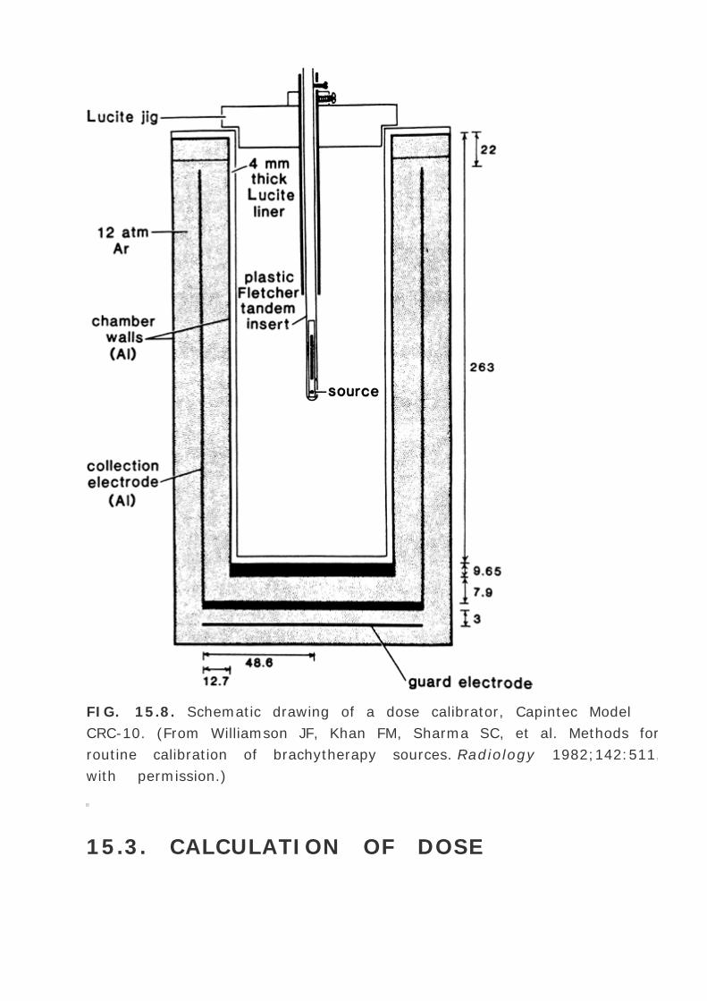
FIG. 15.8. Schematic drawing of a dose calibrator, Capintec Model

CRC-10. (From Williamson JF, Khan FM, Sharma SC, et al. Methods for

routine calibration of brachytherapy sources. Radiology 1982;142:511,

with permission.)

15.3. CALCULATION OF DOSE

DISTRIBUTIONS

A. Exposure Rate

Exposure rate distribution around a linear brachytherapy source can

be calculated using the Sievert integral, introduced by Sievert (40 ) in

1921. The method (1 ,41 ) consists of dividing the line source into

small elementary sources and applying inverse square law and

filtration corrections to each. Consider a source of active length L and

filtration t (Fig. 15.9 ). The exposure rate dI at a point P (x, y )

contributed by the source element of length dx is given by:

where A and “ are the activity and exposure rate constant of the

unfiltered source and µâ€² is the effective attenuation coefficient for

the filter. Other variables are defined by Fig. 15.9 .

P.370

Making use of the following relationships:

and integrating Equation 15.9 , we obtain the exposure rate I (x, y )

for the whole source.

The above Sievert integral can be evaluated by numerical methods (1

).

FIG. 15.9. Diagram illustrating geometrical relationships used in

calculation of exposure at point P , from a linear source.

If the source intensity is specified in terms of exposure rate

s at a specified distance s far from the source, i.e., s â‰« L , then

the Sievert integral can be written as:

Alternatively, if the source strength is specified in terms of equivalent

mass of radium, m eq , such that

s = meq · “Ra ·s -2 , then:

If the source strength is specified in air kerma strength, then:

Several additional corrections are applied to compute the exposure

rate accurately using the Sievert integral. A correction for self-

absorption in the source material, although small for clinical sources,

has been used by Shalek and Stovall (1 ). Wall thickness, t , should

be corrected for the internal radius of the source, because some

photons traverse a thickness of filter greater than the radial thickness

of the wall (42 ,43 ). Depending on the type of source and filtration,

the energy spectrum may be significantly altered by the filter. Not

only is an â€œeffective attenuation coefficientâ€ needed but this

coefficient varies with filter thickness (43 ,44 ). This problem becomes

more severe when the effects of oblique filtration are considered (45

).

In the case of 226 Ra encapsulated in platinum, measured values of

µâ€² (43 ,44 ) may be used (Fig. 15.10 ). However, if such data are

not available for a given source-filter

P.371

combination, calculated values have to be used. Williamson et al. (45

) give the following expression for µâ€² as a function of filter

thickness d:

where pi denotes the number of photons with energy E i emitted per

disintegration, and ( µen / )air i is the mass energy absorption

coefficient in air for photon of energy Ei .

FIG. 15.10. Effective energy absorption coefficients of radium gamma

rays in platinum. (Data are from Whyte GN. Attenuation of radium

gamma radiation in cylindrical geometry. Br J Radiol 1955;28:635;

and Keyser GM. Absorption correction for radium standardization. Can

J Phys 1951;29:301.)

Because the Sievert integral uses the energy absorption coefficient,

the underlying assumption is that the emitted energy fluence is

exponentially attenuated by the filter thickness traversed by the

photons. This is an approximation that has been shown to work well

for 226 Ra and 192 Ir seeds in the region bounded by the active source

ends (1 ,45 ). However, Monte Carlo simulations (45 ) have shown

that beyond the end of the active source region, the Sievert approach

introduces significant errors and practically breaks down in the

extreme oblique directions.

A.1. Effect of Inverse Square Law

Figure 15.11 compares the radial exposure rate distribution of a line

source of radium with that of a point source of radium, both filtered

by 1 mm Pt. Whereas the curve for the point source represents an

inverse square law function, the linear source curve was obtained

using the Sievert integral. The exposure rate constant for 226 Ra with

1 mm Pt filter was assumed to be 7.71 Rcm2 mg-1 h-1 . It is evident

from Fig. 15.11 that for the linear source, the exposure rate is less

than that predicted by the inverse square law, especially at points

close to the source. This is as expected because the photons reaching

these points from the source extremities travel larger distances and

suffer oblique filtration which is greater than the radial wall thickness.

As the distance is increased, however, these effects of the

P.372

linear source approach those of the point source and, therefore, its

exposure rate curve approaches inverse square law.

FIG. 15.11. Plot of exposure rate from 1-mg 226 Ra source as a

function of radial distance. Point source with 1.0 mm Pt filtration.

Linear source with 1.0 mm Pt filtration, 1.5 cm active length.

B. Absorbed Dose in Tissue

The Sievert integral gives the exposure rate distribution in air and

considers only the inverse square law and filtration effects. When a

source is implanted in the tissue, one needs to consider, in addition,

attenuation as well as scattering in the surrounding tissue. The

exposure rate calculated at a point in tissue can then be converted

into absorbed dose rate by using the appropriate roentgen-to-rad

factor (see Chapter 8 ).

Several investigators have experimentally determined the ratio of

exposure in water to exposure in air as a function of distance for a

number of isotopes. Because of the large discrepancies between

various sets of experimental data, Meisberger et al. (46 ) formulated

a third order polynomial to fit the average of their theoretical and all

available experimental data (46 ,47 ,48 ,49 ,50 ,51 ,52 ). This

polynomial is commonly used for routine calculation of absorbed dose

in tissue in various computer programs.

More recently, Webb and Fox (53 ) calculated the dose distribution

around point ³ ray emitters in water by the Monte Carlo method.

Their results agree very well with Meisberger's average or

â€œselectedâ€ curve.

The radial dependence of dose in a water medium, with the inverse

square law removed can also be represented by Dr = Br e - µr where

µ denotes the linear attenuation coefficient and Br is a build-up

factor at distance r from the source. This expression is similar to the

P.373

ratio of exposure in water to exposure in air. Evans (54 ) has

suggested that Br may be represented by:

where ka and kb are constants. Kornelsen and Young (55 ) have fitted

the Monte Carlo data of Webb and Fox (53 ) to determine the

constants ka and kb . These are given in Table 15.3 . Figure 15.12

shows the curves calculated by these authors.4

60 Co

0.0632

0.896

1.063226 Ra

0.0811

1.17

1.19137 Cs

0.0858

1.14

1.20198 Au

0.105

1.48

1.32192 Ir

0.113

1.59

1.36

Data from Kornelsen RO, Young MEJ. Brachytherapy build-up factors.

Br J Radiol 1981;54:136.

Isotope µ (cm2 /g) k a k b

TABLE 15.3. CONSTANTS k a AND k b DETERMINED BY USE OF

MONTE CARLO DATA

Figure 15.12 shows that at short distances, the attenuation of the

primary photons is very much compensated for by the contribution of

scattered photons with the result that the exposure in water is almost

equal to the exposure in air at the same point. However, tissue

attenuation overtakes scattering at larger distances. For radium

sources, the net reduction is about 1% per cm of intervening tissue up

to 5 cm.

It is instructive to study the dose falloff with distance in tissue.

Figure 15.13 is a plot of percent dose as a function of distance in

water for point sources of 60 Co, 226 Ra, 137 Cs, 198 Au, 192 Ir, and 125

I. These plots also are compared with the inverse square law function

(1/r 2 ). These data show that over a distance of about 5 cm the

percent dose rates for 226 Ra, 60 Co, and 137 Cs are about equal and

show a slight decrease below inverse square law due to tissue

attenuation. The curves for 192 Ir and 198 Au, on the other hand, are

practically indistinguishable from the inverse square law curve up to

about 5 cm. The dose distribution for 125 I progressively deviates from

the inverse square law as a result of increased tissue attenuation for

this isotope. However, up to about 1 cm, all the curves are

indistinguishable due to the severity of the inverse square law effect

at such short distances.

Absorbed dose rate tables for linear radium sources have been

published by Shalek and Stovall (1 ) which take into account

attenuation and scattering in tissue. Similar data also are available

for 137 Cs and 125 I (9 ,56 ). Such tables are useful for manual

calculations as well as for checking the accuracy of computer

calculations.

C. Modular Dose Calculation Model: TG-43

The traditional method of calculating dose in a medium (sections

15.3A and 15.3B ) using Sievert integral requires the determination of

µâ€², the effective attenuation coefficient for the filter as a function

of thickness and the tissue attenuation factors. Both of these

parameters are difficult to measure or calculate, especially for sources

of complex design such as 125 I and 103 Pd. It is, therefore,

advantageous to calculate dose rates from quantities measured solely

in the medium. The data for a particular source can be compiled in a

tabular form as a function of position. A modular approach has been

proposed by the AAPM Task Group 43 in which the effects of several

physical factors on dose rate distribution are considered separately

(57 ). The dose rate, [D with dot above](r , ¸) at point P with polar

coordinates (r , ¸) in a medium

P.374

P.375

(e.g., water) from the center of a source of air kerma strength SK can

be expressed as:

where › is the dose rate constant, defined as the dose rate per unit

air kerma strength (U) at 1 cm along the transverse axis of the seed

and has units of cGy h-1 U-1 , i.e.,

FIG. 15.12. Attenuation correction factor in water as a function of

distance for a point source. Curves are calculated by Equation 15.15

and fitted to Monte Carlo data. See text for details.

FIG. 15.13. Percent dose variation with distance in water for point

sources of 60 Co, 226 Ra, 137 Cs, 198 Au, 192 Ir, and 125 I. Function

(1/r 2 ) represents inverse square falloff. (125 I data are from

Krishnaswamy V. Dose distribution around an 125 I seed source in

tissue. Radiology 1976;126:489.) The other isotope data were

calculated from Fig. 15.12 in addition to the inverse square law.

125 I model 6702

0.919

1.16125 I model 6711

0.847

1.07192 Ir

1.11

4.55

The units for U are µGy m2 h-1 or cGy cm2 h-1 .

From Meli JA, Anderson LL, Weaver KA. Dose distribution. In:

Interstitial Collaborative Working Group, ed. Interstitial

brachytherapy. New York: Raven, 1990:21, with permission.

Seed cGy hr- 1 U- 1 cGy mCi- 1 hr- 1

TABLE 15.4. RECOMMENDED DOSE RATE CONSTANTS IN

WATER

The dose rate constant, ›, depends on the type of source, its

construction, and its encapsulation. The values recommended for 125 I

seeds (models 6702 and 6711) and 192 Ir seed are listed in Table 15.4

.

G (r , ¸) is the geometry factor (cm-2 ) that accounts for the

geometric falloff of the photon fluence with distance from the source

and depends on the distribution of radioactive material. For a point

source, G (r , ¸) = 1/r 2 and for uniformly distributed line source, G

(r , ¸) = ( ¸2 - ¸1 )/Ly .5

F (r , ¸) is the anisotropy factor normalized at ¸ = €/2

(transverse axis), with the geometric factor factored out, that is,

The anisotropy factor accounts for the angular dependence of photon

absorption and scatter in the encapsulation and the medium.

The radial dose function, g (r ), accounts for radial dependence of

photon absorption and scatter in the medium along the transverse

axis and is given by:

Again the geometric factor is factored out from the dose rates in

defining g (r ).

Table 15.5 is an example of the geometry factor calculated for a 3-

mm-long line source. Table 15.6 provides anisotropy and radial dose

function data measured for 125 I seeds, models 6702 and 6711.

Because anisotropy is not as serious a problem for 192 Ir seeds as it is

for 125 I seeds, iridium seeds may be treated as point sources in a

dose calculation formalism. For a point source, Equation 15.16

reduces to:

where †an is the average anisotropy factor. It is defined as the ratio

of 4 € averaged dose rate at a given radial distance divided by the

dose rate at the same distance along the transverse

P.376

axis. †an for 192 Ir seeds may be equated to unity. The data for g (r

) for 192 Ir seeds are given in Table 15.7 .

0

4.396

1.023

10

4.377

1.022

20

4.323

1.019

30

4.246

1.015

90

3.885

0.993




¸ (deg) r = 0.5 cm r = 1.0 cm

TABLE 15.5. EXAMPLE OF THE GEOMETRY FACTOR , G (r , ¸),

FOR A 3.0-MM LINE SOURCE

D. Isodose Curves

The above methods can be used to calculate absorbed dose to a

matrix of points around a source. The isodose curves are then

constructed by interpolation between points, connecting those points

receiving the same dose. Because of the complex and time-consuming

calculations required to generate isodose curves, the job is ideally

suited for computers. Presently, almost all commercial treatment

planning computers offer brachytherapy software that can perform

sophisticated treatment planning involving three-dimensional

distribution of multiple sources.

Experimental determination of isodose curves is sometimes necessary

to check new calculation algorithms. Film and thermoluminescent

dosimetry (TLD) (see Chapter 8 ) require the least apparatus for such

measurements. Film offers a high resolution but has a serious

limitation of energy dependence, that is, increased sensitivity to low-

energy photons

P.377

present in the nuclidesâ€™ ³ ray spectrum and the scattered

radiation. TLD shows energy dependence (58 ) also but to a lesser

degree than the film.

6702

0.5

0.448

0.544

0.701

0.815

1.0

1.04

1.0

0.501

0.598

0.758

0.866

1.0

1.00

2.0

0.537

0.628

0.781

0.874

1.0

0.851

3.0

0.572

0.656

0.798

0.873

1.0

0.670

4.0

0.605

0.683

0.814

0.872

1.0

0.510

5.0

0.634

0.707

0.826

0.871

1.0

0.389

6.0

0.651

0.719

0.828

0.870

1.0

0.302

8.0

0.178

10.0

0.131

6711

0.5

0.376

0.448

0.627

0.783

1.00

1.04

1.0

0.369

0.464

0.658

0.799

1.00

1.00

2.0

0.419

0.503

0.683

0.791

1.00

0.832

3.0

0.474

0.551

0.715

0.800

1.00

0.632

4.0

0.493

0.579

0.736

0.813

1.00

0.463

5.0

0.478

0.583

0.743

0.823

1.00

0.344

6.0

0.264

8.0

0.145

10.0

0.0820a For r < 0.5 cm g (r ) = 1.00 ± 0.1.




Model

r

(cm)a

Anisotropy FactorRadial Dose

Function0 ° 10 ° 20 ° 30 ° 90 °

TABLE 15.6. THE ANISOTROPY FACTOR , F (r , ¸), AND

RADIAL DOSE FUNCTION , g (r ), FOR 125 I MODELS 6702 AND

6711

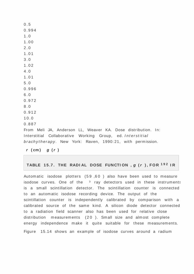
0.5

0.994

1.0

1.00

2.0

1.01

3.0

1.02

4.0

1.01

5.0

0.996

6.0

0.972

8.0

0.912

10.0

0.887




r (cm) g (r )

TABLE 15.7. THE RADIAL DOSE FUNCTION , g (r ), FOR 192 IR

Automatic isodose plotters (59 ,60 ) also have been used to measure

isodose curves. One of the ³ ray detectors used in these instruments

is a small scintillation detector. The scintillation counter is connected

to an automatic isodose recording device. The output of the

scintillation counter is independently calibrated by comparison with a

calibrated source of the same kind. A silicon diode detector connected

to a radiation field scanner also has been used for relative close

distribution measurements (20 ). Small size and almost complete

energy independence make it quite suitable for these measurements.

Figure 15.14 shows an example of isodose curves around a radium

needle. Examination of the curves indicates that close to the source

they are more or less elliptical. At large distances, the isodose curves

become circles, because the source behaves as a point source. The dip

in the curves close to the source axis is due to the effect of oblique

filtration.

FIG. 15.14. Isodose curves in terms of rad/h around a 1-mg radium

source. Active length = 3.0 cm; filtration = 0.5 mm Pt.

P.378

15.4. SYSTEMS OF IMPLANT DOSIMETRY

The objectives of treatment planning are (a ) to determine the

distribution and type of radiation sources to provide optimum dose

distribution and (b ) to provide a complete dose distribution in the

irradiated volume. Numerous systems of dosimetric planning have

been devised over the past 50 years. Of these the Paterson-Parker

system (61 ) and the Quimby system (62 ) have received the most

widespread use. These and other systems were designed during the

times when computers were not available for routine treatment

planning. Extensive tables and elaborate rules of source distribution

were devised to facilitate the process of manual treatment planning.

Then a more significant development occurred: the use of digital

computers to calculate isodose distributions for individual patients (63

,64 ,65 ). This gave the radiation therapist freedom to deviate from

the established systems. Although, the old systems with their rules

and tables are still being used, the computer treatment planning is

fast replacing the traditional systems. Some of these methods will be

reviewed here to illustrate the basic problems and concepts of

brachytherapy planning.

A. The Paterson-Parker System

The Paterson-Parker or Manchester system (61 ) was developed to

deliver uniform dose (within ±10%) to a plane or volume. The

system specified rules of source distribution to achieve the dose

uniformity and provided dosage tables for these idealized implants.

These tables are reproduced in the appendix.

A.1. Planar Implant

In the case of planar implants the uniformity of dose is achieved in

parallel planes at 0.5 cm from the implanted plane and within the

area bounded by the projection of the peripheral needles on that

plane. The â€œstatedâ€ dose, determined from the Paterson-Parker

tables, is 10% higher than the minimum dose. The maximum dose

should not exceed 10% above the stated dose to satisfy the

uniformity criterion. The dose is, however, much more nonuniform

within the plane of implant. For example, the dose at the surface of

the needles is about five times the stated dose.

The distribution rules for the planar implants are:

The ratio between the amount of radium in the periphery and the

amount of radium over the area itself depends on the size of the

implant, for example:

Less than 25 cm2

2/3

25â€“100 cm2

½

Over 100 cm2

1/3

Area Fraction Used in Periphery

The spacing of the needles should not be more than 1 cm from

each other or from the crossing ends.

If the ends of the implant are uncrossed (Fig. 15.15B or C ), the

effective area of dose uniformity is reduced.6 The area is,

therefore, reduced by 10% for each uncrossed end for table

reading purposes.

In the case of multiple implant planes, the radium should be

arranged as in rules 1â€“3, and the planes should be parallel to

each other.

FIG. 15.15. Examples of three planar implants. A: Both ends crossed.

B: One end uncrossed. C: Both ends uncrossed.

P.379

A.2. Volume Implants

Some tumors are better implanted using three-dimensional shapes

such as cylinders, spheres, or cuboids.

The total amount of radium is divided into eight parts and

distributed as follows for the various shapes. The cylinder is

composed of belt, four parts; core, two parts; and each end, one

part (Fig. 15.16 ). The sphere is made up of shell, six parts, and

core, two parts. The cuboid consists of each side, one part; each

end, one part; and core, two parts.

The needles should be spaced as uniformly as possible, not more

than 1 cm apart. There should be at least eight needles in the belt

and four in the core.

P.380

If the ends of the volume implant are uncrossed, 7.5% is deducted

from the volume for uncrossed end for table reading purposes.

FIG. 15.16. Example of a volume implant with one end uncrossed.

The implant has eight needles in the belt, four in the core (not

shown), and four at one end. Whereas the needles in the belt and core

are 1 mg each, the crossing needles at the end are 0.5 mg each, thus

satisfying the Paterson-Parker rule of radium distribution.

For a volume implant, the prescribed dose is stated 10% higher than

the minimum dose within the implanted volume.

A.3. Paterson-Parker Tables

The Paterson-Parker tables (61 ) are designed to give milligram

hours/1,000 roentgens (mg-h/1,000 R) for implants of various sizes,

both for planar and volume implants (see Tables A.12.1 and A.12.2 in

the appendix). To convert Paterson-Parker roentgens to cGy in tissue,

one needs to make the following corrections: (a ) Exposure rate

constant ( “): the tables assume “ = 8.4 Rcm2 /mg-h instead of the

current value of 8.25 Rcm2 /mg-h. (b ) A roentgen:cGy factor of 0.957

should be used to convert exposure into dose in muscle. (c ) Oblique

filtration: Paterson-Parker tables do not take into account increased

attenuation by oblique filtration by the platinum capsule, giving rise

to a 2% to 4% error for typical implants. (d ) Paterson-Parker tables

are based on exposure in air. Corrections are needed for tissue

attenuation and scattering (section 15.3B ).

Stovall and Shalek (66 ) have demonstrated that for typical planar

and volume implants a combined factor of 0.90 selects an isodose

curve approximately equivalent to the Paterson-Parker dosage. Thus

the mg-h/1,000 R in the original Paterson-Parker tables should be

considered equivalent to mg-h/900 cGy.

A.4. Determination of Implant Area or

Volume

Dosage tables for interstitial implants require the knowledge of area

or volume of implant. If the needles are close to the surface, one can

determine the size of the implant directly. If not, it has to be

determined radiographically.

Orthogonal Radiographs

Three-dimensional localization of individual sources can be obtained

by orthogonal (perpendicular) radiographs, such as anteroposterior

(AP) and lateral (Lat) views. It is important that the central axes of

the anteroposterior and lateral x-ray beams meet at a point,

approximately in the middle of the implant. This can be easily

achieved by an isocentric radiographic unit, such as a treatment

simulator. For the above isocentric geometry, the film magnification

factor is given by SFD/SAD, where SFD is source-to-film distance and

SAD is source-to-axis distance. Alternatively, a circular object, such

as a metallic ring, may be taped to the patient at the level of the

implant. The ratio of the largest outside diameter of the ring image to

the actual outside diameter of the ring gives the magnification factor.

To determine the width or length of an implant, one needs to

determine the distance between two points, three dimensionally.

Figure 15.17 illustrates the principle of deriving this information from

orthogonal radiographs. Let A (x 1 , y 1 , z 1 ) and B (x 2 , y 2 , z 2 )

be the two points in question. Then by the application of the

Pythagorean theorem, it can be shown that:

Equation 15.21 can also be written as:

where a is the length of the image of AB on one of the radiographs

and c is the projection of the image of AB to the baseline in the other

radiograph (the baseline is a line perpendicular to the intersection of

the radiographs, usually parallel to the edges of the films). Figure

15.17 assumes a magnification factor of unity. However, in actual

practice, a and c will have to be corrected for film magnification.

FIG. 15.17. Orthogonal radiographs of an implant. Baseline is parallel

to the edge of the film.

Thus, by determining the width of the implant image on one film and

its width projected to the baseline on the other, one can calculate the

actual width of the implant. The length of the implant can also be

determined the same way but is usually given by the known active

length of the needles.

P.381

Example

Figure 15.17 shows the anteroposterior and lateral radiographs of a

planar implant that was planned according to the Paterson-Parker

system. Assume a magnification factor of 1.4 for both films.

Determine the time to deliver 6500 cGy at 0.5 cm from the plane of

implant.

Given width of the implant image on the lateral radiograph = a =

3.8 cm

Projection of AP image on baseline = c = 0.9 cm

Peripheral needles = 3 — 2 mg

Central needles = 2 — 1 mg

All needles have active length of 3 cm and 0.5 mm Pt filtration.

Treatment distance = 0.5 cm from the plane of implant

Width of implant

= 2.79 cm

Length of implant = 3 cm

Area of implant = 2.79 — 3 = 8.4 cm2

Because one end is uncrossed, the area for table reading purposes =

8.4 - 10% (8.4) = 7.6 cm2 . From Paterson-Parker table (Table A.12.1

in the appendix), the mg-h/1,000 R or mg-h/900 cGy required = 200.

B. The Quimby System

The Quimby system (62 ) of interstitial implantation is characterized

by a uniform distribution of sources of equal linear activity.

Consequently, this arrangement of sources results in a nonuniform

dose distribution, higher in the central region of treatment. For planar

P.382

implants, the Quimby table gives the milligram-hours required to

produce 1,000 R in the center of the treatment planes, up to 3 cm

distance from the plane of implant. The stated dose is thus the

maximum dose in the plane of treatment. For volume implants, the

stated dose is the minimum dose within the implanted volume.

The original Quimby tables, like the Manchester tables, are based on

an exposure rate constant of 8.4 Rcm2 /mg-h instead of the currently

accepted value of 8.25 Rcm2 /mg-h. Also, other corrections, namely

the roentgen:cGy factor, oblique filtration, and tissue attenuation,

have to be applied as in the case of the Paterson-Parker tables.

Shalek and Stovall compared the Quimby and the Paterson-Parker

systems for selected idealized cases and found that fundamental

differences exist between the two systems. They caution against the

use of these systems interchangeably. â€œIt is imperative that a

radiation therapist use one radium system to the exclusion of the

otherâ€ (1 ).

C. The Memorial System

The Memorial system, as described by Laughlin et al. (64 ) in 1963, is

an extension of the Quimby system and is characterized by complete

dose distributions around lattices of point sources of uniform strength

spaced 1 cm apart. Based on computer-generated dose distributions,

tables were constructed that gave milligram-hours to deliver 1,000

rads at designated points, for example, â€œminimum peripheralâ€

and â€œreference maximum doseâ€ points in the plane 0.5 cm from

the source plane for the planar implants. For volume implants, similar

data points within the implanted volume as well as â€œcentral line

peripheral doseâ€ points were chosen. These tables use proper

exposure rate constant and include the effects of oblique filtration and

tissue attenuation.

Another method, known as the â€œdimension averagingâ€ technique

also has been used at Memorial Hospital for permanent implants (67

,68 ). The method is based on the rationale that radiation tolerance of

tissue depends on the size of the implant and the smaller volumes

could be intentionally given larger doses. According to this method,

the total activity required for an implant is directly proportional to the

average of the three dimensions of the implant region.

Mathematically,

where A is the activity in mCi and d is the averaged dimension, that

is, [d with bar above] = (a + b + c )/3, where a, b , and c are the

three mutually perpendicular dimensions. The constant K of

proportionality is based on clinical experience: K = 10 for 222 Rn and

K = 5 for 125 I.

In addition to the total activity required for an implant, one needs to

know the number of seeds and the spacing between seeds. Anderson

(68 ) has described a nomogram for 125 I seed spacing that takes into

account the elongation factor for the implant shape, for example,

spheroid or cylinder.

D. The Paris System

The Paris system (69 ) of dosimetry is intended primarily for

removable implants of long line sources, such as 192 Ir wires. The

system prescribes wider spacing for longer sources or larger treatment

volumes. As summarized in Table 15.8 , the sources are of uniform

linear activity and are implanted in parallel lines. The details of the

system are described by Pierquin et al. (70 ).

In the Paris system the dose specification is based on an isodose

surface, called the reference isodose. However, in practice, the value

of the reference isodose is fixed at 85% of the â€œbasal dose,â€

which is defined as the average of the minimum dose between

sources. It has been shown that the reference isodose for a Paris

implant surrounds the implant within a few millimeters, and its value

is approximately equal to 85% of the basal dose (71 ). Figure 15.18

illustrates how the basal dose is calculated in different patterns of

implants using the Paris system.

Linear strength

Variable (full intensity, 0.66 mg Ra/cm; half intensity, 0.33 mg

Ra/cm)

Constant (full intensity, 1 mg Ra/cm; half intensity, 0.5 mg Ra/cm)

Constant (0.6â€“1.8 mg Ra eq/cm)

Constant (0.2â€“0.4 mg Ra eq/cm)

Source distribution

Planar implants: Area <25 cm2 , 2/3 Ra in periphery; area 25 to 100

cm2 , 1/2 Ra in periphery. Area >100 cm2 , 1/3 Ra in periphery

Uniform

Uniform

Uniform

Volume implants

Cylinder: belt, four parts; core, two parts; each end, one part.

Sphere: shell, six parts; core, two parts.

Cube: each side, one part; core, two parts.

Uniform distribution of sources throughout the volume

Line sources arranged in parallel planes

Line sources arranged in parallel planes or cylindric volumes

Line source spacing

Constant approximately 1 cm apart from each other or from crossing

ends

Same as Paterson-Parker

Constant, but selected according to implant dimensions-larger spacing

used in large volumes; 8 mm minimum to 15 mm maximum

separation

Constant, 1â€“1.5 cm, depending on size of implant (larger spacing

for larger size implants)

Crossing needles

Crossing needles required to enhance dose at implant ends

Same as Paterson-Parker

Crossing needles not used; active length 30% to 40% longer than

target length

Crossing needles not required; active length of sources 30% to 40%

longer than target lengtha The computer system used at the University of Minnesota Hospital.

From Khan FM. Brachytherapy: rules of implantation and dose

specification. In: Levitt SH, Khan FM, Potish RA, eds. Technological

basis of radiation therapy. Philadelphia: Lea & Febiger, 1992:113,

with permission.

Characteristic Paterson-Parker Quimby Paris Computera

TABLE 15.8. RULES OF INTERSTITIAL IMPLANT SYSTEMS

P.383

E. Computer System

An implant system that has evolved through the use of computers but

bears no formal name is used in many institutions in the United

States. I will call it the computer system. The implantation rules are

very simple: the sources of uniform strength are implanted, spaced

uniformly (e.g., 1.0 to 1.5 cm, with larger spacing for larger size

implants), and cover the entire target volume.

It is realized that the implantation of uniform activity sources gives

rise to an implant that is â€œhotterâ€ in the middle than in the

periphery, as is the case with the Quimby and the Paris systems.

However, this dose inhomogeneity is accepted with the belief that the

central part of the target would need higher doses to sterilize than the

periphery.

In the computer system, the target volume is designed with sufficient

safety margins so that the peripheral sources can be placed at the

target boundary with adequate coverage of the tumor. The dose is

specified by the isodose surface that just surrounds the target or the

implant. An important criterion is followed: It is better to implant a

larger volume than to select a lower value isodose curve to increase

the coverage. If the target volume is designed with adequate safety

margins, the peripheral sources should then be implanted on the outer

surface of the target volume. Also, the active length of the line

sources should be suitably longer ([asymptotically equal to]40%

longer) than the length of the target volume because of uncrossed

ends.

Figure 15.19A shows isodose distribution in the central cross-sectional

plane for a computer system volume implant (two parallel planes).

The prescription isodose curve just surrounds the peripheral sources.

Figure 15.19B shows the isodose pattern in the longitudinal plane

through the middle of implant to assess adequate coverage by the

P.384

prescription isodose curve in this plane. In fact, target volume

coverage can be viewed in any plane or three-dimensionally, provided

volumetric data for the target are available.

FIG. 15.18. Determination of basal dose (BD) in implants using the

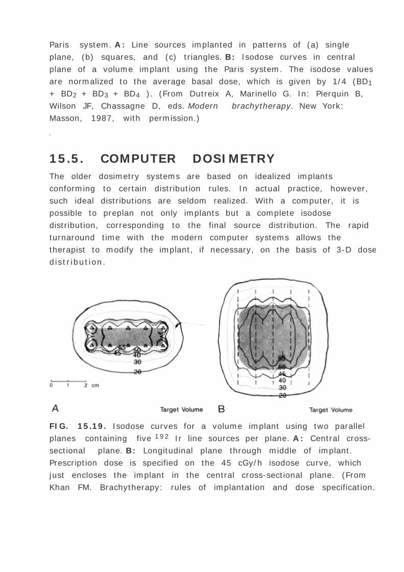
Paris system. A: Line sources implanted in patterns of (a) single

plane, (b) squares, and (c) triangles. B: Isodose curves in central

plane of a volume implant using the Paris system. The isodose values

are normalized to the average basal dose, which is given by 1/4 (BD1

+ BD2 + BD3 + BD4 ). (From Dutreix A, Marinello G. In: Pierquin B,

Wilson JF, Chassagne D, eds. Modern brachytherapy. New York:

Masson, 1987, with permission.)

15.5. COMPUTER DOSIMETRY

The older dosimetry systems are based on idealized implants

conforming to certain distribution rules. In actual practice, however,

such ideal distributions are seldom realized. With a computer, it is

possible to preplan not only implants but a complete isodose

distribution, corresponding to the final source distribution. The rapid

turnaround time with the modern computer systems allows the

therapist to modify the implant, if necessary, on the basis of 3-D dose

distribution.

FIG. 15.19. Isodose curves for a volume implant using two parallel

planes containing five 192 Ir line sources per plane. A: Central cross-

sectional plane. B: Longitudinal plane through middle of implant.

Prescription dose is specified on the 45 cGy/h isodose curve, which

just encloses the implant in the central cross-sectional plane. (From

Khan FM. Brachytherapy: rules of implantation and dose specification.

In: Levitt SH, Khan FM, Potish RA, eds. Technological basis of

radiation therapy. Philadelphia: Lea & Febiger, 1992:113, with

permission.)

P.385

Computer calculation of a brachytherapy dose distribution consists of

repeated calculation of dose at a point for each of the implant

sources. The total dose at a given point is determined by summing the

individual source contributions. Point dose rates are computed for

each of a grid of points arranged in a cubic lattice so that isodose

curves may be generated in any arbitrary plane. The isodose patterns

can also be magnified and superimposed on an implant radiograph for

viewing the distribution in relation to the patient's anatomy.

A. Localization of Sources

Dose calculation algorithms require spatial coordinates for each

radioactive source. Three-dimensional reconstruction of the source

geometry is usually accomplished by using a set of two radiographs,

exposed with either orthogonal or â€œstereo-shiftâ€ geometry. Most

programs allow input of the film coordinates using a digitizer.

A.1. Orthogonal Imaging Method

As discussed in section 15.4A.4 , the orthogonal radiographs are taken

at right angles, with the central axes of the x-ray beams meeting

approximately in the middle of the implant. Usually, AP film and

lateral film, exposed isocentrically, provide such a geometry. The

coordinate system is conventionally established with the x axis from

the right to the left of the patient, the y axis from inferior to superior,

and the z axis from posterior to anterior. The anteroposterior film

represents a magnified view of the implant image projected onto the x

â€“y plane while the lateral film presents the image projected onto

the z â€“y plane. The origin of the coordinate system is chosen to be

a point identified to be the same on both films such as one end of a

source. The sources can be identified by comparing the y coordinates

of the ends on both films. For example, a source end having the

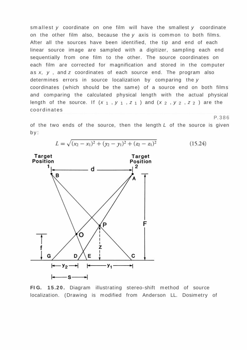
smallest y coordinate on one film will have the smallest y coordinate

on the other film also, because the y axis is common to both films.

After all the sources have been identified, the tip and end of each

linear source image are sampled with a digitizer, sampling each end

sequentially from one film to the other. The source coordinates on

each film are corrected for magnification and stored in the computer

as x, y , and z coordinates of each source end. The program also

determines errors in source localization by comparing the y

coordinates (which should be the same) of a source end on both films

and comparing the calculated physical length with the actual physical

length of the source. If (x 1 , y 1 , z 1 ) and (x 2 , y 2 , z 2 ) are the

coordinates

P.386

of the two ends of the source, then the length L of the source is given

by:

FIG. 15.20. Diagram illustrating stereo-shift method of source

localization. (Drawing is modified from Anderson LL. Dosimetry of

interstitial radiation therapy. In: Hilaris BS, ed. Handbook of

interstitial brachytherapy. Acton, MA: Publishing Sciences Group,

1975:87.)

A.2. Stereo-shift Method

The stereo-shift method of source localization consists of taking two

radiographs of the same view but the patient or the x-ray tube is

shifted a certain distance (e.g., 20 cm) between the two exposures.

The principle of the method is illustrated in Fig. 15.20 . Suppose both

films are anteroposterior, parallel to the x-y plane of the patient as

the tube is shifted in the y direction between films. A tabletop fiducial

marker is used to serve as origin at O. Because the x, y coordinates of

a point source or a source end can be obtained from either of the

films, the z coordinates can be derived as follows. Let:

P = point to be localized three dimensionally

y 1 = distance between images of P and O on the first film

y 2 = distance between images of P and O on the second film

s = film shift in the origin O due to tube shift

d = tube shift distance

F = target-to-film distance

f = table-to-film distance

From similar triangles APB and CPD

Also, from similar triangles AOB and EOG

P.387

From Equations 15.25 and 15.26 , we get

The accuracy of the orthogonal film method is generally better than

that of the stereo-shift method (72 ). For example, small errors in the

measurement of y coordinates produces a large error in the z values.

However, the stereo-shift method is more suitable for cases in which

sources cannot be easily identified by orthogonal films such as a large

number of seeds or some sources being masked by overlying bone.

B. Dose Computation

Earlier computer programs were used mostly to obtain linear source

tables, build-up factors, and scatter factors. Later, programs became

available (63 ,64 ,65 ) to calculate isodose distributions for individual

patients. Currently, almost all treatment-planning software packages

provide brachytherapy dosimetry. Most of these programs use either

the Sievert integral directly or precalculated dose tables for different

types of sources. Some, but not all, use tissue attenuation

corrections, discussed in section 15.3B .

For radium and other long-lived isotopes, the dose rates, presented in

the form of isodose curves, can be directly used to calculate implant

duration. In the case of temporary implants of relatively short-lived

isotopes such as 192 Ir, the computer calculates cumulated dose,

using decay correction for the implant duration. An approximate time

for the implant duration can first be determined from dose rate [D

with dot above]0 without decay correction and the total dose to be

delivered. The cumulated dose Dc is then given by:

where T av is the average life and t is the implant duration.

For permanent implants such as 125 I or 198 Au, cumulated dose (to

complete decay) is given by:

15.6. IMPLANTATION TECHNIQUES

Brachytherapy sources are applied in three ways: external applicators

or molds, interstitial implantation, and intracavitary therapy. A choice

of one technique or the other is dictated primarily by the size and

location of the tumor. For example, surface molds are used to treat

small superficial areas, such as the ear or the lip; interstitial therapy

is indicated when the tumor is well-localized and can be implanted

directly according to accepted rules of distribution; intracavitary

therapy is used when applicators containing radioactive sources can

be introduced into body cavities. In all these cases, owing to the short

treatment distance, the geometry of source distribution is critical.

A. Surface Molds

Plastic molds are prepared (73 ) to conform to the surface to be

treated and the sources are securely positioned on the outer surface

of the mold. The distance between the plane of the sources to the skin

surface is chosen to give a treatment distance of usually 0.5 to 1.0

cm. The dosimetry and source distribution rules are the same for

external molds as for interstitial sources (61 ).

B. Interstitial Therapy

In interstitial therapy, the radioactive sources are fabricated in the

form of needles, wires, or seeds, which can be inserted directly into

the tissue. There are basically two types of

P.388

interstitial implants: temporary and permanent. In a temporary

implant, the sources are removed after the desired dose has been

delivered (e.g., radium needles, iridium wires, or iridium seeds). In a

permanent implant, the sources are left permanently in the implanted

tissues (e.g., 198 Au and 125 I seeds). In general, a temporary implant

provides better control of source distribution and dosimetry than a

permanent implant. However, the permanent implant is a one-time

procedure and is a preferred method for some tumors such as those in

the abdominal and thoracic cavities.

A major improvement in temporary implant technique occurred with

the introduction of â€œafterloadingâ€ techniques (74 ,75 ) in which

the sources are loaded into tubes previously implanted in the tissues.

This procedure eliminates exposure in the operating room, x-ray

room, and the areas through which the patient is transported.

â€œDummyâ€ sources are used for radiographic localization and

dosimetry. The radioactive sources are loaded after the patient is

returned to his or her room and the implant has been evaluated.

Figure 15.21 illustrates the basic principles of the afterloading

technique described by Henschke et al. (74 ). Stainless steel needles

(e.g., 17 gauge) are first implanted in and around the tumor. The

nylon tubes are threaded through the needles, and the needles are

then withdrawn, leaving the nylon tubes in place. The nylon tubes are

secured in position by buttons on the skin surface. The tube ends are

then usually cut off a few centimeters beyond the buttons.

Many variations of the above procedure have been published in the

literature. Further details can be obtained from Hilaris (76 ).

The simplest device for permanent implants is a single-seed inserter

consisting of a stainless-steel needle. Each seed is individually loaded

into the tip of this needle and, after insertion into the tissue, the seed

is pushed out by a stylet. This technique, however, is unsatisfactory

for the implantation of deep-seated tumors and volume implants

requiring many seeds.

FIG. 15.21. Illustration of an afterloading technique for 192 Ir seeds.

(From Hilaris BS, ed. Handbook of interstitial brachytherapy. Acton,

MA: Publishing Sciences Group, 1975:87, with permission.)

P.389

An afterloading technique has also been adopted for the permanent

implants (77 ). The first step in this technique consists of inserting

unloaded 17-gauge stainless-steel needles into the tumor. The

needles are spaced 1 to 2 cm apart, depending on the size of the

tumor. The needles are then afterloaded with radioactive seeds, using

a special implantation instrument that allows insertion of several

seeds at different depths, determined by a gauge as the needle is

withdrawn.

Seed-introducing guns (76 ,78 ) have been devised that allow

preloading of radioactive seeds into a magazine from which they are

pushed into the needle, and then into the tissue. These instruments

are convenient to use and can provide greater precision than possible

with single seed inserters. Modern techniques of seed implants are

discussed in Chapter 23 .

C. Intracavitary Therapy

C.1. Uterine Cervix

Intracavitary therapy is mostly used for cancers of the uterine cervix,

uterine body, and vagina. A variety of applicators have been designed

to hold the sources in a fixed configuration. A cervix applicator

basically consists of a central tube, called the tandem, and lateral

capsules or â€œovoids.â€ The ovoids are separated from each other

by spacers.

Since the first application of radium in the treatment of cancer of the

uterus in 1908, several techniques have evolved, most of which are

modifications of the Stockholm technique (79 ) and the Paris

technique (80 ). The Manchester system, which evolved from the Paris

technique, uses a rubber uterine tandem to hold one to three radium

tubes and rubber ovoids, separated by a rubber spacer, to each hold a

radium tube. The radiation is delivered in at least two applications. In

the Fletcher-Suit applicator (75 ,81 ) (Fig. 15.22 ) the tandem and the

ovoids (or the colpostats) are made of stainless steel and then

secured to hollow handles to permit afterloading of the sources.

Tables have been devised with various combinations of external beam

therapy and intracavitary radium using standard loadings (82 ).

FIG. 15.22. A Fletcher-Suite applicator set. (From Fletcher GH.

Textbook of radiotherapy , 2nd ed. Philadelphia: Lea & Febiger,


P.390

C.2. Uterine Corpus

Cancer of the uterine body can be treated with radium or cesium

sources using Heyman capsules (83 ). These capsules are available in

different sizes, each containing 5 to 10 mg-Ra eq source. The Heyman

technique consists of packing the uterine cavity with multiple sources.

Tables have been published that specify dose to the inside surface of

the uterine cavity in terms of milligram-hours (83 ). These dosages

have been established on the basis of various measurements, and

therefore, individual patient calculations are usually not required.

15.7. DOSE SPECIFICATION: CANCER OF

THE CERVIX

Pierquin et al. (70 ) have reviewed various systems of dose

specification for the cervix treatment. Whereas no single system has

been devised that can meet all the criteria of dose specification, three

systems are described that are most commonly used in many forms

and combinations.

A. Milligram-Hours

One of the oldest system of dose specification for the brachytherapy

treatment of cervix is the milligram-hours, that is, the product of total

source strength and the implant duration. The rationale for this

system is based on extensive clinical data that have been

accumulated using particular applicators and guidelines for source

loading and implant duration for various stages of the disease. The

most notable example of this system is the Fletcher guidelines , which

were developed on the basis of M. D. Anderson experience (84 ).

It is obvious that the dose specification by milligram-hours alone is

not adequate. It lacks the information on source arrangement,

position of tandem relative to the ovoids, packing of the applicators,

tumor size, and patient anatomy. By computer dosimetry, it is easy to

show that a dose specification system based on milligram-hours alone

is fraught with large uncertainties in the dose distribution from

patient to patient. Although the milligram-hours is an important

treatment parameter, it cannot be made the sole basis of dose-

response curve.

B. The Manchester System

The Manchester system is one of the oldest and the most extensively

used systems in the world. It is characterized by doses to four points:

point A , point B , a bladder point, and a rectum point. The duration of

the implant is based on the dose rate calculated at point A , although

the dose at the other points is taken into consideration in evaluating a

treatment plan. With the availability of the treatment planning

computers, most users of the Manchester system examine the isodose

distributions in the frontal and sagittal planes in addition to obtaining

dose at the four designated points. Point A still remains the point of

dose prescription.

Point A was originally defined as 2 cm superior to the lateral vaginal

fornix and 2 cm lateral to the cervical canal (Fig. 15.23 ) (85 ). Later,

it was redefined to be 2 cm superior to the external cervical os (or

cervical end of the tandem), and 2 cm lateral to the cervical canal (86

). Point B is defined 3 cm lateral to point A.

Ideally, a point A represents the location where the uterine vessels

cross the ureter. It is believed that the tolerance of these structures

is the main limiting factor in the irradiation of the uterine cervix. The

anatomic significance of point A , however, has been questioned by

several investigators (70 ,84 ,87 ). The critics point out the following

limitations of point A: (a) it relates to the position of the sources and

not to a specific anatomic structure; (b ) dose to point A is very

sensitive to the position of the ovoid sources relative to the tandem

sources, which should not be the determining factor in deciding on

implant duration; and

P.391

(c ) depending on the size of the cervix, point A may lie inside the

tumor or outside the tumor (Fig. 15.24 ). Thus, dose prescription at

point A could risk underdosage of large cervical cancers or overdosage

of small ones.

FIG. 15.23. Original definition of points A and B , according to the

Manchester system. (From Meredith WJ. Radium dosage: the

Manchester system. Edinburgh: Livingstone, 1967, with permission.)

B.1. Dose to Bladder and Rectum

The colpostats in the Fletcher-Suit applicator are partially shielded at

the top and the bottom to provide some protection to bladder and

rectum. However, dosimetrically it is difficult to demonstrate the

extent of protection actually provided by these shields.

FIG. 15.24. Variation of point A relative to anatomy. A: Point A inside

large cervix, resulting in underdosage. B: Point A outside small cervix,

resulting in overdosage. (From Pierquin B, Wilson JF, Chassagne D,

eds. Modern brachytherapy. New York: Masson, 1987, with

permission.)

P.392

The dose to bladder and rectum depends on the distribution of sources

in a given application. If this dose is assessed to be too high either by

measurement or calculation, one has the option of altering the

geometry of the sources. Although various instruments, including

intracavitary ionization chambers, are available for such

measurements, the calculation method has been found to be more

reliable in this case. The localization of bladder and rectum can be

performed using radiographs taken with contrast media in the bladder

and rectum. The maximum dose to bladder and rectum should be, as

far as possible, less than the dose to point A (e.g., 80% or less of the

dose to point A ).

C. The International Commission on

Radiation Units and Measurements

System

The ICRU has recommended a system of dose specification that

relates the dose distribution to the target volume, instead of the dose

to a specific point (88 ). The dose is prescribed as the value of an

isodose surface that just surrounds the target volume.

Figure 15.25 illustrates the concept of target volume when only

intracavitary treatment is given and when intracavitary and external

beam therapy are combined. For the intracavitary treatment, the

target volume includes the cervix region and the corpus.

Table 15.9 summarizes the ICRU system of dose specifications, which

includes recording of various treatment parameters. These parameters

are discussed.

Description of the Technique. Minimum information should include

the applicator type, source type and loading and orthogonal

radiographs of the application.

Total Reference Air Kerma. By this parameter is meant the total

air kerma strength of sources times the implant duration. This is

similar to the total milligram-hours of radium or total mg-Ra eq-h

except that the sources are calibrated in units of air kerma

strength, that is, µGy m2 h-1 .

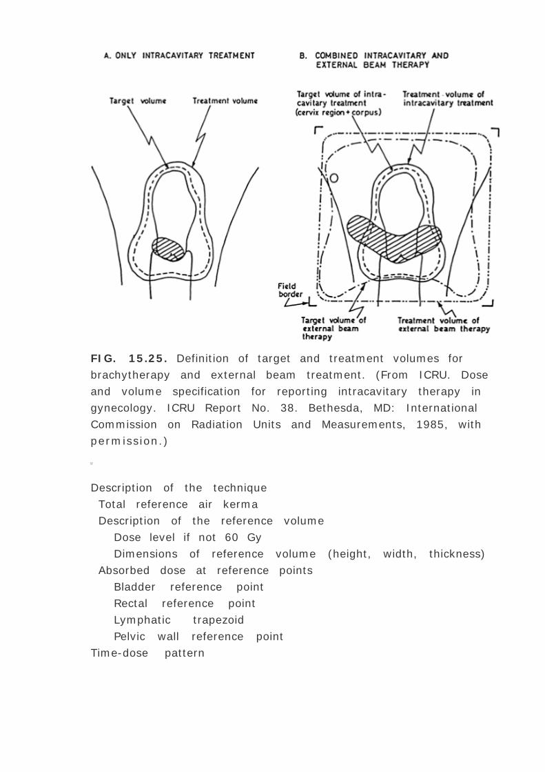
FIG. 15.25. Definition of target and treatment volumes for

brachytherapy and external beam treatment. (From ICRU. Dose

and volume specification for reporting intracavitary therapy in

gynecology. ICRU Report No. 38. Bethesda, MD: International


permission.)

Description of the technique

Total reference air kerma

Description of the reference volume

Dose level if not 60 Gy

Dimensions of reference volume (height, width, thickness)

Absorbed dose at reference points

Bladder reference point

Rectal reference point

Lymphatic trapezoid

Pelvic wall reference point

Time-dose pattern

From ICRU. Dose and volume specification for reporting

intracavitary therapy in gynecology. ICRU report no. 38. Bethesda,

MD: International Commission on Radiation Units and

Measurements, 1985.

TABLE 15.9. DATA NEEDED FOR REPORTING

INTRACAVITARY THERAPY IN GYNECOLOGY (ICRU)

P.393

Reference Volume. The reference volume is the volume of the

isodose surface that just surrounds the target volume. The value

of this isodose surface, based on the Paris experience (70 ), is set

at 60 Gy.

The prescription isodose value of 60 Gy includes the dose contribution

from the external beam. The reference volume for the intracavitary

part of the treatment should be identified and its dimensions

recorded. Figure 15.26 shows how the height (dh ), width

P.394

(dw ), and thickness (dt ) of the pear-shaped reference volume can be

measured from the oblique frontal and oblique sagittal planes. The

reference volume is approximated by (dh — dw — dt ) cm3 .

FIG. 15.26. Determination of the reference isodose surface

dimensions. dw , width; dh , height; dt , thickness. (From ICRU. Dose

and volume specification for reporting intracavitary therapy in



permission.)

FIG. 15.27. Localization of bladder and rectum points. (From ICRU.

Dose and volume specification for reporting intracavitary therapy in



permission.)

C.1. Absorbed Dose at Reference Points

Bladder Point. The bladder point is localized by using a Foley

catheter, with the balloon filled with a contrast material. On the

frontal radiograph, the bladder point is marked at the center of

the balloon; on the lateral radiograph, the bladder point is

obtained on a line drawn anteroposteriorly through the center of

the balloon, at the posterior surface (Fig. 15.27 ).

Rectal Point. The rectal point is identified on the frontal

radiograph at the midpoint of the ovoid sources (or at the lower

end of the intrauterine source). On the lateral radiograph, the

rectal point is located on a line drawn from the middle of the

ovoid sources, 5 mm behind the posterior vaginal wall (Fig. 15.27

). The posterior vaginal wall may be visualized by using

radiopaque gauze for the vaginal packing.

Lymphatic Trapezoid of Fletcher. These points correspond to the

paraaortic and iliac nodes and are shown in Fig. 15.28 .

Pelvic Wall Points. On the anteroposterior radiograph, the pelvic

wall points are located at the intersection of a horizontal tangent

to superior aspect of the acetabulum and a vertical line touching

the medial aspect of the acetabulum. On the lateral view, these

points are marked as the highest middistance points of the right

and left acetabulums (Fig. 15.29 ).

Time Dose Pattern. The duration and time sequence of the implant

relative to the external beam treatment should be recorded.

D. Commentary

Several papers have discussed the pros and cons of various dose

specification systems for the intracavitary treatment of cervix cancer

(70 ,88 ,89 ,90 ). At present, universal agreement does not exist as to

the superiority of any one system. The problem is perhaps with the

nature of brachytherapyâ€”a highly empirical discipline, no more

sophisticated than gourmet cooking. However, as in cooking, there is

a little bit of everything: art, science, technique, and taste. Although

dose specification systems should be endorsed by appropriate

committees,

P.395

I would like to take the author's privilege and express my opinion on

the subject of dose specification for cervix treatment.

FIG. 15.28. Determination of reference points corresponding to the

lymphatic trapezoid of Fletcher. (From ICRU. Dose and volume

specification for reporting intracavitary therapy in gynecology. ICRU

Report No. 38. Bethesda, MD: International Commission on Radiation

Units and Measurements, 1985, with permission.)

Established technique guidelines should be followed to take

advantage of the vast amount of clinical data that have been

accumulated with excellent results.

By using semirigid applicator such as Fletcher-Suit and the

recommended source loadings one ensures consistency of

technique. However, the dose distribution patterns will vary from

patient to patient, depending on the packing and the source

geometry achieved.

The most significant parameters that determine the clinical

outcome, in terms of tumor control and complications, are the mg

Ra eq-h or the total reference air kerma, source loading, and the

type of applicator used.

Dose to the ICRU recommended reference points provide useful

information in regard to the tolerance and adequacy of treatment.

For each application, the isodose distribution should be viewed at

least in the frontal and sagittal planes (containing the initial

straight part of the tandem). The target (cervix regions and

corpus) should be visualized on the isodose patterns to determine

the isodose surface value that just surrounds the target volume.

This should be called the minimum target dose.

The implant duration should be based on the minimum target dose

rate.

FIG. 15.29. Definition of pelvic wall points. Left , Anteroposterior

view. Right , Lateral view. (From ICRU. Dose and volume specification

for reporting intracavitary therapy in gynecology. ICRU Report No. 38.

Bethesda, MD: International Commission on Radiation Units and

Measurements, 1985, with permission.)

P.396

It is realized that the weakness of the whole system lies in the

inability to visualize the target volume. Unless the target volume can

be accurately determined and superimposed on the isodose pattern,

one cannot determine the minimum target dose.

In summary, the ICRU system of dose specification is probably the

best that can be achieved at this time. Its greatest weakness,

however, is in the determination of reference volume. Further

progress needs to be made in the determination and delineation of

target volume so that the cervix dose can be specified by the

minimum target dose.

15.8. REMOTE AFTERLOADING UNITS

Most brachytherapy is now practiced with devices that allow loading of

radioactive sources after the source containers (applicators or

catheters) are put in place in the patient and have been checked out

radiographically for proper positioning using radiopaque markers or

source dummies. Traditionally, the afterloading techniques require

manual handling of radioactive material during source preparation and

loading of the sources into the previously inserted applicators.

Although these procedures, when carried out properly, pose no greater

risk to patients and personnel than the nationally or internationally

accepted standards, they are not state of the art in minimizing

radiation hazards. Remotely controlled afterloading devices are now

available that eliminate the direct handling of the radioactive sources.

In addition, the sources can be instantly loaded and unloaded, making

it possible to provide patient care with the sources retracted into their

shielded position.

Remote afterloaders are available for either low-dose rate (LDR) or

high-dose rate (HDR) brachytherapy and for interstitial or

intracavitary treatments. With the LDR units, it is possible to use the

same type of applicators (e.g., Fletcher-Suit) and dose rates as used

in conventional brachytherapy. The room shielding requirements are

the same except that instead of using mobile shields for staff

protection, sources are automatically retracted whenever required for

patient care and reinserted after each interruption.

The HDR remote afterloader treatments are performed in a fully

shielded room with safety requirements comparable with those

required for a cobalt teletherapy unit. For example, the walls are

shielded, the room is equipped with door interlocks that retract the

source when the door is opened or when the emergency button is

pushed, radiation monitors are installed with visible and audible

alarms, the patient is monitored via remote closed-circuit television

camera and intercommunication devices, and the emergency

procedures are posted at the control station. In practice, HDR

equipment is often housed in existing cobalt or accelerator rooms.

192 Ir is the most commonly used radioisotope in remote afterloaders,

although 137 Cs or 60 Co sources also are used in some units. The

sources are contained in a storage safe when not in use. Several

channels for source transport and a mechanism to move the source(s)

from the storage safe into the applicator(s) in the patient are

provided. The most common method of source transfer is the steel

drive cable to which the source is welded. The cable is moved by a

stepping motor. In one system (Selectron), source trains with source

pallets and inactive spacers are moved by microprocessor controlled

pneumatic devices.

HDR remote afterloading implants are achieved by moving a single

high-strength (e.g., 10 Ci) 192 Ir source, welded to the end of a

flexible cable, through one or many available channels. The source

can be precisely positioned at any point in the implanted catheters or

applicators. By programming dwell position and dwell time of the

source, desired isodose distributions can be obtained. These high-dose

rate units can be used for interstitial, interluminal, or intracavitary

implant (see Chapter 22 for details).

A single-source system (micro-Selectron-PDR) also has been adopted

to provide equivalent LDR brachytherapy, using pulsed brachytherapy

principle (91 ). In this unit a single 192 Ir source of activity in the

range of 0.5 to 1.0 Ci is used. The dose is delivered in several pulses

of programmable duration and frequency.

Some of the commercially available remote afterloading systems

include the Curietron, the micro-Selectron, the Gamma Med, and the

Buchler unit. Many of these systems come in different models with

specialized functions. For a review of these systems see Glasgow (92

).

P.397

A. Advantages

The major advantage of the remote afterloaders is the elimination

or reduction of exposure to medical personnel.

Well-designed systems can provide the capability of optimizing

dose distributions beyond what is possible with manual

afterloading.

Treatment techniques can be made more consistent and

reproducible.

In LDR remote afterloading, sources can be retracted into shielded

position to allow better patient care under normal as well as

emergency conditions.

HDR remote afterloading permits treatment on an outpatient

basis, using multiple fraction regimens.

HDR remote afterloading is suited for treating large patient

populations that would otherwise require prolonged hospitalization

if treated by LDR brachytherapy.

B. Disadvantages

Remote afterloading devices are expensive and require a

substantial capital expenditure ($200,000â€“$300,000) for

equipment acquisition.

In the case of HDR, additional costs must be considered for room

shielding (if not located in an existing shielded facility) and

installing ancillary imaging equipment.

Locating HDR in an existing radiation therapy room compounds

the problem of patient scheduling unless the room is dedicated to

HDR brachytherapy.

No significant improvements are expected in clinical outcome over

state-of-the-art conventional LDR brachytherapy, although the

issue is still controversial and needs further investigation.

Quality assurance requirements for remote afterloading devices

are significantly greater because of the greater complexity of the

equipment and frequent source changes.

C. High-dose Rate versus Low-dose Rate

Whereas remote afterloading is undoubtedly a superior technique

when it comes to radiation protection and reproducibility of treatment,

the question of how HDR compares with LDR in clinical outcome is a

highly controversial issue. If HDR is or can be made equivalent to

LDR, this would be a victory for HDR, because of its other advantages

such as its ability to treat large patient populations, convenience of

treating on an outpatient basis, etc. However, the question is not

close to being settled, because the outcome data in terms of survival

rates and early and late tissue complication rates for the HDR

technique to date are not sufficient to draw definitive conclusions. The

reader is referred to selected papers to understand these issues (93

,94 ,95 ,96 ,97 ).

REFERENCES

1. Shalek RJ, Stovall M. Dosimetry in implant therapy. In: Attix

FH, Roesch WC, eds. Radiation dosimetry . Vol 3. New York:

Academic Press, 1969.


Washington, DC: International Commission on Radiation Units and

Measurements, 1971.


Washington, DC: International Commission on Radiation Units and

Measurements, 1980.

4. ICRU. Radioactivity. Report No. 10C. Washington, DC:


1963.

5. Whyte GN. Attenuation of radium gamma radiation in cylindrical

geometry. Br J Radiol 1955;28:635.

6. Van Roosenbeek E, Shalek RJ, Moore EB. Safe encapsulation

period for sealed medical radium sources. AJR 1968;102:697.

7. Meisberger LL, Keller RJ, Shalek RJ. The effective attenuation in

water of gamma rays of gold 198, iridium 192, cesium 137, radium

226, and cobalt 60. Radiology 1968;90:953.

8. Horsler AFC, Jones JC, Stacey AJ. Cesium 137 sources for use in

intracavitary and interstitial radiotherapy. Br J Radiol

1964;37:385.

P.398

9. Krishnaswamy V. Dose distribution about 137 Cs sources in

tissue. Radiology 1972;105:181.

10. Attix FH. Computed values of specific gamma ray constant for137 Cs and 60 Co. Phys Med Biol 1968;13:119.

11. O'Connell D, Joslin CA, Howard N, et al. The treatment of

uterine carcinoma using the cathetron. Br J Radiol 1967;40:882.

12. Joslin CAF, Smith CW. The use of high activity 60 Co sources

for intracavitary and surface mould therapy. Proc R Soc Med

1970;63:1029.

13. Snelling MD, Lambert HE, Yarnold JR. The treatment of

carcinoma of the cervix and endometrium at the Middlesex

Hospital. Clin Radiol 1979;30:253.

14. Henschke UK, Hilaris BS, Mahan GD. Afterloading in interstitial

and intracavitary radiation therapy. AJR 1963;90:386.

15. Pierquin B, Chassagne D, Baillet F, et al.

Lâ€™endocurietherapie des Cancers de la Langue Mobile et due

Plancher buccal par 1â€™iridium-192. Rev Med 1971;31:1947.

16. Glasgow GP, Dillman LT. Specific ³-ray constant and

exposure rate constant of 192 Ir. Med Phys 1979;6:49.

17. Boggs RF, Williams KD, Schmidt GD. Radiological health

aspects of spent radon seeds. Radiat Health Data Rep

1969;10:185.

18. Hilaris BS, ed. Handbook of interstitial brachytherapy . Acton,

MA: Publishing Science Group, 1975.

19. Kim JH, Hilaris BS. Iodine 125 source in interstitial tumor

therapy. AJR 1975;123:163.

20. Ling CC, Yorke ED, Spiro IJ, et al. Physical dosimetry of 125 I

seeds of a new design for interstitial implant. Int J Radiat Oncol

Biol Phys 1983;9:1747.

21. Schulz RJ, Chandra P, Nath R. Determination of the exposure

rate constant for 125 I using a scintillation detector. Med Phys

1980;7:355.

22. Orton CG. Time-dose-factors (TDFs) in brachytherapy. Br J

Radiol 1974;47:603.

23. Meigooni AS, Sabnis S, Nath R. Dosimetry of Pd-103

brachytherapy sources for permanent

implantsâ€”endocuriether/hyperthermia. Oncology 1990;6:107.

24. Chiu-Tsao ST, Anderson LL. Thermoluminescent dosimetry of103 Pd seeds (model 200) in solid water phantom. Med Phys

1990;18:449.

25. National Council on Radiation Protection and Measurements

(NCRP). Specification of gamma-ray brachytherapy sources. NCRP

Report No. 41. Washington, DC: U.S. Government Printing Office,

1974.

26. Loevinger R. The role of standards laboratory in brachytherapy.

In: Shearer DR, ed. Recent advances in brachytherapy physics

(AAPM Med. Phys. Monograph No. 7). New York: American Institute

of Physics, 1981.

27. American Association of Physicists in Medicine. Specification of

brachytherapy source strength. AAPM Report No. 21. New York:

American Institute of Physics, 1987.

28. Loftus TP. Standardization of cesium-137 gamma-ray sources

in terms of exposure units (roentgens). J Res Natl Bur Stand (US)

1970;74A:1â€“6.

29. Loftus TP. Standardization of iridium-192 gamma-ray sources

in terms of exposure. J Res Natl Bur Stand (US) 1980;85:19â€“25.

30. Loftus TP. Exposure standardization of 125 I seeds used for

brachytherapy. J Res Bur Stand 1984;89:295.

31. Dale JWG, Perry WE, Pulfer RF. A beta-gamma ionization

chamber for substandards of radioactivity. I and II. Int J Radiat

Isotopes 1961;10:65.

32. Berkley LW, Hanson WF, Shalek RJ. Discussion of the

characteristics and results of measurements with a portable well

ionization chamber for calibration of brachytherapy sources. In:

Shearer DR, ed. Recent advances in brachytherapy physics . New

York: American Institute of Physics, 1981.

33. Loftus TP. Standardization of iridium-192 gamma ray sources

in terms of exposure. J Res Natl Bur Stand (US) 1979;80:19.

34. Williamson JF, Khan FM, Sharma SC, et al. Methods for routine

calibration of brachytherapy sources. Radiology 1982;142:511.

35. Kubiatowciz DO. Calibration of cesium-137 brachytherapy

sources. In: Shearer DR, ed. Recent advances in brachytherapy

physics . New York: American Institute of Physics, 1981.

36. Cobb PD, Chen TS, Kase KR. Calibration of brachytherapy

iridium-192 sources. Int J Radiat Oncol Biol Phys 1981;7:259.

37. Suzuki A, Suzuki MN, Weis AM. Analysis of a radioisotope

calibration. J Nucl Med Technol 1976;4:193.

38. Boyer AL, Cobb PD, Kase KR, et al., Shearer DR, ed. Recent

advances in brachytherapy physics . New York: American Institute

of Physics, 1981.

39. Williamson JF, Morin RL, Khan FM. Dose calibrator response to

brachytherapy sources: a Monte Carlo and analytic evaluation. Med

Phys 1983;10:135.

40. Sievert RM. Die Intensit ¤tsverteilung der Prim ¤ren ³-

Strahlung in der N ¤he medizinischer Radiumpr ¤parate. Acta

Radiol 1921;1:89.

41. Young MEJ, Batho HF. Dose tables for linear radium sources

calculated by an electronic computer. Br J Radiol 1964;37:38.

P.399

42. Evans RD, Evans RO. Studies of self absorption in gamma-ray

sources. Rev Mod Phys 1948;20:305.

43. Keyser GM. Absorption correction for radium standardization.

Can J Phys 1951;29:301.

44. Whyte GN. Attenuation of radium gamma radiation in

cylindrical geometry. Br J Radiol 1955;28:635.

45. Williamson JF, Morin RL, Khan FM. Monte Carlo evaluation of

the Sievert integral for brachytherapy dosimetry. Phys Med Biol

1983;28:1021.

46. Meisberger LL, Keller R, Shalek RJ. The effective attenuation in

water of the gamma rays of gold-198, iridium-192, cesium-137,

radium-226, and cobalt-60. Radiology 1968;90:953.

47. Van Dilla MA, Hine GJ. Gamma-ray diffusion experiments in

water. Nucleonics 1952;10:54.

48. Ter-Pogossian M, Ittner WB III, Aly SM. Comparison of air and

tissue doses for radium gamma rays. Nucleonics 1952;10:50.

49. Wooton P, Shalek RJ, Fletcher GH. Investigation of the

effective absorption of radium and cobalt gamma radiation in water

and its clinical significance. AJR 1954;71:683.

50. Reuss A, Brunner F. Phantommessungen mit den

Mikroionisationskammern des Bomke-Dosimeters an Radium and

Kobalt 6. Stahlentherapie 1957;103:279.

51. Kenney GN, Kartha KIP, Cameron JR. Measurement of the

absorption and build-up factor for radium, cobalt 60 and cesium

137. Phys Med Biol 1966;11:145.

52. Meredith WJ, Greene D, Kawashima K. The attenuation and

scattering in a phantom of gamma rays from some radionuclides

used in mould and interstitial gamma-ray therapy. Br J Radiol

1966;39:280.

53. Webb S, Fox RA. The dose in water surrounding point isotropic

gamma-ray emitters. Br J Radiol 1979;52:482.

54. Evans RD. The atomic nucleus . New York: McGraw-Hill,

1955:732.

55. Kornelsen RO, Young MEJ. Brachytherapy build-up factors. Br J

Radiol 1981;54:136.

56. Krishnaswamy V. Dose distribution around an 125 I seed source

in tissue. Radiology 1976;126:489.

57. Nath R, Anderson LL, Luxton G, et al. Dosimetry of interstitial

brachytherapy sources: recommendations of the AAPM Radiation

Therapy Committee Task Group no. 43. Med Phys

1995;22:209â€“234.

58. Camerson JR, Suntharalingam N, Kenney GN.

Thermoluminescence dosimetry . Madison: University of Wisconsin

Press, 1968.

59. Hine GJ, Friedman M. Isodose measurements of linear radium

sources in air and water by means of an automatic isodose

recorder. AJR 1950;64:989.

60. Cole A, Moore EB, Shalek RJ. A simplified automatic isodose

recorder. Nucleonics 1953;11:46.

61. Merredith WJ, ed. Radium dosage: the Manchester system .

Edinburgh: Livingstone, Ltd, 1967.

62. Glasser O, Quimby EH, Taylor LS, et al. Physical foundations of

radiology , 3rd ed. New York: Harper & Row, 1961.

63. Stovall M, Shalek RJ. A study of the explicit distribution of

radiation in interstitial implantation. I. A method of calculation

with an automatic digital computer. Radiology 1962;78:950.

64. Laughlin JS, Siler WM, Holodny EI, et al. A dose description

system for interstitial radiation therapy. AJR 1963;89:470.

65. Powers WE, Bogardus CR, White W, et al. Computer estimation

of dosage of interstitial and intracavitary implants. Radiology

1965;85:135.

66. Stovall M, Shalek RJ. The M.D. Anderson method for the

computation of isodose curves around interstitial and intracavitary

radiation sources. III. Roentgenograms for input data and the

relation of isodose calculations to the Paterson Parker system. AJR

1968;102:677.

67. Henschke UK, Cevc P. Dimension averaging-a simple method

for dosimetry of interstitial implants. Radiat Biol Ther 1968;9:287.

68. Anderson LL. Dosimetry of interstitial radiation therapy. In:

Hilaris BS, ed. Handbook of interstitial brachytherapy . Acton, MA:

Publishing Sciences Group, 1975:87.

69. Pierquin B, Dutreix A, Paine C. The Paris system in interstitial

radiation therapy. Acta Radiol Oncol 1978;17:33.

70. Pierquin B, Wilson JF, Chassagne D, eds. Modern

brachytherapy . New York: Masson, 1987.

71. Dutreix A. Can we compare systems for interstitial therapy?.

Radiother Oncol 1988;13:127.

72. Sharma SC, Williamson JF, Cytacki E. Dosimetric analysis of

stereo and orthogonal reconstruction of interstitial implants. Int J


73. Paterson R. The treatment of malignant disease by

radiotherapy . Baltimore: Williams & Wilkins, 1963.

74. Henschke UK, Hilaris BS, Mahan GD. Afterloading in interstitial

and intracavitary radiation therapy. AJR 1963;90:386.

75. Suit HD, Moore EB, Fletcher GH, et al. Modifications of Fletcher

ovoid system for afterloading using standard-size radium tubes

(milligram and microgram). Radiology 1963;81:126.

76. Hilaris BS, ed. Handbook of interstitial brachytherapy . Acton,

MA: Publishing Science Group, 1975.

77. Henschke UK. Interstitial implantation with radioisotopes. In:

Hahn PF, ed. Therapeutic use of artificial radioisotopes . New York:


78. Jones CH, Taylor KW, Stedeford JBH. Modification to the Royal

Marsden Hospital gold grain implantation gun. Br J Radiol

1965;38:672.

79. Heyman J. The technique in the treatment of cancer uteri at

radium-hemmet. Acta Radiol 1929;10:49.

P.400

80. Regaud C. Radium therapy of cancer at the radium institute of

Paris. AJR 1929;21:1.

81. Fletcher GH, Shalek RJ, Cole A. Cervical radium applicators

with screening in the direction of bladder and rectum. Radiology

1953;60:77.

82. Fletcher GH. Textbook of radiotherapy , 2nd ed. Philadelphia:

Lea & Febiger, 1973:620.

83. Heyman J, Reuterwall O, Benner S. The radium-hemmet

experience with radiotherapy in cancer of the corpus of the uterus.

Acta Radiol 1941;22:11.

84. Fletcher GH. Squamous cell carcinoma of the uterine cervix.

In: Fletcher GH, ed. Textbook of radiotherapy , 3rd ed.

Philadelphia: Lea & Febiger, 1980:720.

85. Tod MC, Meredith WJ. A dosage system for use in the

treatment of cancer of the uterine cervix. Br J Radiol 1938;11:809.

86. Tod M, Meredith WJ. Treatment of cancer of the cervix uteri-a

revised â€œManchester method.â€ . Br J Radiol 1953;26:252.

87. Schwaz G. An evaluation of the Manchester system of

treatment of carcinoma of the cervix. AJR 1969;105:579.

88. ICRU. Dose and volume specification for reporting intracavitary

therapy in gynecology. ICRU Report No. 38. Bethesda, MD:


1985.

89. Potish RA. Cervix cancer. In: Levitt SH, Khan FM, Potish RA,

eds. Technological basis of radiation therapy . Philadelphia: Lea &

Febiger, 1992:289.

90. Khan FM. Brachytherapy: rules of implantation and dose

specification. In: Levitt SH, Khan FM, Potish RA, eds. Technological

basis of radiation therapy . Philadelphia: Lea & Febiger, 1992:113.

91. Hall EJ, Brenner DJ. Conditions for the equivalence of

continuous to pulsed low dose rate brachytherapy. Int J Radiat


92. Glasgow GP. High dose rate afterloaders: dosimetry and quality

assurance. In: Purdy JA, ed. Advances in radiation oncology

physics . AAPM Monograph No. 19. New York: American Institute of

Physics, 1990:770.

93. Speiser B. Advances of high dose rate remote afterloading:

physics or biology. Int J Radiat Oncol Biol Phys 1991;20:1133.

94. Orton C, Seyedsadr M, Somnay A. Comparison of high and low

dose rate remote afterloading for cervix cancer and the importance

of fractionation. Int J Radiat Oncol Biol Phys 1991;21:1425.

95. Hall E, Brenner D. The dose-rate effect revisited:

radiobiological considerations of importance in radiotherapy. Int J


96. Stitt J, Fowler J, Thomadsen B, et al. High dose rate

intracavitary brachytherapy for carcinoma of the cervix: the

Madison system: I-clinical and biological considerations. Int J


97. Eifel PJ. High-dose-rate brachytherapy for carcinoma of the

cervix: high tech or high risk?. Int J Radiat Oncol Biol Phys

1992;24:383.

1 ICRU (2 ) defines the exposure rate constant as:

where (dx /dt ) ´ is the exposure rate due to photons of energy

greater than ´, at a distance l from a point source of activity A.

Special units of “ ´ are Rm2 h-1 Ci-1 or any convenient multiple of

these.

This quantity replaces, but is not identical to, the specific ³ ray

constant. The latter applied to ³ rays only and did not include the

exposure rate of emitted x-rays such as characteristic x-rays and

internal bremsstrahlung.

A further change has been made by the ICRU (3 ). A new quantity,

called air kerma rate constant , has been recommended to replace the

exposure rate constant. This quantity is still named “ ´ , but is now

defined as:

where k air is the air kerma. The SI unit for this quantity is m2 Jkg-1

h-1 Ci-1 . When the special names, gray (Gy) and becquerel (Bq) are

used, the unit becomes m2 Gy Bq-1 sec-1 .

2 Medical Products Division/3M, New Brighton, Minnesota.

3 Manufactured by Theragenics Corp., Norcross, Georgia.

4 The authors appear to have normalized the dose values to unity at r

= 1 cm. Spot checks of Fig. 15.12 revealed that the tissue attenuation

correction factor is given by Dr /D 1 , where D 1 is the dose at 1 cm.

5 These results can be ascertained by substituting µâ€² = 0 in

Equation 15.10 and separating out the geometric factor.

6 If it is not possible to cross an end, one can increase the size of the

implant by using longer needles so that the effective area of dose

uniformity adequately covers the tumor. Again, 10% is deducted from

the implant area for each uncrossed end for table reading purposes.





16 - Radiation Protection

16

Radiation Protection

Radiation exposure limits or standards were introduced as early as

the start of the twentieth century when the potential hazards of

radiation were realized. One of the first standard setting bodies

was the International Commission on Radiological Protection

(ICRP), which continues its function through its series of

publications. These reports form the basis for many national

protection guidelines. In the United States, the National Council

on Radiation Protection and Measurements (NCRP) has functioned

as a primary standard-setting body through its separate

publications. One of the agencies with regulatory powers in this

country is the Nuclear Regulatory Commission (NRC), which has

control over the use of all reactor-produced materials (e.g., 60 Co

and 192 Ir). The naturally occurring radioactive materials (e.g.,

radium and radon) and x-ray machines are regulated by individual

states.

16.1. DOSE EQUIVALENT

Because the biologic effects of radiation depend not only on dose

but also on the type of radiation, the dosimetric quantity relevant

to radiation protection is the dose equivalent (TH ). It is defined

as:

where D is the absorbed dose and Q is the quality factor for the

radiation.1

The SI unit for both dose and dose equivalent is joules per

kilogram, but the special name for the SI unit of dose equivalent

is sievert (Sv).

1 Sv = 1 J/kg

If dose is expressed in units of rad, the special unit for dose

equivalent is called the rem.

H (rem) = D (rad) ·Q

Because Q is a factor and has no units,

1 rem = 10-2 , J/kg

The use of quality factor in radiation protection is analogous to the

use of relative biological effectiveness (RBE) in radiation biology.

However, the quality factor is a somewhat arbitrarily chosen

conservative value based on a range of RBEs related to the linear

energy transfer (LET) of the radiation. Thus the Q factor

encompasses RBEs in a very broad sense, independent of the

organ or tissue or of the biologic endpoint under consideration.

Although the dose equivalent for particular situations can be

calculated (1 ), it is convenient for quick-and-rough calculations to

have a table of practical quality factors available. Table 16.1 gives

these approximate factors for a variety of radiations used in

radiation therapy.

X-rays, ³ rays, and electrons

1

Thermal neutrons

5

Neutrons, heavy particles

20

Data are from NCRP. Recommendations on limits for exposure to

ionizing radiation. Report no. 91. Bethesda, MD: National Council

on Radiation Protection and Measurements, 1987, with permission.

Radiation Quality Factor

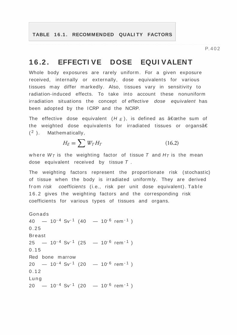
TABLE 16.1. RECOMMENDED QUALITY FACTORS

P.402

16.2. EFFECTIVE DOSE EQUIVALENT

Whole body exposures are rarely uniform. For a given exposure

received, internally or externally, dose equivalents for various

tissues may differ markedly. Also, tissues vary in sensitivity to

radiation-induced effects. To take into account these nonuniform

irradiation situations the concept of effective dose equivalent has

been adopted by the ICRP and the NCRP.

The effective dose equivalent (H E ), is defined as â€œthe sum of

the weighted dose equivalents for irradiated tissues or organsâ€

(2 ). Mathematically,

where WT is the weighting factor of tissue T and HT is the mean

dose equivalent received by tissue T .

The weighting factors represent the proportionate risk (stochastic)

of tissue when the body is irradiated uniformly. They are derived

from risk coefficients (i.e., risk per unit dose equivalent). Table

16.2 gives the weighting factors and the corresponding risk

coefficients for various types of tissues and organs.

Gonads

40 — 10-4 Sv-1 (40 — 10-6 rem-1 )

0.25

Breast

25 — 10-4 Sv-1 (25 — 10-6 rem-1 )

0.15

Red bone marrow

20 — 10-4 Sv-1 (20 — 10-6 rem-1 )

0.12

Lung

20 — 10-4 Sv-1 (20 — 10-6 rem-1 )

0.12

Thyroid

5 — 10-4 Sv-1 (5 — 10-6 rem-1 )

0.03

Bone surface

5 — 10-4 Sv-1 (5 — 10-6 rem-1 )

0.03

Remainder

50 — 10-4 Sv-1 (50 — 10-6 rem-1 )

0.30

Total

165 — 10-4 Sv-1 (165 — 10-6 rem-1 )

1.00

From NCRP. Recommendations on limits for exposure to ionizing

radiation. Report no. 91. Bethesda, MD: National Council on

Radiation Protection and Measurements, 1987, with permission.

Values are from ICRP. Recommendations of the International

Commission on Radiological Protection. Report no. 26. New York:

Pergamon Press, 1977.

Tissue (T) Risk Coefficient WT

TABLE 16.2. RECOMMENDED VALUES OF THE WEIGHTING

FACTORS WT , FOR CALCULATING EFFECTIVE DOSE

EQUIVALENT AND THE RISK COEFFICIENTS FROM WHICH

THEY WERE DERIVED

A. Risk Estimates

The risk estimates given in Table 16.2 include an assumption of

full expression of the cancer risk and an assumption of a

population distribution over all ages and both sexes. The genetic

component includes severe genetic effects for the first two

generations. In the total risk coefficient, the somatic risk is 125

— 10-4 Sv-1 (125 — 10-6 rem-1 ), which for radiation

protection purposes is rounded off to 1 — 10-2 Sv-1 (1 — 10-4

rem-1 ). The genetic component of the risk is 40 — 10-4 Sv-1

(0.4 — 10-4 rem-1 ).

P.403

16.3. BACKGROUND RADIATION

Radiation is a part of the natural environment. This background

radiation is contributed principally by three sources: terrestrial

radiation, cosmic radiation, and radiation from radioactive

elements in our bodies. Table 16.3 gives average values of

background radiation to which various parts of the body are

exposed annually. The total effective dose equivalent for a

member of the population in the United States from various

sources of natural background radiation is approximately 3.0

mSv/year (300 mrem/year).

WT

0.12

0.25

0.03

0.12

0.48

1.0

Cosmic

0.03

0.07

0.008

0.03

0.13

0.27

Cosmogenic

0.001

0.002

â€”

0.004

0.003

0.01

Terrestrial

0.03

0.07

0.008

0.03

0.14

0.28

Inhaled

2.0

â€”

â€”

â€”

â€”

2.0

In the body

0.04

0.09

0.03

0.06

0.17

0.40

Rounded totals

2.1

0.23

0.05

0.12

0.44

3.0a The effective dose equivalent rates for Canada are approximately

20% lower for the terrestrial and inhaled components.b 1mSv = 100 mrem.

From NCRP. Exposure of the population in the United States and

Canada from natural background radiation. Report no. 94.

Bethesda, MD: National Council on Radiation Protection and

Measurements, 1987, with permission.

Source Total Effective Dose Equivalent Rate

(mSv/y)b

Lung Gonads Bone

Surfaces

Bone

Marrow

Other

Tissues

Total

TABLE 16.3. ESTIMATED TOTAL EFFECTIVE DOSE

EQUIVALENT RATE FOR A MEMBER OF THE POPULATION IN

THE UNITED STATES AND CANADA a FROM VARIOUS

SOURCES OF NATURAL BACKGROUND RADIATION

The terrestrial radiation varies over the earth because of

differences in the amount of naturally occurring elements in the

earthâ€™s surface. In addition, building materials may incorporate

naturally occurring radioactive materials. Many buildings may have

elevated levels of radon emitted by naturally occurring uranium-

238 in the soil. It has been estimated (3 ) that the average annual

dose equivalent to bronchial epithelium from radon decay products

is approximately 24 mSv (2.4 rem).

Cosmic radiation levels change with elevation. For example, air

travel exposes individuals to increased radiation exposure. It has

been estimated that at 30,000 feet the dose equivalent is

approximately 0.5 mrem/hour (4 ).

The internal irradiation arises mainly from 40 K in our body, which

emits ² and ³ rays and decays with a half-life of 1.3 — 109

years.

In addition to the background radiation, the population is exposed

to radiation from various medical proceduresâ€”the planned

exposure of patients, as distinct from occupational exposures

received by health personnel. It was estimated by the U.S. Public

Health Service that the average annual genetically significant dose

equivalent2 in 1970 was approximately 20 mrem/year from

radiologic procedures.

Under ordinary circumstances, exposures from natural background

radiation and medical procedures are not included in the

occupational exposure controls for the individual cases.

16.4. LOW-LEVEL RADIATION EFFECTS

A vast literature exists on the biologic effects of radiation.

Discussions pertinent to radiation protection can be found in

reports of the United Nations Scientific Committee on the Effects

of Atomic Radiation (6 ).

P.404

Whereas large doses of radiation produce identifiable effects

within a relatively short period, the effects are difficult to

ascertain at low doses (e.g., less than 10 cGy). The difficulty is

due mainly to the extremely low frequency with which these

effects might occur. The statistical problems are enormous in

identifying small effects in the constant presence of spontaneously

occurring effects. However, certain effects have been

demonstrated in humans and other mammals at doses lower than

those required to produce acute radiation syndrome but greatly in

excess of dose limits recommended by the standards setting

bodies. Thus exposures to low-level radiation may produce (a)

genetic effects, such as radiation-induced gene mutations,

chromosome breaks, and anomalies; (b) neoplastic diseases, such

as increased incidence of leukemia, thyroid tumors, and skin

lesions; (c) effect on growth and development, such as adverse

effects on fetus and young children; (d) effect on life span, such

as diminishing of life span or premature aging; and (e) cataracts

or opacification of the eye lens.

The harmful effects of radiation may be classified into two general

categories: stochastic effects and nonstochastic effects. The NCRP

(2 ) defines these effects as follows.

A stochastic effect is one in which â€œthe probability of

occurrence increases with increasing absorbed dose but the

severity in affected individuals does not depend on the magnitude

of the absorbed dose.â€ In other words, a stochastic effect is an

all or none phenomenon, such as the development of a cancer or

genetic effect. Although the probability of such effects occurring

increases with dose, their severity does not.

A nonstochastic effect is one â€œwhich increases in severity with

increasing absorbed dose in affected individuals, owing to damage

to increasing number of cells and tissues.â€ Examples of

nonstochastic effects are radiation-induced degenerative changes

such as organ atrophy, fibrosis, lens opacification, blood changes,

and decrease in sperm count.

Whereas no threshold dose can be predicted for stochastic effects,

it is possible to set threshold limits on nonstochastic effects that

are significant or seriously health impairing. However, for the

purpose of radiation protection, a cautious assumption is made

that â€œthe dose-risk relationship is strictly proportional (linear)

without threshold, throughout the range of dose equivalent and

dose equivalent rates of importance in routine radiation

protect ion.â€

Many analysts believe that these two assumptions may

overestimate the biologic effects at low dose levels. Some have

proposed a linear quadratic dose-response curve that assigns

relatively reduced effects to low doses. However, in the absence of

more reliable data it seems prudent to adopt a conservative

model, the nonthreshold linear response, for predicting low dose

effects. For further discussion of dose-response models, the reader

is referred to references 7 to 10.

16.5. EFFECTIVE DOSE EQUIVALENT

LIMITS

NCRP (2 ) recommendations on exposure limits of radiation

workers are based on the following criteria: (a) at low radiation

levels the nonstochastic effects are essentially avoided; (b) the

predicted risk for stochastic effects should not be greater than the

average risk of accidental death among workers in â€œsafeâ€

industries; and (c) ALARA principle should be followed, for which

the risks are kept as low as reasonably achievable , taking into

account social and economic factors.

It is important to compare radiation risks with the risks in other

industries when setting radiation protection standards. Table 16.4

gives data on annual fatality rates from accidents in different

occupations. On the basis of these data, â€œsafeâ€ industries

are defined as â€œthose having an associated annual fatality

accident rate of 1 or less per 10,000 workers, that is, an average

annual risk of 10-4 (2 ). The available data for the radiation

industries show average fatal accident rate of less than 0.3 —

10-4 (11 ). From this perspective, the radiation industries compare

favorably with the â€œsafeâ€ industries. For radiation protection

purposes, the total risk coefficient is assumed to be 1 — 10-2 Sv-

1 (1 — 10-4 rem-1 ).

Trade

24,000

0.5

Manufacturing

19,900

0.6

Service

28,900

0.7

Government

15,900

0.9

Transportation and utilities

5,500

2.7

Construction

5,700

3.9

Agriculture

3,400

4.6

Mining, quarrying

1,000

6.0

All industries (U.S.)

104,300

1.1a Certain occupations have higher annual fatal accident rates than

those given here.

Reprinted from NCRP. Recommendations on limits for exposure to

ionizing radiation. Report no. 91. Bethesda, MD: National Council

on Radiation Protection and Measurements, 1987, with permission.

Data are from NSC. Accident facts 1984. Chicago: National Safety

Council, 1985.

Occupation Number of

Workers — 103

Annual Fatal Accident Rate

(per 10,000 Workers)

TABLE 16.4. ANNUAL FATALITY RATES FROM ACCIDENTS

IN DIFFERENT OCCUPATIONS a

P.405

A. Occupational and Public Dose Limits

Table 16.5 gives occupational and public dose equivalent limits as

recommended by the NCRP (2 ). These limits do not include

exposure received from medical procedures or the natural

background. Radiation workers are limited to an annual effective

dose equivalent of 50 mSv (5 rem) and the general public is not to

exceed one tenth of this value (0.5 rem) for infrequent exposure

and 1 mSv (0.1 rem) for continuous or frequent exposure. Higher

P.406

limits are set for some organs and areas of the body that involve

nonstochastic effects and are less sensitive to radiation than

others. For example, the annual occupational dose equivalent limit

to the lens of the eye is 150 mSv (15 rem) and to other organs is

500 mSv (50 rem).

A. Occupational exposures (annual)

1. Effective dose equivalent limit (stochastic effects)

50 mSv

(5 rem)

2. Dose equivalent limits for tissues and organs (nonstochastic

effects)

a. Lens of eye

150 mSv

(15 rem)

b. All others (e.g., red bone marrow, breast, lung, gonads,

skin, and extremities)

500 mSv

(50 rem)

3. Guidance: cumulative exposure

10 mSv — age

(1 rem — age in yr)

B. Planned special occupational exposure, effective dose

equivalent limit

see section 15a

C. Guidance for emergency occupational exposure

See section 16a

D. Public exposures (annual)

1. Effective dose equivalent limit, continuous or frequent

exposure

1 mSv

(0.1 rem)

2. Effective dose equivalent limit, infrequent exposure

5 mSv

(0.5 rem)

3. Remedial action recommended when:

a. Effective dose equivalent

>5 mSv

(>0.5 rem)

b. Exposure to radon and its decay products

>0.007 Jhm-3

(>2 WLM)

4. Dose equivalent limits for lens of eye, skin, and extremities

50 mSv

(5 rem)

E. Education and training exposures (annual)

1. Effective dose equivalent

1 mSv

(0.1 rem)

2. Dose equivalent limit for lens of eye, skin, and extremities

50 mSv

(5 rem)

F. Embryo-fetus exposures

1. Total dose equivalent limit

5 mSv

(0.5 rem)

2. Dose equivalent limit in a month

0.5 mSv

(0.05 rem)

G. Negligible individual risk level (annual) effective dose

equivalent per source or practice

0.01 mSv

(0.001 rem)a In NCRP Report no. 91.

From NCRP. Recommendations on limits for exposure to ionizing

radiation. Report no. 91. Bethesda, MD: National Council on

Radiation Protection and Measurements, 1987, with permission.

TABLE 16.5. SUMMARY OF RECOMMENDATIONS

The NCRP has discontinued its previous recommendation of the

age-proration formula for the cumulative limit, that is, (age - 18)

— 5 rem. The new guidance is that the numerical value of the

individual workerâ€™s lifetime effective dose equivalent in tens of

mSv (rem) does not exceed the value of his or her age in years.

Students under the age of 18 who may be exposed to radiation as

a result of their educational or training activities should not

receive more than 1 mSv (0.1 rem) per year.

B. Dose Limits for Pregnant Women

The pregnant woman who is a radiation worker can be considered

as an occupationally exposed individual, but the fetus cannot. The

total dose equivalent limit to an embryo-fetus is 5 mSv (0.5 rem),

with the added recommendation that exposure to the fetus should

not exceed 0.5 mSv (0.05 rem) in any one month.

Premenopausal women must be informed of the potential risk of

exposure to the fetus and methods available to minimize the

exposure. If there is a possibility of the fetus receiving more than

5 mSv (0.5 rem) during the gestation period, the employee should

discuss her options with her employer. Once a pregnancy is made

known, the dose equivalent limit of 0.5 mSv (0.05 rem) in any one

month should be the guiding principle. Even if there is practically

no possibility of this limit being exceeded, it is prudent to assign

pregnant workers to duties that involve potential exposure much

lower than the recommended limit. For example, some institutions

have developed a policy of not assigning pregnant technologists to

work with cobalt-60 teletherapy units (because of constant

radiation leakage from the source housing) or to handle

brachytherapy sources. Such measures come under the ALARA

principle, that is, the principle of limiting the dose of exposed

persons (in this case the fetus) to levels as low as is reasonably

achievable, taking into account economic and social factors.

C. Negligible Individual Risk Level

A negligible individual risk level (NIRL) is defined by the NCRP (2 )

as â€œa level of average annual excess risk of fatal health effects

attributable to irradiation, below which further effort to reduce

radiation exposure to the individual is unwarranted.â€ The NCRP

also states that â€œthe NIRL is regarded as trivial compared to

the risk of fatality associated with ordinary, normal societal

activities and can, therefore, be dismissed from consideration

. â €

The concept of NIRL is applied to radiation protection because of

the need for having a reasonably negligible risk level that can be

considered as a threshold below which efforts to reduce the risk

further would not be warranted or, in the words of the NCRP,

â€œwould be deliberately and specifically curtailed.â€

To avoid misinterpretation of the relationships between the NIRL,

ALARA, and maximum permissible levels, the NCRP points out that

the NIRL should not be thought of as an acceptable risk level, a

level of significance, or a limit. Nor should it be the goal of ALARA,

although it does provide a lower limit for application of the ALARA

process. The ALARA principle encourages efforts to keep radiation

exposure as low as reasonably achievable, considering the

economic and social factors.

The annual NIRL has been set at a risk of 10-7 , corresponding to a

dose equivalent of 0.01 mSv (0.001 rem). This corresponds to a

lifetime (70 years) risk of 0.7 — 10-5 .

Example

Calculate the risk for (a) radiation workers, (b) members of the

general public, and (c) NIRL, corresponding to respective annual

effective dose equivalent limits (Table 16.5 ). Assume risk

coefficient of 10-2 Sv-1 (10-4 rem-1 ).

P.407

Annual effective dose equivalent limit for:

radiation workers = 50 mSv (5 rem)

Annual risk = 5 rem — (10-4 rem-1 )

= 5 — 10-4

Annual effective dose equivalent limit for members of:

general public = 1 mSv (0.1 rem)

Annual risk = 0.1 rem — (10-4 rem-1 )

= 10-5

Annual effective dose equivalent limit for NIRL:

= 0.01 mSv (0.001 rem)

Annual risk = 0.001 rem — (10-4 rem-1 )

= 10-7

16.6. STRUCTURAL SHIELDING DESIGN

Radiation protection guidelines for the design of structural

shielding for radiation installations are discussed in the NCRP

Reports 49 and 51 (12 ,13 ). These reports contain the necessary

technical information as well as recommendations for planning

new facilities and remodeling existing facilities. The reader is

referred to these reports for comprehensive details on this subject.

This section will discuss only some of the basic factors that are

considered in the calculation of barrier thicknesses.

Protective barriers are designed to ensure that the dose equivalent

received by any individual does not exceed the applicable

maximum permissible value. The areas surrounding the room are

designated as controlled or noncontrolled , depending on whether

or not the exposure of persons in the area is under the supervision

of a radiation protection supervisor. For protection calculations,

the dose equivalent limit is assumed to be 0.1 rem/week for the

controlled areas and 0.01 rem/week for the noncontrolled areas.

These values approximately correspond to the annual limits of 5

rem/year and 0.5 rem/year, respectively.

Protection is required against three types of radiation: the primary

radiation; the scattered radiation; and the leakage radiation

through the source housing. A barrier sufficient to attenuate the

useful beam to the required degree is called the primary barrier .

The required barrier against stray radiation (leakage and scatter)

is called the secondary barrier . The following factors enter into

the calculation of barrier thicknesses.

Workload (W) . For x-ray equipment operating below 500 kVp,

the workload is usually expressed in milliampere minutes per

week, which can be computed by multiplying the maximum mA

with approximate minutes/week of beam â€œonâ€ time. For

megavoltage machines, the workload is usually stated in terms

of weekly dose delivered at 1 m from the source. This can be

estimated by multiplying the number of patients treated per

week with the dose delivered per patient at 1 m. W is

expressed in rad/week at 1 m.

Use Factor (U) . Fraction of the operating time during which

the radiation under consideration is directed toward a

particular barrier. Although the use factors vary depending on

the techniques used in a given facility, typical values are

given in Table 16.6 .

Occupancy Factor (T) . Fraction of the operating time during

which the area of interest is occupied by the individual. If

more realistic occupancy factors are not available, values

given in Table 16.7 may be used.

Distance (d) . Distance in meters from the radiation source to

the area to be protected. Inverse square law is assumed for

both the primary and stray radiation.

Floor

1

Walls

¼

Ceiling

¼â€“ ½, depending on equipment and techniques

Location Use Factor

TABLE 16.6. TYPICAL USE FACTOR FOR PRIMARY

PROTECTIVE BARRIERS

Full occupancy (T = 1)

Work areas, offices, nursesâ€™ stations

Partial occupancy (T = ¼)

Corridors, restrooms, elevators with operators

Occasional occupancy (T = 1/8â€“1/16)

Waiting rooms, restrooms, stairways, unattended elevators,

outside areas used only for pedestrians or vehicular traffic

TABLE 16.7. TYPICAL OCCUPANCY FACTORS

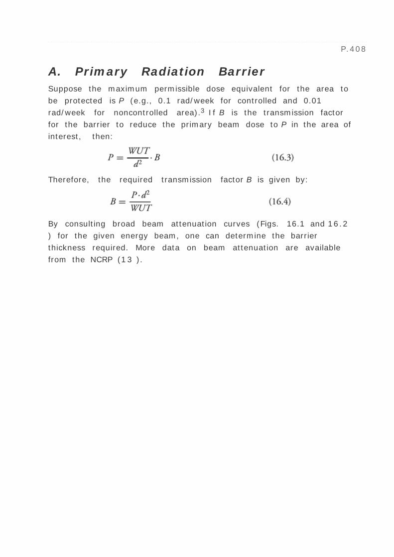
P.408

A. Primary Radiation Barrier

Suppose the maximum permissible dose equivalent for the area to

be protected is P (e.g., 0.1 rad/week for controlled and 0.01

rad/week for noncontrolled area).3 If B is the transmission factor

for the barrier to reduce the primary beam dose to P in the area of

interest, then:

Therefore, the required transmission factor B is given by:

By consulting broad beam attenuation curves (Figs. 16.1 and 16.2

) for the given energy beam, one can determine the barrier

thickness required. More data on beam attenuation are available

from the NCRP (13 ).

FIG. 16.1. Transmission through concrete (density 2.35 g cm-3 )

of x-rays produced by 0.1- to 0.4-MeV electrons, under broad-

beam conditions. Electron energies designated by an asterisk were

accelerated by voltages with pulsed wave form; unmarked electron

energies were accelerated by a constant potential generator.

Curves represent transmission in dose-equivalent index ratio.

(Reprinted with permission from NCRP. Radiation protection design

guidelines for 0.1â€“100 MeV particle accelerator facilities. Report

No. 51. Washington, DC: National Council on Radiation Protection

and Measurements, 1977.)

FIG. 16.2. Transmission of thick-target x-rays through ordinary

concrete (density 2.35 g cm-3 ), under broad-beam conditions.

Energy designations on each curve (0.5 to 176 MeV) refer to the

monoenergetic electron energy incident on the thick x-ray

production target. Curves represent transmission to dose

equivalent index ratio. (Reprinted with permission from NCRP.

Radiation protection design guidelines for 0.1â€“100 MeV particle

accelerator facilities. Report No. 51. Washington, DC: National

Council on Radiation Protection and Measurements, 1977.)

The choice of barrier material, for example, concrete, lead, or

steel, depends on structural and spatial considerations. Because

concrete is relatively cheap, the walls and roof barriers are usually

constructed out of concrete. Lead or steel can be used where space

is at a premium. For megavoltage x and ³ radiation, equivalent

thickness of various materials can be calculated by comparing

tenth value layers (TVL) for the given beam energy. If such

information is not available specifically for a given material,

relative densities can be used in most cases. Densities and TVLs

for different materials and beam energies are available from the

NCRP (13 ).

B. Secondary Barrier for Scattered

Radiation

Radiation is scattered from the patient in all directions. The

amount of scattered radiation depends on the beam intensity

incident on the scatterer, the quality of radiation, the area of the

beam at the scatterer, and the scattering angle. The ratio of

scattered dose to the incident dose may be denoted by ±. Table

16.8 gives values of ± for various angles and beam qualities. For

megavoltage beams, ± is usually assumed to be 0.1% for 90

degrees scatter.

15

9 — 10-3

30

6.0 — 10-3

7 — 10-3

45

3.6 — 10-3

2.7 — 10-3

1.8 — 10-3

60

2.3 — 10-3

1.1 — 10-3

90

0.9 — 10-3

0.6 — 10-3

135

0.6 — 10-3

0.4 — 10-3

a Scattered radiation measured at 1 m from phantom when field

area is 400 cm2 at the phantom surface; incident exposure

measured at center of field but without phantom.

From NCRP. Medical x-ray and gamma-ray protection for energies

up to 10 MeV. Structural shielding design and evaluation. Report

no. 34. Washington, DC: National Council on Radiation Protection

and Measurements, 1970, with permission.

Data also are available in NCRP. Radiation protection design and

guidelines for 0.1â€“100 MeV particle accelerator facilities. Report

no. 51. Washington, DC: National Council on Radiation Protection

and Measurements, 1977.

Scattering Angle (From Central

Ray)

³

Rays

X-

Rays

60 Co 4 MV 6

MV

TABLE 16.8. RATIO, ±, OF SCATTERED TO INCIDENT

EXPOSURE a

The scattered radiation, in general, has lower energy compared

with the incident energy. However, the softening of the beam as a

result of Compton scatter depends on the incident energy and the

direction of scatter. For orthovoltage radiation, the quality of

scattered radiation is usually assumed to be the same as that of

the incident beam. For megavoltage beams, on the other hand, the

maximum energy of the 90-degree scattered photons is 500 keV.

Therefore, the transmission of this scattered radiation through a

barrier is estimated to be approximately the same as that for a

500-kVp useful beam. At smaller scattering angles, however, the

scattered beam has greater penetrating power (14 ). In addition, a

greater fraction of the incident beam is scattered at smaller

angles.

Suppose a transmission factor of Bs is required to reduce the

scattered dose to an acceptable level P in the area of interest;

then:

P.409

where ± is the fractional scatter at 1 m from the scatterer, for

beam area of 400 cm2 incident at the scatterer, d is the distance

from source to the scatterer, d â€² is the distance from the

scatterer to the area of interest, and F is the area of the beam

incident at the scatterer. The use factor for the secondary barrier

is considered unity.

Thus the barrier transmission Bs is given by:

The required thickness of concrete or lead can be determined for

appropriate transmission curves given by the NCRP (13 ) or Figs.

16.1 and 16.2 .

C. Secondary Barrier for Leakage

Radiation

The leakage requirements of therapeutic source assemblies have

been revised and are currently described in the NCRP Report 102

(15 ). This report supersedes the previous NCRP Report 33. The

new recommendations are summarized below:

P.410

5 to 50 kVp . The leakage exposure rate4 shall not exceed 0.1

R in any 1 hour at any point 5 cm from the source assembly.

Greater than 50 kVp and less than 500 kVp . The leakage

exposure rate at a distance of 1 m from the source shall not

exceed 1 R in any 1 hour. In addition, these assemblies shall

limit exposure rate to 30 R/h at 5 cm from the surface of the

assembly.

Greater than 500 kVp . The absorbed dose rate due to leakage

radiation (excluding neutrons) at any point outside the

maximum field size, but within a circular plane of radius 2 m

that is perpendicular to and centered on the central axis at the

normal treatment distance, shall not exceed 0.2% of the

useful beam dose rate at the treatment distance. Except for

the area defined above, the leakage dose rate from the source

assembly at any point at a distance of 1 m from the electron

path between the source and the target shall not exceed 0.5%

of the useful beam dose rate at the treatment distance. The

neutron contribution to the dose within the useful beam shall

be kept well below 1% of the x-ray dose. Outside the useful

beam, the neutron dose should be reduced to as low as

practicable.

Cobalt teletherapy . Leakage dose rate from this source

housing with the beam in the â€œoffâ€ position shall not

exceed 2 mrad/hour on the average and 10 mrad/hour

maximum in any direction, at a distance of 1 m from the

source. With the beam in the â€œonâ€ position, the leakage

dose rate from the source housing shall not exceed 0.1% of

the useful beam dose rate, both measured at a distance of 1 m

from the source. In addition, for sources that give rise to a

useful beam dose rate of less than 1,000 rad/hour at 1 m, the

leakage from the source housing shall not exceed 1 rad/h at 1

m from the source.

P.411

Because leakage radiation is present whenever the machine is

operated, the use factor for leakage is unity. Suppose the required

secondary barrier for leakage radiation has a transmission factor

of BL to reduce the leakage dose to the maximum permissible level

P (rem/week).

For therapy units below 500 kVp:

where I is the maximum tube current. The number 60 is used to

convert leakage limit of 1 R/hour to 1/60 R/minute, because the

workload W is expressed in terms of mA-minute/week.

For a megavoltage therapy unit,

The factor 0.001 is the 0.1% leakage limit through the source

housing.5

Thus the transmission factor BL for the leakage barrier is given by:

and

The quality of leakage radiation is approximately the same as that

of the primary beam. Therefore, the transmission curve for the

primary beam should be used to determine the leakage barrier

thickness (Figs. 16.1 , 16.2 ).

For megavoltage therapy installations, the leakage barrier usually

far exceeds that required for the scattered radiation, because the

leakage radiation is more penetrating than the scattered radiation.

For the lower-energy x-ray beams, however, the difference

between the barrier thickness for the leakage and for the scattered

radiation is relatively less.

A barrier designed for primary radiation provides adequate

protection against leakage and scattered radiation. If a barrier is

designed for stray radiation only, the thickness is computed for

leakage and scattered radiations separately. If the thicknesses of

the two

P.412

barriers differ by at least three HVLs, the thicker of the two will be

adequate. If the difference is less than three HVLs, one HVL

should be added to the larger one to obtain the required secondary

barrier.

D. Door Shielding

Unless a maze entranceway is provided, the door must provide

shielding equivalent to the wall surrounding the door. For

megavoltage installations, a door that provides direct access to

the treatment room will have to be extremely heavy. It will

require a motor drive as well as a means of manual operation in

case of emergency. A maze arrangement, on the other hand,

drastically reduces the shielding requirements for the door. The

function of the maze is to prevent direct incidence of radiation at

the door. With a proper maze design, the door is exposed mainly

to the multiply scattered radiation of significantly reduced

intensity and energy. For example, in Fig. 16.3 , radiation is

scattered at least twice before incidence on the door. Each

Compton scatter at 90 degrees or greater will reduce the energy to

500 keV or less. The intensity will also be greatly reduced at each

large angle scatter. The door shielding in this case can be

calculated by tracing the path of the scattered radiation from the

patient to the door and repeatedly applying Equation 16.6 . For

megavoltage units, the attenuation curves for the 500-kVp x-rays

may be used to determine the door shielding from multiply

scattered x-rays. In most cases, the required shielding turns out

to be less than 6 mm of lead.

FIG. 16.3. Schematic diagram of a megavoltage x-ray therapy

installation (drawing not to scale). Radiation scatter from patient

can reach the door, as shown.

E. Protection against Neutrons

High-energy x-ray beams (e.g., >10 MV) are contaminated with

neutrons. These are produced by high-energy photons and

electrons incident on the various materials of target, flattening

filter, collimators, and other shielding components. The cross-

sections for (e,n) reactions are smaller by a factor of about 10

than those for ( ³,n) reactions. Because of this, the neutron

production during electron beam therapy mode is quite small

compared with that during the x-ray mode.

P.413

The neutron contamination increases rapidly as the energy of the

beam is increased from 10 to 20 MV, and then remains

approximately constant above this. Measurements have shown (16

,17 ,18 ) that in the 16 to 25 MV x-ray therapy mode the neutron

dose equivalent along central axis is approximately 0.5% of the x-

ray dose and falls off to about 0.1% outside the field. Sohrabi and

Morgan (17 ) have listed a wide range of neutron contamination

values that have been reported in the literature for some medical

accelerators.

The energy spectrum (19 ) of emitted neutrons within the x-ray

beam is similar to the uranium fission spectrum, showing a broad

maximum in the range of 1 MeV. The neutron energy is

considerably degraded after multiple scattering from walls, roof,

and floor, and consequently, the proportion of the fast neutron

(>0.1 MeV) reaching the inside of the maze is usually small.

Concrete barriers designed for x-ray shielding are sufficient for

protection against neutrons. However, the door must be protected

against neutrons that diffuse into the maze and reach the door.

Reflections from the walls cause a reduction in the neutron fluence

and, depending on the accelerator configuration, a decrease in

neutron fluence of two orders of magnitude (10-2 ) from machine

location to the inside of the maze can be expected (20 ). The

shielding required for the door can be further reduced by the maze

design. In general, a longer maze (>5 m) is desirable in reducing

the neutron fluence at the door. Finally, a few inches of a

hydrogenous material such as polyethylene can be added to the

door to thermalize the neutrons and reduce the neutron dose

further. A steel or lead sheet may be added to the door to protect

against scattered x-rays, as discussed previously.

When thermal neutrons are absorbed by the nuclei of atoms within

the shielding door, energetic ³ radiations (called the neutron-

capture ³ rays) are produced. These radiations have a spectrum

of energies ranging up to 8 MeV, but most have energies in the

region of 1 MeV. Unless the neutron fluence at the door is high

such as in the case of a short maze, the intensity of capture ³

rays generated within the shielding door is usually low. Because

the capture ³ rays have high energy, thick sheets of lead are

required to provide effective attenuation. Thus it is more desirable

to reduce the neutron fluence incident at the door such as by

designing a longer maze than to have a high neutron fluence at

the door and add prohibitive amounts of lead shielding to the door

to attenuate the capture ³ rays.

Computation of shielding requirements for a high-energy

installation requires many considerations that cannot be discussed

in adequate detail in this text. The reader is referred to the

literature for further guidance (13 ,19 ,21 ,22 ).

16.7. PROTECTION AGAINST

RADIATION FROM BRACHYTHERAPY

SOURCES

This subject has been dealt with in detail in NCRP Report 40 (23 ).

In this section, only a brief review will be given of some practical

guidelines that have been developed for safe handling and use of

brachytherapy sources.

A. Storage

Lead-lined safes with lead-filled drawers are commercially

available for storing brachytherapy sources. In choosing a

particular safe, consideration should be given to the adequacy of

shielding, distribution of sources, and time required for personnel

to remove sources from, and return sources to, the safe.

The storage area for radium should be ventilated by a direct

filtered exhaust to the outdoors, because of the possibility of

radon leaks. A similar arrangement is recommended for

encapsulated powdered sources or sources containing

microspheres. This precaution is taken so that if a source

ruptures, the radionuclide is not drawn into the general ventilation

system of the building.

The storage rooms are usually provided with a sink of cleaning

source applicators. The sink should be provided with a filter or

trap to prevent loss of source.

P.414

B. Source Preparation

A source preparation bench should be provided close to the safe.

The preparation and dismantling of source applicators should be

carried out behind a suitable barrier to shield the operator

adequately. Many facilities are equipped with a protective â€œL-

block,â€ usually constructed of lead. A lead glass viewing

window provides some protection by providing shielding as well as

a suitable distance between the face of the operator and the

sources.

Brachytherapy sources must never be touched with the hands.

Suitably long forceps should be used to provide as much distance

as practical between sources and the operator.

Besides various kinds of protective shielding available for

brachytherapy applications, the operator must be aware of the

effectiveness of time and distance in radiation protection.

Exposures of individuals can be greatly reduced if, as far as

practical, the time spent in the vicinity of the sources is minimized

and the distance from the sources is maximized.

Certain brachytherapy techniques have the advantages of giving

reduced exposure to personnel. For example, afterloading

techniques involve no exposure to operating room personnel or x-

ray technologists. Some exposure is received during the loading

and removal of sources, but even these exposures can be reduced

by using mobile protective shields. The use of low-energy sources

in place of radium or radon is another example of how personnel

exposure can be minimized.

C. Source Transportation

The sources can be transported in lead containers or leaded carts.

The thickness of lead required will depend on the type of source

and the amount of radioactive material to be transported. A table

of required thickness for various conditions is given by the NCRP

(23 ).

D. Leak Testing

Various methods of leak testing of a sealed source are available

(23 ). A radium source can be checked for radon leaks by placing

it in a small test tube with some activated carbon or a ball of

cotton. After 24 hours, the carbon or the cotton ball can be

counted in a scintillation-well counter. It is sometimes convenient

to leak test the entire stock of radium by pumping the air from the

safe and passing it through on an activated charcoal filter. The

filter is counted for ± activity. If a leak is detected, then

individual sources will have to be tested to isolate the defective

source.

Periodic leak testing of radium is usually specified by state

regulations. A source is considered to be leaking if a presence of

0.005 µCi or more of removable contamination is measured. The

leaking source should be returned to a suitable agency that is

authorized for the disposal of radioactive materials.

16.8. RADIATION PROTECTION

SURVEYS

After the installation of radiation equipment, a qualified expert

must carry out a radiation protection survey of the installation.

The survey includes checking equipment specifications and

interlocks related to radiation safety and evaluation of potential

radiation exposure to individuals in the surrounding environment.

A. Radiation Monitoring Instruments

The choice of a particular radiation detector or dosimeter depends

on the type of measurement required. In radiation protection

surveys, low levels of radiation are measured and, therefore, the

instrument must be sensitive enough to measure such low levels.

The detectors most often used for x-ray measurements are the

ionization chambers, Geiger

P.415

counters, thermoluminescent dosimeters (TLD), and photographic

film. The TLD and film dosimetry have been discussed in Chapter 8

. In this section, the Geiger counter and an ionization chamber

suitable for low-level radiation measurements will be briefly

described.

A.1. Ionization Chamber

An ionization chamber used for low-level x-ray measurements (of

the order of milliroentgens per hour) has a large volume (~600

ml) to obtain high sensitivity (Fig. 16.4 ). A direct-current voltage

is applied between the outer shell and the central electrode to

collect ionization charge produced by radiation in the internal air

volume when the chamber is exposed to radiation. This causes an

ion current to flow in the external circuit. These currents are

extremely small, however, and special electrometer circuitry,

including a current amplifier, is required to measure them. The

output current is directly proportional to the exposure rate.

FIG. 16.4. A Cutie Pie survey meter. (Courtesy of the Victoreen

Instrument Division, Cleveland, OH.)

An ion chamber survey meter is usually calibrated for exposure in

a ³ ray beam from a cesium or a radium brachytherapy source

using an open-air measurement geometry (see section 15.2B.1 ).

For accurate usage at middle and high energies, the energy

response curve for the chamber should be used to correct the

exposure. Additional corrections for scale linearity, air

temperature, and pressure and angular dependence may also be

necessary.

A.2. Geiger-M ¼ller Counters

The Geiger-M ¼ller counter (G-M tube) consists essentially of a

cylindrical cathode with a fine wire stretched along the axis of the

cylinder. The tube is filled with a special mixture of gases at a

pressure of about 100 mm Hg. The voltage applied to the

electrodes is much higher than the saturation voltage applied to

an ionization chamber. Potential is so high that the particles from

the original ionization become energetic enough to produce further

secondary ionization giving rise to â€œgas amplification.â€ If

the voltage is high enough that an â€œavalancheâ€ of charge is

generated by the original ionizing event, independent of its size,

the detector is called a Geiger-M ¼ller counter.

The G-M tube is much more sensitive than the ionization chamber.

For example, the Geiger counter can detect individual photons or

individual particles that could never be

P.416

observed in a ionization chamber. However, this detector is not a

dose-measuring device. Although a Geiger counter is useful for

preliminary surveys to detect the presence of radiation, ionization

chambers are recommended for quantitative measurement.

Because of their inherently slow recovery time (~50 to 300 µs),

they can never record more than 1 count/machine pulse. Thus a

G-M counter could significantly underestimate radiation levels

when used to count radiation around pulsed machines such as

accelerators.

A.3. Neutron Detectors

Neutrons can be detected with the aid of their various

interactions. In a hydrogenous material, neutrons produce

hydrogen recoils or protons that can be detected by ionization

measurements, proportional counters, scintillation counters, cloud

chambers, or photographic emulsions. Neutrons can also be

detected by their induced nuclear reactions. Certain materials,

called activation detectors, become radioactive when exposed to

neutrons. The detector, after exposure to the neutron field, is

counted for ² or ³ ray activity.

Neutron measurements in or near the primary x-ray beam can be

made with passive detectors such as activation detectors, without

being adversely affected by pulsed radiation. An activation

detector can be used either as a bare threshold detector or inside

a moderator such as polyethylene. An example of bare threshold

detector is phosphorus (in the form of phosphorus pentoxide) that

has been successfully used by several investigators to measure

neutrons in as well as outside the primary beam (18 ,24 ). A

phosphorus detector can monitor both fast and slow or thermal

neutrons, using 31 P(n,p)31 Si and 31 P(n, ³)32 P reactions. The

activation products 31 Si and 32 P are essentially pure ² emitters

and are counted using a calibrated liquid scintillation

spectrometer. The problem of photon interference (activation of

the detector by photons) is minimal with this detector.

Moderated activation systems suffer from photoneutron production

in the moderator itself. Therefore, these detectors are primarily

useful outside the primary beam. Examples of the moderated

activation detectors are activation remmeters and moderated foil

detectors. A gold foil placed in a polyethylene cylinder (24 cm long

and 22 cm in diameter) has been used by Rogers and Van Dyk (25

) for measurements outside the primary photon beam. McCall et

al. (26 ) have developed a system in which a gold foil is

surrounded by a polyethylene cylinder covered by a layer of

cadmium and boron to absorb thermal neutrons. The activity

induced in the gold foil is measured by using a calibrated Ge(Li)

detector system.

Outside the treatment room, it is a common practice to use two

detectors that respond predominantly to one or the other

radiation. For example, a conventional air-filled ionization

chamber with nonhydrogenous walls (carbon) predominantly

measures photons, and its response to neutrons can be negligible

because the n: ³ ratio outside the shield is usually small and the

neutrons are low energy. An ion chamber with hydrogenous walls,

on the other hand, can detect both neutrons and x-rays. An ion

chamber that can be filled with either argon or propane to obtain a

predominantly photon or photon plus neutron response,

respectively, has also been used to estimate photon and neutron

exposure rates outside the shield of a medical accelerator (27 ).

Also, proportional counters, with filling gases such as BF3 , are

often used inside moderators to detect thermalized neutrons with

good discrimination against signals produced by photons. Such a

gas proportional counter, used either in the counting mode or

current measurement, may be regarded as an ionization chamber

with internal gas multiplication. The voltage is high enough so

that ionization by collision occurs and, as a result, the current due

to primary ionization is increased manyfold. The basis of the

detection system is the reaction 10 B(n, ±)7 Li, whereby the ±

particles can be counted or the ionization current caused by them

is measured. A moderated BF3 counter will also count proton recoil

particles produced by neutrons in the hydrogenous material.

Figure 16.5 shows one of the commercially available neutron

survey meters, the Eberline Neutron Rem Counter. The instrument

consists of a BF3 proportional counter surrounded by a 9-inch

cadmium-loaded polyethylene sphere to moderate the neutrons.

The counter operates typically at 1,600 to 2,000 V and can be

used for measuring neutrons

P.417

from thermal to approximately 10-MeV energy. The response is

displayed in terms of count rate, mR/hour, and millirem/hour. The

survey meter is calibrated using an NIST-calibrated Pu-Be neutron

source.

FIG. 16.5. A portable neutron rem counter, â€œRascal.â€

(Courtesy of Eberline, Santa Fe, NM.)

B. Equipment Survey

Some of the design specifications (15 ) related to patient and

personnel safety can be determined by visual inspection. Various

operational and beam-limiting interlocks are checked out as part

of the field testing of the machine. The leakage radiation through

the source housing may be measured as follows:

The collimator opening is blocked with at least 10 half-value

layers of lead.

Sheets of prepacked film may be wrapped around the source

housing to locate areas of high radiation leakage.

Using an ionization chamber of appropriate volume or

sensitivity (e.g., survey meter), the dose rate is determined at

a distance of 1 m from the source, as a function of the primary

beam dose rate at 1 m. These measurements should be made

in selected directions in which leakage is expected to be

maximum.

In the case of 60 Co teletherapy, the leakage radiation through

the source housing with the beam â€œonâ€ position is

determined in the same manner as above. In the beam

â€œoffâ€ condition, however, measurements are made in 14

different directions to determine the average and maximum

leakage dose rate (15 ). A calibrated ionization chamber such

as a Cutie Pie is a suitable instrument for these

measurements.

The leakage limits through the source assemblies for various

energy radiation generators were discussed in section 16.6C . If a

unit is equipped with a beam interceptor to reduce

P.418

structural shielding requirements, the radiation transmitted

through the interceptor must not exceed 0.1% of the useful beam.

It should also reduce by the same factor the radiation scattered by

the patient through an angle of up to 30 degrees from the central

ray.

C. Area Survey

Areas outside the treatment room that are accessible to any

individual should be designed as controlled or noncontrolled,

depending on whether the exposure of persons in the area is

monitored or not. Exposure levels in these areas should be

measured with the beam oriented in various possible directions.

The transmitted radiation through the primary barrier should be

measured with the beam of maximum size directly incident at the

barrier. Measurements outside the secondary barriers should be

made with a phantom at the treatment position. Other operational

conditions such as total body irradiation may present special

treatment conditions that should be considered in the area survey.

The results of the survey should be evaluated by taking into

account the actual operating conditions, including workload, use

factor, occupancy factor, and attenuation and scattering of the

useful beam by the patient. The environmental safety will be

considered acceptable if no person is likely to receive more than

the applicable dose equivalent limit.

The survey data based on instantaneous dose rate measurements

should be supplemented with cumulative radiation measurements

and personnel monitoring over appropriate time periods.

If, as a result of a radiation survey, supplementary shielding is

added to the protective barriers, a survey should be made to

evaluate the adequacy of the shielding after the modification.

16.9. PERSONNEL MONITORING

Personnel monitoring must be used in controlled areas for

occupationally exposed individuals. Cumulative radiation

monitoring is mostly performed with film badges, although TLD

badges are also used in some case. Because the badge is mostly

used to monitor whole body exposure, it should be worn on the

chest or abdomen. Special badges may also be used to measure

exposure to specific parts of the body (e.g., hands) if higher

exposures are expected during particular procedures.

Although film monitoring is a simple and convenient method of

personnel monitoring, it has certain drawbacks. The energy

dependence poses a major problem especially when an individual

is exposed to both soft- and high-energy radiation. However, some

information is obtained concerning beam quality by placing filters

of different materials and thickness to partly cover the film. By

comparing the film darkening under the filter with that of the part

without filter gives some indication of the penetration ability of

the radiation.

Radiation monitoring during a particular procedure may also be

performed with pocket dosimeters. These instruments are useful

where exposure needs to be monitored more frequently than

possible with the regular film badge service.

16.10. NUCLEAR REGULATORY

COMMISSION REGULATIONS

The United States NRC (USNRC) controls the use of all reactor-

produced materials (byproduct materials) in this country. The use

of naturally occurring radioactive materials (e.g., radium) and x-

ray machines is regulated by individual states. Also, the USNRC

has an agreement with a number of states, called the agreement

states , that allows these states to enforce the NRC regulations.

The NRC regulations that govern the medical use of byproduct

materials are contained in the Code of Federal Regulations 10 CFR

Part 35 (28 ). These regulations, for the most part, are based on

the recommendations of various advisory groups such as the

NCRP, the

P.419

ICRP, and the AAPM. However, some regulations are enacted in

response to problems that are brought to the attention of the NRC.

All new regulations go through the usual public and congressional

hearing process as is customary for the enactment of any federal

regulation.

Technical details and legal ramifications of the NRC regulations

are beyond the scope of this book. These regulations may change

from time to time. For a complete text of these regulations, the

reader is referred to the most up-to-date NRC document. In this

section, a summary will be presented of current regulations that

pertain to teletherapy and brachytherapy use of radioisotopes.

A. License

License is required from the NRC (or the agreement state) for

possession or use of byproduct materials. A license is issued after

a detailed review of the applicantâ€™s education and training,

administrative requirements, technical requirements, management

program, etc. Any subsequent changes in the conditions stipulated

in the license require approval by the NRC in the form of license

amendments.

B. Administrative Requirements

B.1. ALARA Program

A written radiation program is required that includes the ALARA

principles (see section 16.5 ). The program must be communicated

to the workers and be reviewed periodically to ensure that a

reasonable effort is being made to keep individual and collective

occupational doses ALARA.

B.2. Radiation Safety Officer

A radiation safety officer (RSO) must be appointed who will have

the responsibility of implementing the radiation protection

program. The licensee, through the RSO, must ensure that the

program is conducted in accordance with the approved procedures

and regulatory requirements.

B.3. Radiation Safety Committee

Each medical institution licensee shall establish a radiation safety

committee to oversee the use of byproduct material. The

committee must include the radiation safety officer, authorized

user, nurse, and a representative of management who is neither

the RSO nor an authorized user. The charge of the committee is

outlined in the 10 CFR Part 35 document (28 ). The committee

must meet at least quarterly.

B.4. Quality Management Program

The licensee must maintain a written quality management

program. This program must include the following objectives:

A written directive is prepared before administration. The

directive must specify the dosage and the quantities of the

radioactive material to be administered.

Patient identity is verified by more than one method before

administration.

The final plans of treatment and related calculations are in

accordance with the written directive.

Each administration is in accordance with the written directive.

Any unintended deviation from the written directive is

identified and evaluated in terms of a recordable event or a

misadministration .

P.420

Recordable Event . A recordable event means the

administration of (a) a radiopharmaceutical dosage that differs

from the prescribed dosage by more than 10%, (b) a weekly

calculated administered teletherapy dose that is greater than

the weekly prescribed dose by 15%, and (c) a calculated

brachytherapy-administered dose that differs from the

prescribed dose by more than 10% of the prescribed dose.

Misadministration . Misadministration means the

administration of (a) radiation therapy to the wrong patient;

(b) radiopharmaceutical dosage that differs from the

prescribed dose by more than 20% of the prescribed dose; (c)

a calculated ³ stereotactic radiation surgery dose that differs

from the prescribed dose by more than 10%; (d) a teletherapy

dose when the treatment consists of three or fewer fractions

and the calculated total administered dose differs from the

total prescribed dose by more than 10% of the total prescribed

dose, when the calculated weekly administered dose is 30%

greater than the weekly prescribed dose, or when the total

administered dose differs from the total prescribed dose by

more than 20% of the total prescribed dose; and/or (e)

brachytherapy involving a sealed source that is leaking, when

for a temporary implant one or more sealed sources are not

removed after completion of the procedure, or when the

calculated administered dose differs from the prescribed dose

by more than 20% of the prescribed dose.

In case of misadministration the licensee must (a) notify the

NRC Operations Center by telephone no later than the next

calendar day after discovery of the misadministration; (b)

submit a written report to the appropriate NRC regional office

within 15 days of the discovery of the misadministration; and

(c) notify the referring physician and the patient no later than

24 hours of the misadministration, unless the referring

physician takes the responsibility of informing the patient or

based on medical judgment, telling the patient would be

harmful. If the patient was notified, a written report should be

sent to the patient within 15 days of the discovery of the

misadministration.

The licensee shall develop procedures for conducting a review

of the quality management program at intervals no greater

than 12 months. This review must include (a) an audit of a

representative sample of patient administration, (b) all

recordable events, and (c) all misadministrations.

C. Technical Requirements

The licensee authorized to use radiopharmaceuticals must

possess a dose calibrator to measure activity administered to

each patient. The calibrator must be checked for constancy of

response, accuracy of calibration, linearity, and source

geometry dependence. The records of these checks must be

retained for 3 years.

The licensee must possess calibrated survey instruments .

Calibration of the survey meter must be done annually and

following repair. This calibration must include (a) all scales

with readings up to 1,000 mrem/h, (b) two separate readings

on each scale, (c) conspicuous indication on the instrument of

the apparent exposure rate from a dedicated check source, and

(d) a description of the calibration procedure. Records of each

survey instrument calibration must be retained for 3 years.

A licensee in possession of sealed sources or brachytherapy

sources must follow the radiation safety instructions supplied

by the manufacturer and maintain the instructions for the

duration of source use in a legible form convenient to the

users: (a) The licensee must leak test the source before its

first use unless the licensee has a leak test certificate from

the supplier. Subsequent leak tests must be performed at

intervals not to exceed 6 months. If the leakage test reveals

the presence of 0.005 µCi or more of removable

contamination, the source must be withdrawn from use and

appropriately stored; (b) The licensee must conduct a

quarterly physical inventory of all sources in possession, and

(c) measure ambient dose rates quarterly in all areas where

such sources are stored and retain records of these surveys for

3 years.

A licensee may not release a patient administered a

radiopharmaceutical from confinement for medical care until

either the measured dose rate at a distance of 1 m from the

P.421

patient is less than 5 mrem/h or the activity remaining in the

patent is less than 30 µCi. In the case of a permanent

brachytherapy implant, the patient must not be released until

the measured dose at a distance of 1 m from the patient is

less than 5 mrem/h. A patient with a temporary implant must

not be released until all sources have been removed and the

patient surveyed with a radiation detector to confirm that all

sources have been removed. A record of patient surveys have

to be retained by the licensee for 3 years.

Promptly after removing sources from the patient, the licensee

(a) shall return the sources to the storage and (b) count the

number to ensure that all sources taken from the storage have

been returned. Immediately after implanting sources in a

patient, the licensee shall make a radiation survey of the

patient and the area of use to confirm that no sources have

been misplaced. The records of the above activities shall be

retained by the licensee for 3 years.

A licensee shall provide radiation safety instructions to all

personnel caring for the patient undergoing implant therapy.

These instruction records shall be retained for 3 years.

A licensee shall not house a patient receiving implant therapy

in the same room with another patient who is not receiving

radiation therapy. Exceptions must be justified by other

relevant provisions of the NRC. The patientâ€™s door shall be

posted with a â€œRadioactive Materialsâ€ sign. Visits by

individuals under age 18 shall be authorized only on a patient-

by-patient basis with the approval of the authorized user and

the RSO. The radiation safety officer must be notified

immediately if the patient dies or has a medical emergency.

D. Teletherapy

The following regulations govern the use of teletherapy units for

medical use that contain a sealed source of cobalt-60 or cesium-

137.

Maintenance and repair . Only a person specifically licensed by

the commission (or an agreement state) to perform

teletherapy unit maintenance and repair shall (a) install,

relocate, or remove a teletherapy sealed source or a

teletherapy unit containing a sealed source and (b) maintain,

adjust, or repair the source drawer or other mechanism that

could expose the source, reduce the shielding around the

source, or result in increased radiation levels.

License amendments . Amendments are required in case of (a)

any change in treatment room shielding, (b) any change in the

unit location within the room, (c) relocation of the teletherapy

unit, (d) use of the unit in a manner that would increase the

radiation levels outside the treatment room, and (e) an

individual not listed on the license being allowed to perform

the duties of the teletherapy physicist.

Safety instructions . A licensee shall (a) post safety

instructions at the teletherapy unit console informing the

operator of procedures to follow before turning the beam on

and emergency procedure in case of source movement failure

and (b) provide education and training to all individuals who

operate a teletherapy unit. The records shall be kept for 3

years.

Safety precautions . A licensee shall (a) control access to the

teletherapy room by a door; (b) install door interlocks to

prevent the beam from turning on when the door is open, to

turn the beam off when the door is opened, and prevent the

beam from turning back on after a door interlock interruption

without closing the door and resetting beam â€œon/offâ€

control at the console; (c) install a permanent radiation

monitor capable of continuously monitoring beam status; and

(d) equip teletherapy room to permit continuous observation of

the patient from the teletherapy unit console during

irradiation.

Dosimetry equipment . A licensee shall have a calibrated

dosimetry system that must have been calibrated by the NIST

or by a calibration laboratory accredited by the American

Association of Physicists in Medicine (AAPM). The calibration of

the dosimeter must

P.422

have been performed within the previous 2 years and after any

repair. The 2-year interval for calibration may be extended to

4 years if chamber intercomparisons are carried out according

to the NRC specifications; see 10 CFR Part 35.630 (28 ). The

licensee shall retain a record of each chamber calibration and

intercomparison for the duration of the license.

Full calibration . A licensee shall perform full calibration

measurements on the teletherapy unit (a) before the first

medical use of the unit; (b) if spot check measurements

indicate that the output differs more than 5% from the output

obtained at the last full calibration, corrected for radioactive

decay; (c) following replacement of source or relocation of the

unit; (d) following repair of the unit; and (e) at intervals not

exceeding 1 year. Full calibration measurements must include

(a) output for the range of field sizes and distances used

clinically, (b) light field versus radiation field coincidence, (c)

radiation field uniformity and its dependence on beam

orientation, (d) timer constancy and linearity, (e) on/off error

(shutter correction), and (f) accuracy of distance measuring

and localization devices. Full calibration measurements must

be made using protocols published by the AAPM, either the one

described in reference 29 or 30 . Full calibration

measurements must be performed by the licenseeâ€™s

teletherapy physicist. A licensee shall retain a record of each

calibration for the duration of the teletherapy unit source.

Periodic spot checks . A licensee shall perform output spot

checks once in each calendar month. These checks must

include (a) timer constancy and linearity, (b) on/off error, (c)

light field versus radiation field coincidence, (d) accuracy of

all distance measuring and localization devices, and (e) the

output for one typical set of operating conditions and its

comparison with the value obtained at last full calibration,

corrected for radioactive decay. In addition to the above

checks, the licensee shall perform safety checks once in each

calendar month of (a) door interlock, (b) interlocks for

restrictions on beam orientation (if installed), (c) beam

condition indicator lights on the console, and (d) patient

viewing system. In case of malfunction of a safety mechanism,

the licensee shall lock the control console in the off position

and not use the unit until necessary repairs have been made.

Radiation surveys . Before medical use, after each installation

of a teletherapy source, and after making any change for

which an amendment is required, the licensee shall perform a

radiation survey of the facility. The survey must verify that (a)

the leakage from the source head with the beam in the off

position does not exceed 2 mrem/hour on the average and 10

mrem/hour maximum, both measured at a distance of 1 m

from the source and (b) dose rates outside the room in the

restricted and unrestricted areas do not exceed the limits

specified by the NRC in 10 CFR Parts 20.101â€“20.105 (28 ).

The maximum permissible whole-body exposure for individuals

in the restricted area is 1.25 rem per calendar quarter. In the

unrestricted area, radiation levels must not exceed 2 mrem in

any 1 hour, 100 mrem in any 1 week, and 0.5 rem in any 1

year.

Five-year inspection . A licensee shall have the teletherapy

unit fully inspected and serviced during teletherapy source

replacement or at intervals not to exceed 5 years, whichever

comes first. This inspection and servicing may only be

performed by persons specifically licensed to do so by the

commission or an agreement state.

E. Training and Experience

Requirements

Training and experience requirements for the licensee, radiation

safety officer, and teletherapy physicist are listed under 10 CFR

Parts 35.900 to 35.972 (28 ).

REFERENCES

1. Relative Biological Effectiveness Committee of the ICRP and

ICRU. Report of the RBE Committee to the International

Commission on Radiological Protection and on Radiological

Units and Measurements. Health Phys 1963;9:357.

P.423

2. NCRP. Recommendations on limits for exposure to ionizing

radiation. Report No. 91. Bethesda, MD: National Council on

Radiation Protection and Measurements, 1987.

3. NCRP. Ionizing radiation exposure of the population of the

United States. Report No. 93. Bethesda, MD: National Council

on Radiation Protection and Measurements, 1987.

4. Friedell HI. Radiation protectionâ€”concepts and trade-offs.

Perception of risk, proceedings of the National Council on

Radiation Protection and Measurements. Washington, DC 1980.

5. NCRP. Basic radiation protection criteria. Report No. 39.

Washington, DC: National Council on Radiation Protection and

Measurements, 1971.

6. United States Scientific Committee on the Effects of Atomic

Radiation. Report of the United Nations Scientific Committee on

the Effects of Atomic Radiation. General Assembly, Official

Records: 13th Session Suppl. No. 17 (A/3838) (1958); 17th

Session, Suppl. No. 16 (A/5216) (1962); 21st Session, Suppl.

No. 14 (A/6314) (1966); 24th Session, Suppl. No. 13 (A/7613)

(1969). New York: United Nations

7. Elkind MM. The initial part of the survival curve: implication

for low-dose-rate radiation responses. Radiat Res 1977;71:1.

8. Withers HR. Response of tissues to multiple small dose

fractions. Radiat Res 1977;71:24.

9. Brown MM. The shape of the dose-response curve for

radiation carcinogenesis: extrapolation to low doses. Radiat

Res 1977;71:34.

10. Upton AC. Radiological effects of low doses: implications

for radiological protection. Radiat Res 1977;71:51.

11. Department of Energy. U.S. Department of Energy injury

and property damage summary . Springfield, VA: National

Technical Information Service, 1984.

12. NCRP. Structural shielding design and evaluation for

medical use of x rays and gamma rays of energies up to 10

MeV. Report No. 49. Washington, DC: National Council on

Radiation Protection and Measurements, 1976

13. NCRP. Radiation protection design guidelines for 0.1â€“100

MeV particle accelerator facilities. Report No. 51. Washington,

DC: National Council on Radiation Protection and

Measurements, 1977.

14. Karzmark CJ, Capone T. Measurements of 6 MV x-rays. II.

Characteristics of secondary radiation. Br J Radiol

1968;41:224.

15. NCRP. Medical x-ray, electron beam and gamma-ray

protection for energies up to 50 MeV. Report No. 102.

Bethesda, MD: National Council on Radiation Protection and

Measurements, 1989.

16. Axton E, Bardell A. Neutron production from electron

accelerators used for medical purposes. Phys Med Biol

1972;17:293.

17. Sohrabi M, Morgan KZ. Neutron dosimetry in high energy x-

ray beams of medical accelerators. Phys Med Biol 1979;24:756.

18. Price KW, Nath R, Holeman GR. Fast and thermal neutron

profiles for a 25-MV x-ray beam. Med Phys 1978;5:285.

19. NCRP. Shielding for high-energy electron accelerator

installations. Report No. 31. Washington, DC: National

Committee on Radiation Protection and Measurements, 1964.

20. Deye JA, Young FC. Neutron production from a 10 MV

medical linac. Phys Med Biol 1977;22:90.

21. ICRP. Protection against electromagnetic radiation above 3

MeV and electrons, neutrons, and protons. Report No. 4. New

York: Pergamon Press, 1964.

22. Kersey R. Estimation of neutron and gamma radiation doses

in the entrance mazes of SL 75â€“20 linear accelerator

treatment rooms. Medicamundi 1979;24:151.

23. NCRP. Protection against radiation from brachytherapy

sources. Report No. 40. Washington, DC: National Council on

Radiation Protection and Measurements, 1972.

24. Bading JR, Zeitz L, Laughlin JS. Phosphorus activation

neutron dosimetry and its application to an 18-MV radiotherapy

accelerator. Med Phys 1982;9:835.

25. Rogers DWO, Van Dyk G. Use of a neutron remmeter to

measure leakage neutrons from medical electron accelerators.

Med Phys 1981;8:163.

26. McCall RC, Jenkins TM, Shore RA. Transport of accelerator

produced neutrons in a concrete room. IEEE Trans Nucl Sci

1979;NS-26:1593.

27. Schulz RJ. Argon/propane ionizationâ€”chamber dosimetry

for mixed x-ray/neutron fields. Med Phys 1978;5:525.

28. Nuclear Regulatory Commission. Code of federal

regulations, 10 CFR Part 0â€“50. Washington, DC: U.S.


29. AAPM. Protocol for the dosimetry of x- and gamma-ray

beams with maximum energies between 0.6 and 50 MeV. Phys

Med Biol 1971;16:379.

30. AAPM. A protocol for the determination of absorbed dose

from high energy photon and electron beams. Med Phys

1983;10:741.

1 The distribution factor (N ) once used in this equation has been

deleted.

2 The genetically significant dose equivalent is the per capita dose

equivalent when the long-term genetic effects of radiation are

averaged over the whole population. This dose is expected to

produce the same total genetic injury to the population as do the

actual doses received by the various individuals (5 ).

3 For x and ³ radiations, one can assume 1 rad = 1 rem.

4 The NCRP Report 102 (14 ) uses the quantity kerma rate instead

of exposure rate to conform with the SI units. As an approximation

the quantities exposure, air kerma, and dose are assumed here to

have the same numerical value. For exact relationship, refer to

Chapter 8 .

5 Any leakage limit may be used in Equation 16.8 . However, most

megavoltage units do not exceed the limit of 0.1% for source

housing.





17 - Quality Assurance

17

Quality Assurance

The term quality assurance (QA) describes a program that is designed to control and maintain

the standard of quality set for that program. For radiation oncology, a quality assurance

program is essentially a set of policies and procedures to maintain the quality of patient care.

The general criteria or standards of quality are usually set collectively by the profession. It is

expected that a QA program designed specifically for an institution will meet those standards.

Model QA programs in radiation oncology have been proposed by professional organizations

such as the American College of Radiology (ACR) (1 ), the American Association of Physicists

in Medicine (AAPM) (2 ,8 ), and the American College of Medical Physics (ACMP) (3 ). These

programs incorporate many of the standards and criteria developed by the National Council on

Radiation Protection and Measurements (NCRP), the International Commission on Radiation

Units and Measurements (ICRU), the International Commission on Radiological Protection

(ICRP), and the International Electrotechnical Commission (IEC). In addition, mandatory

programs with QA components have been instituted by the Nuclear Regulatory Commission

(NRC) and the individual states. The Joint Commission for Accreditation of Health Care

Organizations (JCAHO) has also set minimum standards of QA that are required of hospitals

seeking accreditation.

Despite the many standard-setting bodies and the regulatory agencies, the standards of

radiation oncology practice are quite varied across the United States. A patterns of care study

(4 ), using Hodgkin's disease, prostate cancer, and cervix cancer as examples, showed

correlations between patient outcome and facility equipment, structure, technical support,

and physician characteristics. These data underscore the importance of quality assurance in

providing patients the best chance for cure.

The major reason for the lack of commitment to QA by many institutions is financial. An

adequate QA program requires increased staffing and up-to-date equipment, both of which

can be expensive. According to the analysis by Peters (5 ), the total cost of the QA program

in radiation therapy amounts to approximately 3% of the annual billing for combined

technical and professional charges. Because QA programs are voluntary (with the exception of

the NRC or the state-mandated component), the only incentive to establishing these programs

is a desire to practice good radiation therapy or avoid malpractice suits. However, the latter

has not been a sufficient deterrent to effect change.

17.1. GOALS

The Inter-Society Council for Radiation Oncology specifies the goals of a QA program in what

is called the â€œBlue Bookâ€ (6 ):

The purpose of a Quality Assurance Program is the objective, systematic

monitoring of the quality and appropriateness of patient care. Such a

program is essential for all activities in

P.425

Radiation Oncology. The Quality Assurance Program should be related to

structure, process and outcome, all of which can be measured. Structure

includes the staff, equipment and facility. Process covers the pre- and post-

treatment evaluations and the actual treatment application. Outcome is

documented by the frequency of accomplishing stated objectives, usually

tumor control, and by the frequency and seriousness of treatment-induced

sequelae.

That â€œsuch a program is essentially for all activities in radiation oncologyâ€ emphasizes

the need for a comprehensive QA program that includes administrative, clinical, physical, and

technical aspects of radiation oncology. Operationally no single personnel has the expertise to

cover all these areas. Therefore, teamwork is essential among administrators, radiation

oncologists, nurses, medical physicists, and therapy technologists. For a QA program to be

effective, all the staff involved with the radiation oncology service must be well-coordinated

and committed to QA.

The American College of Radiology has recommended that a quality assurance committee

(QAC) be formed with appropriate personnel (e.g., radiation oncologist, physicist, dosimetrist,

therapist, nurse, and administrator) to represent the various aspects of radiation oncology (7

). This committee will meet on a regular basis to review the QA program and oversee its

implementation. If there were a hospital-wide QA program, the radiation oncology QAC would

coordinate its activities with the hospital QAC.

The multidisciplinary nature of a radiation oncology QA program precludes a comprehensive

coverage of the subject in this book. Only the physical aspects of radiation oncology QA will

be presented here. For further details, the reader is referred to reports generated by the

various organizations (1 ,2 ,3 ,8 ).

17.2. PHYSICS STAFFING

The physics component of quality assurance in radiation oncology is one of the major

responsibilities of the radiation physicist. Adequate physics staffing, in proportion to patient

load and equipment, is required to carry out these responsibilities properly. The Blue Book

recommends at least one physicist per center for up to 400 patients treated annually (Table

17.1 ). Additional physicists are recommended in the ratio of one per 400 patients treated

annually. These recommendations are for clinical service only. Additional personnel will be

required for research, teaching, or administrative functions.

Many of the clinical physics tasks that have been traditionally performed by physicists can be

delegated to dosimetrists or physics assistants. For example, dosimetrists can assist in

routine QA checks, computer treatment planning, and monitor unit calculations and

brachytherapy source preparations. A physicist in this case has a role in establishing the

procedures, directing the activities, and reviewing the results.

In treatment planning, Fig. 17.1 illustrates how physics support is usually organized in this

country. Arrangement A in which the physician practically works alone or does not seek

consultation from the physics team is obviously not appropriate and is contrary to the concept

of multidisciplinary approach to radiation oncology. Arrangement B is not satisfactory either

but is prevalent in many institutions. There may be several reasons why an essential member

of the team, the physicist, is excluded in this case from the clinical process. Economics is one

reason, as physicists are usually higher salaried than the dosimetrists. Other reasons may

include having physicists who lack clinical training or a well-defined role in the clinic.

Nonetheless, Arrangement C is probably the best approach, as it involves teamwork among

personnel whose responsibilities are matched with their credentials.

The Blue Book recommendation on dosimetrist staffing is one per 300 patients treated

annually. In some institutions, dosimetrists perform physics work only, whereas in others

they also do simulations. The relative proportion of a dosimetrist's effort to various tasks is

dictated by the individual needs of the department, the scope of the physics activities, and

the extent of other physics and technical support available.

Radiation oncologist-in-chief

One per program

Staff radiation oncologist

One additional for each 200â€“250 patients treated annually; no more than 25â€“30 patients

under treatment by a single physician

Radiation physicist

One per center for up to 400 patients annually; additional in ratio of one per 400 patients

treated annually

Treatment-planning staff

Dosimetrist or physics assistant

One per 300 patients treated annually

Physics technologist (mold room)

One per 600 patients treated annually

Radiation therapy technologist

Supervisor

One per center

Staff (treatment)

Two per megavoltage unit up to 25 patients treated daily per unit; four per megavoltage unit

up to 50 patients treated daily per unit

Staff (simulation)

Two for every 500 patients simulated annually

Staff (brachytherapy)

As needed

Treatment aid

As needed, usually one per 300â€“400 patients treated annually

Nurseb

One per center for up to 300 patients treated annually and an additional one per 300 patients

treated annually

Social worker

As needed to provide service

Dietitian


Physical therapist


Maintenance engineer/electronics technician

One per 2 megavoltage units or 1 megavoltage unit and a simulator if equipment serviced

inhouse

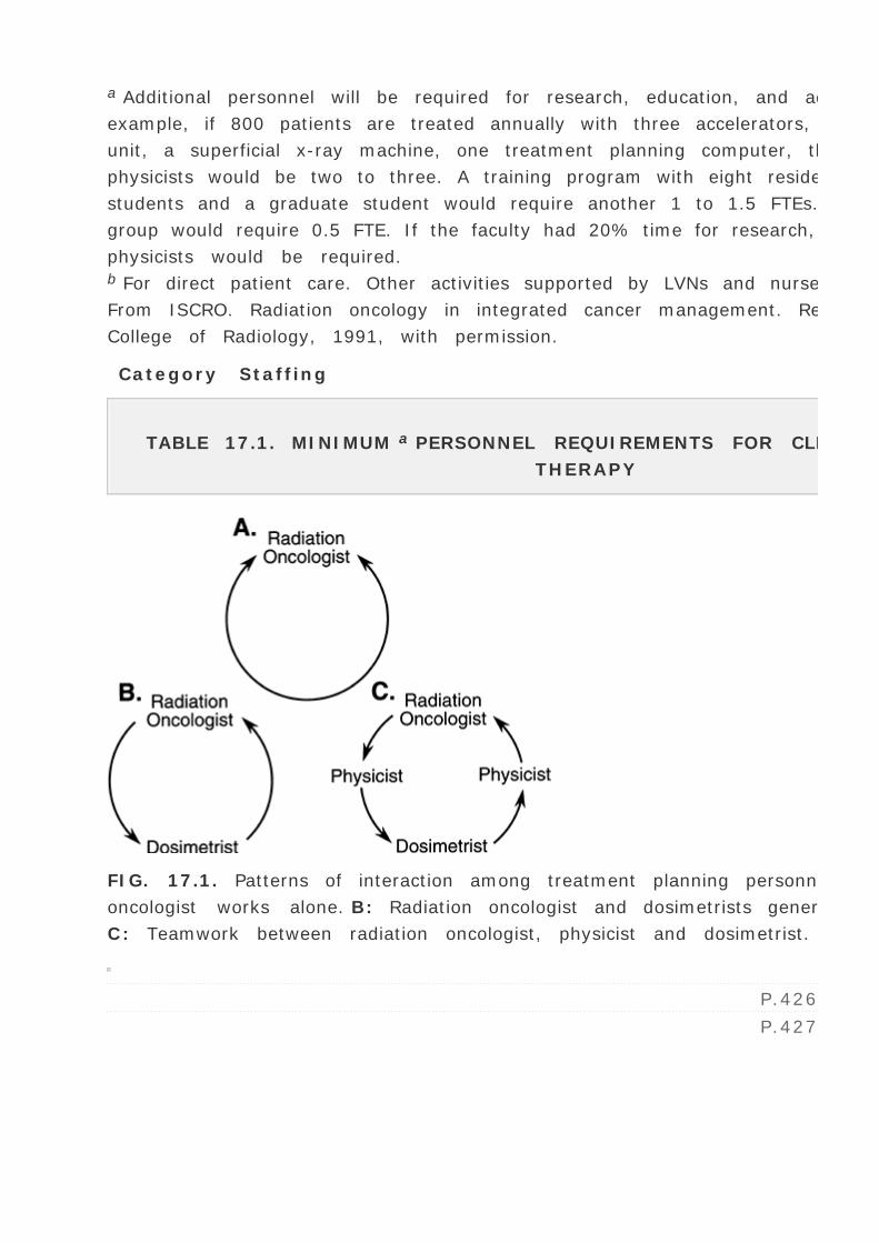
a Additional personnel will be required for research, education, and administration. For

example, if 800 patients are treated annually with three accelerators, one 60 Co teletherapy

unit, a superficial x-ray machine, one treatment planning computer, the clinical allotment for

physicists would be two to three. A training program with eight residents, two technology

students and a graduate student would require another 1 to 1.5 FTEs. Administration of this

group would require 0.5 FTE. If the faculty had 20% time for research, a total of five to six

physicists would be required.b For direct patient care. Other activities supported by LVNs and nurses aides.

From ISCRO. Radiation oncology in integrated cancer management. Reston, VA: American

College of Radiology, 1991, with permission.

Category Staffing

TABLE 17.1. MINIMUM a PERSONNEL REQUIREMENTS FOR CLINICAL RADIATION

THERAPY

FIG. 17.1. Patterns of interaction among treatment planning personnel. A: Radiation

oncologist works alone. B: Radiation oncologist and dosimetrists generate a treatment plan.

C: Teamwork between radiation oncologist, physicist and dosimetrist.

P.426

P.427

A. Training

Besides the adequacy of physics staffing in terms of number of personnel in relation to the

patient load or equipment, education and training of these personnel are of critical

importance. The greatest weakness in this regard has been the physicist's training. Most

physicists are hired with less-than-adequate clinical training. Structured clinical training

programs have been traditionally nonexistent. Certification boards for physicists exist, but the

entry requirements for the examination still do not mandate residency-type clinical training

as is required of the physicians. As a result, there is an unchecked influx of inadequately

trained physicists into the field.

The physicist's training problems are being addressed at the national level (9 ,10 ,11 ).

Physics residency programs are now being instituted, although at a much slower pace than

needed. It is hoped that eventually clinical medical physicists will go through nationally

accredited residency programs before taking the board examinations or assuming independent

clinical responsibilities.

Just as formalized clinical training is important for physicians and physicists, it is also

important for dosimetrists. Efforts are being made by the American Association of Medical

Dosimetrists to formalize the training of dosimetrists by establishing training curricula,

accreditation, and professional certification.

B. Qualifications

Qualifications of a clinical medical physicist have been debated in the past, but recently a

consensus has developed among the various national organizations. A radiation oncology

physicist is considered qualified if he or she has an M.S. or Ph.D. degree in physics, medical

physics, or a closely related field and a certification in radiation oncology physics by the

American Board of Radiology, the American Board of Medical Physics, or another appropriate

certifying body.

A qualified medical dosimetrist has a minimum of high school diploma and a certification by

the American Association of Medical Dosimetrists. Most certified dosimetrists also are certified

radiation therapy technologists.

C. Roles and Responsibilities

The roles and responsibilities of the physics team have been discussed in the literature (11

,12 ,13 ) and are summarized in Table 17.2 . As emphasized previously, the physicist must

direct the physics team and assume full responsibility of the physics data and procedures

applied to the patients, irrespective of whether these activities are carried out by the

physicist, dosimetrist, or other personnel. This unambiguous responsibility of physics

procedures by

P.428

the physicist is based on the same rationale as the physician's control of medical prescription.

Nonconformity to this principle can pose a serious risk to the patient.

Selection, specifications

Management/QA of treatment-planning computer

Dose calculation formalism

Regulatory

Teaching

Acceptance testing

Beam data management

Special treatment techniques

Radiation survey

Research

Commissioning, beam data measurement

Simulation consultation

Special dosimetry

Personnel monitoring

Developmental

Calibration

Patient data for treatment planning

In vivo dosimetry

Facility design

Administrative

Quality assurance

Technique optimization; isodose planning; plan analysis/evaluation; treatment aids; beam

modifiers

From Khan FM. Residency training for medical physicists. Int J Radiat Oncol Biol Phys

1992;24:853, with permission.

Equipment

(Teletherapy,

Brachytherapy,

Simulator)

Treatment

Planning

(Teletherapy

and

Brachytherapy) Dosimetry

Radiation

Protection Academic/Administrative

TABLE 17.2. ROLES AND RESPONSIBILITIES OF PHYSICISTS

The radiation oncologist undoubtedly has the overall responsibility for the conduct of the

entire treatment process. Because of that role, it is his or her responsibility to ensure that an

adequate and competent physics team is in place and that the roles of different personnel on

the team are appropriately defined. It has been recognized that inadequacy of physics support

translates into substandard or less than optimal patient care (4 ,6 ).

Calibration of radiation generators or sources is the exclusive responsibility of the medical

physicist. No other personnel has the expertise to perform this most critical function. Because

of the absolute necessity of the calibration procedure before the machine can be released for

patient treatment, all institutions manage to acquire physics support at least sufficient to

provide periodic calibration of the radiation equipment. However, these periodic calibrations,

outside of a well-structured quality assurance program, are inadequate and cannot ensure

continued safety of machine operation on a daily basis (14 ).

Next to calibration and quality assurance of radiation equipment is the physicist's role in

treatment planning. Although the treatment planning process involves sophisticated physics

concepts in designing and optimizing patient treatments, most institutions do not involve

physicists sufficiently in this process. As discussed previously (Fig. 17.1 ), some physicians

tend to work alone or with dosimetrists to design treatment plans. It should be realized that

the absence of physicist from the treatment-planning scene takes away an important element

of quality control, namely, the optimization and scientific authentication of the treatment

plan.

The physicist's direct involvement in the treatment-planning process is possible only if the

consultation is sought by the radiation oncologist. If the latter is not accustomed, by training

or experience, to such interactions, the physicist is not brought into the treatment-planning

loop. Consequently, an important member of the treatment-planning team is bypassed.

At some institutions, the physicist's role in treatment planning has been made indispensable.

For example, at the University of Minnesota the physicist's consultation is made as important

as other consultations, such as those sought from the medical oncologist, the surgeon, or the

radiologist. To prevent bypassing the physics consultation, each patient is assigned a

physicist who is available at the time of simulation to assist the radiation oncologist in

formulating the best possible treatment plan. Subsequent physics work is the designated

physicist's responsibility, although he or she may be assisted by the dosimetrist or other

technical personnel. The final treatment plan is approved by the radiation oncologist after

discussing the plan with the physicist. Also, the physicist is present at the time of first

treatment and subsequent treatments, if needed, to ensure proper implementation of the

plan.

Not all the clinical physics procedures need to be performed by physicists. Many of the

technical tasks can be delegated to dosimetrists so that physicists can devote time to

essential developmental activities. Every radiation oncology department needs to develop new

programs as well as revise the old ones to keep current with advancements in the field.

Responsibility often rests with the physicist to implement these advances while maintaining

the quality of care. Examples from the past three decades include development of linear

accelerator technology, computer imaging, 3-D treatment planning, conformal and dynamic

therapy, and remote afterloading brachytherapy. Whereas these technologies were not

developed exclusively by physicists, they had an important role in their design and clinical

application. Along with these major advancements came the innovations in treatment

techniques, for example, mantle fields, total body irradiation, electron beam therapy,

intensity-modulated radiation therapy, stereotactic radiosurgery, low-energy source

brachytherapy, and high dose rate brachytherapy. These refinements form an integral part of

the physicist's responsibilities and are often not separated from his or her routine clinical

duties. It is, therefore, important to recognize the need of providing sufficient technical

support to the physicist for a proper fulfillment of his or her role.

P.429

17.3. EQUIPMENT

High-quality patient care cannot be achieved or maintained without appropriate equipment.

Tumors occur in many forms, shapes, and locations. Unless radiation can be effectively

delivered to the tumor site with minimal side effects, the whole treatment process becomes

no more than a costly exerciseâ€”costly in terms of economics as well as human life. For any

institution to embark on a radiation therapy program, foremost attention must be paid to its

capability of providing optimal care to all the patients who will be referred to it. Thus the

available equipment must be suitable to treat effectively the many different kinds of cancers

that are presented in the clinic.

A. External Beam Units

The type or quality of radiation beam is dictated by the type and location of cancer to be

treated. Most head and neck cancers can be treated with low-energy megavoltage units:

cobalt-60 or linear accelerators in the energy range of 4 to 6 MV. That does not mean that a

facility equipped with only one of these units is capable of providing quality care to all

patients with head and neck cancers. On the contrary, institutions whose sole treatment

equipment is one of these units are not in a position to undertake complex and sophisticated

treatment techniques required for most head and neck cancers. Depending on the kind and

stage of the disease, an optimal treatment plan may call for other types of beams such as a

combination of low- and high-energy photon beams or an electron beam. A facility equipped

with a single-energy beam tends to follow suboptimal treatment plans or obsolete treatment

techniques when the best available radiation therapy equipment is a cobalt unit.

Because of the wide variety of cancers normally seen in a radiation therapy clinic, it is

necessary to have at least two qualities of photon beams: a low-energy (cobalt-60 or 4 to 6

MV x-rays) and a high-energy (10 MV or higher) beam. In addition, electron beams of several

different energies between 6 and 20 MeV must be available because approximately 30% of

patients require an electron beam for boost or an entire course of treatment.

A dual-energy linear accelerator can provide all the beams necessary for modern radiation

therapy. These machines are usually equipped with one low- and one high-energy photon

beam and a number of electron energies up to 18 or 20 MeV. That provides sufficient

capability to treat any cancer that needs external beam.

Additional machines are required if the patient load exceeds about 30 patients per day.

Although it is possible to treat more than 30 patients per machine per day, higher patient

loads necessitate hurried treatments and consequently allow less attention to detail. It is

important for a radiotherapy facility to be equipped not only with appropriate type and quality

of beams but also with a sufficient number of machines to handle the patient load.

B. Brachytherapy Sources

Certain cancers need brachytherapy, usually in combination with external beam. Cancer of the

uterine cervix and some other gynecologic malignancies are best treated with these

techniques. Unless the center has the policy not to treat patients for whom the brachytherapy

is the treatment of choice, brachytherapy equipment must be available to provide quality care

to patients who need this form of therapy.

For intracavitary application, radium and cesium are equally effective as far as the

therapeutic effects are concerned. Cesium has replaced radium mainly on the basis of

radiation protection considerations pertaining to storing and handling of these sources. For

interstitial implants, iridium-192 is the best available source although iodine-125 offers some

advantages for particular techniques, for example, permanent implants or temporary brain

implants with high-intensity sources.

Availability of brachytherapy sources and equipment adds to the comprehensiveness of a

center to provide radiation therapy. Again, if this capability is not available, a patient's

treatment may be compromised if the institution does not have a suitable alternative or

P.430

rationalizes the use of external beam alone not on the basis of merit but on the

nonavailability of brachytherapy service.

Afterloading procedures are the standard of practice in brachytherapy. The therapeutic quality

of the procedure is little affected by whether the afterloading is done by the bedside or

remotely. An institution can provide quality brachytherapy by using conventional afterloading

applicators. The need for the remote afterloaders (the LDR or the HDR) is based primarily on

considerations such as minimizing radiation exposure to personnel or handling large patient

loads. Again, if it can be established that the remote afterloading will improve patient care

(e.g., by allowing better nursing care or optimizing source placement), a case can be made to

acquire such equipment. High-tech equipment such as the remote afterloaders can be very

expensive and can drive up the cost of patient care. Therefore, the additional cost must be

justified on the basis of cost versus patient benefit analysis.

C. Simulator

The simulator is an essential tool for planning and designing radiation therapy treatments.

Because of the poor imaging quality of the treatment beam and the logistic difficulty of

obtaining time on the treatment machine, a simulator is the appropriate equipment to image

the treatment fields and optimize their placement before actual treatment. Because the

simulator offers the same beam geometry as the treatment machine, simulator films are used

to outline the field shape and dimensions for custom designing field blocks. The simulator

room is the place where different techniques can be modeled and solutions to technical

problems devised.

An essential requirement for simulation is the geometric accuracy that must be maintained at

the same level as that of the treatment machine. If the simulated field cannot be accurately

reproduced under the treatment machine, the whole simulation process becomes a useless

exercise. Inaccurate simulation can result in erroneous treatment.

Besides the mechanical and radiation field accuracy of a simulator, its imaging quality cannot

be overemphasized. Unless anatomic structures can be made visible with reasonable clarity,

fields cannot be accurately outlined, negating the very purpose of simulation.

Fluoroscopic capability of a simulator is a desirable option because it allows iterative field

adjustments and viewing before a final radiograph is obtained. Nonavailability of fluoroscopic

option results in an increased number of film retakes and, in the long run, is not cost-

effective. Moreover, too many repeats could deter from optimization of the simulation

process.

New developments in simulation are taking place in the area of computed tomography (CT)

simulation. A large number of CT scans taken through the region of the body to be simulated

can be processed to produce a digital reconstructed radiography (DRR) in any plane. The DRR

corrected for beam divergence is like the simulator radiograph, except that it is created from

individual CT slices. If targets and critical structures are outlined on each CT slice, a DRR can

be created to provide any simulator view with the target and the critical structures

highlighted in different shades of color. The DRR view is used to optimize the design and

placement of treatment fields before a simulation film is taken for verification.

17.4. DOSIMETRIC ACCURACY

Available evidence for effectively treating certain types of cancers points to the need for an

accuracy of approximately ±5% in dose delivery (15 ,16 ). This is indeed a very stringent

requirement, considering the uncertainties in equipment calibration, treatment planning, and

patient set-up. Further reduction in the dose accuracy limit will be not only very difficult but

probably of marginal value.

Calculation of overall uncertainty in a radiation therapy procedure is a complex problem,

because some errors are random while others can be systematic. Loevinger and Loftus (15 )

P.431

have proposed a model in which the random and systematic errors are statistically treated the

same way. Individual uncertainties are represented by standard deviations that are then

added in quadrature to determine the cumulative uncertainty. The combined standard

deviation may be multiplied by two to obtain an uncertainty with a 95% confidence interval.

Physical constants

1.1

Standard beam, NIST

0.5

Secondary standard, NIST

0.4

Field instrument, ADCL

1.0

Cumulative

1.6

ADCL, Accredited Dose Calibration Laboratory; NIST, National Institute of Standards and

Technology.a 95% confidence interval.

From ICRU. Determination of absorbed dose in a patient irradiated by beams of x or gamma

rays in radiotherapy procedures. Report no. 24. Washington DC: International Commission on

Radiation Units and Measures, 1976, with permission.

Step Uncertainty (Percent)

TABLE 17.3. UNCERTAINTY a IN THE CALIBRATION OF AN ION CHAMBER

Table 17.3 gives an estimate of uncertainty in the calibration of a treatment beam with a field

ion chamber (e.g., 0.6 cm3 Farmer-type chamber). The analysis shows that an ion chamber

suitable for calibrating radiation therapy beams and provided with a 60 Co exposure

calibration factor from an accredited dosimetry calibration laboratory (ADCL) has a cumulative

uncertainty of approximately 1.5% (two standard deviations). Calibration of beams with this

chamber will introduce additional uncertainties such as in the measurement procedure and in

the parameters of the dosimetry protocol. The overall uncertainty of the treatment beam

calibration using current protocols is estimated to be about 2.5% under optimal conditions

(15 ).

Table 17.4 gives uncertainties in the various steps involved in delivering a certain dose to a

patient at a reference point such as at the isocenter. The estimate of the uncertainties in

these steps is approximate and arrived at by considering the various procedures as they may

be typically carried out. These uncertainties could be further refined and broadened to include

uncertainties in the dose distribution within the target volume and the surrounding structures

(2 ).

A QA program must address not only the issues of random and systematic errors inherent in

the procedures but also the possibilities of human error such as in reading an instrument,

selecting a treatment parameter, making arithmetic computations, or interpreting a treatment

plan. Although human errors cannot be eliminated altogether, the

P.432

probability of their occurrence can be minimized by a well-designed QA program. An undue

relaxation of a QA program or the lack of it can be construed as professional negligence.

Ion chamber calibration

1.6

Calibration procedure

2.0

Dose calculation parameters and methods

3.0

Effective depth

2.0

SSD

2.0

Wedges

2.0

Blocking trays

2.0

Cumulative

5.6a 95% confidence interval.

SSD, source-to-surface distance.

Step Uncertainty (Percent)

TABLE 17.4. OVERALL UNCERTAINTY a IN DOSE DELIVERED AT A POINT IN A

PATIENT

17.5. EQUIPMENT SPECIFICATIONS

Acquisition of a major piece of equipment involves many steps: justification of need, market

evaluation of different makes and models, checks of vendorsâ€™ business relations and

service record, calling up users for their opinions, writing bid specifications, making final

evaluation, and doing price negotiations. Even if the institution does not require closed bids,

it is important to prepare detailed specifications and obtain a formal written response from

the vendor before deciding on the purchase.

Most vendors list their equipment specifications in company brochures that are available on

request. These specifications should be carefully compared with other vendorsâ€™

specifications. Formal bid specifications can then be written for the product that most closely

meets the institution's needs. For an impartial bid process, the specifications should be as

generic as possible, so that all major vendors have a fair chance of responding to the bids.

Specifications that the institution considers essential must be identified so that vendors who

cannot meet those specifications do not have to go through the process of answering the bid.

If a particular system is specified to meet a certain function, vendors should have the

opportunity to suggest alternative systems with equivalent or better specifications.

The purchase of radiation therapy equipment is usually a shared responsibility between the

radiation oncologist, the physicist, and the hospital administrator. The physicist's role is

primarily to write technical specifications although most participate in the whole decision

process.

The specifications are written in a suitable format so that the vendors can respond to them

item by item. Because the vendorsâ€™ responses are legally binding, clarification should be

sought if response to a particular item is not clear. Also, if a specification in a company's

brochure falls short of a desired specification, negotiations may be carried out with the

vendor to improve the specification in question. Many improvements in the accelerator

technology have occurred as a result of customer demand for better specifications.

Certain specifications in regard to beam characteristics and acceptance criteria require

carefully stated definitions and methods of measurement. The specifications should clearly

spell out these details, especially when conflicting definitions or criteria exist in the

literature. As far as possible, the specifications should follow national or international

terminology and guidelines unless a special need exists to justify deviations from the

accepted standards.

17.6. ACCEPTANCE TESTING

Unless the vendor has agreed to a written set of specifications, the customer has no recourse

but to go along with the vendor's acceptance test procedures. These procedures are set up by

the company to demonstrate that the product meets the specifications contained in its

brochures and satisfies the legal requirements of equipment safety.

If a set of bid specifications was agreed on before the machine was purchased, then the

vendor is obligated to satisfy all the specifications and criteria contained in the purchase

contract. In practice, the vendor first performs all the tests in accordance with the company's

procedure manual. Any deviations or additions stipulated in the bid specifications are then

addressed to complete the acceptance testing process.

As a general rule, acceptance testing is required on any piece of equipment that is used in

conjunction with patient treatments. Whereas formal testing procedures have been developed

for major equipment (linear accelerators, simulators, brachytherapy sources, etc.), these

have to be improvised for other equipment. The guiding principle is that any

P.433

equipment to be used for patients must be tested to ensure that it meets its performance

specifications and safety standards.

A. Linear Accelerator

A linear accelerator is a sophisticated piece of equipment that requires several months for

installation, acceptance testing, and commissioning. Whereas installation is carried out by the

vendor personnel, the acceptance testing and commissioning are the responsibility of the

institution's physicist. Patient treatments do not begin until the unit has been commissioned,

that is, the machine tested to be acceptable and sufficient data have been acquired to permit

treatment planning and dose calculations for patient treatments.

A.1. Radiation Survey

As soon as the installation has reached a stage at which a radiation beam can be generated,

the physicist is called on to perform a preliminary radiation survey of the treatment facility

(Chapter 16 ). The survey is evaluated to ensure that during the testing of the machine the

exposure levels outside the room will not exceed permissible limits, considering the dose rate

output, machine on time, use factors, and occupancy factors for the surrounding areas. A

preliminary calibration of the machine output (cGy/MU) is needed to determine the expected

dose levels as a function of machine output (MU/min).

After completion of the installation, a formal radiation protection survey is carried out,

including the measurement of head leakage; area survey, and tests of interlocks, warning

lights, and emergency switches. The survey is evaluated for conditions that are expected to

exist in the clinical use of the machine, for example, workload, use factors, and occupancy

factors.

A.2. Jaw Symmetry

One of the methods of checking jaw symmetry is with a machinist's dial indicator (Fig. 17.2 ).

With the gantry pointing horizontally and the jaws open to a large field, the feeler of the dial

indicator is made to touch the face of one of the jaws and the indicator's reading is noted.

The collimator is then rotated through 180 degrees and the reading is taken with the feeler

now resting on the opposite jaw. A leveling device is used to set the collimator angles for

these measurements. The symmetry error is one-half of the difference between the two

readings of the dial indicator. The procedure is repeated for the second set of jaws. The

symmetry error of the collimator jaws is typically less than 1 mm.

A.3. Coincidence

Collimator Axis, Light Beam Axis, and Cross-hairs

With a graph paper taped on the table and the gantry vertical, turn on the field light to obtain

a rectangular field. Mark the edges of the light field, intersection of the diagonals, and the

position of the cross-hair images. Rotate the collimator through 180 degrees and check the

coincidence of (a) the light field edges and (b) the intersection of diagonals and the position

of cross-hair images. If significant misalignment exists, the field light and cross-hairs should

be adjusted to bring about the desired coincidence.

Light Beam with X-ray Beam

Place a ready pack film on the table at the source-to-axis distance (SAD). With the collimator

angle set at 0 degrees, obtain a rectangular or square light field and mark the edges with a

radiopaque object or a ballpoint pen by drawing lines on the film jacket with sufficient

pressure to scratch the emulsion. The film orientation and the collimator angle are noted. A

plastic sheet, thick enough to provide maximum electronic buildup, is placed over the film

without disturbing its position. This is done to eliminate the perturbing influence of

P.434

the incident electron contamination. The film is exposed to obtain an optical density in the

linear range of its sensitometric curve, usually around 1. Two more exposures at collimator

angles of ±90 degrees are made using fresh areas of the same film or on a second film. The

film is processed in an automatic rapid processor.

FIG. 17.2. Determination of jaw symmetry with the machinist's dial indicator. The feeler of

the dial indicator is shown to rest on the right jaw.

The alignment between the x-ray beam edges (corresponding to an optical density of 50%

relative to that on central axis) and the light beam marks can be checked visually or by

cross-beam optical density profiles. A typical alignment film is shown in Fig. 17.3 . For

acceptance testing, the above process should be repeated at 0 degrees, 90 degrees, 180

degrees, and 270 degrees angulation of the gantry.

According to the AAPM guidelines, the alignment between the light beam and the x-ray beam

should be within ±3 mm (2 ). However, a more stringent requirement of ±2 mm can be

maintained without difficulty with the modern linear accelerators.

A.4. Mechanical Isocenter

Mechanical isocenter is the intersection point of the axis of rotation of the collimator and the

axis of rotation of the gantry. Due to heavy weight, the gantry frame may flex during

rotation. This may cause the axis of the gantry rotation to miss the axis of the collimator

rotation, thereby creating an uncertainty in the position of the isocenter.

Collimator Rotation

Attach a piece of graph paper on a flat surface of a plastic sheet and mark an intersection

point of two graph lines (center point). Using the distance measuring rod attached to the

accessory mount, place the center point of the graph at the assumed isocenter (point P).

P.435

Reverse the distance rod and attach an adjustable pointer device with a sharp point, called

the center finder or wiggler, to its distal end (Fig. 17.4A ).1 Starting with a 0-degree angle,

rotate the collimator to + 90 degrees and note the maximum displacement of the wiggler tip

from point P in the X and Y directions. Tap the wiggler point to move it in the X direction

through half the distance from point P and then tap the plastic sheet to bring point P under

the wiggler tip. Repeat the procedure for the Y axis. Rotate the collimator to ±90 degrees

and repeat the whole procedure. By iterative adjustment of the wiggler tip and point P, the

displacement of the wiggler tip from point P can be minimized as the collimator is rotated. For

an acceptable alignment, the isocenter should stay within a 2-mm-diameter circle when the

collimator is rotated through its full range of rotation.

FIG. 17.3. Films to measure coincidence between light beam and radiation beam. Light field

borders appear as scratch marks as the corner edges of the radiation field.

Gantry Rotation

With the wiggler point positioned at the isocenter as determined previously, another

horizontal rod with a fine point is held in a ring stand so that the two points coincide as best

as possible (Fig. 17.4B ). The stand for the horizontal rod should rest on the couch near its

end so that there is no possibility of gantry collision with the couch or the apparatus. By

moving the gantry through 360 degrees, the displacement between the wiggler point and the

horizontal rod point is visually noted and measured. The tolerance of the isocenter motion

with full gantry rotation is ±1 mm.

A.5. Radiation Isocenter

Collimator

With the gantry vertical, place a ready pack film flat on the tabletop at the SAD. Open the

upper jaws of the collimator wide open and close the lower jaws to obtain a narrow

P.436

P.437

slit of minimum possible width. Place build-up sheet on top of the film. By rotating the

collimator through a number of different angles, the film is exposed to obtain an optical

density of about 1. The interval between angles should be such that six to seven exposures

can be made to cover full rotation of the collimator without overlaps. Using a new film, repeat

the above process with the lower jaws open and the upper jaws closed to a narrow slit.

FIG. 17.4. Determination of mechanical isocenter. A: Collimator rotation. B: Gantry rotation.

See text for details.

The processed films will show star patterns, with a dark central region (Fig. 17.5A ). By using

a ballpoint pen or another film marker with a fine point, lines may be drawn through the

middle of the slit images to define more clearly the intersection point(s) of the slit images.

For an acceptable result, all the lines should intersect or pass within a 2-mm-diameter circle.

FIG. 17.5. Star pattern to determine radiation isocenter of (A) collimator rotation, (B) table

rotation, and (C) gantry rotation.

P.438

Treatment Table

Place a film on the tabletop at the SAD. Open the upper collimator jaws wide and close down

the lower jaws to a narrow slit. Place a buildup sheet on top of the film. Make six to seven

exposures on the same film with the table rotated through a series of different angles to

cover the full range of couch rotation. Some exposures may have to be staggered to avoid

overlap of images.

A star pattern (Fig. 17.5B ) on the processed film should ideally show all the slit images

intersecting at one point, the radiation isocenter. Acceptable specification requires that all

the lines should intersect or pass within a 2-mm-diameter circle. Stricter specification may be

required for a unit designated for stereotactic radiosurgery.

Gantry

A ready pack film, sandwiched between two plastic sheets (e.g., acrylic or clear polystyrene),

is placed on the table so that the plane of the film is perpendicular to the plane of couch top

and contains the beam central axis for all gantry angles. Create a slit of beam parallel to the

gantry axis of rotation. Make 12 exposures on the same film with the gantry rotated between

exposures. To avoid overlaps, the first six exposures may be made at 30-degree intervals, the

next one at 45 degrees beyond, and the subsequent exposures successively 30 degrees apart.

The gantry star pattern (Fig. 17.5C ) should show the lines intersecting or passing within a 2-

mm-diameter circle centered around the presumed radiation isocenter.

A.6. Multiple Beam Alignment Check

When a patient is treated with more than one beam, misalignment between beams can occur

due to any of the causes discussed previously. Lutz et al. (17 ) have recommended a test

procedure that can detect simultaneously three general causes of beam misalignment: (a)

focal spot displacement; (b) asymmetry of collimator jaws, and (c) displacement in the

collimator rotation axis or the gantry rotation axis. This method is called the split-field test.

The split-field test consists of double-exposing a film (sandwiched between buildup sheets) to

two fields, 180 degrees apart. As shown schematically in Fig. 17.6 , a square field is first

exposed from above with half the field (region 2) blocked and then exposed from below to

expose region 2 with region 1 blocked. Relative shift of the two images is indicative of

P.439

the misalignment of the parallel-opposed beams. A similar test can be performed between any

two beams rotated through 180 degrees.

FIG. 17.6. Schematic illustration of Lutz et al. (17 ) method of determining alignment

between opposing fields. A: Perfect alignment. B: Misalignment.

If beam misalignment is shown by the above test, one can then proceed to investigate the

cause of misalignment by checking individually the alignment of the radiation isocenter with

the axis of the collimator or gantry rotation as described previously.

A.7. X-ray Beam Performance

Energy

Measurement and specification of photon beam energy have been discussed in Chapter 7 . The

most practical method of specifying clinical beam energy is by the depth-dose distribution. A

central axis depth-dose curve measured with a suitable ion chamber in a water phantom can

be compared with published data to specify the energy. The following considerations are

relevant to making such a determination.

The ion chamber internal diameter should be small (less than 3 mm) to minimize

displacement correction (Chapter 8 ). For a larger diameter chamber, the depth-dose

curve should be shifted to the left (toward the source) by 0.6r , where r is the radius of

the chamber.

In comparing depth-dose distribution with published data, care must be exercised in

regard to the reference depth used in the definition of percent depth dose. To avoid

ambiguity, it is preferable to compare depth dose ratios for depths beyond the depth of

dose maximum (d max ) rather than the absolute values of the percent depth dose.

Suitable depths for comparing depth dose ratios are 10 and 20 cm.

The reference depth-dose data used for comparison must be reliable. Data published by

national or international organizations are preferable in this regard. The depth-dose data

published in the British Journal of Radiology (18 ) is commonly used for specifying energy,

although some prefer the method of ionization ratio as a measure of energy and using the

data given in the TG-21 protocol (19 ). Either method is acceptable.

The acceptance criteria is usually specified in terms of depth-dose variance for a 10 — 10-

cm field size, 100-cm SSD, and 10-cm depth. A difference of ±2% in the depth-dose ratio or

ionization ratio from the published values is acceptable, considering the fact that this

comparison is just for nominal energy designation only. The depth-dose data for clinical use is

not the published data but the one that is actually measured for the given accelerator. A

small uncertainty in the nominal beam energy designation is not important as long as

calibration and the clinically used depth-dose data are based on accurately measured energy

parameters (e.g., TG-51 data).

Field Flatness

Field flatness for photon beams has been traditionally defined as the variation of dose relative

to the central axis over the central 80% of the field size (reference region) at a 10-cm depth

in a plane perpendicular to the central axis (Fig. 17.7A ). A dose variation of ±3% is

considered acceptable (20 ).

The AAPM Task Group 45 (14 ) specifies flatness in terms of maximum percentage variation

from average dose across the central 80% of the full width at half maximum (FWHM) of the

profile in a plane transverse to the beam axis. This variation or flatness F is mathematically

given by:

where M and m are the maximum and minimum dose values in the central 80% of the profile.

The above definitions of field flatness do not distinguish between the dose variation produced

by the flattening filter and that due to the penumbra. Whereas flatness can be altered by the

flattening filter, the dose variation in the penumbra region is governed

P.440

primarily by the geometric and transmission penumbra, photon scatter, and electron scatter.

The flatness criteria should, therefore, reflect the effect of the flattening filter and not the

penumbra, which is basically unalterable.

FIG. 17.7. Alternate definitions of photon field flatness. A: Flatness is measured within a

region bounded by 80% of the field width (W). B: Flatness is measured within a region

bounded by lines drawn a certain distance (e.g., 2 cm) inside from the field edges. Depth of

measurement is specified at 10 cm.

Boyer (21 ) has suggested that the x-ray beam field flatness should be specified to exclude

the penumbral effects. The reference region of flatness should be defined with lines at a

specified distance from the field edges instead of a certain percentage of the field size (Fig.

17.7B ). Typical flatness at a 10-cm depth within the region extending up to 2 cm from the

field edge is +3% to -5% (21 ).

Definitions that specify field flatness and symmetry with respect to average profile values

create ambiguity and clinical inconsistency. Because beams are calibrated at the central axis,

it is more logical to characterize dose variation relative to the central axis.

In the light of the above discussion, there is a need for a national or international group to

examine the prevailing definitions of field flatness and recommend a criterion that checks the

effectiveness of the flattening filter, excluding the penumbra. In the meantime, the flatness

definition given by Equation (17.1) may be used with the acceptable limit being within

±3%.

For acceptance testing, flatness should be checked for the maximum field size at least at two

depths: 10 cm and d max . Whereas the flatness criteria is applied to the profile at a

P.441

10-cm depth, the profile at d max should be examined for the extent of peripheral hot spots,

or â€œhorns.â€ These horns should not exceed 105%. For bigger horns, an accessory filter

may have to be designed to reduce them when using large fields (22 ).

In addition to the profiles along the principal axes of the field, diagonal scans should be

obtained to check field flatness. Typically, the diagonal flatness is +4% to -6% in the

reference region, extending up to 2.8 cm from the 50% isodose curve in a plane

perpendicular to the central axis and at a 10-cm depth (21 ).

Field Symmetry

The cross-beam profiles obtained for flatness also can be used for symmetry. The profile plot

may be folded at the field center and the two halves of the profiles compared. In the

reference region, the dose should not differ more than 2% at any pair of points situated

symmetrically with respect to the central ray.

A.8. Electron Beam Performance

Energy

Specification and measurement of electron beam energy are discussed in Chapter 14 as well

as in the AAPM TG-25 protocol (23 ). The depth-dose or depth ionization curve for a broad

beam measured with a suitable ion chamber in a water phantom gives the practical or

extrapolated range, Rp. The most probable energy (Ep )o is given by Equation 14.4 . (Ep )o

should be within about ±0.5 MeV of the nominal energy shown on the accelerator control

panel.

For a routine check of electron beam energies, film can be used to determine Rp as well as

other parameters such as R 100 , R 90 , R 80 , and R 50 . Computer-driven densitometers are

commercially available that can analyze these parameters, including the most probable and

mean energies.

Flatness and Symmetry

The flatness and symmetry specifications of electron beams are given in the AAPM TG-25

report (23 ) and also are discussed in Chapter 14 . Again, film dosimetry is quite useful in

analyzing flatness and symmetry on a routine basis.

A.9. Monitor Chambers

Linearity of monitor chambers is an important requirement and should be checked as a

function of dose rate and for special operating conditions such as total body irradiation, total

skin irradiation, and arc rotation. Long-term stability check of monitor chambers forms a

major part of the quality assurance program.

A.10. Wedges

Wedge isodose distribution for a 10 — 10-cm field may be used to check wedge angle

(Chapter 11 ). The measured wedge angles should be within ±2 degrees of the values

specified. This uncertainty in nominal wedge angles is acceptable because wedge filters are

always planned using isodose distribution determined for the given wedge.

A.11. Miscellaneous Checks

Isocenter shift with couch motion up and down should not exceed ±2 mm.

Optical distance indicators should be accurate within ±2 mm.

Field size indicators should be accurate within ±2 mm.

Gantry angle and collimator angles should be accurate within 1 degree.

Laser lights should be aligned with the isocenter within ±2 mm.

Tabletop sag with lateral or longitudinal travel under a distributed weight (similar to

patient) of 180 lbs. should not exceed 2 mm.

P.442

The tennis racket insert for the couch should not sag more than 0.5 cm under the above

stated conditions.

Other ancillary devices provided with the accelerator should be checked in accordance

with the vendor's specifications or as specified in the purchase contract.

B. Simulator

Acceptance testing of a simulator may be divided into two parts: (a) checking of the

geometric and spatial accuracies and (b) performance evaluation of the x-ray generator and

the associated imaging system. The first part is similar to the acceptance testing of a linear

accelerator. The second part deals with the simulator performance like a diagnostic x-ray and

fluoroscopic unit.

Several publications have discussed the specifications of treatment simulators and the

required testing procedures (24 ,25 ,26 ,27 ). A comprehensive review of the subject has been

provided (28 ). The quality assurance for the x-ray generator and the imaging system has

been discussed by the NCRP (29 ). Specifications and acceptance test procedures may also be

available from vendors (30 ).

Because the simulators are designed to mimic the treatment machines, for example, linear

accelerators, their geometric accuracy should be comparable with these machines. Ideally,

the simulator should be at least as accurate as the treatment machine in localizing treatment

fields. However, differences between the simulator port and the treatment port may arise

because of the differences in the treatment tables or accessories. To minimize these

differences, it is preferable to have a simulator with the same table design and the accessory

holders as the treatment machines.

Table 17.5 is the list of acceptance tests recommended by the British Institute of Radiology.

The suggested tolerances for various parameters are the same as or better than their

equivalent for linear accelerators as recommended by the IEC (31 ).

Illumination of light field indication

1. Average illuminance at the normal treatment distance

40 lux

40 lux

Reproducibility

2. The difference between the maximum and minimum x-ray field size for repeated settings of

the same numerical field indication

2 mm

1 mm

3. The maximum distance between any light field edge and x-ray field edge for repeated

settings of the same numerical field indication

2 mm

1 mm

Numerical indication of field size

4. The maximum difference in mm or percentage of field dimension between the numerical

field indication and the dimensions of the x-ray field at the normal treatment distance

5 cm — 5 cm to 20 cm — 20 cm

3 mm

2 mm

Greater than 20 cm — 20 cm

1.5%

1%

Light field indication

5. The maximum distance along the major axes in mm or percentage of field dimension

between the light beam edge and the x-ray field edge at the normal treatment distance

5 cm — 5 cm to 20 cm — 20 cm

2 mm

1 mm


1%

0.5%

6. The maximum distance along the major axes between the light beam edge and the x-ray

field edge at 1.5 normal treatment distance

5 cm — 5 cm to 20 cm — 20 cm

4 mm

2 mm


2%

1%

7. The maximum distance between the centers of the x-ray field and the light field at the

normal treatment distance

2 mm

1 mm

8. The maximum distance between the centers of the x-ray field and the light field at 1.5

times the normal treatment distance

4 mm

2 mm

Geometry of field delineators

9. The maximum deviation from parallelity of opposing edges

0.5 °

0.5 °

10. The maximum deviation from orthogonality of adjacent edges

0.5 °

0.5 °

Indication of x-ray beam axis

11. Maximum deviation of the indication of the radiation beam axis from the radiation beam

axis

Over -25 cm from the normal treatment distance (NTD) or the working range of the indicator,

beam entry

2 mm

1 mm

12. Over NTD to NTD +50 cm or working range, beam exit

3 mm

2 mm

Displacement of the x-ray beam axis from the isocenter

13. Maximum displacement of the x-ray beam axis from the radiation isocenter

2 mm

1 mm

Indication of the isocenter

14. Maximum displacement from the radiation isocenter of any device mounted on the

machine for indicating the position of the isocenter

2 mm

1 mm

Indication of distance along the x-ray beam axis

15. Maximum difference between the indicated distance and the actual distance from

isocenter

2 mm

1 mm

16. Maximum difference between the indicated distance and the actual distance from the x-

ray target

5 mm

2 mm

17. Maximum difference between the indicated distance and the actual distance between the

isocenter and the image plane

N/A

2 mm

Zero position of rotational scales

Maximum difference between the zero position indicated by the rotational scale and the

intended zero position

18. Rotation of gantry

0.5 °

0.5 °

19. Rotation of diaphragm housing

0.5 °

0.5 °

20. Isocenter rotation of the table

0.5 °

0.5 °

21. Rotation of the tabletop

0.5 °

0.5 °

22. Pitch of the table

0.5 °

0.5 °

23. Roll of the table

0.5 °

0.5 °

Opposing fields

24. Maximum angular deviation between axes of opposed x-ray fields

1 °

1 °

Movements of the patient table

25. Maximum horizontal displacement of the table for a change in height of 20 cm when

loaded with 30 kg distributed over 1 m and when loaded with 135 kg distributed over 2 m,

both weights acting through the isocenter

2 mm

2 mm

26. Maximum displacement of the axis of isocenter rotation of the table from the radiation

isocenter

2 mm

1 mm

Parallelism of table rotation axes

27. Maximum angle between the isocenter rotation of the table and the axis of rotation of the

tabletop

0.5 °

0.5 °

Longitudinal rigidity of the table

28. Maximum difference in table height near isocenter between 30 kg load retracted position

and 135 kg load extended position

5 mm

5 mm

Lateral rigidity of the table (a)

29. Maximum angle of lateral tilt from horizontal of the plane of the tabletop

0.5 °

0.5 °

Lateral rigidity of the table (b)

30. Maximum deviation of the height of the table as the table is laterally displaced

5 mm

5 mm

X-ray tube

31. Maximum focal spot size for at least one focal spot

N/A

0.3 mm — 0.3 mm

32. Maximum shift of image at the isocenter for change of focal spot

N/A

0.5 mm

From Treatment Simulators. Br J Radiol 1989;[Suppl. 23], with permission.

Parameter

IEC Tolerance for Electron

Accelerators

BIR Proposed Tolerance for

Simulators

TABLE 17.5. TREATMENT SIMULATOR TOLERANCES

P.443

P.444

C. Brachytherapy

The purpose of acceptance testing of brachytherapy equipment is to ensure that the sources

and the associated equipment meet the user's specifications. The results of these tests should

be carefully evaluated and documented for future reference.

C.1. Intracavitary Sources and Applicators

The following procedures are recommended to evaluate intracavitary sources and manual

afterloading applicators.

Source Identity

Physical length, diameter, serial number, and color-coding of all sources should be checked.

Whereas source dimensions may be checked by physical measurement or by radiography, the

serial number and color-coding can be checked by visual inspection.

Source Uniformity and Symmetry

An autoradiograph of a brachytherapy source reveals distribution of activity as well as active

length (Fig. 15.2 ). The symmetry of the source loading within the capsule may be

ascertained by taking a simulator radiograph of the source but leaving it on the film for an

appropriate length of time to obtain an autoradiograph. The superposition of the

autoradiograph and transmission radiograph provides the required information on source

symmetry relative to the physical ends of the sources.

All sources should be checked for source uniformity and symmetry. In addition, one randomly

chosen source from each group of designated strength may be autoradiographed to obtain

isooptical density curves. This will document symmetry of dose distribution around these

sources.

Source Calibration

All sources should be individually calibrated to check source strength specified by the vendor.

Methods of source calibration were discussed in section 15.2 . A well ionization chamber (e.g.,

a dose calibrator) is convenient for these calibration checks. A standard source of the same

radionuclide and construction having a calibration traceable to NIST is required for these

measurements. If the disagreement between the vendor and the user calibration is within

±5%, the vendor calibration should be used unless the user's calibration is deemed more

accurate than the vendor's. In the latter case, the user's methodology and results of

calibration must be fully documented and justification provided for not using the vendor's

calibration. Differences larger than ±5% are not acceptable and would require recalibration

by the vendor and issuance of a new calibration certificate.

Applicator Evaluation

Applicators for intracavitary application are constructed to hold the sources in a specified

geometry. Some applicators (e.g., Fletcher-Suit) have strategically placed lead or tungsten

shields to reduce the dose to the rectum and the bladder. Acceptance testing of these

applicators is essential to ensure proper source placement and protection of critical structures

by the shields.

The internal structure of applicators may be examined by orthogonal radiographs using a 4-

or 6-MV x-ray beam. Dummy sources may be inserted to check the position of sources in the

applicator. The position of shields should be compared with the vendor's drawings. Mechanical

functions such as the ease of source loading and removal should also be checked before

accepting the applicators.

C.2. Interstitial Sources

Sources for interstitial implant in the form of needles (e.g., cesium-137) can be tested in the

same way as the intracavitary sources described above. For calibration checks, needles of the

P.445

same radionuclide and construction should be used to obtain a calibration factor for the well

ionization chamber. All sources should be individually checked before commissioning into

clinical use.

Short-lived interstitial sources in the form of seeds, wires, or seed-loaded ribbons can be

tested by visual inspection (behind a leaded glass window) and calibration can be checked

with a dose calibrator, as described in the previous section. For a batch of a large number of

sources (e.g., 192 Ir ribbons), a randomly selected sample of three or four ribbons of a given

strength should be checked for calibration. A standard seed of the same kind (with calibration

traceable to the NIST) should be used to calibrate the well ionization chamber. Because

ribbons of different lengths are used, the ion chamber response should be corrected as a

function of ribbon length. These correction factors can be established by using the standard

seed and measuring chamber response as a function of seed position in the well ionization

chamber.

The calibration check of 125 I seeds is difficult because of the low energy of the emitted

photons. Unless suitable equipment is available for checking 125 I seed calibration, the

institution may accept the vendor's calibration. However, the vendor's calibration

methodology should be reviewed to ensure that the calibration is performed with an

appropriate instrument with a calibration factor traceable to NIST. The vendor's calibration

service may be checked by obtaining a repeat calibration of a seed by NIST or an ADCL.

D. Remote Afterloaders

Acceptance procedures for remote afterloading equipment have been discussed by several

investigators (32 ,33 ,34 ,35 ) and reviewed by Glasgow et al. (36 ). The procedures may be

broadly divided into (a) operational testing of the afterloading unit, (b) radiation safety check

of the facility, (c) checking of source calibration and transport, and (d) checking of treatment

planning software. Although the details are presented by Glasgow et al., some of the

recommendations are listed in Table 17.6 . Most of the acceptance test

P.446

procedures consist of testing the unit for its functional performance and safety features,

usually covered in the operator's manual. These can be simply carried out by activating

various functions and observing the results. The accuracy of source localization and

calibration can be checked using procedures that are more or less similar to those used for

conventional brachytherapy. Considerations specific to remote afterloaders are discussed

below.

Functional performance

Console functions . Main power, battery power, source on/off, door open/close, etc.a.

Source control . Source dwell time and source retraction at the end of preset time,

unplanned interruption or emergency shutoff

b.

Battery voltage . Adequacy of battery voltage under load conditions and functional

performance under battery power

c.

d.

e.

c.

Timer. Timer accuracy and end-time effectsd.

Decay correction . Accuracy of computer-calculated decay correctionse.

Multichannel indexer . Proper source sequencing and channel selectionf .

Backup systems . Proper functioning during simulated power failures or air pressure losses

(for pneumatically driven devices)

g.

Radiation detectors . Proper functioning as specifiedh.

Facility check and survey

Door interlocks . Source retracts when the door is opened; the unit does not start until

the door is closed and the interlock is reset

a.

Radiation warning lights . Proper functioning to indicate radiation on/off conditionb.

Patient viewing and communication . Proper functioning of closed-circuit TV and the

intercommunication system

c.

Radiation survey . Exposure rates outside the radiation facility should meet the NRC

regulations and the leakage radiation rates around the unit should be acceptable (see

chapter 16 )

d.

Source calibration and transport

Check of source specifications, leak testing, calibration, transport to the applicators,

autoradiograph of simulated source positions, and isodose distribution to determine dose

anisotropy

TABLE 17.6. ACCEPTANCE TESTING PROCEDURES FOR REMOTE AFTERLOADERS

D.1. Source Positioning

Source position accuracy can be checked by taking radiographs of dummy sources in the

applicators with their positions marked on a ready pack film and combining with

autoradiographs of the radioactive sources in the same applicators. The position of dummy

sources and radioactive sources should correspond within ±1 mm.

Special test devices have been designed to test source positioning by autoradiography (34 ,35

,37 ). Figure 17.8A shows a test phantom designed by Aldrich and Samant (37 ). The system

consists of an acrylic plate with channels drilled to hold the treatment catheters. Lead sheets

of dimensions 20 — 20 — 0.8 mm are accurately set into one surface at a regular spacing

of 20 mm. The phantom is placed on a ready pack XV2 film with lead sheets facing the film.

The sources are programmed to stop every 10 mm for intervals suitable for autoradiography.

The autoradiograph thus obtained shows source positions together with

P.447

fiducial markers provided by the edges of lead sheets (Fig. 17.8B ). An accuracy of ±1 mm

in the source positions is acceptable.

FIG. 17.8. Quality control test for HDR remote afterloaders. A: Test phantom to check the

accuracy of source positioning. B: Autoradiograph of the test phantom showing dwell

positions. (From Aldrich JE, Samant S. A test phantom for HDR daily quality control. Activity


D.2. Source Calibration

The LDR sources in remote afterloading units can be calibrated in a well ionization chamber

as described by the AAPM Report 13 (2 ) and in Chapter 15 of this book. The well ionization

chamber must bear a calibration for the same kind and specification of source as the given

LDR source.

For the calibration of HDR sources, the well ionization chamber must be capable of measuring

large currents associated with these sources. Goetsch et al. (38 ) have described such a

chamber for use with 192 Ir HDR sources. Calibration of well-type ionization chambers

suitable for calibrating HDR sources is available at some ADCLs (University of Wisconsin and

K&S Associates, Inc.).

A cylindrical lead insert for a conventional well-ionization chamber (e.g., dose calibrator) has

also been used to reduce the ionization current from an HDR source to a measurable value

(36 ). It is important to check the accuracy of such a system by an independent calibration.

Cylindrical ion chambers (e.g., Farmer-type or larger volume, depending on source strength)

can be used to calibrate LDR and HDR sources using a free-air geometry (Chapter 15 ). The

ion chamber must be fitted with an appropriate build-up cap and bear a calibration for photon

energies emitted by the radionuclide. Goetsch et al. (39 ) have described an interpolative

method of obtaining exposure calibration factor for the chamber. For 192 Ir, the calibration

factor is obtained by interpolating between factors for 137 Cs and 250 kVp x-rays. Ezzell (40 )

has described a method of interpolating chamber factors for 60 Co with a build-up cap and

250 kVp without a cap to obtain chamber factor for 192 Ir. Until NIST develops a direct

method of chamber calibration with 192 Ir, the AAPM (36 ) recommends this interpolative

technique.

17.7. COMMISSIONING

Most equipment is ready for clinical use after acceptance testing. However, some equipment

requires additional data before it can be used in conjunction with patient treatments. For

example, a linear accelerator cannot be used for patient treatments until it has been

calibrated and all the beam data and necessary parameters for treatment planning have been

obtained. These data are then input into a treatment-planning computer in accordance with

the software requirements. The computer-generated dose distributions are checked against

measured data and/or manually calculated distributions. After all the necessary beam data

have been acquired and adopted to the treatment-planning system, the machine can be

released or commissioned for clinical use.

Commissioning of a linear accelerator is the responsibility of the medical physicist. The

machine should not be used for patient treatments until the physicist has declared it

commissioned. Because of different beam modalities and energies, it may not be possible to

commission the machine in one step. For example, commissioning may be done for photon

beams while data are being acquired on electron beams. However, because commissioning

takes long periods for machine use and apparatus set-up, it is better not to release the

machine for clinical use until all the commissioning has been completed.


Table 17.7 gives a list of typical data that are required for commissioning a linear accelerator.

Details of various measurement procedures have been discussed in the previous chapters.

P.448

Commissioning is complete only after the beam data have been input into the treatment-

planning computer and the computer-generated dose distributions have been checked.

Calibration

Dose per monitor unit calibration of all modalities and energies according to current protocol

Depth dose

Central axis depth-dose distribution for all modalities and energies, sufficient number of field

sizes to allow interpolation of data and all available electron cones

Profiles

Transverse, longitudinal, and diagonal dose profiles for all modalities and energies at d max

for electrons and selected depths for photons (e.g., d max , 5, 10, and 20 cm); all cones for

electrons and selected field sizes for photons (e.g., 5 — 5, 10 — 10, and 40 — 40 cm)

Isodose distribution

Isodose curves for all modalities and energies, all cones for electrons and selected field sizes

for photons (e.g., 5 — 5, 10 — 10, 40 — 40 cm), all wedge filters for selected field sizes

(e.g., 5 — 5, 10 — 10, maximum)

Output factors

Sc,p , Sc , and Sp factors as a function of field size for all photon energies: output factors for

all electron energies, cones, and standard inserts; tray transmission factors and wedge

transmission factors

Off-axis ratios

A table of off-axis ratios for all photon energies as a function of distance from central axis;

these data may be obtained from dose profiles for a 5 — 40-cm field at selected depths

(e.g., d max , 5, 10, 20 cm)

Inverse square law

Verification of inverse square law for all photon energies, virtual source position for all

electron energies, and effective SSD for all electron energies and cones

Tissue-phantom ratios

Direct measurement of TPRs/TMRs for all photon energies and selected field sizes (e.g. 5 —

5, 10 — 10, 40 — 40 cm) and depths (5, 10, 30 cm) for verification of values calculated

from percent depth doses

Surface and buildup dose

For all photon energies and selected field sizes (5 — 5, 10 — 10, 30 — 30, and 40 —

40 cm), percent surface dose for all electron energies for a 10 — 10-cm cone

Treatment-planning system

Beam data input, generation, and verification of central axis percent depth dose and tissue-

phantom/tissue-maximum ratio tables; sample isodose curves (e.g. 5 — 5, 10 — 10,

maximum) for unwedged, wedged, asymmetric and blocked fields; sample isodose curves for

multiple field plans using rectangular and elliptical contours; electron beam depth dose data,

isodose curves for all cones and sample isodose curves on rectangular and circular contours

Special dosimetry

Data for special techniques such as total body irradiation, total skin irradiation, stereotactic

radiosurgery, intraoperative electron therapy, etc.

Data Description

TABLE 17.7. COMMISSIONING DATA FOR A LINEAR ACCELERATOR

A.1. Central Axis Depth-dose Tables

The percent depth dose and TPR/TMR tables may be prepared manually by interpolation of the

measured data or generated by the computer. The measured and the computer-generated

depth-dose distributions for all clinically used depths and field sizes should agree within

±2% (preferably ±1%).

A.2. Isodose Curves

The measured and computer-generated isodose curves should agree within ±2% in the

central part of the field (e.g., up to about 1 cm inside the field edge) and within about 2 mm

in the penumbra region (e.g., between 90% and 20% decrement lines). The same criteria

apply to the wedge isodose curves, except that the computer algorithms usually are not as

accurate near the thin edges of the wedges. Also, some algorithms may not accurately

calculate the beam-hardening correction, which needs to be applied as a function of depth

and field size.

P.449

A.3. Monitor Unit Calculations

Calculation of monitor units to deliver a certain dose at a point at depth on the central axis

(e.g., isocenter) requires a number of dosimetric quantities measured as part of

commissioning. A final check of the formalism (Chapter 10 ) should be made to ascertain that

doses can be accurately delivered at a point for a given energy, field size, and depth. It is

important to establish the accuracy of the relationship between calibration and the dose to be

delivered at any point in the patient.

B. Treatment-planning Computer System

Acceptance testing and commissioning of the treatment-planning computer system have been

discussed by a few investigators (41 ,42 ,43 ,44 ,45 ). Procedures have been described for

testing both hardware and software. The hardware tests include, but are not limited to,

checking the accuracy and linearity of input digitizers, output plotters, and printers. The

software tests pertain to checking the accuracy of dose distributions for a selected set of

treatment conditions against measured distributions or manual calculations.

Another important aspect of commissioning of a treatment-planning computer is the algorithm

verificationâ€”its accuracy, precision, limitations, and special features. It is imperative for the

user to understand the algorithm as it pertains to beam generation, normalization, beam

weights, contour corrections, field blocking, off-axis distribution, asymmetric collimation,

tissue heterogeneities, wedged beams, blocked wedged beams, etc. It is the responsibility of

the medical physicist to oversee proper use of the system and interpretation of the treatment

plan.

Brachytherapy software commissioning includes testing of the linear source and seed

programs. Dose distributions around individual sources should be generated and compared

with published tables. An agreement of ±2% in dose rates and published tables is

acceptable, excluding anisotropy or extreme oblique filtration conditions. Special attention

should be directed to the units of source strength, filtration, tissue attenuation, source

anisotropy, and other relevant features of the program that affects the accuracy of dose

distribution or the interpretation of the treatment plan. Multiple source distributions should

be checked by manual calculations for typical intracavitary and interstitial implant conditions.

17.8. PERIODIC QUALITY ASSURANCE

A periodic quality assurance program is designed to maintain the system within its acceptable

performance standards. The program is usually designed to conduct tests similar to

acceptance testing on a regular basis. The type and frequency of testing is dictated primarily

by the probability of occurrence of a particular performance error, its clinical impact, and the

time required for performing the test. Because the amount of testing required to make the

equipment absolutely error-proof is unlimited, practical and logistic considerations play an

important part in designing a periodic QA program. The guiding principle is to follow national

or international standards if they exist. If formal standards do not exist, the institution should

design its own program by consulting relevant literature, manufacturer's manuals, and other

equipment users. Moreover, a QA program should be reviewed on a regular basis (e.g.,

annually) to incorporate ideas from new protocols, the user's experience, and the experience

of other users.


Periodic quality assurance for linear accelerator has been discussed by the AAPM (2 ,8 ).

Institutions should carry out this program at the recommended frequency to maintain

conformity with the national standards. Some tests or their frequency may have to be

P.450

P.451

modified to take into account certain unique characteristics of a given accelerator. However,

these modifications should be made with the intention of improving the QA program rather

than cutting corners.

Daily

Dosimetry

X-ray output constancy

3%

Electron output constancyb

3%

Mechanical

Localizing lasers

2 mm

Distance indicator (ODI)

2 mm

Safety

Door interlock

Functional

Audiovisual monitor

Functional

Monthly

Dosimetry

x-ray output constancyc

2%

Electron output constancyc

2%

Backup monitor constancy

2%

x-ray central axis dosimetry parameter (PDD, TAR) constancy

2%

Electron central axis dosimetry parameter constancy (PDD)

2 mm at therapeutic depth

x-ray beam flatness constancy

2%

Electron beam flatness constancy

3%

x-ray and electron symmetry

3%

Safety interlocks

Emergency off switches

Functional

Wedge, electron cone interlocks

Functional

Mechanical checks

Light/radiation field coincidence

2 mm or 1% on a sided

Gantry/collimator angle indicators

1 °

Wedge position

2 mm (or 2% change in transmission factor)

Tray position

2 mm

Applicator position

2 mm

Field size indicators

2 mm

Cross-hair centering

2 mm diameter

Treatment couch position indicators

2 mm/1 °

Latching of wedges, blocking tray

Functional

Jaw symmetrye

2 mm

Field light intensity

Functional

Annual

Dosimetry

x-ray/electron output calibration constancy

2%

Field size dependence of x-ray output constancy

2%

Output factor constancy for electron applicators

2%

Central axis parameter constancy (PDD, TAR)

2%

Off-axis factor constancy

2%

Transmission factor constancy for all treatment accessories

2%

Wedge transmission factor constancyf

2%

Monitor chamber linearity

1%

x-ray output constancy vs gantry angle

2%

Electron output constancy vs gantry angle

2%

Off-axis factor constancy vs gantry angle

2%

Arc mode

Mfrs. specs.

Safety interlocks

Follow manufacturers test procedures

Functional

Mechanical checks

Collimator rotation isocenter

2 mm diameter

Gantry rotation isocenter

2 mm diameter

Couch rotation isocenter

2 mm diameter

Coincidence of collimetry, gantry, couch axes with isocenter

2 mm diameter

Coincidence of radiation and mechanical isocenter

2 mm diameter

Table top sag

2 mm

Vertical travel of table

2 mma The tolerances listed in the tables should be interpreted to mean that if a parameter either:

(1) exceeds the tabulated value (e.g., the measured isocenter under gantry rotation exceeds

2 mm diameter); or (2) that the change in the parameter exceeds the nominal value (e.g.,

the output changes by more than 2%), then an action is required. The distinction is

emphasized by the use of the term constancy for the latter case. Moreover, for constancy,

percent values are ± the deviation of the parameter with respect its nominal value;

distances are referenced to the isocenter or nominal SSD.b All electron energies need not be checked daily, but all electron energies are to be checked

at least twice weekly.c A constancy check with a field instrument using temperature/pressure corrections.d Whichever is greater. Should also be checked after change in light field source.e Jaw symmetry is defined as difference in distance of each jaw from the isocenter.f Most wedgesâ€™ transmission factors are field size and depth dependent.

From AAPM. Comprehensive QA for radiation oncology: report of the AAPM Radiation Therapy

Committee Task Group 40. Med Phys 1994;21:581â€“618, with permission.

Frequency Procedure Tolerancea

TABLE 17.8. PERIODIC QA OF LINEAR ACCELERATORS

All QA measurements must be entered in log books. This is important not only in following

machine performance over the years but also because it is a legal record that documents the

operational health of the machine for any time in which patients were treated.

A procedure must be in place to deal with incidents in which significant deviation in the

machine performance is noted. For example, if output calibration (dose/MU) changes

P.452

suddenly, this should be investigated thoroughly before calibration pots are adjusted to bring

the machine into correct calibration. Checks with another dosimeter system and/or by another

physicist may be necessary to verify the change. Changes in output calibration can also occur

due to detuning of the machine or changes in beam flatness. All these factors should be

checked before adjusting the calibration. If the calibration change is unusually large (beyond

an occasional drift), the matter should be thoroughly investigated and discussed with the

manufacturer. Monitor chambers could get unsealed, which could cause calibration to change.

In short, the QA program must be designed so that significant changes in machine

performance receive prompt attention and investigation to determine the cause of the

malfunction.

Daily

Safety

Door interlock

Functional

Radiation room monitor

Functional

Audiovisual monitor

Functional

Mechanical

Lasers

2 mm


2 mm

Weekly

Check of source positioning

3 mm

Monthly

Dosimetry

Output constancy

2%

Mechanical checks


3 mm

Field size indicator (collimator setting)

2 mm

Gantry and collimator angle indicator

1 °


1 mm

Latching of wedges, trays

Functional

Safety interlocks

Emergency off

Functional

Wedge interlocks

Functional

Annual

Dosimetry

Output constancy

2%

Field size dependence of output constancy

2%

Central axis dosimetry parameter constancy (PDD/TAR)

2%

Transmission factor constancy for all standard accessories

2%

Wedge transmission factor constancy

2%

Timer linearity and error

1%

Output constancy vs gantry angle

2%

Beam uniformity vs gantry angle

3%

Safety interlocks

Follow test procedures of manufacturers

Functional

Mechanical checks


2 mm diameter


2 mm diameter


2 mm diameter

Coincidence of collim., gantry, couch axis with isocenter

2 mm diameter

Coincidence of radiation and mechanical isocenter

2 mm diameter

Table top sag

2 mm

Vertical travel of table

2 mm

Field-light intensity

Functionala The tolerances listed in the tables should be interpreted to mean that if a parameter either:

(1) exceeds the tabulated value (e.g., the measured isocenter under gantry rotation exceeds

2 mm diameter); or (2) that the change in the parameter exceeds the nominal value (e.g.,

the output changes by more than 2%), then an action is required. The distinction is

emphasized by the use of the term constancy for the latter case. Moreover, for constancy,

percent values are ± the deviation of the parameter with respect to its nominal value;

distances are referenced to the isocenter or nominal SSD.




TABLE 17.9. PERIODIC QA OF COBALT-60 UNITS

Daily

Localizing lasers

2 mm


2 mm

Monthly

Field size indicator

2 mm

Gantry/collimator angle indicators

1 °


2 mm diameter

Focal spot-axis indicator

2 mm

Fluoroscopic image quality

Baseline

Emergency/collision avoidance

Functional


2 mm or 1%

Film processor sensitometry

Baseline

Annual

Mechanical checks


2 mm diameter


2 mm diameter


2 mm diameter

Coincidence of collimator, gantry, couch axes and isocenter

2 mm diameter

Table top sag

2 mm

Vertical travel of couch

2 mm

Radiographic checks

Exposure rate

Baseline

Table top exposure with fluoroscopy

Baseline

Kvp and mAs calibration

Baseline

High and low contrast resolution

Baselinea The tolerances mean that the parameter exceeds the tabulated value (e.g., the measured

isocenter under gantry rotation exceeds 2 mm diameter).




TABLE 17.10. PERIODIC QA OF SIMULATORS

Table 17.8 is based on the AAPM recommended list of various tests, the frequency with which

they should be performed and the acceptable limit of variation. The annual full calibration

should include output calibration in accordance with the current protocol, central axis depth

dose curves for selected field sizes, beam profiles at selected depths and field sizes, output

factors, check of inverse square law, tray factors, wedge factors, and other parameters that

are not covered in the tests on a more frequent basis.

B. Cobalt-60 Unit

Quality assurance of cobalt-60 teletherapy should be similar to that of a linear accelerator

except that some aspects of the QA are mandated by the Nuclear Regulatory Commission (46

). Table 17.9 contains the NRC requirements as well as recommendations by the AAPM.

Greater details on this subject are provided by the American National Standards Institute

(ANSI) (47 ).

As discussed in Chapter 16 , the NRC requires full calibration of a teletherapy unit: (a) before

the first medical use of the unit; (b) whenever spot-check measurements differ by more than

5% from the output at the last full calibration, corrected for radioactive decay;

P.453

(c) following replacement of the source or relocation of the unit; (d) following repairs that

could affect the source exposure assembly; and (e) at intervals not exceeding 1 year.

The NRC requirements for full calibration checks include (a) output being within ±3% for

the range of field sizes and distances used clinically, (b) coincidence of radiation and light

fields, (c) uniformity of radiation field and its dependence on the orientation of the radiation

field, (d) timer constancy and linearity over the range of use, (e) on-off error, and (f)

accuracy of all distance measuring and localization devices in medical use.

C. Simulator

Geometric accuracy of a simulator must be comparable with that of the linear accelerator.

Therefore, the simulator is subjected to the same QA checks as the accelerator except for the

checks related to the image quality of the former and the dosimetry of the later. A formal

periodic QA program for simulators has been proposed by the AAPM (8 ), which contains

specific recommendations on the subject (Table 17.10 ).

REFERENCES

1. ACR. Physical aspects of quality assurance . Reston, VA: American College of Radiology,

1990.

2. AAPM. Physical aspects of quality assurance in radiation therapy, Report No. 13

Colchester, VT: AIDC, 1984.

3. ACMP. Radiation control and quality assurance in radiation oncology: a suggested

protocol, Report No. 2 Reston, VA: American College of Medical Physics, 1986.

4. Hank GE, Herring DF, Kramer S. The need for complex technology in radiation oncology:

correlations of facility characteristics and structure with outcome. Cancer 1985;55:2198.

5. Peters LJ. Departmental support for a quality assurance program. In: Starkschall G,

Horton J, eds. Quality assurance in radiotherapy physics . Madison, WI: Medical Physics,

1991:105.

6. ISCRO. Radiation oncology in integrated cancer management: report of the Inter-

Society Council for Radiation Oncology. Reston, VA: American College of Radiology, 1991.

7. ACR. Quality assurance program in radiation oncology. Reston, VA: American College of

Radiology, 1989.

8. AAPM. Comprehensive QA for radiation oncology: report of the Radiation Therapy Task

Group 40. Med Phys 1994;21:581â€“618.

9. AAPM. Essentials and guidelines for hospital-based medical physics residency training

programs, Report No. 36 Colchester, VT: AIDC, 1990.

10. Khan FM. Residency training for medical physicists. Med Phys 1991;18:339.

11. Khan FM. Residency training for medical physicists. Int J Radiat Oncol Biol Phys

1992;24:853.

12. AAPM. The roles, responsibilities, and status for the clinical medical physicist.

Colchester, VT: AIDC, 1986.

13. AAPM. The role of a physicist in radiation oncology, Report No. 38 Colchester, VT:

AIDC, 1993.

14. Nath R, Biggs PJ, Bova FJ, et al., AAPM code of practice for radiotherapy accelerators:

report of AAPM Radiation Therapy Task Group No. 45. Med Phys 1994;21:1093â€“1121.

15. ICRU. Determination of absorbed dose in a patient irradiated by beams of x or gamma

rays in radiotherapy procedures, Report No. 24 Washington, DC: International Commission

on Radiation Units and Measurements, 1976.

16. ICRU. Use of computers in external beam radiotherapy procedures with high energy

photons and electrons, Report No. 42 Washington, DC: International Commission on

Radiation Units and Measurements, 1988.

17. Lutz WR, Larsen RD, Bj ¤rngard BE. Beam alignment tests for therapy accelerators.

Int J Radiat Oncol Biol Phys 1981;7:1727.

18. Central axis depth dose data for use in radiotherapy. Br J Radiol 1983;[suppl 17].

19. AAPM. A protocol for the determination of absorbed dose from high energy photons and

electron beams. Med Phys 1983;10:741.

20. NCRP. Dosimetry of x-ray and gamma ray beams for radiation therapy in the energy

range of 10 keV to 50 MeV, Report No. 69 Bethesda, MD: National Council on Radiation

Protection and Measurements, 1981.

21. Boyer AL. QA foundations in equipment specifications, acceptance testing, and

commissioning. In: Starkschall G, Horton J, eds. Quality assurance in radiotherapy physics

. Madison, WI: Medical Physics, 1991:5.

22. Boge RJ, Tolbert DD, Edland RW. Accessory beam flattening filter for the Varian

Clinac-4 linear accelerator. Radiology 1975;115:475.

23. Khan FM, Doppke K, Hogstrom KR, et al., Clinical electron-beam dosimetry. Report of

the AAPM Radiation Therapy Committee Task Group No. 25. Med Phys 1991;18:73.

P.454

24. McCullough EC, Earl JD. The selection, acceptance testing, and quality control of

radiotherapy simulators. Radiology 1979;131:221.

25. Connors SG, Battista JJ, Bertin RJ. On technical specifications of radiotherapy

simulators. Med Phys 1984;11:341.

26. IEC. Functional performance characteristics of radiotherapy simulators. Draft Report.

Geneva: International Electrotechnical Commission, Subcommittee 62C, 1990.

27. Suntharalingam N. Quality assurance of radiotherapy localizer/simulators. In:

Starkschall G, Horton J, eds. Quality assurance in radiotherapy physics . Madison, WI:

Medical Physics, 1991:61.

28. Bomford CK, et al., Treatment simulators. Br J Radiol 1989;[suppl 23]:1â€“49.

29. NCRP. Quality assurance for diagnostic imaging equipment, Report No. 99 Bethesda,

MD: National Council on Radiation Protection and Measurements, 1988.

30. Customer acceptance test procedure for Ximatron C-series . Palo Alto, CA: Varian

Associates, 1990.

31. IEC. Medical electron accelerators, functional performance, characteristics. Geneva:

International Electrotechnical Commission, Subcommittee 62C, 1988.

32. Grigsby PW. Quality assurance of remote afterloading equipment at the Mallinckrodt

Institute of Radiology. Selectron Brachytherapy 1989;1:15.

33. Flynn A. Quality assurance check on a MicroSelection-HDR. Selectron Brachytherapy

1990;4:112.

34. Jones CH. Quality assurance in brachytherapy using the Selectron LDR/MDR and

MicroSelectron-HDR. Selectron Brachytherapy 1990;4:48.

35. Ezzell GA. Acceptance testing and quality assurance of high dose rate afterloading

systems. In: Martinez AA, Orton CG, Mould RF, eds. Brachytherapy HDR and LDR .

Columbia, MD: Nucletron, 1990:138.

36. AAPM. Remote afterloading technology, Report No. 41 Colchester, VT: AIDC, 1993.

37. Aldrich JE, Samant S. A test phantom for HDR daily quality control. Activity

1992;6:82.

38. Goetsch SJ, Attix FH, DeWerd LA, et al., A new re-entrant ionization chamber for the

calibration of Ir-192 HDR sources. Int J Radiat Oncol Biol Phys 1992;24:167.

39. Goetsch SJ, Attix FH, Pearson DW, et al., Calibration of 192 Ir high dose rate

afterloading systems. Med Phys 1991;18:462.

40. Ezzell GA. Evaluation of calibration technique for a high dose rate remote afterloading

iridium-192 source. Endocuriether Hyperthermia Oncol 1990;6:101.

41. Rosenow UF, Dannhausen HW, Lubbert K, et al., Quality assurance in treatment

planning: report from the German Task Group. In: Bruinvis IAD, Van der Giessen PH, van

Kleffens HJ, et al., eds. Proceedings of the ninth international conference on the use of

computers in radiotherapy . Silver Spring, MD: IEEE Computer Society, 1987.

42. Jacky J, White CP. Testing a 3-D radiation therapy planning program. Int J Radiat


43. Curran B, Starkschall G. A program for quality assurance of dose planning computers.

In: Starkschall G, Horton J, eds. Quality assurance in radiotherapy physics . Madison, WI:

Medical Physics, 1991:207.

44. Van Dyk J, Barnett R, Cygler J, et al., Commissioning and QA of treatment planning

computers. Int J Radiat Oncol Biol Phys 1993;26:261â€“273.

45. Fraas BA. Quality assurance for 3-D treatment planning. In: Mackie TR, Palta JR, eds.

Teletherapy: present and future . Madison, WI: Advanced Medical Publishing,

1996:253â€“302.

46. NRC. Code of federal regulations , 10 CFR Part 0â€“50 Washington, DC: U.S.


47. American National Standards Institute. Guidelines for maintaining cobalt-60 and

cesium-137 teletherapy equipment. ANSI N449.1â€“1974 New York: ANSI, 1974.

1 A center finder or wiggler is available from LS Starrett Co., Athol, Massachusetts.





18 - Total Body Irradiation

18

Total Body Irradiation

Total body irradiation (TBI) with megavoltage photon beams is

most commonly used as part of the conditioning regimen for

bone marrow transplantation which is used in the treatment of a

variety of diseases such as leukemia, aplastic anemia,

lymphoma, multiple myeloma, autoimmune diseases, inborn

errors of metabolism, and so on. The role of TBI is to destroy

the recipient's bone marrow and tumor cells, and to

immunosuppress the patient sufficiently to avoid rejection of the

donor bone marrow transplant. Usually the patient undergoes a

chemotherapy conditioning program before the TBI and bone

marrow transplant. Although chemotherapy alone can be used as

a conditioning regimen, addition of TBI is considered beneficial

for certain diseases and clinical conditions. For example, TBI

allows the delivery of a homogeneous dose to the entire body

including â€œsanctuary areasâ€ where chemotherapy may not

be effective. Also, selected parts of the body (e.g., lungs,

kidneys, head) can be shielded, if desired.

18.1. TECHNIQUES AND EQUIPMENT

Numerous techniques have been used to deliver TBI. Details of

some of the commonly used techniques and the associated

dosimetry are discussed in the literature (1 ,2 ,3 ,4 ,5 ). The

choice of a particular technique depends on the available

equipment, photon beam energy, maximum possible field size,

treatment distance, dose rate, patient dimensions, and the need

to selectively shield certain body structures. An anteroposterior

(AP/PA) technique generally provides a better dose uniformity

along the longitudinal body axis but the patient positioning,

other than standing upright, may pose problems. Bilateral TBI

(treating from left and right) can be more comfortable to the

patient if seated or laying down supine on a TBI couch, but

presents greater variation in body thickness along the path of

the beam. Compensators are required to achieve dose uniformity

along the body axis to within +10%, although extremities and

some noncritical structures may exceed this specification.

A. Beam Energy

Lower energy megavoltage beams (e.g., cobalt-60) have been

used to deliver TBI, especially for protocols involving low dose

rate of 5 to 10 cGy/min. A review of these techniques and the

modifications required to achieve large homogeneous fields with

these machines is summarized in the AAPM Report No. 17 (3 ).

Because linear accelerator is the most commonly used

equipment for radiation therapy, current TBI techniques have

been adopted for linacs. The choice of photon beam energy is

dictated by patient thickness and the specification of dose

homogeneity. In addition to the thickness variation along the

axis of the patient, the patient diameter along the path of beam

also affects dose uniformity, depending upon beam energy. As

discussed in Chapter 11 , Section 11.5A , the thicker the patient,

the higher is the beam energy required to produce acceptable

dose uniformity for parallel-opposed fields. A term tissue lateral

effect has been used to describe the situation in

P.456

which lower energy or a thicker patient treated with parallel-

opposed beams can give rise to an excessively higher dose to

the subcutaneous tissues compared with the midpoint dose.

Figure 18.1 shows that the ratio of the maximum dose to the

midline dose is a function of energy and patient thickness when

parallel-opposed beams are used. Not considering the initial

dose build-up effect, it is seen that higher the beam energy,

greater is the dose uniformity for any thickness patient. If the

maximum thickness of the patient parallel to the beam central

axis is less than 35 cm and source-to-surface dose (SSD) is at

least 300 cm, a 6-MV beam can be used for parallel-opposed TBI

fields without increasing the peripheral dose to greater than

110% of the midline dose. For patients of thickness greater than

35 cm, energies higher than 6 MV should be used to minimize

the tissue lateral effect.

FIG. 18.1. A plot of the ratio of dose at dmax to that at the

midplane as a function of patient thickness for a number of

beam energies. The shaded region represents a 15% spread in

the ratio. Regions A and B represent the range of adult patient

thickness in the AP and lateral directions, respectively. SSD,

source-to-surface distance in centimeters. (From American

Association of Physicists in Medicine. The physical aspects of

total and half body photon irradiation. AAPM Report No. 17.

Colchester, VT: AIDC, 1986, with permission.)

B. Initial Dose Build-up

Surface or skin dose in megavoltage beams is substantially less

than the dose at the point of maximum dose (Dmax ), as has

been discussed in Chapter 13 , Section 13.3 . The dose build-up

characteristics depend on many factors such as energy, field

size, SSD, and beam angle relative to the surface. Dose build-up

data obtained at normal SSDs (e.g., 100 cm) does not apply

accurately at TBI distances (e.g., 400 cm) because of the longer

distance and the intervening air (1 ). However, most TBI

protocols do not require skin sparing. Instead, a bolus or a beam

spoiler is specified to bring the surface dose to at least 90% of

the prescribed TBI dose. A large spoiler screen of 1- to 2-cm

thick acrylic is sufficient to meet these requirements, provided

the screen is placed as close as possible to the patient surface.

C. Patient Support/Positioning

Devices

Patient support and positioning devices are designed to

implement a given treatment technique. Important criteria

include patient comfort, stability, and reproducibility of set-up

and treatment geometry that allows accurate calculation and

delivery of dose in accordance with the TBI protocol. The

following techniques are currently in use at the University of

Minnesota and are presented here as examples. The associated

equipment have been designed to meet various protocol criteria,

based principally on two techniques: AP/PA and bilateral.

C.1. Bilateral Total Body Irradiation

A technique involving left and right lateral opposing fields with

the patient seated on a couch in a semi-fetal position was

designed by Khan et al. (1 ). Basic treatment geometry is

P.457

illustrated in Fig. 18.2 . A special TBI couch allows the patient

to be seated comfortably with the back supported and legs semi-

collapsed as seen in Fig. 18.3 . The arms are positioned laterally

to follow the body contour and placed in contact with the body

at the mid AP-thickness level. Care is taken to assure that the

arms shadow the lungs instead of the spinal column located

posteriorly. The patient set-up is recorded in terms of distances

measured between external bony landmarks as shown in Fig.

18.4 . The source-to-body axis distance is measured by a

sagittal laser light installed in the ceiling to mark the TBI

distance. The laser light also helps to position the patient's

sagittal axis at right angles to the beam's central axis.

FIG. 18.2. Schematic diagram illustrating patient set-up

geometry for the bilateral TBI technique. (From Khan FM,

Williamson JF, Sewchand W, et al. Basic data for dosage

calculation and compensation. Int J Radiat Oncol Biol Phys


Lateral body thickness along the patient axis varies considerably

in the bilateral TBI technique. To achieve dose uniformity within

approximately +10% along the sagittal axis of the body,

compensators are designed for head and neck, lungs (if needed),

and legs. The reference thickness for compensation is the lateral

diameter of the body at the level of umbilicus (not including the

arms), assuming that the protocol specifies dose prescription to

be at the midpoint at the level of umbilicus. Compensators can

be designed out of any material, but at the University of

Minnesota they are custom-made out of aluminum. A special

tray and clamps are used to hold these compensators in place

(Fig. 18.5 ). Field light

P.458

is used to cast a shadow of the compensator onto the patient's

body. Alignment is checked using shadows of positioning pegs on

the compensators and the patient's reference bony landmarks.

FIG. 18.3. Photograph demonstrating patient set-up on the TBI

couch for the bilateral technique.

FIG. 18.4. Patient positioning measurements. (From Khan FM,

Kim TH. Total body irradiation. In: Paliwal BR, Griem ML, eds.

Syllabus: a categorical course in radiation therapy. Oakbrook,

IL: Radiological Society of North America, 1986:111â€“116, with

permission.)

C.2. AP/PA Total Body Irradiation

The patient is irradiated anteroposteriorly by parallel-opposed

fields while positioned in a standing upright position at the TBI

distance. This technique was developed at the Memorial Sloan

Kettering Hospital in New York (6 ) and adopted at the

University of Minnesota. Details of the technique and the

modifications made to it to accommodate shielding of specific

organs such as lungs, kidneys, and brain, are described by

Dusenbery and Gerbi (5 ). The principle of the technique is that

the standing TBI allows shielding of certain critical organs from

photons and boosting of superficial tissues in the shadow of the

blocks with electrons. For example, dose to the lungs can be

reduced using lung blocks of about one half-value thickness and

the chest wall under the blocks can be boosted with electrons of

appropriate energy. For a special group of patients treated for

inborn error of metabolism such as Hurler's syndrome,

adrenoleukodystrophy and metachromatic leukodystrophy, TBI

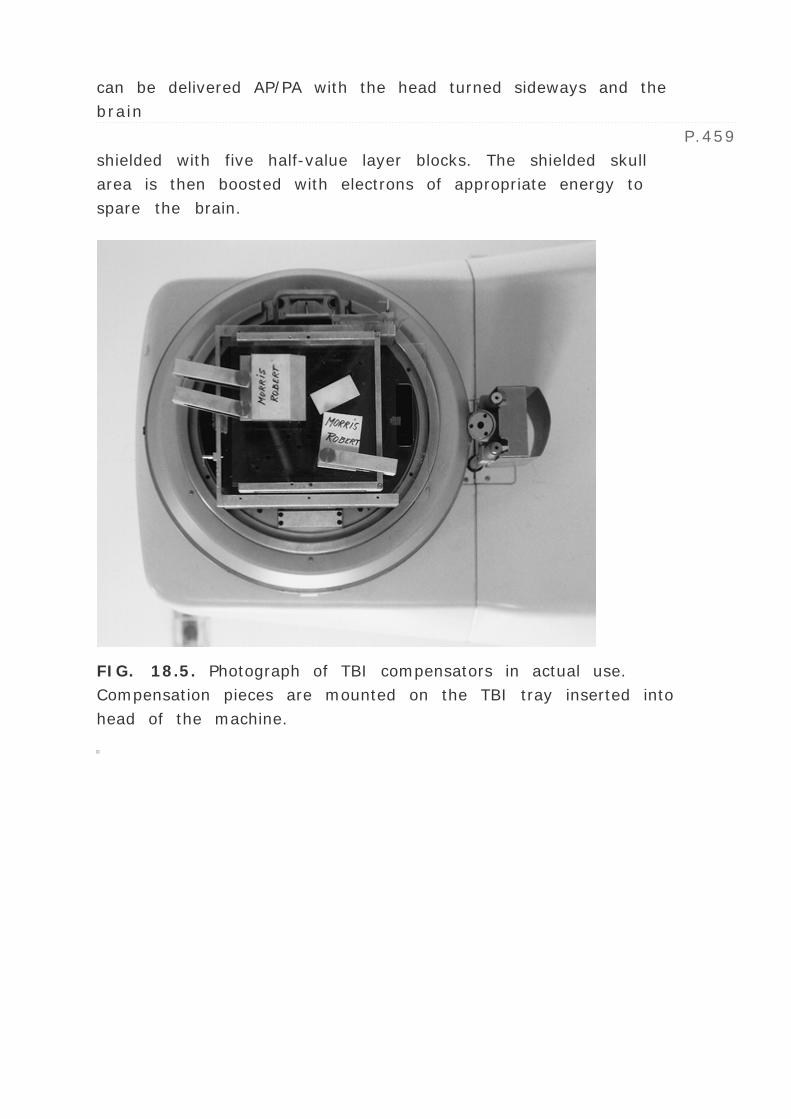
can be delivered AP/PA with the head turned sideways and the

brain

P.459

shielded with five half-value layer blocks. The shielded skull

area is then boosted with electrons of appropriate energy to

spare the brain.

FIG. 18.5. Photograph of TBI compensators in actual use.

Compensation pieces are mounted on the TBI tray inserted into

head of the machine.

FIG. 18.6. Patient in the standing TBI position with the head

turned sideways for shielding of the brain. A 5-HVL cerrobend

block is mounted on an acrylic plate attached to the TBI stand.

(From Dusenbery KE, Gerbi BJ. Total body irradiation in

conditioning regimens for bone marrow transplantation. In:

Levitt SH, Khan FM, Potish RA, et al., eds. Philadelphia:

Lippincott Williams & Wilkins, 1999:499â€“518, with

permission.)

The AP/PA technique can also be adopted for treating small

children in the reclining position. The patient is treated in the

supine and posterior positions while laying down on a low-height

couch, with the couch top only a few inches off the floor. The

shielding blocks are placed on top of an acrylic box tray at a

short distance from the patient's surface. The tray, which is

about 1 cm thick, also acts as a beam spoiler to build up the

skin dose to at least 90% of the prescription dose when treated

with parallel-opposed TBI fields. Figures 18.6 and 18.7 show

AP/PA technique for standing and reclining TBI, respectively.

D. Dosimetry Data

Details of machine calibration, dosimetry, and monitor unit

calculation for TBI have been discussed in the literature (1 ,2 ,3

,4 ,5 ). A direct output calibration of the machine for TBI may be

performed by measuring dose per monitor unit using a 0.6 cm3

Farmer type ionization chamber placed in a water phantom of

dimensions approximately 40 — 40 — 40 cm3 . The position

of the chamber is fixed at the TBI distance (source-to-body axis

distance). The collimator is opened to its maximum size and the

chamber depth is varied by moving the chamber and the

phantom while keeping the source-to-chamber distance

P.460

constant (= TBI distance). A table of output factors (dose per

MU) is generated as a function of depth that can be used to

calculate monitor units for a patient of given midline depth at

the prescription point. It is assumed in this case that the patient

is dosimetrically equivalent to the phantom, which is not a bad

approximation considering the fact that tissue maximal ratios

(TMRs) for large fields (e.g., >30 — 30 cm) are not very

sensitive to field dimensions.

FIG. 18.7. Pediatric patient in the reclining TBI position on the

floor. The legs are placed in the â€œfrog leggedâ€ position to

cover the entire patient in the radiation field with adequate

margins. Brain-sparing shielding block is placed on top of an

acrylic tray to shadow the central part of the skull with the head

turned sideways.

Alternative to direct output factor measurements, is the

calculation formalism based on TMRs, Sc , Sp , and the inverse

square law factor (see Chapter 10 ). The basic equation to

calculate dose per monitor unit (D/MU) is:

where D is dose in cGy, k is 1 cGy/MU under reference

calibration conditions, TMR is the tissue-maximum ratio at depth

d and field size equivalent to the patient (re ), S c is the

collimator scatter factor for the field size projected at isocenter

(r c ), S p is the phantom scatter factor for the patient-

equivalent field size (r e ), f is the source-to-calibration point

distance, f â€² is the source-to-patient axis distance at the

prescription point, OAR is off-axis ratio at depth d , and TF is

the transmission factor for the block tray, beam spoiler or any

other absorber placed between the machine diaphragm and the

patient.

The equivalent field at the point of calculation means that it is

dosimetrically equivalent to the patient in terms of scatter. In

theory one could determine equivalent field by doing Clarkson

integration (see Chapter 9 ) of a scatter function (e.g., scatter-

air ratio, SAR, or scatter-maximum ratio, SMR) at the point of

calculation in the patient and comparing it with the average

scatter function calculated at the same depth for a square field

in a water phantom. Such calculations done for a standard Rando

phantom exposed to a TBI field have been reported in the

literature (7 ) and are presented in Table 18.1 . For example, for

the umbilicus point, the Rando phantom-equivalent field is 28

— 28 cm on the average. Although patient dimensions vary,

scatter factors are not too sensitive to field size variation for

large fields. Therefore, it is reasonable to use a fixed equivalent

field size for TBI. A 40 — 40 cm field for large patients and a

30 — 30 cm field for pediatric patients seem to be reasonable

approximations (within approximately ±2% of dose accuracy).

The TMR data obtained under standard conditions (at isocenter)

must be checked for its validity at the TBI distance. In addition,

the inverse square law factor must also be verified for the TBI

distance. Alternatively, D/MU calculated by Equation 18.1 using

standard TMRs, S c , S p and inverse square law factors may be

compared with directly

P.461

measured output factors (D/MU) at the TBI distance. If the

difference is within +2%, Equation 18.1 may be used for TBI as

it is used for regular isocentric treatments. Larger differences

should be investigated and, if necessary, directly measured

output factors at the TBI distance should be used.

Co-60

17

22

31

30

28

4 MV

16

20

30

29

23

6 MV

18

23

29

27

26

10 MV

17

22

33

27

26

18 MV

>18

>18

>18

>18

>18

Mean

17

22

31

28

26

Lateral dimension

15

12â€“16

31

27

31

Equivalent length

19

30

31

29

20

From Kirby HT, Hanson WF, Cates DA. Verification of total body

photon irradiation dosimetry techniques. Med Phys 1988;15:364,

with permission.

Photon Energy

Side of Equivalent Square (cm)

Head Neck Chest Umbilicus Hips

TABLE 18.1. EQUIVALENT FIELD AT VARIOUS POINTS OF

CALCULATION IN A RANDO PHANTOM IRRADIATED WITH

TBI FIELD USING DIFFERENT BEAM ENERGIES

E. Compensator Design

Most TBI protocols require dose homogeneity along the body

axis to be within +10%. This requirement cannot be met without

the use of compensators. General principles of compensator

design have been discussed in Chapter 12 . Compensator design

for TBI is complicated because of large variation in body

thickness, lack of complete body immobilization, and internal

tissue heterogeneities. Considering only the lung inhomogeneity

and change in body thickness, compensators can be designed to

deliver the dose within acceptable uniformity.

The design of TBI compensators is discussed in the literature (1

,3 ,8 ). The thickness of compensator required along a ray-line

depends on the tissue deficit compared to the reference depth at

the prescription point, material of the compensator (e.g., its

density), distance of the compensator from the point of dose

compensation, depth of the point of dose compensation, field

size, and beam energy (see Chapter 12 ). Because the

compensator is designed to be dosimetrically equivalent to a

bolus (of thickness equal to the tissue deficit) but placed at a

distance from the skin surface, the bolus-equivalent thickness of

the compensator is reduced to compensate for reduction in

scatter reaching the point of dose compensation. The required

thickness of a tissue-equivalent compensator that gives the

same dose at the point of interest as would a bolus of thickness

equal to the tissue deficit, is called the thickness ratio ( „) (9

). The „ depends on many variables but for TBI an average

value of 0.70 provides a good approximation for all beam

energies and compensation conditions (1 ). The overall

dosimetric accuracy of a compensator is approximately +5%

considering all variables (1 ,9 ).

The thickness of a compensator, t c , at any point in the field is

given by:

where TD is the tissue deficit and c is the density of the

compensator. Equation 18.2 gives compensator thickness based

on tissue deficit at a given point but does not take into account

cross-beam profile or off-axis ratio.

An alternative method of determining compensator thickness, t c

, at any point in the field is based on the following equations (3

):

P.462

and

where I o and I are the doses administered before and after the

compensator is added, T (AR , dR ) and T (A,d ) are the tissue-

phantom ratios or TMRs for the reference body section and the

section to be compensated for equivalent fields AR and A at

midline depths dR and d , OARd is the off-axis ratio at depth d

relative to the prescription point, and µeff is the effective

linear attenuation coefficient for the compensator material

measured under TBI conditions.

FIG. 18.8. Schematic diagram showing areas of compensation.

(From Khan FM, Williamson JF, Sewchand W, et al. Basic data for

dosage calculation and compensation. Int J Radiat Oncol Biol

Phys 1980;6:745â€“751, with permission.)

Depending on the tissue deficits encountered in a particular TBI

technique (AP/PA or bilateral), compensator material should be

selected so that the compensator is not too bulky or of too high

a density that small errors in machining would amount to large

errors in dose. Because of these and other practical

considerations, aluminum compensators are used at the

University of Minnesota. The compensators are designed in two

dimensions (varying in thickness only along the sagittal body

axis) and are held in the beam by clamps attached to a

compensator tray (Figs. 18.5 , 18.8 ).

Compensators can be designed not only to take into account

tissue deficit but also tissue inhomogeneities such as lungs. In

the latter case, a bulk density correction is used to calculate

radiologic path length through the inhomogeneity.

F. In Vivo Patient Dosimetry

After a particular TBI technique has been established and

commissioned for clinical use, it is recommended that an in vivo

dosimetry check be performed on the first 20 or so patients.

Thermoluminescent dosimeter (TLD) capsules or chips,

surrounded by suitable build-up bolus, may be placed on the

patient skin at strategic locations and doses measured for the

actual treatments given. TLD results should be compared with

expected doses, calculated by summing entrance and exit doses

at the location of the TLDs and taking into account thickness

variation, compensation, and off-axis ratios at the depth of

TLDs. An agreement of +5% between the calculated and

measured doses is considered reasonably good. An overall dose

uniformity of +10% is considered acceptable for most protocols.

P.463

G. Total Body Irradiation Program

Implementation

The use of TBI in conjunction with bone marrow transplantation

involves numerous protocols, specifying many different

regimens: single fraction with low dose rate, single fraction with

high dose rate, fractionated TBI, hyperfractionated TBI, AP/PA

technique, bilateral technique, use of compensators or no

compensators, blocking of critical organs or no blocking, and so

on. Each of these procedures involve special equipment or

treatment aids, custom dosimetry, and rigorous quality

assurance. Before embarking on a TBI program, institutions

must design a careful plan of implementation. One of the most

important part of this plan should be to form a TBI team,

including radiation oncologist, medical physicist, medical

dosimetrist, and radiation therapist. Key members of this team

should visit another institution that has an active TBI program,

to learn all aspects of the TBI procedure, down to the most

minute details such as patient measurements, patient set-up,

dosimetry, quality assurance procedures, and worksheets

specifically designed for TBI. General TBI principles are

presented in this chapter along with selected references in the

literature for further details. But aside from acquiring pertinent

knowledge from the literature, it is emphasized that the TBI

team needs practical training, which may be obtained at another

institution with a well-established TBI program.

REFERENCES

1. Khan FM, Williamson JF, Sewchand W, et al., Basic data

for dosage calculation and compensation. Int J Radiat Oncol

Biology Phys 1980;6:745â€“751.

2. Glasgow GP. The dosimetry of fixed, single source

hemibody and total body irradiators. Med Phys

1982;9:311â€“323.

3. American Association of Physicists in Medicine. The

physical aspects of total and half body photon irradiation.

AAPM Report No. 17 Colchester, VT: American Institute of

Physics, c/o AIDC, 1986.

4. Khan FM, Kim TH. Total body irradiation. In: Paliwal BR,

Greim ML, eds. Syllabus: a categorical course in radiation

therapy treatment planning . Oak Brook, IL: Radiological

Society of North America, 1986:111â€“116.

5. Dusenbery KE, Gerbi BJ. Total body irradiation in

conditioning regimens for bone marrow transplantation. In:

Levitt SH, Khan FM, Potish RA, et al., eds. Technological

basis of radiation therapy . Philadelphia: Lippincott Williams

& Wilkins, 1999:499â€“518.

6. Shank B, Chu FCH, Dinsmore R, et al., Hyperfractionated

total body irradiation for bone marrow transplantation:

results in seventy leukemia patients with allogeneic

transplants. Int J Radiat Oncol Biol Physics

1983;9:1607â€“1611.

7. Kirby TH, Hanson WF, Cates CA. Verification of total body

photon irradiation dosimetry techniques. Med Phys

1988;15:364â€“369.

8. Galvin JM, D'Angio GJ, Walsh G. Use of tissue

compensators to improve the dose uniformity for total body

irradiation. Int J Radiat Oncol Biol Phys 1980;6:767â€“771.

9. Khan FM, Moore VC, Burns DJ. The construction of

compensators for cobalt teletherapy. Radiology 1970;96:187.




> Table of Contents > Part III - Modern Radiation Therapy >

19 - Three-Dimensional Conformal Radiation Therapy

19

Three-Dimensional ConformalRadiation Therapy

19.1. INTRODUCTION

By three-dimensional conformal radiotherapy (3-D CRT), we mean

treatments that are based on 3-D anatomic information and use

dose distributions that conform as closely as possible to the target

volume in terms of adequate dose to the tumor and minimum

possible dose to normal tissue. The concept of conformal dose

distribution has also been extended to include clinical objectives

such as maximizing tumor control probability (TCP) and

minimizing normal tissue complication probability (NTCP). Thus,

the 3-D CRT technique encompasses both the physical and

biologic rationales in achieving the desired clinical results.

Although 3-D CRT calls for optimal dose distribution, there are

many obstacles to achieving these objectives. The most major

limitation is the knowledge of the tumor extent. Despite the

modern advances in imaging, the clinical target volume (CTV) is

often not fully discernible. Depending on the invasive capacity of

the disease, what is imaged is usually not the CTV. It may be

what is called the gross tumor volume (GTV). Thus, if the CTVs

drawn on the cross-sectional images do not fully include the

microscopic spread of the disease, the 3-D CRT loses its meaning

of being conformal. If any part of the diseased tissue is missed or

seriously underdosed, it will inevitably result in failure despite all

the care and effort expended in treatment planning, treatment

delivery, and quality assurance. From the TCP point of view,

accuracy in localization of CTV is more critical in 3-D CRT than in

techniques that use generously wide fields and simpler beam

arrangements to compensate for the uncertainty in tumor

localization.

In addition to the difficulties in the assessment and localization of

CTV, there are other potential errors that must be considered

before planning 3-D CRT. Patient motion, including that of tumor

volume, critical organs and external fiducial marks during

imaging, simulation, and treatment, can give rise to systematic as

well as random errors that must be accounted for when designing

the planning target volume (PTV). If sufficient margins have been

allowed for in the localization of PTV, the beam apertures are then

shaped to conform and adequately cover the PTV (e.g., within

95% to 105% isodose surface relative to prescribed dose). In the

design of conformal fields to adequately treat the PTV,

consideration must be given to the cross-beam profile, penumbra,

and lateral radiation transport as a function of depth, radial

distance, and tissue density. Therefore, sufficient margins must

be given between the PTV outline and the field boundary to

ensure adequate dose to PTV at every treatment session.

Even if the fields have been optimally designed, biologic response

of the tumor and the normal tissues needs to be considered in

achieving the goals of 3-D CRT. In other words, the optimization

of a treatment plan has to be evaluated not only in terms of dose

distribution (e.g., dose volume histograms) but also in terms of

dose-response characteristics of the given disease and the

irradiated normal tissues. Various models involving TCP and NTCP

have been proposed, but the clinical data to validate these models

are scarce.

P.468

Until more reliable data are available, caution is needed in using

these concepts to evaluate treatment plans. This is especially

important in considering dose-escalation schemes that invariably

test the limits of normal tissue tolerance within or in proximity to

the PTV.

Notwithstanding the formidable obstacles in defining and outlining

the true extent of the disease, the clinician must follow an

analytic plan recommended by the International Commission on

Radiation Units and Measurements (ICRU) (1). Various target

volumes (GTV, CTV, PTV, etc.) should be carefully designed

considering the inherent limitations or uncertainties at each step

of the process. The final PTV should be based not only on the

given imaging data and other diagnostic studies but also the

clinical experience that has been obtained in the management of

that disease. Tightening of field margins around image-based

GTV, with little attention to occult disease, patient motion, or

technical limitations of dose delivery, is a misuse of 3-D CRT

concept that must be avoided at all cost. It should be recognized

that 3-D CRT is not a new modality of treatment, nor is it

synonymous with better results than successful and well-tested

conventional radiation therapy. Its superiority rests entirely on

how accurate the PTV is and how much better the dose

distribution is. So, instead of calling it a new modality, it should

be considered as a superior tool for treatment planning with a

potential of achieving better results.

19.2. TREATMENT-PLANNING PROCESS

The main distinction between treatment planning of 3-D CRT and

that of conventional radiation therapy is that the former requires

the availability of 3-D anatomic information and a treatment-

planning system that allows optimization of dose distribution in

accordance with the clinical objectives. The anatomic information

is usually obtained in the form of closely spaced transverse

images, which can be processed to reconstruct anatomy in any

plane, or in three dimensions. Depending on the imaging

modality, visible tumor, critical structures, and other relevant

landmarks are outlined slice-by-slice by the planner. The radiation

oncologist draws the target volumes in each slice with appropriate

margins to include visible tumor, the suspected tumor spread, and

patient motion uncertainties. This process of delineating targets

and relevant anatomic structures is called segmentation.

The next step is to follow the 3-D treatment-planning software to

design fields and beam arrangements. One of the most useful

features of these systems is the computer graphics, which allow

beamâ€™s-eye-view (BEV) visualization of the delineated targets

and other structures. The term BEV denotes display of the

segmented target and normal structures in a plane perpendicular

to the central axis of the beam, as if being viewed from the

vantage point of the radiation source. Using the BEV option, field

margins (distance between field edge and the PTV outline) are set

to cover the PTV dosimetrically within a sufficiently high isodose

level (e.g., â‰¥95% of the prescribed dose). Ordinarily a field

margin of approximately 2 cm is considered sufficient to achieve

this, but it may need further adjustments depending on the given

beam profile and the presence of critical structures in the vicinity

of the PTV.

Nonetheless, it is important to remember that each beam has a

physical penumbra (e.g., region between 90% and 20% isodose

level) where the dose varies rapidly and that the dose at the field

edge is approximately 50% of the dose at the center of the field.

For a uniform and adequate irradiation of the PTV, the field

penumbra should lie sufficiently outside the PTV to offset any

uncertainties in PTV.

Optimization of a treatment plan requires not only the design of

optimal field apertures, but also appropriate beam directions,

number of fields, beam weights, and intensity modifiers (e.g.,

wedges, compensators, dynamic multileaf collimators, etc.) In a

forward-planning system, these parameters are selected

iteratively or on a trial-and-error basis and therefore, for a

complex case, the whole process can become very labor intensive

if a high degree of optimization is desired. In practice, however,

most planners start with a

P.469

standard technique and optimize it for the given patient using 3-D

treatment-planning tools such as BEV, 3-D dose displays, non-

coplanar beam options, intensity modulation, and dose-volume

histograms. The time required to plan a 3-D CRT treatment

depends on the complexity of a given case, experience of the

treatment-planning team, and the speed of the treatment-

planning system. The final product, the treatment plan, is as good

as its individual components, namely, the quality of input patient

data, image segmentation, image registration, field apertures,

dose computation, plan evaluation, and plan optimization.

A. Imaging Data

Anatomic images of high quality are required to accurately

delineate target volumes and normal structures. Modern imaging

modalities for treatment planning include computed tomography

(CT), magnetic resonance imaging (MRI), ultrasound (US), single

photon emission tomography (SPECT), and positron emission

tomography (PET). Although CT and MRI are the most commonly

used procedures, other modalities offer special advantages in

imaging certain types of tumors. A brief review of image

characteristics of these modalities is presented to elucidate

particular advantages and limitations with regard to their use in

treatment planning.

A.1. Computed Tomography

As discussed in Chapter 12, a CT image is reconstructed from a

matrix of relative linear attenuation coefficients measured by the

CT scanner. The matrix typically consists of 1,024 — 1,024

picture elements, called pixels. Each pixel is a measure of relative

linear attenuation coefficient of the tissue for the scanning beam

used in the CT scanner. By appropriate calibration of the CT

scanner using phantoms containing tissue substitutes (CT

phantoms), a relationship between pixel value (CT numbers) and

tissue density can be established. This allows pixel by pixel

correction for tissue inhomogeneities in computing dose

distributions.

One of the important features of 3-D treatment planning is the

ability to reconstruct images in planes other than that of the

original transverse image. These are called the digitally

reconstructed radiographs (DRRs). An example is shown in Fig.

19.1. To obtain high-quality DRRs, not only images of high

contrast and resolution are required, the slice thickness must also

be sufficiently small. A slice thickness of 2 to 10 mm is commonly

used depending on the need, for example, thinner slices for tumor

localization or high-quality DRRs and thicker slices for regions

outside the tumor volume. The spiral or helical CT scanners allow

continuous rotation of the x-ray tube as the patient is translated

through the scanner aperture. This substantially reduces the

overall scanning time and therefore allows acquisition of a large

number of thin slices required for high-quality CT images and the

DRRs.

Besides high-image-quality CT scanning, treatment planning

requires special considerations such as patient positioning,

immobilization, and external markings that are visible in the

images. For treatment planning, the CT couch must be flat and

the patient must be set up in the same position as for actual

treatment. Immobilization devices are essential for 3-D CRT and

should be the same as those for CT as used in the treatment.

Fiducial points marked on the patient skin or masks should be

visible in the CT images by using radiopaque markers such as

plastic catheters.

Because CT images can be processed to generate DRRs in any

plane, conventional simulation may be replaced by CT simulation.

A CT simulator is a CT scanner equipped with some additional

hardware such as laser localizers to set up the treatment

isocenter, a flat table or couch insert, and image registration

devices. A computer workstation with special software to process

a CT data, plan beam directions and generate BEV DRRs, allows

CT simulation films with the same geometry as the treatment

beams. For a practical detail of CT simulation, the reader is

referred to Coia et al. (2).

FIG. 19.1. An example of digital reconstructed radiographs

created from transverse computed tomography scans. Image A

is frontal and image B is lateral.

P.470

P.471

A.2. Magnetic Resonance Imaging

Principles of MRI are discussed in Chapter 12. In treatment

planning, MRI images may be used alone or in conjunction with CT

images. In general, MRI is considered superior to CT in soft tissue

discrimination such as CNS tumors and abnormalities in the brain.

Also, MRI is well suited to imaging head and neck cancers,

sarcomas, the prostate gland, and lymph nodes. On the other

hand, it is insensitive to calcification and bony structures, which

are best imaged with CT. Although important differences exist

between CT and MRI image characteristics, the two are considered

complementary in their roles in treatment planning.

The most basic difference between CT and MRI is that the former

is related to electron density and atomic number (actually

representing x-ray linear attenuation coefficients) while the latter

shows proton density distribution. Although the best spatial

resolution of both modalities is similar (~1 mm), MRI takes much

longer than CT and, therefore, is susceptible to artifacts from

patient movement. On the advantageous side, MRI can be used to

directly generate scans in axial, sagittal, coronal, or oblique

planes.

One of the most important requirements in treatment planning is

the geometric accuracy. Of all the imaging modalities, CT provides

the best geometric accuracy and, therefore, CT images are

considered a reference for anatomic landmarks, when compared

with the other modality images.

Functional MRI (fMRI) also has potential to be useful in treatment

planning by showing physiologic activity as it happens and,

therefore, may be useful in outlining of the target volumes and

critical structures for highly conformal radiation therapy such as

in the brain.

B. Image Registration

The term registration as applied to images connotes a process of

correlating different image data sets to identify corresponding

structures or regions. Image registration facilitates comparison of

images from one study to another and fuses them into one data

set that could be used for treatment planning. For example,

computer programs are now available that allow image fusing, for

example, mapping of structures seen in MRI onto the CT images.

Various registration techniques include point-to-point fitting,

interactively superimposing images in the two data sets, and

surface or topography matching. An example of image fusion of a

CT and MRI study is shown in Fig. 19.2 (see color insert). For

further discussion on image registration, the reader is referred to

Kessler et al. (3), Pelizzari et al. (4), and Austin-Seymour et al.

(5).

C. Image Segmentation

The term image segmentation in treatment planning refers to

slice-by-slice delineation of anatomic regions of interest, for

example, external contours, targets, critical normal structures,

anatomic landmarks, etc. The segmented regions can be rendered

in different colors and can be viewed in BEV configuration or in

other planes using DRRs. Segmentation is also essential for

calculating dose-volume histograms (DVHs) for the selected

regions of interest.

Image segmentation is one of the most laborious but important

processes in treatment planning. Although the process can be

aided for automatic delineation based on image contrast near the

boundaries of structures, target delineation requires clinical

judgment, which cannot be automated or completely image-based.

Nor should it be delegated to personnel other than the physician

in charge of the case, the radiation oncologist. Figure 19.3 (see

color insert) shows an example of a segmented image for prostate

gland treatment planning.

D. Beam Aperture Design

After image segmentation has been completed, the treatment

planner gets to the task of selecting beam direction and designing

beam apertures. This is greatly aided by the BEV

P.472

P.473

capability of the 3-D treatment-planning system. Targets and

critical normal structures made visible in different colors through

segmentation can be viewed from different directions in planes

perpendicular to the beamâ€™s central axis. Beam directions that

create greater separation between targets and critical structures

are generally preferred unless other constraints such as

obstructions in the path of the beam, gantry collision with the

couch or patient, etc., preclude those choices. BEV capability,

combined with DRRs, is a powerful tool in selecting beam

directions and shaping fields around the target.

FIG. 19.2. An example of fusion between CT (A) and MR (B)

images. Three points of correlation were selected for fusion.

Split slice image (C) shows correlation at the interface of two

images. Fused image (D) (see color insert) shows slice

overlay with CT as red and MR as green.

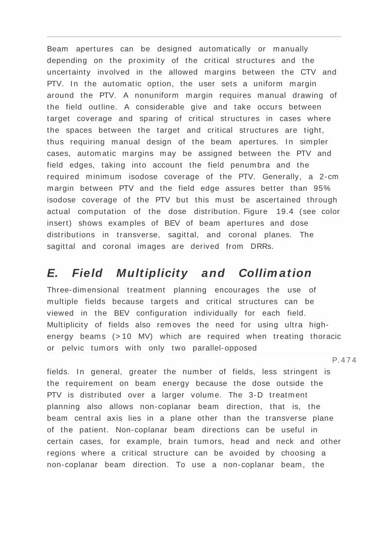
Beam apertures can be designed automatically or manually

depending on the proximity of the critical structures and the

uncertainty involved in the allowed margins between the CTV and

PTV. In the automatic option, the user sets a uniform margin

around the PTV. A nonuniform margin requires manual drawing of

the field outline. A considerable give and take occurs between

target coverage and sparing of critical structures in cases where

the spaces between the target and critical structures are tight,

thus requiring manual design of the beam apertures. In simpler

cases, automatic margins may be assigned between the PTV and

field edges, taking into account the field penumbra and the

required minimum isodose coverage of the PTV. Generally, a 2-cm

margin between PTV and the field edge assures better than 95%

isodose coverage of the PTV but this must be ascertained through

actual computation of the dose distribution. Figure 19.4 (see color

insert) shows examples of BEV of beam apertures and dose

distributions in transverse, sagittal, and coronal planes. The

sagittal and coronal images are derived from DRRs.

E. Field Multiplicity and Collimation

Three-dimensional treatment planning encourages the use of

multiple fields because targets and critical structures can be

viewed in the BEV configuration individually for each field.

Multiplicity of fields also removes the need for using ultra high-

energy beams (>10 MV) which are required when treating thoracic

or pelvic tumors with only two parallel-opposed

P.474

fields. In general, greater the number of fields, less stringent is

the requirement on beam energy because the dose outside the

PTV is distributed over a larger volume. The 3-D treatment

planning also allows non-coplanar beam direction, that is, the

beam central axis lies in a plane other than the transverse plane

of the patient. Non-coplanar beam directions can be useful in

certain cases, for example, brain tumors, head and neck and other

regions where a critical structure can be avoided by choosing a

non-coplanar beam direction. To use a non-coplanar beam, the

couch is rotated (â€œkickedâ€ ) through a specified angle,

making sure that it will not collide with the gantry.

Using a large number of fields (greater than four) creates the

problem of designing an excessive number of beam shaping blocks

and requiring longer set-up times as each block is individually

inserted into the accessory mount and verified for correct

placement of the field on the patient. Carrying so many heavy

blocks, patient after patient, creates a nuisance for therapists who

have to guard against dropping a block accidentally or using a

wrong block.

A good alternative to multiple field blocking is the use of a

multileaf collimator (MLC) (Chapter 13). MLCs can be used with

great ease and convenience to shape fields electronically. A field

drawn on a simulator film or a BEV print out can be digitized to

set the MLC setting. BEV field outlines can also be transmitted

electronically to the accelerator to program the MLC. Because MLC

fields can be set at the control console as programmed, a large

number of fields can be treated efficiently and reproducibly.

Combination of MLCs and independent jaws provides almost

unlimited capability of designing fields of any shape. Custom

designed blocks are still useful, however, in treating small fields

(unless mini-MLCs with ultra small step size are available), mid-

field blocking (â€œislandâ€ blocks), or complex field matching.

Thus, in 3-D conformal radiation therapy, where the use of shaped

multiple-fields is the norm, MLC provides a logistic solution to the

problem of designing, carrying, and storing a large number of

heavy blocks. For further details on MLC use and characteristics,

the reader is referred to Boyer (6).

F. Plan Optimization and Evaluation

Criteria for an optimal plan include both the biologic and the

physical aspects of radiation oncology. By definition, an optimal

plan should deliver tumoricidal dose to the entire tumor and spare

all the normal tissues. These goals can be set, but are not

attainable in the absolute terms. To achieve quantitative biologic

endpoints, models have been developed involving biologic indices

such as tumor control probability (TCP) and normal tissue

complication probability (NTCP). Clinical data required to validate

these models are scarce and, therefore, currently most

evaluations are carried out on the basis of physical endpoints,

namely, dose distribution within the specified target volumes and

dose to organs designated as critical. Discussion of biologic

models is beyond the scope of this book. The reader is referred to

Kutcher and Jackson (7) for a review. Physical aspects of plan

optimization and evaluation are discussed below.

F.1. Isodose Curves and Surfaces

Traditionally treatment plans are optimized iteratively by using

multiple fields, beam modifiers (e.g., wedges and compensators,

etc.), beam weights, and appropriate beam directions. Dose

distributions of competing plans are evaluated by viewing isodose

curves in individual slices, orthogonal planes (e.g., transverse,

sagittal, and coronal), or 3-D isodose surfaces. The latter

represent surfaces of a designated dose value covering a volume.

An isodose surface can be rotated to assess volumetric dose

coverage from different angles. Figure 19.5 (see color insert) is

an example of isodose curves displayed in orthogonal planes and

an isodose surface just covering the target volume. One of the

major advantages of 3-D treatment planning is the display of dose

distribution, which can be manipulated with ease to show

volumetric dose coverage in individual slices, orthogonal planes,

or as 3-D isodose surfaces.

P.475

The dose distribution is usually normalized to be 100% at the

point of dose prescription (see ICRU) (1) so that the isodose

curves represent lines of equal dose as a percentage of the

prescribed dose. For a treatment plan involving one or more

â€œboostsâ€ (increased dose to certain parts of the target,

usually the GTV), a composite isodose plan is useful, which can

again be displayed by isodose distribution in individual slices,

orthogonal planes, or as isodose surfaces.

F.2. Dose-volume Histograms

Display of dose distribution in the form of isodose curves or

surfaces is useful not only because it shows regions of uniform

dose, high dose, or low dose but also their anatomic location and

extent. In 3-D treatment planning, this information is essential

but should be supplemented by dose-volume histograms (DVH) for

the segmented structures, for example, targets, critical

structures, etc. A DVH not only provides quantitative information

with regard to how much dose is absorbed in how much volume

but also summarizes the entire dose distribution into a single

curve for each anatomic structure of interest. It is, therefore, a

great tool for evaluating a given plan or comparing competing

plans.

The DVH may be represented in two forms: the cumulative

integral DVH and the differential DVH. The cumulative DVH is a

plot of the volume of a given structure receiving a certain dose or

higher as a function of dose (Fig. 19.6) (see color insert). Any

point on the cumulative DVH curve shows the volume that

receives the indicated dose or higher. The differential DVH is a

plot of volume receiving a dose within a specified dose interval

(or dose bin) as a function of dose. As seen in Fig. 19.6E (see

color insert), the differential form of DVH shows the extent of

dose variation within a given structure. For example, the

differential DVH of a uniformly irradiated structure is a single bar

of 100% volume at the stated dose. Of the two forms of DVH, the

cumulative DVH has been found to be more useful and is more

commonly used than the differential form.

19.3. DOSE COMPUTATION

ALGORITHMS

Semi-empirical methods suitable for the calculation of dose at a

point in a patient have been discussed in Chapter 10. Corrections

for contour irregularity and tissue heterogeneity were also

presented in Chapter 12. Some elements of these methods have

been adopted into dose computation algorithms in some of the

commercially available computer treatment-planning systems.

Modern treatment planning systems have upgraded the software

additionally for 3-D data input and processing, dose calculation,

and special 3-D graphics. Some 3-D treatment-planning systems

continue to use basically two-dimensional dose computation

algorithms (calculation of dose distribution in a given slice being

unaffected by changes in tissue composition in the adjacent

slices) but rendered into three dimensions through interpolation.

In the case of tissue heterogeneities, it is assumed that the

adjacent slices are identical in the tissue composition to the slice

in which the dose is being calculated. This assumption is

obviously wrong but is not as bad as it sounds. Lateral scatter

from adjacent slices is usually a second order effect except for

situations in which small fields are used to treat tumors or

structures surrounded by lung or large air cavities. On the other

hand, by assuming the same composition for the adjacent slices,

simpler algorithms can be used that greatly speed up the dose

computation process. However, in 3-D CRT, where non-coplanar

beams are often used and dose distributions are evaluated in

multiple planes or volumes, it is essential that the dose

calculation algorithm has acceptable accuracy (within ±3% for

homogeneous and ±5% for heterogeneous tissues such as lung).

Because plan optimization is an iterative process, speed of

calculation is of paramount importance. Therefore, the best

computational algorithm is the one in which accuracy and speed

are well balanced.

Dose calculation algorithms for computerized treatment planning

have been evolving since the middle of the 1950s. In broad terms

the algorithms fall into three categories:

P.476

(a) correction-based, (b) model-based, and (c) direct Monte Carlo.

Either one of the methods can be used for 3-D treatment

planning, although with a varying degree of accuracy and speed.

However, the model-based algorithms and the direct Monte Carlo

are becoming more and more the algorithms of the future. This is

because of their ability to simulate radiation transport in three

dimensions and therefore, more accurately predict dose

distribution under conditions of charged particle disequilibrium,

which can occur in low-density tissues such as lung and

heterogeneous tissue interfaces. Although currently they are

plagued by slow speed, this limitation is fast disappearing with

the ever-increasing speed and data storage capacity of modern

computers.

A. Correction-based Algorithms

These algorithms are semi-empirical. They are based primarily on

measured data (e.g., percent depth doses and cross-beam

profiles, etc.) obtained in a cubic water phantom. Various

corrections in the form of analytic functions or factors are applied

to calculate dose distributions in a patient. The corrections

typically consist of a (a) attenuation corrections for contour

irregularity; (b) scatter corrections as a function of scattering

volume, field size, shape and radial distance; (c) geometric

corrections for source to point of calculation distance based on

inverse square law; (d) attenuation corrections for beam intensity

modifiers such as wedge filters, compensators, blocks, etc.; and

(e) attenuation corrections for tissue heterogeneities based on

radiologic path length (unit-density equivalent depth).

Correction-based algorithms represent a variety of methods

ranging from those that simply interpolate measured depth-dose

data to specially formulated analytic functions that predict the

various correction factors under specified conditions. The dose at

any point is usually analyzed into primary and scattered

components, which are computed separately and then summed to

obtain the total dose. Equations 9.31 and 10.14 are examples of

calculations that measured quantities such as percent depth

doses, TARs, TMRs, etc., and the Clarksonâ€™s method (see

Chapter 9) of dose integration for any shaped field. Contour

corrections and tissue heterogeneity corrections are discussed in

Chapter 12. These methods can be used for manual calculations

as well as made part of a correction-based computer algorithm for

the calculation of absorbed dose at a point in a patient.

As pointed out previously, the accuracy of correction-based

algorithms is limited for 3-D heterogeneity corrections in lung and

tissue interfaces especially in situations where electronic

equilibrium is not fully established.

B. Model-based Algorithms

A model-based algorithm computes dose distribution with a

physical model that simulates the actual radiation transport.

Because of its ability to model primary photon energy fluence

incident at a point and the distribution of energy subsequent to

primary photon interaction, it is able to simulate the transport of

scattered photon and electrons away from the interaction site. A

class of model-based algorithms, called convolution-superposition,

has been under development since the mid 1980s (8,9,10,11). An

example of such methods is discussed below. For a literature

review the reader in referred to Mackie et al. (12,13).

B.1. Convolution-superposition Method

A convolution-superposition method involves a convolution

equation that separately considers the transport of primary

photons and that of the scatter photon and electron emerging

from the primary photon interaction. The dose D (

) at a point

is given by:

P.477

where µ/ is the mass attenuation coefficient, ¨p(

â€²) is the primary photon energy fluence, and A(

â€“

â€²) is the convolution kernel (a matrix of dose distribution

deposited by scatter photons and electrons set in motion at the

primary photon interaction site). Figure 19.7 shows the geometry

of the radiation transport. The product of mass attenuation

coefficient and the primary energy fluence is called terma, Tp(

â€²), which stands for total energy released per unit mass. Terma

is analogous to kerma, which represents the kinetic energy

released per unit mass in the form of electrons set in motion by

photons (see Chapter 8). Kernel is the dose matrix generated per

unit terma at the interaction site. The product of terma and the

dose kernal when integrated (convolved) over a volume gives the

dose D(

) as given in Equation 19.1.

FIG. 19.7. Geometry of photon interaction and radiation

transport from the site of interaction. (From Mackie TR,

personal communication.)

The convolution kernel, A(

â€“

â€²), can be represented by a dose spread array obtained by

calculation or by direct measurement. The most commonly used

method is the Monte Carlo which simulates interactions of a large

number of primary photons and determines dose deposited in all

directions by electrons and scattered photons originating at the

primary photon interaction site. Figure 19.8 shows a 60Co kernel

for water generated by a Monte Carlo program (EGS4 Monte Carlo

code). Examination of dose distribution in the kernel indicates

that the dose deposition by the kernel is forward peaked, as

expected for a megavoltage photon beam.

Modeling of primary photon transport and the calculation of dose

kernel for a linear accelerator x-ray beam requires the knowledge

of photon energy spectrum. Again, Monte Carlo may be used to

calculate the energy spectrum of a linac beam. Mohan and Chui

(14) used EGS4 code to calculate energy spectrum of linac x-ray

beams. Such spectra can be used both for the transport of primary

photons and the generation of a dose kernel by the Monte Carlo

method. Thus, the Monte Carlo generated energy spectrum and

the kernel are essential ingredients of the convolution equation to

compute dose at any point in the patient. One of the important

tasks of commissioning a treatment-planning system that uses a

convolution equation such as Equation 19.1 is to modify (tweak)

the Monte Carlo generated energy spectrum in order to fit the

modeled beam with the measured depth dose distribution and

cross-beam dose profiles as a function of field size and depth.

A convolution equation when modified for radiological path length

(distance corrected for electron density relative to water) is called

the convolution-superposition equation:

P.478

where

â€² ·

â€² is the radiologic path length from the source to the primary

photon interaction site and

â€“

â€² · (

â€“

â€²) is the radiologic path length from the site of primary photon

interaction to the site of dose deposition. The dose kernel A(

â€“

â€² · (

â€“

â€²)) can be calculated by using range scaling by electron density

of the Monte Carlo generated kernel in water. Figure 19.9 shows

that the kernel obtained with the range scaling method compares

well with that generated by Monte Carlo directly for the

heterogeneous medium.

FIG. 19.8. Cobalt-60 dose kernels for water computed with

Monte Carlo simulation. The isovalue lines are in units of

cGyMeV-1 photon-1. Top: primary contribution by electrons set

in motion by primary photons. Middle: the first-scatter

contribution. Bottom: the sum of primary and scatter

contributions. (From Mackie TR, Bielajew AF, Rogers DWO, et

al. Generation of photon energy deposition kernels using the

EGS4 Monte Carlo Code. Phys Med Biol 1988;33:1â€“20, with

permission.)

B.2. Direct Monte Carlo

The Monte Carlo technique consists of a computer program (MC

code) that simulates the transport of millions of photons and

particles through matter. It uses fundamental laws of physics to

determine probability distributions of individual interactions of

photons

P.479

and particles. The larger the number of simulated particles

(histories), the greater the accuracy of predicting their

distributions. However, as the number of simulated particles is

increased, the computational time becomes prohibitively long. So

the challenge in writing an MC code is that of being able to use a

relatively small sample of randomly selected particles to predict

the average behavior of the particles in the beam. The dose

distribution is calculated by accumulating (scoring) ionizing

events in bins (voxels) that give rise to energy deposition in the

medium. It is estimated that the transport of a few hundred

million to a billion histories will be required for radiation therapy

treatment planning with adequate precision.

FIG. 19.9. Comparison of Monte Carlo-generated 6-MeV

primary photon kernel in a water phantom containing a ring of

air. The continuous line is a kernel computed expressly for the

heterogeneous situation. The dashed line is a kernel modified

for the heterogeneous phantom using range scaling. (From

Woo MK, Cunningham JR. The validity of the density scaling

method in primary electron transport for photon and electron

beams. Med Phys 1990;17:187â€“194, with permission.)

A number of MC codes has been used in radiation transport

simulation and, more recently, in treatment planning: Electron

Gamma Shower version 4 (EGS4) (15), ETRAN/ITS (16), Monte

Carlo N-particle (MCNP) (17), PENELOPE (18) and PEREGRINE

(developed at Lawrence Livermore National Laboratory) (19). For

a detailed review and bibliography of MC codes, the reader is

referred to (20,21).

Notwithstanding inordinate amounts of computational times,

Monte Carlo is the most accurate method of calculating dose

distribution in a patient. Sample plans done with Monte Carlo

simulation has shown significant gains in accuracy of dose

calculation, especially at interfaces of heterogeneous tissues and

in lung where particle disequilibrium can occur under certain

conditions. With the continuing advancement in computer

technology and computation algorithms, it now seems probable

that the Monte Carlo methodology will be implemented for routine

treatment planning in the not too distant future.

REFERENCES


therapy. Report No. 50. Bethesda, MD: International

Commission on Radiation Units and Measurements, 1993.

P.480

2. Coia LR, Schutheiss TE, Hanks GE, eds. A practical guide to

CT simulation. Madison, WI: Advanced Medical Publishing,

1995.

3. Keller ML, Pitluck S, Petti P, et al. Integration of

multimodality imaging data for radiotherapy treatment

planning. Int J Radiat Oncol Biol Phys 1991;21:1653â€“1667.

4. Pelizzari CA, Chen GTY, Spelbring DR, et al. Accurate three-

dimensional registration of PET, CT, and MR images of the

brain. J Comput Assist Tomogr 1989;13:20â€“27.

5. Austin-Seymour M, Chen GTY, Rosenman J, et al. Tumor and

target delineation: current research and future challenges. Int

J Radiat Oncol Biol Phys 1995;33:1041â€“1052.

6. Boyer AL. Basic applications of a multileaf collimator. In:

Mackie TR, Palta JR, eds. Teletherapy: present and future.

College Park, MD: American Association of Physicists in

Medicine, 1996.

7. Kutcher GJ, Jackson A. Treatment plan evaluation. In: Khan

FM, Potish RA, eds. Treatment planning in radiation oncology.

Baltimore: Williams & Wilkins, 1998.

8. Mackie TR, Scrimger JW, Battista JJ. A convolution method

of calculating dose for 15 MV x-rays. Med Phys

1985;12:188â€“196.

9. Boyer AL, Mok EC. A photon dose distribution model

employing convolution calculations. Med Phys

1985;12:169â€“177.

10. Mohan R, Chui C, Lidofsky L. Differential pencil beam dose

computation model for photons. Med Phys 1986;13:64â€“73.

11. Ahnesjo A, Andreo P, Brahme A. Calculation and

application of point spread functions for treatment planning

with high energy photon beams. Acta Oncol 1987;26:49â€“56.

12. Mackie TR, Reckwerdt P, McNutt T, et al. Photon beam dose

computation. In: Mackie TR, Palta JR, eds. Teletherapy:

present and future. College Park, MD: American Association of

Physicists in Medicine, 1996.

13. Mackie TR, Helen HL, McCullough EC. Treatment planning

algorithms. In: Khan FM, Potish RA, eds. Treatment planning in

radiation oncology. Baltimore: Williams & Wilkins, 1998.

14. Mohan R, Chui C. Energy and angular distributions of

photons from medical linear accelerators. Med Phys

1985;12:592â€“597.

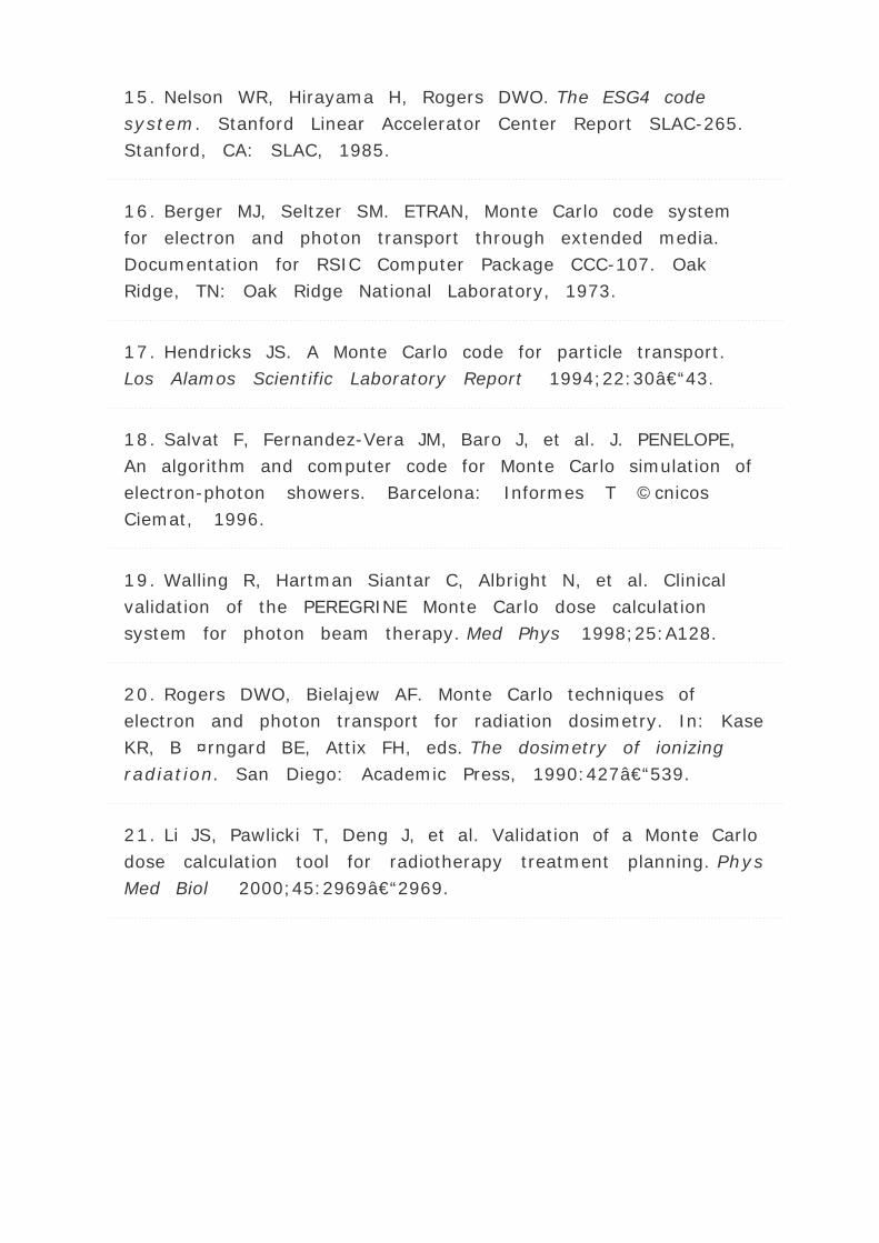
15. Nelson WR, Hirayama H, Rogers DWO. The ESG4 code

system. Stanford Linear Accelerator Center Report SLAC-265.

Stanford, CA: SLAC, 1985.

16. Berger MJ, Seltzer SM. ETRAN, Monte Carlo code system

for electron and photon transport through extended media.

Documentation for RSIC Computer Package CCC-107. Oak

Ridge, TN: Oak Ridge National Laboratory, 1973.

17. Hendricks JS. A Monte Carlo code for particle transport.

Los Alamos Scientific Laboratory Report 1994;22:30â€“43.

18. Salvat F, Fernandez-Vera JM, Baro J, et al. J. PENELOPE,

An algorithm and computer code for Monte Carlo simulation of

electron-photon showers. Barcelona: Informes T ©cnicos

Ciemat, 1996.

19. Walling R, Hartman Siantar C, Albright N, et al. Clinical

validation of the PEREGRINE Monte Carlo dose calculation

system for photon beam therapy. Med Phys 1998;25:A128.

20. Rogers DWO, Bielajew AF. Monte Carlo techniques of

electron and photon transport for radiation dosimetry. In: Kase

KR, B ¤rngard BE, Attix FH, eds. The dosimetry of ionizing

radiation. San Diego: Academic Press, 1990:427â€“539.

21. Li JS, Pawlicki T, Deng J, et al. Validation of a Monte Carlo

dose calculation tool for radiotherapy treatment planning. Phys

Med Biol 2000;45:2969â€“2969.





20 - Intensity-Modulated Radiation Therapy

20

Intensity-Modulated RadiationTherapy

20.1. INTRODUCTION

In the traditional external beam photon radiation therapy, most

treatments are delivered with radiation beams that are of uniform

intensity across the field (within the flatness specification limits).

Occasionally, wedges or compensators are used to modify the

intensity profile to offset contour irregularities and/or produce more

uniform composite dose distributions such as in techniques using

wedges. This process of changing beam intensity profiles to meet

the goals of a composite plan is called intensity modulation. Thus,

the compensators and wedges may be called as intensity

modulators, albeit much simpler than the modern computer-

controlled intensity modulation systems such as dynamic multileaf

collimators.

The term intensity-modulated radiation therapy (IMRT) refers to a

radiation therapy technique in which nonuniform fluence is delivered

to the patient from any given position of the treatment beam to

optimize the composite dose distribution. The treatment criteria for

plan optimization are specified by the planner and the optimal

fluence profiles for a given set of beam directions are determined

through â€œinverse planning.â€ The fluence files thus generated

are electronically transmitted to the linear accelerator, which is

computer-controlled, that is, equipped with the required software

and hardware to deliver the intensity-modulated beams (IMBs) as

calculated.

The clinical implementation of IMRT requires at least two systems:

(1 ) a treatment-planning computer system that can calculate

nonuniform fluence maps for multiple beams directed from different

directions to maximize dose to the target volume while minimizing

dose to the critical normal structures, and (2 ) a system of

delivering the nonuniform fluences as planned. Each of these

systems must be appropriately tested and commissioned before

actual clinical use.

20.2. INTENSITY-MODULATED

RADIATION THERAPY PLANNING

The principle of IMRT is to treat a patient from a number of different

directions (or continuous arcs) with beams of nonuniform fluences,

which have been optimized to deliver a high dose to the target

volume and acceptably low dose to the surrounding normal

structures. The treatment-planning program divides each beam into

a large number of beamlets and determines optimum setting of their

fluences or weights. The optimization process involves inverse

planning in which beamlet weights or intensities are adjusted to

satisfy predefined dose distribution criteria for the composite plan.

A number of computer methods have been devised to calculate

optimum intensity profiles (1 ,2 ,3 ,4 ,5 ,6 ,7 ,8 ,9 ,10 ). These

methods, which are based on inverse planning, can be divided into

two broad categories:

Analytic methods. These involve mathematical techniques in

which the desired dose distribution is inverted by using a back

projection algorithm. In effect, this is a reverse

P.482

of a computed tomography (CT) reconstruction algorithm in

which two-dimensional images are reconstructed from one-

dimensional intensity functions. If one assumes that the dose

distribution is the result of convolutions of a point-dose kernel

and kernel density, then the reverse is also possible, namely, by

deconvolving a dose kernel from the desired dose distribution,

one can obtain kernel density or fluence distribution in the

patient. These fluences can then be projected onto the beam

geometry to create incident beam intensity profiles.

One problem with analytical methods is that, unlike CT

reconstruction, exact analytical solutions do not exist for

determining incident fluences that would produce the desired

dose distribution without allowing negative beam weights. The

problem can be circumvented by setting negative weights to zero

but not without penalty in terms of unwanted deviations from

the desired goal. So some algorithms have been devised to

involve both analytical and iterative procedures.

Iterative methods. Optimization techniques have been devised in

which beamlet weights for a given number of beams are

iteratively adjusted to minimize the value of a cost function,

which quantitatively represents deviation from the desired goal.

For example, the cost function may be a least square function of

the form:

where C n is the cost at the n th iteration, D o (

) is the desired dose at some point

in the patient, D n (

) is the computed dose at the same point, W (

) is the weight (relative importance) factor in terms of

contribution to the cost from different structures and the sum is

taken over a large N number of dose points. Thus, for targets

the cost is the root mean squared difference between the desired

(prescribed) dose and the realized dose. For the designated

critical normal structures, the cost is the root mean squared

difference between zero dose (or an acceptable low dose value)

and the realized dose. The overall cost is the sum of the costs

for the targets and the normal structures, based on their

respective weights.

The optimization algorithm attempts to minimize the overall cost at

each iteration until the desired goal (close to a predefined dose

distribution) is achieved. A quadratic cost function such as that

given by Equation 20.1 has only one minimum. However, when

optimizing beam weights for all the beams from different directions

to reach a global minimum, the same cost function exhibits multiple

local minima. Therefore, in the iteration process occasionally it is

necessary to accept a higher cost to avoid â€œtrappingâ€ in local

minima. An optimization process, called simulated annealing (3 ,10 )

has been devised that allows the system to accept some higher costs

in pursuit of a global minimum.

Simulated annealing takes its name from the process by which

metals are annealed. The annealing process for metals involves a

controlled process of slow cooling to avoid amorphous states, which

can develop if the temperature is allowed to decrease too fast. In

the analogous process of simulated annealing, the decision to accept

a change in cost is controlled by a probability function. In other

words, If ”C n < 0, the change in the variables is always accepted.

But if ”C n > 0 the change is accepted with an acceptance

probability, P acc , given by:

where ”C n = C n - C n - 1 , Tn is analogous to thermal energy at

iteration n (it has the same dimensions as ”C n ), T n may be

thought of as temperature and as Boltzmann constant.1 At the

start of simulated annealing, the â€œthermal energyâ€ is large,

resulting in a larger probability of accepting a change in variables

that gives rise to a higher cost. As

P.483

the optimization process proceeds, the acceptance probability

decreases exponentially in accordance with Equation 20.2 and thus

drives the system to an optimal solution. The process is described

by Web (10 ) as being analogous to a skier descending from a hilltop

to the lowest point in a valley.

The patient input data for the inverse planning algorithm is the

same as that needed for forward planning, as discussed in Chapter

19 . Three-dimensional image data, image registration, and

segmentation are all required when planning for IMRT. For each

target (PTV) the user enters the plan criteria: maximum dose,

minimum dose, and a dose-volume histogram. For the critical

structures, the program requires the desired limiting dose and a

dose-volume histogram. Depending on the IMRT software, the user

may be required to provide other data such as beam energy, beam

directions, number of iterations, etc., before proceeding to

optimizing intensity profiles and calculating the resulting dose

distribution. The evaluation of an IMRT treatment plan also requires

the same considerations as the â€œconventionalâ€ 3-D CRT plans,

namely, viewing isodose curves in orthogonal planes, individual

slices, or 3-D volume surfaces. The isodose distributions are usually

supplemented by dose-volume histograms.

After an acceptable IMRT plan has been generated, the intensity

profiles (or fluence maps) for each beam are electronically

transmitted to the treatment accelerator fitted with appropriate

hardware and software to deliver the planned intensity-modulated

beams. The treatment-planning and delivery systems must be

integrated to ensure accurate and efficient delivery of the planned

treatment. Because of the â€œblack boxâ€ nature of the entire

process, rigorous verification and quality assurance procedures are

required to implement IMRT.

20.3. INTENSITY-MODULATED

RADIATION THERAPY DELIVERY

Radiation therapy accelerators normally generate x-ray beams that

are flattened (made uniform by the use of flattening filters) and

collimated by four moveable jaws to produce rectangular fields.

Precollimation dose rate can be changed uniformly within the beam

but not spatially, although the scanning beam accelerators (e.g.,

Microtron) have the capability of modulating the intensity of

elementary scanning beams. To produce intensity-modulated fluence

profiles, precalculated by a treatment plan, the accelerator must be

equipped with a system that can change the given beam profile into

a profile of arbitrary shape.

Many classes of intensity-modulated systems have been devised.

These include compensators, wedges, transmission blocks, dynamic

jaws, moving bar, multileaf collimators, tomotherapy collimators,

and scanned elementary beams of variable intensity. Of these, only

the last five allow dynamic intensity modulation. Compensators,

wedges, and transmission blocks are manual techniques that are

time consuming, inefficient, and do not belong to the modern class

of IMRT systems. Dynamic jaws are suited for creating wedged

shaped distributions but are not significantly superior to

conventional metal wedges. Although a scanning beam accelerator

can deliver intensity-modulated elementary beams (11 ), the

Gaussian half-width of the photon â€œpencilâ€ at the isocenter

can be as large as 4 cm and therefore does not have the desired

resolution by itself for full intensity modulation. However, scanning

beam may be used together with a dynamic MLC to overcome this

problem and provide an additional degree of freedom for full

dynamic intensity modulation. The case of dynamic MLC with

upstream fluence modulation is a powerful but complex technique

that is currently possible only with scanning beam accelerators such

as microtrons (12 ).

For linear accelerators it seems the computer-controlled MLC is the

most practical device for delivering intensity-modulated beams

(IMB). Competing with this technology are the tomotherapy-based

collimatorsâ€”one embodied by the MIMiC collimator of the NOMOS

Corporation and the other designed for a tomotherapy machine

under construction at the University of Wisconsin.

P.484

A. Multileaf Collimator as Intensity

Modulator

A computer-controlled multileaf collimator is not only useful in

shaping beam apertures for conventional radiotherapy it can also be

programmed to deliver IMRT. This has been done in three different

ways:

A.1. Multisegmented Static Fields Delivery

The patient is treated by multiple fields and each field is subdivided

into a set of subfields irradiated with uniform beam intensity levels.

The subfields are created by the MLC and delivered in a stack

arrangement one at a time in sequence without operator

intervention. The accelerator is turned off while the leaves move to

create the next subfield. The composite of dose increments delivered

to each subfield creates the intensity modulated beam as planned by

the treatment planning system. This method of IMRT delivery is also

called â€œstep-and-shootâ€ or â€œstop-and-shoot.â€ The theory

of creating subfields and leaf-setting sequence to generate the

desired intensity modulation has been discussed by Bortfeld et al.

(13 ). The method is illustrated in Fig. 20.1 for one-dimensional

intensity modulation in which a leaf-pair takes up a number of static

locations and the radiation from each static field thus defined is

delivered at discrete intervals of fluence (shown by dotted lines). In

this example ten separate fields have been stacked in a leaf-setting

arrangement known as the â€œclose-inâ€ technique (Fig. 20.2A ).

Another arrangement called the â€œleaf-sweepâ€ is also shown

(Fig. 20.2B ). The two arrangements are equivalent and take the

same number of cumulative monitor units. In fact, if N is the

number of subfields stacked, it has been shown that there are (N!)2

possible equivalent arrangements (14 ). The two-dimensional

intensity modulation is realized as a combination of multiple

subfields of different sizes and shapes created by the entire MLC.

The advantage of step-and-shoot method is the ease of

implementation from the engineering and safety points of view. A

possible disadvantage is the instability of some accelerators when

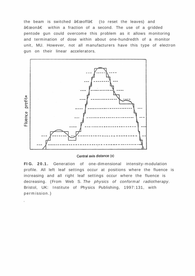
the beam is switched â€œoffâ€ (to reset the leaves) and

â€œonâ€ within a fraction of a second. The use of a gridded

pentode gun could overcome this problem as it allows monitoring

and termination of dose within about one-hundredth of a monitor

unit, MU. However, not all manufacturers have this type of electron

gun on their linear accelerators.

FIG. 20.1. Generation of one-dimensional intensity-modulation

profile. All left leaf settings occur at positions where the fluence is

increasing and all right leaf settings occur where the fluence is

decreasing. (From Web S. The physics of conformal radiotherapy.

Bristol, UK: Institute of Physics Publishing, 1997:131, with

permission.)

FIG. 20.2. Ten separate fields are stacked to generate the beam

profile shown in Fig. 20.1 . Multileaf collimator leaves are shown

schematically below the fields; (A) leaf setting as â€œclose-inâ€

technique; (B) leaf settings as â€œleaf-sweepâ€ technique. (From

Web S. The physics of conformal radiotherapy. Bristol, UK: Institute

of Physics Publishing, 1997:132, with permission.)

P.485

A mixed mode of IMB delivery, called â€œdynamic-step-and-

shoot,â€ has also been used. In this method the radiation is

â€œonâ€ all the time, even when the leaves are moving from one

static subfield position to the next. This technique has the

advantage of blurring the incremental steps in the delivery of static

subfields (15 ).

Bortfeld et al. (13 ) have demonstrated that relatively small number

of steps (10 to 30 to cover a 20-cm wide field) can be used to

deliver an intensity-modulated profile with an accuracy of 2% to

5%. A nine-field plan could be delivered in less than 20 minutes,

including extra time allowed for gantry rotation (13 ). Figure 20.3 is

an example of intensity-modulated fluence profile generated by the

step-and-shoot method and compared with calculated and measured

dose.

A.2. Dynamic Delivery

In this technique the corresponding (opposing) leaves sweep

simultaneously and unidirectionally, each with a different velocity as

a function of time. The period that the aperture between leaves

remains open (dwell time) allows the delivery of variable intensity

to different points in the field. The method has been called by

several names: the â€œsliding window,â€ â€œleaf-chasing,â€

â€œcamera-shutter,â€ and â€œsweeping variable gap.â€

The leaves of a dynamic MLC are motor driven and are capable of

moving with a speed of greater than 2 cm per second. The motion is

under the control of a computer, which also accurately monitors the

leaf positions. The problem of determining leaf velocity profiles has

been solved by several investigators (12 ,16 ,17 ). The solution is

not unique but rather consists of an optimization algorithm to

accurately deliver the planned intensity-modulated profiles under

the constraints of maximum possible leaf velocity and minimum

possible treatment time.

The basic principle of dynamic collimation is illustrated in Fig. 20.4 .

A pair of leaves defines an aperture with the leading leaf 2 moving

with velocity V 2 (x ) and the trailing leaf 1

P.486

with velocity V 1 (x ). Assuming that the beam output is constant

with no transmission through the leaves, penumbra or scattering,

the profile intensity I (x ) as a function of position x is given by the

cumulative beam-on times, t 1 (x ) and t 2 (x ), in terms of

cumulative MUs that the inside edges of leaves 1 and 2,

respectively, reach point x , that is:

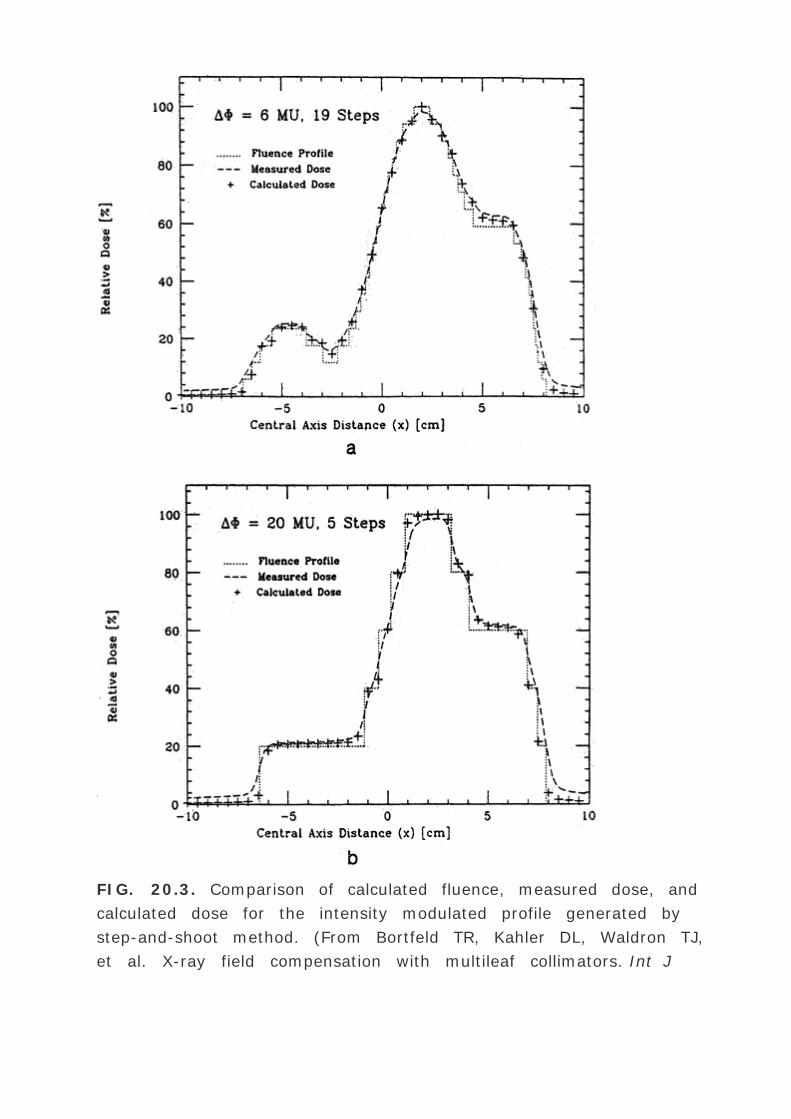
FIG. 20.3. Comparison of calculated fluence, measured dose, and

calculated dose for the intensity modulated profile generated by

step-and-shoot method. (From Bortfeld TR, Kahler DL, Waldron TJ,

et al. X-ray field compensation with multileaf collimators. Int J

Radiat Oncol Biol Phys 1994;28:723â€“730, with permission.)

FIG. 20.4. Illustration of dynamic multileaf collimator motion to

generate intensity-modulated profile. A pair of leaves with the

leading leaf 2 moving with velocity V 2 (x ) and the trailing leaf 1

with velocity V 1 (x ). In the rising part of the fluence profile, leaf 2

moves with the maximum speed V max and in the falling part of the

fluence, leaf 1 moves with V max . (Adapted from Web S. The physics

of conformal radiotherapy. Bristol, UK: Institute of Physics

Publishing, 1997:104.)

Differentiating Equation 20.3 with respect to x gives:

or

To minimize the total treatment time, the optimal solution is to

move the faster of the two leaves at the maximum allowed speed, V

max and modulate the intensity with the slower leaf. If the gradient

of the profile dI (x )/dx is zero, then according to Equation 20.5 ,

the two speeds are equal and should be set to V max . If the gradient

is positive, then the speed of leaf 2 is higher than that of leaf 1 and

therefore it is set equal to V max ; and if the

P.487

gradient is negative then the speed of leaf 1 is set equal to V max .

Once the speed of the faster leaf is set to V max , the speed of the

slower leaf can be uniquely determined from Equation 20.5 , that is:

and

In summary, the DMLC algorithm is based on the following

principles:

if the gradient of the intensity profile is positive (increasing

fluence), the leading leaf should move at the maximum speed

and the trailing leaf should provide the required intensity

modulation;

if the spatial gradient of the intensity profile is negative

(decreasing fluence), the trailing leaf should move at the

maximum speed and the leading leaf should provide the required

intensity modulation.

A.3. Intensity-modulated Arc Therapy

Yu et al. (14 ) have developed an intensity-modulated arc therapy

(IMAT) technique that uses the MLC dynamically to shape the fields

as well as rotate the gantry in the arc therapy mode. The method is

similar to the step-and-shoot in that each field (positioned along the

arc) is subdivided into subfields of uniform intensity, which are

superimposed to produce the desired intensity modulation. However,

the MLC moves dynamically to shape each subfield while the gantry

is rotating and the beam is on all the time. Multiple overlapping arcs

are delivered with the leaves moving to new positions at a regular

angular interval, for example, 5 degrees. Each arc is programmed to

deliver one subfield at each gantry angle. A new arc is started to

deliver the next subfield and so on until all the planned arcs and

their

P.488

subfields have been delivered. The magnitude of the intensity step

per arc and the number of arcs required depend on the complexity of

the treatment. A typical treatment takes three to five arcs and the

operational complexity is comparable to conventional arc therapy

(18 ).

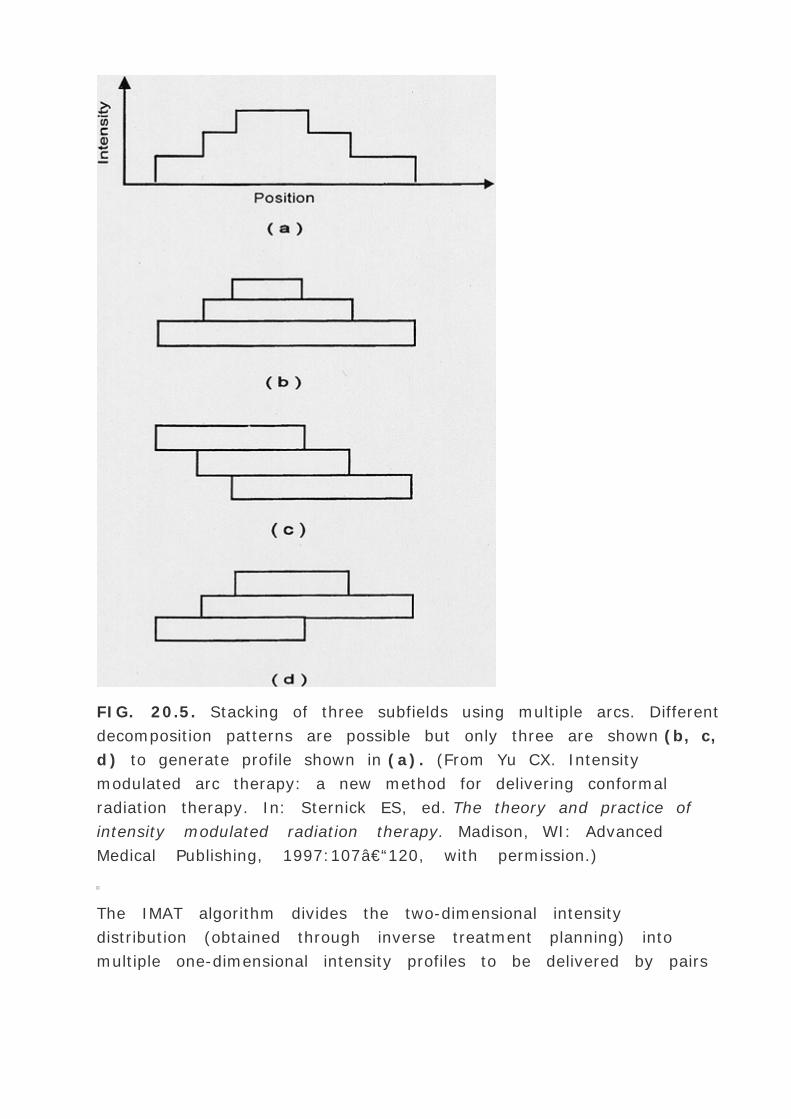
FIG. 20.5. Stacking of three subfields using multiple arcs. Different

decomposition patterns are possible but only three are shown (b, c,

d) to generate profile shown in (a). (From Yu CX. Intensity

modulated arc therapy: a new method for delivering conformal

radiation therapy. In: Sternick ES, ed. The theory and practice of

intensity modulated radiation therapy. Madison, WI: Advanced

Medical Publishing, 1997:107â€“120, with permission.)

The IMAT algorithm divides the two-dimensional intensity

distribution (obtained through inverse treatment planning) into

multiple one-dimensional intensity profiles to be delivered by pairs

of opposing leaves. The intensity profiles are then decomposed into

discrete intensity levels to be delivered by subfields in a stack

arrangement using multiple arcs as shown in Fig. 20.5 . The leaf

positions for each subfield are determined based on the

decomposition pattern selected. As discussed earlier, there are (N!

)2 possible decomposition patterns for an N -level profile (to be

delivered by N arcs) of only one peak. For example, a simple case of

one-dimensional profile with three levels (Fig. 20.5A ), there are

(3!)2 = 36 different decomposition patterns of which only three are

shown (Fig. 20.5B-D ). The decomposition patterns are determined

by a computer algorithm, which creates field apertures by

positioning left and right edges of each leaf pair. For efficiency, each

edge is used once for leaf positioning. From a large number of

decomposition patterns available, the algorithm favors those in

which the subfields at adjacent beam angles require the least

distance of travel by the MLC leaves.

As discussed earlier, the superimposition of subfields (through

multiple arcs) creates the intensity modulation of fields at each

beam angle. Whereas a one-dimensional profile is generated by

stacking of fields defined by one leaf pair, the two-dimensional

profiles are created by repeating the whole process for all the leaf

pairs of the MLC.

B. Tomotherapy

Tomotherapy is an IMRT technique in which the patient is treated

slice by slice by intensity-modulated beams in a manner analogous

to CT imaging. A special collimator is designed to generate the IMBs

as the gantry rotates around the longitudinal axis of

P.489

the patient. In one device the couch is indexed one to two slices at

a time and in the other the couch moves continuously as in a helical

CT. The former was developed by the NOMOS Corporation2 and the

latter by the medical physics group at the University of Wisconsin.3

FIG. 20.6. Multileaf intensity-modulating collimator consisting of a

long transverse slit aperture with two banks of 20 leaves each.

(From Curran B. Conformal radiation therapy using a multileaf

intensity modulating collimator. In: Sternick ES, ed. The theory and

practice of intensity modulated radiation therapy. Madison, WI:

Advanced Medical Publishing, 1997:75â€“90, with permission.)

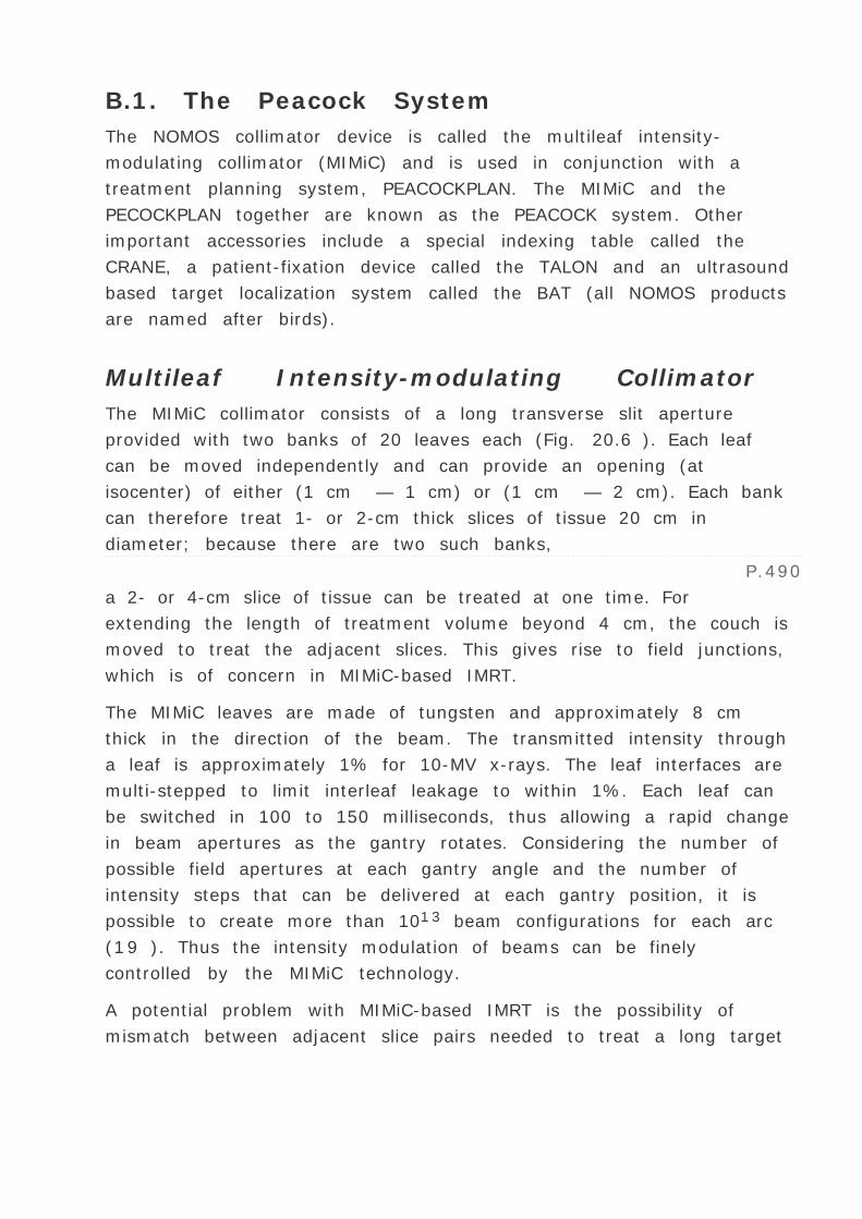
B.1. The Peacock System

The NOMOS collimator device is called the multileaf intensity-

modulating collimator (MIMiC) and is used in conjunction with a

treatment planning system, PEACOCKPLAN. The MIMiC and the

PECOCKPLAN together are known as the PEACOCK system. Other

important accessories include a special indexing table called the

CRANE, a patient-fixation device called the TALON and an ultrasound

based target localization system called the BAT (all NOMOS products

are named after birds).

Multileaf Intensity-modulating Collimator

The MIMiC collimator consists of a long transverse slit aperture

provided with two banks of 20 leaves each (Fig. 20.6 ). Each leaf

can be moved independently and can provide an opening (at

isocenter) of either (1 cm — 1 cm) or (1 cm — 2 cm). Each bank

can therefore treat 1- or 2-cm thick slices of tissue 20 cm in

diameter; because there are two such banks,

P.490

a 2- or 4-cm slice of tissue can be treated at one time. For

extending the length of treatment volume beyond 4 cm, the couch is

moved to treat the adjacent slices. This gives rise to field junctions,

which is of concern in MIMiC-based IMRT.

The MIMiC leaves are made of tungsten and approximately 8 cm

thick in the direction of the beam. The transmitted intensity through

a leaf is approximately 1% for 10-MV x-rays. The leaf interfaces are

multi-stepped to limit interleaf leakage to within 1%. Each leaf can

be switched in 100 to 150 milliseconds, thus allowing a rapid change

in beam apertures as the gantry rotates. Considering the number of

possible field apertures at each gantry angle and the number of

intensity steps that can be delivered at each gantry position, it is

possible to create more than 1013 beam configurations for each arc

(19 ). Thus the intensity modulation of beams can be finely

controlled by the MIMiC technology.

A potential problem with MIMiC-based IMRT is the possibility of

mismatch between adjacent slice pairs needed to treat a long target

volume. Carol et al. (20 ) have studied the problem and shown that

perfectly matched slices gave rise to 2% to 3% dose inhomogeneity

across the junction. However, even a 2-mm error in indexing the

couch resulted in dose inhomogeneity of the order of 40%. NOMOS

solved this problem by designing accurate table indexing and patient

fixation devices.

Crane

Because of the potential field matching problems in the use of MIMiC

for treating adjacent slice pairs along the length of the patient, it is

imperative to move the couch with extreme accuracy. A special

indexing table called the CRANE has been designed by NOMOS,

which is capable of moving the couch longitudinally with a 300-lb

weight to distances of 0.1 to 0.2 mm. With such accuracy it is

possible to reduce the junctional dose inhomogeneity to within

±3% (20 ).

Talon

Because of the stringent matchline requirements, NOMOS supplies

an invasive head fixation system called the TALON. The device is

attachable to the CT or the treatment unit couch and fixes the head

position by the insertion of two bone screws into the inner table of

the skull. Once the bone screws have been inserted, the TALON can

be removed or reattached quickly as needed. An evacuated headrest

can also be used to assist in repositioning at each treatment

session.

For further details on the PEACOCK system of IMRT the reader is

referred to reference 19.

B.2. Helical Tomotherapy

Mackie et al. (21 ) have proposed a method of IMRT delivery in

which the linac head and gantry rotate while the patient is

translated through the doughnut-shaped aperture in a manner

analogous to a helical CT scanner. In this form of tomotherapy, the

problem of inter-slice matchlines is minimized because of the

continuous helical motion of the beam around the longitudinal axis

of the patient.

A schematic diagram of the tomotherapy unit proposed by Mackie et

al. is shown in Fig. 20.7 . The linear accelerator is mounted on a CT-

like gantry and rotates through a full circle. At the same time the

patient couch is translated slowly through the aperture, thus

creating a helical motion of the beam with respect to the patient.

The unit is also equipped with a diagnostic CT scanner for target

localization and treatment planning. The unit is able to perform both

the diagnostic CT and the megavoltage CT.

The intensity-modulation of the fan beam is created by a specially

designed collimator: a temporally modulated MLC consisting of a

long, narrow slit with a set of multiple leaves at right angles. The

leaves can be moved dynamically under computer control, in and out

of the slit aperture to define a one-dimensional profile of the IMB as

with the MIMiC. The major difference between the MIMiC-based

tomotherapy and the helical tomotherapy is that in the former case

the patient couch is stationary while the gantry rotates to treat each

slice pair at a time and in the latter case the patient is translated

continuously along

P.491

with the gantry rotation. The field match problems are thus

minimized in the helical tomotherapy.

FIG. 20.7. A schematic diagram of the tomotherapy unit. (From

Mackie TR, Holmes T, Swerdloff S, et al. Tomotherapy: a new

concept for the delivery of conformal radiotherapy using dynamic

collimation. Med Physics 1993;20:1709â€“1719, with permission.)

20.4. COMMISSIONING OF INTENSITY-

MODULATED RADIATION THERAPY

IMRT is an integrated planning and delivery system of intensity-

modulated beams, which are optimized to create highly conformal

dose distributions for the treatment of planning target volume. Its

clinical implementation requires careful testing of its component

systems: the IMRT treatment-planning system (TPS) and the

intensity-modulated beam (IMB) delivery system. In general, this

will involve acquisition and input of appropriate beam data into the

computer as required by the TPS algorithm, mechanical checks of

the IMB delivery system and dosimetric verification of selected IMBs

and IMRT plans. Some of the tests are repeated at scheduled

intervals as part of a quality assurance program.

As a matter of principle, national or international protocols should

be followed with regard to commissioning and QA. However, in the

absence of established protocols, the user is advised to work closely

with the equipment manufacturer as well as review the relevant

literature to design appropriate programs. Many of the essential

tests are devised by manufacturers who are more than willing to

assist the physicist in acceptance testing and commissioning

because it is in their interest to ensure safe operation and use of the

equipment. The final approval for clinical application is the

responsibility of the physicist and the physician in charge.

Although the commissioning and QA procedures will vary depending

upon the IMRT system to be implemented, (e.g., step-and-shoot,

sliding window, IMAT, tomotherapy) the critical issue is the

confirmation that the approved treatment of a patient is delivered

safely and with acceptable accuracy. The following discussion

pertains to the sliding window IMRT technique, as an example.

P.492

A. Mechanical Testing of Dynamic

Multileaf Collimator

To assure accurate delivery of IMBs with the dynamic multileaf

collimator (DMLC), it is essential that the speed, acceleration, and

position of leaves are controlled precisely and accurately as planned

by the TPS. Chui et al. (22 ) have recommended the following five

tests as a check of the mechanical accuracy of DMLC, which is

fundamental to the accurate delivery of IMBs.

A.1. Stability of Leaf Speed

Individual pairs of opposed leaves should be tested for stability of

their speed. This can be accomplished by instructing the opposed

leaf pairs to move at different but constant speeds. If the leaf

speeds are stable, the generated intensity profiles will be uniform.

Figure 20.8 shows dose profiles generated by different leaf pairs

which were made to move at different speeds. The profiles are

measured using film placed perpendicular to central axis and at a

depth greater than that of maximum dose in a phantom. Any

fluctuations (over and above the film variation or artifacts) should

indicate instability of leaf motion.

FIG. 20.8. Dose profiles obtained with test 1 to check the stability

of leaf speed. (From Chui CS, Spirou S, LoSasso T. Testing of

dynamic multileaf collimation. Med Phys 1996;23:635â€“641, with

permission.)

A.2. Dose Profile Across Adjacent Leaves

The film obtained with the test described above may be scanned in

the direction perpendicular to leaf motion. Since the intensity within

the width of each leaf is uniform, the intensity profile across the leaf

pairs is expected to be a step function indicating different speeds or

intensity levels for each leaf pair. However, the dose profile

measured in a phantom will show a wavy pattern as seen in Fig.

20.9 . The smearing of the intensity steps is caused by lateral

scatter of photons and electrons in the phantom.

In this test one should look for any irregularity in the expected dose

profile pattern in the direction perpendicular to the path of leaf

motion.

A.3. Leaf Acceleration and Deceleration

In a normal delivery of intensity-modulated beams with DMLC,

leaves are instructed to move at different speeds from one segment

of the field to another. Discontinuities in

P.493

planned intensity profiles could possibly occur as a result of

acceleration or deceleration of leaves due to inertia. The extent of

any such problem may be determined by repeating the test in A.1

and intentionally interrupting the beam several times. As the beam

is turned off, the leaves decelerate to stop. Similarly, when the

beam is resumed, the leaves accelerate to reach their normal speed.

Dosimetric consequences of leaf acceleration and deceleration can

thus be observed in the form of discontinuities in dose profiles at

the points of beam interruption. Figure 20.10 shows no fluctuation

beyond normal uncertainty in film dosimetry.

FIG. 20.9. Dose profile resulting from test 2 to check dose profile

between adjacent leaves. The exposed film is scanned across the

leaves in the direction perpendicular to the leaf motion. Due to the

spread of secondary electrons and scattered photons, there is no flat

dose region within the width of the leaves. (From Chui CS, Spirou S,

LoSasso T. Testing of dynamic multileaf collimation. Med Phys


FIG. 20.10. Dose profiles resulting from leaf acceleration and

deceleration (test 3). A dose variation of ±1% is shown by dashed

lines. (From Chui CS, Spirou S, LoSasso T. Testing of dynamic

multileaf collimation. Med Phys 1996;23:635â€“641, with

permission.)

FIG. 20.11. Dose profile resulting from test 4 to check positional

accuracy and the effect of rounded leaf end. A hot spot of

approximately 5% in dose is seen in all profiles. (From Chui CS,

Spirou S, LoSasso T. Testing of dynamic multileaf collimation. Med

Phys 1996;23:635â€“641, with permission.)

P.494

A.4. Positional Accuracy of Leaves

To test the positional accuracy of leaves, the left and right leaves of

an opposed pair are made to travel at the same speed but with a

time lag between them. Each leaf is instructed to stop at the same

position for a fixed duration of beam-on time and then continues its

motion as before. Different pairs are instructed to stop at different

positions. The uniformity of dose profiles in this case will indicate

accurate leaf positioning. If any of the leaves were to under-travel

or over-travel, there would be a hot spot or cold spot created

depending upon if a gap or overlap occurred between the opposing

leaves at the stoppage points. The MLC designed with rounded ends

will naturally give rise to hot spots because of extra radiation

leakage at the match positions. Thus the presence of hot or cold

spots in dose profiles indicates positional inaccuracy except for the

normal hot spots caused by the rounded ends of the leaves. Figure

20.11 shows the results indicating hot spots due to rounded ends

but none due to positional errors.

A.5. Routine Mechanical Check

An overall check of the mechanical accuracy of DMLC has also been

recommended (22 ), which may be incorporated into a routine QA

program (e.g., daily or on the day of DMLC use). The test is similar

to A.4 except that the stop positions of the opposing leaves are

shifted with respect to each other to create a 1-mm gap. As a result,

a hot spot appears at the gap positions. Driving all the leaves in

fixed steps (e.g., 2 cm) and creating 1-mm-wide gaps at the stop

positions will give rise to a pattern of straight dark lines on an

irradiated film as shown in Fig. 20.12 . Any variation in the location

or the width of the dark lines would indicate positional error of a

leaf. This can be assessed by visual inspection of the film image.

The precision of this procedure is approximately 0.2 mm, which is

approximately the tolerance allowed in the leaf calibration.

B. Dosimetric Checks

A series of dosimetric checks have been recommended by LoSasso et

al. (23 ) specifically for the â€œsliding windowâ€ technique. These

include measurements of MLC transmission, transmission through

leaf ends, head scatter, and dose distribution in selected intensity

modulated fields.

FIG. 20.12. Routine mechanical check (test 5). All 26 pairs produce

dark lines on film at equally placed positions. If there is a positional

error in any leaf, the location or width of the dark lines would differ

from the other pairs. A: Normal condition with no discernible

positional error. B: Shift of dark lines caused by an intentional error

of 1mm introduced in three leaf pairs. (From Chui CS, Spirou S,

LoSasso T. Testing of dynamic multileaf collimation. Med Phys


FIG. 20.13. The midleaf and interleaf transmission measured with

film at isocenter. Transmission is the ratio of dose with the multileaf

collimator blocked to that with the field open. Field size = 10 — 10

cm2 and depth = 15cm. (From LoSasso T, Chui CS, Ling CC. Physical

and dosimetric aspects of a multileaf collimation system used in the

dynamic mode for implementing intensity-modulated radiotherapy.

Med Phys 1998;25:1919â€“1927, with permission.)

P.495

P.496

B.1. Multileaf Collimator Transmission

Transmission through the MLC may be determined by measuring

dose/MU in a phantom with the MLC closed and dividing it by

dose/MU measured with the MLC open. Because the measurements

are relative, the ratio of detector responses is equated to the ratio

of doses. Because of the difference through the leaf and interleaf

transmissions, the reading should be averaged with the detector

(e.g., ion chambers) at different positions under the leaves. A film

may also be used provided its response is corrected for the

sensitometric curve determined for the given beam energy and

depth in the phantom. Figure 20.13 shows the results obtained for a

Varian MLC. It is seen that the MLC transmission varies between

1.7% at midleaf to 2.7% between leaves. An average transmission

of 2% may be assumed in this case for the purpose of treatment

planning calculations.

Several manufacturers offer MLCs with rounded leaf ends. This is

done to maintain a constant geometric penumbra at different leaf

positions in the beam. As an example, Fig. 20.14 shows the views of

a Varian MLC from the side and from the front. Each leaf is 6-cm

thick and has a rounded end. The central 3 cm of the end is circular

with an 8.0-cm radius of curvature. The rest of end is straight at an

angle of 11.3 degrees relative to the vertical axis. It has also been

suggested that the effect of rounded leaf edges may be

approximated in the treatment planning algorithm as an offset of

leaves by 1 mm (23 ).

The leakage between the adjacent leaves is minimized by designing

the leaves so that their sides partially overlap, that is, one side of

the leaf protrudes outwards (â€œtongueâ€ ) and the other recesses

inward (â€œgrooveâ€ ) so that the central parts of the adjacent

leaves fit like a jigsaw puzzle. This overlap of the leaves reduces the

extent of radiation leakage through interleaf gaps, which are

necessary for leaf motion relative to each other. This so called

â€œtongue and grooveâ€ effect gives rise to higher radiation

leakage than that through middle body of the leaves but less than

what it would be if the leaf sides were designed plane-faced. As

shown earlier, interleaf transmission with the â€œtongue and

grooveâ€ is between 2.5% to 2.7% (Fig. 20.13 ).

B.2. Head Scatter

Definition and measurement of collimator or head scatter factor (Sc

) has been discussed in Chapter 10 . If the MLC in the linac head is

installed closer to the patient surface than the collimator jaws (as in

Varian accelerators) the Sc factor depends predominately on the jaw

opening and not on the MLC opening. In the use of static MLC in

conventional radiotherapy, Sc for a given jaw opening is affected

very little by the MLC setting for fields

P.497

larger than 4 — 4 cm. However, as the MLC aperture is reduced to

much smaller openings, S c factor could drop significantly (e.g., by

5% for a 1 — 1 cm field). The reduction is caused by the MLC

aperture approaching the geometric penumbra (radiation source has

a finite size). On the other hand, if the MLC is located above the

collimator jaws, the head scatter would be affected more by the MLC

setting than the jaw opening. In either case, the treatment-planning

algorithm must account for the Sc factors depending upon the MLC

geometry and the IMRT technique used.

FIG. 20.14. Views of the leaves (top ) from the side and (bottom )

from the front. (From LoSasso T, Chui CS, Ling CC. Physical and

dosimetric aspects of a multileaf collimation system used in the

dynamic mode for implementing intensity modulated radiotherapy.


In the sliding window technique with the Varian DMLC, typically 1-

to 4-cm wide moving gaps are used. The overall effect of the head

scatter as a percentage of the target dose is minimal. A comparative

influence of head scatter, MLC transmission, and the rounded edge

transmission is shown in Fig. 20.15 . As part of the commissioning

procedure, these data should be measured and accounted for in the

TPS.

B.4. Treatment Verification

After basic checks have been made with regard to the mechanical

and dosimetric accuracy of DMLC, the following checks are needed to

verify relative dose distribution as well as absolute dose delivered

by DMLC for selected fields and treatment plans:

FIG. 20.15. Relative contribution of multileaf collimator

transmission through midleaf, rounded edge and overall head

scatter. (From LoSasso T, Chui CS, Ling CC. Physical and dosimetric

aspects of a multileaf collimation system used in the dynamic mode

for implementing intensity modulated radiotherapy. Med Phys


P.498

Sliding Aperture Field. Using a film placed perpendicular to central

axis and at a suitable depth in a phantom (e.g., 10 cm), dose

distribution for a 10 — 10 cm field generated by a sliding MLC

aperture (e.g., 5-mm wide) may be compared with a 10 — 10 cm

static field. Absolute dose may also be verified by comparing optical

densities (related to dose through a film sensitrometic curve

measured at the same depth) or by an ion chamber in a water

phantom.

FIG. 20.16. Comparison of calculated and measured dose

distribution with corrections for multileaf collimator transmission

and head scatter. (From LoSasso T, Chui CS, Ling CC. Physical and

dosimetric aspects of a multileaf collimation system used in the

dynamic mode for implementing intensity modulated radiotherapy.


Before first treatment

Individual field verification, plan verification

3% (point dose), other per clinical significance

Daily

Dose to a test point in each IMRT field

3%

Weekly

Static field vs. sliding window field dose distribution as a function of

gantry and collimator angles

3% in dose delivery

Annually

All commissioning procedures: stability of leaf speed, leaf

acceleration and deceleration, multileaf collimator transmission, leaf

positional accuracy, static field vs. sliding window field as a function

of gantry and collimator angles, standard plan verification

3% in dose delivery, other per clinical significancea As an example for a â€œsliding windowâ€ IMRT program.

Frequency Procedure Tolerance

TABLE 20.1. IMRT QUALITY ASSURANCE PROGRAM a

P.499

Individual IMRT fields generated by the treatment planning system

can be verified by film dosimetry in a cubic phantom at a suitable

depth (e.g., 10 cm). Commercial systems are available which allow

side-by-side comparison of calculated vs. measured dose

distributions. Exposed films are scanned into the computer, which

has the software to convert optical densities into dose by using an

appropriate sensitometric curve. The calculated and measured dose

distributions are compared side by side or by viewing the differences

between the two.

Multiple Field Plan. A multiple field IMRT plan may be generated in a

cubic or cylindrical phantom and the dose distribution as well as

absolute dose may be verified using film or an ion chamber.

Alternatively, an IMRT plan of a particular patient (e.g., prostate

plan) may be set up on a cylindrical or a cubic phantom to compare

the calculated vs. measured distribution. Figure 20.16 is an example

of such a comparison.

C. Quality Assurance

After the IMRT technique has been commissioned it is essential to

set up a quality assurance program to maintain original accuracies,

tolerances, and specifications of the system. Because of the

complexity of the IMRT beams and the difficulty of verifying

treatment doses by manual calculations, it is generally

recommended to do plan verification and pre-treatment checks in

addition to the periodic testing of the system. A few of these tests

are listed in Table 20.1 , which are recommended until superseded

by national/international QA protocols.

Plan verification procedure is discussed in section B.2 above. This

check should be performed before the first treatment is delivered. In

the daily pre-treatment check, each IMRT field should be spot-

checked in a phantom by measuring dose to a test point. Detector

systems that are routinely used for daily linac output constancy

check or in vivo patient dose monitoring (e.g., ion chamber matrix,

diode system) can also be used for this measurement.

20.5. DOSE CALCULATION ALGORITHMS

Dose calculation algorithms for IMRT are basically the same as those

for standard 3-D treatment planning (see Chapter 19 ) except for

the dynamic features of multileaf collimation. In-air fluence

distribution is first calculated based on the time (or MUs) a point is

exposed to in the open part of the MLC window and the time it is

shielded by the leaves. For simplicity, the calculated fluence may be

represented by a step function, having full intensity in the open and

only transmitted intensity in the shielded part of the

P.500

field. Refinements are added by taking into account leaf-edge

penumbra (e.g., offset for rounded edges), interleaf transmission

(e.g., â€œtongue and grooveâ€ effect) and head scatter as a

function of MLC aperture and jaw position.

A. In-air Fluence Distribution

The in-air photon fluence information for an intensity-modulated

beam is imbedded in a computer file, which specifies the position of

each leaf and jaw at any instant of time. The algorithm reconstructs

the fluence distribution by integrating an output function, which is

dependent on whether the point is in the open portion of the field or

under the MLC, for example,

where ¨(x, y ) is the photon energy fluence in air at a point (x, y )

and I air (x, y, t ) is the beam intensity or energy fluence rate at

time t; T (x, y, t ) is the leaf transmission factor at any time t ,

being unity when the point is in the open portion of the field and a

transmission fraction when under a jaw or leaf.


Once the photon energy fluence distribution incident on the patient

has been calculated, any of the methods discussed in Chapter 19

may be used to compute depth-dose distribution. Because the size

and shape of the beam apertures are greatly variable and field

dimensions of 1 cm or less may be frequently required to provide

intensity modulation, the most commonly used methods of dose

calculation in IMRT are the pencil beam and the convolution-

superposition. Monte Carlo techniques are also under development

but are considered futuristic at this time because of their limitation

on computation speed.

C. Monitor Unit Calculations

Manual calculations of monitor units for IMRT is difficult, if not

impossible. Reliance is usually made on the TPS to calculate monitor

units, following the same algorithm as used in the calculation of

depth-dose distribution. Some additional data (e.g., SC , SP , TMRs,

reference dose/MU) specific to the accelerator and the algorithm

may be required but the MU calculations are performed internally by

the TPS in parallel with dose calculations. This practice seems

contrary to the long-standing principle that the monitor units must

be calculated or checked independently of the TPS. IMRT, however,

is given an exception because of its complexity, caused primarily by

intensity modulation. The user is encouraged to develop or acquire

an independent MU calculation system, if available commercially.

The latter will require rigorous commissioning of its own before it

could be used as a check on the TPS. Nonetheless, it is incumbent

on the user to verify MUs either by independent calculations or by

phantom measurements. These checks are part of patient-specific

quality assurance and should be conducted in addition to the initial

commissioning of IMRT (even though commissioning includes

experimental verification of MU calculations by the TPS under

benchmark conditions).

In view of the facts that the IMRT treatment planning system is like

a â€œblack box,â€ that manual calculations are impractical and

that patient-specific dosimetry is labor intensive, the need for

independent MU calculation cannot be overemphasized. A few

reports (24 ,25 ) have addressed this problem but commercial

software needs to be developed as an adjunct to the TPS to provide

an independent verification of MUs.

Methods of calculating MUs to deliver a certain dose are inverse of

the methods used in the calculation of dose when a patient is

irradiated with a given beam weight or fluence. Although doses in a

TPS are calculated as relative distributions, the normalizing

P.501

conditions used by the algorithm can be related to the calibration

conditions to provide MUs. In IMRT, because beam intensity within

the field is modulated (beam profile is no longer uniform), pencil

beam or convolution-superposition algorithms are the methods of

choice for dose calculations. However, they are not suitable for

manual calculation of monitor units. It is more practical to write a

separate computer program, which simplifies these or other models

and applies them more transparently to the problem of monitor unit

calculation. Basic principles of this approach are presented below as

examples.

C.1. Finite-size Pencil Beam

Instead of generating an infinitesimally small pencil beam

analytically, it is possible to measure a finite-size pencil beam

(FSPB) experimentally. The latter consists of measured depth-dose

distribution and profiles for a small field size (e.g., 1 — 1 cm2 ).

In the FSPB dose calculation formalism, a given intensity modulated

field is divided into finite-size elements (1 — 1 cm2 ) and the dose

from all the FSPBs is integrated, taking into account the relative

weight for the total fluence for each pencil beam. The following

equation summarizes the relationship between monitor units (MU)

and dose Di (P ) at a point P at depth d contributed by the n th

FSPB:

where K is the calibration factor of the accelerator (dose/MU under

reference conditions); TMR (d ) is the tissue-maximum ratio at

depth d for the FSPB; S C,P is the output factor at the reference

depth of maximum dose for the FSPB relative to the calibration field

size (10 — 10 cm2 ); T i is the transmission factor (T i is a small

fraction when P is under the leaf and is equal to unity when P is in

the open); ISF is the inverse square law factor to account for change

in distance from the source to point P versus the distance from the

source to the reference point of calibration; and OARi (d ) is the off-

axis ratio at point P relative to the central axis of FSPB i . It should

be noted that the above equation is similar to the one used for

traditional radiation therapy beams (see Chapter 10 ). Total dose at

point P is calculated by summing the contribution of all FSPBs to the

point P .

The above method of calculating dose distribution has been used by

a commercially available TPS, CORVUS4 . Details of the algorithm

have been published by Sternick et al. (26 ). Because the method

involves convolution of FSPBs and many other corrections related to

patient contours and the specific IMB collimator, it is not possible to

adopt it as such for manual calculations. However, with a few

reasonable approximations, a simpler computer program can be

written to provide an independent verification of monitor units. Such

a program has been developed by Kung et al. (25 ) and is briefly

discussed below.

Kung et al.â€™s method is based on the concept of modified

Clarkson integration (see Chapter 9 ) in which the Clarkson

integration is carried out over annular sectors instead of pie sectors.

A given IMRT field is divided into concentric circles, centered at

central axis. It is assumed that the fluence contributed to central

axis from subfields located at radius r is the same as would be by

uniformly irradiated subfields of averaged fluence at radius r . In

other words, fluence or MUs delivered to subfields at radius r can be

averaged to calculate their contribution to scattered dose along

central axis, because of the azimuthal symmetry.

Details of monitor units to be delivered to subfields are contained in

the DMLC file. Composite of weighted MUs of each subfield gives a

fluence map in terms of MU(x, y ). Average fluence,

U(r ), at the circumference of a circle of radius r is given by:

FIG. 20.17. Schematic of modified Clarkson method in which

integration is carried out over annular sectors. The dose contributed

by an annulus (dotted) is the difference between the doses from the

circular fields of radii r + ”r and r . (Redrawn from Kung JH, Chen

GTY, Kuchnir FK. A monitor unit verification calculation in intensity

modulated radiotherapy as a dosimetry quality assurance. Med Phys

2000;27:2226â€“2230.)

P.502

The contribution of scattered D s to central axis at depth from an

annulus between radii r and r + ”r , uniformly irradiated by

U(r ), is given by:

where K is the dose/MU under reference conditions of calibration, SC

is the head scatter (corresponding to jaw opening, ignoring MLC

scatter); SP and TMR (defined in Chapter 10 ) correspond to a

circular field of radius r which can be derived from equivalent

rectangular field data (see Chapter 9 ); and ISF is the inverse

squarer law factor, defined earlier.

Total dose, D (d ), at the center of an annulus is the sum of primary

dose DP , and scattered dose; DS .

Referring to Fig. 20.17 , DP is calculated from

U(0), which is obtained by averaging MU(x, y ) over a small central

circular area (e.g., r = 1 cm).

The total scattered dose at central axis, DS , is calculated by

Clarkson integration over all annuli:

Kung et al. (25 ) have tested the above algorithm for a number of

IMRT cases and found an agreement within ±3% with CORVUS.

C.2. Convolution Algorithms

The convolution method involves radiation transport in which

primary interactions are calculated separately from the interaction

of secondary particles (charged particles and scattered photons).

The dose in a phantom is calculated by convolving the terma

distribution

P.503

with dose kernels (see Chapter 19 ). The convolution dose engine

basically calculates dose per unit energy fluence. Since the incident

energy fluence is proportional to MUs, the dose can be scaled to give

dose/MU.

A suitable formalism for the calculation of monitor units using

convolution algorithm could be based on dose per unit energy

fluence. For example, the basic equation used by ADAC Pinnacle5

treatment planning system is of the form:

where Dd is the prescribed dose at depth d and ND is the normalized

dose factor. ND is the ratio of dose per unit energy fluence at the

prescription point to the dose per unit energy fluence at the

reference point of calibration.

It can be shown that for a normally incident beam in a water

phantom, ND = TMR — Sp . Let C denote the field size defined by

collimator jaws; C o be the reference field size (10 — 10 cm2 );

and ¨ be the photon energy fluence.

By definition, at the prescription point:

or,

From the definitions of TMR, SC , Sp and S C,p (see Chapter 10 ),

Equation 20.17 becomes:

or,

Thus the MU calculation formalism based on dose per unit energy

fluence is consistent with the traditional system using TMR, SC , Sp ,

etc. The advantage of using dose per unit energy fluence is that the

MUs are calculated simultaneously with dose computation by the

convolution dose engine for which the raw output is the dose per

unit energy fluence.

Mackie et al. (27 ) have suggested calibration of the accelerator in

terms of incident energy fluence per monitor unit ¨(P )/MU at a

defined point P (e.g., reference point of calibration). If D meas is the

measured dose in a water phantom at P and D calc is the calculated

dose (by convolution algorithm) at the same point in a simulated

water phantom, under the same irradiation conditions, then the

energy fluence calibration factor is given by:

The computed dose per incident energy fluence D (x, y, z )/ ¨(P )

at any point can thus be converted to dose per monitor unit D (x, y,

z )/MU using the energy fluence calibration factor given by Equation

20.20 :

As discussed earlier, for a conventional radiotherapy beam, monitor

units calculated by convolution algorithms can be verified by using

traditional concepts of TMRs and measured

P.504

output factors. In IMRT, where the fields are irradiated with

intensity-modulated beams, the traditional formalisms break down

unless the field is subdivided into elementary fields of uniform

intensity but different fluences. A method like the modified Clarkson

integration could then be applied using TMRs and output factors for

the reference elementary beam, as described earlier. Since manual

verification is still difficult, the need for independent computer

codes cannot be avoided.

20.6. CLINICAL APPLICATION

IMRT can be used for any treatment for which external beam

radiation therapy is an appropriate choice. The basic difference

between conventional radiotherapy (including 3-D CRT) and IMRT is

that the latter provides an extra degree of freedom, that is,

intensity modulation, in achieving dose conformity. Especially

targets of concave shape surrounding sensitive structures can be

treated conformly with steep dose gradients outside the target

boundariesâ€”a task that is almost impossible to accomplish with

conventional techniques. Figure 20.18 (see color insert) is an

example of such a target.

For localized lesions in any part of the body, IMRT compares well

with or exceeds the capabilities of other techniques or modalities. In

treating brain lesions, IMRT can generate dose distributions

comparable to those obtained with stereotactic radiation therapy

using x-ray knife or gamma knife. Figure 20.19 (see color insert)

shows a few examples of head and neck tumors. Additionally, IMRT

is not limited by target size or its location.

IMRT can also compete well with proton beam therapy for all disease

sites, albeit with some subtle differences radiobiologically but not so

subtle differences cost wise. The price of IMRT capability is only a

small fraction of that of a proton beam facility.

Superficial disease sites (e.g., parotid, neck nodes, chest wall),

often treated with electrons, can also be treated with IMRT as

effectively, if not better. However, practical considerations may

preclude sometimes the use of IMRT for cases where electrons offer

a technically simpler option, e.g., skin cancers, total skin

irradiation, superficial breast boost, etc.

IMRT is comparable to brachytherapy in dose conformity but it is a

different modality radiobiologically. So the choice between IMRT and

brachytherapy should be based not only on the technical or

dosimetric considerations, but also on the radiobiologic properties of

brachytherapy versus external beam. For example, treatment of

prostate with seed implants has a different rationale than it is for

IMRT although dose conformity is comparable in terms of dose fall

off beyond the prostate volume. Radiobiology of the two modalities

is obviously different because of differences in dose homogeneity

and dose rate or fractionation (e.g., continuous vs. fractionated dose

delivery).

Of all the sites suitable for IMRT, the prostate gland has received

the greatest attention because of the greater degree of dose

conformity that can be achieved compared to the conventional

techniques, including 3-D conformal (Fig. 20.20 ) (see color insert).

However, it is debatable whether a higher degree of dose conformity

correlates with better treatment outcome or if it is a sufficient

rationale for dose escalation. The reader should bear in mind that

dose conformity is a â€œdouble-edged sword,â€ with more normal

tissue sparing on the one hand and greater possibility of target miss

on the other. As discussed earlier in conjunction with 3-D CRT (see

Chapter 19 ), an image-based treatment plan cannot fully account

for (a) the true extent of clinical target volume, (b) accurately

applicable TCP and NTC, and (c) natural motion of target volume and

organs at risk. Because of these unavoidable uncertainties, too much

emphasis on dose conformity can backfire, resulting in inadequate

target coverage or increase in normal tissue complication especially

when following aggressive dose-escalation schemes. The reader is

referred to Levitt and Khan (28 ) for a cautionary note on conformal

radiotherapy and dose escalation in the prostate gland.

IMRT is an elegant treatment planning and delivery technique. It

allows practically unlimited control over shaping of dose distribution

to fit tumors of complex shape while

P.505

sparing critical normal tissues in close proximity. Undoubtedly, the

IMRT is the ultimate tool in external beam radiation therapy and is

expected to supersede other techniques including 3-D CRT and

stereotactic radiation therapy. However, it should be recognized that

technical precision alone in dose planning and delivery does not

ensure superior clinical results. Of equal or greater importance are

the design of PTV, localization of organs at risk, patient

immobilization, and on-line portal imaging. In short, the success of

IMRT when indicated does not depend on i f it is applied but rather

how it is applied.

REFERENCES

1. Brahme A. Optimization of stationary and moving beam

radiation therapy techniques. Radiother Oncol

1988;12:129â€“140.

2. K ¤llman P, Lind B, Ekloff A, et al. Shaping of arbitrary dose

distribution by dynamic Multileaf collimation. Phys Med Biol

1988;33:1291â€“1300.

3. Web S. Optimization of conformal dose distributions by

simulated annealing. Phys Med Biol 1989;34:1349â€“1370.

4. Bortfeld TR, Burkelbach J, Boesecke R, et al. Methods of image

reconstruction from projections applied to conformation therapy.

Phys Med Biol 1990;35:1423â€“1434.

5. Rosen II, Lane RG, Morrill SM, et al. Treatment planning

optimization using linear programming. Med Phys

1991;18:141â€“152.

6. Convery DJ, Rosenbloom ME. The generation of intensity-

modulated fields for conformal radiotherapy by dynamic

collimation. Phys Med Biol 1992;37:1359â€“1374.

7. Mohan R, Mageras GS, Baldwin B, et al. Clinically relevant

optimization of 3D conformal treatments. Med Phys

1992:933â€“944.

8. Holmes T, Mackie TR. A filtered back projection dose

calculation method for inverse treatment planning. Med Phys

1994;21:303â€“313.

9. Mageras GS, Mohan R. Application of fast simulated annealing

to optimization of conformal radiation treatment. Med Phys

1993;20:639â€“647.

10. Web S. The physics of conformal radiotherapy . Bristol, UK:

IOP Publishing, 1997.

11. Lind B, Brahme A. Development of treatment technique for

radiotherapy optimization. Int J Imaging Sys Technol

1995;6:33â€“42.

12. Spirou SV, Chui CS. Generation of arbitrary intensity profiles

by combining the scanning beam with dynamic Multileaf

collimation. Med Phys 1996;23:1â€“8.

13. Bortfeld TR, Kahler DL, Waldron TJ, et al. X-ray field

compensation with multileaf collimators. Int J Radiat Oncol Biol

Phys 1994;28:723â€“730.

14. Yu CX. Intensity modulated arc therapy with dynamic

Multileaf collimation: an alternative to tomotherapy. Phys Med

Biol 1995;40:1435â€“1449.

15. Yu CX, Symons M, Du MN, et al. A method for implementing

dynamic photon beam intensity modulation using independent

jaws and a Multileaf collimator. Phys Med Biol

1995;40:769â€“787.

16. Stein J, Bortfeld T, D ¶rshel B, et al. Dynamic x-ray

compensation for conformal radiotherapy by dynamic collimation.

Radiother Oncol 1994;32:163â€“173.

17. Svensson R, K ¤llman P, Brahme A. Analytical solution for

the dynamic control of Multileaf collimators. Phys Med Biol

1994;39:37â€“61.

18. Yu CX. Intensity modulated arc therapy: a new method for

delivering conformal radiation therapy. In: Sternick ES, ed. The

theory and practice of intensity modulated radiotherapy .

Madison, WI: Advanced Medical Publishing, 1997:107â€“120.

19. Curran B. Conformal radiation therapy using a multileaf

intensity modulating collimator. In: Sternick ES, ed. The theory

and practice of intensity modulated radiotherapy . Madison, WI:

Advanced Medical Publishing, 1997:75â€“90.

20. Carol MP, Grant W, Bleier AR, et al. The field-matching

problem as it applies to the Peacock three-dimensional conformal

system for intensity modulation. Int J Radiat Oncol Biol Phys

1996:183â€“187.

21. Mackie TR, Holmes T, Swerdloff S, et al. Tomotherapy: a new

concept for the delivery of conformal radiotherapy using dynamic


22. Chui CS, Spirou S, LoSasso T. Testing of dynamic multileaf


23. LoSosso T, Chui CS, Ling CC. Physical and dosimetric aspects

of a Multileaf collimation system used in the dynamic mode for

implementing intensity modulated radiotherapy. Med Phys

1998;25:1919â€“1927.

24. Boyer A, Xing L, Ma C-M, et al. Theoretical considerations of

monitor unit calculations for intensity modulated beam treatment

planning. Med Phys 1999;26:187â€“195.

P.506

25. Kung JH, Chen GTY, Kuchnir FK. A monitor unit verification

calculation in intensity modulated radiotherapy as a dosimetry

quality assurance. Med Phys 2000;27:2226â€“2230.

26. Sternick ES, Carol MP, Grand W. Intensity-modulated

radiotherapy. In: Khan FM, Potish RA, eds. Treatment planning in

radiation oncology . Baltimore: Williams & Wilkins,

1998:187â€“213.

27. Mackie TR, Rechwerdt P, McNutt T, et al. Photon beam dose

computations. In: Mackie TR, Palta JR, eds. Teletherapy: present

and future . Madison, WI: Advanced Medical Publishing,

1996:103â€“135.

28. Levitt SH, Khan FM. The rush to judgment: does the evidence

support the enthusiasm over three-dimensional conformal

radiation therapy and dose escalation in the treatment of

prostate cancer?. Int J Radiat Oncol Biol Phys

2001;51:871â€“879.

1 Boltzmann constant is derived from the theory of expansion of

gasses.

2 NOMOS Corporation, Sewickley, Pennsylvania.

3 University of Wisconsin, Madison, Wisconsin.

4 Produced by NOMOS Corporation, Sewickley, Pennsylvania.

5 ADAC Laboratories, Milpitas, California.





21 - Stereotactic Radiosurgery

21

Stereotactic Radiosurgery

21.1. INTRODUCTION

Stereotactic radiosurgery (SRS) is a single fraction radiation

therapy procedure for treating intracranial lesions using a

combination of a stereotactic apparatus and narrow multiple

beams delivered through noncoplanar isocentric arcs. The same

procedure when used for delivering multiple dose fractions is

called stereotactic radiotherapy (SRT). Both techniques involve

three-dimensional imaging to localize the lesion and delivering

treatment that concentrates the dose in the target volume and

spares as much as possible the normal brain. A high degree of

dose conformity is a hallmark of SRS, which is generally

achieved by using appropriate circular beams to fit the lesion,

optimizing arc angles and weights and using multiple isocenters

or dynamically shaping the field during arc rotations with mini

(or micro) multileaf collimators.

Accuracy of beam delivery is another hallmark of SRS. It is

strictly controlled by a specially designed stereotactic apparatus,

which is used through all steps of the process: imaging, target

localization, head immobilization, and treatment set-up. Because

of the critical nature of brain tissue, elaborate quality assurance

procedures are observed. The best achievable mechanical

accuracy in terms of isocenter displacement from the defined

center of target image is 0.2 mm ± 0.1 mm, although a

maximum error of ± 1.0 mm is commonly accepted in view of

the unavoidable uncertainties in target localization.

The term radiosurgery was coined by a neurosurgeon Lars

Leksell in 1951 (1 ). He developed the procedure in the late

1940s to destroy dysfunctional loci in the brain using

orthovoltage x-rays and particle accelerators. His later work

involved the use of a specially designed cobalt unit, called the

gamma knife. Currently there are three types of radiation used

in SRS and SRT: heavy-charged particles, cobalt-60 gamma

rays, and megavoltage x-rays. Of these, the most commonly

used modality is the x-rays produced by a linear accelerator. In

analogy to gamma knife, the linac-based SRS unit may be called

x-ray knife. Although the clinical differences between the

gamma knife and x-ray knife are insignificant, the cost of the

former is about ten times that of the latter; both are

substantially cheaper than a heavy particle accelerator. Of

course, most of the radiation generators used for SRS are also

used for other radiotherapy procedures with the exception of

gamma knife, which is dedicated solely for SRS.

21.2. STEREOTACTIC RADIOSURGERY

TECHNIQUES

Two SRS techniques are described in this chapter: linac-based x-

ray knife, and gamma knife. Greater details are provided on the

most frequently used system, the x-ray knife, while a brief

review is given on the gamma knife for general information.

Extensive literature exists on SRS techniques. The reader is

referred to AAPM Report No. 54 (2 ) for review and pertinent

bibliography.

P.508

A. X-ray Knife

The linac-based SRS technique consists of using multiple

noncoplanar arcs of circular (or dynamically shaped) beams

converging on to the machine isocenter, which is stereotactically

placed at the center of imaged target volume. A spherical dose

distribution obtained in this case can be shaped to fit the lesion

more closely by manipulating several parameters: selectively

blocking parts of the circular field, shaping the beams-eye-

aperture dynamically with a multileaf collimator, changing arc

angles and weights, using more than one isocenter and

combining stationary beams with arcing beams. Optimization of

some of these parameters is carried out automatically by the

treatment-planning software.

A.1. Stereotactic Frame

There are basically two linac-based SRS systems: pedestal-

mounted frame and couch-mounted frame. The frame in this

case refers to an apparatus called stereotactic frame, which is

attachable to the patientâ€™s skull as well as to the couch or

pedestal. This provides a rigidly fixed frame of coordinates for

relating the center of imaged target to isocenter of treatment.

Several frames have been developed for general stereotactic

applications and some of these have been adopted for SRS. The

most noteworthy of the SRS frames are: Leksell, Riechert-

Mundinger, Todd-Wells, and Brown-Robert-Wells (BRW). These

have been described in detail by Galloway and Maciunas (3 ).

Only the BRW frame will be discussed in this chapter.

Figure 21.1 shows the basic stereotactic system with the BRW

frame, computed tomography (CT) localizer, angiographic

localizer and a device for fixing the frame to the patient support

table. The BRW frame has three orthogonal axes: anterior,

lateral, and axial (Fig. 21.2 ). The three axes intersect at the

center of the circular frame and the origin is defined 80 mm

from the top surface of the ring.

The CT localizer frame is equipped with nine fiducial rods, which

appear as dots in the transaxial slice image. Since the location

of these points in the frame space is precisely known, any point

in the image can be defined in terms of the frame coordinates. A

patient docking device couples the frame to the accelerator

through the patient support system (pedestal or couch-mount

bracket). The origin of the frame is aligned with the linac

isocenter to within 0.2 to 1.0 mm, depending on the system

(pedestal-mounted systems tend to be more accurate than the

couch mounted ones).

The angiographic localizer frame consists of four plates and

attaches to the BRW head ring. Each plate is embedded with four

lead markers, which act as fiducial markers for the angiographic

images.

The MRI localizer is a slightly modified version of the CT

localizer and is compatible with magnetic resonance imaging

(MRI). It has fiducial rods whose locations are precisely known

with respect to the BRW frame, thus allowing the localization of

any point within the MRI image.

A special relocatable head ring, called the Gill-Thomas-Cosman

(GTC), has been designed for fractionated SRT (Fig. 21.3 ). It

uses a bite block system, headrest bracket and Velcro straps

attached to the BRW frame.

A.2. Linac Isocentric Accuracy

An essential element of SRS procedure is the alignment of

stereotactic frame coordinates with the linac isocenter (point of

intersection of the axes of rotation of the gantry, collimator and

couch). Acceptable specification of linac isocentric accuracy

requires that the isocenter (mechanical as well as radiation

isocenter) remains within a sphere of radius 1.0 mm with any

combination of gantry, collimator, and couch rotation. The same

specification holds good for a linac used for SRS, with an added

stipulation that the stereotactically determined target isocenter

is coincident with the linac isocenter within ± 1.0 mm (2 ) .

Tests required to check the linac specifications and its isocentric

accuracy are described in the AAPM

P.509

P.510

Reports 40 and 45 (2 ,4 ). These recommendations, which are

also discussed in Chapter 17 , form the basis of linac QA

required for SRS.

FIG. 21.1. Basic stereotactic system showing (A) (starting

clockwise from upper right) CT localizer, angiographic localizer,

patient-positioning mount and head ring with posts and pins;

(B) angiographic localizer; and (C) CT localizer. (From Bova FJ,

Meeks SL, Friedman WA. Linac radiosurgery: system

requirements, procedures, and testing. In: Khan FM, Potish RA,

eds. Treatment planning in radiation oncology. Baltimore:


A.3. Stereotactic Accuracy

The BRW frame system includes a verification device called the

phantom base (Fig. 21.4 ). It has identical coordinates

(anteroposterior, lateral, and vertical) to those of the BRW

frame. As a standalone device, it provides an absolute frame of

reference for stereotactic coordinates of the entire system: BRW

frame, patient support system, and the localizer systems for CT,

MRI, and angiography. The accuracy of phantom base should be

carefully maintained because it serves as a reference standard

for all other steps in the stereotactic localization process. Gerbi

et al. (5 ) have constructed a simple and mechanically rugged

device to routinely test the accuracy of the phantom base.

Lutz et al. (6 ) have described a procedure of using the phantom

base to check the alignment of radiation isocenter with the

target point defined by the coordinates set on the BRW pedestal.

This test is performed by setting the target point (treatment

isocenter) coordinates on the phantom base. The tip of the

phantom base pointer is matched to the tip of the transfer

pointer. The tapered tip of the transfer pointer is then replaced

with

P.511

P.512

a tungsten ball, thus assuring that its center is located exactly

at the tapered tip position (Fig. 21.5A ). The transfer pointer

(also known as target simulator) is then attached to the pedestal

(also known as independent support stand [ISS]) whose

coordinates are set to the same BRW coordinates as those set on

the phantom base. A series of port films of the tungsten ball is

taken at a number of gantry and couch angle combinations (Fig.

21.5B ). Figure 21.5C shows the results for eight gantry-table

combinations. Concentricity of the ball image within the circular

field is analyzed with special magnifying eyepiece containing a

fine scale. This test can indicate alignment to within ± 0.1

mm.

FIG. 21.2. Schematic drawing of BRW frame. (From Cho KH,

Gerbi BJ, Hall WA. Stereotactic radiosurgery and radiotherapy.

In: Levitt SH, Khan FM, Potish RA, et al., eds. Technological

basis of radiation therapy. Philadelphia: Lippincott Williams &

Wilkins, 1999:147â€“172, with permission.)

FIG. 21.3. A: The GTC relocatable head ring with bite block and

Velcro straps. B: The GTC head ring worn by the patient. (From

Cho KH, Gerbi BJ, Hall WA. Stereotactic radiosurgery and

radiotherapy. In: Levitt SH, Khan FM, Potish RA, et al., eds.

Technological basis of radiation therapy. Philadelphia: Lippincott


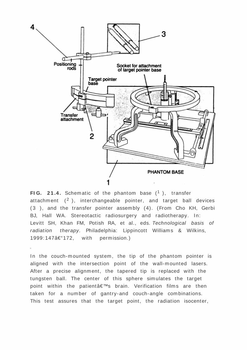
FIG. 21.4. Schematic of the phantom base (1 ), transfer

attachment (2 ), interchangeable pointer, and target ball devices

(3 ), and the transfer pointer assembly (4). (From Cho KH, Gerbi

BJ, Hall WA. Stereotactic radiosurgery and radiotherapy. In:

Levitt SH, Khan FM, Potish RA, et al., eds. Technological basis of

radiation therapy. Philadelphia: Lippincott Williams & Wilkins,


In the couch-mounted system, the tip of the phantom pointer is

aligned with the intersection point of the wall-mounted lasers.

After a precise alignment, the tapered tip is replaced with the

tungsten ball. The center of this sphere simulates the target

point within the patientâ€™s brain. Verification films are then

taken for a number of gantry-and couch-angle combinations.

This test assures that the target point, the radiation isocenter,

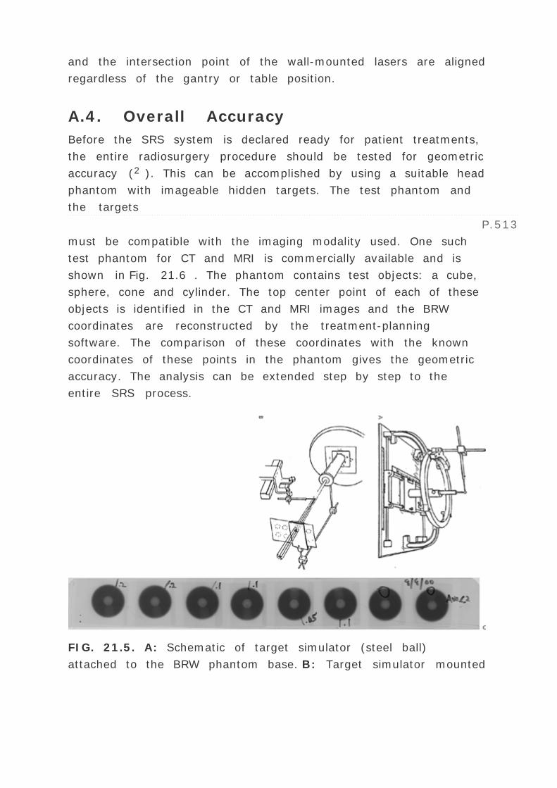
and the intersection point of the wall-mounted lasers are aligned

regardless of the gantry or table position.

A.4. Overall Accuracy

Before the SRS system is declared ready for patient treatments,

the entire radiosurgery procedure should be tested for geometric

accuracy (2 ). This can be accomplished by using a suitable head

phantom with imageable hidden targets. The test phantom and

the targets

P.513

must be compatible with the imaging modality used. One such

test phantom for CT and MRI is commercially available and is

shown in Fig. 21.6 . The phantom contains test objects: a cube,

sphere, cone and cylinder. The top center point of each of these

objects is identified in the CT and MRI images and the BRW

coordinates are reconstructed by the treatment-planning

software. The comparison of these coordinates with the known

coordinates of these points in the phantom gives the geometric

accuracy. The analysis can be extended step by step to the

entire SRS process.

FIG. 21.5. A: Schematic of target simulator (steel ball)

attached to the BRW phantom base. B: Target simulator mounted

on the pedestal to verify target alignment with radiation

isocenter as a function of table and gantry angles. C: Port films

of the tungsten ball for eight gantry-ball combinations. (Figure

21.5A,B are reproduced from Lutz W, Winston KR, Maleki N. A

system for stereotactic radiosurgery with a linear accelerator.

Int J Radiat Oncol Biol Phys 1988;14:373, with permission.)

FIG. 21.6. A head phantom used for the verification of CT and

MRI scanners. (From Cho KH, Gerbi BJ, Hall WA. Stereotactic

radiosurgery and radiotherapy. In: Levitt SH, Khan FM, Potish

RA, et al., eds. Technological basis of radiation therapy.

Philadelphia: Lippincott Williams & Wilkins, 1999:147â€“172,

with permission.)

If the change in individual coordinates is denoted by ”, the

localization error, LE, is given by:

Lutz et al. have analyzed localization accuracy in the

â€œtreatmentâ€ of 18 hidden targets in a test phantom and

reported average errors of 1 ·3 ± 0.5 mm and 0.6 mm ±

0.2 mm, respectively, for CT and plane film angiography.

The geometric accuracy of target localization for MRI is not as

good as for CT or angiography. However, MRI is a superior

diagnostic tool for many types of brain lesions. Moreover, it is

often desirable to use all of the three imaging modalities for

improved target localization. Special software is commercially

available which allows correlation between CT, MRI, and

angiography using automatic image fusion (see Chapter 19 ).

A.5. Beam Collimation

SRS or SRT is normally used for small lesions requiring much

smaller fields than those for conventional radiation therapy. In

addition, the geometric penumbra (which is inversely

proportional to source-to-diaphragm distance, see Equation 4.2

in Chapter 4 ) must be as small as possible. A tertiary

collimation system for SRS is therefore designed to bring the

collimator diaphragm closer to the surface. This has been

achieved, for example, by using 15-cm-long circular cones made

of Cerrobend lead, encased in stainless steel. The cones are

mounted below the x-ray jaws, which provide a square opening

larger than the inside diameter of the cone, but small enough to

prevent radiation escape from the sidewalls of the cone. A range

of cone diameters from 5 mm to 30 mm is needed for treating

SRS lesions. A few cones of larger diameter may also be

available for treating larger lesions with SRT.

FIG. 21.7. Schematic of patient treatment set-up showing

gantry positions and ISS subgantry to maintain isocenter

accuracy independent of the linac isocenter accuracy. (From

Friedman WA, Bova FJ. The University of Florida radiosurgery

systems. Surg Neurol 1989;32:334, with permission.)

P.514

As stated previously, attachment of long cones below the x-ray

jaws extends the SDD, thus reducing the geometric penumbra.

The cones are mounted with their central axes aligned with the

beam central axis. As a result the radiation isocenter of the

beam remains centered within the cone opening and follows the

same deviation (less than ± 1 mm) as allowed with gantry

rotation.

Isocentric accuracy of the accelerator gantry and the attached

cones have been improved by the design of a special ISS

subgantry at the University of Florida1 (Fig. 21.7 ). The cone is

rigidly attached to the subgantry and, therefore, its isocenter

remains fixed as defined by the subgantry rotation. The top end

of the cone is attached to the accelerator gantry through a

gimbal bearing with a sliding mount, which couples the linac

gantry with the ISS subgantry. The isocentric stability is thus

governed by the rotation of the ISS subgantry rather than that

of the linac gantry, although a slight misalignment may exist

between the mechanical isocenters of the two gantries. Because

the isocenter of the ISS subgantry is more stable (because it is

lighter) than that of the accelerator gantry, the accuracy of this

system is better than that of the couch-mounted systems and, in

fact, comparable to the accuracy achievable with a gamma knife

(e.g., better than 0.5 mm).

As mentioned earlier, the SRS fields can be shaped with

multileaf collimators (MLC). BrainLab2 has designed a micro-

multileaf collimator specifically for SRS, which shapes the field

to fit the beams-eye-view outline of the target as the gantry

rotates to deliver the treatment. The treatment-planning

software shapes the MLC dynamically at each angle to achieve

conformity to the outlined target as well adjust arc weights to

optimize dose distribution.

B. Gamma Knife

The gamma knife delivers radiation to a target lesion in the

brain by simultaneous irradiation with a large number of

isocentric gamma ray beams. In a modern unit 201 cobalt-60

sources are housed in a hemispherical shield (central body) and

the beams are collimated to focus on a single point at a source-

to-focus distance of 40.3 cm (Fig. 21.8 ). The central beam is

tilted through an angle of 55 degrees with respect to the

horizontal plane. The

P.515

sources are distributed along two hemispherical arcs: one in the

longitudinal plane and the other in the transverse plane of the

treatment unit. The lower half of the housing contains a shielded

entrance door. The opening and closing of the door as well as

movement of the patient treatment table in and out of the unit

are controlled by a hydraulic system.

FIG. 21.8. A: Cross-sectional view of the gamma knife unit. B:

Picture of the Leksell gamma unit. (Figure 21.8A is reproduced

from Wu A, Maitz AH, Kalend AM, et al. Physics of gamma knife

approach on convergent beams in stereotactic radiosurgery. Int J

Radiat Oncol Biol Phys 1990;18:941, with permission. Figure

21.8b is reproduced courtesy of Elekta Instruments, Stockholm,

Sweden.)

Beam channels machined in the central body provide the primary

collimation of individual gamma ray beams. Further collimation

is achieved by one of four interchangeable helmets with

collimator channels aligned with the central body channels. The

central axes of all 201 beams intersect at the focus with a

mechanical precision of ±0.3 mm. Micro switches control the

alignment of helmet channels with the central body channels

with a positioning accuracy of ± 0.1 mm. Each helmet is

characterized by its channel diameter that produces a circular

field opening of 4, 8, 14, or 18 mm at the focus point. Selected

channels can be blocked with plugs to shield the eyes or to

optimize the dose distribution. The plugs are made of 6-cm-thick

tungsten alloy.

Treatment target in the brain is localized with the Leksellâ€™s

stereotactic frame attached to the patientâ€™s skull and by

performing imaging studies, such as CT, MRI or angiography.

After the target pint coordinates with respect to the Leksellâ€™s

stereotactic frame have been determined through treatment

planning, the frame is positioned in the helmet by setting these

coordinates and fixing the frame to the trunnions of the helmet.

This brings the target point to the focal point of the unit. The

process can be repeated if there are multiple target points (e.g.,

to shape the dose distribution) or if more than one target is to

be treated in the brain.

As stated previously, there are no significant clinical differences

between gamma knife and x-ray knife treatments. However,

gamma knife can only be used for small lesions because of its

field size limitation (maximum diameter of 18 mm), although

several isocenters can be placed within the same target to

expand or shape dose distribution. For treating multiple

isocenters or targets, gamma knife is more practical than the x-

ray knife because of its simplicity of set-up. For the same

reasons, gamma knife can produce a more conformal dose

distribution than that possible with x-ray knife unless the latter

is equipped with special field-shaping collimators such as the

dynamic MLC. On the other hand the x-ray knife is far more

economical because it is linac-based. Besides, the linac can be

used for all kinds of radiation therapy techniques including SRS,

SRT, intensity-modulated radiation therapy, and conventional

radiation therapy.

21.3. DOSIMETRY

Typically there are three quantities of interest in SRS dosimetry:

central axis depth distribution (% depth dose or TMRs), cross-

beam profiles (off-axis ratios), and output factors

P.516

(Sc, p or dose/MU). Measurement of these quantities is

complicated by two factors: detector size relative to the field

dimensions and a possible lack of charged particle equilibrium.

In either case, the detector size must be as small as possible

compared to the field size.

For the measurement of central axis depth dose, an essential

criterion is that the sensitive volume of the detector must be

irradiated with uniform electron fluence (e.g., within ± 0.5%).

Because in a small circular field the central axis area of uniform

intensity does not extend beyond a few mm in diameter, this

puts a stringent requirement on the detector diameter. For a

crossbeam profile measurement, the detector size is again

important because of the steep dose gradients at the field

edges. The dosimeter, in such a case, must have high spatial

resolution to accurately measure field penumbra, which is

critically important in SRS.

Several different types of detector systems have been used in

SRS dosimetry: ion chambers, film, thermoluminescent

dosimeters, and diodes. There are advantages and disadvantages

to each of these systems. For example, ion chamber is the most

precise and the least energy-dependent system but usually has a

size limitation; film has the best spatial resolution but shows

energy dependence and a greater statistical uncertainty (e.g.,

±3%); thermoluminescent dosimeters show little energy

dependence and can have a small size in the form of chips but

suffer from the same degree of statistical uncertainty as the

film; and diodes have small size but show energy dependence as

well as possible directional dependence. Thus the choice of any

detector system for SRS dosimetry depends on the quantity to

be measured and the measurement conditions.

A. Cross-beam Profiles

The effect of detector size on the accuracy of beam profiles has

been investigated by Dawson et al. (7 ) and Rice et al. (8 ). It

has been shown that with a detector size of 3.5 mm diameter,

the beam profiles of circular fields in the range of 12.5 to 30.0

mm in diameter can be measured accurately within 1 mm.

Because cross-beam profiles involve relative dose measurement

(doses are normalized to central axis value) and there is little

change in the photon energy spectrum across small fields,

diodes and film are the detectors of choice.

Beam profiles at various depths can be measured with a film

(e.g., Kodak X-OMAT V) sandwiched parallel to central axis

between slabs of a unit-density phantom (e.g., polystyrene or

solid water) as discussed in Chapter 14 . Because in film

dosimetry, spatial resolution is governed primarily by the

densitometer aperture, it is recommended that the aperture size

be 1 mm or less. Digital film scanners are commercially

available with special dosimetry software that allows the input

of film sensitrometric data and other corrections to convert

optical density to dose.


Measurement of central axis depth dose in a small field requires

that the detector dimensions should be small enough so that it

lies well within the central uniform area of the beam profile. For

field sizes of diameter 12.5 mm or greater, it has been shown

that the central axis depth dose can be measured correctly with

a parallel plate ionization chamber of diameter not exceeding

3.0 mm (10 ). Smaller diameter chambers will be required for

smaller field sizes.

Film or diodes can also be used for central axis depth dose

distribution, especially for very small field sizes. Because the

proportions of scattered photons of lower energy increases with

depth, energy-dependence of the film or diodes must be taken

into account. Depth dependent correction factors can be

determined by comparing film or diode curves with ion chamber

curves using larger fields (e.g., 30 to 50 mm diameter).

Although TMRs can be measured directly, they can be calculated

from percent depth doses as discussed in Chapter 10 .

P.517

C. Output Factors

Output factors (Sc, p ) for small fields pose the same kinds of

problems as for beam profiles and depth-dose measurements.

Detector size in relation to the field size is the critical

parameter. It has been shown that for fields of diameter 12.5

mm and larger, cylindrical or parallel-plate chambers of 3.5 mm

diameter allow the output factors to be measured accurately to

within 0.5% (8 ). Figure 21.9 shows an example of output

factors as a function of field size.

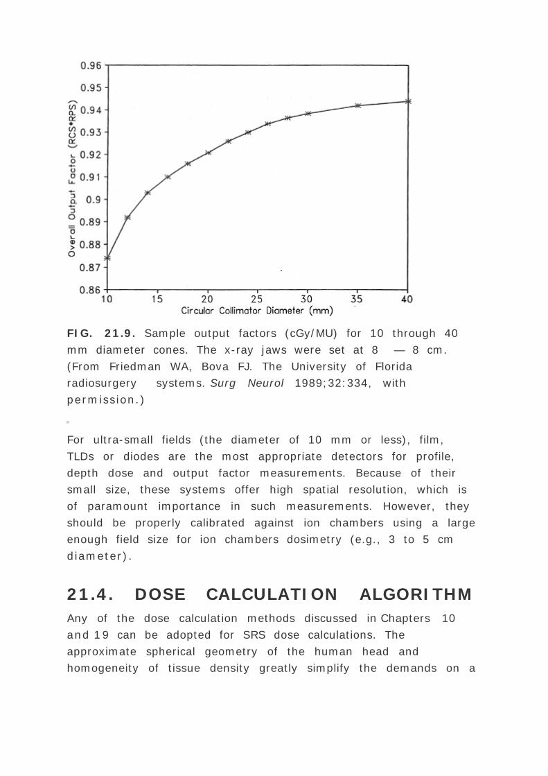
FIG. 21.9. Sample output factors (cGy/MU) for 10 through 40

mm diameter cones. The x-ray jaws were set at 8 — 8 cm.

(From Friedman WA, Bova FJ. The University of Florida

radiosurgery systems. Surg Neurol 1989;32:334, with

permission.)

For ultra-small fields (the diameter of 10 mm or less), film,

TLDs or diodes are the most appropriate detectors for profile,

depth dose and output factor measurements. Because of their

small size, these systems offer high spatial resolution, which is

of paramount importance in such measurements. However, they

should be properly calibrated against ion chambers using a large

enough field size for ion chambers dosimetry (e.g., 3 to 5 cm

diameter).

21.4. DOSE CALCULATION ALGORITHM

Any of the dose calculation methods discussed in Chapters 10

and 19 can be adopted for SRS dose calculations. The

approximate spherical geometry of the human head and

homogeneity of tissue density greatly simplify the demands on a

dose calculation algorithm. One of the simplest methods of beam

modeling is based on tissue-maximum ratios, off-axis ratios,

exponential attenuation, output factors and inverse-square law.

The beam data are acquired specifically for the beam energy and

circular fields, used in SRS, as discussed previously.

The patient surface contour geometry is defined three-

dimensionally by CT scans. The multiple arc geometries are

simulated by stationary beams separated by angles of 5 to 10

degrees. The choice of dose calculation grid has been discussed

by Niemierko and Goitein (11 ). They have shown that a 2-mm

grid spacing produces a dose uncertainty of 1% to 2%,

compared to 3% to 4% uncertainty with a 4-mm grid spacing. Of

course, the overall accuracy depends on the accuracy of all dose

calculation parameters, beam modeling, interpolation routines,

grid size, positional accuracy, etc.

The CT and MRI scans for treatment planning are obtained with

a slice separation typically between 3 and 10 mm. Greater

resolution is required for target definition. So a smaller slice

separation of 1 to 3 mm is used to scan the lesion and the

critical structures in

P.518

its close vicinity. Target volumes are outlined slice by slice in

the CT images and correlated with MRI scans and angiograms

through fusion techniques.

Calculated dose distributions are overlaid on individual CT, MRI,

or angiographic images. Volumetric displays in the form of

isodose surfaces are also useful. Dose volume histograms (DVH)

of the target and normal structures complement the isodose

display.

21.5. QUALITY ASSURANCE

Stereotactic radiosurgery or radiotherapy is a special procedure,

which requires careful commissioning followed by a rigorous

quality assurance program to maintain its original accuracy

specifications. Several QA protocols pertinent to SRS have been

published (2 ,4 ). These protocols should provide guidelines for

an institution to design its QA program.

Quality assurance involves both the clinical and physical aspects

of SRS. The physics part may be divided into two categories:

treatment QA and routine QA. The former involves checking or

double-checking of the procedures and treatment parameters

pertaining to individual patients; and the latter is designed to

periodically inspect the hardware and software performance to

ensure compliance with original specifications.

A. Treatment Quality Assurance

Patient treatment involves many steps and procedures. It is

highly desirable that detailed checklists are prepared to

documents these steps in a proper sequence. The objective of

the checklist should be to ensure procedural accuracy at each

step of the way and to minimize the chance of a treatment error.

Major components of treatment QA consist of checking (a)

stereotactic frame accuracy including phantom base,

CT/MRI/angiographic localizer, pedestal or couch mount; (b)

imaging data transfer, treatment plan parameters, target

position, monitor unit calculations; (c) frame alignment with

gantry and couch eccentricity, congruence of target point with

radiation isocenter, collimator setting, cone diameter, couch

position, patient immobilization and safety locks; and (d)

treatment console programming of beam energy, monitor units,

arc angles, etc.

Examples of treatment QA checklists have been published (2 )

that may be used as rough guides. It should be realized that the

SRS QA program involves health professionals in different

departments. Therefore, personnel coordination is important for

successful implementation of a QA program.

B. Routine Quality Assurance

A routine QA program is designed to check the

hardware/software performance of SRS equipment on a

scheduled frequency basis. For the linear accelerator, the

relevant QA protocol is the AAPM Report No. 40 (4 ). For the SRS

apparatus, the routine QA schedule is recommended by the

AAPM Report No. 54 (2 ) .

A QA program for the gamma knife must be compliant with the

NRC regulations. An example program, implemented at the

University of Pittsburgh is published in the AAPM Report 54.

21.6. CLINICAL APPLICATIONS

Stereotactic radiosurgery was originally developed for the

treatment of benign lesions of the brain such as arteriovenous

malformations (AVM), meningiomas, and acoustic neuromas. Its

use has been extended to treat many malignant tumors such as

gliomas and brain metastases. More recently SRS has also been

used to treat functional disorders, for example, trigeminal

neuralgia and movement disorders. Fractional SRT is now

commonly being used

P.519

to treat malignant brain tumors, especially those in proximity to

critical structures such as brain stem and optic pathways. For

overviews of clinical rationale, the reader is referred to

McKenzie et al. (12 ), Luxton et al. (13 ), and Cho et al. (9 ).

Radiobiologic principles of SRS are currently not well

understood. However, attempts have been made to rationalize

the delivery of a single large fraction of dose to a small-

circumscribed lesion (e.g., less than 4 cm in diameter) in the

brain. Because the intended effect is to cause thrombosis in the

case of AVM and reproductive cell death in the case of a tumor,

the potential benefits of fractionated radiation therapy are not

considered in SRS. However, in the case of malignant tumors

treated with SRT, the well-established principles of radiobiology,

namely repair, reoxygenation, redistribution and repopulation

(i.e., â€œ4 Râ€™sâ€ ) are considered just as important as in

conventional radiation therapy. Accordingly, the fractionation

schemes are similar depending on the tumor volume and the

radiobiologic characteristics of the disease.

Dose distribution achievable with SRS is highly conformal. This

is made possible by tertiary collimation (i.e., cones) and the use

of multiple non-coplanar arcs. Because in single-fraction

radiosurgery, no attempt is made to spare normal tissue within

the target volume, dose conformity is essential to minimize

irradiation of the normal brain outside the target. Tight margins

between the target and the prescription isodose are made

possible by rigid immobilization of the patient and the

stereotactic accuracy of the SRS procedure. In the fractionated

SRT of malignant tumors, same considerations apply to the

design of target volume (e.g., planning target volume) as in

three-dimensional conformal radiation therapy. Figures 21.10

,21.11 (see color insert) show selected examples of cases

treated with SRS and SRT.

FIG. 21.10. An example of stereotactic radiosurgery treatment

of arteriovenous malformation. (A) Anterior angiographic view

of nidus; (B) lateral view of nidus; (C) beam arrangement using

five noncoplanar arcs (see color insert); isodose region (color

wash) corresponding to 90% of the maximum dose is shown in

anterior view (D) and lateral view (E) (see color insert).

REFERENCES

1. Leksell L. The stereotactic method and radiosurgery of the

brain. Acta Chir Scand 1951;102:316â€“319.

2. AAPM. Stereotactic radiosurgery . Report No. 54 Woodbury,

NY: American Institute of Physics, 1995.

3. Galloway RL, Maciunas RJ. Stereotactic neurosurgery.

Biomedical Engineering 1990;18:181.

P.520

4. AAPM. Comprehensive QA for radiation oncology: report of

the AAPM Radiation Therapy Committee Task Group 40. Med

Phys 1994;21:581â€“618.

5. Gerbi BJ, Roback DM, Humphery SD, et al. Maintaining

accuracy in radiosurgery. Int J Radiat Oncol Biol Phys

1995;32:1199â€“1203.

6. Lutz WA, Winston KR, Maleki N. A system for stereotactic

radiosurgery with a linear accelerator. Int J Radiat Oncol Biol

Phys 1988;14:373.

7. Dawson DJ, Schroeder NJ, Hoya JD. Penumbral

measurements in water for high-energy x-rays. Med Phys

1986;13:101â€“104.

8. Rice KR, Hansen JL, Svensson GK, et al. Measurement of

dose distribution in small beams of 6MV x-rays. Phys Med

Biol 1987;32:1087â€“1099.

9. Cho KH, Gerbi BJ, Hall WA. Stereotactic radiosurgery and

radiotherapy. In: Levitt SH, Khan FM, Potish RA, et al., eds.

Technological basis of radiation therapy . Philadelphia:

Lippincott Williams & Wilkins, 1999:147â€“172

10. Bjarngard BE, Tsai JS, Rice RK. Doses on central axis of

narrow 6-MV x-ray beams. Med Phys 1990;17:794.

11. Niemierko A, Goitein M. The influence of the size of the

grid used for dose calculation on the accuracy of dose

estimation. Med Phys 1989;16:239.

12. McKenzie MR, Southami L, Podgorsak EB, et al. Photon

radiosurgery: a clinical review. Canadian J Neurol Sci

1992;19:212.

13. Luxton G, Zbigniew P, Jozsef G, et al. Stereotactic

radiosurgery: principles and comparison of treatment

methods. Neurosurgery 1993;32:241.

1 Commercially available from Elekta Oncology Systems, Inc.,

Norcross, Georgia.

2 BrainLab, Inc., Glen Court, Moorestown, New Jersey.





22 - High Dose Rate Brachytherapy

22

High Dose Rate Brachytherapy

22.1. INTRODUCTION

Most of the clinical experience in brachytherapy has been

obtained using low dose rate (LDR) implants, that is, with

prescription dose rate on the order of 0.5 to 2 cGy/min. ICRU

Report 38 (1 ) classifies high dose rate (HDR) as 20 cGy/min or

higher. With the introduction of remote afterloading technology,

it is possible to deliver HDR brachytherapy safely and more

precisely than possible with the classical LDR brachytherapy.

Although LDR brachytherapy can also be delivered using remote

afterloading devices, logistic problems of prolonged treatment

and patient hospitalization make LDR less attractive than HDR.

As discussed in Chapter 15 , the principal advantage of HDR

over LDR is that it permits treatments on an outpatient basis.

For that reason, it is well suited for treating large patient

populations. Greater control over dose distribution is another

major advantage, which is being explored as a tool for delivering

highly conformal dose to well-localized tumors, for example, as

a boost or primary treatment for prostate cancer. Although the

role of HDR in brachytherapy is not yet fully established, all

indications point toward its widespread use as a sole procedure

or in conjunction with external beam. If the current trends

continue, it is quite possible that HDR will replace all

brachytherapy techniques in the not too distant future.

22.2. HIGH DOSE RATE UNIT

A. Remote Afterloader

A HDR remote afterloading unit contains a single source of high

activity (~10 Ci or 370 GBq). Although cobalt-60 and cesium-

137 have been used in the past, iridium-192 is the most

commonly used radioisotope in HDR. For HDR brachytherapy, 192

Ir is the best choice because of its higher specific activity

(allows smaller source for the same activity) and lower photon

energy (requires less shielding). A disadvantage, on the other

hand, is its shorter half-life, necessitating source replacement

every 3 to 4 months.

The 192 Ir source used in HDR is a small line source welded to

the end of a flexible drive cable. The cable with the source

attached at the end is also called source wire. The dimensions of

the source vary between 0.3 to 0.6 mm in diameter and 3.5 to

10 mm in length, depending on the HDR model. The source wire,

when not extended, is stored in a shielded safe of the HDR unit

(Fig. 22.1 ). In compliance with the NRC regulations (2 ), the

leakage radiation levels outside the unit do not exceed 1 mR/h

at a distance of 10 cm from the nearest accessible surface

surrounding the safe with the source in the shielded position.

The HDR unit is equipped with several channels and an indexer

system to direct the source to each channel. In one of the

models,1 channels are provided on a rotating turret

P.522

in which any channel can be aligned with the source wire path.

Applicators or catheters implanted in the patient are connected

to the channels by catheters called transfer tubes or transfer

guides. Before the active source wire is extended for treatment,

a dummy wire is extended to verify that the path is clear of any

obstruction.

FIG. 22.1. A picture of Varian high dose rate unit (VariSource).

The source wire (or dummy wire) can be advanced or retracted

through individual channels, transfer tubes and applicators by a

remote computer controlled drive mechanism consisting of

stepper motors. The positioning of the source at the

programmed dwell positions in the applicators is accomplished in

precise increments by the stepper motors. The positioning

accuracy of the source is specified at ±1 mm. The dose control

precision is provided by a 0.1-second dwell time resolution.

A number of safety systems are provided for the HDR. For

example, interlocks prevent initiation of treatment if the door is

open or the applicator is not attached or the connections

between a programmed channel, the transfer tube and the

applicator are not secure. Backup batteries are provided to take

over operation in case of power failure. A manual source

retraction mechanism is available to withdraw the source into

the storage safe if it gets stuck and cannot be retracted by the

emergency switch. The treatment is aborted if the system

detects blockage or excessive friction during source transit.

B. High Dose Rate Applicators

Brachytherapy applicators used for low dose rate implants can

also be used for HDR. For example, some of the most commonly

used applicators, for a variety of HDR applications, are:

Fletcher-Suit or Fletcher-Suit-Delclos. These applicators are used

for the treatment of gynecological malignancies of the uterus,

cervix and pelvic side walls. The applicator set typically consists

of three rigid intrauterine tandems, with curvature of 15-, 30-,

and 45-degree angles, and a pair of ovoids or colpostats with

shields in place to reduce dose to rectum and bladder.

Vaginal Cylinder. These are acrylic cylinders having a variety of

diameters and axially drilled holes to accommodate a stainless

steel tandem. Coupling catheters for attachment to the transfer

tubes and marker wires to fit the length of the tandem are

provided in the set. The applicator is suitable for treating tumors

in the vaginal wall.

Rectal Applicator. Acrylic cylinders of different diameters are

designed to treat superficial tumors of the rectum. Selective

shielding is incorporated to spare normal tissue. Coupling

catheters and marker wires are provided in the HDR set.

P.523

Intraluminal Catheter. Suitable diameter catheters of various

lengths are available for treating intraluminal disease such as

endobronchial carcinoma.

Nasopharyngeal Applicators. These applicators are used for

treating nasopharyngeal tumors with HDR. The applicator set

includes tracheal tube, catheter, and a nasopharyngeal

connector.

Besides the above examples, HDR applicators and catheters are

available for virtually every type of application deemed suitable

for intravitary brachytherapy.

Interstitial Implants. Hollow, stainless steel needles are

implanted into the tumor following standard brachytherapy rules

of implant (see Chapter 15 ) and closed ended catheters are

inserted to accommodate the HDR source wire. Marker wires are

used to plan the dwell positions of the source as with the other

HDR applicators. Examples of interstitial implants are prostate

gland, breast, and some head and neck tumors.

C. Facility Design

C.1. Shielding

The HDR unit must be housed in an adequately shielded room.

The shielding and safety requirements are mandated by the

Nuclear Regulatory Commission (2 ). The HDR treatment room

can be designed as a dedicated facility (e.g., â€œHDR suiteâ€ )

or adopted from an existing 60 Co or linac room. In either case,

the shielding must satisfy or exceed the NRC requirements.

The shielding calculations are based on the dose limits specified

by the NRC in 10 CFR 20.1301 (for individual members of the

public) and 10CFR 20.1201 (for occupational personnel). The

NRC annual effective dose equivalent limits follow the NCRP

guidelines (see Table 16.5 ). These are summarized as follows:

Public: 0.1 rem (1mSv) in 1 year for continuous or frequent

exposures; or 0.5 rem (5mSv) in 1 year for infrequent exposure.

In the case of HDR the limit for infrequent exposure, namely,

0.5 rem in 1 year is more relevant.

Occupational: 5 rems (50mSv) in 1 year.

In addition to the annual limits, the NRC requires that the dose

in any unrestricted area must not exceed 2 mrem (20 mSv) in

any 1 hour. The underlined words mean that with the workload

and use factor applied, the dose received in an unrestricted area

shall not exceed 2 mrem in any 1 hour.

The methods of calculating primary and secondary barriers are

the same as discussed for megavoltage beams in Chapter 16 .

Equations 16.4 , 16.6 , and 16.10 are valid also for HDR room

design, provided appropriate factors related to 192 Ir source are

used. These factors include: average photon energy = 0.38 MeV,

tenth-value layer (TVL) = 5.8 inches of concrete (density 2.35 g

cm-3 ) and exposure rate constant = 4.69R cm2 /mCi - h. The

following examples illustrate the method of barrier thickness

calculation or evaluation of an existing barrier.

Example 1

Calculate barrier thickness at a distance of 5 feet from the HDR

source to protect a controlled area.

Because the HDR source, 192 Ir, requires less shielding than a

megavoltage teletherapy unit and can be assumed isotropic

(same intensity in all directions) in the context of shielding

design, it is reasonable to construct all barriers of the same

thickness. Additionally, as a conservative measure, one could

design all barriers as primary, for a maximum transmission of 2

mrems in any 1 hour. Or, even more conservatively, a limit of 2

mrem/h (instantaneous dose rate) could be adopted.

Assuming that, from radiation protection point of view in this

case, 1R [congruent] 1cGy [congruent] 1 rem, the dose

equivalent rate (

) at a distance of 5 feet from the source is given by

P.524

(inverse square law):

If B is the barrier transmission factor required to reduce

to 2 mrem/h, then:

If n is the number of TVLs required for shielding.

or

or

Since TVL = 5.8 inches of concrete (3 ),

Thus an HDR suite in this case would have all barriers (walls,

floor, and ceiling) of thickness about 18 inches of concrete

provided a minimum clearance, 5 ft in this case, between the

source and the area to be protected is assured. These shielding

requirements could be reduced if a larger clearance is

maintained and realistic workload and occupancy factors are

applied.

If no maze is provided to prevent direct incidence of radiation

beam at the door, the door must be shielded (e.g., with lead

lining) for a transmission equivalent to that of 18 inches of

concrete or 3 TVLs. Because the TVL for 192 Ir gamma rays in

lead is 2 cm (3 ), the equivalent lead thickness must be 2 — 3

= 6 cm. A better alternative is to provide a maze or add a

shielded partition between the source and the door.

Example 2

What is the door shielding required if a maze is provided for an

HDR suite, with source to wall (facing the door) distance of 15 ft

and maze length of 10 ft?

With the maze wall thickness of 18 inches of concrete, the

transmitted dose incident at the door would be 2 mrem/h or

less. The dose due to scatter off the wall facing the inside of the

door can be calculated as follows:

Assuming average reflection coefficient ( ±) of 2 — 10-2 per

m2 for 192 Ir (4 ) and the area of scatter at the facing wall to be

5m2 , the dose rate (

s ) at the inside of the door due to scattering would be:

which is negligible. Thus, no shielding is required for the door if

an appropriate maze is provided in an HDR suite.

Example 3

Evaluate the shielding of an existing 6 MV linear accelerator for

HDR use.

Transmitted dose for each existing barrier can be calculated

using inverse square law and TVL for 192 Ir gamma rays, as

discussed above. For example, if a secondary barrier for

P.525

a 6-MV room is 40 inches of concrete and the minimum distance

between the source and the area to be evaluated for protection

is 10 ft, then the effective dose equivalent rate (

) in the area can be calculated as below:

which is negligible. Similar calculations have shown that rooms

designed with adequate shielding for megavoltage teletherapy

units are more than adequate for HDR shielding (5 ).

Whether it is a dedicated HDR suite or an existing teletherapy

vault, the shielding adequacy of the facility must be documented

before applying for an HDR license. Since most institutions use

existing teletherapy rooms to house HDR units, a shielding

evaluation report must be submitted with the license application

as required by the NRC.

C.2. Safety Features

Safety requirements for a dedicated HDR vault or an existing

teletherapy room adopted for HDR, are mandated by the NRC (2

). These include: electrical interlock system that retracts the

source when the door is opened and does not allow resumption

of the treatment unless the door is closed and the interlock is

reset; mechanism to ensure that only one device can be placed

in operation at a given time if the HDR is installed in an existing

teletherapy room; inaccessibility of console keys to unauthorized

persons; a permanent radiation monitor capable of continuous

monitoring of the source status; continuous viewing and

intercom systems to allow for patient observation during

treatment; and restricted area controls such as signs, locks,

visible/audible alarms, door warning lights indicating

â€œRadiation On,â€ etc.

22.3. LICENSING REQUIREMENTS

Purchasers of HDR units must apply for a license or license

amendment with the appropriate regulatory agency. In the

United States, it is the Nuclear Regulatory Commission (NRC) or

the state if it is an Agreement State. The licensing requirements

for LDR brachytherapy were discussed in Chapter 16 , Section

16.10 . Essential items included (a) applicantâ€™s qualifications

(education, training, experience) and a description of personnel

training program (initial as well as periodic); (b) administrative

requirements: ALARA program, radiation safety officer, radiation

safety committee and a written quality management program;

and (c) technical requirements: calibration and survey

instruments, leak testing and inventory of sources, conditions

for patient release, post treatment survey of patients, and

posting of radiation signs. If the applicant already has an LDR

brachytherapy license, an amendment must be requested for the

remote afterloading device by listing license conditions specific

to the use of that device.

The information required specifically for HDR licensing is

contained in the NRC document (2 ). A typical license application

includes the following information:

Source description (radionuclide, manufacturerâ€™s name

and model number, maximum activity, maximum number of

sources to be possessed at the facility at any given time and

the physical construction of the source).

Manufacturerâ€™s name and model of the HDR unit.

Intended use (cancer treatment in humans using interstitial,

intracavitary, intraluminal brachytherapy, etc.)

Authorized users (physicians) and authorized physicist(s),

verifying that they meet educational and experience

qualifications set forth in 10CFR 35.940 and 10CFR 35.961,

respectively.

P.526

An outline of initial training of authorized users and device

operators (didactic training plus a minimum of 8 hours of

â€œhands onâ€ device operation training.)

Description of radiation detection and survey instruments to

be used.

A floor plan of the facility, identifying room(s), doors,

windows, conduits, density and thickness of shielding

materials of walls, floors and ceiling and distances to the

adjacent inhabitable areas with indication of whether the

areas are restricted or unrestricted.

Shielding calculations to show that the adjacent areas

comply with the regulatory standards.

Area security and safety features (Section 22.2C.2 )

Calibration procedures and frequency, leak test procedures

and frequency and the qualifications of those performing

these tests.

Quality assurance program, including pretreatment or daily

quality assurance procedures and periodic testing (e.g.,

monthly, quarterly, annually).

Training and frequency of retraining of individual operators

(e.g., annually or every 2 years).

Training or certification of individuals performing source

changes (normally vendor representative).

Personnel radiation monitoring program.

Emergency procedures, postings, locations.

Disposal arrangements of decayed sources (usually by return

to vendor).

Operating procedures and manuals, their availability to

personnel and location.

Inspection and servicing of HDR equipment at intervals not

to exceed one year, by the manufacturer or a person

licensed by NRC/Agreement State. Records of inspection and

service to be maintained for the durations of the license for

guidance.

Note: Requirements of License application may change from

time to time. The applicant should consult the most current

NRC document.

A. High Dose Rate Quality

Management Program

As a condition for awarding an HDR license, the NRC requires a

written quality management program (QMP) as it does for the

LDR brachytherapy. General requirements of such a program

were discussed in Chapter 16 , Section 16.10B . An HDR QMP

includes general as well as specific tests to assure safe

application of the HDR procedure. The program is designed by

the institution and must be submitted as part of the license

application. A sample HDR QMP is described below.

A.1. Written Directive

A written directive (prescription) must be provided by the

â€œauthorized physician userâ€ that includes the name and

hospital number of the patient, the HDR source material, the

dose per fraction, the total dose, and the site of administration.

A.2. Patient Identification

The identity of the patient must be verified by two independent

methods as the individual named in the written directive. This

may be accomplished by asking the patient his/her name and

confirming the name by comparison with the patientâ€™s

identification bracelet or hospital identification card.

A.3. Treatment Plan Verification

The â€œauthorized physicianâ€ and the â€œauthorized

physicistâ€ must check the treatment plan to ensure that (i)

the plan parameters (e.g., source specification, source strength,

source position, dose per fraction, total dose) are correct and in

accordance with the written directive; (ii) the treatment

parameters generated by the plan for input into the HDR device

P.527

(e.g., channel numbers, source positions, dwell times) are

correct; and (iii) the dose distribution agrees with an

independent (e.g., manual) spot check within reasonable limits

(e.g., ±5%).

A.4. Pre-treatment Safety Checks

Pre-treatment safety checks of the HDR equipment must be

performed on any day that the HDR procedure is schedules. A

sample is provided in section 22.3B .

A.5. Treatment Delivery

Prior to the initiation of treatment, the â€œauthorized

operatorâ€ (authorized medical physicist, dosimetrist or

radiation therapist) must verify that the name of the patient,

the dose, the site of administration and the times for each dwell

locations are in agreement with the written directive and the

approved treatment plan.

A.6. Post-treatment Survey

Immediately after each treatment, a survey of the afterloading

device and the patient must be performed to assure that the

source has been returned to the fully shielded position. The

survey will include connectors and applicator apparatus, the full

length of the catheter guide tube, and the external surface of

the device to ensure that the source is fully retracted. The

patient shall be surveyed over the body surface near the

treatment site before removing the patient from the treatment

room.

A.7. Source Replacement and Calibration

Check

Vendor will conduct source replacement and perform source and

performance checks following installation. A copy of this report

will be on file. Calibration of the source will be performed by

â€œauthorized physicistâ€ before first patient treatment.

A.8. Recording

The operator administering the treatment will record and initial

the treatment after completion. Following the treatment, he/she

will assemble and file records of the prescription, patient

identification, and treatment delivery, and post-treatment

surveys. The records for each treatment along with a completed

checklist will be kept on file. These records will be maintained in

an auditable form for a minimum of 3 years.

A.9. Supervision

During all patient treatments, both the â€œauthorized physician

userâ€ and the â€œauthorized medical physicistâ€ will be

physically present. Physical presence, for this purpose, is

defined as within audible range of normal human speech.

A.10. Recordable Event or

Misadministration

Any unintended deviation from the written directive will be

identified and evaluated in terms of a â€œrecordable eventâ€

or a â€œmisadministration.â€ Definitions of these terms and

the required actions are the same as for the LDR brachytherapy,

discussed in Chapter 16 , Section 16.10B .

A.11. Periodic Reviews

Brachytherapy cases will be reviewed at intervals no greater

than 12 months by an â€œauthorized physicianâ€ and/or

an â€œauthorized physicist.â€ A representative number of

P.528

cases, corresponding to lot tolerance defective of 2%, using

the acceptance sampling table of 10CFR 32.110, will undergo

this review which will consist of checking that the delivered

radiation dose was in accordance with the written directive

and plan of treatment.

If a recordable event or misadministration is uncovered

during the periodic review, the number of cases to be

reviewed will be expanded to include all cases for that

calendar year.

The QMP will be reviewed on an annual basis to determine

the effectiveness of the program and to identify actions to

make the program more effective.

A written summary of this annual review will be submitted to

the Radiation Safety Officer and the Radiation Safety

Committee for review and final approval.

Any modification made to the QMP will be reported to the

appropriate NRC Regional Office (or the state if governed by

Agreement State) within 30 days after modification has been

made. Ministerial changes authorized under 19 CFR35 will

not require the notification of the NRC.

B. Pre-treatment Safety Checks

The HDR pre-treatment safety checks are performed before

treatment on any day that the HDR procedure is to be carried

out. A sample is provided below for an HDR unit installed in a 6-

MV linear accelerator room.

Verify that the double pole-double throw HDR door interlock

switch is turned to the HDR position. Then verify that the 6-

MV linac console cannot be activated. Activate the HDR

console ON.

Check radiation monitor in the treatment room for proper

operation with a dedicated check source, which is located in

HDR afterloader storage room. This check will verify

expected reading within ±20% as well as activation of the

warning light.

The two video monitors (one with a long view and the other

for close up) at the HDR console will be viewed to verify

proper visualization by the cameras in the treatment room.

The two-way audio communication will be checked by one

person in the room at the location of the patient and the

other at the console.

Turn on HDR afterloader and position for test. Verify that all

lights/status indicators are operational.

Clear any personnel in room, and close treatment door as

you leave. Verify that the door warning light is operational

and console lights/status indicators are operational. Test

console printer operation.

Activate HDR test run from console. Verify that the door

warning light indicates â€œRadiation On.â€ Verify that the

door interlock terminates treatment by opening door during

test run. Re-close the door and verify that the HDR unit

cannot be turned on without resetting the HDR activation

button.

If the door interlock malfunctions, the HDR unit will be

locked in the â€œoffâ€ position and not used until the door

interlock system is restored to proper operation.

Check mechanical integrity of all applicators, source guide

tubes, and connectors to be used in this treatment by visual

inspection and/or radiographics.

Check â€œQuick-Connectâ€ sensor by placing an

incorrectly seated catheter â€œQuick-Connectâ€ with

catheter into the HDR turret. Using dummy wire check that

treatment is prevented.

Results of these tests will be recorded on the morning

checklist.

C. High Dose Rate Operating

Procedures

The NRC requires HDR operating procedures to be submitted as

part of the license application (Item 17, Section 22.3 ). The

procedures must be available to personnel at a suitable location.

Depending on the particular device, the operating procedures

are written to guide

P.529

the operator step-by-step in the safe operation of the equipment

and treatment delivery. The following is a generic sample, which

may be adopted with appropriate modifications to suit the

available equipment and personnel.

The HDR unit will be stored in a storage space provided in

the designated shielded room (e.g., 6-MV linear accelerator

room). The storage area will be locked when the unit is

unattended. The door key will be available only to the

authorized operator(s).

Pre-treatment safety checks will be performed on the day of

the treatment (section 22.3B ).

Only the patient under treatment will be in the treatment

room during activation of the HDR unit for treatment. Patient

identification will be verified by two independent means.

The following pre-treatment checks are to be performed

before initiating HDR treatment:

Verify that the source activity and calibration date are

correct on the printouts;

Verify the correct patient file name in the case of

multiple patient files on the same disk;

Verify that the printout matches the one shown on the

afterloader printout;

The planned dwell times should be verified before

initiating treatment;

Ensure that in multiple-channel treatments each catheter

is connected to the correct machine channel. Catheters

should be marked and verified that the treatment plan

and the afterloader match as far as which catheter is

which;

Verify correctness of patient information on printouts;

Verify dwell positions with catheter measurements;

Ensure that all catheters are fully seated into the

machine connectors, with the connector plunger fully

extended;

Before positioning the active source into the patient

treatment catheter, the dummy source wire will be run

into each treatment catheter to verify that the catheter

is not blocked or kinked. The HDR afterloader will not

run the active source into the catheter if the dummy wire

encounters resistance.

For each catheter channel run, check total source dwell time

using manual timer and verify that the manual timer

measurement agrees with the total programmed dwell time.

Treatment planning computer disk with the plan data stored

for each patientâ€™s treatment will be labeled with the

corresponding patientâ€™s name and identification number.

If these disks are reused, they will be re-labeled in

accordance with the manufacturerâ€™s instructions.

Immediately after each use of the HDR device, the physicist

will ensure the source has been returned to the full-shielded

position and will perform a survey of the device and the

patient. The survey will include the patient, connectors,

applicators, full length of guide tubes, and the external

surface of the device to ensure that the source is fully

retracted.

The post-treatment survey will be recorded on an

appropriate survey form and the report maintained for a

period of at least 3 years.

If the radiation monitor or post-treatment patient survey

indicated that the source is not fully retracted to a shielded

position in the device, personnel (authorized physician and

physicist) will immediately implement the applicable

emergency procedures (posted at the HDR console and in the

treatment room) (see section D ). If other emergencies occur

during HDR treatment (e.g., electrical power loss, applicator

dislodge, timer failure) authorized HDR personnel will

immediately implement the applicable emergency procedure.

No treatment procedure will be continued for which a de-

coupled or jammed source cannot be removed expeditiously

from the patient and placed in the shielded container

available in the room.

During all patient treatments using HDR device, both the

authorized physician and

P.530

the medical physicist must be physically present. Physical

presence, for this purpose, is defined as within audible range

of normal human speech.

D. Emergency Procedures

One of the licensing requirements (Item 15, Section 22.3 ) is

the submission of emergency procedures, postings, and

locations. The following emergency procedures are presented as

samples (assuming a particular HDR unit, Varisource).

Appropriate emergency equipment, for example, two pairs of

long-handled forceps, shielded container, heavy duty cable

cutters, pair of long-handled scissors, portable survey meter and

stop watch or timer, must be available at all times.

D.1. Improper Source Retraction

If the room monitor or afterloader console indicates that the

active source wire has failed to retract, proceed as follows:

Enter the room with a portable survey meter and observe the

emergency hand wheel. If the hand wheel is not turning, and

radiation is present: turn the wheel clockwise through eight

revolutions, or until the independent radiation monitor no

longer detects radiation. If radiation is still detected,

proceed to procedure (b).

If the hand wheel is turning, and radiation is present,

proceed to procedure (b).

Remove all applicators/catheters from the patient without

disconnection at any point and place them in the shielded

container. The removal of applicators/catheters is

accomplished by cutting any external sutures, physically

removing the entire applicator/catheter apparatus and

placing it in the shielded container provided. Surgical tools

for removal of the sutures are located in the HDR treatment

room.

In all cases above, remove the patient from the immediate

area, survey the patient, and if it is safe to do so, evacuate

the patient from the room and lock the room. Post a warning

sign: â€œThis room must remain locked. HDR source

exposed. Do not enter.â€ Notify all emergency contacts

listed below (e.g., Radiation Safety Officer, vendor).

Estimate and record the additional dose to the patient. Also

estimate and record any exposure to hospital staff.

D.2. Electrical Power Loss

In case of power loss during treatment, the afterloader unit

has an uninterrupted power supply (UPS) that enables all

systems to continue operation for up to 30 minutes. This will

enable completion of any HDR treatment in progress at the

time of AC power failure.

If both AC power and UPS system fail to operate, the HDR

afterloader unit is equipped with an emergency backup

source retract battery that will automatically retract the

source into the storage position and if a patient is being

treated, will record the date and time at which the patient

treatment is interrupted.

If all the AC, UPS and emergency backup source retract

battery all fail at the same time, the operator must follow

the emergency manual source retraction procedure (section

22.3 D.1 ). For any of the above emergency occurrences the

HDR operator must notify the emergency call list posted at

the HDR console.

D.3. Applicator Dislodging

In the event that the applicator dislodges from the patient

during an HDR treatment, or a source guide tube becomes

dislodged, the following emergency steps must be taken:

Activate HDR emergency off button at control console.

P.531

If the source fails to retract, follow emergency manual

source retraction procedure (section 22.3 D.1 ).

Immediately notify individuals on Emergency call list posted

at HDR console.

D.4. Timer Failure

In the event that the HDR treatment timer fails to operate or

terminate the treatment, the following steps must be taken:

Activate HDR emergency OFF button at control console.

Stop manual timer at time that emergency OFF button

retracts source (this manual timer is started at the

beginning of every HDR treatment).

If this emergency OFF button fails to retract the source,

follow the emergency manual source retraction procedure

(section 22.3 D.1 ).

Immediately call persons on emergency call list posted at

HDR console.

22.4. HIGH DOSE RATE SOURCE

CALIBRATION

As discussed in Chapter 15 , the strength of a brachytherapy

source may be specified in terms of activity, exposure rate at a

specified distance, equivalent mass of radium, apparent activity,

or air kerma strength. The American Association of Physicists in

Medicine (AAPM) recommends air kerma strength (Sk ). In

practice, Sk is determined from exposure rate ( ·X) measured in

free air at a distance of 1 m from the source. The relationship

between Sk and ·X has been derived in section 15.2 .

If ·X is measured in R/h at a distance of 1 m, then Equation

15.6 gives:

The National Institute of Standards and Technology (NIST) has

established air kerma (or exposure) calibration standards for the

LDR brachytherapy sources, for example, radium, 60 Co, 137 Cs,

and 192 Ir. The NIST calibrates a working standard of each

source type and construction with spherical graphite thimble

chambers of known volume using open-air geometry. Because

the air volume in the chamber cavity is precisely known, and the

chamber is irradiated under conditions of electronic equilibrium,

exposure rate can be measured in accordance with its definition

(1R = 2.58 — 10-4 C/kg air). For lower energy LDR

brachytherapy sources (e.g., 125 I, 103 Pd), the NIST has

developed a wide-angle free-air ionization chamber that is

capable of measuring radiation from a 2 € area of the source (6

). The NIST also uses a spherical re-entrant (well) chamber for

calibrating brachytherapy sources. The calibration factors for

these chambers are maintained by comparative measurements

with a spherical thimble chamber used in open-air geometry or

the wide-angle free-air chamber, depending upon the source

type.

Secondary calibration laboratories such as the Accredited

Dosimetry Calibration Laboratories (ADCLs) provide calibration

of re-entrant well ionization chambers for commonly used

brachytherapy sources. They can also provide calibration of

standard sources. The ADCL calibrations are â€œdirectly

traceableâ€ to NIST because ADCLs possess reference class

chambers or standard sources that are calibrated by the NIST.

For the users to have their source calibrations traceable to NIST,

they should get their well chamber calibrated by an ADCL or

acquire an ADCL calibrated standard source of a given type and

design to calibrate the well chamber. Unlike the LDR sources,

the NIST has no standard, as of yet, for calibrating HDR sources.

Goetsch et al (7 ) have described a method of calibrating a

thimble-type chamber for 192 Ir HDR sources by interpolation of

its response to 137 Cs gamma rays and 250 kVp (medium filter)

x-rays. To ensure electronic equilibrium, a wall plus cap

thickness of 0.3 g/cm2 is recommended for all measurements.

An open-air geometry is used at distances ranging from 10 to 40

cm from the source in a low scatter

P.532

environment. Because the thimble chamber bears a NIST

exposure calibration for 137 Cs and 250 kVp x-rays, this

interpolative method can be considered as directly traceable to

NIST.

A. Re-entrant Chamber

Calibration of 192 Ir HDR sources with a thimble chamber using

open-air geometry is a time-consuming procedure and is not

suitable for routine calibrations. The nuclear medicine well-type

chamber (â€œdose calibratorâ€ ), which is commonly used for

routine calibration of LDR sources (section 15.2B ), is also not

suitable for calibrating HDR sources, because of its overly large

sensitive volume and, consequently, too high a sensitivity. A

well-type re-entrant chamber of smaller volume has been

designed specifically for 192 Ir HDR sources (8 ).

The University of Wisconsin re-entrant ion chamber2 is filled

with air and communicates to the outside air through a vent

hole. The active volume of the chamber is approximately 245

cm3 , which for HDR measurements is just large enough to give

an optimum ionization current to be measured accurately with

most clinical electrometers. A thin-walled aluminum tube is

fitted on the axis of the chamber, which allows the insertion of

HDR source catheter until the end of it touches the bottom. The

thickness of aluminum between the source and the ion-collecting

volume of the chamber exceeds 0.3 g/cm2 , as required for

attaining electronic equilibrium with 192 Ir gamma rays. The bias

voltage applied to the chamber is about 300 V, which gives ionic

collection efficiency of better than 99.96% for measuring a 6.5

Ci, 192 Ir source.

The HDR-specific re-entrant chamber is calibrated by an ADCL

using calibrated thimble chambers in an open-air geometry, as

discussed previously. A yearly calibration of this chamber by the

ADCL is recommended. The constancy of its calibration may be

checked routinely (e.g., before each use) by means of a

strontium-90â€“yttrium-90 opthalmic applicator, which can be

positioned reproducibly at the top of the well when the central

tube assembly is removed.

The ionization current reading of a re-entrant chamber is

dependent on the position of the source in the well. If the

source is positioned at the maximum reading point, the chamber

response is typically constant within ±5 mm of the maximum

reading position. For example, if a source catheter is inserted in

the well chamber (all the way), the HDR source may be

programmed to dwell at maximum reading positions to obtain

multiple readings. The mean maximum reading may thus be

determined to check the source strength.

The calibration factor for the chamber is given in terms of air

kerma strength per unit reading. Measurements can be of either

charge or current. In the current mode of measurement,

where Sk is the air kerma strength of the source, I is the current

reading, CT,P is the correction for temperature and pressure, N e l

is the electrometer calibration factor, NC is the chamber

calibration factor, A ion is the ion recombination correction factor

at the time of chamber calibration, and P ion is the ion

recombination correction at the time of source calibration. In the

integrate mode, charge can be measured for a given interval or

dwell time. Equation 22.2 can be used to determine Sk , where I

is the integrated charge measured per unit time and NC is the

chamber calibration factor in terms of air kerma strength per

unit charge. For a routine calibration of the HDR source, it is

preferable to use the current mode of measurement because it is

free of the source transit effect.

P.533

22.5. TREATMENT PLANNING

A. Simulation

The HDR treatment planning process starts with the patient

preparation and placement of applicators, catheters or needles,

depending upon the procedure. The physician places the implant

devices in the treatment area, normally under local anesthesia,

for example, gynecologic applicators with palpation and visual

inspection, prostate template with ultrasound, endobronchial

tube with bronchoscopy guidance. The patient is then simulated

using an isocentric x-ray unit such as a C-arm or a simulator.

Marker wires are inserted into the applicators all the way to the

closed ends. Orthogonal radiographs are obtained to localize the

applicators and the marker wires. These radiographs allow the

radiation oncologist to plan the treatment segment and dwell

locations in relation to the distal end of the applicator. Next, the

total length of the catheter required for source travel is

determined. This is accomplished by connecting the transfer

guide tube to the applicator and passing a measurement wire

through the catheter to the distal end. A measurement clip is

attached to the wire at the point where it exits the free end of

the guide tube. The wire is then removed and inserted into a

calibration ruler until the measurement clip is at the zero end of

the ruler. The catheter length is determined by reading the tip

of the measurement wire within the catheter against the ruler

graduation.

The simulation films are carefully labeled with patient name,

date, catheter identification and length, magnification factor and

marker seeds consecutively from the distal end of each catheter.

Regions of interest including anatomical structures where dose

contribution is to be calculated are drawn on the films.

B. Computer Planning

B.1. Orthogonal Radiography-based

The computer planning session starts with the input of patient

and simulation data. Orthogonal films are scanned into the

computer and the target volumes as well as organs at risk are

outlined on the images. Selected dose specification points are

marked and can be used to optimize dose distributions according

to constraints.

Most optimization methods consist of obtaining desired doses at

a number of points designated by the planner. The codes are

written to search for dwell times to deliver the desired doses at

the selected points as closely as possible. Several analytic

techniques of optimization have been discussed in the literature

including least squares minimization (9 ), linear programming

(10 ), simulated annealing (11 ), and others (12 ,13 ). It should

be realized that although these techniques are capable of

meeting the specified dose constraints, not all result in the same

dose distribution or the same set of dwell times.

Treatment plans are iteratively optimized and evaluated by

viewing isodose curves in different planes. Because the

applicators do not necessarily lie in planes parallel to those of

the orthogonal films, it is important that appropriate planes of

calculation are chosen for dose specification. For example, in a

tandem and ovoid case, the frontal plane of calculation should

be rotated to coincide with the plane that contains the length of

the tandem (or the initial straight part of a curved tandem) and

bisects the vaginal sources. In the lateral view, the plane of

calculation should again include the length of the tandem, with

the vaginal sources lying anterior and posterior to that plane.

After physicianâ€™s review and approval, the plan is printed out

with all the input and output data including planned source

positions and dwell times. A floppy diskette is prepared to

export the plan to the HDR afterloader computer.

B.2. Three-dimensional Image-based

Traditionally, computer treatment planning of brachytherapy has

been based on orthogonal radiography. Although dose

distribution is calculated in three dimensions and can be

P.534

displayed in any plane, it cannot be viewed three-dimensionally

relative to the patient anatomy. With the advent of three-

dimensional (3-D) imaging by means of computed tomography

(CT), magnetic resonance (MR), and ultrasounds (US), it is now

possible to perform full-fledged 3-D treatment planning of

brachytherapy implants. Software has been developed that

allows slice-by slice delineation of targets, applicators, and

organs at risk. The structures can be reconstructed three-

dimensionally and viewed in any plane with the overlaid isodose

curves. Treatment plans can be evaluated by viewing isodose

curves, isodose surfaces, or dose-volume histograms.

A number of papers have been published on 3-D treatment

planning of brachytherapy (14 ,15 ,16 ) although most of these

programs pertain to LDR brachytherapy including permanent

seed implants for the treatment of prostate cancer. Software for

3-D treatment planning of HDR implants is under active

development and should be commercially available in the very

near future.

C. Dose Computation

Dose distribution around a linear 192 Ir source used in HDR

afterloaders can be calculated using a number of methods such

as Sievert integral, TG-43 formalism or Monte Carlo. As

discussed in Chapter 15 , the TG-43 formalism (17 ) has

advantages over the Sievert integral approach in that the effects

of various physical factors on dose distribution are considered

separately and that the dosimetric quantities involved can be

individually measured or calculated using Monte Carlo. TG-43 is

especially suitable for sources of complex design or those in

which filtration effects of the source or its encapsulation cannot

be accurately modeled analytically.

Basic data for a number of commercial HDR sources have been

measured or calculated using TG-43 and Monte Carlo (18 ,19 ,20

,21 ). Along and away tables, dose rate constant, radial dose

function, and anisotropy function for these sources have been

published. However, a given HDR treatment-planning system

may or may not incorporate these data. For example, some

systems are based on the Sievert integral or even a point source

approximation, ignoring oblique filtration through the source or

its anisotropy. The user of these systems must be aware of the

accuracy limitations of such algorithms.

Even if a system uses TG-43 formalism based on measured data

or Monte Carlo, it may lack full implementation. For example,

some TG-43 based systems use an average anisotropy factor

instead of the anisotropy function as a function of angle.

Commercial HDR sources exhibit significant anisotropy along the

axis, e.g., in the range of 35% to 60% depending on the source

model (19 ,21 ). It should be pointed out that even the LDR

steel-clad 192 Ir seed shows axial anisotropy of 19% to 23% (17

).

Tables have been published that give dose rate distribution as a

function of distance away and along the available HDR sources

(19 ,21 ). These Monte Carlo data can be used as the basis of a

dose computation algorithm or as quality assurance of treatment

planning systems for afterloaders that use these sources.

Alternatively, TG-43 formula (Equation 15.16 ) may be used with

factors measured or calculated specifically for the given HDR

source. These factors for the above-mentioned sources have

been calculated using Monte Carlo codes (19 ,21 ).

D. Plan Verification

Independent verification of a computer plan is an essential part

of HDR quality assurance. Some of these checks consist of

verifying the accuracy of input data such as dose prescription,

catheter lengths, dwell times, current source strength, etc.

Others involve independent spot checks of dose calculation,

manually or by a second computer program. Verification of the

dose at the prescription point (or another suitable point) within

±5% is considered reasonable, considering the severe dose

gradients encountered in brachytherapy.

A number of manual methods of checking HDR computer

calculations have been discussed in the AAPM Task Group No. 59

(22 ). The reader is referred to these for review

P.535

and possible adoption in the quality assurance program. One of

the simplest methods consists of using inverse square law. The

dose is calculated at the prescription point or at a point in its

close vicinity, provided the distance of the point of calculation

from the dwell positions (center of source) is at least twice the

active length of the source. As discussed in section 15.3A.1 , at

these distances inverse square law can be assumed without

significant loss of accuracy.

For a point source of 192 Ir, the TG-43 formula (see Equation

15.6 ) reduces to:

where

is the dose rate at a distance r in the medium, › is the dose

rate constant for the source, g (r ) is the radial dose function

and ¦an is the average anisotropy factor. As a further

approximation in a manual check, g (r ) and ¦an can each be

equated to unity. Then Equation 22.3 simplifies to:

In practice, r is measured from the center of the source at each

dwell position. Dose rates calculated by Equation 22.4 at the

various dwell positions are multiplied by the corresponding dwell

times and summated to give the total dose.

In the use of Equation 22.4 , care must be taken regarding

units. If Sk is given in units of air kerma strength (U) (1U = cGy

cm2 h-1 in air), then › must be in terms of dose rate in the

medium (water) per unit air kerma strength (cGy h-1 U-1 ). If Sk

is given in units of apparent activity (mCi), then › must be in

units of cGy h-1 mCi-1 .

In order to assess agreement with the computer output, the

value of › used in Equation 22.4 should be the same as used

by the computer program. The following › values have been

calculated for two of the commercially available HDR sources

using Monte Carlo codes: VariSource (Varian Oncology Systems),

› = 1.044cGy h-1 U-1 (21 ); microSelectron (Nucletron), › =

1.115cGy h-1 U-1 (19 ).


A quality assurance (QA) program is a set of policies and

procedures to maintain the quality of patient care. Whereas the

standards of quality are set collectively by the profession, a QA

program is designed to follow these standards as closely as

possible and minimize the occurrence of treatment mistakes

caused by equipment malfunction or human error. The design of

such a program for HDR starts with the license application. The

United States Nuclear Regulatory Commission requires the

licensee to meet certain standards including personnel education

and training, operating procedures, equipment safety checks,

radiation monitoring, emergency procedures, recording and

maintenance of treatment data and reporting of any

misadministration. A policy and guidance directive for the HDR

brachytherapy license has been published by the NRC (2 ), which

provides a template for designing a quality management

program acceptable to the NRC (or Agreement State). A

summary review of the NRC requirements was presented earlier

in section 22.3 . It should be understood that all tests and

procedures written in the license application are legally binding

and therefore, represent minimum QA standards. These

standards should be augmented by QA tests and procedures

recommended by professional organizations, national or

international.

The AAPM has published several documents on quality assurance

in radiation therapy. For HDR, the reader is referred to TG-59

(22 ). Additional reports, TG-56 (23 ) and TG-40 (24 ), are also

useful and should be consulted. It should be realized that

because of the broad range of HDR afterloader designs a

universal set of QA tests has not been formulated. It is expected

that each institution will design its own QA program, which

addresses the characteristics of the specific equipment, NRC

requirements and treatment standards set for the program.

P.536

The AAPM recommends QA tests at three frequencies: daily,

quarterly, and annually (23 ). Unless HDR treatments are given

every day, it is sufficient to perform â€œdaily QAâ€ tests only

on days when patients are treated. These tests are described in

section 22.3 . The quarterly QA essentially consists of source

calibration and a more thorough review of equipment function.

The quarterly interval coincides with the frequency with which

HDR sources are replaced. The annual QA is a comprehensive

review of all equipment, procedures, and patient records,

approaching the thoroughness of initial acceptance

testing/commissioning of the system.

22.7. CLINICAL APPLICATIONS

HDR brachytherapy can be used essentially for any cancer that

is suitable for LDR brachytherapy. The most common uses of

HDR are in the treatment of endobronchial

P.537

obstruction by lung cancer, postoperative treatment of

endometrial carcinoma (vaginal cuff irradiation), and localized

prostate cancer. The use of HDR in the treatment of cervical

carcinoma is not as common because clinically it is not expected

to outperform the LDR treatment in terms of disease control or

survival. However, HDR does offer theoretical advantages of

better dose distribution for the target volume and greater

sparing of the bladder and rectum than possible with the LDR.

Although HDR is not yet a well-established procedure for

treating cervix cancer, it has the potential to replace LDR for

practical reasons if not clinical.

Figure 22.2 shows an example of HDR use in the treatment of

endometrial cancer with familiar isodose distribution around

ovoids. The shape of the isodose curves can be optimized by

adjusting dwell times as discussed earlier. Figure 22.3 is an

example of HDR prostate implant using ultrasound for guidance.

This procedure is discussed in Chapter 23 . For further review of

clinical applications of HDR, the reader is referred to reference

24.

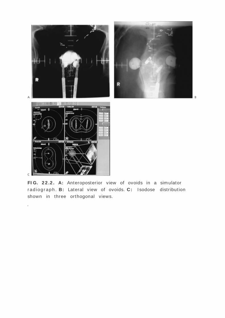
FIG. 22.2. A: Anteroposterior view of ovoids in a simulator

radiograph. B: Lateral view of ovoids. C: Isodose distribution

shown in three orthogonal views.

FIG. 22.3. Prostate gland high dose rate implant shown in a

transverse computed tomography slice.

REFERENCES

1. ICRU. Dose and volume specifications for reporting

intracavitary therapy. ICRU Report No. 38. Bethesda, MD:

International Commission on Radiation Units and

Measurements, 1985.

2. NRC. Policy and guidance directive, FC-86â€“4; Revision

1: Information required for licensing remote afterloading

devices. Nuclear Regulatory Commission. Washington, DC:

U.S. Government Printing Office, 1993.

3. NCRP. Protection against radiation from brachytherapy

sources. NCRP Report No. 40. Washington DC: National

Council on Radiation Protection and Measurements, 1972.

4. NCRP. Structural shielding design and evaluation for

medical use of x-rays and gamma rays of energies up to 10

MeV. NCRP Report No. 49. Washington, DC: National Council

on Radiation Protection and Measurements, 1976.

5. Klein EE, Grisby PW, Williamson JF, Meigooni AS. Pre-

installation empirical testing of room shielding for high dose

rate remote afterloaders. Int J Radiat Oncol Biol Phys

1993;27:927â€“931.

6. Weaver JT, Loftus TP, Loevinger R. NBS measurement

services: calibration of gamma-ray-emitting brachytherapy

sources National Bureau of Standards (NIST) special

publication no. 250â€“19 Gaithersburg, MD: National Bureau

of Standards, 1988.

7. Goetsch SJ, Attix FJ, Pearson DW, et al. Calibration of 192

Ir high-dose rate afterloading systems. Med Phys

1991:462â€“467.

8. Goetsch SJ, Attix FH, DeWerd LA, et al. A new well

ionization chamber for the calibration of iridium-192 high

dose rate sources. Int J Radiat Oncol Biol Phys

1992;24:167â€“170.

9. Anderson LL. Plan optimization and dose evaluation in

brachytherapy. Semin Radiat Oncol 1993;3:290â€“300.

10. Renner WD, Oâ€™Conner TP, Bermudez NM. An algorithm

for generation of implant plans for high-dose rate irradiators.

Med Phys 1990;17:35â€“40.

P.538

11. Sloboda RS. Optimization of brachytherapy dose

distribution by simulated annealing. Med Phys

1992;19:955â€“964.

12. Van der Laars R, Prius TPE. Introduction to HDR

brachytherapy optimization. In: Mould RF, Battermann JJ,

Martinez AA, et al., eds. Brachytherapy from radium to

optimization . Veenendaal, The Netherlands: Nucletron

Corporation, 1994.

13. Ezzel GA, Luthermann RW. Clinical implementation of

dwell time optimization techniques for single stepping-source

remote applicators. In: Williamson J, Thomadsen B, Nath R,

eds. Brachytherapy physics . Madison, WI: Medical Physics

Publishing, 1994.

14. McShan DL, Ten Haken RK, Fraas BA. 3-D treatment

planning: IV. Integrated brachytherapy planning. In:

Bruimvis IAD, et al., eds. Proceedings of the Ninth

International Conference: the use of computers in radiation

therapy. Scheveningen, The Netherlands. North-Holland:

Elsevier Science Publishers BV, 1987:249â€“252

15. Schoeppel SL, Lavigne ML, Mantel MK, et al. Three

dimensional treatment planning of intercavity gynecologic

implants analysis of ten cases and implications for dose

specification. Int J Radiat Oncol Biol Phys

1993;28:277â€“283.

16. Weeks KJ. Brachytherapy object-oriented treatment

planning based on three dimensional image guidance. In:

Thomadsen B, eds. Categorical course in brachytherapy

physics . Oak Brook, IL: Radiological Society of North

America, 1997:79â€“86

17. Nath R, Anderson LL, Luxton G, et al. Dosimetry of

interstitial brachytherapy sources: recommendations of the

AAPM Radiation Therapy Committee Task Group No. 43. Med

Phys 1995;22:209â€“234.

18. Muller-Runkel R, Cho SH. Anisotropy measurements of a

high dose rate Ir-192 source in air and polystyrene. Med Phys

1994;21:1131â€“1134.

19. Williamson JF, Li Z. Monte Carlo aided dosimetry of the

microselection pulsed and high dose-rate 192 Ir sources. Med

Phys 1995;22:809â€“819.

20. Mishra V, Waterman FM, Suntharalingam N. Anisotropy of

an iridium 192 high dose rate source measured with a

miniature ionization chamber. Med Phys 1997;24:751â€“755.

21. Wang R, Sloboda RS. Monte Carlo dosimetry of the

VariSource high dose rate 192 Ir source. Med Phys

1998;25:415â€“423.

22. Kubo HD, Glasgow GP, Pethel TD, et al. High dose-rate

brachytherapy treatment delivery: report of the AAPM

Radiation Therapy Committee Task Group No. 59. Med Phys

1998;25:375â€“403.

23. Nath R, Anderson LL, Meli JA, et al. Code of practice for

brachytherapy physics: AAPM Radiation Therapy Committee

Task Group No. 56. Med Phys 1997;24:1557â€“1598.

24. Stitt JA, Thomadsen BR. Clinical applications of low dose

rate and high dose rate brachytherapy. In: Levitt SH, Khan

FM, Potish RA, et al., eds. Technological basis of radiation

therapy . Philadelphia: Lippincott Williams & Wilkins,

1999:210â€“219

1 VariSource, Varian Oncology Systems, Palo Alto, California.

2 Commercially available at Standard Imaging, Middleton,

Wisconsin.





23 - Prostate Implants

23

Prostate Implants

23.1. INTRODUCTION

Treatment options for carcinoma of the prostate include radical

prostatectomy (e.g., nerve-sparing surgical procedure), external

photon beam irradiation and brachytherapy implantation. The

selection of a particular procedure or a combination of

procedures depends on established prognostic factors such as

stage, grade, and pre-treatment prostate-specific antigen (PSA)

concentration. In general, surgery is indicated if the tumor is

confined to the prostate gland with no extension through the

capsule or into the seminal vesicles. Implants are used for early

stage cancers, either alone or in conjunction with external beam

radiation therapy. However, patients with extensive tumors

(TNM stage T3 and T4) are not good candidates for implantation.

Except as general information, clinical aspects of prostate gland

cancer and its treatment are beyond the scope of this book. The

reader is referred to a wealth of information on this subject in

the medical literature. In this chapter we will discuss the

physical and technologic aspects of prostate gland implants

using radioactive seeds and high-dose-rate brachytherapy.

23.2. SEED IMPLANTS

Two types of seed implants have been used for prostate gland: a

temporary implant and a permanent implant. The temporary

implants involve radioisotopes of relatively long half-life and

sufficient dose rate to deliver the prescribed target dose in 3 to

4 days. The sources are removed at the end of that period. In

the permanent implant the radioisotope either has a short half-

life (e.g., gold-198) or emits photons of low enough energy that

the radiation from the patient poses no significant hazard to

persons in the surrounding environment. The sources are left in

the patient forever and the prescribed dose is delivered during

complete decay of the sources. Of these two types of seed

implants, the permanent implants are gaining more popularity

and will be discussed in greater detail.

A. Permanent Implants

Permanent implants with iodine-125 or palladium-103 are used

in the treatment of early stage prostate cancer as the sole

modality or in combination with external beam radiation

therapy. The target volume for implantation in either case is the

prostate gland itself, with minimal margins allowed to account

for uncertainty of prostate localization.

Whitmore and Hilaris pioneered prostatic implantation with 125 I

seeds in the early 1970s at Memorial-Sloan Kettering Cancer

Center. They used retropubic approach, which entailed a major

surgical procedure. The treatment results were disappointing

and so, by the mid-1980s, the retropubic technique was

abandoned.

The modern technique of implantation, which began in the

1980s, consists of transperineal approach in which 125 I or 103

Pd seeds are inserted into the prostate gland with the

P.540

guidance of transrectal ultrasonography and perineal template.

The procedure is nonsurgical and performed on an outpatient

basis. The implant is done in an approved operating room with

the patient requiring a spinal anesthetic.

A.1. Volume Study

Localization of prostate by a series of transverse ultrasound

images constitutes a volume study. The patient is placed in the

dorsal lithotomy position and the transrectal ultrasound probe

(5- to 6-MHz transducer) is securely anchored. The probe is

moved precisely to obtain transverse images of the prostate

gland from base to apex at 5-mm intervals. A grid is

superimposed on each image to represent template coordinates.

The prostate gland is visualized on each of the transverse

images and the implantation target is drawn to encompass the

prostate. The sagittal image is also obtained to measure the

length of the gland from the base to the apex. This provides a

double check of the number of transverse images and the

number of seeds required for the central needle.

Prior to the volume study, evaluation is made from computed

tomography (CT) scans of the prostate gland size and the pubic

arch in relation to the prostate. If the pubic arch is too narrow it

would prevent the needles from reaching the target. In the case

of a large gland and significant pubic arch interference, the

patient may need hormonal therapy for a few months to shrink

the gland to allow for an adequate implant. Some radiation

oncologists prefer hormonal therapy in most cases to reduce the

gland size to minimize technical problems of implantation.

A.2. Treatment Planning

A treatment-planning system specifically designed for prostate

gland implants allows the target outlines from the volume study

to be digitized into the computer. The implant is planned with

an interseed spacing of 1 cm (center to center) and a needle

spacing of 1 cm. The computer software allows the placement of

seeds in the template grid in each of the ultrasound image.

Individual seeds can be added or deleted iteratively to optimize

isodose coverage of the target volume. Seed strength can be

adjusted to deliver a prescribed minimum peripheral dose (MPD)

which is the isodose surface just covering the prostate target

volume. Before the availability of computer dosimetry, seed

strength and the required number of seeds were determined by

the method of dimension averaging used in conjunction with a

precalculated nomogram (1 ). The modern computer programs

allow the use of any seed strength as well as fine adjustment of

this parameter to obtain the desired MPD. Typical seed strengths

required are on the order of 0.3 mCi for 125 I (MPD = 144Gy)

and 1.7 mCi for 103 Pd (MPD = 125Gy).

Based on the approved computer plan, a worksheet is prepared

specifying the number of needles, seeds in each needle and the

template coordinates. Figure 23.1 (see color insert) shows an

example of pre-implant treatment plan for 125 I along with the

dose-volume histogram and statistics.

Post-implant dosimetry may also be performed using CT scans to

assess stability of the implant after swelling of the prostate

gland has gone down. A major problem with permanent seed

implants is the usual disagreement between the pre-implant and

post-implant dose distributions. Hot and cold spots can develop

as a result of source movement with time (Fig. 23.2 ) (see color

insert), leaving one to wonder if the prescribed dose was

delivered to the target accurately with a pattern of dose

distribution as originally planned.

Another equally serious problem is that of source anisotropy.

Because of the low gamma ray energy emitted and the design of

the source in which radiation is severely attenuated along the

length of the seed, cold spots of greater than 50% (reduction in

dose) exist at the ends (see Figs. 15.4 and 15.6 ). This

anisotropy in dose distribution however, is more of a problem if

the sources are aligned permanently end to end with each other

along straight lines. A certain degree of randomness that

naturally develops after implantation reduces the overall

anisotropy effect in a prostate gland implant.

P.541

The seed anisotropy has been significantly reduced by a newly

designed 125 I source (model L S-1 BrachySeed manufactured by

DRAXIMAGE Inc.1 ). Dosimetric Characteristics of this source

have been discussed by Nath and Yue (2 ).

FIG. 23.3. Schematic diagram showing ultrasound-guided

transperineal template implant procedure. (From Grim PD,

Blasko JC, Ragde H. Atlas of the Urologic Clinics of North

America 1994;2:113â€“125, with permission.)

A.3. Implant Procedure

The implant procedure is carried out as an outpatient treatment

in an operating room with the patient in the dorsal lithotomy

position under spinal anesthesia. Figure 23.3 shows the

implantation apparatus consisting of a transrectal ultrasound

probe and a template to guide specifically designed sterile 18-

gauge, 21-cm long needles. The needles are preloaded with the

planned number of seeds and spacers and placed in a needle

holder at appropriate template coordinates. The needle loading

procedure is performed behind an L-shaped leaded glass barrier.

Each needle is equipped with a plunger and the tip is sealed

with bone wax to keep the seeds in place until implantation.

The needles are inserted one at a time into the prostate using

the ultrasound and template guidance. In each case, using

sagittal images and distance measurements from the hub of the

needle to the template, it is ascertained that the needle tip is at

the correct plane and depth. After verifying the needle position,

the needle is slowly withdrawn while the plunger is held

stationary. This action results in the injection of the seeds and

the spacers into the tissues along the track of the withdrawing

needle. Each ultrasound image is carefully reviewed to assess

the position of the seeds. Final verification of the implant is

made with anteroposterior fluoroscopy. Extra seeds are available

for implantation if cold spots are identified. Cystoscopy is

performed at the conclusion of the procedure to retrieve any

stray seeds in the bladder or the urethra.

For further technical details of the operative technique and

implant procedure, the reader is referred to Grim et al. (3 ,4 ).

A.4. Radiation Protection

The AAPM code of practice for brachytherapy (5 ) is a

comprehensive document on the physics and quality assurance

of brachytherapy procedures. Before implementing a prostate

P.542

implant program, one should consult this document together

with the relevant Nuclear Regulatory Commission regulations.

The basic requirement for releasing a permanent implant patient

from the hospital is that the total exposure to any other

individual from the released patient does not exceed 0.5 rem

over the life of the implant. This condition is easily met with a

prostate implant using 125 I or 103 Pd seeds. Low energy

radiation is locally absorbed within the patient, posing little risk

to surrounding organs or people. However, patients are

instructed at the time of discharge to observe certain

precautions. For example, they are advised not to have

prolonged physical contact with pregnant women or young

children for a period of 2 months, to abstain from sexual activity

for 2 weeks, and to use condoms during intercourse for the first

few weeks in case a seed is discharged into the vagina.

During the implant procedure, a medical physicist or dosimetrist

assisting in the procedure also assures that the total number of

seeds is accounted for at all times. A thin window GM tube or a

scintillation counter is available to locate any dropped or

misplaced seed. Personnel are not allowed to leave the

operating room without being surveyed to prevent accidental

transport of any seed outside the room. At the conclusion of the

procedure, the trash, the room, and the personnel are surveyed

for any misplaced seed.

B. Temporary Implants

Temporary prostate gland implants have almost exclusively used

iridium-192. The treatment is given mainly as a boost to

external beam therapy (6 ,7 and 8 ). Traditionally, these

implants have been carried out at the time of laparotomy and

pelvic-node sampling. The needles are implanted

intraoperatively with the guidance of a transperineal template.

Iridium seeds in plastic ribbons are afterloaded into the needles

and left in place for about 3 days. Usually 10 to 15 needles are

required for the implant. The patient is hospitalized and bed-

bound for the duration of the implant, requiring analgesia.

Current refinements in the temporary implantation technique

include ultrasound guidance, avoiding open laparotomy.

However, patient hospitalization is still required with the

attendant radioprotection problems for personnel administering

postoperative care.

23.3. DOSIMETRY

A. Calibration

Brachytherapy sources are calibrated by the vendor before

shipment and bear a calibration certificate with stated limits of

uncertainty, usually 10%. Although vendor calibrations are, in

most cases, traceable to the National Institute of Standards and

Technology (NIST), the user is advised to check the calibration

values of a sample of sources from the batch as a matter of

quality assurance. Agreement within ±5% with the vendor

calibration is acceptable, in which case the vendor values may

be used for patient dose calculations. In case of a larger

disagreement, the user must resolve the difference with the

vendor and if unsuccessful, use the in-house calibration, with

full documentation of the procedure used.

The NIST uses large-volume ion chambers in a open-air

geometry to calibrate 192 Ir sources and free-air ionization

chamber for 125 I (9 ,10 ). The stated uncertainties in these

calibrations are on the order of 2%. The NIST calibration

techniques require considerable attention to detail and are not

practical for routine use.

The most suitable method of routine calibration of

brachytherapy sources is the well ionization or re-entrant

chamber. As discussed in section 15.2B , a nuclear medicine

dose calibrator may be converted into a brachytherapy well

chamber by placing a source-holding tube along the axis of the

chamber. The chamber response, however, depends significantly

on the energy of radiation, source construction, and source

position along the chamber axis. It is therefore essential that

the well chamber bears a NIST-traceable calibration specifically

for the type of source to be calibrated.

P.543

The well chamber calibration for given types of sources may be

obtained from the Accredited Dose Calibration Laboratories

(ADCLs) which maintain traceability with the NIST.

Alternatively, the chamber may be calibrated in-house by using

a standard source of the same type, which has been calibrated

by an ADCL. The standard source should not only be the same

Radionuclide but also have the same construction or model. In

addition, the calibration geometry (source position along the

chamber axis) should be the same for the standard source as for

the source to be calibrated. If different source positions are

intended appropriate corrections should be determined as a

function of source position.

B. Dose Computation

Dose distribution around 125 I, 103 Pd, or 192 Ir is not isotropic.

Analytical methods of dose calculations such as Sievert integral

are not suitable for these sources because of complexity in

source construction, filtration, and low energy of the emitted

radiation. The AAPM Task Group 43 or simply TG-43 formalism

(11 ) gets around this problem by parametrizing the dose

distribution around a specific source type in terms of actual

measurements or detailed Monte Carlo calculations. The general

TG-43 equation (Equation 15.16 ) for the calibration of dose at a

point P (r , ¸) which includes anisotropy effects, is as follows:

where [D with dot above](r , ¸) is the dose rate at point P in a

medium (e.g., water), › is the dose rate constant, Sk is the air

kerma strength of the source, G is the geometry factor, g is

radial dose function and F is the anisotropy function. These

quantities are defined in Chapter 15 .

In order to use Equation 23.1 rigorously for an implant, the seed

orientation must be known and fixed. In prostate gland

implants, although seeds are placed along straight lines with

known coordinates, their post-implant orientation becomes

somewhat randomized and variable with time. It is therefore

acceptable to treat these seeds as point sources in a dose

calculation formalism. For a point source, Equation 23.1 reduces

to:

where

is the average anisotropy factor. Current values of ›, g (r )

and

for prostate implant sources are given in Tables 23.1 ,2 and 23.3

.

192 Ir

1.12

Iron clad

125 I model 6702

0.93

125 I model 6711

0.88

103 Pd model 200

0.74

From Nath R, Anderson LL, Luxton G, et al. Dosimetry of


AAPM Radiation Therapy Committee Task Group no. 43. Med

Phys 1995;22:209â€“234, with permission.

Seed cGy hr- 1 U- 1

TABLE 23.1. RECOMMENDED DOSE RATE CONSTANTS IN A

WATER MEDIUM

0.5

1.29

1.04

1.04

0.994

1.0

1.00

1.00

1.00

1.00

1.5

0.765

0.926

0.934

1.01

2.0

0.576

0.832

0.851

1.01

2.5

0.425

0.731

0.760

1.01

3.0

0.310

0.632

0.670

1.02

3.5

0.224

0.541

0.586

1.01

4.0

0.165

0.463

0.511

1.01

4.5

0.123

0.397

0.445

1.00

5.0

0.0893

0.344

0.389

0.996

5.5

0.300

0.341

0.985

6.0

0.264

0.301

0.972

6.5

0.233

0.266

0.957

7.0

0.204

0.235

0.942

7.5

0.927

8.0

0.913

8.5

0.900

9.0

0.891




Phys 1995;22: 209â€“234, with permission.

Distance Along

Transverse Axis

(cm)

Radial Dose Function, g (r )

103

Pd

126 I

Model

6711

125 I

Model

6702

192

Ir

TABLE 23.2. RADIAL DOSE FUNCTIONS, g (r )

A treatment-planning system for prostate gland implants usually

has the reference data ( ›, g (r ) and ¦an ) stored for a

number of commercially available seeds. It is the responsibility

of the user to assure that these data pertain to the type of

sources to be implanted and represent currently accepted values

(e.g., published in peer-reviewed literature).

P.544

B.1. Total Dose

As the sources decay with a half-life T 1/2 , the dose rate

decreases exponentially with time t as:

where [D with dot above] is the dose rate (dD/dt ) and [D with

dot above]0 is the initial dose rate as given by Equation 23.2 .

The cumulated dose Dc in time t is obtained by integrating

Equation 23.3 :

which is the same as Equation 15.28 , since 1.44T 1/2 is the

average life (T av ). For a permanent implant, the total dose D

total is delivered after complete decay of the sources (i.e., t

â‰« T 1/2 ).

P.545

In that case, Equation 23.4 reduces to:

1

0.921

0.944

0.968

0.991

2

0.889

0.936

0.928

0.947

3

0.820

0.893

0.897

0.970

4

0.834

0.887

0.942

0.989

5

0.888

0.884

0.959

0.998

6

0.880

0.891

0.949

7

0.901

0.907

0.965

8

0.955

9

0.974

Anisotropy constants †an

0.90

0.93

0.95

0.98




Phys 1995;22:209â€“234, with permission.

Anisotropy Factors, †an (r )

Distance, r

(cm)

103

Pd

125 I Model

6711

125 I Model

6702

192

Ir

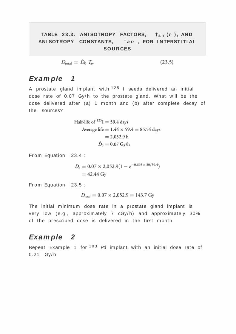
TABLE 23.3. ANISOTROPY FACTORS, †an (r ), AND

ANISOTROPY CONSTANTS, †an , FOR INTERSTITIAL

SOURCES

Example 1

A prostate gland implant with 125 I seeds delivered an initial

dose rate of 0.07 Gy/h to the prostate gland. What will be the

dose delivered after (a) 1 month and (b) after complete decay of

the sources?

From Equation 23.4 :


The initial minimum dose rate in a prostate gland implant is

very low (e.g., approximately 7 cGy/h) and approximately 30%

of the prescribed dose is delivered in the first month.

Example 2

Repeat Example 1 for 103 Pd implant with an initial dose rate of

0.21 Gy/h.



For respective prescribed doses, the dose rate for a 103 Pd

implant is typically about three times that for an 125 I implant.

In the case of 103 Pd, because of its shorter half-life, the bulk of

the prescribed dose (approximately 70%) is delivered in the first

month.

23.4. HIGH DOSE RATE IMPLANTS

Prostate cancer is a slowly progressive disease. Consequently,

the superiority of one treatment technique over another cannot

be established in a short time (e.g., 5 to 10 years).

P.546

Although the results with seed implants are so far encouraging,

caution is needed to interpret these results because of the

relative short time of the studies and the many competing

causes of failure in these patients. In addition, the clinical

impact of dose inhomogeneity (caused by seed displacement and

anisotropy) and extremely low dose rate (LDR) in a permanent

implant is not well understood. However, the ability of

brachytherapy to concentrate the dose in the tumor and spare

surrounding normal tissues is well recognized. High-dose-rate

(HDR) brachytherapy has that advantage and, in addition, offers

better control of dose homogeneity and dose conformity

compared to LDR brachytherapy.

P.547

A. Procedure

The HDR prostatic implant procedure using transrectal guidance

is similar to the LDR brachytherapy with 192 Ir (12 ). The patient

is placed in a lithotomy position and receives epidural

anesthesia. A transrectal ultrasound probe is used to evaluate

the prostate gland. Coronal and sagittal images allow the

determination of prostate volume. A prostate gland template is

sutured transperineally and HDR guide needles are implanted

into the prostate gland with ultrasound guidance (Fig. 23.4a ).

Ten to fifteen needles are usually required to cover the prostate

gland. The bladder is filled with Hypaque and dummy source

wires are loaded into the guide needles to obtain intraoperative

x-ray localization radiographs. The patient is sent to the

recovery room and subsequently simulated to obtain orthogonal

films for HDR treatment planning.

FIG. 23.4. Prostate implant procedure using ultrasound-guided

HDR procedure showing (A) implant needles in place; (B)

flexible adapters screwed into guide needles; and (C) flexible

adapters connected to the HDR remote afterloaders. (From Syed

AMN, Puthawala AA, Barth N, et al. High dose rate brachytherapy

treatment of the prostate: preliminary results. Journal of

Brachytherapy Intl 1997;13:315â€“331, with permission.)

Treatment-planning algorithms for HDR have been discussed in

Chapter 22 . These programs are based on either orthogonal

films or CT data. Dwell times of the source in each needle are

calculated to provide optimized dose distribution. CT-based

treatment planning provides full three-dimensional dose

distributions including slice-by-slice isodose curves, isodose

surfaces, and dose-volume histograms.

After the treatment plan has been optimized and approved, the

guide needles are connected to the HDR afterloader through

adapters and transfer catheters (Fig. 23.4B,C ). The treatment is

delivered as planned. After conclusion of the treatment, the

transfer catheters are disconnected from the adapters and the

patient is sent to his room.

Although dose fractionation with HDR is not yet well established,

the total dose typically ranges from 10 to 25 Gy (minimum

isodose surface) given in three to four fractions. This dose is

given in addition to the 45 Gy of external beam radiation

therapy.

REFERENCES

1. Hilaris BS, Nori D, Anderson LL. Atlas of brachytherapy .

New York: MacMillan, 1988.

2. Nath R, Yue N. Dosimetric characterization of a newly

designed encapsulated interstitial brachytherapy source of

iodine-125-model LS-1 BrachySeed. Appl Radiat Isot

2001;55:813â€“821.

3. Grim PD, Blasko JC, Ragde H. Ultrasound-guided

transperineal implantation of iodine-125 and palladium-103

for the treatment of early-stage prostate cancer. Atlas of the

Urologic Clinics of North America 1994;2:113â€“125.

4. Porter AT, Blasko JC, Grimm PD, et al. Brachytherapy for

prostate cancer. CA Cancer J Clin 1995;45:165â€“178.




6. Tansey LA, Shanberg AM, Syed AMN, et al. Treatment of

prostatic cancer by pelvic lymphadenectomy, temporary

iridium-192 implant and external irradiation. Urology

1983;21:594â€“598.

7. Syed AMN, Puthawala AA, Tansey LA, et al. Temporary

interstitial irradiation in the management of carcinoma of the

prostate: â€œcurrent status of a new approach.â€ . Int Med

Spec 1984;5:146â€“161.

8. Syed AMN, Puthawala A, Austin P, et al. Temporary

iridium-192 implant in the management of carcinoma of the

prostate. Cancer 1992;69:2515â€“2524.

9. Weaver JT, Loftus TP, Loevinger R. NBS measurement

services: calibration of gamma-ray emitting brachytherapy

sources. National Bureau of Standards (NIST) special

publication no. 250â€“19. Gaithersburg, MD: National Bureau

of Standards, 1988.

10. Loftus TP. Standardizing of 125-I seeds used for

brachytherapy. J Res Natl Bureau Stand 1984;89:295â€“303.

11. Nath R, Anderson LL, Luxton G, et al. Dosimetry of


AAPM Radiation Therapy Committee Task Group No. 43. Med

Phys 1995;22:209â€“234.

12. Syed AMN, Puthawala AA, Barth N, et al. High dose rate

brachytherapy in the treatment of carcinoma of the prostate:

preliminary results. J Brachytherapy Int 1997;13:315â€“331.

1 DRAXIMAGE, Inc., 16751, Route Transcandienne, Kirkland

(Quebec), Canada.





24 - Intravascular Brachytherapy

24

Intravascular Brachytherapy

24.1. INTRODUCTION

Coronary artery disease is most commonly treated using bypass

surgery or percutaneous transluminal coronary angioplasty

(PTCA). A major problem with PTCA, however, is the high

incidence of restenosis and recurrence of artery blockage at the

site of treatment. Restenosis is usually arbitrarily defined as a

narrowing of the lumen by 50% or greater in diameter compared

to the adjacent normal appearing segments. Although the

occurrence of restenosis is significantly reduced by the

implantation of coronary stents, the restenosis rate following

balloon angioplasty in randomized trials is 30% to 40% (1 ).

Most restenosis after angioplasty or stenting is caused by

thrombosis or blood clotting at the PTCA site, which can be

prevented partially by using anti-clotting drugs. However,

another process, which begins within days after angioplasty, is

the neointimal growth of tissues prompted by the wound healing

process following tissue injury by angioplasty. This component of

restenosis cannot be prevented by anticoagulants or stents.

Intraluminal irradiation of coronary and peripheral arteries

together with balloon angioplasty and/or stent implantation

significantly lowers the rate of neointimal formation, thereby

reducing the rate of restenosis to well below 10% (2 ). Radiation

kills cells and inhibits the growth of neointimal tissues in a

manner similar to its effect on benign diseases such as keloids

and heterotopic bone formation. Basic radiation biology and

vascular pathology are discussed by several authors (3 ,4 ,5 ).

24.2. TREATMENT VOLUME

A. Arterial Anatomy

The arteries carry blood from the heart to various parts of the

body. The main artery, the aorta, is the largest blood vessel (2

to 3 cm in diameter) and carries blood from the left ventricle of

the heart to the branching arteries and capillaries in all the body

organs and tissues, including the heart muscle. The coronary

arteries are blood vessels lying on the outer surface of the heart

and the peripheral arteries supply blood to other organs and

tissues. The luminal diameter of arteries ranges from 3 to 5 mm

initially and tapers slowly through their path length. Within this

range, the peripheral arteries tend to be of larger diameter than

the coronary arteries. The minimum normal artery diameter

required for angioplasty and stenting is approximately 3 mm.

The inside of the arteries is lined with a layer of cells called

endothelium. Next to the endothelium is the connective tissue

layer, the intima, followed by layers of elastic membrane,

smooth muscle cells, and elastic tissues. The outermost layer of

the arteries is called adventitia, made up chiefly of collagenous

fiber.

B. Angioplasty and Restenosis

The arteries can be partially blocked due to atherosclerosis or

plaque formation. Reduction of their lumen diameter

compromises the flow of blood and the delivery of oxygen to

P.549

the body tissues. As an alternative to a major surgical procedure

such as bypass surgery, balloon angioplasty is used to dilate the

lumen diameter. This stretching action often ruptures the

internal elastic lamina of the wall and causes fissures in the

medial layers. The acute risk of angioplasty procedure is

thrombosis that can be controlled by drugs, as mentioned

previously. The more protracted risk, however, is that of

restenosis by neointimal hyperplasia. This process involves

growth of new tissues in the cracks and crevices of the arterial

wall caused by angioplastic injury. Although implantation of

stent angioplasty reduces the overall rate of restenosis by

approximately 50%, it does not prevent neointimal growth and

may, in fact, stimulate the process.

C. Target Volume

Target volume for vascular brachytherapy is confined to the

region of angioplasty. Typically, it is 2 to 5 cm in length of

artery and 0.5 to 2 mm in thickness of arterial wall.

Occasionally, these dimensions may be exceeded depending on

the location and extent of the disease. With 3 to 5 mm of

luminal diameter, the radial range of treatment may extend as

far as to about 5 mm from the center of the artery.

Because of the severity of inverse square fall-off of radiation at

short distances, transluminal irradiation with intravascular

brachytherapy produces highly conformal dose distribution,

delivering a high dose to the arterial wall while sparing

surrounding normal vessels or myocardium. Again, because of

the predominance of inverse square law effect, penetrating

power of radiation, depending on energy and modality, is not

critically important, except with regard to dose rate or duration

of implant and radiation protection of personnel involved with

the procedure. Beta particle sources, in general, give higher

dose rates and provide greater radiation protection compared to

the gamma ray sources.

The depth of dose prescription for intracoronary irradiation is

recommended by the American Association of Physicists in

Medicine (AAPM) (6 ) to be 2 mm from the center of the source

and for the peripheral arteries 2 mm beyond the average lumen

radius. For each case, dose distribution in at least three planes

perpendicular to the catheter and along its length should be

determined. In addition, average, maximum, and minimum doses

within the target volume should be reported (6 ).

24.3. IRRADIATION TECHNIQUES

Intravascular brachytherapy techniques may be classified into

two categories: temporary implants (sealed sources or liquid-

filled balloons) and permanent implants (radioactive stents).

Each method has its advantages and limitations, but the

catheter-based sealed source is the most commonly used method

of treatment. It is the preferred method because of its better

control of dose delivery. A variety of ² and ³-ray sources

have been used for endovascular therapy although the choice of

one modality over the other is yet not clearly established. The

pros and cons of a few sources and devices are discussed below.

A. Radiation Sources

Typical dosimetric requirements of a temporary intravascular

implant are: (a) to deliver a target dose of 15 to 20 Gy to a 2-

to 3-cm length of the arterial wall involved at a radial distance

of about 2 mm from the source center; (b) to minimize the dose

to tissues outside the region of angioplasty; and (c) to take as

little a time as possible for completion of the procedure, that is,

provide target dose rates on the order of 5 Gy/min or greater.

These requirements suggest the suitability of high-energy ²-

sources such as strontium-90, yttrium-90, and phosphorus-32 or

high activity ³-sources such as iridium-192. The latter could be

a high dose rate (HDR) afterloading unit with the source

dimensions small enough to allow intravascular brachytherapy.

The ²-sources have several advantages over ³-sources:

higher specific activity, higher dose rate, longer half-life, and

greater radiation safety for the patient as well as personnel.

P.550

The major disadvantage of ²-sources, however, is the

extremely rapid radial dose fall-off within the target region; ³-

sources such as 192 Ir provide relatively more uniform target

dose, governed primarily by the inverse square law fall-off with

distance, but require high activity to yield reasonably high dose

rate (â‰¥5 Gy/min). Consequently, radiation protection

problems with such sources become more significant. Although

the HDR afterloaders using gamma sources could provide

sufficiently high dose rate, they would require expensive

shielding of the catheterization laboratories.

Table 24.1 contains a list of possible isotopes that have been or

could be used for intravascular brachytherapy. The last column

shows the activities required to obtain a dose rate of 5 Gy/min

to a 2 cm length of a vessel at a radial distance of 2 mm from

the source center. It is seen that the ³-sources, because of

lower specific activity, require much higher activities than the

²-sources for a catheter-based intravascular procedure. On the

other hand, a permanent radioactive stent using 48 V requires

only 1 µCi to produce the same dose rate.

In-192

Gamma

612

375

74 d

1.0 Ci (37 GBq)

Iodine-125

X ray

35

28

60 d

3.8 Ci (140.6 GBq)

Palladium-103

X ray

21

21

19 d

3.9 Ci (144.3 GBq)

Phosphorus-32

Beta-

1,710

690

14 d

40.0 Ci (1,480 MBq)

Strontium/yttrium-90

Beta-

2,270

970

28 d

30.0 Ci (1,110 MBq)

Tungsten/rhenium-188

Beta-

2,130

780

69 d

35.0 Ci (1,295 MBq)

Vanadium-48

Beta+

690

230

16 d

1.0 µCi (37 Bq) stent

From Amols HI. Physics and dosimetry of intravascular

brachytherapy. In: Thomadsen B, ed. Categorical course in

brachytherapy physics. Oak Brook, IL: Radiological Society of

North America, 1997, with permission.

Isotope Emission Maximum

Energy

(keV)

Average

Energy

(keV)

Half-

Life

Activity

Required

TABLE 24.1. POSSIBLE ISOTOPES FOR INTRALUMINAL

BRACHYTHERAPY

Although dose rate per unit-activity favors ²-emitters, radial

dose distribution is better for the ³-sources, if it is assumed

that the dose uniformity across the target volume is

radiobiologically beneficial. This assumption has not been

clinically validated but it seems logical, based on experience in

conventional radiation therapy. Figure 24.1 compares radial dose

distribution as a function of radial distance for some of the

sources listed in Table 24.1 . Nath and Liu (7 ) have studied

radial dose function (g) for point sources of photons and

electrons using Monte Carlo simulation. Their data show that

from the point of view of adequate depth of penetration for

intravascular brachytherapy, photon sources above 20 keV and

electron sources above 1.0 MeV are acceptable.

FIG. 24.1. Radial dose fall off with distance for a number of

sources. Doses are normalized to 1.0 at a radial distance of 2.0

mm. (From Amols HI, Zaider M, Weinberger J, et al. Dosimetric

considerations for catheter-based beta and gamma emitters in

the therapy of neointimal hyperplasia in human coronary

arteries. Int J Radiat Oncol Biol Phys 1996;36:913â€“921, with

permission.)

P.551

B. Radiation Delivery Systems

Irradiation of blood vessels to prevent restenosis following

angioplasty has been carried out using external beam as well as

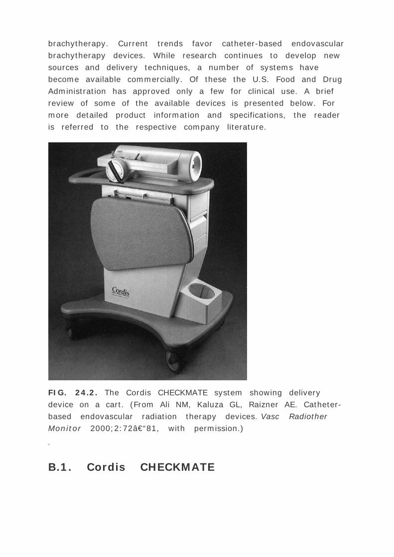
brachytherapy. Current trends favor catheter-based endovascular

brachytherapy devices. While research continues to develop new

sources and delivery techniques, a number of systems have

become available commercially. Of these the U.S. Food and Drug

Administration has approved only a few for clinical use. A brief

review of some of the available devices is presented below. For

more detailed product information and specifications, the reader

is referred to the respective company literature.

FIG. 24.2. The Cordis CHECKMATE system showing delivery

device on a cart. (From Ali NM, Kaluza GL, Raizner AE. Catheter-

based endovascular radiation therapy devices. Vasc Radiother

Monitor 2000;2:72â€“81, with permission.)

B.1. Cordis CHECKMATE

The Cordis CHECKMATE System1 consists of three components:

(a) a nylon ribbon containing an array of 192 Ir seeds, (b) a

delivery catheter, and (c) a ribbon delivery device. The Iridium

seeds are 3 mm in length and 0.5 mm in diameter. The interseed

spacing is 1mm and the outer diameter of the nylon ribbon

containing the seeds is 1mm. The number of seeds in a ribbon

can be altered to provide source lengths of 19 to 80 mm. Each192 Ir seed has an activity of about 33 mCi, thus making it

possible to keep the treatment time within 15 to 25 minutes.

The ribbon delivery device is mounted on a cart (Fig. 24.2 ) and

uses a hand-crank mechanism to advance the ribbon into a

closed-end delivery catheter.

Although the 192 Ir source provides better dose homogeneity

because of the lower depth-dose gradient (ratio of surface-to-

adventitial dose), its higher activity and gamma ray energy raise

radiation protection concerns for personnel. Longer irradiation

times and non-centering of the delivery catheter are other

disadvantages of this device.

P.552

B.2. Guidant GALILEO

The Guidant GALILEO System2 uses a ²-source, 32 P, for

intravascular brachytherapy. The 32 P source is hermetically

sealed in the distal 27-mm tip of a flexible 0.018-inch nitinol

wire. A spiral centering balloon catheter (Fig. 24.3 ), which

centers the source wire, is flexible to navigate through the

arteries and also has perfusion capabilities to limit myocardial

ischemia during the procedure. The source delivery unit is an

automatic afterloader device that can be controlled from a

remote location to advance and retract the source wire. A

treatment-planning system is provided to calculate dwell times

required to deliver the prescribed dose.

FIG. 24.3. Guidant GALILEO system: (A) source wire; (B)

source delivery unit; and (C) spiral centering catheter. (From Ali

NM, Kaluza GL, Raizner AE. Catheter-based endovascular

radiation therapy devices. Vasc Radiother Monitor


The major advantages of the system are the centering capability

of the delivery catheter, automation of the afterloader, and

availability of the treatment-planning system. The disadvantage

is the rapid dose fall-off radially, which is a characteristic of all

the ²-sources.

B.3. Novoste Beta-Cath

The Novoste Beta-Cath System3 uses ²-sources of 90 Sr/90 Y

isotope. It is a manual afterloader device with a catheter-based

delivery system. The system consists of two main components:

(a) a transfer device for housing and hydraulic delivery of a

radiation source train, and (b) a delivery catheter to transport

the source train.

The delivery catheter (Fig. 24.4 ) has three lumens. The first

lumen is used for travel of the guidewire. The second lumen is

for transport of the source train consisting of sealed

P.553

cylindrical seeds of 90 Sr/90 Y. The source train is delivered to

the distal end of the delivery catheter by applying manual

hydraulic pressure through a syringe, which contains sterile

water and is attached to the transfer device. The third lumen,

which is also attached to the transfer device, is designed to

provide an opposite hydraulic pressure for returning the source

train back into the storage position of the transfer device.

FIG. 24.4. Novoste Beta-Cath system with source train and

transfer device. (Courtesy of Novoste: http://www.novoste.com

.)

Major advantages of the Novoste system is its use of the 90

Sr/90 Y source, which is one of the highest energy ²-emitters

with a long half-life (28 years). Other advantages include high

dose rate (treatment time approximately 5 minutes), patient and

personnel safety, and simplicity of the handheld transfer device.

The major disadvantage is the lack of a catheter-centering

device, which could result in extreme dosimetric hot and cold

spots within the target volume.

B.4. ²-Emitting Liquid-filled Balloon

An alternative to catheter-based wires and seeds is to inflate the

balloon dilation catheter with ²-emitting radioactive liquid. The

advantages of a liquid-filled balloon are inherent source

centering and dose uniformity to the vessel wall. Several ²-

emitting isotopes such as 32 P, 90 Y, and 188 Re, which can be

obtained in a liquid radiopharmaceutical preparation, may be

used in this technique.

The major disadvantages of liquid-filled balloons include: (a)

higher ratio of surface/adventitial dose compared to the catheter

based ³-source systems; and (b) the possibility, although

remote, of balloon rupture and consequently leakage of

radioisotope within the patient. Of the radioisotopes mentioned

previously, the rhenium-188 formulation is preferable because of

the reduced radiation dose to organs such as colon and thyroid

due to its rapid renal elimination in the event of balloon rupture.188 Re also has a favorable maximum ²-energy (2.13 MeV).

One of the liquid-filled balloon devices was developed at the

Columbia University/Oak Ridge National Laboratory (8 ). The

system uses a liquid preparation of 188 Re (188 Re-MAG3 ), which

is obtained at high specific activities from a tungsten (188 W)

generator and delivered into a perfusion angiography balloon. A

commercial system (RADIANT4 ) also

P.554

uses a 188 Re-filled balloon and is similar to conventional balloon

PTCA (Fig. 24.5 ). It may be used before or after stent

placement.

FIG. 24.5. (A) Schematic of RADIANT radiation delivery system;

(B) PAS RADIANT isolated beta source balloon. Top , inflated

balloon. Bottom , WRAP balloon protective sheath. (From Eigler

N, Whiting JS, Makkar R, et al. Isolated liquid beta source

balloon radiation delivery system (RADIANT). In: Waksman R,

Serruys PW, eds. Handbook of vascular brachytherapy. London:

Martin Dunitz Ltd, 1998:107â€“110, with permission.)

B.5. Radioactive Stents

Because permanent stents are frequently used in conjunction

with balloon angioplasty, incorporation of radioactivity into the

stent has been suggested to make it more effective in preventing

restenosis (9 , 10 , 11 , 12 and 13 ). 32 P, 90 Y, and 48 V are

some of the suitable ²-emitting isotopes for impregnation into

the stent. The stent is rendered radioactive by activation in a

cyclotron or by ion implantation with the radioisotope.

The advantage of a radioactive stent is primarily the combining

of two procedures, stenting and irradiation, into one. Proximity

of the radioactive source with the vessel walls may be another

advantage, although the gridded structure of the stent gives rise

to greater dose inhomogeneity at the vessel surface than with a

liquid-filled balloon or a catheter-based source. Figure 24.6

shows peaks and valleys of dose distribution for a 1.0- µCi 32 P

Palmaz-Schatz stent.5

FIG. 24.6. Calculated dose distribution for a 1.0 µCi 32 P

Palmaz-Schatz stent, 15 mm in length. Dose to tissue is that

given in 14.3 days after implant. (From Janicki C, Duggan DM,

Coffey CW, et al. Radiation dose from a phosphorus-32

impregnated wire mesh vascular stent. Med Phys


The implantation technique of a radioactive stent is the same as

that required for a non-radioactive stent. Because of the very

low activity (e.g., 0.5 to 5.0 µCi) of the ²-radioisotope, the

radioactive stent procedure is the safest from the radiation

protection point of view. However, the dosimetry is much more

complicated than that of the catheter-based systems, as will be

discussed later.

P.555

24.4. DOSIMETRY

A. Dose Calculation Formalisms

A.1. Catheter-based Gamma Emitters

The AAPM TG-43 formalism (13 ) is generally applicable to the

problem of dose calculation for catheter-based intravascular

systems. For a system using photon-emitting sources, the dose D

at a point (r , ¸) is given by:

where Sk is the air kerma strength, › is the dose rate constant,

G is the geometry factor, g is the radial dose function, F is the

anistrophy factor, and (ro , o̧ ) are the polar coordinates of

the reference point.

As discussed in Chapter 15 , the reference distance ro in

conventional brachytherapy is 1 cm. For intravascular

brachytherapy, the AAPM (6 ) recommends ro = 2 mm. Equation

(24.1) is therefore modified to incorporate this reference point

specifically:

where ›ro is the dose rate constant at a reference distance of ro

and gro is the radial dose function normalized to the reference

radial distance ro .

Depending upon the source dimensions and the location of the

point (r , ¸), the source may be considered as a line source or

a point source. In the case of the point source, Equation 24.2

can be written as an approximation:

where ¦an is the average anisotropy factor.

For a uniformly distributed line source, the geometry factor is

given by:

where L is the active length of the source.

A.2. Catheter-based Beta Emitters

Because the quantity air kerma strength does not apply to beta-

emitting sources, the AAPM TG-60 report recommends the

following equation for the calculation of dose at a point

P.556

(r , ¸) for the beta sources:

where D (ro , ¸o ) is the dose rate in water at the reference

point (ro , o̧ ). This quantity, D (ro , o̧ ) may be

determined by calibration of the beta source at the reference

point of ro = 2 mm and o̧ = €/2.

A.3. Radioactive Liquid-filled Balloons

Amols et al. (14 ) have calculated dose at a point P(x â€², y â€²,

z â€²) from a radioactive liquid-filled balloon (Fig. 24.7 ) by

numeric integration of a Monte Carloâ€“generated beta dose

kernel over the volume of the balloon:

where D (P ) is the dose rate (grays per second) at point P, k (r

) = dose kernel (grays per decay), r â€²(cm) = [(x â€² - x )2 +

(y â€² - sin ¸)2 + (z â€² - r cos ¸)2 ] ½ , A/V = activity per

unit volume (becquerels/cm3 ), and dv = r.dr.d ¸.dx. The

integration limits are -L/2 < x < L/2, Ri < r < Ro and 0 < ¸ <

2 €. As seen in Fig. 24.7 , the central channel of the catheter

contains a lumen of radius Ri to allow passage of the guide wire.

FIG. 24.7. Geometry of dose calculation at a point P (x â€², y

â€², z â€²) from a balloon catheter with outer diameter Ro ,

inner diameter R i and axial length L , uniformly filled with beta-

emitting radioisotope. (From Amols HI, Reinstein LE, Weinberger

J. Dosimetry of a radioactive coronary balloon dilution catheter

for treatment of neointimal hyperplasia. Med Phys


Using a 3-mm diameter and 20-mm long balloon filled with 90 Y-

chloride solution, Amols et al. (14 ) verified the calculated dose

distribution by measurement with Gaf-Chromic film. The

agreement between the measured and calculated radial dose

distribution was ±6% at distances of 2.5 to 5.0 mm from the

center of the catheter (or 1.0 to 3.5 mm from the surface of the

balloon). They used the kernel for 90 Y, which had been

calculated by Simpkin and Mackie (15 ).

The dose kernel is defined (15 ) as â€œthe expectation value of

the spatial distribution of the energy deposited in target volumes

centered about a point radionuclide source per unit mass of the

target volume per decay of the point source.â€ Dose kernels

for a number of beta emitters, 32 P, 67 Cu, 90 Y, 105 Rh, 131 I,153 Sm, and 188 Re have been calculated using EGS4 Monte Carlo

code (15 ). Some of these have potential use in intravascular

brachytherapy with liquid-filled balloons.

P.557

A.4. Radioactive Stents

Dosimetric and radiobiologic characteristics of radioactive stents

are complicated because of the gridded structure of the stent

and the differences in dose rates delivered by stent versus an

acute catheter-based irradiation. Dosimetric evaluation of

clinical studies in animals by the AAPM task group (6 ) revealed

â€œa confusing variety of different dose specifications in

radioactive stent implantation.â€ The analysis of a group of

cases also showed that the dose delivered per unit-activity for

the same radionuclide varied by almost a factor of four. Thus,

the user must exercise caution in using stent activities and

dosages specified in the clinical studies reported in the

literature. The AAPM recommends (6 ) that â€œfor each type of

radioactive stent the three-dimensional dose distributions around

stents of various lengths, diameters, and activities should be

carefully determined by benchmark dosimetry studies before

clinical implementation.â€

The dosimetric calculations of radioactive stents have been

investigated by a number of investigators (16 ,17 ,18 ,19 ). A

stent is modeled theoretically as a cylindrical shell of water,

immersed in water, with the radioisotope (a ²-emitter)

uniformly distributed throughout the shell. The source is divided

into infinitesimal elements of volume, each representing a point

source. The dose distribution of a point source is represented by

the dose-point-kernel function K (

,

â€²), which is defined as the dose at point

produced by a point source of unit activity located at

â€². The dose D (

, t ) at a point

outside the stent, accumulated over a time t is calculated by

convolution:

where a (

, t ) is the activity volume density. The dose point kernel is

derived from Monte Carlo simulation of electron transport in

water (15 ).

For mathematical details of the above or similar algorithms, the

reader is referred to Prestwich et al. (16 ) and Janicki et al. (18

).

B. Measurement of Dose Distribution

Dose distribution around intravascular brachytherapy sources is

best measured by film dosimetry. Because of the high dose rate

and steep dose gradients near the source, the film must have

very thin emulsion, slow speed, and high resolution.

Radiochromic films meet these requirements and are the

detectors of choice for measuring dose distribution around

brachytherapy sources in a contact geometry (see Chapter 8 ).

GafChromic film is tissue equivalent, has a linear sensitometric

(optical density vs. dose) response and a large dynamic range

(e.g., several grays to obtain an optical density between 0.5 and

2.5). The film does not require processing after irradiation.

In dosimetric measurements, the film is sandwiched in a water

equivalent plastic phantom or wrapped around a cylindrical

phantom, just like any film dosimetry arrangement. The exposed

film is analyzed by a high resolution scanning densitometer

(spatial resolution on the order of 0.1 mm). Optical density is

converted to dose based on the predetermined sensitometric

curve.

C. Calibration

C.1. Catheter-based Gamma Sources

The strength of the gamma-emitter sources is determined by

measurement of exposure rate in free-space at 1m using a free-

air ionization chamber or a well-type ionization chamber, which

bears calibration traceable to the National Institute of Standards

and Technology (NIST) for a source of the same type. The air

kerma strength, Sk , at distance â„“ is given by:

P.558

where

â„“ is the exposure rate at distance â„“, and

is the average energy absorbed per unit charge of ionization in

air, assuming energy loss due to bremsstrahlung in air to be

negligible (see section 15.2 , A.5 ).

The calibration procedure of gamma-emitting seeds for

conventional brachytherapy has been discussed in Chapter 15

and Chapter 23 . In the case of intravascular sources, the AAPM

(6 ) recommends that the dose rate in water at a distance of 2

mm from the center of the source must be specified. Equation

24.2 may be used to calculate dose rate at the reference point of

(2 mm, €/2). However, at this point, the data for ›r o and g r o

are not available. Amols et al. (20 ) have used extrapolated

values of the line source functions given by the AAPM TG-43 (13

) to calculate dose distribution at distances less than 1 cm. For192 Ir source (0.5 mm diameter, 3 mm length), they have

compared calculated distributions with those measured with

GafChromic film and shown an agreement of ±7% at distances

of 1.5 to 5.0 mm. Thus, until TG-43 functions are available at

distances less than 0.5 cm, the user may use Amols et al.â€™s

calculative or experimental methodology to determine the dose

rate at the reference point of (2 mm, €/2).

C.2. Catheter-based Beta Sources

The strength of beta sources for intravascular brachytherapy is

specified in terms of dose rate in water at the reference point (ro

, ¸o ). Accordingly, the reference point for calibration of these

sources should at ro = 2 mm and o̧ = €/2. Soares et al. (21

) have described a method of calibrating beta sources using an

extrapolation ionization chamber that has a 1-mm diameter

collecting electrode (22 ). The absorbed dose rate at a depth

close to 2 mm averaged over a 1-mm diameter area is

determined from measurements in a A150 plastic phantom. The

absorbed dose to A150 plastic is converted to absorbed dose to

water using an appropriate scaling factor and density corrections

(21 ).

C.3. Radioactive Stents

Calibration of a radioactive stent is complicated by the fact that

stents are shipped under sterile conditions in acrylic cylinders of

wall thickness sufficient to absorb all the beta particles. Activity

measurements need therefore be made without disturbing the

sterile environment. Although the beta particles are completely

absorbed in the acrylic shield, bremsstrahlung x-rays escape.

The intensity of these x-rays is proportional to the numbers of

beta particles emitted, thus making it possible to infer activity of

the radioactive stent by external measurement of

bremsstrahlung. This method of assaying stent activity has been

discussed by Larson and Mohrbacher (23 ) and Coffey and

Duggan (24 ).

Relative calibration procedures based on bremsstrahlung

measurements are available using a well-type ionization

chamber, a NaI(Tr) scintillation counter, or a liquid scintillation

counter. However, standards are needed to first calibrate the

instrument. NIST offers a reference 32 P standard for activity

analysis and hopefully more will be forthcoming for users to

calibrate their instruments through transfer techniques. Relative

calibrations require reference standards of the same radionuclide

and construction. Large errors can result if one compares sources

of different geometries for relative calibrations.


A comprehensive quality assurance (QA) program should assure

accurate and safe delivery of intravascular brachytherapy. In

addition, it should be designed to satisfy the relevant

regulations of the Nuclear Regulatory Commission (NRC) or state

if it is designated as an Agreement State. Although several QA

reports have been published on the use of conventional

brachytherapy (25 ,26 ), the report most pertinent to

intravascular brachytherapy is the AAPM TG-60 (6 ).

Recommendations of this report are summarized below:

P.559

Document radiation source properties.

Develop protocols for receipt of sources, acceptance testing,

and commissioning procedures.

Develop guidelines for storage, access, and inventory of

sources.

Check physical integrity of sealed source; perform leak

testing and other essential pre-treatment QA procedures,

depending on the source or device (e.g., remote afterloader).

Verify source activity using in-house equipment such as dose

calibrator, re-entrant chamber, etc.

Develop methods to properly sterilize sources.

Develop protocol for safe transportation of radioactive

material.

Develop protocol for safe disposal of sources after use.

Assure availability of ancillary equipment at the time of the

procedure.

Develop emergency procedures.

Develop roles and responsibilities of each individual involved

with the procedure.

Develop a prescription form (written directive).

Develop dose calculation check/double check procedures.

Verify correct choice of sources and treatment parameters for

the patient in question.

Monitor radiation levels around patient and surrounding

areas during treatment.

Perform post-treatment radiation survey of the patient and

surrounding areas.

Provide radiation safety instructions to patients with

permanent implants (e.g., radioactive stent) at the time of

patient discharge.

Develop education and training program for personnel.

REFERENCES

1. Fisherman DL, Leon MB, Bain DS. A randomized

comparison of stent placement and balloon angioplasty in the

treatment of coronary artery disease. N Engl J Med

1994;331:496â€“501.

2. Waksman R. Radiation for prevention of restenosis: where

are we?. Int J Radiat Oncol Biol Phys 1996;36:959â€“961.

3. Hall EJ, Miller RC, Brenner DJ. The basic radiobiology of

intravascular irradiation. In: Waksman R, eds. Vascular

brachytherapy . Armonk, NY: Futura, 1999.

4. Fajardo LF, Berthrong M. Vascular lesions following

radiation. Pathol Annu 1988;23:297â€“330.

5. Reinhold HS, Fajardo LF, Hopewell JW. The vascular

system. In: Altman KI, Lett JT, eds. Advances in radiation

biology Vol 14 Relative radiation sensitivities of human organ

systems, Part II San Diego: Academic Press, 1990:177â€“226

6. Nath R, Amols H, Coffey C, et al. Intravascular

brachytherapy physics: report of the AAPM Radiation Therapy

Committee Task Group No. 60. Med Phys 1999;26:119â€“152.

7. Nath R, Lui L. On the depth of penetration of photons and

electrons for intravascular brachytherapy. Med Phys

1997;24:1358 (abst.)

8. Weinburger J, Schiff PB, Trichter F, et al. Results of the

Columbia Safety and Feasibility (CURE) trial of liquid isotopes

for coronary vascular brachytherapy. Circulation

1999;100[suppl 1] 1â€“75.

9. Fischell TA, Kharma BK, Fischell DR, et al. Low-dose beta

particle emission from â€ stentâ€™ wire results in complete,

localized inhibition of smooth muscle cell proliferation.

Circulation 1994;90:2956â€“2963.

10. Laird JR, Carter AJ, Kuffs WM, et al. Inhibition of

neointimal proliferation with a beta particle emitting stent.

Circulation 1996;93:529â€“536.

11. Hehrleim C, Stintz M, Kinscherf R, et al. Pure ²-particle

emitting stents inhibit neointimal formation in rabbits.

Circulation 1996;93:641â€“645.

12. Carter AJ, Laird JR. Experimental results with

endovascular irradiation via a radioactive stent. Int J Radiat

Oncol Biol Phys 1996;36:797â€“803.

13. Nath R, Anderson L, Luxton G, et al. Dosimetry of


AAPM Radiation Therapy Task Group No. 43. Med Phys

1995;22:209â€“234.

14. Amols HI, Reinstein LE, Weinberger J. Dosimetry of a

radioactive coronary balloon dilution catheter for treatment of

neointimal hyperplasia. Med Phys 1996;23:1783â€“1788.

15. Simpkin DJ, Mackie TR. EGS4 Monte Carlo determination

of the beta dose kernel in water. Med Phys

1990;17:179â€“186.

16. Prestwich WV, Kennet TJ, Kus FW. The dose distribution

produced by a 32 P-coated stent. Med Phys

1995;22:313â€“320.

17. Prestwich WV. Analytic representation of the dose from a32 P-coated stent. Med Phys 1996;23:9â€“13.

18. Janicki C, Duggan DM, Coffey CW, et al. Radiation dose

from a 32 P impregnated Palmaz-Schatz wire mesh vascular

stent. Med Phys 1997;24:437â€“445.

P.560

19. Duggan DM, Coffey CW, Levit S. Dose distribution for a 32

P impregnated coronary stent: comparison of theoretical

calculations and measurements with radiochromic film. Int J

Radiat Oncol Biol Phys 1998;40:713â€“720.

20. Amols HI, Zaider M, Weinberger J, et al. Dosimetric

considerations for catheter-based beta and gamma emitters

in the therapy of neointimal hyperplasia in human coronary

arteries. Int J Radiat Oncol Biol Phys 1996;36:913â€“921.

21. Soares CG, Halpern DG, Wang CK. Calibration and

characterization of beta-particle sources for intravascular

brachytherapy. Med Phys 1998;25:339â€“346.

22. Soares CG. Calibration of ophthalmic applicators at

NISTâ€”a revised approach. Med Phys 1991;18:787â€“193.

23. Larson IL, Mohrbacher DA. Analysis of P-32 labeled

solutions using integrated bremsstrahlung radiation. Radioact

Radiochem 1992;3:4â€“7.

24. Coffey C, Duggan D. Dosimetric consideration and dose

measurement analysis of a P-32 radioisotope stent. In:

Waksman R, King S, Crocker IA, et al., eds. Vascular

brachytherapy . The Netherlands: Nucletron, 1996:207â€“216

25. Kutcher GJ, Coia J, Gillin M, et al. Comprehensive QA for

radiation oncology: report of AAPM Radiation Therapy

Committee Task Group No. 40. Med Phys 1994;21:581â€“618.




1 http://www.cordis.com .

2 http://www.guidant.com .

3 http://www.novoste.com .

4 Progresive Angioplasy Systems, Menlo Park, California.

5 Isocent, Inc., Belmont, California.




> Back of Book > Resources > Appendix

Appendix

Tables

TABLE A.1. RATIOS OF AVERAGE, RESTRICTED STOPPING

POWERS FOR PHOTON BEAMS, ” = 10 keV

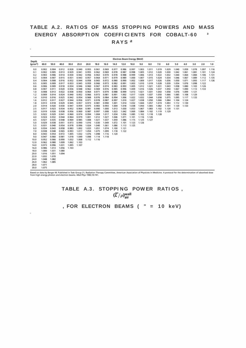
TABLE A.2. RATIOS OF MASS STOPPING POWERS AND MASS

ENERGY ABSORPTION COEFFICIENTS FOR COBALT-60 ³

RAYS a

TABLE A.3. STOPPING POWER RATIOS ,

, FOR ELECTRON BEAMS ( ” = 10 keV)



TABLE A.6. RATIOS OF MEAN MASS-ENERGY ABSORPTION

COEFFICIENTS ,

, FOR VARIOUS MATERIALS

TABLE A.7. PHOTON MASS ATTENUATION COEFFICIENTS,

µ/ , AND MASS ENERGY-ABSORPTION COEFFICIENTS

µen / , IN m2 /kg FOR ENERGIES 1 keV TO 20 MeV

(MULTIPLY m2 /kg BY 10 TO CONVERT TO cm2 /g).

TABLE A.8. COLLISION MASS STOPPING POWERS, S / ,

IN MeV cm2 /g, FOR ELECTRONS IN VARIOUS MATERIALS

TABLE A.9.1. COBALT-60 PERCENT DEPTH DOSES: 80 cm

SSD

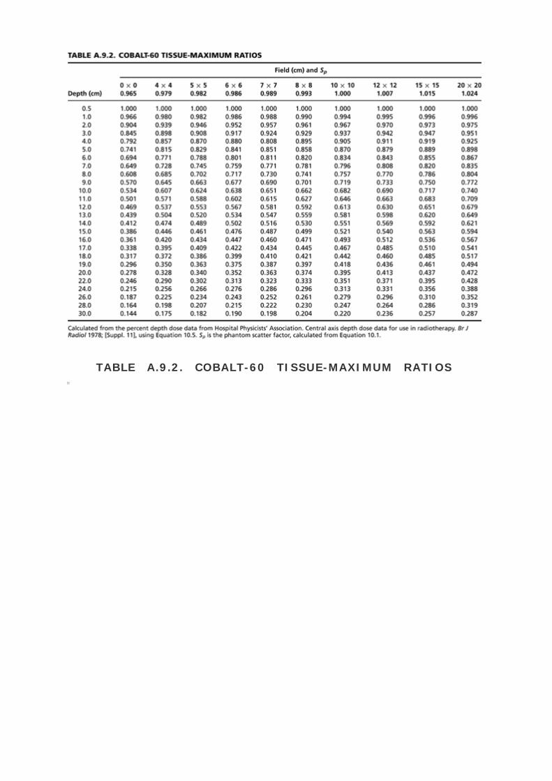
TABLE A.9.2. COBALT-60 TISSUE-MAXIMUM RATIOS

TABLE A.9.3. COBALT-60 SCATTER-MAXIMUM RATIOS FOR

CIRCULAR FIELDS a

TABLE A.10.1. 4-MV X-RAY PERCENT DEPTH DOSES: 100 cm

SSD

TABLE A.10.2. 4-MV X-RAY TISSUE-MAXIMUM RATIOS

TABLE A.10.3. 4-MV X-RAY SCATTER-MAXIMUM RATIOS FOR

CIRCULAR FIELDS

TABLE A.11.1. 10-MV X-RAY PERCENT DEPTH DOSES

TABLE A.11.2. 10-MV X-RAY TISSUE-MAXIMUM RATIOS

TABLE A.11.3. 10-MV X-RAY SCATTER-MAXIMUM RATIOS

P.A-3

P.A-4

P.A-5

P.A-6

P.A-7

P.A-8

P.A-9

P.A-

10

P.A-

11

P.A-

12

P.A-

13

P.A-

14

P.A-

15

P.A-

16

P.A-

17

P.A-

18

P.A-

19

P.A-

20

P.A-

21

P.A-

22

TABLE A.12.1. PATTERSON-PARKER PLANAR IMPLANT

TABLES

TABLE A.12.1A. MILLIGRAME-HOURS PER 1,000 R FOR

DIFFERENT AREAS AND VARIOUS TREATING DISTANCES a

TABLE A.12.1B. LARGER AREAS

TABLE A.12.1C. SOME FILTRATION CORRECTORS

P.A-

23

TABLE A.12.2. PATERSON-PARKER VOLUME IMPLANT

TABLES

TABLE A.12.2A.

TABLE A.12.2B.

TABLE A.12.2C. USEFUL FILTRATION CORRECTORS

Colore Plates

COLOR PLATE 19.2D.

COLOR PLATE 19.3. Image segmentation for prostate gland

treatment planning. Prostate gland, bladder, and rectum are

delineated in different colors. Segmented structures are shown

in transverse (A) , lateral (B) , and coronal (C) planes.

COLOR PLATE 19.4. Beam's eye view of anterior-posterior (A)

and left-right lateral (B) fields used in the treatment of prostate

gland. Composite (initial plus boost) isodose curves for a four-

field plan are displayed in transverse (C) , sagittal (D) , and

coronal (E) planes.

COLOR PLATE 19.5. A conformal stereotactic treatment plan for

a pituitary tumor showing isodose curves in the transverse (A) ,

lateral (B) , and coronal (C) planes. Prescription isodose

surfaces covering the target volume are displayed in frontal (D)

and lateral (E) views.

COLOR PLATE 19.6. A three-dimensional plan for the treatment

of glioblastoma is displayed. Isodose curves in transverse (A) ,

lateral (B) , and coronal (C) planes are used to evaluate the

plan. Cumulative DVH (D) is also useful in the evaluation

process. Differential DVH (E) shown here for the tumor only, is

more of an academic interest.

COLOR PLATE 20.18. A concave shape target of a thyroid tumor

in close vicinity of spinal cord (A) and the intensity-modulated

radiation therapyâ€“generated isodose plan in a transverse slice

(B).

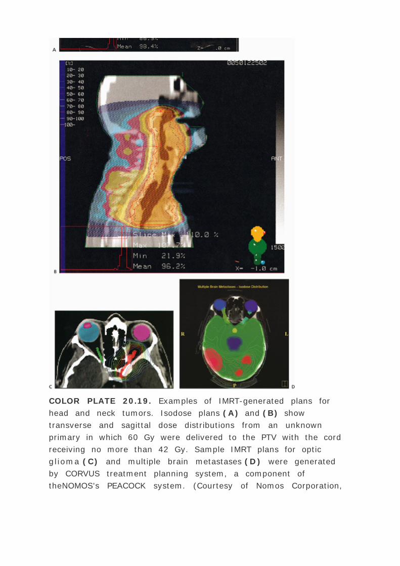
COLOR PLATE 20.19. Examples of IMRT-generated plans for

head and neck tumors. Isodose plans (A) and (B) show

transverse and sagittal dose distributions from an unknown

primary in which 60 Gy were delivered to the PTV with the cord

receiving no more than 42 Gy. Sample IMRT plans for optic

glioma (C) and multiple brain metastases (D) were generated

by CORVUS treatment planning system, a component of

theNOMOS's PEACOCK system. (Courtesy of Nomos Corporation,

Sewickley, PA.)

COLOR PLATE 20.20. An example of intensity-modulated

radiation therapy plan for the prostate gland using five fields.

Any number of intensity modulated fields may be used

depending upon the degree of optimization desired in dose

distribution and practical considerations of patient set-up and

equipment limitations.

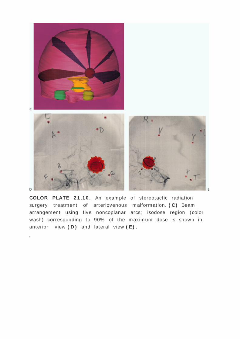
COLOR PLATE 21.10. An example of stereotactic radiation

surgery treatment of arteriovenous malformation. (C) Beam

arrangement using five noncoplanar arcs; isodose region (color

wash) corresponding to 90% of the maximum dose is shown in

anterior view (D) and lateral view (E).

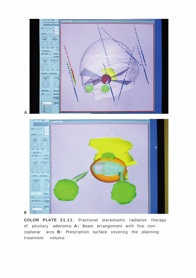
COLOR PLATE 21.11. Fractional stereotactic radiation therapy

of pituitary adenoma. A: Beam arrangement with five non-

coplanar arcs. B: Prescription surface covering the planning-

treatment volume.

COLOR PLATE 23.1. A sample of pre-treatment plan with 125 I

seeds showing (A) seeds and isodose curves in four ultrasound

cross sections of prostate gland and (B) dose volume histogram

for target (prostate gland) and normal tissue (rectum).

COLOR PLATE 23.2. A sample of post-treatment plan of the

same patient as in Fig. 23.1 showing (A) seeds and isodose

curves in the four ultrasound cross sections of the prostate

gland and (B) dose volume histogram for target (prostate gland)

and normal tissue (rectum).

Physics of Radiation Therapy - Third Edition by Faiz M. Khan

Documents

Transcript of Physics of Radiation Therapy - Third Edition by Faiz M. Khan