“7th AGILE Conference on Geographic Information Science” 29 April-1May 2004, Heraklion, Greece Parallel Session 4.1- “Geographic Knowledge Discovery” 313

Modelling Urban Dynamics with Cellular Automata: A Model of the City of Heraklion

Ivan Blecic1, Arnaldo Cecchini2, Poulicos Prastacos3, Giuseppe A. Trunfio4,

Emmanuil Verigos5

1 Università IUAV di Venezia - Dept. of Planning - Faculty of Urban Planning Venezia, Italy - ivan@iuav.it

2 University of Sassari - Dept. of Architecture and Urban Planning - Faculty of Architecture Sassari, Italy - cecchini@uniss.it

3 Foundation for Research and Technology-Hellas Institute of Applied and Computational Mathematics, Regional Analysis Division

Heraklion, Greece - poulicos@iacm.forth.gr 4 University of Calabria - Dept. of Mathematics,

Cosenza, Italy - trunfio@unical.it 5 University Ca’Foscari, Interdepartmental Center for Dynamic Interactions Between Economy,

Environment and Society Venezia, Italy - vrgsmm01@hostsun.com

SUMMARY

This paper is an attempt to explore and to propose a model of interactions between social, environmental and economic variables in land-use and urban development dynamics, using cellular automata. Such models can simulate spatial evolutions with different development perspectives and can produce future development scenarios useful for decision-making processes. For the purposes of this study, a cellular automaton applied in the City of Heraklion (Crete) has been developed. The implementation of the model hereby illustrated is a pilot experience and still in a groundwork phase. However, we believe that this paper, addressing few methodological, theoretical and practical issues, offers an unpretentious, but useful contribution for cellular automata based modelling, and more importantly, suggests why such models are particularly useful for urban simulations.

STEERING COMPLEX SYSTEMS We all can have our own “vision” of the future of a city, and that can be a non est disputandum: anyone,

everyone has right on his or her own vision, more or less freely chosen, which then “competes” and collides with other visions. But if, and as long, a vision is accepted and shared, the decision about all the rest should be defined on the basis of the case in question, it is in that case a true problem. And as such requires the actual situation be understood, which means the adoption of tools and techniques for a clear reading, description, interpretation, and forecast. All this means the adoption of a convenient “tool box” with the necessary models for the needs at hand. The role of models in the government of the city is thus fundamental; but the proper attention is due.

The mentality set on a “dogma of the continuity”, which holds that great causes are required in order to obtain great effects, is largely responsible for many of the famous errors created by so called “realised socialism” and the disastrous effects of its “organic” concept of planning. It forgets that grand objectives are not achieved with grand policies but with great policies, which do not underestimate certain flexibility, the ability to maintain a sense of balance, and the capability of autopoiesis present in many social sub-systems.

A “good” decision-maker, will intervene with maximum efficiency when and where it is needed, understanding and taking advantage of system’s “natural” tendencies, while frequently making decisions which are “open and reversible”. Tools that can help in this task, controlling, but not being reductive with

314

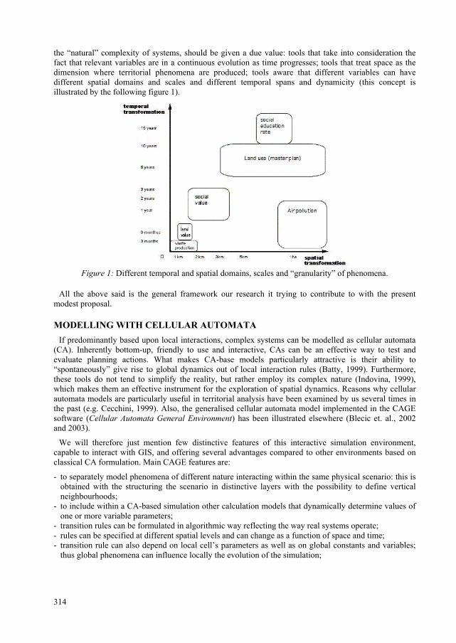
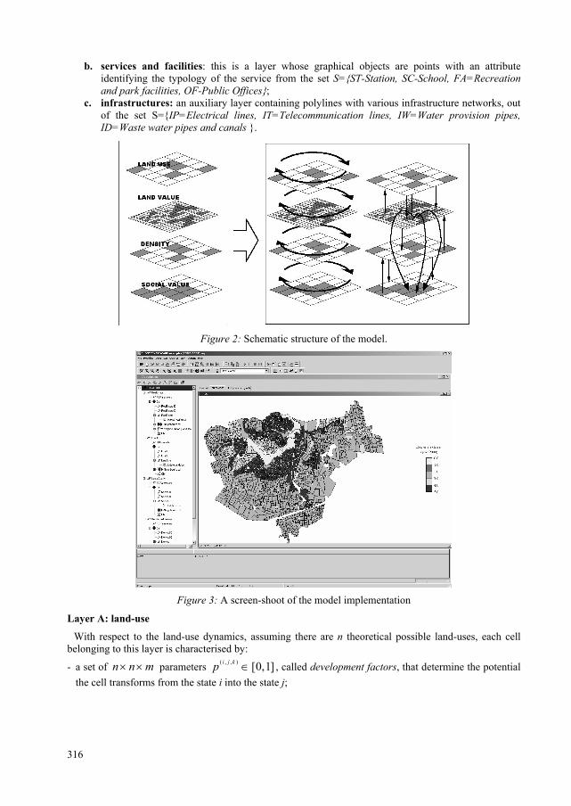
the “natural” complexity of systems, should be given a due value: tools that take into consideration the fact that relevant variables are in a continuous evolution as time progresses; tools that treat space as the dimension where territorial phenomena are produced; tools aware that different variables can have different spatial domains and scales and different temporal spans and dynamicity (this concept is illustrated by the following figure 1).

Figure 1: Different temporal and spatial domains, scales and “granularity” of phenomena.

All the above said is the general framework our research it trying to contribute to with the present

modest proposal. MODELLING WITH CELLULAR AUTOMATA

If predominantly based upon local interactions, complex systems can be modelled as cellular automata (CA). Inherently bottom-up, friendly to use and interactive, CAs can be an effective way to test and evaluate planning actions. What makes CA-base models particularly attractive is their ability to “spontaneously” give rise to global dynamics out of local interaction rules (Batty, 1999). Furthermore, these tools do not tend to simplify the reality, but rather employ its complex nature (Indovina, 1999), which makes them an effective instrument for the exploration of spatial dynamics. Reasons why cellular automata models are particularly useful in territorial analysis have been examined by us several times in the past (e.g. Cecchini, 1999). Also, the generalised cellular automata model implemented in the CAGE software (Cellular Automata General Environment) has been illustrated elsewhere (Blecic et. al., 2002 and 2003).

We will therefore just mention few distinctive features of this interactive simulation environment, capable to interact with GIS, and offering several advantages compared to other environments based on classical CA formulation. Main CAGE features are:

- to separately model phenomena of different nature interacting within the same physical scenario: this is obtained with the structuring the scenario in distinctive layers with the possibility to define vertical neighbourhoods;

- to include within a CA-based simulation other calculation models that dynamically determine values of one or more variable parameters;

- transition rules can be formulated in algorithmic way reflecting the way real systems operate; - rules can be specified at different spatial levels and can change as a function of space and time; - transition rule can also depend on local cell’s parameters as well as on global constants and variables;

thus global phenomena can influence locally the evolution of the simulation;

315

- the neighbourhoods are defined as abstract sets of cells satisfying abstract conditions and queries; neighbourhoods can also change with time, and are not necessarily defined as topological relation (normally proximity) between objects of the simulated system;

- the graphical representations associated to cells are considered attributes whose particular appearance is not a priori subject to constraints of spatial or temporal regularity; in fact, the objects of an urban models naturally lead to non-regular, and even non-lattice structures.

THE CASE STUDY

We have attempted to develop a model for the City of Heraklion in Crete. The data-sets used were made available by the local development masterplans, at the city-block level accuracy. In particular, the spatial data available were:

urban density variable for 1980 and 2000, expressed in persons/hq; real-estate value for 1980 and 2000, expressed in Dr./hq; a “social value” indicator for 1980 and 2000, expressed as a qualitative ordinal value; effective land-use for 1961-1980; 1998 masterplan zoning and restrictions.

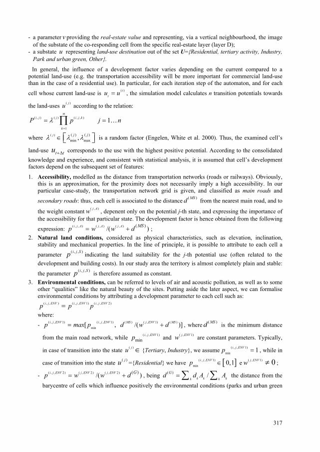
Our model is articulated in several layers where distinctive dynamics are simulated. For purposes of a better “readability” and usability, we have also introduced few auxiliary layers containing entities with constant attributes. The graphical object characterising layers are of three types:

- irregular cells of the “region” type representing city blocks and containing predominantly buildings, but also internal and capillary street network and undeveloped land;

- poly-lines representing the main street and road network, organised in main and secondary roads; - points representing positions of urban services and special facilities.

The model is organised in the following layers: I) Dynamic layers with cells representing city blocks. These are layers where different aspects of urban

dynamics are evolving, depending on a set of parameters deriving from auxiliary (constant) layers. The mechanisms of vertical neighbourhoods permit the simulation of reciprocal interactions among layers. The simulation model has the following dynamic layers: a. land-use: each cell has a “dominant land-use” substate, a categorical finite-set variable, and a set

of parameters and constants. During the simulation, it is possible to obtain a cell state transition, in other words a transformation of the dominant land-use, through a probabilistic model that takes due consideration of the urban masterplan norms;

b. social quality: cells have a “social quality” substate, an ordinal variable with five possible values, and a set of parameters. During the simulation, the level of social quality can rise or drop according to a series of transition rules dependent on layer’s parameters;

c. residential density: cells have a “density” substate and a set of parameters. The density may vary dynamically according to automaton rules.

d. real-estate values: each cell has a “real-estate value” substate, an ordinal variable with five possible values, and a set of variable and constant parameters. During the simulation, a cell can experience increase or decrease of its real-estate value according to a set of rules dependent on layer’s parameters;

II) Auxiliary layers: a. roads and streets: this is an auxiliary information whose graphical objects are polylines, each

with a particular string attribute form the set S={Main road, secondary road};

316

b. services and facilities: this is a layer whose graphical objects are points with an attribute identifying the typology of the service from the set S={ST-Station, SC-School, FA=Recreation and park facilities, OF-Public Offices};

c. infrastructures: an auxiliary layer containing polylines with various infrastructure networks, out of the set S={IP=Electrical lines, IT=Telecommunication lines, IW=Water provision pipes, ID=Waste water pipes and canals }.

Figure 2: Schematic structure of the model.

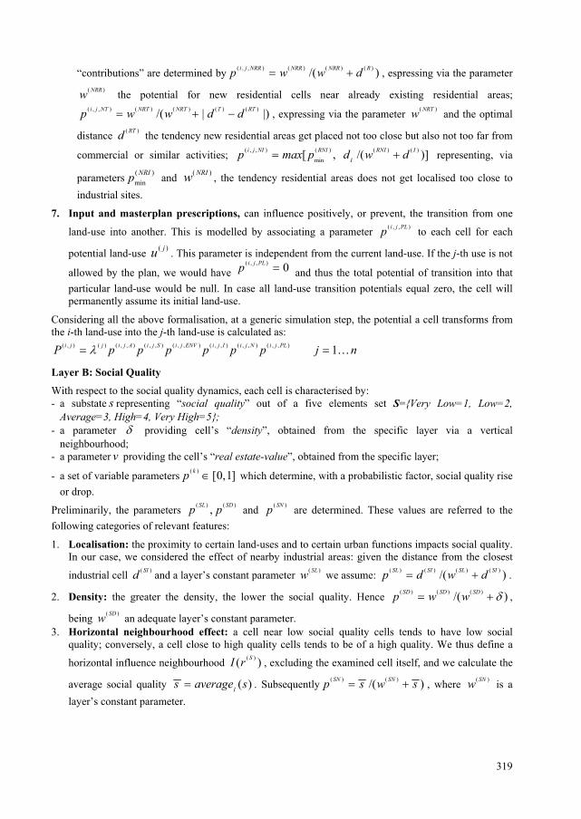
Figure 3: A screen-shoot of the model implementation

Layer A: land-use

With respect to the land-use dynamics, assuming there are n theoretical possible land-uses, each cell belonging to this layer is characterised by:

- a set of n n m× × parameters ( , , ) [0,1]i j kp ∈ , called development factors, that determine the potential the cell transforms from the state i into the state j;

317

- a parameter v providing the real-estate value and representing, via a vertical neighbourhood, the image of the substate of the co-responding cell from the specific real-estate layer (layer D);

- a substate u representing land-use destination out of the set U={Residential, tertiary activity, Industry, Park and urban green, Other}.

In general, the influence of a development factor varies depending on the current compared to a potential land-use (e.g. the transportation accessibility will be more important for commercial land-use than in the case of a residential use). In particular, for each iteration step of the automaton, and for each

cell whose current land-use is ( )i

tu u= , the simulation model calculates n transition potentials towards

the land-uses ( )ju according to the relation:

( , ) ( ) ( , , )

1

1m

i j j i j k

k

P p j nλ=

= =∏ K

where ( ) ( ) ( )min max,j j jλ λ λ∈ ⎡ ⎤⎣ ⎦ is a random factor (Engelen, White et al. 2000). Thus, the examined cell’s

land-use t tu +∆ corresponds to the use with the highest positive potential. According to the consolidated knowledge and experience, and consistent with statistical analysis, it is assumed that cell’s development factors depend on the subsequent set of features:

1. Accessibility, modelled as the distance from transportation networks (roads or railways). Obviously, this is an approximation, for the proximity does not necessarily imply a high accessibility. In our particular case-study, the transportation network grid is given, and classified as main roads and

secondary roads: thus, each cell is associated to the distance ( )MSd from the nearest main road, and to

the weight constant ( , )j Aw , depenent only on the potential j-th state, and expressing the importance of the accessibility for that particular state. The development factor is hence obtained from the following

expression: ( , , ) ( , ) ( , ) ( )/( )i j A j A j A MSp w w d= + ; 2. Natural land conditions, considered as physical characteristics, such as elevation, inclination,

stability and mechanical properties. In the line of principle, it is possible to attribute to each cell a

parameter ( , , )i j Sp indicating the land suitability for the j-th potential use (often related to the development and building costs). In our study area the territory is almost completely plain and stable:

the parameter ( , , )i j Sp is therefore assumed as constant. 3. Environmental conditions, can be referred to levels of air and acoustic pollution, as well as to some

other “qualities” like the natural beauty of the sites. Putting aside the later aspect, we can formalise environmental conditions by attributing a development parameter to each cell such as:

( , , ) ( , , 1) ( , , 2)i j ENV i j ENV i j ENVp p p= where:

- ( , , 1) ( , , 1) ( ) ( , 1) ( )

min[ , /( )]i j ENV i j ENV MS j ENV MSp max p d w d= + , where ( )MSd is the minimum distance

from the main road network, while ( , , 1)

mini j ENVp and ( , 1)j ENVw are constant parameters. Typically,

in case of transition into the state ( )ju ∈{Tertiary, Industry}, we assume ( , , 1)

min 1i j ENVp = , while in

case of transition into the state ( )ju ={Residential} we have [ ]( , , 1)

min 0,1i j ENVp ∈ e ( , 1) 0j ENVw ≠ ;

- ( , , 2) ( , 2) ( , 2) ( )/( )i j ENV j ENV j ENV Gp w w d= + , being ( ) /k k kk k

Gd d A A= ∑ ∑ the distance from the

barycentre of cells which influence positively the environmental conditions (parks and urban green

318

areas, sea side, no-traffic zones, etc.), each characterised by the area kA and the distance from the

examined cell kd .

4. Presence of infrastructure networks and facilities, like electrical, telecommunication, water supply and sewage networks and facilities. By the way of a vertical neighbourhood to the auxiliary infrastructure layer (layer G), the minimum distances from infrastructure networks are calculated,

respectively ( ) ( ) ( ), ,IP IT IWd d d and ( )IDd . Each distance value is associated to a weight constant ( , )j Yw , depending only on the potential j-th state, providing thus the development factor ( , , ) ( , ) ( , ) ( )/( )i j Y j Y j Y Yp w w d= + . This permits us to aggregate the influences of the infrastructure

networks in a single factor: ( , , ) ( , , ) ( , , ) ( , , ) ( , , )i j I i j P i j T i j W i j DWp p p p p= 5. Localisation of urban services and other facilities. Via a vertical neighbourhood with the services

& facilities layer (layer F), this factor takes into account the influence of essential urban services such as schools, public parks, offices, etc. Analogously as with the infrastructures, per each category, the

distance ( )Yd from the examined cell, as well as thr weight constant ( , )j Yw permit us to calculate the

development factor as ( , , ) ( , ) ( , ) ( )/( )i j Y j Y j Y Yp w w d= + . The influence of all the present services is

subsequently determined as ( , , ) ( , , )i j S i j Y

Yp p= ∏ , where Y=ST,SC,FA,OF;

6. Neighbourhood effects is a “drag‘n’brake” effect of the neighbouring cells on the cell being

examined. The horizontal neighbourhood is the set of cells ( , )( )i jI r satisfying the condition of being

within a given distance range ( , )i jr from the barycentre of the examined cell. In general, this range

depends on the current ( ( )iu ) and on the potential ( ( )ju ) cell’s land-use. The neighbouring cells’ influence is expressed as another development factor that assumes unitary value in case of no

influence. In our model, the non-unitary values ( , , )( 1)i j Np ≠ are assumed only in the following cases, depending on the potential land-use destination:

- ( )ju ={Tertiary activity}: if the neighbouring cells mark a scarce economical convenience for

tertiary activities, the factor ( , , )i j Np is less than 1. In particular, if we consider the two sets

RI I⊆ and TI I⊆ , respectively of residential and tertiary cells, then the total real-estate values

are calculated as R

R Iv v= ∑ and

TT I

v v= ∑ ; if T Rv v> then we assume ( , , ) 1i j Np = ,

otherwise ( , , ) ( ) ( )/( )i j N NT NT

R Tp w w v v= + − , where the parameter ( )NTw indicates the grade of sensibility related to the economical convenience. An analogous relation exists for the substate transition into the industrial land-use, considering the respective subset of meighbouring cells II

and an adequate parameter ( )NIw ;

- ( )ju ={Residential}: the land allocation for new residential uses is influenced by the presence of effective residential areas in the vicinity, but also by the presence of industrial or tertiary activities (assuming that too close or too distant intense commercial activities deter residential use).

Practically, being ( )Td and ( )Rd the distances between the examined cell and the barycentre of

cells from the two subsets TI and RI , we have ( , , ) ( , , ) ( , , ) ( , , )i j N i j NR i j NT i j NIp p p p= , where single

319

“contributions” are determined by ( , , ) ( ) ( ) ( )/( )i j NRR NRR NRR Rp w w d= + , espressing via the parameter ( )NRRw the potential for new residential cells near already existing residential areas; ( , , ) ( ) ( ) ( ) ( )/( | |)i j NT NRT NRT T RTp w w d d= + − , expressing via the parameter ( )NRTw and the optimal

distance ( )RTd the tendency new residential areas get placed not too close but also not too far from

commercial or similar activities; ( , , ) ( ) ( ) ( )

min[ , /( )]i j NI RNI RNI I

Ip max p d w d= + representing, via

parameters ( )min

NRIp and ( )NRIw , the tendency residential areas does not get localised too close to industrial sites.

7. Input and masterplan prescriptions, can influence positively, or prevent, the transition from one

land-use into another. This is modelled by associating a parameter ( , , )i j PLp to each cell for each

potential land-use ( )ju . This parameter is independent from the current land-use. If the j-th use is not

allowed by the plan, we would have ( , , ) 0i j PLp = and thus the total potential of transition into that

particular land-use would be null. In case all land-use transition potentials equal zero, the cell will permanently assume its initial land-use.

Considering all the above formalisation, at a generic simulation step, the potential a cell transforms from the i-th land-use into the j-th land-use is calculated as:

( , ) ( ) ( , , ) ( , , ) ( , , ) ( , , ) ( , , ) ( , , ) 1i j j i j A i j S i j ENV i j I i j N i j PLP p p p p p p j nλ= = K

Layer B: Social Quality

With respect to the social quality dynamics, each cell is characterised by: - a substate s representing “social quality” out of a five elements set S={Very Low=1, Low=2,

Average=3, High=4, Very High=5}; - a parameter δ providing cell’s “density”, obtained from the specific layer via a vertical

neighbourhood; - a parameter v providing the cell’s “real estate-value”, obtained from the specific layer;

- a set of variable parameters ( ) [0,1]kp ∈ which determine, with a probabilistic factor, social quality rise or drop.

Preliminarily, the parameters ( ) ( ),SL SDp p and ( )SNp are determined. These values are referred to the following categories of relevant features:

1. Localisation: the proximity to certain land-uses and to certain urban functions impacts social quality. In our case, we considered the effect of nearby industrial areas: given the distance from the closest

industrial cell ( )SId and a layer’s constant parameter ( )SLw we assume: ( ) ( ) ( ) ( )/( )SL SI SL SIp d w d= + .

2. Density: the greater the density, the lower the social quality. Hence ( ) ( ) ( )/( )SD SD SDp w w δ= + ,

being ( )SDw an adequate layer’s constant parameter. 3. Horizontal neighbourhood effect: a cell near low social quality cells tends to have low social

quality; conversely, a cell close to high quality cells tends to be of a high quality. We thus define a

horizontal influence neighbourhood ( )( )SI r , excluding the examined cell itself, and we calculate the

average social quality ( )Is average s= . Subsequently ( ) ( )/( )SN SNp s w s= + , where ( )SNw is a layer’s constant parameter.

320

4. Vertical neighbourhood effect: a high real-estate value normally procudes a high social quality.

Given a vertical neighbourhood as a set of cells ( )( )VI r from the real-estate layer, and calculated the

set’s average real-estate value ( )Iv average v= , we can express ( ) ( )/( )SV SVp v w v= + , where ( )SVw is a layer’s constant parameter.

Given all the above parameters ( )kp , the cell’s social quality value in particular state and at a specific

step of simulation ts is obtained as: ( ) ( ) ( ) ( ) ( )(5 )S SL SD SV SN

t ts round p p p pλ+∆ = , where [ ]( ) ( )

min max

( ) ,S SSλ λ λ∈ is a random factor.

Layer C: Residential Density

For an adequate simulation of the density dynamics, each cell is defined by:

- a substateδ providing its residential density; - a parameter s representing cell’s “social quality”, obtained from the specific layer via a vertical

neighbourhood;

- a set of variable parameters ( ) [0,1]kp ∈ determining with a probabilistic factor, the increase or decrease of cell’s density;

- a factor ( )Dk representing the maximum allowed density change between two consequent cellular automaton steps.

The discussed model considers three types of factors influencing the residential density:

1. Increasing factors: a low social quality in the neighbourhood determines a rise of density; this is

simulated via the cell’s parameter ( ) ( ) ( )/( )DS DS DSp w w s= + , where ( )Is average s= is the

average social quality among cells members of a horizontal neighbourhood set ( )( )DI r , while ( )DSw is a layer’s constant parameter;

2. Decreasing factors: a high density sway against high density due to the crowdedness; we calculate a

cell’s parameter ( )

maxmax[1, / ]DAp δ δ= , where maxδ is a maximum allowed density; 3. Stabilising factors: a high social quality tends to stabilise the density; this is represented via the cell’s

parameter ( ) ( ) ( )/( )DT DT DTp w w s= + , where s is the average social quality among neighbouring

cells already defined above, while ( )DTw is a layer’s constant parameter.

Bringing together all the above mentioned, for each step of the simulation, first the parameters ( )kp get calculated, and subsequently the new cell’s density is determined as:

( ) ( ) ( ) ( ) ( )[ ]D D DS DA DTt t t tk p p pδ δ λ δ+∆ = + − , where [ ]( ) ( )

min max

( ) ,D DDλ λ λ∈ is a random factor.

Layer D: Real-Estate Value

Every cell belonging to this layer is defined by:

- a subset v representing cell’s “real-estate value”, out of a five possible values V={VL=1,L=2,A=3,H=4,VH=5};

- a series of parameters ( )kp , which determine the tendency for a real-estate value variation;

321

- a parameter ( ) 1Vc > defining inertia of a value change.

A cell changes its value due to the predominance of one of the two contrasting tendencies, qualified with

the parameters ( ) [0,1]VIp ∈ and ( ) [0,1]VDp ∈ . The following relations are determinative in the parameters’ quantification:

1. Value increase:

- Horizontal neighbourhood effect: a cell with a higher average value of neighbouring cells tends to

experience an increase of its value. Given a horizontal neighbourhood ( )( )VI r , which excludes the

examined cell, we calculate the average value ( )Iv average v= . If v v≥ , we

assume ( 1) 0VIp = , otherwise ( 1) ( 1)( ) /( )VI VIp v v w v v= − + − , where ( 1)VIw is a layer’s constant parameter;

- Vertical neighbourhood effect: a high social quality neighbourhood priviledges the increase of the

real-estate values. Given a vertical neighbourhood set of cells ( )( )SI r , from the respective social

quality layer, we can calculate ( )Is average s= . Thus we assume ( 2) ( 2)/( )VI VIp s w s= + ,

where ( 2)VIw is a layer’s constant parameter; - Localisation: the proximity to services and facilities such as schools, parks, recreation facilities,

etc. plays in favour of a real-estate value increase. Via a vertical neighbourhood from the services

layer (layer F), we attribute the distance from the examined cell ( )Yd and a weight constant ( )VIYw

separately for each category of services, and we calculate ( ) ( ) ( ) ( )/( )VIY VIY VIY Yp w w d= + . The total

services and facilities proximity influence is expressed by the parameter ( 3) ( )VI VIY

Yp p= ∏ ,

where Y=ST,SC,FA,OF; - Land use: some potential and effective land-uses play in favour of the real-estate value, e.g. a cell

with high potential for transforming into a tertiary activity can tend to have a higher real-estate value (even without effectively being a tertiary activity). For that reason, we are introducing a

parameter ( 4) ( 4) ( , )VI VI i Tp w P= representing a quote of the potential transition into a tertiary land-use calculated above.

2. Value decrease:

- Horizontal neighbourhood effect: a cell with a lower average value of its neighbours tends to decrease its real-estate value. Given the average value of the neighbouring cells ( )Iv average v= ,

if v v≤ we assume ( 1) 0VDp = , otherwise ( 1) ( 1)( ) /( )VD VDp v v w v v= − + − , where ( 1)VDw is a layer’s constant parameter;

- Vertical neighbourhood effect: too high density in the neighbouring cells depresses the real-estate

value of the examined cell. We hence define a vertical neighbourhood ( )( )DI r from the density

layer, and can subsequently calculate the average density ( )Iaverageδ δ= . Thereafter we

define ( 2) ( 2) ( 2)/( )VD VD VDp w w δ= + , where ( 2)VDw is a layer’s constant parameter; - Localisation: an excessive vicinity of certain facilities depresses the real-estate value. Being Y a

generic “depressing” facility, ( )Yd distant from the examined cell, and given the weight constant

322

( )VDYw , we define the specific development factor ( ) ( ) ( ) ( )/( )VDY VDY VDY Yp w w d= + . The influence of the “depressing” facilities in the examined cell’s proximity is subsequently defined as

( 3) ( )VI VIY

Yp p= ∏ where Y=ST,SC,FA,OF;

Therefore, for the real-estate layer, we calculate an aggregated cell’s parameter as: ( ) ( )VI VIk

kp p= ∑ e

( ) ( )VD VDk

kp p= ∑

Finally, For each automaton’s simulation step, if ( ) ( ) ( )VI V VDp c p> , with ( ) 1Vc > , we have the value

transition 1 (5, 1)t tv min v+

= + ; otherwise, if ( ) ( ) ( )VD V VIp c p> we have 1 (0, 1)t tv max v+

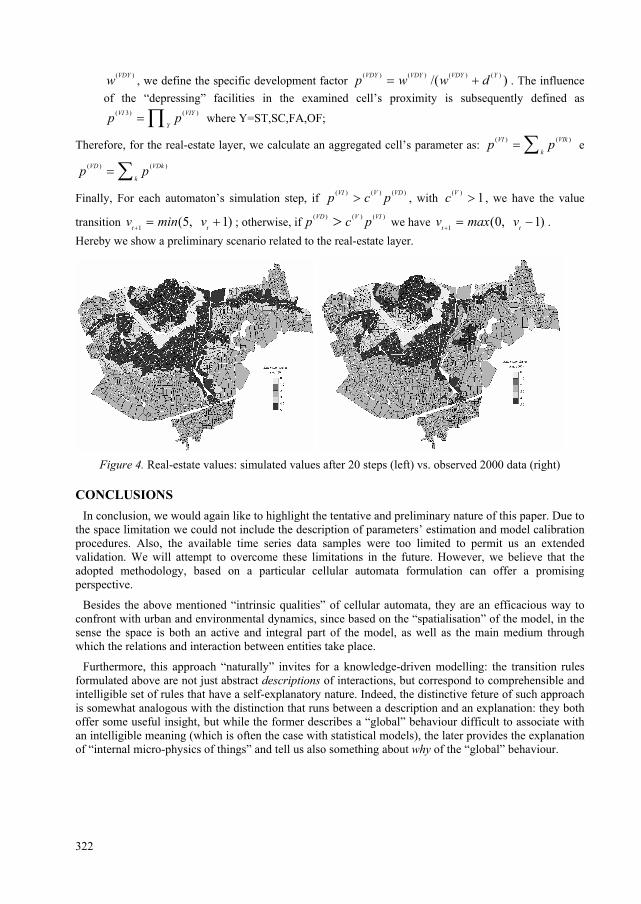
= − . Hereby we show a preliminary scenario related to the real-estate layer.

Figure 4. Real-estate values: simulated values after 20 steps (left) vs. observed 2000 data (right)

CONCLUSIONS

In conclusion, we would again like to highlight the tentative and preliminary nature of this paper. Due to the space limitation we could not include the description of parameters’ estimation and model calibration procedures. Also, the available time series data samples were too limited to permit us an extended validation. We will attempt to overcome these limitations in the future. However, we believe that the adopted methodology, based on a particular cellular automata formulation can offer a promising perspective.

Besides the above mentioned “intrinsic qualities” of cellular automata, they are an efficacious way to confront with urban and environmental dynamics, since based on the “spatialisation” of the model, in the sense the space is both an active and integral part of the model, as well as the main medium through which the relations and interaction between entities take place.

Furthermore, this approach “naturally” invites for a knowledge-driven modelling: the transition rules formulated above are not just abstract descriptions of interactions, but correspond to comprehensible and intelligible set of rules that have a self-explanatory nature. Indeed, the distinctive feture of such approach is somewhat analogous with the distinction that runs between a description and an explanation: they both offer some useful insight, but while the former describes a “global” behaviour difficult to associate with an intelligible meaning (which is often the case with statistical models), the later provides the explanation of “internal micro-physics of things” and tell us also something about why of the “global” behaviour.

323

BIBLIOGRAPHY Batty M., Xie Y. “From cells to cities” Environment and Planning B, 21, 31–48, 1994. Batty, M., Editorial “Urban systems as cellular automata” Environment and Planning B, 24, 159–164,

1997. Batty M., Xie Y., Sun, Z., “Modelling urban dynamics through GIS-based cellular automata” Computers,

Environment and Urban Systems, 23, 205–233, 1999. Barredo J.I., Kasanko M., McCormick N., Lavalle C., ”Modelling dynamic spatial processes: simulation

of urban future scenarios through cellular automata” Landscape and Urban Planning, 64, 145-160, 2003.

Blecic, I., Cecchini, A., Rizzi, P., Trunfio, G.A., “Playing With Automata. An Innovative Perspective for Gaming Simulation”, in S. Bandini, B. Chopard, M. Tomassini (Eds.), Cellular Automata: 5th International Conference on Cellular Automata for Research and Industry, Proceedings ACRI 2002 9-11 Ottobre 2002, Ginevra, Springer-Verlag in the Lecture Notes in Computer Science, 2002

Blecic I., Cecchini A., Rizzi P., Trunfio G.A., “Playing with Automata. An Innovative Perspective for Gaming Simulation (with CAGE - Cellular Automata General Environment)” CUPUM - 8th International Conference on Computers in Urban Planning and Urban Management, Sendai, Japan, 27-29,May 2003.

Cecchini A., “Urban modelling by means of cellular automata: generalised urban automata with the help on-line (AUGH) model” Environment and Planning B, 23, 721–732, 1996.

Couclelis H,. “From Cellular Automata to Urban models: new principles for model development and implementation” Environment and Planning B, 24, 165-174, 1988.

Clarke K.C., Gaydos L.J., “Loose-coupling a cellular automaton model and GIS: long-term urban growth predictions for San Francisco and Baltimore” International Journal of Geographic Information Science, 12, 699–714, 1998.

Engelen, G., R. White, et al., “Cellular Automata as the Integrator of Land Use and Land Cover Models”. MODULUS Final Report. E. I. F. C. a. N. H. Programme. Brussels Belgium, 2000.

Forrester J.M., “Urban dynamics”, MIT Press, 1969. Itami R.M., “Simulating spatial dynamics: cellular automata theory” Landscape Urban Planning, 30, 27–

47, 1994. Indovina F., ”New tecnologies and the future of cities” Computers, Environment and Urban Systems,23

233-241, 1999. Torrens P.M., O’Sullivan, D., “Editorial: Cellular automata and urban simulation: where do we go from

here” Environment and Planning B, 28, 163–168, 2001. Wagner D. F., “Cellular automata and geographic information systems” Environment and Planning B, 24,

219–234. 1997. Xia, L., & Yeh, A. G., “Modelling sustainable urban development by the integration of constrained

cellular automata and GIS” International Journal of Geographic Information Science, 14, 131–152. 2000.

CAGE and the free software at: http://lamp.sigis.net-