Cellular Automata, Reaction-Diffusion and Multiagents Systems for Artificial Cell Modeling

Abdallah Zemirline1, Pascal Ballet1, Lionel Marcé1, Patrick Amar2,3, Gilles Bernot2, Franck Delaplace2, Jean-Louis Giavitto2, Olivier Michel2, Jean-Marc Delosme2, Roberto Incitti4, Paul Bourgine5, Christophe Godin6, François Képès7 , Philippe Tracqui8, Vic Norris9, Janine Guespin9, Maurice Demarty9, Camille Ripoll9 1 EA2215, Département d'Informatique, Université de Bretagne Occidentale, Brest 2 Laboratoire de Méthodes Informatiques, CNRS UMR 8042, Université d'Evry, 91025 Evry 3 Laboratoire de Recherche en Informatique, CNRS UMR 8623, Université Paris-Sud, Orsay 4 Institut des Hautes Études Scientifiques, Bures, France & genopole®, Evry, France 5 CREA - Ecole Polytechnique 6 UMR Cirad/Inra modélisation des plantes, TA40/PSII, Montpellier 7 ATelier de Génomique Cognitive CNRS ESA8071/genopole, Evry 8 Lab. TIMC-IMAG, Equipe DynaCell , CNRS UMR, 5525, Faculté de Médecine, La Tronche 9 Laboratoire des Processus Intégratifs Cellulaires, UPRESA CNRS 6037, Faculté des Sciences & Techniques , Université de Rouen, 76821, Mont-Saint-Aignan France

Introduction

Objectives of the simulation Simulation is the experiment on a model. A model represents a simplification of a real

phenomenon. Only certain relevant parameters are taken into account and numerous others are untidy. The simulation of a model has sense only if its behavior is close to the real phenomenon, that is, if it can approach reality. So, by changing the parameter values of the model, the simulation allows to infer what would take place in reality under the influence of similar actions.

The simulation has various objectives. First, when the model is validated by the real experiment, the simulation allows to make numerous and accelerated experiments, with a very accurate parameter control. Secondly, if the model is incomplete or insufficient, the simulation allows to test hypotheses. In that case, it participates in the settling of the model. Numerous fields of research and industry use the simulation, either for the model development, for the product settling or either for the forecast of complex phenomena. Aeronautics, motorcar, economy, chemistry, meteorology, astrophysics, cosmology, nuclear physics or more recently biology use it frequently.

Simulation and biology The in-vitro experiment, constitutes for biology the most wide-spread type of

simulation. Cells are taken apart from an organism, then are studied outside, generally in a test tube. Around the beginning of the 20th century, Michaelis and Menten described the biochemical phenomenon of enzymatic reaction using differential equations. So, mathematical models became an alternative to in-vivo or in-vitro experiments. This is the start of the computational biology. Several biological fields of research use the mathematical tool to describe or explain their phenomenon. For example, in 1966 the first mathematical model describing an immune phenomenon was developed [HEG66]. A few years later, by 1970 , the

immune models based on differential equations became more complex. In 1974, Jerne [JER74] described his model of the idiotypic network. His model is highly non linear and no simple analytical solution can be found. The use of the numeric computation then became a necessity. At the same time, data processing evolves, both from the point of view of the calculation power and from the languages of development. Several paradigms appear like artificial life, cellular automata, reaction-diffusion system, object programming or multi-agents system. Thus, it becomes possible to model and to simulate biological mechanisms not by using differential equations only.

Today, data processing is a useful tool for biology and for the alive world exploration. We are convinced, and this course tries to show it, that the study of living cells can be made partially by means of computer, that is in-silico (also called in machina or in-virtuo). We will see how we can connect together different computational systems to build an artificial cell. Each system describes a level of detail for the cell (Table 1):

- reaction-diffusion system allows to model the lower granularity of the cell, that is ionic and small molecules (from Angstrom to nanometer)

- cellular automata represents the macromolecular level (few nanometers). Macro molecules are the basic components of hyperstructures

- multiagents system will be used to model the hyperstructure level (several nanometers).

- reaction-diffusion system could be used again to model some tissue morphogenesis. Perhaps, it could be use to model intra-cellular membrane too.

Biological Level Dimension Model

Ionic / Small molecules 10-10 m Reaction - Diffusion System Macromolecules 10-9 m Cellular Automata

Hyperstructures & membranes 10-8 to 10-7 m Multiagents System Membrane & Tissues 10-7 m to 10-5 m Reaction - Diffusion System

Table 1: different possible levels of granularity for an integrated artificial cell modeling

Before the description of the different approaches, we will see a short state-of-the-art

in software tools aiming to simulate intra-cellular mechanisms. First, we will see the global objectives thanks to the Microbial Cell Project, then we will focus on two advanced software applications: electronic cell and virtual-cell.

Advanced applications

Principle An advanced application in cell simulation offers software tools to model, simulate

and interpret results. It must be used by biologists without any programming and it offers an intuitive interface. An advanced application must point out its own limitations, the robustness of the model parameters, the link between the model and the simulation and the results accuracy. An advanced application is integrated when it combines different means of modeling together.

We will see two applications that are integrated and advanced: e-cell [ECE01] and v-cell [VCE01]. They are based on a differential equation model (see example of Equation 1). The first one (e-cell) includes settled metabolic pathways which could be coupled with an

hypothetic biologist pathway model. The second one (v-cell) uses images (from microscopy) to put the simulation into the « real » image.

Integrated Project: Microbial Cell Project From Notice 01-21; Advanced Modeling and Simulation of Biological Systems [MCP01]

“ SUMMARY (January 2001): The Offices of Advanced Scientific Computing Research (ASCR) and Biological and Environmental Research (OBER) of the Office of Science (SC), U.S. Department of Energy, hereby announce interest in receiving applications for grants in support of computational modeling and simulation of biological systems. The goal of this program is to enable the use of terascale computers to explore fundamental biological processes and predict the behavior of a broad range of protein interactions and molecular pathways in prokaryotic microbes of importance to DOE. This goal will be achieved through the creation of scientific simulation codes that are high performance, scalable to hundreds of nodes and thousands of processors, and able to evolve over time and be ported to future generations of high performance computers. The research efforts being sought under this Program Notice will take advantage of extensive information inferred from the complete DNA sequence, such as the genetics and the biochemical processes available for a well-characterized prokaryotic microbe; for example, Escherichia coli (E. coli). This notice encourages applications from the disciplines of applied mathematics and computer science in partnership with microbiology, molecular biology, biochemistry and structural and computational biology to combine information available on a well characterized prokaryotic microbe with advanced mathematics and computer science to enable this new understanding. This announcement is being issued in parallel with Program Notice 01-20, the Microbial Cell Project. Together, they represent a planned first step in an ambitious effort to understand the functions of the proteins in a prokaryotic microbial cell, to understand their interactions as they form pathways that carry out DOE-relevant activities, and to eventually build predictive models for microbial activities that address DOE mission needs. Different goals of the project: Goal 1: Identify and Characterize the Molecular Machines of Life -- the Multiprotein Complexes that Execute Cellular Functions and Govern Cell Form Goal 2: Characterize Gene Regulatory Networks Goal 3: Characterize the Functional Repertoire of Complex Microbial Communities in Their Natural Environments at the Molecular Level Goal 4: Develop the Computational Methods and Capabilities to Advance Understanding of complex Biological Systems and Predict Their Behavior: Category Research Goal Sequencing Informatics �Automated microbial genome assembly

�Laboratory Information Management Systems (LIMS)

Sequence Annotation �Consistent gene finding, especially for translation start

�Identification of operon and regulon regions �Promoter and ribosome binding-site recognition �Repressor and activator-site prediction

Structural Annotation �High-throughput automated protein-fold recognition�Comparative protein modeling from structure

homologs �Modeling geometry of complexes from component

proteins Functional Annotation �Computational support for protein identification,

post-translational modification, and expression �Protein-function inference from sequence

homology, fold type, protein interactions, and expression

Category Research Goal �Methods for large-scale comparison of genome

sequences �Mass spectrometry LIMS and analysis algorithms �Image analysis of protein interactions and dynamics

New Databases �Environmental microbial populations �Protein complexes and interactions �Protein expression and post-translational

modification Data Integration �Tools interoperation and database integration

�Tools for multigene, multigenome comparisons �Automated linkage of gene/protein/function catalog

to phylogenetic, structural, and metabolic relationships

Microbial Ecology Support �Statistical methods for analyzing environmental sampling

�Sequence- and expression-data analysis from heterogeneous samples

�Pathway inference from known pathways to new organisms and communities

Modeling and Simulations �Molecular simulations of protein function and macromolecular interactions

�Development of computational tools for modeling biochemical pathways and cell processes

�Implementation of computational tools �Structural modeling of protein variants �Computational tools for modeling complex

microbial communities Visualization �Methods for hierarchical display of biological data:

(System level > Pathway > Multiprotein machines > Proteins > mRNA > Gene)

�Displays of interspecies comparisons �Visualization by functional pathways (e.g., DNA

repair, protein synthesis, cell-cycle control) Technology Needs The Human Genome Project taught that evolutionary improvement in existing technologies (e.g., DNA sequencing) can have a revolutionary impact on science. The systems approach taken by the Genomes to Life program dictates that existing technologies must evolve to a high-throughput capability. In addition, revolutionary technologies need to be developed, incorporating new modes of robotics and automation as well as advanced information and computing technologies. The following is a list of some key high-throughput technologies. DNA, RNA, Protein, Protein Machine, and Functional Analyses and Imaging · High-throughput identification of the components of protein complexes; mass spectrometry, new chip-based analyses, and capture assays · Parallel, comparative, high-throughput identification of DNA fragments among microbial communities and for community characterization · Whole-cell imaging; novel imaging technologies, including magnetic resonance optical, confocal, · soft X-ray, and electron microscopy; and new approaches for in vivo mapping of spatial proximity · New technologies for mapping contact surfaces between proteins involved in complexes or molecular machines (e.g., FRET and neutron scattering)

· Functional assays; development of novel technologies and approaches for defining the functions of genes from uncultured microorganisms Sampling and Sample Production · Approaches for recovering RNA and high-molecular-weight DNA from environmental samples and for isolating single cells of uncultured microorganisms · Advances in separation techniques, including new techniques to capture targeted proteins, and high-affinity ligands for all gene products · Improved approaches for studying proteins that are hard to crystallize (e.g., membrane proteins) Informatics, Modeling, and Simulation · Algorithms for genome assembly and annotation and for bioinformatics to measure protein expression and interactions · Standardized formats, databases, and visualization methods for complex biological data sets, including expression profiles and protein-protein interaction data · Molecular modeling methods for long-timescale, low-energy macromolecular interactions and for prediction of chemical reaction paths in enzyme active sites · Methods for automated collection and integration of biological data for cell-level metabolic network analysis or pathway modeling; improved methods for simulation, analysis, and visualization of complex biological pathways; and methods for prediction of emergent functional capabilities of microbial communities. ”

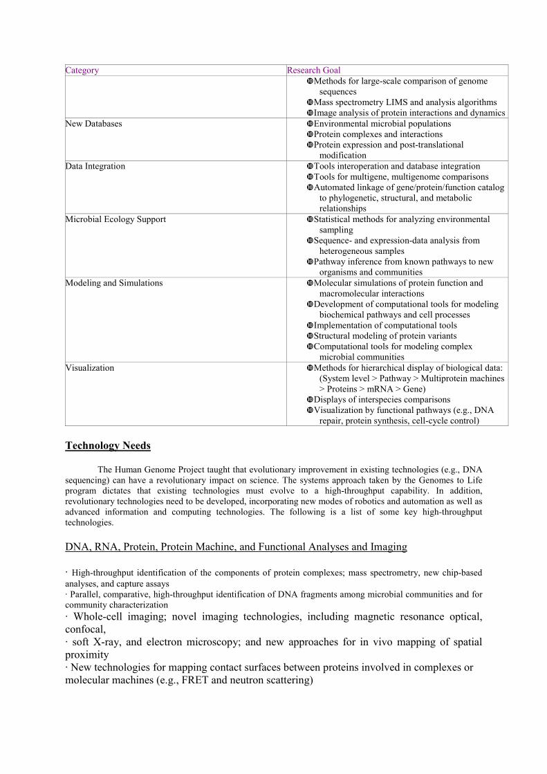
Advanced Application: Electronic Cell This application is able to process differential equations that model a molecular transformation (A + E -> A' + E), a complex formation (A + B -> AB), a dissociation (AB -> A + B) and an enzymatic reaction (A + B + E -> C + D + E) (Figure 1).

Figure 1: (1) concentrations in one compartment - (2) interactions(3) balance

reaction - (4) speed of non enzymatic reactions (5) speed of Michaelis-Menten reaction

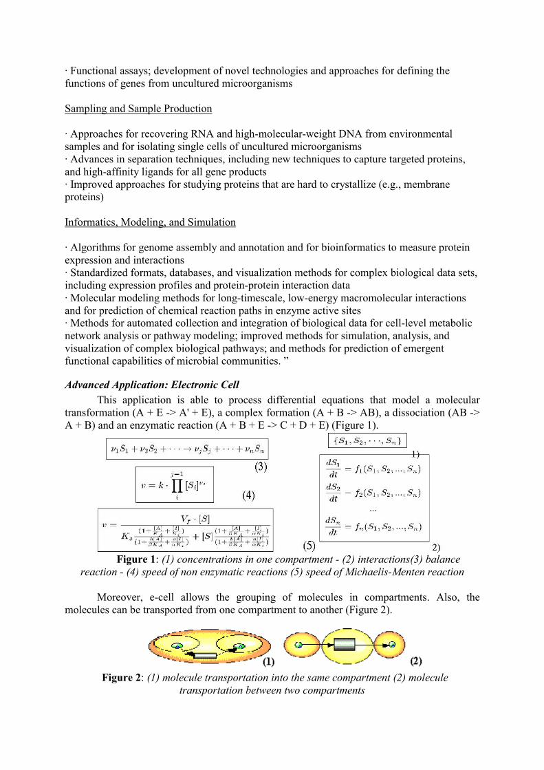
Moreover, e-cell allows the grouping of molecules in compartments. Also, the molecules can be transported from one compartment to another (Figure 2).

Figure 2: (1) molecule transportation into the same compartment (2) molecule

transportation between two compartments

There are six metabolic pathways included into the system : nucleotide biosynthesis,

phospholipid biosynthesis, amino acid biosynthesis, energy metabolism and gene expression System. Like this, the biologist can coupled its own metabolic pathway models to the whole system (Figure 3).

Figure 3: pre-existing metabolic pathways in e-cell.

The molecules, reactions and compartments are describe in a text file called “rule file”.

The e-cell system analyzes this file (the source code looks like C or C++) and allows a dynamic simulation of the molecule concentrations (Figure 4).

Figure 4: Information flow in the E-Cell System.

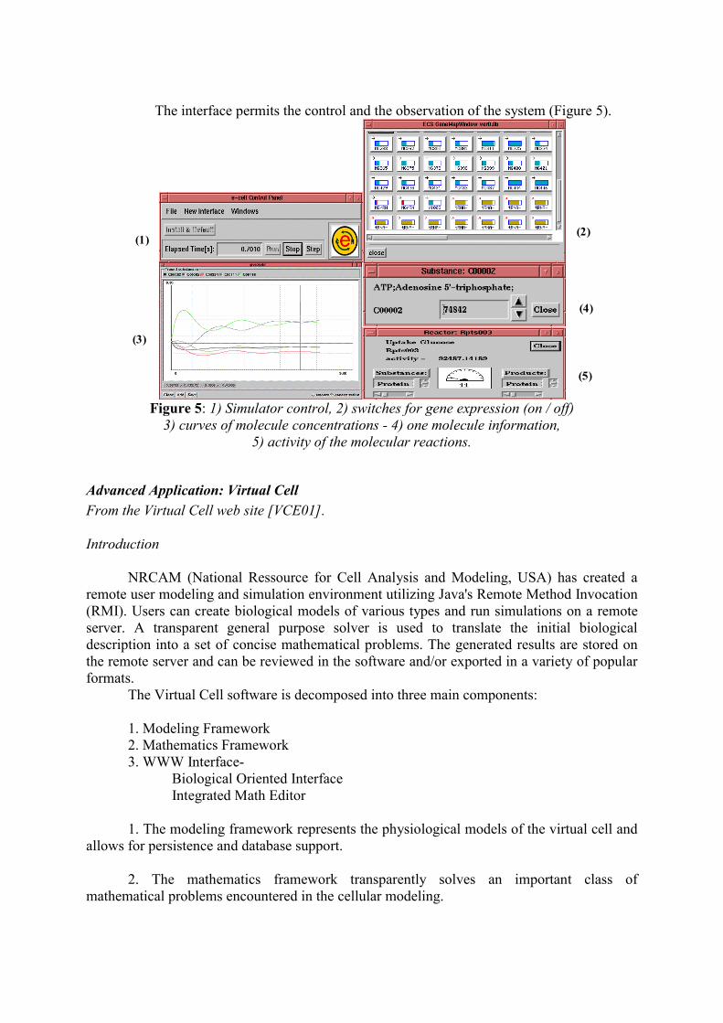
The interface permits the control and the observation of the system (Figure 5).

(1)(2)

(3)

(4)

(5)

Figure 5: 1) Simulator control, 2) switches for gene expression (on / off)

3) curves of molecule concentrations - 4) one molecule information, 5) activity of the molecular reactions.

Advanced Application: Virtual Cell From the Virtual Cell web site [VCE01]. Introduction

NRCAM (National Ressource for Cell Analysis and Modeling, USA) has created a

remote user modeling and simulation environment utilizing Java's Remote Method Invocation (RMI). Users can create biological models of various types and run simulations on a remote server. A transparent general purpose solver is used to translate the initial biological description into a set of concise mathematical problems. The generated results are stored on the remote server and can be reviewed in the software and/or exported in a variety of popular formats.

The Virtual Cell software is decomposed into three main components: 1. Modeling Framework 2. Mathematics Framework 3. WWW Interface- Biological Oriented Interface Integrated Math Editor 1. The modeling framework represents the physiological models of the virtual cell and

allows for persistence and database support. 2. The mathematics framework transparently solves an important class of

mathematical problems encountered in the cellular modeling.

3. The WWW accessible graphical user interface provides access to the technology mentioned above. The user interface has been developed using Java 2 Applets.

The biologically oriented user interface allows experimentalists to create models,

define cellular geometry, specify simulations, and analyze simulation results. There is a Math Editor component which has been integrated within the biological interface. The design of the biological to mathematical mapping allows for separate use of biological and math components, and includes automatic mathematical simplification using pseudo-steady approximations and mass conservation relationships. This allows for direct specification of mathematical problems, performing simulations and analysis on those systems. Equations may still be generated automatically from the biological interface. The stand alone mathematics user interface is also a tool for modeling reaction-diffusion systems.

Different steps needed to develop a simulation

1. The BioModel contains all the necessary information needed to define the biological model, i.e. species, compartments, reactions, fluxes:

2. The Geometry Editor is the main workspace for creating geometries. Create new

Geometries from uploaded experimental images or from analytically defined Geometries. The Geometry Database displays the Geometries and any associated files, i.e. BioModels, math models. The following snapshot shows the Virtual Cell Geometry interface:

To determine a geometry, it is possible to use a segmented experimental image:

from a photo to a segmented image where the simu-lation will take place.

3. The Application establishes the relationship between the BioModel and Geometry:

4. Creation of the mathematical code according to the Virtual Cell Math Description Language, VCMDL, in the Math Workspace. VCMDL is a declarative mathematics language, which has been developed to concisely describe the class of mathematical systems that are encountered in the Virtual Cell project. This language defines parameters, independent variables, differential/algebraic systems defined over a complex geometry including

discontinuous solutions and membrane boundaries and the description of the task to perform on such a system:

Currently six integration methods are available to solve differential equations: - Forward Euler (first order) - Runge-Kutta (second order) - Runge-Kutta (fourth order) - Adams-Moulton (fifth order) - Runge-Kutta-Fehlberg (fifth order) - LSODA (Variable order, Variable Time Step) 5. Run Simulations for Compartmental and Spatial models:

6. View Results for Spatial and Compartmental simulations:

After these brief descriptions of advanced applications, it possible to say that one of the main problem of these applications is that they represent a cell like a “soupe” where spatial structuration and mechanical aspect are neglected. We think that these aspects are essential to understand the whole cell functioning. That why, the next chapters will introduce computational approaches that could be used to get a more realistic representation of a cell: reaction-diffusion systems, cellular automata and multiagents systems.

Reaction-diffusion

Principles In his article of 1952 " The chemical bases of the morphogenesis ", Turing proposes a

mathematical theory of the interaction between cells via chemical substances [TUR52]. He shows that its system can express stable states and proposes it as a possible mechanism of development of cellular configuration (multi-cellular organisms) in forming. A reaction-diffusion system shows how two or more chemical species diffusing on a n-dimensional space and reacting with one another can form many stable, cyclic or chaotic patterns. These patterns are formerly used to describe signals in multi-cellular organisms to control their growth. This model is the source of developments as those of Meinhardt [MEI82] onto the forming of biologic patterns, of Linen [LIN88] on the chimiotactism, Bard [BAR81] on the generation of zebra fur, Murray [MUR81] on the forming of pattern in the wings of butterflies or De Boer [DEB89] on the cellular division.

The basic form of a diffusion-reaction system involves two chemical species that diffuse in one or more dimensions and react together according to the following equations:

where a and b represent the concentration of two chemical species. The first equation

indicates that the variation of the a concentration during the time depends on a function F of the local concentrations of a and b plus the diffusion of a from places nearby. The constant Da indicates how fast a is diffusing (Da is bounded by 0 and 1). The Laplacian ∇2 determines how a is diffusing according to the nearby concentration of a. For example, if nearby places have lower concentrations, ∇2 will be negative and a will diffuse away from its location.

To simulate this system, we have to digitize the different terms of the equations. The diffusion term becomes Da (ai+1 + ai-1 -2ai) and the reaction term depends on chemical equations.

Let us go with a one-dimensional example from Turing: ∆ai = s (16 - aibi) + Da (ai+1 + ai-1 -2ai) ∆bi = s ( aibi - bi - βi) + Db (bi+1 + bi-1 -2bi) Here, the system is described using discrete equations. ai is the concentration of a at

the position i. ai is the “cell” number i among cells putted linearly.

The neighbours of ai are ai-1 and ai+1. The different parameters have the following values :

i ∈ [0, 500[ to get 500 cells Da = 2-2 for molecule a diffusion Db = 2-4 for molecule b diffusion s = 2-10 to control the balance between reaction and diffusion βi = 12±0.25 for irregularities in chemical concentration along the cells. The figure 6 shows the evolution of the system up to 35000 iterations. We notice the

formation of distinct peaks and valleys around step 10 000. If we increase the value of s the peaks and valleys become larger. For different values of βi , peaks and valleys are not at the same place, but are roughly similar.

t = 0 t = 1000 t = 35000

Figure 6: evolution of the system at 0, 1000 and 35000 iterations. In x there are the indexes of the different cells (from 0 to 360) and in y there is the concentration of each cell : ai at the top

and bi at the bottom. We can see the formation of pic and valleys. A 2 or 3 dimensional reaction-diffusion system is more attractive for a cellular

modeling. For example, it could be viewed as a multi-cellular tissue morphogenesis or as a membrane formation system. For example, using the Brusselator system (Figure 7), we can obtain tubular patterns. They could be used to describe the forming of a tubular network in a cell (see the F. Kepes & Al course in this book).

Figure 7: tubular patterns obtained thanks the Brusselator system [DEC99].

(see plate 14 at the endof the book) An other example of the reaction-diffusion systems is the “chemical flower” [BOI01]

(Figure 8).

Figure 8: four stages of evolution of a chemical flower made using the Brusselator. We notice

a Turing-like patterns formation. (see plate 15 at the end of the book) Inside a real cell, there are many concurrent and interacting processes. Thus, a multi-

models approach seems to be adapted for cellular simulation in absence of unified theory. For instance, we can imagine that the reaction-diffusion matrix could be an environment for entities like agents representing hyperstructures. Moreover, these agents could represents nucleation centers or skeletons for the reaction-diffusion process.

So, before the descriprion of hyperstrucure, let us deal with an interesting related field of research: cellular automata. For our artificial cell, the cellular automata approach is used to model discrete molecules. These molecules are the basic shape of an hyperstructure. Into the next section, we will introduce the cellular automata concept which is used for the basis of hyperstructure forming.

Cellular Automata

Principles From the theoretical point of view, Cellular Automata (CA) were introduced in the late

1940´s by John von Neumann [VNE66]. Before going further, let us clarify the functioning of a cellular machine on a simple but very rich example.

A cellular machine is represented by a n dimensional matrix which contains integer values. Each value (at the (i,j) position for in 2D) depends on the values of its direct neighbors (at the (i ± 1, j ± 1) positions). According to these dependancies (rules) and the matrix at time t, the matrix at time t+1 is generated.

The most popular 2D cellular automata is the John Conway's game of life [GAR70]. Here are the basic rules of this cellular automata :

For a space (a matrix element) that is “populated” (value is 1) : Each cell with one or no neighbors dies, as if by loneliness. Each cell with four or more neighbors dies, as if by overpopulation. Each cell with two or three neighbors survives. For a space that is 'empty' or “unpopulated” (value is 0) : Each cell with three neighbors becomes populated. These operations are repeated as often as necessary to observe the evolutions of the

matrix configuration and its patterns. This cellular automata is very rich in interesting patterns. We show four of the simplest ones (Figure 9). Every pattern seems to have its own “life” and generally are called boat, oscillator or glider.

Oscillator

Block

Boat

Glider

Figure 9: Examples of patterns in the game of life More theoretically, “cellular automata are discrete dynamical systems and are often

described as a counterpart to partial differential equations, which have the ability to describe continuous dynamical systems. The meaning of discrete is that, space time and properties of the automaton can have only a finite number of states. The basic idea is to describe a complex system by simulating interaction of cells following easy rules. Thus, macromolecules and their interactions between one another are locally defined to allow the emergence of hyperstructures. In other words:

We do not describe a complex system with global equations, but let the complexity emerge from interaction between simple individual rules.

Practically, the essential properties of a CA are: - a regular n-dimensional lattice, where each cell of this lattice has a specific state, - a dynamical behavior, described by neighborhood rules. These rules describe the

state of a cell for the next time step [SCH99]. Cellular automata can be mathematically formalized (Equation 2). Therefore, some

properties could be found a priori like symmetry, reversible rules, ising model, non-ergodicity or period doubling “ [VIC84].

(1) L={(i,j) | i,j ∈N, 0 ≤ i < n, 0 ≤ j < m} (2) Nij = {(k,l) ∈L | |k-i| ≤ 1 and | l - j | 1 }

(3) zi j (t+1) = { 1, if (zi-1 j (t) + zi j-1 (t) + zi j (t) ) = C else 0}

Equation 2: L is a m.n matrix, N is the neighborhood definition and z is the rule of cell evolution.

Wolfram divides the cellular automata into 4 classes [WOL84]:

�Class 1 - limit points ( Evolves to homogeneous state) �Class 2 - limit cycle ( Evolves to simple separated periodic structures) �Class 3 - chaotic - "strange" attractor ( Yields chaotic aperiodic patterns)

�Class 4 - more complex behavior ( Yields complex pattern of localized structures)

Many applications using cellular automata have been developed. An interesting choice

for this course is a cellular automata modeling an artificial immune system. « A Computer Model of Cellular Interactions in the Immune System» F. Celada

and P. Seiden [CEL92b]. F Celada and P. Seiden have developed since 1992 a simulator (ImmSim) allowing to

study the humoral answer. The purpose of this cellular machine is to reproduce immune phenomena occurring within the lymphatic ganglions. It consists of a set of compartments arranged in a bidimensionnel grid. Each compartment can have various "values" according to what it represents (Figure 10). It can be the representation of a molecule or a cell. The modeled cells are B-cells, memory B-cells, plasmocytes, T-cells and antigen presenting cells. The modeled molecules are the molecules of antigens and antibodies. Each cell has a receptor which is represented by a string of binary characters allowing a variety of the molecular diversity. Each of the entities is initially placed at random on the grid. Then, the interactions between nearby entities are estimated (the interactions are probabilistic and depend on the equivalence of both involved receptors. Then, the interactions become possible only for the entities being on the same compartment (it is about a modification of the rules of the cellular machines: here a compartment changes of state according to the entities which it contains). Finally, the entities can move from a compartment into another. This sequence is repeated as often as necessary.

The simulator of Celada and Seiden was used in 1997 to check a theory on the paradox about the rhumatoide factor [STE97]. The simulation confirms the theory according to which the rhumatoide factor is auto-regulated without adding a pathologic entity in the immune system.

Figure 10: Simulation of humoral answer at two different times. At the left, we observe the beginning of a immune response and at the right we see a clonal expansion of B-cells. B-cells are in blue, T in red,

macrophages in green and antigens in gray [ CEL92a] (see plate 16 at the end of the book)

This example shows that cellular automata are relevant to model and simulate cellular and molecular phenomenon. In this book, there is a description of a cellular automata for hyperstructure modeling by Vic Norris & Al.

However, many biological mechanisms are not easily modeled using this approach. For example, to allow hyperstructure to move, a multiagent approach seems to be more relevant. The aim of such systems is to gather different basic cells of a cellular automata into a single and interacting entity named “agent”. Thus, a single entity compound with several molecular units could be used to describe the moving of an hyperstructure and their interactions. So, it allows the emergence of new complex structures.

Multiagents Systems

Principles In nature, numerous collective systems are able to carry out difficult tasks into

dynamic and varied environments without any piloting nor external control like central coordination [BON94]. We notice it with ant colonies, swarms of wasps or the immune system. The researche in the field of Multiagents Systems has two major objectives. The first one concerns the theoretical and experimental analysis of the mechanisms of auto-organization which take place when several autonomous entities interact. The second focuses onthe realization of distributed systems able to carry out complex tasks by cooperation and interaction [FER95].

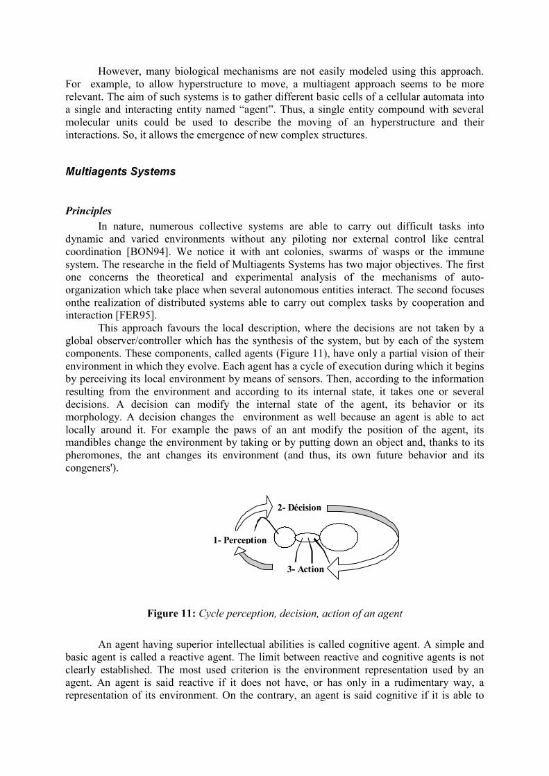
This approach favours the local description, where the decisions are not taken by a global observer/controller which has the synthesis of the system, but by each of the system components. These components, called agents (Figure 11), have only a partial vision of their environment in which they evolve. Each agent has a cycle of execution during which it begins by perceiving its local environment by means of sensors. Then, according to the information resulting from the environment and according to its internal state, it takes one or several decisions. A decision can modify the internal state of the agent, its behavior or its morphology. A decision changes the environment as well because an agent is able to act locally around it. For example the paws of an ant modify the position of the agent, its mandibles change the environment by taking or by putting down an object and, thanks to its pheromones, the ant changes its environment (and thus, its own future behavior and its congeners').

Figure 11: Cycle perception, decision, action of an agent An agent having superior intellectual abilities is called cognitive agent. A simple and

basic agent is called a reactive agent. The limit between reactive and cognitive agents is not clearly established. The most used criterion is the environment representation used by an agent. An agent is said reactive if it does not have, or has only in a rudimentary way, a representation of its environment. On the contrary, an agent is said cognitive if it is able to

2- Décision

3- Action

1- Perception

represent its environment and to make a map in order to plan its actions. The agents we use for our works are exclusively reactive because they do not have any representation of their environment and are unable to plan their decision.

In spite of these limits, the collective, that is all the agents, has the possibility of making sensible/interesting decisions up to a certain limit. For example, ants build their hill on their own without any coordinator. Moreover, the immune system is able to defend an organism against numerous pathogenic factors without the help of a superior system. To sum up, these systems give evidence of a good adaptability, stability and robustness of this reactive and local approach.

In spite of all these advantages, the reactive multiagent systems are not entirely reliable. For the immune system, cancers or auto-immune diseases proove it. As for the coagulation system, haemophilia or thromboses show us their limits. During these dysfunctions, the cells assume to make relevant decisions to assure the maintening of organisms whereas an outside observation shows that they do not.

From a computer point of view, the multiagent system paradigm comes from the problem of the collective intelligence and from the emergence of structures by interactions [PES97]. Thus, the purpose is to create computer systems constituted of simple software elements having the ability to resolve one or few simple problems. For J. Ferber, the objective is to give birth to computer systems able to evolve by interaction, adaptation and self-replication based on agents and working in physically distributed universes. With this kind of system, only the collective can, thanks to the multiple interactions between agents, lead to a solution. This qualitative break between the individual abilities and the collective potential is called emergence.

The study of this emergence is difficult because the conventional logic does not allow to explain the observed qualitative break. Different descriptive and theoretical works [PES97] were led but without a mathematical formalization of the phenomena. However, the experimental characterization of the emergence is possible. Indeed, a qualitative change can be observed to point out strong differences in the potential of the collective with regards to the individual one. We notice such phenomenon even if all the entities have exactly the same abilities. One of the simplest illustration corresponds to the simulation of the ant sorting [DEN91]. Thanks to the same basic behavior, a population of artificial ants manages to sort out its brood. The brood represents the larvas of ants which are differentiated according to their stage of growth.

What it is necessary to note above all, it is that this sorting intervenes only if the number of artificial ants is important enough. In other words, a single ant is unable to sort out on its own whereas several ants can. Here, the heaps made by ants allow to characterize the phenomenon of emergence. The emergence is one of the key of the agent approach. However, the systems where the emergence is really used remain marginal. Indeed, no rule of evident causality exists between the individual behavior and the collective one.

The multiagent approach seems to be particularly adapted to the modeling and to the simulation of molecular and cellular phenomenon for different reasons. First, the notions of environment, autonomous entities, spatial distribution, distribution of roles are essential in biology and for a multiagent system. Second, interaction and cooperation are central both in biology and in the multiagent concepts. These similarities make the multiagent approach a natural bridge between the world of biology and that of computer simulation.

The next section will describe the development of a multiagent system for hyperstrucure modeling.

Applications To represent basic hyperstructure phenomena inside a cell, the model must take into account the aggregation and dissociation of molecular complexes. It must be computationally efficient to simulate numerous (> 104) interacting molecules and extensive enough to include enhanced phenomenon like dynamic molecular shapes, simplified molecular flows or electromagnetic fields. We propose such a system with the following properties: A molecule is represented by:

�a deformable shape located into a 3D grid

�a specific behavior according to the difference of chemical species

The shape of a molecule represented by an agent (a molecule-agent) is based on a continuous 3D shape or a dicrete 3D shape. To be efficiently simulated, a shape must be divided in many elementary cubes (Figure 12-b) that represents an approximation of the original shape (Figure 12-a).

(a) (b)

Figure 12: the left shape (a) is the original shape and the right one (b) is an approximation after a simple rotation.

An agent has receptors into its shape to get information from its local environment (Figure 13-a). According to a local observation and its internal state, it takes decisions (Figure 13-b).

(a) (b)

Figure 13: the shape has receptors to allow an agent to get information from its local environment (a). According to this information and its internal state, an agent can take decisions (binding, activating, moving,

creating a deformation...) (b)

The figure 14 shows a binding/separation of two agents to create hyperstructures and the figure 15 represents a molecule activation.

Figure 14: binding a separation of two agents.

Figure 14: activation of a single molecule.

The original shape can have two types of deformation:

�with internal constraints: Original Shape + Constraints -> New Original Shape -> New Cube based Shape -> Shape possible into the environment ? -> If it is, acceptance of the new Original Shape, else cancelation.

�With external constraints: Cube based Shape + Constraints -> Deformation forces applied to the Original Shape -> New Original Shape -> New Cube based Shape -> Possible into the environment ? -> If yes, acceptance of the new Original, else cancelation.

Example of the transformation Original Shape -> Cube based Shape:

Example of a deformation coming from internal constraints

Example of a deformation coming from external constraints

The basic behavior can modify the Original Shape of the molecule (internal or external deformation), the position of the molecule-agent (x, y, z, rx, ry, rz) according to its local environment (a molecule agent looks for 6 translations, 6 rotations and no move). More accurately, it calculates different stabilities for each choice and only one of those is applied. The specific behavior can be any type of algorithms.

The molecule-agents live into an environment which is a set of 3D-grids. Each 3D-grid contains data shared by the agent-molecules and a molecule-agent can read data around itself to make decisions. For example, it can read into the grid the identification of each molecule-agent to decide if they can bind together. It can also take into account an electromagnetic and other type of fields.

An important part is the visualization of the 3D-matrix containing the hyperstructures. That is why, we have developed a 3D viewer to explore the in-silico environment (Figure 16).

A classical 3D plotter is used to draw the simulation results and a basic simulation controller is included (play, pause, stop).

Figure 16: 3D viewer of our hyperstructure simulator. (see plate 18 at the end of the book)

We have seen three possible approaches to model different cellular levels / systems. The next chapter explains how a reaction-diffusion system can be merged with a multiagent system into a multi-cellular simulator.

Example of an integrated application

From « A Simulation Testbed for the Study of Multicellular Development: the Multiple Mechanisms of Morphogenesis », Kurt Fleisher and Alan Barr [FLE94].

This paper presents a simulation framework and computational testbed to study multi-cellular pattern formation. The approach combines several developmental mechanisms (chemical, mechanical, genetic and electrical) known to be important for biological pattern formation. The mechanisms are present in an environment containing discrete cells which are able to move independently (cell migration). Experience with the testbed indicates that the interactions between the developmental mechanisms are important in determining multicellular and developmental patterns.

Each simulated cell has an artificial genome whose expression is dependent only upon its internal state and its local environment. The changes of each cell's state and of the environment are determined by piecewise continuous differential equations. The current two-dimensional simulation exhibits a variety of multicellular behaviors, including cell migration, cell differentiation, gradient following, clustering, lateral inhibition and neurite outgrowth.

The next table summaries the modeling framework:

Modeling Framework

(abstraction)

Testbed

(implementation) Discrete cells (allows cell migration)

- cell geometry

- cell substructures

-growth cones

- neurites

- 2D circles

- none

- modeled as small cells

- path of growth cone and communication link between cell and growth cone

Genetic / Cell lineage

- genetic control of cell operations

- inherit state from parent cell

- control over orientation of cell divisions

- asymmetric cell division

- Parallel Oes w/conditions

- yes

- yes

- not implemented yet Extracellular environments

- chemical

- mechanical

- 2D reaction-diffusion grid

- mechanical barriers, viscous drag Cell-cell interactions

- mechanical

- chemical (membrane, proteins)

- electrical (gap function, synapse)

- collisions and adhesion between cells

- adhesion and contact recognition

- not implemented yet Cell-environment interactions

- chemical

- mechanical

- emit, absorb, sense values in grid

- cell-environment collisions and adhesion Table 1: the modeling framework and its implementation.

Detailed implementation: Cell: A cell is modeled as a geometric shape (currently a circle, with optional neurites)

with a given response to applied forces, as well as an array of cell state variables. Continuous cell behaviors: Cells exhibit several continuous behaviors, determined by

the cell behavior functions - attempt to move in some direction (may be limited by collision, adhesion or drag) - attempt to grow in size - emit or absorb chemical from the environment - change amount of particular proteins in the membrane (eg. Cell adhesion proteins,

which mediate how much this cell will adhere to another cell) Discontinuous cell behaviors (events): The cell provides functions which determine

the timing of the following events. An event is a discontinuty in the solution, which stops the solver and may create or destroy data structures. The timing of events is determined by cell behavior functions:

- split (cell division) - die - emit neurite with growth cone

Cell state variables: An array of variables which loosely represent the amounts of

proteins within the cell. The values of these variables affect the cell's movements, the timing of events and the cell's interaction with the environment.

Environment: All the simulated cells interact within a single global environment. The

environment contains diffusing, reacting chemicals, as well as physical barriers. Within the simulation, cells access information about their environment locally through an array of local environment variables.

Local environment variables: An array of variables which represent the local

environment of a cell. The values available to the cell as a function of time and they depend on the extracellular environment. Since each cell is in a different location, in general the local environment of two cells will differ. These variations can then lead to different behavior for the cells, even though their genomes”may be identical.

The figure 17 shows an example of the development of a multicellular system using

the Fleischer's simulator:

Figure 17: Multicellular growth (discrete cells in blue (light)) and reaction-diffusion molecules in red (dark)) into a 2D environment (black). Three states of evolution of the same simulation are shown here. [FLE95] (see

plate 17 at the end of the book)

Conclusion The field of cell simulators is quickly growing. Many applications or projects are launched or ready to start. They aim to treate the numerous data (numerous in size and diversity) coming from the high scale molecular biology to help biologists on the living cell understanding. We have seen three major modelers/simulators available for biologists to compute cell mechanisms and see some of their principal drawbacks: they do not include spatial and mechanical phenomenon nor self-organized molecular structures (like hyperstructures or membranes). Then, to avoid these drawbacks, we introduce, according to the granularity level of cell modeling, different approaches that could be used: reaction-diffusion systems for ionic/atomic descriptions, cellular automata for small molecules representation and multiagents systems for membrane or hyperstructures modeling. One of the problem is to merge these different approaches into an integrated cell system. Thus, we have seen how a recent application couple a multiagents system and a reaction-diffusion system. The next step will be the design of multi-levels models to develop a realistic integrated cell software system.

References [BAR81] Bard, A model for generating aspects of zebra and other mammalian coat patterns, J. Theor. Biol., 93 : 501-531, 1981. [BOI01]Boissonade J, De Kepper P., 2001: Morphogénèse Chimique, modes de croissance atypiques, http://www.crpp.u-bordeaux.fr/MC2_morphochim_main.html [BON94] E. Bonabeau, Robotique Collective, Intelligence Collective, Hermes pages 181-202, 1994. [CEL92a] Franco Celada et Philip E. Seiden, A model for simulating cognate recognition and response in the immune system, Journal of Theorical Biology, volume 158, pages 329-357, 1992. [CEL92b] Franco Celada et Philip E. Seiden, A computer model of cellular interactions in the immune system, Immunology Today, volume 13, pages 56-62, 1992. [GAR70] Martin Gardner, Mathematical Games - The fantastic combinations of John Conway's new solitaire game Life, Scientific American, October 1970, pp 120-123. [DEB89] M.J.M. de Boer, Analysis and computer generation of division patterns in cell layers using developmental algorithms, rapport de thèse de doctorat, Université d’Utrecht, soutenue le 20 novembre 1989. [DEN91] J-L. Deneubourg, S. Goss, A. Sendova-Franks, C. Detrain et L. Chretien, The Dynamics of Collective Sorting Robot-like Ants and Ant-Like Robots, From Animals to Animats, pages 356-363, MIT Press, 1991. [ECE01] Electronic Cell, http://www.e-cell.org [FER95] J. Ferber, Les systèmes Multiagents, InterEdition, Paris, 1995. [FLE94] Kurt Fleisher et Alan H. Barr, A simulation testbed for the study of multicellular development :the multiple mechanisms of morphogenesis, Artificial Life III, Ed C. G. Langton, SFI Studies in the Sciences of Complexity, Proc. Vol. XVII, Addison-Wesley, pages 389-417, 1994. [FLE95] Kurt W. Fleischer, A Multiple-Mechanism Developmental Model for Defining Self-Organizing Geometric Structures, California Institute of Technology, rapport de thèse, 1995. [DEC99] Luc Decker, Modèles de Structures Aléatoires de Type Réaction-Diffusion, thèse de doctorat présentée à l'École Nationale Supérieure des Mines de Paris, 1999. Web: http://www.oragenet.org/decker/these [HEG66] J.S. Hege et G. Cole, A mathematical model relating circulating antibodies and antibody forming cells, Journal of Immunology, V.97, pages 34-40, 1966. [JER74] Jerne, N.K., Towards a network theory of the immune system, Ann. Immunol. (Institut Pasteur), 125C, 373, 1974. [LIN88] C. C. Lin and L. A. Segel, Mathematics applied to deterministic problems in the natural sciences, Philadelphia, PA : SIAM, 1988. [MCP01] The Microbial Cell Project, http://microbialcellproject.org [MEI82] Hans Meinhardt, Models of biological pattern formation, Londre : Academic Press, 1982. [MUR81] J. D. Murray, On pattern formation mechanisms for Lepidoptera wing pattern and mammalian coat marking, Phil. Trans. Roy. Soc. (B) 295 : 473-496, 1981. [PES97] S. Pesty, E. Batar, C. Brassac, L. Delépine, M.P. Gleizes, P. Glize, O. Labbani, C. Lenay, P. Marcenac, L. Magnin, J.P. Muller, J. Quinqueton et P. Vidal, Emergence et SMA, Intelligence Artificielle et systèmes Multi-Agents, pages 323-341, 5e journées francophones, JFIADSMA 1997. [SCH99] Alexander Schatten, Cellular Automata, Digital Worlds, 1999. Web: http://www.ifs.tuwien.ac.at/~aschatt/info/ca/ca.html

[STE97] Jeffrey J. Stewart, Harvey Agosto, Samuel Litwin, J. Douglas Welsh, Mark Shlomchik, Martin Weigert et Philip E. Seiden, A solution of the rheumatoid factor paradox, The Journal of Immunology, Volume 159, pages 1728-1738, 1997. [TUR52] A.M. Turing, The chemical basis of morphogenesis, Philos. Trans. Roy. Soc. London B237: 37-72, 1952. [TUR] Greg Turk, Generating Textures on Arbitrary Surfaces using Reaction-Diffusion, [VNE66] John von Neumann, Theory of Self-Reproducing Automata, University of Illinois Press, Champain, IL, 1966. [VCE01] Virtual Cell, http://www.nrcam.uchc.edu [VIC84] Vichniac G.Y., 1984: Physical modeling, containing symmetry properties, reversible rules, Ising model, non-ergodicity and order parameters, period doubling. [WOL84] Wolfram S., 1984: universality and complexity in CA´s, the classification of one-dimensional automata into four classes and their properties.