J. Parallel Distrib. Comput. ( ) –

Contents lists available at ScienceDirect

J. Parallel Distrib. Comput.

journal homepage: www.elsevier.com/locate/jpdc

A cellular learning automata-based deployment strategy for mobile wirelesssensor networksM. Esnaashari ∗, M.R. MeybodiSoft Computing Laboratory, Computer Engineering and Information Technology Department, Amirkabir University of Technology, Tehran 15914, Iran

a r t i c l e i n f o

Article history:Received 18 July 2010Accepted 23 October 2010Available online xxxx

Keywords:Mobile sensor networkCellular learning automataSelf-regulated deployment

a b s t r a c t

One important problemwhichmay arise in designing a deployment strategy for awireless sensor networkis how to deploy a specific number of sensor nodes throughout an unknown network area so that thecovered section of the area is maximized. In a mobile sensor network, this problem can be addressedby first deploying sensor nodes randomly in some initial positions within the area of the network, andthen letting sensor nodes to move around and find their best positions according to the positions oftheir neighboring nodes. The problem becomes more complicated if sensor nodes have no informationabout their positions or even their relative distances to each other. In this paper, we propose a cellularlearning automata-based deployment strategy which guides the movements of sensor nodes within thearea of the networkwithout any sensor to know its position or its relative distance to other sensors. In theproposed algorithm, the learning automaton in each node in cooperation with the learning automata inthe neighboring nodes controls themovements of the node in order to attain high coverage. Experimentalresults have shown that in noise-free environments, the proposed algorithm can compete with theexisting algorithms such as PF, DSSA, IDCA, and VEC in terms of network coverage. It has also been shownthat in noisy environments, where utilized location estimation techniques such as GPS-based devices andlocalization algorithms experience inaccuracies in theirmeasurements, or themovements of sensor nodesare not perfect and follow a probabilistic motionmodel, the proposed algorithm outperforms the existingalgorithms in terms of network coverage.

© 2010 Elsevier Inc. All rights reserved.

1. Introduction

Sensor deployment is a fundamental issue for wireless sensornetworks [22]. Themain objective of a sensor deployment strategyis to achieve desirable coverage of the network area. In general,sensor deployment strategies can be classified into the followingfour categories [11,41]:

- Predetermined: This strategy is useful only if the network areais completely known [11,30,35,36,32,7].

- Randomly undetermined: In this strategy, sensor nodes arespread uniformly throughout the network area [41,18,17,19,25,26].

- Biased distribution: In some contexts, the uniform deploymentof sensor nodesmay not always satisfy the design requirementsand biased deployment can then be a viable option [50].

- Self-regulated: In this strategy which is useful only in mobilesensor networks, sensor nodes are deployed randomly in someinitial positions within the area of the network. After this

∗ Corresponding author.E-mail addresses: Esnaashari@aut.ac.ir (M. Esnaashari), mmeybodi@aut.ac.ir

(M.R. Meybodi).

initial placement, sensor nodes move around and find theirbest positions according to the positions of their neighboringnodes [21,57,33,58,20,44].

One important problem which may arise in designing a de-ployment strategy for a wireless sensor network is how to de-ploy a specific number of sensor nodes so that the covered sectionof the area is maximized. Since this is an optimization problem,random based deployment strategies (randomly undeterminedand biased distribution) are not suitable approaches for solving it.Predetermined deployment strategies which are commonly cen-tralized are not well suited to this problem as well. This is becausea counterpart of this problem in the computational geometry do-main, which is tomaximize the guarded interior of an art gallery bya specific number of vertex guards, is proved to be APX-hard [12].This indicates that finding an approximation close enough to theoptimal solution of the problem is impossible in polynomial time.Self-regulated deployment strategies on the other hand are wellsuited to this problem.

To the best of our knowledge, all of the self-regulated deploy-ment strategies given in the literature require every node to beaware of either its geographical position within the area of thenetwork or its relative distance to all of its neighbors. If noneof this information is available to the nodes of a network, the

0743-7315/$ – see front matter© 2010 Elsevier Inc. All rights reserved.doi:10.1016/j.jpdc.2010.10.015

2 M. Esnaashari, M.R. Meybodi / J. Parallel Distrib. Comput. ( ) –

problem becomes more complicated. In this paper, we proposea self-regulated deployment strategy based on cellular learningautomata called CLA-DS which guides the movements of sensornodes within the area of the network without any sensor know-ing its position or its relative distance to other sensors. In the de-ployment strategy proposed in this paper, neighboring nodes applyforces to each other whichmake every nodemove according to theresultant force vector applied to it. Each node is equipped with alearning automaton. The learning automaton of a node at any giventime decides for the nodewhether to apply force to its neighbors ornot. This way, each node in cooperationwith its neighboring nodesgradually learns its best position within the area of the networkso as to attain high coverage. Experimental results show that interms of network coverage, the proposed deployment algorithmcan compete with the existing deployment algorithms such as PF,DSSA, IDCA, and VEC in noise-free environments, and outperformsthe existing deployment algorithms in noisy environments, whereutilized location estimation techniques such as GPS-based devicesand localization algorithms experience inaccuracies in their mea-surements, or the movements of sensor nodes are noisy.

The rest of this paper is organized as follows. Section 2 gives abrief literature overview on deployment problem in mobile wire-less sensor networks. Cellular learning automata will be discussedin Section 3. The problem statement is given in Section 4. InSection 5 the proposed deployment algorithm is presented. Sim-ulation results are given in Section 6. Section 7 is the conclusion.

2. Related work

Mobile sensor nodes can be used to improve the coverageof wireless sensor networks in different ways [47]. In a hybridnetwork consisting of both stationary and mobile sensor nodes,they can be used mainly to heal the coverage holes caused by thestationary nodes. In a mobile network consisting of only mobilenodes, they can be used to maximize the coverage of the area. Andin event monitoring scenarios where some short-lived events mayappear in different locations, mobile nodes can be dispatched tomonitor the event sources for better event coverage.

The Voronoi diagram is a major tool used to detect coverageholes in hybrid networks [16,42]. A Voronoi diagram is firstconstructed for all stationary sensor nodes, assuming that eachnode knows its own and its neighbors’ positions. In the constructeddiagram, if some points of a Voronoi cell are not covered bythe cell’s generating sensor node, these points will contribute tocoverage holes. When a coverage hole is detected, a stationarynode can bid mobile nodes to heal its coverage hole.

In mobile sensor networks, nodes can adjust their positionsafter initial deployment in order to reduce their overlaps andmaximize area coverage. Wang et al. in [46] groups the existingmovement schemes for mobile sensor networks into the followingthree categories: coverage pattern based movement, virtual forcebased movement, and grid quorum based movement. Methodsin the coverage pattern based movement group [45,46,49] try torelocate mobile nodes based on a predefined coverage pattern.The most commonly used coverage pattern is the regular hexagonwith the sensing range Rs as its side length. In [45], initiallyone node is selected as a seed. The seed node computes sixlocations surrounding itself so as to form a regular hexagon andgreedily selects its nearest neighbors to each of the selectedlocations. Selected neighbors then move to the selected locationsand become new seeds. Another hexagonal coverage patternis given in [46] which can completely cover the sensor field.According to this coverage pattern, final locations of mobile nodesare specified. The sensormovement problem is then converted intoa maximum-weight maximum-matching problem and is centrally

solved. This approach is extended in [49] to provide k-coverage ofthe environment.

In the group of virtual force based node movement methods[21,57,33,58,20,44], sensor nodes apply some kinds of virtualforces to their neighboring nodes. The resultant force vectorapplied to each sensor node from its neighboring nodes specifiesthe direction and distance that the node should move. In [21], adistributed potential-field-based approach is presented in whicheach node is repelled by other neighboring nodes. In addition to therepulsive forces, nodes are also subject to a viscous friction force.This force is used to ensure that the network will eventually reachstatic equilibrium; i.e., to ensure that all nodes will ultimatelycome to a complete stop. In [57,58], a nodemay apply attractive orrepulsive forces to its neighboring nodes according to its distancewith them. Nearby neighbors are repelled and far away ones areattracted. In order to reduce the movement of sensor nodes, thealgorithm is virtually executed on cluster heads and then sensornodes move directly to the locations specified for them by theresult of the algorithm. Like the algorithm given in [21], thedeployment algorithm proposed in [33] is also based on virtualpotential fields, but it considers the constraint that in the deployednetwork, each of the nodes has at least K neighbors. Heo andVarshney in [20] proposed three different distributed deploymentalgorithms called DSSA, IDCA, and VDDA. DSSA uses virtual repul-sive forces between neighboring nodes. IDCA modifies DSSA byfiltering out nodes, for which local density is very near to thedesired density, from moving. VDDA is a distributed deploymentapproach based on the Voronoi diagram. Wang et al. in [44] givetwo sets of distributed protocols for controlling the movement ofsensors, one favoring communication and one favoringmovement.In each set of protocols, Voronoi diagrams are used to detectcoverage holes.

In the group of grid quorum based movement methods [8,9,23,43,53,52,54], the area of the network is divided into a number ofgrid cells and each mobile sensor node must find a suitable cell asits final location and move to that cell.

In an event detection and monitoring sensor network, sensingtasks are performed in an on-demand manner. At first, sensors areused to detect events. After detecting an event, it is often desirableto relocate more mobile sensors close to the event location forperforming the sensing task. Wang et al. in [48] consider a hybridnetwork in which stationary nodes detect events. When a newevent is detected, one mobile node is assigned to that event formore advanced sensing and analysis tasks. In [6] Butler and Rusproposed twomoving strategies for the event coverage problem ina mobile sensor network; history-free strategy and history-basedstrategy. Either of these strategies moves sensors closer to theevent locations. Using a Voronoi diagram, a mobile node stopsmoving if it detects that its movement causes coverage holes.

3. Dynamic irregular cellular learning automata (DICLA)

In this section we briefly review learning automata, cellularlearning automata, irregular cellular learning automata, and thenintroduce dynamic irregular cellular learning automata.

3.1. Learning automata

Learning automata (LA) are adaptive decision-making devicesthat operate on unknown random environments. A learningautomaton has a finite set of actions to choose from and ateach stage, its choice (action) depends upon its action probabilityvector. For each action chosen by the automaton, the environmentgives a reinforcement signal with fixed unknown probabilitydistribution. The automaton then updates its action probabilityvector depending upon the reinforcement signal at that stage, and

M. Esnaashari, M.R. Meybodi / J. Parallel Distrib. Comput. ( ) – 3

evolves to some final desired behavior. A class of learning automatais called variable structure learning automata and are representedby quadruple α, β, p, T in which α = α1, α2, . . . , αr

represents the action set of the automata, β = β1, β2, . . . , βr

represents the input set, p = p1, p2, . . . , pr represents theaction probability set, and finally p(n + 1) = T [α(n), β(n), p(n)]represents the learning algorithm. Let αi be the action chosen attime n, then the recurrence equation for updating p is defined as

pi(n + 1) = pi(n)+ a.(1 − pi(n))pj(n + 1) = pj(n)− a.pj(n) ∀j j = i (1)

for favorable responses, and

pi(n + 1) = (1 − b).pi(n)

pj(n + 1) =b

r − 1+ (1 − b)pj(n) ∀j j = i (2)

for unfavorable ones. In these equations, a and b are rewardand penalty parameters respectively. For more information aboutlearning automata the reader may refer to [39,31,40].

3.2. Cellular learning automata

Cellular learning automaton (CLA), which is a combination ofcellular automaton (CA) [51] and learning automaton (LA), is apowerful mathematical model for many decentralized problemsand phenomena. The basic idea of CLA is to utilize learningautomata to adjust the state transition of CA. A CLA is a CAin which a learning automaton is assigned to every cell. Thelearning automaton residing in a particular cell determines itsaction (state) on the basis of its action probability vector. LikeCA, there is a rule that the CLA operates under. The local ruleof CLA and the actions selected by the neighboring LAs of anyparticular LA determine the reinforcement signal to the LA residingin a cell. The neighboring LAs of any particular LA constitute thelocal environment of that cell. The local environment of a cellis non-stationary because the action probability vectors of theneighboring LAs vary during evolution of the CLA. A CLA is calledsynchronous if all LAs are activated at the same time in parallel.CLA has found many applications such as image processing [27],rumor diffusion [29], channel assignment in cellular networks [1]and VLSI placement [28], to mention a few. For more informationabout CLA the reader may refer to [2–5].

3.3. Irregular cellular learning automata

An irregular cellular learning automaton (ICLA) is a cellularlearning automaton (CLA) in which the restriction of rectangulargrid structure in traditional CLA is removed. This generalization isexpected because there are applications such as wireless sensornetworks, immune network systems, graph related applications,etc. that cannot be adequately modeled with rectangular grids.An ICLA is defined as an undirected graph in which each vertexrepresents a cell which is equipped with a learning automaton.Despite its irregular structure, ICLA operation is equivalent to thatof CLA. CLA has found a number of applications in wireless sensornetworks [13–15].

3.4. Dynamic irregular cellular learning automata

We define Dynamic ICLA (DICLA) as an undirected graph inwhich each vertex represents a cell and a learning automaton isassigned to every cell (vertex). A finite set of interests is defined forDICLA. For each cell ofDICLA a tendency vector is definedwhose jthelement shows the degree of tendency of the cell to the jth interest.In DICLA, the state of each cell consists of two parts; the actionselected by the learning automaton and the tendency vector. Twocells are neighbors in DICLA if the distance between their tendencyvectors is smaller than or equal to the neighborhood radius.

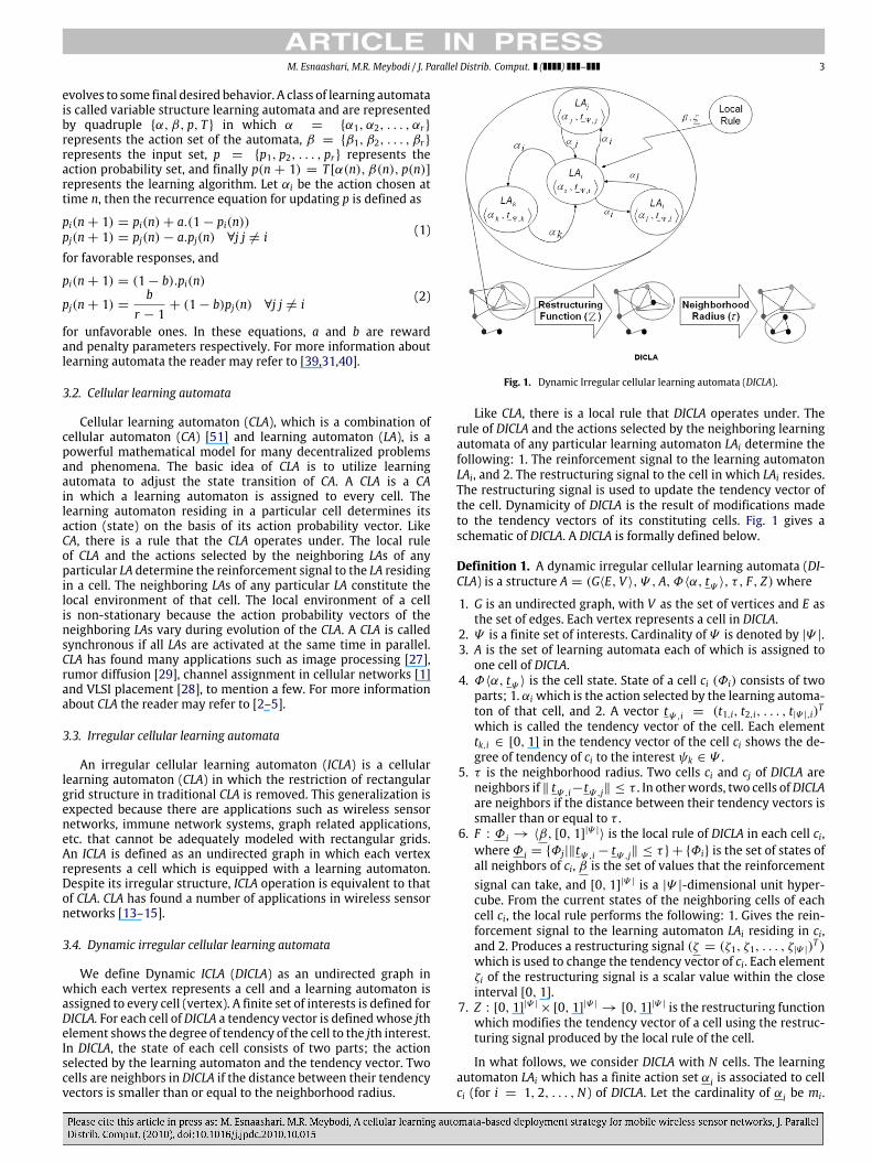
Fig. 1. Dynamic Irregular cellular learning automata (DICLA).

Like CLA, there is a local rule that DICLA operates under. Therule of DICLA and the actions selected by the neighboring learningautomata of any particular learning automaton LAi determine thefollowing: 1. The reinforcement signal to the learning automatonLAi, and 2. The restructuring signal to the cell in which LAi resides.The restructuring signal is used to update the tendency vector ofthe cell. Dynamicity of DICLA is the result of modifications madeto the tendency vectors of its constituting cells. Fig. 1 gives aschematic of DICLA. A DICLA is formally defined below.

Definition 1. A dynamic irregular cellular learning automata (DI-CLA) is a structure A = (G⟨E, V ⟩,Ψ , A,Φ⟨α, tΨ ⟩, τ , F , Z)where

1. G is an undirected graph, with V as the set of vertices and E asthe set of edges. Each vertex represents a cell in DICLA.

2. Ψ is a finite set of interests. Cardinality of Ψ is denoted by |Ψ |.3. A is the set of learning automata each of which is assigned to

one cell of DICLA.4. Φ⟨α, tΨ ⟩ is the cell state. State of a cell ci (Φi) consists of two

parts; 1. αi which is the action selected by the learning automa-ton of that cell, and 2. A vector tΨ ,i = (t1,i, t2,i, . . . , t|Ψ |,i)

T

which is called the tendency vector of the cell. Each elementtk,i ∈ [0, 1] in the tendency vector of the cell ci shows the de-gree of tendency of ci to the interest ψk ∈ Ψ .

5. τ is the neighborhood radius. Two cells ci and cj of DICLA areneighbors if ‖ tΨ ,i−tΨ ,j‖ ≤ τ . In otherwords, two cells ofDICLAare neighbors if the distance between their tendency vectors issmaller than or equal to τ .

6. F : Φ i → ⟨β, [0, 1]|Ψ |⟩ is the local rule of DICLA in each cell ci,

whereΦ i = Φj|‖tΨ ,i − tΨ ,j‖ ≤ τ + Φi is the set of states ofall neighbors of ci, β is the set of values that the reinforcementsignal can take, and [0, 1]|Ψ | is a |Ψ |-dimensional unit hyper-cube. From the current states of the neighboring cells of eachcell ci, the local rule performs the following: 1. Gives the rein-forcement signal to the learning automaton LAi residing in ci,and 2. Produces a restructuring signal (ζ = (ζ1, ζ1, . . . , ζ|Ψ |)

T )which is used to change the tendency vector of ci. Each elementζi of the restructuring signal is a scalar value within the closeinterval [0, 1].

7. Z : [0, 1]|Ψ |×[0, 1]|Ψ |

→ [0, 1]|Ψ | is the restructuring functionwhich modifies the tendency vector of a cell using the restruc-turing signal produced by the local rule of the cell.

In what follows, we consider DICLA with N cells. The learningautomaton LAi which has a finite action set αi is associated to cellci (for i = 1, 2, . . . ,N) of DICLA. Let the cardinality of αi be mi.

4 M. Esnaashari, M.R. Meybodi / J. Parallel Distrib. Comput. ( ) –

The state of DICLA represented by p = (p1, p2, . . . , pN), wherepi = (pi1, pi2, . . . , pimi) is the action probability vector of LAi.

The operation of DICLA takes place as the following iterations.At iteration n, each learning automaton chooses an action. Letαi ∈ αi be the action chosen by LAi. Then, each learning automatonreceives a reinforcement signal. Let βi ∈ β be the reinforcementsignal received by LAi. This reinforcement signal is produced bythe application of the local rule F(Φ j) → ⟨β, [0, 1]|Ψ |

⟩. Each LAupdates its action probability vector on the basis of the suppliedreinforcement signal and the action chosen by the cell. Next, eachcell ci updates its tendency vector using the restructuring functionZ (Eq. (3)).

tΨ ,i(n + 1) = Z(tΨ ,i(n), ζ i(n)). (3)

A DICLA is called asynchronous if at a given time only somecells are activated independently from each other, rather than alltogether in parallel. The cells may be activated in either a time-driven or step-drivenmanner. In time-driven asynchronousDICLA,each cell is assumed to have an internal clock which wakes up theLA associated to that cell while in step-driven asynchronous DICLAa cell is selected in fixed or random sequence.

3.4.1. DICLA norms of behaviorThe behavior of DICLA within its environment can be studied

from two different aspects; the operation of DICLA in the envi-ronment, which is a macroscopic view of the actions performedby its constituting learning automata, and the restructurings ofDICLA, which is the result of application of the restructuring func-tion. To study the operation ofDICLA in the environmentweuse en-tropy and to study the restructurings ofDICLAwe use restructuringtendency.3.4.1.1. Entropy

Entropy, as introduced in the context of information theoryby Shannon [37], is a measure of uncertainty associated with arandom variable and is defined according to Eq. (4),

H(X) = −

−X∈χ

P(X) · ln(P(X)) (4)

where X represents a random variable with set of values χ andprobability mass function P(X). Considering the action chosen bya learning automaton LAi as a random variable, the concept ofentropy can be used to measure the uncertainty associated withthis random variable at any given time instant n according toEq. (5),

Hi(n) = −

mi−j=1

pij(n) · ln(pij(n)) (5)

wheremi is the cardinality of the action set of learning automatonLAi. In the learning process, Hi(n) represents the uncertaintyassociated with the decision of LAi at time instant n. Larger valuesof Hi(n) mean more uncertainty in the decision of the learningautomaton LAi. Hi can only represent the uncertainty associatedwith the operation of a single learning automaton, but as theoperation ofDICLA in the environment is amacroscopic view of theoperations of all of its constituting learning automata, we extendthe concept of entropy through Eq. (6) in order to provide a metricfor evaluating the uncertainty associated with the operation of aDICLA.

H(n) =

N−i=1

Hi(n). (6)

In the above equation, N is the number of learning automata inDICLA. The value of zero for H(n) means pij(n) ∈ 0, 1,∀i, j. Thismeans that no learning automaton in DICLA changes its selectedaction over time, or in other words, the behavior of DICLA remains

unchanged over time. Higher values of H(n) mean higher rates ofchanges in the behavior of DICLA.3.4.1.2. Restructuring tendency

Restructuring tendency (υ), as defined by Eq. (7), is used tomeasure the dynamicity of the structure of DICLA.

υ(n) =

N−i=1

|ζi(n)|. (7)

The value of zero for υ(n) means that the tendency vector of nocell of DICLA during the nth iteration has changed which meansthat no changes have occurred in the structure of DICLA during thenth iteration. Higher values of υ(n) mean higher changes in thestructure of DICLAduring the nth iteration.

4. Problem statement

Consider N mobile sensor nodes s1, s2, . . . , sN with equalsensing ranges ofRs = r and transmission ranges ofRt = 2.r whichare initially deployed in some initial positions within an unknown2 dimensional environment Ω . Assume that a rough estimate ofthe surface ofΩ (SΩ) is available (using Googlemaps for example).According to this estimate, the expected number of neighbors for asensor node (number of sensors residing within its transmissionrange) referred to as E[Nnei] is equal to N ·

π ·R2tSΩ − 1. E[Nnei] isprovided to all sensor nodes prior to their initial deployments.Sensor nodes are able to move in any desired direction within thearea of the network at a constant speed, but they cannot cross thebarrier of Ω . We assume that sensor nodes have no mechanismfor estimating their physical positions or their relative distances toeach other.

Consider the following definitions:

Definition 2. Sensing region of a node si denoted by C(si) is a circlewith radius Rs centered on si.

Definition 3. Covered sub-area denoted by C(Ω) refers to anypoint within the network area which is in the sensing region of atleast one of the sensor nodes. C(Ω) is stated using Eq. (8)

C(Ω) =

Ω,

Ni=1

(C(si))

. (8)

Definition 4. Covered sectiondenotedby SC(Ω) is the surface of thecovered sub-area.

Definition 5. Deployment strategy is an algorithmwhich gives forany given sensor node si a certain position within the area of thenetwork.

Definition 6. Deployed network refers to a sensor network whichresults from a deployment strategy.

Definition 7. Self-regulated deployment strategy is a deploymentstrategy in which each sensor node finds its proper positionwithinthe network area by exploring the area and cooperating with itsneighboring sensor nodes.

Definition 8. A connected network is a network in which there isa route between any two sensor nodes.

Using the above definitions and assumptions, the problemconsidered in this paper can be stated as follows: Propose a self-regulated deployment strategy which deploys N mobile sensornodes throughout an unknown network area Ω with estimatedsurface SΩ so that the covered section of Ω (SC(Ω)) is maximizedand the deployed network is connected.

M. Esnaashari, M.R. Meybodi / J. Parallel Distrib. Comput. ( ) – 5

5. CLA-DS: a cellular learning automata-based deploymentstrategy

The proposed deployment strategy consists of 4 major phases;Initial deployment, mapping, deployment, and maintenance.During the initialization phase, sensor nodes are initially deployedin some initial positions within the area of the network. Mappingthe network topology to a DICLA is done in the mapping phase.Deploying sensor nodes throughout the area of the network is per-formed during the deployment phase. Finally, in the maintenancephase, deployed network ismaintained in order to compensate theeffect of possibly node failures on the covered sub-area (C(Ω)).Weexplain these 4 phases in more detail in the subsequent sections.

5.1. Initial deployment

Three main strategies exist for initially deploying sensor nodesin some initial positions within the area of the network (Ω):

- Random deployment: In random deployment strategy, a ran-dom based deployment strategy [41,18,17,19,25,26,50] is usedto deploy sensor nodes uniformly at random throughoutΩ . Us-ing this strategy for initial deployment reduces the cost of thedeployment phase due to the fact that after such initial deploy-ment, sensor nodes need only to heal coverage holes withintheir vicinities rather than exploringΩ for finding their properpositions.

- Sub-area deployment: In this deployment strategy, sensornodes are placed manually in some initial positions within asmall accessible sub-area of the network.

- Hybrid deployment: In this approach, sensor nodes are de-ployed randomly within a small sub-area of the network.

Any of the randomdeployment, sub-area deployment, or hybriddeployment strategy can be used for the initial deployment phaseof CLA-DS.

5.2. Mapping

In the mapping phase, a time-driven asynchronous DICLA,which is isomorphic to the sensor network topology, is created.Each sensor node si located at (xi, yi) in the sensor networkcorresponds to the cell ci in DICLA. Interest set of DICLA consists oftwo members; X-axis and Y -axis of the network area. Initially (attime instant 0), tendency levels of each cell ci to these interests aret1,i(0) =

xi(0)max(MaxX,MaxY ) and t2,i(0) =

yi(0)max(MaxX,MaxY ) respectively.

(MaxX, MaxY ) is the farthest location within the network area atwhich a sensor node can be located. The neighborhood radius (τ )of DICLA is equal to Rt

max(MaxX,MaxY ) , and hence two cells ci and cj inDICLA are adjacent to each other if si and sj in the sensor networkare close enough to hear each other’s signals.

According to the definition of DICLA, values of tendency levelsare used along with the neighborhood radius of DICLA to specifythe neighboring cells of a cell. But here, values of t1,i(0) and t2,i(0)cannot be computeddue to the fact that sensor nodes are not awareof their physical positions. This does not cause any problems dueto the fact that in a DICLA which is mapped into a sensor network,neighboring cells of each cell are implicitly specified according tothe topology of the network (two cells are adjacent to each otherif their corresponding sensor nodes are within the transmissionranges of each other).

The learning automaton in each cell ci of DICLA, referred toas LAi, has two actions α0, and α1. Action α0 is ‘‘apply forceto neighboring nodes’’, and action α1 is ‘‘do not apply force toneighboring nodes’’. The probability of selecting each of theseactions is initially set to .5.

5.3. Deployment

Each sensor node has a state which can be ‘‘mobile’’ or ‘‘fixed’’.Initially, each sensor node selects its state randomly with proba-bility of selecting ‘‘fixed’’ state to be Pfix. Pfix is a constant which isknown to all sensor nodes. A ‘‘fixed’’ sensor node leaves the deploy-ment phase immediately and starts with the maintenance phase.

Deployment phase for each ‘‘mobile’’ sensor node si is dividedinto a number of rounds Ri(0), Ri(1), Ri(2), . . . . Each round Ri(n) isstarted by the asynchronous activation of cell ci of DICLA. The nthactivation of cell ci occurs at time δi + n × ROUND_DURATIONwhere δi is a random number generated for cell ci andROUND_DURATION is an upper bound for the duration of a singleround. We call n the local iteration number for the cell. Delays δiare chosen randomly in order to reduce the probability of collisionsbetween neighboring nodes.

Upon the startup of a new round Ri(n), LAi selects one of itsactions randomly according to its action probability vector. Theselected action, which is one of ‘‘apply force to neighboring nodes’’,or ‘‘do not apply force to neighboring nodes’’, specifies whethersensor node si will apply any forces to its neighboring nodesduring the current round or not. Sensor node si then creates apacket called APPLIED_FORCE containing its state and the selectedaction and broadcasts it in its neighborhood. After broadcastingthe APPLIED_FORCE packet, sensor node si waits for a certainduration (RECEIVE_DURATION) to receive APPLIED_FORCE packetsfrom its neighboring nodes. Received packets are stored into a localdatabase within the node.

When RECEIVE_DURATION is over, sensor node si collects thefollowing statistics from the stored information in its local data-base: number of received packets (N r

i (n)), and number of neigh-bors selecting ‘‘apply force to neighboring nodes’’ action (N f

i (n)).According to the collected statistics, the local rule of the cell cicomputes the reinforcement signal βi(n) and the restructuring sig-nal ζ

i(n)which are used to update the action probability vector of

LAi and the tendency vector of ci. Details on this will be given inSection 5.3.1.

Next, sensor node si uses vector ζ i(n) as its movement path for

the current round. In other words, if si is located at (xi(n), yi(n)), itmoves to (xi(n+1), yi(n+1)) = (xi(n)+ζ1,i, yi(n)+ζ2,i). Last stepduring round Ri(n) is the application of the restructuring function Zwhich updates the tendency levels of cell ci using the restructuringsignal ζ

i(n) according to Eq. (9).

t1,i(n + 1) = t1,i(n)+ζ1,i(n)

max(MaxX,MaxY )

t2,i(n + 1) = t2,i(n)+ζ2,i(n)

max(MaxX,MaxY ).

(9)

When this step is done, sensor node si waits for the nextactivation time of its corresponding cell ci in DICLA to start its nextround (Ri(n + 1)).

The deployment phase for a sensor node si is completed uponthe occurrence of one of the following:- Stability: Sensor node si moves less than a specified threshold(LEAST_DISTANCE) during its last Nr rounds.

- Oscillation: Sensor node si oscillates between almost the samepositions for more than No rounds.

When a sensor node si completes the deployment phase ofCLA-DS, its state is changed to ‘‘fixed’’ and it starts with themaintenance phase.

5.3.1. Applying local ruleThe local rule of a cell ci based on the states of the cell and its

neighboring cells computes the reinforcement signal βi and therestructuring signal ζ

i.

6 M. Esnaashari, M.R. Meybodi / J. Parallel Distrib. Comput. ( ) –

Reinforcement signal: The reinforcement signal for the nth roundin a node si is computed based on a comparison between thenumber of neighbors of si(N r

i (n)) and the expected number ofneighbors (E[Nnei]). According to this comparison, the followingtwo cases may occur:- N r

i (n) is almost equal to E[Nnei] or formally |N ri (n)−E[Nnei]| < ε

where ε is a specified constant: In this case, if the selected actionof LAi is ‘‘do not apply force to neighboring nodes’’, then thereinforcement signal is to reward the action. Otherwise, thereinforcement signal is to penalize the action. N r

i (n) is smaller or greater than E[Nnei] or formally |N ri (n) −

E[Nnei]| > ε: In this case, if the selected action of LAi is ‘‘applyforce to neighboring nodes’’, then the reinforcement signal isto reward the action. Otherwise, the reinforcement signal isto penalize the action.

Eqs. (1) and (2) are used for rewarding or penalizing the selectedaction of LAi. The idea behind the above method of computingthe reinforcement signal is that to have a uniform deployment ofsensor nodes, one way is to minimize the difference between thenumber of neighbors of each sensor node and the expected numberof neighbors (E[Nnei]). When N r

i (n) is almost equal to E[Nnei], itmeans that the number of neighbors of sensor node si is as it mustbe, and hence it is better for this node not to apply any forces toits neighbors. In the other case when |N r

i (n) − E[Nnei]| > ε, thenumber of neighbors of si differs from that expected, and hence itis better for it to apply forces to its neighbors.Restructuring signal: The restructuring signal ζ

i(n) = (ζ1,i(n),

ζ2,i(n))T is a 2 dimensional vector with a random orientationwhose magnitude is N f

i (n) (number of neighbors selecting ‘‘applyforce to neighboring nodes’’ action). The elements of this vector arecomputed according to Eq. (10) using an angle θ which is selecteduniformly at random from the range [0, 2π ].ζ1,i(n) = N f

i (n) · cos(θ)

ζ2,i(n) = N fi (n) · sin(θ).

(10)

This vector specifies the orientation, direction, and distance ofmovement for the node si during the current round.

5.4. Maintenance

The maintenance phase in a sensor node si is similar to thedeployment phase except that si remains fixed during this phaseand the force vectors applied by its neighbors have no effect onit. Additionally, during this phase, sensor node si collects a listof its ‘‘fixed’’ neighboring nodes (neighboring nodes which are inmaintenance phase). If something happens to a member sj of thislist (its battery is exhausted, it experiences some failures, it leavesthe sensing region of si, . . .) then sensor node si does not receiveAPPLIED_FORCE packets from sj anymore. This indicates that a holemay occur in the vicinity of si. As a result, si leaves themaintenancephase, set its state to ‘‘mobile’’ and starts over with the deploymentphase in order to fill any probable holes. Since collisions may alsoresult in not receiving APPLIED_FORCE packets from neighbors, anode si starts over with the deployment phase only if it does notreceive APPLIED_FORCE packets from one of its ‘‘fixed’’ neighborsfor more than k rounds.

6. Experimental results

To evaluate the performance of CLA-DS several experimentshave been conducted and the results are comparedwith the resultsobtained for the potential field-based algorithm given in [21]referred to as PF hereafter, DSSA and IDCA algorithms given in [20],and the basic VEC algorithm given in [44]. The algorithms arecomparedwith respect to three criteria: coverage, node separation,and distance.

Table 1Parameters of CLA-DS algorithm and their values.

Parameter Value

Pfix .1ROUND_DURATION 11 (s)RECEIVE_DURATION 10 (s)LEAST_DISTANCE 1 (m)No 6 roundsε 1a (reward parameter) .25b (penalty parameter) .25K 3 rounds

- Coverage: Fraction of the areawhich is covered by the deployednetwork. Coverage is specified according to Eq. (11).

Coverage =SC(Ω)SΩ

. (11)

- Node separation: Average distance from the nearest-neighborin the deployed network. Node separation can be computed us-ing Eq. (12). In this equation, dist(si, sj) is the Euclidean distancebetween sensor nodes si and sj. Node separation is a measureof the overlapping area between the sensing regions of sensornodes; smaller node separation means more overlapping.

Node separation =1N

N−i=1

minsj∈Nei(si)

(dist(si, sj)). (12)

- Distance: The average distance traveled by each node. This cri-terion is directly related to the energy consumed by the sensornodes.

Experiments are performed for three different simulation areaswhich are shown in Fig. 2. Networks of different sizes fromN = 50to N = 500 sensor nodes are considered for simulations. Sensingranges (Rs = r) and transmission ranges (Rt = 2.r) of sensornodes are assumed to be 5 (m) and 10 (m) respectively. Energyconsumption of nodes follows the energy model of the J-Simsimulator [38]. Table 1 gives the values for different parametersof the algorithm.

All simulations have been implemented using the J-Sim simula-tor. J-Sim is a java based simulator which is implemented on top ofa component-based software architecture. Using this component-based architecture, new protocols and algorithms can be designed,implemented and tested in the simulator without any changes tothe rest of the simulator’s codes.

All reported results are averaged over 50 runs. We haveused CSMA as the MAC layer protocol, free space model as thepropagation model, binary sensing model and omni-directionalantenna.

6.1. Experiment 1

In this experiment we compare the behavior of the CLA-DSalgorithmwith that of PF, DSSA, IDCA, and VEC algorithms in termsof coverage as defined by Eq. (11). The experiment is performedfor N = 50, 100, 200, 300, 400, and 500 sensor nodes whichare initially deployed using a hybrid deployment method withina square with side length 10 (m) centered on the center of thenetwork area. Figs. 3–5 give the results of this experiment fordifferent network areas given in Fig. 2. From the results we canconclude the following:

1. Although the CLA-DS algorithm does not use any informationabout sensor positions or their relative distances to each other,its performance in covering the network area in all threeenvironments is almost equal to that of the PF algorithmin which sensor nodes have information about their relative

M. Esnaashari, M.R. Meybodi / J. Parallel Distrib. Comput. ( ) – 7

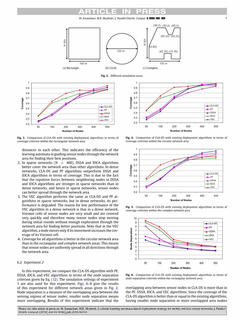
(a) Rectangle. (b) Circle. (c) Complex.

Fig. 2. Different simulation areas.

Fig. 3. Comparison of CLA-DS with existing deployment algorithms in terms ofcoverage criterion within the rectangular network area.

distances to each other. This indicates the efficiency of thelearning automata in guiding sensor nodes through the networkarea for finding their best positions.

2. In sparse networks (N < 400), DSSA and IDCA algorithmsbetter cover the network area than other algorithms. In densenetworks, CLA-DS and PF algorithms outperform DSSA andIDCA algorithms in terms of coverage. This is due to the factthat the repulsive forces between neighboring nodes in DSSAand IDCA algorithms are stronger in sparse networks than indense networks, and hence in sparse networks, sensor nodescan better spread through the network area.

3. The VEC algorithm performs the same as CLA-DS and PF al-gorithms in sparse networks, but in dense networks, its per-formance is degraded. The reason for low performance of theVEC algorithm in a dense network is that in a dense network,Voronoi cells of sensor nodes are very small and are coveredvery quickly and therefore many sensor nodes stop movingduring initial rounds without enough exploration through thenetwork area for finding better positions. Note that in the VECalgorithm, a nodemoves only if itsmovement increases the cov-erage of its Voronoi cell.

4. Coverage for all algorithms is better in the circular network areathan in the rectangular and complex network areas. This meansthat sensor nodes are uniformly spread in all directions throughthe network area.

6.2. Experiment 2

In this experiment, we compare the CLA-DS algorithm with PF,DSSA, IDCA, and VEC algorithms in terms of the node separationcriterion given by Eq. (12). The simulation settings of experiment1 are also used for this experiment. Figs. 6–8 give the resultsof this experiment for different network areas given in Fig. 2.Node separation is a measure of the overlapping area between thesensing regions of sensor nodes; smaller node separation meansmore overlapping. Results of this experiment indicate that the

Fig. 4. Comparison of CLA-DS with existing deployment algorithms in terms ofcoverage criterion within the circular network area.

Fig. 5. Comparison of CLA-DS with existing deployment algorithms in terms ofcoverage criterion within the complex network area.

Fig. 6. Comparison of CLA-DS with existing deployment algorithms in terms ofnode separation criterion within the rectangular network area.

overlapping area between sensor nodes in CLA-DS is more than inthe PF, DSSA, IDCA, and VEC algorithms. Since the coverage of theCLA-DS algorithm is better than or equal to the existing algorithms,having smaller node separation or more overlapped area makes

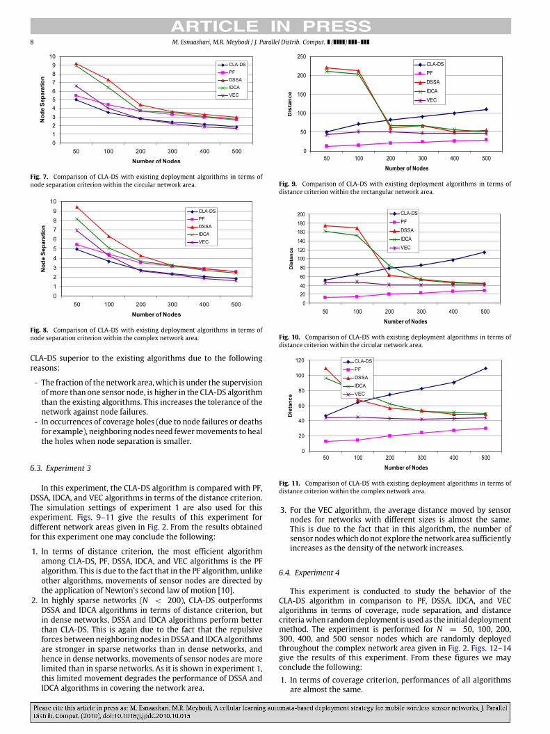
8 M. Esnaashari, M.R. Meybodi / J. Parallel Distrib. Comput. ( ) –

Fig. 7. Comparison of CLA-DS with existing deployment algorithms in terms ofnode separation criterion within the circular network area.

Fig. 8. Comparison of CLA-DS with existing deployment algorithms in terms ofnode separation criterion within the complex network area.

CLA-DS superior to the existing algorithms due to the followingreasons:

- The fraction of the network area, which is under the supervisionofmore than one sensor node, is higher in the CLA-DS algorithmthan the existing algorithms. This increases the tolerance of thenetwork against node failures.

- In occurrences of coverage holes (due to node failures or deathsfor example), neighboring nodes need fewermovements to healthe holes when node separation is smaller.

6.3. Experiment 3

In this experiment, the CLA-DS algorithm is compared with PF,DSSA, IDCA, and VEC algorithms in terms of the distance criterion.The simulation settings of experiment 1 are also used for thisexperiment. Figs. 9–11 give the results of this experiment fordifferent network areas given in Fig. 2. From the results obtainedfor this experiment one may conclude the following:

1. In terms of distance criterion, the most efficient algorithmamong CLA-DS, PF, DSSA, IDCA, and VEC algorithms is the PFalgorithm. This is due to the fact that in the PF algorithm, unlikeother algorithms, movements of sensor nodes are directed bythe application of Newton’s second law of motion [10].

2. In highly sparse networks (N < 200), CLA-DS outperformsDSSA and IDCA algorithms in terms of distance criterion, butin dense networks, DSSA and IDCA algorithms perform betterthan CLA-DS. This is again due to the fact that the repulsiveforces between neighboring nodes inDSSA and IDCA algorithmsare stronger in sparse networks than in dense networks, andhence in dense networks, movements of sensor nodes are morelimited than in sparse networks. As it is shown in experiment 1,this limited movement degrades the performance of DSSA andIDCA algorithms in covering the network area.

Fig. 9. Comparison of CLA-DS with existing deployment algorithms in terms ofdistance criterion within the rectangular network area.

Fig. 10. Comparison of CLA-DS with existing deployment algorithms in terms ofdistance criterion within the circular network area.

Fig. 11. Comparison of CLA-DS with existing deployment algorithms in terms ofdistance criterion within the complex network area.

3. For the VEC algorithm, the average distance moved by sensornodes for networks with different sizes is almost the same.This is due to the fact that in this algorithm, the number ofsensor nodeswhich donot explore the network area sufficientlyincreases as the density of the network increases.

6.4. Experiment 4

This experiment is conducted to study the behavior of theCLA-DS algorithm in comparison to PF, DSSA, IDCA, and VECalgorithms in terms of coverage, node separation, and distancecriteriawhen randomdeployment is used as the initial deploymentmethod. The experiment is performed for N = 50, 100, 200,300, 400, and 500 sensor nodes which are randomly deployedthroughout the complex network area given in Fig. 2. Figs. 12–14give the results of this experiment. From these figures we mayconclude the following:1. In terms of coverage criterion, performances of all algorithms

are almost the same.

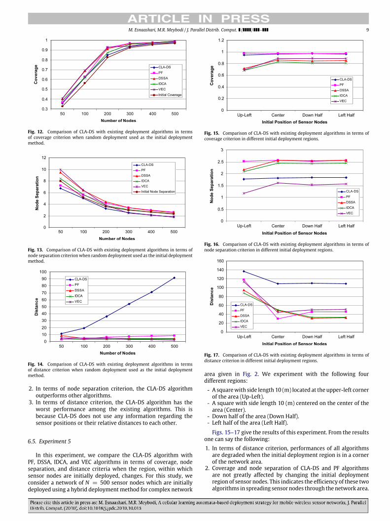
M. Esnaashari, M.R. Meybodi / J. Parallel Distrib. Comput. ( ) – 9

Fig. 12. Comparison of CLA-DS with existing deployment algorithms in termsof coverage criterion when random deployment used as the initial deploymentmethod.

Fig. 13. Comparison of CLA-DS with existing deployment algorithms in terms ofnode separation criterionwhen random deployment used as the initial deploymentmethod.

Fig. 14. Comparison of CLA-DS with existing deployment algorithms in termsof distance criterion when random deployment used as the initial deploymentmethod.

2. In terms of node separation criterion, the CLA-DS algorithmoutperforms other algorithms.

3. In terms of distance criterion, the CLA-DS algorithm has theworst performance among the existing algorithms. This isbecause CLA-DS does not use any information regarding thesensor positions or their relative distances to each other.

6.5. Experiment 5

In this experiment, we compare the CLA-DS algorithm withPF, DSSA, IDCA, and VEC algorithms in terms of coverage, nodeseparation, and distance criteria when the region, within whichsensor nodes are initially deployed, changes. For this study, weconsider a network of N = 500 sensor nodes which are initiallydeployed using a hybrid deploymentmethod for complex network

Fig. 15. Comparison of CLA-DS with existing deployment algorithms in terms ofcoverage criterion in different initial deployment regions.

Fig. 16. Comparison of CLA-DS with existing deployment algorithms in terms ofnode separation criterion in different initial deployment regions.

Fig. 17. Comparison of CLA-DS with existing deployment algorithms in terms ofdistance criterion in different initial deployment regions.

area given in Fig. 2. We experiment with the following fourdifferent regions:- A squarewith side length 10 (m) located at the upper-left cornerof the area (Up-Left).

- A square with side length 10 (m) centered on the center of thearea (Center).

- Down half of the area (Down Half).- Left half of the area (Left Half).

Figs. 15–17 give the results of this experiment. From the resultsone can say the following:1. In terms of distance criterion, performances of all algorithms

are degraded when the initial deployment region is in a cornerof the network area.

2. Coverage and node separation of CLA-DS and PF algorithmsare not greatly affected by changing the initial deploymentregion of sensor nodes. This indicates the efficiency of these twoalgorithms in spreading sensor nodes through thenetwork area.

10 M. Esnaashari, M.R. Meybodi / J. Parallel Distrib. Comput. ( ) –

3. Starting from a corner of the region greatly affects the perfor-mance of DSSA, IDCA, and VEC algorithms in terms of coverageand node separation criteria. To explain the reason for this phe-nomenon, we may say that in these algorithms, sensor nodeshave limited movements which do not allow them to suffi-ciently explore the network area. This drawback becomesmoreserious when the initial deployment region is in a corner of thearea.

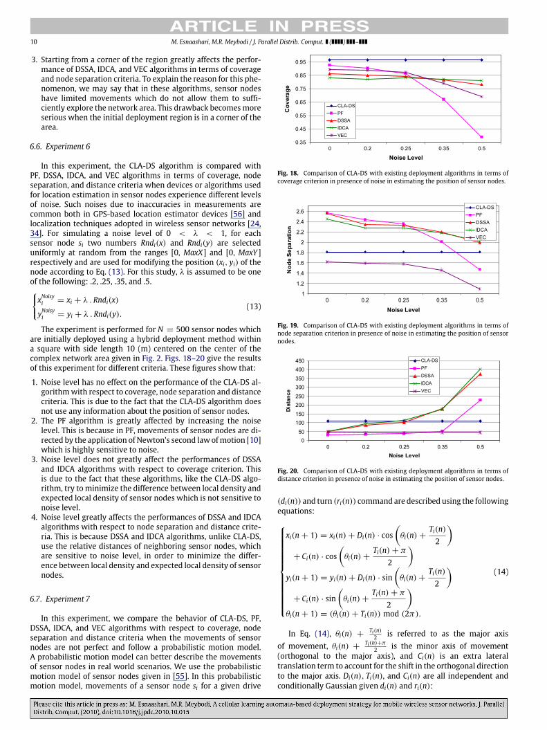
6.6. Experiment 6

In this experiment, the CLA-DS algorithm is compared withPF, DSSA, IDCA, and VEC algorithms in terms of coverage, nodeseparation, and distance criteria when devices or algorithms usedfor location estimation in sensor nodes experience different levelsof noise. Such noises due to inaccuracies in measurements arecommon both in GPS-based location estimator devices [56] andlocalization techniques adopted in wireless sensor networks [24,34]. For simulating a noise level of 0 < λ < 1, for eachsensor node si two numbers Rndi(x) and Rndi(y) are selecteduniformly at random from the ranges [0, MaxX] and [0, MaxY ]respectively and are used for modifying the position (xi, yi) of thenode according to Eq. (13). For this study, λ is assumed to be oneof the following: .2, .25, .35, and .5.xNoisyi = xi + λ . Rndi(x)

yNoisyi = yi + λ . Rndi(y).(13)

The experiment is performed for N = 500 sensor nodes whichare initially deployed using a hybrid deployment method withina square with side length 10 (m) centered on the center of thecomplex network area given in Fig. 2. Figs. 18–20 give the resultsof this experiment for different criteria. These figures show that:

1. Noise level has no effect on the performance of the CLA-DS al-gorithmwith respect to coverage, node separation and distancecriteria. This is due to the fact that the CLA-DS algorithm doesnot use any information about the position of sensor nodes.

2. The PF algorithm is greatly affected by increasing the noiselevel. This is because in PF, movements of sensor nodes are di-rected by the application of Newton’s second law ofmotion [10]which is highly sensitive to noise.

3. Noise level does not greatly affect the performances of DSSAand IDCA algorithms with respect to coverage criterion. Thisis due to the fact that these algorithms, like the CLA-DS algo-rithm, try to minimize the difference between local density andexpected local density of sensor nodes which is not sensitive tonoise level.

4. Noise level greatly affects the performances of DSSA and IDCAalgorithms with respect to node separation and distance crite-ria. This is because DSSA and IDCA algorithms, unlike CLA-DS,use the relative distances of neighboring sensor nodes, whichare sensitive to noise level, in order to minimize the differ-ence between local density and expected local density of sensornodes.

6.7. Experiment 7

In this experiment, we compare the behavior of CLA-DS, PF,DSSA, IDCA, and VEC algorithms with respect to coverage, nodeseparation and distance criteria when the movements of sensornodes are not perfect and follow a probabilistic motion model.A probabilistic motion model can better describe the movementsof sensor nodes in real world scenarios. We use the probabilisticmotion model of sensor nodes given in [55]. In this probabilisticmotion model, movements of a sensor node si for a given drive

Fig. 18. Comparison of CLA-DS with existing deployment algorithms in terms ofcoverage criterion in presence of noise in estimating the position of sensor nodes.

Fig. 19. Comparison of CLA-DS with existing deployment algorithms in terms ofnode separation criterion in presence of noise in estimating the position of sensornodes.

Fig. 20. Comparison of CLA-DS with existing deployment algorithms in terms ofdistance criterion in presence of noise in estimating the position of sensor nodes.

(di(n)) and turn (ri(n)) command are described using the followingequations:

xi(n + 1) = xi(n)+ Di(n) · cosθi(n)+

Ti(n)2

+ Ci(n) · cos

θi(n)+

Ti(n)+ π

2

yi(n + 1) = yi(n)+ Di(n) · sin

θi(n)+

Ti(n)2

+ Ci(n) · sin

θi(n)+

Ti(n)+ π

2

θi(n + 1) = (θi(n)+ Ti(n)) mod (2π).

(14)

In Eq. (14), θi(n) +Ti(n)2 is referred to as the major axis

of movement, θi(n) +Ti(n)+π

2 is the minor axis of movement(orthogonal to the major axis), and Ci(n) is an extra lateraltranslation term to account for the shift in the orthogonal directionto the major axis. Di(n), Ti(n), and Ci(n) are all independent andconditionally Gaussian given di(n) and ri(n):

M. Esnaashari, M.R. Meybodi / J. Parallel Distrib. Comput. ( ) – 11

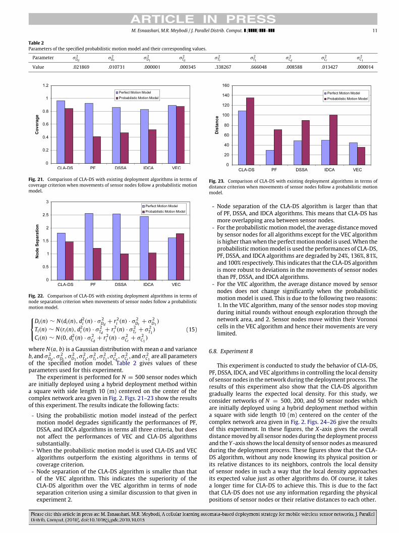
Table 2Parameters of the specified probabilistic motion model and their corresponding values.

Parameter σ 2Dd

σ 2Dr

σ 2D1

σ 2Td

σ 2Tr σ 2

T1σ 2Cd

σ 2Cr σ 2

C1

Value .021869 .010731 .000001 .000345 .338267 .666048 .008588 .013427 .000014

Fig. 21. Comparison of CLA-DS with existing deployment algorithms in terms ofcoverage criterion when movements of sensor nodes follow a probabilistic motionmodel.

Fig. 22. Comparison of CLA-DS with existing deployment algorithms in terms ofnode separation criterion when movements of sensor nodes follow a probabilisticmotion model.

Di(n) ∼ N(di(n), d2i (n) · σ 2Dd

+ r2i (n) · σ 2Dr

+ σ 2D1)

Ti(n) ∼ N(ri(n), d2i (n) · σ 2Td + r2i (n) · σ 2

Tr + σ 2T1)

Ci(n) ∼ N(0, d2i (n) · σ 2Cd + r2i (n) · σ 2

Cr + σ 2C1)

(15)

where N(a, b) is a Gaussian distribution with mean a and varianceb, and σ 2

Dd, σ 2

Dr, σ 2

D1, σ 2

Td, σ 2

Tr , σ2T1, σ 2

Cd, σ 2

Cr , and σ2C1

are all parametersof the specified motion model. Table 2 gives values of theseparameters used for this experiment.

The experiment is performed for N = 500 sensor nodes whichare initially deployed using a hybrid deployment method withina square with side length 10 (m) centered on the center of thecomplex network area given in Fig. 2. Figs. 21–23 show the resultsof this experiment. The results indicate the following facts:

- Using the probabilistic motion model instead of the perfectmotion model degrades significantly the performances of PF,DSSA, and IDCA algorithms in terms all three criteria, but doesnot affect the performances of VEC and CLA-DS algorithmssubstantially.

- When the probabilistic motion model is used CLA-DS and VECalgorithms outperform the existing algorithms in terms ofcoverage criterion.

- Node separation of the CLA-DS algorithm is smaller than thatof the VEC algorithm. This indicates the superiority of theCLA-DS algorithm over the VEC algorithm in terms of nodeseparation criterion using a similar discussion to that given inexperiment 2.

Fig. 23. Comparison of CLA-DS with existing deployment algorithms in terms ofdistance criterion when movements of sensor nodes follow a probabilistic motionmodel.

- Node separation of the CLA-DS algorithm is larger than thatof PF, DSSA, and IDCA algorithms. This means that CLA-DS hasmore overlapping area between sensor nodes.

- For the probabilisticmotionmodel, the average distancemovedby sensor nodes for all algorithms except for the VEC algorithmis higher thanwhen the perfectmotionmodel is used.When theprobabilisticmotionmodel is used the performances of CLA-DS,PF, DSSA, and IDCA algorithms are degraded by 24%, 136%, 81%,and 100% respectively. This indicates that the CLA-DS algorithmis more robust to deviations in the movements of sensor nodesthan PF, DSSA, and IDCA algorithms.

- For the VEC algorithm, the average distance moved by sensornodes does not change significantly when the probabilisticmotion model is used. This is due to the following two reasons:1. In the VEC algorithm, many of the sensor nodes stop movingduring initial rounds without enough exploration through thenetwork area, and 2. Sensor nodes move within their Voronoicells in the VEC algorithm and hence their movements are verylimited.

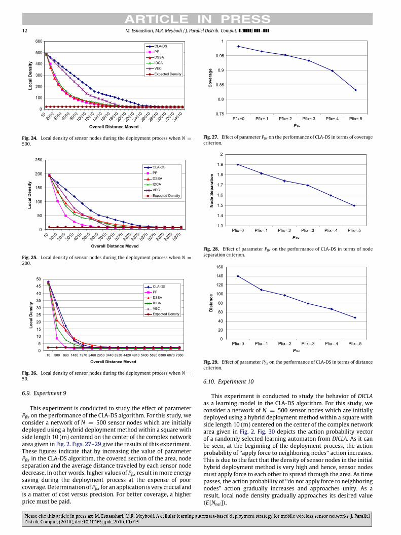
6.8. Experiment 8

This experiment is conducted to study the behavior of CLA-DS,PF, DSSA, IDCA, and VEC algorithms in controlling the local densityof sensor nodes in the network during the deployment process. Theresults of this experiment also show that the CLA-DS algorithmgradually learns the expected local density. For this study, weconsider networks of N = 500, 200, and 50 sensor nodes whichare initially deployed using a hybrid deployment method withina square with side length 10 (m) centered on the center of thecomplex network area given in Fig. 2. Figs. 24–26 give the resultsof this experiment. In these figures, the X-axis gives the overalldistancemoved by all sensor nodes during the deployment processand the Y -axis shows the local density of sensor nodes asmeasuredduring the deployment process. These figures show that the CLA-DS algorithm, without any node knowing its physical position orits relative distances to its neighbors, controls the local densityof sensor nodes in such a way that the local density approachesits expected value just as other algorithms do. Of course, it takesa longer time for CLA-DS to achieve this. This is due to the factthat CLA-DS does not use any information regarding the physicalpositions of sensor nodes or their relative distances to each other.

12 M. Esnaashari, M.R. Meybodi / J. Parallel Distrib. Comput. ( ) –

Fig. 24. Local density of sensor nodes during the deployment process when N =

500.

Fig. 25. Local density of sensor nodes during the deployment process when N =

200.

Fig. 26. Local density of sensor nodes during the deployment process when N =

50.

6.9. Experiment 9

This experiment is conducted to study the effect of parameterPfix on the performance of the CLA-DS algorithm. For this study, weconsider a network of N = 500 sensor nodes which are initiallydeployed using a hybrid deployment method within a square withside length 10 (m) centered on the center of the complex networkarea given in Fig. 2. Figs. 27–29 give the results of this experiment.These figures indicate that by increasing the value of parameterPfix in the CLA-DS algorithm, the covered section of the area, nodeseparation and the average distance traveled by each sensor nodedecrease. In other words, higher values of Pfix result inmore energysaving during the deployment process at the expense of poorcoverage. Determination of Pfix for an application is very crucial andis a matter of cost versus precision. For better coverage, a higherprice must be paid.

Fig. 27. Effect of parameter Pfix on the performance of CLA-DS in terms of coveragecriterion.

Fig. 28. Effect of parameter Pfix on the performance of CLA-DS in terms of nodeseparation criterion.

Fig. 29. Effect of parameter Pfix on the performance of CLA-DS in terms of distancecriterion.

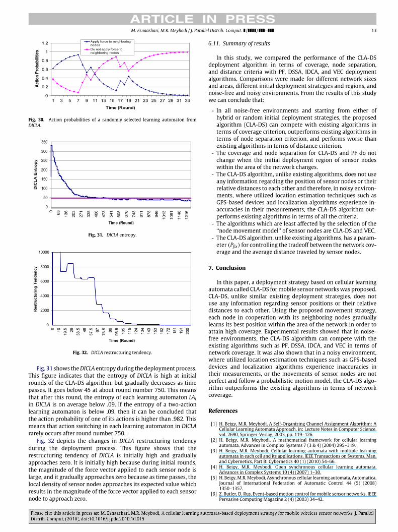
6.10. Experiment 10

This experiment is conducted to study the behavior of DICLAas a learning model in the CLA-DS algorithm. For this study, weconsider a network of N = 500 sensor nodes which are initiallydeployed using a hybrid deployment method within a square withside length 10 (m) centered on the center of the complex networkarea given in Fig. 2. Fig. 30 depicts the action probability vectorof a randomly selected learning automaton from DICLA. As it canbe seen, at the beginning of the deployment process, the actionprobability of ‘‘apply force to neighboring nodes’’ action increases.This is due to the fact that the density of sensor nodes in the initialhybrid deployment method is very high and hence, sensor nodesmust apply force to each other to spread through the area. As timepasses, the action probability of ‘‘do not apply force to neighboringnodes’’ action gradually increases and approaches unity. As aresult, local node density gradually approaches its desired value(E[Nnei]).

M. Esnaashari, M.R. Meybodi / J. Parallel Distrib. Comput. ( ) – 13

Fig. 30. Action probabilities of a randomly selected learning automaton fromDICLA.

Fig. 31. DICLA entropy.

Fig. 32. DICLA restructuring tendency.

Fig. 31 shows theDICLA entropy during the deployment process.This figure indicates that the entropy of DICLA is high at initialrounds of the CLA-DS algorithm, but gradually decreases as timepasses. It goes below 45 at about round number 750. This meansthat after this round, the entropy of each learning automaton LAiin DICLA is on average below .09. If the entropy of a two-actionlearning automaton is below .09, then it can be concluded thatthe action probability of one of its actions is higher than .982. Thismeans that action switching in each learning automaton in DICLArarely occurs after round number 750.

Fig. 32 depicts the changes in DICLA restructuring tendencyduring the deployment process. This figure shows that therestructuring tendency of DICLA is initially high and graduallyapproaches zero. It is initially high because during initial rounds,the magnitude of the force vector applied to each sensor node islarge, and it gradually approaches zero because as time passes, thelocal density of sensor nodes approaches its expected value whichresults in the magnitude of the force vector applied to each sensornode to approach zero.

6.11. Summary of results

In this study, we compared the performance of the CLA-DSdeployment algorithm in terms of coverage, node separation,and distance criteria with PF, DSSA, IDCA, and VEC deploymentalgorithms. Comparisons were made for different network sizesand areas, different initial deployment strategies and regions, andnoise-free and noisy environments. From the results of this studywe can conclude that:

- In all noise-free environments and starting from either ofhybrid or random initial deployment strategies, the proposedalgorithm (CLA-DS) can compete with existing algorithms interms of coverage criterion, outperforms existing algorithms interms of node separation criterion, and performs worse thanexisting algorithms in terms of distance criterion.

- The coverage and node separation for CLA-DS and PF do notchange when the initial deployment region of sensor nodeswithin the area of the network changes.

- The CLA-DS algorithm, unlike existing algorithms, does not useany information regarding the position of sensor nodes or theirrelative distances to each other and therefore, in noisy environ-ments, where utilized location estimation techniques such asGPS-based devices and localization algorithms experience in-accuracies in their measurements, the CLA-DS algorithm out-performs existing algorithms in terms of all the criteria.

- The algorithms which are least affected by the selection of the‘‘node movement model’’ of sensor nodes are CLA-DS and VEC.

- The CLA-DS algorithm, unlike existing algorithms, has a param-eter (Pfix) for controlling the tradeoff between the network cov-erage and the average distance traveled by sensor nodes.

7. Conclusion

In this paper, a deployment strategy based on cellular learningautomata called CLA-DS formobile sensor networkswas proposed.CLA-DS, unlike similar existing deployment strategies, does notuse any information regarding sensor positions or their relativedistances to each other. Using the proposed movement strategy,each node in cooperation with its neighboring nodes graduallylearns its best position within the area of the network in order toattain high coverage. Experimental results showed that in noise-free environments, the CLA-DS algorithm can compete with theexisting algorithms such as PF, DSSA, IDCA, and VEC in terms ofnetwork coverage. It was also shown that in a noisy environment,where utilized location estimation techniques such as GPS-baseddevices and localization algorithms experience inaccuracies intheir measurements, or the movements of sensor nodes are notperfect and follow a probabilistic motion model, the CLA-DS algo-rithm outperforms the existing algorithms in terms of networkcoverage.

References

[1] H. Beigy, M.R. Meybodi, A Self-Organizing Channel Assignment Algorithm: ACellular Learning Automata Approach, in: Lecture Notes in Computer Science,vol. 2690, Springer-Verlag, 2003, pp. 119–126.

[2] H. Beigy, M.R. Meybodi, A mathematical framework for cellular learningautomata, Advances in Complex Systems 7 (3 & 4) (2004) 295–319.

[3] H. Beigy, M.R. Meybodi, Cellular learning automata with multiple learningautomata in each cell and its applications, IEEE Transactions on Systems, Man,and Cybernetics, Part B: Cybernetics 40 (1) (2010) 54–66.

[4] H. Beigy, M.R. Meybodi, Open synchronous cellular learning automata,Advances in Complex Systems 10 (4) (2007) 1–30.

[5] H. Beigy,M.R.Meybodi, Asynchronous cellular learning automata, Automatica,Journal of International Federation of Automatic Control 44 (5) (2008)1350–1357.

[6] Z. Butler, D. Rus, Event-basedmotion control for mobile sensor networks, IEEEPervasive Computing Magazine 2 (4) (2003) 34–42.

14 M. Esnaashari, M.R. Meybodi / J. Parallel Distrib. Comput. ( ) –

[7] K. Chakrabarty, S.S. Iyengar, H. Qi, E. Cho, Grid coverage for surveillanceand target location in distributed sensor networks, IEEE Transactions onComputers 51 (2002) 1448–1453.

[8] S. Chellappan, X. Bai, B. Ma, D. Xuan, C. Xu, Mobility limited flip-based sensornetworks deployment, IEEE Transactions on Parallel and Distributed Systems18 (2) (2007) 199–211.

[9] S. Chellappan,W.Gu, X. Bai, D. Xuan, B.Ma, K. Zhang, Deployingwireless sensornetworks under limited mobility constraints, IEEE Transactions on MobileComputing 6 (10) (2007) 1142–1157.

[10] B. Crowell, Newtonian physics, Light and Matter (2004).[11] S.S. Dhillon, K. Chakrabarty, S.S. Iyengar, Sensor placement for grid coverage

under imprecise detections, in: Int. Conf. on Information Fusion (FUSION)2002, Annapolis, 2002, pp. 1581–1587.

[12] I.Z. Emiris, Ch. Fragoudakis, E. Markou, Maximizing the guarded interior of anart gallery, in: 22nd EuropeanWorkshop on Computational Geometry, Delphi,March, 2006, pp. 165–168.

[13] M. Esnaashari, M.R. Meybodi, A cellular learning automata based clusteringalgorithm for wireless sensor networks, Sensor Letters 6 (5) (2008) 723–735.

[14] M. Esnaashari, M.R. Meybodi, Dynamic point coverage problem in wirelesssensor networks: a cellular learning automata approach, Journal of Ad hoc andSensors Wireless Networks 10 (2–3) (2010) 193–234.

[15] R. Ghaderi, M. Esnaashari, M.R.Meybodi, Maintaining coverage and connectiv-ity in sensor networks: a cellular learning automata approach, in: Proc. of the15th Annual CSI Computer Conf., CSICC’10, Tehran, Iran, Feb. 20–22, 2010.

[16] A. Ghosh, Estimating coverage holes and enhancing coverage in mixed sensornetworks, in: IEEE Intl. Conf. on Local Computer Networks, 2004, pp. 68– 76.

[17] W. Heinzelman, Application-Specific Protocol Architecture for WirelessNetworks, Ph.D. Dissertation, Massachusetts Institute of Technology, June2000.

[18] W. Heinzelman, A. Chandrakasan, H. Balakrishnan, Energy-efficient communi-cation protocol for wireless microsensor networks, HICSS 2000, Maui, January2000, pp. 8020–8029.

[19] W.B. Heinzelman, A.P. Chandrakasan, H. Balakrishnan, An application-specificprotocol architecture for wirelessmicrosensor networks, IEEE Transactions onWireless Communications 1 (4) (2002) 660–670.

[20] N. Heo, P.K. Varshney, Energy-efficient deployment of intelligent mobilesensor networks, IEEE Transactions on Systems, Man, and Cybernetics (PartA) 35 (1) (2005) 78–92.

[21] A. Howard, M.J. Mataric, G.S. Sukhatme, Mobile sensor network deploymentusing potential fields: a distributed scalable solution to the area coverageproblem, in: Intl. Symposium on Distributed Autonomous Robotics Systems,Fukuoka, Japan, June, 2002, pp. 299–308.

[22] M. Ilyas, I. Mahgoub, Handbook of Sensor Networks: Compact Wireless andWired Sensing Systems, CRC Press, London, Washington, DC, 2005.

[23] Z. Jiang, J. Wu, R. Kline, J. Krantz, Mobility control for complete coveragein wireless sensor networks, in: 28th Intl. Conf. on Distributed ComputingSystems Workshops, ICDCS, 2008, pp. 291–296.

[24] H. Lee, H. Dong, H. Aghajan, Robot-assisted localization techniques forwirelessimage sensor networks, in: IEEE Intl. Conf. on Sensor, Mesh, and Ad HocCommunications and Networks, SECON, September, 2006, pp. 383–392.

[25] S. Lindsey, C.S. Raghavendra, PEGASIS: power-efficient gathering in sensorinformation systems, in: IEEE Aerospace Conf., March, 2002, pp. 1125– 1130.

[26] S. Lindsey, C. Raghavendra, K.M. Sivalingam, Data gathering algorithmsin sensor networks using energy metrics, IEEE Transactions on ParallelDistributed Systems 13 (9) (2002) 924–935.

[27] M.R. Meybodi, H. Beygi, M. Taherkhani, Cellular learning automata and itsapplications, Journal of Science and Technology, Sharif (Sharif University ofTechnology, Tehran, Iran) (2004) 54–77.

[28] M.R. Meybodi, F. Mehdipour, Application of cellular learning automata withinput to VLSI placement, Journal of Modarres, University of Tarbeit Modarres16 (summer) (2004) 81–95.

[29] M.R. Meybodi, M. Taherkhani, Application of cellular learning automata inmodeling of rumor diffusion, in: Proc. of 9th Conf. on Electrical Engineering,Power and Water Institute of Technology, Tehran, Iran, May 2001, pp.102–110.

[30] S. Musman, P.E. Lehner, C. Elsaesser, Sensor planning for elusive targets,Journal of Computer and Mathematical Modeling 25 (3) (1997) 103–115.

[31] K.S. Narendra, M.A.L. Thathachar, Learning Automata: An Introduction,Prentice-Hall Inc., 1989.

[32] E.M. Petriu, N.D. Georganas, D. Petriu, D. Makrakis, V.Z. Groza, Sensor-basedinformation appliances, IEEE Instrumentation Measurement Mag (December)(2000) 31–35.

[33] S. Poduri, G. Sukhatme, Constrained coverage for mobile sensor networks, in:Proc. of IEEE Intl. Conf. on Robotics and Automation, ICRA’04, 2004.

[34] V. Ramadurai, M.L. Sichitiu, Localization in wireless sensor networks: aprobabilistic approach, in: Intl. Conf. on Wireless Networks, 2003, pp.275–281.

[35] A. Salhieh, J. Weinmann, M. Kochhal, L. Schwiebert, Power efficient topologiesfor wireless sensor network, in: Int. Conf. on Parallel Processing, Spain, 2001,pp. 156– 163.

[36] L. Schwiebert, S.K.S. Gupta, J. Weinamann, Research challenges in wirelessnetworks of biomedical sensors, in: ACM SIGMOBILE 2001, Rome, July 2001,pp. 151–165.

[37] C.E. Shannon, Amathematical theory of communication, Bell SystemTechnicalJournal 27 (July, October) (1948) 379–423. 623–656.

[38] A. Sobeih, W.P. Chen, J.C. Hou, L.C. Kung, N. Li, H. Lim, H.Y. Tyan, H. Zhang, J-Sim: a simulation and emulation environment for wireless sensor networks,IEEE Wireless Communications 13 (4) (2006) 104–119.

[39] M.A.L. Thathachar, P.S. Sastry, Varieties of learning automata: an overview,IEEE Transaction on Systems, Man, and Cybernetics-Part B: Cybernetics 32 (6)(2002) 711–722.

[40] M.A.L. Thathachar, P.S. Sastry, Networks of Learning Automata, KluwerAcademic Publishers, 2004.

[41] S. Tilak, N.B. Abu-Ghazaleh, W. Heinzelman, Infrastructure trade-offs forsensor networks, in: ACMWSNA’02, September 2002, pp. 49–58.

[42] G.Wang, G. Cao, P. Berman, T.F.L. Porta, Bidding protocols for deployingmobilesensors, IEEE Transactions on Mobile Computing 6 (5) (2007) 515–528.

[43] G. Wang, G. Cao, T.L. Porta, W. Zhang, Sensor relocation in mobile sensornetworks, IEEE INFOCOM (2005) 2302–2312.

[44] G. Wang, G. Cao, Th, F. La Porta, Movement-assisted sensor deployment, IEEETransactions on Mobile Computing 5 (6) (2006) 640–652.

[45] P.C. Wang, T.W. Hou, R.H. Yan, Maintaining coverage by progressive crys-tal lattice permutation in mobile wireless sensor networks, IEEE Interna-tional Conference on Systems and Networks Communication, ICSNC (2006)1–6.

[46] Y.C. Wang, C.C. Hu, Y.C. Tseng, Efficient placement and dispatch of sensors in awireless sensor network, IEEE Transactions onMobile Computing 7 (2) (2008)262–274.

[47] B. Wang, H.B. Lim, D. Ma, A survey of movements strategies for improvingnetwork coverage inwireless sensor networks, Computer Communications 32(2009) 1427–1436.

[48] Y.C. Wang, W.C. Peng, M.H. Chang, Y.C. Tseng, Exploring load-balance todispatch mobile sensors in wireless sensor networks, in: 16th IEEE Intl. Conf.on Computer Communications and Networks, ICCCN, 2007, pp. 669–674.

[49] Y.C. Wang, Y.C. Tseng, Distributed deployment schemes for mobile wirelesssensor networks to ensure multi-level coverage, IEEE Transactions on Paralleland Distributed Systems (2008).

[50] A. Willig, R. Shah, J. Rabaey, A. Wolisz, Altruists in the picoradio sensornetwork, in: 4th IEEE Int. Workshop on Factory Commun. Syst., Sweden,August 2002, pp. 175–184.

[51] S. Wolfram, A New Kind of Science, Wolfram Media Inc., 2002.[52] J. Wu, S. Yang, Optimal movement-assisted sensor deployment and its

extensions in wireless sensor networks, Simulation Modeling Practice andTheory 15 (4) (2007) 383–399.

[53] S. Yang, M. Li, J. Wu, Scan-based movement-assisted sensor deploymentmethods in wireless sensor networks, IEEE Transactions on Parallel andDistributed Systems 18 (8) (2007) 1108–1121.

[54] S. Yang, J. Wu, F. Dai, Localized movement-assisted sensor deployment inwireless sensor networks, in: IEEE Workshops in the Interl. Conf. on MobileAd hoc and Sensor Systems, MASS, 2006, pp. 753–758.

[55] T.N. Yap, Ch.R. Shelton, Simultaneous learning of motion and sensor modelparameters for mobile robots, in: Proc. of IEEE Intl. Conf. on Robotics andAutomation, 2008, pp. 2091–2097.

[56] Y. Zhou, J. Schembri, L. Lamont, J. Bird, Analysis of stand-alone GPS for relativelocation discovery in wireless sensor network, in: Canadian Conf. on Electricaland Computer Engineering, Newfoundland, Canada, 2009, pp. 437–441.

[57] Y. Zou, K. Chakrabarty, Sensor deployment and target localization based onvirtual forces, in: Proc. of IEEE Infocom Conf., 2003, pp. 1293–1303.

[58] Y. Zou, K. Chakrabarty, Sensor deployment and target localization indistributed sensor networks, in: Networked Embedded Computing: Tools,Architectures and Applications, ACM Transactions on Embedded ComputingSystems 3 (1) (2004) 61–91 (special issue).

M. Esnaashari received both the B.S. and M.S. Degrees inComputer Engineering from the Amirkabir University ofTechnology in Iran, in 2002 and 2005, respectively. Cur-rently, he is a Ph.D. student in the Computer Engineer-ingDepartment at the Amirkabir University of Technology,Tehran, Iran. His research interests include computer net-works, learning systems and soft computing.

M.R. Meybodi received the B.S. and M.S. Degrees in Eco-nomics from the Shahid Beheshti University in Iran, in1973 and 1977, respectively. He also received the M.S. andPh.D. Degrees from the University of Oklahoma, USA, in1980 and 1983, respectively, in Computer Science. Cur-rently he is a Full Professor in the Computer EngineeringDepartment, Amirkabir University of Technology, Tehran,Iran. Prior to his current position, he worked from 1983to 1985 as an Assistant Professor at Western MichiganUniversity, USA, and from 1985 to 1991 as an AssociateProfessor at the University of Ohio, USA. His research in-

terests include channel management in cellular networks, learning systems, paral-lel algorithms, soft computing and software development.