Is prediction possible? Chaotic behavior of Multiple Equilibria Regulation Model in cellular...

Is Prediction Possible? Chaotic Behavior ofMultiple Equilibria Regulation Model in

Cellular Automata Topology

IOANNIS D. KATERELOS AND ANDREAS G. KOULOURISPsychology Department, Panteion University, 17671, Athens, Greece

Received April 5, 2004; revised June 10 and September 4, 2004; accepted September 4, 2004

In this article, we present the Multiple Equilibria Regulation (MER) Model in cellular automata topology. Asargued in previous explorations of the model, for certain parameter values, the behavior of the system exhibitstransient chaos (namely, the system is unpredictable but ends in a final steady state). In order to approachempirical reality, we introduce a cellular automata topology. Examining the outcome of the simulations leadsus to conclude that for certain parameter values tested, the system yields chaotic behavior. Thus, cellularautomata contribution has proven crucial, because the introduced topology converts the behavior of the systemfrom transient chaos to “pure” chaos, i.e., the system is not only unpredictable on the long run but, in addition,it will never rest in a final steady state. According to these findings, authors argue the theoretical hypothesis thatthe urge for “prediction” in social sciences should be reconsidered in terms of “predictability horizon”. © 2004Wiley Periodicals, Inc. Complexity 10: 23–36, 2004

Key Words: MER model; chaos; simulation; cellular automata; prediction; opinion dynamics; predictabilityhorizon

1. INTRODUCTION

P ositivism has exercised enormous influence over social

sciences’ understanding of theirs explanatory task [1,

2]. According to this point of view, prediction is only

possible if the appropriate predictors can be determined.

Following this rationale, prediction error depends on the

accuracy with which the predictors and the predicted be-

havior are measured. Hence, our ability to predict future

events should depend almost entirely on measurement er-

ror.

However, socio-behavioral sciences seem to have certain

limitations in their capacity to accumulate knowledge in the

traditional sense [3, 4]. Patterns of human conduct are sub-

ject to continuous alteration across time. Therefore, many

complex environmental systems are not as stable as linear

statistical models might suggest. On the other hand, the

ability to predict future events and to react accordingly is an

important survival skill of humans. In many real life situa-Correspondence to: Ioannis D. Katerelos, E-mail: [email protected]

© 2004 Wiley Periodicals, Inc., Vol. 10, No. 1 C O M P L E X I T Y 23DOI 10.1002/cplx.20052

tions such as social interactions, the anticipation of our ownand others’ behavior is vital.

2. PREDICTION IN SOCIAL SCIENCES: WHENCE ANDWHITHERNo doubt, social sciences were meant to be predictive sci-ences. This was a key component of their constitution assciences, in contrast to religious mythology and metaphys-ics [5]. According to Wright Mills, prediction had a pre-eminent position in the social sciences even as late as in the1950s. He does not hesitate to claim that “the purpose ofsocial science is the prediction and control of human be-haviour” [6]. The positivist vision of social sciences is nowcharacterised as a rather “naıve” project: we all know thatthere are profound problems about prediction (for example,see [7, 8]).

Although prediction should not be seen as somethingconfined to the caste of scientists,1 as Giddens [10, p. 248]claims, “orthodox” social scientists had an “oversimplifiedrevelatory model of social science” in which they producedstartling insights that supposedly left common people inawe. However, the debate about prediction in social sci-ences is, more or less, based on their perceived “utility” insociety2: if they cannot predict, what are they good for? Onthe other hand, if they can make valuable predictions, socialsciences can become some kind of a common foreteller,useful for individuals as well as for societies. Let us notforget that during the 1950s and 1960s, psychology as well asall other social sciences was perceived like “intimidatingmagic.” It was believed to offer explanation for humanbehavior in terms of predicting and controlling even in an“unconscious” way.3

What is demanded once again is unmistakably a “reno-vated” positivistic conception of social sciences. Implicit inthis conception is, always, the assumption that “scientific”knowledge of social conditions can contribute, positively, tointerventions that assist the course of human development.It is therefore a conception of social science that entails aparticular relationship between the acquisition of knowl-

edge and its potential use. Hence Comte’s famous pro-nouncement that “from science comes prevision and fromprevision comes control” can be argued in the sense that theoutcome of social sciences had to be, in the best case, apolitical argument. Hence, the central task of social sciencesis to “discover” the knowledge required by politicians inorder to enact the necessary “rational” interventions. How-ever, the fact that social science and policy are not simply orcontingently related can be shown by looking at the natureof the relationship between causal explanation and predic-tion. According to Fay [12], causal explanation necessarilyimplies prediction and, by extension, the desire to control,because they share a “structural identity.” For Mills [6],accepting prediction as the central element for social sci-ences coincides with an anti-democratic (“bureaucratic”)ethos. In most cases, scientific innovation would be muti-lated in a modern “cline of Procroustes” where a “grandtheory with predictive power” should grant ideological legit-imacy to political choices while abstracted empiricism sup-plies them with technology of social control [13].

Even so, recognizing the limits of prediction and aban-doning prediction as the “grand project” does not mean thatno predictions should be attempted [5]. Katerelos and Kou-louris [14] recently presented a new model of opinion dy-namics called the Multiple Equilibria Regulation (MER)Model, which seems to correspond better in the aforemen-tioned framework: under certain parameter values, the sys-tem becomes unpredictable. In the following paragraph, wegive a brief outline of the MER Model as can be found in [14]and define a cellular automata topology (CAT) in order toexamine the concept of “prediction” in a chaotic systemthat has the ambition to represent social reality in a morerealistic scope.

3. MULTIPLE EQUILIBRIA REGULATION MODEL IN CAT

3.1. The Use of Topology in Social SimulationsModelingOne weakness4 of MER model is that every agent is poten-tially in position to communicate with all other agents if andonly if, their opinions differ less or equal than the Bound ofConfidence, �. This functional postulate assumes that thereis not any geographical or any other kind of obstacle ex-cluding the magnitude of the Bound of Confidence. Never-theless, in real life, two (or more) individuals may nevercommunicate just because they will never meet each other.Consequently, in order to approach empirical reality, weshould consider first a topology of agents and then take intoaccount their opinions.

A suitable tool, according to our view, is cellular autom-ata (CA). The main feature of CA is locality. This means that

1In some cases, naive subjects can predict chaotic numberseries better than linear statistical models [9].2Thus, the concept of “public opinion,” which is unstable insuch manner, pushed many experts to accuse it of beinguseless, because of its instability and lack of prediction: asConverse [11, p. 77] once put it, public opinion is “impalpa-ble,” “amorphous,” and “mercurial.”3The subliminal influence (advertisement) was recognizedlike a threat to common wealth (see rigorous legislation). Adreadful perspective indeed: someone can influence me to dothings without even knowing it. Nevertheless, the experi-ments conducted under this title were strongly questioned interms of replicability. 4Inherited by the Bounded Confidence Model [15].

24 C O M P L E X I T Y © 2004 Wiley Periodicals, Inc.

all interactions take place only within well-defined spatialneighborhoods. Low dimensional, especially two-dimen-sional, CA is believed to be a promising modeling approachfor understanding social dynamics [16]. Hence, we supposethat unlimited communication between agents is beingcompromised due to a proximity-locality criterion. Thismeans those two agents, even if they find themselves havingsimilar opinions (within the Bound of Confidence �), theydo not exchange opinions unless the criterion of “proxim-ity” is fulfilled. The idea is not new: applying a topology inthe form of CA or neural networks on a set of “entities”usually signifies that we impose one more specific rule ofinteraction between them. Thus, one can hypothesise that(in simple terms because we do not refer to restrainedgroups of experts but rather to large groups of individuals orentire “artificial societies”) a geographical pattern of inter-action, alias a form of social geometry, between agents mustbe taken into account [17].

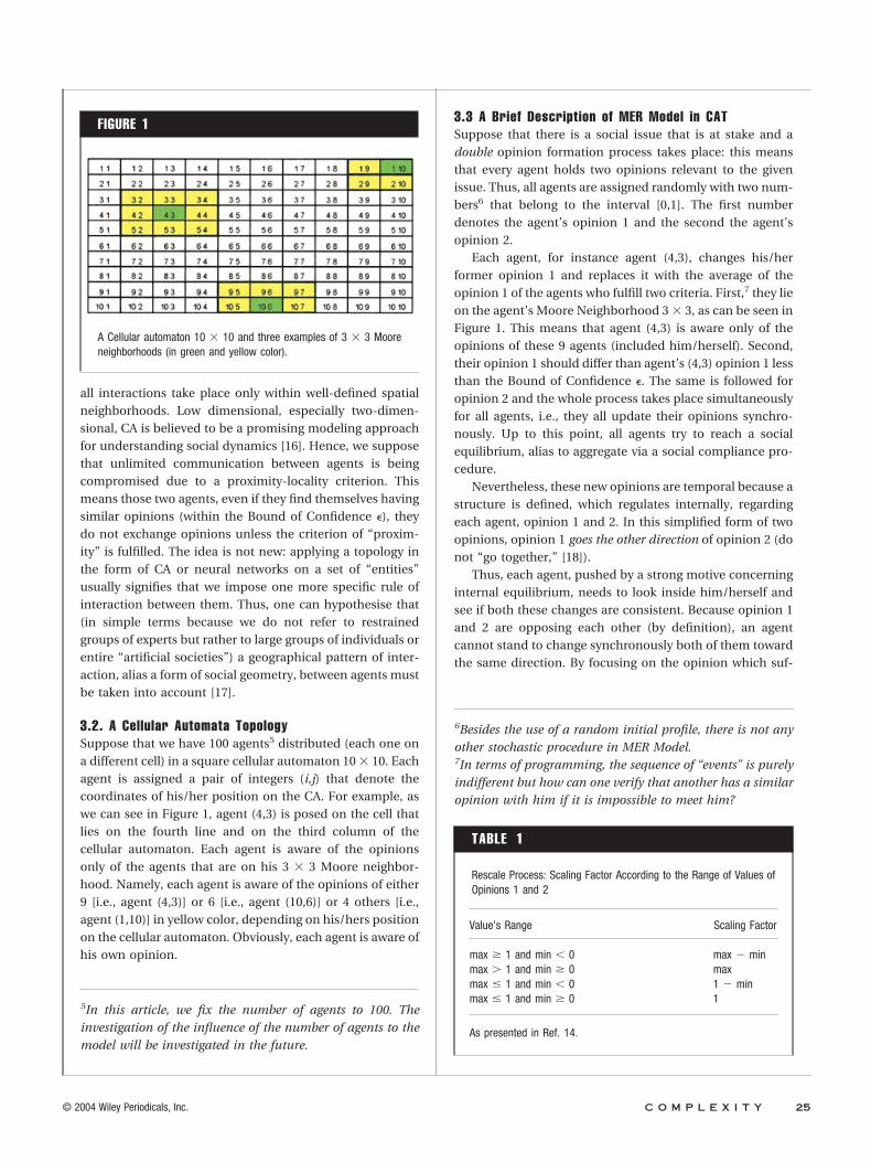
3.2. A Cellular Automata TopologySuppose that we have 100 agents5 distributed (each one ona different cell) in a square cellular automaton 10 � 10. Eachagent is assigned a pair of integers (i,j) that denote thecoordinates of his/her position on the CA. For example, aswe can see in Figure 1, agent (4,3) is posed on the cell thatlies on the fourth line and on the third column of thecellular automaton. Each agent is aware of the opinionsonly of the agents that are on his 3 � 3 Moore neighbor-hood. Namely, each agent is aware of the opinions of either9 [i.e., agent (4,3)] or 6 [i.e., agent (10,6)] or 4 others [i.e.,agent (1,10)] in yellow color, depending on his/hers positionon the cellular automaton. Obviously, each agent is aware ofhis own opinion.

3.3 A Brief Description of MER Model in CATSuppose that there is a social issue that is at stake and adouble opinion formation process takes place: this meansthat every agent holds two opinions relevant to the givenissue. Thus, all agents are assigned randomly with two num-bers6 that belong to the interval [0,1]. The first numberdenotes the agent’s opinion 1 and the second the agent’sopinion 2.

Each agent, for instance agent (4,3), changes his/herformer opinion 1 and replaces it with the average of theopinion 1 of the agents who fulfill two criteria. First,7 they lieon the agent’s Moore Neighborhood 3 � 3, as can be seen inFigure 1. This means that agent (4,3) is aware only of theopinions of these 9 agents (included him/herself). Second,their opinion 1 should differ than agent’s (4,3) opinion 1 lessthan the Bound of Confidence �. The same is followed foropinion 2 and the whole process takes place simultaneouslyfor all agents, i.e., they all update their opinions synchro-nously. Up to this point, all agents try to reach a socialequilibrium, alias to aggregate via a social compliance pro-cedure.

Nevertheless, these new opinions are temporal because astructure is defined, which regulates internally, regardingeach agent, opinion 1 and 2. In this simplified form of twoopinions, opinion 1 goes the other direction of opinion 2 (donot “go together,” [18]).

Thus, each agent, pushed by a strong motive concerninginternal equilibrium, needs to look inside him/herself andsee if both these changes are consistent. Because opinion 1and 2 are opposing each other (by definition), an agentcannot stand to change synchronously both of them towardthe same direction. By focusing on the opinion which suf-

5In this article, we fix the number of agents to 100. Theinvestigation of the influence of the number of agents to themodel will be investigated in the future.

6Besides the use of a random initial profile, there is not anyother stochastic procedure in MER Model.7In terms of programming, the sequence of “events” is purelyindifferent but how can one verify that another has a similaropinion with him if it is impossible to meet him?

FIGURE 1

A Cellular automaton 10 � 10 and three examples of 3 � 3 Mooreneighborhoods (in green and yellow color).

TABLE 1

Rescale Process: Scaling Factor According to the Range of Values ofOpinions 1 and 2

Value’s Range Scaling Factor

max � 1 and min � 0 max � minmax � 1 and min � 0 maxmax � 1 and min � 0 1 � minmax � 1 and min � 0 1

As presented in Ref. 14.

© 2004 Wiley Periodicals, Inc. C O M P L E X I T Y 25

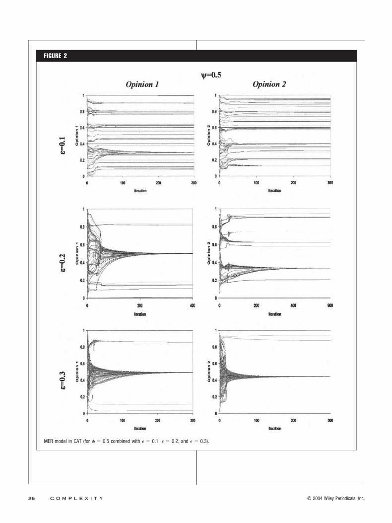
FIGURE 2

MER model in CAT (for � � 0.5 combined with � � 0.1, � � 0.2, and � � 0.3).


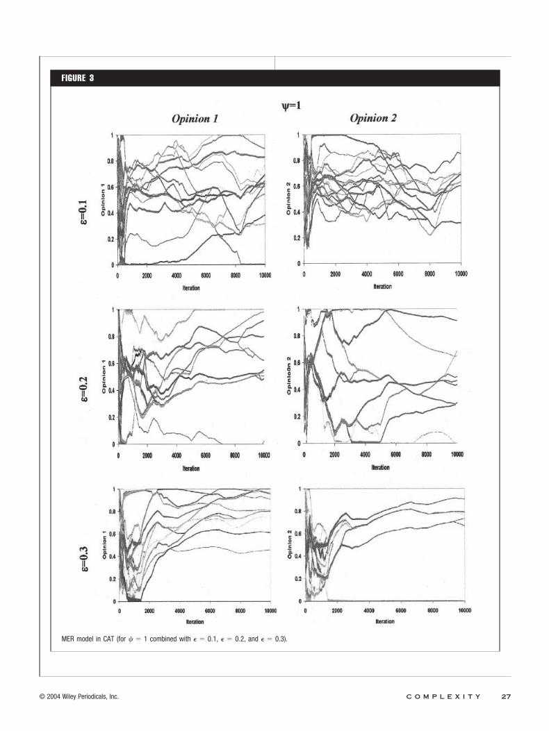
FIGURE 3

MER model in CAT (for � � 1 combined with � � 0.1, � � 0.2, and � � 0.3).


fered the maximum change (lets say that this was opinion1), s/he accepts new opinion 1 and s/he changes his/hersother opinion (opinion 2) on the opposite direction. Themagnitude of the change equals the change suffered inopinion 1 multiplied with the intra-regulation factor �.

Obviously, � can take values between zero (where thetendency to intra-individual equilibrium is absent) and in-finity. Nevertheless, � is considered to be limited theoreti-cally because values above 2 seem to be rather “unrealistic”[14]. This means that adding or subtracting the double ofthe difference found in one opinion to the other can alreadybe characterised as “over-reaction.” For instance, if � � 1,the magnitude of maximal difference is added or subtractedto the dissonant opinion. If � � 2, the dissonant opinion isadjusted by doubling the maximal difference and if � � 0.5the dissonant opinion is corrected by adding or subtractinghalf of the maximal difference.

Because, in MER Model, opinions escape the pre-defined interval [0,1], in order to keep them into theoriginal interval and, at the same time, not to change thedynamical behavior of the system, a procedure called“rescale” is applied. If, for some iteration, in case thateven one opinion of an agent escapes the interval [0,1],we rescale all opinions as follow: we calculate the maxi-mum � max and the minimum � min of opinions 1 and2 of all agents. If min is negative, then we translate allopinions upwards by subtracting min (min is negative),so in fact we augment all opinions and make them pos-itive or zero. Then we divide all opinions by a scalingfactor, which is the range of their values.

All options of rescale are described in Table 1.

4. SIMULATIONS: DISTURBING PERIODICITY LEADS TO“PURE” CHAOSAs we can see in Figure 2 (� � 0.5 and � � 0.1, � � 0.2, � �

0.3), the fact of imposing a cellular automata topology inMER Model does not affect significantly (compare with Ta-ble 3 in [14]) the dynamics of the system. Nevertheless, weobserve a more fragmented repartition, alias a configura-tional change, due to the topological restrictions in com-munication between agents.

As shown in [14], for � � 1 (regardless of �), MER Model(without CAT) presented periodicity as final state. This kindof dynamics signifies that the system is fully “balanced” butnot motionless. In this setting of parameters, the systemattains equilibrium in the form of periodicity, which israther “improbable” regarding “social reality”. On the con-trary, in MER Model with CAT, as can be seen in Figure 3.(� � 1 and � � 0.1, � � 0.2, � � 0.3), periodicity is trans-formed into chaos, a radical change concerning the sys-tem’s dynamic. The system “deteriorates” in an unpredict-able future (regardless of �). We also note that in bothopinions a group formation takes place. This means that thesystem exhibits self-organization. However, these groupsappear to move in a chaotic8 way and group membership9

8Although a general definition of chaos suitable for the mostinteresting cases is still lacking, most researchers would agreethat a dynamical system is chaotic if it is deterministic andunpredictable. Chaotic systems are characterised only byshort-term predictability. An unpredictable system can beeither deterministic or stochastic. MER model is clearly a

FIGURE 4

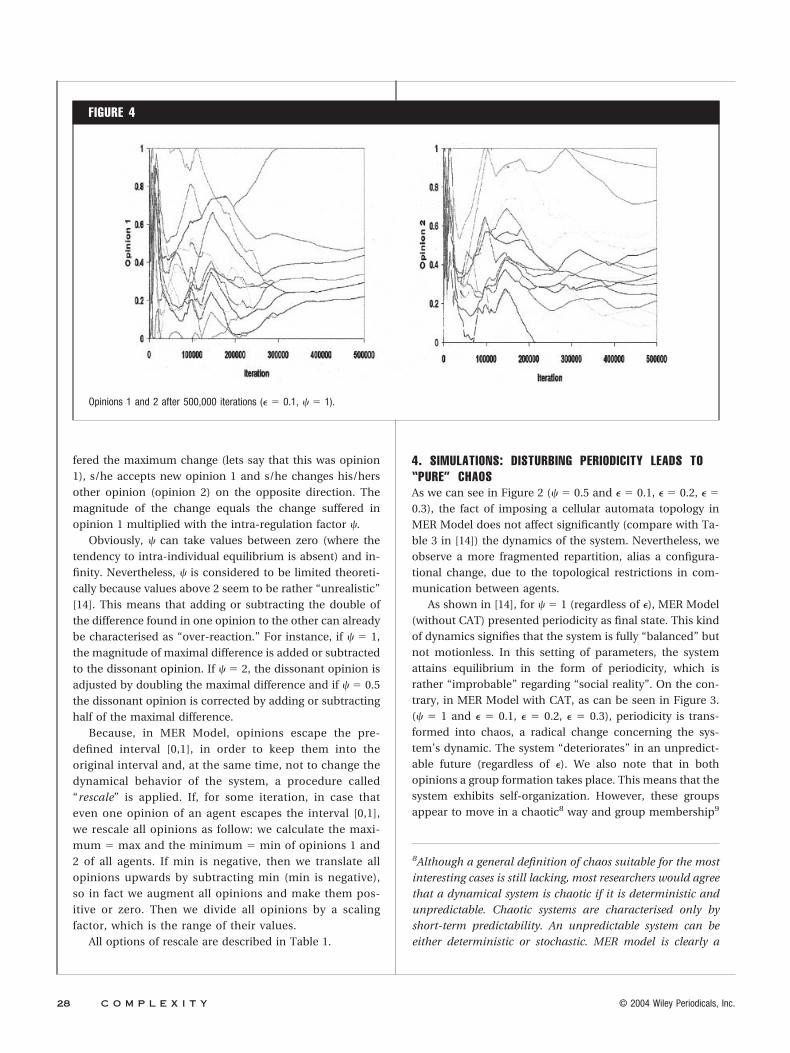
Opinions 1 and 2 after 500,000 iterations (� � 0.1, � � 1).


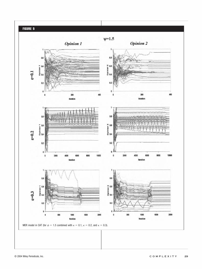
FIGURE 5

MER model in CAT (for � � 1.5 combined with � � 0.1, � � 0.2, and � � 0.3).


is not stable any more: occasionally agents seem to quit theirgroup and join another. In order to find out whether thissystem stays restless indeed or reaches a final steady state,we run the simulation10 for 500,000 iterations. In Figure 4,we see that, even after 500,000 iterations the system is stillmoving, which strongly indicates that there will be no finalsteady state. Nevertheless, we cannot state that the systemis chaotic unless we calculate the Lyapunov Exponent (see§5).

For � � 1.5 and � � 0.1, � � 0.2, � � 0.3 (Figure 5), thealteration caused by the cellular automata topology is sig-nificant regarding the distribution of groups in the finalsteady state (compared with results obtained without CAT[14]). Although the system’s dynamics is obviously similar tothe outcome of MER Model, for the same parameter setting(transient chaos), we observe that the agent’s corpus ishighly fragmented in both opinions. In [14], the systempresented noteworthy differences in the configurations ofthe two opinions: one of the opinions was highly frag-mented, whereas the other ended either in consensus or infragmentation of a much lower order (significantly fewergroups).

It is noticeable, however, for � � 1.5 and � � 0.2, � � 0.3,that a “crazy” agent appears to be capable to create turbu-lence in the whole system’s dynamic. For � � 0.2, an agentseems to oscillate in a continuously larger width until s/he“coordinates” with all the others and let the whole systemrest in a final steady state, after about 10,000 iterations. For� � 0.3, another agent follows a highly differentiated trajec-tory for a number of iterations and, then, when s/he reachesthe others, s/he torments gravely their trajectories andcauses a “mini crisis” (see Figure 5).

In both cases, it seems that a single agent characterizedby a rather “abnormal” behavior can seriously alter thedynamics of the whole system. This incident can only hap-pen in a system whose dynamic is characterized by thewell-known “butterfly effect.”

5. COMPUTATION OF LYAPUNOV EXPONENTIn order to examine whether the system is unpredictableand thus chaotic, we examine if it exhibits sensitivity toinitial conditions. The phenomenon of sensitivity meansthat even the slightest “error” in the initial conditions will bemagnified after a number of iterations. Nevertheless, sensi-

tivity does not automatically lead to unpredictability. In-deed, there are some sensitive systems that are predictable,e.g., all linear transformations xn�1 � c � xn, c � �, n � N�.In this case, an initial error is magnified after we iterate, butthe error remains significantly smaller than xn [19, p. 512].In a chaotic system, given the slightest deviation in initialconditions, the error increases exponentially with time andafter a certain number of iterations, it becomes of the sameorder of magnitude as the correct values.

In order to quantify error propagation and examine ifMER model in CAT exhibits strong sensitivity to initial con-ditions and thus is unpredictable, we compute the LargestLyapunov Exponent. The Lyapunov numbers are the aver-age per-step divergence rate of nearby points along the orbitand the Lyapunov Exponents are the natural logarithm ofthe Lyapunov numbers [20]. Thus, Lyapunov Exponent �

characterizes the average logarithmic growth of the relativeerror per iteration. A small error in an initial point will bescaled by the factor of e� (on the average) in each iteration.Lyapunov Exponents provide the most useful indication ofchaos [21, p. 58]. When the system is Lyapunov-positive, theperturbation grows and predictability is lost. A chaotic orbitis one that forever continues to experience the unstablebehavior; it never manages to find a sink to be attracted to.

At any point of such an orbit, there are points arbitrarilynear that will move away from the point during furtheriteration. Lyapunov Numbers and Lyapunov Exponentsquantify this sustained irregularity. For a more detailedexplanation about the calculation of the Lyapunov Expo-nent, see the Appendix.

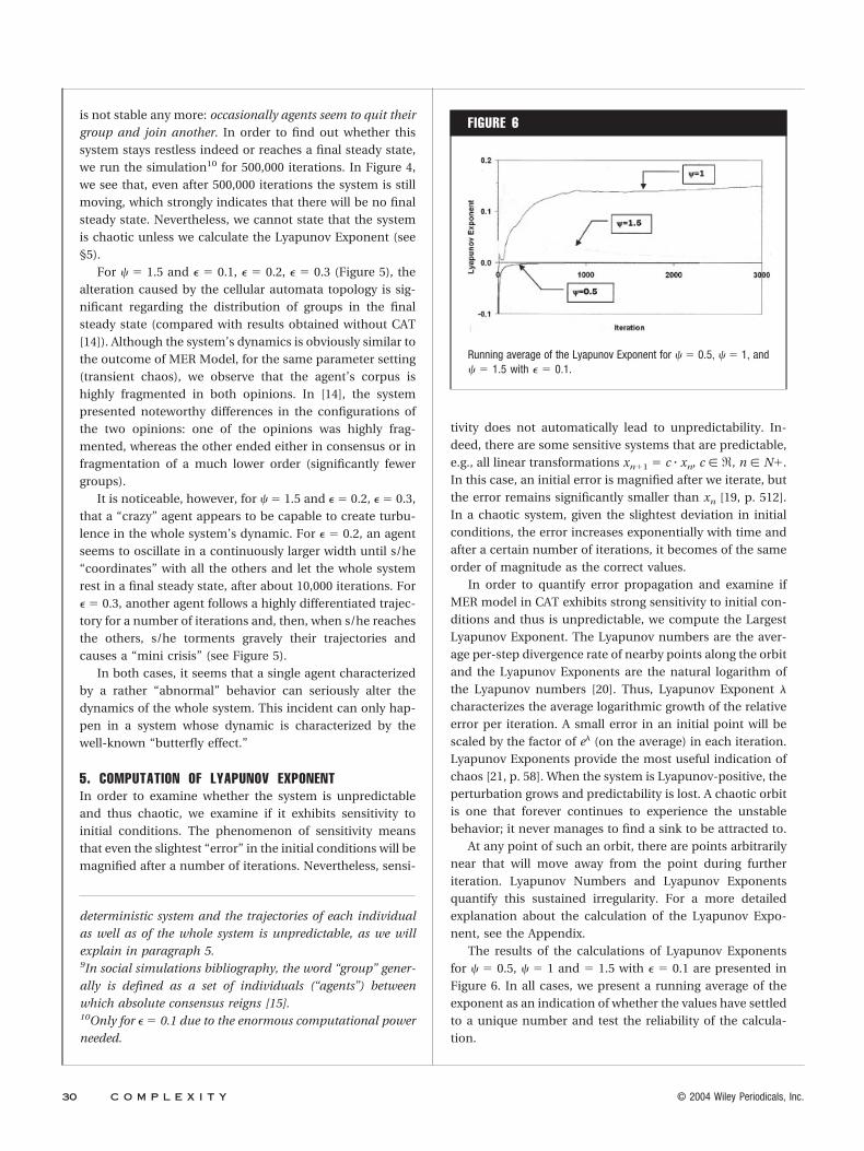
The results of the calculations of Lyapunov Exponentsfor � � 0.5, � � 1 and � 1.5 with � � 0.1 are presented inFigure 6. In all cases, we present a running average of theexponent as an indication of whether the values have settledto a unique number and test the reliability of the calcula-tion.

deterministic system and the trajectories of each individualas well as of the whole system is unpredictable, as we willexplain in paragraph 5.9In social simulations bibliography, the word “group” gener-ally is defined as a set of individuals (“agents”) betweenwhich absolute consensus reigns [15].10Only for � � 0.1 due to the enormous computational powerneeded.

FIGURE 6

Running average of the Lyapunov Exponent for � � 0.5, � � 1, and� � 1.5 with � � 0.1.


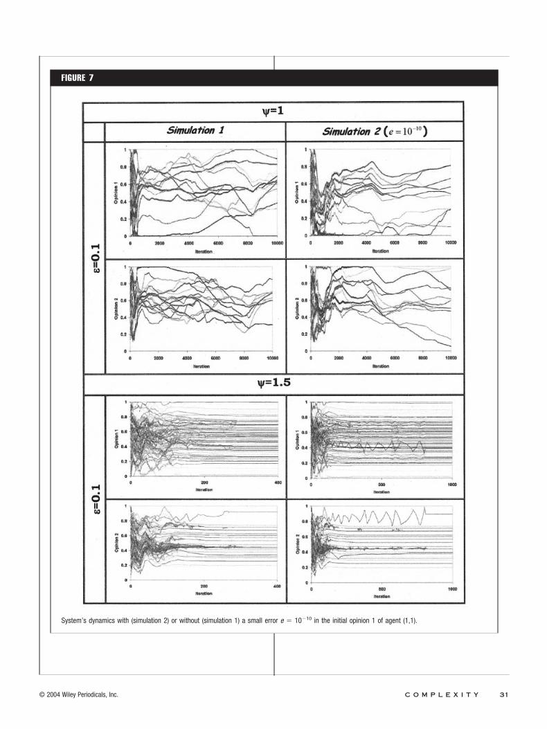
FIGURE 7

System’s dynamics with (simulation 2) or without (simulation 1) a small error e � 10�10 in the initial opinion 1 of agent (1,1).


For � � 0.5 the running average of the Lyapunov Expo-nent is negative for a few number of iterations (error de-creases and trajectories converge) and, finally, tends to zero(the system reaches a finally steady state).

For � � 1 the running average of the Lyapunov Exponentis clearly positive and converges11 to the number 0.126.Because Lyapunov Exponent equals 0.126, a tiny mistake inthe initial conditions will increase by e0.126 � 1.13 times onthe average for each iteration. Thus, the system exhibitsstrong sensitivity to initial conditions and it is chaotic.

For � � 1.5 the running average of the Lyapunov Expo-nent is positive for a large number of iterations and tends tozero. This means that Lyapunov Exponent equals zero. Forthe first few iterations, trajectories of agents diverge expo-nentially but finally the system stabilise in a final state, sotrajectories neither converge nor diverge. This phenomenoncan be found in the bibliography as final state sensitivity[19] or transient chaos [22] and is the same as presented andanalysed in [14].

6. SENSITIVITY TO INITIAL CONDITIONS: BUTTERFLYEFFECT ON (SIMULATED) SOCIAL DATAAssuming that MER Model can depict social reality in acertain degree, we re-approach our results in a more “em-pirical” way, trying to show the effect of sensitivity to initialconditions in analyzing social data.

6.1. A Macro ViewWe re-run the simulation that we can see in the first row ofFigure 3 (referred as simulation 1) with the same parametervalues (100 agents on a 10 � 10 cellular automaton, a 3 � 3Moore Neighborhood) but with “almost” the same initialprofile. This means that all agents have exactly the sameinitial opinion 1 and 2 except agent (1,1) whose opinion 1 insimulation 1 is 0.7055475 and in simulation 2 is0.7055475001. This slight difference (error) of e � 10�10 ismagnified in simulation 2 as can be seen in Figure 7 (for � �

1 and � � 1.5112 combined with � � 0.113). Note that the

simulations in the left column of Figure 7 are the same withthose presented in Figures 3 and 5.

Both agents’ trajectories and final configurations are dif-ferent due to sensitivity to initial conditions. The observeddissimilarities are noteworthy14: this demonstration showsclearly that the effects of sensitivity to initial conditions aredecisive concerning the outcome of the system in a macroview.

6.2. A Micro ViewAlthough personal histories are rather indifferent for the“typical” social researcher, it seems appealing to locate theaforementioned sensitivity in a micro (agent) level (Figure8). The slightest perturbation in initial conditions causes acompletely different outcome. The difference of their opin-ion in these two simulations is given in Figure 9.

Sensitivity to initial conditions is not limited to one agentwho experienced the slight difference. As previously shown,in such a system, each component of the system is highlyinterrelated with all others, i.e., if we shift slightly even oneof them, all the others will be affected. For example, in

11We have run the simulation up to 1,000,000 iterations totest the convergence of the running average of the LyapunovExponent. We have also tested that this number is indepen-dent from the initial opinion profile and the direction of theinitial error at the first iteration.12We do not present the simulations concerning � � 0.5because in these cases, the initial error becomes even smalleror disappears.13Because the type of system’s dynamic seems to be indifferent tothe variation of �, we have chosen � � 0.1. This argumentconcerns the type of dynamic only and not the outcome, whichcan be more or less fragmented according to the magnitude of �.

14For � � 1.5 a “crazy” agent appeared in simulation 2!

FIGURE 8

Opinion 1 of agent (1,1) in simulations 1 and 2.

FIGURE 9

Differences of opinion 1 of agent (1,1) in simulations 1 and 2.


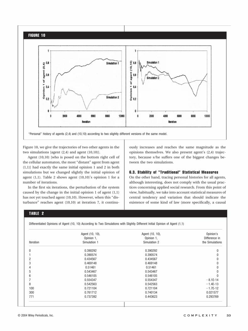
Figure 10, we give the trajectories of two other agents in thetwo simulations [agent (2,4) and agent (10,10)].

Agent (10,10) [who is posed on the bottom right cell ofthe cellular automaton, the most “distant” agent from agent(1,1)] had exactly the same initial opinion 1 and 2 in bothsimulations but we changed slightly the initial opinion ofagent (1,1). Table 2 shows agent (10,10)’s opinion 1 for anumber of iterations.

In the first six iterations, the perturbation of the systemcaused by the change in the initial opinion 1 of agent (1,1)has not yet touched agent (10,10). However, when this “dis-turbance” reaches agent (10,10) at iteration 7, it continu-

ously increases and reaches the same magnitude as theopinions themselves. We also present agent’s (2,4) trajec-tory, because s/he suffers one of the biggest changes be-tween the two simulations.

6.3. Stability of “Traditional” Statistical MeasuresOn the other hand, tracing personal histories for all agents,although interesting, does not comply with the usual prac-tices concerning applied social research. From this point ofview, habitually, we take into account statistical measures ofcentral tendency and variation that should indicate theexistence of some kind of law (more specifically, a causal

FIGURE 10

“Personal” history of agents (2,4) and (10,10) according to two slightly different versions of the same model.

TABLE 2

Differentiated Opinions of Agent (10, 10) According to Two Simulations with Slightly Different Initial Opinion of Agent (1,1)

Iteration

Agent (10, 10),Opinion 1,

Simulation 1

Agent (10, 10),Opinion 1,

Simulation 2

Opinion’sDifference in

the Simulations

0 0.390292 0.390292 01 0.390574 0.390574 02 0.434567 0.434567 03 0.469148 0.469148 04 0.51461 0.51461 05 0.543467 0.543467 06 0.546105 0.546105 07 0.554347 0.554347 �8.1E-148 0.542563 0.542563 �1.4E-13100 0.721104 0.721104 �1.7E-12300 0.761712 0.740134 0.021577771 0.737392 0.443623 0.293769


inference law [23]. Thus, attesting variations concerning oneand only person, among others, is considered to be of littlevalue and the focus is always on evaluating more “social” or“collective” measures, which should depict the stability,15

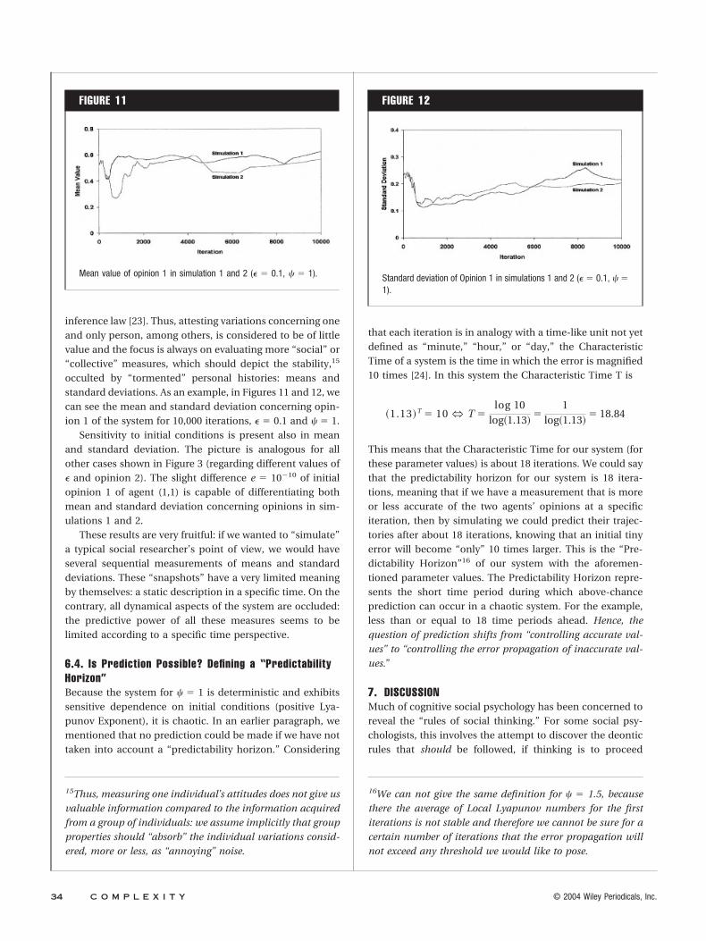
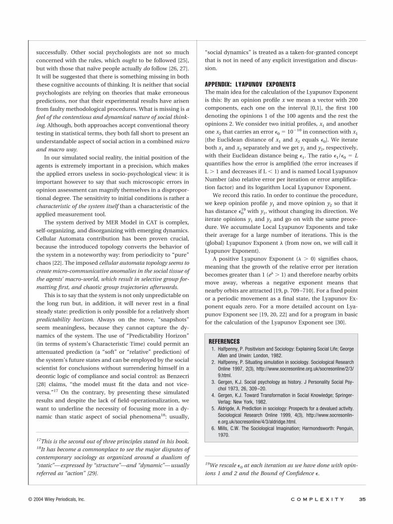
occulted by “tormented” personal histories: means andstandard deviations. As an example, in Figures 11 and 12, wecan see the mean and standard deviation concerning opin-ion 1 of the system for 10,000 iterations, � � 0.1 and � � 1.

Sensitivity to initial conditions is present also in meanand standard deviation. The picture is analogous for allother cases shown in Figure 3 (regarding different values of� and opinion 2). The slight difference e � 10�10 of initialopinion 1 of agent (1,1) is capable of differentiating bothmean and standard deviation concerning opinions in sim-ulations 1 and 2.

These results are very fruitful: if we wanted to “simulate”a typical social researcher’s point of view, we would haveseveral sequential measurements of means and standarddeviations. These “snapshots” have a very limited meaningby themselves: a static description in a specific time. On thecontrary, all dynamical aspects of the system are occluded:the predictive power of all these measures seems to belimited according to a specific time perspective.

6.4. Is Prediction Possible? Defining a “PredictabilityHorizon”Because the system for � � 1 is deterministic and exhibitssensitive dependence on initial conditions (positive Lya-punov Exponent), it is chaotic. In an earlier paragraph, wementioned that no prediction could be made if we have nottaken into account a “predictability horizon.” Considering

that each iteration is in analogy with a time-like unit not yetdefined as “minute,” “hour,” or “day,” the CharacteristicTime of a system is the time in which the error is magnified10 times [24]. In this system the Characteristic Time T is

�1.13�T � 10 N T �log 10

log�1.13��

1log�1.13�

� 18.84

This means that the Characteristic Time for our system (forthese parameter values) is about 18 iterations. We could saythat the predictability horizon for our system is 18 itera-tions, meaning that if we have a measurement that is moreor less accurate of the two agents’ opinions at a specificiteration, then by simulating we could predict their trajec-tories after about 18 iterations, knowing that an initial tinyerror will become “only” 10 times larger. This is the “Pre-dictability Horizon”16 of our system with the aforemen-tioned parameter values. The Predictability Horizon repre-sents the short time period during which above-chanceprediction can occur in a chaotic system. For the example,less than or equal to 18 time periods ahead. Hence, thequestion of prediction shifts from “controlling accurate val-ues” to “controlling the error propagation of inaccurate val-ues.”

7. DISCUSSIONMuch of cognitive social psychology has been concerned toreveal the “rules of social thinking.” For some social psy-chologists, this involves the attempt to discover the deonticrules that should be followed, if thinking is to proceed

15Thus, measuring one individual’s attitudes does not give usvaluable information compared to the information acquiredfrom a group of individuals: we assume implicitly that groupproperties should “absorb” the individual variations consid-ered, more or less, as “annoying” noise.

16We can not give the same definition for � � 1.5, becausethere the average of Local Lyapunov numbers for the firstiterations is not stable and therefore we cannot be sure for acertain number of iterations that the error propagation willnot exceed any threshold we would like to pose.

FIGURE 11

Mean value of opinion 1 in simulation 1 and 2 (� � 0.1, � � 1).

FIGURE 12

Standard deviation of Opinion 1 in simulations 1 and 2 (� � 0.1, � �1).


successfully. Other social psychologists are not so much

concerned with the rules, which ought to be followed [25],

but with those that naıve people actually do follow [26, 27].

It will be suggested that there is something missing in both

these cognitive accounts of thinking. It is neither that social

psychologists are relying on theories that make erroneous

predictions, nor that their experimental results have arisen

from faulty methodological procedures. What is missing is a

feel of the contentious and dynamical nature of social think-

ing. Although, both approaches accept conventional theory

testing in statistical terms, they both fall short to present an

understandable aspect of social action in a combined micro

and macro way.

In our simulated social reality, the initial position of the

agents is extremely important in a precision, which makes

the applied errors useless in socio-psychological view: it is

important however to say that such microscopic errors in

opinion assessment can magnify themselves in a dispropor-

tional degree. The sensitivity to initial conditions is rather a

characteristic of the system itself than a characteristic of the

applied measurement tool.

The system derived by MER Model in CAT is complex,

self-organizing, and disorganizing with emerging dynamics.

Cellular Automata contribution has been proven crucial,

because the introduced topology converts the behavior of

the system in a noteworthy way: from periodicity to “pure”

chaos [22]. The imposed cellular automata topology seems to

create micro-communicative anomalies in the social tissue of

the agents’ macro-world, which result in selective group for-

matting first, and chaotic group trajectories afterwards.

This is to say that the system is not only unpredictable on

the long run but, in addition, it will never rest in a final

steady state: prediction is only possible for a relatively short

predictability horizon. Always on the move, “snapshots”

seem meaningless, because they cannot capture the dy-

namics of the system. The use of “Predictability Horizon”

(in terms of system’s Characteristic Time) could permit an

attenuated prediction (a “soft” or “relative” prediction) of

the system’s future states and can be employed by the social

scientist for conclusions without surrendering himself in a

deontic logic of compliance and social control: as Benzecri

[28] claims, “the model must fit the data and not vice-

versa.”17 On the contrary, by presenting these simulated

results and despite the lack of field-operationalization, we

want to underline the necessity of focusing more in a dy-

namic than static aspect of social phenomena18: usually,

“social dynamics” is treated as a taken-for-granted conceptthat is not in need of any explicit investigation and discus-sion.

APPENDIX: LYAPUNOV EXPONENTSThe main idea for the calculation of the Lyapunov Exponentis this: By an opinion profile x we mean a vector with 200components, each one on the interval [0,1], the first 100denoting the opinions 1 of the 100 agents and the rest theopinions 2. We consider two initial profiles, x1 and anotherone x2 that carries an error �0 � 10�10 in connection with x1

[the Euclidean distance of x1 and x2 equals �0]. We iterateboth x1 and x2 separately and we get y1 and y2, respectively,with their Euclidean distance being �1. The ratio �1/�0 � Lquantifies how the error is amplified (the error increases ifL � 1 and decreases if L � 1) and is named Local LyapunovNumber (also relative error per iteration or error amplifica-tion factor) and its logarithm Local Lyapunov Exponent.

We record this ratio. In order to continue the procedure,we keep opinion profile y1 and move opinion y2 so that ithas distance �0

19 with y1, without changing its direction. Weiterate opinions y1 and y2 and go on with the same proce-dure. We accumulate Local Lyapunov Exponents and taketheir average for a large number of iterations. This is the(global) Lyapunov Exponent � (from now on, we will call itLyapunov Exponent).

A positive Lyapunov Exponent (� � 0) signifies chaos,meaning that the growth of the relative error per iterationbecomes greater than 1 (e� � 1) and therefore nearby orbitsmove away, whereas a negative exponent means thatnearby orbits are attracted [19, p. 709 –710]. For a fixed pointor a periodic movement as a final state, the Lyapunov Ex-ponent equals zero. For a more detailed account on Lya-punov Exponent see [19, 20, 22] and for a program in basicfor the calculation of the Lyapunov Exponent see [30].

REFERENCES1. Halfpenny, P. Positivism and Sociology: Explaining Social Life; George

Allen and Unwin: London, 1982.2. Halfpenny, P. Situating simulation in sociology. Sociological Research

Online 1997, 2(3), http://www.socresonline.org.uk/socresonline/2/3/9.html.

3. Gergen, K.J. Social psychology as history. J Personality Social Psy-chol 1973, 26, 309–20.

4. Gergen, K.J. Toward Transformation in Social Knowledge; Springer-Verlag: New York, 1982.

5. Aldrigde, A. Prediction in sociology: Prospects for a devalued activity.Sociological Research Online 1999, 4(3), http://www.socresonlin-e.org.uk/socresonline/4/3/aldridge.html.

6. Mills, C.W. The Sociological Imagination; Harmondsworth: Penguin,1970.

17This is the second out of three principles stated in his book.18It has become a commonplace to see the major disputes ofcontemporary sociology as organized around a dualism of“static”— expressed by “structure”—and “dynamic”— usuallyreferred as “action” [29].

19We rescale �0 at each iteration as we have done with opin-ions 1 and 2 and the Bound of Confidence �.


7. Fiske, D.W.; Sweder, R.A. Metatheory in Social Science; The Univer-sity of Chicago Press: Chicago, 1986.

8. Gilbert, N. Simulation: An Emergent Perspective. Lecture given at theconference on New Technologies in the Social Sciences, 27–29thOctober 1995, Bournemouth, UK and then at LAFORIA, Paris, 22ndJanuary 1996. http://www.soc.surrey.ac.uk/research/cress/resourc-es/emergent.html.

9. Heath, R.A. Can people predict chaotic sequences? Nonlinear Dy-namics, Psychology and Life Sciences 2002, 6(1), 37–54.

10. Giddens, A. The Constitution of Society; Polity Press: Cambridge,1984.

11. Converse, P.E. Public opinion and voting behavior. In: Handbook ofPolitical Science; Greenstein, F.I.; Polsby, N.W., Eds.; Addison-Wes-ley: Reading, MA, 1975; pp 75–168.

12. Fay, B. Social Theory and Political Practice; George Allen and Unwin:London, 1975.

13. Hodgkinson, P. Who wants to be a social engineer? A commentary onDavid Blunkett’s Speech to the ESRC. Sociological Research Online2000, 5(1), http://www.socresonline.org.uk/5/1/hodgkinson.html.

14. Katerelos, I.; Koulouris, A. Seeking equilibrium leads to chaos: Mul-tiple equilibria regulation model. J Artif Soc Soc Simul 2004, http://jasss.soc.surrey.ac.uk/7/2/4.html.

15. Hegselmann, R.; Krause, U. Opinion dynamics and bounded confi-dence models: Analysis and simulation. J Artif Soc Soc Simul 2002,5(3), http://jasss.soc.surrey.ac.uk/5/3/2/2.pdf.

16. Hegselmann, R.; Flache, A. Understanding complex social dynamics:A plea for cellular automata based modelling. J Artif Soc Soc Simul1998, 1(3), http://jasss.soc.surrey.ac.uk/1/3/1.html.

17. Kluver, J. The evolution of social geometry. Complexity 2004, 9(1), 13–22.18. Flament, C. L’ Analyse de Similitude: Une Technique pour les Re-

cherches sur les Representations Sociales. Cahiers de PsychologieCognitive 1981, 4, 357–396.

19. Peitgen, H.-O.; Jurgens, H.; Saupe, D. Chaos and Fractals, NewFrontiers of Science. Springer-Verlag: New York, 1992.

20. Alligood, K.T.; Sauer, T.D.; Yorke, J.A. Chaos, an Introduction toDynamical Systems; Springer-Verlag: New York, 2000.

21. Kiel, L.D.; Elliott, E. Chaos Theory in the Social Sciences; TheUniversity of Michigan Press: 1997/2000.

22. Sprott, J.C. Chaos and Time-Series Analysis; Oxford University Press:Oxford, 2003.

23. McKim, V.; Turner, S. Causality in Crisis? University of Notre DamePress: South Bend, IN, 1997.

24. Ekeland, I. Le Chaos. Flammarion: Paris, 1995.25. Campbell, D.T. Common fate, similarity and other indices of the

status of aggregates of persons as social entities. Behav Sci 1958, 3,14–25.

26. Guimelli, C. La pensee Sociale; Presses Universitaires de France:Paris, 1999.

27. Papastamou, S., Ed. Introduction to Social Psychology; Tome I, Vol. 1,Ellinika Grammata: Athens, GA, 2001.

28. Benzecri, J.P. Correspondence Analysis Handbook; Marcel Dekker:New York, 1992.

29. Lopez, J.; Scott, J. Social Structure; Open University Press: Philadel-phia, PA, 2000.

30. Sprott, J.C. Numerical Calculation of Largest Lyapunov Exponent;1998. http://sprott.physics.wisc.edu/chaos/lyapexp.htm.


Is prediction possible? Chaotic behavior of Multiple Equilibria Regulation Model in cellular...

Documents

Transcript of Is prediction possible? Chaotic behavior of Multiple Equilibria Regulation Model in cellular...