Computing equilibria in discounted 2x2 supergames

Computational Economics manuscript No.(will be inserted by the editor)

Computing equilibria in discounted 2×2 supergames

Kimmo Berg · Mitri Kitti

Received: date / Accepted: date

Abstract This paper examines the subgame perfect pure strategy equilib-rium paths and payoff sets of discounted supergames with perfect monitoring.The main contribution is to provide methods for computing and tools for an-alyzing the equilibrium paths and payoffs in repeated games. We introducethe concept of a first-action feasible path, which simplifies the computation ofequilibria. These paths can be composed into a directed multigraph, which is auseful representation for the equilibrium paths. We examine how the payoffs,discount factors and the properties of the multigraph affect the possible pay-offs, their Hausdorff dimension, and the complexity of the equilibrium paths.The computational methods are applied to the twelve symmetric strictly or-dinal 2×2 games. We find that these games can be classified into three groupsbased on the complexity of the equilibrium paths.

Keywords repeated game · 2×2 game · subgame perfect equilibrium ·equilibrium path · payoff set · multigraph

1 Introduction

Supergames provide an elementary framework for examining competition andcooperation in long-term relationships. It is well-known that the equilibriaof the stage game differ fundamentally from both the finitely and infinitelyrepeated games (Benoit and Krishna 1985; Mailath and Samuelson 2006). Ourfirst objective is to present methods for computing and analyzing equilibriumpaths and payoffs in discounted supergames. The second is to apply these

K. BergAalto University School of Science, Systems Analysis Laboratory, P.O.Box 11100, FI-00076Aalto, Finland, [email protected], Tel.: +358-9-47023066, Fax: +358-9-47023096

M. KittiAalto University School of Economics, Department of Economics, P.O.Box 21240, FI-00076Aalto, Finland

2 Kimmo Berg, Mitri Kitti

methods to the symmetric 2×2 games which constitute an important class ofgames as they capture a wide range of applications in economic, social andbiological sciences (Maynard Smith 1982; Axelrod 1984; Hauert 2001; Brams2003).

The main ideas of this paper stem from a recent work by Berg and Kitti(2011), who analyze paths of action profiles that are induced by subgame per-fect pure strategies in infinitely repeated discounted games with perfect moni-toring. They show that it is possible to characterize the equilibrium paths withfragments called elementary subpaths. Their characterization builds upon theset-valued recursive methods developed by Abreu et al. (1986, 1990); Cron-shaw and Luenberger (1994). This paper gives an alternative approach usingonly paths. This approach is based on Abreu (1988), who characterizes theequilibria using simple strategies and the one-shot deviation principle.

The first step in constructing the elementary subpaths is the computationof the first-action feasible (FAF) paths. These are finite paths that providehigh enough payoffs such that none of the players is willing to deviate fromthe first action profile on the path. To illustrate the idea of a FAF path, letus assume that there are two action profiles a and b in the stage game that isbeing repeated. If bbaa is a FAF path then the sequence baa combined withany equilibrium payoff guarantee that there are no profitable deviations fromthe first action b. This does not, however, mean yet that bbaa could be a partof an equilibrium path, since there might be profitable deviations from theother parts of the path, like the second b or the a’s.

The second step is to construct the equilibrium paths from the FAF paths,i.e., find the elementary paths of the game or a representation for them. Theidea is to combine the FAF paths so that the subgame perfect equilibrium(SPE) paths are obtained. For example, we cannot combine bbaa with babsince the first requires that the path after ba continues with a and the secondrequires it continues with b. We can, however, combine FAF paths bbaa andba, and thus there are no profitable deviations from both b’s in bbaa. It turnsout that there is a simple algorithm for combining the FAF paths, and we canrepresent the equilibrium paths with a directed multigraph.

The multigraph representation allows us to analyze and compute the pay-off set and the equilibrium paths of the game. We find that the payoff set isa graph directed self-affine set, i.e., a particular fractal. It is possible to esti-mate the Hausdorff dimension of the payoff set using tools developed for thiskind of fractals (Mauldin and Williams 1988; Edgar and Mauldin 1992; Edgarand Golds 1999; Falconer 1988, 1992). Intuitively, the Hausdorff dimensionmeasures the complexity of the set; how the set fills the payoff space.

It is important to distinguish the difference of paths and payoffs: the com-plexity of the game is in the paths and the payoff set is a mapping from thesepaths. We find that the Hausdorff dimension is related to the cycles and thecontractions of the arcs in the multigraph. The dimension is zero if there isno node with more than one cycle. It may happen that the paths increasebut the cycles remain the same, and thus, the paths affect the dimension onlythrough the cycles. On the contrary, the discount factor affects directly all the

Equilibria in 2×2 supergames 3

contractions, which means that the dimension depends only on the discountfactor if the cycles do not change.

Another advantage of the multigraph representation is that it can be usedin finding an approximation for the set of equilibrium payoffs. The computationof the payoff set has been previously studied in Cronshaw and Luenberger(1994); Cronshaw (1997); Judd et al. (2003). These papers, however, assumethat the players use correlated strategies, which convexifies the payoff set. Inthis paper, we do not assume correlated nor mixed strategies. The differenceto earlier results comes from the methodology, i.e., we focus on specific pathsthat generate the payoff set rather than try to find the payoff set as a whole.

As an application of the computational methods, we examine all the twelvesymmetric strictly ordinal 2×2 games (Robinson and Goforth 2005) for differ-ent discount factors and payoff values. We find that the payoff sets and thecomplexity of the equilibrium paths are quite different in the twelve games.They are roughly classified into three groups based on the complexity of thepaths: i) prisoner’s dilemma, stag hunt, chicken and no conflict games havemore complex equilibrium paths than the others, where all four actions canbe played with suitable combinations; ii) the paths in leader, battle of thesexes, coordination and anti-coordination games consist mainly of repetitionof the two stage game’s Nash equilibria; iii) the equilibrium in the rest of theanti-games is the repetition of the stage game’s only Nash equilibrium.

The paper is structured as follows. Section 2 characterizes the subgameperfect equilibria. In Section 3, we define the first-action feasible paths anddevelop algorithms to compute the FAF paths. We also construct and ana-lyze the multigraph and the payoff set. The symmetric 2×2 supergames areexamined in Section 4. The results are discussed in Section 5.

2 Subgame perfect equilibria

2.1 Discounted supergames

We assume that there are n players. The set of players is N = {1, . . . , n}.The actions available for player i in the stage game is Ai. Sets Ai, i ∈ N , areassumed to be finite. The set of action profiles in the stage game is denoted asA = ×iAi. As usual, a−i denotes the actions of other players than player i, andthe corresponding set of action profiles is A−i = ×j 6=iAj . Function u : A 7→ R

n

gives the vector of payoffs that the players receive in the stage game when agiven action profile is played, i.e., if a ∈ A is played then player i receivespayoff ui(a).

In the supergame the stage game is infinitely repeated, and the playersdiscount the future payoffs with discount factors δi, i ∈ N . We assume perfectmonitoring: all players observe the action profile played at the end of eachperiod. A history contains the path of action profiles that have previouslybeen played in the game. The set of length k histories or paths is denoted asAk = ×kA. The empty path is ∅, and the initial history is the null set, i.e.,


A0 = {∅}. Infinitely long paths are denoted as A∞. When referring to the setof paths beginning with a given action profile a we use Ak(a) and A∞(a) forlength k paths and infinitely long paths, respectively. Moreover, A is the setof all paths, finite or infinite, and A(a) is the set of all paths that start witha, i.e., union of Ak(a), k = 1, 2, . . . and A∞(a).

A strategy for player i in the supergame is a sequence of mappings σ0i , σ

1i , . . .

where σki : Ak 7→ A. The set of strategies for player i is Σi. The strategy pro-

file consisting of σ1, . . . , σn is denoted as σ. Given a strategy profile σ anda path p, the restriction of the strategy profile after p is is σ|p. The out-come path, simply path, that σ induces is (a0(σ), a1(σ), . . .) ∈ A∞, whereak(σ) = σk(a0(σ) · · · ak−1(σ)) for all k.

The average discounted payoff for player i corresponding to strategy profileσ is

Ui(σ) = (1− δi)

∞∑

k=0

δki ui(ak(σ)).

Subgame perfection is defined in the usual way; σ is a subgame perfect equi-librium (SPE) of the supergame if

Ui(σ|p) ≥ Ui(σ′i, σ−i|p) ∀i ∈ N, k ≥ 0, p ∈ Ak, and σ′

i ∈ Σi.

This paper focuses on subgame perfect equilibrium paths (SPEP), which arethe paths p ∈ A∞ that are induced by the pure strategy SPE profiles σ.

2.2 Equilibrium conditions for SPE paths

Subgame perfect equilibrium strategies can be extremely complex. However,the analysis of equilibrium paths is simplified by the fact that any equilibriumbehavior is supported by the threat of extremal punishments, i.e., those pun-ishments which lead to players’ smallest SPE payoffs (Abreu 1988). This meansthat to check whether a given path of action profiles is SPE, it only needs to beshown that at any stage in the path there are no profitable one-shot deviationswhen the deviations lead to extremal punishments. The composition of pathsleading to the extremal punishments is called the extremal penal code. Theidea of the extremal penal code has been recently utilized for more generaldynamic games (Kitti 2010, 2011).

In the following, the least equilibrium payoffs, i.e., the extremal punish-ments, are denoted as

vi = min {vi : v ∈ V } ,

where V is the set of SPE payoffs. As mentioned, the SPE paths are character-ized by the fact that there are no profitable one-shot deviations at any stage.Thus, a path p = a0(σ)a1(σ) · · · induced by σ is a SPE path if and only if

(1− δi)ui

(

ak(σ))

+ δivki ≥ max

ai∈Ai

[

(1− δi)ui

(

ai, ak−i(σ)

)

+ δivi]

, (1)


for all i ∈ N , k ≥ 0, and where

vki = (1− δi)

∞∑

j=0

δji ui

(

ak+1+j(σ))

is the continuation payoff after ak(σ). The condition (1) means that the actiontaken at any stage is incentive compatible (IC) for all players, i.e., at any stageall players prefer taking the action prescribed by the SPE path than deviatingand then receiving the extremal punishment payoff.

We note that it is possible that there are no subgame perfect equilibriain pure strategies, i.e., V = ∅. This happens, for example, in the game ofmatching pennies. A sufficient condition that V 6= ∅ is that the stage gamehas a pure strategy Nash equilibrium. In the numerical examples of this paper,this is not a problem. The examples always have subgame perfect equilibria,and we know the minimal payoffs corresponding to the extremal penal codes.

3 Algorithms to compute equilibrium paths and payoff sets

3.1 First-action feasible paths

We define a first-action feasible (FAF) path as a finite path whose first actionprofile is incentive compatible as long as the final element of the path is followedby another SPE path. FAF paths will play a central role in this paper and theywill be used in constructing SPE paths.

For p ∈ A, let us define pj as the path that starts from the element j+1, andpk is the path of the first k elements of path p. For example, when p = a0a1 . . .we have p1 = a1a2 . . ., pk = a0 . . . ak−1 and pkj = aj . . . aj+k−1. The length ofpath p is denoted as |p|, i(p) is the initial and f(p) the final element of p. If pis infinitely long, then f(p) = ∅. If p and p′ are two paths then pp′ is the pathobtained by juxtaposing the terms of p and p′.

Let us denote the action profiles by A = {a, b, c, d}. Moreover, a∞ is theinfinite repetition of action profile a ∈ A, and aN means that a is repeatedarbitrarily many time, here N = {0, 1, . . .}. For example, (bc)2 = bcbc meansthat path bc is repeated twice.

For each action profile a ∈ A, it is possible to define the least payoff in Vwhich makes a incentive compatible. This payoff vector is denoted as con(a),where coni(a) is the solution of

(1− δi)ui(a) + δiconi(a) = maxai∈Ai

[(1 − δi)ui(ai, a−i) + δivi] .

Moreover, we define the least continuation for p = pk−1a ∈ Ak, k ≥ 2, a ∈ A,by

coni(p) = δ−1

i

[

coni(pk−1)− (1− δi)ui(a)

]

.

This gives us con(p) which is the continuation payoff that is required after f(p)to make the first action profile of p incentive compatible. If path p requires


less than what the last action requires, i.e., con(p) ≤ con(f(p)), then p isa FAF path. The condition means that all SPE paths that start from f(p)are possible continuations to path p. These finite paths make the structure ofequilibrium paths recursive. When the length of path p is one, it is a FAF pathif con(p) ≤ v. This means that any SPE path may follow path p.

Definition 1 A finite path p ∈ Ak is a FAF path if

con(p) ≤ con(f(p)), when k ≥ 2,con(p) ≤ v, when k = 1.

(2)

We note that FAF paths can be interpreted as finite filters that find equi-librium patterns in infinite paths. FAF paths can be used in verifying that apath is SPE without examining the whole infinite continuation path in eachstage. The following example demonstrates how we can utilize FAF paths.

Example 1 Let us examine if a given path p = (abba)∞ is a SPE path whena, ba and bbaa are FAF paths in the game. We need to show that there areno profitable one-shot deviations in any stage, i.e., the payoff on the path isgreater than maximum deviation plus punishment payoff after the deviation.The whole infinite path needs to be checked but as the path is recursive, onlyfour variations need to be checked: the starts from both a’s and both b’s. Botha’s are IC as a is FAF path, first b is IC as bbaa is FAF path, and the secondb is IC as ba is FAF path. Thus, the path p is a SPE path.

In addition to testing whether a path is FAF, we can rather easily check ifit cannot be FAF.

Definition 2 A finite path p ∈ Ak(a) is a first-action infeasible (FAI) path if

coni(p) > v̄i, for some i ∈ N, (3)

where v̄i = max {vi : v ∈ V }, i ∈ N .

The FAI paths are not incentive compatible no matter what SPE path followsthem. If the largest SPE payoff v̄i for player i is not known, then we can usethe maximum payoff in the stage game.

We can now classify any finite path as either FAF, FAI, or neither FAFnor FAI. In the latter case, we say that a path is neutral (N). Thus, all finitepaths are either FAF, FAI or N paths. Moreover, we examine only the shortestFAF and FAI paths, since pp′ is a FAF (FAI) path if p is a FAF (FAI) pathand p′ is any SPE path (p′ is any path). Algorithm 1 classifies the finite pathsusing the breadth-first search (BFS).

3.2 Constructing multigraph

It is possible that the FAF paths contain parts that are infeasible. For example,bdd may be a FAF path but dd is a FAI path, which means that bdd cannotbe part of an equilibrium path. When we remove these infeasible FAF paths,


Algorithm 1: BFS to find FAF pathsinput : u, v, v̄, δ and maximum path length.output: FAF, FAI and N paths up to the given path length.

begin

Add paths a, b, c and d to queue q. Set queue counter i = 1.while |q(i)| ≤ maximum path length do

if q(i) satisfies Eq. (2) then q(i) is a FAF path.else if q(i) satisfies Eq. (3) then q(i) is a FAI path.else add paths q(i)a, q(i)b, q(i)c and q(i)d to queue q.if end of queue then Stop. Otherwise, set i = i+ 1.

we get the elementary paths of the game (Berg and Kitti 2011), which arethe fragments that generate the SPE paths. This can be done at the sametime when we form a directed multigraph representation of the SPE paths.The multigraph consists of states and transitions between the states, and it isconstructed from the FAF paths.

The FAF paths are represented as a tree, and the nodes in the tree arethe states of the multigraph. The tree also gives the directed arcs between thestates, except for the leaf nodes. For the leaf nodes, we find the smallest k ≥ 1such that pk is found in the tree. If this is not found and the longest part ofpk is an inner node of the tree, then there is no continuation to p. The pathp is then an infeasible FAF path, and the state and the arcs pointing to itare removed. This guarantees that there are no profitable deviations in anypart of the constructed path. The graph is simplified by removing the statesthat have only one destination and are not children of the root node. The arcspointing to these removed states are redirected to the new destinations, whichmakes the graph as a multigraph, i.e., there may be multiple arcs between thestates. Algorithm 2 constructs the multigraph.

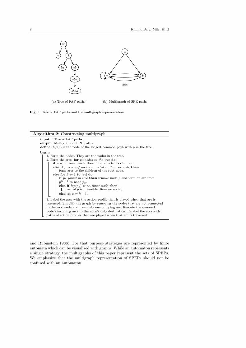
Example 2 Assume that a, ba and bbaa are the only FAF paths in the game.The tree of FAF paths is presented in Fig. 1, where the root node is theempty history ∅. The tree is the starting point in forming the multigraph. Thepurpose is to find the destinations for the FAF paths: a links a and b, and balinks to a. For p = bbaa, we first try to find p1 = baa in the tree. Since it isnot found and ba is a FAF path, there are no profitable deviations from thefirst two b’s in bbaa. We then try to find p2 = aa, which is also not found.Hence, bba can be played only if a follows, i.e., if bbaa is played. Finally, wefind p3 = a in the tree, which is the destination of bba. Thus, we remove nodebbaa and link bba to a. After the simplification, we get the multigraph in Fig.1. The arc labels, e.g., baa, denote the actions that are played when the arc istraversed. If the label is empty, it means that the destination node’s action isplayed when the arc is traversed. We note that there are many SPE paths inaddition to (abba)∞, e.g., a∞ and (ba)∞ are SPEPs.

Directed multigraphs have been previously utilized in the framework ofsupergames for analyzing the complexity of strategies (Rubinstein 1986; Abreu


∅

a b

ba bb

bba

bbaa

∅

a b

baa

(a) Tree of FAF paths (b) Multigraph of SPE paths

Fig. 1 Tree of FAF paths and the multigraph representation.

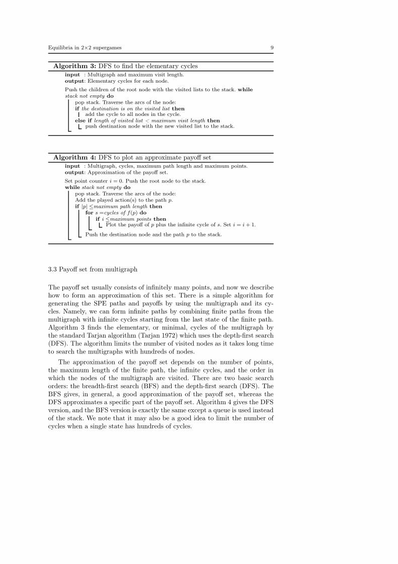
Algorithm 2: Constructing multigraphinput : Tree of FAF paths.output: Multigraph of SPE paths.define: lcp(p) is the node of the longest common path with p in the tree.

begin1. Form the nodes. They are the nodes in the tree.2. Form the arcs. for p=nodes in the tree do

if p is an inner node then form arcs to its children.else if p is a leaf node connected to the root node then

form arcs to the children of the root node.else for k ← 1 to |p1| do

if pk found in tree then remove node p and form an arc fromp|p|−1 to node pk.else if lcp(pk) is an inner node then

part of p is infeasible. Remove node p.

else set k = k + 1.

3. Label the arcs with the action profile that is played when that arc istraversed. Simplify the graph by removing the nodes that are not connectedto the root node and have only one outgoing arc. Reroute the removednode’s incoming arcs to the node’s only destination. Relabel the arcs withpaths of action profiles that are played when that arc is traversed.

and Rubinstein 1988). For that purpose strategies are represented by finiteautomata which can be visualized with graphs. While an automaton representsa single strategy, the multigraphs of this paper represent the sets of SPEPs.We emphasize that the multigraph representation of SPEPs should not beconfused with an automaton.


Algorithm 3: DFS to find the elementary cyclesinput : Multigraph and maximum visit length.output: Elementary cycles for each node.

Push the children of the root node with the visited lists to the stack. while

stack not empty do

pop stack. Traverse the arcs of the node:if the destination is on the visited list then

add the cycle to all nodes in the cycle.else if length of visited list < maximum visit length then

push destination node with the new visited list to the stack.

Algorithm 4: DFS to plot an approximate payoff setinput : Multigraph, cycles, maximum path length and maximum points.output: Approximation of the payoff set.

Set point counter i = 0. Push the root node to the stack.while stack not empty do

pop stack. Traverse the arcs of the node:Add the played action(s) to the path p.if |p| ≤maximum path length then

for s =cycles of f(p) do

if i ≤maximum points thenPlot the payoff of p plus the infinite cycle of s. Set i = i+ 1.

Push the destination node and the path p to the stack.

3.3 Payoff set from multigraph

The payoff set usually consists of infinitely many points, and now we describehow to form an approximation of this set. There is a simple algorithm forgenerating the SPE paths and payoffs by using the multigraph and its cy-cles. Namely, we can form infinite paths by combining finite paths from themultigraph with infinite cycles starting from the last state of the finite path.Algorithm 3 finds the elementary, or minimal, cycles of the multigraph bythe standard Tarjan algorithm (Tarjan 1972) which uses the depth-first search(DFS). The algorithm limits the number of visited nodes as it takes long timeto search the multigraphs with hundreds of nodes.

The approximation of the payoff set depends on the number of points,the maximum length of the finite path, the infinite cycles, and the order inwhich the nodes of the multigraph are visited. There are two basic searchorders: the breadth-first search (BFS) and the depth-first search (DFS). TheBFS gives, in general, a good approximation of the payoff set, whereas theDFS approximates a specific part of the payoff set. Algorithm 4 gives the DFSversion, and the BFS version is exactly the same except a queue is used insteadof the stack. We note that it may also be a good idea to limit the number ofcycles when a single state has hundreds of cycles.


3.4 Dimension estimates

It is possible to analyze the properties of the payoff set by using the con-structed multigraph. The payoff set is a fractal and we can estimate the Haus-dorff dimension with the graph directed constructions of Mauldin and Williams(1988). The estimation of the exact payoff set dimension is, however, compli-cated because of the possibility of overlapping payoffs. For this reason, wedistinguish two dimension estimates: the payoff set dimension, which can becomputed only in special cases, and the path dimension with no overlaps. Thepath dimension can always be computed and it serves as an upper bound forthe payoff set dimension. These notions will be demonstrated with numericalexamples in Section 4.2.

Berg and Kitti (2011) observe that the set of SPE payoffs is a fixed-pointof a particular iterated function system (IFS) and consequently a fractal. Awidely studied class of fixed-points of IFS are self-affine sets. A self-affine setS satisfies

S =⋃

a∈A

Ba(S),

where Ba, a ∈ A, are affine contractions. The payoff set would be a self-affine set if there were no incentive compatibility constraints. In that caseBa(v) = (I −T )u(a)+Tv, where T is a diagonal matrix with discount factorson its diagonal. As observed by Berg and Kitti (2011), the payoff set is notnecessarily self-affine but rather a subset of a self-affine set.

Let us now formulate the payoff set as a graph directed construction. AnIFS directed by a multigraph consists of nodes M , arcs Eqr, i.e., the arcs fromq to r, and functions fp, p ∈ Eqr. The invariant set list is defined as

Vq =⋃

r∈M

⋃

p∈Eqr

fp(Vr), for all q ∈ M,

where fp corresponds to the affine mapping of arc p, e.g., fp = BaBbBc whenp = abc is played on the arc. Furthermore, the payoff set is the union of theinvariant set lists, i.e., V = ∪{Vq : q ∈ M} = V∅.

The Hausdorff dimension of the payoff set is estimated by associating apositive number rp to each arc p ∈ Eqr . If we assume that the players use thesame discount factor δ, we can define rp = δ|p|, e.g., rp = δ3 when p = abcis played on the arc. Let L(s) be the matrix with Lqr(s) =

∑

p∈Eqrrsp, and

Φ(s) = ρ(L(s)) is the spectral radius of L(s), i.e., ρ(L) = maxi |λi|, whereλ is the eigenvalue of L. Then the unique solution s1 ≥ 0 of Φ(s1) = 1 isthe Hausdorff dimension of the Mauldin-Williams graph when the open setcondition is satisfied (Mauldin and Williams 1988; Edgar and Mauldin 1992),i.e., the subsets do not overlap.

The open set condition is satisfied in supergames when the discount factoris less than 1/2. When the discount factor is higher, it is in general difficultto find the exact dimension. It is, however, possible to model the overlaps and


give lower and upper bound estimates (Edgar and Golds 1999; Ngai and Wang2001).

The dimension of the SPE paths can, however, be computed since theoverlap is of no concern for the tree structures (Rellick et al. 1991). The uniquesolution s of

wsq =

∑

p∈Eqr

rspwsr , (4)

is the Hausdorff dimension of the multigraph. Here wq, q ∈ M , are positivenumbers. This equation has a more simple form if each arc is associated withonly one action profile, i.e., if we skip part 3 of Algorithm 2. If we denote Pas the adjacency matrix of the graph, then the Hausdorff dimension s satisfies

(I − δsP )w = 0,

where w is a vector of positive numbers with the size of the number of statesin the graph. Now, we can see that the Hausdorff dimension is related tothe eigenvalues of the weighted adjacency matrix P , which are studied in thespectral graph theory.

If the multigraph is not strongly connected, then the dimensions of thesubgraphs may differ. In that case the dimension of the graph is the maximumdimension of the subgraphs. We can also simplify Eq. (4) when the multigraphhas only one node. Then the dimension is given by (Rellick et al. 1991)

1 =∑

p∈C

rsp,

where C is the set of cycles from the single node.Besides the Hausdorff dimension, we can numerically analyze the payoff

sets and the SPE paths. For example, we can examine how the payoff setcovers the different parts of the payoff space, and how high the payoffs arefor the players in the game. We can also measure how many different SPEpaths there are by examining the versatility of the paths. One way to examinethis is to compute the entropy of the different action profiles in certain lengthSPE paths. For example, a game where three actions can be played has higherentropy than a game where only two actions can be played. Finally, we mayanalyze the number of states and cycles in the multigraph, and the numberand length of FAF paths in the game.

4 Equilibria in symmetric 2×2 supergames

4.1 Classification of 2×2 games

The 2×2 games can be classified into 144 strict ordinal games of which 12are symmetric (Robinson and Goforth 2005); see Rapoport and Guyer (1966);Kilgour and Fraser (1988); Walliser (1988) for earlier taxonomies. The twelvesymmetric ordinal games are presented in Figure 2. The two strategies are C


R

RP

P

T

S

Prisoner’sDilemma

Hawk−DoveChicken

2 Leader3

of SexesBattle

4

Stag Hunt

Harmonyanti−

6 7

Stag−Hunt

12anti−PD

11anti−

Coordination

9

Coordinationanti−

85

1

10

DC

TD

C SR

P

anti−HawkDove

No−ConflictHarmony

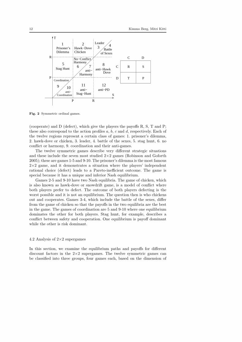
Fig. 2 Symmetric ordinal games.

(cooperate) and D (defect), which give the players the payoffs R, S, T and P;these also correspond to the action profiles a, b, c and d, respectively. Each ofthe twelve regions represent a certain class of games: 1. prisoner’s dilemma,2. hawk-dove or chicken, 3. leader, 4. battle of the sexes, 5. stag hunt, 6. noconflict or harmony, 9. coordination and their anti-games.

The twelve symmetric games describe very different strategic situationsand these include the seven most studied 2×2 games (Robinson and Goforth2005); these are games 1-5 and 9-10. The prisoner’s dilemma is the most famous2×2 game, and it demonstrates a situation where the players’ independentrational choice (defect) leads to a Pareto-inefficient outcome. The game isspecial because it has a unique and inferior Nash equilibrium.

Games 2-5 and 9-10 have two Nash equilibria. The game of chicken, whichis also known as hawk-dove or snowdrift game, is a model of conflict whereboth players prefer to defect. The outcome of both players defecting is theworst possible and it is not an equilibrium. The question then is who chickensout and cooperates. Games 3-4, which include the battle of the sexes, differfrom the game of chicken so that the payoffs in the two equilibria are the bestin the game. The games of coordination are 5 and 9-10 where one equilibriumdominates the other for both players. Stag hunt, for example, describes aconflict between safety and cooperation. One equilibrium is payoff dominantwhile the other is risk dominant.

4.2 Analysis of 2×2 supergames

In this section, we examine the equilibrium paths and payoffs for differentdiscount factors in the 2×2 supergames. The twelve symmetric games canbe classified into three groups, four games each, based on the dimension of


the SPE paths. The most interesting games are prisoner’s dilemma, chicken,stag hunt and no conflict games. In these games, all four action profiles can beplayed in suitable sequences and the SPE payoffs cover large portion of feasiblepayoffs when the discount factor is moderate. The second group consists ofgames, where only the two stage game’s Nash equilibria can be repeated inarbitrary order. The third group consists of anti-games, where there is onlyone subgame perfect equilibrium, i.e., the repetition of the Nash equilibrium.

Let us normalize the payoffs on the diagonals, i.e., R=5 and P=2. Thepayoffs T and S are chosen in the following way: pairs (S,T) and (T,S) takevalues (1,7), (3,7), (6,7), (1,4), (3,4) and (0,1). For example, a pair (S,T)=(1,7)is a prisoner’s dilemma and (S,T)=(3,7) is a game of chicken. The anti-gamesare defined by interchanging the values of S and T. The sensitivity analysiswith respect to the payoff values is examined more thoroughly in the nextsection.

The third group consists of anti-games 7-8 and 11-12. These games haveonly one subgame perfect equilibrium, which is the repetition of stage game’sNash equilibrium. The payoff set and path dimensions in these games arenaturally zero. We note, however, that the payoff values affect the number ofequilibria in games 8 and 12. It is possible that these games have more thanone subgame perfect equilibrium, e.g., when the value of S is higher.

The second group, games 3-4 and 9-10, behaves the same way for widerange of discount factors. The stage games have two equilibria, and the SPEpaths are arbitrary combinations of these two equilibria. In games 3-4, actionsb and c are repeated and all SPE paths are of form (bNcN)∞. In games 9-10,actions a and d are repeated and the paths are (aNdN)∞. When δ ≤ 1/2,the payoff set consists of isolated points between the two payoff values, i.e.,between b and c in games 3-4, and between a and d in games 9-10. The valueδ = 1/2 is the limit when the payoff set fills the line between the two points,and the Hausdorff dimension of the payoff set gets to the value 1. After this,the payoff set and its dimension remain the same even if δ is increased. This isalso the limit when the geometric payoff set dimension breaks from the pathdimension. This can be interpreted so that the dimension of the paths increasesbut the payoff set remains the same, i.e., multiple paths give the same payoffvalue.

The SPE paths and payoff sets change when it is possible to play actionsoutside the two equilibria. This happens when the discount factor is highenough. In game 3, the limit of δ is the highest, and the path a(bc)∞ is thefirst new SPE path when δ ≥ 13/16 ≈ 0.81. In game 4, it is possible to playa with a suitable combination of b and c when δ ≥ 0.67. In games 9-10, thelimits are lower as the payoff of equilibrium d, i.e., P=2, is much lower than theother equilibrium a, i.e., R=5. Moreover, it is possible to play ba∞ and ca∞

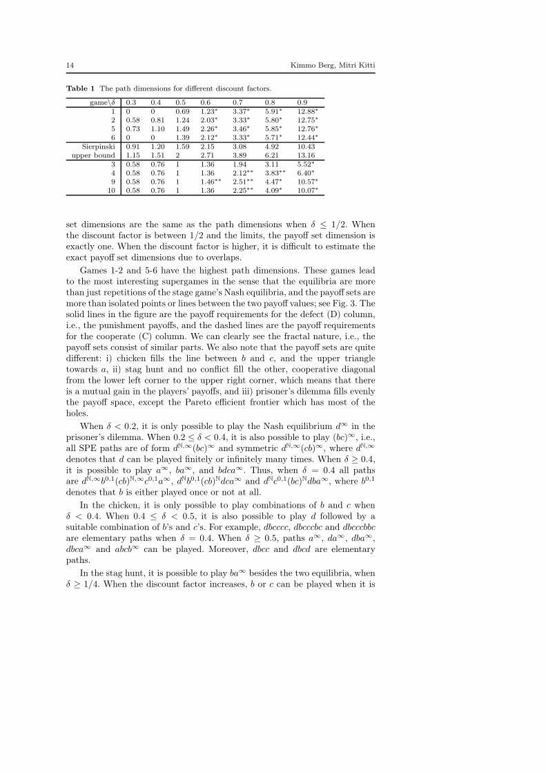
in game 9 (10) when δ ≥ 4/7 ≈ 0.57 (5/8 ≈ 0.63). The Hausdorff dimensionsof the SPE paths are given in Table 1. The values are exact up to the abovelimits of 0.81, 0.67, 0.57 and 0.63 for games 3, 4, 9 and 10, respectively. Forhigher δ, the values are lower bound estimates as the lengths of FAF paths arerestricted to eight (∗) and twelve (∗∗) for computational reasons. The payoff


Table 1 The path dimensions for different discount factors.

game\δ 0.3 0.4 0.5 0.6 0.7 0.8 0.91 0 0 0.69 1.23∗ 3.37∗ 5.91∗ 12.88∗

2 0.58 0.81 1.24 2.03∗ 3.33∗ 5.80∗ 12.75∗

5 0.73 1.10 1.49 2.26∗ 3.46∗ 5.85∗ 12.76∗

6 0 0 1.39 2.12∗ 3.33∗ 5.71∗ 12.44∗

Sierpinski 0.91 1.20 1.59 2.15 3.08 4.92 10.43upper bound 1.15 1.51 2 2.71 3.89 6.21 13.16

3 0.58 0.76 1 1.36 1.94 3.11 5.52∗

4 0.58 0.76 1 1.36 2.12∗∗ 3.83∗∗ 6.40∗

9 0.58 0.76 1 1.46∗∗ 2.51∗∗ 4.47∗ 10.57∗

10 0.58 0.76 1 1.36 2.25∗∗ 4.09∗ 10.07∗

set dimensions are the same as the path dimensions when δ ≤ 1/2. Whenthe discount factor is between 1/2 and the limits, the payoff set dimension isexactly one. When the discount factor is higher, it is difficult to estimate theexact payoff set dimensions due to overlaps.

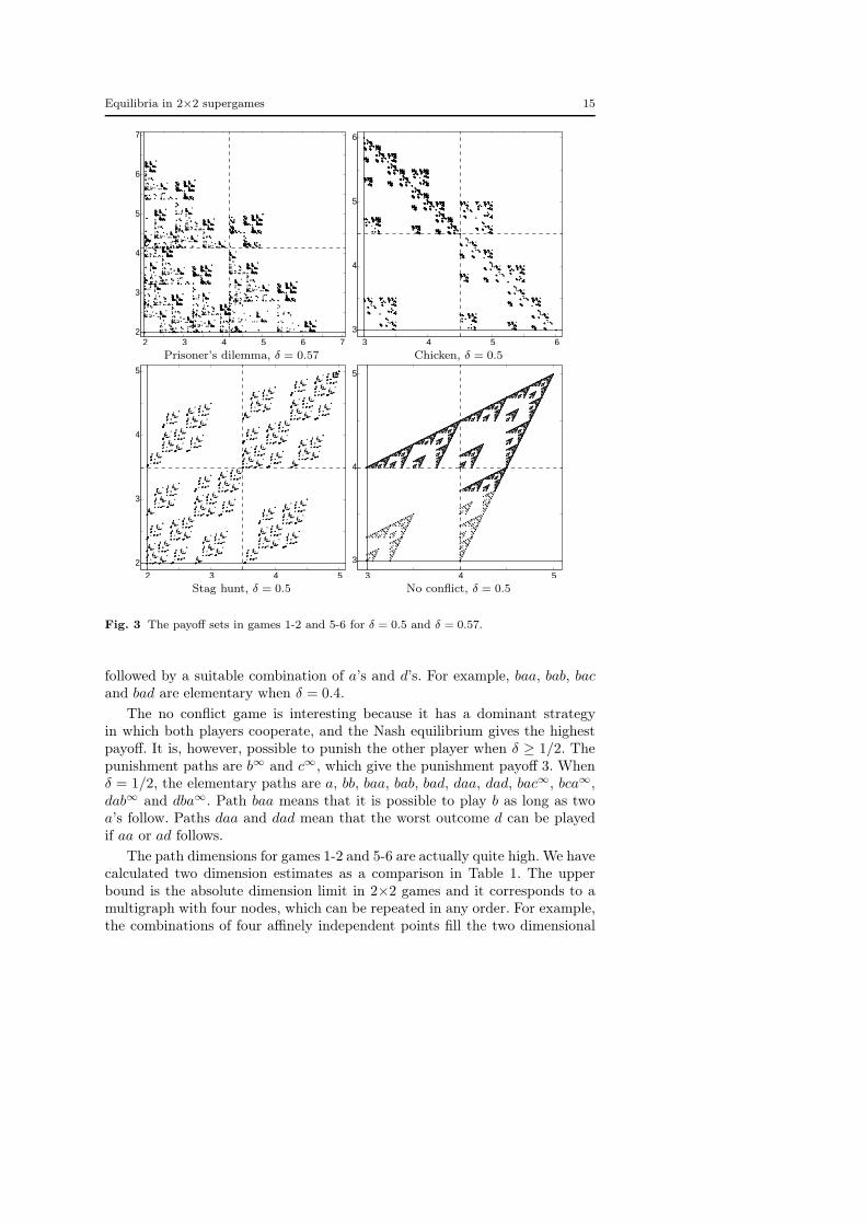
Games 1-2 and 5-6 have the highest path dimensions. These games leadto the most interesting supergames in the sense that the equilibria are morethan just repetitions of the stage game’s Nash equilibria, and the payoff sets aremore than isolated points or lines between the two payoff values; see Fig. 3. Thesolid lines in the figure are the payoff requirements for the defect (D) column,i.e., the punishment payoffs, and the dashed lines are the payoff requirementsfor the cooperate (C) column. We can clearly see the fractal nature, i.e., thepayoff sets consist of similar parts. We also note that the payoff sets are quitedifferent: i) chicken fills the line between b and c, and the upper triangletowards a, ii) stag hunt and no conflict fill the other, cooperative diagonalfrom the lower left corner to the upper right corner, which means that thereis a mutual gain in the players’ payoffs, and iii) prisoner’s dilemma fills evenlythe payoff space, except the Pareto efficient frontier which has most of theholes.

When δ < 0.2, it is only possible to play the Nash equilibrium d∞ in theprisoner’s dilemma. When 0.2 ≤ δ < 0.4, it is also possible to play (bc)∞, i.e.,all SPE paths are of form dN,∞(bc)∞ and symmetric dN,∞(cb)∞, where dN,∞

denotes that d can be played finitely or infinitely many times. When δ ≥ 0.4,it is possible to play a∞, ba∞, and bdca∞. Thus, when δ = 0.4 all pathsare dN,∞b0,1(cb)N,∞c0,1a∞, dNb0,1(cb)Ndca∞ and dNc0,1(bc)Ndba∞, where b0,1

denotes that b is either played once or not at all.

In the chicken, it is only possible to play combinations of b and c whenδ < 0.4. When 0.4 ≤ δ < 0.5, it is also possible to play d followed by asuitable combination of b’s and c’s. For example, dbcccc, dbcccbc and dbcccbbcare elementary paths when δ = 0.4. When δ ≥ 0.5, paths a∞, da∞, dba∞,dbca∞ and abcb∞ can be played. Moreover, dbcc and dbcd are elementarypaths.

In the stag hunt, it is possible to play ba∞ besides the two equilibria, whenδ ≥ 1/4. When the discount factor increases, b or c can be played when it is


2 3 4 5 6 72

3

4

5

6

7

3 4 5 6

3

4

5

6

Prisoner’s dilemma, δ = 0.57 Chicken, δ = 0.5

2 3 4 5

2

3

4

5

3 4 5

3

4

5

Stag hunt, δ = 0.5 No conflict, δ = 0.5

Fig. 3 The payoff sets in games 1-2 and 5-6 for δ = 0.5 and δ = 0.57.

followed by a suitable combination of a’s and d’s. For example, baa, bab, bacand bad are elementary when δ = 0.4.

The no conflict game is interesting because it has a dominant strategyin which both players cooperate, and the Nash equilibrium gives the highestpayoff. It is, however, possible to punish the other player when δ ≥ 1/2. Thepunishment paths are b∞ and c∞, which give the punishment payoff 3. Whenδ = 1/2, the elementary paths are a, bb, baa, bab, bad, daa, dad, bac∞, bca∞,dab∞ and dba∞. Path baa means that it is possible to play b as long as twoa’s follow. Paths daa and dad mean that the worst outcome d can be playedif aa or ad follows.

The path dimensions for games 1-2 and 5-6 are actually quite high. We havecalculated two dimension estimates as a comparison in Table 1. The upperbound is the absolute dimension limit in 2×2 games and it corresponds to amultigraph with four nodes, which can be repeated in any order. For example,the combinations of four affinely independent points fill the two dimensional


space when the contraction is 1/2, i.e., the upper bound is 2 when δ = 1/2.Sierpinski game corresponds to a multigraph with three nodes, which can berepeated in any order. An example of such game is given in Berg and Kitti(2011), which has three Nash equilibria. We can see that the path dimensionsof games 1-2 and 5-6 are higher than the Sierpinski game and close to theupper bound of 2×2 games when δ ≥ 0.7.

4.3 Sensitivity analysis

The numerical examples of the previous section illustrate the differences ofthe payoff set and path dimensions, and their relation to the discount factor.Prisoner’s dilemma with a low discount factor is a good example of a casewhere the elementary paths increase but both of the dimensions remain thesame. First, it is possible to play d∞, and when the discount factor increasesthen (bc)∞ and a∞ are available, but both of the dimensions remain at zero.This is because there is no state in the multigraph which has more than onecycle. When the first dual cycle appears, the dimension jumps up from zero.

Games 3-4 and 8-9, with discount factor δ < 1/2, are good examples of acase where the paths and the multigraph remains the same but the dimensionsincrease when the discount factor is increased. These games also illustrate thedifference of path and payoff set dimensions. When δ is more than half butless than the calculated limits, the payoff set dimension is one but the pathdimension increases. The increase in path dimension can be interpreted so thatmultiple paths give the same payoff value.

The path dimension depends on two things: the cycles in the multigraphand the discounting. If the cycles do not change and there is a dual cycle, thenthe dimension increases continuously with the discount factor. But when anew cycle appears in the multigraph, the dimension jumps up discontinuously.For example, the dimension jumps up from zero to 1.39 in the no conflictgame when δ = 0.5. The payoff set changes dramatically from one point to thefractal, which is shown in Fig. 3.

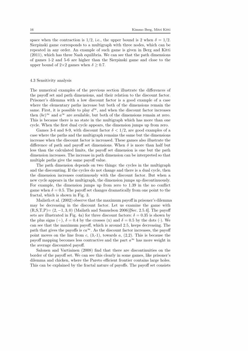
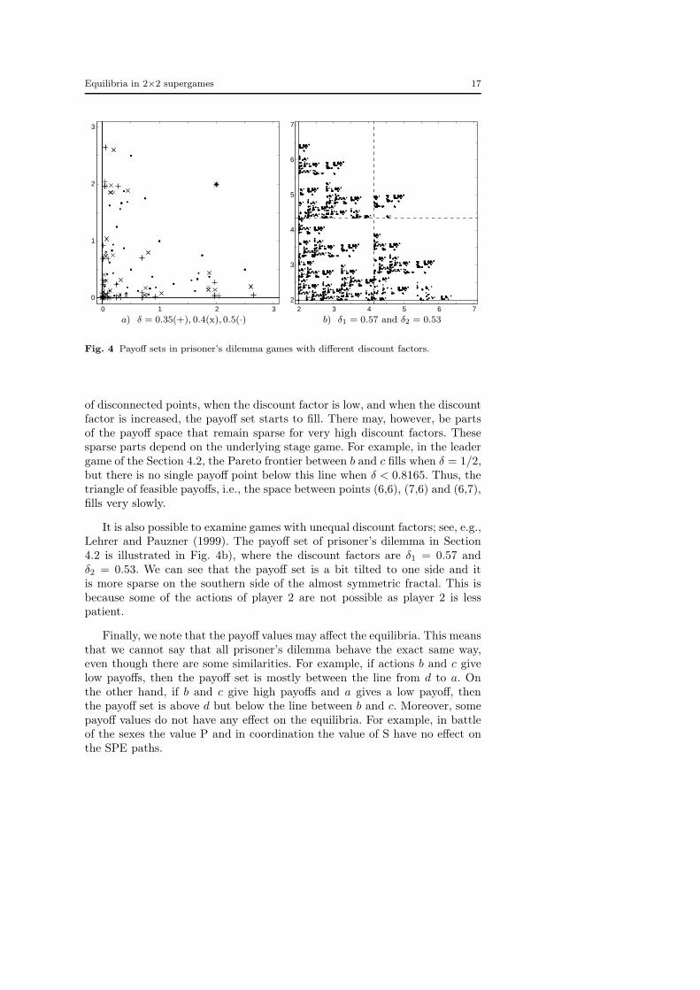
Mailath et al. (2002) observe that the maximum payoff in prisoner’s dilemmamay be decreasing in the discount factor. Let us examine the game with(R,S,T,P)= (2,−1, 3, 0) (Mailath and Samuelson 2006)[Sec. 2.5.4]. The payoffsets are illustrated in Fig. 4a) for three discount factors: δ = 0.35 is shown bythe plus signs (+), δ = 0.4 by the crosses (x) and δ = 0.5 by the dots (·). Wecan see that the maximum payoff, which is around 2.5, keeps decreasing. Thepath that gives the payoffs is ca∞. As the discount factor increases, the payoffpoint moves on the line from c, (3,-1), towards a, (2,2). This is because thepayoff mapping becomes less contractive and the part a∞ has more weight inthe average discounted payoff.

Salonen and Vartiainen (2008) find that there are discontinuities on theborder of the payoff set. We can see this clearly in some games, like prisoner’sdilemma and chicken, where the Pareto efficient frontier contains large holes.This can be explained by the fractal nature of payoffs. The payoff set consists


0 1 2 3

0

1

2

3

2 3 4 5 6 72

3

4

5

6

7

a) δ = 0.35(+), 0.4(x), 0.5(·) b) δ1 = 0.57 and δ2 = 0.53

Fig. 4 Payoff sets in prisoner’s dilemma games with different discount factors.

of disconnected points, when the discount factor is low, and when the discountfactor is increased, the payoff set starts to fill. There may, however, be partsof the payoff space that remain sparse for very high discount factors. Thesesparse parts depend on the underlying stage game. For example, in the leadergame of the Section 4.2, the Pareto frontier between b and c fills when δ = 1/2,but there is no single payoff point below this line when δ < 0.8165. Thus, thetriangle of feasible payoffs, i.e., the space between points (6,6), (7,6) and (6,7),fills very slowly.

It is also possible to examine games with unequal discount factors; see, e.g.,Lehrer and Pauzner (1999). The payoff set of prisoner’s dilemma in Section4.2 is illustrated in Fig. 4b), where the discount factors are δ1 = 0.57 andδ2 = 0.53. We can see that the payoff set is a bit tilted to one side and itis more sparse on the southern side of the almost symmetric fractal. This isbecause some of the actions of player 2 are not possible as player 2 is lesspatient.

Finally, we note that the payoff values may affect the equilibria. This meansthat we cannot say that all prisoner’s dilemma behave the exact same way,even though there are some similarities. For example, if actions b and c givelow payoffs, then the payoff set is mostly between the line from d to a. Onthe other hand, if b and c give high payoffs and a gives a low payoff, thenthe payoff set is above d but below the line between b and c. Moreover, somepayoff values do not have any effect on the equilibria. For example, in battleof the sexes the value P and in coordination the value of S have no effect onthe SPE paths.


5 Discussion

This paper provides new methods for analyzing and computing the subgameperfect pure strategy equilibrium paths and payoff sets in discounted su-pergames with perfect monitoring. Berg and Kitti (2011) present the underly-ing theory following the tradition of Abreu et al. (1990) for recursive charac-terization of equilibrium payoffs. This paper gives a simple presentation of thekey ideas using only paths of action profiles. We apply the algorithms to thesymmetric 2×2 games. However, the methods can also be used in analyzingasymmetric games where there are several players with more than two actions.

We have shown that the SPE paths can be conveniently represented with adirected multigraph. It allows us to analyze what kind of actions are possiblein the game, how complex paths there can be, and what happens in the gamewhen the discount factor changes. The multigraph also offers a unique viewof the payoff sets, which are particular fractals. Moreover, it turns out thatthere are useful tools for analyzing the multigraphs, i.e., the graph directedconstructions (Mauldin and Williams 1988).

There are couple of observations we want to emphasize. One is the dif-ference of paths and the payoff set dimension. When the discount factor islow and the payoff set is sparse, then the SPE paths may increase withoutchanging the payoff set dimension. This happens when the multigraph doesnot have a state with multiple cycles, which are related to the dimension. Itis also possible that the paths remain the same but the dimension increases.Thus, the dimension increases for two reasons: i) the discount factor increaseswhich makes the mappings on the cycles less contractive, and ii) the numberof cycles increases. Moreover, it is difficult to estimate the exact payoff setdimension when the payoff points overlap.

We also observe that the payoff sets fill up uniquely for different gamesand for different parts of the payoff space. This gives a new insight into folktheorems, see, e.g., Fudenberg and Maskin (1986). For example, it may requirevery high discount factor to fill the Pareto efficient frontier of the game. Thepayoff set may also remain sparse in other parts of the payoff space.

References

Abreu, D. (1988). On the theory of infinitely repeated games with discounting.Econometrica, 56(2), 383–396.

Abreu, D., Rubinstein, A. (1988). The structure of Nash equilibrium in re-peated games with finite automata. Econometrica, 56(6), 1259–1281.

Abreu, D., Pearce, D., Stacchetti, E. (1986). Optimal cartel equilibria withimperfect monitoring. Journal of Economic Theory, 39(1), 251–269.

Abreu, D., Pearce, D., Stacchetti, E. (1990). Toward a theory of discountedrepeated games with imperfect monitoring. Econometrica, 58(5), 1041–1063.

Axelrod, R. (1984). The Evolution of Cooperation. New York: Basic.


Benoit, J.P., Krishna, V. (1985). Finitely repeated games. Econometrica, 53(4),905–922.

Berg, K., Kitti, M. (2011). Equilibrium paths in discounted supergames. Work-ing paper.

Brams, S.J. (2003). Negotiation Games: Applying game theory to bargaining

and arbitration. Routledge.Cronshaw, M.B. (1997). Algorithms for finding repeated game equilibria. Com-

putational Economics, 10, 139–168.Cronshaw, M.B., Luenberger, D.G. (1994). Strongly symmetric subgame per-

fect equilibria in infinitely repeated games with perfect monitoring. Games

and Economic Behavior, 6, 220–237.Edgar, G.A., Golds, J. (1999). A fractal dimension estimate for a graph-

directed iterated function system of non-similarities. Indiana University

Mathematics Journal, 48(2), 429–447.Edgar, G.A., Mauldin, R.D. (1992). Multifractal decompositions of digraph

recursive fractals. Proceedings of the London Mathematical Society, 65, 604–628.

Falconer, K.J. (1988). The Hausdorff dimension of self-affine fractals. Mathe-

matical Proceedings of the Cambridge Philosophical Society, 103, 169–179.Falconer, K.J. (1992). The dimension of self-affine fractals ii. Mathematical

Proceedings of the Cambridge Philosophical Society, 111, 339–350.Fudenberg, D., Maskin, E. (1986). The folk theorem in repeated games with

discounting and incomplete information. Econometrica, 54, 533–554.Hauert, C. (2001). Fundamental clusters in 2 × 2 spatial games. Proceedings

of the Royal Society B, 268, 761–769.Judd, K., Yeltekin, Ş., Conklin, J. (2003). Computing supergame equilibria.

Econometrica, 71, 1239–1254.Kilgour, D.M., Fraser, N.M. (1988). A taxonomy of all ordinal 2x2 games.

Theory and Decision, 24, 99–117.Kitti, M. (2010). Quasi-stationary equilibria in dynamic games. Working pa-

per.Kitti, M. (2011). Quasi-markov equilibria in discounted dynamic games. Work-

ing paper.Lehrer, E., Pauzner, A. (1999). Repeated games with differential time prefer-

ences. Econometrica, 67, 393–412.Mailath, G.J., Samuelson, L. (2006). Repeated Games and Reputations: Long-

Run Relationships. Oxford University Press.Mailath, G.J., Obara, I., Sekiguchi, T. (2002). The maximum efficient equi-

librium payoff in the repeated prisoners’ dilemma. Games and Economic

Behavior, 40, 99–122.Mauldin, R.D., Williams, S.C. (1988). Hausdorff dimension in graph directed

constructions. Transactions of the American Mathematical Society, 309(2),811–829.

Maynard Smith, J. (1982). Evolution and the theory of games. CambridgeUniversity Press.


Ngai, S.M., Wang, Y. (2001). Hausdorff dimension of self-similar sets withoverlaps. Journal of the London Mathematicl Society, 63, 655–672.

Rapoport, A., Guyer, M. (1966). A taxonomy of 2×2 games. General Systems:

Yearbook of the Society for General Systems Research, 11, 203–214.Rellick, L.M., Edgar, G.A., Klapper, M.H. (1991). Calculating the Hausdorff

dimension of tree structures. Journal of Statistical Physics, 64(1), 77–85.Robinson, D., Goforth, D. (2005). The Topology of the 2 × 2 Games: A New

Periodic Table. Routledge.Rubinstein, A. (1986). Finite automata play the repeated prisoner’s dilemma.

Journal of Economic Theory, 39, 83–96.Salonen, H., Vartiainen, H. (2008). Valuating payoff streams under unequal

discount factors. Economics Letters, 99(3), 595–598.Tarjan, R. (1972). Depth-first search and linear graph algorithms. SIAM Jour-

nal on Computing, 1(2), 146–160.Walliser, B. (1988). A simplified taxonomy of 2×2 games. Theory and Decision,

25, 163–191.

Computing equilibria in discounted 2x2 supergames

Documents

Transcript of Computing equilibria in discounted 2x2 supergames