Finding all pure strategy Nash equilibria in a planar location game

J. M. Dıaz-Banez∗

M. Heredia∗

B. Pelegrın†

P. Perez-Lantero∗

I. Ventura∗

January 14, 2011

Abstract

In this paper, we deal with a planar location-price game where firms first select their locationsand then set delivered prices in order to maximize their profits. If firms set the equilibriumprices in the second stage, the game is reduced to a location game for which pure strategy Nashequilibria are studied assuming that the marginal delivered cost is proportional to the distancebetween the customer and the facility from which it is served. We present characterizations oflocal and global Nash equilibria. Then an algorithm is shown in order to find all possible Nashequilibrium pairs of locations. The minimization of the social cost leads to a Nash equilibrium.An example shows that there may exist multiple Nash equilibria which are not minimizers ofthe social cost.

Keywords: Location, Game theory, Nash equilibrium.

1 Introduction

Major decisions for firms selling the same type of product and competing for customers are where tolocate their facilities and what price to set. When the firms use delivered pricing, profit is stronglyaffected by both the location of their facilities and the price they set in each demand point. Themaximization of profit for each competing firm can be seen as a location-price game, which hasbeen studied since the work by Hotelling [19]. Many existing literature deals with this type ofproblem on a linear location space (see [4], [14], [22]), which is in part due to the complexity ofsolving the associated location problems in other location spaces as the plane or a network (see thesurvey papers [12], [13], [25], [26]).

The existence of a price equilibrium was shown for the first time by Hoover [18], who analyzedspatial discriminatory pricing for firms with fixed locations and concluded that a firm serving aparticular market would be constrained in its local price by the delivery cost of the other firmsserving that market. In situations where demand elasticity is ‘not too high’, the equilibrium priceat a given market is equal to the delivery cost of the firm with the second lowest delivery cost. Thisresult was extended later to spatial duopoly (see [20], [21]) and to spatial oligopoly for differenttypes of location spaces (see [8], [15]).

If firms set the equilibrium prices, which are determined by their facility locations, the location-price game reduces to a location game. This location game has been scarcely studied in the location

∗Departamento de Matematica Aplicada II, Universidad de Sevilla, Spain. Partially supported by project MEC

MTM2009-08652. {dbanez,manuelhz,pplantero,iventura}@us.es.†Departamento de Estadıstica e Investigacion Operativa, Universidad de Murcia, Spain. Partially supported by

project MEC ECO2008-00667. pelegrin@um.es.

1

literature. In a duopoly with completely inelastic demand and constant marginal production costs,Lederer and Thisse [21] showed that a location equilibrium exists which is a global minimizer ofthe social cost. The social cost is defined as the total delivered cost if each customer were servedwith the lowest marginal delivered cost. In oligopoly, the same result is obtained by Dorta et al.[8], who present a model where firms make location and delivery price decisions along a network ofconnected but spatially separated markets.

The problem of finding Nash equilibria to the location game has been solved by social cost min-imization. This optimization problem is equivalent to the p-median problem when the marginaldelivered cost from each site location to each demand point is the same for all competing firms.There is an extensive literature on algorithms to solve the p-median problem for both network andplanar location spaces (see for instance [1, 9, 27]). If marginal delivered cost from each site locationto each demand point is different for each competitor the social cost minimization problem hasbeen solved on a network location space by using a Mixed Integer Linear Programming (MILP)formulation (see [23]). If demand is price sensitive or marginal production costs are not constant,the socially optimal locations may not be an equilibrium of the location game which has beenshown in [16] and [17]. Other similar location games where the payoffs are given by market sharehave been recently studied in [2, 3] and [10].

In this paper, we study the location game for two firms in a two-dimensional location space assumingthat the marginal delivered cost is proportional to the distance between customer and facility fromwhich it is served. In Section 2 we state the problem. In Section 3 we prove the existence of atleast a Nash equilibrium. In Section 4 some useful properties and characterizations of local andglobal Nash equilibria are presented. In Section 5, we propose an algorithm to generate all Nashequilibria to the location game, and show some illustrative examples. It is also shown the existenceof Nash equilibria which are not minimizers of social cost. Finally, some conclusions are presentedin Section 6.

2 The problem

We consider the location-price game in a planar space for two competing firms, Firm 1 and Firm2. For simplicity we assume that the marginal delivered cost is given by the distance between thecustomer and the facility from which it is served. The Euclidean metric is taken to measure thedistance between any pair of points. Thus d(x, y) denotes the Euclidean distance between the pointsx and y. Customers are located in different points in the plane, we denote by P = {p1, p2, . . . , pn}the set of demand points representing the customers. They have fixed demands for an homogeneousproduct. Let qi > 0 be the demand at the point pi, 1 ≤ i ≤ n. Each customer buys from the facilityoffering the lowest price.

It is assumed that demand is completely inelastic at each node. Each firm locates a single facilityand set a delivered price at each demand point which is the equilibrium price resulting from theprice competition process. Let x and y be any fixed pair of locations for the competing firms. Theequilibrium price at each demand point pi for Firm 1 and Firm 2 are respectively:

P 1i (x, y) =

�d (pi, y) if d (pi, x) < d (pi, y)d (pi, x) otherwise

P 2i (x, y) =

�d (pi, x) if d (pi, y) < d (pi, x)d (pi, y) otherwise

2

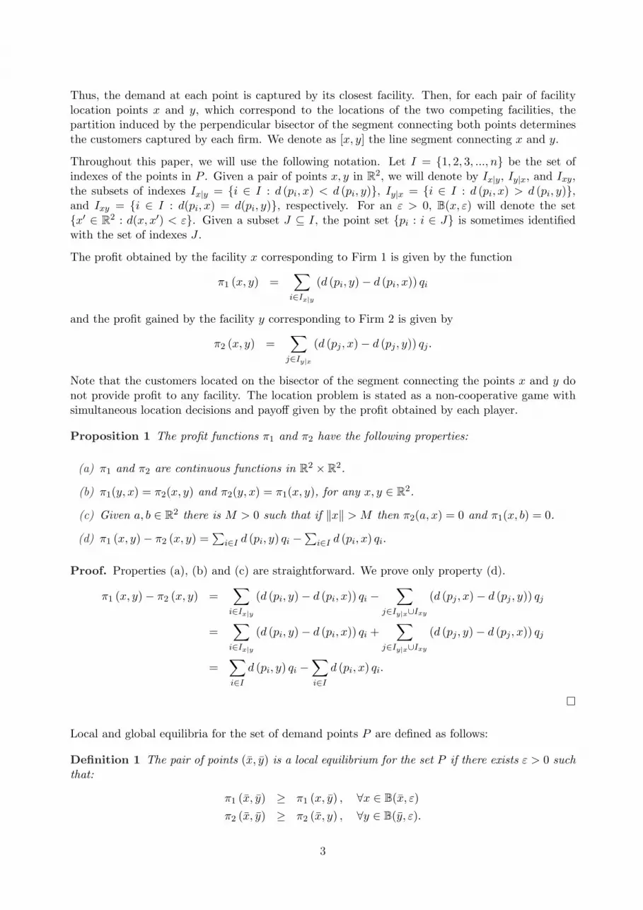
Thus, the demand at each point is captured by its closest facility. Then, for each pair of facilitylocation points x and y, which correspond to the locations of the two competing facilities, thepartition induced by the perpendicular bisector of the segment connecting both points determinesthe customers captured by each firm. We denote as [x, y] the line segment connecting x and y.

Throughout this paper, we will use the following notation. Let I = {1, 2, 3, ..., n} be the set ofindexes of the points in P . Given a pair of points x, y in R2, we will denote by Ix|y, Iy|x, and Ixy,the subsets of indexes Ix|y = {i ∈ I : d (pi, x) < d (pi, y)}, Iy|x = {i ∈ I : d (pi, x) > d (pi, y)},and Ixy = {i ∈ I : d(pi, x) = d(pi, y)}, respectively. For an ε > 0, B(x, ε) will denote the set{x� ∈ R2 : d(x, x�) < ε}. Given a subset J ⊆ I, the point set {pi : i ∈ J} is sometimes identifiedwith the set of indexes J .

The profit obtained by the facility x corresponding to Firm 1 is given by the function

π1 (x, y) =�

i∈Ix|y

(d (pi, y)− d (pi, x)) qi

and the profit gained by the facility y corresponding to Firm 2 is given by

π2 (x, y) =�

j∈Iy|x

(d (pj , x)− d (pj , y)) qj .

Note that the customers located on the bisector of the segment connecting the points x and y donot provide profit to any facility. The location problem is stated as a non-cooperative game withsimultaneous location decisions and payoff given by the profit obtained by each player.

Proposition 1 The profit functions π1 and π2 have the following properties:

(a) π1 and π2 are continuous functions in R2 × R2.

(b) π1(y, x) = π2(x, y) and π2(y, x) = π1(x, y), for any x, y ∈ R2.

(c) Given a, b ∈ R2 there is M > 0 such that if �x� > M then π2(a, x) = 0 and π1(x, b) = 0.

(d) π1 (x, y)− π2 (x, y) =�

i∈I d (pi, y) qi −�

i∈I d (pi, x) qi.

Proof. Properties (a), (b) and (c) are straightforward. We prove only property (d).

π1 (x, y)− π2 (x, y) =�

i∈Ix|y

(d (pi, y)− d (pi, x)) qi −�

j∈Iy|x∪Ixy

(d (pj , x)− d (pj , y)) qj

=�

i∈Ix|y

(d (pi, y)− d (pi, x)) qi +�

j∈Iy|x∪Ixy

(d (pj , y)− d (pj , x)) qj

=�

i∈I

d (pi, y) qi −�

i∈I

d (pi, x) qi.

�

Local and global equilibria for the set of demand points P are defined as follows:

Definition 1 The pair of points (x, y) is a local equilibrium for the set P if there exists ε > 0 suchthat:

π1 (x, y) ≥ π1 (x, y) , ∀x ∈ B(x, ε)π2 (x, y) ≥ π2 (x, y) , ∀y ∈ B(y, ε).

3

Definition 2 The pair of points (x, y) is a global (or Nash) equilibrium for the set P if:

π1 (x, y) ≥ π1 (x, y) , ∀x ∈ R2

π2 (x, y) ≥ π2 (x, y) , ∀y ∈ R2.

Note that every global equilibrium is also a local one. In the following, we will deal with the problemof finding all Nash equilibrium pairs of points for the location game considering the previous profitfunctions.

3 Existence of Nash equilibria

In this section, we introduce the social cost function in order to prove that there exists at least oneglobal equilibrium for the proposed location game.

Definition 3 Given a pair of points x, y in R2, its social cost function is defined by

S(x, y) =�

i∈I

min{d (pi, x) , d (pi, y)}qi.

The social cost function has the following properties:

Proposition 2 S(x, y) is continuous in R2 × R2, and there is a pair of points x, y such thatS(x, y) ≤ S(x, y) for all x, y in R2.

Proof. Let CH(P ) be the convex hull of P . Given x, y in R2 there are two points x�, y� in CH(P )such that

d(pi, x�) ≤ d(pi, x) and d(pi, y

�) ≤ d(pi, y), for i = 1, 2, . . . , n.

Hence S(x�, y�) ≤ S(x, y). The function S(x, y) is continuous in the compact set CH(P )×CH(P ),therefore there is a pair (x, y) in CH(P )× CH(P ) that minimizes the function S(x, y). �

Proposition 3 The profit and social cost functions satisfy:

π1(x, y) =�

i∈I

d (pi, y) qi − S(x, y), π2(x, y) =�

i∈I

d (pi, x) qi − S(x, y).

Proof. The social cost function can be expressed as follows:

S(x, y) =�

i∈Ix|y

d(pi, x)qi +�

i∈Iy|x∪Ixy

d(pi, y)qi

Then we have:

π1(x, y) =�

i∈Ix|y

(d (pi, y)− d (pi, x)) qi

=�

i∈Ix|y

d (pi, y) qi −�

i∈Ix|y

d (pi, x) qi

=�

i∈Ix|y

d (pi, y) qi +�

i∈Iy|x∪Ixy

d(pi, y)qi −�

i∈Iy|x∪Ixy

d(pi, y)qi −�

i∈Ix|y

d (pi, x) qi

=�

i∈I

d (pi, y) qi − S(x, y).

A similar expression can be obtained for the profit function π2. �

4

Proposition 4 Any global minimizer of S(x, y) is a global equilibrium for P .

Proof. Let (x, y) be a global minimizer of S(x, y). Then, for all x in R2 we have:

π1(x, y) =�

i∈I

d(pi, y)qi − S(x, y) ≥�

i∈I

d(pi, y)qi − S(x, y) = π1(x, y).

Similarly, we obtain that π2(x, y) ≥ π2(x, y) for all y in R2. Therefore, (x, y) is a global equilibriumfor P . �

We notice that the claim of Proposition 4 is also valid for any metric space. The converse ofProposition 4 is not true in general. In Subsection 5.1 an example is shown for which there existglobal equilibria which are not social cost minimizers.

From Propositions 2 and 4 we obtain the following result:

Proposition 5 There always exists a Nash equilibrium for P .

4 Properties of local and global equilibria

Before describing the procedure to find all Nash equilibria, in this section we give some propertiesto discretize the search space for equilibrium positions.

Definition 4 A point w in R2 is a Weber point of a given subset J ⊆ I if and only if�

j∈J

d (pj , w) qj ≤�

j∈J

d (pj , x) qj , ∀x ∈ R2

that is, w is a 1-median point of the set {pj : j ∈ J}.

Definition 5 A subset J ⊆ I is a candidate subset of P if the sets {pi ∈ P : i ∈ J} and {pi ∈ P :i ∈ I\J} are separable by a straight line.

Given two points x and y, let suppose that Ixy is empty. Then, both subsets Ix|y and Iy|x arecandidates since they are separable by the bisector of the segment joining x and y, [x, y]. Otherwise,if Ixy is not empty, then the subsets Ix|y ∪ Ixy and Iy|x are also candidates by considering a parallelstraight line close enough to the bisector of [x, y]. Analogously for the sets Ix|y and Iy|x ∪ Ixy.

Definition 6 The Weber set of P , denoted by W , is the set of Weber points corresponding to thecandidate subsets of P .

In the following we will show that the search for equilibrium pairs can be reduced to the set W×W .Before that, we give a technical lemma on candidate sets that will be useful later.

Lemma 6 Given a demand point set P and two points x, y in R2, we have:

(1) There exists ε > 0 such that Ix|y ⊆ Ix|y ⊆ Ix|y ∪ Ixy for all x ∈ B(x, ε).

(2) There exists ε� > 0 such that Iy|x ⊆ Iy|x ⊆ Iy|x ∪ Ixy for all y ∈ B(y, ε�).

5

Proof. We prove only statement (1). The proof of statement (2) is similar. Let y be fixed and foreach point pi ∈ P define εi as follows:

εi =

d(pi, y)− d(pi, x) if pi ∈ Ix|yd(pi, x)− d(pi, y) if pi ∈ Iy|x

+∞ otherwise

Let ε be a positive value less than min{εi}, x ∈ B(x, ε), and pi ∈ P . On one hand, if pi ∈ Ix|y then:

d(pi, x) ≤ d(x, x) + d(pi, x)< ε + d(pi, x)< εi + d(pi, x)= d(pi, y)− d(pi, x) + d(pi, x)= d(pi, y)

Thus pi ∈ Ix|y and therefore Ix|y ⊆ Ix|y. On the other hand, if pi ∈ Iy|x then:

d(pi, x) ≥ d(pi, x)− d(x, x)> d(pi, x)− ε

> d(pi, x)− εi

= d(pi, x)− (d(pi, x)− d(pi, y))= d(pi, y)

It means that Iy|x ⊆ Iy|x which is equivalent to Ix|y∪Ixy ⊆ Ix|y∪Ixy, implying that Ix|y ⊆ Ix|y∪Ixy.Hence, the result follows. �

Lemma 7 Let (x, y) be a pair of points and {J1, J2} be any partition of Ixy induced by a straightline. The following statements hold:

(1) If ε > 0 satisfies condition (1) of Lemma 6, then there exist x, x� ∈ B(x, ε) such that Ix|y =Ix|y ∪ J1 and Ix�|y = Ix|y ∪ J2.

(2) If ε� > 0 satisfies condition (2) of Lemma 6, then there exist y, y� ∈ B(y, ε�) such that Iy|x =Iy|x ∪ J1 and Iy�|x = Iy|x ∪ J2.

Proof. We prove the existence of x in statement (1). The rest of the proof is similar. Let {J1, J2}be a partition of Ixy induced by the straight line �, q be the intersection point of � and the bisector�xy of [x, y], and ε > 0 satisfy condition (1) of Lemma 6. It suffices to prove that there existsx ∈ B(x, ε) \ {x} such that the bisector of [x, y] passes through q. It is as follows. Denote byx� ∈ R2 the point such that � is the bisector of [x�, y]. If we rotate � with center at q in order toreach �xy, then x� tends to x. Then there is an instant in which x� ∈ B(x, ε) \ {x}. By takingx = x� at this instant the result follows. �

Proposition 8 Let x and y be two points in R2. The next statements hold:

(a) If there exists ε > 0 such that π1(x, y) ≥ π1(x, y) for all x ∈ B(x, ε), then x is a Weber pointof Ix|y for all x such that Ix|y ⊆ Ix|y ⊆ Ix|y ∪ Ixy.

(b) If there exists ε� > 0 such that every y ∈ B(y, ε�) satisfies π2(x, y) ≥ π2(x, y), then y is aWeber point of Iy|x for all y such that Iy|x ⊆ Iy|x ⊆ Iy|x ∪ Ixy.

6

Proof. We prove only the first part of the proposition. The second one is analogous. Let ε1 > 0such that π1(x, y) ≥ π1(x, y) for all x ∈ B(x, ε1), ε2 > 0 satisfy condition (1) of Lemma 6, andε = min{ε1, ε2}. On one hand, by Lemma 7, every set Ix|y such that x satisfies Ix|y ⊆ Ix|y ⊆ Ix|y∪Ixy

can be obtained by taking some point x ∈ B(x, ε). On the other hand, we have the following forall x ∈ B(x, ε):

π1(x, y) ≥ π1(x, y)�

i∈Ix|y

(d(pi, y)− d(pi, x))qi ≥�

i∈Ix|y

(d(pi, y)− d(pi, x))qi

�

i∈Ix|y

(d(pi, y)− d(pi, x))qi ≥�

i∈Ix|y

(d(pi, y)− d(pi, x))qi

�

i∈Ix|y

d(pi, x)qi ≥�

i∈Ix|y

d(pi, x)qi

Consequently, x is a local minimum of the convex positive function Φ(z) =�

i∈Ix|yd(pi, z)qi, z ∈ R2,

in B(x, ε). Then x is a global minimizer of Φ(z) and thus a Weber point of Ix|y. �

From Proposition 8 the following corollary can be obtained:

Corollary 9 If (x, y) is a local equilibrium for P , then (x, y) ∈ W ×W . Moreover, x is a Weberpoint of Ix|y and y is a Weber point of Iy|x.

The above corollary reduces the search for local equilibrium pairs, and therefore the search forglobal equilibrium pairs, to Weber pair of points. Notice that a Weber pair is determined by apartition of the plane induced by a straight line. If the points in a candidate subset J are notcollinear, then there is only one Weber point corresponding to J , but there may exist a segmentof Weber points corresponding to J if the points in J are collinear (see [24]). Hence an infinitenumber of Nash equilibria may exist as shown in an example of subsection 5.1.

It is easy to see that the inverse of Corollary 9 is not true in general. In Figure 1, a partition inducedby the dashed line is given. The pair of Weber points (w1, w2) corresponding to the partition, isnot a local equilibrium for P . Indeed, the perpendicular bisector of the segment [w1, w2] gives adifferent partition. On the contrary, if the partition induced by a pair of Weber points fits theoriginal partition, then the Weber pair might be a local equilibrium pair.

The following proposition gives a complete characterization of local equilibria for P .

Proposition 10 The pair (x, y) is a local equilibrium for P if and only if:

(a) x is a Weber point of Ix|y for all x such that Ix|y ⊆ Ix|y ⊆ Ix|y ∪ Ixy, and

(b) y is a Weber point of Iy|x for all y such that Iy|x ⊆ Iy|x ⊆ Iy|x ∪ Ixy.

Proof. If (x, y) is a local equilibrium for P , then conditions (a) and (b) hold by Proposition 8.Conversely, suppose that the pair (x, y) satisfies conditions (a) and (b). By Lemma 6, there exists

7

w1 w2

partitionbisector

Figure 1: Two Weber points w1 and w2 which are not a local equilibrium pair.

ε1 > 0 such that Ix|y ⊆ Ix|y ⊆ Ix|y ∪ Ixy for all x ∈ B(x, ε1). Then:

π1(x, y) =�

i∈Ix|y

(d(pi, y)− d(pi, x))qi

≤�

i∈Ix|y

(d(pi, y)− d(pi, x))qi

=�

i∈Ix|y

(d(pi, y)− d(pi, x))qi

= π1(x, y)

In a similar way, we can prove that there exists ε2 > 0 such that π2(x, y) ≤ π2(x, y) for ally ∈ B(y, ε2). By taking ε = min{ε1, ε2} it follows that (x, y) is a local equilibrium pair. �

Figure 2 illustrates Proposition 10. The demand points are represented as solid dots. The demandpoint x (resp. y) satisfies condition (a) (resp. (b)) of Proposition 10, and the pair (x, y) is a localequilibrium. Note that if we remove y, then (x, y) is not a local equilibrium because y is not aWeber point of Iy|x.

x

y

Figure 2: The pair (x, y) is a local equilibrium and satisfies the two conditions in Proposition 10.

The following result provides a procedure for finding the Nash equilibria of a demand point set P .

8

Proposition 11 The pair (x, y) is a global equilibrium for P if and only if π1(x, y) ≥ π1(w, y) andπ2(x, y) ≥ π2(x, w) for all w in W .

Proof. The necessary condition is straightforward. To see the sufficient condition we prove onlythat π1(x, y) ≥ π1(x, y) for all x in R2. The proof for π2 is analogous.

Let x be a point in R2. Notice that, based on Proposition 1, the function π1(x, y) is continuous inR2 and takes value zero when �x� is big enough. Then a maximum value of the function π1(x, y)is reached. Moreover, from Proposition 8, all local maxima of π1(x, y) are Weber points. Hence,the point x is a Weber point satisfying:

π1(x, y) = max{π1(w, y) : w ∈ W} ≥ π1(x, y), ∀x ∈ R2

and the result follows. �

5 The algorithm

The properties given in the above section suggest a procedure in order to find all pure strategy Nashequilibria in the location game. The idea of our procedure, stated in Algorithm 1, is the following.In a first step, we find all local equilibrium pairs corresponding to partitions of P induced by astraight line. After that, by using Proposition 11, we test if each local equilibrium pair found is ornot global.

By considering Algorithm 1, we arrive to the following result:

Proposition 12 An approximation to all the global equilibrium pairs for a demand set P with npoints in the plane can be found in O(n5) time.

Proof. The correctness of Algorithm 1 is due to Propositions 10 and 11. The complexity is thefollowing.

Finding all partitions of P induced by a straight line can be done in O(n3) time by using the dualarrangement of P . Refer to [11].

Computing the set of Weber points of a point set (lines 4 and 5) can be done by using Weiszfeld’salgorithm [29, 30]. In order to analyze the complexity we assume that Weiszfeld’s algorithm makesa sufficient large but constant number of iterations. Thus its time complexity is linear. Moreover,we can also use the O(n)-time randomized (or O(n log n)-time deterministic) ε-approximation al-gorithm of [6] to compute the Weber point of a point set.

Discarding local equilibrium pairs in line 8 can be done in linear time if w2 is a point. In case w2

is segment, we partition w2 into O(n) subsegments so that in each subsegment s the partition ofP induced by the bisector of [w1, x] does not change for all x ∈ s. We select the subsegment s ofw2 such that the pair (w1, x) satisfies Proposition 10 for all x ∈ s, and set w2 equal to s. Thisstep can be done in O(n log n) time by considering the order of the subsegments of w2. We proceedanalogously in order to discard local equilibrium pairs in line 11.

A subset of P with exactly k points, whose set of Weber points is a segment and belongs to W , isa k-set [7] of P consisting of collinear points. Notice that every collinear k-set of P , k ≥ 3, inducea 2-set of P which is also collinear. Then, the number of collinear k-sets, k ≥ 2, is at most twicethe number of 2-sets, and thus O(n) [7]. Denote by np (resp. ns) the number of pairs in A suchthat both elements are points (resp. one element is a segment). We have that np is O(n2) and ns

9

Algorithm 1 Compute all global equilibrium pairsInput: A demand point set P .Output: All global equilibrium pairs of P .1. A ← ∅2. W ← ∅

{Find the set A of all local equilibrium pairs:}3. for all partitions {J1, J2} of P induced by a straight line do

4. w1 ← the set of Weber points of J1

5. w2 ← the set of Weber points of J2

6. W ← W ∪ {w1, w2}7. if w1 is a point then

8. w2 ← {w ∈ w2 : (w1, w) is a local equilibrium pair}9. A ← A ∪ {(w1, w2)}

10. else if w2 is a point then

11. w1 ← {w ∈ w1 : (w,w2) is a local equilibrium pair}12. A ← A ∪ {(w1, w2)}13. end if

14. end for

{Discard all local equilibrium pairs which are not global:}15. for all pairs (w1, w2) in A do

16. for all sets u of Weber points in W do

17. if w1 is a point then

18. Remove from w2 the set {w ∈ w2 : ∃u� ∈ u such that π1(w1, w) < π1(u�, w)}19. Remove from w2 the set {w ∈ w2 : ∃u� ∈ u such that π2(w1, w) < π2(w1, u�)}20. else

21. Remove from w1 the set {w ∈ w1 : ∃u� ∈ u such that π1(w, w2) < π1(u�, w2)}22. Remove from w1 the set {w ∈ w1 : ∃u� ∈ u such that π2(w, w2) < π2(w, u�)}23. end if

24. if w1 = ∅ or w2 = ∅ then

25. A ← A \ {(w1, w2)}26. end if

27. end for

28. end for

29. return A

10

is O(n). Thus, the set W is obtained in O(n3) time and the set A in np · O(n) + ns · O(n log n) =O(n2) · O(n) + O(n) · O(n log n) = O(n3) time.

In line 18 local equilibrium pairs belonging to w1×w2 are discarded, where w1 is a point. This canbe done by considering four cases:

Case 1: Both w2 and u are points. In linear time we compute and compare the profits π1(w1, w2)and π1(u,w2).

Case 2: w2 is a point and u is a segment. First, we find in O(n log n) time a point u� ∈ u suchthat Pu is equal to Iu�|w2

, where Pu is the subset of P for which u is the set of Weber points. Afterthat, we compute and compare the profits π1(w1, w2) and π1(u�, w2).

Case 3: w2 is a segment and u is a point. First we find in O(n log n) time the maximal-lengthsubsegment w�

2 of w2 such that Pw2 is equal to Iu|w for all w ∈ w�2. After that, we discard the points

w ∈ w�2 such that π1(w1, w) < π1(u,w) by comparing the convex functions π1(w1, x) and π1(u, x),

x ∈ w�2.

Case 4: Both w2 and u are segments. We find in O(n log n) time the maximal-length subsegmentw�

2 of w2 such that for all w ∈ w�2 there exists a point u� ∈ u satisfying Pu = Iu�|w. After that, we

pick any element u� ∈ u and proceed similarly as was done in Case 3.

A similar processing divided into four cases can be done for lines 19, 21, and 22. In the overallalgorithm, we spend np ·np ·O(n) = O(n5) time in Case 1, np ·ns ·O(n log n) = O(n4 log n) time inCase 2, ns · np · O(n log n) = O(n4 log n) time in Case 3, and ns · ns · O(n log n) = O(n3 log n) timein Case 4. Thus, Algorithm 1 runs in O(n5) time. �

Remarks:

(1) In Algorithm 1 we do not consider the case in which both w1 and w2 (computed in lines 4and 5) are segments. Notice that in this situation the demand points are partitioned by astraight line into two sets of collinear points, and it almost never occurs in practice. If thiscase happens, it can be treated as follows: First, we discard from w2 the points w�

2 suchthat there exists a set of Weber points u ∈ W \ {w1, w2} containing a point u� that satisfiesPu = Iu�|w�

2and π1(w1, w�

2) < π1(u�, w�2). After that, we discard from w1 the points w�

1 suchthat there exists a set of Weber points u ∈ W \ {w1, w2} containing a point u� that satisfiesPu = Iu�|w�

1and π2(w�

1, w2) < π2(w�1, u

�). Notice that w1 (resp. w2) is now equal to the unionof at most two maximal-length segments. Finally, we discard from w1×w2 the elements thatdo not satisfy Proposition 10, and the remaining pair of points are thus global equilibria.

(2) Notice that the time complexity of Algorithm 1 strongly depends on the number k of elementsof the set A. We considered in the time complexity analysis that k is O(n2), but maybe itis too much. In some real situations demand points are well distributed and we can observethat any line that partitions the demand points into two subsets, one of which containingmany less elements than the other, gives with high probability pairs of Weber points that donot correspond to local equilibrium pairs.

(3) If we are interested in finding just one global equilibrium pair, Proposition 4 can be used tofind it more efficiently. In fact, the local equilibrium pair of A with minimum social cost is aglobal equilibrium pair and, as a consequence, a global equilibrium pair for n demand pointsin the plane can be found in O(n3) time.

(4) In [5] it is shown that in general there is no exact algorithm involving only arithmetic opera-tions and kth roots for computing the Weber points of a point set. Therefore only numerical

11

or symbolic approximations are possible under this model of computation. In this senseAlgorithm 1 is an approximation algorithm, unless a different model of computation is used.

5.1 Examples

In the following, we show some examples which illustrate some results related to Nash equilibria ofthe proposed game.

Example 1. The inverse of Proposition 4 is not true in general, as we mentioned in Section 3. Letus give a counterexample. Consider the demand set

P = {p1 = (2.3038, 2.5668), p2 = (2.2868, 1.3156), p3 = (2.2534, 0.0346), p4 = (2.0611, 1.4695),p5 = (4.5080, 2.6378), p6 = (0.0279, 2.7786), p7 = (1.4870, 3.2199), p8 = (0.2458, 2.9565),

p9 = (3.4659, 1.2871), p10 = (3.2505, 2.1728), p11 = (4.9149, 2.5595), p12 = (2.7634, 0.6786),p13 = (2.0004, 3.1668), p14 = (0.9939, 1.9922), p15 = (3.1260, 2.2113)}.

The demand at each one of these points (filled circles in Figure 3) is considered equal to one.

The global equilibria (stars in Figure 3) have been obtained by applying Algorithm 1 . Table 1shows the local equilibria together with their social cost, arranged in increasing order. We denoteby wx (resp. wy) the abscissa (resp. ordinate) of w, and by (w,w�) a local equilibrium pair.

The global equilibrium pairs illustrated in Figure 3 are: (w1, w�1), (w2, w�

2) and (w3, w�3). Note that,

there are infinite global equilibria that correspond to all pairs (w3, w) such that w is any point inthe segment joining p5 and p11, in Figure 3. We also observe in Table 1 that only the first pair ofpoints w1=(0.8512, 2.8212), w�

1=(3.0357, 1.7817) is a global equilibrium that minimizes the socialcost function.

0 0.5 1 1.5 2 2.5 3 3.5 4 4.5 50

0.5

1

1.5

2

2.5

3

3.5

ω1 ω

2

ω3 ω’

1

ω’2

ω’3

p5 p11

Figure 3: Example 1.

Example 2. It is possible the existence of a unique local equilibrium which is the global equilibrium.

12

Local equilibriaGlobal Equilibria wx wy w�

x w�y Social Cost

(w1, w�1) 0.8512 2.8212 3.0357 1.7817 15.5433

(w2, w�2) 1.3162 2.8870 3.1027 1.6252 15.6237

0.3162 2.8658 2.9978 1.9259 15.70903.2466 2.1792 1.8695 1.5623 17.2673

(w3, w�3) 2.1771 1.9168 4.7115 2.5987 17.3665

1.9010 2.0390 4.3455 2.4272 17.57122.3038 2.5668 2.5082 1.0225 17.70812.3247 2.6008 2.2868 1.3156 17.8206

Table 1: The global and local equilibria for P in Example 1.

For instance, consider the following 20 demand points set:

P = {p1 = (0.9501, 0.7621), p2 = (0.2311, 0.4565), p3 = (0.6068, 0.0185), p4 = (0.4860, 0.8214),p5 = (0.8913, 0.4447), p6 = (3.8132, 3.2722), p7 = (3.0099, 3.1988), p8 = (3.1389, 3.0153),

p9 = (3.2028, 3.7468), p10 = (3.1987, 3.4451), p11 = (3.6038, 3.9318), p12 = (4.3028,−1.1002),p13 = (4.5417,−1.1784), p14 = (4.1509,−1.3551), p15 = (4.6979,−1.1820), p16 = (4.3784,−1.3398),p17 = (4.8600,−1.6580), p18 = (4.8537,−1.7103), p19 = (4.5936,−1.6588), p20 = (4.4966,−1.4659)}.

The set of points P is represented in Figure 4 and the demand at each point is considered equal toone. We have three clusters, distributed around the points (0.5, 0.5), (3.5, 3.5) and (4.5,−1.5). Wefound 190 Weber pairs but only one local equilibrium (represented with triangles in Figure 4).

0 0.5 1 1.5 2 2.5 3 3.5 4 4.5 5−2

−1

0

1

2

3

4

Figure 4: Example 2.

Table 2 shows the local equilibrium together with its social cost.

Example 3. Consider a new unweighted point set by removing the last five points from thedemand set in Example 2. In this case, we found three local equilibria and only one of these is aglobal equilibrium.

Table 3 shows the results and Figure 5 illustrates the location of local (triangles) and global (stars)equilibrium pairs.

13

Local equilibriaGlobal Equilibria wx wy w�

x w�y Social Cost

(w1, w�1) 2.9920 3.0532 4.5097 -1.4058 23.4304

Table 2: There only exists one local equilibrium in Example 2.

Local equilibriaGlobal Equilibria wx wy w�

x w�y Social Cost

(w1, w�1) 3.1988 3.4451 1.0454 0.3492 19.9090

2.9920 3.0532 4.5416 -1.1784 21.64743.0227 3.1600 4.3142 -1.1241 21.7083

Table 3: The local equilibria in Example 3.

6 Conclusions

In this paper we have presented a competition location model that can be viewed as a geometriclocation game in the two-dimensional Euclidean space. The goal is to find the equilibrium positionsfor two firms that select their locations and then set delivered prices in order to maximize theirprofits. In the existing literature, Nash equilibria to this type of game are found by social costminimization. We have presented characterizations of both a local and a global Nash equilibriumand proved that there may exist Nash equilibria which are not social cost minimizers. Based onsuch characterizations, we have proposed an algorithm to find all possible Nash equilibria. Anadvantage of the approach is that the method can be easily adapted to a more general modelby using a measuring distance different to the Euclidean one. Note that in this case, the onlydifference is that the bisector of two points is not a straight line and the computational model hasto be augmented. Similarly, the results presented in this setting can be extended to the case inwhich the marginal delivered cost is given by the production cost (independent of distance) plusthe delivered cost (proportional to distance). As an open problem, an improvement of the timecomplexity for computing the Nash equilibrium pairs is of interest.

Acknowledgements

The authors would like to thank the referees for their comments and useful suggestions.

References

[1] P. Avella, A. Sassano, and T. Vasilev (2007). Computational study of large-scale p-Medianproblems. Mathematical Programming Ser. A 109: 89–114.

[2] M. Abellanas, I. Lillo, M.D. Lopez, and J. Rodrigo (2006). Electoral strategies in a dynamicaldemocratic system. Geometric models. European Journal of Operational Research 175: 870–878.

[3] M. Abellanas, M.D. Lopez, and J. Rodrigo (2010). Searching for equilibrium positions in agame of political competition. European Journal of Operational Research 201: 892–896.

[4] C. D´Aspremont, J.J. Gabszewicz, and J.F. Thisse (1979). On Hotelling´s stability in compe-tition. Econometrica 47: 1145–1150.

14

0 0.5 1 1.5 2 2.5 3 3.5 4 4.5 5−2

−1

0

1

2

3

4

ω2 ω3 ω

1

ω’1

ω’3 ω’

2

Figure 5: Example 3.

[5] C. Bajaj (1986). Proving geometric algorithm non-solvability: An application of factoringpolynomials. Journal of Symbolic Computation 2(1):99–102.

[6] P. Bose, A. Maheshwari, and P. Morin (2003). Fast approximations for sums of distances,clustering and the Fermat–Weber problem. Computational Geometry: Theory and Applications24(3):135-–146.

[7] T.K. Dey (1997). Improved Bounds for Planar k-Sets and Related Problems. Discrete andComputational Geometry 19(3):373-382.

[8] P. Dorta-Gonzalez , D.R. Santos-Penate, and R. Suarez-Vega (2005). Spatial competition innetworks under delivered pricing. Papers in Regional Science, 84: 271–280.

[9] Z. Drezner (1984). The planar two center and two median problems. Transportation Science18: 351–361.

[10] C. Durr and N. K. Thang (2007). Nash Equilibria in Voronoi Games on Graphs. Lecture Notesin Computer Science 4698, 17–28.

[11] H. Edelsbrunner, J. O’Rourke, and R. Seidel (1986). Constructing arrangements of lines andhyperplanes with applications. SIAM J. Comput. 15:341–363.

[12] H.A. Eiselt and G. Laporte (1993). Sequential location problems. European Journal of Oper-ations Research 96: 217–231.

[13] H.A. Eiselt, G. Laporte, and J.F. Thisse (1993). Competitive location models: A frameworkand bibliography. Transportation Science 27: 44–54.

[14] J.J. Gabszewicz and J.F. Thisse (1992). Location. In: Aumann R and Hart S (Eds.), Handbookof Game Theory with Economic Applications. Elsevier: Amsterdam, pp 281–304.

[15] M.D. Garcıa, P. Fernandez, and B. Pelegrın (2004). On price competition in location-pricemodels with spatially separated markets. TOP 12: 351–374.

[16] P. Gupta (1994). Competitive spatial price discrimination with strictly convex productioncosts. Regional Science and Urban Economics 24: 265–272.

15

[17] J.H. Hamilton, J.F. Thisse, and A. Weskamp (1989). Spatial discrimination, Bertrand vs.Cournot in a model of location choice. Regional Science and Urban Economics 19: 87–102.

[18] E.M. Hoover (1936). Spatial price discrimination. Review of Economic Studies 4:182–191.

[19] H. Hotelling (1929). Stability in competition. Economic Journal 39:41–57.

[20] P.J. Lederer and A.P. Hurter (1986). Competition of firms: Discriminatory pricing and loca-tion. Econometrica 54:623–640.

[21] P.J. Lederer and J.F. Thisse (1990). Competitive location on networks under delivered pricing.Operations Research Letters 9:147–153.

[22] M.J. Osborne and C. Pitchik (1987). Equilibrium in Hotelling´s model of spatial competition.Econometrica 55:911–922.

[23] B. Pelegrın, P. Dorta-Gonzalez, and P. Fernandez (2010). Finding location equilibria for com-peting firms under delivered pricing. Journal of the Operations Research Society. To appear.

[24] B. Pelegrın, C. Michelot, and F. Plastria (1985). On the uniqueness of optimal solutions incontinuous location theory. European Journal of Operations Research 20:327–331.

[25] F. Plastria (2001). Static competitive facility location: An overview of optimization ap-proaches. European Journal of Operational Research 129:461–470.

[26] C.S. Revelle and H.A. Eiselt (2005). Location analysis: A synthesis and a survey. EuropeanJournal of Operational Research 165:1–19.

[27] S. Salhi and M.H.D. Gamal (2003). GA-based heuristic for the multiWeber problem. Annalsof Operations Research 123:203–222.

[28] R. Seidel (1998). The Nature and Meaning of Perturbations in Geometric Computing. Discreteand Computational Geometry 19:1–17.

[29] Y. Vardi and C-H. Zhang (2001). A modified Weiszfeld algorithm for the Fermat–Weber loca-tion problem. Math Program Ser A, 90:559—566.

[30] E. Weiszfeld (1937). Sur le point pour lequel la somme des distances de n points donnes estminimum. Tohoku Mathematics Journal 43:355—386.

16