Chapter 13

Ionization equilibria of acids and basesunder hydrothermal conditions

Peter Tremaine,a,* Kai Zhang,a Pascale Benezethb and Caibin Xiaoc

a Department of Chemistry, University of Guelph, Guelph, Ont., Canada N1G 2W1b Chemical Sciences Division, Oak Ridge National Laboratory, Building 4500S, P.O. Box 2008,

Oak Ridge, TN 37831-6110, USAc GE Water Technologies, 4636 Somerton Road, P.O. Box 3002, Trevose, PA 19053-6783, USA

13.1. Introduction

13.1.1. Acids and Bases Under Hydrothermal Conditions

The properties of acids and bases control much of the aqueous chemistry of

geochemical, industrial and biological systems. Ionization constants for simple

acids and bases at 25 8C are tabulated in many sources, including all under-

graduate chemistry textbooks. The behavior of acids and bases, including the

ionization of water itself, under extremes of temperature and pressure is much less

widely known. Our purpose in this chapter is to present a practical discussion and

compilation of the effects of temperature, pressure, and in some cases, ionic

strength on the ionization constants of simple acids and bases, from room

temperature to hydrothermal conditions.

The first measurements of the ionization constants of water and aqueous acids

and bases were made by Noyes (1907), who used the change in conductance

associated with ionization to measure equilibrium constants up to about 300 8C at

steam saturation. Only modest research on hydrothermal effects was carried out

until the 1950s, when interest in nuclear reactor coolant chemistry led national

laboratories in several countries to develop experimental methodologies

suitable for the corrosive conditions encountered at elevated temperatures.

Complementary studies by geochemists investigating geothermal systems and

ore body formation have led to the development of additional experi-

mental techniques suitable for near critical and supercritical conditions

*Corresponding author. E-mail: tremaine@uoguelph.ca

Aqueous Systems at Elevated Temperatures and Pressures:Physical Chemistry in Water, Steam and Hydrothermal SolutionsD.A. Palmer, R. Fernandez-Prini and A.H. Harvey (editors)q 2004 Elsevier Ltd. All rights reserved

(see, e.g., Mesmer et al., 1997; Ulmer and Barnes, 1983). Academic research has

been spurred by these applications and by a desire to use wide variations in

temperature and pressure as a probe to understand ion–water and ion–ion

interactions.

The first two sections of this chapter consist of a short review of the

underlying chemical thermodynamics, experimental methods and the substituent

and hydration effects that determine the magnitude of the ionization constants of

acids and bases at elevated temperatures and pressures. The remaining four

sections describe the behavior of several classes of inorganic and organic acids

and bases. The chapter includes practical tables for use by non-specialists, based

on the equations and database for the dissociation of water developed at Oak

Ridge National Laboratory (Mesmer et al., 1970; Busey and Mesmer, 1978;

Palmer and Drummond, 1988).

13.1.2. Thermodynamic Relations

13.1.2.1. Equations for Pressure and Temperature Dependence of DGo

and log10 K

Here we are concerned with the Bronsted definition of acids and bases, as solutes

capable of releasing hydrogen ions and hydroxide ions, respectively.

HAðaqÞO HþðaqÞ þ A2ðaqÞ ð13:1Þ

and

BðaqÞ þ H2OðlÞO BHþðaqÞ þ OH2ðaqÞ ð13:2Þ

The ionization product A2(aq) is the conjugate base of HA(aq), because it

behaves as a base in reacting with water to form HA(aq).

A2ðaqÞ þ H2OðlÞO HAðaqÞ þ OH2ðaqÞ ð13:3Þ

Similarly, BHþ(aq) is the conjugate acid of B(aq).

The equilibrium quotient of the acid ionization reaction, reaction 13.1, is

defined as

Q1a ¼ mA2mH2=mHA ð13:4Þ

where mA2 ; mHþ and mHA are molalities of the species A2(aq), Hþ(aq) and

HA(aq), respectively. Molalities (mol·kg21) are generally used instead of concen-

tration (mol·dm23) because molalities are not affected by the expansion or

contraction of water with temperature and pressure. The equilibrium quotient Q1a

is a function of temperature, pressure and ionic strength.

The equilibrium constant of reaction 13.1 refers to infinitely dilute solutions

in the hypothetical 1 mol·kg21 standard state, and thus it is not a function

P. Tremaine et al.442

of ionic strength:

K1a ¼ aA2aHþ=aHA ð13:5Þ

where aA2 ; aHA and aHþ are activities in molality units. The corresponding

expressions may be written for the ionization of bases, which we define as Qb and

Kb. The ratio between molalities and activities of solutes is defined as the activity

coefficient, g ¼ a=m; so that

log10 K1a ¼ log10 Q1a þ log10ðgA2gHþ=gHAÞ ð13:6Þ

where gA2 ; gHþ and gHA are activity coefficients of A2(aq), Hþ(aq) and HA(aq),

respectively. Since the last term in Eq. 13.6 vanishes as ionic strength approaches

zero, log10 K1a is usually obtained from experimentally determined log10 Q1a

values by extrapolation to infinite dilution.

Values for log10 K can also be calculated from the Gibbs energy change of the

reaction through the relationship:

DGo ¼ 2RT ln K ð13:7Þ

where T is the temperature in kelvin and R is the molar gas constant. The Gibbs

energy change is not usually determined experimentally at elevated temperature

but rather is calculated from experimental values of K measured by means of

potentiometric titration or other techniques. The temperature dependence of

log10 K is described by the following relationships.

Starting with two basic thermodynamic equations, DGo ¼ DHo 2 TDSo and

DSo ¼ 2ð›DGo=›TÞp; we have

ðdðDGo=TÞ ¼ 2DHo=T2 dT ð13:8Þ

If DH o of a reaction is independent of temperature and pressure, then

log10 KT ;p ¼ log KTr;prþ DHo

Tr;prð1=Tr 2 1=TÞ=ð2:303RÞ ð13:9Þ

where r is the reference state ðTr ¼ 298:15 KÞ: The above equation does not

provide a satisfactory estimation for log10 K at elevated temperatures, especially

for reactions with an asymmetric charge distribution.

More accurate estimations for log10 K require the addition of standard partial

molar heat capacity and volume functions for the reaction. Adding DV ¼

ð›DG=›pÞT and DCp ¼ Tð›DS=›TÞp into the exact differential equation yields the

expression:

dDG ¼ ð›DG=›TÞpdT þ ð›DG=›pÞTdp ð13:10Þ

Ionization equilibria of acids and bases 443

which can be integrated from the reference state ðTr; prÞ to state ðT ; pÞ; yielding the

expression:

DGoT ;p ¼ DGo

Tr;prþ

ðpath

ðpath

DCop=T dT þ DSo

Tr;pr

� �dT þ DVo dp

� �ð13:11Þ

The above line integral is independent of the path chosen. However, the path for

the first part (heat capacity) must be the same as for the second (volume) part. For

T , critical temperature, integration along the saturation curve yields

log10 KT ;p ¼ ðlog10 KTr;prþ DHo

Tr;prð1=Tr 2 1=TÞÞ=ð2:303RÞ

þððDCo

p=TÞ dT 2 ð1=TÞðDCo

p dT 2ððDVo=TÞ dp ð13:12Þ

Appropriate expressions for DCop and DVo can be used as a fitting expression in

Eq. 13.12, to represent the temperature and pressure dependence of experimental

values for log10 K. Alternatively, if DCop and DV o are known as a function of

temperature, Eq. 13.12 can be used to calculate log10 K vs. T and p (Pitzer, 1995;

Mesmer et al., 1988). The effects of temperature and pressure on activity

coefficients are discussed below.

13.1.3. Acid–Base Equilibria to 300 8C

13.1.3.1. Factors Controlling the Ionization of Acids and Bases at Elevated

Temperatures and Pressures

The principles governing the ionization of acids and bases at elevated

temperatures and pressures have been discussed by Mesmer et al. (1988, 1991)

and others (e.g., Fernandez-Prini et al., 1992; Levelt Sengers, 1991), using

interpretations based on hard-won experimental data for about 20 systems,

described in subsequent sections. At ambient temperatures, liquid water consists

of long-range hydrogen-bonded networks, roughly tetrahedral, that extend on a

time-averaged basis to three or more nearest neighbors, with a considerable degree

of thermal motion and inter-penetration (Svishchev and Kusalik, 1995). As the

temperature is raised along the saturation pressure curve, long-range hydrogen

bonding breaks down and water becomes more compressible until, at the critical

temperature and pressure, the compressibility of water becomes infinite.

The degree of ionization, i.e., the magnitude of the ionization constant in

reaction 13.1 or 13.2, is governed by the thermodynamic relationship that defines

Gibbs energy:

DGo ¼ DHo 2 TDSo ¼ DUo þ pDVo 2 TDSo ð13:13Þ

At ambient temperatures and pressures, the hydration of the species HA(aq),

Hþ(aq) and A2(aq) reflects hydrogen bonding effects associated with both

P. Tremaine et al.444

short-range and long-range interactions with water. Strong hydrogen bonding to

the acid or conjugate base that minimizes energetic effects (DU o) may cause the

entropic term (DS o) and volumetric term (DV o) to also be reduced. The difficulties

in modeling hydration effects that have occupied researchers for more than 100

years result from the subtle balance between these three effects that exists at

temperatures near 25 8C.

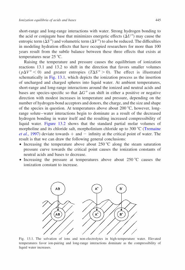
Raising the temperature and pressure causes the equilibrium of ionization

reactions 13.1 and 13.2 to shift in the direction that favors smaller volumes

( pDV o , 0) and greater entropies (TDS o . 0). The effect is illustrated

schematically in Fig. 13.1, which depicts the ionization process as the insertion

of uncharged and charged spheres into liquid water. At ambient temperatures,

short-range and long-range interactions around the ionized and neutral acids and

bases are species-specific so that DG o can shift in either a positive or negative

direction with modest increases in temperature and pressure, depending on the

number of hydrogen-bond acceptors and donors, the charge, and the size and shape

of the species in question. At temperatures above about 200 8C, however, long-

range solute–water interactions begin to dominate as a result of the decreased

hydrogen bonding in water itself and the resulting increased compressibility of

liquid water. Figure 13.2 shows that the standard partial molar volumes of

morpholine and its chloride salt, morpholinium chloride up to 300 8C (Tremaine

et al., 1997) deviate towards þ and 2 infinity at the critical point of water. The

result is that we can draw the following general conclusions:

† Increasing the temperature above about 250 8C along the steam saturation

pressure curve towards the critical point causes the ionization constants of

neutral acids and bases to decrease.

† Increasing the pressure at temperatures above about 250 8C causes the

ionization constant to increase.

Fig. 13.1. The solvation of ions and non-electrolytes in high-temperature water. Elevated

temperatures favor ion-pairing and long-range interactions dominate as the compressibility of

liquid water increases.

Ionization equilibria of acids and bases 445

† At temperatures below 100 8C, ionization behavior is species-specific.

† Ionization constants in the range 100 , t , 250 8C display intermediate

behavior.

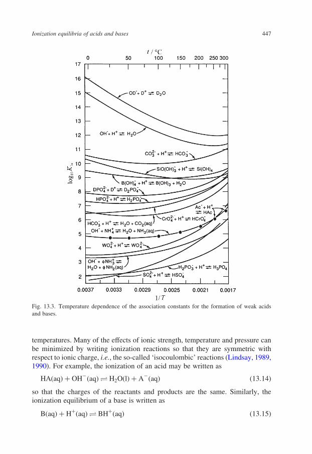
Here and elsewhere, the symbol t is used for temperature in 8C. Typical values

of log10 K for ionization equilibria below 300 8C are plotted as a function of

temperature in Fig. 13.3.

Experimental ionization and association constants have been measured under

supercritical conditions, primarily using the conductivity, heat capacity and

density methods described in a later section and by Mesmer et al. (1991). The

major factors controlling ionization above the critical point of water continue to be

temperature and solvent density, for the reasons described above.

13.1.3.2. Isocoulombic Extrapolations

Experimental measurements of log10 K and the other thermodynamic constants

used in Eq. 13.12 at elevated temperatures and pressures are extremely difficult.

As a result, the standard Gibbs energies of formation, standard enthalpies of

formation and partial molar entropies for many species are known only at ambient

0 50 100 150 200 250 300 3500

25

50

75

100

125

150

Neutral SpeciesC4H8ONH

Ionic SpeciesC4H8ONH2

+Cl–

t / ˚C

V2/(

cm3 .

mol

–1)

Fig. 13.2. Standard partial molar volumes of neutral morpholine and its salt, morpholinium chloride,

showing increasingly large positive and negative deviations as the temperature is raised along the

steam saturation curve (Tremaine et al., 1997). The solid line is a fit to an extended version of the

‘density’ model discussed in the text.

P. Tremaine et al.446

temperatures. Many of the effects of ionic strength, temperature and pressure can

be minimized by writing ionization reactions so that they are symmetric with

respect to ionic charge, i.e., the so-called ‘isocoulombic’ reactions (Lindsay, 1989,

1990). For example, the ionization of an acid may be written as

HAðaqÞ þ OH2ðaqÞO H2OðlÞ þ A2ðaqÞ ð13:14Þ

so that the charges of the reactants and products are the same. Similarly, the

ionization equilibrium of a base is written as

BðaqÞ þ HþðaqÞO BHþðaqÞ ð13:15Þ

Fig. 13.3. Temperature dependence of the association constants for the formation of weak acids

and bases.

Ionization equilibria of acids and bases 447

The equilibrium quotients of neutralization reactions, such as reactions 13.14

and 13.15, are defined as

Q1a;OH ¼ Q1a=Qw ¼mA2

mHAmOH2

ð13:16Þ

and

Q1b;H ¼ Q1b=Qw ¼mBHþ

mBmHþ

ð13:17Þ

with the analogous equations for K1a;OH and K1b;H:For several aqueous systems, both K1a;OH (or K1b;H) and functions for DV o or

DCop have been independently measured. As an example to illustrate the usefulness

of Eq. 13.12, Tremaine et al. (1997) have used the experimental values of V o for

morpholine and the morpholinium ion shown in Fig. 13.2, and values of Cop

obtained below 55 8C, to estimate DCop for the morpholine ionization equilibrium

at high temperatures using the semi-empirical Helgeson–Kirkham–Flowers

(HKF) model. Combining these contributions with that from the first term in

Eq. 13.12 yields log10 K ¼ 24:843 at 300 8C, which is in excellent agreement

with the values 24.79 ^ 0.06 and 24.69 ^ 0.06 measured in KCl media by

Mesmer and Hitch (1977), and in sodium trifluoromethanesulfonate (NaCF3SO3)

by Ridley et al. (2000), respectively.

As a consequence of the symmetry of isocoulombic reactions, plots of

log10 Q1a,OH vs. 1/T are almost linear over a very wide range of temperatures, and

the temperature dependence can be described quite accurately by assuming a

constant mean value of DCop between some condition of T and p, and a reference

condition, Tr and pr:

log10 K1a;OH;T ;p ¼ log10 K1a;OH;Tr;prþ {DHo

Tr;prð1=Tr 2 1=TÞ

þ DCop½ln ðT=TrÞ þ Tr=T 2 1�2 ðDVo=TÞ½p 2 pr�}=ð2:303RÞ

ð13:18Þ

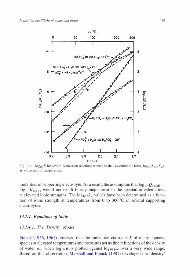
Typical examples are plotted in Fig. 13.4 in their isocoulombic forms. Figure

13.5 shows the temperature dependence of DCop for several of these reactions when

written in the non-isocoulombic and isocoulombic forms. For isocoulombic

equilibria at temperatures below 300 8C, the contribution of DV o to log10 K1a,OH,T

is often less than the experimental uncertainty.

Values of log10 Q1a for ionization reaction 13.1 can be calculated from the

experimentally determined value for the isocoulombic ionization equilibrium (Eq.

13.14), by using the value for the ionization of water at ionic strength I, log10 Qw:

log10 Q1a ¼ log10 Qw þ log10 K1a;OH ðIsocoulombicÞ ð13:19Þ

It has been shown in a number of experimental studies (Mesmer et al., 1988,

1991; Lindsay, 1989, 1990) that for most reactions log10 Q1a,OH is almost

independent of ionic strength for most isocoulombic equilibria at moderate

P. Tremaine et al.448

molalities of supporting electrolyte. As a result, the assumption that log10 Q1a;OH ¼

log10 K1a;OH would not result in any major error in the speciation calculations

at elevated ionic strengths. The log10 Qw values have been determined as a func-

tion of ionic strength at temperatures from 0 to 300 8C in several supporting

electrolytes.

13.1.4. Equations of State

13.1.4.1. The ‘Density’ Model

Franck (1956, 1961) observed that the ionization constants K of many aqueous

species at elevated temperatures and pressures act as linear functions of the density

of water rw, when log10 K is plotted against log10 rw over a very wide range.

Based on this observation, Marshall and Franck (1981) developed the ‘density’

Fig. 13.4. log10 K for several ionization reactions written in the isocoulombic form, log10ðK1a=KwÞ;as a function of temperature.

Ionization equilibria of acids and bases 449

model to represent the ionization constant Kw of water at temperatures up to

1273 K and at pressures up to 1000 MPa. Equations of this form have been used

for representing K of general ionization reactions by Mesmer et al. (1988):

log10 K ¼ a þb

Tþ

c

T2þ

d

T3

� �þ k log10 rw ð13:20Þ

k ¼ e þf

Tþ

g

T2

� �ð13:21Þ

where a, b, c, d, e, f and g are adjustable parameters (a number of these parameters

may be set to zero for many reactions) and rw is the density of pure water

(in g·cm23).

Fig. 13.5. The behavior of DCop for the ionization reactions written in both the non-isocoulombic and

isocoulombic forms, as a function of temperature.

P. Tremaine et al.450

Other thermodynamic quantities can be derived from the above equations. The

Gibbs energy of ionization DG o is related to K by Eq. 13.7, so that

DGo ¼ 22:303RT a þb

Tþ

c

T2þ

d

T3

� �þ e þ

f

Tþ

g

T2

� �log10 rw

� �

ð13:22Þ

The enthalpy of ionization DH o can be obtained from the identity:

›

›T

DGo

T

� �p¼ 2

DHo

T2ð13:23Þ

to yield

DHo ¼ 22:303R b þ2c

Tþ

3d

T2þ f þ

2g

T

� �log10 rw

� �2 RT2kaw ð13:24Þ

where aw ¼ 2ð1=rwÞð›rw=›TÞp is the thermal expansion coefficient of water and

k is the fitted function given in Eq. 13.21.

Similarly, the entropy of ionization DS o, the standard partial molar heat

capacity of ionization DrCpo, and the standard partial molar volume of ionization

DV o can be derived from DG o using standard thermodynamic identities (Mesmer

et al., 1988) so that

DSo ¼ 2:303R a 2c

T22

2d

T3þ e 2

g

T2

� �log10 rw

� �2 RTkaw ð13:25Þ

DCop ¼2 2:303R 2

2c

T22

6d

T32

2g

T2

� �log10 rw

� �

2 Raw 2eT 22g

T

� �2 RT2k

›aw

›T

� �p

ð13:26Þ

DVo ¼ 2RTkbw ð13:27Þ

Here bw ¼ ð1=rwÞð›rw=›pÞT is the compressibility of water.

Equation 13.22 can be further simplified over a restricted region, and the

simplified form has fewer parameters (Anderson et al., 1991). More complex

versions have been adopted to describe DV o accurately at low temperatures

(Clarke et al., 2000). Figure 13.6 shows the behavior of log10 K, DSo, DCop and

DV o for the ionization of ammonia over a wide range of temperature and pressure,

according to the density model fit reported by Mesmer et al. (1988). The functions

for DCop and DV o clearly show the very large electrostriction effects that arise from

the ability of ions to attract increasing numbers of water molecules as the

compressibility of water increases under near critical conditions.

Ionization equilibria of acids and bases 451

Fig. 13.6.

P. Tremaine et al.452

13.1.4.2. The Revised Helgeson–Kirkham–Flowers Model

Helgeson and co-workers (Helgeson et al., 1981; Tanger and Helgeson, 1988)

have developed an equation of state, based on the Born equation for ionic

hydration, which is widely used by geochemists (see Chapter 4 for more details).

Briefly, the HKF model consists of expressions for standard partial heat capacity

and volume functions in Eq. 13.12, and assumes that the standard molar Gibbs

energy and enthalpy of formation of each species at 298.15 K and 0.1 MPa are

known properties.

In this model, the standard molar properties, Y o, of aqueous ions are considered

to have two contributions: an electrostatic term based on the Born equation DYoBorn;

and a non-electrostatic term Yon :

Yo ¼ Yon þ DYo

Born ð13:28Þ

The Born equation describes the Gibbs energy of ionic hydration, i.e., the

transfer of an ion from the ideal gas state to liquid water, by representing the ion as

Fig. 13.6. The behavior of (a) log10 K, (b)DS o and (c)DV o for the association of ammonia over a wide

range of temperature and pressure, according to the density model fit reported by Mesmer et al. (1988).

Ionization equilibria of acids and bases 453

a charged conducting sphere and water as a continuous dielectric medium without

molecular structure. The Born equation takes the form:

DGoBorn ¼ 2veffð1=1r 2 1Þ ð13:29Þ

with

veff ¼NAðzeÞ2

8p10reff

ð13:30Þ

where 1r is the solvent dielectric constant; veff is a term that includes the ionic

charge z, electron charge e, ionic radius reff, permittivity of free space 10 and

Avogadro’s number NA.

The HKF model employs an effective ionic radius, where reff is a linear function

of crystallographic radius rx and charge z, reff ¼ rx þ 0:94lzl (with r in angstroms)

for cations and reff ¼ rx for anions. The revised HKF model (Tanger and

Helgeson, 1988; Shock and Helgeson, 1988) also considered reff to be a function of

T and p. The appropriate temperature and pressure derivatives of DGoBorn yield

expressions for DCop;Born and DVo

Born in terms of the same parameters.

The non-electrostatic term Yon includes three contributions: (i) the intrinsic gas

phase property of the solute, (ii) the change arising from the difference in standard

states between the gas phase and solution, and (iii) short-range hydration effects

(Fernandez-Prini et al., 1992). In the HKF treatment, Yon is used as an empirical

fitting equation with the following form:

Vo ¼ a1 þ a2

1

›2V

›v2þ p

0BBB@

1CCCAþ a3 þ a4

1

Cþ p

� �� �1

T 2Q

� �þ Vo

Born ð13:31Þ

Here Q is a solvent parameter equal to 228 K, which corresponds to the

temperature at which supercooled liquid water may undergo anomalous behavior

(Angell, 1983); C is a similar solvent parameter equal to 2600 bar; and a1, a2, a3

and a4 are temperature- and pressure-independent, but species-dependent, fitting

parameters.

The non-electrostatic contribution DCop;n can be represented by a temperature-

dependent function similar to that used for V o. The pressure dependence of DCop;n

can be derived from the V o expression based on the thermodynamic identity

ð›Cp=›pÞT ¼ 2Tð›2V=›T2Þp to yield the following expression for the entire

standard partial molar heat capacity:

Cop ¼ c1 þ c2

1

T 2Q

� �2

22T1

T 2Q

� �3

a3ðp2 prÞþ a4 lnCþ p

Cþ pr

� �� �þCo

p;Born

ð13:32Þ

P. Tremaine et al.454

Here c1 and c2 are temperature- and pressure-independent, but species-

dependent, parameters; Q is again a parameter with the value of 228 K; pr is

the reference pressure (1 bar); and a3 and a4 are determined by the fits to V o

from Eq. 13.31.

Standard partial molar volumes and heat capacities of aqueous ions and

electrolytes typically exhibit an inverted U-shape as a function of temperature

(Fig. 13.2). This is consistent with the singularity at water’s critical temperature

of 647 K where second-derivative thermodynamic parameters approach þ1,

and with the behavior in supercooled water where these properties also show a

large increase (which may or may not be associated with a singularity near 228 K).

The parameters in the revised HKF model have been selected so that the

electrostatic contribution dominates at high temperatures where the Born model is

most satisfactory, and the non-electrostatic contribution to V o and Cop dominates at

low temperatures. The revised HKF model has been used widely for the

extrapolation of low-temperature standard partial molar properties of aqueous ions

and electrolytes to elevated temperatures and pressures.

The revised HKF model has also been used by Shock and Helgeson (1990)

for the prediction of the standard partial molar properties of neutral aqueous

organic species up to 1273 K and 500 MPa. It was fitted to the available

experimental data for neutral aqueous organic species at elevated temperatures

and pressures. The fitted parameters were then used to develop correlations with

other low-temperature thermodynamic constants. In contrast to the negative

Cop;Born and Vo

Born for aqueous ions and electrolytes, as required by theory, the fitted

Born terms for neutral species can be either positive or negative. According to Eq.

13.30, positive values of Cop;Born and Vo

Born correspond to negative values of veff, so

that z, the effective charge, is an imaginary number. Clearly, the expression for the

electrostatic contribution has no physical meaning, and the validity of the revised

HKF model for neutral species is questionable. The predictive capability stated in

the paper is also limited by the rather sparse experimental data available at the

time the correlations were derived.

13.1.4.3. Fluctuation Solution Theory Models

O’Connell, Wood and their co-workers (Plyasunov et al., 2000a,b; Sedlbauer et al.,

2000) have developed equations of state for aqueous electrolytes and non-

electrolytes based on the approach proposed by O’Connell et al. (1996). This

approach makes use of the dimensionless Krichevskii parameter

A12 ¼Vo

2

kRT¼ lim

n2!0

›ðpV=RTÞ

›n2

� �T ;V;n2

ð13:33Þ

which is a smooth, continuous and finite function, even at the critical point. Here

n2 is the number of moles of solute. The equations are constructed so that they

Ionization equilibria of acids and bases 455

have the correct limiting behavior in dilute solutions of low-pressure steam, i.e.,

they converge to the second cross virial coefficient between the solute and water.

Details are discussed in Chapter 4.

13.1.4.4. Propagation of Error

Uncertainties associated with log10DCop in Eq. 13.9 lead to an uncertainty in the

estimated values for log10 KT,p:

s2log10 K ¼

Xð› log10 K=›xÞ2s2

x ð13:34Þ

where s2x is the variance of independent variable x and s2

log10 K is the variance of

the dependent variable log10 KT,p. For the special case of Eq. 13.12, where DCop is

temperature independent and DV o is small:

s2log10 K ¼ s2

log10 K;298 þ ½ð1=298:15 2 1=TÞ=R�s2H

þ ½{lnðT=298:15Þ þ 298:15=T 2 1}=R�s2Cp

ð13:35Þ

If the uncertainty in DH o at 25 8C is assumed to be 4 kJ·mol21, this leads to an

uncertainty of 0.34 in log10 K at 300 8C. If the uncertainty in DCop is 2 J·K21·mol21

and 10 J·K21·mol21 at 25 and 300 8C, respectively, and linear with respect to

temperature in this temperature range, these uncertainties result in an error of 0.05

in log10 K at 300 8C. This analysis reveals that accurate DH o values for the heat

capacity function at the reference temperature (usually 25 8C) are essential for the

accurate estimation of log10 K using the equations given above.

13.1.5. Activity Coefficients

Equilibrium quotients Q are usually measured in a solution in which ionic strength

is dictated by the addition of supporting electrolytes such as NaCl, KCl or

NaCF3SO3. Clearly, activity coefficient models are needed to extrapolate the Q

values to infinite dilution for such equilibria. A detailed discussion of models that

incorporate pressure and temperature effects has been given by Millero (1979) and

Pitzer (1991). As an example, the following semi-empirical equation has been

widely used to analyze high-temperature potentiometric titration data by the

ORNL group:

log10 Q ¼ log10 K 2 ðDz2Aw=2:303Þ{ffiffiI

p=ð1 þ 1:2

ffiffiI

pÞ þ 1:667 lnð1 þ 1:2

ffiffiI

pÞ}

þ a1I þ a2I2 þ a3FðIÞ þ 0:0157fI ð13:36Þ

Here I is the ionic strength (I ¼ ð1=2ÞP

miz2i ; where the summation extends to

all ions in solution of molality m and charge z), Dz2 ¼P

z2ðproductsÞ2Pz2ðreactantsÞ is related to the coulombic asymmetry of the equilibrium and Aw

represents the Debye–Huckel limiting slope for the osmotic coefficient. The term

P. Tremaine et al.456

f is the osmotic coefficient of the solution, which is only needed for equilibria in

which water is involved. The values of f for NaCl reported by Archer (1992) as a

function of temperature and ionic strength are used as an approximation. The

Debye–Huckel limiting law term in the above equation was proposed by Pitzer

(1991); the function F(I), takes the form:

FðIÞ ¼ ½1 2 ð1 þ 2ffiffiI

p2 2IÞ expð22

ffiffiI

pÞ�=ð4IÞ ð13:37Þ

The quadratic term a2I 2 is not always needed. Because solute ions undergo

specific interactions with the highly charged anions and cations in the supporting

electrolyte, activity coefficients cannot be described solely by the ionic strength of

the medium. However, it has been found that the nature of the supporting

electrolyte (KCl, NaCl or NaCF3SO3) barely affects the value of log10 K.

Practically, Eq. 13.36 with the coefficients reported by the ORNL group can be

used in speciation calculations at ionic strengths up to 5 mol·kg21 (Baes and

Mesmer, 1986).

Concentrated aqueous media containing more than one pair of ions can be

treated with the Pitzer ion interaction theory for activity coefficients. The Pitzer

equation contains many terms that arise from the binary and ternary interactions of

the ions. These parameters are usually determined by fitting the Pitzer equation

to the experimental activity coefficient of a single electrolyte or a common-ion

mixed electrolyte system and can be used to calculate activity coefficients for

more complicated systems. Although the binary and ternary interaction parameters

for many ions are reported at ambient conditions, these parameters for several

important electrolyte systems such as sulfate and phosphate are still not available

at elevated temperatures. Extensive databases for the Pitzer ion interaction model,

as well as its application to modeling industrial and geochemical systems, have

been presented in several reviews (see, e.g., Pitzer, 1991).

† It is very important to use the same activity coefficient model as that used to

treat the original extrapolation of log10 Q to infinite dilution, or errors will

arise from loss of self-consistency.

When no data are available, empirical and semi-empirical approaches can be

used to estimate activity coefficients for concentrated, mixed electrolytes at

elevated temperatures. For many engineering applications (e.g., bulk properties of

steam condensate and boiler water), the aqueous media are rather dilute

(I p 0.01 mol·kg21), so that the Debye–Huckel limiting law provides sufficiently

accurate activity coefficients. The most practical method at low to moderate ionic

strengths (I & 2.0 mol·kg21) is to avoid using any activity coefficient model if

possible by writing each weak acid/base ionization equilibrium in an isocoulombic

fashion and using Eq. 13.18.

When the isocoulombic approximation is not feasible, an approach suggested

by Lindsay (1989, 1990) can be useful in engineering calculations involving acid–

base equilibria. Here, the activity coefficient of a single ion is estimated by using

Ionization equilibria of acids and bases 457

NaCl(aq) as a model system, through the expression:

glzl ¼ g z2

^ðNaClÞ ð13:38Þ

where gjzj is the single-ion activity coefficient for an ion with charge z, and g^(NaCl)

is the activity coefficient of NaCl(aq) at the same temperature and ionic strength.

Within this approximation, the activity coefficient quotient, log10ðgHPO224=

gH2PO4gOH2Þ for H2PO2

4 ðaqÞ þ OH2ðaqÞO HPO224 ðaqÞ; is estimated to be

2 log10 g^(NaCl). It has been shown that this approximation could provide a

reasonable estimation for activity coefficients of electrolytes at ionic strengths up

to about 1.0 mol·kg21 at temperatures in the range 200 , t , 300 8C (Lindsay,

1989, 1990).

13.2. Experimental Methods

13.2.1. Electrical Conductance

The use of electric conductance measurements to determine the degree of

association in aqueous solutions at high temperature was pioneered by Noyes

(1907) and a detailed description of the conductance technique is given in Chapter

10. Throughout the 1950s and 1960s, Franck and Marshall carried out electrical

conductance studies of a number of electrolytes, mostly in the temperature–

pressure ranges of 400–800 8C and 1–400 MPa, using a platinum-lined cell

described by Franck (1956, 1961), Franck et al. (1962) and Quist and Marshall

(1968a). The aqueous electrolytes studied include the alkali metal halides, K2SO4,

KHSO4, HBr and NH3. A modified version of this apparatus was described by Ho

et al. (1994). Much of our knowledge about ion association at temperatures above

200 8C was obtained from these investigations, which were made before other

methods became available.

Measuring the conductance of aqueous solutions under ambient conditions is

straightforward, but specialized techniques are required to extend these techniques

to high temperature and pressure conditions. Experimental challenges include the

need to use corrosion-resistant metals (usually platinum and its alloys), accurate

temperature and pressure control, and electrically insulated high-pressure seals for

the electrodes. Experience has shown that a static apparatus, of the type used by

Quist and Marshall, does not allow accurate measurements for very dilute

solutions, especially under conditions close to the critical temperature of water.

Accurate conductance values for dilute solutions (,1025 mol·kg21) are essential

if one wants to calculate ion association constants, which are independent of

the activity coefficient model chosen. To overcome this problem, Wood and his

co-workers at the University of Delaware and Ho and Palmer at Oak Ridge

P. Tremaine et al.458

National Laboratory have developed flow-through conductance apparatus for

high-temperature applications (Zimmerman et al., 1995; Ho et al., 2000a). The

flow-through cells allow rapid and accurate electric conductance measurements to

be made on aqueous solutions with concentration as low as 4 £ 1028 mol·kg21,

even in the vicinity of the critical point of water. Since then, a number of acids

(HCl), bases (LiOH, KOH and NaOH) and salts (Na2SO4, alkali metal halides)

have been studied (Zimmerman et al., 1995; Gruszkiewicz and Wood, 1997;

Sharygin et al., 2001; Ho et al., 1994, 2000b, 2001; Ho and Palmer, 1995, 1996,

1997, 1998).

Calculating ion association constants from conductivity data is tedious and

difficult, because modern conductance equations for simple electrolyte solutions

often contain several dozen terms (Fernandez-Prini, 1969). Recently, Wood and

co-workers have evaluated several data interpretation strategies for electrolyte

mixtures that use various combinations of mixing rules, theoretical conductance

equations and activity coefficient models (Sharygin et al., 2001). It was found that

the latest conductance equation developed by Turq et al. (1995), together with the

constant-ionic-strength mixing rule, was suitable for treating high-temperature

conductance data for Na2SO4(aq) solutions containing six ionic species, to

calculate ion association constants for species such as the Naþ·SO422(aq) ion pair.

This method should allow rapid and accurate determination of the equilibrium

constant for any association reaction, which changes the concentration of ions in

solution. Conductance techniques are treated in detail in Chapter 10.

13.2.2. The Hydrogen-Electrode Concentration Cell (HECC)

The use of hydrogen electrodes in a concentration cell configuration was

pioneered at Oak Ridge 30 years ago (Mesmer et al., 1970). The design and

function of the HECC have been described in numerous publications (e.g.,

Mesmer et al., 1970; Kettler et al., 1991; Benezeth et al., 1997) and have been

used in a large number of studies of reactions such as acid–base ionization, metal

ion hydrolysis and complexation, solubility measurements and adsorption studies.

A detailed discussion of this cell is given in Chapter 11, but briefly, it consists of a

300 mL or 1 L capacity pressure vessel containing two concentric Teflon cups

separated by a porous Teflon plug, which acts as a liquid junction completing the

electric circuit. Teflon-insulated platinum wires coated with platinum black

protrude into each cup and serve as electrodes. The solutions in each cup are

stirred magnetically. The solution in the inner cup serves as the reference of

known hydrogen ion molality (usually a strong acid or base), whereas the outer

cup contains the test solution in which a titration can be performed. Both solutions

are thoroughly purged with hydrogen at ambient temperature prior to placing the

vessel in the aluminum block tube furnace or oil bath for equilibration at

temperature.

Ionization equilibria of acids and bases 459

The initial configuration of the cell in a typical study of the ionization of a weak

acid, HA, is as follows:

Pt;H2lmHA;mNaCl;mNaATest

llmNaCl;mHClReference

lH2; Pt ð13:39Þ

where NaCl represents a supporting, non-complexing electrolyte, which is ideally

50–100 times more abundant than the other components so that gHþ,test < gHþ,ref

and the liquid junction potential is minimized. Note that the working definition of

pH is pHm ¼ 2log10 mHþ in stoichiometric molal concentration units. The

convention used here is that Hþ is not complexed by the medium ions and ion

pairing is treated implicitly by the activity coefficient model employed.

Each platinum–hydrogen electrode responds to the half-cell reaction:

H2ðgÞ! 2HþðaqÞ þ 2e2 ð13:40Þ

and the difference in potential between the electrodes is described by the Nernst

equation:

DE ¼ 2RT

FlnðmHþ;t=mHþ;rÞ2 Elj ð13:41Þ

where mHþ;t and mHþ;r refer to the stoichiometric molalities of hydrogen ions in the

test and reference compartments, respectively. The stoichiometric molal activity

coefficients of Hþ in the test and reference compartments are assumed to be equal

at all points in the titration. The ideal gas and Faraday constants are designated by

R and F, respectively; T denotes the temperature in kelvin; and Elj represents the

liquid junction potential based on the full Henderson equation (Baes and Mesmer,

1986), which involves the limiting conductivities of the individual ions.

From the measured mHþ together with a solution of known pHm

(; 2 log10 mHþ in molal units) used in the reference cup, and mass and charge

balance constraints, the molal dissociation constant (QHA) for the acid at the ionic

strength of interest can be calculated, typically with an accuracy of about ^0.01 -

log10 units. By varying the total ionic strength from ca. 0.1–5 molal, the pK

value and activity coefficient ratio for the dissociation reaction can be obtained

by regressing the equation log10 QHA ¼ log10 KHA 2 log10ðgHþgA2=gHAÞ using

an appropriate activity coefficient model such as the Pitzer ion interaction

treatment.

13.2.3. Other pH Sensing Electrodes and Reference Electrodes

Over the few past decades, numerous efforts have been made to develop instru-

ments suitable for pH measurements in aqueous fluids at elevated temperatures

and pressures other than the HECC described above. These include:

† yttria-stabilized zirconia (YSZ) membrane electrodes (150–500 8C) (Mac-

Donald et al., 1988; Hettiarachchi et al., 1992; Ding and Seyfried, 1995, 1996;

Lvov et al., 1999);

P. Tremaine et al.460

† metal–metal oxide electrodes (100–300 8C) such as Pt–PtO2, Ir–IrO2, Zr–

ZrO2, Rh–Rh2O3, W/WO3 (e.g., Kriksunov et al., 1994);

† glass electrode (25–200 8C) (Diakonov et al., 1996).

The principles, development, application and limitations of pH-sensing

electrodes and reference electrodes are discussed in detail in Chapter 11.

13.2.4. Spectroscopic Methods

Over the years, there have been a series of attempts to use UV–visible and

Raman spectroscopy to measure equilibrium constants at elevated temperatures,

usually at steam saturation. The availability of stable UV–visible spectrometers

with fast data acquisition has allowed several workers to develop high-pressure

flow systems with on-line injection, using sapphire or quartz windows.

Suleimenov and Seward (1997) have used these to determine ionization and

complexation constants of species where the spectra of the acid and conjugate

base differ in the visible or near-UV. An alternative approach has been taken

by Johnston’s group, who have developed several thermally stable colorimetric

pH indicators for hydrothermal applications (Johnston et al., 1997; Xiang et al.,

1996).

Several researchers have used Raman spectroscopy to study the speciation

of hydrothermal solutions (see, e.g., Rudolph et al., 1997). Because of the small

diameter of the exciting laser beam, cell construction can make use of small

sapphire tubes or diamond windows, thereby simplifying construction and

extending the temperature range. Recent developments in hydrothermal diamond

anvil cells (Bassett et al., 1993), the use of high-pressure flow injection systems

and the availability of Raman microscopes promise to increase the versatility of

this technique as a tool for obtaining ionization constant data under extreme

conditions.

13.2.5. Flow Calorimetry

Flow calorimetry is an important tool for determining the thermodynamic

properties of aqueous solutes under hydrothermal conditions. Two kinds of flow

calorimeters have been used to determine ionization constants. High-pressure

heat-of-mixing calorimeters have been used at Brigham Young University to

determine DrHo of ionization reactions as a function of temperature, up to about

325 8C. These yield DrCop by differentiation. In favorable cases, the instruments

can be operated as titration calorimeters to obtain equilibrium constants directly at

elevated temperature and pressure (Oscarson et al., 1992).

The second method uses heat capacity flow micro-calorimeters and vibrating

tube densimeters to determine the standard partial molar heat capacities and

Ionization equilibria of acids and bases 461

volumes of the acid and conjugate base, Cop and V o, from which Co

p and DrVo

can be calculated for use in Eq. 13.12 (Sedlbauer et al., 2000; Clarke et al., 2000).

The method is particularly attractive because it yields standard partial molar

properties of individual species, so that equations of state can be derived.

13.3. Ionization of Water

13.3.1. log10 Kw as a Function of Temperature and Pressure

A number of research groups have used EMF methods, conductivity, calorimetry

and spectroscopy to determine values of log10 Qw, which corresponds to the self-

ionization reaction:

H2OðlÞO HþðaqÞ þ OH2ðaqÞ ð13:42Þ

at elevated temperatures, as a function of ionic strength. The critical review

by Marshall and Franck (1981) contains most of the modern values, and

a comprehensive, weighted fit of the infinite-dilution values, log10 Kw, to the

density model (Eq. 13.21):

log10 Kw ¼ 24:098 2 3245:2=ðT=KÞ þ 2:2362 £ 105=ðT=KÞ2

2 3:984 £ 107=ðT=KÞ3 þ ½13:957 2 1262:3=ðT=KÞ

þ 8:5641 £ 105=ðT=KÞ2� log10 rw ð13:43Þ

The temperature- and pressure-dependence of log10 Kw yields values of DH o,

DS o, DCop and DV o up to 1000 8C and 1 GPa. IAPWS has adopted the Marshall–

Franck formulation as its ‘best’ values for log10 Kw vs. T and p for densities

.0.35 g·cm23.

Mesmer, Baes and others at Oak Ridge National Laboratory have measured

ionization constants for water, log10 Qw, vs. I in KCl, NaCl and NaCF3SO3 media

from 0 to 300 8C, and the corresponding values of DH o, DS o, DCop and DV o

(Sweeton et al., 1974; Busey and Mesmer, 1978; Palmer and Drummond, 1988).

These are not entirely consistent with the IAPWS selection of Marshall and

Franck’s values for the ion product of water, but they are complete, internally

consistent with each other, and have been used as the de facto standard by most

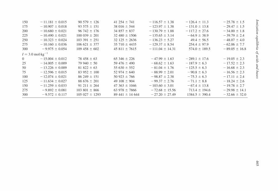
other workers. Values of log10 Qw vs. I are listed in Table 13.1. Olofsson and

Hepler (1975) reported a critical evaluation of the consistency of the available data

with the calorimetric results, and found them to be in very good agreement. Values

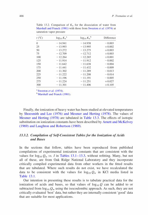
of log10 Kw from Sweeton et al. (1974) are compared with those of Marshall and

Franck (1981) in Table 13.2.

P. Tremaine et al.462

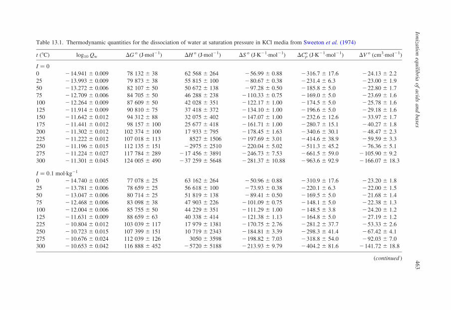
Table 13.1. Thermodynamic quantities for the dissociation of water at saturation pressure in KCl media from Sweeton et al. (1974)

t (8C) log10 Qw DG o (J·mol21) DH o (J·mol21) DS o (J·K21·mol21) DCpo (J·K21·mol21) DV o (cm3·mol21)

I ¼ 0

0 214.941 ^ 0.009 78 132 ^ 38 62 568 ^ 264 256.99 ^ 0.88 2316.7 ^ 17.6 224.13 ^ 2.2

25 213.993 ^ 0.009 79 873 ^ 38 55 815 ^ 100 280.67 ^ 0.38 2231.4 ^ 6.3 223.00 ^ 1.9

50 213.272 ^ 0.006 82 107 ^ 50 50 672 ^ 138 297.28 ^ 0.50 2185.8 ^ 5.0 222.80 ^ 1.7

75 212.709 ^ 0.006 84 705 ^ 50 46 288 ^ 238 2110.33 ^ 0.75 2169.0 ^ 5.0 223.69 ^ 1.6

100 212.264 ^ 0.009 87 609 ^ 50 42 028 ^ 351 2122.17 ^ 1.00 2174.5 ^ 5.0 225.78 ^ 1.6

125 211.914 ^ 0.009 90 810 ^ 75 37 418 ^ 372 2134.10 ^ 1.00 2196.6 ^ 5.0 229.18 ^ 1.6

150 211.642 ^ 0.012 94 312 ^ 88 32 075 ^ 402 2147.07 ^ 1.00 2232.6 ^ 12.6 233.97 ^ 1.7

175 211.441 ^ 0.012 98 157 ^ 100 25 677 ^ 418 2161.71 ^ 1.00 2280.7 ^ 15.1 240.27 ^ 1.8

200 211.302 ^ 0.012 102 374 ^ 100 17 933 ^ 795 2178.45 ^ 1.63 2340.6 ^ 30.1 248.47 ^ 2.3

225 211.222 ^ 0.012 107 018 ^ 113 8527 ^ 1506 2197.69 ^ 3.01 2414.6 ^ 38.9 259.59 ^ 3.3

250 211.196 ^ 0.015 112 135 ^ 151 22975 ^ 2510 2220.04 ^ 5.02 2511.3 ^ 45.2 276.36 ^ 5.1

275 211.224 ^ 0.027 117 784 ^ 289 217 456 ^ 3891 2246.73 ^ 7.53 2661.5 ^ 59.0 2105.90 ^ 9.2

300 211.301 ^ 0.045 124 005 ^ 490 237 259 ^ 5648 2281.37 ^ 10.88 2963.6 ^ 92.9 2166.07 ^ 18.3

I ¼ 0:1 mol·kg21

0 214.740 ^ 0.005 77 078 ^ 25 63 162 ^ 264 250.96 ^ 0.88 2310.9 ^ 17.6 223.20 ^ 1.8

25 213.781 ^ 0.006 78 659 ^ 25 56 618 ^ 100 273.93 ^ 0.38 2220.1 ^ 6.3 222.00 ^ 1.5

50 213.047 ^ 0.006 80 714 ^ 25 51 819 ^ 138 289.41 ^ 0.50 2169.5 ^ 5.0 221.68 ^ 1.4

75 212.468 ^ 0.006 83 098 ^ 38 47 903 ^ 226 2101.09 ^ 0.75 2148.1 ^ 5.0 222.38 ^ 1.3

100 212.004 ^ 0.006 85 755 ^ 50 44 229 ^ 351 2111.29 ^ 1.00 2148.5 ^ 3.8 224.20 ^ 1.2

125 211.631 ^ 0.009 88 659 ^ 63 40 338 ^ 414 2121.38 ^ 1.13 2164.8 ^ 5.0 227.19 ^ 1.2

225 210.804 ^ 0.012 103 039 ^ 117 17 979 ^ 1381 2170.75 ^ 2.76 2281.2 ^ 37.7 253.33 ^ 2.6

250 210.723 ^ 0.015 107 399 ^ 151 10 719 ^ 2343 2184.81 ^ 3.39 2298.3 ^ 41.4 267.42 ^ 4.1

275 210.676 ^ 0.024 112 039 ^ 126 3050 ^ 3598 2198.82 ^ 7.03 2318.8 ^ 54.0 292.03 ^ 7.0

300 210.653 ^ 0.042 116 888 ^ 452 25720 ^ 5188 2213.93 ^ 9.79 2404.2 ^ 81.6 2141.72 ^ 18.8

(continued )

Ion

izatio

neq

uilib

riao

fa

cids

an

db

ases

46

3

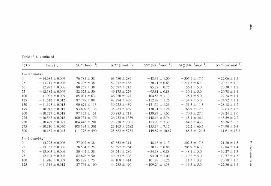
Table 13.1. continued

t (8C) log10 Qw DG o (J·mol21) DH o (J·mol21) DS o (J·K21·mol21) DCpo (J·K21·mol21) DV o (cm3·mol21)

I ¼ 0:5 mol·kg21

0 214.684 ^ 0.009 76 785 ^ 38 63 580 ^ 289 248.37 ^ 1.00 2305.9 ^ 17.6 222.06 ^ 1.5

25 213.717 ^ 0.006 78 295 ^ 38 57 212 ^ 188 270.71 ^ 0.63 2211.3 ^ 6.3 220.77 ^ 1.2

50 212.973 ^ 0.006 80 257 ^ 38 52 697 ^ 213 285.27 ^ 0.75 2156.1 ^ 5.0 220.30 ^ 1.2

75 212.382 ^ 0.009 82 525 ^ 50 49 175 ^ 276 295.81 ^ 0.88 2130.1 ^ 5.0 220.78 ^ 1.1

100 211.903 ^ 0.009 85 031 ^ 63 46 020 ^ 377 2104.56 ^ 1.13 2125.1 ^ 5.0 222.24 ^ 1.1

125 211.512 ^ 0.012 87 747 ^ 88 42 794 ^ 439 2112.88 ^ 1.26 2134.7 ^ 5.0 224.72 ^ 1.1

150 211.193 ^ 0.015 90 671 ^ 113 39 225 ^ 439 2121.59 ^ 1.26 2151.5 ^ 11.3 228.18 ^ 1.2

175 210.943 ^ 0.015 93 809 ^ 138 35 233 ^ 439 2130.71 ^ 1.26 2166.9 ^ 12.6 232.63 ^ 1.3

200 210.727 ^ 0.018 97 173 ^ 151 30 983 ^ 711 2139.87 ^ 1.63 2170.3 ^ 27.6 238.24 ^ 1.6

225 210.563 ^ 0.018 100 734 ^ 176 26 932 ^ 1339 2148.16 ^ 2.76 2148.1 ^ 36.4 245.59 ^ 2.2

250 210.429 ^ 0.021 104 445 ^ 201 23 928 ^ 2301 2153.93 ^ 3.39 284.5 ^ 43.9 256.36 ^ 3.5

275 210.310 ^ 0.030 108 194 ^ 301 23 163 ^ 3682 2155.14 ^ 7.15 32.2 ^ 66.5 274.90 ^ 6.4

300 210.187 ^ 0.045 111 776 ^ 490 25 882 ^ 5732 2149.87 ^ 10.67 188.3 ^ 120.5 2111.61 ^ 13.2

I ¼ 1:0 mol·kg21

0 214.725 ^ 0.006 77 002 ^ 38 63 852 ^ 314 248.16 ^ 1.13 2302.5 ^ 17.6 221.20 ^ 1.5

25 213.753 ^ 0.006 78 504 ^ 25 57 597 ^ 264 270.12 ^ 0.88 2205.9 ^ 6.3 219.84 ^ 1.4

50 213.003 ^ 0.006 80 442 ^ 38 53 241 ^ 289 284.18 ^ 0.88 2148.1 ^ 5.0 219.27 ^ 1.3

75 212.404 ^ 0.006 82 676 ^ 50 49 953 ^ 326 294.01 ^ 1.00 2119.2 ^ 5.0 219.57 ^ 1.3

100 211.916 ^ 0.009 85 128 ^ 75 47 108 ^ 414 2101.88 ^ 1.26 2111.3 ^ 3.8 220.78 ^ 1.3

125 211.514 ^ 0.012 87 764 ^ 100 44 283 ^ 490 2109.20 ^ 1.38 2116.3 ^ 5.0 222.86 ^ 1.4

P.

Trem

ain

eet

al.

46

4

150 211.181 ^ 0.015 90 579 ^ 126 41 254 ^ 741 2116.57 ^ 1.38 2126.4 ^ 11.3 225.78 ^ 1.5

175 210.907 ^ 0.018 93 575 ^ 151 38 016 ^ 544 2123.97 ^ 1.38 2131.0 ^ 13.8 229.47 ^ 1.5

200 210.680 ^ 0.021 96 742 ^ 176 34 857 ^ 837 2130.79 ^ 1.88 2117.2 ^ 27.6 234.00 ^ 1.8

225 210.490 ^ 0.021 100 039 ^ 201 32 480 ^ 1506 2135.65 ^ 3.14 264.9 ^ 38.9 239.79 ^ 2.4

250 210.323 ^ 0.024 103 391 ^ 251 32 125 ^ 2636 2136.23 ^ 5.27 49.4 ^ 56.5 248.07 ^ 4.0

275 210.160 ^ 0.036 106 621 ^ 377 35 710 ^ 4435 2129.37 ^ 8.54 254.4 ^ 97.9 262.06 ^ 7.7

300 29.975 ^ 0.054 109 458 ^ 602 45 811 ^ 7615 2111.04 ^ 14.31 574.0 ^ 189.5 289.05 ^ 16.8

I ¼ 3:0 mol·kg21

0 215.004 ^ 0.012 78 458 ^ 63 65 346 ^ 226 247.99 ^ 1.63 2289.1 ^ 17.6 219.05 ^ 2.3

25 214.005 ^ 0.009 79 940 ^ 50 59 476 ^ 490 268.62 ^ 1.63 2187.9 ^ 6.3 217.52 ^ 2.3

50 213.226 ^ 0.009 81 822 ^ 63 55 630 ^ 552 281.04 ^ 1.76 2125.5 ^ 6.3 216.68 ^ 2.3

75 212.596 ^ 0.015 83 952 ^ 100 52 974 ^ 640 288.99 ^ 2.01 290.8 ^ 6.3 216.56 ^ 2.3

100 212.074 ^ 0.021 86 249 ^ 151 50 923 ^ 766 298.87 ^ 2.38 275.3 ^ 6.3 217.11 ^ 2.4

125 211.634 ^ 0.027 88 676 ^ 201 49 108 ^ 904 299.37 ^ 2.76 271.1 ^ 8.8 218.24 ^ 2.6

150 211.259 ^ 0.033 91 211 ^ 264 47 363 ^ 1046 2103.60 ^ 3.01 267.4 ^ 13.8 219.78 ^ 2.7

275 29.892 ^ 0.081 103 801 ^ 866 63 978 ^ 7866 272.68 ^ 15.56 713.4 ^ 194.6 229.98 ^ 14.1

300 29.572 ^ 0.117 105 027 ^ 1293 89 441 ^ 14 644 227.20 ^ 27.49 1384.5 ^ 390.4 232.66 ^ 32.0

Ion

izatio

neq

uilib

riao

fa

cids

an

db

ases

46

5

Finally, the ionization of heavy water has been studied at elevated temperatures

by Shoesmith and Lee (1976) and Mesmer and Herting (1978). The values of

Mesmer and Herting (1978) are tabulated in Table 13.3. The effects of isotopic

substitution on ionization constants have been described by Arnett and McKelvey

(1969) and Laughton and Robertson (1969).

13.3.2. Compilation of Self-Consistent Tables for the Ionization of Acidsand Bases

In the sections that follow, tables have been reproduced from published

compilations of experimental ionization constants that are consistent with the

values for log10 Qw vs. I in Tables 13.1–13.3, without refitting. Many, but not

all of these, are from Oak Ridge National Laboratory and they incorporate

critically compiled experimental data from other workers in the fitted results

that are tabulated. Where such results do not exist, we have recalculated the

data to be consistent with the values for log10 Qw in KCl media listed in

Table 13.1.

Our intention in presenting these results is to tabulate practical data for the

ionization of acids and bases, so that values of log10 Q can be added to or

subtracted from log10 Qw using the isocoulombic approach. As such, they are not

critically evaluated ‘best’ data, but rather they are internally consistent ‘good’ data

that are suitable for most applications.

Table 13.2. Comparison of Kw for the dissociation of water from

Marshall and Franck (1981) with those from Sweeton et al. (1974) at

saturation vapor pressure

t (8C) log10 Kwa log10 Kw

b Difference

0 214.941 214.938 20.003

25 213.993 213.995 þ0.002

50 213.272 213.275 þ0.003

75 212.709 212.712 þ0.003

100 212.264 212.265 þ0.001

125 211.914 211.912 20.002

150 211.642 211.638 20.004

175 211.441 211.432 20.009

200 211.302 211.289 20.013

225 211.222 211.208 20.014

250 211.196 211.191 20.005

275 211.224 211.251 þ0.027

300 211.301 211.406 þ0.105

a Sweeton et al. (1974).b Marshall and Franck (1981).

P. Tremaine et al.466

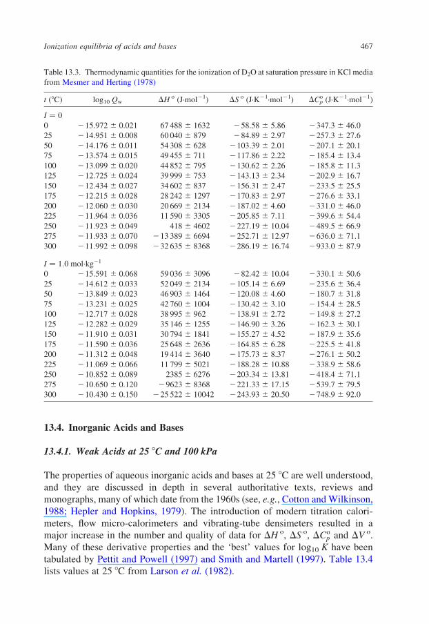
13.4. Inorganic Acids and Bases

13.4.1. Weak Acids at 25 8C and 100 kPa

The properties of aqueous inorganic acids and bases at 25 8C are well understood,

and they are discussed in depth in several authoritative texts, reviews and

monographs, many of which date from the 1960s (see, e.g., Cotton and Wilkinson,

1988; Hepler and Hopkins, 1979). The introduction of modern titration calori-

meters, flow micro-calorimeters and vibrating-tube densimeters resulted in a

major increase in the number and quality of data for DH o, DS o, DCop and DV o.

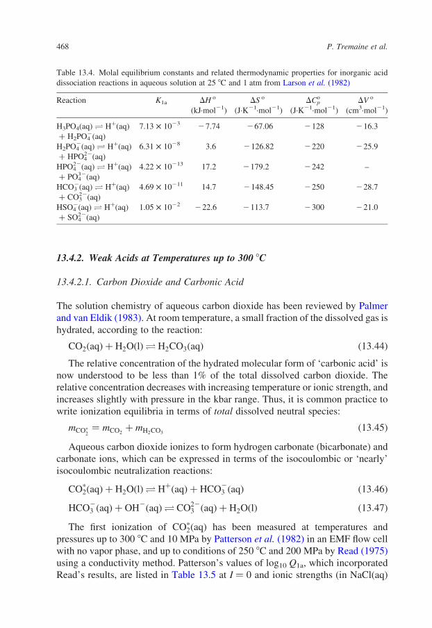
Many of these derivative properties and the ‘best’ values for log10 K have been

tabulated by Pettit and Powell (1997) and Smith and Martell (1997). Table 13.4

lists values at 25 8C from Larson et al. (1982).

Table 13.3. Thermodynamic quantities for the ionization of D2O at saturation pressure in KCl media

from Mesmer and Herting (1978)

t (8C) log10 Qw DH o (J·mol21) DS o (J·K21·mol21) DCpo (J·K21·mol21)

I ¼ 0

0 215.972 ^ 0.021 67 488 ^ 1632 258.58 ^ 5.86 2347.3 ^ 46.0

25 214.951 ^ 0.008 60 040 ^ 879 284.89 ^ 2.97 2257.3 ^ 27.6

50 214.176 ^ 0.011 54 308 ^ 628 2103.39 ^ 2.01 2207.1 ^ 20.1

75 213.574 ^ 0.015 49 455 ^ 711 2117.86 ^ 2.22 2185.4 ^ 13.4

100 213.099 ^ 0.020 44 852 ^ 795 2130.62 ^ 2.26 2185.8 ^ 11.3

125 212.725 ^ 0.024 39 999 ^ 753 2143.13 ^ 2.34 2202.9 ^ 16.7

150 212.434 ^ 0.027 34 602 ^ 837 2156.31 ^ 2.47 2233.5 ^ 25.5

175 212.215 ^ 0.028 28 242 ^ 1297 2170.83 ^ 2.97 2276.6 ^ 33.1

200 212.060 ^ 0.030 20 669 ^ 2134 2187.02 ^ 4.60 2331.0 ^ 46.0

225 211.964 ^ 0.036 11 590 ^ 3305 2205.85 ^ 7.11 2399.6 ^ 54.4

250 211.923 ^ 0.049 418 ^ 4602 2227.19 ^ 10.04 2489.5 ^ 66.9

275 211.933 ^ 0.070 213 389 ^ 6694 2252.71 ^ 12.97 2636.0 ^ 71.1

300 211.992 ^ 0.098 232 635 ^ 8368 2286.19 ^ 16.74 2933.0 ^ 87.9

I ¼ 1:0 mol·kg21

0 215.591 ^ 0.068 59 036 ^ 3096 282.42 ^ 10.04 2330.1 ^ 50.6

25 214.612 ^ 0.033 52 049 ^ 2134 2105.14 ^ 6.69 2235.6 ^ 36.4

50 213.849 ^ 0.023 46 903 ^ 1464 2120.08 ^ 4.60 2180.7 ^ 31.8

75 213.231 ^ 0.025 42 760 ^ 1004 2130.42 ^ 3.10 2154.4 ^ 28.5

100 212.717 ^ 0.028 38 995 ^ 962 2138.91 ^ 2.72 2149.8 ^ 27.2

125 212.282 ^ 0.029 35 146 ^ 1255 2146.90 ^ 3.26 2162.3 ^ 30.1

150 211.910 ^ 0.031 30 794 ^ 1841 2155.27 ^ 4.52 2187.9 ^ 35.6

175 211.590 ^ 0.036 25 648 ^ 2636 2164.85 ^ 6.28 2225.5 ^ 41.8

200 211.312 ^ 0.048 19 414 ^ 3640 2175.73 ^ 8.37 2276.1 ^ 50.2

225 211.069 ^ 0.066 11 799 ^ 5021 2188.28 ^ 10.88 2338.9 ^ 58.6

250 210.852 ^ 0.089 2385 ^ 6276 2203.34 ^ 13.81 2418.4 ^ 71.1

275 210.650 ^ 0.120 29623 ^ 8368 2221.33 ^ 17.15 2539.7 ^ 79.5

300 210.430 ^ 0.150 225 522 ^ 10042 2243.93 ^ 20.50 2748.9 ^ 92.0

Ionization equilibria of acids and bases 467

13.4.2. Weak Acids at Temperatures up to 300 8C

13.4.2.1. Carbon Dioxide and Carbonic Acid

The solution chemistry of aqueous carbon dioxide has been reviewed by Palmer

and van Eldik (1983). At room temperature, a small fraction of the dissolved gas is

hydrated, according to the reaction:

CO2ðaqÞ þ H2OðlÞO H2CO3ðaqÞ ð13:44Þ

The relative concentration of the hydrated molecular form of ‘carbonic acid’ is

now understood to be less than 1% of the total dissolved carbon dioxide. The

relative concentration decreases with increasing temperature or ionic strength, and

increases slightly with pressure in the kbar range. Thus, it is common practice to

write ionization equilibria in terms of total dissolved neutral species:

mCOp2¼ mCO2

þ mH2CO3ð13:45Þ

Aqueous carbon dioxide ionizes to form hydrogen carbonate (bicarbonate) and

carbonate ions, which can be expressed in terms of the isocoulombic or ‘nearly’

isocoulombic neutralization reactions:

COp2ðaqÞ þ H2OðlÞO HþðaqÞ þ HCO2

3 ðaqÞ ð13:46Þ

HCO23 ðaqÞ þ OH2ðaqÞO CO22

3 ðaqÞ þ H2OðlÞ ð13:47Þ

The first ionization of COp2ðaqÞ has been measured at temperatures and

pressures up to 300 8C and 10 MPa by Patterson et al. (1982) in an EMF flow cell

with no vapor phase, and up to conditions of 250 8C and 200 MPa by Read (1975)

using a conductivity method. Patterson’s values of log10 Q1a, which incorporated

Read’s results, are listed in Table 13.5 at I ¼ 0 and ionic strengths (in NaCl(aq)

Table 13.4. Molal equilibrium constants and related thermodynamic properties for inorganic acid

dissociation reactions in aqueous solution at 25 8C and 1 atm from Larson et al. (1982)

Reaction K1a DH o

(kJ·mol21)

DS o

(J·K21·mol21)

DCpo

(J·K21·mol21)

DV o

(cm3·mol21)

H3PO4(aq) O Hþ(aq)

þ H2PO42(aq)

7.13 £ 1023 27.74 267.06 2128 216.3

H2PO42(aq) O Hþ(aq)

þ HPO422(aq)

6.31 £ 1028 3.6 2126.82 2220 225.9

HPO422(aq) O Hþ(aq)

þ PO432(aq)

4.22 £ 10213 17.2 2179.2 2242 –

HCO32(aq) O Hþ(aq)

þ CO322(aq)

4.69 £ 10211 14.7 2148.45 2250 228.7

HSO42(aq) O Hþ(aq)

þ SO422(aq)

1.05 £ 1022 222.6 2113.7 2300 221.0

P. Tremaine et al.468

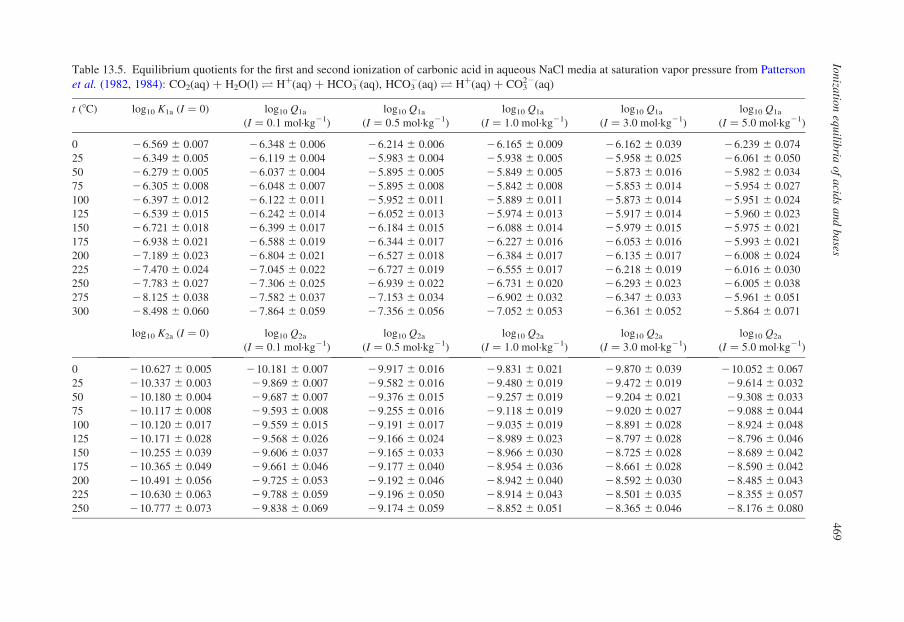
Table 13.5. Equilibrium quotients for the first and second ionization of carbonic acid in aqueous NaCl media at saturation vapor pressure from Patterson

et al. (1982, 1984): CO2(aq) þ H2O(l) O Hþ(aq) þ HCO32(aq), HCO3

2(aq) O Hþ(aq) þ CO322(aq)

t (8C) log10 K1a (I ¼ 0) log10 Q1a

(I ¼ 0:1 mol·kg21)

log10 Q1a

(I ¼ 0:5 mol·kg21)

log10 Q1a

(I ¼ 1:0 mol·kg21)

log10 Q1a

(I ¼ 3:0 mol·kg21)

log10 Q1a

(I ¼ 5:0 mol·kg21)

0 26.569 ^ 0.007 26.348 ^ 0.006 26.214 ^ 0.006 26.165 ^ 0.009 26.162 ^ 0.039 26.239 ^ 0.074

25 26.349 ^ 0.005 26.119 ^ 0.004 25.983 ^ 0.004 25.938 ^ 0.005 25.958 ^ 0.025 26.061 ^ 0.050

50 26.279 ^ 0.005 26.037 ^ 0.004 25.895 ^ 0.005 25.849 ^ 0.005 25.873 ^ 0.016 25.982 ^ 0.034

75 26.305 ^ 0.008 26.048 ^ 0.007 25.895 ^ 0.008 25.842 ^ 0.008 25.853 ^ 0.014 25.954 ^ 0.027

100 26.397 ^ 0.012 26.122 ^ 0.011 25.952 ^ 0.011 25.889 ^ 0.011 25.873 ^ 0.014 25.951 ^ 0.024

125 26.539 ^ 0.015 26.242 ^ 0.014 26.052 ^ 0.013 25.974 ^ 0.013 25.917 ^ 0.014 25.960 ^ 0.023

150 26.721 ^ 0.018 26.399 ^ 0.017 26.184 ^ 0.015 26.088 ^ 0.014 25.979 ^ 0.015 25.975 ^ 0.021

175 26.938 ^ 0.021 26.588 ^ 0.019 26.344 ^ 0.017 26.227 ^ 0.016 26.053 ^ 0.016 25.993 ^ 0.021

200 27.189 ^ 0.023 26.804 ^ 0.021 26.527 ^ 0.018 26.384 ^ 0.017 26.135 ^ 0.017 26.008 ^ 0.024

225 27.470 ^ 0.024 27.045 ^ 0.022 26.727 ^ 0.019 26.555 ^ 0.017 26.218 ^ 0.019 26.016 ^ 0.030

250 27.783 ^ 0.027 27.306 ^ 0.025 26.939 ^ 0.022 26.731 ^ 0.020 26.293 ^ 0.023 26.005 ^ 0.038

275 28.125 ^ 0.038 27.582 ^ 0.037 27.153 ^ 0.034 26.902 ^ 0.032 26.347 ^ 0.033 25.961 ^ 0.051

300 28.498 ^ 0.060 27.864 ^ 0.059 27.356 ^ 0.056 27.052 ^ 0.053 26.361 ^ 0.052 25.864 ^ 0.071

log10 K2a (I ¼ 0) log10 Q2a

(I ¼ 0:1 mol·kg21)

log10 Q2a

(I ¼ 0:5 mol·kg21)

log10 Q2a

(I ¼ 1:0 mol·kg21)

log10 Q2a

(I ¼ 3:0 mol·kg21)

log10 Q2a

(I ¼ 5:0 mol·kg21)

0 210.627 ^ 0.005 210.181 ^ 0.007 29.917 ^ 0.016 29.831 ^ 0.021 29.870 ^ 0.039 210.052 ^ 0.067

25 210.337 ^ 0.003 29.869 ^ 0.007 29.582 ^ 0.016 29.480 ^ 0.019 29.472 ^ 0.019 29.614 ^ 0.032

50 210.180 ^ 0.004 29.687 ^ 0.007 29.376 ^ 0.015 29.257 ^ 0.019 29.204 ^ 0.021 29.308 ^ 0.033

75 210.117 ^ 0.008 29.593 ^ 0.008 29.255 ^ 0.016 29.118 ^ 0.019 29.020 ^ 0.027 29.088 ^ 0.044

100 210.120 ^ 0.017 29.559 ^ 0.015 29.191 ^ 0.017 29.035 ^ 0.019 28.891 ^ 0.028 28.924 ^ 0.048

125 210.171 ^ 0.028 29.568 ^ 0.026 29.166 ^ 0.024 28.989 ^ 0.023 28.797 ^ 0.028 28.796 ^ 0.046

150 210.255 ^ 0.039 29.606 ^ 0.037 29.165 ^ 0.033 28.966 ^ 0.030 28.725 ^ 0.028 28.689 ^ 0.042

175 210.365 ^ 0.049 29.661 ^ 0.046 29.177 ^ 0.040 28.954 ^ 0.036 28.661 ^ 0.028 28.590 ^ 0.042

200 210.491 ^ 0.056 29.725 ^ 0.053 29.192 ^ 0.046 28.942 ^ 0.040 28.592 ^ 0.030 28.485 ^ 0.043

225 210.630 ^ 0.063 29.788 ^ 0.059 29.196 ^ 0.050 28.914 ^ 0.043 28.501 ^ 0.035 28.355 ^ 0.057

250 210.777 ^ 0.073 29.838 ^ 0.069 29.174 ^ 0.059 28.852 ^ 0.051 28.365 ^ 0.046 28.176 ^ 0.080

Ion

izatio

neq

uilib

riao

fa

cids

an

db

ases

46

9

media) up to 5.0 mol·kg21. The second ionization constant, which has been

measured to 250 8C by Patterson et al. (1984), decreases with increasing tempera-

ture for reasons outlined earlier.

13.4.2.2. Phosphoric Acid

The sodium salts of aqueous phosphoric acid are widely used as pH buffers in the

boiler water of thermal electric power stations. Phosphoric acid ionizes according

to the reactions:

H3PO4ðaqÞ þ OH2ðaqÞO H2PO24 ðaqÞ þ H2OðlÞ ð13:48Þ

H2PO24 ðaqÞ þ OH2ðaqÞO HPO22

4 ðaqÞ þ H2OðlÞ ð13:49Þ

HPO224 ðaqÞ þ OH2ðaqÞO PO32

4 ðaqÞ þ H2OðlÞ ð13:50Þ

The first and second dissociation equilibria, reactions 13.48 and 13.49, have

been determined potentiometrically at temperatures up to 300 8C by Mesmer and

Baes (1974). Their values of log10 Q1a,OH and log10 Q2a,OH at ionic strengths in

KCl(aq) up to 1.0 mol·kg21 are listed in Table 13.6. The third ionization constant

is expected to decrease with increasing temperature. Values have been estimated

by Lindsay (1990) and Shock and Helgeson (1988).

13.4.2.3. Hydrogen Sulfate Ion

Sulfuric acid, H2SO4(aq), is considered to be a strong acid, which ionizes

according to the reaction:

H2SO4ðaqÞO HSO24 ðaqÞ þ HþðaqÞ ð13:51Þ

Colorimetric measurements of the pH of ammonia/sulfuric acid mixtures by

Xiang et al. (1996) yielded values for the first dissociation constant of H2SO4(aq)

from 350 to 400 8C.

The hydrogen sulfate (‘bisulfate’) ion is a moderately strong acid, which is

found in boilers and in the feed-train of nuclear and thermal electric power stations

as an impurity from condenser leaks. The HSO24 ion is iso-electronic with

perchlorate ClO24 and, as a result, it can be used as a non-complexing ion for high-

temperature experiments (Rudolph et al., 1997). The ionization of hydrogen

sulfate has been studied as the reaction:

HSO24 ðaqÞO HþðaqÞ þ SO22

4 ðaqÞ ð13:52Þ

up to 250 8C by Dickson et al. (1990). The values for log10 Q2a at ionic strengths in

NaCl(aq) up to 5.0 mol·kg21 are tabulated in Table 13.7.

P. Tremaine et al.470

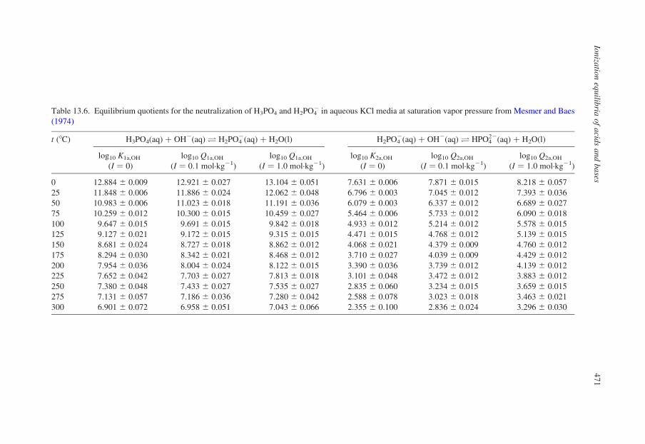
Table 13.6. Equilibrium quotients for the neutralization of H3PO4 and H2PO42 in aqueous KCl media at saturation vapor pressure from Mesmer and Baes

(1974)

t (8C) H3PO4(aq) þ OH2(aq) O H2PO42(aq) þ H2O(l) H2PO4

2(aq) þ OH2(aq) O HPO422(aq) þ H2O(l)

log10 K1a,OH

(I ¼ 0)

log10 Q1a,OH

(I ¼ 0:1 mol·kg21)

log10 Q1a,OH

(I ¼ 1:0 mol·kg21)

log10 K2a,OH

(I ¼ 0)

log10 Q2a,OH

(I ¼ 0:1 mol·kg21)

log10 Q2a,OH

(I ¼ 1:0 mol·kg21)

0 12.884 ^ 0.009 12.921 ^ 0.027 13.104 ^ 0.051 7.631 ^ 0.006 7.871 ^ 0.015 8.218 ^ 0.057

25 11.848 ^ 0.006 11.886 ^ 0.024 12.062 ^ 0.048 6.796 ^ 0.003 7.045 ^ 0.012 7.393 ^ 0.036

50 10.983 ^ 0.006 11.023 ^ 0.018 11.191 ^ 0.036 6.079 ^ 0.003 6.337 ^ 0.012 6.689 ^ 0.027

75 10.259 ^ 0.012 10.300 ^ 0.015 10.459 ^ 0.027 5.464 ^ 0.006 5.733 ^ 0.012 6.090 ^ 0.018

100 9.647 ^ 0.015 9.691 ^ 0.015 9.842 ^ 0.018 4.933 ^ 0.012 5.214 ^ 0.012 5.578 ^ 0.015

125 9.127 ^ 0.021 9.172 ^ 0.015 9.315 ^ 0.015 4.471 ^ 0.015 4.768 ^ 0.012 5.139 ^ 0.015

150 8.681 ^ 0.024 8.727 ^ 0.018 8.862 ^ 0.012 4.068 ^ 0.021 4.379 ^ 0.009 4.760 ^ 0.012

175 8.294 ^ 0.030 8.342 ^ 0.021 8.468 ^ 0.012 3.710 ^ 0.027 4.039 ^ 0.009 4.429 ^ 0.012

200 7.954 ^ 0.036 8.004 ^ 0.024 8.122 ^ 0.015 3.390 ^ 0.036 3.739 ^ 0.012 4.139 ^ 0.012

225 7.652 ^ 0.042 7.703 ^ 0.027 7.813 ^ 0.018 3.101 ^ 0.048 3.472 ^ 0.012 3.883 ^ 0.012

250 7.380 ^ 0.048 7.433 ^ 0.027 7.535 ^ 0.027 2.835 ^ 0.060 3.234 ^ 0.015 3.659 ^ 0.015

275 7.131 ^ 0.057 7.186 ^ 0.036 7.280 ^ 0.042 2.588 ^ 0.078 3.023 ^ 0.018 3.463 ^ 0.021

300 6.901 ^ 0.072 6.958 ^ 0.051 7.043 ^ 0.066 2.355 ^ 0.100 2.836 ^ 0.024 3.296 ^ 0.030

Ion

izatio

neq

uilib

riao

fa

cids

an

db

ases

47

1

Table 13.7. Equilibrium quotients for the hydrogen sulfate ionization in aqueous NaCl media at saturation vapor pressure from Dickson et al. (1990):

HSO42(aq) O Hþ(aq) þ SO4

22(aq)

t

(8C)

log10 K2a

(I ¼ 0)

log10 Q2a

(I ¼ 0:1 mol·kg21)

log10 Q2a

(I ¼ 0:5 mol·kg21)

log10 Q2a

(I ¼ 1:0 mol·kg21)

log10 Q2a

(I ¼ 3:0 mol·kg21)

log10 Q2a

(I ¼ 5:0 mol·kg21)

0 21.659 ^ 0.030 21.198 ^ 0.030 20.900 ^ 0.030 20.788 ^ 0.031 20.737 ^ 0.032 20.806 ^ 0.032

25 21.964 ^ 0.018 21.487 ^ 0.017 21.178 ^ 0.017 21.055 ^ 0.018 20.971 ^ 0.019 21.010 ^ 0.019

50 22.316 ^ 0.012 21.817 ^ 0.010 21.493 ^ 0.009 21.358 ^ 0.010 21.238 ^ 0.011 21.250 ^ 0.011

75 22.686 ^ 0.009 22.161 ^ 0.007 21.817 ^ 0.005 21.669 ^ 0.005 21.511 ^ 0.007 21.495 ^ 0.006

100 23.061 ^ 0.008 22.504 ^ 0.006 22.135 ^ 0.004 21.972 ^ 0.004 21.775 ^ 0.006 21.730 ^ 0.005

125 23.436 ^ 0.007 22.840 ^ 0.005 22.442 ^ 0.003 22.261 ^ 0.003 22.020 ^ 0.005 21.946 ^ 0.005

150 23.809 ^ 0.007 23.167 ^ 0.005 22.735 ^ 0.003 22.533 ^ 0.003 22.244 ^ 0.005 22.140 ^ 0.004

175 24.182 ^ 0.007 23.488 ^ 0.006 23.015 ^ 0.004 22.788 ^ 0.004 22.446 ^ 0.005 22.309 ^ 0.005

200 24.561 ^ 0.008 23.804 ^ 0.006 23.282 ^ 0.004 23.027 ^ 0.004 22.624 ^ 0.005 22.450 ^ 0.005

225 24.951 ^ 0.009 24.118 ^ 0.007 23.537 ^ 0.005 23.248 ^ 0.005 22.775 ^ 0.006 22.560 ^ 0.006

250 25.355 ^ 0.012 24.432 ^ 0.010 23.778 ^ 0.009 23.447 ^ 0.009 22.892 ^ 0.011 22.629 ^ 0.012

P.

Trem

ain

eet

al.

47

2

13.4.2.4. Hydrogen Sulfide

It is not possible to study the ionization of hydrogen sulfide in electrochemical or

conductivity cells that contain platinum electrodes. Suleimenov and Seward

(1997) have circumvented this problem by determining the degree of ionization of

H2S/HS2 buffers by UV–visible spectrophotometry at temperatures up to 350 8C.

The resulting values for log10 K1a are listed in Table 13.8, for the reaction:

H2SðaqÞO HþðaqÞ þ HS2ðaqÞ ð13:53Þ

The further ionization of HS2(aq) to form the sulfide ion:

HS2ðaqÞO S22ðaqÞ þ HþðaqÞ ð13:54Þ

has been shown to be negligible, even in very concentrated solutions of base (Rao

and Hepler, 1977; Giggenbach, 1971). The destabilization of polyvalent ions in

high-temperature water is expected to make S22(aq) even more unstable.

13.4.2.5. Nitric Acid

The ionization constant of nitric acid has been determined at temperatures from

250 to 320 8C by Oscarson et al. (1992) by using flow calorimetry to determine

enthalpies of dilution as a function of nitric acid molality for the ionization

reaction:

HNO3ðaqÞO NO23 ðaqÞ þ HþðaqÞ ð13:55Þ

Table 13.8. First ionization constant of H2S (molal) and ionization constant of HNO3 from

Suleimenov and Seward (1997) and Oscarson et al. (1992)

t (8C) H2S(aq) O Hþ(aq) þ HS2(aq) HNO3(aq) O Hþ(aq) þ NO32(aq)

p (MPa) log10 K1a log10 K1a (p ¼ psata) p (MPa) log10 K1a

25 10 26.96 ^ 0.022 26.99

50 10 26.66 ^ 0.018 26.68

100 10 26.46 ^ 0.013 26.49

150 10 26.47 ^ 0.019 26.49

200 10 26.70 ^ 0.023 26.73

250 10 27.16 ^ 0.076 27.19 10.3 21

275 11 21.42

300 11 27.87 ^ 0.076 27.89 11 21.92

319 12.8 22.39

350 20 28.77 ^ 0.051 28.89

a Saturation vapor pressure.

Ionization equilibria of acids and bases 473

The results are consistent with earlier high-temperature conductance (Noyes,

1907) and solubility (Marshall and Slusher, 1975a,b) studies, which show that

nitric acid becomes an increasingly weak acid at elevated temperature as do all

acids, and that undissociated HNO3 is an important species above about 250 8C.

Values for log10 K1a are reported in Table 13.8. Chlistunoff et al. (1999) have used

UV–visible spectroscopy to determine equilibrium constants for the reactions by

which HNO3(aq) converts to the more reduced species HNO2(aq) and NO(aq) in

supercritical water.

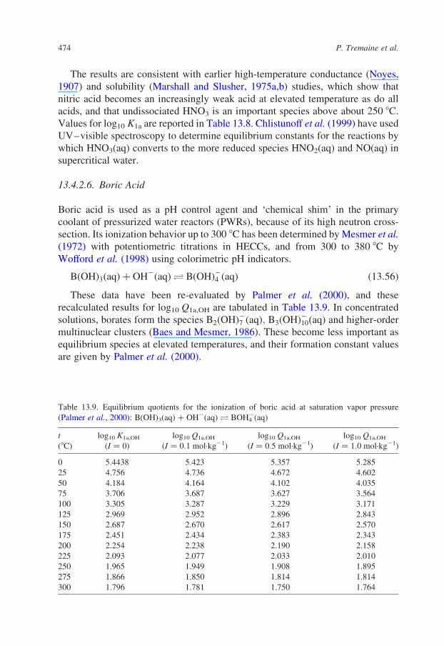
13.4.2.6. Boric Acid

Boric acid is used as a pH control agent and ‘chemical shim’ in the primary

coolant of pressurized water reactors (PWRs), because of its high neutron cross-

section. Its ionization behavior up to 300 8C has been determined by Mesmer et al.

(1972) with potentiometric titrations in HECCs, and from 300 to 380 8C by

Wofford et al. (1998) using colorimetric pH indicators.

BðOHÞ3ðaqÞ þ OH2ðaqÞO BðOHÞ24 ðaqÞ ð13:56Þ

These data have been re-evaluated by Palmer et al. (2000), and these

recalculated results for log10 Q1a,OH are tabulated in Table 13.9. In concentrated

solutions, borates form the species B2ðOHÞ27 ðaqÞ; B3ðOHÞ210ðaqÞ and higher-order

multinuclear clusters (Baes and Mesmer, 1986). These become less important as

equilibrium species at elevated temperatures, and their formation constant values

are given by Palmer et al. (2000).

Table 13.9. Equilibrium quotients for the ionization of boric acid at saturation vapor pressure

(Palmer et al., 2000): B(OH)3(aq) þ OH2(aq) O BOH42(aq)

t

(8C)

log10 K1a,OH

(I ¼ 0)

log10 Q1a,OH

(I ¼ 0:1 mol·kg21)

log10 Q1a,OH

(I ¼ 0:5 mol·kg21)

log10 Q1a,OH

(I ¼ 1:0 mol·kg21)

0 5.4438 5.423 5.357 5.285

25 4.756 4.736 4.672 4.602

50 4.184 4.164 4.102 4.035

75 3.706 3.687 3.627 3.564

100 3.305 3.287 3.229 3.171

125 2.969 2.952 2.896 2.843

150 2.687 2.670 2.617 2.570

175 2.451 2.434 2.383 2.343

200 2.254 2.238 2.190 2.158

225 2.093 2.077 2.033 2.010

250 1.965 1.949 1.908 1.895

275 1.866 1.850 1.814 1.814

300 1.796 1.781 1.750 1.764

P. Tremaine et al.474

13.4.2.7. Silicic Acid

The ionization of silicic acid is one of the most important reactions in geo-

chemistry, as it is responsible for the enhanced solubility of quartz and other

silicate minerals at high pH. Busey and Mesmer (1977) used potentiometric

titrations to determine log10 Q1a,OH for the reaction:

SiðOHÞ4ðaqÞ þ OH2ðaqÞO SiOðOHÞ23 ðaqÞ þ H2OðlÞ ð13:57Þ

The results are listed in Table 13.10 at ionic strengths in NaCl(aq) up to

5.0 mol·kg21. Silicates also form the multimeric clusters in concentrated solutions

(Baes and Mesmer, 1986). Like the polynuclear borates, polysilicates are less

stable at elevated temperatures.

13.4.3. Weak and ‘Almost Strong’ Acids and Bases at Temperaturesto Supercritical Conditions

13.4.3.1. Hydrochloric Acid

Like nitric acid, HCl(aq) becomes a weak acid at elevated temperatures and

pressures. Heat of dilution studies (Holmes et al., 1987) have shown that

the association of hydrochloric acid under subcritical conditions becomes

important at temperatures above about 250 8C. The degree of ionization of

HCl(aq) in the supercritical region has been studied by a number of authors using

conductance methods. Recent high-resolution conductance measurements by Ho

et al. (2001) have resolved earlier discrepancies, and values of 2 log10 K1a for the

association reaction:

HþðaqÞ þ Cl2ðaqÞO HClðaqÞ ð13:58Þ

from this work are presented in Table 13.11. Mesmer et al. (1988, 1991) have used

a treatment based on a fit of the density model to earlier experimental data to

describe the factors that affect the association of HCl(aq) in the sub- and super-

critical regions.

13.4.3.2. Alkali Metal Hydroxides

The ionization properties of the alkali metal hydroxides LiOH, NaOH and KOH

are of much importance because LiOH(aq) is used under subcritical conditions to

control the pH of the primary coolant circuits in nuclear reactors, while NaOH(aq)

and KOH(aq) are common components of geologic fluids that formed under

supercritical conditions. Conductance measurements by a number of groups have

shown that association increases at elevated temperatures for reasons similar to

those for HCl(aq) (Mesmer et al., 1991). Tables 13.12 and 13.13 list values for the

Ionization equilibria of acids and bases 475

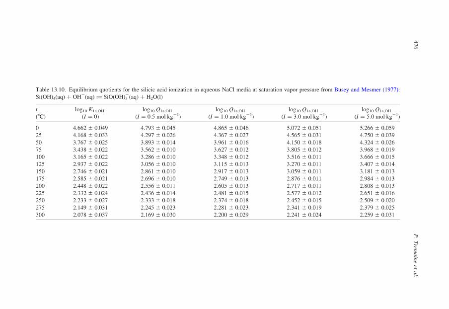
Table 13.10. Equilibrium quotients for the silicic acid ionization in aqueous NaCl media at saturation vapor pressure from Busey and Mesmer (1977):

Si(OH)4(aq) þ OH2(aq) O SiO(OH)32(aq) þ H2O(l)

t

(8C)

log10 K1a,OH

(I ¼ 0)

log10 Q1a,OH

(I ¼ 0:5 mol·kg21)

log10 Q1a,OH

(I ¼ 1:0 mol·kg21)

log10 Q1a,OH

(I ¼ 3:0 mol·kg21)

log10 Q1a,OH

(I ¼ 5:0 mol·kg21)

0 4.662 ^ 0.049 4.793 ^ 0.045 4.865 ^ 0.046 5.072 ^ 0.051 5.266 ^ 0.059

25 4.168 ^ 0.033 4.297 ^ 0.026 4.367 ^ 0.027 4.565 ^ 0.031 4.750 ^ 0.039

50 3.767 ^ 0.025 3.893 ^ 0.014 3.961 ^ 0.016 4.150 ^ 0.018 4.324 ^ 0.026

75 3.438 ^ 0.022 3.562 ^ 0.010 3.627 ^ 0.012 3.805 ^ 0.012 3.968 ^ 0.019

100 3.165 ^ 0.022 3.286 ^ 0.010 3.348 ^ 0.012 3.516 ^ 0.011 3.666 ^ 0.015

125 2.937 ^ 0.022 3.056 ^ 0.010 3.115 ^ 0.013 3.270 ^ 0.011 3.407 ^ 0.014

150 2.746 ^ 0.021 2.861 ^ 0.010 2.917 ^ 0.013 3.059 ^ 0.011 3.181 ^ 0.013

175 2.585 ^ 0.021 2.696 ^ 0.010 2.749 ^ 0.013 2.876 ^ 0.011 2.984 ^ 0.013

200 2.448 ^ 0.022 2.556 ^ 0.011 2.605 ^ 0.013 2.717 ^ 0.011 2.808 ^ 0.013

225 2.332 ^ 0.024 2.436 ^ 0.014 2.481 ^ 0.015 2.577 ^ 0.012 2.651 ^ 0.016

250 2.233 ^ 0.027 2.333 ^ 0.018 2.374 ^ 0.018 2.452 ^ 0.015 2.509 ^ 0.020

275 2.149 ^ 0.031 2.245 ^ 0.023 2.281 ^ 0.023 2.341 ^ 0.019 2.379 ^ 0.025

300 2.078 ^ 0.037 2.169 ^ 0.030 2.200 ^ 0.029 2.241 ^ 0.024 2.259 ^ 0.031

P.

Trem

ain

eet

al.

47

6

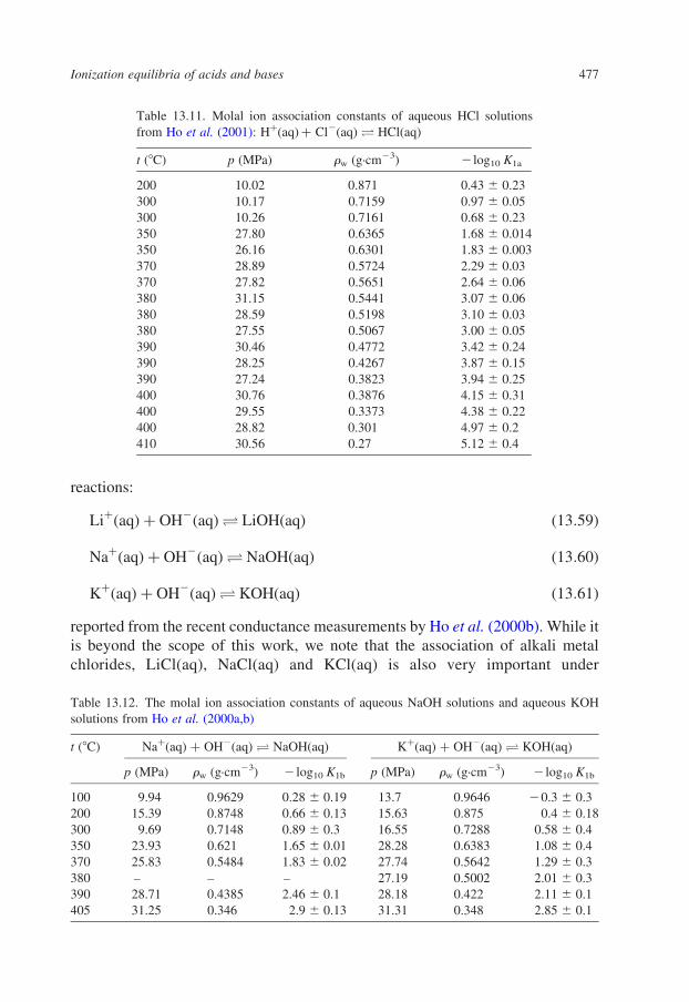
reactions:

LiþðaqÞ þ OH2ðaqÞO LiOHðaqÞ ð13:59Þ

NaþðaqÞ þ OH2ðaqÞO NaOHðaqÞ ð13:60Þ

KþðaqÞ þ OH2ðaqÞO KOHðaqÞ ð13:61Þ

reported from the recent conductance measurements by Ho et al. (2000b). While it

is beyond the scope of this work, we note that the association of alkali metal

chlorides, LiCl(aq), NaCl(aq) and KCl(aq) is also very important under

Table 13.12. The molal ion association constants of aqueous NaOH solutions and aqueous KOH

solutions from Ho et al. (2000a,b)

t (8C) Naþ(aq) þ OH2(aq) O NaOH(aq) Kþ(aq) þ OH2(aq) O KOH(aq)

p (MPa) rw (g·cm23) 2 log10 K1b p (MPa) rw (g·cm23) 2 log10 K1b

100 9.94 0.9629 0.28 ^ 0.19 13.7 0.9646 20.3 ^ 0.3

200 15.39 0.8748 0.66 ^ 0.13 15.63 0.875 0.4 ^ 0.18

300 9.69 0.7148 0.89 ^ 0.3 16.55 0.7288 0.58 ^ 0.4

350 23.93 0.621 1.65 ^ 0.01 28.28 0.6383 1.08 ^ 0.4

370 25.83 0.5484 1.83 ^ 0.02 27.74 0.5642 1.29 ^ 0.3

380 – – – 27.19 0.5002 2.01 ^ 0.3

390 28.71 0.4385 2.46 ^ 0.1 28.18 0.422 2.11 ^ 0.1

405 31.25 0.346 2.9 ^ 0.13 31.31 0.348 2.85 ^ 0.1

Table 13.11. Molal ion association constants of aqueous HCl solutions

from Ho et al. (2001): Hþ(aq)þ Cl2(aq) O HCl(aq)

t (8C) p (MPa) rw (g·cm23) 2 log10 K1a

200 10.02 0.871 0.43 ^ 0.23

300 10.17 0.7159 0.97 ^ 0.05

300 10.26 0.7161 0.68 ^ 0.23

350 27.80 0.6365 1.68 ^ 0.014

350 26.16 0.6301 1.83 ^ 0.003

370 28.89 0.5724 2.29 ^ 0.03

370 27.82 0.5651 2.64 ^ 0.06

380 31.15 0.5441 3.07 ^ 0.06

380 28.59 0.5198 3.10 ^ 0.03

380 27.55 0.5067 3.00 ^ 0.05

390 30.46 0.4772 3.42 ^ 0.24

390 28.25 0.4267 3.87 ^ 0.15

390 27.24 0.3823 3.94 ^ 0.25

400 30.76 0.3876 4.15 ^ 0.31

400 29.55 0.3373 4.38 ^ 0.22

400 28.82 0.301 4.97 ^ 0.2

410 30.56 0.27 5.12 ^ 0.4

Ionization equilibria of acids and bases 477

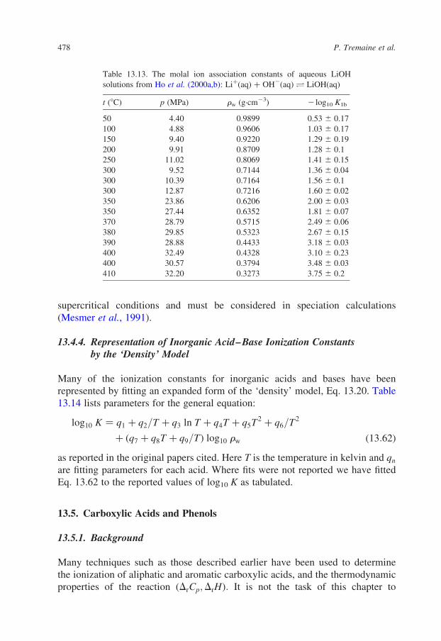
supercritical conditions and must be considered in speciation calculations

(Mesmer et al., 1991).

13.4.4. Representation of Inorganic Acid–Base Ionization Constantsby the ‘Density’ Model

Many of the ionization constants for inorganic acids and bases have been

represented by fitting an expanded form of the ‘density’ model, Eq. 13.20. Table

13.14 lists parameters for the general equation:

log10 K ¼ q1 þ q2=T þ q3 ln T þ q4T þ q5T2 þ q6=T2

þ ðq7 þ q8T þ q9=TÞ log10 rw ð13:62Þ

as reported in the original papers cited. Here T is the temperature in kelvin and qn

are fitting parameters for each acid. Where fits were not reported we have fitted

Eq. 13.62 to the reported values of log10 K as tabulated.

13.5. Carboxylic Acids and Phenols

13.5.1. Background

Many techniques such as those described earlier have been used to determine

the ionization of aliphatic and aromatic carboxylic acids, and the thermodynamic

properties of the reaction ðDrCp;DrHÞ: It is not the task of this chapter to

Table 13.13. The molal ion association constants of aqueous LiOH

solutions from Ho et al. (2000a,b): Liþ(aq) þ OH2(aq) O LiOH(aq)

t (8C) p (MPa) rw (g·cm23) 2 log10 K1b

50 4.40 0.9899 0.53 ^ 0.17

100 4.88 0.9606 1.03 ^ 0.17

150 9.40 0.9220 1.29 ^ 0.19

200 9.91 0.8709 1.28 ^ 0.1

250 11.02 0.8069 1.41 ^ 0.15

300 9.52 0.7144 1.36 ^ 0.04

300 10.39 0.7164 1.56 ^ 0.1

300 12.87 0.7216 1.60 ^ 0.02

350 23.86 0.6206 2.00 ^ 0.03

350 27.44 0.6352 1.81 ^ 0.07

370 28.79 0.5715 2.49 ^ 0.06

380 29.85 0.5323 2.67 ^ 0.15

390 28.88 0.4433 3.18 ^ 0.03

400 32.49 0.4328 3.10 ^ 0.23

400 30.57 0.3794 3.48 ^ 0.03

410 32.20 0.3273 3.75 ^ 0.2

P. Tremaine et al.478

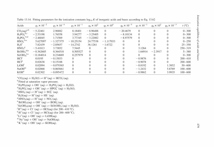
Table 13.14. Fitting parameters for the ionization constants log10 K of inorganic acids and bases according to Eq. 13.62

Acids q1 £ 1022 q2 £ 1024 q3 £ 1021 q4 £ 102 q5 £ 104 q6 £ 1025 q7 £ 1021 q8 £ 102 q9 £ 1023 t (8C)

CO2(aq)a,b 25.22461 2.96882 8.18401 28.96488 0 220.4679 0 0 0 0–300

H3PO4b,c 22.53198 1.76558 3.94277 23.25405 0 28.10134 0 0 0 0–300

H2PO42b,d 22.46045 1.71569 3.77345 23.22082 0 28.97579 0 0 0 0–300

HSO42b,e 5.627097 21.327375 210.25154 24.77538 21.117033 0 0 0 0 0–250

H2Sf 7.82439 22.05657 214.2742 36.1261 21.6722 0 0 0 0 25–350

HNO3g 25.41813 3.73852 7.5445 0 0 0 3.1264 0 0 250–319

B(OH)3b,h 20.362605 0.364518 0.505527 0 0 0 1.64914 22.3917 0 5–380

Si(OH)4b,i 20.184014 0.234669 0.257979 0 0 0 0 0 0 0–300

HClj 0.0195 20.13033 0 0 0 0 20.9876 0 0 200–410

HClk 0.02638 20.15188 0 0 0 0 20.9078 0 0 200–600

LiOHl 0.02094 20.079365 0 0 0 0 20.8192 0 1.3852 50–600

NaOHm 0.02068 20.065661 0 0 0 0 21.2432 0 5.8769 100–600

KOHn 0.02302 20.095472 0 0 0 0 20.9862 0 3.9935 100–600

a CO2(aq) þ H2O(l) O Hþ(aq) þ HCO32(aq).

b Fitted at saturation vapor pressure.c H3PO4(aq) þ OH2(aq) O H2PO4

2(aq) þ H2O(l).d H2PO4

2(aq) þ OH2(aq) O HPO422(aq) þ H2O(l).

e HSO42(aq) O Hþ(aq) þ SO4

22(aq).f H2S(aq) O Hþ(aq) þ HS2(aq).g HNO3(aq) O Hþ(aq) þ NO3

2(aq).h B(OH)3(aq) þ OH2(aq) O BOH4

2(aq).i Si(OH)4(aq) þ OH2(aq) O SiO(OH)3

2(aq) þ H2O(l).j Hþ(aq) þ Cl2(aq) O HCl(aq) (for 200–410 8C).k Hþ(aq) þ Cl2(aq) O HCl(aq) (for 200–600 8C).l Liþ(aq) þ OH2(aq) O LiOH(aq).m Naþ(aq) þ OH2(aq) O NaOH(aq).n Kþ(aq) þ OH2(aq) O KOH(aq).

Ion

izatio

neq

uilib

riao

fa

cids

an

db

ases

47

9

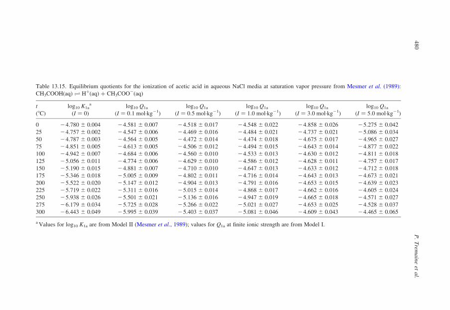
Table 13.15. Equilibrium quotients for the ionization of acetic acid in aqueous NaCl media at saturation vapor pressure from Mesmer et al. (1989):

CH3COOH(aq) O Hþ(aq) þ CH3COO2(aq)

t

(8C)

log10 K1aa

(I ¼ 0)

log10 Q1a

(I ¼ 0:1 mol·kg21)

log10 Q1a

(I ¼ 0:5 mol·kg21)

log10 Q1a

(I ¼ 1:0 mol·kg21)

log10 Q1a

(I ¼ 3:0 mol·kg21)

log10 Q1a

(I ¼ 5:0 mol·kg21)

0 24.780 ^ 0.004 24.581 ^ 0.007 24.518 ^ 0.017 24.548 ^ 0.022 24.858 ^ 0.026 25.275 ^ 0.042

25 24.757 ^ 0.002 24.547 ^ 0.006 24.469 ^ 0.016 24.484 ^ 0.021 24.737 ^ 0.021 25.086 ^ 0.034

50 24.787 ^ 0.003 24.564 ^ 0.005 24.472 ^ 0.014 24.474 ^ 0.018 24.675 ^ 0.017 24.965 ^ 0.027

75 24.851 ^ 0.005 24.613 ^ 0.005 24.506 ^ 0.012 24.494 ^ 0.015 24.643 ^ 0.014 24.877 ^ 0.022

100 24.942 ^ 0.007 24.684 ^ 0.006 24.560 ^ 0.010 24.533 ^ 0.013 24.630 ^ 0.012 24.811 ^ 0.018

125 25.056 ^ 0.011 24.774 ^ 0.006 24.629 ^ 0.010 24.586 ^ 0.012 24.628 ^ 0.011 24.757 ^ 0.017

150 25.190 ^ 0.015 24.881 ^ 0.007 24.710 ^ 0.010 24.647 ^ 0.013 24.633 ^ 0.012 24.712 ^ 0.018

175 25.346 ^ 0.018 25.005 ^ 0.009 24.802 ^ 0.011 24.716 ^ 0.014 24.643 ^ 0.013 24.673 ^ 0.021

200 25.522 ^ 0.020 25.147 ^ 0.012 24.904 ^ 0.013 24.791 ^ 0.016 24.653 ^ 0.015 24.639 ^ 0.023

225 25.719 ^ 0.022 25.311 ^ 0.016 25.015 ^ 0.014 24.868 ^ 0.017 24.662 ^ 0.016 24.605 ^ 0.024

250 25.938 ^ 0.026 25.501 ^ 0.021 25.136 ^ 0.016 24.947 ^ 0.019 24.665 ^ 0.018 24.571 ^ 0.027

275 26.179 ^ 0.034 25.725 ^ 0.028 25.266 ^ 0.022 25.021 ^ 0.027 24.653 ^ 0.025 24.528 ^ 0.037

300 26.443 ^ 0.049 25.995 ^ 0.039 25.403 ^ 0.037 25.081 ^ 0.046 24.609 ^ 0.043 24.465 ^ 0.065

a Values for log10 K1a are from Model II (Mesmer et al., 1989); values for Q1a at finite ionic strength are from Model I.

P.

Trem

ain

eet

al.

48

0

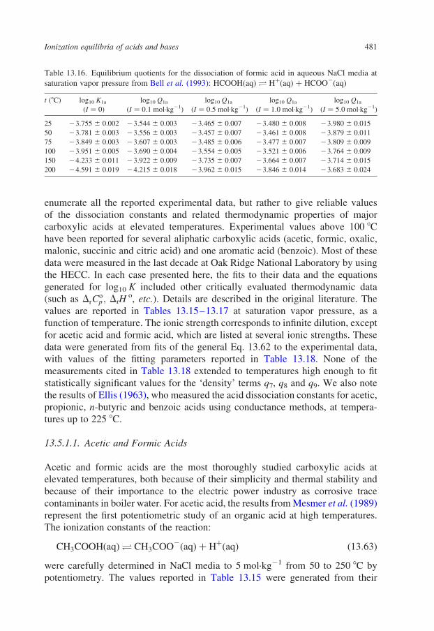
enumerate all the reported experimental data, but rather to give reliable values

of the dissociation constants and related thermodynamic properties of major

carboxylic acids at elevated temperatures. Experimental values above 100 8C

have been reported for several aliphatic carboxylic acids (acetic, formic, oxalic,

malonic, succinic and citric acid) and one aromatic acid (benzoic). Most of these

data were measured in the last decade at Oak Ridge National Laboratory by using

the HECC. In each case presented here, the fits to their data and the equations

generated for log10 K included other critically evaluated thermodynamic data

(such as DrCop; DrH

o, etc.). Details are described in the original literature. The

values are reported in Tables 13.15–13.17 at saturation vapor pressure, as a

function of temperature. The ionic strength corresponds to infinite dilution, except

for acetic acid and formic acid, which are listed at several ionic strengths. These

data were generated from fits of the general Eq. 13.62 to the experimental data,

with values of the fitting parameters reported in Table 13.18. None of the

measurements cited in Table 13.18 extended to temperatures high enough to fit

statistically significant values for the ‘density’ terms q7, q8 and q9. We also note

the results of Ellis (1963), who measured the acid dissociation constants for acetic,

propionic, n-butyric and benzoic acids using conductance methods, at tempera-

tures up to 225 8C.

13.5.1.1. Acetic and Formic Acids

Acetic and formic acids are the most thoroughly studied carboxylic acids at

elevated temperatures, both because of their simplicity and thermal stability and

because of their importance to the electric power industry as corrosive trace

contaminants in boiler water. For acetic acid, the results from Mesmer et al. (1989)

represent the first potentiometric study of an organic acid at high temperatures.

The ionization constants of the reaction:

CH3COOHðaqÞO CH3COO2ðaqÞ þ HþðaqÞ ð13:63Þ

were carefully determined in NaCl media to 5 mol·kg21 from 50 to 250 8C by

potentiometry. The values reported in Table 13.15 were generated from their

Table 13.16. Equilibrium quotients for the dissociation of formic acid in aqueous NaCl media at

saturation vapor pressure from Bell et al. (1993): HCOOH(aq) O Hþ(aq) þ HCOO2(aq)

t (8C) log10 K1a

(I ¼ 0)

log10 Q1a

(I ¼ 0:1 mol·kg21)

log10 Q1a

(I ¼ 0:5 mol·kg21)

log10 Q1a

(I ¼ 1:0 mol·kg21)

log10 Q1a

(I ¼ 5:0 mol·kg21)

25 23.755 ^ 0.002 23.544 ^ 0.003 23.465 ^ 0.007 23.480 ^ 0.008 23.980 ^ 0.015

50 23.781 ^ 0.003 23.556 ^ 0.003 23.457 ^ 0.007 23.461 ^ 0.008 23.879 ^ 0.011

75 23.849 ^ 0.003 23.607 ^ 0.003 23.485 ^ 0.006 23.477 ^ 0.007 23.809 ^ 0.009

100 23.951 ^ 0.005 23.690 ^ 0.004 23.554 ^ 0.005 23.521 ^ 0.006 23.764 ^ 0.009

150 24.233 ^ 0.011 23.922 ^ 0.009 23.735 ^ 0.007 23.664 ^ 0.007 23.714 ^ 0.015

200 24.591 ^ 0.019 24.215 ^ 0.018 23.962 ^ 0.015 23.846 ^ 0.014 23.683 ^ 0.024

Ionization equilibria of acids and bases 481

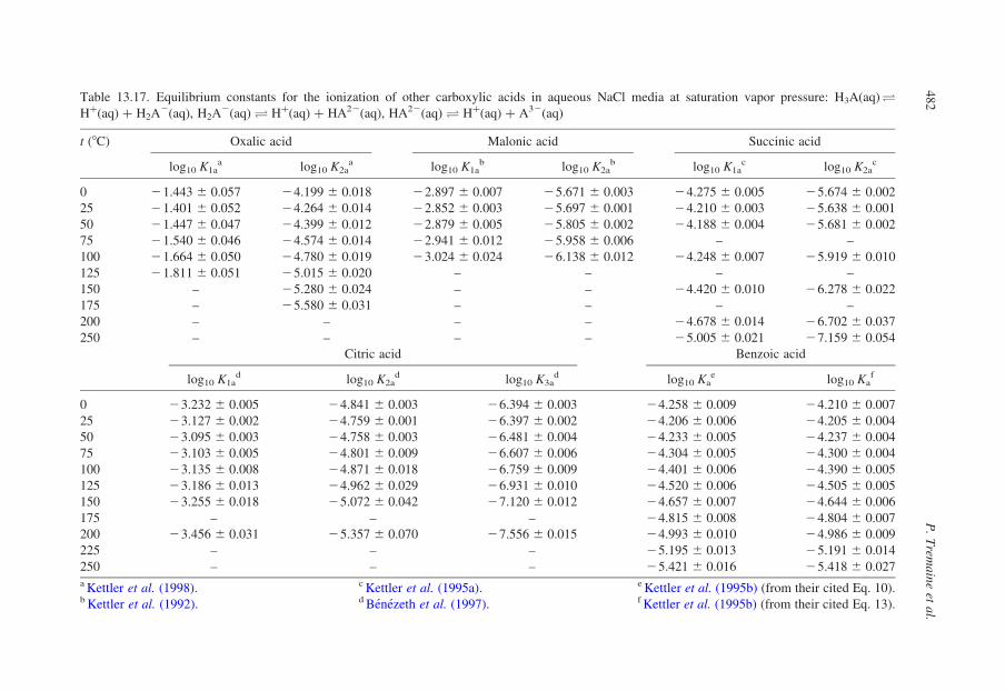
Table 13.17. Equilibrium constants for the ionization of other carboxylic acids in aqueous NaCl media at saturation vapor pressure: H3A(aq)O

Hþ(aq) þ H2A2(aq), H2A2(aq) O Hþ(aq) þ HA22(aq), HA22(aq) O Hþ(aq) þ A32(aq)

t (8C) Oxalic acid Malonic acid Succinic acid

log10 K1aa log10 K2a

a log10 K1ab log10 K2a

b log10 K1ac log10 K2a

c

0 21.443 ^ 0.057 24.199 ^ 0.018 22.897 ^ 0.007 25.671 ^ 0.003 24.275 ^ 0.005 25.674 ^ 0.002

25 21.401 ^ 0.052 24.264 ^ 0.014 22.852 ^ 0.003 25.697 ^ 0.001 24.210 ^ 0.003 25.638 ^ 0.001

50 21.447 ^ 0.047 24.399 ^ 0.012 22.879 ^ 0.005 25.805 ^ 0.002 24.188 ^ 0.004 25.681 ^ 0.002

75 21.540 ^ 0.046 24.574 ^ 0.014 22.941 ^ 0.012 25.958 ^ 0.006 – –

100 21.664 ^ 0.050 24.780 ^ 0.019 23.024 ^ 0.024 26.138 ^ 0.012 24.248 ^ 0.007 25.919 ^ 0.010

125 21.811 ^ 0.051 25.015 ^ 0.020 – – – –

150 – 25.280 ^ 0.024 – – 24.420 ^ 0.010 26.278 ^ 0.022

175 – 25.580 ^ 0.031 – – – –

200 – – – – 24.678 ^ 0.014 26.702 ^ 0.037

250 – – – – 25.005 ^ 0.021 27.159 ^ 0.054

Citric acid Benzoic acid

log10 K1ad log10 K2a

d log10 K3ad log10 Ka

e log10 Kaf

0 23.232 ^ 0.005 24.841 ^ 0.003 26.394 ^ 0.003 24.258 ^ 0.009 24.210 ^ 0.007

25 23.127 ^ 0.002 24.759 ^ 0.001 26.397 ^ 0.002 24.206 ^ 0.006 24.205 ^ 0.004

50 23.095 ^ 0.003 24.758 ^ 0.003 26.481 ^ 0.004 24.233 ^ 0.005 24.237 ^ 0.004

75 23.103 ^ 0.005 24.801 ^ 0.009 26.607 ^ 0.006 24.304 ^ 0.005 24.300 ^ 0.004

100 23.135 ^ 0.008 24.871 ^ 0.018 26.759 ^ 0.009 24.401 ^ 0.006 24.390 ^ 0.005

125 23.186 ^ 0.013 24.962 ^ 0.029 26.931 ^ 0.010 24.520 ^ 0.006 24.505 ^ 0.005

150 23.255 ^ 0.018 25.072 ^ 0.042 27.120 ^ 0.012 24.657 ^ 0.007 24.644 ^ 0.006

175 – – – 24.815 ^ 0.008 24.804 ^ 0.007

200 23.456 ^ 0.031 25.357 ^ 0.070 27.556 ^ 0.015 24.993 ^ 0.010 24.986 ^ 0.009

225 – – – 25.195 ^ 0.013 25.191 ^ 0.014

250 – – – 25.421 ^ 0.016 25.418 ^ 0.027a Kettler et al. (1998).b Kettler et al. (1992).

c Kettler et al. (1995a).d Benezeth et al. (1997).

e Kettler et al. (1995b) (from their cited Eq. 10).f Kettler et al. (1995b) (from their cited Eq. 13).

P.

Trem

ain

eet

al.

48

2

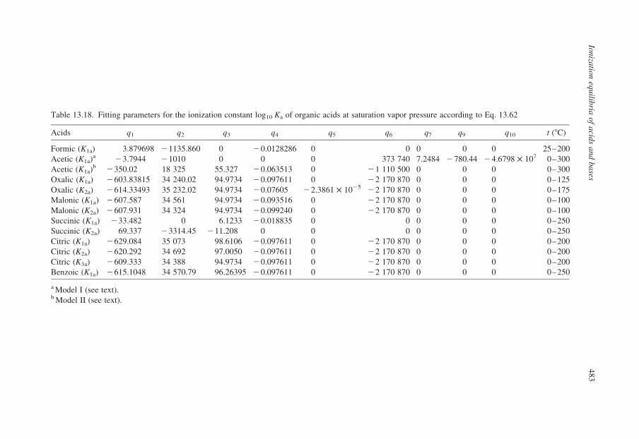
Table 13.18. Fitting parameters for the ionization constant log10 Ka of organic acids at saturation vapor pressure according to Eq. 13.62

Acids q1 q2 q3 q4 q5 q6 q7 q9 q10 t (8C)

Formic (K1a) 3.879698 21135.860 0 20.0128286 0 0 0 0 0 25–200

Acetic (K1a)a 23.7944 21010 0 0 0 373 740 7.2484 2780.44 24.6798 £ 107 0–300

Acetic (K1a)b 2350.02 18 325 55.327 20.063513 0 21 110 500 0 0 0 0–300

Oxalic (K1a) 2603.83815 34 240.02 94.9734 20.097611 0 22 170 870 0 0 0 0–125

Oxalic (K2a) 2614.33493 35 232.02 94.9734 20.07605 22.3861 £ 1025 22 170 870 0 0 0 0–175

Malonic (K1a) 2607.587 34 561 94.9734 20.093516 0 22 170 870 0 0 0 0–100

Malonic (K2a) 2607.931 34 324 94.9734 20.099240 0 22 170 870 0 0 0 0–100

Succinic (K1a) 233.482 0 6.1233 20.018835 0 0 0 0 0 0–250

Succinic (K2a) 69.337 23314.45 211.208 0 0 0 0 0 0 0–250

Citric (K1a) 2629.084 35 073 98.6106 20.097611 0 22 170 870 0 0 0 0–200

Citric (K2a) 2620.292 34 692 97.0050 20.097611 0 22 170 870 0 0 0 0–200

Citric (K3a) 2609.333 34 388 94.9734 20.097611 0 22 170 870 0 0 0 0–200

Benzoic (K1a) 2615.1048 34 570.79 96.26395 20.097611 0 22 170 870 0 0 0 0–250

a Model I (see text).b Model II (see text).

Ion

izatio

neq

uilib

riao

fa

cids

an

db

ases

48

3

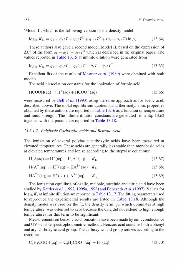
‘Model I’, which is the following version of the density model:

log10 K1a ¼ q1 þ q2=T þ q6=T2 þ q10=T3 þ ðq7 þ q9=TÞ ln rw ð13:64Þ

These authors also gave a second model, Model II, based on the expression of

DCop of the form a1 þ a2T þ a3=T2 which is described in the original paper. The

values reported in Table 13.15 at infinite dilution were generated from

log10 K1a ¼ q1 þ q2=T þ q3 ln T þ q4T þ q6=T2 ð13:65Þ

Excellent fits of the results of Mesmer et al. (1989) were obtained with both

models.

The acid dissociation constants for the ionization of formic acid:

HCOOHðaqÞO HþðaqÞ þ HCOO2ðaqÞ ð13:66Þ

were measured by Bell et al. (1993) using the same approach as for acetic acid,

described above. The molal equilibrium quotients and thermodynamic properties

obtained by these authors are reported in Table 13.16 as a function of temperature

and ionic strength. The infinite dilution constants are generated from Eq. 13.62

together with the parameters reported in Table 13.18.

13.5.1.2. Polybasic Carboxylic acids and Benzoic Acid

The ionization of several polybasic carboxylic acids have been measured at

elevated temperatures. These acids are generally less stable than monobasic acids

at elevated temperatures and ionize according to the stepwise equations:

H3AðaqÞO HþðaqÞ þ H2A2ðaqÞ K1a ð13:67Þ

H2A2ðaqÞO HþðaqÞ þ HA22ðaqÞ K2a ð13:68Þ

HA22ðaqÞO HþðaqÞ þ A32ðaqÞ K3a ð13:69Þ

The ionization equilibria of oxalic, malonic, succinic and citric acid have been

studied by Kettler et al. (1992, 1995a, 1998) and Benezeth et al. (1997). Values for

log10 Ka at infinite dilution are reported in Table 13.17. The fitting parameters used

to reproduce the experimental results are listed in Table 13.18. Although the

density model was used for the fit, the density term, q9, which dominates at high

temperature, was often set to zero because the data did not extend to high enough

temperatures for this term to be significant.

Measurements on benzoic acid ionization have been made by emf, conductance

and UV–visible spectrophotometric methods. Benzoic acid contains both a phenyl

and aryl carboxylic acid group. The carboxylic acid group ionizes according to the

reaction:

C6H5COOHðaqÞO C6H5COO2ðaqÞ þ HþðaqÞ ð13:70Þ

P. Tremaine et al.484

Equilibrium constants have been measured by Kettler et al. (1995b) using

potentiometric titration methods. Values of log10 Ka and fitting parameters are

listed in Tables 13.17 and 13.18, respectively.

13.6. Amines and Alkanol Amines

13.6.1. Effects of Amine Structure on Ionization and the Formationof Carbamates

Amines and alkanolamines have seen wide application in the energy industry as

‘all volatile’ additives for boiler-water pH control and as ‘chemical solvents’ for

removing carbon dioxide and other acid gases from natural gas and combustion

gases. Boiler pH control applications typically involve dilute solutions of a few

parts per million at temperatures from 25 to 350 8C, while gas treatment

applications require concentrated solutions in excess of 1 mol·kg21 at tempera-

tures from 25 to 150 8C.

Factors influencing the ionization constants of amines have been reviewed by

Jones and Arnett (1974). Briefly, amines and alkanolamines consist of three alkyl,

alkanol or hydrogen substituent groups covalently bound to a central nitrogen

atom. Together with the unbonded lone pair of valence electrons, these groups give

the amine a tetrahedral structure. The basicity of the amine is controlled by the

availability of the valence band electrons for chemical bonding to Hþ(aq). Electron

donor substituent groups enhance the basicity and increase Kb, while electron-

withdrawing groups reduce the magnitude of Kb. Steric effects (i.e., crowding

effects) due to interactions among the three substituent groups may also suppress

the value of Kb. This is particularly true for tertiary amines. Steric effects are also

affected by hydration. Because of these competing factors, the relative base

strengths of primary, secondary and tertiary amines at 25 8C follow the sequence:

NH3ðaqÞ , RNH2ðaqÞ , RR0NHðaqÞ . RR0R00NðaqÞ

In addition to the ionization reaction:

RR0R00NðaqÞ þ HþðaqÞO ½RR0R00NH�þðaqÞ ð13:71Þ

ammonia, primary and secondary amines can also react with carbon dioxide to

form carbamic acid according to the reaction:

H2CO3ðaqÞ þ RR0NHðaqÞO RR0NCOO2ðaqÞ þ HþðaqÞ þ H2OðlÞ ð13:72Þ

Carbamate formation, which is a reversible reaction, does not occur in the dilute

solutions used in boiler treatment applications, and is less favored at elevated

temperatures (Roberts and Tremaine, 1985). Indeed, the decreasing stability with

increasing temperature allows carbamate formation to be used in reversible cyclic

Ionization equilibria of acids and bases 485

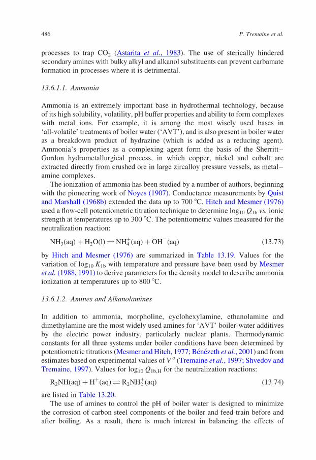
processes to trap CO2 (Astarita et al., 1983). The use of sterically hindered

secondary amines with bulky alkyl and alkanol substituents can prevent carbamate

formation in processes where it is detrimental.

13.6.1.1. Ammonia

Ammonia is an extremely important base in hydrothermal technology, because

of its high solubility, volatility, pH buffer properties and ability to form complexes

with metal ions. For example, it is among the most wisely used bases in

‘all-volatile’ treatments of boiler water (‘AVT’), and is also present in boiler water

as a breakdown product of hydrazine (which is added as a reducing agent).

Ammonia’s properties as a complexing agent form the basis of the Sherritt–

Gordon hydrometallurgical process, in which copper, nickel and cobalt are

extracted directly from crushed ore in large zircalloy pressure vessels, as metal–

amine complexes.

The ionization of ammonia has been studied by a number of authors, beginning

with the pioneering work of Noyes (1907). Conductance measurements by Quist

and Marshall (1968b) extended the data up to 700 8C. Hitch and Mesmer (1976)

used a flow-cell potentiometric titration technique to determine log10 Q1b vs. ionic

strength at temperatures up to 300 8C. The potentiometric values measured for the

neutralization reaction:

NH3ðaqÞ þ H2OðlÞO NHþ4 ðaqÞ þ OH2ðaqÞ ð13:73Þ

by Hitch and Mesmer (1976) are summarized in Table 13.19. Values for the

variation of log10 K1b with temperature and pressure have been used by Mesmer

et al. (1988, 1991) to derive parameters for the density model to describe ammonia

ionization at temperatures up to 800 8C.

13.6.1.2. Amines and Alkanolamines

In addition to ammonia, morpholine, cyclohexylamine, ethanolamine and

dimethylamine are the most widely used amines for ‘AVT’ boiler-water additives

by the electric power industry, particularly nuclear plants. Thermodynamic

constants for all three systems under boiler conditions have been determined by

potentiometric titrations (Mesmer and Hitch, 1977; Benezeth et al., 2001) and from

estimates based on experimental values of V o (Tremaine et al., 1997; Shvedov and

Tremaine, 1997). Values for log10 Q1b,H for the neutralization reactions:

R2NHðaqÞ þ HþðaqÞO R2NHþ2 ðaqÞ ð13:74Þ

are listed in Table 13.20.

The use of amines to control the pH of boiler water is designed to minimize

the corrosion of carbon steel components of the boiler and feed-train before and

after boiling. As a result, there is much interest in balancing the effects of

P. Tremaine et al.486

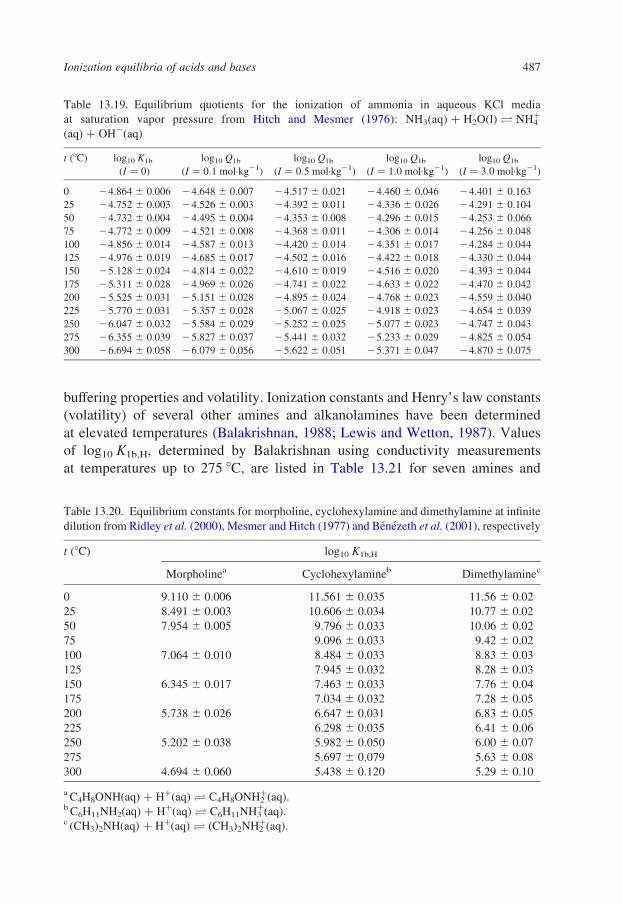
buffering properties and volatility. Ionization constants and Henry’s law constants

(volatility) of several other amines and alkanolamines have been determined

at elevated temperatures (Balakrishnan, 1988; Lewis and Wetton, 1987). Values

of log10 K1b,H, determined by Balakrishnan using conductivity measurements

at temperatures up to 275 8C, are listed in Table 13.21 for seven amines and

Table 13.19. Equilibrium quotients for the ionization of ammonia in aqueous KCl media

at saturation vapor pressure from Hitch and Mesmer (1976): NH3(aq) þ H2O(l) O NH4þ

(aq) þ OH2(aq)

t (8C) log10 K1b

(I ¼ 0)

log10 Q1b

(I ¼ 0:1 mol·kg21)

log10 Q1b

(I ¼ 0:5 mol·kg21)

log10 Q1b

(I ¼ 1:0 mol·kg21)

log10 Q1b

(I ¼ 3:0 mol·kg21)

0 24.864 ^ 0.006 24.648 ^ 0.007 24.517 ^ 0.021 24.460 ^ 0.046 24.401 ^ 0.163

25 24.752 ^ 0.003 24.526 ^ 0.003 24.392 ^ 0.011 24.336 ^ 0.026 24.291 ^ 0.104

50 24.732 ^ 0.004 24.495 ^ 0.004 24.353 ^ 0.008 24.296 ^ 0.015 24.253 ^ 0.066

75 24.772 ^ 0.009 24.521 ^ 0.008 24.368 ^ 0.011 24.306 ^ 0.014 24.256 ^ 0.048

100 24.856 ^ 0.014 24.587 ^ 0.013 24.420 ^ 0.014 24.351 ^ 0.017 24.284 ^ 0.044

125 24.976 ^ 0.019 24.685 ^ 0.017 24.502 ^ 0.016 24.422 ^ 0.018 24.330 ^ 0.044

150 25.128 ^ 0.024 24.814 ^ 0.022 24.610 ^ 0.019 24.516 ^ 0.020 24.393 ^ 0.044

175 25.311 ^ 0.028 24.969 ^ 0.026 24.741 ^ 0.022 24.633 ^ 0.022 24.470 ^ 0.042

200 25.525 ^ 0.031 25.151 ^ 0.028 24.895 ^ 0.024 24.768 ^ 0.023 24.559 ^ 0.040

225 25.770 ^ 0.031 25.357 ^ 0.028 25.067 ^ 0.025 24.918 ^ 0.023 24.654 ^ 0.039

250 26.047 ^ 0.032 25.584 ^ 0.029 25.252 ^ 0.025 25.077 ^ 0.023 24.747 ^ 0.043

275 26.355 ^ 0.039 25.827 ^ 0.037 25.441 ^ 0.032 25.233 ^ 0.029 24.825 ^ 0.054

300 26.694 ^ 0.058 26.079 ^ 0.056 25.622 ^ 0.051 25.371 ^ 0.047 24.870 ^ 0.075

Table 13.20. Equilibrium constants for morpholine, cyclohexylamine and dimethylamine at infinite

dilution from Ridley et al. (2000), Mesmer and Hitch (1977) and Benezeth et al. (2001), respectively

t (8C) log10 K1b,H

Morpholinea Cyclohexylamineb Dimethylaminec

0 9.110 ^ 0.006 11.561 ^ 0.035 11.56 ^ 0.02

25 8.491 ^ 0.003 10.606 ^ 0.034 10.77 ^ 0.02

50 7.954 ^ 0.005 9.796 ^ 0.033 10.06 ^ 0.02

75 9.096 ^ 0.033 9.42 ^ 0.02

100 7.064 ^ 0.010 8.484 ^ 0.033 8.83 ^ 0.03

125 7.945 ^ 0.032 8.28 ^ 0.03

150 6.345 ^ 0.017 7.463 ^ 0.033 7.76 ^ 0.04

175 7.034 ^ 0.032 7.28 ^ 0.05

200 5.738 ^ 0.026 6.647 ^ 0.031 6.83 ^ 0.05

225 6.298 ^ 0.035 6.41 ^ 0.06

250 5.202 ^ 0.038 5.982 ^ 0.050 6.00 ^ 0.07

275 5.697 ^ 0.079 5.63 ^ 0.08

300 4.694 ^ 0.060 5.438 ^ 0.120 5.29 ^ 0.10

a C4H8ONH(aq) þ Hþ(aq) O C4H8ONH2þ(aq).

b C6H11NH2(aq) þ Hþ(aq) O C6H11NH3þ(aq).

c (CH3)2NH(aq) þ Hþ(aq) O (CH3)2NH2þ(aq).

Ionization equilibria of acids and bases 487

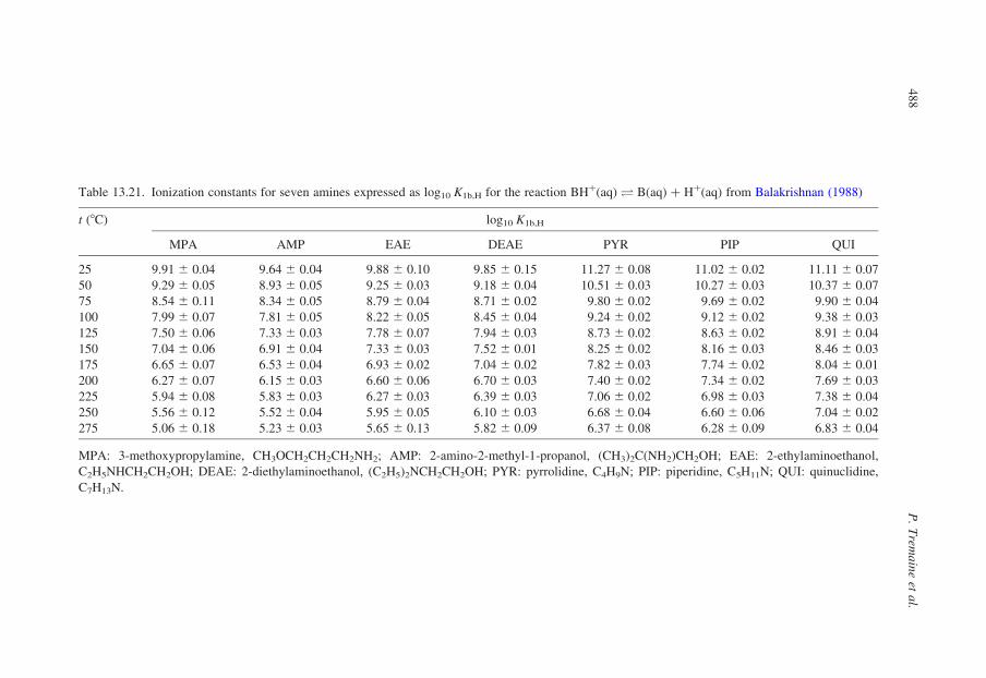
Table 13.21. Ionization constants for seven amines expressed as log10 K1b,H for the reaction BHþ(aq) O B(aq) þ Hþ(aq) from Balakrishnan (1988)

t (8C) log10 K1b,H

MPA AMP EAE DEAE PYR PIP QUI

25 9.91 ^ 0.04 9.64 ^ 0.04 9.88 ^ 0.10 9.85 ^ 0.15 11.27 ^ 0.08 11.02 ^ 0.02 11.11 ^ 0.07

50 9.29 ^ 0.05 8.93 ^ 0.05 9.25 ^ 0.03 9.18 ^ 0.04 10.51 ^ 0.03 10.27 ^ 0.03 10.37 ^ 0.07

75 8.54 ^ 0.11 8.34 ^ 0.05 8.79 ^ 0.04 8.71 ^ 0.02 9.80 ^ 0.02 9.69 ^ 0.02 9.90 ^ 0.04

100 7.99 ^ 0.07 7.81 ^ 0.05 8.22 ^ 0.05 8.45 ^ 0.04 9.24 ^ 0.02 9.12 ^ 0.02 9.38 ^ 0.03

125 7.50 ^ 0.06 7.33 ^ 0.03 7.78 ^ 0.07 7.94 ^ 0.03 8.73 ^ 0.02 8.63 ^ 0.02 8.91 ^ 0.04

150 7.04 ^ 0.06 6.91 ^ 0.04 7.33 ^ 0.03 7.52 ^ 0.01 8.25 ^ 0.02 8.16 ^ 0.03 8.46 ^ 0.03

175 6.65 ^ 0.07 6.53 ^ 0.04 6.93 ^ 0.02 7.04 ^ 0.02 7.82 ^ 0.03 7.74 ^ 0.02 8.04 ^ 0.01

200 6.27 ^ 0.07 6.15 ^ 0.03 6.60 ^ 0.06 6.70 ^ 0.03 7.40 ^ 0.02 7.34 ^ 0.02 7.69 ^ 0.03

225 5.94 ^ 0.08 5.83 ^ 0.03 6.27 ^ 0.03 6.39 ^ 0.03 7.06 ^ 0.02 6.98 ^ 0.03 7.38 ^ 0.04

250 5.56 ^ 0.12 5.52 ^ 0.04 5.95 ^ 0.05 6.10 ^ 0.03 6.68 ^ 0.04 6.60 ^ 0.06 7.04 ^ 0.02

275 5.06 ^ 0.18 5.23 ^ 0.03 5.65 ^ 0.13 5.82 ^ 0.09 6.37 ^ 0.08 6.28 ^ 0.09 6.83 ^ 0.04

MPA: 3-methoxypropylamine, CH3OCH2CH2CH2NH2; AMP: 2-amino-2-methyl-1-propanol, (CH3)2C(NH2)CH2OH; EAE: 2-ethylaminoethanol,

C2H5NHCH2CH2OH; DEAE: 2-diethylaminoethanol, (C2H5)2NCH2CH2OH; PYR: pyrrolidine, C4H9N; PIP: piperidine, C5H11N; QUI: quinuclidine,

C7H13N.

P.

Trem

ain

eet

al.

48

8

alkanolamines: 3-methoxypropylamine (MPA), 2-amino-2-methyl-1-propanol

(AMP), 2-ethylaminoethanol (EAE), 2-diethylaminoethanol (DEAE), pyrrolidine,

piperidine and quinuclidine.

13.7. Other Sources of Data

Values for the ionization constants of many acids and bases at 25 8C are listed in

compilations by Pettit and Powell (1997), Smith and Martell (1997), Christensen

et al. (1976) and Oscarson et al. (1992). Some high-temperature values are

included. Proprietary databases of high-temperature ionization constants are

maintained and developed for electric power industry applications by EPRI

(Alexander and Liu, 1989) and for more general chemical industry applications by

OLI Systems Inc. (Anderko, 1995).

A large database and computer code for calculating the thermodynamic

properties of inorganic ions and their reactions at elevated temperature and pressure

is incorporated in the public database SUPCRT92 (Johnson et al., 1992). This is

based on the HKF equation of state, and primarily on experimental data available

before the late 1980s. Many of the standard partial molar heat capacity and volume

data at that time were limited to temperatures below 50 8C, and the HKF

extrapolations are not always in agreement with later experiments. The papers on

which the program is based (Shock and Helgeson, 1988) are a good source of

literature related to experimental studies. The HKF equation of state has also been

used to predict the ionization and complexation constants of many organic species

under hydrothermal conditions (Shock and Helgeson, 1990; Shock et al., 1992;

Shock and Koretsky, 1993, 1995; Amend and Helgeson, 1997). Because the HKF

model has no theoretical basis for neutral species, high-temperature values of

log10 K should be treated with caution unless the results have been obtained by

direct fitting of high-temperature experimental data for the species in question.

These papers are exhaustively referenced and are a valuable guide to the literature.

Finally, a number of authors have reported functional-group additivity models

for organic species from which heat capacity and volume functions can be

calculated. We particularly note the treatments by Sedlbauer et al. (2000) and

Plyasunov et al. (2000a,b), which appear to provide reliable extrapolations of

log10 K for many reactions up to about 250 8C.

References

Alexander, J.H. and Liu, L., Users Manual, Vol. I. EPRI Report NP-5561-CCM, 1989.

Amend, J.P. and Helgeson, H.C., J. Chem. Soc., Faraday Trans., 93, 1927–1941 (1997).

Anderko, A., 18th OLI Users Conference, Morristown, NJ, October 10, 1995.

Anderson, G.M., Castet, S., Schott, J. and Mesmer, R.E., Geochim. Cosmochim. Acta, 55,

1769–1779 (1991).

Ionization equilibria of acids and bases 489

Angell, C.A., Annu. Rev. Phys. Chem., 34, 593–630 (1983).

Archer, D.G., J. Phys. Chem. Ref. Data, 21, 793–823 (1992).

Arnett, E.M. and McKelvey, D.R. In: Coetzee, J.F. and Ritchie, C.D. (Eds.), Solute–Solvent

Interactions. Marcel Dekker, New York, 1969.

Astarita, G., Savage, D.W. and Bisio, A., Gas Treating with Chemical Solvents. Wiley, New York,

1983.

Baes, C.F. Jr. and Mesmer, R.E., The Hydrolysis of Cations. Robert E. Krieger Publishing, Malibar,

FL, 1986, Reprint with corrections of the 1976 edition by Wiley.

Balakrishnan, P.V., J. Solution Chem., 17, 825–840 (1988).

Bassett, W.A., Shen, A.H. and Bucknum, M., Rev. Sci. Instrum., 64, 2340–2345 (1993).

Bell, J.L.S., Wesolowski, D.J. and Palmer, D.A., J. Solution Chem., 22, 125–136 (1993).

Benezeth, P., Palmer, D.A. and Wesolowski, D.J., J. Solution Chem., 26, 63–84 (1997).

Benezeth, P., Palmer, D.A. and Wesolowski, D.J., J. Chem. Eng. Data, 46, 202–207 (2001).

Busey, R.H. and Mesmer, R.E., Inorg. Chem., 16, 2444–2450 (1977).

Busey, R.H. and Mesmer, R.E., J. Chem. Eng. Data, 23, 175–176 (1978).

Chlistunoff, J., Ziegler, K.J., Lasdon, L. and Johnston, K.P., J. Phys. Chem. A, 103, 1678–1688

(1999).

Christensen, J.J., Hansen, L.D. and Izatt, R.M., Handbook of Proton Ionization Heats and Related

Thermodynamic Quantities. Wiley, New York, 1976.

Clarke, R.G., Hnedkovsky, L., Tremaine, P.R. and Majer, V., J. Phys. Chem. B, 104, 11781–11793

(2000).

Cotton, F.A. and Wilkinson, G., Advanced Inorganic Chemistry, 5th edn. Wiley-Interscience,

New York, 1988.

Diakonov, I., Pokrovski, G., Schott, J., Castet, S. and Gout, R., Geochim. Cosmochim. Acta, 60,

197–211 (1996).

Dickson, A.G., Wesolowski, D.J., Palmer, D.A. and Mesmer, R.E., J. Phys. Chem., 94, 7978–7985

(1990).

Ding, K. and Seyfried, W.E. Jr., Geochim. Cosmochim. Acta, 59, 4769–4773 (1995).

Ding, K. and Seyfried, W.E. Jr., J. Solution Chem., 25, 421–433 (1996).

Ellis, A.J., J. Chem. Soc., 2299–2310 (1963).

Fernandez-Prini, R., Trans. Faraday Soc., 65, 3311–3313 (1969).

Fernandez-Prini, R., Corti, H.R. and Japas, M.L., High-Temperature Aqueous Solutions:

Thermodynamic Properties. CRC Press, Boca Raton, FL, 1992.

Franck, E.U., Z. Phys. Chem., 8, 107–126 (1956).

Franck, E.U., Angew. Chem., 73, 309–322 (1961).

Franck, E.U., Savolainen, J.E. and Marshall, W.L., Rev. Sci. Instrum., 33, 115–117 (1962).

Giggenbach, W., Inorg. Chem., 10, 1333–1338 (1971).

Gruszkiewicz, M.S. and Wood, R.H., J. Phys. Chem. B, 101, 6549–6559 (1997).

Helgeson, H.C., Kirkham, D.H. and Flowers, G.C., Am. J. Sci., 281, 1249–1516 (1981).

Hepler, L.G. and Hopkins, H.P. Jr., Rev. Inorg. Chem., 1, 303–332 (1979).

Hettiarachchi, S., Makela, K., Song, H. and MacDonald, D.D., J. Electrochem. Soc., 139, L3–L4

(1992).

Hitch, B.F. and Mesmer, R.E., J. Solution Chem., 5, 667–680 (1976).

Ho, P.C. and Palmer, D.A., J. Solution Chem., 24, 753–769 (1995).

Ho, P.C. and Palmer, D.A., J. Solution Chem., 25, 711–729 (1996).

Ho, P.C. and Palmer, D.A., Geochim. Cosmochim. Acta, 61, 3027–3040 (1997).

Ho, P.C. and Palmer, D.A., J. Chem. Eng. Data, 43, 162–170 (1998).

Ho, P.C., Palmer, D.A. and Mesmer, R.E., J. Solution Chem., 23, 997–1017 (1994).

Ho, P.C., Bianchi, H., Palmer, D.A. and Wood, R.H., J. Solution Chem., 29, 217–235 (2000a).

Ho, P.C., Palmer, D.A. and Wood, R.H., J. Phys. Chem. B, 104, 12084–12089 (2000b).

P. Tremaine et al.490

Ho, P.C., Palmer, D.A. and Gruszkiewicz, M.S., J. Phys. Chem. B, 105, 1260–1266 (2001).

Holmes, H.F., Busey, R.H., Simonson, J.M., Mesmer, R.E., Archer, D.G. and Wood, R.H., J. Chem.

Thermodyn., 19, 863–890 (1987).

Johnson, J.W., Oelkers, E.H. and Helgeson, H.C., Comput. Geosci., 18, 899–947 (1992).

Johnston, K.P., Balbuena, P., Xiang, T., Wofford, W. and Flanagin, L. In: Palmer, D.A. and

Wesolowski, D.J. (Eds.), Proceedings of the 5th International Symposium on Hydrothermal

Reactions, Gatlinburg, TN, 1997, pp. 15–17.

Jones, F.M. and Arnett, E.M., Progr. Phys. Org. Chem., 11, 263–322 (1974).

Kettler, R.M., Palmer, D.A. and Wesolowski, D.J., J. Solution Chem., 20, 905–927 (1991).

Kettler, R.M., Wesolowski, D.J. and Palmer, D.A., J. Solution Chem., 21, 883–900 (1992).

Kettler, R.M., Palmer, D.A. and Wesolowski, D.J., J. Solution Chem., 24, 65–87 (1995a).

Kettler, R.M., Wesolowski, D.J. and Palmer, D.A., J. Solution Chem., 24, 385–407 (1995b).

Kettler, R.M., Wesolowski, D.J. and Palmer, D.A., J. Chem. Eng. Data, 43, 337–350 (1998).

Kriksunov, L., MacDonald, D.D. and Millett, P.J., J. Electrochem. Soc., 141, 3002–3005 (1994).

Larson, J.W., Zeeb, K.G. and Hepler, L.G., Can. J. Chem., 60, 2141–2150 (1982).

Laughton, P.M. and Robertson, R.E. In: Coetzee, J.F. and Ritchie, C.D. (Eds.), Solute–Solvent

Interactions. Marcel Dekker, New York, 1969.

Levelt Sengers, J.M.H. In: Bruno, J.J. and Ely, J.F. (Eds.), Supercritical Fluid Technology. CRC

Press, Boca Raton, FL, 1991, pp. 1–56.

Lewis, G.G. and Wetton, E.A.M., Central Electricity Generating Board Report, Report No. OED/

STN/87/20083/M, 1987.

Lindsay, W.T. Jr. In: Pichal, M. and Sifner, O. (Eds.), Properties of Water and Steam. Hemisphere,

New York, 1989, pp. 29–38.

Lindsay, W.T. Jr. In: Cohen, P. (Ed.), The ASME Handbook on Water Technology for Thermal Power

Systems. American Society of Mechanical Engineers, New York, 1990, pp. 341–544, chapter 7.

Lvov, S.N., Zhou, X.Y. and Macdonald, D.D., J. Electroanal. Chem., 463, 146–156 (1999).

MacDonald, D.D., Hettiarachchi, S. and Lenhart, S.J., J. Solution Chem., 17, 719–732 (1988).

Marshall, W.L. and Franck, E.U., J. Phys. Chem. Ref. Data, 10, 295–304 (1981).

Marshall, W.L. and Slusher, R., J. Inorg. Nucl. Chem., 37, 1191–1202 (1975a).

Marshall, W.L. and Slusher, R., J. Inorg. Nucl. Chem., 37, 2165–2170 (1975b).

Mesmer, R.E. and Baes, C.F. Jr., J. Solution Chem., 3, 307–322 (1974).

Mesmer, R.E. and Herting, D.L., J. Solution Chem., 7, 901–913 (1978).

Mesmer, R.E. and Hitch, B.F., J. Solution Chem., 6, 251–261 (1977).

Mesmer, R.E., Baes, C.F. Jr. and Sweeton, F.H., J. Phys. Chem., 74, 1937–1942 (1970).

Mesmer, R.E., Baes, C.F. Jr. and Sweeton, F.H., Inorg. Chem., 11, 537–543 (1972).

Mesmer, R.E., Marshall, W.L., Palmer, D.A., Simonson, J.M. and Holmes, H.F., J. Solution Chem.,

17, 699–718 (1988).

Mesmer, R.E., Patterson, C.S., Busey, R.H. and Holmes, H.F., J. Phys. Chem., 93, 7483–7490 (1989).

Mesmer, R.E., Palmer, D.A. and Simonson, J.M. In: Pitzer, K.S. (Ed.), Activity Coefficients in

Aqueous Solutions, 2nd edn. CRC Press, Boca Raton, FL, 1991, chapter 8.

Mesmer, R.E., Palmer, D.A., Simonson, J.M., Holmes, H.F., Ho, P.C., Wesolowski, D.J. and

Gruszkiewicz, M.S., Pure Appl. Chem., 69, 905–914 (1997).

Millero, F.J. In: Pytkowicz, M. (Ed.), Activity Coefficients in Electrolyte Solutions. Vol. 2, CRC

Press, Boca Raton, FL, 1979.

Noyes, A.A., The Electrical Conductivity of Aqueous Solutions, Publication No. 63, 1907, Carnegie

Institution of Washington.

O’Connell, J.P., Sharygin, A.V. and Wood, R.H., Ind. Eng. Chem. Res., 35, 2808–2812 (1996).

Olofsson, G. and Hepler, L.G., J. Solution Chem., 4, 127–143 (1975).

Oscarson, J.L., Gillespie, S.E., Izatt, R.M., Chen, X. and Pando, C., J. Solution Chem., 21, 789–801

(1992).

Ionization equilibria of acids and bases 491

Palmer, D.A. and Drummond, S.E., J. Solution Chem., 17, 153–164 (1988).

Palmer, D.A. and van Eldik, R., Chem. Rev., 83, 651–731 (1983).

Palmer, D.A., Benezeth, P. and Wesolowski, D.J., PowerPlant Chem., 2, 261–264 (2000).

Patterson, C.S., Slocum, G.H., Busey, R.H. and Mesmer, R.E., Geochim. Cosmochim. Acta, 46,

1653–1663 (1982).

Patterson, C.S., Busey, R.H. and Mesmer, R.E., J. Solution Chem., 13, 647–661 (1984).

Pettit, L.D. and Powell, K.J., IUPAC Stability Constants Database SC-Database for Windows.

IUPAC, 1997.

Pitzer, K.S. (Ed.), Activity Coefficients in Electrolyte Solutions, 2nd edn. CRC Press, Boca Raton,

FL, 1991.

Pitzer, K.S., Thermodynamics, McGraw-Hill Series in Advanced Chemistry, 3rd edn. McGraw-Hill,

New York, 1995.

Plyasunov, A.V., O’Connell, J.P. and Wood, R.H., Geochim. Cosmochim. Acta, 64, 495–512 (2000a).

Plyasunov, A.V., O’Connell, J.P., Wood, R.H. and Shock, E.L., Geochim. Cosmochim. Acta, 64,

2779–2795 (2000b).

Quist, A.S. and Marshall, W.L., J. Phys. Chem., 72, 684–703 (1968a).

Quist, A.S. and Marshall, W.L., J. Phys. Chem., 72, 3122–3128 (1968b).

Rao, R.S. and Hepler, L.G., Hydrometallurgy, 2, 293–299 (1977).

Read, A.J., J. Solution Chem., 4, 53–72 (1975).

Ridley, M.K., Xiao, C., Palmer, D.A. and Wesolowski, D.J., J. Chem. Eng. Data, 45, 502–507

(2000).

Roberts, B. and Tremaine, P.R., Can. J. Chem. Eng., 63, 294–300 (1985).

Rudolph, W., Brooker, M.H. and Tremaine, P.R., J. Solution Chem., 26, 757–777 (1997).

Sedlbauer, J., O’Connell, J.P. and Wood, R.H., Chem. Geol., 163, 43–63 (2000).

Sharygin, A.V., Mokbel, I., Xiao, C. and Wood, R.H., J. Phys. Chem. B, 105, 229–237 (2001).

Shoesmith, D.W. and Lee, W., Can. J. Chem., 54, 3553–3558 (1976).

Shock, E.L. and Helgeson, H.C., Geochim. Cosmochim. Acta, 52, 2009–2036 (1988).

Shock, E.L. and Helgeson, H.C., Geochim. Cosmochim. Acta, 54, 915–945 (1990).

Shock, E.L. and Koretsky, C.M., Geochim. Cosmochim. Acta, 57, 4899–4922 (1993).

Shock, E.L. and Koretsky, C.M., Geochim. Cosmochim. Acta, 59, 1497–1532 (1995).

Shock, E.L., Oelkers, E.H., Johnson, J.W., Sverjensky, D.A. and Helgeson, H.C., J. Chem. Soc.,

Faraday Trans., 88, 803–826 (1992), and references cited therein.

Shvedov, D. and Tremaine, P.R., J. Solution Chem., 26, 1113–1143 (1997).

Smith, R.M. and Martell, A.E., NIST Critically Selected Stability Constants of Metal Complexes

Database Version 4.0. National Institute of Standards and Technology, Gaithersburg, MD, 1997.

Suleimenov, M. and Seward, T.M., Geochim. Cosmochim. Acta, 61, 5187–5198 (1997).

Svishchev, I.M. and Kusalik, P.G. In: White, H.J. Jr., Sengers, J.V., Neumann, D.B., and Bellows,

J.C. (Eds.), Physical Chemistry of Aqueous Systems: Meeting the Needs of Industry, Proceedings

of the 12th International Conference on the Properties of Water and Steam. Begell House,

New York, 1995, pp. 222–228.

Sweeton, F.H., Mesmer, R.E. and Baes, C.F. Jr., J. Solution Chem., 3, 191–214 (1974).

Tanger, J.C. and Helgeson, H.C., Am. J. Sci., 288, 19–98 (1988).

Tremaine, P.R., Shvedov, D. and Xiao, C., J. Phys. Chem. B, 101, 409–419 (1997).

Turq, P., Blum, L., Bernard, O. and Kunz, W., J. Phys. Chem., 99, 822–827 (1995).

Ulmer, G.C. and Barnes, H.L., Hydrothermal Experimental Techniques. Wiley-Interscience,

New York, 1983.

Wofford, W.T., Gloyna, E.F. and Johnston, K.P., Ind. Eng. Chem. Res., 37, 2045–2051 (1998).

Xiang, T., Johnston, K.P., Wofford, W. and Gloyna, E.F., Ind. Eng. Chem. Res., 35, 4788–4795

(1996).

Zimmerman, G.H., Gruszkiewicz, M.S. and Wood, R.H., J. Phys. Chem., 99, 11612–11624 (1995).

P. Tremaine et al.492