Meta-Optimization Using Cellular Automata with Application to the Combined Trip Distribution and...

Computer-Aided Civil and Infrastructure Engineering 16(6) (2001) 384–398

Meta-Optimization Using CellularAutomata with Application to the Combined Trip

Distribution and Assignment SystemOptimal Problem

Wael M. ElDessouki*

University of Connecticut, Department of Civil and Environment Engineering, U-37,Storrs, Connecticut 06269

Yahya Fathi

North Carolina State University, Department of Industrial Engineering,Raleigh, North Carolina 27695

&

Nagui Rouphail

North Carolina State University, Department of Civil and Environmental Engineering,Raleigh, North Carolina 27695

Abstract: In this paper, meta-optimization and cellularautomata have been introduced as a modeling environ-ment for solving large-scale and complex transportationproblems. A constrained system optimum combined trip dis-tribution and assignment problem was selected to demon-strate the applicability of the cellular automata approachover classical mixed integer formulation. A mathematicalformulation for the selected problem has been developedand a methodology for applying cellular automata has beenpresented. A numerical example network was used to illus-trate the potential for using cellular automata as a model-ing environment for solving optimization problems.

*To whom correspondence should be addressed. E-mail: [email protected].

1 INTRODUCTION AND BACKGROUND

Transportation network models, and algorithms for theirsolution, have received considerable attention in the trans-portation literature. Even with recent breakthroughs in com-putational efficiency and the introduction of fast digitalcomputers for solving these models, many problems stillrequire extensive enumeration and need long CPU time tobe solved. This fact renders the current modeling schemesquestionable, since current modeling schemes may imposeunnecessary complexities on the problems rather than sim-plifying them. This article illustrates an example of suchadded complexities by developing a mathematical program-ming model (a classical modeling environment) to solve

© 2001 Computer-Aided Civil and Infrastructure Engineering. Published by Blackwell Publishers, 350 Main Street, Malden, MA 02148, USA,and 108 Cowley Road, Oxford OX4 1JF, UK.

Meta-optimization using cellular automata 385

the system optimum combined trip distribution and assign-ment problem. Then, a cellular automata (CA) model isintroduced as an alternative modeling environment for solv-ing the same problem. The preliminary results using bothtechniques demonstrate the usefulness of the CA over theclassical modeling environment. The paper is organized asfollows. A brief description of CA is given, followed bya summary for the combined trip distribution and assign-ment problem (CTDAP). Then, a discussion of the advan-tages of CA over other heuristic methods is given. Themethodology section includes a mathematical formulationfor the CTDAP and the CA model. At the conclusion ofthis chapter, preliminary numerical results are presentedand discussed.

1.1 Cellular automata

Cellular automata are discrete systems of simple construc-tion that can maintain the capabilities of representing thebehavior of a complex system. Classically, CA is definedas a set of cells {x}, with a defined set of states (Q), neigh-borhood function u(x), and a cell state transition functionf (u). The state transition function maps the states in theneighborhood of the cell and determines the new state ofthe cell.

Cellular automata have a relatively long history. Thework of early pioneers like Neumann (1966) was the basisfor other researchers to develop numerous CA models andimplementations for different applications. In most cases,CA was used as a simulation environment for fluid turbu-lence, thermodynamics, and chemical reactions. Recently,a few researchers began developing CA models for trans-portation applications, for example, Wagner et al. (1997),Chopard et al. (1996), and Benjamin et al. (1996). Most ofthese applications focus on traffic flow simulation and lanechanges. Implementing CA in an optimization context isvery limited. Tzionas et al. (1992) developed an implemen-tation of CA for estimating a minimum cost path on binarynetworks for designing VLSI circuits. Stiles et al. (1994)developed a route-planning model based on CA, where thesearch was based on searching the pixels of an image forthe area between the origin and a destination. Adamatzky(1996) implemented an excitable media CA to prove theexistence of lower bounds for the Dijkstra’s shortest pathalgorithm and the all-pair shortest path problems. The workof Adamatzky (1996) could be considered a milestone anda starting point for the CA implementation proposed in thecurrent research.

1.2 The combined trip distribution andassignment problem (CTDAP)

Combined trip distribution and assignment is a commonproblem that faces most transportation systems analysts inthe four-step planning process. In this paper, we focus on

a different version of the CTDAP problem: the constrainedsystem optimum version of the CTDAP. The constrainedsystem optimum combined trip distribution and assignmentproblem replicate the emergency evacuation planning pro-cess, where the goal is to identify a finite set of evacuationroutes and to distribute evacuees over shelters such that thetotal evacuation time is minimized (i.e., the total exposureto risk is minimum). This problem exhibits a high levelof complexity. In fact, it could be divided into two sub-problems, similar to the way it is handled in the four-stepprocess. The first step is trip distribution. Usually, this stepis solved using a gravity model based on the shortest pathfree flow travel time. The second is the traffic assignmentproblem. This elementary approach for solving the problemdoes not give accurate results nor does it reflect the actualbehavior of trip makers in selecting their destinations orroutes. Other investigators proposed more rigorous modelsfor solving the problem without separating the two sub-problems. Evans’ model (1973, 1976) is the best knownmathematical model for the combined trip distribution andassignment problem. Other investigators have developedalgorithms and modifications for solving Evans’ model, forexample Horowitz (1989), Lam and Huang (1992a, 1992b,1992c, and 1996), and Boyce and Daskin (1997). However,most of the existing algorithms for solving Evans’ modelcannot handle large networks within reasonable CPU timeand/or memory resources. The main problem with thosealgorithms other than CPU time is the large number of deci-sion variables required for solving the problem. Therefore,it is apparent that the CTDAP is a good example to demon-strate the potential advantages of using CA as a modelingenvironment over classical modeling schemes.

1.3 Why cellular automata?

Many heuristic methods exist in the literature that can bepointed out as potential approaches for solving the CTDAP.These methods include simulated annealing (SA), tabusearch (TS), and genetic algorithms (GA). In recent yearsthese heuristic methods have been successfully employedto solve many large-scale discrete or continuous optimiza-tion problems. Both SA and TS are neighborhood searchtechniques, with added features to avoid getting trapped atpoor local optimum solutions. GA is somewhat differentfrom these methods in the sense that it allows combiningthe features of two or more solutions through a crossoveroperation. But even GA relies on changing the structure ofgiven solutions in order to search the solution space.

However, multi-layer optimization problems, where themain problem is composed of two (or more) embeddedsub-problems, such as in CTDAP, have more than one setof variables. Usually, these sets are heterogeneous in natureand possess a complicated neighborhood structure, whichis very large and difficult to define. For such complicated

386 ElDessouki, Fathi & Rouphail

problems, a meta-optimization approach, such as CA, witha well-defined logic allows the search to explore the mostinteresting parts in the search space, and to visit only rel-evant areas in the solution space. Since CA is based onthe interactions of a cell and its neighbors (as opposed toa solution and its neighbors as in the SA, TS, and GA), astime increments increase the automata expands the searchto the most promising parts in the decision space.

2 METHODOLOGY

In this section, we propose an integer programming (IP)model as well as a CA model for solving the system opti-mal version of the CTDAP. In order to develop a solv-able model for the problem, we made several simplifyingassumptions. These assumptions are as follows.

1. Link travel time was assumed constant (i.e., flowindependent).

2. Entropy in route choice was not considered in theassignment phase.

3. A maximum number of alternative routes was consid-ered for each origin.

Although we have developed both models with thesesimplifying assumptions, we believe that removing theseassumptions in the context of the CA model would berelatively easy, while their removal in the context of theIP model would be extremely difficult (if at all possible).Furthermore, the third assumption is not only for simpli-fication, but it is also a potential way to limit the num-ber of evacuation routes. For this simplified version of theCTDAP, the following mathematical model is developed.

2.1 Simplified CTDAP mathematical model

2.1.1 Notations and labels

o— origin/evacuation zoned— destination/shelterk— route number (or evacuation route ID)i— start node of link(ij )j— end node of link(ij )z— zone label

2.1.2 Decision variables

Fod— total flow from origin o to destination dVd— total flow volume arriving at destination dfodk— flow from origin o to destination d on route kf odkij — flow on link ij due to the flow from origin o to

destination d on route k; this is, if link ij is partof route k then, f odkij = fodk , otherwise f odkij = 0

Xodkij — binary variable, = 1 if link ij is part of route kbetween o and d , = 0 otherwise

LRij— binary variable, = 1 if link ij is reverted, and = 0otherwise

FTodk— flow time for traffic moving from origin o to des-tination d on route k

2.1.3 Model input coefficients

Vo— total flow volume generated at origin oCd— capacity of destination/shelter dT Tij— free flow travel time on link ij

2.1.4 Objective function. The goal of this mathematicalformulation is to simultaneously perform trip distributionand assignment to routes with the objective of minimizingtotal travel time. This function is represented as:

MIN∑o

∑d

∑k

FTodk (1)

where, FTodk , is the sum for the travel time for the trafficflow between origin o to destination d on route k.FTodk is computed as follows:

FTodk =∑ij∈E

T Tij ∗ f odkij (2)

2.1.5 Constraint equations. The following sets of equa-tions describe the sets of constraints in the model and theirpurpose.

2.1.5.1 Route generation.These sets of constraints are introduced to generate

sets of alternative routes from each origin to all potentialdestinations

2.1.5.1.1 Unit flow continuity constraint:

∑j∈in(i)

Xodkij −∑

j∈out (i)Xodkij

=

1 for i = d−1 for i = o0 otherwise

∀i, o, d, k (3)

where, in(i) is the set of start nodes of all incoming linksinto node i, and out(i) is the set of end nodes of all outgo-ing links from node i.

2.1.5.1.2 Path feasibility constraints:This subset of constraints is introduced to prevent the

formation of sub-tours or closed cycles that are not part ofthe route between an origin node and a destination node.∑

j∈in(i)Xodkji ≤ 1 ∀i, o, d, k (4)

∑j∈out (i)

Xodkij ≤ 1 ∀i, o, d, k (5)

Xodkij +Xodkji ≤ 1 ∀i, j, o, d, k (6)


2.1.5.2 Traffic assignment:The following equations are used to assign all traffic

originating at each origin to the set of feasible routes (gen-erated by the route generation equations) to the selecteddestinations.

2.1.5.2.1 Feasible Traffic Assignment Constraints:This equation restricts flow assignment to only the links

that are included in each route k.

f odkij ≤ Xodkij ∗M ∀i, j, o, d, k (7)

where M is a large number.

2.1.5.2.2 Traffic Flow Continuity Constraints:

∑j∈in(i)

f odkji −∑

j∈out (i)f odkij

=

fodk for i = d−fodk for i = o0 otherwise

∀i, o, d, k (8)

where, ∑k

fodk = Fod ∀o, d (9)

2.1.5.3 Origin Demand and Destination Capacity:For each origin o, the volume originated at this origin,

Vo, is equal to the sum of flows from that origin to alldestinations; ∑

d∈DestinationsFod = Vo ∀o (10)

For each destination, d, the volume arriving to this des-tination, Vd , is equal to the sum of flows coming to thatdestination from all origins;∑

O∈OriginsFod = Vd ∀d (11)

For each destination, the volume arriving, Vd , should beequal to or less than destination capacity, Cd ;

Vd ≤ Cd ∀d (12)

2.1.5.4 Link Capacity Constraints:For each link, the assigned volume Volij should be equal

or less than link capacity, Cij ,

Volij ≤ Cij ∀i, j (13)

where,

Volij =∑o

∑d

∑k

f odkij ∀i, j (14)

2.1.6 Mathematical model complexity. It is apparent thatthe above model encompasses a high degree of complexity.The number of decision variables will be in the order ofO(no

∗nd∗nk∗nl), where no, nd, nk and nl are the numberof origins, destinations, alternative routes, and links in thenetwork, respectively. Therefore, the addition of an originor a destination to the problem will correspond to a largeincrease in the number of decision variables. For a realis-tic network with 1000 links, 100 origins, 100 destinations,and a maximum of 3 alternative routes between each originand destination, the expected number of decision variableswill be 3 × 109 variables. Notice that some of these deci-sion variables, specifically the route binary variables, areunnecessary and irrelevant and will be set to zero if themathematical model is successfully solved. However, suchvariables cannot be identified and excluded from the IPmodel, simply because we do not know beforehand whichvariables will be set to zero.

2.2 CA model: cell and states definition

The cell in our case will be the highway/street segment.Each cell will include two vectors that respectively repre-sent the states of the origins and destinations at that cell.Furthermore, each cell will include the basic link attributes,such as link length, travel time, and capacity.

Thus, with this representation, the cell could be referredto as x, and consequently we will have two types of states,{x(o[i])} and {x(d[i])}. The first set represents the states ofa particular origin o[i] at cell x, and similarly the secondset represents the states of a particular destination d[i], atthe cell. Each set of states has its own transition rules.

The following are the transition rules applied for updat-ing origin and destination states at each time increment.

2.2.1 Origin state transition rules. There are three statesfor an origin at a cell. The first state is the null state (•),which takes place if the excitation wave originating fromthat origin had not yet reached that cell, or if the capac-ity of that cell is null. The second state is the true state(⊕). The second state has two meanings. First, it meansthat the excitation wave for that origin has reached oneof the predecessor cells and is able to cross that neigh-boring cell with a state less than the global state. Globalstate, or GState for short, is the value of the primary timecounter (t), which is incrementally increasing throughoutthe procedure, as described later. The second meaning isthat, either the origin state at this cell in the previous timestep was null or greater than the crossing neighbor state.The third state is the same state as in the previous timestep. This state rule takes place when there is no neighborfor the cell with the origin state less than the current stateat the cell and all neighbors have been visited by that ori-


gin’s excitation wave. These states are represented mathe-matically as follows:

Q(Oi)t+1l =

• {(Q

(Oi

)tl=•)∧(∀ yt ∈uPred

l :yt =•)∧(Q(l)=•)}

⊕ {∃ yt ∈uPredl :yt ≤GState

∨{(Q

(Oi

)tl=•)∧(yt ≤Q(Oi)tl )

}}

Q(Oi)tl

{¬∃yt ∈uPredl :yt �=•∨yt ≤Q(Oi)tl

}

(15)

where,

Q(Oi)t+1l is the state of origin (i) at time (t+1) at cell (l)

Q(Oi)tl is the state of origin (i) at time (t) at cell (l)

Q(l) is state of cell (l)uPredl is predecessor neighborhood of cell (l)yt is state at a neighboring cell at time (t)

2.2.2 Destination states transition rules. Similar to the ori-gin states, a destination at the cell has three states. The firststate is the null state, which takes place when the excitationwave originating from that destination has not yet reachedthat cell, or if the capacity of that cell is null. The secondstate is the true state. This state has two interpretations. Thefirst means that the excitation wave for that destination hasreached one of the successor cells and is able to cross thatneighboring cell with a state less than the global state—GState. The second interpretation is that either the desti-nation state at this cell in the previous time step was nullor greater than the crossing neighbor state. The third stateis the same state in the previous time step. This state ruletakes place when there is no neighbor for the cell with thedestination state less than the current state at the cell andall neighbors have been visited by that destination’s excita-tion wave. These states are represented mathematically asshown below.

Q(Di)t+1l =

• {(Q

(Di

)tl=•)∧(∀ yt ∈uSuccl :yt =•)

∧(Q(l)=•)}

⊕ {∃ yt ∈uSuccl :yt ≤GState∨{(

Q(Di

)tl=•)∧(yt ≤Q(Di)tl )

}}

Q(Di)tl

{¬∃ yt ∈uSuccl :yt �=•∨yt ≤Q(Di)tl}

(16)

where,

Q(Di)t+1l is the state of destination (i) at time (t + 1) at

cell (l)Q(Di)

tl is the state of destination (i) at time (t) at cell

(l)Q(l) is state of cell (l)uSuccl is successor neighborhood of cell (l)yt is state at a neighboring cell at time (t)

2.2.3 Origin destination state (OD-State). At each timestep, all cells are checked for origins and destinations col-lisions. If a collision occurs, then an origin destinationstate (OD-State) is developed. This state represents simply

a route that has been generated at this time step betweenthe origin and the destination whose waves have collided.This route will be extracted by back tracking pointers atorigin and destination states at the cells. The route free flowtravel time is expected to be less than double the globaltime state. The following rules should be satisfied whiledeveloping an OD-State:

1. Free flow travel time <= 2 ∗GState.2. Cells composing the OD-State do not appear in the list

of previously generated OD-States in order to avoidrepetition.

2.2.4 Origin global state. There is a state for each originon the global state. This state determines demand satisfia-bility at each time step. For example, if the traffic demandat a specific origin was totally distributed and assigned aftera certain time increment, or at a specific GState, the asser-tion for the Global State of that origin is True, and other-wise False. The consequences of a True state, the excitationwaves for that origin will be frozen and will not be updatedin subsequent time increments. Thus,

Q(Oi)tG =

•; if some of the demand

was not assigned

⊗; if all demand was assigned,Frozen

(17)

At all time increments, all origins global states arechecked. If all origins are frozen, this means that alldemands have been assigned, and the model terminates.

2.3 CA model: the procedure

The CA model is founded on two basic components. Thefirst component is a cellular automata model, while thesecond is a heuristic assignment model based on a simplegreedy method. The second component works within thefirst; that is, the cellular automata model is the shell wherethe assignment heuristic works within its domain. The cel-lular automata model is based on generating simultaneousexcitation waves at origins and destinations. The followingsteps describe the model:

Step 0: Time counter initialization. At this step, a timecounter (t) the global state (GState) is set to zero. Excita-tion waves at all origins and destinations are initialized.Step 1: Global time state is updated by adding a time

increment dt . The time counter (t) represents the numberof time increments since the start of the procedure; thus,when we increase (t) by 1, we increase the actual timeclock by dt . The time increment dt has a predeterminedtime value. The rule for selecting this value is as follows:

dt = min{f tl/2 : l ∈ {A}} (18)


where

{A} is the set of all arcs in the networkf tl is the free flow travel time for link l

The reason for this definition is to make sure that a cellwill not be passed over by origin and destination waveswithout having them collide at this cell.

Step 2: Cell states are updated according to the newglobal time state, t + 1.Step 3: As the state in the cells change, some cells are

visited by origin waves and possibly by destination waves.If this is the case, then for those cells where the two typesof waves collide, a new state is introduced. This state wasreferred to earlier as the OD-State. If there are no new OD-States developed in this step, proceed to step 1.Step 4: If some OD-States are developed in step 3, then

an assignment phase is performed and the algorithm pro-ceeds to step 5.Step 5: Origin States are updated. If all origins are

frozen, the algorithm stops. Otherwise, it ends back tostep 1.

2.4 Optimization aspects of the proposedCA model

As mentioned earlier, cellular automata is well known forits simulation applications. The optimization facet of theproposed CA model is a unique application in this research.This section will explain the optimization nature of themodel.

The problem we are trying to optimize is the combinedtrip distribution and assignment problem. The proposed CAmodel consisted of two parts, the CA shell, where even-tually routes are developed, and a traffic distribution andassignment component. If all routes between origins anddestinations were known and have been developed in a pre-vious step, then the mathematical model will be reducedto the following linear programming model (LP1). Noticehere that the constraint for maximum number of alterna-tives has been relaxed.LP1 Model:

minZ1(f ) =∑o

∑d

∑k∈Kod

Ckod ∗ f kod (19)

Subject to: ∑d

∑k∈Kod

f kod = Fo ∀o ∈ O (20)

∑o

∑k∈Kod

f kod ≤ Cd ∀d ∈ D (21)

∑o

∑d

∑k∈Kod

δlod ∗ f kod ≤ Cl ∀l ∈ L (22)

where

δlod ={

1 if l ∈ k0 if l /∈ k

whereKod is the set of all routes between the OD pair (od)k is a route in the set Kod

f kod is the flow on route (k) between origin (o) to destina-tion (d)

f is a vector consisting of f kodCkod is the cost for route (k) between OD pair (od)

In fact, if all alternatives are considered, then solvingLP1 will take a very long CPU time and requires largememory size. The proposed CA model is aimed at gener-ating only those routes that are required to obtain an opti-mum solution for the problem. Thus, if we consider only asubset of routes between alternatives that are less than orequal to a maximum route cost tmax , we will be emulatingthe behavior of the CA model. Then in the scope of thisassumption, LP1 will be modified to LP2. The modifica-tion in LP2 is a new set of decision variables go, whichare assigned to an imaginary route with cost tmax .LP2 Model :

minZ2(g)=∑o

∑d

∑k∈Kodtmax

Ckod ∗gkod+∑o

tmax∗go (23)

Subject to: ∑d

∑k∈Kodtmax

gkod + go = Fo ∀o ∈ O (24)

∑o

∑k∈Kodtmax

gkod ≤ Cd ∀d ∈ D (25)

∑o

∑d

∑k∈Kodutmax

δlod ∗ gkod ≤ Cl ∀l ∈ L (26)

where

δlod ={

1 if l ∈ k0 if l /∈ k

where

Kodtmax is the set of all routes between the OD pair (od)such that their costs are ≤ t max

k is a route in the set of routes Kodtmaxgkod is the flow on route (k) from origin (o) to destina-

tion (d)go is unassigned traffic held at origin (o)g is a vector consisting of {gkod, go}

Ckod is the cost of route (k)m between OD pair (od)Fo is total number of trips out of origin (o)Cd is capacity of destination (d)Cl is capacity of link (l)


In fact, LP2 is the problem that is solved after each timeincrement in the CA model. In order to show the opti-mization aspects in solving LP2, the following theorem isrequired.

Theorem: If tmax is such that at the optimal solution ofLP2, say g∗, we have g∗o = 0 for all origins, then, thissolution represents an optimal solution for LP1 defined asfollowing:

f ∗ ={f k

∗od = god ∀o, d, k ∈ Kodtmax

f k∗od = 0 ∀o, d, k �∈ Kodtmax

Proof: We prove this theorem in two stages. First, we showthat f ∗ is a feasible solution for LP1; then, we show thatit is indeed an optimal solution for LP1.

1. Claim: f ∗ is feasible for LP1.If g∗ is an optimum solution of LP1, where g∗o =0 for all origins, the set of constraints shown inEquation (24) will be equivalent to those in LP1defined by Equation (20). Thus, f ∗ will be feasiblefor LP1.

2. Claim: f ∗ is optimum for LP1.We show the claim by contradiction. Suppose f ∗ is notan optimal solution of LP1, and f is a better solutionfor LP1 with Z1(f ) < Z1(f

∗).

Case 1:If f kod = 0 ∀o, d, k, /∈ Kodt max, then we define the corre-

sponding solution for LP2 as:

g ={gkod = f kod ∀o, d, k ∈ Kodt max

go = 0 ∀oIt follows that g is a feasible solution to LP2 and

Z2(g) < Z2(g∗) which is a contradiction.

Case 2:Suppose for some indices o, d, k /∈ Kodt max we have f kod �=

0. Now, construct the following solution for LP2

g ={gkod = f kod ∀o, d, k ∈ Kodt max

go =∑d

∑k f

kod ∀o, d, k /∈ Kodt max

It follows that for some origins go �= 0. The objective nowis to show that g is feasible and optimal for LP2. The fea-sibility is verifiable by inspection. In order to show opti-mality, the objective function for LP2, can be rewritten asfollowing:

Z2(g) =∑o

∑d

∑k∈Kodtmax

Ckod ∗ gkod+∑o

tmax∗ go

Z2(g) =∑o

∑d

∑k∈Kodtmax

Ckod ∗ gkod+∑o

tmax∗ go

+∑o

∑d

∑k∈Kodtmax

Ckod ∗ f kod−∑o

∑d

∑k /∈Kodtmax

Ckod ∗ f kod

The first term and third terms in the above equation consti-tute Z1, thus,

Z2(g) = Z1(f )+∑o

tmax ∗ go −∑o

∑d

∑k /∈Kodtmax

Ckod ∗ f kod

Z2(g) = Z1(f )+∑o

tmax ∗∑d

∑k /∈Kodtmax

f kod

−∑o

∑d

∑k /∈Kodtmax

Ckod ∗ f kod

Z2(g) = Z1(f )+∑o

∑d

∑k /∈Kodtmax

(tmax − Ckod) ∗ f kod

It is obvious that the coefficients of the second term(tmax −Ckod) < 0, thus, Z2(g) < Z1(f ) < Z1(f

∗) = Z2(g∗),

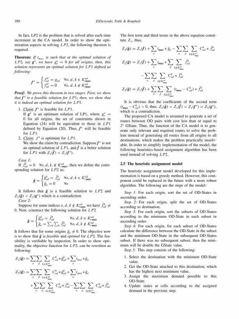
which is a contradiction.The proposed CA model is assumed to generate a set of

routes between OD pairs with cost less than or equal to2∗ GState. Thus, the function of the CA model is to gen-erate only relevant and required routes to solve the prob-lem instead of generating all routes from all origins to alldestinations, which makes the problem practically unsolv-able. In order to simplify implementation of the model, thefollowing heuristics-based assignment algorithm has beenused instead of solving LP2.

2.5 The heuristic assignment model

The heuristic assignment model developed for this imple-mentation is based on a greedy method. However, this com-ponent could be replaced in the future with a more robustalgorithm. The following are the steps of the model:

Step 1: For each origin, sort the set of OD-States inascending order.Step 2: For each origin, split the set of OD-States

according to destination.Step 3: For each origin, sort the subsets of OD-States

according to the minimum OD-State in each subset inascending order.Step 4: For each origin, for each subset of OD-States

calculate the difference between the OD-State in the subsetand the minimum OD-State in the subsequent OD-Statessubset. If there was no subsequent subset, then the mini-mum will be double the GState value.Step 5: This step consists of the following:

1. Select the destination with the minimum OD-Statevalue.

2. Get the OD-State attached to this destination, whichhas the highest next minimum value.

3. Assign the maximum demand possible to thisOD-State.

4. Update states at cells according to the assigneddemand in the previous step.


5. If the destination capacity was not exhausted, goto (b), otherwise go to (a).

3 NUMERICAL EVALUATION

In this section, the numerical network example and testingschemes are presented. Each testing scheme is intended todemonstrate different aspects of the proposed CA model.This test focuses on demonstrating the performance of themodel against exact solutions obtained by solving the math-ematical programming model of the CTDAP.

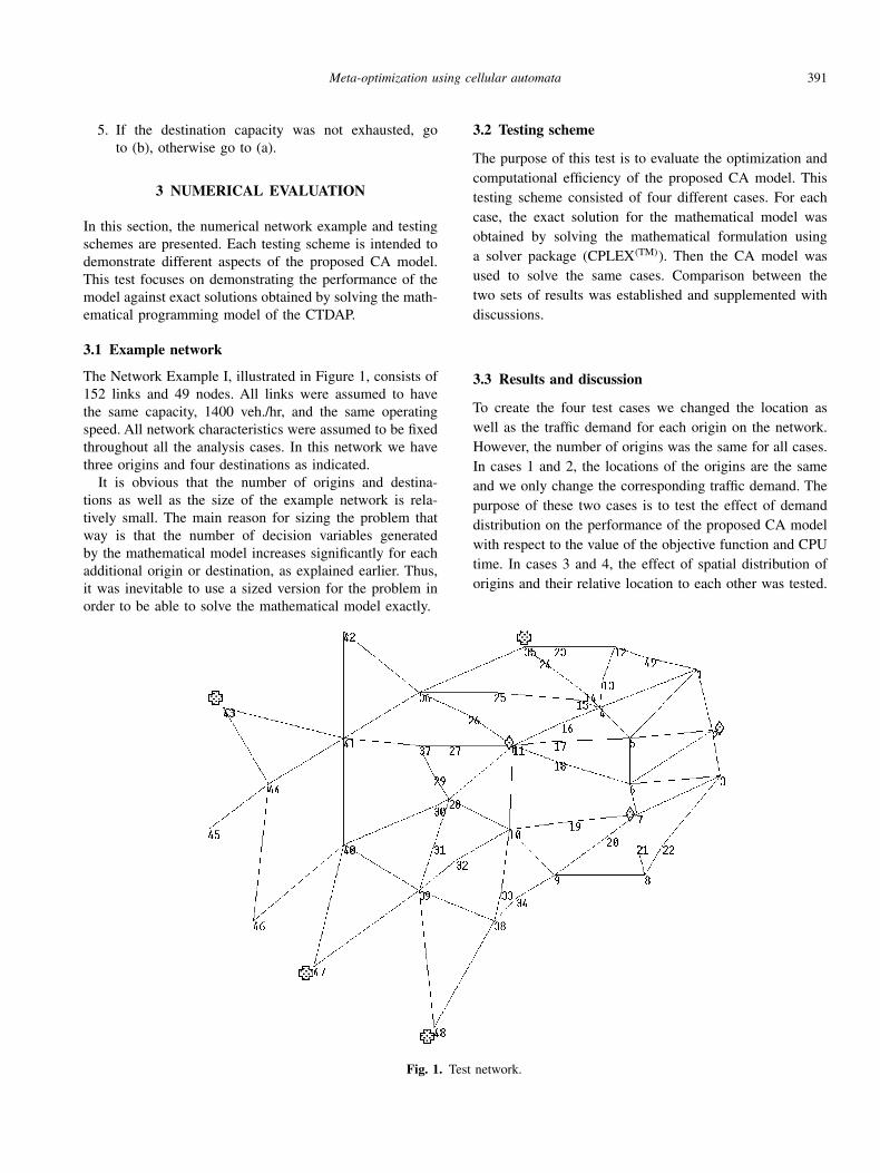
3.1 Example network

The Network Example I, illustrated in Figure 1, consists of152 links and 49 nodes. All links were assumed to havethe same capacity, 1400 veh./hr, and the same operatingspeed. All network characteristics were assumed to be fixedthroughout all the analysis cases. In this network we havethree origins and four destinations as indicated.

It is obvious that the number of origins and destina-tions as well as the size of the example network is rela-tively small. The main reason for sizing the problem thatway is that the number of decision variables generatedby the mathematical model increases significantly for eachadditional origin or destination, as explained earlier. Thus,it was inevitable to use a sized version for the problem inorder to be able to solve the mathematical model exactly.

Fig. 1. Test network.

3.2 Testing scheme

The purpose of this test is to evaluate the optimization andcomputational efficiency of the proposed CA model. Thistesting scheme consisted of four different cases. For eachcase, the exact solution for the mathematical model wasobtained by solving the mathematical formulation usinga solver package (CPLEX(TM)). Then the CA model wasused to solve the same cases. Comparison between thetwo sets of results was established and supplemented withdiscussions.

3.3 Results and discussion

To create the four test cases we changed the location aswell as the traffic demand for each origin on the network.However, the number of origins was the same for all cases.In cases 1 and 2, the locations of the origins are the sameand we only change the corresponding traffic demand. Thepurpose of these two cases is to test the effect of demanddistribution on the performance of the proposed CA modelwith respect to the value of the objective function and CPUtime. In cases 3 and 4, the effect of spatial distribution oforigins and their relative location to each other was tested.


Fig. 2. Case 1 results.

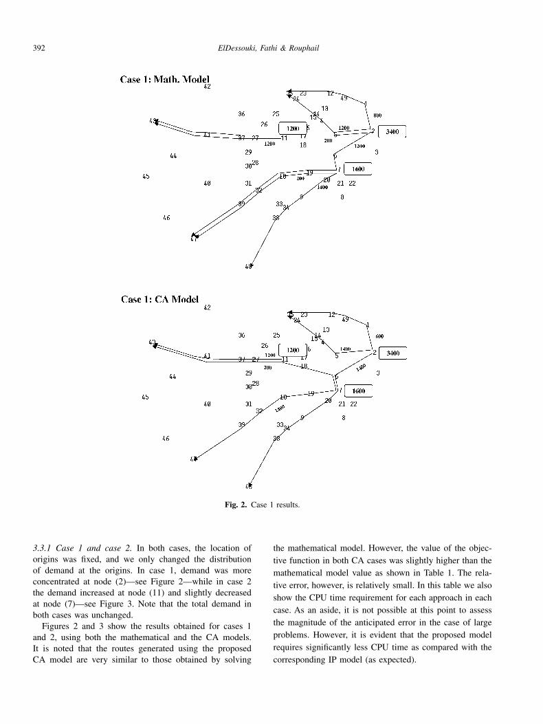
3.3.1 Case 1 and case 2. In both cases, the location oforigins was fixed, and we only changed the distributionof demand at the origins. In case 1, demand was moreconcentrated at node (2)—see Figure 2—while in case 2the demand increased at node (11) and slightly decreasedat node (7)—see Figure 3. Note that the total demand inboth cases was unchanged.

Figures 2 and 3 show the results obtained for cases 1and 2, using both the mathematical and the CA models.It is noted that the routes generated using the proposedCA model are very similar to those obtained by solving

the mathematical model. However, the value of the objec-tive function in both CA cases was slightly higher than themathematical model value as shown in Table 1. The rela-tive error, however, is relatively small. In this table we alsoshow the CPU time requirement for each approach in eachcase. As an aside, it is not possible at this point to assessthe magnitude of the anticipated error in the case of largeproblems. However, it is evident that the proposed modelrequires significantly less CPU time as compared with thecorresponding IP model (as expected).



Table 1CA and mathematical model results

Objective Function Value CPU Time(Veh. Min.) (Sec.)

CA Math. Error % CA Math.

Case 1 267118.0 265140.0 0.75 6.82 103.42Case 2 249708.0 249490.0 0.09 5.50 42.40Case 3 264202.0 263640.0 0.21 6.97 64.59Case 4 213020.0 212660.0 0.17 3.84 46.08



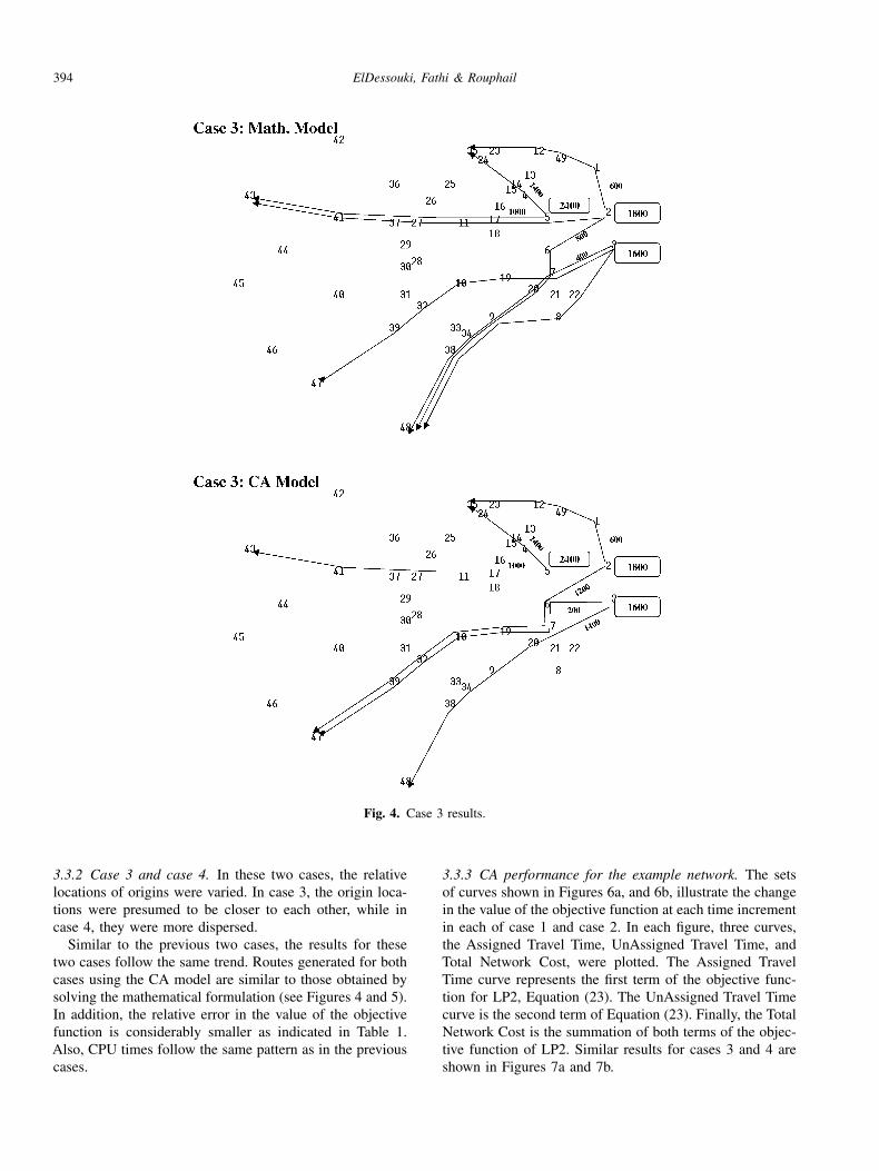
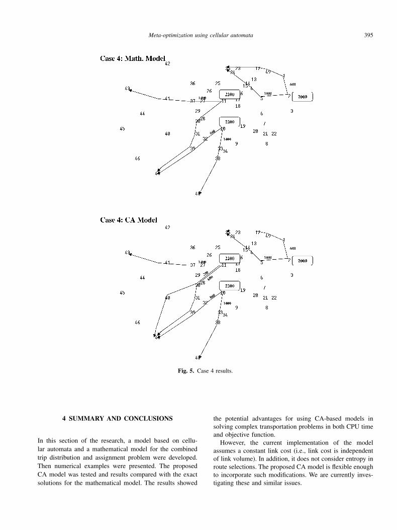
3.3.2 Case 3 and case 4. In these two cases, the relativelocations of origins were varied. In case 3, the origin loca-tions were presumed to be closer to each other, while incase 4, they were more dispersed.

Similar to the previous two cases, the results for thesetwo cases follow the same trend. Routes generated for bothcases using the CA model are similar to those obtained bysolving the mathematical formulation (see Figures 4 and 5).In addition, the relative error in the value of the objectivefunction is considerably smaller as indicated in Table 1.Also, CPU times follow the same pattern as in the previouscases.

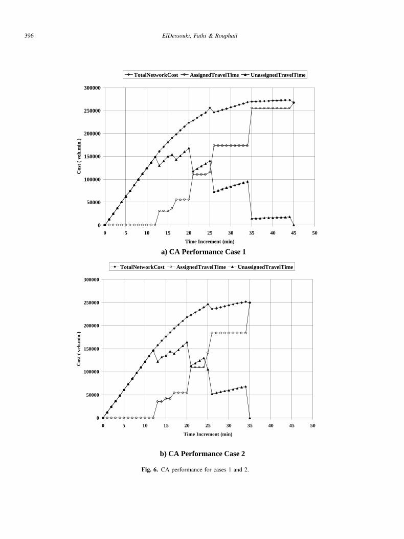
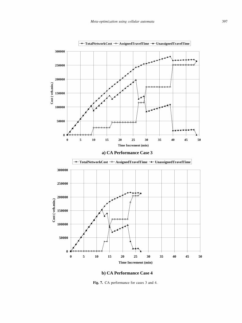
3.3.3 CA performance for the example network. The setsof curves shown in Figures 6a, and 6b, illustrate the changein the value of the objective function at each time incrementin each of case 1 and case 2. In each figure, three curves,the Assigned Travel Time, UnAssigned Travel Time, andTotal Network Cost, were plotted. The Assigned TravelTime curve represents the first term of the objective func-tion for LP2, Equation (23). The UnAssigned Travel Timecurve is the second term of Equation (23). Finally, the TotalNetwork Cost is the summation of both terms of the objec-tive function of LP2. Similar results for cases 3 and 4 areshown in Figures 7a and 7b.



4 SUMMARY AND CONCLUSIONS

In this section of the research, a model based on cellu-lar automata and a mathematical model for the combinedtrip distribution and assignment problem were developed.Then numerical examples were presented. The proposedCA model was tested and results compared with the exactsolutions for the mathematical model. The results showed

the potential advantages for using CA-based models insolving complex transportation problems in both CPU timeand objective function.

However, the current implementation of the modelassumes a constant link cost (i.e., link cost is independentof link volume). In addition, it does not consider entropy inroute selections. The proposed CA model is flexible enoughto incorporate such modifications. We are currently inves-tigating these and similar issues.


0

50000

100000

150000

200000

250000

300000

0 5 10 15 20 25 30 35 40 45 50

Time Increment (min)

Cos

t (

veh.

min

.)TotalNetworkCost AssignedTravelTime UnassignedTravelTime

a) CA Performance Case 1

0

50000

100000

150000

200000

250000

300000

0 5 10 15 20 25 30 35 40 45 50


Cos

t (

veh.

min

.)

TotalNetworkCost AssignedTravelTime UnassignedTravelTime

b) CA Performance Case 2

Fig. 6. CA performance for cases 1 and 2.


0

50000

100000

150000

200000

250000

300000

0 5 10 15 20 25 30 35 40 45 50


Cos

t (

veh.

min

.)


a) CA Performance Case 3

0

50000

100000

150000

200000

250000

300000

0 5 10 15 20 25 30 35 40 45 50


Cos

t (

veh.

min

.)


b) CA Performance Case 4

Fig. 7. CA performance for cases 3 and 4.


REFERENCES

Adamatzky, A. I. (1996), Computation of shortest path in cellularautomata, Math. Comput. Modeling, 23 (4), 105–113.

Benjamin, S. C., Johnson, N. F. & Hui, P. M. (1996), Cellularautomata models of traffic flow along a highway containing ajunction, Jour. Phys. A: Math. Gen 29, 3119–27.

Boyce, D. & Daskin, M. (1997), Design and operation of civil andenvironmental engineering systems, Chapter 7, Eds. ReVelle, C.and McGarity, J. Wiley, New York.

Chopard, B., Luthi, P.O. & Queloz, P. (1996), A. cellular automatamodel of car traffic in a two-dimensional street network, Jour.Phys. A: Math. Gen 29, 2325–36.

CPLEX Manual (1993), Using the CPLEX(TM) Linear Optimizer,CPLEX Optimization Inc., CPLEX Corporation.

Evans, S. P. (1973), A relationship between the gravity modelfor trip distribution and the transportation problem in linearprogramming, Trans. Res. 7, 39–61.

Evans, S. P. (1976), Derivation and analysis of some models for com-bined trip distribution and assignment, Trans. Res. 10, 35–57.

Horowitz, A. J. (1989), Tests of an ad hoc algorithm of elas-tic demand equilibrium traffic assignment, Trans. Res. Part B,Vol. 23B (4) 309–13.

Lam, W. H. K. & Huang, H. J. (1992a), Calibration of the com-bined trip distribution and assignment model for multiple userclasses, Trans. Res. Part B, 26B (4), 289–305.

Lam, W. H. K. & Huang, H. J. (1992b), Modified Evan’s Algo-rithm for solving the combined trip distribution and assignmentproblem, Trans. Res. Part B, 26 (4), 325–37.

Lam, W. H. K. & Huang, H. J. (1992c), A combined trip distri-bution and assignment model for multiple user classes, Trans.Res. Part B, 26B (4), 275–87.

Lam, W. H. K. & Huang, H. J. (1996), Link choice proportionsfrom trip distribution and assignment models: An overview andcomparison, Jour. of Advanced Trans. 30 (1), 1–21.

Neumann, J. V. & Burks, A. W (1966), Theory of Self-ReproducingAutomata, University of Illinois Press, Urbana, IL.

Stiles, P. N. & Glickstein, I. S. (1994), Highly parallelizable routeplanner based on cellular automata algorithms, IBM Jour. Res.Develop., 38 (2), 167–74.

Tzionas, P., Tsalides, Ph. & Thanailakis, A. (1992), Cellularautomata based minimum cost path estimation on binary maps,Electronics Letters, 28 (17), 1653–1654.

Wagner, P., Nagel, K. & Wolf, D. E. (1997), Realistic multi-lane traffic rules for cellular automata, Physica A 234,687–98.

Meta-Optimization Using Cellular Automata with Application to the Combined Trip Distribution and...

Documents

Transcript of Meta-Optimization Using Cellular Automata with Application to the Combined Trip Distribution and...