lable at ScienceDirect

Biomaterials 30 (2009) 1978–1987

Contents lists avai

Biomaterials

journal homepage: www.elsevier .com/locate/biomater ia ls

Cellular automata model for drug release from binary matrix and reservoirpolymeric devices

Timo Johannes Laaksonen a,*, Hannu Mikael Laaksonen b, Jouni Tapio Hirvonen a, Lasse Murtomaki c,d

a Division of Pharmaceutical Technology, University of Helsinki, P.O. Box 56 (Viikinkaari 5E), FI-00014 Helsinki, Finlandb Brain Research Unit, Low Temperature Laboratory, Helsinki University of Technology, P.O. Box 5100, FI-02015 TKK, Finlandc Centre for Drug Research, University of Helsinki, P.O. Box 56 (Viikinkaari 5E), FI-00014, Finlandd Laboratory of Physical Chemistry and Electrochemistry, Helsinki University of Technology, P.O. Box 6100, FI-02015 TKK, Finland

a r t i c l e i n f o

Article history:Received 19 September 2008Accepted 14 December 2008Available online 9 January 2009

Keywords:Drug releaseDissolutionCellular automataModelingPercolation

* Corresponding author. Tel.: þ358 9 191 59161; faE-mail address: timo.laaksonen@helsinki.fi (T. Joh

0142-9612/$ – see front matter � 2008 Elsevier Ltd.doi:10.1016/j.biomaterials.2008.12.028

a b s t r a c t

Kinetics of drug release from polymeric tablets, inserts and implants is an important and widely studiedarea. Here we present a new and widely applicable cellular automata model for diffusion and erosionprocesses occurring during drug release from polymeric drug release devices. The model divides a 2Drepresentation of the release device into an array of cells. Each cell contains information about thematerial, drug, polymer or solvent that the domain contains. Cells are then allowed to rearrangeaccording to statistical rules designed to match realistic drug release. Diffusion is modeled by a randomwalk of mobile cells and kinetics of chemical or physical processes by probabilities of conversion fromone state to another. This is according to the basis of diffusion coefficients and kinetic rate constants,which are on fundamental level just probabilities for certain occurrences. The model is applied to threekinds of devices with different release mechanisms: erodable matrices, diffusion through channels orpores and membrane controlled release. The dissolution curves obtained are compared to analyticalmodels from literature and the validity of the model is considered. The model is shown to be compatiblewith all three release devices, highlighting easy adaptability of the model to virtually any release systemand geometry. Further extension and applications of the model are envisioned.

� 2008 Elsevier Ltd. All rights reserved.

1. Introduction

Controlled release of drugs can be achieved by using polymersto bind drugs into tablets, inserts or other solid devices. Dependingon the nature of the binding polymer, three major release mecha-nisms have been observed [1]. First, biodegradable or erodingpolymer systems release their contents via surface erosion, i.e. newdrug surface is revealed as the polymeric matrix is eroded away.Second, the drug can be released through channels or pores insidea non-eroding polymeric matrix. In the third case, a polymericpermeable membrane is used to control the release rate. All threecases follow different release kinetic profiles, for which severalanalytical solutions have been proposed [2,3].

Most analytical models are based on assumed steady statediffusion profiles and are simple to use. Perhaps the most famous ofthese is the Higuchi model, where a linear concentration gradient isassumed to begin from a solid drug and the water/solid interface isconsumed and recedes as the dissolution proceeds [4,5]. Another

x: þ358 9 191 59144.annes Laaksonen).

All rights reserved.

approach is to use percolation theory and percolation thresholds toestimate the kinetic parameters [6–8]. Models have also beenapplied for several different geometries such as slabs, cylinders andspheres [2]. Although some semi-empirical equations such as thePeppas model exist to model a general system [9,10], mostanalytical equations can only be used for the single system theywere derived for. Another common limitation is that only someregion of the whole release curve can be modeled. Lag times andburst release mechanisms are not usually considered and somemodels are not applicable for the late time release. While someauthors do consider the whole time scale by applying the realdifferential diffusion equations [11–13], even these are limited toa single geometry. For a completely new system, one has to choosethe right equation or derive new ones.

Here, a generic approach which can model all three majorrelease mechanism types for virtually any geometry is proposed. Itis based on cellular automata simulations, which have been used byBadiali et al. to model corrosion of metal surfaces [14–16]. It hasalso been used to model drug release from eroding polymericmatrices [12,17–23]. A 2D representation of the release device isdivided into a grid space, where each cell represents a small part ofthe whole system. Each cell is connected to 4 neighboring cells and

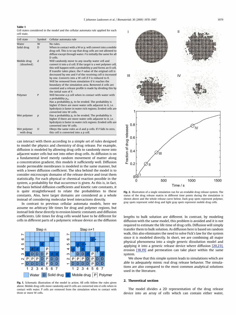
Table 1Cell states considered in the model and the cellular automata rule applied for eachcell state.

Cell state Symbol Cellular automata rule

Water W No rules.Solid drug D When in contact with a W or p, will convert into a mobile

drug cell. This is to say that drug cells are not allowed todiffuse except through water. q is initially the same for allD cells.

Mobile drug(dissolved)

d Will randomly move to any nearby water cell andconvert it into a d cell. If the target is a wet polymer cell,this will happen with a probability p and forms an O cell.If transfer takes place, the q value of the original cell isdecreased by one and q of the receiving cell is increasedby one. Converts into a W cell if q is reduced to 0.Will be removed from simulation if it reaches theboundary of the simulation area. Removed d cells arecounted and a release profile is made by dividing this bythe initial sum of q.

Polymer P Will become a p cell when in contact with water witha probability pw.Has a probability pe to be eroded. The probability ishigher if there are more water cells adjacent to it, i.e.hydrolysis is faster in water rich regions. Eroded cells areconverted into W cells.

Wet polymer p Has a probability pe to be eroded. The probability ishigher if there are more water cells adjacent to it, i.e.hydrolysis is faster in water rich regions. Eroded cells areconverted into W cells.

Wet polymerwith drug

O Obeys the same rules as d and p cells. If q falls to zero,this cell is converted into a p cell.

Fig. 2. Illustration of a single simulation run for an erodable drug release system. Thestatus of the drug release matrix in different time points during the simulation isshown above and the whole release curve below. Dark gray spots represent polymer,gray spots represent solid drug and light gray spots represent mobile drug cells.

T. Johannes Laaksonen et al. / Biomaterials 30 (2009) 1978–1987 1979

can interact with them according to a simple set of rules designedto model the physics and chemistry of drug release. For example,diffusion is modeled by allowing drug cells to randomly move intoadjacent water cells but not into other drug cells. As diffusion is ona fundamental level merely random movement of matter alonga concentration gradient, this models it sufficiently well. Diffusioninside permeable membranes is modeled in the same manner, butwith a lower diffusion coefficient. The idea behind the model is toconsider microscopic domains of the release device and treat themstatistically. For each physical or chemical reaction possible in thesystem, a probability for that occurrence is given. As this is, in fact,the basis behind diffusion coefficients and kinetic rate constants, itis quite straightforward to relate the probabilities to theseconstants. Also, here larger domains are considered as a wholeinstead of considering molecular level interactions directly.

In contrast to previous cellular automata models, here weassume no arbitrary life times for drug and polymer regions, butinstead link these directly to erosion kinetic constants and diffusioncoefficients. Life times for drug cells would have to be different forcells in different parts of a polymeric release device as the diffusion

Fig. 1. Schematic illustration of the model in action. All cells follow the rules givenabove. Mobile drug cells move randomly and D cells are converted into d cells when incontact with water. P cells are removed from the simulation when in contact withthree or more W cells.

lengths to bulk solution are different. In contrast, by modelingdiffusion with the same model, this problem is avoided and it is notrequired to estimate the life time of drug cells. Diffusion will simplytransfer them to bulk solution. As diffusion here is based on randomwalk, this also eliminates the need to solve Fick’s law for the systemsince it is modeled directly. In short, we are combining all majorphysical phenomena into a single generic dissolution model andapplying it into a generic release device where diffusion [20,23],erosion [18,19] and permeation can take place within the samesystem.

We show that this simple system leads to simulations which areable to adequately mimic real drug release behavior. The simula-tions are also compared to the most common analytical solutionsused in the literature.

2. Theoretical section

The model divides a 2D representation of the drug releasedevice into an array of cells which can contain either water,

0 500 1000 15000

0.2

0.4

0.6

0.8

1

Time / s

Frac

tion

of d

rug

rele

ased

Increasing drug

fraction

101 102 10310-5

10-4

10-3

10-2

10-1

100

Time / s

Frac

tion

of d

rug

rele

ased

Fig. 3. (Left) Release curves simulated for an erodable drug release system. Parameters were as follows: p¼ 0, pc¼ 0.001 for 2 flanking W cells and pc¼ 1 for 3 or 4 flanking W cells,q¼ 1. Volume fraction of D cells was varied from 15% to 80% with 5% increments. The last few curves overlap almost completely and cannot be distinguished from the graph. (Right)Logarithmic representation of the same data. The simulations match analytical equations in the linear regions. Release curves are an average of 10 simulation runs each.

T. Johannes Laaksonen et al. / Biomaterials 30 (2009) 1978–19871980

polymer or drug. Each cell is connected to the 4 adjacent cells. Allinteractions are limited to these connections and diagonal move-ment is not considered. In a typical system, a water cell layersurrounds a continuous matrix of polymer and drug cells, i.e. thedrug release device is suspended in water. The system is thenallowed to rearrange according to a simple set of rules. Each cellrepresents a domain of the release device, not single molecules oreven groups of molecules. In a typical simulation presented below,each unit cell is assumed to be ca. 100 mm wide. Concentration issimply represented by the density of drug filled domains anda chemical reaction is assumed to have taken place when it wouldhave had time to proceed for the whole volume of a single cell. Eachcell behaves statistically, i.e. it has a certain probability to do certainthings such as to move to a neighboring cell or to be converted intoanother type of a cell. The time scale of the simulation is defined bythe fastest species. In this case that is assumed to be the diffusingdrug species. The probability for its movement is set to 1 and all

0 500 1000 15000

0.2

0.4

0.6

0.8

1

Time / s

Frac

tion

of d

rug

rele

ased

Increasing θ

Fig. 4. (Left) Release curves simulated for an erodable drug release system. Parameters wereVolume fraction of D cells was 50% and q was varied from 1 to 6. (Right) Logarithmic reprregions. Release curves are an average of 10 simulation runs each.

other probabilities are relative to this. The considerations above areaccording to the basis of diffusion coefficients and kinetic rateconstants, which are on fundamental level just probabilities forcertain occurrences. A high probability means that the occurrence itmodels has a high rate constant and vice versa. The exact chemicalnature of the modeled substances is not considered here. Whiledifferent drugs could have widely different behavior, for thepurposes of this model only the diffusion coefficient and, toa certain degree, estimation for the solubility are needed. Similarly,a polymer has only two characteristics: permeability to drug (andwater) and erodability. Other characteristics of the simulation arisefrom the overall design of the system: geometry, the way the drugand polymer cells are mixed and the maximum dimensions.

The model allows each cell to have one of six different statesand has different rules for each state. These are shown in Table 1.Each cell is checked in random order during each calculation cycleand the above rules are applied. Fig. 1 illustrates how this works.

101 102 10310-5

10-4

10-3

10-2

10-1

100

Time / s

Frac

tion

of d

rug

rele

ased

as follows: p¼ 0, pc¼ 0.001 for 2 flanking W cells and pc¼ 1 for 3 or 4 flanking W cells.esentation of the same data. The simulations match analytical equations in the linear

10 20 30 40 50 60 70 800

5000

10000

15000

20000

25000

30000

Volume fraction of drug (%)

t 50

/ s

Fig. 5. Time to dissolve 50% of the initial drug content obtained from Fig. 3. Lines arefor highlighting the two kinetic regions observed for the system.

Fig. 7. Illustration of a single simulation run for drug release system where the drug isreleased through pores in a non-erodable polymeric matrix. The status of the drugrelease matrix in different time points during the simulation is shown above and thewhole release curve below. Dark gray spots represent polymer, gray spots representsolid drug and light gray spots represent mobile drug cells.

T. Johannes Laaksonen et al. / Biomaterials 30 (2009) 1978–1987 1981

W cells do nothing, while D cells are automatically converted intod cells if adjacent to water like in the case of the cell at (4,3). Inthis example P cells are impermeable to water and drug, but areeroded if surrounded by water from three or four directions.Accordingly, the P cell at (5,4) is eroded after step n. Mobile drugcells will move to random directions but can only enter W cells. Ifthey try to move to other types of cells they simply will not moveduring this step.

Mobile drug cells are allowed to randomly move to W cells. Thisleads to a random walk behavior, and intrinsically creates a diffu-sion field in the simulation. Convection inside or close to the deviceis not considered. To model the effect of convection, the limits ofthe simulation area can be changed. As it is taken that each d cellreaching the limit of the simulation is removed from the system,this naturally means that sink conditions apply at the edges and thelength of the stagnant water layer around the device is equal to theW cell thickness surrounding the drug matrix. The relationshipbetween the simulation time step dt, diffusion coefficient D and thelattice size of the simulated matrix a is shown in Eq. (1) [15].

D ¼ 14

a2

dt(1)

1 2 3 4 5 6

4000

5000

6000

7000

8000

9000

θ

t 50

/ s

Fig. 6. Time to dissolve 50% of the initial drug content obtained from Fig. 4. The line isfor eye-guide only.

Probability p indicates the permeability of the polymer to the drug,i.e. the solubility of the drug into the polymer matrix. For dense,impermeable polymers this will be 0. For permeable walls as in thecase of coated matrices it will be higher depending on the diffusioncoefficient of the drug inside the polymer membrane, as per Eq. (2).Similarly, pw measures how fast water can penetrate or wet thepolymer. Again, this is 0 for dense hydrophobic polymers and largerfor permeable/hydrophilic polymers.

p ¼�

Dpolymer=D�1=2

(2)

Polymer erosion parameter (pe) indicates the probability that a P/pcell is destroyed during each calculation cycle. It can mean eitherthe dissolution of the polymer, as would be the case with degrad-able polymers, or erosion of hard insoluble polymers, i.e. washingaway of strands of the polymer. The rate of disintegration (k) can beobtained from Eq. (3) when pe is known [15]. The equation assumedzero-order kinetics for linear erosion of a polymeric layer. The

0 500 1000 15000

0.2

0.4

0.6

0.8

1

Time / s

Frac

tion

of d

rug

rele

ased

Increasingvolumefraction

0 10 20 30 400

1

Frac

tion

of d

rug

rele

ased

0.2

0.4

0.6

0.8

t1/2 / s1/2

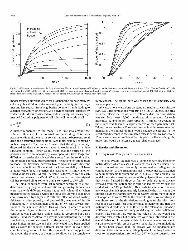
Fig. 8. (Left) Release curves simulated for drug release by diffusion through a polymer/drug binary matrix. Parameters were as follows: p¼ 0, pc¼ 0, q¼ 1. Volume fraction of D cellswas varied from 20% to 80% with 5% increments. (Right) The same data normalized and plotted against t1/2. Linear curves for released fractions of 0.10–0.70 indicate that thesimulations correspond to analytical models. Release curves are an average of 10 simulation runs each.

T. Johannes Laaksonen et al. / Biomaterials 30 (2009) 1978–19871982

model assumes different values for pe depending on how many Wcells neighbor it. More water means higher mobility for the poly-mer and less support from neighboring polymer strands leading toa higher probability for erosion. So a polymer cell that is flanked bywater on all sides is considered to erode instantly, whereas a poly-mer cell flanked by polymers on all sides will not erode at all.

k ¼ peadt

(3)

A further refinement to the model is to take into account thevolume difference of the solvated and solid drug. This extraparameter q is equivalent to the concentration ratio between a soliddrug and a saturated drug solution. Each initial drug cell contains q

mobile drug cells. The case q¼ 1 means that the drug is initiallydispersed in the same concentration it would reach in a fullysaturated solution. Higher values mean that the surface of theparticle erodes in an increasingly slower pace as it takes longer fordiffusion to transfer the solvated drug away from the solid or thatthe solution is initially supersaturated. The parameter can be usedto model the difference between two compounds with differentsaturated solubilities. The one with a lower solubility will havea higher value for q. In practice, this parameter is simply anotherstored value for each D/d cell. The value is decreased by one eachtime a d cell moves to a W cell. When it reaches zero, the originalcell has released all its contents and is converted to a W cell.

The initial conditions were set randomly according to a pre-determined drug/polymer volume ratio and geometry. Simulationswere run with different volume ratios and values of q. Whenmodeling coated release devices, the initial set-up was a solid drugcore surrounded by a layer of P cells. The effect of varied coatingthickness, coating porosity and permeability was studied in thesimulations. A predetermined amount of W cells always sur-rounded the simulated device. This was done in order to modelthe stagnant layer diffusion around the matrix. The systemconsidered was a cylinder or a fiber, which is represented as a discin the 2D grid space. Although a cyclindrical system was used in allsimulations, it must be stressed that the geometry of the modelledis not limited in any way and the model could have been appliedjust as easily for squares, different aspect ratios or even morecomplex configurations. In fact, this is one of the strong points ofthe model: the geometry of the initial condition can be completely

freely chosen. The set-up here was chosen for its simplicity andvisual appearance.

All calculations were done on standard mathematical software(MATLAB). The simulations were run on a 126�126 grid. The areawith the release matrix was a 101 cell wide disc. Each simulationwas run for at least 15,000 rounds and all simulations for eachindividual parameter set were repeated 10 times. An average ofthese runs was taken as a representative of each parameter set.Taking the average from 20 runs was tested in order to see whetherincreasing the number of runs would change the results. As nosignificant difference in the simulated release curves was observed,10 runs were deemed sufficient for this grid size. For smaller grids,more runs would be necessary to get reliable averages.

3. Results and discussion

3.1. Drug release through an erosion mechanism

The first system studied was a simple binary drug/polymermatrix device which releases its contents via surface erosion. Theinitial composition was randomly determined according to thevolume fraction of the drug. In this case, the polymer was assumedto be impermeable to water and drug (p, pw¼ 0) and erodable. Tomodel the surface erosion process of the polymer, it was assumedthat P cells flanked by three or four W cells are automaticallyremoved from the system and P cells flanked by two W cells areeroded with a 0.1% probability. This leads to simulations, wherenew water channels spontaneously form inside the matrices as thethinner polymer structure slowly erode away, leaving more of the Dcells exposed to water. While the choice for the pe was arbitrary, itwas chosen so that the simulations would give results which cor-responded well with real drug formulation behavior and that thesystem would erode in ca. 15,000 steps of the calculation. Choosinga different pe value would simply model a system with a differenterosion rate constant. By varying the value of pe, we would getdifferent release rates, but as here we were only interested in theoverall behavior of the system, this choice was deemed sufficient.Fig. 2 shows how this sort of a system looks like in the simulations.

It has been shown that the release will be fundamentallydifferent if there is no or very little polymer, if the drug fraction isclose to the percolation threshold (ca. 59% with the square lattice

Fig. 9. Illustration of a single simulation run for a permeable membrane controlled drugrelease system. The status of the drug release matrix in different time points during thesimulation is shown above and the whole release curve below. Dark gray spots representpolymer, gray spots represent solid drug and light gray spots represent mobile drug cells.

0 500 1000 15000

0.2

0.4

0.6

0.8

1

Time / s

Frac

tion

of d

rug

rele

ased

Increasingcoating thickness

Fig. 10. (Left) Simulated release curves for a permeable membrane controlled release deviceto 0.20. (Right) The same data with the released fraction scaled to �ln(1� f). Linear curvesaverage of 10 simulation runs each.

T. Johannes Laaksonen et al. / Biomaterials 30 (2009) 1978–1987 1983

used here [8]), or if there is a large fraction of the polymer. In thefirst case, the amount of polymer will have negligible effect on therelease profile, since there is not enough of it to slow down drugdiffusion. In the second case the release profile is very sensitive tothe volume fraction and a critical kinetic variable will be linearlydependent on the volume fraction. In the last case, release will bevery slow and some of the drug may be retained by the device sincethe drug can be indefinitely bound by polymer cavities [1,6,8].Therefore, modeling the effect of the volume fraction is of funda-mental interest.

Volume fraction was varied from 15% to 80% and the releasecurve simulations were run for q¼ 1–6. The results are shown inFigs. 3 and 4. The time scale is set according to Eq. (1) assuming thatthe sphere is 1 cm in diameter and that the diffusion coefficient ofthe drug is 2.5�10�6 cm2/s. All subsequent simulations were per-formed assuming the same size for the system.

For drug amounts exceeding the percolation limit of the drug,the release rate is relatively independent of the polymer content, aswas to be expected for an eroding device. For drug amountsexceeding the percolation limit, the rate is considerably faster as isshown by the t50 values in Fig. 5. For these results, it was expectedthat the profile would follow a tn dependence, with n depending onthe diffusion mechanism [2]. For example, the well-known Higuchimodel predicts n¼½ for pure diffusion controlled release. This isreproduced by the current simulations as can be seen in the loga-rithmic plots in Figs. 3 and 4. For low amounts of polymer, therelease is essentially in pure bulk diffusion control. This is alsoreproduced here in the case where the drug content exceeds 60%,the percolation limit for a square lattice. The new model alsopredicts burst release during the early stages of the process,t< 200 s, when the drug with less diffusion resistance from thesurface of the device is released. This demonstrates the flexibility ofthe model, since many analytical models only predict either early orlate release.

Fig. 6 shows the same analysis as above for the simulations runfor different values of q. As would be expected, an increase in q, i.e.a decrease in saturated solubility, decreases the rate of release.Time to dissolve 50% of the drug is linearly dependent on q, as itwould be on the saturated solubility according to the analyticalmodels. In conclusion, it can be said that the simulations for thesurface erosion type drug release compare well with analyticalmodels.

0 500 1000 15000

1

2

3

Time / s

2.5

1.5

0.5

-ln(1

-f)

. Parameters were as follows: p¼ 0.90, pw¼ 1, pc¼ 0, q¼ 2 and l/r0 was varied from 0.02indicate that the simulations correspond to analytical models. Release curves are an

0 500 1000 15000

0.2

0.4

0.6

0.8

1

Time / s

Frac

tion

of d

rug

rele

ased

Increasingpermability

0 500 1000 15000

1

2

3

4

Time / s

-ln(1

-f)

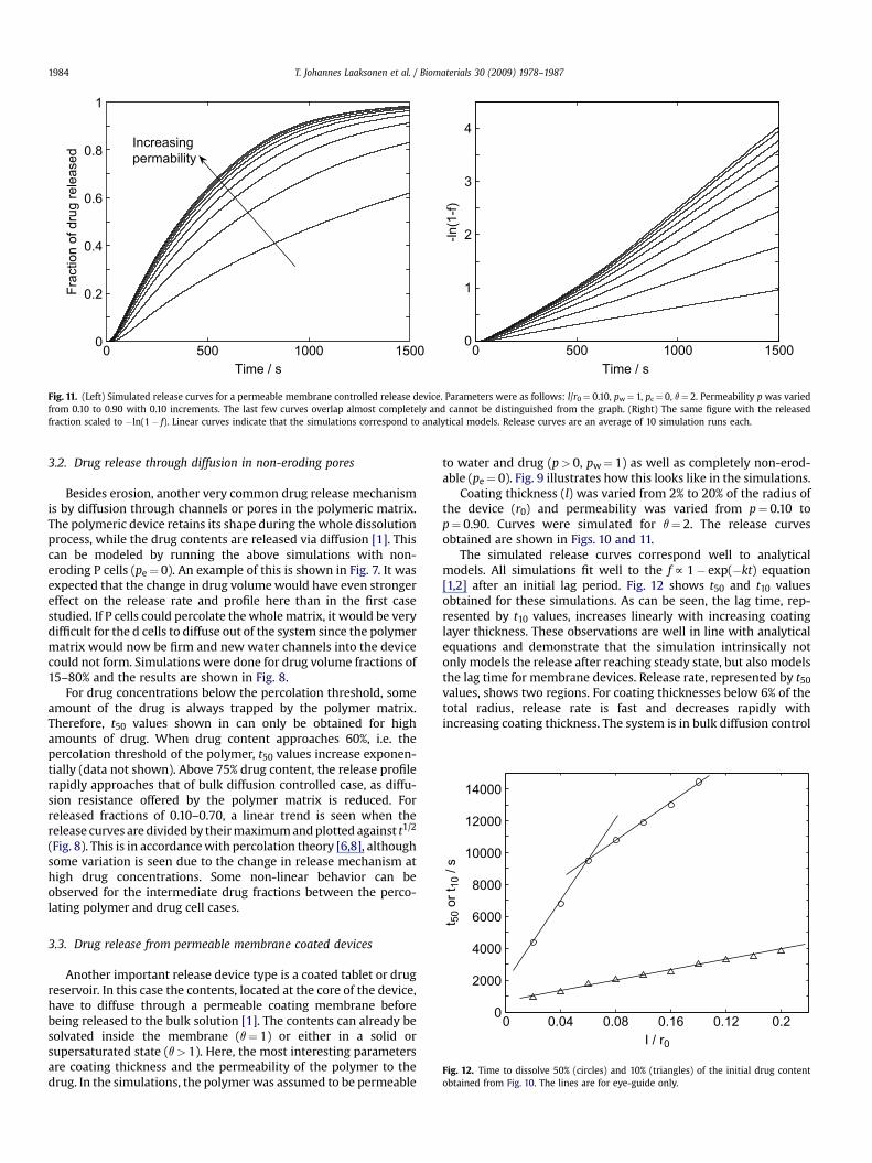
Fig. 11. (Left) Simulated release curves for a permeable membrane controlled release device. Parameters were as follows: l/r0¼ 0.10, pw¼ 1, pc¼ 0, q¼ 2. Permeability p was variedfrom 0.10 to 0.90 with 0.10 increments. The last few curves overlap almost completely and cannot be distinguished from the graph. (Right) The same figure with the releasedfraction scaled to �ln(1� f). Linear curves indicate that the simulations correspond to analytical models. Release curves are an average of 10 simulation runs each.

8000

10000

12000

14000

0 or

t 10

/ s

T. Johannes Laaksonen et al. / Biomaterials 30 (2009) 1978–19871984

3.2. Drug release through diffusion in non-eroding pores

Besides erosion, another very common drug release mechanismis by diffusion through channels or pores in the polymeric matrix.The polymeric device retains its shape during the whole dissolutionprocess, while the drug contents are released via diffusion [1]. Thiscan be modeled by running the above simulations with non-eroding P cells (pe¼ 0). An example of this is shown in Fig. 7. It wasexpected that the change in drug volume would have even strongereffect on the release rate and profile here than in the first casestudied. If P cells could percolate the whole matrix, it would be verydifficult for the d cells to diffuse out of the system since the polymermatrix would now be firm and new water channels into the devicecould not form. Simulations were done for drug volume fractions of15–80% and the results are shown in Fig. 8.

For drug concentrations below the percolation threshold, someamount of the drug is always trapped by the polymer matrix.Therefore, t50 values shown in can only be obtained for highamounts of drug. When drug content approaches 60%, i.e. thepercolation threshold of the polymer, t50 values increase exponen-tially (data not shown). Above 75% drug content, the release profilerapidly approaches that of bulk diffusion controlled case, as diffu-sion resistance offered by the polymer matrix is reduced. Forreleased fractions of 0.10–0.70, a linear trend is seen when therelease curves are divided by their maximum and plotted against t1/2

(Fig. 8). This is in accordance with percolation theory [6,8], althoughsome variation is seen due to the change in release mechanism athigh drug concentrations. Some non-linear behavior can beobserved for the intermediate drug fractions between the perco-lating polymer and drug cell cases.

00

2000

4000

6000

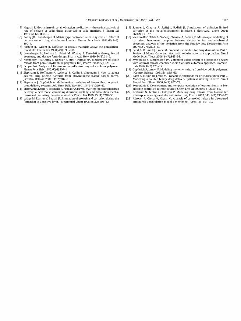
0.04 0.08 0.120.16 0.2I / r0

t 5

Fig. 12. Time to dissolve 50% (circles) and 10% (triangles) of the initial drug contentobtained from Fig. 10. The lines are for eye-guide only.

3.3. Drug release from permeable membrane coated devices

Another important release device type is a coated tablet or drugreservoir. In this case the contents, located at the core of the device,have to diffuse through a permeable coating membrane beforebeing released to the bulk solution [1]. The contents can already besolvated inside the membrane (q¼ 1) or either in a solid orsupersaturated state (q> 1). Here, the most interesting parametersare coating thickness and the permeability of the polymer to thedrug. In the simulations, the polymer was assumed to be permeable

to water and drug (p> 0, pw¼ 1) as well as completely non-erod-able (pe¼ 0). Fig. 9 illustrates how this looks like in the simulations.

Coating thickness (l) was varied from 2% to 20% of the radius ofthe device (r0) and permeability was varied from p¼ 0.10 top¼ 0.90. Curves were simulated for q¼ 2. The release curvesobtained are shown in Figs. 10 and 11.

The simulated release curves correspond well to analyticalmodels. All simulations fit well to the f f 1� exp(�kt) equation[1,2] after an initial lag period. Fig. 12 shows t50 and t10 valuesobtained for these simulations. As can be seen, the lag time, rep-resented by t10 values, increases linearly with increasing coatinglayer thickness. These observations are well in line with analyticalequations and demonstrate that the simulation intrinsically notonly models the release after reaching steady state, but also modelsthe lag time for membrane devices. Release rate, represented by t50

values, shows two regions. For coating thicknesses below 6% of thetotal radius, release rate is fast and decreases rapidly withincreasing coating thickness. The system is in bulk diffusion control

0 500 1000 15000

0.2

0.4

0.6

0.8

1

Time / s

Frac

tion

of d

rug

rele

ased

Increasingporosity

0 500 1000 15000

1

2

3

4

Time / s

-ln(1

-f)

Fig. 13. (Left) Simulated release curves for a porous membrane controlled release device. Parameters were as follows: l/r0¼ 0.10, p¼ 0.90, pw¼ 1, pc¼ 0, q¼ 2. Porosity was variedfrom 10% to 90% with 10% increments. (Right) The same figure with the released fraction scaled to �ln(1� f). Linear curves indicate that the simulations correspond to analyticalmodels. Release curves are an average of 10 simulation runs each.

T. Johannes Laaksonen et al. / Biomaterials 30 (2009) 1978–1987 1985

for zero thickness. Above l/r0¼ 0.06, internal diffusion startscontrolling the release and the slope of t50 vs. l/r0 changes. Anincrease in permeability increased the release rate exponentiallyafter it had passed a certain value, here ca. p¼ 0.3. For thinnercoatings, the permeability value where release starts to slow downsignificantly is much lower than for thicker coatings (simulationsnot shown).

The model was further extended to consider the effect ofporosity of the coating layer on the release kinetics. Here, thecoating layer was randomly filled with holes (W cells) in order tocreate a simulated porous coating. Otherwise the model parame-ters were as for the normal coated device case. Simulations wererun for porosities of 10–90%. The release curves are shown in Fig. 13.

As for the other membrane device simulations, these simula-tions corresponded well with the f f 1� exp(kt) law. An increase inthe porosity of a poorly permeable membrane increased the releaserate from the device. Two regions in the t50 values are shown inFig. 14. For low porosity, the release is still partially controlled bypermeation through the membrane, whereas for high porosity,diffusion through the pores dominates the release mechanism. Forvery high porosities, the release approaches bulk diffusion limited

0 20 40 60 80 100

4000

5000

6000

7000

8000

9000

10000

porosity (%)

t 50

/ s

Fig. 14. Time to dissolve 50% of the initial drug content obtained from Fig. 13. The linesare for eye-guide only and highlight the two kinetic regions observed for the system.

case. The transition point for these two responses is near thepercolation threshold of the drug volume fraction.

3.4. Further extensions

The model was demonstrated to be applicable for the three mostcommon drug release mechanisms: surface erosion, releasethrough matrix pores and membrane controlled release. But it is byno means limited to these cases. As we make no strong assump-tions about the whole system, i.e. the rules are designed to applylocally to only small parts of the matrix, it is easy to combinedifferent types of release devices into a single model. This can bedone simply by applying different initial conditions and giving thecells the desired properties. Combining, for example, a layer of puredrug with a non-erodable polymer/drug core, one gets a model foran instant release layer covering a slow release device as is illus-trated in Fig. 15. By combining several impermeable layers whicherode slowly, it is possible to model a multilayered release device,which releases its contents in a series of pulses, as is also shown inFig. 15. As long as it is possible to draw a representative map of therelease device and outline simple rules which the system mustobey, there are virtually no limitations to what systems the modelcan simulate. This could be very useful for the design and devel-opment of novel release devices with multiple functionalities.

The results presented here were for a 2D grid. Naturally, it wouldbe useful to do these simulations in 3D as well. Although this wouldrequire significantly longer calculation times, it would be instruc-tive to see whether the results change in any significant way. Oneother thing that should be noted is that the percolation thresholdsobserved above are dependent on the lattice type used. Herea square lattice was used. For other lattice types such as cubical, FCCor diamond, the threshold would naturally be different [6,8]. Thisshould not change the general features of the simulations, butnaturally would lead to different dependency on the polymer/drugratio. In further extensions, the model should be flexible enough toaccommodate more features as need arises. For example, it ispossible to design a simple set of rules that would allow the poly-mer matrix to swell or to add other components such as dis-integrants into the system. Finite kinetics for drug dissolution couldbe easily implemented by assigning a probability for the d to D cellconversion, as has been done earlier by Adrover et al. [23]. Othermore complex geometries and devices such as nanoporous silicon,

Fig. 15. Simulated results for (Left) an instant release layer covering a slow bulk release device and (Right) a multilayered release device, which releases its contents in a series ofpulses. Images above the release graphs show what the simulation matrix looks like during different time points of the simulation. Release curves and images are from only a singlesimulation run.

T. Johannes Laaksonen et al. / Biomaterials 30 (2009) 1978–19871986

transdermal patches and multiarrays of polymeric inserts can alsobe imagined to benefit from this type of modeling.

A great advantage with using cellular automata simulations isthat one does not have to worry about the exact geometry of thedevice used. As long as it is possible to draw it in the simplified formpresented above, it can be modeled. With analytical models, thereis a real danger that wrong models are used when one does notcheck what the assumptions behind each model were and whatgeometry was used to derive each equation. Modeling diffusiondirectly reduces the amount of assumptions needed. Previouscellular automata models used for erodable systems have assumeda life time for each cell [18,19,21]. As this should be different fordrug cells deeper inside the polymeric matrix, it is not straight-forward to use a single value for this. Modeling diffusion, however,gives the added benefit of realistically modeling the different timeit takes for a drug cluster near the surface to be transported into thebulk solution in contrast to a drug cluster near the center of therelease device. The diffusion lengths for these two cases are verydifferent and cannot be modeled with simple life time assignments.

As a further benefit of using the model presented here, itintrinsically models the early burst release and/or lag time of thesystem as well as the late time release. Comparisons to analyticalmodels, which very often only apply to mid-time release, gaveproof that this model can be applicable to the full time releasemodeling of drug release from polymeric devices. Combining thedifferent kinetic regions of drug release is not a simple task foranalytical solutions.

4. Conclusions

A cellular, probabilistic model representing drug release waspresented. It was simple to implement with relatively few

parameters, and gave realistic results with limited calculationpower required. The model is extremely flexible and was able tosimulate three major polymeric release device types with compa-rable results to established analytical models. Lag time and burstrelease were also intrinsically simulated. There are no limitationswith combining these types to a single calculation with this modelor with using more complicated geometries. Therefore, it is envi-sioned that it could be used to predict and design the behavior offorthcoming, increasingly complicated devices with multiplefunctionalities and/or release time control measures.

Acknowledgements

The authors acknowledge financial support from the Universityof Helsinki (Development of Nano Sciences/HENAKOTO, 700036,T.L.).

Appendix. Supplementary data

Movie files of the simulations in Figs. 2, 7, 9, and 15 are provided.Supplementary material can be found in the online version at doi:10.1016/j.biomaterials.2008.12.028.

References

[1] Graham NB, Wood DA. Polymeric inserts and implants for the controlledrelease of drugs. In: Hastings GW, Ducheyne P, editors. Macromolecularbiomaterials. Boca Raton, FL: CRC Press; 1984. p. 184–214.

[2] Costa P, Sousa Lobo JM. Modeling and comparison of dissolution profiles. Eur JPharm Sci 2001;13(2):123–33.

[3] Narasimhan B. Accurate models in controlled drug delivery systems. In:Wise DL, editor. Handbook of pharmaceutical controlled release technology.New York: Marcel Dekker; 2000. p. 155–81.

[4] Higuchi T. Rate of release of medicaments from ointment bases containingdrugs in suspension. J Pharm Sci 1961;50(10):874–5.

T. Johannes Laaksonen et al. / Biomaterials 30 (2009) 1978–1987 1987

[5] Higuchi T. Mechanism of sustained-action medication – theoretical analysis ofrate of release of solid drugs dispersed in solid matrices. J Pharm Sci1963;52(12):1145–9.

[6] Bonny JD, Leuenberger H. Matrix type controlled release systems: I. Effect ofpercolation on drug dissolution kinetics. Pharm Acta Helv 1991;66(5–6):160–4.

[7] Hastedt JE, Wright JL. Diffusion in porous materials above the percolation-threshold. Pharm Res 1990;7(9):893–901.

[8] Leuenberger H, Holman L, Usteri M, Winzap S. Percolation theory, fractalgeometry, and dosage form design. Pharm Acta Helv 1989;64(2):34–9.

[9] Korsmeyer RW, Gurny R, Doelker E, Buri P, Peppas NA. Mechanisms of soluterelease from porous hydrophilic polymers. Int J Pharm 1983;15(1):25–35.

[10] Peppas NA. Analysis of Fickian and non-Fickian drug release from polymers.Pharm Acta Helv 1985;60(4):110–1.

[11] Siepmann F, Hoffmann A, Leclercq B, Carlin B, Siepmann J. How to adjustdesired drug release patterns from ethylcellulose-coated dosage forms.J Control Release 2007;119(2):182–9.

[12] Siepmann J, Gopferich A. Mathematical modeling of bioerodible, polymericdrug delivery systems. Adv Drug Deliv Rev 2001;48(2–3):229–47.

[13] Siepmann J, Kranz H, Bodmeier R, Peppas NA. HPMC-matrices for controlled drugdelivery: a new model combining diffusion, swelling, and dissolution mecha-nisms and predicting the release kinetics. Pharm Res 1999;16(11):1748–56.

[14] Lafage M, Russier V, Badiali JP. Simulation of growth and corrosion during theformation of a passive layer. J Electroanal Chem 1998;450(2):203–12.

[15] Saunier J, Chausse A, Stafiej J, Badiali JP. Simulations of diffusion limitedcorrosion at the metal/environment interface. J Electroanal Chem 2004;563(2):239–47.

[16] Vautrin-Ul C, Taleb A, Stafiej J, Chausse A, Badiali JP. Mesoscopic modelling ofcorrosion phenomena: coupling between electrochemical and mechanicalprocesses, analysis of the deviation from the Faraday law. Electrochim Acta2007;52(27):7802–10.

[17] Barat A, Ruskin HJ, Crane M. Probabilistic models for drug dissolution. Part 1.Review of Monte Carlo and stochastic cellular automata approaches. SimulModel Pract Theor 2006;14(7):843–56.

[18] Zygourakis K, Markenscoff PA. Computer-aided design of bioerodible deviceswith optimal release characteristics: a cellular automata approach. Biomate-rials 1996;17(2):125–35.

[19] Gopferich A, Langer R. Modeling monomer release from bioerodible polymers.J Control Release 1995;33(1):55–69.

[20] Barat A, Ruskin HJ, Crane M. Probabilistic methods for drug dissolution. Part 2.Modelling a soluble binary drug delivery system dissolving in vitro. SimulModel Pract Theor 2006;14(7):857–73.

[21] Zygourakis K. Development and temporal evolution of erosion fronts in bio-erodible controlled release devices. Chem Eng Sci 1990;45(8):2359–66.

[22] Bertrand N, Leclair G, Hildgen P. Modeling drug release from bioerodiblemicrospheres using a cellular automaton. Int J Pharm 2007;343(1–2):196–207.

[23] Adrover A, Giona M, Grassi M. Analysis of controlled release in disorderedstructures: a percolation model. J Membr Sci 1996;113(1):21–30.