1

Cellular automata in the hyperbolic plane: proposal for a new environment.

Kamel Chelghoum, Maurice Margenstern, Benoît Martin, and Isabelle Pecci

LITA, University of Metz, Île du Saulcy, 57045 Metz, Cedex 01, France {chelghoum, margens, martin, pecci}@sciences.univ-metz.fr

Abstract. In this paper, we deal with new environment to visualise and to in-teract with cellular automata implemented in a grid of the hyperbolic plane. We use two kinds of tiling: the ternary heptagrid and the rectangular pentagrid. We show that both grids have the same spanning tree: the same numbering with maximal Fibonacci numbers can be used to identify all tiles. We give all the materials to compute the neighbourhood of any tile in the heptagrid or in the pentagrid. Then we propose visualisation and interaction techniques to interact with cellular automata which are grounded in these two grids.

1 Introduction

Cellular automata are used in a lot of fields, especially in industrial applications, in order to simulate reaction diffusion phenomena. In most of these cases, we are able to perform measures before the phenomena and after it happened, but measures during the process it-self are usually out of reach. Cellular automata turned out to be an effi-cient way for trying to understand what happens during the phenomenon, thanks to their great power of simulation. In these simulations, the initial configuration of the cellular automaton and the states of the cells during the process are discretisations of the situation before and during the event. In Euclidean geometry this raises no prob-lem and usually no attention is given to this issue.

The situation is very different in the hyperbolic plane. Hyperbolic geometry is more and more used for solving more easily complex problems. This is the main reason to use the tiling of the hyperbolic plane to implement and manipulate automata cellular. We refer the reader to [10] [11] for introductory material on hyperbolic ge-ometry. In order to fix things and to spare space, we shall use Poincaré’s disc model of the hyperbolic plane. The open unit disc U of the Euclidean plane constitutes the points of the hyperbolic plane IH2. The border of U, ∂U is the set of points at infinity. Lines are the trace in U of its diameters or the trace in U of circles which are or-thogonal to ∂U.

In this paper, we present a new environment to visualise and to interact with cellu-lar automata implemented in the rectangular pentagrid and similarly in the ternary heptagrid on the hyperbolic plane. For cellular automata being grounded on a poly-grid of the hyperbolic plane, a polygon represents a cell. The problem of initialising cellular automata based on locating points on the polygrid is already studied and

2

algorithms are given in [1] [3] for the pentagrid and in [5] for the heptagrid. Our goal is to compute the neighbours of a cell and to show the state of each cell of the cellular automaton. In section 2, we shortly present the splitting method for the ternary hepta-grid and the rectangular pentagrid. Then, in section 3, we propose algorithms to find direct neighbours of a cell using the maximal Fibonacci representation. Thanks to this neighbourhood, we can write now algorithms for implementing cellular automata in the both grids of the hyperbolic plane. Thus, in section 4, we propose algorithms to visualise and to interact with them.

2 Splitting the plane

Recall that in the theory of tilings, a particular case consists in considering a polygon P and then, all the reflections of P in its sides and, recursively, of the images in their sides: this is called a tessellation of P. We say that the obtained polygons are gener-ated by P. Of course, we assume that we have the tiling property: two distinct poly-gons being generated by P have non intersecting interiors and any point of the plane is in the closure of at least one polygon of the set. In this case, we say that the tiling is generated by P; we shall also say that the tiling is the grid defined by P.

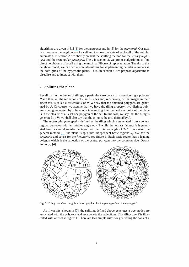
The rectangular pentagrid is defined as the tiling which is generated from a central regular pentagon with an interior angle of π/2 while the ternary heptagrid is gener-ated from a central regular heptagon with an interior angle of 2π/3. Following the general method [9], the plane is split into independent basic regions Ri, five for the pentagrid and seven for the heptagrid, see figure 1. Each basic region has a leading polygon which is the reflection of the central polygon into the common side. Details are in [2] [4].

10

R1

R5 R4

R2

R3

R1 R2R3

R4

R5R6R7

Fig. 1. Tiling tree T and neighbourhood graph G for the pentagrid and the heptagrid.

As it was first shown in [7], the splitting defined above generates a tree: nodes are associated with the polygons and arcs denote the reflections. This tiling tree T is illus-trated with arrows in figure 1. There are two simple rules for generating the sons of a

3

node. One rule applies to 3-nodes, in white in the tree, and the other rule applies to 2-nodes, in black in the tree [7]:

• a 3-node has three sons: to left, a 2-node and, in the middle and to right in both cases, 3-nodes.

• a 2-node has 2 sons: to left a 2-node, to right a 3-node. These rules are applied for splitting the heptagrid and for splitting the pentagrid.

They generate the same spanning tree for the basic regions of both grids. Proof and correctness are in [4]. To complete the tiling tree, the main node which corresponds to the central polygon and represented by a white square has arcs which connect it with the leading polygon of each basic region Ri.

Notice that this tree is a spanning tree of the neighbourhood graph G. It is not dif-ficult to restore that dual graph from this tree. It is enough to define additional connections which are represented in bold lines and dotted lines in figure 1.

3 Cellular automata in the hyperbolic plane

Initialising a cellular automaton and locating a cell and its neighbours in the hyper-bolic plane is not that trivial as it is in the Euclidean case. We focus now in this prob-lem of locating a cell and its neighbours. Required information can be extracted from the Fibonacci representations attached to the polygons, hence to the cells of the automaton.

3.1 Fibonacci numbering

In [6], a new ingredient is brought. Numbering the nodes of the tree which is obtained from the splitting, we use what is called the standard Fibonacci representation of the positive integers. Indeed, it is well known that any positive number n can be written as wn = , which means:

)α...α(αw k-k 11= with αi ∈ {0,1}, ∑=

=k

iii.fαw

1with

⎩⎨⎧

≥∀+===

−− 21

12

10nfff

ff

nnn

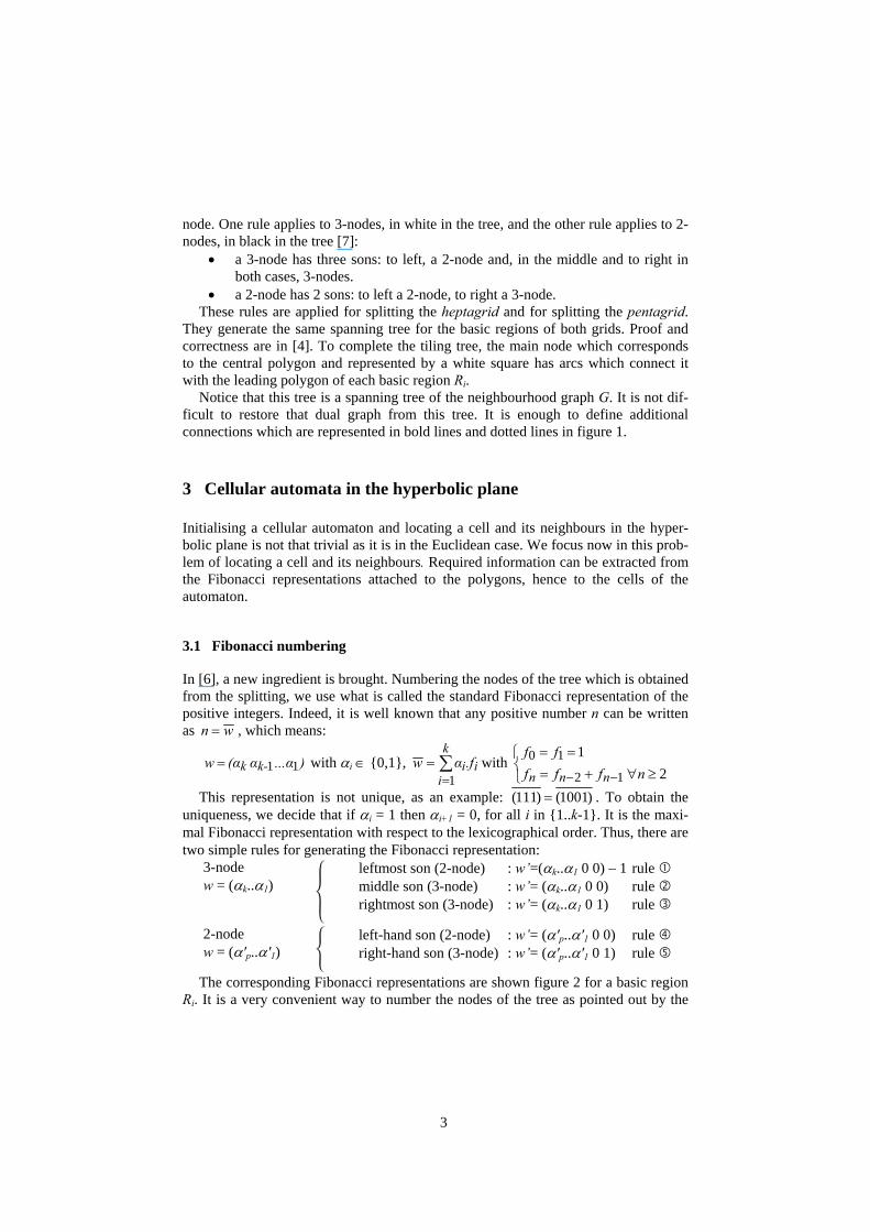
This representation is not unique, as an example: )1001()111( = . To obtain the uniqueness, we decide that if αi = 1 then αi+1 = 0, for all i in {1..k-1}. It is the maxi-mal Fibonacci representation with respect to the lexicographical order. Thus, there are two simple rules for generating the Fibonacci representation:

3-node w = (αk..α1)

leftmost son (2-node) : w’=(αk..α1 0 0) – 1 rule middle son (3-node) : w’= (αk..α1 0 0) rule rightmost son (3-node) : w’= (αk..α1 0 1) rule

2-node w = (α'p..α'1)

left-hand son (2-node) : w’= (α'p..α'1 0 0) rule right-hand son (3-node) : w’= (α'p..α'1 0 1) rule

The corresponding Fibonacci representations are shown figure 2 for a basic region Ri. It is a very convenient way to number the nodes of the tree as pointed out by the

4

above rules. For example, it is easy to determine the type of a node n numbered w: we can note w = u1(0)p with p≥0. If p is odd, we know that w is a 2-node. In the contrary, if p is even, n is a 3-node.

100000

100001

100010

100100

100101

101000

101001

101010

1000000

1000001

1000010

1000100

1000101

1001000

1001001

1001010

1010000

1010001

1010010

1010100

1010101

12 3 4

5 6 7 8 9 10 11 12

13 14 15 16 17 18 19 20 21 22 23 24 25 26 27 28 29 30 31 32 33

10

100

101

1000

1001

1010

10000

10001

10010

10100

10101

1

Fig. 2. Fibonacci numbering for a basic region Ri.

The maximal Fibonacci representation gives a coordinate for all polygons of the basic regions. By extension, we define 0 to be the coordinate of the central polygon. Next numbering the basic regions from 1 up to nbSides (five for the pentagrid and seven for the heptagrid), counter clockwise, we obtain the coordinate of a polygon as a couple (r, w) with r being the basic region containing the polygon and w being a maximal Fibonacci representation of a positive number.

3.2 Neighbourhood computation

The immediate neighbours of a polygon p are the polygons which are obtained by reflection of p in one of its sides. In [8], we obtained the following theorem: “there is a linear algorithm to compute the path from a node of the spanning tree of a basic region to its root as a list of coordinates. There is also a linear algorithm to compute the coordinates of the immediate neighbours of a polygon from its coordinates”.

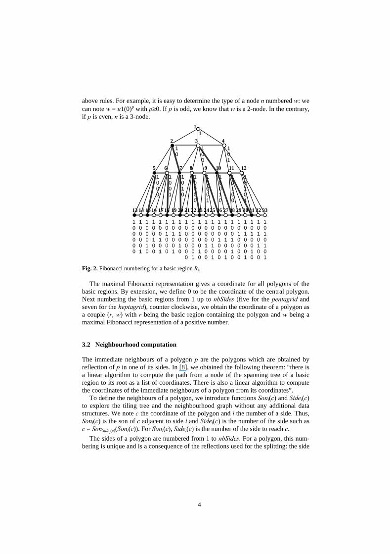
To define the neighbours of a polygon, we introduce functions Soni(c) and Sidei(c) to explore the tiling tree and the neighbourhood graph without any additional data structures. We note c the coordinate of the polygon and i the number of a side. Thus, Soni(c) is the son of c adjacent to side i and Sidei(c) is the number of the side such as c = SonSidei(c)(Soni(c)). For Soni(c), Sidei(c) is the number of the side to reach c.

The sides of a polygon are numbered from 1 to nbSides. For a polygon, this num-bering is unique and is a consequence of the reflections used for the splitting: the side

5

numbered nbSides is the parent side. It is the side which is adjacent with its parent. Then, the other sides are numbered counter clockwise from this parent side from 1 to nbSides-1. For the central polygon, side 1 indicates region 1 and so on. Figure 3 shows functions Son and Side for the heptagrid by using the following functions inc and pred:

⎩⎨⎧

−∈+==

]1..1[ with 1)(1)(

nbSidesiiiincnbSidesinc

⎩⎨⎧

∈−==

]..2[ with 1)()1(

nbSidesiiiprednbSidespred

(0, 0)5

1

2 3

4

(1, 1)

7

(2, 1)(3, 1)

(4, 1)

(5, 1)

67

(6, 1)

(7, 1)

7

77

7

7

7

(r, w=1(01)n)n>0

5

12

34

6

7

(r, w00)

(r, w01)

n=0:(r, 10)n>0:(r, 1(01)n-10010)

(inc(r), 10(00)n)

n=0:(0, 0)

n>0:(r, 1(01)n-1)

n>0:(inc(r),10(00)n-1)

n=0:(inc(r), 1)

n=0:(pred(r), 1)n>0:(r, 1(01)n-100) 6

7

7

7

1

1

2

4

r

(r, w10)

n>0:(r, 10(00)n-1)(pred(r), 1(01)n)n=0:(r, 1)

5

12

34

6

7

(r, w00)

(r, w01)

(pred(r), 1(01)n+1)

n=0:(r, 100)n>0:(r, 10(00)n-101)

(r,w=10(00)n)n>0

5

6

7

71

1

2

3

(r, w=u(01)n)n>0u∉{O,1}

5

12

34

6

7

(r, w00)

(r, w01)

(r, u(01)n-10010)

(r, u10(00)n)

n>1:(r, u(01)n-1)n=1: let u=v(0)q with q>0(r, u) if q even(r, u) if q odd

(r, u10(00)n-1)

6

7

7

7

1

2

4

n>1:(r, u(01)n-100)n=1: let u=v(0)q with q>0

(r, u00) if q even(r, u00) if q odd

5

12

34

6

7

(r, w00)

(r, w01)

(r, u1(00)n-1)u=O:(r, u0(10)n+1)u=O:(r, (10)n+1)

(r,u1(00)n-101)

(r, w10)

u=O:(r, u0(10)n)u=O:(r, (10)n)

(r,w=u1(00)n)n>0

6

7

7

7

1

1

3

(r, u(10)n-101)

5

1

(r, w=u(10)n)u=Oor n>1

2

34

6

7

(r, w00)

(r, w01)(r, w10)

n>1: (r, u(10)n-1)n=1, let u=v(0)q, q>0

q even: (r, u)q odd: (r, u)

u=O, n>1: (r, 1(00)n-1)u=O, let u=v00(r, v01(00)n-1)

u=O: (r, 1(00)n)u=O, let u=v00(r, v01(00)n)

1

2

5

6

7

7

1

(r,w=u10(00)n)n>0u=O

5

12

34

6

7

(r, u10(00)n-101)

(r, w10)

(r, u10(00)n-1)

(r, w01)

(r, w00)

(r, u(01)n+1)

(r, u(01)n) 5

6

7

7 1

1

3

Fig. 3. The neighbourhood of a heptagon of the heptagrid.

We obtain the corresponding neighbourhood of the pentagrid just by removing the light seams. Then side 7 becomes side 5 and we number the sides counter clockwise from 1 to 4 starting from side 5. Details and proof of correctness are in [2] and [4].

6

4. Visualisation and interaction techniques

For cellular automata being grounded on the hyperbolic plane, a polygon represents a cell. The Fibonacci numbering allows us to compute the coordinates of the immediate neighbours of a cell, which is the starting point of an implementation of cellular auto-mata in the pentagrid or the heptagrid. However, our goal is to use the tiling as a display to show the state of each cell too. For this, many techniques can be used: different colours, values … We propose to dissociate the polygon of the display from the cell which is displayed in. In this case, the tiling tree T is viewed as the display and the neighbourhood graph G is viewed as the cellular automaton. By bringing a cell to the centre of the tiling, user focuses on a specific cell. We note that this action is not a scaling in the hyperbolic plane but a shift of the cells. The distortion of the mapping between the hyperbolic plane and the Poincaré’s disc gives the feeling of a zoom.

By this way, some cells not yet visible can appear, some visible cells can disap-pear, some cells become more important while other become less important ... Of course, in all cases, the neighbourhood of the cells must be kept. In this paper, we propose a technique to associate any cells to the main polygon of the tiling while keeping the neighbourhood. We will call the cell displayed in the central polygon, the main cell.

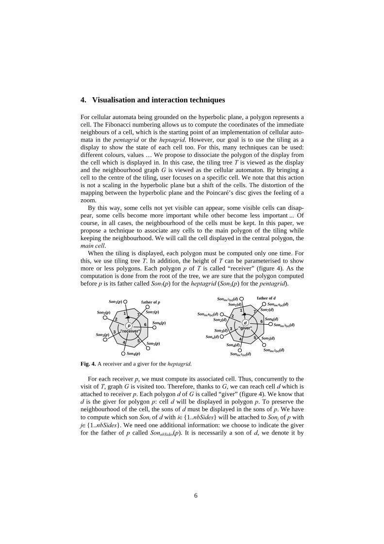
When the tiling is displayed, each polygon must be computed only one time. For this, we use tiling tree T. In addition, the height of T can be parameterised to show more or less polygons. Each polygon p of T is called “receiver” (figure 4). As the computation is done from the root of the tree, we are sure that the polygon computed before p is its father called Son7(p) for the heptagrid (Son5(p) for the pentagrid).

5

12

3

4

6

7

p"receiver"

Son1(p)

Son2(p)

Son3(p)

Son4(p)

Son5(p)

Son7(p)

Son6(p)

father of p

Son1(d)

Son2(d)

Son3(d)Sonu(d)

Soninc1(u)(d)

5

12

3

4

6

7

father of d

d"giver"

Son4(d)Son5(d)

Son6(d)

Son7(d)

Soninc2(u)(d)

Soninc4(u)(d)

Soninc3(u)(d)

Soninc5(u)(d)

Soninc6(u)(d)

Fig. 4. A receiver and a giver for the heptagrid.

For each receiver p, we must compute its associated cell. Thus, concurrently to the visit of T, graph G is visited too. Therefore, thanks to G, we can reach cell d which is attached to receiver p. Each polygon d of G is called “giver” (figure 4). We know that d is the giver for polygon p: cell d will be displayed in polygon p. To preserve the neighbourhood of the cell, the sons of d must be displayed in the sons of p. We have to compute which son Soni of d with i∈{1..nbSides} will be attached to Sonj of p with j∈{1..nbSides}. We need one additional information: we choose to indicate the giver for the father of p called SonnbSides(p). It is necessarily a son of d, we denote it by

7

Sonu(d) with u∈{1..nbSides}. Now, we take the givers and the receivers counter clockwise from Sonu(d) and SonnbSides(p) respectively:

for all i in {1..nbSides}, the giver for Soni(p) is Soninci(u)(d) The function inci is an extension of the previous function inc:

for all u in {1..nbSides} inc0(u) = u inci(u) = inc(inci-1(u)) with i>1

In addition, we know that from the point of view of Soninci(u)(d), the giver for p is

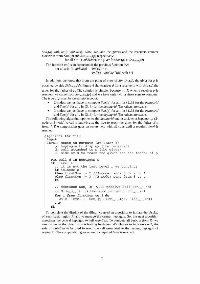
obtained by side Sideinci(u)(d). Figure 4 shows giver d for a receiver p with Son3(d) the giver for the father of p. The solution is simpler because, in T, when a receiver p is reached, we come from SonnbSides(p) and we have only two or three sons to compute. The type of p must be taken into account:

• 2-nodes: we just have to compute Soni(p) for all i in {2..3} for the pentagrid and Soni(p) for all i in {3..4} for the heptagrid. The others are seams.

• 3-nodes: we just have to compute Soni(p) for all i in {1..3} for the pentagrid and Soni(p) for all i in {2..4} for the heptagrid. The others are seams.

The following algorithm applies to the heptagrid and associates a heptagon p (2-node or 3-node) to cell d knowing u, the side to reach the giver for the father of p from d. The computation goes on recursively with all sons until a required level is reached. Algorithm for Walk input level: depth to compute (at least 1) p: heptagon to display (the receiver) d: cell attached to p (the giver) u: side of d to reach the giver for the father of p Put cell d in heptagon p if (level > 1) // it is not the last level … we continue if is3Node(p) then firstSon := 2 //3-node: sons from 2 to 4 else firstSon := 3 //2-node: sons from 3 to 4 fi // heptagon Soni (p) will receive cell Soninc

i(u)(d)

// Sideinci(u)(d) is the side to reach Soninc

i(u)(d)

for i from firstSon to 4 do Walk (level-1, Soni(p), Soninc

i(u)(d), Sideinc

i(u)(d))

rof fi

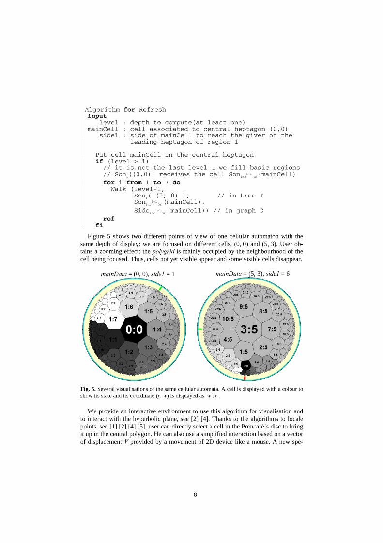
To complete the display of the tiling, we need an algorithm to initiate the display of each basic region Ri and to manage the central heptagon. So, the next algorithm associates the central heptagon to cell mainCell. To compute all basic regions Ri, we need to know the giver for one leading heptagon. We choose to indicate side1, the side of mainCell to be used to reach the cell associated to the leading heptagon of region R1. The computation goes on until a required level is reached.

8

Algorithm for Refresh input level : depth to compute(at least one) mainCell : cell associated to central heptagon (0,0) side1 : side of mainCell to reach the giver of the leading heptagon of region 1 Put cell mainCell in the central heptagon if (level > 1) // it is not the last level … we fill basic regions // Soni((0,0)) receives the cell Soninc

i-1(u)(mainCell)

for i from 1 to 7 do Walk (level-1, Soni( (0, 0) ), // in tree T Soninc

i-1(u)(mainCell),

Sideinci-1

(u)(mainCell)) // in graph G rof fi

Figure 5 shows two different points of view of one cellular automaton with the same depth of display: we are focused on different cells, (0, 0) and (5, 3). User ob-tains a zooming effect: the polygrid is mainly occupied by the neighbourhood of the cell being focused. Thus, cells not yet visible appear and some visible cells disappear.

mainData = (0, 0), side1 = 1

mainData = (5, 3), side1 = 6

Fig. 5. Several visualisations of the same cellular automata. A cell is displayed with a colour to show its state and its coordinate (r, w) is displayed as rw : .

We provide an interactive environment to use this algorithm for visualisation and to interact with the hyperbolic plane, see [2] [4]. Thanks to the algorithms to locale points, see [1] [2] [4] [5], user can directly select a cell in the Poincaré’s disc to bring it up in the central polygon. He can also use a simplified interaction based on a vector of displacement V provided by a movement of 2D device like a mouse. A new spe-

9

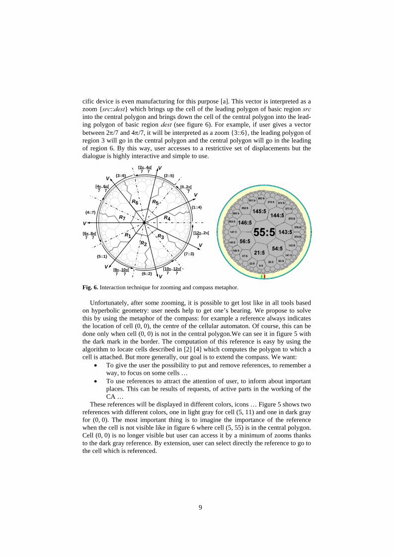
cific device is even manufacturing for this purpose [a]. This vector is interpreted as a zoom {src::dest} which brings up the cell of the leading polygon of basic region src into the central polygon and brings down the cell of the central polygon into the lead-ing polygon of basic region dest (see figure 6). For example, if user gives a vector between 2π/7 and 4π/7, it will be interpreted as a zoom {3::6}, the leading polygon of region 3 will go in the central polygon and the central polygon will go in the leading of region 6. By this way, user accesses to a restrictive set of displacements but the dialogue is highly interactive and simple to use.

R1

{2::5}

{4::7}

{6::2}

{7::3}

{1::4}

{5::1}

{3::6}

[0..2π[7

[2π..4π[7 7

[4π..6π[7 7

[6π..8π[7 7

[8π..10π[7 7

[10π..12π[7 7

[12π..2π[7

R2R3

R4

R5R6

R7

V

V

V

V

V

V

V Fig. 6. Interaction technique for zooming and compass metaphor.

Unfortunately, after some zooming, it is possible to get lost like in all tools based on hyperbolic geometry: user needs help to get one’s bearing. We propose to solve this by using the metaphor of the compass: for example a reference always indicates the location of cell (0, 0), the centre of the cellular automaton. Of course, this can be done only when cell (0, 0) is not in the central polygon.We can see it in figure 5 with the dark mark in the border. The computation of this reference is easy by using the algorithm to locate cells described in [2] [4] which computes the polygon to which a cell is attached. But more generally, our goal is to extend the compass. We want:

• To give the user the possibility to put and remove references, to remember a way, to focus on some cells …

• To use references to attract the attention of user, to inform about important places. This can be results of requests, of active parts in the working of the CA …

These references will be displayed in different colors, icons … Figure 5 shows two references with different colors, one in light gray for cell (5, 11) and one in dark gray for (0, 0). The most important thing is to imagine the importance of the reference when the cell is not visible like in figure 6 where cell (5, 55) is in the central polygon. Cell (0, 0) is no longer visible but user can access it by a minimum of zooms thanks to the dark gray reference. By extension, user can select directly the reference to go to the cell which is referenced.

10

5. Conclusion

In this paper we provide all the materials to ground and compare cellular automata in the rectangular pentagrid and the ternary heptagrid of the hyperbolic plane. In par-ticular, we describe the neighbourhood computation with the Fibonacci numbering and an interactive environment for visualisation and interaction. By using the “fish-eye” effect of the Poincaré’s disc, this environment allows user to concentrate on a part of a snapshot from a cellular automaton. The introduction of the compass avoids any loss of reference during this interaction. In future development, we hope to en-hance our environment to provide tools to follow and to better understand the evolu-tion of the cellular automaton during a period of time. On another hand, we can note that the ternary heptagrid introduces a very important and useful feature: the connec-tion between neighbours. As suggested by the content of [12], this would have inter-esting consequences in complexity issues.

References

a. B. Martin. TrackMouse: a 4D solution for interacting with two cursors. Accepted in IHM’04, Namur, Belgique, Sepember, 2004.

1. K. Chelghoum, M. Margenstern, B. Martin, I. Pecci. Locating Points in the Pentagonal Rectangular Tiling of the Hyperbolic Plane. Proceeding of the 7th World Multiconference on Systemics, Cybernetics and Informatics, SCI’2003, Orlando, Florida, July 27-30, Vol. V, pages 25-30, 2003.

2. K. Chelghoum, M. Margenstern, B. Martin, I. Pecci. Cellular Automata in the pentagrid of the hyperbolic plane: tools for interactions, Publications du LITA, technical report, 2004-101, 63 pages, January 2004.

3. K. Chelghoum, M. Margenstern, B. Martin et I. Pecci. Initialising Cellular Automata in the Hyperbolic Plane. IEICE Transactions on Information and Systems, Special Section on Cellular Automata, vol. E87-D, No3, 677-686, March, 2004.

4. K. Chelghoum, M. Margenstern, B. Martin, I. Pecci. Cellular Automata in the ternary heptagrid of the hyperbolic plane: tools for interactions, Publications du LITA, technical report, 2004-103, 75 pages, March 2004.

5. K. Chelghoum, M. Margenstern, B. Martin, I. Pecci. Tools for implementing cellular auto-mata in grid {7,3} of the hyperbolic plane. Accepted in DMCS, Turku, July, 2004.

6. M. Margenstern. New tools for Cellular Automata in the Hyperbolic Plane, Journal of Universal Computer Science, vol 6, issue 12, 1226-1252, 2000.

7. M. Margenstern, K. Morita. NP-problems are tractable in the space of cellular automata in the hyperbolic plane, Theoretical Computer Science, 259, 99-128, 2001.

8. M. Margenstern. Implementing Cellular Automata on the Triangular Grids of the Hyper-bolic Plane for New Simulation Tools, Proceedings of ASTC'2003, Orlando, March, 29- April, 4, 14-21, ISBN 1-56555-263-6, 2003

9. M. Margenstern. Cellular Automata and Combinatoric Tilings in Hyperbolic Spaces, a survey, Lecture Notes of Computer Sciences, 2731, (2003), 48-72, (proceedings of DMTCS'2003, Dijon, July, 7-12, 2003, invited talk).

10. H. Meschkowski. Non-Euclidean geometry, translated by A. Shenitzer, Academic Press, New-York, 1964.

11. A. Ramsey, R. D. Richtmyer. Introduction to hyperbolic geometry, Springer, Berlin, 1995.

11

12. T. Worsch. Simulations Between Cellular Automata on Trees Extended by Horizontal Edges, Fundamenta Informaticae, vol. 58, No3, 241-260, 2004.