wat e r r e s e a r c h 4 5 ( 2 0 1 1 ) 2 7 2 4e2 7 3 8

Avai lab le at www.sc iencedi rect .com

journa l homepage : www.e lsev ier . com/ loca te /wat res

Modelling Escherichia coli concentrations in the tidal Scheldtriver and estuary

Anouk de Brauwere a,b,c,*, Benjamin de Brye b,c, Pierre Servais d, Julien Passerat d,Eric Deleersnijder b,e

aVrije Universiteit Brussel, Analytical and Environmental Chemistry, Pleinlaan 2, B-1050 Brussels, BelgiumbUniversite catholique de Louvain, Institute of Mechanics, Materials and Civil Engineering (IMMC), 4 Avenue G. Lemaıtre,

B-1348 Louvain-la-Neuve, BelgiumcUniversite catholique de Louvain, Georges Lemaıtre Centre for Earth and Climate Research (TECLIM), 2 Chemin du Cyclotron,

B-1348 Louvain-la-Neuve, BelgiumdUniversite Libre de Bruxelles, Ecologies des Systemes Aquatiques, Campus de la Plaine, CP 221, B-1050 Brussels, BelgiumeUniversite catholique de Louvain, Earth and Life Institute (ELI), Georges Lemaıtre Centre for Earth and Climate Research (TECLIM),

2 Chemin du Cyclotron, B-1348 Louvain-la-Neuve, Belgium

a r t i c l e i n f o

Article history:

Received 27 July 2010

Received in revised form

31 January 2011

Accepted 3 February 2011

Available online 13 February 2011

Keywords:

Escherichia coli

Fecal indicators

Microbiological water quality

Waste water

Modelling

Scheldt

Estuary

Tidal rivers

* Corresponding author. Vrije Universiteit BTel.: þ32 2 629 32 64; fax: þ32 2 629 32 74.

E-mail address: adebrauw@vub.ac.be (B.0043-1354/$ e see front matter ª 2011 Elsevdoi:10.1016/j.watres.2011.02.003

a b s t r a c t

Recent observations in the tidal Scheldt River and Estuary revealed a poor microbiological

water quality and substantial variability of this quality which can hardly be assigned to

a single factor. To assess the importance of tides, river discharge, point sources, upstream

concentrations, mortality and settling a new model (SLIM-EC) was built. This model was

first validated by comparison with the available field measurements of Escherichia coli

(E. coli, a common fecal bacterial indicator) concentrations. The model simulations agreed

well with the observations, and in particular were able to reproduce the observed long-

term median concentrations and variability. Next, the model was used to perform sensi-

tivity runs in which one process/forcing was removed at a time. These simulations

revealed that the tide, upstream concentrations and the mortality process are the primary

factors controlling the long-termmedian E. coli concentrations and the observed variability.

The tide is crucial to explain the increased concentrations upstream of important inputs,

as well as a generally increased variability. Remarkably, the wastewater treatment plants

discharging in the study domain do not seem to have a significant impact. This is due to

a dilution effect, and to the fact that the concentrations coming from upstream (where

large cities are located) are high. Overall, the settling process as it is presently described in

the model does not significantly affect the simulated E. coli concentrations.

ª 2011 Elsevier Ltd. All rights reserved.

1. Introduction agriculture and animal farming, the Scheldt watershed

With its population density of more than 500 inhabitants per

km2, its active industrial development and its intensive

russel, Analytical and E

de Brye).ier Ltd. All rights reserve

(20,000 km2 from the North of France to the BelgianeDutch

border, see Fig. 1) represents an extreme case of surface water

and groundwater pollution (EEA, 2004). Improvement of water

nvironmental Chemistry, Pleinlaan 2, B-1050 Brussels, Belgium.

d.

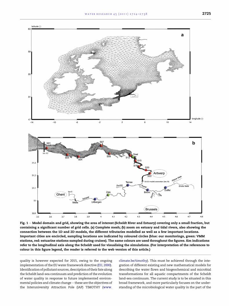
Fig. 1 e Model domain and grid, showing the area of interest (Scheldt River and Estuary) covering only a small fraction, but

containing a significant number of grid cells. (a) Complete mesh; (b) zoom on estuary and tidal rivers, also showing the

connection between the 1D and 2D models, the different tributaries modelled as well as a few important locations.

Important cities are encircled, sampling locations are indicated by coloured circles (blue: our monitorings, green: VMM

stations, red: estuarine stations sampled during cruises). The same colours are used throughout the figures. Km indications

refer to the longitudinal axis along the Scheldt used for visualising the simulations. (For interpretation of the references to

colour in this figure legend, the reader is referred to the web version of this article.)

wat e r r e s e a r c h 4 5 ( 2 0 1 1 ) 2 7 2 4e2 7 3 8 2725

quality is however expected for 2015, owing to the ongoing

implementation of the EUwater framework directive (EU, 2000).

Identificationofpollutantsources,descriptionoftheir fatealong

the Scheldt land-sea continuumand prediction of the evolution

of water quality in response to future implemented environ-

mental policies and climate changee these are theobjectivesof

the Interuniversity Attraction Pole (IAP) TIMOTHY (www.

climate.be/timothy). This must be achieved through the inte-

gration of different existing and new mathematical models for

describing the water flows and biogeochemical and microbial

transformations for all aquatic compartments of the Scheldt

land-sea continuum. The current study is to be situated in this

broad framework, and more particularly focuses on the under-

standing of the microbiological water quality in the part of the

wat e r r e s e a r c h 4 5 ( 2 0 1 1 ) 2 7 2 4e2 7 3 82726

Scheldt influenced by the tide. Recent field measurements

(Ouattaraetal.,2011)havedemonstratedaratherpoormicrobial

water quality in the Scheldt watershed concentrations above

theminimalwater quality standards of thenewEUDirective for

bathing water (EU, 2006). In addition, a large variability in the

measured concentrations was observed. Understanding these

observations is the primary motivation for the current study.

Themonitoring ofmicrobiologicalwater quality is based on

the concept of fecal bacterial indicators, whose abundance is

related to the risk of pathogens being present (Havelaar et al.,

2001). Today, Escherichia coli (E. coli) is the more commonly

used fecal bacterial indicator, as there was evidence from

epidemiological studies (Kay et al., 2004) that its abundance is

a good indicator to predict the sanitary risks associated with

waters (Edberg et al., 2000).

E. coli concentrations measured in river waters often

exhibit a variability which is so high that the concentrations

are classically visualised on a log-scale. This variability is

especially important in systems under tidal influence, as the

part of the Scheldt studied here. Table 1 summarises the

factors generally thought to affect E. coli concentrations and

variability in natural waters. However, it is often not clear

which factors are the main drivers explaining the mean

concentrations and the concentration variability.

Hydrological factors include the tide, river discharge and

lateral runoff, which all influence the local transport, and

hence the local residence time, of the bacteria. These factors

vary at different scales (and interact with each other); but it is

clear that short term variations at the scale of the hour cannot

be neglected.

Inputs of E. coli bacteria into the domain are also major

factors controlling the E. coli concentrations in the system.

Indeed, it is generally assumed that fecal bacteria cannot grow

in natural water, and hence must be brought into the system

Table 1 e Summary of factors affecting E. coliconcentration in natural surface waters and the waythese factors are represented in the model used in thisstudy (SLIM-EC) for the Scheldt simulations.

Factor affectingE. coli concentration

Representation in SLIM-EC

Hydrological factors

Tide 15 min resolution

Upstream discharges Daily resolution

Lateral runoff Parameterised (only in river part),

at daily resolution

E. coli inputs

Upstream concentrations

(boundaries)

Constant concentration

Concentration entering

by tributaries

Main tributaries explicitly in model

WWTP point sources Constant discharge

Diffuse sources No

E. coli processes

Mortality First order kinetic process, with

time-dependent coefficient (seasonal

variation linked to temperature)

Sedimentation First order process, coefficient vsed/H

(with constant vsed)

through external sources. Regarding the tidal Scheldt River

and Estuary, bacteria can enter through the upstream

boundaries and tributaries. Obviously these inputs are highly

variable. In addition, E. coli are brought into the domain by

point sources of domestic waste water. Domestic wastewater

is released into the aquatic system after treatment in waste

water treatment plants (WWTPs); the type of treatment

greatly affects the concentration of fecal bacteria in the

released effluents (George et al., 2002; Servais et al., 2007b).

Wastewater discharges are expected to vary greatly on short

time scales, especially during rain events. Finally, fecal

pollution can also be brought to surface waters through

diffuse sources (surface runoff and soil leaching). In a recent

study, (Ouattara et al., (2011) compared the respective

contribution of point and non-point sources of fecal contam-

ination at the scale of the whole Scheldt watershed. They

concluded that point sources were largely predominant when

compared to non-point sources (around 30 times more for

E. coli at the scale of the Scheldt watershed). Predominance of

point sources was also demonstrated for the Seine watershed

which is just south of the Scheldt one and is also highly

urbanised (Garcia-Armisen and Servais, 2007; Servais et al.,

2007b). However, these results are based on catchment-scale

calculations and diffuse sources can still have a significant

local impact on the E. coli concentrations, especially in small

rivers in rural areas.

After their release in rivers, fecal bacteria abundance

decreases more or less rapidly. The disappearance of fecal

bacteria in aquatic environments results from the combined

actions of various biological (grazing by protozoa, virus-

induced cell lysis and autolysis) and physico-chemical

conditions (stress due to osmotic shock when released in

seawater, nutrient depletion, exposition to sunlight and

temperature decrease) and also to possible settling to the

sediments (Barcina et al., 1997; Rozen and Belkin, 2001).

Unfortunately, it is difficult to identify the respective contri-

bution of each of these factors to the decay rate at a given

moment but it can be expected that their rate of disappear-

ance varies on timescales from hours to years. In models, the

decay of fecal bacteria is usually described by a first order

kinetics (Servais et al., 2007b).

From the above overview it is clear thatmany factors act on

the local E. coli concentrations, andmost of them vary on short

time scales. The goal of this study is to bring some insight into

the (relative) importance of these different factors in causing

the observed E. coli concentrations in the tidal Scheldt River

and Estuary. The focus will be on understanding both the

long-term median concentrations (varying in space) and the

local variability in concentration. For this purpose, the SLIM-

EC model is set up which includes as many of these factors as

possible (Table 1). This is the first E. coli model developed for

the Scheldt tidal River, tributaries and Estuary, and the

current paper presents the first realistic simulation results.

As a number of factors can be included only approximately

(due to a lack of information), it is not expected that concen-

trations can be predicted for a specific point and time.

Furthermore, although the model is capable of simulating the

intra-tidal E. coli concentrations, the necessary high-resolu-

tion observations and boundary conditions are not available

to evaluate the model performance at this scale. Rather, the

wat e r r e s e a r c h 4 5 ( 2 0 1 1 ) 2 7 2 4e2 7 3 8 2727

objective is to reconstruct the right median E. coli concentra-

tions (taken over time periods of the order of one day to a year)

and concentration variability, both in time and in space. The

ability of the model to achieve this goal is assessed by

comparison with the available data.

2. Model description

The model used in this study is a version of the Second

generation Louvain-la-Neuve Ice-ocean Model (SLIM: www.

climate.be/slim). As its name indicates, this model originally

focuses on the physical processes in the aquatic environment,

and does so by solving the governing equations using the

finite element method on unstructured meshes (“second

generation”). Unstructured grids offer the possibility of amore

accurate representation of coastlines and grid sizes varying in

space (and time) e without having to increase the total

number of discrete unknowns. A validated SLIM version for

the hydrodynamics in the Scheldt (de Brye et al., 2010) is

combined with a simple reactive tracer module for the simu-

lation of E. coli concentrations, forming SLIM-EC. Table 1

summarises the main processes and inputs and at which

temporal resolution they are represented by the model.

2.1. Model domain and mesh

The computational domain (see Fig. 1) is identical to that used

by de Brye et al. (2010): although the focus is on the Scheldt

Estuary (indicated by the rectangle in Fig. 1a and shown in the

zoom of Fig. 1b), the domain is extended both upstream and

downstream. Upstream the domain reaches as far as the tidal

influence is significant, covering a riverine network of the

Scheldt and its tributaries. So, although the Scheldt is the

main focus of this study, all main (tidally influenced)

tributaries are also modelled explicitly. This riverine part of

the model is 1D (averaged over the cross section), while the

estuary and the downstream extension covering the whole

North-Western European continental shelf are modelled by

2D, depth-averaged equations.

Fig. 1 also shows the unstructured mesh used, constructed

by Gmsh (Geuzaine and Remacle, 2009; Lambrechts et al.,

2008), which is made up of approximately 21,000 triangles (in

the 2D part) and 400 line segments (in the 1D part). In the

current study a mesh was used with triangle sizes covering

several orders of magnitude (the ratio of the size of the largest

triangle to the smallest exceeds 1000, the smallest with

a characteristic lengthofw60mare in the Scheldt Estuary). For

a more detailed discussion of the computational domain and

construction of the mesh, please refer to de Brye et al. (2010).

2.2. Hydrodynamics

A detailed presentation and validation of the hydrodynamical

model SLIM can be found in de Brye et al. (2010). We only

repeat here the aspects determining its temporal resolution.

The model has a time step of 15 min. It is forced

- at the shelf break: by elevation and velocity harmonics of

the global ocean tidal model TPXO7.1;

- by wind fields at 10 m above the sea level. These fields are 4

times daily NCEP Reanalysis data provided by the NOAA/

OAR/ESRL PSD;

- at the upstream river boundaries, the mouths of the Seine,

Thames, Rhine/Meuse, the Bath Canal, Ghent-Terneuzen

Canal and the Antwerp Harbour locks: by discharges inter-

polated from daily measurements.

2.3. E. coli module

SLIM-EC combines the hydrodynamic SLIM with a module

describing the dynamics of E. coli in the aquatic system. In this

module the bacteria are modelled as a single type of reactive

tracer, i.e. once they enter the model domain (through

external sources), they are transported by the hydrodynamics

and their concentration is affected by E. coli-specific processes.

In the 2D part of the model domain, the depth-averaged

concentration C of E. coli is described by the following advec-

tion-diffusion-reaction equation:

v

vtðHCÞ þ V � ðHuCÞ ¼ V � ðKHVCÞ þHR (1)

where t is the time, V the horizontal del operator, H the water

depth, u the depth-averaged velocity vector, K the diffusivity

coefficient and R the reaction term (which will be described in

more detail below). As the mesh size varies greatly over the

computational domain, it is essential to that the horizontal

diffusivity varies with the mesh size. In this study the diffu-

sivity coefficient K depends on the mesh size D according to

a relation inspired by Okubo (1971): K ¼ a D1.15, with

a ¼ 0.03 m 0.85s�1.

In the 1D part of the model the following advection-diffu-

sion-reaction equation is solved for the section-averaged

concentration C of E. coli:

v

vtðSCÞ þ v

vxðSuCÞ ¼ v

vx

�KS

v

vx

�þ SR (2)

where S is the section of the river and u the section-averaged

velocity. The variable x represents the along-river distance.

The processes affecting E. coli concentration in the water

column that are considered in the SLIM-EC model are

mortality and sedimentation. The approach used to model

these processes is similar to that of Servais et al. (2007a, b) to

model the dynamics of fecal coliforms in the rivers of the

Seine drainage network. Both mortality and settling are

modelled by first order (type) reaction terms:

R ¼ �kmortC� vsed

HC (3)

The sedimentation velocity vsed is assumed to be constant and

equal to 5.56 � 10�6 ms�1. This value is based on experiments

conducted to study the fecal bacteria settling rate in rivers

from the Scheldt and Seine watersheds (Garcia-Armisen and

Servais, 2008). Note that this representation of the disap-

pearance rate by sedimentation is a parameterisation for

depth-averaged models, implying that the water column is

well-mixed. In practice, this assumption may not be entirely

valid, but it has been shown that the error made remains

relatively small (de Brauwere and Deleersnijder, 2010).

wat e r r e s e a r c h 4 5 ( 2 0 1 1 ) 2 7 2 4e2 7 3 82728

The mortality rate varies with temperature following

a sigmoid relation (Servais et al., 2007a, 2007b):

kmortðTÞ ¼ k20

exp�� ðT�25Þ2

400

�exp

�� 25400

� (4)

with T representing temperature in �C and k20¼1.25� 10�5 s�1.

Wedonothavehigh-frequencyhigh-resolution temperature

measurements in the Scheldt. But using the temperature

measurements made at the monthly intervals during

2007e2008 at several locations, we fitted a sine through these

points in order to get the average seasonal temperature in the

whole domain as a function of time (Fig. 2). Using this relation,

we can now approximate the temperature at any time during

the simulations. Substituting this in equation (4), we effectively

get a mortality rate varying seasonally. The value of the

mortality ratewassimilar totheoneusedbyServaisetal. (2007a,

b) for modelling the dynamics of fecal bacteria in the Seine

watershed. We verified in batch experiments (data not shown)

that the mortality rates in the large rivers of the Scheldt water-

shed were not significantly different from those estimated for

the large rivers of the Seine watershed. In this model, to the

“basemortality”noadditionalmortality termwasadded related

to solar effects, as is done in some other studies (Liu et al., 2006;

Thupaki et al., 2010). The main reason for this is that in the

modelled domain water is quite turbid (from 20 mg/l of sus-

pendedmatter tomorethan1g/l inthemaximumturbidityzone

of the estuary), resulting in a low light penetration and thus

a limited impact of solar irradiation on fecal bacteria.

2.4. Input of E. coli into the system

2.4.1. Input by WWTPsAs Ouattara et al., (2011) showed that E. coli enter the Scheldt

mostly through point sources (cf. Introduction),WWTP outlets

are the only sources included in the model (see also Table 1).

WWTP data are compiled from information provided by the

VlaamseMilieumaatschappij (FlemishEnvironmental Agency,

VMM), Rijkswaterstaat Zeeland and Waterschap Zeeuwse

Eilanden for the whole (tidal) basin. Data processing steps

involved the localisation of the WWTP outlet, the actual

discharge point in the model domain, and the distance

between these two points. The number of E. coli discharged by

a WWTP per second was approximated to be proportional to

27.03.2007 28.05.2007 25.07.2007 24.09.2007 06.14

6

8

10

12

14

16

18

20

22

24

da

tem

pera

ture

(°C

)

Fig. 2 e Fitted sine (black line) through temperature measurem

tributaries (dots).

the average volume treated in the WWTP (which depends on

the number of inhabitants-equivalents connected to the

WWTP)multiplied by an E. coli concentrationdepending on the

treatment type applied in the WWTP (George et al., 2002;

Servais et al., 2007b). The E. coli concentrations considered in

the treated effluents was 2.8� 105 E. coli (100ml)�1 when a the

primary treatment followedbyanactivatedsludgeprocesswas

applied, 1.7 � 105 E. coli (100 ml)�1 when the N removal treat-

ment (nitrificationþ denitrification) was added to an activated

sludge process and 1.1 � 105 E. coli (100 ml)�1 when the treat-

ment included activated sludge followed by N and P removal;

these values result from measurements performed in treated

effluents of various WWTPs located in the Scheldt watershed.

After this procedure, the E. colidischarges in themodel domain

by the WWTPs ranged from 8 � 106s�1 to 8 � 108s�1.

2.4.2. Open boundary concentrationsThe concentration of E. coli entering the domain through the

open boundaries must also be assigned (see Fig. 1 for location

and Table 2 for values). The concentration at the shelf break

was assumed to be zero, aswell as the concentrations entering

the estuary laterally (the Bath and Terneuzen Canals, and

water coming from the Antwerp harbour locks). The assump-

tion for the shelf break seems undisputable, due to its large

distance from land. The concentrations in the canals were not

measured but estuarine observations indicate that their effect

is very limited (see below). The effect of the harbour was

neglected based on specific measurements made inside and

outside the locks, which were quasi-identical (unpublished

data). Furthermore the harbour authorities estimated the

average residence time in the harbour to be of the order of

several months, suggesting that bacteria entering the harbour

are probably long dead before they could reach the locks.

The only boundaries through which a significant amount

of bacteria enters the domain are the upstream river bound-

aries. These boundary concentrations are based on field

measurements taken at the boundary locations (unpublished

data). If only one measurement is available, this value was

considered, otherwise the median value of all measurements

available at that point was used. The data did not allow to

impose boundary concentrations varying in time e although

we did investigate whether the measured concentrations

correlated with discharge, but no significant relation was

revealed (Ouattara et al., 2011).

1.2007 04.02.2008 17.03.2008 14.05.2008te

ents made at several locations in the Scheldt and its

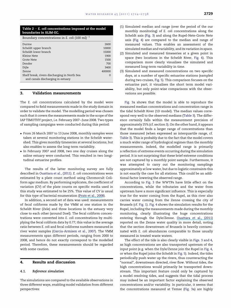
Table 2 e E. coli concentrations imposed at the modelboundaries in SLIM-EC.

Boundary concentrations in E. coli (100 ml)�1

Durme 2600

Scheldt upper branch 10000

Scheldt lower branch 15000

Kleine Nete 1900

Grote Nete 1500

Dender 700

Dijle 3400

Zenne 400000

Shelf break, rivers discharging in North Sea

and canals discharging in estuary

0

wat e r r e s e a r c h 4 5 ( 2 0 1 1 ) 2 7 2 4e2 7 3 8 2729

3. Validation measurements

The E. coli concentrations calculated by the model were

compared to fieldmeasurementsmade in the study domain in

order to validate the model. The modelling period was chosen

such that it covers themeasurementsmade in the scope of the

IAP TIMOTHY project, i.e. February 2007eJune 2008. Two types

of sampling campaigns were conducted during this period:

� From 26 March 2007 to 13 June 2008, monthly samples were

taken at several monitoring stations in the Scheldt water-

shed. This givesmonthly timeseries at several locations, but

also enables to assess the long-term variability.

� In February 2007 and 2008, two one day cruises along the

saline estuary were conducted. This resulted in two longi-

tudinal estuarine profiles.

The results of the latter monitoring survey are fully

described in Ouattara et al., (2011). E. coli concentrations were

estimated by a plate count method using Chromocult Coli-

form agarmedium. By performing replicates, the coefficient of

variation (CV) of the plate counts on specific media used in

this study was estimated to be 25%. This value of CV is usual

for this type of bacterial enumeration (Prats et al., 2008).

In addition, a second set of data was used: measurements

of fecal coliforms made by the VMM at one station in the

Scheldt River (Zele) and three locations in the estuary very

close to each other (around Doel). The fecal coliform concen-

trations were converted into E. coli concentrations by multi-

plying the fecal coliform data by 0.77; this value is the average

ratio between E. coli and fecal coliforms numbers measured in

river water samples (Garcia-Armisen et al., 2007). The VMM

measurements span different periods, ranging from 2000 to

2008, and hence do not exactly correspond to the modelled

period. Therefore, these measurements should be regarded

with some caution.

4. Results and discussion

4.1. Reference simulation

The simulations are compared to the available observations in

three different ways, enablingmodel validation from different

perspectives:

(1) Simulated median and range (over the period of the our

monthly monitoring) of E. coli concentrations along the

Scheldt axis (Fig. 3) and along the Rupel-Nete-Grote Nete

axis (Fig. 4) are compared to the median and range of

measured values. This enables an assessment of the

simulatedmedianandvariability, and its variation in space.

(2) Simulated and measured timeseries at a given point in

space (two locations in the Scheldt River, Fig. 6). This

comparison more clearly visualises the simulated and

measured long-term variability in time.

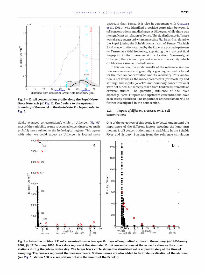
(3) Simulated and measured concentrations on two specific

days, at a number of specific estuarine stations (sampled

during two cruises, Fig. 5). This comparison focuses on the

estuarine part; it visualises the short term model vari-

ability, but only point-wise comparisons with the obser-

vations are possible.

Fig. 3a shows that the model is able to reproduce the

measured median concentrations and concentration range in

the tidal Scheldt River (1D model). The median values corre-

spond very well to the observed medians (Table 3). The differ-

ence certainly falls within the measurement precision of

approximately 25% (cf. section 3). On the otherhand, it appears

that the model finds a larger range of concentrations than

those measured (when expressed as interquartile range, cf.

Table 3). This is probably due to the fact that the model covers

a muchwider range of hydrological regimes than themonthly

measurements. Indeed, the modelled range is primarily

a reflection of extreme events occurring during the simulation

period. It is not surprising that these brief extreme conditions

are not captured by a monthly point sample. Furthermore, it

was attempted to carry out the monitoring samplings

approximately at lowwater, but due to logistic constraints this

is not exactly the case for all stations. This could be an addi-

tional factor lowering the observed range.

According to Fig. 3 the WWTPs have little effect on the

concentrations, while the tributaries and the water from

upstream have a more significant influence. This is especially

true for the water coming from the Rupel, as this river also

carries water coming from the Zenne crossing the city of

Brussels (cf. Fig. 1). Fig. 4 shows the simulation results for the

Rupel, including themeasurements made during themonthly

monitoring, clearly illustrating the huge concentrations

entering through the Dyle/Zenne. Ouattara et al., (2011)

reported on the Zenne water quality in more detail, noting

that the section downstream of Brussels is heavily contami-

nated with E. coli abundances comparable to those usually

measured in treated waste waters.

The effect of the tide is also clearly visible in Figs. 3 and 4,

as high concentrations are also transported upstream of the

input point (e.g. when the Dyle/Zenne join the Rupel in Fig. 4,

or when the Rupel joins the Scheldt in Fig. 5). Indeed, the tides

periodically push water up the rivers, thus counteracting the

“normal”, downstream directed, river flow. Without tides, the

high concentrations would primarily be transported down-

stream. This important feature could only be captured by

a model resolving tides, and suggests that the tidal process

may indeed be an important factor explaining the observed

concentrations and/or variability. In particular, it seems that

the concentrations measured at Temse (Fig. 3a) are highly

0 10 20 30 40 50 60 700

0.5

1

1.5

2

2.5

3

3.5

4

4.5x 104

distance from Ghent (km) − 1D model

E. c

oli (

100

ml)−1

Temse Uitbergen

Zele

Rupel ↑Durme ↑Dender ↑southern ↑Scheldt branch

← A

arts

elaa

r← B

orne

m←

Tem

se

← S

int−

Aman

ds

← D

ende

rmon

de

← Z

ele

← B

erla

re

← L

ede

& W

iche

len

← O

vers

chel

de←

Wet

tere

n

← D

este

lber

gen

80 90 100 110 120 130 140 1500

500

1000

1500

2000

2500

3000

Doel

distance from Ghent (km) − 2D model

E. c

oli (

100

ml)−1

← B

urch

t←

Ant

wer

pen−

Zuid

← B

ath

& W

aard

e

← W

illem

Ann

apol

der

← W

alch

eren

SLIM−EC interquartile bandSLIM−EC min − max valuesSLIM−EC median valuemeasurements

b

a

Fig. 3 e E. coli concentration profile along the Scheldt, from Ghent (km 0, cf. Fig. 1) to themouth. (a) Results from 1Dmodel. (b)

Results from the 2D model. Red vertical lines indicate the location of the WWTPs, blue vertical lines the location of

tributaries joining the Scheldt. Only the simulation results covering the our monthly monitoring period are considered. The

simulations are summarised as their median value at every position (black line), the interquartile range (grey band) and the

min-max range (dotted lines). The available measurements are shown as dots: cyan dots referring to our monthly

monitoring, and green dots referring to VMM measurements (only the bigger dots represent samples taken during the

simulation period), squares indicate the median value of the measurements at each location. (For interpretation of the

references to colour in this figure legend, the reader is referred to the web version of this article.)

wat e r r e s e a r c h 4 5 ( 2 0 1 1 ) 2 7 2 4e2 7 3 82730

influenced by the Rupel although Temse is situated upstream

of the Rupel connection. The importance of the tide will be

further discussed in section 4.2.

In the estuary, the major feature is a steep decrease in simu-

latedconcentrations (Fig.3b).Thisdecrease iscoincidentwith the

maximum turbidity zone (MTZ) in the Scheldt, which is reported

approximatelybetweenkm60and100,orbetweensalinityvalues

2 and 10 (Baeyens et al., 1998; Chen et al., 2005; Muylaert and

Sabbe, 1999). Measured timeseries in the estuary are scarce. The

only timeseries in the estuaryavailable tous are thoseperformed

byVMM.Asdiscussed in section3, thesemeasurements are to be

interpreted with care, but it appears that the model underesti-

mates the concentrations in this part of the estuary, or at least

cannot reproduce some of the higher values measured. The

model performance in the estuary is further assessed in Fig. 5,

comparing measurements made during two estuarine cruises

with model outputs from the same days. These results suggest

that the model predicts the correct concentrations in the begin-

ning and at the mouth of the estuary, but simulates too fast

adecreasebetweenthesetwoextremes.Again, theconcentration

decrease occurs in the MTZ. Therefore, the poor model perfor-

mance in this part of the Scheldt is probably related to the fact

that the E. coli dynamics are modelled as independent of

suspended matter. For instance, explicitly modelling resus-

pension and longer survival times for E. coli bacteria attached to

sediment particles (Craig et al., 2004; Davies and Bavor, 2000;

Davies et al., 1995) may indeed increase the modelled concen-

trations in theMTZ. A second possible explanation for themodel

underestimation is missing sources. WWTPs are included in the

model, butnot thepossible pollutioneffect of canals, or of diffuse

sources (most of the estuary lies in a rural area).

In Fig. 6 themodel results are visualised as timeseries at two

monitoring stations in the Scheldt. These figures visualisemore

explicitly the temporal variability in the observations and

simulations. It can be seen that the model is not able to repro-

duce the observations exactly, i.e. themodel is not accurate for

predictions of the exact concentration at a given time and

location.However, themedianvalueandrangearesatisfactorily

modelled, especially when comparing with the generally

reportedperformances ofmicrobial qualitymodels described in

the literature, where one is generally satisfied with model

simulations falling within half a log unit of the observations

(Collins and Rutherford, 2004; Garcia-Armisen et al., 2006;

Sanders et al., 2005). The modelled variability has a different

nature at the two locations: in Temse (Fig. 6a) a large portion of

the variability is due to the tide (compare raw outputs with

0 5 10 15 20 25 30 35 400

0.5

1

1.5

2

2.5

x 105

distance from upstream Grote Nete boundary (km)

E. c

oli (

100

ml)−1

Duffel

Boom

↑ Dijle/Zenne↑ Kleine Nete←

Boo

m

Fig. 4 e E. coli concentration profile along the Rupel-Nete-

Grote Nete axis (cf. Fig. 1). Km 0 refers to the upstream

boundary of themodel in the Grote Nete. For legend refer to

Fig. 3.

wat e r r e s e a r c h 4 5 ( 2 0 1 1 ) 2 7 2 4e2 7 3 8 2731

tidally averaged concentrations), while in Uitbergen (Fig. 6b)

mostof thevariability seemstooccur at longer timescalesand is

probably more related to the hydrological regime. This agrees

with what we could expect as Uitbergen is located more

0 5 10 15 20 25 300

1000

2000

3000

4000

5000

6000

7000

8000

salinity

E. c

oli (

100

ml)−1

a

S18

S20

S22

S22

S18

S20

S15 S12 S09 S07 S04 S03S01

150

Fig. 5 e Estuarine profiles of E. coli concentrations on two specifi

2007, (b) 12 February 2008. Black dots represent the simulated E

stations during the whole cruise day. The larger black circle sh

sampling. The crosses represent the measurements. Station na

(see Fig. 1, station 150 is a sea station outside the mouth of the

upstream than Temse. It is also in agreement with Ouattara

et al., (2011), who identified a positive correlation between E.

coli concentrations and discharge at Uitbergen, while there was

nosignificant correlationatTemse.The tidal influence inTemse

was already suggestedwhen inspecting Fig. 3a, and is related to

the Rupel joining the Scheldt downstream of Temse. The high

E. coli concentrations carried by the Rupel are pushed upstream

(to Temse) at a tidal frequency, explaining the important tidal

fingerprint in the timeseries at this location. Conversely, at

Uitbergen, there is no important source in the vicinity which

could cause a similar tidal influence.

In this section, the model results of the reference simula-

tion were assessed and generally a good agreement is found

for the median concentration and its variability. This valida-

tion is not trivial as the model parameters (for mortality and

settling) and inputs (WWTPs and boundary concentrations)

were not tuned, but directly taken fromfieldmeasurements or

external studies. The (potential) influence of tide, river

discharge, WWTP inputs and upstream concentrations have

been briefly discussed. The importance of these factors will be

further investigated in the next section.

4.2. Impact of different processes on E. coliconcentrations

One of the objectives of this study is to better understand the

importance of the different factors affecting the long-term

median E. coli concentration and its variability in the Scheldt

River and Estuary. Starting from the reference simulation

0 5 10 15 20 25 300

200

400

600

800

1000

1200

1400

salinity

E. c

oli (

100

ml)−1

b

150S01S04S07S09S20 S12S18

S15S22

c days of longitudinal cruises in the estuary: (a) 14 February

. coli concentrations at the same location as the cruise

ows the simulated value approximately at the time of

mes are also added to facilitate localisation of the stations

Scheldt).

Fig. 6 e E. coli concentration timeseries at two locations in the Scheldt River (see Figs. 1 and 3 for location): (a) Temse, (b)

Uitbergen. Simulation period covers our monthly monitoring. Black line shows the model output, grey line the tidal moving

average of these outputs. Dots represent field measurements made during this monitoring.

wat e r r e s e a r c h 4 5 ( 2 0 1 1 ) 2 7 2 4e2 7 3 82732

presented in the previous section, we removed, one by one,

the major processes (cf. Table 1). Table 3 summarises the

results of these different simulations.

4.2.1. Tide and upstream dischargeTo assess the role of the tides, a simulation was run with the

tides removed from the hydrodynamics, while all other forc-

ings and processes are kept identical.

Table 3 e Comparison of observed and simulatedmedianand interquartile concentrations all expressed as E. coli(100 ml)L1. The comparison is done at two monitoringlocations, where samples were taken at approximatelymonthly intervals from 26 March 2007 to 13 June 2008.The simulations cover the same period, but all modeloutputs (at 15 min intervals) are used to compute thestatistics.

Temse Uitbergen

Median Interquartilerange

Median Interquartilerange

Observations 1400 1200 3500 3700

Simulations

Reference 1500 3000 3600 4700

No tide 80 280 5500 4700

No upstream

conc.

110 51 300 120

No WWTPs 1400 3000 3300 4900

kmort ¼ 0 16000 20000 10000 2900

vsed ¼ 0 1900 3800 4700 5100

First inspecting what happens at the two monitoring

stations Temse and Uitbergen (Table 3), it is seen that the

change is largest at Temse. Indeed, bothmedian concentration

and variability (interquartile range) are significantly reduced.

Surprisingly, themedianconcentrationatUitbergen increases,

while the variability remains equal. This confirms the

hypothesis formulated when discussing Fig. 6 that Temse is

much more influenced by the tide, because it is the tide that

allows water mass to flow from downstream to upstream and

thusbrings thehighRupel concentrationsupstream.When the

tide is switched off, the Rupel concentration cannot reach as

far upstream anymore (Fig. 7). Fig. 8a shows the simulated

timeseries at Temse, showing the reduced concentrations and

variability. The remaining variability is related to theupstream

discharge (average daily discharges are prescribed). Fig. 8c

shows thedailywater discharge atMelle (see Fig. 1 for location)

and there is indeed a clear similarity with the concentration

timeseries at Temse. High concentrations at Temse generally

coincide with high discharge periods.

TheconcentrationsatUitbergenareoverall less influencedby

the tide. Therefore, it is no surprise that the simulated concen-

trationtimeseriesatUitbergen (without tide,Fig.8b)alsoexhibits

a clear similarity with the discharge timeseries, although the

concentrations seem to be less “sensitive” to high discharges

than was the case at Temse. This suggests that the two coun-

teracting effects of high discharge e reduced transit time

(increasing E. coli concentrations downstream) and increased

dilution (decreasing concentrations) e are balanced differently

at these two locations. But the overall result at both locations is

an increase of the E. coli concentrations with discharge.

0 10 20 30 40 50 60 700

1

2

3

4

5

x 104

distance from Ghent (km) − 1D model

E. c

oli (

100

ml)−1

Temse Uitbergen Zele

Rupel ↑Durme ↑Dender ↑southern ↑Scheldt branch

← A

arts

elaa

r

← B

orne

m←

Tem

se

← S

int−

Aman

ds

← D

ende

rmon

de

← Z

ele

← B

erla

re

← L

ede

& W

iche

len

← O

vers

chel

de←

Wet

tere

n

← D

este

lber

gen

80 90 100 110 120 130 140 1500

500

1000

1500

2000

2500

3000

Doel

distance from Ghent (km) − 2D model

E. c

oli (

100

ml)−1 ←

Bur

cht

← A

ntw

erpe

n−Zu

id

← B

ath

& W

aard

e

← W

illem

Ann

apol

der

← W

alch

eren

SLIM−EC interquartile bandSLIM−EC min − max valuesSLIM−EC median valuemeasurements

a

b

Fig. 7 e E. coli concentration profile along the Scheldt (cf. Fig. 3 for legend). Model results refer to simulation without tide.

wat e r r e s e a r c h 4 5 ( 2 0 1 1 ) 2 7 2 4e2 7 3 8 2733

Further inspecting the simulations at Uitbergen without

tides, it is remarkable that the median simulated concentra-

tion is increased, while the interquartile range remains

unchanged. When comparing Fig. 8b with Fig. 6b, it appears

that switching off the tide induces two main changes:

(i) the short term variability due to the tidal effect vanishes,

as expected. Because this variability has a smaller

amplitude than the long-term variations, this barely

influences the overall interquartile range.

(ii) the minimal concentrations are higher (although the

maximal concentrations remain quasi-identical). Indeed,

in the simulation with tides, the concentrations drop to

lower, almost-zero values. As for Uitbergen no major

sources lie downstream, during rising tide, waters with

lower E. coli concentrations are brought upstream to Uit-

bergen, effectively reducing the concentration at Uitber-

gen. It is remarkable that the concentrations remain at

these low levels for significantly longer periods than

a tidal cycle. Therefore, these low values cannot (only)

result from the periodic tidal current upstream. Rather, it

seems that the tidal oscillation has a mixing effect acting

on longer timescales, especially during periods of low

discharge, when there is less counteraction from the river

flow.

These results clearly demonstrate that the concentrations

at bothmonitoring locations are influenced by the tides, but in

a different manner. In order to get a more detailed picture of

the spatially varying effect of the tides on median concen-

tration and variability, we visualised the differences between

Fig. 3 (with tides) and Fig. 7 (without tides) in Fig. 9. This figure

reveals a complex role of the tides: they can locally either

increase or decrease the median concentration and, surpris-

ingly, the same holds for the variability. Indeed, in the central

part (between km 22 and 50) the tides effectively reduce the

observed variability in E. coli concentrations. Further down-

stream (from km 50 to the Rupel) the tides hugely increase

both the variability and the median concentrations, until

almost 100% of their value is due to the tides. This is the

upstream Rupel influence zone, as discussed for the sampling

station Temse. Upstream of km 50 themedian concentrations

are lowered by the tides (cf. discussion for Uitbergen), and this

reduction is higher than 50% for a significant section of the

river.

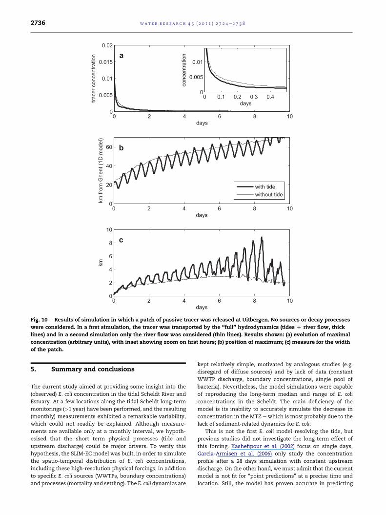
In order to better understand why the tides reduce median

and interquartile range in the central part of the river, we

performed an additional model test. A narrow patch of tracer

was initialised at Uitbergen on 1/2/2007 at 0:00 and followed

during 10 days e once transported by the “full” hydrody-

namics (tides þ river flow), and once with only the river flow.

For simplicity, all other sources and decay reactions were

removed (passive tracer). Fig. 10 shows the results of these

two simulations. It is seen that, in addition to moving the

patch up and down the river, the tides increase the width of

the patch and accordingly reduce the maximal concentration.

This suggests that the tides indeed have an increased “mix-

ing” effect, smoothing the patchmore efficiently thanwithout

tidal action, which is compatible with the observed lower

median concentrations and variability in this section of the

river.

In the estuary, the picture does not change so much by

removing the tidal effect (Fig. 7b). Without tides, the high

Rupel concentrations propagate less far downstream. Only

Fig. 8 e E. coli concentration timeseries at (a) Temse and (b) Uitbergen (cf. Fig. 1 for location). Model results refer to simulation

without tide. (c) Measured daily discharge at Melle.

wat e r r e s e a r c h 4 5 ( 2 0 1 1 ) 2 7 2 4e2 7 3 82734

the residual current drives the concentrations downstream,

resulting in slightly higher concentrations close to the Rupel

and a faster decrease to quasi-zero values.

In conclusion, the tide appears to have a significant influ-

ence on the E. coli concentrations (median and range)e but the

effect is different depending on the location. Overall, the tide

has the effect to enlarge the influence radius of a source (or

tributary) by pushingwater upstream and further downstream

than if there were no tides. In zones lying (not too far)

upstream of important sources, the tides therefore cause an

increase of the average concentrations, otherwise the average

concentrations tend to decrease. In this particular case of the

Scheldt, this means that the extent of the region influenced by

the high Rupel concentrations is significantly enlarged by the

presence of tides, mostly upstream but also downstream.

Conversely, themost upstream section of the Scheldt ismainly

influenced by what comes from further upstream, and only to

a lesser extent by the tide. In this part, the tides rather have the

effect to decrease the concentrations by bringing downstream

waterwhich contains lower concentrations of E. coli. Finally, by

removing the tidal forcing it was also clearly seen that both at

Temse and Uitbergen the modelled E. coli concentrations

correlate positively with upstream discharge, although their

response is different. Clearly, the impact of the tides on the E.

coli concentrations is crucial but very complex, implying that

“tidal corrections” in models which would not explicitly

simulate the tides are unlikely to be reliable.

4.2.2. Upstream concentrations and WWTPsTable 3 clearly shows that from the two inputs considered in

this study (upstream concentrations and WWTPs), the main

“source” of E. coli in the Scheldt is what comes through the

upstream boundaries. This is probably due to the fact that

(i) a huge amount of bacteria enter the model domain thr-

ough the Zenne boundary, caused by the large volumes of

0 10 20 30 40 50 60 70−4000

−2000

0

2000

4000

Rupel ↑Durme ↑Dender ↑Southern ↑Scheldt branch

Temse

Uitbergen

km

E.co

li (1

00 m

l)−1

a

medians IQRs

0 10 20 30 40 50 60 70−100

−50

0

50

100

Rupel ↑Durme ↑Dender ↑Southern ↑Scheldt branch

Temse

Uitbergen

km

%

b

medians IQRs

Fig. 9 e Difference between simulation with tides and simulation without tides. (a) Absolute difference and (b) relative

difference betweenmedians (full line) and interquartile ranges (IQRs, dashed line). Positive values mean that the simulation

with tides is associated with higher median or IQR. The location of tributaries joining the Scheldt and the two monitoring

stations Temse and Uitbergen are also indicated.

wat e r r e s e a r c h 4 5 ( 2 0 1 1 ) 2 7 2 4e2 7 3 8 2735

waste water discharged in the Brussels area (upstream of

the model boundary) in the relatively small river Zenne.

These massive concentrations propagate through the

Rupel into the Scheldt, where they overwhelm the effect

of local WWTPs.

(ii) the largest WWTPs in the Scheldt (the part under tidal

influence) have a limited effect. Most of them are located

in the Antwerp area, where they either discharge in

canals or in the Antwerp harbour, avoiding a direct effect

on the Scheldt. The few large WWTPs that discharge

directly in the Scheldt (e.g. Antwerpen-Zuid and Aartse-

laar), do so in the downstream part of the river (down-

stream of the Rupel connection) where water discharges

are much higher and therefore their impact is immedi-

ately reduced by dilution.

Although Table 3 only focuses on Temse andUitbergen, the

concentrations are reduced in the whole domain when

the boundary concentrations are set to zero (not shown). The

effect of the WWTPs is then more visible but remains only

very local, suggesting an efficient mixing/dilution.

4.2.3. Disappearance processesFinally, we tested the impact of taking out either of the two

considered disappearance processes: mortality and settling.

Table 3 shows that sedimentation has a negligible effect, but

mortality certainly not. In other words, it is the mortality

process which is primarily responsible for the decrease in

concentrations following the input by a WWTP or tributary

(Fig. 3). The negligible importance of the settling process on

the overall disappearance rate is probably due to the fact

that the rivers considered in this study are relatively deep,

implying that bacteria need to cross a significant water

depth before they actually disappear by settling. The (local)

relative importance of mortality versus sedimentation can

be expressed as q ¼ kmortH/vsed, with H the water height. In

the freshwater (1D) part of the Scheldt and during the study

period (26 March 2007e15 June 2008) this ratio ranges

between 2 and 35, with a median value of 9. In other words,

disappearance by mortality is always faster than by sedi-

mentation. For the Seine watershed, it was already found

that the relative importance of settling versus mortality in

the total disappearance rate decreases with increasing

hydrological order of the stream (Servais et al., 2009). For

small streams, settling was the dominant cause of E. coli

disappearance, while its importance became negligible in

the largest rivers of the watershed. Nevertheless, we must

keep in mind that the settling process was modelled by

means of a very simple first order parameterisation, while

a more accurate representation would include an explicit

model of suspended matter (including resuspension). It was

already discussed that such a representation is expected to

improve the model performance in the estuarine MTZ.

However, it is not obvious whether it will significantly

influence the results in the riverine part. Based on the E. coli

concentrations measured in the bottom sediments and the

concentrations of suspended matter, Ouattara et al., (2011)

estimated the potential contribution of sediment resus-

pension to the E. coli concentration in the water column.

Sediment resuspension contributed significantly to the

water contamination only at two sites in the Scheldt

watershed. These results suggest that resuspension can

have important but localised impacts in the rivers. Model-

ling these effect will be a challenge for the future.

0 2 4 6 8 100

0.005

0.01

0.015

0.02

days

trace

r con

cent

ratio

n0 0.1 0.2 0.3 0.4

0

0.005

0.01

days

conc

entra

tion

0 2 4 6 8 100

20

40

60

days

km fr

om G

hent

(1D

mod

el)

with tidewithout tide

0 2 4 6 8 100

2

4

6

8

10

days

km

a

b

c

Fig. 10 e Results of simulation in which a patch of passive tracer was released at Uitbergen. No sources or decay processes

were considered. In a first simulation, the tracer was transported by the “full” hydrodynamics (tides D river flow, thick

lines) and in a second simulation only the river flow was considered (thin lines). Results shown: (a) evolution of maximal

concentration (arbitrary units), with inset showing zoom on first hours; (b) position of maximum; (c) measure for the width

of the patch.

wat e r r e s e a r c h 4 5 ( 2 0 1 1 ) 2 7 2 4e2 7 3 82736

5. Summary and conclusions

The current study aimed at providing some insight into the

(observed) E. coli concentration in the tidal Scheldt River and

Estuary. At a few locations along the tidal Scheldt long-term

monitorings (>1 year) have been performed, and the resulting

(monthly) measurements exhibited a remarkable variability,

which could not readily be explained. Although measure-

ments are available only at a monthly interval, we hypoth-

esised that the short term physical processes (tide and

upstream discharge) could be major drivers. To verify this

hypothesis, the SLIM-EC model was built, in order to simulate

the spatio-temporal distribution of E. coli concentrations,

including these high-resolution physical forcings, in addition

to specific E. coli sources (WWTPs, boundary concentrations)

and processes (mortality and settling). The E. coli dynamics are

kept relatively simple, motivated by analogous studies (e.g.

disregard of diffuse sources) and by lack of data (constant

WWTP discharge, boundary concentrations, single pool of

bacteria). Nevertheless, the model simulations were capable

of reproducing the long-term median and range of E. coli

concentrations in the Scheldt. The main deficiency of the

model is its inability to accurately simulate the decrease in

concentration in the MTZ ewhich is most probably due to the

lack of sediment-related dynamics for E. coli.

This is not the first E. coli model resolving the tide, but

previous studies did not investigate the long-term effect of

this forcing. Kashefipour et al. (2002) focus on single days,

Garcia-Armisen et al. (2006) only study the concentration

profile after a 28 days simulation with constant upstream

discharge. On the other hand, we must admit that the current

model is not fit for “point predictions” at a precise time and

location. Still, the model has proven accurate in predicting

wat e r r e s e a r c h 4 5 ( 2 0 1 1 ) 2 7 2 4e2 7 3 8 2737

long-term median and range, making it a potentially inter-

esting tool for long-term risk assessment studies. Indeed, for

risk studies, understanding of the median behaviour is not

sufficient; it is crucial to have some insight into the variability

and the processes driving it.

Comparing the reference simulation to reduced model

setups, a deeper understanding of the controlling processes

was possible:

(1) The tide, the concentrations coming from upstream and

the mortality process are the main factors causing the

observed E. coli concentrations and variability.

(2) The tide is crucial to find correct median and range of

concentrations. However, its effect is complex: it can

either increase or decrease the local (median) concentra-

tions (depending on the location of the closest sources)

and increase or decrease the local variability.

(3) The impact of the WWTPs inside the model domain are

minor, suggesting that investment in these WWTPs may

not be the most efficient management action to improve

the water quality in terms of fecal contamination. At the

opposite, improving wastewater treatment in some

WWTPs locatedupstreamof the studieddomain (especially

in the Brussels area) would be important from a water

quality point of view.

These results point towards a few directions for future

developments:

(1) Model improvements:

a. A better model representation of the estuarine decrease

in E. coli concentrationsmay be achieved by complexifying the

E. coli module by including a direct link with sediment

dynamics.

b. Include further variability in the forcings, especially the

boundaryconcentrations. IncludingvaryingWWTPdischarges

does not seem relevant, due to the small impact of these

sources. However, a more accurate representation of what

enters from upstream could be achieved by extending the

model to the more upstream (non-tidal) river sections, espe-

cially the Zenne section crossing Brussels, as this appears to be

a major source of contamination.

(2) Additional data. Indeed, the above-mentioned model

improvement are only possible if additional measure-

ments are made/become available. But also for the vali-

dation of themodel additional data are necessary. Visually

it is clear that data (timeseries) are lacking in the estuary,

but also in the riverine part additional monitoring stations

would be useful. The model may be a useful guide to

determine the optimal position and/or timing of future

samples (e.g. de Brauwere et al., 2009).

Acknowledgements

The authors wish to thank the Vlaamse Milieumaatschappij

for providing data on fecal coliforms in the Scheldt. Anouk de

Brauwere performed this study while she was a postdoctoral

researcher with the Research Foundation Flanders (FWO), and

with the Belgian National Fund for Scientific Research

(FRS-FNRS). Eric Deleersnijder is a Research associate with the

Belgian National Fund for Scientific Research (FRS-FNRS). The

research was conducted within the framework of the Inter-

university Attraction Pole TIMOTHY (IAP VI.13), funded by the

Belgian Science Policy (BELSPO). SLIM is developed under the

auspices of the programme ARC 04/09-316 and ARC 10/15-028

(Communaute francaise de Belgique).

r e f e r e n c e s

Baeyens, W., van Eck, B., Lambert, C., Wollast, R., Goeyens, L.,1998. General description of the Scheldt estuary.Hydrobiologia 366, 1e14.

Barcina, I., Lebaron, P., VivesRego, J., 1997. Survival ofallochthonous bacteria in aquatic systems: A biologicalapproach. Fems Microbiology Ecology 23, 1e9.

Chen, M.S., Wartel, S., Van Eck, B., Van Maldegem, D., 2005.Suspended matter in the Scheldt estuary. Hydrobiologia 540,79e104.

Collins, R., Rutherford, K., 2004. Modelling bacterial water qualityin streams draining pastoral land. Water Research 38,700e712.

Craig, D.L., Fallowfield, H.J., Cromar, N.J., 2004. Use ofmacrocosms to determine persistence of Escherichia coil inrecreational coastal water and sediment and validation within situ measurements. Journal of Applied Microbiology 96,922e930.

Davies, C.M., Bavor, H.J., 2000. The fate of stormwater-associated bacteria in constructed wetland and waterpollution control pond systems. Journal of AppliedMicrobiology 89, 349e360.

Davies, C.M., Long, J.A.H., Donald, M., Ashbolt, N.J., 1995. Survivalof fecal microorganisms in marine and fresh-watersediments. Applied and Environmental Microbiology 61,1888e1896.

de Brauwere, A., De Ridder, F., Gourgue, O., Lambrechts, J.,Comblen, R., Pintelon, R., Passerat, J., Servais, P., Elskens, M.,Baeyens, W., Karna, T., de Brye, B., Deleersnijder, E., 2009.Design of a sampling strategy to optimally calibrate a reactivetransport model: Exploring the potential for Escherichia coli inthe Scheldt Estuary. Environmental Modelling & Software 24,969e981.

de Brauwere, A., Deleersnijder, E., 2010. Assessing theparameterisation of the settling flux in a depth-integratedmodel of the fate of decaying and sinking particles, withapplication to fecal bacteria in the Scheldt Estuary.Environmental Fluid Mechanics 10, 157e175.

de Brye, B., de Brauwere, A., Gourgue, O., Karna, T., Lambrechts, J.,Comblen, R., Deleersnijder, E., 2010. A finite-element, multi-scale model of the Scheldt tributaries, River, Estuary and ROFI.Coastal Engineering 57, 850e863.

Edberg, S.C., Rice, E.W., Karlin, R.J., Allen, M.J., 2000. Escherichiacoli: the best biological drinking water indicator for publichealth protection. Journal of Applied Microbiology 88,106Se116S.

EEA, 2004. Impacts of Europe’s Changing Climate. An Indicator-based Assessment. Report n�2/2004. Office for OfficialPublications of the EC, Luxembourg.

EU, 2000. Directive 2000/60/EC of the European Parliament andthe Council of 23 October 2000-Establishing a framework forCommunity action in the field of water policy. 72p.

EU, 2006. Directive 2006/7/EC of the European Parliament and ofthe COuncil of 15 February 2006 concerning the management

wat e r r e s e a r c h 4 5 ( 2 0 1 1 ) 2 7 2 4e2 7 3 82738

of bathing water quality. Official Journal of the EuropeanUnion 64, 37e51.

Garcia-Armisen, T., Prats, J., Servais, P., 2007. Comparison ofculturable fecal coliforms and Escherichia coli enumeration infreshwaters. Canadian Journal of Microbiology 53, 798e801.

Garcia-Armisen, T., Servais, P., 2007. Respective contributions ofpoint and non-point sources of E. coli and enterococci ina large urbanized watershed (the Seine river, France). Journalof Environmental Management 82, 512e518.

Garcia-Armisen, T., Servais, P., 2008. Partitioning and fate ofparticle-associated E. coli in river waters. Water EnvironmentResearch 81, 21e28.

Garcia-Armisen, T., Thouvenin, B., Servais, P., 2006. Modellingfaecal coliforms dynamics in the Seine estuary, France. WaterScience and Technology 54, 177e184.

George, I., Crop, P., Servais, P., 2002. Fecal coliform removal inwastewater treatment plants studied by plate counts andenzymatic methods. Water Research 36, 2607e2617.

Geuzaine, C., Remacle, J.F., 2009. Gmsh: A 3-D finite element meshgenerator with built-in pre- and post-processing facilities.International Journal for Numerical Methods in Engineering79, 1309e1331.

Havelaar, A., Blummenthal, U.J., Strauss, M., Kay, D., Bartram, J.,2001. Guidelines the current position. In: Fewtrell, L.,Bartram, J. (Eds.), Water Quality: Guidelines, Standards andHealth. In World Health Organization Water Series. IWAPublishing, London.

Kashefipour, S.M., Lin, B., Harris, E., Falconer, R.A., 2002. Hydro-environmental modelling for bathing water compliance of anestuarine basin. Water Research 36, 1854e1868.

Kay, D., Bartram, J., Pruss, A., Ashbolt, N.,Wyer,M.D., Fleisher, J.M.,Fewtrell, L., Rogers, A., Rees, G., 2004. Derivation of numericalvalues for the World Health Organization guidelines forrecreational waters. Water Research 38, 1236e1304.

Lambrechts, J., Comblen, R., Legat, V., Geuzaine, C., Remacle, J.F.,2008. Multiscale mesh generation on the sphere. OceanDynamics 58, 461e473.

Liu, L., Phanikumar, M.S., Molloy, S.L., Whitman, R.L., Shively, D.A., Nevers, M.B., Schwab, D.J., Rose, J.B., 2006. Modeling thetransport and inactivation of E. coli and enterococci in the

near-shore region of lake michigan. Environmental Science &Technology 40, 5022e5028.

Muylaert, K., Sabbe, K., 1999. Spring phytoplankton assemblagesin and around the maximum turbidity zone of the estuaries ofthe Elbe (Germany), the Schelde (Belgium/The Netherlands)and the Gironde (France). Journal of Marine Systems 22,133e149.

Okubo, A., 1971. Oceanic diffusion diagrams. Deep-sea Reserach18, 789e802.

Ouattara, N.K., Passerat, J., Servais, P. 2011. Faecal contaminationof water and sediment in the rivers of the Scheldt drainagenetwork. Environmental Monitoring and Assessment. doi:10.1007/s10661-011-1918-9.

Prats, J., Garcia-Armisen, T., Larrea, J., Servais, P., 2008.Comparison of culture-based methods to enumerateEscherichia coli in tropical and temperate freshwaters. Lettersin Applied Microbiology 46, 243e246.

Rozen, Y., Belkin, S., 2001. Survival of enteric bacteria in seawater.Fems Microbiology Reviews 25, 513e529.

Sanders, B.F., Arega, F., Sutula, M., 2005. Modeling the dry-weather tidal cycling of fecal indicator bacteria in surfacewaters of an intertidal wetland. Water Research 39,3394e3408.

ServaisP, Billen, G., Garcia-Armisen, T., George, I.,Goncalves, A., Thibert, S., 2009. La contaminationmicrobienne du bassin de la Seine. ProgrammeInterdisciplinaire de Recherche sur l’Environnement de laSeine. PIREN-Seine, ISBN 978-2-918251-07-1.

Servais, P., Billen, G., Goncalves, A., Garcia-Armisen, T., 2007a.Modelling microbiological water quality in the Seine riverdrainage network: past, present and future situations.Hydrology and Earth System Sciences 11, 1581e1592.

Servais, P., Garcia-Armisen, T., George, I., Billen, G., 2007b. Fecalbacteria in the rivers of the Seine drainage network (France):sources, fate and modelling. Science of the Total Environment375, 152e167.

Thupaki, P., Phanikumar, M.S., Beletsky, D., Schwab, D.J.,Nevers, M.B., Whitman, R.L., 2010. Budget analysis ofEscherichia coli at a southern lake michigan beach.Environmental Science & Technology 44, 1010e1016.