Modelling CO2-enrichment effects using an interactive vegetation SVAT scheme

Agricultural and Forest Meteorology 108 (2001) 129–152

Modelling CO2-enrichment effects using aninteractive vegetation SVAT scheme

Jean-Christophe Calvet a,∗, Jean-François Soussana b

a Météo-France/CNRM, 42 Av. Coriolis, F-31057 Toulouse Cedex 1, Franceb INRA/Agronomie, 234 Av. du Brézet, F-63039 Clermont-Ferrand Cedex 2, France

Received 30 May 2000; received in revised form 5 February 2001; accepted 19 February 2001

Abstract

A new version of the ISBA-A-gs (interactions between soil, biosphere, and atmosphere, CO2-reactive) scheme is employedto simulate the observed plant growth and energy and water budget of perennial ryegrass swards grown in highly ventilatedplastic tunnels. The model is modified in order to represent the greenhouse conditions, and best-fit vegetation parametersare proposed for two nitrogen fertiliser supplies. The simulations are performed in ambient or doubled CO2 concentration,and with a 3◦C increase in air temperature in doubled [CO2] conditions. It is shown that in the case of perennial ryegrass,the ratio between leaf area index and active biomass depends on both nitrogen supply and climate conditions. A simpleparameterisation of this variable is proposed, based on a plant nitrogen decline model. The enhanced model still needs a smallnumber of parameters (only five) and is able to describe leaf area index, the total biomass, the nitrogen use, and the dry matteryield. Finally, a control 10-year simulation using the new version of ISBA-A-gs is performed and a sensitivity study showsthat the model is able to simulate contrasting responses of leaf area index to CO2 or nitrogen enrichment. © 2001 ElsevierScience B.V. All rights reserved.

Keywords: CO2-enrichment; ISBA-A-gs; Nitrogen

1. Introduction

The ISBA-A-gs model presented in Calvet et al.(1998) is a new version of the ISBA soil–vegetation–atmosphere transfer (SVAT) scheme (Noilhan andPlanton, 1989). Like ISBA, ISBA-A-gs was designedfor use in atmospheric and hydrological models. Itallows a more realistic description of the canopystomatal conductance by considering the functionalrelationship between stomatal aperture and photosyn-thesis (Jacobs et al., 1996), and the estimated assimi-lation rate is used to both simulate plant growth and

∗ Corresponding author. Tel.: +33-561079341;fax: +33-561079626.E-mail address: [email protected] (J.-C. Calvet).

mortality and diagnose a leaf area index (L) whichis consistent with the prescribed climate and CO2concentration ([CO2]). Although the model uses alimited number of parameters, Calvet et al. (1998)showed that ISBA-A-gs is able to depict very distinctsituations in terms of climate, soil and vegetation-typeconditions. Since ISBA-A-gs accounts for the maineffects of changes in [CO2] on the water balance, itseems to be a good tool to analyse the plant responseto climate change. From the water balance viewpoint,an increase in [CO2] has two immediate conflictingeffects: (1) L may increase because of the photosyn-thesis enhancement (at least for C3 plants), (2) theleaf conductance decreases. The first effect tends toincrease transpiration, and the second effect tendsto decrease transpiration. Therefore, the resulting

0168-1923/01/$ – see front matter © 2001 Elsevier Science B.V. All rights reserved.PII: S0 1 6 8 -1 9 23 (01 )00235 -0

130 J.-C. Calvet, J.-F. Soussana / Agricultural and Forest Meteorology 108 (2001) 129–152

change in evapotranspiration and soil moisture maybe totally different from one plant type to another forgiven climate conditions. Also, there is a third effectrelated to the feedback between transpiration and soilmoisture: changes in transpiration affect soil moistureavailability and thereby also change leaf conductance.This latter effect occurs over longer periods of timeand may trigger seasonal differences in the resultingwater balance change. Such a feedback is accountedfor in ISBA-A-gs. A sensitivity study performed byCalvet et al. (1998) showed that the L simulated byISBA-A-gs may be dramatically increased in responseto CO2-enrichment, if the model’s parameters areassumed to remain constant.

In reality, the physiological response of the plantmay be more complex than the photosynthetic directresponse to changes in the atmospheric concentrationof CO2. The objective of this study is to comparethe model’s results with data from a CO2-enrichmentexperiment conducted in controlled conditions overa C3 grass species which has little response toCO2-enrichment in terms of L (Casella et al., 1996).In this experiment, the same cultivar was grown inthree tunnels corresponding to different climate con-ditions, and for each of them, two contrasting nitrogenfertilisation levels were applied. Therefore, six treat-ments are available, each consisting of biomass andnitrogen measurements in different environmentalconditions. In this study, a simple method is proposedto simulate the total biomass and the plant nitrogencontent using ISBA-A-gs. Optimal parameters of thenew version of the model are proposed (Section 6),and the ability of the model to simulate soil and vege-tation variables (Section 7) such as L, net assimilationof CO2, and the water balance of each treatment isinvestigated.

2. Data set

The observations employed in this study wereobtained during a 2-year CO2-enrichment experimentperformed by INRA (Institut National de la RechercheAgronomique, France) at Clermont-Ferrand (45◦47′N,3◦05′E, 332 m) in 1993 and 1994. The consideredperiod lasted for 631 days, from 10 April 1993 to 31December 1994. A full description of the experimen-tal set-up can be found in Casella et al. (1996).

2.1. Sward management

Perennial ryegrass (Lolium perenne L., cv Préfé-rence) was grown in 225 l containers filled with aloamy soil. The swards were assigned randomly tothree highly ventilated plastic tunnels correspondingto either outdoor [CO2] (350 ppm), doubled [CO2](700 ppm), or doubled [CO2] and a 3◦C increase inair temperature. These three climate treatments arehenceforth referred to as 350, 700, and 700+, respec-tively. The nitrogen fertilisation was either low or high(nitrogen supply of 160 and 530 kg N ha−1 yr−1,henceforth referred to as N− and N+, respectively).Two irrigation regimes were applied, but in this study,we only consider the treatments supplied with thesame amount of water (referred to as W- in Casellaet al. (1996)). During the considered period, all swardswere cut simultaneously at 4 cm height at 11 dates:in May, June, July, September, and October of 1993and 1994, and in April 1994.

Details about the sward management and the soilproperties are given in Casella et al. (1996) andSoussana et al. (1996). Section 6 lists the constantsoil and vegetation characteristics (common to the sixtreatments) whose values are needed in the simula-tions of ISBA-A-gs. The parameters which were notmeasured are assumed to have the same value as thoseover the grassland of the modelling the usable soilreservoir experimentally (MUREX) campaign (Cal-vet et al., 1999). The vegetation height and coverageare parameterised as a function of L using classicalrelationships.

2.2. Available atmospheric measurements

Air humidity and temperature, as well as [CO2],were measured in each plastic tunnel and outdoors(close to the tunnels). The measured in situ atmosphe-ric variables (incident solar radiation, air temperature,and relative humidity) were registered at irregular timeintervals of 24 ± 8 min. In this study, they were inter-polated to regular 30 min intervals. Over the 631-dayperiod considered, between 15 and 20% of the atmos-pheric variables were missing. In order to obtain acontinuous half-hourly atmospheric forcing series,data from a neighbouring automatic weather station ofMétéo-France (47◦47′N, 3◦10′E) were used. The miss-ing indoor values (Vin) were derived from the weather

J.-C. Calvet, J.-F. Soussana / Agricultural and Forest Meteorology 108 (2001) 129–152 131

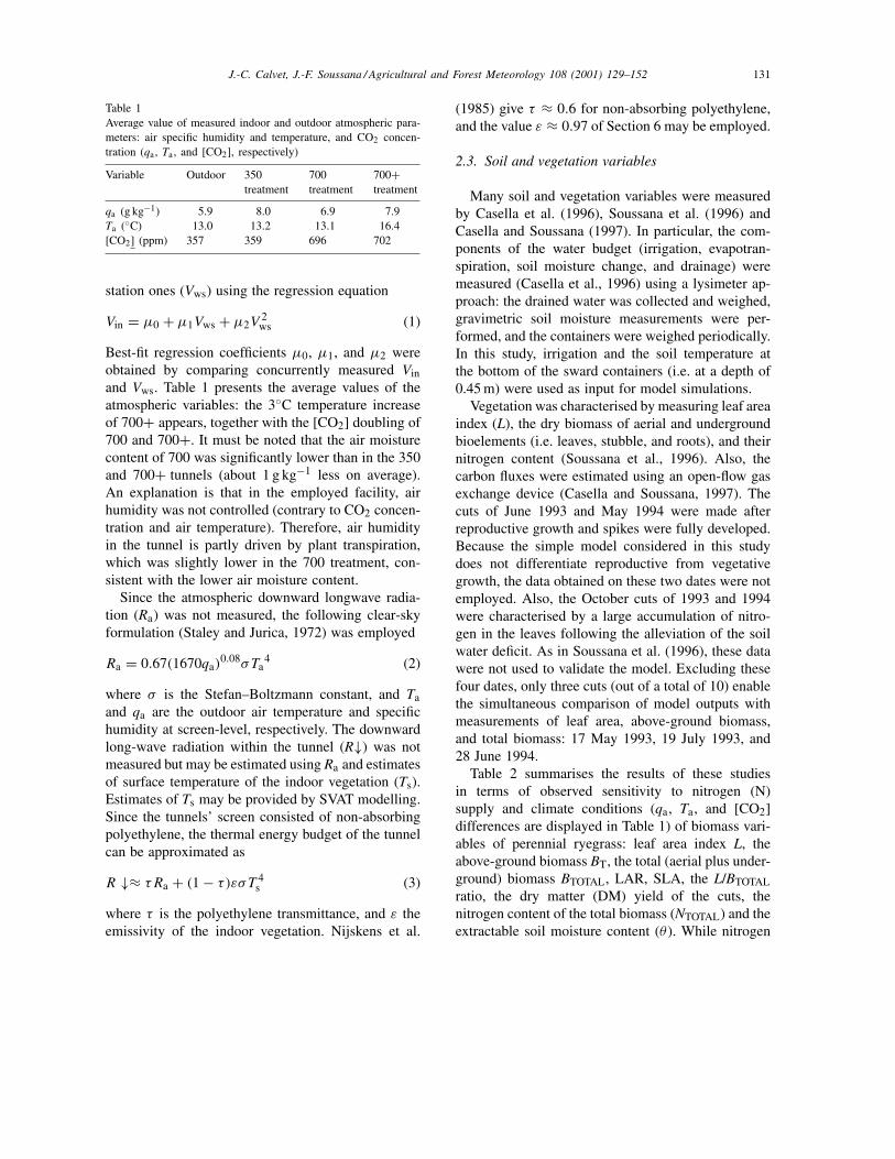
Table 1Average value of measured indoor and outdoor atmospheric para-meters: air specific humidity and temperature, and CO2 concen-tration (qa, Ta, and [CO2], respectively)

Variable Outdoor 350treatment

700treatment

700+treatment

qa (g kg−1) 5.9 8.0 6.9 7.9Ta (◦C) 13.0 13.2 13.1 16.4[CO2] (ppm) 357 359 696 702

station ones (Vws) using the regression equation

Vin = µ0 + µ1Vws + µ2V2ws (1)

Best-fit regression coefficients µ0, µ1, and µ2 wereobtained by comparing concurrently measured Vinand Vws. Table 1 presents the average values of theatmospheric variables: the 3◦C temperature increaseof 700+ appears, together with the [CO2] doubling of700 and 700+. It must be noted that the air moisturecontent of 700 was significantly lower than in the 350and 700+ tunnels (about 1 g kg−1 less on average).An explanation is that in the employed facility, airhumidity was not controlled (contrary to CO2 concen-tration and air temperature). Therefore, air humidityin the tunnel is partly driven by plant transpiration,which was slightly lower in the 700 treatment, con-sistent with the lower air moisture content.

Since the atmospheric downward longwave radia-tion (Ra) was not measured, the following clear-skyformulation (Staley and Jurica, 1972) was employed

Ra = 0.67(1670qa)0.08σTa

4 (2)

where σ is the Stefan–Boltzmann constant, and Taand qa are the outdoor air temperature and specifichumidity at screen-level, respectively. The downwardlong-wave radiation within the tunnel (R↓) was notmeasured but may be estimated using Ra and estimatesof surface temperature of the indoor vegetation (Ts).Estimates of Ts may be provided by SVAT modelling.Since the tunnels’ screen consisted of non-absorbingpolyethylene, the thermal energy budget of the tunnelcan be approximated as

R ↓≈ τRa + (1 − τ)εσT 4s (3)

where τ is the polyethylene transmittance, and ε theemissivity of the indoor vegetation. Nijskens et al.

(1985) give τ ≈ 0.6 for non-absorbing polyethylene,and the value ε ≈ 0.97 of Section 6 may be employed.

2.3. Soil and vegetation variables

Many soil and vegetation variables were measuredby Casella et al. (1996), Soussana et al. (1996) andCasella and Soussana (1997). In particular, the com-ponents of the water budget (irrigation, evapotran-spiration, soil moisture change, and drainage) weremeasured (Casella et al., 1996) using a lysimeter ap-proach: the drained water was collected and weighed,gravimetric soil moisture measurements were per-formed, and the containers were weighed periodically.In this study, irrigation and the soil temperature atthe bottom of the sward containers (i.e. at a depth of0.45 m) were used as input for model simulations.

Vegetation was characterised by measuring leaf areaindex (L), the dry biomass of aerial and undergroundbioelements (i.e. leaves, stubble, and roots), and theirnitrogen content (Soussana et al., 1996). Also, thecarbon fluxes were estimated using an open-flow gasexchange device (Casella and Soussana, 1997). Thecuts of June 1993 and May 1994 were made afterreproductive growth and spikes were fully developed.Because the simple model considered in this studydoes not differentiate reproductive from vegetativegrowth, the data obtained on these two dates were notemployed. Also, the October cuts of 1993 and 1994were characterised by a large accumulation of nitro-gen in the leaves following the alleviation of the soilwater deficit. As in Soussana et al. (1996), these datawere not used to validate the model. Excluding thesefour dates, only three cuts (out of a total of 10) enablethe simultaneous comparison of model outputs withmeasurements of leaf area, above-ground biomass,and total biomass: 17 May 1993, 19 July 1993, and28 June 1994.

Table 2 summarises the results of these studiesin terms of observed sensitivity to nitrogen (N)supply and climate conditions (qa, Ta, and [CO2]differences are displayed in Table 1) of biomass vari-ables of perennial ryegrass: leaf area index L, theabove-ground biomass BT, the total (aerial plus under-ground) biomass BTOTAL, LAR, SLA, the L/BTOTALratio, the dry matter (DM) yield of the cuts, thenitrogen content of the total biomass (NTOTAL) and theextractable soil moisture content (θ ). While nitrogen


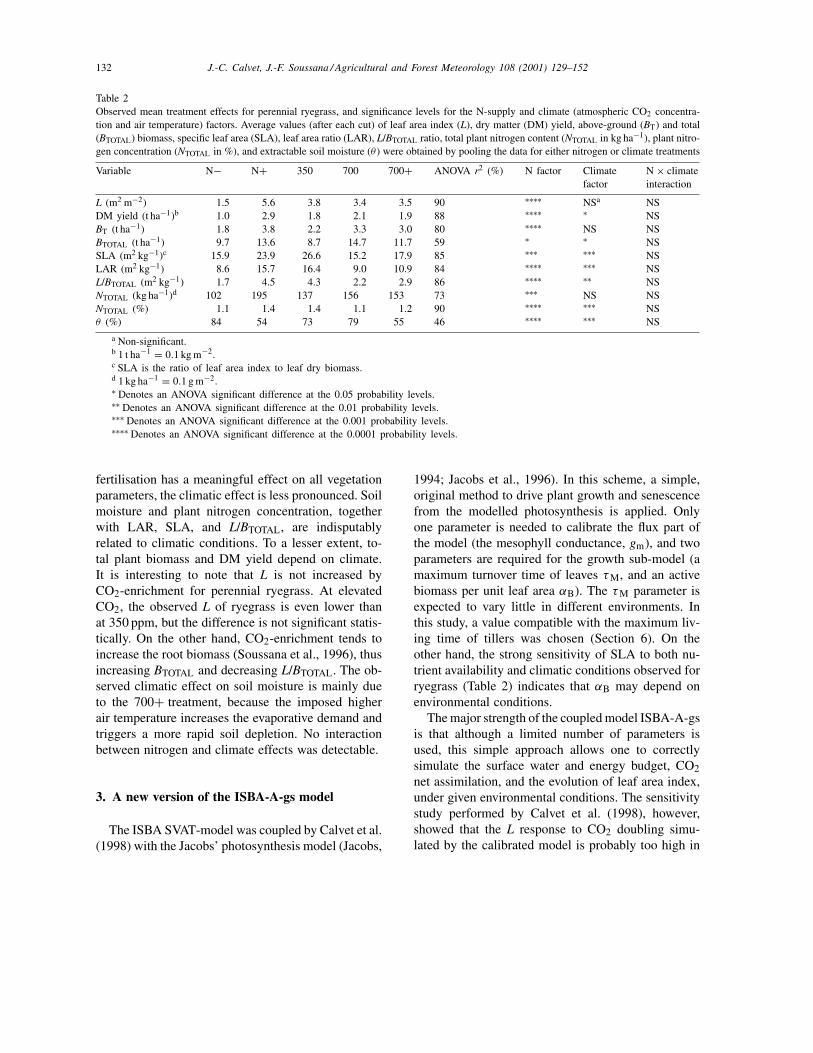
Table 2Observed mean treatment effects for perennial ryegrass, and significance levels for the N-supply and climate (atmospheric CO2 concentra-tion and air temperature) factors. Average values (after each cut) of leaf area index (L), dry matter (DM) yield, above-ground (BT) and total(BTOTAL) biomass, specific leaf area (SLA), leaf area ratio (LAR), L/BTOTAL ratio, total plant nitrogen content (NTOTAL in kg ha−1), plant nitro-gen concentration (NTOTAL in %), and extractable soil moisture (θ ) were obtained by pooling the data for either nitrogen or climate treatments

Variable N− N+ 350 700 700+ ANOVA r2 (%) N factor Climatefactor

N × climateinteraction

L (m2 m−2) 1.5 5.6 3.8 3.4 3.5 90 ∗∗∗∗ NSa NSDM yield (t ha−1)b 1.0 2.9 1.8 2.1 1.9 88 ∗∗∗∗ ∗ NSBT (t ha−1) 1.8 3.8 2.2 3.3 3.0 80 ∗∗∗∗ NS NSBTOTAL (t ha−1) 9.7 13.6 8.7 14.7 11.7 59 ∗ ∗ NSSLA (m2 kg−1)c 15.9 23.9 26.6 15.2 17.9 85 ∗∗∗ ∗∗∗ NSLAR (m2 kg−1) 8.6 15.7 16.4 9.0 10.9 84 ∗∗∗∗ ∗∗∗ NSL/BTOTAL (m2 kg−1) 1.7 4.5 4.3 2.2 2.9 86 ∗∗∗∗ ∗∗ NSNTOTAL (kg ha−1)d 102 195 137 156 153 73 ∗∗∗ NS NSNTOTAL (%) 1.1 1.4 1.4 1.1 1.2 90 ∗∗∗∗ ∗∗∗ NSθ (%) 84 54 73 79 55 46 ∗∗∗∗ ∗∗∗ NS

a Non-significant.b 1 t ha−1 = 0.1 kg m−2.c SLA is the ratio of leaf area index to leaf dry biomass.d 1 kg ha−1 = 0.1 g m−2.∗ Denotes an ANOVA significant difference at the 0.05 probability levels.∗∗ Denotes an ANOVA significant difference at the 0.01 probability levels.∗∗∗ Denotes an ANOVA significant difference at the 0.001 probability levels.∗∗∗∗ Denotes an ANOVA significant difference at the 0.0001 probability levels.

fertilisation has a meaningful effect on all vegetationparameters, the climatic effect is less pronounced. Soilmoisture and plant nitrogen concentration, togetherwith LAR, SLA, and L/BTOTAL, are indisputablyrelated to climatic conditions. To a lesser extent, to-tal plant biomass and DM yield depend on climate.It is interesting to note that L is not increased byCO2-enrichment for perennial ryegrass. At elevatedCO2, the observed L of ryegrass is even lower thanat 350 ppm, but the difference is not significant statis-tically. On the other hand, CO2-enrichment tends toincrease the root biomass (Soussana et al., 1996), thusincreasing BTOTAL and decreasing L/BTOTAL. The ob-served climatic effect on soil moisture is mainly dueto the 700+ treatment, because the imposed higherair temperature increases the evaporative demand andtriggers a more rapid soil depletion. No interactionbetween nitrogen and climate effects was detectable.

3. A new version of the ISBA-A-gs model

The ISBA SVAT-model was coupled by Calvet et al.(1998) with the Jacobs’ photosynthesis model (Jacobs,

1994; Jacobs et al., 1996). In this scheme, a simple,original method to drive plant growth and senescencefrom the modelled photosynthesis is applied. Onlyone parameter is needed to calibrate the flux part ofthe model (the mesophyll conductance, gm), and twoparameters are required for the growth sub-model (amaximum turnover time of leaves τM, and an activebiomass per unit leaf area αB). The τM parameter isexpected to vary little in different environments. Inthis study, a value compatible with the maximum liv-ing time of tillers was chosen (Section 6). On theother hand, the strong sensitivity of SLA to both nu-trient availability and climatic conditions observed forryegrass (Table 2) indicates that αB may depend onenvironmental conditions.

The major strength of the coupled model ISBA-A-gsis that although a limited number of parameters isused, this simple approach allows one to correctlysimulate the surface water and energy budget, CO2net assimilation, and the evolution of leaf area index,under given environmental conditions. The sensitivitystudy performed by Calvet et al. (1998), however,showed that the L response to CO2 doubling simu-lated by the calibrated model is probably too high in


many cases (e.g., the maximum L of a soybean testsite was increased by a factor of 2 at high CO2 con-centrations). An explanation is that using the samecalibrated model under different climate conditionsis not adequate because the effect of limiting factorssuch as nutrient availability is not accounted for.

In this study, a simple method to modify the αBparameter according to nitrogen dilution is tested. TheαB parameter is no longer a calibration parameter ofthe model. Instead, the value of αB is obtained by iter-ations from a fixed value of nitrogen concentration andthe maximum above-ground biomass obtained fromthe model’s calculations.

3.1. ISBA

The ISBA scheme simulates surface fluxes — evap-otranspiration, heat flux, and ground heat flux (LE, H,G) — and predicts the evolution of surface state vari-ables using the equations of the force-restore methodof Deardorff (1977, 1978). Five variables (surfacetemperature Ts, mean surface temperature T2, surfacesoil volumetric moisture wg, total soil volumetricmoisture w2, and the canopy interception reservoirWr) are obtained through prognostic equations. Itmust be noted that w2 is the volumetric soil moistureassociated with a bulk layer of thickness d2 includingthe root zone. When used in stand-alone simulations,the ISBA model is driven by measurements of in-coming radiation, precipitation, atmospheric pressure,air temperature and humidity, and wind speed at areference level. In the standard version, vegetationcharacteristics such as L and canopy height must beprescribed. The biological control of transpiration ismade through a Jarvis-like parameterisation of thecanopy stomatal conductance.

3.2. The A-gs model

The A-gs model proposed by Jacobs (1994) andJacobs et al. (1996) describes leaf CO2 net assimilationAn. In all the simulations presented in this study, thephotosynthesis parameters other than gm were takenas indicated in Jacobs (1994) and Calvet et al. (1998)for C3 plants. In ISBA-A-gs, a slightly modified ver-sion of the Jacobs’ model is employed, allowing therepresentation of the soil water stress: the normalisedsoil moisture θ (Section 7) affects the parameters of

photosynthesis and stomatal conductance, based ontwo possible plant strategies to respond to drought (de-fensive and offensive), as described by Calvet (2000).Ryegrass was not investigated by Calvet (2000), butpreliminary tests showed that the defensive strategy isappropriate to simulate the data analysed in this study.

3.3. Growth and mortality in ISBA-A-gs

The most obvious way to predict L is to use the com-puted net assimilation of the canopy AnI (expressed inunits of kg CO2 m−2 s−1): growth may be describedas the accumulation of carbon obtained from assimila-tion of atmospheric CO2, and senescence as the resultof a deficit of photosynthesis (due to external factors).In ISBA-A-gs, the ‘active’ biomass B is obtained fromthe differential equation

dB = MC

PCMCO2

AnI dt − B d

(t

τ

)(4)

This equation does not account for respiratory lossesfrom non-active components of the plant. In the growthincrement term of Eq. (4), PC is the proportion of car-bon in the dry plant biomass and MC andMCO2 are themolecular weights of carbon and CO2, respectively.

The mortality increment term of Eq. (4) representsan exponential extinction of B characterised by atime-dependent effective life expectancy (expressedin units of days)

τ(t) = τMAnfm(t)

An,max(5)

where τM is the maximum effective life expectancyof the active biomass, Anfm(t) the maximum leaf netassimilation reached on the day before time t andAn,max is the optimum leaf net assimilation (Calvetet al., 1998).

As in Mougin et al. (1995) and Ji (1995), the valueof L is obtained from B by assuming that for a givenvegetation canopy, the ratio between B and L is a con-stant: αB. Therefore, L is given by

L = B

αB(6)

The computed value of L is related to the integratednet assimilation through the growth model representedby Eqs. (5) and (6). Only two parameters, the αB ratioand τM have to be determined for each canopy type


from L measurements or estimations. These vegeta-tion parameters have to be retrieved during the modelcalibration, together with the mesophyll conductancegm.

3.4. Adaptation of ISBA-A-gs to greenhouseconditions

In the considered data set the plants were grownin highly ventilated plastic tunnels. This characteris-tic had to be accounted for in the model simulationsbecause it affects the representation of the turbulenceand of the incident thermal radiation.

The greenhouse effect on thermal radiation wasaccounted for by using Eq. (3) in the model simula-tions. The Ts term of Eq. (3) was prescribed as themodel surface temperature resulting from the reso-lution of the surface energy budget of the ryegrassswards. The turbulence problem was more difficultto solve because of the complex configuration of thecontainers and of the ventilation system within the tun-nel. The pragmatic method used to account for turbu-lence effects consisted of prescribing a constant valueof wind speed at a level of 1 m above the soil sur-face, and employing the standard stability functions ofthe model. Preliminary tests using ISBA-A-gs showedthat values of the prescribed wind speed lower than4 m s−1 lead to the overestimation of soil moisturecontent by the model, whatever value of gm is pre-scribed in the model. Prescribed values of wind speedand gm of 4 and 1 mm s−1, respectively, provide sim-ulations of root extraction of water consistent withmeasurements.

Another difference from natural growing conditionsis that the studied ryegrass was regularly cut. In themodel, the Lmin parameter represents the prescribedvalue of L after cutting (Section 6).

3.5. A simple biomass model

In the case of perennial ryegrass, the effects ofclimate change cannot be accounted for by ISBA-A-gsby prescribing a constant value of the model’sparameters. In particular, preliminary calibrationsof ISBA-A-gs showed that the B/L parameter (αB)responds to systematic changes in climatic variables(Ta and [CO2]) and nitrogen fertilisation. There-fore, the ISBA-A-gs model needs to be improved to

account for changes in plant morphology. Rather thanimplementing a complex biomass allocation scheme,which in practice would be difficult to calibrate foruse in an atmospheric model, one may try to relatethe theoretical concept of ‘active’ biomass B to theabove-ground biomass quantity BT. As explained inLemaire and Gastal (1997), the nitrogen distributionin the plant biomass depends on growing conditionsand has a strong influence on the plant nitrogenconcentration (N): the plant N decline model is asimple way to relate N to biomass and to estimateN-use.

The plant N decline model is a well-establishedagronomical law relating the plant N in non-limitingN-supply conditions to the accumulated above-groundDM (Greenwood et al., 1990; Greenwood et al., 1991;Justes et al., 1994; Lemaire and Gastal, 1997). Thecritical plant N is the value of N maximizing growth,and this value decreases for increasing biomass accu-mulation following a negative power law. The basisof the model is that the metabolic component of theplant biomass is related to total biomass through an al-lometric logarithmic law. In this study, the ‘metabolicbiomass’ concept of Lemaire and Gastal (1997)is identified as the ‘active biomass’ employed inISBA-A-gs. Using (intentionally) the same variablesas above, the ratio between active and total biomassis given by the following allometric equation:

B

BT= cBT

−a (7)

Since the metabolic biomass is assumed to containmost of the plant N, and noting Na the nitrogenproportion in the active biomass (a constant value),the total plant nitrogen content may be written as(Lemaire and Gastal, 1997)

BTNT ≈ BNa (8)

Combining Eqs. (7) and (8) gives

NT = cNaBT−a (9)

This equation represents the plant N decline: the plantnitrogen concentration decreases with increasingsward biomass because the relative rate of N accu-mulation is lower than the relative biomass increase.Lemaire and Gastal (1997) showed that values ofthe coefficient a given by a number of authors from


above-ground biomass and N measurements overvarious plant types (including C3 and C4 plants) areremarkably consistent, and are close to 1

3 . Soussanaet al. (1996), in a high fertilisation treatment calledN++, obtained a similar result for ryegrass at ambient[CO2], with a = 0.38 ± 0.03. On the other hand, theyfound that under doubled [CO2], the value of a is sig-nificantly higher: a = 0.52 ± 0.03. The cNa factor ofEq. (9) presents less variability under optimal nutrientsupply and is always close to 4.9 ± 0.1 for C3 plants(Soussana et al., 1996; Lemaire and Gastal, 1997). Be-cause the maximum value of Na is about 6.5% for C3plants (Lemaire and Gastal, 1997), an estimation ofthe c parameter is c = 0.754 (Section 6). These resultswere obtained in optimal nutrient supply. In this study,Eqs. (7)–(9) defining the plant N decline model areextended to limiting N-supply by prescribing valuesof Na lower than 6.5%. As illustrated by Fig. 1 (left),Eq. (9) can be applied to sub-critical values of Na: thebest-fit values of Na for the N− and N+ treatementsare 2.4 and 4.9%, respectively. The increasing valueof Na derived from the measurements (2.4, 4.9, and6.5% for N−, N+, and N++ treatments, respectively)indicates that Eq. (9) is able to account for the effectof N-supply through the Na parameter. Indeed, giventhe N fertiliser supply of 160 and 530 kg N ha−1 yr−1

for the N− and N+ treatments, respectively, bothsituations corresponded to limiting N conditions:Soussana et al. (1996) obtained non-limited N-uptakeby applying 1000 kg N ha−1 yr−1. Using the plant Ndecline model, the above-ground biomass is related to

Fig. 1. Observed and modelled nitrogen and biomass allometric relationships for perennial ryegrass: (A) above-ground nitrogen concentrationNT versus biomass BT, (B) leaf area ratio (LAR as defined in Section 7) versus NT. In (A) the solid and dashed lines represent themodel’s parameterisation for 350 and 700 (or 700+) treatments, respectively, and the fine and thick lines represent N− and N+ treatments,respectively. Measurements by Casella et al. (1996) and Soussana et al. (1996) are represented by circles and ∗ for N−, boxes and + forN+, open symbols for 350, closed symbols for 700, and ∗ and + for 700+ treatments.

the growth parameter αB of ISBA-A-gs by combiningEqs. (6) and (7):

BT =(αBL

c

)1/(1−a)(10)

The above equation is not sufficient to estimate bothαB and BT values. Based on the available measure-ments over perennial ryegrass, a closure equation wasderived from the studied data set. Fig. 1 shows thata very good relationship (r2 = 0.84) exists betweenthe measured average LAR and the above-groundnitrogen concentration NT at the end of eachregrowth

L

BT= eNT + f (11)

where e and f are regression parameters indicated inSection 6. This allometric equation may be used as aclosure assumption to estimate the model’s B/L ratio.Indeed, combining Eqs. (9)–(11), the αB parameter isgiven by

αB = 1

eNa + f/(cBT−a)

(12)

In Eq. (12), αB depends on N-supply through theNa parameter, and on the above-ground biomass BT.This latter term provides a representation of the sen-sitivity of αB to the climatic factors since BT maydepend on climate conditions, as shown in Table 2.Since CO2-enrichment tends to increase BT, the


obtained negative value of f (Section 6) corresponds toan increase of αB due to CO2-enrichment. A positivevalue of f would have given the opposite result. It isexpected that for other plant types, the e and f parame-ters may differ and Eq. (12) may describe contrastingplant responses to either N or CO2-enrichment.

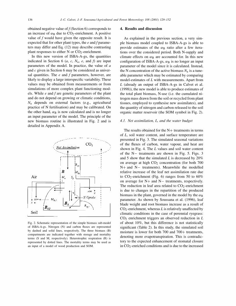
In this new version of ISBA-A-gs, the quantitiesindicated in Section 6 (a, c, Na, e, and f) are inputparameters of the model. In practice, the value of aand c given in Section 6 may be considered as univer-sal quantities. The e and f parameters, however, arelikely to display a large interspecific variability. Thesevalues may be obtained from measurements or fromsimulations of more complex plant functioning mod-els. While e and f are genetic parameters of the plantand do not depend on growing or climatic conditions,Na depends on external factors (e.g., agriculturalpractice of N fertilisation) and may be calibrated. Onthe other hand, αB is now calculated and is no longeran input parameter of the model. The principle of thenew biomass routine is illustrated in Fig. 2 and isdetailed in Appendix A.

Fig. 2. Schematic representation of the simple biomass sub-modelof ISBA-A-gs. Nitrogen (N) and carbon fluxes are representedby dashed and solid lines, respectively. The three biomass (B)compartments are indicated together with storage and mortalityterms (S and M, respectively). Heterotrophic respiration (R) isrepresented by dotted lines. The mortality terms may be used asan input of a model of wood production and SOM.

4. Results and discussion

As explained in the previous section, a very sim-ple biomass model coupled to ISBA-A-gs is able toprovide estimates of the αB ratio after a few itera-tions over the considered period. Both N-supply andclimate effects on αB are accounted for. In this newconfiguration of ISBA-A-gs, αB is no longer an inputparameter of the model since it is calculated. Instead,the N concentration of the active biomass Na is a tune-able parameter which may be estimated by comparingmodel-estimates of L with measurements. Apart fromL (already an output of ISBA-A-gs in Calvet et al.(1998)), the new model is able to produce estimates ofthe total plant biomass, N-use (i.e. the cumulated ni-trogen mass drawn from the soil or recycled from planttissues, employed to synthesise new assimilates), andthe quantity of nitrogen and carbon released to the soilorganic matter reservoir (the SOM symbol in Fig. 2).

4.1. Net assimilation, L, and the water budget

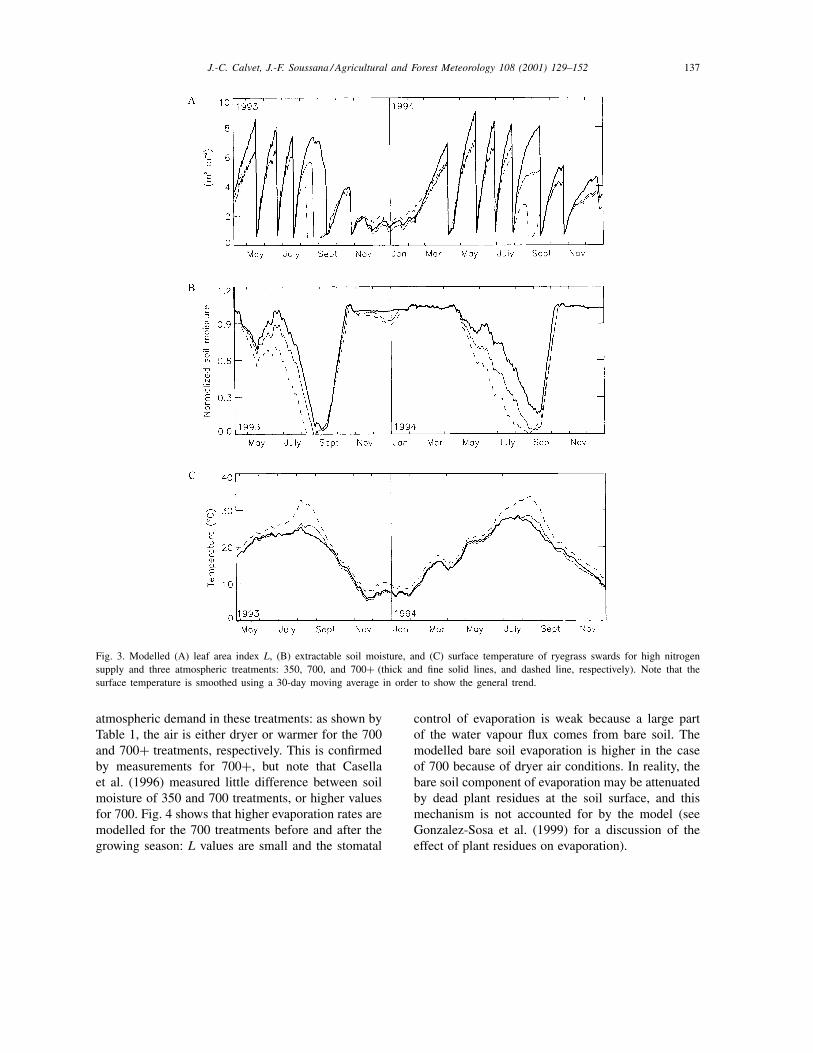
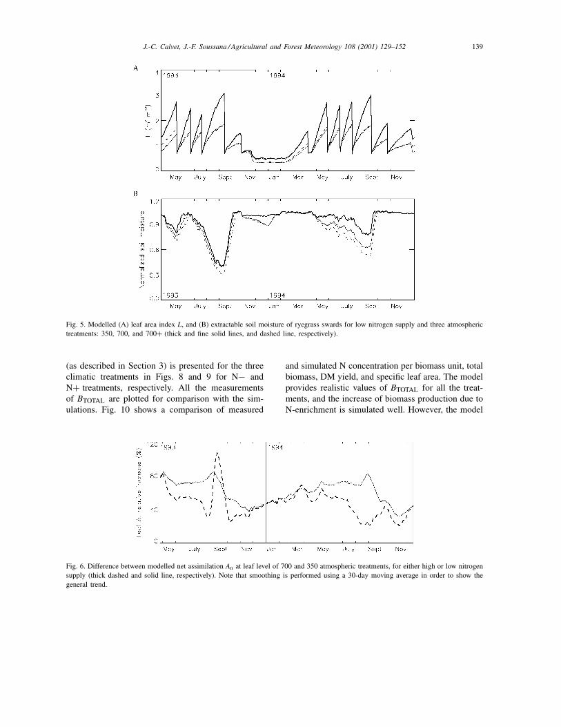
The results obtained for the N+ treatments in termsof L, soil water content, and surface temperature arepresented in Fig. 3. The simulated seasonal variationsof the fluxes of carbon, water vapour, and heat areshown in Fig. 4. The L values and soil water contentof the N− treatments are shown in Fig. 5. Figs. 3and 5 show that the simulated L is decreased by 20%on average at high CO2 concentration (for both 700N+ and N− treatments). Meanwhile the modelledrelative increase of the leaf net assimilation rate dueto CO2-enrichment (Fig. 6) ranges from 50 to 60%on average for N+ and N− treatments, respectively.The reduction in leaf area related to CO2-enrichmentis due to changes in the repartition of the producedbiomass in the plant, governed in the model by the αBparameter. As shown by Soussana et al. (1996), leafblade weight and root biomass increase as a result ofCO2-enrichment, whereas L is relatively unaffected byclimatic conditions in the case of perennial ryegrass:CO2 enrichment triggers an observed reduction in Lof about 10%, but this difference is not statisticallysignificant (Table 2). In this study, the simulated soilmoisture is lower for both 700 and 700+ treatments,denoting more evapotranspiration. This is contradic-tory to the expected enhancement of stomatal closurein CO2-enriched conditions and is due to the increased


Fig. 3. Modelled (A) leaf area index L, (B) extractable soil moisture, and (C) surface temperature of ryegrass swards for high nitrogensupply and three atmospheric treatments: 350, 700, and 700+ (thick and fine solid lines, and dashed line, respectively). Note that thesurface temperature is smoothed using a 30-day moving average in order to show the general trend.

atmospheric demand in these treatments: as shown byTable 1, the air is either dryer or warmer for the 700and 700+ treatments, respectively. This is confirmedby measurements for 700+, but note that Casellaet al. (1996) measured little difference between soilmoisture of 350 and 700 treatments, or higher valuesfor 700. Fig. 4 shows that higher evaporation rates aremodelled for the 700 treatments before and after thegrowing season: L values are small and the stomatal

control of evaporation is weak because a large partof the water vapour flux comes from bare soil. Themodelled bare soil evaporation is higher in the caseof 700 because of dryer air conditions. In reality, thebare soil component of evaporation may be attenuatedby dead plant residues at the soil surface, and thismechanism is not accounted for by the model (seeGonzalez-Sosa et al. (1999) for a discussion of theeffect of plant residues on evaporation).


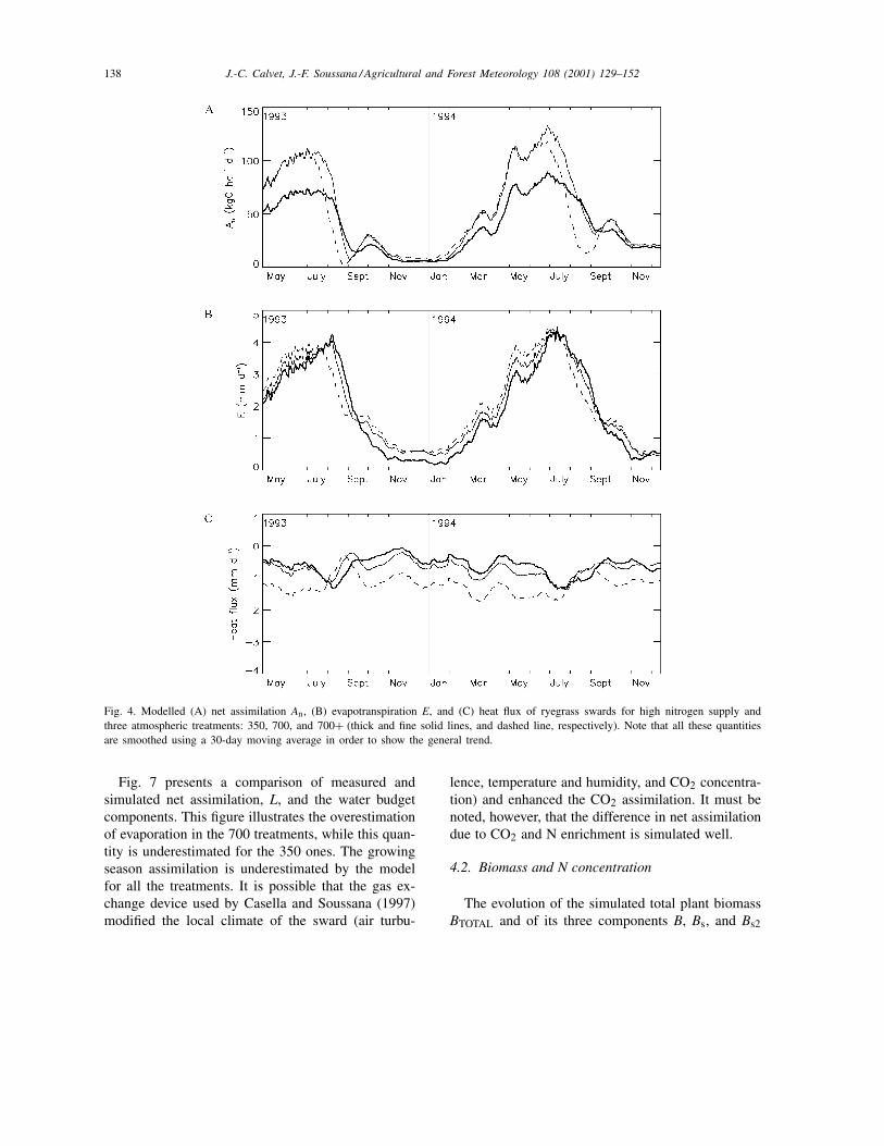
Fig. 4. Modelled (A) net assimilation An, (B) evapotranspiration E, and (C) heat flux of ryegrass swards for high nitrogen supply andthree atmospheric treatments: 350, 700, and 700+ (thick and fine solid lines, and dashed line, respectively). Note that all these quantitiesare smoothed using a 30-day moving average in order to show the general trend.

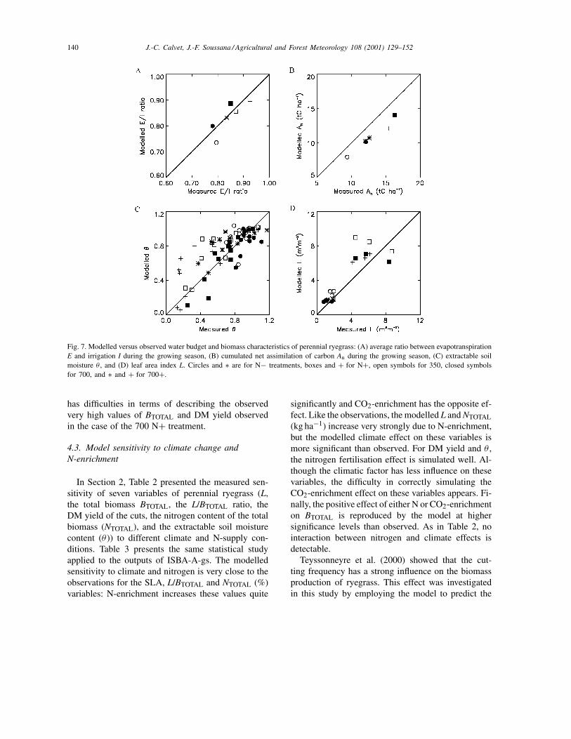
Fig. 7 presents a comparison of measured andsimulated net assimilation, L, and the water budgetcomponents. This figure illustrates the overestimationof evaporation in the 700 treatments, while this quan-tity is underestimated for the 350 ones. The growingseason assimilation is underestimated by the modelfor all the treatments. It is possible that the gas ex-change device used by Casella and Soussana (1997)modified the local climate of the sward (air turbu-

lence, temperature and humidity, and CO2 concentra-tion) and enhanced the CO2 assimilation. It must benoted, however, that the difference in net assimilationdue to CO2 and N enrichment is simulated well.

4.2. Biomass and N concentration

The evolution of the simulated total plant biomassBTOTAL and of its three components B, Bs, and Bs2


Fig. 5. Modelled (A) leaf area index L, and (B) extractable soil moisture of ryegrass swards for low nitrogen supply and three atmospherictreatments: 350, 700, and 700+ (thick and fine solid lines, and dashed line, respectively).

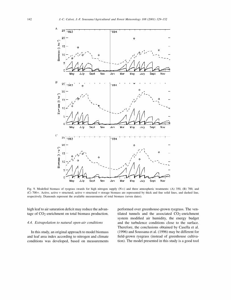
(as described in Section 3) is presented for the threeclimatic treatments in Figs. 8 and 9 for N− andN+ treatments, respectively. All the measurementsof BTOTAL are plotted for comparison with the sim-ulations. Fig. 10 shows a comparison of measured

Fig. 6. Difference between modelled net assimilation An at leaf level of 700 and 350 atmospheric treatments, for either high or low nitrogensupply (thick dashed and solid line, respectively). Note that smoothing is performed using a 30-day moving average in order to show thegeneral trend.

and simulated N concentration per biomass unit, totalbiomass, DM yield, and specific leaf area. The modelprovides realistic values of BTOTAL for all the treat-ments, and the increase of biomass production due toN-enrichment is simulated well. However, the model


Fig. 7. Modelled versus observed water budget and biomass characteristics of perennial ryegrass: (A) average ratio between evapotranspirationE and irrigation I during the growing season, (B) cumulated net assimilation of carbon An during the growing season, (C) extractable soilmoisture θ , and (D) leaf area index L. Circles and ∗ are for N− treatments, boxes and + for N+, open symbols for 350, closed symbolsfor 700, and ∗ and + for 700+.

has difficulties in terms of describing the observedvery high values of BTOTAL and DM yield observedin the case of the 700 N+ treatment.

4.3. Model sensitivity to climate change andN-enrichment

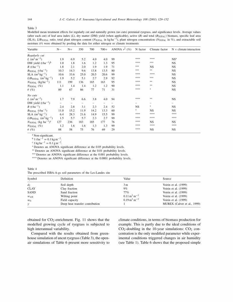
In Section 2, Table 2 presented the measured sen-sitivity of seven variables of perennial ryegrass (L,the total biomass BTOTAL, the L/BTOTAL ratio, theDM yield of the cuts, the nitrogen content of the totalbiomass (NTOTAL), and the extractable soil moisturecontent (θ )) to different climate and N-supply con-ditions. Table 3 presents the same statistical studyapplied to the outputs of ISBA-A-gs. The modelledsensitivity to climate and nitrogen is very close to theobservations for the SLA, L/BTOTAL and NTOTAL (%)variables: N-enrichment increases these values quite

significantly and CO2-enrichment has the opposite ef-fect. Like the observations, the modelled L and NTOTAL(kg ha−1) increase very strongly due to N-enrichment,but the modelled climate effect on these variables ismore significant than observed. For DM yield and θ ,the nitrogen fertilisation effect is simulated well. Al-though the climatic factor has less influence on thesevariables, the difficulty in correctly simulating theCO2-enrichment effect on these variables appears. Fi-nally, the positive effect of either N or CO2-enrichmenton BTOTAL is reproduced by the model at highersignificance levels than observed. As in Table 2, nointeraction between nitrogen and climate effects isdetectable.

Teyssonneyre et al. (2000) showed that the cut-ting frequency has a strong influence on the biomassproduction of ryegrass. This effect was investigatedin this study by employing the model to predict the


Fig. 8. Modelled biomass of ryegrass swards for low nitrogen supply (N−) and three atmospheric treatments: (A) 350, (B) 700, and (C)700+. Active, active + structural, active + structural + storage biomass are represented by thick and fine solid lines, and dashed line,respectively. Diamonds represent the available measurements of total biomass (seven dates).

‘natural’ plant growth (i.e. without cutting) in differ-ent growing conditions. The results obtained in thismodel configuration are presented in Table 3. Again,the N effect is very pronounced. On the other hand,the climate effect is no longer significant for NTOTAL(kg ha−1) and BTOTAL. Table 3 shows that regular cutsstimulate the N and CO2 enrichment effect on totalbiomass. Also, the effect of N-enrichment on active

biomass is increased and cuttings attenuate the ad-verse N-dilution effect due to CO2 enrichment on thisvariable. The main difference between the cut and thenatural simulation is that cutting the grass triggers aconstant regeneration of the canopy (i.e. the vegeta-tion is constantly growing), while undisturbed growthallows senescence to develop. For naturally grown rye-grass, stress factors such as soil moisture depletion or


Fig. 9. Modelled biomass of ryegrass swards for high nitrogen supply (N+) and three atmospheric treatments: (A) 350, (B) 700, and(C) 700+. Active, active + structural, active + structural + storage biomass are represented by thick and fine solid lines, and dashed line,respectively. Diamonds represent the available measurements of total biomass (seven dates).

high leaf to air saturation deficit may reduce the advan-tage of CO2-enrichment on total biomass production.

4.4. Extrapolation to natural open-air conditions

In this study, an original approach to model biomassand leaf area index according to nitrogen and climateconditions was developed, based on measurements

performed over greenhouse-grown ryegrass. The ven-tilated tunnels and the associated CO2-enrichmentsystem modified air humidity, the energy budgetand the turbulence conditions close to the surface.Therefore, the conclusions obtained by Casella et al.(1996) and Soussana et al. (1996) may be different forfield-grown ryegrass (instead of greenhouse cultiva-tion). The model presented in this study is a good tool


Fig. 10. Modelled versus observed nitrogen content and biomass characteristics of perennial ryegrass: (A) total plant nitrogen contentNTOTAL per total biomass unit, (B) total biomass BTOTAL (aerial + roots), (C) dry matter (DM) yield, and (D) the ratio between leaf areaindex L and BTOTAL. Circles and ∗ are for N− treatments, boxes and + for N+, open symbols for 350, closed symbols for 700, and ∗and + for 700+.

to estimate the behaviour of the same plant grown inmore natural conditions: the same parameters may beemployed while using a measured natural atmosphericforcing and different soil conditions. Also, using along atmospheric time series is a way to assess theinterannual variability of the model outputs.

The model was applied to the Le-Bray site of theLes-Landes forest (44◦42′N, 0◦46′E, 62 m), for whichVoirin et al. (1999) derived a 10-year atmosphericseries (1 August 1985 to 31 July 1995) from theMétéo-France weather station network. The soil ofLes-Landes forest is generally sandy, as shown bythe value of the soil parameters employed by Voirinet al. (1999), presented in Table 4. The simulationseries were performed for perennial ryegrass without

prescribing cutting. The model parameters corre-sponding to ryegrass are those displayed in Section 6.

Table 5 compares the initial and equilibrium valuesof αB obtained from iterations on the 10-year period(the αB parameter was assumed constant during thewhole period). The analysis of the 10-year simula-tions obtained for the treatments described in Table 5is summarised in Table 6. Since a long period oftime is considered (10 annual cycles), it is possibleto analyse annual quantities such as N-use, minimumavailable soil moisture, total evaporation, and net as-similation of CO2. As far as L is concerned, the sameresult as before is obtained for ryegrass: the nitrogenfertilisation has a strong positive influence on theproduction of leaf surface while the reverse effect is


Table 3Modelled mean treatment effects for regularly cut and naturally grown (no cuts) perennial ryegrass, and significance levels. Average values(after each cut) of leaf area index (L), dry matter (DM) yield (when applicable), active (B) and total (BTOTAL) biomass, specific leaf area(SLA), L/BTOTAL ratio, total plant nitrogen content (NTOTAL in kg ha−1), plant nitrogen concentration (NTOTAL in %), and extractable soilmoisture (θ ) were obtained by pooling the data for either nitrogen or climate treatments

Variable N− N+ 350 700 700+ ANOVA r2 (%) N factor Climate factor N × climate interaction

Regularly cutL (m2 m−2) 1.9 6.9 5.2 4.0 4.0 99 ∗∗∗∗ ∗∗∗∗ NSa

DM yield (t ha−1)b 1.0 1.8 1.6 1.2 1.3 95 ∗∗∗∗ ∗∗∗ NSB (t ha−1) 1.8 2.1 2.0 1.9 1.9 71 ∗∗∗ NS NSBTOTAL (t ha−1) 10.3 14.3 9.6 13.8 13.5 80 ∗∗∗ ∗∗ NSSLA (m2 kg−1) 10.6 33.6 25.0 20.5 20.6 99 ∗∗∗∗ ∗∗∗∗ NSL/BTOTAL (m2 kg−1) 1.9 5.2 5.1 2.7 2.9 92 ∗∗∗∗ ∗∗∗ NSNTOTAL (kg ha−1) 111 199 136 165 163 95 ∗∗∗∗ ∗∗ NSNTOTAL (%) 1.1 1.4 1.4 1.2 1.2 90 ∗∗∗∗ ∗∗ NSθ (%) 89 67 86 77 71 31 ∗∗∗∗ ∗ NS

No cutsL (m2 m−2) 1.7 7.9 6.6 3.8 4.0 94 ∗∗∗∗ ∗∗ NSDM yield (t ha−1) – – – – – – – – –B (t ha−1) 2.4 2.8 3.1 2.3 2.4 52 NS ∗ NSBTOTAL (t ha−1) 11.0 15.2 11.9 14.2 13.3 60 ∗ NS NSSLA (m2 kg−1) 6.4 28.3 21.6 14.9 15.5 99 ∗∗∗∗ ∗∗∗∗ ∗∗∗∗L/BTOTAL (m2 kg−1) 1.5 5.7 5.7 2.3 2.7 99 ∗∗∗∗ ∗∗∗∗ ∗∗∗∗NTOTAL (kg ha−1)c 127 236 183 185 177 76 ∗∗∗∗ NS NSNTOTAL (%) 1.2 1.6 1.6 1.3 1.3 99 ∗∗∗∗ ∗∗∗∗ ∗∗∗∗θ (%) 88 58 75 76 69 29 ∗∗∗∗ NS NS

a Non-significant.b 1 t ha−1 = 0.1 kg m−2.c 1 kg ha−1 = 0.1 g m−2.∗ Denotes an ANOVA significant difference at the 0.05 probability levels.∗∗ Denotes an ANOVA significant difference at the 0.01 probability levels.∗∗∗ Denotes an ANOVA significant difference at the 0.001 probability levels.∗∗∗∗ Denotes an ANOVA significant difference at the 0.0001 probability levels.

Table 4The prescribed ISBA-A-gs soil parameters of the Les-Landes site

Symbol Definition Value Source

d2 Soil depth 3 m Voirin et al. (1999)CLAY Clay fraction 9% Voirin et al. (1999)SAND Sand fraction 77% Voirin et al. (1999)wwilt Wilting point 0.11 m3 m−3 Voirin et al. (1999)wfc Field capacity 0.19 m3 m−3 Voirin et al. (1999)γ Deep heat transfer contribution 1 MUREX (Calvet et al., 1999)

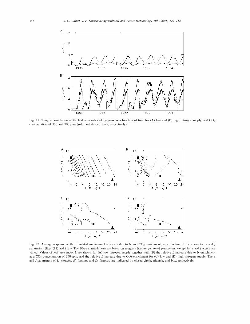
obtained for CO2-enrichment. Fig. 11 shows that themodelled growing cycle of ryegrass is subjected tohigh interannual variability.

Compared with the results obtained from green-house simulation of uncut ryegrass (Table 3), the open-air simulations of Table 6 present more sensitivity to

climate conditions, in terms of biomass production forexample. This is partly due to the ideal conditions ofCO2-doubling in the 10-year simulations: CO2 con-centration is the only modified parameter while exper-imental conditions triggered changes in air humidity(see Table 1). Table 6 shows that the proposed simple


Table 5Ryegrass optimal value of the ISBA-A-gs biomass parameter αB

for combined nitrogen and climate treatments, using the extendedplant N decline model over a 10-year period, in natural conditions.The prescribed nitrogen concentration of the active biomass (Na)is indicated. Two values of αB are presented: the initial valueαBini, and the equilibrium value. Note that ryegrass is not cut inthese simulations

Treatment Na (%) αBini (g m−2) αB (g m−2)

350 N− 2.4 54 111350 N+ 4.9 24 30700 N− 2.4 54 229700 N+ 4.9 24 46

model is able to simulate rather complex responses toN and CO2 enrichment.

In these simulations, a large part of the modelledL response is determined by the allometric para-meters e and f presented in Section 3. In order toassess the effect of e and f, the 10-year simulationsdetailed in the previous section were performed forvarious values of e and f, using the ryegrass parame-ters of Section 6. Fig. 12 shows the effect of e and f onthe average value of the modelled maximum L, and

Table 6Modelled N and CO2 enrichment effects for naturally grown perennial ryegrass. The significance levels are based on 10-year simulations.Maximum values of leaf area index (L), active (B) and total (BTOTAL) biomass, and total plant nitrogen content (NTOTAL in kg ha−1) areindicated, together with specific leaf area (SLA), L/BTOTAL, average plant nitrogen concentration (NTOTAL in %), minimum extractable soilmoisture (θ ), annual evaporation (E), net assimilation of CO2 (An), and N-use

Variable 350N− 350 N+ 700 N− 700 N+ ANOVA r2 (%) N factor CO2 factor N × CO2

interaction

Maximum L (m2 m−2) 3.5 9.9 1.1 7.5 82 ∗∗∗∗ ∗∗∗∗ NSa

Maximum B (t ha−1)b 3.8 2.8 2.4 3.2 54 NS ∗∗ ∗∗∗∗Maximum BTOTAL (t ha−1) 14.4 10.6 12.0 22.8 93 ∗∗∗∗ ∗∗∗∗ ∗∗∗∗SLA (m2 kg−1) 9.2 34.9 4.5 23.2 99 ∗∗∗∗ ∗∗∗∗ ∗∗∗∗L/BTOTAL (m2 kg−1) 2.5 9.0 0.9 3.3 83 ∗∗∗∗ ∗∗∗∗ ∗∗∗∗Maximum NTOTAL (kg ha−1)c 143 125 113 229 89 ∗∗∗∗ ∗∗∗∗ ∗∗∗∗Average NTOTAL (%) 0.96 1.10 0.93 0.96 67 ∗∗∗∗ ∗∗∗∗ ∗∗∗N-use (t ha−1 yr−1) 0.73 1.09 0.76 2.38 67 ∗∗∗∗ ∗∗∗ ∗∗∗Minimum � (%) 18 7 58 11 48 ∗∗∗ ∗∗ ∗Total An (t C ha−1 yr−1) 9.5 7.6 9.8 16.8 47 ∗ ∗∗∗ ∗∗∗Total E (mm yr−1) 542 583 430 567 13 NS NS NS

a Non-significant.b 1 t ha−1 = 0.1 kg m−2.c 1 kg ha−1 = 0.1 g m−2.∗ Denotes an ANOVA significant difference at the 0.05 probability levels.∗∗ Denotes an ANOVA significant difference at the 0.01 probability levels.∗∗∗ Denotes an ANOVA significant difference at the 0.001 probability levels.∗∗∗∗ Denotes an ANOVA significant difference at the 0.0001 probability levels.

the relative response of this variable to N and CO2enrichment. The reference e and f values of ryegrass(Section 6) are indicated, together with those ob-tained for Holcus lanatus and Deschampsia flexuosa,based on biomass and N measurements performedby Van de Vijver et al. (1993). It appears that thevalue of f has a strong influence on maximum L: lowvalues of f (negative values in particular) correspondto plants growing slowly in infertile conditions, andpresenting a very marked response to N-enrichment(up to 5-fold). This conclusion is consistent with theobservations made by Van de Vijver et al. (1993):most plant characteristics of D. flexuosa present amore pronounced response to N-enrichment than H.lanatus, and the f parameter derived for D. flexuosais lower than for H. lanatus (10.4 and 22.2 m2 kg−1,respectively). In other words, low values of f corre-spond to higher phenotypic plasticity in response toN supply. The same plants, however, present a lowerresponse to CO2-enrichment, and even a decrease ofmaximum L. It must be noted that in Fig. 12, the simu-lated effect of CO2-enrichment on grass L is moderate(30% at most). These results are in agreement withexperimental evidence in Teyssonneyre et al. (2000)


Fig. 11. Ten-year simulation of the leaf area index of ryegrass as a function of time for (A) low and (B) high nitrogen supply, and CO2

concentration of 350 and 700 ppm (solid and dashed lines, respectively).

Fig. 12. Average response of the simulated maximum leaf area index to N and CO2 enrichment, as a function of the allometric e and fparameters (Eqs. (11) and (12)). The 10-year simulations are based on ryegrass (Lolium perenne) parameters, except for e and f which arevaried. Values of leaf area index L are shown for (A) low nitrogen supply together with (B) the relative L increase due to N-enrichmentat a CO2 concentration of 350 ppm, and the relative L increase due to CO2-enrichment for (C) low and (D) high nitrogen supply. The eand f parameters of L. perenne, H. lanatus, and D. flexuosa are indicated by closed circle, triangle, and box, respectively.


that H. lanatus responds to CO2-enrichment by an in-creased leaf mass production while ryegrass does not.Furthermore, when ryegrass is grown with other grassspecies, its leaf mass production is significantly re-duced by CO2-enrichment (down to −25%). Fig. 12shows that values of f close to 0 are critical. Indeed, inthis case, a small change in f has strong consequencesin terms of the plant’s response to N and CO2 enrich-ment. Excessively low values of e and/or f may leadto negative values of LAR (Eq. (10)), denoting theimpossibility for the plant to survive at the prescribedvalue of Na (i.e. the corresponding plant would needhigher N-supply).

5. Conclusion

The simple interactive vegetation SVAT modelISBA-A-gs was tested against biomass measurementsof perennial ryegrass grown under six different condi-tions of nitrogen supply and climate. It is shown thatthe model is able to describe the plant growth in dif-ferent conditions using the same values of mesophyllconductance and maximum life expectancy of activebiomass. However, the optimal value of the ratio be-tween the model’s active biomass and the leaf areaindex αB differs from one treatment to another. A

6. List of symbols: parameters

Symbol Definition Value Reference

Vegetation parametersA Albedo 0.20 Calvet et al. (1999)z0/z0h Roughness length ratio 450 Calvet et al. (1999)CV Thermal coefficient 2.0 × 10−5 K m2 J−1 Calvet et al. (1999)gm Mesophyll conductance 1 mm s−1 Calibratedh Vegetation height L/24 Allen et al. (1989)veg Vegetation coverage 1 − exp(−0.6L) Kanemasu et al. (1977)ε Emissivity 0.97 Calvet et al. (1999)

Biomass parametersa Rate of nitrogen dilution of the above-

ground biomass at ambient [CO2]0.38 Soussana et al. (1996)

a Rate of nitrogen dilution of the above-ground biomass at doubled [CO2]

0.52 Soussana et al. (1996)

c Proportion of active biomass forBT = 1 t ha−1

0.754 Derived from measurements

simple parameterisation of αB is proposed, based onthe plant N decline model and from a closure equa-tion derived from Eq. (11): a major conclusion of thisstudy is that the observed linear relationship betweenLAR and the above-ground N concentration can beused to predict the allocation and growth responses tonutrient availability and climate change. In the finalalgorithm, αB is calculated and is no longer an inputparameter of the model. Instead, the nitrogen concen-tration of the active biomass (Na) is prescribed, andmay be optimised based on L estimates. The outputsof the model are half-hourly surface state variablesand fluxes (including net assimilation of CO2 and het-erotrophic respiration of the plant), daily values of L,total living biomass, mortality rate and nitrogen use.

Since only five parameters are needed to drivethe model (gm, Na, e, f, τM), this new version ofISBA-A-gs may easily be operated in atmosphericand hydrological models to quantify the vegetationresponse to climate change, and its consequences interms of nitrogen supply. A difficulty, however, is theestimation of the e and f parameters, which governthe plant response to nitrogen availability and to theprescribed climate. In this study, estimates of e and fwere derived for three grass species. More complexmodels (crop models for example) may be used toprovide estimates of e and f for other plant types.


List of symbols: parameters (continued )

Symbol Definition Value Reference

e LAR sensitivity to N concentration of ryegrass 9.12 × 102 m2 kg−1 Derived from measurementsf Lethal minimum value of LAR of ryegrass −3.4 m2 kg−1 Derived from measurementsLmin Value of leaf area index after cutting 0.7 m2 m−2 Derived from measurementsNa N concentration of active biomass of

ryegrass for N− treatments2.4% Derived from measurements

Na N concentration of active biomass ofryegrass for N+ treatments

4.9% Derived from measurements

NS N concentration of structural biomass 0.8% Lemaire and Gastal (1997)PC Proportion of carbon in the dry plant biomass 40% Calvet et al. (1998)ηR Maintenance respiration rate 1% per day Faurie (1994)τM Potential leaf life expectancy 250 days Arbitrary value

Soil parametersd2 Soil depth 0.45 m Casella et al. (1996)CLAY Clay fraction 15% Casella et al. (1996)SAND Sand fraction 42% Casella et al. (1996)wwilt Wilting point 0.06 m3 m−3 Casella et al. (1996)wfc Field capacity 0.29 m3 m−3 Casella et al. (1996)γ Deep heat transfer contribution 1 Calvet et al. (1999)

7. List of symbols: variables

Symbol Definition Unit

Atmospheric forcing variables[CO2] Air CO2 concentration ppmI Irrigation mm per dayqa Air moisture content g kg−1

Ra Downwelling atmospheric thermal emission W m−2

Rg Solar radiation W m−2

Ta Air temperature Ku Wind speed (a constant value of 4 m s−1 is prescribed in this study) m s−1

Soil-vegetation variablesE Evapotranspiration mm per dayTs Surface temperature KT2 Average surface temperature Kw2 Soil volumetric moisture in the root-zone m3 m−3

Wr Canopy rainfall interception reservoir Mmθ Extractable soil moisture content (θ = (w2 − wwilt)/(wfc − wwilt)) –

Biomass variablesAn Net assimilation kg C ha−1 per dayB Metabolic (or active) biomass t ha−1


List of symbols: variables (continued )

Symbol Definition Unit

Bs Structural biomass t ha−1

Bs2 Deep structural biomass t ha−1

BT Above-ground biomass (BT = B + Bs) t ha−1

BTOTAL Total plant biomass (BTOTAL = B + Bs + Bs2) t ha−1

L Leaf area index m2 m−2

LAR Leaf area ratio (LAR = L/BT) m2 kg−1

NT Nitrogen content of above-ground biomass % or kg ha−1

NTOTAL Nitrogen content of the whole plant % or kg ha−1

MB Mortality of active biomass t ha−1 per dayMBs Mortality of structural biomass t ha−1 per dayMBs2 Mortality of deep structural biomass t ha−1 per dayRBs Respiration of structural biomass t ha−1 per dayRBs2 Respiration of deep structural biomass t ha−1 per daySB Storage of active biomass into the structural compartments t ha−1 per daySLA Specific leaf area (SLA = L/B) m2 kg−1

αB B/L ratio g m−2

Note that 1 t ha−1 = 0.1 kg m−2.

Acknowledgements

The authors wish to thank Jean-Pierre Wigneron(INRA), Sophie Voirin and Aaron Boone (CNRM) forhelpful comments.

Appendix A. The simplified allocation scheme

In the simple allocation scheme employed in thisstudy, three biomass reservoirs are considered: theactive biomass (B), the structural biomass (Bs), anda deep structural storage reservoir (Bs2). The dailynet assimilation and leaf turnover time τ (Eq. (5))estimated by ISBA-A-gs are the main input variablesof daily biomass calculations. Following Eq. (4), netassimilation contributes to increases in B, while τ isemployed to describe the B decline. The B-declineterm of Eq. (4) is split into a mortality and a storageterm (MB and SB, respectively)

B d

(t

τ

)= MB + SB (A.1)

The way the distinction is made between MB and SBis described below.

A.1. Growing phase and senescence

The growing phase is characterised by positivevalues of dB in Eq. (4), net assimilation exceedsthe B-decline term. When this condition is satis-fied, the plant N decline model can be applied: theabove-ground biomass BT is derived from B usingEq. (10) and Bs is the difference between the twoterms. The mortality of Bs is assumed to be indepen-dent of photosynthesis and is given by

MBs = Bs d

(t

τM

)(A.2)

The structural biomass also loses carbon through res-piration. This term is estimated using the commonobservation that maintenance respiration of non-activebiomass is proportional to the biomass value, with aQ10 temperature dependence

RBs = ηRBsQ(T−25)/1010 dt (A.3)

where dt represents 1 day, T the surface temperature(in ◦C), ηR a respiration coefficient (Section 6), andQ10 = 2.


Finally, the storage term SB of Eq. (A.1) is cal-culated as the residual of the structural biomassbudget

SB = dBs +MBs + RBs (A.4)

The MB term of Eq. (A.1) is obtained by difference.The MB and MBs quantities may be used as input ofa soil organic matter (SOM) model. It must be notedthat B and MB contain nitrogen at concentration Na,while the N-content of Bs and MBs (NS) is lower(Section 6). In situations where storage exceeds themortality of active biomass MB, an alternative formu-lation of B-decline is employed. The above-groundbiomass BT is recalculated assuming that there is noloss of active biomass outside the plant system, dur-ing the considered time step: MB = 0 and dBT is thedifference between the daily net assimilation and themortality and respiration losses of structural biomass(Eqs. (A.2) and (A.3)). The active biomass B is de-rived from BT using Eq. (7), and Bs is the differencebetween the two terms. A new value of the storageterm SB is given by Eq. (A.4).

When the vegetation becomes senescent (nega-tive values of dB), the plant N decline equations(Eqs. (7)–(12)) are no longer valid. In this case, the Bsreservoir evolves independently from B: a nil storageterm is prescribed and the mortality and respirationlosses (Eqs. (A.2) and (A.3)) are applied to Bs.

A.2. Deep storage of biomass

The Bs2 reservoir of Fig. 2 represents a supple-mentary compartment of biomass corresponding

Table 7Obtained optimal values of the ISBA-A-gs biomass parameters for the six nitrogen and climate treatments using the extended plant Ndecline model. Different values of the ratio between active biomass and green L (αB) are presented: the initial value αBini, the equilibriumvalue with cuts, and with no cut prescribed. The achieved maximum value of total biomass BTOTAL during the equilibrium simulation isindicated, together with the nitrogen use during the 631-day period considered

Treatment αBini

(g m−2)αB withcuts (g m−2)

αB no cut(g m−2)

BTOTAL withcuts (t ha−1)a

BTOTAL nocut (t ha−1)

N-use withcuts (t ha−1)

N-use nocuts (t ha−1)

350 N− 54 74 109 8.6 16.4 0.95 1.31700 N− 54 104 192 12.1 13.2 1.25 1.08700+ N− 54 103 190 11.1 12.9 1.26 1.14350 N+ 24 28 30 10.9 12.6 2.85 2.25700 N+ 24 33 41 17.9 20.0 3.97 3.59700+ N+ 24 33 39 16.0 17.5 3.48 3.09

a 1 t ha−1 = 0.1 kg m−2.

essentially to underground biomass. This biomass cat-egory is not treated by the plant N decline model. Themortality and respiration loss of Bs2 (MBs2 and RBs2,respectively) are calculated using equations similar toEqs. (A.2) and (A.3), where Bs is replaced by Bs2,with T representing soil temperature in Eq. (A.3).In the model calculations, this biomass reservoir isfed by two mechanisms: (1) when the storage termSB is negative (this happens, e.g., when a cut is pre-scribed in the model), this quantity is redirected tothe Bs2 reservoir, (2) when the above-ground plantbiomass BT is lower than c1/a (a value below whichEq. (7) is not applicable), it is assumed that the MBmortality becomes a storage term which increasesBs2.

A.3. Estimation of the αB parameter and of N-use

Eq. (12) shows that for a given value of Na, theαB parameter depends on above-ground biomass BT.In this study, the αB parameter is assumed to repre-sent rather intrinsic plant characteristics denoting abiological adaptation to average climate and growingconditions. Therefore, a constant value of αB is em-ployed for the 631-day simulations covering the con-sidered period. In order to estimate αB using Eq. (12),iterations must be performed: after running the modelduring the 631-day period with a first estimate ofαB, the maximum value of BT obtained during thisperiod is converted into a αB estimate using Eq. (12),and this value is employed in a new simulation. Iter-ations between maximum BT values and αB are per-formed until αB is little modified by a new iteration


(a difference less than 1% is imposed). The initialvalue of αB is given by

αBini = 1

eNa + f (A.5)

In this study, 4–8 iterations are necessary to convergeto equilibrium values of αB and BT.

Table 7 summarises the obtained equilibrium val-ues of αB, together with αBini, and the resultingN-use. Whereas the αBini values are the same forgiven N supply conditions, the climate effect (actingon the biomass component of Eq. (12)) has a stronginfluence on the final estimates of αB. In particular,CO2-enrichment tends to increase the modelled val-ues of αB shown in Table 7. The model was run, also,without interfering with plant growth through cuts. Inthis case, the αB parameter is higher, especially forN− treatments, and the obtained maximum biomassvalue is higher. This result shows that the model tendsto favour the production of leaf surface area whenthe vegetation is regularly cut. Not cutting the vege-tation has relatively little influence on the modelledN-use.

References

Allen, R.G., Jensen, M.E., Wright, J.L., Burman, R.D., 1989.Operational estimates of reference evapotranspiration. Agron.J. 81, 650–662.

Calvet, J.-C., 2000. Investigating soil and atmospheric plant waterstress using physiological and micrometeorological data sets.Agric. For. Meteorol. 103, 229–247.

Calvet, J.-C., Noilhan, J., Roujean, J.-L., Bessemoulin, P.,Cabelguenne, M., Olioso, A., Wigneron, J.P., 1998. Aninteractive vegetation SVAT model tested against data from sixcontrasting sites. Agric. For. Meteorol. 92, 73–95.

Calvet, J.-C., Bessemoulin, P., Noilhan, J., et al., 1999. MUREX:a land-surface field experiment to study the annual cycle of theenergy and water budgets. Ann. Geophys. 17, 838–854.

Casella, E., Soussana, J.-F., 1997. Long-term effects of CO2

enrichment and temperature increase on the carbon balance of atemperate grass sward. J. Exp. Bot. 48 (311), 1309–1321.

Casella, E., Soussana, J.-F., Loiseau, P., 1996. Long-term effectsof CO2 enrichment and temperature increase on a temperategrass sward. I. Productivity and use. Plant and Soil 182,83–99.

Deardorff, J.W., 1977. A parameterization of the ground surfacemoisture content for use in atmospheric prediction models. J.Appl. Meteor. 16, 1182–1185.

Deardorff, J.W., 1978. Efficient prediction of ground temperatureand moisture with inclusion of a layer of vegetation. J. Geophys.Res. 83, 1889–1903.

Faurié, O., 1994. Interactions carbone-azote dans des associationsprairiales graminées (Lolium perenne L.) légumineuses (Trifo-lium repens L.). Etude d’associations simulées en conditionscontrôlées. Ph.D. Thesis. University Clermont II, Clermont-Ferrand, 203 pp.

Gonzalez-Sosa, E., Braud, I., Thony, J.-L., Vauclin, M.,Bessemoulin, P., Calvet, J.-C., 1999. Modelling heat and waterexchanges of fallow land covered with plant-residue mulch.Agric. For. Meteorol. 97, 151–169.

Greenwood, D.J., Lemaire, G., Gosse, G., Cruz, P., Draycott,A., Neeteson, J.J., 1990. Decline in percentage N of C3

and C4 crops with increasing plant mass. Ann. Bot. 66,425–436.

Greenwood, D.J., Gastal, F., Lemaire, G., Draycott, A., Millard,P., Neeteson, J.J., 1991. Growth rate and %N of field growncrops: theory and experiments. Ann. Bot. 67, 181–190.

Jacobs, C.M.J., 1994. Direct impact of atmospheric CO2

enrichment on regional transpiration. Ph.D. Thesis. AgriculturalUniversity, Wageningen.

Jacobs, C.M.J., van den Hurk, B.J.J.M., de Bruin, H.A.R.,1996. Stomatal behaviour and photosynthetic rate of unstressedgrapevines in semi-arid conditions. Agric. For. Meteorol. 80,111–134.

Ji, J.J., 1995. A climate–vegetation interaction model: simulatingphysical and biological processes at the surface. J. Biogeogr.22, 445–451.

Justes, E., Mary, B., Meynard, J.M., Machet, J.M., Thelier-Huché,L., 1994. Determination of a critical nitrogen dilution curve forwinter wheat crops. Ann. Bot. 74, 397–407.

Kanemasu, T., Rosenthal, U.D., Stone, R.J., Stone, L.R., 1977.Evaluation of an evapotranspiration model of corn. J. Agron.69, 461–464.

Lemaire, G., Gastal, F., 1997. N uptake and distribution in plantcanopies. In: Lemaire, G. (Ed.), Diagnosis of the NitrogenStatus in Crops. Springer, Berlin, pp. 3–43.

Mougin, E., Lo Seen, D., Rambal, S., Gaston, A., Hiernaux, P.,1995. A regional Sahelian grassland model to be coupled withmultispectral satellite data. I. Model description and validation.Rem. Sens. Environ. 52, 181–193.

Nijskens, J., Deltour, J., Coutisse, S., Nisen, A., 1985. Radiationtransfer through covering materials, solar and thermal screensof greenhouses. Agric. For. Meteorol. 35, 229–242.

Noilhan, J., Planton, S., 1989. A simple parameterization of landsurface processes for meteorological models. Mon. Wea. Rev.117, 536–549.

Soussana, J.-F., Casella, E., Loiseau, P., 1996. Long-term effectsof CO2 enrichment and temperature increase on a temperategrass sward. II. Plant nitrogen budgets and root fraction. Plantand Soil 182, 101–114.

Staley, D.O., Jurica, G.M., 1972. Effective atmospheric emissivityunder clear skies. J. Appl. Meterol. 11, 349–356.

Teyssonneyre, F., Picon-Cochard, C., Soussana, J.-F., 2000.Productivity of pure and mixed temperate forage grassesunder elevated CO2 at two cutting frequencies. In: Soergaard,K., Ohlsson, C. (Eds.), Grassland Farming: BalancingEnvironmental and Economic Demands. Grassland Science inEurope, Vol. 5, pp. 116–118.


Van de Vijver, C.A.D.M., Boot, R.G.A., Poorter, H., Lambers,H., 1993. Phenotypic plasticity in response to nitrate supply ofan inherently fast-growing species from a fertile habitat andan inherently slow-growing species from an infertile habitat.Oecologia 96, 548–554.

Voirin, S., Calvet, J.-C., Noilhan, J., 1999. Impact d’une végétationinteractive sur les simulations des bilans hydriques et desdébits sur le bassin versant de l’Adour. In: Proc. Atelierde Modélisation de l’Atmosphère, Toulouse, December 1999.Météo-France/CNRM, Toulouse, pp. 263–266.

Modelling CO2-enrichment effects using an interactive vegetation SVAT scheme

Documents

Transcript of Modelling CO2-enrichment effects using an interactive vegetation SVAT scheme